A characterization of the Anderson metal-insulator transport transition
36
A characterization of the Anderson metal-insulator transport transition Fran¸ cois Germinet 1 , Abel Klein 2 1 Universit´ e de Lille 1, UMR 8524 CNRS, UFR de Math´ ematiques, F-59655 Vil- leneuve d’Ascq C´ edex, France. e-mail: [email protected] 2 University of California, Irvine, Department of Mathematics, Irvine, CA 92697- 3875, USA. e-mail: [email protected] Dedicated to Jean-Michel Combes on the occasion of his Sixtieth Birthday Abstract. We investigate the Anderson metal-insulator transition for random Schr¨ odinger operators. We define the strong insulator region to be the part of the spectrum where the random operator ex- hibits strong dynamical localization in the Hilbert-Schmidt norm. We introduce a local transport exponent β (E), and set the metallic trans- port region to be the part of the spectrum with nontrivial transport (i.e., β (E) > 0). We prove that these insulator and metallic regions are complementary sets in the spectrum of the random operator, and that the local transport exponent β (E) provides a characterization of the metal-insulator transport transition. Moreover, we show that if there is such a transition, then β (E) has to be discontinuous at a transport mobility edge. More precisely, we show that if the trans- port is nontrivial then β (E) ≥ 1 2d , where d is the space dimension. These results follow from a proof that slow time evolution of quantum waves in random media implies the starting hypothesis for the au- thors’ bootstrap multiscale analysis. We also conclude that the strong insulator region coincides with the part of the spectrum where we can perform a bootstrap multiscale analysis, proving that the multiscale analysis is valid all the way up to a transport mobility edge. Contents 1. Introduction .................................. 2 2. Statement of main results .......................... 5 3. Transport exponents ............................. 14 4. The strong insulator region ......................... 17 Partially supported by NSF Grants DMS-9800883 and DMS-9800860
-
Upload
independent -
Category
Documents
-
view
0 -
download
0
Transcript of A characterization of the Anderson metal-insulator transport transition
A characterization of the Andersonmetal-insulator transport transition
Francois Germinet1, Abel Klein2
1 Universite de Lille 1, UMR 8524 CNRS, UFR de Mathematiques, F-59655 Vil-leneuve d’Ascq Cedex, France. e-mail: [email protected]
2 University of California, Irvine, Department of Mathematics, Irvine, CA 92697-3875, USA. e-mail: [email protected]
Dedicated to Jean-Michel Combes on the occasion of his Sixtieth Birthday
Abstract. We investigate the Anderson metal-insulator transitionfor random Schrodinger operators. We define the strong insulatorregion to be the part of the spectrum where the random operator ex-hibits strong dynamical localization in the Hilbert-Schmidt norm. Weintroduce a local transport exponent β(E), and set the metallic trans-port region to be the part of the spectrum with nontrivial transport(i.e., β(E) > 0). We prove that these insulator and metallic regionsare complementary sets in the spectrum of the random operator, andthat the local transport exponent β(E) provides a characterizationof the metal-insulator transport transition. Moreover, we show thatif there is such a transition, then β(E) has to be discontinuous ata transport mobility edge. More precisely, we show that if the trans-port is nontrivial then β(E) ≥ 1
2d , where d is the space dimension.These results follow from a proof that slow time evolution of quantumwaves in random media implies the starting hypothesis for the au-thors’ bootstrap multiscale analysis. We also conclude that the stronginsulator region coincides with the part of the spectrum where we canperform a bootstrap multiscale analysis, proving that the multiscaleanalysis is valid all the way up to a transport mobility edge.
Contents
1. Introduction . . . . . . . . . . . . . . . . . . . . . . . . . . . . . . . . . . 22. Statement of main results . . . . . . . . . . . . . . . . . . . . . . . . . . 53. Transport exponents . . . . . . . . . . . . . . . . . . . . . . . . . . . . . 144. The strong insulator region . . . . . . . . . . . . . . . . . . . . . . . . . 17
Partially supported by NSF Grants DMS-9800883 and DMS-9800860
2 Francois Germinet, Abel Klein
5. The metallic transport region . . . . . . . . . . . . . . . . . . . . . . . . 206. The main proof . . . . . . . . . . . . . . . . . . . . . . . . . . . . . . . . 21A. Properties of random Schrodinger operators . . . . . . . . . . . . . . . . 30
1. Introduction
In his seminal 1958 article [An], Anderson argued that a Schrodingeroperator in a highly disordered medium would exhibit exponentiallylocalized eigenstates, in contrast to the extended eigenstates of aSchrodinger operator in a periodic medium. For a Schrodinger oper-ator with a random potential and spectrum of the form [E0,∞), thefollowing picture (e.g., [LGP, Section 4.2]) is widely accepted: Theregion of the spectrum near the bottom of the spectrum E0 resultsfrom large fluctuations of the potential, with the corresponding stateslocalized primarily in the regions of such fluctuations. But in three ormore dimensions, at very large energies the kinetic term should dom-inate the fluctuations of the potential to produce extended states.Thus a transition must occur from an insulator regime, characterizedby localized states, to a very different metallic regime characterizedby extended states. The energy Eme at which this metal-insulatortransition occurs is called the mobility edge. The medium should havezero conductivity in the insulator region [E0, Eme] and nonzero con-ductivity in the metallic region [Eme,∞). The standard mathematicalinterpretation of this picture is that the random Schrodinger operatorshould have pure point spectrum with exponentially decaying eigen-states in the interval [E0, Eme] and absolutely continuous spectrumon the interval [Eme,∞).
Fortysome years have passed since Anderson’s article, but ourmathematical understanding of this picture is still unsatisfactory andone-sided: we know that there exists an energy E1 > E0 such thatthe random Schrodinger operator exhibits exponential localization(i.e., pure point spectrum with exponentially decaying eigenstates) inthe interval [E0, E1] (e.g., [GMP,KS,FS,HM,FMSS,CKM,vDK,AM,Ai,CH1,Klo2,KSS,Wa2,GK1,Klo3,Klo4,GK3]). But up to now thereare no mathematical results on the existence of continuous spectrumand a metal-insulator transition. (Except for the special case of theAnderson model on the Bethe lattice, where one of us has proved thatfor small disorder the random operator has purely absolutely contin-uous spectrum in a nontrivial interval [Kle1] and exhibits ballisticbehavior [Kle2].) The existence of a mobility edge separating purepoint spectrum from pure absolutely continuous spectrum remains aconjecture. Moreover, the issue of the nature of the metal-insulatortransition, if it exists, is widely open. The possibility of an interval ofsingular continuous spectrum interpolating between the pure pointspectrum and the expected absolutely continuous spectrum cannot
A characterization of the Anderson metal-insulator transport transition 3
be ruled out, nor can the possible coexistence of spectra of differenttype (but see [JaL]).
The intuitive physical notion of localization has also a dynamicalinterpretation: an initially localized wave packet should remain lo-calized under time evolution. In a periodic medium there is ballisticmotion: the n-th moment of an initially localized wave packet growswith time as tn [AK,KL]. In a random medium the insulator regimeshould exhibit dynamical localization: all moments of an initially lo-calized wave packet are uniformly bounded in time.
Exponential and dynamical localization are not equivalent no-tions. Although dynamical localization implies pure point spectrumby the RAGE Theorem (e.g., the argument in [CFKS, Theorem 9.21]),the converse is not true. Dynamical localization is actually a strictlystronger notion than pure point spectrum: exponential localizationcan take place whereas a quasi-ballistic motion is observed [DR+1,DR+2]. Dynamical localization always excludes transport, but expo-nential localization may allow transport. (See also [DR+2,Tc] for ananalysis of the difference between the two notions of localization.)These considerations raise the question of what is the appropriatecharacterization of the insulator region.
But in spite of the differences between exponential and dynamicallocalization, it turns out that for the Anderson model, the most com-monly studied random Schrodinger operator, wherever exponentiallocalization has been proved, so far, so has dynamical localization,even strong (i.e., in expectation) dynamical localization, both on thelattice [Ai,ASFH] and on the continuum [GDB,DSS,GK1]. (For sim-ilar results in related contexts see [Ge,DBG,JiL,GJ,DSS].) In fact,one can always proves more: strong dynamical localization in theHilbert-Schmidt norm [GK1].
There are similar questions about the metallic region. Absolutelycontinuous spectrum (and more generally uniformly α-Holder contin-uous spectrum with α ∈ (0, 1])) is known to force nontrivial transport[Gu,Co,La]. But the situation is not clear as far as point or singularcontinuum spectrum is concerned, since either kind of singular spec-trum may or may not give rise to nontrivial transport. It is possibleto go through different types of spectra while the transport propertiesremain essentially the same. (E.g., [GKT], where an example is givenof a random decaying potential which exhibits a transition from purepoint to singular continuous spectrum, with the Hausdorff dimensiongoing from 0 to 1, but for which the lower asymptotic transport ex-ponent β(E) (see (2.20)) is equal to 1 everywhere on the spectrum.)Thus a spectral transition is far from being sufficient to determine atransport transition.
In this article we present a new approach to the metal-insulatortransition based on transport instead of spectral properties. This newpoint of view, in addition to being closer to the physical meaning of

4 Francois Germinet, Abel Klein
a “metal-insulator” transition, allows for a better understanding ofthe transition as shown in this paper. We define the strong insulatorregion to be the part of the spectrum where the random operatorexhibits strong dynamical localization in the Hilbert-Schmidt norm,and hence no transport. We introduce a local transport exponentβ(E), and set the metallic transport region to be the part of thespectrum with nontrivial transport (i.e., β(E) > 0). We prove thatthese insulator and metallic regions are complementary sets in thespectrum of the random operator. (This rules out the possibility oftrivial transport, i.e., transport with β(E) = 0.) Since the stronginsulator region is defined as a relatively open subset of the spectrum,there is a natural definition of a transport mobility edge. We thus showthat the local transport exponent β(E) provides a characterizationof the metal-insulator transport transition. Moreover, we show thatif there is such a transition, then β(E) has to be discontinuous at atransport mobility edge. More precisely, we show that if the transportis nontrivial then β(E) ≥ 1
2d , where d is the space dimension.These results follow from a proof that slow time evolution of quan-
tum waves in random media implies the starting hypothesis for theauthors’ bootstrap multiscale analysis [GK1]. We also conclude thatthe strong insulator region coincides with the part of the spectrumwhere we can perform a bootstrap multiscale analysis, proving thatthe multiscale analysis is valid all the way to a transport mobilityedge.
It turns out that the strong insulator region may be defined by alarge number of very natural properties, all equivalent. There is an ap-pealing analogy with classical statistical mechanics: the energy is theparameter that corresponds to the temperature, the region of expo-nential localization is the analogous concept to the single phase regionwith exponentially decaying correlation functions, and the strong in-sulator region corresponds to the region of complete analyticity [DS1,DS1], possessing every possible virtue we can imagine!
In this article our results are stated for random Schrodinger oper-ators in the continuum, but the present analysis remains valid in themore general setting when there is a Wegner estimate and the boot-strap multiscale analysis can be performed. In particular, it appliesto the Anderson model in the lattice, to classical waves in randommedia as in [FK1,FK2,KK1,KK2], and to Landau Hamiltonians withrandom potentials as in [CH2,Wa1,GK3].
This paper is organized as follows: In Section 2 we first introducethe random Schrodinger operators we consider in this article; theirrelevant properties are proven in Appendix A. We then define thestrong insulator and the metallic transport regions, and state ourmain results: Theorems 2.8, 2.10, and 2.11. The first two theorems areconsequences of the third, which is proven in Section 6. In Section 3 westudy properties of transport exponents. Section 4 is devoted to the
A characterization of the Anderson metal-insulator transport transition 5
study of the strong insulator region; we show that it may be defined bya large number of natural properties, all equivalent (Theorem 4.2). InSection 5 we give a characterization of the metallic transport region,and a criterion for an energy to be in this region (Theorem 5.1).
2. Statement of main results
In this article a random Schrodinger operator will be a random op-erator of the form
Hω = −∆ + Vω on L2(Rd,dx), (2.1)
where ∆ is the d-dimensional Laplacian operator and Vω is a randompotential, i.e., Vω(x); x ∈ Rd is a real valued measurable processon a complete probability space (Ω,F ,P), such that:
(R) Regularity: Vω = V(1)ω + V
(2)ω , where V (i)
ω (x); x ∈ Rd, i = 1, 2,are real valued measurable processes on (Ω,F ,P) such that forP-a.e. ω we have:(R1) 0 ≤ V
(1)ω ∈ L1
loc(Rd,dx).
(R2) V(2)ω is relatively form-bounded with respect to −∆ with
relative bound < 1.(E) Zd-ergodicity: There is an ergodic family τy; y ∈ Zd of mea-
sure preserving transformations on (Ω,F ,P) such that V(i)τyω(x) =
V(i)ω (x− y) for i = 1, 2 and all y ∈ Zd.
(IAD) Independence at a distance: There exists > 0 such that forany bounded subsets B1, B2 of Rd with dist(B1, B2) > the pro-cesses Vω(x); x ∈ B1 and Vω(x); x ∈ B2 are independent.
It follows from (R) that Hω is defined as a semi-bounded self-adjoint operator for P-a.e. ω. Note that using (R2) and the ergodicitygiven in (E), we conclude that there are nonnegative constants Θ1 < 1and Θ2 such that for all ψ ∈ D(∇) we have∣∣∣⟨ψ, V (2)
ω ψ⟩∣∣∣ ≤ Θ1‖∇ψ‖2 + Θ2‖ψ‖2 for P-a.e. ω . (2.2)
Thus Hω ≥ −Θ2 for P-a.e. ω. Moreover, Hω is a random operator, i.e.,the mappings ω → f(Hω) are strongly measurable for all boundedmeasurable functions on R. (That H
(2)ω = −∆ + V
(2)ω is a random
operator follows from [KM, Proposition 6]. Using H(2)ω ≥ −Θ2 and
the Trotter product formula for e−t(H
(2)ω +V
(1)ω
), we conclude that Hω
is a random operator as in [KM, Proof of Proposition 4].) In view of(E), it now follows from [KM, Theorem 1] that there exists a nonran-dom set Σ such that σ(Hω) = Σ with probability one, and that the
6 Francois Germinet, Abel Klein
decomposition of σ(Hω) into pure point spectrum, absolutely contin-uous spectrum, and singular continuous spectrum is also independentof the choice of ω with probability one.
A typical example is given by an Anderson-type Hamiltonian, arandom Schrodinger operator with a random potential of the form
Vω = Vper + Wω , (2.3)
where Vper is a periodic potential (by rescaling we take the period tobe one), and
Wω(x) =∑i∈Zd
λi(ω)u(x− i), (2.4)
where u is a real valued measurable function with compact support,and the λi(ω); i ∈ Zd are independent identically distributed ran-dom variables; see [CH1,Klo2,KSS]. We require Vper = V
(1)per + V
(2)per ,
with V(i)per, i = 1, 2, periodic with period one, 0 ≤ V
(1)per ∈ L1
loc(Rd,dx),
V(2)per relatively form-bounded with respect to −∆ with relative bound
< 1 (e.g., V(2)per ∈ Lp
loc(Rd,dx) with p > d
2 if d ≥ 2 and p = 2 if d = 1),u ∈ Lq(Rd,dx) with q > d
2 if d ≥ 2 and q = 2 if d = 1, and takethe random variables λi(ω) to be bounded. It follows that Wω is apotential in Kato class for P-a.e. ω (see [Si]), and Hω = Vper + Wω
is a random Schrodinger operator satisfying conditions (R), (E), and(IAD). Other examples of random Schrodinger operators are studiedin [Klo1,CH1,CHM,CHN,HK,CHKN].
Remark 2.1. Although in this paper we only treat explicitly ran-dom Schrodinger operators on the continuum, our results also ap-ply to random Schrodinger operators on the lattice. These are ofthe form Hω = −∆ + Vω on "2(Zd), where ∆ is the discrete Lapla-cian and Vω(x); x ∈ Zd is a real valued stochastic process on acomplete probability space (Ω,F ,P). We still require conditions (E)and (IAD), but (R) is not needed since the discrete Laplacian is abounded operator. (It is not hard to see that the results of [GK2]hold for any Schrodinger operator on the lattice, with the constantsin the estimates independent of the potential.) Such operators includethe usual Anderson model (e.g., [FS,FMSS,MS,vDK,AM,Ai,ASFH,Wa2,Klo3]).
A random Schrodinger operator satisfies all the requirements forthe bootstrap multiscale analysis [GK1] with the possible exception ofa Wegner estimate (Theorem A.1). It also satisfies an interior estimate(Lemma A.2) and the kernel polynomial decay estimate of [GK2,Theorem 2] (see Theorem A.5).
In this article a Wegner estimate in an open interval (AssumptionW in [GK1]) will be an explicit hypothesis in our theorems. To state it
A characterization of the Anderson metal-insulator transport transition 7
we need to consider the restriction of a random Schrodinger operatorHω to a finite box. By ΛL(x) we denote the open box (or cube) ofside L > 0:
ΛL(x) = y ∈ Rd; ‖y − x‖ < L/2, (2.5)
and by ΛL(x) the closed box, where Throughout this paper we usethe sup norm in Rd:
‖x‖ = max|xi|, i = 1, . . . , d . (2.6)
(We will use |x| to denote the usual Euclidean norm.) In this articlewe will always take boxes with side L ∈ 2N. The operator Hω,x,L isdefined as the restriction of Hω, either to the open box ΛL(x) withDirichlet boundary condition, or to the closed box ΛL(x) with peri-odic boundary condition. (We consistently work with either Dirichletor periodic boundary condition, and denote by ‖ ‖x,L the norm or theoperator norm on L2(ΛL(x),dy).) To see that Hω,x,L is well definedas a semi-bounded self-adjoint operator on L2(ΛL(x),dy), note thatif ∇x,L is the gradient operator restricted to either to the open boxΛL(x) with Dirichlet boundary condition, or to the closed box ΛL(x)with periodic boundary condition, then it follows from (2.2) that forall ψ ∈ D(∇x,L) we have∣∣∣∣⟨ψ, V (2)
ω ψ⟩
x,L
∣∣∣∣ ≤ Θ1‖∇x,Lψ‖2x,L + Θ2‖ψ‖2x,L for P-a.e. ω . (2.7)
(For Dirichlet boundary condition (2.7) follows immediately from(2.2) for all boxes with the same Θ1 and Θ2 as in (2.2). For peri-odic boundary condition (2.7) follows from (2.2) by using a smoothpartition of the identity on the torus, with the same Θ1 but with Θ2
enlarged by a finite constant depending only on the dimension d, sowe can modify Θ2 in (2.2) so (2.2) and (2.7) hold with the same Θ1
and Θ2 for all boxes ΛL(x).) We write Rω,x,L(z) = (Hω,x,L− z)−1 forthe resolvent.
We say that the random Schrodinger operator Hω satisfies a Weg-ner estimate in an open interval I if for every E ∈ I there exists aconstant QE, bounded on compact subintervals of I, such that
P dist(σ(Hω,x,L), E) ≤ η ≤ QEηLd , (2.8)
for all η > 0, x ∈ Zd, and L ∈ 2N.
Remark 2.2. Wegner estimates have been proven for a large varietyof random operators [Weg,HM,CKM,CL,PF,CH1,Klo2,CH2,CHM,Ki,FK1,FK2,Wa1,KSS,St,CHN,HK,CHKN,KK2]. In some of theseestimates one gets Lbd instead of Ld in the right-hand-side of (2.8),with b > 1. Recently the expected volume dependency (i.e., Ld) has
8 Francois Germinet, Abel Klein
been obtained for certain random operators, at the price of loosing abit in the η dependency [CHN,HK,CHKN]. In this paper, we shall use(2.8) as stated, the modifications in our methods required for theseother forms of (2.8) being obvious (see Remark 2.13). Our methodsmay also accomodate (2.8) being valid only for large L, and/or onlyfor η < ηL with ηL = L−r, r > 0.
Remark 2.3. For Bernoulli and other singular potentials, there areWegner-type estimates, but they are not of the same form as (2.8);they only estimate the probabilities of sub-exponentially small dis-tances to the spectrum, i.e., η = e−Lβ
with 0 < β < 1 [CKM,LKS,DSS]. While the bootstrap multiscale analysis may still be performedwith these Wegner-type estimates (see [GK1, Remark 3.13, Theorems5.6 and 5.7], and hence applied to the random Schrodinger operatorsin [CKM,LKS,DBG,DSS], the results of this paper are not applicableto such operators with our proof of Theorem 2.11. This is due to thefact that whereas we only have polynomial decay for the operatorkernels of smooth functions of these operators (see Theorem A.5),the bootstrap multiscalse analysis for such operators requires sub-exponentially small probabilities for bad events.
If x ∈ Rd we write 〈x〉 =√
1 + |x|2. We use 〈X〉 to denote theoperator given by multiplication by the function 〈x〉. By χx we de-note the characteristic function of the the cube of side 1 centered atx ∈ Rd. Given an open interval I ⊂ R, we denote by C∞c (I) the classof real valued infinitely differentiable functions on R with compactsupport contained in I, with C∞c,+(I) being the subclass of nonnega-tive functions. The Hilbert-Schmidt norm of an operator A is writtenas ‖A‖2, i.e., ‖A‖22 = trA∗A. Ca,b,... will always denote some finiteconstant depending only on a, b, . . ..
We start by defining the (random) moment of order n ≥ 0 at time tfor the time evolution in the Hilbert-Schmidt norm, initially spatiallylocalized in the cube of side one around the origin, and “localized”in energy by the function X ∈ C∞c,+(R), by
Mω(n,X , t) =∥∥∥〈X〉n
2 e−itHωX (Hω)χ0
∥∥∥2
2, (2.9)
its expectation by
M(n,X , t) = E Mω(n,X , t) , (2.10)
and its time averaged expectation by
M(n,X , T ) =2T
∫ ∞0
e−2tT M(n,X , t) dt. (2.11)
These quantities are always finite for X ∈ C∞c,+(R) (see Proposi-tion 3.1).
A characterization of the Anderson metal-insulator transport transition 9
Definition 2.4. The random Schrodinger operator Hω exhibits strongHS-dynamical localization in the open interval I if for all X ∈ C∞c,+(I)we have
E
supt∈R
Mω(n,X , t)
<∞ for all n ≥ 0 . (2.12)
The random operator Hω exhibits strong HS-dynamical localization atthe energy E ∈ R if there exists an open interval I, with E ∈ I, suchthat there is strong HS-dynamical localization in the open interval I.
The intuitive idea behind the last definition is that the momentsof an initially localized wave packet remain uniformly bounded undertime evolution “localized” in an open interval around the energy E.By taking the Hilbert-Schmidt norm we take into account all possiblewave packets localized in a given bounded region.
Note that Hω exhibits strong HS-dynamical localization in anopen interval I if and only if Hω exhibits strong HS-dynamical local-ization at every energy E ∈ I, as it should. The “if” part can be shownby using the compacteness of the support of functions X ∈ C∞c,+(I)and a smooth partition of unity.
Definition 2.5. The strong insulator region ΣSI for Hω is defined as
ΣSI = E ∈ Σ ; Hω exhibits strong HS-dynamical localization at E .
Note that ΣSI is a relatively open subset of the spectrum Σ.The existence of a nontrivial strong insulator region is now proven
for the usual random Schrodinger operators. It is a consequence ofwell established results on Anderson localization and of the boot-strap multiscale analysis [GK1, Theorem 3.4] that yields strong HS-dynamical localization [GK1, Corollary 3.10]. The relevant results,adapted for this article, are stated in Theorem 4.1.
Definition 2.6. The multiscale analysis region ΣMSA is defined asthe set of energies where we can perform the bootstrap multiscaleanalysis:
ΣMSA = E ∈ Σ ; the hypotheses of Theorem 4.1 hold at E .
Note that the conclusion of Theorem 4.1 is that ΣMSA ⊂ ΣSI.On the lattice strong HS-dynamical localization turns out to be
the same as strong dynamical localization (of wave packets) and wasoriginally proven by the Aizenman-Molchanov method [Ai,ASFH].Note that if ΣAM denotes the set of energies in the spectrum satisfyingthe the starting hypothesis of the Aizenman-Molchanov method [AM,Ai,ASFH], we have ΣAM = ΣMSA.
On the continuum strong dynamical localization of operators (notjust of wave packets) appears to be the appropriate notion. The mostnatural definition from the point of view of applicability was given

10 Francois Germinet, Abel Klein
in Definition 2.4 and uses the Hilbert-Schmidt norm. But it is alsonatural to use operator norms, we may say that Hω exhibits strongoperator-norm-dynamical localization in an open interval or at anenergy if we replace condition (2.12) in Definition 2.4 by
E
supt∈R
∥∥∥〈X〉n2 e−itHωX (Hω)χ0
∥∥∥<∞ for all n ≥ 0 . (2.13)
It turns out that for random Schrodinger operators the two notionsare equivalent (see Theorem 4.2), as pointed out to the authors byB. Simon with a different proof.
In Section 4 we show that the strong insulator region is defined bya large number of very natural properties, all equivalent. In the anal-ogy with classical statistical mechanics: the strong insulator regioncorresponds to the region of complete analyticity [DS1,DS1].
We now turn to transport properties. If X ∈ C∞c,+(R), we have thatX (Hω) is either = 0 or = 0 with probability one. To measure the rateof growth of moments of initially spatially localized wave packetsunder the time evolution, “localized” in energy by X ∈ C∞c,+(R) withX (Hω) = 0, we compute the upper and lower transport exponents
β+(n,X ) = lim supT→∞
logM(n,X , T )n log T
, (2.14)
β−(n,X ) = lim infT→∞
logM(n,X , T )n log T
. (2.15)
(Note that we normalize by n.) If X (Hω) = 0 we set β±(n,X ) = 0.We define the n-th upper and lower transport exponents in an openinterval I by
β±(n, I) = supX∈C∞c,+(I)
β±(n,X ) , (2.16)
and the n-th local upper and lower transport exponents at the energyE by
β±(n, E) = infIE
β±(n, I) . (2.17)
Roughly speaking, the exponents β±(n, E) provide a measure of therate of transport for which E is responsible. (We discuss an inversionformula for (2.17) in Remark 3.3.)
In Proposition 3.2 we show that each exponent is increasing in nand prove the ballistic bound
0 ≤ β±(n,X ), β±(n, I), β±(n, E) ≤ 1 . (2.18)
Note that β±(n, E) = 0 if E /∈ Σ.The asymptotic upper and lower transport exponents may thus be
defined byβ±(I) = lim
n→∞β±(n, I) = sup
nβ±(n, I) , (2.19)
A characterization of the Anderson metal-insulator transport transition 11
and the local asymptotic upper and lower transport exponents by
β±(E) = limn→∞
β±(n, E) = supn
β±(n, E) , (2.20)
and we have 0 ≤ β±(I), β±(E) ≤ 1, with β±(E) = 0 if E /∈ Σ. Notethat β±(E) > 0 if and only if β±(n, E) > 0 for some n > 0.
In this paper we will mostly work with the lower transport expo-nents; for convenience we will drop the superscript and use simply βfor β−, i.e., we will write β(E) for β−(E), etc.
Definition 2.7. The metallic transport region ΣMT for Hω is definedas the set of energies with nontrivial transport:
ΣMT = E ∈ R, β(E) > 0 = E ∈ Σ, β(E) > 0 . (2.21)
Its complementary set in the spectrum will be called the trivial trans-port region ΣTT (note that logarithmic transport is not excluded apriori):
ΣTT = Σ\ΣMT = E ∈ Σ, β(E) = 0 . (2.22)
It follows from the definitions and [GK1, Corollary 3.10] that
ΣMSA ⊂ ΣSI ⊂ ΣTT . (2.23)
Our first theorem states that if we have a Wegner estimate in anopen interval I, then we have equality in (2.23) inside I. We use thenotation BI = B ∩ I for a subset B of R.
Theorem 2.8. Let Hω be a random Schrodinger operator satisfyinga Wegner estimate in an open interval I. Then ΣITT ⊂ ΣIMSA andhence
ΣIMSA = ΣISI = ΣITT . (2.24)
In particular, the strong insulator region and the metallic transportregion are complementary sets in the spectrum ΣI of Hω in I, i.e.,
ΣISI ∩ΣIMT = ∅ and ΣISI ∪ΣIMT = ΣI . (2.25)
The equality (2.24) shows that the strong insulator region is canon-ical in the sense that it may be defined by three equivalent conditionsor properties, all very natural. In fact we will see in Theorem 4.2 thatthe number of such conditions/properties is actually much larger.
Remark 2.9. Theorem 2.8 asserts that the range of applicability ofthe multiscale analysis is optimal in the sense that it includes thewhole strong insulator region. From this point of view, Theorem 2.8may be regarded as the converse to the multiscale analysis intro-duced in [FS], of which the bootstrap version of [GK1] is the mostpowerful version. By showing that the input and the conclusion ofthe bootstrap multiscale analysis are equivalent, Theorem 2.8 shows

12 Francois Germinet, Abel Klein
that the multiscale analysis functions everywhere in the strong insu-lator region, and thereby, all the way to a metal-insulator transporttransition (if any). This leads to a characterization of the metallictransport region (Theorem 5.1).
Since the strong insulator region is a relatively open subset of thespectrum, we have
ΣSI =
N⋃
j=1
Ij
∩Σ , (2.26)
where the Ij ’s are disjoint open intervals; N may be either finite orinfinite. An energy E ∈ Σ that is an edge of one of the intervals Ij
will be called a transport mobility edge. If we have a Wegner estimateon an open interval I, then if E ∈ I is a transport mobility edge itfollows from Theorem 2.8 that we must have E ∈ ΣMT.
Our second theorem shows that the transport exponents have adiscontinuity at a transport mobility edge, by providing an estimateon the minimal rate of transport that can exist inside the metallictransport region.
Theorem 2.10. Let Hω be a random Schrodinger operator satisfyinga Wegner estimate in an open interval I. If β(E) > 0 for some E ∈ Ithen β(E) ≥ 1
2d , i.e. the metallic transport region in I is given by
ΣIMT =
E ∈ I, β(E) ≥ 12d
. (2.27)
In fact, if β(E) > 0 for some E ∈ I, then β(n, E) ≥ 12d − 11
2n for alln ≥ 0.
Theorem 2.8 shows that the local transport exponent β(E) pro-vides a characterization of the metal-insulator transport transition.Theorem 2.10 says that if this transition occurs, β(E) has to be dis-continuous at a transport mobility edge.
To put this result in perspective, note that existence of absolutelycontinuous spectrum would imply β(E) ≥ 1
d [Gu,Co]. In fact, theexistence of uniformly α-Holder continuous spectrum (α ∈ (0, 1])implies β(E) ≥ α
d [La]. (While the Guarnieri-Combes-Last boundis stated for a fixed self-adjoint operator, the same bound followsfor random operators using Fatou’s Lemma and Jensen’s inequality.)But the converse is not true, a lower bound on the local transportexponent does not specify the spectrum (e.g., [DR+2,La,DBF,BGT,CM,GKT]).
We stress that the lower bound on the local transport exponentsupplied by Theorem 2.10 is obtained without any knowledge of thetype of spectrum that may exist in ΣMT.
A characterization of the Anderson metal-insulator transport transition 13
Theorems 2.8 and 2.10 are consequences of our main technical re-sult, namely Theorem 2.11 below, which ensures that slow transportcannot take place for random Schrodinger operators satisfying our as-sumptions. Note that a weaker form of this result has been discussedby Martinelli and Scoppola [MS, Section 8] for the discrete Andersonmodel.
Theorem 2.11. Let Hω be a random Schrodinger operator satisfyinga Wegner estimate in an open interval I. Let X ∈ C∞c,+(R), withX ≡ 1 on some open interval J ⊂ I, α ≥ 0, and n > 2dα + 11d. If
lim infT→∞
1TαM(n,X , T ) <∞ , (2.28)
then J ∩Σ ⊂ ΣMSA, and hence J ∩Σ ⊂ ΣSI.
Remark 2.12. If we only have (2.28) for some n > 2dα + 8d (ratherthan n > 2dα + 11d), the proof of Theorem 2.11 shows that ΣMSA\Jhas Lebesgue measure zero, and hence under the hypotheses of [CHM,Corollary 1.3] we have Anderson localization in J ∩ Σ by spectralaveraging.
Remark 2.13. If we have a Wegner estimate with Lbd instead of Ld inthe right-hand-side of (2.8), as in [HM,MS], where b = d
2 +2, and [Ki,FK1,FK2,KSS,St,KK2], where b = 2, the only changes in our resultswould be that in Theorem 2.11 we would need n > 2bdα + (9b + 2)d,and hence we would have β(E) ≥ 1
2bd in (2.27). If we have QEηsLd
with 0 < s < 1 in the right-hand-side of (2.8), as in [CHN,CHKN,HK], there are no changes in our results.
Theorem 2.11 has the following immediate corollary, which canbe read as follows: if the transport at an energy E is too slow (i.e.,β(n, E) < 1
2d − 112n for some n > 11d), then strong HS-dynamical
localization has to hold at E.
Corollary 2.14. Let Hω be a random Schrodinger operator satisfyinga Wegner estimate in an open interval I. If E ∈ I∩Σ and β(n, E) <12d − 11
2n for some n > 11d, then E ∈ ΣMSA ⊂ ΣSI.
Proof. If β(n0, E) < 12d − 11
2n0for a given n0 > 11d, we pick α > 0
such that β(n0, E) < αn0
< 12d − 11
2n0. It follows from (2.17) and (2.16)
that there is an open interval I E, such that β(n0,X ) < αn0
forall X ∈ C∞c,+(I), and hence we have (2.28) with n0 > 2dα + 11d forall X ∈ C∞c,+(I). Since we can pick X ∈ C∞c,+(I) such that X ≡ 1 onsome open interval J ⊂ I, with E ∈ J , we can apply Theorem 2.11to conclude that E ∈ ΣMSA ⊂ ΣSI.
14 Francois Germinet, Abel Klein
Theorem 2.8 follows immediately from Corollary 2.14, since β(E) =0 ⇒ β(n, E) = 0 for all n ≥ 0. The same is true for Theorem 2.10,since if β(n, E) < 1
2d − 112n for some n > 11d, it follows from Corol-
lary 2.14 that E ∈ ΣSI and hence β(E) = 0.Theorem 2.11 is proven in Section 6. We show that (2.28) implies
the starting hypothesis for the bootstrap multiscale analysis of [GK1](recalled below as Theorem 4.1), which only requires polynomial de-cay of the finite volume resolvent at some large scale with probabilityclose to one (how close being independent of the scale). The kernelpolynomial decay estimate, which follows from [GK2], plays an im-portant role in the proof. The Wegner estimate also plays a majorrole, in particular, it is used to rule out a possible set of energiesof zero Lebesgue measure of singular energies where the starting hy-pothesis for the bootstrap multiscale analysis may not hold.
3. Transport exponents
In this section we study properties of the moments (2.9)-(2.11) andof the transport exponents (2.14)-(2.17) of a random Schrodingeroperator Hω.
Proposition 3.1. Let X ∈ C∞c,+(R) such that X (Hω) = 0 with prob-ability one. Then
0 ≤Mω(0,X , 0) ≤Mω(n,X , t) ≤ Cd,Θ1,Θ2,X ,n 〈t〉[n+ 3d2 ]+3 (3.1)
for P-a.e. ω ,
0 < M(0,X , 0) ≤M(n,X , t) ≤ Cd,Θ1,Θ2,X ,n 〈t〉[n+ 3d2 ]+3 , (3.2)
0 < M(0,X , 0) ≤M(n,X , T ) ≤ C ′d,Θ1,Θ2,X ,n〈T 〉[n+ 3d2 ]+3, (3.3)
where [u] denotes the largest integer ≤ u.
Proof. It is easy to see that
0 ≤Mω(0,X , 0) = Mω(0,X , t) ≤Mω(n,X , t) . (3.4)
Since M(0,X , 0) = E
(‖X (Hω)χx‖22
)for all x ∈ Zd as Hω is Zd-
ergodic, it follows that M(0,X , 0) > 0. Thus we also have the firsttwo inequalities in (3.2).
To prove the last inequality in (3.1), note that if Y ∈ C∞c (R;C),we have
‖χxY(Hω)χ0‖22 = tr (χxY(Hω)χ0Y(Hω)χx) (3.5)≤ ‖χxY(Hω)χ0‖‖χ0Y(Hω)χx‖1 ,
A characterization of the Anderson metal-insulator transport transition 15
where ‖B‖1 denotes the trace norm of the operator B. We now pickν > d
4 and use‖χx0 〈X〉n ‖ ≤ 2
n2 〈x0〉n (3.6)
to get
‖χxY(Hω)χ0‖1 = ‖χx 〈X〉2ν 〈X〉−2ν Y(Hω) 〈X〉−2ν 〈X〉2ν χ0‖1≤ 22ν 〈x〉2ν ‖ 〈X〉−2ν Y(Hω) 〈X〉−2ν ‖1 (3.7)
≤ 22ν 〈x〉2ν 4 ‖ 〈X〉−2ν |Y|(Hω) 〈X〉−2ν ‖1≤ 22ν+2Tν,d,Θ1,Θ2 ‖YΦd,Θ1,Θ2‖∞ 〈x〉
2ν ,
where we used (A.12).It now follows from (3.5), (3.7) and the kernel decay estimate
(A.15) that
‖χxY(Hω)χ0‖22 ≤ Cν,d,Θ1,Θ2,k ‖YΦd,Θ1,Θ2‖∞ |||Y|||k+2 〈x〉−k+2ν (3.8)
for P-a.e. ω and all k = 1, 2, . . ..We conclude from (3.6) and (3.8) that for P-a.e. ω
Mω(n,X , t) ≤ 2n2
∑x∈Zd
〈x〉n ‖χxe−itHωX (Hω)χ0‖22 (3.9)
≤ 2n2 Cν,d,Θ1,Θ2,k ‖XΦd,Θ1,Θ2‖∞ ||| e
−ituX|||k+2
∑x∈Zd
〈x〉−k+n+2ν
for all k = 1, 2, . . . and n ≥ 0. Recalling (A.16), we see that
||| e−ituX|||k+2 ≤ CX ,k 〈t〉k+2 . (3.10)
Given n ≥ 0, we pick ν = d4 + 1
4
(1 +
[n + 3d
2
]−
(n + 3d
2
)), and
choose k =[n + 3d
2
]+ 1; note k − n − 2ν > d. It follows from (3.9)
and (3.10) that for P-a.e. ω
Mω(n,X , t) ≤ Cd,Θ1,Θ2,X ,n 〈t〉[n+ 3d2 ]+3 , (3.11)
which is the last inequality in (3.1).The inequalities in (3.2) follow immediately from (3.1). The in-
equalities in (3.3) follow from (3.2) by averaging in time and using〈tT 〉 ≤ 〈t〉 〈T 〉.
Proposition 3.2. Let X ∈ C∞c,+(R), I an open interval, and E ∈ R.Then
(i) β±(n,X ), β±(n, I) and β±(n, E) are monotone increasing in n ≥0.
(ii) 0 ≤ β±(n,X ), β±(n, I), β±(n, E) ≤ 1.
16 Francois Germinet, Abel Klein
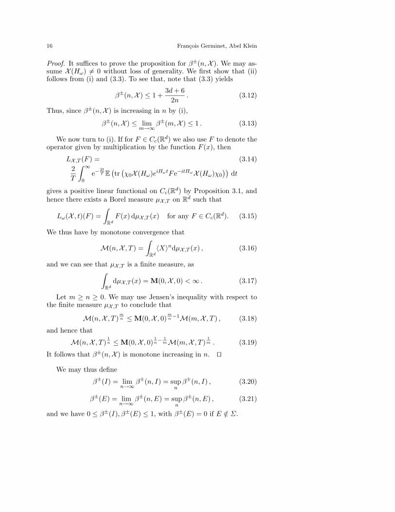
Proof. It suffices to prove the proposition for β±(n,X ). We may as-sume X (Hω) = 0 without loss of generality. We first show that (ii)follows from (i) and (3.3). To see that, note that (3.3) yields
β±(n,X ) ≤ 1 +3d + 6
2n. (3.12)
Thus, since β±(n,X ) is increasing in n by (i),
β±(n,X ) ≤ limm→∞
β±(m,X ) ≤ 1 . (3.13)
We now turn to (i). If for F ∈ Cc(Rd) we also use F to denote theoperator given by multiplication by the function F (x), then
LX ,T (F ) = (3.14)2T
∫ ∞0
e−2tT E
(tr
(χ0X (Hω)eiHωtF e−itHωX (Hω)χ0
))dt
gives a positive linear functional on Cc(Rd) by Proposition 3.1, andhence there exists a Borel measure µX ,T on Rd such that
Lω(X , t)(F ) =∫Rd
F (x) dµX ,T (x) for any F ∈ Cc(Rd). (3.15)
We thus have by monotone convergence that
M(n,X , T ) =∫Rd
〈X〉ndµX ,T (x) , (3.16)
and we can see that µX ,T is a finite measure, as∫Rd
dµX ,T (x) = M(0,X , 0) <∞ . (3.17)
Let m ≥ n ≥ 0. We may use Jensen’s inequality with respect tothe finite measure µX ,T to conclude that
M(n,X , T )mn ≤M(0,X , 0)
mn−1M(m,X , T ) , (3.18)
and hence that
M(n,X , T )1n ≤M(0,X , 0)
1n− 1
mM(m,X , T )1m . (3.19)
It follows that β±(n,X ) is monotone increasing in n.
We may thus define
β±(I) = limn→∞
β±(n, I) = supn
β±(n, I) , (3.20)
β±(E) = limn→∞
β±(n, E) = supn
β±(n, E) , (3.21)
and we have 0 ≤ β±(I), β±(E) ≤ 1, with β±(E) = 0 if E /∈ Σ.

A characterization of the Anderson metal-insulator transport transition 17
Remark 3.3. It is natural to wonder whether one can recover β±(n, I)from the local transport exponents β±(n, E) for E ∈ I. One can easilycheck that this is true locally, i.e. that for each E one can find a smallintervall J containing E such that β±(n, J) ≈ supE′∈J β±(n, E′).More precisely, one shows that for any E, n ∈ N and ν > 0, thereexists JE,n,ν E such that: supE′∈JE,n,ν
β±(n, E′) ≤ β±(n, JE,n,ν) ≤supE′∈JE,n,ν
β±(n, E′)+ ν, or, using the monotonicity of the functionβ±(n, I) in I:
β±(n, E) = infIE
supE′∈I
β±(n, E′). (3.22)
(This should compared to (2.17).) This local inversion formula turnsinto a global one for upper exponents:
β+(n, I) = supE∈I
β+(n, E). (3.23)
This can be seen by combining the local inversion formula and acompactness argument, plus the fact that
β+(n, I1 ∪ I2) = max(β+(n, I1), β+(n, I2)) . (3.24)
Note also that (3.23) trivially extends to the upper asymptotic trans-port exponents: β+(I) = supE∈I β+(E), using Proposition 3.2 (i).
4. The strong insulator region
In this section we show that the strong insulator region may be de-fined by a large number of very natural properties, all equivalent,courtesy of the bootstrap multiscale analysis and Theorem 2.11.
The characteristic function of a set Λ ⊂ Rd is denoted by χΛ. Ifx ∈ Rd, L ∈ 2N, and ΛL(x) is a finite box as in (2.5), we set
χx,L = χΛL(x) (χx = χx,1 = χΛ1(x)) , (4.1)
ΥL(x) =
y ∈ Zd; ‖y − x‖ = L2 − 1
, (4.2)
and define its boundary belt by
ΥL(x) = ΛL−1(x)\ΛL−3(x) =⋃
y∈ΥL(x)
Λ1(y) ; (4.3)
it has the characteristic function
Γx,L = χΥL(x) =∑
y∈ΥL(x)
χy a.e. (4.4)
18 Francois Germinet, Abel Klein
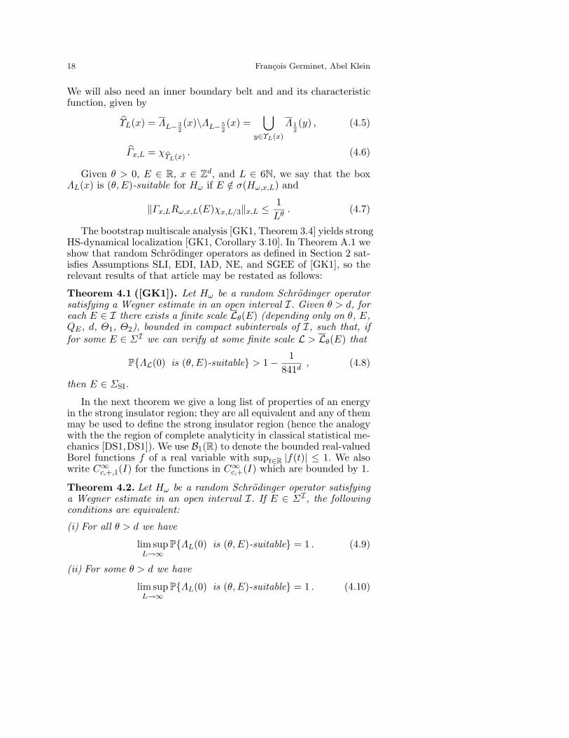
We will also need an inner boundary belt and and its characteristicfunction, given by
ΥL(x) = ΛL− 32(x)\ΛL− 5
2(x) =
⋃y∈ΥL(x)
Λ 12(y) , (4.5)
Γx,L = χΥL(x)
. (4.6)
Given θ > 0, E ∈ R, x ∈ Zd, and L ∈ 6N, we say that the boxΛL(x) is (θ, E)-suitable for Hω if E /∈ σ(Hω,x,L) and
‖Γx,LRω,x,L(E)χx,L/3‖x,L ≤1Lθ
. (4.7)
The bootstrap multiscale analysis [GK1, Theorem 3.4] yields strongHS-dynamical localization [GK1, Corollary 3.10]. In Theorem A.1 weshow that random Schrodinger operators as defined in Section 2 sat-isfies Assumptions SLI, EDI, IAD, NE, and SGEE of [GK1], so therelevant results of that article may be restated as follows:
Theorem 4.1 ([GK1]). Let Hω be a random Schrodinger operatorsatisfying a Wegner estimate in an open interval I. Given θ > d, foreach E ∈ I there exists a finite scale Lθ(E) (depending only on θ, E,QE, d, Θ1, Θ2), bounded in compact subintervals of I, such that, iffor some E ∈ ΣI we can verify at some finite scale L > Lθ(E) that
PΛL(0) is (θ, E)-suitable > 1− 1841d
, (4.8)
then E ∈ ΣSI.
In the next theorem we give a long list of properties of an energyin the strong insulator region; they are all equivalent and any of themmay be used to define the strong insulator region (hence the analogywith the the region of complete analyticity in classical statistical me-chanics [DS1,DS1]). We use B1(R) to denote the bounded real-valuedBorel functions f of a real variable with supt∈R |f(t)| ≤ 1. We alsowrite C∞c,+,1(I) for the functions in C∞c,+(I) which are bounded by 1.
Theorem 4.2. Let Hω be a random Schrodinger operator satisfyinga Wegner estimate in an open interval I. If E ∈ ΣI , the followingconditions are equivalent:
(i) For all θ > d we have
lim supL→∞
PΛL(0) is (θ, E)-suitable = 1 . (4.9)
(ii) For some θ > d we have
lim supL→∞
PΛL(0) is (θ, E)-suitable = 1 . (4.10)

A characterization of the Anderson metal-insulator transport transition 19
(iii) For some θ > d we have
lim supL→∞
PΛL(0) is (θ, E)-suitable > 1− 1841d
. (4.11)
(iv) E ∈ ΣMSA, i.e., for some θ > d we can verify (4.8) at some finitescale L > Lθ(E), where Lθ(E) is given in Theorem 4.1.
(v) There exists δ > 0 such that for each 0 < ζ < 1 we have
E
(sup
f∈B1(R)‖χxf(Hω)EHω([E − δ, E + δ])χy‖22
)≤ Cζ e−|x−y|ζ (4.12)
for all x, y ∈ Zd, with Cζ <∞.(vi) For some 0 < ζ < 1 there exists δ > 0 such that
E
(sup
f∈B1(R)‖χxf(Hω)EHω([E − δ, E + δ])χy‖22
)≤ C e−|x−y|ζ (4.13)
for all x, y ∈ Zd, with C <∞.(vii) There exists δ > 0 such that for each p = 1, 2, . . . we have
E
(sup
f∈B1(R)‖χxf(Hω)EHω([E − δ, E + δ])χy‖22
)≤ Cp
〈x− y〉p (4.14)
for all x, y ∈ Zd, with Cp <∞.(viii) There exists δ > 0 such that we have
E
(sup
f∈B1(R)
∥∥∥〈X〉n2 f(Hω)EHω([E − δ, E + δ])χ0
∥∥∥2
2
)<∞ (4.15)
for all n ≥ 0.(ix) There exists δ > 0 such that we have
E
(sup
X∈C∞c,+,1((E−δ,E+δ))
∥∥∥〈X〉n2X (Hω)χ0
∥∥∥2
2
)<∞ (4.16)
for all n ≥ 0.(x) E ∈ ΣSI , i.e., Hω exhibits strong HS-dynamical localization at E.(xi) Hω exhibits strong operator-norm-dynamical localization at E
(see (2.13)).(xii) β+(E) = 0.(xiii) E ∈ ΣTT , i.e., β(E) = 0.(xiv) For some n > 11d we have β(n, E) = 0.(xv) For some n > 11d we have β(n, E) < 1
2d − 112n .

20 Francois Germinet, Abel Klein
(xvi) There exist X ∈ C∞c,+(R), with X ≡ 1 on some open intervalcontaining E, α ≥ 0, and n > 2dα + 11d, such that we have(2.28).
Proof. It is clear that (i) ⇒ (ii) ⇒ (iii) ⇒ (iv), that (v) ⇒ (vi) ⇒(vii), that (viii) ⇒ (ix) ⇒ (x) ⇒ (xii) ⇒ (xiii) ⇒ (xiv) ⇒ (xv) ⇒(xvi), and that (x) ⇒ (xi). The proof of [GK1, Corollary 3.10] showsthat (vii) ⇒ (viii).
To see that (xi) ⇒ (x), note that, proceeding as in the proof ofProposition 3.1 and using (A.12) as in (3.7),
Mω(n,X , t) = tr(χ0X (Hω)eitHω〈X〉ne−itHωX (Hω)χ0
)(4.17)
≤ 22ν‖〈X〉n+2νe−itHωX (Hω)χ0‖‖ 〈X〉−2ν X (Hω)eitHω 〈X〉−2ν ‖1≤ 22ν+2Tν,d,Θ1,Θ2 ‖XΦd,Θ1,Θ2‖∞ ‖〈X〉
n+2νe−itHωX (Hω)χ0‖ .
The nontrivial content of the theorem is that (iv)⇒ (v), and (xvi)⇒ (i). The first implication is the content of [GK1, Theorem 3.8]. Toprove the second implification, we note first that (xvi) ⇒ (iv) byTheorem 2.11. To finish the proof, we must show that (iv) ⇒ (i).This can be proved by, either adapting the proof of [GK1, Theorems5.1 and 5.2], or by using the already established fact that (iv) ⇒(xiii), that it follows from (xiii) that there exists X ∈ C∞c,+(R), withX ≡ 1 on some open interval containing E, such that for all α ≥ 0and n > 2dα + 11d we have (2.28), and hence that (i) follows fromthe proof of Theorem 2.11 since given arbitrary θ > d we can pickα ≥ 0 and n > 2dα + 11d such that the proof of Theorem 2.11 gives(4.9) with this θ (see (6.47) and (6.54)).
Remark 4.3. In [GK1] we used (viii) as the definition of strong HS-dynamical localization in the interval [E − δ, E + δ].
5. The metallic transport region
In this section we give a characterization of the metallic transportregion, and a criterion for an energy to be in it. Roughly speaking,the criterion says that if the finite volume resolvent does not decayfaster than the inverse of the volume of the box, then the energy Emust be in the metallic transport region. More precisely, it says thatif (4.10) is violated with θ = d, then E ∈ ΣMT .
Given θ > 0, E ∈ R, x ∈ Zd, and L ∈ 6N, we say that the boxΛL(x) is (θ, E)-unsuitable for Hω if it is not (θ, E)-suitable for Hω
(see (4.7)), i.e., if either E ∈ σ(Hω,x,L) or
‖Γx,LRω,x,L(E)χx,L/3‖x,L >1Lθ
. (5.1)
A characterization of the Anderson metal-insulator transport transition 21
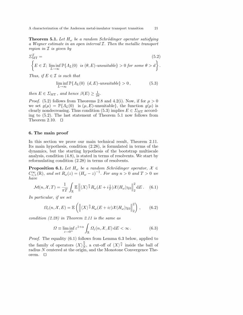
Theorem 5.1. Let Hω be a random Schrodinger operator satisfyinga Wegner estimate in an open interval I. Then the metallic transportregion in I is given by
ΣIMT = (5.2)E ∈ I; lim inf
L→∞PΛL(0) is (θ, E)-unsuitable > 0 for some θ > d
.
Thus, if E ∈ I is such that
lim infL→∞
PΛL(0) (d, E)-unsuitable > 0 , (5.3)
then E ∈ ΣMT , and hence β(E) ≥ 12d .
Proof. (5.2) follows from Theorems 2.8 and 4.2(i). Now, if for µ > 0we set g(µ) = PΛL(0) is (µ, E)-unsuitable, the function g(µ) isclearly nondecreasing. Thus condition (5.3) implies E ∈ ΣMT accord-ing to (5.2). The last statement of Theorem 5.1 now follows fromTheorem 2.10.
6. The main proof
In this section we prove our main technical result, Theorem 2.11.Its main hypothesis, condition (2.28), is formulated in terms of thedynamics, but the starting hypothesis of the bootstrap multiscaleanalysis, condition (4.8), is stated in terms of resolvents. We start byreformulating condition (2.28) in terms of resolvents.
Proposition 6.1. Let Hω be a random Schrodinger operator, X ∈C∞c,+(R), and set Rω(z) = (Hω − z)−1. For any n > 0 and T > 0 wehave
M(n,X , T ) =1
πT
∫R
E
∥∥∥〈X〉n2 Rω(E + i 1
T )X (Hω)χ0
∥∥∥2
2dE . (6.1)
In particular, if we set
Ωε(n,X , E) = E(∥∥∥〈X〉n
2 Rω(E + iε)X (Hω)χ0
∥∥∥2
2
), (6.2)
condition (2.28) in Theorem 2.11 is the same as
Ω ≡ lim infε→0+
ε1+α
∫R
Ωε(n,X , E) dE < ∞ . (6.3)
Proof. The equality (6.1) follows from Lemma 6.3 below, applied tothe family of operators 〈X〉
n2N , a cut-off of 〈X〉n
2 inside the ball ofradius N centered at the origin, and the Monotone Convergence The-orem.

22 Francois Germinet, Abel Klein
Remark 6.2. Proposition 6.1 is the main reason for the use of Hilbert-Schmidt norms in our definitions. Their use is justified by [GK1,Corollary 3.10] and Theorem 4.2.
Lemma 6.3. Let A, B be bounded operators, H a self-adjoint opera-tor, and R(z) = (H − z)−1. Then for all T > 0 we have∫ ∞
0e−
2tT
∥∥Ae−iHtB∥∥2
2dt = 2π
∫R
∥∥AR(E + i 1T )B
∥∥2
2dE . (6.4)
Proof. By the spectral theorem,(H −
(E + i 1
T
))−1 = i
∫ ∞0
eitEe−it(H−i
1T
)dt . (6.5)
Multiplying on the left by the operator A and on the right by the oper-ator B, taking matrix elements of both sides, and applying Plancherel’sTheorem we get that for any vector ψ ∈ H we have∫ ∞
0e−
2tT
∥∥Ae−iHtBψ∥∥2
dt = 2π
∫R
∥∥AR(E + i 1T )Bψ
∥∥2 dE . (6.6)
The lemma then follows from the definition of the Hilbert-Schmidtnorm: ‖T‖22 =
∑n ‖Ten‖2, where (en)n∈N is any orthonormal basis
for the Hilbert space.
The proof of Theorem 2.11 requires that we obtain the finite vol-ume condition (4.8) out of the infinite volume condition (6.3). Thefollowing lemma will play an important role in estimating finite vol-ume probabilities out of infinite volume expectations.
We recall our notation for finite volume introduced in (2.5) andin Section 4 (see (4.1) - (4.6)). Following [FK1,FK2,KK1], we equipeach cube ΛL(x) with functions φx,L and ρx,L ∈ C1
c (Rd), such thatsuppφx,L, supp ρx,L ⊂ ΛL(x), 0 ≤ φx,L, ρx,L ≤ 1, and
χx, L2− 5
4φx,L = χx, L
2− 5
4, χx, L
2− 3
4φx,L = φx,L , (6.7)
Γx,L (∇φx,L) = ∇φx,L , |∇φx,L| ≤ 3√
d , (6.8)
Γx,L ρx,L = Γx,L , Γx,L ρx,L = ρx,L , (6.9)
|∇ρx,L| ≤ 5√
d . (6.10)
In what follows we work with boxes centered at 0 and omit thecenter from the notation.
Lemma 6.4. Let Hω be a random Schrodinger operator satisfying aWegner estimate in an open interval I. Let p0 > 0 and γ > d. Foreach E ∈ I there exists L1 = L1(d, Θ1, Θ2, E, QE , γ, p0), bounded oncompact subsets of I, such that given L ∈ 2N with L ≥ L1, and

A characterization of the Anderson metal-insulator transport transition 23
subsets B1 and B2 of ΛL with B1 ⊂ ΛL/2−5/4 and ΥL ⊂ B2 , then foreach a > 0 and 0 < ε ≤ 1 we have
P
(‖χB2Rω,L(E + iε)χB1‖L >
a
4
)≤ (6.11)
Lγ
aE (‖χB2Rω(E + iε)χB1‖) +
p0
10,
and
P
(‖χB2Rω,L(E)χB1‖L >
a
2
)≤ (6.12)
Lγ
aE (‖χB2Rω(E + iε)χB1‖) +
p0
10+ 2QE
( ε
a
) 12Ld.
We shall use Lemma 6.4 with B2 equal to either ΥL (recall ΓL =χΥL
) or ΛL\Λ 2L3
, and B1 equal to either Λ 2L3
or ΛL3.
Proof of Lemma 6.4. We write χ1 and χ2 for χB1 and χB2 , notethat φLχ1 = χ1 and ΓL ≤ χ2. We start by estimating the quantity‖χ2Rω,L(E + iε)χ1‖L in terms of ‖χ2Rω(E + iε)χ1‖. (The estimateis given in (6.18) below.) To do so, we proceed as in [KK1, Lemma3.7], obtaining
Rω(E − iε)φLJL = JLφLRω,L(E − iε) (6.13)+ Rω(E − iε)(∇φL)∗JL∇LRω,L(E − iε)− Rω(E − iε)∇∗JL(∇φL)Rω,L(E − iε) ,
as bounded operators from L2(ΛL,dx) to L2(Rd,dx), whereJL: L2(ΛL,dx) → L2(Rd,dx) is the canonical injection. Taking ad-joints, we get
χ2Rω,L(E + iε)χ1J∗L = χ2Rω,L(E + iε)φLJ∗Lχ1 = (6.14)
χ2J∗LφLRω(E + iε)χ1 − χ2Rω,L(E + iε)∇∗LJ∗L(∇φL)Rω(E + iε)χ1
+ χ2Rω,L(E + iε)(∇φL)∗J∗L∇Rω(E + iε)χ1 .
Thus, proceeding as in the proof of [KK1, Lemma 3.8], and recalling(6.7)-(6.10),
‖χ2Rω,L(E + iε)χ1‖L ≤ ‖χ2Rω(E + iε)χ1‖+ (6.15)
3√
d ‖χ2Rω,L(E + iε)∇∗LρL‖L‖ΓLRω(E + iε)χ1‖+ ‖χ2Rω,L(E + iε)ΓL‖L‖ρL∇Rω(E + iε)χ1‖ .
We now use Lemma A.2 (choosing always an appropriate a > 0 in(A.2)) to obtain
‖ρL∇Rω(E + iε)χ1‖ ≤ (6.16)
C(1)d,Θ1,Θ2
(1 + |E + iε|)‖ΓLRω(E + iε)χ1‖ ,
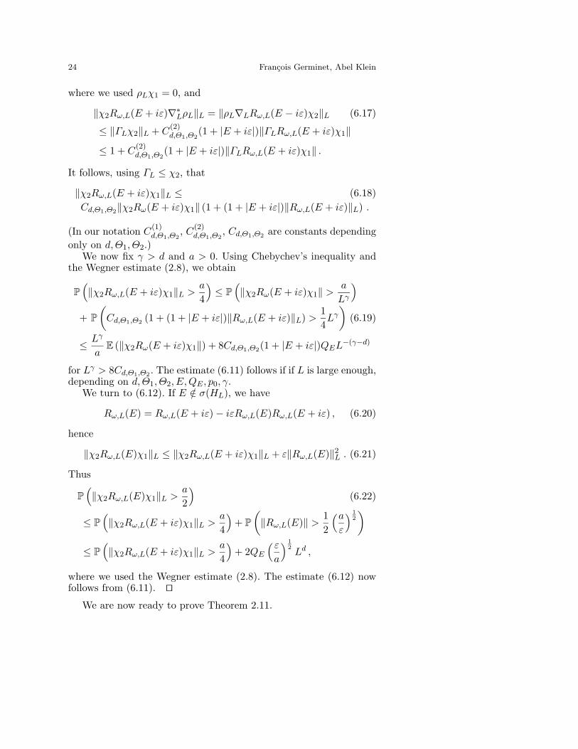
24 Francois Germinet, Abel Klein
where we used ρLχ1 = 0, and
‖χ2Rω,L(E + iε)∇∗LρL‖L = ‖ρL∇LRω,L(E − iε)χ2‖L (6.17)
≤ ‖ΓLχ2‖L + C(2)d,Θ1,Θ2
(1 + |E + iε|)‖ΓLRω,L(E + iε)χ1‖
≤ 1 + C(2)d,Θ1,Θ2
(1 + |E + iε|)‖ΓLRω,L(E + iε)χ1‖ .
It follows, using ΓL ≤ χ2, that
‖χ2Rω,L(E + iε)χ1‖L ≤ (6.18)Cd,Θ1,Θ2‖χ2Rω(E + iε)χ1‖ (1 + (1 + |E + iε|)‖Rω,L(E + iε)‖L) .
(In our notation C(1)d,Θ1,Θ2
, C(2)d,Θ1,Θ2
, Cd,Θ1,Θ2 are constants dependingonly on d, Θ1, Θ2.)
We now fix γ > d and a > 0. Using Chebychev’s inequality andthe Wegner estimate (2.8), we obtain
P
(‖χ2Rω,L(E + iε)χ1‖L >
a
4
)≤ P
(‖χ2Rω(E + iε)χ1‖ >
a
Lγ
)+ P
(Cd,Θ1,Θ2 (1 + (1 + |E + iε|)‖Rω,L(E + iε)‖L) >
14Lγ
)(6.19)
≤ Lγ
aE (‖χ2Rω(E + iε)χ1‖) + 8Cd,Θ1,Θ2(1 + |E + iε|)QEL−(γ−d)
for Lγ > 8Cd,Θ1,Θ2 . The estimate (6.11) follows if if L is large enough,depending on d, Θ1, Θ2, E, QE , p0, γ.
We turn to (6.12). If E /∈ σ(HL), we have
Rω,L(E) = Rω,L(E + iε)− iεRω,L(E)Rω,L(E + iε) , (6.20)
hence
‖χ2Rω,L(E)χ1‖L ≤ ‖χ2Rω,L(E + iε)χ1‖L + ε‖Rω,L(E)‖2L . (6.21)
Thus
P
(‖χ2Rω,L(E)χ1‖L >
a
2
)(6.22)
≤ P(‖χ2Rω,L(E + iε)χ1‖L >
a
4
)+ P
(‖Rω,L(E)‖ >
12
(a
ε
) 12
)≤ P
(‖χ2Rω,L(E + iε)χ1‖L >
a
4
)+ 2QE
( ε
a
) 12Ld ,
where we used the Wegner estimate (2.8). The estimate (6.12) nowfollows from (6.11).
We are now ready to prove Theorem 2.11.
A characterization of the Anderson metal-insulator transport transition 25
Proof of Theorem 2.11. Suppose condition (2.28) holds for given X ∈C∞c,+(R), with X ≡ 1 in an open interval J ⊂ I, α ≥ 0, and n >2dα + 11d, so we have (6.3) by Proposition 6.1. To prove Theorem2.11, it suffices to show that for each E ∈ J there is some θ > d suchthat condition (4.10) is satisfied, i.e.,
lim supL→∞
P
(‖ΓLRω,L(E)χL/3‖L ≤
1Lθ
)= 1 , (6.23)
so the starting condition (4.8) of the bootstrap multiscale analysisholds at some finite scale L > Lθ(E).
So let E ∈ J , θ > d, and L ∈ 6N. We start by estimating
PE,L = P(‖ΓLRω,L(E)χL/3‖L >
12Lθ
). (6.24)
Using (6.12) in Lemma 6.4 with a = 2L−θ would provide an estimatefor PE,L. But later on we would need n > 3dα + 11d to concludethe proof. To work with n > 2dα + 11d, we squeeze a bit more fromLemma 6.4. We use the resolvent identity (6.20), plus
χL = χ 2L3
+ χL\ 2L3
, where χL\ 2L3≡ χΛL\Λ 2L
3
, (6.25)
to obtain
‖ΓLRω,L(E)χL/3‖L ≤ ‖ΓLRω,L(E + iε)χL/3‖L (6.26)+ ε ‖ΓLRω,L(E)χ2L/3‖L ‖Rω,L(E + iε)‖L (6.27)+ ε ‖Rω,L(E)‖L ‖χL\2L/3Rω,L(E + iε)χL/3‖L . (6.28)
We now estimate ‖ΓLRω,L(E + iε)χL/3‖L in (6.26) using (6.11) witha = L−θ, ‖ΓLRω,L(E)χ2L/3‖L in (6.27) by (6.12) with a = 1, and‖χL\2L/3Rω,L(E + iε)χL/3‖L in (6.28) using (6.11) with a = 1. Theprobability that ε‖Rω,L(E)‖L is greater than 1
4L−θ is estimated by(2.8). We obtain
PE,L ≤ Lθ+γE
(‖ΓLRω(E + iε)χL/3‖
)+ (6.29)
LγE
(‖ΓLRω(E + iε)χ2L/3‖
)+ Lγ
E(‖χL\2L/3Rω(E + iε)χL/3‖
)+ 4QEεLθ+d + 2QIε
12 Ld +
3 p0
10,
where γ > d, 0 < ε ≤ 1, and 0 < p0 < 1. The estimate is valid forL > L1, where L1 = L1(d, Θ1, Θ2, E, QE , γ, p0) is as in Lemma 6.4.
Compared to the direct use of (6.12) with a = L−θ, the gain lies inthe fact that now L will be chosen such that ε ≈ L−θ−d (recall θ > d)instead of ε ≈ L−θ−2d. This will allow us to work with n > 2dα+11dinstead of n > 3dα + 11d.
26 Francois Germinet, Abel Klein
Let I be a compact subinterval of J . We will estimate the right-hand-side of (6.29) for E ∈ I. To do so, let
QI = supE∈I
QE <∞ , (6.30)
where QE is given in (2.8). We need to estimate the expressionL(θ+γ)
E(‖ΓLRω(E + iε)χL/3‖
), plus two similar terms. To do so, we
use
E(‖ΓLRω(E + iε)χL/3‖
)≤ E
(‖ΓLRω(E + iε)X (Hω)χL/3‖
)+ E
(‖ΓLRω(E + iε)(1−X (Hω))χL/3‖
). (6.31)
To estimate the last term, note that since X (u) = 1 for all u ∈ J , thefunction
fE,ε(u) = (u− (E + iε))−1(1−X (u)) (6.32)
is a bounded, infinitely differentiable function on the real line forE ∈ J and ε ∈ R. Moreover, it is easy to see that
supE∈I
sup|ε|≤1
|||fE,ε|||k <∞ for all k = 1, 2, . . . . (6.33)
(The norms are defined in (A.16).) It follows from (A.15) and (6.33)that for all E ∈ I and |ε| ≤ 1 we h ve
sup|ε|≤1
Lθ+γE
(‖ΓLRω(E + iε)(1−X (Hω))χL/3‖
)≤ p0
10(6.34)
if L ≥ L2(I), with L2(I) = L2(d, Θ1, Θ2,X , I, θ, γ, p0) <∞.On the other hand,
E(‖ΓLRω(E + iε)X (Hω)χL/3‖
)(6.35)
≤∑
y∈Zd∩Λ L3
(0)
E (‖ΓLRω(E + iε)X (Hω)χy‖)
=∑
y∈Zd∩Λ L3
(0)
E
(‖χΥL−yRω(E + iε)X (Hω)χ0‖
)
≤(
L
3− 3
2
)−n2 ∑
y∈Zd∩Λ L3
(0)
E
(‖|〈X〉n
2 χΥL−yRω(E + iε)X (Hω)χ0‖)
≤(
L
3− 3
2
)−n2
(L
3
)d
E
(‖|〈X〉n
2 Rω(E + iε)X (Hω)χ0‖)
≤ 12n
3dL−
n2+dE
(‖〈X〉n
2 Rω(E + iε)X (Hω)χ0‖2)
,
where we used L ≥ 6 and ‖A‖ ≤ ‖A‖2.
A characterization of the Anderson metal-insulator transport transition 27
Combining (6.31), (6.34), (6.35), and (6.2), we conclude that forE ∈ I and 0 < ε ≤ 1 we have
Lθ+γE
(‖ΓLRω(E + iε)χL/3‖
)(6.36)
≤ 12n
3dL−
n2+d+θ+γ
E
(‖〈X〉
n2 Rω(E + iε)X (Hω)χ0‖2
)+
p0
10
≤ 12n
3dL−
n2+d+θ+γ
(E
(‖〈X〉
n2 Rω(E + iε)X (Hω)χ0‖22
))1/2+
p0
10
≤ 12n
3dΩε(n,X , E)
12 L−
n2+d+θ+γ +
p0
10,
for L ≥ L2(I).The two other similar terms in (6.29), namely the terms given
by LγE(‖ΓLRω,L(E + iε)χ 2L
3‖) and Lγ
E(‖χL\2L/3Rω,L(E + iε)χL3‖),
are estimated in the same way, using the fact that dist(ΥL, Λ 2L3
) ≥L6 − 3
2 and dist(ΛL\ 2L3
, ΛL3) ≥ L
6 . We conclude that there is L3(I) =L3(d, Θ1, Θ2,X , I, QI , θ, γ, p0), such that if L ≥ L3(I) we have
PE,L ≤ (6.37)
Cn,d Ωε(n,X , E)12 L−
12n+d+θ+γ + 4QI εLθ+d + 2QIε
12 Ld +
3p0
5
for all E ∈ I and 0 < ε ≤ 1.For a given ε > 0 we set (with [K]6N = maxL ∈ 6N; L ≤ K)
L(I, ε) =
[(p0
40QI ε
) 1θ+d
]6N
. (6.38)
Thus 4QIεL(I, ε)θ+d ≤ p0/10. In addition, since θ > d, 2QIε12 L(I, ε)d ≤
p0
10 for ε small enough, depending on QI , θ, d, p0. From (6.38) we alsohave
p0
160 QIL(I, ε)−(θ+d) ≤ ε ≤ p0
80 QIL(I, ε)−(θ+d) (6.39)
for ε small enough, depending on QI , p0, d. It follows from (6.37) and(6.39) that there exists ε(I) = ε((d, Θ1, Θ2,X , I, QI , θ, γ, p0) > 0,such that for all 0 < ε ≤ ε(I) and E ∈ I we have
PE,L(I,ε) ≤ Cn,d Ωε(n,X , E)12 L(I, ε)−
n2+d+θ+γ +
45p0 . (6.40)
At this point we might be tempted to conclude the proof by notingthat applying Fatou’s Lemma to condition (6.3) yields∫
R
lim infε→0+
ε1+αΩε(n,X , E) dE < +∞, (6.41)
28 Francois Germinet, Abel Klein
hence lim infε→0+ ε1+αΩε(n,X , E) <∞ for for a.e. E. If n > 2dα+8d,it follows from (6.40), (6.39), and (6.41) that we can choose θ > dand γ > d such that
lim infL→∞
PE,L ≤ lim infε→0+
PE,L(E,ε) ≤ p0 (6.42)
for a.e. E ∈ I, and hence, since I is an arbitrary compact subin-terval of J , for a.e. E ∈ J . Since p0 is also arbitrary, the startingcondition (6.23) for the bootstrap multiscale analysis is satisfied ata.e. E ∈ J . It follows from [GK1, Corollary 3.10 and Theorem 3.11]that there is a open subset G of J , such that J\G has zero Lebesguemeasure and the random operator Hω exhibits pure point spectrumand strong HS-dynamical localization in G. (If we assumed the hy-potheses of [CHM, Corollary 1.3], we could even conclude that Hω
has pure point spectrum in the whole interval J .) But we cannot con-clude that there is strong HS-dynamical localization in J ; we cannotrule out the possibility of energies where the multiscale analysis can-not be performed (i.e., energies outside ΣMSA), although the set ofsuch singular energies must have zero measure.
To overcome this difficulty we use two facts: a) the Wegner esti-mate (2.8) holds everywhere in the interval J , and, b) the informationthat we have at our disposal is stronger than (6.41), we are given thefiniteness of the right-hand-side of the inequality in Fatou’s Lemma,namely condition (6.3).
We shall prove that there are no singular energies, i.e., that (6.23)holds for all E ∈ J . In view of (6.3) we can pick a sequence εk → 0+such that
ε1+αk
∫R
Ωεk(n,X , E) dE ≤ 2Ω for k = 1, 2, . . . . (6.43)
Given a compact subinterval of I of J and M > 0, we set
Ak,I,M = E ∈ I; ε1+αk Ωεk
(n,X , E) ≤M . (6.44)
In view of (6.43), we have
|I\Ak,I,M | ≤2 Ω
Mfor all k and M , (6.45)
where |A| denotes the Lebesgue measure of the set A. It follows from(6.40) and (6.39) that for each E ∈ Ak,I,M we have
PE,Lk(I) ≤ Cn,dM1/2Lk(I)−m +
45p0 , (6.46)
where Lk(I) = L(I, εk), and
m =n
2− d− θ − γ − 1
2(1 + α)(θ + d), (6.47)
A characterization of the Anderson metal-insulator transport transition 29
with m > 0 for suitable n’s. We set
Mk,I = 2ΩLk(I)θ+2γ , (6.48)Ak(I) = Ak,I,Mk,I
. (6.49)
From (6.46) we see that
PE,Lk(I) ≤ Cn,d(2Ω)1/2Lk(I)−m+ 12θ+γ +
45p0 if E ∈ Ak(I) , (6.50)
hence there exists k(I) = k(d, I, n, α, Ω, θ, γ, p0) < ∞, such that ifk ≥ k(I) we have PE,Lk(I) ≤ p0 for all E ∈ Ak(I).
Let E′ ∈ I. It follows from (6.45) and (6.48) that we can findE ∈ Ak(I) such that
|E − E′| ≤ 2Ω
Mk= Lk(I)−θ−2γ . (6.51)
The resolvent identity gives
‖ΓLRω,L(E′)χL3‖L (6.52)
≤ ‖ΓLRω,L(E)χL3‖L + |E − E′|‖Rω,L(E′)‖L‖Rω,L(E)‖L
≤ ‖ΓLRω,L(E)χL3‖L + Lk(I)−θ−2γ‖Rω,L(E′)‖L‖Rω,L(E)‖L ,
for any L. If dist(E, σ(HLk(I)) > 2Lk(I)−γ , it follows from (6.51) thatdist(E′, σ(HLk(I))) > Lk(I)−γ for k large enough, depending only onθ and γ. Using the Wegner estimate (2.8) with the estimates (6.52)and (6.50), we see that we have
P
(∥∥∥∥ΓLk(I)Rω,Lk(I)(E′)χLk(I)
3
∥∥∥∥Lk(I)
>1
Lk(I)θ
)(6.53)
≤ PE,Lk(I) + 2QILk(E)−γ+d
≤ Cn,d(2Ω)1/2Lk(I)−m+ 12θ+γ +
45p0 + 2QILk(I)−γ+d
≤ Cn,d(2Ω)1/2Lk(I)−m+ 12θ+γ +
910
p0 ,
for all k large enough, depending on QI , θ, γ, p0, but independent ofthe energy E′ ∈ I.
Given n > n(α) = 2dα + 11d, we now choose θ > d and γ > dsuch that
m >12θ + γ . (6.54)
30 Francois Germinet, Abel Klein
It follows from (6.53) that for all E′ ∈ I we have
lim supk→∞
P
(∥∥∥∥ΓLk(I)Rω,Lk(I)(E′)χLk(I)
3
∥∥∥∥Lk(I)
>1
Lk(I)θ
)≤ p0 .
(6.55)Since 0 < p0 < 1 is arbitrary, we conclude that (6.23) holds for eachE′ ∈ I.
Theorem 2.11 is proven.
A. Properties of random Schrodinger operators
In this appendix we verify properties of random Schrodinger oper-ators that are needed for the bootstrap multiscale analysis [GK1](justifying Theorem 4.1) and for the proof of Theorem 2.11.
Theorem A.1. Let Hω be a random Schrodinger operator (as de-fined in Section 2, satifying conditions (R), (E), and (IAD)). ThenHω is a Zd-ergodic random self-adjoint operator satisfying Assump-tions SLI, EDI, IAD, NE, and SGEE of [GK1]. The constants γI0in Assumption SLI and γI0 in Assumption EDI are given by γI0 =γI0 = supE∈I0 γE, with
γE = 6√
2d
1−Θ1
√|E|+ Θ2 +
200d
1−Θ1. (A.1)
Proof. We saw in Section 2 that Hω is a random self-adjoint operator;Z
d-ergodicity is the content of condition (E), and Assumption IADof [GK1] was built into condition (IAD). (Condition (IAD) is notneeded to prove any of the other properties.)
We consider a (nonrandom) Schrodinger operator H = −∆ + V
on L2(Rd,dx), where the potential V = V (1) + V (2) satisfies theregularity condition (R) of Section 2, with constants 0 ≤ Θ1 < 1 and0 ≤ Θ2 < ∞ as in (2.7). We will prove properties for H that willthen be valid for random Schrodinger operators with probability one,proving Assumptions SLI, EDI, NE, and SGEE.
We start with an interior estimate, which is also used in the proofof Lemma 6.4.
Lemma A.2. Let x ∈ Rd, L ∈ 2N∪∞, and η a real valued, contin-uously differentiable function on Rd with compact support K ⊂ Λx,L
and ‖η‖∞ ≤ 1. Then for any a > 0 we have
‖η∇x,Lψ‖2x,L ≤ (A.2)
a ‖χKHx,Lψ‖2x,L + 2(1−Θ1)2
(12a + Θ2(1−Θ1) + 8‖∇η‖2∞
)‖χKψ‖2x,L
for all ψ ∈ D(Hx,L).
A characterization of the Anderson metal-insulator transport transition 31
Proof. We adapt the proof of [Wei, Auxiliary Theorem 10.26]. In thefollowing the constants r, s, t > 0 will be chosen later on. We have(we omit x, L from the norms)
r ‖ηHx,Lψ‖2 + 1r ‖ηψ‖2 ≥ 2Re
⟨Hx,Lψ, η2ψ
⟩(A.3)
= 2Re⟨∇x,Lψ,∇x,Lη2ψ
⟩+ 〈ηψ, V ηψ〉
≥ 2Re
⟨∇x,Lψ, η2∇x,Lψ
⟩+ 2 〈η∇x,Lψ, (∇η)ψ〉+
⟨ηψ, V (2)ηψ
⟩≥ 2
(1− s) ‖η∇x,Lψ‖2 − 1
s ‖(∇η)ψ‖2 −Θ1 ‖∇x,Lηψ‖2 −Θ2 ‖ηψ‖2
≥ 2
(1− s− (1 + t)Θ1) ‖η∇x,Lψ‖2 −(
1s +
(1 + 1
t
)Θ1
)‖(∇η)ψ‖2
−Θ2 ‖ηψ‖2
,
where we used (2.7) and the fact that
‖∇x,Lηψ‖2 ≤ (1 + t) ‖η∇x,Lψ‖2 +(1 + 1
t
)‖(∇η)ψ‖2 . (A.4)
The desired estimate (A.2) now follows from (A.3) if ‖η‖∞ ≤ 1, bychoosing s = 1−Θ1
4 , t = sΘ1
, and r = 2a(1−s−(1+t)Θ1) = a(1−Θ1).
Assumption SLI can now be proven for H exactly as in [KK1,Lemma 3.8], using Lemma A.2 instead of [KK1, Lemma 3.4]. Theconstant γE corresponding to [KK1, eq. (3.80)], i.e., γE such that theconstant γI0 in [GK1, eq. (2.9)] is given by γI0 = supE∈I0 γE , is givenby (A.1)
Similarly, Assumption EDI is proven as in [KK1, Lemma 3.9], withthe constant γI0 appearing in [GK1, eq. (2.15)] being the same as γI0in Assumption SLI.
We now turn to Assumption NE, and prove a deterministic esti-mate. Since it follows from (2.7) that for x ∈ Rd, L ∈ 2N ∪ ∞ wehave
Hx,L ≥ −(1−Θ1)∆x,L −Θ2, (A.5)
it follows by standard arguments (e.g., [KK1, Lemma 3.3]) that
trχ(−∞,E)(Hx,L)
≤ tr
χ(−∞,
E+Θ21−Θ1
)(−∆x,L)
(A.6)
≤ Cd
((E + Θ2) ∨ 0
1−Θ1
) d2
Ld ,
for some constant Cd depending on d only. Assumption NE follows.It remains to prove Assumption SGEE. This will be done in two
lemmas.
32 Francois Germinet, Abel Klein
Lemma A.3. The set D0(H) = φ ∈ D(H); φ has compact supportis an operator core for H.
Proof. Given a semi-bounded self-adjoint operator W , the correspond-ing quadratic form will be denoted by W (ϕ, ψ), with ϕ, ψ ∈ Q(W ),the quadratic form domain of W .
Since we have Q(H) = D(∇) ∩Q(V (1)), it follows that ηQ(H) ⊂Q(H) if η is a real valued, twice continuously differentiable functionon Rd which is bounded with bounded first and second derivatives.Thus, if ψ ∈ D(H) and ϕ ∈ Q(H), we have
H(ϕ, ηψ) = 〈∇ϕ,∇ηψ〉+ 〈ϕ, V ηψ〉 (A.7)= 〈∇ηϕ,∇ψ〉+ 〈ηϕ, V ψ〉 − 〈ϕ, (∇η) · ∇ψ〉+ 〈∇ϕ, (∇η)ψ〉= 〈ηϕ, Hψ〉 − 2〈ϕ, (∇η) · ∇ψ〉 − 〈ϕ, (∆η)ψ〉 .
Thus, using also (A.5), we get
|H(ϕ, ηψ)| ≤ (A.8)(‖η‖∞ + 2‖∇η‖∞√
1−Θ1
)‖Hψ‖+
(‖∆η‖∞ + 2
√Θ2‖∇η‖∞√
1−Θ1
)‖ψ‖
‖ϕ‖ .
thus ηψ ∈ D(H) and
‖Hηψ‖ ≤ (A.9)(‖η‖∞ + 2‖∇η‖∞√
1−Θ1
)‖Hψ‖+
(‖∆η‖∞ + 2
√Θ2‖∇η‖∞√
1−Θ1
)‖ψ‖
.
We now pick a real valued, twice continuously differentiable func-tion ρ on Rd with compact support, such that 0 ≤ ρ ≤ 1 and ρ(0) = 1.For each n = 1, 2, . . . we set ρn(x) = ρ( 1
nx) and ηn = 1 − ρn. Givenψ ∈ D(H). we let ψn = ρnψ. Then ψn ∈ D0(H), ‖ψ − ψn‖ → 0, and‖H(ψ − ψn)‖ = ‖H(ηnψ)‖ → 0 by (A.9). Thus D0(H) is a core forH.
Let ν > d/4, H+ = L2(Rd, 〈x〉4νdx), and D+(H) = φ ∈ D(H) ∩H+; Hφ ∈ H+. Since if ψ ∈ D0(H) we can see that Hψ has compactsupport by looking at the quadratic form, we have D0(H) ⊂ D+(H),and hence D+(H) is a core for H. It is also easy to see that D0(H),and hence also D+(H), is dense in H+. This proves the first part ofAssumption GEE in [GK1, page 425], which is also the first part ofSGEE. The second part of SGEE, [GK1, eq. (2.32)], will follow fromthe following lemma. Note that the lemma proves the stronger [GK1,eq. (2.36)].
Lemma A.4. Let ν > d4 . There is a finite constant Tν,d,Θ1,Θ2, de-
pending only on the indicated constants, such that
tr(〈X〉−2ν (H + Θ2 + (1−Θ1))
−2[[ d4]] 〈X〉−2ν
)≤ Tν,d,Θ1,Θ2 , (A.10)
A characterization of the Anderson metal-insulator transport transition 33
where [[d4 ]] is the smallest integer > d4 . Thus, letting
Φd,Θ1,Θ2(E) = (E + Θ2 + (1−Θ1))2[[ d
4]] , (A.11)
we have
tr(〈X〉−2ν f(H) 〈X〉−2ν
)≤ Tν,d,Θ1,Θ2‖fΦd,Θ1,Θ2‖∞ <∞ (A.12)
for every bounded measurable function f ≥ 0 on the real line withcompact support.
Proof. It follows form (A.5) that for any L ∈ 2N we have
H0,L + Θ2 + (1−Θ1) ≥ (1−Θ1)(−∆0,L + 1) . (A.13)
Recalling that for self-adjoint operators T and S, if 0 ≤ S ≤ T thentrf(S) ≤ trf(T ) for any positive decreasing function on [0,∞), weget
tr (H0,L + Θ2 + (1−Θ1))−2[[ d
4]] ≤ (A.14)
(1−Θ1)−2[[ d4]]tr (−∆0,L + 1)−2[[ d
4]] <∞.
(The finiteness is easy to see for periodic boundary condition.)We may now proceed as in the proof of [KKS, Theorem 1.1] and
obtain (A.10). The bound (A.12) is an immediate consequence. Theorem A.1 is proven. The following kernel polynomial decay estimate follows immedi-
ately from [GK2, Theorem 2]:
Theorem A.5. Let Hω be a random Schrodinger operator (as de-fined in Section 2) satifying conditions (R) and (E). There is a finiteconstant Cd, depending only on the dimension d (thus independent ofHω), such that for all infinitely differentiable functions f on the realline we have
‖χxf(Hω)χy‖ ≤ Cd |||f |||k+2
(3k (Θ2 + 8)√
1−Θ1
)k
〈x− y〉−k (A.15)
for P-a.e. ω, all k = 1, 2, . . ., and all x, y ∈ Rd, where Θ1 and Θ2 aregiven in (2.2), and
|||f |||n =n∑
r=0
∫R
|f (r)(u)|〈u〉r−1du , n = 1, 2, . . . . (A.16)
Acknowledgements. F.G. would like to thank S. De Bievre for numerous valuablesuggestions and for his support, and S. Tcheremchantsev for many interestingdiscussions about spectrum and dynamics. A.K. would like to thank A. Figotin,S. Jitomirskaya, and H. Schulz-Baldes for many helpful discussions.
34 Francois Germinet, Abel Klein
References
[Ai] Aizenman, M.: Localization at weak disorder: some elementary bounds.Rev. Math. Phys. 6, 1163-1182 (1994)
[AM] Aizenman, M., Molchanov, S.: Localization at large disorder and extremeenergies: an elementary derivation. Commun. Math. Phys. 157, 245-278(1993)
[ASFH] Aizenman, M., Schenker, J., Friedrich, R., Hundertmark, D.: Finitevolume fractional-moment criteria for Anderson localization. Commun.Math. Phys. 224, 219-253 (2001)
[An] Anderson, P.: Absence of diffusion in certain random lattices. Phys. Rev.109, 1492-1505 (1958)
[AK] Asch, J., Knauf, A.: Motion in periodic potentials. Nonlinearity 11, 175-200 (1998)
[BGT] Barbaroux, J-M., Germinet, F., Tcheremchantsev, S. : Fractal dimen-sions and the phenomenon of intermittency in quantum dynamics. DukeMath. J. 110, 161-193 (2001)
[CKM] Carmona, R., Klein, A., Martinelli, F.: Anderson localization forBernoulli and other singular potentials. Commun. Math. Phys. 108, 41-66 (1987)
[CL] Carmona, R, Lacroix, J.: Spectral theory of random Schrodinger opera-tors. Boston: Birkhauser, 1990
[Co] Combes, J.M.: Connection between quantum dynamics and spectralproperties of time evolution operators in Differential Equations and Ap-plications in Mathematical Physics, Eds. W.F. Ames, E.M. Harrel, J.V.Herod, Academic Press, 59-69 (1993)
[CH1] Combes, J.M., Hislop, P.D.: Localization for some continuous, randomHamiltonian in d-dimension. J. Funct. Anal. 124, 149-180 (1994)
[CH2] Combes, J.M., Hislop, P.D.: Landau Hamiltonians with random poten-tials: localization and the density of states. Commun. Math. Phys. 177,603-629 (1996)
[CHKN] Combes, J.M., Hislop, P.D., Klopp, F. Nakamura, S.: The Wegner es-timate and the integrated density of states for some random operators.Preprint
[CHM] Combes, J.M., Hislop, P.D., Mourre, E.: Spectral averaging, perturba-tion of singular spectra, and localization. Trans. Amer. Math. Soc. 348,4883-4894 (1996)
[CHN] Combes, J.M., Hislop, P.D., Nakamura, S.: The Lp-theory of the spectralshift function, the Wegner estimate and the integrated density of statesfor some random operators. Commun. Math. Phys. 218, 113-130 (2001)
[CM] Combes, J.M., Mantica, G.: Fractal dimensions and quantum evolutionassociated with sparse potential Jacobi matrices. Long time behaviourof classical and quantum systems (Bologna, 1999), 107–123, Ser. Concr.Appl. Math., 1, World Sci. Publishing, River Edge, NJ, 2001
[CFKS] Cycon, H.L., Froese, R.G., Kirsch, W., Simon, B.: Schrodinger operators.Heidelberg: Springer-Verlag, 1987
[DSS] Damanik, D., Sims, R., Stolz, G.: Localization for one dimensional, con-tinuum, Bernoulli-Anderson models. Duke Math. J. To appear
[DSS] Damanik, D., Stollmann, P.: Multi-scale analysis implies strong dynam-ical localization. Geom. Funct. Anal. 11, 11-29 (2001)
[DBF] De Bievre, S., Forni, G.: Transport properties of kicked and quasiperiodicHamiltonians. J. Statist. Phys. 90, 1201-1223 (1998)
[DBG] De Bievre, S., Germinet, F.: Dynamical localization for random dimerSchrodinger operator. J. Stat. Phys. 98, 1135-1147 (2000)
[DR+1] Del Rio, R., Jitomirskaya, S., Last, Y., Simon, B.: What is Localization?Phys. Rev. Lett. 75, 117-119 (1995)
A characterization of the Anderson metal-insulator transport transition 35
[DR+2] Del Rio, R., Jitomirskaya, S., Last, Y., Simon, B.: Operators with sin-gular continuous spectrum IV: Hausdorff dimensions, rank one pertuba-tions and localization. J. d’Analyse Math. 69, 153-200 (1996)
[DS1] Dobrushin, R., Shloshman, S.: Completely analytical Gibbs fields. Progin Phys. 10, 347-370 (1985)
[DS1] Dobrushin, R., Shloshman, S.: Completely analytical interactions. J.Stat. Phys. 46, 983-1014 (1987)
[vDK] von Dreifus, H., Klein, A.: A new proof of localization in the Andersontight binding model. Commun. Math. Phys. 124, 285-299 (1989)
[FK1] Figotin, A., Klein, A.: Localization of classical waves I: Acoustic waves.Commun. Math. Phys. 180, 439-482 (1996)
[FK2] Figotin, A., Klein, A.: Localization of classical waves II: Electromagneticwaves. Commun. Math. Phys. 184, 411-441 (1997)
[FMSS] Frohlich, J., Martinelli, F., Scoppola, E., Spencer, T.: Constructive proofof localization in the Anderson tight binding model. Commun. Math.Phys. 101, 21-46 (1985)
[FS] Frohlich, J., Spencer, T.: Absence of diffusion with Anderson tight bind-ing model for large disorder or low energy. Commun. Math. Phys. 88,151-184 (1983)
[Ge] Germinet, F.: Dynamical localization II with an application to the al-most Mathieu operator. J. Stat Phys. 95, 273-286 (1999)
[GDB] Germinet, F., De Bievre, S.: Dynamical localization for discrete andcontinuous random Schrodinger operators. Commun. Math. Phys. 194,323-341 (1998)
[GJ] Germinet, F., Jitomirskaya, S.: Strong Dynamical Localization for thealmost Mathieu model. Rev. Math. Phys. 13, 755-765 (2001)
[GKT] Germinet, F., Kiselev, A., Tcheremchantsev, S.: In preparation[GK1] Germinet, F., Klein, A.: Bootstrap Multiscale Analysis and Localization
in random media. Commun. Math. Phys. 222, 415-448 (2001)[GK2] Germinet, F, Klein, A.: Decay of operator-valued kernels of functions
of generalized Schrodinger and other operators. Proc. Amer. Math. Soc.To appear
[GK3] Germinet, F., Klein, A.: Finite volume criteria for localization in randommedia. In preparation.
[GMP] Gol’dsheid, Ya., Molchanov, S., Pastur, L.: Pure point spectrum ofstochastic one dimensional Schrodinger operators. Funct. Anal. Appl.11, 1-10 (1977)
[Gu] Guarneri, I., Spectral properties of quantum diffusion on discrete lat-tices, Europhys. Lett. 10 (1989), 95-100; On an estimate concerningquantum diffusion in the presence of a fractal spectrum, Europhys.Lett. 21, 729-733 (1993).
[HK] Hislop, P.D., Klopp, F.: The integrated density of states for some randomoperators with nonsign definite potentials. Preprint
[HM] Holden, H., Martinelli, F.: On absence of diffusion near the bottom ofthe spectrum for a random Schrodinger operator. Commun. Math. Phys.93, 197-217 (1984)
[JaL] Jaksic, V., Last, Y.: Spectral structure of Anderson type Hamiltonians.Invent. Math. 141 561–577 (2000).
[JiL] Jitomirskaya, S., Last, Y.: Anderson localization for the almost Mathieuequation, III. Semi-uniform localization, continuity of gaps, and measureof the spectrum. Commun. Math. Phys. 195, 1-14 (1998)
[Ki] Kirsch, W.: Wegner estimates and Anderson localization for alloy-typepotentials. Math. Z. 221, 507–512 (1996)
[KM] Kirsch, W., Martinelli, F. : On the ergodic properties of the spectrum ofgeneral random operators. J. Reine Angew. Math. 334, 141-156 (1982)
36 Francois Germinet, Abel Klein
[KSS] Kirsch, W., Stolz, G., Stollmann, P.: Localization for random perturba-tions of periodic Schrodinger operators. Random Oper. Stochastic Equa-tions 6, 241-268 (1998)
[KL] Kiselev, A., Last, Y.: Solutions, spectrum, and dynamics for Schrodingeroperators on infinite domains. Duke Math. J. 102, 125-150 (2000)
[Kle1] Klein, A.: Extended states in the Anderson model on the Bethe lattice.Adv. Math. 133, 163–184 (1998)
[Kle2] Klein, A.: Spreading of wave packets in the Anderson model on the Bethelattice. Commun. Math. Phys. 177, 755–773 (1996)
[KK1] Klein, A., Koines, A.: A general framework for localization of classicalwaves: I. Inhomogeneous media and defect eigenmodes. Math. Phys.Anal. Geom. 4, 97-130 (2001)
[KK2] Klein, A., Koines, A.: A general framework for localization of classicalwaves: II. Random media. In preparation.
[KKS] Klein, A., Koines, A., Seifert, M.: Generalized eigenfunctions for wavesin inhomogeneous media. J. Funct. Anal. To appear
[Klo1] Klopp, F.: Localization for semiclassical continuous random Schrodingeroperators. II. The random displacement model. Helv. Phys. Acta 66,810–841 (1993)
[Klo2] Klopp, F.: Localization for continuous random Schrodinger operators.Commun. Math. Phys. 167, 553-569 (1995)
[Klo3] Klopp, F.:Weak disorder localization and Lifshitz tails. Preprint[Klo4] Klopp, F.: Weak disorder localization and Lifshitz tails: continuous
Hamiltonians. Preprint[KS] Kunz, H., Souillard, B.: Sur le spectre des operateurs aux differences
finies aleatoires. Commun. Math. Phys. 78, 201-246 (1980)[LKS] Lacroix, J., Klein, A., Speis, A.: Localization for the Anderson model on
a strip with singular potentials. J. Funct. Anal. 94, 135-155 (1990)[La] Last, Y: Quantum dynamics and decompositions of singular continuous
spectra. J. Funct. Anal. 142, 406-445 (1996)[LGP] Lifshits, I.M., Gredeskul, A.G., Pastur, L.A.: Introduction to the Theory
of Disordered Systems, Wiley-Interscience, New York, 1988.[MS] Martinelli, F., Scoppola, E.: Introduction to the mathematical theory of
Anderson localization. Riv. Nuovo Cimento 10, 1-90 (1987)[Pa] Pastur, L.: Spectral properties of disordered systems in one-body ap-
proximation. Commun. Math. Phys. 75, 179-196 (1980)[PF] Pastur, L., Figotin, A.: Spectra of Random and Almost-Periodic Opera-
tors. Heidelberg: Springer-Verlag, 1992[Si] Simon, B.: Schrodinger semi-groups. Bull. Amer. Math. Soc. Vol.7, 447-
526 (1982)[St] Stollmann. P.: Wegner estimates and localization for continuum Ander-
son models with some singular distributions. Arch. Math. (Basel) 75,307-311 (2000)
[Tc] Tcheremchantsev, S.: How to prove dynamical localization. Commun.Math. Phys. 221, 27-56 (2001)
[Wa1] Wang, W.-M.: Microlocalization, percolation, and Anderson localizationfor the magnetic Schrodinger operator with a random potential. J. Funct.Anal. 146, 1-26 (1997)
[Wa2] Wang, W.-M.: Localization and universality of Poisson statistics nearAnderson transition. Invent. Math. 146, 365-398 (2001)
[Weg] Wegner, F.: Bounds on the density of states in disordered systems. Z.Phys. B 44, 9-15 (1981)
[Wei] Weidmann, J.: Linear Operators in Hilbert Spaces. Berlin: Springer-Verlag, 1980