-1-

A Cell-Based Dynamic Congestion Pricing Scheme Considering Travel

Distance and Time Delay

Qixiu Cheng a, Zhiyuan Liu *b, W.Y. Szeto c

a,b Jiangsu Key Laboratory of Urban ITS, Jiangsu Province Collaborative Innovation Center

of Modern Urban Traffic Technologies, Southeast University, Nanjing, China c Department of Civil Engineering, The University of Hong Kong, Hong Kong, China

* Corresponding author. E-mail address: zhiyuanl@seu.edu.cn (Z. Liu)

ABSTRACT This study introduces the dynamic congestion pricing (DCP) problem with the consideration

of the actual travel distance and time delay (i.e., a joint distance and time-delay toll, JDTDT)

in a dynamic network, which is more equitable and effective compared with existing tolling

scheme such as flat tolling. The nonlinear distance-based toll is approximated by a stepwise

linear toll function and the congestion-based toll is measured by the delay inside the cordon

charging area. The system dynamics can be reflected in two aspects: (a) travelers’ path choice

decisions follow the dynamic user equilibrium (DUE) principle and (b) the joint distance and

time-delay toll takes a time-varying pattern. The dynamic traffic flow component is

represented by the path-based cell transmission model (CTM). A new averaging scheme is

proposed to estimate the en-route travel time for the travelers departing at the same time of

each path with the output of path-based CTM. In our proposed averaging approach, two new

arriving time indexes are introduced, to calculate the en-route travel time. To better depict the

dynamic congestion pricing problem, a multi-period demand scheme is adopted during the

entire modeling horizon. Then, a bi-level programming model for the DCP is formulated to

obtain the optimal toll value. The aim of the upper level is to optimize the total system travel

time, and the lower level depicts travel behaviors based on the DUE theory, which is modeled

as a variational inequality problem and solved with a self-adaptive gradient projection (SAGP)

algorithm. A hybrid SAGP and artificial bee colony algorithm is developed to solve the

proposed bi-level model. Finally, four numerical tests are conducted to verify the proposed

methodology. Results indicate that the percentage reductions of the minimum total system

travel time in the dynamic JDTDT scheme are 6.28%, 4.30% and 7.45% compared to that

obtained by the static joint JDTDT, the dynamic joint distance and time toll, and the dynamic

pure distance toll, respectively.

KEYWORDS

Joint Distance and Time-delay Toll; Path-Based Cell Transmission Model; Dynamic User

Equilibrium; Bi-Level Programming Model; Variational Inequality

-2-

1 Introduction

As one of the demand side strategies for transportation management, congestion pricing is

widely recognized among economists as an effective economic measurement to ease the traffic

congestion problem and improve the system performance in urban areas, and also has received

more and more attention both academically and practically. Studies of congestion pricing focus

on the first-best pricing as well as the second-best pricing. In the transportation network

modeling and analysis, most studies consider that every link in the network is tolled as the

first-best pricing scheme (e.g., Yang and Huang 1998; Sumalee and Xu 2011), while only a

subset of the links in the network is tolled as the second-best pricing scheme (e.g., Liu and

McDonald 1999; Verhoef 2000, 2002; Zhang et al. 2011; Liu, Meng, and Wang 2014; Di, Liu,

and Ban 2016; Han, Wang, and Zhu 2017); interested readers can get a comprehensive review

from Yang and Huang (2005).

One of the critical issues in congestion pricing is to determine the charging rates. Most of the

actualized congestion pricing policies adopt the flat-toll method in a cordon-based toll scheme,

including the pay-per-entry charge as well as the daily licensing charge, in disregard of the

actual travel distance inside the cordon charging area. Consequently, this toll method may

cause unfair charging problems due to undercharging for long journeys and overcharging for

short ones, and the disruptive problems because it may increase the congestion level on the

boundary routes immediately outside the cordon (May et al. 2008). Moreover, it is not

thoroughly compelling for easing traffic congestion with the flat-toll method, because a portion

of drivers may designedly utilize more road segments inside the cordon charging area to

maximize the utility of their defrayed toll (Meng, Liu, and Wang 2012). This may actually

increase the congestion phenomena inside the cordon area. Therefore, in order to give full play

to congestion pricing in alleviating urban traffic congestion, and improve the fairness and

effectiveness of congestion pricing, it is necessary to consider the travel distance (or usage)

inside the cordon charging area and establish the distance-based congestion toll scheme. Meng,

Liu, and Wang (2012) and Liu et al. (2017) addressed the optimal distance-based congestion

pricing problem and adopted a piecewise linear function to formulate the nonlinear distance-

based toll. It is worth noting that the distance-based pricing scheme will be the next generation

of Electronic Road Pricing (ERP) system in Singapore (Land Transport Authority of Singapore

2013).

However, as claimed in Liu, Wang, and Meng (2014), the distance-based pricing model still

has its limitation: travelers would wittingly select the shorter routes to reduce their toll in the

pricing cordon, regardless this route is highly congested. In order to cope with this problem,

they proposed a joint distance and time toll (JDTT) scheme. Nevertheless, there is an overlap

between the distance toll and time toll in terms of the free flow travel time. For example, a

traveler went through a charging cordon along with a particular route, spending 15mins and

traveling for 6km inside the cordon. However, it only takes him 12mins with the same route

when the network is in a free-flow state. In the part of distance-based toll, it has already

contained the toll in the free-flow traffic state because the total length of the experienced route

is fixed and related to the constant free-flow travel time. This overlap implies that there is an

overcharge in JDTT and leads to sub-optimality. Thus, this part should be cut out. To this end,

the time-based toll should be replaced by a time-delay-based toll scheme. In this paper, we

-3-

extend the JDTT to the joint distance and time-delay toll (JDTDT), which is more efficient

than the JDTT.

As for the congestion toll problem, most studies focus on deterministic processes in static

transport networks. Nevertheless, there are significant limitations of congestion pricing based

on static traffic assignment (Chiu et al. 2011; Chung et al. 2012; Dong and Mahmassani 2013).

Static models only focus on travelers’ static path choice decisions, and the static user

equilibrium ignores the time-dependent nature of traffic flows. Moreover, the influence of the

current toll on the congestion level in future is not taken into consideration in static pricing

models (Wie and Tobin 1998). Furthermore, due to the inherent dynamics of a transportation

system, the travel behavior of people will change as the external circumstances change.

Therefore, it is important to introduce the dynamic traffic assignment (DTA) theory for the

application of the JDTDT scheme. This study formulates the JDTDT problem using DTA

theory.

The dynamic congestion pricing problem is usually formulated as a bi-level programming

model, with the upper level of optimizing the total system performance and the lower level for

modeling the dynamic path choice of each individual. The lower level problem can be

formulated as a dynamic user equilibrium (DUE) problem, which is to determine the route

flow pattern such that the total generalized costs incurred by travelers for each OD pair

departing at any time are equal and minimal (Ran and Boyce 1996; Szeto and Lo 2004). In the

DUE problem, two issues of crucial importance are flow dynamics and flow propagation

constraints. In other words, how to obtain the actual path travel times from path flows is a

crucial problem. Numerous studies are conducted in this field (e.g., Ban et al. 2008; Han,

Piccoli, and Friesz 2015; Han, Piccoli, and Szeto 2016; Huang and Lam 2002; Long et al. 2013;

Long et al. 2016; Zhan and Ukkusuri 2017). In this paper, the dynamic traffic flow component

is represented by a path-based CTM (Doan and Ukkusuri 2012; Ukkusuri, Han, and Doan 2012;

Doan and Ukkusuri 2015). Compared to the original CTM (Daganzo 1994, 1995), the main

advantages of the path-based CTM are as follows: (a) cells and cell connectors can be traced

in different paths, (b) the flows at merging and diverging links can be uniquely determined

without exogenous turning ratios, and (c) the waiting time of each cell occupancy is no longer

needed. For the sake of avoiding calculating the inverse function (Lo and Szeto 2002), a new

averaging scheme is proposed to estimate the en-route travel time for the traffic departing

simultaneously of each path with the output of path-based CTM. In our proposed averaging

approach, two new arriving time indexes are introduced, making it more concise to calculate

the en-route travel time. Besides, compared with other cell-based dynamic traffic assignment

models adopting a uniform demand as an input during the entire modeling horizon (e.g., Lo

and Szeto 2002; Doan and Ukkusuri 2015), a multi-period demand scheme is adopted as input

to better depict the dynamic congestion pricing problem.

The DUE problem is modeled as a variational inequality (VI) problem, which is the lower level

for the dynamic congestion pricing problem, while the upper level is to minimize the total

system time. It is well known that the bi-level programming problem is NP-hard and

cumbersome to solve (Jeroslow 1985; Gao, Wu, and Sun 2005; Rahmani, Jenelius, and

Koutsopoulos 2015; Rahmani and MirHassani 2015; Kheirkhah, Navidi, and Bidgoli 2016).

Therefore, a hybrid self-adaptive gradient projection (SAGP) and artificial bee colony (ABC)

-4-

algorithm is proposed to solve the proposed bi-level model, with the SAGP to solve the VI

problem for the lower level and ABC for solving the dynamic JDTDT problem for the upper

level. Noting that the system dynamics can be reflected in two aspects: (a) travelers’ path

choice decisions follow the DUE principle and (b) the JDTDT is extended from the static

pattern to the time-varying pattern, which can be handled by changing the toll value every

discrete time interval (e.g., 30 min in the ERP system at Singapore). At the end of each time

interval, the travel demand changes, and thus a new JDTDT is levied.

This paper aims to solve the dynamic congestion pricing problem taking into consideration the

actual travel distance and congestion level inside the cordon charging area. The contributions

of this paper are threefold. The first one is that we originally propose an integrated modeling

methodology for the novel optimal joint distance and time-delay toll design problem, and

extend it from static to dynamic transportation networks. The second one is that we propose a

new averaging scheme to estimate the en-route travel time in the dynamic network loading

process for the traffic departing simultaneously of each path with the output of path-based

CTM for a general transportation network. The last one is that a hybrid self-adaptive gradient

projection and artificial bee colony algorithm is developed to solve the proposed bi-level

programming model.

The following sections are structured as follows: the next section introduces the distance-based

toll, the congestion-based toll, the JDTDT and the path-based CTM. Section 3 presents the

time-varying JDTDT and the DUE conditions; then a bi-level programming model is built for

the dynamic JDTDT problem. Section 4 develops a hybrid SAGP and ABC algorithm to solve

the proposed model. Section 5 presents the numerical results, and finally, Section 6 concludes

this paper.

2 Problem Description

As for a strongly connected transportation network ( , )G N A= , we use N and A denote the

sets of nodes and directed links, respectively. W represents the set of all origin-destination

(OD) pairs. wP denotes the set of paths connecting an OD pair w W and wq denotes the

travel demand between OD pair w W . The modeling period is subdivided into time intervals

for departure and also charging interval for charging tolls. Other notations are summarized in

alphabetical order in Table 1.

Table 1: Notations (in alphabetical order)

Notation Definition

d index of charging intervals for charging a time-varying toll

,

w

p tf flow during time interval t on path p of OD pair w

,p th departure rate during time interval t on path p

i cell index ( , )i j indices for links

l travel distance inside the cordon charging area

p wp P

-5-

Notation Definition wq total demand between OD pair w

origin cell s sink cell t index for time intervals

w W

,

i

p tx occupancy of cell i at the beginning of time interval t of path p

i

tx ,

i i

t p t

p

x x=

,i j

tx aggregated occupancy of diverging cell i at the beginning of time

interval t which will go to cell j i

tx occupancy of cell i at the beginning of time interval t ,

,

i j

p ty flow on path p from cell i to cell j at the beginning of time interval t

,i j

ty flow from cell i to cell j at the beginning of time interval t

DC set of diverging cells

MC set of merging cells

RC set of source cells

SC set of sink cells

OC set of ordinary cells

DE set of diverging links

ME set of merging links

OE set of ordinary links iN jam density of cell i

set of paths between OD pair iQ maximum flow out of cell i

T maximum time horizon

dT d th charging interval of time-varying tolls, dT T

set of all OD pairs

value-of-time positive pricing rate with the time spent in the congestion

(or , )i j k

p p p if cell (or , )i j k is on path p , then (or , ) 1i j k

p p p = ; otherwise

(or , ) 0i j k

p p p =

,

w

p t travel time of path p connecting OD pair w for flow departing during

time interval t

1 predetermined weight for distance-based toll

2 predetermined weight for congestion-based toll

,

r

p t cumulative traffic on path p departing from cell r at the beginning of

time interval t

r

w

wP w W

W

-6-

Notation Definition

,

s

p cumulative traffic on path p arriving at cell s at the beginning of time

interval t

an infinitesimal number ( 0 )

ratio of the backward speed to the free-flow speed w

t minimum cost during time interval t of OD pair w

( , )l joint distance and time-delay toll function

( , )d l time-varying joint distance and time-delay toll function for the charging

interval d

( )t congestion-based toll function

( )l distance-based toll function

1 minimum time index value which fulfills 1, , 1

s r

p p t−

2 minimum time index value which fulfills 2, ,

s r

p p t

1

i

− set of predecessors of cell i

i set of successors of cell i

t delay

,

w

p t generalized travel cost of the flow on path p between OD pair w

departing during time interval t

set of feasible vectors of path flows

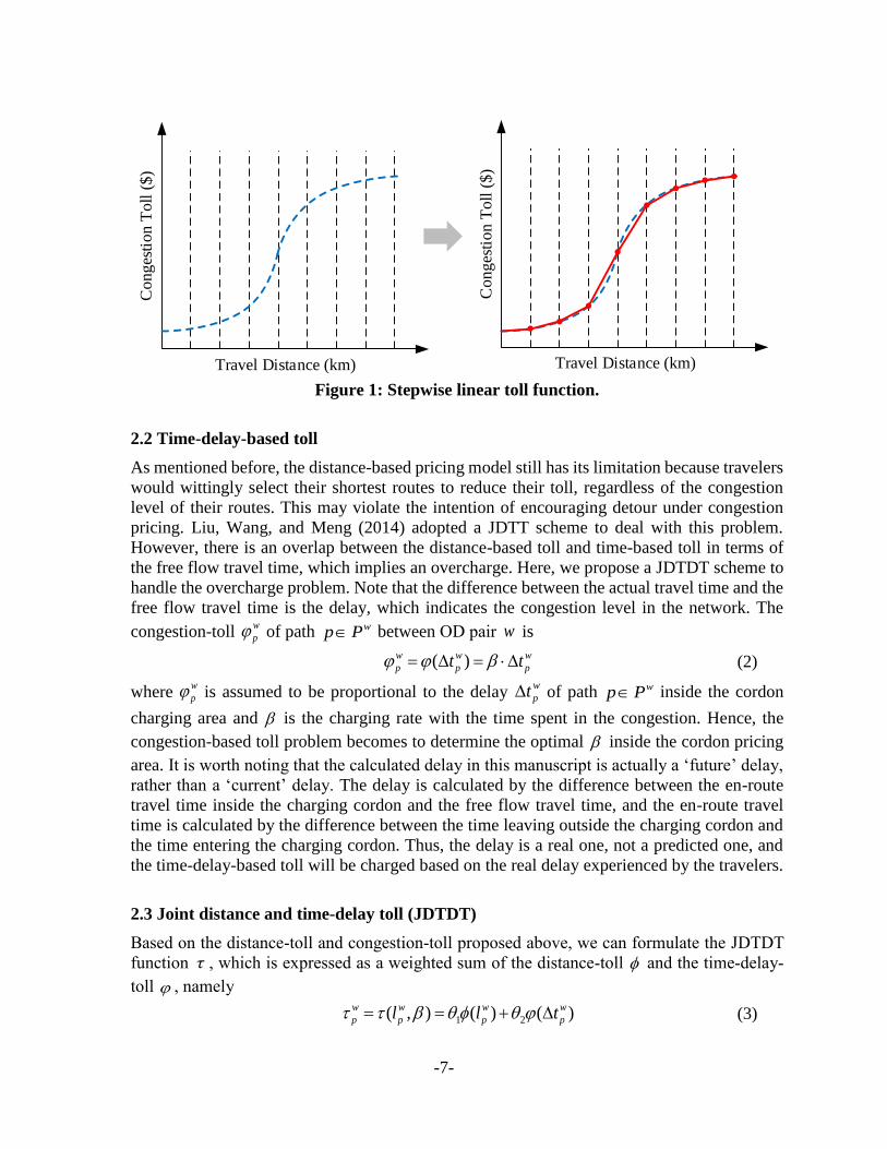
2.1 Distance-based toll

As shown in the left of Figure 1, the distance-based toll function can be described as a

continuous nonlinear function. However, it is difficult to analytically deduce and solve this

type of function. A general solution method is to approximate the nonlinear function with a

stepwise linear function according to the travel distance l in the cordon. Assuming that the

minimal and maximal length inside the cordon charging area are 0l and Kl , we can divide the

travel distance into K equal intervals and the distance-toll function of each interval can be

expressed by the two endpoints as shown in Figure 1. This piecewise linear approximation

method follows that in Meng, Liu, and Wang (2012).

Suppose that the vertexes of travel distances are 0 1( , , , , , )T

k Kl l l l l= , and the corresponding

toll values are ( )0 1, , , , ,T

k K = . Let w

pl be the distance length of path wp P inside

the cordon pricing area. Suppose w

pl lies in the k th interval of the distance toll function. Then

we can approximate the distance-toll of path wp P inside the cordon pricing area by the

following function:

( )1

1 1

1

( )

w

p kw w

p p k k k

k k

l ll

l l

−

− −

−

−= = + −

− (1)

-7-

Travel Distance (km)

Co

ng

esti

on

To

ll (

$)

Travel Distance (km)

Co

ng

esti

on

To

ll (

$)

Figure 1: Stepwise linear toll function.

2.2 Time-delay-based toll

As mentioned before, the distance-based pricing model still has its limitation because travelers

would wittingly select their shortest routes to reduce their toll, regardless of the congestion

level of their routes. This may violate the intention of encouraging detour under congestion

pricing. Liu, Wang, and Meng (2014) adopted a JDTT scheme to deal with this problem.

However, there is an overlap between the distance-based toll and time-based toll in terms of

the free flow travel time, which implies an overcharge. Here, we propose a JDTDT scheme to

handle the overcharge problem. Note that the difference between the actual travel time and the

free flow travel time is the delay, which indicates the congestion level in the network. The

congestion-toll w

p of path wp P between OD pair w is

( )w w w

p p pt t= = (2)

where w

p is assumed to be proportional to the delay w

pt of path wp P inside the cordon

charging area and is the charging rate with the time spent in the congestion. Hence, the

congestion-based toll problem becomes to determine the optimal inside the cordon pricing

area. It is worth noting that the calculated delay in this manuscript is actually a ‘future’ delay,

rather than a ‘current’ delay. The delay is calculated by the difference between the en-route

travel time inside the charging cordon and the free flow travel time, and the en-route travel

time is calculated by the difference between the time leaving outside the charging cordon and

the time entering the charging cordon. Thus, the delay is a real one, not a predicted one, and

the time-delay-based toll will be charged based on the real delay experienced by the travelers.

2.3 Joint distance and time-delay toll (JDTDT)

Based on the distance-toll and congestion-toll proposed above, we can formulate the JDTDT

function τ , which is expressed as a weighted sum of the distance-toll and the time-delay-

toll , namely

1 2( , ) ( ) ( )w w w w

p p p pl l t= = + (3)

-8-

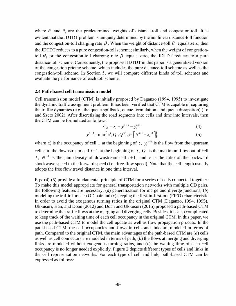
where 1θ and 2θ are the predetermined weights of distance-toll and congestion-toll. It is

evident that the JDTDT problem is uniquely determined by the nonlinear distance-toll function

and the congestion-toll charging rate . When the weight of distance-toll 1 equals zero, then

the JDTDT reduces to a pure congestion-toll scheme; similarly, when the weight of congestion-

toll 2 or the congestion-toll charging rate equals zero, the JDTDT reduces to a pure

distance-toll scheme. Consequently, the proposed JDTDT in this paper is a generalized version

of the congestion pricing scheme, which includes the pure distance-toll scheme as well as the

congestion-toll scheme. In Section 5, we will compare different kinds of toll schemes and

evaluate the performance of each toll scheme.

2.4 Path-based cell transmission model

Cell transmission model (CTM) is initially proposed by Daganzo (1994, 1995) to investigate

the dynamic traffic assignment problem. It has been verified that CTM is capable of capturing

the traffic dynamics (e.g., the queue spillback, queue formulation, and queue dissipation) (Lo

and Szeto 2002). After discretizing the road segments into cells and time into intervals, then

the CTM can be formulated as follows:

1, , 1

1

i i i i i i

t t t tx x y y− +

+ = + − (4)

, 1 1 1 1min , , ,i i i i i i i

t t ty = x Q Q N x+ + + + − (5)

where i

tx is the occupancy of cell i at the beginning of t , , 1i i

ty + is the flow from the upstream

cell i to the downstream cell 1i + at the beginning of t , iQ is the maximum flow out of cell

i , 1iN + is the jam density of downstream cell 1i + , and is the ratio of the backward

shockwave speed to the forward speed (i.e., free-flow speed). Note that the cell length usually

adopts the free flow travel distance in one time interval.

Eqs. (4)-(5) provide a fundamental principle of CTM for a series of cells connected together.

To make this model appropriate for general transportation networks with multiple OD pairs,

the following features are necessary: (a) generalization for merge and diverge junctions, (b)

modeling the traffic for each OD pair and (c) keeping the first-in-first-out (FIFO) characteristic.

In order to avoid the exogenous turning ratios in the original CTM (Daganzo, 1994, 1995),

Ukkusuri, Han, and Doan (2012) and Doan and Ukkusuri (2015) proposed a path-based CTM

to determine the traffic flows at the merging and diverging cells. Besides, it is also complicated

to keep track of the waiting time of each cell occupancy in the original CTM. In this paper, we

use the path-based CTM to model the cell update as well as flow propagation process. In the

path-based CTM, the cell occupancies and flows in cells and links are modeled in terms of

path. Compared to the original CTM, the main advantages of the path-based CTM are (a) cells

as well as cell connectors are modeled in terms of path, (b) the flows at merging and diverging

links are modeled without exogenous turning ratios, and (c) the waiting time of each cell

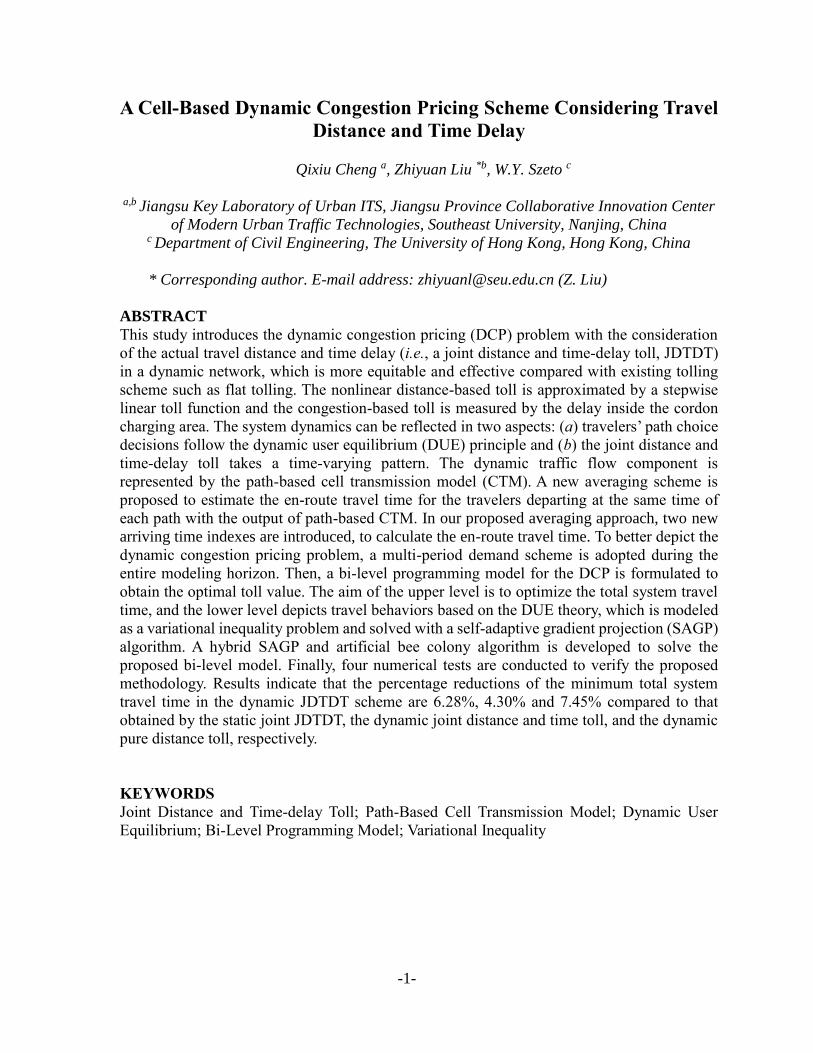
occupancy is no longer needed explicitly. Figure 2 depicts different types of cells and links in

the cell representation networks. For each type of cell and link, path-based CTM can be

expressed as follows:

-9-

Initialization

,0 0 , ,i w w

px i C p P P P= (6)

,

,0 0 ( , ) , ,i j w w

py i j E p P P P= (7)

Source cells

,

, , 1 , 1 , 1( ) , , 1, ,i i i i j

p t p p t p t p t R ix h x y i C j t T− − −= + − = (8)

Ordinal cells

, , 1

, , 1 , 1 , 1( ) , , , 1, ,i i i k i i j

p t p p t p t p t O i ix x y y i C k j t T−

− − −= + − = = (9)

Merging and diverging cells

, , 1

, , 1 , 1 , 1( ) , , , 1, ,i k i j i k i i j

p t p p p p t p t p t M D i ix x y y i C C k j t T−

− − −= + − = =

(10)

Sink cells

, 1

, , 1 , 1( ) , , 1, ,i i i k i

p t p p t p t S ix x y i C k t T−

− −= + = (11)

Ordinary links

( )( ) ,,

, min , , , ( , ) , , 1, ,

i

p ti j i i i j j j

p t p t t O ii

t

xy x Q Q N x i j E j t T

x

= − =

+ (12)

Diverging links

( )( )( )( )( )

,, ,

, ,,min , , min 1,

min , ,

, , 1, ,

i

iip ti j i j i j j j j

p t p p t t i ji j j j jtt t

j

D i

xQy x Q N x

xx Q N x

i C j t T

= − + − +

=

(13)

Merging links

( )

( )( )( )( )

1

,,

,

1

min ,min , min 1,

min ,

, , 1, ,

i

i i i kt p tk i k i k k

p t p p t kk ktt

k

M i

Q N x xy Q x

xQ x

i C k t T

−

−

−

= ++

=

(14)

Figure 2: Different types of cells and links in cell representation networks.

-10-

Eqs. (6) and (7) assume that the initial cell occupancies and outflows equal to zero. Actually,

it is also possible to start the CTM loading by other nonzero values in terms of the actual traffic

conditions. Eqs. (8)-(11) depict the path-based (disaggregate) cell updating procedure, and Eqs.

(12)-(14) are the path-based (disaggregate) flow propagation constraints. Noting that the

turning ratio in the path-based CTM is not exogenous, but uniquely determined by the supply

and demand of upstream and downstream cells. The details can be found in Ukkusuri, Han,

and Doan (2012) and are not repeated here.

To avoid the discontinuity in the flow propagation process, Lebacque and Khoshyaran (2005)

claimed that the node flow solutions should respect the invariance principle. This principle

states that when the flows are under supply/demand constraints, the node flow solutions should

be invariant to the increases in the demand/supply. Those solutions violating the invariance

principle may result in unrealistic dynamics on the links, i.e., the likelihood of waves

propagating in the wrong directions. Most of the traffic flow models for merging and diverging

junctions in the literature (e.g., the exogenous ratio distribution in Daganzo 1995, the demand

proportional distribution in Jin and Zhang 2003, the capacity proportional distribution in Ni

and Leonard 2005, just to name a few) do not satisfy the invariance principle, while only a few

studies in recent tend to respect the invariance principle (Lebacque and Khoshyaran 2005;

Corthout et al. 2012; Flötteröd and Rohde 2011; Jin 2010; Tampère et al. 2011; Jabari 2016).

To ensure the invariance principle, the distribution of supply must be independent of the ratio

of the demands (Tampère et al. 2011). As for the merging and diverging cells in the path-based

CTM, it does not exist the distribution problem because it is impossible for different incoming

(or outgoing) cells of one particular receiving (or sending) cell that are in the same path.

Besides, as claimed in Tampère et al. (2011), the invariance principle for supply in the

diverging links is automatically satisfied because the solution is derived by distributing the

supply rather than the demand. Thus, only the merging links need to be considered for the

invariance principle in the path-based CTM. It is obvious that when we calculate ,

,

k i

p ty of the

merging links, the endogenous ratio of ( )( )( )

1

min ,

min ,

i

k k

t

k k

t

k

Q x

Q x−

+ is demand-dependent, thus

may violate the invariance principle. However, the main focus of this paper is on the joint

distance and time-delay based dynamic congestion pricing, rather than the first-order node

model of the dynamic network loading problem. In the future research, it is necessary to

investigate the node models of the dynamic network loading process taking into considerations

of the invariance principle and then study the dynamic congestion pricing problem with this

more realistic dynamic network loading process.

3 Mathematical Model

In order to formulate the cell-based dynamic JDTDT problem, we first introduce the time-

varying JDTDT problem, and then the DUE conditions and the VI formulation for the lower

level problem is introduced. Finally, a bi-level programming model of this problem is proposed

in this section.

-11-

3.1 Time-varying JDTDT

In Section 2, we have described the JDTDT scheme for static networks; here we will extend it

to a time-varying scheme. It is impractical to change the toll value at every moment because

travelers cannot respond to such frequent change of the toll value. An alternative is to change

the toll value every half hour, which is a comparatively reasonable time interval for travelers

to make responses to the change and currently adopted in the ERP system of Singapore. At the

end of each time interval, the travel demand changes, and a new toll value is levied. Note that

we adopt a multi-period demand scheme as an input to better depict the dynamic congestion

pricing problem in this paper.

For simplicity, we only consider the morning commute traffic in this study. Hence, the whole

modeling period can be set from 7:30 am to 9:30 am, which means a total of 120 minutes for

the charging time length. As claimed before, the toll value changes every half hour, so there

will be four charging intervals and thus four different toll patterns during the entire charging

duration. For the thd subinterval, the JDTDT can be expressed as:

, 1 2( , ) ( ) ( )w w w w

p d d p d p d pl l t = = + (15)

Note that the specific time when vehicles arriving at the charging cordon can be determined

according to the travel time from the origin to the charging cordon, thus we can calculate the

correct charging interval d as follows:

( )

30

t td

+ =

(16)

where · is the smallest integer greater than or equal to the number in the brackets, t and

are the travel time from the origin to the charging cordon and the time interval length (unit of

minute) in the CTM, respectively.

3.2 Dynamic user equilibrium problem

The equilibrium conditions of an ideal DUE state can be stated as follows: the total generalized

costs incurred by travelers for each OD pair departing simultaneously are equal and minimal.

Mathematically, it can be formulated as

( ), , ,( ) 0, , ,w w w w w

p t p d p t tf w W p P t T − = (17)

, 0, , ,w w w

p t t w W p P t T− (18)

where

, , , , , ,w w w w

p t p t p d w W p P t T= + (19)

Note that the path flow ,

w

p tf is a function of the toll value ,

w

p d . Thus, the DUE problem is to

find a feasible , , , ,w w

p tf w W p P t T= f f which satisfies Eqs. (17)-(18) and the

demand-flow incidence relationship as well as non-negativity constraints:

-12-

, ,( ) ,

w

w w w

p t p d t

p P

f q w W t T

= (20)

( ) , f τ 0 u 0 (21)

where u is a column vector of w

t , i.e., , ,w

t w W t T= u u .

The DUE problem introduced in Eqs. (17)-(21) is equivalent to a finite dimensional VI

problem:

( )* *( ) ( ) 0 ( )T

− f τ f τ Ψ f τ (22)

where the superscript * represents the optimal solution, Ψ is the column vector of ,

w

p t , i.e.,

, , , ,w w

p tψ w W p P t T= Ψ Ψ , and is the set of feasible vectors of path flows,

which fulfills the demand-flow incidence relationship in Eq. (20) and non-negativity condition

in Eq. (21).

Ran and Boyce (1996) demonstrated the equivalence between the DUE problem (17)-(21) and

the VI problem (22), and Lo and Szeto (2002) discussed the existence as well as the uniqueness

of the solution of this proposed VI problem. Those interested in the detailed proofs may refer

to their studies.

A vital issue of solving the DUE problem in Eq. (22) is to dynamically model the travel times

as a unique mapping function of path flows. As for traditional static traffic assignment

problems, the link performance function (e.g., Bureau of Public Roads, known as the BPR

function) is widely adopted to describe travel times from traffic volumes. However, the static

BPR-type function can only express the steady-state link travel time as a mapping function of

the traffic volume on that link, without consideration of the oversaturation, queue spillback or

peak spreading. By encapsulating the CTM in DUE, Lo and Szeto (2002) proposed an

averaging scheme to calculate the actual path travel time from the output of CTM so that the

whole traffic departing simultaneously has one uniquely determined average en-route travel

time (AERTT) ,

w

p t . However, this method needs to calculate an inverse function to obtain the

AERTT. Based on the path-based CTM, a more concise approach to obtain the AERTT is

proposed in this paper.

According to the CTM discussed before, we know that the output of CTM is the cell

occupancies of traffic at each time interval. Then, the cumulative traffic departing from the

origin cell r on path p at the beginning of time interval t is the sum of the cumulative traffic

departing from cell r on path p at the beginning of time interval 1t − and the outflow of cell r

on path p during time interval t, and the cumulative traffic arriving at the sink cell s on path p

at the beginning of time interval is the sum of the cumulative traffic arriving at cell s on

path p at the beginning time interval 1 − and the inflow of cell s on path p during time

interval , namely,

,

, , 1 , , , , ,r r r j

p t p t p t R iy r C j t 1 T−= + = (23)

, 1

, , 1 , , , , ,s s k s

p p p S sy s C k 1 T−

−= + = (24)

-13-

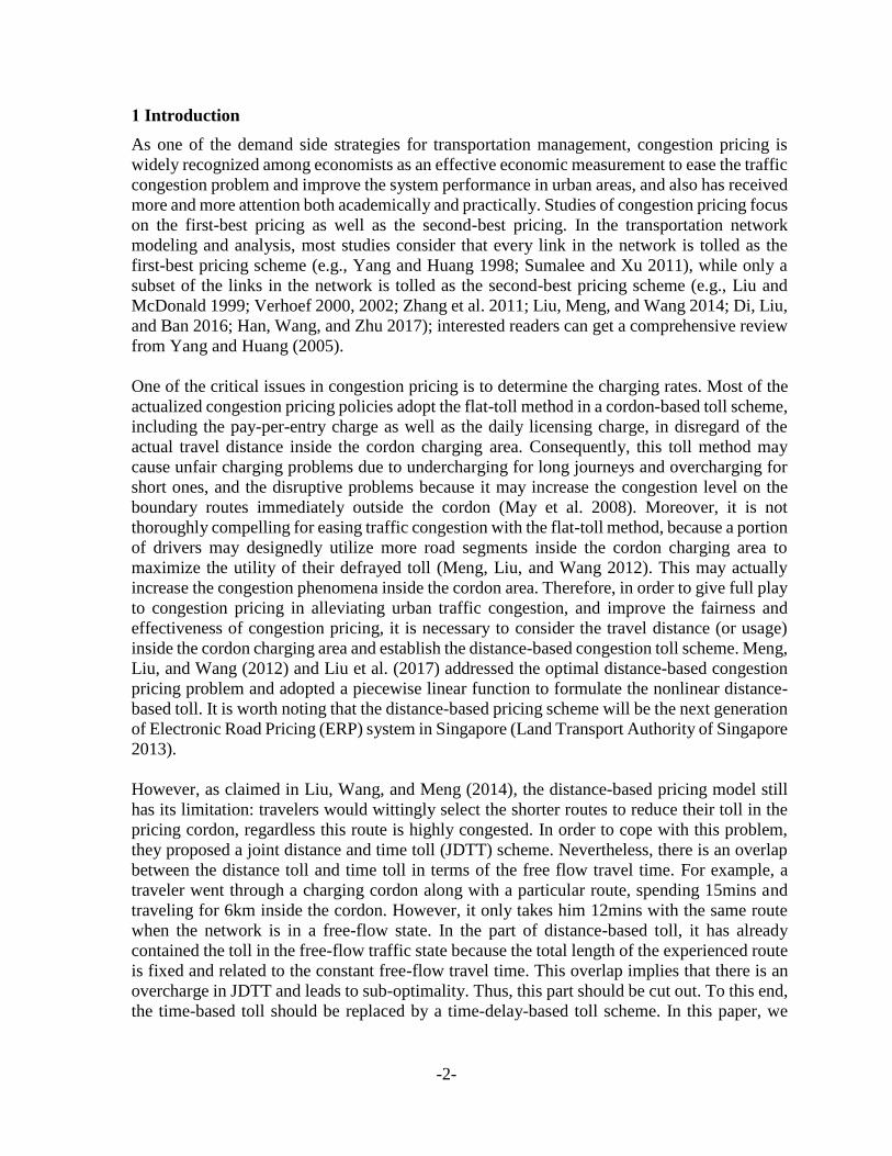
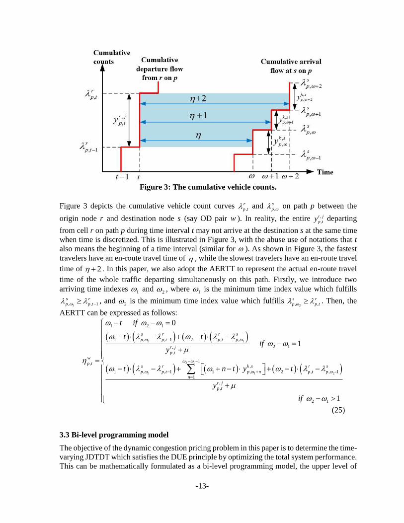
Figure 3: The cumulative vehicle counts.

Figure 3 depicts the cumulative vehicle count curves ,

r

p t and ,

s

p on path p between the

origin node r and destination node s (say OD pair w ). In reality, the entire ,

,

r j

p ty departing

from cell r on path p during time interval t may not arrive at the destination s at the same time

when time is discretized. This is illustrated in Figure 3, with the abuse use of notations that t

also means the beginning of a time interval (similar for ). As shown in Figure 3, the fastest

travelers have an en-route travel time of , while the slowest travelers have an en-route travel

time of 2+ . In this paper, we also adopt the AERTT to represent the actual en-route travel

time of the whole traffic departing simultaneously on this path. Firstly, we introduce two

arriving time indexes 1 and 2 , where 1 is the minimum time index value which fulfills

1, , 1

s r

p p t− , and 2 is the minimum time index value which fulfills

2, ,

s r

p p t . Then, the

AERTT can be expressed as follows:

( ) ( ) ( ) ( )

( ) ( ) ( ) ( ) ( )

1 1

2 1

1 1 2

1 2 1

1 , , 1 2 , ,

2 1,

,

1,

,

1 , , 1 1 , 2 , , -1

1

,

,

2 1

0

1

1

s r r s

p p t p t p

r j

p t

w

p ts r k s r s

p p t p n p t p

n

r j

p t

t if

t tif

y

t n t y t

y

if

−

− −

− +

=

− − =

− − + − −− =

+

= − − + + − + − −

+

−

(25)

3.3 Bi-level programming model

The objective of the dynamic congestion pricing problem in this paper is to determine the time-

varying JDTDT which satisfies the DUE principle by optimizing the total system performance.

This can be mathematically formulated as a bi-level programming model, the upper level of

-14-

which is to optimize the total system performance and the lower level is to achieve a DUE

state, which can be expressed as a VI formulation. The details of this bi-level model are given

as follows:

Upper level

, , ,( , , )

( )w

w w w

p t p t p dl

t T w Wp R

Min f

τ

(26)

where τ is a nonnegative toll vector for Eq. (15), which is a combination of the distance-

based toll ( 0 d K ) and the congestion-based toll ( 0d ).

Lower level

The DUE problem is formulated by a VI problem (22).

4 Solution Algorithms

It is well known that the bi-level programming problem is NP-hard and cumbersome to solve,

see Jeroslow (1985), etc. A hybrid SAGP and ABC algorithm is developed to solve the

proposed bi-level model, with SAGP to solve the VI problem of the lower level and ABC to

solve the time-varying JDTDT problem of the upper level.

4.1 Self-adaptive gradient projection algorithm

There are many solution algorithms for solving VI problems, we choose the SAGP algorithm

because it can automatically calculate and obtain an appropriate step size based on the results

of previous iterations, and relieve the computational burden due to the projection process on a

nonnegative orthant (Chen, Zhou, and Xu 2012). Generally, the SAGP algorithm is used for

solving static traffic equilibrium problems, and in this paper we will modify and extend this

algorithm to solve the DUE problem. The procedure of the SAGP algorithm is summarized

below:

Step 0: Set (0,1) , [0.5,1]u , 0 , max 0 ,

0 0 and 0 f ; set

0 0 =

and 0k = .

Step 1: Find the smallest nonnegative integer kl such that 1

kl

k k u+ = and update the

non-shortest path flows:

, , 1 ,max 0, , , ,w w w w w

p k p k k p k kf f F p P p p w W+ = − (27)

which satisfies the following constraint: 2 2

222 11 1 1 1 2

( ) ( )(2 ) ( ) max ( , ) ,0

( )

T k kk k k k k k k k

k

e++ + + +

− − − − −

f f F F f (28)

where w

kp is the shortest path between OD pair w in the thk iteration; , , ,

w w w

p k p k p kF = − , kF

is the vector of ,( , , )w T

p kF ; kf is the vector of ,( , , )w T

p kf ; and

| | | | | |( , ) [ ( )]P R Sk k k k k kRe P −

+

= − −f f f F f . Then, update the shortest path flows:

, 1

,

, 1,w kw

w k

w w w

p p k

p Pp p

f q f w W+ +

= − (29)

-15-

and set , 1 , 1 ,, ,w w w

p k p k w kf f p P p p w W+ += ，

Step 2: If the inequality condition of (30) is fulfilled, then select

11 maxmin ,k

ku

++

=

; otherwise

1 1k k+ + = .

2 2

1 1 1 1

2 221

2

0.5 ( ) ( ) ( ) || ||

( ) ( )max || ( , ) || ,0

( )

T

k k k k k k k k

k kk k

k

e

+ + + +

+

− − − −

−

f f F F F F

f (30)

Step 3: If a predetermined convergence criterion is satisfied, then stop with 1k+f as the

final solution; otherwise, set 1k k= + and go to step 1.

4.2 Artificial bee colony algorithm

The ABC algorithm was proposed by Karaboga (2005) for solving unimodal and multi-modal

numerical optimization problems. Recent years, the ABC algorithm has attracted more and

more attention in transportation studies (e.g., Chen et al. 2015; Huang et al. 2016; Szeto, Wu,

and Ho 2011). Unlike the existing evolutionary algorithms such as the particle swarm

optimization algorithm and the genetic algorithm, the local search mechanism in the ABC

algorithm is much better, and this can enhance the quality of solutions. The procedure of the

ABC algorithm is shown below:

Step 1: Set the colony size cN , the number of employed bees eN , the number of

onlookers o c eN N N= = ; set the counter limit; set the iteration counter 1I = , and its maximum

value maxI .

Step 2: Generate randomly the initial solutions (i.e., food sources), and calculate the

fitness for every employed bee. Initialize limit as zero.

Step 3: Conduct a neighborhood search according to the current solution, and evaluate

the fitness of the newly generated neighbor solution. If the neighbor solution is better, then

substitute the current solution with the newly generated neighbor solution, and reset limit as

zero; otherwise, do not change the current solution but increase limit by one.

Step 4: Each onlooker chooses a solution in terms of the roulette wheel selection

method. More specifically, generate a random number R which is uniformly distributed

between [0,1) ; if the chosen probability is larger than R , then the onlooker will conduct a

neighborhood search to find a neighbor solution and evaluate its fitness. If the neighbor

solution is better, then substitute the current solution with the neighbor solution and reset limit

as zero; otherwise, do not change the current solution but increase limit by one.

Step 5: According to the current solutions, choose the one with the highest fitness. If

there exists one solution which cannot improve its fitness within limit iterations, and it is not

the best solution with the highest fitness, then the corresponding employed bee will become a

scout and conduct a neighborhood search again. Then, generate randomly a new solution and

reset its limit to zero.

Step 6: Set 1I I= + . If maxI I , then return to Step 3; otherwise, terminate the

algorithm and output the best solution.

-16-

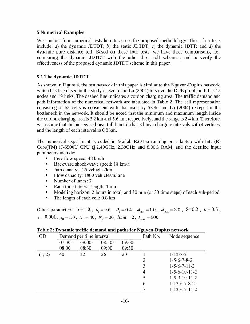
5 Numerical Examples

We conduct four numerical tests here to assess the proposed methodology. These four tests

include: a) the dynamic JDTDT; b) the static JDTDT; c) the dynamic JDTT; and d) the

dynamic pure distance toll. Based on these four tests, we have three comparisons, i.e.,

comparing the dynamic JDTDT with the other three toll schemes, and to verify the

effectiveness of the proposed dynamic JDTDT scheme in this paper.

5.1 The dynamic JDTDT

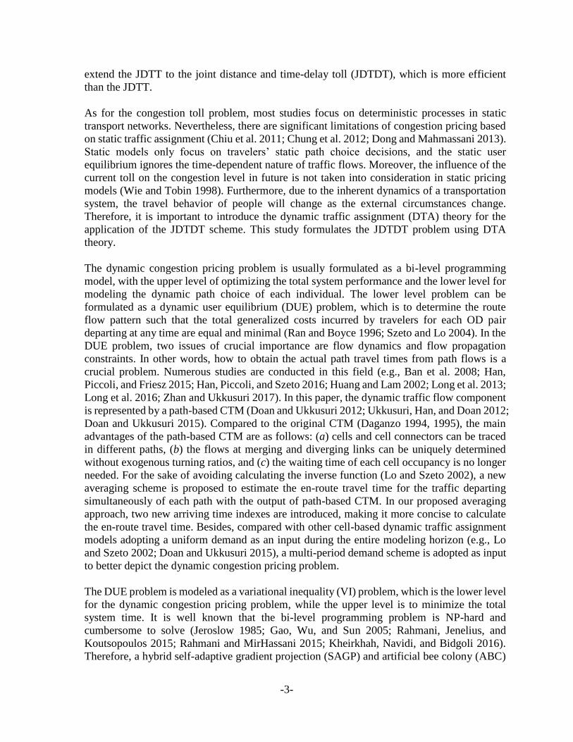
As shown in Figure 4, the test network in this paper is similar to the Nguyen-Dupius network,

which has been used in the study of Szeto and Lo (2004) to solve the DUE problem. It has 13

nodes and 19 links. The dashed line indicates a cordon charging area. The traffic demand and

path information of the numerical network are tabulated in Table 2. The cell representation

consisting of 63 cells is consistent with that used by Szeto and Lo (2004) except for the

bottleneck in the network. It should be noted that the minimum and maximum length inside

the cordon charging area is 3.2 km and 5.6 km, respectively, and the range is 2.4 km. Therefore,

we assume that the piecewise linear toll function has 3 linear charging intervals with 4 vertices,

and the length of each interval is 0.8 km.

The numerical experiment is coded in Matlab R2016a running on a laptop with Inter(R)

Core(TM) i7-5500U CPU @2.40GHz, 2.39GHz and 8.00G RAM, and the detailed input

parameters include:

Free flow speed: 48 km/h

Backward shock-wave speed: 18 km/h

Jam density: 125 vehicles/km

Flow capacity: 1800 vehicles/h/lane

Number of lanes: 2

Each time interval length: 1 min

Modeling horizon: 2 hours in total, and 30 min (or 30 time steps) of each sub-period

The length of each cell: 0.8 km

Other parameters: 1.0α = , 1 0.6θ = ,

2 0.4θ = , min 1.0= , max 3.0= , 0.2= , 0.6u = ,

0.001 = , 0 1.0 = , 40cN = , 20eN = , 2limit = ,

max 500I =

Table 2: Dynamic traffic demand and paths for Nguyen-Dupius network

OD Demand per time interval Path No. Node sequence

07:30-

08:00

08:00-

08:30

08:30-

09:00

09:00-

09:30

(1, 2) 40 32 26 20 1 1-12-8-2

2 1-5-6-7-8-2

3 1-5-6-7-11-2

4 1-5-6-10-11-2

5 1-5-9-10-11-2

6 1-12-6-7-8-2

7 1-12-6-7-11-2

-17-

8 1-12-6-10-11-2

(1, 3) 70 60 48 36 9 1-5-9-13-3

10 1-5-6-7-11-3

11 1-5-6-10-11-3

12 1-5-9-10-11-3

13 1-12-6-7-11-3

14 1-12-6-10-11-3

(4, 2) 64 52 40 30 15 4-9-10-11-2

16 4-5-6-7-8-2

17 4-5-6-7-11-2

18 4-5-6-10-11-2

19 4-5-9-10-11-2

(4, 3) 64 52 40 30 20 4-9-13-3

21 4-9-10-11-3

22 4-5-9-13-3

23 4-5-6-7-11-3

24 4-5-6-10-11-3

25 4-5-9-10-11-3

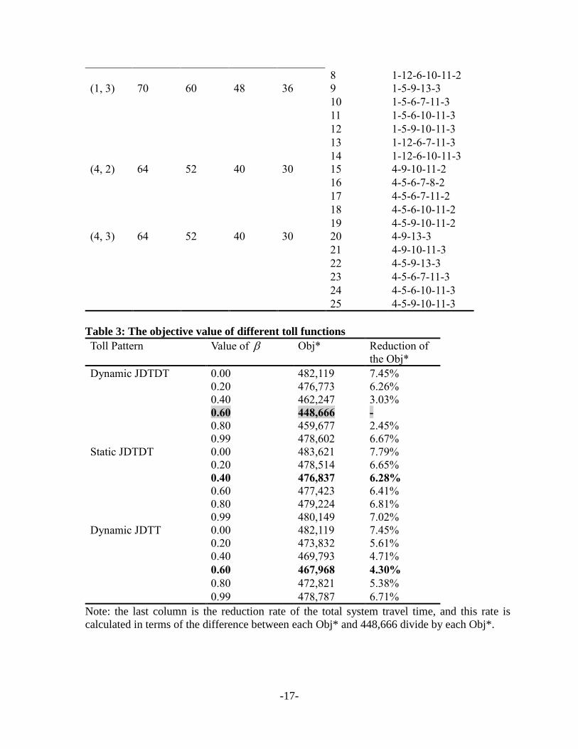
Table 3: The objective value of different toll functions

Toll Pattern Value of Obj* Reduction of

the Obj*

Dynamic JDTDT 0.00 482,119 7.45%

0.20 476,773 6.26%

0.40 462,247 3.03%

0.60 448,666 -

0.80 459,677 2.45%

0.99 478,602 6.67%

Static JDTDT 0.00 483,621 7.79%

0.20 478,514 6.65%

0.40 476,837 6.28%

0.60 477,423 6.41%

0.80 479,224 6.81%

0.99 480,149 7.02%

Dynamic JDTT 0.00 482,119 7.45%

0.20 473,832 5.61%

0.40 469,793 4.71%

0.60 467,968 4.30%

0.80 472,821 5.38%

0.99 478,787 6.71%

Note: the last column is the reduction rate of the total system travel time, and this rate is

calculated in terms of the difference between each Obj* and 448,666 divide by each Obj*.

-18-

1

5

9

12

6

10

7 8

11 2

3

4

13

Origin

Origin

Destination

Destination

1

2

3

4

5

6

7

8

9

10 11

12

13

14 15

16

1718

19

(a) Nguyen-Dupuis network with toll cordon

(b) Cell representation of Nguyen-Dupuis network

Figure 4: Network structure.

1

14

2

15

25 26

12 13

49

50

292827

3

30

51

52

18

16

31

17

32 33

54

53

54

34

55

56

4219 40 41

35 36 37

57

58

4543 44

38 39 61

62

63

4846 47

20 59

60

242322

21

6

7

8

9

10

11

-19-

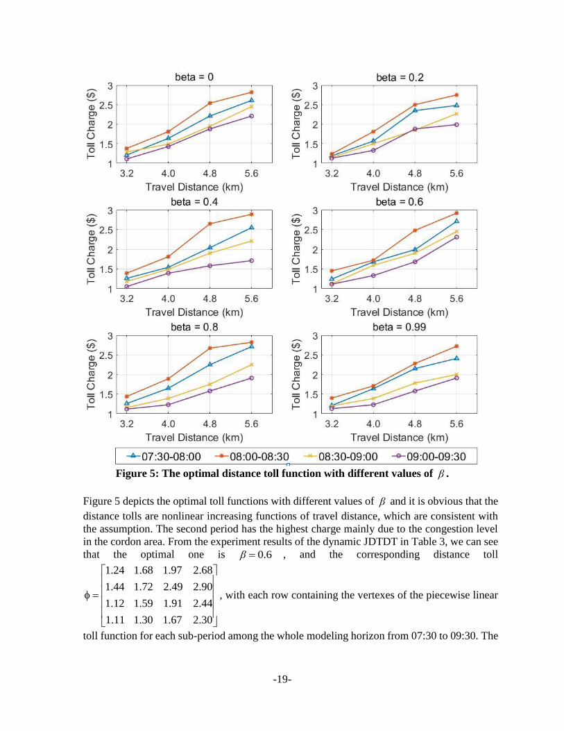
Figure 5: The optimal distance toll function with different values of β .

Figure 5 depicts the optimal toll functions with different values of β and it is obvious that the

distance tolls are nonlinear increasing functions of travel distance, which are consistent with

the assumption. The second period has the highest charge mainly due to the congestion level

in the cordon area. From the experiment results of the dynamic JDTDT in Table 3, we can see

that the optimal one is 0.6β = , and the corresponding distance toll

1.24 1.68 1.97 2.68

1.44 1.72 2.49 2.90

1.12 1.59 1.91 2.44

1.11 1.30 1.67 2.30

=

, with each row containing the vertexes of the piecewise linear

toll function for each sub-period among the whole modeling horizon from 07:30 to 09:30. The

-20-

convergence process of the dynamic JDTDT with 0.60 = is shown in Figure 6. It is clear

that the objective value converged in a stepwise form within less than 200 iterations.

Figure 6: The convergence process of the dynamic JDTDT with 0.60 =

It should be noted that the link flows of the entire network are zero when it is 07:30 in this

case. However, this assumption is obviously unrealistic. A more realistic traffic demand

should be input and the experiment should be tested in the future.

5.2 Comparisons

To illustrate the superiorities of the dynamic JDTDT scheme, three controlled experiments (i.e.,

the static JDTDT, the dynamic JDTT, and the pure distance toll) are conducted here. The

network structure in these three controlled experiments are the same as the dynamic JDTDT

shown in Figure 4(a). As for the static toll pattern, the input demand in Table 4 is aggregated

by the dynamic demand during the study period from 07:30 to 09:30, and the typical BPR

(Bureau of Public Roads) type function is adopted to calculate the link travel times.

Table 4: Aggregate demand during the study period from 07:30 to 09:30

OD Demand (veh) OD Demand (veh)

(1, 2) 3540 (4, 2) 5580

(1, 3) 6420 (4, 3) 5580

(1) The dynamic vs. static JDTDT

From the results of the static JDTDT in Table 3, it is obvious that the optimal value of in a

static JDTDT scheme is 0.40, which is different from the dynamic toll pattern. We can also see

that the overall system performance of the transportation network under the dynamic toll

pattern is superior to that under the static one, which is expected because the dynamic toll

pattern based on the dynamic network modeling can better capture the system dynamics.

Quantitatively, the total system travel time decreases by 6.28% when the JDTDT scheme is

-21-

implemented from a static pattern to a dynamic pattern. This percentage reduction of the total

system travel time may not be significant, but when the dynamic JDTDT is implemented for a

large-scale urban area, the total value of the total system travel time may decrease signally.

(2) The dynamic JDTDT vs. JDTT

The difference between the JDTDT and the JDTT is whether the travel time or delay inside the

cordon charging area is adopted in the toll scheme. Other parameters of the dynamic JDTT

scheme in the cell-based DTA and solution algorithms are the same as the dynamic JDTDT

scheme. From the results of the dynamic JDTT shown in Table 3, we can see that the optimal

value of is also 0.60, which is the same as the optimal value in the dynamic JDTDT scheme.

Compared to the dynamic JDTT scheme, the optimal value of the total system travel time

decreases by 4.30% in the dynamic JDTDT scheme, indicating that the dynamic JDTDT is

more efficient than the dynamic JDTT. This result also confirms the assumption of the

overcharging problem in the JDTT scheme.

(3) The JDTDT vs. pure distance toll

Note that when 0 = for either dynamic or static toll pattern, it becomes an entirely nonlinear

distance toll scheme. An interesting phenomenon can be found for both dynamic and static toll

patterns, i.e., the objective value of the pure distance-toll scheme (when 0 = ) is inferior to

all the other cases, indicating that introducing the congestion-toll together with distance-toll

leads to a better performance for the system. This phenomenon is in line with the real life of

travelers who prefer to pay less for their trips inside the cordon charging area. When the pure

distance-toll scheme is implemented, most travelers prefer to choose the shorter route(s) in the

cordon to reduce their toll for the trip, regardless the route(s) is/are highly congested. However,

after combining the congestion-toll with the distance-toll, the congestion effect will be

incorporated into the payment of travelers. Thus, travelers reconsider the route choice under

the JDTDT pattern. This clearly shows that the JDTDT encourages detour behaviours

compared to a pure distance-toll for either the dynamic or static toll pattern, which is consistent

with the principle of JDTDT. Similarly, we can obtain the reduction rate of the total system

travel time in the dynamic JDTDT is 7.45% compared to the dynamic pure distance toll scheme.

6 Conclusions

This paper addressed a dynamic congestion pricing problem considering travelers’ actual travel

distance and congestion level in the network. The proposed dynamic JDTDT scheme is more

equitable than the traditional flat toll schemes, and more effective than the static JDTDT,

dynamic JDTT, and the dynamic pure distance toll. The dynamic optimal toll design problem

is formulated as a bi-level programming model, the upper level of which is to optimize the

total system performance, and the lower level is a DUE problem. The path-based CTM is

adopted in this paper to formulate the dynamic traffic flow propagation process, and a new

averaging scheme is proposed to estimate the en-route travel time for the traffic departing

simultaneously of each path. Then the DUE problem can be expressed as a VI. A hybrid SAGP

and ABC algorithm is developed to solve this bi-level model. The validity of the proposed

methodology is verified with four numerical tests. More specifically, based on the results of

the comparison, we find that the reduction rates of the minimum total system travel time in the

dynamic JDTDT scheme are 6.28%, 4.30% and 7.45% compared to the static JDTDT, the

-22-

dynamic JDTT and the dynamic pure distance toll, respectively. These percentage reductions

may not be significant, but when the dynamic JDTDT is implemented for a large-scale urban

area, the total volume of the total system travel time may decrease signally.

This paper is an initial study of the cell-based dynamic congestion pricing problem. The traffic

demand is assumed piecewise fixed and the path choice decisions are deterministic in this

paper. For future researches, the demand can be extended to elastic and stochastic dynamics of

travelers’ decision behaviors can be captured, and the toll framework can be extended to a day-

to-day dynamic setting. The optimal second-best toll can be approximated with a linear

programming model based on the concept of toll set (see Hearn and Ramana 1998;

Lawphongpanich and Hearn 2004; Chen, Zhou, and List 2011). The congestion pricing policy

can be also integrated with public transit design and network design. In addition, in the cell-

based model, one link is divided to multiple cells, which largely increase the computing time

for large urban transportation networks. This computing issue may be solved by the following

two approaches: (a) parallel computing algorithms can be used, which are suitable for the cell-

based dynamic congestion pricing problems due to the good property of path-based CTM; (b)

the link transmission model, which is another discrete version of the macro-simulation

approach, can be introduced to this dynamic congestion pricing problem to reduce the

computational cost. In the future work, we will evaluate the proposed dynamic JDTDT scheme

in mesoscopic dynamic traffic simulation packages such as DTALite (Zhou and Taylor 2014;

Xiong, Zhou, and Zhang 2018).

Acknowledgement

This study is supported by the General Project (71771050) of the National Natural Science

Foundation of China, the Research Grants Council of the Hong Kong Special

Administrative Region of China (17201915), and the Scientific Research Foundation of

Graduate School of Southeast University (NO. YBPY1885).

References

Ban, X., H. X. Liu, M. C. Ferris, and B. Ran. 2008. “A Link-Node Complementarity Model

and Solution Algorithm for Dynamic User Equilibria with Exact Flow Propagations.”

Transportation Research Part B 42 (9): 823–842.

Chen, A., Z. Zhou, and X. Xu. 2012. “A Self-Adaptive Gradient Projection Algorithm for

the Nonadditive Traffic Equilibrium Problem.” Computers and Operations Research

39 (2): 127–138.

Chen, J., Z. Liu, S. Zhu, and W. Wang. 2015. “Design of Limited-Stop Bus Service with

Capacity Constraint and Stochastic Travel Time.” Transportation Research Part E 83:

1–15.

Chen, X., X. Zhou, and G. F. List. 2011. “Using time-varying tolls to optimize truck

arrivals at ports.” Transportation Research Part E 47 (6): 965-982.

Chiu, Y. C., J. Bottom, M. Mahut, A. Paz, R. Balakrishna, T. Waller, and J. Hicks. 2011.

Dynamic Traffic Assignment: A Primer. Transportation Network Modeling

Committee.

-23-

Chung, B. D., T. Yao, T. L. Friesz, and H. Liu. 2012. “Dynamic Congestion Pricing with

Demand Uncertainty: A Robust Optimization Approach.” Transportation Research

Part B 46 (10): 1504–1518.

Corthout, R., G. Flötteröd, F. Viti, and C. M. Tampère. 2012. “Non-unique flows in

macroscopic first-order intersection models.” Transportation Research Part B 46 (3):

343-359.

Daganzo, C. F. 1994. “The Cell Transmission Model: A Dynamic Representation of

Highway Traffic Consistent with the Hydrodynamic Theory.” Transportation

Research Part B 28 (4): 269–287.

Daganzo, C. F. 1995. “The Cell Transmission Model, Part II: Network Traffic.”

Transportation Research Part B 29 (2): 79–93.

Di, X., H. X. Liu, and X. Ban. 2016. “Second Best Toll Pricing within the Framework of

Bounded Rationality.” Transportation Research Part B 83: 74–90.

Doan, K., and S. V. Ukkusuri. 2012. “On the Holding-Back Problem in the Cell

Transmission Based Dynamic Traffic Assignment Models.” Transportation Research

Part B 46 (9): 1218–1238.

Doan, K., and S. V. Ukkusuri. 2015. “Dynamic System Optimal Model for Multi-OD

Traffic Networks with an Advanced Spatial Queuing Model.” Transportation

Research Part C 51: 41–65.

Dong, J., and H. Mahmassani. 2013. “Improving network traffic flow reliability through

dynamic anticipatory tolls.” Transportmetrica B 1(3): 226–236.

Flötteröd, G., and J. Rohde. 2011. “Operational macroscopic modeling of complex urban

road intersections.” Transportation Research Part B 45 (6): 903-922.

Gao, Z., J. Wu, and H. Sun. 2005. “Solution Algorithm for the Bi-Level Discrete Network

Design Problem.” Transportation Research Part B 39 (6): 479–495.

Han, K., B. Piccoli, and T. L. Friesz. 2016. “Continuity of the Path Delay Operator for

Dynamic Network Loading with Spillback.” Transportation Research Part B 92:

211–233.

Han, K., B. Piccoli, and W. Y. Szeto. 2016. “Continuous-time link-based kinematic wave

model: formulation, solution existence, and well-posedness.” Transportmetrica B 4

(3): 187-222.

Han, L., D. Z. W. Wang, and C. Zhu. 2017. “The Discrete-Time Second-Best Dynamic

Road Pricing Scheme.” In Transportation Research Procedia, 23: 322–340.

Hearn, D. W., and M. V. Ramana. 1998. “Solving congestion toll pricing models.” In

Equilibrium and Advanced Transportation Modeling, 109-124.

Huang, D., Z. Liu, P. Liu, and J. Chen. 2016. “Optimal Transit Fare and Service Frequency

of a Nonlinear Origin-Destination Based Fare Structure.” Transportation Research

Part E 96: 1–19.

Huang, H. J., and W. H. K. Lam. 2002. “Modeling and Solving the Dynamic User

Equilibrium Route and Departure Time Choice Problem in Network with Queues.”

Transportation Research Part B 36 (3): 253–273.

Jabari, S. E. 2016. “Node modeling for congested urban road networks.” Transportation

Research Part B 91: 229-249.

Jeroslow, R. G. 1985. “The Polynomial Hierarchy and a Simple Model for Competitive

Analysis.” Mathematical Programming 32 (2): 146–164.

-24-

Jin, W. L. 2012. “Continuous kinematic wave models of merging traffic flow.”

Transportation Research Part B 44 (8): 1084-1103.

Jin, W. L., and H. M. Zhang. 2003. “On the distribution schemes for determining flows

through a merge.” Transportation Research Part B 37 (6): 521-540.

Karaboga, D. 2005. An Idea Based on Honey Bee Swarm for Numerical Optimization.

Kheirkhah, A., H. Navidi, and M. M. Bidgoli. 2016. “A Bi-Level Network Interdiction

Model for Solving the Hazmat Routing Problem.” International Journal of

Production Research 54 (2): 459–471.

Lebacque, J. P., and M. M. Khoshyaran. 2005. “First-order macroscopic traffic flow

models: Intersection modeling, network modeling.” In the 16th International

Symposium on Transportation and Traffic Theory, University of Maryland, College

Park.

Lawphongpanich, S., and D. W. Hearn. 2004. “An MPEC approach to second-best toll

pricing.” Mathematical Programming 101 (1): 33-55.

Land Transport Authority of Singapore. 2013. Land Transport Master Plan 2013.

Singapore Land Transport Authority.

Liu, L. N., and J. F. McDonald. 1999. “Economic Efficiency of Second-Best Congestion

Pricing Schemes in Urban Highway Systems.” Transportation Research Part B 33

(3): 157–188.

Liu, Z., Q. Meng, and S. Wang. 2014. “Variational Inequality Model for Cordon-Based

Congestion Pricing under Side Constrained Stochastic User Equilibrium Conditions.”

Transportmetrica A 10 (8): 693–704.

Liu, Z., S. Wang, and Q. Meng. 2014. “Optimal Joint Distance and Time Toll for Cordon-

Based Congestion Pricing.” Transportation Research Part B 69: 81–97.

Liu, Z., S. Wang, B. Zhou, and Q. Cheng. 2017. “Robust Optimization of Distance-Based

Tolls in a Network Considering Stochastic Day to Day Dynamics.” Transportation

Research Part C 79: 58–72.

Lo, H. K., and W. Y. Szeto. 2002. “A Cell-Based Variational Inequality Formulation of

the Dynamic User Optimal Assignment Problem.” Transportation Research Part B

36 (5): 421–443.

Long, J., H. J. Huang, Z. Gao, and W. Y. Szeto. 2013. “An Intersection-Movement-Based

Dynamic User Optimal Route Choice Problem.” Operations Research 61 (5): 1134–

1147.

Long, J., W. Y. Szeto, Z. Gao, H. J. Huang, and Q. Shi. 2016. “The Nonlinear Equation

System Approach to Solving Dynamic User Optimal Simultaneous Route and

Departure Time Choice Problems.” Transportation Research Part B 83: 179–206.

May, A. D., S. P. Shepherd, A. Sumalee, and A. Koh. 2008. “Design Tools for Road Pricing

Cordons.” In Road Congestion Pricing in Europe: Implications for the United States,

138. Northampton: Edward Elgar Publishing.

Meng, Q., Z. Liu, and S. Wang. 2012. “Optimal Distance Tolls under Congestion Pricing

and Continuously Distributed Value of Time.” Transportation Research Part E 48 (5):

937–957.

Ni, D., and J. D. Leonard II. 2005. “A simplified kinematic wave model at a merge

bottleneck.” Applied Mathematical Modelling 29(11): 1054-1072.

Rahmani, A., and S. A. MirHassani. 2015. “Lagrangean Relaxation-Based Algorithm for

Bi-Level Problems.” Optimization Methods and Software 30 (1): 1–14.

-25-

Rahmani, M., E. Jenelius, and H. N. Koutsopoulos. 2015. “Non-Parametric Estimation of

Route Travel Time Distributions from Low-Frequency Floating Car Data.”

Transportation Research Part C 58: 343–362.

Ran, B., and D. Boyce. 1996. Modeling Dynamic Transportation Networks. An Intelligent

Transportation System Oriented Approach. Heidelberg: Springer-Verlag.

Sumalee, A., and W. Xu. 2011. “First-Best Marginal Cost Toll for a Traffic Network with

Stochastic Demand.” Transportation Research Part B 45 (1): 41–59.

Szeto, W. Y., and H. K. Lo. 2004. “A Cell-Based Simultaneous Route and Departure Time

Choice Model with Elastic Demand.” Transportation Research Part B 38 (7): 593–

612.

Szeto, W. Y., Y. Wu, and S. C. Ho. 2011. “An Artificial Bee Colony Algorithm for the

Capacitated Vehicle Routing Problem.” European Journal of Operational Research

215 (1): 126–135.

Tampère, C. M., R. Corthout, D. Cattrysse, and L. H. Immers. 2011. “A generic class of

first order node models for dynamic macroscopic simulation of traffic flows.”

Transportation Research Part B 45 (1): 289-309.

Ukkusuri, S. V., L. Han, and K. Doan. 2012. “Dynamic User Equilibrium with a Path Based

Cell Transmission Model for General Traffic Networks.” Transportation Research

Part B 46 (10): 1657–1684.

Verhoef, E. T. 2000. “Second-Best Congestion Pricing in General Networks” Tinbergen

Institute Discussion Paper TI 2000-084/3, Amsterdam.

Verhoef, E. T. 2002. “Second-Best Congestion Pricing in General Networks. Heuristic

Algorithms for Finding Second-Best Optimal Toll Levels and Toll Points.”

Transportation Research Part B 36 (8): 707–729.

Wie, B. W., and R. L. Tobin. 1998. “Dynamic Congestion Pricing Models for General

Traffic Networks.” Transportation Research Part B 32 (5): 313–327.

Xiong, C., X. Zhou, & L. Zhang. 2018. “AgBM-DTALite: An integrated modelling system

of agent-based travel behaviour and transportation network dynamics.” Travel

Behaviour and Society 12: 141-150.

Yang, H., and H. J. Huang. 1998. “Principle of Marginal-Cost Pricing: How Does It Work

in a General Road Network?” Transportation Research Part A 32 (1): 45–54.

Yang, H., and H. J. Huang. 2005. Mathematical and Economic Theory of Road Pricing.

Elsevier.

Zhan, X., and S. V. Ukkusuri. 2017. “Multiclass, simultaneous route and departure time

choice dynamic traffic assignment with an embedded spatial queuing model.”

Transportmetrica B, in press.

Zhang, X., H. M. Zhang, H. J. Huang, L. Sun, and T. Q. Tang. 2011. “Competitive,

Cooperative and Stackelberg Congestion Pricing for Multiple Regions in

Transportation Networks.” Transportmetrica 7 (4): 297–320.

Zhou, X., and J. Taylor. 2014. “DTALite: A queue-based mesoscopic traffic simulator for

fast model evaluation and calibration.” Cogent Engineering 1 (1): 961345.