A better Horizon Auto Tracker - Poweredby Machine Learning

Monika Maria Dyrendahl

Petroleum Geoscience and Engineering

Supervisor: Ståle Emil Johansen, IGPCo-supervisor: Victor Aarre, Schlumberger

Department of Geoscience and Petroleum

Submission date: June 2018

Norwegian University of Science and Technology

i

Abstract

Computer-assisted horizon interpretation on 3D seismic data has been commercially

available for almost 15 years. The process is generally referred to as 3D horizon autotracking

and is a powerful method when interpreting seismic horizons. The desire of a new autonomous

horizon tracker is growing in the market. This thesis is combining the fields of seismic

interpretation and data science to perform the early testing on a software aiming to fill this gap

in the market. The goal is to find out if the new algorithm based on machine learning is a good

replacement for the 3D horizon autotracker regarding a more effective and time-saving

workflow.

The new method uses radial basis functions (RBF) that enables the IntelliTracker to

store information acquired during the workflow. This is necessary because of the complex

nature of the geology and the varying quality of seismic data.

The IntelliTracker was tested against the horizontal autotracker on the NH0301 dataset

covering the top reservoir unconformity in the Troll field. Testing was performed by

interpreting the top reservoir horizon with the existing 3D autotracker and then tracking the

same horizon with the new method.

The results from the testing prove that the current autotracker is still better on some

areas. The IntelliTracker can, however, be used as a guidance tool by the interpreter for a more

effective workflow. Although the ML technologies have developed rapidly over the last couples

of years, the interpretation done by a machine will always need to be quality checked.

ii

Sammendrag

Data assistert tolkning av seismiske horisonter på 3D seismiske data har vært

kommersielt tilgjengelig i nesten 15 år. Prosessen blir referert til som 3D horisont autotracking

og er et kraftig verktøy når man tolker seismiske horisonter. I markedet har det lenge vært et

ønske om en autonom sporer som kan tolke horisonter automatisk. Denne oppgaven kombinerer

seismisk tolkning og datavitenskap for å kunne utføre tidlig testing av en programvare som skal

fylle dette hullet i markedet. Målet er å finne ut om en data algoritme basert på maskinlære kan

være en erstatter for den eksisterende 3D horisont autotrackeren.

Teknologien bruker radiale basisfunksjoner som gjør at IntelliTrackeren kan lagre den

informasjon som blir generert under tolknings-prosessen. Dette er nødvendig på grunn av den

komplekse geologien og den varierende kvaliteten på seismiske data.

IntelliTrackeren ble testet på NH0301 datasettet på den horisonten som tilsvarer toppen

av reservoaret i Troll feltet og består av en diskonformitet. Testingen ble utført ved å spore

horisonten over denne diskonformiteten med den eksisterende horisont sporeren og deretter

spore den samme horisonten med den nye metoden.

Resultatene fra testen viser at den nåværende autotrackeren fortsatt er ledende på flere

områder. IntelliTrackeren kan i midlertidig brukes som et veiledende verktøy av tolkeren for å

effektivisere prosessen. Selv om teknologien rundt maskinlære har utviklet seg raskt de siste

årene, må tolkningen utført av en datamaskin alltid være kvalitetssjekket av noen med

kompetanse innenfor fagfeltet

iii

Acknowledgments

I want to thank my supervisor Professor Ståle Emil Johansen (IPT, NTNU). His

guidance and supervision has helped me throughout the work. I would also like to thank Jarl

Eirik Tronerud (Schlumberger) for the resources and expertise he and his team have provided

me with. My co-supervisor Victor Aarre (Schlumberger) has been very helpful throughout my

stay in Schlumberger with his guidance, data preparation and expertise. Many thanks to Trond

Hellem Bøe (SSR, Schlumberger) for helping with any software related problems. In addition,

I would like to thank Dicky Harishidayat (IPT, NTNU).

I would like to thank Odd Bakke Kristiansen from Oljedirektoratet for accepting a visit

to their core stock, making it possible to have a look on the cores from well number 31/5-2.

Last, but not least I would like to thank my fellow students at Schlumberger for

motivating professional discussion time-outs during the day, my family members for their

patient when not always being available and my partner for supporting me in ups and downs

throughout this year.

Table of contents

Abstract........................................................................................................................... 1 Sammendrag ................................................................................................................... ii Acknowledgments ......................................................................................................... iii Table of contents ........................................................................................................... iv

List of figures ................................................................................................................ vi List of tables ................................................................................................................... x 1 Introduction .............................................................................................................. 1

1.1 Scope of the thesis ............................................................................................ 5

1.3 Previous studies ................................................................................................ 6

Theory............................................................................................................................. 8 2 Background of the Troll Field .................................................................................. 8

2.1 Dataset and software ....................................................................................... 11

3 Geology .................................................................................................................. 17

3.1 Geological definitions..................................................................................... 17

3.2 Evolution of the Northern North Sea .............................................................. 25

3.3 Depositional Environment .............................................................................. 27

4 Machine Learning .................................................................................................. 29

4.1 Instance-Based Learning ................................................................................ 29

4.1.1 K-nearest neighbor learning...................................................................... 30

4.1.2 Radial basis function (RBF) ..................................................................... 30

4.2 Neural Networks ............................................................................................. 32

4.3 Precision and recall ......................................................................................... 34

4.4 IntelliTracker .................................................................................................. 36

Methodology................................................................................................................. 39 5 Horizon Interpretation ............................................................................................ 39

5.1 Workflow for the 3D autotracker engine ........................................................ 40

5.2 Parameters (Priority, Quality and Signal Feature) .......................................... 42

5.3 IntelliTracker .................................................................................................. 47

5.3.1 How to use the IntelliTracker in Petrel 2017.2 ......................................... 51

5.3.2 OriginalPointSet-method (OPS-method) .................................................. 53

5.3.3 Filter-method ............................................................................................ 54

5.3.4 Adding-method ......................................................................................... 57

Results .......................................................................................................................... 58 6 Horizon interpretation ............................................................................................ 58

6.1 Results from the horizon autotracker.............................................................. 58

6.1.1 Priority Parameter ..................................................................................... 60

6.1.2 Quality Parameter ..................................................................................... 64

6.2 Results from IntelliTracker ............................................................................. 68

6.2.1 Horizon autotracker and IntelliTracker..................................................... 68

6.2.2 Original Point Set-method (OPS-method) ................................................ 75

6.2.3 Filter-method ............................................................................................ 93

Discussion................................................................................................................... 100

7 Discussion of Results ........................................................................................... 100

7.1 3D Horizon Autotracker ............................................................................... 100

7.2 IntelliTracker ................................................................................................ 101

7.3 Comparison between Autotracker and IntelliTracker .................................. 101

7.4 Suggesting Methods ..................................................................................... 103

7.5 Sources of error regarding Interpretation ..................................................... 105

7.6 Improvements and Further Work ................................................................. 105

7.6.1 Graphical interface .................................................................................. 105

7.6.2 Efficiency ................................................................................................ 106

7.6.3 Functionality ........................................................................................... 106

Conclusion .................................................................................................................. 108

Appendix A ................................................................................................................ 109

Parameters and Constraints .................................................................................... 109

Appendix B ................................................................................................................. 114

Abstract for Generalized Spectral Decomposition (GSD) ..................................... 114

References .................................................................................................................. 115

List of figures

Figure 1: Location of the Troll field (both Troll East and Troll West) ...................................... 8

Figure 2: Stratigraphy of the North Viking Graben ................................................................. 10

Figure 3: Statistics from the data set NH0301 from settings in Petrel ..................................... 11

Figure 4: A 2D Inline showing the NH0301 with outlined elements ....................................... 13

Figure 5: Interpreted top reservoir horizon .............................................................................. 14

Figure 6: Amplitude attribute map ........................................................................................... 15

Figure 7: Structural framework of the northern North Sea ...................................................... 18

Figure 8: Angular unconformity .............................................................................................. 19

Figure 9: Disconformity ........................................................................................................... 20

Figure 10: Nonconformity ........................................................................................................ 20

Figure 11: Illustration of a transgression .................................................................................. 21

Figure 12: Facies change during a transgression ..................................................................... 22

Figure 13: Illustration of a regression. ..................................................................................... 23

Figure 14: Facies change during a regression .......................................................................... 24

Figure 15: Mode of rotation in the Horda platform. ................................................................ 26

Figure 16: Illustration of a cross-section showing the continental shelf through the continental

slope down to the oceanic crust ................................................................................................ 27

Figure 17: A radial basis function network .............................................................................. 31

Figure 18: A simple mathematical model for a neuron ............................................................ 33

Figure 19: General structure of a neural network .................................................................... 34

Figure 20: Figure demonstrating precision and recall (Walber 2014) ..................................... 35

Figure 21: Settings for ML Tracker in workflows ................................................................... 36

Figure 22: The expansion process of a seed point ................................................................... 37

Figure 23: Expansion process as seen from above. .................................................................. 38

Figure 24: Tool palette for seismic horizon interpretation ....................................................... 39

Figure 25: This is the autotracking tab (red) in settings for the specific horizon (pink) available

in Petrel 2017.2 ........................................................................................................................ 42

Figure 26: Settings for the option “priority” ............................................................................ 42

Figure 27: Settings for the quality ............................................................................................ 43

Figure 28: Basic 3x3 expansion ............................................................................................... 43

Figure 29: Validated 3x3 expansion......................................................................................... 44

Figure 30: Validated 5x5 expansion......................................................................................... 45

Figure 31: Settings for the parameter “signal feature” ............................................................. 45

Figure 32: Illustration of how Z- and S-crossings looks like as features. ................................ 46

Figure 33: Graph showing different options from the toggled-on non-zero centric check-box

.................................................................................................................................................. 46

Figure 34: Snapshots from Figure 35 showing variation within one trace. ............................. 48

Figure 35: Inline section of the seismic cube of how the input for the IntelliTracker looks like

.................................................................................................................................................. 49

Figure 36: Crossline section of the seismic cube of how the input looks like for the

IntelliTracker

Figure 37: Settings for ML Tracker in workflows ................................................................... 51

Figure 38: Message log when clicking on run in Figure 37. .................................................... 51

Figure 39: Subsections below the point set. ............................................................................. 54

Figure 40: Style settings for the current point set .................................................................... 54

Figure 41: Operation done in “Attribute filter” within settings dialog box. ............................ 55

Figure 42: Green point seeded on a strong amplitude reflector. .............................................. 58

Figure 43: Fully interpreted top reservoir horizon ................................................................... 59

Figure 44: Priority option; Amplitude ...................................................................................... 60

Figure 45: Priority option; Proximity ....................................................................................... 61

Figure 46: Priority option; Amplitude & Proximity ................................................................. 61

Figure 47: A comparison between all the priority options in the general area ........................ 62

Figure 48: Quality option; Basic 3x3 ....................................................................................... 64

Figure 49: Quality option; Validated 3x3 ................................................................................ 65

Figure 50: Quality option; Validated 5x5 ................................................................................ 66

Figure 51: Comparison between the basic 3x3 (pink), validated 3x3 (green) and validated 5x5

(light blue, not visible) expansion techniques in the quality option ......................................... 67

Figure 52: Single green seed point located in crossline direction 1236 ................................... 68

Figure 53: Message log for the new algorithm ran in the workflow. ....................................... 69

Figure 54: One seed expansion by the IntelliTracker. ............................................................. 70

Figure 55: A comparison between the IntelliTracker and the Basic 3x3 Horizon Autotracker70

Figure 56: 2D inline time-slice showing the determined seed points ...................................... 72

Figure 57: 2D crossline time-slice showing the determined seed points ................................. 73

Figure 58: Reservoir horizon in 3D view with eight seeded points ......................................... 74

Figure 59: From eight seed-point set. ....................................................................................... 76

Figure 60: Comparison of the results from autotracker (turquoise) and IntelliTracker (orange)

.................................................................................................................................................. 77

Figure 61: Comparison of a fully interpreted surface, IntelliTracker surface, and horizon

autotracker surface ................................................................................................................... 78

Figure 62: Misinterpretations of the IntelliTracker along the crossline time-slice section ...... 79

Figure 63: A whole misinterpreted surface, compared to the reference surface ...................... 79

Figure 64: Crossline direction showing several strong reflection horizons (red) at 1480 ms, 1440

ms, 1400 ms, 13800 ms and 1340 ms ...................................................................................... 81

Figure 65: Same crossline section as Figure 64, only with the interpretation of reference horizon

(smooth surface) and IntelliTracker (point surface) ................................................................. 82

Figure 66: Avoid-points inserted in the area where the new method tracked wrong............... 83

Figure 67: Second iteration (blue) with the IntelliTracker ...................................................... 84

Figure 68: View from above when inserted AvoidPoints (purple) and tracked again (blue) .. 84

Figure 69: Third iteration with the IntelliTracker (green point set) ......................................... 85

Figure 70: The workflow for the IntelliTracker ....................................................................... 86

Figure 71: Fail during testing of the workflow procedure. ...................................................... 86

Figure 72: Xline 1388. 1750 – 1650 X-line. Upside down for a better view of seed points. .. 87

Figure 73: Xline 1388. 100-250 X-line. Upside down for a better view of seed points. ......... 87

Figure 74: Inline 972. 475-275 X-line. upside down for a better view of the seed points. ...... 88

Figure 75: Result from seed points as seeded in Figure 73. ..................................................... 88

Figure 76: Another side of Figure 75. The IntelliTracker expands in the correct horizon. ..... 89

Figure 77: Statistics for 1teration_erased and Reservoir – Refined showing the number of points

in the red outline ....................................................................................................................... 90

Figure 78: Comparison between reservoir refined (blue) and 1iteration (pink) with shown seed

points (orange). ......................................................................................................................... 91

Figure 79: Results from not making any changes in the settings box ...................................... 93

Figure 80: The IntelliTracker expands on the correct horizon showing an area with yellow to

red colors indicating high confidence-score value ................................................................... 94

Figure 81: Wrong tracked horizon colored in dark red ............................................................ 94

Figure 82: Results after changing the minimum value from 0.500 to 0.600 ............................ 95

Figure 83: Mis-tracked horizon with changed minimal values ................................................ 96

Figure 84: Results after changing the minimum confidence-score value from 0.500 to 0.815.

.................................................................................................................................................. 96

Figure 85: By changing the minimum confidence-score value, the lowest values are eliminated

.................................................................................................................................................. 97

Figure 86: Message log during the second iteration. ............................................................... 97

Figure 87: Second iteration with seed points corrected by the Filter-method. ........................ 98

Figure 88: Results after running several iterations based on the filter-method. ...................... 99

Figure 89: Parameters to change in the parameters subtab .................................................... 109

Figure 90: Theory supporting the order of picked traces and its movement in inline and crossline

direction. ................................................................................................................................. 111

Figure 91: Constraints subtab in the settings for autotracking parameters. ........................... 112

List of tables

Table 1: Distribution of tasks and time given during the master thesis project ......................... 4

Table 2: Three main building blocks of the master thesis .......................................................... 5

Table 3: Workflow for the 3D seeded autotracker that exist today in Petrel 2017.2 ............... 40

Table 4: This table explains the words in Figure 53, what they mean, and what they do ....... 52

Table 5: OriginalPointSet-method workflow illustrated for the IntelliTracker ....................... 53

Table 6: Filter-method workflow for the IntelliTracker ........................................................... 56

Table 7: Adding-method workflow for the IntelliTracker ....................................................... 57

Table 8: Number of points for the 3D seeded autotracker and the IntelliTracker ................. 103

Table 9: Numbers of point for the IntelliTracker and the fully interpreted reference horizon

................................................................................................................................................ 104

1

1 Introduction

Petrel is a commercial software developed by Schlumberger. This software is used to

make predictions based on simulations in various fields from exploration to production. The

geophysical part is mainly used for seismic interpretation. This part of the software generates

2D and 3D models of the seismic data acquired to ease the visualization and understanding of

the subsurface, compared to old methods.

The horizon autotracker has for a long time been a useful tool when interpreting horizons

on both 2D and 3D seismic data. This tool is however limited when the seismic reflections of

horizons are weak, ambiguous or heavily faulted. In such areas, the interpreter needs manually

interpret the horizon, which can be a time-consuming process.

Artificial Intelligence, Machine Learning, Supervised and Unsupervised Learning and

Pattern Recognition are now revolutionizing the software industry. The increase in available

computational power and computational algorithms has made it possible to contribute within

the field of seismic interpretation. This functionality is highly desired when working on big

interpretation data in the petroleum industry. All simulations in this thesis were performed on

a single core CPU (central processing unit) with a clocking speed of 3.1 GHz.

Machine learning is “learning by doing”. It is based on statistical techniques and

algorithms that make it possible to learn from previous iterations and make a new prediction

based on the previous results, without manipulating the software code. The algorithm can be

based on methods like neural networks, k-nearest neighbor learning and bias learning within

machine learning.

IntelliTracker is a new method for horizon interpretation based on an algorithm that uses

machine learning to autonomously interpret seismic horizons. The regular workflow for an

interpreter is to extract all the geological information possible, including structure, stratigraphy,

and rock properties from the given data. Today, the existing horizon autotracker has remained

unchanged for the last 15 years. With new technology and computing algorithms combined, it

should be possible to make a new horizon autotracker outscoring the current 3D seeded horizon

autotracker.

2

There are three different types of horizon autotrackers used in Petrel today. Manual

picking, 2D seeded Autotracking and 3D seeded Autotracking. Depending on the users

preference, these can be used individually or combined during the workflow. Depending on the

geology and seismic resolution, the seed-point expands from the parent seed to potential child

seeds. The goal is to obtain a horizon surface representing the subsurface as accurate as possible.

The process of the IntelliTracker is different. Mapping the horizon starts with picking a

single or several points along the target horizon and creating a point set. The algorithm also let

the user pre-set avoid-points that it will ignore when tracking the horizon. The expansion

method is based on an expansion technique called neighboring traces and is based on radial

basis functions. It evaluates the neighboring values in the vertical direction and calculates the

confidence-score values for further expansion.

The testing is performed on the NH0301 dataset from the Troll field located in the North

Sea, offshore Norway. The Troll field lies on the western margin of Horda Platform (Birtles

1986). The geology in the area is quite complex, with an unconformity covering the top

reservoir. The unconformity includes faulted areas. This makes the seismic reflectors difficult

to recognize in some places. This results in horizons that are discontinuous and have low

amplitude reflectors. The seismic section is therefore difficult to interpret.

Based on the geology given in this thesis, the interpretation is both time-consuming and

inefficient due to a large amount of complex data. This thesis will approach a solution, where

the new machine learning algorithm will ease the interpreters work by giving complete

suggestions for a fully interpreted seismic horizon. This is supposed to ease the workflow for

horizon interpretation. The idea is to compare the existing autotracker with the machine learning

based method.

It is important to have in mind that this product developed by Schlumberger SNTC/SSR

is tested during development. The name “IntelliTracker” is not a permanent trademark for the

new machine learning algorithm, it is just a convenient name to separate the trackers in this

thesis. When commercializing the product, there will be another name representing the new

algorithm implemented in Petrel. The use of the software Petrel 2017.2 has been used

continuously throughout this thesis work. All 3D figures with a green/red arrow in the down-

right corner represent Schlumberger trademark and visualize the use of the software Petrel.

3

Table 1 is a timeline illustrates how the work was distributed from January 2018 until

the deadline of the thesis. The first version was given late in February 2018. The latest version

was given in the beginning of May 2018. Testing of the new method has been done, but due to

the postponed publishing of the license using this type of Plug-In in Petrel 2017.2 some methods

using the new algorithm are explained instead of tested.

In addition to testing the current Autotracker and the new algorithm based on machine

learning, the Z-line was examined with various seismic attributes. This included the generalized

spectral decomposition (GSD) where the results of this examination appeared in an abstract

submitted for the SEG conference 2018 in Anaheim. The lack of publications regarding this

subject were the motivation to write the abstract. The abstract is given in the Appendix of this

master thesis.

4

Table 1: Distribution of tasks and time given during the master thesis project. Several

versions of the new machine learning algorithm were given. In periods of waiting for a new

version, literature study of the Troll field was performed. Also, the abstract for SEG 2018

conference in Anaheim was created during waiting. SLB refers to Schlumberger.

Month January February March

Information • Become familiar

with SLB; office

and introduction

to master thesis

material

• Litterateur study on

geology from the

Troll field

• A New version of

IntelliTracker

• Making structure of the

thesis

• Main field excursion to

Brazil

Task

performance

• Petrel Geology

course

• Familiarizing

with the current

Autotracker in

Petrel 2017.2

• Testing the current

Autotracker with

different parameters

• Testing new

IntelliTracker

• Paper was written to

SEG regarding GSD

(See appendix)

• The Chapter about

machine learning and

geology background

Month April May June

Information • A New version

of IntelliTracker

• SEG abstract

published

• The Most recent

version of

IntelliTracker

• Submission deadline is

approaching

Task

performance

• Testing and

comparing

Autotracker

versus

IntelliTracker

• Testing of the final

version of

IntelliTracker

• Finishing chapters

• Reviewing and

correcting final steps of

the thesis

Deadline 11th of June

5

1.1 Scope of the thesis

The main objective of this work is to test the new algorithm up against the current 3D-

seeded autotracker in the Petrel Software version 2017.2. The new algorithm, named

IntelliTracker is a software extension to Petrel that Schlumberger is developing.

The overall goals for the present study include:

i. Gain understanding of how the current horizon autotracker expands and find the

limitations when tracking.

ii. Implement the new algorithm – IntelliTracker, that is powered by machine

learning and understand how it works and its limitations.

iii. Compare the results from the current autotracker and the new IntelliTracker.

iv. Discuss whether the IntelliTracker is effective enough to substitute a human

interpreter.

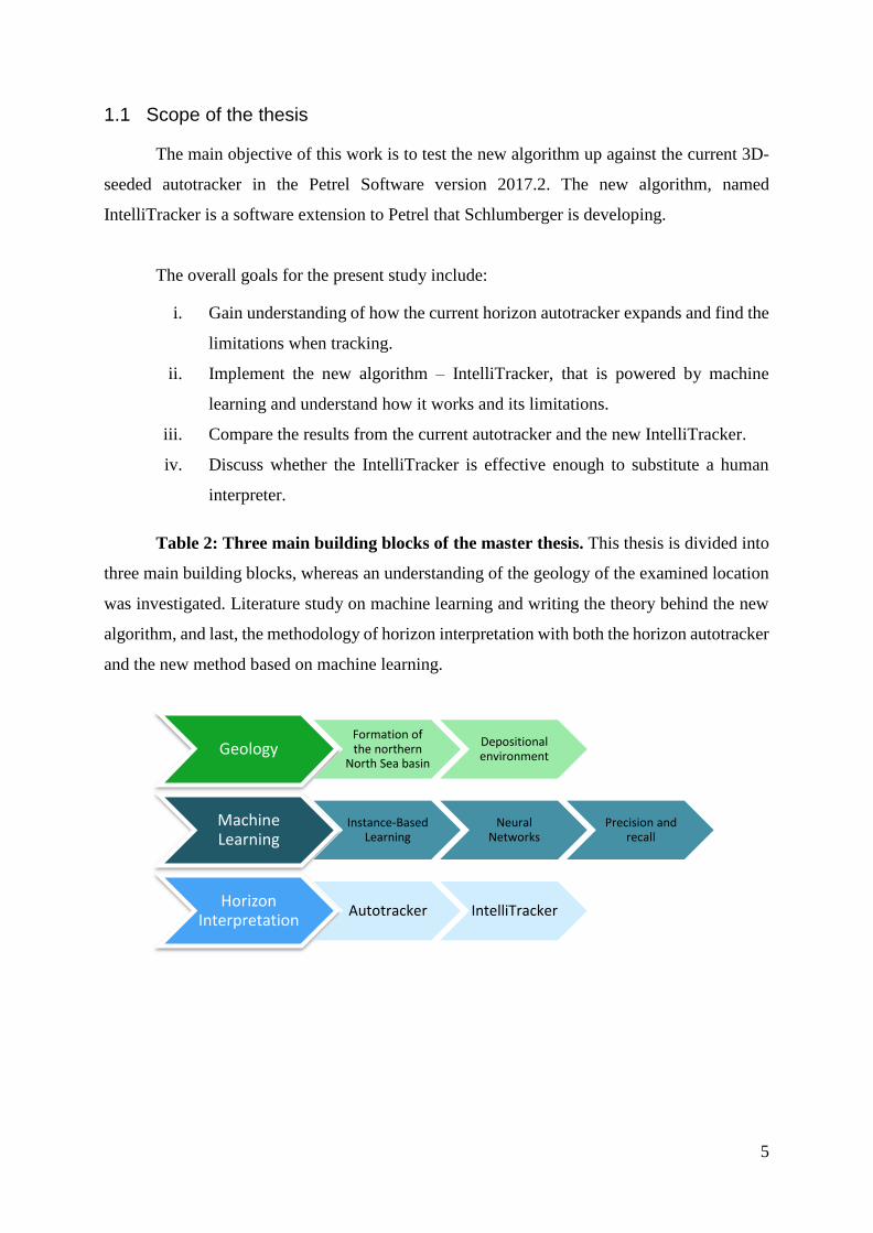
Table 2: Three main building blocks of the master thesis. This thesis is divided into

three main building blocks, whereas an understanding of the geology of the examined location

was investigated. Literature study on machine learning and writing the theory behind the new

algorithm, and last, the methodology of horizon interpretation with both the horizon autotracker

and the new method based on machine learning.

GeologyFormation of the northern

North Sea basin

Depositional environment

Machine Learning

Instance-Based Learning

Neural Networks

Precision and recall

Horizon Interpretation

Autotracker IntelliTracker

6

1.3 Previous studies

The Horda Platform offshore Norway and the presence of Triassic sedimentary basins

have long been recognized. The study on the northern North Sea has been crucial for

investigation of hydrocarbons in the area. Many reports have been purposed with seismic data,

well data and log data as well as core interpretation, but the area has proven to be quite difficult

due to its complex geology (Bolle 1992).

Regarding the implementation of machine learning to seismic horizons there is not much

research published, meaning that this project is opening for a new era where there will be a

steep curve to innovating technology solutions for the geoscience market. It is only a question

of time until the industrial market will have these opportunities offered by several companies.

There exist two methods with machine learning implementation developed by

Schlumberger SSR. These are not applied to this thesis. The first is known as Seismic DNA.

“This is a method for extracting geological features from seismic data that is able to make non-

local searces on multi-attribute datasets. The input data, which can be seismic data, seismic

attributes or any other data type, are first transformed into characters. The transformed data are

searched for complex features with specific character-signatures using text-based search

technology. Since this search methodology for character-signatures holds many similarities

with DNA searches for human genes, it is named ‘Seismic DNA’ “(Bakke, Gramstad et al.

2013). The other method is named Extrema. “A methodology for automated 3D interpretation

is presented. Sequences of horizons (seismic events) are constructed from pre-computed

horizon primitives. These horizon primitives are subsequently used to generate geobodies.

Classification techniques can be applied to automatically group seismic events into classes of

similar seismic waveform when performing seismic interpretation, as described by Borgos et

al. (2003). In this work we describe how the classification approach can be used to extract a set

of geometry primitives, constituting building blocks that the seismic interpreter can apply to

construct a structural description of the reservoir. These primitives can be either surface

segments or closed volumes, referred to as geobodies. Attributes from the classification are

stored along with the primitives, allowing a later refinement of the reservoir description through

further classification” (Borgos, Gramstad et al. 2006).

7

Earlier experience with machine learning on seismic data exists regarding faults, salt

domes and sand bodies like channels and stratigraphic units. These tests have shown positive

outcome in performance and time but are not tested in this thesis. The thesis emphasizes use of

machine learning on seismic horizons.

8

Theory

2 Background of the Troll Field

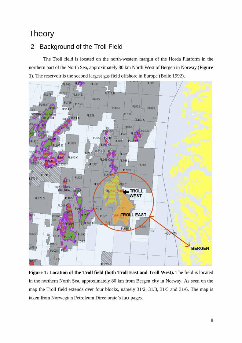
The Troll field is located on the north-western margin of the Horda Platform in the

northern part of the North Sea, approximately 80 km North West of Bergen in Norway (Figure

1). The reservoir is the second largest gas field offshore in Europe (Bolle 1992).

Figure 1: Location of the Troll field (both Troll East and Troll West). The field is located

in the northern North Sea, approximately 80 km from Bergen city in Norway. As seen on the

map the Troll field extends over four blocks, namely 31/2, 31/3, 31/5 and 31/6. The map is

taken from Norwegian Petroleum Directorate’s fact pages.

9

The field contains large amounts of gas and is the biggest producing field on Norwegian

Continental Shelf (Birtles 1986, Bolle 1992). The Troll field is divided into two main structures;

Troll East and Troll West. Both are large rotated fault blocks. Troll West is again divided into

two provinces, the Troll West oil province and the Troll West gas province (Oljemuseum 2018).

The Troll field is a part of four formations in the Jurassic Viking Group, namely

Sognefjord Formation, Fensfjord Formation, Heather Formation, and Krossfjord Formation, as

demonstrated in Figure 2. Most of the gas lies in reservoir sandstones deposited in the middle

and upper Jurassic. The hydrocarbons are mainly found in the Sognefjord Formation, which is

built up from shallow marine sandstones. Part of the reservoir also extends into the underlying

Fensfjord Formation. With its high permeability, these sandstones have good properties for

production.

The hydrocarbons, mainly gas, are trapped in three main easterly- and southeasterly-

tilted fault blocks. The geological area of the Troll field is somewhat complex, as shown in

Figure 5, and will be further investigated throughout this chapter.

10

Figure 2: Stratigraphy of the North Viking Graben (after Lee and Hwang, 1993 from article

by (Osivwi 2012)). The Troll field is found within the Viking Group where the zoomed-in outlined

area characterizes the main formations found in the Troll field. As mentioned earlier the reservoir

is found in the Sognefjord Formation of middle to upper Jurassic age. The relevant colors are

described as; Draupne – orange and Heather - blue : shallow-marine deposits, mainly shale.

Sognefjord, Fensfjord and Krossfjord – yellow : marine deposits, mainly sandstone.

11

2.1 Dataset and software

The NH0301 3D seismic cube covers the desired area intended to investigate. The settings for

the data set are shown in Figure 3. The seismic data from this faulted and destructed reservoir

(Figure 5) is a 3D seismic survey consisting of 1665 inlines and 2751 crosslines. The 3D survey

has a high resolution, and the time-depth windows extend from 0 to 2804 meters (Schlumberger

2011) as seen in Figure 4. This means that the survey has horizon maps down to the Late

Triassic, which is sufficient for this study as the main interpreted horizon is localized around

1600 ms to 1900 ms [TWT] (Jonassen 2015).

Figure 3: Statistics from the data set NH0301 from settings in Petrel. This is the information

given when opening the settings dialog box in Petrel. Here, information regarding the seismic

data, such as latitudes, number of inlines and crosslines and survey type is found.

12

Society of Exploration Geophysicists (SEG) hold the current convention of red color as

positive and blue color as negative reflection coefficients in normal polarity and vice versa in

reversed polarity. The polarity can represent a seismic reflection from two end-members:

minimum phase (asymmetric-design) or zero-phase (symmetric-design).

Both phase and polarity can be assessed from the flatspot (Figure 4) as direct

hydrocarbon indicator (DHI) in the Troll Field. In this study, the applied data, survey NH0301,

hold normal polarity (Birtles 1986).

The reference tool used in this project is Petrel E&P Software version 2017.2 and its

implementation of the autotracker. This shared earth approach enables the users to standardize

workflows from exploration to production – and make more informed decisions with a clear

understanding of both opportunities and risks (Schlumberger 2017).

13

Figure 4: A 2D Inline showing the NH0301 with outlined elements. As seen on the left, the black arrow indicates where the survey recording

stops at 2800 ms [TWT]. Other interesting elements are the bright spots (marked in green) and flat spots (marked in orange).

14

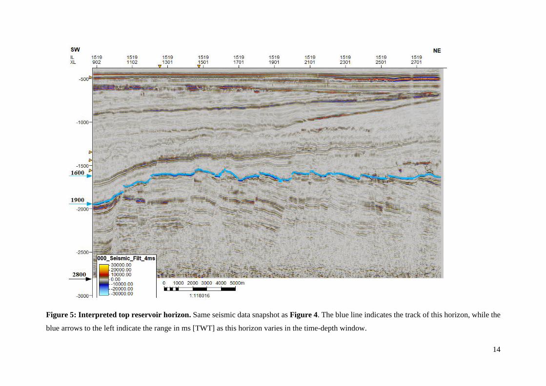
Figure 5: Interpreted top reservoir horizon. Same seismic data snapshot as Figure 4. The blue line indicates the track of this horizon, while the

blue arrows to the left indicate the range in ms [TWT] as this horizon varies in the time-depth window.

15

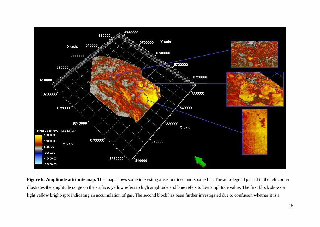
Figure 6: Amplitude attribute map. This map shows some interesting areas outlined and zoomed in. The auto-legend placed in the left corner

illustrates the amplitude range on the surface; yellow refers to high amplitude and blue refers to low amplitude value. The first block shows a

light yellow bright-spot indicating an accumulation of gas. The second block has been further investigated due to confusion whether it is a

16

processing artefact or a bigger area with high amplitudes. It turned out to be the latter, where it is a block unit surrounded by faults possible to

contain large amounts of hydrocarbons. The last could be interpreted as scouring stripes of erosion but are most likely just acquisition footprints.

17

3 Geology

To better understand how the autotracker performs on the Troll field dataset, it is crucial

to also understand how the geology has developed over time. Therefore, this chapter will

explain the main geological events that have structured the northern North Sea as it is today.

Further, a description of the sedimentological processes forming the Troll field is presented.

An amplitude map from the top unconformity in the Troll field was extracted in Petrel

2017.2 as illustrated in Figure 6. Three areas of interest are outlined and zoomed in. The

uppermost section contains a small yellow bright-spot that is interpreted to be a gas

accumulation. The middle section contains a block-unit that could easily be considered a

processing-artefact, but it appeared to be a high-amplitude block-unit surrounded by faults that

may contain gas when closely examined. The lowermost section is an amplitude anomaly that

is parallel to the inline direction, and probably represent acquisition footprints.

3.1 Geological definitions

This sub-chapter will explain some basic geological definitions used to characterize

events forming the examined area as shown in Figure 7, which is beneficial to better understand

the rest of chapter 3.

According to the Petrel manual (Schlumberger 2011), a horizon is defined as “A 2D

grid that belongs to a 3D model. It can be computed from a surface or a seismic horizon

interpretation or any point or line data. The horizon cannot have multiple z-values”. Horizon

interpretation is according to the manual defined as “Interpretation done on seismic following

reflective events”. The Petrel Seismic Interpretation enables basin-, prospect-, and field-scale

2D and 3D seismic interpretation and mapping. Advanced visualization tools provide seismic

overlay and RGB/CMY color blending to enhance the delineation of structural and

stratigraphic features. Accurate interpretation of those features are made possible by the

complete set of tools, such as advanced horizon interpretation.

18

Figure 7: Structural framework of the northern North Sea. As seen at base Cretaceous

level. Main structural elements: East Shetland Basin (ESB), East Shetland Platform (ESP),

Horda Platform (HP), Lomre Terrace (LT), Uer Terrace (UT), Magnus Basin (MgB), Marulk

Basin (MrB), Måløy Fault Block (MFB), Stord Basin (SB), Sogn Graben (SG), Tampen Spur

(TS), Utsira High (UH), Viking Graben (VK), Witch Ground Graben (WG) (Kyrkjebø,

Gabrielsen et al. 2004).

19

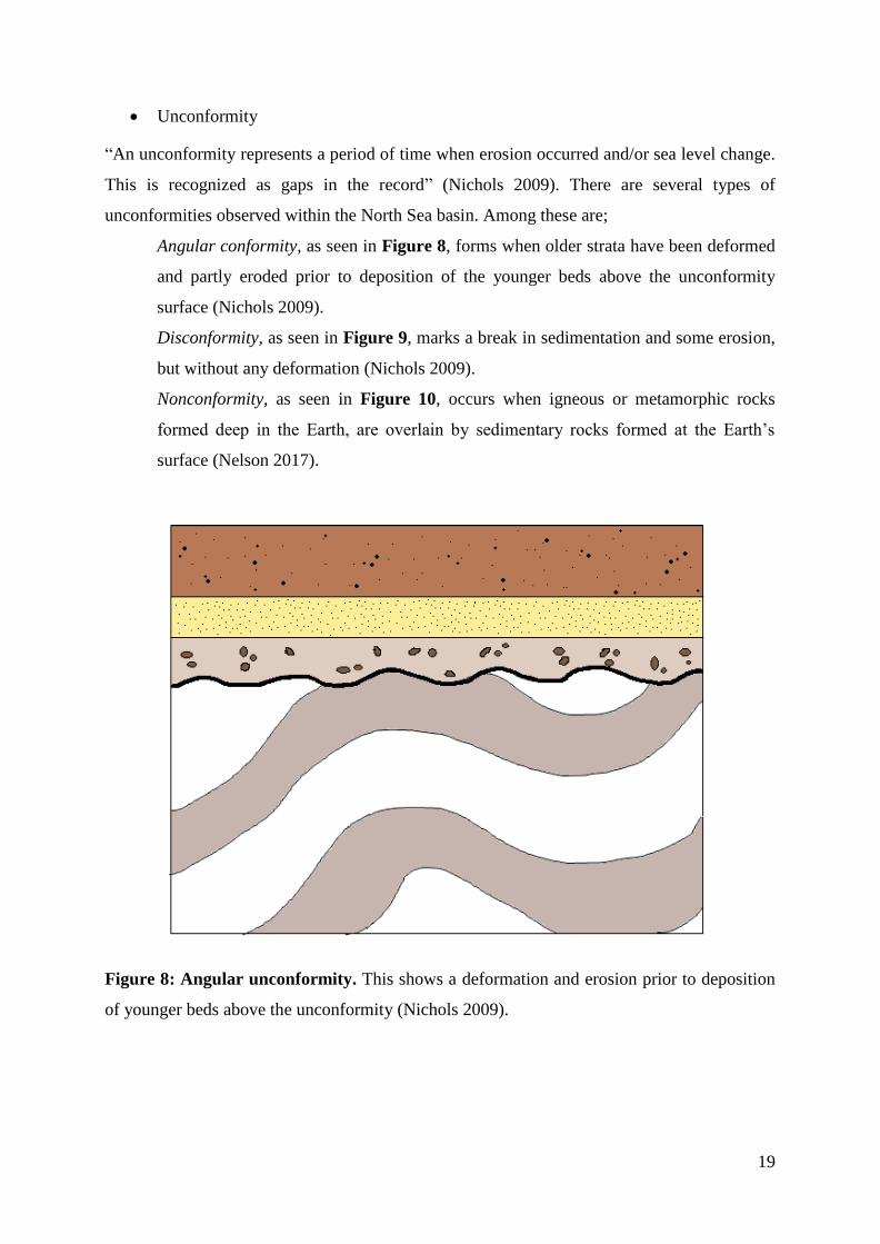
• Unconformity

“An unconformity represents a period of time when erosion occurred and/or sea level change.

This is recognized as gaps in the record” (Nichols 2009). There are several types of

unconformities observed within the North Sea basin. Among these are;

Angular conformity, as seen in Figure 8, forms when older strata have been deformed

and partly eroded prior to deposition of the younger beds above the unconformity

surface (Nichols 2009).

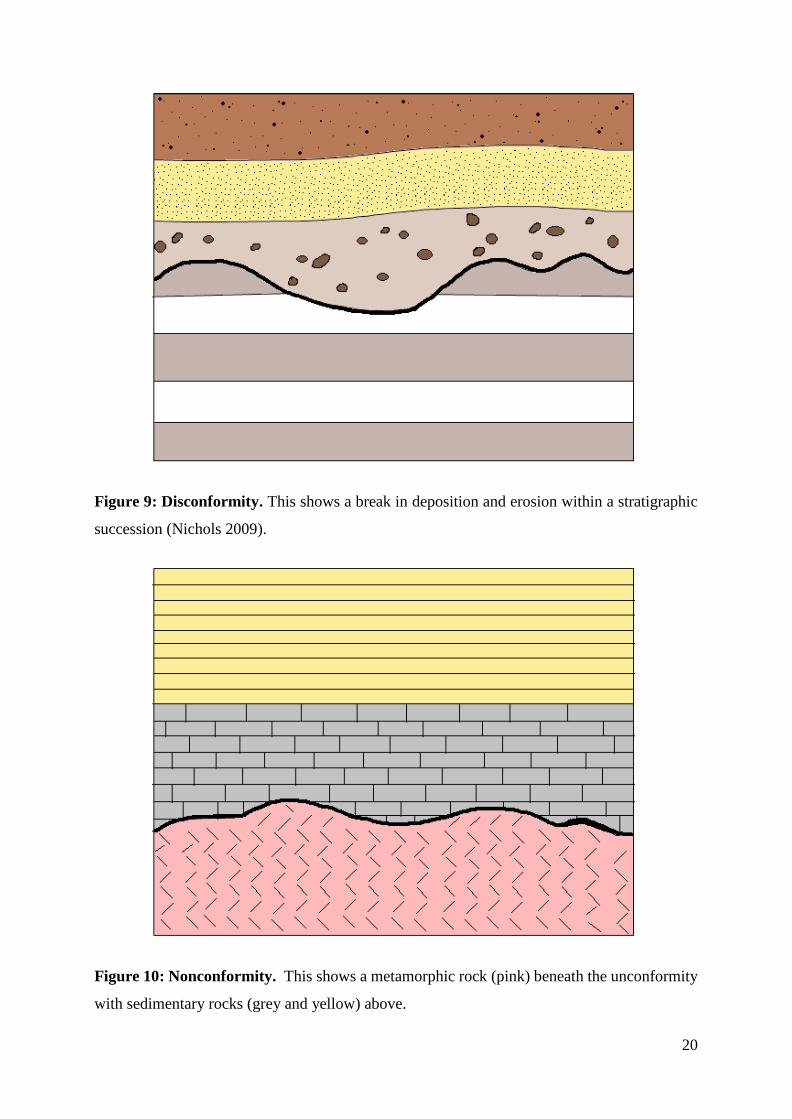
Disconformity, as seen in Figure 9, marks a break in sedimentation and some erosion,

but without any deformation (Nichols 2009).

Nonconformity, as seen in Figure 10, occurs when igneous or metamorphic rocks

formed deep in the Earth, are overlain by sedimentary rocks formed at the Earth’s

surface (Nelson 2017).

Figure 8: Angular unconformity. This shows a deformation and erosion prior to deposition

of younger beds above the unconformity (Nichols 2009).

20

Figure 9: Disconformity. This shows a break in deposition and erosion within a stratigraphic

succession (Nichols 2009).

Figure 10: Nonconformity. This shows a metamorphic rock (pink) beneath the unconformity

with sedimentary rocks (grey and yellow) above.

21

• Transgression

Transgression (Figure 11) is referred to as the landward movement of the shoreline.

This means that the relative sea-level rises or a subsidence of land and seafloor has

occured (Nichols 2009). When the shoreline moves to a place that used to be land, the

coastal plain deposits will be overlain by beach deposits (Figure 12). The facies pattern

will change from shallower to deeper across the whole shelf – deepen-up (Nichols

2009).

Figure 11: Illustration of a transgression. Relative sea-level rises, the water depth increases

and there is a landward movement of the shoreline. Another result of landward movement of

the shoreline is subsidence of land and seafloor.

22

Figure 12: Facies change during a transgression. Here, the coastal plain deposits are

overlain by offshore deposits. This pattern is called retrogradational, because the sea level

rises faster than sediment is supplied, and the shoreline moves landward.

23

• Regression

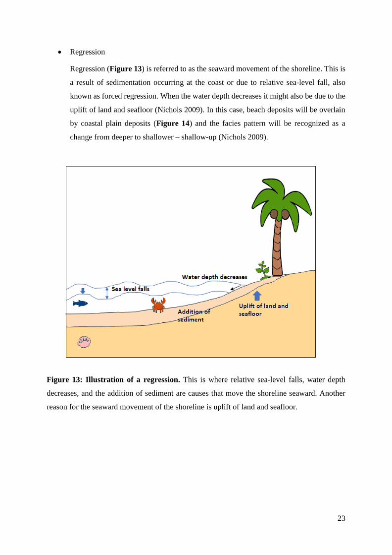
Regression (Figure 13) is referred to as the seaward movement of the shoreline. This is

a result of sedimentation occurring at the coast or due to relative sea-level fall, also

known as forced regression. When the water depth decreases it might also be due to the

uplift of land and seafloor (Nichols 2009). In this case, beach deposits will be overlain

by coastal plain deposits (Figure 14) and the facies pattern will be recognized as a

change from deeper to shallower – shallow-up (Nichols 2009).

Figure 13: Illustration of a regression. This is where relative sea-level falls, water depth

decreases, and the addition of sediment are causes that move the shoreline seaward. Another

reason for the seaward movement of the shoreline is uplift of land and seafloor.

24

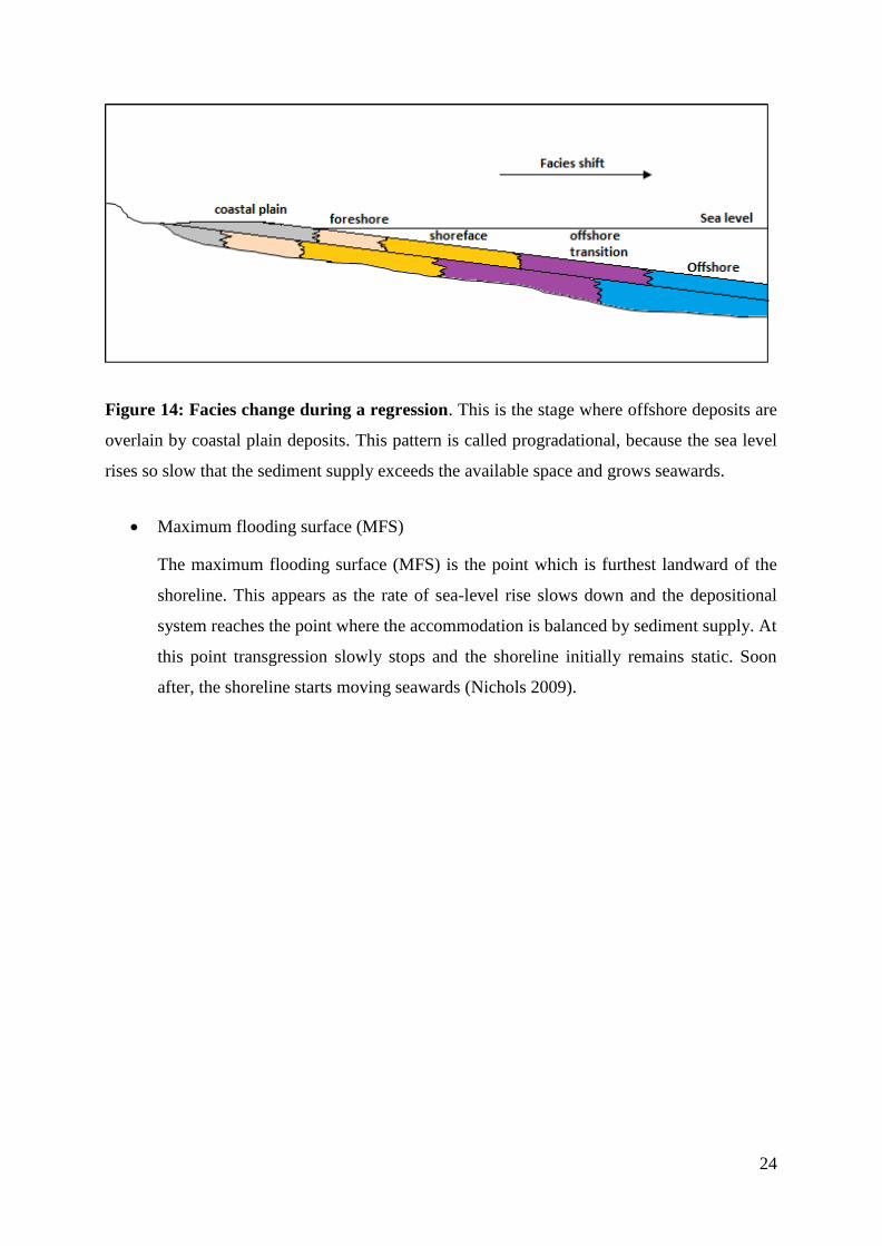
Figure 14: Facies change during a regression. This is the stage where offshore deposits are

overlain by coastal plain deposits. This pattern is called progradational, because the sea level

rises so slow that the sediment supply exceeds the available space and grows seawards.

• Maximum flooding surface (MFS)

The maximum flooding surface (MFS) is the point which is furthest landward of the

shoreline. This appears as the rate of sea-level rise slows down and the depositional

system reaches the point where the accommodation is balanced by sediment supply. At

this point transgression slowly stops and the shoreline initially remains static. Soon

after, the shoreline starts moving seawards (Nichols 2009).

25

3.2 Evolution of the Northern North Sea

The North Sea basin has an unconformity which is an important marker horizon, due to

its distinct character in seismic reflection data and the fact that it is easy to recognize (Kyrkjebø,

Gabrielsen et al. 2004). The unconformity displays both great local complexity (with respect to

seismic reflection) in many locations, as well as great variability on a regional scale (Kyrkjebø,

Gabrielsen et al. 2004). Generally, the basin is characterized by tilted fault blocks, in which

rotation is described from lithospheric stretching, sedimentary loading and thermal response

(Ziegler 1981, Gabrielsen, Færseth et al. 1990, Yielding, Badley et al. 1991). The current 3D

seeded autotracker has difficulties to track across areas involving faults, decreases in continuity

and reflector amplitude. To ease the interpreters’ workflow around such complex areas, that are

time-consuming and uncertain, the automated tracker based on machine learning is supposed

to perform the interpretation faster and more accurate. Leading to a continuous tracking across

the target horizon despite faults, decrease in continuity and reflector amplitude.

There are several reasons the unconformity in the northern North Sea is complex;

general basin geometry, position within the basin, fault configuration, fault-related variations

in subsidence patterns and possibly spatial and temporal heat flow variations (Kyrkjebø,

Gabrielsen et al. 2004). Further, detailed interpretation and chronological correlation are

difficult because the precise age is still uncertain, due to lack of well logs in the area (Kyrkjebø,

Gabrielsen et al. 2004).

The North Sea basin developed mainly due to two major rift events during the Late-

Paleozoic to Mesozoic eras (Jonassen 2015): the syn-rift sequence episode and the post-rift

sequence episode as indicated in Figure 15. Additional subsidence and uplift affected the area

at various times in the basin evolution

The transition from syn-rift to post-rift stage is characterized with “the point at which

the amount of heat transported out of the system is greater than heat transported into the system

from beneath” (Kyrkjebø, Gabrielsen et al. 2004). In the seismic image, this is recognized by

different tilt patterns throughout the area. This particular shift, with the initiation of net thermal

subsidence, produces a tectonically influenced onlap surface (Kyrkjebø, Gabrielsen et al. 2004).

26

Figure 15: Mode of rotation in the Horda platform. In (a) syn-rift and (b) post-rift stages.

(c) Conceptual model for graben architecture (Kyrkjebø, Gabrielsen et al. 2004).

The seismic amplitude reflector is easily noticed mainly due to two reasons. The first

reason for this distinct reflection character is caused by stacked sequences associated with facies

change. The diversity of rocks present above and below the unconformity indicate a change in

polarity of the seismic reflection signal as well as variations in amplitude across this surface

(Kyrkjebø, Gabrielsen et al. 2004). The other reason this sequence shift occurs is due to abrupt

change in tectonic style between the heavily faulted upper Jurassic (syn-rift) and the relatively

un-faulted Cretaceous (post-rift) sequences. The reflection signature of the unconformity itself

is complex and varies due to the geometry of strata above and below. Another factor is local

tectonic disturbances which yield low-frequency high-amplitude double reflectors (Kyrkjebø,

Gabrielsen et al. 2004). These are mainly the reasons why the current autotracker finds it

difficult to track the horizon. When the signal is weak/ambiguous or has discontinuous

reflection pattern, the tracker will stop and require devoted interpretation on the signals. This is

a time-consuming process demanding experience and geological understanding of the

investigated area.

27

3.3 Depositional Environment

The Horda platform is located on the eastern flank of the North Viking Graben and is

up to 50 km wide north-south trending, fault blocks. The late Jurassic stratigraphy of the Horda

Platform contains three shallow marine, coarse-grained siliciclastic wedges that were deposited

by westward-prograding deltas sourced from the Norwegian mainland; these wedges

correspond to the Krossfjord, Fensfjord and Sognefjord formations (Patruno, Jackson et al.

2015). These formations are separated by incursions of the offshore Heather Formation that

represent transgressive maxima. The internal architecture is defined by multiple regressive-

transgressive tongues (Patruno, Jackson et al. 2015).

The Troll field is interpreted to be a wave- and tide-dominated deltaic shoreline and

shelf depositional environment with varying reservoir potential (Holgate, Jackson et al. 2015)

and (Patruno, Jackson et al. 2015). There is no evidence of fluvial nor coastal plain facies

(Stewart, Schwander et al. 1995). The sediments represent delta and coastal progradation over

a shallow marginal marine shelf (Figure 16) (Johnsen, Rutledal et al. 1995).

Figure 16: Illustration of a cross-section showing the continental shelf through the

continental slope down to the oceanic crust. A description of different processes and how

they interact depending on their water depth. (Nichols 2009).

28

There have been several events of transgression and regression including maximum

flooding surfaces that have been used as correlation framework. This is observed in late-middle

to upper Jurassic (Fensfjord-Sognefjord Formations (Figure 2) (Stewart, Schwander et al.

1995). The particular Late Ryazanian transgression marked a facies shift and distinguished

different system tracts. The facies shift usually marks a strong reflector in the seismic data,

which makes it easy for the interpreter to follow a horizon. If the facies shift goes from shale to

sand in depth, it also assumes to be a potential reservoir for hydrocarbons. This yields strong

amplitudes across the horizon and the horizon autotracker easily tracks the target surface.

(Kyrkjebø, Gabrielsen et al. 2004).

29

4 Machine Learning

Machine Learning, Artificial Intelligence, Big Data and Pattern Recognition are

entering the geoscience domain. Big companies such as Google, Apple, Equinor, Schlumberger

and many others are already taking advantage of this new technology. Even though the

introduction to these terms are outdated and have existed in the market since the late 1950’s,

the applications to new areas are innovative. Particulary, the integration of machine learning

with new algorithms to geoscience purpose is a relatively new concept.

Machine learning is basically using the data that is already available and training

algorithms to make predictions based on these data. The application into geoscience is attractive

in terms of making a more effective workflow for interpretation. Especially pattern recognition

and applying algorithms that can learn from data and store information in the memory.

This chapter will focus on explaining the methods listed below:

• Instance-Based Learning

o K-nearest neighbor learning

o Radial Basis Function (RBF)

• Neural Networks

• Precision and Recall

4.1 Instance-Based Learning

The advantage of instance-based learning is that it stores the training data. This means

that every time a new instance occurs, the relationship with previous stored examples are

examined and compared to assign a target function value for the new instance (Mitchell 1997).

Instance-based learning includes nearest neighbor and locally weighted regression methods that

assume instances that can be represented as points in a Euclidean space (Mitchell 1997). The

instance-based learning methods have a delay in processing until a new instance must be

classified. A key advantage of this delayed learning is that instead of estimating the target

function once for the entire instance space, these methods can estimate it locally and differently

for each new instance to be classified (Mitchell 1997).

There are also some disadvantages to using this method. One disadvantage is that the

cost of classifying new instances can be high, due to computation which takes place at

classification time rather than when the training examples are first encountered. A second

disadvantage to several of the instance-based approaches, especially nearest-neighbor

30

approaches, is that they typically consider all attributes of the instances when attempting to

retrieve similar training examples from memory (Mitchell 1997).

4.1.1 K-nearest neighbor learning

The most basic instance-based method is the k-nearest neighbor algorithm. This

algorithm assumes that all instances correspond to points in the n-dimensional space 𝑅𝑛

(Mitchell 1997). The nearest neighbors of an instance are defined in terms of the standard

Euclidean distance. More precisely, an arbitrary instance x is described by the feature vector

⟨𝑎1(𝑥), 𝑎2(𝑥), … 𝑎𝑛(𝑥)⟩

where 𝑎𝑟(𝑥) denotes the value of the 𝑟th attribute of instance 𝑥. Classification with k nearest

neighbors is determined by majority voting among the k nearest neighbors of all saved

instances. Then the distance between for example two instances 𝑥𝑖 and 𝑥𝑗 is defined to be

𝑑(𝑥𝑖, 𝑥𝑗), where

𝑑(𝑥𝑖, 𝑥𝑗) ≡ √∑ (𝑎𝑟(𝑥𝑖) − 𝑎𝑟(𝑥𝑗))2𝑛𝑟=1 (Mitchell 1997)

4.1.2 Radial basis function (RBF)

Radial basis functions (RBF) are a type of approximation that is similar to distance-

weighted regression and also to artificial neural networks (Mitchell 1997). It is represented by

a linear combination of many local kernel functions. The learned hypothesis is a function of the

form,

𝑓(𝑥) = 𝑤0 + ∑ 𝑤𝑢𝐾𝑢(𝑑(𝑥𝑢, 𝑥))

𝑘

𝑢=1

where each 𝑥𝑢 is an instance from X and where the kernel function 𝐾𝑢(𝑑(𝑥𝑢, 𝑥)) is defined so

that it decreases as the distance 𝑑(𝑥𝑢, 𝑥) increases. Here 𝑘 is a user-provided constant that

specifies the number of kernel functions to be included. Even though 𝑓(𝑥) is a global

approximation to 𝑓(𝑥), the contribution from each of the 𝐾𝑢(𝑑(𝑥𝑢, 𝑥)) terms are localized to a

region nearby the point 𝑥𝑢. It is common to choose each function 𝐾𝑢(𝑑(𝑥𝑢, 𝑥)) to be a Gaussian

function centered at the point 𝑥𝑢 with some variance 𝜎𝑢2 (Mitchell 1997). The most common

31

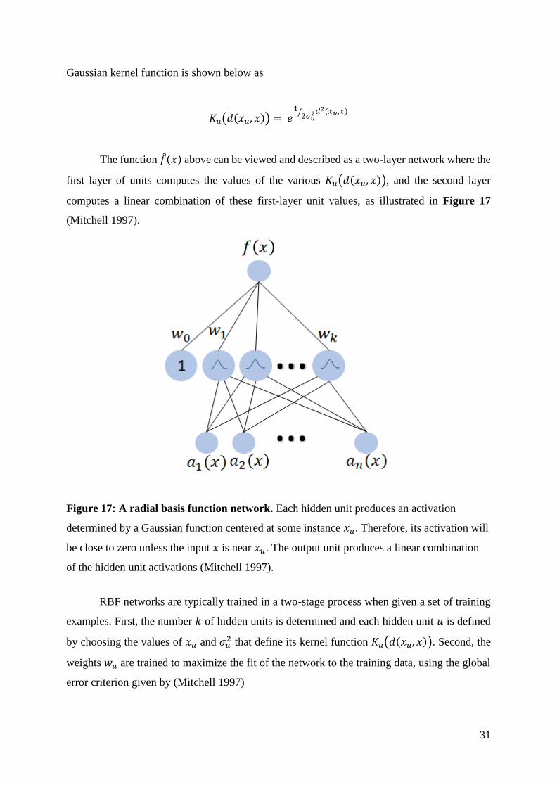
Gaussian kernel function is shown below as

𝐾𝑢(𝑑(𝑥𝑢, 𝑥)) = 𝑒1

2𝜎𝑢2⁄ 𝑑2(𝑥𝑢,𝑥)

The function 𝑓(𝑥) above can be viewed and described as a two-layer network where the

first layer of units computes the values of the various 𝐾𝑢(𝑑(𝑥𝑢, 𝑥)), and the second layer

computes a linear combination of these first-layer unit values, as illustrated in Figure 17

(Mitchell 1997).

Figure 17: A radial basis function network. Each hidden unit produces an activation

determined by a Gaussian function centered at some instance 𝑥𝑢. Therefore, its activation will

be close to zero unless the input 𝑥 is near 𝑥𝑢. The output unit produces a linear combination

of the hidden unit activations (Mitchell 1997).

RBF networks are typically trained in a two-stage process when given a set of training

examples. First, the number 𝑘 of hidden units is determined and each hidden unit 𝑢 is defined

by choosing the values of 𝑥𝑢 and 𝜎𝑢2 that define its kernel function 𝐾𝑢(𝑑(𝑥𝑢, 𝑥)). Second, the

weights 𝑤𝑢 are trained to maximize the fit of the network to the training data, using the global

error criterion given by (Mitchell 1997)

32

Minimizing the squared error over just the 𝑘 nearest neighbors: (Mitchell 1997).

𝐸 ≡1

2∑(𝑓(𝑥) −

𝑥∈𝐷

𝑓(𝑥))2

Because the kernel functions are held fixed during this second stage, the linear weight values

𝑤𝑢 can be trained very efficiently.

An approach for choosing the appropriate number of hidden units or kernel functions

when the number of training examples is large is to choose a set of kernel functions that is

smaller than the number of training examples (Mitchell 1997). The set of kernel functions may

be distributed with centers spaced uniformly throughout the instance space X.

The network can be viewed as a smooth linear combination of many local

approximations to the target function. One key advantage to RBF networks is that they can be

trained much more efficiently than feed-forward networks trained with backpropagation. This

follows from the fact that the input layer and the output layer of an RBF are trained separately

(Mitchell 1997).

4.2 Neural Networks

A neuron is a cell in the brain whose principal function is the collection, processing, and

dissemination of electrical signals (Russel and Norvig 1995). The earliest work performed on

artificial intelligence aimed to create such artificial neuron networks, that copies the workflow

to a human’s brain. An example of the neuron is presented in Figure 18. Today, there exist

much more detailed and realistic models for neurons than the one in Figure 18, which only

fires when a linear combination of its input exceeds some threshold.

33

Figure 18: A simple mathematical model for a neuron. The unit’s output activation is 𝑎𝑖 =

𝑔 ∑ 𝑊𝑗,𝑖𝑎𝑗)𝑛𝑗=0 , where 𝑎𝑗 is the output activation of unit 𝑗 and 𝑊𝑗,𝑖is the weight on the link from

unit 𝑗 to this unit (Russel and Norvig 1995).

A neural net is a set of little machine learning algorithms (little logistic regressions) that

are combined to mimic neural activity. These models are then trained to perform a task, such

as for example image recognition. There are two main categories of neural networks; acyclic

(or feed-forward) networks, and cyclic or recurrent networks. The main difference between a

feed-forward network and a recurrent network is that the first represents a function of its current

input, while the last feeds its outputs back into its own inputs. This means that the activation

levels of the network form a dynamical system that may reach a stable state or exhibit

oscillations or even chaotic behavior. Further consideration of neural network structures will

deal with recurrent networks, due to its support of short-term memory. This method utilizes the

concept in machine learning, the ability to memorize input and learn from it (Russel and Norvig

1995).

A multilayer feed-forward neural network has a structure as shown in Figure 19. The

input component usually takes in a numerical value varying from 0 to 1. A neuron with no input

will always output the same value, which is useful for shifting of the activation function, known

as a “bias”. As seen in Figure 18, the weights are assigned to a certain input with a real value.

This value indicates how important the input is. Each input is multiplied by its weight. The

activation function in the same figure is a mathematical function mapping the weighted input

to an output. Usually, the output value is somewhere between 0 and 1. The last component is

the output, which receives the results from the activation function (Ask, Frøysa et al. 2016).

34

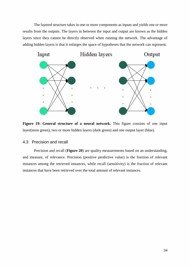
The layered structure takes in one or more components as inputs and yields one or more

results from the outputs. The layers in between the input and output are known as the hidden

layers since they cannot be directly observed when running the network. The advantage of

adding hidden layers is that it enlarges the space of hypotheses that the network can represent.

Figure 19: General structure of a neural network. This figure consists of one input

layer(neon green), two or more hidden layers (dark green) and one output layer (blue).

4.3 Precision and recall

Precision and recall (Figure 20) are quality measurements based on an understanding,

and measure, of relevance. Precision (positive predictive value) is the fraction of relevant

instances among the retrieved instances, while recall (sensitivity) is the fraction of relevant

instances that have been retrieved over the total amount of relevant instances.

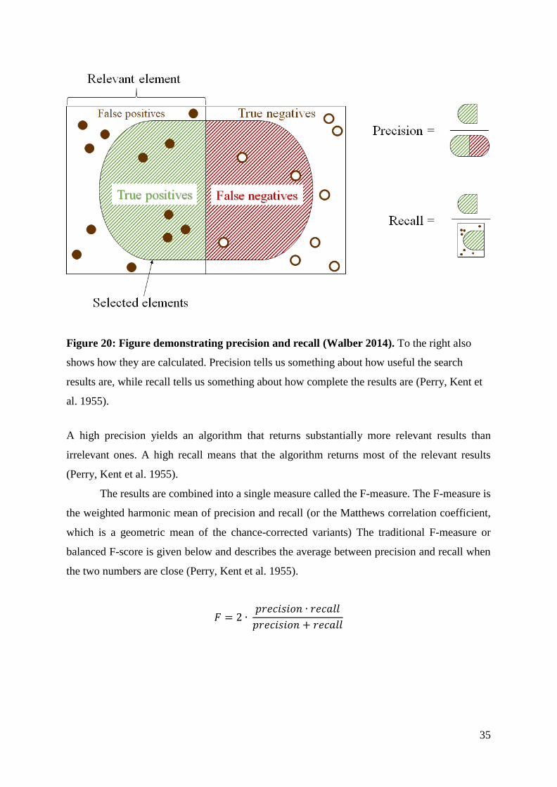
35

Figure 20: Figure demonstrating precision and recall (Walber 2014). To the right also

shows how they are calculated. Precision tells us something about how useful the search

results are, while recall tells us something about how complete the results are (Perry, Kent et

al. 1955).

A high precision yields an algorithm that returns substantially more relevant results than

irrelevant ones. A high recall means that the algorithm returns most of the relevant results

(Perry, Kent et al. 1955).

The results are combined into a single measure called the F-measure. The F-measure is

the weighted harmonic mean of precision and recall (or the Matthews correlation coefficient,

which is a geometric mean of the chance-corrected variants) The traditional F-measure or

balanced F-score is given below and describes the average between precision and recall when

the two numbers are close (Perry, Kent et al. 1955).

𝐹 = 2 ∙ 𝑝𝑟𝑒𝑐𝑖𝑠𝑖𝑜𝑛 ∙ 𝑟𝑒𝑐𝑎𝑙𝑙

𝑝𝑟𝑒𝑐𝑖𝑠𝑖𝑜𝑛 + 𝑟𝑒𝑐𝑎𝑙𝑙

36

4.4 IntelliTracker

The IntelliTracker is based on two methods within machine learning. Both Radial Basis

Functions (RBF) and Neural Networks (NN) are options within the new method, as shown in

Figure 21. If the “UseNN” box is toggled on the theory described in the section on Neural

Networks is essential for the expansion method. If the box stays un-toggled the expansion

method is based on the section about Radial basis function (RBF).

Figure 21: Settings for ML Tracker in workflows. Insert the seismic cube in ‘Cube’, point

set created along the horizon in ‘Points’ and optionally point set created for ‘Avoid’. Then the

‘Run’ button is outlined in blue. The ‘Use NN’ is currently not available during the testing of

this thsis.

Further examination is based on the RBF method. The seed point goes through a

validation process, as shown in Figure 22. Before further expansion, the seed point looks for

either maximas or minimas within an interval of [-5,5] surrounding traces. If the next seed point

meets these criteria it generates a model based on the trained input data. It then calculates a

confidence score based on these training data. The user sets a limit for the confidence-score,

which in this case is set to 0.5. Those seed points that has a confidence-score over this value

are further put in a priority queue. The seed point with the highest confidence score value is put

first in the queue before it is accepted as a parent seed and the process starts all over again with

a new potential seed point.

37

Figure 22: The expansion process of a seed point. One seed point is compared to the

surrounding seeds in an interval of [-5,5] samples up or down on neighboring traces. If the seed

is max or min the seed will calculate the confidence interval. If this again is over a specific

value; here 0.5, the seed will be put in a priority queue, and the process will continue to the next

seed.

The expansion process itself is based on Figure 23. The first step referred to as step 1

shows a single parent seed in dark green color, while the surrounding potential seed points as

light green. As explained in Figure 22, the validation of the surrounding potential seed point

begins. Step 2 shows how the expansion has grown to the red middle seed point. Further

examination of potential parent points is done from this red seed point and to those points

marked within the red box-shaped as an upside-down L. If none of the red potential seed points

has high enough confidence-score the expansion continues from the last parent seed as

illustrated in step 3. The next seed point that has high enough confidence-score to meet the

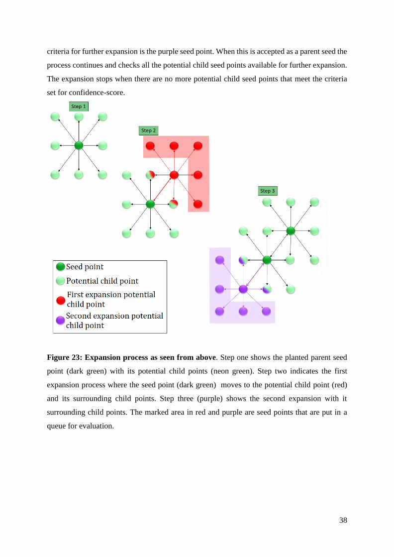
38

criteria for further expansion is the purple seed point. When this is accepted as a parent seed the

process continues and checks all the potential child seed points available for further expansion.

The expansion stops when there are no more potential child seed points that meet the criteria

set for confidence-score.

Figure 23: Expansion process as seen from above. Step one shows the planted parent seed

point (dark green) with its potential child points (neon green). Step two indicates the first

expansion process where the seed point (dark green) moves to the potential child point (red)

and its surrounding child points. Step three (purple) shows the second expansion with it

surrounding child points. The marked area in red and purple are seed points that are put in a

queue for evaluation.

39

Methodology

5 Horizon Interpretation

For the interpreter to effectively interpret a given seismic cube, it requires a good

reflector that the planted seed points can track outwards in all directions. This thesis is based

on the experience gained from the software Petrel as presented in “2.1 Dataset and software”.

The procedures described in the leading chapter are recognized from the Petrel Manual of

Geophysics (Schlumberger 2011). The following sections describe the horizon interpretation

procedure, emphasizing the Troll area in the northern North Sea.

There exist four different methods of horizon tracking in the current version of Petrel as

shown in Figure 24.

• Manual interpretation interprets a horizon by clicking (or drawing) points on a seismic

intersection.

• Guided autotracking picks interpretation points and the tracker follows the optimal

events between them.

• Seeded 2D autotracking interprets by picking seed points on an intersection. Points

will be tracked in the direction of the selected intersection.

• Seeded 3D autotracking interprets by picking seed points in a seismic volume. Points

will be tracked outwards, snapped to the selected signal feature.

Figure 24: Tool palette for seismic horizon interpretation. Manual interpreting (dark green

circle), guided autotracking (light green circle), seeded 2D autotracking (blue circle) and seeded

3D autotracking (red circle). The latter one is used when compared with the IntelliTracker.

40

In this thesis, seeded 3D autotracking will be used when discussed and compared to the

IntelliTracker.

5.1 Workflow for the 3D autotracker engine

The process works as follows: a user puts a “seed-point” on the seismic event (a peak,

trough or zero-crossing) that the user would like to generate a horizon map for. The computer

then takes a subset of the seismic trace around this seed-point and correlates this extracted

wavelet with all candidate wavelets of similar length in the immediate 3D neighborhood of the

seed-point. If any of the neighboring wavelets are found to be sufficiently similar (according to

the wavelet correlation coefficient), the center of these accepted neighboring wavelets is

accepted as new interpretation points. This point will then become a newly derived seed-point

which the auto-tracker will continue to try growing, until there are no more potential points to

grow into, given the constraints.

At this point, the auto-tracker has generated a 2D surface “patch” from the initial seed-

point. If the surface is easy to track, the extracted surface patch will have grown to cover the

whole lateral extent of the 3D seismic cube. Otherwise, as with the given 3D seismic from the

Troll field, the user needs to manually insert another seed-point and continue auto-tracking,

until the whole area of interest is covered.

Open settings for seismic horizon wanted to be

intepreted and evaluate the parameters and

constraints

Start the tracking by clicking on the horizon

with a seed point

Pick multiple seed points along the horizon to expand the tracking area (until the

user is satisfied with the horizon surface tracked)

3D-track for automated expansion of the horizon

surface

Evaluate the interpreted horizon surface and erase

seed points that are picked wrong

Re-pick seed points on the corect horiozon such

that the end-result gets as desired

Table 3: Workflow for the 3D seeded autotracker that exist today in Petrel 2017.2.

41

The regular workflow when using the seismic horizon seeded 3D autotracker shown in

Table 3. Primarily, when the interpreter is introduced to a new seismic cube, both inline and

crossline sections need to be carefully examined. This is to gain information about geological

features that can be extracted, and hence obtain a basic knowledge about depositional

environments contributing to those reservoir qualities which the Troll Field has. After all, the

regular workflow for an interpreter is to extract all the possible geological information,

including structure, stratigraphy and rock properties from the given data.

The next step is the evaluation of parameters and constraints in the settings dialog box.

The parameters will be further explained in section 0.1, while the constraints are found in

Appendix A. Depending on how the user wants the autotracker to run, one chooses the

appropriate options that are available. When these settings are set, the next step is to localize a

seed point in the seismic cube based on the target horizon. The autotracker will collect all seeds

for expanding and mark each node of the horizon grid either as expandable or non-expandable.

This is based on the area where the tracking continues to grow.

The auto tracker will then expand from the parent seed based on the selected technique:

basic 3x3, validated 3x3 or validated 5x5. In the process of expanding the seeds, the tracker

will find the event in the neighboring traces of a known seed according to the selected signal

feature. If more than one event has been found in a single trace, doublet handling will be used

and only one event will be selected for further expansion. The event finding system will help

to find the event on the adjacent trace (child trace) given a seed trace (parent trace) and help to

find up to a maximum of two events nearest to the seed event location on the adjacent trace of

the seed trace. The doublet is defined by having a wavelet with 4 or more inflection points and

only 2 zero crossings. This wavelet is located around the seed point within a vertical window

defined by the inline/crossline samples per trace and the maximum vertical delta for 3D and 2D

tracking respectively.

If one event has been found in the adjacent trace of the seed trace, then the constraint

parameters (Figure 25) settings will be used to determine if the event meets the “passing”

criteria. If the event has met the constraint, it will be pushed into the appropriate location in a

priority queue for future expansion. The auto tracker will stop/finish tracking when either there

are no more seeds to expand or if the user clicks “Stop” or “Cancel” from within the application.

42

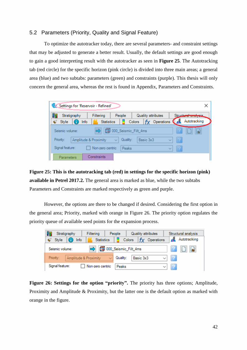
5.2 Parameters (Priority, Quality and Signal Feature)

To optimize the autotracker today, there are several parameters- and constraint settings

that may be adjusted to generate a better result. Usually, the default settings are good enough

to gain a good interpreting result with the autotracker as seen in Figure 25. The Autotracking

tab (red circle) for the specific horizon (pink circle) is divided into three main areas; a general

area (blue) and two subtabs: parameters (green) and constraints (purple). This thesis will only

concern the general area, whereas the rest is found in Appendix, Parameters and Constraints.

Figure 25: This is the autotracking tab (red) in settings for the specific horizon (pink)

available in Petrel 2017.2. The general area is marked as blue, while the two subtabs

Parameters and Constraints are marked respectively as green and purple.

However, the options are there to be changed if desired. Considering the first option in

the general area; Priority, marked with orange in Figure 26. The priority option regulates the

priority queue of available seed points for the expansion process.

Figure 26: Settings for the option “priority”. The priority has three options; Amplitude,

Proximity and Amplitude & Proximity, but the latter one is the default option as marked with

orange in the figure.

43

The priority contains three options; amplitude, proximity and amplitude & proximity.

The amplitude option prioritizes picks of higher extrema for early expansion, leaving lower

extrema picks to expand later. The proximity option prioritizes pics with the shortest expansion

paths over picks with longer expansion paths illustrates the expansion of the proximity option.

Last, a combination of amplitude and proximity that offers both high-quality growth and timely

finish of points close to the seeds called “amplitude & proximity” as highlighted with orange

in Figure 26.

The next option considered is the quality as highlighted with blue in Figure 27. The

quality option controls how stringently each seed point is checked before it expands.

Figure 27: Settings for the quality. The quality has three options; basic 3x3, validated 3x3

and validated 5x5. As shown in this figure, basic 3x3 is the default option.

Also, the quality parameter has three options, whereas the first option is basic 3x3 which is the

default one. This method expands a seed point to its 8 closest neighbors, validating each only

against the seed point as illustrated in Figure 28. This is the first phase of extended technique

that is used in the autotracker.

Figure 28: Basic 3x3 expansion; Seed point, Potential child points.

44

Each new accepted point (child) becomes a potential parent for all the neighboring traces. The

seed point expansion is done using a 3x3 grid cell validation to verify the eight neighbor traces

of each parent point. All eight neighbors of an accepted seed point must pass validation for that

seed to be flagged expandable. In this technique, all eight neighbors are only compared against

the seed point to find a valid pick. If this phase fails, the tracker stops, marking the seed point

as non-expandable.

The second option is validated 3x3 and is illustrated in Figure 29. The validated 3x3

method expands a seed point to its eight closest neighbors, validating each against the seed

point and their two closest neighbors. If one validation fails, the seed point is not expanded.

Figure 29: Validated 3x3 expansion; Seed point, Potential child points.

The last option is the most advanced tracking technique; validated 5x5. This technique

expands a seed point to its 24 closest neighbors, validating each against their closest neighbors.

The validated 5x5 involves two phases as illustrated in Figure 30.

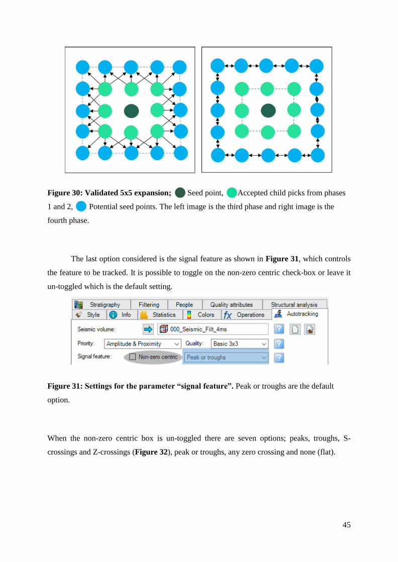
45

Figure 30: Validated 5x5 expansion; Seed point, Accepted child picks from phases

1 and 2, Potential seed points. The left image is the third phase and right image is the

fourth phase.

The last option considered is the signal feature as shown in Figure 31, which controls

the feature to be tracked. It is possible to toggle on the non-zero centric check-box or leave it

un-toggled which is the default setting.

Figure 31: Settings for the parameter “signal feature”. Peak or troughs are the default

option.

When the non-zero centric box is un-toggled there are seven options; peaks, troughs, S-

crossings and Z-crossings (Figure 32), peak or troughs, any zero crossing and none (flat).

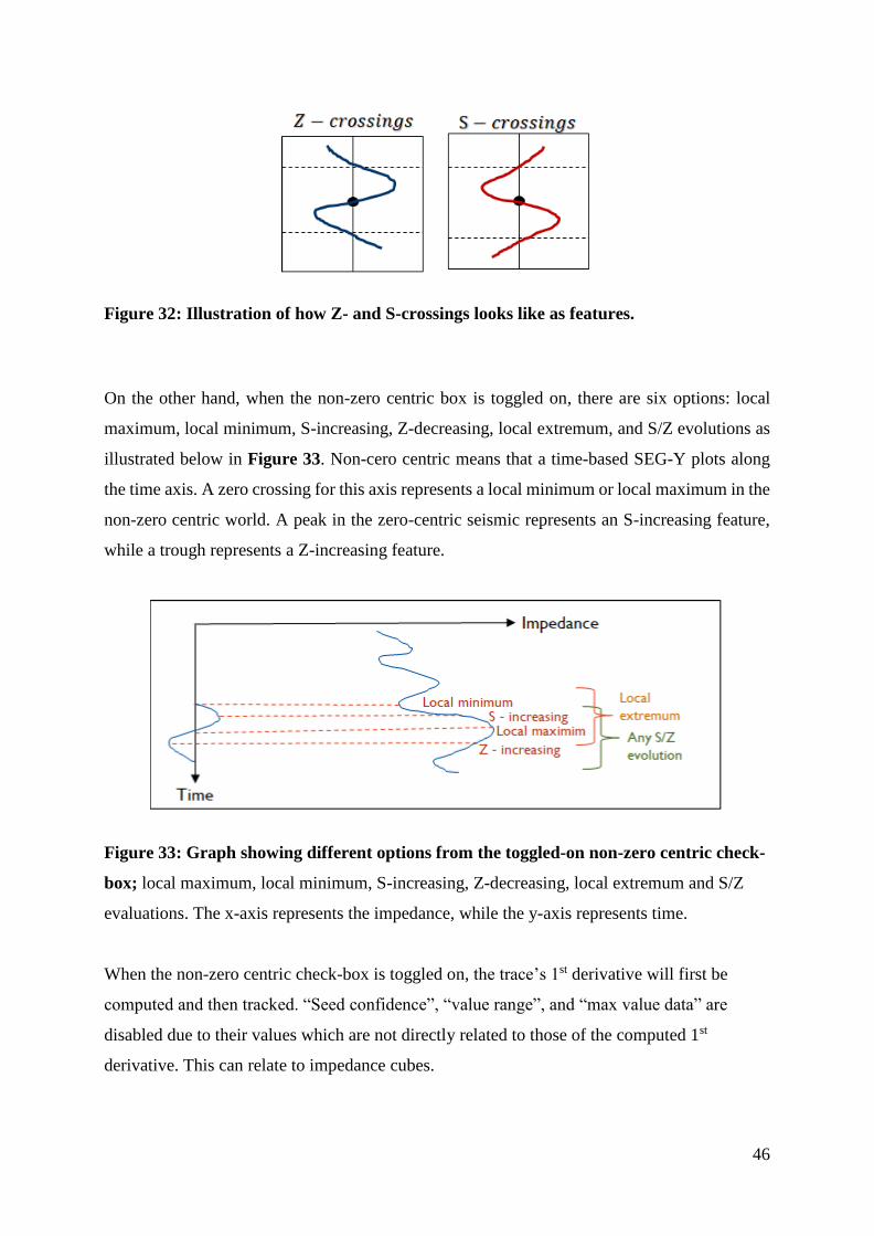
46

Figure 32: Illustration of how Z- and S-crossings looks like as features.

On the other hand, when the non-zero centric box is toggled on, there are six options: local

maximum, local minimum, S-increasing, Z-decreasing, local extremum, and S/Z evolutions as

illustrated below in Figure 33. Non-cero centric means that a time-based SEG-Y plots along

the time axis. A zero crossing for this axis represents a local minimum or local maximum in the

non-zero centric world. A peak in the zero-centric seismic represents an S-increasing feature,

while a trough represents a Z-increasing feature.

Figure 33: Graph showing different options from the toggled-on non-zero centric check-

box; local maximum, local minimum, S-increasing, Z-decreasing, local extremum and S/Z

evaluations. The x-axis represents the impedance, while the y-axis represents time.

When the non-zero centric check-box is toggled on, the trace’s 1st derivative will first be

computed and then tracked. “Seed confidence”, “value range”, and “max value data” are

disabled due to their values which are not directly related to those of the computed 1st

derivative. This can relate to impedance cubes.

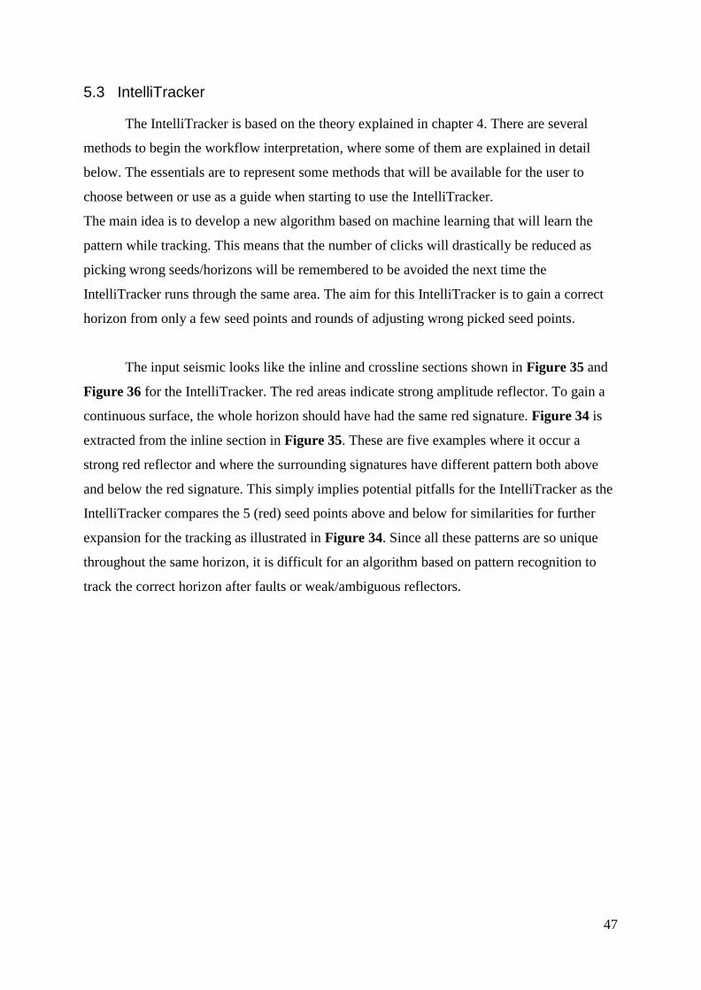
47

5.3 IntelliTracker

The IntelliTracker is based on the theory explained in chapter 4. There are several

methods to begin the workflow interpretation, where some of them are explained in detail

below. The essentials are to represent some methods that will be available for the user to

choose between or use as a guide when starting to use the IntelliTracker.

The main idea is to develop a new algorithm based on machine learning that will learn the

pattern while tracking. This means that the number of clicks will drastically be reduced as

picking wrong seeds/horizons will be remembered to be avoided the next time the

IntelliTracker runs through the same area. The aim for this IntelliTracker is to gain a correct

horizon from only a few seed points and rounds of adjusting wrong picked seed points.

The input seismic looks like the inline and crossline sections shown in Figure 35 and

Figure 36 for the IntelliTracker. The red areas indicate strong amplitude reflector. To gain a

continuous surface, the whole horizon should have had the same red signature. Figure 34 is

extracted from the inline section in Figure 35. These are five examples where it occur a

strong red reflector and where the surrounding signatures have different pattern both above

and below the red signature. This simply implies potential pitfalls for the IntelliTracker as the

IntelliTracker compares the 5 (red) seed points above and below for similarities for further

expansion for the tracking as illustrated in Figure 34. Since all these patterns are so unique

throughout the same horizon, it is difficult for an algorithm based on pattern recognition to

track the correct horizon after faults or weak/ambiguous reflectors.

48

Figure 34: Snapshots from Figure 35 showing variation within one trace. Signatures from

the same horizon throughout the inline direction proving potential pitfalls for the new

algorithm based on machine learning. The red points are compared to the original seed point

indicated as the red trace. For the new method to continue tracking, the small outcome should

look identical, which is not the case for the Troll field.

49

Figure 35: Inline section of the seismic cube of how the input for the IntelliTracker looks like. This seismic section is the feeding training

data for the machine learning algorithm. Based on this, the algorithm calculates the confidence value of neighboring points and compares the

highest value before expanding. The red areas indicate high amplitude and a bigger chance of continuous tracking as they are similar in the pattern

above and below the initial seed point placed on a high amplitude value (bright red).

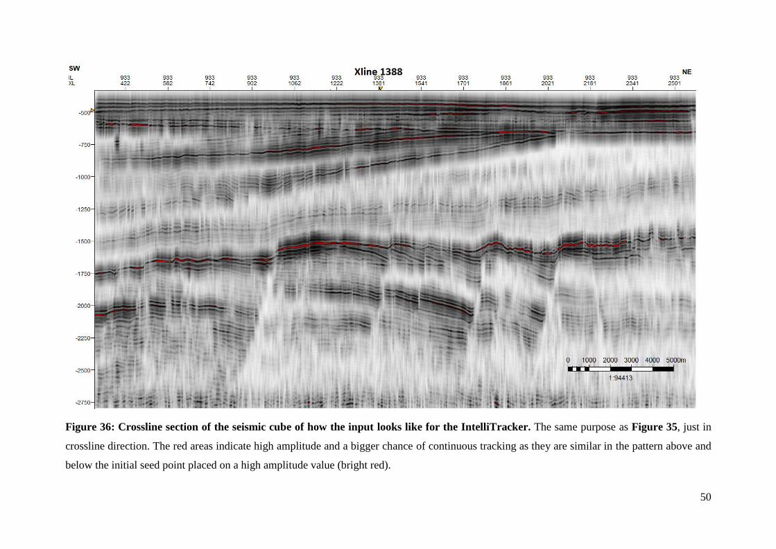
50

Figure 36: Crossline section of the seismic cube of how the input looks like for the IntelliTracker. The same purpose as Figure 35, just in

crossline direction. The red areas indicate high amplitude and a bigger chance of continuous tracking as they are similar in the pattern above and

below the initial seed point placed on a high amplitude value (bright red).

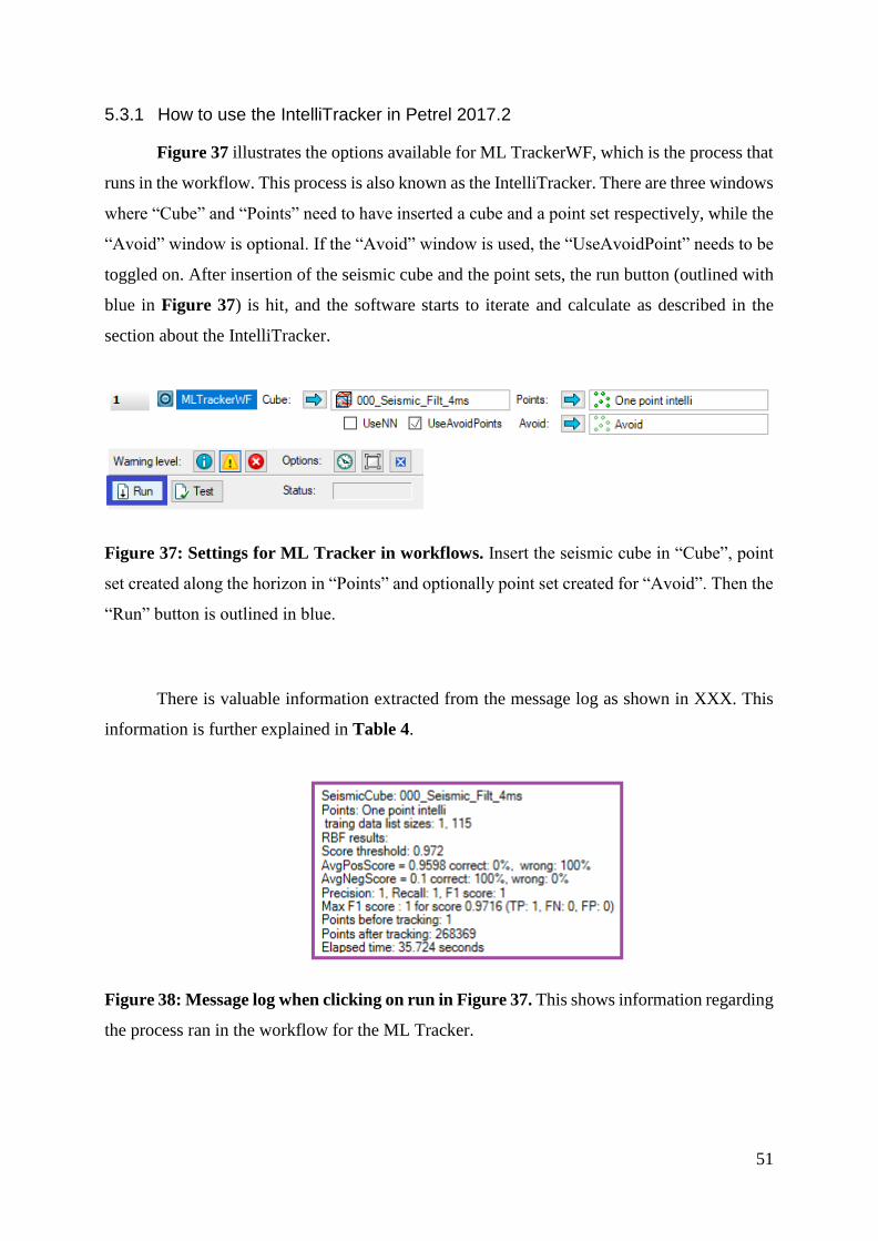
51

5.3.1 How to use the IntelliTracker in Petrel 2017.2

Figure 37 illustrates the options available for ML TrackerWF, which is the process that

runs in the workflow. This process is also known as the IntelliTracker. There are three windows

where “Cube” and “Points” need to have inserted a cube and a point set respectively, while the

“Avoid” window is optional. If the “Avoid” window is used, the “UseAvoidPoint” needs to be

toggled on. After insertion of the seismic cube and the point sets, the run button (outlined with

blue in Figure 37) is hit, and the software starts to iterate and calculate as described in the

section about the IntelliTracker.

Figure 37: Settings for ML Tracker in workflows. Insert the seismic cube in “Cube”, point

set created along the horizon in “Points” and optionally point set created for “Avoid”. Then the

“Run” button is outlined in blue.

There is valuable information extracted from the message log as shown in XXX. This

information is further explained in Table 4.

Figure 38: Message log when clicking on run in Figure 37. This shows information regarding

the process ran in the workflow for the ML Tracker.

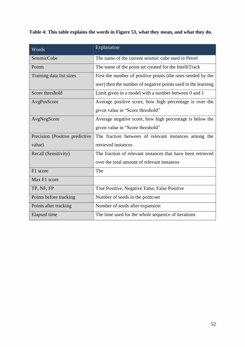
52

Table 4: This table explains the words in Figure 53, what they mean, and what they do.

Words Explanation

SeismicCube The name of the current seismic cube used in Petrel

Points The name of the point set created for the IntelliTrack

Training data list sizes First the number of positive points (the ones seeded by the

user) then the number of negative points used in the learning

Score threshold Limit given in a model with a number between 0 and 1

AvgPosScore Average positive score, how high percentage is over the

given value in “Score threshold”

AvgNegScore Average negative score, how high percentage is below the

given value in “Score threshold”

Precision (Positive predictive

value)

The fraction between of relevant instances among the

retrieved instances

Recall (Sensitivity) The fraction of relevant instances that have been retrieved

over the total amount of relevant instances

F1 score The

Max F1 score

TP, NF, FP True Positive, Negative False, False Positive

Points before tracking Number of seeds in the point-set

Points after tracking Number of seeds after expansion

Elapsed time The time used for the whole sequence of iterations

53

5.3.2 OriginalPointSet-method (OPS-method)

The first method introduced is the OriginalPointSet-method (OPS-method). This is

based on a method where the user inserts one or several points on the target horizon and keep

using expansion from these original seed points as an input to gain a fully interpreted horizon

surface. The output horizon then needs to be quality checked before any further expansion.

Erasing and deleting wrong picks is crucial for the end-result. A surface without any

misinterpretation is now the new point-set inserted in “Points”. The IntelliTracker has now a

bigger point set of training data which gives the seed point network new expandable traces.

The new results need again a new quality check. This process of erasing misinterpreted points

is continued until satisfied horizon surface. It is important to also quality check earlier erased

points, which is not supposed to be traced again unless there are some steps where the

IntelliTracker fails during tracking.

Table 5: OriginalPointSet-method workflow illustrated for the IntelliTracker.

54

5.3.3 Filter-method

The other method described in this chapter is referred to as “Filter-method”. This

method converts the points to an attribute. The Filter-method is activated when the Track

Scores is toggled on as shown in Figure 39.

Figure 39: Subsections below the point set. Toggle on Track Scores for this method.

Opening the settings for the current point set and selecting style, the chosen options

should look like those defined in Figure 40.

Figure 40: Style settings for the current point set. The changes made are under the subtab

“Common” and the user should select “As attribute” for the Filter-method.

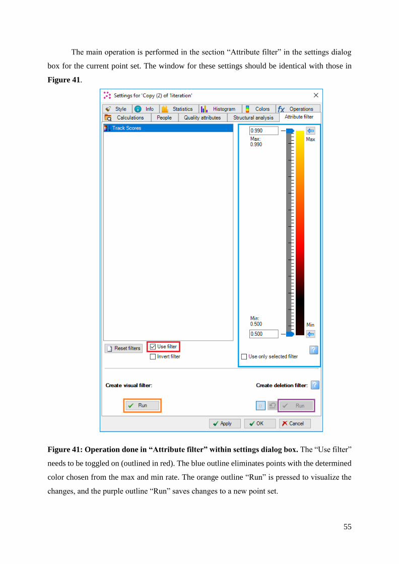
55

The main operation is performed in the section “Attribute filter” in the settings dialog

box for the current point set. The window for these settings should be identical with those in

Figure 41.

Figure 41: Operation done in “Attribute filter” within settings dialog box. The “Use filter”

needs to be toggled on (outlined in red). The blue outline eliminates points with the determined

color chosen from the max and min rate. The orange outline “Run” is pressed to visualize the

changes, and the purple outline “Run” saves changes to a new point set.

56

The main idea of the Filter-method is to eliminate seed points that most likely has grown

wrong. These are characterized with a darker red to black color as shown in the blue box in

Figure 41. This attribute filter divides the points into different colors based on the likelihood

of having the highest confidence-score value. Those seed points that are closest to yellow has a

high confidence-score value, while those seed points closest to black has a low confidence-

score value. As seen in Figure 41 the max value for this point set is 0.990 and min value is

0.500. When these values are changed, usually the min value arrow is moved upwards and the

point surface gains fewer points which have a low confidence-value. The workflow for the

filter-method is as illustrated in

Table 6: Filter-method workflow for the IntelliTracker.

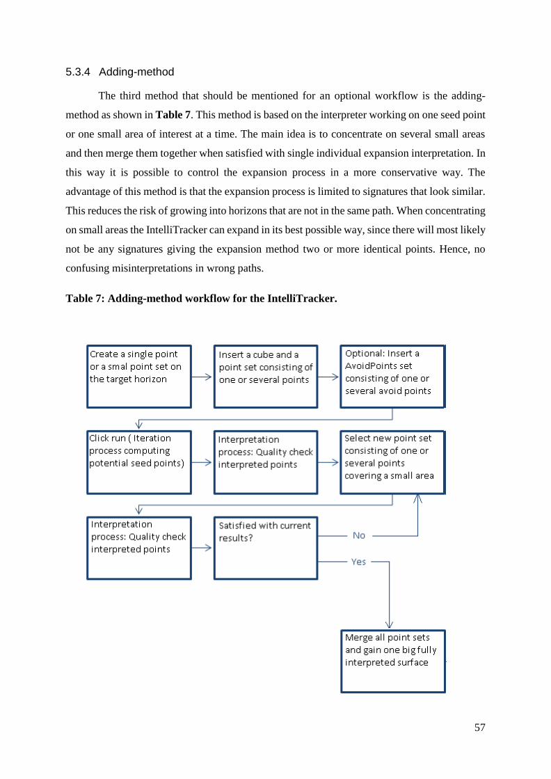
57

5.3.4 Adding-method

The third method that should be mentioned for an optional workflow is the adding-

method as shown in Table 7. This method is based on the interpreter working on one seed point

or one small area of interest at a time. The main idea is to concentrate on several small areas

and then merge them together when satisfied with single individual expansion interpretation. In

this way it is possible to control the expansion process in a more conservative way. The

advantage of this method is that the expansion process is limited to signatures that look similar.

This reduces the risk of growing into horizons that are not in the same path. When concentrating

on small areas the IntelliTracker can expand in its best possible way, since there will most likely

not be any signatures giving the expansion method two or more identical points. Hence, no

confusing misinterpretations in wrong paths.

Table 7: Adding-method workflow for the IntelliTracker.

58

Results

6 Horizon interpretation

6.1 Results from the horizon autotracker

Figure 42 shows a green reference point that is used to illustrate how the different

options in the general area (blue) in Figure 25 affect the horizon tracking. To make the

comparison as accurate as possible, the same point is used for all testing regarding the horizon

autotracker that is commercial today in Petrel. This ensures that the expansion process begins

at the exact same point. The results will vary based on the criteria for the expansion procedure.

This is chosen by the user before tracking the horizon in the setting dialog box.

Figure 42: Green point seeded on a strong amplitude reflector. The green point refers to the

reference point used during the testing of different options available in the general area. To the

upper left is the auto legend bar, while the blue and orange numbers indicate specifically where

on the seismic the snapshot is taken.

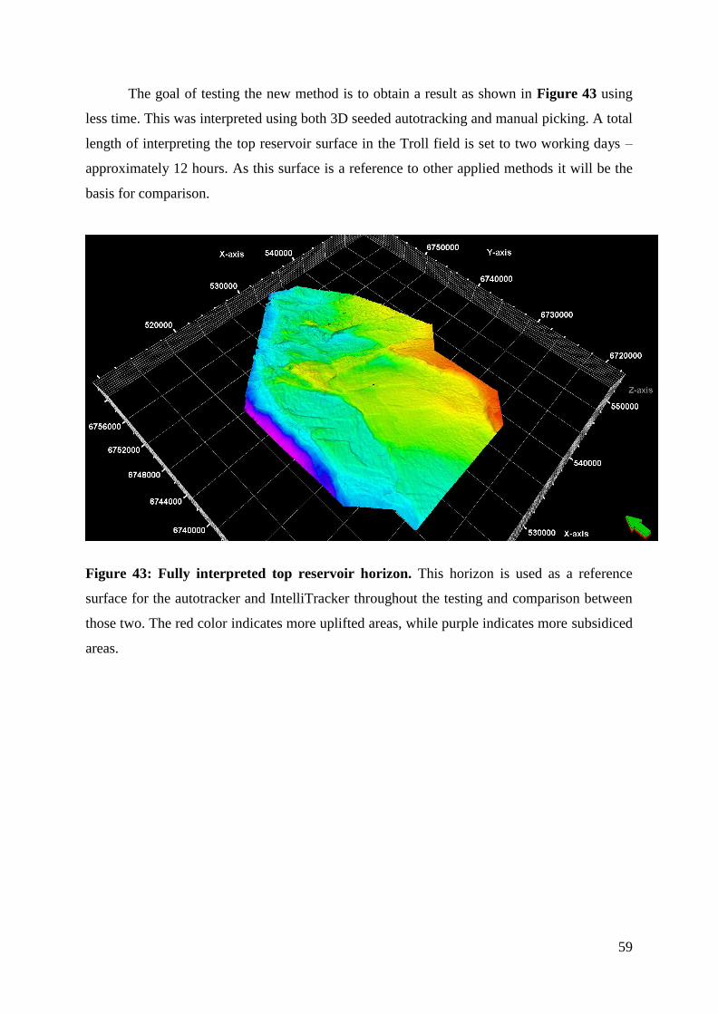
59

The goal of testing the new method is to obtain a result as shown in Figure 43 using

less time. This was interpreted using both 3D seeded autotracking and manual picking. A total

length of interpreting the top reservoir surface in the Troll field is set to two working days –

approximately 12 hours. As this surface is a reference to other applied methods it will be the

basis for comparison.

Figure 43: Fully interpreted top reservoir horizon. This horizon is used as a reference

surface for the autotracker and IntelliTracker throughout the testing and comparison between

those two. The red color indicates more uplifted areas, while purple indicates more subsidiced

areas.

60

6.1.1 Priority Parameter

The results of the different priority options are shown in Figure 44, Figure 45, Figure

46 and Figure 47. It should be mentioned that the only parameter that varies is the priority,

while the quality and signal feature is set to basic 3x3 and peaks respectively as shown in Figure

26. These are usually the default settings for the horizon autotracker and is therefore used

throughout the testing if nothing else is mentioned. The green seed point shown in Figure 44,

Figure 45, Figure 46 and Figure 47 is the same as the one stated in Figure 42.

Figure 44: Priority option; Amplitude. The blue surface is the expansion of only one seed

point after one iteration.

61

Figure 45: Priority option; Proximity. The green point shows where the seed point was set,

and the orange surface is the raw result of the first iteration.

Figure 46: Priority option; Amplitude & Proximity. The green point shows where the seed

point was set, and the green surface is the result from only one iteration with one seed point.

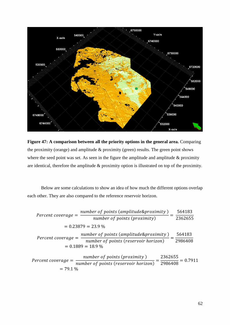
62

Figure 47: A comparison between all the priority options in the general area. Comparing

the proximity (orange) and amplitude & proximity (green) results. The green point shows

where the seed point was set. As seen in the figure the amplitude and amplitude & proximity

are identical, therefore the amplitude & proximity option is illustrated on top of the proximity.

Below are some calculations to show an idea of how much the different options overlap

each other. They are also compared to the reference reservoir horizon.

𝑃𝑒𝑟𝑐𝑒𝑛𝑡 𝑐𝑜𝑣𝑒𝑟𝑎𝑔𝑒 = 𝑛𝑢𝑚𝑏𝑒𝑟 𝑜𝑓 𝑝𝑜𝑖𝑛𝑡𝑠 (𝑎𝑚𝑝𝑙𝑖𝑡𝑢𝑑𝑒&𝑝𝑟𝑜𝑥𝑖𝑚𝑖𝑡𝑦 )

𝑛𝑢𝑚𝑏𝑒𝑟 𝑜𝑓 𝑝𝑜𝑖𝑛𝑡𝑠 (𝑝𝑟𝑜𝑥𝑖𝑚𝑖𝑡𝑦)=

564183

2362655

= 0.23879 = 23.9 %

𝑃𝑒𝑟𝑐𝑒𝑛𝑡 𝑐𝑜𝑣𝑒𝑟𝑎𝑔𝑒 = 𝑛𝑢𝑚𝑏𝑒𝑟 𝑜𝑓 𝑝𝑜𝑖𝑛𝑡𝑠 (𝑎𝑚𝑝𝑙𝑖𝑡𝑢𝑑𝑒&𝑝𝑟𝑜𝑥𝑖𝑚𝑖𝑡𝑦 )

𝑛𝑢𝑚𝑏𝑒𝑟 𝑜𝑓 𝑝𝑜𝑖𝑛𝑡𝑠 (𝑟𝑒𝑠𝑒𝑟𝑣𝑜𝑖𝑟 ℎ𝑜𝑟𝑖𝑧𝑜𝑛)=

564183

2986408= 0.1889 = 18.9 %

𝑃𝑒𝑟𝑐𝑒𝑛𝑡 𝑐𝑜𝑣𝑒𝑟𝑎𝑔𝑒 = 𝑛𝑢𝑚𝑏𝑒𝑟 𝑜𝑓 𝑝𝑜𝑖𝑛𝑡𝑠 (𝑝𝑟𝑜𝑥𝑖𝑚𝑖𝑡𝑦 )

𝑛𝑢𝑚𝑏𝑒𝑟 𝑜𝑓 𝑝𝑜𝑖𝑛𝑡𝑠 (𝑟𝑒𝑠𝑒𝑟𝑣𝑜𝑖𝑟 ℎ𝑜𝑟𝑖𝑧𝑜𝑛)=

2362655

2986408= 0.7911

= 79.1 %

63

The methods differ in expansion method due to different criterions. The amplitude

options prioritizes picks of higher extrema for early expansion. This means that the target

horizon contains several areas where the horizon reflector is weak or ambiguous. The proximity

options prioritizes picks with the shortest expansion paths. Since the reservoir horizon is an

unconformity there are several strong amplitude reflector events parallel to each other. If one

strong event is close enough to the expanding seed, the tracker will continue on the wrong event,

leading to misinterpretations. The results presented above are however just the raw output from

the expansion and are not matching the reference horizon one hundred percent.

64

6.1.2 Quality Parameter

The results of the different quality options are shown in Figure 48, Figure 49 and

Figure 50. They are based on the green seed point as illustrated in Figure 42. It considers how

stringtly each seed point is checked before it expands. The first result of using basic 3x3

expansion technique is shown in Figure 48.

Figure 48: Quality option; Basic 3x3. After one iteration of expansion, the pink surface is the

result based on the green seed as shown earlier.

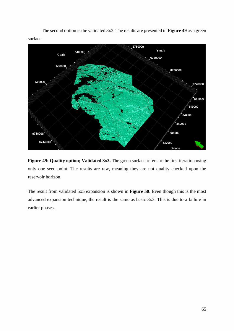
65

The second option is the validated 3x3. The results are presented in Figure 49 as a green

surface.

Figure 49: Quality option; Validated 3x3. The green surface refers to the first iteration using

only one seed point. The results are raw, meaning they are not quality checked upon the

reservoir horizon.

The result from validated 5x5 expansion is shown in Figure 50. Even though this is the most

advanced expansion technique, the result is the same as basic 3x3. This is due to a failure in

earlier phases.

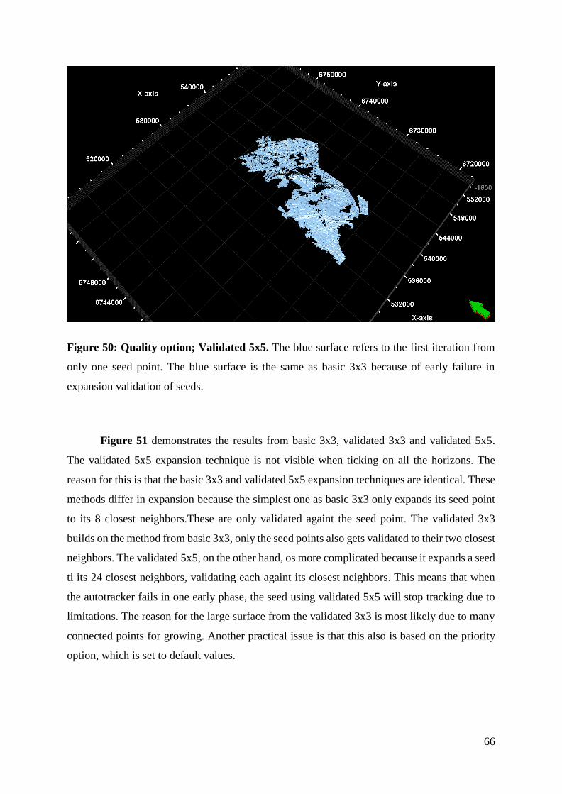
66

Figure 50: Quality option; Validated 5x5. The blue surface refers to the first iteration from

only one seed point. The blue surface is the same as basic 3x3 because of early failure in

expansion validation of seeds.

Figure 51 demonstrates the results from basic 3x3, validated 3x3 and validated 5x5.

The validated 5x5 expansion technique is not visible when ticking on all the horizons. The

reason for this is that the basic 3x3 and validated 5x5 expansion techniques are identical. These

methods differ in expansion because the simplest one as basic 3x3 only expands its seed point

to its 8 closest neighbors.These are only validated againt the seed point. The validated 3x3

builds on the method from basic 3x3, only the seed points also gets validated to their two closest

neighbors. The validated 5x5, on the other hand, os more complicated because it expands a seed

ti its 24 closest neighbors, validating each againt its closest neighbors. This means that when

the autotracker fails in one early phase, the seed using validated 5x5 will stop tracking due to

limitations. The reason for the large surface from the validated 3x3 is most likely due to many

connected points for growing. Another practical issue is that this also is based on the priority

option, which is set to default values.

67

Figure 51: Comparison between the basic 3x3 (pink), validated 3x3 (green) and validated

5x5 (light blue, not visible) expansion techniques in the quality option. The basic 3x3 and

validated 5x5 are identical and the validated 5x5 is therefore not visible.This is due to failure

in early expansion of validated 5x5 or because it is the priority parameter which dominates

these results.

As calculated below, the basic 3x3 surface (pink) covers approximately 24 % of the

validated 3x3 (green) surface. Compared to the fully interpreted reservoir, the basic 3x3 (pink)

covers approximately 20 % and the validated 3x3 covers approximately 80 % of the horizon

surface.

𝑃𝑒𝑟𝑐𝑒𝑛𝑡 𝑐𝑜𝑣𝑒𝑟𝑎𝑔𝑒 = 𝑛𝑢𝑚𝑏𝑒𝑟 𝑜𝑓 𝑝𝑜𝑖𝑛𝑡𝑠 (𝑏𝑎𝑠𝑖𝑐 3𝑥3 )

𝑛𝑢𝑚𝑏𝑒𝑟 𝑜𝑓 𝑝𝑜𝑖𝑛𝑡𝑠 (𝑣𝑎𝑙𝑖𝑑𝑎𝑡𝑒𝑑 3𝑥3)=

564183

2362655= 0.23879

= 23.9 %

𝑃𝑒𝑟𝑐𝑒𝑛𝑡 𝑐𝑜𝑣𝑒𝑟𝑎𝑔𝑒 = 𝑛𝑢𝑚𝑏𝑒𝑟 𝑜𝑓 𝑝𝑜𝑖𝑛𝑡𝑠 (𝑏𝑎𝑠𝑖𝑐 3𝑥3 )

𝑛𝑢𝑚𝑏𝑒𝑟 𝑜𝑓 𝑝𝑜𝑖𝑛𝑡𝑠 (𝑟𝑒𝑓𝑒𝑟𝑎𝑛𝑐𝑒 𝑟𝑒𝑠𝑒𝑟𝑣𝑜𝑖𝑟)=

564183

2986408= 0.1889

= 18.9 %

𝑃𝑒𝑟𝑐𝑒𝑛𝑡 𝑐𝑜𝑣𝑒𝑟𝑎𝑔𝑒 = 𝑛𝑢𝑚𝑏𝑒𝑟 𝑜𝑓 𝑝𝑜𝑖𝑛𝑡𝑠 (𝑣𝑎𝑙𝑖𝑑𝑎𝑡𝑒𝑑 3𝑥3 )

𝑛𝑢𝑚𝑏𝑒𝑟 𝑜𝑓 𝑝𝑜𝑖𝑛𝑡𝑠 (𝑟𝑒𝑓𝑒𝑟𝑎𝑛𝑐𝑒 𝑟𝑒𝑠𝑒𝑟𝑣𝑜𝑖𝑟)=

2362655

2986408= 0.7911

= 79.1 %

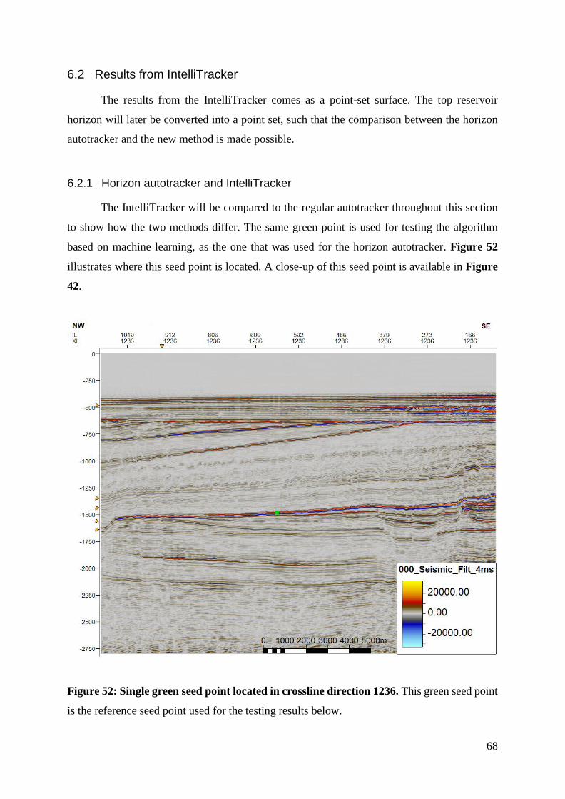
68

6.2 Results from IntelliTracker

The results from the IntelliTracker comes as a point-set surface. The top reservoir

horizon will later be converted into a point set, such that the comparison between the horizon

autotracker and the new method is made possible.

6.2.1 Horizon autotracker and IntelliTracker

The IntelliTracker will be compared to the regular autotracker throughout this section

to show how the two methods differ. The same green point is used for testing the algorithm

based on machine learning, as the one that was used for the horizon autotracker. Figure 52

illustrates where this seed point is located. A close-up of this seed point is available in Figure

42.

Figure 52: Single green seed point located in crossline direction 1236. This green seed point

is the reference seed point used for the testing results below.

69

To gain the results as shown in Figure 54 one start with converting the green seed point

in Figure 52 into a point sets such that it will meet the criteria for the IntelliTracker workflow.

After the process is done, the message log in Petrel shows the information as shown in Figure

53. The content in Figure 53 is explained in Table 4 on page 52.

Figure 53: Message log for the new algorithm ran in the workflow. The results gained from

the IntelliTracker when it has run through the inserted points and expanded. The elapsed time

to run and track the horizon in Figure 54 is 35.724 seconds.

70

Figure 54: One seed expansion by the IntelliTracker. The point set surface colored in blue

is the raw outcome from the workflow.

Figure 55: A comparison between the IntelliTracker and the Basic 3x3 Horizon

Autotracker. The blue point set surface represents the IntelliTracker, while the pink smooth

71

surface represents the horizon autotracker with quality parameter basic 3x3 chosen. This

coverage is an illustration to show how much the IntelliTracker covers a horizon versus a

horizon autotracker.

In Figure 55 the 3D seeded autotracker with the quality basic 3x3 expansion technique

surface (pink) is compared with the IntelliTracker (blue). They both expand from the same

point. As seen, the IntelliTracker covers a smaller area and follows another path than the regular

horizon autotracker. Below are calculations based on the number of seed points given from the

different expansion methods from the regular horizon autotracker and the IntelliTracker.

𝑃𝑒𝑟𝑐𝑒𝑛𝑡 𝑐𝑜𝑣𝑒𝑟𝑎𝑔𝑒 = 𝑛𝑢𝑚𝑏𝑒𝑟 𝑜𝑓 𝑝𝑜𝑖𝑛𝑡𝑠 (𝐼𝑛𝑡𝑒𝑙𝑙𝑖𝑇𝑟𝑎𝑐𝑘𝑒𝑟 𝑝𝑜𝑖𝑛𝑡 𝑠𝑒𝑡 (𝑏𝑙𝑢𝑒))

𝑛𝑢𝑚𝑏𝑒𝑟 𝑜𝑓 𝑝𝑜𝑖𝑛𝑡𝑠 (𝑏𝑎𝑠𝑖𝑐 3𝑥3 (𝑝𝑖𝑛𝑘)) =

268369

564183

= 0.47567 = 47.6 %

𝑃𝑒𝑟𝑐𝑒𝑛𝑡 𝑐𝑜𝑣𝑒𝑟𝑎𝑔𝑒 = 𝑛𝑢𝑚𝑏𝑒𝑟 𝑜𝑓 𝑝𝑜𝑖𝑛𝑡𝑠 (𝐼𝑛𝑡𝑒𝑙𝑙𝑖𝑇𝑟𝑎𝑐𝑘𝑒𝑟 𝑝𝑜𝑖𝑛𝑡 𝑠𝑒𝑡 (𝑏𝑙𝑢𝑒))

𝑛𝑢𝑚𝑏𝑒𝑟 𝑜𝑓 𝑝𝑜𝑖𝑛𝑡𝑠 (𝑟𝑒𝑓𝑒𝑟𝑒𝑛𝑐𝑒 ℎ𝑜𝑟𝑖𝑧𝑜𝑛) =

268369

2986408

= 0.08986 = 9 %

The IntelliTracker covers almost 50 percent of the basic 3x3 surface, even though they

have two different tracking paths. Compared to the fully interpreted reference horizon (Figure

43) it only covers 9 percent versus almost 19 percent coverage of basic 3x3 expansion

technique

The results from the new algorithm are gained using a method of seeding 8 points as shown in

the inline direction in Figure 56 and crossline direction Figure 57. The reason for placing the

seed-points at exactly this place is because the signature around these points are different and

unique and makes good training data for the expansion process. They are also set in peak events

where the amplitude reflection is strong.

.

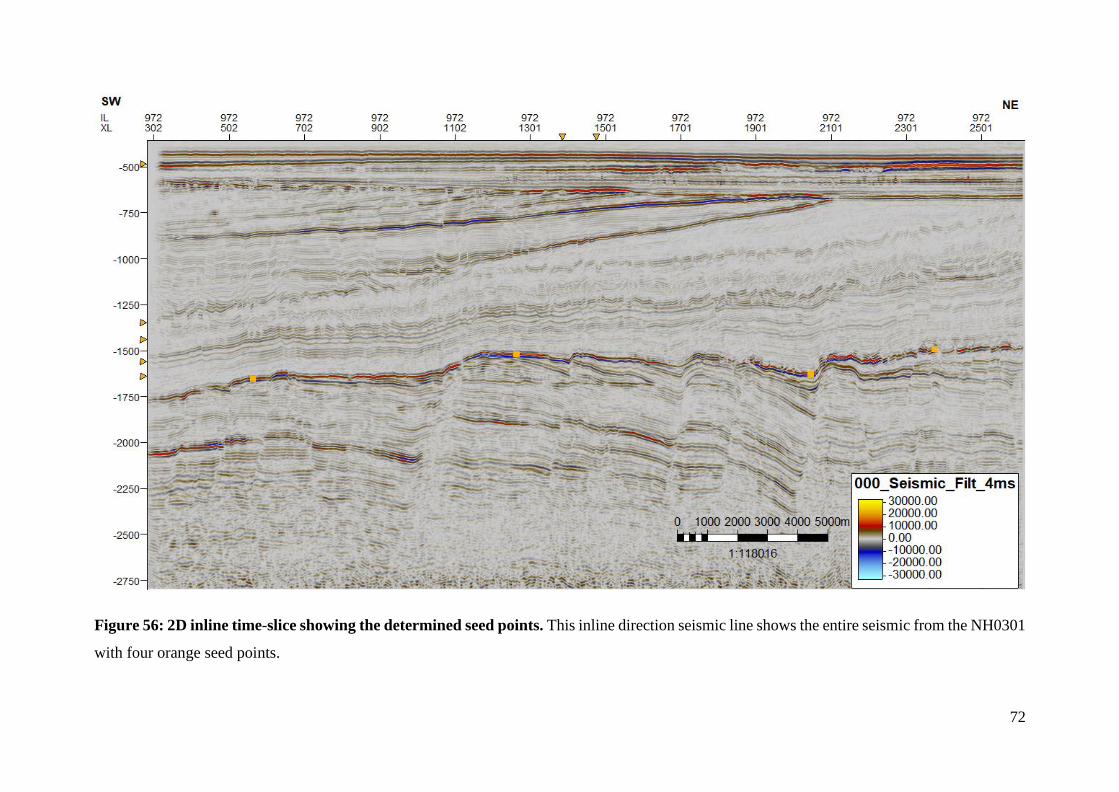
72

Figure 56: 2D inline time-slice showing the determined seed points. This inline direction seismic line shows the entire seismic from the NH0301

with four orange seed points.

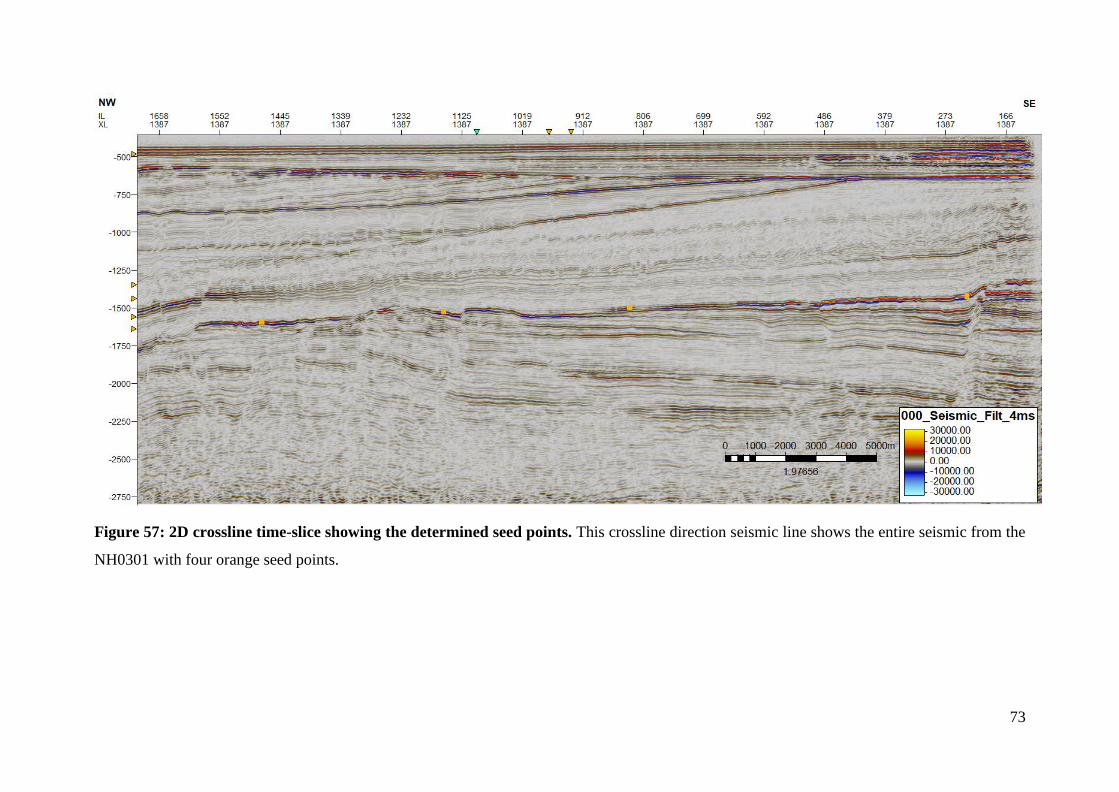
73

Figure 57: 2D crossline time-slice showing the determined seed points. This crossline direction seismic line shows the entire seismic from the

NH0301 with four orange seed points.

74

Figure 58: Reservoir horizon in 3D view with eight seeded points. Four points are set in inline direction, and four points are set in crossline

direction as shown in Figure 56 and Figure 57.

75

6.2.2 Original Point Set-method (OPS-method)

The first method presented is named Original Point Set-method (OPS-method) because

it uses only one point-set throughout the workflow. The way it works is that the method uses

the same seed points that first was inserted before further tracking. The results are based on the

seed points located as shown in Figure 56 and Figure 57. To show the location on the fully

interpreted surface, an example is shown in Figure 58. When the IntelliTracker has run once,

the raw results before any quality check is shown in Figure 59. The overlapping is calculated

below and covers approximately 70 % of the reference horizon.

This new point set is then quality checked for misinterpretations. When misinterpreted

areas occur as shown in Figure 62 and Figure 63, these points are erased and the remaining

points are then applied as a new point set for further workflow. This procedure continues until

the user is satisfied with the interpretation done.

𝑃𝑒𝑟𝑐𝑒𝑛𝑡 𝑐𝑜𝑣𝑒𝑟𝑎𝑔𝑒 = 𝑛𝑢𝑚𝑏𝑒𝑟 𝑜𝑓 𝑝𝑜𝑖𝑛𝑡𝑠 (𝐼𝑛𝑡𝑒𝑙𝑙𝑖𝑇𝑟𝑎𝑐𝑘𝑒𝑟 𝑝𝑜𝑖𝑛𝑡 𝑠𝑒𝑡 (𝑜𝑟𝑎𝑛𝑔𝑒))

𝑛𝑢𝑚𝑏𝑒𝑟 𝑜𝑓 𝑝𝑜𝑖𝑛𝑡𝑠 (𝑟𝑒𝑓𝑒𝑟𝑒𝑛𝑐𝑒 ℎ𝑜𝑟𝑖𝑧𝑜𝑛)

= 29209048586408

2986408= 0.69999 = 70 %

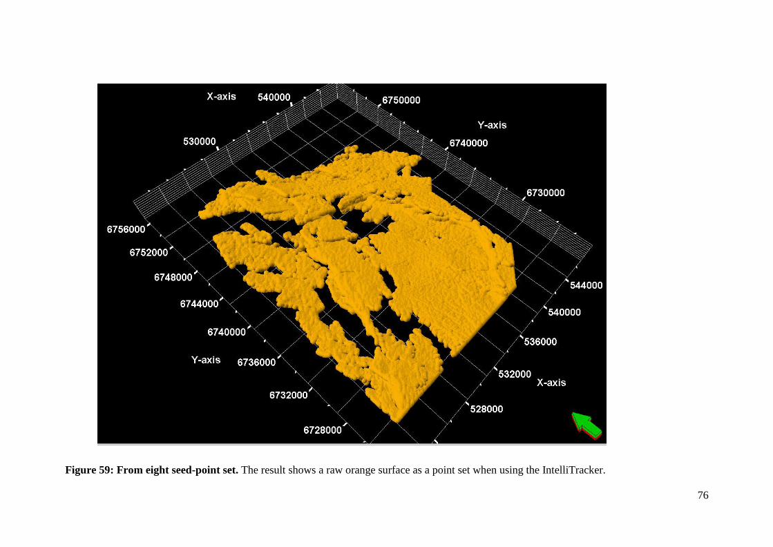
76

Figure 59: From eight seed-point set. The result shows a raw orange surface as a point set when using the IntelliTracker.

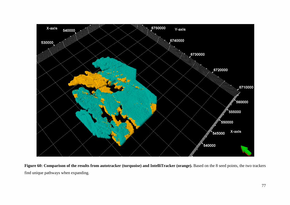
77

Figure 60: Comparison of the results from autotracker (turquoise) and IntelliTracker (orange). Based on the 8 seed points, the two trackers

find unique pathways when expanding.

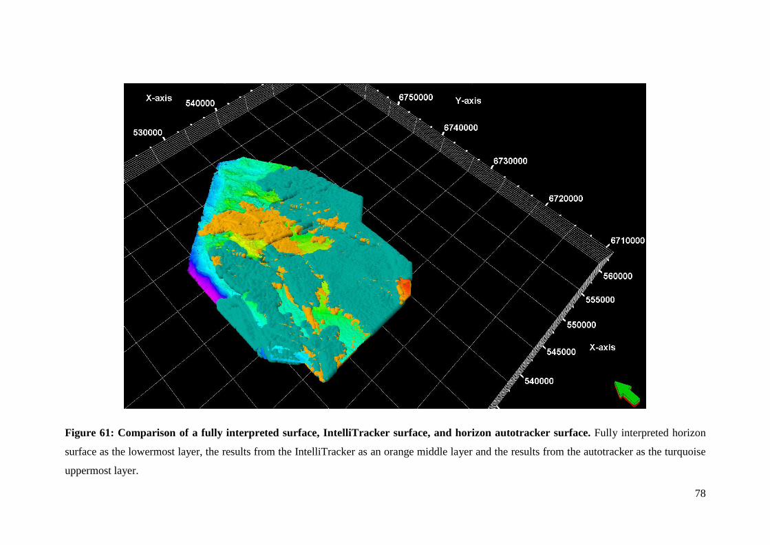
78

Figure 61: Comparison of a fully interpreted surface, IntelliTracker surface, and horizon autotracker surface. Fully interpreted horizon

surface as the lowermost layer, the results from the IntelliTracker as an orange middle layer and the results from the autotracker as the turquoise

uppermost layer.

79

Figure 62: Misinterpretations of the IntelliTracker along the crossline time-slice section. When an underlying strong amplitude reflector

occurs, the new method loses track and interprets horizons that are not correct as seen in this figure.

Figure 63: A whole misinterpreted surface, compared to the reference surface. Here, the new method manages to interpret a large area

wrong, due to uncertainties of pattern recognition of those two horizons.

80

When it comes to faulted areas, both the horizon autotracker and the new method has

difficulties tracking the target horizon. Figure 64 illustrates an example where there appear a

fault and several strong amplitude horizon events parallel to each other. This is an area where

it is easy for the two methods to grow into the wrong horizon. Especially for the new method

which is based on pattern recognition. As the figure illustrates, the strongest amplitude

reflector is the one that is expanding, meaning that the tracker moves from right to left in the

image. The surface is tilted upside down to more clearly see where the tracking fails.

Figure 64 is a part of the 8 seeded points as shown in Figure 56, Figure 57 and

Figure 58 and the related results come from the exact same seed points as previous figures.

In Figure 65 the tracking grows mostly wrong. There are some points that continue

on the right horizon. The reason for this tracking is due to the strong amplitude above the

target horizon which is weaker than the one the IntelliTracker follows. In the same figure,

there is also shown the message log, where we can see that this is the results from the second

iteration as input point were 1053 points. Also, the elapsed time to continue interpreting was

estimated to 329.819 seconds.

Next step is to quality check the expansion process. Misinterpretations are erased, and

to avoid the IntelliTracker to grow in the same place, one can insert a point set in

AvoidPoints. This process is shown in Figure 66 where some points along the wrong and

strong amplitude reflector are set as avoid points. When running the IntelliTracker again with

these new avoid points, the tracker is forced to continue on the horizon below. The result of

this is shown in Figure 67 and Figure 68. These two figures illustrate how the Avoid option

works. The results are good, since its functionality works well. There are several points

tracking the target horizon. For this to be optimized the avoid points should cover the rest of

the wrong horizon, both in inline and crossline direction.

Again the misinterpreted areas are erased , this time with no additional avoid points

inserted, just the same as the last round of tracking. The results from the third iteration are

shown in Figure 69, where the tracker grows wrong into even higher events from the target

horizon.

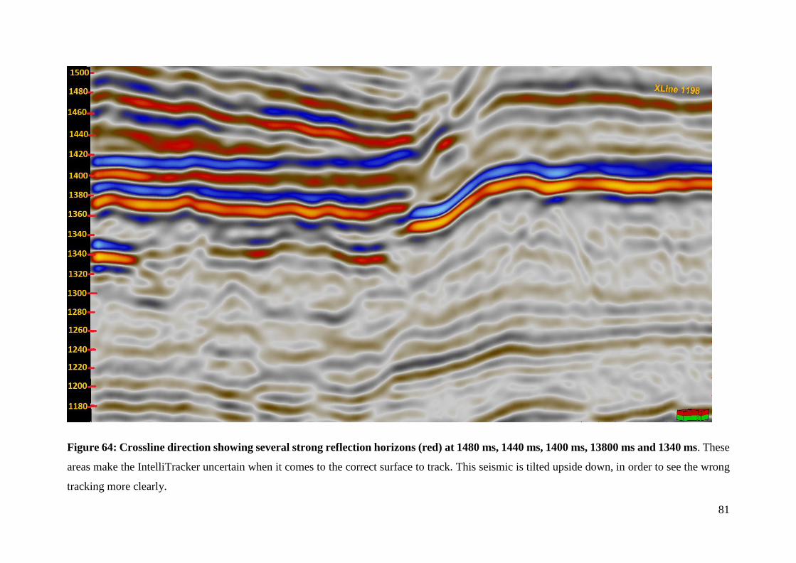
81

Figure 64: Crossline direction showing several strong reflection horizons (red) at 1480 ms, 1440 ms, 1400 ms, 13800 ms and 1340 ms. These

areas make the IntelliTracker uncertain when it comes to the correct surface to track. This seismic is tilted upside down, in order to see the wrong

tracking more clearly.

82

Figure 65: Same crossline section as Figure 64, only with the interpretation of reference horizon (smooth surface) and IntelliTracker

(point surface).The message log is also implemented to gain information of the input, output and time spent on the iteration. As seen from the

figure, the new method grows wrong as there appears to be a strong amplitude reflector in the horizon above the target horizon.

83

Figure 66: Avoid-points inserted in the area where the new method tracked wrong. Again, the same crossline section as in Figure 64, only

this time mis-tracked surface is erased and randomly selected avoid points from that surface is elected as purple points (outlined purple circle).

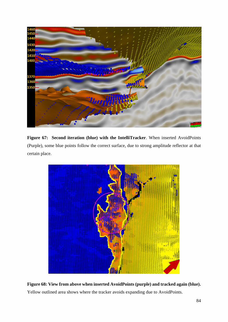
84

Figure 67: Second iteration (blue) with the IntelliTracker. When inserted AvoidPoints

(Purple), some blue points follow the correct surface, due to strong amplitude reflector at that

certain place.

Figure 68: View from above when inserted AvoidPoints (purple) and tracked again (blue).

Yellow outlined area shows where the tracker avoids expanding due to AvoidPoints.

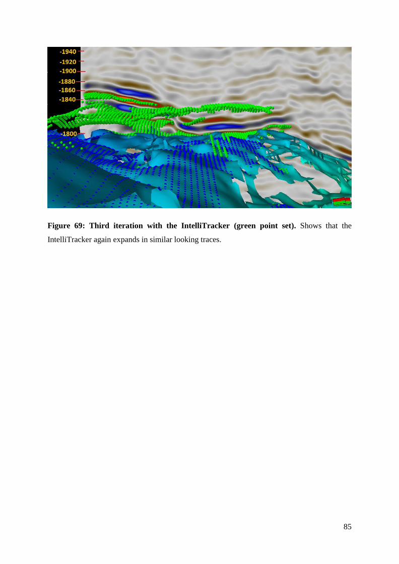
85

Figure 69: Third iteration with the IntelliTracker (green point set). Shows that the

IntelliTracker again expands in similar looking traces.

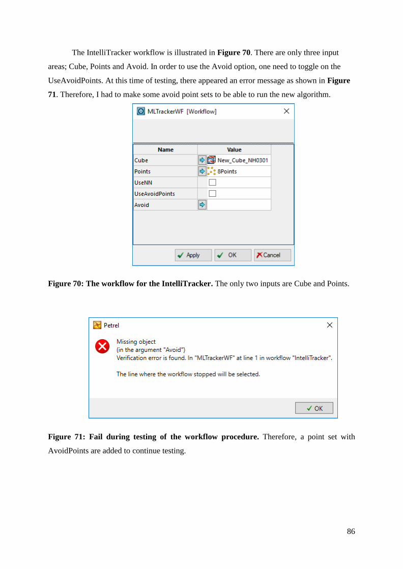
86

The IntelliTracker workflow is illustrated in Figure 70. There are only three input

areas; Cube, Points and Avoid. In order to use the Avoid option, one need to toggle on the

UseAvoidPoints. At this time of testing, there appeared an error message as shown in Figure

71. Therefore, I had to make some avoid point sets to be able to run the new algorithm.

Figure 70: The workflow for the IntelliTracker. The only two inputs are Cube and Points.

Figure 71: Fail during testing of the workflow procedure. Therefore, a point set with

AvoidPoints are added to continue testing.

87

These avoid points are shown in Figure 72, Figure 73 and Figure 74. These figures are

also flipped upside down to get a more clearly observation of what happens when the tracker is

expanding.

Figure 72: Xline 1388. 1750 – 1650 X-line. Upside down for a better view of seed points.

Figure 73: Xline 1388. 100-250 X-line. Upside down for a better view of seed points.

88

Figure 74: Inline 972. 475-275 X-line. upside down for a better view of the seed points.

Based on Figure 73, this area is easily mis-tracked as it contains several strong reflector

events over a large area. The avoidpoints are able to some extent to avoid the wrong horizon,

but when it gets to far from the original avoid points set, the IntelliTracker again choses the

wrong event and it occurs a misinterpretation.

Figure 75: Result from seed points as seeded in Figure 73. The IntelliTracker avoids tracking

the avoidpoints to a certain extent before tracking on the parallel horizon again.

89

On the other side, if the extent of the tracked area is limited, the IntelliTracker is able

with help from the avoid point set, to track on the target horizon. This is impressive, since all

these examples are compared with the horizon autotracker where the horizon autotracker

actually tracked wrong. Due to this avoid point option, one can eliminate several mis-

interpretations done by the 3D Seeded autotracker and IntelliTracker. In this way, it is easier to

obtain a more effective and time-saving interpretation of seismic with complex geology.

Figure 76: Another side of Figure 75. The IntelliTracker expands in the correct horizon.

The reference reservoir surface was converted into a point set. This is done due to being

able to compare the new (pink) surface to the correct one as illustrated in Figure 78. This figure

also shows where the original 8 seed points were placed. Here we have an idea of where the

seeds expanded first and where they stopped.

When opening the settings for both point sets, and click on ‘Statistics’, the outlines area

in Figure 77 are of high interest. This value shows the number of points that are used for

comparison.

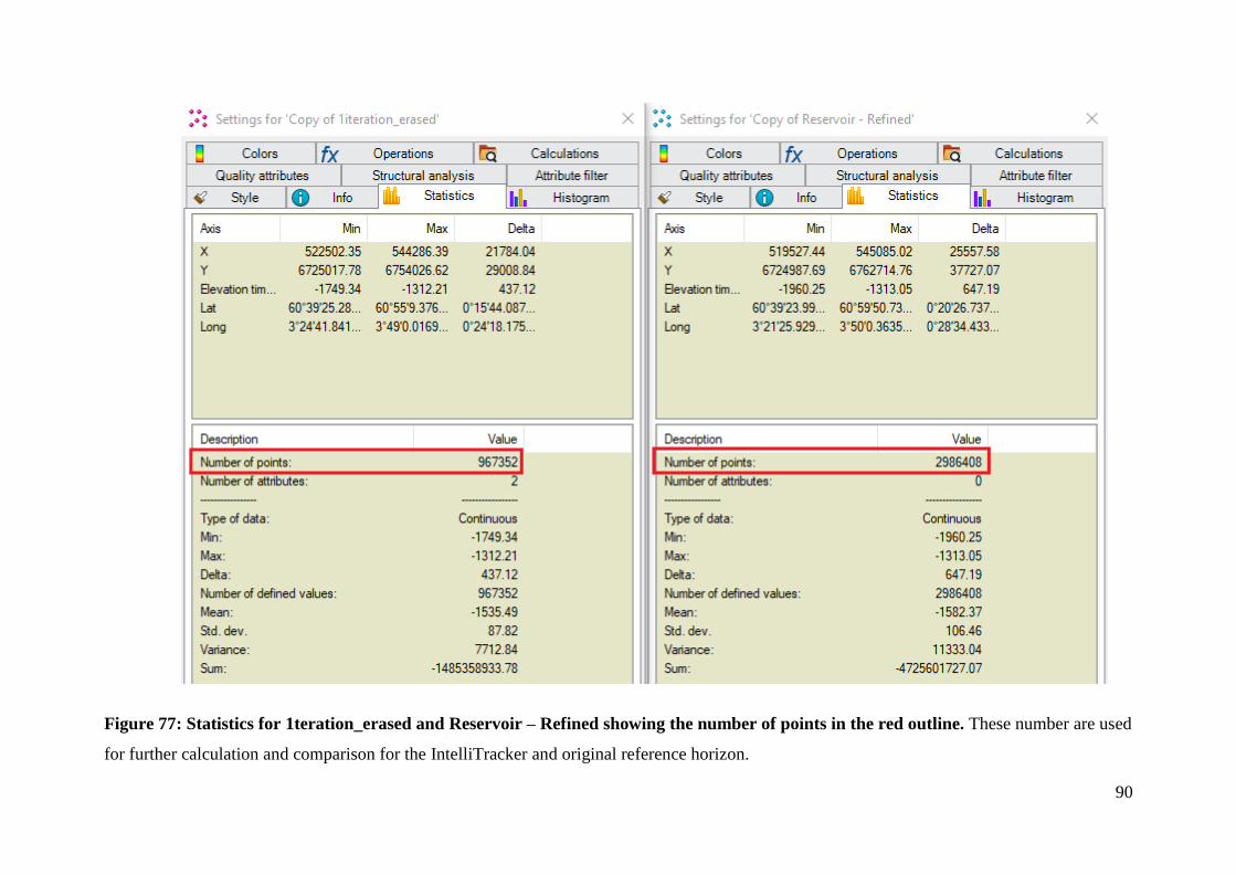
90

Figure 77: Statistics for 1teration_erased and Reservoir – Refined showing the number of points in the red outline. These number are used

for further calculation and comparison for the IntelliTracker and original reference horizon.

91

Figure 78: Comparison between reservoir refined (blue) and 1iteration (pink) with shown seed points (orange).

92

From Figure 77 the coverage of the first iteration is based on numbers of points tracked. To

calculate this the number of points for the 1iterations is divided by the number of points in the

reservoir refined, the results are shown below.

𝑃𝑒𝑟𝑐𝑒𝑛𝑡 𝑐𝑜𝑣𝑒𝑟𝑎𝑔𝑒 = 𝑛𝑢𝑚𝑏𝑒𝑟 𝑜𝑓 𝑝𝑜𝑖𝑛𝑡𝑠 (𝐼𝑛𝑡𝑒𝑙𝑙𝑖𝑇𝑟𝑎𝑐𝑘𝑒𝑟 𝑝𝑜𝑖𝑛𝑡 𝑠𝑒𝑡 𝑟𝑒𝑠𝑢𝑙𝑡)

𝑛𝑢𝑚𝑏𝑒𝑟 𝑜𝑓 𝑝𝑜𝑖𝑛𝑡𝑠 (𝑟𝑒𝑓𝑒𝑟𝑒𝑛𝑐𝑒 𝑟𝑒𝑠𝑟𝑣𝑜𝑖𝑟 𝑝𝑜𝑖𝑛𝑡 𝑠𝑒𝑡) =

1358351

2986408

= 0.4548444 = 45.48 %

As seen here the coverage of the pink horizon is approximately 45 percent of the whole area.

93

6.2.3 Filter-method

The Filter-method is described in the section on How to use the IntelliTracker in Petrel

2017.2. The results of using this method are shown in Figure 79. The first step is represented

to show how the results are without changing any values. The dark red, almost black seed points

represent a seed with a confidence-score value near 0.5, which is set to the critical value. If the

confidence-score value turns out to be lower than 0.5 the IntelliTracker fails and stops tracking.

The lower the confidence-score value is, the darker the color of the seeds are and the more

uncertain are the accuracy of the seed points. When the seed point turns orange and yellow, the

confidence-score value is high, closer to 1. This means that the accuracy of the seeded points is

high and trustable.

Figure 79: Results from not making any changes in the settings box. The blue surface

represents the reservoir surface used as a reference horizon surface and the seismic filter

attribute represents point set expanded from the same points as in Figure 78. The auto legend

indicates dark colors that have a low confidence-score value and yellow colors that have a high

confidence-score value.

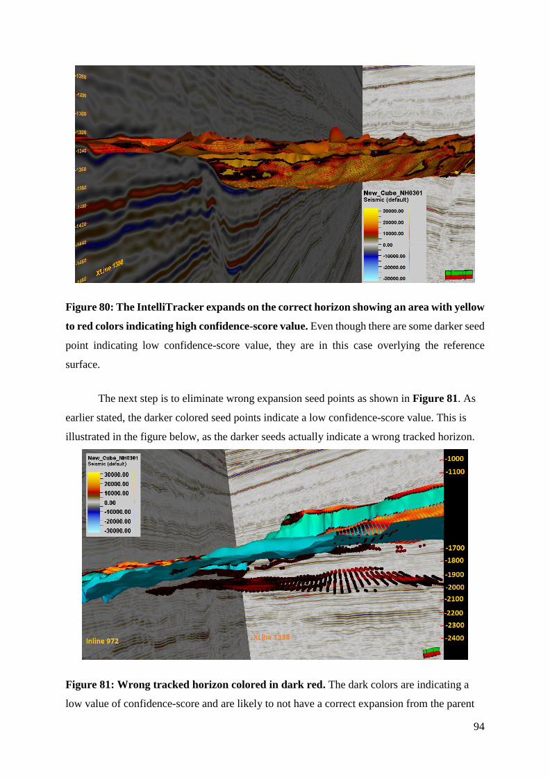
94

Figure 80: The IntelliTracker expands on the correct horizon showing an area with yellow

to red colors indicating high confidence-score value. Even though there are some darker seed

point indicating low confidence-score value, they are in this case overlying the reference

surface.

The next step is to eliminate wrong expansion seed points as shown in Figure 81. As

earlier stated, the darker colored seed points indicate a low confidence-score value. This is

illustrated in the figure below, as the darker seeds actually indicate a wrong tracked horizon.

Figure 81: Wrong tracked horizon colored in dark red. The dark colors are indicating a

low value of confidence-score and are likely to not have a correct expansion from the parent

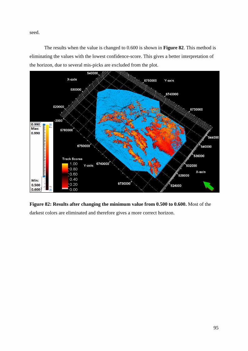
95

seed.

The results when the value is changed to 0.600 is shown in Figure 82. This method is

eliminating the values with the lowest confidence-score. This gives a better interpretation of

the horizon, due to several mis-picks are excluded from the plot.

Figure 82: Results after changing the minimum value from 0.500 to 0.600. Most of the

darkest colors are eliminated and therefore gives a more correct horizon.

96

Figure 83: Mis-tracked horizon with changed minimal values. Fewer misinterpreted points

compared to the misinterpreted points in Figure 81.

Figure 84 illustrates a typical scenario when the confidence-score value is adjusted to

exclude values lower than a certain amount.

Figure 84: Results after changing the minimum confidence-score value from 0.500 to

0.815, most of the darkest colors are eliminated and therefore gives a more correct horizon.

97

Figure 85: By changing the minimum confidence-score value, the lowest values are

eliminated. The remaining seed points that are overlying the reservoir surface are kept until the

next phase.

By clicking the run button (outlined with purple as shown in Figure 41) the remaining points

are either collected in a new point set or will overwrite the previous point set. Both the new

point set and the overwritten point set can then be inserted as input to the “points” column

shown in Figure 37. The IntelliTracker spent 159.036 seconds generating the new horizon

surface.

Figure 86: Message log during the second iteration. The new point set is based on the

Filter-method.

98

As seen in Figure 87, the IntelliTracker expands over a horizon that is characterized as

wrong regarding the reservoir horizon. These seed points are also dark red to black in color

indicating uncertainty and low confidence-score value.

Figure 87: Second iteration with seed points corrected by the Filter-method. These results

show signs of misinterpretations. The dark-colored seeds indicate a low confidence-score value.

To complete a fully interpreted horizon surface, the Filter method workflow as described

in Table 6 is run until receiving a horizon that covers the whole area of interest. The results

are shown in Figure 88. The cover percentage is calculated below.

𝑃𝑒𝑟𝑐𝑒𝑛𝑡 𝑐𝑜𝑣𝑒𝑟𝑎𝑔𝑒 = 𝑛𝑢𝑚𝑏𝑒𝑟 𝑜𝑓 𝑝𝑜𝑖𝑛𝑡𝑠 (𝐼𝑛𝑡𝑒𝑙𝑙𝑖𝑇𝑟𝑎𝑐𝑘𝑒𝑟 𝑝𝑜𝑖𝑛𝑡 𝑠𝑒𝑡 𝑟𝑒𝑠𝑢𝑙𝑡)

𝑛𝑢𝑚𝑏𝑒𝑟 𝑜𝑓 𝑝𝑜𝑖𝑛𝑡𝑠 (𝑟𝑒𝑓𝑒𝑟𝑒𝑛𝑐𝑒 𝑟𝑒𝑠𝑟𝑣𝑜𝑖𝑟 𝑝𝑜𝑖𝑛𝑡 𝑠𝑒𝑡) =

1843482

2986408

= 0.61729 = 61.7 %

These results show that the expansion process based on the Filter-method will cover

approximately 62 % of the fully interpreted horizon. It is important to have in mind that these

results are generated from the 8 seed points, as shown in Figure 56 and Figure 57.

99

Figure 88: Results after running several iterations based on the filter-method. In order to

avoid all the misinterpreted points, the confidence-score value needs to be adjusted to a

minimum value of 0.660.

100

Discussion

7 Discussion of Results

This thesis emphasizes recent research regarding machine learning and digitalization in

the field of seismic interpretation. The existing horizon autotracker method is a powerful tool

when analyzing and interpreting seismic horizons. The weakness is however the lack of iterative

learning during the interpretation process. Implementation of a tool that can make choices based

on previous iterations can be a step towards a more efficient and cost-effective solution. Where

the main goal is to ease the workflow for an interpreter saving valuable time for the more

complex situations.

It is important to keep in mind that this has been a product under continuous

development, which means that there have been several updated software iterations of the

algorithm. Due to lack of testing time of the last version, there will be a separate section

regarding different performing methods using the new algorithm. Yet, another section will

cover improvements and further work with the new method.

7.1 3D Horizon Autotracker

The current autotracker has historically outscored any competition that have tried to

outperform the method. The horizon autotracker give the user several options when interpreting

horizons; guided autotracking, 2D seeded autotracking and 3D seeded autotracking. This thesis

emphasizes the use of 3D seeded horizon autotracking. There is also a variability in options to

optimize the parameters and constraints before tracking the target horizon as seen in Figure 25.

This is also further discussed in the sections Parameters (Priority, Quality and Signal Feature)

and Appendix A.

The weaknesses of the existing autotracker is noticed when there are faults in the dataset

as illustrated in Figure 64. Faults cause breaks in the continuity of the seismic, creating areas

with weak amplitude reflectors. These discontinuities can make the tracker stop growing or

continue to track along a different horizon event. The autotracker also find it problematic

running through areas where the seismic quality is poor, yielding weak or ambiguous reflector

signature. For instance, these may either arise from seismic processing artefacts or originate

from actual geology, such as fault heaves.

101

7.2 IntelliTracker

The dataset NH0301 has a challenging geology for an autonomous tracker due to the

top reservoir unconformity. Figure 35 and Figure 36 illustrates the target horizon at 1600 ms

[TWT] containing several faults and parallel horizon events. The surrounding pattern along this

horizon have large variations. The IntelliTracker appears to be mis- tracking when:

• Two similar events occur after a fault structure

• Similar looking parallel patterns (horizons) are neighboring

The IntelliTracker relies on pattern recognition in the same trace as the inserted seed

point. The confidence values of the five points above and below the inserted point are then

calculated. If the new potential seed point meets the criteria set, it will be transformed to a

parent seed and further expansion begins. The geology related to the seismic data has a pattern

that varies a lot throughout the target horizon. Based on the eight seed points located throughout

the seismic section as shown in Figure 56 and Figure 57, the IntelliTracker expands as far as

possible with the given confidence value criteria set. Running out of seeds that match the criteria

value stops the tracking. It is impressive how accurate the IntelliTracker can be at the less

complicated parts of the seismic. This opens for a possibility where the interpreter could be

informed when the tracker is in a difficult area with several good options. It is therefore possible

to ease the workflow for the interpreter at the simple regions as illustrated in Figure 80.

Examples of areas that are difficult to track are shown in Figure 65 and Figure 81.

The IntelliTracker has mainly been tested by the programmer (Trond Hellem Bøe,

Schlumberger SSR) and the author of this thesis, and recently by SSR geologists to test its

capability and quality. For instance, the tracker has been tested on channels and seismic

horizons with strong amplitude reflectors. These data sets are confidential and cannot be

included in this thesis. But the results are in general promising on other datasets with less

complex geology.

7.3 Comparison between Autotracker and IntelliTracker

The main goal for the IntelliTracker is to improve the horizon tracking features in

following areas:

102

• Faults

• Weak/ambiguous amplitude reflectors

• Discontinuous horizons

• Ease the workflow for the interpreter

• Exploitation of erased information

Faults present in the seismic data, cause disorder in the continuous horizon signal

leading to diffraction patterns. The existing horizon autotracker tends to fail every time it

crosses a fault, or track into a nearby horizon and when the signals are weak/ambiguous. This

makes it necessary to quality check the results by the interpreter. This can be a time-consuming

process, as the interpreter needs to go in and manually exclude misinterpretations. These points

will however be saved in the software and the algorithm will autonomously look for patterns

that can be used in similar areas. The algorithm will therefor get more powerful the more it is

used. This can reduce the number of mouse clicks, which will ease the workflow for the

interpreter. Where the traditional horizon autotracker normally will come up with the same

result every time, the IntelliTracker will get better.

The comparison between the horizon autotracker and the new algorithm is shown with

the green seed point illustrated in Figure 52. The comparison is generated using the quality

parameter ‘basic 3x3’ and the priority parameter ‘Amplitude & Proximity’ for the horizon

autotracking parameters and the one seed point for the IntelliTracker. Figure 54 and Figure 48

illustrates how the two methods expand individually, while Figure 55 illustrates the results

from the IntelliTracker overlaying the autotracker. The tracking path for these two methods are

different due to different expanding techniques. The horizon autotracker is based on an

expansion technique where the seed point expands to its 8 closes neighbors, validating each

against the seed point. The tracker stops when one of the eight points fail to pass the validation.

The IntelliTracker is based on an expansion technique where the 8 closest seed points are

validated against a confidence-score value based on the radial basis function (RBF). The tracker

stops when there are no more seed points meeting the critical value. Based on the results from

Table 8 the number of points for the autotracker is higher than the number of points for the

IntelliTracker. The IntelliTracker surface covers almost half the autotracker surface. This

suggest that the autotracker yields a better result based on expansion from one seed point.

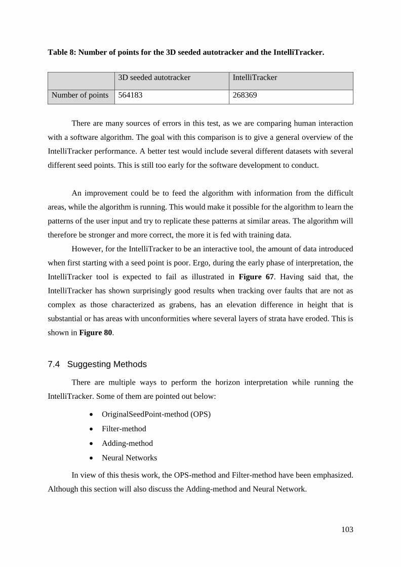
103

Table 8: Number of points for the 3D seeded autotracker and the IntelliTracker.

3D seeded autotracker IntelliTracker

Number of points 564183 268369

There are many sources of errors in this test, as we are comparing human interaction

with a software algorithm. The goal with this comparison is to give a general overview of the

IntelliTracker performance. A better test would include several different datasets with several

different seed points. This is still too early for the software development to conduct.

An improvement could be to feed the algorithm with information from the difficult

areas, while the algorithm is running. This would make it possible for the algorithm to learn the

patterns of the user input and try to replicate these patterns at similar areas. The algorithm will

therefore be stronger and more correct, the more it is fed with training data.

However, for the IntelliTracker to be an interactive tool, the amount of data introduced

when first starting with a seed point is poor. Ergo, during the early phase of interpretation, the

IntelliTracker tool is expected to fail as illustrated in Figure 67. Having said that, the

IntelliTracker has shown surprisingly good results when tracking over faults that are not as

complex as those characterized as grabens, has an elevation difference in height that is

substantial or has areas with unconformities where several layers of strata have eroded. This is

shown in Figure 80.

7.4 Suggesting Methods

There are multiple ways to perform the horizon interpretation while running the

IntelliTracker. Some of them are pointed out below:

• OriginalSeedPoint-method (OPS)

• Filter-method

• Adding-method

• Neural Networks

In view of this thesis work, the OPS-method and Filter-method have been emphasized.

Although this section will also discuss the Adding-method and Neural Network.

104

Based on the seed points located as shown in Figure 56 and Figure 57 and illustrated

on the fully interpreted surface in Figure 58, the surface from the IntelliTracker covers

approximately 70 percent of the reference horizon. This is shown in Table 9.

Table 9: Numbers of point for the IntelliTracker and the fully interpreted reference

horizon.

IntelliTracker Reference horizon

Number of points 2090485 2986408

When the algorithm stops expanding it is due to no more seed points meeting the criteria

set for expansion. After one iteration the results are high, but not perfect. There are some

misinterpretations caused by a strong reflector event below the target horizon. This leads to an

expansion of the surface in the horizon below. This is illustrated in Figure 62 and Figure 63.

The Filter-method is based on the same expansion technique as the OPS-method. They

differ in the workflow progress. The best results are obtained by the Filter-method due to a

more restricted tracking. A tracking score is generated where the algorithm assigns a score to

the individual seed points showing how confident the autotracker is that this point is correctly

tracked. This is illustrated in Figure 79, where the user can observe and decide which seed

points that needs to be revaluated. The tracking score scale can be modified by the user to a

preferred value. This could be useful for rapid tracking of the target horizon with a moderate

accuracy of the results.

The Adding-method is based on a strategy that only concerns small areas at a time,

preferably with a similar pattern. The main idea is to give the algorithm a training data that only

has a similar pattern, such that the restricted area has a higher confidence-score value. After the

simulation, the restricted areas can be added to one surface. The advantage of using this strategy

is that the user always has the possibility to quality check the interpreted horizon. Since the

areas are small, the interpreter can control it.

The NeuralNetwork strategy is implemented in the workflow for the IntelliTracker. Due

to complications with this option, it was not possible to test this option during my master thesis.

The theory, on the other hand, is promising for future work of the horizon autotracker with

105

machine learning. This strategy concerns more about the actual memorizing part, where the

tracker saves information on erased points and does not track the same area again.

7.5 Sources of error regarding Interpretation

The quality of seismic data will always play an important role when it comes to horizon

interpretation. This is due to processing artefacts that may arise during acquisition. Hence, low

quality seismic will yield a higher uncertainty when interpreting. The reason for this error

occurs when misinterpretations are made due to locations of weak and ambiguous reflectors

where the correlation of horizontal strata are demanding.

The human error has a massive impact on interpreted seismic. The work performed is

highly dependent on the interpreter himself. Lack of knowledge and geological understanding

may lead to crucial mistakes. Experienced interpreters can recognize different structures and

patterns in the seismic image, because of various tasks on different geomorphologic features

and environmental settings. For instance, give the same seismic section to three different people

and you will get back three different interpretations. It is important to emphasize that the

interpreter needs to understand how these algorithms works and know the strengths and the

weaknesses of the tracking functions.

Both the horizon autotracker and the new algorithm has currently in the available

version challenges when tracking faulted, weak, and discontinuous areas as shown in Figure

62, Figure 63 and Figure 65.

7.6 Improvements and Further Work

7.6.1 Graphical interface

The machine learning algorithm recognized as the IntelliTracker is under development.

The IntelliTracker workflow itself is a simply constructed graphical interface as illustrated in

Figure 70. There are both advantages and disadvantages regarding this. Positively, the end-user

will highly appreciate this layout as it is user-friendly. With only three input options there is

not much effort expected from the user before running the tracker. On the other side, there

might be more experienced interpreters that miss more advanced features and parameters. Some

areas require tools that are easily alternated for small improvements on the tracking to purpose

a sufficient solution.

106

Another positive outcome of this new algorithm method is that it looks almost like the

current autotracker and it mimics the current workflow for Petrel. The adaption to this workflow

passes more fluently as the end-user does not need be coursed when starting to use the

IntelliTracker. But, it is still important to get a picture of what the strengths and weaknesses

are.

It is often beneficial for geologists to work on seismic horizons that have smooth

surfaces, and not a point set as the output is today. This could be implemented as an option due

to the individual preferences. It should be possible to interpolate between the points to construct

a smooth surface. It is however possible to reconstruct the point set to a smooth surface when

the interpretation is finished.

Implementation of a fault cube would be beneficial when dealing with heavily faulted

networks. At this point, the IntelliTracker cannot be trusted due to lack of testing. A fault cube

would reduce the risk of misinterpretations. Another solution may be to insert a quality attribute

as an input instead of a point set.

7.6.2 Efficiency

A disadvantage is that the window freezes when running the workflow for the

IntelliTracker. This means that it is not possible to work on another project when using the

workflow. This may become inconvenient for people working on several projects at the same

time.

Also, if the tracker grows into another horizon in the expansion process, user input is

required to erase the points that are wrong. This process also freezes the window and is a very

slow and time-consuming process.

If the IntelliTracker automatically could sort out the low confidence-score valued points

and in real-time ask the interpreter whether these uncertain points should be implemented or

not. This could drastically speed up the process and make the interpretation process easier for

the user.

7.6.3 Functionality

A good feature to implement would be a feature that is able to interpret all horizons at

once. Today the version tested in this version concerns interpreting one horizon at the time. It

107

should, however, be possible to run several workflows of the IntelliTracker at the same time,

but it will still favor the main workflow and finish the expansion process before starting on the

next. Therefore, the research continues to develop a better algorithm which produces several

horizons at once in a short time. In addition, the new algorithm needs to be able to interpret in

less than a minute to outperform today’s auto tracker which is quite interactive and reliable

when it comes to quality in performance.

By implementing and combining other Machine Learning algorithms and methods it

could be possible to have a better result than the IntelliTracker tested in this thesis.

Implementing methodologies such as Big Data, Compute or Cluster Compute are relevant for

this. At this stage the IntelliTracker shows promising results and it could be better with even

more learning capabilities. An example of this is shown in Figure 62, Figure 63 and Figure

65 where the IntelliTracker expanded over to another horizon. Such variations are difficult to

overcome by pre-programming. There are too many variables the IntelliTracker needs to master

before it can substitute a human interpreter at a short time perspective. This is due to the

complex variations in the nature of geology and poor quality of the seismic data. It is, however,

possible that the IntelliTracker has potential to collaborate with the interpreter to speed up the

process and ease the workflow.

108

Conclusion

An autonomous function that could interpret a seismic dataset is of great interest in the

industry. Such a function would revolutionize the field of seismic interpretation and would lead

to time and cost savings. This thesis focus on the early development of such a function in the

commercially available software Petrel.

The already existing horizon autotracker is limited to track reflector events that are

continuous and has a strong amplitude reflector. It therefore requires user input to connect the

different horizons into a 2D or 3D surface.

IntelliTracker is the name of the new function that Schlumberger is developing for

Petrel. The ongoing research is focusing on instance-based learning and neural networks as

expansion techniques. Results are promising, but more research is required before extensive

testing can be performed. Developing a fully autonomous system has proven to be difficult due

to large amount of variations that occur in seismic datasets.

The IntelliTracker was tested against the 3D seeded horizon autotracker on the NH0301

dataset from the Troll field. The results show that the IntelliTracker performs better on smaller

faulted areas. Both trackers tend to fail when there is a big gap between the reflectors due to

faults in the seismic. A big advantage with the IntelliTracker is that the user can input

‘AviodPoints’ that will feed the algorithm with information to avoid tracking along these points.

The graphical interface is also simply constructed, with only three input parameters: ‘Cube’,

‘Points’ and ‘AvoidPoints’ which makes is user-friendly. The horizon autotracker scored a

higher overall test value. This is due to too many variations in the training dataset for the

algorithm to interactively give a good enough solution.

At this point, the IntelliTracker is far from being a substitute for a human interpreter.

The complex variations in the nature of geology and poor quality of the seismic data makes it

difficult to pre-program a software that can interpret a horizon autonomously. It should however

in the near future be powerful enough to cooperate with a human being and ease the workflow.

This could speed up the process drastically and be both timesaving and cost reducing. This

process requires that the interpreter has knowledge of the strengths and weaknesses of the

machine learning algorithms.

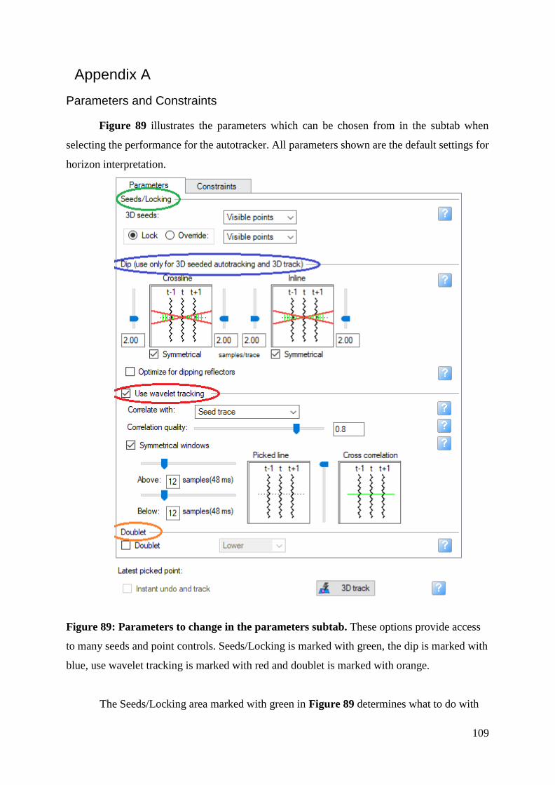
109

Appendix A

Parameters and Constraints

Figure 89 illustrates the parameters which can be chosen from in the subtab when

selecting the performance for the autotracker. All parameters shown are the default settings for

horizon interpretation.

Figure 89: Parameters to change in the parameters subtab. These options provide access

to many seeds and point controls. Seeds/Locking is marked with green, the dip is marked with

blue, use wavelet tracking is marked with red and doublet is marked with orange.

The Seeds/Locking area marked with green in Figure 89 determines what to do with

110

the existing interpretation. The first line “3D seeds” has three options; visible points, selected

points and inclusion filter. When choosing visible points, Petrel will use all the visible points

in the current interpretation as seed points. While choosing selected points, Petrel only uses

the points selected as seed points in the current interpretation. If the user chooses the option

inclusion filter, Petrel will use an interpretation filter to determine which seed points that are

used in auto tracking.

The second line “lock/override option” is basically the same as explained in the first

line “3D seeds”. The Lock/override visible points option use all visible points in the active

window. The lock/override selected points option uses only selected interpreted points in the

active window and are a subset of all visible points. While the lock/override filter option uses

only the interpreted points that match the selected filter.

The dip area is marked with blue in Figure 89 and allows the user to optimize the

autotracking parameters for dipping reflectors. The symmetrical checkboxes control if vertical

position changes in the inline and crossline directions can be symmetrical (toggled on) or

asymmetrical (toggled off). Using these options increases the user’s ability to fine-tune the

autotracking. Using the scrollbars along the diagrams one can control the number of samples

per trace. The options vary from 0.0-10.0 for symmetric slope and -10.0-10.0 for asymmetric

slope. It is possible to choose between decimal numbers which imply interpolating the two

closest samples’ amplitude. The green vertical lines between the red crossing lines in the

diagram indicate the possible tracking slope. The default value, as displayed in Figure 89, is a

window length equivalent to two samples. When the “optimize for dipping reflectors”

checkbox is toggled on one activate a guided plane that goes through the neighbors of the

dipping reflectors (3x3 and 5x5 points) and uses its trend when autotracking the event. Using

this option can increase the accuracy in areas where reflectors are dipping steeply.

When “use wavelet tracking” checkbox (marked with red in Figure 89) is toggled on,

the autotracker tests potential expansion points to use the correlation of a seismic trace

window. There are two correlation methods available in the first line; seed trace which cross-

correlate with the waveform of the seed trace and adjacent parent which cross-correlate with

the waveform of the adjacent parent trace.

Correlation quality in the second line sets the correlation threshold at which tracking

111

fails. Identical neighboring traces give a value of 1.0. The seed trace method has a default

value of 0.5 and a range from 0 to 1.0. The operational value used in this project is 0.8. If the

adjacent parent method is chosen, the method has a default value of 0.95 and a range from

0.75 to 1.0.

The symmetrical windows checkbox in the third line controls if the window tracking

can be different above and below the picked seed point. Selecting the checkbox means that

the tracking is symmetrical, while deselecting means that the tracking is asymmetrical. If

desired, it is possible to choose the distance above and below the seed point by entering a

numerical value (number of samples) or using the slider bars. The cross-correlation diagram is

a live diagram which displays the window lengths used and the correlation results of the

picked trace with its adjacent four traces in the following order:

1. t(j − 1) = correlation of the picked trace with neighboring inline trace (j − 1)

2. t(j + 1) = correlation of the picked trace with neighboring inline trace (j + 1)

3. t = correlation of the picked trace with neighboring crossline

4. t(I − 1) = correlation of the picked trace with neighboring crossline trace (i − 1)

5. t(I + 1) = correlation of the picked trace with neighboring crossline trace (i + 1)

Figure 90: Theory supporting the order of picked traces and its movement in inline and

crossline direction.

The doublet area is marked as orange in Figure 89 and specifies which part of a doublet the

tracker follows. A doublet is defined as a wavelet having four or more inflection points and

only two zero crossings. When doublet is toggled on, there are two options available: lower or

upper.

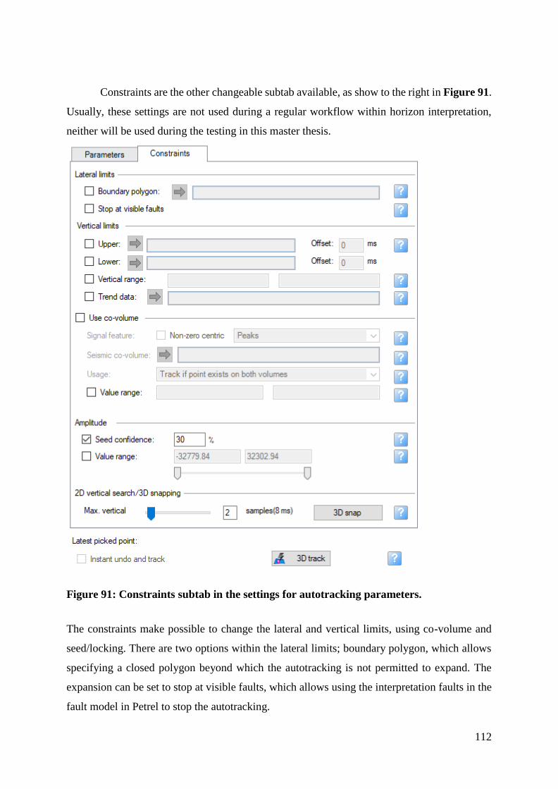
112

Constraints are the other changeable subtab available, as show to the right in Figure 91.

Usually, these settings are not used during a regular workflow within horizon interpretation,

neither will be used during the testing in this master thesis.

Figure 91: Constraints subtab in the settings for autotracking parameters.

The constraints make possible to change the lateral and vertical limits, using co-volume and

seed/locking. There are two options within the lateral limits; boundary polygon, which allows

specifying a closed polygon beyond which the autotracking is not permitted to expand. The

expansion can be set to stop at visible faults, which allows using the interpretation faults in the

fault model in Petrel to stop the autotracking.

113

The vertical limits have four options; upper, lower, vertical range and trend data.

Choosing the upper, the horizon above which the autotracking is not permitted to expand.

Lower, the horizon below which the autotracking is not permitted to expand. Vertical range

controls the vertical interval for the autotracked horizon in project units. For example, if it is

specified a vertical range from -1,750 to -1,790 ms, the resulting autotracked horizon is limited

to this vertical interval. The last, trend data, is a surface or another interpreted object that Petrel

tries to match (in shape) when tracking. This option is recommended to use when dealing with

dipping events, such that the seed expansion takes place only where the trend is defined.

Toggling on the “use co-volume” checkbox, the autotracking uses two seismic inputs

instead of one. Petrel will then evaluate points on both volumes and choose the best evaluation.

Toggling on the “value range” checkbox only values within the set range in the co-volume will

be tracked.

Below the amplitude, the user can choose to change the seed confidence and value range.

Seed confidence specifies the minimum value for the seismic amplitude as a percentage of the

seed point. The confidence level determines how much slack the tracker applies to the seed

values when determining if expansion points are to be accepted or rejected. For example,

picking an amplitude of 120 with a confidence interval of 30% rejects amplitude values below

36. A high value makes the tracker stricter, yielding fewer points, on the other hand, a low value

makes the tracker less discriminate, yielding more points. When used with the ‘3D track’

button, the confidence level will be applied to each seed point, so a potential expansion point

may be reached from a seed point with a high value but could be unreachable from a seed point

with a low value.

The last option in the constraints tab is the “2D vertical search/3D snapping”. In this

section the interpretation can be snapped to another part of the signal tracking feature, this is

also where you can apply the settings and track. The maximum vertical parameter controls how

much the vertical position can change from one trace to the next when the user auto pick along

2D lines. The default value is set to two vertical data units. The 3D snap button allows the

interpreter to search within the defined maximum vertical delta window for points defined as

3D seeds and snaps these points to the selected signal feature. This button can only be used on

3D seismic data.

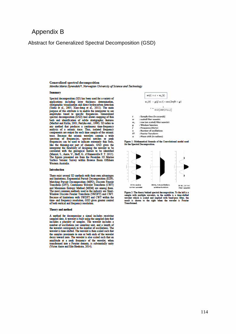
114

Appendix B

Abstract for Generalized Spectral Decomposition (GSD)

115

References

Ask, T., et al. (2016). "Auto Track Sub-Surface Salt Structures." TDT4290, Customer Driven Project. Bakke, J. O. H., et al. (2013). "Seismic DNA - a novel non-local search method for multi-attribute datasets." first break 31. Birtles, R. (1986). The seismic flatspot discovery and delineation of the Troll Field. London, Graham & Trotman. Bolle, L. (1992). "Troll Field. Norway's Giant Offshore Gas Field." Giant Oil and Gas Fields of the Decade 1978-1988 M54: 447-458. Borgos, H. G., et al. (2006). "Extracting horizon patches and geo-bodies from 3D seismic waveform sequences " Society of Exploration Geophysicists. Gabrielsen, R. H., et al. (1990). Architectural styles of basin fill in the northern Viking Graben. Oxford, Oxford Science Publications. Holgate, N. E., et al. (2015). "Seismic Stratigraphic analysis of the Middle Jurassic Krossfjord and Fensfjord formations, Troll oil and gas field, northern North Sea." Elsevier Marine and Petroleum Geology 68(Part A): 352-380. Johnsen, J. R., et al. (1995). "Jurassic reservoirs; field examples from the Oseberg and Troll fields: Horda Platform area." Elsevier 4: 199-234. Jonassen, P. (2015). Fault analysis based on 3D seismic data from the northern Horda Platform. Department of Geosciences. Oslo, University of Oslo. Master. Kyrkjebø, R., et al. (2004). "Unconformities related to the Jurassic-Cretaceous synrift-post-rift transition of the northern

116

North Sea." Journal of the Geological Society 161(1): 1-17. Mitchell, T. M. (1997). Machine Learning. Singapore, The McGraw-Hill Companies, Inc. Nelson, S. A. (2017) Geologic time. Nichols, G. (2009). Sedimentology and Stratigraphy. Wiley-Blackwell, John Wiley & Sons, Ltd. Publication. Oljemuseum, N. (2018). "Troll." 07.05.2018, from http://www.norskolje.museum.no/troll/. Osivwi, T.-I. (2012). "Sequence Stratigraphic Update of the 3-Series pf the Troll Field." Search and Discovery Article #20133. Patruno, S., et al. (2015). "Clinoform geometry, geomorphology, facies character and stratigraphic architecture of an ancient sand-rich subaqueous delta: Upper Jurassic Sognefjord Formation, Troll Field, Offshore Norway." Sedimentology, International Association of Sedimentologists 62: 350–388. Perry, J. W., et al. (1955). "Machine literature searching X. Machine language; factors underlying its design and development." American Documentation 6(4): 242-254. Russel, S. J. and P. Norvig (1995). Neural Networks. Artificial Intelligence - A Modern Approach. Upper Saddle River, New Jersey, Pearson Education International: 736-748. Schlumberger (2011). Petrel Geophysics Course. Houston, Schlumberger. Schlumberger (2017). "Petrel E&P Software Platform." Retrieved 18.01.2018, from https://www.software.slb.com/products/petrel. Stewart, D. J., et al. (1995). "Jurassic depositional systems of the horda platform, Norwegian north sea: practical consequences of

117

applying sequence stratigraphic models." Elsevier 5: 291-323. Walber (2014). Precision and recall. Wikipedia. Yielding, G., et al. (1991). "Seismic reflections from normal faults in the northern North Sea." Geological Society of London 56(The Geometry of Normal Faults): 79-89. Ziegler, P. (1981). "Evolution of sedimentary basins in North-West Europe." Petroleum Geology and the Continental Shelf of North West Europe 2: 3-39.