m tpgm^.'.wi.^Mij«*' ".iflT .1

A

AD/A-OM 822

COMMUNITY NOISE EXPOSURE RESULTING FROM AIRCRAFT

OPERATIONS: TECHNICAL REVIEW

BOLT BERANEK AND NEWMAN, INCORPORATED

PREPARED FOR

AEROSPACE MEDICAL RESEARCH LABORATORY

NOVEMBER 1974

DISTRIBUTED BY:

urn National Technical iRforaation Senrtci U. S. DEPARTMENT 3F COMMERCE

·•·

THIS DOCUMENT IS BEST QUALITY AVAILABLE. THE COPY

FURNISHED TO DTIC CONTAINED

A SIGNIFICANT NUMBER OF

PAGES WHICH DO NOT

REPRODUCE LEGIBLY,

lJW^»B>^^WWIWXivlw™w'S^f^ *■ IS^Bfp^BMl! P5ff^«pW^p5S5?Gai

SECURITY CLASSIFICATION OF THIS PAGE W>«i 9aia Emtrtd)

REPORT DOCUMENTATION PAGE I. REPORT NÜSTER

AMRL-TR-73-106 2. OOVT ACCESSION NO

4. TITLE («a* SuHttl,)

COMMUNITY NOISE EXPOSURE RESULTING FROM AIRCRAFT OPERATIONS: TECHNICAL REVIEW

T. AUTHOR/«)

William J. Galloway

». PERFORMINOOROANIIATION NAME AND ADDRESS

Bolt Beranek and Newman Inc. 21120 Vanowen Street Canoga Park, California 91303

• <■ CONTROLLING Of-FlCE NAME AND ADDRESS

Aerospace Medical Research Laboratory Aerospace Medical Division, Air Force Systems Command. Wright-Patterson AFB.OH

14. MONITORlNO AOENCV NAME • AOOMEtty« dllltti« Ircm Canlrallln« Ölllct)

READ INSTRUCTIONS BEFORE COMPLETING FORM

1. REClPlfcNT'i CATALOG NUMBER

rr.t/j i S. TVP|tOF REPORT * PERIOO COVERED

final report

• PERFORMING ORC. REPORT NUMBER

2581 I. CONTRACT OR OR ANT NUMBERf«)

F-33615-73-C-4160

10. PROGRAM ELEMENT, PROJECT, TASK AREA * WORK UNIT NUMBERS

62202F 72310424

I! REPORT DATE

November 1974 13. NUMBER OF PAGES

23^ IS. SECURITY CLASS, (WIM* »port;

unclassified

IS«. OECASSIFICATION/OOWNGRAOINO SCHEDULE

I«. DISTRIBUTION STATEMENT (»I <nl« A»p«l)

Approved for public release; distribution unlimited

IT. DISTRIBUTION STATEMENT (»i ih. thittmti m \»t*4In Stock 30, II dlllttmti from Rtpoti) D D

IS. tU^^UCMCNTAKV NO?« Kiproducad by

NATIONAL TECHNICAL —.„, ».....,.*, »« ».»A« INFORMATION SERVICE I1QCIS SÜBJKT TO CHANGE "OStttässr

u-

JUG m *i lays

D <t. KEY WOROS CConlliH • «MWH »Urn II n.c...«r «JlB Umntllr «T Woe* itoft-.r)

aircraft noise airpo.. b planning noise exposure forecast community .noise

noise surveys human response to noise day night average sound level

10. ABSTRACT fCanlfmM «n itnrn «IB* II «»ctfiy an* IdinlUr bf Woe« numbtr)

This report is one of a series describing the research program undertaken by the Aerospace Medical Research Laboratory to develop procedures for predicting the community noise exposure resulting from aircraft operations. It reviews current methods for predicting noise exposure around an airport, the results of various social surveys around airports, and psychoacoustic studies of aircraft noise slgials, as well as effects of aircraft

a 's

DD i FORM JAN 71 1473 EDITION OP I NOV St IS OBSOLETE

1 SECURITY CLASSIFICATION OF THIS PAOE f»T.«fi Oaf« Ei>(.r«r

r ummmimm

WCESSIMj«

RIß W\t SKIIM

DDC Sull SMliM ' O

(H»I(H0Ü."C£D D

JWTIilCAHtfll

It Disifciit;

NOTICES

(

(

When US Government drawings, specifications, or other data are used for any purpose other than a definitely relnted Government procurement operation, the Government thereby incurs no respon- sibility nor any obligation whatsoever, and the fact that the Government may have formulated, furnished, or in any way supplied the said drawings, specifications, or other data, is not to be regarded by implication or otherwise, as in any manner licensing the holder o*- any other person or corporation, or conveying any rights or permission to manufacture, use, 01 sell any patented in- vention that may in any way be related thereto.

Organizations and individuals receiving announcements or reports via the Aerospace Medical Re- search Laboratory automatic mailing lists should submit the addressograph plate stamp on the report envelope or refer to the code number when corresponding about change of address or can- cellation.

Do not return this copy. Retain or destroy.

Please do not request copies of this report from Aerospace Medical Research Laboratory. Additional copies may be purcha ed from:

National Technical Information Service 5285 Port Royal Road Springfield, Virginia 22151

The experiments reported herein were conducted according to the "Guide for the Care and Use of Laboratory Animals," DHEW 73-23.

The voluntary informed consent of the subjects used in this research was obtained as required by Air Force Regulation 80-33.

This report has been reviewed and cleared for open publication and/or public release by the appropriate Office of Information (01) in accordance with AFR 190-17 and DODD 5230.0. There is no objection to unlimited distribution of this report to the public at large, or by DDC to the National Technical Information Service (NTIS).

This technical report has been reviewed and is approved for publication.

FOR THE COMMANDER

HENHllGiJE. VOM GIERKE Director Biodynamics and Bionics Division Aerospace Medical Research Laboratory

AIR FORCe/56780/29 January 1975 - 250

L Sis

mm^&mmi*mm^m ?*V<w«HKf-'i« '!SS*v i. l..l..7:|i>l!.lll.J|HiPJ9 «ggpnp|pvpi«sm

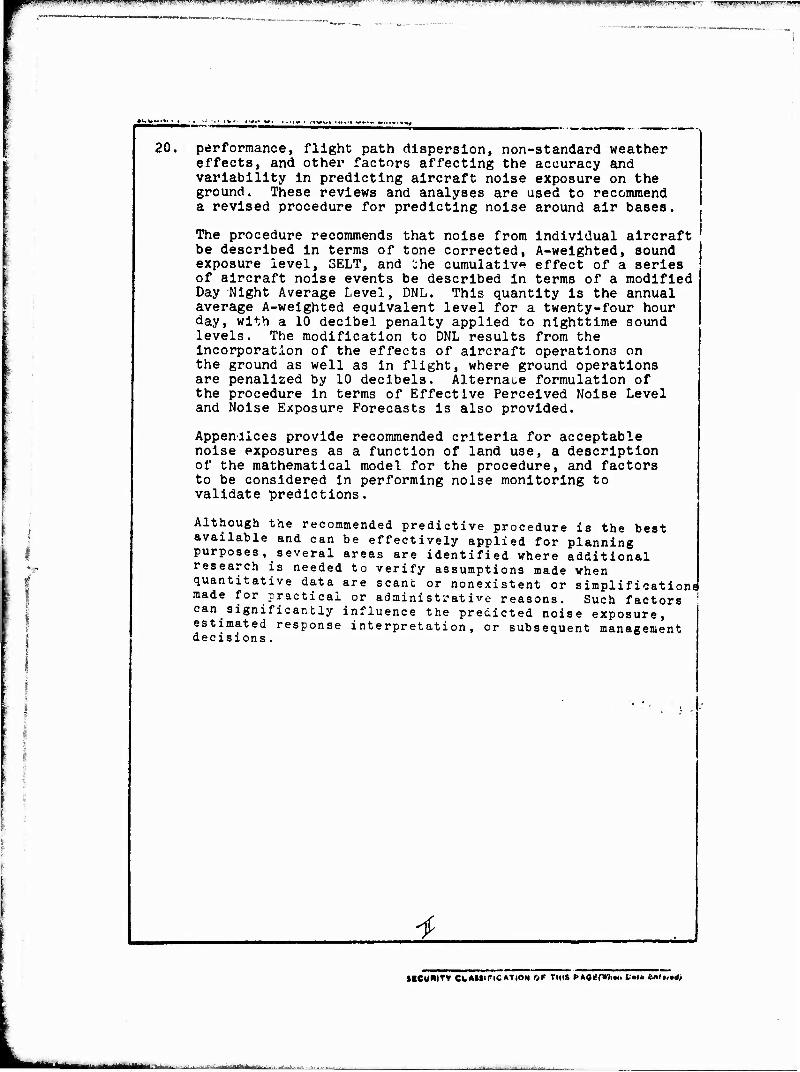
20. performance, flight path dispersion, non-standard weather effects, and other factors affecting the accuracy and variability in predicting aircraft noise exposure on the ground. These reviews and analyses are used to recommend a revised procedure for predicting noise around air bases.

The procedure recommends that noise from individual aircraft be described in terms of tone corrected, A-weighted, sound exposure level, SELT, and 'the cumulative effect of a series of aircraft noise events be described in terms of a modified Day Night Average Level, DNL. This quantity is the annual average A-weighted equivalent level for a twenty-four hour day, with a 10 decibel penalty applied to nighttime sound levels. The modification to DNL results from the incorporation of the effects of aircraft operations on the ground as well as in flight, where ground operations are penalized by 10 decibels. Alternate formulation of the procedure in terms of Effective Perceived Noise Level and Noise Exposure Forecasts is also provided.

Appenlices provide recommended criteria for acceptable noise exposures as a function of land use, a description of the mathematical model for the procedure, and factors to be considered in performing noise monitoring to validate predictions.

Although the recommended predictive procedure is the best available and can be effectively applied for planning purposes .several areas are identified where additional research is needed to verify assumptions made when quantitative data are scant or nonexistent or simplifications made for practical or administrative reasons. Such factors can significantly influence the predicted noise exposure, estimated response interpretation, or subsequent management decisions.

■i

IKCUftlTY ClAMtFlCATtON <>? THIS P*QH(Wht* Lmtu &mi,«tf)

IftlMiiMAMdNariiUiMu. LA^. —"i jrfttM ■ i _...

IJIflljljjg^PiyPII^^ '.■«:■■ " '■^^^r^-^-^*tr*™ttmfrt7?»-* ■ ^ j-rry^s.^.,-^ ._TTf:=-" - " ■ -S^** *"v-^--w ^--^^^'^'"'™"- -^^v^j^-T^r^^-^K,^™,,^,^^™ -.; ,^: ■■ .„-.r,;^«.-;^-- ^s ■^rs^^s^p.^-^iKpfs;'!!!^

PREFACE

The author wishes to acknowledge the assistance of

Dwlght E. Dishop for general discussions, review, and comment

during the preparation of this report and fur his specific

contributions to the analysis of the acoustical effects of

nonstandard weather and flight path dispersion, and for the

preparation of Appendix D. The assistance of Karl S. Pearsons

in preparation of the review of psychoacoustic literature is

also acknowledged.

Detailed discussion of content, critical review, and

suggestions by Jerry D. Speakman and John N. Cole of the

Biodynamics and Bionics Division, Aerospace Medical Research

Laboratory, Wright-Patterson Air Force Base, have been of

great assistance throughout the period of the study.

The engineering description of the computer implementation

of the recommended noise calculation procedure described in 1 Appendix C was prepared by Nicolaas Reddinglus.

| This report is one of a series describing the contractual I and in-house research program u^der Pro/tict/Task 723104,

Measurement of Noise and Vibration Environments of Air Force I

Operations, undertaken by the Aerospace Medical Research

Laboratory to develop a procedure for predicting the community

noise exposure resulting from aircraft operations. The companion

reports are listed as References 78, 79, 80, 3l, and 82. The

Air Force Weapons Laboratory provided funding to partially

support development of this program.

jrÜft^ÜÜ^ÜiPliiiigi'i - - ' - - - iMiiiiiiTfriiMafcrhiiiiir i r .„

I ~

^*' '. WWWSPHfqppWfflPP t4P*. ^?r^pR*?ir-* ■.■?>»y'^^

TABLE OP CONTENTS

Page

I. INTRODUCTION 11

II. NOISE RATING PROCEDURES AND THEIR VALIDITY ... 15

A. Factors Included in Aircraft Noise Rating Measures 16

1. Description of the Sound Produced by a Single Aircraft Flyover 16

2. Effect of Number of Events 21

3. Period of Day 23

h. Time of Year 28

B. Summary of Aircraft Noise Rating Measures 31

C. Correlation of Noise Ratings with Community Annoyance 35

1. O'Hare Study 35

2. Bradley Study 38

3. Tracor Study 40

4. London Study 46

5. Generality of the Relationship Between Average Annoyance and Noise Exposure . 51

D. Noise Criteria for Land Use Planning ... 52

E. Other Forms of Noise Impact Analysis ... 59

Preceding page blank

,. :T.^- ~,S 17^:^^^~- ^t-

TABLE OP CONTENTS (Cont'd)

Page

III. REVIEW OF PSYCHOACOUSTIC EVALUATIONS OF AIRCRAFT NOISE 67

A. Spectral Effects 67

B. Effects of Discrete Frequency Components . . 68

C. Temporal Pattern Effect 69

D. Doppler Shift Effect 70

E. Speech Interference Effect 71 F. Background Noise Effect 71 G. Combination Effects 72

IV. REVIEW OF THE TECHNOLOGY OF NOISE EXPOSURE \ ?? COMPUTATION \ "

A. Basic Approaches to Existing Models 79

B. Acoustical Factors 83

1. EPNL Computations 83

2. Air-to-Ground Sound Propagation 98

3. Ground-to-Ground Sound Propagation . . . 103

H. Transition from Ground-to-Ground to Air- to-Ground Sound Propagation Rules .... 105

5. Duration Effects 208

6. Effects of Topography and Geometry . . . 10g

7. Density Altitude Effects 110

8. Nonotandard Weather Effects 113

9. Presence of Background Noise 121

10. Shielding Effects 121

IB!jBsgMi^!gi|i|»«BS»npi!|gni!ii- JU'UHWBP»iWPBWPTPIgpwwpwIHPBWWWWIWWIP'W**^'Tssp^™^r!'»7f»ayjp»m»KWW'- -. ..^.4L.^,^iM«i^#«t^H^' ''JI^BMIB^ »" jipi

: f

TABLE OF CONTENTS (Cont'd)

Page

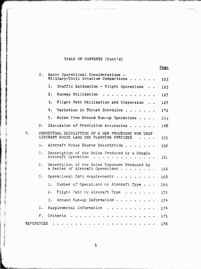
C. Basic Operational Considerations - Military/Civil Aviation Comparisons 123

1. Traffic Estimation - Flight Operations . . 123

2. Runway Utilization 127

3. Flight Path Utilization and Dispersion . . 127

4. Variation in Thrust Schedules l'»2

5. Noise from Ground Run-up Operations .... lijj

D. Discussion of Prediction Accuracies 148

V. CONCEPTUAL DESCRIPTION OF A NEW PROCEDURE FOR USAF AIRCRAFT NOISE LAND USE PLANNING PURPOSES .... 155

A. Aircraft Noise Source Description 156

3. Description of the Noise Produced by a Single 1 Aircraft Operation 161 § I I C. Description of the Noise Exposure Produced by I a Series of Aircraft Operations 164

i D. Operational Data Requirements 168

1 1. Number of Operations by Aircraft Type . . . 169

2. Flight Path by Aircraft Type 170 :~ I

3. Ground Run-up Information 17I4

E. Supplemental Information 174

F. Criteria 175

REFERENCES 176

■ --' -- r'-~ :,--,„_, ....,-. :-.-,,...- ,„„„^,^: [^'--- -■--:■-- ,:-._- r:i7.«r-r,. ..-.«B^a.fl.i^iirfti^'! ■ ■ =•■ T-^;v.r=™^^»'^-:a^= ~5-ri-.--j-^-^^==—#■ f ^T" ="■ " ■ ■■-?««T*- ,^LW- - ..-■-. — ■

I

TABLE OF CONTENTS (Cont'd)

Page

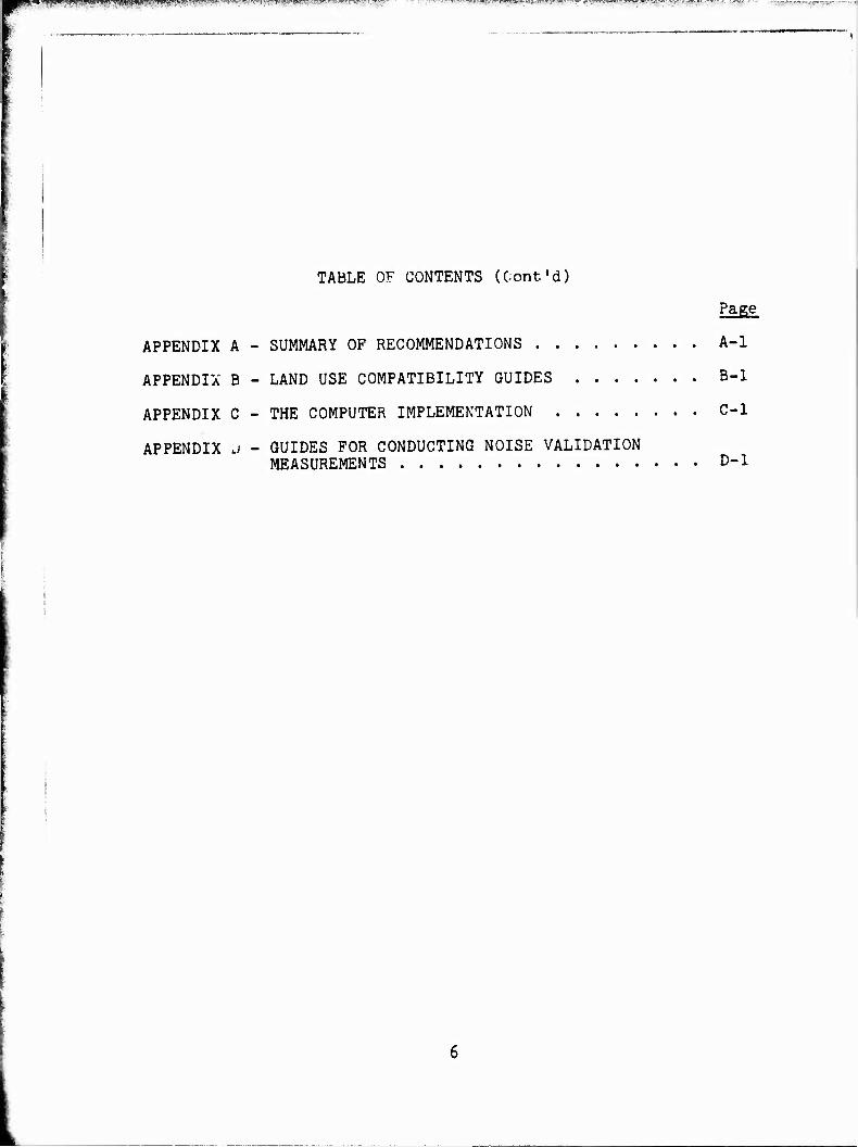
APPENDIX A - SUMMARY OF RECOMMENDATIONS A-l

APPENDIX B - LAND USE COMPATIBILITY GUIDES B-l

APPENDIX C - THE COMPUTER IMPLEMENTATION C-l

APPENDIX J - GUIDES FOR CONDUCTING NOISE VALIDATION MEASUREMENTS D-l

p&-mwp*swT/.'- , "j.™ .'■»•■JWJ"'■->'■'-■

LIST OP FIGURES

Figure Page

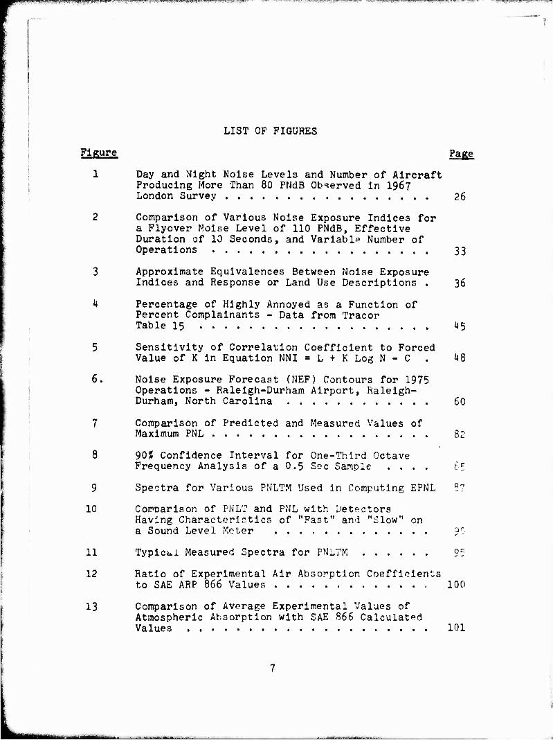
1 Day and Night Noise Levels and Number of Aircraft Producing More Than 80 PNdB Observed in 1967 London Survey 26

2 Comparison of Various Noise Exposure Indices for a Flyover Noise Level of 110 PNdB, Effective Duration of 10 Seconds, and Variable Number of Operations 33

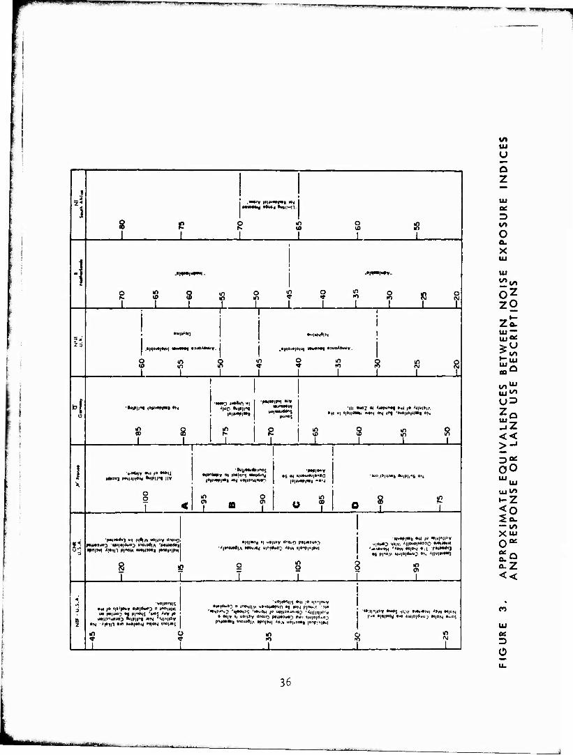
3 Approximate Equivalences Between Noise Exposure Indices and Response or Land Use Descriptions . 36

4 Percentage of Highly Annoyed as a Function of Percent Complainants - Data from Tracor Table 15 4 5

5 Sensitivity of Correlation Coefficient to Forced Value of K in Equation NNI = L + K Log N - C . H8

6. Noise Exposure Forecast (NEF) Contours for 1975 Operations - Raleigh-Durham Airport, Raleigh- Durham, North Carolina 60

7 Comparison of Predicted and Measured Values of Maximum PNL 82

8 90? Confidence Interval for One-Third Octave Frequency Analysis of a 0.5 Soc Sample .... t>

9 Spectra for Various PNLTM Used in Computing EPNL 3?

10 ComDarison of PNLT and PNL with Detectors Having Characteristics of "Fast" and "Slow" en a Sound Level Meter 9'

11 Typical Measured Spectra for PNLTM 9^

12 Ratio of Experimental Air Absorption Coefficients to SAE ARP 866 Values 100

13 Comparison of Average Experimental Values of Atmospheric Absorption with SAE 866 Calculated Values 101

~~ :1 .r-u. re ------

1 •

-~ I

LIST OF FIGURES (Cort'd)

Tra:~st~ __ :un frcrr: G~·uur.d to Air !ittenuation

~: • "./f. •"' l...J, ..

~ ......... . · ~~ L···

•• 1 :i ..

' .

...

f h·

: .

, .... ,.... ..... ,,.._ i. "' ....... ,

..

. . .-·~

. .... ..

· .... . ' ~-

-· . -

·.·.

. -· ~

Irr

':'urtojet

Typ!cal 7urbofan

:." , .. -.; ... .. .. J ..... ' ~

R.E

.. ~

'\ta 1 u~s ~~ !. th :r;.rp!cal

'!'_• •. ~;; •. . n • ... '

..._,. l '"'. r- r ~t ,: ., ~ ..

•'.: 1 .. -~ .. ·~-'-

8

and Takeoff

ar.d Approach

Respect Turbofan

56

a

106

111

.116

11?

. .. . . --.

.., ....,. -, l.,:..:

Lin OF TABLES

Table

I

II

III

IV

VI

VII

VIII

Page

Relative Effect of N.ght Corrections 2k

Attributes of Various Noise Rating Measures . . 32

Variation in EPNL Repeat Measurements for Spectra of Fig. 9-6 Trials 86

Variation in One-third Octave Band SPL for Different Sample Periods 88

Stability of Repeated Analyses of a Flyover Signal with "Fast" and "Slow" Detectors .... 92

Coefficient of Variation in Vertical Dispersion of Takeoff Flight Paths 131

Variability of EPNL Values Under the Nominal Approach Path - 31,000 to 82,000 feet from Touchdown Expressed as Standard Deviations in dB 152

Predicted Minus Measured NEF , _, J-b 5

«WOT-i-WP-W» ■^■PP^WPjP^P1^

SECTION I

INTRODUCTION

Noise produced on the ground by aircraft operations on and

J? ;he vicinity of air bases and the way in which this noise

affects land use has been an important concern of the Air Force

for many years. The first published procedure specifically

directed towards aircraft noise and land use planning was Issued

by the Air Force, after a pioneering research program, in 19*57- .

As a result of research performed subsequent to this publication, 2/

a revised procedure was published in 1964-, This procedure,

using the Composite Noise riating (CNR) concept and the Perceived

Noise Level (PNL) measure for aircraft noise was derived for

both military and civil aircraft operations, being jointly

published as a tri-service document and as an FAA report. It

has been widely used in evaluating the impact of aircraft noise

on residential land use in many military and civil airport

planning studies.

During the middle 1960's, the evolving knowledge of

subjective reaction to aircraft noise introduced the concept of

Effective Perceived Noise Level (EPNL) as the measure for the

noise produced by a specific aircraft noise signal. In 1967

the FAA developed a revised aircraft noise-land use planning

procedure, termed the Noise Exposure Forecast (NEF) for poten-

tial use in civil aviation-^- . The NEF procedure is a direct

adaptation of VNR, using EPNL instead of PNL as the measure of

aircraft noise. An almost identical procedure to NEF, Weighted

Equivalent Continuous Perceived Noise Level (WECPNL), has been

adopted by the International Civil Aviation Organization (ICAO)-,

During the past decade the evaluation of aircraft noise

and its effect on land use has become an international problem.

11 Preceding page blank

fc-MiPJL- ■ ■ -^^ -^-^- --— ■ - ._.._.,^_jsimmKäMiiÜb*imiimmmua

^^.™*S^33f3^

As a result many countries have developed their own methods,

rating scales, and techniques for assessing the effects of

aircraft noise. Research has also continued at the laboratory

level on psychoacoustic evaluation of complex noise such as tnat

produced by modern aircraft, sociological investigations into

the response of people exposed to aircraft noise have been

continued, and land use planners have become directly involved

in the studies.

In 1973 the Environmental Protection Agency (EPA), in

response to a requirement of the Noise Control Act of 1972,

published its study of aircraft/airport noise— . This study

reviewed not only the aircraft/airport noise measures and plan-

ning procedures, but also considered the eventual combination of

noise exposures from aircraft with that from other sources. The

extensive use of EPNL and NEF as measures for aircraft noise

notwithstanding, the EPA had more compelling reasons to recommend

the use of A-weighted sound level to describe the noise from

individual events, and proposed the day-night equivalent sound

level (symbolized as L, or DNL) as the measure of cumulative

exposure. Day-night sound level is a twenty-four hour logarith-

mically averaged cumulative noise exposure with a penalty for

nighttime noise levels.

The USAF is now considering the revision of its present

aircraft noise-land use planning proced ires to reflect the

current state-of-the-art as developed by recent research efforts.

A critical review is required of the existing procedures and how

they might be influenced by the newer researcn results. This

report provides such a review, and concludes with a recommended

procedure for future USAF use in land use planning as it is

affected by noise from aircraft operations.

12

pmaEMiaajp^MMMii^JJifct^^ '"~J??'^>'^Tv«:^^flw«iji^#-*-^ - ftwi«p#jfmnnp^M

In performing this critique, two basically separate aspects

are considered. The first relates to the conceptual and philo-

sophical attributes of different aircraft noise measures, ratings,

standards, and criteria. Various systems in use in the world are

compared. The results of contemporary psychological and socio-

logical research efforts are then reviewed to assess how their

results affect the validity of present and proposed planning

procedures. A review of current land use criteria for aircraft

noise exposure areas is also provided.

The second aspect of this review considers the technological

problems of physical acoustics, aircraft performance, and opera-

tional considerations which influence the prediction of aircraft

noise exposure irrespective of the rating method or land use

criteria employed in planning procedures. Particular emphasis

is placed on identifying omissions, deficiences, and inaccuracies

in present procedures.

Throughout the review, material conclusions are presented

on each element entering into the development of aircraft noise-

land use procedures. In the final part of this report these

elements are summarized as a recommended procedure for military

application. This procedure is equally valid for civil a 'iation

planning purposes.

At the present time there is no national policy specified

for land use olanning with respect to aircraft noise, nothwith- ?/ standing the unified military service procedure— . The USAF is

conducting this study in accordance with the continuing require-

ments of the Environmental Policy Act of 1969 (Public Law No. 91-

190) and Executive Order No. 11511* which directs all Federal

agencies to "Monitor, evaluate, and control on a continuing basis

their agencies' activities so as to protect and enhance the

13

quality of the environment." In accordance with these

rulings it is recognized that adoption of the planning pro-

cedure developed in this program is subject to review and

approval of the Environmental Protection Agency (EPA) and

the Council on Environmental Quality. The procedures recom-

mended are consistent with those of EPA in its study of

aircraft/airport noise— .

1U

■-*"■-■■-

SECTION II

NOISE RATING PROCEDURES AND THEIR VALIDITY

In the past decade or so at least one dozen rating measures

have been developed for relating the noise produced by aircraft

operations to the response of communities in the vicinity of

airports. All measures have two things in common:

a) a description of the physical noise exposure produced

by a complex of aircraft noises, including weighting

factors for the physical variables that are considered

to influence response;

b) criteria for estimating the response or degree of

acceptability associated with various numerical values

of weighted noise exposure.

The evolution of the most significant of these measures and

an intercomparlson of their resultant criteria has been traced h/

in a recent FAA report— . In this present report we are

primarily concerned with the validity of the concepts involved

in these measures. As such, in the following discussion we

shall be mostly concerned with the differences in methodology

employed rather than the historical development of any one of

the measures.

All procedures for computing noise exposure include the

following elements:

a) noise level of separate events;

b) distribution of noise over the audible frequency spectrum;

c) the number of noise events in some specified time period;

d) normalizing constants.

15

■-:■■-■, ' -:;.: = !.—-*.?, * [ -^fg&^^i^m^-w-vwr;--^^

Many of the noise indices also provide means to account

for the effect of variation in the time patterns for individual

events, the number of events occurring within different time

periods of the 24-hour day, and for seasonal effects. All, of

course, have in common the practical problems of correlating

noise data with aircraft performance, sound propagation effects,

and evaluating the operational factors involved in real aircraft

operations. These practical problems v*lll be discussed later in

this report. For now, we are concerned only with the conceptual

aspects of noise exposure rating methods. In the following

parts of this section of this report we examine only the

acoustical factors and how they are related in various noise

rating measures.

A. Factors Included in Aircraft Noise Rating Measures

1. Description of the Sound Produced by a Single Aircraft

Flyover

All methods for measuring the sound produced by a single

event must consider the magnitude of sound and how it is distri-

buted in frequency and time. All measurer presently used for

aircraft noise evaluate sound magnitude and its frequency

distribution explicitly. The variation of sound level with

time, on the other hand, is considered explicitly in some

aircraft noise rating methods, in others only the maximum

magnitude of the sound produced during an evert is used. The

methods for accounting for these attributes of a sound signal

are discussed here.

The primary factor in any noise ratin? procedure is the

method used to specify the magnitude of the noise produced by

an aircraft; event. The choice of measure for this quantity

has been the subject of controversy since it is desirable to

16

nHHSgrnEHfrTS

have a measure that not only describes physical magnitude, but,

for simplicity in analysis, also provides a single number

descriptor that accounts for the frequency distribution of

sound energy over the audible spectrum. In particular, it is

desirable to have a frequency weighting that scales directly

to subjective response, accounting for the variation in

response of the human hearing system with frequency. The

alternate to this, of course, is to provide a spectral analysis

of each event, requiring 8, 24, or more separate sound pressure

levels (SPL) to span the audible spectrum.

All existing rating methods use a frequency-weighted

measure to describe the magnitude of sound. More than 50 such

measures have been described in the technical literature.

Fortunately, standards and recommended planning procedures for

aircraft noise have restricted these measures to A-weighted

sound level (or its time integral), PNL, and EPNL, the last

being a variant on PNL. The argument for PNL is that it is a

psychoacoustically derived measure that purports to allow

sounds of widely differing spectral content to be compared by

a single measure which directly scales to subjective response.

It is computed by a summation process which considers the SPL

in each octave or cne-thlru octave band ever most of the

audible frequency range.

On the other hand, A-weighted sound level has the merit

of being easily obtainable with a simple frequency weighting-

network that alters a measuring system to de-emphasize the

lower frequency range. Its use is further supporte by the

fact that, for most transportation generated noises, it pro-

vide? almost as good an experimental fit to subjective tests

as the more complex measures. It is this "almost as good"

feature that is the issue.

17

Aircraft noise signals have become considerably more

complex in their frequency content than most other sources

of noise. Where the early Jet engine noise was a rather

smoothly varying random noise having a predominantly low

frequency characteristic, present engines often have pro-

nounced high frequency energy content, and often have a

substantial structure of high frequency discrete tones super-

posed on the random noise of the jet. These newer sounds

generally occur in the frequency range above 1000 Hz, yet in

this frequency regime A-weighted sound level diverges from

PNL in accurately scaling human response. Nevertheless,

because of its wide use for describing other noise sources,

A-weighted sound level has strong support, and has been

recommended for EPA use in a task group report by the EPA

Aircraft/Airport Noise Report task force— .

While the initial controversy over PNL as compared to

A-weighted sound level was waging internationally, two other

factors in scaling response to noise wen becoming of concern.

Psychoacoustic phenomena exhibit the characteristic of being

additive on an energy basis. As such, the duration of a noise

event becomes as important as its magnitude. Since the noise

produced by an aircraft flyover is a time varying signal, the

effect of its duration was believed to be important. Subse-

quent laboratory experiments confirm this point.

Secondly, the pronounced tonal structure developed by

newer engine designs indicated that even PNL did not properly

assess the subjective reaction to these sounds; it tended to

underestimate the response. Experiments in this country and

in England led to correction procedures that added penalties

for the presence of tones.

18

«IT

pWPiW.wui,-,'"w^'lM»»mJ'' ■ - - ' " ' ,ww*! *m*mr

A re-ult of the consideration of duration and tones led

to the specification of the quantity called Effective Perceived

Noise Level, EPNL, which is time-integrated, tone corrected,

PNL. We discuss the validity of these measures in Section III

of this report; we are now concerned only with the attributes

of noise signals that have been considered in noise rating

methods.

Each of the noise measures has been employed in one or

more of the aircraft noise rating methods in current use. In

any one of the noise ratings the choice of a single event

noise measure is in part historical, In part a question of the

intended use of the rating method, and in part the degree of

complexity one is willing to consider in its use. Clearly, if

monitoring the noise exposure Is of primary concern, A-weighted

sound level Is easiest to use, time integrated A-weighted sound

level is next in complexity, and PNL or EPNL the most complex.

On the other hand, for land use planning purposes, since the

description of an aircraft as a noise source can be provided

In any of the measures, no one is preferable over the next from

a computational point of view.

A concern completely separate from land use planning is

the accurate evaluation of the noise from an individual air-

craft for engineering design purposes and for noise certifi-

cation purposes. EPNL has been specified as the noise measure

in both USA and international certification documents^4-;- since

it is considered to be the currently available measure that

most accurately scales the subjective response to aircraft

noise. Similarly one can argue that the best available noise

measure should also be used for land use planning purposes.

It is for this reason that EPNL is also specified in both the

International Civil Aviation Organization and International

19

-'--■■■—-■

ppg^KK'VHUHUUmmf pull»"!!-., i l.ll.'i.. .. .« ALU'-'-■»'iJP«"M.»|ii; J »J. . HH„"

Standard Organization documents on aircraft noise and land use

planning-*-1—' . In the event that a measure other than EPNL is

chosen for use in land use planning, through new national or

international agreement, conversion of EPNL values to the new

measure is readily accomplished if the original data used to

compute EPNL are available.

One argument against the exclusive use of A-weighted

sound level is the concern that knowledge of the spectral

and temporal content of a noise signal will be lost if only

a sound level meter is used for noise measurement. In order

to make good engineering projections of noise measurements

obtained at one distance to other distances, spectral distri-

butions of noise level are essential. Corrections for tone

penalties also require spectral data. A compromise can be

reached between the desire for detailed knowledge of a noise

signal on one hand and the desire for a uniform measure,

A-weighted sound level, on the other hand, by acquiring the

noise data in full spectral and temporal detail, then express-

ing the final answer In terms of A-weighted sound levels.

The measure that most nearly combines the desirable

features of EPNL, but expresses the final result in A-weighted

form, is the single event A-weighted sound exposure level.

This quantity can be obtained from one-third octave sound

pressure levels by applying the A frequency weighting instead

of the PNL weighting. Tone correction and time integration

procedures can be applied identically as in the EPNL computa-

tion. The resulting quantity is the logarithmically weighted,

time integral of A-weighted sound level, corrected for tones,

over the duration of the noise event, normalized to a

reference duration of one second. The symbol for this quantity,

20

■-- aa—

JlJIjipiJPWm |i »_r IIIIPM. .^srrr?^-:—~r???X*:*\-9:*-l*m*, ! ■•***•- r,r^!«^»»-'"»,,^,rTiü-*' pjgPB^HHPgWW! BWHPMP

without tone corrections, has been variously labeled as SEL, Lex' and in very slmilar form» SENEL, wirh its unit being the decibel. (Recent international standardization efforts are

proposing L.x or AXL for the symbol.) The comparable symbol

for this quantity with tone corrections is SELT.

Recommendation No. 1 - The USAP land use planning

procedure for aircraft noise should use the tone

corrected, A-weighted sound exposure level, SELT,

for describing the noise from an individual aircraft

noise event.

2. Effect of Number of Events

The preponderance of case histories and social surveys

indicates that the response of a community to aircraft noise

is affected not only by how loud the noise is, but also how

often noise events occur, e.g., the total noise exposure in

a specified time period. This is consistent with the labora-

tory results of psychoacoustics experiments that shew that

magnitude of sound and its duration are exchanged on an energy

summation basis. On the assumption that community response is

related to the total noise energy in a specified time period,

a rating scale would sum events of equal magnitude on the

bases of 10 log,n N where N is the number of events. Most

rating scales use this assumption. The question remains, how-

ever, as to whether this is a valid assumption, and, if so,

why some rating methods use a different summation rule.

The three deviations from the simple energy summation are

contained in the UK, German, and Dutch ratings. The first to

obtain prominence was in the UK Noise and Number Index (NNI)

where number of events is summed as 15 lo?10 N« This factor

21

BülW -»-.-uif.if

was proposed as a result of analyses of a social survey con-

ducted around Heathrow airport in I961- . As has been shown

by Galloway and Von Gierke—, however, the survey results

could be fitted equally as accurately to the 10 log,Q M

summation.

In the German Stör index, Q, a 13.3 loEin N summation is

used. The justification for this choice is somewhat obscure,

but appears to have been chosen on the basis of certain

psychoacoustic tests— . The choice of 20 log1Q N in the

Dutch rating method is reported to have been selected on the 12/ basis of a social survey around Schlphol airport— .

Considerably more light on the choice of multiplier for

number of events has been shed in the recently published

analyses of a second social survey around Heathrow conducted

in 1967—/ . In these analyses a number cf correlations between

response and noise exposure were made with a forced variation

in K from 2 to 22 in the expression K iog10 N for four dif-

ferent combinations of noise exposure. It was found that the

degree of correlation was, in general, quite insensitive to

the value of K, although some form of K lop N is useful for

assessing annoyance in the community. In summary, psycho-

acoustic experiments indicate that magnitude, duration and

number of events should be combined on an energy basis.

Sociological results indicate that energy summation is equally

good for assessing community annoyance, although the results

are somewhat insensitive to the actual form of the assessment

of number of events, just as lone a? some measure Is used. It

seems reasonable, therefore, to retain the energy summation

approach in assessing community annoyance. Again the inter-

national documents support this position.

22

Recommendation No. 2 - Number of events be accounted

for by 10 log,g N.

3. Period of Day

In several of the noise rating methods nighttime operations

are penalized in terms of their effect on the rating scale as

compared to daytime operations. These penalties are arbitrar-

ily assigned on the basis of results from complaint studies and

social survey data that indicate a higher sensitivity to night-

time noise. Solid data to support the actual choice of numbers

for this effect are hard to come by. The higher nighttime

sensitivity value of 10 dB in equivalent exposure used in the

CNR and civil NEF methods is based on overt community response

evaluations. It was estimated in the 1961 Lcndon survey that

a reduction of 17 NNI exposure units was required to reach the

same acceptability for night operations as was obtained for

day operations. (For a fixed noise level this is equivalent

to li units in CNR or NEF.)

The existing rating methods that do make adjustments for

day/night have substantially different computational approaches.

Both CNR and NEF assess nighttime exposure, on an energy basis,

to be 10 dB more sensitive than daytime. The French system ha?

a complex weighting appiiel to a three period day in which

daytime (0600-2200), early nighttime (2200-020C), and late

nighttime (0200-0600) are weighted according to the expression:

10 log1Q ND + 6 iog10 [(3K-, + N2) - l] where ND> Nj_ and N2 are the number of operations in the three time periods. The

ICAO index, WECPNL, allows for either two or three period days.

Using the two period day, 0700-2200 and 2200-0730, the night-

time noise levels are weighted by an additional 10 dB. The

23

taa

_LJ_ljlil_l .. l^l!l;- P1L-1- J }:.W =:=,ifs^=^?^i?;^ "1

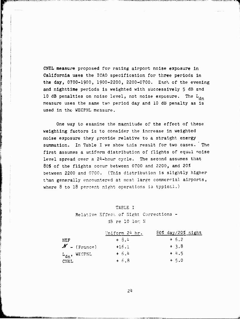
CNEL measure proposed for rating airport noise exposure in

California uses the ICAO specification for three periods in

the day, 0700-1900, 1900-2200, 2200-0700. Each of the evening

and nighttime periods is weighted with successively 5 dB and

10 dB penalties on noise level, not noise exposure. The L,

measure uses the same two period day and 10 dB penalty as is

used in the WECPNL measure.

One way to examine the magnitude of the effect of these

weighting factors is to consider the increase in weighted

noise exposure they provide relative to a straight energy

summation. In Table I we show tnis result for two cases. The

first assumes a uniform distribution of flights of equal noise

level spread over a 24-hour cycle. The second assumes that

80* of the flights occur between 0700 and 2200, and 20*

between 2200 and 0700. (This distribution is slightly higher

than generally encountered at most large commercial, airports,

where 8 to 18 percent night operations is typical.)

TABLE I

Relative Effect of Night Corrections -

dB re 10 lor N

NEF

Jf - (France)

Ldn, WECPNL

CNEL

Uniform 24 hr.

+ 8.4

+16.1

+ 6. 4

+ 6.8

80* day/20* night

+ 6.2

+ 3.8

+ 4.5

+ 5.0

24

P^ipilWJ,,.-.^*^:*^ . ^-«r^-~™-S^-:- ^""l-"---^— -.-: ■-■-^-■--■7^---v-:~-r— :-■ - ■ -.■ v:*v r^s™^-^^*?*^ ^^■■•m-nvf,^-,^:,^^ -.-£«-

These differences for the same situation reflect the

uncertainty associated with this factor, largely due to

whether it is the noise level itself or the noise exposure

which receives the weight. For most practical cases, where

night operations are typically less than 20$ of day

operations, the numerical differences in the effects cf one

method as compared to another are small.

Little help in resolving the uncertainty is available

from two major social surveys conducted in the last five 1*4/

years—that by Tracor, Inc.— , • ider NASA sponsorship, in I

which seven cities were surveyed, and the second London survey

already mentioned. In a preliminary report of the Tracor

work, Hazard— indicated that average annoyance scores were

more than doubled if aircraft were heard between midnight and

6 a.m. Nothing whatsoever is said in the Tracor final report i

on this subject. On the other hand, a substantial effort was

made in the London survey to examine this problem. A separate

I annoyance scale for nighttime operations was even constructed 1

for use in studying night as compared to day operations. No

clear results were obtained, however. This is not surprising

since the nighttime noise exposure is substantially curtailed

at London by limits on both number of flights and use of

noisier aircraft.

The effect of this curtailment and its effect on night-

time noise exposure can be estimated from the London survey

data as provided in Ref. 13. One can compare both noise level

distributions and number of events, as experienced at the

survey subjects' homes, for both day and night operations.

These data, in a cumulative distribution form, are plotted on

Fig. 1. While the differences in noise level between day and

25

—,— ■■->, ii -•-- -■

ttmmmBmmm p*PSf BPWWPB TOBPP WfS »5-^mmi.k n? pepiPHpBSp^gB^. S *u ppmnnn^pHl

100

90

80

70

60

50

40

JO

20

10

Jü? NIGHT

/ o / /DAY

/ / / /

if / / 11

11 /1

4

80

100

90

PNdB

100

>

/ /NIGHT

/ / 6 1 Sow

1 1 1 J 1 / \ / 1 / 1 /

7 50 100 150

Number of Aircraft 200

FIGURE 1. DAY AND NIGHT NOISE LEVELS AND NUMBER OF AIRCRAFT PRODUCING MORE THAN 80 PNdB OBSERVED IN 1967 LONDON SURVEY

26

■ ■

•w» qnpiip Kü=f!WiS!S»im^™ ■ )--^";l=--^-

night are not substantial, the difference in number of events

in excess of 80 PNdB is striking. Making the crude assumption

that a relative difference between day and night can be made

by comparing the daytime and nighttime values of CNR or NNI

computed from the medians of the distribution, one can show

that the nighttime exposure is 13 dB less than the daytime on

a CNR scale (not using night penalties), and 18 dB less on the

NNI scale. A comparable difference is obtained at the upper

25$ point of the distributions, even though the noise exposure

increases by 15 dB in the case of both day and night. Using

the CNR estimate that night exposure should be penalized by

10 dB, one would clearly estimate that the day operations in

this study still subjectively outrank the night operations

substantially. This point is cubstantiated by numerous

qualitative results in the survey analysis.

Clearly, ehe adjustment of noise exposure to account for

differences in day and night operations is not on a firm

quantitative basis. There is little doubt, however, that

the phenomenon exists. Criticisms can be directed to the

size of the penalty, the time periods chosen and the "quantum"

Jumps taken as the clock passes the hour. On the other hand,

the two-period day seems reasonable for the typical living

habits in this country (and in England, for that matter, as

shown in Ref. 13), and there is r^ strong evidence to contra-

dict the 10 dB penalty on night exposure. While the three

period day approach may be more esthetically satisfying,

little data exist to Justify the additional complexity of

its use in land use planning. Furthermore, for any rational

distribution of events and ncise levels, the two period day

and the three period day with its additional penalty for the

evening period noise levels yield numerical values for average

27

m—ä .^-^.„,. fjggj^jji

^^*"'P^"^ " ' 'i in mm i

noise levels that are no more than 0.5 decibels apart.

There are little data to justify applying the 10 dB

penalty on exposure (e.g., weighting levels so that the two

j time periods have an exposure difference of 10 dB) as

compared to applying the penalty directly to the nighttime

levels alone. The latter method is simpler to implement in

j monitoring systems, and the numerical results are little I

different from weighting exposure instead of level.

Recommendation No, 3 - Nighttime noise exposure

should be assessed a penalty by adding a 10 dB

increment to nighttime noise levels when combining

day and night exposures to obtain a 2^ hour value.

I The combination of Recommendations Mo. 1, 2, and 3 are

i the essential ingredients for the use of L, as the measure ° an for cumulative noise exposure. These recommendations differ

from the EPA formulation only in the recommendation that

tone corrections be incorporated in the description of

individual noise signals.

I ^' Time of Year

Adjustment of noise rating indices to include an allow-

ance for seasonal variations has been considered for many

years. This adjustment stems from the argument that during

hot weather people in areas without aircondltioning will leave

windows open, reducing the noise reduction provided by a

building with windows closed. Conversely, in winter with all

windows closed, the noise reduction of a building will be

greater than the average throughout the year.

28

■■MrTiiiiili¥ririMiMnir i m

A second consideration is that dui ing hot weather the

performance of jet aircraft is lower than for standard condi-

tions, and during cold weather is better than under standard

conditions. The argument is that the hot weather performance

increases noise exposure, while cold weather decreases noise

exposure.

There is little question, for those localities where hot

summer weather causes an open window condition not normal to

the area, or increased use of outdoor areas, that complaints

from aircraft noise increase. On the other hand, in more

temperate climates, little difference in response is indi-

cated on a seasonal basis. Unfortunately little substantive

data are available to quantify the situation.

The argument that aircraft takeoff performance, and

thus noise exposure, is affected by temperature is equally

valid. For most operations, however, at airports near sea

level, the variability in takeoff noise exposure as a result

of different takeoff weights and pilot techniques is far more

significant than the changes due to temperature effects on

aircraft performance for most .let aircraft. (Propeller

aircraft are often more subject to degraded performance with

increased temperature.) Such performance effects can b .•

included in the basic noise exposure computation as disc. d

later.

A further factor involved in "time-of year" is that

related to runway utilization. For many airports the pre-

vailing wind direction is seasonal in nature. The difference

in noise exposure due to this element is generally accounted

for by examining airport operations on an annual average basis,

29

' ■ -x ■■' -■

gjyggggggfgPPg! p^^BJg i. j'.'.T :4.-J -ItJLl^J. »II _i l..4:...

Consideration of possible seasonal correction factors

for noise exposure has been given in the ICAO Annex 16- .

In this document suggested weighting factors for noise

exposure are based on a temperature exposure basis as

follows:

"S * seasonal adjustment

■ -5 dB for months in which there are normally less than 100 hours at or above 20°C (68°F)

= 0 dB for months in which there are normally

more than 100 hours at or above 20°C (68°F)

and less than 100 hours at or above

25.6° (78°F)

= +5 dB for months in v.-';.ich there are normally

more than 100 hours at or above 25.6°C (78°F)."

Unfortunately, universal application of such correction

factors does not seem practicable. Variation in building

construction, inside-outside use of property, use or lack of

airconditioning, and similar factors do not lead to a general-

izable rule for seasonal corrections. In special cases where

these factors can be assessed accurately in an airport com-

munity, and community response can be evaluated, the seasonal

adjustments to noise rating procedures may be appropriate.

Recommendation '.lo 4 - Adjustment? for seasonal factors

should be included in the generalised noise ratine

procedure; where clear justification for their use is

evident at a particular air base, the TCAO adjustments

may be employed.

30

IL. WlüiLlwt'-'^ft *J-W MM

B. Summary of Aircraft Noise Rating Measures

Despite the international proliferation of aircraft noise

rating measures, each combines the factors discussed above in

a very similar fashion. The primary differences between the

measures are related to the choice of sound level measure for

individual events, the rule for addition of the effect of

multiple events, and the choice of normalizing constants. In

the next section of this report we examine the results of

various studies of community response. Since many of these

studies were correlated to the noise measure most popular in

the country of the study, it is useful to show that the

individual ratings are highly intercorrelated, and thus the

social surveys can be correlated on the basis of any of the

rating measures.

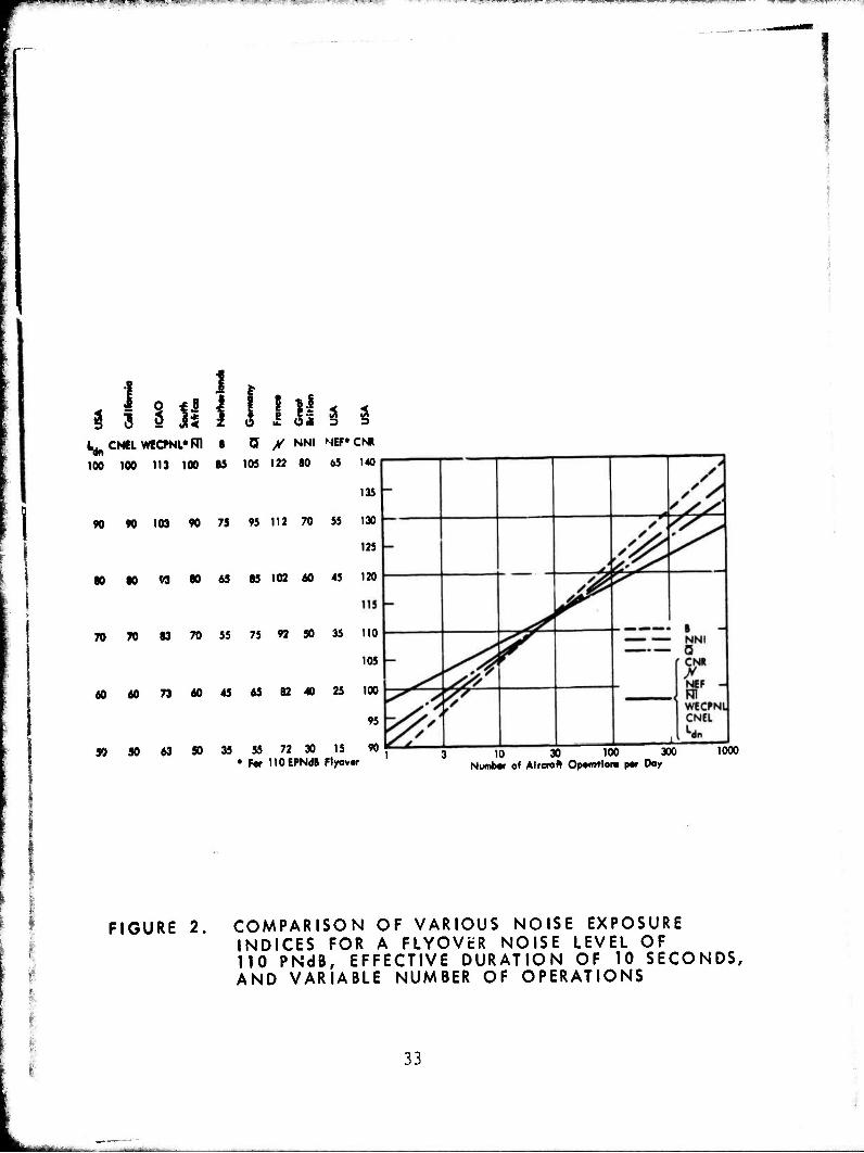
We first identify the most prominent existing noise

rating measures in terms of the elements they consider and

their combinatorial rules used for calculation. A summary of

the various elements and how they are considered in a number

of rating indices is provided in Table II. The great simi-

larity in all their formats can be illustrated by comparing

their equations for the summation of a number of identical

daytime events. Assuming an effective duration of 10 seconds,

a maximum PNL of 110 dB, and that A-weighted sound level is

13 dB less than PNL, plotting these equations as a function of

the number of events, N, provides an illustration of their

similarity. This is shown in Fig. 2, as plotted from the

following equations:

31

»■»^•iw "W""^" ■ « »■■*■■' ■ . I.

V CQ LO l-l TJ

cq + CQ XI CQ

■O \ n cö n O * ■a iH M p j> 0 o L, o o«

.C t-i ■H rH <TS rH in bC + Li + > + +

■H \ <D \ \ \ \

^ "8 a T3 O o o o

>a •H oo •H •H •H •H CO Ll U L. Li Li Q CD L. CD CD CD CD

a 0 iX a a O.

C\J CM CM m CM no

to •o o £ p cu 6 bO c P rt L,

r W

CQ

co 0) L, 3 in rt CD E:

bfl C

■H -P 10

OS

0) CQ

o 2

to 3 O

•H L, CO > C-. o CO 1' p 3 Xi «H L. P P <

2 Z 2 hü O

2 2 2

bObOhOhOhü-H bOhOhOhOhO

o o o o in ro o o o o o _i _l rH r-t rH CM rH

co co CD 0) O

ca co O 01 o >» >5 C

o c

CO CO CD cu

o c

o c

o

co co to CU <D O CD >> >> c >>

CO CO O CD O D C >> C >>

■a r-{

c CD 3 > o 0) W J

J -a ►J X r>

a. £ £ 2

w CO < <c <

< 2

»H J-> ft) cc

2 a.

&, o UJ 14 2 3S

CC V H 2 ^ 2 Ü ^ 2 la

c w T3 Z

2 CQ W

bd Li O <

CO 3

o < < to 2

O c Li tx.

c >» fc c o rt in e -H L, < H cu co rt

CJ !3 O

rt o •H L

<

P 3 O

CO

CO T3 C cti rH L, cu

P O CD CO Z H

P c CD Li 0)

<M CM

•a CU CO 3

CU Li rt

CU > CU

•a c 3 O CO

M C •H c a: > <D

Li O

P £ hO

Li O

CM

CO

m l

< l

P H rH rH rt c s 0) o a i-i

P to 3 O

o <u

CO

Li 0) rt 0> > *

CO

32

Pi» ip KP in u ii m J» i « w" WW^F«. ^■.^■T^T-.n—^s» .^755^

1 4 * 3 3 * 3* I i i Si 3 i

l^CNtl WECPNL'Rl B 3 /NNI NEF'CNR

100 100 113 100 85 105 122 80 65 HO

135

90 90 103 90 75 95 112 70 55 130

125

80 80 W 80 65 85 102 60 45 120

70 70 83 70 55 75 92 SO 35 110

105

60 60 73604565824025 100

95

50 50 63 50 35 55 72 30 15 90 If * For HOEPNdB Flyovor '

10 30 100 300 1000 Number of Aircraft Opomtlom par Day

FIGURE 2. COMPARISON OF VARIOUS NOISE EXPOSURE INDICES FOR A FLYOVcR NOISE LEVEL OF 110 PNdB, EFFECTIVE DURATION OF 10 SECONDS, AND VARIABLE NUMBER OF OPERATIONS

33

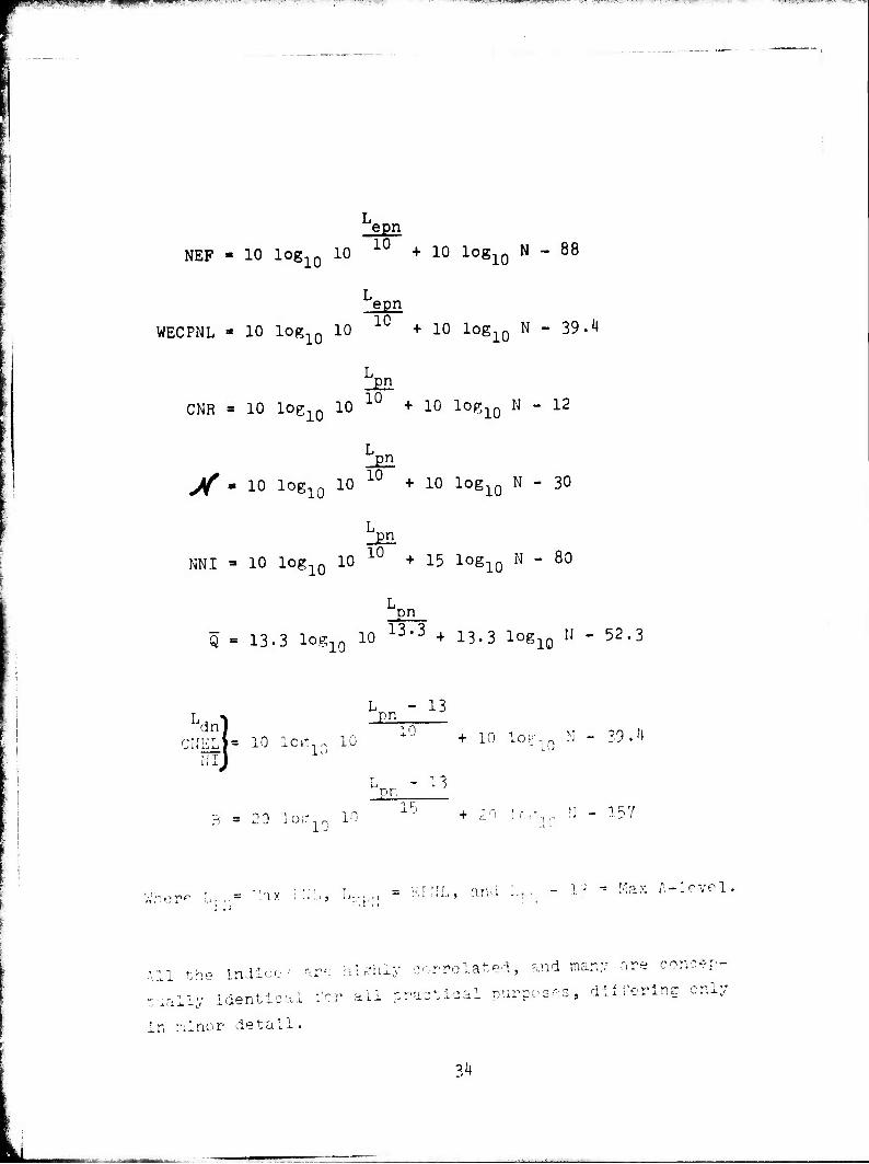
epn

NEF - 10 log1Q 10 10 + 10 log1Q N - 88

epn

WECPNL = 10 login 10 1C + 10 login N - 39. ^ '10 '10

10 CNR = 10 login 10

±u + 10 log Q N - 12 '10

10 X - 10 log1(J 10

iU + 10 log10 N - 30

NNI =

^n

10 log,n 10 10 + 15 login N - 80 •10 '10

Q = 13.3 log1Q 10 13,3 + 13-3 log10 N - 52.3 '10

L - 13 pn

:iiEL)= io iogin io x- +io IOP-10 h iilj

39 . 1\

on - ii lOf'n 10 157

> pr* ' j .= :'l X ' i'i'j

.:,, ana - l - = Max A-level

". ii the indlcc

dually identical

in minor detail.

all c

orrelated, and many are concep- f fart A n<r nn ■s-3, diliering

3^

wmtgrimr,\ir.. ,m i, i agBgp*

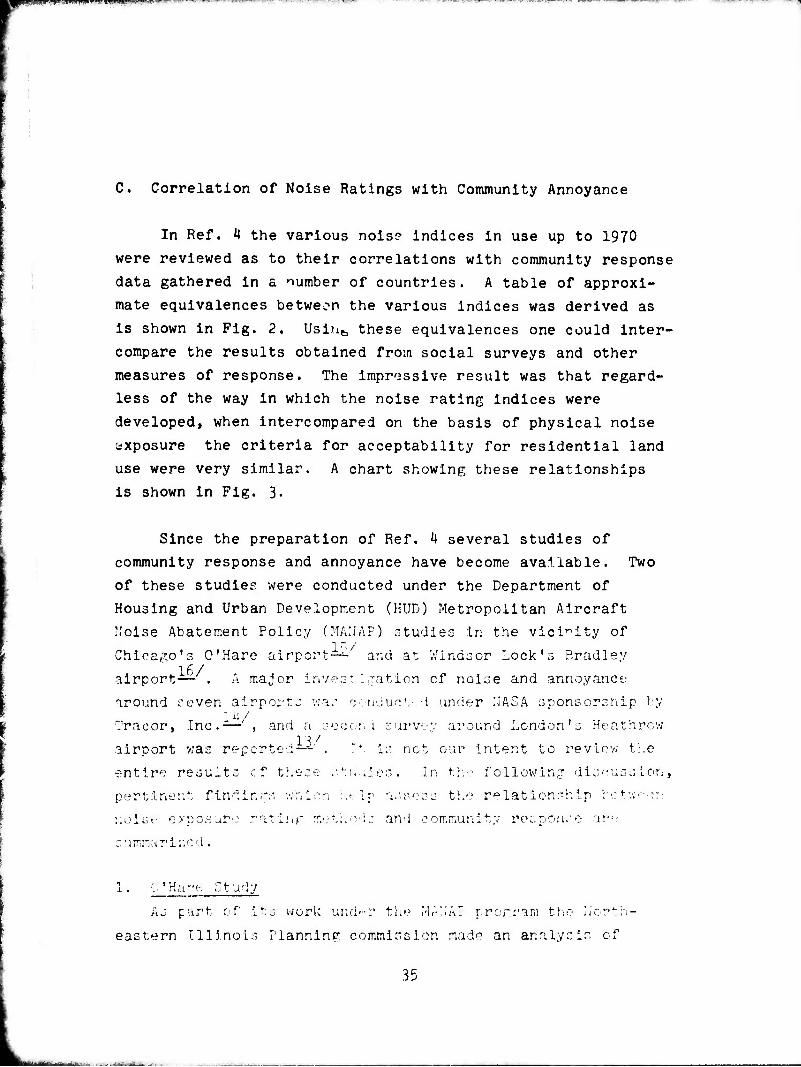
C. Correlation of Noise Ratings with Community Annoyance

In Ref. 4 the various noise indices in use up to 1970

were reviewed as to their correlations with community response

data gathered in a number of countries. A table of approxi-

mate equivalences between the various indices was derived as

is shown in Fig. 2. Usinb these equivalences one could inter-

compare the results obtained from social surveys and other

measures of response. The impressive result was that regard-

less of the way in which the noise rating indices were

developed, when intercompared on the basis of physical noise

exposure the criteria for acceptability for residential land

use were very similar. A chart showing these relationships

is shown in Fig. 3.

Since the preparation of Ref. 4 several studies of

community response and annoyance have become available. Two

of these studies were conducted under the Department of

Housing and Urban Development (HUD) Metropolitan Aircraft

Noise Abatement Policy (MANAP) studies in the vicinity of

Chicago's O'Hare airport—- and at Windsor Lock's Bradley 16/ airport— . A major investigation cf noise and annoyance

around seven airports was conduct-.d under NASA sponsorship by

Tracer, Inc.— , and a second survey around London's Heathrow IV airport was reported—* . ;.t is not our intent to review the

entire results of these studies. In the following discussion,

pertinent findings which \tt in assess the relationship between

noise exposure rating method: and community response are

summarised.

1. O'Hare Study

As part of its work unch-r the MAMAF program the North-

eastern Illinois Planning commission made an analysis oT

3 C

ffUfi'tiYfirT i "lii n

tu U

13-

•r

!-

'ucj Butt!"!*!

8 o

_L m 10 s m

-•H»I"»V.

o m ID 3 in

m O in

m o m « °

«IWiOlN

.»)qOi.|01u| <m»3t OJuoAOguy,.

s m m 8 in o

_L in 8 9

o z UJ oc 3 to

o o. X UJ

tu

oz zo zt UJ "^

*UJ

■Bu|P||"0, lOW^PI»! «N

to UJ

in oo S

«|"C *MP|I"« |0|»*P|»o,

•p«t.»|t~l «V Mjmoo*

u<>la«xKlKS punej

'lil OU02 °* ««puftoo, »HI JO *4|u|3|A W| l|D4|dWK »ON «N l<*t *IUO|4S|i|»l| ON

in ID 8

_1_ in in 8

>o*i|v Osi ,0 oiom

o o

-ouuoojdpufto^ 0|onbopy D| 13o!q"t fOlodJflrf

|0||U00|I0| JOJ uO||3fUj«UO-

in en

o 0>

•pop|0»y

• fj 04 l|UOuiÖO|OA#0 |Onuopi»ii MN

in CO

■|uo|(3|jjW]j OUjP|,nj ON

pooootj 04 ««ivy uojuv 8no<3 jOOUOOOO^ 'I4*|0|ÖW03 IflOiOOIA 'ponjoooa| OKI™! *|»1I1 »I1»* "on*»» |ono|«|pu||

S _1_ _L

s s

Uinpiio« 04I )0 «III«»'» O|0MOD itii/» «||wo|io«o '»l»W

■i«*o»OH '"«w ol|oN Oil rotooonj o| p|"ow nu|0|dwii3 ON *MO||uo*l3

m 01

-UO||on||{

•m t0 l|»*|onv 0I0|0**>5 o |00*44|M uo 0O|uoj H PI"«M$ '*"5 AU* »• I

UO|P-mao3 Ouiptl"« »N '<llAlt»V ON ^lOin Orf> NiiO|QOJ4 #«|ON I«>I*S |

•uojioniij •■*, jo i|*'|nuv

D Oi|y t| U0|*3v dnojr) p«|M»uO"^ PU» .|U(0|rl'.«.n;j ■*«:(|Alpy ••**>$ i|4|V MJ94MI *o« «I^N

pae *jfl|»oj »JO (,u]D|divvj »»JON »"-^^

8 in

<< >J

oo UJ

UJ Ujl/»

►-Z <o —10 XUJ

o-Z <<

UJ

Di D Ü

36

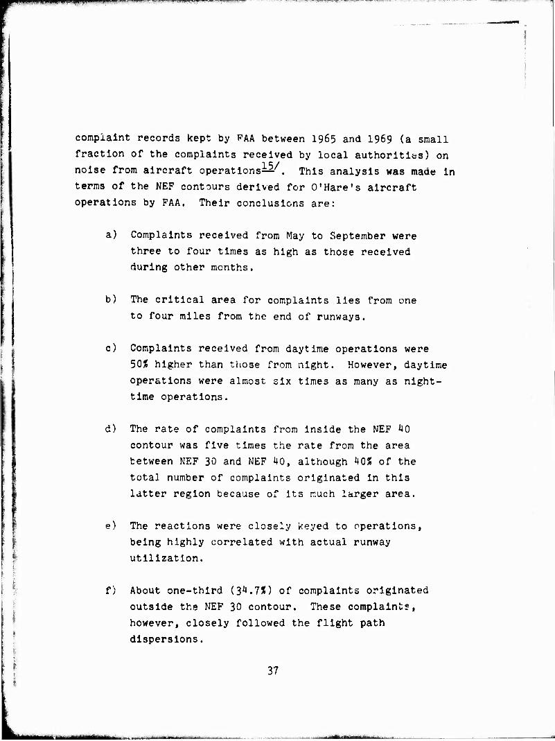
complaint records kept by FAA between 1965 and 1969 (a small

fraction of the complaints received by local authorities) on

noise from aircraft operations^- . This analysis was made in

terms of the NEF contours derived for 0'Hare's aircraft

operations by FAA. Their conclusions are:

a) Complaints received from May to September were

three to four times as high as those received

during other months.

b) The critical area for complaints lies from one

to four miles from the end of runways.

c) Complaints received from daytime operations were

50$ higher than those from night. However, daytime

operations were almost six times as many as night- time operations.

d) The rate of complaints from inside the NEF ^0

contour was five times the rate from the area

between NEF 30 and NEF 40, although HQ% of the

total number of complaints originated in this

latter region because of its much larger area.

e) The reactions were closely keyed to operations,

being highly correlated with actual runway

I utilization.

1 I f) About one-third (3^.7$) of complaints originated

I outside the NEF 30 contour. These complaints, f

however, closely followed the flight path

dispersions.

I 37

K

-—- ----"-'-

WP1WT»T»—»»W um.» mir—m n ^nii »w^ipuM ■■ I ■■ » ■ ■ ■" . I«<IP«O ' IP—'- w ' ■'■ i. I I ■ ■- -■ ■ .■■■-- II II I III! »^

2. Bradley Study

Another study under the MANAP program conducted by the

Capitol Region Planning Agency in the vicinity of Bradley

International Airport is particularly revealing—. As part

of this program, a questionnaire survey was conducted to

obtain 790 respondents' attitudes about aircraft noise. A

sampling distribution was used to cover residents in NEF

zones of 25 and higher, plus control areas which were outside

the NEF 25 contours but still relatively close to tne airport

The correlations were made to 1967 contours, which, due to

unreliable operational data, were later found not to depict

turning flight paths accurately, but were still believed

satisfactory at the higher NEF value;. Pertinent conclusions

from this survey are:

a) The percentages of response indicating that

aircraft noise was extremely disruptive, by

class of operation, in different NEF zones

were:

NEF Military Air Carrier Gen. Avn.

40 75 30 10

35 r;'0 18 2

3n 28 10 3

25 IS 11 3

Oper ati ons (ai iprox in-it, ?ly U -.0,0 J u i n 1969)

were 5^2» general aviation, 39* air Carrier

(all Jets, 90% turbofan), and 7% military

(of which almost half were F102's).

38

i-'MWPfygp f^mm^mmfW^SS^S^ -IHP? 'srfS3!S7"?^:, .3fC"^.,ii ..^| im^JijMii ß !>UPP. V. »^ i^TTP??^«!?',^:"---- ^'v*^- '

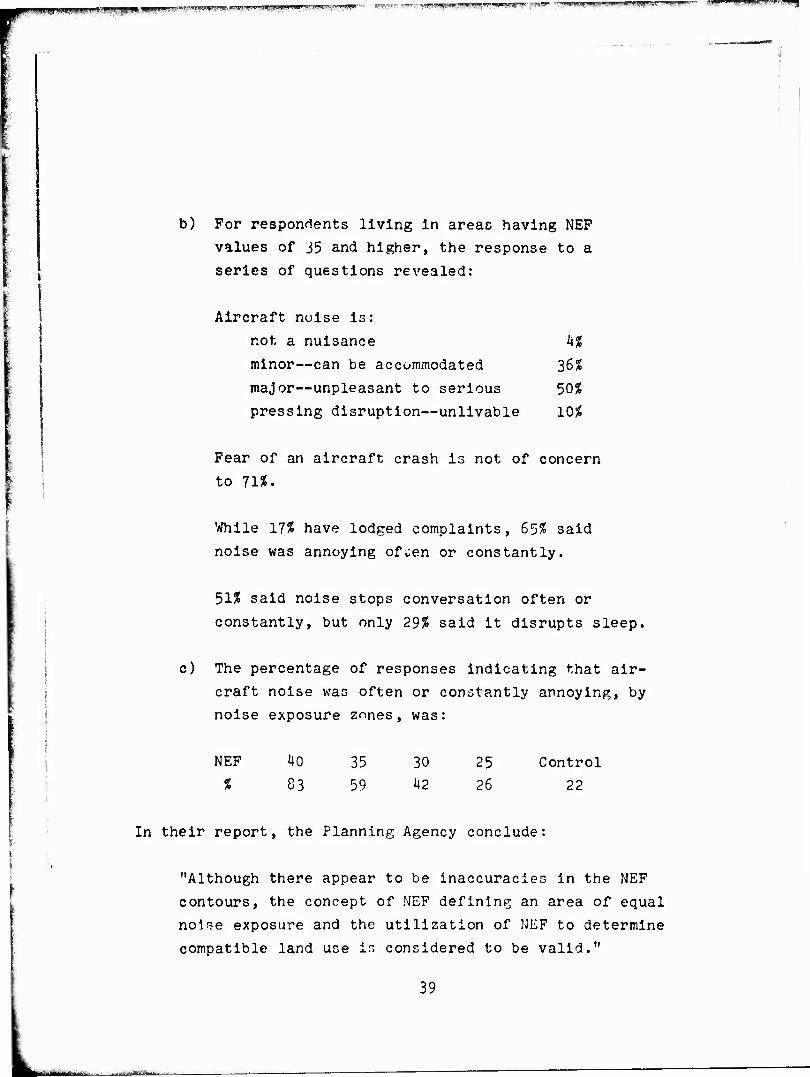
b) For respondents living in areas having NEP

values of 35 and higher, the response to a

series of questions revealed:

Aircraft noise is:

not a nuisance k%

minor—can be accommodated 36%

major—unpleasant to serious 50%

pressing disruption—unlivable 10/S

Fear of an aircraft crash is not of concern

to 11%.

While 17% have lodged complaints, 65% said

noise was annoying ofuen or constantly.

51? said noise stops conversation often or

constantly, but only 29J& said it disrupts sleep.

c) The percentage of responses indicating that air-

craft noise was often or constantly annoying, by

noise exposure zones, was:

NEF kQ 35 30 25 Control

% 83 59 12 26 22

In their report, the Planning Agency conclude:

"Although there appear to be inaccuracies in the NEF

contours, the concept of NEF defining an area of equal

nol*e exposure and the utilization of NEF to determine

compatible land use Is considered to be valid."

39

■pfqppnc^of^f 4,iiJri|Hi,|...^JT»lfcWW**L

3. Tracor Study

An intensive, three-year study of noise exposure and

annoyance due to aircraft noise was completed in 1971 by Tracor Ik/ under NASA sponsorship— . This program surveyed communities

around the major airports in Boston, Chicago, Dallas, Denver,

Los Angeles, Miami, and New York. A total of 8207 interviews

were obtained, and noise exposure data at the interview areas

was obtained from the analysis of more than 10,000 aircraft

flyovers. Whereas the two studies mentioned above we^e

concerned only with assessing certain conditions occurring

within various NEF regions, the Tracor program was a general

study to model annoyance.

Among the general conclusions from this program were:

a) CNR, NNI, and NEF are essentially interchangeable

in predicting annoyance.

b) General estimation of annoyance frcm noise exposure

alone provides correlation coefficient? of the

order of 0. -U to 0.5; the addition of attitudinal

variables to the model predicts individual annoy-

ance with a correlation coefficient of up to 0.8

These additional factors are also intercorrelated

with noise exposure in most instances.

c) A significant reduction of annoyance requires a

CNR of 9 3 or less; above 107 CNR, annoyance

increases steadily; above 115 CNR, noise exposure

is associated with increased complaint.

d) The number of highly annoyed households in a

10

^lV?iywf!r~:;-'ry^ • ■'■?

community can, within certain limits, be predicted

from the number of complainants. Complainants are

not more sensitive to noise than random respondents.

Complainants tend to come from higher socio-economic

status than non-complainants.

The results of this program are expressed in terms of a

model for predicting individual annoyance when exposed to

aircraft noise. To apply the model, however, *.t is necessary

to conduct a social survey in the community of concern to

ascertain the attitudinal characteristics necessary for use

in the model. These characteristics include fear of aircraft

crashes, susceptibility of noise, positive or negativeness

about air transportation, degree of confidence that authorities

are trying to solve noise problems. Unfortunately, exercising

the model in a land use planning procedure is not feasible in

most instances, since the cost of a social survey is generally

prohibitive.

The mass of data obtained from this project permits many

analyses to be made. Two pertinent relationships can be

established which relate directly to the use of noise exposure

predictive techniques as estimators of community response.

One is related to the correlation of percent of people highly

annoyed in a population exposed to differing decrees of noise

exposure; the second correlates the percentage of highly

annoyed in a population to the number of complainants.

Borsky— has reviewed the Tracor data of Ref. 1*4 and present?

population percentages annoyed as a function cf noise level,

fear, and misfeasance. On the basic of this analysis i working

croup of the Bloacoustics Panel of the Interagency Transporta-

tion Noise Abatement Program (ITNAP) derived various values of

Hi

fg^M^yy fw1^ ^fm^gmmpmf>

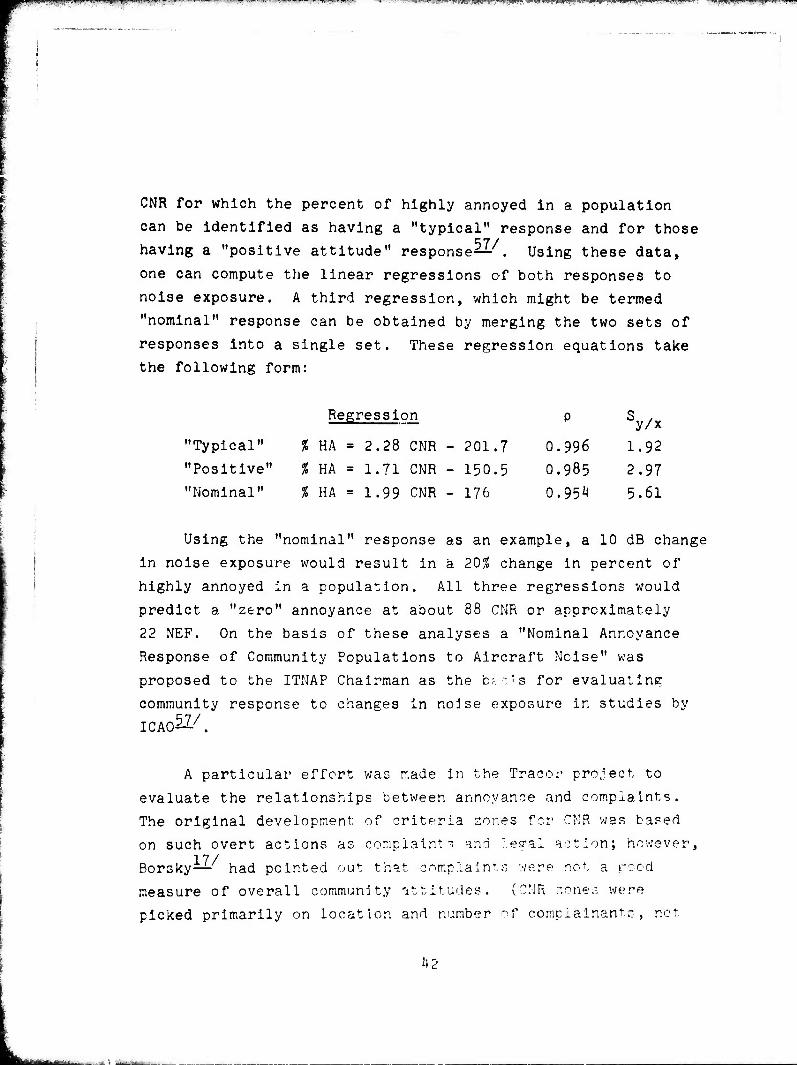
CNR for which the percent of highly annoyed in a population

can be identified as having a "typical" response and for those

having a "positive attitude" response—. Using these data,

one can compute the linear regressions of both responses to

noise exposure. A third regression, which might be termed

"nominal" response can be obtained by merging the two sets of

responses into a single set. These regression equations take

the following form:

Regression P Sy/x

"Typical" % HA = 2.28 CNR - 201.7 0.996 1.92

"Positive" % HA = 1.71 CNR - 150.5 0.985 2.97

"Nominal" % HA = 1.99 CNR - 176 0.95^ 5.61

Using the "nominal" response as an example, a 10 dB change

in noise exposure would result in ä 20$ change in percent of

highly annoyed in a population. All three regressions would

predict a "zero" annoyance at about 88 CNR or approximately

22 NEF. On the basis of these analyses a "Nominal Annoyance

Response of Community Populations to Aircraft Noise" was

proposed to the ITNAP Chairman as the c^-'s for evaluating

community response to changes in noise exposure in studies by ICA()5jy.

A particular effort was made in the Tracer project to

evaluate the relationships between annoyance and complaints.

The original development of criteria zones for CNR was based

on such overt actions as complaints and legal action; however, 17/ Borsky— had pointed out that complaints were not a rood

measure of overall community attitudes. (CNR zones were

picked primarily on location and number of complainants, not

Ü2

• f f tit* 'riiftiVr-

wg/f^mgjgggmi^ißllgBfi/mgBm. ii»B!g^gjffwwiwH»PBppjB■ s» I I*I™Jim*^ßiA.mu<mm*<mw*!s*>Qi-*J>wipg^ ■^■pspiiBaRiBiSHaw

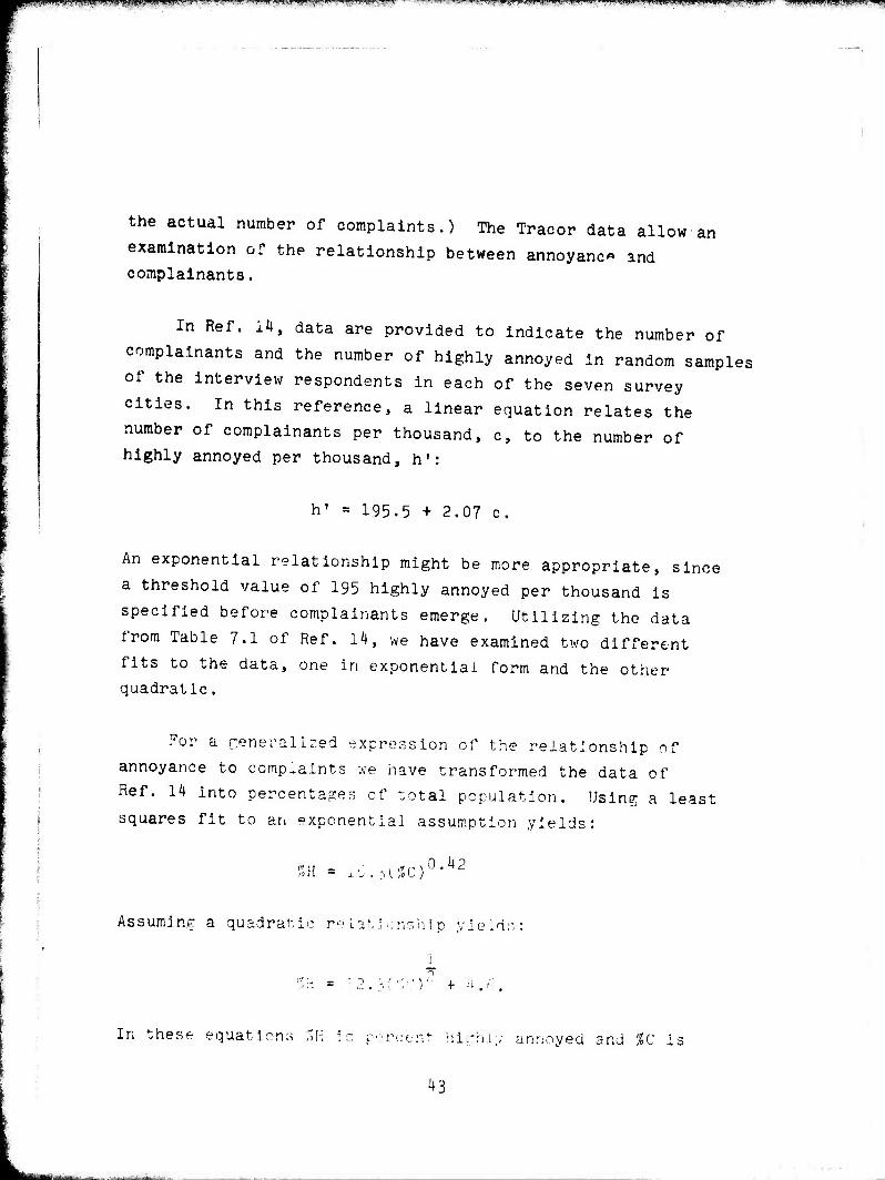
the actual number of complaints.) The Tracor data allow an

examination of the relationship between annoyance and complainants.

In Ref. 14, data are provided to indicate the number of

complainants and the number of highly annoyed in random samples

of the interview respondents in each of the seven survey

cities. In this reference, a linear equation relates the

number of complainants per thousand, c, to the number of

highly annoyed per thousand, h':

h' = 195-5 + 2.07 c.

An exponential relationship might be more appropriate, since

a threshold value of 195 highly annoyed per thousand is

specified before complainants emerge. Utilizing the data

from Table 7.1 of Ref. 14, we have examined two different

fits to the data, one in exponential form and the other- quadratic .

For a generalized expression of the relationship of

annoyance to complaints we have transformed the data of

Ref. 14 into percentages of total population. Using; a least

squares fit to an exponential assumption yields:

0 U ? .oil = i'jOti'U

Assuming a quadratic relationship yield;;:

SH =12.3(";cr: f a.,;.

In these equations %\i ic percent highly annoyed and %C i«.

43

iPP9ps*8imfP9 jiBbjf.'wiiwp1-. i iw v "i'i' ■^ *™T.'«y' *WX*KtWj! ^!7f.-"T

percent complainants. The correlation coefficient for the

exponential form is 0.96 and for the quadratic is 0.98. We

prefer to use the quadratic form because of its simplicity

of use in computation and interpretation.

Subsequent to the publication of Ref. 14 a second study 7 Pi /

of two smaller cities was performed by Tracor— . In this

report the data from the first seven cities were combined

with the additional two, and a revised regression equation

derived, now using the quadratic format. In this case, a

forced fit to zero complaints at zero annoyance resulted in

the following expression for percent annoyed as a function

of percent complainants:

%H = 14.3 /C~

We prefer the assumption we made previously that, with

no complaint action at all, there will still be a residual

annoyance. Using this approach to the nine city data

marginally changes the expression we derived above to:

%\i = 12.3 /C~ +4.3

The correlation coefficient changes only slightly, from 0.975

to 0.984, hardly significant, while the standard error

improves slightly from 3.50 to 3.20.

This equation, with the data points from which it was

derived, is shown in Fig. 4. Acknowledging the inherent risk

in extrapolating these data beyond their experimental values,

it is Interesting to note that the equation would indicate

that at zero complaints, 4.3% of the population would still

44 \

p^Bpp^sgjppg' ■■-» apfws ■*■'■■ ■ppffil' I -''* Ü5H

I <

O) X

#

70

60

50

40

30

20

10

J. /

i

h

J-

/

/

^:

/

v /

/■

;^

% HA = 12.3\/"%C + 4.3

r = 0.98 S , = 4.1 y/x

• A

10 15 % Complainants (C)

20 25

FIGURE 4. PERCENTAGE OF HIGHLY ANNOYED AS A FUNCTION OF PERCENT COMPLAINANTS- DATA FROM TRACOR TABLE 15

H5

gpi^pppqgp^p^^g^ipnupi *W^*T^i1»^;/1*!^^?? VKIW 'h 4;"-'^w".'^r p"^ ■-' '"??■ J»r»Bariff ■»;»■*■

be highly annoyed. Also, with 100!? of a population highly

annoyed, only 61$ would be expected to complain. Said another

way, the percentage of highly annoyed in the population

increases with the square rout of the number of people who

complain. Note that, as originally considered in the CNR

development, it is the number of different individuals lodging

complaints, not the number of complaints that count, since

individuals who complain are often repeat complainants.

Using the two relationships derived above, one can esti-

mate the percentage of highly annoyed for a specified noise

exposure, and from this anticipate the number of individuals

expected to lodge complaints. This is particularly useful in

assessing the possible change in community response to be

expected from operational changes at an airport such as the

use of new runways, altered flight paths, introduction of new

aircraft, and other factors which affect noise exposure.

4. London Study - 1967

One of the most extensive social surveys of response to

aircraft noise was performed around London's Heathrow airport

in 1961. This survey led directly to the NNI rating proce-

dure now in use in England. The rapid increase in jet

aircraft traffic after 1961 and the introduction of the turbo-

fan engine have produced major changes in noise exposure

around Heathrow. In order to assess the changes in both the

noise exposure and the community response to these changes,

a combined noise measurement program and social survey were

made in 1967, although the results first became publicly

available in 1971^/.

The 1967 survey was more extensive than that of 1961.

ne

«Plllü'ii"1*«!* Pipv^isipiQPWfllPVqB^i^ippip ^j^^^A^: J^li^.^

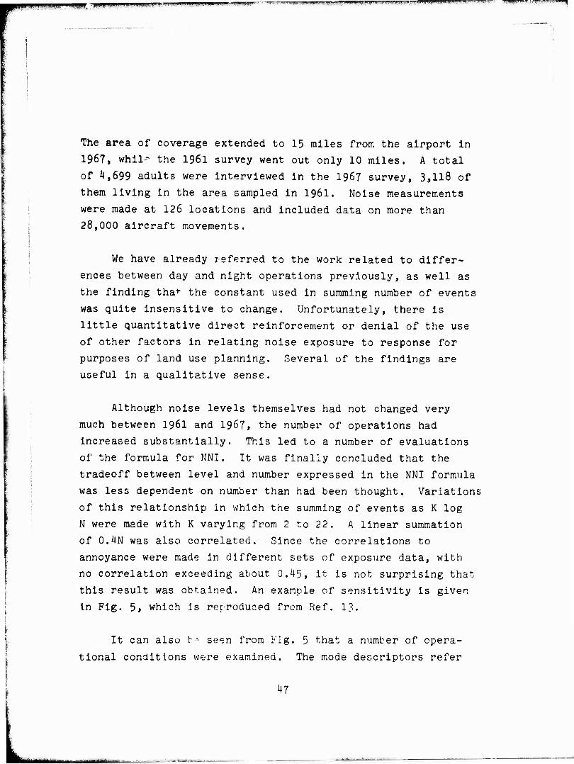
The area of coverage extended to 15 miles from the airport in

1967, whil^ the 1961 survey went out only 10 miles. A total

of 4,699 adults were Interviewed in the 1967 survey, 3,118 of

them living in the area sampled in 196I. Noise measurements

were made at 126 locations and included data on more than

28,000 aircraft movements.

We have already referred to the work related to differ-

ences between day and night operations previously, as well as

the finding tha^ the constant used in summing number of events

was quite insensitive to change. Unfortunately, there is

little quantitative direct reinforcement or denial of the use

of other factors in relating noise exposure to response for

purposes of land use planning. Several of the findings are

useful in a qualitative sense.

Although noise levels themselves had not changed very

much between 1961 and 1967, the number of operations had

increased substantially. This led to a number of evaluations

of the formula for NNI. It was finally concluded that the

tradeoff between level and number expressed in the NNI formula

was less dependent on number than had been thought. Variations

of this relationship in which the summing of events as K log

N were made with K varying from 2 to 22. A linear summation

of O.JJN was also correlated. Since the correlations to

annoyance were made in different sets of exposure data, with

no correlation exceeding about 0.45, it is not surprising that

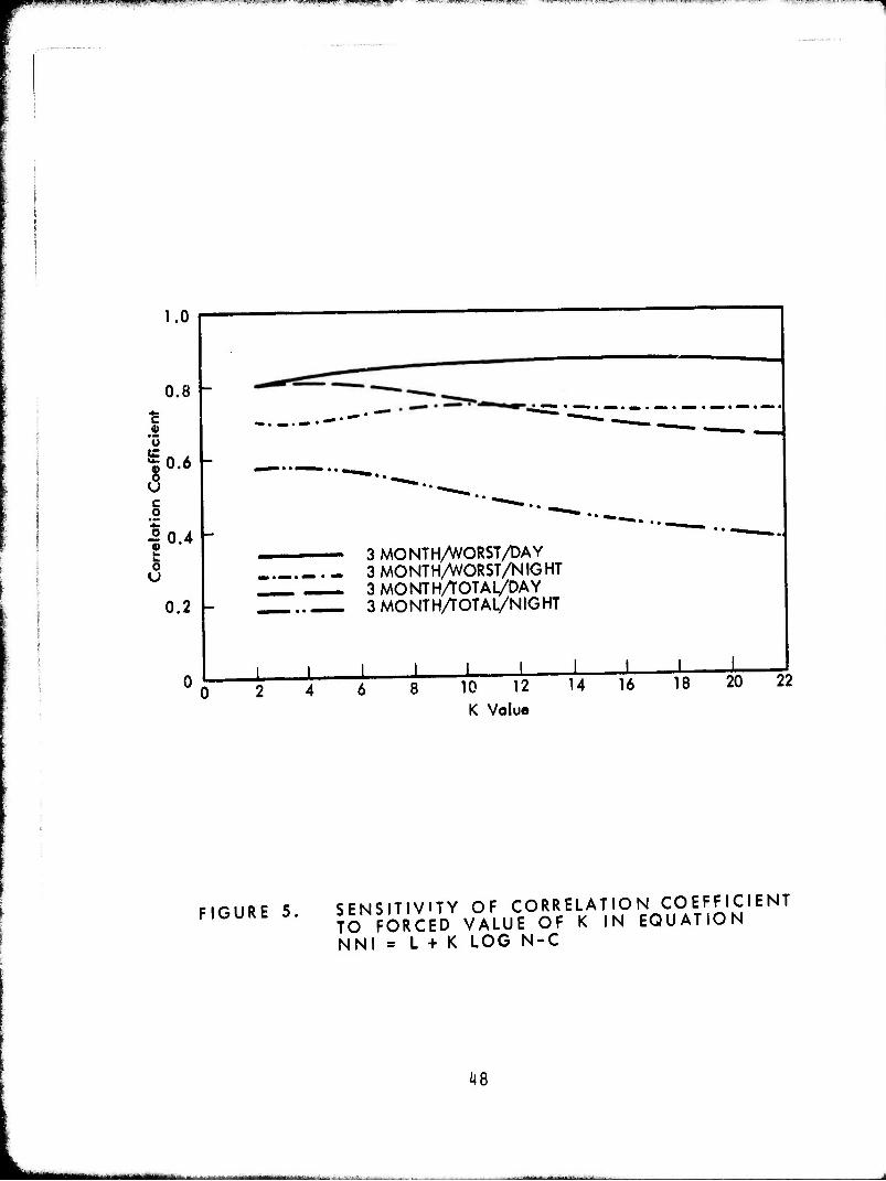
this result was obtained. An example of sensitivity is given

In Fig. 5, which is reproduced from Ref. 13.

It can also t-- seen from Fig. 5 that a number of opera-

tional conditions were examined. The mode descriptors refer

kj

ttm .Truii win run m

p »««im ui> i.i ii ii in*» .in »,ii,..iJUj,„jjiT«?'i'»!R,iiiiip»ji. ^mmmtfm? 9.9 .^A--J^=* -^J^i^p.*M" I'.J-. ?*4/w ! -

1.0

0.8

c .2 '5

1 1

|0.« 1 U

c 1 .2 ;] '£ 1 f -5 0.4 f w

i_ '■ O

<J

0.2

) • «■■» • 4

3 MONTH/WORST/DAY 3 MONTH/WORST/NIGHT 3 MONTHAOTAl/DAY 3 MONTHAOTAL/NIGHT

1 10 12

K Value 14 16 18 20 22

FIGURE 5. SENSITIVITY OF CORRELATION COEFFICIENT TO FORCED VALUE OF K IN EQUATION NNI = L + K LOG N-C

48

i miiaiB ■ IHH j ~ ■■-■ : i

- (ftjui m$ mmm *-***r?*?e ? F ^nnp^^g9^9RPl —^

to the three basic traffic structures which are due to wind

conditions. These modes are East to West - 7958, West to East -

1955, Northeast to Southwest - 2%. The designation "total mode"

refers to the average noise exposure at a given survey location

over all modes; "worst mode" relates to the highest exposure

mode in each sampled area. It was concluded that the "3 month/

worst mode/day" exposure was most highly correlated with

response. This implies that response is best correlated to an

average over periods of time when the most active operations

occur. This is similar to the "average busy day" concept in

the present USAF procedure. As discussed previously, the

night exposure is so substantially l^wer than the day exposure

that it is not surprising that daytime should be the control-

ling condition.

Some of the conclusions arrived at in measuring annoyance

are of specific interest here. They include:

if a) Respondents' self ratings to one of the survey

questions, a category scale of annoyance, were

0.77 correlated with th<* Guttman scale derived

from the survey to express annoyance. The word

descriptors used in assessing the numerical values

of the derived annoyance scores are taken from

this simple scale of self rating.

b) Middle class respondents tended to have higher

annoyance scales than working class respondents.

c) In 19bl those claiming to feel afraid of aircraft

crashes "very often" were l^% of the survey; in

1967 this had dropped to 9%.

49

PdM mmm/mmne ■** gn .«fnwppp

d) Mean annoyance scores were almost identical in the

two surveys. The point on the scale considered

critical in terms of acceptability was the same

in both surveys (between 3 and h on the annoyance

scale which ranges from 0 to 5).

e) Assessments of acclimation to aircraft noise

revealed that the majority of people acclimate

at low noise levels, but this proportion drops

markedly with increasing noise level. Further,

at the higher noise levels those living in the

area longest tend to be more highly annoyed.

f) An investigation of the ratio of landings to

all other movements showed that inclusion of

this factor as a separate element in the NNI

formula was not justified.

g) Investigations of the separate effect of duration

were inconclusive. Since duration was measured

at the time the noise level exceeded 80 PNdB,

regardless of its maximum level, the confusion

in results is not surprising.

h) While not conclusive, there is some eviience

that the higher the background level, the ]ess

people are annoyed by aircraft noise, e.g.,

signal level to background level is of seme

importance.

50

■:*-»« I '.WiUV'*«:'^

5• Generality of the Relationship Between Average Annoyance

and Noise Exposure

In Section II-C-3 we showed how the results of the Tracor

data could be used to derive an expression for the percent of

a noise exposed population that would be highly annoyed as a

function of the noise exposure. It is of interest to examine

how well this relationship can be applied to the results of

other surveys. Two such evaluations, conducted simultaneously

in recent months, have been published.

In one study, a task group of the EPA Study of Aircraft/

Airport noise reviewed the various U.S. and English survey

results and showed that the relationship between percentages

of population highly annoyed and noise exposure were essentially

identical when compared on a common noise measure— . In the

second study Alexandra compared the results of the two English

surveys, the Dutch survey, and two French surveys, one completed

in 1972, to obtain a general relationship between annoyance 69/

and noise exposure for the aggregated results— .

These twu evaluations gave almost identical results and

confirm the analysis of percent population highly annoyed

described in Section II-C-3 within a few percent for a speci-

fied noise exposure.

It is reasonable to conclude that the relationship

between percentage of an exposed population highly annoyed

and the magnitude of noise exposure nroduced by aircraft in

flight is well established.

51

D. Noise Criteria for Land Use Planning

In the previous sections we have examined the concepts

of aircraft noise exposure and the efforts to c vrrelate noise

exposure with annoyance. Most of the work is principally

related to residential living. Annoyance is seen tc be a

complex structure of personal attitudes, conditioning

variables in the local env" onment, and interference elements

affecting individuals. These factors are discussed in detail

in the various referenced documents and need not be reviewed

further here. What is of concern is how this information is

reflected in criteria for land use planning.

In its simplest terms our purpose is to derive a means

for estimating the noise exposure fron aircraft operations

and from this infer the kind of functional uses that can be

reasonably acceptable for various values of noise exposure.

The calculation of noise exposure is basically an engineering

procedure to summarize the overall noise environment produced

by a complicated series of noisy event?. We attempt to

express the result;; of this calculation in quantities which

scale as w- 11 as possible to the subjective response of people

For planning purposes we must a^so specify the points along

these scales that provide satisfactory noise environments for

various human activities. The se Led Ion of the.-- points is

in all cases a value judgment on the part of the scale raker.

In essentially all criticism:;, of various aircraf' land use

planning procedures, the heart of the criticisms relates to

the validity of these judgments.

Criteria for estimating acceptable conditions for

residential living have been reviewed In Ref. k . The

~> <:,

* r"r.«w.=»'j.-M»r.;"r*1"'^-"- .*

corresponding criteria used in various countries were examined,

are repeated in Fig. 3 of this report, and are generally found

to be completely consistent with each other regardless of the

technique for their derivation. The CNR and NEF criteria

expressed in Fip. 3 have been resisted for more than a decade

by the civil aviation community, fueled by the variability

obtained in annoyance studies in this country and in the UK.

In developing an updated Air Force procedure we need to con-

sider whether or not there is evidence on which to improve or

alter the existing criteria.

Much of the criticism of the CNK and NFF criteria values

revolves around the low correlation (0.4 to 0.5) of specific

values of CNR or NEF to scales of Individual annoyance as

obtained in the social surveys. The argument is that this

casts doubt on the entire approach since the low correlations

indicate that individual annoyance is not accurately predictable

from noise exposure. For planning purposes this question is

just reversed from the order of interest. What should be asked

is, given a value of noise exposure. ...-.at can be said about the

expectation in average response and compatible land uses.

All social surveys reported in Ref. 4 show that the higher

the aircraft noise exposure, above some relatively low threshold

level, the higher the disturbance. The more recent studies

reviewed in the previous section *"ot only substantiate the

general trend, but, in the case of the Tracor studies, allow

a much better quantification cf expected annoyance for a given

noise exposure. The Tracor work allowed a derivation of both

percentage of highly annoyed in a population and the expected

percentage of complainants for a given noise exposure. On this

basis, the 100 CNR value, which sets the boundary below which

aircraft exposure noise will be tolerated in the present.

53

W^FW^ ■■■■■■■■ ■■■-■■- ~~7r ^7^-=;-v^<^3^e'"- ■:y~?-??™-?~'-'*-^* VI^r- -j'-'^"^"'-?'.■* IT-M^ vwirfT^rr 'w^JWMT:*!'^^^.' ■ MM""

criteria, corresponds to a population where approximately 20!?

of the people would be highly annoyed, but only a few percent

or less would complain. The subsequent analyses reported in

Ref. 68 and 69 extend the validity of these results by showing

the combined analysis of surveys in four countries give

essentially identical relationships between noise exposure

and average annoyance of a community. The correlation coef-

ficients between population average annoyance and noise

exposure are in excess of 0.95, even though much noise vari-

ability is obtained for individuals. For land planning purposes,

it is the population average response that is of primary interest

The words currently associated with exposures of 100 CNR

(30 HEP) or less are:

"Essentially no complaints would be expected. The

noise may, however, interfere occasionally with

certain activities of the resident."

At the point of 115 CNR (40 NEF) the Tracor data allow a

prediction of about 50% highly annoyed in the population, with

about 15% complainants. The words in the CNR-NEP criteria for

noise exposures of this value and greater are:

"Individual reaction." would likely include repeated,

vigorous complaints. Concerted group action might

be expected."

In the light of the Tracor data one might conclude that the

words associated with the present CNR-NEF criteria, if

anything, might be understatements.

54

■BSWWW.W rrmrj-z.TJwryrrrriT -;'•; "■"*■*" ^^S*5 ■'"'" 7? v-.v-p-;;'^^-':-?1:-^/''■;.;-

One of the criticims of the present CNR-NEF criteria is

that the contours of noise exposure do not adequately reflect

the noise problems at civil airports. While part of these

criticisms are due to the precision of obtaining contours

(standard deviations of + 2 units between measured and pre-

dicted values are typical, with total deviations of + 5 units

possible when inadequate operational data are used), most have

to do with whether the community response is adequately de-

scribed by the criteria. Interestingly enough, the direction

of this criticism is opposite when it comes from social

scientists as compared to airport operators. There is a

growing sentiment among some social scientists that community rg/

attitude is underestimated by the present criteria— . On the

other hand the airport operator's definition of "noise problem"

has to do with whether he will be able to continue his airport

operations in their present form. He is thus concerned with

whether the criteria overstate the severity of aircraft noise,

particularly if the criteria become public policy statements—- .

The obvious dichotomy between the social scientists and

the airport operators has to do with the complexities of how

an annoyed population can exert it;- feelings through public

action. Since the purpose of a land use planning procedure is

to evaluate compatibility of noise exposure with land use, not

to resolve the public administration issues, the above criti-

cisms should be recogni. but not arbitrarily used to change

the present criteria wl.'c:. seem to reflect reasonably accurately

the data on community acceptability.

Present criteria for residential use were derived from a

broad spectrum of communities and tend to integrate over the

variations in social and economic factors existing in many

55

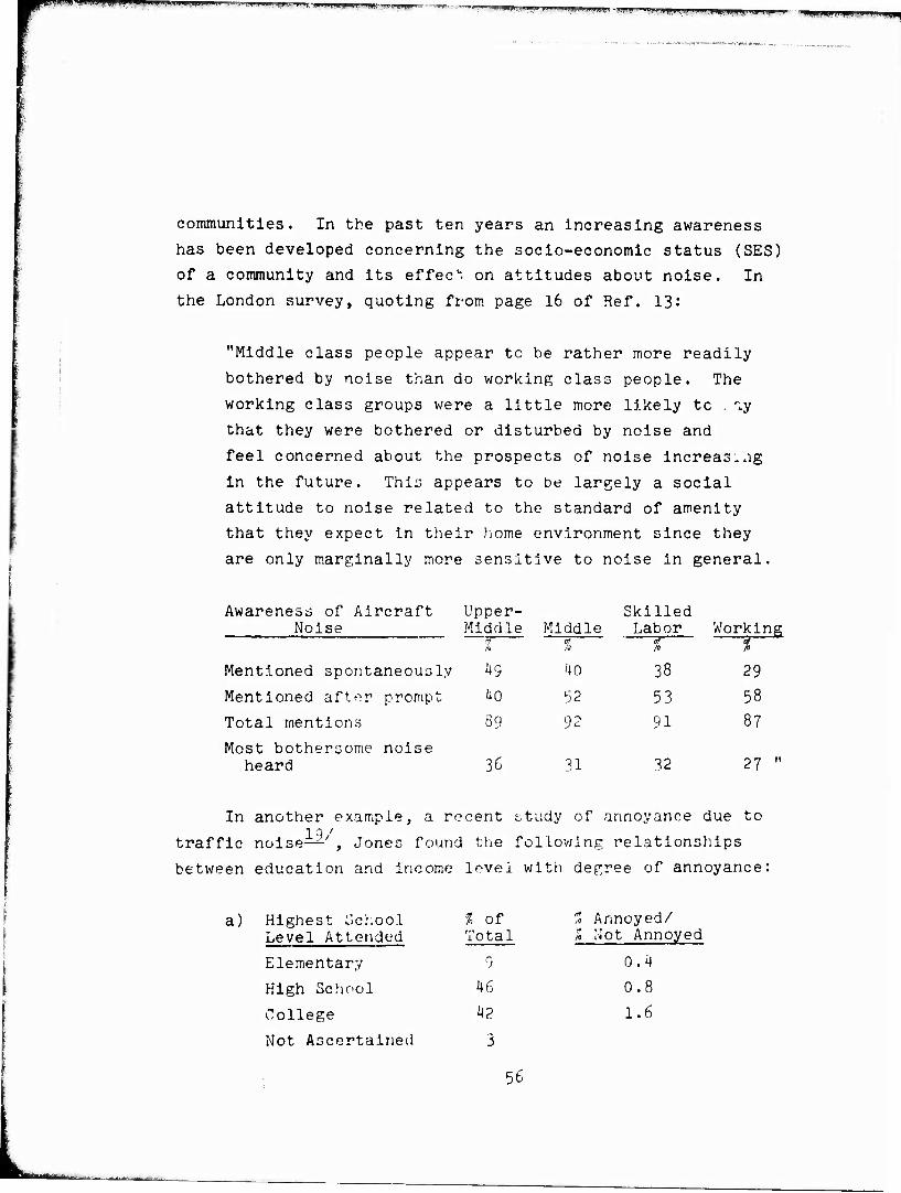
!WM!LJ»lllH!iy.,J.lJIL _ __

mi

communities. In the past ten years an increasing awareness

has been developed concerning the socio-economic status (SES)

of a community and its effec1-, on attitudes about noise. In

the London survey, quoting from page 16 of Ref. 13:

"Middle class people appear to be rather more readily

bothered by noise than do working class people. The

working class groups were a little more likely tc . ly

that they were bothered or disturbed by noise and

feel concerned about the prospects of noise increasing

in the future. This appears to be largely a social

attitude to noise related to the standard of amenity

that they expect in their home environment since they

are only marginally more sensitive to noise in general.

Awareness of Aircraft Noise

Mentioned spontaneously

Mentioned after prompt

Total mentions

Upper- Middle Middle

at

Skilled Labor

% Working

i 49 40 38 29

40 52 53 58

39 92 91 87

Most bothersome noise heard 36 31 32 27

In another example, a recent study of annoyance due to i q /

traffic noise—' , Jones found the following relationships

between education and income level with degree of annoyance:

a) Highest School Level Attended

% of Total 1*

11

Annoyed/ Not Annoyed

Elementary 9 0.4

High School 46 0.8

College 42 1.6

Not Ascertained 3

56

b) Those with annual income closest to $5,000 were

0.7 as likely to express annoyance as the sample

whole; those with $25,000 were twice as likely

to express annoyance as the sample whole.

In a further example, Galloway was able to increase the

correlation between annoyance and noise exposure from about ■I Q /

0.5 to 0.9 by weighting responses with SES considerations—.

Notwithstanding the increasing evidence that expressed

annoyance scales with SES, it does not appear prudent in a

general planning procedure to provide explicit adjustment

factors for SES. It would be a difficult political decision

to argue that people of high SES should have lower noise

exposure than those of lo^'e. SES. Nevertheless the planner

should be made aware that within any specific community the

variance in response obtained from a given noise exposure,

as compared to present criteria, may be directly related to

SES variables.

Looking at criteria from a national policy position, the

Department of Housing and Urban Development (HUD) has reviewed

noise criteria for a variety of land uses. Prior guidance

with respect to the suitability for residential use of land

exposed to aircraft had been provided by the Federal Housing

Administration in terms of the CNR-NEF criteria. The suit-

ability of these criteria has been reaffirmed, with their

applicability broadened to Include all HUD programs in HUD

Policy Circular 1390.2 of August 1971. This policy provides

for local approval of projects exposed to values of CNR less

than 100 (NEF less than 30); requires an environmental state-

ment outlining noise control measures for projects in CNR

57

gPPSPRi^JJI^yj*.^ ^ :■-■ •*<*■**■■■ '■^«r^-.*-utAi^"-»^ w•■■,■;pynM^^K»^1 w».»^ww ■ n«im*y ■JJIA'HIUMBJI,IufImm

regions of 100 to 115 (NEF 30 to 40), plus concurrence of •••:;■» Regional Administrator; and at higher noise exposure reoui.. .s

approval of the Secretary for any exceptions—stating that

such exceptions are strongly discouraged.

While much of the effort to develop criteria for use in

noise exposed areas has been directed to residential appli-

cations, it has been recognized that there are also other land

uses having various sensitivities to noise exposure, e.g.,

school, churches, places of public assembly. In most of these

situations one can examine the influence of aircraft noise

primarily in terms of its effect on speech communication within

the spaces involved rather than on the more complex measure of

annoyance. The suitability of a school room, for example, is

determined by how well the teacher and clcss can tolerate

Interference with their ability to communicate. Methods have

been developed to assess speech communication in the presence

of aircraft noise for a variety of functional purposes, con-

sidering the spectral characteristics of aircraft noise,

typical building construction, and the importance of speech

intelligibility. Such guidelines are provided in Ref. 4, in

terms of NEF exposure units, for a wide variety of uses,

identified by codes from the HUD standard Land Use Code manual.

This information is reproduced here as Appendix B. The same

information has been adopted in the recent HUD Planning Guide- 70/ lines for Local Agencies-1— .

Recommendation Ho. 5 - Adopt the land use compatibility

guides and noise compatibility interpretation guidelines

specified in HUD report "Aircraft IJoise Impact: Planning

Guidelines for Local Agencies— .

58

jMjISHgpWfiMWPliPBP^fflTOlir^W^^

E. Other Forms of Noise Impact Analysis

The criteria discussed previously are directed towards

estimating the acceptability of different noise exposures for

various types of land use. There is additional interest in

determining the general "impact" of noise exposure over an

area. The usual technique for examining such effects is to

consider factors related to population and land use within

contours of equal noise exposure around an airport. A typical

set of contours is indicated in Fig. 6.

A direct measure of impact is to identify the total

permanent residential population exposed to a specified or

greater noise exposure. HUD policy, for example, states that

noise exposures of bo NEF or greater are unsuitable for resi-

dential use. A measure of the severity of an airport noise

problem is the residential population exposed to such noise

levels. A related use of contours to determine noise impact

is employed in the California state airport noise law. In

this law the area of incompatible land use within a noise

exposure boundary comparable to 30 IJEF is used as the measure

of impact. Only the area devoted to dwelling units and schools

"of standard construction" is used to determine the incompatible

area; other land user, are considered "compatible."

A somewhat related evaluation of noise impact was used in

a study conducted by the Aviation Advisory Commission around 7 1 / eleven commercial airports—1 . In this study several measures

of impact were employed. The first, was. to determine trie popu-

lation and land areas associated with permanent dwelling units,

schools, churches, and commercial activities related basically

to the affected neirhborhond functions within various NEP

59

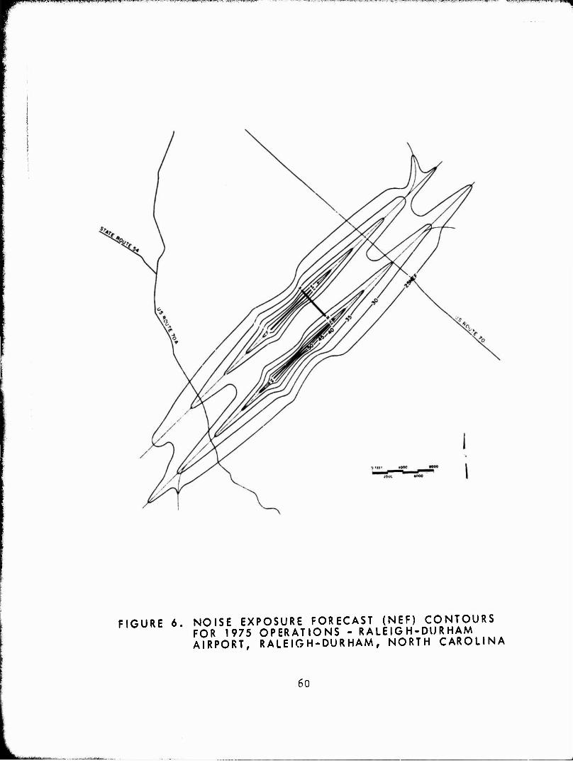
MSPSJfcPWSWMfU x.J.iii.tiuyiLi.j.u «|E«im)!.i'r'i*.>!,« .*«=*™*-r--^-- w,^.m.p>„.l^,,^TO-:^H^^r?-.^.v,^"r^"

FIGURE 6. NOISE EXPOSURE FORECAST (NEF) CONTOURS FOR 1975 OPERATIONS - RALEIGH-DURHAM AIRPORT, RALEIGH-DURHAM, NORTH CAROLINA

60

{ji&yj^^^JfeH' '-MMMyj- pwwrpwwiw "iVH-f'SfffiW

contours. The second step was to determine the cash cost of

land acquisition, clearance, and relocation costs for those

uses incompatible with the noise. An atte/npt was also made

to assess the social implications and political feasibility of

total relocation of people. Conversion of the affected land

areas to other revenue producing uses, effects on tax structures,

and other considerations necessary if such a plan were actually

put into action were not considered because of the time and

funds available for the studies.

A refinement of the concept of determining the number of

people exposed to various zones of noise exposure has been

introduced by Pianko and used in the evaluation of impact of

various commercial aircraft retrofit programs by the ICAO 72/ Committee on Aircraft Noise-1— . Pianko determines the impact

by the relative magnitude of a function called Significant Area

of Global Annoyance (SAGA). Three elements are involved in

computing SAGA: noise exposure contours, population density

in the exposed areas, and a function, IT, relating noise exposure

to percent of exposed population expected to be highly annoyed.

The ii function is the same as described in Section II-C-3 of

this report on page 29, except that the function is defined

as zero below NEF 30. These factors are integrated over the

noise exposed area to obtain the total number of people highly

annoyed at exposure levels of NLF 30 or higher, i.e., the SAGA

for the airport, situation.

A different approach to impact analysis has been suggested

by Richards— . His proposal is directed to commercial air

carrier airports, but might be adopted for military use with

further study. His basic evaluator is a Disbeneflt-Benefit

ratio, which hu defines as the number of individuals seriously

61

^ff^W^mtffnm^pn»!JWi;!«g,<WJR.,gP' < ' ","'F?sr■, ■'■■»■«■«■"«■■w >■ WJ«!^«».?«!««^^ iwi =*.'!--<• •^t,>*>^™*T^*y&&^^v^mL[-$\?*i^hi■.-w -.! ■«;>■■ ■?*-<- J!ii!yLyyyL;,B^'«(i>^t._j _jjij{

disturbed by noise in a given area to the total number of

passenger movements contained in the flight operations causing

the noise, expressed on a percentage basis. In his evaluation

he considers, based on the London airport studies^ ■■-" , that the proportion of people seriously disturbed in a residential

area is given by 0.75 NNI/100. This predicts that approxi-

mately 40? of the population would be seriously disturbed at

NEP HO (compared to the 50? highly annoyed predicted from the

Tracor results in the analysis of Section II-3-C).

A recent effort by FAA to provide a means for evaluating

aircraft noise has produced the Aircraft Sound Description

System (ASDS)-^- . This procedure defines the impact area, by

aircraft type and mode of operation, as that area exposed to

an A-weighted sound level in excess of 85 dB (a PNL of about

98 dB). It is then assumed that the average exposure to levels

in excess of 85 dB is 15 seconds for takeoffs and 10 seconds

for approaches everywhere within the 85 dB contour. The effect

of a succession of similar events is assessed by multiplying

the number of events in the time period of interest times the

respective duration factors to obtain the total average time

in excess of 85 dB. This "exposure time" is thus the measure of impact.

Since noise from operations at an airport is generated by

different types of aircraft on a number of different flight

paths, the ASDS approach accounts for this in an aggregating

method to obtain a single number called the Situation Index (31).

This aggregation consists of multiplying the area of each

individual 85 dB contour by the "exposure time" for that contour,

then adding the results for each contour to obtain a total

number, the SI in "acre-minutes."

62

M#IWL^UW&M..P ■».!-■ yr-vr.-^-Tr-- -,-:^v--^----,- ■

No attempt is made in Ref. 73 to relate this criterion

to community response, i.e., "Further, no criteria are specified

for the purpose of advising how much exposure is excessive or

appropriate, nor are there any implicit personal criteria

embodied in the physical and temporal quantities which form

its basis."

It is clear that no generally accepted technique for

assessing noise impact as such is yet developed. Part of the

slow development of such procedures is undoubtedly due to the

slow development of regional planning organizations in airport

areas and thus the general unavailability of demographic and

land use data on a systematized basis. This situation is

changing rapidly as a result of a number of federal programs.

Regional planning is becoming a necessity in order to parti-

cipate in many of the HUD grants. Further, the 1970 census

data, Just now becoming generally available is organized in

a way that data of interest in examining noise impact concepts

can be obtained in a uniform manner. It Is reasonable to

expect that more sophisticated methods for noise impact

analyses will be forthcoming in the next several years.

The increasing availability of planning and census data

leads naturally to thoughts of computing impact indices as

part of the basic noise exposure calculation process. One of

the difficulties with this concept .i r, the lack of detail

available from census data and another is the coding of the

data for automatic computation. Local plann.inr agencies obtain

data on population for various census tracts. These tracts

may cover a few city blocks or a number of square miles.

Vi/hen the arta of a census tract is completely contained within

the noise contour of interest, no problem is caused. However,

63

any specific contour generally will intercept a fractional

part of many different tracts. Since the census data on

population are averages over a tract, no reliable way of

counting population can be based on an arbitrary assignment

of population proportional to the area of the tract lying

inside a noise contour and the area outside the contour.

In the most planning efforts known to the author, where

population counts in noise exposed areas have been made,

boundary problems have been resolved by utilizing aerial

photographs of the region to obtain actual building counts

in the partial areas of censuc tracts. This process is

reasonably effective since populations per building can be

determined fairly accurately in conjunction with the basic

census data. The procedure, however, is not amenable to

automation since it require visual inspection and judgment.

Since the data can be obtained reasonably quickly, say in

one man day, it is questionable whether automatic computation,

if it were feasible, would really be much of an improvement.

One of the major difficulties in defining a suitable

impact index is the lack of a national criterion for accept-

ability. For example, using the approaches described here,

it is possible to define the proportion of exposed population

annoyed at any level of annoyance, the schools, churches, or

other uses exposed to different noise levels, and even the

dollar values association with impacted property. The same

information can be derived for different noise exposures

produced by different, assumptions on airport operational

variations such as runway layout, flight path changes, or

change in aircraft complement at an air Läse. Thus the com-

parative effects of noise exposure in a community can be

:,:-.:-:-r -^:—^-^-" -T

obtained. Knowing that only 5,000 people will be highly

annoyed for one situation, as compared to 10,000 for another,

certainly scales the relative merits of the two conditions.

However, in the absence of quantitative limits for accept-

ability, whether either situation is acceptable or unacceptable

is simply a matter of opinion.

68/ In the EPA Airport/Aircraft Study—/ , the task group

examining noise impact recommended a long range goal that would

provide a noise environment in residential areas not in excess

of Ldn 60 or NEF 25. Even if this goal were adopted, it must

become a matter of national policy to determine whether, in the

overall public benefit, it might be more vital to maintain an

air base mission capability even though significant numbers of

people might be exposed to substantially higher noise exposures,

In the process of evaluating the impact of noise on a

community it should be remembered that generalized accept-

ability criteria such as those proposed by HUD are derived

from responses average: over a number of airport situations.

Evaluation of case histories at individual airports indicate

that local conditions can easily shift impart up or down for

a specific noise exposure value—'—- . Variation in response

due to socio-economic factors has already t^en cited. Other

significant factors include the length of previous exposure

of the community to aircraft noise, the importance of the air

base to the local economy, and the degree to which the com-

munity believes the air base is trying to minimize the noise 1 Ik 17 56/

it produces1»1 *Ll >'- .

Until such time as more highly developed impact assessment

techniques are defined, the airport planner would do well to

maintain maps of noise exposed areas on which basic land uses

65

PPgjBlipgJH^BiWHPJWBIglu 4-t.y»jU' 111 J IMH <h- "* '-■ IWUMAU. ti'wimijww- "—■.;=—r -'-=-■- ff^pppppfl4pitppptpM|

are coded. The general location of residential areas, schools,

and churches should be defined. Color coding is helpful in the

delineation of such areas. Map pins locating complainant

addresses on this same map in conjunction with the coded land

use will assist in obtaining a graphic description of the extent

of at least the overt response to the noise produced at the

air base. In the last analysis, the planning tools and suggested

criteria can tell an air base commander or planner only what the

expected effect aircraft noise will have on a community. The

actual impact can only be assessed by detailed local evaluation

of the community and its attitudes.

66

SECTION III

REVIEW OF PSYCHOACOTISTIC EVALUATION? OP AIRCRAFT NOISE

Significant psychoacoustic research concerning people's

response to noise has been completed since the introduction of

CNR. Much of the work has been directed toward improving

objective measures of an individual's subjective assessment of

aircraft flyovers. Included in this research have been in-

vestigations of multiple and modulated pure tones, temporal

patterns of simulated aircraft flyovers, flyover signal duration,

combination effects of pure tones and duration, and the effects

of Doppler shift. In addition, investigation into the effects

of background noise, speech interference, and the growth of

noisiness have been conducted. Some reserrch to revise the

shape of the noy contours at low frequencies ar.d high amplitude

has also been undertaken. Most of the research appears to

substantiate the use of EPNL in its present formulation as a

reliable and accurate measure of the noisiness of aircraft

flyovers. The following is a review of various effects and the

results of related studies.

A. Spectral Effects

Functional relationships between SPL at various frequencies

and values of equal noisiness (noy contours) are employed in the

calculation procedure for perceived noise level. Since the

inception of these curves in 1959, and later modifications in

1963, other investigators have conducted tests to either vali-

date or modify the noy contours—'— . Some investigators—1^-/

have lntercompared the results of the various studies in an

attempt to determine an average noy weighting function. While

there is some variation in the results obtained by the various

67

iWMlTTH"T ......Ml.,, M ■_- , .rnrrt,«^, J„^.u„ _-„.,__ — —

fPü^pppn liPJPilBP^p^^^p.Liji^jiMmBij^^ 'p^p-^ fw s^-t %rv^ fw'.^i'.w-'iw.wrff.w, »i .^aap^ 'Jt- *??PV ■ ^ !

investigators, probably the greatest discrepancies are at low 2k/ frequencies. One investigator— has Introduced a different

combination rule in determining perceived noise level from 1/3

octave band SPL. This combination rule, in essence, changes

the low frequency weighting in a manner such that the low fre-

quencies become less important in determining the perceived

noise level. In spite of these studies there does not seem to

be enough evidence at present to warrant changing the noy

weighting contours as they presently appear in standards C £ *7 /

documents2-*—*-*■ .

B. Effects of Discrete Frequency Components

Many aircraft noise signals, in addition to their random

noise structure, contain discrete frequency components. There

is no doubt that the presence of pronounced discrete frequency

components adds to the noisiness of aircraft flyovers. Several

early studies led to a correction procedure whereby the per-

ceived noise level was increased, over the value computed

strictly in accordance with the noy contours for random noise,

to account for the subjective judgments produced by the presence

of discrete frequency components More recently, studies have

been completed-2-1 *—- in which modulated and multiple tones

have been examined to determine the validity of the pure tone

correction procedure. It appears that the increased noisiness

caused by modulated tones and some of the multiple tones is

accounted for by the pure tone correction procedures adopted

in existing standards2-1—1-^ . However, for multiple tones such

as those present in some high bypass-ratio engines, so called

"buzz tones," there is additional noisiness present which is

not accounted for in current tone correction procedures. More

work needs to be done on multiple tones to determine the

68

■rtir MI ■ ii'iMfcMMirimiT I

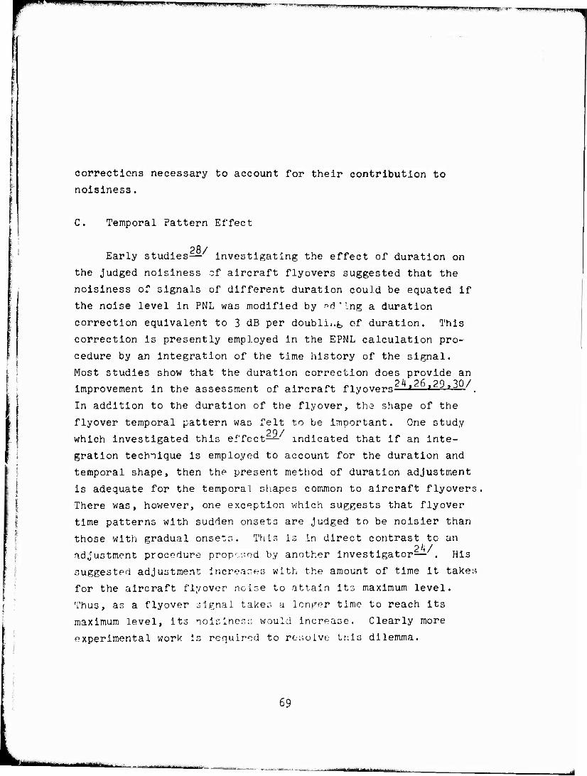
; !i iijiiiyiim, un,i, .pity nyi HBWüPHHPü m ■ mm» wm*mm mmmmmw ^^m'^nmmmm - - .- - -

corrections necessary to account for their contribution to

noisiness.

C. Temporal Pattern Effect

O Q / Early studies—investigating the effect of duration on

the judged noisiness of aircraft flyovers suggested that the

noisiness of signals of different duration could be equated if

the noise level in PNL was modified by .^d ' Lng a duration

correction equivalent to 3 dB per doubling of duration. This

correction is presently employed in the EPNL calculation pro-

cedure by an integration of the time history of the signal.

Most studies show that the duration correction does provide an 24 26 29 ^0/ improvement in the assessment of aircraft flyovers—* » * 1~' .

In addition to the duration of the flyover, the shape of the

flyover temporal pattern was felt to be irrroortant. One study 20/ which investigated this effect— indicated that if an inte-

gration technique is employed to account for the duration and

temporal shape, then the present method of duration adjustment

is adequate for the temporal shapes common to aircraft flyovers

There was, however, one exception which suggests that flyover

time patterns with sudden onsets are judged to be noisier than

those with gradual onsets. This is in direct contrast to an 2 4 / adjustment procedure proposed by another investigator— . His

suggested adjustment increases with the amount of time it takes

for the aircraft flyover noise to attain its maximum level.

Thus, as a flyover signal take;-, a longer time to reach its

maximum level, its noisiness would increase. Clearly more

experimental work is required to resolve tnis dilemma.

69

ffyp. jüggjBj^g^iqaiamggpwjpjij i^pqpg ggMPgwg^g

D. Doppler Shift Effect

There has been some concern that Doppler shift may effect •3Q 31/

the judged noisiness of aircraft flyovers. Two studies^ *■* have been completed which suggest that this may indeed be the

case. However, the effect appears to be quite small and con-

centrated mainly at low altitudes. On close examination of

the data of Ref. 30 it appears that the Doppler shift correction

is confounded with the duration correction. Aircraft flyover

noise with a pronounced Doppler shift required less correction

for duration than noise without Doppler shift. However, the

3 dB increase in judged magnitude per doubling of duration

incorporated in the EPNL calculation procedure still provided

a reasonable measure of the aircraft flyover noisiness.

Another study^- which related to Doppler shift,

investigated the effect of an approaching aircraft versus a

receding aircraft. The study found that approaching aircraft

are Judged to be noisier than those which appear to be moving

away from the observer. The effect was not verified in a 30/ subsequent study by another researcher^— but further tests

are being carried out by the original investigators using

more realistic aircraft flyover simulations as a further check

on the phenomenon. In the most recent report on this subject—

it was found that while there may be some evidence that per-

ception of aircraft noioe is related to distance, the effect

was not measurably significant.

70

H^IP.llUPP'liipj.L J^IJ.iPiSHfcWpWl-LÄ^ILL': w-. '" m^np^ü^fHIPIgpgpm"'" "**w " ^;.,.-.,)IUJ.LI,.l..).J _.J|.|tM^T"WWpiPJ-Tgpr'=»WJ!»JPKl---J4^ai^,. ,,11 IJll|I.PIJIJI.,tl.L-'»,AWv-,l "^TggM^|jWJp'jffipgqB|M

E. Speech Interference Effect

One of the objections to aircraft noise is that it inter-

feres with speech communication. Some investigations have

been completed to determine quantitatively the amount of speech

interference caused by aircraft noise and to also determine a

measure which best oredicts the speech Interference effects^ '^,

These studies reported that the articulation index provides the

best predictor of speech interference. However, PNL also pro-

vided a reasonable measure of speech interference.

Since the amplitude of aircraft flyover noise changes with

time, an average measure of speech interference has little

meaning. Possibly more important is that level above which

speech cannot be understood at a given distance. This would

provide a duration of time for which one would be unable to ■3K/

communicate. It is interesting to note that in one study-*^

the level at which speech communication became quite difficult

was the same level as that which resulted in a rating of "barely

acceptable" and "unacceptable" in a category scaling experiment.

This is another indication that speech interference is certainly

a strong contributor to the assessment of the annoyance of

aircraft flyover noise.

F. Background Noise Effect

There is evidence- '■'■-' that background noise r ambient

noise affects the assessnont of other intruding ;.ound;'. This

is particularly true when the intruding signal is clore in

level to the background noise, becoming clone to inaudible,

and thus not annoying. One study—' suggests that if the

71

bUSUIPW -MJM!!.-:L!!!,|A .M. . ? .,_ , .,-,•.,*. ^:,„^..^ .„,-:;., j : ;„,

signal to background noise ratio is 40 dB, the effect on the

perceived noise level of a judged noise would be to reduce it

by 3 PNdB. For aircraft flyovers the noise levels are rela-

tively high and thus a background correction is not incorporated

in the present NEF since

a) its effect would be relatively small and

b) it is difficult to specify a representative

leve of background noise because of its

wide variability.

A background noise level correction could actually provide

a very undesirable effect if it were to encourage an increase

in background noise as a means of reducing the annoyance of

aircraft noise intrusions. This has actually been recommended

in one study of means for alleviating noise problems around

airports.

G. Combination Effects

Many of the investigations relating to the acceptability k of aircraft flyover noise have concentrated on one or another

aspect of the noise. For example, some have studied the pure

tone effects, others have studied the duration effect. Since

correction factors have been developed to account for these

effects it is certainly desirable to determine If the effects

are additive when presented in combination. Some studies such 29/

as those investigating temporal and spectral combinations—

and tone and duration combinations— , have shown that the

effects do appear to be additive and that both tone and

duration corrections are necessary. Further studies—*^—

72

Mpm> imtm .'..i: - ^j,ii",«,.mgiamgFJ*-.m*>: >,m' L. . L >. ,-^srrrnrrssmpTF-är-r-

using both recorded and real life aircraft flyovers as stimuli

have shown that tone and duration corrected perceived noise

levels provide as good if not better correlation with subjective

assessment than other measures without the tone and duration

correction. These investigations further suggest that the

present EPNL calculation procedure could be Improved upon but

at this time it appears to work adequately well for present

day aircraft and also for future V/STOL aircraft.

In the most recent report—on combination effects the

author concludes that the manner of accounting for frequency

weighting and duration effects in EPNL were close to optimum,

although a small change in noisiness summation might improve

the accuracy of computed values of EPNL as compared to judgment

tests. The author also concluded that improvements in tone

correction procedures should be made at frequencies below

500 Hz since his results showed that the present corrections

overestimated the effect of tones at low frequencies, increasing

the standard deviation in the difference between calculated and

judged levels by from 0.3 to 0.8 dB, depending upon the type of

aircraft. Examination of his data indicates, however, that

he incorrectly applied the tone correction at low frequencies

(e.g. the correction below 500 Hz should be numerical' ' half

of what it would be above 500 Hz). Thus his conclusion at

this time is not justified. This is particularly pertinent in

that 26 of the 119 aircraft noise signals used in the study

were from helicopters where low frequency noise is most

important. A re-analysis of this data should be performed

to provide better insight on the applicability of EPNL in its

present form to helicopter noise.

73

LWÄAWWliM- .J!* .:■■■■:.- "

It is very important to bear in mind that many methods

might work nearly as well as EPNL for current aircraft;

however, the real question is whether or not the other

measures would work with possible future aircraft flyover

noise whose spectra may bear no relationship to tne flyover

noise spectra of the present. In this regard, judgment

tests using some radically different spectra were undertaken

to determine how well the various measures agreed with sub- 29/ jective assessments— . Again, EPNL provides about the best

correlation with the judgment result. Thus, while the present

form of EPNL can probably be improved upon, it does not appear

at this time, that adequate data are available to warrant a

significant change In the present calculation procedure.

The above research shows that noise signals having the

features characteristic of aircraft flyover noise are best

related to human judgments when frequency weighting, cor-

rections for tones, and time integration are utilized. For

sounds having similar temporal characteristics and without 29 39/

predominant tones it has been shown—-— that the frequency

weighting provided by A-weighting, as compared with PNL,

provides reasonable accuracy in judgments of noisiness, for

reasonably well behaved spectra. No tests have been per-

formed in which the temporal and tonal correction procedures

of EPNL have been applied to A-weighted noise signals. One

would expect that these additional factors should improve

the ability of A-weighted noise measures to predict accept-

ability of sounds in the same way chat PNL is improved in

the EPNL measure.

In the previous sections of this report we recommend

the SELT measure as a compromise between the desirability of*

71»

-mi 11 iiiiBÜM

^Hwnfwmnf^pfWTigi mn-ui i. HMUU..,.» .,., ,w. ,.„

using A-weighting for uniformity in comparison to other

noise sources, yet providing the temporal and tone factors

of E?NL. Clearly the validity of this choice should be

determined by psychoacoustic experimentation. The hypothesis

is reasonable, but the verification of the range of its

validity is missing.

75

BiWPW ii)u»i.MiHiHii^KiJuii.,...,.i^i.uiji,»'*j^,j^pjj)».pp»<^^jj.if,.,l»Jj^--.

•

j SECTION IV i I

{ REVIEW OP THE TECHNOLOGY OF NOISE EXPOSURE COMPUTATION 1 I

The accuracy of models for computing the noise exposure

produced at any point around an airport from a series of

aircraft operations is determined by the methodology used to

describe the basic noise characteristics of a specific aircraft,

the way in which this information is interpolated or extrapo-

lated from actual measured data at specific distances to other

distances, and on the accuracy of the operational data used to 1

describe mixes of aircraft, operating conditions, and flight

I trajectories. Th^ first two categories involve factors of

both aircraft performance and physical acoustics. The ways

in which these factors are considered form the differences

between models currently in use. The third category, reli-

ability of operational data, is a problem common to all models.

In the following discussion we consider how these factors are

treated in present models and indicate where improvement in

accuracy can be expected in a new procedure. It should be

noted that improvement of existing models is a question of

refinement, not change in fundamental concepts.

Before addressing the methodology for noise exposure

computation, one should consider the reasons why one uses such

a methodology at all. The question is often asked as to why

one should not simply go into the field and measure the expo-

sure directly. Clearly, for planning purposes where one is

projecting new aircraft, new operations, different procedures,

new runways, the physical situation doesn't exist even if a

measurement program were feasible.

The answer for the case of an existing airport operation,

77 Preceding page blank

PPM|PP!^^PPP||Pt$ffjPPPH!P IIKIWippi-m&W "^T* jMP -,XS,m„iAUjtywmy^.4-11 -w.fr...nt-yy

projected to remain essentially stable, is not as obvious.

Consider, however, the problems of performing such a measure-

ment program. The goal of the planner is to obtain a

representation of the variation in noise exposure, over the

geographic area of concern around the airport, in a suffi-

ciently stable form that he can assess various planning

options. To obtain this goal through a measurement program

would require continuous noise measurements at geographic

points ranging from 200 to 2,000 feet apart, varying with

distance from the runway. These measurements would need to

be made continuously over a long enough period of time that

daily fluctuations in traffic, weather, and runway utilization

were effectively averaged.

Consider the relatively simple airport layout of Fig. 6.

The area of concern is approximately 12,000 feet wide by

^10,000 feet long, or about 500 million square feet. Assuming

an average grid spacing of 1,000 feet, it would require about

500 separate measurement locations. If one were to measure

for only one week at each of these locations, the cost of data

acquisition and analysis, even using automatic, unattended

equipment, would be of the order of one million dollars. This

is clearly not a feasible approach for airport planning.

The above example is in no way meant to infer that no

measurements should be made around airports. Carefully selected

measurement locations with a wel] designed noise measurement

sample design are often useful for validating the results of

noise exposure calculations obtained from computational models.

The point is, with the model, only a few measurement sites

need be considered, reducing the validation procedure to a

78

^tm i i niiiTna^ iMitel tiiMiiiiä

reasonable cost and performance period. Factors to be con­

sidered in designing such a measurement program are discussed in Appendix D.

A. Basic Approaches to Existing Models

Regardless ~r the final summation process used to obtain ~. ·-

noise exposure, i.e., the su~mation of a totality of events,

there are two ba~ic approaches used to compute the noise

produced at ~ given point in space from a single aircraft

operation. Each has the problem of describing the basic noise

source characteristics of an aircraft, and then relating them

to where that aircraft is in space so that the noise source

data can be used to compute noise levels at points on the

~round around an airport.

The more sophisticated approach, as developed by

von i~iekirk and hi::; cO-'i-Jor:.::ers in South Africa~/, starts

with a description of the noise source characteristics, in

o~ sound pres~ure levels in one-third octave bands, as

nrodu~ed ~t a re~crcnce distance under specified aircraft

oper:;.ting cond:!.~tc;.:~. Tht~ po~it.ion of the aircraft in space

is ccr.puted frCJr.; ~:v:' b::l:~~c ·"'luations of r:;otion of the aircr.:1ft,

us::.:~~ i-h•:•~il~,, ·J~:r:;.~·-, l~~'t., ~nd dra1.~ ln~·o:r:nation derived from

~hich con~!d0rs dis~ance ana the speed of the aircraft, as

L

at the ground point as they are in EPNL computations.

Variations in source noise output for density altitude

effects and thrust management schedules are also accommo­

dated in the procedure.

The second, and more generally used approach for land

use planning (e.g., CNR, civil NEF, ISO) describes noise

source cha~acteristics of an aircraft (usually by classes of

aircraft having similar engines and performance) in terms of

~oise levels as a function of slant distance from the

observer to the a:rcraft. Different curves are necessary to

describe different operating conditions, e.g., takeoff and

a~p~oach. The der!vation of these curves requires knowledge

or assuffiptio~s of toth the noise source characteristic~~ in

::er:::s of ::::he :wi:oe J.e:;criptor used (EfHL, A-~t;eighted sound

level), and ~ou~d prcp~~atlon phenomena. Aircraft position

·~ space ls cttai~~d f~cffi data which de~cribe aircraft height

~s ~ fu~ct!c~ of ii3tance from a reference point (brake

r0le~3e fer ta~0c~f, touchdown for approach). The noise

level predi~~e~ fer a~y point on the ground is obtained by

:o:.·:in;: t:1.o.- :r..::.~_::c!lcr:.etric proble:n of locating the distance of

~:csest a~rrcact h0:ween the aircra~t fl:ght path and the

fu~ct~o~ of ~lant di~tance.

t~e derr~e cf co~rl~xlty wi~h the accuracy and variety of the

~~~ilatl~ l~~u~ data. ~here few aircraf~ types are involved,

~J :-J~ p r"'· c ~ ~~ <_: ~-:no:·:~ r: d i~~ 0 f 1.-1(' i ['"!"! t ~~ , fl I.;;!!~ procedures , thrust

::-.ar.ag;er:-.er: t $ c:-;e~_: u >:..:, ::!nd- !'l icht pc::.th~~ L~ a vat-lab le, the first

:..~thod of com;::t..:t i:;,: r,ols~ expo!;ure should be capable of !1igher

80

accuracy than the second. Where many airports are involved,

with widely varying aircraft types and operating procedures,

where detailed knowledge of aircraft 1-reights is not available,

and flight path dispersion ~s not precisely known, the first

concept is difficult to use and its complexity is not often

warranted. The second concept tends to smooth out some of the

uncertainties in operational data in~ut by using average

noise level and performance data for typical aircraft cldsses

as they are normally operated at most airports. Thus the

second method may not predict the noise produced by a specific

aircraft fli~~t a3 accura:ely as the first, but does predict

~he average of a number of no~inally si~ilar flights quite

3orne examples of t~P acc~racy of prediction of individual

aircraft noise levels by :.he ~urrent CNR procedures are shown

The top two examples are obtained from the Tracor

da:.a o: F.:::-:~~ .:.4, the bottom :"'ron a ra:1dom sample taken from

Exarn~les of prediction accuracies f0r :~F values

are jls~us~ed !~ Section IV-2.

?ec::r::r::er:.:ia<:. :or: ?ic. ::_ - L'escription of noise source

chara~ter!~:~cs !n t~~,s of noise level as a function

of s.:.a~: d!stance and description of aircraft per-

. ' rr.oae~

as the basis for land use

" .. ~··" ... ···• .,.,..,_ '

WWH^^WB^^y^ pp miujiLj#w ii m^t^m J .» »ggpgypi* WW'lfgjIL, ! .amK-.-^jirmms**^ "^?*~f

«JU

P A

20

10

0 1 I Vi 1 70 80 90 100

PNLM 110 120 130

S x

I

60

40

20

100

P = PREDICTED VALUE OR RANGE FROM LAND USE GUIDE

130 PNLM

FIGURE 7 COMPARISON OF PREDICTED AND MFASURED VALUES OF MAXIMUM PNL

82

|ak^|MriM i ■ - i - ■ - ■ ■ HI 11 riMinag ^IBamiiiiiriiiir

mm mm*-w»mwu.< wK^mmmm

B. Acoustical Factors

1. EPNL Computation

The emphasis in analyses of aircraft noise signatures

in the past six to eight years has been related to EPNL as

a measure. Even if A-weighted sound exposure level is used

for land planning purposes, the methods for approximating

time integrals, defining tone corrections, and questions of

stability of analyses are still the same as for EPNL, as

long as spectral data are still required for the development

of aircraft noise level as a function of distance. In the

following discussion we refer to EPNL computation since it

is the source of the data discussed. The arguments apply

equally to A-weighted sound exposure level.

In Section III we reviewed the psychoacoustic data

incorporated in the EPNL concept. The scientific evidence

available supports the concepts of frequency weighting of

SPL, inclusion of duration effects, and adjustments for the

presence of discrete tones in the spectrum. One may ask,

however, wuether certain of the decisions made with respect

to the process of incorpui .Ling these factors in EPNL, as

now defined in the various national and international docu-

ments, are satisfactory when applied to real aircraft

signals. Put another way, how stable Is an EPNL value, for

a particular aircraft ncise signal, when subject to artifacts

in the measurement/analysis process? In the following dis-

cussion it is assumed that the frequency response character-

istics and dynamic r-anre of the measurement/analysis system

meet pi ent requirement;; of P.ef. 5,6 and are not at issue.

The noise signal produced on the ground by an aircraft

«3

■ ■■■^--^--

wgBm^*mmmm*mmmmmmim^*w« mem » ,.IULW ipmm.u.i wm**sB^w?mmzz* - ■ *^T-HP?~ ^^S+aT"

in flight will vary rapidly in amplitude if the aircraft is

flying fast and relatively low to the ground. The EPNL

computation requires one-third octave spectral analyses for

successive time segments of this signal. The stability of

these analyses is a function of the integration time of the

detector used in the spectral analysis and the duration of

the time segments. Current EPNL measurement procedures

specify a detector time constant equivalent to the "slow" 41/

scale of a precision sound level meter— and successive

time segments of 0.5 second duration. As in all analyses of

time varying signals, one is caught with the dilemma that the

detector time constant should be small enough to reasonably

follow the time envelope of the signal, while the effective

frequency band width of analysis must be sufficiently great

to insuie satisfactory statistical reliability in the analysis

Two factors are involved in assessing the validity cf the

0.5 second time segment choice. One has to do with the confi-

dence placed on a particular sound level derived from the

analysis, and the second has to do with what effects the

uncertainty in this value has on a final computation of EPNL.

Examining the first point, one can establish confidence

intervals for the spectral analysis on the basis of the 42/ effective bandwidth of the various one-third octave filters—-

Various confidence intervals for the 2!\ one-third octave

frequency bands used in EPrJL analysis are shown in Fig. 8.

It is clear that, at the lower frequencies, there is a sizable

uncertainty in any one measurement providing an accurate

measure of SPL for a given event.

The second question, how significant is the instability

In low frequency SPL's when computing EPNL is most easily

8H

— ..^,,— .. n.

«•^^W^^^W^WW » » ■■ U ■>! ■! II» % »—-.»■,

s i

8 o c

-8 c o

31.5 63 125 250 500 1000 2000 4000

One-Third Octave Bond Center Frequencies in Hz

8000 16,000

FIGURE 8. 90% CONFIDENCE INTERVAL FOR ONE-THIRD OCTAVE FREQUENCY ANALYSIS OF A 0.5 ^:C SAMPLE

85

■MMJM^

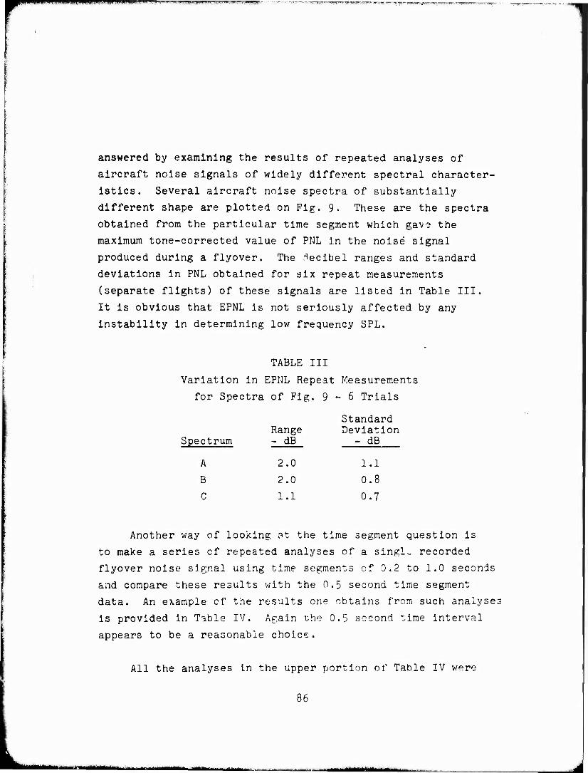
gB^ppapppiPjpps m wg^wBwwwePBiiy^pipticwyi^^BBtwHpig'

answered by examining the results of repeated analyses of

aircraft noise signals of widely different spectral character-

istics. Several aircraft noise spectra of substantially

different shape are plotted on Fig. 9. These are the spectra

obtained from the particular time segment which gave» the

maximum tone-corrected value of PNL in the noise signal

produced during a flyover. The decibel ranges and standard

deviations in PNL obtained for six repeat measurements

(separate flights) of these signals are listed in Table III.

It is obvious that EPNL is not seriously affected by any

instability in determining low frequency SPL.

TABLE III

Variation in EPNL Repeat Measurements

for Spectra of Fig. 9-6 Trials

Standard Deviation

- dB

1.1

0.8

0.7

Another way of looking ft the time segment question is

to make a series of repeated analyses of a single recorded

flyover noise signal using time segments of 0.2 to 1.0 seconds

and compare these results with the 0.5 second time segment

data. An example of the results one obtains from such analyses

is provided in Table IV. Again the 0.5 second time interval

appears to be a reasonable choice.

All the analyses in the upper portion of Table IV were

86

Spectrum Range - dB

A 2.0

B 2.0

C 1.1

•aaMHilUM

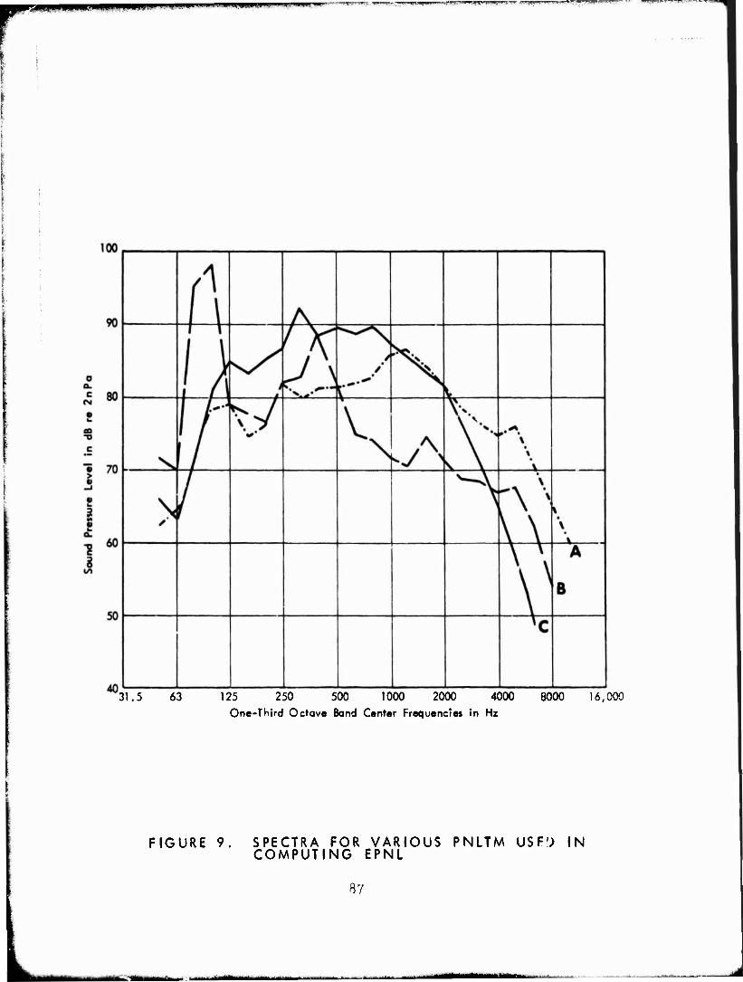
VUMJ^MI (P|«Bl»piPlU4L,.J^«>H^WlHP<HI I!. J. .1*1111 M.

31.5 63 125 250 500 1000 2000 4000 8000 16,000

One-THird Octave Bond Center Frequencies in Hz

FIGURE 9. SPECTRA FOR VARIOUS PNLTM USFO IN COMPUTING EPNL

87

-■

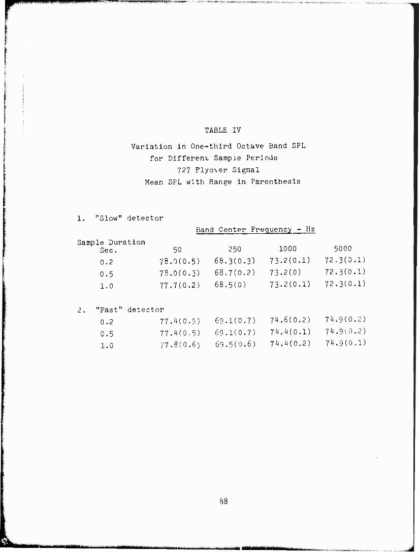
wpjupjegysv "^w'MJ1-.» I PS^m^piggjjpppfgB^q^wwiw

TABLE IV

Variation in One-third Octave Band SPL

for Different Sample Periods

727 Flyover Signal

Mean SPL with Range in Parenthesis

1. "Slow" detector

Sample Duration Sec.

0.2

0.5

1.0

Band Center Frequency - Hz

50

78.0(0.5)

78.0(0.3)

77.7(0.2)

250

68.3(0.3)

68.7(0.2)

68.5(0)

1000

73.2(0.1)

73.2(0)

73-2(0.1)

5000

72.3(0.1)

72.3(0.1)

72.3(0.1)

"Fast" detector 0.2 77.4(0.9) 69-1(0.7) 7^.6(0.2) 74.9(0.2)

0.5 77.^(0,5) 69.1(0.7) 74.4(0.1) 74.9(0.2)

1.0 77.8(0.6) 69-5(0.6) 74.4(0.2) 74.9(0.1)

88

■kuB

!gjjiP!pg»B^iuiu^pii»-g,-,i>^^

made using a detector having the "slow" characteristics of

the sound level meter. This implies an equivalent RC smooth-

ing where the time constant is of the order of one second.

(The tolerances for the precision sound level meter allow the

equivalent RC time constant to lie between 720 and 1315

milliseconds. The experimentally obtained time constant for

the analyzer used for these analyses was 1110 ms.) Clearly,

many aircraft noise signals vary in amplitude so rapidly,

e.g., 10 dB/sec, that one should question the suitability of

such a long time constant for the detector. One way of

examining this question is to perform the spectral analysis

with a time constant of about an order of magnitude smaller

and compare the results. The "fast" scale specification for

the sound level meter has an equivalent RC time constant of

127 milliseconds and thus admirably serves as a convenient

value.

We are most concerned with the effects of these factors

in computing EPNL, whi^h '.-• an integration c, PNL over time.

One can visually assess the effect of differences in detector

smoothing characteristics by examining the PNL values at

successive 0.5 second intervals as obtained by the tv,c

different detectors. In order to make the difference1: bet.'.'TO

these two analyses te as large as possible, we examined the

approach noise of a low bypass fan-engined aircraft at a

nominal height of 107 meters (350 feet) above terrain at an

approach speed of 80 meters per second (153 knots). Thus

the signal has a complex, multi-toned spectrum, short overall

duration, and rapid rate of change of sound pressure with

t ime .

The results of these analyses are shewn in Fig. 10 and

89

■ --"—-■■ -

-- -"v:-:| II ■ IT -II — -mi M—ana

.HI"'»i pmmnfpK

110

100

90

4 / /

i

^ 1 ^

rFAST EPNL = 98.5

•

// If

r / i jf * Si t^r f

SLOW—" EPNL = 98.1

t

PNLTM s\

V 9 5

> \ * <*•'"*

v>

FIGURE 10 COMPARISON OF PNLT AND PNL WITH DETECTORS HAVING CHARACTERISTICS OF "FAST" AND"SLOW" ON A SOUND LEVEL METER

90

■nmm.ijpi.iti ji-ii ' M üwuwwepiCTmBwpn

Table V. The data in Fig. 10 show, in the upper part of the

figure, the value of PNLT for each 0.5 second interval as

obtained with both "fast" and "slow" detectors. Clearly, the

"slow" detector neither tracks as accurately in amplitude on

the rise or fall of the signal as does the "fast" detector.

Yet, the integration of PNLT to obtain EPNL yields almost

identical results. The lower part of Pig. 10 shows similar

results for PNL, without the tone correction application. The

data presented in Table V are intended to provide a feel for

the stability of results obtained from repeated analysis of

the same flyover signal indicated in Fig. 10. We conclude

that there is no reason, for land use planning purposes, to

change the detector time constant or sample Interval fcr

determining EPNL as they are presently specified in Ref. 5

and 6, provided due precautions are required in specifying

heights and air speeds to be used in obtaining reference

EPNL values from flight tests so that undue inaccuracies are

not introduced because of detector time constants.

Many USAF aircraft cannot, however, be flown at suffi-

ciently slow speeds to make accurate noise analyses at

reasonable test heights with the 0.5 second time constant.

When the combinations of speed/height provide extremely short 79/ durations, we propose— that the following criteria be

applied, where d is the duration between levels 10 decibels

below the maximum:

Sampling Interval Duration (10 dB) and Integration Time

- sec - sec

d >_ 5 0.5 5 > d > 2 0.25

d > 2 0.125

91

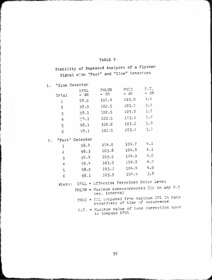
iiymm p ■UpwilHimygLH^N.

TABLE V

Stability of Repeated Analyses of a Flyover

Signal with "Fast" and "Slow" Detectors

"Slow Detector

EPNL PNLTM PNLC P . T.

Trial - dB - dB - dB - dB

1 98.0 102.4 103.0 3.9

2 98.0 102.5 103.0 3.9

3 98.1 102.5 IO3.O 3.7

4 0 °, 1 102.5 103.1 3.8

5 98.1 102.6 103.1 3-3

6 98.1 102.5 103.1 ■} 0

"Fast" Detector

1 98.4 104.0 104.7 4.1

2 98.3 103.8 104.8 4.1

3 98.4 103.9 10 4.9 4.0

4 98.4 103.9 104.3 4.0

5 98.2 103.3 104.9 4.0

6 98.1 103.9 10 4.9 3-8

Where 0.!

EPNL = Effective Perceived Noise Level

PNLTM = Maximum tone-corrected PNL in any sec. interval

PNLC = PNL computed from maximum GPL in band regardless of time of occurrence

P.T. = Maximum value of tone correction used to compute EPNL

92

J>WMÜ

The duration may be estimated from slant distance to the

aircraft in feet, s, and airspeed in knots, V, from the

following expression:

d = K —

where K, a function of directivity, is approximately 2 for

takeoff operations and 3 for approach operations.

One of the potential artifacts involved with computing

EFNL from measured spectra has to do with the process for

identification of discrete tones. In order to make the

tedious process of computing- EPNL simple tc perform with a

computer, an algorithm was required for defining the presence

of discrete tones, and their level above the equivalent

random noise that would be presert if the tone were not.

The algorithm estimates the banc1 level without tones, and

the "presence" of a tone, by comparing levels at adjacent

frequency bands and the rate of level change from band tc

band. In the original development of EFNL several forms of

the algorithm were tested against a wide range of flyover

bpectra, with the final form being selected as correctly

identifying tones for all the test spectra examined.

As the method of rating aircraft noise in terms of EPNL

has come into being;, many different groups are now making

EPNL measurements on a wide variety of aircraft noise signals.

In the course of these programs it has become apparent that

the present algorithm for tone identification can sometimes

define a "psuedotone" as being present when a highly irregular

spectrum is examined. This can occur most commonly in two

cases.

93

i liiifiiiii« —

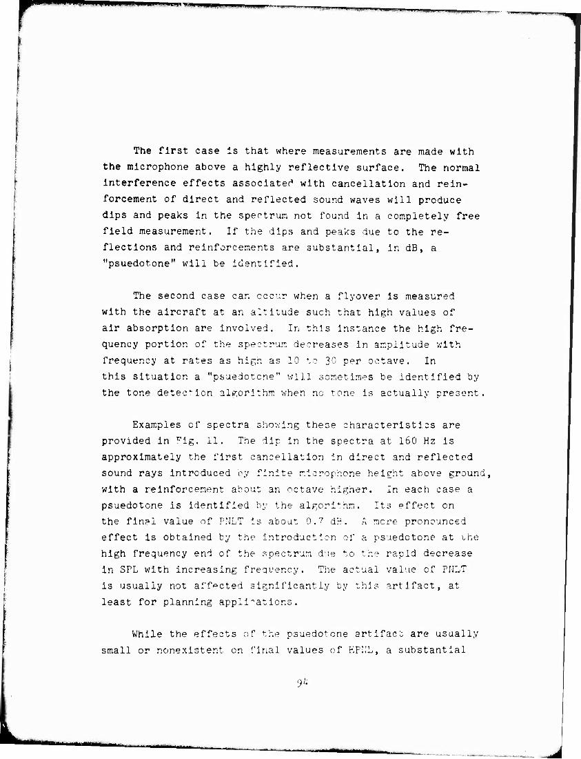
■■■*• HP 'Ii in ■ ""'I - Kswmwi „!«.■ - . 11-llLIJIIJM^lJll. esB^

The first case is that where measurements are made with

the microphone above a highly reflective surface. The normal

interference effects associated with cancellation and rein-

forcement of direct and reflected sound waves will produce

dips and peaks in the spectrum not found in a completely free

field measurement. If the dips and peaks due to the re-

flections and reinforcements are substantial, in dB, a

"psuedotone" will be identified.

The second case can occur when a flyover is measured

with the aircraft at an altitude such that high values of

air absorption are involved. In this instance the high fre-

quency portion of the spectrum decreases in amplitude with

frequency at rates as high as 10 to 30 per octave. In

this situation a "psuedotone" will sometimes be identified by

the tone detection algorithm when no tone is actually present.

Examples of spectra shoeing these characteristics are

provided in Fig. 11. The dip in the spectra at 160 Hz is

approximately the first cancellation in direct and reflected

sound rays introduced by finite microphone height above ground,

with a reinforcement about an ^ctave higher. In each case a

psuedotone is identified by the algorithm. Its effect en

the final value of PNLT is about 0.7 dB. A mere pronounced

effect is obtained by the introduct: psuedotone at the

high frequency end of the spectrum d'ie to the rapid decrease

in SPL with increasing frequency. The actual value of PNLT

is usually not affected significantly by this artifact, at

least for planning applications.

While the effects of the psuedotone artifact are usually

small or nonexistent on final values of EPIIL, a substantial

94

^^MMM

■sppp^pBiiP^piirva mmmw*

■ UV

w 90 9 i V ^»%

1 i 1

- k. . — Run 200-4 - Londlng '

.000

2 m

i

S

W 99.5 i •PNdB

I"»""*

o % « A-' jk*** #

-—Run 192- 3.5 N.M. 1 ^\ fij 102.4 EPNdB % "O /i % c it \

11 % _ 70 • /1 \ > « //

r i

\

\ *> 5 /

/ \

| 60 N. % \

•v \ c \ rf i

tn % 1

50 \ * \

1 \ \ ^ » *r

Aft \

31.5 63 125 250 500 1000 2000 1/3 Octave Band Center Frequency in Hz

4000 8000 16,000

FIGURE 11. TYPICAL MEASURED SPECTRA FOR PNLTM

^^^

Sfipi^WP;'MtMl)&/i|WI!lll..J--1--'^^ tJÜHiSpa,""' ^ ÜHamP^g I". IW>^lJlJWfJilHI^,^,JliBBHjBB|li.,'l!-!lW'J»-MI^JIW 'MH^r-'MHqHin*. -'

WBWWWwtw»»««' ■»' ■

should be greater than 35 to 40 dB before these background

levels Intrude on the aircraft spectrum. In most cases where

this Is so, computation with or without the background level

influenced frequency bands included will not affect the

numerical value of PNL. Where the desired aircraft signal

does not permit this dynamic range, the accuracy of the

entire measurement should be questioned.

A last concern in computing EPNL is the possibility of

encountering what may initially be regarded as an excessively

great duration effect. Some high flyovers tend to produce a

noise signal which, through atmospheric scattering of sound,

tends to be audible for some period of time. The effect of

this phenomenon on the numerical value of EPNL is not as

great as often imagined. This result stems directly from the

logarithmic integration involved with EPNL. Only noise levels

within the order of 5 dB of the maximum level have any signi-

ficant contribution to EPNL unless they exist for a very long

time. ^PNL values are generally lower than the maximum PNL

for signals having durations (between the 0.5 second interval

noi^e levels 10 dB below and on either side of the maximum

level) of less than 25 to 30 seconds. Duration corrections

whivh increase EPNL over maximum PNL must have "10 dB down''

durations of the order of a minute or more before a signifi-

cant effect is observed. Signals of this nature are just not

significant in land use planning applications since they

contribute negligibly to the summation of the much more noisy

events.

y

Recommendation 7 - The computation of EPNL should 3/ be performed as presently described in FAR Part 36- .

Computation of SELT should be identical except that

97

iium» ii i\>tmm>w<»mmm* ^n.'>" fF^BPT^^-^Fl^jWf —S^^^g^^^y» ^£=-^'1 s-^^a^T^-äsy^, ''Uj^^ujMM^pnp?

A frequency weighting should be used instead of

noy weighting, and a reference time of one second

instead of ten seconds should be employed.

2. Air-to-Qround Sound Propagation

One of the major sources of uncertainty in computing

noise exposure is the effect of air absorption on sound

propagation. In theory the effects of classical and mole-

cular absorption on the attenuation of sound are well under-

stood. Precise measurements of attenuation have been

performed under carefully controlled laboratory conditions.

The measurements and the theory are in reasonably good

agreement.

Unfortunately the atmosphere of the earth is not at all

as homogeneous as the conditions obtainable in a laboratory.

In a real atmosphere sound attenuation is a function of

absolute humidity, wind and temperature gradient, and level

of turbulence. In the case of aircraft noiso, where one is

concerned about propagation paths up to several tens of

thousands of feet in lenth, the variations in these factors

can be highly significant in their effect on sound propagation.

It is clearly impracticable to provide an accurate model

of the atmosphere for use in predicting aircraft noise sound

propagation losses. While a number of attempts to model the

atmosphere (use of stratified layers, turbulence models, etc.)

have been partially successful in understanding the problems,

measurement of the properties of the atmosphere for application

in noise planning studies is clearly out of the question. The

only choice is to resort to experimental data, expressed in

98

riMMfUM ^_klUI - t!r*mr"-»lhMiig1ittüf: i'lrfi i

pwmäHlt-.IIWUW. J.il,lun!,«JJiiii \mn _,j. *-j^-r«H-"

terms of statistically averaged results.

The best currently available results on the attenuation

of aircraft noise have been combined into a set of average

absorption coefficients presented in the Society of Automotive

Engineers (SAE) Aerospace Recommended Practice (ARP) No. 866.

These values are used in current aircraft noise certification c c n /

documents and in the ISO and ICAO planning documents ' ' .

Much discussion has taken place, however, questioning whether

ARP 866 needs improvement, particularly for the coefficients

specified at frequencies above 1000 Hz.

An example of how variable the results can be in deter-

mining sound absorption coefficients is shown in Fig. 12 where

six sets of absorption coefficients, experimentally obtained

from aircraft noise data, are plotted as ratios with respect

to the values of ARP 866. While many different factors were

involved in the different experiments, the variability is

alarming. The difficulty lies in having a good knowledge of

the atmosphere at the time of the measurements.

Another view of the variability in determining air

absorption values, net quite so alarming, is available from

a set of controlled experiments, performed under a NASA

program, where a fairly good understanding of the atmosphere 4 ii /

variables was possible— . A summary comparison of these

data to ARP 866 is shown in Pig. 13. These results indicate,

that, on average, the SAE data are quite reasonable.

A recent program for evaluating air absorption of sound

from an aircraft in flight was performed by FAA at Pendleton,

99

»." i««i|j,ui.j.!Jl].i„li, »JiiJ.-ii.n>'«1ii.

2.50

2.00

1.50

a Field

1.00

0.50

• A 0 o

ii

&AC Rolls Royce D.A.C.

0 Boeing N.P.L.

II 1

t i

( > - i ( i

i i

k

» , i

>

t ' , > < > 1

( > i ( \ ( 1 <

< ► < > l i < > ( )

< > ( < > < >

1 <

1 >

1 < *

< >

00 12. 50 16 00 20< DO 25 30 31i 50 40 00 50( )0 63 DO 8a )0 16, Frequency in Hz

FIGURE 12 RATIO OF EXPERIMENTAL AIR ABSORPTION COEFFICIENTS TO SAE ARP 866 VALUES

100

■ ■■—■«I

•Wiliui^ T^WW' ' ■ ■;-..- ;.T ■.■.--■:■■ ^ ■■

'250 500 1000 2000 4000 8000 One-Third Octave Band Center Frequency in Hz

FIGURE 13. COMPARISON OF AVERAGE EXPERIMENTAL VALUES OF ATMOSPHERIC ABSORPTION WITH SAE 866 CALCULATED VALUES (FIG.19 OF REF.24)

101

- • - - -HI UTiir.anii-rr.n.MiiM I

^»FjniBpp^r- ■ -<!'WWL1. Wi'MlJJJ^HVWr-.-■---,-- .-,-,-

Oregon-* . A series of ten test groups was used to obtain

noise data at four microphone positions located at distances

of 250 to 1500 feet from the flight track, normal to it,

from level flyovers of a T-33A at heights of 100, 700, 1500,

and 2000 feet above the runway.

Most of the data in this program were taken at quite

low humidity conditions, e.g. primarily below k0% relative

humidity. Background noise levels precluded useful data

above about 3150 Hz. Below this frequency it was concluded

that the test results indicated absorption coefficients

somewhat greater than would be predicted by ARP 866. This

is similar, at frequencies below 2000 Hz, to the results of

the NASA program. At these frequencies absorption coeffi-

cients are typically in the range of less than one to

usually not more than three dB per 1000 feet, and thus

difficult to measure. Unfortunately no information is given

in Ref. 63 to indicate the variability in the data, so no

indication of confidence levels can be calculated.

The most recent, and one of the best controlled studies

of aircraft sound propagation, was performed by Hawker-

Siddeley— . This project used the same aircraft and instru-

mentation to obtain propagation data at a number of locations

in Europe and the USA under a variety of temperature and

humidity conditions. While these data have somewhat higher

absorption values than ARP 866 at the higher frequencies, the

differences are not great. These data provide further

substantiation of the general applicability of ARP 866, and

show that, if anything, it is slightly conservative. This is

appropriate for planning applications.

102

■■■*r Mtftii

-v- T^r^^.^^^f-,^»' j^^^wM<^jj||;^!^-^>'g^^m^w,ljg|wg»ff|J 'm* ,?!<"»; «n,wr« .PBJHWMW1^^«^-^ " ?P^^f^5f^^ppS5^S^

Recommendation 8 - The air absorption data

contained in SAE ARP 866 be used in noise exposure

calculations. The Air Force land use planning

procedure should be so designed that it can be

easily modified to accept new air absorption

information when this information is available

and considered acceptable to the scientific and

technical community.

3. Ground-to-Ground Sound Propagation

In the above discussion we acknowledge the substantial

uncertainty in predicting the effects of atmospheric absorption

on sound propagated from an aircraft in flight to a point on

the ground. When one now considers propagation of sound from

a source on the ground to another point on the ground the

problem becomes even more complex.

The presence of the intervening ground surface introduces

substantial new effects not experienced in air-to-ground

propagation. Wind and temperature gradients and the wind

direction immediately above the ground cause shadow zones

and refraction of sound. Localized temperature fluctuations

above the ground surface cause increa ,ed turbulence in the

air, introducing substantial fluctuations in noise levels

received at a distance from a steady.sound source. The

acoustical impedance of the ground surface introduces addi-

tional complexities in the estimation of attenuation.

A number of attempts have been made to derive prediction

techniques for estimating ground-to-ground attenuation effects.

Various SAE documents have been drafted for use in accounting

103

^i^^^i^^^^'^-v-^^y-^'^^^ij^vwps^--

for ground effects at relatively short distances from a noise 45 47/

source ±* ■" . At distances of concern in land use planning

arounu airports, however, the best currently available infor- 46/

mation was obtained in a NASA study—' of noise propagation

at several commercial airports. In this study, statistical

data on noise propagation were obtained for a variety of

weather conditions over extended time periods. The propagation

distances examined were typical of those involved in airport

land use planning problems. The data used in the previous

references were reviewed and compared with the results obtained

from the NASA project. The engineering procedure derived in

this stiAvIy is that currently in use in the civil NEP V computations— .

An empirical expression, advanced "somewhat tentatively" 40/

by von Niekirk and Müller— , at about the same time as the

NASA project was being conducted, expresses excess ground

attenuation in sound level A as n (7 + 10 logy-j^r), where n is

a coefficient describing the ground surface and s is dista ice

from source in meters. Values of n suggested are 0.5 foT

hard surfaces, 1.0 for grass up to one foot high, 3.5 for

wheat or shrubs up to five feet high, and 7.0 for forests.

This expression is reasonably consistent with the results of

the NASA project for values of n of the order of unity.

Recommendation 9 - Utilize the method for predicting

ground propagation losses now in use for civil NEF

computations in the Air Force procedure. Provide

for easy modification in the procedure when improved

data are available. Develop additional data wherever

possible in measurement of noise from aircraft

operations.

104

^MIM

a;wi;A»ay- ™r^^^?;~^^g'^^ '

9

4. Transition from Oround-to-Ground to 4ir-to-Ground

Sound Propagation Rules

Aircraft noise exposure around an airport is usually

caused primarily by aircraft performing takeoff or. approach •

operations. The variation in height of the aircraft causes \

the angle between the horizon and the line of sight from an .

observer to the aircraft, 8, to vary from zero to as much as

90 degrees. At small angles, the effects of excess propagation

due to ground induced effects are apparent; at some finite

angle these effects will become negligible with only the air-

to-ground attenuation being important. In order to compute

noise exposure around the airport an algorithm must be

sleeted to provide the transition from ground-to-ground

attenuation.

Several algorithms have been proposed or are in use in

various computational models. The current NEP model in use

by FAA uses ground attenuation only for the angles between

zero and 4°l8', interpolates between ground and air from

4°l8' to 7°11'> and uses air attenuation only for angles

above 7°11'. The choice of angles was based on empirical

data- ; the precise values selected not being due to accuracy

of data but simply as a choice of values for the arguments of

the tangents of the angles as 0.075 and 0.125, respectively.

4/ In the South African procedure— , an empirical relation-

ship, derived for the transition when levels are expressed in

sound level / is given by exp(-6/2). This relationship

provides complete ground attenuation effects at zero degrees,

and essentially no excess attenuation from ground effects at

angles of e greater than 6 or 7 degrees, as shown in Fig. 14.

105

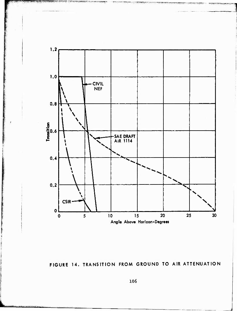
HP--J)M*JIJ!UWA!H.*lJr" I """ S3SCTBF!»

1.2

1.0

0.8

|0.6 e

0.4

0.2

•—CIVIL NEF

1 * i \ i \

i \ \ \

\

1\ -^ -SAE DRAFT AIR 1114

\ \ \

\

--.

\

\ \

CSIR—^

\\

X N

N \

10 15 20 Angle Above Horizon-Degrees

25 30

FIGURE 14. TRANSITION FROM GROUND TO AIR ATTENUATION

106

ritirtfttifuri until

gjmUPmmpiPeiJ.'UUmJJ*'. """^l,J"',*"!" ''"***' *'"'">'*'Wut JMWJ.-.".-,-»** fet™«H»RMS» -' -^"snTOsa^tswi-nFT nj>WTr«!wj,.-»"j»j TV; s-fum-», ,:„^,„~—„„„

A different form for the transition was arbitrarily

chosen in an early draft of an SAE procedure— . in the fcrm r wi

of exp [-(tan 3 6) 2J , based solely on the assumption

that ground attenuation becomes significant at angles of 6

less than 15 degrees. The form of this transition is also

shown in Fig. 14. (This form of the transition algorithm

was originally included in the program prepared for DOT use lift/

at the Transportation Systems Center— ; the algorithm has

subsequently been changed to be consistent with the PAA

version.)

The question at hand is to choose an algorithm for the

proposed USAF procedure. Clearly, the data used by van

Niekirk and Müller— , based on their own work and on data 4g/

from Scholes and Parkin—*• j do not support the use of excess

ground attenuation above values of 6 greater than approxi-

mately seven degrees. In the course of evaluating the

selection of sideline microphone locations for noise certi- «50/ fication Galloway^^— has shown that at values of 8 between

seven and ten degrees the effects of ground attenuation on

EPNL are completely missing, while substantial ground

attenuation effects occur at angles less than seven degrees.

This conclusion is also consistent with the NASA data of 85/

Hubbard and Maglicri— . Notwithstanding these results, some

aircraft manufacturers claim extra ground attenuation effects

exist at angles as high as 45 to 60 degrees. We find no

physical basis for these claims.

6 3/ Much of the data obtained by FAA at Pendleton— were

at low angles of elevation. Unfortunately the data in the

report are categorized as above 15 degrees and below 15

degrees. Since the transition out of ground-to-ground

107

g^gUgHiHimiii .., ...iit)iay .-- ----^ . .■i^aag.jJi,-

P|pjPppBfim|^W.BIi»i»'H!'.l^i.i>"u'i| ' '^^|^.l'»^'^^'""ll^l^:"■" »^»»wi|^f'"v«'E>^"^-'--y™g"''Tg»^^

propagation takes place below 15 degrees it is essential to

know the actual angles. The data are available to do this

analysis and hopefully will be analyzed for this effect. As

yet this has not been done.

Present evidence appears to indicate that ground atten-

uation is certainly present for angles of several degrees,

and non-existent at angles greater than six to eight degrees.

The algorithm used for this transition in the current NEF

procedures used by FAA seem to express this result in a

reasonable form.

Recommendation 10 - The algorithm now used in the

civil aviation NEF program for transltionlng between

ground and air attenuation should be employed in

the USAF procedure. Develop additional data wherever

possible in noise measurement programs to verify or

modify this algorithm.

5. Duration Effects

The EPNL produced by an aircraft at any point around

an airport is influenced by the duration of the noise signal.

The duration is a function of aircraft speed, distance, and

the directivity pattern of the aircraft as a noise source .

The EPNL values are particularly affected if the aircraf: is

undergoing acceleration.

For a specified directivity pattern, the duration of a

noise signal is directly proportional to distance between

aircraft and observer, and inversely proportional to aircraft

speed. These factors can be explicitly incorporated in

108

r HMppp! pinpp i M

extrapolating EFNL from one test condition to another condition

of distance and speed, since the directivity pattern is assumed

to remain constant. This assumption is not as valid for large

slant distances where the effective directivity pattern changes

due to air attenuPti.n effects.

Acceleration effects are most significant for mar.y

aircraft during the takeoff phase of flight. The shape of

contours of equal EPNL to the side of the runway are directly

affected by this effect. In both the South African model and

the FAA model for calculating noise exposure these effects

are accounted for. In the model used at the DOT Transportation

Systems Center this effect is not included. For those airports

having "sideline" noise problems adjaceno t i c runways the

effects of acceleration on EPNL are significant, of the order

of 5 dB, and should be examined carefully.

Recommendation No. 11 - The effects of acceleration

on EPNL or SELT should be accounted for in the noise

exposure model. Data to derive these effects should

be acquired in aircraft noise test programs wherever

possible.

V

6. Effects of Topography and Geometry

For most calculations of noise exposure it is perfectly

satisfactory to consider the terrain in the vicinity of an

airport as being planar at the elevation of the airport

itself. Some criticism of NEF calculations assumes that

this is always the case, not recognizing that the height of

the observer related to the height of the runway may be

accounted for in any of the present models. All computations

109

■ -. ^^lajjuam . ■. .- ,-t„ r^t^uammiim tf**E°"--'- -"-"hi ■:-

•~* :- ■ - ^W: ■'- ■U^«WMI|LIP^1UII--Jll*t imrv&mr*™7*&MV*WW i «■>*■■■ -;f^==- -^? -'-r-"^^^?wt^5>-""'!^JJ»l-i^^v,--I»1 P7V7^--?^T" ^T"*^ ,5

use a complete three-dimensional space in their determinations

of slant distance.

In most models it is convenient to use a Cartesian

coordinate system in wMch the origin of the coordinates is

taken as the brake release point on takeoff, positive x is

along the runway, y is perpendicular to the runway, and z

is positive above the runway. Since all coordinates are

free to assume positive and negative values, variation in

terrain height is easily accounted for by assigning heights

to various points on the basis of elevations obtained from

normal topographic maps.

The ülant distance, s, from any observation point to the

flight path is given by (see Fig. 15): ■il

op 2 2 sa " zo) cos Y + yo J ■[■ It is usually adequate to approximate this equation by setting

the term cos y equal to one, where y is the angle of climb of

the aircraft, since values of y of 12 degrees or less introduce

less than 0.1 dB error in calculating EPNL, with the error at

a Y of 28 degrees rising to only 0.5 dB. Even for modern

interceptor aircraft such climb angles are rarely attainable,

requiring thrust-to-weight ratios <. f 0.55 or higher, and are

certainly not comfortable for the pilot. We conclude that the

approximation is reasonable, even for military aircraft, and

provides a substantial simplification in computation.

7. Density Altitude Effects

The noise produced on the ground is a function of the

engine power delivered and the heights of the aircraft.

110

Both

— * --

^mt^mtmmm* jga-<r*m*!nFt<zm*%£WmpBm!m ,.M4|NU*i-1! nimm L,w,|j,u«ungH 1 "■'" " '■"" "

FIGURE 15 GEOMETRICAL RELATIONSHIPS IN CALCULATING NOISE EXPOSURE

ill

jJM.im^b^^EJ^.^^^B

WffWpWHff.'PW^ifW I'f'WBpiff,,"!" ■ ^w^^-^giL,Pif'UjL. \>v._r >i ujtryw WBBff. i' '■ ■"■ v*^?*

of these factors are dependent on density altitude (pressure

altitude corrected for temperature and atmospheric pressure).

Engine noise power output is directly correlatable to net

thrust, which decreases with increasing density altitude.

Length of takeoff roll increases, and cl:.mb angle decreases,

with increasing density altitude. Accounting for these effects

in current noise exposure procedures is not normally considered

(except in the South African method) except in special cases.

Application of the USAF procedure is likely to occur at

air bases having substantial physical elevations relative to

sea level, and extended periods of hot weather. In order to

provide for these effects in noise exposure computations it

is necessary to derive aircraft takeoff performance data and

noise output data as a function of density altitude. The

performance data are available in the appropriate Technical

Orders for the aircraft, and the noise data can be determined

from the basic noise test data in terms of decreased engine

performance at various density altitudes. For those air bases

having density altitude conditions significantly above sea

level standard conditions, the ncise exposure is then cal-

culated simply by specifying the appropriate aircraft data

at the time of computation.

No general procedure can be specified for selecting

the density altitude conditions for which noise exposure

calculations should be made with other than standard day (15°C)

conditions because of the variation in the performance of

different aircraft with temperature. For example, many modern

jet engines are "flat-rated" to a temperature considerably

above standard — 30°C for example. Under these conditions

standard day thrust is available for takeoff up to this

112

mmmsmmmtm*!'

temperature. On the other hand, many engines in use are not

rated this way, with their available thrust degrading with

temperature continuously.

The two factors to be considered in judging density

altitude effects on noise are the change in thrust with

temperature (and thus climb performance), and the change in

noise level with engine thrust. For many aircraft these

factors compensate for each other. That is, the decrease

in climb performance is offset by a decreased engine noise

level. Again, each aircraft needs to be assessed in terms

of its specific performance.

As a general guide, where sustained temperatures at

sea level air bases are in excess of 30°C for more than three

months of the year or for bases at field elevations in excess

of 3000 feet where sustained temperatures are greater than

20°C, the performance of the aircraft using the base should

be assessed to determine if other than standard day conditions

should be used in noise calculations. If noise levels expected

one mile beyond the runway extension are more than 7 dB

larger than for standard day conditions, the reduced perfor-

mance should be used in noise calculations.

Recommendation No. 12 - Data on density altitude

performance and noise effects should be included

in the USAF procedure.

8. Non-standard Weather Effects

In current civil aircraft NEF procedures, EPNL values

are those expected under acoustic standard day conditions of

15°C (59°F), 70!? relative humidity. No corrections or

113

■emaf^mif^im.. .w^a^pi-vfifjA'WfllW«;.'. '1

adjustments are made in E?NL values for local temperature

and humiuity conditions at Individual airports. At least

two different general questions can be raised concerning

this procedure. First, and most important, for a particular

airport, how applicable are such curves when local conditions

may rarely (or only occasionally) approximate 15°C, 70%

relative humidity. The second question, directed towards

comparison of test data, is to what extent noise data

developed on the basis of ICAO standard day conditions may

differ from that obtained under FAR 36 acoustical day con-

ditions of 25°C (77°F), 70? relative humidity.

These questions are examined in this section in terms

of the expected variations in air absorption due to changes

in temperature and humidity. In actual field situations,

where one is concerned with the variation in noise levels

received on the ground, the influence of temperature on air-

craft performance may partially compensate for (or, in some

cases, accentuate) the effects of temperature and humidity

on air absorption.

First of all, it should be remembered that the selection

of the standard reference conditions of 15°C (59°F) and 70?

relative humidity is based upon a study of average surface

conditions existing at a number of civil airports in the iio/

U.S. and throughout the world—7 . The "standard" day condi-

tions are frequently encountered in a number of major civil

airports and presumably at many military air bases as well.

Field noise data that can be analyzed in terms of

temperature and humidity effects alone are simply not avail-

able. Thus, in looking at the effects of non-standard weather

114

iwpww ppppmpjl jp II HI i - L» j 11-3- m^f=?£?* ^^A^^'^'T ?*^

effects, we adopted an analytic approach based upon selection

of four representative one-third octave band noise spectra

at reference distances, and projection of these spectra to

different distances, for different values of temperature and

humidity. Air absorption values from Ref. 43 were selected

for the different temperatures and humidities. From the

resulting spectra, PNLM and PNLTM values were calculated and

compared.

Figures 1o and 17 show the results for two of the cases

studied—a turbojet takeoff and a turbofan approach spectra,

<.:;amined for standard day conditions and for -7°C (20°F) at

10 and 90? relative humidity, and 38°C (100°F) at 10 and 90*

relative humidity. Typically, there is greater variation for

the turbofan spectrum because of the higher proportion of

high frequency noise energy, more affected by atmospheric

absorption.

Figure 18 compares the turbofan approach noise levels

for 10$ and 90S? relative humidity at 38°C (100°F) with the

standard day conditions, normalized to a reference spectrum

at 120 meters (400 feet). Comparison of sets of spectra on

this basis shows that for most of the non-standard day con-

ditions noise spectra projected beyond referenced distances

of 120 m (400 ft) or 300 m (1000 ft) will show lower levels

(i.e. greater absorption) for non-standard day conditions.

Thus EPNL values predicted on the basis of standard conditions

tend to be conservative by estimating higher noise levels than

might exist for non-standai'd conditions. (This conclusion was

earlier documented tu Ref. 67.) The data from Fig. 18 shows

that this holds true for all except for tra condition of -7°C

(20°F) and 10% relative humidity.

115

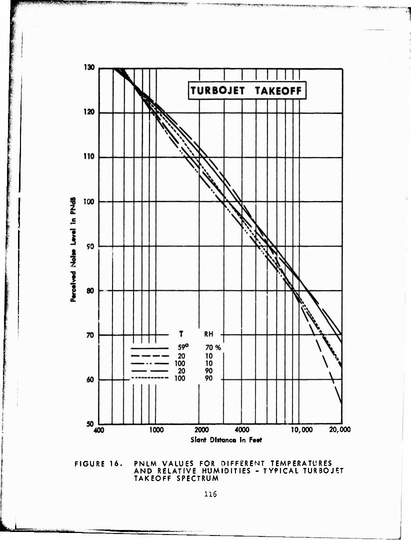
p^sfUfp^üHUf. i mmm- m impi^sipBiinH ^■.«M«^

2000 4000 Slant Dfftanco tn Feet

10,000 20,000

FIGURE 16. PNLM VALUES FOR DIFFERENT TEMPERATURES AND RELATIVE HUMIDITIES - TYPICAL TURBOJF.T TAKEOFF SPECTRUM

116

l^gg

uwyPHBiJU,LU,p-^- WPP£ ''"U1'-'- ' ■-' -llL -^**" =v^r-,".-^ --.-v? ■-'.--'- -.

2000 4000

Slant DUtanc« In f««t

20,000

FIGURE 17. PNLM VALUES FOR DIFFERENT TEMPERATURES AND RELATIVE HUMIDITIES - TYPICAL TURBOFAN APPROACH SPECTRUM

117

ws^ggmmm^emmssmmi*^.!»-.JJP11.i,! V*-7.-^^-yg--^»!''^^'MaM»,w«#'A"L4 w »m*?^**1.- w «.Mi--i^*™^™!*^

1

2 o

1000 2000 4000 Slant Distance In Foet

0,000 20,000

FIGURE 18. RELATIVE VARIATION IN PNLM VALUES WITH RESPECT TO PNLM FOR 59° F, 70% R.H. - TYPICAL TURBOFAN APPROACH SPECTRUM

118

■IP^BJPMBWWHWW'W'W1*1**^^"'''*'''-' ii .. IM i ■i.»»^»WCT^WI"1. '.P !" "ttmm J -». VWWMSWWPWIiJlWII*-1-1"1*9

The primary determinant of absorption is the absolute

humidity Since a rough measure of absolute humidity is

given by the product of temperature (in degrees) times

relative humidity, an approximate sorting of atmospheric

effects can be determined by use of this estimate. Examin-

ation of the curves of Fig. 18 in terms of this estimate

shows that greatest negative differences occur for relatively

small products of temperature and relative humidity, with the

possibility of positive differences occurring for very small

values of temperature and humidity.

Mean monthly temperatures and average humidity data

are given in the climatology summary for military air bases,

hence temperature and humidity information is readily avail-

able for making decisions.

The technique for calculating EPNL vs. distance curves

for a specified temperature and humidity follows exactly

that given in Section 12 of Ref. 55, with substitution of

the appropriate sound attenuation coefficients for these at

15°C (59°F), 70* relative humidity. This technique does, of

course, require spectrum and EPNL information from basic

flight test measurements.

The remaining question, that of comparison of differ-

ences in noise levels, assuming FAR 36 conditions and ICAO

standard day conditions, can be answered in terms of noise

level comparisons using the same analytic approach. Com-

parison of PNLTM values for several spectra shows that for

distances from approximately 120 m (400 ft) to 120C m

(4000 ft), the differences in PNLM values typically do not

exceed one dB. For projected distances from 1200 m ('4000 ft)

119

Pf^pWjpppiBfJPJf'SllgUJW'Vit^, .'■ »w..:ujiu^'i«

to 6100 m (20,000 ft) the values based upon FAR 36 conditions

are generally not more than 2 dB less than those projected

for 15°C (59°P), 705? relative humidity. Thus one may con-

clude that the differences in noise level projections based

upon FAR 36 and ICAO standard day conditions are generally

not large, except at very large slant distances. The pro-

jections based upon ICAO conditions will generally predict

slightly higher noise levels than those projected on the

basis of FAR 36 conditions.

One major reason for using standard day weather as the

reference base for noise exposure calculations is the ready

availability of aircraft performance data referenced to

these conditions. Use of FAR Part 36 acoustical reference

day weather requires the development of aircraft performance

data for each aircraft of concern. V/hile these calculations

can be derived from available data, the non-standard presen-

tation of the necessary information from aircraft to aircraft

makes the performance data development a tedious and time

consuming process for no basic improvement in the noise

exposure calculation process.

Recommendation Mo. 13 - Utilize EPML or SELT curves

derived on the basis of acoustical standard day

conditions (15°C, 7055 relative humidity) unless

examination of the mean monthly temperatures and

relative humidities show three months during the

year in which the product of temperature in degrees

F and relative humidity in percent is less than

2000. When such small products occur, the noise

exposure calculations for the air base should

utilize EPNL/or SELT/distance curves based on air

120

BgB^gP^i!pi|gBW6^l'^>m»ie*^iaB^P^^ " " wi^y ^>

absorption calculations from SAE 866 for the

appropriate weather conditions.

9. Presence of Back»»-.-"»und Noise

In many communJ ,;.. >ise level evaluations, the presence

of background noise levels, e.g., noise produced by other

than the noise sources under consideration, is a necessary

consideration. Clearly, if the background noise levels are

sufficiently high, they will mask the intruding noise. In

one noise measure formulated to describe noise exposure, ■51/

noise pollution level, Robinson— explicitly includes both

background noise and the intruding noise in terms of the

time history of noise exposure.

Unfortunately for the community residents in the vicin-

ity of an airport, aircraft noise is usually substantially

higher than the general background noise in any residential

community. By truncating noise exposure computations at

distances from the aircraft where the noise level drops to

80 EPNL one can in almost all instances be sure that the

background noise is substantially below the aircraft noise,

yet the area of interest around the airport has been covered

in the analysis. This expedient obviates the need for con-

sidering background noise levels explicitly in the aircraft

noise exposure computations.

10. Shielding Effects

Two types of shieldii,<z; effects have been considered in

noise exposure models. One has to do with the presence of

intervening structures between the noise source and the

121

w^gmm: J^UHMpf^T^ J:^""-*; ;-^^^r^--^^^^j^vf^«v^^ IL.. ."■.■wi,j|iW,»- ■ ■■ ■ r-^.^-T^T-^w—'o^sP

observer, the other has to do with the effects of multiple

engines on an aircraft.

The effects of physical obstructions intervening between

a noise source and an observer are covered in all standard

acoustical texts. In the case of aircraft noise these effects

are useful almost exclusively in the Instance of ground run-up

operations. A discussion of this problem as it pertains to

air base installations is provided in Ref. 52.

In the draft for a noise exposure procedure proposed by

SAE, an allowance is included for an assumed shielding effect,

at lew angles of elevation, for the presence of aircraft

engines on the side cf an aircraft avay from the observer—1- .

The maximum attenuation credited is 3 dB. This effect can be

accounted for, when it exists, in the derivation of the

description of an aircraft as a basic noise source from

flight test measurements, A special treatment of this factor

in noise exposure calculations is not considered necessary in

the proposed USAF procedure.

122

I jfWju.'i'i.M. "i »puiiiimiiiHi jgjwagi ^^ffi#!»fWtf^'' mm»

C. Basic Operational Considerations - Military/Civil

Aviation Comparisons

Calculations of aircraft noise exposure are highly depen-

dent not only on the noise properties of the individual

sources, and how this noise propagates, but also on detailed

knowledge of the aircraft operations at a particular air base.

Often the knowledge of noise source characteristics is of

higher precision than that of the operational data. In the

following section we consider hese variables and how they

affect noise exposure. In essence, we want to know how many

aircraft are doing what type of operation, at what locations,

over a specific period of time.

1. Traffic Estimation - Flight Operations

One of the first considerations in analyzing an air base

noise problem is to obtain an estimate of the total number of

operations, by type of operation and aircraft, over a speci-

fied time period. In the civil case, current operations are

generally estimated from a combination of total aircraft

movements (a record kept by control towers) and by analyzing

flight schedules. Operations at most civilian jei airports

occur on a relatively closely maintained schedule. Airline

operations can thus be estimated by reviewing these schedules,

from which one can quite accurately assess aircraft movements

by time, aircraft type, and destination. For given seasons

of the year these schedules do not fluctuate very much, and

for many airports the annual fluctuation is not more than 2055.

Military air base operations are not as easily assessed.

A detailed discussion of these operations is contained in

123

■■

pp^PIWiMitWiWliiWfffy^' T^vr^c.-- 4***?w-*fe***9** i-m*m ■""*'** ««rFJ*j"*ifrmmp w ■* ^m - .„H,,^,,,,,. ....

Ref. 52,53« In brief, military flights generally occur as a

random function of time, usually during the week days. An

example from Ref. 52 is shown in Fig. 19. Various methods

for estimating these operations are outlined in Ref. 52,53.

One may analyze total aircraft assigned, availability records,

mission requirements. Where such records are not easily

obtainable, 1 is usually necessary to request that a special

log of operations be kept for a period or, say, four weeks, in

order that a reasonable estimate can be made. Attention needs

to be paid to whether the base is fundamentally an activity of

one of the normal commands or is primarily for reserve training.

In the first instance activities are primarily week day, in

the second they often are concentrated primarily on weekends.

Some decision rules need to be stated to determine how

the operational data should be used in the USAF procedure.

Current civil practice, in most instances, assumes an average

daily number of operations on the basis of annual data. This

is reasonable for civil airports because of the uniformity

introduced by scheduled flights. As Indicated above, this

is not the case for military bases. In the present procedure

the concept of "average busy day" is used for military air

bases. This concept comes from the following assumption.

First, on the basis of case history data, it appears that

community response is based on periods of sustained high

activity. (This is also borne out by the recent London survey 15/

data—- .) For most air bases, although the day-to-day fluc-

tuations may be wide, weekdays show a sustained activity

significantly higher than weekends. The opposite is true

when the activity is primarily National Guard flights.

Further, within the weekday fluctuations, no particular day

124

, - — - —

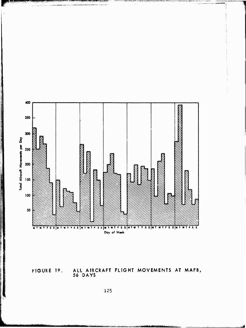
wfwztmieekWFJi^tB&w^^ - ^^-!--^-~^f^'/i^«¥-iis-«7.rjW™.?tr.r=?; ■"^rrt-SF'- r^*i-n, ^i-"" "-".^ ■^■.,:r7"I»-1'^^"*-^r'--;._'?;"",i "=■

MTWT FSS MTWT FSS]MTWTF SS MTWTFS 8

Day of Week

M T * T F S S

FIGURE 1? ALL AIRCRAFT FLIGHT MOVEMENTS AT MAFB, 56 DAYS

125

— ■"- I "" T'llliiTM BlWifii I

mf*rij>-,j I, I.-

appears to be predominant. A reasonable way to estimate the

activity to which the community responds is to average the

number of operations over the five week days and specify this

as the base for noise exposure computations.

If pronounced changes take place in operations during

one part of the year as compared to another (e.g., summer

versus winter, a pronounced increase in training operations

relative to normal operations, temporary assignment of

squadrons, etc.) the noise exposures for the two conditions

should be considered separately. If the variation is a

repeated condition annually, it may be desirable to logarith-

mically combine the different noise exposures to determine a

weighted average. It is probably not necessary to consider

these refinements if the average number of operations in any

monthly period does not vary more than 50$ from the annual

"busy day" average.

Porecasting future flight operations is always an

inaccurate business. In the civil case, forecasts are made

by the FAA, by airport operators, and by airlines. These

forecasts are based on estimated passenger and cargo growth

and expected equipment complements.

For military aircraft operations, accurate forecasts

are sometimes easier to come by than civil forecasts. If it

is known that a i>;iven base mission and aircraft complement

will be retained, or changed at some particular point in time,

operations generally can be extrapolated with reasonable

accuracy. The overall planning cycle for military operations

is usually sufficiently extensive In time that forecasts have

a reasonable expectation to be fulfilled.

126

■P pi,|.ipkui|i»iijy... mmemmiKR"-'' \Mft**fmmmw!v> gUjmtjitiijMu,»!.»-' '■wi:iklM'*.M.«'i*1»»~utww|-^".!»! .»'.'«*■ „... ^srmmt*m

Recommendation No. 14 - Computation of the number of

average daily operations should be based on a "busy

day" principle. For military air bases this average

is usually ti*3 weekday average, based on a monthly

period. Average "busy day" operations per month for

each month of the year should be obtained, then

averaged on a yearly basis. If any quarter of the

year has operations that are higher or lower by a

factor of two when compared to the annual average,

consideration should be given to computing separate

noise exposure contours for these periods of the

year.

2. Runway Utilization

Given a total of operations, the next step in analysis

is to assign these operations to particular runways and

nominal flight paths. This assignment is made on the basis

of actual runway use records when available. If such records

are not available (they usually are not), a reasonable approx-

imation can be made from statistical records of wind conditions.

These records need to be used with an understanding of local

operational restrictions, such as allowable tail or cross-wind

components. Again, interrogation of local operations personnel

will provide insight helpful in making reasonable decisions.

This problem is identical for both civil and military airports.

3. Flight Path Utilization and Dispersion

Given a runway use assignment, the next problem is to

determine the various flight paths employed with these runways.

This information, in terms of nominal paths, is usually

obtained from air traffic control personnel. It is essential

127

«■PPH ■■■■»"" Ji.n.1 uiijii Bfl»4 -Mil •^mm&mmemimm ^wmBnpwi!i».ii«inin I-- ™

that it also be verified with pilots and flight operations

personnel. Particular attention should be given to variations

in prescribed paths if substantial VPR flights are involved.

It can not be emphasized too strongly that uncertainty

or inaccuracy in developing adequate flight path data is a

primary source of inaccuracy in final computations of noise

exposure contours. It is strongly suggested that flight

paths claimed to be appropriate for an air base be verified

by actual observation wherever possible. Major deviations

in prescribed flight paths usually occur in radar controlled

environments under VFR (and ofton IFR) conditions. Radar

vectors for both departure and approach will be given to

pilots routinely. These vectors will usually cause flight

paths to depart from prescribed arrival or departure proce-

dures. A day spent on watching radar presentations will often

enable an observer to plot these deviations. Thus a reasonable

estimate of mean flight paths as well as dispersion in paths

can be made from these observations.

Present noise exposure eomputationr generally allocate

percentages of flights to various flight path segments that

are specified as average flight track::. An example of such

segments is shown in Fig. 20. Unfortunately, variations in

thrust-to-weight ratios of specific flights, air traffic

procedures, and pilot technique tend to disperse individual

flight tracks around the specified average track. Little

quantitative data are available on this dispersion and its

effect on noise exposure.

Some preliminary studies of flight path dispersion are

provided in Ref. 52. Experimental observations are reported

128

. ■J,.'.*.-^fM.Jt^.«^.sa..

imiiHtummiiip «i wnw *iiwij«n.w-^~^-«lp,i»-F'"*' —*-..~. «... ^ T^^sä^i^jiaHs^-^^rLiuwi'L-i ^^«•(Kv-^wT^ui-v^/i^ ■*<■"*. ^M «* ;SP- flrai

1 H

/

/

/

/

/ / \

\

/

/

/

/

/

^F

I I

/ / /

//

, 'I

/ o/ I /v /

/ , w f

/ /

/

' J. ^ */

//

FIGURE 20. FLIGHT TRACK DESIGNATION AT AN AIRPORT

129

{■pppgwipüHmuigii^HitWit-'J». --i-m^-, -:in M- ami.»jw»m,i,ii

for several different types of aircraft, such as interceptors,

transports, and bombers, making nominal "straight out" as

well as 90 degree turns after departure. We have recently

examined these data further in an initial attempt to provide

a model for flight path dispersion.

The assumption in Ref. 53» which seems plausible from

the experimental results, is that dispersion around a mean

flight path is normally distributed in both vertical and

lateral dimensions. We can then describe the dispersion in

terms of the standard deviations from the mean. The data

indicate that, to a reasonable approximation, the coefficient

of variation in the vertical dispersion is a constant,

assignable to the kind of flight operation. That is, the

ratio of the standard deviation to mean height is an assignable

constant. The approximate values we have derived for this

constant from the data in Ref. 53 for several different

operations are listed in Table VI. Note that these are all

based on military applications. One would expect that civil

jet transports would be comparable to the military transport

conditions.

Lateral dispersion was found to vary differently for

straight-out departures as compared to 90 degree turns after

departure. Lateral dispersion in straight-out departures was

again normally distributed, the standard deviation varying

directly with distance from takeoff. From the data of

Ref. 53 we were able to derive an empirical equation for

the straight out lateral standard deviation, a , as y bu

syso = 0.08 (x - x0),

where x is the distance from brake release and xQ is the

lift-off distance from brake release.

130

■ IIM

tm IK U «■ , «..Uli- ■. » ■ flflUtM»!««»!*». "mn™ " »»-V — ~ «

TABLE VI

Coefficient of Variation in Vertical Dispersion

of Takeoff Flight Paths

Condition s /z

Maximum gross weight transports 0.1

Transports - variable weights 0.2

Interceptor - military power takeoff 0.3

Interceptor - afterburner takeoff 0.3

cut to military power 0.2 Heavy bombers - mixed weights 0.4

s = standard deviation in height

z = mean height

131

' % 1ti!^^^4L|f Ji»rW!

We have also examined lateral dispersions after a 90-

degree turn, where the turn is begun at a specified height,

e.g. 150 m (500 ft). These lateral dispersions were found

to be directly proportional to the coefficient of variation

in the vertical dispersion, with o

s, * 6 x 10J s„/z y90 z

where z is average height.

In the data examined above no information was available

on takeoff gross weights. If it is assumed that a constant

takeoff power is used, the noise level underneath the takeoff

flight should vary directly with takeoff weight. In order -o

assess this effect we have examined data on the takeoff weight

distribution of 727 aircraft during one month of an airline's 64/ operations— . These data can be used to show that the take-

off weights are normally distributed (between 70S& and 90% of

maximum) with a mean of 78.5% and a standard deviation of

4.8?.

Using the "equivalent ground roll" concept (e.g. ground

roll defined as distance from brake release "o the intercept

of the climb profile projected to the ground), the climb

profile for a 727 with 15 degree flaps, gear retracted,

climbing at V_ + 10 knots, can be expressed as

z * 16.4 (x - x ) W"1

z = 16.4 (x - 0.3 W2) V;"1

where z is height,(x - 0.3 W2) is distance from liftoff in

132

fffmmmmm>mim vi'n m mni'n iii-w- "»■ PBKM^BBP I I I^JIII lll|||JjJ|IIIIJ||JJ||l 11)111 Ill _l_ I I HUI I H«V>'ll9»u-.>«

i f ( i i I «

feet» and W is gross weight in thousands of pounds.

The airline data may be combined to show that the mean

height of the aircraft after lift-off is 0.132 (x - x ). One

standard deviation in weight yields a coefficient of variation

in height, sz/z, of 0.055. Comparing this value with those

of Table VI for transports of variable weight indicates

that the effect of weight alone only accounts for about one-

third of the vertical dispersion. Clearly, pilot technique,

airspeed control, and weather conditions, all random in nature,

are the primary contributors to dispersion in takeoff height.

A similar analysis can be made of lateral dispersion in a

turn. Using the above equation for climb profile, the stan-

dard deviation in distance from brake release to a height of

150 m (500 ft) is approximately 210 m (700 ft). This gives

a dispersion equation of s - 3.5 x 103 sz/z. Comparing this

value with that obtained previously indicates that slightly

more than half the lateral dispersion in a turn after takeoff

can be attributed to takeoff weight effects alone, with the

remaining portion due to other procedure variables.

The significance of the above analyses in terms of

defining noise exposure lies in the fact that the weight

dependent dispersion is taken into account in the noise

computation through the specification of appropriate takeoff

profiles. The remaining portion of the dispersion could be

taken into account by several techniques. One would be to

build dispersion explicitly into the computation. This

would entail a fairly extensive simulation calculation. We

are exploring this possibility but as yet have not reached

133

BPpgMBWB n i mtm^mmmmm.

a conclusion as to its practicality.

An alternative approach is to collapse the dispersion

distributions to a set of, say, three paths for an aircraft

type with a weighting function used to proportion different

percentages of the total number of aircraft to the different

paths.

In the above analyses we have identified and quantified

various dispersions in takeoff flight paths. Before arriving

at any conclusions on how to account for such dispersion in

noise exposure calculations, the importance of the dispersion

on the noise calculations should be assessed. One way to

make this assessment is to simulate the dispersive flight

paths and compute the resultant noise exposure.

In simulation, a binormal distribution of flight paths

is defined in the y-z plane, perpendicular to the flight

track. The space described by plus or minus two standard

deviations in y and z defines an ellipse whose center is

located by the values of y and z for the mean flight path.

The ellipse is segmented into 225 equally spaced rectangles

(15 divisions each in y and z). The probability of a flight

path going through each rectangle is assigned according to

the binormal distribution. The noise produced on the ground

at various distances from the mean flight track from the

total array is summed on an energy basis. This sum is then

normalized to an equivalent number of aircraft flying on the

mer.n flight path. The result is the difference in the mean

EPNL value generated by the dispersion distribution relative

to the EPNL for the non-dispersive flight path.

131*

■:jw:u_,w,:«p-jp ss BffWS -'- ^? |{f»nppp9lP^Hp*jpgf|

Examples of this simulation are shown for specific

takeoff situations in Pigs. 21 and 22, and for generalized

situations in Figs. 23 and 24.

The first simulation considers the case of "straightout"

departures incorporating both vertical and lateral dispersion.

The results plotted on the left hand graph of Pig. 21 show

the change in noise levels, relative to the noise levels of

a non-dispersive distribution, as a function of distance y

perpendicular to the extended centerline of the runway at a

distance of 5800 m (19,000 ft) from liftoff. In this case

the standard deviation in height, s , is 60 m (200 ft) with

mean height of 300 m (1000 ft), and the standard deviation in

y, s , is 435 m (1530 ft). The three curves show the effect

of vertical dispersion only, lateral dispersion only, and

the combined effect of both dispersions. It is quite clear

that dispersion in height very minimally affects the noise

results. Lateral dispersion, however, shows pronounced

effects, varying from -2.5 to +3 dB. This would result in

foreshortening the length of a given EPNL contour, while

causing a bulging out of the contour at an intermediate

distance.

In order to show the effect of the result that lateral

dispersion varies directly with distance from liftoff, the

change in EPNL at 3500 m (11,600 ft) and 5800 m (19,000 ft)

from liftoff is shown in the right hand graph of Fig. 21.

The decrease in effect of a lowe- lateral dispersion is

clearly evident.

The second simulation considers the case of aircraft

following a procedure which calls for a 90 degree standard

135

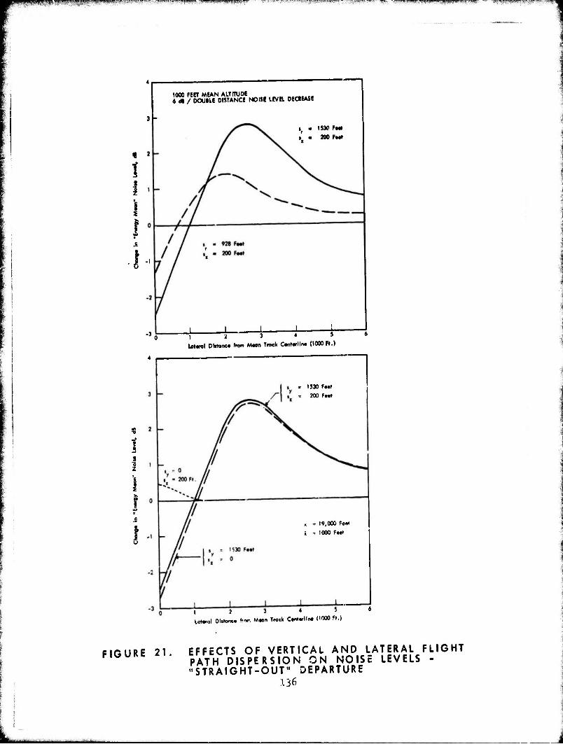
PBIAUM'V U'." •■'■mim. JW«"»J."' ■ .—J!,si»mä.» -■*j.üMow-A<wfl.ü»4Pyi"ni£m*-4-.|;.J!:: -. U

1000 FEET MEAN ALTITUDE 4 * / DOUILE DISTANCE NOSE LEVEL DECREASE

l' - 200 FM»

i-,

12 3 4 5

latarol Dlitanc* from Mton Track Ctntarlli» (1000 Ff.)

i u

• 1530 F...

. 200 F..t

.-»0F,

, » 19,000 Fast

i •= 1000 Ft.t

I J 3 Lottral DSitanc» Fror. M«an Track C»nt«rl!r» (1000 ft.)

FIGURE 21 EFFECTS OF VERTICAL AND LATERAL FLIGHT PATH DISPERSION ON NOISE LEVELS - "STRAIGHT-OUT" DEPARTURE

136

_______^

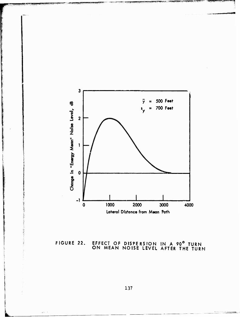
g%t;JJj|L.LJjjPJI^^WI^#«^^;^S**'tt'y^^r' -. ^f^ppD^n^Rqn^! qp wi sw Krp^gqf^^ry;!ppwf^^ PgMia^' TTfW-Wws^SW^fflffPB!*

« y = 500 Feet

s = 700 Feet y

1000 2000 3000 Lateral Distance from Mean Path

4000

FIGURE 22. EFFECT OF DISPERSION IN A 90° TURN ON MEAN NOISE LEVEL AFTER THE TURN

137

1 J 4

I I

£

-2

1.,.. 1 NOISE LEVEL DECREASE. 6dB PER DOUBLE DISTANCE 1

-I. 0.3- ^7 ■ 0.2

x#1 - 0.)

Lot TO I Dlttonc« from Myon Troek Cwitf lln» MMn Altltud*

i. i

i

i i i i

Jf . 1.0

NOISE LEVEL DECREASE, 9dB PER DOUBLE DISTANCE

y x 0.3

-£=0.2-

//

/} '/

i-o.i

r*

12 3 4 5 Lotfol Olttonc« from M»on Track Cfttflln«

Mean Altltud«

FIGURE 23. EFFECT OF FLIGHT PATH DISPERSION ON NOISE LEVELS FOR DIFFERENT DEGREES OF VERTICAL DISPERSION

138

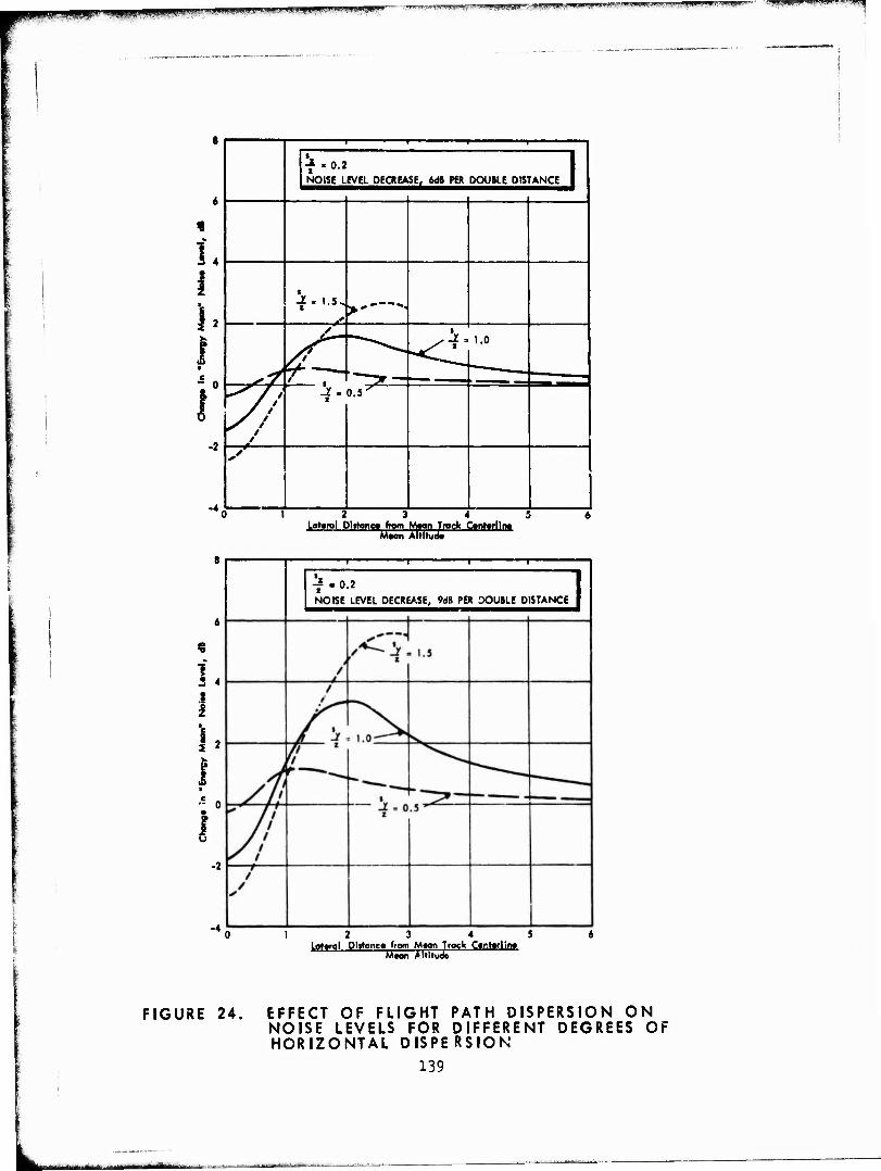
■■■■BP ! upj»i;i«^ ■\-^i^?g^iT^B?lMMWSTO?Pr-^'J.W.--U -".-' ■U'fJ'-ipiHgf

«

i. i. I ■

•s 0

I -2

-4

»- -* - 0.2 NOISE LEVEL DECREASE, 6dB PER DOUBLE DISTANCE

•

t

• 1.0

z oT^

y

Lateral Dlrtone» from Moon Tmek Contorllno Mm AlmüS

1 2 4 8

i

I ■e- 0

I -2

-4

-f • 0.2

NOISE LEVEL DECREASE, °dB PER DOUBLE DISTANCE

12 3 4 5 Lgffol DUtonc» from Moon Track ConHf lino

Moan Altitude1

FIGURE 24. EFFECT OF FLIGHT PATH DISPERSION ON NOISE LEVELS FOR DIFFERENT DEGREES OF HORIZONTAL DISPE RSION

139

rtTltiii-fl T ifc " IIMIHü nfcrtitWi '

MgBB*ES ■ wß • i*w iffiplfl IM 5«

rate turn after reaching a specified altitude. Using the

equation for 727 takeoff profiles stated above, we find that

the standard deviation in lateral dispersion after the turn

is 210 m (700 ft) for the takeoff weight distribution

described previously if the height for the beginning of the

turn is 150 m (500 ft). (This height is chosen to emphasize

the effect of the turn; it would probably not be used in

practice.) The results are shown in Fig. 22. The dispersion

curve is similar in shape to those for the previous simulation.

Again, the levels on the mean path are 1 dB lower with dis-

persion, are higher by 2 dB at 300 m (1000 ft), and diminish

to essentially zero by 900 m (3000 ft). The resultant noise

contour would be slightly broader and slightly shorter than

that obtained if no dispersion at all is assumed.

We conclude that vertical dispersion in takeoff paths

negligibly affects noise exposure computations as compared to

assuming mean flight profiles for a given aircraft type.

Lateral dispersion, however, can both broaden and foreshorten

the contours. Suitable means for accommodating the effects

of lateral dispersion on takeoff should be explored further

for incorporation in noise exposure models.

Similar analyses of the effects of dispersion in

approaches to landing have been explored in this study. It

is assumed in most noise exposure computations that the

aircraft is following a 3 degree approach path, normally

that defined by an ILS. Pull lateral deviation on trie local-

izer part of the system is 2.5 degrees, while full vertical

deviation is 0.5 degrees on the glideslope part of the ILS.

This amounts to a lateral deviation of 750 m (2300 ft) and

140

tf;piilfp,4i|l-U>^a^^ P^R9S {' pmWflRpsiPB

a vertical deviation of 140 m (460 ft) at 1C miles from touch-

down (a mean height of 970 m [3180 ft] for a 3 degree glide

slope). These deviations proportionately decrease as distance

to touchdown decreases.

A qualified pilot will typically expect to maintain his

approach well within less than half of these deviations. An

auto-coupled approach will restrict deviations to considerably

less than one-quarter of these deviations. Variations in

noise levels produced on the ground due solely to variations

in flight paths on an ILS approach can be expected to be less

than plus or minus 0.5 dB. Dispersion in flight paths on

final approach is thus not considered significant.

The results of the simulation studies can be further

generalized, with results as shown in Figs. 23 and 24. These

figures show the results of dispersion for assumed noise level

decreases with distance of 6 dB and 9 d& per doubling of

distance (Figs. 21 and 22 assumed a 6 dB decrease per doubling

of distance). Comparison of the left and right graphs of

Figs. 23 and 24 clearly shows that dispersion effects increase

in magnitude as noise levels decrease with distance at greater W

| rates.

k

Figure 23 illustrates the changes in noise levels as the

vertical dispersion is changed, holding the horizontal dis-

persion constant. The results confirm that noise levels are

relatively Insensitive to changes in vertical dispersion.

Figure 24, comparing changes in noise levels for changes in

horizontal dispersion, for a fixed vertical dispersion,

illustrates the greater sensitivity of noise level to changes

141

ig»ppg^p^j^lj^j|MpM^I|gpippiii#.w.ji.i-pi-jiu wp|W|^MPB|PllW!WSW|IB^yg " ~*"*&***'- ■ ^PpWHPPWJHPWflWl PSSi^^BPSP

in horizontal dispersion. For the relatively large horizontal

dispersion ratios used in Pig. 2^, the maxima of the curves

increase almost linearly with the horizontal dispersion ratios,

Recommendation 15 - Allowance for flight path

dispersion should be included in the USAF procedure.

Until better dispersion models are available, the

empirical equations derived here should be used.

Where it is possible to make an experimental

determination of flight path data, the observed

information should be used in the procedure.

H. Variation in Thrust Schedules

Thrust on takeoff or approach varies between different

aircraft flights as a result of operating weights, airspeed

specification, and normal operating procedures. These

procedures are usually identified with specific segments of

a given operation. With civil aircraft, for example, thrust

changes typically occur on power reduction from takeoff to

climb, or in .specific noise abatement thrust reduction pro-

cedures. Military aircraft employ similar thrust schedules,

e.g. "afterburner to 200Ü feet, then reduce to military

power."

All thi specified thrust management procedures are

accommodated in present noise exposure computational pro-

cedures by specifying the noise output for various thrust

values. Since thrust changes are accompanied by a change in

flight profile, it is customary to account for the thrust

conditions and flight profile variations by dividing the

142

■i!ii iiHM»ii"i i i i mm im 11 I in i -r-vm*F***&m8Q iiJimmu. IWIIJ vwmnmQ^^ miiiwij .__i >_.

I

flight path into segments for which the specific conditions

apply.

5. Noise from Ground Run-up Operations

Fundamentally, there are no differences in noise exposure

calculations between civil and military flight operations.

Normal takeoff and approach operations are similar in both

instances. Touch-and-go operations occur in both cases. The

military use of afterburner or water injection is treated by

flight path segmentation as indicated previously. As long as

thrust schedules and their associated flight paths are defin-

able into segments, any set of conditions can be accommodated,

including overhead approaches and multiple aircraft (e.g.

"flight of two") takeoffs.

Significant differences between civil and military

operations occur for the method of treating noise produced

on the ground by aircraft on the ground. The present civil

NEP computations do not Include ground run-ups, either for

maintenance or pre-takeoff operations. Most civil aircraft

maintenance operations involving engine operation are per-

formed in test cells or under isolated conditions at carefully

controlled locations. This is not true at most military bases,

where protracted ground running often occurs. Pre-takeoff

runup, or afterburner lighting, is customary for military

aircraft, while civil aircraft most often use a "rolling"

start.

Noise from ground operations should be incorporated in

any complete nois». exposure computational model. The pro-

cedure now in use in the present USAF procedure describes

aircraft ground operations in terms of polar diagrams of PNL,

1*3

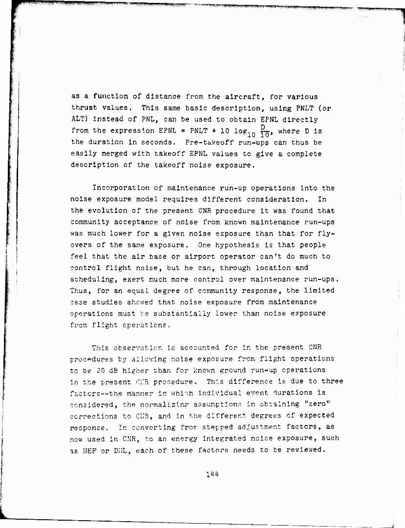
as a function of distance from the aircraft, for various

thrust values. This same basic description, using PNLT (or

ALT) instead of PNL, can be used to obtain EPNL directly

from the expression EPNL = PNLT + 10 log,Q «-, where D is

the duration in seconds. Pre-takeoff run-ups can thus be

easily merged with takeoff EPNL values to give a complete

description of the takeoff noise exposure.

Incorporation of maintenance run-up operations into the

noise exposure model requires different consideration. In

the evolution of the present CNR procedure it was found that

community acceptance of noise from known maintenance run-ups

was much lower for a given noise exposure than that for fly-

overs of the same exposure. One hypothesis is that people

feel that the air base or airport operator can't do much to

control flight noise, but he can, through location and

scheduling, exert much more control over maintenance run-ups.

Thus, for an equal degree of community response, the limited

case studies shewed that noise exposure from maintenance

operations must be substantially lower than noise exposure

from flight operations.

This observation is accounted for in the present CNR

procedures by allowing noise exposure from flight operations

to be 20 dB higher than for known ground run-up operations

in the present CNR procedure. This difference is due to three

factors—the manner in whioh individual event durations is

considered, the normalizing assumptions in obtaining "zero"

corrections to CNR, and in the different degrees of expected

response. In converting fron: stepped adjustment factors, as

now used in CNR, to an energy integrated noise exposure, such

as NEF or DHL, each of these factors needs to be reviewed.

11(14

■nmappmn ■vvgr^Fg, r^^M.pxrrr,.,yiir*,j!r,,

The implicit duration assumed in the present CNR

procedure for flight operations, as defined by the duration

between the points in the time history that are 10 dB below

the maximum, was 15 seconds for takeoffs. For many typical

flyover signals in the vicinity of airports this results in

an EPNL value that is almost equal to the maximum PNLT value.

(For a Gaussian shaped time history the integration procedure

provides EPNL ■ PNLTM - 0.8 dB; the "effective" duration is 8.3 seconds for the 15 second duration between ]0 dB down

points.) The "zero" correction CNR for flight operations in

the day time applies to 10 to 30 operations. Assuming an

average of 20 operations, the effective total exposure is

PNL + 10 log (8.3 x 20) = PNL + 22 dB.

The run-up duration for zero correction is 1 to 5

minutes. Assume an average of 3 minutes. The zero correction

for operational factors applies to "5 or less." Assume a

typical value to be 3- The effective total exposure for

run-ups at zero correction in the CNR procedure is thus

PNL + 10 log (3 x 3 x 60) = PNL + 27 dB, or actually 5 dB

more than for the zero correction case for flight operations.

In the CNR procedure the operational adjustment and

criteria values were selected so that ground and flight

operations could be compared on an equal response basis. The

penalty of 20 dB for ground operations becomes 15 dB when

equal noise exposures between ground and flight operations are

compared, since the ground noise exposure is actually over-

stated by 5 dB as compared to the flight noise exposures.

In order to assess the validity of the ground operations

noise criteria used in the CNR procedure we reviewed the case

1*5

3_!HJIJUPLI!P'MU!!AJ-llll I I J I II ,;;.--—-~-r- -*V*^* '-* ■ V*»-" -^;^; '<"*K<14 J***!*^". " ■■»L^ - i I^I,*; «-, i« n ---~—*-:

histories used in developing the procedure. There were only

five case histories available to assess ground operations.

Each had three things in common. First, all operations were

conducted at night, with low background levels when the air-

craft noise was not present. Second, there were essentially

no flight operations during the time of the maintenance

operations. Third, in each case jet operations had not been

in effect for much more than one year at the time the case

was identified.

It is reasonable to speculate that these factors, as better

identified in social surveys, tend to provide a stronger

community response than the noise exposure would indicate for

more normal circumstances. Lack of previous exposure, quiet

background levels when the run-ups were not in operation,

night time conditions probably thought unnecessary (misfeasance

on the part of the operators?) all would tend to increase

response. In retrospect, the penalty applied to ground

operations is based on only a few data points with these

unusual conditioning factors involved. The ground operation

noise penalty might well be too stringent, or even not required

under most circumstances. Unfortunately, no new data on

response to ground maintenance operations are available in any

documented form. For example, the data on annoyance obtained

in community social surveys make no reference to ground

operations.

The importance of resolving this problem cannot be over-

estimated. For those bases where maintenance run-ups are a

significant part of the operations, overestimating the

expected response of a community by defining noise contours

at too low a value of exposure can extend to a large area the

146

1 juj UALJ U11 UJJIJPJ u Pp i'j|papi BggPjesp *-■■■»■ " n^wp^^j^m pppr " --^--■^■ü^ijJA.J^ijgiuij.Mp.. pi ppBgJJlg^gHpEgg^ . Ripjyii^Pjft^jptxii,^ ^IB

region that would be Judged incompatible for residential use.

It would seem that two steps might be taken to resolve this

problem. First, those air bases suspected or known to have

run-up noise problems should be identified. Second, a survey

of the community response at several selected bases should be

made. The correlation of thi? information with noise

exposure due to ground operations could then be used to

determine the appropriate noise criteria.

In the interim, it appears to the author, after reviewing

the limited case histories currently available, that the

present criteria in the CNR procedure overstated the ground

noise situation by at least 5 dB of equivalent noise exposure.

On this basis, noise from ground operations would be penalized

by 10 dB, on an exposure level basis, as compared to noise

from flight operations. We propose this factor be used in

the USAF procedure until further evaluation provides a clearer

picture of the proper means for evaluating noise from ground operations.

Recommendation 16 - Ground run-up operations for

maintenance purposes should be included in noise

exposure calculations by computing their EPNL or

SELT values. These values should then be weighted

by an additional 10 dB when summing the total exposure at the air base.

Recommendation 17 - Run-up associated with takeoff

operations should be included in the takeoff noise

calculations directly in terms of their contribution

to the takeoff EPNL or SELT.

1^7

^mmgomrmmimgmmm*m** nujiu»Biw»ppf»f««B IMW i- •II-»..>-^- -?■-——»-^ HIJIJB'»!«!!»,«.».! imiww IUM-JJ-UI ,»*,

D. Discussion of Prediction Accuracies

Differences between predicted noise exposures around

an air base and those that would be measured can be considered

in two different ways. One can first examine the possible

error in predicting the EPNL for a single aircraft at any point on the ground. A second, more generally useful approach

is to examine the possible error in the noise exposure for an

accumulation of events. Since a twenty-four hour assessment

of noise exposure is the base of computation for CNR, NEF and

other indices, the accuracy of predicting the exposure from a number of events is of more interest for planning purposes.

One may examine the case of the individual event pre-

diction by considering first the accuracy of generation of

the EPNL/distance function from controlled test measurements.

As we show in Ref. 55» the EPNL produced on the ground at

slant distance LX by an aircraft in flight is given by:

EPNL * EPNL, + PNLT - PNLTM, + A0 + Ar x h x h 2x 6 o o

where: A,x - 10 flog1(J ^-p_i . Vx_^ "I I» o ret J

A,- = incremental char.ge in noise power output

relative to the noise power at reference

conditions.

LX = L- j-L J (See Fig. 25) s In e

148

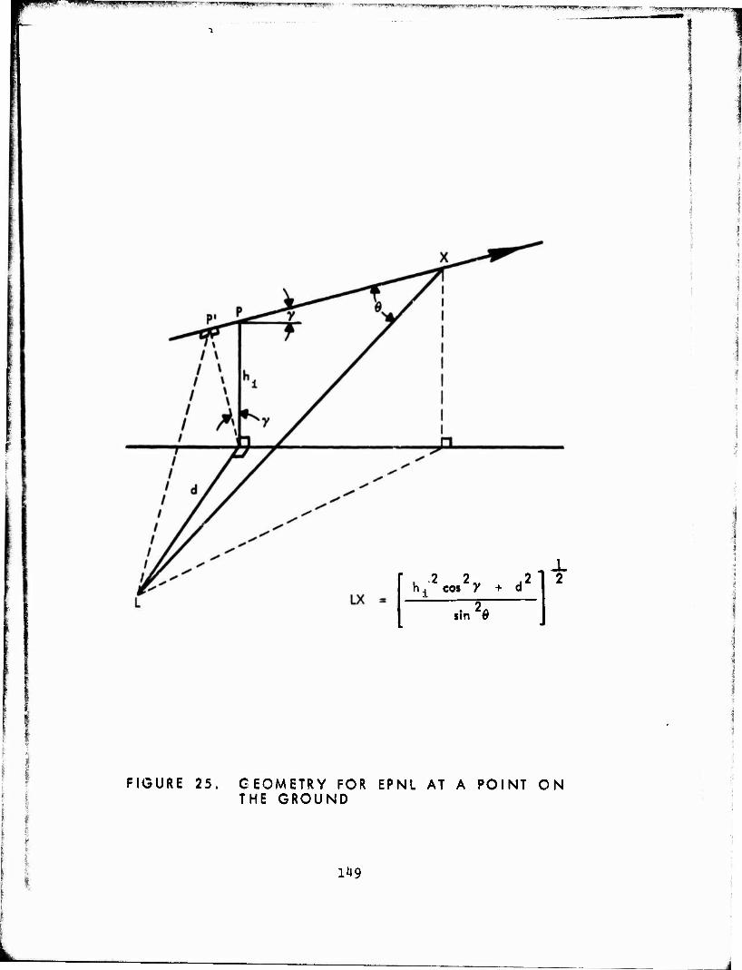
u^yn,j*wt-, i!w § BgaWF?9py»PBIj

f . .2 2„ 1^ cos y + j2l

$in26 s

X

FIGURE 25. GEOMETRY FOR EPNL AT A POINT ON THE GROUND

1U9

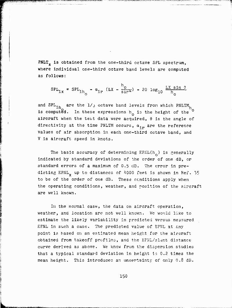
|HtfI'MJJ'-.L'iuP'*«wixuywp*-«,'!','. i ' ^TT-.Sr^yL.L'^f'*

PNLT is obtained from the one-third octave SPL spectrum,

where individual one-third octave band levels are computed

as follows:

SPLix " SPLih - air (LX " £ln*> " 20 loS10 ^^ o o

and spLj. are the 1/j octave band levels fron which PNLTM.

is computed. In these expressions h is the height of the °

aircraft when the test data were acquired, 9 is the angle of

directivity at the time PNLTM occurs, a. are the reference

values of air absorption in each one-third octave band, and

V is aircraft speed in knots.

The basic accuracy of determining EPNL(h ) is generally

indicated by standard deviations of the order of one dB, or

standard errors of a maximum of 0.5 dB. The error in pre-

dicting EPNL up to distances of '-1000 feet is shown in Ref. 55

to be of the order of one dB. These ccnditions apply when

the operating conditions, weather, and position of the aircraft

are well known.

In the normal case, the data on aircraft operation,

weather, and location are not well known. We would like to

estimate the likely variability in predicted versus measured

EPNL in such a case. The predicted value of EPNL at f.ny

point is based on an estimated mean height for the aircraft

obtained from takeoff profiles, and the EPNL/sldnt distance

curve derived as above. We know from the dispersion studies

that a typical standard deviation in height is 0.2 times the

mean height. This introduces an uncertainty of only 0.8 dB.

150

■■ - - - ■

mBfmatamg&BHIG^ ■-ff. g^pwsiSPWypi'ffitffPffWB'P

Variations in power management can introduce? from zero to H dB

uncertainty in any given flight. Finally, variations in

weather conditions can introduce from 5 to 10 dB differences

between measured and predicted noise levels at slant distances

in excess of 10,000 feet under most ranges of weather typically

encountered or as much as 17 dB under extreme weather condi-

tions- In these extreme weather cases, the change in air

absorption is often compensated partially by changes in

aircraft performance.

Quantifying the differences between predicted and measured

EPNL values with any degree of reliability when the operational

and weather conditions are unknown is at best a guessing game.

Of more usefulness is the examination of data where aircraft

positional information is available, permitting comparisons

of predictions with noise measurements.

One example of these kind of data is available irom a

recent FAA project—2- . In this study a series of controlled

takeoff and approach procedures were evaluated for several

types of jet transports. The data scatter at any measurement

location was generally between 5 and 10 dB, corresponding to

standard deviations of the order of + 2 dB.

Another example of measured versus predicted EPNL values

is available in another recent FAA study of approach noise

with typical airline operations at a commercial airport— .

The following table indicates the standard deviation for sets

of noie-e measurements of three classes of civil jet transport

aircraft. The table also shows the standard deviation for

the components of the variance due to distance and air

131

-if nrr™""

^jOT«S"UJ.t^"^|fcflW^Wa'»JIH«"':ll'll:'»1-™»:i !J".J«^SH»» *W^«*'*'"/W'W --'««*'' --^^»^^^S»'r?r^llfli™«V»';W<l»»^^^ .-;«^<M|J|L)MIMB,,<!>J^

absorption, and the standard deviation for the residual

variance.

TABLE VII

Variability of EPNL Values Under the Nominal Approach

Path - 31,000 to 82,000 feet from Touchdown Expressed

as Standard Deviatiors in dB

Aircraft Type No Total Distance Weather Other

Pour-engine 332 7.6 5.9 2.5 ^.o Three-engine 3^4 6.5 5.M 1.9 3.0

Two-engine 251* 7.0 5.6 1.9 3.8

Assessing the accuracy in predicting noise exposure from

a series of events is another matter. Several factors enter

into 1 he problem which make it difficult to derive analyti-

cally a basic accuracy of prediction. First is the accuracy

of knowing the aircraft type mix. For aircraft of the same

basic type and engine configuration it is not important to

know the exact numbers of each model, only the total. Further,

an inaccuracy in forecasting total numbers within the class of

as much as 25$ introduces only a one dB error in the noise

exposure calculations.

Of most importance is the proper identification of flight

tracks. We have shown in the discussion on dispersion that

errors up to 3 dB or more can be introduced by assuming no

dispersion. The error associated with total mis-identification

of flight tracks cannot even be assessed.

152

W^^S^W^^^^^^^!^^^^W>'^^fl^^sfmi^m

Errors in estimating flight track utilization, however,

of 25$ are required to make a one dB error. For the main

runways where utilizations may be 30 to 90 percent, a 25$

error in estimated usage is not too likely. However, the

utilization for little used runways (e.g. 1 to 5 percent

utilization) can often be mis-estimated by factors of two or

more, introducing errors of 3 dB or even greater.

Probably of more significance in assessing errors in

noise exposure computation is to compare some actual measure-

ments of exposure with those predicted by NEF methodology for

the same cases. One comparison can be made for the data

reported in Table VII. These data were obtained at six

different positions directly under the normal flight track

over a number of days. Traffic density did not vary signi-

ficantly during the days of measurement. The following

table lists the difference between predicted and measured

values of NEF.

TABLE VIII

Predicted Minus Measured NEF

Position A NEF

1 0.9 2 1.2

3 1.0 a -0.6

5 -3-5

6 -1.9

Average -0.5

Standard Dev iation 2.0

153

■g't.1 •■■} ,'^T^V'hLH^^r^,^'y:-,~v' ggpgpjppi ..'■■.'-■■. ", T,.y7^^y--aggg''- - - -^i^^Tr^^;^.yaT^5Tf-w?™?.^ip-^g% ar^iigwi^i^p^inpB^M^piHB^aafpPWWgppW^rgl "WWif" - .tWU^iil^WBBfpw

It should be observed that the average EPNL at position

5 was higher than generally expected, hence the larger A NEP

value.

Other examples are available from recent noise monitoring

experience at civil airports, where monitored noise data has

been compared with computed CNEL values. At one civil airport,

noise measurements were made at 17 positions for periods vary- 77/ ing from two to eleven days— . The computed CNEL contours

overestimated measured takeoff CNEL values by an average of

0.8 dB, with a standard deviation among stations of 1.4 dB.

The computed landing CNEL contours underestimates measured

CNEL values by an average of 1.4 dB, with a standard deviation

among positions of 2.1 dB.

In summary, if accurate data on aircraft performance,

weather, and position are available, one can expect to predict

EPNL (over reasonable weather limits) tc within a standard

deviation of plus or minus one to two dB up to slant distances

of the order of 10,000 feet. Where the performance, position,

and weather information is only nominally known, the standard

deviations increase to as much as + 4 dB. On the other hand,

cumulative noise exposure from a number of events seems to be

predictable to about one-half the variation in prediction of

EFNL alone. It is reasonable to assume that a good noise

exposure model with reasonably reliable input data can be

expected to predict actual noise exposure with a standard

deviation of about + 2 units of NEF.

154

jjiLj.-ui-mmnu"

CONCEPTUAL DESCRIPTION OF A NEW PROCEDURE FOR

USAF AIRCRAFT NOISE LAND USE PLANNING PURPOSES

2/ The present USAF procedure- is purposely designed for

easy application, through the use of equal PNL design contours

that permit hand computation of the noise exposure from a

series of aircraft operations. This ease of application has

provided a useful tool for planning purposes. The simplifi-

cation process, however, can lead to sizable errors, as much

as 10 dB, if proper judgment is not used when borderline

operational correction factors are applied.

The evolution of exposure level descriptors such as EPNL

and SELT, instead of maximum PNL, has been shown to be a

substantially more general quantity for a variety of aircraft

noist?s. In order tj make best use of the exposure level

measures in land use planning procedures the simplified

5 dB step operational adjustment factors used on the current

procedure need to be replaced with more accurate assessments

of aircraft movements. Further, mere refined treatment of

sound propagation factors, allowance for variability in

flight paths, and more refined aircraft performance data

will improve the accuracy of noise exposure computations.

In order to accommodate the above items in a planning

tool, it is most practical to utilize a computer model for

noise exposure computation. A suitable computer program

allows as much refinement as desired in order to improve the

accuracy of the noise exposure computations.

155

P^pi^l^pllBPPigpgBMBPJWPPq ." gpp ■ »wiqffjiBgff^iigwwpuwi 'T" nswaeppa!

The following descriotion outlines the procedural

framework for a revised aircraft noise/land use plai-.a.'wr

procedure developed in this project as a result of' tu.- i -re-

going review. This procedure is programmed to provide a

computer generated graphic plct of noise exposure level

contours for the entire comp\ex of operations at an airport.

It is not the intent of tht.^ description to provide the

detailed implementation of all the technical elements em-

ployed in the computation itself. The primary purpose-is to

discuss the input data for the model and to describe the

combinatorial rules used for developing a single number

descriptor of the noise produced by a complex of aircraft

operations. All the recommendations provided in the previous

sections of this report are either included explicitly in

this description, or are implicitly included in the computer

development of the procedure. An engineering description of

the computational method is provided in Apoendix C. Companion 73/

reports in this series provide an applications guide-1—■ , a 79/ test procedure for source noise data acquisition—- , computer Op pi /

program operators manual and program description—*— , and ftp /

a basic acoustic date fi'o for military aircraft— .

A. Aircraft Noise Source Description

During the initial part of this project the wide use of

EPNL as a descriptor for aircraft noise because of the

tecnnical reasons for Its superiority lea to our preference

for its use in the proposed U3AF procedure. During the pro-

jects development, however, it became c j ear that EPA wa.«

strongly urging the adoption of A-weighr,ed sound level as a

universal descriptor of noise from all ;ourees. It became

apparent that, while a final decision on the use of EPNL or

156

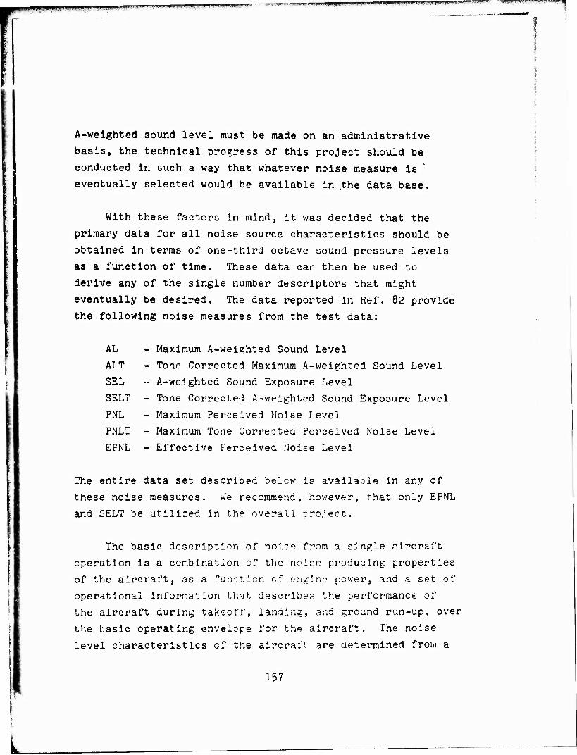
tmmtmm'mmm >,-. ■ ^gmmm wmt "'* "-! -' . j,iH!»LiP4|,HjjH-ii.l.U HjH '.' iiJ^MUM..... • '!»

A-weighted sound level must be made on an administrative

basis, the technical progress of this project should be

conducted in such a way that whatever noise measure is

eventually selected would be available in the data base.

With these factors in mind, it was decided that the

primary data for all noise source characteristics should be

obtained in terms of one-third octave sound pressure levels

as a function of time. These data can then be used to

derive any of the single number descriptors that might

eventually be desired. The data reported in Ref. 82 provide

the following noise measures from the test data:

AL - Maximum A-weighted Sound Level

ALT - Tone Corrected Maximum A-weighted Sound Level

SEL - A-weighted Sound Exposure Level

SELT - Tone Corrected A-weighted Sound Exposure Level

PNL - Maximum Perceived Noise Level

PNLT - Maximum Tone Corrected Perceived Noise Level

EPNL - Effective Perceived Noise Level

The entire data set described belcw is available in any of

these noise measures. We recommend, however, that only EPNL

and SELT be utilized in the overall project.

The basic description of noise from a single circraft

operation is a combination of the noise producing properties

of the aircraft, as a function of engine power, and a set of

operational information that describes the performance of

the aircraft during takeoff, landing, and ground run-up, over

the basic operating envelope for the aircraft. The noise

level characteristics of the aircraft are determined from a

157

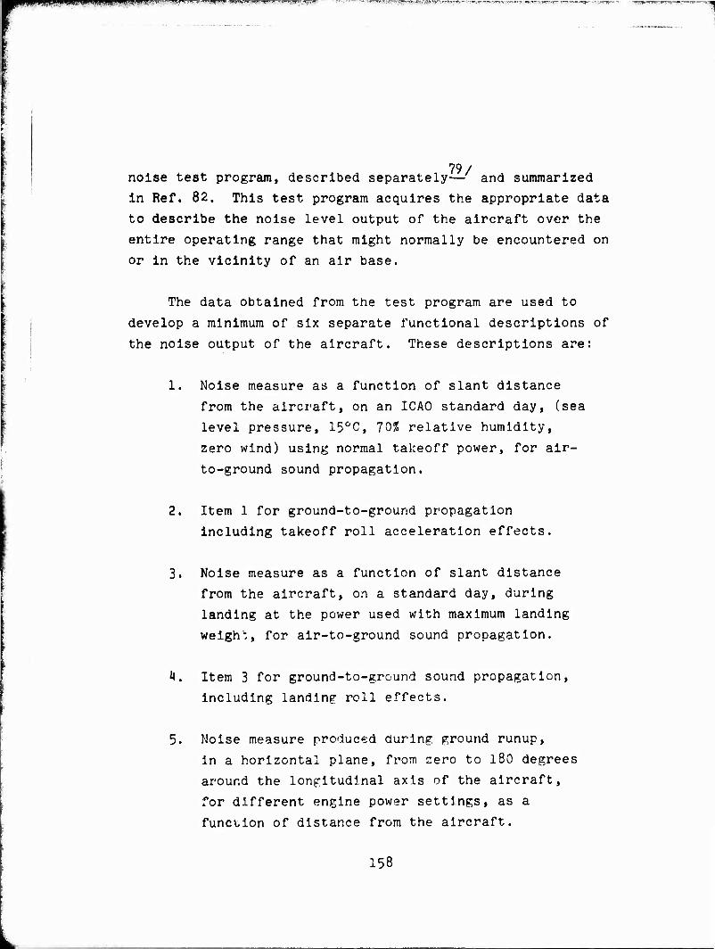
HimB!pnis«miinppBiff»

79/ noise test program, described separately— and summarized

in Ref. 82. This test program acquires the appropriate data

to describe the noise level output of the aircraft over the

entire operating range that might normally be encountered on

or in the vicinity of an air base.

The data obtained from the test program are used to

develop a minimum of six separate functional descriptions of

the noise output of the aircraft. These descriptions are:

1. Noise measure as a function of slant distance

from the aircraft, on an ICAO standard day, (sea

level pressure, 15°C, 70% relative humidity,

zero wind) using normal talceoff power, for air-

to-ground sound propagation.

2. Item 1 for ground-to-ground propagation

including takeoff roll acceleration effects.

3. Noise measure as a function of slant distance

from the aircraft, on a standard day, during

landing at the power used with maximum landing

weigh:, for air-to-ground sound propagation.

4. Item 3 for ground-to-ground sound propagation,

including landing roll effects.

5. Noise measure produced during ground runup,

in a horizontal plane, from zero to 180 degrees

around the longitudinal axis of the aircraft,

for different engine power settings, as a

function of distance from the aircraft.

158

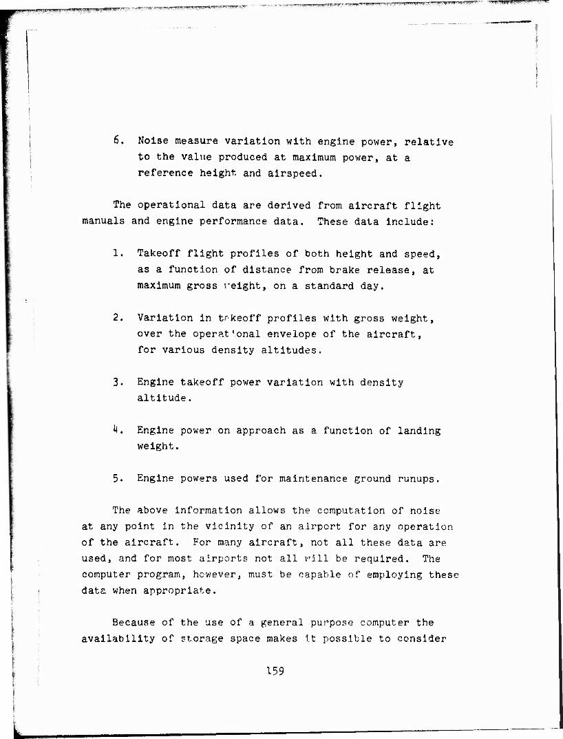
6. Noise measure variation with engine power, relative

to the value produced at maximum power, at a

reference height and airspeed.

The operational data are derived from aircraft flight

manuals and engine performance data. These data include:

1. Takeoff flight profiles of both height and speed,

as a function of distance from brake release, at

maximum gross relght, on a standard day.

2. Variation in trkeoff profiles with gross weight,

over the operational envelope of the aircraft,

for various density altitudes.

3. Engine takeoff power variation with density

altitude.

h, Engine power on approach as a function of landing

weight.

5. Engine powers used for maintenance ground runups.

The above information allows the computation of noise

at any point in the vicinity of an airport for any operation

of the aircraft. For many aircraft, not all these data are

used, and for most airports not all vill be required. The

computer program, however, must be capable of employing these

data when appropriate.

Because of the use of a general purpose computer the

availability of storage space makes it possible to consider

159

performance data for each aircraft individually, and for

many specific aircraft, data for various mission types

(e.g. afterburner and non-afterburner takeoffs, various

operating weights, training operations as compared to other

missions). A major test program has been conducted by the

USAF, following the test methods of Ref. 79, to provide the

basic input to the noise exposure computation. Results of

these tests are described in Ref. 82. These test data are

further processed, using procedures described in Ref. 79 to

develop the noise level data required for the computations

in the noise exposure program.

This data file is now available for different aircraft.

The noise test program is continuing, with the goal of

having a data file that will eventually cover essentially

ail USAF aircraft. In addition, performance data for these

aircraft, sometir.es for several different mission types, are

stored in the data file. Where performance differences exist

between different lettered versions of an aircraft type,

separate data files are provided. Thus in the new procedure

individual modele of each aircraft can be specified rather

than by classes t interceptors, etc.) at: is done in the present

USAF procedure. The data file also accommodates estimated

noise and performance data for some aircraft systems where

test data are not yet available. Such estimates can be made

for projected new systems if desired, sc that the effect of

these aircraft systems on noise at any airbase can be

evaluated prior to the development or 'introduction of the

system into service use (e.g. new STCL designs, or a new

engine design for an exist!.ig aircraft1.

160

■nun „ ____„_„—„_^ - -.-;--1 „ —vacs* >WUfHi*>*«P!UfjiiM<r'"•! !"w I'". *Pf« »""'■'

B. Description of the Noise Produced by A

Single Aircraft Operation

The noise produced by a single aircraft may be described

by a set of contours of constant noise measure, plotted at

5 dB increments, with the range of levels selected in terms

of the problem at hand. For flight operations, the noise at

any point is determined by first calculating the distance of

closest approach from the point of observation on the ground

to the aircraft trajectory (minimum slant distance) and the

angle subtended between the horizon and the vector describing

the minimum slant distance (see Pig. 15). The noise value at

the observation point is then determined from the appropriate

noise-slant distance function, either air-to-ground, ground-

to-ground, or an interpolation between the two, depending

upon the value of angle 9 of Fig. 15 (page 111).

It is often convenient to break the flight trajectory

into a series of segments. The choice of segment lengths

is governed by both engine power conditions and by geometrical

changes in flight profile or track. Segments are chosen tc

be representable by straight line segments or circular arcs

whenever possible. While it is possible to have a change in

flight track without a power change, a power change will

almost always cause a fllg.nt profile change. Thus each

segment requires an engine power specifjcation, and a noise- I | slant distance specification. In this manner the noise

contour for any operatlor, along any flight path, may he

computed.

The noise from a grc.und runup operation is calculated

by first determining the distance from the observation point

I 161

PH.UII.U.» IIJM .Jip^.M-Mmilf^-Vig«!,«'"*- ',,J- >- J'.ITJ^JWIUf»';

to the aircraft, s, and the angle, <|>, defined as the angle

between a line from the observation point to the longitudinal

axis of the aircraft, as measured from the forward part of

the aircraft. The value of PNLTM (<J>,s) or ALT (<t>,s) at the

observation point is determined from the polar data on noise

level as a function of angle and distance from the aircraft.

The value of EPML (<J>,s) is given by:

EPNL U,s) = PNLT (<j>,s) + 10 log1QAt - 10 (1)

where At is the duration in seconds.

NOTE:

EPNL in decibels .Is defined in Ref. 5 as:

EPNL = PNLTM + D (2)

where PNLTM is the maximum tone-corrected PNL during an event,

and D is a duration correction factor defined as:

rt2 PNLT 10

D = 10 log10 jp / 10 dt - PNLTM (3)

h

where T is a normalizing constant, specified as 10 seconds,

and t, and t? are the points of the tir.e distribution of

PNLT where the PNLT values are 10 dB less than that for

PNLTM. The expression for EPNL may be rewritten as

t.

EPNL = 10 log1Q . ^0 / CO

162

i|p^p^p^j|l»,4Wi|^^w^M*iiM^Ayyi^iJ :,.a<**mn3irr- T- '-vfi.i'i, '.imijkB^ii.. .AMW^-WJ^.J^'h"1^^ ^m-^mm^ w t^^aaf Hi jF i a .jjy^j

or EPNL = 10 log10

2 PNLT , 10

10 dt - 10 (5)

In the above specification for EPNL (<j>,s), equation (1), it

is assumed that PNLT values will be constant over the

duration At for a specified operating condition. Thus equation (5) becomes

EPNL * PNLT + 10 log1Q J dt - 10 (6)

as stated in equation (1).

In an essentially parallel fashion, SELT IS defined

t„

as

SELT = 10 lot 10 T

ALT

10 10 dt (7)

where T is now specified as one second. In this case SELT

for ground operations is merely:

SELT * ALT + 10 log dt (8)

The computation of equal noise contours may be deter-

mined in two ways. One way is to define an x,y,? grid

system over the ground plane and compute noise values at

each grid point, then determine contours of equal noise

163

PPps^pqpBlffpjpjg! B'^^l^^ra'BW^HWi'f ^MM^!£t^U^f.Jire»^ '^wv^ffW^W^^^P^^^^^^^^m-mwm^m-m^mtim^m.:-^^-- jjmi w»««

by connecting grid points (or interpolating between them) of

equal value. The second way is to select a specific noise

value and compute a series of coordinates which when con-

nected will form equal valued noise contours. Both systems

have been used in previous models. The fixed grid system

has an advantage in handling curved flight tracks, since the

increased duration on the concave side of the track as

compared to the convex side may more easily be computed and

the effect of superposition of different operations is more

easily accommodated. This method is used in the new program.

C. Description of the Noise Exposure Produced by a Series

of Aircraft Operations

The gc?.l of the noise exposure computations is to ob;?in

a single number, at every point in the vicinity of the air

base, that represents the accumulated effect of all the

operations. This numoer is then related to the anticipated

acceptability of the noise from the oparations for various

functional uses of the land. Pending resolution of the

choice of EPNL or SELT as the basic descriptor for individual

aircraft noise events, the computer Drogram currently computes

NEF values as in the current civil NEF programs, with appro-

priate modifications for military operations. If SELT is

chosen as the basic noise descriptor, the program can easily

be changed to compute DHL instead of NEF. The program also

provides the computational improvements In description of

noise sources, sound propagation factors, and operational

characteristics which are not now used in the civil NEF

program. These items do not affect the concept of NEF but

should improve the accuracy of its representation.

161

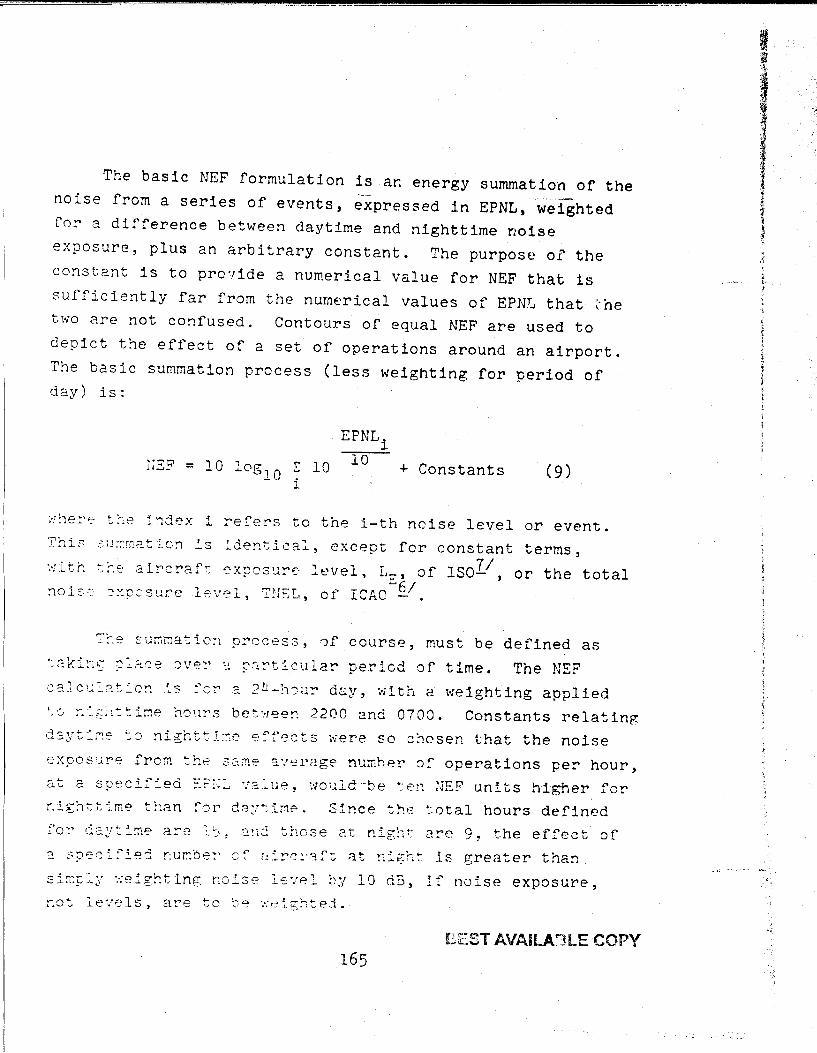
The basic NEF formulation is ar. energy summation of the

noise from a series of events, expressed in EPNL, weighted for a difference between daytime and nighttime noise

exposure, plus an arbitrary constant. The purpose of the

constant is to pregide a numerical value for NEF that is

sufficiently far from the numerical values of EPNL that ~he two are not confused. Contours of equal NEF are used to

depict t~e effect of a set of operations around an airport.

The basic summation precess (less weighting for period of day) is:

= 10 log10

[ 10 i

EPNLi 10

+ Constants (9)

~he~~ the i~dex i refers to the i-th noise level or event.

This ~u~matlcn is !dentica:, except fer constant terms,

·.-::Ltr. ~:l'" . .::.· aircraf:: expcsur~ level, Lr:, of Isoi1 , or the total noisi~ ~XJ::csure le\rel, 7~.JSI.,, of' ICAO .w~;.

?~e 2um~aticn precess, 0f course, must be defined as

~aki~~ ~lace ~v~r a p~rticular period of time. The NEF cq}cu~at~cn is for a 2~-h~ur day, with a weighting applied

',c, :-:>;:1:tir.:e l101trs bet··1een :?200 and 0700. Constants relating

dsyt~~E ~a nighttl~e e~f0cts were so chosen that the noise

expos•Jre frcm t!:e .3C-:.me S'!"==l'<l.ge nu:r.her of operations per hour,

at a syeci:~ied E?::::., '.'a:"..ue, :·wulct··be tE·r:. :JEP units higher for

~ighttime t~an for day~ine. Since the total hours defined

.Co:"' ric.~.r~i:ne a~e ~5! ~2:1~ ~r1cse .?..t nig:1t a:--e 9, the effect of

greater than

BEST AVAILA'1LE COPY 165

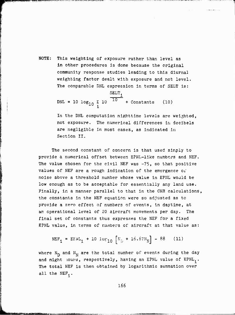
»flPBPWagailgWBIP ■ NP*4* I4JH1II" IftMf', ff ■ *■■ u ?-.!■■■ *M *■'■':' i.. L. . [i._ i.^■^.jj.ujqjjLi^«^-.«i f ^v fW.'-< - »■ ?;*■%■ "° ■' ., ^,^., ,,™™^.^# ,. mm*,*; .^«Hw^sapaws-r^^ra»»* = ;-?p5*Rfy

NOTE: This weighting of exposure rather than level as

in other procedures is done because the original

community response studies leading to this diurnal

weighting factor dealt with exposure and not level.

The comparable DNL expression in terms of SELT is:

SELTi

DNL = 10 log1Q I 10 10 + Constants (10)

In the DNL computation nighttime levels are weighted,

not exposure. The numerical differences in decibels

are negligible in most cases, as indicated In

Section II.

The second constant of concern is that used simply to

provide a numerical offset between EPNL—like numbers and NEP.

The value chosen for the civil NEF was -75, so that positive

values of NEF are a rough indication of the emergence or

noise above a threshold number whose value in EPNL would be

low enough as to be acceptable for essentially any land use.

Finally, in a manner parallel to that in the CNR calculations,

the constants in the NEF equation were so adjusted as to

provide a zero effect of numbers of events, in daytime, at

an operational level of 20 aircraft movements per day. The

final set of constants thus expresses the NEF for a fixed

EPNL value, in terms of numbers of aircraft at that value as:

NEF^^ = EFWL1 + 10 lof10 [V + 16.67*0 - 88 (11)

where ND and NN are the total number of events during the day

and night lours, respectively, having an EPNL value of EPNL..

The total NEF is then obtained by logarithmic summation over

all the NEF1.

166

mm ■■'■ iMiiii i

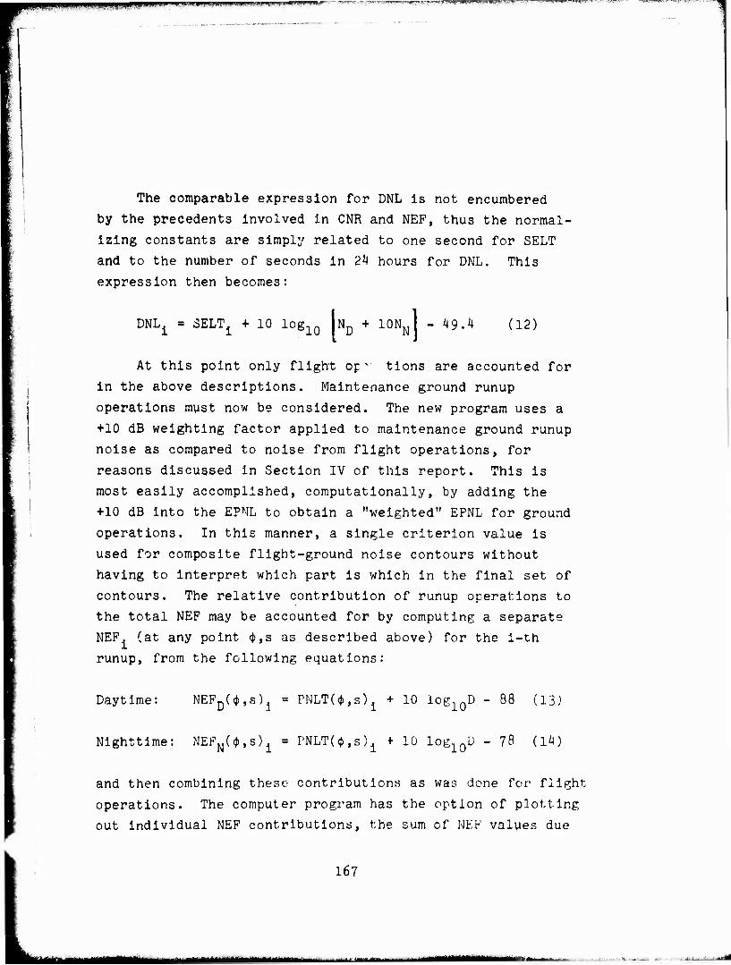
npntpiiP! IP wpwwiWipppBppHPilBWf W ww.JW>'

The comparable expression for DNL is not encumbered

by the precedents involved in CNR and NEF, thus the normal-

izing constants are simply related to one second for SELT

and to the number of seconds in 24 hours for DNL. This

expression then becomes:

DNI^ = 3ELT1 + 10 log1Q ND + IONJ - 49.4 (12)

At this point only flight op- tions are accounted for

in the above descriptions. Maintenance ground runup

operations must now be considered. The new program uses a

+10 dB weighting factor applied to maintenance ground runup

noise as compared to noise from flight operations, for

reasons discussed in Section IV of this report. This is

most easily accomplished, computationally, by adding the

+10 dB into the EPNL to obtain a "weighted" EPNL for ground

operations. In this manner, a single criterion value is

used for composite flight-ground noise contours without

having to Interpret which part is which in the final set of

contours. The relative contribution of runup operations to

the total NEP may be accounted for by computing a separate

NEF. (at any point 4>,s as described above) for the i-th

runup, from the following equations:

Daytime: NEPD(*,s)1 = PNLT(<J>,s)jL + 10 log10D - 88 (13)

Nighttime: NEFN(4»,8)1 = PNLT($,s)1 t 10 log1QD - 78 (14)

and then combining these contributions as was done for flight

operations. The computer program has the option of plotting

out individual NEF contributions, the sum of NEF values due

167

-——————■■■ . . ... . .. . . ■!——■—■ _

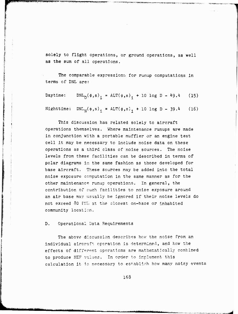
!BWWWHW.imT|w»'.W.im'iMKi.Wft- - " ' »W.W..II«,I..,II,W,

solely to flight operations, or ground operations, as well

as the sum of all operations.

The comparable expressions for runup computations in

terms of DNL are:

Daytime: DNLpU.s^ = ALTdfr.s^ + 10 log D - 49.4 (15)

Nighttime: DNl^Ctfr.s^ = ALT(<j>,s) 1 + 10 log D - 39.4 (16)

This discussion has related solely to aircraft

operations themselves. Where maintenance runups are made

in conjunction with a portable muffler or an engine test

cell It may be necessary to include noise data on these

operations as a third class of noise sources. The noise

levels from these facilities can be described in terms of

polar diagrams in the same fashion as those developed for

base aircraft. These sources may be added into the total

noise exposure computation in the same manner as for the

other maintenance runup operations. In general, the

contribution of such facilities to noise exposure around

an air base may usually be ignored if their noise levels do

not exceed 80 ML at the closest on-base or inhabited

community location.

D. Operational Data Requirements

The above discussion describes how the noise from an

individual aircraft operation is determined, and how the

effects of different operations are mathematically combined

to produce NEF values. In order to implement this

calculation it is necessary to establish how many noisy events

168

»■—i^—M—»ja-"-'- —_.. ,—^^^nm^

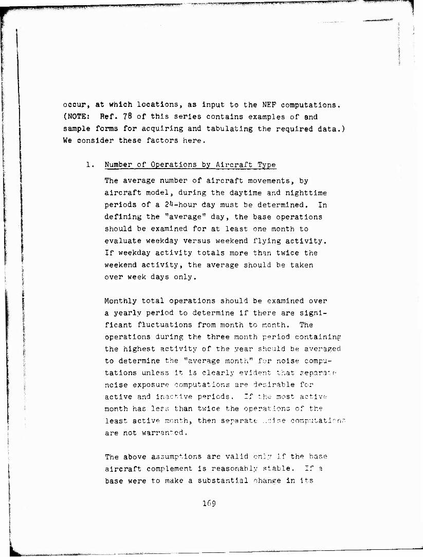
gMpgPPjj^PfHfW^^JIUW:■!»," J RntPRPH WPSfigPfF^W« " ■aqp awpwWByMMHWWg'lBP "-■■ Liai'JBHijAj ,-' J '-i%V^^ ^PW|,M|L' qpapaWBg^PHigw

occur, at which locations, as input to the NEF computations.

(NOTE: Ref. 78 of this series contains examples of and

sample forms for acquiring and tabulating the required data.)

We consider these factors here.

1. Number of Operations by Aircraft Type

The average number of aircraft movements, by

aircraft model, during the daytime and nighttime

periods of a 24-hour day must be determined. In

defining the "average" day, the base operations

should be examined for at least one month to

evaluate weekday versus weekend flying activity.

If weekday activity totals more than twice the

weekend activity, the average should be taken

over week days only.

Monthly total operations should be examined over

a yearly period to determine if there are signi-

ficant fluctuations from month to month. The

operations during the three month period containing

the highest activity of the year should be averaged

to determine the "average month" for noise compu-

tations unless it is clearly evident that separate

noise exposure computations are desirable for

active and inactive periods. If the most active

month has less than twice the operations of the

least active month, then separate .,oise computation;

are not warranted.

The above assumptions are valid only if the base

aircraft complement is reasonably stable. If a

base were to make a substantial change in its

169

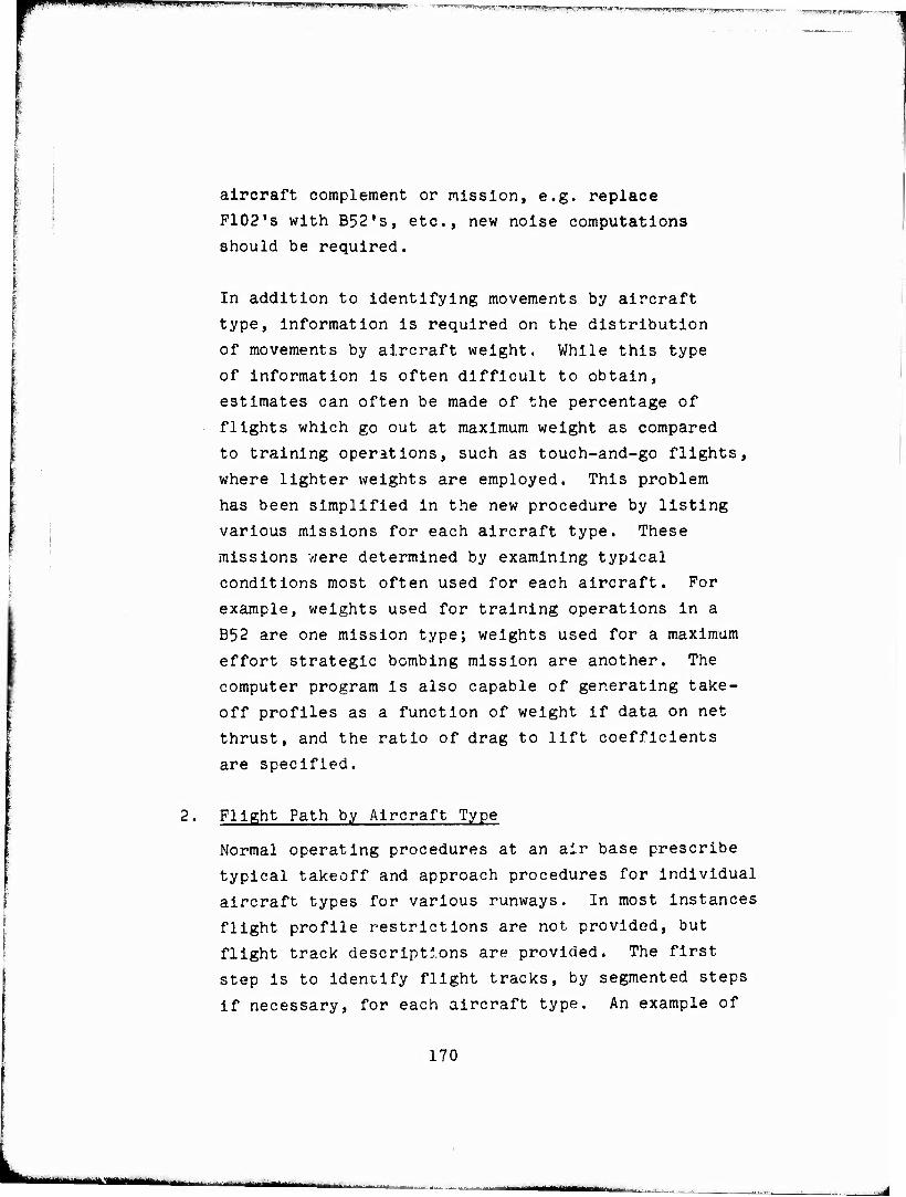
p—fmpmpwp ,..»mtiiuiij.iM a wm*9*^m**rmmmm*!m

aircraft complement or mission, e.g. replace

F102's with B52's, etc., new noise computations

should be required.

In addition to identifying movements by aircraft

type, information is required on the distribution

of movements by aircraft weight. While this type

of information is often difficult to obtain,

estimates can often be made of the percentage of

flights which go out at maximum weight as compared

to training operations, such as touch-and-go flights,

where lighter weights are employed. This problem

has been simplified in the new procedure by listing

various missions for each aircraft type. These

missions vjere determined by examining typical

conditions most often used for each aircraft. For

example, weights used for training operations in a

B52 are one mission type; weights used for a maximum

effort strategic bombing mission are another. The

computer program is also capable of generating take-

off profiles as a function of weight if data on net

thrust, and the ratio of drag to lift coefficients

are specified.

Flight Path by Aircraft Type

Normal operating procedures at an air base prescribe

typical takeoff and approach procedures for individual

aircraft types for various runways. In most instances

flight profile restrictions are not provided, but

flight track descriptions are provided. The first

step is to identify flight tracks, by segmented steps

if necessary, for each aircraft type. An example of

170

-"" I

MWWMjgpp^^HCflgBB'ffPBgi IP^gHPWflWBWPPWWgWFmW ' BBT" " ^P*?*1*? .T^^SWJLJI I««jAäINJI -■''--. '" "1

segment identification is shown in Fig. 20. An

example of a flight profile and track designation

where a profile restriction is specified for

takeoff is shown in Fig. 26.

It should be recognized that differences in air-

craft performance, takeoff weights, and pilot

technique will introduce substantial variation in

flight paths. Whenever possible the average flight

path and range of variation around it should be

obtained by discussions with pilots, operations, and

traffic control personnel. Flight track descriptions

are most easily reported by drawing them on an

overlay of a standard 2000 feet per inch C&G.S. map

of the air base vicinity.

The graphic presentation of flight path data should

be accompanied by a tabulation of flight path

segments used by the different aircraft at a base.

This tabulation should also indicate the percentage

of use estimated for each aircraft type/flight path

segment. Where specific utilization percentages

cannot be obtained, an estimate can be made on the

basis of runway utilization. This estimate can be

obtained from either the percentage of time the

runway is in use, or if this is not available, from

wind rose data. When making estimates of this kind,

specific attention should bo paid to runway

restrictions which may be imposed on certain air-

craft or on certain typer of operations. Examples

are

171

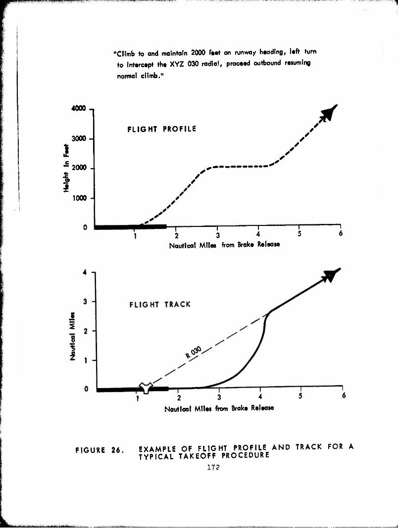
wwf^m^^^W -■yrKj-qr-;r'^v^'•■* ' w»™'.?*-

"Climb to and maintain 2000 feet on runway heading, left turn

to intercept the XYZ 030 radial, proceed outbound resuming

normal climb."

4000

3000-4

"2000

a>

3 1000 A

FLIGHT PROFILE

T

*

.*'

2 3 4 5 Nautical Miles from Brake Release

2 3 4

Nautical Mtles from Brake Release

FIGURE 26, EXAMPLE OF FLIGHT PROFILE AND TRACK FOR A TYPICAL TAKEOFF PROCEDURE

172

---'---■ —-■■ •

PPPpmmppWEHWgWWWWw, .»mmV,..mmJiw-tu»»*mimmm^-*w

"Runway 9L is used for touch-and-go's, 9R

being used for operational missions;"

"F4's use both 6-24 ar^ 11-29, but C-124»s use

only 11-29."

In order to simplify the identification of flight

path information and to build into the computer

program a means for generating flight path dis-

persion effects caused by different aircraft/

mission types supposedly following the same

flight procedures, a powerful new option has

been incorporated in the new procedure. Instead

of providing a map of estimated flight tracks,

actual departure or arrival clearances may be

used to generate the appropriate flight paths.

The clearance can be in the form of vectors and

altitudes, or can be referenced to different

navigational aids. For example, the departure

track defined in Pig. 26, "Climb to and maintain

2000 feet on runway heading, left turn to inter-

cept XYZ 030 radial, proceed outbound resuming

normal climb" can be specified in just this fashion.

The computer program will determine the actual

track and profile on the basis of the stored per-

formance data for each aircraft/mission type

using this procedure. Thus a variety of flight

paths will result, depending on specific aircraft

performance. The program accepts arrival pro-

cedures in the same format. Obviously, mixtures

of this method and tne older "lines-on-the-map"

method can be specified tc the program.

173

Mi - —

l.M««l.UJU.UIv. i ..l iip,|.ii|.tai)illP|BpippjW»il>iUtu.jtiWmwt. ■-■f^«T™^^«j^«iM„, -^-*&*m>$*±wi*<ki'tmtt*wut&*m-niii!imriiitit*>-' ' !T""mwv?»~<r''

3. Ground Runup Information

Data should be provided on all maintenance runup

operations by each aircraft or engine type. This

information should Include the following:

a) Aircraft or engine type

b) Runup cycle, e.g. duration at different

power settings

c) "Average" number of runups per day and night

periods by aircraft or engine type by

applying the same criteria used to define

"average" for flight operations

d) Geographical location and orientation of

runup padt;, depicted on an overlay of a

map of the air base.

e) The use, if any, of noise suppressors, and

if used, type of suppressor.

E. Supplemental Information

The information on aircraft noise and operational

factors is all that is necessary to define the NEF contours

around an air base. The eventual use of this information is

for land use planning purposes. A significant input require-

ment to the overall evaluation is information on the location,

structure, and occupancy of buildings and open spaces on and

in the vicinity of the air base. The detail and extent of

data gathering employed for this part of the program will vary

markedly from base to base.

174

■ - ■ ■■■-•■ I • -■■■

MPP^MMWPC! ww^W^mmtmimm^S^ mmrmnt&&&

Since the resolution of noise problems may well be

handled exclusively at base level, valuable information for

overall USAP studies may not be acquired in ?. central

location unless firm requirements are established to supply

land use information in the basic data package. We suggest

that the minimal information should consist of an overlay of

the vicinity of the airport, with areas indicated for

residential, commercial, industrial, manufacturing, and

agricultural use. The location of all schools and churches

should also be identified.

P. Criteria

Criteria for recommended land uses within various NEF

zones are provided in Ref. 4 and Appendix B. At the present

time both PAA and HUD are in the process of reviewing pend-

ing policy circulars that will provide word descriptions

associated with the recommended land uses. The new USAP

procedure will use the land use compatibility guides

specified in Ref. 4 until the revised HUD material is

available.

Each base should be encouraged to keep an accurate

record of any complaints due to aircraft noise exposure.

The minimum information desired should include name and

location of complainant, time of day and date, and the nature

of the complaint itself (e.g. activity interrupted, unusual

flight activity, aircraft type and operation, if possible).

175

■■PpapHBWWBgpWWHP^BSgWlSP^ =■=■-■{&•-■ ■'. W-«J*:' ^."-''.-tf "■

1.

REFERENCES

Stevens, K. N. and Pietrasanta, A. C, and the Staff of Bolt Beranek and Newman Inc., "Procedures for Estimating Noise Exposure and Resulting Community Reactions from Air Base Operations" Wright-Patterson Air Force Base, Ohio: Development Center (1957).

WADC TN-57-10, Wright Mv

Galloway, W. J. and Pietrasanta, A. C, "Land Use Planning Relating to Aircraft Noise," Technical Report No. 821, Bolt Beranek and Newman Inc., published by the FAA, October 1964. Published by the Department of Defense as AFM 86-5, TM 5-365, NAVDOCKS P-98, "Land Use Planning with Respect to Aircraft Noise."

Bishop, D. E. and Horonjeff, R. D., "Procedures for Developing Noise Exposure Forecast Areas for Aircraft Flight Operations August 1967.

FAA Report DS-67-10, Washington,

4. Galloway, W. J. and Bishop, D. E., "Noise Exposure Forecasts: Evolution, Evaluation, Extensions, and Land Use Interpretations." FAA Report NO-70-9, Washington, August 1970.

5• Federal Aviation Regulations, Aircraft Type Certification,"

Part 36, "Noise 1 December 19 6 9

Standard"

6. "Aircraft Noise - Annex 16 to the Convention on Internationa~T~Clvil Aviation," International Ci'vl 1 Aviation Organization, August 1971.

7. "Procedure for Describing Aircraft Noise Around an Airport." ISO Recommendation R507, 2nd edition, International Organization for Standardization, June 1970.

"Report of the Special Meeting on Aircraft Noise In the Vicinity of Aerodromes." Internationa] Civil Aviation i—1

Organization, DOC 8857 (Noise) 1969-

9. "Noise-Final Report,' July 196 3-

Cmnd. 20 56, K.M London,

177 Preceding page blank

10. Galloway, W. J. and Von Gierke, H. E., "Individual and Community Reaction to Aircraft Noise; Present Status and Standardization Efforts." Paper No. INC/CVP9, International Conference on the Reduction of Noise and Disturbance Caused by Civil Aircraft, London, November 1966.

11. Bürck, W., Grützmacher, M., Meister, P. J., and Müller, E. A., "Fluglärm," Göttingen, May 1965-

12. Bitter, C., "Noise Nuisance Due to Aircraft," Collogue sur la definition des exigences humaines a" l'£gard du bruit, Paris, November, 1968.

13. "Second Survey of Aircraft Noise Annoyance around London (Heathrow) Airport," H.M.S.O., London, 1971.

I*». "Community Reaction to Airport Noise - Vol. lV prepared by Tracor Inc. NASA CR-I76I, July 1971-

15. "Metropolitan Aircraft Noise Abatement Policy Study - O'Hare International Airport," prepared by Northeastern Illinois Planning Commission, 1971.

16. "Metropolitan Aircraft Noise Abatement Policy Study - Bradley International Airport, Windsor Locks, Connecticut - Work Task I," prepared by Capitol Region Planning Agency, 1970.

17. Borsky, P. N. "Community Reactions to Air Force Noise," WADD TR 60-609, Parts 1 and 2, Wright Air Force Development Center, Wright-Patterson Air Force Base, Ohio, March 1961.

18. Galloway, W. J., Clark, W. E., and Kerrick, J. S., "Highway Noise: Measurement, Simulation, and Mixed Reactions." NCHRP Program Report 7», Highway Research Board, Washington, 1969-

19. Galloway, W. J., "Motor Vehicle Noise: Identification and Analysis of Situations Contributing to Annoyance." BBN Report 2002 .for the Automobile Manufacturers Association Inc., June 1971.

20. "Irogress of NASA Research Relating to Noise Alleviation of Large Subsonic Jet Aircraft," A Conference Held at Langley Research Center, Hampton, Virginia, October 8-10, 1968, NASA 3P-189, Scientific and Technical Information Division, Office of Technology Utilization, National Aeronautics and Space Administration, Washington, D.C.

178

L

*-r\-~-' = •——*"-: .|»1»JUJJIPJ|UI ill

21. Wells, R. J.,"Recent research relative to perceived noise level." (A) J. Acoust. Soc. Am. 42, 1151 (1967).

22. Ollerhead, J. B., "The Noisiness of Diffuse Sound Fields at High Intensities,*' Wyle Laboratories, Contract No. FA6ÖWA-1971, for the Office of Noise Abatement, Federal Aviation Administration, Final Report No. FAA-NO-70-3» August 1969.

23. Stevens, S. S., "Assessment of Noise: Calculation Procedure Mark VII." Paper 355-128. Laboratory of Psychophysics, Harvard University, Cambridge, Ma., December 1969.

24. Kryter, K. D., "Possible for the Calculation of

CR-1635.

Modifications Perceived

to Procedures Noisiness. *"

Report Park, Ca., 1969

Stanford Research Institute, Menlo

25. Pearsons, Karl S., Bishop, Dwight E. and Horonjeff, Richard D., "Judged Noisiness of Modulated and Multiple Tones in Broad-Band Noise," J. Acoust. Soc Am., 45, No. 3, P. 742-750, 1969.

26. Pearsons, Karl S., "Combination Effects of Tone and Duration Parameters on Perceived Noisiness?" Bolt Beranek and Newman Inc. for Langley Research Center, National Aeronautics and Space Administration, Washington, D. C, NASA CR-1283, (BBN Report 1701), February, 19 69.

27- Karl S. and Wells, Richard J., "Judged of Sounds Containing Multiple Pure Tones,'

Soc. Am., 78th Meeting, San Diego, Ca., November 4-7, 1969-

Pearsons, Noisiness J. Acoust

28. Pearsons, Karl "The Effects of Duration Background Noise Level on Perceived Noisine: Technical Report FAA-ADS-78, April 1966.

and 0—w

29. Pearsons, Karl S. and Bennett, Ricard of Temporal and Spectral Combinations Noisiness of Aircraft ______ 49, No. 4 (Part 1), p. 1076-1082, December 1970

L., "Effects on the Judged

Sounds," J. Acoust. Soc. Am.,

30. Ollerhead, J. B., "Subjective Evaluation of General Aircraft Noise," Wyle Laboratories, Contract No. FA67WA-I73.I, Federal Aviation Administration Technical Report No. 68-35, 1967.

179

I I.JUJI.l .I.JI..U . Pf^WWiP|MWWTI!J.WJ[ HUIJI1

I !

31.

33-

34.

35,

36.

37.

Pearsons, Karl S., Bennett, Ricarda L. and Fidell, Sanford, "Study of the Effects of the Doppler Shift on Perceived Noisiness," Bolt Beranek and Newman, Inc., for Langley Research Center, National Aeronautics and Sr-ace Administration, Washington, D. o. . NASA CR-1779, July 1971.

"Some Factors Kryter, K. D. and Williams, C. E. Influencing Human Response to Aircraft Noise: Maskino of Speech and Variability of Subjective Judgmen ~*. " Report FAA-ADA-42. Federal Aviation Admini : ation, Washington, D. C, 1965.

Williams, Carl E., Pearsons, Karl S. and Hecker, Michael H. L., "Speech Intel!' ^ility in the Presence of Timo-Varying Aircraf"; Noise," J. Acoust. Soc. Am. . 50, Number 2 (Part 1) p. 1*26-434, April 197!

Williams, c. E., Stevens, K. N. and Klatt, M., "Judgments of the Acceptability of Aircraft Noise in the Presence of Speech," J. Sound Vibration, 9_, 263-275, 1969. ' ~"~" "~

Rosinger, George, Nixon, Kjnnlng E., "Quantification "Approaching" and "Receding Am., 48, No. 4 (Part l;, p.

and Von Gierke. Charles W, of the Noisiness of Sounds," J. Acoust. 843-853, March i°70.

Soc,

Nagel, David C, Parnell, John E. and Parry, Hugh J., "The Effects of Background Noise Upon Perceived Noisiness," Bolt Beranek and Newman"! Inc. Contract FA65WA-11Ö0, Department of Transportation Federal Aviation Administration, Aircraft Development Service, Washington, D. C, Technical Report, December 1967.

Pearsons, Karl 3 Background Noise

"The Effects of Duration and Perceived Noisiness," Level on

Newman"! Tnc Bolt Beranek and "Newman, Tnc, Contract No. FA65WA-1180, mechnical Report No. FAA-ADS-78, (BBN Report 1375), for Federal Aviation Agency, Aircraft Development Service, April 1)66.

38. Adcock. B. D. and Ollerhead, J. B., "Effective Perceived Noise Level Evaluated for Stol and Other Perceived Noise Level Evaluated for Stol and Other Aircraft Sounds," Wyle Laboratories, Contract No. FAÖ7WA-1731, Federal Aviation Administration, Final Report No. FAA-NO-70-5, May 1070.

1Ö0

L u^tmm

yjHUMW- PW „i,,i.^.^ww«W'ii)..itM,'i

39. Kryter, K. D., Johnson, P. J. and Young, J. R., "Judgment Tests of Flyover Noise from Various Aircraft." Stanford Research Institute, Menlo Park, Calif., prepared for: National Aeronautics and Space Administration, Langley Research Center, Contract NASl-6855, SRI Project 6352, Final Report, November 1969.

40. van Niekirk, C. G., and Müller, J. L., "Assessment of Aircraft Noise Disturbance," J. R. Aer. Soc, 73, 383-396 (1969). ~~

41. "Specification for Precision Sound Level Meters," IEC Recommendation Publication 179, International Electrotechnical Commission, July 1965.

42. Galloway, W. J., "Frequency Analysis of Short-Duration Random Signals," Sound, Vol. 1, No. 6, 31-34, Nov.-Dec. (1962).

43. "Standard Values of Atmospheric Absorption as a Function of Temperature and Humidity for Use in Evaluating Aircraft Flyover Noise," ARP 866, Society of Automotive Engineers, Inc., 1964.

44. Bishop, D. E., and Simpson, M. A., and Chang, D., "Experimental Atmospheric Absorption Values From Aircraft Flyover Noise Signals/' NASA~~CR-1751, June 1971.

45. "Method for Calculating the Attenuation of Aircraft Ground to Ground Noise Propagation During Takeoff and Landing," AIR 9 23, Society of Automotive Engineers, Inc., 1966.

46. Franken, P. A. and Bishop, D. E., "The Propagation of Scund From Alrport Ground Operations," NASA CR-767, May 19b7.

47. "Procedures for Calculating Noise Exposure Forecast Values/' Draft AIR 1114, Society of Automotive Engineers, Inc., 1969•

48. "A Study of the Magnitude of Transpoitation Noise Generation and Potential Abatement - Volume III -" Airport/Aircraft System Noise," Report No. 0ST-0NA-71-1, prepared by Seiend?pity, Inc., for Department of Transportation, November 1970.

181

IPIJPPPPI!!^PHWI1PIB>WWWHI-Wl.,^:*l4"1 ,t™w^i:-M'l<»l^«lw«yw4.^WL^'^tj»v5'«»^*J~"--'-'T»--"-—- - w?™nm^.™..

1»9. Parkin, P. H. and Scholes, W. E., "The Horizontal Propagation of Sound From a Jet Engine Close to the Ground at Radlett." J. Sound and Vib., 1, 1-13 (196*0.

50. Galloway, W. J., "Criteria for Selection of Measurement Positions for Maximal Jet Aircraft Sideline Noise," J. Acous. Soc. Am. 50., 1^9 (1971) (A).

51. Robinson, D. W. , "The Concept of Noise Pollution Level," NPL Aero Report AC3Ö, March 19b9-

52. Clark, W. E., "Noise From Aircraft Operations," ASD Technical Report bl-bll, Aeronautical systems Division Wright-Patterson Air Force Base, Ohio, November 1961.

5^. Clark, W. E. and Pietrasanta, A. C, "Intrusion of Aircraft Noise into Communities Near Two USAF Air Bases," WADC Technical Note 5B-213, Wrignt Air Development Center, Wright-Patterson Air Force Base, Ohio, February 1959-

54. Hazard, W. R., "Community Reactions to Aircraft Noise - Public Reactions," Paper 41 of Progress or NASA hesearcn Relating to Noise Alleviation of Large Subsonic Jet Aircraft, NASA SP-189, October 1968.

55. Bishop, D. E., and Galloway, W. J., "Measurement and Analysis Test Plan for Acquisition of Aircraft Noise and Performance Data for Noise Exposure Forecast Calculations."

56. Borsky, P. N., "Noise as Perceived by the Community," Proc. SAE/DOT Conf. on Aircraft and the Environment, Report No. OST-ONA-71-3» June iy/1.

57. Von Gierke, H. E., Recommendation to ITNAP, letter, 31 January 1972.

58. Kryter, K. D., "The Effects of Noise on Man," Academic Press, New York, 1970.

59. KoeDke, J. E., "AOCI Position on Noise Exposure Forecast (NKF) Draft Order." Comments submitted to FAA, June 15, 1971.

60. Richards, E. J., "M^lse and Cocietj ," p. 1-18, Proc. Purdue Noise Control Conference, Purdue university, West Lafayette, Indiana, July 1971

182

UMM—Mt—m——MMMgam ^aaaaa—1 —*

MB^PH^pijJI.TLIJIH.lll ' lT"~l TTTTI I 1

61.

62.

63.

61.

65.

66.

67.

68.

69.

70.

71.

Ollerhead, J. B., "An Evaluation of Methods for Scaling Aircraft Noise Perception," NASA CR-1ÖH3, October 1971.

"Definitions and Procedures for Computing the Effec- tlve Perceived Noise Level for Flyover Aircraft Noise," APR 1071, Society of Automotive Engineers, Inc., 1971.

Tanner, C, "Experimental Atmospheric Absorption Coefficients," FAA-RD-71-99, November 1971.

Horonjeff, R., Mitric, S., "An Analysis of Noise Levels Generated by Jet Transport Aircraft/' Report submitted to DOT, September 1970.

Tanner, C, "Measurement and Analysis of Noise from Four Aircraft During Approach and Departure Operations" T727", KC-135» 707-320B, and DC-9), FAA-RD-71-Ö4, September 1971.

Bishop, D. E., "Noise Measurements During Approach Operations on Runway 21R at Detroit Metropolitan Airport," FAA-RD-71-117, December 1971.

Bishop, D. E., Horonjeff, R. D., "A Study of Aircraft Flyover Noise Variation Due to Changes in Flight Paths and Atmospheric Sound Transmission Characteristics," FAA SRDS RD-65-130, Part VI, 1965.

Von Gierke, H. E., Chmn., "Impact Characterization of Noise Including Implications of Identifying and Achieving Levels of Cumulative Noise Exposure," Task Group 3 Report, EPA Aircraft/Airport Noise Report Study, EPA 73.1, July 1973-

Alexandre, A., "Decision Criteria Based on Spatio- Temporal Comparisons of Surveys on Aircraft Noise," Proc, Intnl. Conf. Noise as a Pub. Health Prob., EPA 550/9-73-008, May 1973-

Beland, R. D., et al, "Aircraft Noise Impact: Planning Guidelines for Local Agencies," U.S. Dept. of Housing and Urban Development, November 1972.

Galloway, W. J., "Aircraft Noise Analyses for thp Existing Air Carrier System," BBH Report 221*, for Aviation Advisory Commission, September 1972.

183

L.

72. Pianko, M., "Evaluation Criterion for the Annoyance Caused by Aircraft Noise," Service Technique Aero- nautique, France, and Report of the ICAO Committee on Aircraft Noise. Third Meeting, 5-23 March 1973.

73. Cruz, J. E., "Aircraft Sound Description System - Background and Application," FAA-EQ-73-3. March 1973.

7^. Connor, W. K., Patterson, H. P., "Community Reaction to Aircraft Noise Around Smaller City "Airports,1' NASA CR-2104, August 1972.

75. U.S. Department of housing and Urban Development Circular 1390.2 "Noise Abatement and Control: Departmental Policy, Implementation Responsibilities, and Standards," dated August k, 1971, with Change 1 dated 1 September 1971.

76. Bricken, 0. L., "Report to the California Department of Aeronautics on Results of Using Ecology-I Noise ~" Monitoring System to Evaluate the Proposed Calif- " örnla Noise Standard/' Northrup Corp. Report 70Y319, December 1970.

77. Bishop, D. E., "Development of an Airport Monitoring Plan for Lindberg Field, San Diego," BBN Rept. 221^7 October 1972.

78. Bishop., D. E., "Community Nojse Exposure Resulting From Aircraft Operations: Application Guide for Predictive Procedure," AMRL TR-73-105» Aerospace Medical Research Laboratory, Wright-Patterson Air Force Base, Ohio, October 1974.

79. Bishop, D. E. and Galloway, W. J., "Community Noise Resulting From Aircrai'"- Operations: Acquisition and Analysis of Aircraft Noise and Performance DataT* AMRL TR-73-107, Aerospace Medical Research Laboratory, Wright-Patterson Air Force Base, On^o, October, 1974.

80. Reddingius, N. H., "Community Noise Exposure Resulting From Aircraft Operations: Computer Program Operator's Manual," AMRL TR-73-10Ö, Aerospace Medical Research Laboratory, Wright-Patterson Air Force Base, Ohio, July 197 4.

81. Roronjeff, R. D., Kandukuri, R. R., and Reddingius, "Community Noise Exposure Resulting From Aircraft Operations: Computer Program Description," AMRL TR-73- 109, Aerospace Medical Research Laboratory, October, 1974.

184

fc^

pHnpüPPPpi i" 11 qpf fjwgiiBWgwwgrappw *V*± 1JWW » r t+il.1T

82. Speakman, T. D., Powell, R. G., and Cole, J. N., "Community Noise Exposure Resulting From Aircraft Operations: Acoustic Data on Military Aircraft^ AMRL TR-73-110, Aerospace Medical Research Laboratory, Wright-Patterson Air Force Base, Ohio, December, 1974.

83. "Report on Aircraft-Airport Noise," Report of the Administrator, EPA, to Committee on Public Works, U.S. Senate, Serial No. 93-8, August 1973.

8*1. Smith, C. M., "Atmospheric Attenuation of Aircraft Noise - Experimental* Values Measured In a Range of CTTmatlc Conditions," Vol. I & II, Hawker Siddeley Aviation Limited HSA.HAD.R.GEN.214, September 1973.

85. Hubbard, H. and Maglieri, D., "An Investigation of Sound Phenomena Relating to Aural Detection of Airplanes," NASA-TN '1337 - 195».

185

L. niM •aa

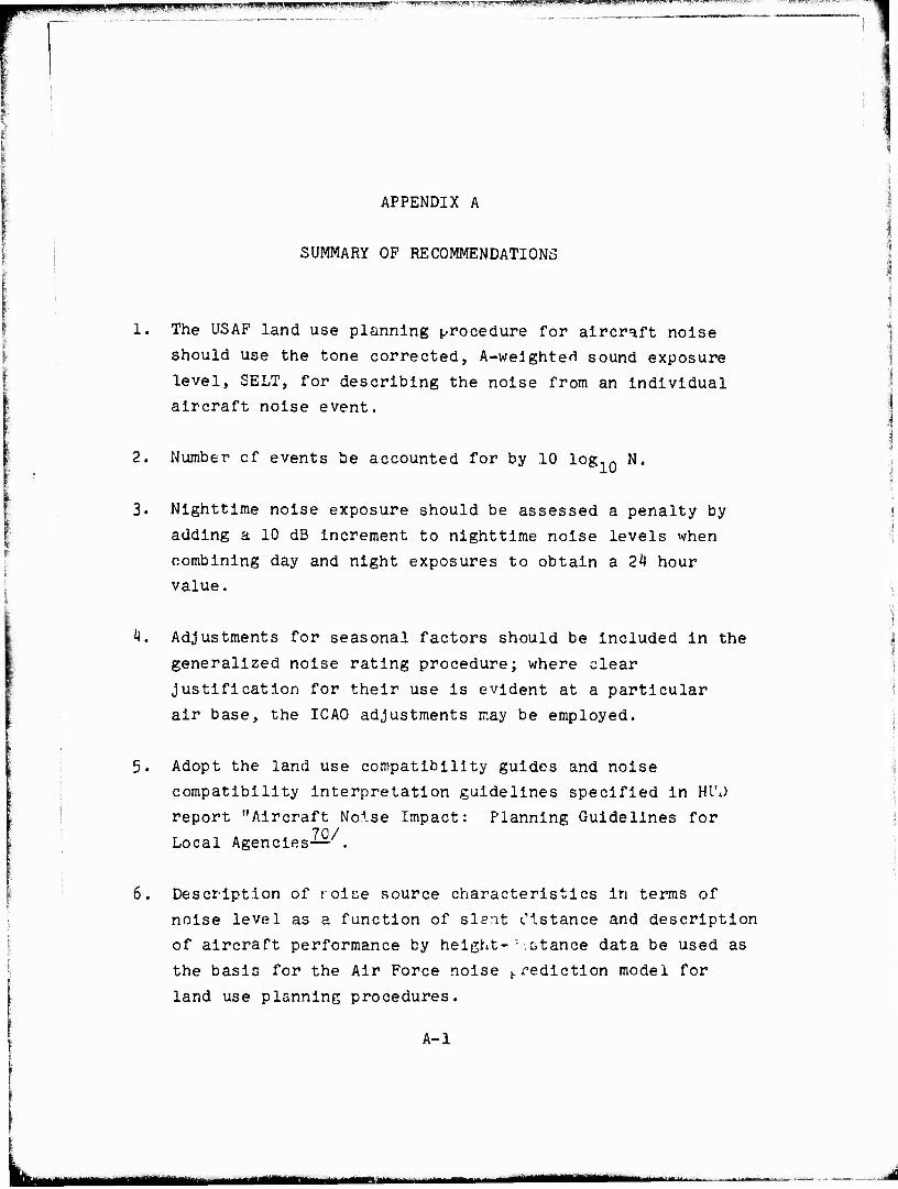
&v**£-m--':~'s&-*'* t^v^

APPENDIX A

SUMMARY OF RECOMMENDATIONS

1. The USAF land use planning procedure for aircraft noise

should use the tone corrected, A-weighte<i sound exposure

level, SELT, for describing the noise from an individual

aircraft noise event.

2. Number cf events be accounted for by 10 log,ß N.

3. Nighttime noise exposure should be assessed a penalty by

adding a 10 dB increment to nighttime noise levels when

combining day and night exposures to obtain a 2k hour

value.

4. Adjustments for seasonal factors should be included in the

generalized noise rating procedure; where clear

justification for their use is evident at a particular

air base, the ICAO adjustments may be employed.

5. Adopt the land use compatibility guides and noise

compatibility interpretation guidelines specified in HUJ

report "Aircraft Noise Impact: Planning Guidelines for 70/ Local Agencies-1— .

6. Description of roise source characteristics in terms of

noise level as a function of slant distance and description

of aircraft performance by height- • -stance data be used as

the basis for the Air Force noise prediction model for

land use planning procedures.

A-l

■-..__- inimuppm IJIPipipmmilm I. ■,:....,,:.-..

7. The computation of EPNL should be performed as presently

described in PAR Part 36- . Computation of SELT should be

identical except that A frequency weighting should be used

instead of noy weighting, and a reference time of one

second instead of ten seconds should be employed.

8. The air absorption data contained in SAE ARP 866 be used

in noise exposure calculations. The Air Force land use

planning procedure should be so designed that it can be

easily modified to accept new air absorption information

when this information is available and considered acceptable

to the scientific and technical community.

9. Utilize the method for predicting ground propagation losses

now in use for civil NEF computations in the Air Force

procedure. Provide for easy modification in the procedure

when improved data are available. Develop additional data

wherever possible in measurement of noise from aircraft

operations.

10. The algorithm now used in the civil aviation NEF program

for transitioning between ground and air attenuation should

be employed in the USAF procedure. Develop additional data

wherever possible in noise measurement programs to verify

or modify this algorithm.

11. The effects of acceleration on EPNL or SELT should be

accounted for in the noise exposure model. Data to derive

these effects should be acquired in aircraft noise test

programs wherever possible.

A-2

tmmt - - 1 11 mMMimt. Mm

IMPJ4UVI'-JLMWIWWI*5B«PP5"W»F«.^'."''1 "■ ""<"J »AiWtJf .ypu i.i-.iM*w«»j.'!y>.v-yJV~M

12. Data on density altitude performance and noise effects

should be included in the USAF procedure.

13. Utilize EPNL or SELT curves derived on the basis of

acoustical standard day conditions (15°C, 70Ü relative

humidity) unless examination of the mean monthly

temperatures and relative humidities show three months

during the year in which the product of temperature in

degrees F and relative humidity in percent is less than

2000. When such small products occur, the no.1 se

exposure calculations for the air base should utilize

EPNL/or SELT/distance curves based on air absorption

calculations from SAE 866 for the appropriate weather

conditions.

Ik. Computation of the number of average daily operations

should be based on a "busy day" principle. For military

air bases this average is usually the weekday average,

based on a monthly period. Average "busy day" operations

per month for each month of the year should be obtained,

then averaged on a yearly bases. If any quarter of the

year has operations that are higher or lower by a factor

of two when compared to the annual average, consideration

should be. given to computing separate noise exposure

contours for these periods of the year.

15. Allowance for flight path dispersion should be included

in the USAF procedure. Until better dispersion models

are available, the empirical equations derived here should

be used. Where it Is possible to make an experimental

determination of flight path data, the observed information

should be used in the procedure.

A-3

*m4AlVl|&#tWPW^M*^ ^m^rrsmmffv T"1***"« T-^ "-iT --T: -f—

16. Ground run-up operations for maintenance purposes should

be Included in noise exposure calculations by computing

their EPNL or SELT values. These values should then be

weighted by an additional 10 dB when summing the total

exposure at the air base.

17. Run-up associated with takeoff operations should be

included in the takeoff noise calculations directly in

terms of their contribution to the takeoff EPNL or SELT.

A-4

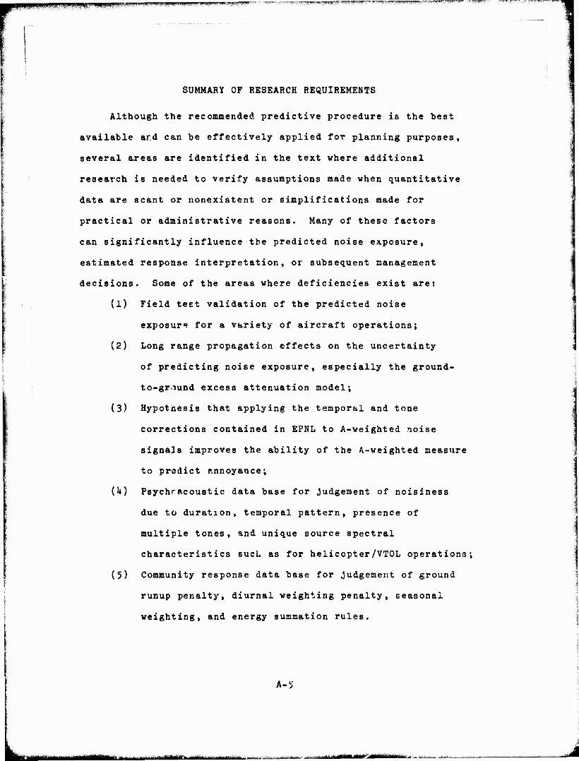
■ppBPW9^P9aisv*m£V7^!npn

SUMMARY OF RESEARCH REQUIREMENTS

Although the recommended predictive procedure is the best

available and can be effectively applied for planning purposes,

several areas are identified in the text where additional

research is needed to verify assumptions made when quantitative

data are scant or nonexistent or simplifications made for

practical or administrative reasons. Many of theso factors

can significantly influence the predicted noise exposure,

estimated response interpretation, or subsequent management

decisions. Some of the areas where deficiencies exist are:

(1) Field test validation of the predicted noise

exposure for a variety of aircraft operations;

(2) Long range propagation effects on the uncertainty

of predicting noise exposure, especially the ground-

to-ground excess attenuation model;

(3) Hypothesis that applying the temporal and tone

corrections contained in EPNL to A-weighted noise

signals improves the ability of the A-weighted measure

to predict annoyance;

{k) Psychracoustic data base for judgement of noisiness

due to duration, temporal pattern, presence of

multiple tones, and unique source spectral

characteristics such as for helicopter/VTOL operations;

(5) Community response data base for judgement of ground

runup penalty, diurnal weighting penalty, seasonal

weighting, and energy summation rules.

A-5

mm MMMMiifci • ■ • i —MM-"- .i.v,---- ■I» Ml" Il

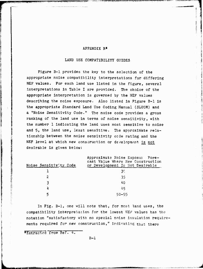
npupmiipp ^g^PPPH .wwinpn^jJUii-JMiij. TI^WW'^^I^^^^^MP' ^WW^^^-^^'"1^^»™1^^1

APPENDIX B*

LAND USE COMPATIBILITY GUIDES

Figure B-l provides the key to the selection of the

appropriate noise compatibility interpretations for differing

NEP values. For each land use listed in the figure, several

interpretations in Table I are provided. The choice of the

appropriate interpretation is governed by the NEF values

describing the noise exposure. Also listed in Figure B-l is

the appropriate Standard Land Use Coding Manual (SLUCM) and

a "Noise Sensitivity Code." The noise code provides a gross

ranking of the land use in terms of noise sensitivity, with

the number 1 indicating the land uses most sensitive to noise

and 5, the land use, least sensitive. The approximate rela-

tionship between the noise sensitivity cede rating and the

NEF level at which new construction or development is_ not

desirable is given below:

£ b

I

Noise Sensitivity Code

1

2

3 k

5

Approximate Noise Exposm Fore- cast Value Where New Construction or Development Is Not Desirable

3C

35

40

45

50-55

In Fig. B-l, one will note that, for most "land uses, the

compatibility interpretation for the lowest NEr1 values has the

notation "satisfactory with no special noise Insulation require-

ments required for new construction," indicating that there

'Extracted from Ref. 4. B-l

--■-■■

Wm' '»" BW^Jg.aiL'J^JflWg^V!!1-^1' -, , "'- »'WO****' -r-,^f rWyy^^U!^^ r'-'.^'pr"- .;.7-■?■ ■■■!*■«">■

FIGURE B-1. LAND USE COMPATIBILITY CHART FOR AIRCRAFT NOISE

1. STANDARD LAND USI COO'NO MANUAL 2 RELATIVE RANKING OF LAUD USES WITH RESPECT TO NOISi SENSITIVITY. SEE TEXT }. DESCRIPTORS AM LISTED IN TAUE IV 4. ">' REPRESENTS A SLUCM CATEGORY IROADER OR NARROWER THAN, HIT GENERALLY INCLUSIVE OF, THE CATEGORY DESCRIltD 9. EXCLUDING HOSPITALS i, JU" SOME IXCEFTIONS MAY OCCUR !R FARTICULAR OR SPECIALIZED NOISE SENSITIVE ACTIVITY 7. DEFfNDENT UFON SPECIFIC TASK REQUIREMENTS

R. NOT ELiEWHERE CLASSIFIED B-2

I ^■■Miina I 1 ■- - ■ : •'' ' — >

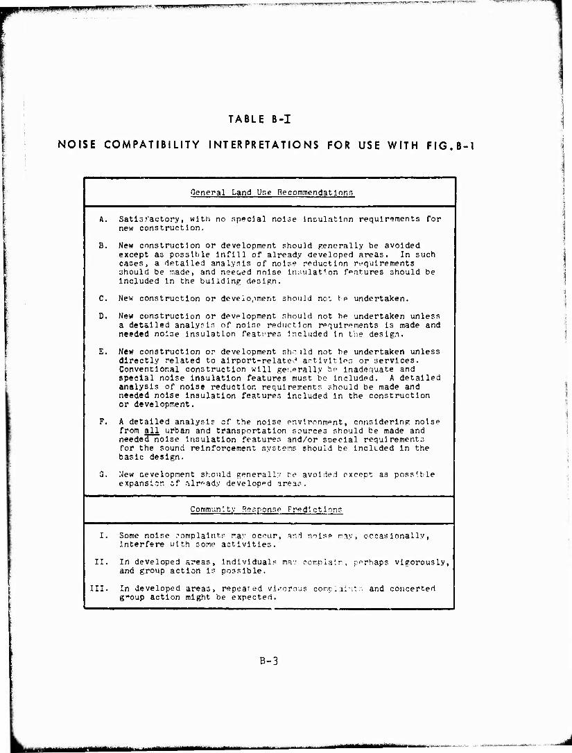
mmmme&m pep , lJ../lftM:yHl||pi|?lllL'J'^ml:JS-VP*";'

TABLE B-I

NOISE COMPATIBILITY INTERPRETATIONS FOR USE WITH FIG.B-1

General Land Use Recommendations

A. Satis factory, with no special noise insulation requirements for new construction.

B. New construction or development should generally be avoided except as possible infill of already developed areas. In such cases, a detailed analysis of noise reduction requirements should be made, and neeaed noise insulation features should be included in the building design.

C. New construction or development should not be undertaken.

D. New construction or development should not be undertaken unless a detailed analysis of noise reduction requirements is made and needed noise insulation featrres Included in tiie design.

E. New construction or development she ild not be undertaken unless directly related to airport-related activities or services. Conventional construction will generally be inadequate and special noise Insulation features must be included. A detailed analysis of noise reduction requirements should be made and needed noise insulation features included in the construction or development.

F. A detailed analysis cf the noise environment, considering noise from all urban and transportation sources should be made and needed noise insulation features and/or sDecial requirements for the sound reinforcement systems should be included in the basic design.

3. New cevelopment should generally be avoided except as possible expansion zT already developed areas.

Community Response Prediction;

I. Some noise complaint:- ma,'.' occur, and noise nay, occasionally, interfere with some activities.

II, In developed areas, Individuals may ccmpia'.r, perhaps vigorously, and group action is possible.

III. In developed areas, repeated vigorous complaints and coticerted g"oup action might be expected.

B-3

Wok KMMMIMi -- - ■■

Ii 11 . i iiiimninniiii|,i y*m* ' immivum '- -u! m ■».mnwmjm i HI v'ntyvwv ■>■"- —....„„... ,. -, ,,. ... , ,.r~*~ ... ,-y.^r-..^—^..^na .---■^w^-- -^»m.,

II

should be no adverse effects from aircraft noise. Corresponding

to higher levels of noise exposure, the interpretations gener-

ally define a range of noise exposure in which new construction

or development should not be undertaken unless an analysis of

noise requirements is made and needed noise insulation features

are included in the building design and site development. For

more extreme noise exposure, many of the land uses are assigned

an interpretation saying that new construction or development

should not be undertaken.

B-1

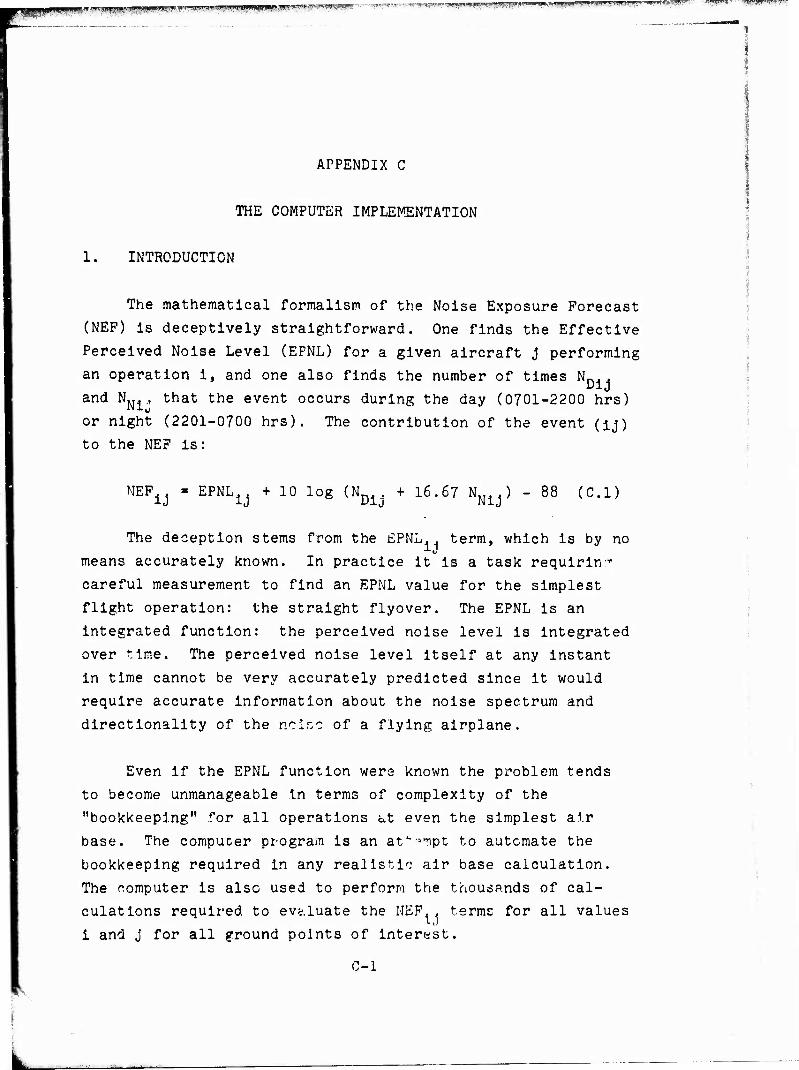
■-. ™,SWS">SB73«^^

APPENDIX C

THE COMPUTER IMPLEMENTATION

1. INTRODUCTION

The mathematical formalism of the Noise Exposure Forecast

(NEF) is deceptively straightforward. One finds the Effective

Perceived Noise Level (EPNL) for a given aircraft j performing

an operation i, and one also finds the number of times ND1.

and NNi., that the event occurs during the day (0701-2200 hrs)

or night (2201-0700 hrs). The contribution of the event (ij)

to the NEF is:

MEF1J = EPNL1J + 10 log (N + 16.67 NN1J) - 88 (C.l)

The deception stems from the EPNL.. term, which is by no

means accurately known. In practice it Is a task requiring

careful measurement to find an EPNL value for the simplest

flight operation: the straight flyover. The EPNL Is an

integrated function: the perceived noise level is integrated

over time. The perceived noise level itself at any instant

in time cannot be very accurately predicted since it would

require accurate information about the noise spectrum and

directionality of the ncicc of a flying airplane.

Even if the EPNL function were known the problem tends

to become unmanageable in terms of complexity of the

"bookkeeping" for all operations &t even the simplest air

base. The computer program is an af^mpt to automate the

bookkeeping required in any realistic air base calculation.

The computer is also used to perform the thousands of cal-

culations required to evaluate the NEF., terms for all values

i and j for all ground points of interest.

C-l

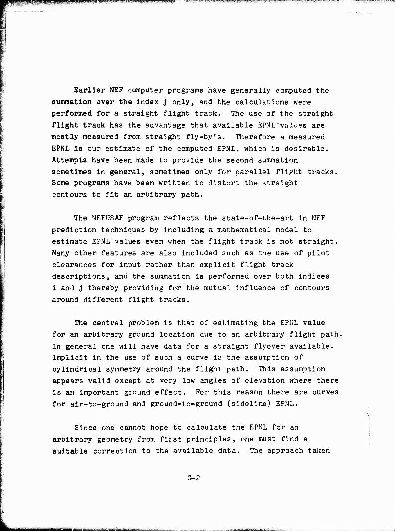
WPBWPBjipmmW uuiiii.il. " m»w""JI " ■"WIU-^IHI wiMiiiiwi

Earlier NEP computer programs have generally computed the

summation over the index j only, and the calculations were

performed for a straight flight track. The use of the straight

flight track has the advantage that available EPNL values are

mostly measured from straight fly-by's. Therefore a measured

EPNL is our estimate of the computed EPNL, which Is desirable.

Attempts have been made to provide the second summation

sometimes in general, sometimes only for parallel flight tracks.

Some programs have been written to distort the straight

contours to fit an arbitrary path.

The NEFUSAF program reflects the state-of-the-art in NEF

prediction techniques by including a mathematical model to

estimate EPNL values even when the flight track is not straight.

Many other features are also included such as the use of pilot

clearances for input rather than explicit flight track

descriptions, and the summation is performed over both indices

i and J thereby providing for the mutual influence of contours

around different flight tracks.

The central problem is that of estimating the EPNL value

for an arbitrary ground location due to an arbitrary flight path.

In general one will have data for a straight flyover available.

Implicit in the use of such a curve is the assumption of

cylindrical symmetry around the flight path. This assumption

appears valid except at very low angles of elevation where there

is an important ground effect. For this reason there are curves

for air-to-ground and ground-to-ground (sideline) EPNL.

Since one cannot hope to calculate the EPNL for an

arbitrary geometry from first principles, one must find a

suitable correction to the available data. The approach taken

C-2

- — ~^^.^:^.^.^

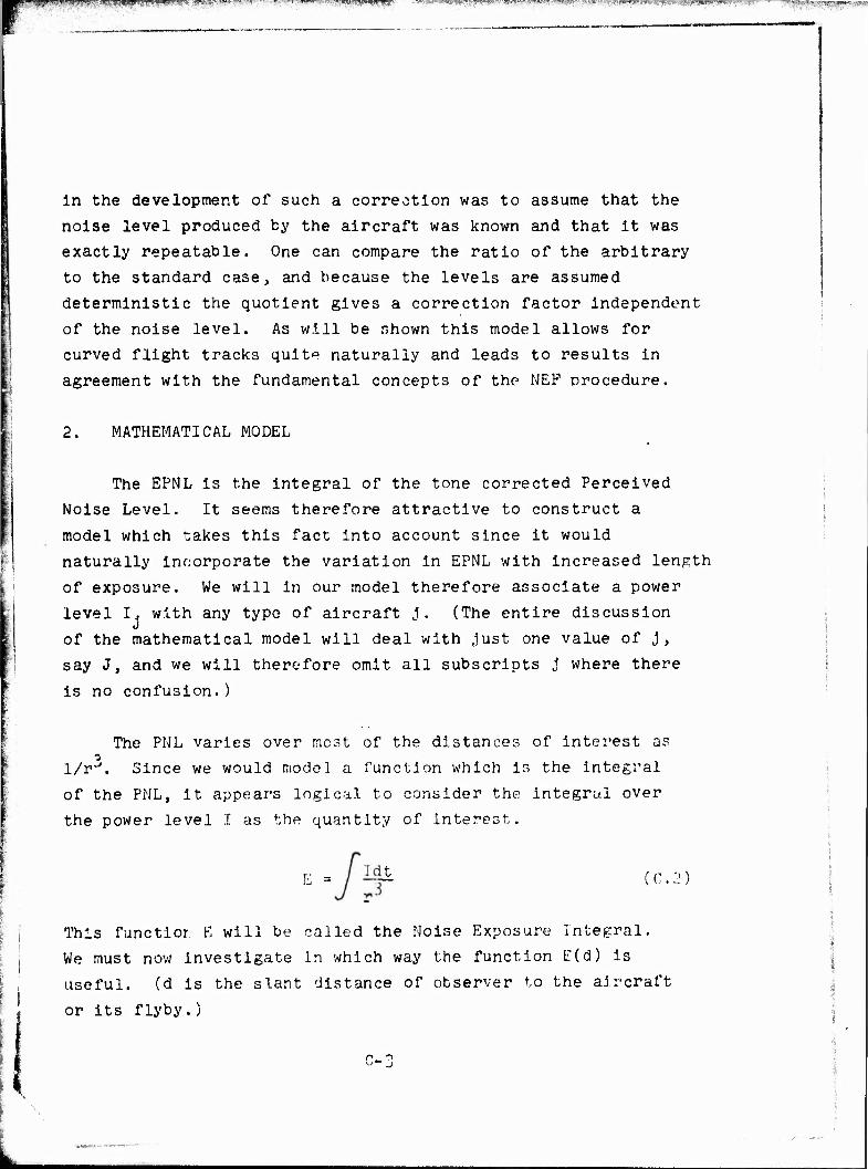
-'■r ■ V7«Sp^!?^TjHP?'V*rfT V»--^^^'---;-F:;;?:;,-tr-,-: 1T -^ . ,T_ . , ; ^,-^^T-, ■ -_- = . f - ^.„.y-j,^ .; .^ ,, ^..,^-. .. , ^^=,^»^.^:>^,„-,!?;rW^p jp,^.

in the development of such a correction was to assume that the

noise level produced by the aircraft was known and that it was

exactly repeatable. One can compare the ratio of the arbitrary

to the standard case, and because the levels are assumed

deterministic the quotient gives a correction factor independent

of the noise level. As will be shown this model allows for

curved flight tracks quite naturally and leads to results in

agreement with the fundamental concepts of the NEP procedure.

2. MATHEMATICAL MODEL

The EPNL is the integral of the tone corrected Perceived

Noise Level. It seems therefore attractive to construct a

model which takes this fact into account since it would

naturally incorporate the variation in EPNL with Increased length

of exposure. We will in our model therefore associate a power

level I. with any type of aircraft j. (The entire discussion

of the mathematical model will deal with just one value of j,

say J, and we will therefore omit all subscripts j where there

is no confusion.)

The PNL varies over most of the distances of interest as

1/r''. Since we would model a function which is the integral

of the PNL, it appears logical to consider the integral over

the power level I as the quantity of interest.

E = / ^ (0.2)

This functior. E will be called the Noise Exposure Integral.

We must now investigate in which way the function E(d) is

useful. (d is the slant distance of observer to the aircraft

or its flyby.)

IPp^lPPWpp^pffPlffiafffgft?-i'-.IM ii.tfffr^^^it;r^. vwy-K^^i-^wgawwy^^ ■ ^ffSp^ai^ESgSgl yr^T^ ^ -^^^rp^^SSg^E^^.flJW-T^^---: SflgjraSgg?™

Since directional information about I is not available

our model must limit the dependence of I on any variable to the

time t. This variation is implied through the more obvious

parameter s, the distance travelled, since one may expect power

changes to occur during the flight of an aircraft. Therefore

we restrict I to the dependence:

I ■ I[s(t)] (C3)

which is not a function of observer orientation. The consequence

is, of course, that we assume the aircraft noise source as

omnidirectional. This assumption is not as bad as it may seem

at first glance. The noise exposure integral will be used to

arrive at a correction to the EPML, a function which is also

not explicitly dependent on orientation.

The approach to take is to compute the noise exposure

integral lor the arbitrary flight path and compare this value

to the noi^e exposure integral for the straight flyby reference

case. The ratio of these two integrals expressed in dB yields

the correction factor to be applied to the EPNL found in the

measured data. Or put differently,.. the weighting function for

an arbitrary flight path is the noise exposure integral for

that flight path normalized to the noise exposure integral of

the reference case.

The next few sections discuss the evaluation of the noise

exposure integral for straight and circular flight track

sections (the only two allowed) and the computation of the final

NEF. This last section is concerned with the fact that the

model is not perfect and that therefore some technique must be

used to minimize the difference between the predicted value and

a field measurement.

C-Ü

ii MI it nil ]]Mmmtmm •uu.teu^.

«J in in im I i|ij|ii ^q ii i|i tin i ""»"»wfjiii . . H«*M|B"«r''Vl»J»iil«IBJli!i.'iJ...J!t.

We have put one additional limitation on the model. This

Is the functional dependence of I on s: the power level function

can only depend linearly on the distance s. This limitation

does not seem to severely hamper the model and it allows closed

form solutions to all integrals. Therefore we have stipulated

I

I = I(s) - I + ks (c.M

In what is to follow the reader is assumed to be familiar

with the transformation of coordinate systems and vector algebra,

as well as elementary calculus. A simple discussion of

coordinate transformation may be found below in Section 8

(page C-25).

3- NOISE EXPOSURE INTEGRAL FOR A STRAIGHT LINE

\

C-'

i'.'e consider a straight

line section, arbitrarily

oriented with respect to

the ground plane. An

observer is located at 0.

1

tarn in ■

■■-:-■■• ---^-I^.":-*■:..■ :--^?P^^WP?^^MW:- - c^n^^^mp|HfpgpfiR^ ■ ■ -.■■«-*fT«7^-«-^. iM-nfi-H«--*,- , TiFyTiT*~-r. ■ ::T^^**^W!^

It is most advantageous to consider the problen in the frame of reference where the observer is at the origin and the y-axis is parallel to ÄB while the line OC is coincident with the x-axis. Assume the aircraft is at A and B at time t, and t2. The distance travelled s ■ Vt is a more useful variable so we will transform the variable of integration. Furthermore, we introduce a = OC the slant distance.

t2 yB yE

f Mt s f Ms = f J r3 J vr3 J

l&L V(a2

+y2)3/2 " a3v/ (l+y2/a2)3/2 /

Idy (C5)

In the above derivation we have taken the speed outside of the

integration. It is not necessary to do this since variation in

speed can be taken into account explicitly. It makes the

computation unnecessarily complicated to do this, however, and

speed changes can be accommodated implicitly by their effect

on the EPNL using an EPNL adjustment. The effects of power

changes and speed changes are combined in this adjustment rather

than entering each effect separately. That this is desirable

is best illustrated by the fact that, for example, a power cutback

will give a lower noise output, but often due to the slower

resultant speed a prolonged exposure. The EPNL adjustment by

means of the delta-EPNL profile combines these two effects into

one adjustment profile.

We can now proceed by substituting y/a = tg <t> and if we

also assume I = I + ky, as discussed previously, we have:

C-6

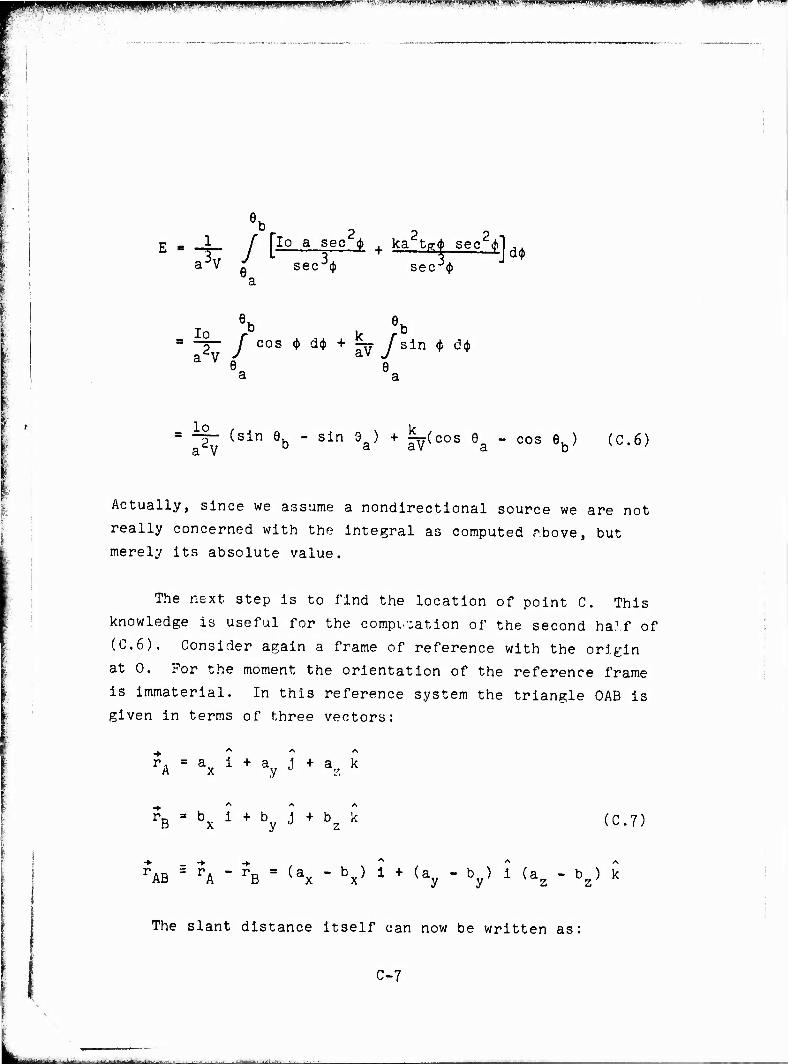
■HWWin|PWP^Pf^|W|lgPiqB IJIW^I^WWWIBIWWSPWJWIWM^HU'JT-'''" "■ "^*'-»WP««W!rw™gNi»ii»»tT;Tif»i- i.MMU»iBMMiii.--iiwJ>M'«-'- i ■.n»]!g.»qyv -W»"-«"1 -WT «™*w™

eb E « 4- / [lo^asecj, + ka tg& sec^]d

aJV J secJ<J> sec3« a

lo > k > — J cos <j) dij> + -gj J sin <J> d<$> a V 0 e

a a

= -§- (sin 9b - sin 9&) + ^(cos 6a - cos efe) (C.6)

Actually, since we assume a nondirectional source we are not

really concerned with the integral as computed rbove, but

merely its absolute value.

The next step is to find the location of point C. This

knowledge is useful for the compilation of the second half of

(C.6). Consider again a frame of reference with the origin

at 0. For the moment the orientation of the reference frame

is immaterial. In this reference system the triangle OAB is

given in terms of three vectors:

. A A. A

rA = ax 1 + ay J + a?, k

h ' bx * + by J + bz * (C7)

rAB ' rA " rB = (ax " V 1 + (ay " V * <az ' V k

The slant distance itself can now be written as

C-7

gfläiääfcä^ h^--,;.:.. ;..:.,- , ,. __

UPPPPPMH'nwnnwym.UPM«m■ J mm.mil■ n ■*.p ew.R,' ..s-i^ä^-Kie^«^«^ „l.,,.^^^

r„ = c i+c j + c k * C x y z

(C.8)

If we ian find the coefficients in (C.8) we know the

location of the point C. These coefficients can be found

when we realize that C lies on the line AB and that OC is

perpendicular to AB. The perpendicular property is expressed

by the product:

AB rc - 0 (C.9)

The remaining relationship is that r

r.R which leads to the relation: AC

rA - rc is along

AC

'AC

AB

'AB

(CIO)

Equation (CIO) gives us two relations between the components

of rp. The scalar relationship (C.9) gives a third equation.

The simultaneous solution of this trio gives the components of

rr. The three Cartesian coord'

by the vector components of rc

r ." The three Cartesian coordinates of point C are then given

Equation (C.9) expands into:

(a. - bv)cv + (av - bv)cv + (az - bz)c2 = 0 x x y y

(en)

and (CIO) can be written as:

a - b a - b a ^x _x _ Jt y_ = _L ax " cx ay "cy

az - cz (C.12)

C-8

puwwi '«■ a v i. w •IL.JdJyiUj !U4,41H4.L JJ,i»Hfcät!»!' " ^^^M^!" ' lA^-^T>g?^',^^r^',^^^?-wvwywyys?ipi^:^^^

The solution is straightforward, but—particularly in

the computer calculation—care must be taken that we do not

use (C.12) to reduce (C.ll) to an equation in c. if a. a b,

since in that case substitution into (C.12) to find the

remaining two components of C results in an indeterminate

form. It is preferable to use c. = c and if that is not

desirable c. = c , rather than to use the altitude component,

because of the problem of finding a solution for an aircraft

in level flight in a direction parallel to the axes of the

reference system.

It is more useful, however, to combine vector calcula-

tions as above with some simple trigonometry in the triangle

OAB. The ratio of equation (C.12) is of course the ratio of

the magnitudes of vectors r.ß and r.p.

(b - a )R + a XX X

(by - ay)R + ay

cz = (bz = az)R + az

(C13)

In our earlier discussion we have chosen as a preferred

coordinate system the one where r.R is aligned with the

positive y-axis. As we will see shortly, the question of the

sign of yA and yQ in this coordinate system is of importance.

To find what these values are we can resort to Eulerlan

angles and transform coordinate systems. On the other hand

since we are really only concerned viith relative sign of the distance AC and BC with respect to the origin at 0, we can

C-9

_^

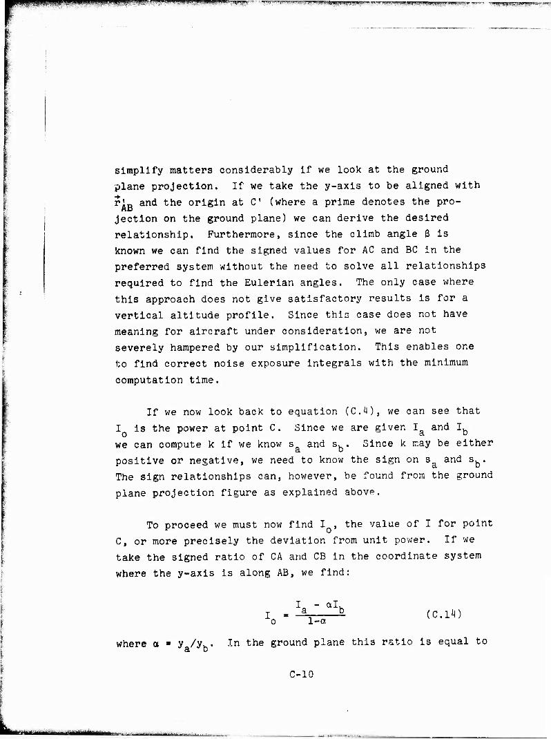
vHBt**jvmmi'p****mifr'***m **""■: ••• ■-"- -"*w^t,- SSBPWP? w ^wf T H>"H»-'»WM«WVJ ww^MWwwyiBiftu1''m

simplify matters considerably if we look at the ground

plane projection. If we take the y-axis to be aligned with

r' and the origin at C (where a prime denotes the pro-

jection on the ground plane) we can derive the desired

relationship. Furthermore, since the climb angle ß is

known we can find the signed values for AC and BC in the preferred system without the need to solve all relationships

required to find the Eulerian angles. The only case where

this approach does not give satisfactory results is for a

vertical altitude profile. Since this case does not have

meaning for aircraft under consideration, we are not

severely hampered by our simplification. This enables one

to find correct noise exposure integrals with the minimum

computation time.

If we now look back to equation (CO, we can see that

I is the power at point C. Since we are given I and I.

we can compute k if we know s and s. . Since k may be either

positive or negative, we need to know the sign on s and s. .

The sign relationships can, however, be found from the ground

plane projection figure as explained above.

To proceed we must now find I , the value of I for point

C, or more precisely the deviation from unit power. If we

take the signed ratio of CA and CB in the coordinate system

where the y-axis is along AB, we find:

I - al. I s a b (c§11|) o 1-a

V'b' where a ■ ya/yh. In the ground plane this ratio is equal to

C-10

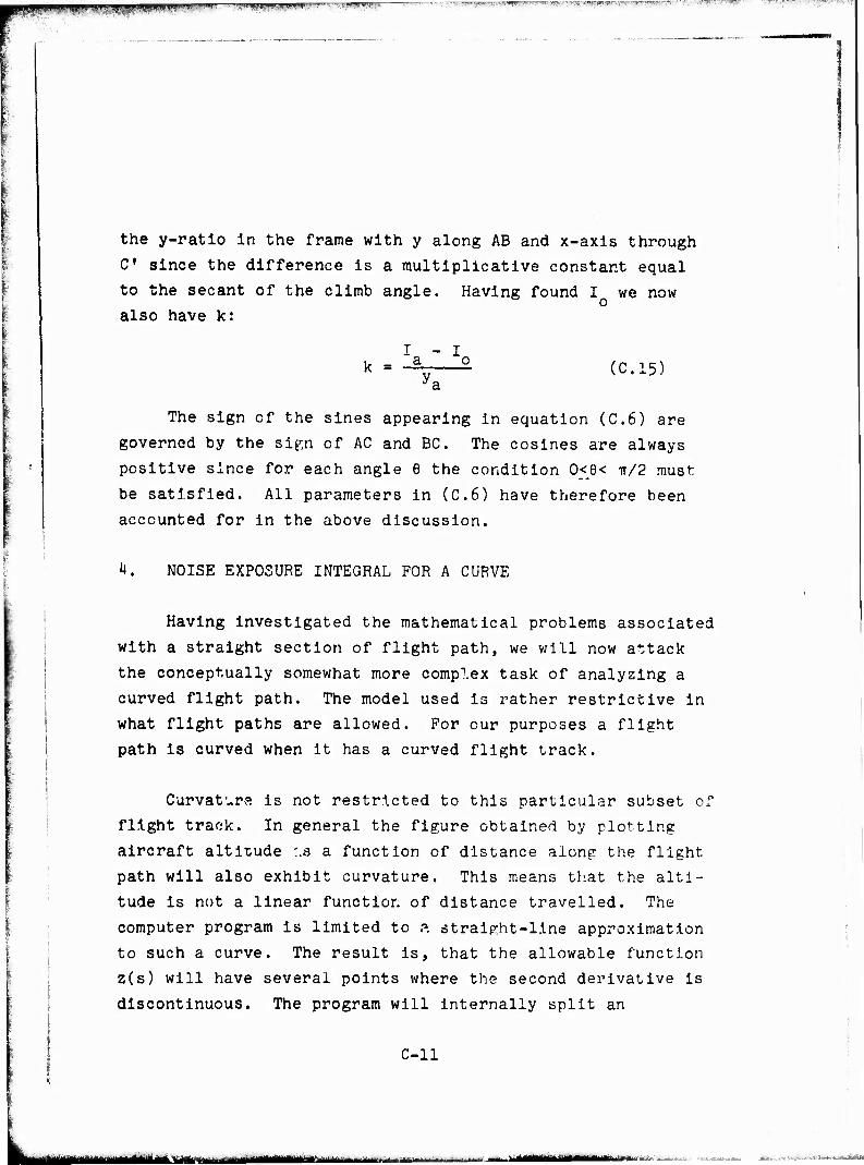
PPP»^, WWMy* .■ mm 1' I. ■!■ :***»*is?f»,S:".W«»'" •!"*■* ■*"*** ^"j ■ J^/V ■■ -^-^%t:^'.-'^-5TT-,T.''"''. ; " ;?-^^nv=:r-"^v- ' ■7v:rV7^qf^-"=~^=e1vr ">'-," ',

the y-ratio in the frame with y along AB and x-axls through

C since the difference is a multiplicative constant equal

to the secant of the climb angle. Having found I we now

also have k:

k = \'Zo

(C.15)

The sign of the sines appearing in equation (C.6) are

governed by the sign of AC and BC. The cosines are always

positive since for each angle 6 the condition O<_0< TT/2 must

be satisfied. All parameters in (C.6) have therefore been

accounted for in the above discussion.

4. NOISE EXPOSURE INTEGRAL FOR A CURVE

Having investigated the mathematical problems associated

with a straight section of flight path, we will now attack

the conceptually somewhat more complex task of analyzing a

curved flight path. The model used is rather restrictive in

what flight paths are allowed. For our purposes a flight

path is curved when it has a curved flight track.

Curvature is not restricted to this particular subset of

flight track. In general the figure obtained by plotting

aircraft altitude '.s a function of distance along the flight

path will also exhibit curvature. This means that the alti-

tude is not a linear function of distance travelled. The

computer program is limited to p. straight-line approximation

to such a curve. The result is, that the allowable function

z(s) will have several points where the second derivative is

discontinuous. The program will internally split an

C-ll

-■

Wm^M Wi%ipwiW^>*™^'w-.»-- m-jJ-iB^

externally supplied flight track at such points, so that

over any section of flight path which is considered in the

noise exposure integral calculation, the function has a

uniform climb angle.

A further constraint is placed upon the curvature of

the flight track: only circle sectors are allowed as curvod

flight tracks. An arbitrarily curved flight track, therefore,

must be approximated by the user as a set of circle sectors

and straight lines. In general such restrictions are not

particularly severe sirce in most cases a constant radius

turn is flown. The effects of climb or descent upon the

shape of the ground track can be neglected in realistic cases.

The combination of constraints on flight track and the

function >( -■» r- (s) is general1y referred to as the altitude

profile] means that we are always looking at an aircraft

describing a helix. The limiting case of the aircraft flying

a turn parallel to the ground plane is included in the subset

of admissible paths.

Consider the geometry

of an aircraft at A

proceeding between Q

and T. The turn radius

is R, the vertex angle

of the sector is 8, and

the observer is located

on the ground at 0.

Since we are looking at

a circular helix we are

Geometric relations for helical flight path. C-12

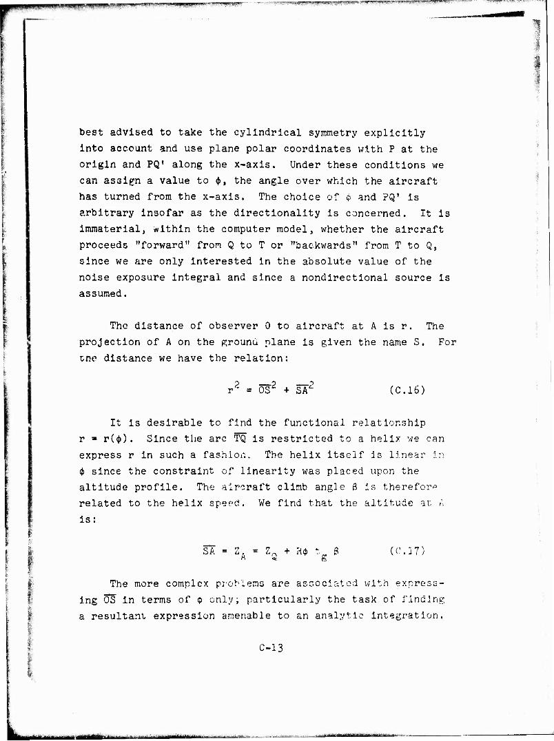
m-^-^^s^v^^v^^^-w^m^Mm --;^:ÄTTi\^r*'^«™'r'-TT^,?:i

best advised to take the cylindrical symmetry explicitly

into account and use plane polar coordinates with P at the

origin and PQ' along the x-axis. Under these conditions we

can assign a value to <j>, the angle over which the aircraft

has turned from the x-axis. The choice of $ and PQ' is

arbitrary insofar as the directionality is concerned. It is

immaterial, within the computer model, whether the aircraft

proceeds "forward" from Q to T or "backwards" from T to Q,

since we are only interested in the absolute value of the

noise exposure integral and since a nondirectional source is

assumed.

The distance of observer 0 to aircraft at A is r. The

projection of A on the ground plane is given the name S. For

zne distance we have the relation:

r2 = OS2 + SA' (C.16)

It is desirable to find the functional relationship

r ■ r((J>). Since the arc TQ is restricted to a helix we can

express r in such a fashion. The helix itself is linear in

<J> since the constraint of linearity was placed upon the

altitude profile. The aircraft climb angle ß is therefore

related to the helix speed. We find that the altitude at A

is:

SA = Z = Z + Ft* t ß (C17)

The more complex problems are associated with express-

ing ÖS in terms of $ only; particularly the task of finding

a resultant expression amenable to an analytic integration.

4

I C-13

. .. , ftjM||yflfr3j|frg

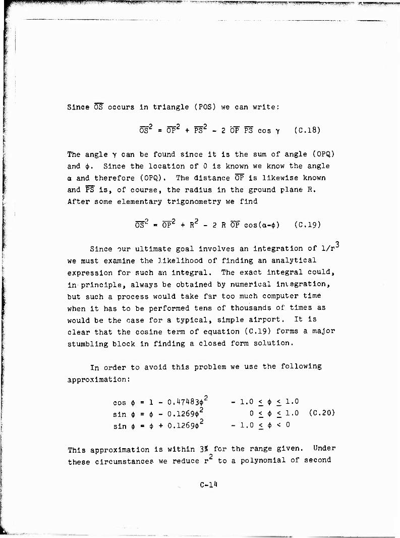
PJj|i!B^B^c^i#-Wü--Li.i_^fflJL,'llilHI!'i.1 '* *J «Jjww^pwfP »- i mm s~^*?TWi- ^■•r-^-***?w ™-^ *. | it <F-m mjHjmpg gH

Since OS occurs in triangle (POS) we can write:

ÖS2 = ÖP2 + PS2 - 2 "OP PS cos Y (C.18)

The angle y can be found since it is the sum of angle (OPQ)

and (J>. Since the location of 0 is known we know the angle

a and therefore (OPQ). The distance OP is likewise known

and PS is, of course, the radius in the ground plane R.

After some elementary trigonometry we find

OS2 - OP2 + R2 - 2 R OP cos(a-(f>) (C19)

Since our ultimate goal involves an integration of l/r:

we must examine the likelihood of finding an analytical

expression for such an integral. The exact integral could,

in principle, always be obtained by numerical integration,

but such a process would take far too much computer time

when it has to be performed tens of thousands of times as

would be the case for a typical, simple airport. It is

clear that the cosine term of equation (C.19) forms a major

stumbling block in finding a closed form solution.

In order to avoid this problem we use the following

approximation:

cos $ - 1 - 0.^74834»'

sin <J> = <J> - 0.1269<t>2

sin ♦ ■ ♦ + 0.12694»2

- 1.0 < ♦ < 1.0

0 < <j> < 1.0

- 1.0 < ♦ < o

(C.20)

This approximation is within 3% for the range given. Under

these circumstances we reduce r to a polynomial of second

C-ll

Is^jp-Jp^mjP^'W^J i.,11 ' J 'j _ j_ffi HI M'lW'iy'AM-LUJ1^--^ - '^T' !: -"-.i-r^'^-^'rVi-=»«:*r"~ '-"'" "; """'""■ ~" ^* ■■■■-■-" r;7-?»^^^'

degree in <J> for which we can readily find an analytic

integral:

/

2(2C2» 4 Cl)

r3 = q r (C21)

in which r ■ c2<j> + C 1* + Co] 1 2

q = 4 C2Co - (-

(C.22)

and C~ ■ R2 tg2(3 + 2R OP(0.47483 cos a + 0.1269 sin a)

C1 = 2R tgß Z - 2 R OP sin a

Co B Za + 0p2 + R2 - 2R OP cos a

(C23)

Since we always integrate over an angle interval where one of

the limits is zero we have:

.0

3 4C2 6 + 2C1

rTfil 2 C

<Co)?- 4C2C0- Cl'

(C.24)

Having thus established the basic framework for the

mathematical operations to De performed we must now consider

the steps involved in the computations and the particular

problems encountered when attempting machine calculation of

this formalism.

As before we are concerned with solutions to equation

C-15

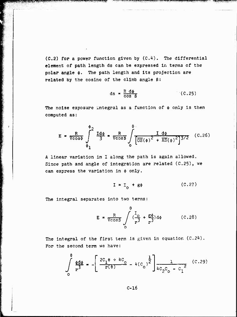
pjmJ.aUMjHiil., l.i " vr***i*f ",--<Ht.ti»H?«.y»wi i. i.,i. p.u-ujj wiB3B|»Bpi?apwn!(5Cfü -iM, ',*.i!U pMtP0p|pH||mppi!qppqpppi ,,--

(C.2) for a power function given by (C.4). The differential

element of path length ds can be expressed in terms of the

polar angle <J>. The path length and its projection are

related by the cosine of the climb angle 8:

ds * B 14 as cos 0 (C25)

The noise exposure integral as a function of $ only is then

computed as:

*,

Vcos<t /

e

T* " *^/[OT(»>s ♦ XJl*)sP (C'26) 0 L

A linear variation in I along the path is again allowed.

Since path and angle of integration are related (C.25), we

can express the variation in <J> only.

I ■ I0 + g* (C.27)

The integral separates into two terms:

9

(C.28)

The integral of the first term Is $;iven in equation (0.2*1)

For the second term we have:

e did» -3

2Cn6 r 4C * (C.29)

-*C2Co -°l'

C-16

PlfMBMIPQPf HBWP^WPPI. .- m XW-mi'm» I ....JIUIL^Ufllll.» »!-' I "WURIII -■ -™- «^B»«M»glPW»mi^ggP! »»■■MkP.lJLH. .1 ^vwwayfnyrn-T^

The preferred coordinate system in which to compute the

noise exposure integral is that in which the center of

curvature P is at the origin and P*Q' is along the x-axis. If

we take Q to be the point where the turn is started, we also

lenow the transformation matrix. That this is so is clear from

the consideration that the aircraft heading, and therefore

the sine and cosine of the heading referred to the ground

plane, are known and at the same time, since Q' is on the

ground circle, PQ1 perpendicular to the aircraft.

The only Quantity which needs to be computed in this

rotated reference frame is the angle o. Since we have that

sin a » y / OP (c>30)

cos a * x / OP

where x and y are the observer coordinates in the rotated

reference frame, we can easily find these quantities with

their correct sign. Furthermore, since in equation (C.22)

we see that these functions are always multiplied by a factor

ÖP we do not have to concern ourselves with the question of

limits for a when the observer approaches arbitrarily closely

to the center of curvature P.

We now realize that in our chosen frame of reference a

left hand turn will have a positive angle 9 associated with

it, whereas a right hand turn will correspond to a negative

6. Having made this observation there is one more agreement

to be made so that equation (C.17) will correctly specify

the aircraft altitude. We consider tgß positive if an

aircraft climbs from Q to A in a right hand turn, or if it

descends from Q to A in a left hand turn.

C-17

■ ^,.^-am-,. ... ... - ._ m ,,„,„_ , .« imftmimUMMti

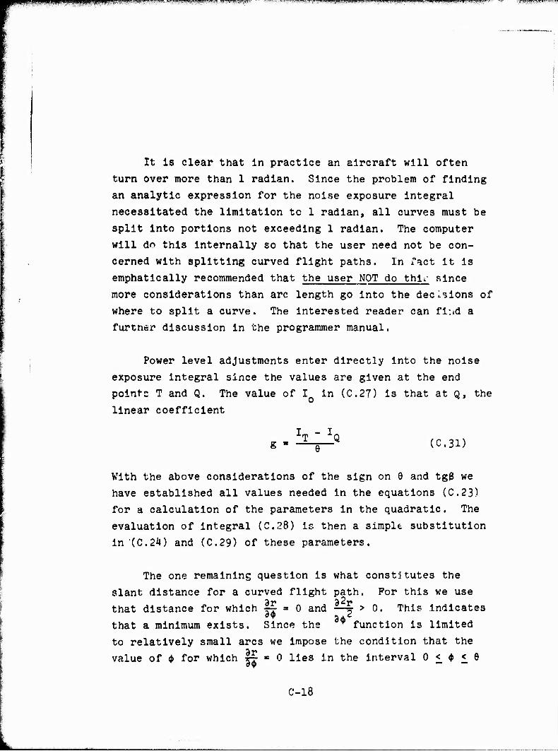
ppipimiPgpmmMlpiyipi! W PB™ BSPBB^^BH .,,L iMviJi/jw*-» .■ ■^*-3WY.-iHWÄ,i™^ii<«^j^^vi-ii--i^«»ww*u»*»t'# «m^m

It is clear that in practice an aircraft will often

turn over more than 1 radian. Since the problem of finding

an analytic expression for the noise exposure integral

necessitated the limitation tc 1 radian, all curves must be

split into portions not exceeding 1 radian. The computer

will do this internally so that the user need not be con-

cerned with splitting curved flight paths. In fact it is

emphatically recommended that the user NOT do thl^ since

more considerations than arc length go into the decisions of

where to split a curve. The interested reader can fi-.id a

furtner discussion in the programmer manual.

Power level adjustments enter directly into the noise

exposure integral since the values are given at the end

points T and Q. The value of I in (C.27) is that at Q, the

linear coefficient

g - -^—Q (C31)

With the above considerations of the sign on 6 and tgß we

have established all values needed in the equations (C.23)

for a calculation of the parameters in the quadratic. The

evaluation of integral (C.28) is then a simple, substitution

in (0.2*0 and (C.29) of these parameters.

The one remaining question is what constitutes the

slant distance for a curved flight path. For this we use

that distance for which 1? ■ 0 and 2-~ > o. This indicates

that a minimum exists. Since the v function is limited

to relatively small arcs we Impose the condition that the

value of A for which IT * 0 lies in the interval 0 < $ < 6

C-18

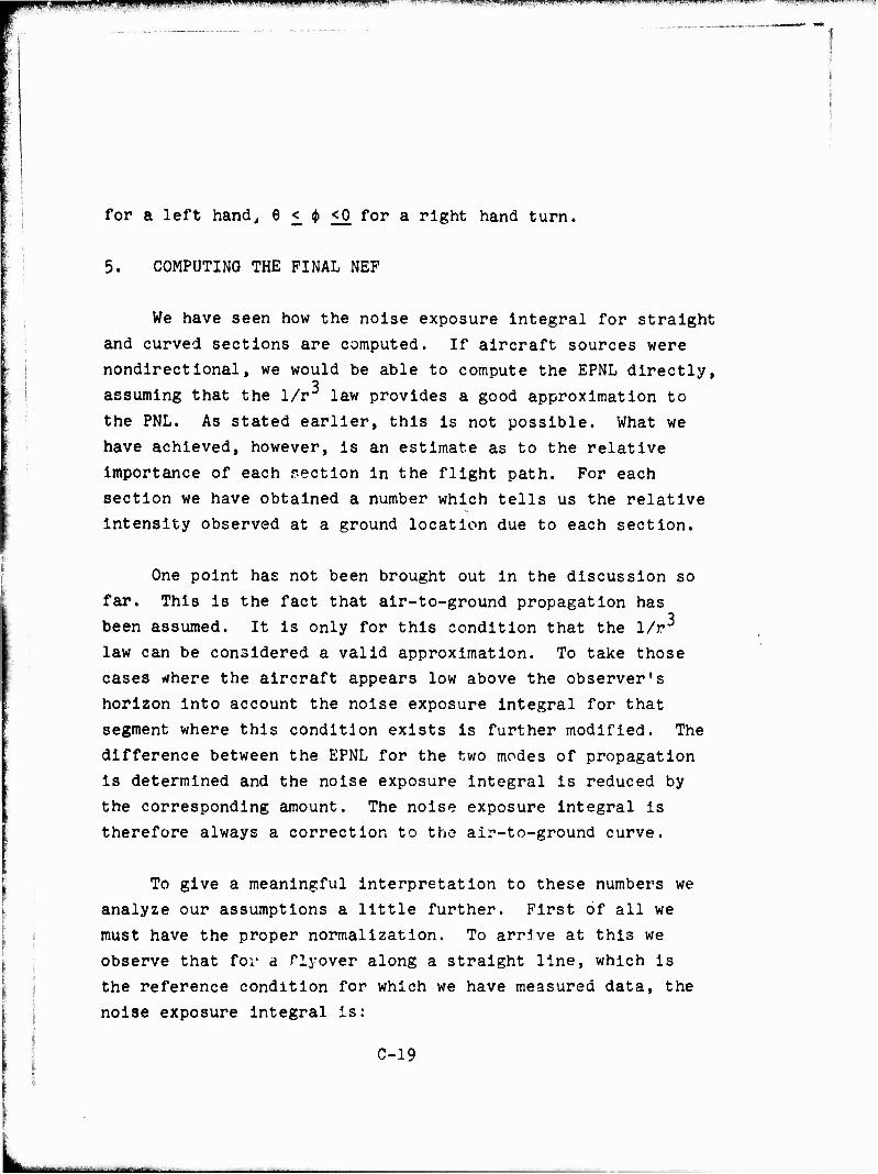
PIIBIiPfaillili.lMJIlWpMHWtfl!»««111 ,i?!!Mi,",Mli.,-if.-i|i..W..i,l«»*"<-l H UMH»,»I »W»~ ™n^-^~ü,rfiJS*.iTiVtwim.M,.l,>^' 4J,m«*-h*-*-4"»*,>-w*,*»l!™I»*-»H'l'...-'*l«',

for a left hand, 8 <_ <J> <0 for a right hand turn.

5. COMPUTING THE FINAL NEF

We have seen how the noise exposure integral for straight

and curved sections are computed. If aircraft sources were

nondirectional, we would be able to compute the EPNL directly,

assuming that the 1/r^ law provides a good approximation to

the PNL. As stated earlier, this is not possible. What we

have achieved, however, is an estimate as to the relative

importance of each section in the flight path. For each

section we have obtained a number which tells us the relative

intensity observed at a ground location due to each section.

One point has not been brought out in the discussion so

far. This is the fact that air-to-ground propagation has

been assumed. It is only for this condition that the l/rJ

law can be considered a valid approximation. To take those

cases tfhere the aircraft appears low above the observer's

horizon into account the noise exposure integral for that

segment where this condition exists is further modified. The

difference between the EPNL for the two modes of propagation

is determined and the noise exposure integral is reduced by

the corresponding amount. The noise exposure integral is

therefore always a correction to the air-to-ground curve.

To give a meaningful interpretation to these numbers we

analyze our assumptions a little further. First of all we

must have the proper normalization. To arrive at this we

observe that for a flyover along a straight line, which is

the reference condition for which we have measured data, the

noise exposure integral is:

C-19

pgpipsr ?". m^^fl^Jm^^!^,-}, &?^W*f7&--*W^**^,M&Hh. "H:1- T^°^^ -■^^™*^^3^ ■' ^-^T*VT^a^ j..^p^.^p.i^pw^ii..f,,;.. u,.n. ^v! u-UlW-yHi"1 ijLj^g^.qP^^ggf^WfW^KWraMF^^^.^

Eref " 2/d2 (C*32)

If we take this into consideration we can establish the

following correction term for the EPNL. Let the total engergy

as computed from the noise exposure be PE ■ Z E. . We pick

the dominant term in this summation. The EPNL value found in

the measured data for the slant distance corresponding to this

section is EPNL... Then the EPNL can be written as:

EPNL = EPNLM + 10 log [g^M (C.33)

wnere EPNL« is the maximum EPNL adjusted for the fact that

this section (probably) did not correspond to the reference

condition with the aircraft coming from - «° and proceeding

to + «.

We have developed in (C.32) the normalization constant

corresponding tc the reference case. Therefore, if the table

entry is designated as EPNL(d), we have

EPNLM = EPNL(d) - 10 log \¥^- \ max

which we can now substitute in (C.33) to obtain:

EPNL = EPNL(d) + 10 log ^- (0.3*0 I 2/d2

The NEF at a point due to operations of all aircraft type J

on all flight path 1 is expressible as

NEF = 10 log IZ antilog NEfft) (C.35) ij 1U

C-20

HWPgP!i^wp,HHii 11 u w<*immv*'*-> r* »w^«' *—<**-* ^gglsriGgmmmgg* ■ ,p mpqi LJ«

Therefore we are at the time that we generate the grid of

data points more interested in antilog NEP(ij) than in

NEF(ij) itself. This type of summation is generally referred

to as an energy sum. Since NEF(ij) is given in terms of EPNL

plus a correction factor, the goal of our immediate interest

is the energy equivalent of the EPNL of (0.3*0 to be used in

the expression:

NEF( (ij) » EPNL(ij) + 10 log (N. + 16.67 N ht) - 88 (C.36)

which when converted to energy becomes:

NEP(ij) = EPNL(ij) * (Nday + 16.67 Nnight) * C (C.37)

From (C.34) we have:

EPNL(iJ) = EPNL(d) * PE

2/d' (C38

After this rather lengthy discussion we can now see the

reasons for some of the basic decisions in the architecture

of the computer program. We are basically accumulating

NEF(ij) at our grid points. It is therefore most efficient

to run the entire program in an energy mode. All data or

input are converted to energy equivalent; only on final

output are logarithms taken. This saves a very considerable

amount of computer time plus the additional bonus of a

minimal roundoff error. (It Is necessary to divide by 10—

as in equation (C.35)—-since many computers cannot represent

antilog EPML(iJ) internally.) Similarly, the constant C of

equation (C.37) is left off and 88 is subtracted from the

value computed according to (C. 35) since we need to perform

C-21

HmWMHWpHHUPWBPWIPW" -M»"'-'-' ii.i'U[WJ-W W**'™..*M»W-*.-JW -■-Tiorr»™««! . i.ua^^j^j.^i.^.-j.i^^^^

this operation only once this way; besides subtraction is

faster than division.

The one question which we have not addressed ourselves

to in computing NEF values due to aircraft flight operations

is what happens when we change EPNL curves during flight.

When drastic power changes occur, which make using a simple

across-the-board adjustment in the EPNL unrealistic (e.g. T&G

patterns), it is possible to change to a different EPHL curve.

Internally the program handles this by breaking the flight

path up in as many "subflights" k as needed to have each

subflight reference only one EPNL curve. The NSF(ijk) is

then accumulated over the index k first, but the process is

exactly the sain« as for a single EPNL curve.

6. GROUND RUNUP OPERATIONS

Having completed the discussion of the NEF contributions

from flight operations we now proceed with ground operations.

The approach here is entirely straightforward and no mathe-

matical model is needed to simulate the operations. The

runup data contain directional information and the assumption

here is only that the noise levels expressed in tone corrected

perceived noise level (PNLT) have mirror symmetry around the

vertical plane through the longitudinal axis of the aircraft.

The EPNL at a location a distance S removed observing

the aircraft under an angle <J> is

EPNL U,S) ■ PNLT (<j>,S) + 10 log D - 10.0 (C.39)

C-22

JMJiUmiaiÜiiE-i.ir. --M--ri.nl T üftrilf liil"^-'*"-"'-"-'.]! r, ■ I .:■-. aUgftfc.

u.:.iW:W^ill>iiLjipMa^J!..a.uMm.»t-1'— """"■'"""

..,m..,,-:. WW-5WW-ESB.- - «^«•-™™*-**TO><fflr*I^^ ■ --■"«----*•<'-=■•--•-' ™

The symbol D stands for the duration of the runup in seconds.

The value 10.0 is a normalizing constant so that for a 10

second duration the EPNL equals the PNLT. On the other hand

a + 10.0 dB ground runup sensitivity correction is aaded to

account for subjective difference in the response to runup

noise and flyover noise, These two correction factors cancel

and we obtain for ground runups:

NEP1j * PNLTit + 10 iop; (DD1, + 16.6? DNj_ 1) - 88 (C.10)

exactly analogous to equation (C.l) for flight operations.

As for flight operations the program will internally

perform table lookups to determine the proper PNLT value for

each $ and S. The NEF., term will be added to the terms for

flight operations to yield a final NEF

NEF

NEF = 10.0 log T. I 10.0^^ i j

where summation takes place over ail aircraft ,i performing

all operations i appropriate for the index j. The index i

includes runup operations on an equal footing with flight

operations.

7. SOME CONSIDERATIONS FOR THE PROGRAM ARCHITECTURE

The computer program calculates NEF values at ground

observer locations on a square grid with 1000 foot spacing.

This allows one to follow the gradients of NEF and to form

a good idea of the behavior of the contours of equal NEF.

A contouring program may construct such NEF contours from

t e data points.

C-23

-ffmmmff^mmmni!!*m™^liwww^4mi^'u iijmu. m, mrm*!**mw?s m ,«.-.<- . »^»-—^-^.-,. [...„n^..!, .,..».

With the level of complexity which is allowed in the

data input it is most e/fedient to keep NEP values in the

computer and process '.>.■ data cards one by one. The

alternative approach . keeping all aircraft operations

information in the machine and calculating by successive

approximation the specified NEP values requires more storage

or excessive I/O operations.

An advantage of a fixed grid which accumulates NEP

contributions is that one can at any time read the grid back

into the computer to add new operations. If new aircraft

are added to an airbase, one can process just the new

additions without the need to recompute the NEF of the

previous aircraft.

The advantage of being able to output grid values

directly is that one can still compute NEP contours but

further study of the data can also be done. For example,

a program producing only NEF contours or output does not

provide any information about where the 30 NEF contour would

move if the operations at the base doubled. On the other

hand, one can from the gridded data easily calculate the 27

NEF contour either by hand or by contouring program without

having to recompute any NEF values.

Finally, gridded data can be superposed on any other

NEF grid. This opens the possibility to add other trans-

portation systems to the model. If one were to write a

program to produce NEF values for other transportation noise

sources using such a grid, then the aircraft and other sources

can be represented in one unified plot.

C-24

^■--^^"Mbitfr-i -

mmm mnm" mi . ^ |1 .4!^l!J#4!|J(KlL,^.^ ■-yVS^^TffjSjnpg^ •*? fcVT»^g=g^?fgrra|5^

To keep the execution speed high the program will not

compute grid points of le.:s than 7 NEF. How this is imple-

mented is discussed in the programmer manual. Similarly,

the program keeps all EPNL, PNLT and NEF values internally

as exponentiated values ("energy units"). Only if the

program needs to output the data for external use are

logarithms taken. This method saves a very considerable

amount of computer time since otherwise each addition

involves two exponentiations plus r logarithm. Neither of

these operations are trivial to perform and since they are

performed tens of thousands of times, the time saving is

significant.

8. COMPUTER GRAPHICS AND ANALYTICAL GEOMETRY

The human mind in viewing or visualizing even a simple

piece of graphics, such as a flighttrack map, is capable

of an astounding amount cf data processing. Equivalently,

one can observe that the eyes are a very powerful input

channel. In the following we will observe some of the methods

used to generate the computer graphics and the processing

necessary to keep track of the aircraft along its flightpath.

When even elementary information, such as left and right,

must be communicated to a computer, the resulting code

becomes almost immediately quite obscure. It becomes quite

clear that "one picture is worth a thousand words," parti-

cularly when dealing with computers.

Very liberal use is made throughout the program of the

methods of analytical geometry. To improve the clarity of

the FORTRAN code, most of the analytical geometry is left

C-25

IMuaMMUi ijail*i~i'".i*.d , ..■■,:, ~..~~—"■-M-yttii--

PP|||Plg|j^f»l^ .Ijl^^ " - "S-^V- 7^—^•^^^s^-.^IWSim «gp!SE^«*ig,M: *±^-V*1l?Z**f&Z!*?^ß^l- ■ jj^W^- W.^W.-1-gp^ agaq«*? - -.^«WFJ^^F^W?^—

in a step-by-step form. Rather than giving the equations

for a particular curve in terms of all the parameters of the

computer internal reference frame, we have generally adopted

the approach of starting in the preferred reference frame

for a particular application and then transforming this

result to the desired reference frame. This makes the code

much clearer to the reader and anyone wishing to add to,

delete from, or change a particular part of the program

will be able to do so quite easily.

A. Aircraft Course and Analytical Heading

The very first problem deals with that of aircraft head-

ing. For purposes of the program the heading of an aircraft

is the direction of the groundtrack, it is really, therefore,

the course rather than the heading. Furthermore, since we

are going to use analytical geometry we will have to change

coordinate systems. Assume a Cartesian coordinate system

where the positive X-axis points east and the positive Y-axis

points north. This is the frame of reference used by the

program. Furthermore, angles are measured irom the X-axis and

are considered to be positive when counterclockwise. Normal

aviation practice is to use the compass divided into 360

degrees, and consider angles positive when clockwise, with

zero being due north. The angles given as input are therefore

transformed to the internal system. Furthermore, all angles

used internally are in radians since this is the natural

measure for angles in mathematical considerations. This

internal representation of the course of the aircraft is

called the "analytical heading" in this program:

Analytical Heading « ((450-Course) Modulo 360) • 0.0174533

(CHI)

C-26

— :'- r. ■-■ ■■..-.--: ■■ .

«wag^fpi^jpF^

B. Transformation of Coordinates

A full discussion of coordinate transformations is

clearly beyond the scope of this manual. The following

few comments should suffice to make the transformations

used in the program undt 'standablc. Tne two basic trans-

formations are a rotation and a translation. The trans-

lation consists of adding the appropriate value to the x,

y and z coordinate of each point. If we translate a

coordinate system a units in x, b units in y, and leave

the z direction unchanged, we have

x' = x + a

y1 * y + b CC.42)

z' = z

The rotation of a coordinate system is a little more

complex. If we wish to rotate the coordinate system around

the z-axis over an angle 6 we arrive at the coordinates in

the rotated frame of reference by means of the following:

x' = x cos 0 + y sin 6

y' = y cos 9 - x sin 9 (C.43)

It is important to remember that the primed values are

the coordinates of the same point expressed in the new

reference frame. The following few sections discuss how

these transformations are useful in terms of the program.

C-27

p^SM^i^^^i^^lHIII^^!*ß^Ah^i^'9^mir^,y^^«^mm!^- «-■■■■ 'üiw"»-t'»wMi'»pr ■'vrw*^*\^**'i!ie^mfmu.-Mi&ii<m&',*i'*!*!1i^>rF'. w*m**qit!!W™T!'

C. Typical Application: The Distinction Between Left and Right

When we look at a flighttrack, it is immediately

obvious which side is left and which side is right. We

must, however, define things in absolute mathematical terms

before the computer can make such a decision. A look at

the problem will easily tell us what the preferred coordinate

system is. (We are generally interested in the location of

a point on the ground relative to the flight track, therefore

we are not really concerned with the z-coordinate in what

follows.) The simplest way to express the problem is by

looking at the case where the aircraft ground projection is

at the origin of the coordinate system and the instantaneous

velocity vector is along the positive X-axis. In this

coordinate system to the right means a negative y, to the

left a positive y. This coordinate system is therefore the

preferred system.

Let us assume we wish to know if a navigational aid

located at (x . y ) will be passed on the left or on the n n

right. We have seen which coordinate system will give us a

ready answer. The first step is to find a coordinate system,

parallel to the old one, but with the origin at the aircraft

ground projection. We will assume at the aircraft at the

given moment to be at (x . y ), while the analytical heading

is 8 radians. In this translated system we find

x'n " xn " xa

y n * yn " ya

(z'n - zn - 0)

C-28

p>tPBjBPPLp.^in^iig^pi^p!i^^!-''i.-w.:^.-! '»-I i ^-^t'Ji-k-^u^^v,- .^-jw^wy ■■-•5'-:.-T-^-T.^»-*S!=^^'?? ,----■■'■ -"^^^■^WT»T^pnc?n^;f^?^^S^

The next step is to find the frame of reference where

the velocity vector is along the positive X-axis. This is

done, of course, by rotating our primed system over an

angle 6.

Therefore we have:

x" = x' cos 6 + y' sin 9 n n n

y" = y' cos 6 - x* sin 6

If y"n is les'j than zero the navaid is to the right of

the aircraft, therefore a negative value indicates that the

aircraft will pass the navaid on the left. Whether the

navaid is ahead or already past is given by x" . If x" is

positive, the navaid is ahead; if x" is negative it is

behind. Of course, the values could be zero. If y" is n

zero, the navaid is directly on course; if x" is zero the

navaid is on a line perpendicular to the current heading at

this particular location (x , y ). a a

In general we have taken the approach outlined above

to guide the user (programmer) through the steps involved in

a particular geometric problem. We could equally well have

said that the condition for a point being to the right of

the aircraft ground projection is

(xT. - xj sin 6 - (y - y ) cos 0 > 0 (C.44)

One could have arrived at this inequality by considering

only the basic reference frame and finding those relation-

ships between the coordinates and headings which give

C-29

IgjrjpjgJIIQjß^lt^lgjg/ef^^ - ■ ^W^rm^^^itr^-*-^*^^f'^*mW^W^-¥9^^^^S f«JP'lU* .91 ^^«l^i-IM^^^Mf/W« a^^PHI-wp^-*- ■■■ Hf WIWfltfl^BIfgf^S

necessary and sufficient conditions for the desired prop-

erties. In practice, however, it is a very laborious

enterprise to find conditions «such as (C.44).

It should he emphasized that there is a large difference

between verifying the correctness of (C.M) and concluding

from purely geometric reasoning that, of all possible

relations between x . x . y . y and 9, (CM) is the n ana

necessary and sufficient condition to f nd points to the

right of an aircraft. Also, once the relation is given It

is fairly simple to give it geometric interpretation, but

It is not always a priori obvious which particular geometric

relationship we are looking for.

A particularly unpleasant concomitant of all geometric

reasoning is that one must satisfy oneself that a relation-

ship, derived from geometric considerations, is valid for

all quadrants. It is for this reason that we feel the

approach used In our treatments is by far the more lucid,

and nowhere do we attempt to give any geometric interpre-

tation of relationships such as (C.4M)a unless, of course,

the geometric interpretation is the goal we are after!

D. The Transformation in Reverse: Drawing a Circle on the Plotter

The process of coordinate transformation is wholly

symmetrical. In other words, it is entirely the same thing

whether we rotate the coordinate system and look at the

change in values of a coordinate pair or if we keep the

coordinate system fixed and let the coordinate pair move in

the opposite sense over a circle with the origin as its

C-30

JUP^IpWpTpWgWPP'TO'W"*1.'^^'"11 pin ,|pi, HJ.U.U.,«. : ;:Y?^r,!w^«P^T^!P!»s!ipwPTJ^T^ sppi^esw^«*

center. A rotation of the coordinate axes through + 6 is

mathematically equivalent to rotating the (position vector

of) coordinate pair (x , y ) around the origin by - 0.

This is precisely the way in which we draw circles on

the plotter. We take a point located a distance R along

the positive x-axls. The circle will be drawn by connecting

closely spaced points on the circle by straight lines, so we

must find points on the circle. To specify things further

we will make this a left hand turn. We want therefore to

rotate our radius R counterclockwise around the origin. The

point on the circle which is a small anrle ß removed from

the current position is now given by:

x' = x cos ß - y sin ß

y' ■ y cos 3 + x sin ß (r.Ü5)

Note the difference with (C.^3) in the sign of the sine

terms. We can now repeat this process by successive appli-

cation of (C.45) to each new set of (x1, y') values and trace

out a circle sector of arbitrary length. This will give us a

set of points (x* , y',) which are spaced an arc ß apart

and all of which lie on a circle of radius R, centered on the origin.

The next step then is to move this circle sector to

where we need it. To accomplish this we rotate the sector

around the point (x = R, y = o) which is the "start" of the

turn. First we translate the origin to the start of the

turn, then we rotate around this point. Having the correct

C-31

v*hM,P .-a-!«" "*' v + Li vmn ^tpnm^jmBmßm. ^M U,HI

orientation, we translate to the point where the turn is

needed. The rotation in this case is a little less

straightforward because of the way we chose our preferred

coordinate system. The requirement of tangency of the

circle which we are constructing, with the previous flight-

track means, in the preferred system, that the aircraft was

moving parallel to the y-axis in the direction of increasing

y. Therefore, the aircraft is assumed to be on an analytical

heading of 90 degrees in the reference frame. The correct

angle cf rotation is therefore not 6 but 6 - TT/2. Therefore,

the trigonometric functions are different at first sight

since: i.

sin (9 - TT/2) = cos 6

cos (6 - TT/2) * - sin 6

Aircraft heading assumed in preferred system = TT/2

If we connect all "doubly transformed" coordinate

pairs (x'j, y',) by straight line segments, we will construct

a polygon which is circumscribed by the desired circle. In

C-32

mppppqmvim .amiujipfi,/ -*■»'-■* i.uiiiu,;jjx,-iu.y .ji imumi-ui i juii.iiJLLJi.ui- Ulli,.! -" mmmmm.

the limit of 6 * o we trace the complete circle sector.

The computer will draw the circle for a finite 0 such that

the resulting polygon edges are 0.1 inch or correspond to

not more than 2 degrees of arc, whichever is smaller. The

resulting figure is entirely satisfactory for constructing

a flighttrack map.

3i

1»

C-33

■RMüfjpvfpsgmnw

i

APPENDIX D

GUIDES FOR CONDUCTING NOISE VALIDATION MEASUREMENTS

Noise monitoring for purposes of validating noise level

or noise exposure values will typically be undertaken for one

or both of the following reasons:

a) There are uncertainties in basic assumptions

with regard to aircraft flight paths, aircraft

profiles, or noise data. For example, due to

diversities in training missions, one may sus-

pect considerable variability in aircraft take-

off profiles and tracks, leading to questions

as to how well the computed noise values com-

pare with field values. Noise level projec-

tions may be questioned for ground runup opera-

tions at distant locations, particularly when

there are large variations in weather or

irregular terrain.

b) There is a need to determine the noise exposure

to close tolerances. Such conditions often arise

where noise criteria have been set for land

zoning or for land development. For example, HUD

noise policy guidelines-1-^ makes eligibility for

federal funding for residential development

dependent on the NEF value on the site.

In respect to reason (b) above, it should be noted that

the translation of tolerances in NEF values into changes in

contour locations on the ground can easily result in demands

D-l

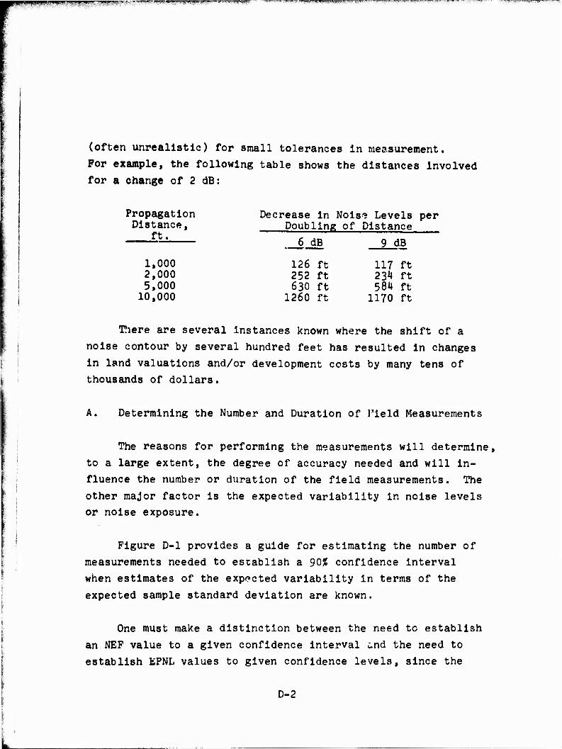
Kj^gjppg^^r^TTWTjrW■' ' "W *• -* ' -*<a-W~*i'-f «■■ii.!( I4*',P »»»> J 11 I i.ii1»Ol"P nff-rwwiTWT^" —

(often unrealistic) for small tolerances in measurement.

For example, the following table shows the distances Involved

for a change of 2 dB:

Propagation Distance,

Decrease in Nois? Levels per Doubling of Distance

ft. 6 dB 9 dB

126 ft 117 ft 252 ft 23*» ft 630 ft 584 ft

1260 ft 1170 ft

1,000 2,000 5,000

10,000

There are several instances known where the shift of a

noise contour by several hundred feet has resulted in changes

in land valuations and/or development costs by many tens of

thousands of dollars.

A. Determining the Number and Duration of Field Measurements

The reasons for performing the measurements will determine,

to a large extent, the degree of accuracy needed and will in-

fluence the number or duration of the field measurements. The

other major factor is the expected variability in noise levels

or noise exposure.

Figure D-l provides a guide for estimating the number of

measurements needed to establish a 9055 confidence interval

when estimates of the expected variability in terms of the

expected sample standard deviation are known.

One must make a distinction between the need to establish

an NEF value to a given confidence interval ^nd the need to

establish EPNL values to given confidence levels, since the

D-2

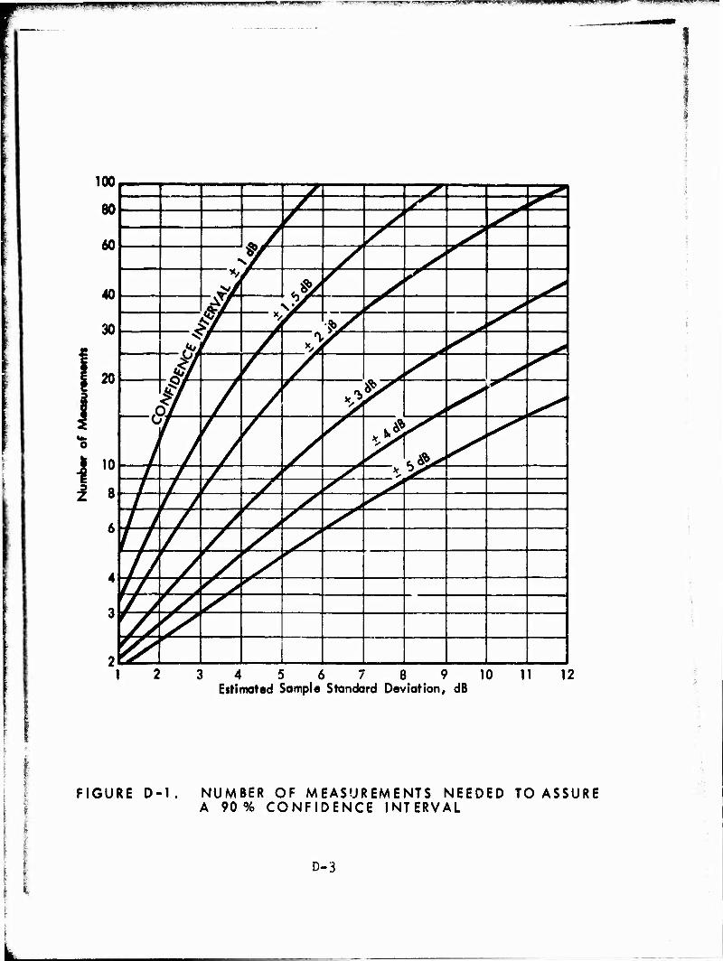
|pH mI -' "WU ! HI IJJLH. 11 jjJ "M" JM. .■» -, JH-. ■ - J ■ * - M ■ *M '^'ll 4M U^-tf J-*^*^f "^ J^1 JJ. * n ypp ipppflapn^mpi

100

80

60

40 *A

M iS^" t

30 >v */ 5/ L- *>4

I 20 i —(5 V >1

&x*

'S

110

I 8

it

its'

6

4

3

2 34 56789 10

Estimated Sample Standard Deviation, dB 11 12

FIGURE D-1 NUMBER OF MEASUREMENTS NEEDED TO ASSURE A 90% CONFIDENCE INTERVAL

D-3

wmfK^w-Mmv.-M-inJ.,9W-mi*»-M*■ *-- -i',i, mmv

degree of variability and time requirements may be vastly

different. For example, an air base may have a wide variation

in the number of operations on a day-to-day basis. Thus, it

may take a considerable period of time to establish a field

NEP value to a given degree of confidence, since one can

accumulate only one NEP value per 2^-hours of measurements.

However, one might well be able to determine noise levels to

a given confidence level in one or two days if there is a

large number of the desired operations per day.

Section IV-D of the report provides estimates of the

expected variability in noise levels resulting from flight

operations. Standard deviations can range from 2 to 7 dB.

Factors influencing the variability include the type of

operations, variability in flight tracks and profiles, and

the sound propagation distance.

The sound propagation distance will likely have consi-

derably more Influence on variability for ground runup than

for flight operations (provided the elevation angles are

sufficiently high [greater than about 15°] to avoid ground

attenuation effects). For short to moderate sound propagation

distances from flight operations (several hundred to one

thousand feet), variations in flight paths can contribute

significantly to the variability of observed ground levels.

At larger distances, the effect of the aircraft path variations

on actual propagation distances usually becomes very small, but

the effect of variations in atmosphere attenuation increases.

Hence, results from recent measurements involving propagation

distances from 2000 to over 5000 feet show only a slight

increase in variability with distance.

D-4

unppsg^^ ?^

Variability in day-to-day NEP values will be directly

related to variations in volume of operations and usage of

flight paths, and may be heavily influenced by weather

conditions which result in changes in runway usage. Some

information on variability is available from civil airport

measurements. For the case of relatively "close-in" measure-

ment positions at civil airports where there are few shifts

or reversals of runway usage, NEF values will show small

variability. Results of CNEL monitoring at Orange County

Airport, California— show standard deviations in day-to-day

measurements of 2 to 3 dB for monitoring over 66 days.

Measurements over a period of 11 days at another airport-^

at a close-in position showed a standard deviation of 1.2 dB.

Measurements showed considerable greater variability at

another civil airport in which tnere were frequent reversals of

runway usage over a 30 day period (takeoff operations

predominated on 17 days, landing operations predominated on

10 d?»ys and there were three days of nearly equal takeoffs

and landings). The standard deviation in CNEL values at

individual measurement positions ranged from 3.3 to 4.6 dB

for measurements over a 30 day period, with observed ranges

in CNEL values per station of 13 to 17 dB.

Thus, experience from civil airport measurements indicates

typical noise exposure value standard deviations ranging from

under 2 up to 5 dB. This range in variability Indicates a

possible wide range in measurement periods to establish a

given confidence interval. Reference to Figure D-l shows

that for a 90 percent confidence Interval of + 2 dB, one needs

about five sets of measurements for a standard deviation of

2 dB, increasing to about 20 days of measurement for a standard

deviation of five dB.

D-5

mrnn^mnvmk>*m»w- ',.m*mtwKx mjmm -^w, «,, ^mumm w^,, ™- --™

B. Number and Location of Measuring Positions

When it is desired to verify the noise environment over an area rather than at a single position, it is desirable to measure noise levels at two or more, and preferably, three or more positions simultaneously. Information obtained at two or more positions simultaneously allows one to establish gradients in noise levels and permits some degree of extrapolation or interpolation between measurement positions. Further, with more than two measurement positions, one measurement position can be maintained as a "control" position, while the other instruments are moved about. Comparison of noise levels at the various "moveable" positions with these observed at the control position enable one to adjust for variations in noise exposure occurring on a day-to-day basis, which might arise from changes in volume of operations or changes in the mix of aircraft.

In verifying noise contours due to flight operations, the control position would typically be placed directly underneath the flight path, and ehe other stations placed on perpendiculars to eitner side, or placed further out under the projected flight path.

Figure D-2 shows one measurement approach, utilizing three measurement instruments, where it is desired to verify one side of a takeoff contour. The instruments are first placed at positions marked "A". After the first series of measurements, two of the instruments are moved VJ new positions for the second series of measurements, denoted as "B" in the figure. This "leap frog" procedure can be repeated, as needed, until the contour is mapped. Note that it is desirable to place the instruments on a perpendicular to the flight path outside of the

D-6

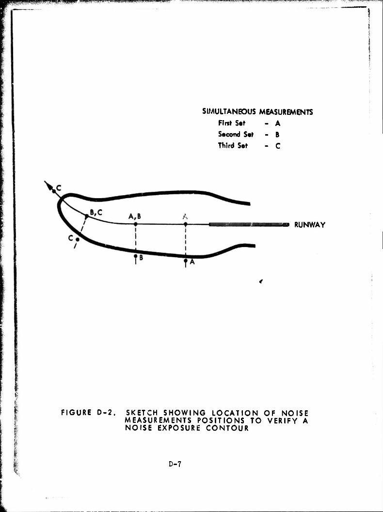
Wm<..i«u!u_,u r ipip^pprap« ::>^.;-- -:_..,- .l^^l.J^HPjl^lt* y^^nF^a^^-'i^i-T*:-^^

SIMULTANEOUS MEASUREMENTS

First Set - A

Second Set - B

Third Set - C

RUNWAY

$ I;

FIGURE D-2. SKETCH SHOWING LOCATION OF NOISE MEASUREMENTS POSITIONS TO VERIFY A NOISE EXPOSURE CONTOUR

D-7

^

igaj^Tj-??^^Tig»g^^.,jg^q.--^<g:i'?

contour, to permit interpolation, rather than extrapolation,

in defining the contour ground location.

A number of variations in the measurement plan sketched

in Figure D-2 can be developed. However, the concept of

keeping one position as a "control" point should be retained.

Regardless of the number of simultaneous measurement

positions, and the use of "control" points, it is important

that accurate records of operations using the flight paths

under study be kept during the period of measurement.

Variations in noise exposure will occur, and knowledge of the

actual history of operations will usually be vital in under-

standing the reasons for the variations.

In validating the noise exposure due to ground runup

operations, the control position should be placed within 250

to 500 feet of the source, and in line .'ith a radial extending

from the source to one or more of the distant measuring

positions. As the distant positions are shifted, it will

usually be desirable to shift the close-in control position

so that the measuring positions are along the same radial

extending out from the .source. This procedure permits one to

compare the differences in noise level without the need for

detailed knowledge of, or adjustment for, the horizontal

directional characteristics of the source.

D-8

«U.S.Qovtrnmtnt Printing Offlc«: 197« - 657-017/360