9781119185727_Automotive Aerodynamics by Joseph Katz.pdf

AUTOMOTIVEAERODYNAMICS

Automotive Series

Series Editor: Thomas Kurfess

Automotive Aerodynamics Katz April 2016

The Global Automotive Industry Nieuwenhuisand Wells

September 2015

Vehicle Dynamics Meywerk May 2015

Vehicle Gearbox Noise and Vibration:Measurement, Signal Analysis, Signal Processingand Noise Reduction Measures

Tůma April 2014

Modeling and Control of Engines and Drivelines Eriksson and Nielsen April 2014

Modelling, Simulation and Control ofTwo-Wheeled Vehicles

Tanelli, Cornoand Savaresi

March 2014

Advanced Composite Materials for AutomotiveApplications: Structural Integrity and Crashworthiness

Elmarakbi December 2013

Guide to Load Analysis for Durability inVehicle Engineering

Johannessonand Speckert

November 2013

AUTOMOTIVEAERODYNAMICS

Joseph KatzSan Diego State University, USA

This edition first published 2016© 2016 John Wiley & Sons, LtdSome text copyright © 2010 Joseph Katz. Reprinted with the permission of Cambridge University Press.

Registered OfficeJohn Wiley & Sons, Ltd, The Atrium, Southern Gate, Chichester, West Sussex, PO19 8SQ, United Kingdom

For details of our global editorial offices, for customer services and for information about how to apply for permission toreuse the copyright material in this book please see our website at www.wiley.com.

The right of the author to be identified as the author of this work has been asserted in accordance with theCopyright, Designs and Patents Act 1988.

All rights reserved. No part of this publication may be reproduced, stored in a retrieval system, or transmitted, in any formor by any means, electronic, mechanical, photocopying, recording or otherwise, except as permitted by the UK Copyright,Designs and Patents Act 1988, without the prior permission of the publisher.

Wiley also publishes its books in a variety of electronic formats. Some content that appears in print may not be available inelectronic books.

Designations used by companies to distinguish their products are often claimed as trademarks. All brand names andproduct names used in this book are trade names, service marks, trademarks or registered trademarks of their respectiveowners. The publisher is not associated with any product or vendor mentioned in this book.

Limit of Liability/Disclaimer of Warranty: While the publisher and author have used their best efforts in preparing thisbook, they make no representations or warranties with respect to the accuracy or completeness of the contents of this bookand specifically disclaim any implied warranties of merchantability or fitness for a particular purpose. It is sold on theunderstanding that the publisher is not engaged in rendering professional services and neither the publisher nor the authorshall be liable for damages arising herefrom. If professional advice or other expert assistance is required, the services of acompetent professional should be sought.

The advice and strategies contained herein may not be suitable for every situation. In view of ongoing research, equipmentmodifications, changes in governmental regulations, and the constant flow of information relating to the use ofexperimental reagents, equipment, and devices, the reader is urged to review and evaluate the information provided in thepackage insert or instructions for each chemical, piece of equipment, reagent, or device for, among other things, anychanges in the instructions or indication of usage and for added warnings and precautions. The fact that an organization orWebsite is referred to in this work as a citation and/or a potential source of further information does not mean that the authoror the publisher endorses the information the organization or Website may provide or recommendations it may make.Further, readers should be aware that Internet Websites listed in this work may have changed or disappeared between whenthis work was written and when it is read. No warranty may be created or extended by any promotional statements for thiswork. Neither the publisher nor the author shall be liable for any damages arising herefrom.

Library of Congress Cataloging-in-Publication Data

Names: Katz, Joseph, 1947– author.Title: Automotive aerodynamics / Joseph Katz.Description: Chichester, UK ; Hoboken, NJ : John Wiley & Sons, 2016. | Includesbibliographical references and index.

Identifiers: LCCN 2016002817| ISBN 9781119185727 (cloth) | ISBN 9781119185734 (epub)Subjects: LCSH: Automobiles–Aerodynamics–Textbooks. | Fluid dynamics–Textbooks.Classification: LCC TL245 .K379 2016 | DDC 629.2/31–dc23LC record available at http://lccn.loc.gov/2016002817

A catalogue record for this book is available from the British Library.

Set in 10 /12.5pt Times by SPi Global, Pondicherry, India

1 2016

http://www.wiley.com

Contents

xii
Series Preface Preface xiv
1 Introduction and Basic Principles 11.1 Introduction 11.2 Aerodynamics as a Subset of Fluid Dynamics 21.3 Dimensions and Units 31.4 Automobile/Vehicle Aerodynamics 51.5 General Features of Fluid Flow 9

1.5.1 Continuum 101.5.2 Laminar and Turbulent Flow 111.5.3 Attached and Separated Flow 12

1.6 Properties of Fluids 131.6.1 Density 131.6.2 Pressure 141.6.3 Temperature 141.6.4 Viscosity 161.6.5 Specific Heat 191.6.6 Heat Transfer Coefficient, k 191.6.7 Modulus of Elasticity, E 201.6.8 Vapor Pressure 22

1.7 Advanced Topics: Fluid Properties and the Kinetic Theory of Gases 231.8 Summary and Concluding Remarks 26Reference 27Problems 27

2 The Fluid Dynamic Equations 352.1 Introduction 352.2 Description of Fluid Motion 362.3 Choice of Coordinate System 382.4 Pathlines, Streak Lines, and Streamlines 392.5 Forces in a Fluid 402.6 Integral Form of the Fluid Dynamic Equations 432.7 Differential Form of the Fluid Dynamic Equations 502.8 The Material Derivative 572.9 Alternate Derivation of the Fluid Dynamic Equations 592.10 Example for an Analytic Solution: Two-Dimensional,

Inviscid Incompressible, Vortex Flow 622.10.1 Velocity Induced by a Straight Vortex Segment 652.10.2 Angular Velocity, Vorticity, and Circulation 66

2.11 Summary and Concluding Remarks 69References 72Problems 72

3 One-Dimensional (Frictionless) Flow 813.1 Introduction 813.2 The Bernoulli Equation 823.3 Summary of One-Dimensional Tools 843.4 Applications of the One-Dimensional Friction-Free Flow Model 85

3.4.1 Free Jets 853.4.2 Examples for Using the Bernoulli Equation 893.4.3 Simple Models for Time-Dependent Changes in a Control Volume 93

3.5 Flow Measurements (Based on Bernoulli’s Equation) 963.5.1 The Pitot Tube 963.5.2 The Venturi Tube 983.5.3 The Orifice 1003.5.4 Nozzles and Injectors 101

3.6 Summary and Conclusions 1023.6.1 Concluding Remarks 103

Problems 104

4 Dimensional Analysis, High Reynolds Number Flows,and Definition of Aerodynamics 1224.1 Introduction 1224.2 Dimensional Analysis of the Fluid Dynamic Equations 1234.3 The Process of Simplifying the Governing Equations 1264.4 Similarity of Flows 1274.5 High Reynolds Number Flow and Aerodynamics 1294.6 High Reynolds Number Flows and Turbulence 133

vi Contents

4.7 Summary and Conclusions 136References 136Problems 136

5 The Laminar Boundary Layer 1415.1 Introduction 1415.2 Two-Dimensional Laminar Boundary Layer Model –

The Integral Approach 1435.3 Solutions using the von Kármán Integral Equation 1475.4 Summary and Practical Conclusions 1565.5 Effect of Pressure Gradient 1615.6 Advanced Topics: The Two-Dimensional Laminar Boundary

Layer Equations 1645.6.1 Summary of the Exact Blasius Solution for the Laminar

Boundary Layer 1675.7 Concluding Remarks 169References 170Problems 170

6 High Reynolds Number Incompressible Flow Over Bodies: AutomobileAerodynamics 1766.1 Introduction 1766.2 The Inviscid Irrotational Flow (and Some Math) 1786.3 Advanced Topics: A More Detailed Evaluation of the Bernoulli Equation 1816.4 The Potential Flow Model 183

6.4.1 Methods for Solving the Potential Flow Equations 1836.4.2 The Principle of Superposition 184

6.5 Two-Dimensional Elementary Solutions 1846.5.1 Polynomial Solutions 1856.5.2 Two-Dimensional Source (or Sink) 1876.5.3 Two-Dimensional Doublet 1906.5.4 Two-Dimensional Vortex 1936.5.5 Advanced Topics: Solutions Based on Green’s Identity 196

6.6 Superposition of a Doublet and a Free-Stream: Flow Over a Cylinder 1996.7 Fluid Mechanic Drag 204

6.7.1 The Drag of Simple Shapes 2056.7.2 The Drag of More Complex Shapes 210

6.8 Periodic Vortex Shedding 2156.9 The Case for Lift 218

6.9.1 A Cylinder with Circulation in a Free Stream 2186.9.2 Two-Dimensional Flat Plate at a Small Angle of Attack

(in a Free Stream) 2226.9.3 Note About the Center of Pressure 224

viiContents

6.10 Lifting Surfaces: Wings and Airfoils 2256.10.1 The Two-Dimensional Airfoil 2266.10.2 An Airfoil’s Lift 2286.10.3 An Airfoil’s Drag 2296.10.4 An Airfoil Stall 2316.10.5 The Effect of Reynolds Number 2326.10.6 Three-Dimensional Wings 233

6.11 Summary of High Reynolds Number Aerodynamics 2486.12 Concluding Remarks 249References 249Problems 250

7 Automotive Aerodynamics: Examples 2627.1 Introduction 2627.2 Generic Trends (For Most Vehicles) 263

7.2.1 Ground Effect 2647.2.2 Generic Automobile Shapes and Vortex Flows 265

7.3 Downforce and Vehicle Performance 2697.4 How to Generate Downforce 2747.5 Tools used for Aerodynamic Evaluations 274

7.5.1 Example for Aero Data Collection: Wind Tunnels 2767.5.2 Wind Tunnel Wall/Floor Interference 2797.5.3 Simulation of Moving Ground 2817.5.4 Expected Results of CFD, Road, or Wind Tunnel Tests

(and Measurement Techniques) 2837.6 Variable (Adaptive) Aerodynamic Devices 2867.7 Vehicle Examples 291

7.7.1 Passenger Cars 2927.7.2 Pickup Trucks 2987.7.3 Motorcycles 2997.7.4 Competition Cars (Enclosed Wheel) 3027.7.5 Open-Wheel Racecars 306

7.8 Concluding Remarks 312References 314Problems 314

8 Introduction to Computational Fluid Mechanics (CFD) 3168.1 Introduction 3168.2 The Finite-Difference Formulation 3178.3 Discretization and Grid Generation 3208.4 The Finite-Difference Equation 3218.5 The Solution: Convergence and Stability 3248.6 The Finite-Volume Method 326

viii Contents

8.7 Example: Viscous Flow Over a Cylinder 3288.8 Potential-Flow Solvers: Panel Methods 3318.9 Summary 335References 337Problems 337

9 Viscous Incompressible Flow: “Exact Solutions” 3399.1 Introduction 3399.2 The Viscous Incompressible Flow Equations (Steady State) 3409.3 Laminar Flow between Two Infinite Parallel Plates: The Couette Flow 340

9.3.1 Flow with a Moving Upper Surface 3429.3.2 Flow between Two Infinite Parallel Plates: The Results 3439.3.3 Flow between Two Infinite Parallel Plates – The Poiseuille Flow 3479.3.4 The Hydrodynamic Bearing (Reynolds Lubrication Theory) 351

9.4 Flow in Circular Pipes (The Hagen-Poiseuille Flow) 3599.5 Fully Developed Laminar Flow between Two Concentric Circular Pipes 3649.6 Laminar Flow between Two Concentric, Rotating Circular Cylinders 3669.7 Flow in Pipes: Darcy’s Formula 3709.8 The Reynolds Dye Experiment, Laminar/Turbulent Flow in Pipes 3719.9 Additional Losses in Pipe Flow 3749.10 Summary of 1D Pipe Flow 375

9.10.1 Simple Pump Model 3789.10.2 Flow in Pipes with Noncircular Cross Sections 3799.10.3 Examples for One-Dimensional Pipe Flow 3819.10.4 Network of Pipes 391

9.11 Free Vortex in a Pool 3949.12 Summary and Concluding Remarks 397Reference 397Problems 397

10 Fluid Machinery 41110.1 Introduction 41110.2 Work of a Continuous-Flow Machine 41510.3 The Axial Compressor (The Mean Radius Model) 417

10.3.1 Velocity Triangles 42110.3.2 Power and Compression Ratio Calculations 42410.3.3 Radial Variations 42910.3.4 Pressure Rise Limitations 43110.3.5 Performance Envelope of Compressors and Pumps 43410.3.6 Degree of Reaction 441

10.4 The Centrifugal Compressor (or Pump) 44610.4.1 Torque, Power, and Pressure Rise 44710.4.2 Impeller Geometry 450

ixContents

10.4.3 The Diffuser 45410.4.4 Concluding Remarks: Axial versus Centrifugal Design 457

10.5 Axial Turbines 45810.5.1 Torque, Power, and Pressure Drop 45910.5.2 Axial Turbine Geometry and Velocity Triangles 46110.5.3 Turbine Degree of Reaction 46410.5.4 Turbochargers (for Internal Combustion Engines) 47310.5.5 Remarks on Exposed Tip Rotors (Wind Turbines

and Propellers) 47410.6 Concluding Remarks 478Reference 478Problems 478

11 Elements of Heat Transfer 48511.1 Introduction 48511.2 Elementary Mechanisms of Heat Transfer 486

11.2.1 Conductive Heat Transfer 48611.2.2 Convective Heat Transfer 48911.2.3 Radiation Heat Transfer 491

11.3 Heat Conduction 49511.3.1 Steady One-Dimensional Heat Conduction 49711.3.2 Combined Heat Transfer 49911.3.3 Heat Conduction in Cylinders 50211.3.4 Cooling Fins 506

11.4 Heat Transfer by Convection 51511.4.1 The Flat Plate Model 51611.4.2 Formulas for Forced External Heat Convection 52011.4.3 Formulas for Forced Internal Heat Convection 52611.4.4 Formulas for Free (Natural) Heat Convection 529

11.5 Heat Exchangers 53411.6 Concluding Remarks 536References 539Problems 539

12 Automobile Aero-Acoustics 54412.1 Introduction 54412.2 Sound as a Pressure Wave 54612.3 Sound Loudness Scale 54912.4 The Human Ear Perception 55212.5 The One-Dimensional Linear Wave Equation 55312.6 Sound Radiation, Transmission, Reflection, Absorption 556

12.6.1 Sound Wave Expansion (Radiation) 556

x Contents

12.6.2 Reflections, Transmission, Absorption 55912.6.3 Standing Wave (Resonance), Interference, and Noise

Cancellations 56012.7 Vortex Sound 56112.8 Example: Sound from a Shear Layer 56412.9 Buffeting 56812.10 Experimental Examples for Sound Generation on a Typical Automobile 57412.11 Sound and Flow Control 57612.12 Concluding Remarks 577References 578Problems 578

Appendix A 581Appendix B 583Index 589

xiContents

Series Preface

The automobile touches nearly every part of our lives. The manufacture of the automobilegenerates significant economic benefits, which is clear by the efforts that nations make tosecure automobile manufacturing plants within their borders. Furthermore, issues such asemissions and fuel economy are critical to providing a sustainable path for the human racewell into the future. Not only is the automobile a critical aspect of our lives, it is interwoveninto our society, culture, and global wellbeing, as well as being a very fertile platform fortremendous technical advancements.The primary objective of the Automotive Series is to publish practical and topical books

for researchers, and practitioners in industry, and postgraduate/advanced undergraduateeducators in the automotive engineering sector. The series addresses new and emergingtechnologies in automotive engineering supporting the development of more fuel efficient,safer and more environmentally friendly vehicles. It covers a wide range of topics, includingdesign, manufacture, and operation, and the intention is to provide a source of relevant infor-mation that will be of interest and benefit to people working in the field of automotiveengineering.A critical aspect of vehicle system performance is the aerodynamic characteristics of the

vehicle. These characteristics are major factors in vehicle performance, efficiency, safety,and marketability. This text, Automotive Aerodynamics, follows in the strong tradition ofthe Automotive Series, in that it presents classical fundamental concepts in aero and fluidmechanics in a pragmatic and concise fashion using the automobile as the primary exemplar.The text is designed to be used in an introductory aero/fluid mechanics course, and groundsthe theoretical concepts in vehicle system examples that provide a familiar foundation to thestudents. Moreover, it does go beyond the basic aero/fluid topics addressing related issuessuch as heat-transfer, cooling, and aeroacoustics. Using the automobile as an example forthese concepts provides the students with a critical touchstone to their life experiences.

Automotive Aerodynamics covers a number of classical topics including basic fluidmechanics, internal and external flows, viscosity and drag, as well as providing an introduc-tion to numerical simulations, which are critical given the increasing access engineers haveto cloud and high performance computing. Given that the text is well grounded in funda-mentals, and has relevant and in-depth examples of modern systems, it is also a valuableprofessional reference. This book is an excellent text that is both relevant and forward think-ing. It is written by a recognized expert in the field and is a welcome addition to the Auto-motive Series.

Thomas KurfessNovember 2015

xiiiSeries Preface

Preface

This text was planned for engineering students as a first course in the complex field of aero/fluid mechanics. It does contain complex math, mainly to serve as the foundation for futurestudies. But the chapters focus onmore applied examples, which can be solved in class usingelementary algebra. Thus, the intention is not to avoid complex physical problems, but tokeep them simple. Therefore, emphasis is placed on providing complete solutions, whichcan be solved in class. The material provided is self-contained and the reader is not directedelsewhere for more detailed formulations. On the other hand, the automobile is a part of oureveryday life and the first complete engineering system fascinating the younger generations.As such, focusing on automotive examples can provide the much needed inspiration, andaccelerate the attention and learning curve of the students.Aero/fluid mechanics is a complex science and some problems cannot be solved by sim-

ple intuition. The reason behind this is the complex nonlinear differential equations, whichhave no closed form solutions. Historically, simple models were developed for some spe-cific cases, and one educational approach is to present a series of case studies based on thoselocalized solutions. However, when following this approach, the connection among thecase-studies is unclear and long term learning benefits diminish. In addition, numerical solu-tions matured recently and most CAD programs have modules that can generate “a solution”by a simple “run” command. This usually leads to an iterative “learning curve” withoutunderstanding the main variables affecting the solution. Therefore, presenting the governingequations early on (as painful as it can be), and explaining the possible simplifications willprovide a clear roadmap that will pay-off at the end of the course.The first objective of this text, as advocated in the previous paragraphs, is to provide a

systematic approach to the field of aero/fluid mechanics and to serve as a long-term refer-ence. Also, some engineering programs are forced to shorten the curriculum and requireonly one course related to thermo/fluid mechanics. Consequently, the second objective is

to introduce related areas not covered in traditional curriculum, such as heat-transfer,cooling, and aeroacoustics.

A Word to the Instructor

A first course in aero/fluid mechanics is always challenging due to the numerous new con-cepts that weren’t used in previous engineering courses. The students were usually exposed tostatics and dynamics, and will not easily adjust to “control volume”methods. Thus, after shortintroduction (Chapter 1), I suggest formulating the integral continuity and momentum equa-tion. This allows opportunity to dwell on the principles of conservation (of mass and momen-tum) and allows the introduction of the differential form of the same equations. By the way, insome program this subject is taught throughout a whole semester, as a prelude to courses on“transport phenomena”. Once the student understands the meaning of the various terms in theequations, simple examples can follow, in hope of explaining the mechanisms responsiblefor skin friction, pressure distribution and eventually lift, and drag of various vehicles.A one-semester introductory course (~45 hours total) may cover the following sections

(in the order presented):

Chapter 1 This is basically an introduction. A survey of engineering units is recom-mended, and Section 1.7 can be omitted.

Chapter 2 The fluid dynamic equations. The integral form (Section 2.6) is easily devel-oped in class, but the differential form (Section 2.7) is more difficult. Sections 2.8–2.11can be omitted in an introductory course. The suggested objective here is for the studentsto recognize the various terms (e.g., acceleration, body force, etc…).

Chapter 3 After a rather complex discussion in Chapter 2, simple one-dimensional exam-ples serve to demonstrate the conservation of mass and momentum. It is suggested tocover Sections 3.1 through 3.4.2, and 3.5.

Chapter 4 This chapter serves as an introduction to the following chapters dealing withhigh Reynolds number flows. It also explains the relation between aerodynamics and themore general field of fluid mechanics. It is suggested to cover the whole chapter quicklyand demonstrate the method of neglecting smaller terms in the governing equations.

Chapter 5 This chapter demonstrates the effect of viscosity and the mechanism for fric-tion drag. Sections 5.6 and 5.7 can be omitted.

Chapter 6 This introduces the concept of ideal flow. Note that only the velocity potentialis presented, because in more advanced courses it can be extended to three-dimensionalflows. The approach is to present a case which can be solved in class (e.g., the flow over acylinder), based on which experimental data base can be used for lift and drag. This chap-ter is the main topic in this course and requires most of the attention. Usually, Sections6.4–6.10 are covered with examples from Chapter 7.

Chapter 9 This chapter introduces viscous flow examples, with the flow in pipes beingthe main topic. Usually, Sections 9.4–9.9 are included.

xvPreface

Chapter 8 A short discussion on numerical solution can be included at the end of thesemester. Most programs will offer an additional one-semester course on CFD.

Chapter 10–Chapter 12 These chapters introduce additional practical examples relatedto aerodynamics. Topics can be included in more advanced courses or be used in thefuture for quick reference.

xvi Preface

1Introduction and Basic Principles

1.1 Introduction

Wind and water flows played an important role in the evolution of our civilization and pro-vided inspiration in early agriculture, transportation, and even power generation. Ancientship builders and architects of the land all respected the forces of nature and tried to utilizenature’s potential. At the onset of the industrial revolution, as early as the nineteenth century,motorized vehicles appeared and considerations for improved efficiency drove the need tobetter understand the mechanics of fluid flow. Parallel to that progress the mathematicalaspects and the governing equations, called the Navier–Stokes (NS) equations, were estab-lished (by the mid-1800s) but analytic solutions didn’t follow immediately. The reason ofcourse is the complexity of these nonlinear partial differential equations that have no closedform analytical solution (for an arbitrary case). Consequently, the science of fluid mechanicshas focused on simplifying this complex mathematical model and on providing partial solu-tions for more restricted conditions. This explains why the term fluid mechanics (or dynam-ics) is used first and not aerodynamics. The reason is that by neglecting lower-order terms inthe complex NS equations, simplified solutions can be obtained, which still preserve thedominant physical effects. Aerodynamics therefore is an excellent example for generatinguseful engineering solutions via “simple” models that were responsible for the huge prog-ress in vehicle development both on the ground and in the air. By focusing on automobileaerodynamics, the problem is simplified even more and we can consider the air as incom-pressible, contrary to airplanes flying at supersonic speeds.At this point one must remember the enormous development of computational power in

the twenty-first century, which made numerical solution of the fluid mechanic equations areality. However, in spite of these advances, elements of modeling are still used in those

Automotive Aerodynamics, First Edition. Joseph Katz.© 2016 John Wiley & Sons, Ltd. Published 2016 by John Wiley & Sons, Ltd.

solutions and the understanding of the “classical” but limited models is essential to suc-cessfully use those modern tools.Prior to discussing the airflow over vehicles, some basic definitions, the engineering units

to be used, and the properties of air and other fluids must be revisited. After this short intro-duction, the fluid dynamic equations will be discussed and the field of aerodynamic will bebetter defined.

1.2 Aerodynamics as a Subset of Fluid Dynamics

The science of fluid mechanics is neither really new nor biblical; although most of the prog-ress in this field was made in the latest century. Therefore, it is appropriate to open this textwith a brief history of the discipline with only a very few names mentioned.As far as we could document history, fluid dynamics and related engineering was always

an integral part of human evolution. Ancient civilizations built ships, sails, irrigation sys-tems, or flood management structures, all requiring some basic understanding of fluid flow.Perhaps the best known early scientist in this field is Archimedes of Syracuse (287–212 BC),founder of the field now we call “fluid statics”, whose laws on buoyancy and flotation areused to this day.Major progress in the understanding of fluid mechanics begun with the European Renais-

sance of the fourteenth to seventeenth centuries. The famous Italian painter sculptor, Leonardoda Vinci (1452–1519) was one of the first to document basic laws such as the conservation ofmass. He sketched complex flow fields, suggested viable configuration for airplanes, para-chutes, or even helicopters, and introduced the principle of streamlining to reduce drag.During the next couple of hundred years, sciences gradually developed and then suddenly

were accelerated by the rational mathematical approach of Englishman, Sir Isaac Newton(1642–1727) to physics. Apart from his basic laws of mechanics, and particularly the secondlaw connecting acceleration with force, Newton developed the concept for drag and shear ina moving fluid, principles widely used today.The foundations of fluid mechanics really crystallized in the eighteenth century. One of

the more famous scientists, Daniel Bernoulli (1700–1782, Dutch-Swiss) pointed out therelation between velocity and pressure in a moving fluid, the equation of which bears hisname in every textbook. However, his friend Leonhard Euler (1707–1783, Swiss born),a real giant in this field is the one actually formulating the Bernoulli equations in the formknown today. In addition Euler, using Newton’s principles, developed the continuity andmomentum equations for fluid flow. These differential equations, the Euler equations arethe basis for modern fluid dynamics and perhaps the most significant contribution in theprocess of understanding fluid flows. Although Euler derived the mathematical formulation,he didn’t provide solution to his equations.Science and experimentation in the field advanced but only in the next century were the

governing equations finalized in the form known today. Frenchman, Claude-Louis-Marie-Henri Navier (1785–1836) understood that friction in a flowing fluid must be added to theforce balance. He incorporated these terms into the Euler equations, and published the first

2 Automotive Aerodynamics

version of the complete set of equation in 1822. These equations are known today as theNavier–Stokes equations. Communications and information transfer weren’t well devel-oped those days. For example, Sir George Gabriel Stokes (1819–1903) lived at the Englishside of the Channel but didn’t communicate directly with Navier. Independently, he alsoadded the viscosity term to the Euler equations, hence the shared glory by naming the equa-tions after both scientists. Stokes can be also considered as the first to solve the equations forthe motion of a sphere in a viscous flow, which is now called Stokes flow.Although the theoretical basis for the governing equationwas laid down by now, it was clear

that the solution is far from reach and therefore scientists focused on “approximate models”using only portions of the equation, which can be solved. Experimental fluid mechanics alsogained momentum, with important discoveries by Englishman Osborne Reynolds(1842–1912) about turbulence and transition from laminar to turbulent flow. This brings usto the twentieth century, when science and technology grew at an explosive rate, particularly,after the first powered flight of the Wright brothers in the US (Dec 1903). Fluid mechanicsattracted not only the greatest talent but also investments from governments, as the potentialof flying machines was recognized. If we mention one name per century then Ludwig Prandtl(1874–1953) of Gottingen Germany deserves the glory. He made tremendous progress indeveloping simple models for problems such as boundary layers and airplane wings.The efforts of Prandtl lead to the initial definition of aerodynamics. His assumptions usu-

ally considered low-speed airflow as incompressible, an assumption leading to significantsimplifications (as will be explained in Chapter 4). Also, inmost cases the effects of viscositywere considered to be confined into a thin boundary layer, so that the viscous flow termswereneglected. These twomajor simplifications allowed the development of (aerodynamic) mod-els that could be solved analytically and eventually comparedwell with experimental results!This trend of solving models and not the complex Navier–Stokes equations continued

well into the mid-1990s, until the tremendous growth in computer power finally allowednumerical solution of these equations. Physical modeling is still required but the numericalapproach allows the solution of nonlinear partial differential equations, an impossible taskfrom the pure analytical point of view. Nowadays, the flow over complex shapes and theresulting forces can be computed by commercial computer codes but without being exposedto simple models our ability to analyze the results would be incomplete.

1.3 Dimensions and Units

The magnitude (or dimensions) of physical variables is expressed using engineering units.In this text we shall follow the metric system, which was accepted by most professionalsocieties in the mid-1970s. This international system of units (SI) is based on the decimalsystem and is much easier to use than other (e.g., British) systems of units. For example, thebasic length is measured by meters (m) and 1000 m is called a kilometer (km) or 1/100 of ameter is a centimeter. Along the same line 1/1000 m is a millimeter.Mass is measured in grams, which is the weight of one cubic centimeter of water. One

thousand grams are one kilogram (kg) and 1000 kg is one metric ton. Time is still measured


the old fashion way, by hours (h) and 1/60th of an hour is a minute (min), while 1/60 of aminute is a second (s).For the present text velocity is one of the most important variables and its basic measure

therefore is m/s. Vehicles speed are usually measured in km/h and clearly 1 km/h = 1000/3600 = 1/3.6 m/s Acceleration is the rate of change of velocity and therefore it is measuredby m/s2.Newton’s Second Law defines the units for the force F, when a mass m is accelerated at a

rate of a

F =ma = kgmsec2

Therefore, this unit is called Newton (N). Sometimes the unit kilogram-force is used(kgf) since the gravitational pull of 1 kg mass at sea level is 1 kgf. If we approximate thegravitational acceleration as g = 9.8 m/s2, then

1kgf = 9 8N

The pressure, which is the force per unit area is measured using the previous units

p=F

S=kg

msec2

m2=

Nm2

= 1 Pascal

and this unit is called after the French scientist Blaise Pascal (1623–1662). Sometimesatmosphere (atm) is used to measure pressure and this unit is about 1 kgf/cm2, or moreaccurately

l atm = 1 013 105 N m2

There are a large number of engineering units and a list of the most common ones is pro-vided in Appendix A.The definition of engineering quantities, such as forces or pressures, requires the selection

of a coordinate system. In this text, the preferred system is the Cartesian (named after theseventeenth century mathematician Rene Cartesius) shown in Fig. 1.1. The cylindrical

z (lift)

x (drag)

y(side force)

Figure 1.1 Cartesian coordinate system and its definition relative to an automobile


coordinates system (r, θ, x) will be used only when the problem formulation becomes sig-nificantly simpler.In the next section, some examples are presented demonstrating the relevance of aerody-

namics to vehicle design. The discussion that follows lists some of the more important prop-erties of air and other fluids, along with the units used to quantify them.

1.4 Automobile/Vehicle Aerodynamics

Ask any fluid/aerodynamicist and he will tell you that “everything” is related to this science;weather, ocean flows, human organs such as the heart or lungs, or even the flow of concreteand metals. So if this science is so important there is nothing more rewarding than to studyand explore its principle on an object close to all of us; the automobile. This will not deprivethe discussion because all elements of fluid mechanics are included. Therefore, this preludeprovides a comprehensive foundation for more advanced coursework the student may latertake, focusing on more specific topics.Returning to automobiles, one must remember that aerodynamics relates to ventilation/

AC, engine in-and-out flows, brake cooling, and resulting forces on the vehicle. To dem-onstrate the effect of aerodynamics on vehicles, let us start with a simple example; the drag(force resisting the motion), which also affects the shape and styling of modern vehicles. Theforces that a moving vehicle must overcome increase with speed, and the tire rolling resist-ance and driveline friction effects are shown in Fig. 1.2, along with the total force resistingthe motion (indicating the significance of aerodynamic drag).From the early twentieth century, both fuel cost and vehicle speeds gradually increased

and the importance of aerodynamic drag reduction, based on Fig. 1.2 is obvious. A careful

00

200

400

600

800

1000

20 40 60

Speed, Km/h

80 100 120 140

Aerodynamic drag+ rolling resistance

Res

ista

nce

forc

e, N

Tire rolling resistance

Figure 1.2 Increase of vehicle total drag and tires rolling resistance on a horizontal surface, versusspeed (measured in a tow test of a 1970 Opel Record)


examination of the data in this figure reveals that the aerodynamic drag increases with thesquare of the velocity while all other components of drag change only marginally. There-fore, engineers devised a nondimensional number, called the drag coefficient (CD), whichquantifies the aerodynamic sleekness of the vehicle configuration. One of the major advan-tages of this approach is that scaling (e.g., changing the size) is quite simple. The definitionof the drag coefficient is:

CD =D

0 5ρU2S1 1

whereD is the drag force, ρ is the density,U is vehicle speed, and S is the frontal area. Later,we shall see that the denominator represent a useful, widely used quantity. Now suppose thatsome manufacturer decides to reduce its vehicle dimensions by 10% and asks his engineersto estimate the fuel saving:

Example 1.1A passenger car has a drag coefficient of 0.4 and management propose to reduce all dimen-sions by 10%. Apart from the weight saving, how much can be saved, based on the aero-dynamic considerations?Assuming that fuel consumption is related to the power (P), which is force (D) times

velocity (U) we can write:

P=D U =CD0 5ρU2S U

The scaling enters this formula via the frontal area S, which is now smaller by 0.9 09(=0.81). So if vehicle shape is unchanged then the power for the 10% smaller vehicle will be:

P=D U = 0 81 CD 0 5ρU3S

So at a specific speed, saving is estimated at 19%. Also note that power requirementsincrease with U3.This simple example shows that by focusing on vehicle drag reduction,significant fuel savings can be achieved. Drag reduction trends over recent years are shownin Fig. 1.3, an overall trend that was probably driven by the increasing cost of fuel (and theenvironmental emission control of recent years).Figure 1.3 also provides the range of practical drag coefficients, which could start as high

asCD = 1 0, but in recent years most manufacturers hope to cross theCD = 0 3 “barrier”. Thetrends of styling changes are hinted by the small sketches, and modern cars have smoothsurfaces and utilize all available “practical” tricks to reduce drag (we can learn about thislater). Also, two extreme examples were presented in this figure. First, the streamlined shapeat the lower left part of the figure, which indicates that a CD 0 15 is possible. Furthermore,the placing of this shape indicates that engineers new early how to reduce drag but automo-bile designs were mostly driven by artistic considerations (not so in the twenty-first century).Just to prove this anecdotal point, Fig. 1.4 shows the 1924 Tropfenwagen (droplet-shaped


1920 300.1

0.2

0.3

0.4

0.5

0.6

0.70.80.91.0

40 50 60 70 80 90 2000 10

Year

CD

CD = 0.15

Figure 1.3 Schematic representation of the historic trends in the aerodynamic drag of Passenger cars

Figure 1.4 The 1924 Tropfenwagen, which had a better drag coefficient CD = 0 28 than mostmodern cars. Illustration by Brian Hatton


car, in German), designed by E. Rumpler. Both the vehicle body and its cabin had a teardropshape, with the objective of reducing aerodynamic drag.By the way, the original Tropfenwagen automobile residing in the German Museum in

Munich, was tested in the VW AG wind tunnel in 1979. The measured drag coefficientsurpassed most modern cars and was found atCD = 0 28. This car also featured a mid-enginelayout, which was reinvented in the 1960s by racecar engineers, but in the 1920s the designwas too much for the traditional automobile buyer and resulted in commercial failure.Let us now return to the second extreme example at the top right-hand side of Fig.1.3,

representing the high drag of most modern racecars. This observation sounds contradictoryto the purpose of racing fast and is the result of generating a force called “aerodynamicdownforce”, pushing the car to the ground. Because most races involve high-speedcornering and acceleration, increasing tire adhesion (using aerodynamic downforce) resultsin faster cornering, and in improved braking and acceleration. Of course top speed is com-promised but overall vehicles utilizing downforce are not only faster on a closed track butalso more stable.The evolution of the maximum lateral acceleration (during cornering) over the years is

illustrated schematically in Fig. 1.5. The gray area shows the gradual improvement in sports

19500.0

1.0

2.0

3.0

4.0

1960 1970 1980 1990 2000

Racing carswith aerodynamicdownforce

Racing carswithout aerodynamicdownforce

Production sportscars and sedans

Year

Max

imum

late

ral a

ccel

erat

ion

(ay/

g)

Figure 1.5 Trends of increased lateral acceleration over recent years for various racecars


(and production) car handling, which is a direct result of improvements in tire (and suspen-sion) construction. The solid line indicates a somewhat larger envelope of performance dueto the softer and stickier tire compounds used for racing purposes. The gradual increase inracecars’ maximum lateral acceleration, prior to 1966, is again a result of improvements intire and chassis technology. However, the rapid increase that follows is due to the suddenutilization of aerodynamic downforce. The interesting question is: how, for the first 65 yearsof motor racing, was aerodynamics more like an art with a bit of drag reduction and why didno one notice the tremendous advantage of creating downforce on the tires without increas-ing the vehicle’s mass? (We can always blame politics.)Of course, the large values in Fig. 1.5 represent momentary limits and it is quite difficult

to experience a lateral acceleration of three gs for more than a few seconds. For this reason,in many races where large lateral forces will be generated, the helmet of the driver isstrapped to the vehicle’s sides to avoid excess neck stress. If one must speculate aboutthe future of racing, it seems that the 4 g shown in this diagram is a reasonable limit, andis based on human comfort (limits).Most vehicles (e.g., passenger cars) have positive lift and not downforce and sport car

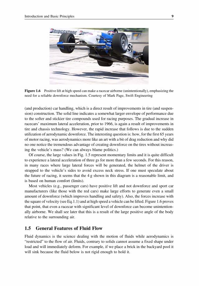
manufacturers (like those with the red cars) make large efforts to generate even a smallamount of downforce (which improves handling and safety). Also, the forces increase withthe square of velocity (see Eq.1.1) and at high speed a vehicle can be lifted. Figure 1.6 provesthat point, that even a racecar with significant level of downforce can become unintention-ally airborne. We shall see later that this is a result of the large positive angle of the bodyrelative to the surrounding air.

1.5 General Features of Fluid Flow

Fluid dynamics is the science dealing with the motion of fluids while aerodynamics is“restricted” to the flow of air. Fluids, contrary to solids cannot assume a fixed shape underload and will immediately deform. For example, if we place a brick in the backyard pool itwill sink because the fluid below is not rigid enough to hold it.

Figure 1.6 Positive lift at high speed can make a racecar airborne (unintentionally), emphasizing theneed for a reliable downforce mechanism. Courtesy of Mark Page, Swift Engineering


Also, both gases and liquids behave similarly under load and both are considered fluids.A typical engineering question that we’ll try to answer here is: what are the forces due tofluid motion? Examples could focus on estimating the aerodynamic forces acting on a car orloads needed to calculate the size and shape of a wing lifting an airplane. So let us start withthe first question: what is a fluid?As noted, in general, we refer to liquids and gases as fluids, but using the principles of

fluid mechanics can treat the flow of grain in agricultural machines, a crowd of people leav-ing a large stadium, or the flow of cars on the highway. So one of the basic features is that wecan look at the fluid as a continuum and not analyze each element or molecule (hence theanalogy to grain or seeds). The second important feature of fluid is that it deforms easily,unlike solids. For example, a static fluid cannot resist a shear force without moving and,once the particles move, it is not a static fluid. So in order to generate shear force the fluidmust be in motion. This will be clarified in the following paragraphs.

1.5.1 Continuum

Most of us are acquainted with Newtonian mechanics and therefore it would be natural tolook at particle (or group of particles) motion and discuss their dynamics using the sameapproach used in courses such as dynamics. Although this approach has some followers,let us first look at some basics.Consideration a: The number of molecules is very large and it would be difficult to apply

the laws of dynamics, even when using a statistical approach. For example, the number ofmolecules in one gram-mole is called the Avogadro number (after the Italian scientist, Ama-deo Avogadro 1776–1856). One gram-mole is the molecular weight multiplied by 1 gram.For example, for a hydrogen molecule (H2) the molecular weight is two, therefore 2 g ofhydrogen are 1 gram-mole. The Avogadro number NA is:

NA = 6 02 1023 molecules gmole 1 2

Because the number of molecules is very large it is easier to assume a continuous fluid ratherthan discuss the dynamics of each molecule or even their dynamics, using a statisticalapproach.Consideration b: In gases, which we can view as the least condensed fluid, the particles

are far from each other, but as Brown (Robert Brown, botanist 1773–1858) observed in1827, the molecules are constantly moving, and hence this phenomenon is called the Brow-nian motion. The particles move at various speeds and into arbitrary directions and the aver-age distance between particle collisions is called the mean free path, λ, which for standard airis about 6 10−6 cm. Now, suppose that a pressure disturbance (or a jump in the particlesvelocity) is introduced, this effect will be communicated to the rest of the fluid by these interparticle collisions. The speed that this disturbance spreads in the fluid is called the speed ofsound and this gives us an estimate about the order of molecular speeds (the speed of soundis about 340 m/s in air at 288 K). Of course, many particles must move faster than this speedbecause of the three-dimensional nature of the collisions (see Section 1.6). It is only logical


that the speed of sound depends on temperature since temperature is related to the internalenergy of the fluid. If this molecular mean free path distance λ is much smaller than thecharacteristic length L in the flow of interest (e.g., L ~ the length of a car) then, for example,we can consider the air (fluid) as a continuum! In fact, a nondimensional number, called theKnudsen number (after the Danish scientist Martin Knudsen: 1871–1949) exists based onthis relation.

Kn =λ

L1 3

Thus, if Kn < 0 01, meaning that the characteristic length is 100 times larger than the freemean path, then the continuum assumption may be used. Exceptions for this assumptionof course would be when the gas is very rare Kn> 1 , for example in a vacuum or at veryhigh altitude in the atmosphere.It appears that for most practical engineering problems, the aforementioned considera-

tions (a) and (b) are easily met, justifying the continuum assumption. So if we agree tothe concept of continuum, then we do not need to trace individual molecules (or groupsof ) in the fluid but rather observe the changes in the average properties. Apart from proper-ties such as density or viscosity, the fluid flow may have certain features that must be clar-ified early on. Let us first briefly discuss frequently used terms such as laminar/turbulent andattached/separated flow, and then focus on the properties of the fluid material itself.

1.5.2 Laminar and Turbulent Flow

Now that via the continuum assumption we have eliminated the discussion about the arbi-trary molecular motion, a somewhat similar but much larger scale phenomenon must be dis-cussed. For the discussion let us assume a free-stream flow along the x-axis with uniformvelocity U. If we follow the traces made by several particles in the fluid we would expect tosee parallel lines as shown in the upper part of Fig. 1.7. If, indeed, these lines are parallel andfollow in the direction of the average velocity, and the motion of the fluid seems to be “wellorganized”, then this flow is called laminar. If we consider a velocity vector in a Cartesiansystem

q = u,v,w 1 4

then for this steady state flow the velocity vector will be

q = U,0,0 1 4a

and hereU is the velocity into the x direction. Note that we are usingq for the velocity vector!On the other hand it is possible to have the same average speed in the flow, but in addition

to this average speed the fluid particles will momentarily move into the other directions(lower part of Fig. 1.7). The fluid is then called turbulent (even though the average velocity


Uav could be the same for both the laminar and turbulent flows). Again, note that at this pointin the discussion the fluid is continuous and the turbulent fluid scale is much larger than themolecular scale. Also, in this two-dimensional case the flow is time dependent everywhereand the velocity vector then becomes

q = Uav + u ,v ,w 1 5

and here u , v ,w are the perturbation into the x, y, and z directions. Also it is clear that theaverage velocities into the other directions are zero

Vav =Wav = 0

So if a simple one-dimensional laminar flow transitions into a turbulent flow, then it alsobecomes three-dimensional (not to mention time dependent). Knowing whether the flowis laminar or turbulent is very important for most engineering problems since features suchas friction and momentum exchange can change significantly between these two types offlow. The fluid flow can become turbulent in numerous situations such as inside long pipesor near the surface of high-speed vehicles.

1.5.3 Attached and Separated Flow

Tracing streamlines in the flow (by injecting smoke, for example) allows us to observeif the flow follows the shape of an object (e.g., vehicle’s body) close to its surface. Whenthe streamlines near the solid surface follow exactly the shape of the body (as in Fig. 1.8a)the flow is considered to be attached. If the flow does not follow the shape of the surface(as seen behind the vehicle in Fig. 1.8b) then the flow is considered detached or separated(in that region). Usually, such separated flows behind the vehicle will result in anunsteady wake flow, which can be felt up to large distances behind it. Also, in case

Laminar flow

Turbulent flow

Figure 1.7 Schematic descriptions of laminar and turbulent flows with the same average velocity


of Fig. 1.8(b) the flow is attached on the upper surface and is separated only behind thevehicle. As we shall see later, having attached flow fields is extremely important becausevehicles with larger areas of flow separation are likely to generate higher resistance(drag). Now, to complicate matters we may add that if the flow above this model is tur-bulent then, because of the momentum influx from the outer flow layers, the flow sep-aration can be delayed.

1.6 Properties of Fluids

Fluids, in general, may have many properties related to thermodynamics, mechanics, orother fields of science. In the following paragraphs we shall mention only a few, whichare used in introductory aero/fluid mechanics.

1.6.1 Density

The density by definition is mass (m) per unit volume. In case of fluids, we can define thedensity (with the aid of Fig. 1.9) as the limit of this ratio, when a measuring volume V shrinksto zero. We need to use this definition since density can change from one point to the other.Also in this picture we can relate to a volume element in space that we can call “controlvolume”, which moves with the fluid or can be stationary (better if it is attached to an inertialframe of reference).Therefore, the definition of density at a point is:

ρ= limV 0m

V1 6

Typical units are: kg/m3 or g/cm3

(a)

(b)

Attached flow

Separated flow

U∞

Figure 1.8 Attached flow over a streamlined car (a) and the locally separated flow behind a morerealistic automobile shape (b)


1.6.2 Pressure

We can describe the pressure p as the normal force F, per unit area, acting on a surface S(seeFig. 1.10). Again, we will use the limit process to define pressure at a point, since it may varyon a surface.

p = limS 0F

S1 7

Bernoulli pictured the pressure to be a result of molecules impinging on a surface (so thisforce per area is a result of the continuous bombardment of the molecules). The fluid pres-sure acting on a solid surface is normal to the surface as shown in the figure. Consequently,the direction is obtained by multiplying with the unit vector n normal to the surface. Thus,the pressure acts normal to a surface, and the resulting force, ΔF is:

ΔF = −pn dS 1 8

Here, the minus sign is a result of the normal unit-vector pointing outside the surface whilethe force due to pressure points inward. Also note that the pressure at a point inside a fluid isthe same in all directions. This property of the pressure is called isetropic. The observationabout the fluid pressure at a point, acting equally into any arbitrary directions, was docu-mented first by Blaise Pascal (1623–1662).The units used for pressure were introduced in Section 1.3. However, the Pascal is a small

unit and more popular units are the kilopascal (kP), the atmosphere (atm), or the bar

1 kP= 1000N

m21atm = 101300

N

m21bar = 100000

N

m2

1.6.3 Temperature

The temperature is a measure of the internal energy at a point in the fluid. Over the yearsdifferent methods evolved to measure temperature and, for example, the freezing point ofwater was considered as zero in the Celsius system while water boiling temperature under

Control volume

V

m

Figure 1.9 Mass m in a control volume V. Density is the ratio of m/V, as V shrinks


standard condition is 100 C. Kelvin units are similar to Celsius, however, they measure tem-perature from absolute zero, the temperature found in space that represents when molecularmotion will stop. The relation between the two temperature measuring systems is:

K = 273 16 +C 1 9

The Celsius system is widely used in European countries while in the US the Fahrenheitscale is still used. In this case the 100 F was set to be close to the human body’s temperature.The conversion between these temperature systems is

C = 5 9 F – 32 1 10

Which indicates that 0 C = 32 F. The absolute temperature in these units is called the Ran-kine scale and this is higher by 459.69 .

R = 459 69 + F 1 11

Now that we have introduced density, pressure, and temperature it is important to recallthe ideal gas relation, where these properties are linked together by the gas constant, R.

p ρ=RT 1 12

If we define v as the volume per unit mass then v = 1 ρ, and we can write

pv=RT 1 13

However, R is different for various gases or for their mixtures, but it can be easily cal-culated by using the universal gas constant, ( = 8314.3 J/mol K). Then R can befound by dividing this universal by the average molecular weight M of the mixtureof gases.

n→

dS

Figure 1.10 Pressure acts normal to the surface dS (n is the unit vector normal to the surface)


Example 1.2 The ideal gas formulaAs an example, for air we can assume that the molecular weight is M= 29, and therefore

R = M=8314 3 29 = 286 7 m2 sec2K for air 1 14

Suppose we want to calculate the density of air when the temperature is 300 K, and thepressure is 1 kgf/cm2.

ρ= p RT= 1 9 8 104 286 7 300 = 1 139 kg m3

Here we used 1 kgf/cm2 = 9.8 104 N/m2, and g = 9.8 m/s2.Another interesting use of the universal gas constant iswhenwe calculate the volume (V) of

one gram-mole of gas in the following conditions: T = 300 K and p = 1 atm = 101,300 N/m2.For air we can take 29 g (since M = 29) and then is multiplied by 10−3 because we con-sidering one gram-mole and not one kg-mole. Based on Eq. 1.3 and 1.4, and using the factthat the volume per unit mass is V/M we can write:

pV M = M T

or

V= T p = 8314 3 10−3 300 101300 = 24 62 10−3m3 = 24 62 liter

Note that the molecular weight was cancelled, and 1 gram-mole of any gas will occupy thesame volume because we have the same number of molecules (as postulated by Avogadro).Also 1 liter is equal to 0.001 m3.

1.6.4 Viscosity

The viscosity is a very important property of fluids, particularly when fluid motion is dis-cussed. In fact the schematic diagram of Fig. 1.11 is often used to demonstrate the differencebetween solids and fluids. A fluid must be in motion in order to generate a shear force, whilea solid can support shear forces in a stationary condition.In this figure the upper plate moves at a velocity of U∞ while the lower surface is at rest.

A fluid is placed between these parallel plates and when pulling the upper plate, a force F isneeded. At this point we can introduce another important observation. The fluid particles inimmediate contactwith theplateswill notmove relative to theplate (as if theywereglued to it).This is called the no-slip boundary condition and we will use this in later chapters. Conse-quently, we can expect the upper particles tomove at the upper plate’s speed while the lowestfluid particles attached to the lower plate will be at rest. Newton’s Law of Friction states that:

τ = μdU

dz1 15


here τ is the shear force per unit area and μ is the fluid viscosity. In this case the resultingvelocity distribution is linear and the shear will be constant inside the fluid (for h > z > 0). Forthis particular case we can write:

τ = μU∞

h1 16

A fluid that behaves like this is called a Newtonian fluid, indicating a linear relationbetween the stress and the strain. As noted earlier, this is an important property of fluidssince without motion there is no shear force.The units used for τ are force per unit area and the units for the viscosity μ are defined by

Eq. 1.15. Some frequently used properties of some common fluids are provided in Table 1.1.Also note that the viscosity of most fluids depends on the temperature and this is shown

for several common fluids in Fig. 1.12.

Example 1.3 The units of shearTo demonstrate the units of shear let us calculate the force required to pull a plate floating ona 2-cm thick layer of SAE 30 oil at U∞ = 3 m/s.Taking the value of the viscosity from Table 1.1: μ = 0.29 kg/m s at 20 CThus:

τ= 0 29 3 0 02 = 43 kg m s2 = 43 N m2

So if the plate area is 2 m2 then a force of 86 N will be required to pull it at 3 m/s.Sometimes the ratio between viscosity and the density is denoted as ν, the “kinematic

viscosity”. Its definition is:ν=

μ

ρ1 17

x

F

No-slip condition

No-slip conditionSolid boundaries

h Fluid

z

U∞

Figure 1.11 The flow between two parallel plates. The lower is stationary while the upper moves at avelocity of U∞


Table 1.1 Approximate properties of some common fluids at 20 C(ρ = density, μ = viscosity)

ρ (kg/m3) μ (N s/m2)

Air 1.22 1.8 10–5

Helium 0.179 1.9 10–5

Gasoline 680 3.1 10–4

Kerosene 814 1.9 10–3

Water 1000 1.0 10–3

Sea water 1030 1.2 10–3

Motor oil (SAE 30) 919 0.29Glycerin 1254 0.62Mercury 13,600 1.6 10–3

GlycerinSAE 10w oil

Water

Air

Hydrogen

–2068

2

468

2

468

2

Vis

cosi

ty, μ

, N s

/m2

468

2

468

2

1.0

2.0

4.0

468

1 ·10–5

1 ·10–4

1 ·10–3

1 ·10–2

1 ·10–1

0 20 40 60 80 100 120

Temperature, °C

Figure 1.12 Variation of viscosity versus temperature for several fluids


1.6.5 Specific Heat

Fluids have several thermodynamic properties and we shall mention only two related to heatexchange. For example, if heat Q is added in a constant pressure process to a mass m, thenthe relation between temperature change and heat is stated by the simple formula

Q=mcpΔT 1 18

Here, cp is the specific heat coefficient used in a constant pressure process. However, if thefluid is not changing its volume during the process then cv is used for the specific heat in thisprocess.

Q=mcvΔT 1 19

The ratio between these two specific heat coefficients is denoted by γ

γ =cPcV

1 20

The heat (energy) required to raise the temperature of 1 g of water by 1 C is called a cal-

orie (cal). Therefore, the units for cp or cv arecal

kg Cand 1 cal = 4.2 J (J = Joule). Work in

mechanics is force times distance and therefore units of 1 Joule are

1 J = kgmsec2

m= kgm2

sec2

Also, for an ideal gas undergoing an adiabatic process, the two heat capacities relate to thegas constant, R (see Ref. 1.1 p. 90) by:

cp−cv =R 1 21

1.6.6 Heat Transfer Coefficient, k

Heat transfer can take several forms such as conduction, convection, or radiation (seeChapter 11). As an example at this introductory stage, we can mention only one basic modeof heat transfer, called conduction. The elementary one-dimensional model is depicted inFig. 1.13 where the temperature at one side of the wall is higher than on the other side.The basic heat transfer equation for this case, called theFourier equation, states that the heatflux Q is proportional to the area A, the temperature gradient, and to the coefficient k, whichdepends on the material through which the heat is conducted.

Q = −kAdT

dx1 22


For the case in the figure we could state that the heat flux is

Q= −kAT2−T1

d1 22a

And here T2 is larger than T1, and the minus sign indicates that the heat flux is in the leftdirection. The units for k are defined by Eq. 1.22 as W/(m C) or cal/(m C s). Note that thetemperature distribution in the wall in Fig. 1.13 is linear. This is proved later in Chapter 11.

1.6.7 Modulus of Elasticity, E

The modulus of elasticity E is a measure of compressibility. It can be defined as

E = dp dV V or dp=E dV V 1 23

And the second form indicates how much pressure is needed to compress a material hav-ing a modulus of E. Also, the change in volume is directly related to the change in density,and we can write:

dρ ρ= dV V 1 24

And by substituting dV/V instead of dρ/ρ in Eq. 1.23 we get:

E = dp dρ ρ 1 25

Most liquid are not very compressible, but gases are easily compressed and for an idealgas we already introduced this relation (in Eq. 1.12):

dp dρ=RT 1 26

d

Q

x

TT1

T2

Figure 1.13 Conductive heat transfer through a wall of thickness d


Therefore, substituting Eq. 1.26 into Eq. 1.25 results (for an ideal gas):

E = ρRT 1 27

The units for E, based on Eq. 1.23 areN m2

m3 m3=N m2

Example 1.4 Compressibility of a liquidFor this example, let us consider the compressibility of sea water. The modulus of elasticityis E = 2.34 109 N/m2 and let us evaluate the change in volume at a depth of 1 Km. Thechange in pressure at 1000 m depth is

dp= ρgh= 1000 9 8 1000 N m2

and

dV V = dp E = 1000 9 8 1000 2 34 109 = 4 188 10−3 0 42

which is less than half a percent. This shows that water is really incompressible.It is interesting to point out that compressibility relates to the speed of sound in a fluid.

If we use the letter a to denote the speed of sound, then later we shall see that

a2 = dp dρ 1 28

For liquids, we can use Eq. 1.25 to show that

a2 = dp dρ =E ρ 1 29

For ideal gases undergoing an adiabatic process (thermally isolated), the relation betweenpressure and density (Ref. 1.1) is:

p

ργ=C 1 30

where C is a constant. To find the speed of sound the derivative dpdρ is evaluated using

Eq. 1.30 and the ideal gas definition:

dp

dρ=C γ ργ−1 =C γ

ργ

ρ=

p

ργγ

ργ

ρ= γ

p

ρ= γRT 1 31

Therefore

a= γRT 1 32

indicating that the speed of sound is a function of the temperature.


Example 1.5 The speed of soundLet us calculate the speed of sound in air at 300 K. Taking the value of R from Eq. 1.14 andassuming γ = 1 4:

a= 1 4 286 6 300 = 346 9m s forair

Now, to calculate the speed of sound in water we must use Eq. 1.29. Based on the mod-ulus of elasticity of sea water:

a =E

ρ=

2 34 109

1000= 1529m s

and the resulting speed of sound is significantly higher.

1.6.8 Vapor Pressure

Vapor pressure is a property related to the phase change of fluids. One way to describe itis to observe the interface between the liquid and the gas phase of a particular fluid andthe vapor pressure indicates that there is equilibrium between the molecules leaving andjoining the liquid phase. The best example is to examine the vapor pressure of water asshown in Fig. 1.14. Because molecular energy is a function of the temperature, it is clear

00.0

0.2

0.4

0.6

0.8

1.0

20 40 60 80 100

p (a

tm)

T (°C)

Figure 1.14 Vapor pressure of air versus temperature


that vapor pressure will increase with temperature. The vapor pressure is zero at 0 C, andof course is equal to one atmosphere at 100 C, which is the standard boiling pointof water.In later chapters we shall see that the pressure can change in a moving fluid. So even

if there is no temperature change, there could be a situation when the pressure in the fluid(liquid) falls below the vapor pressure. The result is formation of bubbles, because at thiscondition the liquid will evaporate locally. This phenomenon is called cavitation and canhappen in an overheating engine coolant when the radiator pressure cap cannot hold thedesigned pressure. If pump cavitation occurs, this will reduce coolant flow rate and coolingsystem performance, and will affect the pump efficiency. One possible solution is to increasethe pressure in an engine cooling system to delay cavitation, resulting in better coolingperformance.Fluids have many more properties such as enthalpy, entropy, internal energy, and so on,

but they are not used in this text.

1.7 Advanced Topics: Fluid Properties and theKinetic Theory of Gases

Gases were defined earlier as fluids where the molecules can move freely and are far fromeach other, occasionally colliding with each other. This model led Daniel Bernoulli in 1738to explain pressure in gases based on this type of molecular motion. Bernoulli considered acylindrical container, filled with gas, as shown in the figure. As the molecules move insidethe container, they also impinge on the walls as shown in Fig. 1.15. Now we may neglect theintermolecular collisions and assume that when a molecule hits the wall it will bounce backwithout losses (elastic collision). This assumption also includes pure elastic collisions withthe sides of the cylinder.

y S

A

L

zx

Figure 1.15 Gas molecules moving randomly inside a container


Therefore the total forces due to these collisions must produce the pressure on the contain-er’s walls. For example, the particle in Fig. 1.15 hitting the top has a velocity

q = u,v,w 1 33

and when it hits the top, the change in its linear momentum in the x direction is

2 mu

and the 2 is a result of the elastic collision, while m is the mass of the molecule, and u is thevelocity component into the x direction. Because the particle is contained inside the cylinderand it is continuously bouncing back and forth, we can estimate the time Δt between thesecollisions on the upper wall by

Δt = 2 L u

where L is the length of the cylinder. The force due to the collisions of this particle, based onNewton’s Momentum Theory is

F =Δ mu

Δt=2mu2 L u

=mu2 L 1 34

Now recall that the particles are likely to move at the same speed into any direction and

q2 = u2 + v2 +w2

and if all directions are of the same order of magnitude we can assume

q2≈3u2

Now suppose that there are N particles in the container and therefore the force due to theinner gas is

F =Nmq2 3

L1 35

and the pressure is simply the force per unit area

p =F

S=N

mq2 3LS

=N

3Vmq2 1 36

and here the volume V = LS, and S is the cylinder top (or bottom) area. This is a surprisinglysimple approach that connects the pressure to the molecular kinetic energy. Now if we recallthe ideal gas equation


pV = nRT =N

NART 1 37

Where n =N NA, is the number of moles in the cylinder (recall thatNA is the Avogadro num-ber in Eq. 1.2). By equating these two equations (1.36 and 1.37) we solve for thetemperature:

T =NA

3Rmq2 1 38

This simple model shows that for an ideal gas the molecular kinetic energy is propor-tional to the absolute temperature. This means that at the absolute zero the molecularmotion will stop; a concept that wasn’t received well in Bernoulli’s era. About 100 yearslater, the Scottish physicist, James Maxwell (1831–1879) revived this theory and intro-duced a statistical approach. He suggested a universal velocity distribution (Fig. 1.16)that shows the velocity range of the molecular motion. Our interest at this point is todemonstrate the magnitude of the molecular velocity, which mainly depends on temper-ature and molecular weight. The probability is depicted on the ordinate and the probablevelocity is on the abscissa. Of course the total area under the curve is always one,because all particles in the container are included. Note that the average velocity is abit over the top to the right (468 m/s for air) which is somewhat higher than the speedof sound, mentioned earlier.Another interesting aspect of this molecular model is that for flows over bodies, it can

intuitively explain the effect of curvature on the pressure distribution. For example,Fig. 1.17 shows a generic automobile, which is moving forward at a constant speed.

00

0.0002

0.0004

0.0006

0.0008

0.001

0.0012

0.0014

200 400 600 800 1000 1200 1400 1600 1800

Prob

abili

ty

Molecular speed (m/s)

Figure 1.16 Maxwell’s universal velocity distribution for the molecules of air M=29 , at 300 K


The air molecules are moving towards the car at an average velocity, in addition to theirBrownian motion (see Fig. 1.17). At the base of the windshield the number of collisionswill increase because the incoming molecules will hit head on and some may even bounceback again due to intermolecular collisions. On the other hand, when observing the flowover a convex surface as shown in the figure (e.g., behind the roof top). The particles willnot hit the rear window head on. They will fill the void mainly due to intermolecular colli-sions. Hence a lower pressure is expected there. We can also guess that the velocity at thebase of the windshield (concave surface) slows down while the undisturbed particles at theback (convex surface) will accelerate to cover the additional distance created by the void.This generic discussion suggests that the pressure is lower if the velocity is increased insuch flows. We shall see later that this observation led to the formulation of the well-known Bernoulli equation.

1.8 Summary and Concluding Remarks

In this introductory chapter, the properties of fluids were discussed. The reader must haveseen those during earlier studies and the only ones worth mentioning again are related to theforces in fluids. The first is of course the pressure, which acts normal to a surface, and thesecond is the shear force. The shear stress in a fluid exists only when the fluid is in motion,contrary to solids that can resist shear under static conditions. This situation is created by the“no slip boundary condition”, which postulates that the fluid particles in contact with a sur-face will have zero relative velocity at the contact area.

Concavesurface

Convexsurface

Highpressure

Lowpressure

Figure 1.17 Using the kinetic theory of gases we can explain the high pressure near a concavecurvature and the lower pressure near a convex curvature


Reference1.1. Karlekar, B. V., Thermodynamics for Engineers, Prentice-Hall, Englewood Cliffs, NJ,1983.

Problems

1.1. The recommended pressure on the tires of a sedan is 30 psi. Convert this to units ofN/m2 and atmospheres.

1.2. The frontal area of a pickup truck is 2 m2 and the air resistance (drag) at 100 km/h is 500N. Calculate the truck’s drag coefficient (assume air density is 1.2 kg/m3).

1.3. How many kg of air at standard conditions are in a container with a volume of 2 m3?1.4. A uniform pressure is acting on a plate 0.5 m tall and 3.0 m wide. Assuming the pressure

difference between the two sides of the plate is 0.05 atm, calculate the resultant force.

Constantpressure

3.0 m

0.5 m

F

Problem Figure 1.4

1.5. Identical bricks 0.1 m wide, and weighing 2 kg are placed on a plate (assume theplate has negligible weight). Calculate the total weight (and force F required to bal-ance the plate). How far from x = 0 should F be placed so that the plate will nottip over?

1

1 2

1 2 3

1 2 3 4

1 2 3 4 5

0 0.1 0.2 0.3 0.4 0.5

F

x

Problem Figure 1.5


1.6. A linearly varying pressure [P(x) = Pmax x /L] is acting on a plate. Calculate the totalforce (resultant) and how far it acts from the origin. (Later we shall call this the centerof pressure.)

p =Pmax

Pmax

Lx

x0 L

Problem Figure 1.6

1.7. Suppose that a 1 m3 metal container holds air at standard conditions (p = 1 atm andT = 300 K).a. Calculate the pressure inside the container if it is heated up to 400 K?b. Calculate the density ρ inside the container.

R= 286 6m2 sec2K

1.8. A two-dimensional velocity field is given by the following formulation

u =x

x2 + z2w=

z

x2 + z2

Calculate the value of the velocity vector q at a point (1, 3).1.9. On a warm day the thermometer reads 30 C. Calculate the absolute temperature in

Kelvin and also the temperature in degrees Fahrenheit.1.10. 1 m3 of air at 1 atm, and at 300 K is sealed in a container. Calculate the pressure inside

the container if:a. The volume is reduced to 0.5 m3 but the temperature cooled off to 300 K, andb. when the temperature was 350 K.

1.11. A 1 m3 balloon is filled with helium at an ambient temperature of 30 C. The pressureinside the balloon is 1.1 atm while outside it is 1.0 atm. The molecular weight ofhelium is about 4 and the surrounding air is about 29. Calculate the weight of thehelium inside the balloon. What is the weight of outside air that has the same volumeas the balloon? What is the meaning of this weight difference?

1.12. Usually, we check the tire pressure in our car early morning when the temperature iscold. Suppose that the temperature is 288 K (about 15 C), the volume of air inside is0.025 m3, inside air density is 2.4 kg/m3, and the tire pressure gauge indicates a pres-sure of 2 atm (2 1.1013 105 N/m2).a. What is the tire pressure when the car is left in the summer sunshine and the tire

temperature reaches 333 K?b. Suppose the tire is inflated with helium (M ~ 4) instead of air (M ~ 29); how much

weight is saved?


1.13. A 200 cm3 container is filled with air at standard conditions. Estimate the number ofair molecules in the container.

1.14. The temperature inside the container in the previous question was raised to 350 K.Calculate the pressure, density, and the number of air molecules inside the container.

1.15. A 3 m3 tank is filled with helium at standard conditions. If the molecular weight ofhelium is 4.0, calculate the mass of the gas inside the tank.

1.16. The tire pressure in a car wasmeasured in themorning, at 280K andwas found to be 2.5atm. After a long trip on a warm afternoon the pressure rose to 3.1 atm. Assuming thereis no change in the tire volume, calculate the air temperature due to the pressure rise.

1.17. A flat plate floating above a 0.05 cm thick film of oil being pulled to the right at a speedof 1m/s (see sketch in Fig. 1.18). If the fluid viscosity is 0.4 N s/m2, calculate the shearforce τ on the lower and upper interfaces (e.g., on the floor and below the plate) and atthe center of the liquid film.

1.18. A flat plate floating on a 0.05 cm thick water film is pulled by the force F. Calculate Ffor an area of 1 m2 and for U = 1 m/s (note that for water, μ = 0.001 kg/(m/s).

F

Water

U

0.05 cm

Problem Figure 1.18

1.19. A flat plate is pulled to the right above a 0.1 cm thick layer of viscous liquid (seesketch in Fig. 1.18) at a speed of 1 m/s. If the force required to pull the plate is200 N per 1 m2, then calculate the viscosity of the liquid.

1.20. Consider a stationary vertical line in the figure of the previous problem (fixed to thelower surface). Calculate how much water per 1 m width flows during 1 s to the rightacross that line?

1.21. The velocity distribution above a solid surface represented by the x coordinate is

u= 3 z − 3z3

w= 0

Calculate the shear stress on the surface (at z = 0) and at z = 0.5.

F

θ

h

m

S (contact area)

Oil film

Problem Figure 1.21


1.22. A thin oil film covers the surface of an inclined plane, as shown. Develop an expres-sion for the terminal velocity of a block of weightW, sliding down the slope. Assumethat the oil film thickness and viscosity are known, as well as the incline angle and thecontact surface area.

1.23. Calculate the terminal velocity of a 0.2 m wide, 0.3 m long, and 5 kg block slidingdown an incline of 30 , as shown in sketch for Problem 1.22. Assume the oil filmthickness is 1 mm and the oil viscosity (from Table 1.1) is 0.29 N s/m2.

1.24. The block in the sketch for Problem 1.22 slides at a velocity of 2m/s due to the forceF.In this case, however, the slope θ = 0. Calculate themagnitude of the force if the oil filmthickness is 1 mm and the oil viscosity (from Table 1.1), is 0.29 N s/m2.

1.25. A thin plate is pulled to the right, between two parallel plates at a velocityU, as shown.It is separated by two viscous fluids with viscosity μ1, μ2, and the spacing is h1, h2,accordingly. Assuming that the plates are very large, calculate the force per unit arearequired to pull the central plate.

h1μ1

μ2h2

F, U

Problem Figure 1.25

1.26. A small bird with a characteristic length of L = 0.2 m flies near the ocean at a speed of14 m/s. The mean free path of air molecules at sea level is about λ = 6.8 10–8 m, andthe average molecular sped can be estimated as c = 468 m/s. Calculate the Knudsennumber. Can you assume that the fluid is continuous?

1.27. At standard atmospheric condition the average speed of the air molecules is estimatedat c = 468 m/s (see Fig. 1.16). Calculate the speed of sound for this condition (at T =300 K). Can you explain the large difference?

1.28. An important parameter for grouping different flow regimes (called the Reynoldsnumber) represents the ratio between the actual and the molecular scaling of length

times velocity. It can be approximated by the following formulation Re = 2V

c

L

λ(see

Chapter 4, Section 4.2). Calculate this ratio for the small bird of the previous problemflying at a speed of 14 m/s. (recall that c = 468 m/s, and λ = 6.8 10–8 m).

1.29. A 0.3 m wide, 0.5 m long, and 10 kg block (m1) slides on a 1 mm thin oil film, pulledby the mass m2, as shown. Calculate the terminal velocity using the oil viscosity fromTable 1.1 (0.29 N s/m2).


m2 =10 kg

m1=10 kg

Oil film

h

Problem Figure 1.29

1.30. Calculate the terminal velocity in Problem 1.29, but now m1 = 20 kg.1.31. The disk shown in the figure rotates at a speed of 50 RPM above a stationary plane

separated by an oil film. If the oil viscosity is μ = 0.01 kg/(m/s), the spacing betweenthe disc and the stationary surface is 2 mm, and R = 5 cm, calculate the torque requiredto rotate the disk (assume linear velocity distribution in the gap).

Disk

hROil

Problem Figure 1.31

1.32. A rotary damper consists of a disk immersed in a container as shown in the figure.Assuming that the gap h is the same on both sides and the viscosity μ and the diskradius R are known, calculate the torque required to rotate the disk at a particu-lar RPM.

Rh

Oil

Problem Figure 1.32

1.33. The diameter of the rotary damper, shown in the figure is 2R = 20 cm. The oil viscosityis μ = 0.29 kg/(m/s), and the gap is h = 1 mm. Calculate the torque on the shaft at1000 RPM.

1.34. Suppose the gap is increased to h = 2mm in both sides, by howmuch would the torquechange?


1.35. Two concentric cylinders with radius R1 and R2 are separated by an oil film withviscosity μ as shown in the figure. Next, the inner cylinder is rotated and a linear veloc-ity distribution is assumed in the gap between the cylinders (the lower surface is notactive). Develop a formula for the torque on the shaft, as a function of rotation speed.

Oil

h

R1

R2

Problem Figure 1.35

1.36. The two concentric cylinders shown in the sketch for Problem 1.35 are separatedby an oil film with viscosity μ = 0.023 kg/(m/s). If the shaft rotates at 200 RPM,calculate the torque on the shaft (R1 = 15.12 cm, R2 = 15 cm, and h = 70 cm).

1.37. The device, based on the two concentric cylinders (shown in the sketch for Problem 1.35)can be used to measure the viscosity of a fluid. Assuming that the shaft rotates at 200RPM and the torque measured is 6 Nm, calculate the viscosity of the fluid. (Use thedimensions from the previous problem (R1 = 15.12 cm, R2 = 15 cm, and h = 70 cm).

1.38. Some desalination processes are based on evaporating the sea water. Energy canbe saved by reducing the boiling temperature of the water. Based on Fig. 1.14,determine the water boiling temperature if the pressure is lowered to 0.5 atm.

1.39. The disk shown in the sketch rotates at a speed ofω = 50 rad/s above a stationary planeseparated by an oil film. If the oil viscosity is μ = 0.01 kg/(m/s), the spacing betweenthe disc and the stationary surface is 2 mm, and D = 10 cm, calculate the torquerequired to rotate the disk.

Disk

h

D

Oil

ω

Problem Figure 1.39


1.40. Oil with a viscosity of μ flows between two parallel plates, as shown. Suppose thevelocity distribution is given as:

u z = −kz

h−z2

h2

Then plot and calculate the shear stress as a function of z. Where (in terms of z) is thehighest and where is the lowest shear stress? What is the relation between k in theequation and Umax in the figure?

x

u(z)

Umaxh

z

Problem Figure 1.40

1.41. Two layers of fluid are dragged along by the motion of an upper plate as shown (with-out mixing). The bottom plate is stationary. The top fluid applies a shear stress on theupper plate and the lower fluid applies a shear stress on the bottom plate. Calculate thevelocity of the boundary between the two fluids.

3 m/s

Fluid 1

Fluid 2

0.02 m

0.02 m

U

μ1 = 0.4 N s/m2

μ2 = 0.2 N s/m2

Problem Figure 1.41

1.42. A noise created by small earthquake at a depth of 1200 m in the ocean propagatesupward and eventually reaches a bird flying above, at an altitude of 400 m. Calculatehow long it takes for the noise to reach the bird.For the seawater use E = 2.34 109 N/m2, ρ = 1030 kg/m3, and for air, γ = 1.4 andT = 270 K).


400 m

1200 m

Air

Seawater

Sound origin

Problem Figure 1.42

1.43. A small explosion in the ocean is 3000 m from two swimmers. The first has his earsunder water while the second swimmer’s head is above the water. How soon willeach hear the noise of the explosion? For the seawater use E = 2.34 109 N/m2,ρ = 1030 kg/m3, and for air, γ = 1.4 and T = 300 K).

1.44. The speed of an airplane is frequently stated in terms of the Mach number, which issimply the ratio between the actual speed and the speed of soundM=U/a. Suppose anairplane flies at sea level atM = 0.8 where the temperature is 27 C, calculate the actualspeed of the airplane.

Next, calculate the speed at the same Mach number but at an altitude of 13 km,where the temperature is −57 C (for air, γ = 1.4).

1.45. A piston floats over a 1 m high column of water enclosed in a 2 cm diameter, pressure-tight cylinder. Calculate how deep the 100 kg weight will push the cylinder down.Assume the water modulus of elasticity is E = 2.34 109 N/m2.

Water1m

100kg

Problem Figure 1.45


2The Fluid Dynamic Equations

2.1 Introduction

One approach in teaching introductory aero/fluid mechanics is to avoid the presentation ofthe complex fluid dynamic equations. This is done for very good reasons, including the lackof preparation in partial differential equations and due to the overall complexity of the prob-lem. Although avoiding the introduction of the complex equations is welcomed by the aver-age students, the negative and long-term outcome of this approach is that there is no clearrationale and connecting string between the various chapters that will follow. Therefore, weask the students to be patient and “suffer quietly” at the beginning, and the benefits of a clearroad-map will surface with the systematic approach that will follow.The mechanisms controlling fluid motion may include elements of basic mechanics, heat

transfer, phase change, chemical reactions, and even molecular mechanics. Limiting the dis-cussion to simple fluid flow and eventually, aerodynamics, allows us to focus on principlessuch as the conservation of mass momentum and energy. In this text, however, we shallconcentrate on the conservation of mass (called the continuity equation) and on the conser-vation of momentum, and also assume a simple Newtonian fluid without heat transfer. Theobjective of this chapter is to derive those two conservation laws; the conservation of massand momentum.The conservation of massm, simply states that there is no change in the total mass (usually

referring to a control volume):

d m

dt= 0 2 1


and the momentum equation simply applies Newton’s Second Law of motion stating that thechange in linear momentum is equal to the sum of the forces acting on the mass m (e.g., in acontrol volume):

d mq

dt=ΣF 2 2

As will be demonstrated, in the case of fluids, these equations will be quite complicated andtheir exact solutions are very limited. Therefore, the disciplines of fluid mechanics and aer-odynamics are based on simplified models using only portions of the full equations. Thissimplification can be accomplished by identifying the dominant terms in the formulationand neglecting terms of much lower orders of magnitude. It appears that this approachallows the engineers to appreciate both the power and the limitations of the techniques thatwill be presented in this text. Furthermore, the learning process will be easier, as the linkbetween the various chapters is understood.Note to the Instructor: When teaching an introductory course (and dedicating only one

or two lectures to this chapter) it is easier to focus in class on the integral approach(Section 2.6). The rest of the chapter can be assigned as a reading assignment at home fol-lowed by a brief discussion in class. The overall objective is that the student will be familiarwith the terms in the continuity and momentum equations.

2.2 Description of Fluid Motion

The fluid being studied here is modeled as a continuum and infinitesimally small regions ofthe fluid (with a fixed mass) are called fluid elements or fluid particles. The motion of thefluid can be described by two different methods. One adopts the particle point of view andfollows the motion of the individual particles. The other adopts the field point of view andprovides the flow variables as functions of position in space and time. The particle point ofview, which uses the approach of classical mechanics, is called the Lagrangian method(after the Italian scientist Joseph-Louis Lagrange: 1736–1813). To trace the motion of eachfluid particle, it is convenient to introduce a Cartesian coordinate system with the coordi-nates x, y, and z. The position of any fluid particle P (see Fig. 2.1) is then given by

x= xP xo,yo,zo, t

y= yP xo,yo,zo, t 2 3

z= zP xo,yo,zo, t

where (xo, yo, zo) is the position ofP at some initial time t = 0. (Note that the quantity (xo, yo, zo)represents the vector with components xo, yo, and zo.) The components of the velocity of thisparticle are then given by


http://en.wikipedia.org/wiki/1736

http://en.wikipedia.org/wiki/1813

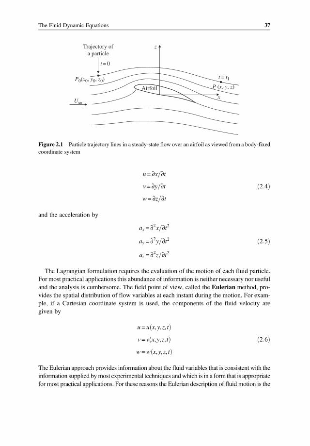
u = ∂x ∂t

v = ∂y ∂t 2 4

w= ∂z ∂t

and the acceleration by

ax = ∂2x ∂t2

ay = ∂2y ∂t2 2 5

az = ∂2z ∂t2

The Lagrangian formulation requires the evaluation of the motion of each fluid particle.For most practical applications this abundance of information is neither necessary nor usefuland the analysis is cumbersome. The field point of view, called the Eulerian method, pro-vides the spatial distribution of flow variables at each instant during the motion. For exam-ple, if a Cartesian coordinate system is used, the components of the fluid velocity aregiven by

u = u x,y,z, t

v = v x,y,z, t 2 6

w=w x,y,z, t

The Eulerian approach provides information about the fluid variables that is consistent with theinformation supplied bymost experimental techniques andwhich is in a form that is appropriatefor most practical applications. For these reasons the Eulerian description of fluid motion is the

Trajectory ofa particle

Airfoil

U∞

t = 0

t = t1P0(x0, y0, z0)P (x, y, z)

x

z

Figure 2.1 Particle trajectory lines in a steady-state flow over an airfoil as viewed from a body-fixedcoordinate system


most widely used (and will be developed in this chapter). Also note that we shall useq for thevelocity vector:

q = u,v,w 2 7

And, for example, a constant velocity of U∞, into the x direction is:

q = U∞ , 0, 0 2 7a

2.3 Choice of Coordinate System

For the following chapters, when possible, primarily a Cartesian coordinate system will beused. Other coordinate system such as the cylindrical will be introduced and used if neces-sary, mainly to simplify the treatment of certain problems. As an example, consider the for-wardmotion of streamlined body (e.g., an airfoil), with a constant speedU∞ , in a fluid that isotherwise at rest – as shown in Fig. 2.1. Here, the origin of the coordinate system is attachedto the moving airfoil and the trajectory of a fluid particle inserted at point Po at t = 0 is shownin the figure. By following the trajectories of several particles a more complete description ofthe flowfield is obtained from the figure. It is important to observe that, for a constant veloc-ity forward motion of the airfoil in this frame of reference, these trajectory lines becomeindependent of time. That is, if various particles are introduced at the same point in space,then they will follow the same trajectory. Now let’s examine the same flow, but from a coor-dinate system that is fixed relative to the undisturbed fluid. At t = 0, the airfoil was at theright side of Fig. 2.2 (dashed line) and as a result of its constant velocity forward motion(with a speed U∞ towards the left side of the page), later at t = t1 it has moved to thenew position indicated in the figure. A typical particle’s trajectory line between t = 0 andt = t1, for this case, is shown in Fig. 2.2. The particle’s motion (as viewed from the stationaryframe of reference) now depends on time and a new trajectory has to be established for eachparticle. This simple example depicts the importance of a “good” coordinate system selec-tion. For many problems where a constant velocity and a fixed geometry (with time) arepresent, the use of a body-fixed frame of reference will result in a steady or time-independentflow.

Airfoil position at t = t1Particle trajectory

U∞

Airfoil positionat t = 0

t = t1 t = 0

z

x

Figure 2.2 A single particle trajectory line for an airfoil moving left at a constant speed U∞ (as inFig. 2.1), as viewed from a stationary frame of reference


Figure 2.2 also demonstrates the principle of the Lagrangian formulation. In this case it isquite common to use a nonmoving, inertial frame of reference and to trace the dynamics ofthe particles (or group of particles) as shown in the figure. It is also clear that each group ofparticles must be followed individually, thereby significantly complicating the process. Incontrast, the Eulerian approach observes a fixed control volume attached to the airfoil (asshown in Fig. 2.3), and as noted the streamlines and the whole problem appears to be inde-pendent of time. In most cases this results in a major simplification and therefore the Euler-ian approach is widely used in classical fluid mechanics (and throughout this book).

2.4 Pathlines, Streak Lines, and Streamlines

Three sets of curves are normally associated with providing a pictorial description of a fluidmotion; pathlines, streak lines, and streamlines. Pathlines: A curve describing the trajectoryof a fluid element is called a pathline or a particle path. Pathlines are obtained in the Lagran-gian approach by an integration of the equations of dynamics for each fluid particle. If thevelocity field of a fluid motion is given in the Eulerian framework by Eq. 2.6 in a body-fixedframe, the pathline for a particle at Po in Fig. 2.1 can be obtained by an integration of thevelocity. For steady flows the pathlines in the body-fixed frame become independent of timeand can be drawn as in the case of flow over the airfoil shown in Fig. 2.1 and 2.3. Streaklines: In many cases of experimental flow visualization, particles (e.g., dye or smoke) areintroduced into the flow at a fixed point in space. The line connecting all of these particles iscalled a streak line. To construct streak lines using the Lagrangian approach, draw a series ofpathlines for particles passing through a given point in space and, at a particular instant intime, connect the ends of these pathlines. Streamlines: Another set of curves can beobtained (at a given time) by lines that are parallel to the local velocity vector. To expressanalytically the equation of a streamline at a certain instant of time, at any point P in the

Particletrajectory

Controlvolume

Airfoil

U∞x

z

Figure 2.3 Particle trajectories for the case shown in Fig. 2.2, but as viewed in a control volumeattached to the airfoil


fluid, the velocityqmust be parallel to the streamline element dl (Fig. 2.4a). Therefore, on astreamline:

q dl = 0 2 8

If the velocity vector is q = u,v,w , then the vector equation (Eq. 2.8) reduces to the fol-lowing scalar equations:

wdy−vdz = 0

udz−wdx= 0 2 9

vdx−udy= 0

or in a differential equation form:

dx

u=dy

v=dz

w2 9a

This equation is described schematically in Fig. 2.4b. For example, the velocity componentsin the x - z plane are q = u,w and the slope of the streamline is dz/dx, which is equal to theslope of the velocity vector

dz

dx=w

u

and this is identical to Eq. 2.9a. Also, in Eq. 2.9a, the velocity (u, v,w) is a function of thecoordinates and of time. However, for steady flows the streamlines are independent of timeand streamlines, pathlines, and streak lines become identical, as shown in Fig. 2.4.

2.5 Forces in a Fluid

Prior to discussing the dynamics of fluid motion, the types of forces that act on a fluidelement should be identified. Here, forces such as body forces per unit mass f , and surfaceforces that are a result of the stress vector t will be considered. The body forces are

Streamline

Streamline

(a) (b)

dz

dxx

zq2

q1

P1

P2q→

dl→

Figure 2.4 Schematic description of streamlines in a steady-state flow: The velocity vector q isparallel to the streamline l


independent of any contact with the fluid, as in the case of gravitational or magnetic forces,and their magnitude ΔF is proportional to the local mass.

ΔF = ρf ΔV 2 10

and ΔV is the volume increment. To define the stress vector t at a point, consider theforce F acting on a planar area S (shown in Fig. 2.5) with n being an outward normal toS. Then

t = limS 0F

S2 11

Note that in Eq. 1.7 we used a similar formulation to define the pressure. As we shall seesoon the pressure is the normal component of the stress vector. In order to obtain the com-ponents of the stress vector consider the force equilibrium on an infinitesimal cubical fluidelement, shown in Fig. 2.6. To simplify the discussion let us use momentarily an indicialnotation. Note that τij acts in the xi direction on a surface whose outward normal pointsin the xj direction. This indicial notation allows a simpler presentation of the equationsand the subscripts 1, 2, and 3 denote the coordinate directions x, y, and z, respectively.For example,

x1 = x, x2 = y, x3 = z

and

q1 = u, q2 = v, q3 =w

The stress components shown on the cubical fluid element of Fig. 2.6 can be summarizedin a matrix form or in an indicial form as follows:

τxx τxy τxzτyx τyy τyzτzx τzy τzz

=τ11 τ12 τ13τ21 τ22 τ23τ31 τ32 τ33

= τij 2 12

Fn

S

Figure 2.5 A force F is acting on a surface S


A treatment of the moment equilibrium results in the symmetry of the stress vector compo-nents so that τij = τji. Also, it is customary to sum over any index that is repeated, such that,

3

j= 1

τijnj ≡ τijnj for i= 1,2,3 2 13

and to interpret an equation with a free index (as in in Eq. 2.13) as being valid for all valuesof that index. For a Newtonian fluid (where the stress components τij are linear in the deri-

vatives ∂qi∂xj), the stress components are related to the velocity field by (see, e.g., Ref.

2.1, p. 147)

τij = −p−23μ∂qk∂xk

δij + μ∂qi∂xj

+∂qj∂xi

2 14

where μ is the viscosity coefficient, p is the pressure, the dummy variable k is summed from1 to 3, and δij is the Kronecker delta function defined by

δij ≡1 i= j0 i j

2 15

Equation 2.14 is quite complex and only simple cases will be used in this book. For example,when the fluid is at rest, the viscous stresses vanish and the normal stress component simplybecomes the pressure. Thus the stress components become

τij =−p 0 00 −p 00 0 −p

2 16

τzy τyy

τyz

τzz

τxz

τxy

τzx

τyxτxx

x

y

z

Figure 2.6 Stress components on a cubical fluid element


A closer look at the term −23μ∂qk∂xk

reveals that it represents the viscous (shear) forces during

the compression of the fluid. It becomes important in compressible viscous flows that are notincluded in the current text. Another interesting case of Eq. 2.14 is the one-degree-of-freedom shear flow between a stationary and a moving infinite plate with a velocity U∞ ,which was discussed in Chapter 1 (see Fig. 1.11). Let us repeat this case in Fig. 2.7 andassume that there is no pressure gradient and the fluid motion is due to the motion of theupper plate. This flow is called Couette Flow and was used in Chapter 1 to demonstratethe shear stress in a moving fluid.Since this is a steady state problem, with only the x component of the velocity,

q = u, 0, 0 , and no pressure gradient, Eq. 2.14 reduces to:

τxz = μ∂u

∂z=μU∞

h2 17

This example also clarifies the use of the notation xz. The shear stress τxz points in the xdirection and acts on the surface, which normal, and points in the z direction. Because thereis no pressure gradient in the flow, the fluid motion in the x direction is entirely due to theaction of the viscous forces. The forceF on the plate can be found by integrating τxz on theupper moving surface.

2.6 Integral Form of the Fluid Dynamic Equations

To develop the governing integral and differential equations describing fluid motion, thevarious properties of the fluid are investigated in an arbitrary control volume that is station-ary and submerged in the fluid (Fig. 2.8). In fact, selection of the control volume is not “tooarbitrary” and it must surround the object of interest (e.g., a car, on which the aerodynamicforces are calculated). The properties inside the control volume can be density, momentum,energy, and so on, and of course they may change with time. A typical accounting for the

Solid boundaries

Fluid

No-slip condition

F = ʃ τxz ds

z

x

h

U∞

Figure 2.7 Flow between a stationary (lower) and a moving (upper) plates


change in one of those properties inside the control volume must be the sum of the accu-mulation of the property inside the control volume and the transfer of this property throughthe control volume boundaries. As an example, the conservation of mass can be analyzed byobserving the changes in fluid density ρ for the control volume (c v in Fig. 2.8. The massmc.v. within the control volume is then:

mc v =c v

ρdV 2 18

where dV is the volume element. The accumulation of mass within the control volume issimply the derivative of Eq. 2.18

∂mc v

∂t=∂

∂t c vρdV 2 18a

The change in the mass within the control volume, due to the mass leaving (mout) and tothe mass entering (min) through the control volume boundaries (c.s.) is:

mout −min =c s

ρ q n dS 2 19

whereq is the velocity vector (u, v,w) and ρ q n dS is the rate of mass leaving normal to thesurface element dS (n is the outward normal), as shown in Fig. 2.8. As an example consider aflow in a tube, with constant velocity q = U, 0, 0 in the x direction, as shown in Fig. 2.9.The unit normal vector is n = 1, 0, 0 and therefore the mass flow rate (outward from thearea S) is

mout =Sρ q n dS= ρ U, 0, 0 1 0 0 S= ρUS

This example also shows that the flow outward of the control volume is actually reducingthe mass inside. Since mass is conserved and no new material is being produced, it isclear that

c.v.

dS

(q ·n)→ →n→

q→

Figure 2.8 Control volume in the fluid. Note that to calculate the flux of the fluid crossing a surfaceelement ds we use only the normal (to the surface) component


∂mc v

∂t=min−mout

Replacing the left- and right-hand side terms with Eq. 2.18a and Eq. 2.19, respectively,yields:

∂

∂t c vρdV +

c sρ q n dS= 0 2 20

or we can state that mc.v. is conserved (conservation of mass):

dmc v

dt=∂

∂t c vρdV +

c sρ q n dS= 0 2 20a

As noted, Eq. 2.20 is the integral representation of the conservation of mass (often called thecontinuity equation). It is the equivalent of Eq. 2.1 and it simply states that any change in themass of the fluid in the control volume is equal to the rate of mass being transported acrossthe control surface (c.s.) boundaries. In a similar manner the rate of change in the momentumof the fluid flowing through the control volume at any instant d mq c v dt is the sum of theaccumulation of the momentum ρq per unit volume within the control volume and of thechange of the momentum across the control surface boundaries (so all we need is to multiplyEq. 2.20 by q ):

d mqc v

dt=∂

∂t c vρq dV +

c sρq q n dS 2 21

This change in the momentum, as given in Eq. 2.2, according to Newton’s second Law, must

be equal to the forces ΣF applied to the fluid inside the control volume:

d mq c v

dt=ΣF 2 22

The forces acting on the fluid in the control volume in the xi direction are either body forcesρfi per unit volume, or surface forces nj τij per unit area, as discussed in Section 2.4:

ΣF i =c v

ρfidV +c s

njτijdS 2 23

U

z

x

Sn→

Figure 2.9 Pictorial description of the ρ q n dS term


where n is the unit normal vector which points outward from the control volume. Bysubstituting Eqns 2.21 and 2.23 into Eq. 2.22, the integral form of the momentum equationin the i direction is obtained:

∂

∂t c vρqidV +

c sρqi q n dS=

c vρfidV +

c snjτijdS 2 24

Sometimes the pressure and the shear terms are separated, and Eq. 2.24 will have the form:

∂

∂t c vρqidV +

c sρqi q n dS=

c vρfidV +

c snjτijdS−

c spnidS 2 24a

and the minus sign in front of the pressure term is a result of the outward normal pointingopposite to the pressure force (see Eq. 1.8). Also τij now represents the shear stress only.This approach can be used to develop additional governing equations, such as the energy

equation. However, for the fluid dynamic cases that are being considered here, the mass andthe momentum equations are sufficient to describe the fluid motion.

Example 2.1 Flow through a stream tubeAt this point we have developed the equivalents of the two basic equations (Eq. 2.1 and 2.2)in integral form and applied them to a control volume. To demonstrate their applicability tofluid motion let us consider the one-dimensional flow through a stream tube. Here the fluidflows in the x direction (Fig. 2.10) and it enters the stream tube through inlet of area A1 andexits through A2.We may further assume an incompressible ( ρ = constant) flow and the one-dimensional

flow assumption suggests that the velocity entering the streamtube at section 1 is uniformq1 = u1, 0, 0 as well as the exiting velocity q2 = u2, 0, 0 . The control surface contains theentire stream tube in Fig. 2.10 (shown by the solid lines) and the outside pressure is pa. Thecontinuity equation 2.20 in the steady state becomes

c sρ q n dS= 0 2 25

Next we need to consider all the areas where fluid is crossing the control volume (namelythe areas A1 and A2) in the figure. The velocity vector in section 1 is (u1,0,0) and in

A1n1

A2

n2

u2u1

z

x

21 Fx

pa

Figure 2.10 Example: one-dimensional flow through a stream tube


section 2: (u2,0,0). Also, the unit normal vector is defined as pointing outside of the controlvolume and thereforen1 = (−1,0,0) whilen2 = (1,0,0), as shown in the figure. The integrationon all other areas is zero since the velocity is not penetrating the surface. ConsequentlyEq. 2.25 for this case becomes:

ρ u1,0,0 −1,0,0 A1 + ρ u2, 0, 0 1, 0, 0 A2 = 0

and the minus sign in the first term is due to n1 = (−1,0,0). Or we can write:

m= ρu1A1 = ρu2A2 2 26

where m is the mass flow rate. So basically this states that all the flow entering the controlvolume at station #1, must leave at the other end. Let us now continue with the momentumequation for the steady state, incompressible case without body forces:

c sρqi q n dS=

c snjτijdS 2 27

By looking at the forces (at the right hand side of the equation) we can separate the pressure(as in Eq. 2.24a) acting on the surfaces A1 and A2 and call the sum of the shear forces actingon the axisymmetric stream tube shell Fx. Consequently, this simplified force term is now:

c snjτijdS=Fx−

c sp ndS

The steady-state momentum equation (Eq. 2.24) with this modified force term will have thefollowing form:

c sρqx qx n dS=Fx−

c sp ndS 2 28

Also, instead of using p as the pressure we can use the pressure difference ( p − pa). This hasno effect on the result because the integral of a constant pressure pa over a closed body iszero. Consequently, the momentum equation 2.28, when applied to the stream tube, willhave the following form:

ρu1 u1, 0, 0 −1,0,0 A1 + ρu2 u2, 0, 0 1, 0, 0 A2

=Fx− −1,0,0 p1−pa A1− 1, 0, 0 p2−pa A2

and after rearranging

Fx = ρu22A2−ρu

21A1 + p2−pa A2− p1−pa A1 2 29


So the force Fx. acting on the stream tube is a result of the change in the linear momentumplus the change in pressure on the two open ends. Also the force Fx is positive into thepositive x direction, and in order for the control volume to stay stationary the momentumand pressure forces are balanced by the external force Fx. This equation is useful forcalculating the thrust created by jet engines and a simpler example is presented next.

Example 2.2 Static thrust of a rocketAs a second example, let us use these relations to derive the static thrust of a rocket engine asshown in Fig. 2.11:

In this case, the control volume encloses the whole engine and the fluid exchange takesplace only through the exit area A2. Consequently, by using Eqns 2.29 we get

Fx = ρu22A2 + p2−pa A2

and by using the continuity equation

m = ρu2A2

we can write:

Fx =mu2 + p2−pa A2

This indicates that the thrust of the rocket engine consists of the exhaust momentum and thepressure term at the exit.

Example 2.3 Conservation of massAs a numerical example for the principle of continuity (Eq. 2.26), consider the flow into apipe but instead of one exit as in Fig. 2.10, let us have two (Fig. 2.12)! Assume that waterenters at station #1 where A1 = 30 cm2 (0.003 m2) at an average velocity of u1 = 1 m/s, andleaves at station #3 where A3 = 20 cm2, and u3 = 1.2 m/s. Rest of the flow leaves throughsection #2 where the cross section area is A2 = 20 cm2. Calculate the flow rates entering atstation #1 and leaving at station #2, and the average exit velocity at station #2.

Fx

u2

2

pa

A2

Figure 2.11 The static thrust of a rocket engine


Solution:We can imagine a control volume surrounding the pipes, having one entrance and two exits.The flow rate entering at station #1 can be calculated by using Eq. 2.26

m1 = ρu1A1 = 1000kgm3

1ms0 003m2 = 3

kgs

and here we used the water density from Table 1.1. Also note that the volume flow rate is 3 lsince 1 l of water has a mass of 1 kg. The flow leaving at station #3 is calculated using thesame method

m3 = ρu3A3 = 1000kgm3

1 2ms0 002m2 = 2 4

kgs

The conservation of mass implies that

m2 =m1−m3 = 0 6kgs

The average velocity leaving at station #2 is then:

u2 =m2

ρA2=

0 61000 0 002

= 0 3ms

Example 2.4 The momentum of a jetTo demonstrate the application of Eq. 2.29 let us calculate the force on the water pipe due tothe jet, shown in the figure. The average exit velocity is 5 m/s, the exit area is 20 cm2 and thepressure at the exit is equal to the pressure outside (so no pressure term in Eq. 2.29).

Solution:The pipe and the tap assembly is surrounded by a control volume, and our interest is to findthe horizontal force only. In this case the momentum in the horizontal direction is leavingonly thorough the exit, as in the case of the rocket in Example 2.2.

u2 A2

u3 A3

u1 A1

Figure 2.12 Simple example of the conservation of mass


The mass flow rate is

me = ρueAe = 1000 5 0 002 = 10 kg s

To calculate the force due to the jet we can use the same equation:

Fx =mue = ρu2eAe = 1000 52 0 002 = 50N

This force Fx acts on the control volume (to the right). The reaction force acting on the pipe ispushing the assembly to the left. Now suppose that the cross-sectional area of the pipeline isAz = 0.006 m2 then the average velocity ahead of the tap is

uz =m

ρAz=

101000 0 006

= 1 66m s

and we selected the upward direction as positive. Using the same method, the force on thepipeline is

Fz = ρu2z −Az = −1000 1 662 0 006 = −16 66N

because the unit vector on Az points downward! This example helps to explain (again) thatthe force on the control volume is the force pushing the assembly down (in Fig. 2.13)! How-ever, the force on the assembly due to the fluid flow is the reaction which is pushing the tapassembly upward.

2.7 Differential Form of the Fluid Dynamic Equations

Equations 2.20 and 2.24 are the integral forms of the conservation of mass and momentumequations. In many cases, though, the differential representation is more useful. These equa-tions can be developed using the continuity and momentum consideration on an infinites-imal control volume, as will be shown later in Section 2.9. However, at this point it is easierto rely on the results of the integral formulation. So, in order to derive the differential form of

ρ = 1000 kg/m3

pe = pa

FxAe = 20 cm2

ue = 5 m/s

Figure 2.13 Force due to a water jet


the conservation of mass equation, both integrals of Eq. 2.20 should be volume integrals.This can be accomplished by the use of the divergence theorem (see, Ref. 2.2, p. 39) whichstates that for a vector q:

c sn q dS=

c v∇ q dV 2 30

Ifq is the velocity vector then this equation states that the fluid flux through the boundaryof the control surface (left-hand side) is equal to the rate of expansion of the fluid (right-handside) inside the control volume. In Eq. 2.30, ∇ is the gradient operator, and, in Cartesiancoordinates, is

∇= i∂

∂x+ j

∂

∂y+ k

∂

∂z

or in indicial form

∇=ej∂

∂xj

where ej is the unit vector (i , j , k, for j = 1,2,3). Thus the indicial form of the divergencetheorem becomes

c snjqjdS=

c v

∂qj∂xj

dV 2 30a

An application of Eq. 2.30 to the surface integral term in Eq. 2.20 transforms it to a vol-ume integral:

c sρ q n dS=

c v∇ ρq dV

This allows the two terms to be combined as one volume integral:

c v

∂ρ

∂t+∇ ρq dV = 0

where the time derivative is taken inside the integral since the control volume is stationary.Because the equation must hold for an arbitrary control volume anywhere in the fluid, theintegrand is also equal to zero. Thus, the following differential form of the conservation ofmass or the continuity equation is obtained:

∂ρ

∂t+∇ ρq = 0 2 31


Expansion of the second term of Eq. 2.31 highlights all terms appearing in the continuityequation:

∂ρ

∂t+ q ∇ρ+ ρ∇q = 0 2 31a

and in Cartesian coordinates this becomes:

∂ρ

∂t+ u

∂ρ

∂x+ v

∂ρ

∂y+w

∂ρ

∂z+ ρ

∂u

∂x+∂v

∂y+∂w

∂z= 0 2 31b

We can use the material derivative, which is defined as:

D

Dt≡

∂

∂t+ q ∇=

∂

∂t+ u

∂

∂x+ v

∂

∂y+w

∂

∂z

Because this is an important operator it will be discussed with more detail in Section 2.8.Using this operator, Eq. 2.31 becomes

Dρ

Dt+ ρ∇ q = 0 2 31c

The material derivative D

Dtrepresents the rate of change following a fluid particle. For

example, the acceleration of a fluid particle is given by

a =Dq

Dt=∂q

∂t+ q ∇q 2 32

An incompressible fluid is a fluid whose elements cannot experience volume change(think of water). Since by definition, the mass of a fluid element is constant, the fluid ele-ments of an incompressible fluid must have constant density. (A homogeneous incompress-ible fluid is therefore a constant density fluid.) Therefore, the continuity equation 2.31 for anincompressible fluid reduces to

∇ q =∂u

∂x+∂v

∂y+∂w

∂z= 0 2 33

Note that the incompressible continuity equation does not have time derivatives (but timedependency can be introduced via time-dependent boundary conditions). To obtain the dif-ferential form of the momentum equation, we follow the same approach and the divergencetheorem (Eq. 2.30a) is applied to the surface integral terms of Eq. 2.24:

c sρqi q n dS=

c v∇ ρqi q dV


c snjτijdS=

c v

∂τij∂xj

dV

Substituting these results into Eq. 2.24 yields

c v

∂

∂tρqi +∇ ρqi q−ρfi−

∂τij∂xj

dV = 0 2 34

Again, this integral holds for an arbitrary control volume and therefore the integrand must bezero, too:

∂

∂tρqi +∇ ρqi q = ρfi +

∂τij∂xj

i= 1,2,3 2 35

Expanding the left-hand side of Eq. 2.35 first, and then using the continuity equation, willreduce the left-hand side to

∂

∂tρqi +∇ ρqi q = qi

∂ρ

∂t+∇ ρq + ρ

∂qi∂t

+ q ∇qi = ρDqiDt

Note that the fluid acceleration is really the material derivative, as noted in Eq. 2.32:

ai =DqiDt

=∂qi∂t

+ q ∇qi

which, according to Newton’s Second Law, when multiplied by the mass per volume mustbe equal to ΣFi. So, after substituting this form of the acceleration term into Eq. 2.35, thedifferential form of the momentum equation becomes ρai =ΣFi or:

ρai = ρfi +∂τij∂xj

i= 1,2,3 2 36

or by using the material derivative:

ρDqiDt

= ρfi +∂τij∂xj

i= 1,2,3 2 36a

and in Cartesian coordinates:

ρ∂u

∂t+ u

∂u

∂x+ v

∂u

∂y+w

∂u

alz=ΣFx = ρfx +

∂τxx∂x

+∂τxy∂y

+∂τxz∂z

2 36b


ρ∂v

∂t+ u

∂v

∂x+ v

∂v

∂y+w

∂v

∂z=ΣFy = ρfy +

∂τxy∂x

+∂τyy∂y

+∂τyz∂z

2 36c

ρ∂w

∂t+ u

∂w

∂x+ v

∂w

∂y+w

∂w

∂z=ΣFz = ρfz +

∂τxz∂x

+∂τyz∂y

+∂τzz∂z

2 36d

and the stress components on the fluid element were described in Fig. 2.6. Also note that inEqns 2.36a–c the symmetry of the stress vector has been enforced. For a Newtonian fluid thestress components τij are given by Eq. 2.14, and by substituting them into Eqns. 2.36a–c, theNavier–Stokes equations are obtained:

ρ∂qi∂t

+ q ∇qi = ρfi−∂

∂xip +

23μ∇ q +

∂

∂xjμ

∂qi∂xj

+∂qj∂xi

i= 1,2,3 2 37

and in Cartesian coordinates:

ρ∂u

∂t+ q ∇u = ρfx−

∂p

∂x+

∂

∂xμ 2

∂u

∂x−23

∇ q +∂

∂yμ

∂u

∂y+∂v

∂x+

∂

∂zμ

∂w

∂x+∂u

∂z

2 37a

ρ∂v

∂t+ q ∇v = ρfy−

∂p

∂y+

∂

∂yμ 2

∂v

∂y−23

∇ q +∂

∂zμ

∂v

∂z+∂w

∂y+

∂

∂xμ

∂u

∂y+∂v

∂x

2 37b

ρ∂w

∂t+ q ∇w = ρfz−

∂p

∂z+

∂

∂zμ 2

∂w

∂z−23

∇ q +∂

∂xμ

∂w

∂x+∂u

∂z+

∂

∂yμ

∂v

∂z+∂w

∂y

2 37c

Typical boundary conditions for this problem require that, on stationary, solid boundaries(Fig. 2.14) both the normal and tangential velocity components will reduce to zero:

qn = 0 on solid surface 2 38a

qt = 0 on solid surface 2 38b

qn

qt

Figure 2.14 Definition of tangential and normal velocity components near a solid boundary


The number of exact solutions to the Navier–Stokes equations is small because of thenonlinearity of the differential equations. However, in many situations some terms canbe neglected so that simpler equations can be obtained. For example, by assuming a constantviscosity coefficient μ, Eq. 2.37 becomes

ρ∂q

∂t+ q ∇q = ρ f −∇p+ μ∇2q +

μ

3∇ ∇ q 2 39

Furthermore, by assuming an incompressible fluid (for which the continuity equation(Eq. 2.33) becomes ∇ q = 0 , Eq. 2.37 reduces to

ρ∂q

∂t+ q ∇q = ρ f −∇p+ μ∇2q 2 40

For an inviscid compressible fluid:

∂q

∂t+ q ∇q = f −

∇pρ

2 41

This equation is called the Euler equation. The general approach for simplifying (neglect-ing certain terms) the Navier–Stokes equation is discussed in Chapter 4. In situationswhen the problem has cylindrical or spherical symmetry, the use of appropriate coordinatescan simplify the solution. As an example, the fundamental equations for an incompressiblefluid with constant viscosity are presented. The cylindrical coordinate system is describedin Fig. 2.15, and for this example the r, θ coordinates are in a plane normal to the x coor-

dinate. The operators ∇, ∇2, and D

Dtin the r, θ, x system are (see Ref. 2.3, p. 38 or Ref.

2.4, p. 132)

x

r

θy

z

Figure 2.15 A cylindrical coordinate system


∇ = er∂

∂r,eθ

1r

∂

∂θ,ex

∂

∂x2 42

∇2 =∂2

∂r2+1r

∂

∂r+1r2

∂2

∂θ2+

∂2

∂x22 43

D

Dt=∂

∂t+ qr

∂

∂r+qθr

∂

∂θ+ qx

∂

∂x2 44

The continuity equation in cylindrical coordinates for an incompressible fluid thenbecomes

∂qr∂r

+1r

∂qθ∂θ

+∂qx∂x

+qrr= 0 2 45

The momentum equation for an incompressible fluid in the r direction:

ρDqrDt

−q2θr

= ρfr −∂p

∂r+ μ ∇2qr −

qrr2

−2r2∂qθ∂θ

2 46

θ direction:

ρDqθDt

+qrqθr

= ρfθ−1r

∂p

∂θ+ μ ∇2qθ +

2r2∂qr∂θ

−qθr2

2 47

x direction:

ρDqxDt

= ρfx−∂p

∂x+ μ∇2qx 2 48

When a two-dimensional flowfield is treated in this text, it will be described in either aCartesian coordinate system with coordinates x and z or in a corresponding polar coordinatesystem with coordinates r and θ (see Fig. 2.16). In this polar coordinate system, the conti-

nuity equation for an incompressible fluid is obtained from Eq. 2.45 by eliminating ∂qx∂x

and

z

x

P

r

θ

Figure 2.16 Two-dimensional polar coordinate system


the r and θ-momentum equations for an incompressible fluid are identical to Eqns 2.46 and2.47, respectively.

2.8 The Material Derivative

In the process of developing the differential form of the momentum equation a sequence ofderivatives called the material derivative was obtained. In this section we return to discussthis operator and to demonstrate that it represents fluid acceleration. Consider an Euleriandescription of the fluid motion where the velocity of a particle is

q = u,v,w

The Eulerian control volume of Fig. 2.3 is redrawn in Fig. 2.17 and the velocity components(e.g., u, v, or w) are a function of location and time.For example the velocity into the x direction of a selected particle (shown for simplicity as

u(t) in the figure) is described by the function f

u= f x,y,z, t 2 49

After a short time interval Δt, the particle has moved to a new location, as shown, and itsvelocity is now u+Δu (shown as u(t+Δt) in the figure). To estimate the change in the veloc-ity we can use Eq. 2.49 as

u +Δu = f x +Δx,y +Δy,z+Δz, t +Δt 2 50

Assuming all quantities appearing with Δ are small, Eq. 2.50 can be expanded into a Taylorseries

u+Δu= f x,y,z, t +∂f

∂xΔx+

∂f

∂yΔy +

∂f

∂zΔz +

∂f

∂tΔt +

∂2f

∂x2Δx 2

2+∂2f

∂y2Δy 2

2…………

2 51

u(t) u(t + Δt)

Controlvolume

Airfoil

x

z

Figure 2.17 The motion of a particle in a fixed control volume


The distance the particle traveled during the time interval Δt is

Δx = uΔt, Δy= vΔt, Δz=wΔt 2 52

Substitute this into Eq. 2.51, recalling that u = f x,y,z, t , and neglecting the higher-orderterms, Eq. 2.51 becomes

Δu =∂f

∂xuΔt +

∂f

∂yvΔt +

∂f

∂zwΔt +

∂f

∂tΔt

dividing by Δt and recalling (again) that f is actually u, and taking the limit for very smallincrements

ax = limΔuΔt 0

= u∂u

∂x+ v

∂u

∂y+w

∂u

∂z+∂u

∂t2 53

Thus, the derivative of the x component of the velocity is the particle acceleration ax into thex direction.1 As noted, this operator is called the material derivative and it can be applied toany other property.

D

Dt=∂

∂t+ u

∂

∂x+ v

∂

∂y+w

∂

∂z2 54

Of course the acceleration in the y and z directions will have a similar form and for thethree-dimensional particle acceleration we can recall Eq. 2.32

a =Dq

Dt=∂q

∂t+ q ∇q 2 32

In order to rewrite the momentum equation in the x direction, recall the acceleration termfrom Eq. 2.53

ax =∂u

∂t+ u

∂u

∂x+ v

∂u

∂y+w

∂u

∂z

and the acceleration times the density must be equal to the sum of the forces acting into thex direction

1 The approached used here was aimed at visualizing the meaning of the material derivative. The acceleration intothe x direction expressed by Eq. 2.53 can be obtained by using the chain rule for the derivative of f(x, y, z, t)

du

dt=∂f

∂t+∂f

∂x

∂x

∂t+∂f

∂y

∂y

∂t+∂f

∂z

∂z

∂t=∂u

∂t+ u

∂u

∂x+ v

∂u

∂y+w

∂u

∂z


ρax = ρ∂u

∂t+ u

∂u

∂x+ v

∂u

∂y+w

∂u

∂z=ΣFx 2 55

This is the same momentum term as in Eq. 2.39. Once detailing the force term, the Navier–Stokes equation will result.

2.9 Alternate Derivation of the Fluid Dynamic Equations

The differential form of the continuity and momentum equations so far is based (for sake ofsimplicity) on the integral formulation. However, these equations can be derived usingelementary principles. To demonstrate the method, let us consider and infinitesimal (verysmall) cubical control volume, as shown in Fig. 2.18. For example, the flow in the y directionenters the control volume across an area of ds = dx dz, at a speed of v. The mass flow rateacross this plane is therefore ρv dx dz. At the other side of the cube (at a distance of dy) bothvelocity and density may have changed and the mass flow rate across the exit plane is

ρv +∂

∂yρv dy dx dz. The net change in the y direction is therefore

ρv dx dz− ρv+∂

∂yρv dy dx dz= −

∂

∂yρv dx dy dz

and similar expressions can be formulated in the x and z directions as well.The total change of mass in the cubical control volume is the sum of the changes in the

three orthogonal directions:

−∂

∂xρu dx dy dz−

∂

∂yρv dx dy dz−

∂

∂zρw dx dy dz

Now let us examine the conservation of mass principle, as stated in Eq. 2.20. According tothis principle, the accumulation of mass inside the cubical element is:

(ρν) (dx dz) 𝜕y𝜕[ρν + (ρν)dy](dx dz)

z

y

x

dx

dy

dz

Figure 2.18 Infinitesimal control volume (Cartesian coordinates)


∂m

∂t=∂ρ

∂tdV =

∂ρ

∂tdx dy dz

which must be equal to the change due to the flux in and out of the control volume

∂ρ

∂tdx dy dz = −

∂

∂xρu dx dy dz−

∂

∂yρv dx dy dz−

∂

∂zρw dx dy dz

Canceling the volume of the cubical element (dx dy dz) results in the continuity equation inCartesian coordinates:

∂ρ

∂t+

∂

∂xρu +

∂

∂yρv +

∂

∂zρw = 0 2 56

and this is exactly the same as Eq. 2.31b

∂ρ

∂t+ u

∂ρ

∂x+ v

∂ρ

∂y+w

∂ρ

∂z+ ρ

∂u

∂x+∂v

∂y+∂w

∂z= 0 2 31b

The momentum equation, too, can be developed using the cubical element in Fig. 2.18, butnow the momentum balance must be made in the three directions (of the Cartesian coordi-nate selected). For example, the momentum change in the x direction can be obtained byreplacing ρ with ρu in Eq. 2.53. However, the result will include more terms, which canbe eliminated by using the continuity equation (Eq. 2.53). The result, of course is the accel-eration, as discussed in the previous section (about the material derivative). Because wealready developed this term in Eq. 2.53, it can be readily applied. Let us demonstrate thisinto the x direction. Recall the acceleration term:

ax =∂u

∂t+ u

∂u

∂x+ v

∂u

∂y+w

∂u

∂z2 57

and the acceleration times the density must be equal to the sum of the forces acting in thex direction

ρax = ρ∂u

∂t+ u

∂u

∂x+ v

∂u

∂y+w

∂u

∂z=ΣFx 2 58

The forces on the infinitesimal cubical element consist of body force, shear stress, and pres-sure, as discussed in Section 2.5. The body force acts on the mass inside the cube and its


magnitude in the x direction (per unit volume) is ρfx. The stress on the cubical element wasdiscussed in reference to Fig. 2.6, which is reintroduced here in Fig. 2.19.The force in the x direction due to the pressure on the panels facing the plus and minus x

directions is

∂τxx∂x

= −∂p

∂x

The force in the x direction due to the panels facing the plus and minus y direction is a resultof the change in the shear on those panels:

∂τxy∂y

and finally a similar term due to the change in shear on the panels facing the plus and minus zdirection:

∂τxz∂z

The total force on the cubical element in the x direction is therefore the sum of thesecomponents:

ΣFx = ρfx +∂τxx∂x

+∂τxy∂y

+∂τxz∂z

The momentum balance in the x direction, as noted earlier is

ρax =ΣFx

τzy τyy

τyz

τzz

τxz

τxy

τzx

τyxτxx

x

y

z

Figure 2.19 Stress components on a cubical fluid element


and by substituting the acceleration and the force terms (for the x direction only) we get thesame result as presented earlier in Eq. 2.36b:

ρ∂u

∂t+ u

∂u

∂x+ v

∂u

∂y+w

∂u

alz=ΣFx = ρfx +

∂τxx∂x

+∂τxy∂y

+∂τxz∂z

2 59

Of course, the same procedure must be repeated for the y and z directions. Finally, replacingthe stress terms with their definitions in Eq. 2.14 results in the Navier–Stokes equations, asgiven by Eqns 2.37.

2.10 Example for an Analytic Solution: Two-Dimensional,Inviscid Incompressible, Vortex Flow

The method of simplifying the NS equation by omitting smaller order terms can be demon-strated with the two-dimensional vortex flow problem. The general objective is to reduce theequations to a level where existing mathematical models can provide a solution, but stillretain the important physical nature of the flow. This is also the first example where thecylindrical coordinates are used! Other “exact” solutions are possible (e.g., the laminar flowin circular pipes) and a systematic approach to simplify the NS equations is developed inChapter 4.The importance of the vortex flow lies in the fact that it was one of the most important

models developed early in the twentieth century (see Ref. 2.5, pp. 282–296). This simpleflow establishes important relations between solid body type rotation and terms such as vor-ticity and circulation, that will be used when discussing high Reynolds number flows.Vortex flows are often seen in nature and the basic properties can be calculates by atwo-dimensional model. To illustrate the flowfield of a two-dimensional vortex considera two-dimensional rigid cylinder of radius R rotating in a viscous fluid at a constant angularvelocity ofω, as shown in Fig. 2.20a (think about mixing the paint by a rotating rod). The noslip boundary condition dictates that the particles near the wall (or surface) of the rotatingcylinder will move at the same velocity. Because of the axisymmetric nature of this flow wecan assume circular streamlines with zero radial velocity components.We select the cylindrical coordinate system with the rotation ω (see direction in

Fig. 2.20a) about the x axis. Because we have only tangential velocity, the continuity equa-tion (Eq. 2.45) in the r−θ plane reduces to

∂qθ∂θ

= 0 2 60

Integrating this equation suggests that qθ is a function of the other coordinate r:

qθ = qθ r 2 61


With the previous assumptions, the Navier–Stokes equation into the r direction (Eq. 2.46),and after neglecting the body force terms, becomes

−ρq2θr= −

∂p

∂r2 62

Because qθ is a function of r only, and due to the axial symmetry of the problem, the pressuremust be either a function of r or a constant. Therefore, its derivative will not appear in themomentum equation into the θ direction (Eq. 2.47)

0 = μ∂2qθ∂r2

+1r

∂qθ∂r

−qθr2

2 63

and since qθ is a function of r only, ordinary differentials are used. After rearranging theterms in Eq. 2.63 we get

Streamlines

2R

(a)

(b)

rω

R r0

rr

Δr

Δθ

qθ

θ

Г2πr

qθ =

ωy

Figure 2.20 Two-dimensional flow near a cylindrical core rotating as a rigid body


0 =d2qθdr2

+d

dr

qθr

Integrating with respect to r yields

dqθdr

+qθr=A

where A is the constant of integration. Rearranging this yields

1r

d

drrqθ =A

and after an additional integration

qθ =A

2r +

B

r

The boundary conditions are

At r =R, qθ = −Rω 2 64a

At r = ∞ , qθ = 0 2 64b

The second boundary condition is satisfied only if A= 0, and by using the first boundarycondition, the velocity becomes

qθ = −R2ω

r2 65

This velocity distribution is plotted in Fig. 2.20b. The velocity within the solid coreincreases with the radius (rω– as in solid body rotation) but in the fluid it decreases at a rate,inverse to the distance r. This is exactly the conservation of angular momentum, since wecan write for two points in the fluid that:

qθr 1 = qθr 2 2 66

When discussing vortex flows the term “circulation” is often mentioned. The basic defini-tion of the circulation Γ is:

Γ≡c

q dl 2 67

and c is a closed curve. To investigate the meaning of this term, let us perform the closedloop integral into the same direction of ω. The path of integration is a circle enclosing therotating core at a distance r > R.


Γ=o

2πqθrdθ =

o

2π

−R2ω

rrdθ = 2ωπR2 2 68

and this quantity is independent of r and is constant. With the help of the circulation Γ theresults of Eq. 2.68 are inserted into Eq. 2.65 and the tangential velocity can be rewritten as

qθ = −Γ2πr

2 69

This velocity distribution is shown in Fig. 2.20b and is called vortex flow. If r 0 then thevelocity becomes very large near the core, as shown by the dashed lines. More important isthat it has been demonstrated that Γ is the circulation generated by the rotating cylinder.Based on Eq. 2.68 the circulation is

Γ = 2ωS 2 70

and its magnitude is twice the solid body rotation of the cylinder multiplied by the area S ofthe rotating core. In many texts circulation remains a mystic term, however, Eq. 2.70 clearlyexplains its meaning.

2.10.1 Velocity Induced by a Straight Vortex Segment

Quite often three-dimensional vortex lines are used to model the flow over bodies andwings. In such cases, a straight segment is used to approximate curved vortex cores. Obvi-ously, the velocity qθ will be less than the two-dimensional velocity predicted by Eq. 2.70.The correction, based on the view angles β1 and β2 (shown in Fig. 2.21) is provided inRef. 2.6 (Section 2.12).

1

2

P

β1

β2

Γ

d

Δqθ

Figure 2.21 Nomenclature for the velocity induced by a straight vortex segment


In this case the vortex line strength is Γ, and the velocity is measured at a distance d fromthe vortex line. Assuming that the vortex line and the point P lie on the same plane, then thevelocity induced normal to that plane is:

qθ =Γ4πd

cosβ1−cosβ2 2 71

2.10.2 Angular Velocity, Vorticity, and Circulation

The discussion about vortex flow and angular momentum provides the opportunity toexplain other related terms, often used in aerodynamics. So let us start with the term “angularvelocity” and try to illustrate it in a moving fluid (see Fig. 2.22).In general, the arbitrary motion of a fluid element consists of translation, rotation, and

deformation. To illustrate the rotation of a moving fluid element, consider at t = to the controlvolume shown in Fig. 2.22 (on the left). Here, for simplicity, an infinitesimal rectangularelement is selected which is being translated in the z= 0 plane by a velocity (u, v) of its cor-ner no. 1. The lengths of the sides, parallel to the x and y directions, are Δx and Δy, respec-tively. Because of the velocity variations within the fluid the element may deform and rotate,and, for example, the x component of the velocity at the upper corner (no. 4) of the element

will be u + ∂u

∂yΔy , where higher-order terms in the small quantities Δx and Δy are

neglected. At a later time (e.g., t = to +Δt), this will cause the deformation shown at theright-hand side of Fig. 2.22. The angular velocity component ωz (note positive direction

3

2

4

1 t = t0 + Δt

Δx∂v∂x

Δy∂u∂y

34

2

(a) (b)

1

Δy

Δx

+ωz

u

v

t = t0

x

yu + Δy∂u

∂y

v + Δx∂v∂x

Δy

Δx

Figure 2.22 Angular velocity of a rectangular fluid element


in the figure follows the right-hand rule) of the fluid element can be obtained by averagingthe instantaneous angular velocities of the segments 1–2 and 1–4 of the element. The instan-taneous angular velocity of segment 1–2 is the difference in the linear velocities of the twoedges of this segment, divided by the distance (Δx)

Angular velocity of segment 1 – 2≈relative velocity

radius=v + ∂v

∂xΔx−v

Δx=∂v

∂x

and the angular velocity of the 1–4 segment is

− u + ∂u

alyΔy + u

Δy= −

∂u

∂y

The z component of the angular velocity of the fluid element is then the average of these twocomponents

ωz =12

∂v

∂x−∂u

∂y2 72

The two additional components of the angular velocity can be obtained similarly and in vec-tor form the angular velocity becomes

ω =12∇ q 2 73

It is convenient to define the vorticity ζ as twice the angular velocity

ζ ≡ 2ω =∇ q 2 74

For example, in Cartesian coordinates the vorticity components are

ζx = 2ωx =∂w

∂y−∂v

∂z

ζy = 2ωy =∂u

∂z−∂w

∂x2 75

ζz = 2ωz =∂v

∂x−∂u

∂y

Because vorticity is directly related to solid body rotation, flows with vorticity are some-times called rotational and vorticity-free flows are called irrotational!


Since we already introduced the term circulation (in Eq. 2.67) let us investigate its relationto vorticity. This relation can be illustrated again with the simple fluid element of Fig. 2.22.The circulation Γ is obtained by evaluating the closed line integral of the tangential velocitycomponent around the fluid element (Eq. 2.64). Note that the positive direction correspondsto the positive direction of ω.

Γ =

c

q dl = uΔx+ v+ ∂v

alyΔx Δy− u + ∂u

alyΔy Δx−vΔy =

∂v

∂x−∂u

∂yΔxΔy=

s

ζzdS

2 76

The circulation is therefore somehow tied to the rotation in the fluid (e.g., to the angularvelocity of a solid body type rotation). To estimate the vorticity in the vortex flow ofFig. 2.20 we observe the results of Eq. 2.70:

Γ = 2ωS 2 70

which is exactly the same result if we use ζx = 2ω. Now let us calculate the same integralalong a line (not including the origin) shown by the dashed lines in Fig. 2.20a. Integratingthe velocity in a clockwise direction, and recalling that qr = 0, results in:

q dl = 0 Δr +Γ

2π r +Δrr +Δr Δθ−0 Δr−

Γ2πr

rΔθ = 0 2 77

This indicates that this vortex flow is irrotational (vorticity free) everywhere, but at the corewhere all the vorticity is generated. When the core size approaches zero R 0 then thisflow is called an irrotational vortex (excluding the core point, where the velocityapproaches infinity).Some important conclusions can be drawn from this example:

1. Vorticity (and rotation) is generated near solid boundaries and in this case we call theflow rotational since

∇ q 0 2 78

2. However, even in viscous flows, but not close to the solid surface boundary, the fluid willnot be rotated by the shear force of the neighboring fluid elements. In this case the flow isconsidered as irrotational.

∇ q = 0 2 79

3. It appears that when the flow is irrotational, there are no viscous flow losses (or friction)and we can define a conservative flow field. A possible benefit of that condition is that


without viscous losses the Bernoulli equation can be applied between any two points inthe flow. This will be clarified in Chapter 3.

4. Because the vortex flow appears to be inviscid (apart from the core) vortex decay is verysmall. Indeed, tornadoes and other vortices in nature appear to be very persistent.

To conclude this discussion, Fig. 2.23 demonstrates the difference between flowwith vor-ticity and vorticity-free flow. Let us use the same example of Fig. 2.20 with the rotating rod.The velocity distribution of the vortex (as in Eq. 2.69) is shown at the right-hand side of thefigure and, clearly, the tangential velocity decays as 1/r. Basically, the angular momentumof the fluid is conserved and viscous effects are negligible (e.g., ∇ q = 0). At the left-handside, the velocity profile due to solid body rotation is depicted, which is (according toEq. 2.74) representative of flow with a vorticity (∇ q 0). Note that the velocity willincrease with the radius as qθ = rω and to create such a condition in a fluid, large adhesiveforces are needed (e.g., no relative motion between the adjacent fluid particles). It is quiteclear that this condition is unlikely in most situations, while the vorticity-free condition ismore likely in flows over ground vehicles. In fact, these observations are used in Chapter 4to define high Reynolds number flow and automotive aerodynamics.


The equations developed in this chapter provide the foundations for fluid dynamicsand will be used in almost every chapter that follows. Therefore, it is useful to regroupthem at the end of the chapter where it is easier to locate them. Let us start with the

qθ= rω

Rω

R rVortex flow

Solid bodyrotation qθ=

–R2ωr

∇ · q ≠ 0→

∇ · q = 0→

Rω

Figure 2.23 Velocity distribution in a vorticity free fluid (right-hand side), due to a rotating cylinder.The left-hand side depicts a solid-body type velocity-distribution that creates vorticity (so no relativemotion between the adjacent fluid particles)


integral form of the equations. The first, the continuity equation states that no fluidis lost

∂

∂t c vρdV +

c sρ q n dS= 0 2 20

And the second equation is the conservation of momentum:

∂

∂t c vρqidV +

c sρqi q n dS=

c vρfidV +

c snjτijdS 2 24

The same equations derived in a differential form, which is more frequently used for com-putations are (starting with the continuity equation):

∂ρ

∂t+∇ ρq = 0 2 31

and for an incompressible fluid where ρ = const:

∇ q =∂u

∂x+∂v

∂y+∂w

∂z= 0 2 33

Here also the Cartesian form was added. The momentum equation still states the same, thatthe acceleration is a result of the forces acting on the fluid:

ρai =ΣFi 2 36

Writing this in differential form for a Newtonian fluid:

ρ∂qi∂t

+ q ∇qi = ρfi−∂

∂xip+

23μ∇ q +

∂

∂xjμ

∂qi∂xj

+∂qj∂xi

i = 1,2,3 2 37

and by assuming constant viscosity coefficient μ,

ρ∂q

∂t+ q ∇q = ρ f −∇p+ μ∇2q +

μ

3∇ ∇ q 2 39

and for an incompressible fluid

ρ∂q

∂t+ q ∇q = ρ f −∇p+ μ∇2q 2 40


For an inviscid compressible fluid we end up with the Euler equation:

∂q

∂t+ q ∇q = f −

∇pρ

2 41

These equations are complex and analytical solutions exist only for their simplified forms,as will be demonstrated later. However, numerical solutions (see later, Chapter 8) madetremendous progress in recent years and this is summarized in the following graph,Figure 2.24.In Fig. 2.24 the complexity of the flowfield is shown schematically on the ordinate and the

complexity of the applicable equations are on the abscissa. For example, in the 1970s, theflow over a three-dimensional wing could be solved by using potential flow methods. Some20 years later, the same problem could be solved (numerically) by solving the Navier–Stokes equations and modeling turbulent effects. Past the year 2000, the complexity ofthe geometry that can be modeled increased gradually, as shown in the figure.

Com

plex

ity o

f ge

omet

ry

Complexity of equations

3-D

2-D

2-D

1970

1980

1990

V/STOL2000

Potentialflow

(Panelmethods)

Euler(Finite

difference)

LaminarNavier-Stokes

ParabolisedNavier-Stokes

ReynoldsaveragedNavier-Stokes

FullNavier-Stokes

Figure 2.24 Progress in solving the fluid dynamic equations


References2.1. Batchelor, G. K., An Introduction to Fluid Mechanics, Cambridge University Press, New York, 1967.2.2. Kellogg, O. D., Foundation of Potential Theory, Dover Publishing Co., New York, 1953.2.3. Pai, Shih-I, Viscous Flow Theory, Van Nostrand Co. Inc., 1956.2.4. Yuan, S. W., Foundations of Fluid Mechanics, Prentice-Hall, Englewood Cliffs, NJ, 1969.2.5. Anderson, J. D., A History of Aerodynamics, Cambridge University Press, Cambridge, 1998.2.6. Katz, J., and Plotkin, A., Low-Speed Aerodynamics, 2nd Edn, Cambridge University Press, NY, 2001.

Problems

2.1. Calculate the net force due to the shear forces acting on two opposite sides of the cubeshown in the figure. What is the direction of the resultant (net) force?

2 mx

y

z

τxy = 7 Nm2

τxy = 5 Nm2

Problem Figure 2.1

2.2. The velocity field in the x-z plane is given by the following expressions

u= xw= −z

Determine the equation describing the streamline passing through the point (2,1) andsketch the flow field described by this formula.

2.3. The velocity field in the x-z plane is given by the following expressions:

u = −3z2

w= −6x

Determine the equation describing the streamline passing through the point (1,1) andsketch the flow field described by this formula.

2.4. A two-dimensional velocity field is given by the following equation:

u=x

x2 + z2


w=z

x2 + z2

Check if this satisfies the incompressible continuity equation.2.5. The velocity distribution between two parallel horizontal plates is given by the follow-

ing expression:

u z = −kz

h−z2

h2

where k is a constant and h (in the z direction) is the clearance between the two plates.Calculate the shear along a vertical line (between z = 0 and z = h). Where does the shearforce reach its maximum value?

2.6. Based on Eq. 2.37, write down the two-dimensional Euler equation in Cartesiancoordinates.

2.7. Based on Eq. 2.46 and 2.47, write down the two-dimensional Euler equation in cylin-drical coordinates (r − θ directions).

2.8. Based on Eq. 2.37, write down the three-dimensional incompressible Navier–Stokesequation in Cartesian coordinates.

2.9. A two-dimensional steady state flow between two parallel plates (shown schematically inthe figure) is given by the following function:

u = az

h−

z

h

20 < z < h

w= 0

Note that the velocity is in the x direction only, but the flow is still two-dimensional.a. Find the maximum velocityb. Calculate the flow rate Q at a station x = const, which is given by the integral from

the continuity equation

Q =c s

ρ q n dS

x

h

z

Umax

u (z)

Problem Figure 2.9


2.10. Calculate the force per unit area (in the Problem 2.9) acting on the surface z = 0, and onthe surface z = h. Assume fluid viscosity μ.

2.11. Fluid flows through a circular pipe into a cubical control volume, as shown in the sketch.If the cube dimensions are a = 30 cm and S = 3 cm2, the velocity vector is (0.−1,0) m/s,and the outside density is ρa = 1.0 kg/m3, determine the value of the integral

c sρ q n dS

z

x

y

S

𝜐

a

ρa

Problem Figure 2.11

2.12. Evaluate the value of the integral∂

∂t c vρdV for the control volume discussed in the

Problem 2.11. Assume initial conditions at t = 0, ρ = 0.2.13. Calculate the magnitude and direction of the force acting on the cube. Assume the

pressure at the pipe inlet is the same as the pressure surrounding the cube.2.14. A two-dimensional steady-state velocity field is described by the following velocity

components:

u= 5x, w= −5z

Calculate the corresponding acceleration field (using the material derivative). What isthe magnitude and direction of the acceleration at point x = 1,z = 1?

2.15. A two-dimensional steady-state velocity field is described by the following velocitycomponents:

u=x

x2 + z2w=

z

x2 + z2

Provide a graphical representation of the velocity distribution along the lines:a. z = 0 andb. x = 0.



u=x

x2 + z2w=

z

x2 + z2

Calculate the corresponding acceleration field (using the material derivative). What isthe magnitude and direction of the acceleration at point x = 0,z= 1?

2.17. Try to sketch the streamlines from Problem 2.16, starting at the origin. What is theshape of this flow?


u =z

x2 + z2w= −

x

x2 + z2

Calculate the corresponding acceleration field (using the material derivative). What isthe magnitude and direction of the acceleration at point x = 0,z= 1?

2.19. Try to sketch the streamlines from the previous problem, starting at the origin. What isthe shape of this flow?


u= 1 + 2 x + z, w= 1−2x+ 3z

Calculate the corresponding acceleration field (using the material derivative). What isthe magnitude and direction of the acceleration at point x = 1,z = 1?

2.21. An incompressible (one-dimensional) steady-state flow in a circular diffuserflows from station #1 at x = 0 (where the velocity is U, to station #2 at x = x2. Ifthe inlet radius at station #1 is r1, the at radius station #2 is r2. Assuming r2 > r1develop an expression for the fluid acceleration as a function of x.

z

x0

1

2

r1r2

Problem Figure 2.21

2.22. An incompressible (one-dimensional) steady-state flow in a circular diffuserflows from station #1 at x = 0 (where the velocity is U = 3 m/s, to station #2 atx = 10 cm. If the inlet radius at station #1 is r1 = 5 cm, the radius at station #2 isr2 = 10 cm. Calculate the fluid acceleration as a function of x.


2.23. An incompressible (one-dimensional) steady-state flow in a nozzle with a rectangu-lar cross section flows from station #1 at x = 0 (where the velocity is U, to station #2at x = x2. If the inlet height at station #1 is b1 and at station #2 is b2. Assumingb2 < b1, develop an expression for the fluid acceleration as a function of x.

z

x

1 2

b1

b2

Problem Figure 2.23

2.24. An incompressible (one-dimensional) steady-state flow in a nozzle with a rectangularcross section flows from station #1 at x = 0 (where the velocity is U = 3 m/s, to station#2 at x=10cm. If the inlet height at station#1 isb1=10cm, and at station#2 isb2=5 cm,calculate the fluid acceleration as a function of x.

2.25. A two-dimensional steady-state flow is given by the following function.

u = a1z+ a2z2 0 < z < hw = 0

Note that the velocity is in the x direction only but the flow is still two-dimensional.a. Sketch the velocity distribution along a vertical line (between z = 0, and z = h)b. Calculate the shear stress τxz and its value at z = 0.

2.26. The velocity profile above a horizontal flat plate (within the range of 0 < z < δ) isdescribed by the following function

u

Ue= sin

πz

2δz ≤ δ

Calculate the force per unit area acting on the surface z = 0. Assume fluid viscosity μ.2.27. The velocity profile above a horizontal flat plate (within the range of 0 < z < δ) is

described by the following function

u

Ue=

z

δ

19

z ≤ δ

a. Calculate the force per unit area acting on the surface z = 0. Assume fluid viscosity μ.b. Compare with the force calculated in the Problem 2.26. Which one is higher?

(Note that these two formulas relate to the shape of a boundary layer above a flatplate, the latter is for turbulent flows.)

2.28. Wine in poured from a barrel into a 1 l bottle, as shown. At a certain point, the fluidvelocity is 1 m/s, and the cross section area is 0.5 cm2. How long does it take to fill the1 l bottle?


u1 A1

Problem Figure 2.28

2.29. A firefighter holds a water hose as shown. The water leaves the nozzle at a velocity of10 m/s, and the diameter of the circular jet is 0.03 m. Assuming the pressure at the exitof the nozzle is atmospheric, calculate the force pushing the fire fighter backward.(ρwater = 1000 kg/m3).

4

0.03 m

u= 10 ms

Problem Figure 2.29

2.30. A small fan engine (as shown in the figure) was tested and the incoming speed u1 was100 m/s. The inlet area is A1 = 0.1 m2, and the exhaust speed is u2 = 200 m/s. Assum-ing that the flow is accelerated by the fan, and that the pressure and density are thesame at the inlet and exit (and ρ = 1.2 kg/m3), calculate the exit area A2. Also, calculatethe thrust generated by this unit.

u1 u2

A2A1

Problem Figure 2.30

2.31. Water enters a 0.05 m diameter tube at section #1 at an average speed of 0.5 m/s andexits through station #2 and #3, as shown. The diameter of the exit at station #2 is 0.03 m


and the average velocity there is 0.5 m/s as well. Calculate the average exit velocity atstation #3 if the tube diameter there is 0.02 m.

u1

u2

u3

A2

A3

A1

Problem Figure 2.31

2.32. At t = 0, the pipe above an empty cylindrical container is opened pouring water at a rateofQ1=1 l/s.At thebottomof thecontainer, anopenpipecandrain thecontainer at a rateofQ2=0.3 l/s.Howlongwill it take tofillup thecontainer (dimensionsshownin the sketch)?

Q2

Q1

0.3 m

0.4 m

Problem Figure 2.32

2.33. A water stream is flowing from a pipe at a rate ofQ = 1 l/s into a container placed on ascale, as shown. Assuming the effective height of the water column is 1 m (e.g., thevertical velocity is zero at that height), calculate the force due to the impinging jetmeasured by the scale.

1 m

Scale

Q = 1ls

Problem Figure 2.33

2.34. Oil is poured at a rate of Q = 1 l/s into a conical funnel of r = 0.3 m as shown. Assum-ing it exits at the bottom of the funnel at a constant average speed of U = 0.8 m/s


through a 0.03 m diameter tube, calculate how long it will take to fill up the conicalsection. (The volume of a cone = 1/3 base area height.)

d= 3 cm

30°

r

u= 0.8ms

Q= 1 ls

Problem Figure 2.34

2.35. A water jet horizontally hits a 50 kg block. The friction coefficient between theblock and the ground is 0.9. What is the minimum diameter d of the water jet inorder for the block to slide to the right? Assume the jet speed, as it hits the block,is 20 m/s.

50 kg

Friction coeff = 0.9

Nozzle

Jet d

pa p0

Problem Figure 2.35

2.36. Consider the flow in a circular pipe of radius R. Assuming that the axisymmetric

velocity distribution is given by the expression qx =A 1−r

R

2, where A is a con-

stant. Calculate the volumetric flow rate and the average velocity.

x

R

r

Problem Figure 2.36


2.37. Calculate the shear stress on the inner wall of the pipe shown in Problem 2.36 andestimate the shear force per unit length of the pipe, Find where in the fluid the shearstress is at a minimum.

2.38. A fluid jet exits a large container and the two-dimensional velocity distribution can be

described as u z =Uz

hwhere U is the maximum velocity at the top. Assuming the

exit pressure is the same as ambient, calculate the flow rate per unit width, the averagevelocity, and the force on the container.

x

Large container

z

U

e

pe = pa

h

Problem Figure 2.38

2.39. The two-dimensional velocity profile between a plate moving at a velocity U and astationary plate is given by

u z =U sinπz

2 h0 ≤ z ≤ h

Calculate the two-dimensional flow rate (per unit width) crossing the x = 0 plane

x

z

U

h

Problem Figure 2.39

2.40. Calculate the shear stress on the upper and lower walls in Problem 2.39.2.41. An infinite vortex line of strength Γ = 10 m2/s extends along the y-axis.

a. Calculate the velocity at point A = (10,0,0).b. What if the vortex starts at y = 0 and ends at y = ∞?c. Calculate the velocity induced by the vortex if it starts at y = 20 m and ends at

y = 50 m.


3One-Dimensional(Frictionless) Flow

3.1 Introduction

In the previous chapter, the Navier–Stokes equations were introduced and it was argued thatonly simple cases can be solved analytically. For simplicity, it is assumed in this chapter thatthe flow is one-dimensional and the effects of viscosity are negligible. The addition of theviscous terms (and the resulting friction) will be discussed in later chapters. In spite of thesemajor simplifications, the examples presented will focus on cases where such assumptionsare acceptable. Another advantage is that by starting with the simple one-dimensional modelthe basic principles can be easily demonstrated. The conservation of momentum, for exam-ple, closely resembles the classical mechanical formulation and easily can be explained. Atfirst, however, we must clarify the meaning of the one-dimensional flow assumption. Let usstart by observing the velocity distribution inside a stream of fluid leaving a pipeline(Fig. 3.1). It is likely that the exiting flow velocity will not be uniform and the sizes ofthe arrows in the figure describe the velocity distribution. If this velocity distribution willhave an axisymmetric shape then we can call the flow two-dimensional, because the velocityuwill have a distribution u = u r , where r is the radial direction (e.g., we must consider boththe x and r variables). However, if we define an average velocity ū for the exiting streamhaving the same mass flow (as shown in the lower sketch in the figure) then we can callthis a one-dimensional flow, because only one quantity (namely ū) exists when describingthe flow into the x direction. Of course, in reality the flow could have a much more complexthree-dimensional velocity distribution.The basic equations used for such one-dimensional flows are the integral form of

the continuity and momentum equations (as developed in Section 2.6). However, an


additional equation, called the Bernoulli equation, is frequently used and therefore wemust derive it first.

3.2 The Bernoulli Equation

In the earlier discussion about the kinetic theory of gases (see Fig. 1.17), we speculated howDaniel Bernoulli connected (in the mid-1700s) velocity with pressure variations in a movingfluid. This equation is widely used in numerous engineering applications, but it is initiallylimited to flows without friction (this can be modified later by including a head loss term).The objective of this section is to introduce the Bernoulli equation for inviscid flows, and amore detailed discussion of its limitation will follow in Section 6.3. To clarify the applica-bility of this equation, consider the flow over a moving vehicle, as shown in Fig. 3.2. Wemay follow a particle moving along a streamline as shown, but we assume that there are nolosses such as friction along this path. This assumption suggests that we must use the invis-cid form of the momentum equation (Eq. 2.41), called the Euler equation.

∂q

∂t+ q ∇q = f −

∇pρ

2 41

The x component of the Euler equation may be rewritten (recall that the discussion is onone-dimensional flow only) as:

∂u

∂t+ u

∂u

∂x+ v

∂u

∂y+w

∂u

∂z= fx−

1ρ

∂p

∂x3 1

The only body force we consider for this case is gravity, which acts in the vertical direction:

f = 0,0, −g

The negative sign reflects that gravity acts opposite to the z (or h) direction. This force isconservative and the work along the streamline depends only on h. Consequently we canwrite that the force is a gradient of a conservative potential (−gh)

Two dimensional

One dimensional

x

u

r

Figure 3.1 One- and two-dimensional velocity distributions


f =∇ 0,0, −gh

Again, note that here (see Fig. 3.2) h is positive in the +z direction! Next, let us limit the

discussion to steady flows∂u

∂t= 0 and replace the x coordinate with a coordinate s along

the streamline. Because this is a one-dimensional model (along the streamline) we do nothave velocity components into the other directions, and Eq. 3.1 reduces to:

u∂u

∂s=

∂

∂s−gh−

p

ρ

and here, only one term remains on the inertia side (left-hand side) while the force compo-nents due to gravity and pressure are on the right-hand side. This can be rearranged such that:

∂

∂sgh+

p

ρ+u2

2= 0

To calculate the changes along the streamline we integrate along s (e.g., between point a andb in Fig. 3.2) to get

gh+p

ρ+u2

2= const 3 2

This equation is named after Daniel Bernoulli (1700–1782) and a more rigorous develop-ment of this equation, clarifying its applicability, will follow later in Section 6.3. As anexample, we can apply Eq. 3.2 to the two points in Fig. 3.2 to get

gha +paρ+u2a2= ghb +

pbρ+u2b2

3 3

and here we assumed that the fluid is incompressible. This equation shows the change inpressure versus the change in velocity (taking into account the loss of energy due to altitudechange). A much more common use of the equation is to refer to a vehicle moving at a speedof U∞ and to apply the equation to the far undisturbed field (at ∞ ) and to a point where the

U∞a s

cb

h

∞

Figure 3.2 Frictionless flow along a streamline

83One-Dimensional (Frictionless) Flow

flow stops relative to the vehicle (as point c in the figure where the velocity uC is zero).Neglecting the changes in altitude we can write:

pc−p∞ =ρ

2U2

∞ 3 4

This equation shows the increase of pressure (ram effect) ahead of the cooling system as afunction of the vehicle’s speed. The higher pressure at point c is called total pressure (some-times stagnation pressure) because the velocity is zero there while p∞ in this case is called

the static pressure. The right hand sideρ

2U2

∞ is called the dynamic pressure. Conse-

quently we can rewrite Eq. 3.4 as:

Total pressure−Static pressure = dynamic pressure 3 4a

3.3 Summary of One-Dimensional Tools

The proposed one-dimensional model is not necessarily limited to flows along a singlestraight line, as will be demonstrated by the following examples. Three equations will beused for this one-dimensional fluid flow model, depicted schematically in Fig. 3.3. Thestream tube is wrapped by a control volume and the flow enters at station #1 and exits atstation #2, as shown. For the continuity equation (or conservation of mass) we use Eq. 2.26

m= ρu1A1 = ρu2A2 3 5

which basically states that in steady flow the fluid flow that enters the control volume isequal to the flow leaving it.The one-dimensional momentum equation (Eq. 2.29) is used to calculate the forces due to

momentum change and the pressure acting on the two surfaces at stations #1 and #2 (e.g., p1,p2, and pa).

Fx = ρu22A2−ρu

21A1 + p2−pa A2− p1−pa A1 3 6a

Controlvolume

u1

ρ1

u2

A2A1 ρ2

21

Figure 3.3 Basic model for one-dimensional flow


If there is no mass addition/subtraction inside the control volume, then using Eq. 3.5 wecan write:

Fx =mu2−mu1 + p2−pa A2− p1−pa A1 3 6b

Note that the momentum equation is a vector expression and, for example in a Cartesiancoordinate system, we can write three such equations into each of the directions. The con-tinuity and momentum relate to a control volume while Bernoulli is between two points, asshown in Fig. 3.2

gha +paρ+u2a2= ghb +

pbρ+u2b2

3 7

The use of this model and the applicability of these three equations are demonstrated in thefollowing examples.

3.4 Applications of the One-Dimensional Friction-Free Flow Model

In cases where friction effects are negligible, this model can provide fast and simple esti-mates on the forces generated by a moving fluid. Because this model closely resembles clas-sical particle dynamics it is easily understood and cases such as the forces due to free jets canbe simply estimated.

3.4.1 Free Jets

Let us consider a liquid jet leaving a nozzle and being turned by a solid frictionless sur-face, as shown in Fig. 3.4. In order to calculate the forces acting on the structure we definethe control volume (as shown by the dashed lines) and the inflow station #1 and the exitstation #2.

Controlvolume

1

2

u1

u2 θ

z

x

Figure 3.4 Free jet turned by a solid surface


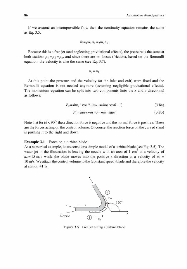
If we assume an incompressible flow then the continuity equation remains the sameas Eq. 3.5.

m= ρu1A1 = ρu2A2

Because this is a free jet (and neglecting gravitational effects), the pressure is the same atboth stations p1 = p2 = pa, and since there are no losses (friction), based on the Bernoulliequation, the velocity is also the same (see Eq. 3.7).

u2 = u1

At this point the pressure and the velocity (at the inlet and exit) were fixed and theBernoulli equation is not needed anymore (assuming negligible gravitational effects).The momentum equation can be split into two components (into the x and z directions)as follows:

Fx =mu2 cosθ−mu1 =mu cosθ−1 3 8a

Fz =mw2−m 0 =mu sinθ 3 8b

Note that for (θ < 90 ) the x direction force is negative and the normal force is positive. Theseare the forces acting on the control volume. Of course, the reaction force on the curved standis pushing it to the right and down.

Example 3.1 Force on a turbine bladeAs a numerical example, let us consider a simple model of a turbine blade (see Fig. 3.5). Thewater jet in the illustration is leaving the nozzle with an area of 1 cm2 at a velocity ofun = 15m s while the blade moves into the positive x direction at a velocity of ub =10m/s. We attach the control volume to the (constant speed) blade and therefore the velocityat station #1 is

Nozzlex

ub

z120°

2

1

Figure 3.5 Free jet hitting a turbine blade


u1 = 5m s = u2

which is the same as the velocity at station #2The forces can be found by using Eq. 3.8:

Fx = ρu2A cosθ−1 = 1000 52 0 0001 cos120−1 = −3 75N

Fz = ρu2Asinθ = 1000 52 0 0001 sin120 = 2 16N

Again the force into the x direction is negative, indicating the direction of the externalforce acting on the control volume. This means that the fluid (reaction) is pushing the tur-bine blade into the right and the z component of the reaction force is pushing the bladedown. The powerW generated by this turbine blade is simply the force times its translationvelocity ub.

W =Fxub = 37 5W

Example 3.2 Force on a wedgeA circular water jet of velocity u1= 15 m/s and diameter 0.1 m is impinging on a wedge, asshown in Fig. 3.6. The jet is split into two equal jets and it is required to calculate the force onthe wedge.

Controlvolume

u2

u2

0.1m 30°

x

zFx

1

u1

2

2

Figure 3.6 Free jet hitting a symmetric wedge


We start by defining the control volume as shown in the figure, assuming no changes inthe pressure (free jet). Also, as in Example 3.1, we assume that there are no losses and thevelocity at the exit remains the same (as in the previous example):

u1 = u2 = 15m s

Because the flow is incompressible, the total jet cross-section area is not changing(A1 = 2A2 =A). Now we can write the momentum equation 3.6 into the horizontal direction,assuming symmetry between the upper and lower exiting jets

Fx = 2 ρu2212A2 cosθ−ρu

21A1 = ρu

2A cosθ−1 = 1000 152π0 12

4cos60−1 = −883 6N

and due to symmetry the vertical force is zero!

Fz =12ρu2Asinθ−

12ρu2Asinθ = 0

Example 3.3 Thrust of a jet engineA jet engine flies at a speed ofU∞ as depicted in Fig. 3.7, and the surrounding pressure is pa.In order to calculate the thrust of the engine we need to use both the continuity and themomentum equations. Let us wrap the nacelle by a control volume and the air enters throughthe inlet section i and leaves at the exhaust section e. Based on Eq. 3.6, the thrust T is:

T =Fx = ρu2eAe−ρu

2i Ai + pe−pa Ae− pi−pa Ai 3 9

We can use the continuity equation, which states that the incoming and exitingmass flows are:

ma = ρiuiAi

me = ρeueAe

pa

U∞ ue

xmf.

z

a i e

Figure 3.7 Calculating the thrust of a jet engine


However, the fuel-flow mf must be taken into account:

me =ma +mf

Substituting these results into Eq. 3.9 yields:

T = ma +mf ue−maui + pe−pa Ae− pi−pa Ai 3 10

Usually the exhaust conditions and flight speed are known while the inlet conditions at sta-tion #i are not. To further simplify this relation (and eliminate the unknowns at the inlet) wecan introduce a new control volume in front of the nacelle, between a far field station a andthe inlet i. By applying the momentum equation to this control volume and noting that thereis no thrust generated by it, we get

0 =maui−maU∞ + pi−pa Ai− pa−pa Aa

and after rearranging:

maU∞ =maui + pi−pa Ai

Substituting this into Eq. 3.10 yields

T = ma +mf ue−maU∞ + pe−pa Ae 3 11

In modern engines the nozzle converts most of the pressure to exhaust velocity and the lastterm is small relative to the other two terms. Consequently, we can approximate the thrust as:

T = ma +mf ue−maU∞ 3 11a

Compare this to the rocket at the end of Section 2.6 and you’ll see that the rocket appears tohave a higher thrust because there is no incoming momentum.

3.4.2 Examples for Using the Bernoulli Equation

In these cases we must identify the two points for applying the Bernoulli equation and makesure that there are no losses as the fluid moves from one point to the other.

Example 3.4 The velocity of a jet leaving a large reservoirTo demonstrate the applicability of the Bernoulli equation let us analyze the flow leaving alarge reservoir as shown in Fig. 3.8. The exit section #2 is very small and the fluid loss due tothe flow through this exit has negligible effect on the height h of the liquid inside the res-ervoir. The control volume exit section is placed slightly outside the container and therefore


the outside pressure (in the free-jet) is the same as on the top (e.g., p1 = p2 = pa). Now weassume that there are no losses such as friction along the path s, and apply Eq. 3.7 at the topof the reservoir (station #1) and at the exit (station #2), but it is clear that there is no velocityat station #1

gh1 +paρ+02

2= gh2 +

paρ+u222

Note that here h is positive into the + z direction, as shown in Fig. 3.2. After rearranging theterms we get

g h1−h2 = gh=u222

and the velocity is exactly the same as calculated by assuming a free fall (recall we assumedno friction losses):

u2 = 2 gh 3 12

Example 3.5 The forces on a water hoseThis example is similar to the free-jet examples, but now we’ll try to use the Bernoulli equa-tion as well. Assume that the pressure inside the pipeline shown in Fig. 3.9 is p0 and it ismuch larger than the ambient pressure pa. Also the inflow u1, and cross-sectional area A1 areknown. It appears, though, that both the continuity and the Bernoulli equation control theexit velocity. Of course we all know that for a smooth jet we need to adjust the jet exit area.For example, if it is too small then the excess pressure will break the jet and then we cannotassume that there are no losses in this flow. So in our example (compared to Example 2.4) let

s

Streamline

pa

u2

h

1

2

Figure 3.8 Flow leaving a large reservoir


us first find the ideal exit velocity, by using the Bernoulli equation, assuming no losses throughthe nozzle for this incompressible flow. Also, the measured pressure inside the pipe is p0.

u222=u212+p0−pa

ρ3 13

From the continuity equation we can calculate the required exit area for this matched flow.

A2 =A1u1u2

3 14

If the exit area is different, then the pressure is not matched and friction losses may occur.However, the continuity equation will hold while the exit velocity calculated by the Ber-noulli equation (Eq. 3.13) will not.The force calculation now proceeds by using the momentum equation 3.6 (recall that the

exit area was selected such that p2 = pa) in both directions:

Fx = ρu22A2

Fz = −ρu21A1− p0−pa A1 3 15

So the external force on the control volume acts down and to the right. To a person holdingthe hose, the reaction force is felt pushing back (to the left) and up. If we want to rewrite thisin terms of the mass flow ratem and the incoming velocity u1 then with Eq. 3.13 (recall – nolosses) this becomes

Fx =m u21 +2 p0−pa

ρ

Fz = −mu1− p0−pa A1 3 16

Example 3.6 Velocity and pressure in a wind tunnel test sectionThis is a practical example because many wind tunnels measure test-section velocity with atube pointing into the flow (see Fig. 3.10). The static pressure is measured by holes in thefloor or ceiling (ahead of the model).

1

2

u2

u1

zx

Figure 3.9 Forces on a bent fire hose


As an example, assume that the desirable velocity in the test section is 150 km/h andthe pressure difference between the two tubes is measured with a water column in the con-necting pipes (this is called a manometer), as shown in Figure 3.10. So what is the corre-sponding water column height and what is the pressure difference acting on the testsection walls?First let us follow the logic of the Bernoulli equation. We can consider a point outside the

wind tunnel (far to the left) where the fluid particles are at rest and therefore their velocity iszero and the pressure there is the same as the ambient pa. Now take one particle, which entersthe tunnel but stops at the entrance to the measuring tube, so again its velocity there is zeroand the pressure there recovers to pa. We call this a stagnation point because the flow isstagnant (not moving) there. Also, there are no apparent losses in the process, so the stag-nation pressure recovers to the ambient pressure outside! Now let us observe a second fluidparticle, which was stagnant outside but doesn’t stops inside the test section and continues atan average velocity ofU.As a matter of fact, the whole flow is assumed to have this averagevelocity (because we assume one-dimensional flow) and therefore the pressure at themanometer tube entrance on the floor (called static pressure) is

p= pa−0 5ρU2

assuming air density at 1.2 kg/m3 we get

pa−p= 0 5 1 2 150 3 6 2 = 1041 67N m2

It is clear that the pressure at the forward facing tube entrance is larger and if measured by themanometer tube, filled with water (ρwater = 1000 kg/m3), the pressure difference is equal tothe hydrostatic pressure of the water column. This is an important conclusion, worth doc-umenting: the hydrostatic pressure in a stationary fluid varies linearly with the liquid columnheight (h in this case):

Δp = ρgh 3 17

paU

h

Wind tunnel

Water

Figure 3.10 Schematic description of an open circuit wind tunnel


where ρ is the fluid density and g is the gravitational acceleration. In this particular examplethe measuring fluid is water and therefore, the height of the water column h is calculatedfrom this relation as:

pa−p = ρwatergh

h=pa−p

ρwaterg=

1041 671000 9 8

= 0 106m

and the pressure in the test section is lower and the force on the wall is 1041.67 N/m2, push-ing the walls in.

3.4.3 Simple Models for Time-Dependent Changes in a Control Volume

Certain time-dependent problems can be approximated by using the one-dimensional flowmodel. As an example, the incompressible flow from a container due to gravity or the flowleaving a pressurized container are presented here.

Example 3.7 Flow (due to gravity) through a small hole in a containerFor the first case, consider a container with a (fixed) cross section A1, as shown in Fig. 3.11.The momentary height of the liquid is h and the outside pressure is pa. The flow exits the con-tainer at the bottom through a small pipe of cross section areaA2. It is clear that the exit velocitydepends on the liquid height h and therefore a solution for this variable versus time is sought.The exit velocity (at the bottom) can be calculated by using Eq. 3.12

u2 = 2 gh

and the mass flow rate leaving the container is

m= ρu2A2 = ρ 2 gh A2

h0

u2

A2

A1

pa

h

Figure 3.11 Time dependent flow due to gravity


Next, consider a control volume containing all the liquid inside the container. The conser-vation of mass principle requires that no mass is lost,

d

dtmtank =

d

dtρA1h = −ρA2 2 gh

This means that the mass reduction in the tank is equal to the fluid leaving at the bottom(hence the minus sign). This equation can be rearranged, with a separation of the variables,as follows:

dh

h= −

A2

A12 g dt

After integrating both sides of the equation we get

2 h = −A2

A12 g t +C

and C is the constant of integration. Solving for h we get:

h= C1−A2

A1

g

2t

2

and C1 is a modified constant of integration to be calculated by using the initial conditions.Assuming that at t = 0, h= h0 we get c1 = h0 and therefore the time dependent height of theliquid in the container is

h = h0−A2

A1

g

2t

2

3 18

the corresponding exit velocity at the bottom is:

u2 = 2 gh0−A2

A1g t 3 19

and the time to drain the container [e.g., t (h=0)] becomes

th = 0 =A1

A2

2h0g

3 20

Example 3.8 The velocity of a water balloonThis example is similar to the example in Fig. 3.8, but now a one-dimensional equation ofmotion (for the system) is added. Consider a popular children’s toy (Fig. 3.12) consisting of


a water-inflated balloon placed on a small rolling platform. The objective is to calculate themomentary velocity of the apparatus.This problem can be solved with a few simplifying assumptions. First, assume that the

exit velocity and internal pressure p0 do not change as the balloon deflates. Second, assumethat the nozzle losses are negligible and we can use the Bernoulli equation (Eq. 3.3) to cal-culate the water jet exit velocity ue:

ue =2 p0−pa

ρ≈const

with these assumptions, the equation of motion into the x direction becomes:

m tdu t

dt=mue =

−dm t

dtue

where u(t) is the apparatus velocity and the minus sign at the right-hand side is a result of themass m(t) shrinking with time. After separating the variables and neglecting friction forcesin the wheels we get

du t =−dm t

m tue

After integration we get

u t t10 = ue lnm t t1

0

Assuming initial conditions at t = 0,

u 0 = 0, and m 0 =m0

and replacing the variable t1 with t we get:

u t = ue lnm0

m t=

2 p0−paρ

lnm0

m t3 21

ue

pa

p0

m0u(t)

x

Figure 3.12 A water balloon placed on frictionless wheels


This result indicates that both acceleration and momentary speed will increase with time. Ifthe mass of the system, without the water is ms, then the final velocity uf becomes

uf =2 p0−pa

ρlnm0

mf3 22

Of course in most cases the pressure inside the balloon may change and then the equationsare more complex.As a numeric example consider a balloon filled with 1 kg water at a pressure of 0.5 105 N/m2.

The nozzle area is 0.5 cm2 and the mass of the whole system, without the water, is 0.5 kg.The solution starts with calculating the exit velocity as

ue =2 0 5 105

1000= 10

ms

At this point we can calculate the mass flow rate, but it is not needed to calculate the finalvelocity;

m = ρueAe = 1000 10 0 5 10−4 = 0 5 kg s

The time it takes to empty the “propellant” is:

t =m0−mf

m=

10 5

= 2 s

The final velocity of the system, based on Eq. 3.21 is

uf = 10 ln1 50 5

= 10 98ms

Note that the final velocity is higher than the exit velocity of the jet

3.5 Flow Measurements (Based on Bernoulli’s Equation)

These one-dimensional models (mainly based on Bernoulli’s equation) led to the develop-ments of several important flow measuring devices. The principle of their operation will bediscussed next:

3.5.1 The Pitot Tube

The principle introduced by Bernoulli’s equation allows us to measure speed at a point in theflow by simplymeasuring a pressure difference. The device utilizing this principle is called the


Pitot tube and was named after Henry Pitot (1695–1771), a French hydraulic engineer whoinvented this device to measure river flows. The basic apparatus is described schematicallyin Fig. 3.13 and consists of two concentric tubes. It is assumed that at the tip the velocity comesto a halt. Therefore, at its tip, the inner tubemeasures the total pressure, which increases as flowspeed increases (as at point c inFig. 3.2).Theholes surrounding theouter tubemeasure the staticpressure and this should be equal to the undisturbed pressure (at ∞ ), which is not affected bythe vehicle’s speed. So it is assumed that around the tube the velocity is U∞ and the differ-ence between the pressure in the two concentric tubes (the dynamic pressure) can be meas-ured and connected to a display that shows the speed of the fluid stream (see Eq. 3.4).Now if we attach the Pitot tube to the moving vehicle and make sure that it points straight

into the flow, then based on Eq. 3.4 we can measure the vehicle’s speed as

U∞ =2 ptot −p∞

ρ3 23

Pitot tubes are widely used on airplanes, ships, and in wind tunnels to measure the flowspeed. For best accuracy, the tube must be aligned with the flow and placed away from dis-turbances created by the moving vehicle. Therefore, Pitot tubes are frequently mounted onlong rods extending ahead of an airplane or any other test vehicle.

Example 3.9 Measuring air speed in a wind tunnelA Pitot tube was inserted into the flow in a wind tunnel and the pressure difference betweenthe tubes was measured by a water column of 20 cm H2O. If air density is about

ρa = 1 2kgm3

then calculate the air speed in the wind tunnel.

The solution is given by Eq. 3.23; however, the pressure difference is given as

Δp= ρwgh= 1000 9 8 0 2 = 1960Nm2

Total pressure port

U∞

Static pressure ports

Internal,total pressure tube

Static pressure tube

Figure 3.13 The Pitot tube


Substituting this into Eq. 3.22 gives us:

U∞ =2 19601 2

= 57 15ms= 205 75

kmhr

3.5.2 The Venturi Tube

Another device that can be used to measure fluid flow (or the average velocity) is the Venturitube (or meter), named after the Italian physicist G. B. Venturi (1746–1822), who was the firstto investigate its operating principles in 1791. The Venturi meter consists of a tube with a nar-rowed center section as shown in Fig. 3.14 and when in operation, the air flow (or water, or anyother fluid) moves faster through the narrow section, as expected. Usually, the Venturi meter isused to measure the flow inside a pipe while the Pitot tubes used mainly for external flows.To measure the pressure difference, a thinner U-tube is connected to the large and narrow

sections (as shown in the figure) and filled partially with (sometimes heavier) liquid. Thepressure difference between the wide and narrow sections of the Venturi causes the fluidto rise in the lower pressure side of the tube. The level of the fluid in the thin tube canbe directly related (and calibrated) to the velocity inside the Venturi. In general, the pressuredifference (and signal) created by a Venturi meter is smaller than the signal from a Pitot tube.This makes the Venturi meter less desirable for measuring external velocity (e.g., airspeeds),and in actual practice Venturi meters are used primarily to measure liquid flow rates in pipes.To demonstrate the principle of operation let us assume that the fluid inside the tube isincompressible and the relation between the two velocities and cross section areas (basedon the continuity equation) is

u2 = u1A1

A23 24

1 2

A1

u1u2

Δh

x

A2

Figure 3.14 Nomenclature for the Venturi Tube


Now we can apply the Bernoulli equation between these two points

p1−p2 = ρu222−u212

Next, we substitute u2 from (3.24) into the Bernoulli equation to get

p1−p2 = ρu212

A21

A22

−1

Solving for u1 we get

u1 =2 p1−p2

ρA21

A22

−1

3 25

Usually the flow rate is more important and therefore

m= ρu1A1 =2ρ p1−p21A22

−1A21

3 26

Note that when measuring the pressure difference with a liquid column, as shown inFig. 3.14, then

p1−p2 = ρmgΔh

and here the measuring fluid density ρm is used.In order to incorporate the losses in the pipeline due to the installation of this measuring

device, a discharge or loss coefficient CD is used. Consequently, the frictionless Venturiformula is modified by simply adding the discharge coefficient CD as follows:

m=CD2ρ p1−p21

A22

−1

A21

3 27

In reality the performance of the Venturi tube depends on the fluid properties and speed, andon the tube geometry. Typical experimental results for the discharge coefficient are given inFig. 3.15 for a range of diameter ratios. Note that as the contraction ratio D2/D1 decreases,losses in the tube increase!


The Venturi tube is very efficient and the losses are quite small, as seen in Fig. 3.15 wheretypical values for CD are between 0.97 and 0.99! Also note that the discharge coefficientvaries with the internal flow speed. However, instead of the speed u1, a nondimensional

numberρu1D1

μwas used. This number is called the Reynolds number and will be discussed

in the next chapter.

3.5.3 The Orifice

The orifice shown in Fig. 3.16 is a popular flow measuring device and its advantage is in itssimplicity. Basically, a simple flange is added to the pipeline with a narrower hole, as shownin the figure. Because of this narrower passage, the flow accelerates near the smaller holeand the pressure drops accordingly. Contrary to the smoother flow in a Venturi tube, theflow in the orifice is separated, causing more losses.

1.00

0.99

0.98 0.60.4

0.2

Venturi

D2

D1

CD 0.97

0.96

0.95

0.94104 105 106 107

= 0.8D2D1

ρu1D1μ

Figure 3.15 Experimental results for the discharge coefficient

1

u1 u2

Δh

2

Figure 3.16 The orifice


The flow rate in the orifice is measured using the same formula developed for the Ven-turi (Eq. 3.27) but the loss coefficient CD is much larger. The discharge coefficientdepends much more on the ratio between the two areas and typically varies between0.55 for smaller holes to 0.65 for the relatively larger openings. Experimental data show-ing the discharge coefficient versus the nondimensional flow speed are shown inFig. 3.17.

3.5.4 Nozzles and Injectors

The discussion in this section is aimed at flow measuring devices. Nozzles and injectors canalso be viewed as a flow control devices since they deliver a pre-measured flow rate. Fur-thermore, the flow rate of liquids through the narrow orifice (of area Ai) is controlled by thesame formulas used in this section. Three generic injector shapes are shown in Fig. 3.18,all having the same exit area, Ai. If the stagnation pressure inside the nozzle is p0, andthe pressure outside is pa, then the one-dimensional exit velocityU can be estimated by usingEq. 3.23

U =CD2 p0−pa

ρ3 28

and here CD is the discharge coefficient, as defined earlier. Typical values for the dischargecoefficient are also shown on Fig. 3.18.

0.64

0.63

0.62

0.5

D1 D2

0.4

0.2

Orifice

CD 0.61

0.6

0.59

0.58104 105 106 107

= 0.7D2D1

ρu1D1μ

Figure 3.17 Discharge coefficients for an orifice


Frequently the flow rate of the injector is sought and then by using the continuity equationwe get

m= ρUAi =CDAi 2ρ p0−pa 3 29

3.6 Summary and Conclusions

As a summary to the one-dimensional model, let us consider a case, similar to the coolingsystem in a car, where slight changes in the density are included. The system consists of aduct, a heat exchanger, and a fan, as shown in Fig. 3.19.For this example, assume that the cooling air at 20 C enters a duct with a cross-sectional

area of A1 = 0.5 m2 at an average speed of u1 = 5 m/s. After the heat exchanger, the exittemperature rises to 45 C and the exit area at section #2 is A2 = 0.35 m2. Assuming the pres-sure at both the inlet and at the exit is 1 atm, calculate the average exit velocity and the axialforce on the duct system.In this case we can use the continuity equation because we can calculate the density and

have the cross section area information. So first let us calculate the ideal gas constant, for air(M = 29):

R =R M= 8317 29 = 286 79,

and the density

ρ =p

RT=

1 013 105

286 79 293 16= 1 204

kgm3

CD = 0.65

CD = 0.80

CD = 0.85

Ai

p0

p0

p0

Figure 3.18 Simple injector/nozzle geometries (for liquids) and typical discharge coefficients


Next, the mass flow rate is

m= ρuA= 1 204 5 0 5 = 3 kg s

Based on ideal gas assumption, the density at the exit is

ρ2 = ρ1T1T2

= 1 204293 16318 16

= 1 109kgm3

Because the mass flow rate is the same we can write

m = ρ1u1A1 = ρ2u2A2

and

u2 =ρ1u1A1

ρ2A2=

31 109 0 35

= 7 729m s

The net external force on the duct, into the positive x direction, is

Fx =m u2−u1 = 3 7 729−5 = 8 18N

The more important engineering questions are about the power required to drive the fan andthe pressure drop across the heat exchanger. We can discuss those calculations in the laterchapters.

3.6.1 Concluding Remarks

In this chapter a simple one-dimensional model was introduced, which could be very usefulwhen the average velocity can be estimated. Because the integral form of both the continuityand the momentum equations are based on elementary considerations, their applicability iswider than that of the Bernoulli equation.

Q

Heatexchanger

12

T2 = 45°Cp2 = pau2 = ?A2 = 0.35 m2

T1 = 20°Cp1 = pa

u1 = 5

A1 = 0.5 m2

ms

Figure 3.19 Schematic description of a typical cooling system


The Bernoulli equation introduced the relation between velocity and pressure in a friction-less environment, and several flowmeasuring devices using this principle were introduced. Inviscous flow its use is restricted and examples of such flows are discussed in Chapter 9.Of course, one of the objectives of this chapter is to demonstrate the applicability of the

elementary equations (developed in Chapter 2) and to capture student interest with someuseful examples. Sometimes, however, the simplicity of this one-dimensional model createsthe impression that fluid mechanics is an easy subject (and some students stop paying atten-tion to the following chapters). Of course, this is great misconception.

Problems

3.1. Water flows through the circular nozzle shown in the figure at a rate of 0.3 m3/s (or300 kg/s). The diameter at section 1 is 0.3 m and at section 2 is 0.1 m. Using the simplestream tube model, calculate the velocities at station 1 and 2, and the force acting on theflange. Assume that the pressure at station #1 inside the nozzle is 720,000 N/m2 and useBernoulli’s equation to calculate the pressure at station #2.

1 2

D1

D2

Problem Figure 3.1

3.2. The rocket motor shown in the sketch is tested under static condition. Suppose the exitvelocity is 500 m/s, exit area A2 = 0.1 m2, and the density of the jet at the exit is ρ2 = 0.6kg/m3, then calculate the static thrust (e.g., Fx). Assume the exit pressure is p2 = 1.5 atmand the ambient pressure is pa = 1 atm.

Fx

paue

A2

2

Problem Figure 3.2

3.3. The rocket motor in Problem 3.2 is fired into space. Calculate it’s thrust. Is it differentfrom the value obtained during static test at sea level?


3.4. The container shown in the figure is filled with water. The water discharges through ahole of area A2 at the lower right.a. Develop an expression for the discharge velocity u2.b. At which rate does the water level drop at point 1?c. Develop an expression for the force required to hold the container in place.

F

A1

p1

p2A2

u2

h

1

2

Problem Figure 3.4

3.5. A jet-ski is propelled at a constant speed of 20 km/hr by a hydraulic jet. The diam-eter of the exit section of the cylindrical exhaust nozzle is 10cm and the jet speedrelative to the nozzle is 45km/hr. Calculate the water mass flow rate and the thrustof the jet.

3.6. The Pitot tube shown in the sketch is mounted in front of a moving vehicle. The pres-sure in the stagnation tube is higher than the one measured in the static pressure tube by10 cm of water. Calculate the speed of the vehicle in terms of km/h and mph. Assumethe air density is ρ = 1.2 kg/m3.

Stagnationpressure tap

Staticpressure tap

U

Problem Figure 3.6

3.7. A conical weight of 40 N is “floating” on the jet, as shown (ignore the wire which isthere to stabilize the weight). The jet leaving the orifice at the bottom has an upwardvelocity of 15 m/s and diameter of 3 cm. Note that the jet speed is reduced with height!Find the height h at which the weight will remain stationary.


Wire forstability

60°

h

du

Problem Figure 3.7

3.8. According to Bernoulli’s principle, the pressure ahead of an automobile radiatorwill increase with increasing U∞, thereby pushing the cooling air across the densefins. Assuming that the air ahead of the radiator (point A) stops completely,estimate the pressure rise for the speed of 60, 100, and 140 km/h (take air densityas 1.22 kg/m3).

U∞A

Problem Figure 3.8

3.9. A 70 km/h wind is blowing on a concave dish antenna, with a radius of R = 0.4 m.Estimate the pressure acting on the frontal surface and the resulting forces on the frontalsurface of the antenna (compare your results with the results of Example 6.9).

U∞R

Problem Figure 3.9


3.10. A stationary water jet impinges on a turning vane mounted on a container with fric-tionless wheels, as shown in the left-hand side of the figure. If the jet’s cross-sectionalarea is 5 cm2 and its horizontal velocity is 10 m/s, calculate the force Fx in the x direc-tion while the container is not moving. Calculate its initial acceleration if it contains 5lof water. How will the force change when the container is moving to the right at aspeed of 3 m/s (assume mass is the same)?

Stationarynozzle

U 30°

(b)(a)

Stationarynozzle

30°U

x

Problem Figure 3.10

3.11. A stationary water jet impinges on a turning vane mounted on a container with fric-tionless wheels (right-hand side of sketch in Problem 3.10). In this case, however,the vane is mounted forward and the returning jet hits the water in the container. If thejet’s cross-sectional area is 5 cm2 and its horizontal velocity is 10 m/s, calculate theforce Fx in the x direction while the container is not moving. Calculate its initial accel-eration if it contains 5 l of water. How will the force change when the container ismoving to the right at a speed of 3 m/s (assume mass is the same)?

3.12. An airplane is flying at a speed of 500 km/h. It uses a simple Pitot tube to measure itsvelocity. Calculate the pressure difference the probe will register where air density is1.1 kg/m2. Provide your answer in atm (atmospheres).

Total pressure port

Static pressure tubeInternal,

total pressure tube

Static pressure ports

U∞

Problem Figure 3.12

3.13. A strong wind is blowing at a velocity of U∞ past a probe pointing directly into thewind. The lower end of the tube is inserted into a small water tank and the inside waterlevel reaches Δh = 4 cm below the water level in the tank. Calculate the wind speed(assume air density is 1.22 kg/m3).


U∞

Δh

Problem Figure 3.13

3.14. A 6 cm diameter jet with a velocity of 20 m/s hits the turning vane, as shown in thesketch. Assuming the vane is moving away from the nozzle at a speed of 7 m/s, then(assuming no friction) calculate the horizontal and vertical forces on the vane.

u1 uvane = 7 m/s

45°x

Problem Figure 3.14

3.15. A simple model of a turbofan engine is shown and at the exit, two concentric jets canbe seen. Assume that at a flight speed of 300 m/s the total incoming air flow rate is 300kg/s. At the exit, however, the inner jet has an exit velocity of 1000 m/s and mass flowrate of 100 kg/s, while the outer flow speed is 600 m/s and mass flow rate of 200 kg/s(fuel mass is negligible). Calculate the thrust of this unit.

Bypass

300 m/s600 m/s

1000 m/sm1

m2

Problem Figure 3.15


3.16. A turbofan engine can be modeled by two concentric jets, the outer fan flow is leavingthe engine at a speed of 250m/s and at a flow rate of 80 kg/s. If the thrust of the engine is10,000 N, assuming a bypass ratio of 4 (the outer cold flow is 4 times larger than thehot core flow) calculate the exhaust speed of the core flow (inner flow) at a flightspeed of 200 m/s.

3.17. The turbofan engine is modeled by two concentric jets, as shown. The outer fan flow isleaving the engine at a speed of 260 m/s and the inner hot flow leaves at 800 m/s.Assuming a core mass flow rate of 20 kg/s and a bypass ratio of 4 (the outer cold flowis 4 times larger than the hot core flow) calculate the thrust of this engine at a flightspeed of 200 m/s.

3.18. Consider a water jet turned by a solid frictionless surface, as shown in Fig. 4.4.Calculate the forces acting on the structure when u1 = 10 m/s, the jet crosssection is 5 cm2, and the angle θ = 20 .

u2

u1

1

2

θ

z

x

Problem Figure 3.18

3.19. A water jet (as in the previous problem) is turned by a solid frictionless surface and adownward force of 20 N is measured. The incoming jet velocity is u1 = 15 m/s and itscross section is 5 cm2.a. Calculate the turning angle θ.b. Calculate the horizontal force on the solid surface.

3.20. An airplane flies at a speed ofU∞ = 250 m/s and the air mass flow rate into the engineis m = 50 kg s and the exhaust speed is ue = 800 m/s.a. If the air to fuel ratio is about 2%, calculate the engine thrust (assume pe = pa).b. Suppose the airplane lift to drag ratio is 10 and it has two engines. Calculate the

airplane weight.

u∞ ue

pema

mf

Problem Figure 3.20


3.21. Julia emptied a bucket of water on Romeo from her window, which is 5 m above hishead. Assume the jet diameter is 5 cm at section 2 (just above Romeo’s head).a. Calculate the jet velocity (at point 2) as it hits Romeo’s head.b. What is the force acting on Romeo’s head if the water is splashed sideways (no

vertical speed)?

1

2

5 m

A2 = 0.05 m

Problem Figure 3.21

3.22. A jet of fluid hits a flat plate and leaves without any horizontal velocity component, asshown in the sketch.a. If the flow rate is 50 m/s and the velocity of the jet hitting the plate is 20 m/s, cal-

culate the force on the plate.b. Calculate the force in case the plate moves away from the jet at a speed of 50 km/h.

Jet

20 m/s

Plate

Problem Figure 3.22


3.23. A small boat is propelled by a water jet and is travels at a speed of 5 m/s. The forcerequired to propel the boat is 100 N and the water flow rate is 5 kg/s.a. Calculate the jet exit velocity (assume exit pressure = ambient pressure).b. Would it matter if the exiting jet is submerged (still assume the exit pressure =

ambient pressure)?

Pump Jet

Problem Figure 3.23

3.24. A water jet hits horizontally a 50 kg block. The friction coefficient between the blockand the ground is 0.9. What is the minimum diameter d of the water jet in order for theblock to slide to the left? Assume the stagnation pressure in the nozzle is p0 = 4 atmand outside the nozzle pa = 1 atm (also 1 atm = 1.013 105 N/m2).

Jet

50 kg

d

pa p0

Frictionlessnozzle

Friction coeff = 0.9 m

Problem Figure 3.24

3.25. A segment of an air conditioning duct is shown in the figure where the axial velocity atsection #1 is 2 m/s and the pressure is 1 atm (same as outside). Assuming air density is1.2 kg/m3, b1 = 0.4 m and b2 = 0.3 m, calculate the net force and its direction on thisduct segment (assume flow is incompressible).

z

b2

x

21

b1

Problem Figure 3.25


3.26. The neighbor kid decided to water the garden while standing on his skateboard. As heopened the valve, the jet speed was 7 m/s and its diameter was d2 = 0.02 m. If his massis 40 kg, then calculate the force of the jet and his initial acceleration (assuming nofriction).

0.02 m

ms7

Problem Figure 3.26

3.27. Wine is poured from a barrel into a 5 l bottle, as shown. At a certain point, the fluidvelocity is 1 m/s, and the cross section area is 1 cm2 (the wine density is 980 kg/m3).a. How long it takes to fill the 5 l bottle?b. If the vertical distance between the exit from the tap to the surface of the wine in

the bottle is 60 cm, calculate the force on the bottle.

u1 A1

Problem Figure 3.27

3.28. A free stream of U = 50 m/s is blowing on a 0.6 m diameter cylinder, as shown in thesketch. A simple approximation of the flow behind it indicates that the velocity wasreduced to 30 m/s for a strip of 0.6 m (e.g., same as the cylinder’s diameter). Suppose

we define a force coefficient as CF =F

0 5ρU2Dwhere F is the force per unit width on

the cylinder, then calculate the value of CF (you may use Table 1.1 for the air density).


0.6 m

50 –50

30ms

ms

ms

Problem Figure 3.28

3.29. The orifice shown in the sketch is used to measure the water flow in the pipe. Thepressure difference across the orifice registers as a column of 10 cm water. Assumingwater density at ρ = 1000 kg/m3, R1 = 20 cm, and R2 = 10 cm, and the discharge coef-ficient is CD = 0.6, calculate the mass flow rate in the pipe.

2 R1

1 2

2 R2

u1 u2

Δh

Problem Figure 3.29

3.30. The orifice from Problem 3.29 is used to measure the water flow in the pipe. Assum-ing water density at ρ = 1000 kg/m3, R1 = 20 cm and R2 = 10 cm, and the dischargecoefficient is CD = 0.6, calculate the average speed in the pipe when the mass flowrate is 100 kg/s. What is the pressure difference (in terms of cm water) for thisflow rate?

3.31. The flow rate across the orifice in Problem 3.29 is 100 l/s (1 liter water = 1 kg).Calculate the water column height registered in the U-tube manometer.


A1

1 2

x

u2u1

A2

Δh

Problem Figure 3.31

3.32. A Venturi meter is used to measure the water flow in a 3 cm diameter pipe. Thediameter of the narrow section is 1.5 cm. The pressure difference between thelarge and small diameter pipes registers as a column of 5 cm water. Assuminga discharge coefficient of CD = 0.95, calculate the mass flow rate in the pipe(ρ = 1000 kg/m3).

3.33. The Venturi tube shown in the sketch is used to measure water flow in a pipe. Theincoming pipe diameter is D1 = 20 cm and the throat diameter is D2 = 10 cm. Assum-ing a discharge coefficient ofCD = 1.0, u1 = 0.5 m/s, and the density of water, ρ = 1000kg/m3 calculate:a. The water flow rate.b. The pressure difference measured as Δh, m (water column).

3.34. Air is drawn into a long tube, as shown in the sketch. The air velocity inside the tubeis 50 m/s and the pressure outside, in the still air, is 1 atm. Assuming air density is1.22 kg/m3 and constant, calculate the pressure inside the tube.

p∞=1 atm

p= ?

50msρ∞=1.22

kg

m3

Problem Figure 3.34

3.35. Air is drawn into a wind tunnel during automobile testing, as shown in the sketch.A simple manometer measures the velocity in terms of water column height h. Ifthe velocity at the test section is 120 km/h, then calculate the height of the water col-umn in cm (ρwater = 1000 kg/m3, ρair = 1.22 kg/m3).


pa

pa

U

h

Wind tunnel

Water

Problem Figure 3.35

3.36. We repeat the previous experiment, but now we use a tube to measure the total pres-sure as shown. If the water column height in the manometer h = 8 cm, calculate thevelocity at the test section (ρwater = 1000 kg/m3, ρair = 1.22 kg/m3).

paU

h

Wind tunnel

Water

Problem Figure 3.36

3.37. Air flows at a rate of 1.7 kg/s through a smooth contraction in a pipe with negligiblefriction losses. The pressure difference between the two sections is measured by awater manometer. If the pipe diameters are D1 = 0.3 m and D2 = 0.15 m, calculatethe height difference, Δh, measured between the two vertical tubes (assume air den-sity is 1.22 kg/m3).

D1 D2U

Δh

Problem Figure 3.37


3.38. Air flows through a smooth contraction in a pipe with negligible friction losses(the pipe diameters are D1 = 0.3 m and D2 = 0.15 m, respectively). The pressuredifference between the two sections is measured by a water manometer. If the heightdifference Δh measured between the two vertical tubes is 0.2 m calculate the massflow rate (assume air density is 1.22 kg/m3).

D1 D2U

Δh

Problem Figure 3.38

3.39. Air flows through a smooth contraction in a pipe with negligible friction losses (thepipe diameters areD1 = 0.3 m andD2 = 0.15 m, respectively). The pressure differencebetween the two sections is measured by a water manometer. If the height differenceΔh measured between the two vertical tubes is 0.15 m, calculate the mass flow rate(assume air density is 1.22 kg/m3).

D1 D2U

Δh

Problem Figure 3.39

3.40. Air flows at a rate of 3 kg/s through a smooth contraction in a pipe with negligiblefriction losses (the pipe diameters are D1 = 0.4 m and D2 = 0.2 m, respectively).The pressure difference between the two sections is measured by two tubes connectedto a water manometer. Calculate the height Δh measured between the two verticaltubes (assume air density is 1.22 kg/m3).

3.41. Air flows through a smooth contraction in a pipe with negligible friction losses andthe pressure difference between the two vertical tubes in Problem 3.40 is measured atΔh = 0.3 m. If the pipe diameters are D1 = 0.3 m and D2 = 0.2 m, respectively,calculate the flow rate (assume air density is 1.22 kg/m3).


3.42. Cooling air flows at a rate of 2 kg/s through a smooth contraction in a circular duct (asin the Problem 3.41) with negligible friction losses (the inflow pipe diameter is D1 =0.5 m). The pressure difference between the two sections is measured by two tubesconnected to a water manometer. If the water column height Δh is 0.08 m, then cal-culate the diameter D2 of the smaller pipe (assume air density is 1.22 kg/m3 and waterdensity is 1000 kg/m3).

3.43. A small jet with a cross sectional area of 5 cm2 is flowing out at the bottom of a largecontainer, and aims at 30 upward. At a horizontal distance of 0.5 m, the jet impingeson a vertical plate. Calculate the horizontal force required to hold the plate in place, ifthe water level in the container is h = 5 m. Also, estimate the height from the bottomwhere the jet hits the plate.

hFx

0.5 m

30°

Problem Figure 3.43

3.44. Water is flowing through two holes from a container with frictionless wheels. The lefthole is located at a height of h1 = 0.3 m and its area is 3 cm2, while the right hole area is1 cm2. If the water level in the container is h2 = 0.7 m, calculate the resultant force andits direction on the container.

h1

h2

A2A1

Problem Figure 3.44


3.45. A ball weighting 1 kg is “floating” on a circular jet, as shown (ignore the wire, which isthere to stabilize the weight). The jet leaving the orifice at the bottom has an upwardvelocity of 10 m/s and the jet diameter at the exit is 2 cm. Assuming the jet spills side-ways at 90 , find the height h at which the ball will float.

ms

1

2

h

z

Jet

D1 = 0.02 m

w1 = 10

Problem Figure 3.45

3.46. A jet flowing from the bottom of a water tank is aimed upward at 30 , as shown.Assuming no friction losses at the nozzle, calculate the maximum height and distanceof the jet (again, neglecting friction with the outside air).

h = 10 m

Water

30°H

x

Problem Figure 3.46


3.47. A rectangular container is filled with water, as shown. At a time t = 0, a small openingwith an area Ae is opened at the bottom. Develop the formulation for the exit velocityue and the water column height h, as a function of time.

a

h

ue Ae

Problem Figure 3.47

3.48. If the width of the container in the previous problem is a = 20 cm, h = 80 cm, andthe opening area Ae is 3 cm2, then calculate how long it will take to empty thecontainer.

3.49. A 1 m diameter spherical tank is half full with water. A circular drain of 1 cm diameteropened at the bottom, as shown in the sketch. How long does it take to empty the tank?Note that the radius r of the liquid surface area inside the tank can be expressed

as πr2 = π R2− R−h 2 .

R

h

1 cm

Problem Figure 3.49

3.50. A cylindrical container with a diameter of D = 0.3 m is filled with water to a level ofh0 = 0.5 m. Suddenly, the drain plug with an area of 3 cm2 is opened allowing the


water to flow out. Calculate the horizontal force versus time until the tank is com-pletely drained. Also, develop a formula for the water height versus time. How longit will take to drain the container?

D

h0

Ae

Problem Figure 3.50

3.51. A cylindrical container with a diameter of D1 is filled with water to a level of h1.A drain plug with a diameter of D2, located at a height of h2 above the ground isopened allowing the water to flow out. Develop an expression for the distance x ver-sus time.

D2

D1

h1

h2

x

Problem Figure 3.51

3.52. The balloon shown in Fig. 3.12 is filled with 2 kg water at a pressure of 0.8 105 N/m2

and the mass of the whole system, without the water, is 0.5 kg. Assuming constantdischarge velocity (without friction losses), calculate the maximum velocity of thedevice. Can it move faster than the exit jet velocity?


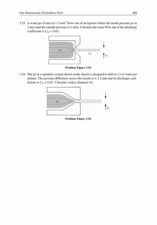
3.53. A water jet of area Ai = 5 mm2 flows out of an injector where the inside pressure po is2 atm (and the outside pressure is 1 atm). Calculate the water flow rate if the dischargecoefficient is CD = 0.65.

p0

Ai

pa

Problem Figure 3.53

3.54. The jet in a sprinkler system shown in the sketch is designed to deliver 2 l of water perminute. The pressure difference across the nozzle is is 1.5 atm and its discharge coef-ficient is CD = 0.85. Calculate orifice diameter Di.

p0

Di

Problem Figure 3.54


4Dimensional Analysis, HighReynolds Number Flows, andDefinition of Aerodynamics

4.1 Introduction

Aerodynamics, as a science, gained momentum at the beginning of the twentieth century,when simple models were introduced to solve practical problems such as the flow overstreamlined shapes. Typical engineering objectives include the determination of the aero-dynamic loads, the pressure distribution, or even the shear stress distribution. The early, sim-ple potential flow based models that were used generated amazingly accurate results for theattached flow cases. Therefore, in addition to defining the field of aerodynamics, a second-ary objective is to explain why those methods worked.We have seen that for the case of the two-dimensional vortex (Section 2.10) certain terms

of the fluid dynamic equations were neglected, yet the simplified solution retained thedominant physical elements. One of the objectives of this chapter is to demonstrate thatneglecting certain terms in the governing equations can be done systematically. The useof dimensional analysis allows a logical approach to simplifying the governing equationsand provides relative scaling for the various terms. A secondary objective of this chapteris to introduce a flow regime called high-Reynolds number flow and to explain the successof incompressible flow models. In spite of the complex equations, a reasonable solution forthe flow over bodies (and the resulting forces such as lift and drag) can be obtained and theirphysical origins explained. This approach of treating high-Reynolds number flows providesthe basis for modern Aerodynamics and Hydrodynamics, and allows a more detailed sub-division and definition of the term Aerodynamics.As noted, the process of simplifying the fluid dynamic equations (and neglecting certain

terms) is not arbitrary. In fact it is based on rigorous assumptions. To demonstrate this proc-ess, let us apply dimensional analysis to the fluid mechanics equations.


4.2 Dimensional Analysis of the Fluid Dynamic Equations

The governing equations that were developed in Chapter 2 are very complex and as men-tioned, their solution, even by numerical methods, is difficult for many practical applica-tions. If some of the more complex terms can be neglected in certain regions of the flowfield, and at the same time the dominant physical features will be retained, then a set ofsimplified equations will result (and probably solved with less effort). This rationale forsimplifying the governing equations is based on comparing the magnitude of the variousterms in these equations. In order to determine the relative magnitude of the various com-ponents, the following dimensional analysis is performed. For simplicity, consider the fluiddynamic equations with constant properties (μ = const and ρ = const). The continuity equa-tion for this case (Eq. 2.33) in vector form is:

∇ q = 0 4 1

and the momentum equation (Eq. 2.40) is:

ρ∂q

∂t+ q ∇q = ρf −∇p + μ∇2q 4 2

The first step is to define some characteristic or reference quantities, relevant to the physicalproblem to be studied:

L – reference length (e.g., length of a car)V – reference speed (e.g., the free stream speed)T – characteristic time (e.g., one cycle of a periodic process, or simply L/V)po – reference pressure (e.g., the free stream pressure, p∞)fo – body force (e.g., magnitude of earth’s gravitation, g)

With the aid of these characteristic quantities we can define the following nondimensionalvariables:

x∗ =x

L, y∗ =

y

L, z∗ =

z

L

u∗ =u

V, v∗ =

v

V, w∗ =

w

V

t∗ =t

Tp∗ =

p

p0f ∗ =

f

fo4 3

Usually it is advised to take larger constant, such as the length of a car, or the free streamspeed. If the magnitudes of these characteristic quantities are properly selected, then all thenondimensional variables in Eq. (4.3) will be of the order of one, O(1). Next, the governing

123Dimensional Analysis, High Reynolds Number Flows

equations need to be rewritten using the quantities of Eq. 4.3. As an example, the first term ofthe continuity equation becomes

∂u

∂x=

∂u

∂u∗∂u∗

∂x∗∂x∗

∂x=V

L

∂u∗

∂x∗

and applying this methods to all three terms in the incompressible continuity equation yields

V

L

∂u∗

∂x∗+∂v∗

∂y∗+∂w∗

∂z∗= 0 4 4

and it appears that all terms have the same magnitude (none of the terms can be neglected).As an example for the momentum equation, only the equation into the x direction is shown.By applying the chain derivatives to the various terms it appears that the multiplier can read-ily be written, based on the method used for the continuity equation. For example the first(unsteady term) becomes

∂u

∂t=

∂u

∂u∗∂u∗

∂t∗∂t∗

∂t=V

T

∂u∗

∂t∗

and the momentum equation into the x direction is

ρV

T

∂u∗

∂t∗+V

V

Lu∗

∂u∗

∂x∗+V

V

Lv∗∂u∗

∂y∗+V

V

Lw∗ ∂u

∗

∂z∗= ρfof

∗x −

poL

∂p∗

∂x∗+ μ

V

L2∂2u∗

∂x∗2+∂2u∗

∂y∗2+∂2u∗

∂z∗2

4 5

The corresponding equations in the y and z directions can be obtained by the same proce-

dure, and they will have the same multipliers. Now, by multiplying Eq. 4.4 by L

Vand Eq. 4.5

by L

ρV2we end up with the nondimensional continuity and momentum equations:

∂u∗

∂x∗+∂v∗

∂y∗+∂w∗

∂z∗= 0 4 6

L

TV

∂u∗

∂t∗+ u∗

∂u∗

∂x∗+ v∗

∂u∗

∂y∗+w∗ ∂u

∗

∂z∗=

LfoV2

f ∗x −poρV2

∂p∗

∂x∗+

μ

ρVL

∂2u∗

∂x∗2+∂2u∗

∂y∗2+∂2u∗

∂z∗2

4 7

If all the nondimensional variables in Eq. 4.3 are order of one, then all terms appearing withan asterisk ∗ will also be of order one, and the relative magnitude of each group in theequations is determined by the nondimensional group of variables appearing inside the


parentheses. In the continuity equation (Eq. 4.6), all terms have the same order of magnitudeand for an arbitrary three-dimensional flow all terms are equally important (so we cannotneglect any term). In the momentum equation, however, several nondimensional numbersmultiply the various terms. The magnitude of that term is therefore determined by the multi-pliers inside the parentheses. The first nondimensional number is

Ω=L

TV4 8

Ω is often called a time constant and it signifies the importance of time dependent phenom-ena. A more frequently used form of this nondimensional number is the Strouhal numberwhere the characteristic time is the inverse of the frequency ω of a periodic occurrence(e.g., wake shedding frequency behind a separated plate)

St =L

1 ω V=ωL

V4 9

If the Strouhal number is very small, perhaps due to very low frequencies, then the time-dependent first term in Eq. 4.7 can be neglected compared to the other terms of order of 1.The second group of nondimensional numbers (when gravity is the body force and f0 is thegravitational acceleration (g) is called the Froude number, and stands for the ratio of inertialforce to gravitational force:

F =V

Lg4 10

Small values of F (note that F−2 appears in Eq. 4.7) will mean that body forces such as grav-ity should be included in the equations, as in the case of free surface river flows, waterfalls,ship hydrodynamics, and so on. The third nondimensional number is the Euler number,which represents the ratio between the pressure and the inertia forces:

Eu=poρV2

4 11

A frequently used quantity, which is related to the Euler number, is the pressure coefficientCp that measures the nondimensional pressure difference, relative to a reference pressure po:

Cp ≡p−po12 ρV

24 12

The last nondimensional group in Eq. 4.7 represents the ratio between the inertial and vis-cous forces and is called the Reynolds number, which was introduced in the discussionabout the Venturi tube in Chapter 3.


Re =ρVL

μ=VL

ν4 13

Here, ν is the kinematic viscosity, which is often used for sake of brevity.

ν=μ

ρ4 14

For the flow of gases, from the kinetic theory point of view (see Ref. 4.1, p. 257) the vis-cosity can be connected to the average velocity of the molecules c and to the mean distance λthat they travel between collisions (mean free path), by

μ≈ρcλ

2

Substituting this into Eq. 4.13 yields:

Re≈2V

c

L

λ

This formulation shows that the Reynolds number represents the scaling of the velocitytimes length, compared to the molecular scale. Note that c is larger than the speed of sound(see Eq. 1.32). The conditions for neglecting the viscous terms when Re>> 1 will be dis-cussed with more details in the next section. For simplicity, at the beginning of this analysisan incompressible fluid was assumed. However, if compressibility is to be considered, anadditional nondimensional number appears, which is called the Mach number and is theratio of the velocity to the speed of sound a (see Eq. 1.32 for evaluating the speed of soundfor an ideal gas):

M =V

a4 15

Usually when the characteristic velocity V is much less than the speed of sound then the flowcan be considered as incompressible (e.g., a car traveling at 150 km/h).

4.3 The Process of Simplifying the Governing Equations

The most important outcome of this dimensional analysis of the governing equations is thatnow the relative magnitude of the terms appearing in the equations can be determined andcompared. If desired, small terms can be neglected, resulting in simplified equations that areeasier to solve but still contain the dominant physical effects. In the case of the continuityequation all terms have the same magnitude and none can be neglected. For the momentum


equation the relative magnitude of the terms can be obtained by substituting the nondimen-sional numbers into Eq. 4.7, and for the x direction we get

Ω∂u∗

∂t∗+ u∗

∂u∗

∂x∗+ v∗

∂u∗

∂y∗+w∗ ∂u

∗

∂z∗=

1F2

f ∗x −Eu∂p∗

∂x∗+

1Re

∂2u∗

∂x∗2+∂2u∗

∂y∗2+∂2u∗

∂z∗24 16

The first term on the left-hand side is multiplied by the time constant, while rest of the termsare of order O(1). In case where time dependent changes are small (or the time scale is verylarge) then Ω is also small. Consequently, for Ω<< 1 the first term can be neglected and wecan solve just the steady-state problem. Similarly if the Froude number F is large, then bodyforces have negligible effects and the body force term can be neglected. The Euler numberEu is usually not negligible since the pressure is responsible for the changes in the inertia ofthe moving fluid. This leaves us with the last nondimensional group, the Reynolds number.Note that it multiplies a second order differential term and if neglected only a first-orderdifferential equation remains.There are many specific situations in fluid mechanics where simpler forms of the equa-

tions can be used. As an example, consider a situation when the viscosity is very high and theReynolds number is on the order of O(1). This flow regime is called “creeping flow” wheredue to high viscosity the fluid motion is slow, and the inertia terms are negligible. It is usu-ally assumed that for Re < 1 the viscous terms are large and cannot be neglected. With theseconsiderations in mind the momentum equation, Eq. 4.2 is reduced to

0 = −∇p+ μ∇2q 4 17

The general solution of this equation is beyond the scope of the present text but for example,the viscous flow in pipes is very similar and will be discussed in Chapter 9.

4.4 Similarity of Flows

Another interesting aspect of the process of nondimensionalizing the equations in the pre-vious section is that two different flows are considered to be similar if the nondimensionalnumbers of Eq. 4.16 are the same. For most practical cases, where gravity and unsteadyeffects are negligible, only the Reynolds and the Mach numbers need to be matched. Forexample, many airplanes are tested in small scale (e.g., 1/5 scale). In order to keep theReynolds number the same then either the airspeed or the air density must be increased(e.g., by a factor of 5). This is a typical conflict that test engineers face, since increasingthe airspeed five times will bring the Mach number to an unreasonably high range. The sec-ond alternative of reducing the kinematic viscosity ν by compressing the air is only possiblein a very few wind tunnels and, in most cases, matching both of these nondimensional num-bers is difficult. Another possibility of applying the similarity principle is to exchange fluidsbetween the actual and the test conditions (e.g., water with air where the ratio of kinematic


viscosity is about 1:15). Thus a 1/15th-scale model of a submarine can be tested in a windtunnel at true speed conditions. Usually, it is better to increase the speed in the wind-tunneland then even a smaller scale model can be tested (of course the Mach number is not alwaysmatched but for such low Mach number applications this is less critical).

Example 4.1 Wind Tunnel versus Water TunnelLet us examine the possibility of changing the fluid (water or air) when testing a car or asubmarine model. The main considerations here are model size and available tunnel speeds.As stated the kinematic viscosity ratio between air and water is

ρaμwρwμa

=1 21000

10−3

1 8 10−5 =115

So, if the Reynolds number is to be kept constant between the air and water experiments:

ρUL

μ a

=ρUL

μ w

Consequently, the relation between the speed and model size becomes:

UaLaUwLw

= 15

Now let us examine the case of a 40 m long submarine cruising at 6 m/s. Because largesubsonic wind tunnels are available, testing in full scale is possible. The desirable windspeed is then

Ua = 15LwLa

Ua = 90m s 324 km hr

This is a very high speed and above the range of the major subsonic wind tunnels. The onlyoption then is to reduce test speed a bit.Now let us examine the reverse alternative, a 4 m long automobile that is expected to

cruise at 100 km/h (27.77 m/s). Testing a quarter-scale model in a water tank will requirea test speed of:

Uw =LaLw

Ua

15=4 27 771 15

= 7 4m s

This is quite high speed for a tow tank so again the speed could be reduced a bit.

This short example demonstrates the principle of using similarity, but also highlights theimpracticality involved!


4.5 High Reynolds Number Flow and Aerodynamics

One of the most important conclusions from Eq. 4.16 is that the second-order differentialterm (the viscous term) becomes small for high Reynolds number flows! Consequentlyinviscid flow models can be used, which explains the success of such models, proposedin the early twentieth century. These models are significantly simpler and in several impor-tant cases closed form solutions can be obtained.The first objective of this discussion, therefore, is to demonstrate why incompressible

inviscid models are successfully used to predict the lift of airplanes or the pressure fieldaround road vehicles. The second objective is to better define the field of Aerodynamics,which involves the flow of air. Air, however, is a gas, which appears to be compressible(while we are trying to show that it is not). Consequently, the goal here is to arrive at equa-tions that are both inviscid and incompressible! But the effects of compressibility are relatedto the air being compressed due to the motion of an object through it (like a car). So, in orderto evaluate the importance of compressibility in air we must return to the definition of theMach number, as in Eq. 4.15, and recall that the speed of sound for air at 300 K was cal-culated in Example 1.5 to be 346.9 m/s. This is equivalent to 1248.8 km/h, which is a veryhigh speed that only a few airplanes can reach. For example, if an airplane flies at the speedof sound then the maximum compression at its stagnation point is about 1.9 (seeAppendix B in Ref. 4.2) andmuch less at other areas. Consequently, based on the free streamMach number, the importance of compressible effects is subdivided into several flowregimes (see for example Ref. 4.3, pp. 7–12):

1. Subsonic 0 0 <M<0 5The flow is considered to be incompressible and the term “Low Speed Aerodynamics” isoften used. Automotive Aerodynamics falls within this region!

2. Subsonic (with mild corrections) 0 5 <M<0 8The flow is still subsonic but when the local Mach number on the vehicle (or airplane)rises towards the M = 0.8, mild compressibility corrections are required.

3. Transonic 0 8 <M<1 2If the local speed in the fluid exceeds the speed of sound then the flow becomes super-sonic. For example, an airplane can fly at M = 0.85, but the flow over the wing can accel-erate beyond M = 1. Because the local Mach number in transonic flow can be above one,shock waves may be present.

4. Supersonic 1 2 <M<3 0When the flow is significantly faster, then this flow-regime is called supersonic and somevery fast airplanes do operate within this flow regime.

5. High Supersonic 3 0 <M<5 0For much faster flows serious temperature increase may take place and this flow regimeis called high supersonic. Temperature at stagnation points may rise above the meltingpoint of certain metals, and near M = 5.0 air temperature can heat to combustion tem-peratures. Therefore, both materials and propulsion system face serious challenges in thisrange.


6. Hypersonic 5 0 <MSome researches define the start of this region as low asM= 3.0, but most of them place itabove M = 5.0. Space vehicles reentering the atmosphere may fly in this region, butbecause of the high stagnation temperatures flight duration is limited.

After this short discussion about compressibility effects, we are able to identify the rangeof automotive aerodynamics that falls at the low Mach number end of the low speed aero-dynamics regime. Before we proceed further, let us reassure the high Reynolds numberassumption for a typical automobile.

Example 4.2 The Reynolds number of an automobileLet us assume that the length of the vehicle is 4.0 m and it travels at 100 km/h. The air den-sity and viscosity are taken from Table 1.1

Re =ρUL

μ=1 22 100 3 6 4 0

1 8 10−5 = 7 5 106

This is clearly a very high number and justifies the assumption of high Reynolds number.The same argument can be applied to the rear view mirror that has a length of about 15 cm.The mirror’s local Reynolds number is

Re =ρUL

μ=1 22 100 3 6 0 15

1 8 10−5 = 0 28 106

which is still a very large number.Checking the Mach number for this case (using the speed of sound of 346.9 m/s, from

Example 1.5):

M =100 3 6346 9

= 0 08

and this is a small number – proving the assumption that air can be considered incompress-ible for Automobile Aerodynamics.

Before proceeding further let us examine the range of Reynolds number and Mach num-bers for some typical engineering problems. Since the viscosity of typical fluids such as airand water is very small, a large variety of practical engineering problems (automobile andaircraft aerodynamics, hydrodynamics of naval vessels, etc.) fall within the large Reynoldsnumber range, as shown in Fig. 4.1.Based on the large variety of cases shown in Fig. 4.1, we can conclude that for high

Reynolds number flows, the viscous terms become small compared to the other terms oforder O(1) in Eq. (4.16). But before neglecting these terms, a closer look at the high Reynoldsnumber flow condition is needed. As an example, consider the flow near a streamlined body,as shown in Fig. 4.2. In general, based on the assumption of a high Reynolds number,


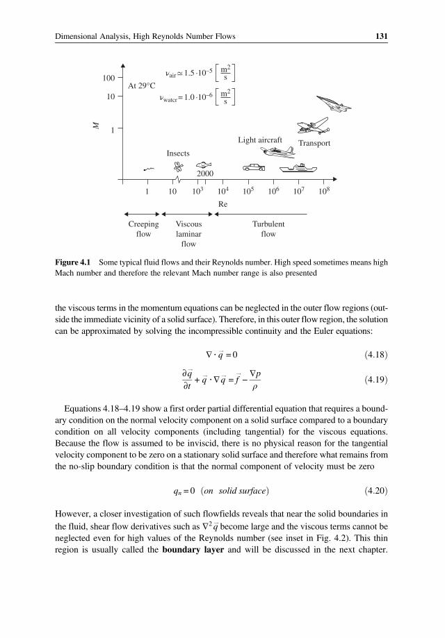
the viscous terms in the momentum equations can be neglected in the outer flow regions (out-side the immediate vicinity of a solid surface). Therefore, in this outer flow region, the solutioncan be approximated by solving the incompressible continuity and the Euler equations:

∇ q = 0 4 18

∂q

∂t+ q ∇q = f −

∇pρ

4 19

Equations 4.18–4.19 show a first order partial differential equation that requires a bound-ary condition on the normal velocity component on a solid surface compared to a boundarycondition on all velocity components (including tangential) for the viscous equations.Because the flow is assumed to be inviscid, there is no physical reason for the tangentialvelocity component to be zero on a stationary solid surface and therefore what remains fromthe no-slip boundary condition is that the normal component of velocity must be zero

qn = 0 on solid surface 4 20

However, a closer investigation of such flowfields reveals that near the solid boundaries inthe fluid, shear flow derivatives such as ∇2q become large and the viscous terms cannot beneglected even for high values of the Reynolds number (see inset in Fig. 4.2). This thinregion is usually called the boundary layer and will be discussed in the next chapter.

At 29°C100

10

1M

1 10 103

Insects

2000

Light aircraft Transport

Creepingflow

Viscouslaminar

flow

Turbulentflow

104

Re

105 106 107 108

νair≃ 1.5 ·10–5 m2

s

νwatcr = 1.0 ·10–6 m2

s

Figure 4.1 Some typical fluid flows and their Reynolds number. High speed sometimes means highMach number and therefore the relevant Mach number range is also presented


So, in conclusion, for high Reynolds number flows we can identify two dominant regions inthe flowfield:

1. The outer flow (away from the solid boundaries) where the viscous effects are negligible.A solution for the inviscid flow in this region provides information about the pressuredistribution and the related forces. Only the zero normal velocity boundary conditionis used (e.g., Eq. 4.20)

2. The thin boundary layer (near the solid boundaries) where the viscous effects cannot beneglected. Solution of the boundary-layer equations will provide information about theshear stress distribution and the related (friction) forces. For the solution of the boundary-layer equations, the no-slip boundary condition is applied on the solid boundary. Thetangential velocity profile inside the boundary layer is shown schematically in Fig. 4.2and it is seen that as the outer region is approached, the tangential velocity componentreach the speed of the outer flow. The interface between the boundary-layer region andthe outer flow region is not precisely defined and occurs at a distance δ, the boundary-layer thickness, from the wall.

Based on these observations, the complete solution for a high Reynolds number attachedflow field proceeds as follows:

1. A solution is found for the inviscid flow past the body (as in Fig. 4.2). For this solutionthe boundary condition of zero velocity normal to the solid surface is applied at the sur-face of the body (which is indistinguishable from the edge of the boundary layer on thescale of the body’s length). Note that the required velocity field can be calculated usingthe continuity equation only (Eq. 4.17). The tangential velocity component on the bodysurface Ue is then obtained as part of the inviscid solution and the pressure distributionalong the solid surface is then determined. For irrotational flows the Bernoulli equationcan be used to calculate the pressure field (instead of solving the Euler equation).Figure 4.3 depicts a schematic pressure distribution obtained from the outer solution.

Viscous effects arenot negligible∇2q >> 1

Viscous effects arenegligible∇2q < 1

U∞

z

u

Figure 4.2 Two major flow regimes in an attached, high-Reynolds number flow. (1) The outermostly inviscid and (2) the thin inner region, shown by the dashed lines, dominated by viscous effects


Integrating these pressure forces on the body will provide the so called pressure lift andpressure drag.

2. Next, the surface pressure distribution is taken from the inviscid flow solution andinserted into the boundary layer equations (see next chapter). Also, Ue is taken fromthe inviscid solution as the tangential component of the velocity at the outer edge ofthe boundary layer and is used as a boundary condition in the solution of the boundary-layer equations. The solution for a high Reynolds number flowfield with the assumptionof an inviscid fluid is therefore the first step towards the solution of the complete physicalproblem. In terms of results, this secondary solution will provide information on theboundary layer thickness and the skin friction, integration of which will give the viscousdrag. Note that the pressure field is dictated entirely by the outer solution since there are nopressure changes across the boundary layer.

Now to complicate matters, we must return to Fig. 1.8, which describes attached and sepa-rated flows. The method proposed here is applicable to streamlined shape without flow sep-aration and often can be used to estimate the pressure distribution on the attached regions(say on a streamlined car) where flow separation are not major.There is a strong link between the onset of flow separation and the boundary layer on the

vehicle or on the wing of an airplane. Furthermore, a high Reynolds number means highspeed and probably a thin boundary layer. This clearly results in large shear force and rapiddissipation of the momentum in a thin layer near the solid surface. Consequently, instabil-ities develop in the boundary layer causing the fluid particles to move to directions otherthan the prevailing outer flow. This condition is called turbulent boundary layer and the gen-eral nature of turbulent flow (see also Fig. 1.7) is discussed briefly in the next section.

4.6 High Reynolds Number Flows and Turbulence

The concept of laminar and turbulent flows, as was mentioned briefly in Section 1.5.2, wasinvestigated by Osborne Reynolds during the late nineteenth century. In his experiments(circa 1883) he demonstrated that laminar flow transitions to turbulent flow when a

Positivepressure

Negativepressure

U∞

Figure 4.3 The pressure distribution for the attached flow can be obtained by solving the outer(irrotational) flow


nondimensional number (the Reynolds number) is reached. Because the next two chapterswill focus on this high Reynolds number flow region, the subject of turbulent flow is revis-ited here briefly. For this discussion, consider a velocity-measuring probe that is insertedinto the turbulent free-stream (as in Fig. 1.7) and the momentary velocity is recorded.Although the average speed is in one direction only, small fluctuations in the other directionscan be detected, as well. As an example, Fig. 4.4 shows the time dependent recording of themomentary velocity in the x direction.Based on the data in Fig. 4.4 the average velocity u for the time period between t1 and t2 is

defined as

u =1

t2− t1

t2

t1

udt 4 21

and the momentary velocity vector will have components in all directions (u , v ,w )

q = u + u ,v ,w 4 22

and the average velocity qav is in one direction only

qav = u, 0, 0

This short introduction suggests that turbulent flows are time dependent and three-dimensional! This feature significantly complicates the fluid mechanic model and usuallyaverage flow based models are used. The next question is related to how, and under whichconditions does turbulence evolve? Usually strong shear conditions near solid surface or inopen jets can lead to turbulence, but most laminar flows may turn turbulent if the Reynoldsnumber is increased (up to a point called the transition point). The original Reynolds exper-iment (in 1883) suggested that transition from laminar to turbulent flow inside a smooth

u(t)

t1 t2 t

u

Figure 4.4 Fluctuation of the u velocity component over time (t) and the average velocity


pipe occurs at about Re = 2000. For external flows over streamlined shapes, such as airfoils,transition occurs at much higher Reynolds numbers (e.g., Re = 105–107) and depends on thebody’s shape (if it is streamlined?) and its surface roughness.The illustration in Fig. 4.5 provides an oversimplified model for the transition from lam-

inar to turbulent flow near the surface of a flat plate. Initially the Reynolds number is low andthe flow is laminar. Near the surface the fluid particles come to a halt (the no slip boundarycondition) and the shear-flow near the wall is described by the velocity diagram on the left.The shear naturally creates angular momentum, or vorticity as illustrated by the single span-wise vortex. As the angular momentum accumulates, an instability develops, partially liftingthe vortices above the wall. Of course the velocity above the wall is faster resulting in thestretching and eventually the braking up of the vortices into small segments. These vorticesare now responsible for the perturbations of the velocity vector in the other directions.This brief introduction suggests that in turbulent flow more momentum is lost (larger fric-

tion), but diffusion is enhanced. So if a red drop of dye is placed on the surface it will smearfast and will not clearly follow a streamline, as expected in laminar flow.One possible approach for modeling turbulent flows was proposed by Osborne Reynolds

and is based on averaging the velocity components. Based on Eq. 4.22 the velocity vector is.

q = u+ u ,v + v ,w+w 4 23

For this example, let us assume steady state (average) flow, and no body forces and theincompressible momentum equation (Eq. 4.2) in the x direction becomes

u∂u

∂x+ v

∂u

∂y+w

∂u

∂z=−1ρ

∂p

∂x+μ

ρ

∂2u

∂x2+∂2u

∂y2+∂2u

∂z24 24

By introducing the turbulent velocity vector of Eq. 4.23 this equation may end up in thefollowing form and the (¯) sign indicates average quantities.

Unstablespanwise

vortex

yx

zu(z)

Lifted andstretched

vortexfilament

Regions ofstreamwise

vorticity

Finalbreakup

toturbulent

flow

Figure 4.5 Schematic description of transition to turbulent flow


u∂u

∂x+ v

∂u

∂y+w

∂u

∂z=−1ρ

∂p

∂x+μ

ρ

∂2u

∂x2+∂2u

∂y2+∂2u

∂z2−

∂u 2

∂x+∂u v

∂y+∂u w

∂z4 25

This demonstrates the level of complication due to the addition of more unknowns. Theadditional perturbation based Reynolds stresses (the terms in the right-hand parentheses) areresponsible for the additional momentum transfer. In recent years, large efforts wereinvested in modeling turbulent flows. Because of the highly complex nature of such models,in the following chapters an empirical approach is taken when turbulent flows are discussed.

4.7 Summary and Conclusions

The dimensional analysis presented here provides a rational approach for simplifying thegoverning equations. After examining the various nondimensional numbers and particularlythe Reynolds number, the field of aerodynamic was better defined. Because a very largepercentage of fluid mechanic problems can be classified as high Reynolds number flows(e.g., subsonic aerodynamics or hydrodynamics) solutions for attached flow problemscan be significantly simplified. From the historical perspective, inviscid solutions evolvedrapidly and were used to calculate the flow and resulting pressure field over objects (withoutstarting first with the Navier–Stokes equations). One important example is the explanationof an airplane wing’s lift by using simple vortex models. The analysis of this chapterattempts to explain why these methods produced reasonably accurate results.

References4.1. Yuan, S. W., Foundations of Fluid Mechanics, Prentice-Hall, Englewood Cliffs, NJ, 1969.4.2. Katz, J., Introductory Fluid Mechanics, Cambridge University Press, Cambridge, 2010.4.3. Anderson, J. D., Modern Compressible Flow, 2nd Edn, McGraw Hill, NY, 1990.

Problems

4.1. Write the Euler equations in the two-dimensional r − θ coordinate system (hint: startwith Eqns 2.46–2.47).

4.2. The incompressible, steady-state, two-dimensional momentum equation in the x direc-tion (without body forces) is:

u∂u

∂x+w

∂u

∂z=−1ρ

∂p

∂x+μ

ρ

∂2u

∂x2+∂2u

∂z2

Derive the nondimensional form of this equation using the following characteristicquantities for the dimensional analysis.


x∗ =x

L, z∗ =

z

δu∗ =

u

U, w∗ =

w

Wp∗ =

p

po

Suppose that δ<<L and U >>W , then which terms can be neglected?4.3. Use the characteristic quantities from the previous problem to simplify the two-

dimensional momentum equation in the z direction

u∂w

∂x+w

∂w

∂z=−1ρ

∂p

∂z+μ

ρ

∂2w

∂x2+∂2w

∂z2

Again, assume δ<< L and W <<U.4.4. Perform a dimensional analysis on the two-dimensional incompressible NS

equations

u∂u

∂x+w

∂u

∂z= fx−

1ρ

∂p

∂x+μ

ρ

∂2u

∂x2+∂2u

∂z2

u∂w

∂x+w

∂w

∂z= fz−

1ρ

∂p

∂z+μ

ρ

∂2w

∂x2+∂2w

∂z2

Use the following nondimensional parameters

x∗ =x

L, z∗ =

z

Lu∗ =

u

U, w∗ =

w

Uf ∗ =

f

gp∗ =

p

po

but now consider the creeping flow assumptions where U2 >> Lg and μ >> ρUL.4.5. In the discussion about the viscous terms in the fluid dynamic equations, it was

mentioned that the Reynolds number represents the ratio between actual and molec-ular scaling of length times velocity. To check this model, consider a bird with acharacteristic length of L = 0.2 m, flying at a speed of 14 m/s. Assuming standardconditions: c = 468 m/s and λ = 6 8 10−8m, calculate the Reynolds number usingthe formula

Re = 2V

c

L

λ

and by using the definition in Eq. 4.13 (and taking the density and viscosity valuesfor air from Table 1.1).

4.6. Prove that the Reynolds and the Strouhal numbers are nondimensional by substitut-ing engineering units into their definitions.

4.7. The vortex shedding frequencyω behind a large truck traveling at a speed ofU can be

estimated by the Strouhal number as St =Ω2π

L

U= 0 2 where L is the truck width.


L

D

Problem Figure 4.7

This can be felt by smaller vehicles (such as a motorcycle) traveling behind the truck.Calculate the shedding frequency for a 2 m wide truck traveling at 100 km/h. Alsoestimate the distance between two cycles.

4.8. A quarter-scale model of truck from Problem 4.7 was placed in a wind tunnel. If themodel is tested at a true speed of 100 km/h, calculate the vortex shedding frequencyand the distance between two shedding cycles. If the intention is to have the samefrequency as in full scale, then what is the desirable air speed in the wind tunnel?

4.9. The quarter-scale model of a tall cylindrical chimney was tested in a wind tunnel at aspeed of 25 km/h and the vortex shedding frequency was measured at 3 Hz.a. At what wind speed will the vortex shedding frequency be the same for the full

scale chimney? (Hint: Keep the St number constant.)b. Can you keep both the Reynolds number and the Strouhal number constant in

such a quarter-scale test?4.10. The Froude number for an open channel flowof velocityU and a depth ofh is defined as

Fr =U

gh

a. Calculate the value of the Froude number for a 1 m deep channel where the wateris flowing at an average speed of 0.5 m/s.

b. The channel shape was tested in a 1/10 scale model. What is the desirable averagevelocity in order to keep the same Froude number (and not to change the surfacewave behavior)?

4.11. The length of a proposed submarine is 100 m and the planned speed is 20 km/h. Inorder to estimate the power requirements for the propulsion system, the vehicleresistance must be evaluated. It was proposed to build a wind tunnel model of thesubmarine and test it in air. If we are using the similitude assumption, what is therequired length of the wind tunnel model if test speed is 80 m/s?

4.12. A 0.3 m long fish is swimming in a river at a speed of 0.2 m/s. Calculate the Reynoldsnumber based on its length.

4.13. A 20 m long boat sails at a speed of 20 km/h. Calculate the Reynolds number, usingthe sea water properties listed in Table 1.1.

4.14. In order to study the velocity profile of motoroil flow in a circular pipe it was pro-posed to conduct a test using water (instead of oil). The oil conducting pipe diameteris 0.4 m and the expected average velocity is about 1.5 m/s. For the properties ofthese two fluids use the values listed in Table 1.1.


a. Suppose, the same diameter pipe is used for the test with the water, what is theaverage water velocity for the two flows to be similar?

b. Would you change the pipe diameter, too, for the test with the water?4.15. Near the radiator inlet of a car moving at a speed of U = 100 km/h the air is stopped

and the pressure coefficient is

Cp ≡p−po12ρU2

= 1 0

Calculate the pressure rise, compared to the undisturbed surrounding pressurep0 (ρ = 1.2 kg/m3).Convert your results to pressure in terms of water head (water density is 1000 kg/m3).

4.16. On the roof of the car in the previous problem, a pressure coefficient of −1.0 wasmeasured. Calculate the airspeed at that point.

4.17. Suppose a quarter-scale model of the same automobile was tested but at a true speedof 100 km/h. Then calculate the pressure in front of the radiator (where Cp = 1) andon the roof, where Cp = −1.

4.18. The average chord of an airplane is 4 m and it flies at sea level (ρ = 1.225 kg/m3,μ = 1.78 10−5 Ns/m2, T = 288 K, γ = 1.4) at a speed of 1000 km/h. Calculatethe Mach number and the Reynolds number based on the wing average chord.

4.19. The airplane of the previous problem flies at the same speed of 1000 km/h, but at analtitude of 10,000 m (where ρ = 0.413 kg/m3, μ = 1.46 10−5 Ns/m2, T = 223 K,γ = 1.4).a. Calculate the Mach number and the Reynolds number based on the wing aver-

age chord.b. What percentage of speed reduction is required if the airplane must fly at the same

Mach number as calculated for sea level (in the previous problem)?4.20. Water flows in a 2.5 cm inner diameter pipe. Calculate the minimum flow rate at

which the flow is expected to be laminar (assume that transition occurs atRe = 2000: Use fluid properties from Table 1.1).

4.21. Oil flows through a tube with an inner diameter of 3 mm to lubricate the bearings of alarge machine.a. Taking the properties of SAE 30 oil from Table 1.1, calculate the flow rate for a

laminar Reynolds number of Re = 1000.b. This flow is modeled by using a larger tube of inner diameter of 2.5 cm. Calculate

the flow rate for the same Reynolds number.4.22. An airplane flies at a speed of 900 km/h, at an altitude of 10,000 m where

ρ = 0.413 kg/m3, μ = 1.46 10−5Ns/m2, T = 223 K, γ = 1.4. If the wing average chordis 4 m and transition from laminar to turbulent flow is expected at Re = 106, calculatethe percentage of chord with laminar flow.

4.23. The drag of a football is investigated in a water tunnel using a quarter-scale modeland matching the full-scale Reynolds number. If the actual throwing speed is


assumed at 95 km/h estimate the ratio of the drag force between themodel and the fullsize football. Use the fluid properties (for air and water) as listed in Table 1.1 andassume that the force F on the ball varies as F ~ ρU2D2, where D is the ball diameter.

4.24. A 5mwide and 2m deep irrigation water channel is simulated by a 1/10-scale model.In order to maintain smooth flow, without strong surface waves, the Froude number(u/√gh) must be kept below 1. Estimate the average speed and the water flow rate infull scale and for the small scale model for Fr = 0.8.

4.25. A 4 m wide road sign oscillates heavily in a 15 km/h cross wind. In order to study theproblem a 1/20-scale model was placed in the water tunnel. Estimate the water tunnelspeed if both the Reynolds number and the Strouhal number must be kept the same(at 0.2) as in full scale, as well as the oscillation frequency of 5 Hz (use the fluidproperties from Table 1.1).

4.26. In order to study a small insect’s aerodynamics, helium was used instead of air in awind tunnel. If flow speed remains the same as in actual scale, estimate how muchcan the insect model size increase by and still maintain the true Reynolds number (forhelium use, ρ = 0.179 kg/m3 μ = 1.9 10−5 Ns/m2).

4.27. It is proposed to build a wind tunnel using compressed air so that smaller models canbe tested (but at the same Reynolds number). Compare the power requirements fortwo wind tunnels operating at the same speed, one uses atmospheric condition andthe other (one half width and height) has two-atmosphere compressed air inside.(Assume the required power is proportional to the mass flow rate, and air viscosityis independent of pressure.)

4.28. The free-stream velocity in the test section during an earlymorning wind tunnel test was100 km/h and the temperature was 280K (use ρ = 1.2 kg/m3, μ = 1.8 10−5 Ns/m2).The same test is repeated in the afternoon but now the temperature is 310 K (to calculateρ, use the ideal gas relation, μ = 2.0 10−5 Ns/m2).a. Calculate the desirable free-stream speed in order to maintain the Reynolds num-

ber of the morning test.b. At what speed the forces (e.g., lift and drag) will be the same as in the morning?

4.29. Near the moon-roof of the car in Problem 4.28, the pressure coefficient is Cp = −2.Calculate the local velocity at this point (the car is moving at a speed of 100 km/h andair density is 1.2 kg/m3).

4.30. A wind tunnel test was proposed to study the highly efficient shape of a dolphin. Forthis study, a 1.5 m long fish was selected with an average swimming speed of 1.5 m/s.Based on facility performance, wind tunnel speed was set at 40 m/s. Calculate thedesirable wind tunnel model length (use properties of air and water fromTable 1.1). Explain which principle you used for this calculation.


5The Laminar Boundary Layer

5.1 Introduction

The previous chapter discussed the physical aspects of high Reynolds number flow and con-cluded that far from a solid surface the viscous effects are negligible. It was also concludedthat near a solid surface the fluid particles must adhere to the zero slip boundary conditionand therefore viscous effects cannot be neglected. This region is called the boundary layerand is assumed to be thin, compared to the dimensions (e.g., length) of the body aroundwhich the fluid flows. This is the first chapter that will discuss viscous effects, in spiteof the “high Reynolds number flow” assumption. To clarify this high Reynolds number flowassumption consider a 4 m long streamlined automobile traveling at U∞ = 50 km/h (as inFig. 5.1). Taking the density and viscosity values for air from Table 1.1 we can calculate theReynolds number:

Re =ρU∞L

μ=1 22 50 3 6 4

1 8 10−5 = 3 7 106

This is a very large number, considering that all nondimensional terms in Eq. 4.7 were oforder O(1), and clearly indicates that the viscous terms are negligible. The conclusion at thispoint is that indeed many flows of interest fall within this high Reynolds number flow cat-egory. Figure 5.1 demonstrates the nature of the two flow regimes. As the air moves aroundthe body, its velocity changes and at any point we can call this (outer) velocity Ue. (How tocalculate this velocity will be discussed in Chapter 6.) Within the thin boundary layer, itsthickness denoted as δ, the velocity must change from zero on the solid surface to Ue, asshown in the inset to Fig. 5.1.


Consequently, the discussion in this chapter is aimed at deriving a basic boundary layermodel and the elements necessary to explain the concept of combining the inner viscousand the outer inviscid flows.With these two (inner and outer) highReynolds number flowmod-els in mind, the information sought from the viscous boundary layer solution in this chapter is:

1. The scale, or thickness, of the boundary layer and its streamwise growth.2. Displacement effects (to the outer flow model) due to the slower velocity inside the vis-

cous layer.3. The skin-friction and resulting drag estimates that cannot be calculated by the outer invis-

cid flow.4. Based on the laminar boundary layer model, parameters such as the boundary layer thick-

ness or the skin friction will be extended into the turbulent flow range, mostly usingempirical correlations.

From the historical perspective, the German Scientist Ludwig Prandtl (1874–1953) was thefirst to develop the two-dimensional boundary-layer equations, circa 1904. One of his firststudents, Paul Richard Heinrich Blasius (1883–1970) provided the first analytical solution(circa 1908) for these equations. This solution is quite complex and beyond the scope of thistext, but its results will be described in the advanced topics, Section 5.6.1. Of course, now-adays we can solve the boundary layer equations numerically, and the results should dupli-cate the Blasius solution. A third approach is called the integral approach, which is quitesimple to explain and will be presented in the next section. However, these classic solutionsconsider the viscous flow over a flat plate, while in most practical cases the solid surface isnot flat. This problem is depicted schematically in Fig. 5.2 where the expected boundarylayer above an airfoil and a flat plate are described (and appear to be similar). In principle,the proposed boundary layer model starts at the forward zero-velocity point for both the flowover the airfoil and for the flat plate (but at the airfoil it is clearly a stagnation point). Addi-tionally, as noted, the airfoil’s surface has significant curvature and the resemblance to theflat plate flow is not very convincing. However, the analysis in Section 14.2 of Ref. 5.1

Viscousbounday layer

x

z

U∞

δ

Ue

Figure 5.1 Schematic description of a high Reynolds number flow boundary layer on the uppersurface of a car. The inset depicts the velocity distribution near the solid surface


shows that for moderately curved surfaces the above approximation is accurate to the firstorder and even for second order approximation, the correction is small. Therefore, we shallproceed with the simple flat plate model and assume that for attached flows this model canreasonably estimate the expected boundary layer properties.

5.2 Two-Dimensional Laminar Boundary LayerModel – The Integral Approach

Let us propose a simple flat plate model, as shown in Fig. 5.3, where the plate is parallel tothe free-streamU∞. In actual flows, as in the case described in Fig. 5.1, the surface is curvedand the outer velocity changes locally (e.g.,Ue =Ue x, t where x is the coordinate along thesurface). In this case however we assume a thin plate and therefore the outer velocityremains (Ue = U∞). We can select several vertical points and inject tracers (or coloreddye) at t = 0. After a while (1 s in Fig. 5.3) we observe the location of the tracers andwe can see the expected velocity profile inside the boundary layer. An additional objectiveof this model, therefore, would be the determination of the velocity distribution depicted inFig. 5.3. Of course in the case shown in this figure, such a boundary layer will form bothabove and under the plate, but our discussion will focus on one (the upper) layer only. Asnoted earlier, the formulation here is limited to a flat plate, but the model holds for slightlycurved surfaces.After developing the complex fluid dynamic equations in Chapter 2 it was argued that an

analytical solution is next to impossible. However, through careful modeling of specificcases, much simpler models can be developed, which can be solved analytically. This caseis no exception and we can start with the assumption of constant properties (μ = const. andρ = const.) and that body forces such as gravity are negligible. Next we limit ourselves to atwo-dimensional, laminar flow case (as in Fig. 5.3). Another very important assumption,based on the exact solution, is that the velocity profiles u(z) at any station along the plateare similar in shape. This means that a universal velocity profile can be assumed (when there

Airfoil Flat plate

z

zz

zU∞U∞xx

u

u

Figure 5.2 Similarity of the boundary layer developing on a curved surface to the proposed flat-plate model


is no pressure gradient). Also, as noted, a control volume approach, for developing theboundary-layer integral formulation is more intuitive and much simpler to present.This basic model is described schematically in Fig. 5.4, where a laminar boundary layer

develops along a flat plate, placed in a parallel free-stream with a velocity ofUe.A x–z coor-dinate system is placed at the leading edge of the plate, as shown in the figure. From thispoint and on, a boundary layer of thickness δ(x) develops, having a velocity profile (not yetknown) with zero velocity at z = 0. A rectangular control volume (actually control surface)of length dx, is placed such that it is bounded by the four corners 1–2–3–4. The plane 2–4 isplaced above the boundary layer, at z= ze, where there are no transverse changes in theu component of the velocity and a constant free-stream speed Ue prevails. Our objectiveis to evaluate the change in the momentum entering and leaving the control volume andto balance this change with the external forces (namely the shear stress on the plate andthe pressure gradient into the x direction).Let us start by evaluating the mass flow rate entering the control element through plane

1–2 and assume the flow is incompressible

ρze

oudz

The flow rate leaving through plane 3–4 can be approximated by using the first term of aTaylor series:

ρze

oudz+ ρ

d

dx

ze

oudz dx

Position ofinjection att = 0

Position ofparticles att = 1s

Flat plate

u

z

Magnitude ofvelocity vectorFree-stream

velocity

U∞

Figure 5.3 Boundary-layer model on a flat plate


Since there is no flow across the wall (plane 1–3), the net change in the mass flow rate musthave occurred through plane 2–4 and is

ρd

dx

ze

oudz dx 5 1

In a similar manner (simply multiplying by the velocity), the momentum in the x directionentering across plane 1–2 is

ρze

ou2dz 5 2

and leaving through plane 3–4 is

ρze

ou2dz+ ρ

d

dx

ze

ou2dz dx 5 3

The mass flow rate entering through plane 2–4, expressed by Eq. 5.1 has a constant speed ofUe outside the control surface. Therefore, the momentum change across this plane is

ρUed

dx

ze

oudz dx 5 4

The time rate of the momentum change within the control surface is

ρ∂

∂t

ze

oudz dx 5 5

1 3

42

dx

ze

Ue

u

z

x

z

δ(x)τw

δ

Figure 5.4 The control volume model used to develop the integral boundary layer equations


Thus, the net rate of change of the momentum in the x direction is due to the change withtime (Eq. 5.5) and due to the difference between the momentum leaving (Eq. 5.3) and enter-ing (Eqns 5.2 and 5.4) the control surface;

ρ∂

∂t

ze

oudz dx+ ρ

ze

ou2dz+ ρ

d

dx

ze

ou2dz dx−ρ

ze

ou2dz−ρUe

d

dx

ze

oudz dx

= ρ∂

∂t

ze

oudz dx+ ρ

d

dx

ze

ou2dz dx−ρUe

d

dx

ze

oudz dx 5 6

At this point, Eq. 5.6 provides the information on the fluid acceleration. To complete themomentum relation (e.g., ρax =ΣF), the forces acting on the control element must be added.Thus, according to the momentum principle, this change in the linear momentum (as inEq. 5.6) must be equal to the forces acting on the control volume in Fig. 5.3. Since the bodyforces were neglected the only forces acting are the pressure and the laminar shear stress onthe wall. Using Eq. 1.15, the shear force on the wall, along the segment 1–3, is

−τwdx= −μ∂u

∂z z= 0

dx 5 7

Because this is a thin layer and the vertical velocity components are small, all terms in themomentum equation vanish and we conclude that the pressure is independent of z (inside theboundary layer). To strengthen this argument one must observe the momentum equation inthe z direction, as in Eq. 2.37 c. Because the previous assumptions and because the w veloc-

ity component is negligible, only 0 = −∂p

∂zis left from that equation. Therefore, we conclude

that p(x) is a function of x only. Consequently the pressure force on segment 1–2 is simplypze and on segment 3–4 is

− p +dp

dxdx ze

and the difference is:

− p +dp

dxdx ze + pze = −

dp

dxdx ze

The net force acting on the control surface is the sum of the shear and pressure forces

−τwdx−dp

dxdxze 5 8


Equating the forces in Eq. 5.8 with the change in the momentum in Eq. 5.6 results in:

ρ∂

∂t

ze

oudz dx+ ρ

d

dx

ze

ou2dz dx−ρUe

d

dx

ze

oudz dx= −τwdx−

dp

dxdxze

Now if we let ze δ and divide by ρdx, we obtain the von Kármán integral equation for theboundary layer

∂

∂t

δ

oudz+

d

dx

δ

ou2dz−Ue

d

dx

δ

oudz= −

τwρ−1ρ

dp

dxδ 5 9

This equation is named after the Hungarian born and later US scientist Theodore vonKármán (1881–1963) who completed his Doctoral dissertation under Prandtl.

5.3 Solutions using the von Kármán Integral Equation

The original (Blasius in 1908) solution of the differential boundary layer equations actuallyincluded three additional simplifying assumptions. Because this is a flat plate and the outerflow is constant, the pressure must be constant as well. Note that earlier we assumed that thepressure is a function of x only, and for example, this is possible when the plate is not flat.It is also convenient to assume steady flow condition and therefore the time and pressurederivative terms are neglected. The third simplifying assumption relates to the shear onthe wall in the integral momentum equation Eq. 5.9, which depends on the velocity distri-bution inside the boundary layer. The necessary information can be obtained from anassumed similar velocity profile family f(η) in the form:

u x,zUe

= f η 5 10

where the nondimensional vertical parameter η is defined as

η=z

δ x5 11

This means that at any x station along the plate, the shape of the velocity distribution(Eq. 5.10) is uniform. For example at z = δ the velocity is equal to the outer flow,u z =Ue, as well as the first and second derivatives of u(z) are equal to zero! This ideawas actually presented by Blasius in his 1908 solution of the boundary layer equations.He, too, assumed that the shape of the velocity profile is uniform and will grow along x,and its nondimensional shape (as in Eq. 5.10) is unchanged (and there is no pressure gra-dient). Consequently, the first step in the process of solving this problem is to guess a veloc-ity profile inside the boundary layer.


The simplicity of the integral approach can be demonstrated by suggesting an approxi-mate velocity distribution within the boundary layer. Then, parameters such as the boundarylayer thicknesses and skin-friction coefficient can be readily calculated. For example, evensimple polynomial velocity profiles can be used:

u

Ue= f η = a0 + a1η+ a2η

2 +… 0 ≤ η ≤ 1

As noted earlier, let us limit the discussion to the case for the boundary layer along a flatplate, in steady state and without pressure gradient. A first glance at the proposed polyno-mial suggests that the a0 term must be zero because the velocity must be zero on the plate(z = 0). In an effort to expand the number of terms used, let us propose the following velocitydistribution

u

Ue= a1η + a2η

2 + a3η3 + a4η

4 5 12

The boundary conditions for the original boundary layer problem are:

at z = 0; u =w= 0

at z = δ; u =Ue,∂u

∂z= 0 5 13

and the requirement for smooth transition at the outer edge of the boundary layer forces∂u

∂z= 0 at z = δ. Additional boundary conditions can be generated by observing the change

of the streamwise momentum inside the boundary layer, but without the pressure gradient.

Thus, assuming ∂Ue

∂x= 0, combined with the previous boundary conditions, results in

at z = 0;∂2u

∂z2= 0

at z= δ;∂2u

∂z2= 0 5 14a

Applying at z= δ, u =Ue to Eq. 5.12

1 = a1 + a2 + a3 + a4 5 14b

at z= δ∂u

∂z= 0

0 = a1 + 2a2 + 3a3 + 4a4 5 14c


at z= δ∂2u

∂z2= 0

0 = 2a2 + 6a3 + 12a4 5 14d

and the last boundary condition at z= 0∂2u

∂z2= 0

0 = 2a2 5 14e

Solving these four equations for the four coefficients a1, a2, a3, a4 results in the followingequation for the velocity profile:

u

Ue= 2η−2η3 + η4 5 15

As noted this is a universal velocity distribution that is similar along the plate.The next step is to solve for the evolution of the boundary layer thickness along the plate

and for the associated frictional losses. As noted earlier, we assume steady state conditionwithout pressure gradient (e.g., ∂ ∂t = 0, and dp/dx = 0). To solve the problem for δ we sub-stitute this velocity profile into von Kármán’s integral equation (5.9), but first the wall shearstress is calculated (using Eq. 5.15)

τw = μ∂u

∂z z= 0

= μ2Ue

δ5 16

Substituting this and the velocity profile into Eq. 5.9, without the time derivative and thepressure terms, yields

d

dx

δ

0U2

e 2z

δ−2

z

δ

3+

z

δ

4 2

dz−Ued

dx

δ

0Ue 2

z

δ−2

z

δ

3+

z

δ

4dz = −

μ

ρ

2Ue

δ

Evaluating the two integrals, we get

U2e

d

dx0 5825δ −U2

e

d

dx0 7000δ = −

μ

ρ

2Ue

δ


δdδ

dx= 17 021

μ

ρUe


Integrating with x and recalling that δ = 0 at x= 0 we get

δ2

2= 17 021

μx

ρUe

and after rearranging, the growth of the boundary layer with x is obtained.

δ= 5 836μx

ρUe5 17

This is an important result since it demonstrates that the boundary layer grows at a rate ofx. This relation can further be rearranged as:

δ = 5 836μx

ρUe= 5 836 x

μ

ρUex

Now, if we define a length (x) based Reynolds number

Rex =ρUex

μ5 18

then we can write:

δ= 5 836x

Rex5 19

With this solution for δ and with the velocity profile of Eq. (5.15), u(x, z) is known every-where and the values for the boundary layer thickness can be calculated. It is customary torewrite Eq. 5.19 in a nondimensional form as:

δ

x=5 836

Rex5 20

At this point the question about the boundary layer thickness was answered, and next weneed to develop the displacement thickness relation. This quantity should provide a “thick-ness loss” information for the outer flow. Consider the velocity profile in the boundary layer,as depicted on the left hand side of Fig. 5.5, where the outer velocity Ue is reduced to zeronear the plate. If the plate (and resulting skin friction) weren’t there then the velocity wouldremain Ue everywhere. So the net effect of placing the plate in the free stream is a loss offluid flow with a thickness of δ∗ – a quantity called the displacement thickness (as shown inthe figure). In other words, the free-stream flow rate is reduced by Ueδ

∗ due to the boundarylayer presence.


In order to evaluate the displacement thickness, the flow rate loss due to the reducedvelocity Ue−u in the boundary layer (see Fig. 5.5a) must be calculated. This loss is

∞

0Ue−u dz

and of course the integration is from 0 to δ, but for added confidence the infinity sign is used.On the right-hand side of Fig. 5.5 the flow rate loss is shown – due to not having any flow upto a height of δ∗. This loss is Ueδ

∗, per unit width, and therefore

Ueδ∗ =

∞

0Ue−u dz

Consequently, the definition of the displacement thickness is

δ∗ =∞

01−

u

Uedz 5 21

After using the velocity profile of Eq. 5.15 and performing the integration, the boundarylayer thickness is substituted from Eq. 5.17, and we get

δ∗ =δ

01−

u

Uedz =

δ

01−2

z

δ+ 2

z

δ

3−

z

δ

4dz= 1 751

x

Rex

Or in nondimensional form

δ∗

x=1 751

Rex5 22

x

z

(a) (b)

u(z)

z

x

Ue Ue

(Ue – u)

δ* δ*

Figure 5.5 The concept of displacement thickness. The two flows depicted have the same massflow rate


Now, returning to Fig. 5.1 the displacement thickness means that the body shape effectivelygained thickness and the outer flow must be solved over a thicker body shape. Sometimesthe displacement thickness at a particular x location is described schematically, as in Fig. 5.6.The solid curve shows the actual velocity profile. However, by eliminating the flow belowz = δ∗ and transferring it above this line, will result in a constant velocity profile ofUe (so theflow rate inside the two triangular-shaped shaded areas is the same).It is possible to define another boundary layer thickness θ, representing the deficiency in

the momentum due to the presence of the boundary layer. Referring to Fig. 5.5, the calcu-lation is similar, but now we simply multiply by the local velocity u. Consequently, theequation for calculating the momentum thickness, θ, is:

θ =∞

01−

u

Ue

u

Uedz 5 23

and by substituting the velocity profile of Eq. 5.15 and the boundary layer thickness fromEq. 5.17 (and performing the integration) we get

θ =δ

01−

u

Ue

u

Uedz = 0 685

x

Rex

and in nondimensional form:

θ

x=0 685

Rex5 24

Uez

u

u(z) δ*

Figure 5.6 The presence of the boundary layer reduces the flow rate (of velocity Ue) by thedisplacement thickness δ∗


Sometimes the ratio between these two boundary layer thicknesses is defined asH, the shapefactor and in this case it equals to 2.556:

H =δ∗

θ= 2 556 5 25

The importance of the shape factor is in identifying transition to turbulent flows where thisratio is quite different.With the aid of the momentum thickness we can demonstrate the effect of the boundary

layer; see the schematic diagram in Fig. 5.7. At the leading edge of the plate the velocity isuniform and equal to the free stream. After a while the viscous flow losses on the plate createa momentum loss of thickness θ, as shown. Therefore, the drag force (per unit width) on theplate must be equal to this loss

D= ρU2e θ 5 26

The same result can be obtained by applying the one-dimensional momentum equation(Eq. 2.29) between the plate leading edge and station x on the figure.More specifically, we can show this by integrating the loss of momentum across the

boundary layer:

D= ρδ

0Ue−u udz= ρU2

e

∞

01−

u

Ue

u

Uedz = ρU2

e θ 5 27

and this is the same result obtained earlier. The nondimensional form of the drag force iscalled the drag coefficient and is defined (by Eq. 1.1) as:

CD ≡D

1 2ρU2S5 28

and S is the reference area. Substituting the drag from Eq. 5.26 and the momentum thicknessfrom Eq. 5.24 yields:

CD x =ρU2

eθ

1 2ρU2e S

=2S

0 685

Rexx

Thin platex

U∞ U∞

θ(x)θ

Figure 5.7 The momentum thickness represents the momentum loss up a particular point on theplate point


and CD(x) represent the drag up to a point x on the plate. For a plate of length x = L and unitwidth (so S = L x 1) we get

CD =1 370

ReL5 29

Next, let us calculate the shear stress along the plate. Using the result of Eq. 5.16, andsubstituting δ from Eq. 5.20 we get

τw = μ2Ue

δ=

2Ue

5 836ρμUe

x= 0 3427

ρμU3e

x5 30

This is again, an important result because it shows that the shear force is the largest at the

plate’s leading edge and the decays at the rate of1x. Next, we can use this result to calculate

the skin friction coefficient, which is defined as:

Cf =τw

12ρU2

e

=0 685

Rex5 31

The drag D on the upper surface can be calculated also, by integrating the shear stress alongthe plate (and it must verify Eq. 5.27)

D=

L

0

τwdx=

L

0

μ2Ue

δdx=

L

0

μ2Ue

5 836x

Rex

dx

=2

5 836ρμU3

e

L

0

1xdx=

25 836

ρμU3e 2 L= 0 685 ρμU3

e L

5 32

To make sure that this is the same result for the drag as obtained in Eq. 5.29, we use thenondimensional formula, the drag coefficient

CD =D

1 2ρU2e S

=0 685 ρμU3

e L

1 2ρU2e L 1

=1 370

ReL= 2Cf 5 33

and this is the same result of Eq. 5.29. Also note that the drag of the whole plate (one side) istwice the local friction coefficient Cf. Finally, Fig. 5.8 shows the variation of some of theboundary layer parameters along the plate. Clearly the boundary layer thicknesses increasewith x and the momentum thickness is much smaller than the displacement thickness. Theskin friction coefficient and shear stress are the largest at the leading edge since the boundarylayer is thin near the leading edge. These are very important engineering conclusions thatcan help in understanding the sources of skin friction drag.


As noted earlier, the integral boundary layer method was used here, mainly because of itssimplicity. It is quite remarkable, that other simple velocity distributions can be examinedinstead of the fourth order polynomial of Eq. 5.12. A short list of approximate velocity dis-tributions is presented in the Table 5.1. The results are obtained by substituting these veloc-ity distributions into the integral boundary layer integral (Eq. 5.9), as it was done here.

0.40 0.60

ReL = 2000

x0.80 1.00

Cf0.00

0.00

0.04

0.08

0.12

0.16

0.18

0.20

L

θ

δ*

z L

Figure 5.8 Variation of the displacement and momentum thickness, and the skin friction coefficientalong the plate (laminar flow)

Table 5.1 Several approximate boundary-layer velocitydistributions and the corresponding BL thickness and frictioncoefficient, for steady flow without pressure gradient. The fourthfrom the top is the solution derived here

u

Ue

δ Cf

y

δ3 46

Rex

0 578

Rex

2y

δ−

y

δ

2 5 48

Rex

0 730

Rex32

y

δ−12

y

δ

3 4 64

Rex

0 646

Rex

2y

δ−2

y

δ

3+

y

δ

4 5 83

Rex

0 685

Rex

sinπ

2y

δ4 79

Rex

0 655

Rex

Blasius (exact) 5 00

Rex

0 664

Rex


5.4 Summary and Practical Conclusions

Although we started with the approximate equations and an approximate (similar) velocityprofile, the results generated are quite satisfactory. The exact solution presented by Blasius(in 1908) was based on a more detailed velocity distribution and experimental results (seethe laminar flow curve in Fig. 5.9) show excellent agreement between his model andexperiments.As we discussed earlier in Section 4.6, laminar flow may transition to turbulent at higher

Reynolds numbers. Even on a flat plate, as the Reynolds number increases a transition toturbulent flow takes place. The velocity profile inside the turbulent boundary layer is shownin Fig. 5.9 as well, and clearly the shear near the wall is larger, suggesting significantly largerfriction coefficients (also a thicker boundary layer). An approximate formula, based onexperimental observations, describing the velocity profile inside the turbulent boundarylayer is

u

Ue= η

17 5 34

and the turbulent shear stress now must include additional losses (called Reynolds stress)due to turbulent velocity fluctuations and the resulting momentum transfer (see Ref.5.2 p. 559)

0

1

2

3

4

5

6

7

8

9

0.1 0.2 0.3

Turbulent:Rex

RexBlasius

2.19 ·105

9.47 ·1042.12 ·1053.02 ·1056.24 ·105

Laminar:

0.4 0.5 0.6 0.7 0.8 0.9 1.0 1.1u

Ue

zρU

eμx

Figure 5.9 Velocity profiles in both laminar (Blasius solution) and turbulent boundary layers andcomparison with experimental results


τxz = μ∂u

∂z−ρu w 5 35

So not only the velocity gradient is larger but there is an additional loss of momentumthrough the average turbulent components u and w (e.g., momentum loss in the other direc-tions). A possible situation in a high Reynolds number flow is shown schematically inFig. 5.10. Here the simplest case of the parallel flow above a thin plate is shown, and asexpected, at the front a laminar boundary layer forms. As the local Reynolds numberincreases (within the range of 105–107) a transition takes place, perhaps through thesequence shown in Fig. 4.5. From this point and onward, the boundary layer is much thicker(due to the lateral perturbations) and the momentum losses increase.The boundary layer parameters for our approximate laminar flow solution and for

the exact Blasius solution, along with data for turbulent flow are presented in Table 5.2.First, note the quite good agreement of the approximate model with the exact solutionfor the laminar flow case. Also the turbulent boundary layer is thicker (Fig. 5.10) andhas larger friction coefficient (so look closer at the formulas). The shape factor, on the otherhand, is much smaller for turbulent flow and because of this feature it can be used to identifytransition.From the engineering point of view, estimating the friction drag is very important. There-

fore, it is desirable to provide information on the friction coefficient for a wide range ofReynolds numbers. Such data is presented in Fig. 5.11 and the laminar flow curve forthe drag coefficient is the Blasius solution from Table 5.2. The curve for turbulent boundarylayers is based on experimental data and can be used reliably for engineering calculations.Also, there is a large overlap between the laminar and turbulent flow regions (Re ~ 105–107)presenting an engineering opportunity to reduce skin friction by retaining longer laminarflow regions. Note that Cf is the local friction coefficient, while the drag coefficient isfor the entire plate of length L. According to Eq. 5.33 for laminar flow:

CD = 2Cf 5 33

Let us demonstrate the applicability of this formulation and prove that the boundary layeris thin, using the following examples:

Flat plate

Laminar

Transition Turbulent

x (or length)

U∞

δ

Figure 5.10 Schematic description of transition from laminar to turbulent flow on a flat plate


20.1

0.2

0.4

0.60.8

1

210

00

·CD

4

68

10

20

40

6080

100

4 6 8 2105104 106 107 108 109

4 6 8 2 4 6 8 2

Turbulent

(Blasius)1.328

CD=

Laminar (Blasius)

24 46 68 8

ReL

ρμU∞L

ReL=

Figure 5.11 Drag coefficients on a smooth flat plate of length L for laminar and turbulent flows

Table 5.2 Comparison of boundary layer properties between laminar(Blasius and approximate) and turbulent (based on the 1

7-power law), fora flat plate

Approximate Solution Exact Solution (Blasius) Turbulent flow

δ99x

=5 83

Rex

5 00

Rex

0 37

Rex5

δ∗

x=1 751

Rex

1 721

Rex

0 046

Rex5

θ

x=0 685

Rex

0 664

Rex

0 036

Rex5

Cf =0 685

Rex

0 664

Rex

0 0576

Rex5

CD =1 370

Rex

1 328

Rex

0 074

Rex5

H = 2.56 2.59 1.28


Example 5.1 Skin-friction drag of a flat plateA 1mwide, and 0.5 m long, thin plate is towed in a water tank at a speed of 2 m/s. Assumingthere is laminar flow, calculate the drag force, displacement, and momentum thicknesses.

Solution:We shall use the Blasius solution for this case. First, we calculate the Reynolds number at theend of the plate.

ReL =1000 2 0 5

10−3 = 106

The drag coefficient, per side, is then

CD = 2Cf = 20 664

ReL= 1 328 10−3

The total drag on the plate (two sides) is

D= 2CD12ρU2S = 2 1 328 10−3 1

21000 4 0 5 1 = 2 656N

Next let us calculate the boundary layer thicknesses:

δ=5 00

ReLL= 2 49 10−3m= 2 49mm

δ∗ =1 721

ReLL= 0 86 10−3m= 0 86mm

and the momentum thickness is

θ =0 664

ReLL= 0 33 10−3m = 0 33mm

Now let us repeat the same calculations but with the plate turned by 90 , so L = 1 m. TheReynolds number at the end of the plate is

ReL =1000 2 1

10−3 = 2 106

and the drag coefficient per side:

CD = 2Cf = 20 664

ReL= 0 939 10−3


The total drag on the plate (two sides) is

D= 2CD12ρU2S = 2 0 939 10−3 1

21000 4 0 5 1 = 1 878N

Next, let us calculate the boundary layer thicknesses:

δ =5 00

ReLL= 3 54 10−3m = 3 54mm

δ∗ =1 721

ReLL= 1 22 10−3m = 1 22mm

and the momentum thickness is

θ =0 664

ReLL= 0 47 10−3m = 0 47mm

So although the boundary layer at the trailing edge is thicker in the second case, the drag islower. This is because the skin friction is larger near the leading edge and a wider leadingedge results in more drag.

Example 5.2 Turbulent drag of a flat plateA 12 m s−1 wind is blowing parallel to the roof of an exposed carport. Its width (relative tothe wind) is 10 m and length is 4 m. Because of the surface roughness, assume the flow isfully turbulent. Calculate the drag force on the roof.

Solution:First we calculate the Reynolds number at the end of the plate (the properties of air are takenfrom Table 1.1)

ReL =1 22 12 4

1 8 10−5 = 3 25 106

Based on Fig. 5.11, both laminar and turbulent boundary layers are possible. However, asstated, because of the not so smooth surface we assume turbulent flow and the value of thedrag coefficient per side (from Fig. 5.11) is CD = 0.0032. The total drag on the plate (twosides) is

D= 2CD12ρU2S= 2 0 0032

12

1 22 122 10 4 = 22 49N


Now let us calculate displacement thickness:

δ∗ =0 046

ReL5L= 9 17 10−3m= 9 17mm

We can conclude at this point that the boundary layer is very thin, even if the flow isturbulent!

5.5 Effect of Pressure Gradient

The boundary layer solution in the previous section (for the sake of simplicity) assumed aflat plate with no pressure gradient. In most practical applications, however, the surface isnot flat and there is a pressure gradient. Typically, in most flow fields the pressure gradient isa function of the surface shape, and both positive and negative pressure gradients are pos-sible. If the pressure outside the boundary layer (along the surface) changes from high pres-

sure to lowdp

dx< 0 then we call this the favorable pressure gradient. Such a pressure

gradient energizes the boundary layer and usually transition to turbulent flow is delayed.

Figure 5.12b depicts the case when the pressure gradientdp

dx> 0 is unfavorable or

adverse. In this case the pressure increases with x along the surface and in effect slows downthe flow. For example, Fig. 5.12a shows the velocity profile inside the boundary layer withno pressure gradient, while Fig. 5.12b schematically depicts the effect of adverse pressurefield. The particular case shown here is where the adverse pressure slows down the flow nearthe wall, and the shear stress there is zero. This condition is usually the borderline ahead offlow separation, which is described schematically in Fig. 5.12c. In this case the adverse pres-sure forces the flow backward and flow recirculation is observed. It is possible to have all

Reverseflow

Ue

u

(a) (b) (c)

Ue

u

dpdx

= 0dpdx

> 0Ue

u

τω = 0

Figure 5.12 Effect of pressure gradient on velocity profile inside the boundary layer


these cases in one flow. For example, the boundary layer starts as in Fig. 5.12a and grad-ually, due to the adverse pressure, transitions into zero shear stress and then to flowseparation.In addition to the velocity profile inside the boundary layer we can observe the effect of

pressure gradient on other parameters. As noted, if the pressure gradient is favorable (as inthe left side of Fig. 5.13) then an initially laminar boundary layer stays laminar up toReynolds numbers of several millions (see Fig. 5.11). Even if the conditions without a pres-sure gradient would determine transition to turbulent flow, the presence of a favorablepressure gradient will delay the transition (and also flow separation – as depicted inFig. 5.12c). If the outer conditions will dictate an adverse pressure gradient, as shown onthe right-hand side of Fig. 5.13, then transition to turbulent flow will be soon triggered,as shown schematically in this figure. The corresponding friction coefficient is sketchedon the lower diagram in Fig. 5.13. The local laminar friction coefficient drops sharply withthe distance x, but it suddenly increases due to the transition to turbulent flow. Using theseprinciples can lead to designs with less drag. An example where the shape of an airfoil wasdesigned such that the outer flow will have long favorable pressure distribution is shownlater in Fig. 6.38). Consequently, the longer laminar flow resulted in significant reductionin the drag.

TurbulentB.L.

Transition

Laminar Turbulent

dpdx

< 0p

Cf

x

x

dpdx

> 0

δ

Figure 5.13 Effect of pressure gradient on the boundary layer. A changing pressure distributionslope is shown on top, resulting in transition to turbulent BL (center), and the expected changes inthe skin friction (lower graph)


At this point it is not clear why and how the pressure distribution will change along thesurface of a solid body (and this will be discussed in the next chapter). The thick airfoil case,presented in Fig. 5.14, can be used to summarize these principles and the pressure distribu-tion is obtained by computations. The shape of the airfoil and the nearby streamlines areshown at the center, and above it the expected pressure distribution (due to the external flow).The stagnation streamline is shown at front and it stops at the leading edge resulting in a highpressure there. From that point on (on both the upper and lower surfaces) the flow acceler-ates, the velocity increases, and the pressure is reduced (recall the Bernoulli equation).Throughout this initial region a favorable pressure gradient exists and the boundary layerstays laminar! However, from the geometrical point of view, the airfoil surface curvaturemust change towards the trailing edge – so that a closed body is formed. Consequently

dpdx

< 0dpdx

> 0

Upper surfacetransition

Lower surfacetransition

1.0

0.5

0.0

–0.5

–1.0

–1.5

–2.0

–3.0

–4.0

–3.5

–2.5

Flowseparation

x

Cp

(a)

Flow separationand reversed flow

Transition

(b)

TurbulentB.L.

LaminarB.L.

U∞

Figure 5.14 High Reynolds number flow over a thick airfoil, and effect of boundary layer transitionand separation on pressure distribution (Re = 106). The expected pressure distribution is based onnumerical solution


the pressure gradient becomes negative indicating that the velocity slows down towards thetrailing edge. In the case shown in Fig. 5.14, the initial downward slope of dp/dx is moderateand the boundary layer transition to turbulent flow is delayed a bit. The transition can bedetected by the small kinks in the pressure distribution curve (on both upper and lower sur-faces), as indicated in the figure. This kink is a result of the sudden increase in boundary layerthickness. Behind these transition points, the skin friction increases, increasing the airfoilskin friction drag. As the upper surface curvature decreases, closing-in on the trailing edge,dp/dx increases (see upper surface pressure distribution) leading to boundary layer separa-tion near the trailing edge. The reverse flow inside the boundary layer is shown by the inset.Also the pressure inside the separated flow region is almost constant (negative), resulting inincreased pressure-drag on the airfoil. Of course, this figure was drawn to highlight theeffects of pressure gradient on the boundary layer. However, in case of a good airfoil design,flow separation must be eliminated (or reduced) for less drag and better performance.

5.6 Advanced Topics: The Two-Dimensional Laminar BoundaryLayer Equations

From the historical point of view, the differential form of the boundary layer equations wasdeveloped first (by Prandtl in 1904). These equations can be derived by neglecting smallerterms in the Navier–Stokes equations. This differential form of the equations is included inthe advanced topics because students must be exposed to it one way or another. However,it wasn’t presented earlier because the solution is beyond the scope of an introductorycourse, while the integral approach used earlier requires much simpler mathematics.Another reason is that time is limited when presenting a comprehensive introduction tofluid flow, and a more detailed treatment usually belongs in a more advanced viscous flowcourse.For simplicity, we limit ourselves to the two-dimensional case (as in Fig. 5.3) without

body forces, and the incompressible fluid dynamic equations for this case (Eq. 4.1, 4.2) are

∂u

∂x+∂w

∂z= 0 5 36

∂u

∂t+ u

∂u

∂x+w

∂u

∂z=−1ρ

∂p

∂x+μ

ρ

∂2u

∂x2+∂2u

∂z25 37

∂w

∂t+ u

∂w

∂x+w

∂w

∂z=−1ρ

∂p

∂z+μ

ρ

∂2w

∂x2+∂2w

∂z25 38

Let us reiterate that the boundary layer thickness δ = δ x is much smaller than the charac-teristic length, L (e.g., the plate length), along the solid surface:

δ << L 5 39


This is probably true everywhere but at the leading edge where both the length and theboundary layer thickness are zero. Equations 5.36–5.38 can be simplified by a dimensionalanalysis, similar to the one used in Chapter 4, and a consideration of the order of magnitudeof the terms. For this analysis a set of characteristic quantities may be defined again; how-ever, now we make a distinction between the streamwise and the normal directions:

x∗ =x

L, z∗ =

z

δ

u∗ =u

U, w∗ =

w

W5 40

p∗ =p

po

t∗ =t

T=

t

L U

and here U (instead of U∞.) is the characteristic velocity into the x direction, and W is thecharacteristic speed into the z direction. The flow equations are now rewritten in terms of thenew variables and the continuity equation becomes

U

L

∂u∗

∂x∗+W

δ

∂w∗

∂z∗= 0 5 41

If we assume that all nondimensional variables of Eq. 5.41 are of order O(1) inside theboundary layer, then for both terms in the continuity equation to be of the same order it

is necessary that U

Lbe of the order of W

δ. Therefore, if δ<< L, then it follows that

W <<U, and the order of magnitude of W is determined as

W

U=O

δ

L5 42

Consequently we conclude that the continuity equation is unchanged (and we cannot neglectany of the two terms). Introducing the nondimensional variables into the momentum equa-tion in the x direction (similar to the treatment of Eq. 4.16) results in

Ω∂u∗

∂t∗+ u∗

∂u∗

∂x∗+W

U

L

δw∗ ∂u

∗

∂z∗= −Eu

∂p∗

∂x∗+

1Re

∂2u∗

∂x∗2+

L2

δ2∂2u∗

∂z∗25 43

All three terms on the left-hand side of this equation appear to have the same order of mag-

nitude. On the right-hand side, clearly∂2u∗

∂x∗2<<

L2

δ2∂2u∗

∂z∗2, and therefore the first term can


be neglected in comparison with the second viscous term. If we recall our basic assumptionthat inside the boundary layer, the inertia terms (left hand side of Eq. 5.43) are of the sameorder of magnitude as the viscous terms, then the remaining viscous term is of the orderO (1), and therefore,

1Re

L2

δ2≈O 1

and it follows that

δ

L=O Re−1 2 , and

W

U=O Re−1 2 5 44

Consequently, only one term, the second viscous term, is retained in this equation! Substi-tuting the nondimensional quantities into the momentum equation in the z direction results in

W

UΩ∂w∗

∂t∗+W

Uu∗∂w∗

∂x∗+W2

U2

L

δw∗ ∂w

∗

∂z∗= −

L

δEu

∂p∗

∂z∗+

1Re

W

U

∂2w∗

∂x∗2+

L2

δ2∂2w∗

∂z∗25 45

Again, all inertia terms on the left-hand side are of the same order of magnitude Oδ

L,

and are considerably smaller than the pressure term, which is multiplied by L

δ. The viscous

terms are of the same order as the inertia terms Oδ

Lsince according to Eq. (5.44),

1Re

=O δ2

L2. Therefore, all inertia and viscous terms appearing in this equation are much

smaller than the pressure term and can be neglected. Rearranging the remaining terms inthe three equations yields:

∂u

∂x+∂w

∂z= 0 5 46

for the continuity. For the momentum equation in the x-direction only one viscous term isneglected

∂u

∂t+ u

∂u

∂x+w

∂u

∂z= −

1ρ

∂p

∂x+μ

ρ

∂2u

∂z25 47

while, in the z direction, all terms but the normal pressure gradient become negligible,implying that the normal pressure gradient itself is equal to zero, as well:

0 = −∂p

∂z5 48


Therefore, the pressure is dictated by the outer flow and there are no changes in p across theboundary layer. Equations 5.46–5.48 define the classical two-dimensional boundary layerequations proposed by Prandtl (German Scientist, 1874–1953) in 1904. At the wall, theno-slip boundary condition remains

z= 0, u=w= 0 5 49a

and at the edge of the boundary layer (z= δ the tangential velocity component mustapproach the inviscid surface value of Ue(x, t).

z = δ, u =Ue x, t 5 49b

The momentum equation in the x direction can be simplified by rewriting it at the outeredge of the boundary layer (at z > δ) where there are no changes with z:

∂Ue

∂t+Ue

∂Ue

∂x=−1ρ

∂p

∂x5 50

This value can be inserted into Eq. 5.47 so that the pressure p is no longer an unknown in theproblem. With these assumptions and for the case of steady state flow, Eq. 5.47 reduces to

u∂u

∂x+w

∂u

∂z=Ue

∂Ue

∂x+μ

ρ

∂2u

∂z25 51

An exact solution of the boundary layer equations is quite complex (and beyond the scope ofthis introductory text), but as noted earlier, it was solved by Heinrich Blasius, one ofPrandtl’s first students, circa 1908. Results are shown in Table 5.2.

5.6.1 Summary of the Exact Blasius Solution for the LaminarBoundary Layer

The key to the analytic solution of the boundary layer equation was a uniform velocity dis-tribution proposed by Heinrich Blasius. The assumption is that along the flat plate (as inFig. 5.4) the boundary layer will grow but the shape of the velocity profile will stay similar

u x,zUe

= fz

δ x= f η 5 52

With this assumption he was able to solve the boundary layer equations and the resultingvelocity distribution is depicted in Fig. 5.15 (also in Fig. 5.9). Note that at the edge ofthe boundary layer (z = δ) the velocity is equal to the outer velocity (Ue), while the slopenear the wall is determined by the solution for the velocity profile. This velocity profile


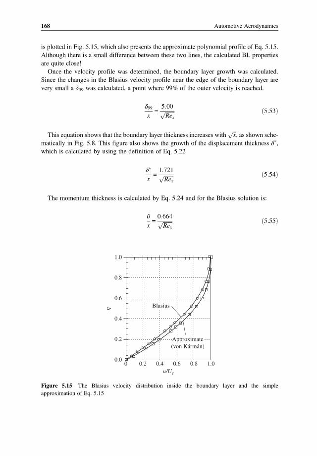
is plotted in Fig. 5.15, which also presents the approximate polynomial profile of Eq. 5.15.Although there is a small difference between these two lines, the calculated BL propertiesare quite close!Once the velocity profile was determined, the boundary layer growth was calculated.

Since the changes in the Blasius velocity profile near the edge of the boundary layer arevery small a δ99 was calculated, a point where 99% of the outer velocity is reached.

δ99x

=5 00

Rex5 53

This equation shows that the boundary layer thickness increases with x, as shown sche-matically in Fig. 5.8. This figure also shows the growth of the displacement thickness δ∗,which is calculated by using the definition of Eq. 5.22

δ∗

x=1 721

Rex5 54

The momentum thickness is calculated by Eq. 5.24 and for the Blasius solution is:

θ

x=0 664

Rex5 55

00.0

0.2

0.4

η

0.6

0.8

1.0

0.2u/Ue

0.4 0.6

Approximate(von Kármán)

0.8 1.0

Blasius

Figure 5.15 The Blasius velocity distribution inside the boundary layer and the simpleapproximation of Eq. 5.15


The friction coefficient is calculated next (as in Eq. 5.31):

Cf =0 664

Rex5 56

and the shape factorH is obtained by dividing the displacement thickness by the momentumthickness

H = 2 59 5 57

Of course, these results were presented in Table 5.2.

5.7 Concluding Remarks

As noted in earlier chapters, analytic solutions of the NS equations could be obtained onlyafter neglecting several terms and focusing on very simple cases. This chapter, in spite of itssimplistic treatment, provides valuable information about the formation of boundary layer inhigh Reynolds number flows. This engineering method, adapted over years, was based ondetermining the dominant variables of the flow, as in this case of the laminar boundary layerand extending prediction capabilities into the turbulent flow region, based on experimentaldata. Consequently, values of the shear stress and resulting drag could be estimated for awide range of practical problems. Also, the present analysis indicates that the boundary layerin an attached flow is very thin, compared to the length scale. Most of the shear force isgenerated near the leading edge of the body and boundary layer thickness grows as thesquare root of the distance. The experimental data presented indicate that laminar flow fric-tion drag is significantly less than the drag in turbulent flow. Therefore, the possibility ofdelaying boundary layer transition provides an opportunity for drag reduction.Finally, in Section 2.10.2 the vorticity term was introduced and in Section 3.2 the Ber-

noulli equation was formulated. At that point it was noted that this equation holds along astreamline or in completely frictionless flow (e.g., vorticity free). The viscous BL flow in

U∞ U∞ U∞u(x, z)

z

x

δ(x)

δ*

Figure 5.16 Schematic description of the Blasius solution for laminar boundary layer. The shape ofthe nondimensional velocity distribution inside the BL is the same at any distance from the plate’sleading edge


this Chapter is not vorticity free and therefore the Bernoulli equation is not valid inside the

BL. For example, Eq. 5.48 states that∂p

∂z= 0 and therefore we cannot apply the Bernoulli

equation between z = 0 in the velocity profile (see Fig. 5.16) and z = δ (although the velocityis different)!

References5.1. Katz, J., and Plotkin, A., Low-Speed Aerodynamics. 2nd Edn. Cambridge University Press, NY, 2001.5.2. Schlichting, H., Boundary Layer Theory, 7th Edn, McGraw Hill, New York, NY, 1979.

Problems

5.1. A 15 km/h wind is blowing parallel to a 5 m long flat plate. Calculate the shear stressat a distance of 5 cm from the leading edge, at 1 m from the leading edge and at theend of the plate (e.g., 5 m from the leading edge). Calculate ReL first to assure the useof the laminar flow formulas. Assume μ = 1 8 10−5N s m2 and ρ = 1 2 kg m3.

5.2. A 15 km/h wind is blowing parallel to a 5 m long flat plate. Calculate the boundarylayer thickness at a distance of 5 cm from the leading edge, at 1 m from the leadingedge and at the end of the plate (e.g., 5 m from the leading edge). Calculate ReL firstto assure the use of the laminar flow formulas. Assume μ= 1 8 10−5N s m2

and ρ= 1 2 kg m3.5.3. The wing of a sail plane is mostly laminar and it wingspan is 8 m. If the average

chord is 0.4 m, calculate the laminar, skin-friction drag force on the wing at aspeed of 60 km/h (use air properties from Table 1.1). Do you think the actual dragis higher?

5.4. The chord of an airplane’s thin wing is 2 m and it is flying at 300 km/h. Calculate thefriction drag for unit width:a. Assuming laminar flow on both the upper and lower surfaces, andb. Assuming turbulent flow on both surfaces.Assume μ= 1 8 10−5N s m2 and ρ= 1 2 kg m3.

5.5. The chord of an airplane’s thin wing is 2 m and it is flying at 200 km/h. Using the flatplate model calculate the displacement thickness and friction coefficient at the wing’strailing edge:a. Assuming laminar flow andb. Assuming turbulent flow.Assume μ= 1 8 10−5N s m2 and ρ= 1 2 kg m3.

5.6. A typical setup for automobile model testing is shown in the sketch. The modellength is L = 1.5 m, the ground clearance is h = 3 cm and the test speed is100km h μ= 1 8 10−5N s m2 ρ= 1 2 kg m3 . Ahead of the model, on the floorthere is a suction slot and it is assumed that the boundary layer is eliminated there.


Calculate the Reynolds number and the boundary layer thickness on the floor at adistance l = 2 m for non-moving floor. Also calculate the boundary layer thicknesson the lower surface of the model (of length L). Assume laminar flow and use theBlasius formulas. Can these two boundary layers affect the test results?

StingInternalbalance

Moving groundSuction

h

Ll

U∞

Problem Figure 5.6

5.7. The boundary layer on the bottom of the vehicle was tripped by a stripe of coarse sandpaper and it is turbulent along the whole surface. Estimate the boundary-layer thick-ness on the lower surface of the vehicle and the drag if model width is 0.5 m. Wouldyou recommend using the moving ground simulation?

5.8. A 1 m long and 3 m wide plate is towed at a velocity of 2 m/s in a fluid. Assuminglaminar flow, find the boundary-layer thickness δ, displacement thickness δ∗, andmomentum thickness θ, at the end of the plate. Also calculate the drag force onone side of the plate μ= 10−3N s m2 ρ= 1000 kg m3 .

5.9. A 1.5 m long and 1 mwide flat plate is towed in water at a speed of 0.2 m/s. Calculatethe drag force (resistance) of the plate and the boundary layer thickness at its end. Isthis a laminar boundary layer?

5.10. A flat plate is towed in a resting fluid. The density of the fluid is 1.5 kg/m3 and itsviscosity is 10−5 N/m2. Find the skin friction drag on the plate per unit width, if theplate is 2 m long and the free stream velocity is 20 m/s. Also calculate the wall veloc-ity gradient at the center of the plate (1 m from the leading edge). Assume turbulentflow where: δ = 0 16 Re1 7 CD = 0 523 ln2 0 06Re .

5.11. Assuming a laminar boundary layer exist over a submerged flat plate (in water,ρ = 1000 kg m3, μ = 10−3N s m2 ). If the free-stream velocity is U∞ = 10 m s, cal-culate the displacement thickness δ∗ at a distance of L = 2 m from the plate’s leadingedge. Also calculate the total friction force (on one side of the plate) per unit width forthe 2 m long section. Use the Blasius laminar flow formulas.

5.12. A 1m long and thin symmetric airfoil is placed at a free stream as shown in the sketch.Calculate the Re number and the drag force for the speed of U∞ = 50 m s andU∞ = 150 m s. Assume the average friction coefficient per side is CD = 0.002(μ = 1.8 10−5 N s/m2, ρ = 1.2 kg/m3).


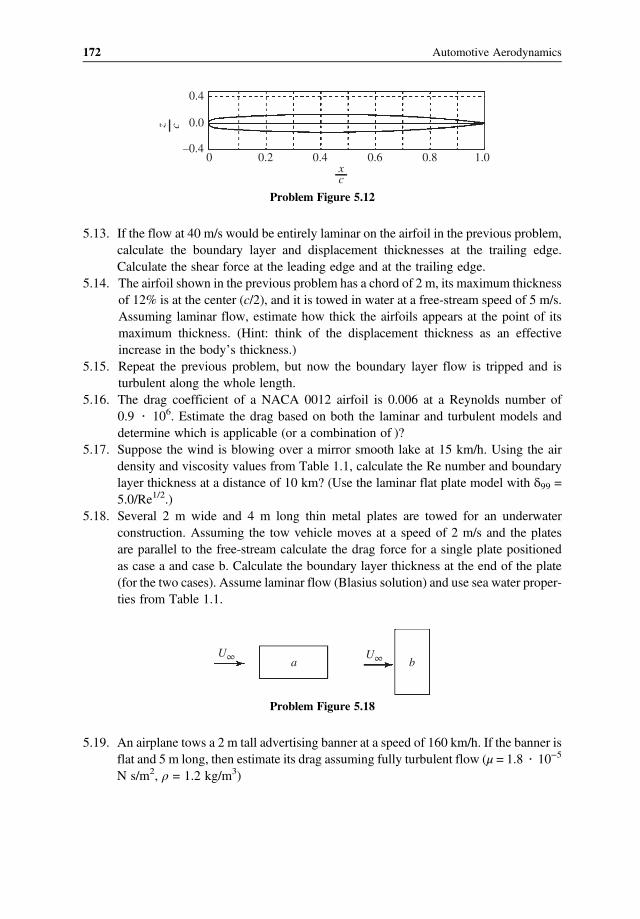
0.4 0.6 0.8 1.00–0.4

0.0

0.4

0.2z c

xc

Problem Figure 5.12

5.13. If the flow at 40m/s would be entirely laminar on the airfoil in the previous problem,calculate the boundary layer and displacement thicknesses at the trailing edge.Calculate the shear force at the leading edge and at the trailing edge.

5.14. The airfoil shown in the previous problem has a chord of 2m, its maximum thicknessof 12% is at the center (c/2), and it is towed in water at a free-stream speed of 5 m/s.Assuming laminar flow, estimate how thick the airfoils appears at the point of itsmaximum thickness. (Hint: think of the displacement thickness as an effectiveincrease in the body’s thickness.)

5.15. Repeat the previous problem, but now the boundary layer flow is tripped and isturbulent along the whole length.

5.16. The drag coefficient of a NACA 0012 airfoil is 0.006 at a Reynolds number of0.9 106. Estimate the drag based on both the laminar and turbulent models anddetermine which is applicable (or a combination of )?

5.17. Suppose the wind is blowing over a mirror smooth lake at 15 km/h. Using the airdensity and viscosity values from Table 1.1, calculate the Re number and boundarylayer thickness at a distance of 10 km? (Use the laminar flat plate model with δ99 =5.0/Re1/2.)

5.18. Several 2 m wide and 4 m long thin metal plates are towed for an underwaterconstruction. Assuming the tow vehicle moves at a speed of 2 m/s and the platesare parallel to the free-stream calculate the drag force for a single plate positionedas case a and case b. Calculate the boundary layer thickness at the end of the plate(for the two cases).Assume laminar flow (Blasius solution) and use sea water proper-ties from Table 1.1.

U∞ U∞a b

Problem Figure 5.18

5.19. An airplane tows a 2m tall advertising banner at a speed of 160 km/h. If the banner isflat and 5 m long, then estimate its drag assuming fully turbulent flow (μ = 1.8 10−5

N s/m2, ρ = 1.2 kg/m3)


Go Aztecs

Problem Figure 5.19

5.20. How thick is the boundary layer at the trailing edge of the banner? Also calculatethe shear force at the trailing edge. Use turbulent boundary layer properties fromTable 5.2.

5.21. A carport is covered by a 20 m long and 4 m wide flat roof (length is parallel to theprevailing wind). The boundary-layer thickness wasmeasured at the end of the (20m)roof and found to be 25 cm thick. Assuming turbulent flow along the whole surfaceestimate the wind speed and the drag force on the roof (from both upper and lowerboundary layers). Use air properties from Table 1.1.

5.22. The velocity profile above a flat plate placed parallel to the stream is:

u

Ue= 2

z

δ−2

z

δ

3+

z

δ

4

Obviously when z> δ then the velocity is constant at Ue. The incoming flow ratebetween z = 0 to z= δ, per unit width (without the plate) is then ρUeδ. However, whenthe plate is inserted then, due to the above described boundary layer, the mass flowwill be reduced. This new mass flow rate is simply the integral of the velocity deficit

ρδ

0Ue−u dz

Calculate the percentage loss of the mass flow rate due to the plate.5.23. If the boundary layer thickness is given by (as in Eq. 5.19):

δ

x=5 836

Rex

Then by substituting the polynomial from Problem 5.22 into the definition of δ∗

(Eq. 5.21), prove Eq. 5.22 forδ∗

x.

5.24. A laminar boundary layer develops along a flat plate and its thickness at a particularpoint is δ = 0.1 m. If we approximate the boundary layer velocity distribution by

u

Ue= 2

z

δ−2

z

δ

3+

z

δ

4

then calculate the local shear τ, and friction coefficient Cf. Assume U∞ = 30 m sec,ρ= 1 2 kg m3, μ = 1 8 10−5N s m2.


5.25. The sinusoidal shape is one of the simplest velocity profiles proposed for the bound-ary layer. Suppose we approximate the velocity distribution as

u

Ue= sin

πz

2δz ≤ δ

then calculate the displacement thickness and the momentum thickness, in terms ofthe local boundary layer thickness δ.

5.26. Using the sinusoidal shapeu

Ue= sin

πz

2δz ≤ δ

calculate the expression for the boundary layer thickness δ by evaluating the vonKarman integral equation.

5.27. Use the results from the previous problem to calculate the local shear on the wall andthe total drag for a plate with a length L. How this approximation compares with theexact result of Blasius?

5.28. Calculate the local skin friction and the drag coefficient for a plate of length L, usingthe previous sinusoidal velocity profile.

5.29. Assuming a velocity profile for the laminar flat plate in the form

u

Ue= 2

z

δ−

z

δ

2

Develop a relation for the boundary layer (δ/x) as a function of the local Reynoldsnumber by evaluating the von Karman integral equation. Compare with the exactresults of Blasius.

5.30. Calculate the displacement and momentum thickness for the velocity profile inProblem 5.29 and compare with the exact results.

5.31. Calculate the local shear stress and friction coefficient for the velocity profile inProblem 5.29 and compare with the exact results.

5.32. Suppose that the velocity profile proposed for a turbulent boundary layer has the form

u

Ue=

z

δ

19

then calculate the displacement thickness and the momentum thickness, in terms ofthe local boundary layer thickness δ.

5.33. The schematic growth of the boundary layer along a flat plate is shown in thesketch. Can the Bernoulli equation provide the pressure difference between point#1 and point #2 (the latter is on the surface where we apply the no-slip boundarycondition)? What is the pressure difference between point #2 and point #3 andpoint #1?


Boundary layer

3

2

1

x

z

δ(x)

U∞

Problem Figure 5.33

5.34. Air enters a small, two-dimensional laminar flow wind tunnel at a speed of u1 =10 m/s (L = 1 m, h = 0.2 m). Calculate the boundary layer thickness at the exit ofthe wind tunnel, at section #2. Also calculate the exit velocity u2.

1 2

hu1u2

L

Problem Figure 5.34

5.35. Repeat the previous problem, but now assume the flow is forced to be fully turbulentby placing sandpaper stripes at the entrance (use Table 5.2 for the boundary layerproperties).


6High Reynolds NumberIncompressible Flow Over Bodies:Automobile Aerodynamics

6.1 Introduction

The previous chapters provided the background for aerodynamics and on general fluidflows. Consequently, the formulation for the forces acting on a vehicle moving throughair or other fluids was developed. However, in case of automobile or airplane aerodynamics,the major contribution to the loads is the pressure distribution, which will be discussed inthis chapter. For simplicity and brevity, the attention will focus on vehicle drag and lift, butside force and moments are important as well. Also note that the forces such as lift and dragwill increase with the square of vehicle speed, while power to overcome drag is increasingwith the cube of speed!The concept of high Reynolds number flows was discussed in Chapter 4 and it was con-

cluded that near a solid body surface a thin boundary layer exist. In Chapter 5 this boundarylayer was investigated and the small thickness assumption was verified. It was also con-cluded that the pressure distribution around a vehicle could be obtained by solving the invis-cid flow outside the thin boundary layer. These modeling conclusions, along with somegeneral features of such flow fields, are summarized in Fig. 6.1. The nondimensional

pressure distribution (Cp=p−p∞

12ρU2

∞, Eq. 4.12) from the outer solution is shown in the

upper diagram and the viscous flow effects (inner solution) are depicted in the lowerdiagram.In term of forces, the boundary layer solution provides the skin friction estimate and the

resulting friction-drag force component. However, viscous effects, in addition to the bound-ary layer can be present in the wake and in areas of flow separation. For example we can seethe effects of viscous flowmomentum loss by comparing the velocity distribution ahead and


behind the vehicle (as shown in the figure). Clearly, in the wake the flow is slower and thereis a loss of linear momentum (which is the drag).Solution of the flow outside this viscous layer should provide information on the velocity

and pressure distributions, as depicted in the upper part of Fig. 6.1 (recall that there is nochange in the pressure across the boundary layer). In case when the flow is attached, wecan define an irrotational flow model and solve for the velocity distribution (recall thatthe term irrotational was defined in Section 2.10.2). The corresponding pressure fieldcan be calculated by using the Bernoulli equations (instead of the full Euler equation). Thisprocess will be demonstrated in this chapter. It is expected that the integration of the pressurewill result in a force (in addition to the skin friction) that may act to other directions (e.g., lift,side force or drag). However, when the flow is separated (and unsteady) as in the wake,shown in Fig. 6.1, then these models may not be accurate. The engineering approach is thento define force coefficients for a wide range of Reynolds numbers (similar to the approachtaken for estimating the friction coefficient in the previous chapter) and with such a “data-base” approach we can estimate the forces even in separated or turbulent or both typeof flows.The first task therefore is to demonstrate a solution that will provide the pressure distri-

bution for a particular geometry (even a very simple one). This model should demonstrate

Irrotationalflow

τwall

1.0

0 L

x

U∞

0.5

0

–0.5Cp

–1.0

–1.5

–2.0

Uppersurface

Lowersurface

Viscous effects(rotational flow)

WakeSeparation

Boundarylayer

Figure 6.1 Summary of the expected results from a high Reynolds number flow solution

177High Reynolds Number Incompressible Flow Over Bodies

the process and allow the extrapolation for treating more complex engineering problems.Only two-dimensional mathematical models will be used here and more complex three-dimensional solutions are presented in Ref. 6.1. However, prior to solving the flow overa simple shape, we must regroup the mathematical tools required to treat this problem:

6.2 The Inviscid Irrotational Flow (and Some Math)

The conclusions from the dimensional analysis in Chapter 4 is that the flow outside theboundary layer is mostly inviscid and the simplified equations are the continuity and theEuler equations,

∇ q = 0

∂q

∂t+ q ∇q = f −

∇pρ

4 19

Because the viscous terms in this model were neglected, only the boundary conditionrequiring zero velocity normal to a solid surface remains.This set of equations is still quite complex (for exact analytic solutions) and additional

simplifications are required. For example, if the flow is irrotational, there are no frictionallosses, and we can use potential (or conservative) models. This is similar to mechanics, whenwe claim that the work done by the gravitational force is independent of the path (as long asthere is no friction). So the first task is to convince ourselves that the outer flow is vorticityζfree (e.g., irrotational). The vorticity was defined in Chapter 2 (Eq. 2.74) and it is twice thesolid body rotation

ζ = 2ω =∇ q 2 74

Solid body rotation is possible only when strong viscous forces are present. This was dis-cussed in Section 2.10.2 and also depicted in Fig. 2.23. To illustrate (again) the motion of afluid with rotation consider the control volume shown in Fig. 6.2a, moving along the path l.We can describe the fluid motion by placing a short floating straw indicating the initial direc-

(a)

Rotationalmotion

l

Irrotationalmotion

l

(b)

Figure 6.2 Rotational and irrotational motion of a fluid element


tion in the fluid (see the small arrows in the figure). Let us assume that the viscous forces arevery large (e.g., think of it as a cup filled with jelly) and the fluid will rotate as a rigid body,while following the path l. In this case ∇ q 0 and the flow is called rotational. For thefluid motion described in Fig. 6.2b, the shear forces in the fluid are negligible (think of it asa cup filled with water), and the fluid will not rotate by the shear force of the neighboringfluid elements. In this case ∇ q = 0 and the flow is considered to be irrotational.To further clarify our argument let us select a fluid element of length dx, in a boundary

layer, as shown in Fig. 6.3. Recall the definition of vorticity in Cartesian coordi-nates (Eq. 2.75),

ζy = 2ωy =∂u

∂z−∂w

∂x

Note that inside the boundary layer w ~ 0 and we can approximate the change in the uvelocity component between point #1 and #2 as

ζy =∂u

∂z−∂w

∂x≈Ue

δ

and δ is the local boundary layer thickness.We arrived at a similar conclusion in the exampleabout the flow near a rotating cylinder (the vortex in Section 2.10), namely that near thesurface where the zero slip boundary condition is fulfilled, the vorticity is nonzero! How-ever, away from the surface, the flow is irrotational. So to conclude this discussion: vorticityis generated near the surface (or in the wakes) and rest of the flow can be considered asirrotational (a more rigorous proof can be found in Ref. 6.1, Chapter 2).Once it is accepted that the vorticity in the high Reynolds number flowfields is confined to

the boundary layer and wake regions where the influence of viscosity is not negligible, wecan assume an irrotational, as well as inviscid flow, outside these confined regions. Now wecan return to our analogy to work done by a (conservative) gravitational force (e.g., without

1 4

32

Ue

x

z

dx

δ(x)

Figure 6.3 Vorticity is created in the boundary layer


friction) where the force times distance integral is independent of path. In a similar way wecan consider the line integral (of the velocity instead of the force vector) along the line C:

Cq dl =

Cudx+ vdy+wdz 6 1

If the flow is irrotational in this region (e.g.,ζ =∇ q = 0) then udx+ vdy +wdz is an exactdifferential (see Ref. 6.2, p. 427) of a potential Φ which is independent of the integrationpath C. The potential at a point P(x, y, z) is therefore

Φ x,y,z =P

Po

udx+ vdy+wdz 6 2

where Po is an arbitrary reference point and P is the point where the potential is evaluated.The result of the integration,Φ, is called the velocity potential and the velocity at each pointcan be obtained as its gradient

q =∇Φ 6 3

and in Cartesian coordinates

u =∂Φ∂x

, v =∂Φ∂y

, w =∂Φ∂z

6 4

The substitution of Eq. (6.3) into the continuity equation (Eq. 6.1) leads to the differentialequation for the velocity potential (which is really the continuity equation):

∇ q =∇ ∇Φ =∇2Φ = 0 6 5

Of course, this is the Laplace equation (named after the French mathematician Pierre S.De Laplace: 1749–1827). It is a statement of the incompressible continuity equation for anirrotational fluid. Note that Laplace’s equation is a linear differential equation. Because thefluid’s viscosity was neglected, the no-slip boundary condition on a solid-fluid boundarycannot be enforced and only the normal velocity on a solid surface is set to zero:

qn = 0 6 6

In a more general form (as shown in Fig. 6.4), this boundary condition is obtained bysimply multiplying the unit-normal to the surface (n ) by the local velocity vector q

q n = 0 6 7

It now appears that the velocity field can be obtained from a solution of Laplace’s equa-tion for the velocity potential. This is a major simplification for the solution procedure!Instead of solving for a velocity vector field (with three unknowns: u, v, w, at any point)we must find a scalar function Φ with only one unknown per point.


Note that we have not yet used the Euler equation, which connects the velocity to thepressure. Once the velocity field is obtained it is necessary to also obtain the pressure dis-tribution on the body surface to allow for a calculation of the fluid dynamic forces andmoments (and this is discussed next).For completeness (and we shall need this later) the two-dimensional continuity and

Laplace equations are rewritten in cylindrical coordinates:

1. The continuity equation, based on Eq. 2.45, is:

∂qr∂r

+1r

∂qθ∂θ

+∂qx∂x

+qrr= 0 6 8

2. and the Laplace equation in cylindrical coordinates (using Eq. 2.43)

∇2Φ =∂2Φ∂r2

+1r

∂Φ∂r

+1r2∂2Φ∂θ2

+∂2Φ∂x2

6 9

6.3 Advanced Topics: A More Detailed Evaluation of theBernoulli Equation

The objective of this section is to arrive at the Bernoulli equation directly from the Eulerequation (Eq. 4.19). Now that we understand the connection between the effects of viscosityand vorticity, it will be easier to understand the limitation that applies to the usage of thisrelation. Simple vector algebra can show that the steady state inertia term in the Navier–Stokes equation can be rewritten by using the following vector identity:

q ∇q = − q ∇ q +∇q2

2= − q ζ +∇

q2

26 10

n q

qt

qn

Figure 6.4 In an irrotational fluid only the “zero normal velocity” boundary condition remains


The incompressible Euler equation now can be rewritten with the use of Eq. 6.10 as

∂q

∂t− q ζ +∇

q2

2= f −∇

p

ρ6 11

For irrotational flow ζ = 0, and the time derivative of the velocity can be written as

∂q

∂t=∂

∂t∇Φ=∇

∂Φ∂t

6 12

Let us also assume that the body force is conservative with a potential gh,

f = −∇ gh 6 13

The Euler equation for incompressible irrotational flow and with this conservative bodyforce (by substituting Eqns 6.12 and 6.13 into Eq. 6.11) becomes

∇ gh+p

ρ+q2

2+∂Φ∂t

= 0

This is true only if the quantity in parentheses is a function of time only:

gh+p

ρ+q2

2+∂Φ∂t

=C t

This is the more general Bernoulli equation for inviscid, incompressible, irrotationalflow. A more useful form of the Bernoulli equation is obtained by comparing the quantitieson the left-hand side of this equation at two points in the fluid; the first is an arbitrary pointand the second is a reference point at infinity. The equation then becomes

gh+p

ρ+q2

2+∂Φ∂t

= gh+p

ρ+q2

2+∂Φ∂t ∞

6 14

At this point we can conclude that:

1. The Bernoulli equation is valid between two arbitrary points in an incompressible irro-tational fluid.

2. If the flow is steady, incompressible but rotational, the Bernoulli equation (Eq. 6.14) isstill valid with the time-derivative term set equal to zero if the constant on the right-handside is now allowed to vary from streamline to streamline. (This is because the productq ζ is normal to the streamline dl and their dot product vanishes along the streamline.


Consequently, Eq. 6.14 can be used in a rotational fluid between two points lying on thesame streamline.)

For the cases discussed here we shall use only the steady state form of the Bernoulli equa-tion, and we can write that

gh+p

ρ+q2

2= const 6 15

Note that for the incompressible, irrotational model presented here, the three complexmomentum equations were replaced by a simple algebraic expression – the Bernoulliequation!

6.4 The Potential Flow Model

In the last three chapters we have established the notion that outside viscous regions (such asthe boundary layer) the flow can be considered irrotational and incompressible. With thedefinition of the velocity potential, this model is called “potential flow” and the governingequations can be summarized (in Cartesian coordinates) as follows:

∂2Φ∂x2

+∂2Φ∂y2

+∂2Φ∂z2

= 0 6 16

This is of course the continuity equation and its solution will yield the velocity field. Theboundary condition, as stated in Eq. 6.7 is

∇Φ n = 0 6 17

Once the velocity field is known the pressure can be calculated at any point using theBernoulli equation (which now replaces the momentum equations).

gh+p

ρ+q2

2= const 6 15

Note that the two-dimensional potential flow problem can be stated in terms of the streamfunction, which immediately visualize the streamlines. This method is not easily extended tothree-dimensions and therefore not discussed here (recall that this is an introductory text).More information on this attractive approach can be found in Ref. 6.1, Section 2.13 and inChapter 3.

6.4.1 Methods for Solving the Potential Flow Equations

There are various approaches to solve the Laplace equation. Of course a simple trial and errorapproach may work, and by substituting various functions into the Laplace equation, viable


solutions can be found. Plotting the corresponding streamlines can visualize the nature of thesolutions, and polynomial functions are probably the first candidates for such an exercise.A more systematic method is based on Green’s identity (after the British Physicist GeorgeGreen: 1793–1841), by which generic flow fields can be constructed by the superpositionof several basic solutions. From the fluid dynamic point of view, the need to solve the flowfor an arbitrary geometry (e.g., the flow over a car) is probably the top priority. Such anapproach, in the spirit of Green’s identity, is described in (Ref. 6.1) and in Section 6.5.5 ofthis chapter. Therefore, prior to attempting the solution of any practical problem, some ofthe elementary solutions to Eq. 6.16 are sought. We already have seen that the flow near avortex (Section 2.10) is irrotational and therefore the vortex could qualify as an elementarysolution.We shall develop two additional elements (the source and the doublet) and combinedwith a free stream model, the flow over many practical shapes can be solved (we can viewthose basic solutions as individual tools in a toolbox). The basic approach then is to combinethese elementary solutions in a manner that the zero normal flow on a solid surface boundarycondition is satisfied. In fact this process can be automated and several computer codes arebased on these principles. The first step, however, is to establish that several basic (or elemen-tary) solutions of the Laplace equation can be added or combined.

6.4.2 The Principle of Superposition

If Φ1,Φ2….,Φn are solutions of the Laplace equation (Eq. 6.16), which is linear, then alinear combination of those solutions:

Φ=n

k = 1

ckΦk 6 18

is also a solution for that equation in that region. Here, c1, c2…, cn are arbitrary constantsand therefore

∇2Φ =n

k = 1

ck∇2Φk = 0

This principle is a very important property of the Laplace equation, paving the way forsolutions of the flowfield near complex boundaries. In principle, by using a set of elementarysolutions, the solution process (of satisfying a set of given boundary conditions) can bereduced to an algebraic search for the right linear combination of these elementary solutions.As stated in the introduction to this chapter, only two-dimensional solutions will be pre-

sented here.

6.5 Two-Dimensional Elementary Solutions

The principle of superposition allows us to combine elementary solution and calculate theflow over various body shapes. The next step therefore is to develop those solutions, andas noted, the discussion is limited to two-dimensional flows only. A polynomial series can


be a good start and clearly low order terms should work – so let us suggest such a solu-tion next.

6.5.1 Polynomial Solutions

Because Laplace’s equation is a second order differential equation, a linear function of posi-tion will be a solution, too. So let us propose a first-order polynomial:

Φ =Ax+Bz 6 19

The velocity components due to such a potential are:

u =∂Φ∂x

=A≡U∞ , w=∂Φ∂z

=B≡W∞ 6 20

where U∞ and W∞ are constant velocity components in the x and z directions. Hence, thevelocity potential due a constant free-stream flow in the x direction is:

Φ =U∞x 6 21

The velocity field due to the potential of Eq. 6.21 is described in Fig. 6.5a. Similarly, afree stream into the z direction can be defined by the velocity potential

Φ=W∞ z 6 22

which is shown in Fig. 6.5b. Based on the principle of superposition we can combine the twoand in general

Φ =U∞x +W∞ z 6 23

(b)

x

W∞

z

ϕ = W∞z

(a)

x

z U∞

ϕ = U∞x

Figure 6.5 Velocity potential of a free stream: (a) parallel to the x-axis and (b) parallel to the z-axis


and this potential describes a free-stream to the combined direction. For example, ifU∞ =W∞ , then the free stream will be at 45 between the x- and z-axes and its magnitude

is U2∞ +W2

∞ .Along the same lines, additional polynomial solutions can be sought and as an example

let’s consider the second order polynomial with A and B being constants:

Φ =Ax2 +Bz2 6 24

To satisfy the continuity equation

∇2Φ=A+B= 0

The solution to this equation is

A= −B 6 25

and by substituting this result into Eq. 6.24 the velocity potential becomes

Φ =A x2−z2 6 26

The velocity components for this two-dimensional flow in the x-z plane are the derivativesof Eq. 6.26:

u =∂Φ∂x

= 2Ax

w=∂Φ∂z

= −2Az

6 27

To visualize this flow, the streamlines can be plotted. Recall Eq. 2.9 indicating that theflow is parallel to the streamline:

dx

u=dz

w2 9

and after substituting the velocity components we get

dx

2Ax=

dz

−2Az

Integration by separation of variables results in

xz = const =D 6 28


The streamlines for different constant values of D = 1, 2, 3… are plotted in Fig. 6.6 and,for example, if only the first quadrant of the x-z plane is considered, then this potentialdescribes the flow into a corner. If the upper half of the x-z plane is considered then thisflow describes a stagnation flow against a wall. Note that when x= z = 0, the velocity com-ponents u =w= 0 vanish too, which means that a stagnation point is present at the origin andthe coordinate axes x and z are also the stagnation streamlines. The constant potential linesare also plotted in this figure, by the dashed lines.

6.5.2 Two-Dimensional Source (or Sink)

A source is a point from which fluid flows into the radial direction, in straight lines. Thus, inthe two-dimensional r−θ coordinate system the tangential velocity component vanishes(e.g., qθ = 0). Because we are searching for a potential flow solution, this flowfield mustbe irrotational! Therefore, we can start with the definition of vorticity (representing rotation)and require it to be zero! Using the cylindrical coordinates:

ζy = 2ωy = −1r

∂

∂rrqθ −

∂

∂θqr =

1r

∂

∂θqr = 0 6 29

Thus, the velocity component in the r direction is a function of r only [qr = qr r . Also,the remaining radial velocity component must satisfy the continuity equation (Eq. 2.45)which in the r−θ coordinate system is:

∇ q =dqrdr

+qrr=1r

d

drrqr = 0 6 30

3

0ϕ = –4

z

4

21

–1–2–3

xD =

321

–1–2–3

D =

Figure 6.6 Streamlines defined by x-z = const. Each quadrant describes the flow in a 90 corner.Also note the constant potential lines, shown by the dashed lines


This indicates that

rqr = const =A

Using this constant, the velocity components are

qθ = 0, qr =A

r6 31

Let us call the flow rate passing through an arbitrary circle at a distance r1, as σ and,according to the continuity equation, it must be the same at a different distance, r2:

σ = qr2πr =A

r12πr1 =

A

r22πr2 = 2π A

Based on this we conclude that the constant in Eq. 6.31 is:

A=σ

2π6 32

and σ represents volume flow rate introduced by the source. The resulting velocity compo-nents for a source element at the origin are

qθ = 0, qr =σ

2πr6 33

This element is described in Fig. 6.7 and the streamlines are clearly straight radial lineswhile the velocity decays as a function of 1/r. This trend is shown in Fig. 6.7b. At the centerof the source (origin in this case) the velocity goes to infinity, and these types of elements arecalled singular solutions. In terms of the velocity potential in the r−θ coordinate system

qr =∂Φ∂r

=σ

2πr6 34

qθ =1r

∂Φ∂θ

= 0 6 35

By integrating these equations the velocity potential is found,

Φ =σ

2πlnr +C 6 36

and the constant C can be set to zero. Also a source is emitting fluid while a sink is removingfluid at a rate of σ. The only difference is the sign and in general we can write:

Φ= ±σ

2πlnr 6 37

and the minus sign is for a sink.


Equations 6.34–6.37 describe a source/sink placed at the origin and for any other location(as in r0) we can replace the distance r with r−r0. Similarly, in Cartesian coordinates thedistance r between two points (x, z) and (x0, z0) is

r = x−xo2 + z−zo

2

Based in this, the corresponding equations for a source located at (xo, zo) are

Φ x,z =σ

2πln x−xo

2 + z−zo2 6 38

and the velocity components obtained by deriving the velocity potential:

u =∂Φ∂x

=σ

2πx−xo

x−x02 + z−zo

2 6 39

w=∂Φ∂z

=σ

2πz−zo

x−x02 + z−zo

2 6 40

Note that the source here is placed at (x0, z0). If placed at the origin then clearly x0 = z0 = 0.As noted, a sink is the same as a source but the flow direction is reversed. The only dif-

ference is that instead of positive flux a negative sign is added (−σ) in the source equations!In this case σ represents the flow disappearing at the point sink.

0

(b)

r

qr

qr=σ

2πr

(a)

Streamlines

x

z

ϕ = const.

Figure 6.7 Streamlines and equipotential lines for a two-dimensional source, t placed the origin


Example 6.1 Velocity induced by a sourceA source of strength σ = 5 m2/s is located at a point (1, 1). Calculate the velocity at anotherpoint: (0, −1)

Solution:Using the velocity equations in Cartesian coordinates for the source and substituting thevalues for the two points we get:

u =52π

0−1

−1−1 2 + 0−1 2 = −0 159ms

w=52π

−1−1

−1−1 2 + 0−1 2 = −0 318ms

6.5.3 Two-Dimensional Doublet

A doublet is like a small jet engine emitting fluid into one direction and sucking the sameamount of flow from behind (so no fluid is introduced contrary to the case of a source). Con-sequently, the two-dimensional doublet can be obtained by letting a point source and apoint sink (of equal strength) approach each other, as depicted in Fig. 6.8.The velocity potential at an arbitrary point P due to the two point elements is (based

on Eq. 6.37)

Φ=σ

2πlnr2− lnr1 = −

σ

2πlnr1r2

6 41

and the source is located forward. So the fluid is ejected into the +x direction. Since r1 is onlya bit longer in the figure (e.g., Δx is small) we can write

r1r2

= 1 +Δrr

Sink Source

θ

r1 r2

x

Pz

θ +Δθ

Δx

Δr

Figure 6.8 A doublet is a product of a source and a sink placed next to each other


and here r is the average distance to P and 1Δrr. Consequently we can rewrite Eq. 6.41 as

Φ = −σ

2πln 1 +

Δrr

and expanding the log term assuming Δr is small.

Φ= −σ

2πln 1 +

Δrr

= −σ

2πΔrr−12

Δrr

2

+13

Δrr

3

−…

Next, observing the geometry in Fig. 6.8, it appears that

Δr =Δx cosθ

Taking the limit process as Δx 0, neglecting smaller terms, and assuming that thesource/sink strength multiplied by their separation distance becomes the constant μ(σΔx μ) we get

Φ= limΔx 0−σ

2πΔx cosθ

r−12

Δx cosθr

2

+13

Δx cosθr

3

−… =−μcosθ2πr

Consequently, the velocity potential for a doublet at the origin becomes

Φ r,θ =−μ

2πcosθ

r6 42

The velocity field due to this element can be obtained by differentiating the velocitypotential:

qr =∂Φ∂r

=μcosθ

2πr26 43

qθ =1r

∂Φ∂θ

=μsinθ

2πr26 44

Again, this doublet is placed at the origin. In Cartesian coordinates the sin and cosfunctions are (also see Fig. 6.8):

cosθ =x−xo

x−xo2 + z−zo

2

sinθ =z−zo

x−xo2 + z−zo

2

and recall the expression for the distance r

r = x−xo2 + z−zo

2


Using these expressions, the velocity potential in Cartesian coordinates for such a doubletat a point (xo, zo) is

Φ x,z =−μ

2πx−xo

x−xo2 + z−zo

2 6 45

and the velocity components are

u =μ

2πx−xo

2− z−zo2

x−xo2 + z−z0

22 6 46

w=μ

2π2 x−xo z−zo

x−xo2 + z−z0

22 6 47

The velocity field and constant potential lines for this doublet are depicted schematicallyin Fig. 6.9. The streamlines are circles originating at the doublet front and returning at itsback. The constant potential lines are normal to the streamlines and consist of similar circles,but rotated by 90 , as shown in the figure.The arrow in Fig. 6.9 indicates that a doublet is directional and the one formulated here

points into the positive x direction. Doublets pointing into other directions can be derived bysimple (rotational) transformation of these equations. The simplest case is when the doubletformulas are multiplied by –1 to get a doublet pointing into the –x direction.

z

x

Streamlines

Constant Φlines

μ

Figure 6.9 Streamlines and equipotential lines for a two-dimensional doublet placed at the origin.Note that this doublet points into the positive x direction


Example 6.2 Velocity induced by a doubletCalculate the velocity induced by a doublet of strength μ = 1m3 s (located at the origin), at apoint x = 1, and z = 0.For the solution let us use the Cartesian form of the velocity formulas

u =μ

2πx−xo

2− z−zo2

x−xo2 + z−z0

22 =

12π

12−02

12 + 022 =

12π

ms

w=μ

2π2 x−xo z−zo

x−xo2 + z−z0

22 =

12π

2 1 0

12 + 022 = 0

Suppose we want to find the velocity at a point located at x = 1 and z = 1, then based onFig. 6.9, we suspect that the velocity vector will point straight upward (since we are at a90 position on the streamline).

u =12π

12−12

12 + 122 = 0

w=12π

2 1 1

12 + 122 =

14π

ms

and this result verifies the expected direction of the velocity vector.

6.5.4 Two-Dimensional Vortex

The velocity field due to a two-dimensional vortex was developed in Section 2.10. It wasalso demonstrated that the flow due to a rotating vortex core is vorticity-free whenexcluding the vortex core itself. We would like to develop the same two-dimensionalvortex element, but using the approach used for the source element (in this section).We can start by searching for a singularity element with only a tangential velocitycomponent, as shown in Fig. 6.10a, whose velocity will decay in a manner similar tothe decay of the radial velocity component of a two-dimensional source (e.g., will varywith 1/r).The expected velocity components are then

qr = 0

qθ = qθ r,θ

Substituting these velocity components (e.g., qr = 0) into the continuity equation(Eq. 2.45) results in qθ being a function of r only

qθ = qθ r


Similar to the approach used to develop the source, we can substitute these relations intothe vorticity expression and require that the rotation be zero:

ζy = 2ωy = −1r

∂

∂rrqθ −

∂

∂θqr = −

1r

∂

∂rrqθ = 0

By integrating with respect to r, we get

rqθ = const =A 6 48

So the magnitude of the velocity varies with 1/r similar to the radial velocity componentof a source. The value of the constant A can be calculated by using the definition of the cir-culation Γ as in Eq. (2.67):

Γ =

c

q d l =o

2πqθ rdθ =

o

2π

A

rrdθ = −2πA

Note that positive Γ is defined according to the right-hand rule (positive clockwise), there-fore, in the x–z plane as in Fig. 6.10 the line integral must be taken in the direction opposite tothat of increasing θ. Also, recall that the circulation represents the solid body rotation timesthe core area (Γ= 2ωS) as shown by Eq. 2.70. The constant A is then

A= −Γ2π

6 49

Substituting A into Eq. 6.48 we can summarize the vortex’s velocity field

qr = 0 6 50a

qθ = −Γ2πr

6 50b

(b)

r

qθΓ

2πrqθ =–

Streamlines

(a)

θ

zLines of constant

potentialVelocitydue to

positive Γ

Figure 6.10 Streamlines and equipotential lines for a two-dimensional vortex placed at the origin.Note that the tangential velocity decays as 1/r


As expected, the tangential velocity component decays at a rate of1ras shown in

Fig. 6.10b. The velocity potential for a vortex element at the origin can be obtained by usingthe basic definition of the velocity potential; that is, by the integration of Eq. 6.50:

Φ= qθrdθ = −Γ2π

θ +C 6 51

where C is an arbitrary constant that can be set to zero. Equation 6.51 indicates too that thevelocity potential of a vortex is multivalued and depends on the number of revolutionsaround the vortex point. So when integrating around a vortex we do find vorticity is con-centrated at a zero area point, but with finite circulation (see Section 2.10). However, if inte-gratingq dl around any closed curve in the field (not surrounding the vortex – see Eq. 2.77)the value of the integral will be zero. Thus, the vortex is a solution to the Laplace equationand results in an irrotational flow, excluding the vortex point itself. Equations 6.50–6.51 arefor a vortex at the origin. For a vortex located at an arbitrary point xo,zo) expressed in Car-tesian coordinates the formulation is:

Φ= −Γ2π

tan−1 z−zox−x0

6 52

u =Γ2π

z−zo

x−x02 + z−zo

2 6 53

w= −Γ2π

x−xo

x−x02 + z−zo

2 6 54

Example 6.3 Velocity induced by a vortexA vortex with a circulation of Γ = 5 m2/s is located at a point (1, 1). Calculate the velocity at(0, −1) and (3, 0).

Solution:Using the velocity equations for the vortex we get for the first point:

u=52π

−1−1

−1−1 2 + 0−1 2 = −0 318ms

w=−52π

0−1

−1−1 2 + 0−1 2 = 0 159ms

and for the second point

u =52π

0−1

1−0 2 + 3−1 2 = −0 159ms

w=−52π

3−1

0−1 2 + 3−1 2 = −0 318ms


Example 6.4 A vortex is a solution for Laplace equationProve that the vortex of Eq. 6.51 satisfies the Laplace equation.

Solution:Let us substitute the vortex equation 6.51, into Eq. 6.9:

∇2Φ =∂2 − Γ

2π θ

∂r2+1r

∂ − Γ2π θ

∂r+1r2

∂2 − Γ2π θ

∂θ2= 0 + 0 + 0

6.5.5 Advanced Topics: Solutions Based on Green’s Identity

Another method, with a much wider application range is based on Green’s identity (seeRef. 6.1). This approach is the basis for numerical methods, called panel methods, andcan be used for solving the flow over complex shapes. One form of this identity, statedin Eq. 6.55, postulates that the velocity potential representing the flow over a solid bodycan be constructed by adding the contribution of sources and a doublets with a free stream.According to this two-dimensional Green’s formula, the potential at an arbitrary point (x,z)in the fluid can be constructed by the following summation

Φ x,z =12π SB

σlnr−μ∂

∂nlnr dS+Φ∞ 6 55

Here, r, as before, represents the distance between the element and the point of interest(x, z) and SB is the body’s surface (or even its wake, as shown).At first it appears that this formulation is identical to the principle of superposition. How-

ever, it is also implied that the sources and doublets must be placed on the surface, as shownin Figure 6.11.The first term in this equation (σlnr) is the source as given by Eq. 6.37; however, the dou-

blet μ∂

∂nlnr is not immediately recognizable. This is because the doublet in this formula is

normal to the surface (in the direction ofn). However, if the derivative of lnr is taken into the

Thick surfaceThin surface

(wake)

n = 0∂ϕ∂n

SΦi = const

U∞

Figure 6.11 Schematic description for the use of Green’s identity to solve the flow over a two-dimensional streamlined body


x direction (see Eq. 6.39), then clearly the doublet potential is obtained (compare Eq. 6.39with Eq. 6.45). This comparison also proves that the doublet is a derivative of the source.The application of Green’s identity is shown schematically in Fig. 6.11. The correct com-

bination of sources and doublet can be found by fulfilling the zero normal flow boundarycondition:

∂Φ∂n

= 0 on S

and this velocity based formulation is usually called the Neumann Boundary condition (afterCarl Neumann, German mathematician, 1832–1925). Also in case of flow with forces intothe vertical direction (lift) usually a zero pressure jump is forced at the sharp trailing edgewhere a thin wake is formed, as shown in the figure (this is called the Kutta condition). Now,

if∂Φ∂n

= 0 on the surface then the internal potential Φi is unchanged, as shown in Fig. 6.11.

Therefore, we conclude that:

Φi = const 6 56

This is called the Dirichlet boundary condition (after the German mathematician, JohannPeter Gustav Lejeune Dirichlet, 1805–1859) which in this case is much simpler than theNeumann condition. Usually the inner potential value in Eq. 6.56 is set as zero. The appli-cation of this type of boundary condition is beyond the scope of this chapter but is describedin detail in Ref. 6.1. This topic will be revisited in Section 8.8, when numerical solution ofthe potential flow is discussed.The concept introduced by the Green’s formula in Eq. 6.55 contains the principle of

superposition (as in Eq. 6.18). Therefore, the following example serves to demonstratethe method for obtaining a solution for the potential flow using the principle of superposi-tion. Although this clarifies somewhat the Green’s identity approach, the singular elementsare not placed on the solid boundary as suggested by Eq. 6.55.

Example 6.5 The superposition of a source, a sink, and a free-streamFind the combined velocity potential and the velocity distribution for the combination of asource, a sink, and a free stream.

Solution:To demonstrate the principle of superposition, let us place a source with a strength σ atx = −xo, and a sink with a strength −σ at x = + xo, both on the x-axis (as shown in Fig. 6.12).The free stream with a speed U∞ is flowing in the x direction as shown in the figure.The velocity potential at an arbitrary point P(x, z) is obtained by combining the three sep-

arate potentials:

Φ x,z =U∞x+σ

2πln r1 −

σ

2πln r2


where r1 = x + x02 + z2, and r2 = x−x0

2 + z2. With these relations the velocity poten-

tial in Cartesian coordinates becomes:

Φ x,z =U∞x +σ

2πln x + xo

2 + z2−σ

2πln x−xo

2 + z2 6 56a

The velocity field due to this potential is obtained by differentiating the velocity potential

u =∂Φ∂x

=U∞ +σ

2πx + xo

x + x02 + z2

−σ

2πx−xo

x−x02 + z2

6 57a

w=∂Φ∂z

=σ

2πz

x + x02 + z2

−σ

2πz

x−x02 + z2

6 57b

It appears that ahead of the source, along the x-axis, there must be a point (let us call itx = −a) where the velocity is zero (stagnation point). Based on these equations, the w com-ponent of the velocity along the x-axis is automatically zero. In order to find the location ofthe stagnation point we equate the u component to zero

u −a,0 =U∞ +σ

2π1

−a + x0−

σ

2π1

−a−x0=U∞ −

σ

π

xoa2−x2o

= 0

and solving for a we get

a = ±σxoπU∞

+ x2o 6 58

This suggests that there is a fore/aft symmetry about the vertical z-axis and another stag-nation point exists at x = a. To visualize the streamlines we can start at a point far to the leftand based on Eq. 2.9a, march forward, using the following procedure

xi+ 1 = x1 + uΔtzi+ 1 = z1 + uΔt

6 59

Source Sink

P(x, z)

+

z

r1r2

x0

x

–x0

θ1

θ2

U∞

Figure 6.12 Schematic description of combining a free stream with a source and a sink


Here i is a virtual time interval counter and Δt is a small time interval. The resultingstreamlines are shown in Fig. 6.13, based on the results from Ref. 6.1.As seen, the stagnation streamline includes a closed oval shape (called Rankine’s oval,

after W. J. M. Rankine, a Scottish engineer who lived between 1820 and 1872). This flowtherefore, can be considered as a flow past an oval of length 2a. For this application, thestreamlines inside the oval have no physical significance. By varying the parameters σand xo or a, the flow past a family of such ovals can be derived.Also note that the velocity normal to the stagnation streamline is zero! Therefore, this

example demonstrates how the flow over a particular body can be obtained by the principleof superposition and by fulfilling the zero-normal-flow boundary condition. Of course,when the source and sink in this flow approach each other (and create a doublet) thenthe flow over a circle is obtained. This limiting case, of the flow over a cylinder is studiedin the next section.

6.6 Superposition of a Doublet and a Free-Stream:Flow Over a Cylinder

The basic solutions developed in Section 6.4 can be combined (using the principle of super-position) to simulate the flow over complex shapes. The general method for doing this (forarbitrary geometries) is beyond the scope of this text, but the examples in this section dem-onstrate the approach. The potential flow model assumes no flow separation and thereforethis method is powerful for attached flow cases such as the flow over airplane wings or sub-marine hulls. This second case, the flow over a cylinder, serves to show how the flow fieldover a practical shape can be obtained. However, in reality the flow over a cylinder is sepa-rated throughout most of the Reynolds number range. In spite of this model leading to anincorrect physical solution, the results create a systematic approach for creating a databasefor the fluid dynamic forces such as lift and drag. (In other words, if we could solve here theflow over a thick airfoil at a small angle of attack, then the calculated results would be very

Streamlines

x0 x0

z

x

a a

Stagnationstreamline

Figure 6.13 Streamlines describing the flow of combined source, sink, and a free stream


close to the experimental data. Unfortunately the math involved is beyond the scope of thischapter.Let us consider the superposition of the free stream potential of Eq. 6.21, with the poten-

tial of a doublet (Eq. 6.41) pointing in the negative x direction, as shown in Fig. 6.14. How-ever, it is much easier to use the r−θ coordinate system and instead of x in Eq. 6.21 we usethe transformation between the two systems: x = rcosθ. Consequently the velocity potentialof the free stream blowing into the positive x direction is:

Φ=U∞ r cosθ 6 60

Next we add a doublet at the origin but pointing in the –x direction (see coordinate systemin Fig. 6.14) resulting in the change of sign for the doublet potential. The combined flow hasthe following velocity potential

Φ=U∞ rcosθ +μ

2πcosθ

r6 61

The velocity field of this potential can be obtained by differentiating Eq. 6.61:

qr =∂Φ∂r

= U∞ −μ

2πr2cosθ 6 62

qθ =1r

∂Φ∂θ

= − U∞ +μ

2πr2sinθ 6 63

To visualize this flow we can use the property of streamlines, as stated in Eq. 2.9 (orEq. 6.59) and the result is shown in Fig. 6.15. Basically the doublet (recall the jet enginemodel) is blowing into the free-stream. At a certain point (see P1 in the figure) the velocitystops and this point is the forward stagnation point. It appears that a circle of radius R isdividing the streamlines of the inner flow solution from the outer one. We will show later

Streamlinesfor a uniform

flow

Streamlinesfor a doublet

+–μ

U∞

r

θ

Figure 6.14 Combination of a free-stream U∞ with a doublet pointing into the –x direction


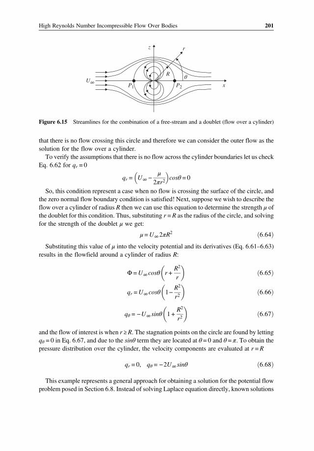
that there is no flow crossing this circle and therefore we can consider the outer flow as thesolution for the flow over a cylinder.To verify the assumptions that there is no flow across the cylinder boundaries let us check

Eq. 6.62 for qr = 0

qr = U∞ −μ

2πr2cosθ = 0

So, this condition represent a case when no flow is crossing the surface of the circle, andthe zero normal flow boundary condition is satisfied! Next, suppose we wish to describe theflow over a cylinder of radius R then we can use this equation to determine the strength μ ofthe doublet for this condition. Thus, substituting r =R as the radius of the circle, and solvingfor the strength of the doublet μ we get:

μ=U∞2πR2 6 64

Substituting this value of μ into the velocity potential and its derivatives (Eq. 6.61–6.63)results in the flowfield around a cylinder of radius R:

Φ =U∞cosθ r +R2

r6 65

qr =U∞cosθ 1−R2

r26 66

qθ = −U∞ sinθ 1 +R2

r26 67

and the flow of interest is when r ≥R. The stagnation points on the circle are found by lettingqθ = 0 in Eq. 6.67, and due to the sinθ term they are located at θ = 0 and θ = π. To obtain thepressure distribution over the cylinder, the velocity components are evaluated at r =R

qr = 0, qθ = −2U∞ sinθ 6 68

This example represents a general approach for obtaining a solution for the potential flowproblem posed in Section 6.8. Instead of solving Laplace equation directly, known solutions

z

U∞

r

x

R θP2P1

Figure 6.15 Streamlines for the combination of a free-stream and a doublet (flow over a cylinder)


are combined using the principle of superposition, in a manner that the boundary condition(Eq. 6.17) is satisfied. This is exactly the condition, shown by Eq. 6.68 (e.g., qr = 0), statingthat the velocity normal to the surface of the cylinder is zero!The pressure distribution at r =R is obtained now by applying Bernoulli’s equation on the

surface of the cylinder. We take a reference point far left where the flow is undisturbed(p = p∞ and u=U∞ ) and the other point is on the surface of the cylinder (where we haveonly qθ)

p∞ +ρ

2U2

∞ = p +ρ

2q2θ 6 69

Substituting the value of qθ at r =R yields:

p−p∞ =12ρU2

∞ 1−4sin2θ 6 70

This equation describes the pressure distribution on the surface of the cylinder. In terms ofthe pressure coefficient (Eq. 4.12), when using p∞ as the reference pressure

Cp =p−p∞12ρU

2∞

= 1−4sin2θ 6 71

Note that by taking p−p∞ directly from Eq. 6.69 and substituting into the definition of thepressure coefficient we get:

Cp =p−p∞12ρU

2∞

=ρ2U

2∞ − ρ

2q2θ

12ρU

2∞

Cp = 1−q2

U2∞

6 72

The results of Eq. 6.71 are plotted schematically in Fig. 6.16a showing positive pressureat the front and at the back of the cylinder. As the flow accelerates around the top (or bottom)of the cylinder, the velocity increases, and large suction force results.

Suction

U∞

(a)

1801

0

–1

–2

–3

–4

Cp

(b)

90 0θ (deg)

270 180

Equation 8.71Experiment atRe = 6.7 ·105

Figure 6.16 Theoretical pressure distribution around a cylinder (Eq. 6.71) and comparison withexperimental data (Fig. 6.16b). The solid line shows the ideal flow solution and the broken linerepresents the high Reynolds number experimental data


The same pressure distribution (of Eq. 6.71) is also shown in Fig. 6.16b by the solid line(versus the angle, θ). It can be easily observed that at the stagnation points θ = 0 and π (whereboth components of the velocity are zero: q= 0), the pressure coefficient is the highest atCp = 1. Also the maximum speed occurs at the top and bottom of the cylinder

θ =π

2,3π2

and the pressure coefficient there is −3. Note that there is a fore/aft symmetry

as well as a top/bottom symmetry (suggesting no lift or drag).To evaluate the components of the fluid dynamic force acting on the cylinder, this pres-

sure distribution must be integrated. Let L be the lift acting in the z direction and D the dragacting in the x direction. Integrating the components of the pressure force on an element oflength Rdθ leads to

L=2π

o−pRdθsinθ =

2π

o− p−p∞ Rdθsinθ =

−12ρU2

∞

2π

o1−4sin2θ Rsinθdθ = 0 6 73

D=2π

o−pRdθcosθ =

2π

o− p−p∞ Rdθcosθ =

−12ρU2

∞

2π

o1−4sin2θ Rcosθdθ = 0

6 74

Here, the pressure was replaced by the pressure difference p−p∞ term and this has noeffect on the results, since the integral of a constant pressure p∞ around a closed body iszero. As noted, because of the fore and aft symmetry the calculated pressure loads cancelout. In reality the flow separates (and is also unsteady), and will not follow the cylinder’srear surface, as shown in Fig. 6.17. The pressure distribution due to this real flow, along withthe results of Eq. 6.71, is plotted in Fig. 6.16. This shows that at the front section of thecylinder, where the flow is attached, the pressures are well predicted by this model. How-ever, behind the cylinder, because of the flow separation, the pressure distribution is differ-ent. For example, near the rear stagnation point (θ = 0) the experimental pressure coefficientin Fig. 6.16 is negative, compared to +1, predicted by the ideal flow solution. Consequentlythe pressure drag is not zero!As noted earlier, the inviscid flow results do not account for flow separation and viscous

friction near the body’s surface and therefore the calculated drag coefficient for the cylinder

Figure 6.17 Experimental visualization of the high Reynolds number flow over a cylinder


is zero. This fact disturbed the French mathematician Jean le Rond d’Alembert(1717–1783), who arrived at a similar conclusion that the drag of a closed body in two-dimensional inviscid incompressible flow is zero (even though he realized that experimentalresult indicate that there is drag). Ever since, those early days of fluid dynamics, this problemhas been known as d’Alembert’s paradox.Although the flow over a sphere isn’t solved here, the method of solution is very similar

and the resulting pressure distribution is

Cp = 1−94sin2θ 6 75

Because of the fore/aft symmetry the potential flow, drag is zero and the two theoreticalpressure distributions (for one side – say upper) are depicted in Fig. 6.18. The importantobservation here is that the maximum velocity (and the corresponding pressure coefficients)is much smaller in the three-dimensional case, because the flow can move around the sidesas well.

6.7 Fluid Mechanic Drag

This first example of the flow over a cylinder may not be the best when comparing withexperiments. As noted earlier, a solution of a streamlined shape (such as an airfoil) wouldbe a much better example but the mathematical formulation is far more complicated. Nev-ertheless, this solution provides the approach for calculating engineering quantities such asthe pressure distribution and the force coefficients. Let us start by observing the drag of

90

1.0

0

–1.0

–2.0

–3.0

Circular cylinder

80 60 40 20 0 –20 –40 –60 –80θ (deg)

–90

Sphere

Cp

Figure 6.18 Comparison between the theoretical (ideal flow) pressure distribution around a cylinderand a sphere


simple shapes like the cylinder and flat plate, and then extend the method to include morecomplex shapes (and the discussion on the lift will be resumed later).

6.7.1 The Drag of Simple Shapes

In a manner similar to plotting the friction coefficient for the boundary layer versus the Rey-nolds number we can plot the experimental drag coefficient of the cylinder versus a widerange of the Reynolds number (Fig. 6.19). In addition, the drag coefficient of a sphere isalso shown and the trends in both curves are similar. This graph seems quite complicatedand in the next paragraph we’ll try to provide some observations based explanations.At the very low Reynolds number we expect laminar flow and the drag (as the friction

coefficient in the previous chapter) should decrease with increasing Reynolds number. Thiswas validated by experiments and flow visualizations indicating that the flow is attached upto Re < 4. This is described schematically in Fig 6.20a and also marked as region (a) inFig. 6.19. For the case of the sphere at this low Reynolds number range, Stokes(1819–1903), of the Navier–Stokes fame developed a closed form solution, resemblingthe results for the friction coefficient on plates and in pipes

CD =24Re

6 76

This equation compares well with the experimental data in Fig. 6.19, up to a Reynoldsnumber of about 4.As the Reynolds number increases the flow will separate behind the cylinder and a

“stationary” separation bubble is observed (see Fig. 6.20b). This condition remains up to

10010–10.060.3

1.0

a

b c d e10

CD

100

400

101 102 103 104

Sphere

Cylinder

105 106

Re =ρU∞D

μ

Figure 6.19 Experimental drag coefficient of a cylinder and a sphere, over a wide range of Reynoldsnumbers


Reynolds numbers of about 40. At the next range of Reynolds numbers (up to say 400) alter-nate vortex shedding begins (Fig. 6.20c) with laminar separation bubble behind. As the Rey-nolds number further increases (up to 0.3 106), wake vortices become more turbulent, butthe front is still laminar (Fig. 6.20d). The separation point is actually a few degrees (up to 8)ahead of the top, which explains the larger drag (of over 1.0). The next important region isindicated by the sharp drop in CD (Re > 3 106) when the boundary layer becomes turbulentat the front and as a result the rear separation area is reduced (up to 30 back from the top).Turbulent vortex shedding continues, but the reduced area of flow separation results in muchlower drag, as shown in region (e) in the figure (again, see the sharp drop in the drag inFig. 6.19).This example provides valuable insight about the resistance force in a moving fluid. The

skin friction originating at the boundary layer is clearly one component. However, the sepa-rated flow creates a pressure distribution that results in drag. This component of the drag iscalled the pressure drag (or sometimes form drag) and in many practical cases (e.g., a car)it is much larger than the drag due to skin friction. Figure 6.20 clearly demonstrates that it

(a)

(b)

(c)

(d)

(e)

Figure 6.20 Schematic description of the various observed flow fields over a cylinder (versusReynolds number)


depends on the Reynolds number and whether the flow is laminar or turbulent. Note that thispressure drag is zero for two-dimensional shapes in fully attached flows (as suggested by thepresent potential flow model – the fact that puzzled d’Alembert).As a conclusion let us present a “good example” where the flow is attached. Naturally, a

streamlined shape, such as shown in Fig. 6.21, can qualify. The potential-flow pressure dis-tribution (calculated by adding sources and sinks to a free-stream) compares well withexperimental data and the actual drag force can be estimated by using the skin friction datafrom the boundary layer section. Consequently, there is no form drag (if there is no flowseparation) and the approach used in the present section will be successful in predictingthe pressure distribution and resulting loads. The next example helps to demonstrate theseclaims for the attached flow case.

Example 6.6 Drag due to skin friction onlyEstimate the drag coefficient at a Reynolds number of 3 106, on a streamline shape, such asshown in Fig. 6.21.

Solution:In this case we assume that the flow is attached and the drag is a result of the skin frictiononly. We can estimate the drag coefficient from the boundary layer data of Fig. 5.11 wherewe get CD ~ 0.004 for turbulent flow and for laminar flow we use the Blasius formula:

CD = 20 664

3 106= 0 00077

Based on the shape of the pressure distribution the gradient is favorable for about 40% ofthe length, so we can assume that the boundary layer is laminar there, while it is turbulentalong the rest of the surface. The total drag per side is

CD = 0 4 0 00077 + 0 6 0 004 = 0 0027

And for the two sides (2 0.0027) the drag coefficient is estimated at

CD = 0 0054

and this number is very close to experimental results (for this airfoil).

1 NACA 0012

0

–1

Cp

Cp

Figure 6.21 Potential flow solution of the flow over a streamlined shape and calculated pressurecoefficient (which are close to experimental data). Note that the upper and lower pressuredistributions are identical at an angle of attack of zero. Also 0012 means a 12% thickness ratio.


Example 6.7 Drag of a poleA 15 m tall vertical pole of diameter 0.25 is exposed to winds of up to 30 m/s. Calculate theforce on the pole and the moment at the base (assuming a two dimensional cylinder model).Assume air density is ρ = 1.2 kg m−3 and viscosity μ = 1.81 10–5 N s/m2.

Solution:First we need to check the Reynolds number

Re =1 2 30 0 25

1 81 10−5 = 0 497 106

At this Reynolds number range the flow is turbulent and the drag coefficient is about 0.7(from Fig. 6.19) Note that here the drag coefficient is based on the frontal area while in theprevious example the drag is based on the length of the streamwise surface. Nevertheless thedrag numbers in this example are much larger (than in the previous one) due to the flowseparations. Now we can calculate the drag force:

D=CD12ρU2S = 0 7

12

1 2 302 0 25 15 = 1417 5N

For the moment at the base we may assume that the resultant force acts halfway to the top

M =h

2D=

1521417 5 = 10631Nm

Example 6.8 Terminal velocity of a sphere [at Re ~O(1)]An aluminum ball of 0.5 cm diameter was dropped into a container filled with motor-oil.Calculate how fast the ball will sink in the oil? Note that the density of aluminum isρ = 2700 kg m–3 and the properties of oil are taken from Table 1.1.

Solution:This is an important example because it requires the calculation of terminal velocity (and theReynolds number cannot be readily calculated). Let us assume that the Reynolds number isless than 4 and we can use Stokes formula (Eq. 6.76). The force pulling the ball down is itsweight minus the buoyancy:

ρAl−ρoil Vg= ρAl−ρoil43R3g

and the force acting upward is the resistance to the motion

D =CD12ρoilU

2 πR2 =24ReD

12ρoilU

2 πR2 = 6πUμ

During equilibrium these two forces are equal. Solving for U we get

U =29μ

ρAl−ρoil gR2 6 77


Now this formula can be used to calculate the aluminum ball sinking speed:

U =2

9 0 292700−919 9 8 0 00252 = 0 084

ms

Next the Reynolds number must be calculated to validate the Stokes flow assumption:

Re =919 0 084 0 005

0 29= 1 33

and clearly the assumption was reasonable.

Example 6.9 Flow normal to a two-dimensional flat plateThis is an important case because the flow separates at the two edges, as shown in Fig. 6.22.Because the separation points are fixed, the drag coefficient does not change significantlywith Reynolds number andCD ~ 1.2 is a good estimate for Re > 104 (for width to height ratioof up to 5). This example also demonstrates how to extend the method to shapes other than acylinder. Of course, tables documenting experimental results for the drag coefficient of var-ious shapes will be provided in the next section.The measured centerline pressure distribution is shown at the lower part of the figure and

it clearly indicates that inside the aft separation bubble the pressure is almost unchanged. Atthe center (front) a stagnation point is present and the pressure coefficient there is about+1.0. As the fluid particles move to the sides, their velocity increases, resulting in high speedand low pressure at the edges. This low pressure prevails at the back and is the reason for thehigh drag.Let us try to estimate the drag coefficient based on the pressure distribution in Fig. 6.22.

The drag force is basically the pressure difference between the front at the back of the platemultiplied by the area:

D= pfront −prear S

for the pressure at the front and rear we can use the average pressure coefficient:

pfront −p∞ =Cp front

12ρU2S

prear −p∞ =Cp rear

12ρU2S

and by adding the two sides, the drag is

D = pfront −prear S = Cp front−Cp rear

12ρU2S

or in nondimensional form

CD =Cp front−Cp rear


Now based on Fig. 6.22 the average quantities for Cp|rear is about –1.1 and the front mustbeCp|front ~ +0.1 in order for the drag coefficient to be 1.2. This is possible only if the suctionat the edges of the forward facing side is quite large, so this can counteract the high pressureat the center.For a numerical example assume that workers are moving a 1 m by 1 m glass plate and a

wind of 15 km/h is blowing normal to it. The force on the plate is then

D=CD12ρU2S= 1 2

121 2

153 6

2

1 1 = 12 5N

6.7.2 The Drag of More Complex Shapes

In the previous cases of the cylinder, the airfoil, and the flat plate, we used the pressure dis-tribution in order to explain the resulting drag (mostly pressure drag in the case of the

(a)

+

+

+U∞

+

–––

–––

Negativerelative pressurePositive

relative pressure

+10

z

Cp frontCp rear

Plate

bU∞

(b)

+0.5 0 –0.5 –1.0 –1.5Cp

Figure 6.22 Flow normal to a flat plate and the resulting pressure distribution


cylinder and the flat plate). Next, let us analyze a more complex shape, a two-dimensionalautomobile shape (as in Fig. 6.23).The argument here is that the lessons learned from the ideal cylinder case are applicable to

more complicated shapes (as shown in Fig. 6.23). For example, at the front of the cylinderthe flow faces a concave curvature and the pressure is higher. At the top, the curvature isconvex, the velocity increases, and the pressure is lower (recall Bernoulli’s model inFig. 1.17). The same observations can be made for the automobile shape, where the suctionpeaks occur in areas where the surface is convex.

0

(a)

+1.0

0

–1

–2

–3

20

U∞

40 60 80

θ

θ (deg)

100 120

Front stagnation point

140 160 180

Cp

(b) –2.0

–1.5

–1.0

–0.5

0

0.5

1.0

–1.0

–0.5

0

0.5

1.000.750.50

x/L

0.250

0L x

Upper surface

Lower surface

Cp u

pper

Cp lo

wer

U∞

Unfavorablepressuregradient

Favorablepressuregradient

Figure 6.23 Pressure distribution (two-dimensional) on an automobile shape


When discussing the boundary layer flow (Section 5.5) we observed that favorable pres-sure gradient energizes the boundary layer and flow separation is unlikely. This is indicatedin the figure, where in the front, the pressure coefficient slopes upward (hence the pressuregoes from high to low = favorable). At the aft section of the cylinder and of the car, thepressure distribution is unfavorable (or adverse) and flow separation is likely. Consequentlythe flow separates in both cases resulting in pressure drag (which for high Re number flowsis much larger than the skin friction drag).To demonstrate the effect of flow separation on drag Fig. 6.24 shows a small cylinder and

a much larger airfoil shape. The high Reynolds number drag of both shapes is the same! Thedrag of the airfoil is mostly due to the skin friction in the boundary layer, while pressure (orform) drag is the main contributor to the drag of the cylinder. So if drag reduction relates tofuel efficiency, then streamlining becomes very important!One engineering approach is to develop a database for the drag coefficients of var-

ious configurations, to allow better drag estimates in the design phase. Thus, the fol-lowing table (Fig. 6.25) shows the drag coefficients for several more complexconfigurations. More practical examples, related to automobile aerodynamics, are pre-sented in Chapter 7.Note in most of these cases the drag and lift coefficients are based on the frontal area. In

certain application the top view is used (so always verify which of the two is used).

Example 6.10 Aerodynamic dragA student rides his bicycle at 25 km/h for 1 h. Calculate air resistance, power required andtotal calories invested during 1 h.

Solution:Based on Fig. 6.25 the average frontal area of a bicycle rider is 0.36 m2, and the drag coef-ficient is about 0.88. Using this information the drag force can be calculated:

D =CD12ρU2S = 0 88

121 2

253 6

2

0 36 = 9 17N

The power P required is simply the force time velocity

P=D U 6 78

U∞

Figure 6.24 The drag of the small cylinder and of the much larger streamlined airfoil is the same(at about Re = 105)


and therefore

P= 9 17253 6

= 63 65W

in terms of horse power (HP) we divide by (75 9.8) and this is equal to 0.085 HP (and thisisn’t much). Also 1 cal = 4.2 J ( joules) and therefore in 1 h (3600 s) the total energy spent is:

E =P t = 63 65W 3600s = 229 2Kcal

So now he can eat his ice cream.

Example 6.11 Power requirement for a cruising automobileThe drag coefficient of a sports car is 0.32 and its frontal area is 1.8 m2. Although the engineoutput is rated at 300 HP, how much power is required to cruise at 100 km/h?

D

D

L

L

60˚

Averageperson

Flutteringflag

EmpireState

Building

TreeU

D

L

Six-car passenger train

Withfairing and

gap seal

Gap seal

Fairing

With fairing

Standard

Streamlined

Drafting

Racing

Circular placeLow dragbody ofrevolution

Low drag vehiclenear the ground

Generic (older)automobile

Modemcoupe

Coupe plusfront splitterplace

Same +rear wing

Prototypereace car

MotorcycleA = 0.5 – 0.8 m2

Bicycle

Trucks

Six car passengertrain

0 0 0.04

0.15

0.43

0.35

0.35

0.41

0.75

0.8–1.3

1.1

0.88

0.50

0.12

0.96

0.76

0.70

1.8

0.18

0.32

0.30

0.20

–0.30

–3.00

0.15–0.20

1.17

1.150.900.850.87

1.18

1.201.301.501.98

2.00

1.50

1.39

1.20

2.30

0.39

0.39

1.10

0.81

0.49

1.20

1.00–1.30

0.070.120.15

1.4

0.30–0.45

0

0

0

0

0

0

0

0

0

0

0

0

0

123

L/D

CL CD CL CD

Circularcylinder

Rectangularplate

Rectangularcylinder

Square rod

TriangularcylinderSemicircularshell

2D

Square rod2D

2D

2D

Semicircular

HemisphericalshellHemisphericalshell

Cube

Cube

Cone–60°vertex

Parachute

A = 0.5 – 0.8 m2Averageman

Fluttering flag

Empire statebuilding

Tree

A = L.D

shell 2D

L/D

L/D

0.51

151020

24

Figure 6.25 High Reynolds number force coefficients for various shapes (based on frontal area A)


Solution:Let us first calculate the drag:

D =CD12ρU2S = 0 32

121 2

1003 6

2

1 8 = 266 7N

P= 266 71003 6

= 7 4kW=9 9HP

So one can probably only use one cylinder.Now let us repeat the same exercise for a race car traveling at 300 km/h and having a

frontal area of 1.4 m2. If we assume a moderate drag coefficient of 0.75 for an open wheelrace car (and they have large drag due to the exposed wheels, and wings), then the drag is:

D = 0 75121 2

3003 6

2

1 4 = 4375N

P= 43753003 6

= 364 6kW=489HP

and this car definitely needs the power.

Example 6.12 Hydrodynamic dragA submarine is cruising underwater at 20 km/h and its drag coefficient (based on frontalarea) is 0.15. If its frontal area is 4 m2 and the sea water density is 1025 kg/m3, then calculatethe drag force and the power required to drive the submarine.

Solution:The drag force on the submarine is:

D =CD12ρU2S= 0 15

121025

203 6

2

4 = 9491N

The power P required is simply the force time velocity

P= 9491203 6

= 52 7kW

and this is about 71 HP.

Example 6.13 Terminal velocity of a parachuteA 90 kg paratrooper jumps out of an airplane. If the chute diameter is 6 m, calculate hissinking/descent speed.


Solution:First, we find the drag coefficient of a parachute (from Fig. 6.25) to be 1.2. In steady state thedrag of the parachute is equal to the weight mg of the parachutist (we neglect the weight ofthe chute).

mg =CD12ρU2S

Solving for U and substituting the numerical values we get:

U =2mg

CDρS=

2 90 9 8

1 2 1 2 π 32= 6 58

ms

Based on my experience this is too fast (4 m/s is better) and the paratrooper must losesome weight.

6.8 Periodic Vortex Shedding

The experimental results for the flow over a cylinder indicated that beyond Reynolds num-ber of 40–90, a periodic vortex wake develops, as shown in Fig. 6.20. This in fact is true forother shapes (such as the flat plate in Fig. 6.22) where such alternating vortices are visible.This phenomenon, seen on ocean currents flowing around islands or when winds causingthe vibrations of telephone cables, is named the Kármán vortex street after Theodore vonKármán (1881–1963) who also developed the boundary layer integral formulation.Figure 6.26a shows the alternating vortices behind the cylinder. As noted when flow sep-

aration exist in a high Reynolds number flow, such a vortex street can develop and as anexample the vortices behind a large truck are shown schematically in Fig. 6.26b. The shed-ding frequency is quite well defined by the Strouhal (St) number (Eq. 4.9) which is veryclose to the value of 0.2. Figure 6.27 shows the range of observed St number, versus Rey-nolds number and indeed the variation is not large (the shaded area shows the range/spread

(a)

U∞

(b)

Truck D

l

Figure 6.26 Vortex shedding behind a cylinder (a) and a large truck (b), frequently referred to as theKármán vortex street


of different experimental data). Experimental data for other shapes such as a disk or a spherefall amazingly close to the St ~ 0.2 value, although the wake structure is significantly morecomplex. Also for the case of the sphere, experiments indicate the existence of an additionalsecondary frequency in a narrow Reynolds number range. This secondary frequency starts atRe ~ 103 at St ~ 0.2 and rapidly increases to St ~ 2 at Re ~ 104.The Strouhal number is defined here as

St =fD

U∞6 79

and f is the frequency in Hz (cycles per second) and D is the approximate lateral spacingbetween the separation points (for a cylinder we takeD as the diameter). The spread in exper-imental results usually narrows if the lateral spacing between the vortices (D in Fig. 6.26b) isused instead of the actual width of the body, responsible for shedding the vortices. From theengineering point of view it is important to know the fluid mechanic frequencies in order notto design structures with similar frequencies (and ending with mechanical resonance). If thedistance (l in Fig. 6.26b) between the vortices is sought, it can be calculated as:

l =U∞

f6 80

Let us demonstrate the applicability of this simple formula by the following examples:

Example 6.14 Vortex shedding frequency of a flag-poleCalculate the vortex shedding frequency from a 0.3 m diameter, tall flag pole, at a max windspeed of 35 m/s.

0.10102 103 104 105 106

Spread ofexparimental data

107

0.20

0.30

0.40

Re =ρU∞D

μ

U∞

St=

fD

Figure 6.27 Non dimensional vortex shedding frequency (Strouhal number) versus Reynoldsnumber for a two-dimensional cylinder


Solution:Let us first calculate the Reynolds number and then look up the St number from Fig. 6.27

Re =1 2 35 0 3

1 81 10−5 = 0 7 106

Using this value in Fig. 6.27 we estimate St ~ 0.23. The frequency is then calculated byusing Eq. 6.79

f = StU∞

D= 0 23

350 3

= 27Hz

So there are 27 full cycles per second.

Example 6.15 Flow oscillation behind a large truckA motorcycle rides behind a large truck and feels the flow oscillations. If the truck is 2 mwide and travels at a speed of 100 km/h, calculate the shedding frequency and the spacing lbetween the cycles.

Solution:Let us refer to the schematics in Fig. 6.26b. Using the width of the truck asD, and calculatingthe Reynolds number as in the previous example we get Re = 3.6 106. Let us use the sameSt number of 0.23. The oscillation frequency is then

f = StU∞

D= 0 23

100 3 62

= 3 19Hz

The distance l between the two cycles is

l =U∞

f=

1003 19 3 6

= 8 69m

Example 6.16 Acoustic effects of vortex sheddingAs a musical example, calculate the “singing telephone wires” frequency at a 50 km/h cross-wind. The wire diameter is 0.65 cm.

Solution:Let us calculate the Reynolds number first:

Re =1 2 50 3 6 0 0065

1 81 10−5 = 5985

The Strouhal number from Fig. 6.27 is about 0.21, and the vortex shedding frequency is:

f = StU∞

D= 0 21

50 3 60 0065

= 449Hz

and this is close to note C (about 440 Hz).


6.9 The Case for Lift

In Chapter 1 the importance of aerodynamic lift (negative in this case) for automobile per-formance and stability was briefly discussed (see also Fig. 1.5). Here, we shall demonstratehow an aerodynamic force, normal to the free-stream, can be generated. The simple solutionfor the flow over a cylinder was used earlier to calculate the pressure distribution and thenpresent an explanation for the form or pressure drag. The same approach may be used forestimating the lift. This is not only done because these simple solutions are (probably) theonly ones that can be presented at this introductory level, but because the lifting case of thecylinder contains the basic mechanism responsible for the upper/lower asymmetry, explain-ing this effect.From the historical perspective, aerodynamic lift was one of the more important compo-

nents of early research in this field, mainly because of the rapid development of airplanes atthe beginning of the twentieth century. Automobile designers, on the other hand, mostlyignored the vertical component of the aerodynamic force, until in the mid-1960 s when race-car designers “discovered” aerodynamic downforce. The principle of generating lift ordownforce is based on bending the streamlines around the solid body, and as noted, bestexplained by using the flow over a cylinder example.

6.9.1 A Cylinder with Circulation in a Free Stream

Up to this point the discussion was focused on the drag force, however, it is possible to createforces normal to the flow direction, and this is the topic of this section. For convenience weshall continue with the approach where the free stream is flowing along the x-axis and thenormal force into the z direction will be called the lift. The approach so far was to study theflow over a geometry (cylinder) that can be solved and then extrapolate (based on experi-mental and other data) to cases involving more complex geometries. Consequently, we canstart again with the flow over a cylinder (which had upper/lower symmetry – and no lift) andsearch for a method to generate lift. A lifting condition can be obtained by introducing anasymmetry, in the form of a clockwise vortex with strength Γ situated at the origin. Thevelocity potential for this case is therefore a sum of a free stream, a doublet, and a vortex:

Φ =U∞cosθ r +R2

r−Γ2π

θ 6 81

Note that we used the velocity potential of the flow over the cylinder and the addition ofthe tangential vortex flow is not expected to affect the boundary condition on the cylinder’ssurface at r = R. This can be verified by differentiating the velocity potential to get the veloc-ity components

qr =∂Φ∂r

=U∞cosθ 1−R2

r26 82


and clearly at r =R the radial velocity is zero. Also, the vortex has no effect on the radialcomponent of the velocity, which remains the same as for the cylinder without the circula-tion. The tangential velocity component is:

qθ =1r

∂Φ∂θ

= −U∞ sinθ 1 +R2

r2−

Γ2πr

6 83

As expected, this potential still describes the flow around a cylinder (e.g., at r =R theradial velocity component is zero), but the stagnation points are not on the x-axis. The loca-tion of the stagnation points for this case can be obtained by finding the tangential velocitycomponent at r =R

qθ = −2U∞ sinθ−Γ

2πR6 84

and by solving for qθ = 0 we can see that they moved to a lower point on both sides of thecylinder

sinθs = −Γ

4πRU∞6 85

These stagnation points (located at an angular position θs) are shown by the two dots inFig. 6.28 and they lie on the cylinder as long as Γ ≤ 4πRU∞ . The lift and drag will be foundby using Bernoulli’s equation. Substituting the tangential velocity of Eq. 6.84 yields thepressure distribution

p−p∞ =12ρU2

∞ 1− 2sinθ +Γ

2πRU∞

2

Because of the fore and aft symmetry, no drag is expected from this calculation. For thelift, the tangential velocity component is substituted into the Bernoulli equation and

U∞

z

R

x

Г

Figure 6.28 Streamlines for the flow over a cylinder with circulation


L=2π

o− p−p∞ Rdθsinθ = −

2π

o

ρU2∞

2−ρ

22U∞ sinθ +

Γ2πR

2

sinθRdθ

But the integrals2π

osinθ =

2π

osin3θ = 0, and the lift integral reduce to

L=ρU∞Γ

π

2π

osin2θdθ =

ρU∞Γπ

2π

o

121−cos2θ dθ = ρU∞Γ 6 86

This very important result states that the force in this two-dimensional flow is directlyproportional to the circulation and acts normal to the free stream. A generalization of thisresult was discovered independently by the German mathematician M. W. Kutta(1867–1944) in 1902 and by the Russian physicist N. E. Joukowski (1847–1921) in1906. They observed that the lift per unit span on a lifting airfoil or cylinder is proportionalto the circulation. Consequently the Kutta–Joukowski theorem states: The resultant aerody-namic force in an incompressible, inviscid, irrotational flow in an unbounded fluid is ofmagnitude ρU∞Γ per unit width, and acts in a direction normal to the free stream

L= ρU∞Γ 6 87

The connection between circulation and angular rotation was established inSection 2.10. So the conclusion here is that this is a mechanism to create force in a fluidby introducing angular momentum. Consequently a fore/aft symmetry of the flow existsand no pressure drag results (if the flow is attached). Of course this very efficient prin-ciple is used by flying birds and swimming fish (and airplanes). This remark about theefficiency can be demonstrated by considering the streamlines in Fig. 6.28 far ahead andfar behind the rotating cylinder. Because there is no vertical deflection of the flow, at adistance ahead and behind, the flow will be parallel to the x coordinate and there is nochange in the linear momentum (hence no drag – in terms of ideal flow). This is depictedin the schematics of Fig. 6.29a. In terms of pressure distribution the fluid particles movefaster on the upper surface than on the lower one and there is a net lift force (althoughfrom a distance no change is detected between the incoming and leaving free-streamvelocity and direction). At the other hand, when force is created by changing the linearmomentum as in the case of an impinging jet on a deflector (see Eq. 3.8), and as shownin Fig 6.29b, there will be a drag force, even if the incoming and exiting velocity remainsthe same.This principle of creating lift in attached flow is utilized by airplane wings and will be

discussed in the next section. However, it is interesting to examine the results for lift anddrag created by both a rotating cylinder and a sphere, as depicted in Fig. 6.30. As expectedthe flow over both cases is separated and therefore the drag is larger than zero and the lift isconsiderably less than estimated by the current model. This effect, called the Magnuseffect, after German physicist Heinrich Gustav Magnus (1802–1870) who described this


phenomena in 1853. A similar spin effect is responsible for the curved balls in baseball or insoccer, or for the dispersion of artillery shells due to side winds.In order to estimate the effect of flow separation on the theoretical results for an attached

flow, recall Eq. 2.68, which estimates the circulation created by a rotating cylinder as

Γ = 2πR2ω 2 68

The lift calculated by Eq. 6.86, on the rotating cylinder with the attached flow is then

L= ρU∞2πR2ω

and the lift coefficient is

CL = 2πRω

U∞

which is much larger than the values shown in Fig. 6.30 (so flow-separation reduces the lift).As noted, in addition to flow separation, surface roughness also has an effect on the lift anddrag data in Fig. 6.30 (and this can be considered as a first order estimate).

Example 6.17 Lift of a rotating ballEstimate the lift and drag of a 3 cm diameter ping pong ball flying at 11 m/s and rotating at7000 RPM.

Solution:First we need to calculate the lift and drag coefficients from Fig. 6.30. The nondimensionalrotational parameter is:

Rω

U∞=0 015 2π 7000 60

11= 1 0

L = ρU∞ω2πR2

ω

D = 0

U∞ U∞

(a)

L = mU∞sin θ

D = mU∞(1 – cos θ)

θ

U∞

U∞

(b)

Figure 6.29 Methods of generating two-dimensional force in a fluid: (a) by introducing angularmomentum (without drag), and (b) change of linear momentum (as in the case of an impinging jeton a deflector – a case that results in drag)


The lift and drag coefficients are obtained from Fig. 6.30b as CL = 0 27 CD = 0 63. Thecorresponding forces are then

L=CL12ρU2S= 0 27

121 2 112 π 0 0152 = 0 014N

D=CD12ρU2S= 0 63

121 2 112 π 0 0152 = 0 032N

If the ball moves to the left and the rotation is in the direction shown in Fig. 6.30b, then theball will experience lift.

6.9.2 Two-Dimensional Flat Plate at a Small Angle of Attack(in a Free Stream)

The rotating cylinder example demonstrated the concept of lift; however, due to flow sep-aration the estimated lift didn’t compare well with experimental results. A flat plate at asmall incidence (or angle of attack), as shown in Fig. 6.31, is a much better example inthe absence of flow separation. The solution of this problem can be obtained by using vor-tices on the flat plate combined with a free stream; however, the math involved is beyond thescope of this text. The circulation for a flat plate with a chord c and at an angle of attack α(see Ref. 6.1, Chapter 5) is:

Γ = πU∞cα 6 88

CD

CD

CL

CL

Cylinder1.0 1.0

Sphere

++U∞ U∞

ω Rω

0.8

0.6

0.4

0.2

0

0.8

0.6

0.4

0.2

00 2 4 6 8 0 2 4 6 8

R

U∞

RωU∞

Rω

Figure 6.30 Lift and drag of rotating cylinder and sphere. Note that ω is measured in radians/s!(Re = 0.4 – 6.6 105, after Ref. 6.3, Chapter 21)


The lift is calculated by using Eq. 6.87,

L= ρU∞Γ= πρU2∞cα 6 89

Note that this is the lift per unit width. Therefore, for the two-dimensional lift coefficient(per unit width) we use lower-case l instead of L:

Cl =L

12ρU

2c 1= 2πα 6 90

This result is amazingly close to experimental results as long as the flow is attached (up toα ~ 5–7 ). The pressure difference resulting from this solution is shown in Fig. 6.31b and itappears that most of the lift is generated at the front. The calculated center of pressure is atthe quarter chord – and this is close to experimental results, as well. Also note that in effect,the flat plate creates circulation of the magnitude given by Eq. 6.88 and the lift mechanism issimilar to the lift of the rotating cylinder (however now there is no massive flow separation).Consequently the dragCDi (due to the pressure distribution) is zero (as in the case of the idealflow over the cylinder)!

CDi = 0 6 91

Note that the drag due to skin friction (let us call itCDo) is not included and for calculatingthe total two-dimensional drag it must be added

CD =CDi +CDo 6 92

Example 6.6 provides a simple example about estimating the skin friction drag compo-nent of a symmetric airfoil which resulted in CD0 = 0.0054 at zero angle of attack.

c

zL = πρU∞2cα

D = 0

xα

U∞

(a)

c

–ΔC

p

c x

4

c.p.

–5.0

α= 9°

–4.0

–3.0

–2.0

–1.0

0.00

(b)

Figure 6.31 Potential flow model of a two-dimensional flat plate at an angle of attack (a) and theresulting pressure difference along the plate (b)


Example 6.18 Lift of a two-dimensional flat plateThe chord of a carport roof in an apartment complex is c = 3.5 m and its span is very wide(consider b ~ ∞). Calculate the lift per unit span for a 20 km/h wind blowing at α = 5(straight on).

Solution:For this two-dimensional case we use Eq. 6.90

Cl = 2πα= 2π5π180

= 0 548

Note that α is calculated in radians. The lift per unit span is

L=Cl12ρU2S= 0 548

121 2

203 6

2

3 5 1 = 35 53N

6.9.3 Note About the Center of Pressure

Calculating the resultant force and its action point is very important for many engineeringapplications. In case of a moving fluid over an object, such as a baseball, a car, or an air-plane, the resulting pressure distribution is complex, and the center of pressure calculationrequires elaborate integration schemes. However, the previous examples provide some use-ful hints about the expected location of the center of pressure, as demonstrated in Fig. 6.32.As noted in the previous section, the center of pressure for a flat plate at an angle of attack

is at a quarter-length from the leading edge. This location does not move when the angle ofattack is changed, and aerodynamicists call it the aerodynamic center because the moments

U∞

L

c

c4

(a)

U∞

c = 2 R

L

c2

(b)

Figure 6.32 Schematic description of the pressure distribution over a flat plate (a) and over the uppersurface of half a cylinder in potential flow (b)


are not affected by the plate angle. Also note that a larger portion of the lift is due to thesuction on the upper surface and not the high pressure on the lower surface (see Fig. 6.32a)!At the right-hand side of Fig. 6.32, the pressure distribution over the upper surface of half

a cylinder is shown. The lift can be obtained by using the integration of Eq. 6.73 between thelimits: θ = 0, and θ = π, and results in Cl = 5 4. Because of the fore/aft symmetry, the centerof pressure is located at the center (e.g., c/2 in the figure). The important conclusion is thatfor lifting surfaces and wings the center of pressure is between the quarter and half chord. Incase of flat surfaces (or symmetric airfoils) it is at quarter chord and for cambered surfaces(or airfoils) the center of pressure moves backward (but not as much as shown in Fig. 6.32b.

6.10 Lifting Surfaces: Wings and Airfoils

The previous discussion about the flat plate (at a small angle of attack) established theapproach for generating fluid dynamic lift. Because of the importance of this topic, a shortdiscussion on lifting surfaces (e.g., wings) is presented. Let us start with some definitionsaerodynamicist use for wing design, as shown in Fig. 6.33.A three-dimensional wing of chord c and span b is shown at the top of the figure. The two-

dimensional cross section of a three-dimensional wing is frequently called an airfoil, and ageneric airfoil shape is shown by the shaded cross section in Fig. 6.33a. Thus, a two-dimensional airfoil can be viewed as the cross section of a rectangular wing with an infinitespan and the side view of this infinitely wide wing is shown in Fig. 6.33b (also showing thedefinition of angle of attack, α). The leading edge is usually rounded and the trailing edge is

U∞

b

(a)

U∞

Side view

α

(b)

c cSymmetric airfoil Cambered airfoil

Camberline

T.E. (trailing edge)L.E. (leading edge)

t = maxthickness

t = maxthickness

(c)

Figure 6.33 Basic definitions used to describe the shape of a wing


pointed and the letter t is used to denote its maximum thickness. The thickness is usuallymeasured in percentage of t/c. Figure 6.33c shows that an airfoil can be symmetrical orit can have a camber, and the shape of the camberline (centerline) is depicted by the dashedline.It is interesting look back in history, when the first airplanes were designed, when the main

focus was on understanding the aerodynamics of wings. Between 1914 and 1917, the grouplead by Ludwig Prandtl in Gottingen, Germany developed the so-called lifting-line theoryto calculate the lift and drag of wings. One of the main conclusions from those studies wasthat for typical wings, when their span b is much larger than the airfoil’s chord (e.g., b/c > 5),the two-dimensional airfoil shape can be developed separately. As a result, NACA initiated alarge study to formulate a large number of airfoil shapes so future designers can search adatabase to select a suitable airfoil profile for their design. The three-dimensional wing shapefrom top view (we can call it planform), which can have sweep, twist, taper, etc., initially canbe developed independently from the airfoil shape. In this chapter we shall follow in theirfootsteps and discuss the flow over two-dimensional airfoils first, and only later the effects ofthe three-dimensional planform shape (of course for an ideal design both airfoil and planformshape must be optimized in harmony).

6.10.1 The Two-Dimensional Airfoil

The streamlines over a generic airfoil moving through a fluid (such as air) are presented inFig. 6.34. The streamline that stops under the leading edge is called the stagnation streamlinebecause the flow stagnates (stops) at this point. The point itself is called a stagnation point.The overall effect of the airfoil on the surrounding fluid results in a faster flow above it and aslower flow under it. Because of this velocity difference the pressure above the airfoil will belower than under it, and the resultant force (lift) will act upward. Also when comparing(from a distance) the ideal-flow streamlines in Fig. 6.34 with those for the lifting cylinder

U∞

+

–

Pressure is lowerthan p∞

Pressure is higherthan p∞

(b)(a)

Stagnationstreamline

Stagnationpoint

Figure 6.34 Schematic description of the streamlines near an airfoil and the resulting pressuredistribution


(Fig. 6.28) there is no change in the linear momentum. So from a distance the attached-flowairfoil appears as a rotating cylinder. This is another reason we used earlier the potential flowmodel around a cylinder.The shape of the pressure distribution is a direct outcome of the velocity distribution near

the airfoil. For example, a fluid particle traveling along a streamline placed slightly abovethe stagnation streamline (in Fig. 6.34) will turn sharply to the left near the stagnation point.Because this turn is against the solid surface of the airfoil, the particle will slow down, result-ing in a larger pressure near the stagnation point on the lower surface. But as it reaches theleading edge, it is forced to turn upward (but now the particle wants to move away fromthe surface) and, therefore, its acceleration increases, resulting in a very low pressure nearthe leading edge. A similar particle moving under the stagnation streamline experiences nomajor direction changes, and will generally slow down near the airfoil and increase the pres-sure on the airfoil’s lower surface. Thus, the (+) sign in Fig. 6.34b represents the area wherethe pressure is higher than the free-stream static pressure, while the (–) sign represents thearea with lower pressure. Also, in most cases the contribution of the suction side (–) to the liftis considerably larger than that of the pressure side (+).Next we try to demonstrate how an airfoil’s geometry affects the shape of the pressure

distribution. First, a typical pressure distribution on a symmetric airfoil at an angle of attackis shown at the left-hand side of Fig. 6.35 (as it was shown in Fig. 6.32a). The vertical arrowsdepict the direction of the pressure force acting on its surface. The shape of the pressuredistribution on an airfoil with a cylindrical arc-shaped camber, at zero angle of attack, isshown at the center of the figure. These two generic pressure distribution shapes can be com-bined to generate a desirable pressure distribution, as shown at the right-hand side of thefigure. Because of this observation, airfoils are frequently identified by their thickness dis-tribution (which is a symmetric airfoil) and by an additional centerline camber shape (thecamber line shown in Fig. 6.33c). In conclusion, the angle of attack, the camberline shape,and the thickness distribution determine an airfoil’s pressure distribution.The center of pressure of the symmetric airfoil is at the quarter chord point (x/c = 0.25) as

mentioned in the discussion about the flat plate (see Fig. 6.32). On the other hand the shapeof the pressure distribution on the circular arc suggests that its center of pressure is located atthe center (due to symmetry). Consequently it appears that by increasing the camber of an

–

–

–

+

+++ =

Suction side

Pressure side

Figure 6.35 The effect of an airfoil’s shape on the resulting pressure distribution


airfoil the center of pressure will shift backward (from x/c = 0.25). Also, the symmetric air-foil’s center of pressure is not affected by the change in angle of attack and it remains at thequarter chord (a point called the aerodynamic center).These observations are a direct outcome from the research of the Prandtl-led group in Got-

tingen, early in the twentieth century. This is also a direct outcome of the principle of super-position in potential flow, stated in Section 6.4.2. The following discussion on lift is alsodictated by the conclusions reached by that famous group. Finally, one may ask; what isthe best pressure distribution for a particular lift coefficient? In general, large suction peaksmust be avoided along with sharp unfavorable pressure gradients (e.g., like the pressure dis-tribution in Fig. 5.14, if flow separation could be avoided). More details about designing thebest airfoil shape, and its pressure distribution can be found in Ref. 6.1 Chapter 15.

6.10.2 An Airfoil’s Lift

To summarize the lift calculation of a two-dimensional symmetric airfoil, we can start withthe results for the flat plate (Eq. 6.90)

Cl = 2πα 6 93

The lower case subscript l is usually used for the two-dimensional case while the subscriptL (e.g., CL) is used for the three-dimensional wing. Consequently, when using Eq. 6.93, thereference area becomes the chord c multiplied by a unit width, and the lift is also measuredper unit width. Note that α is measured in radians! As an example, consider a symmetricairfoil at an angle α= 8 and the lift coefficient is then:

Cl = 2π8π180

= 0 877

Figure 6.36 shows the experimental data for a typical symmetric airfoil and the lift slope(2π) is amazingly close to the experimental results (up to stall, which in this case is beyondthe 10 angle of attack).An interesting observation is that for a cambered airfoil the coefficient 2π does not

change, but there is an increment in the effective angle of attack by αL0 Thus, the symmetricairfoil will have zero lift at α= 0while the cambered airfoil will have a lift of 2π −αL0 , evenat a zero degree angle of attack. Note that αL0 is a negative number – see Fig 6.37! Conse-quently, for a cambered airfoil, Eq. 6.93 can be rewritten as:

Cl = 2π α−αL0 6 94

This is shown by the experimental data in Fig. 6.37, for two 12% thick airfoils. Note thatthe effect of camber can be calculated accurately by using a combination of elementary solu-tions (e.g., doublets and sources).The figure shows experimental results (two sets for the symmetric airfoil). Note that αL0

is a negative number! A first order estimate for the zero lift angle is provided by Ref. 6.1

(Chapter 5, Example 5.2), based on a parabolic camber: αLo = −2ε

c.


Here ε is the maximum height of a parabolic shape camberline.Finally, we can generalize the airfoil lift equation (for two- and three-dimensional wings)

by using a single formula that is also good for symmetric (αL0 = 0) and cambered airfoils:

CL =CLα α−αL0 6 95

and for the two-dimensional case the lift slope is

CLα = 2π 6 96

6.10.3 An Airfoil’s Drag

The high Reynolds number (potential flow) model developed in this chapter postulates thatthere is no pressure drag in ideal two dimensional flows (and flow separation is excluded).Therefore, an airfoil’s drag is driven by the viscous-flow effects such as the skin friction andflow separation. The experimental data in Fig. 6.36 shows that there is drag and this is due tothe shear stress in the boundary layer. Of course at the higher angles of attack, flow sepa-ration results in pressure drag, which is much larger, as shown in the figure. Although thedrag numbers are low, improvements can be obtained by reducing the skin friction in theboundary layer. Figure 6.38 shows two 15% thick, NACA airfoils with similar shape. Inthe more recent design (NACA 642–415) an effort was made to keep a longer laminar region

Cd

Cl

–Cmc/4

Re = 9 ·106

–10–0.5

0

0.5

1.0

1.5

2.0

0 10 20

NACA 00092πα

α (deg)

Figure 6.36 Typical data for the NACA 0009 airfoil (the last two digits “09”mean that the airfoil is9% thick)


on the airfoil. This was achieved by slightly changing the shape of the upper surface so that alonger region will be exposed to favorable pressure gradient (see the discussion related toFigs 5.11–5.13 in the previous Chapter 5). Because the skin friction is lower in the laminarboundary layer, visible drag reduction was achieved. This advantage is limited to a narrowrange and at higher angles of attack the gain is lost.Note that the viscous drag shown in these two figures is the CD0 term in Eq. 6.92!

Example 6.19 Sizing of an airfoilFrequently, experimental airfoil data, such as in Fig. 6.38, is used for wing design. Supposethe design of a small airplane is aimed at low drag and therefore a lift coefficient of 0.5 isselected for cruise, using the NACA 642–415 airfoil. Calculate the required chord length for

–2

2.0

1.5

1.0

0.5Cl

0.0

–0.5

–1.0–10 0 10

α (deg)

αLO

2π

20

0

0–0.1

0.0 0.2 0.4

NACA 631-412

NACA 0012

x/c

Camberedairfoil

Symmetricairfoil

Re = 9 ·106

Smooth surface

0.6 0.8 1.0

Figure 6.37 The effect of camber is like an incremental angle of attack but it does not change thelift slope


a lift of 50 kgf (per unit span) at a speed of 150 km/h. Also what is the lift to drag ratio at thiscondition?

Solution:Based on the definition of the lift coefficient we can write

c=L

0 5ρU2Cl=

50 9 8

0 5 1 2 1503 6

20 5

= 0 94m

To estimate the drag we simply look at the figure and for Cl = 0.5, it is about 0.005. Notethat this represents the viscous friction drag (CD0). The lift to drag ratio is then

L

D=

0 50 005

= 100

and the viscous drag, per unit span, is 0.5 kgf.

6.10.4 An Airfoil Stall

The models developed in this Chapter were aimed at predicting the attached flow overstreamlined shapes. Figures 6.36 show excellent agreement in the prediction of the lift,

0.2

–0.2

0

0

0 0.2 0.4 0.6 0.8 1.0

0.024

0.020

0.016

0.012

0.008

0.004

0.000–1.2

Re = 6 ·106

NACA 2415

NACA 2415

NACA 642 - 415

NACA 642 - 415

–0.8 –0.4 0 0.4 0.8 1.2 1.6

Cd

Cl

y c

xc

y c

Figure 6.38 Longer laminar flow on the airfoil results in a lower drag coefficient. Of course, at largerangles of attack the boundary layer thickness increases and the advantage disappears. (Note, you canview this graph as CD versus α, since the lift coefficient in ideal flow varies linearly with the angle ofattack.)


but the model fails when the flow separates. This condition is called stall and airplanes orships not supposed to operate within this region. The streamlines for an attached airfoil areshown schematically at the left hand side of Fig. 6.39 and they follow the shape of the airfoil.Usually when angle of attack is significantly increased and reach a stall-angle, the stream-lines will not follow the airfoil shapes and the flow will be separated. This will result indramatic loss of lift (stall) and sudden increase in drag (see data in Fig. 6.36 for angles largerthan 12 ).As the Reynolds number increases there is a slight delay in the onset of stall and also

drooping the leading edge of the airfoil can delay the stall. The effect of stall on the pressuredistribution is demonstrated in Fig. 6.40. The dashed lines show a hypothetical shape for thepressure distribution, which would be expected without flow separation. The experimentaldata, however, shows a sharp drop in the suction behind the separation point, an effect that isreducing lift. Also note that inside the separated flow region the pressure is not chan-ging much.

6.10.5 The Effect of Reynolds Number

The discussion on high Reynolds number flows throughout the last three chapters suggeststhat the boundary layer flow and flow separation are the main parameters affected by theReynolds number (and the transition to turbulent flow). Although such flow fields are quitecomplex, in general, flow separation is delayed in turbulent flow because of the momentumexchange with the outer flow (but skin friction will increase). On the other hand if the flow isattached then maintaining longer laminar flow regions results in less drag. These conflictingobservations indicate that optimizing a design for best lift-to-drag ratio is not trivial. Nev-ertheless, the effect of increasing Reynolds number can be demonstrated by testing the sameairfoil at various speeds, as shown in Fig. 6.41. Again, note that when the flow is attached,the lift slope is unchanged, and it is the same as predicted by the outer flowmodel (Eq. 6.93).The first and most prominent effect seen on this figure is the onset of separation, which

starts at smaller angles of attack for the lower Reynolds numbers. A more careful observa-tion of this case indicates that flow separation starts at the trailing edge. By increasing theReynolds number the trailing edge separation is delayed and higher angles of attack can beobtained without flow separation (hence, the higher maximum lift). This trend continues, butnear α= 160 flow separation cannot be avoided and the lift loss is much sharper. This

Separated flowAttached flow

Figure 6.39 Schematic description of the streamlines near an airfoil in attached and separated flow


condition when the flow separates near the leading edge is called leading edge-stall, asshown in the figure.A secondary conclusion from Fig. 6.41 is the maximum lift coefficient dependency on the

Reynolds number. For example, if a racecar model is developed with a small-scale model, orat lower speeds – stall will occur earlier!

6.10.6 Three-Dimensional Wings

The formulation used for the two-dimensional airfoil can be extended to include three-dimensional wings; however, an important wing-tip effect must be taken into consideration.We can speculate that the airfoil pressure distribution (as depicted in Fig. 6.34) will bereduced if wing span is reduced, due to this wing-tip effect. The lift, as before, is a resultof high pressure below the wing and the low pressure above it. However, near the tipsthe higher pressure (below it) creates a flow that escapes and rolls upward, generating a trail-ing vortex, as shown in Fig. 6.42. So it is clear that the lift will be less than the two-dimensional value because of this edge effect. In other words, the pressure difference atthe tip cannot be maintained and the lift there drops to zero. Therefore, it is logical to assumethat the average pressure difference between the upper and lower surfaces will increase withincreased span (and the same can be assumed for the local lift).

Separated flow (measured)

Separation point

–9

x/c

Cp

Attached flow (calculated)

GA(W) – 1

α = 20.0°

–8

–7

–6

–5

–4

–3

–2

–1

0

10 0.2 0.4 0.6 0.8 1.0

Figure 6.40 Hypothetical attached flow pressure distribution (dashed line) on an airfoil, comparedwith the actual separated flow pressure distribution (triangles)


The geometry of a finite wing shape is usually identified by the two-dimensional airfoilsection (or sections), and by the planform (top view) shape. The influence of airfoil shape onthe aerodynamic properties was discussed in the previous section, and the effect of planformshape is discussed briefly here. In principle, Fig. 6.42 shows that the two large tip vorticesinduce a downward velocity on the wing (downwash), thereby reducing its lift (and increas-ing the drag). Therefore, it is clear that the wider the wing the less effect these tip vorticeswill have. The relative width of a three-dimensional wing is usually identified by its aspectratio, AR, which is defined as

AR =b2

S6 97

Of course for a rectangular wing

AR =b2

b c=b

c6 98

Several generic planform shapes of planar wings are shown in Fig. 6.43. The simplestshape is the rectangular wing with a span b, and a constant chord c (Fig. 6.43a). The aspect

NACA 0012Re ·10–6

3.181.6

1.4

1.2

1.0

0.8

0.6

0.4

00 4 8 12 16

T.E. separation

L.E. separation

Clα= 2π

Cl

α (deg)20 24 28

2.381.340.660.330.17

Figure 6.41 Effect of Reynolds number on the lift coefficient of a symmetric NACA 0012 airfoil.(Reproduced from Ref. 6.1, Katz J., and Plotkin A., Low-Speed Aerodynamics, Second Edition,Cambridge University Press, NY, 2001, Fig. 15.6)


ratio AR is then a measure of the width of the wing span compared to its chord (Eq. 6.98).The wing can be swept, and in Fig. 6.43b the wing leading edge is swept backward by anangleΛ. In this case the wing has a taper, as well, and the tip chord ct is smaller than the rootchord co. The taper ratio λ simply describes the ratio between the tip and root chord lengths.

λ=ctc0

6 99

The wing planform can have an elliptic shape, as shown in Fig. 6.43c, and in this case thewing chord varies along the span, in a manner similar to an ellipse. The triangular shape ofFig. 6.43d is seen on many high-speed aircraft, and can be viewed as a swept-aft rectangularwing with a taper ratio of zero (or simply: delta wing). Any wing can be twisted so that thetip has a different angle of attack from its root chord, and it can be tilted upward at its tips(called dihedral) or downward at the tip, compared to the wing root (called anhedral). Bytailoring these geometrical parameters, engineers can control the spanwise lift distribution

U∞

b

c

Trailingvortex

Figure 6.42 Nomenclature for the finite flat plate at an angle of attack. Note the edge effect, forminga trailing tip vortex

Λ

U∞

ct

c0c

(a) (b) (c) (d)

c0 c0 b

Figure 6.43 Generic planform shapes of three-dimensional wings


on the wing. In most cases, however, the lift is the largest at the centerline (without fuselage)and is zero at the tip (as discussed earlier).The three-dimensional lift and drag are calculated in a manner similar to the method used

for the two-dimensional airfoil. For the lift, we may use Eq. 6.95

CL =CLα α−αL0 6 100

and the subscript L represents the total lift of the wing with an area S. The three-dimensionaleffect (due to the tip vortices) that is reducing the lift slope is then included in a modified liftslope that depends on the wing aspect ratio. For most wings we can use the following simpleequation

CLα =2π

1 + 1 + δ1 2AR

6 101

This equation was developed for elliptic wings where δ1 = 0. In other cases δ1 is small andits evaluation is beyond the scope of this text (so we can approximate here as: δ1 = 0). Asdiscussed in the case of the flat plate, the tip vortices bend the streamlines behind the wing,creating an induced drag (which is an inviscid effect). This drag is

CDi =1 + δ2πAR

C2L 6 102

Again, his equation was developed for elliptic wings where δ2 = 0. In other cases δ2 issmall and its evaluation is beyond the scope of this text (so, again, we can approximateδ2 = 0). For more details how to calculate the lift and drag of more complex wing shapessee Ref. 6.1, Chapter 12. The total drag of the wing then includes the airfoil-section viscousdrag CD0 (as in Figs 6.36 and 6.38) and the induced drag (as in Eq. 6.102)

CD =CD0 +CDi 6 103

Example 6.20 Lift of a three-dimensional flat plateThe chord of a carport roof (from the example in Section 6.9, Example 6.17) in an apartmentcomplex is c = 3.5 m but its span is now b = 10 m. Calculate the lift of the roof for a 20 km/hwind blowing at α = 5 (straight on).

Solution:This is now a finite plate and since there is no camber αL0 = 0. Next, we use Eq. 6.101 toapproximate the three-dimensional lift slope

CL =2πα

1 + 2cb

=2π 5π

180

1 + 2 3 510

= 0 322


and indeed the lift coefficient is much smaller than in the two-dimensional case. Next wecalculate the lift of the roof as

L=CL12ρU2S = 0 322

121 2

203 6

2

3 5 10 = 209 05N

and for the average lift per unit width we divide by 10 to get: 20.90 N which is significantlyless than in the previous example (where it was 35.53 N).To calculate the induced drag coefficient we use Eq. 6.102, and AR = 10/3.5 = 2.86

CDi =1

πARC2L = 0 0155

and the induced drag is then

Di =CDi12ρU2S = 7 499N

In order to calculate the total drag (as in Eq. 6.103) we can estimate CD0 using the bound-ary layer calculations of Chapter 5.The approach presented here simplifies the process for estimating the lift and drag gen-

erated by lifting surfaces. The lift slope for complex shapes can be evaluated by computa-tions and typical results for a rectangular wing (with or without sweep) is shown in Fig. 6.44.The reduction in the lift with reduced AR (as predicted by Eq. 6.101) is quite large, and the

7

6

5

4

3

2

1

0 1 2 3 4 5

Aspect ration AR

6 7

2π

π AR

ΛΛ= 0°

45°

60°

b

c

CL

α 12

∞

Figure 6.44 Effect of AR and sweep on the lift slope of a planar rectangular wing


addition of sweep reduces the lift even further. Note the dashed line, which show the two-dimensional value of 2π, and demonstrates the sharp loss in CLα with reduced AR!In general, this formulation was developed for wings with AR larger than 7. For the very

low range of AR < 1, a simple formula was developed by the NASA scientist R. T. Jones(1910–1999):

CL =π

2ARα 6 104

and the induced drag is still calculated by Eq. 6.102. The lift slope predicted by this formulais also shown in Fig. 6.44. This formulation, however, holds only for very small angles ofattack (e.g., α< 4 ).This range of very small aspect ratio wings is important for high-speed flight and super-

sonic aircraft (e.g.,Concord) have such small aspect ratio wings. At slightly higher angles ofattack (e.g., α> 7 ) a leading edge separation takes place as shown in Fig. 6.45. The sidevortices are then roll up and induce low pressure on the upper surface of the wing. The result(contrary to high AR wing stall) is significantly higher lift than predicted by Eq. 6.104. Thisphenomenon is called vortex lift and sometimes small swept winglets (called strakes) areused ahead of larger aspect ratio wings.

U∞

U∞

Slender delta wing

Core ofvortex wake

L.E. separationbubble

Slender rectangular wing

Figure 6.45 Schematic description of leading and side edge separation on slender wings


For the case of these very slender wings (AR < 1 and α > 7 ) the following formulation canbe used

CL = a1 + a2AR sinα 6 105

CD =CL tanα 6 106

and the constants are a1 = 0.963 and a2 = 1.512 for delta wings, while a1 = 1.395 anda2 = 1.705 for slender rectangular wings.The fact that such highly swept (or small aspect-ratio) surfaces can generate significant

vortex lift, at very high angles of attack, was realized by aircraft designers and most modernmilitary airplanes have such highly swept strakes (see Fig. 6.46). For example, if such a strakeis added in front of a less swept back wing then the vortex originating from the strake willinduce low pressures on the upper surface of the main wing and the total gain in lift will sur-pass the lift of the strake alone. Thepotential benefits of vortex liftwere recognized by race carengineers only in the late 1980 s, who used it to generate downforce to increase tire adhesion.

2.0

Strake

Lift gain due tointeraction

1.5

1.0

0.5

CL

00 10 20

α, deg

30 40

Figure 6.46 Effect of strakes on the lift of a slender wing/body configuration. From Skow, A. M.,Titiriga, A., and Moore, W. A., Forebody/Wing Vortex Interactions and their Influence onDeparture and Spin Resistance, published by AGARD/NATO in CP 247-High Angle of AttackAerodynamics, 1978


This gain in lift, as shown in Fig. 6.46, begins at an angle of attack of 10 and has a sig-nificant effect up to angles of about 40 . A more careful examination of this figure revealsthat the highly swept wing stalls, too, but at a fairly large angle of attack. This stall, though,is somewhat different from the unswept-wing stall and is due to “vortex burst” (or break-down). This condition is shown schematically in Fig. 6.47a, and at a certain point the axialvelocity in the vortex core is reduced and the vortex becomes unstable, its core bursts, andthe induced suction on the wing disappears. So, as a result of the vortex burst the lift of thewing is reduced and a condition similar to stall is observed (but as noted this takes place at avery high angle of attack).The onset of vortex burst was investigated in many studies and the results for a delta wing

can be summed up best by the schematic diagram in Fig. 6.48. The abscissa in this figureshows the wing aspect ratio, and the ordinate indicates the angle of attack range. The curveon the right hand side indicates the boundary at which vortex burst will reach the wing’strailing edge. As an example for how to read this figure, consider a slender delta wing ofan aspect ratio, AR = 1, and let us gradually increase its angle of attack. Initially, say atα= 15 a vortex burst may appear, but it will be far behind the trailing edge, not effectingthe lift. As the angle of attack is further increased, this vortex burst will move toward thetrailing edge, and according to this figure, will reach the trailing edge near α= 35 . Once thevortex burst moves ahead of the trailing edge, the vortex suction and resulting lift increasewill be reduced, and slender-wing stall will begin. Also, based on this figure, for largeraspect ratio wings (less LE sweep) the burst will occur at lower angles of attack. On theother hand, as the wing becomes very slender the leading edge vortices become very strongand the burst is delayed. But for these wings another flow phenomenon, called “vortexasymmetry”, is observed. This situation (shown schematically in Fig. 6.47b) occurs whenthe physical spanwise space is reduced and consequently one vortex rises above the other.The onset of this condition is depicted by the left hand curve in Fig. 6.48. For example, if theangle of attack of an AR = 0.5 delta wing is gradually increased, then above α≈20 this

U∞

Vortex burst(breakdown)

(a)

Vortex asymmetry

Rear view

(b)

Figure 6.47 Possible high angle-of-attack instabilities of the flow over slender wings: (a) leadingedge vortex breakdown and (b) leading edge vortex asymmetry (rear view)


vortex asymmetry will develop. If the angle of attack is increased, say up to α= 40o, the liftwill still grow and probably near α= 45o the vortex burst will advance beyond the trailingedge and wing stall will be initiated. In general the condition of an asymmetric vortex patternis not desirable because of the large rolling moments caused by this asymmetry. Further-more, the pattern of asymmetry is sensitive to disturbances and can arbitrarily flip from sideto side. The presence of a vertical fin (e.g., a rudder) between the two vortices or a centralbody (as in missiles) can have a stabilizing effect and delay the appearance of this vortexasymmetry.Prior to concluding the discussion on three-dimensional lifting surfaces, the effect of the

wing-tip vortices and the wake is discussed. Flow visualizations, such as water vapor con-densation near the wing-tips of airplanes, clearly demonstrate the existence of tip vortices (asindicated in Fig. 6.42). Early models, as proposed by the British engineer, Frederick Lan-chester (1886–1946) represent the lifting wing by a horse shoe shaped vortex, as shown inFig. 6.49, and this model is quite useful for simple, preliminary calculations (this model waslater refined by Prandtl). Recall the Kutta–Joukowski theorem of Eq. 6.87 which connectsthe lift to the circulation (or angular momentum). For example, the conservation of angularmomentum principle suggests that the lifting vortex (representing the wing) cannot stop atthe wing-tip and it is bent into the free-stream and trails behind the wing, as shown (also,because the wake vortex is parallel to the free-stream it creates no force).The first effect of these trailing vortices is to create a downwash and reduce the wing’s lift

(as discussed earlier). But at a large distance behind the airplane, the vortices continue tocreate a velocity field as suggested by the figure. Between the vortices there is a strongdownwash, while outside there is an upwash. Because of this principle, air controllers delaysubsequent landings and take-offs of airplanes, to reduce the effect of the wake vortices.Probably, similar reasons encourage bird flocks to fly in a close V-shape formation.

40Vortex

asymmetryVortex

breakdown

Stable symmetricvortex pattern

30

20

10

0 0.5 1.0 1.5

AR

2.0 2.5

α (d

eg)

Figure 6.48 Stability boundaries of leading edge vortices for flat delta wings in incompressible flow(adapted from Ref. 6.4, Hoerner S. F., and Borst H. V., Fluid Dynamic Lift, Hoernrt Fluid Dynamics,Albuquerque, NM 1985)


To demonstrate the applicability of the equations developed for the lift and drag of three-dimensional wings let us present several examples.

Example 6.21 Wing trailing vorticesIn order to estimate the effect of an airplane’s trailing vortices, consider a large 100 tonairplane (such as the Boeing 767) taking off at 200 km/h. If the wing span is b = 47 m(in Fig. 6.49) let us calculate the downwash far behind the airplane centerline (as in point Ain Fig. 6.49).

Solution:The Kutta–Joukowski theorem of Eq. 6.87 determines the circulation per unit length, basedon the lift (or the weight of the airplane). Therefore, we can estimate the order of magnitudeof Γ as:

Γ =L

ρU∞b=

100000 9 81 22 200 3 6 47

= 307 63m2 s

The resulting downwash at point A (due to the two trailing vortices) is then

w= 2Γ

2π b 2=307 63π 23 5

= 4 16m s 15km hr

This could be significant for a following smaller airplane.

Example 6.22 Effect of aspect ratioCompare the lift and drag coefficients of two rectangular wings at α= 5 , both having asymmetric airfoil and chord of 0.5 m. One wing has a span of b = 2 m and the other hasa span of b = 4 m.

Liftingwing

b

A

ГГ

ГTipvortex

Figure 6.49 The horse shoe model for a lifting wing at its trailing vortex wake (as proposed by theBritish engineer, Frederick Lanchester). From Katz, J., Introductory Fluid Mechanics, CambridgeUniversity Press, 2010, Fig. 8.49


Solution:Let us approximate the lift slope by Eq. 6.101. The aspect ratios of the two wings are

Wing 1 Wing 2

AR =20 5

= 4 AR =40 5

= 8

The corresponding lift slope

CLα =2π

1 + 24

= 4 19 CLα =2π

1 + 28

= 5 02

The lift coefficient is then

CL = 4 198π180

= 0 585 CL = 5 028π180

= 0 599

The induced drag is

CDi =1

π 40 5852 = 0 027 CDi =

1π 8

0 5992 = 0 014

and the lift to induced drag ratio is

L

Di= 21 66

L

Di= 42 78

Clearly the higher aspect ratio wing is more efficient.

Example 6.23 The need for high lift devicesA B-747 jet weights 250 tons and is approaching the landing runway. Its wing span is 64.4 mand wing area is 541 m2, and its average wing chord is c = 8.4 m. Assuming air density at 1.1kg/m3, and speed of 600 km/h calculate lift coefficient and estimate lift slope.

Solution:The lift coefficient is calculated as follows

CL =L

12ρU

2S=

250000 9 8121 1 600

3 62541

= 0 296

Let us estimate the lift slope based on the rectangular wing formula (but we know that thisis a bit off since the airplane has swept wings). The aspect ratio is then

AR=64 42

541= 7 66


and the lift slope is

CLα =2π

1 + 2AR

=2π

1 + 27 66

= 4 98

Based on Eq. 6.100 we can estimate the airplane angle of attack

α−αL0 =CL

CLα= 3 4

In reality the airplane fuselage at cruise is at a zero degree angle relative to the free-streamand this angle mainly represents the camber effects.Now let us repeat the same calculations for a landing speed of 220 km/h, and assume that

the flaps are not used. In this case the lift coefficient is

CL =L

12ρU

2S=

250000 9 8121 1 220

3 62541

= 2 2

Suppose we didn’t change the wing geometry, and the lift slope is unchanged, then theestimated angle of attack is

α−αL0 =CL

CLα= 25 3

Of course both the lift and required angles of attack are too high and the airplane must useflaps for landing. The flaps are the surfaces that extend at the trailing edge and significantlyincrease the lift coefficient (and also wing area).

This example demonstrates the need for high-lift devices on airplanes. Clearly, during highspeed cruise, less lift is needed (recall that lift increases with the square of speed) and wingsize is designed for this condition to optimize drag. However, as this example shows, at lowspeed the required lift coefficient increases dramatically, to a level that cannot be attained bysimple fixed wings. The widely used solution is to change the wing geometry in order toboth increase the airfoil’s lift and to increase the wing area. A typical three-element airplaneairfoil is shown in Fig. 6.50. By extending the rear flap the airfoil camber is increased,increasing the lift coefficient as shown by the upper curve. As the lift increases, the frontstagnation point moves lower (as in the case of the circle in Section 6.9.1) and the leadingedge slat must be drooped to avoid stall. Note that the leading edge element is mainly pro-tecting against stall and thereby extending the useful range of angle of attack, but notincreasing directly the lift. Also the two-dimensional lift slope is still the same as predictedby the simple linear theory (CLα = 2π)!

Example 6.24 Hydrofoil boatA high-speed hydrofoil boat is using two rectangular hydrofoils (each is 4 m wide, has a 0.5chord, and α= 5 ) to elevate it above the water level. Assuming a symmetric airfoil shape


and a speed of 12 m/s, calculate the ship weight and the power required to overcome theinduced drag.

Solution:Let us approximate the airfoil’s lift slope by Eq. 6.101. The wing aspect ratio is

AR =40 5

= 8

and the lift slope (approximating with the elliptic loading equation):

CLα =2π

1 + 28

=8π5

The lift coefficient is then

CL =8π5

5π180

=π2

22 5

The weight of the boat is calculated using the sea-water density from Table 1.1 (1030kg/m3)

W=CL12ρU2S =

π2

22 512

1030 122 2 + 2 = 130120N

3.0With extended

slat

With extendedslat

Slat

CL

Wing + flapat 50°

Wing + flapat 0°

WingFlap

δ

α (deg)

2.5

2.0

1.5

0.5

–5 0 5 10 15 20 25

1.0

Figure 6.50 Effect of high lift devices on the lift coefficient of a three-element airfoil


which is about 13.3 tons. In order to calculate the power, the induced drag is calculated

CDi≈1

πARC2L =

1π 8

π2

22 5

2

= 0 0077

We assume that most of the drag is induced drag and for the total drag we must add thecontribution of the viscous effects (e.g., skin friction), as stated in Eq. 6.103. The induceddrag is then

Di =CDi12ρU2S = 0 0077

12

1030 122 2 + 2 = 2271N

and the power required to overcome the induced drag is

P=Di V = 2271 12 = 27252W

which is 27.25 KW or about 37 HP (horse-power).

Example 6.25 Lift of a slender wingA supersonic delta winged airplane is landing at a speed of 70 m/s, at an angle of attackof 20 . Wing span is 15 m and wing chord is 25 m. Calculate airplane weight and its drag

Solution:Let us first calculate the wing aspect ratio

AR =b2

S=

b2

0 5 b c=2bc=3025

= 1 2

For the lift coefficient at such high angles of attack we use Eq. 6.105

CL = 0 963 + 1 512 1 2 sin20 = 0 95

The airplane weight is then

W=CL12ρU2S= 0 95

121 2 702

15 252

= 523687 5N

which is about 53.4 tons. The drag is calculated using Eq. 6.106

D= L tanα= 190606 7N

which is about 19.45 tons. So the lift to drag ratio is quite low!

Example 6.26 Adding lifting surfaces to a passenger carIn order to compete in a touring car race, lifting surfaces were added (at negative angle) tocreate downforce (see Fig. 6.51). At the front two triangular (AR = 1) dive plates of area


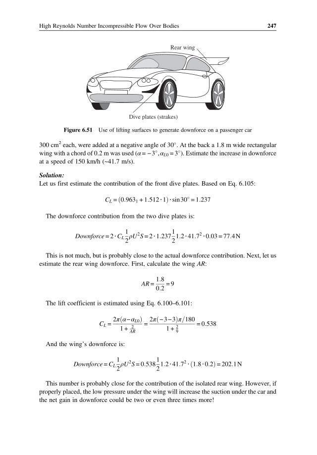
300 cm2 each, were added at a negative angle of 30 . At the back a 1.8 m wide rectangularwing with a chord of 0.2 m was used (α= −3 ,αL0 = 3 ). Estimate the increase in downforceat a speed of 150 km/h (~41.7 m/s).

Solution:Let us first estimate the contribution of the front dive plates. Based on Eq. 6.105:

CL = 0 9631 + 1 512 1 sin30 = 1 237

The downforce contribution from the two dive plates is:

Downforce= 2 CL12ρU2S= 2 1 237

121 2 41 72 0 03 = 77 4N

This is not much, but is probably close to the actual downforce contribution. Next, let usestimate the rear wing downforce. First, calculate the wing AR:

AR =1 80 2

= 9

The lift coefficient is estimated using Eq. 6.100–6.101:

CL =2π α−αL0

1 + 2AR

=2π −3−3 π 180

1 + 29

= 0 538

And the wing’s downforce is:

Downforce=CL12ρU2S= 0 538

121 2 41 72 1 8 0 2 = 202 1N

This number is probably close for the contribution of the isolated rear wing. However, ifproperly placed, the low pressure under the wing will increase the suction under the car andthe net gain in downforce could be two or even three times more!

Dive plates (strakes)

Rear wing

Figure 6.51 Use of lifting surfaces to generate downforce on a passenger car


6.11 Summary of High Reynolds Number Aerodynamics

The last three chapters discussed the possible simplification of the governing equations, theapplication of this approach to an inner viscous boundary layer model and to an outer invis-cid flow model. Only at the end of this discussion we can present a case demonstrating thecombined inner and outer solution (see Fig. 6.52). The calculated pressure distribution withthe potential flow assumption (dashed lines), and when accounting for the boundary layereffects (solid line), shows little effect and the lift is almost the same for both computations.The boundary layer calculations indicate transition from laminar to turbulent flow at about17% chord, while the flow on the lower surface is fully laminar. The small kink in the pres-sure distribution indicates the location of the transition point. This is the result of a “laminarbubble” – a local separation of the laminar BL and an immediate reattachment in the tur-bulent flow. Also, note the importance of the shape factor in identifying the location of thistransition. Boundary layer thicknesses remain very small, and this is the reason for the smalldifference between the potential and the combined flow calculations.

–2.0

–1.5

–1.0

–0.5

θδ*

0.5

NACA 0012

Transition

upper

Cp

0.0

1.0

1.0

0.00

0.015

0.010

0.005

0.0000.20 0.40 0.60 0.80 1.00

H

4.0

3.0

1.0

2.0

0.0

α= 5°Re = 106

Cl = 0.57Cd = 0.0086

XC

Cf

Figure 6.52 Combining the results of inner boundary layer with the outer potential flow model for aNACA 0012 airfoil. Pressure distribution is shown (top) along with the boundary layer parameters onthe upper surface


The importance of combining the viscous and the inviscid solutions, at the lower angles ofattack, is for better estimates of skin friction drag (for attached flows). At higher angles whenthe flow separates, the method allows a reasonable prediction of the stall angles but fails incalculating the separated flow itself.


The topics discussed in this chapter have important engineering implementations. The highReynolds number flow region includes a large variety of day to day applications, includingroad, sea, and airborne vehicles. From the mathematical point of view, the governing equa-tion can be simplified significantly. For example, the velocity field can be evaluated by sol-ving the uncoupled continuity equation. Then the pressures and fluid dynamic loads can becalculated as a second step using the Bernoulli equation (and not using the momentum equa-tion – e.g., Euler). Of course all this works for attached flows. However, the method of usingexperimental coefficients for the lift and drag forces facilitates acceptable engineering pre-diction capability, even for separated and turbulent flows.The force vector acting on a body moving through a fluid is traditionally divided into a

force parallel to the free-stream (drag) and into a normal component (lift). The modelingresults presented here lead to simple formulation for the drag on moving objects. Fortwo-dimensions we can write:

CD =CD0

and CD0 can be further split into drag due to skin friction and into form drag due to flowseparations. For the three-dimensional case a new element due to lift is added, the induceddrag (and this is true for shapes other than wings):

CD =CD0 +CDi

The lift of most objects (and certainly wings) depends on their angle of attack, and the cam-ber effects can be included as a zero lift angle αL0. The lift slope CLα is larger for widerobjects (and the largest for the two-dimensional case) and can be obtained via computationsor experiments. With these assumptions, the lift can be calculated as:

CL =CLα α−αL0

References6.1. Katz, J., and Plotkin, A., Low-Speed Aerodynamics, 2nd Edn, Cambridge University Press, NY, 2001.6.2. Kreyszig, E., Advanced Engineering Mathematics, 9th Edn, John Wiley & Sons, Inc., Hoboken, NJ, 2006.6.3. Polhamus, E. C. Prediction of vortex characteristics by a leading-edge suction analogy, J. Aircraft, Vol. 8,

No. 4, 1971, pp. 193–199.6.4. Hoerner, S. F., and Borst, H. V., Fluid Dynamic Lift, Hoerner Fluid Dynamics, Albuquerque, NM, 1985.


Problems

6.1. Prove that a two-dimensional source fulfills the Laplace equation. The source equationin Cartesian coordinates is:

Φ x,z =σ

2πln x−xo

2 + z−zo2

6.2. Prove that a two-dimensional doublet fulfills the Laplace equation. The doublet equa-tion in Cartesian coordinates is:

Φ x,z =−μ

2πx−xo

x−xo2 + z−zo

2

6.3. The velocity components of a two-dimensional vortex located at (x0, z0) are:

u =Γ2π

z−zo

z−zo2 + x−xo

2

w= −Γ2π

x−xo

z−zo2 + x−x0

2

Prove that these velocity components fulfill the continuity equation.6.4. Prove the following vector identity. Use two-dimensional Cartesian coordi-

nates q ∇q = −q ∇ q +∇q2

26.5. If the velocity potential of a two-dimensional flow is given by the function:

Φ =U∞cosθ r +R2

r

Then, around the circle r = R:a. Plot the pressure coefficient for the range of θ = 0 to 180 .b. Calculate the velocity and pressure coefficient at θ = 0, 90, and 180 .

6.6. The velocity potential of a two-dimensional flow is given by the function:

Φ = 5 x2−z2

a. Derive an expression for the velocity components (u, w) in the x-z plane.b. Sketch the streamlines in the first quadrant (e.g., x > 0, and z > 0).

6.7. The velocity potential of a free stream is Φ1 = 5x and for a doublet is Φ2 = 5x

x2 + z2a. Write the velocity potential for the combined doublet and free stream

(e.g., Φ=Φ1 +Φ2)b. Calculate the velocity distribution (u, w) due to this velocity potential.


c. Find the stagnation points along the x-axis.d. What kind of flow field is described by Φ?

6.8. The velocity potential in the first quadrant is given by Φ2 = 5 x2−z2 . Provide anexpression for the velocity vector along a line z = 2.

6.9. Asourceof strengthσ=10m2/s is locatedatapoint (5,1).Calculate thevelocity at (0,−2).6.10. Calculate the velocity induced by a doublet of strength μ= 1m3 s pointing into the

–x direction, at a point x = 1 and z = 1. The doublet is placed at (5, 2).6.11. A two-dimensional vortex with a circulation of Γ = 10 m2/s is located at a point (0,0).

Calculate the velocity at (10, 0).6.12. Calculate the velocity components (u, v, w) due to a semi-infinite (but three-

dimensional) vortex line with strength Γ = 1.0, at a point (0, 0, 0.5).

0

0.5

1.0

Γ

z

Py

x

Problem Figure 6.12

6.13. A two-dimensional vortex with strength Γ = 1.0 is placed at point (3, 3), as shown in thefigure. Find the value of the integral q dl along the spiral path circling twice the pointP.

0

0

1

2

3

z

P

ʃq dlΓ

1 2 3x

Problem Figure 6.13


6.14. Write down the expression for the combination of a free stream of velocity U∞ par-allel to the x-axis and a source of strength of K, placed at (5, 0). Also calculate thevelocity at a point (3, 3).

6.15. Find the location of the stagnation point (where the velocity is 0) for the flowdescribed in Problem 6.14.

6.16. Calculate the value of the integral c q dl for a vortex of strength Γ = 10 placed at theorigin. The path and direction for the integration is shown in the sketch.

–4 –3

–3

–2

–2

–1–1

1

1

2

Γ

3

2 3 4 x

Problem Figure 6.16

6.17. Consider the two-dimensional flow along a wall with a circular hump of radius R,as shown.a. What is the velocity potential for such a flow?b. Calculate the lift coefficient due to the upper surface of the semicircular hump.

R

U∞

Problem Figure 6.17

6.18. What is the velocity and the corresponding pressure distribution on the “floor” behindthe semi-cylinder shown in Problem 6.17 (at r >R, where rmeasures the distance fromthe center of the cylinder)?

6.19. Calculate the force on the floor (between R and∞) for the flow in Problem 6.17.Whatis the direction of this force (up or down)?

6.20. Consider the two-dimensional flow along a wall with a circular hump of radius R = 5and a free-stream velocity of U∞ = 10 m/s.a. What is the velocity potential for such a flow?b. Calculate the velocity (u, w) at a point: (−5, 0).c. Calculate the velocity (u, w) at a point: (0, 5).d. Calculate the velocity (u, w) at a point: (10, 10).


6.21. Consider the two-dimensional flow along a wall with a circular hump of radius R = 5and a free-stream velocity of U∞ = 16 m/s.

Z

U∞

XR

Problem Figure 6.21

a. What is the velocity potential for such a flow?b. Calculate the velocity (u, w) at a point: (−10, 0).c. Calculate the velocity (u, w) at a point: (0, 15).d. Calculate the pressure coefficient at these two points.

6.22. Consider the two-dimensional flow over a cylinder of radius R = 5, at a free-streamvelocity of U∞ = 15 m/s. Assuming the cylinder rotates and creates a circulation ofΓ = 50 m2/s.a. Calculate the angle of the stagnation points.b. Calculate the pressure coefficient at a point (0,15).

6.23. Consider the two-dimensional flow due to a source of strength σ and a vortex ofstrength Γ, placed at the origin.a. What is magnitude and the direction of the velocity at a point (r = R, θ = 0)?b. What is the angle between the radial and tangential velocity (does it change

with r?)? Sketch the angle at (r = R, θ = 0).6.24. The velocity potential in the x-z coordinates is given as

Φ = 5x+5x

x2 + z2

a. Sketch this flow field (stream lines).b. What is the velocity at a point (1, 0)?c. What is the velocity at a point (10, 0)?d. What is the velocity at a point (0, 1)?

6.25. Water flows horizontally, at a velocity of 10 m/s, against a cylinder of radius R =20 cm. Using the potential flow formulas, estimate the pressure difference betweenthe far field and points A and B.

A

B

RU∞

Problem Figure 6.25


6.26. A U∞ = 20 m/s wind is blowing over an R = 5 m cylinder, as shown in the figure.

U∞= 20

Z

— R

X

= 5ms

Problem Figure 6.26

a. What is the velocity potential for this flow?b. What are the velocity vector components outside the cylinder?c. Calculate the velocity at a point (0, 10).d. Calculate the velocity at a point (30, 0).e. Calculate the pressure coefficient at a point (0, −5).

6.27. The pressure distribution on the lifting airfoil of a hydrofoil boat is shown in thesketch. Assuming the boat operates in a 40 C warm, fresh/sweat water and the foilis about 1 m below the water surface estimate at what speed would cavitation begin(and where)? (The vapor pressure from Fig. 1.14, at 40 C, is about 0.1 atm.)

1.0

0.0

Cp

0.5 1.00.5

0.0

–0.5

–1.0

–1.5

–2.0

xc

xc

Problem Figure 6.27

6.28. A 40 km/h wind is blowing parallel to a storage unit, as shown in the sketch. Estimatethe normal force on a 0.5 m high and 1 m long window, if the front door was left open.Assume the wind speed along the outside of the window is 1.2U∞ and take air densityfrom Table 1.1.

1 mU∞

0.5 m

Problem Figure 6.28


6.29. A tall, cylindrical chimney has a 3 m diameter. Assuming wind speed is 40 m/s, cal-culate the Re number and vortex shedding frequency. What is the distance betweentwo subsequent vortices? μ= 1 8 10−5N s m2 ρ = 1 2 kg m3 .

6.30. A long cylindrical antenna of 4 mm (0.004 m) diameter is mounted vertically on avehicle moving at 100 km/h. If the Strouhal number is estimated at 0.18, then calculatethe vortex shedding frequency. Also, calculate the length in cm between two adjacentvortices (e.g., the spacing).

6.31. Calculate the vortex shedding frequency from a 8 cm diameter vertical exhaust pipemounted on a truck traveling at 100 km/h. What is the distance between two cycles?(Use air properties from Table 1.1.)

6.32. The antenna of a car traveling at 90 km/h is resonating (vibrating violently) at a fre-quency of 500 Hz. Estimate the antenna’s diameter (or which diameter should beavoided).

6.33. Estimate the wind forces on a billboard 10 ft high and 30 ft wide when a 50 mph windis blowing normal to it.

6.34. Calculate the resistance force when a 1 m diameter submerged disk is towed behind aboat at a speed of 5 m/s. Assume the disk is perpendicular to the stream.

6.35. A large 1.9 m wide and 0.5 m high plate is carried above a truck perpendicular to thevehicle motion (like a flat plate normal to the free stream). Calculate theadditional power required to carry the plate at a speed of 72 km/h. Use the air proper-ties from the previous problems and estimate the drag coefficient from tables inthe book.

6.36. Assuming a person’s drag coefficient is CD ~ 1.2, frontal area is 0.55 m2 and air den-sity is 1.2 g/m3. Calculate the wind forces on his body when the stormy wind speedreaches 108 km/h.

6.37. A bicyclist is coasting down a hill with a slope of 8 into a head wind of 5 m/s (meas-ured relative to the ground). The total mass of bicycle and rider is 80 kg and thecoefficient of rolling friction is 0.02. Assuming that the frontal area is about 0.5m2 and the drag coefficient is about 0.5, calculate the bicycle speed. (For air, use:μ = 1.8 10−5 N s/m2, ρ = 1.2 kg/m3).

6.38. A 0.7 cm diameter telephone wire is stretched between two poles, set 40 m apart. Atwhat wind speed (blowing normal to the wire) will the wire “sing” at a frequency of450 Hz? Also calculate the drag on the wire (use air properties from Table 1.1).

6.39. A 7 cm diameter hockey ball is launched at a speed of 50 m/s and a spin rate of1000 RPM. Estimate the lift and drag forces, based on Fig. 6.30, and use the airproperties from Table 1.1.

6.40. A soccer player kicks a 22 cm diameter ball at a speed of 30m/s and a spin rate of 1000RPM with the intention to create a curved trajectory. If the ball weight is 0.45 kg,estimate the percentage of the resulting side force to weight ratio. (Estimate the liftforce based on Fig. 6.30 and use the air properties from Table 1.1.)

U∞ω

Problem Figure 6.40


6.41. The wingspan of the first successful human powered airplane was about 30 m and thewing chord was 2.2 m. If the structural weight is about 32 kg and the pilot weight is68 kg, calculate the lift coefficient and the induced drag coefficient. If the additionalviscous drag is CDO = 0.01, calculate the power required for a steady cruise at a speedof 16 km/h (use the elliptic wing equations and air properties from Table 1.1).

Problem Figure 6.41

6.42. A large cruise ship is cruising at an average speed of 40 km/h and the power suppliedto the propellers is 42 MW. The sunken frontal are of a cruise ship can be estimated at340 m2, and the propulsion efficiency is about 0.8. Based on these numbers, estimatethe hull drag coefficient.

6.43. Calculate the drag force on the ship under the conditions in Problem 6.42.6.44. The frontal area of a 58 m long blimp can be approximated by a circle with an 8 m

radius. If the drag coefficient is CD = 0.07, estimate the power required to cruise at60 km/h (use air properties from Table 1.1).

Problem Figure 6.44

6.45. The combined weight of a parachute and the jumper is 80 kg. Calculate the requiredchute diameter for a desirable sinking speed of 5m/s (take air properties fromTable 1.1).

6.46. A 80 kg (combined weight) skydiver jumps out of an airplane with his head initiallypointing down.a. Calculate his terminal speed at this condition when his frontal area is about 0.22 m2

and the drag coefficient is 1.3.b. After a while he changes into a prone position (looking down) and his frontal area

is 0.8 m2 with a drag coefficient of 1.2. What is his terminal speed?c. Finally, a 7 m diameter parachute opens; estimate his descent speed.(Take air density from Table 1.1.)

6.47. A steel ball of 3 mm diameter was dropped into a 0.5 m deep container filled withmotor-oil. Assuming that the ball sinking speed is the same from the moment it hits


the oil surface, calculate how long it will take for the ball to sink to the bottom of thecontainer? Note that the density of Steel is ρ = 7850 kg/m3 and the properties of oil aretaken from Table 1.1. Also, calculate the Reynolds number.

6.48. A student is rolling down a slope of 5 with his skateboard. Neglecting the friction inthe wheels and assuming he weighs 70 kg, his frontal area is 0.7 m2, and his dragcoefficient is 1.1, calculate his terminal velocity (ρ = 1.2 kg/m3).

6.49. The frontal area of a small motorcycle is 0.60 m2, its drag coefficient is 0.62, and itsmaximum speed is 150 km/h. Next, the driver lowers his head and effectively reducesthe frontal area to 0.58 m2, and the drag coefficient to 0.60. Assuming the power of theengine is unchanged, estimate the new maximum speed (ρ = 1.2 kg/m3).

Problem Figure 6.49

6.50. A 50 km/h wind is blowing on a 10 m tall pole of 0.2 m diameter.a. Calculate the Reynolds number (ρ = 1.22 kg/m3, μ = 1.8 10−5 Ns/m2).b. Calculate the Strouhal number, based on Fig. 6.27, and the drag coefficient from

Fig. 6.19.c. What is the wake oscillation frequency f ?d. And the total drag of the pole?

6.51. Air is drawn into a wind tunnel during automobile testing, as shown in the sketch.A simple manometer measures the velocity in terms of water column height h =7 cm. If the drag coefficient of the car is CD = 0.4, and its frontal area 1.5 m2, calculatethe drag force acting on the vehicle. (ρwater = 1000 kg/m3, ρair = 1.22 kg/m3).

Wind tunnel

Water

U

pa

pah

Problem Figure 6.51


6.52. Air is drawn into a wind tunnel during automobile testing, as shown in the sketch fromProblem 6.51. A simple manometer measures the velocity in terms of water columnheight h = 8 cm. The vehicle weight is 1500 kg, its frontal area is 1.5 m2 and the dragforce measured in this test is 50 kgf.a. Calculate the drag coefficient (ρwater = 1000 kg/m3, ρair = 1.22 kg/m3).b. Calculate the power required to overcome the aerodynamic drag at the test speed.c. Suppose the vehicle is driving up on a slope of 3 at the same speed; how much

additional power is required?6.53. A 650 kg racecar was attached to a wind tunnel ceiling as shown in the sketch. Next,

airspeed was increased up to a point (and beyond) when the aerodynamic forces couldkeep the car attached to the ceiling.a. If the lift coefficient of the car is CL = −3.0, and its frontal area is 1.5 m2, calculate

at what speed the aerodynamic forces are equal to its weight.b. What is the water column height h in the manometer measuring the tunnel

speed? (ρwater = 1000, ρair = 1 22kg m3)

Wind tunnel

Water

U

pa

pa

h

Problem Figure 6.53

6.54. A 0.1 m diameter cannon ball is flying at 150 m/s and spins about a horizontal axisat 3600 RPM. Based on Fig. 6.30, estimate the vertical force on the ball. Use ρ =1.1 kg/m3.

6.55. An airplane has a rectangular wing with an elliptic spanwise loading. The mass of theairplane is: 1200 kg and its wing area is 20 m2, wing span is 14 m and it is flying at aspeed of 60 m/s. If the form drag is 0.01, calculate the total drag (e.g., calculate theinduced drag) and the power required to propel the airplane. Use ρ = 0.88 kg/m3.

6.56. The rectangular roofof a carport is 2mwideand6mlongandhasan incidenceangleof5 .If a 20m/swindblows, as shown in the sketch, calculate the lift force on the roof.Approx-imate the lift coefficient by using the elliptic wing formula, and use ρ = 1.2 kg/m3.

U5°

2 m

Problem Figure 6.56


6.57. The students built a small airplanewith a rectangularwinghavinga spanofb=1.5manda chord of 0.4m.Theydesigned it to fly at a speed of 60 km/h, and thewing is at an angleof α = 1 relative to the free stream. If the zero lift angle αLo = −5 , then calculate the liftcoefficient (assume ρ = 1.2 kg/m3). Also, calculate the weight of the airplane.

6.58. After experimentingwith the above airplane the students found that it cannot fly at angleslarger than α = 10 (or it stalls). Calculate the lowest flight speed called “stall speed”.

6.59. Let us approximate the wing of the Concord airplane by a triangle with a span of25.6 m and a root chord of 27.6 m. Calculate the wing aspect ratio, wing area,and lift line slope CLα (based on the equation given for slender wings). Supposethe airplane takes off at α = 17 and at a speed of 300 km/h – estimate its weight(use ρ = 1.2 kg/m3).

6.60. The space shuttle orbiter lands at about 340 km/h and weighs about 100 tons. Approx-imating the wing shape with a triangle of 18 m span (the actual span with the fuselageis 23.8 m), and an area of 220 m2. Calculate the angle of attack during landing (use theequations for slender delta wings at high angle of attack and ρ = 1.2 kg/m3).

6.61. A 2 2 m glass plate is carried on top of a pick-up truck. As the car travels at 80 km/hthe vehicle hits a bump and the angle of the glass relative to the free stream is about 5 .Calculate the aerodynamic force lifting the glass (ρ = 1.2 kg/m3).

6.62. John bought a 1 mwide and 2.5 m long door and decided to bring it home on top of histruck (he also placed it a 4 angle of attack). If his maximum speed on the highwaywas 100 km/h, calculate (ρ = 1.22 kg/m3, μ = 1.8 10−5 Ns/m2):a. The lift and induced drag coefficients of the door (assuming no interaction with

the cabin).b. The drag coefficient due to skin friction (use the Blasius formula for Cf ).c. The total lift and drag on this surface.

U4°

1 m

Problem Figure 6.62

6.63. A hydrofoil boat weights 10 tons and when fully submerged its maximum frontal area(of the submerged portion) is S = 1.5 m2. When the hydrofoil is retracted, the boat’smaximum speed is 20 km/h. Assuming a drag coefficient of CD = 0.2 (based on S)calculate the following:a. The power required to propel the boat with the hydrofoils retracted.b. Suppose the boat can use two hydrofoils with a chord of 0.5 m and 2 m wide. Then

calculate the maximum speed of the boat using the same power as in (a). Estimatethe lift and drag of the hydrofoils by using Eqns 6.101 and 6.102 (with δ= 0) andassume the angle of attack is 10 .


0.5 m 0.5 m

Problem Figure 6.63

6.64. A large bird is soaring horizontally at a speed of 25 km/h. We can approximatethe wing span at about 0.6 m and wing chord at 0.12 m. Assuming that air densityis ρ = 1.2 kg/m3, angle of attack is 10 , and using the lift coefficient formulas devel-oped for finite wings (elliptic), calculate the lift coefficient. Also, calculate the bird’sweight.

U

10°

Problem Figure 6.64

6.65. A 70 kg ski jumper leaves the ramp at a speed of 120 km/h and at this position, hisbody is at a 30 angle of attack relative to the free-stream. Calculate the lift, by com-paring his body to a 0.6 m wide and 1.8 m long plate, and using the formulation ofEq. 6.105 (use air density from Table 1.1).

6.66. A small airplane weighs 1.5 ton and it flies at sea level at a speed of 270 km/h. Its wingcan be approximated by a 10 m wide and 1.6 m chord rectangle.a. Estimate the required lift coefficient and power to overcome the induced drag (use

δ2 = 0, and air density from Table 1.1).b. The power of the engines is about 150 kW, what percentage of available power is

needed to overcome the induced drag?6.67. It is said that some racecars develop so much downforce that they can run on an

inverted (upside down) road. If a 750 kg racecar frontal area is 1.5 m2 and its lift coef-ficient is −3.5 (downforce), then how fast should it go in order to be able to driveupside down (e.g., on the ceiling)?

6.68. The pressure coefficient distribution on the upper and lower surfaces of a two-dimensional lifting surface is approximated by a straight line, as shown in the sketch.Calculate the lift coefficient and the center of pressure.


–3

Upper surface

Lower surface

c/2 c x

–2

–1

Cp

0

+1

Problem Figure 6.68

6.69. The chord of the lifting surface shown in the previous figure is 1m and the free-streamspeed is 50 m/s. Calculate the lift of the lifting surface (assume standard airconditions).


7Automotive Aerodynamics:Examples

7.1 Introduction

The analytic solution of the flow over practical vehicle configurations is quite complexand beyond the scope of this text. A possible approach, presented in Fig. 6.25, is to pro-vide an experimental range for the lift and drag coefficients of several generic shapes, sothat preliminary estimates on the magnitudes of these coefficients can be made. For exam-ple, a streamlined shape may have a drag coefficient of 0.15 while a flat plate, perpen-dicular to the free stream, may create a drag coefficient of about 1.2 (based on the frontalarea). For more complicated shapes, however, identifying the contribution of the differentgeometries to the total force coefficients must be clarified. The intention in this chapter isto provide examples of vehicle aerodynamics that can guide future engineers in under-standing the sources of lift and drag, and consequently they will be able to improvethe designs they work on. Naturally, only a short list of vehicles will be discussed hereand for a wider range of vehicles and for more specific details the reader is referred topublications such as Ref. 7.1–7.3. Returning to aerodynamics, the most important “obser-vations” regarding road vehicles is that they move close to the ground, have rotatingwheels, have regions of flow separation, and generate vortex flows. These features resultin “nonlinear” effects, which are hard to model, but provide an opportunity to introduceseveral important aerodynamic mechanisms. Also, automotive aerodynamics is not lim-ited to external aerodynamics and includes elements such as engine cooling, internal ven-tilation, air conditioning, aerodynamic noise, vehicle high-speed stability, dirt deposition,and more! In the following examples we shall focus on external aerodynamics only andmost results will be based on experimental data.


7.2 Generic Trends (For Most Vehicles)

The shape of a vehicle moving close to the ground forces the air particles to change velocityand direction resulting in a complex pressure distribution over the surface (see Fig. 6.1).Knowledge of the pressure distribution allows the location of cooling/ventilation inlets (highpressure) or exits (low pressure). The integration of the pressure and shear force distributionover the whole vehicle surface results in forces and moments (and at this level the focus ismainly on the aerodynamic drag and lift). The importance of vehicle’s aerodynamic dragand its effect on fuel consumption was realized as soon as the early automobiles started roll-ing. This was demonstrated in Fig. 1.2, which clearly shows that vehicle’s rolling resistancebecomes negligible at speeds of over 100 km/h. Furthermore, driving power to overcomeaerodynamic drag increases with the cube of speed:

P=D U =CD 0 5ρU3S 7 1

Therefore, driving power requirements and fuel-consumption-reduction depend strongly onvehicle drag coefficient times its frontal area. The importance of vehicle lift (or lack of it)was realized much later (in the 1960s) and its effect on vehicle handling and cornering wasimmediately understood. To demonstrate the relevant range of these coefficients, let usrepeat a portion of Fig. 6.25 in Fig. 7.1.The first configuration represents a streamline-shaped body without flow separation. If

the flow is completely laminar, a drag coefficient close to 0.025 can be expected, but in mostcases transition to a turbulent boundary layer is present and a typical drag coefficient of 0.04

1

2

3

4

Low dragbody of

revolution0

0.18

0.28 0.35

0.75–3.00

0.15

0.04

CL CD

Low drag vehiclenear the ground

Genericautomobile

Prototyperace car

Figure 7.1 Generic range of the lift and drag coefficients (based on frontal area) for ground vehicles

263Automotive Aerodynamics: Examples

is shown in Fig. 7.1. For such a symmetric body, far from the ground, no lift force isexpected. Keeping a streamlined shape, but bringing it close to the ground and addingwheels increases the drag to a level of CD = 0 15, but the long boat tail is impractical formost vehicles. Also note that this geometry, (as in Fig. 7.1) produces a significant levelof lift. For practical sedan configurations (as shown in the figure) both the drag and liftincrease significantly, beyond the level of the streamlined shape. Finally, a high downforceprototype racecar shape is added to demonstrate the extreme range of the drag and lift coef-ficients. The high downforce for such racecars is needed for better tire adhesion (resulting infaster laps) as will be explained later in this chapter. The large increase in drag is a result ofthe increased negative lift (downforce) and it resembles the induced drag dependency on lift(similar to the relation presented by Eq. 6.102).Before discussing the effects of various vehicle components on the aerodynamic coeffi-

cients, let us observe some generic trends affecting the complete-vehicle aerodynamics. Themost important among those affects is the ground effect and vortex flow.

7.2.1 Ground Effect

The flow over a body will change when it is close to a boundary, and in case of groundvehicles the streamlines close to the ground are eventually forced to be parallel to the road.This “ground effect”was observed early in the twentieth century during takeoff and landing,when airplanes flying close to the ground experienced increased lift. Consequently, theattached-flow over an airfoil, in ground effect was studied and it was found that the increasein force is present for both positive and negative lifting airfoils. A typical variation of thenegative lift and the drag coefficients versus ground clearance for an inverted wing is shownin Fig. 7.2. As noted in Section 6.10 the wing lift depends on its aspect ratio (AR) and ingeneral the wing’s lift will increase with AR. Therefore, the values for the lift in Fig. 7.2 aresmaller than in the two-dimensional case. Clearly, both lift (negative in this case) and dragincrease as ground clearance is reduced, but at a very small clearance the trend stops (thismay be called stall). Of course, at a very small ground clearance, the boundary layer in thenarrow gap between the airfoil and the ground slows down the flow and stalls the aftsection of the airfoil (resulting in a reduction in the downforce). Also, when h= 0, thereis no flow under the airfoil!The airfoil example provides a quantitative demonstration of ground effect for the

attached flow case. However, ground vehicles have less streamlined shapes and to investi-gate ground effect for automobile shapes, let us consider the two generic bodies (with ratiosresembling road vehicles) shown in Fig. 7.3, whose shapes are based on elliptic sections(both have the same frontal area and volume) and measure their lift and drag as theyapproach the ground. These geometries represent two basic automobile styling trendsobserved over the years: (1) styling that tries to block the flow under the vehicle and (2)styling that tries to push as much air as possible under the car. Both styling schools can createreasonably low drag coefficients, but if high downforce is sought, the latter approach is moreattractive. Returning to Fig. 7.3, in case of the symmetric ellipsoid, decreasing the groundclearance will cause the flow to accelerate under the body, creating more downforce


(remember Bernoulli’s equation stating that faster speed results in lower pressure). Ofcourse the drag will increase too, due to flow separation behind the ellipsoid and due toinduced drag. This trend (for the lift) is reversed in the flow over the semi-ellipsoid becausethe reduction in ground clearance tends to block the flow under the body (as a result of thesharp edges surrounding the lower surface). The drag force follows a similar trend to that ofthe symmetric body, but in this experiment somewhat lower drag values were obtained forthe semi-ellipsoid.In many passenger cars, rear wings or spoilers are added to increase downforce (or reduce

lift). This interaction can be demonstrated when mounting a rear wing to the generic ellip-soid shape of Fig. 7.3 (having a smooth underbody). The expected streamlines and the par-tial flow separations at the rear are depicted in the upper part of Fig. 7.4. When an invertedwing is added at the back, the flow under the ellipsoid accelerates as a result of the lowerbase pressure (at the back), induced by the wing. The higher speed causes more downforceon the body, apart from the downforce created by the wing itself. Furthermore, on manyoccasions, the high-speed flow created near the wing partially reattaches the flow on thebody, reducing the area of flow separation. This simple example demonstrates why propermounting of a rear wing can increase the downforce of a vehicle more than the expected liftof the wing itself!

7.2.2 Generic Automobile Shapes and Vortex Flows

Vortex flow was discussed in Chapter 6 and the three-dimensional wing formulation(Section 6.10.6) provided practical examples, showing the formation of wing tip and trailing

1.80

1.70

1.60

1.50

1.40

1.30

1.20

1.10

1.00

0.90

0.80

CL

CD

CD

h

0.0 0.1 0.2 0.3 0.4

h/c

0.5 0.60.02

0.04

0.06

0.08

0.10

0.12

0.7

–CL

0.70

Figure 7.2 Effect of ground clearance on the lift and drag of an AR = 5 wing (GAW −2 airfoil atAlpha = 1 . Re ~ 0.2 106, Adapted using data from Ref. 7.4)


vortices. In fact, vortices can emerge on various areas on a moving vehicle as a result of localshear, pressure or velocity differences in the flow. Some typical flow fields over genericbodies with quite sharp corners, resembling a variety of road vehicles are presented inFig. 7.5. In order to reintroduce this concept of vortex-dominated flows, let us return tothe discussion on slender flat-plates at an angle of attack (see Fig. 6.45). The main aspectof this flow field, relevant to the present discussion, is the formation of two concentrated sideedge vortices that dominate the nearby flow field (Fig. 7.5a). These two vortices induce highvelocity on the plate (under the vortices), creating strong suction forces, which considerablyincrease the lift of the flat-plate wing.

hL

0.4

0.2

L

L

h

Frontview

CD

CD

CL

CL

h

Length/max. height = 3.6Cross section aspect ratio = 1.25ReL = 0.5 ·106

Frontview

0.0

–0.2

–0.4

–0.6

0.4

0.2

0.00.0 0.05 0.10

Figure 7.3 Effect of ground clearance on the lift and drag coefficients of two generic ellipsoidshaving the same width: height ratio (1.25) and length/height ratio (3.6). Also maximum thicknessis located at one-third of the length. Reprinted with permission from SAE Paper 920349.Copyright © 1992 SAE, Inc.


More down force

Figure 7.4 Effect of adding a rear wing to a ground vehicle

A-pillar

vortex flow

(a) Flat plate at angle of attack

(c) “Three box” body (d) Tapered lower surface

(e) Basic venturi (f) Flow near A pillar

Separated flow

(b) Slanted upper surface

U∞

U∞

Mirror wake oscillatious

Figure 7.5 Vortex flow on some generic automobile shapes


Interestingly, a similar situation develops when slanting the rear, upper surface of ageneric body (Fig. 7.5b). This vortex-dominated flow is present for a slant-angle rangeof 10–30 (slant angle is measured relative to a horizontal line – see definition in Fig. 7.6).Another typical pattern of flow-separation, frequently found on three-box-type sedans isdepicted in Fig. 7.5c. In this case a separated bubble, with locally recirculating flow (vortex),is observed at the front, along the junction between the bonnet and the windshield. The largeangle created between the rear windshield and trunk area results in a second, similar recir-culation area.When introducing a slanted surface to the lower aft section of the body (as in Fig. 7.5d), a

similar trend can be expected (to the one shown in Fig. 7.5b). This principle can be utilizedfor racecars, and for moderate slant angles (less than 15 ) an increase in the downforce isobserved. In the racing circuits, such upward deflections of the vehicle lower surface areusually called “diffusers”.However, a far more interesting case is when two side plates are added to create an under-

body tunnel, sometimes called Venturi (Fig. 7.5e). This geometry can generate very largevalues of negative lift, with only a moderate increase in drag. Furthermore, the downforcecreated by this geometry increases with smaller ground clearances, as is demonstrated later.

0.5

V∞0.4

0.3

0.2

0.1

0.5

0.4

0.3

0.2

0.1

0.0

–0.1

–0.20°

CL

Cp

CD

30°

θ

θ

–0.5 0.0y/b

0.560° 90°

I

I

I

–1.0 Region I

A

b A

Region II

–0.8

–0.6

–0.4

–0.2

II

II

II

(a) (b) (c)

Figure 7.6 Lift drag and lateral pressure distribution along the slant rear section of the configurationshown in Fig. 7.5b (after Morel, T, “The effect of base slant on the flow pattern and drag of three-dimensional bodies with blunt ends,” pp. 191–217, published in Sovran, G., Morel, T. and Mason,W. (Eds), Aerodynamic Drag Mechanisms of Bluff Bodies and Road Vehicles, Plenum Press 1978.Reproduced with permission of Springer Science + Business Media)


A closer look at the flow near a road car may reveal more areas with vortex flow and, as anexample, the A pillar area is shown in Fig. 7.5f. Themain vortex here is responsible for waterdeposition while driving in the rain and the rear viewmirror creates an oscillating wake, sim-ilar to the one behind a cylinder (see Section 6.8). The vortex flow in this area of the A pillarand the rearview mirror is also responsible for vortex noise during high speed driving.The flows depicted in the cases presented in Fig. 7.5b, d, and e deserves a closer examina-

tion, because of their relevance topractical automobile aerodynamics. For example, in the caseof the shape in Fig. 7.5b, this vortex-dominated flow is present only for slant-angles between10 and 30 , as indicated by the lift and drag data in Fig. 7.6 (mode I). At larger slant angles,however, the flowover thewhole rear base area is separated, as on a typical bluff body (see theschematic illustration at lower part of Fig. 7.6c), and let us call this condition – mode II.The corresponding lateral pressure distribution, along section AA, is shown at the lower

part of Fig. 7.6b. In case of the “mode I” flow, the two concentrated side vortices attach theflow near the body’s longitudinal centerline (see schematics in the upper part of Fig. 7.6c),effectively creating a lifting flow. The pressure distribution for this case (mode I) shows thelarge negative pressure peaks created by the vortices at the side of the slanted rear surfaceresulting in a force acting normal to the slanted surface (which can be resolved into lift anddrag). Once the slant angle is increased beyond the critical angle (~30 ) the flow separatescompletely, as noted (see again the lower part of Fig. 7.6c), and the pressure distribution isquite flat, as indicated by the curve (for mode II) in Fig. 7.6b.After this brief description of the pressure distribution, we can return to the lift and drag

data in Fig. 7.6a. As the slant angle is increased from zero, a positive lift will develop, whichincreases up to a slant angle of 30 . At slant angles larger than 10 the rearward projection ofthis negative pressure causes quite a large increase in drag, as shown in Fig. 7.6a. The mostinteresting feature of this data is that above a critical angle (close to 30 ) the vortex structurebreaks down and the drag and lift contributions of the slanted surface are much smaller. Thisfact has an effect on hatchback automobile design, where rear window inclination angleshould bemore than 35 or less than, say, 25 . Also, note that in this case the basic body (witha 0 slant – resembling a station wagon) has negative lift due to ground effect and less drag.To conclude the discussion on vortex flows over generic bodies, let us observe the forces

generated by the shape of Fig. 7.5e, as ground clearance is reduced. In this case too, twolarge vortices are created as the flow moves from outside, under the side plates, towardsthe underside of the body. The presence of the sideplates not only increases the vortexstrength but also “protects” the low pressure area under the car (e.g., increase downforce).The resulting lift and drag coefficient data (Fig. 7.7) show similar trends to the ground effectin Fig. 7.3. For such shapes (with automobile geometrical ratios) the rear slanted area is usu-ally called the “rear diffuser”.

7.3 Downforce and Vehicle Performance

Up to this point, possible benefits due to drag reduction (e.g., fuel saving) were discussed,and the importance of aerodynamic downforce was mentioned, but not explained. There-fore, in this section, the effect of downforce on (high-speed) performance is discussed


briefly. The resultant aerodynamic loads acting on a road vehicle may be described by threeforce and three moment components (e.g., in Cartesian coordinates). At this introductorylevel, however, effort was made to reduce the discussion to only the drag and lift compo-nents. However, the effects of lift (or downforce)are easier to explain by introducing the sideforce and yawing moments acting on a vehicle and its tires.Figure 7.8 schematically depicts the sideforce generated by a tire as its slip sideway at an

angle β (also note the definition of forces in the inset). Initially the force increases linearly,up to a point where the maximum friction coefficient is reached. The friction coefficient isdefined as the ratio between the vertical load and the horizontal friction force:

μtire =Fy

Fz7 2

A diagram similar to Fig. 7.8 can be defined for acceleration and braking and in these con-ditions the slip is the ratio between tire contact speed versus forward velocity (see Ref. 7.3,p. 159). Next, let us compare two cases, the first when the vertical force on the tire is 200 kg(due to vehicle weight) and a second case when the aerodynamic downforce increases thenormal load to 300 kg, and assume that other tire characteristics are not affected much bythis change (in reality the maximum available friction coefficient is reduced somewhat withincreased downforce). Now, point A (in Fig. 7.8) represents a condition when the vehicle

0.9U∞ 10°

–CL

CD

h

L

0.8

0.7

0.6

0.5

0.4

0.3

0.2

0 0.05 0.1 0.15

h/L

0.2 0.25 0.3

Figure 7.7 Lift and drag variation versus ground clearance for the geometry described in Fig. 7.6e(Adapted from data in Ref. 7.5)


without aerodynamic downforce corners and due to its weight the normal force on the tire isFz = 200 kg. If, due to aerodynamic loads, the normal force is increased by 50% (to Fz = 300kg), then the same side force can be created at about 50% less sideslip (shown by point B).This means that a vehicle using aerodynamic downforce will preserve its tires and reducetheir heating and wear due to friction (slip). On the other hand, for maximum performancethe largest possible force is sought and then point C represents a condition with the same tireslip as in A, but now the vehicle with the aerodynamic downforce is turning faster (or brak-ing harder when longitudinal slip is considered).This short description demonstrates the increased tire performance due to aerodynamic

downforce (e.g., increased horizontal forces without an increase in vehicle’s mass). How-ever, there is an additional benefit of using downforce; to improve vehicle stability! Let ususe the simplistic description in Fig. 7.9 where the forces on the four tires, due to amomentary sideslip are depicted. In this case the vehicle is moving forward at a velocityV in the direction shown, but due to a perturbation, it slips sideways at an angle β. Con-sequently, the four tires will produce friction forces, as shown by the arrows in this figure.Of course the side force of each tire is related to the vertical load on it and on the tirefriction coefficient.Let us consider two cases, based on the moments acting on the vehicle (about the center of

gravity). For the first case, assume that the product of the forces acting on the rear tires Fr

multiplied by their distance from the center of gravity lr is larger than the same product of thefront tires:

Fr lr >Ff lf

300

200

100

0

0 5 10

AB

C

Slip angle, β, deg

Sliding

Linearrange

Directionof travel

Fz = 300 kg

F y [

kg]

Fz = 200 kg

z

yxFz

Fyv

β

Ω

Direction ofheading

15

Figure 7.8 The effect of increased normal (vertical) force on tire lateral performance


In this case, the resulting moment about the center of gravity acts to reduce the sideslip angleand to straighten the vehicle into the initial direction of V. The immediate conclusion is thatsuch a condition is statically stabilizing (and positive momentM is defined in the direction ofpositive β).

dM

dβ= −Fr lr +Ff lf < 0 Stable 7 3

The second condition of interest is when the resultant moment acts in the direction of thesideslip angle β (e.g., Fr lr <Ff lf ). In this case the forces will increase and tend to rotate thevehicle further – therefore, this condition is statically unstable.

dM

dβ> 0 Unstable 7 4

During cornering, a statically unstable vehicle tends to oversteer, while the statically sta-ble vehicle will understeer. The complete vehicle dynamics is far more complicated andmore information can be found in references such as Ref. 7.6.Now let us return to the discussion about aerodynamic downforce. The yawing moment

shown in Fig. 7.9 can be easily affected aerodynamically by increasing the verticalload on the wheels (e.g., tires). For example, if a vehicle tends to be slightly unstable,the addition of rear downforce can increase the available side force of the rear tires and con-sequently stabilize the vehicle (and also make it safer to drive). These effects become moreimportant at higher speeds, as in the case of racecars driving close to the tire maximumfriction coefficient. This also explains why sports cars with mid engines (and aft locationof center of gravity) use wider titers at the back to counter the shorter moment arm lr.

l f

l r

Front force

Rear force

V

β

Figure 7.9 Schematic description of the forces on vehicle tires as a result of a momentary sideslip β


Additional advantages of aerodynamic downforce prevail, even during acceleration andbraking because of the increased vertical force on the tires and due to the correspondingincrease in maximum tire adhesion. This can result in shorter braking distances and fasterexits from turns. Based on numerical simulations, Fig. 7.10 shows the reduction in lap timesof a prototype racecar, around a closed loop road circuit (Portland, Oregon). Note that thefastest lap requires a lift coefficient of about −3.0, but only a downforce of CL = −2.1 couldbe obtained with the racecar analyzed in this diagram.As expected, the increase in downforce also increases the vehicle drag and maximum

speed will be reduced. The increase in drag due to increased downforce resemblesEq. 6.102, which was developed for induced drag estimates. Based on the inset in Fig. 7.10,for this particular racecar the relation was:

CD =CD0 + k CL +CL02 7 5

Here, CD0 and CL0 stand for the baseline vehicle coefficients without the rear wing, and k isthe experimental polar coefficient (see actual values in the inset to Fig. 7.10).In conclusion, the increased downforce increases the average speed in a closed circuit,

mainly due to faster braking and cornering, and faster exits from sharp corners (in spiteof the increased drag and reduction in maximum speed).Amazingly, this fact was realizedonly in the mid-1960s, and for the first 65 years of motor racing aerodynamics was more of

1

55

56

57

58

59

Lap

tim

e (s

ec)

60Lap time

CD = 0.04 (CL- 0.2)2+ 0.3

Portland (1.915 miles)

1

23

4 5

–LD

6

78

9

1991 Pole position56.4 sec/123.1 mph

61

62

0 –1

–1

0

1

2

3

4

5

–2

CL

–3 –4 –5

–LD

Figure 7.10 Effect of aerodynamic downforce on the lap times of a prototype racecar. The roadcourse shape is shown by the inset. Reprinted with permission from SAE 920349, Copyright© 1992 SAE Inc.


an art and designers were influenced more by styling and perhaps looked a bit on drag reduc-tion (and meeting cooling requirements). The huge puzzle is, why no one noticed the tre-mendous advantage of creating downforce on the tires without increasing the vehicle’smass. The anecdotal story mentions a group of GM engineers flying to a track-test andone of the “managers” looked at the airplane’s wings and suddenly the light bulb lit on.If an airplane wing can lift such a heavy craft, why can’t we use a wing to lift the racecar(to go faster than the Ford GT40 in LeMans)? So if the boss wants a wing, the engineers didit, but they inverted it to push the vehicle down. As a result, sometime in mid-1964 theyadded front and rear spoilers to the Chaparral 2 (a later version with a wing is shown inFig. 7.21) to check the idea and, guess what, the idea worked well. Naturally, the momentthe concept was digested, numerous solutions to generate downforce, in form of invertedwings and suction fans were proposed.

7.4 How to Generate Downforce

Both Figs 7.1 and 7.3 show that generic shapes with typical automobile proportions producelift, which based on the previous section has a detrimental effect on performance (or what wecall “handling”). Therefore, let us list some of the more popular options to reduce the aer-odynamic lift or even create downforce and group then into two categories:

1. The simplest method would be to use the shape of the vehicle so that it produces down-force. This usually requires the contouring of the underbody. Some of the options are:a. Ground effect, as suggested by Fig. 7.2 and 7.3.b. Rear diffuser (sometimes called the Venturi), as in Fig. 7.7.c. Underbody tunnels (which are a combination of the previous two).d. Vacuum cleaner: Sealing the whole lower part of the vehicle and creating low pres-

sure by suction.2. Downforce can be generated by adding negative lifting devices such as:

a. Inverted Wingsb. Splitter platesc. Dive platesd. Louverse. Vortex generators.

Most of the add-ons (category 2) were developed for competition cars; however,designers of recent automobiles are placingmore attention on the options listed in category 1.Examples for most of these devices will be presented later in this chapter, in the discussionabout the various vehicles.

7.5 Tools used for Aerodynamic Evaluations

The engineering design process starts from conceptual design and continues with product(performance) evaluations, and modifications to existing vehicles. In each of these phases,quantifying the effects of proposed changes and modifications must rely on solid


engineering evaluation methods. In case of vehicle aerodynamics, typically, three evalua-tion/validation methods are considered: road testing, wind tunnel testing, and, morerecently, computations. Each method has its own advantages and disadvantages, and bud-geting considerations and the availability of certain testing facilities will dictate which toolswill be used for a particular vehicle design and development.Computations or simulations may seem the ideal answer to an aerodynamicist’s dream.

After all, no real car is necessary. This sounds even more attractive in view of the rapidincrease in computational power accompanied by the reduced hardware and software costs.However, so far not all the physical elements of the flow (e.g., laminar/turbulent transition)are easily modeled, and, therefore, high skill levels are needed to operate and interpret thecomputed results. An introductory discussion about such computational methods is pro-vided in the next chapter. In spite of all limitations, computational methods provide instantinformation on total forces and loads, local pressure and shear force distributions, on and offthe body velocity, pressures, and streamline information – just to mention a few. Also, theeffects of pressure and friction can be isolated for a particular component and provide guide-lines where improvements are most needed. Because of these advantages, computationaltechniques are now widely used in all phases of vehicle development and in conjunctionwith wind tunnel and road testing.Road testing at first seems to be the easiest way to obtain desirable performance data. But

the moment we think about measuring lift, drag, and their front/rear axle distribution wediscover the serious difficulties involved, such as suspension vibration, varying ambientconditions, and so on. Of course, while developing a new vehicle there is no actual carto test, so this method cannot be applied in the early design stages. Even later the methodhas its drawbacks because many model changes (changes in body shape, wings, etc.) willrequire considerable time, while driver performance and ambient conditions may not berepeatable, and track time and vehicle support may be very expensive. Typical testing meth-ods include tow-tests, constant velocity test (vehicle drives itself ) and coast down tests(mainly for drag estimates). The instrumentation used for loads, pressures, and flow visua-lizations are similar to those used in wind tunnels, but must be more compact and robust tobe mounted on a moving vehicle. Finally, let us not forget that road tests with the actualvehicle provide the definite answers and validations for the planned/expected performance.Contrary to road tests, wind tunnels have a controlled environment, but full-scale testing

is usually expensive, and models may not be available (or built yet). On the other hand,small-scale models and their testing may not duplicate exactly full-scale conditions. Further-more, the wind tunnel’s walls and stationary floor (if not rolling) introduce additional pro-blems that may result in data that is substantially different from track data. In spite of theselimitations, wind tunnel testing is used in almost all stages of vehicle development.Before continuing further, let us clarify the types of aerodynamic information expected

from these tools. Typically, the collected data should include at least part or all of thefollowing:

• Total aerodynamic forces and moments (lift, drag, pitching moment etc.), and possiblysubdivision to the contribution of the various vehicle components (wheels, underbody,fenders, etc.).


• Surface pressure and shear distribution. This data can provide clues on how to improvevehicle shape (e.g., extend laminar flow regions, delay flow separation, etc.).

• Flow visualization data, such as streamlines (on or off the body), which can determinewhere the flow transitions, separates, and hints on vortex shedding, vortex flows, wakes,and flow induced oscillations.

There are many other types of useful aerodynamic data (e.g., boundary layer thickness, cli-matic impact on air conditioning, deposition of dirt due to reversed flow, etc.), but the col-lected data is usually focused and limited to the specific task at hand (e.g., drag reduction of acomponent).The conclusion is that the field of fluid dynamics is quite complicated and no one tool is

perfect. Consequently, more than one or even all the previously mentioned methods can beused. Because computational methods will be discussed in the next chapter, and there is asimilarity between track and wind tunnel testing (and for sake of brevity), we shall use onlywind tunnel testing as an example for methods of data collection.

7.5.1 Example for Aero Data Collection: Wind Tunnels

The study of external flow aerodynamics in Chapter 6 placed the frame of reference on the“stationary” object of interest (cylinder, airfoil, etc.) and the free stream particles movedrelatively to it. Similarly, in a wind tunnel, the airplane or the automobile are stationary,while the air is flowing relative to them. Also, wind tunnels allow test conditions to be wellcontrolled and in principle, are independent of external atmospheric conditions, and mea-suring instrumentation are stationary (and no need to carry them on amoving car). As simpleas this idea looks, it turns out that there are many ways of constructing a wind tunnel andeven more problems associated with each approach. Therefore, let us visit some of themore popular options of wind tunnel design and discuss briefly their advantages anddisadvantages.In an elementary wind tunnel (see Fig. 7.11), the air is blown by one or several fans

(in certain wind tunnels high-pressure tanks or jets are used). In addition, wind tunnelsmay be used for climatic studies where extreme temperatures can be generated or incase of acoustic wind tunnels where sound-producing sources can be identified. Thefollowing discussion is limited to automotive-type wind tunnels, used for aerodynamicload testing. There are basically open or closed circuit designs and several options fortest section geometry.The simplest open circuit wind tunnel design is depicted in Fig. 7.11 and the first

wind tunnel of this type was constructed by the Wright brothers in 1901! In this casea fan is placed toward the aft section of a diffuser, sucking the flow from the test sec-tion. A large contraction at the front, usually with straightening screens, accelerates theflow into the test section, where the model is placed. The test section may have a rec-tangular, circular, oval, or similar cross section. Larger contraction ratios usually resultin more uniform free-stream conditions. Of course, larger contraction cones cost more


and tie up more space. The large anti-turbulence screen at the inlet can be made of smallhoneycomb elements or from several simple screen meshes. Its primary purpose is toreduce the effect of outside wind currents and to straighten the inflow so that flow qual-ity (including the turbulence level) behind the screen will be as uniform as possible. Thediverging section behind the test section (the diffuser) reduces the speed ahead of thefan. All automotive (subsonic) wind tunnels will have these basic components. Theprimary differences will be due to open- or closed-circuit air flows and due to differenttest-section shapes. The wind tunnel shown in Fig. 7.11 is usually called an open-return type wind tunnel and many small-scale wind tunnels are built like that.However, it is logical not to waste the momentum of the air ejected behind the fanby building a return tube so that the air will circulate. Such a tunnel is a closed-returntype, shown in Fig. 7.12, and the fan works only against the resistance created by thefriction on the walls and by the model. For this energy saving reason, most large windtunnels are of the closed return configuration and usually have a heat exchanger to keepsteady test conditions (due to heating of the internal air).In general, open-return (or open-circuit) tunnels will have lower construction cost,

and are attractive when materials such as smoke (for flow visualization), or exhaustgas products (from a running engine) should be purged. Also, if ambient conditionsare constant, then test-section temperature will not change during a long test as inthe closed-return wind tunnel (but in a cold climate would freeze its operators).On the down side, noise from the test section, or from the fan and its drive unit, andfrom the exit nozzle radiates directly outside, and if the tunnel is placed outside, thenwinds may have a strong effect on the flow quality and the velocity profile in the testsection. Consequently, a large number of small, open-circuit tunnels can be found inuniversities and other educational establishments, where by placing them inside largerrooms the disadvantages generally disappear.

Anti-turbulencescreen

Test section

Contractionsection

DiffuserFan

Figure 7.11 An elementary open return wind tunnel. Similar components were used in the Wrightbrothers’ wind tunnel in 1901


The test section can be of a closed type, as in Figs. 7.11 and 7.12, or an open type as shownin Fig. 7.13. The configuration in Fig. 7.13 is frequently called the Eiffel-type tunnel, afterGustave Eiffel (1832–1923), of Eiffel Tower fame. Eiffel built such wind tunnels in 1909.With an open test section the inlet contraction cone acts like a nozzle and the model is sub-merged in its jet. The simplest open jet tunnel has an open-return circuit, and a schematicdescription of such a type is shown in Fig. 7.13.A large number of automotive wind tunnels have open-jet test sections (Fig. 7.13 or 7.14)

because larger models can be mounted and the effect of test-section walls is smaller. Acces-sibility is easier to the models and operators can hide outside the jet boundaries, using longprobes to inject smoke near the model. Also the static pressure outside the jet varies far lessthan in the case of a closed test section (where a longitudinal pressure change may be pres-ent) and therefore drag measurements are considered to be more accurate. On the other hand,the open jet tends to dissipate through its mixing with the surrounding air, and therefore opentest-section length is limited (shorter) and more power is required to drive the air comparedto a closed test section. The wind tunnel shown in Fig. 7.14 is called the Gottingen type

5:1 contractionratio

Balanceplatform

Test section

Heatexchanger

Turning vanes3000 HP motor

Figure 7.12 Closed return type wind tunnel

Test section

Figure 7.13 Open test section in an open circuit tunnel (Eiffel type)


after the first such large wind tunnel was built by the group led by Prandtl in 1920 (in Gottin-gen Germany). The rule of thumb is to use the largest closed wall test section if possible(e.g., if affordable)!A third alternative for test-section configuration is the slotted wall design. Usually, lon-

gitudinal slots are opened in the test-section walls and ceiling. Up to 30% of the wall area isleft open so that larger models can be tested. The presence of a model in the testsection forces some part of the flow to move in and out through the slotted walls, and usuallyan outer wall will seal the inner circuit from external air. This idea sounds “promising” butnever really caught up in major automotive wind tunnels.A more advanced variation of the slotted wall design is the use of an “adaptive wall” test

section. In this case the slots are usually running vertically and the wall shape can be altered,based onmodel shape. In some recent adaptive wall test sections the walls are solid (no slots)and can be reconfigured, based on CFD, to accommodate a particular model shape. Thisapproach is attractive to racecar designers because the racecar model geometry does notchange much, and the test-section walls shape can be fine-tuned to reduce the effect ofthe larger blockage (see discussion on test section wall interference, next).

7.5.2 Wind Tunnel Wall/Floor Interference

The addition of solid surfaces around a model will change the flow field. The engineeringobjectives when using such facilities is to understand these differences and reduce theireffect on the measured data. As an example, let us briefly describe the difficulties arisingfrom model wall-blockage and from efforts to simulate moving ground conditions.The wind tunnel-wall blockage effect on the tested model is depicted schematically in

Fig. 7.15. At the left hand side of the figure a streamlined body moves through open air,causing the nearby streamlines to deform due to its presence. This disturbance in the flow

54.5 m

7.38 m

Testsection

Fan

30.1

m

Figure 7.14 Open test section in a closed circuit tunnel (Gottingen type)


is local; far from the body the streamlines will not be affected but stay parallel and straight. Ifthis body is placed within two walls, as shown at the right hand side of the figure, then theconfinement forces the nearby streamlines to adjust to the wall shape. In practice, a wall thatis too close will cause the flow to move faster in the gap between the model and the walls,creating larger lift and drag readings. Based on this, the first part of the dilemma is that thelargest possible test section is desirable (or the smallest model) to reduce the effects of thewall in an effort to obtain results closer to open-road conditions. However, the cost of windtunnels and their operation increaseswith size, as do the power requirements. Theother part ofthe dilemma is thatmodel designers prefer largermodels (even full-scale) so thatmore detailscan be incorporated.In addition to these described blockage effect there are reflection effects that change the

lift of lifting surfaces near solid boundaries (as in the case of “ground effect”). Consequently,so-called “wind tunnel corrections” are used for larger blockage ratios. A variety of windtunnel correction methods are listed in Ref. 7.7, which (on p. 371), recommends that max-imal model to test-section frontal-area ratio does not exceed 7.5%, while Hucho (Ref. 7.1,p. 635), suggests a less restrictive limit of 10%. Of course, the best method to estimate windtunnel wall corrections is to use CFD and first compute the flow with the model in the freestream and next with the model in the wind tunnel (and compare these results). In the past,however, simple formulas were proposed, and, for example, let us demonstrate one of thesimplest wind tunnel corrections:

Example 7.1 Wind Tunnel Blockage CorrectionsMost of the wall correction methods are based on the ratio between the model frontal area Aand the wind-tunnel test-section (or open jet) cross-section area C. For example, one of thesimplest formulas for the blockage correction in a closed test section (from Ref. 7.7,p. 371) is:

1 2ρV2∞ c

1 2ρV2∞ m

= 1 +14

A

C

2

7 6

V∞

(a) (b)

Figure 7.15 Schematic description of the streamlines over a streamlined shape in free air (a) andwhen constrained between two walls (b)


Here, the correction is applied to the dynamic pressure (defined in Eq. 3.4) and the subscriptc stands for corrected and subscript m for measured, respectively. This correction can beapplied to any aerodynamic coefficient and, for example, when applied to the lift coefficientwe can write that

CLc =CLm1

1 +14

A

C

2 7 7

To demonstrate the principle of this equation let us assume a blockage ratio of A/C =0.075(7.5%) and assume that we have measured a lift coefficient of = 0.300 in the wind tunnel.The corrected lift coefficient value (estimated for the road), based on the correction ofEq. 7.6, is

CLc = 0 3001

1 +140 075

2 = 0 289

7.5.3 Simulation of Moving Ground

The need to simulate a moving ground (or road) in the wind tunnel complicates wind tunneltesting as depicted by Fig. 7.16. When the vehicle moves on the road there is a boundarylayer on the car and the expected velocity profile under the car is depicted in Fig. 7.16a. Inthe wind tunnel, the floor is stationary and a boundary layer exists on the floor, as well. Thisis shown by the second circular inset that samples the velocity profile ahead of the model in

Vehicle on the roadV∞

(a) (b)

Vehicle in wind tunnel

Wind tunnelfloor

boundarylayer

Figure 7.16 The moving ground problem: (a) On the road there is a boundary layer on the vehicleunderbody, and (b) In a wind tunnel with stationary floor, there are two boundary layers under the car,and the flow is different


the wind tunnel. When a car is placed in the wind tunnel, the velocity profile under the vehi-cle (right-hand circle) is the result of the two boundary layers, one formed on the ground andone on the vehicle’s lower surface.The main questions are: how thick are those boundary layers, and how large an effect do

they have on the aerodynamic results? For example, the measured boundary layer thicknessvalues in the full-scale GM wind tunnel (Ref. 7.8), even when applying boundary layer suc-tion ahead of the model, are close to 0.1 m. If we test a truck with a ground clearance of 0.6 mat a speed of 200 km/h, then there is no need to worry about the effect of the floor boundarylayer. But if a racecar, with a ground clearance of 0.05–0.1 m is tested, then downforce canbe underestimated by 30% without a moving ground simulation!So, the simplest method for testing an actual car in a full-scale wind tunnel is by placing its

wheels on the tunnel floor and to use individual load cells under them (for both lift and drag).This condition is similar to the illustration in Fig. 6.1. If we want the vehicle’s wheels torotate during the test, then motors turning the wheels can be mounted under the floor. Usu-ally the suspension is secured directly to the load cells and wheel rotation speed is synchro-nized with the airspeed in the test section. As noted, this method is ideal for fast andinexpensive evaluation of production cars (by the manufacturers).If rolling ground simulation is preferred (particularly for racecars with small ground clear-

ance), the method is depicted in Fig. 7.17. However, even this method it is not free of somemajor problems. First, the model is usually supported by a “sting”, which is attached either tothe back or to the roof of the model and it may interfere with the flow toward the rear wings.The second problem is how to measure the loads on the rotating wheels, which are in contactwith the rolling belt (some tunnels use a narrow belt, running between the wheels only, sothat this problem is avoided). The third problem is that the high suction under some racecars(prototypes, Indy, etc.) may suck up the belt. This is cured in the more expensive installa-tions with an additional suction plates placed under the belt (e.g., the moving ground).In recent years the racing industry “standardized” their testing methods and most small-

scale models are mounted as shown in Fig 7.18a. In this case the supporting strut is hangingfrom the ceiling and the vehicle’s body is attached to the balance, which measures the loadson the vehicle body only. The major advantage is that the body’s ride height and rake (pitch)

Internalbalance

Moving groundSuction

Sting

Figure 7.17 Typical mounting of a model in a wind tunnel test section with moving groundsimulation. Sting balance can be mounted in the back or hang from the ceiling (see Fig. 7.18)


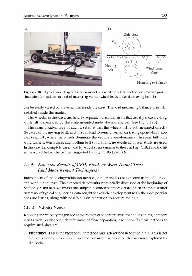
can be easily varied by a mechanism inside the strut. The load measuring balance is usuallyinstalled inside the model.The wheels, in this case, are held by separate horizontal struts that usually measure drag,

while lift is measured by the scale mounted under the moving belt (see Fig. 7.18b).The main disadvantage of such a setup is that the wheels lift is not measured directly

(because of the moving belt), and this can lead to some errors when testing open-wheel race-cars (e.g., F1, where the wheels dominate the vehicle’s aerodynamics). In some full-scalewind tunnels, when using such rolling belt simulations, no overhead or rear struts are used.In this case the complete car is held by wheel struts (similar to those in Fig. 7.18a) and the liftis measured below the belt as suggested by Fig. 7.18b (Ref. 7.9).

7.5.4 Expected Results of CFD, Road, or Wind Tunnel Tests(and Measurement Techniques)

Independent of the testing/validation method, similar results are expected from CFD, road,and wind tunnel tests. The expected data/results were briefly discussed at the beginning ofSection 7.5 and here we revisit this subject in somewhat more detail. As an example, a briefsummary of typical engineering data sought for vehicle development (only the most popularones are listed), along with possible instrumentation to acquire the data.

7.5.4.1 Velocity Vector

Knowing the velocity magnitude and direction can identify areas for cooling inlets, compareresults with predictions, identify areas of flow separation, and more. Typical methods toacquire such data are:

1. Pitot tubes: This is the most popular method and is described in Section 3.5.1. This is nota direct velocity measurement method because it is based on the pressures captured bythe probe.

(b)(a)

Side view

Movingbelt Wind tunnel

floor

Mounting to balance

V∞

Figure 7.18 Typical mounting of a racecar model in a wind tunnel test section with moving groundsimulation (a), and the method of measuring vertical wheel loads under the moving belt (b)


2. Hot wire: A thin wire is inserted into the flow and its heat transfer (or electricalcurrent) can be calibrated to measure velocity. The main advantage of this probe is itssmall size and fast response, making it ideal for unsteady flow and for turbulence mea-surements.Both the Pitot tube and the hot wire probes can come in arrays so that flow direction

can be measured.3. LDV (laser Doppler velocity meter): This method requires seeding the flow with light

reflecting particles (usually light oil spray). Two coherent laser beams (set at differentangles) are focused at a point and as the beams intersect, due to their interference, a fringepattern is formed. When a seeded particle crosses the set of fringes, its scattered lightreturns as a high frequency signal. The fluctuating light signal is picked up by sensitiveoptics and the frequency of the signal is directly related to the particle speed. This methodis nonintrusive but works at only one point where the light fringes were created by twointersecting laser beams (of the same wave length). By the way, the use of “Doppler”name here is coincidental!

4. PIV (particle image velocity meter): This is a more advanced development of the pre-vious method and is described schematically in Fig. 7.19. In this case, too the flow isseeded with small tracer particles (again some sort of light oil spray) and a laser lightsheet is created. A measurement area is defined within the light sheet (see figure) andhigh-speed camera(s) take two subsequent pictures in a very short time. The ingenuity

Seedingparticles

Mirror

Light sheet

Camera

Image plane

Particlelocationat t +Δt

Particleslocation

at t

Frame #2

Frame #1

Measurementarea

Flowwith particles

Lasersource

Optics

(light sheet)

Figure 7.19 Schematic description of a PIV system (without a model in the measurement area). Theimage plane depicts the results of two subsequent exposures showing particle positions at t and t +Δt.This allows the calculation of local velocity vectors


of the method lies in the fast analysis of the two photos where the particles are identifiedand based on their different position (in the two pictures) their velocity vector is calcu-lated. The method can be easily extended to measure the velocity distribution in a vol-ume, as long as it can be illuminated. When applicable, the method is very powerful andresults are similar to CFD results (e.g., velocity contours, turbulence levels, and pressurecalculations are all possible).

7.5.4.2 Aerodynamic Loads

First and most obvious is the integral load data. This includes downforce, drag, side force,and the pitching, rolling, and yawing moments. The primary parameters that will affect vehi-cle performance are downforce, drag, their ratio (L/D), and the front/rear axle distribution ofthe downforce (e.g., a 40:60 ratio can be considered as satisfactory for a touring car). Loadmeasurements are usually done by various load cells (e.g., balances or scales). Quite fre-quently more details are required, such as the forces on a rear spoiler, or on each wheel,and in these cases additional (smaller load cells or strain gauges) can be used. Informationon the aerodynamic loads on various vehicle components can be evaluated during wind tun-nel or road tests, but are significantly simpler when using CFD!

7.5.4.3 Surface Pressure and Shear

Whenmore data is required to understand the aerodynamics of a vehicle, surface pressure andshear force distribution is needed. Such information is, again, easily produced byCFD, but dif-ficult (because of the supporting instrumentation) in a road test, and much easier to implementin thewind tunnel.Typical pressure distribution,measured along thecenterlineof a small-scalemodel (usingstaticholesdrilled in thesurface) ispresented inFig. 6.1.Basedon theshapeof thepressure distribution, flow separation and other flow features can be investigated. By identify-ing low- andhigh-pressure areas on the vehicle, cooling andventilation intakes and exits can belocated. Evaluation of surface shear can help identify boundary layer transition and separationlines – information needed to improve the flow (mainly) on streamline shaped objects.In recent years pressure sensitive paint and also shear sensitive paint was developed. By

projecting specific (light) wavelengths, pressure (or shear) contours can be visible – similarto CFD results. The capability of these methods was successfully demonstrated, but practicalapplication is still limited. The main drawback of the method is the fact that the model mustbe covered with the specific “paint” and also view angles and lighting conditions are notalways ideal.

7.5.4.4 Flow Visualization (Flow Direction and Streamlines)

Qualitative information on the flow can be obtained by visualization techniques, informa-tion that can be used as a diagnostic tool to improve a vehicle’s design. This data can beobtained on the body’s surface or off the surface and can help explain some of the resultsobtained from the load tests. Again, when using CFD, velocity vectors and streamlines can


be plotted quite easily. Experimental methods to evaluate such data in a wind tunnel or aroad test are:

1. Tufts: can be glued to the surface of the model to indicate flow direction. When the tuftsstay parallel to the surface and don’t move; this usually indicates attached flow.When theflow is separated, the tufts will oscillate violently to all directions. This method can beused for off body visualization by using rakes, or arrays of thin wires to which the tuftsare attached, and then placing them in the area of interest.

2. Smoke: releasing smoke in a narrow stream can show streamlines. This method is attrac-tive for photography but limited to low speeds and mostly laminar flows.

3. Helium filled soap bubbles: Similar to smoke, small helium filled soap bubbles can bereleased by a probe to trace streamlines (actually streak lines). The buoyancy due to thehelium filling is supposed to counteract the water weight and result in zero total buoy-ancy. The light source can be arranged so that it reflects from the bubbles, highlightingthe streamlines in the flow. Again the method is attractive for very low speeds.

4. PIV: is again an attractive (if available) for flow visualization, and the main advantage isthat quite large areas can be covered. Also, post processing is similar to the post proces-sing of CFD results (as described earlier in this section).

In summary, selecting any of these tools depends on availability and on the problem to bestudied. Having all three options (e.g., CFD, experiment, and road testing) is probably thepreferred situation, and then eachmethod can be used where it is most suitable. For example,CFD can be used in the initial/conceptual design phase, the wind tunnel to validate anddevelop final details, and a road test to finally validate the expected performance.

7.6 Variable (Adaptive) Aerodynamic Devices

Aswas pointed out at the beginning of this chapter, the aerodynamic forces increase with thesquare of vehicle’s speed. Therefore, it is logical to use some variable geometries to adjustthe aerodynamic effects according to needs such as drag reduction, improved handling orcooling. Typical areas that could benefit from adaptive vehicle geometry (that will changewith speed or temperature) are:

1. Downforce (front and rear and the balance between these two)2. Engine cooling, internal ventilation and air conditioning3. Drag reduction4. Noise reduction5. Dirt, water, ice deposition (or reduction of ).

Some practical options to respond to those needs are:

1. Moveable components (wings, spoilers, etc.) – which can be used for downforce controlor opening/closing cooling inlets. We can include variable suspension to control rideheight and rake.


2. Adaptive/flexible surfaces – could be used to reduce flow separation behind the vehicleand improve underbody flow or even change effective rake.

3. Boundary layer control (surface roughness, blowing, synthetic jets, etc.) – can be used toreduce flow separation and increase laminar boundary layer regions.

4. Use of existing components (exhaust blowing, wheel rotation) – can be used to moveexternal air to increase downforce or improve cooling.

Most of these ideas were tested in racing environment and subsequently outlawed by reg-ulations, but only a few showed up in daily driver vehicles. In the following paragraphs, letus observe some of those trends.The simplest method to control vehicle aerodynamics is by adjusting ride height and rake

via suspension control. One of the earliest passenger cars was the Citroen DS (circa 1960s)which used hydraulic suspension that allowed raising and lowering the car. This wasn’tdesigned for aerodynamic gains but could be used for such. As an example, Fig. 7.20 shows

–3 –2

0.29

0.28

0.27

0.26

0.25

0.240 1 2 3 4 5 6

hL

7 8 9 10 11 12 cm

.29

.30

.31

.32

CD

CD

CLCL

ReL = 3 ·106, α = 0fixed ground plane

.33

.34

–1 0

0.1

0.2 hCL

CD

ReL = 3 ·106

h = 5 cm, fixed ground plane

0.3

0.4

0.5

α, deg

1

(a)

(b)

Figure 7.20 Lift and drag variation of a generic sedan versus pitch angle (a) and ride height (b).1/5 scale stationary floor wind runnel results


typical variation of the aerodynamic drag and lift for a generic passenger car. This data indi-cates that by lowering this car the drag was reduced and by pitching the nose down (rake) thelift was reduced (which is desirable for higher speeds).We have already discussed (Section 7.3) that for high speed stability and improved tire

traction, downforce is needed. The simplest method to generate downforce (and it is mostneeded at the back) was to add an inverted wing as shown in Fig. 7.21. However, at highspeeds the aerodynamic downforce can compress the suspension springs resulting in poten-tial damage to the vehicle (and driver’s bones). The logical solution was to use variable air-foil incidence, to reduce the loads at high speeds and to mount the wing support strutsdirectly onto the wheel uprights (and leave the sprung mass alone). This method was usedon the 1966 Chaparral 2E, which is considered to be the car pioneering the use of invertedwings in motor racing. The car was immediately a winner and as expected in racing, theconcept was copied almost instantaneously by other teams and in other racing series.The same principle is used in numerous road vehicles that have rear wings or spoilers

popping up at high speed. For example, Fig. 7.22 shows the moveable rear spoiler of aChrysler Crossfire (circa 2007).Similarly, front spoilers can be used to increase front downforce and even improve cooling

flow (by reducing pressure under the car). Such a device is described in Fig. 7.23, where asimple horizontal surface extends forward. By controlling its length or angle, the vehicle fron-tal downforce (or reduction of lift) can be controlled. Such spoilers are simple to integrate intoexisting designs and some showcars already used them (examples about their effect on down-force and drag are presented later, in Tables 7.2 and 7.3). Another interesting aspect of thisphoto is the direction of the streamlines ahead of the front spoiler. This suggests that near thevehicle centerline the spoiler tip must be raised to match the incoming flow direction. If therelative angle between the flow and the plate is too large flow separation under the plate canreduce the spoiler effectiveness and reduce the flow rate under the car.

Figure 7.21 The 1966 Chaparral 2E is considered to be the first to use inverted wings to createdownforce. Courtesy of Zoe Schafer, LAT Photographic


Cooling requirements may depend on speed and ambient temperature and adaptive airinlet/exit geometry can help in increasing their effectiveness and even reducing vehicle drag(such as cooling drag). One of the best examples is the Lamborghini Murcielago (the one inFig. 7.24 is a 2005 model) where the cooling air intake could be extended, as shown in thepicture. Of course this increases vehicle drag and for cold weather this could be left closed,even for high speeds.

Figure 7.22 A spoiler popping up at the rear end of a 2007 Chrysler Crossfire to reduce rear lift athigher speeds

Figure 7.23 Typical example of a front splitter plate (or front spoiler) and visualization of the flowdirection ahead of it


Variable geometry components can be helpful in improving comfort for open top vehi-cles. Even at moderate speeds aerodynamic buffeting (pressure fluctuations) caused byopening the window or the sunroof of a sedan can create considerable discomfort. As anexample, the reversed flow behind the windshield of a convertible car is depicted inFig. 7.25a. In this case the unsteady reverse flow can blow the driver’s hair into his face,interfering with his concentration or simply blow away items left inside the car.A typical solution is a moveable screen or a rear wind deflector that blocks the reverse flowpath (see Fig. 7.25b). Such devices can be controlled automatically raising at speed and

Movable cooling intake

Figure 7.24 Lamborghini Murcielago (2005 model) where the cooling air intake could be extended,as shown in the picture

Wind deflector

Winddeflector

(a)

(b) (d)

(c)

Figure 7.25 Movable aerodynamic devices aimed at improving comfort: (a) rear wind deflectorbehind the driver of an open top car (b) or at the top of the windshield (c), and a wind deflectorused to reduce noise and buffeting when opening a sun roof (d)


retract and low-speeds. Such wind deflectors can be also mounted at the top of the wind-shield as shown in Fig. 7.25c. By redirecting the flow over the whole open top of the vehiclethe unpleasant wind-gusts are eliminated. Such method is quite simple and effective at lowspeeds but will increase drag at higher speeds. Another such deflector, used to reduce buf-feting (pressure fluctuations) when opening the sunroof of a sedan is shown in Fig. 7.25c. Byslightly diverting the streamlines upward, the shear layer avoids hitting the rear edge of theopening and therefore the amplitude of the pressure fluctuations is reduced. This aero-acoustic effect will be discussed in more detail in Chapter 12.Finally, it is interesting to discuss a completely different application of adaptive aerodynam-

ics in the form of blowing a jet to reduce lift! Such tricks were used during the 2012 F1 season(called “F ducts”, see Fig. 7.26) and are intended to reduce drag near top speeds. In this casethe free stream pressure (captured at the front) is directed via an internal duct to the rear wingand blown normal to the surface, causing the wing to stall at high speeds (see illustration inFig. 7.26). Rumor is that it occurs at high speed when the system is activated and downforce isreduced, and the car gains 3–5 km/h in speed. One may ask, how is the drag reduced by stal-ling the wing? The answer lies in the fact that the vehicle’s downforce-induced drag is a resultof interactions and the wing drag may increase but the total vehicle’s drag (from the diffusers,etc.) is actually reduced. Critics also used this example to point out how racing regulationsforce developments that are completely irrelevant to automobile design.

7.7 Vehicle Examples

There are many types of vehicles such as commercial, agricultural, competition, and ofcourse, our daily transportation. For sake of brevity let us focus on the daily transportationand on some racecars, and in both cases aerodynamics becomes important with increasedspeeds (and for many other examples; see publications such as Ref. 7.1–7.3).

Rear wing

Blowing slot(normal to airfoil surface)

Figure 7.26 Blowing at the rear flap of a racecar to reduce high speed drag by stalling the flow on theflap (this trick was called the F-duct and was used during the 2012 F1 season)


7.7.1 Passenger Cars

Let us start with typical passenger cars. Possible variants offered by a particular manufac-turer may have one of the generic shapes depicted in Fig. 7.27. The reported aerodynamicdata usually depends on measuring methods and facilities. For example, most manufac-turers will test full scale vehicles, but data may be affected by using (or not using) movingground or wheel rotation, not to mention blockage and other corrections (see previous dis-cussion on wind tunnels). Wheel rotation and moving ground has a larger effect on lift andthis may be one reason why passenger car manufacturers don’t provide lift data (lift data isshown here only for two configurations). In most cases, though a station wagon will haveslightly less drag than the sedan and a well-designed hatchback (see the slant angle prob-lem in Fig. 7.6) may fall in between as shown here. The flow usually separates behind thewindshield of open top cars (convertibles), which explains why their drag is typicallyhigher. Lastly, SUVs are based on existing trucks and have boxy shape and edgy cornersand their drag is the highest. Also, the legend says that driving with windows closed andair-conditioning on saves fuel, is based on the fact that opening the windows increases thevehicle drag. Typical incremental drag coefficient numbers when comparing a vehicle withfully closed or fully opened windows are shown in the Table 7.1. The largest increment iswith boxy shapes as shown for the SUV. Also, opening just one window at lower speedswill create low frequency pressure fluctuations (buffeting), which will be discussed inChapter 12.The next question is which part of the vehicle and how much it contributes to the overall

drag. This is not a simple question because such a breakdown of the total drag is difficult tomeasure experimentally and may depend on the method of the CFD used (when evaluatingnumerically). Some estimated numbers, based on computations, are presented in Table 7.2.Note that the most dominant contributors are the underbody and the rear surfaces (behind therear window and trunk).A lower drag coefficient is associated with lower fuel consumption, and diagrams such

as Fig. 1.3 show the trend of reducing the drag of passenger cars over the years. To dem-onstrate the effect of the aerodynamic drag on an automobile’s power requirements, let usobserve first a typical power versus time diagram of an average driver. He may initiallyaccelerate and then perhaps peak at 60 HP while accelerating into traffic on the highway,but after a while, at an average of 100 km/h (60 mph) only about 16 HP are needed (seeFig. 7.28).

Table 7.1 Typical drag and lift coefficient for several passenger car configurations

CD CLf CLr ΔCD (Open Window)

Sedan 0.32 0.067 0.114 ~0.05Wagon 0.30 ~0.04Hatchback 0.31 ~0.03Convertible 0.40 0.011 0.143SUV 0.40–0.50 ~0.06


Figure 7.27 Generic shapes of most popular passenger cars and typical drag coefficients


To verify this observation let us estimate the power requirements in the followingexample:

Example 7.2 Power requirement for a cruising automobileLet us repeat Example 6.11 for a typical passenger car with a frontal area of 1.8 m2. Assum-ing a drag coefficient of 0.32 and tire plus mechanical friction is estimated at 150 N (at100 km/h). The total resistance is then

Actual power requirement

Av. power requirement (at 100 km/h)

70.0

60.0

50.0

40.0

Hor

se p

ower

30.0

20.0

10.0

0.0–5 0 5 10 15

Time (min)20 25 30

Figure 7.28 Driving power requirement for a sedan on a flat horizontal road

Table 7.2 Computed breakdown of the drag components on atypical sedan

ΔCD

bodywork 0.050rearview mirrors 0.015rear surfaces 0.085engine bay 0.024cooling drag 0.048underbody + chassis 0.085F wheel + suspension 0.025R wheel + suspension 0.023Total Drag Coefficient 0.355


D=CD12ρU2S + 150N= 0 32

121 2

1003 6

2

1 8 + 150 = 416 7 N

The power requirement at 100 km/h is the drag multiplied by the speed:

P= 416 71003 6

= 7 4 kW=15 7HP

and this number is the same as measured on the car in Fig. 7.27.The aerodynamic coefficients depend or ride height, rake, and side wind, among other

effects. Such data is not always available for most vehicles and some typical variation ofthe lift and drag with rake and ride height was presented earlier in Fig. 7.20. The trendsshown in that figure are quite representative of generic passenger cars, and a similar exper-imental data for the aerodynamic coefficients versus side slip is presented in Fig. 7.29.Note that all coefficients increase with side slip and part of this increase can be contributed

V∞

CD

CY

6448321600.0

0.4

0.8

1.2

1.6

2.0

2.4

CL

ReL = 3.0 ·106

βW

βW, deg

Figure 7.29 Variation of the aerodynamic coefficients versus sideslip for a generic passenger car


to the increase in frontal area, relative to the free stream (vehicle frontal area remains thereference area).Another frequently asked question is how can we improve the aerodynamics of an exist-

ing vehicle? The answer is not simple because of the interactions between the differentcomponents (e.g., sometime a part may work and sometime not), but let us list some ofthe typical add-ons and discuss only sedan shapes. In most cases, manufacturers try topreserve the original styling of the vehicle and aerodynamic add-ons are mounted usuallynear the lower surface of the car, apart from wings or rear spoilers (which are mounted onthe rear deck). The front spoiler was already presented in Fig 7.23 and it usually adds frontdownforce with minimal drag increments (or even a decrease in drag). Another device thatis used on racecars (and will be discussed later; see Fig. 7.43) is the vortex generator, asshown in Fig. 7.30. The vortex generator generates a vortex that creates suction under thecar, increasing its downforce. Typical numbers for such devices (with smooth under-tray) are:

ΔCL ΔCD

Front splitter plate ~ − 0.10 + − 0.02Underbody vortex generators ~ − 0.03 + − 0.01

Note that drag reduction is possible with both of these devices (usually byreducing separated flow areas).

Similar, hardly visible underbody treatment to generate downforce on sports cars is theaddition of a rear diffuser. The principle is similar to the concept presented in Fig. 7.7 andtypical effect of a rear diffuser, incorporated into the aft section of a sedan, is shown inFig. 7.31. This diffuser is efficient in creating rear downforce and (in this case) also reducingvehicle’s drag.

Splitterplate

Vortexgenerator

Figure 7.30 Front splitter plate and underbody vortex generators (work well with smooth undertray)


Because the tires may redirect the flow behind them sideways, straightening vanes (seeFig. 7.31b) can be used. These vanes usually delay flow separation, thereby increasing bothdownforce and even reducing drag. These devices will work best with a smooth undertray,but may have a negative effect on vehicle ground clearance (e.g., may rub on uneven roadsurfaces).A far more popular aerodynamic addition to existing road cars is the rear spoiler or wing.

The discussion related to Fig. 7.4 already established that such a device has the potential toincrease the flow under the car, thereby reducing lift (or increasing downforce). Again, thisbecomes more evident with smooth underbody, which is becoming the standard on mostmodern sports cars. The simplest form of a rear spoiler is a plate attached to the rear deckand typical data (in this case, for a large NASCAR type sedan) is shown in Fig. 7.32. Notethat in spite of its simple design, such a spoiler works quite well in creating rear downforce,but the drag increment is quite large.A more attractive solution for increasing rear downforce is adding a rear wing, as

shown in the inset to Fig. 7.33. The main advantage of such a wing is that it can be movedrelative to the rear deck to investigate its most efficient position. In this case only the wingheight was investigated, and its trailing edge was aligned with the rear bumper of the car(1990 Mazda RX7 GTO). Those changes had minimal effect on the drag but had a verylarge effect on downforce, and the lower wing position appeared to increase the flowunder the car. This was shown by measuring the pressure distribution along the centerlineunder the car, with and without the rear wing (Fig. 7.34). These measurements prove againthat the effect of the wing is not localized and increase the suction under the car – as sug-gested in Fig. 7.34!

0.26

0.25

0.24

0.23

0.2

0.1

0.0

–0.1

CD

CLRθ

0° 2° 4° 6°Diffuser angle, θ

8° 10° 12°

LDL

= 0.176LD

L

(a) (b)

CD

CL

R

Figure 7.31 Effect of rear diffuser angle (a) on vehicle’s drag and rear axle lift (based on Ref. 7.1,p. 167) and typical straightening vanes inside a rear diffuser (b)


7.7.2 Pickup Trucks

This is an excellent example of the unpredictability of aerodynamics. Pickup trucks weredesigned for work and naturally their aerodynamics is not ideal. Because of consumer demandthere are single/dual cabin and short/long bed versions (see model shapes in Fig. 7.35). Inter-estingly, inmost cases, lower dragnumbersweremeasured for the longer cabinwith the shorterbed. In addition, lowering the tailgate, actually increases drag – opposite to what is expected!Before trying to explain let us observe some experimental drag coefficient numbers (lift is usu-ally not provided). Typical drag coefficient numbers for such pickup trucks are about CD ~0.45–0.50. In this particular case, the drag numbers are as follows:

Baseline Tailgate down Tonneau

single cabin truck 0.483 +1.0% −7.0%extended cabin 0.472 +1.8% −5.7%

These results are representative of most pick-up trucks where lowering the tailgate hasminimal effect and in most cases even (slightly) increases the drag. The tonneau is a simplecover of the truck bed so that the upper surface is flat and it seems to lower the drag in most

0.10

CD

0 10 20 30 40

Spoiler angle, θ deg

50 60 70

CLf

CLr

0.05

0.00

–0.05

–0.10

–0.15

–0.20

θ

Figure 7.32 Effect of rear spoiler angle on the lift and drag of a sedan based racecar (after Duncan,L. T., “Wind Tunnel and Track Testing an ARCA Racecar,” SAE Paper 90–1867, Feb. 1990.)


cases. Next we can prove that in aerodynamics anything can be explained. Let us observe thestreamline following the cabin’s rooftop. Referring to Fig. 7.35, it appears that for the shortbed and extended cabin (Fig. 7.35b), this streamline is positioned above the rear tailgate,which is placed within the separation bubble behind the cabin. As a result, less drag isexpected and the tailgate open/closed position may have less effect (the numbers here showan increase of 1.8% drag but in some cases similar reduction in drag is reported). For theshort cabin (Fig. 7.35a) and the long bed, the separation bubble behind the cabin is shorterand the roof top streamline may hit the tailgate area. When lowering the tailgate, the rooftopstreamline could be displaced lower, which results in a faster flow over the cabin and hencelower pressure behind and above the cabin (and an increase in drag and in lift is expected), inspite of the gain by lowering the tailgate!

7.7.3 Motorcycles

Motorcycles emerged as an inexpensive mode of transportation, and emphasis was on sim-ple and fuel efficient. Over the years, however, engine power increased and full size motor-cycle performance significantly exceeded the performance of passenger cars. Because thedrag of these two-wheeled vehicles was high, as power increased, streamlined fairings were

0.6

0.5

0.4

0.3

0.2

0.1

CD

–CL

h

αw = 15°ReL = 3.5 ·106

0 1 2 3

h/c

4 5 6

Large chord

Small chord

Figure 7.33 Effect of rear wing height on the drag and downforce of a passenger car based racecar(1990 Mazda RX7 GTO). Both wings had the same chord, but the larger wing’s span was equal to themaximum width of the vehicle


added. As an example consider a typical sport bike (Fig. 7.36) mounted in a wind tunnel testsection with a real rider on it. In this particular case, in addition to evaluating the aerody-namic fairings, the effect of driver seating position and possible effect on maximum speedcould have been evaluated.The reference frontal area in this test was 0.55 m2, and the measured force coeffi-

cients were:

CD = 0 56

CL = 0 CLf = 0 28 CLr = −0 28

Note that because of the high center of pressure, the aerodynamic drag results in a rear loadtransfer, which actually reduces tire slip at higher speed (e.g., downforce at the rear tire).When comparing the performance of different motorcycles, usually the value of drag coef-ficient multiplied by the frontal area (CD A) is used. For this case

CD A= 0 56 0 55 = 0 308 m2

Cp

Lower centerline

Baseline + wingBaseline

αw = –17°ReL = 3.5 · 106

–2.50

–2.25

–2.00

–1.75

–1.50

–1.25

–1.00

–0.75

–0.50

–0.25

0.00

0.25

0.500.0 0.5

x/L1.0

Figure 7.34 Effect of rear wing height on the underbody centerline pressure distribution of apassenger car based racecar (1990 Mazda RX7 GTO). Wing height is 0.75c


Opening the tailgate

lowers the streamlines(a)

(b)

Tailgate

LbedLcabin

Figure 7.35 Schematic description of the flow field above a single (a) and extended cabin (b) pick-

up truck

Figure 7.36 A full scale motorcycle as mounted in a wind tunnel test section


and the units are units of area. This number varies for the various motorcycles between 0.30and 0.50, and the motorcycle shown in Fig. 7.36 is considered one of the most streamlinedexamples. Note the wide area behind the driver and above the rear tire; by widening thebodywork under the seat vortices can form there to create down force on the rear axle. Also,toe-out of the rider’s foot introduces flow from the sides into this area, reducing overall drag!This is quite surprising because of the added frontal area and the high speed outer flow hit-ting the rider’s toes.Because the side view area in this case is much larger than the frontal area, motorcycles

are sensitive to side winds. Figure 7.37 shows the variation of the side force coefficientsversus side slip angle β and clearly the side force CY increases significantly. Note that asbefore, sideslip is defined as wind from the right and the resulting force acts to the left (hencenegative force). The drag increases with increasing sideslip angle, while the total lift is notaffected much.

7.7.4 Competition Cars (Enclosed Wheel)

Motor racing was probably inspired by human competitiveness, much like any other sport.Proving who is the better sportsman (driver), or who has the better technology, appealed tofans and served as a promising marketing tool. Most of the tricks used on sedan-based race-cars (NASCAR, touring, etc.) are similar to the elements shown in Section 7.7.1, and somecan be found on popular daily drivers. This cannot be said about open-wheel or even

CY

CD

CL

1.4

1.2

1

0.8

0.6

0.4

0.2

0

–0.2–5

–1

–0.8

–0.6

–0.4

–0.2

CD

, CL

0

0 5 10 15 20 25

β, deg

CY

Figure 7.37 Force coefficients (CL,CD, andCY) versus side slip angle for a typical sports motorcycle


prototype-based (IMSA, LeMans) racecars. Over the years, regulations controlling the vehi-cle’s shape got out of proportion, occasionally leading to irrelevant designs, not applicableto any practical road vehicle (see Fig. 7.26). Therefore, instead of focusing on specific race-cars, let us limit the discussion to generic enclosed wheel (e.g., prototype) and to open wheeldesigns (such as Indy or F1), and discuss some relevant aerodynamic elements.From the aerodynamic point of view, competition cars rely on aerodynamic downforce

for improved tire adhesion in cornering, accelerations, or even in straight-line drag racing(see Section 7.3). Therefore, designers search for downforce with as low drag as possible,and for desirable balance between front and rear downforce (for stability reasons). The num-bers shown in Fig. 7.1 (CL = −3.0, and CD = 0.75) probably represent the upper values of thedownforce coefficient. The main reason is that at higher speeds the downforce is larger thanthe vehicle’s weight so suspension springs must be very stiff, and cornering accelerations inexcess of 3 G are quite uncomfortable for the driver. Also, the increased drag (due to down-force) compromises straight line speed but the time gained during cornering, braking, andacceleration out of turns, significantly reduces lap times.As a first example for this category let us examine a typical Le Mans prototype car of the

2010s (see Fig. 7.38). This type of car represents the most aerodynamic vehicle design andby contouring the lower surface huge levels of downforce can be generated. Recently, how-ever, in the name of cost reduction the underbody of such cars must be flat. The rear wing isvisible, and the “front wing” is quite different, as it will be explained later. Note the long rearfin which is mandated to reduce lift under severe side slip condition (to eliminate lift off ),during an accident. During normal conditions, when there is no sideslip, the fin has a minoreffect on drag (its skin friction) and a minor negative effect on the lift of the rear wing.

Figure 7.38 The Le Mans Audi R 18 prototype racecar, one of winningest cars of the 2010s.Courtesy of Jan Monchaux, Head of Aerodynamics, Audi AG


Typical aerodynamic breakdown of the aerodynamic effects of the various components onsuch cars is shown in Table 7.3. Note that racecar aerodynamics is a nonlinear science andby changing the rear wing location (see e.g., Fig. 7.33), all the numbers in this table canchange.While observing the racecar in Fig. 7.38, note the mandatory cutouts above the rear

wheels and the side cutout (instead of a similar holes above the front wheel), which canbe seen at the inside of the front right wheel. These cutouts reduce the lift in principlebut add some drag due to the wheel wakes disturbing the flow over the body and towardsthe rear wing (these shortcomings were eventually eliminated by the designers of the car inFig. 7.38). Incidentally, when the vehicle slips sideways, it has more of a tendency to lift offthe ground. So if it is already partially airborne, then think of it as a flat plate at angle ofattack, which from the side has a higher aspect ratio (and more lift). With this “model”in mind it is clear that allowing flow from the bottom of the car to exit above the wheelscan separate the flow at the leading edge (which is now the side of the car) and reducethe risk of the vehicle flying high. This fact that the curved bodywork above the front wheelproduces lift was realized quite early (e.g., see pressure distribution in Fig 6.1). As a resultventilation slots were inserted into the front fenders as shown in Fig. 7.39. These slots, called“louvres” or “gills” when properly placed, can reduce the wheel fender lift (or increase thevehicle downforce). As noted, low pressure exists above these louvers, and in order to nixthis effect the higher pressure air from below is allowed to flows upward (across thelouvres). These ventilation slots may also affect the underbody flow. For example, theycan reduce the high pressure ahead of the wheel and in effect increase the speed underthe forward bodywork. As a result, this device works quite well when the flow path insidethe wheels is not obstructed between the underbody and the louvres. For best results, theymust be placed near the maximum curvature and typical incremental effect of such louvers isaboutΔCL of −0.005 with a penalty ofΔCD = 0.004, and the downforce acts where the open-ings are (e.g., on the front fender). A mutation of the idea is the so-called cowl flap shown atthe right-hand side of Fig. 7.39. This adjustable opening in front of the wheel reduces the liftof the curved wheel arch (fender) but usually with larger drag than the louvers. In the par-ticular case of the car shown here, the backward facing cowl flaps were used also to pumpmore flow from under the car – to increase the downforce at the front. This figure also shows

Table 7.3 Typical breakdown of the aerodynamic contribution ofvarious components of a prototype racecar

CL CD

Upper bodywork 0.54 0.20Undertray + diffusor −1.26 0.10“Front wing” −0.72 0.05Rear wing −0.36 0.05Front wheels 0.0 0.05Rear wheels 0.0 0.05Total −1.8 0.50


splitter plates (as discussed earlier – see Fig. 7.30) and dive plates (see Fig. 6.51), whichcould be easily added to increase front downforce (if needed).Typical levels of the incremental lift and drag contribution of these add-on aerodynamic

devices are listed in Table 7.4 and, again, their effectiveness changes from vehicle to vehicle.Finally, the so called “underwing” of sports cars is described in Fig. 7.40. In the early years

of 2000s, however, a flat floor wasmandated, significantly reducing the effects of this under-body treatment. The rear diffuser or rear tunnel, also shown in this figure was used success-fully in the late 1980s producing very large level of downforce. Because of the cost involvedwith developing the lower surface of racecars it was agreed (as noted) that flat underbodywillbe used in almost all forms of racing. However, a feature reminiscent of the “front wing”remained, as mentioned in the discussion about the Audi R18 (see Fig. 7.38). Such a frontwing uses the lower surface ahead of the front wheels and by directing the flow upwardand outside, as shown schematically in Fig. 7.40, significant levels of downforce can be gen-erated. A typical exit for this front wing flow is shown in Fig. 7.39, where the area behind thefront wheel was cut out to allow the underbody flow to exit sideways. Similar treatment isvisible behind (and above) the front wheel in the more recent vehicle in Fig 7.38.In conclusion, the underbody of a racecar is the largest aerodynamic surface (by area) and

even a small negative pressure over it can produce significant downforce. A good example is

Splitter plate Louvre Cowl Flap F. wing side exitsDive plate

Figure 7.39 Possible add on at the front of racecars: dive plates, front splitter plate, cowl flaps,louvres, and front wing side exits

Table 7.4 Typical incremental effects of various add-on aerodynamicdevices

ΔCL ΔCD

Louvres 0.005 0.004Cowl Flaps 0.005 0.005Dive plates 0.03 0.01Cut out over wheel 0.004 0.002Splitter plate (large) 0.09 0.01Rear vertical fin +0 +0


the flat bottomed car in Fig. 7.38 where, by clever use of the rear diffuser (which is allowedbehind the rear axle), the rear wing induced low pressure and a small rake – significantdownforce is generated (see Table 7.5 for that car).

7.7.5 Open-Wheel Racecars

The idea for open-wheel racecars probably surfaced during the early 1900s when the cigarshape body (fuselage) was considered a low drag configuration. The wheels of the erawere quite skinny and designers considered them “low drag”. Over 100 years later, openwheels racecars still exist, in spite of the debris thrown up by the sticky tires and the pos-sibility of one car’s wheel rolling over the other car’s wheel (initiating airborne condi-tions). This is because the top racing venues (F1 and Indy) are committed to openwheel racing, in spite the fact that this configuration introduces significant (aerodynamic)challenges. At first, it appears that the exposed wheels increase the drag significantly andthe engineering challenge is to shield them from the high momentum free-stream. Windtunnel testing of isolated wheels (with tires) shows large variations and strong dependencewhether the wheel was rotating or not during the test. Table 7.5 shows a short list of dif-ferent test results.The data in this table suggest that the narrow tires have less drag than the wider (high

performance) wheel/tire combination. In addition to the above tire width effects, wheelrotation reduces both lift and drag of the wheels. Tire width doesn’t have a very largeeffect on drag, but wheel rotation reduces both lift and drag of the wheels. Typical pres-sure distribution along the centerline of a tire is shown in Fig. 7.41a for both stationaryand rotating wheels. Of course such a pressure distribution depends on tire and threadshape but clearly, in the nonrotating wheel case the suction inside the separated flowregion (on top) is larger. Also, depending on tire thread shape, the pressure coefficientat the forward contact point with the ground can be significantly larger than 1.0 because

Raisedunderbody

Figure 7.40 Possible underbody treatment to increase the downforce of enclosed wheel racecars:The “hidden front wing” at the left and the underbody “tunnels” at the right


of the additional momentum of the air captured by the threads. A schematic description ofthe computed flow field shows the vortex pattern behind the wheel and the shape of thestreamlines near the upper separation bubble (Fig. 7.41b). Again, this is a simplisticdescription and the actual flow over the tire is more complicated; it is unsteady and asym-metric, and also depends on the rim shape.Over the years, designers learned how to reduce the wheel drag by using shrouds and

wing tip devices on the front wing (to reduce front wheel drag). Let us look at two typesof open wheel racecars designed about 15 years apart. The first is a circa year 2000 Indycar while the other is a circa 2010 F1 car. This relatively short period is significant becauseof the increased use of CFD on the later car. A typical Indy car from 2000 is shown inFig. 7.42 and the contribution of the various components to the total drag and lift are listedin Table 7.6. The “winglet” is the small triangular part ahead of the rear wheels and in somecases it was found to reduce drag. The geometry of the rear diffuser and the underbody vor-tex generators are described later in Fig. 7.43.The data in Table 7.6 is based on quarter scale wind tunnel tests and the numbers are a

result of adding/subtracting a component from the test model. Clearly the wheels drag

–1 Stationary wheel

(a) (b)

Rotating wheel

V ω

θ

0

1

CpCp y

x

z

Figure 7.41 Measured pressure distribution along the centerline of a stationary and rotating isolatedtire (Width/Diameter ~0.6 = ReD = 5.3 105). Right is a schematic description of the separated flowand the vortices behind the wheel (after Zhang, 2003: Fig. 16 in Ref. 7.13. With permissionfrom ASME)

Table 7.5 Typical lift and drag coefficient values, reported in the literature, for anisolated wheel. Coefficients are based on wheel frontal area, and the numbers inparentheses are for nonrotating wheels; otherwise the wheels rotate at zero slip

Width/Diameter CD CL Re Number Ref.

0.28 0.180 (0.272) 0.579 (0.593) 1.1 106 7.100.50 0.40 (0.95) 0.65 (0.75) 0.2 106 7.110.612 0.48 (0.76) 0.56 (0.77) 5.3 105 7.12


consists about 29% of the total drag and the rear wing appears to produce the largest portionof the downforce. However, part of this increase is an increase in the suction under the vehi-cle (induced by the rear wing). At this point it is worthwhile to return to the discussion aboutvehicle stability (Section 7.3) and to the front/rear downforce distribution. For such Indycars, Table 7.7 provides some generic numbers about typical driver preferences at variousvenues. A road course, of course, consists of many turns and perhaps a long straightaway,while at the other end of the scale, the superspeedway (e.g., Indy 500) is a continuous fasttrack with moderate turns.

Figure 7.42 Typical Indy car from circa 2000. The winglet is shown in front of rear wheel while theVGs are under the car and not visible

Table 7.6 Aerodynamic load contribution of the various componentsof a generic Indy Car (high downforce configuration)

CL CD

Body 0.13 0.18Wheels, 0.24 0.32F Wing −0.95 0.12R Wing −1.15 0.29Vortex generators (VG) − 0.18 0.08Winglets −0.15 0.0R Diffuser −0.55 0.12Total −2.61 1.11


Also, the numbers in this table suggest that for higher speeds driver prefer more rear(downforce) while for off road, all-wheel drive vehicles, the balance between the front/reardownforce is closer to 50/50%.Table 7.6 lists vortex generators (VG) that were introduced in the discussion related to

Fig. 7.30. Indy cars of the late 1990s and beyond used them, and their “advantage” wasin the fact that they weren’t visible and initially no one knew the magnitude of their effect.

0.4

0.3

0.2

0.1

0.0

–0.1

–CL

0 2 4 6

h (mm)

8 10 12

Indy underbody + VG

Indy underbodyPlate + VG

Plate

Vortexgenerators

Vortices

Reardiffusers

Thumbprint

Vortexgenerators

Figure 7.43 Underbody shape of a circa year 2000 Indy car shown in Fig. 7.42 and similar vortexgenerators mounted on a flat plate. The effect of ground clearance h, on VG induced downforce forboth configurations is shown at the right (numbers are in terms of total vehicle lift coefficient)

Table 7.7 Typical driver’s aerodynamic preferences for INDY cars. Data in original units (note1 lb = 0.453 kg and 1 mile = 1.609 km)

Downforce (lb@200 mph) Drag −CL CD L/D %F

Road course 5000 1579 3.09 0.98 3.16 45Short oval 3500 1280 2.17 0.79 2.73 35Long oval 2500 1100 1.55 0.68 2.27 35Superspeedway 1500 990 0.93 0.61 1.51 33(like Indy 500)


The underbody shape of the car in Fig. 7.42 is shown in Fig. 7.43where theVGs are visible atthe front. These cars also had underbody tunnels and a rear diffuser (as shown in the figure).Themain question at the timewaswhether, theVGs generate downforce locally or their wakecreates additional suction on rest of the underbody thereby indirectly amplifying their effect.Figure 7.43 shows a typical set ofVGs on the underbody of a circa year 2000 Indy car. Here

two large VGs (see curved flat plates) per side are embedded inside an indentation called the“thumbprint”. On the lower part of this figure, similar flat plate VGs of the same size wereadded to a plate, to investigate if they canwork on the flat underbody of a vehicle. The trailingvortices created by these VGs snake under the body and due to the high speed around thevortex core, low-pressure area will surround them (and increase downforce). The combineddownforce and drag contribution for these two underbody shapes versus ride height (in full-scale) are presented in Fig. 7.43 (after Ref. 7.3). The lift coefficient is normalized here by thevehicle frontal area (1.474 m2) and the ride height is in full scale. In general, both the down-force and drag increase as the ground clearance is reduced. The increase in vortex strength andthe reduced distance of the vortex from the underbody explains the increase in both down-force and drag, as ground clearance is reduced.At the very lowground clearance values, how-ever, a maximum in the downforce is reached due to breakdown of the trailing vortices (ofcourse, at zero ground clearance, the flowunder theVG is blocked and this effect diminishes).The discussion about these VG is important because similar vortex flows used extensively

on F1 cars. The main reason is that CFD computations provide estimates for the expectedvortex flows, which can be used to influence the wake of the wheels and send vortices underthe flat underbody, in effect creating downforce with the mechanism described in Fig. 7.43.Such an F1 car is shown in Fig 7.44 and the numerous turning vanes and plates on the frontwing are basically VGs acting on the front wheel and sending vortices under the car.

Figure 7.44 Typical F1 car from circa 2006. Courtesy of Sauber F1 Team


Typical breakdowns of the lift and drag of the various components on such a car are listedin Table 7.8 (after Ref. 7.14). Wheel drag is much less than in the data for Indy cars inTable 7.6, which is achieved by the numerous deflector surfaces mounted on the front wing.Also the rear wing downforce is less than the numbers shown for the Indy car, but the under-tray downforce is larger than the combined downforce of the Indy car’s VGs, diffuser, andwinglets. This high level of the undertray downforce is achieved simply because this is thelargest aerodynamic surface and by careful tailoring of the underbody vortex flow, groundclearance, and rake.Because the aerodynamic coefficients of the complete vehicle depend on ride height and

rake (pitch) each racecar comes with and aerodynamic map that shows the various forcesand moments. As an example, Fig. 7.45 shows one part of the “map” where the total

Table 7.8 Typical breakdown of the aerodynamic contribution ofvarious components of an F1 car (circa 2006, after Ref. 7.14)

CL CD

Upper bodywork 0.26 0.09Undertray + diffusor −1.63 0.14Front wing −0.89 0.18Rear wing −0.78 0.26Front wheels + suspension 0.01 0.10Rear wheels + suspension − 0.06 0.17Total −3.09 0.94

1200

1100

1000

900

800

0.000 10 20 30

Rear ride height [mm]

Dow

nfor

ce @

250

km/h

r, [k

g f]

40

Front ride height [mm]

0.00

6.59.5

12.515.025.0

38.0

50.0

50

Figure 7.45 Typical “aeromap” of downforce versus ride height (and rake) of an Indy car. Similargraphs are produced for drag and percentage front (and for each different configuration)


downforce dependence of front and rear ride height is graphed. Usually, the map includes asimilar graph for the drag and the front/rear downforce ratio. More detailed maps may repeatthe same variables for different add-ons, wing settings, and so on.


In this chapter an effort was made to introduce some practical aspects of automobile aer-odynamics. The main objective was to demonstrate that the background introduced in theprevious chapters is needed and necessary to understand automotive aerodynamics andprovide the reader with the tools needed to design and improve vehicles that he/shemay work on. The main design objectives that were discussed are vehicle’s drag, down-force, and balance, but many other related topics may surface (e.g., cooling, noise,aero-induced vibrations, stability, and safety, etc.). Finally, we must remember thataerodynamic may be highly nonlinear (e.g., unpredictable) and the following two exam-ples help to demonstrate this:In the first case, the aerodynamics of a late 1990s Indy car was studied both numerically

and in the wind tunnel. For the test, the wing and nose cone were mounted on separatebalances and their lift and drag was measured separately from the lift and drag of the com-plete car. As expected the downforce of the wing increases with increased flap angle andthere is no evidence of stall within the range tested (remember that the flap has a small aspectratio). However, the vehicle’s total lift shows a much smaller increase and even drops at thelarger flap angles. Once visualizing the front wing tip vortex trail, the explanation surfaces(as in Fig. 7.46b). Under those conditions, the front wing tip vortex reaches the rear wing andspoils its downforce. This situation is highly undesirable because downforce balance shiftsforward, reducing stability. Possible solutions in this case may be a wider wing (with tipsoutside the wheels) or a lower positioning (if allowed by regulations). However, theserecommendations introduce an additional nonlinearity, and the example in Fig. 7.47 is pre-sented to prove this.In this second example, the front wing height was varied and the drag of the front wheel

was measured. Also, the wing-span was close to the inner face of the wheels (right-hand sideof Fig. 7.47) and the tip vortex wake appeared to flow along the inner surface of the wheels.In case of the stationary wheel (nonrotating and no rolling ground) the effect wasn’t large butwheel drag increased when raising the front wing (due to interaction of the tip vortex withthe separated flow behind the wheel). The last data point shows a reduction in wheel drag atthe highest wing position – which is impractical for such cars. The trend changes dramat-ically when the wheel is rotating (data points are based on results from Ref. 7.15), and byadding the wing at h/c ~ 0.05, the drag was actually reduced! It is clear that the wing tipvortex interacts with the separated flow behind the wheel, but also a glance at Fig. 6.19may help explaining these large variations. In case of the cylinder the sudden changes indrag between Re = 105 to Re = 106 was explained by the boundary layer transitioning to tur-bulent flow. Quite possibly in this three-dimensional case the wheel wake is influenced bythe wing tip vortex and at lower heights (h/c < 0.35) the separated flow area is reduced (for


the rotating wheel case). Once the wing assembly is further raised the drag increases sharply,possibly because of the increase in the separated flow bubble behind the wheel (note thatwing’s chord c and wheel diameter are almost the same). At values of h/c > 0.5 the wheeldrag is reduced (less wing/wheel interaction) but these conditions, again, are impractical forsuch racecars.

0.8

0.75

0.7

0.65

0.6

0.55

0.5–0.2 0 0.2

F Wing height, h/c

Nonrotatingwheel

Rotatingwheel

No wing

0.4 0.6 0.8

1/4-scale, Re = 0.52 ·106, Ref. 151/2-scale, Re = 0.63 ·106

Note: Re (critical) ~ 0.2 ·106

25’’(0.635)

29’’(0.736)

CD

Figure 7.47 Effect of front wing height from ground (h) of an open wheel racecar on the wheel’sdrag. Data is reduced based on wheel’s frontal area (c is the wing’s chord)

2.7

–CLtot –CLw

16 18 20

CLw

22

Alpha, deg

24 26 28 30

2.66

2.62

2.58

2.54

2.5

1.1

1.05

1

0.95

0.9

CLtot

(a) (b)

Figure 7.46 Front wing and total vehicle downforce versus wing’s flap deflection (a) andvisualization of the wing tip flow reaching the rear wing (b)


In conclusion, in vehicle aerodynamics, one should always expect the unexpected andbeing familiar with elementary aero/fluid mechanics can help develop deeper understandingof the observed results.

References7.1. Hucho, W. H., 1998, Aerodynamics of Road Vehicles, 4th Edn, SAE International, Warrendale, PA. 1998.7.2. Sumantran, V, and Sovran G., Vehicle Aerodynamics, SAE PT-49, Warrendale, PA1996.7.3. Katz, J., Racecar Aerodynamics: Designing for Speed, 2nd Edn, Bentley Publishers, Cambridge, MA, 2006.7.4. Zerihan, J. and Zhang, X., “Aerodynamics of a single element wing in ground effect” J. Aircraft, Vol. 37,

No. 6, November-December 2000, pp. 1058–1064.7.5. Cooper, K. R., Bertenyi, T., Dutil, G., Syms, J., and Sovran, G., The Aerodynamic Performance of Automo-

tive Underbody Diffusers, SAE980030, Detroit. MI. Feb 1998.7.6. Milliken, W. F., and Milliken, M. L., Racecar Vehicle Dynamics, SAE International, Warrendale, PA, 1995.7.7. Rae, W. H., and Pope, A., Low-Speed Wind Tunnel Testing, 2nd Edn, John Wiley & Sons, Inc., New

York, 1984.7.8. Kelly, K. B., Provencher, L. G., and Shenkel, F. K., “The General Motors Engineering Staff Aerodynamic

Laboratory – A Full-Scale Automotive Wind Tunnel,” SAE Paper No. 82–0371, 1982.7.9. Walter, J., Bordner, J., Nelson, B., and Boram, A., “The Windshear Rolling Road Wind Tunnel,” SAE Int.

J. Passeng. Cars – Mech. Syst. Vol. 5, No. 1, 2012, pp. 265–288. Also SAE Paper 2012–01–0300.7.10. Cogotti, A., “Aerodynamic characteristics of car wheels,” Int. J. of Vehicle Design, Technological Advances

in Vehicle Design Series, SP3, Impact of Aerodynamics on Vehicle Design, 1983, pp. 173–196.7.11. Stapleford, W. R., and Carr, W.G., Aerodynamic Characteristics of Exposed Rotating Wheels, Motor Indus-

tries Research Association (MIRA), Rep. No. 2, 1970.7.12. Fackrell, J. E., and Harvey, J. K., “The Aerodynamics of an Isolated Road Wheel,” Paper No. 8 in Ref. 2.18,

pp. 119–126.7.13. Zhang, X., Toet, W. and Zerihan, J. “Ground Effect Aerodynamics of Racecars, ASME,” Applied Mechanics

Reviews, Vol. 59, January 2006, pp. 33–49.7.14. Toet, W., “Aerodynamics and Aerodynamic Research in Formula 1,” The Aeronautical J. Vol. 117,

No. 1187, January 2013, pp. 1–26.7.15. van den Berg, M.A. and Zhang, X. “The aerodynamic interaction between an inverted wing and a rotating

wheel.” Journal of Fluids Engineering, Vol. 131, No. 10, 2009, pp. 101101-1–101104-13.

Problems

This chapter is mostly descriptive and the problems are more like web-search assignments.7.1. Collect the official drag coefficients of five passenger cars (advertised by the manufac-

turers) and their frontal areas. Estimate their fuel consumption at 100 km/h and comparewith their advertised values. Assume that the energy in 1 kg of gasoline is 11,300 kcal.

7.2. Collect the official drag coefficients of five pickup trucks (advertised by the manufac-turers) and their frontal areas. Estimate their fuel consumption at 100 km/h and comparewith their advertised values. Assume that the energy in 1 kg of gasoline is 11,300 kcal.

7.3. List three passenger cars that have careful underbody design (e.g., smooth undertrayand rear diffusers).

7.4. Select three popular hatchback cars and measure their rear window slope, as in Fig. 7.6.Is the slope close to 30 ?


7.5. Search the current production cars and find those that have wider tires in the back. Listat least three and try to find their weight distribution (e.g., front/rear).

7.6. If a passenger car’s center of gravity is exactly in between the two axles and you canchoose between front- or rear-wheel drive – which can accelerate faster and why(assuming the same torque)?

7.7. Collect data on weight distribution between front and rear axles for 10 front- and10 rear-wheel drive cars. Try to find manufacturer information on advertised accel-eration and power. Plot these variables and report any trends you find.

7.8. List five current cars that have a deployable rear spoiler (e.g., variable aerodynamicdevice).

7.9. List five convertible cars that offer retractable wind deflectors (as in Fig. 7.25) behindthe seats.

7.10. When driving in rain, try to observe the A-pillar vortex on the side window (as inFig. 7.5f ).

7.11. Collect the advertised fuel consumption of five short- and five long-bed pickup trucksand report if there is any clear trend (based on manufacturer’s data).

7.12. If, due to a minor collision, a racecar looses its front wing, what is expected?a. It will be more stable and will understeer, orb. It will be less stable and tend to oversteer.

7.13. The frontal area of a race car is 1.5 m2, and it weights 750 kg. At what speed can itdrive upside down (on the sealing) if its downforce coefficient is 2.0?

7.14. Collect the names of 30 passenger cars and their advertised powers. How many ofthose have rear wings or rear spoilers?

7.15. Collect the names of 30 passenger cars and their advertised powers. How many ofthose have variable geometry cooling inlets? Do you think that cooling drag hasan effect of fuel economy?


8Introduction to ComputationalFluid Mechanics (CFD)

8.1 Introduction

The fluid dynamic equations developed in Chapter 2 are complex and cannot be solved ana-lytically for an arbitrary case. Up to this point, the classical approach has been presentedwhere major simplifications allowed some partial solutions. In recent years, however,numerical techniques and computational power have improved significantly. This has facili-tated the solution of the nonlinear fluid dynamic equations, which now can be added to thegrowing number of practical engineering tools.There are two major advantages to the numerical approach when attempting to solve the

fluid dynamics equations. The first is the possibility to solve these complex equations, whichcannot be solved analytically. The process begins with a numerical approximation for thefluid dynamics equations. The fluid domain is then discretized into small cells, or into a grid,where the equations are applied. By specifying the equations at each cell or point the partialdifferential equations are reduced into a set of algebraic relations. Thus, the second majoradvantage of the numerical approach is the ability to replace the nonlinear partial differentialequations with a set of algebraic equations, which are usually solved by iterative methods.There is a large number of methods for approximating the equations, or for grid generations,and for solution methodology. This chapter attempts to explain the generic principles of thenumerical approach and the process leading to the numerical solutions. A more comprehen-sive discussion on CFD can be found in texts such as Ref. 8.1 or 8.2.For a typical CFD solution, the computational domain must be defined (e.g., the region of

interest in the flow, as shown in Fig. 8.1). In addition, the boundary or initial conditions mustbe specified (solid symbols) in a physically correct manner (to avoid impossible solutions).


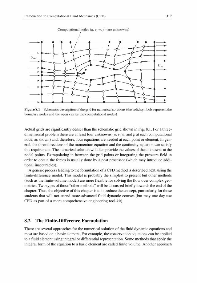
Actual grids are significantly denser than the schematic grid shown in Fig. 8.1. For a three-dimensional problem there are at least four unknowns (u, v, w, and p at each computationalnode, as shown) and, therefore, four equations are needed at each point or element. In gen-eral, the three directions of the momentum equation and the continuity equation can satisfythis requirement. The numerical solution will then provide the values of the unknowns at thenodal points. Extrapolating in between the grid points or integrating the pressure field inorder to obtain the forces is usually done by a post processor (which may introduce addi-tional inaccuracies).A generic process leading to the formulation of a CFDmethod is described next, using the

finite-difference model. This model is probably the simplest to present but other methods(such as the finite-volume model) are more flexible for solving the flow over complex geo-metries. Two types of those “other methods”will be discussed briefly towards the end of thechapter. Thus, the objective of this chapter is to introduce the concept, particularly for thosestudents that will not attend more advanced fluid dynamic courses (but may one day useCFD as part of a more comprehensive engineering tool-kit).

8.2 The Finite-Difference Formulation

There are several approaches for the numerical solution of the fluid dynamic equations andmost are based on a basic element. For example, the conservation equations can be appliedto a fluid element using integral or differential representation. Some methods that apply theintegral form of the equation to a basic element are called finite volume. Another approach

Computational nodes (u, v, w, p – are unknowns)

U∞

U∞

Figure 8.1 Schematic description of the grid for numerical solutions (the solid symbols represent theboundary nodes and the open circles the computational nodes)

317Introduction to Computational Fluid Mechanics (CFD)

uses the finite-difference approximation for the fluid dynamic approach. As noted, for sim-plicity, let us follow this latter method here.The first step of the process is to develop the numerical representation of the various

terms (derivatives) in the fluid dynamic equations. Let us do this by using a one-dimensional model as depicted in Fig. 8.2, where u(x) is an analytic function along thecoordinate x. Next we select several nodal points on the function u(x) separated by thedistance Δx.The objective is then to relate the function to its derivatives, based on the function values

at the nodal points. For smallΔx, u(x) can be expanded in a Taylor series about x as follows:

u x +Δx = u x +Δx∂u

∂x+

Δx 2

2∂2u

∂x2+

Δx 3

3∂3u

∂x3+……… 8 1

For example, we can find the first derivative,∂u

∂x, expressed in terms of the values at the

nearby nodal points, by simple algebraic operation. Using first-order terms from Eq. 8.1,

(and neglecting the higher order terms) and solving for∂u

∂xwe get

∂u

∂x=u x +Δx −u x

Δx+O Δx 8 2

and here we assumed thatΔx is small and all higher order terms combined are on the order ofΔx (so the order of the error is O(Δx)). Note that this is equivalent to a straight line curve-fitbetween the two adjacent points. Equation 8.2 is called a forward difference approximationand by using the same method we can derive a backward differential approximation:

∂u

∂x=u x −u x−Δx

Δx+O Δx 8 3

x

u

u(x)

xi

x +Δx

u(x –Δx)

u(x +Δx)

x –Δxi + 1i – 1

Figure 8.2 Illustrating the method for approximating the derivatives of the function u(x)


and the error is of the same magnitude as before. Also note that we are not discussing theactual “error” but the relation between the intervalΔx and the error (or how fast it is reducedwith reduced mesh size). We can generate a central differential approximation by combiningthese two expressions (using Eq. 8.1 twice for forward and backward differences) to get:

∂u

∂x=u x +Δx −u x−Δx

2Δx+O Δx 2 8 4

Note that the error is reduced for the central difference formulation (see Ref. 8.1). So it isbetter to use this formula and the forward/backward formulation can be retained for theboundaries of the problem (this is usually true for evenly distributed grids where, say,Δx is constant). For the second derivative we use again a Taylor expansion, similar to Eq. 8.1

u x + 2Δx = u x + 2Δx∂u

∂x+

2Δx 2

2∂2u

∂x2+

2Δx 3

3∂3u

∂x3+ ......... 8 5

and by combining Eq. 8.1 and 8.5, and solving for∂2u

∂x2, we get the forward differencing

formula:

∂2u

∂x2=u x + 2Δx −2u x +Δx + u x

Δx 2 +O Δx 8 6

Along the same lines we can write for first order central and backward differencing.

∂2u

∂x2=u x+Δx −2u x + u x−Δx

Δx 2 +O Δx 2 8 7

∂2u

∂x2=u x −2u x−Δx + u x−2Δx

Δx 2 +O Δx 8 8

Note again that the central differencing is more accurate. For simplicity, let us label thefirst three values in Fig. 8.2 using the index i:

u x +Δx ui+ 1

u x ui

u x−Δx ui−1

8 9

and Eq. 8.4 and 8.7, the first-order central derivatives (actually second-order accuracy) canbe expressed as

∂u

∂x=ui+ 1−ui−1

2Δx+O Δx 2 8 10


∂2u

∂x2=ui + 1−2ui + ui−1

Δx 2 +O Δx 2 8 11

Higher or mixed partial derivatives can be derived using the same method. Also these rela-tions are called first-order, since higher-order terms in the Taylor expansion were neglected.For example, the central difference representation for the second-order can be derived by notneglecting the second-order terms and for central differencing they are:

∂u

∂x=−ui+ 2 + 8ui+ 1−8ui−1 + ui−2

12Δx+O Δx 4 8 12

∂2u

∂x2=−ui+ 2 + 16ui+ 1−30ui + 16ui−1−ui−2

12 Δx 2 +O Δx 4 8 13

and the error is of fourth order with Δx. In conclusion, the accuracy increases with reducedΔx (finer grid!), and with the higher order approximation. Accuracy also improves whenusing central differences, mainly when the grid points are evenly distributed.

8.3 Discretization and Grid Generation

One of the most important parts of a numerical solution is the grid generation. The grid canbe structured or nonstructured as shown in Fig. 8.3. Structured grids have a clear order, asshown in the figure, and the discretization of the equations is simpler. However, for complexshapes, the creation of a well structured grid becomes difficult and will require more nodalpoints than an unstructured grid. These advantages of the unstructured grid are somewhatreduced by the more complex formulation of the governing equation. Usually finite volumeelements (based on the integral formulation) are used with an unstructured grid.

(a)

(b)

Figure 8.3 Structured grid for the flow over a backward facing step (a) and an unstructured grid forthe same problem (b)


For the numerical solution the computational domain must be defined. A schematicdescription is provided in Fig. 8.4. In this case we consider the flow over a solid body,and the solution grid must extend far enough where we can consider the perturbations(due to the object) to be small. This problem in subsonic flow (due to the elliptic equations)requires the boundary conditions to be specified along all boundaries, as shown. Conse-quently, on the outer boundary we specify a constant free stream (in at the left and out atthe right) and a constant pressure (see also Fig. 8.1). On the body surface we define the zerovelocity (tangential and normal), as shown schematically in Fig. 8.4.Of course, the grid generation requires a certain level of knowledge about the solution,

and near areas of fast change a denser grid is required. Also note that, in Eqns 8.10–8.13, theerror is reduced with reduced Δx; this means that, in general, the solution will improve withfiner grid. Thus, the first step for generating a numerical solution is to investigate the grid. Inprinciple, grid density should be increased until the solution appears to be independent ofthe grid!

8.4 The Finite-Difference Equation

At this point it is clear that the computational domain was subdivided into small elementswhere the equations will be specified. To demonstrate how the equations can be convertedinto algebraic representation at the solution cell level, let us follow the finite differenceapproach (and not the finite volume method). Therefore, the first step in this process isto replace the terms in the fluid dynamic equations with their finite-difference equivalent,in effect creating a set of algebraic equations. This is a major simplification and allows thesolution of problems that cannot be solved analytically. For simplicity let us consider thetwo-dimensional incompressible continuity equation (Eq. 6.16)

pa

Outer boundaryof computationaldomain

Computation domain

qn = 0

qt = 0

U∞

pa

U∞

Figure 8.4 The computational domain


∂2Φ∂x2

+∂2Φ∂z2

= 0 8 14

replacing the terms with their finite (central) difference equivalent results in:

Φi+ 1, j−2Φi, j +Φi−1, j

Δx 2 +Φi j+ 1−2Φi, j +Φi, j−1

Δz 2 +O Δx 2, Δz 2 = 0 8 15

this equation must be specified for all the grid points in Fig. 8.1 or 8.3. Note that near theboundaries, either the forward or backward difference must be used for one of the terms inEq. 8.14. One approach for the solution of similar equations is the explicit formulationwhere only one unknown per equation remains. For example, an iteration scheme intothe x direction (based on Eq. 8.15) can be proposed such that

Φn + 1i+ 1, j = 2Φui, j−Φi−1, j−

ΔxΔz

2

Φi j+ 1−2Φui, j +Φi, j−1

n

Error≈O Δx 2, Δz 2

8 16

and n here represents the iteration counter.The solution must start from the boundaries where the solution is known (boundary con-

ditions). The finite-difference formulation near the boundaries may use a different scheme,depending on the type of boundary condition (e.g., ifΦ is given, this is a Dirichlet condition

and if∂Φ∂x

is given, this is called the Neumann condition). The process is described schemat-

ically in Fig. 8.5, where the black dots represent known values. By using the informationfrom the neighboring point the solution can march forward (to the right) as depicted by thesmall white circle. This example serves only to demonstrate the explicit approach and willNOT work without using some of the tricks of numerical analysis. The major advantage ofthe explicit formulation is its simplicity, but the solutions are usually less stable and densergrids are required (and usually used for time-dependent problems).An alternate approach, called the implicit formulation, will have more than one unknown

per node, as expressed in Eq. 8.15. Then, when specifying this relation for each of the Nunknown grid points, N equations of the following form will result (based on Eq. 8.15):

Φi, j =1

2 + 2ΔxΔz

2Φui+ 1, j +Φi−1, j +

ΔxΔz

2

Φi j+ 1 +Φi, j−1

Error≈O Δx 2, Δz 2

8 17


When equal grid spacing is used (e.g., Δx=Δz) this reduces to a simple average of the fourneighbor points:

Φi, j =14

Φui+ 1, j +Φi−1, j + Φi j+ 1 +Φi, j−1

Error≈O Δx 2, Δz 28 17a

Of course, in this case too, the boundary conditions are used near the boundaries of the com-putational domain. In practice, the number of such equation can be on the order of severalthousands or even millions (depending on the number of grid points and the computationalpower). The final algebraic problem will have the form of a matrix where the unknowns arecentered near the diagonal, as shown in Fig. 8.6.In principle, all unknowns are solved at once (with the matrix inversion) and therefore the

implicit method is usually more stable than the explicit one and also requires less dense grid.On the other hand, since all equations are solved at once, the programming effort is muchlarger, as well as the required computation time.Because of the large size of the matrix, iterative solvers are used, but as shown, the matrix

is usually diagonally dominant and mostly contains zeroes, which simplifies the solution.Note that in this very simple example (Eq. 8.14) only one unknown per point is solved.

To demonstrate the approach used with more unknown, let us consider the x componentof the steady-state, two-dimensional, incompressible Navier–Stokes equation (fromChapter 5, Eq. 5.37):

u∂u

∂x+w

∂u

∂z=−1ρ

∂p

∂x+μ

ρ

∂2u

∂x2+∂2u

∂z25 37

i + 1

j + 1

i

j

i – 1

j – 1

Figure 8.5 Typical explicit iteration scheme, the unknown is the white circle


Replacing the partial derivatives with their corresponding central difference representationwe get the following finite-difference equation.

ui, jui+ 1, j−ui−1, j

2Δx+wi, j

ui, j+ 1−ui, j−12Δz

=−1ρ

pi+ 1, j−pi−1, j2Δx

+μ

ρ

ui+ 1 j−2ui, j + ui−1, jΔx 2 +

ui j+ 1−2ui, j + ui, j−1Δz 2 +O Δx 2, Δz 2

8 18

This shows that at each point there are three unknowns (u,w, p) and therefore three equa-tions are needed. Of course, there are the continuity and the momentum equation into the zdirection that must be used. In practice, several algebraic substitutions are used to simplifythe resulting equations (or the solution matrix).

8.5 The Solution: Convergence and Stability

In the previous sections the principle of the numerical approach was presented briefly byusing the finite-difference formulation. The grid generation and overseeing the solutionprocess is usually left for the end user of a CFD program. Therefore, first, the grid mustbe evaluated in terms of density, particularly in regions of rapid change. The objective isfor the solution to be independent of the grid, a process that usually increases the numberof grid points. Once the grid geometry is set, the unknown quantities at each nodal point are

=*

Figure 8.6 A typical set of linear algebraic equations resulting from the discretization of the fluiddynamic equations


solved using an iterative scheme. The solution process may involve large matrices and var-ious iterative methods. The applicability of the method often depends on the actual fluiddynamic problem. At the end, after a certain number of iterations, a solution is expected.For example, if we attempt to calculate the drag force on a sphere, then we can define anerror as the difference between a known value and the calculated one.

Error =Dcalculated −Dmeasured

Dmeasured8 19

If there is no experimental data then an average of the recent calculations can be used forDmeasured and the difference in the numerator can be replaced by the change during the lastiteration. Most computer programs will display the residues of the solution, which is thenormalized difference between the previous and the current iteration. The residual principlecan be applied to the equations and then, for example, the residues of the continuity and themomentum equations are provided. A desirable convergence of the solution is shown bycurve #1 in Fig. 8.7. In this case the numerical solution gradually approaches a value thatcan be defined as the “solution”. For example, if the drag coefficient of an object is estimatedthen the error bar could be set at a few percent.In case of nonlinear equations, the solution may end with a false solution, as shown by

curve #2. This may be a result of wrong formulations, wrong boundary condition, or even abad grid. In the worse scenario the results will diverge with increasing number of iterationsand this process could be gradual (curve #3) or completely unstable and oscillatory as incurve #4. This suggests that we must have an idea about the expected results and shouldbe able to recognize convergence and stability issues. This is why the programmer mustbe familiar with the analytical models presented in the previous chapters.

Solution1

2

3

4

Number of iterations

ErrorWrong solution

Figure 8.7 Schematic description of convergence and instability of numerical solutions


Even if a solution is obtained onemust remember that this is an approximate approach andthere are several sources for an error. The most common sources are:

1. Errors due to model (e.g., the equations used do not contain all required physics). Typicalexamples include the modeling of boundary layer transition, turbulence modeling, orvortex flow (and vortex breakdown).

2. Errors due to discretization – such as shown by Eqns 8.1–8.13. These equations clearlyindicate that the solution improves with a finer grid (smaller Δx).

3. Errors due to computer accuracy – such as roundoff or truncation errors.4. Errors due to numerical convergence – as depicted in Fig. 8.7.5. Errors in post processing - integration of shear and pressure, and so on.

In spite of this list of errors, computational tools are quite accurate when the proper model isused (e.g., laminar flow model when the flow is expected to be laminar, or turbulence mod-eling when the flow is expected turbulent, etc.). Typical areas of weakness are cases withflow separation or where transition from laminar to turbulent flow takes place.

8.6 The Finite-Volume Method

The main elements of a generic numerical solution were demonstrated in the previous sec-tions. The discussion was based on the differential form of the Navier–Stokes equations,leading to the finite difference discretization scheme. It is possible, however, to use the inte-gral form of the equations (see Eq. 2.20 and 2.24) and their discretization is obtained by theso called finite-volume approach. So, for the final difference method the differentials areapproximated, while for the finite-volume methods the integrals are approximated. Thefinite-volume methods are gaining popularity, mainly because of the inherent flexibilityto use non-uniform grids and since the integral formulation conserves mass and momentum.Such grids are necessary when modeling the flow over complex shapes, so that grid smooth-ness is not a major concern. Furthermore, by solving the integral form, properties such asmass or momentum are conserved, compared to other methods (where numerical errors canintroduce excess mass, etc.). Therefore, finite-volume methods are considered to be moresuitable for the solution of fluid mechanics problems. Because of the significance of thefinite volume based methods, a brief description, highlighting the element of the model,is presented next.As noted, the finite-volume model is based on the integral form of the fluid mechanic

equations, which were applied to a control volume (see Section 2.6). To demonstrate thediscretization process, based on this model, consider the incompressible, steady-state con-tinuity equation from Eq. 2.25

c sρ q n dS= 0 8 20


As in all numerical solutions the flow field is subdivided to small cells, or control volumes,and this equation is then applied to that finite-volume element. In practice the grid can con-sist of different shape elements and usually tetrahedral or triangular (in two-dimensions) orany polygon shape can be used. For simplicity, however, a two-dimensional rectangular ele-ment is used here, as shown at the center of Fig. 8.8.Of course, the element could be trapezoidal or triangular but then the formulation becomes

more complex. Each of these cells will have a finite volume or a finite area in the two-dimensional case. In one approach, the cell centered model, a central point (marked withthe white circle in the figure) is assigned to each cell. The indexes (i, j) are used to refer tothe cell, and the average variables (u,w, etc.) for the whole cell are assigned at this central point.Also, for this simple case it is assumed that along each of the cell surfaces, the properties areconstant, and this will be clarified later. Next the integral of Eq. 8.20 is applied to the controlvolume (cell), but since the changes are small it is approximated by the following summation

cellρ q n dS≈Σsidesρ q n S = 0 8 21

This is a vector expression and for a complex cell shape must be applied accordingly. For thepresent simple two-dimensional presentation, a perfectly aligned i-j cell (with the x-z coor-dinate) is used. The four corners of the cells are marked by a, b, c, and d, respectively, andconstant velocity is assumed along the cell boundary. For example uad represents the veloc-ity into the x direction, crossing the line a–d. For this perfect cell, therefore, the “dot” productcan be separated into the x and z directions, as follows (also, a constant density is assumed)

Σsides q n S = −uad Δz+ ubc Δz−wdc Δx+wab Δx = 0 8 22

i, j + 1

i, j – 1

b

cdz

(w)

x(u)

i, j

a

i + 1, ji – 1, j

Figure 8.8 Schematic description of a two-dimensional finite-volume cell


However, this relation for the cell must be related to the properties in the centroid. This canbe approximated (first order) as the average between the adjacent cells (even if their shape isnot exactly the same as the shape of the i-j cell)

uad =12

ui−1, j + ui, j

ubc =12

ui, j + ui+ 1, j

wdc =12

wi, j +wi, j−1 8 23

wab =12

wi, j+ 1 +wi, j

Substituting this into Eq. 8.22 results in

ui+ 1, j + ui−1, j2Δx

+wi, j+ 1 +wi, j−1

2Δz= 0 8 24

This is the finite-volume representation of the incompressible continuity equation at cell i-j.It looks similar to the finite difference representation, but the difference is that the variables(e.g., u and w) represent an average for the cell and not the value of the same variable at anodal or grid point (as in the case of the finite differences). This representation is more flex-ible when using unstructured grids. Also this was a first-order representation, and for higher-order and three-dimensional tetrahedral elements, a more complex formulation is used.This short description served to demonstrate the application of the integral approach in

CFD. Once the governing equations are converted to the algebraic form (as in Eq. 8.24) thesolution methods are similar to those described for the finite-difference approach. The appli-cability of the method using the finite-volume model will be demonstrated in the nextexample.

8.7 Example: Viscous Flow Over a Cylinder

As an example, let us solve the flow over a two-dimensional cylinder. This type of flow wasdiscussed in Section 6.6, and experimental results for the drag coefficients are provided inSection 6.7. By selecting a Reynolds number of 100, the laminar momentum equations canbe used, but because of the vortex shedding behind the cylinder, an unsteady solver is used.For simplicity, a structured grid, shown in Fig. 8.9, is selected with about 50,000 cells. Thisnumber is considered low resolution, particularly behind the cylinder, in the wake where anasymmetric vortex shedding is expected. The boundary conditions are simple inflow (free-stream) from the left and exit from the right, and also constant pressure at the outer bound-aries was specified.


For the solution a first order finite volume method was used, with 200 iterations per timestep, and the solution’s convergence history is shown in Fig. 8.10. The time frame shown inthis figure represents a total of about 270,000 iterations. The drag coefficient stabilized firstat a value close to CD = 1 1, which is close to the experimental values shown in Fig. 6.19.The residuals of the continuity equations are also shown indicating a stable convergence tothe solution presented here.

U∞

Figure 8.9 Structured grid used for calculating the laminar flow over a cylinder (Re = 100). Only asmall portion of the grid is visible!

103

102

101

100

10–1

10–2

10–3

1701651601551501451401351301.0500

1.1000

Cd

Cd

1.1500

1.2000

1.2500

Residualcontinuity eq.

U∞t

D

Figure 8.10 Reduction in the residuals (and the error) with iteration number


The calculated streamlines are presented in Fig. 8.11. The computations clearly capturedthe asymmetric vortex shedding and the Strouhal number is close to the values indicated inFig. 6.27. Because of the radial grid that lacked sufficient resolution in the wake, the finerdetails of the vortex streets were not captured. However, near the cylinder the flow compareswell with experimental results. For example the separation line is ahead of the top, as dis-cussed in reference to Fig. 6.17.The computed pressure distribution around the cylinder is plotted in Fig. 8.12, using the

same format used in Fig. 6.16. The ideal-flow “exact” solution of Eq. 6.71 is shown by thesolid line, while the dashed line describes the time average pressure coefficient. The θ = 1800

position represents the front centerline, while θ = 00 is at the back. Because of the aft-flowseparation, the pressure does not recover to the values of the ideal flow and remains nearCp −1 1. Of course the high pressure at the front and the low pressure at the back isthe source of the calculated drag force. Also, comparing the computations with the high Rey-nolds number experimental results of Fig. 6.17 shows earlier flow separation here, resultingin higher suction behind the cylinder and in higher drag coefficient.

Figure 8.11 Display of the streamlines obtained from the numerical solution

270θ (deg)

90 0 1801801

0

–1

–2

–3

–4

Cp

Equation 6.71

CFDRe = 100

Figure 8.12 Comparison between the average pressure coefficient distribution predicted by CFDwith the ideal flow results of Eq. 6.71


This example serves to demonstrate the type of expected results from CFD computations.The presented results could be improved, by refining the grid behind the cylinder. Also inthis type of grid, the cell size increases with the distance from the cylinder. To improve res-olution in the wake, a fairly dense grid should be used in the separated wake area behind thecylinder. For more details on the separation point, a denser grid near the cylinder surfacecould be used. In spite of all these inaccuracies, the major features and even the magnitudeof the forces were captured reasonably well with this simple solution.

8.8 Potential-Flow Solvers: Panel Methods

The computational methods presented so far are used for solving the viscous Navier–Stokesequations. In Chapter 6, however, it was shown that for high Reynolds number attachedflows the viscous terms can be neglected outside of a thin boundary layer. This assumptionled to the potential flow model, presented in Chapter 6, which allows a simple and efficientnumerical solution for three-dimensional external flows over complex shapes. These meth-ods, called panel methods, are based on using the surface singularity distributions andtheir advantage, compared to the finite-difference (or finite-volume) approach, is that theunknown elements are distributed on the surface and not in the whole fluid volume, therebysignificantly reducing computational effort. Another advantage is that the velocity field isobtained by solving the continuity equation only (decoupled from the momentum equation),and instead of three velocity components at each point (e.g., u, v, w) only one unknown,namely the velocity potential, is sought. So in conclusion, these methods are very efficientnumerically but applicable only to inviscid, attached flows.The theoretical background of such panel methods is shown schematically in Fig. 8.13.

A coordinate system is attached to the body which surface is subdivided to panel elements,as shown. The steady-state free-stream magnitude and direction expressed in this frame ofreference is Q∞ = U∞ ,V∞ ,W∞ and the continuity equation is

∇2Φ = 0 8 25

whereΦ is the velocity potential in the body’s frame of reference. The boundary conditionsrequire that the normal component of velocity on the solid boundaries of the body mustbe zero

∇Φ n = 0 8 26a

where n is an outward normal to the surface (as shown for one panel in Fig. 8.13). An alter-nate form of this boundary condition, called the Dirichlet condition, was introduced inEq. 6.56. This alternate boundary condition requires that the potential inside a closed bodybe constant. By setting the constant to zero this boundary condition becomes

Φi = 0 8 26b


Solution of Eq. 8.26 provides the velocity field through the whole fluid domain. The pres-sures and corresponding fluid dynamic loads are then calculated separately by using the Ber-noulli equation (recall that the continuity and momentum equations are not coupled forideal flow).There are a large numbers of numerical methods for solving this problem. They can be

based on source, doublet, or vortex distributions (or a combination of these) and can usevarious forms of the boundary conditions or shapes of the panel elements. The solutionmethodology is usually very similar and here we shall represent only one variant. SinceGreen’s theorem (Eq. 6.55) postulates that the solution of the problem consists of sourcesand doublets distributed on the surface, the problem reduces to finding a singularity distri-bution that will satisfy Eq. 8.26 (since the sources and doublets are already a solution of theLaplace’s equation). Once this distribution is found, the velocityq at each point in the field isknown and the corresponding pressure p can be calculated from the steady state Bernoulliequation (6.15)With these stipulations the velocity potential, based on Green’s theorem, canbe constructed as a sum of source σ and doublet μ distributions placed on the surface S: Thethree-dimensional version of Eq. 6.55 is then

Φ =−14π S

σ1r−μ

∂

∂n

1r

dS+Φ∞ 8 27

The values of the unknowns (σ, μ) can be found by applying the boundary conditions and r isthe distance between the element at (x0, y0, z0) and an arbitrary point (x, y, z). The free streampotential, based on Eq. 6.23 is

Φ∞ =U∞x +V∞y +W∞ z 8 28

Surfacepanels

n

z

y x

Q∞

Unit normalto a panel

Collocationpoint Wake

model

Figure 8.13 Schematic description of the potential flow model over a closed body


The unknowns are then the strengths of the sources and doublets assigned to each panel.However, if the source and doublet strengths on each surface panel are known, then thepotential at any point can be calculated by Eq. 8.27. By applying the boundary conditionof Eq. 8.26b inside the closed body, and setting the inside potential as Φi =Φ∞ ,Eq. 8.27 becomes

−14π S

σ1r−μ

∂

∂n

1r

dS= 0 8 29

In this case, however, the source distribution is known (see Ref. 8.1 p. 209)

σ = n Q∞ 8 30

and only the unknown doublet distribution remains to be solved. The solution is then basedon discretizing Eq. 8.29 and the methodology is described next.The numerical solution begins with a surface grid of N elements (called panels), as shown

in Fig. 8.13 The surface can be made of flat rectilinear panels or more complex shapes(called higher order panels). Similarly, for each panel the singularity distributions (sourceand doublets) are specified. If a constant strength source σ or doublet μ for a particular panelis assumed then this is usually called a first-order method. Higher-order approximations areusually based on a polynomial distribution of the source or doublet strength within the panel.Thus, one of the most basic components of the method is the panel element, which is shownschematically in Fig. 8.14. At the centroid of the panel a collocation point is placed wherethe boundary conditions will be applied (see also small circles in Fig. 8.13). For example,when solving Eq. 8.29, instead of performing the integral over the whole surface S, this inte-gral is calculated for a generic panel element as shown in the figure.

Collocationpoint

3

2

(x,y,z)

4

5

1

–y

zx

Surfacepanels

σ – distributionμ – distribution

Figure 8.14 Schematic description of a generic panel element


The results for a generic panel with a constant source distribution and an index kwill havethe form (see Ref. 8.1, p. 214)

−14π 1,2,3,4

1r

dSk

≡Bk 8 31

and here the constant Bk depends on the panel’s four corner points and on the field point (#5)where the potential due to this panel is evaluated. Similarly, the influence of a constant dou-blet distribution at point #5 (Ck) can be calculated by the integral

14π 1,2,3,4

∂

∂n

1r

dSk

≡Ck 8 32

The most important feature of these influence coefficients (e.g., Bk, Ck) is that this calcula-tion is based on the geometry only (e.g., the location of these five points) and can be exe-cuted without knowing the strength of the singularity elements. As an example, let us use theboundary condition of Eq. 8.29, which is based on an unknown doublet distribution. Theinfluence coefficient Ck is pre-calculated and do not depend on the strength μ. Next, for eachcollocation point (in Fig. 8.13) the potential due to all elements must add to zero inside thebody (so the collocation point is assumed to be on the inner surface of the body). Conse-quently, when Eq. 8.29 is specified at one collocation point with the index j, it will havethe form

N

k = 1

Bjkσk +Cjkμk = 0 8 33

This equation basically states that the potential at the collocation point of panel k is the sumof the potentials of all the surface panels (note that the source strength is known and given byEq. 8.30). This equation is then applied at all N collocation points with N unknowns μk, thusreducing the integral in Eq. 8.29 into a set of linear algebraic equations (matrix of order N).By solving the N equations, the unknown doublets for each panel are calculated and there-fore the potential Φ is known everywhere. In reality vortex wakes must be modeled too andthis is explained in Ref. 8.1, Section 9.3.Once Eq. 8.33 is solved, the unknown singularity values are obtained (μk in this case), and

the local velocity components can be evaluated. Also note that the doublet in Eq. 8.33 rep-resent the potential jump between the outside and the inside of the body (where Φi =Φ∞ ).Therefore, the perturbation velocity components are the derivatives of the potential (seeEq. 6.4), and in terms of the panel local coordinates (l,m, n) the two tangential velocity com-ponents are

ql = −∂μ

∂l, qm = −

∂μ

∂m8 34


The differentiation is done numerically using the values on the neighbor panels, as shown inFig. 8.15. Once the velocity is calculated (and the free-stream velocity is added) the surfacepressure and resulting lift and drag can be calculated, using the Bernoulli equation(Eq. 6.15), or in terms of the pressure coefficient (Eq. 6.72):

Cp = 1−q2

U2∞

8 35

The matrix representing Eq. 8.33 is usually diagonally dominant, since the influence of thepanel on itself is the largest. Also the number of unknown is significantly less than in thefinite-difference/volume methods, and therefore numerical convergence and stability issuesare almost nonexistent. The main sources of errors when calculating the velocity field arethen due to insufficient or incorrect grid distribution. Additional errors can occur during thepressure integration over complex shapes. Of course the main limitation of the method is thesignificantly simplifies physics (as discussed in Chapter 6).

8.9 Summary

Computational fluid mechanics has changed the face of the discipline. Instead of using con-siderably simplified models involving complex mathematics, CFD provides an easily acces-sible tool to solve a large variety of fluid mechanics problems. At the beginning of the thirdmillennium, however, the method is still not fully developed and still controlled by availablecomputer power and the abundance of various methods. It is expected that in the future,artificial intelligence could control processes such as the numerical modeling, grid gener-ation, and optimize solution algorithms on-the-fly (and therefore less programmer interfer-ence will be required).In the meantime, (until CFD is perfected) there is no replacement for studying classical

fluid dynamics. The potential user of such computational methods must be prepared with the

m

l

n

Figure 8.15 Nomenclature for calculating the local (perturbation) tangential velocity. Note that thenormal velocity is zero (see boundary condition Eq. 8.26a)


knowledge of the classical models and also understand the hierarchy of approximations inCFD: This hierarchy can be summarized as follows:

1. The actual, true physics may be more complex than the most advanced models2. The equations solved by CFD are approximations to the physics mentioned in (1). For

example, in the Navier–Stokes equations we assumed a Newtonial fluid.3. Many computer models solve a simpler model (such as laminar, incompressible, or invis-

cid flow, and for high Reynolds number flow – various models for turbulence).4. At the next level, where the equations are discretized (finite-difference, finite-volume or

element, etc.) additional inaccuracies are introduced.5. Grid generation, particularly when inappropriately done, can introduce further errors.6. The numerical solution of a large number of equations can create another form of errors

(such as round-off errors, convergence, stability, etc.).7. Finally, once a solution is obtained, the post processing can further reduce accuracy (e.g.,

errors due to integrating pressures and shear stresses).

At each level of this hierarchy some portion of the true physics is compromised. Being awareof this and understanding the implication is necessary for obtaining good results. At the timeof writing this text there are still many unresolved issues such as boundary layer transition,turbulence modeling, or the preservation of vorticity. In spite of the shortcomings listedhere, CFD is a powerful tool in the hands of a knowledgeable fluid dynamicist. Finally,Fig. 8.16 presents a typical result of a CFD analysis, showing surface pressures and off-body

Figure 8.16 Typical results of CFD: surface pressure distribution and off-body streamlines on anopen wheel racecar. Courtesy of TotalSim USA


streamlines. For example, the front wing tip vortices do not reach the rear wing and the lowpressure at the top of the wheels explains their contribution to lift.

References8.1. Hoffman K. A., and Chiang S. T., Computational Fluid Dynamics for Engineers, Vol I and II, Engineering

Education System, Wichita, KN, 1993.8.2. Ferziger, J. H. and Peric, M, Computational Methods for Fluid Mechanics, 2nd Edn, Springer-Verlag,

NY, 1999.

Problems

8.1. Develop a finite-difference representation for the following equation

∂g

∂x= k

∂2g

∂y2

Use forward differencing for the time derivative and central differencing for the spa-tial terms.

8.2. Modify the proposed finite-difference scheme (of the previous problem) for the bound-ary at y = 0.

8.3. Develop a finite-difference representation for the following equation

∂f

∂t= k

∂2f

∂x2+∂2f

∂z2

Use forward differencing for the time derivative and central differencing for the spa-tial terms.

8.4. Calculate the first derivative of the function f x = sin πx at x = 0.25:a. Using the forward-difference approximation with Δx = 0 01.b. Using the central-difference approximation with Δx = 0 01.c. Using the exact value.

8.5. Calculate the first derivative of the function f x = cos πx at x = 0.3 for three differentincrements of Δx = 0 02,0 01, and 0.005, and compare with the exact result.

8.6. The oscillation of a mass M suspended on a spring K is described by the equation:

Md2x

dt2+Kx= 0

where the spring length x is a function of time x(t).a. Derive a finite difference representation of this problem.b. Describe the first step using the numerical values for t = 0 Δt = 0 01, M = 1, and

K =1. Assume initial conditions: x = 0.1, dx/dt = 0.1.


For the following problems the students must have access to computational tools(either locally or from the Internet). Also, no solutions are provided here (the instruc-tor can post those results, based on the local software used).

8.7. Use a laminar CFD solver to calculate the flow over a two-dimensional cylinder andcompare the results for the drag coefficient with the experimental data in Fig. 6.19.Study two cases:a. Re = 1, andb. Re = 5.Also, plot the surface pressure distribution.

8.8. Use a laminar CFD solver to calculate the flow over a two-dimensional cylinder at aReynolds number of 40. Repeat the computations three times and increase grid den-sity twice (second computation) and four times (third computation). Compare theresults for the drag coefficient with the experimental data in Fig. 6.19 and discussthe effect of grid density on the solution.

8.9. Calculate the viscous laminar flow on a sphere at a Reynolds number of 1 and com-pare your results for the drag coefficient with Stokes formula (Eq. 6.76).

8.10. Calculate the two-dimensional flow normal to a flat plate (as in Fig. 6.22), and com-pare the drag results with the value of CD = 1.17 from Fig. 6.25. Assume Re = 100.

8.11. Use a time-dependent CFD model to calculate the flow over a cylinder at Re = 60.Compare the drag coefficient and the Strouhal number with the experimental data pre-sented in Chapter 6.

8.12. Use a three-dimensional panel code to calculate the lift and (induced) drag of a rec-tangular wing at an angle of attack of 5 . Assume aspect ratios of 5, 7, and 10, andcompare with calculated results based on Eq. 6.101 and 6.102.

8.13. Calculate the laminar flow inside a long cylindrical pipe for Re = 50, based on the pipediameter. Assume a uniform velocity profile at the entrance to the pipe. How longalong the pipe (in terms of diameters) before the velocity profile becomes fully devel-oped (e.g., parabolic)?


9Viscous Incompressible Flow:“Exact Solutions”

9.1 Introduction

The equations governing fluid motion were developed in Chapter 2 and it was immediatelynoted that a general analytical solution is beyond reach. In contrast, the solutions presentedin this chapter are often called “exact solutions”. This is possible for a few limited cases,where a set of logical assumptions leads to simplification of the fluid dynamic equations,facilitating a simple solution (for laminar flows)! The importance of this chapter is the intro-duction of the viscous affects for internal flows, as in the cases of fuel lines, cooling sys-tems, or oil delivery tubes. For example, the velocity distribution for the laminar flow insidea pipe will be formulated and the average velocity will be calculated. This provides the rela-tion between the simple one-dimensional average velocity model (of Chapter 3) and themore complex (and realistic) two- or three-dimensional flows.The second objective of this chapter is to demonstrate the approach that evolved during

the past 200 years for solving the unsolvable fluid dynamic problems. According to thisapproach, in order to develop a practical engineering solution, one must start with a simplebut exact solution that determines the major variables and the basic trends of the problem(e.g., the pressure drop in a circular pipe versus the Reynolds number). Based on these para-meters, an empirical database can be developed for treating a wider range of engineeringproblems. As an example, the viscous laminar flow model in circular pipes is extended intothe high Reynolds number range and the effects of turbulent flow (based on experimentaldata) were included.


9.2 The Viscous Incompressible Flow Equations (Steady State)

When developing the fluid dynamic equations in Chapter 2, we noted that their general ana-lytic solution is next to impossible. There are several simple cases, however, when we canactually derive a solution that contains important physical information. One of the most suc-cessful examples is the viscous flow in circular pipes that provides the rationale for devel-oping an experimental data base to help in more complex (but similar) engineeringproblems. Prior to starting, let us rewrite the governing equations for steady-state, viscous,incompressible flows. The continuity equation is Eq. 2.33

∂u

∂x+∂v

∂y+∂w

∂z= 0 9 1

and the viscous incompressible momentum equations (Eq. 2.40) in Cartesian coordinates are(neglecting the body forces):

u∂u

∂x+ v

∂u

∂y+w

∂u

∂z=−1ρ

∂p

∂x+μ

ρ

∂2u

∂x2+∂2u

∂y2+∂2u

∂z29 2a

u∂v

∂x+ v

∂v

∂y+w

∂v

∂z=−1ρ

∂p

∂y+μ

ρ

∂2v

∂x2+∂2v

∂y2+∂2v

∂z29 2b

u∂w

∂x+ v

∂w

∂y+w

∂w

∂z=−1ρ

∂p

∂z+μ

ρ

∂2w

∂x2+∂2w

∂y2+∂2w

∂z29 2c

At this point the body forces were neglected and if a gravitational force is present its effectcan be included in the pressure gradient term.

9.3 Laminar Flow between Two Infinite Parallel Plates:The Couette Flow

Let us start with the simplest example, the viscous flow between two parallel (infinite)plates, as shown in Fig. 9.1.The fluid is considered viscous and incompressible (such as water or oil) and for this case

we shall neglect the time derivatives and the body forces. We also assume that the flow islaminar and this statement will be clarified towards the end of the chapter. Let us use aCartesian coordinate system attached to the lower plate, as shown in Fig. 9.1, and the gov-erning equations for this case are summarized by Eqns 9.1 and 9.2. Observing Fig. 9.1 wecan assume that the lower plate is stationary and therefore the velocity near the lower surfaceis zero (at z= 0). We may speculate about the shape of the velocity distribution (as shown),however, it is clear that the velocity at z= h is equal to the velocity of the upper plate, U(recall the no-slip boundary condition). This flow is called the Couette flow after Maurice


Marie Alfred Couette (1858–1943), a well-known French physicist. The model is two-dimensional and there are no changes into the y direction. Also there is no velocity intothe z direction and we summarize this as:

v =w= 0 9 3

Now substituting this into the continuity equation (9.1) results in

∂u

∂x= 0 9 4

The conclusion is that the velocity profile is a function of z, and is the same at any x station:

u= u z 9 5

Next we apply all the previous assumptions to the momentum equations (9.2), which nowreduce to

0 =−1ρ

∂p

∂x+μ

ρ

∂2u

∂z29 6a

0 =−1ρ

∂p

∂y9 6b

0 =−1ρ

∂p

∂z9 6c

The last two equations indicate that there is no lateral or vertical change in the pressure.Hence, the pressure can only change with x and is constant vertically

p = p x 9 7

U

z

hu(z)

x

Figure 9.1 Viscous flow between two infinite parallel plates

341Viscous Incompressible Flow: “Exact Solutions”

Also this is a steady-state problem and Eq. 9.4 states that there are no changes in u with x(and the velocity is changing only with z). So, if the second term in Eq. 9.6a is constant alongthe x axis, then we conclude that the pressure gradient must be constant too:

dp

dx= const 9 8

At this point, only Eq. 9.6a remains, and after rearranging it becomes:

∂2u

∂z2=1μ

dp

dx9 9

The only variable now is x and instead of the partial derivatives, an ordinary differentialequation remains. After integrating twice we get:

u z =1μ

dp

dx

z2

2+Az +B 9 10

where A and B are the constants of integration.

9.3.1 Flow with a Moving Upper Surface

This first case is the original Couette flow and the boundary conditions for Eq. 9.10 are

at z = 0 u = 0

at z = h u =U9 11

substituting the z = 0 condition into Eq. 9.10 yields that B= 0, while the second boundarycondition results in:

U =1μ

dp

dx

h2

2+Ah


A=U

h−

h

2μdp

dx

Substituting this result into Eq. 9.10 provides the velocity distribution:

u z =Uz

h−h2

2μdp

dx

z

h1−

z

h9 12


The first term is clearly a linear variation and reduces to the shear flow profile discussed inreference to Fig. 1.11. The second parabolic (shape) term contains the effect of the pressuregradient and this effect is summarized in Fig. 9.2. In order to visualize this, let us define aconstant k, such that:

k = −h2

2μdp

dx9 13

When k = 0, then we get the basic shear flow, and when the pressure gradient is favorable

(negativedp

dxor positive k) then we get an additional parabolic forward velocity distribution,

as shown. When the pressure gradient is opposing the flow then this parabolic shape isreversed. At higher negative values of k, even reverse flows are possible (as shown inthe figure for k = −2).

9.3.2 Flow between Two Infinite Parallel Plates: The Results

With the assumptions posed for the viscous flow between parallel plates we actually arrivedat the “exact solution”. It is important to connect those results with engineering quantitiessuch as the average velocity, which was used in the one-dimensional flow model ofChapter 3. Thus, the average velocity Uav is the velocity which multiplied by the inflowarea will have the same volumetric flow rate Q (per unit width)

Q=Uavh =

h

0

udz 9 14

0

0–1 3

0.2

0.8

k = –20.6 z

hh

U

0.4

1.0 1.2 1.40.80.60.40.20–0.2

Reverseflow

U

u

1 2

Figure 9.2 Effect of the pressure gradient on the velocity profile of the flow between two relativemoving plates


Consequently, we define the average velocity as:

Uav =1h

h

0

udz 9 15

Next, the velocity distribution from Eq. 9.12 is substituted and the integration is performed:

Uav =1h

h

0

Uz

h−h2

2μdp

dx

z

h1−

z

hdz =

U

2z

h

2−h2

2μdp

dx

12

z

h

2−13

z

h

3 h

0

=U

2−

h2

12μdp

dx

9 16

Now we can also solve for the volumetric flow rate (per unit width):

Q≡ hUav =Uh

2−

h3

12μdp

dx9 17

Figure 9.2 shows the various velocity distribution as a function of the pressure gradient.To calculate the maximum velocity we must derive the velocity distribution

du z

dz=U

h−h2

2μdp

dx

1h−2zh2

= 0

and after solving for z:

z

h=12−μ

h2Udp

dx

9 18

Note that this equation is not valid whendp

dxapproaches zero. The next important observation

is that in this viscous flow there is a shear stress. This force acts between the parallel layers asthey slide on each other (creating friction). To calculate the shear stress we use the defini-tions introduced by Eq. 1.15 and using the velocity distribution from Eq. 9.12

τxz = μdu z

dz= μ

U

h−h2

2dp

dx

1h−2 zh2

9 19

From the engineering point of view the determination of the shear force (or friction) on thesolid surface is important. Therefore, a nondimensional friction coefficient Cf can be definedsuch that


Cf ≡τxz

12ρU2

av

9 20

Calculation of this coefficient is important at the upper and lower walls, which can be foundfrom Eq. 9.19

τxz 0 = μU

h−h

2dp

dx9 21a

τxz h = μU

h+h

2dp

dx9 21b

Example 9.1 Shear flow (with no pressure gradient)For this first example let us revisit our introductory model for explaining the effects ofviscosity. Figure 1.11 is redrawn here in Fig. 9.3 and the problem at hand is the case whenthe upper plate moves at a velocity U but there is no pressure gradient.

dp

dx= 0

The average velocity is obtained from Eq. 9.16

Uav =U

29 22

and as expected it is the velocity at the centerline. Similarly the volumetric flow rate(from Eq. 9.17)

Solid boundaries No-slip condition

No-slip condition

Fluid

F

U

z

x

h

Figure 9.3 The flow between two parallel plates. The upper is moving at a velocity of U and thelower is stationary


Q=Uh

29 23

and the maximum velocity is at the contact with the upper plate (z = h)

Umax =U 9 24

The shear force at the wall, based on Eq. 9.19 is constant (with z) and is the same at the upperand lower walls (and this was discussed in Chapter 1):

τxz = μU

h9 25

The friction coefficient on either the upper or lower surface is calculated by substituting thevalues of the shear stress and the average velocity:

Cf =τxz

12ρU2

av

=μU

h

12ρU2

4

=8μρUh

9 26

This is a very important result because it re-introduces the Reynolds number, Re, after theBritish fluid dynamicist Osborne Reynolds (1842–1912). This nondimensional number wasdiscussed in Chapter 4 and, as noted, it represents the ratio between the “inertia” and theviscosity effects.

Re =ρUh

μ9 27

Here, the Re number is based on the clearance h between the plates (but in other cases,different quantities for the length scale may be used). Based on this definition, let us rewritethe friction coefficient for this case as:

Cf =8Re

9 28

This equation is not only simple but also provides the basics for experimental evaluation ofuniversal friction coefficients, as a function of the Reynolds number. Note that in this case(of laminar flow) the friction coefficient is reduced with increasing Reynolds number.

Example 9.2 Numerical example for the flow between two parallel plates, with nopressure gradientAs a numerical example, following Example 9.1, let us consider the flow of water betweentwo parallel plates. The upper plate moves at a velocity of U = 5m s, and the clearance ish = 1 cm. Calculate the average and maximum velocities, flow rate, and shear force.


Solution:The average velocity is at the centerline

Uav =U

2=52= 2 5m s

and the volumetric flow rate is

Q=Uh

2= 0 01 2 5 = 0 025m3 s

The maximum velocity is at the contact with the upper plate z= h

Umax =U = 5m s

and the shear stress at the wall (upper or lower), is

τxz = μU

h= 0 001

50 01

= 0 5Nm2

Here, the viscosity μ = 0 001 for water was taken from Table 1.1. Suppose we want tocalculate the force F required for pulling a unit area, S = 1 m2 of the plate:

F = τxz S = 0 5Nm2

1m2 = 0 5N

9.3.3 Flow between Two Infinite Parallel Plates – The Poiseuille Flow

This is another important case of the flow between plates because now both the upper andlower plates are stationary. Consequently, the fluid motion is due to the pressure gradientonly. This flow is named the Poiseuille flow after Jean LouisMarie Poiseuille (1799–1869) aFrench physician who studied pressure loss in small tubes.Essentially, this case was solved in the previous section and information such as the aver-

age or maximum velocity and other properties can be obtained by simply setting the upperplate velocity to zero U = 0 . The velocity distribution, based on Eq. 9.12 is then

u z = −h2

2μdp

dx

z

h1−

z

h9 29

This is a parabolic shape, as shown in Fig. 9.4, and u z = 0 at z = 0 and at z= h. Also thisestablishes the relation between pressure loss and viscous friction on the walls. The averagevelocity is obtained from Eq. 9.16


Uav = −h2

12μdp

dx9 30

and the volumetric flow rate (per unit width) from Eq. 9.17:

Q= −h3

12μdp

dx9 31

This indicates that the flow rate is directly (linearly) related to the pressure gradient. Themaximum velocity location, based on Eq. 9.18 is found at the centerline

z

h=12

9 32

Substituting this into the velocity distribution, Eq. 9.29, the maximum velocity is found:

Umax = −h2

8μdp

dx9 33

Comparing this with the average velocity yields:

Uav =23Umax 9 34

Because of the symmetry (upper/lower) the shear stress on both walls is the same.To calculate the shear we use Eq. 9.19 (with U = 0):

τxz = −h2

2dp

dx

1h−2zh2

9 35

z

x

Umax

u(z)

h

Figure 9.4 The flow due to a constant pressure gradient between two parallel stationary plates


Note that the shear at the center z = h 2 is zero, and on the walls (z= 0, and z = h) is

τxz wall = ±h

2dp

dx9 36

and it seem to pull opposite to the pressure force. The friction coefficient Cf on one wallis then

Cf =−h

2dp

dx12ρU2

av

9 37

This is not a very useful expression, but based on Eq. 9.30 we can solve for the pressuregradient

dp

dx= −

12μh2

Uav

and substitute this into Eq. 9.37

Cf =

h

212μh2

Uav

12ρU2

av

=12μρUavh

9 38

we see again that the Reynolds number appears in this equation. Using the Re numberdefinition from Eq. 9.27 we can write

Cf =12Re

9 39

It is interesting to compare the shear stress between this case and the basic shear flow(Example 9.1). First we need to rearrange the shear on the wall based on the maximum

velocity. This can be done by solving Eq. 9.33 fordp

dxand substituting the result into Eq. 9.36

τxz wall =h

2dp

dx=h

28μUmax

h2= 4μ

Umax

h9 40

Now recall the shear term for the shear flow of Example 9.1

τxz = μU

h9 19


Based on these results, in order to have the same shear at the wall, the flow created by themoving upper plate must have a maximum velocity, four times larger, than in the case wherethe flow is moved by a pressure gradient (Fig. 9.5).We can also observe the force balance on the fluid in this flow, as depicted in Fig. 9.6.

Since there is no acceleration in the x direction, the sum of the forces acting on the fluidbetween the two plates must be zero. To investigate this hypothesis let us select a segmentof length l, as shown in Fig. 9.6. The shear forces on the upper and lower walls, for theselected segment (per unit width) is then

F1 =F2 = τxz l= −h

2dp

dxl

and here we used the shear term from Eq. 9.36. The force F3 due to the pressure gradient(per unit width) is

F3 =Δp h = −dp

dxl h

and clearly

F3 =F1 +F2

U = 0

(a) (b)

U = Umax

Umax

dpdx ≠0

dpdx = 0

Figure 9.5 Two velocity distributions having the same shear stress at the wall: (a) flow due topressure gradient, and (b) flow between a moving and stationary, parallel plates

l

u(z)

F1

h

F2

F3Umax

Figure 9.6 The shear flow on the walls must be equal to the force due to the pressure drop


Example 9.3 Water flow due to pressure gradient between parallel platesTo demonstrate the applicability of this formulation let us investigate the flow of water withan average velocity of 1 m/s, and the clearance between the plates is 1 cm, Using the vis-cosity value from Table 1.1 calculate the maximum velocity, the pressure gradient, the shearand the friction coefficients.

Solution:First, based on Eq. 9.34 we can calculate the maximum velocity

Umax = 1 5Uav = 1 5m s

Next, we may use Eq. 9.30 to calculate the pressure drop

dp

dx=−12μh2

Uav =−12 0 001 1

0 012= −120

N m2

m

The shear at the wall is calculated using Eq. 9.35

τxz h= 0 = −h

2dp

dx= −

0 012

−120 = 0 6Nm2

The Reynolds number is

Re =ρUh

μ=1000 1 0 01

0 001= 104

and the friction coefficient (based on Eq. 9.39)

Cf =12Re

=12

104= 1 2 10−3

9.3.4 The Hydrodynamic Bearing (Reynolds Lubrication Theory)

The potential of using a thin viscous fluid layer to reduce friction has been recognized andsuccessfully used in many engineering applications. For example, rotating components suchas the camshafts and crankshafts of the internal combustion engine roll on hydrodynamicbearings. The magnetic reader mechanism of rotating computer disks floats above the sur-face, based on the same principle. In all these cases, the moving surface is supported by the


pressure created by the viscous flow within the gap (also resulting in very low friction). Themodels for the rotating shaft and the sliding block (slipper bearing) are quite similar, andhere only the simpler linear slipper bearing is discussed. The theory was first developedby Osborne Reynolds in 1886 and the approach for laminar flow is shown schematicallyin Fig. 9.7.Here, a block slides at a velocity of U on a thin film of viscous fluid. The attempt is to

describe a two-dimensional, steady-state case where l is very large, while the gap h betweenthe block and the solid surface is very small l h . An x-z coordinate system is attached tothe upper sliding block, which moves at a velocity U to the right. Also the slope α is verysmall and the velocity components in the z direction are small too

u >>w

l >> h9 41

With these assumptions only one term remains from the two-dimensional incompressiblecontinuity equation:

∂u

∂x0

Because we expect a small change in the x direction we cannot conclude that the velocityprofile in the x direction is constant. However, the flow rate Q is constant

Q=

h

0

u z dz= const 9 42

l

p0p0

h1

U

z

x

α

1 2

h h2

Figure 9.7 Model for the viscous laminar flow under a linear bearing


Next, we apply the previous assumptions to the momentum equations (Eq. 9.2). For the xdirection we get

u∂u

∂x=−1ρ

∂p

∂x+μ

ρ

∂2u

∂x2+∂2u

∂z29 43

and the momentum equation to the z direction becomes

0 =−1ρ

∂p

∂z9 44

The second equation indicates that there is no lateral or vertical change in the pressure.Hence the pressure can change only with x and is constant vertically

p = p x

Considering the order of magnitude of the terms in the momentum equation in the x directionwe find that the left hand inertia term is of order O(l)

u∂u

∂xO l

The order of the two second-order derivatives, based on Eq. 9.41, are

∂2u

∂x2O

l2

l2=O 1

∂2u

∂z2O

l2

h2

and therefore this second order derivative term is clearly the largest

∂2u

∂z2>>

∂2u

∂x2

Consequently, the inertia term can be neglected too and the momentum equation in thex direction becomes (exactly as in the Couette flow case – see Eq. 9.6):

0 =−1ρ

∂p

∂x+μ

ρ

∂2u

∂z29 45


The boundary conditions, based on Fig. 9.7, at x = 0 are

p = p0

h = h1

u z= 0 = −U

u z= h1 = 0

9 46

Note that the coordinate system is attached to the upper sliding block and therefore the lowersurface appears to bemoving at a velocity of –U. The boundary conditions at the other end ofthe block, at x = l, are

p = p0

h = h2

u z= 0 = −U

u z= h2 = 0

9 47

Prior to integration, the momentum equation is rearranged as follows

∂2u

∂z2=1μ

∂p

∂x

and the velocity profile in the gap is found after two integrations

u z =1μ

∂p

∂x

z2

2+A x z +B x 9 48

The integration constant B(x) is calculated by applying the boundary condition at z = 0(for any x along the gap)

−U =B x 9 49

and A(x) is found by applying the boundary condition at z = h

0 =1μ

∂p

∂x

h2

2+A x h−U 9 50

Substituting A(x) and B(x) into Eq. 9.48, yields

u z =1μ

∂p

∂x

z2

2+

−1μ

∂p

∂x

h

2+U

hz−U


and after rearranging, the velocity profile inside the gap becomes:

u z =h2

2μ∂p

∂x

z2

h2−z

h+U

z

h−1 9 51

The only unknown at this point is the shape of the pressure distribution, which can be foundindirectly by applying the continuity equation (9.42)

Q =

h

0

u z dz =

h

0

h2

2μ∂p

∂x

z2

h2−z

h+U

z

h−1 dz= −

h3

12μ∂p

∂x−Uh

2= const 9 52

Now the pressure gradient as a function of the local h can be calculated

∂p

∂x= −

12μh3

Uh

2+Q 9 53

At this point we can look at the boundary conditions, and see that the pressure at both ends ofthe sliding block is p0. This suggest that the pressure builds up towards the center, and must

have a maximum where∂p

∂x= 0. Let us identify the gap at this point (of maximum pressure)

as h0. With this definition, the flow rate can be easily calculated at h0 (Eq. 9.52) becauseQ isconstant with x

Q= −Uh02

9 54

and the pressure gradient can be simplified by substituting Eq. 9.54 into eq. 9.53

∂p

∂x= −

6μUh3

h−h0 9 55

The pressure distribution can be found by integration with x. However, first, the gap geom-etry (based on Fig. 9.7) is obtained

h= h1 + h2−h1x

l≈h1 + αx 9 56

The integration can be simplified more by exchanging the integration variable

∂p

∂x=∂p

∂h

∂h

∂x=∂p

∂hα


With this modification Eq. 9.55 becomes

∂p

∂h= −

6μUα

1h2

−h0h3

This can be integrated with respect to h

p =6μUα

1h−

h02h2

+C

where C is the integration constant. The two unknowns (C and h0) can be found by applyingthe boundary conditions at the two ends of the sliding block

at x = 0 p= p0 h = h1

at x = l p = p0 h= h2

and after some algebra we get

h0 =2h1h2h1 + h2

9 57

and after solving for the constantC, the longitudinal pressure distribution as a function of thegap h becomes

p−p0 =6μUα

h−h1 h−h2h2 h1 + h2

9 58

The shape of this pressure distribution is shown schematically in Fig. 9.8. The maximumpressure occurs at h = h0 and based on Eq. 9.58 (and recalling that h2−h1 l ≈ α) it is:

pmax−p0 =6μUα

h0−h1 h0−h2h20 h1 + h2

=3μUl2

h2−h1h1h2 h1 + h2

9 59

The position of the maximum pressure in terms of the x coordinate is obtained by substitut-ing h0 from Eq. 9.57 into Eq. 9.56

x

l pmax

=h1

h1 + h29 60

The local velocity distribution is also shown in Fig. 9.8, and it is determined by Eq. 9.51.Initially it resembles the simple shear flow, as in Fig. 9.3, but in this case the pressure gra-dient is not constant. Near the left-hand side of the sliding block, the pressure gradient ispositive and the parabolic term in the velocity profile is more dominant.


From the engineering point of view the total force L lifting the sliding block and the fric-tion drag D must be calculated. The supporting force L (per unit length) can be obtained byintegrating the pressure along the block and again replacing the integration of x with theintegration with h:

L=

l

0

p−p0 dx=6μUα2

h2

h1

h−h1 h−h2h2 h1 + h2

dh

=6μUl2

h21 h2 h1−12 ln

h2h1

−2 h2 h1−1h2 h1 + 1

9 61

The drag force can be found by integrating the shear force along the lower surface of theblock, at z= h. Taking the velocity distribution from Eq. 9.51, the shear stress is:

τ = μdu z

dz h

=h2

2∂p

∂x

2 hh2

−1h

+ μU

h=h

2∂p

∂x+ μ

U

h9 62

Next, substituting∂p

∂xfrom Eq. 9.53 we get

τ = μ4Uh

+6Qh2

9 63

pmax

p – p0

0 1.0 xl

U

Uu h2

h0

Figure 9.8 Schematic description of the pressure distribution under the sliding block (for the case ofh2 h1 = 2 2) and the shape of the velocity distribution in the gap


The drag force (per unit length) is now found by integrating the shear stress and exchangingthe integration in the x direction with the h direction

D =

l

0

τdx=μ

α

h2

h1

4Uh

+6Qh2

dh=μ

α4U lnh−

6Qh

h2

h1

9 64

SubstitutingQ from Eq. 9.54, α from Eq. 9.56, and h0 from Eq. 9.57, the drag force becomes

D =μUl

h1 h2 h1−14ln

h2h1

−6 h2 h1−1h2 h1 + 1

9 65

The maximum lift can be obtained using the derivative of the lift expression:dL d h2 h1 = 0. After some algebra we find that the condition for the maximum lift occurswhen h2 h1 = 2 2. Calculating the lift (from Eq. 9.61) and drag (from Eq. 9.65) for themaximum lift condition we get

Lmax = 0 16μUl

h1

2

DLmax = 0 75μUl

h1

9 66

and the lift to drag ratio (which is the mechanical friction coefficient) for this condition is

D

L Lmax

= 4 7h1l

9 67

Considering that the order of magnitude for typical bearing isl

h110−3 the friction coef-

ficient of the hydrodynamic bearing is significantly lower than the dry friction! Also note

that the pressure drag is ~ Lα≈Lh2−h1

l, which is much less than the value shown

in Eq. 9.67.

Example 9.4 Lift of a linear bearingA 1 cm long magnetic pickup is floating on a rotating disk where the linear velocity is50 m/s. Assuming the allowed gap is h1 = 0 2mm, and h2 h1 = 2 2, calculate the weightof the magnetic head. Also, calculate the drag-to-lift ratio.

Solution:For this case we can use Eq. 9.66 and assume that the disk operates in air. The lift is

L= 0 16μUl

h1

2

= 0 16 1 8 10−5 500 010 0002

2

= 0 36Nm


Suppose the pickup head is 1 cm wide then the lift is 1/100 of this value. The drag to lift ratiocan be calculated using Eq. 9.67

D

L= 4 7

0 00020 01

= 0 094

and this is at least one order of magnitude smaller than dry friction.

9.4 Flow in Circular Pipes (The Hagen-Poiseuille Flow)

Calculations, such as that for the pressure loss in long circular pipes, are of paramountimportance in many engineering applications. This was extensively studied during the earlynineteenth century by the German hydraulic engineer G. H. L. Hagen (1797–1884) and theFrench physiologist J. L. M. Poiseuille (1799–1869). The mathematical formulation of thisproblem is similar to the one used for the flow between parallel plates, however, now a cylin-drical coordinate system is used. The basic model is described in Fig. 9.9 and it is assumedthat the flow is incompressible, viscous, laminar, and fully developed (far from entranceeffects, and no changes with x). The only body forces we consider is gravitation (ρg),and the flow inside the pipeline moves only into the x direction and there are no velocitycomponents into the other directions.

qr = qθ = 0 9 68

With these assumptions, the continuity equation in cylindrical coordinates for an incom-pressible fluid (Eq. 2.45) becomes

∂qx∂x

= 0 9 69

We assume the flow is axisymmetric (and there are no changes with θ) and we reach theconclusion that

r

x

Ru(r)

θ

Figure 9.9 Fully developed laminar flow in a circular pipe


qx = qx r 9 70

The momentum equation in the r direction (Eq. 2.46) is now reduced to

0 = −∂p

∂r9 71

The momentum equation (Eq. 2.47) in the θ direction:

0 = −∂p

∂θ9 72

and in the x direction (Eq. 2.48):

0 = ρg−∂p

∂x+ μ

∂2qx∂r2

+1r

∂qx∂r

9 73

From Eq. 9.71 and 9.72 we conclude that the pressure varies only in the x direction

p = p x 9 74

Now we can rearrange Eq. 9.73 as follows

−ρg +dp

dx= μ

1r

d

drrdqxdr

and a more convenient form is:

d

drrdqxdr

=1μ

dp

dx−ρg r

Now we can integrate with respect to r

rdqxdr

=1μ

dp

dx−ρg

r2

2+A

and A is the constant of integration. We divide first by r

dqxdr

=1μ

dp

dx−ρg

r

2+A

r


and perform the second integration

qx =12μ

dp

dx−ρg

r2

2+A

rlnr +B 9 75

To calculate the integration constant we must use the boundary conditions. At the center ofthe pipe, clearly there is symmetry and we require that

At r = 0dqxdr

= 0

Andat r =R qx = 0

9 76

And the second condition, at the pipe inner wall, requires that the velocity must be zero(based on the zero slip boundary condition). Substituting the first boundary condition intoEq. 9.75 yields:

dqxdr

=1μ

dp

dx−ρg

02+A

0= 0

This is only possible if A is zero. Substituting the second boundary condition to solve for B

0 =12μ

dp

dx−ρg

R2

2+B


B= −12μ

dp

dx−ρg

R2

29 77

and by substituting this into Eq. 9.75, the velocity distribution is obtained:

qx =R2

4μdp

dx−ρg

r

R

2−1 9 78

This velocity distribution has a parabolic shape and maximum velocity is reached at thecenter. Also, note the linear relation with the pressure gradient (e.g., increasing the pressuregradient twice will double the velocity and the flow rate). Next, let us calculate quantitiessuch as the maximum velocity, flow rate, and so on. First, however, let us assume that the ρgterm is similar to the pressure drop and use only one. In this case the velocity distribution is:

qx =R2

4μdp

dx

r

R

2−1 9 79


The maximum velocity is at the center r = 0 :

Umax = −R2

4μdp

dx9 80

and the negative sign is a result of the flow in the positive x direction, for which the pressuregradient must be negative. The maximum velocity can be inserted into Eq. 9.79 to show thevelocity distribution as:

qx =Umax 1−r

R

29 79a

The average velocity times the cross-sectional area has the same volumetric flow rate Q asthe actual flow with the parabolic velocity profile:

Q=UavS= qxdS

Therefore, the average velocity is obtained as follows:

Uav =1S

qxdS 9 81

where S is the pipe cross-sectional area and dS= 2πrdr. Substituting Eq. 9.79 yields

Uav =1

πR2

R

0

R2

4μdp

dx

r

R

2−1 2πrdr =

12μ

dp

dx

R

0

r3

R2−r dr =

12μ

dp

dx

r4

4R2−r2

2

R

0

and after substituting the two integration constants we get

Uav = −R2

8μdp

dx9 82

Comparing this with Eq. 9.80 reveals that

Umax = 2Uav 9 83

The volumetric flow is then

Q =UavS = −R2

8μdp

dxπR2 = −

πR4

8μdp

dx9 84


This is a very important conclusion because it shows the relation between the pressure dropand the flow rate in a circular pipe. As noted earlier, the relation is linear with the pressuredrop indicating that higher pressure gradient will increase the flow rate. The effect ofviscosity is also linear but opposite and, for example, more pressure is needed to drivethe same flow rate if the viscosity is increases. Next, the shear stress in the flow is calculatedby deriving Eq. 9.79

τxr = −μdqxdr

= −μR2

4μdp

dx

2rR2

= −r

2dp

dx9 85

and the minus sign is a result of the coordinate system (e.g., the origin is at the center).The shear is zero at the center of the pipe and increases linearly with the radius, reachingmaximum at the wall. The shear at the wall is then

τxr wall = −R

2dp

dx9 86

It is more useful to replace the pressure drop with an average velocity formulation. This canbe done by rearranging Eq. 9.82

dp

dx= −

8μUav

R2

and by substituting this into Eq. 9.86 the wall shear term becomes:

τrx wall =2μRUmax =

4μRUav 9 87

It is interesting to compare this with the shear stress relation in the flow between parallel

plates (with one plate moving at a velocity of Umax where τwall =μ

hUmax). If the clearance

h is compared with the pipe diameter (2 R) then the shear in the pipe is four times larger!(see the similar discussion related to Fig. 9.5). Once the shear stress is evaluated the frictioncoefficient can be calculated

Cf =τxr

12ρU2

av

=

4μRUav

12ρU2

av

=16μ

ρUav 2R=16Re

9 88

This is an amazingly good result, which was validated by experiments and usually applica-ble up to Re = 2000. It also lays the foundation for more complex pipe flow calculations andwe shall discuss this in the next section. To conclude, let us evaluate the force balancebetween the shear and pressure components (see similar discussion related to Fig. 9.6). Sup-pose we consider a pipe with a length of l, the force pushing the fluid into the x direction is


F1 =Δp πR2 = −dp

dxl πR2

The shear on the wall acting into the opposite direction is:

F2 = −τxr wall S =R

2dp

dx2πRl =

dp

dxπR2l

and the two forces are equal (e.g., in steady flow).

Example 9.5 Pressure drop in a circular pipeEstimate the pressure drop in a 3 m long and 1.2 cm diameter pipe, delivering 0.5 liter/minute of Kerosene (at 20 C).

Solution:To solve the problem we look up the viscosity and density values from Table 1.1. Becausethe flow rate is given, the pressure gradient and the average velocity are easilyobtained (Eq. 9.84)

dp

dx= −

Q8μπR4

= −

0 560

10−3m3 s 8 1 9 10−2Ns m2

π0 0064m4= −31 2

N m2

m

The average velocity is

Uav =Q

S=

0 560

10−3m3 s

π 0 0062m3= 0 0736m s

As mentioned earlier, this formula is valid up to Reynolds number of about 2000, so let uscalculate the Re number

Re =ρUavD

μ=814 0 0736 0 012

1 9 10−3 = 378 8

and this calculation is within the range of this model.

9.5 Fully Developed Laminar Flow between Two ConcentricCircular Pipes

Let us consider the viscous laminar flow between two concentric cylinders (or pipes), asdepicted in Fig. 9.10. The assumptions here are the same as in the previous section (9.3)and we can start with the solution obtained in Eq. 9.75.


qx =12μ

dp

dx

r2

2+A

rlnr +B 9 89

The difference now is in the boundary conditions, since the flow will stop at the wall ofthe inner cylinder. Consequently, the boundary conditions are:

At r =R1 qx = 0

And at r =R2 qx = 09 90

Substituting these conditions into Eq. 9.89 provides two equations:

0 =12μ

dp

dx

R21

2+

A

R1lnR1 +B

0 =12μ

dp

dx

R22

2+

A

R2lnR2 +B

And after solving for the two constants we get:

A= −R2 R1

2−1

ln R2 R1R21

B=R2 R1

2−1

ln R2 R1R21 lnR1−R

21

By substituting the constants A and B into Eq. 9.89, the velocity distribution between the twoconcentric cylinders is obtained

R2

u(r)

R1

r

x

Figure 9.10 Fully developed laminar flow between two concentric circular pipes


qx = −14μ

dp

dxR21−r

2 +R2 R1

2−1

ln R2 R1R21 ln

r

R19 91

The flow rate can be obtained by integrating the velocity between the two boundaries:

Q=

R2

R1

qxdS= −

R2

R1

14μ

dp

dxR21−r

2 +R2 R1

2−1

ln R2 R1R21 ln

r

R12πrdr

=π

4μdp

dx

r4

2−R2

1r2−

R2 R12−1

ln R2 R1R21 ln

r

R1−12

r2

R2

R1

= −πR4

1

8μdp

dxR2 R1

4−1−R2 R1

2−12

ln R2 R1

9 92

The average velocity is calculated by dividing the flow rate by the flow cross-sectional area

Uav =Q

π R22−R

21

= −R21

8μdp

dxR2 R1

2 + 1−R2 R1

2−1ln R2 R1

9 93

The shear stress on the outer wall is calculated as before:

τxr R2= −μ

dqxdr

= −R1

4dp

dx2 R2 R1 −

R2 R12−1

R2 R1

1ln R2 R1

9 94

and the shear stress on the inner cylinder wall is

τxr R1= μ

dqxdr

= −R1

4dp

dx

R2 R12−1

ln R2 R1−2 9 95

and we dropped the minus sign for the inner cylinder because the velocity gradient there ispositive.

9.6 Laminar Flow between Two Concentric, RotatingCircular Cylinders

The assumptions of the Couette flow model (between two parallel plates) can easily beextended to model the tangential flow between two infinite concentric cylinders. Thetwo cylinders rotate at a rate of Ω1 and Ω2, respectively, as shown in Fig. 9.11 and the


resulting velocity field needs to be determined. Again, it is assumed that the flow is incom-pressible, viscous, laminar, and fully developed (far from entrance effects and nochanges with x). For simplicity, we neglect body forces and the flow inside the pipelinemoves only into the tangential direction, and there are no velocity components into the otherdirections.

qx = qr = 0 9 96

With these assumptions the continuity equation in cylindrical coordinates for an incom-pressible fluid (Eq. 2.45) becomes

∂qθ∂θ

= 0 9 97

We assume the there are no changes with x and we reach the conclusion that

qθ = qθ r 9 98

The momentum equation in the r direction (Eq. 2.46) is now reduced to

−ρq2θr= −

∂p

∂r9 99

This can be used later to determine the radial pressure variation. The momentum equation(Eq. 2.47) in the θ direction is:

0 = −1r

∂p

∂θ+ μ

∂2qθ∂r2

+1r

∂qθ∂r

−qθr2

9 100

R2Ω2

Ω1R1

r

x

Figure 9.11 Fully developed laminar flow inside two concentric, rotating cylinders


and in the x direction (Eq. 2.48):

0 = −∂p

∂x9 101

Therefore, it is concluded that the pressure is constant along the x coordinate. Because of theaxial symmetry we assume that the pressure is not a function of θ. After rearrangingEq. (9.100), which is now a function of r only, we can change the derivatives to ordinarydifferentials:

0 =d2qθdr2

+d

dr

qθr

Integrating with respect to r

dqθ∂r

+qθr=A

and A is the constant of integration. This could be rearranged as:

1r

d

drrqθ =A

and after a second integration we get:

rqθ =Ar2

2+B

and the final result is

qθ =Ar

2+B

r9 102

Note that the first term appears as solid body rotation, while the second term is a form ofangular momentum conservation. Note that this is similar to vortex flows (see Section 2.10).To calculate the integration constant we must apply the “no slip” boundary condition:

At r =R1 qθ =R1Ω1

And at r =R2 qθ =R2Ω29 103

Substituting the two boundary conditions into Eq. 9.102 and solving for the constants A,and B:


A=2 R2

2Ω2−R21Ω1

R22−R

21

B=R1R2 Ω1−Ω2

R22−R

21

After substituting the integration constants, the velocity distribution becomes:

qθ =R22Ω2−R2

1Ω1

R22−R

21

r +R21R

22 Ω1−Ω2

R22−R

21

1r

9 104

This velocity distribution normalized by the velocity of the inner cylinder is plotted inFig. 9.12 versus the radial distance. When the clearance between the two cylinders isreduced (e.g., at R2/R1 = 2) the velocity profile resembles the flow between two parallelplates. As the outer radius increases, the vortex flow profile (of 1/r) becomes more dominantas seen for the case where the outer radius approaches infinity.The resulting radial pressure distribution can be calculated from the radial momentum

equation (9.99):

p r = ρq2θrdr = ρ

R2

R1

R22Ω2−R2

1Ω1

R22−R

21

r +R21R

22 Ω1−Ω2

R22−R

21

1r

2

dr

r

and after substituting the integral limits the radial pressure becomes:

p − p1ρ

=1

R22−R

21

2

R22Ω2−R2

1Ω12 r2−R2

1

2+ 2R2

1R22 Ω1−Ω2 R2

2Ω2−R21Ω1 ln

r

R1

+R41R

42

2Ω2−Ω1

2 1R21

−1r2

9 105

0 1 2 3

3

1.0

0.5

04 5

5

rR1

∞

q θR

1Ω1

R2 = 2R1

Figure 9.12 Tangential velocity distribution between two concentric, rotating circular pipes


where p1 is the pressure at the inner cylinder surface. The shear force can be evaluated, too,as a function of r:

τrθ = μ rd

dr

qθr

=2μ

R22−R

21

R21R

22

rΩ2−Ω1 9 106

and the shear is the largest on the inner cylinder wall.

9.7 Flow in Pipes: Darcy’s Formula

Henry Philibert Gaspard Darcy (1803–1858) was a French scientist who made severalimportant contributions to hydraulics. One of his most known contributions is the experi-mental development of the pressure loss formula in pipes. Since we developed the exactlaminar flow solution we should be able to arrive at the same formulation Darcy did. Letus start with the friction coefficient formula and substitute the shear stress from Eq. 9.86into the definition of Cf (Eq. 9.26)

Cf =τxr

12ρU2

av

=−R

2dp

dx12ρU2

av

=−R

dp

dxρU2

av

9 107

This relation basically implies that if the friction coefficient is known then we can calculate

the pressure drop. Assuming these are long circular pipes let us useΔpL

instead of −dp

dxwhere

L is the length of the pipe.

ΔpL

=Cf ρU2

av

R

This could be rearranged in a form used two decades ago

Δpρ

=CfL

RU2

av

Basically this is very close to Darcy’s formula; however, he used the pipe diameter D(instead of 2R) and a friction factor f instead of the friction coefficient, which is also fourtimes larger

f = 4Cf 9 108

and if we use the results of Eq. 9.88 for laminar flow we get:

f = 4Cf =64Re

9 109


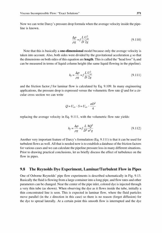
Nowwe can write Darcy’s pressure drop formula when the average velocity inside the pipe-line is known.

Δpρg

= fL

D

U2av

2g9 110

Note that this is basically a one-dimensional model because only the average velocity istaken into account. Also, both sides were divided by the gravitational acceleration g so thatthe dimensions on both sides of this equation are length. This is called the “head loss” hf andcan be measured in terms of liquid column height (the same liquid flowing in the pipeline).

hf =Δpρg

= fL

D

U2av

2g9 111

and the friction factor f for laminar flow is calculated by Eq. 9.109. In many engineeringapplications, the pressure drop is expressed versus the volumetric flow rate Q and for a cir-cular cross section we can write

Q=Uav S =UavπD2

4

replacing the average velocity in Eq. 9.111, with the volumetric flow rate yields:

hf =Δpρg

= fL

D5

8Q2

π2g9 112

Another very important feature of Darcy’s formulation (Eq. 9.111) is that it can be used forturbulent flows as well. All that is needed now is to establish a database of the friction factorsfor various cases and we can calculate the pipeline pressure loss in many different situations.Prior to drawing practical conclusions, let us briefly discuss the effect of turbulence on theflow in pipes.

9.8 The Reynolds Dye Experiment, Laminar/Turbulent Flow in Pipes

One of Osborne Reynolds’ pipe flow experiments is described schematically in Fig. 9.13.Basically the fluid is flowing from a large container into a long pipe, and flow rates and otherparameters can be changed. Near the center of the pipe inlet, colored dye is injected througha very thin tube (as shown). When observing the dye as it flows inside the tube, initially athin concentrated line is seen. This is expected in laminar flow, where the fluid particlesmove parallel (in the x direction in this case) so there is no reason (forget diffusion) forthe dye to spread laterally. At a certain point this smooth flow is interrupted and the dye


shows chaotic motions (laterally) and instead of a thin concentrated line, a rapid mixing ofthe dye is observed. This condition when the fluid particles chaotically move to all direc-tions, in addition to the main flow direction is called turbulent flow. The region when thelaminar flow turns into turbulent is called the transition region. Reynolds was able to showwith his dye experiment that this condition occurs when the nondimensional numberρUavD/μ is about 2000 (and this is of course the Reynolds number).Because of the additional motion of the fluid particles, the turbulent flow losses are larger.

In terms of our definitions, the shear stress and the friction coefficients are larger than in alaminar flow. Even if the average velocity has only one component, the one in the x direc-tion, perturbations in the other directions exchange momentum and create larger losses. Forexample, the two-dimensional shear stress at the wall will have an additional component,clearly increasing the shear stress:

τxr = μ∂u

∂r−ρu w 9 113

and here u w are the perturbation velocities into the x and r directions. These velocity per-turbations are responsible for the additional shear term in Eq. 9.113, called the Reynoldsstress. Turbulence, also has an effect on the velocity distribution inside the pipe as shownin Fig. 9.14, and both flows will have the same average velocity (and flow rate). Clearly, the

turbulent flow has larger shear∂u

∂rnear the wall, compared to the laminar flow solution.

Note that this is an excellent opportunity to observe the effect of turbulence in high-Reynolds number flows. Although flow details in turbulent flow are complex, the engineer-ing approach is to approximate the average quantities, based on the laminar flow model, andextrapolate into the turbulent flow region. Therefore, let us return to Darcy’s formula andplot the friction parameter for a wide range of Reynolds numbers. For laminar flow theresults are the same as in Eq. 9.109, which shows that f is reduced with increased Reynoldsnumber.

f = 4Cf =64Re

9 109

The chart in Fig. 9.15 is known as the Moody diagram, which was published by L. F.Moody in 1944. The turbulent friction curves for smooth pipes are significantly higher than

Laminar flowWater

Dye

Transition Turbulent flow

Figure 9.13 Schematic description of Reynolds’ 1883 pipe flow experiment


Parabolic

curve

Uav

Uav

(a)

Laminar

Turbulent

(b)

Umax

Umax

Figure 9.14 The difference between fully developed laminar and turbulent velocity distribution in a

circular pipe flow

2 3 4 5 7 92 3 4 5 7 92 3 4 5 7 92 3 4 5 7 9103 104

0.01

0.02

Fri

ctio

n f

acto

r, f

0.03

0.04

0.05

0.06

0.07

0.08

Reynolds number

105 106 107

0.000050.0001

0.0002

0.00060.0004

0.00080.001

0.002

Rel

ativ

e ro

ughness,

k/D

0.004

0.006

0.0080.01

0.0150.02

0.03

0.040.05

Equation 9.109

64

Ref =

Smooth pipe

0.00001

Figure 9.15 The Moody friction factor for fully developed flow in circular pipes. Note the effect of

relative roughness (k = average height of inner surface roughness)


for the laminar case and for the higher Reynolds numbers only the turbulent flow case ispresent. Moody also included relative roughness, so that the effect of surface smoothnesscan be incorporated into the pressure loss formula (the relative roughness is the averageheight of the roughness inside the pipe, k, divided by the pipe diameter).

Example 9.6 Pressure loss in terms of head lossWater is flowing in a 10 m long smooth pipe of diameter 0.02 m and the average velocity is0.15 m/s. Calculate the pressure drop.

Solution:First, let us calculate the Reynolds number and use the values for the density and viscosityfrom Table 1.1:

Re =1000 0 15 0 02

10−3 = 3000

It is still possible to maintain laminar flow and the friction coefficient, from Eq. 9.109, is:

f =64

3000= 0 0213

The head loss, based on Eq. 9.111 is then:

hf =Δpρg

= 0 0213100 02

0 152

2 9 8= 0 0122m H2O

so this is a little over 1 cm of water. Now if the flow is turbulent then the friction factor isabout 0.042 and the pressure drop will increase by more than twice.

9.9 Additional Losses in Pipe Flow

Actual pipelines include elbows, flanges, valves, and other devices all may have an effect onthe flow inside the pipe. For example, Fig 9.16a shows the entrance into a pipe where thelocally narrowing streamlines may create local flow recirculations and additional pressurelosses. Similarly, Fig. 9.16b shows the flow in an elbow where the turning streamlines sep-arate and create additional blockage and pressure loss. In order to accommodate such lossesin the pressure-drop calculations, a loss coefficient must be defined.Let us start with Darcy’s formula and we already pointed out that we can call the pressure

loss a head loss, hf. Rewriting Eq. 9.111 we can see that the head loss measures the loss interms of the pipe flow’s liquid column height


hf =Δpρg

= fL

D

U2av

2g9 111

Consequently the loss coefficients K must have the same units and the head loss due to anelbow or the entrance in Fig. 9.16 will be estimated by

hf =Δpρg

=KU2

av

2g9 114

A table showing the loss coefficient K values for various conditions is depicted in Fig. 9.17.Note that these coefficients depend on the geometry and, for example, elbows with differentdiameters or turn radius will have different loss coefficients.In summary, for a long pipeline (with the same diameter) but with elbows and other

fittings, the total pressure loss (or head loss) can be summarized as:

hf =Δpρg

= fL

D+ΣK

U2av

2g9 115

and the first term inside the parenthesis is the friction inside the pipe while the ΣK is the sumof all the additional losses.

9.10 Summary of 1D Pipe Flow

Although we started this chapter with “exact solutions” in mind, Darcy’s experimental for-mula and the Bernoulli equation provide a simple one-dimensional model for calculating theincompressible flow in pipes. The method of using these equations is depicted schematicallyin Fig 9.18.

Separation zone

Separation

(a)

(b)

Figure 9.16 Additional losses in a pipeline: (a) entrance losses, and (b) elbow losses


D

D1

D2

D

r

r/D

r/D

D2/D1

D1

D2

θ

θ

Globe valve

Gate valve

90°smooth bend

90°sharp bend

Expansion

Contraction

Pipeentrance

0.00.1

0.200.400.600.80

0.200.400.60

Turningvanes

Novanes

Withvanes

12468

10

0.350.190.160.210.28

Full-open 0.20

Half-open 2.20

Full-open 10.00

Half-open 5.60

0.32

0.80

0.300.250.150.10

0.870.700.410.15

0.90

0.080.070.060.060.06

0.490.420.270.200.10

>0.2

K

K

Kθ = 60°

Kθ = 180°

D1/D2

Kθ = 20°

K = 1.1

K = 0.2

Kθ = 180°

0.500.120.03

r

Figure 9.17 Loss coefficients for various pipe related fittings


In principle, we can write the Bernoulli equation (Eq. 3.3) between two points, as shown.However, if there are losses (Σhf) in the flow we can add those into the equation as follows

z1 +p1ρg

+u212g

= z2 +p2ρg

+u222g

+Σhf 9 116

and the losses are summarized by Eq. 9.115

hf =Δpρg

= fL

D+ΣK

U2av

2g9 115

Note, that in terms of velocity, here we see three variables (e.g., u1, u2, and Uav – if pipesegment diameters are not equal); therefore, additional equations may be needed (e.g.,the continuity equation). Several examples to demonstrate the application of these formulaswill be presented later in this section.Another important observation highlighting the simplicity of Darcy’s equation can be

demonstrated by a simple water-tower example (see Fig. 9.19). Such water reservoirs areplaced at the highest point in a neighborhood, ensuring the pressurized water supply tothe users below. Assuming that the water level inside the reservoir (point #1) is not changingthen the exit velocity at station #2, without losses is given by the simple one-dimensionalmodel of Eq. 3.12

u2 = 2g z1−z2 = 2gh

and here we use h for the height difference. The losses along the pipeline due to the fluidflow can be summarized by using the head loss term hf as given in Eq. 9.111. Therefore, asimple estimate for the average velocity in the pipe at point #2 can be obtained by reducingthe available water column height for accelerating the fluid.

z

x

K1 K2

K4

K5

K6K3

2

1

z2

z1

Figure 9.18 One-dimensional model for pipe flow calculations


u2 = 2g h−hf 9 117

This example not only visualizes the meaning of the term head loss but also highlights theingenious formulation of Darcy’s formula.

9.10.1 Simple Pump Model

Because we are dealing with pipelines, one important engineering question relates to thepower required to pump the fluid. Let us examine a simple incompressible case wherethe pump creates a pressure jump Δp and the flow rate is Q (see Fig. 9.20).In general, the definition of work W is force F times distance l

W=F l=ΔpS l=Δp V

which translates to the pressure difference Δp times the volume V (and the force is equal tothe pressure difference times the cross-sectional area of the pipe, F =ΔpS). The power is thework per unit time and measured in watts (W)

Power =d

dtW=Δp

d

dtV =ΔpQ

and hereQ is the volumetric flow rate. In conclusion, the power required to move the fluid is

Power =Δp Q 9 118

z

x

u2 z2

z1

h

hf

Watertower

1

2

Figure 9.19 Schematic description of a water tower. By placing the water reservoir at the highestpoint in a neighborhood the supply of pressurized water is solved


If the pump efficiency is denoted as η then the power supplied to the pump is

Powerpump =Δp Q

η9 119

Sometimes, the pump performance is measured as a head gain hpump, which, based on thisrelation becomes

hpump =Δpρg

= ηPowerpump

ρgQ

with this definition, Eq. 9.116 can be modified to account for the pump head gain:

z1 +p1ρg

+u212g

± hpump = z2 +p2ρg

+u222g

+Σhf 9 120

and the ± sign depend on the direction the pump is operating (same applies to the Σhf term).A more detailed discussion on pumps and their internal flows is presented in Chapter 10.

9.10.2 Flow in Pipes with Noncircular Cross Sections

Based on Eq. 9.109, the formula for the friction factor f can be modified to include the flowin pipes with different cross sections. For the laminar case, this can be done by simply repla-cing the number 64 in the numerator with a constantCK (and for circular pipesCK = 64). Themodified formula then becomes:

f =CK

Re9 121

However, the Reynolds number is now based on the hydraulic diameterDh and the hydraulicdiameter is based on the wetted perimeter Ph, and the cross-sectional area S:

QΔp

Figure 9.20 Simple pump model


Dh =4 SPh

9 122

With these definitions, the Reynolds number becomes

Re =ρUavDh

μ9 123

Of course, for a circle the hydraulic diameter remains the circle’s diameter and for a pipewith a square cross section, the hydraulic diameter remains its height.With these modifications, and based on the geometry of the pipe cross-section, the friction

factor f for the cases shown in Fig. 9.21 can be estimated (for fully developed laminar flows).For example, the hydraulic diameter for a rectangular cross section pipe where a = 2 b is

Dh =4 SPh

=4 a 2a2 a + 2a

=43a

To estimate the pressure drop for high Reynolds number turbulent flows in noncircularpipes, Darcy’s formula (Eq. 9.111) can still be used. However, in this case the hydraulicdiameter based on Eq. 9.122 must be used to estimate the friction factor from the Moody

CK

Cross-sectionshape

1

2

4

8

16

56.9

62.2

72.9

82.3

93.0

1

2

4

8

16

64.0

67.3

72.9

76.6

78.2

10°

30°

60°

90°

120°

50.8

52.3

53.3

52.6

51.0

b

a

b

θθ =

ab

=

ab

=

Figure 9.21 Friction factors for several generic pipe cross sections for fully developed laminar flows


diagram. Also, this semi-empirical approach can be extended to open channel flows andmore detail can be found in Ref. 9.1, Section 5.10.

9.10.3 Examples for One-Dimensional Pipe Flow

This section demonstrates a variety of different cases that can be solved using the one-dimensional pipe flow model presented here.

Example 9.7 Head loss in an elbowThe purpose of this example is to demonstrate the use of head loss and associated units. Letus consider a 6 l/min flow of water in a 3 cm diameter pipe, which has a 90 elbow. Calculatethe head loss due to the elbow which has a loss coefficient: K = 0.32.

Solution:The head loss is calculated by Eq. 9.114, but first, the average velocity in the pipe must becalculated.

Uav =Q

S=6 60 10−3 m3 s

π0 0152 m2= 0 141

ms

Now we can use Eq. 9.114 to calculate the head loss

hf =KU2

av

2 g= 0 32

0 1412

2 9 8= 3 24 10−4m

The unit of the head loss is in length (meters in this case) representing the loss in terms of thefluid column height inside the pipeline (ρghf). In order to return to pressure units we mustlook at the left-hand side of Eq. 9.114

hf =Δpρg

Consequently the pressure drop is

Δp = hf ρg= 3 24 10−4 1000 9 8 = 3 18Nm2

Example 9.8 Pressure losses in a long pipeKerosene is flows through the pipeline shown in the Fig. 9.22. Fluid level in the main tank is20 m above the exit and along the line there is an additional elevation drop of 2 m, as shown.


The pipe inner diameter is 0.3 m and the inside resistance coefficient is f = 0.019. Assume aloss coefficients for the two elbows at K = 0.3, and the properties of Kerosene are: ρ = 804kg/m3, and μ = 1.9 10–3 N s/m2 Based on this, calculate:

a. The average discharge velocity at the end of the pipeb. The Re number of the flow.

Solution:Let us use Eq. 9.116 for this case. The coordinate system is set at the lowest elevation of thepipeline and the upper level of the fluid in the tank is considered as point #1 while the pipeexit at the bottom is point #2. The velocity at point #1 is zero, and the pressure at both pointsis ambient (e.g., p1 = p2 = pa since at point #2 the pressure is evaluated outside the pipe),therefore, the pressure terms cancel and Eq. 9.116 becomes:

20 + 2 +paρg

+02g

= 0 +paρg

+u222g

+Σhf

So if the flow had no friction, then the potential energy (ρgz1) will be converted into velocityat point #2, however, the friction in this case will reduce the exit velocity. Next we mustcalculate the friction losses in the pipe and in the elbows

Σhf = fL

D

u222g

+ 2Ku222g

substituting this into (∗) we get

22 =u22

2 9 81 + 0 015

2020 3

+ 2 0 3

Note that the units are meters, since the calculation is for head loss! Basically we can solvenow for the velocity and we get

u2 = 6 07ms

1

2 m

2

K

K

z

x

pa

20 m 150 m 50 m

Figure 9.22 One dimensional flow in a long pipe line


The corresponding flow rate is:

Q= u2S= 6 07 π 0 152 = 0 429m3

s

In this case the friction coefficient was given (if not we have an iterative process with theMoody diagram). In both cases it is desirable to calculate the Re Number (and to see if thefriction factor f selection is reasonable):

Re =804 6 07 0 3

1 9 10−3 = 0 773 106

and by looking at Fig. 9.15 it appears that the friction coefficient selection was reasonable.Also, now that the average velocity was calculated it is interesting to evaluate Σhf and dem-onstrate the meaning of head loss:

Σhf = fL

D

u222g

+ 2Ku222g

= 0 0152020 3

+ 2 0 36 072

2 9 8= 20 12m

This means that instead of the potential height of 22 m only 1.88 m is available at the end ofthe pipeline (in form of the jet kinetic energy)! Thus we can use the ideal flow Eq. 3.12 tocalculate the exit velocity

u2 = 2gh= 2 9 8 1 88 = 6 07ms

and this is the same result!

Example 9.9 Laminar flow in a vertical pipeIn this example we combine the friction formula with Eq. 9.116, resulting in a quadraticequation. Consider the vertical flow of motor oil down a h2 = 2.0 m long circular tube ofdiameter D = 0.01 m, as shown in Fig. 9.23. The liquid height in the large container ish1 = 0.1 m. Estimate the average discharge velocity at the bottom (from Table 1.1 we getρ = 919 kg/m3 and μ = 0.29 N s/m2).

Solution:If we place our coordinate system at the bottom exit then the liquid column height is 2.1 m.Again we consider point #1 at the top of the liquid (at z1 = 2.1 m) and point #2 at the exit(a small distance after the fluid left the pipe) and the ambient pressures are the same. WritingEq. 9.116 for this case results in:

2 1 +paρg

+02 g

= 0 +paρg

+u222 g

+Σhf

Assuming laminar flow (which must be verified at the end) we can use Eq. 9.109 for thepressure loss


f =64Re

Now we can calculate the head loss as:

Σhf = fL

D

u222 g

=64Re

L

D

u222 g

=64μρ

L

D2

u22 g

Substituting the head loss into Eq. 9.116 results in a quadratic equation:

2 1 =u22

2 9 8+32 0 291254

2 0

0 012u29 8

Solving for the exit velocity we get

u2 = 0 14m s

Now, to make sure that we have a laminar flow, let us check the Re number

Re =919 0 14 0 01

0 29= 4 4

The Re number is much less than 2000 so clearly the flow must be laminar.

Example 9.10 Turbulent flow due to gravityIn this case the principle of siphoning is demonstrated. Usually the suction side of the pipe isshorter and the height difference between the two pipe segments is pushing the fluid. Alsonote that the pipe must be filled with liquid (primed) in order for this to work.

1

z

x

D

2

pa

h2

h1

Figure 9.23 Laminar flow in a vertical pipe


In this example a motorist is siphoning gasoline from his automobile tank to help a strandedcar. If the 2 m long tube inner diameter is 0.5 cm then calculate:

a. How long it takes to siphon 2 l gasoline (assuming no effect on the fluid level in the tankand container).

b. Repeat the calculation but assuming no friction in the pipe. How realistic is this solution?

Fuel

tank

0.05 m

0.7 m

Solution:Based on Eq. 9.116 we can write

0 7 +paρg

+02 g

= 0 05 +paρg

+u222 g

+ fL

D

u222 g

We can guess the friction factor as f = 0.02 and repeat the calculation if the guess is wrong.

0 65 = 1 + 0 022 00 007

u2

2 9 8

Solving for the velocity we get u2 = 1.37 m/s. Now we can calculate the Reynolds number:

Re =680 1 37 0 007

3 1 10−4 = 2 1 104

This is clearly in the turbulent flow territory, and based on the Moody diagram, the frictionfactor should be more like 0.025.After repeating the calculation we get u2 = 1.38 m/s and the Reynolds number didn’t

change much. The flow rate is

Q= u2S = 138 π 0 352 = 53 1 cm3 s

Next, to calculate how long it takes to pump 2 l (or 2000 cm3) we simply divide the volumeby the flow rate, and the result is: 38 s to siphon.


if f = 0, the velocity is u2 = 2 gh= 2 9 8 0 65 = 3 57m sthen it will take only 15 s.

Example 9.11 Pressure loss in a fuel lineEstimate the pressure drop in the fuel system of a car where the fuel line inner diameter is0.5 cm and its length is L= 3 5m. The expected flow rate is Q= 2 4 cm3 s and additionallosses include four 90 bends K = 0 4 and one fuel filter K = 2 0 . Also, the fuel tank levelis 0.4 m below the end of the fuel delivery pipeline.

Solution:Because the required flow rate is provided, the Reynolds number and the friction factor canbe estimated. The velocity in the tube is:

u =Q

S=

2 4

π 0 252= 12 22 cm s

and the Reynolds number (based on Table 1.1) is:

Re =680 0 12 0 005

3 1 10−4 = 0 13 104

Based on the Moody diagram, this appears to be in the laminar flow region and the frictionfactor is

f =64

0 13 104= 0 049

The expected pressure drop is then:

Δpρg

= 0 4 + hf = 0 4 + fL

D+ΣK

u2

2 g= 0 4 + 0 049

3 50 005

+ 4 0 4 + 2 00 12222

2 9 8= 0 428m

So most of the pressure drop is due to the elevation change between the fuel tank and thedelivery exit. The estimated pressure drop in the line is

Δp= ρgh= 680 9 8 0 428 = 2852N m2

which is quite small.

Example 9.12 Flow in a pipe with two different diametersWater is flowing from a container through the pipeline as shown in Fig. 9.24. Fluid level inthe main tank is 20 m above the exit and the pipe diameter is 0.3 m for the first 50 m. At thispoint, the diameter is reduced to 0.2 m and the loss coefficient for the contraction is K = 0 1.The smaller diameter pipe line is 100 m long and at the end the water is released. Assume thesame friction factor of f = 0.015 for the two pipe segments and the properties of water aretaken from Table 1.1. Calculate the average discharge velocity at the end of the pipe.


Solution:Let us use again Eq. 9.116 for this case. The coordinate system is set at the lowest elevationof the pipeline and the upper level of the fluid in the tank is considered as point 1 while thepipe exit at the bottom is point 3. The velocity at point #1 is zero, and the pressure at bothpoints is ambient (e.g., p1 = p3 = pa). Because of the change in pipe diameter, station #2 isadded in the larger diameter pipe section. Writing Eq. 9.116 between point #1 and point #3yields

20 +paρg

+02g

= 0 +paρg

+u232g

+Σhf

The friction losses Σhf are calculated using Eq. 9.115

Σhf = fL2D2

u222g

+Ku222g

+ fL3D3

u232g

at this point we use the continuity equation between point #2 and point #3

ρu2S2 = ρu3S3

knowing the pipe diameters, we can write

u2 = u3S3S2

= u30 20 3

2

Substituting the friction losses and the velocity ratio into the Bernoulli equation results:

20 =u23

2 9 81 + 0 015

500 3

0 20 3

4

+ 0 10 20 3

4

+ 0 0151000 2

pa

z

x

K = 0.1

D = 0.3 m D = 0.2 m

50 m 100 m

1

2 320 m

Figure 9.24 One-dimensional flow in a long pipe line with a change in diameter


As noted earlier, the units of these equations are in meters. Solving for the velocity we get

u3 = 6 59ms

The corresponding flow rate is:

Q= u3S3 = 6 59 π 0 12 = 0 20m3

s

Let us calculate the Re number to verify that the flow is within the turbulent range and thatthe estimate of f is reasonable. The density and viscosity are taken from Table 1.1 asρ = 1000 kg/m3 and μ = 1.0 10–3 N s/m2

Re =1000 6 59 0 2

1 0 10−3 = 1 32 106

and clearly this is within the turbulent flow range and the friction factor selection wasreasonable.

Example 9.13 Flow between two containersLet us present an example, in spirit of the baseline model shown in Fig. 9.18. Assume thatwater is flowing in a 0.1 diameter pipe between two reservoirs, as shown in Fig. 9.25. Thedifference in water surface elevation between the two reservoirs is 5 m, and the length of theconnecting pipe between them is 300 m. The loss coefficients for the pipe entrance isKe = 0 5, for the valve loss KV = 0 2, and for the exit loss is Kex = 1 0. Assuming f = 0 02,calculate the average velocity in the pipe, the flow rate, and check the Moody diagramto see if the value used for f is reasonable? (μ = 10–3 m2/s and ρ = 1000 kg/m3).

300 m

Valve

5 m

}

1

2

Figure 9.25 Water flow between two containers


Solution:Following the nomenclature of Fig. 9.18, we set point #1 at the top of the left reservoir andpoint #2 at the top of the right reservoir. Note that in this case the fluid velocity in thesepoints is zero and the pressure is pa. Eq. 9.116 for this case is

5 +paρg

+02g

= 0 +paρg

+02g

+ fL

D+ΣK

u2

2g

substituting the numerical values and solving for the velocity and the flow rate

5 =u2

2 9 80 02

3000 1

+ 0 5 + 0 2 + 1 0

u= 1 26m s

Q= 1 26 π 0 052 = 9 89 l s

Next, checking the Reynolds number

Re =1000 1 26 0 1

10−3 = 1 26 105

and based on the Moody diagram the selected friction factor is reasonable.

Example 9.14 Pump power requirementsConsider a 20 m long, 6 cm diameter pipe discharging into an open container, as shown. Thepipe inclination is 40 . The desirable flow rate is 7.63 l/s, and the liquid (oil) properties are:ρ = 900 kg/m3 and μ = 0.18 N s/m2 (see Fig. 9.26). Calculate the power required to pumpthe liquid.

z

40°

x

1

2

20 m

Pump

Figure 9.26 Pressure requirement for uphill pumping


Solution:Based on Eq. 9.119, we need to calculate the pressure drop in the pipe. Let us select point #1at the pump exit and set z1 = 0 there. Next, place point #2 at the discharge exit of the pipe (asshown in the figure). Because the required flow rate and the pipe diameter are known we cancalculate the average velocity:

u1 = u2 =Q

S=7 63 10−3

π0 032= 2 7m s

Next we can calculate the Reynolds number so that we can select the proper frictioncoefficient (is it laminar or turbulent?):

Re =900 2 7 0 06

0 18= 810

This is within the laminar region and we can use the laminar flow formula

f =64Re

= 0 079

The head loss in the pipe is therefore:

hf = fL

D

u222 g

= 0 079200 06

2 72

2 9 8= 9 79m

Now we can return to Eq. 9.116

0 +p1ρg

+u212 g

= 20sin40 +p2ρg

+u222 g

+ 9 79

But u1 = u2 and we get

p1−p2ρg

= 20sin40 + 9 79 = 22 65m

and after multiplying by ρg

Δp = p1−p2 = 22 65 900 9 8 = 199773Nm2

which is about two atmospheres (2 atm). Now we can calculate the power requirement:

Power =Δp Q = 199773 7 63 10−3 = 1524 3W


which is close to 2 HP. For calculating the total pumping power requirement we must usepump efficiency as well (e.g., divide this result by the efficiency).

9.10.4 Network of Pipes

Complex networks of pipes are used in places such as chemical plants, water distribution ortreatment plants, or even vehicles (cooling and fuel systems). A typical engineering require-ment is to estimate the pressure loss or the flow rates in the pipe network. To demonstrate thegeneric approach for solving such problems let us use the simple one dimensional pipe flowmodel developed in Section 9.6. We can use Darcy’s formula (Eq. 9.115) and apply it to thesimple network shown in Fig. 9.27.Let us assume incompressible fluid and that the input pressure p1, as well as the exit pres-

sure p0 are known. Also the diametersDi and lengths Li of the four segments are known. Theproblem now is to find the flow rates in each of the pipe branches. We can apply Darcy’sformula for the four branches as follows (let us simplify and assume the same friction factor ffor all pipes).

Δpi = ρgfLiDi

U2i

2 gi= 1,2,3,4 9 124

At this point the four velocities and the resulting pressure drops are unknown. Three equa-tions can be constructed, stating the total pressure drop in the system

p1−p0 =Δp1 +Δp2p1−p0 =Δp1 +Δp3p1−p0 =Δp1 +Δp4

9 125

u1D1L1

D2L2

D3L3

D4L4

p1

u2p0

u3p0

u4p0

Figure 9.27 A simple network of pipes


And Δpi i= 1,2,3,4 represents the pressure drop in each pipe segment. An additionalequation can be formulated, based on the continuity equation, stating that the inflow in pipe#1 is equal to the flow leaving through the three branches.

Q1 =Q2 +Q3 +Q4 9 126

The flow rate is related to the average velocity as:

Qi =πD2

i

4Ui i= 1,2,3,4 9 127

and the four equations for the four unknown velocities are:

2g p1−p0ρgf

=L1D1

U21 +

L2D2

U22

2g p1−p0ρgf

=L1D1

U21 +

L3D3

U23 9 128

2g p1−p0ρgf

=L1D1

U21 +

L4D4

U24

D21U1 =D

22U2 +D

23U3 +D

24U4

In principle, these four equations can be solved for the four velocitiesUi. Usually the numberof pipe segments is very large and (iterative) numerical techniques are used to solve the sys-tem of equations.

Example 9.15 Parallel flow in two pipesThe simplest example for a network of pipes is when the flow splits between two pipes, asshown in the figure. Assume water at a flow rate of 5 l/min entering a 10 m long, and 5 cmdiameter pipe at the left. The pipe then splits into two, as shown, but the upper pipe diameteris only 3 cm. The total length of the upper pipe Lu = 12m and the entrance/exit losses areK1 = 0 9 and the loss coefficients in the two bends are K2 = 0 2 (see Fig. 9.28). Assumingf = 0.025 for both pipes, calculate the flow rates for the upper and lower pipes.

Solution:The pressure drop along the two pipes (between the two junctions) is the same. Therefore,the pressure loss (in terms of the head loss) is calculated for the two segments. The head lossin the upper pipe is

hu = fLuDu

+ 2K1 + 2K2u2u2g


and the head loss in the lower pipe is

hL = fLLDL

u2L2g

Because the pressure drop is the same we can compare these two equations

fLuDu

+ 2K1 + 2K2u2u2g

= fLLDL

u2L2g

Solving for the velocity ratio we get

u2uu2L

=f LLDL

f LuDu

+ 2K1 + 2K2=

0 025100 05

0 025120 03

+ 2 0 9 + 2 0 2= 0 4098

and the velocity ratio is

uuuL

= 0 64

The two flow rates are equal to the incoming flow of 5 l/s

π0 0252uL + π0 0152uu = 5 10−3 m3 s

Solving for the velocity and the flow rate in the lower pipe we get:

uL = 2 07m s

QL = π0 0252uL = 4 06 liter s

Q

K2

K1

1 m

K2

K1

D1 = 0.03 m

D2 = 0.05 m

10 m

Figure 9.28 Flow in two parallel pipes


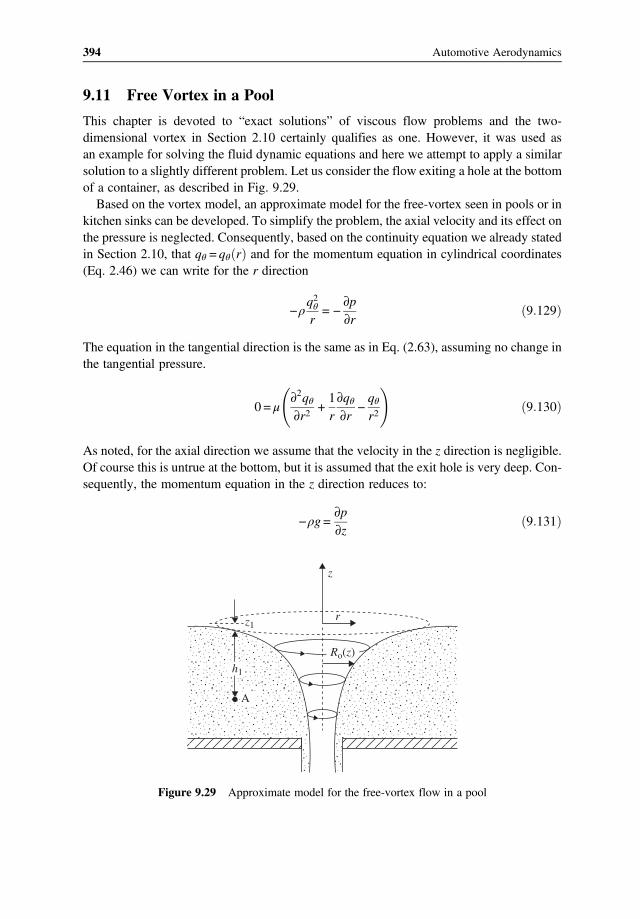
9.11 Free Vortex in a Pool

This chapter is devoted to “exact solutions” of viscous flow problems and the two-dimensional vortex in Section 2.10 certainly qualifies as one. However, it was used asan example for solving the fluid dynamic equations and here we attempt to apply a similarsolution to a slightly different problem. Let us consider the flow exiting a hole at the bottomof a container, as described in Fig. 9.29.Based on the vortex model, an approximate model for the free-vortex seen in pools or in

kitchen sinks can be developed. To simplify the problem, the axial velocity and its effect onthe pressure is neglected. Consequently, based on the continuity equation we already statedin Section 2.10, that qθ = qθ r and for the momentum equation in cylindrical coordinates(Eq. 2.46) we can write for the r direction

−ρq2θr= −

∂p

∂r9 129

The equation in the tangential direction is the same as in Eq. (2.63), assuming no change inthe tangential pressure.

0 = μ∂2qθ∂r2

+1r

∂qθ∂r

−qθr2

9 130

As noted, for the axial direction we assume that the velocity in the z direction is negligible.Of course this is untrue at the bottom, but it is assumed that the exit hole is very deep. Con-sequently, the momentum equation in the z direction reduces to:

−ρg =∂p

∂z9 131

z1r

z

A

Ro(z)h1

Figure 9.29 Approximate model for the free-vortex flow in a pool


The tangential velocity solution of Eq. 9.130 results in the vortex flow, as in Eq. (2.69)

qθ = −Γ2πr

9 132

where the circulation, based on Eq. 2.70 is related to the initial tangential velocity ω:

Γ= 2ωπ R0 z 2

At this point it was demonstrated that, without an external torque, the angular momentum ofthe fluid is conserved. Therefore, the radial variation of the pressure is obtained by integrat-ing Eq. (9.129):

p r =ρ

r

Γ2πr

2

dr = −ρΓ2

8π2r2+ c1

we already assumed that the tangential pressure is constant

p θ = const = c2

and for the vertical component (neglecting the velocity in the z direction) we get:

p z = − ρgdz= −ρgz + c3

where c1 c2, and c3 are the constants of integration. By combining these independent solu-tions we get:

p r,z = −ρΓ2

8π2r2+ gz + c 9 133

where c replaces the previous constants of integration. To calculate this constant we need tospecify the boundary conditions. For example, we observe that at z= 0, and at r ∞ thepressure is equal to the ambient pressure pa. Substituting these boundary conditions intoEq. 9.133 results in:

c = pa

Next, we replace the constant c in Eq. 9.133, finalizing the expression for the pressure dis-tribution inside the liquid:

p r,z −pa = −ρΓ2

8π2r2+ gz 9 134


This simple formula can also be used to estimate the pressure drop in the vortex flow arounda Tornado. The shape of the liquid surface can be found by letting p r,z = pa.

0 = −ρΓ2

8π2r2+ gz

and the shape of the liquid upper surface is:

z= −Γ2

8π2R2og

9 135

Alternately, the vortex core radius can be expressed in terms of the depth as:

R0 z =Γ2

8π2 −z g9 136

and this equation holds for z < 0. Also note that at each point inside the liquid, the pressure issimply:

p−pa = ρgh

where h represents the local liquid column height. To prove this, consider an arbitrary pointA in the liquid (Fig. 9.29) where the depth is:

z = z1−h1 and r = r1

Here, z1 is the depth of the free surface. Based on Eq. (9.134), the pressure at this point is


8π2r21+ g z1−h1

the depth of the free surface z1 is calculated using Eq. (9.135)

z1 = −Γ2

8π2r21g

The pressure at point A is then:


8π2r21+ g −

Γ2

8π2r21g−h1 = ρgh1



This chapter demonstrated several simple solutions showing the effects of viscosity in amoving fluid. At the same time, the engineering approach for treating practical fluid flowrelated problemswas revisited. For example, the analytical solutions for laminar flow clearlyshowed that the friction coefficient depends on the Reynolds number. Consequently, similarrelations were established for the high Reynolds number turbulent flow regime and the prin-cipal coefficients were based on empirical data. This rationale is repeated in many otherengineering disciplines (as in Chapter 6) where simple models were derived analyticallyfor lift and drag, and later extended by using experimental data.

Reference9.1. Katz, J., Introductory Fluid Mechanics, Cambridge University Press, Cambridge, UK, 2010.

Problems

9.1. A flat plate is moving at a velocity of U = 10 m/s on top of a 1 cm thick oil film. Thedensity of the oil is ρ = 920 kg/m3, viscosity μ = 0.4 kg/(m/s). Calculate the averageforward velocity of the oil film, the flow rate, the force required to pull the plate(per 1 m2), and the friction coefficient on the plate.

9.2. Consider the viscous laminar flow of oil between two stationary parallel platesas shown in the sketch (two-dimensional, ρ = 920 kg/m3, μ = 0.4 N s/m2). Assum-ing that the pressure difference between station (1) and (2) is ΔP = 1 atm,calculate:a. The velocity distribution.b. The average and maximum velocity.c. The flow rate (per unit width).d. The shear force on the lower plate and on the upper plate.e. The Reynolds number and the friction coefficient on the lower wall.

1 2

x

z

u(z)

5 m

0.01 m

Problem Figure 9.2

9.3. Consider the laminar viscous flow between two infinite parallel plates (the lower isstationary). Assuming that fluid viscosity μ, the distance between the plates h, andthe pressure gradient dp/dx are known, provide an expression for zero shear-stress con-dition on the upper moving plate.


U

z

hu

x

Problem Figure 9.3

9.4. A flat plate is moving at a velocity of U = 5 m/s on top of a 1 cm thick oil film. Thedensity of the oil is ρ = 920 kg/m3

, viscosity μ = 0.4 kg/(m/s). Also, there is a favorablepressure gradient of dp dx= −2μU h2. Calculate the average forward velocity ofthe oil film, the flow rate, the force required to pull the upper plate (per 1 m2), andthe friction coefficient on the lower surface (z = 0).

9.5. A flat plate ismovingat avelocityofU = 10m/son topof a1 cmthickoil film.Thedensityof the oil is ρ = 920 kg/m3, viscosity μ = 0.4 kg/(m/s). Next, a favorable pressure gradientis applied resulting in no shear on the upper surface (see sketch). Calculate the averageforward velocity of the oil film, the pressure gradient, the flow rate, the force requiredto pull the upper plate (per 1 m2), and the shear stress on the lower surface (z = 0).

h

z U

x

Problem Figure 9.5

9.6. A1 cm long and2 cmwide slipper bearing floats on anoil filmwith a viscosity of 0.29 Ns/m2. Assuming the front gap is h1 = 0.1 mm and h2 h1 = 2 2, calculate the allowedvertical load on the slider at a forward speed of 10 m/s. Also, estimate the friction drag.

F

l

h1

U

z

x

α

1 2

h h2

Problem Figure 9.6


9.7. The laminar flow velocity profile inside a 0.1 m diameter pipe is given by

u x = 5r

R

2−1 m s

a. Calculate the shear force on the wall (μ = 0.3).b. Calculate the flow rate and the average velocity.c. Calculate the friction coefficient (ρ = 800).

9.8. Oil with a density of ρ = 920 kg/m3 and viscosity μ = 0.4 kg/(m/s) is flowing at anaverage velocity of 0.5 m/s in a 5 m long and 0.02 inner diameter smooth pipe.Calculate the Reynolds number, the pressure gradient, and the power required topump the flow.

9.9. Water is flowing down from a container, between two parallel vertical plates, asshown in the sketch. Assuming the density of the water is ρ = 1000 kg/m3, viscosityμ = 0.001 kg/(m/s), and the spacing between the plates is 1 cm, calculate thefollowing:a. maximum velocity of water film,b. average velocity of water film,c. the flow rate,d. shear force on the plate (per 1 m2), ande. the friction coefficient, Cf.

1 cm

Problem Figure 9.9

9.10. Oil from a large container flows vertically down in a 3 cm inner-diameter circularpipe, as shown in the sketch. Assuming the flow is fully developed, calculate the shearstress at the pipe inner wall. Also calculate the shear at the center of the pipe. Estimatethe shear force acting on the inner surface of a 1 m long pipe segment. What are theflow rate and the Reynolds number? Use fluid properties from Table 1.1.


Oil

3 cm

r

z

Problem Figure 9.10

9.11. A fluid with density ρ = 800 kg/m3 and viscosity μ = 0.8 10–3 flows upward throughan 8 cm (diameter) galvanized iron pipe. If the relative roughness inside the pipe isk/d = 0.15mm/80mm = 0.001875, calculate the flow rate between station #1 and sta-tion #2. Note: the inlet pressure is 105 N/m2

p1= 103 Nm2

p2= 0.7 ·105 Nm2

30m

3m

Problem Figure 9.11

9.12. Oil with a density of ρ = 920 kg/m3 and viscosity μ = 0.4 kg/(m/s) flows from an ele-vated container, as shown. If the average velocity at the exit of the pipe is 30 cm/sthen calculate the Reynolds number, the pressure drop along the pipe and the heighthf of the reservoir. The smooth pipe inner diameter is 5 cm, its length is 10m, and theliquid height above the pipe entrance is 0.1m (entrance and pipe elbow effects arenegligible).


D

l

hf

Problem Figure 9.12

9.13. The velocity distribution in the flow between two parallel plates, in case of the Poi-seuille flow is:

u z = −h2

2μdp

dx

z

h1−

z

h

Calculate z/h where the velocity is equal to the average velocity.9.14. Oil flows in a long circular pipe and the laminar velocity profile inside the 0.1 m

diameter pipe has the form:

u x =Kr

R

2−1 m s

a. If dp/dx = 2400 N/m2/m, and the oil viscosity is μ = 0.3, ρ = 920, calculate thevalue of K.

b. Calculate the shear force on the wall.c. Calculate the flow rate and the average velocity.d. Calculate the friction coefficient.

9.15. Estimate the diameter of a cast iron pipe required to carry water at a discharge rate of85 l/s and with a head loss of 1.2 m per 300 m of pipe (assume f = 0.015). Calculatethe Re number and check on the Moody diagram if the value used for f is reasonable?

9.16. A fluid with a density of 800 kg/m3 flows along a long, 0.3 m diameter pipe. If themaximum velocity along the centerline is 1.5 m/s, and the pressure drop along a100 m pipe segment is 1900 N/m2, then calculate the value of the viscosity μ andthe kinematic viscosity υ (assume laminar flow).

9.17. Oil flows at an average velocity of 0.3 m/s in a 3 cm diameter pipe. Calculate the flowrate, and the pressure drop for a 4 m long pipe. Also, calculate the Reynolds numberand check if the laminar flow formula is valid. Howmuch will the flow increase if thepressure gradient is increased by a factor of two? Use fluid properties from Table 1.1.

9.18. A fluid is flowing in a 2 cm diameter pipe at an average velocity of 0.4 m/s. The pres-sure drop along a 5 m long segment is 10,000 N/m2. Assuming laminar flow, calcu-late the fluid viscosity.

9.19. Water is flowing in 3 cm diameter pipe at an average velocity ofUav = 2 m/s. Assum-ing water density of ρ = 1000 kg/m3 and viscosity μ = 10–3 N s/m2 calculate:a. The velocity at the center of the pipe.b. The shear τ at the wall.


c. The Reynolds number.Assuming laminar flow, calculate friction coefficient Cf and the pressure drop dP/dx.

9.20. Water flows between the two reservoirs, as shown in the sketch. The difference inwatersurface elevation between the two reservoirs is 5 m and the horizontal distance betweenthem is 300m. Determine the size (diameter) of steel pipe needed for a discharge of2 m3/s. Use the following loss coefficients for the pipe: entrance Ke = 0.5, valve lossKv = 0.2, and exit loss, Kex = 1.0, and f = 0.0116. Calculate the Re number and checkon the Moody diagram if the value used for f is reasonable (υ =10–6 m2/s andρ = 1000 kg/m3).

Kc Kex

300 m

Kv Valve

5 m

Problem Figure 9.20

9.21. The container shown in the figure is filled with water, as shown. At the left-handside, water is flowing through a 0.01 m diameter hole. Calculate the velocity ua ofthe free falling liquid at a distance of 2.0 m below the container. At the right-hand sidethere is a vertical pipe with an inner diameter of 0.01m. If the inner friction factor is f =0.02, calculate the velocity ub at the exit from the pipe. Compare the two results.

ba0.01 0.01

Water

Pa

2.0 m

1

0.2 m

2ubua

Problem Figure 9.21


9.22. A 100 m long and 0.1 diameter pipe is used to water the garden near a large dam asshown. The water level in the reservoir is 30 m above the horizontal pipe (ρ = 1000kg/m3, μ = 10–3 N s/m2 and assume a friction coefficient f = 0.012)a. Calculate the average discharge velocity, andb. The Reynolds number in the pipe.

0.1 m

100 m

30 m

Water

Problem Figure 9.22

9.23. Water flows through a 0.05 m diameter pipe from a large reservoir, as shown. Thewater level in the reservoir is 25 m above the horizontal pipe segment at the exitfrom the tank. The pipe initially is bent down and later up, emerging aboveground level. The loss coefficient in the three elbows is K = 0.25, and we can assumea Darcy friction coefficient of f = 0.02. Also for water ρ = 1000 kg/m3, μ = 10–3

N s/m2.a. Calculate the average discharge velocity and the Reynolds number in the pipe, andb. Calculate the height h of the water fountain above the end of the pipe.

25 m K= 0.25

K= 0.25

0.05 m

1 m 2 m

h= ?

110 m

Problem Figure 9.23

9.24. Kerosene flows through the pipeline shown in the sketch. Fluid level in the main tankis 20 m above the exit and along the line there is an additional elevation drop of 2 m,as shown. The pipe diameter is 0.3 m and the inside resistance coefficient f = 0.015.Assume the loss coefficients for the two elbows at K = 0.3 and the properties of


kerosene are: ρ = 804 kg/m3 and μ = 1.9 10–3. Calculate the Re number of the flowand the average discharge velocity at the end of the pipe.

20 m 150 m 50 m

2 m

Problem Figure 9.24

9.25. The flow in the previous problem is reversed by placing a pump at the end of thepipeline. Consequently, the kerosene is now flowing into the large reservoir at anaverage velocity of 6 m/s. Calculate the power required to pump the flow (pump effi-ciency is about 0.8).

9.26. Water flows from a large container along an inclined pipe (20 ), as shown in thesketch. Fluid level in the main tank is h = 10 m and the pipe inner diameter is 0.1m and its horizontal length is x = 200 m. Assuming an inside resistance coefficientis f = 0.025 and an entrance loss coefficient of K = 0.5, calculate the following:a. The average discharge velocity at the end of the pipe.b. The Re number of the flow.(ρ = 1000 kg/m3 and μ = 10–3 N s/m2)

x= 200 m

20°

K

h

Problem Figure 9.26

9.27. Water flows from a large container along an incline pipe as shown in the previousproblem. If the water is discharging at the pipe end at a rate of 80 l/s, then calculatethe distance x in the figure ( f = 0.025).


D

h1

h2

d

K

Problem Figure 9.27

9.28. A conical funnel of diameter D = 30 cm is filled with oil and the fluid exits at thebottom of a long vertical pipe, as shown. The oil level in the upper conical part ish1 = 20 cm, the pipe inner diameter is d = 1 cm and its length is h2 = 60 cm. Neglect-ing the losses in the conical section, assuming a resistance coefficient is f = 0.9 in thepipe, and an entrance loss coefficient of K1 = 0.5, calculate the average dischargevelocity at the end of the pipe (assuming h1 is not changing fast).

9.29. A water tower supplies water to a tap through an 8 cm (inner) diameter pipe. Dimen-sions of the pipeline are given in the sketch and the friction coefficient is f = 0.018.Assuming the three loss coefficients are K1 = K2 = K3 = 0.25, calculate the exit veloc-ity and flow rate.

Water

40 m

0.08 m

0.5 m

2 m

300 m

K1

K3 K2

Problem Figure 9.29


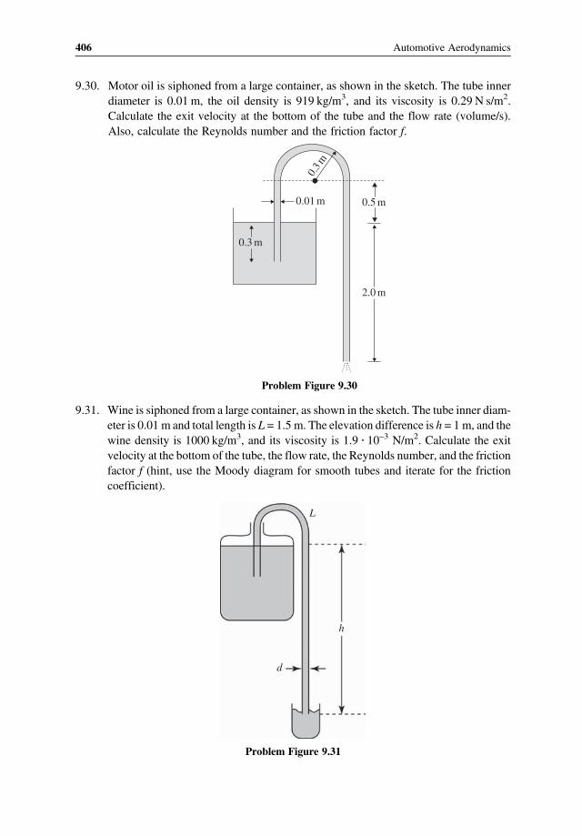
9.30. Motor oil is siphoned from a large container, as shown in the sketch. The tube innerdiameter is 0.01 m, the oil density is 919 kg/m3, and its viscosity is 0.29 N s/m2.Calculate the exit velocity at the bottom of the tube and the flow rate (volume/s).Also, calculate the Reynolds number and the friction factor f.

0.5 m

2.0 m

0.3 m

0.01 m

0.3m

Problem Figure 9.30

9.31. Wine is siphoned from a large container, as shown in the sketch. The tube inner diam-eter is 0.01 m and total length is L = 1.5 m. The elevation difference is h = 1 m, and thewine density is 1000 kg/m3, and its viscosity is 1.9 10–3 N/m2. Calculate the exitvelocity at the bottom of the tube, the flow rate, the Reynolds number, and the frictionfactor f (hint, use the Moody diagram for smooth tubes and iterate for the frictioncoefficient).

L

h

d

Problem Figure 9.31


9.32. A motorist is helping a stranded car is siphoning gasoline from his automobile tank,as shown. The 1.5 m long tube inner diameter is 0.7 cm and the friction coefficient isestimated at f = 0.018.a. How long does it take to siphon 2 l of gasoline (assuming no effect on the fluidlevel in the tank and container)?

b. Repeat the calculation but assuming no friction in the pipe. How realistic is thissolution?

Fuel

tank

0.05 m

0.7 m

Problem Figure 9.32

9.33. An orifice with a friction loss coefficient ofCD = 0.7 is placed in a pipeline. How doesthis loss factor compare with the head loss coefficient K, as defined in this chapter?

hf =Ku2

2g

Note that CD was defined for an orifice/Venturi tube as

m=CD2ρ p1−p21A22

−1A21

3 26

9.34. Water is flowing out of the taller container through 0.05 m diameter pipe, as shownin the figure. Assuming a friction factor of f = 0.03 in the pipe system, K1 =K2 = 0.3,K3 = 0.2, and that the flow rate does not affect the water level in the container,calculate the flow rate in the pipes (Δx = 70 m, Δz = 10 m, z1 = 12 m, z2 = 5 m).

D

Δz

Δx

K1

K2 K3

z1

z2z

x

Problem Figure 9.34


9.35. Water is flowing out of the taller container through 0.05 m diameter pipe, as shown inthe sketch for Problem 9.34. Assuming a friction factor of f = 0.03 in the pipe system,K1 =K2 = 0.3, K3 = 0.2, and that the flow rate does not affect the water level in thecontainer, calculate the required z1 so that the flow rate in the pipes will be 10 l/s(Δx = 70 m, Δz = 10 m, z2 = 2 m).

9.36. Water flows from the taller container through a long pipe with two segments, asshown in the sketch. The inner diameter of the thicker pipe is 6 cm and its lengthis 30 m, while the length of the thinner pipe is 20 m and its inner diameter is4 cm. The loss due to the transition between the two pipe diameters is K1 = 0.2and the friction factor for both pipes is f = 0.03. Calculate the flow rate betweenthe two containers when z1 = 3 m and z2 = 5 m.

z1 D1D2

z2

L1 L2K1

Problem Figure 9.36

9.37. Water is pumped through a 12 m long pipe (inner diameter D = 0.08 m) from a lowerreservoir into a tank. The elevation difference is z1 – z2 = 10 m. Estimate the powerrequired to drive the pump for a flow rate of 10 l/s. Assume pump efficiency is 0.8 andthe fluid properties for water are listed in Table 1.1 (assume smooth pipe when usingthe Moody diagram).

z1 = 10 m

z2 = 0

K1 = 0.2

D= 0.08 m

Pump

Problem Figure 9.37

9.38. Water is pumped from the lower container through 0.05 m diameter pipe, as shown inthe sketch. Assuming a friction factor of f = 0.03 in the pipe system, K1 = K2 = 0.3,K3 = 0.2, and that the flow rate is not affecting the water level in the two containers,


calculate the power required to pump a flow rate of 10 l/s (Δx = 70 m, Δz = 10 m,z1 = 12 m, z2 = 5 m).

D K1

PumpK2

K3

z

z1

x

z2

Δx

Δz

Problem Figure 9.38

9.39. Under normal conditions the left side of the human heart pumps about 5 l blood perminute into the systemic circulation, which creates a pressure drop of about10,600 N/m2. The right-hand side pumps the same flow rate but at a lower pressureof 3400 N/m2 into the pulmonary circulation.a. Using these average values for the pressure and flow rate, calculate the powerrequired to pump the fluid in both sides of the human heart.

b. Some estimate that at the same time, the heart consumes energy at the rate of 12W.Estimate the pumping efficiency.

c. If the flow exits the left-hand side into the aorta with a diameter of 22 mm, thencalculate the local Reynolds number (ρ = 1060 kg/m3, μ = 0.003 N s/m2).

9.40. Oil flows at an average velocity of 0.3 m/s in a 4 cm wide and 2 cm high elliptical pipe.Calculate the flow rate, and the pressure drop for a 4 m long pipe. Also calculate theReynolds number and check if the laminar flow formula is valid (assume density =

919kg/m3, viscosity 0.29 N/m2, andan ellipse circumference is:Ph = 2π 0 5 a2 + b2 ).9.41. Oil flows at an average velocity of 0.3 m/s in a 4 cm wide and 2 cm high rectangular

cross section pipe. Calculate the flow rate and the pressure drop for a 4 m long pipe.Also calculate the Reynolds number and check if the laminar flow formula is valid(assume density = 919 kg/m3, viscosity 0.29 N/m2).

9.42. Oil flows at an average velocity of 0.3 m/s in a 4 cm wide and 2 cm high triangularcross section of pipe. Calculate the flow rate, and the pressure drop for a 4 m longpipe. Also, calculate the Reynolds number and check if the laminar flow formulais valid (assume density = 919 kg/m3, viscosity 0.29 N/m2).

9.43. Compare the pressure drop for two rectangular 5 m long pipes, with oil flowing at anaverage velocity of 0.3 m/s (assume density = 919 kg/m3, viscosity 0.29 N/m2). Thefirst pipe is 4 cm wide and 4 cm high while the other is 8 cm wide and 2 cm high (soboth having the same cross-sectional area).

9.44. Air at 300 K and 1 atm flows at an average speed of 10 m/s through a 10 m longair conditioning duct having a square cross section of 0.3 0.3 m. Calculate theReynolds number based on the hydraulic diameter (assume viscosity is 1.8 10–5

N/m2). Estimate the power needed to pump the air using the Moody diagram to cal-culate the friction coefficient (assume smooth pipe).


9.45. Water flows at 5 l/min into the pipe at the left. The pipe then splits into two, as shownin the sketch, but the upper valve is partially closed. All pipes have the same innerdiameter of 2 cm. Assuming, a loss coefficient K1 = 0.2 at the two junctions, K2 = 0.3at the elbows, and K3 = 10 at the upper valve calculate the flow rate at the upper andlower pipes.

Q

K2 K2

K3

K1 K1

K2K2

Problem Figure 9.45

9.46. Water flows at 5 l/min into a 5 cm diameter pipe at the left. The pipe then splits intotwo, as shown, but the upper pipe diameter is only 3 cm. The total length of the upperpipe L1 = 15 m and it has two bends with a loss coefficient of K1 = 0.2. The length ofthe lower pipe between points A and B is 10 m. Calculate the flow rates for the upperand lower pipes (assume f = 0.025 for both pipes).

Q

K1 K1

L1D1

L2D2

A B

Problem Figure 9.46

9.47. Water flows at 4 l/min into a 5 cm inner diameter pipe on the left. The pipe then splitsinto two, as shown in the Problem 9.46 sketch, and the upper pipe inner diameter isalso 5 cm. The total length of the upper pipe L1 = 10 m and it has two bends with a losscoefficient of K1 = 0.2. The length of the lower pipe between points A and B is 8 m.Calculate the pressure loss between point A and point B (assume f = 0.025 forboth pipes).

9.48. A small rotating rod creates a two-dimensional vortex flow at the origin (x-z coordi-nates) with an intensity of Γ = 5 m2/s. Calculate the velocity components at apoint (5,5).

9.49. A small rotating rod creates a two-dimensional vortex flow at the origin (x-z coordi-nates) with an intensity of Γ = 5 m2/s. Calculate the value of the integral qdl for acircle of radius 5 m around the origin.


10Fluid Machinery

10.1 Introduction

Numerous vehicle components, such as engine cooling, ventilation, fuel, and braking sys-tems, all require some sort of method to move the fluid. From a historical perspective, earlycivilizations needed to channel water flow and other fluids, and one of the better knowninventions, the Archimedes screw, dates back to the third century BC. The Archimedesscrew, or screwpump, shown in Fig. 10.1 was used to transfer water from lower reservoirsinto higher irrigation ditches.Over the years, many inventions focused on developing various machines, either for

pumping fluids or using fluid energy to drive other machinery (e.g., turbines). Thesemachines may be classified as positive displacement or continuous flow machines. Somemechanical solutions using these two types of hardware are shown schematically inFig. 10.2.For example, the most basic configuration is a piston sliding inside a cylinder, as shown in

Fig. 10.2a. If this schematic is considered to be a pump, then while the piston is moving tothe left it is pushing the fluid out of the cylinder through an open valve. The pumping oper-ation of fresh fluid can continue when the piston is moving backward, closing this (exhaust)valve and opening the intake valve, creating a reciprocating cycle. This type of machine iscalled a positive displacement machine since a fixed volume of fluid is captured in thecylinder and then transferred across the pump. Another example is the rotating gear pumpshown in Fig. 10.2b. This is also a positive displacement machine, since there are fixedvolumes of fluid between the outer wall and the gears. Figure 10.2c and d show two typesof continuous flow machines, the first is an axial fan and the second is a centrifugal com-pressor. In this type of machinery, the fluid is not contained inside an enclosed volume and,


Figure 10.1 The Archimedes screwpump used to pump water to higher elevation

(a)

(c)

(d)

(b)

Rotor axisHub

Flow

Rotor blades

Stator blades

Suction Discharge

Casing

OutletRotor

Cylinder

PistonInletvalve

Exhaustvalve

Figure 10.2 Various types of fluid machinery. Positive displacement (a and b), and continuous flow(c and d)


for example, pressure cannot be maintained if the machine is not running (while a cylindercan hold a compressed fluid). Also note that any of these machine-principles can be used as apump or as an engine/turbine. For a large number of potential mechanical solutions, seeRef. 10.1.The difference in the performance between these two types of pumps is demonstrated

schematically in Fig. 10.3. Assume that the positive displacement pump of Fig. 10.2a deli-vers an incompressible fluid through a pipe, which has a valve on it. By partially closing thevalve, the pressure increases, but the volume of the flow remains constant. This is depicted,schematically, by the vertical line in Fig. 10.3. In continuous-flow pumps, however, when arotor moves the fluid, the rotor can rotate even when the valve stops the flow. In such pumpsusually the mass flow rate will increase when the restrictor valve is opened, resulting in theother types of curves shown in Fig. 10.3. In the case of an axial pump, such as shown inFig. 10.2c, the pressure decreases with increasing mass flow rate, while with the centrifugalpump design (Fig. 10.2d) the pressure changes are much smaller. Actually, the centrifugalpump curve depends on the impeller shape, as it is explained in Section 10.4.2. These typesof continuous-flow machines require deeper understanding of the fluid dynamic design andwill be discussed next.The objective of this chapter is to provide an introductory level formulation to estimate

the power requirements, the pressure ratios, and some of the fluid mechanics principlesneeded to design such a machine. Consequently ideal flow models with constant propertieswill be used in the following formulations. The need to estimate fluid pumping power wasaddressed briefly in Chapter 9 when the power requirements for an elementary pump werediscussed. Equation 9.118 was derived for an incompressible-fluid pump where the workWis simply the pressure difference times the volume of the liquid.

W =Δp V

Positivedisplacement

Centrifugalpump

Axialpump

ρ = const.RPM = const.

Δp0

m.

Figure 10.3 Schematic description of the performance difference between positive displacement andcontinuous flow pumps

413Fluid Machinery

If the conditions are changing, as the pressure inside a moving cylinder, then this can beexpressed in terms of the integral

W =

cycle

pdV 10 1

From the thermodynamic point of view, the work in general is related to the change in stag-nation enthalpy, h0, which includes the internal energy as well. Consequently we can writefor an incompressible fluid (and recall that m ρ =V):

W =mΔh0≈mΔp0ρ

=VΔp0 10 2

which is the same result obtained from mechanical considerations leading to Eq. 9.118. Incase of a compressible fluid the change in enthalpy can be estimated byΔh0≈cpΔT0 and thework of the machine is then

W =mΔh0≈m cpΔT0 10 3

and here cp is the heat capacity, as defined in Eq. 1.18 (we also assume that cp is constant).Note that the fluid stagnation-enthalpy includes the energy of the moving fluid, hence for anincompressible fluid:

p0ρ=p

ρ+q2

210 4

and for a compressible fluid

cpT0 = cpT +q2

210 5

As noted earlier, this chapter focuses on the continuous flow design often called “turboma-chinery”. The basic approach will be developed for an axial compressor first and thenextended to centrifugal compressors and axial turbines. In order to estimate machine perfor-mance, the relation between the fluid flow and power requirement must be established. For asuccessful design the effects of component geometry on performance must be clarified aswell (note that propellers and wind turbines are not discussed here because of the much morecomplex modeling of blade tip effects).The first-order approach presented in the following sections is based on simplifications

such as the average radius and the steady flow assumption. More accurate models arebeyond the scope of this text and require complex numerical solution. However, in spiteof the simplicity, the relation between turbomachinery geometry and its performance isestablished, providing a satisfactory preliminary design tool.


10.2 Work of a Continuous-Flow Machine

The first task is to develop a relation between the work of a rotating shaft (with rotor blades)and fluid motion. Let us consider the axisymmetric control volume shown in Fig. 10.4. Thefluid enters at the ring shaped section #1 and leaves at section #2. Note that the flow is con-tinuous across the control volume and there are no changes with time. However, a particleentering at one side will experience accelerations due to the changes between the twostations (#1 and #2). The cylindrical coordinate system is placed on the rotation axis (z)and the r−θ coordinates are as shown in the figure. A particle of mass Δm can enter thecontrol volume at section #1 and leave at section #2 (the particle is shown leaving atsection #2), and its velocity components c are depicted in the figure, as well.

This velocity vector is measured in an inertial frame of reference, which is not rotatingwith the shaft.

c = cr,cθ,cz 10 6

To calculate the tangential force (into the θ direction) we can use the momentum principle

ΔFθ =d

dtΔm cθ

and the torque Tq required to accelerate this particle is

ΔTq = r ΔFθ = rd

dtΔm cθ

Δr

Ω

r

z

z

1

2

θ

r1

r2

m.

Figure 10.4 An axisymmetric control volume for calculating the torque and power of rotatingturbomachinery

415Fluid Machinery

The unit normal-vectorn of the inlet/exit areas (of the control volume) points in the ±z direc-tion and based on Eq. 2.25 the fluid flow rate entering/leaving the control volume is

d

dtΔm≡Δm= ρ q n dS= ρczdS

As noted, the fluid exchange takes place only through the two ring shaped surfaces at sta-tion #1 and #2 and cθ is constant at each station. In order to calculate the total torqueapplied to the fluid in the control volume the contributions of the mass elements mustbe added.

Tq=

cs

ΔTq dS=

cs

r cθ ρczdS=

s2

r cθ ρczdS−

s1

r cθ ρczdS 10 7

Next let us introduce the mean radius approximation. This is equivalent to stating that thering shape inlet and exit surfaces are very thin and the radial variations in the velocity of thefluid elements are negligible. Consequently, all particles at station #1 are considered onentry at r = r1 and having a tangential velocity of cθ1. Assuming the same for the exit (station#2) we get

Tq= r2 cθ2s2

ρczdS−r1 cθ1s1

ρczdS=m r2 cθ2−r1 cθ1 10 8

and of course the mass flow rate entering and leaving the control volume is the same:

s1

ρczdS=

s2

ρczdS=m

For cases when radial variations are significant, Eq. 10.8 can be used by creating sub-layersinside the control volume (see later, Section 10.3.3). The power P required is simply theproduct of torque times the rotation speed.

P= Tq Ω=mΩ r2 cθ2−r1 cθ1 10 9

It is convenient to define a tip velocity U such that

U≡rΩ 10 10

and with this definition the power equation becomes

P =m U2 cθ2−U1 cθ1 10 11


and the work per unit mass flow wc is:

wc =P

m= U2 cθ2−U1 cθ1 10 12

Equations 10.8–10.12 state that the torque and work are related to the change in angularmomentum. Because the focus of this book is fluid mechanics, the next step is to relate thesequantities to the internal geometry of the turbomachinery.

10.3 The Axial Compressor (The Mean Radius Model)

The objective of this section is to formulate a preliminary design approach for an axialcompressor geometry, along with the ability to estimate the compression ratio and therequired power. This method can be extended later to study the performance of centrif-ugal compressors and axial turbines. As the discussion is now focused on continuous-flow machinery, the fluid mechanics of the inner components (e.g., rotor and statorblades) must be clarified. The cross section of a typical multistage axial compressor isshown in Fig. 10.5. It consists of a rotating shaft with airfoil shaped rotor blades attachedto a central hub. In between each row of rotors there is a row of airfoil-shaped statorvanes, attached to the outer casing – which are stationary. Naturally the flow is highlyunsteady, mainly because of the multiple blades in each rotor and stator row. In the fol-lowing model, however, a steady flow model is assumed where for example the tangentialvelocity cθ is not changing tangentially (when z = const.).

Rotor

Compressorouter casing

Stator vane

Rotorblade

DiskDrive shaft

Figure 10.5 Schematics of a typical multistage compressor assembly

417Fluid Machinery

A schematic cross section of such a multistage compressor is shown in Fig. 10.6. Forexample, the entrance to one of the rotor stages is marked as station #1 in Fig. 10.6, andthe exit, as station #2 (which is also the entrance to the stator behind it). A typical axial com-pressor stage consists of a combination of a rotor and stator. Thus, the rotor-stator assemblybetween section #1 and #3 can be considered as a typical stage. Similarly, the stage betweensections #3 and #5 (and so on) can also be considered as a typical stage.In order to relate to the “mean radius” approach of the previous section, let us create a

cut through (section AA) looking down from the top, as shown in Fig. 10.6. This view isdescribed schematically in Fig. 10.7, showing stations #1 through #5, and now the airfoilshape of both rotor and stator blades is visible. Because the cut describes a two-dimensional condition (at the average radius), the z−θ coordinate system is also shownin this figure. Our view point is stationary and therefore the rotor blades appear to moveat a velocity of U = rΩ into the tangential direction. For proper operation, the flow directionmust be reasonably aligned with the airfoil shaped blades of both the rotor and stator, but thisis not clearly visible at this point. Consequently the velocity vectors at each station must beidentified.For example, we can define a velocity vectorw in a frame of reference attached to the rotor

blade and its velocity components are:

w = wr,wθ,wz 10 13

Most textbooks on turbomachinery use the symbolw for the rotor velocity (not to be con-fused with the velocity into the z direction, as used in this book). Consequently, this nomen-clature is used in this chapter only!

Rotor RotorStator Stator

Meanradius Hub

Shaft

A

A

Housing1 2 3 4 5

Figure 10.6 Cross section of a typical axial compressor assembly. Note section AA cuts at theaverage radius at each stage


Returning to the geometry in Fig. 10.7, and assuming attached flow over the rotor andstator blades, the schematic diagram in Fig. 10.8 can be sketched.It is expected that the velocity vector w1 ahead of the rotor blade will have a moderate

angle of attack (relative to the rotor blade) and the exit velocity w2 is parallel to the trailingedge bisector (as shown in Fig. 10.8). The same is assumed for the stationary stator, but nowthe velocityc is measured at the inertial frame. Note the definition of the inlet and exit anglesα and β, as shown in Fig. 10.8. Next, let us think about an experiment where we seed theflow with visible tracer so that by looking at section AA (Fig. 10.7) the velocity vector c(in the inertial frame) becomes visible. This is described in Fig. 10.9 where the velocityc1 leaves parallel to the trailing edge of the previous stator. Observe the two-dimensionalcoordinate system used (note that r = constant) where z points into the axial directionand the tangential coordinate points down. Once the fluid passes through the rotor rows

U z

θ

U

Rotor

1

Stator RotorSection AA

Stator

2 3 4 5

Figure 10.7 Two-dimensional view of the rotor and stator blades at section AA

Rotor1 2

β1

β2 α2

α3

w1

c2

c3

w2

Stator

U

3

Figure 10.8 Velocity vectors entering and leaving rotor/stator blades

419Fluid Machinery

the particles must have increased their tangential velocity, and their exit velocity c2, is point-ing more in the tangential direction. In order to view this velocity from the frame of referenceattached to the rotor, as shown at the left-hand side of Fig. 10.8, the relative motion principleis used (as appears in any textbook on dynamics). This principle states that the velocitymeasured in an inertial frame is equal to the velocity of the origin of the moving frame plusthe velocity measured in this frame of reference. To clarify this, the velocity diagram shownin Fig. 10.9 is constructed. Therefore, the kinematic transformation between the velocitywmeasured in a moving frame of reference and the velocity c measured in the nonmoving(inertial) frame of reference is:

c =qorigin + w

Therefore, qorigin is the velocity of the origin of the frame of reference where w is meas-

ured (and w is the relative velocity in this frame). The velocity of the origin is

qorigin = 0, rΩ, 0

But the tip speed was already defined in Eq. 10.10. Based on this, the origin’s velocity vectoris defined as

U = 0,rΩ,0 10 14

and the transformation of the velocities becomes

c = U + w 10 15

β1

β2

θ

θ

w1

w2

c1

c2

U

U

UStation

Stator

Station

Rotor1

2

α1

α2

z

z

Figure 10.9 Velocity triangles ahead and behind the rotor


This formula allows the construction of the velocity diagrams in the moving rotor frame ofreference describing the proper flow angles β, as shown in Figs 10.8 and 10.9. Conse-quently, when designing a compressor rotor the blade orientation can be properly alignedto ensure desirable performance (and to avoid blade stall).

10.3.1 Velocity Triangles

The discussion about the rotor/stator blade orientation, as shown in Fig. 10.9, leads to a sys-tematic approach for describing the flow across a typical axial stage. Consequently, based onEq. 10.15 the velocity triangle shown in Fig. 10.10 can be drawn. In this case both theincoming (station #1) and exiting (station #2) velocity diagrams are superimposed on az−θ coordinate system. It is assumed that the axial velocity is not changing much so czis the same for incoming and exiting flows. Note that in order to calculate the power inEq. 10.11 the change in tangential velocity is required. Therefore, cθ1 and cθ2 are shownin the figure, basically allowing the calculation of the power.The torque on the rotor stage is then calculated using Eq. 10.8, assuming no change in the

radius across the rotor blade:

Tq=mr cθ2−cθ1 =mrΔcθ 10 16

and the power required to drive the rotor is calculated with Eq. 10.11

P=mU cθ2−cθ1 =mUΔcθ 10 17

w2

w1

c2

cθ1

z

U

cz

c1

β2

θ

α2

α1

β1

Δcθcθ2

Figure 10.10 The average radius velocity triangle for one rotor stage

421Fluid Machinery

A similar representation of the velocity vectors for the stator (between stations #2 and #3) isshown in Fig. 10.11. Because the stator is not moving both vectors are viewed in the sta-tionary frame of reference. The tangential velocity components are shown in the figure andhere, as well, no change in the axial velocity cz was assumed.The torque on the stator can be calculated using Eq. 10.8 and it is similar to the formu-

lation for the rotor

Tq=mr cθ3−cθ2 10 18

and because the stator is not rotating U = 0. Based on Eq. 10.11 the power is therefore zero!

P = 0 10 19

Example 10.1 Simple axial fanA simple cooling fan with symmetric airfoil shape blades is pumping air for a cooling sys-tem, as shown in Fig. 10.12. The rotor with and average radius of 0.3 m rotates at 3000 RPMand the axial velocity is 61 m/s. Draw the velocity diagram and calculate the flow angle β1ahead of the rotor blade.

Solution:First let us calculate the blade velocity U.

U = 2πrΩ= 2π 0 3300060

= 94 25ms

Because there is no turning vane ahead of the rotor the incoming flow is assumed to haveno swirl (e.g., α1 = 0). This means that c1 = 0, 0, cz . With this information the velocity dia-gram can be constructed (see Fig. 10.13). First, the vectorU = 94.25 m/s and c1 = cZ = 61 m/s

cθ2

cθ3

z

c2

c3

cz

α2

θ

α3

Figure 10.11 Stator velocity vectors of the incoming (station #2) and exiting flows (at station #3)


are drawn. And by closing the triangle, the vector w1 is found. The incoming relative angleis then

β1 = tan−1U

cz= 570

Because the blade is oriented at 45 , the blade angle of attack is 12 , which is a bit high butworkable if there is a dense cascade (called high solidity).Next, assuming the flow is attached,it leaves the blade parallel to the trailing edge at β2 = 45 andw2 can be drawn, as shown. It ispossible to calculate the change in the tangential velocity since wθ2 = 61 (because of the 45angle) and wθ1 =U = 94 25m s. Thus, the change in tangential velocity is

Δcθ = cθ1−cθ2 =wθ1−wθ2 = 94 25−61 = 33 25m s

This approach can be used even when the incoming velocity is unknown or need to be cal-culated. From the fluid dynamics point of view, the blade angle of attack should be

m

RPM = 3000Heat

exchangerrav 45°

cz = 61s

Figure 10.12 A single stage fan rotating in a cooling duct

z

U = 94.25

45°

c1 = 61 ms

ms

w1

w2

θ

β1

c2 Δcθ

Figure 10.13 Velocity triangles for the problem shown in Fig. 10.12

423Fluid Machinery

reasonable (e.g., less than say 12 ) and then either blade angle or incoming flow rate can bechanged accordingly.

10.3.2 Power and Compression Ratio Calculations

Based on the first law of thermodynamics, and assuming an adiabatic system (without heattransfer), the work done on the fluid is equal to the change in the fluid’s enthalpy. This wasalready stated by Eqns 10.2 and 10.3 for both incompressible and compressible fluids,respectively. The power P is then the time derivative of the work W

P=d

dtW=mΔh0 10 20

At this point the stage compression efficiency ηc is defined as the ratio between the enthalpychange in an isentropic compression Δh0 s over the actual enthalpy change Δh0 (note thatisentropic means: adiabatic and reversible, so no losses). Also the stage efficiency representsthe combined losses across the rotor and stator (for one stage).

ηc =Δh0 sΔh0

10 21

Consequently, the power per unit mass, invested in the rotor is calculated using Eq. 10.17

P

m=Δh0 =UΔcθ 10 22

The ideal increase in enthalpy (and in compression ratio) is less because of the losses, suchas friction. Based on Eq. 10.2 for the ideal compression of an incompressible fluid we get

Δh0s =Δp0ρ

10 23

Combining Eqns 10.21–10.23 provides the pressure rise for the incompressible case (pump):

Δp0ρ

= ηcUΔcθ 10 24

Note that Eq. 10.24 is based on the enthalpy increase in the rotor only. However, because thework in the stator is zero, this represents the change in the whole stage (rotor and stator).Consequently, Eq. 10.24 shows the pressure rise in the whole stage! For a compressiblefluid, the change in enthalpy, based on Eq. 10.3 is

Δh0 = cpΔT0 10 25


and by using Eq. 10.22 we get

cpΔT0 = cp T02−T01 =UΔcθ 10 26

In order to calculate the pressure rise we assume an isentropic process for which the relationbetween the temperature and pressure change is;

p02p01

=T02 sT01

γγ−1

10 27

Here T02s is the isentropic value of the temperature for the compression to p02 and γ = cp cv,as defined in Eq. 1.20. However, because of the losses in the system, such as friction, theprocess efficiency is defined as in Eq. 10.21

ηc =Δh0 sΔh0

=cp T02s−T01cp T02−T01

10 28

and of course T02 is larger than T02 s. By combining Eq. 10.27 and 10.28 the compressionratio is calculated as:

p02p01

=T02 sT01

γγ−1

= 1 +T02 s−T01

T01

γγ−1

= 1 + ηcT02−T01

T01

γγ−1

and here the actual stagnation temperature change was replaced by the isentropic ratio, asstated in Eq. 10.28. The actual temperature ratio is given by Eq. 10.26 as:

T02−T01T01

=UΔcθcpT01

substituting this into the pressure ratio formulation we get pressure rise for the com-pressible case (for gases):

p02p01

= 1 + ηcUΔcθcpT01

γγ−1

10 29

Equations 10.24 and 10.29 calculate the stagnation pressure rise across the singlestage rotor. Again, the stator is not moving and its power (and work) is zero! Becausethe stage efficiency accounts for the losses in both the rotor and stator, there is no changein the stagnation quantities in the stator. Consequently the stagnation pressure rise in therotor is the same as for the whole stage (between station #1 and station #3, in Fig. 10.7or 10.8). In summary, the pressure rise for an incompressible pump stage is then (Eq. 10.24)

425Fluid Machinery

p03−p01ρ

= ηcUΔcθ 10 30

and for a compressible fluid

p03p01


γγ−1

10 31

Quite often engineers need to estimate the power required for a specified flow rate and pres-sure ratio. For the incompressible case this is obtained from Eq. 10.30 and Eq. 10.22:

P=mp03−p01ηcρ

10 32

and for the compressible case, from Eq. 10.31 and Eq. 10.22 we get

P=mcpT01ηc

p03p01

γ−1γ

−1 10 33

Example 10.2 Pressure rise in an axial compressorThe axial velocity across the third stage of an axial compressor is cz = 120 m/s, the averageradius is rm = 0.5 m, and the stagnation temperature ahead of the rotor is T01 = 300 K. If thecompressor rotates at 4000 RPM, the stator angle from the previous stage is α1 = 22 , and theflow leaves the rotor at an angle β2 = 27 then draw the velocity diagram and calculatethe stagnation pressure rise p03 /p01 across this stage. (ηstage = 0.98, cp = 0.24 kcal/(kg C ),γ = 1.4: see Fig. 10.14).

Solution:Let us start with calculating the tip speed U at the average radius:

U = 2πrΩ= 2π 0 5400060

= 209 43ms

Nowwecanstart constructing thevelocitydiagramas shown(Fig. 10.15).Because cz = 120m/s,is known, by drawing a line pointing down at α1 = 22 the vector c1 is defined. Adding thevectorU, the inflow (station#1) velocity triangle is completed (bydrawingw1). The exit velocitytriangle is formed by drawing a line at β2 = 27 , ending at cz = 120m/s (see the vectorw2). Thisalso defines the vector c2.Now that the velocity triangles are complete, the pressure rise can be calculated. First, let

us calculate Δcθ based on simple trigonometric relations in the diagram:

Δcθ =U−cz tanα1 + tanβ2 = 99 80m s


rav = 0.5 m

1 2 3

r1

r2

StatorRotor

Ω

Figure 10.14 Schematic description of a typical compressor stage

θ

U = 209.43

w1

w2

β2 = 27°

α1 = 22°

c2

cz = 120

c1

z

Δcθ

Figure 10.15 Velocity triangles for the example 10.2

427Fluid Machinery

and the compression ratio is then:

p03p01


γγ−1

= 1 + 0 98209 43 99 800 24 4200 300

3 5

= 1 26

Note that 1 kcal = 4200 J.

Example 10.3 Performance of a single stage pump (as in Fig. 10.16)Water is pumped at a rate of 0.109 m3 by a four bladed axial pump shown in the figure.Rotor blade tip radius is 0.1 m, the hub radius is 0.045 m, exit angle β2 = 60 , (assumingthe flow leaves parallel to the trailing edge), and it rotates at 1450 RPM. Calculate thepressure rise and the power required to drive this pump η= 0 73 .

Solution:Because there is no turning vanes ahead of this pump, the incoming flow angle is α1 = 0.Therefore, the velocity diagram is similar to the one shown in Fig. 10.13 (the numbers willbe different, of course). Assuming the blades are thin, the area between the pump hub andcasing is

A= π 0 12−0 0452 = 0 025054m2

and the corresponding average axial velocity is

cz =Q

A=

0 1090 025054

= 4 35056m s

Figure 10.16 Single stage axial pump


The average radius is

rav = 0 1−0 045 2 + 0 045 = 0 0725m

and the average rotor velocity is

Uav = 2π 0 0725 1450 60 = 11 455m s

Next, let us calculate the rotor blade angles

β1 = tan−1Uav

cz= 69 2

β2 = 60

Now we can calculate the tangential velocity change as:

Δcθ =U−cz tan60 = 3 92m s

and the pressure rise is calculated using Eq. 10.24:

p03−p01ρ

= ηcUΔcθ = 0 73 11 455 3 92 = 32 78 m s 2

p03−p01 = 32 78 1000kgm3

m s 2 = 32779N m2

The expected water head is 32,779/9800 = 3.34 m, which is quite good compared with theexperimental results of 3.2 m for this pump. The power required to drive the pump, based onEq. 10.32 is:

P=mp03−p01ηcρ

= 0 10932779

0 73 1000= 44 9W

10.3.3 Radial Variations

The “average radius” assumption used so far ignores several important variations in com-pressor performance along the blade at different radial positions. This could be partiallyaddressed by subdividing the compressor inner volume (as shown in Fig. 10.17) intoseveral radial layers and analyzing each separately with the average radius approach.

429Fluid Machinery

The radial variations in a typical compressor stage can be separated to the followingcategories:

1. Effects due to radial variations in the axial velocity. So far our assumption was that theaxial velocity cz is constant along the blade, however, it may change if the blade tip-to-hub ratio is large. Also near the compressor walls (hub and outer casing) the boundarylayer slows down the axial flow and compression is reduced.

2. Static pressure varies with the radius due to the fluid tangential rotation. This is simplythe centrifugal acceleration term resulting in increased pressure with increasing radius

(e.g.,dp

dr≈ρ

c2θr, as in solid body rotation).

3. Effect of tangential velocity. This is explained best by observing the stagnation enthalpyincrease in Eq. 10.22.

Δh0 =UΔcθ 10 22

Clearly the tangential velocity U will increase with r (U = rΩ) and usually also Δcθ –resulting in an increase in the compression ratio.

4. The increase in blade speed U: This was mentioned in the previous paragraph however,the increase in radius also results in blade twist. This can be explained by dividing therotor into three segments (hub, average radius, and tip) as shown in Fig. 10.17. This alsodemonstrates the approach of using three substations (and assuming average radius ineach) to better model a compressor stage with significant radial variations.

Uav

rav

Utiprtip

Uh

rh

w1

w1

c1

cz

c1

w1

c1

av

hub

tipStatorRotor

Figure 10.17 Effect of radial variations on rotor blade twist


To clarify this last argument, the incoming velocity triangles for the rotor blade aresketched at three radial positions (namely, at the hub, tip and at the average radius). Assum-ing constant axial velocity cz and no initial swirl (e.g., no turning vanes ahead of rotor andtherefore α1 = 0), then only the blade velocity U will increase with r (U = rΩ). The effect ofthis change in U on the incoming flow velocity triangles is shown at the right-hand side ofthe figure. This variation, not only increases the velocity w1 facing the blade but alsochanges the angle β1. This angle change dictates a blade twist and even increased (airfoil)camber towards the hub, as shown in the figure (recall that a too large angle, relative to theflow, will stall the airfoil). Of course, propellers and cooling fans will have blade twist forexactly the same reason.In multistage high-compression ratio compressors the designers reduce the radial varia-

tions by simply increasing the hub diameter and reducing the difference between the tip andhup radius – if possible. In conclusion, the effect of radial variations cannot be eliminatedentirely and one of the most common compromises is the “free-vortex” design where theproduct rcθ is kept constant along the rotor blade exit.

10.3.4 Pressure Rise Limitations

The previous sections established the relation between the velocity vectors and the rotor/sta-tor blade components, leading to pressure rise calculations. It is clear that the airfoil shapedblades performance is similar to the fluid mechanics of airfoils as discussed in Section 6.10.Also the discussion here is limited to subsonic flows without shock waves. Because of theclose spacing between the rotor (or stator) blades, instead of a single airfoil, a cascade ofairfoils are tested. In spite of the close proximity between the blades and the pulsating floweffects as the rotor blades rotate relative to the stator blades, the average pressure distributionresembles the attached airfoil case as shown in Fig. 10.18. The airfoil shapes usually havemore camber and because of the denser cascade (called solidity) the flow is attached for awider range of angles of attack than for a similar but isolated airfoil (see Section 6.10).

Cp

0

0.0 0.5

Blade shape

Upper surface

Lower surface

1.01

–1

–2

Figure 10.18 Typical pressure distribution on a rotor blade

431Fluid Machinery

Thenext question is about how to relate airfoil angle of attack (as discussed in Section 6.10)to the performance of a cascade? For example, a cascade of airfoils is depicted in Fig. 10.19a,where the blade mounting angle, λ, called the stagger angle is shown. Clearly the angleof attack is β1−λ! However, instead of using lift coefficient, as a measure to the loadingon an isolated airfoil, a pressure rise coefficient CP is defined for the cascade of airfoils.

CP =p2−p112ρw2

1

10 34

Now, returning to Fig. 10.19a where the incoming flow angle of attack appears to be toohigh, thus causing partial stall. Of course, for proper performance the angle of attack must bereduced and in cascade terminology this is approximated as

CP <CP max 10 35

For most airfoil shapes a safe empirical assumption is that

CP max = 0 6

However, highly cambered and optimized airfoils can generate larger pressure rise coeffi-cient values. Now, recall that the discussion on cascades includes stators and rotors as well(so this condition applies to both). If we assume small compression ratio in this stage, or“almost incompressible flow” then by applying the Bernoulli equation between station#1 and #2 we get

CP =p2−p112ρw2

1

≈

12ρ w2

1−w22

12ρw2

1

= 1−w22

w21

10 36

Surge(“positive” stall)

(a) (b)

Negative stall

Flowseparation

Flowseparation

w1w1

β1 β1λ

Figure 10.19 Effect of incoming flow angle on cascade performance. If the angle is too high the flowseparates and positive stall is observed (a). However, if the incoming flow angle is too small,separation on the lower surface is possible, or negative stall (b)


or by applying the same consideration to the stator stage (between station #2 and #3) we get

CP =p3−p212ρc22

≈1−c23c22

10 37

This can be rewritten in terms of the cascade angle. For example, based on trigonometricrelations, the rotor angles are (e.g., see Fig. 10.10):

cosβ1 =czw1

cosβ2 =czw2

10 38

Substituting this into Eq. 10.36 allows the calculation of the pressure rise coefficient basedon rotor angles only

CP = 1−w22

w21

= 1−cosβ21cosβ22

10 39

This equation when combined with the limitation of Eq. 10.35 limits the angular changeacross the cascade. As noted, a similar argument is also valid for the stator row.Turbomachinery performance may be limited by other parameters. For example, if

the airfoil upper surface pressure (as shown in Fig. 10.18) drops below the vapor pres-sure in a pump, cavitation will result (bubbles will be created), even if the flow isattached. In case of compressible gases, at very high speeds sonic shocks may reduceperformance. Consequently, a limiting Mach number M1 is defined by using the localsonic speed a1

M1 =w1

a1< 0 85 10 40

This provides the limit for subsonic compressor performance, although some transonic com-pressors operate at speeds closer to the speed of sound. By combining this, with the pressurerise limit (Eq. 10.35), an approximate maximum compression ratio can be calculated. First,let us rearrange the definition of the pressure rise coefficient (Eq. 10.34)

p2−p1 =CP12ρw2

1

Next, dividing by p1 we get

p2p1

= 1 +CP

2ρ

p1w21 = 1 +

CP

2w21

RT1= 1 +

CP

2γw2

1

γRT1= 1 +

γCP

2M2

1 10 41

and here we first used the ideal gas assumption and then we used the definition of the speedof sound from Eq. 1.32

433Fluid Machinery

a1 = γRT1 1 32

We can use this simple formulation to estimate pressure rise, per stage, in an axial com-pressor. Let us, consider a multistage axial compressor, pumping air for which we have:γ = 1.4. Using the limit of M1 < 0.85 from Eq. 10.40, and Cp = 0.6 for the pressure risecoefficient:

p2p1

= 1 +γCP

2M2

1 = 1 +1 4 0 6

20 852 = 1 3

Assuming similar high loading in the stator, the maximum compression ratio of a singlestage axial compressor is

p3p1

=p2p1

p3p2

= 1 3 1 3 = 1 69

This condition represents a case where both stator and rotor are on the verge of stall and, formaximum stage efficiency, compression ratio is much lower (e.g., 1.1–1.4).

10.3.5 Performance Envelope of Compressors and Pumps

From the fluid mechanics point of view, continuous flow machines can be designed tooperate near an optimum performance point. However, quite often, actual operation dictatesconditions (e.g., in terms of axial velocity or rotation speed) that are far from ideal. To under-stand the effect of these off-design conditions, let us discuss the effect of changing the axialvelocity.Figure 10.19a can help in explaining the effect of changing the axial velocity cz on the

incoming flow angle β1. For simplicity, let us consider a single stage compressor as shownin Fig. 10.20a. Assuming a constant rotation speed (which makes U = const.), then β1depends on the horizontal component of the velocity triangle, namely the axial velocity(or mass flow rate). If cz is too small, the angle β1 is large and the cascade may stall as shownat the left hand side of the figure. At a flow rate higher than “design” the angle β1 is muchsmaller and this may result in negative stall, as shown at the right hand side of Fig. 10.19.This could be also explained by the hypothetical experiment shown in Fig. 10.20a. Here, asingle stage axial compressor pumps air into a duct, at the end of which there is a large valve.Assuming a constant rotation speed, the mass flow rate across this system can be controlledby closing or opening this valve. For example, if the valve is slightly closed, then the axialflow is reduced and the pressure will increase since β1 will increase as shown in Fig. 10.19a.At a certain point, while closing the valve, the axial velocity is too slow and the rotor willstall. In practice when several blades are stalled, then the axial velocity will increase acrossthe rest of the blades on the same rotor disk (reattaching the flow), creating a rotary inba-lance. This quite complex fluid mechanic phenomena is called “rotating stall”. As flow rate


is further reduced, strong vibration may develop and a surge line can be defined. When plot-ting compressor or pump performance versus mass flow rate, as in Fig. 10.20b then thissurge line can be identified by the dashed line, as shown. In general we can conclude thatthe pressure ratio will increase with reduced mass flow rate. Now if the valve behind thecompressor is opened, then the axial velocity will increase, β1 will decrease, as well asthe compression ratio. If the valve is fully opened and there is no resistance, negative stallmay be present (depends on the design point of the system – or on blade stagger angle).Compressor operation in this region (sometimes called chocked region) is not recommendedand the boundaries are shown schematically by the right hand side dashed line. Based on theabove considerations, Fig. 10.20b can be viewed as a generic (continuous flow) axial com-pressor/pump map. The same behavior is observed at other rotations speeds and, for exam-ple, RPM1 in this figure is larger than RPM2.

Example 10.4 Effect of radial variationsTo demonstrate the effects of radial variations, and the considerations for pressure rise lim-itations, consider the first fan-stage of a turbofan engine (Fig. 10.21). For simplicity let usassume that rotor blade airfoil shape is the same along the blade and it turns the flow byβ1−β2 = 15 . The tip radius is r2 = 0.5 m, the hub radius is r1 = 0.2 m, rotation speed is5500 RPM and the axial velocity of cz = 120 m/s.

Calculate pressure rise coefficient at the hub and at the tip and corresponding compres-sion ratios (assume air temperature is T = 350 K, γ = 1 4, and stage efficiency is ηc = 0.98).

Solution:To begin with the solution, the velocity triangles must be constructed. The blade velocitiesU vectors at these two radial locations are:

Uhub = 2πr2Ω= 2π 0 2550060

= 115 19ms

RPM

RPM1

m.

RPM2

Valve

P01 P03

P01

P03

w1

w1

Surge line(b)

(a)

Figure 10.20 Estimated performance curves of a single stage axial compressor

435Fluid Machinery

Utip = 2πr2Ω= 2π 0 5550060

= 287 98ms

The velocity triangles for the hub and tip now can be constructed since there is no turningblade ahead of the rotor and therefore α1 = 0. This is shown schematically in Fig. 10.22. Byconnecting the U vector with the c1 vector the incoming velocity w1 and its direction β1 areidentified. The velocity vector w2 is obtained by simply reducing the angle β by 15 , asshown (assuming constant cz).Let us check if the tip velocity is close to sonic (since the velocities are always the highest

at the tip). The tip velocity is then

w1 = U2 + c2z = 311 95ms

the speed of sound is calculated using Eq. 1.32

a1 = γRT = 1 4 286 6 350 = 374 75ms

and R was taken from Eq. 1.14. The local Mach number is then

M1 =w1

a1= 0 83

r2r1

Rotor Stator

Figure 10.21 A generic first stage of an axial compressor


which is slightly less than the limit stated in Eq. 10.40. Once the velocity triangles are estab-lished, the pressure rise coefficients can be calculated. Let us start at the hub

β1 = tan−1Uhub

cz= 43 83 β2 = β1−15 = 28 83

and the pressure rise coefficient is

CP = 1−cosβ21cosβ22

= 0 32

and this is far from stall. To calculate the compression ratio, the tangential velocity change iscalculated based on the velocity triangle geometry:

Δcθ =U−cz tanβ2 = 49 13m s


p03p01


γγ−1

= 1 + 0 98115 19 49 130 24 4200 350

3 5

= 1 056

θ

w2

w1

15°

U

c2

c1

czz

Figure 10.22 Generic velocity diagram for the first stage in the example

437Fluid Machinery

Next, we repeat these calculations for the rotor tip. The blade angles there are calculated asfollows:

β1 = tan−1Uhub

cz= 67 38 β2 = β1−15 = 52 38

and the pressure rise coefficient at the tip is


= 0 60

which is on the verge of stall.

Δcθ =U−cz tanβ2 = 132 27m s


p03p01


γγ−1

= 1 + 0 98287 98 132 270 24 4200 350

3 5

= 1 42

Note that even if the same airfoil shape is used, tip compression ratio is significantly higher.In this case the tip incidence must be reduced and usually a higher camber and a higher bladeincidence at the hub can increase compression ratio there.

Example 10.5 Effect of changing the axial velocityLarge changes in axial velocity are encountered during the starting process of multistagecompressors of jet engines and on high-speed military airplanes that must operate over awide range of flight speeds. For example, the compressor’s compression ratio of a typicalairplane-engine is over 30 and as a result, the density towards the rear stages is very high(compared with the first stage). When the engine is started, however, the density is almostthe same across all stages and even if the axial flow at the aft stages is larger than “design”,the mass flow rate is significantly less! This dramatic reduction in mass flow rate results insimilar reduction of the axial velocity in the early compressor stages. Consequently, the rotorinflow angle changes accordingly, bringing it closer to the stall condition. A possible rem-edy for large axial velocity changes is to use rotating stators (e.g., stagger angle rotations) toreduce the flow angle ahead of the rotor. This approach is used on military aircraft enginesthat must perform well for a wide range of axial velocity in the compressor (due to largethrust and flight speed changes). As an example, consider the flow conditions in the secondstage of a typical jet engine:Assume that the average radius at this stage is r = 0.5m, the axial velocity is cz = 140m/s,

and the rotor turns at 4000 RPM. The stagnation temperature ahead of the rotor is T0 = 300 K,the incoming velocity angle is α1 = 20 , and the pressure rise coefficient for this rotor stage isCp = 0.45.


First, let us calculate the stagnation pressure rise p03 /p01 across this stage (using thevalues: ηc = 0.98, cp = 0.24, γ = 1.4).

Second, assume that during the starting process the axial velocity is reduced to cz = 100m/s but the rotation stays at the operational level of 4000 RPM. How many degrees shouldthe stator blade (ahead of this rotor) be rotated so that the rotor blade angle β1 will notchange?

Solution:First, we need to generate the velocity diagram for the rotor. The rotation speed is then

U = rΩ= 0 5 2π400060

= 209 43m s

Since the axial velocity and α1 are known, the velocity triangle for the rotor inlet can bedrawn (see Fig. 10.23), and the angle β1 can be calculated:

tanβ1 =U−cz tanα1

cz=209 43 −140tan20

140= 1 131 β1 = 48 5

RotorStator

Δα

θ

β2

β1

w1U

A

w2

α1 c1

cz = 100 140

Δα

z

Figure 10.23 Effect of axial velocity change on rotor performance

439Fluid Machinery

Because the pressure rise coefficient is given, the angle β2 can be calculated, too


= 0 45 = 1−cos202

cosβ22======> β2 = 26 7

With the aid of this angle the vector w2 can be drawn and the rotor velocity diagram is com-plete. To calculate the compression ratio we first calculate the change in the tangential veloc-ity (based on the geometry of the velocity triangle):


and the compression ratio is:

p03p01


γγ−1

= 1 + 0 98209 43 88 120 24 4200 300

3 5

= 1 22

For the second part of this problem, the axial velocity is reduced to 100 m/s, as shown in thevelocity diagram. If no action is taken, then the w1 vector tip will be at point A on the dia-gram; a significant increase in the angle of attack. In order to avoid such high angles ofattack on the rotor blade, the angle β1 must be kept unchanged (at 48.5 ). This is accom-plished by turning the stator ahead of this stage to adjust the incoming flow-angle α1, asshown in the figure. Based on the new triangle geometry the incoming flow angle iscalculated:

tanα1 =U−cz tanβ1

cz=209 43−100 tan48 5

100= 0 964 α1 = 43 9

Therefore, the stator ahead of this stage must be rotated, as shown in the figure by

Δα= 43 9 −20 = 23 9

To calculate the compression ratio for this second case we calculate first the change in thetangential velocity:


and the compression ratio is:

p03p01


γγ−1

= 1 + 0 98209 43 62 900 24 4200 300

3 5

= 1 15

And by adjusting the stator angle α1 rotor stall is avoided and compression ratio stays closeto the design condition.


10.3.6 Degree of Reaction

Many axial compressors consist of multiple stages and from the fluid dynamics point ofview (also from a manufacturing point of view), similar rotor and stator blades are desirable(although may not result in the most efficient design). In Section 10.3.2, using the thermo-dynamics point of view, it was concluded that there is no stagnation pressure rise in the sta-tor. The rotor or stator in a compressor are in fact similar fluid dynamic components andtherefore it is useful to define the static pressure rise in the rotor versus the whole stage.This is done by the Degree of Reaction, R, which is the ratio of enthalpy increase in therotor versus the whole stage. For simplicity, by assuming “almost incompressible flow”in one stage we can estimate

h2−h1≈1ρp2−p1

and the total enthalpy change in the whole stage is

h03−h01≈1ρp03−p01

Thus, the degree of reaction is defined as

R=p2−p1p03−p01

10 42

Using the incompressible Bernoulli relation for the numerator

p2−p1 =ρ

2w21−w

22

and Eq. 10.24 for the denominator

Δh0≈p03−p01

ρ=U cθ2−cθ1

we get a relation, using rotor parameters only!

R=w21−w

22

2U cθ2−cθ110 43

Because the velocity vector in the z−θ coordinate system has two components wecan write

R=w21 z +w

21θ−w

22 z−w

22θ

2U cθ2−cθ1=

w21θ−w

22θ

2U cθ2−cθ1=

wθ1−wθ2 wθ1 +wθ2

2U cθ2−cθ1=

wθ1 +wθ2

2U10 44

441Fluid Machinery

and here the tangential velocity difference: wθ1−wθ2 = cθ2−cθ1 is the same. A moreinformative expression can be obtained by observing the velocity triangles (e.g., inFig. 10.15). Based on the velocity triangle, the two rotor tangential velocity components are:

wθ1 =U−cz tanα1

wθ2 = cz tanβ2

substituting these relations into Eq. 10.44 yields:

R=12−

cz2U

tanα1− tanβ2 10 45

This equation clearly shows that for a 50% degree of reaction stage (e.g., R = 0.5), where thestatic pressure rise is the same for the rotor and the stator, the velocity diagram is symmetric(α1 = β2) and both rotor and stator airfoils see similar incoming and exiting flow angles (seeFig. 10.24)! As noted, the 50% degree of reaction is desirable in the inner stages of a mul-tistage compressor and the visual symmetry, about an imaginary horizontal line, is shown inFig. 10.24.

Example 10.6 50% degree of reaction compressorThe fourth stage of an axial compressor is designed to have a degree of reaction of R = 0.5.The velocity leaving the stator ahead of this stage is c1 = 150 m/s and the rotor blade velocity(at the average radius) is U = 290 m/s. The angle ahead of the rotor is β2 = 37 . and the air

w1

w2

w2

c3

β2

α3 = 37°

β2 = 37°

θ

c1

c2

37°

z

U = 290

Figure 10.24 Velocity diagram for a 50% degree of reaction compressor stage for Example 10.6.Note similar shapes for both rotor and stator.


temperature is T01 = 280 K (also γ = 1 4 and stage efficiency is ηc = 0.85). Draw a velocitydiagram and calculate the compression ratio.

Solution:For a 50% degree of reaction compressor, according to Eq. 10.45, the angles α1 = β2. Con-sequently the velocity triangle for the incoming flow can be drawn (e.g., U = 290 m/s, c1 =150 m/s at α1 = 37 ). Since β2 = 37 the exit velocity triangle can be drawn as well andclearly there is a symmetry about a horizontal centerline. The rotor and stator blades werealso drawn and from the fluid dynamics point of view, the rotor and stator airfoil shapes arethe same (assuming that the stator at station #3 is the same as in station #1, α1 = α3).Once the velocity diagram was established the change in tangential velocity can be cal-

culated, via trigonometric relations:

cθ1 = c1 sinα1 = 150 sin37 = 90 27m s

and

Δcθ =U−2c1 sinα1 = 109 46m s

To calculate the pressure rise coefficient β1 must be calculated

tanβ1 =U− cθ1

cz=

U− cθ1c1 cos37

= 1 67 β1 = 59 04

And the pressure rise coefficient is then


= 0 584

This is high loading but probably will not stall. The compression ratio is then:

p03p01


γγ−1

= 1 + 0 85290 109 46

0 24 4200 280

3 5

= 1 38

Example 10.7 Performance of radiator cooling fanAutomotive cooling fans are installed in tight locations, usually behind the radiator as shownin Fig. 10.25. Naturally, this hurts their efficiency but still, they are capable of providingsufficient airflow across the radiator. As an example, consider a cooling fan of 0.36 m diam-eter, rotating at 2000RPM, drawing in cold air flow (we can assume air density at 1.2 kg/m3).Rotor hub diameter is 0.14 m and the blade’s trailing edge angle, at the average radius, is 75 .Estimate pressure rise and power when mass flow rate is 0.5 kg/s.

443Fluid Machinery

Solution:For simplicity let us calculate the performance at the average radius, which is at rav = (0.36 +0.14)/4 = 0.125 m. The blade velocity U at this section is then

U = 2πravΩ= 2π 0 125200060

= 26 18ms

The axial velocity is obtained by using the continuity equation (assuming incompressi-ble flow):

cz = c1 =m

ρS=

0 5

1 2 π 0 182−0 072= 4 82m s

Nowwe can draw the velocity diagram (andw1), based on the axial and tangential velocities,as in Fig. 10.26. Assuming the flow is attached and β2 = 75 , the exit velocity, w2 can bedrawn. Consequently, the change in tangential velocity can be calculated:

Δcθ =U−cz tan75 = 26 18− 4 82 3 73 = 8 19m s

The pressure rise can be estimated using the incompressible formula (Eq. 10.30), and takingthe efficiency of η= 0 52 from Fig. 10.27:

Δp= η ρ U Δcθ = 0 52 1 2 26 18 8 19 = 133 79N m2

In spite of the less than ideal conditions for this rotor this result is close to the experimentaldata in Fig. 10.27. Also note that efficiency improves with increasing mass flow rate.

Figure 10.25 Typical automotive cooling fan installation on a front mounted radiator (see fan shapeat the left)


This means that cooling effectiveness will improve as vehicle’s speed increases.The power to push the air across the system can be estimated by using Eq. 10.17

P=m U Δcθ = 0 5 26 18 8 19 = 107 2W

The total power required from the motor is higher because of the low fan efficiency, asshown in Fig. 10.27 and is estimated at

Ptot =P

η=107 20 52

= 206 2W

The manufacturer data indicates that at this condition the motor draws about 20 A at 13 V(racall that for an electrical current W = V I ). Consequently we may estimate the fandriving motor efficiency at

ηmotor =206 220 13

= 79

Which is reasonable, but low for similar electric motors.

θ

w2

w1

cz = 4.82 ms z

β2 = 75°

Δcθ

U = 26.18m

s

Figure 10.26 Velocity diagram for the radiator cooling fan

445Fluid Machinery

The effect of the number of blades is somewhat more complicated because of the aero-dynamic interaction between them. Traditional compressor design-practice identifies “solid-ity” as a measure for blade density. Typically it is measured as the ratio between the bladechord c and the spacing between the blades, s. Therefore:

Solidity = blade chord/spacing between blades

In general, the denser blades can have a positive interaction, delaying flow separation. Theimmediate effect is an increased compression ratios, but with increased weight. For typical,cooling fans, as discussed here, the increase in flow rate at the same RPM could be up to40% when comparing a two-blade with an eight-blade design. However, beyond nine or tenblades the increase is small or close to none. Of course this is true for such simple bladeshapes (as used for cooling fans), but in the case of the highly developed jet-engine com-pressors, blade density is much higher.

10.4 The Centrifugal Compressor (or Pump)

Centrifugal compressors and pumps are less sensitive to design parameters such as the rotorblade angle of an axial compressor. They are capable of significantly higher compressionratios than a single-stage axial compressor or pump and are usually less expensive to man-ufacture. Consequently, they are used in numerous application spanning domestic, automo-tive, or agricultural applications. A possible question is then: why do jet engines use the

40

60

80

100

120

140

160

180

–0.1

0

0.1

0.2

η

η

0.3

0.4

0.5

0.6

–0.2 0 0.2 0.4 0.6 0.8 1 1.2

Δp (

N/m

2 )

Mass flow rate (kg/s)

Δp

Figure 10.27 Experimental performance data for the cooling fan of Example 10.7


axial design? And part of the answer is because of the ease of multistaging and the low crosssection for high compression ratios.A centrifugal design usually consists of a rotor with radial vanes (often called the impel-

ler), which rotates inside an outer casing (see Fig. 10.28).The fluid enters at the center inlet, and then it is captured by the rotating radial vanes

accelerating it towards the outer collector. This collector (called a diffuser) slows downthe flow and increases the pressure towards the exit. The schematic in Fig. 10.28 shows onlyone exit but multiple exits are possible. Also note that at the inlet to the rotor, the radial vanesare turned “into” the flow to reduce local flow separation. This is clearly shown in Fig. 10.29where an impeller was photographed outside the casing.In spite of the different geometry, the model developed for the axial turbomachinery

(Sections10.2–10.3) is applicablehereaswell.A typical single stagecompressor thereforecon-sists of a rotor and a stator andwith the geometry shown in Fig. 10.28 the entrance can be iden-tifiedas rotor station#1and theexit fromthe rotor is station#2,while theexit fromthediffuser isstation #3. These stations will be described with more detail in the following sections.

10.4.1 Torque, Power, and Pressure Rise

Because the outer housing (casing) is stationary, only the rotor is turning and therefore thetorque, power and work per unit mass-flow can be readily calculated (based on rotor para-meters only). For example, the torque required to turn the impeller is calculated usingEq. 10.8

Tq=m r2 cθ2−r1 cθ1 10 46

The subscript #1 relates to the rotor inlet, as shown in Fig. 10.30 and similarly station #2is the rotor exit. Note that at the inlet we used the maximum radius instead of the averageradius – but this is only a small inaccuracy as we shall see later.

Diffuser

Ω Ω Diffuser

Outlet

r

Inlet

Impeller

Radial bladedimpeller

(b)(a)

Figure 10.28 Schematic description of a centrifugal compressor/pump

447Fluid Machinery

Once the torque is estimated, the power P is given by Eq. 10.9 as

P =Tq Ω=mΩ r2 cθ2−r1 cθ1 10 47

Again, the impeller tip speeds at the inlet and exit are defined (as shown in Fig. 10.30).Usually cθ1 ≈ 0, and cθ2 depend on impeller exit angle.

U1 = r1Ω

U2 = r2Ω10 48

With this definition the power equation becomes

P=m U2 cθ2−U1 cθ1 10 49

and the work per unit mass flow wc is:

wc =P

m= U2 cθ2−U1 cθ1 10 50

The calculation of the pressure rise is similar to the axial compressor/pump case. The workper unit mass flow, according to Eq. 10.2 is equal to the increase in stagnation enthalpy

wc =Δh0 10 51

Combined with the definition of stage efficiency ηc (Eq. 10.24), the pressure rise for theincompressible case is

Δp0ρ

= ηc U2 cθ2−U1 cθ1 10 52

and for a compressible fluid (as in Eq. 10.31)

p02p01

= 1 + ηcT02−T01

T01

γγ−1

10 53

Figure 10.29 Typical geometry of a centrifugal pump impeller. Note how the leading edge of theblade is turned towards the incoming flow direction


The stagnation temperature change is calculated by Eq. 10.26

cp T02−T01 = U2 cθ2−U1 cθ1 10 54

The pressure rise is therefore related to the change in the angular velocities. For example,Eq. 10.54 can be rearranged such that

T02−T01T01

=U2 cθ2−U1 cθ1

cpT01=

U22

cpT01

cθ2U2

−U1

U2

2 cθ1U1

=U2

2

cpT01

cθ2U2

−r1r2

2 cθ1U1

10 55

To calculate the pressure rise for the compressible flow case, Eq. 10.55 must be substitutedinto Eq. 10.53 (although it is simpler to evaluate these two equations separately).

p02p01

= 1 + ηcU2

2

cpT01

cθ2U2

−r1r2

2 cθ1U1

γγ−1

10 53a

Applying the same algebra to Eq. 10.52, the pressure rise in a pump (incompressible)becomes

Δp0ρ

= ηcU22

cθ2U2

−r1r2

2 cθ1U1

10 52a

Now if there are no turning vanes ahead of the rotor inlet then cθ1≈0. In addition

r1r2

2

<< 1, and therefore an approximate relation for the temperature rise is

Ω

r2

U2

U1

r1

1

2b

Figure 10.30 Schematic description of the rotor (impeller)

449Fluid Machinery

T02−T01T01

=U2

2

cpT01

cθ2U2

in case of straight vanes only, thencθ2U2

≈1 and the pressure rise for a compressible fluid is

p02p01

≈ 1 + ηcU2

2

cpT01

γγ−1

10 56

and for an incompressible fluid

Δp0ρ

= ηcU22 10 57

This indicates that a centrifugal compressor/pump performance can be easily estimatedbased on rotation speed and rotor exit radius (and not on inlet radius). This is why in manyapplications portions of the impeller inlet are eliminated. Some air conditioning centrifugalfans have only the exit tip vanes, for the same reason.

10.4.2 Impeller Geometry

The formulation for the pressure rise in the axial compressor was readily transferred to thecentrifugal compressor model. The rotor geometry, however, is somewhat different andthe inlet (station #1) and exit (station #2) velocity triangles cannot be superimposed (as inthe case of the axial design). In spite of Eqns 10.56–10.57 implying that the compression ratiois not much affected by the inlet condition, a poor inlet can cause flow separations and reducepump/compressor efficiency. The velocity vectors at the inlet can be drawn exactly as it wasdone for the axial compressor case (as in Fig. 10.9). In order to investigate the radial variations,the velocity triangles are shown schematically in three radial locations along the rotor leadingedge (Fig. 10.31). It is assumed that there are no turning vanes ahead of this stage (no swirl)and cθ1 = 0; therefore, c1 = cz, as shown. The blade velocity U, however, changes along theblade, resulting in an increase in the flow angle β1 relative to the rotor blade. In order not tostall the blade leading edge, it must be turned into the flow and more turning is required withincreasing radius. This is the reason for the increasing twist (with increasing radial position)at the impeller inlet, as shown in the impeller’s front view in Fig. 10.29.Next, a limit on the rotor leading edge droop is addressed. This could be viewed as the

lower limit on the mass flow rate, for a given RPM, prior to leading edge stall (or what is themaximum value of β1 before stall)? To clarify this, the inlet area of the impeller is drawnseparately in Fig. 10.32. For a fixed radial position, the inlet segment of the rotor can beviewed as an axial compressor with the inlet at station #1 and the exit section is immediatelybehind, as the blade becomes straight (let us call this station #∗, as shown in Fig. 10.32). Theincoming velocity triangle is exactly the same as drawn in Fig. 10.31. At the exit (station #∗),however, the flow must leave parallel to the blades, which are basically pointing straight


backward (as shown). Consequently the exit velocity has only an axial componentand β∗ = 0.Assuming no major changes in the cross section area, the axial velocity will not change

much and therefore

c1 =wz1 =w∗

2

b

1

Uh

Uav

wh

wav

wt

cz

Ut

βh

βav

βt

Figure 10.31 Rotor (impeller) inlet geometry, and the reason for the leading edge twist shown inFigs 10.28 and 10.29

β1

w1

w*c1

U1

11

2

*

*

Figure 10.32 Rotor (impeller) inlet geometry. Note that the section between station #1 and #∗ wasstretched at the left-hand side (for illustration purpose only)

451Fluid Machinery

where w∗ is the exit velocity vector. To estimate the maximum turning angle β1 we can usethe limits applied to the axial flowmachines. The pressure coefficient (Eq. 10.39) written forthis case is:

CP = 1−w2∗

w21

= 1−w1 cosβ1

w1

2

= 1−cos2β1 10 58

Using the empirical limit for the pressure rise coefficient (e.g., 0.6), as given by Eq. 10.35,provides an estimate for the maximum turning angle

CP = 1−cos2 β1 = 0 6

β1 = 50 810 59

This allows the calculation of the lowest axial velocity (or mass flow rate) for a givenrotation speed of the impeller. In case of compressor the inlet tip velocity should besubsonic to avoid shock waves and flow separation, and similar to Eq. 10.40 wecan write

M1 =w1

a1< 0 9 10 60

and for pumps the vapor pressure must be checked at this point to avoid cavitation.As noted earlier, the rotor exit velocity cannot be drawn in the z−θ plane since the flow is

turned entirely into the radial direction. Consequently the exit velocity triangles are plottedin the r−θ plane, as shown in Fig. 10.33.

Forward-leaning Straight Backward-leaning

wr

r

w2 w2 w2c2 c2 c2

U2 U2 U2

+β2

–β2

θ

Figure 10.33 Effect of rotor blade exit orientation on velocity triangle


This view clarifies the effect of the exit angle β2. For example, considering three impellershaving the same dimensions, apart from the shape of the blades (near the exit), then the resultingvelocity trianglesareshowninFig.10.33.Theexit radialvelocitywr2dependson thebladeheightb, as shown in Fig. 10.31, and from simple continuity consideration it can be calculated as:

wr2 =m

ρ22πr2b10 61

If the three rotors in Fig. 10.33 have the same radial velocity, then (assuming the flow leavesparallel to the vane’s trailing edge) the forward leaning blades will produce the highest tan-gential velocity component and the highest compression ratio (see Eqns 10.52–10.54). Quiteoften, from the manufacturing point of view, the blades are straight, as shown in the middle.Also the backward leaning design is quite popular because of quieter operation (but with lowercompression ratio). If the exit angle is defined as positive for the forward leaning blades (seefigure), then based on the velocity triangle, the tangential velocity component is

cθ2 =U2 +wr2 tanβ2 10 62

Substituting the radial velocity from Eq. 10.61, we get

cθ2 =U2 +m

ρ22πr2btanβ2 10 62a

Substituting this into Eq. 10.52a, for the incompressible case we get

Δp0ρ

= ηcU22 1 +

m tanβ2ρ22πr2bU2

−r1r2

2 cθ1U1

10 63

and for a compressible fluid (using Eq. 10.53)

p02p01

= 1 + ηcU2

2

cpT011 +

m tanβ2ρ22πr2bU2

−r1r2

2 cθ1U1

γγ−1

10 64

As noted earlier the last termr1r2

2 cθ1U1

is negligible, and therefore increasing the mass flow

rate will increase pressure rise for the forward leaning blades and the opposite for the back-ward leaning blades. For straight blades, compression ratio will not be affected by changingmass flow rate (however, inlet flow angles cannot be larger than 50.8 , as determined byEq. 10.59).

453Fluid Machinery

10.4.3 The Diffuser

The fluid leaving the rotor at station #2 is slowed down by the diffuser, increasing the staticpressure at the exit (station #3). The velocity vector c is shown schematically in Fig. 10.33aand it has two components, one in the radial and one in tangential directions. Because thediffuser (collector) is stationary, there is no velocity triangle. The radial velocity at station #2is the same as the exit velocity of the rotor

cr2 =wr2 10 65

and the tangential velocity is given by Eq. 10.62

cθ2 =U2 +wr2 tanβ2 10 62

There are two major types of diffusers; those without internal turning vanes, as shown inFig. 10.34a, or those with guide (or turning) vanes, as shown in Fig. 10.34b. Turning vanescan reduce the size of the diffuser, but add weight and marginally reduce efficiency (morefriction). Vaneless diffusers are preferred (if size is not an issue) because they allow a wideroperation range than diffuser with turning vanes. Figure 10.34c shows the side view of atypical centrifugal pump, and the width of the collector (b in the figure) increases to furtherslow the radial flow down. In case of a vaneless design and where b = const., the exit veloc-ity can be approximated as follows. For the radial velocity component consider the conti-nuity equation

ρcr2πrb = const

ΩΩ

θcθ

cr cα

r b

Collector

(c)(b)(a)

Turningvanes

3

Figure 10.34 The diffuser of the centrifugal pump/compressor


applying this between station #2 and the exit station #3

ρcr2πrb 2 = ρcr2πrb 3

or assuming incompressible flow (and b = const.) we get

cr3cr2

=r2r3

10 66

Similarly, for the tangential velocity component of the vaneless diffuser, the conservation ofangular momentum can be applied

cθr = const

applying this between station #2 and station #3

cθ3cθ2

=r2r3

10 67

Because both velocity components are being reduced inversely with the radius, the angle αbetween these components is the same at any station in the diffuser, as shown in Fig. 10.34a.In conclusion we can write that

c3c2

=r2r3

10 68

For example, to reduce the impeller exit velocity by two, the radius of the exit must be twiceas large as the impeller diameter (assuming b = constant). In airborne applications, as in tur-bojets, a reduction in diffuser size is desirable and internal turning vanes are used.

Example 10.8 Centrifugal compressorEstimate the compression ratio of a centrifugal compressor rotating at 5000 RPM(see Fig. 10.35). The fluid is air, the impeller dimensions are r1 = 0.1 m, r2 = 0.4 m andthe tangential velocity at the impeller inlet is negligible. At the exit, the blade is leaningforward at β= 15 and we assume wr2 =U2 2. Also ηc = 0.90, cp = 0.24, γ = 1.4 andTo1 = 300 K.

Solution:The compression ratio can be calculated using Eq. 10.53 and 10.55, but first the exit velocitydiagram must be constructed (as shown in the figure). Blade tip velocity at station #2 is

U2 = 2π 0 4500060

= 209 44m s

455Fluid Machinery

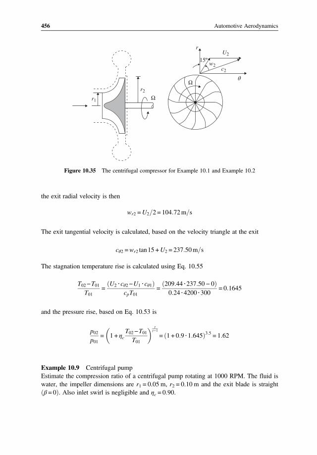
the exit radial velocity is then

wr2 =U2 2 = 104 72m s

The exit tangential velocity is calculated, based on the velocity triangle at the exit

cθ2 =wr2 tan15 +U2 = 237 50m s

The stagnation temperature rise is calculated using Eq. 10.55

T02−T01T01

=U2 cθ2−U1 cθ1

cpT01=

209 44 237 50 − 00 24 4200 300

= 0 1645

and the pressure rise, based on Eq. 10.53 is

p02p01

= 1 + ηcT02−T01

T01

γγ−1

= 1 + 0 9 1 645 3 5 = 1 62

Example 10.9 Centrifugal pumpEstimate the compression ratio of a centrifugal pump rotating at 1000 RPM. The fluid iswater, the impeller dimensions are r1 = 0.05 m, r2 = 0.10 m and the exit blade is straightβ = 0 . Also inlet swirl is negligible and ηc = 0 90.

U2

c2

15º

r

θΩ

Ω

w2

r2

r1

Figure 10.35 The centrifugal compressor for Example 10.1 and Example 10.2


Solution:To calculate the pressure rise in the pump, Eq. 10.52 is used. Note that for straight blades, atthe exit U2 = cθ2

Δp0ρ

= ηc U2 cθ2−0 = 0 90 2π 0 1100060

2

= 174 53ms

2

and the pressure rise is

Δp0 = 1000 174 53 = 174532 3Nm2

about 1 78atm

Next, let us estimate the lowest mass flow rate, on the verge of inlet stall (e.g., when β1≈50 ,based on Eq. 10.59). The tip speed at the inlet is then

U1 = 2π 0 05100060

= 5 24m s

the axial velocity is then calculated, based on the inlet velocity triangle at the tip

c1 =U1 tan 90−β1 = 5,24 tan40 = 4 39m s

and the mass flow rate is

m = ρc1S = 1000 4 39 π 0 052 = 34 50 kg s

The minimum power at this RPM is then calculated using Eq. 10.49

P=m U2 cθ2−0 = 34 50 2π 0 1100060

2

= 3783 35W

which is about 5.14 HP (horse power).This example shows again that a centrifugal compressor performance depends mainly on

the impeller exit radius.

10.4.4 Concluding Remarks: Axial versus Centrifugal Design

After this brief survey of the design principles of continuous flow pumps/compressors, thenext question is: which type of machinery is preferred for a particular application? Whencomparing the centrifugal and the axial designs, delivering the samemass flow rate and pres-sure ratio, then there are nomajor differences in efficiencies. This is probably true when bothdesigns are optimized for a specific operation point. In general, however, the axial designtends to achieve higher efficiencies. In terms of weight, there is also no major difference;

457Fluid Machinery

however, the shape quite frequently dictates the applications. Usually the axial design islonger and its smaller frontal area makes it more attractive for aircraft compressors. Onthe other hand the compression ratio of centrifugal design is significantly higher (per stage).If we consider the compression of air, then the maximum compression ratio of a single stageaxial compressor was estimate in the previous section at about 1.7, but more realistically it iscloser to 1.2. At the same time a centrifugal compressor stage can generate a compressionratio of four! This is why most automotive or hydraulic pumps have a centrifugal design.Another consideration is multistaging, particularly for very high compression ratios (asin jet engines). Stacking up rows of compressor stages one behind the other is naturalfor the axial design but quite awkward for the centrifugal machine.

10.5 Axial Turbines

Turbines are machines that extract power from a moving fluid and were used for centuries,mainly in form of a large bladed wheel rotated by falling water. In modern times turbines areused for power generation, in jet engines, or even to drive the turbochargers in passengercars. Turbine design can be of the axial or centrifugal or even mixed geometry and the dis-cussion is similar to the approach used for the axial and centrifugal compressors. This simpleapproach is suitable for introductory texts and provides valuable insight into the design para-meters of turbines. Also, because the pressure drop across a turbine is favorable (from highto low pressure) it is less sensitive to flow separation, compared to a similar compressor orpump. Therefore, turbine efficiencies are usually higher than for an equivalent compressor.In many applications where the turbine is driven by combustion products (as gas turbines ofjet engines) blade cooling is also a very important aspect of the fluid dynamic considera-tions. Because the axial and centrifugal designs were discussed in detail, only the axial tur-bine will be discussed here, and the formulation can be easily extended to treat centrifugaldesigns as well (as it was done for the compressors).A schematic description of a single stage axial turbine is shown in Fig. 10.36. Although

the approach is the same as used for the axial compressor in Section 10.3, there are someminor differences:

1. A typical stage consists of a rotor and stator blade rows, however, the stator (now calledthe nozzle) is ahead of the rotor. Consequently, station #2 is the exit from the nozzle andthe rotor is between stations #2 and #3.

2. Because in this case the fluid works on the rotor, (a change in sign from the thermody-namics point of view), the direction of rotation was reversed to highlight this change (alsothe direction of the coordinate θ was reversed).

Blade shape and orientations are shown through cut AA, in Fig. 10.36b. This is a two-dimensional representation of the average radius model, and radial variations can be treatedfollowing the approach presented in Section 10.3.3. There are also multistage turbines, andthen a stator (nozzle) row will follow station #3 in Fig. 10.36.


10.5.1 Torque, Power, and Pressure Drop

The torque on the row of stators or rotors can be calculated by Eq. 10.8. When appliedbetween station #2 and station #3 (rotor):

Tq=m r2 cθ2−r3 cθ3 10 69

The power for the rotor is then calculated by Eq. 10.9 (or by simply multiplying the torqueby the rotation speed):

P =Tq Ω=mΩ r2 cθ2−r3 cθ3 10 70

Similarly for the nozzle (stator row) we can write:

Tq=m r1 cθ1−r2 cθ2 10 71

and the torque acting on the nozzle is in the direction opposite to the torque on the rotor.Also, because the nozzle is stationary, it generates no power:

P = 0 10 72

At this point if we limit the discussion to axial turbines and introduce the average radiusassumption, then the rotor blade speed is defined as before

U = rΩ 10 73

U

RotorNozzle

Section AA

(a) (b)

1 2

Nozzle

High-pressureflow

A A

Rotor

1 2 3 3

Figure 10.36 Schematic description of a single stage turbine (a) and the blade geometry as seen fromsection cut AA (b)

459Fluid Machinery

With this definition, Eq. 10.70 for the power generated, becomes

P =mU cθ2−cθ3 10 70a

and the work per unit mass wt is:

wt =P

m=U cθ2−cθ3 10 74

The calculation of the pressure drop would be similar to the axial compressor/pump case.However, the stage efficiency ηt now represents the ratio between the actual work of theturbine, divided by the work invested. In terms of the enthalpy change this becomes

ηt =Δh0Δh0 s

10 75

Note that the losses through both the nozzle and rotor rows are included in this formulation.The actual work invested, per unit mass, is

Δh0 =Δp0ρ

10 76

The work generated by the turbine wt is less (because of the losses) and therefore

wt = ηtΔp0ρ

substituting wt from Eq. 10.74 shows that for the incompressible case, the stagnation pres-sure drop (for a given power) is increased with reduced efficiency!

Δp0ρ

=U

ηtcθ2−cθ3 10 77

In case of a turbine it is more useful to rewrite the power generated as a function of the actualpressure drop. This is done by combining Eq. 10.77 and Eq. 10.74

P=mηtΔp0ρ

=mU cθ2−cθ3 10 78

For the incompressible casewe can rewrite Eq. 10.75, in terms of the stagnation temperature as

ηt =Δh0Δh0 s

=cp T01−T03cp T01−T03 s

10 79


Note that the enthalpy change is calculated across the whole stage, including both rotor andstator. The actual temperature change (for calculating Δh0) is equal to the work per unitmass, in Eq. 10.70a

Δh0 = cp T01−T03 =wt =U cθ2−cθ3 10 80

Consequently, we can write

ΔT0T01

=T01−T03

T01=U cθ2−cθ3

cpT0110 81

As noted earlier, it is more useful to relate the work to the pressure drop across the turbine.This can be accomplished by using the isentropic (adiabatic and reversible) process asdefined by Eq. 10.27

p03p01

=T03 sT01

γγ−1

10 82

The ideal temperature change can be replaced by the actual values, based on Eq. 10.79

p03p01

=T01−T01 + T03 s

T01

γγ−1

= 1−T01−T03 s

T01

γγ−1

= 1−T01−T03ηtT01

γγ−1

10 83

Substituting the temperature change from Eq. 10.81, the pressure drop across the turbinebecomes

p03p01

= 1−U cθ2−cθ3ηtcpT01

γγ−1

10 84

In case of the compressible flow turbine it is also of interest to estimate the power generatedfor a given pressure drop across the whole stage (nozzle and rotor). This is done by combin-ing Eq. 10.70a and 10.84

P =mcpT01ηt 1−p03p01

γ−1γ

10 85

10.5.2 Axial Turbine Geometry and Velocity Triangles

To calculate the pressure drop or the power generated by the turbine, the various velocitycomponents must be identified. Furthermore, drawing of the velocity diagrams allows theproper alignment of the turbine blades relative to the local velocity components. This is

461Fluid Machinery

needed from the blade airfoil-section point of view (to avoid flow separations). A typicalaxial turbine velocity diagram is shown in Fig. 10.37. The stationary nozzle is acceleratingthe high pressure fluid between stations #1 and #2 and the exit velocity c2 is shown in thefigure (and the positive direction for measuring α). The velocity triangles for the rotor areshown in Fig. 10.37b. Note the direction of the U vector (opposing the direction used forcompressors). By adding the blade velocity to the incoming velocity c2 the relative rotorinlet velocity w2 is obtained. This clarifies the orientations of the rotor blades and the rotorexit velocity w3 direction (which should be parallel to the rotor trailing edge bisector). Oncethe incoming and exiting velocity triangles are drawn (as in Fig. 10.37b), assuming there isno change in cz between station #2 and #3, the tangential velocity components are identified.These components (cθ2 cθ3) are then used in the pressure drop and power calculations for-mulas developed in the previous section.

Example 10.10 Axial turbineA turbine wheel shown in Fig. 10.38 is operated by a water jet with a cross section of 3 cm2

and flow rate of 15 kg/s. The nozzle angle is α2 = 68 5 and the blade inflow and outflowangles are the same (β2 = −β3). The average radius of the turbine blades is r = 0.3 m. The tur-bine operates a pulley, which is lifting amass of 100 kg (see Fig. 10.38a), and the rotation rateis stabilized at 1000 RPM. Calculate the blade angle β2 and how fast theweight is being lifted.

Solution:The rotor velocity triangle can be established by calculating U and c2. The blade tip speedis then

U = rΩ= 0 3 2π100060

= 31 41m s

U

Rotor

(a) (b)

Nozzle

1 2 3

c2

w3α2

α3

α2

β3

β2

z

cθ3

c2 w3

U

θ

w2

c3

cθ2

Figure 10.37 Schematic description of axial turbine nozzle and rotor, and resulting rotor velocitytriangle


The nozzle velocity is calculated using the continuity equation (water density is 1000 kg/m3)

c2 =m

ρS=

151000 0 0003

= 50 00m s

Knowing the magnitude of two vectors of the inflow velocity diagram, and the nozzle angleα2 the velocity triangle is drawn (see Fig. 10.37c). The angle β2 is now easily calculatedbased on the triangle trigonometry; but first the axial velocity is calculated

cz = c2 cosα2 = 18 32m s

and the rotor inlet angle is

tan−1β2 =c2 sinα2−U

cz= 0 824

β2 = 39 50

The power of the turbine is calculated using Eq. 10.70

P =mU cθ2−cθ3 =mU 2cz tanβ2 = 15 31 41 30 22 = 14238 15W

which is about 19.35 HP. The power required to lift the mass at a velocity of V is

P=mgV

and therefore

V =P

mg=14238 153100 9 8

= 14 52m s

r

100 kg

(a) (b) (c)

β2β2

β3

α2 α2 = 68.5

U

w2

cz

w3

c2 = 50

Figure 10.38 An axial turbine operated by a water jet, raising a mass of 100 kg

463Fluid Machinery

10.5.3 Turbine Degree of Reaction

The degree of reaction was used in Section 10.3.6 to define the pressure drop ratio betweenthe rotor and the entire stage (including the stator). Similarly, the degree of reaction R can bedefined for a turbine as the enthalpy drop in the rotor versus the stagnation enthalpy changein the whole stage. The changes were approximated using the pressure changes inSection 10.3.6 and using the same approach we get

R=h2−h3h01−h03

≈p2−p3p01−p03

10 86

The pressure drop across the rotor can be estimated by using the incompressible Bernoulliequation (note that this is an approximation only!).

h2−h3 =1ρp2−p3 =

12

w23−w

22

and the total stage stagnation enthalpy change is taken from Eq. 10.80, and therefore

R=w23−w

22

2U cθ2−cθ310 87

Similar to the case of the axial compressor (Eq. 10.44) we can rewrite the numerator in termsof the velocity components

w23−w

22 =w

23θ +w

23 z−w

22θ−w

22 z =w

23θ−w

22θ = w3θ +w2θ w3θ−w2θ

but the tangential velocity difference is the same: w3θ−w2θ = cθ2−cθ3 and therefore thedegree of reaction is

R=w3θ +w2θ

2U10 88

Observing the velocity triangles in Fig. 10.39 we can write

wθ3 = cz tanβ3

wθ2 =U−cz tanα2

Consequently the sum in the numerator becomes

wθ3 +wθ2 = cz tanβ3 +U−cz tanα2


with this in mind, the expression for the degree of reaction becomes:

R=wθ3 +wθ2

2U=cz tanβ3 +U−cz tanα2

2U=12−

cz2U

tanα2− tanβ3 10 89

This indicates that if in the case when a multistage turbine with 50% degree of reactiondesign is sought (e.g., R = 1/2), then the two angles α2, β3 must be equal (and of course point-ing into the opposite directions, as shown in Fig. 10.40b.A schematic description of the blade orientation in aR = 0.5 design is shown in Fig. 10.40,

and the nozzle (stator) and rotor incoming/exiting velocity vectors are the same (but reversedin direction). Consequently the rotor velocity diagram (Fig. 10. 40 b) is symmetrical aboutan imaginary horizontal line, as shown in the figure. This implies that the blades of the noz-zle and of the rotor are exposed to similar angles of attack and therefore their shape is thesame, as well. As noted, Fig. 10.40a depicts this condition where the nozzle exit at station #2is the same as the nozzle exit at station #4, and so on. Using the symmetry assumption, thetangential velocities of the rotor are

cθ2−cθ3 = 2 cz tanα2−U +U

Substituting this into Eq. 10.81 we get

ΔT0T01

=U cθ2−cθ3

cpT01=

U

cpT012 cz tanα2−U +U =

U2

cpT012czUtanα2−1 10 90

This equation indicates that larger nozzle angles α2 result in more power. Of course, that willreduce the axial velocity and α2 = 70 is considered as the maximum nozzle angle.

U

β2

α2α3

w2

c2 w3

c3

cθ2

cθ3

z

θ

Figure 10.39 Generic velocity triangles for an axial turbine

465Fluid Machinery

Example 10.11 Multistage axial turbineThe average radius of the second stage in a multistage axial turbine is r = 0.3 m, rotationspeed is 7000 RPM, and the hot gas flow leaves the nozzle at a temperature of To1 =1200 K (and ρ2 = 0.5 kg/m3). Assuming this is a 50% degree of reaction design and thatthe rotor inflow angle is β2 = 30 and exit angle is β3 = 60 , calculate the following:

a. The power per unit mass generated by this turbine (η = 0.90, γ = 14, cp = 0.24).b. The stagnation pressure drop in the turbine. How much of the static pressure drop takes

place in the rotor?

Solution:In order to establish the rotor velocity triangle, the local blade speed U is calculated:

U = rΩ= 0 3 2π700060

= 219 91m s

Using the symmetry of the velocity triangle in Fig. 10.40 we conclude that α2 = β3 = 60 . Interms of a graphical solution (see Fig. 10.41) we plot the vector U on the θ axis and thendraw a 30 line from the top, representing the direction of w2. Similarly, a 60 curve is drawnat the bottom to represent the direction of the c2 vector. As the two curves intersect, the axialvelocity is found and the velocity triangle for station #2 is complete. The velocity triangle atthe turbine exit (station #3) is drawn next using the symmetry principle (dashed lines).An algebraic solution can be based on the velocity diagram at station #2. For example, we

can write for the tangential component wθ2

U−c2 sin60 =w2 sin30

and for the axial component cz

c2 cos60 =w2 cos30

1

Nozzle(a) (b)

NozzleRotor

c2

w2

w3

w3

w2

c3

c3

z

c4c2

U

Uα2

α3 α4

α2α3

β2 β3

β3

β2

θ

2 3 4

Figure 10.40 50% degree of reaction turbine and corresponding rotor velocity triangle


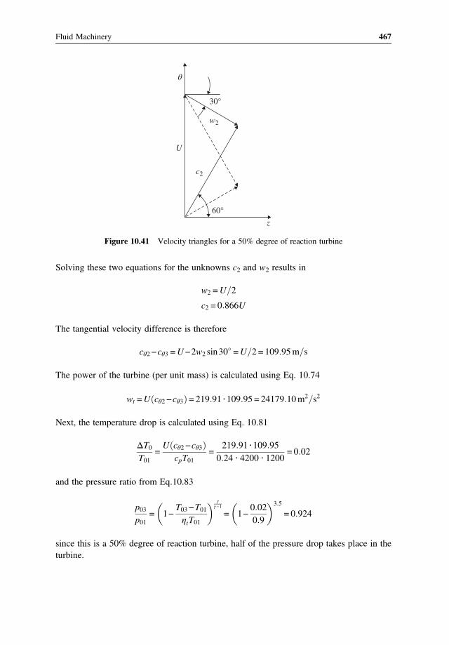
Solving these two equations for the unknowns c2 and w2 results in

w2 =U 2

c2 = 0 866U

The tangential velocity difference is therefore

cθ2−cθ3 =U−2w2 sin30 =U 2 = 109 95m s

The power of the turbine (per unit mass) is calculated using Eq. 10.74

wt =U cθ2−cθ3 = 219 91 109 95 = 24179 10m2 s2

Next, the temperature drop is calculated using Eq. 10.81

ΔT0T01

=U cθ2−cθ3

cpT01=

219 91 109 950 24 4200 1200

= 0 02

and the pressure ratio from Eq.10.83

p03p01

= 1−T03−T01ηtT01

γγ−1

= 1−0 020 9

3 5

= 0 924

since this is a 50% degree of reaction turbine, half of the pressure drop takes place in theturbine.

30°

60°

w2

c2

U

z

θ

Figure 10.41 Velocity triangles for a 50% degree of reaction turbine

467Fluid Machinery

Another interesting example is the impulse turbine. In this case, the whole stagnationpressure drop takes place in the nozzle, and the pressure energy is converted entirely intovelocity. Impulse turbines are usually selected for single stage designs or the last stage of amultistage turbine. This concept is also the oldest form of turbine used with water jets (seeFig. 10.38). It was clear that the best results could be obtained when all the pressure in thewater is converted into velocity (or a jet) and then this jet impinged on the turbine blade.Such design is less sensitive to the delicate airfoil shape of more complex turbine designs.Because the whole stagnation pressure drop takes place in the nozzle, the static pressurechange in the rotor is zero! Consequently, the degree of reaction, according to Eq. 10.86is zero, as well

For impulse turbine R=p2−p3p01−p03

= 0 10 91

Recalling Eq. 10.87 and equating it to zero yields

R=w23−w

22

2U cθ2−cθ3= 0

and therefore the incoming and exiting velocity vectors are of the same magnitude.

For impulse turbine w2 =w3 10 92

As a result the velocity triangles will have the shape depicted in Fig. 10.42. The rotor bladeshape will reflect this fore/aft symmetry, as shown schematically in the figure.

Nozzle

1

Rotor

2

c2

c2

c3

cz z

w2

w2

w3

w3U

U

α2

α2

α3

β2

β2

β3

β3

θ

3

Figure 10.42 Impulse turbine and corresponding rotor velocity triangle


Based on the velocity diagram shown in Fig. 10.42, and assuming that the rotor incomingand exiting velocity vectors have the same magnitude, we can write:

cθ2−cθ3 = 2 cz tanα2−U

and after substituting this into Eq. 10.81 we get

ΔT0T01

=U cθ2−cθ3

cpT01=

2U2

cpT01

czUtanα2−1 10 93

Again, this equation indicates that larger nozzles angles α2 result in more power. And themaximum recommended nozzle angle is α2 = 70 .

Example 10.12 Impulse turbineAn impulse turbine with an average radius of r2 = 0.1 m is operated by a hot gas flow at arate ofm = 1 kg/s, and a temperature of T01 = 1200 K. The jet leaves the nozzle at an angle ofα2 = 65 and speed of c2 = 330 m/s (ρ2 = 0.5 kg/m3).

a. If the flow at the exit has no swirl, then calculate the power generated by this turbine(η = 0.90, γ = 14, cp = 0.24).

b. Calculate the stagnation pressure drop in the turbine. How much of the static pressuredrop takes place in the rotor?

c. Calculate the shaft RPM.

Solution:If the exit velocity c3 has no swirl then α3 = 0 and by observing the velocity diagram inFig. 10.42 (for the impulse turbine with α3 = 0 only) we get

cθ2−cθ3 = 2U = c2 sin65 = 299 08m s

The power of the turbine is calculated using Eq. 10.70

P=mU cθ2−cθ3 = 1 00299 08

2299 08 = 44724 8W

which is about 60 HP. The stagnation temperature drop is calculated using Eq. 10.93

ΔT0T01

=U cθ2−cθ3

cpT01=

299 082

299 08

0 24 4200 1200= 0 037

and the pressure ratio from Eq. 10.83

469Fluid Machinery

p03p01

= 1−T03−T01ηtT01

γγ−1

= 1−0 0370 9

3 5

= 0 863

This is an impulse turbine and the whole stagnation pressure drop takes place in the nozzle(e.g., zero pressure drop in the rotor). Since the vector U and the rotor radius are known therotation rate can be calculated as

RPM =U

2πr=

299 08 22 3 14 0 1

60 = 14280

Usually in the last turbine stage, or if there is only one stage, it is desirable for the exit flow toleave without swirl (or zero tangential velocity). In terms of the velocity diagram this meansthat α3 = 0. Such a condition is sketched in Fig. 10.43 for a 50% degree of reaction and for animpulse turbine. Assuming both having the same radius and rotation speed (sameU), and thesame axial velocity we can see that for the R = 50% design the tangential velocity differenceis equal to the blade speed (cθ2−cθ3 =U). For the impulse turbine, the tangential velocitydifference is twice the rotation speed (cθ2−cθ3 = 2U), suggesting that it generates twicethe power compared to the R = 50% design. This is true for the conditions shown inFig. 10.43, but at the same time the nozzle exit speed c2 is significantly higher for theimpulse turbine. Also the fluid crossing the turbine blades is turned more sharply by the

U

(a)

(b)

U

R = 0

c3

c2

c2

R = 0.5

c3

w3

w3

w2

w2

α2 α2

Figure 10.43 Schematic comparison between a 50% degree of reaction and an impulse turbine, withno swirl at the exit


impulse turbine (more camber). In spite of these considerations, the impulse turbine has thepotential to generate more power.

Example 10.13 The Pelton wheelOne important form of the impulse turbine, called the Pelton wheel (after Ohio born LesterAllan Pelton, 1829–1908), is used in power generating plants and is shown schematically inFig. 10.44. In this case, the whole pressure drop takes place in the nozzle and the turbineblade is simply changing the direction of the jet. This is shown schematically in Fig. 10.44b.The velocity diagram in the z − θ coordinate system is shown schematically in Fig. 10.44c

and the jet velocity c2 has no velocity component into the z direction! Still the treatment ofthis turbine is not different than that of the axial impulse turbine. As an example, consider aPelton wheel with an average radius of r = 0.1 m, which rotates at 1000 RPM by a water jetwith an exit velocity of c2 = 30 m/s (assume the jet cross section is 2 cm2). Also the angle ofthe flow leaving the blade in this example is β3 = 60 . Because this is a Pelton wheel and thenozzle is aligned with the turbine wheel (α2 = 90 ), the velocity relative to the blade (w2) isthe difference between the jet and the wheel tip speeds, as shown Fig. 10.41c

w2 = c2−U

the blade tip velocity is

U = rΩ= 0 1 2π100060

= 10 47m s

and w2 is

w2 = c2−U = 30−10 47 = 19 53m s

(a) (b) (c)

Turbineblade

30°

ΩΔcθ

θ

β3

w3

w3

c2

c3

zc2

w2w2

U

r

Figure 10.44 Schematic description of the Pelton wheel (a), the rotor blade geometry (b), and thevelocity diagram (c)

471Fluid Machinery

Since this is an impulse turbine the exit velocity is unchanged

w3 =w2 = 19 53m s

and the torque and power can be calculated by using Eq. 10.70a, and 10.71. The change intangential velocity is therefore (see Fig. 10.40c):

Δcθ = cθ2−cθ3 = 19 53 1 + sin60 = 36 44m s

The mass flow rate is

m= ρc2S= 1000 30 2 10−4 = 6 kg s

The torque and power now can be calculated as:

Tq=mrΔcθ = 6 0 1 36 44 = 21 86Nm

P=mUΔcθ = 6 10 47 36 44 = 2289 16W

At this point, the relation between turbine geometry, power, and pressure drop was estab-lished, and the generic shape of a typical performance map is briefly discussed. Usually, tur-bine mass flow rate can be controlled, thereby dictating the incoming velocity c2, and thepressure drop across the stage. Consequently, a typical turbine performance map will showthepressuredropversusmass flowrate across the stage (as shownschematically inFig. 10.45).On the left-hand side of the figure, the rotor blade geometry is depicted, and the solid linevelocity triangle represent a lower mass flow rate (point A). If mass flow rate increases at aconstant RPM1, so will c2, as shown by the dashed line (point B). Because the incoming flowangle α2 (nozzle angle) remains unchanged, c2 is longer, as shown. This increases the angle ofattack of the rotor blade, resulting in higher load (e.g., higher lift coefficient) and higher

U

U

RotorChokednozzle

4

2

RPM1

RPM2

(a) (b)

AA

m.

BBw2

p02p03

c2

α2

Figure 10.45 Typical performance curves for a single stage axial turbine


pressure ratio. Therefore, at the higher mass flow rate, pressure ratio will also increase, asshown by point B on the performance map. Now, if rotation is reduced to RPM2, then thesame trend is observed, but at a slightly lower pressure ratios. If mass flow rate is furtherreduced, the incoming flow angle of attack is reduced, up to a point where the turbine cannotgenerate power (this is where the lines end at the lower mass flow rates). At the higher massflow rates, a point is reachedwhere the nozzle is chocked and this represents the highestmassflow rate point in Fig. 10.45b.

10.5.4 Turbochargers (for Internal Combustion Engines)

A turbocharger is a combined system of a compressor and a turbine sharing the same shaft,as shown schematically in Fig. 10.46. The turbine is operated by the engine exhaust gases,which in turn drives the inlet air compressor. Because air/fuel mass ratio is about 15, themass flow rate across the turbine and the compressor are very close! Therefore, the perfor-mance map is based on the compressor map as shown in Fig. 10.47. In this performance mapthe compressor inlet/exit pressure ratio is plotted versus the mass flow rate. The curves for afixed RPM resemble the lines suggested by Fig. 10.20, and for higher RPM the pressureratio is higher. Each of these fixed RPM lines ends at the left at the surge line which repre-sents inlet stall, while the flow is considered “choked” at the right hand side end of each line(e.g., no more flow can be pushed across the system). Efficiency contours are also plottedshowing improved efficiency towards the center of the plot, along with the most efficient“island”. The dotted lines represent the desirable system performance curve where the effi-ciency is the highest for a given mass flow rate.

Exhaustout

Exhaust gasin

Inductionair-in

Turbine

Connectingshaft

Compressor

Compressedair-out

Figure 10.46 Schematic description of a turbocharger. Left is the centrifugal compressor while rightis the turbine

473Fluid Machinery

10.5.5 Remarks on Exposed Tip Rotors (Wind Turbines and Propellers)

The discussion so far focused on turbo-machines where the rotor is enclosed in an outercasing and the discussion was limited to simple two-dimensional models (as demonstratedwith the rotor velocity diagrams). However, quite frequently, similar devices such as windturbines, propellers, and many cooling fans have no outer shroud. The question then is; whywasn’t the simple analysis of this chapter extended to include those cases, as well? The mainreason is that with open tip rotors the flow is highly three-dimensional and more advancedanalysis methods are required (such as CFD in Chapter 8). These effects can be grouped intotwo main categories which can be addressed here briefly, mainly as a prelude for moreadvanced course work. First, at the tip, no pressure difference between the upper and lowersurfaces can be maintained. Therefore, the loading drops to zero (at the tip) compared to theshrouded case where high loading can be present. This is depicted schematically inFig. 10.48a where the expected pressure rise is shown for a shrouded compressor. Onthe right-hand side (Fig. 10.48b) the same rotor is shown but without the shroud. In thiscase the tip effect is reducing the loading (or pressure rise) not only at the tip but along

00

1.5

2

Surgeline

Bestoperating

curve

75000RPM

95000RPM

115000RPM

135000RPM

155000RPM

2.5

3

5 10

Air flow rate, Kg/min.

Com

pres

sor

pres

sure

rat

io

15

η= .65.68.70.72.74.76 η= .65.68.70.72.74.76

Figure 10.47 Turbocharger map for a typical automotive turbocharger (Garrett GT2259). The map isbasically the compressor map, but the mass flow rate across the turbine is very close to that of thecompressor


the whole blade. So in principle, ducted (or shrouded) fans can generate more thrust (or pres-sure rise) but will also require more torque due to higher loading at the larger radius stations.Therefore, the efficiency of open rotors is not necessarily inferior, particularly in airplaneapplications (due to the added drag and weight of the nacelle). The discussion also explainsthe need for a very small gap between the rotor and surrounding casing.The second major feature of open tip rotors is the creation of a strong vortex wake, as

shown in Fig. 10.49 (which is almost nonexistent in the shrouded multistage case). Thisis similar to the tip effect of a finite wing, discussed in reference to Fig. 6.42, where thepressure difference between the pressure and suction sides of the blade results in a rotatingflow near the tip. A simple modeling of this wake is shown in Fig. 10.49 and the velocityfield induced by this vortex wake has a strong effect as well. For example, when the forwardspeed is slow compared to the rotor tip speed (as for a hovering helicopter) this wake-induced velocity may have the same order of magnitude of the free-stream.In spite of the previously mentioned modeling difficulties, simple stream-tube based

models were developed in the past to estimate both propeller and wind turbine performance.These approaches fail to connect blade geometry to parameters such as the pressure rise, butat least one, discussing the maximum efficiency of a wind turbine is worth mentioning.This (anecdotal) model of a wind turbine is shown in Fig. 10.50 and is based on the one-

dimensional stream-tube model presented earlier in Chapter 2.The flow enters the stream tube at station #1 at a speed of U∞ and crosses through the

rotor with a disk area of S. As the flow drives the rotor it slows down (between station(a) and (b) and the stream tube becomes wider at the exit station, #2 (recall the continuityequation), where the velocity is u2. The force on the turbine must be equal to the momentumloss of the stream-tube flow.

F =m U∞ −u2

andm is the mass flow rate. The power given away by the flow is the force times the averagevelocity (uav) across the rotor

Tip loss

Blade workwith exposed tip

Blade workwith shroud

(b)Nacelle

(a)

Figure 10.48 The effect of exposed tip on rotor performance

475Fluid Machinery

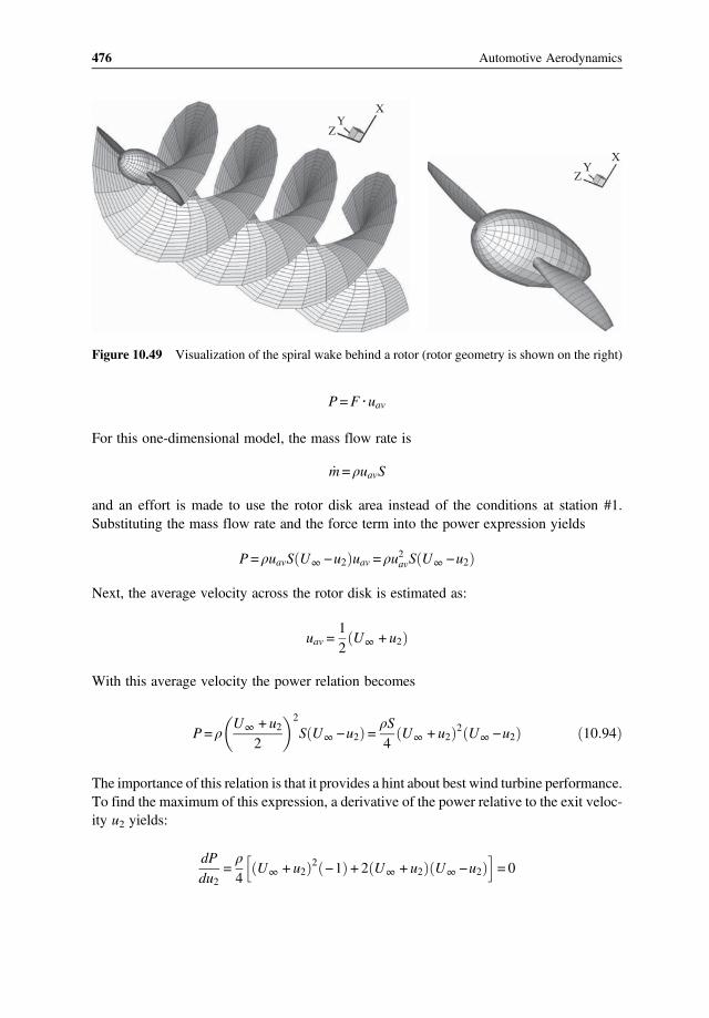
P=F uav

For this one-dimensional model, the mass flow rate is

m= ρuavS

and an effort is made to use the rotor disk area instead of the conditions at station #1.Substituting the mass flow rate and the force term into the power expression yields

P= ρuavS U∞ −u2 uav = ρu2avS U∞ −u2

Next, the average velocity across the rotor disk is estimated as:

uav =12U∞ + u2

With this average velocity the power relation becomes

P= ρU∞ + u2

2

2

S U∞ −u2 =ρS

4U∞ + u2

2 U∞ −u2 10 94

The importance of this relation is that it provides a hint about best wind turbine performance.To find the maximum of this expression, a derivative of the power relative to the exit veloc-ity u2 yields:

dP

du2=ρ

4U∞ + u2

2 −1 + 2 U∞ + u2 U∞ −u2 = 0

ZY

X

ZY

X

Figure 10.49 Visualization of the spiral wake behind a rotor (rotor geometry is shown on the right)


and by solving this equation, the condition for the maximum power becomes:

u2 =U∞

310 95

Substituting this result into the power relation provides the maximum wind tur-bine power

P=ρS

4U∞ + u2

2 U∞ −u2 =827

ρU3∞S 10 96

To place this result in perspective, consider the total kinetic energy entering the stream tubeat station #1

Pavail =12mU2

∞=12ρU3

∞S

Therefore, based on this simple analysis, the maximum energy that a wind turbine canextract from a stream having the same cross section area S (let us call this maximum effi-ciency) is:

ηmax =P

Pavail=1627

10 97

Now, 16/27 is about 59.26% and this number is usually called the Betz number or Betz effi-ciency (dating circa 1926), after Albert Betz (1885–1968) who succeeded Ludwig Prandtl asthe head of the Gottingen center in Germany.The important part of this discussion is that wind turbine performance is evaluated by

similar nomenclature. Typical values for the efficiency defined by Eq. 10.97 are near20–40%, which is significantly less than the Betz value.

1a

b2

Wind

Propeller’sstream tube

U∞uav

u2PP∞

Figure 10.50 Simple stream tube model for a wind turbine

477Fluid Machinery

Example 10.14 Sizing of a wind turbineIt is proposed to build a small wind turbine capable of producing 5 KWpower. If the averagewind speed is 30 km/h and the expected design is capable of extracting 70% of the powerpredicted by the Betz formula (ηp = 0.7), calculate the wind turbine diameter.

Solution:Based on Eq. 10.96, the power is

P= ηp827

ρU3πR2

Solving for the propeller radius we get

R=P 27

8 ηp ρ U 3 6 3π

R=5000 27

8 0 7 1 22 30 3 6 3π= 3 29m


The formulation presented in this chapter establishes the relation between turbo machinerycomponent geometry and the expected performance. It allows proper orientation of the air-foil shaped blade components, and clearly visualizes undesirable conditions such as com-pressor surge (or blade stall). Furthermore, this method allows the preliminary design ofcompressors, pumps, and turbines, and the ability to size their components. Power require-ments and expected pressure ratios are estimated, based on parameters such as the geometryand rotation speed. Such data for commercially available turbomachinery is provided inperformance maps, typically connecting pressure ratio to mass or volumetric flow rate,for several rotation speeds. The trends in these performance maps are also explained, relat-ing component geometry to performance for both compressors/pumps and turbines.

Reference10.1. Wankel, F., Rotary Piston Machines, Iliffe Books Ltd, London, 1965.

Problems

10.1. It is required to pump 2 ls water from a pool into a container 7 m above the water levelin the pool. If the overall efficiency of the pump is 0.7, estimate the continuous powerrequired to pump the water.

10.2. A segment of an axial compressor with six identical stages has a compression ratio of3 (all stages with degree of reaction of R = 1/2, and with the same velocity diagrams,


compression ratio, average radius, etc.). The shaft rotates at 8000 RPM and the aver-age blade radius is rm = 0.3 m. The axial velocity across these stages is assumed to beconstant at cz = 120 m/s. The first stage inlet temperature is T01 = 360 K, and the effi-ciency of all stages is ηst = 0.95, and γ = 1.4.a. Calculate the rotor blade angles β1 β2.b. Calculate rotor pressure coefficient Cp.c. Calculate power (per unit mass flow rate) required to drive all six stages.

10.3. The axial velocity across the second stage of an axial compressor is cz = 120 m/s, theaverage radius is rm = 0.4 m, and the stagnation temperature ahead of the rotor is T0 =300 K. If the compressor rotates at 5000 RPM, the angle α1 = 25 , and the pressurecoefficient of this rotor stage is Cp = 0.5, calculate:a. The angles β1 and β2.b. The stagnation pressure rise p03 /p01 across this stage (ηstage = 0.98, cp = 0.24,

γ = 1.4).c. Degree of reaction R.d. During the starting process the axial velocity is reduced to cz = 80 m/s but RPM =

5000. How many degrees should the stator blade (ahead of this rotor) be rotated sothat the rotor blade angle β1 will not change?

10.4. The average radius of an axial compressor blade is rav = 0.6 m and it rotates at a constantspeedof3500RPM.Theaxial velocity through this stage iscz = 130m/s and the two rotorangles are β1 = 55 and β2 = 35 . Also assume that γ = 1.4, cp = 0.24, and T01 = 300 K.a. Draw a velocity diagram for the compressor blade.b. Calculate the stagnation pressure ratio p03/p01, (ηst = 1.0).c. Calculate the pressure coefficient (Cp) for this rotor. Is blade stall likely?

10.5. A turbofan jet engine operates at a flight speed ofMa = 0.7 and the ambient conditionsare: Ta = 300 K and pa = 1 atm. The axial fan has no stator ahead of the rotor and theaverage radius of the fan blade is rav = 0.7 m and it rotates at 3600 RPM (γ = 1.4, cp =0.24, R = 286.78 (m/s)2/K).a. Assuming ηd = 1.0 and the inlet area ratio is Aa/A2 = 0.63 (A2 is ahead of the fan and

Aa is in the free stream) calculate the axial velocity ahead of the fan blade.b. If the pressure coefficient of the fan rotor blade is Cp = 0.55, calculate the stagna-

tion pressure ratio p03/p0a for the fan (for simplicity, assume ηstage = 1.0).10.6. A single stage axial compressor rotates at 4000 RPM. The incoming flow speed is

cz = 40 m/s, the rotor average radius is rm = 0.25 m, and the rotor blade consists ofa symmetric airfoil shape oriented at 60 (β2 = 60 ). Also, ηst = 0.85, γ = 1.4, cp =0.24 kcal/kg K, and To1 = 300 K.a. Draw the velocity diagram for the rotor (assume no stator ahead of this stage, α1 = 0).b. Calculate rotor angle β1.c. Calculate stagnation pressure ratio p02/p01.d. Calculate torque and power requirements.

10.7. The average radius of an axial compressor blades in the first row of a jet enginecompressor is rm = 0.7, and the local Mach number is M = 0.45.a. Calculate the axial velocity ahead of the rotor (To1 = 356 K, ηst = 0.95, γ = 1.4,

cp = 0.24).

479Fluid Machinery

b. Calculate stagnation pressure rise across this stage at 3300 RPM, if rotor pressurerise coefficient is CP = 0.5.

c. Calculate the degree of reaction.10.8. An axial water pump with an average radius of 0.05 m rotates at 1000 RPM and the

incoming axial velocity is 1.5 m/s. If the blades turn the flow by β2−β1 = 10 , andpump efficiency is η= 0 8, calculate pressure rise and power per unit mass.

rav50° RPM

cz

1 2

Problem Figure 10.8

10.9. The axial pump shown in Problem 10.8 pumps 25 l/s water in a 12 cm diameter pipeline and the required head is hf = 0.8 m of water. If rotation rate is set by the motor at1200 RPM, calculate the symmetric blade angle β2 (assume pump average radius is0.05 m, efficiency is 0.75, and the average velocity in the pipe is the same as the axialvelocity entering the rotor). Also calculate the pressure rise coefficient and estimateif blade stall is likely.

10.10. The axial velocity across an axial compressor blade is cz = 43.5 m/s, the averageradius is rm = 0.2m, and the stagnation temperature ahead of the rotor is T0 = 300 K.The rotor blade is a symmetric untwisted airfoil that rotates at 3600 RPM, the angleβ1 − β2 = 10 , and α1 = 0. Calculate the following:a. The angles β1 and β2.b. The change in the rotor tangential velocity ΔCθ.c. The pressure coefficient of this rotor stage Cp.d. The stagnation pressure rise p03 /p01 across this stage (ηstage = 0.98, cp = 0.24,

γ = 1.4).e. Degree of reaction R.f. During the starting process the axial velocity is reduced to cz = 20 m/s but RPM

stayed at 3600. Howmany degrees should the stator blade (ahead of this rotor) berotated so that the rotor blade angle β1 will not change?

10.11. A centrifugal compressor rotates at 7000 RPM and compresses 6 kg/s air. The impel-ler dimensions are r1 = 0.1 m, r2 = 0.35 m and the blade height at the exit is b2 =0.015 m (see sketch). The tangential velocity at the impeller inlet is negligible, inlettemperature is To1 = 300 K, and the air density at the impeller exit is 2.5 kg/m3. Also,at the exit, the blade is leaning backward at β = 5 , and η = 0.93, cp = 0.24, γ = 1.4.


a. Calculate the stagnation pressure rise p03/p01 across this stage.b. Calculate the power required to drive this compressor.

RPM

r2

b

r1

Problem Figure 10.11

10.12. What is the minimum flow rate for the centrifugal compressor described in the Prob-lem 10.11? Assume air density at the impeller inlet is 1.22 kg/m3.

10.13. A centrifugal water pump rotates at 750 RPM. The impeller inlet radius is0.04 m, exit radius is 0.10 m, and it has straight vanes. The water enters atthe inlet at an average velocity of 2.5 m/s (without swirl). Calculate pressure riseand the power required to operate the pump (η = 0.95). Also estimate the angleβ1 at the inlet.

10.14. A centrifugal pump with a 0.1m diameter impeller (straight exit vanes) is used topump 2 l/s water from a pool into a container, 5 m above the water level in the pool.Calculate the required power and RPM if overall pump efficiency is 0.7.

10.15. A centrifugal pump is used to pump water from a lower to a higher reservoir (seesketch). The impeller has simple straight vanes, diameter D2 = 12 cm, and its inletdiameter is D1 = 6 cm. If z1 = 10 m, z2 = 2 m and the friction losses can be summar-ized as a head loss of hf = 0.5 m. Calculate required RPM (assume efficiency η = 0.8).Estimate the power requirement when flow rate is 12 l/s.

z1

z2

D1

D2


481Fluid Machinery

10.16. Calculate the inlet velocity c1, impeller inlet tip angle β1 and the pressure coefficient(Eq. 10.58) for Problem 10.15. Can the flow rate be reduced to 8 l/s?

10.17. A centrifugal water-pump is designed to provide a pressure jump equivalent to 2 mwater column. The motor designated to run the pump provides a constant rotationspeed of 800 RPM. If efficiency is estimated at 0.75, calculate the straight-vaneimpeller diameter.

10.18. Estimate the compression ratio of a centrifugal compressor with straight impellerexit blades operating at 6000 RPM. The inlet radius is 0.05 m and the impeller exitradius is 0.30 m. The compressed fluid is air (To1 = 300 K, η = 0.90, cp = 0.24,γ = 1.4).

10.19. Suppose a pump with the dimensions used in Problem 10.18 rotates at 1500 RPM,but at this time the fluid is water. Estimate the pressure rise.

10.20. Estimate the compression ratio of a centrifugal compressor with forward leaningblades β = 15 at the impeller exit, rotating at 5000 RPM. Assume the exit radialvelocity wr2 =U2 2. The inlet radius is 0.10 m and the impeller exit radius is0.40 m. The compressed fluid is air (To1 = 300 K, η = 0.90, cp = 0.24, γ = 1.4).

10.21. A centrifugal water pump rotates at 3000 RPM. The impeller inlet radius is 0.04 m,exit radius is 0.10 m and it has straight vanes. The water enters at the inlet at an aver-age velocity of 1.5 m/s (without swirl). Calculate mass flow rate, the pressure rise,and the power required to operate the pump (η= 0 95).

10.22. A small impeller (of a centrifugal compressor shown in Fig. 10.29) with the dimen-sions: r1 = 12 mm, and r2 = 18 mm is used to compress air, and its rotation speed is130,000 RPM (assume γ = 1.4, ρp = 1.0 kg/m3, cp = 0.24, To1 = 300 K, and compres-sor efficiency is η = 0.85).a. Draw the velocity diagrams at the tip of the impeller inlet and impeller exit.

Assume β1 = 48 , and Cθ1 = 0 at the inlet and the blades are turned back 10at the exit (also, blade height at the exit is b2 = 3 mm).

b. Calculate mass flow rate and exit velocity wr2.c. How much power is needed to drive this impeller and what is the compression

ratio of this compressor?10.23. The impeller of a centrifugal compressor stage with the dimensions r1 = 0.08 m, and

r2 = 0.32 m rotates at a constant speed of 5000 RPM. The fluid that is being com-pressed has the following properties: γ = 1.4, ρ1 = 1.2 kg/m

3, cp = 0.24, To1 = 300 K,and the compressor efficiency is η = 0.85.a. Draw the velocity diagrams at the tip of the impeller inlet and impeller exit.

Assume β1 = 45 , and Cθ1 = 0 at the inlet and the blades are turned back 10at the impeller exit (also, blade height at the exit is b2 = 0.01 m and the fluid den-sity there is ρ2 = 1.5 kg/m3).

b. Calculate mass flow rate and exit velocity wr2.c. How much power is needed to drive this impeller and what is the compression

ratio of this compressor?


d. Calculate compression ratio and power if the blades lean forward by 10 at theimpeller exit (instead of backward)?

10.24. A centrifugal compressor rotates at 5000 RPM and compresses 5 kg/s air. The impel-ler dimensions are r1 = 0.1 m, r2 = 0.3 m and the blade height at the exit is b2 = 0.015m. The tangential velocity at the impeller inlet is negligible, inlet temperature isTo1 = 300 K, and the air density at the impeller exit is 2.4 kg/m3. Also, at the exit,the blade is leaning forward at β = −5 , and η = 0.90, cp = 0.24, γ = 1.4.a. Calculate the stagnation pressure rise p03/p01 across the compressor.b. Calculate the power required to drive this compressor.

10.25. An axial turbine with an average radius of r2 = 0.3 m is operated by a hot gas flow at atemperature of To1 = 1200 K and ρ2 = 1.0 kg/m3. The jet leaves the nozzle at an axialvelocity of cZ = 300 m/s). The nozzle total exit area (normal to c2) is A2 = 0.03 m2.a. Draw the rotor velocity diagram based on, β2 = 38 , β3 = −40 , and c3 has no

tangential component. Based on the velocity diagram calculate rotor RPM andnozzle angle α2.

b. Based on your finding sketch the turbine blade shape and calculate massflow rate.

c. How much power is generated by this turbine? Calculate the degree of reaction.10.26. The average radius of a 50% degree of reaction, axial turbine is r = 0.2 m, and rota-

tion speed is 8000 RPM. The hot gas flow leaves the nozzle at a temperature of To1 =1200 K (ρ2 = 0.5 kg/m3) and at an angle of β2 = 30 . If the rotor trailing edge isaligned such that β3 = 60 , calculate the power per unit mass generated by this tur-bine (η = 0.90, γ = 14, cp = 0.24) and the stagnation pressure drop in the turbine.

10.27. An impulse turbine with an average radius of r2 = 0.25 m is operated by a waterjet. The nozzle area is 3 cm2, its jet angle is α2 = 60 and the water flow rate is5 kg/s (ρw = 1000 kg/m3).a. If the flow at the exit has no swirl, then calculate the power generated by this

turbine.b. The turbine operates a lift, raising a mass of 75 kg, at sea level conditions. If the

mechanical efficiency of the gear system is assumed to be 1.0, then calculate howfast the mass could be lifted.

10.28. An impulse turbine with an average radius of r2 = 0.2 m is operated by a hot gas flowat a rate ofm = 1 kg/s, and a temperature of T01 = 1200 K. The jet leaves the nozzle atan angle of α2 = 60 and speed of c2 = 300 m/s (ρ2 = 0.5 kg/m3).a. If the flow at the exit has no swirl, then calculate the power generated by this

turbine (η = 0.90, γ = 14, cp = 0.24).b. Calculate the stagnation pressure drop in the turbine. How much of the static

pressure drop takes place in the rotor?c. Calculate the shaft RPM.

10.29. A Pelton turbine wheel with an average radius r = 0.2 m rotates at 800 RPM isoperated by a water jet with a cross section of 3 cm2 and exit velocity c2 = 25 m/s.

483Fluid Machinery

The nozzle is alignedwith the wheel (α2 = 90 ) and the blade outflow angle is β3 = 60 .Calculate the torque and the power of the turbine.

Turbineblade

30°

Ω

c2

w2

w3

r


10.30. A turbine wheel shown in Fig. 10.42 rotates at 1000 RPM and is operated by a waterjet with a velocity of c2 = 30 m/s. The nozzle angle is α2 = 60 and the blade inflowand outflow angles are the same (β2 = −β3). The average radius of the turbine bladesis r = 0.2 m. Calculate the blade angle β2 and the pressure drop in the nozzle and thepower per unit mass (η = 0.9).

10.31. It is proposed to build a small wind turbine capable of lighting up a 100W light bulb.If the average wind speed is 30 km/h and the expected design is capable of extracting80% of the power predicted by the Betz formula; calculate the wind turbine diameter.


11Elements of Heat Transfer

11.1 Introduction

The previous chapters focused on fluid flow without significant temperature changes, butthere are areas on a moving vehicle, such as across the radiator (or inside the various enginecomponents), where heat exchange is important. Heat transfer results from temperature dif-ferences and the rate of energy transfer is one of the main objectives of a typical engineeringanalysis. Also, as a consequence, from the second law of thermodynamics, the thermalenergy (heat) always flows from a higher temperature to a lower temperature. Traditionally,three different mechanisms are identified in relation to heat transfer, which are conduction,convection, and radiation (see schematic description in Fig. 11.1). The first, conduction,relates to heat transfer between stationary components of a fluid or a solid body. As an exam-ple, heat is transferred between the hot metal components of the engine in Fig. 11.1 and thisis why even the valve cover is hot on a running car. Convection relates to cases where thefluid is moving and the heat is transferred by the moving fluid particles. A good example isthe automobile radiator where heat is transferred to the free-stream airflow. Heat transfer byradiation, as its title suggests, transfers heat without direct contact between the omitting andreceiving objects. This type of heat transfer becomes significant only at very high tempera-tures and, for example, the heat radiating from the exhaust manifold could be easily feltwhen opening the engine cover. Incidentally, although the name “radiator” suggests thatit radiates heat, most of its cooling is through convection and its radiation cooling isrelatively small.The introduction of temperature variation into the study of fluid flows complicates the

problem more than just a simple addition of one more variable. For example, fluid proper-ties, such as density, viscosity, heat conduction, and many other properties may change with


temperature. Furthermore, in most practical cases the geometry of the components involvedin the heat exchange are complex, requiring two- or three-dimensional analysis (or eventime-dependent effects). Therefore, as in the previous chapters, simple, mostly one-dimensional methods are used to explain the mechanisms and the dominant variables driv-ing the heat transfer. These methods can later be extended to more practical cases usingexperimental correlations (e.g., extending a laminar flow model into the turbulent region).

11.2 Elementary Mechanisms of Heat Transfer

Among the three heat exchange mechanisms mentioned earlier, conductive heat transfer isthe most relevant to the present discussion on fluid mechanics. Furthermore, because of thesimilarity between the thermal and viscous boundary layers (of Chapter 5), explaining con-vection without covering the boundary layer models first would be very difficult. Along thesame thoughts, the mechanism of conduction must be clarified before discussing convec-tion, thereby dictating the sequence followed in this chapter. Next, let us describe brieflythese three heat transfer mechanisms.

11.2.1 Conductive Heat Transfer

At the end of Chapter 1 the relation between temperature and molecular motion wasbriefly discussed. Therefore, it is quite logical that if one side of a body is warmer (fastermolecular motion) than its other side (slower molecular motion), then energy will be trans-ferred from the hot to the cooler side as the faster molecules will collide with the slower ones.

Convection

Conduction

Radiation

Figure 11.1 Schematic description of the three elementary mechanisms of heat transfer


The process can be illustrated by a simple one-dimensional model as depicted by Fig. 11.2(a repeat of Fig. 1.13) where the temperature at one side of the wall is higher than at the otherside. The basic heat transfer equation for this case, called the Fourier equation (after theFrench mathematician, Joseph B. J. Fourier, 1768–1830), states that the heat flux is propor-tional to the area A, the temperature gradient, and to the thermal conductivity coefficient k,which depends on the material through which the heat is conducted.

Q = −kAdT

dx11 1

For the case in Fig. 11.2 we could state that the heat flux is

Q= −kAT2−T1

d11 2

and hereT2 is larger thanT1, and theminus sign indicates that the heat flux is in the –x direction.Also note that the temperature distribution in the wall is linear and A represents the wall areanormal to the heat flow. The units for k, as noted in Chapter 1, are defined by Eq. 11.2 asW/(m C)or cal/(m C/s).Ofcourse for somemetals, k is very large,while for insulationmaterialit is low (see Table 11.1 for some typical values). Also note thatQ represents the heat flow rateper unit time.

Example 11.1 Heat transfer across a brick wallAssume that a brick wall (as in Fig. 11.2) of thickness 0.2 m is exposed to an outer temper-ature of 40 C and an inside the temperature is 20 C. Calculate the heat transfer per 1 m2 areaof the wall.

Solution:We can use Eq. 11.2 and take the value for k = 1.3 from Table 11.1. Substituting the valuesfrom this example we get:

T

d

Q

x

T1

T2

Figure 11.2 Conductive heat transfer through a wall of thickness d


Q= −1 3W

m C1 m2 40−20

0 2C

m= 130W

Note that in this text we use the SI (metric units) and the answer to this problem is inenergy per unit time. But energy or work is also measured in Joules (e.g., J = N m),or in calories, cal, which is the energy required to raise the temperature of 1 g of waterby 1 C. Similarly, the British units define 1 Btu as the amount of energy required to raisethe temperature of 1 l b water by 1 F. The conversion factors between these most commonunits are:

1 cal = 4 182 J

1 Btu = 1055 J

Also recall that power is the rate of energy and therefore the units are:

W= J s = 1 4 182 cals s

Table 11.1 Approximate thermal properties of various materials at 20 C. Note that propertiesdepend on temperature

Material Density (kg/m3) k (W/(m K) cp (kJ/kg K)

Air 1.22 0.024 1.00Aluminum 2702 204 0.896Brick 2083 1.3 0.835Concrete 2100 0.76 0.88Copper 8954 386 0.383Cork 160 0.045 1.88Diamond 3500 1000 0.501Engine Oil (SAE 50) 920 0.147 2.05Gasoline 680 0.15 2.22Glass 2700 0.78 0.84Gold 19,300 317 0.129Insulation wool 32 0.038 0.835Iron 7897 73 0.452Kerosene 814 0.15 2.01Lead 11,373 35 0.130Marble 2700 2.5 0.88Sandstone 1400 1.83 0.92Silver 10,524 420 0.235Stainless steel 8030 17 0.500Steel 7854 60 0.434Water 1000 0.604 4.18Wood (oak) 720 0.17 1.55


The heat transfer in this example, converted to calories is:

Q=1304 182

= 31cal s

To conclude this preliminary discussion on heat conduction, Table 11.1 provides the ther-mal properties of some common materials.

11.2.2 Convective Heat Transfer

In the discussion about conductive heat transfer, the wall in Fig. 11.2 was stationary. How-ever, in many cooling devices, a fluid is flowing near a hotter surface, in order to cool it. Heattransfer in this case appears to be faster because the fluid “carries away” the heated chunks ofthe fluid. A simple model for the convective heat transfer is depicted in Fig. 11.3, wherecooling air is flowing parallel to a warm plate. The far field temperature of the cooling flowis T∞ , and of the warm plate’s temperature is T0. Now we must remember the “no slip”boundary condition, stating that the fluid particles near the surface will have zero velocityrelative to the surface. Therefore, a boundary layer, as discussed in Chapter 5, will develop.As it will be shown later, a similar temperature boundary layer exists and because of the noslip boundary condition the fluid particles on the wall are not moving and the Fourierconductive heat transfer model can be used:

Q = kAdT

dz z= 0

11 3

The only problem is that the boundary layer temperature profile must be solved first to getdT

dz z= 0

. An alternate approach is to approximate this distance by an effective thermal

boundary layer thickness δT, and then Eq. 11.3 can be rewritten as:

Q= −kAT∞ −T0

δT= −

kA

δTT∞ −T0 = hA T0−T∞ 11 3a

u(z) T(z)

z z

u

U∞ T∞

T0

T

Q

δ δT

Figure 11.3 Schematic description of convective heat transfer from a warm plate into a cooler fluid(flowingparallel to theplate).Note that the twoboundary layers donot necessarily have the same thickness


and here we approximatedk

δTh. In summary, a convective heat transfer coefficient h, is

used, which of course, depends on the fluid mechanics of the fluid above the plate. Thissimple formulation is called Newton’s law of cooling and some values for h are providedin Table 11.2.

Q= hA T0−T∞ 11 4

Let us not forget, though, that for a proper evaluation of h, the thermal boundary layermust be solved, which is similar to the viscous boundary layer (as shown in Fig. 11.3). Also,the two boundary layer thicknesses may be different as will be discussed later.In general, convective heat transfer can be larger than conductive heat transfer.

Also because of the many variables involved (e.g., fluid velocity, its properties,turbulence, etc.), it is difficult to provide a single value for the heat convection coef-ficient (without specifying the flow details). Therefore, Table 11.2 shows the possiblerange for water and air, two fluids of interest to automotive engineers. The mostimportant observation is that the magnitude of convective heat transfer can vary overa wide range, and the methods to estimate its magnitude will be presented later inSection 11.4.

Example 11.2 Convective heat transfer from a wallAssume that the outside surface of the wall in Example 11.1 is at 40 C and suddenly a 20 Cwind is blowing parallel to it. A reasonable estimate for the convective heat transfer coef-ficient is h = 15 W/(m2 C), and later we shall see how to estimate these coefficients. Let uscalculate the heat transfer per 1 m2 area of the wall.

Solution:We can use Eq. 11.4 for this case:

Q= 15W

m2 C1 m2 40−20 C = 300W=

3004 182

cal s= 71 7cal s

Clearly, the heat convection mechanism has the potential for larger heat transfer rates!

Table 11.2 Range of convective heat transfer coefficients for water and air

Heat transfer mode h, W/m2K

Free convectionAir moving parallel to a heated plate 1–1000Water moving parallel to a heated plate. 10–3000

Forced convectionAir blowing parallel to a heated plate 10–1000Water flowing parallel to a heated plate. 50–10,000


11.2.3 Radiation Heat Transfer

Heat transfer through radiation doesn’t require a medium between the heat source and thereceiving object. For example the sun radiation travels millions of kilometers before reach-ing the Earth’s atmosphere (where some portions of it are being absorbed). In most practicalcases, however (as in the fireplace in the living room), absorption in the air can be neglected.Also, electromagnetic waves span over a wide spectrum of wavelengths, from several kmlong radio waves to sub 10−11 m gamma and cosmic rays. Within this range, thermal radi-ation is considered to cover wavelengths between ultraviolet light (3–400 nm) and up to thefar infrared range of up to 1 mm. Note that visible light wavelengths are within the range of0.4–0.7 μm, while most of the radiation heat transfer is in the infrared range of 0.7–30 μm. Inaddition, the emissive power of a black body varies with temperature, as shown in Fig. 11.4.As the temperature increases, maximum emissive power shifts to lower wavelengths,approaching the visible light range.The mechanism for radiation heat transfer is described schematically in Fig. 11.5.

According to this model, bodies will radiate heat at a rate proportional to the fourth powerof their temperature. Next, a “black body” term is defined such that it will radiate or absorbthe maximum possible radiation energy. However, for most materials the radiation isreduced by a factor ε, called emissivity, which depends on the material, its color, and surface

150

Mon

ochr

omat

ic e

mis

sive

pow

er, e

λ kW

/m2

μm

Wavelength, λ, μm

Max power

100

50

00 1 2 3 4 5 6 7

1646°K

1449°K

998°K

1262°K

Visiblerange

Figure 11.4 Monochromatic black body emissive power variation with wavelength and temperature.Note that the units on the coordinate are divided by the wavelength (in micrometers)


finish. To complicate matters, the emissivity is not the same for all radiation wavelengthsand also depends on temperature. Some typical average emissivity values are listed inTable 11.3, and of course, the values are within the range of 0 ≤ ε ≤ 1 0. Therefore, the heatexchange between two bodies depends on the temperatures of both emitting and receivingbodies (because each radiates at the other). The formulation for such heat exchange is calledthe Stefan–Botzmann law, named after the physicists Josef Stefan (1835–1893) and LudwigBoltzmann (1844–1906). Another complication is that not all the radiation emitted by abody is captured by the other one, as shown schematically in Fig. 11.5. First, from the geo-metrical point of view, the receiving area is enclosing only a fraction of the radiating body(the body radiates around at 360 , while the receiving body view-angle is only a fewdegrees). In addition, some of the radiation reaching the receiving body may transmitthrough, reflect from the surface, or be absorbed by the material of the receiving body.For the purpose of simplicity, all these mentioned effects are included in a simple formu-

lation for the radiation heat transfer

Q= εσFA T42 −T

41 11 5

and temperatures are measured on the absolute scale (K). Additional nomenclature for thisequation is:

ε = emissivity: represents the amount of heat absorbed relative to a blackbody (for whichε = 1.0).

σ = 5 669 10−8W m2K4 is the Stefan Boltzmann constant

Reflection

Transmission

Absorbtion Absorbingsurface

Radiatingsurface

T2

T1

Figure 11.5 Schematic description of radiation heat exchange


A = area receiving the radiationF = Shape factor: fraction of the radiation emitted reaching the receiving body (F ≤ 1.0)

Table 11.3 provides the emissivity for some common materials.The calculation of radiation heat transfer, using Eq. 11.5 is demonstrated in the following

example.

Example 11.3 Radiation heat transfer from an exhaust headerA mechanic examines the exhaust header of a running engine and his face is warmed by itsradiation. The header temperature is about 400 C and the mechanic’s face is approximatelyat 35 C. Assuming the exposed area of his face and neck is about 0.023 m2, estimate theradiation heat transfer.

Solution:In order to use Eq. 11.5, the emissivity and the shape factor F must be estimated. InTable 11.3 we find ε = 0.60 for iron and for F we estimate a value of 0.1 (e.g., only10% of the radiation released hitting the mechanic’s face). The heat transfer then is:

Q= 0 60 5 669 10−8 0 1 0 023 400 + 273 4− 35 + 273 4 = 15 34W

which is about 15.34/4.182 = 3.67 cal/s

A discussion about radiation heat transfer is incomplete without mentioning solar energy.Usually the discussion starts with the “solar constant” which is the average energy reachingEarth. However, part of this 1366W/m2 is lost due to absorption, radiation, and other effects,and the average daily levels on the ground are about 250 W/m2. Next the geographic

Table 11.3 Typical values for the thermalemissivity of various materials

Material ε

Aluminum 0.09Asphalt 0.90Black body 1.00Brick 0.90Concrete 0.91Copper 0.78Glass 0.95Iron 0.60Lead (oxidized) 0.43Marble 0.90Silver 0.04Water 0.96Wood 0.90


location, time of the day and year must be taken in account and typical energy flux levels arebetween 0 to 600 W/m2. To demonstrate solar power relevance to automotive applications,consider the 2 m2 roof area of a typical passenger car. If this area is covered with 20% effi-ciency solar cells and the momentary radiation is about 350 W/m2, then the total power har-vested is, 0.2 350 2 = 140W. This is about 0.2 HP and probably can be used to drive someaccessories on the vehicle.

Example 11.4 Effect of color on automobile roof exposed to solar radiationLet us examine the effect of solar heating on black versus white painted automobile roofunder high heat flux of 600 W/m2. The reflection of the solar energy, due to surface finishand color effects can be accounted for by assuming that the black paint absorbs 90% of thesolar heat while the white colored roof reflects most of it and absorbs only 20%. For suchcases a “sky temperature” is used in Eq. 11.5 and it is usually about 18 C. Also we canassume an emissivity of ε = 0 5 for the shiny roof, and a convective heat transfer coefficientof h = 8 W/m2K (in slight breeze) and an ambient temperature of 30 C!

Solution:In a steady state condition the solar heat transferred to the roof is in equilibrium with theenergy lost due to radiation and convection.

Q

A= ε 5 669 10−8 Troof

4− 18 + 273 4 + h Troof − 30 + 273

Note that for this case we use the “sky temperature” for the radiation and the air temperaturefor the convection (e.g., both radiation from the roof to the sky and convection removingheat from the roof). Substituting numerical values for the black roof we get:

600 0 90 = 0 9 5 669 10−8 Troof4− 18 + 273 4 + 8 Troof − 30 + 273

Solution of this equation gives Troof = 336.1 K or 63.1 C, which is quite hot. For the whiteroof the calculation is the same but with solar heat of

Q

A= 0 25 500 = 125W m2

Using this value, the solution for the roof temperature is: Troof = 307.4 K or 34.1 C,which is not much higher than the ambient temperature. Of course dirt deposition andother factors can increase the heat flux into the roof and the effect calculated heremay be reduced.

As noted earlier, the most relevant heat transfer models to the present discussion on aer-odynamics are the conduction and convection. Therefore, the forthcoming sections of thischapter will focus on these two heat exchange mechanisms.


11.3 Heat Conduction

The previous short discussion was aimed at introducing the principles of the three elemen-tary mechanisms of heat transfer, and in this section the principles of heat conduction areexplored further. In most practical cases, however, the geometry of the problem may requiretwo or even three-dimensional analysis. Therefore, the three-dimensional heat conductionequation is developed first. Fortunately, the one-dimensional heat transfer equation(Eq. 11.1) can provide the basics for such a formulation. It is expected, that by solving thismodel for given boundary conditions, the heat flow rates and the temperature distributionscan be calculated. For the present discussion an isotropic material is assumed with constantproperties. Using the Cartesian coordinate system, an approach, similar to the one used todevelop the continuity equation (see Section 2.9) is used.Consider an infinitesimal cubic element of dimensions dx, dy, dz, as shown in Fig. 11.6.

Let us begin with the heat flow in the x direction, where the heat entering at the left-hand sideof the cube (based on the Fourier law, Eq. 11.1) is:

Qx = −k dy dz∂T

∂x

and here dy dz is the area of the cube’s face. The heat exiting at the other end can be approxi-mated by expanding the heat flow formula into a Taylor series and because dx is very small,taking only the first term:

Qx+Δx = − k∂T

∂x+

∂

∂xk∂T

∂xdx dy dz

x

z

y

Qx

Qy

Qy + Δy

Qx + Δx

Qz

Qz + Δz

Figure 11.6 A differential control volume in Cartesian coordinates, for the heat conduction model


and here the cube area dy dz was placed at the end of the expression. The net changebetween the two sides of the cubic element is therefore:

Qx +Δx−Qx =∂

∂xk∂T

∂xdx dy dz

Similar treatment of the heat flow in the y and z direction results in:

Qy +Δy−Qy =∂

∂yk∂T

∂ydy dx dz

Qz+Δz−Qz =∂

∂zk∂T

∂zdz dx dy

The total change of heat energyΔQ that accumulated in the cubic element is the sum of thesethree quantities.

ΔQ=∂

∂xk∂T

∂xdx dy dz +

∂

∂yk∂T

∂ydy dx dz +

∂

∂zk∂T

∂zdz dx dy

This change in the internal energy results in an increase in the temperature inside theelement, and according to Eq. 1.18:

ΔQ= ρ dx dy dz cp∂T

∂t

And therefore:

ρ dx dy dz cp∂T

∂t=

∂

∂xk∂T

∂xdx dy dz +

∂

∂yk∂T

∂ydy dx dz +

∂

∂zk∂T

∂zdz dx dy

After dividing by the cubic element volume (dx dy dz), the heat conduction equation isobtained:

ρcp∂T

∂t=

∂

∂xk∂T

∂x+

∂

∂yk∂T

∂y+

∂

∂zk∂T

∂z+Qgen 11 6

and here we added a term Qgen representing any additional heat generated inside the cubicelement. This is the general heat conduction equation and its solution provides the heattransfer rates and temperature distribution inside a body. A simpler form of this equationis obtained by assuming a constant heat conductivity k (homogeneous material):

ρcpk

∂T

∂t=∂2T

∂x2+∂2T

∂y2+∂2T

∂z2+Qgen

k11 7


The inverse of the term in the parenthesisk

ρcpis sometimes called the thermal diffusivity.

Without internal heat generation Qgen the equation reduces to:

ρcpk

∂T

∂t=∂2T

∂x2+∂2T

∂y2+∂2T

∂z211 8

Some problems are easier to solve in cylindrical coordinates. The expression for ∇2, incylindrical coordinates is given by Eq. 2.43 and by simply applying it to Eq. 11.7 we get

ρcpk

∂T

∂t=∂2T

∂r2+1r

∂T

∂r+1r2∂2T

∂θ2+∂2T

∂z2+Qgen

k11 9

11.3.1 Steady One-Dimensional Heat Conduction

As noted earlier, we use the simplest model, the one-dimensional approximation, to describethe elements of heat conduction. Consequently, for steady one-dimensional heat conductionin the x direction, Eq. 11.8 becomes

∂2T

∂x2= 0

After double integration we get

T = c1x + c2

where c1 and c2 are the integration constants. To calculate these two constants we observethe boundary condition in Fig. 11.2:

At x= 0, T =T1and at x= d, T =T2

and the solution is

T =T1 +T2−T1

dx 11 10

This solution clearly shows that the temperature distribution inside the wall is indeed linear,as shown in Fig. 11.2. The heat transfer rate is (as stated by the Fourier equation 11.1):

Q= −kAdT

dx= −kA

T2−T1d

11 11

In many applications, heat is transferred across multiple boundaries of different materials,as showed schematically in Fig. 11.7.


However, the heat transfer Q is the same across all layers and therefore we can write that:

Q= −k1AT2−T1d1

= −k2AT3−T2d2

= −k3AT4−T3d3

11 12

and after solving these three equation the heat transfer is:

Q = −AT4−T1

d1k1+ d2

k2+ d3

k3

11 13

Now that the heat transfer is solved the internal temperatures can be solved using the pre-vious equations

Example 11.5 Heat transfer across a wall made of different materialsA copper pan of 3 mm thickness is protected on its two sides by 1 mm thick stainless steelcoating. If one side of the wall is exposed to 350 C and the other is at 95 C, calculate the heattransfer and the temperature distribution T(x) inside the three layers.

Solution:The heat transfer coefficients for the copper and stainless steel are taken from Table 11.1:

kcopper = 386 W/m K, and for the stainless steel ksteel = 17 W/m K.

Stainlesssteel

Stainlesssteel

Copper

T(x)

T4 = 350°C

T1 = 95°C

400

x

T2T3

300

200

100

T °

C

1mm

1mm

3mm

Figure 11.7 Heat transfer across a wall with three different materials. Based on Example 11.5


The heat conduction is then

Q

A= −

T4−T1d1

k1+ d2

k2+ d3

k3

=350−95

0 00117 +

0 002386 +

0 00117

= 2076067W m2

Next, the temperature distribution is calculated using Eq. 11.12

T4−T3 = −Q

A

d1k1

= −20760670 00117

= 122 12 C

T3−T2 = −Q

A

d2k2

= −20760670 002386

= 10 76 C

T2−T1 = −Q

A

d3k3

= −20760670 00117

= 122 12 C

and the results are plotted in Fig. 11.7. Note that because of the high conductivity of copper,the temperature change across this layer is the lowest!

11.3.2 Combined Heat Transfer

The previous example demonstrates how the various conductivities can be added for a wallconsisting of layers of different materials. Similarly, the heat convection on the outer sides ofthe wall can be added to the heat transfer formulation. This is very important because mostautomotive (and other) cooling problems involve similar condition. For example, the cool-ant flow outside a heat exchanger wall and the outer air flow will transfer the heat via con-vection. This is shown schematically in Fig. 11.8 where both sides of a solid wall areexposed to flowing fluids.For this case we can write the one-dimensional heat transfer for the three layers as:

Q= h0A T0−T1 = kAT1−T2

d= hcA T2−Tc 11 14

Because the heat flow is the same, Eq. 11.14 represents a set of three equations. After elim-inating the wall temperatures T1 and T2, the following equation is obtained:

Q=AT0−Tc

1h0 +

dk +

1hc

11 15

This equation can be extended to include multiple layers of different materials in the wall.A more general formula for the heat flow across the wall, as a function of the two externaltemperatures, is:


Q =AT0−Tc

N

1

1hi

+M

1

djkj

11 16

This equation resembles the flow of electrical current at a given voltage, where the denom-inator represents the resistance. Therefore, quite often, this denominator term is referred toas the “thermal resistance”.

Example 11.6 The cooling of an internal combustion engineTo demonstrate the advantages of liquid cooling in internal combustion engines, let ususe the simple one-dimensional model of Eq. 11.15. Although the actual heat transfer inan engine is time dependent and is definitely not one dimensional, the following exam-ple can illustrate the trends of the temperature distribution.

Let us assume that the average temperature inside an engine cylinder head is at T0 = 2000Kand the coolant temperature is atTc = 100 C (373K). The cylinderwall thickness is 1.0 cm andis made of iron.

Calculate the wall temperatures inside and outside the cylinder, where the coolantflows. Use the average heat conduction values from Table 11.1 and assume that the inter-nal thermal convection is h0 = 120 and the outer is hc = 2200 W/m2K.

Solution:From Table 11.1, the heat conduction coefficient for iron is 73 W/m K. Using Eq. 11.15 forthe heat flow we get:

1800

1600

1400

1200

1000

T0

T1 T2 Tc

hch0 k

d

800

600

400

200

0

°C

Figure 11.8 Combined conductive and convection heat transfer across a solid wall


Q

A=

2000−3731

120 +0 01

73 +1

2200= 182,300W m2

After solving for the temperatures we get

T0 = 2000K 1727 C

T1 = 480K 207 C

T2 = 455K 182 C

Tc = 373K 100 C

these temperatures are shown schematically in Fig. 11.8. Note that the temperature variationacross the metal wall is only 25 K while the larger temperature drop takes place inside thecylinder. This example demonstrates the effectiveness of water cooling for internal combus-tion engines.

Example 11.7 Combined heat transferA black temperature sensor is placed in the middle of an intake plenum, of which the wallsare heated by the engine bay to 90 C. Assuming that the walls emissivity is 0.8, the incom-ing air temperature is 17 C, and the convective heat transfer between the sensor and the air is80 W/m2K, what temperature will the thermocouple read?

Solution:Because the sensor is completely surrounded by the plenumwalls the shape factor is F = 1.0.The radiation heat from the wall to the sensor is:

Q= εσFA T4wall−T

4sensor = 0 8 5 669 10−8 1 0 A 3634−T4

sensor

and the convective heat transfer from the sensor to the surrounding air is

Q = hA Tsensor −Tair = 80A Tsensor −290

When these two heat transfer mechanisms reached an equilibrium, the heat transfer to andfrom the probe are the same. The sensor temperature Tsensor is obtained by solving (itera-tively) these two equations. The result is:

Tsensor = 22 3 C

The conclusion here is that radiation heat transfer, even at lower temperatures, is not alwaysnegligible. The expected error in reading the air temperature is about 5 C which must becorrected accordingly.


11.3.3 Heat Conduction in Cylinders

The heat conduction equation in cylindrical coordinates is given by Eq. 11.9. Similar to theone-dimensional heat conduction across a normal wall we can analyze the heat transferacross a cylindrical section, as shown in Fig. 11.9. Considering the terms in the radial direc-tion only, and for steady state, Eq. 11.9 reduces to:

0=∂2T

∂r2+1r

∂T

∂r=1r

∂

∂rr∂T

∂r11 17

After integrating once we get:

r∂T

∂r= c1

where c1 is the integration constant. After integrating again

T = c1 lnr + c2 11 18

To calculate the two constant we observe the boundary condition in Fig. 11.9:

At r = r1 T =T1

and at r = r2 T =T2

T

r

r1

r2

T1

T2

Figure 11.9 Conductive heat transfer in cylinders


After substituting the boundary conditions, the solution is

T = T1−T2−T1

ln r2r1

ln rr1 11 19

This could be expressed in a nondimensional form as

T −T1T2−T1

−ln r

r1

ln r2r1

11 20

and for the heat flow we can use the Fourier equation

Q = −kAdT

dr= −k 2πrL

dT

dr

where L is the axial length. After substituting the derivativedT

drwe get:

Q =k2πL T2−T1

ln r2r1

11 21

we can rearrange Eq. 21 as

Q= 2πLT2−T1

1kln r2

r1

11 22

In case of multiple boundaries, as in Eq. 11.16, we can simply add the heat resistance in thedenominator

Q= 2πLT1−T4

1k1ln r2

r1+

1k2ln r3

r2+1k3ln r4

r3

11 23

and the nomenclature used is described in Fig. 11.10.In case there is fluid flow near the inner and outer boundaries, the convection heat

transfer is:

Q= 2πr1h0L T0−T1

Q= 2πr4h4L T4−T∞ 11 24


Combining these heat flows with those in Eq. 11.23, and observing that the heat flow is thesame across all layers, we get

Q= 2πLT0−T∞

1r1h0

+1k1ln r2

r1+1k2ln r3

r2+1k3ln r4

r3+

1r4h4

11 25

This equation is the equivalent of the one dimensional wall (Eq. 11.16) for the cylindricalgeometry.

Example 11.8 Critical thickness of insulationLet us take a simple tube where the internal temperature is fixed at T1, and the heat transfer iscontrolled by its insulation (see Fig. 11.11). This could be a thin copper tube with a thickerinsulation and therefore the thermal resistance of the copper can be neglected. It is alsoassumed that the outside temperature, the insulation’s thermal conductivity and the convec-tive heat transfer coefficient are known. Using this information, calculate the heat flow,based on Eq. 11.25.

T2

T3

T4T∞

h4

h0

r4r3

r2r1

k3

k2

k1

T1T0

Figure 11.10 Heat transfer across multiple cylindrical boundaries


Solution:The heat transfer, as given by Eq. 11.25 is:

Q = 2πLT1−T∞

1k1ln r2

r1+

1r2h∞

11 26

Next, let us investigate if there is any maximum or minimum in this process. This can beobtained by comparing the first derivatives of Q to zero:

dQ

dr2= 2πL

− T1−T∞1

k1r2−

1

r22h∞

1k1ln r2

r1+

1r2h∞

2 = 0

This reduces to equating the numerator to zero, which yields:

r2 =k1h∞

11 27

This problem appears only in small diameter pipes. In such cases, adding insulation willactually increase the heat transfer! Let us demonstrate this condition by using a numericalexample.

Example 11.9Assume 100 C water (under slight pressure, hence not boiling) flows in a thin coppertube of radius 0.4 cm. To prevent heat loss it is wrapped with insulation material withk = 0.15 W/(mK). The outside temperature is 20 C, and convective heat transfer coefficientoutside is h = 5 W/(m2K).

r1

Insulation

r2T1

k1

h∞ T∞

Figure 11.11 A cylindrical tube with constant internal temperature


Solution:Because the conductivity of copper is very high (see Table 11.1) we can assume that theoutside temperature of the tube is 100 C. If there is no insulation the heat transfer will be

Q

L= h 2πr1 T1−T∞ = 5 2π 0 004 100−20 = 10 0W m

Now, Eq. 11.27 shows that the critical insulation radius is

r2 =k1h∞

=0 155

= 0 03m

So if we add a 1 cm thick insulation (r2 = 1.4 cm) the heat transfer is expected to increase.Let us verify this, by using Eq. 11.26.

Q

L= 2π

100−201

0 15ln 1 4

0 4 +1

0 014 5

= 22 2W m

Let us check again at the critical radius (so insulation thickness is now 0.03 m)

Q

L= 2π

100−201

0 15ln 3 0

0 4 +1

0 03 5

= 35 7W m

to prove the point let us increase the insulation thickness to r2 = 5 cm. The heat transfernow is:

Q

L= 2π

100−201

0 15ln 5 0

0 4 +1

0 05 5

= 24 1W m

So, to be effective, the insulation must be more than 3 cm! However, as noted, this problemexists only for very small diameter tubes.

11.3.4 Cooling Fins

Cooling fins are widely used in numerous industrial applications to augment heat transferand improve cooling performance. As an example, Fig. 11.12 shows a typical air-cooledcylinder head, which were used on light airplanes, motorcycles, and even in automobiles.In recent years, however, air cooled engines became less popular, compared to liquid cooledengines –where more accurate temperature control is possible. However, cooling fins can befound on heat exchangers, electronic units, or even in nature.


In principle, when observing the multilayer heat conduction equation (Eq. 11.16), theaddition of fins to the area with the greatest thermal resistance can improve heat transfer.Thus, the addition of fins increases the effective area for heat transfer but it is typically usedto improve heat transfer due to high convective resistance. The air cooled cylinder head, inFig. 11.12 is an excellent example because the convective heat removal area is much largerthan the plain cylinder walls. The proper estimate of fin thermal performance requiresdetailed computational modeling and the following one-dimensional model is aimed prima-rily to identify the main variables affecting the performance of the various fin shapes. Fur-thermore, in addition to adding area to the external convective heat transfer, this simpleanalysis shows that the conductive heat transfer can be increased too, by adding fins.Typical fin geometries are depicted in Fig. 11.13. The geometry of present model can

be viewed as a constant area rod, extending from a solid wall, as shown in Fig. 11.13a.However, the analysis can be extended to two-dimensional arrays as shown inFig. 11.13b and c.For the proposed model, the fin length is L (along the x coordinate), its cross-sectional

area A is constant, and its perimeter is C (see Fig. 11.13a). The conductivity of the solidis k and the outer heat convection coefficient is h (both constant). The one-dimensional heatflow assumption means that the fin temperature depends only on x and there is no lateraltemperature distribution inside the rod. For example, a possible temperature distribution

Figure 11.12 Typical air cooled internal combustion engine cylinder


inside such a fin is depicted in Fig. 11.14b, showing expected temperature variations acrossthe fin. Also the temperature distribution at the base is quite complex, compared to the one-dimensional assumption that will follow.Returning to the model presented in Fig. 11.14a, we assume that heat flows into the fin at

the base and it is gradually convected at both sides of the fin. Consequently, the fin temper-ature T = T(x) is gradually reduced towards its tip. If the rod is circular then its diameter is d,and if it is two-dimensional, as in Fig. 11.14a, then its height is d. Also in this latter case thefin width is w, a dimension needed to evaluate the outer perimeter for the convective surface(see Fig. 11.13b). Based on all these assumption, only the x component of the heat transferremains in Eq. 11.7. Also, because the temperature is a function of x only, ordinary differ-entials are used:

0 =d2T

dx2+Qgen

k

In this case, however, the heat production/loss termwas left representing the convective heatloss along the fin. Selecting an arbitrary section of length dx along the fin (see Fig. 11.14a),the heat loss due to convection can be estimated as:

Qgen =−h C dx T −T∞

A dx=−h C T −T∞

A

where C is the perimeter at station x. and A is the fin cross-sectional area. Also note that theheat generation Qgen is per unit volume. Combining these two equations results in

d2Θdx2

−h C

k AΘ= 0 11 28

x

A

C (perimeter)

L

Q

w

L CL

d

(a) (b) (c)

Figure 11.13 Simple one-dimensional rod (a) and extension of this model to constant cross sectionsfins (b), or even to cylindrical fins (c)


WhereΘ= T −T∞ . An alternate approach is to observe the energy transfer in the element dx.On the left-hand side the incoming heat flow is:

−kAdT

dx

and on the other side, taking the first term of a series expansion:

−kAdT

dx+d2T

dx2dx

The difference is lost to heat convection on the perimeter

−kAd2T

dx2dx= −h C dx T −T∞

and after rearranging the terms we end up with the same equation.

d2Θdx2

−hC

kAΘ = 0

Standard solution of this ordinary differential equation is Θ= emx. After substituting thisinto Eq. 11.28, the resulting auxiliary equation is

m2−hC

kA= 0

(a)

L

x

dx

d

T∞

T0

Q·

Qx· ·

Qx+Δx

Isothermallines

(b)

Figure 11.14 The proposed, simple one-dimensional model a, and typical temperature distributioninside the two-dimensional fin b


The value of m therefore ishC

kAand the generic solution is:

Θ= T −T∞ =B1e− hC

kA x+B2e

hCkA x

11 29

The boundary condition at the wall is not simple as suggested by Fig. 11.14a, but in this one-dimensional model we state:

At x= 0 T = T0

At the other end x= L we can consider several versions of possible boundary conditions:

1. The fin is long and thin and at the end the temperature is the same as T∞ .2. The end of the fin is insulated, and there is no heat loss from there.3. The fin tip surface loses heat due convection, as the other surfaces.4. The tip has a prescribed tip temperature.

Calculation of the constants for the last two cases becomes more elaborate and can be foundin Ref. 11.1 (p. 161). The solution for the first two cases is simpler (less algebra) and ispresented here. However, the exponential nature of the temperature variation is capturedby any of these solutions.For the first case we use the additional boundary condition:

At x = ∞ T =T∞

This automatically results in B1 = 1 and B2 = 0. The solution for this case is then

ΘΘ0

=T −T∞

T0−T∞= e−

hCkAx 11 30

For the second case we use the boundary condition

At x = LdΘdx

= 0

Applying these boundary conditions to Eq. 11.29 yields:

Θ0 =B1 +B2 at x = 0

0 =hC

kA−B1e

− hCkAL +B2e

hCkAL at x =L


Solving these two equations for the two constants B1 and B2, results in:

ΘΘ0

=T −T∞

T0−T∞=e

hCkA L−x

+ e− hC

kA L−x

ehCkAL + e

− hCkAL

11 31

The fin-tip temperature can be found by setting x = L

Ttip−T∞

T0−T∞=e

hCkA 0

+ e− hC

kA 0

ehCkAL + e

− hCkAL

=2

ehCkAL + e

− hCkAL

11 32

The heat flow at the base for the first case is

Q= −kAdT

dx x = 0

= −kA −hC

kAe−

hCkA0 Θ0 = hCkA T0−T∞ 11 33

and for the second case:

Q = −kAdT

dx x= 0

= −kAhC

kA

1

1 + e−2 hC

kAL

−1

1 + e2 hC

kAL

Θ0

= hCkAe2 hC

kAL−e−2 hC

kAL

e2 hC

kAL + e−2 hC

kAL

T0−T∞

11 34

The very important result is that the heat transfer from the fin depends on hCkA. Also, inthe second case the tip temperature is higher than the ambient temperature, representing acase for which less heat was transferred to the outer flow (than in case where the tip tem-perature is equal to T∞). There are several options to visualize these solutions. For example,

in case (b) the tip temperature is a function ofhC

kAL, and Fig. 11.15 shows the temperature

variation along the fin, for various tip temperatures. Rather than selecting a particular

temperature ratio, the exponent value was plotted for several values ofhC

kAL= 1, 2, 3, 5.

Now, based on Fig. 11.15 the perimeter for a constant area, rectangular fin is (d is itsthickness):

C = 2 w+ d 2w

And the cross sectional area is:

A=wd


Consequently, the value appearing in the exponent is:

hC

kAL=

h 2w+ dkwd

L≈h 2wkwd

L=2hk

L

d

Therefore, the large value ofhC

hAL = 5 in this graph represents, a case of long and thin fin,

which is close to case (a) (tip temperature is close to the ambient temperature). The smallervalues of this parameter represent shorter and thicker fins and therefore their tips remains athigher temperatures.Another option is to define a fin effectiveness ε, representing the additional heat transfer

due to the addition of the fins:

ε =heat flux from wall with fin

heat flux from wall without fin11 35

For case (a), with the long fin, based on Eq. 11.33 we can write

ε =hCkA T0−T∞

hA T0−T∞=

Ck

hA11 36

Using the dimensions for the two-dimensional fin (see Fig. 11.16):

ε =Ck

hA≈

2wkhwd

=2khd

11 37

1.0

0.5

00 0.2 0.4 0.6

x/L

0.8

1

1.0

3

5

T 0 – T ∞

T – T∞

. L = 2kAhC

Figure 11.15 Temperature distribution along the fin for severalhC

hAL values (for insulated tip, as in

the second case). This could also viewed as changing the fin thickness


So we can conclude that fins are useful if this variable is larger than 1. However, taking intoaccount the additional complexity of the geometry and the additional weight, typical recom-mendations are to use fins if:

2khd

> 5

Equation 11.37 suggests an estimate for the heat transfer increase due to the fin itself, butmost practical problems include combined heat transfer (as in Fig. 11.8). For the single wallwith heat convection at both sides Eq. 11.15 states

Q

A=

T0−Tc1

h0 +d

k +1

hc

By adding fins to the outer surface, as in Fig. 11.16, the heat transfer will increase by ε, onlyon the finned area. Therefore, one simple approach is to increase the outer area exposed to

convection by εd

d + t. Consequently, correcting Eq. 11.15, to account for the effect of the fins

results in:Q

A=

T0−Tc1

h0 + dk + 1

hc ε dd + t

11 38

and the spacing t and fin thickness d definitions are depicted in the figure.

Example 11.10 Heat transfer from fins made of copper, aluminum, and stainless steelExamine the temperature distribution T(x) and the heat transfer at the base for a longthin rectangular fin. Consider the geometry, as shown in Fig. 11.16 where the fin thickness

d

Q

T0

Q

T∞

w

L

t

Figure 11.16 Array of constant area cooling fins


is d = 5 mm, its width w = 10 cm, and for the sake of discussion, it has infinite length L= ∞ .The convective heat transfer coefficient is h = 100 W/m2 K, wall temperature is T0 = 110 Cand ambient air temperature is T∞ = 20 C. Repeat calculations for fins made of copper,aluminum, and stainless steel.

Solution:The temperature distribution along the fin, for this condition, is given by Eq. 11.30. Firstwe need to calculate the heat transfer area A = 0.5 10 = 5 cm2, and the circumference C= 2 (10 = 0.2) = 21 cm. Next, let us calculate the values under the square root. For copper(k = 386 W/mK) we get:

hC

kA=

100 0 21

386 5 10−4 = 10 43

Similar calculations for aluminum (k = 180 W/mK) results in 15.27, and for stainless steel(k = 14 W/mK) = 49.70. The temperature distribution along the fin is then (Eq. 11.30):

T −T∞

T0−T∞= e−

hCkAx

Results of this calculation for the three fin materials are plotted in Fig. 11.17. Because thestainless steel has the lowest conductivity, its temperature drop is the sharpest near the base.Also it is clear that a stainless steel fin, if longer than about 5 cm, is not helping the heat

0

20

40

60

T°C

80

100

120

0 0.1 0.2 0.3 0.4 0.5

CopperAluminumS. steel

x, m

Figure 11.17 Temperature distribution along an infinitely long cooling fin, made of three differentmaterials


transfer and the assumption of tip temperature being equal to the ambient temperatureappears as sufficient. The aluminum and copper fins (with the same geometry) have a higherheat transfer (which is not removed by the convection into the air) and therefore the tem-peratures are higher, and it also takes a longer fin to reach the ambient temperature atthe tip. Of course, such a long fin (as for the copper) is impractical and the recommendationis to simply make it thinner!Heat flow at the base can be calculated using Eq. 11.33, and for copper we get

Q = hCkA T0−T∞ = 100 0 21 386 5 10−4 90 = 181 2W

for the aluminum fin

Q = hCkA T0−T∞ = 100 0 21 204 5 10−4 90 = 131 7W

and for the stainless steel:

Q= hCkA T0−T∞ = 100 0 21 17 5 10−4 90 = 38 0W

and clearly, the cooper fin transfers muchmore heat (and it also stays hotter along its length).

The simple analysis presented here demonstrates the importance of using finned surfaces toincrease heat transfer. More detailed analysis of a variety of more complex fin shapes can befound in Ref. 11.1 (Chapter 3). In addition to fin shape variations, boundary layer, and con-vective heat transfer effects must be included. For example, fin spacing should be larger thanthe localboundary layer thickness.Also, the finsadditionalweight andcostmust beconsideredwhendeciding about the final geometry of the finned surface (as in Fig. 11.12).Naturally, suchcomplexity requires much more detailed analysis, using computational solutions.

11.4 Heat Transfer by Convection

Convective heat transfer is the outcome of a fluid moving near a solid wall. Recall that on thesolid surface, the fluid particles velocity is zero as stated by the no slip boundary condition.Therefore, it is expected that at this boundary, heat will flow between the wall and the fluidaccording to the principle of local heat conduction. As the fluid particles move away fromthe wall, however, they are mixed faster with the outer flow thereby increasing the process ofheat transfer. This rapid change in the temperature inside the boundary layer has an effect onthe fluid properties, and at this introductory level, the fluid properties (k, cp, etc.) areevaluated at the average temperature between the wall and the free-stream.The fluid motion near the solid surface can be “forced” as in the case of air moving around

a vehicle or when a cooling fan drives the air across a radiation. The heat transfer process in


this case is called “forced convection”. In cases, however, when the fluid motion is a resultof the temperature gradient created by the heat transfer – this condition is called “free (ornatural) convection”. The heat transfer into the room from a hot stove is a good exampleof this case.Because the thermal boundary layer is similar to the viscous boundary layer the formu-

lation presented here will rely on results obtained in Chapter 5. In addition to the boundarylayer model, the formulation for the flow between parallel walls and in pipes can be readilyimplemented for modeling the heat convection mechanism. In sake of brevity, though, onlythe laminar boundary layer model will be discussed next.The solution of the heat convection problem for complicated geometries is quite dif-

ficult, even more than the solution of the fluid flow over a complex shape. Therefore, asin the previous chapters (pipe flow and boundary layer) we’ll solve first the simple prob-lem of convection for a laminar, heated flat plate. This will provide the main variablesfor the heat convection process, which allow the expansions of the formulation for morecomplicated cases (both in geometry and in terms of turbulent flow). Experimental cor-relations are then provided for cases with other geometries (e.g., cylinders) for both lam-inar and turbulent flows. Furthermore, references are provided for the expected heatconvection coefficients for more complex shapes. Because many of these coefficientsare based on experimental correlations, the applicable formulations presented here arequoted from one reference only (e.g., from Ref. 11.1 – which is a widely used engineer-ing textbook). Another reason for using one reference is the slight variation between thevarious correlations and therefore avoiding confusion from students seeking additionalreading.

11.4.1 The Flat Plate Model

Consider a fluid at a temperature T∞ flowing parallel to a heated flat plate (over its entirelength) to a temperature T0. The formulation is similar to the treatment of the laminar viscousboundary layer in Chapter 5. Following the integral approach presented in section 5.2 wecan sketch the thermal boundary layer development, as in Fig. 11.18. Again it is assumed

2

δT

ze

zδT(x)

4

dx

31To

T∞

T

x

z

Figure 11.18 The control volume model used to develop the integral boundary layer equations


that the flow is laminar and fluid properties are constant. This is not a good assumption andtherefore, at this initial level, properties can be evaluated at the average temperatureof T0 +T∞ 2.Assuming a steady state, let us evaluate the heat transported into the control element

through plane 1–2 and assume the flow is incompressible

ρcpze

oTudz

Note that as in the case of the viscous boundary layer, the upper limit of the control volume isplaced at ze, slightly above the expected local boundary layer thickness δ(x). The flow rateleaving through plane 3–4 can be approximated by using the first term of a Taylor series:

ρcpze

oTudz+ ρcp

d

dx

ze

oTudz dx

Therefore, the net difference in the x direction is the second term only. Because there is noflow across the wall (plane 1–3), the net change in the mass flow rate must have occurredthrough plane 2–4. But its temperature (outside the boundary layer) is constant T∞ . Theenergy lost across plane 2–4 is then:

ρcpT∞d

dx

ze

oudz dx

The heat flow from the wall into the control volume is

dQ = −kdT

dz z= 0

dx

and the viscous energy lost is

μze

o

du

dz

2

dz dx

For the steady state case, assuming that energy is not accumulated in the control volume ornot “lost”, it can be stated that: the heat entering through the wall and the difference in theheat flow in the x direction must be equal to the heat lost through plane 2–4. After furtherdividing by dx we get:

ρcpT∞d

dx

ze

oudz −ρcp

d

dx

ze

oTudz −k

dT

dz z= 0

+ μze

o

du

dz

2

dz = 0


The first two terms can be combined and the integration limited to the thermal boundarylayer thickness (e.g. ze δ). Also, after dividing by ρcp, we get the integral thermal bound-ary layer equation in the following form:

d

dx

δT

oT∞ −T udz+

μ

ρcp

δT

o

du

dz

2

dz =k

ρcp

dT

dz z= 0

11 39

A possible approximate solution of this equation can be based on the results of the integralboundary layer equation of Chapter 5. Let us rewrite Eq. 5.9 for the steady state and withouta pressure gradient

d

dx

δ

ou−Ue udz= −

μ

ρ

du

dz z= 0

11 40

and compare with Eq. 11.39, without the viscous dissipation term

d

dx

δT

oT∞ −T udz=

k

ρcp

dT

dz z = 0

11 41

Thus, the two boundary layer thicknesses will be the same if the Prandtl number (afterLudwig Prandtl, 1875–1953) will be equal

Pr =μcpk

= 1 11 42

Also for

Pr < 1 δT > δ

Pr > 1 δT < δ

Now checking the Pr number, for the most relevant fluids to automobiles: for air we getabout Pr = 0.75 and for water Pr = 7.9. Also for very small Pr numbers the velocity boundarylayer becomes less important. However, if the two boundary layer thicknesses are signifi-cantly different then the integration of the thermal boundary layer becomes more compli-cated (because of the different velocity distribution). Within this range, the ratio betweenthe thermal and velocity boundary layer thicknesses can be approximated as (seeRef. 11.2, p. 294, Ref. 11.4, p. 175, and Ref. 11.3, p. 239):

δ

δTPr3 0 6 < Pr < 15 11 43


With these assumptions, we can use the solution of the boundary layer from Chapter 5,replacing the velocity profile with a similar temperature profile (see Eq. 5.15):

T −T∞

T0−T∞= 2

z

δ−2

z

δ

3+

z

δ

411 44

Substitution of this velocity distribution into the integral thermal boundary-layer equationresults in the same formulation as in Eq. 5.17. Correcting this expression with the ratiobetween the two boundary layers (Eq. 11.43) results in:

δT =δ

Pr3=

1

Pr35 836

μx

ρUe11 45

Note that here we used the approximate solution for the boundary layer thickness obtainedfrom the integral solution. To use the exact Blasius solution, simply replace 5.836 inEq. 11.45 with 5.000. The heat transfer at the wall is then calculated by Eq. 11.3a

Q= −kdT

dz z= 0

= k T0−T∞2δT

= k T0−T∞ Pr3 25 836

ρUe

μx= h T0−T∞ 11 46

So clearly, very much like in the case of the skin friction, the heat transfer is the largest nearthe plate leading edge where the boundary layer is the thinnest. Taking the two right-handterms and solving for h we get:

h = k Pr3 25 836

ρUe

μx= 0 343 Pr3 k

ρUe

μx11 47

Basically, at this point the laminar thermal boundary layer problem was solvedusing the approximate integral approach. However, if the exact solution (as the Blasiussolution cited in Chapter 5) is used then instead of the coefficient 0.343 thenumber 0.332 must be used (see Ref. 11.2, p. 298). Consequently, 0.332 is used inall future expressions! Also, it is more useful to define a local nondimensional heattransfer number, the Nusselt number, which represents the ratio between convectiveand conductive heat transfer (named after the German engineer Wilhelm Nusselt,1882–1957):

Nux≡hx

k= 0 332 Pr3 ρUex

μ= 0 332 Pr3 Rex 11 48


Both the average h and the Nusselt number can be defined (by integration), as in thecase of the boundary layer friction coefficient (and the corresponding drag – seeEq. 5.31 and 5.32):

hav =1L

L

0

h x dx=1L

L

0

0 332 Pr3 kρUe

μxdx=

0 332 Pr3 k

L

ρUe

μ

L

0

dx

x

=0 332 Pr3 k

L

ρUe

μ2 L= 2hL

11 49

This indicates, as in the case of the friction coefficient in Chapter 5, that the average heattransfer of the plate is twice the local h at the end of the heated plate. Similarly we can writefor the Nusselt number

Nuav =havL

kav= 2NuL 11 50

At this point the dominant variables for the laminar heat convection process on a heated platewere identified. Most practical problems, however, may fall in the turbulent flow regime orinvolve more complex geometries. Therefore, in the following sections, correlations are pro-vided for some typical heat convection situations.

11.4.2 Formulas for Forced External Heat Convection

Based on the previous boundary layer analysis, the nondimensional Nusselt number wasidentified as the dominant variable for estimating the convective heat transfer coefficient.Over the years many correlations (based on computations and/or experiments) were devel-oped for both the laminar and the turbulent heat convection, for various geometrical con-ditions. For simple cases such as the flow over the flat plate or over a cylinder numerouscorrelations can be found. Consequently, in this section only one formula was selectedfor a given heat convection condition, to serve as a first approximation for solving the heattransfer problem. The list of the heat convection cases can start with the heated plate at aconstant temperature. Based on the previous analysis of the laminar heated plate we arrivedat the following formulation:

Nux = 0 332 Pr3 Rex 11 51

Nuav = 0 664 Pr3 ReL 11 52

These formulas can be extended into the turbulent flow regime by using the following cor-relations (after Ref. 11.1, p. 463)


Nux = 0 0296 Pr3 Re0 8x 11 53

Nuav = 0 0370Pr0 43 Re0 8L 11 54

In many cases, however, there is a transition between the laminar and the turbulent boundarylayers and in this case separate calculations are needed for the two flow regimes. Insuch mixed flow regimes the temperature changes not only affects the fluid propertiesbut also have an effect on transition location. As an example, Fig. 11.19 shows schemati-cally how the local and average heat transfer coefficients vary when changing the plate’stemperature by 50 . Note the similarity between the variation of the heat transfer coefficientand the friction coefficient (see Fig. 5.13). To further illustrate temperature effects, the tran-sition point was set at Re = 0.5 106, resulting in a shorter laminar region. Also note the largeincrease in convective heat transfer at the higher temperature (the average h doubles)!

Example 11.11 Flow over heated flat plateWater flows at a speed of 1 m/s over a 1 m long heated plate. Estimate the average heattransfer coefficients for laminar and fully turbulent flows. Note that temperatures are notgiven because we are using constant properties for the water.

Solution:First let us calculate the Pr and the Re numbers (based on Table 11.1). For simplicity, asnoted, we assume constant properties.

LaminarTurbulent

350 K

300 K

0.2x (m)

00

2000

4000

6000

8000

0.4 0.6

h (300 K)

h (350 K)h

W m2K

Figure 11.19 Schematic description of the local and average heat transfer coefficients for laminarand turbulent flows, for the heated flat plate. Assumed water velocity is 1 m/s and water propertiesevaluated at 27 C (300 K), and at 77 C (350 K). Also, transition is fixed at Re = 0.5 106. Note,the large difference is mainly a result of the viscosity variation with temperature (see Fig. 1.12)!


Pr =10−3 4180

0 604= 6 92

Re =1000 1 1

10−3 = 106

Now we can calculate the Nusselt numbers for laminar flow (Eq. 11.52)

Nuav = 0 664 Pr3 ReL = 0 664 6 923 106 = 1746

And for turbulent flow (Eq. 11.54)

Nuav = 0 0370Pr0 43 Re0 8L = 0 0370 6 920 43 106

0 8= 5363

and this number is significantly larger! The convective heat transfer for laminarflow is:

hav =k Nu av

L=0 604 1746

1= 1054W m2K

and for the turbulent flow case:

hav =k Nu av

L=0 604 5363

1= 3239W m2K

Note the large difference between these numbers and the ones on Fig. 11.19, where the waterproperties vary with temperature. The main reason for the difference is the change in waterviscosity, as shown by Fig. 1.12.Calculation of the heat transfer coefficient for more complex shapes is usually based on

experimental correlations. As an example, Fig. 11.20 shows the crossflow over a heated cir-cular cylinder. It is assumed that the surface is kept at a constant temperature T0 while thefluid at a temperature of T∞ flows at a speed of U∞ . For most practical Reynolds numbersthe flow is separated and the formulation for the heat transfer coefficient must be based onexperimental data.

For cylinders in cross flow, Ref. 11.1, p. 436, provides the following correlation:

Nuav =havD

k=C RemD Pr3 11 55

and the constants C and m, which vary with the Reynolds number are given inTable 11.4.


Example 11.12 Heat transfer from a heated cylinderAir at a temperature of 25 C flows at a velocity of 15 m/s over a 15 mm diameter cylinderheated to 130 C. Calculate the heat convection from the cylinder.

Solution:The fluid properties must be evaluated at an average temperature but for the present examplelet us use the values listed in Table 1.1 and Table 11.1. The Pr and the Re numbers are:

Pr =1 8 10−5 1000

0 024= 0 75

Re =1 22 10 0 015

1 8 10−5 = 104

Next, the Nusselt number is calculated, based on Eq. 11.55:

Nuav = 0 027 1040 805

0 753 = 40 71

The average convective heat transfer coefficient is then

hav =k Nu av

D=0 024 40 71

0 015= 65 13W m2K

D

T0

U∞ T∞

Figure 11.20 Nomenclature for the heat transfer from a constant temperature circular cylinder in across flow

Table 11.4 Constants for the empirical heat transfer equation 11.55

ReD C m

0.4–4 0.989 0.3304–40 0.911 0.38540–4000 0.683 0.4664000–40,000 0.193 0.61840,000–400,000 0.027 0.805


Suppose the cylinder length is 10 cm, then the total heat transfer is:

Q= hA ΔT = 65 13 π 0 015 0 1 130−25 = 32 2W

The formula for the heated cylinder (Eq. 11.55) can be applied to arrays of heated tubes, suchas found in many heat exchangers (see Fig. 11.21). In this case (after Ref. 11.3, p. 310), twomethods of arranging the tubes are provided. When the number of rows is larger than 10,the constants C and m in Eq. 11.55 are modified according to the values provided inTable 11.5.

Nuav =havD

k=C RemD Pr3 11 55

Here, the Reynolds number is based on individual tube diameter.

The conductive cooling/heating from fins was already discussed, but the average heatconvection coefficient had to be guessed. Based on the heated flat plate model, however,some reasonable estimates can be made, as it will be demonstrated in the next example.Of course the spacing between the fins should be sufficiently wide to accommodate thetwo adjacent boundary layers. For more complex fin geometries more advanced methods,such as CFD or experiments, should be used.

Sp

Sn

Sn

Sp

U∞Sn

Sp

U∞

Aligned tubes Staggered tubes

Figure 11.21 Two typical arrangements of tube arrays. The constants for Eq. 11.55 are provided inTable 11.5


Example 11.13 Heat convection from a finned surfaceEstimate the heat transfer across a rectangular finned surface as shown in Figure 11.22.Assume that the fins are made of aluminum and their dimensions are:

L= 5 cm

w= 20 cm

d = 0 5 cm

s = 1 0 cm

Table 11.5 The constants for Eq. 11.55 when applied to an array of tubes. Suggested number of rowsis over 10 (after Ref. 11.3)

Snd

Spd

1.25 1.5 2.0 3.0

C m C m C m C m

Inline

1.25 0.386 0.592 0.305 0.608 0.111 0.704 0.0703 0.7521.5 0.407 0.586 0.278 0.620 0.112 0.702 0.0753 0.7442.0 0.464 0.570 0.332 0.602 0.254 0.632 0.220 0.6483.0 0.322 0.601 0.396 0.584 0.415 0.581 0.317 0.608

Staggered

1.25 0.575 0.556 0.561 0.554 0.576 0.556 0.579 0.5621.5 0.501 0.568 0.511 0.562 0.502 0.568 0.542 0.5682.0 0.448 0.572 0.432 0.568 0.535 0.556 0.498 0.5703.0 0.344 0.592 0.395 0.580 0.488 0.562 0.467 0.574

L

w

U∞

d s

T∞T0

Figure 11.22 Nomenclature for estimating the heat convection from rectangular fins


The wall (base) temperature is 120 C, cooling air temperature is 20 C, and air speed is20 m/s. Calculate the convective heat transfer coefficient.

Solution:Again, the cooling air properties must be evaluated at an average temperature but for thepresent example let us use the values listed in Table 1.1 and Table 11.1. The Pr and Re num-bers are:

Pr =1 8 10−5 1000

0 024= 0 75

ReL =1 22 20 0 20

1 8 10−5 = 2 71 105

Let us take the turbulent flow correlation for the Nusselt number

Nuav = 0 0370Pr0 43 Re0 8L = 0 0370 0 750 43 2 71 105

0 8= 725 75

and with the turbulent flow assumption:

hav =k Nu av

L=0 024 725 75

0 2= 87 1W m2K

To check the spacing between adjacent fins let us use Table 5.2 for the turbulent bound-ary layer

δ=0 37

ReL5L=

0 37

2 71 1055

0 2 = 0 006m 6mm

And the conclusion is that the spacing s is sufficient. The heat transfer from the aluminum finbase can be approximated by using Eq. 11.33 (but tip temperature will be probably higherthan T∞ : see Fig. 11.17):

Q= hCkA T0−T∞ = 87 1 0 41 204 0 001 100 = 728 5W fin

11.4.3 Formulas for Forced Internal Heat Convection

Internal flows are more complex because heat is continuously added to the same fluid mass,thereby increasing its temperature. The analysis of the local heat transfer is still similar to themethod presented so far, but estimating the total heat transfer from a given pipe lengthrequires the integration of the local heat transfer along the pipe. This change in the temper-ature differences between the wall and the fluid (along the pipe) has a strong effect on fluid


properties and on the local convective heat transfer. Also the initial heat transfer at theentrance to a pipe is significantly different than the fully developed flow and details on suchcases are provided in Ref. 11.1 (Section 8.1). For the present case we consider the fullydeveloped flow in smooth pipes (note that for internally rough tubes, heat transfer willincrease). The distance x from the pipe entrance to the point x, where the flow is consideredto be fully developed, can be estimated as (see Ref. 11.1, p. 491):

x

D laminar≥ 0 05ReD

x

D turbulent≥ 10 11 56

Other references (e.g., Ref. 11.3) cite somewhat larger numbers up to: x/D = 50.The solution for the temperature distribution in a circular pipe is similar to solving the

viscous flow velocity distribution in a pipe, as in Section 9.4. The solution is formulatedin Ref. 11.1 (p. 511) for the fully developed laminar flow with constant temperature walls.The turbulent temperature profiles are based on experimental data and both laminar and tur-bulent temperature distributions inside the pipe are depicted in Fig. 11.23. The result for thelocal laminar Nusselt number is amazingly simple (and constant):

NuD = 3 66 11 57

Also, for the turbulent, fully developed case Ref. 11.1 (p. 516) suggests

NuD = 0 023Prn Re0 8D 11 58

and the constants are different for cooling or heating the fluid:

n = 0.3 for coolingn = 0.4 for heating

For ducts of noncircular cross sections, see Ref. 11.3 (p. 291) or Ref. 11.1 (p. 525).The next example demonstrates the calculation of the local convective heat transfer coef-

ficient and also highlights the problem of the varying fluid temperature along the pipe.

Turbulent Laminar

21

Figure 11.23 Typical temperature profile in laminar and turbulent pipe flows.


Example 11.14 Fully developed flow in a circular pipe with constant wall temperatureAn aftercooler is used to reduce the inlet air temperature of a turbocharged engine. The heatexchanger is made of several 0.5 m long and 2.5 cm diameter tubes. Let us approximate theprocess analyzing one tube and by assuming that air is entering the tube at two atmospheresand at a temperature of 200 C and is flowing at an average speed of 10 m/s. Because the tubeis made of aluminum it is further assumed that the outer cooling air keeps the tube walls at aconstant 20 C temperature. Let us estimate the temperature drop of the inner flow along asingle 0.5 m long tube.

Solution:The first step is to calculate the Reynolds number, in order to evaluate if the flow is laminaror turbulent. We can use the ideal flow relation to calculate the inner flow density

ρ =p

RT=

2 10300287 273 + 200

= 1 49Kg m3

The viscosity, and all other properties change with the temperature, but for this example letus use the values from Table 1.1 and Table 11.1. The Pr and Re numbers are:

Pr =1 8 10−5 1000

0 024= 0 75

ReL =1 49 10 0 025

1 8 10−5 = 0 2 105

The Reynolds number is much higher than 2000 and therefore the flow can be treated asturbulent. For the Nusselt number we can use Eq. 11.58 with the exponent n = 0.3.

NuD = 0 023Prn Re0 8D = 0 023 0 750 3 200000 8 = 58 22

The heat transfer coefficient is;

hav =k Nu av

D=0 024 58 22

0 025= 55 89W m2K

Now the total heat flow for the 0.5 m long pipe is

Q = hAΔT = 55 89 π 0 025 0 5 180 = 395 07W

The average temperature rise of the air in the pipe is

Q =m cp T2−T1 = ρ u πD2

4cp T2−T1


Therefore the temperature increase is

T2−T1 =Q

ρ u πD2

4cp

=395 07

1 49 10 π 0 01252 1000= 54 C

This is a significant change that has an effect on fluid properties and temperature differencesand demonstrates the need for a more detailed calculation.

11.4.4 Formulas for Free (Natural) Heat Convection

So far, the cooling/heating fluid was moving relative to a solid surface as a result of a vehiclemotion or a cooling fan or some other pre-existing “forcing” condition. However, local tem-perature gradients can cause fluid motion in an otherwise stationary fluid. For example,when a hot object is inserted into an otherwise stationary fluid, a velocity field can developbecause of the local density changes, as illustrated in Fig. 11.24. This condition is callednatural (or free) convection. Fires are a good example because the combustion productsand the heated air move upward due to buoyancy forces. The analytical solution of athermal boundary layer for such buoyancy driven flows (as in Fig. 11.24) is similar tothe boundary layer analysis in Chapter 5 and details about the method are given inRef. 11.1 (Section 9.2).

Temperature distribution

(a) (b) (c)

Velocity distribution

z

z

x

T

T∞

T0

δ

Figure 11.24 Constant temperature contours around a heated vertical plate (a) and a heatedhorizontal cylinder (c). Schematic description of the temperature and velocity distribution fornatural heat convection from a heated plate (b). (a, and c are from Ref. 11.4, pp. 321–322.Reproduced with permission of McGraw-Hill. Originally appeared in: Eckert E., and Soehngen E.,“USAF Tech. Rept. 5747”, Dayton, OH, 1948)


Because the flow is gravity (buoyancy) driven, a new nondimensional number is used toreplace the Reynolds number. This is called the Grashof number (after the German engineerFranz Grashof (1826–1893), and is defined as:

GrL≡ρ2gβ T0−T∞ L3

μ211 59

where again T0 is the temperature of the surface while T∞ is the surrounding fluid temper-ature. The buoyancy is represented by the volume expansion coefficient β, (at constant pres-sure) and is defined as:

β =1V

∂V

∂T p

11 60

Assuming ideal gas, the volume expansion coefficient becomes:

β =1V

∂

∂T

RT

p p

=1V

R

p p

=1

RT p

R

p p

=1T

11 61

Note that T is the absolute temperature! As in the previous correlations, where a product ofthe Reynolds and the Prandtl number was used, another nondimensional number can bedefined. This is the Rayleigh number (after Lord J. W. S. Rayleigh, 1842–1919), whichis simply the product of the Grashof and the Prandtl numbers:

Ra =GrPr 11 62

combining this with the definitions of Gr and Pr numbers we get:

Ra=ρ2gβcp T0−T∞ L3

μ k11 63

Typical correlations for the Nusselt number for the heated vertical isothermal plate (seeRef. 11.1, p. 573) are:

Nuav = 0 68 +0 670Ra1 4

L

1 + 0 492 Pr 9 164 9

Ra ≤ 109 11 64

For this case Ref. 11.4 (p. 314) provides the viscous boundary layer thickness for laminarflow as a function of x, where x is the distance measured from the lower edge of the heatedplate (see also Fig. 11.24b)

δ

x= 3 936

0 952 + Pr

Pr2

0 25 1Gr0 25

x

11 65


Note that in this case of natural convection the velocity is zero at the wall and also at δ, whilethe maximum velocity is in between. Typical velocity and temperature profiles for the ver-tical heated plate case are depicted in Fig. 11.24b.Similar correlations for the heated isothermal, horizontal plate are given by

(Ref. 11.1, p. 578)

Nuav = 0 54Ra1 4L 104 ≤RaL ≤ 107

Nuav = 0 15Ra1 3L 107 ≤RaL ≤ 1011

11 66

Similarly for heated horizontal cylinders (see Fig. 11.24c), Ref. 11.1 (p. 581) provides thefollowing correlation:

NuD = 0 60 +0 387Ra1 6

D

1 + 0 559 Pr 9 168 27

2

RaD ≤ 1012 11 67

and for heated spheres Ref. 11.1 (p. 585)

NuD = 2 0 +0 589Ra1 4

D

1 + 0 469 Pr 9 164 9

RaD ≤ 1011 11 68

Example 11.15 Heat transfer from a heated vertical wallA 0.5 m high vertical wall of a hot metal container is kept at a constant temperature of 50 C.The temperature of the surrounding air is 15 C. Calculate the average convective heattransfer.

Solution:To calculate the average heat transfer, the volume expansion coefficient must be calculatedfirst (Eq. 11.61):

βp =1T=

1273 + 50

= 3 095 10−3

The Rayleigh number is calculated using Eq. 11.63:

Ra=ρ2gβcp T0−T∞ L3

μ k=1 22 9 8 3 095 10−3 103 35 0 53

1 8 10−5 0 024= 3 686 108


We approximated the Prandtl number (for air) as 0.75 and therefore based on Eq. 11.64:

Nuav = 0 68 +0 670 3 686 108

0 25

1 + 0 492 0 75 9 16 4 9= 71 69

The heat convection coefficient is then

hav =k Nu av

L=0 024 71 69

0 5= 3 44W m2K

For the boundary layer thickness we use Eq. 11.65, and substitute Gr = Ra/Pr

δ

L= 3 936

0 952 + 0 75

0 752

0 25 1

3 689 108 0 750 25 = 0 079

So the boundary layer is thin but much thicker than in forced convection!

Example 11.16 Temperature of a car’s roofLet us repeat Example 11.4 for the case of free convection (e.g., no breeze). The roof of atypical car can be represented by a 1.5 1.5 m horizontal plate and assume that the Sun’s heatreaching the surface at a rate of 400 W/m2. If the roof color is black and not too reflective,emissivity is about ε = 0 9, and the ambient temperature of the still air is 20 C; calculate theroof’s temperature.

Solution:Assuming the roof temperature reached equilibrium then the heat absorbed from the solarradiation is equal to the heat loss of the roof to its surroundings. For the free convection froma horizontal plate we use Eq. 11.66 and evaluate the volume expansion coefficient at a tem-perature of 100 C

βp =1T=

1273 + 100

= 2 68 10−3

The Rayleigh number is calculated using Eq. 11.63:

Ra =ρ2gβcp T0−T∞ L3

μ k=1 22 9 8 2 68 10−3 103 35 1 53

1 8 10−5 0 024= 8 61 109

We approximated the Prandtl number (for air) as 0.75 and therefore based on Eq. 11.66:

Nuav = 0 15Ra1 3L = 0 15 8 61 109

1 3= 307 44


The heat convection coefficient is then

hav =k Nu av

L=0 024 307 44

1 5= 4 91W m2K

For the equilibrium condition we have

0 9 400 A= 4 91 A Troof −20 C

and

Troof = 93 3 C

For a more accurate result the radiation heat transfer should be included but its magnitude issmall (compared to the accuracy of the correlated heat transfer coefficients).Natural convection always fascinated scientists because of its complex nature. As a result

there are many studies and correlations about various conditions and a summary can befound in Sections 9.7 and 9.8 of Ref. 11.1. For example, in cases such as the natural con-vection between two horizontal plates (the lower is heated), cellular patterns are formed inthe fluid. These are called Rayleigh–Benard cells after the British physicist Lord Rayleigh(1842–1919) and the French physicist Henry Benard (1874–1939). Benard was amongst thefirst studying vortex shedding from bluff bodies (see Section 6.8), but as frequently happens,the glory went to the next person who looked at this problem and as noted in Fig. 6.26, it iscalled the Kármán vortex street.

To conclude the discussion on methods of heat transfer let us briefly discuss the nature ofa typical cooling process. This can relate to a hot engine, slowly cooling after operation or toa hot cup of coffee left on the table. We already included the term for heat accumulation inEq. 11.6, so let us return to the terminology used there. For simplicity assume that a body ofvolume V and surface A has an initial temperature of T0, and is cooled via convection by thesurrounding air (or any other fluid), which is at a temperature T∞ . The heat energy inside thebody, relative to the surrounding temperature is cpρV T −T∞ and the rate at which heat isconvected to the surrounding air is hA T −T∞ . The time dependent temperature can beestablished by the following energy balance

ρVcpd T −T∞

dt= hA T −T∞


d T −T∞

dt−

hA

ρVcpT −T∞ = 0

This is an ordinary differential equation, and its time-dependent solution is

T −T∞ =Be− hAρVcp

t11 69


Where B is the integration constant. For the initial condition at t = 0, take T = T∞ , andEq. 11.62 reduces to

T0−T∞ =B 1

Therefore, the time-dependent temperature during the cooling process is:

T −T∞

T0−T∞= e

− hAρVcp

t11 70

which is an exponential decay. The significance of this example is to demonstrate the nature

of the cooling process. For example, taking a hot sphere out of an oven (V =43πR3,

A= 4πR2), and evaluating its temperature versus time by using Eq. 11.63 results in:

T −T∞

T0−T∞= e

− h4πR2

ρcp43πR3t= e

− 3 hρcpR

t11 71

The interesting observation here is that a larger object (larger R) will cool slower. This is avery important conclusion because the ratio between surface area and volume increases withreduced R. This principle applies to heat or even mass transfer (e.g., evaporation), whichexplains why for fuel injection smaller droplets are sought.

11.5 Heat Exchangers

Many engineering problems require temperature control for reasons such as improved effi-ciency, reliability or even protecting mechanical components. Temperature control isachieved by removing/adding heat, as in the case of household/commercial air-conditioningor even in the cooling system of automobiles. In any of those applications, the heat is trans-ferred by moving fluids in a device called: heat exchanger. For example, the internal com-bustion engine in a car or a nuclear reactor in a power plant, are cooled by a liquid flowing ina closed circuit. The fluid is then heated at the high temperature core (or cylinder) and then itflows into a heat exchanger (radiator in a car) that transfers the heat to another fluid (like theambient air in a car). There are many types of heat exchangers and three typical arrange-ments are shown schematically in Fig. 11.25.One of the simplest arrangements of a heat exchanger is using a set of concentric pipes as

shown in Fig. 11.25a and b. In this case, for example, hot fluid flows in the inner pipe and itis cooled by another fluid flowing in the outer, concentric pipe. There are two options forselecting the flow direction, which are parallel or counter flows (as shown in the figure).Another option is to allow the cooling fluid to flow across, as shown in Fig. 11.25c. Thisarrangement is called “cross flow” and is frequently used when the outer fluid is a gas, as incase of the air-cooled radiator of a car.The heat transfer related performance of such heat exchangers can be analyzed by the

methods presented here (for heat conduction and convection). A more detailed description


of such a process is provided in most heat transfer texts (as in Ref. 11.1, Chapter 11) and hereonly a short description is presented. The main objective of this short discussion is todescribe the resulting temperature variation in cases of the parallel and counter flow cases.For example, consider the flow of hot fluid in a pipe of which the temperature must be

reduced by cooling. For simplicity, let us assume that this tube is cooled by a liquid flowingin the outer concentric pipe as shown in the figure. As noted, there are two options for select-ing the flow direction; the first is when the two fluids flow in opposite direction and thesecond is when they flow in parallel. For the purpose of this comparison assume that itis the same heat exchanger and only the cooling flow direction is reversed. Obviously,the initial temperature difference is the largest for the parallel flow but in the case of thecounter flow, the average temperature difference, along the heat exchanger, appears tobe larger (see Fig. 11.26).Also, the final temperature difference between the two fluids appears to be smaller for the

parallel flow case. However, the objective is to cool the high temperature fluid, which exitsat a colder temperature than in the case of the parallel flow. Another interesting observationis that in case of the parallel flow, the cooling fluid exit temperature cannot be higher thanthe exit temperature of the hot flow. However for the counter flow heat exchanger case, thecooling fluid exit temperature can be higher than the exit temperature of the hot fluid (to becooled). In summary, if the objective is to cool the hotter fluid, then the counter-flow designhas the advantage!At this point, let us return to the practical aspects of heat exchangers, and in particular to

how manufacturers may provide the heat exchanger performance. Usually, typical heatexchanger data provides both the pressure drop and the heat transfer values for both fluids.A compact arrangement of such data for a cross-flow type oil cooler is shown in Fig. 11.27.The left coordinate shows the heat rejection divided by maximum temperature differenceΔTmax between the incoming (hot and cold) fluids, versus the cooling flow rate:

Q

ΔTmax= f mair ,moil

Tube flow

Cross flow

(a) (b) (c)

Counter flow Parallel flow Cross flow

Figure 11.25 Typical arrangements of heat exchangers


As Fig. 11.27 indicates, the internal flow rate effect on the heat transfer is much smaller thanthe cooling air crossflow rate. The corresponding internal and external pressure drops arealso shown, on the right-hand side coordinate.


This chapter provided a brief introduction about the three elementary mechanisms of heattransfer (e.g., conduction, convection, and radiation). The focus was on describing the prin-ciples, and for more detailed discussion on this subject, the reader is referred to moreadvanced texts related to heat transfer (see References at the end of this chapter). Engineerscan use these principles to design products such as heat exchangers, but in most cases,matching the various component performances can lead to an overall more efficient system.As an example, let us observe a typical automotive cooling system, as shown in Fig. 11.28.As noted, having the best heat exchanger may not be the best solution by itself. Matching

the various components of the cooling system with each other and with the external flow isprobably more important than optimizing the performance of any one component (e.g., hav-ing a more powerful cooling fan). In many occasions, repositioning of an exit in a lowerpressure area can have a larger effect than increasing inlet or cooler sizes. However, in manyautomotive applications some components of this system (e.g., diffuser) are either badlydesigned or completely forgotten. Therefore, the schematic description of a generic coolingsystem is shown in Fig. 11.28. In the upper part of the figure, the free-stream flow enters the

Th Th

xCounter flow

(a) (b)

Parallel flowx

Tc

Figure 11.26 Schematic description of the fluid temperature variations along a parallel and a counterflowing heat exchangers (upper curve shows the cooled inner flow temperature)


vehicle through its nose intake. The incoming stream is slowed down by a short duct (dif-fuser), then passes through the heat exchanger, and is ejected outside into a low-pressurearea (behind the front wheels). There are numerous other arrangements of various coolingsystems, but most of them will have these components. The static pressure coefficient var-iation along this schematic cooling system is shown in Fig. 11.28c. The primary function ofthe diffuser is to slow down the incoming flow and increase the static pressure ahead of theheat exchanger (recall the Bernoulli equation; Eq. 3.2). Note that in this figure, a value ofabout Cp ~ 0.8 is shown. As the flow passes through the heat exchanger, the static pressuredrops due to the heating and friction effects inside the radiator core. In most automotivesystems a cooling fan is included which creates the pressure jump that drives the flow

00

0

50

100

Cooling air flow LBS/MIN

Oil flow LBS/MIN

100

200

150

300

200

400

250

500

300

600

0.0 0

1.0 2

4

6

8

10

12

325275225

175

125

2.0

3.0

4.0

5.0

6.0

Oil flowLBS/MIN

500

1000Press. drop

vsCooling air flow

Heat rejectionvs

Cooling air flow

1500

Hea

t rej

ectio

n –

BT

U/M

IN/1

00 F

– I

TD

2000

Press. drop

vsOil flow

Coo

ling

air

pres

sure

dro

p in

H2O

Oil

pres

sure

dro

p –

PSI

2500

3000

3500

4000

Engine oil coolerInlet conditions: Range:Air 130 DEG-F 50 to 250 LBS/MIN SAE 50 oil 250 DEG-F 125 to 325 LBS/MIN Oil pressure drop for core only

Figure 11.27 Typical cross flow heat exchanger data: an automotive oil cooler (using British units –for conversions, see Appendix A)


through the system. In the absence of such a cooling fan, the exits must be placed in an areaof sufficiently low static pressure (e.g., where Cp ~ –0.5), so that the pressure differencebetween the two ends of the cooling duct will drive the flow across. In racecar applications,a cooling fan is not allowed by regulations and the cooling of the various components mustrely on the above principle. The primary drawback is that the pressure difference betweenthe two ends of the cooling system is a function of the vehicle speed, and at zero speed thecooling is zero, too (as many drivers of enclosed cockpit cars have noticed while sitting inthe pits). The addition of a cooling installation usually results in an increase in the externaldrag of a vehicle, called cooling drag. For most passenger cars, cooling drag falls within therange of ΔCD≈ 0.01–0.07, but most of them are closer to 0.03–0.05. However, in a goodsystem, cooling drag close to zero is also possible. This fact of very low or even negative

–0.5

0.0

x

0.5

Cp

1.0

(a)

(b)

(c)

V∞

DiffuserHeat

exchangerCooling

fanExitduct

Cooling airexit

Cooling airintake

54321

54321

Figure 11.28 Anelementary cooling systemas it appears in a racecar (a), its schematic description (b),and expected static pressure variations (c)


cooling drag is known to airplane designers (such as the World War II era P-51 Mustang).By proper design of the cooling ducts and by using the added momentum of the heated air,the total installation drag can be reduced to a value close to zero (or even negative, at least inprinciple).

References11.1. Bergman, T. L., Lavine, A. S., Incropera, F. P., and Dewitt, D. P., Introduction to Heat Transfer, 6th Edn,

John Wiley & Sons, Inc., New York, 2011.11.2. Schlichting, H., Boundary Layer Theory, 7th Edn, McGraw Hill, New York, 1979.11.3. Holman, J. P., Heat Transfer, 7th Edn, McGraw Hill, New York, 1990.11.4. Eckert, E. R. G., and Drake, R. M. Jr, Heat and Mass Transfer, 2nd Edn, McGraw Hill, New York, 1959.

Problems

11.1. The inside temperature of a heat-treating chamber is 1400 K and it is made of 2 cmthick walls using a material with a thermal conductivity of k = 2.5 W/mK. For eco-nomical reasons the heat loss should be limited or less than 1800 W/m2, and an insu-lating material with k = 0.3 W/mK was selected. How thick should the insulation be,assuming outside air temperature is 293 K, and external heat convection coefficient ofh = 4W/m2K?

11.2. A passenger car’s 5 mm thick window is defogged by blowing over it warm air at40 C (while the outside temperature is −10 C). Assuming an inner heat convectioncoefficient of h = 40 W/m2K, and an outer h = 60 W/m2K, calculate the heat transferand the inner and outer temperature of the glass (use k for glass from Table 11.1)

11.3. The walls of a household refrigerator can be estimated by two steel plates, 3 mm thick,and 5 cm thick insulation material with k = 0.045 W/mK. Assuming an inner temper-ature of 3 C, h = 6 W/m2K, and outer temperature of 23 C, and h = 5 W/m2K, cal-culate the heat transfer rate (use k for steel from Table 11.1). Also, calculate inner andouter wall temperatures.

11.4. To reduce heat transfer, double-glazed windows are used with an air layer separatingthe two glass plates. Compare the heat transfer rates between a 1 m2 window using asingle pane of 7 mm thick glass with one that uses two such plates with 7 mmseparation, filled with air. Assume that the outside temperature is 35 C and thecorresponding heat convection coefficient is h = 70 W/m2K. The inside temperatureis kept at 18 C by air conditioning and the estimated heat convection coefficient ish = 10 W/m2K (use k for glass and air from Table 11.1).

11.5. Estimate the heat transfer rate through the 4 mm thick glass windows of a passengercar assuming the glass area is 2.5 m2. The outside air temperature is 40 C and theconvective heat transfer coefficient is h = 90 W/m2K (because of the vehicle motion).The desirable inner temperature is 20 C and the corresponding heat transfer coeffi-cient is h = 10 W/m2K. Also, calculate the inner temperature of the glass (use kfor glass from Table 11.1).


11.6. Estimate the wind chill effect of a 0 C wind blowing at 30 km/h assuming that theconvective heat transfer is about h = 60 W/m2 K, compared with h = 20 W/m2 Kwhen the wind is not blowing. Assume that human skin is 3 mm thick, conductivityis k = 0.2 W/mK, and the inner body temperature is 36 C.

11.7. In Problem 11.6, the wind was blowing at 30 km/h. To estimate the wind chill effectin terms of temperature, calculate the equivalent air temperature but without the windblowing (e.g., for the same heat transfer rate but use the no-wind convective heattransfer rate).

11.8. The fireplace in a living room is made of a 20 cm thick brick wall and the coal burnsat about 1100 K. The coal and brick wall emissivity appear to be close to one butwhen comparing it at the various wavelengths it is closer to 0.4. Also, we estimatethe shape factor at F = 0.03. If the temperature of the wall stabilizes at 500 K (due tothermal radiation), then:a. Calculate the radiation heat transfer to the brick wall of area 0.5 m2

b. Naturally, the brick wall is also cooled by the outer air. Knowing the heat transferrate, calculate the temperature at the outer side of the brick wall.

11.9. The surface temperature of a 20 cm diameter steam pipe is 300 C and the surround-ing air temperature is 20 C. The heat convection coefficient to the surrounding air is20 W/m2K. Estimate the heat transfer due to convection and radiation for a 1 m longpipe segment (assume ε= 0 8 and F = 1.0).

11.10. The original color of a carport roof is black ε= 0 9 and due to overheating inthe sunshine it was proposed to paint it white (which, due to reflection of thewhite paint reduces the solar heat flux by 75%). Taking a high energy flux levelof 500 W/m2 due to solar radiation and a “sky temperature” of 18 C, calculatethe roof temperature for these two cases. For the convective heat transfercoefficient, assume h = 9 W/m2K and an ambient temperature of 36 C.

11.11. The inner diameter of a cylindrical water heater is 0.56 m and its height is 1.4 m.Estimate the heat losses across the side walls (excluding top and bottom) whenthe internal water temperature is 85 C and the outer temperature is 15 C. The con-tainer is made of 2 mm thick steel and surrounded by 0.06 m thick insulation materialwith a conductivity of k = 0.03. Also, the outer heat convection coefficient is h = 3W/(m2K).

11.12. Warm water flows from a household heater in a 1.5 mm thick copper pipe of 0.026 minner diameter. Assuming the average inner temperature along a 5 m long pipe is80 C and the outer temperature is 20 C (and h = 5 W/m2K), calculate the heat losswith and without insulation. Assume that the outer diameter of the insulation is0.06 m and its heat convection coefficient is k = 0.03 W/(m2K).

11.13. Exhaust gases flow out a car’s tail pipe, such that the inner wall temperature isat 250 C and the outside air temperature is 25 C. The steel pipe inner diameter is5 cm and its thickness is 2 mm. Assuming an outside heat convection coefficientof h = 65 W/(m2K), calculate the outside temperature of the pipe. What would bethe outside temperature in case the pipe is made of stainless steel?


11.14. A 2mm thick electrical wire is heated by the electrical current at a rate of 3W/m. Thewire is covered by a 1 mm thick plastic insulation with a heat conduction coefficientof k = 0.2W/mK. Calculate the inner and outer temperature of the insulation, assum-ing the outside temperature is 25 C and h = 10 W/m2K.

11.15. Calculate the insulation outer temperature of the wire from Problem 11.14, but nowinsulation thickness is increased to 3 mm. Also, what is the critical insulation thick-ness for this case?

11.16. The internal temperature of a 3 mm thick (and 20 cm inner diameter) steel pipe is105 C. The outside air temperature is 20 C and the estimated heat convection coef-ficient is 20 W/m2K.a. Calculate the heat loss per unit length.b. What is the heat loss when the pipe is covered with a 5 cm thick insulation having

a conductive heat transfer coefficient of k = 0.06 W/mK?11.17. A 20 cm long circular rod (steel, k = 60 W/mK) of 2.5 cm diameter is attached to a

furnace wall with a constant temperature of 200 C. The convective heat transfercoefficient of the surrounding air is h = 20 W/m2 K, and ambient air temperatureis T∞ = 20 C. Calculate the temperature distribution along the rod and the heat flowat the base, assuming that the tip is at the ambient temperature. Is this assumptionreasonable?

11.18. The safe operation of an electronic component is limited to 50 C. In order to deter-mine the number of cooling fins needed the performance of a single rectangular alu-minum fin (as in Fig. 11.16), 5 cm long, 15 cm wide, and 0.5 mm thin is proposed.The convective heat transfer coefficient of the surrounding air is h = 20W/m2 K, andambient air temperature is T∞ = 20 C. Calculate the temperature distribution alongthe fin assuming that the tip is at the ambient temperature and the heat flow at thebase. Is this assumption a reasonable assumption for this case?

11.19. It was proposed to add a small cooling fan to increase cooling for the device inthe previous problem. This resulted in increasing the average convective heatcoefficient to h = 120 W/m2K. Calculate the temperature distribution alongthe fin assuming that the tip is at the ambient temperature, and the heat flow atthe base.

11.20. A 2 cm diameter circular, aluminum rod protrudes from a hot wall at a temperature of150 C. The rod length is 15 cm, the surrounding air temperature is 26 C, and theaverage convective heat transfer coefficient is h = 120 W/m2 K. Calculate the tem-perature distribution along the rod assuming that the tip is at the ambient tempera-ture, and also the heat flow at the base. To check this assumption, calculate the tiptemperature.

11.21. Estimate the effect of adding cooling fins on the inner wall temperature of an alu-minum cylinder of an internal combustion engine. The cylinder thickness is1 cm, the internal gas temperature is 1000 K, and the heat convection coefficientis h = 150 W/m2K. The rectangular fins (as in Fig. 11.16) are 5 mm thick,25 mm long, and spaced 5 mm apart, and the outside temperature is 310 K. For


simplicity, use the simple two-dimensional fin effectiveness formula (Eq. 11.37) andassume the same convection coefficient (h = 100 W/m2K) with or without the fins.

11.22. Air at 20 C flows parallel to a 0.5 0.5 m, heated plate at 15 m/s. If the plate is kept ata constant 100 C, find the total heat transfer and the average heat transfer coefficient.

11.23. Estimate the boundary layer and the thermal boundary layer thicknesses at the end ofthe plate in Problem 11.22.

11.24. Estimate the convective heat transfer of the airflow at 30 m/s over the windshield of apassenger car. For simplicity use the turbulent boundary layer formulation over aheated flat plate and a windshield length of 0.5 m. Experimental results show anaverage heat transfer coefficient of h = 90 W/m2K. Explain the differences, if any.

11.25. To reduce the aerodynamic drag of an automobile it was proposed to use surface heatexchangers. Estimate the heat transfer for a 0.5 0.5 m aluminum flat, heatexchanger where the wall thickness is 2 mm, and 25 C air blows parallel to it at35 m/s. The inner coolant (assume properties of water) at 100 C is flowing parallelat 1 m/s. For simplicity, assume laminar flow for the coolant and turbulent flow forthe external air.

11.26. Motor oil at 100 C is flowing over a 1 m long flat surface at 0.1 m/s. The surface iskept at a constant 20 C temperature and for this condition oil density is 864 kg/m3

and viscosity is about 0.0744 Ns/m2, k = 0.14 W/mK, and Pr = 1081. Calculate theaverage hat transfer and convective heat transfer coefficient.

11.27. Estimate the temperature of a 1 m long solar panel ε = 0 9 exposed to a solar energyflux of 500 W/m2 and to a 20 C wind blowing parallel to it at 10 m/s. Assume a skytemperature of 18 C for the radiation heat transfer. For the convective heat transfercoefficient assume h = 9 W/m2K and an ambient temperature of 36 C.

11.28. A 6 mm thick, 1 m wide, and 1 m long steel plate exits a heat-treating oven at 300 C.It is then cooled by ambient air at 20 C, blowing parallel to it at 10 m/s. Estimate itscooling versus time. For simplicity assume constant properties, as in Table 11.1.

11.29. In the winter, air at a temperature of −5 C is blowing at a velocity of 3 m/s over a0.1 m diameter pipe delivering hot water. If the pipe outer temperature is 50 C, cal-culate the heat convection per unit length from the cylinder.

11.30. Estimate the heat transfer from the pipe in the previous problem, but now it is cov-ered with a 3 cm insulation with a k = 0.04 W/mK.

11.31. A horizontal array of 12 mm diameter heater tubes at 300 C are used to heat air at20 C flowing at 10 m/s. The aligned array is similar to the one shown at the left-handside of Fig. 11.21 with three spaced horizontally at Sp = 25 mm, and four set ver-tically at Sn = 25 mm (a total of 12 tubes, each 25 cm long). Calculate the total heattransfer.

11.32. In a refrigerator a horizontal array of 10 mm diameter tubes at −5 C are used to coolair at 5 C flowing at 10 m/s. The aligned array is similar to the one shown at the left-hand side of Fig. 11.21 with three spaced horizontally at Sp = 25 mm, and four setvertically at Sn = 20 mm (a total of 12 tubes, each 25 cm long). Calculate the totalheat transfer.


11.33. Motor oil at 20 C flows in a 5 cm inner diameter tube, of which the walls are kept at atemperature of 150 C. If the flow rate is 0.5 l/s, calculate the inner convective heattransfer coefficient, assuming fully developed flow.

11.34. Air at 20 C flows in a 5 cm inner diameter long tube, of which the walls are kept at atemperature of 100 C. If the air velocity is 0.5 m/s, calculate the inner convectiveheat transfer coefficient. Assume fully developed turbulent flow. Estimate the heattransfer in the first segment of the 10 cm long pipe.

11.35. A 0.4 m high rectangular container is filled with water at 40 C, while the outsidetemperature is 15 C. Calculate the natural convective heat transfer from the verticalwalls. How thick is the boundary layer at the top of the vertical wall?

11.36. A black 1 1 1 m metal container was left in the sun and reached a temperature of60 C. To cool it down it was brought inside a building where the air temperature was20 C. Calculate the initial heat transfer from its four sides and from the top.

11.37. A 2 cm diameter copper sphere was removed from the oven at 400 C. It is thencooled by ambient air at 20 C, through natural convection. Estimate its cooling ver-sus time. For simplicity assume constant properties, as in Table 11.1.


12Automobile Aero-Acoustics

12.1 Introduction

At the dawn of the horseless carriage (more recently called the automobile), elementarytransportation was the main function and comfort often lagged behind. As the concept ofmotorized transportation evolved, trips got longer, traffic jams and congested roads resultedin longer time spent in the vehicle, and naturally, coxmfort became a more powerful mar-keting tool. Internal noise levels became an important variable, mainly due to the increasedtrend of establishing a “home office” (e.g., texting, phone conversation, etc.) in the car dur-ing long trips. In addition, noise levels increase with speed and not only interfere with dis-cussions inside the cabin but also increase fatigue due to elongated exposure to high noiselevels. On the other hand, roads and vehicles (traveling on them) got closer or even becamepart of residential and other urban centers and the exterior noise generated by the vehiclesbecame a major concern. Consequently, noise generation (or its suppression) is not onlyimportant to the passengers inside the vehicle but also to the surrounding environment.Therefore, it is important to realize that the effects of sound generation and any efforts toreduce its effect must take into account that:

1. Noise is generated at some source. It can originate from mechanical vibration or fromaerodynamic interaction or any source that results in periodic pressure fluctuations.

2. Noise is transmitted along a path. The path could be open air, could consist of reflectionfrom solid surfaces, or transmission through other materials such as metals or liquids,and so on.


3. Noiseis received by ours ears or microphones (so direction of the receiving device canhave an effect on perceived noise levels). Of course noise cancelling techniques alsowork at this receiving end.

Based on this observation, noise reduction efforts can focus on any of these three areas (e.g.,using sound absorbing materials to reduce transmission or reflection), but most important isto identify some of the primary noise sources on a moving automobile. It is clear that we aresearching for areas where harmonic oscillations exist; either mechanical, like the vibrationof a speaker surface, or fluid mechanic induced pressure oscillations. Typical noise gener-ating areas are shown schematically in Fig. 12.1 and are (but others can exist):

1. Mechanical vibration of solid components (engine, suspension, etc.). Sometimes thesolid surface oscillation or flutter is induced by the flow itself (like window vibrationdue to mirror vortices).

2. Powertrain induced pulsating flow (intakes, exhaust, etc.).3. Vortex flow and shear flow around the vehicle.4. Flow through narrow gaps (window seals, etc.), which also create shear flow as in (3) and

usually results in high pitched noise.5. Air captured between the rotating tires (and its grooves)and the road.6. Air oscillation in cavities (buffeting), as in the case of an open side window or a sunroof

(usually with lower frequency).

Vortexflow

Windowbuffeting(if open) Flow through

window seal A-pillarvortex

Antenna

Mirror

Flow separation(wind noise)

ExhaustMechanical vibrations

(engine, transmission, etc.)

Tire noise

Shear flowon body

Figure 12.1 Schematic description of possible noise sources on a passenger car


The listed noise sources may become more or less dominant on certain automobiles. Atlower speeds, mostly mechanical noises from the driveline, tires, or from the exhaust maybe themost intensive.However, in recent years, sound proofing and lownoise tire and exhaustdesign havemade passenger cars quieter. As a result, aerodynamic noise from flow separationand associated vortex flows became more noticeable, particularly at speeds above 100 km/h.Because our focus here is on vehicle aerodynamics and aerodynamic sound generation,

we shall not discuss mechanical and powertrain-related sound generation sources. From theengineering point of view, however, the prediction of sound intensity and frequency wouldbe the most important outcome of such a discussion. Of course, by solving the fluid dynamicequations (NS), both sound intensity and frequency could be calculated, but even with usingCFD, this is not a simple task. Some simplified models may hint on the order of magnitudesof these quantities, but a deterministic answer to those questions at this introductory level isunlikely. Therefore, the objective of this chapter is to introduce the basic concepts of aer-odynamic sound generation near a moving vehicle and to provide some simple examples sothat the reader can have an understanding of the expected frequencies and noise level asso-ciated with a moving vehicle.

12.2 Sound as a Pressure Wave

Prior to investigating sound generating sources on a vehicle, a brief discussion is presentedon perception of sound and its relation to some physical effects. We can start the discussionby observing that the human ear is sensitive to small pressure vibration in the surroundingair, which is then transmitted to stimulate our brain. As noted earlier, we can describe ourperception of sound by pitch (frequency) and loudness, which we’ll quantify later. A simpleone-dimensional model is presented in Fig. 12.2.Assume that some vibrating surface, such as the diaphragm in a speaker (on the left-hand

side of Fig. 12.2) pushes the nearby air particles back and forth at a given frequency. As aresult, the air molecules will gain an oscillatory motion back and forth, which will travelforward at the speed of sound. At this point we must return to Chapter 1, to the discussionabout the kinetic theory of gases. First, if due to this additional vibrational velocity, momen-tarily more particles concentrate at a certain region, then this represents a localized increasein pressure. The first conclusion, therefore, is that sound is a result of pressure oscillations orpressure waves. Later, we shall see that the pressure increment is very small and usually it isassumed that such compression waves are isentropic (no friction). In Chapter 1 we alsoshowed that for an ideal gas undergoing an adiabatic process (thermally isolated), the speedof sound a, is

a= γRT 1 32

and for example, if we assume that the temperature of the ambient air is at 300 K, then:

a= γRT = 1 4 286 6 300 = 346 9m s

(note that the speed of sound in liquids is given by Eq. 1.32)


Returning to our example (in Fig. 12.2) where the air is “stationary” we must rememberthat the air molecules move into arbitrary direction at large velocity (some over 1000m/s), asdepicted by the Maxwell velocity distribution shown in Fig. 1.16. So we conclude that theincremental velocity (or pressure) disturbance, in our simple one-dimensional model, movesto the right at the speed of sound, as shown in Fig. 12.2. In summary, the average speed (left-right oscillations) of the molecules is small but the wave-form of this perturbation moves tothe right at the speed of sound (which is less than the highest velocity of some of themolecules).The schematic description in Fig. 12.2 shows the relative molecular displacement due to

one frequency. Most sounds we hear, however, are not single frequency nor of fixed ampli-tude, but rather a mix of frequencies and amplitudes. In addition, these two quantities aretime dependent and a typical recording over a short time shows the amplitude (or loudness)in the time domain, but at the same time the different tones or frequencies can be seen in thefrequency domain in Fig. 12.3. As noted the measure of loudness (dB) will be explainedlater in this section. The frequency domain plot is useful for highlighting frequency rangeswith the highest intensity. The engineering challenge then is to identify the source/reason forthat particular tone, and if noise reduction is sought, try to reduce/eliminate it.To complicate matters, sound propagation may be the same/or not to all directions, it may

be reflected from surfaces or absorbed, and this could be for specific wavelengths out of awide spectrum and so on.So far it has been established that sound can be characterized by its frequency and audible

amplitude. However, quantifying these properties, based on our conception of sound, is animportant engineering question. Answering the first part of this question (about the

Compression

Expansion x

Air molecules motion

Averageatmosphericpressure

Pressure

Figure 12.2 Schematic description of the periodic molecular compression of a traveling sound wave.Note that this schematic figure is an oversimplified, one dimensional, and single tone description


frequency) is quite simple. Typical audible frequencies by the human ear are between 16 and16,000 Hz, and the low frequency corresponds to low tones and high frequency to highpitched notes. To provide some subjective measure, consider that the frequencies in a typicalconversation are in the range of 100–10,000 Hz, and the frequency range of a piano isbetween 27.5–4186 Hz. Therefore most of the range above the 4186Hz (up to 16,000Hz)appears very high pitched.A periodic variation of a single-tone sound pressure p can be represented by a sinusoidal

shape (as it will be shown later in Section 12.5):

p t pmax sin 2π f t 12 1

where f is the frequency measured in cycles per second (Hz), and p max is the amplitude, asshown in Fig. 12.3. For many engineering applications, knowing the wavelength is veryimportant. As the speed of sound a is defined by Eq. 1.32, the relation between wavelengthλ and frequency f is easily calculated by the ratio

λ =a

f12 2

Based on this, the wavelength of the piano’s lowest tone at 300 K is λ =346 927 5

= 12 61m

and for the highest tone is λ =346 94186

= 8 3 cm. Knowing these lengths is helpful for design-

ing resonator boxes that scale by the length of the desirable note.Next, we must quantify the sound pressure and the resulting molecular velocity. So, if

sound is a back and forth motion of the particles (in addition to the average velocity of

(a) (b)1

0.8 0.8

0.6

0.60.4

0.4

0.2

0.2

0

0

–0.2

–0.4

–0.6

–0.8

–10 0 2000 4000 6000 80001 2 3 4

Time (s) Frequency (Hz)

5 6 7 8

Pres

sure

am

plitu

de, ·

10–2

N/m

2

9 10

Figure 12.3 Typical recording of sound loudness (a) and a subsequent frequency analysis of thesignal (b)


the fluid molecules) with a velocity amplitude of u , then the corresponding incrementalpressure (amplitude) p can be approximated by (Ref. 12.1, p. 30):

up

ρ0a12 3

and here ρ0 is the undisturbed fluid density. Note that the quantities ()’ refer to the RMSvalue, which is the square root of the momentary pressures, squared, measured over a fixedtime (e.g., one cycle). For example, Fig. 12.2 shows a sinusoidal variation of the pressure fora single tone sound wave with an amplitude of p ’ max. In this case, for a sinusoidal wave, theRMS amplitude will be

p =

cycle

pmax sin 2πft2=pmax

212 4

Returning to Eq. 12.3, as an example, let us estimate the pressure amplitude due to speedoscillations at the level of one-thousandth of the speed of sound. So u ~ 0.34 m/s, and thespeed of sound in air, at 300 K is c = 346.9 m/s, and assuming air density of about ρ0 = 1 2,then based on these numbers sound pressure amplitude is:

p ρ0au = 1 2 346 9 0 34 = 144N m2

This is a small pressure compared to atmospheric (~105N/m2), but later we shall see thatthis represent a very loud sound. So, clearly, fluctuating pressure and velocity wave ampli-tudes are small but they travels forward at the speed of sound (so, a u ).

12.3 Sound Loudness Scale

Next, we’ll try to quantify loudness. Note that most of our discussion so far was about puretones, but in reality, sound is a sum of harmonics with different frequencies and amplitudes(as shown in Fig. 12.3). Also, the human ear perceives differences in both frequency andloudness, based on the ratios between two sound signals (Ref. 12.1 pp.3–4). For example,the pitch difference between 100 and 150 Hz appears as the difference between 200 and300 Hz. The same observation applies to loudness. These observations led to the definitionof a logarithmic scale for sound loudness. Instead of isolating specific tones and their loud-ness, a simpler and more widely accepted approach was developed (based on sound inten-sity, which is defined next).To quantify sound level, usually the pressure wave (or waves) amplitude versus a refer-

ence pressure is measured. Let us first define an acoustic intensity I as the average flow ofenergy E across an area S.

I =E

S12 5


Therefore, the units for measuring intensity are energy/area = W/m2. Note that this is avector expression and the direction of the average velocity is important. The approximaterelation between the sound intensity I and the average pressure and velocity is (fromRef. 12.1, p. 32)

I p u 12 6

Because of the time-dependent nature of the vibrations, the intensity is a time averageof the rate of pressure time the perturbation velocity

I =1T

T

0

p u dt 12 7

where the integration is over one or several complete cycles, T. Therefore, by using Eq. 12.3to eliminate u we find that the intensity is related to the square of the pressure fluctuations

I p u =p 2

ρ0a12 8

As noted earlier, human perception of noise levels is related to the intensity ratios and there-fore a logarithmic definition of noise levels was selected.Traditionally, the loudness L (of the sound pressure p ) in air is measured on a decibel

scale (dB) by the quantity

L dB = 10log10I

I012 9

But according to Eq. 12.8 the intensity is related to the square of the pressure amplitude

L dB = 10log10I

I0= 10log10

p 2

p20= 20log10

p

p0

where the reference pressure is: p0 = 2 10−5 N m2, which represents the threshold ofhuman hearing. The reference intensity level is obtained by using Eq. 12.8

I0 =p20ρ0a

=2 10−5 2

1 2 340≈10−12W m2

By the way, the original sound level unit was the bel, named after Alexander Graham Bell(1847–1922), the inventor of the telephone. However, the scale was reduced by one order ofmagnitude; “deci” meaning one tenth. So this is the origin of the name decibel (dB).


When using the pressure-based formula, the absolute value of the pressure RMS oscilla-tions is used:

L dB = 20log10p

p012 10

As an example, consider a very loud sound producing a pressure amplitude of 144 N/m2

(as mentioned in the previous section), then:

L dB = 20log10144

2 10−5 = 137 15 dB

which is a very loud noise. In order to quantify the “loudness”, Table 12.1 shows the range ofsound pressure from our hearing threshold up to dangerously high levels.Finally, we can quantify the pressure and velocity (RMS) amplitudes, based on the for-

mulation developed earlier. Taking the lowest pressure in this table (hearing threshold)results in the following reference particle velocity

u =p

ρ a=2 10−5

1 2 346= 0 5 10−7m s

Next, let us calculate u for the highest value in this table; at 140 dB where the soundpressure is 200 N/m2, which is still very small compared to 1 atm. Let us estimate the velo-city incremental amplitude (using Eq. 12.3):

u =200

1 2 346= 0 48 m s

Table 12.1 Sound pressure and corresponding dB levels, along withtypical human ear perception of loudness

Sound pressurep (RMS) N/m2

Sound pressurelevel L(dB)

2 10–5 0 Hearing threshold2 10–4 20 Whisper2 10–3 40 Quiet room2 10–2 60 Office2 10–1 80 City street2 100 100 Siren, air hammer2 101 120 Jet airplane (takeoff )2 102 140 Painfully loud, hearing loss


and again this is a very small number compared to the speed of sound. To estimate the cor-responding density change, recall the relation between compressibility and pressure, asdefined using the modulus of elasticity E (see Chapter 1, Eq. 1.25)

E = dp dρ ρ = p ρ ρ0

Therefore

ρ

ρ0=p

E12 11

or we can use Eq. 1.29 E = ρa2 , and therefore:

ρ

ρ0=

p

ρ0a212 12

which is an even smaller number.

12.4 The Human Ear Perception

To complicate things, we must consider human ear perception of loudness for various fre-quencies. It turns out that noise levels at different frequencies are not directly related to thedB level. The human ear perceives lower frequencies as less loud while in general, higherfrequencies are louder and more annoying. Figure 12.4 describes the equal loudness curves

120

100

80

60

40Soun

d le

vel (

dB)

20

0

20 50 100 500

Frequency (Hz)

Inte

nsity

(W

/m2 )

1000 5000 10,000

120

100

80

60

40

20

010–12

10–10

10–8

10–6

10–4

10–2

1

Threshold of hearing

Threshold of pain

Threshold of hearing

Threshold of pain

Figure 12.4 The Fletcher–Munson curve (Ref. 12.2): Equal loudness contours versus frequency(after Fletcher, H. and Munson, W.A. Loudness, its definition, measurement and calculation,Journal of the Acoustic Society of America 5, 82–108, 1933)


as described in the 1933 paper by Fletcher and Munson (Ref. 12.2). Although this is the firstimportant recording of such an observation, recent studies suggest that this depends on ageand other condition, and the curves are more flat at the lower tones (so lower tones percep-tion is a bit better).

12.5 The One-Dimensional Linear Wave Equation

Up to this point we assumed that the sound expands as a pressure (or density or velocity)wave, however, even a simplified mathematical formulation can help strengthening thisassumption. For simplicity, let us approach the problem of small density fluctuations inthe fluid by developing the one-dimensional idealized sound wave equation. As noted ear-lier, the NS equations must contain the solution to this problem, and we can start with theone-dimensional continuity and momentum equations (see Eqns. 2.31 and 2.37). Of course,sound formation and propagation is a three-dimensional problem and the following exampleserves mainly to prove that the solution has the form of the wave equation.The proposed problem is illustrated schematically in Fig. 12.5a, where a small compres-

sion wave travels in the positive x direction. The cylindrical element was selected for illus-tration purpose only, and there are no changes in the r direction. Let us assume that the fluidis at rest and the density variations ρ are much smaller the average density ρ0. Therefore, theone-dimensional continuity equation becomes

x

x

(a)

(c)

ρ0 + ρʹ

ρ0

ρ0 – ρʹ

r

Den

sity

of

air

(b)

Figure 12.5 (a) One-dimensional fluid captured in a cylindrical element, (b) molecular densityrepresentation of a momentarily standing wave, and (c) density variation based on the moleculardensity in (b)


∂ ρ0 + ρ∂t

+∂ ρ0 + ρ u

∂x= 0 12 13

Because ρ0 ρ , the smaller terms can be neglected and the equation reduces to

∂ρ

∂t+ ρ0

∂u

∂x= 0 12 14

assuming small isentropic compression, and applying the same treatment to the momentumequation we get

ρ0∂u

∂t+ u

∂u

∂x= −

∂ p0 + p∂x

12 15

We assumed that the perturbation u is very small and that the average velocity ~0, andtherefore u now stands for the perturbation velocity. Consequently, we observe that

∂u

∂t> u

∂u

∂x

and the momentum equation reduces to

ρ0∂u

∂t= −

∂p

∂x12 16

To arrive at the wave equation we need to eliminate the velocity u. So take the x derivative ofEq. 12.16

∂

∂xρ0

∂u

∂t= −

∂2p

∂x2

next, take the time derivative of Eq. 12.14

∂2ρ

∂t2+∂

∂tρ0∂u

∂x= 0

Eliminate the ρ0∂

∂x

∂

∂tu term between these two equations to get

∂2ρ

∂t2=∂2p

∂x212 17

Next, recall the relation between compressibility and pressure which was defined usingthe modulus of elasticity E (Eq. 1.25):


E = dp dρ ρ = p ρ ρ0

or

ρ =ρ0Ep 12 18

substituting this into Eq. 12.17, to eliminate the density perturbation term:

ρ0E

∂2p

∂t2=∂2p

∂x2

Now recall that we defined the speed of sound as

a2 =E ρ0

and therefore we get the wave equation for the sound pressure as:

∂2p

∂x2=

1a2

∂2p

∂t212 19

Or the same in terms of the density perturbation

∂2ρ

∂x2=

1a2

∂2ρ

∂t212 20

Note, extension of Eq. 12.19 to three-dimensions is obtained by simply adding the y and zderivatives at the left-hand side (see Ref. 12.1, p.28).As noted, this partial differential equation is the wave equation and its solutions are in the

form of

p x, t = f at ± x 12 21

This could be validated by substituting this into Eq. 12.19. Assuming a sinusoidal waveform, the following solution can be proposed:

p x, t =Asin at−x 12 22

and to visualize this we observe that the proposed function f is constant along a line whereat−x = const. Now if we assume that at the origin the constant is zero then the function mustbe constant along a line

x= at 12 23

as shown in Fig. 12.6. So we conclude that Eq. 12.22 describes a sinusoidal waveform trav-eling to the right at the speed of sound a but the form (pressure vs x) remains the same.


Of course if we use the solution with the + sign in Eq. 12.21, the wave will move to the left-hand side of the diagram. Note that in this one-dimensional model the pressure amplitude (orintensity) is not changing with x!

12.6 Sound Radiation, Transmission, Reflection, Absorption

So far, emphasis has been placed on explaining the periodic pressure fluctuations associatedwith noise generation and transmission. However, in practical situations, numerous soundsources are present emitting different frequencies, in different directions, impinging andpassing through various boundaries. Therefore, the objective of this short discussion is tobring attention to the various elements affecting noise perception at a particular location.

12.6.1 Sound Wave Expansion (Radiation)

The one-dimensional example used earlier (e.g., Fig. 12.2 or Fig. 12.5) doesn’t present amechanism for intensity changes of the sound wave (and this was a single tone, too). Inreality, sound is not radiated evenly to all direction and its intensity may change simplybecause of the distance from the source. As an example, consider a spherical source thatemits pressure waves that expand in a sphere. As the sound wave moves away from thesource, assuming the intensity remains unchanged, the wave front area increases by r2 (recallthe area of a sphere with radius r is 4πr2 ). Using Eq. (12.5):

I =E

S=

E

4πr212 24

and if we measure the intensity at two distances r1 and r2

I2I1=r21r22

12 25

t

t2

t1

pʹ

pʹ

x1

x

xx2

x

x2 – x1 = a(t2 – t1)

Figure 12.6 Schematic description of a pressure wave moving at the speed of sound


and the pressure ratio, based on Eq. 12.8,will be

p2p1

=r1r2

12 26

Example 12.1 Sound intensity of a spherical sourceAs an example and a test case for the above formulation consider a pulsating sphericalsource of radius r0 which oscillates at a rate of ω. Let us assume that the displacement velo-city at the solid surface is A0 and therefore the momentary radius is:

r t =A0 sin ωt

the velocity qr0 at r0 is:

qr0 =∂r

∂t=A0ωcos ωt

Based on the continuity equation, and as discussed earlier, the velocity must decay at theinverse of the spherical surface area

qrqr0

=A0r20r2

ωcos ωt

Figure 12.7 Schematic description of the air particles during a spherical compression waveexpansion (horizontal cut, frozen in time). The wave moves radially at the speed of sound. (FromRef. 12.1, Fig. 3.3, p.46. Reproduced with permission of Springer Science + Business Media)


and of course the sound wave will travel in the r direction at the speed of sound. Now if weassume that the sphere of radius 5 cm vibrates at 400 Hz with an amplitude of 0.1 mm,then the velocity at the surface is:

qr0 =A0ωcos ωt = 0 0001 800π cos 800πt = 0 25 cos 800πt m s

Using Eq. 12.3 we can estimate the sound pressure (amplitude) at the source as

p ρ0aqr0 = 1 2 340 0 25 = 102 5N m2

this is very large, but drops sharply at a distance of r = 1m:

p ρ0aqr0r20r2

= 102 50 051 05

2

= 0 232N m2

This is still very large and based on Eq. 12.10 it is about 81 dB; of course the frequency isthe same.

This was a simple example. Now consider a loud speaker whose intensity is varying tan-gentially, as the observer moves away from its centerline. Again, demonstrating the princi-ple using a single frequency sound wave, the resulting density changes may look like thosein Fig. 12.8 (at a horizontal cut).

Figure 12.8 Schematic description of the air particles during a directional compression as emitted bya loud speaker (located at the left) (From Ref. 12.1, Fig. 3.12b, p.60, Reproduced with permission ofSpringer Science + Business Media)


These two examples demonstrate the geometrical dependence of sound intensity on theradiation source. In the one-dimensional case the intensity is unchanged while in the spher-ical case it is reduced with the square of the distance. Most situations, however, fall betweenthese cases and the intension in a concert hall is to minimize intensity loss while in an auto-mobile the reduction of the wind noise is sought.Connecting noise intensity with airflow speed is not a simple task, however, Ref. 12.3

provides some simple hints (based on experiments) about the effect of speed on soundlevel. For the spherical case (as in Fig. 12.7), which he calls a source, the relation isapproximately:

Isourceρ0d

2

r2aU4 12 27

Here d is a typical length at the source andU is the airspeed, and the reduction of intensitywith the distance r resembles Eq. 12.25 (of course r 0). For a dipole case (similar to thefluid dynamic doublet) that transmits asymmetrical signal, his formula is:

Idipoleρ0d

2

r2a3U6 12 28

Note that U/a is the Mach number, so for both cases the intensity increases with the cube(U3) of the air speed! However, human perception (as in Table 12.1) varies on a logarith-mic scale!

12.6.2 Reflections, Transmission, Absorption

The discussion in Section 12.5 established that sound propagation is similar to other wavessuch as electromagnetic waves. Therefore, when crossing from one fluid to another or whenbouncing on a solid surface, change in direction and intensity may be expected. Detaileddiscussion on such conditions can be found in references such as Refs. 12.1, 12.4, or12.5. For brevity some of the possible conditions are discussed next. For example, acousticwave can be reflected from a solid surface (see Fig. 12.9), and as a result the returning soundcould be weakened. This depends on the reflection incidence, and properties of the reflectingsurface. Sometimes a reflection coefficient R is defined as the ratio between the incomingand reflected intensities:

R=IreflectedIincident

12 29

This coefficient can be evaluated for different materials and sound proofing materialwould have low R values.Transmission across a solid surface or through another liquid (as shown in Fig. 12.9) can

be treated the same way. When passing through solids or liquids, wave length and directionsmay change!


Similarly, and acoustic wave can be absorbed when hitting the solid surface. This featureis highly desirable for acoustically quiet rooms where usually porous, synthetic foam mate-rials are used. Since absorption is really a method of receiving energy from the sound wave:most absorbing materials react better to specific frequency ranges. Liquid scan absorbacoustic waves and such data is provided in sound proofing handbooks or even in sometextbooks (e.g., Ref. 12.5: Tables 8.5.1 and 12.5.1). The level of sound absorption canbe measured by formulas similar to 12.29 and some commercial soundproofing productsare rated by their intensity reduction (in dB).

12.6.3 Standing Wave (Resonance), Interference, and Noise Cancellations

A standing wave conditions is possible when a resonator chamber has the dimensions sim-ilar to the sound wave length (or multiplications of it). This could happen in a tube or anacoustic cavity and usually works for a narrow frequency range. Engine intake design some-times uses similar principles to increase the inlet manifold pressure (for a specific RPMrange) while exhaust noise reduction rely on similar principles.Sound can be omitted from several sources and at various frequencies. Different wave

lengths can be combined and as a result the maximum pressure peaks can increase ordecrease. A particular interesting case is when the intention is to cancel the noise from aspecific source. By radiating sound waves with an opposing phase, the pressure fluctuationsare cancelled, eliminating the unwanted noise. Typical examples are the elimination of rotornoise from the helicopter reporting the traffic conditions on the highway. Also, several lux-ury car manufacturers have introduced such techniques to control noise levels in their pas-senger cars.

Solidwall

Incidentsound Absorption

Reflection

Transmission

Figure 12.9 Schematic description of reflection and transmission


Finally, the reception of an acoustic wave depends on the shape and orientation at thereceiving end. For example, we may hear different intensities by simply orienting our earsto a different direction. This fact is also important for establishing standards for sound meas-urement techniques and for various governing regulations (similar to the requirement thatthe noise generated by a passenger car not supposed to be larger than 74 dB).

12.7 Vortex Sound

Sound generation within the airflow is linked to periodic pressure fluctuations. Now wemust remember that the acoustic perturbations are small, and we even assumed that theyare isentropic. However, the generation of such unsteady pressure changes is usually relatedto viscous flow effects. For example, vortices can form in boundary layer, in separatedflows, or in fully turbulent flows. The velocity induced by such vortices may appear periodicat a particular reception point A, resulting in what is called vortex sound (see Fig. 12.10).A comprehensive treatment of vortex sound is provided by Howe (Ref. 12.4) in a book withthe same title. Here, however, we shall describe briefly, only those vortex flows, directlyrelated to sound effects. Typical examples are:

1. Vortices originating from the boundary layer on a solid surfaceThe “no slip” boundary condition was introduced earlier, in reference to Fig. 1.11. There-fore, if a fluid is flowing at a velocity of U∞ over a solid surface, vorticity is formedrotating in the direction depicted in Fig. 12.10. As a result, if the flow separates fromthe solid surface, vortices will be shed into the fluid. A stationary receiver placed at pointA in the figure will be exposed to velocity (and pressure) variations due to the influenceof those vortices (see Eq. 6.50) for the velocity induced by a vortex. Also, in Chapter 6 itwas argued that the velocity field induced by these vortices is inviscid, but here the veloc-ity fluctuations are highly unsteady (to an observer at point A). Therefore, the simpleBernoulli equation developed in Chapter 6 must include the time derivative term.

2. Vortices in turbulent flowIn this case we refer to the vortices inside a turbulent boundary layer surrounding a car.Initially, in the lower layers of the boundary layer, vortex lines are formed by the localshear (see Fig. 12.11, which is a repeat of Fig. 4.5). However, as angular momentumaccumulates inside the boundary layer instabilities develop lifting portions of vortex

U∞

A

Figure 12.10 Vortices forming from a separated boundary layer


lines, which break up later. The result is chaotic velocity fluctuations into all directions,inside the boundary layer, yielding a fully turbulent flow. Because of the wide frequencyrange of the resulting vortices, a wide range of sound tune is generated. At very highspeeds this effect becomes dominant on most automobiles.

3. Vortex streets behind bluff bodies (or even any two opposing shear layers)Flow separation behind bluff bodies, like in the case of a cylinder produces a set of alter-nating vortices as shown in Fig. 12.12. Usually, the frequency is well defined and to anobserver at a distance the effect of the passing vortices results in discrete sound tones.The vortex generating mechanism is similar to the one described in Fig. 12.11, butnow the wake assumes an alternating vortex shape. Sometimes this vortex formationis called “von Karman Street” after Theodore von Karman (1881–1963), a Hungarianborn aerodynamicist.

4. JetsFluid flow froma high pressure area to a lower pressure results in jets. A typical jet will havehigh velocity at the origin and the velocity distributionwill graduallyweaken as the distant isincreased (see Fig. 12.13). At the jet outer edge there is a clear shear layer which forms vor-tices (as in Fig. 12.10) that tend to develop distinct tones. A simple example is the flowthrougha smallgapbetweenanautomobile doorand the seal that results inahighpitchnoise.Usually the cabin pressure is higher inside than in the higher speed area outside the sidewindow. Therefore, recently efforts were placed on improving seal design in this area.

Unstable

spanwise

vortex

yx

z

u(z)

Lifted and

stretched

vortex

filament

Regions of

streamwise

vorticity

Final

breakup

to

turbulent

flow

Figure 12.11 Schematic description of vortex formation inside the boundary layer leading toturbulent flow

Kármanvortex street

Figure 12.12 Vortex street behind bluff bodies, similar to the flow behind a cylinder discussed inChapter 6


5. Vortices from swept angular surfaces (A-pillar, or Delta wing)This type of three-dimensional flow separation is different from the ones listed so far.Typical examples can be found on delta-winged airplanes (see Fig. 6.45) or on the strakesof a fighter airplane. However, when the A-pillar on an automobile has a sharp turn (in ahorizontal cut) then a vortex pattern, as shown in Fig. 12.14 can develop. Similar vorticescan form on the rear window sides of hatchback cars (particularly when the roof slope isless than 30 relative to the horizon), as was discussed in Section 7.2.2. Such vortices aremuch stronger than the previously mentioned vortices and tend to generate lower fre-quency sound due to their up and down movement. Figure 12.14 also shows the vorticescaused by the rear-view mirror, but they are of the form described by Fig. 12.12.

6. Separation bubblesUnder certain conditions a local recirculation zone may develop, as shown in Fig. 12.15.A good example is the flow recirculation at the windshield base (mostly at the center) orbehaind the cabin of a pickup truck. This could be considered as a subset of the previous

Lowpressure

Highpressure

Figure 12.13 Vortex formation as a result of the shear layer at the outer boundaries of jets

A-pillarvortex flow

Mirror wake oscillations

Figure 12.14 Vortices from swept surfaces, as in the case of the A-pillar

U∞

Figure 12.15 Closed separation bubble


case when viewing a horizontal cut near the A-pillar. Pulsation of the bubble or the result-ing turbulent flow can create noise. Note that the shear layer on top is exactly the caseshown in Fig. 12.10, but this time the end result is a closed recirculation zone.

7. Flow over large cavities: buffetingAt first this appears to be very similar to the conditions described in Figs 12.10 and 12.15.However, buffeting is usually associated with low frequency pressure fluctuationsoriginating from larger volumes (although such conditions can develop with smaller cav-ities such as found near door handles, or wiper withdrawal cavities: see Fig. 12.16).A simple example of such a resonator, called the Helmholtz resonator, is presented later.Of course the German scientist Hermann von Helmholtz (1821–1894) was famous formany firsts in science and, for example, he also developed the elementary vortex theo-rems. His most important conclusion was that vortex decay is very small so the vorticesdescribed in these scenarios will stay for long time (and continue to generate small pres-sure fluctuations).

12.8 Example: Sound from a Shear Layer

After the lengthy discussion about vortex flow, let us try to use some of the formulationdeveloped so far to estimate vortex strength and the resulting pressure fluctuations.An approximate method explaining the mechanism of sound production must first calcu-

late the vortex strength shed from a shear layer, as shown in Fig. 12.17. Recall the basicdefinition of circulation (Eq. 2.67):

Γ= q dl

and a generic integration loop is depicted in Fig. 12.17. Assuming a velocity of uu above andul below, and close to zero thickness when vertically crossing the vortex sheet, the circula-tion can be calculated by this integration. Taking the time derivative results in:

dΓdt

=d

dtuudl−uldl = uu−u1

dl

dt≈ uu−u1

uu + u12

=u2u2−u2l2

HelmholtzOscillation

U∞

Figure 12.16 Flow over cavities


In practice the lower velocity in a boundary layer is zero and also there is some “loss” ofup to 40% circulation during the formation process and a reasonable approximation for thevortex strength shed during a time interval Δt is

Γ=Ku2u2Δt 12 30

where K is between 0.5 and 0.6 (see Ref. 12.6). The proposed vortex sheet in Fig. 12.17usually rolls up to form a periodic “vortex street”, which would be responsible for the soundgeneration. Let us investigate this simplistic formulation and in the following example esti-mate the order of magnitude for the frequency and the sound intensity.

Example 12.2 Sound generated by a cylindrical radio antennaThis example serves to demonstrate the applicability of the simple methods presented here toestimate sound frequency and pressure levels. Let us assume that an h = 0.4 m tall radioantenna of diameter 0.004 m is mounted in a vertical position on a vehicle moving at110 km/h. The sound frequency can be estimated, based on the Strouhal number, as shownin Fig. 6.27. Therefore, the Reynolds number is calculated first:

Re =1 2 110 3 6 0 004

1 81 10−5 = 8103

Next, based on Fig. 6.27, the Strouhal number is: St ~ 0.22, and the correspondingfrequency is:

f = StU∞

D= 0 22

110 3 60 004

= 1680Hz

dΓs

dtd q∙dl

qu

Separatedshear layer

Solidsurface

Receptionpoint

t

pql

dl

dt= ∫

Figure 12.17 Vortices forming in a shear layer, at the back of a bluff body (like a cylinder)


The distance l between vortices is simply

l=U∞

f=110 3 61680

= 0 018m

and the corresponding time between two vortices is:

Δt =1f= 5 9 10−4 s

The estimated vortex strength, using Eq. 12.30 (with K = 0.6) is

Γ=Ku2u2Δt = 0 6

110 3 6 2

21

1680= 0 167m2 s

Let us extend this example and estimate the vortex induced (maximum) velocity at a dis-tance of d =1.5 m from the antenna. We can use Eq. 2.71 for this case and assume:

β1 = 900

β2 = 1800− tan−1d

h= 1800−14 930 = 165 070

See Fig. 2.21 for the definition of these view angles. The maximum velocity induced by asingle vortex at a distance of 1.5 m is calculated by Eq. 2.71:

umax =Γ4πd

cos90 − cos165 07 =0 1674π 1 5

cos90 − cos165 07 = 0 0085m s

Now, we must remember that behind the antenna aKarman Vortex street is formed (seeFig. 6.26 and Fig. 12.12)with two rows of counter rotating vortices, spaced about 4mmapart.The spacing between the vortices in each row is l = 0.018m, as calculated previously. To cal-culate the periodic velocity at a distance of 1.5m requires a short numerical calculation (or seeRef. 12.7, Section13.72)yielding avelocity amplitudeof aboutumax≈0 74 10−4 m s, whichis significantly less than the velocity induced by a single vortex (e.g., 0.0085 m/s). Recallthat we are calculating the velocity induced by two rows of counter rotating vortices!

The average RMS velocity is then umax 2 = 0 52 10−4 s, and the estimated pressureamplitude by using Eq. 12.3 is:

p = ρ0au= 1 2 340 2 83 10−4 = 0 0213N m2

Calculating the sound intensity level, using Eq. 12.8:

L dB = 20log100 0213

2 10−5 = 60 5


In order to evaluate the trends presented in these calculations, let us observe the exper-imental data in Fig. 12.18. Note that in this figure, the loudness inside a passenger car wasmeasured with and without the antenna. The first observation is that the estimated frequencydue to the antenna is very close to the measured data. The measured maximum intensity dueto the antenna is about 62 dB (at about 1700 Hz), and this appears to add on top of the exist-ing sound intensity. Reference 12.8 (p. 357) also notes that the human ear adds all frequen-cies and actually detects a smaller intensity (than measured) for the lower frequencies.

65

60

55

50

45

40

35

30

dBA

101 102 103 104

f (Hz)

Baseline

Antenna

Figure 12.18 Typical interior sound levels in the passenger seat of a car traveling at 110 m/h. Thesharp peak at 1700 Hz is due to the antenna. Baseline noise data is from Ref. 12.9

0 1000–60

–50

–40

–30

–20

–10

10

0

2000 3000Frequency (Hz)

Wei

ghtin

g (d

B)

4000 5000

Figure 12.19 The A-weighting curve, used to correct sound intensity data to reflect results closer tothe human ear perception. When such a correction is added, sound intensity is measured by dBA andnot dB! After Hucko, Ref. 12.8, p.357


This is because our perception of wind noise for various frequencies is not directly related tothe measured dB level. The human ear perceives lower frequencies as less loud and for bettercorrelation (with human perception) the so called “A-weighting curve” was suggested. Thiscorrection for the measured loudness is shown in Fig. 12.19 and when applied to the meas-ured data (units of dB) the corrected data units are called dBA (see also Fig. 12.18).To reduce sound pressure and more importantly flow induced oscillations of a thin

antenna, sometimes, a spiral wire is added (Fig. 12.20). This technique is used on tall chim-neys and other structures to reduce wind induced oscillation. The spiral “fin” around the longrod interferes with the separation point and forces a phase lag between the vortex shedding atdifferent heights. Consequently, the force along the antenna (or chimney) is out of face, redu-cing both vibration tendency and sound pressure (by reducing momentary pressure peaks).

12.9 Buffeting

Opening a window or a sunroof in a car, particularly at low speeds, may produce unpleasantpressure oscillations. Flow over large cavities (as the interior of a passenger car) may resultin pressure oscillations due to the vortex sheet rollup and its interaction with the aftsection of the cavity (see Fig. 12.16). A much simpler model for the pressure fluctuationsappearing in open cavities (e.g., acoustic resonance) is called the Helmholtz resonance,named after Herman L. F. von Helmholtz (1821–1894).Let us start with a very simple example of the Helmholtz resonator (Ref. 12.5, p.284).

This model predicts an oscillation frequency and sheds light on the main variables affecting

Figure 12.20 Typical treatment of cylindrical shapes by adding a helical thread to reduce vibrationand noise generation (see Ref. 12.8, p. 351)


the cavity sound vibration. Some of the conclusions can be applied to musical instrumentsand even window buffeting of cars.Consider a simple container of volume V filled with air, as shown in Fig. 12.21a. Here, we

assume that there is a neck of length L and the neck cross-sectional area is S. It is quite obvi-ous that if we relate to the massm in the neck, which is moved by the a spring, represented bythe compressed air in the volume V, then the classical mass spring (Fig. 12.21b) vibrationequation will result (with a distinctive resonance frequency – see Ref. 12.5, p. 2).The mass in the neck is

m = ρSL

Now if this mass in the neck is accelerated along a distance dx, we can write Newton’smomentum equation as

F =ma= ρSLd2x

dt2

Next we need to calculate the force F (of the spring) due to the compression of the fluid.Assuming an isentropic process, the relation between volume and pressure is:

pV γ = const

For small changes we can simply take the derivative of this equation, yielding:

dp

p0= −γ

dV

V= −γ

Sx

V

S

p0 V

(a) (b)

L

dx

xm

x k

m

Figure 12.21 Nomenclature used to develop the relation for the resonant frequency of a Helmholtzresonator (a) and the similarity to the spring mass model (b)


The force in the neck is dp S. Substituting this into the force equation:

F = ρSLd2x

dt2= dpS = −γ

Sx

Vp0S

and after rearranging we get

d2x

dt2+ γ

S

V

p0ρL

x = 0 12 31

which equation describes a simple harmonic motion (e.g., in case of the mass spring in

Fig. 12.21b we would get mdx2

dt2+ kx = 0). The homogenous solution results in a sinusoidal

oscillation in the form (Ref. 12.5, p. 3):

x t =Acos ωt−φ

where A and φ determined by the initial conditions, More important is that the frequencyω isgiven by the constant multiplying x in Eq. 12.30:

ω= γSp0ρVL

12 32

Now, omega is in radians, so to convert to cycles (Hz) we must divide by 2π

f =ω

2π=

12π

γSp0ρVL

Next, recall that the speed of sound a2 = γRT and for an ideal gasp0ρ=RT0. Using this to

modify the expression for the frequency f we get:

f =12π

a2

RT0

Sp0ρVL

=a

2πS

VL12 33

The significance of this simple formulation is that it provides a reasonable estimate to theexpected resonance frequencies in a given volume.Asmentioned earlier, based on this principleHerman L. F. von Helmholtz (1821–1894) made Helmholtz resonators (or oscillators), whichcan be used to generate specific frequencies and are still used in tuning musical instruments,

Example 12.3 Estimating low-speed buffeting frequencyLetus consider a sedanautomobile andassume the followingvalues. Internal volumeV=9m3,the open sun roof area is S = 0.25m2, and assume the depth of the roof opening (neck) ison the order of 0.1 m. These numbers can also represent the side window opening of a similar


car (with similar dimensions). With these numbers, the Helmholtz resonance is calculated,using Eq. 12.33:

f =a

2πS

VL=3402π

0 259 0 1

= 28 5Hz

This is not too bad because typical window (or sunroof ) buffeting is in this order ofmagnitude. Also, this frequency is quite low and most people don’t hear it but feel theannoying pressure fluctuations.

Now if we look at experimental data of a typical sedan with an open sunroof, it appearsthat in reality the vortices described in Fig. 12.16 have an effect on the prevailing frequen-cies but at certain speed (usually low) the Helmholtz resonance is amplified and the meas-ured frequencies are close to it.Let us observe the internal pressure intensity levels estimated inside a passenger car mov-

ing at various speed. The dimensions of the sunroof opening are 0.66 m long, 0.69 m wideand the estimated Helmholtz resonance was at 21 Hz. Figure 12.22 describes the cycle ofusing this simple model (a) applying it to an actual automobile geometry (b) and eventuallyestimating the noise level spectrum at various speeds.The sound pressure levels shown in Fig. 12.22 were measured inside the vehicle, and the

vertical dashed lines indicate the calculated Helmholtz frequency (21 Hz), while vehiclespeed is varied between 25 and165 km/h. This graph is essentially an expansion of the lowerfrequency range of Fig. 12.18 (but now with an open top) and we must remember that fre-quencies below 16 Hz (or even slightly more), are not heard by our ears. However, these lowfrequency pressure fluctuations can be felt and some people consider them uncomfortableand annoying.The main intensity peaks shown in this figure are very close to the predicted Helm-

holtz frequency, particularly around 100 km/h. At the lower speed, two distinct frequen-cies are observed and, as the speed increases, the predicted Helmholtz frequencybecomes dominant. At higher speeds the peak intensity moves to higher frequenciesand its magnitude is reduced (less resonance). The other intensity peaks are amazinglyclose to the prediction of an experimental based formula from Rossiter (Ref.12.11), which also accounts for the vehicle speed. The proposed expression is for shal-low cavities (see Fig. 12.23) and has the form similar to the Strouhal number(see Eq. 6.79):

fw

U∞=

n−α

M∞ + k12 34

and herew is the opening length. Alpha and k are experimental numbers and usually α = 0.25and k = 0.6, while n represents various harmonic modes.As an example, let us examine the case for 49 km/h (13.6 m/s) in Fig. 12.22. The frequen-

cies predicted by Rossiter’s formula are:


f =U∞

w

n−α

M∞ −k=13 60 66

n−0 2513 6 340 + 0 6

for n = 1 f = 24 1

for n = 2 f = 56 3

w

U∞

Figure 12.23 The geometry of a typical shallow cavity, used to develop Rossiter’s formula foracoustic resonance

U∞ U∞

wV

V

130

(a)

(b)

120

dB

110

100

90

80

70

60

50

400 10 20 30 40 50

Frequency (Hz)60 70

165kmhr

80 90 100

U∞ = 49

112

kmhr

21 Hz Helmholtzfrequency

kmhr

Figure 12.22 Applying the simple model (a) to a passenger car (b) and the resulting prediction ofsound intensity inside the car, at various external speeds. The dashed vertical line is the predictedHelmholtz resonance. Data from Ricot, Ref. 12.10


Again, these numbers are close but not accurate. When repeating the same calculation fora lower speed of 24km/hr (7m/s) the two frequencies are: f = 12.8Hz, and 29.9Hz, which arevery close to the low speed frequencies in Fig. 12.22.The conclusion from this discussion is that such an acoustic resonance can appear when

opening windows or roof panels in an otherwise closed cabin. Therefore, efforts have beenmade to reduce this effect and one of the more common methods is to use a simple deflec-tor that diverts the flow from reaching the trailing edge of the cavity opening, as discussedin reference to Fig. 12.16. A schematic description of such a roof-mounted deflector isshown in Fig. 12.24, and its effect on the interior noise is shown in this figure, as well.The large peak at the low frequency is similar to the Helmholtz resonance and appears onlywhen the sunroof is opened. The wind deflector seems to be very effective in diverting theshear flow originating from the roof boundary layer, and consequently reducing the soundlevel inside the cabin. The noise reducing effect decreases with higher frequency and prob-ably at higher speeds, as suggested by Fig. 12.22. Also, at higher speeds, both the sunroofand the deflector will increase aerodynamic drag and have an adverse effect on fuelefficiency.

80

70

60

dB

50

40

3010 25 50 100

Baseline sun roof

f (Hz)

250 500

With winddeflector

1000

Figure 12.24 A typical roof mounted wind deflector and its effect on the internal sound intensity(at about 100 km/h)


12.10 Experimental Examples for Sound Generation ona Typical Automobile

The objective of this chapter was to introduce the elementary concepts of acoustics and toconnect between the fluid flow and the noise generation mechanisms. It was also discussedthat the equations governing fluid noise generation are very complex. The main engineeringtask, however, is focused on determining the expected sound intensity and frequencies, andthis wasn’t completely achieved at this introductory level. Therefore, to conclude this dis-cussion, experimental results are presented for several automobile related cases. We mayrevisit Fig. 12.1 again (after gaining some insight into automotive acoustics) and observesome of the obvious aerodynamic sound generating areas on a typical automobile (notincluded are: driveline, exhaust, intake, etc.). These include:

1. A pillar2. Antenna3. Mirror4. Windshield wiper5. Air trapped between tire/road6. Window/door leaks7. Convertible top8. Cavity – buffeting (including small cavities, for wipers, door handles, and so on)9. Ventilation system (rotating parts)10. Tires

The sum of all these contributors to the noise generated by a moving vehicle can bedivided to noise heard inside and outside the vehicle. For example, the noise outside thecar is regulated and usually measured by microphones at a given distance (e.g., 7.5 m tothe sides). Typical results for the noise generated outside of a passenger car, versus speed,are shown in Fig. 12.25. Note that tire noise appears to be the dominant noise (although aportion of this noise is aerodynamic). Powertrain noise, including the exhaust, has been sig-nificantly reduced in recent years and at speeds of over 100 km/h aerodynamic noise (fromthe body) becomes significant. Reference 12.3 suggests that aerodynamic noise intensityI increases with vehicle velocity U at the power of 6 (see Eq. 12.28).Because of this sharp increase in sound level, regulations were proposed to limit the noise

generated by automobiles. For example, the ISO 362 standard suggests to measure the out-side noise by two microphone spaced 7.5 m (to the side) from centerline. Total noise levelshould be less than 74 dB at a speed of 50 km/h, and the results shown in Fig. 12.25 clearlycomply with this regulation (also aerodynamic noise is quite low for this particular vehicle).Although in this diagram the tire noise appears as dominant, in many passenger cars wind

noise becomes the main source of noise above 100 km/h. As noted earlier, in recent yearsengine and transmission noise have been reduced significantly, as is clearly visible in thedata of Fig. 12.25. The slope of the aerodynamic noise, however, is the steepest of all othersound-sources and if window seals leak (even a bit) the aerodynamic noise can dominate thischart, even at speeds of 70–80 km/h.


It is interesting to compare the wind noise level spectra measured inside and outside of amoving vehicle, which is shown in Fig. 12.26. The interior sound levels represent noiseheard at the passenger seat of a typical sedan traveling at 110 km/h. Similarly the outsidenoise is measured at a distance of 5 m to the side of the vehicle (windows up). The interestingobservation is that the outside wind noise is significantly higher at the higher frequencies,

2055

60

65

70

75

80

85

30 40 50 60 70 80

U1 (Km/hr)

SPL

(dB

A)

90 100

Overall noise

Tire noise

Powertrain noise

Aerodynamic noise

110 120 130

Figure 12.25 Typical trends for the outside noise contribution of a moving automobile, at a distanceof 7.5 m (to the side) versus vehicle speed. From: www.vti.se/en/publications/pdf/tyreroad-noise-myths-and-realities.pdf

65

Externalnoise

Internalnoise

55

60

50

45

40

35

30

dBA

101 102 103 104

f (Hz)

Figure 12.26 Comparison of internal (passenger seat) and external (5 m to the side) noise levels for apassenger car traveling at 110 km/h. Baseline noise data is from Ref. 12.9


http://www.vti.se/en/publications/pdf/tyreroad-noise--myths-and-realities.pdf

http://www.vti.se/en/publications/pdf/tyreroad-noise--myths-and-realities.pdf

and most of this is reduced inside the car. Also note that the higher frequency noise is con-sidered annoying and in this particular car both the window and the internal insulation effec-tively reduced the higher pitch sound level. The lower frequencies (less than 100 Hz) are notaffected much and sound intensity is mostly unchanged when comparing the inner and outersound levels.

12.11 Sound and Flow Control

Most of the discussion so far has been about the passive noise generated by the airflow(although phase shifted active sound suppression/cancellation was mentioned before).How-ever, a rapidly growing field of research is focusing on using acoustic excitations to controlthe flow. For example, acoustic pressure fluctuations have the potential to interact withboundary layer transition and reduce flow separation. Clearly if the flow tends to separateon a curved convex surface, adding periodic vertical velocity perturbations (e.g., soundwaves) can bring higher momentum flow from outside the boundary layer – thereby delay-ing flow separation. Most of the tricks used in the past were based on applying small jets orsmall membranes that vibrate in a manner similar to typical speakers. This latter method isreferred to in recent years, as synthetic jets, because the air is moved back and forth but nofluid is injected. A summary of using such “synthetic jets” to control flow separation is dis-cussed in Ref. 12.12. As an example of the potential benefits of using acoustics for flowcontrol consider a concept, tested in the late 1980s, where speakers were placed inside ahighly cambered low aspect-ratio wing (actually, the rear wing of a racecar).The highly cam-bered airfoil shape is shown at the top of Fig. 12.27 and a narrow lateral opening at 40%

–1.5

–1

–0.5

0

0.5

10 0.2 0.4 0.6

x/c

Cp

0.8 1

No soundSound on (110 Hz)

Re = 0.88 · 106

Alpha = 0°AR = 1.1, with end plates

Figure 12.27 Effect of acoustic excitation (at x/c =0.4) on the suction-side pressure distribution of ahighly cambered wing (c is the airfoil’s chord)


chord location allowed the sound waves to reach the flow over the wing. The location of thisslot (opening) was based on the computed pressure distribution, which showed the inversioninto an unfavorable pressure gradient range (at this chordwise position). The thick wing pro-file allowed the placing of the speakers inside the wing, in hope of generating velocity fluc-tuations normal to the upperwing’s surface. To explain the source of the gain, the effect of thesound on the airfoil’s pressure distribution is shown in Fig. 12.27. Clearly, the vertical exci-tation of the air particles in the boundary layer delays the flow separation (note the regionbeyond x/c > 0.6). As a result of the slight delay in flow separation, larger suction is achieved(as shown) and more lift (or downforce, if inverted) is generated (for the correct frequency).As expected, the sound induced vertical oscillations possibly drew highmomentum particlesfrom outside the boundary layer energizing the flow and delaying flow separation. Therefore,the positive results here are a result of proper placing of the outflow slot, which as noted, wasbased on calculating the expected pressure distribution and the chordwise location of bound-ary layer transition.The effect of the frequency (speaker excitation) on the wing’s lift and the search for the

best frequency was studied first (of course), and typical results are shown in Fig. 12.28. Theinteresting observation is that lift gains were not only recorded at the higher angle of attack(10 ) where the flow was partially separated (even at α=0 ). Also, the internal cavity of thewing was possibly a resonance box (as described earlier) and this may explain the gains inthe frequency range of 100–200 Hz!


As noted in the introduction to this chapter, themain objective herewas to introduce the basicconcepts of aerodynamic sound generation near a moving vehicle. Because high noise levelsare considered annoying and causing fatigue, the next question must focus on how sound

1.2

1.1

1

0.9C

L

0.8

0.7–100 0 100 200

Re = 0.86 · 106

Alpha = 10°Alpha = 0°

Frequency (Hz)

300 400 500

Figure 12.28 Effect of frequency on the lift of an AR = 1.2, highly cambered wing at two angles ofattack (airfoil shape is shown in Fig. 12.27)


levels can be controlled or even reduced. The answer to this question is mixed. While highpitch noise due to leaks from window and other seals can be eliminated by proper design, areduction in the shear-flow related noise (in boundary layers) over the whole surface is moredifficult. Along the same lines, vortex flows may be reduced by streamlining the rear viewmirrors and by eliminating antennas, but cannot be completely eliminated around theA pillar. The same argument applies to the low frequency buffeting, where sound intensitycan be reduced (as shown for the sun roof case) but cannot be completely eliminated. Also,interior noise reduction is possible by soundproofing and even noise cancellation techniques,but the exterior noise reduction is far more difficult.

References12.1. Moser, M., Engineering Acoustics, An Introduction to Noise Control, Springer, NY, 2004.12.2. Fletcher, H. and Munson, W.A. Loudness, its definition, measurement and calculation, Journal of the

Acoustic Society of America, Vol. 5, 1933, pp. 82–108.12.3. George, A. R. “Automobile Aerodynamic Noise,” SAE paper 900315, 1990.12.4. Howe, M. S., Theory of Vortex Sound, Cambridge University Press,Cambridge, 2003.12.5. Kinsler, L. E., Frey, A. R., Coppens, A. B., and Sanders, J. V., Fundamentals of Acoustics, 4thEdn,

John Wiley & Sons, Inc., New York, 2000.12.6. Katz, J., A discrete vortex method for the nonsteady separated flow over an airfoil, J. Fluid Mechanics,

Vol. 102, 1981, pp. 315–328.12.7. Milne-Thomson, L.M., Theoretical Hydrodynamics, 5th Edn, The Macmillan Company, New York, 1968.12.8. Hucho, W. H., Aerodynamics of Road Vehicles, 4th Edn, SAE International, Warrendale, PA, 1998.12.9. Ono, K., Himeno R., and Fukushima T., Prediction of wind noise radiated from passenger cars and its

evaluation based on auralization, Journal of Wind Engineering and Industrial Aerodynamics, Vol. 81,pp. 403–419, 1999.

12.10. Ricot, D., Simulation numerique d’un ecoulement affleurant une cavite par une methode Boltzmann surreseau, et application au toit ouvrant de vehicules automobiles, Ph.D. thesis, Ecole Centrale de Lyon.No 2002–2036. 2002.

12.11. Rossiter, J. E., Wind-tunnel experiments on the flow over rectangular cavities at subsonic and transonicspeeds. Aeronautical Research Council Reports and Memo No. 3438, 1964.

12.12. Rumsey, C. L., Gatski, T. B., Sellers, W. L., Vatsa, V. N., and Viken, S. A., “Summary of the 2004 CFDValidation Workshop on Synthetic Jets and Turbulent Separation Control,” AIAA Paper 2001–2217, 2ndAIAA Flow Control Conference, Portland OR, July 2004.

Problems

12.1. Two swimmers are swimming in the ocean, one with his ears under water while thehead of the other is above water. At a certain moment, an explosion in the shallowwater, 2 km/away, sends sound waves through the water and the air. How soon willeach of the swimmers hear the explosion’s noise? (Ambient temperature is 300 Kand for sea water, assume: ρ = 1026, E = 2.34 109.)

12.2. Calculate the speed of sound in hydrogen (H2, where γ = 1 41) at 0 C. Is it signifi-cantly different than in air?

12.3. Calculate the speed of sound in water ρ = 1000,E = 2 18 109 and in ocean water

ρ = 1026,E = 2 34 109 at 20 C.


12.4. An airplane flies at 15 km altitude where the air density is 0.19 kg/m3, and temper-ature is 216 K γ = 1 4 . Is the speed of sound different than at sea level and if so, byhow much?

12.5. The rear wing of a racecar traveling at 160 km/h was secured by a 0.5 mm wire(perpendicular to the free-stream). Estimate the expected sound frequency, andsound wave length λ (assume St ~0.2). Can we hear this tone?

12.6. What is the average air particle velocity amplitude (RMS) u , in a car where themeasured sound pressure level is 70 dB?

12.7. Near a moving vehicle a sound pressure level of 80 dB was measured. Find thecorresponding RMS pressure and velocity amplitudes.

12.8. Calculate the intensity of an acoustic wave having an RMS pressure amplitude ofp = 1 N/m2. What is the corresponding sound pressure level?

12.9. The sound pressure level at a distance of 1 m from a spherical sound source wasmeasured at 100 dB. Calculate local sound intensity and sound pressure level indB at a distance of 10 m.

12.10. The aerodynamic noise inside the helmet of a motorcycle is 70 dB at 100 km/h. Esti-mate the sound pressure level at 140 km/h. Assume that sound intensity varies withspeed as the intensity of a source (Eq. 12.27).

12.11. The noise from a busy highway was measured at a 7.5 m distance to be 80 dB. Thenearest house is located 80 m from the highway. Estimate the sound pressure leveloutside this residence (assuming a spherical sound source).

12.12. At what distance the highway noise from the previous problem will be below 40 dB?12.13. Estimate the effect of raising the speed limit from 80 to 120 km/h on a busy highway

on the sound pressure. At the lower speed, at 7.5 m to the side, a sound pressure levelof 80 dB was measured. What will be the sound pressure level at and average speedof 120 km/h? (Use Eq. 12.27)

12.14. The internal volume of a compact passenger car is 4 m2. Estimate low speed buffet-ing frequency if a 0.5 mwide and 0.4 m high side window is opened. Assume that thewindow installation thickness (e.g., neck, in Fig. 12.21) is 0.05 m.

12.15. The internal volume of a compact passenger car (in the previous problem) is 4 m2.However, it was packed with boxes that reduced its internal volume to 1.5 m2. Esti-mate the low speed buffeting frequency if a 0.5 m wide and 0.4 m high side windowis opened and compare it with the results of Problem 12.14. Assume that the windowinstallation thickness (e.g., neck, in Fig. 12.21) is 0.05 m.

12.16. Compare the frequencies calculated in the previous problem with the results usingthe Rossiter formula. Calculate the first two frequencies at 30 km/h.

12.17. The internal volume of a passenger car is 6 m2 and when one of its side windows(area = 0.4 m2) is opened, a buffeting frequency of 40 Hz is observed. Estimatethe “effective” installation thickness L in Fig. 12.21.

12.18. The internal volume of a passenger car is 6 m2 and when one of its side windows (of0.8 m long and 0.5 m high) is opened a buffeting is observed. If the effective instal-lation thickness L in Fig. 12.21 is 0.06 m, calculate the lowest buffeting frequency at25 km/h, based on Rossiter’s formula.


12.19. A 0.8 m wide and 0.5 m long sunroof is opened on top of a vehicle which internalvolume is 5 m2. Assume that the window installation thickness (e.g., neck, inFig. 12.21) is 0.05 m. Compare with Rossiter’s lowest frequency at 50 km/h.

12.20. A car is traveling at 80 km/h and it has one window (0.6m long and 0.4 m high) open.In addition it has a 3 mm thick antennal and a 0.1 mm wide side mirror. Estimate theexpected aerodynamic frequencies if internal volume is 4 m2 and the Strouhal num-ber for both the antenna and side mirror is about 0.2. Also, the window installationthickness (e.g., neck, in Fig. 12.21) is 0.05 m.


Appendix AConversion Factors

Length 1 m = 3.281 ft1 cm = 0.3937 in1 km = 3281 ft = 0.6214 mi1 in = 2.54 cm = 25.4 mm1 mi = 5280 ft = 1.609 km

Mass 1 kg = 2.2046 lbm = 0.06853 slug1 lbm = 453.59 gm = 0.45359 kg = 0.03108 slug1 slug = 32.17 lbm = 14.59 kg

Density 1 kg/m3 = 0.06243 lbm/ft3 = 0.001941 slug/ft3

1 slug/ft3 = 32.17 lbm/ft3 = 515.36 kg/ft3

Force 1 N = 0.2248 lbf = 105 dynes1 lbf = 4.448 N1 kgf = 9.81 N

Pressure 1 Pa = 1 N/m2 = 0.02089 lbf/ft2

1 kPa = 0.14504 lbf/in2

1 lbf/in2 (psi) = 6.8948 kPa1 lbf/ft2 (psf ) = 47.88 Pa1 atm = 101.3 kPa = 14.696 psi = 760 mm Hg @ 0 C


Temperature T (K) = T ( C) + 273.15T (K) = T ( R)/1.8T ( C) = [T ( F) – 32]/1.8T ( F) = 1.8 T ( C) + 32T ( R) = T ( F) + 459.67

Velocity 1 m/s = 3.281 ft/s = 3.6 km/h1 ft/s = 0.3048 m/s1 mi/h = 0.4470 m/s = 1.609 km/h = 1.467 ft/s1 rpm = 0.1047 rad/s1 rad/s = 9.549 rpm1 Knot = 0.5144 m/s = 1.852 km/h = 1.151 mi/h

Energy/work 1 J = 1 N m = 0.7376 ft-lbf = 0.9748 10–3 Btu1 Btu = 778.17 ft-lbf = 1055 J1 cal = 4.187 J1 kWh = 3.6 106 J

Power 1 W = 1 J/s = 0.7376 ft-lbf/s = 1.341 10–3 HP (horsepower)1 HP = 550 ft-lbf/s = 0.7457 kW1 Btu/s = 1.415 HP

Viscosity 1 Pa s = 0.02089 lbf s/ft2

1 m2/s = 10.764 ft2/s1 lbf s/ft2 = 47.88 Pa s1 ft2/s = 0.09290 m2/s

Angle 1 degree = 0.01745 rad1 rad = 57.30 degrees

582 Appendix A

Appendix B

This is a list of typical drag coefficient numbers for various passenger vehicles. The datawere collected from several sources and the numbers can vary as much as 10% due tothe method they were collected. For example, if the drag was measured in a wind tunnel,the numbers depend on test section blockage, rolling road simulation, and on various mount-ing techniques (to name a few). Some of the numbers may originate from marketing depart-ments and therefore this table serves only to demonstrate the typical range of automotivedrag coefficients.

Make Model Year Cd

Acura CL 2000–2003 0.32Acura Integra 1994–2001 0.32Acura NSX 1995–2005 0.32Acura RSX 2002–2004 0.32Acura TSX 2004–2008 0.27Alfa Romeo 145 1994–2001 0.32Audi A2 3L 2001–2003 0.25Audi A3 1996–2003 0.31Audi A4 1994–2001 0.29Audi A6 1997–2004 0.29Audi A8 1994–2002 0.28Audi TT 2006– 0.30BMW Compact 1993–2000 0.31

(continued)


(continued)

Make Model Year Cd

BMW 3-series 1990–1999 0.30BMW 5-series 1995–2003 0.27BMW 7-series 1994–2001 0.30Buick LeSabre 1991 0.36Buick Park Avenue 1997–2005 0.31Buick Regal GS 1991 0.36Chevrolet Astro Van 1995–2005 0.40Chevrolet Aveo Hatchback 2009 0.32Chevrolet Aveo Sedan 2009 0.32Chevrolet Camaro 1993–2002 0.34Chevrolet Cavalier 1995–2005 0.36Chevrolet Corvette 2005 0.29Chevrolet Monte Carlo 1995–2000 0.36Chevrolet Volt 2011 0.28Chrysler PT Cruiser 2000–2006 0.40Chrysler Sebring 1995–2000 0.32Chrysler Sebring Convertible 1996–2000 0.36Chrysler Voyager 1996–2000 0.37Citroën 2CV 1950 0.51Citroën C4 2004– 0.28Citroën C8 1994–2003 0.34Citroën Saxo 1996–2003 0.34Citroën Xantia 1993–2001 0.31Citroën XM 1989–2000 0.30Daewoo Espero 1990–1997 0.32Daewoo Nexia 1994–1997 0.34Dodge Avenger 2008–2009 0.326Dodge Caravan 1996–2000 0.35Dodge Magnum SE 2005–2007 0.34Dodge Neon 1995–1999 0.33Dodge RAM 1500 QC 2002–2008 0.52Dodge Shadow 1991–1994 0.42Dodge Viper (open top) 1996 0.45Dodge Viper GTS 1996 0.35Ferrari 360 Modena 2000 0.34Ferrari 458 Italia 2010 0.33Fiat Bravo 1995–2001 0.32Fiat 500 1991–1998 0.33Fiat Punto 1993–1999 0.30Ford Escort 1997–2002 0.36Ford Explorer II 1995–2001 0.43Ford F-150 1999–2004 0.36Ford Fiesta 1995–2002 0.36

584 Appendix B

(continued)

Make Model Year Cd

Ford Fiesta 2011– 0.33Ford Focus 2000– 0.29Ford Fusion 2010– 0.28Ford Ka 1996–2008 0.35Ford Ranger 2001 0.49Ford Scorpio 1985–1998 0.32Ford SVT Mustang 1994–2004 0.37Ford Taurus 1996–2000 0.30Ford Thunderbird 1989–1997 0.31Ford Windstar I 1994–1998 0.35Geo Metro 4dr 1995–1997 0.32GMC Sierra XFE 2009 0.412Honda Accord Ex Coupe 1998–2002 0.34Honda Civic Coupe 2006– 0.29Honda Civic Hatch 1996–2000 0.36Honda Civic Sedan 1996–2000 0.32Honda Civic SI 1996–2000 0.34Honda CR-Z 2010– 0.30Honda Insight 2010– 0.28Honda Fit 2006–2008 0.35Honda Odyssey 2009– 0.39Honda Prelude 1997–2001 0.32Honda S2000 2000– 0.33Hummer H2 2003 0.57Hyundai Accent/ Excel 1994–1999 0.31Hyundai Elantra 2001–2006 0.34Hyundai Elantra 2007– 0.32Hyundai Elantra wagon 1998–2000 0.33Hyundai Sonata 2006– 0.32Hyundai Tiburon GT 2002– 0.32Infiniti G20 1999–2002 0.30Infiniti Q45 2002–2006 0.30Jaguar XJS 1976–1996 0.40Jaguar XKR 2005 0.35Jeep Cherokee 1984–2001 0.52Jeep Grand Cherokee 1993–1998 0.42Jeep Liberty 2012 0.39Jeep Wrangler TJ-Soft Top 1997–2005 0.58Kia Forte 2014– 0.27Kia Optima 2014– 0.27Kia Picanto 2004–2011 0.34Lamborghini Countach 1985 0.42

(continued)

585Appendix B

(continued)

Make Model Year Cd

Lamborghini Diablo 1992 0.31Lamborghini Murcielago 2002 0.33Lancia Delta HPE 1993–1999 0.33Lotus Europa 1967–1974 0.29Lexus LS 400 1994–2000 0.27Mazda 323 1994–1998 0.33Mazda 626 1992–1997 0.29Mazda Miata 1998–2005 0.38Mazda MX-3 1992–1995 0.32Mazda RX-7 1992–2002 0.33Mercedes-Benz C-class 1993–2000 0.30Mercedes CL500 1998–2000 0.28Mercedes-Benz E-class 1995–2002 0.27Mercedes-Benz G-class 1990– 0.53Mercedes-Benz S-class 1991–1999 0.31Mercedes SL600 1989–2002 0.45Mini Mini Cooper S 2001–2006 0.33Mitsubishi Colt 1995–2002 0.30Mitsubishi Eclipse GTS 2000–2005 0.35Mitsubishi Lancer 2000–2007 0.30Mitsubishi Mirage Coupe 1991–1996 0.32Mitsubishi Pajero 1991–1999 0.49Nissan 300ZX Turbo 1990–1996 0.31Nissan 350Z 2002– 0.31Nissan Altima coupe 2007– 0.31Nissan Altima sedan 2007– 0.31Nissan Cube 2008– 0.35Nissan GT-R 2011 0.27Nissan Leaf 2011– 0.28Nissan Maxima 1995–1999 0.32Nissan Murano 2008– 0.39Nissan Sentra 2007– 0.35Nissan Versa 2004– 0.31Opel Astra 1991–1998 0.32Opel Astra Caravan 1991–1998 0.33Opel Corsa B 1992–2000 0.36Opel Corsa C 2000–2006 0.32Opel Sintra 1996–1999 0.34Opel Tigra 1994–2001 0.31Opel Vectra A 1988–1995 0.29Opel Vectra B 1995–2002 0.28Peugeot 106 1991–2004 0.32Peugeot 206 1998– 0.33

586 Appendix B

(continued)

Make Model Year Cd

Peugeot 207 2006– 0.30Peugeot 306 1993–2002 0.32Peugeot 307 Wagon 2001–2008 0.33Peugeot 308 2008– 0.29Peugeot 406 1995–2004 0.31Peugeot 806 1994–2002 0.34Pontiac Bonneville 2002–2005Pontiac Fiero 1986 0.36Pontiac Grand AM GT 1992 0.34Pontiac Grand Prix 1998–2003Pontiac Trans Am 1985–1989 0.29Pontiac Firebird Trans Am 1993–2002 0.34Pontiac Trans Sport (Van) 1990–1996 0.30Pontiac Vibe 2003 0.33Porsche 911 1976– 0.38Porsche 914 1969–1976 0.36Porsche 924 1976–1988 0.32Porsche 928 1977–1995 0.36Porsche 944 1982–1991 0.36Renault Clio 1990–1998 0.33Renault Espace III 1997–2003 0.31Renault Laguna 1993–2001 0.30Renault Megane 1995–2002 0.32Renault Twingo 1992–2007 0.35Range Rover Classic 1990 0.45Rover 214 1995–1999 0.33Saab 9000 CS 1992–1998 0.32Saab Sonett III 1970–1974 0.31Saturn SC 1996–2002 0.31Saturn SW 1996–2001 0.36Scion FR-S 2012– 0.27Scion Tc 2005– 0.32Scion Xa 2004–2007 0.31Scion Xb 2008– 0.32Scion Xd 2008– 0.32Seat Cordoba 1993–2002 0.32Seat Ibiza 1993–1999 0.33Seat Toledo 1991–1998 0.32Škoda Octavia 1996– 0.32Smart Roadster 2003 0.41Subaru Impreza WRX 2002–2007 0.33Subaru Legacy 2009 0.31Subaru Legacy Wagon 1995–1999 0.32

(continued)

587Appendix B

(continued)

Make Model Year Cd

Subaru Outback Wagon 2010– 0.37Tesla Model S 2014 0.24Toyota Camry 1991–1996 0.31Toyota Camry Solara 1999–2003 0.36Toyota Celica GT 2000–2006 0.32Toyota Corolla 2003–2008 0.30Toyota Corolla 2009– 0.29Toyota iQ 3dr 2010– 0.299Toyota Matrix 2009– 0.33Toyota MR2 1991–1995 0.31Toyota Previa 1990–2000 0.33Toyota Prius 2004–2009 0.26Toyota Prius 2010– 0.25Toyota Sienna 2011– 0.309Toyota Supra 1993–2002 0.32Toyota Tercel 1995–1999 0.32Toyota Yaris 2014– 0.29Volkswagen Beetle 1998– 0.38Volkswagen Beetle 1959–1979 0.48Volkswagen Caravelle/Transporter 1990–2003 0.37Volkswagen Golf 1997–2003 0.32Volkswagen Golf Variant 1997–2003 0.34Volkswagen Jetta 2006– 0.31Volkswagen Jetta wagon 2000–2005 0.30Volkswagen Passat 1995–1997 0.31Volkswagen Passat Wagon 1995–1997 0.33Volkswagen Polo 1994–2002 0.33Volvo 850 1992–1997 0.32Volvo 940 1990–1998 0.34Volvo C70 Coupe 1997–2005 0.32

588 Appendix B

Index

A weighting curve, 567acceleration of fluid particle, 52adiabatic process, 21, 425adverse pressure gradient, 162, 163, 211aerodynamic center, 224airfoil, 225, 226angle of attack, 225angular velocity, 66Archimedes, 2, 411, 412aspect ratio, 234Avogadro, Amadeo, 10Avogadro number, 10axial compressor, 417axial turbine, 458

Bell Alexander Graham, 550Benard Henry, 533Bernoulli, Daniel, 2Bernoulli’s equation, 83, 182Betz, Albert, 477Betz number, 477Blasius formula, 158Blasius, Paul, 147, 156, 167, 168blockage corrections, 280, 281

body forces, 41Boltzman constant, 492Boltzmann, Ludwig, 492boundary conditions, 54Brown, Robert, 10buffeting, 545, 568

camber, 225cavitation, 23center of pressure, 224, 227, 228centrifugal pump/compressor, 446Chaparral, 288chord, 225circular cylinder flowlifting, 219non-lifting, 201

circulation, 65, 194collocation point, 332, 333compressibility, 20compressor, 417, 447concentric cylinders, 364, 366continuity equation, 45, 51, 52, 60corner flow, 187Couette flow, 340


Couette, Maurice, 341creeping flow, 127, 131critical insulation, 504cylinder, flow over, 199, 218, 523

d’Alembert, Jean, 204d’Alembert’s paradox, 204, 207da Vinci, Leonardo, 2Darcy, Gaspard, 370Darcy’s formula, 371decibel, 550degree of reaction, 441, 464del, operatorCartesian coordinates, 51cylindrical coordinates, 56

delta wing, 235, 238density, 13, 18diffuser, 268, 447dimensional analysis, 123Dirichlet boundary conditions, 197, 331Dirichlet, Johanne, 197discharge coefficient, 99displacement thickness, 150divergence theorem, 51doublet, 190, 332, 559downwash, 241, 242dragcoefficient, 6, 154, 213friction drag, 154induced drag, 236

dynamic pressure, 84

efficiency, 379, 424Eiffel, Gustave, 278elliptic wing, lift distribution, 236emissivity, 492, 493Euler equations, 55, 82Euler, Leonhard, 2Euler number, 125Eulerian method, 37

favorable pressure gradient, 161, 163, 211finite difference method, 317finite volume method, 326flap, 245

flat plateairfoil, 223boundary layer, 144drag, 209, 210lift, 223

Fletches-Munson curve, 552flow meter, 98–101flow similarity, 127free stream, 185friction coefficient, 154, 345friction drag, 153, 154friction factor, 372, 373Froude number, 125

gas constant, 15Grashof, Franz, 530Green, George, 184Green’s identity, 196, 332ground effect, 264

Hagen, Gotthilf, 359Hagen-Poiseuille flow, 359head loss, 371heat conduction, 486, 495heat convection, 489, 515heat radiation, 491heat transfer coefficient, 19, 488Helmholtz, Hermann, 568Helmholtz resonator, 569high lift devices, 245horseshoe vortex, 242hydraulic diameter, 380hydraulic perimeter, 379

ideal gas, 15impulse turbine, 468incompressible flow, 52induced drag, 221, 236injector, 101irrotational flow, 67, 178isentropic flow, 425, 425

jets, 85Jones, R. T., 238method of, 238

590 Index

Karman vortex street, 215, 562Kelvin, degree, 15kinematic viscosity, 126kinetic theory of gases, 23Knudsen, Martin, 11Knudsen number, 11Kronecker delta, 42Kutta–Joukowski theorem, 220

Lagrange, Joseph, 36Lagrangian method, 36laminar bubble, 206, 248laminar flow, 11, 133, 141, 339Laplace, Pier, 180Laplace’s equationcylindrical coordinates, 181definition, 180

leading edge separation, 232LDV, 284lift, 218, 228lift coefficienttwo-dimensional, 228three-dimensional, 236

lift slope, 229, 236lubrication theory, 351

Mach number, 126Magnus effect, 220manometer, 92material derivative, 52, 57Maxwell, James, 25mean free path, 11, 126modulus of elasticity, 20molecular speed, 24, 25momentum equation, 46, 54, 62momentum thickness, 152Moody chart, 373multielement wing, 245

Navier, Claude Louis, 2Navier–Stokes equations, 54Neumann boundary condition, 197Neumann, Carl, 197Newtonian fluid, 17Newton, Sir Isaac, 2

Newton’s second law, 2, 36noncircular duct, 379, 380no-slip boundary condition, 16Nusselt, Wilhelm, 519

one-dimensional flow, 81orifice, 100

panel methods, 331Particle image velocity meter (PIV), 284Pascal, Blaise, 4pathlines, 39Pelton, Lester, 471Pelton wheel, 471pipe flow, 359Pitot, Henry, 97Pitot tube, 96, 97Poiseuille flow, 347, 359Poiseuille, Jeane, 347, 359potetial flow, 183power, 6, 424Prandtl, Ludwig, 3, 142, 164, 167, 226, 518Prandtl number, 518pressure, 14coefficient, 125drag, 206rise coefficient, 432

propeller, 475pump, 424axial, 428centrifugal, 449, 456

Rankine’s oval, 199Rankine, W. J. M., 199Rayleight J. W. S., Lord, 530, 533rectangular duct flow, 380relative roughness, 373, 374Reynolds lubrication theory, 351Reynolds number, 100, 126, 150, 346Reynolds, Osborne, 3, 133, 346, 352, 371Reynolds pipe flow experiment, 371, 372rotor, 412, 418, 459

sea water properties, 18separated flow, 12, 13, 206, 232, 233

591Index

separation point, 206, 233shape factor, 153shear stress, 41–42similarity of flows, 127, 489sink, 188skin friction, 149, 150, 154slat, 245slender wings, 238, 239slipper bearing, 352sound loudness scale, 550sound pressure, 548, 549source, 187, 188specific heat coefficient, 19specific heat ratio, 19speed of sound, 21, 546sphere, flow past, 204splitter plate, 289, 296stability, 271, 272stagnation flow, 187stagnation point, 84, 187stall, 228, 231–233static pressure, 84stator, 412, 417, 419Stefan, Josef, 492Stokes, George Gabriel, 3Stokes formula, 205strake, 239streak lines, 39streamline, 39stress vector, 41, 42Strouhal number, 125, 216superposition principle, 184surface roughness, 160, 373swept wings, 237symmetric airfoil, 223, 225

tangential stress, 41, 43, 154taper ratio, 235

temperature, 15terminal velocity, 208, 214thermal conductivity, 488thermal emissivity, 493time constant, 125tip vortex, 235, 242total pressure, 84transition, 3, 133, 157, 248, 372transonic flow, 129trailing vortex, 235, 242, 309Tropfenwagen, 7turbines, 458turbulent boundary layer, 156turbulent flow, 11, 134, 156, 372

uniform flow, 185universal gas constant, 15

vapor pressure, 22velocity diagrams, 421velocity potential, 180, 181, 183Venturi, Giovanni, 98Venturi tube, 98, 267viscosity, 16, 18von Karman, Theodore, 147, 215vortex, 62, 394burst (breakdown), 240shedding, 125, 206, 215, 561sound, 561

vorticity, 67, 178

wake, 242wind tunnel, 276–279wind turbines, 477wings, 233–247

zero-lift angle of attack, 228

592 Index

wiley end user license agreementGo to www.wiley.com/go/eula to access Wiley’s ebook EULA.

9781119185727_Automotive Aerodynamics by Joseph Katz.pdf

Documents

Transcript of 9781119185727_Automotive Aerodynamics by Joseph Katz.pdf