joseph chisasa - Unisa Institutional Repository

AN EMPIRICAL STUDY OF THE IMPACT OF BANK CREDIT ON AGRICULTURAL

OUTPUT IN SOUTH AFRICA

by

JOSEPH CHISASA

Submitted in accordance with the requirements for the degree of

DOCTOR OF COMMERCE

in the subject

Business Management

at the

UNIVERSITY OF SOUTH AFRICA

SUPERVISOR: PROF D MAKINA

DECEMBER 2014

i

ABSTRACT

In the literature there are mixed results on the link between credit and agricultural output

growth. Some authors argue that credit leads to growth in agricultural output. Others view

growth as one of the factors that influence credit supply, thus growth leads and credit

follows. By and large, studies have not endeavoured to establish the short-run impact of

agricultural credit on output. They are generally limited in establishing the long-run

relationship between credit and agricultural output and thus present a research gap in this

respect.

This study contributes to the existing body of literature by focusing on the finance-growth

nexus at sectoral level as a departure from extant literature that has focused on the

macroeconomic level. Using South African data, the study investigated the causal

relationship between the supply of credit and agricultural output as well as whether the two

are cointegrated and have a short-run relationship.

The study found that bank credit and agricultural output are cointegrated. Using the error

correction model (ECM), the results showed that, in the short-run, bank credit has a negative

impact on agricultural output, reflecting the uncertainties of institutional credit in South Africa.

However, the ECM coefficient shows that the supply of agricultural credit rapidly adjusts to

short-term disturbances, indicating that there is no room for tardiness in the agricultural

sector. The absence of institutional credit will immediately be replaced by availability of

other credit facilities from non-institutional sources. Conventional Granger causality tests

show unidirectional causality from (1) bank credit to agricultural output growth, (2)

agricultural output to capital formation, (3) agricultural output to labour, (4) capital formation

to credit, and (5) capital formation to labour, and a bi-directional causality between credit and

labour. Noteworthy and significant for South Africa is that for the agricultural sector, the

direction of causality is from finance to growth, in other words supply-leading, whereas at the

macroeconomic level, the direction of causality is from economic growth to finance, in other

words, demand-leading.

Applying a structural equation modelling approach to survey data of smallholder farmers, the

positive relationship between bank credit and agricultural output observed from analysis of

secondary data was confirmed.

Keywords: bank credit; agricultural output; Granger causality; cointegration; ECM; SEM;

South Africa

ii

ACKNOWLEDGEMENTS

For his guidance, patience, rigorous reviews and insightful feedback, I am sincerely

grateful to my promoter, Professor Daniel Makina. Throughout this energy-draining

journey, in him I found a solid fall-back position. My special thanks to the successive

management of the College of Economic and Management Sciences, professors

Hellicy Ngambi, Elmarie Sadler, Valiant Clapper and Raphael Thabani Mpofu, for

their persistent encouragement. To the former and incumbent chairs of the

Department of Finance, Risk Management and Banking, professors Johan Marx and

Maluleka Sam Ngwenya: Your unwavering support did not go in vain. The University

of South Africa deserves special thanks for funding my studies through the Masters

and Doctoral Support Programme, administered by the College of Graduate Studies

under the able leadership of Professor Elana Swanepoel and later Professor Kobus

Wessels, both of whom were very supportive. To my colleagues in the Department of

Finance, Risk Management and Banking for their emotional support and

encouragement, when the chips were down, I thank you all (all names pronounced

silently). Special thanks also go to the presidents of the African Farmers Association

of South Africa, Mr Gideon Morole (North West Province) and Dr Mthethwa

(Mpumalanga Province), for facilitating access to the respondent farmers for data

collection. To Messrs Andries Masenge and Blessing Tawanda Chiyangwa for

providing statistical support: I am grateful. I also thank Laetitia Bedeker for editorial

assistance. The completion of this thesis depended considerably on the buy-in of my

loved ones who were unintentionally sacrificed. My wife, Beatrice Chisasa, in

particular, endured a couple of years of „academic divorce‟. I thank you for your

endurance (no pain no gain!). Finally, I extend my gratitude to our children for being

deprived of the much-needed paternal quality time they duly deserved.

iii

DECLARATION

I, Joseph Chisasa, hereby certify that this thesis which is submitted to the University

of South Africa, Pretoria, is my own work and that all sources that I have used or

cited have been indicated and acknowledged by means of complete references.

Signed…………………………………………..Date………………………………………

iv

CONTENTS

ABSTRACT ................................................................................................................. I

ACKNOWLEDGEMENTS .......................................................................................... II

DECLARATION ......................................................................................................... III

LIST OF TABLES ....................................................................................................... X

LIST OF FIGURES .................................................................................................. XIII

LIST OF APPENDICES .......................................................................................... XIV

CHAPTER 1 ............................................................................................................... 1

INTRODUCTION AND BACKGROUND ..................................................................... 1

1.1 INTRODUCTION ....................................................................................... 1

1.2 AN OVERVIEW OF THE AGRICULTURAL SECTOR IN SOUTH AFRICA3

1.3 SOME HISTORICAL FACTS ABOUT SOUTH AFRICAN AGRICULTURE 6

1.4 OVERVIEW OF THE FINANCIAL SECTOR IN SOUTH AFRICA .............. 7

1.5 BACKGROUND TO THE RESEARCH PROBLEM .................................. 11

1.6 RESEARCH OBJECTIVES ...................................................................... 14

1.7 JUSTIFICATION OF THE STUDY ........................................................... 15

CHAPTER 2 ............................................................................................................. 18

THE FINANCE-GROWTH NEXUS: THEORY AND EVIDENCE .............................. 18

2.1 INTRODUCTION ..................................................................................... 18

2.2 FINANCIAL DEVELOPMENT AND ECONOMIC GROWTH:

THEORETICAL FRAMEWORK ............................................................................ 18

2.3 FINANCIAL DEVELOPMENT AND ECONOMIC GROWTH: EMPIRICAL

EVIDENCE ........................................................................................................... 23

2.3.1 The supply-leading hypothesis ............................................................. 23

2.3.2 Demand-driven hypothesis ................................................................... 26

2.3.3 Bidirectional hypothesis ........................................................................ 28

2.3.4 Unidirectional hypothesis ...................................................................... 29

CHAPTER 3 ............................................................................................................. 32

v

BANK FINANCE AND AGRICULTURAL GROWTH: EMPIRICAL EVIDENCE ........ 32

3.1 INTRODUCTION ..................................................................................... 32

3.2 FINANCE AND GROWTH IN THE AGRICULTURAL SECTOR .............. 32

3.2.1 Capital structure theory and financing costs: an agricultural perspective 32

3.2.2 The demand for agricultural credit .......................................................... 35

3.3 CREDIT AS A FACTOR OF PRODUCTION ............................................ 45

3.4 NON-FINANCIAL FACTORS THAT AFFECT AGRICULTURAL OUTPUT

…………………………………………………………………………………...47

3.4.1 Climate ................................................................................................. 48

3.4.2 Land...................................................................................................... 50

3.4.4 Labour .................................................................................................. 52

CHAPTER 4 ............................................................................................................. 55

METHODOLOGICAL ISSUES REVIEW .................................................................. 55

4.1 INTRODUCTION ..................................................................................... 55

4.2 CONCEPTUAL ISSUES IN MEASURING AGRICULTURAL OUTPUT ... 55

4.3 METHODOLOGICAL APPROACHES ..................................................... 57

4.3.1 Ordinary least squares method ............................................................. 58

4.3.2 The method of two-stage least squares ................................................ 59

4.3.3 The instrumental variable method ........................................................ 60

4.3.4 Three-stage least squares .................................................................... 61

4.3.5 Dynamic panel regression model ......................................................... 62

4.4 DEFINITION OF VARIABLES .................................................................. 63

4.4.1 Dependent variables ............................................................................. 63

4.4.2 Independent variables .......................................................................... 64

CHAPTER 5 ............................................................................................................. 72

RESEARCH DESIGN AND STATISTICAL METHODS............................................ 72

5.1 INTRODUCTION ..................................................................................... 72

vi

5.2 RESEARCH DESIGN .............................................................................. 72

5.3 DATA SOURCES AND COLLECTION METHODS ................................. 73

5.3.1 Secondary data .................................................................................... 73

5.3.2 Survey data .......................................................................................... 75

5.3.3 Study area ............................................................................................ 76

5.3.4 Definition of smallholder farmer ............................................................ 79

5.3.5 Population and sampling procedure ..................................................... 80

5.3.6 Questionnaire design ............................................................................ 82

5.3.7 Data collection ...................................................................................... 83

5.4 METHODOLOGICAL LIMITATIONS ........................................................ 84

5.5 METHODS OF SECONDARY DATA ANALYSIS .................................... 84

5.5.1 Descriptive statistics ............................................................................. 84

5.5.2 Correlation analysis .............................................................................. 85

5.5.3 Unit root test ......................................................................................... 85

5.5.4 Analysis of trends of credit to smallholder farmers: Objective 2 ........... 86

5.5.5 Relationship between credit and agricultural output using the Cobb-

Douglas model: Objective 1 (OLS) .................................................................... 86

5.5.6 Long-run relationship using cointegration test and ECM cointegration

technique .......................................................................................................... 88

5.5.7 Error correction model .......................................................................... 88

5.5.8 Granger causality estimation model ..................................................... 89

5.5.9 Innovative accounting approach for testing impulse responses ............ 90

5.6 ANALYSIS OF SURVEY DATA ............................................................... 91

5.6.2 Statistical technique for testing Objective 1 .......................................... 93




5.6.6 Structural equation modelling ............................................................... 95

vii

CHAPTER 6 ............................................................................................................. 97

HYPOTHESIS TESTING AND EMPIRICAL RESULTS: SECONDARY DATA ........ 97

6.1 INTRODUCTION ..................................................................................... 97

6.2 REVIEW OF CREDIT TRENDS ............................................................... 97

6.3 DESCRIPTIVE STATISTICS AND CORRELATION ANALYSIS ........... 101

6.4 UNIT ROOT TESTS ............................................................................... 103

6.5 ESTIMATION OF EMPIRICAL RESULTS: COINTEGRATION TEST ... 107

6.6 MODEL ESTIMATION FOR THE LONG-RUN RELATIONSHIP ........... 108

6.7 THE ERROR CORRECTION MODEL (ECM) ........................................ 110

6.8 GRANGER CAUSALITY TEST .............................................................. 114

6.9 VARIANCE DECOMPOSITION ............................................................. 115

6.9.1 Variance decomposition of agricultural output .................................... 115

6.9.2 Variance decomposition of credit ........................................................ 116

6.9.3 Variance decomposition of capital formation ...................................... 117

6.9.4 Variance decomposition of labour ...................................................... 117

6.10 IMPULSE RESPONSES ....................................................................... 118

CHAPTER 7 ........................................................................................................... 120

HYPOTHESES TESTING AND EMPIRICAL RESULTS: SURVEY DATA ............. 120

7.1 INTRODUCTION ................................................................................... 120

7.2 VALIDITY AND RELIABILITY TESTS .................................................... 120

7.2.1 Validity test: Confirmatory factor analysis ........................................... 121

7.3 INTERPRETATION OF FACTOR LOADINGS ...................................... 123

7.4 RELIABILITY TEST: CRONBACH‟S ALPHA ......................................... 124

7.4.1 Factor 1: Financial information ........................................................... 125

7.4.2 Factor 2: Production information ......................................................... 126

7.4.3 Factor 3: Borrower attitudes towards borrowing ................................. 127

7.4.4 Factor 4: Credit demand and credit-rationing variables ...................... 127

viii

7.5 DESCRIPTIVE STATISTICS ................................................................. 127

7.6 CORRELATION ANALYSIS .................................................................. 130

7.7 HYPOTHESES TESTING ...................................................................... 133

7.7.1 Testing Hypothesis 1 .......................................................................... 133

7.8 TESTING HYPOTHESIS 2 .................................................................... 135

7.8.1 Descriptive statistics ........................................................................... 135

7.8.2 Bivariate correlation analysis: Chi-square test .................................... 136


7.9.1 Descriptive statistics ........................................................................... 137


7.10.1 Descriptive statistics ........................................................................ 140

7.10.2 Correlation analysis ......................................................................... 140

7.11 STRUCTURAL EQUATION MODELLING .................................................. 142

7.11.1 Goodness-of-model-fit indices ......................................................... 143

7.11.2 Model 1: Agricultural output ............................................................. 145

7.11.3 Maximum likelihood estimates......................................................... 146

7.11.4 Chi-square test for the re-estimated SEM 1 .................................... 148

7.11.5 Model fit for SEM 1 using goodness-of-fit indices............................ 149

7.12 MODEL 2: DEMAND FOR CREDIT ....................................................... 150


7.13 MODEL 3: ACCESS TO CREDIT BY SMALLHOLDER FARMERS ...... 156

7.14 MODEL 4: IMPACT OF CAPITAL STRUCTURE ON FARM

PERFORMANCE ................................................................................................ 160

7.14.1 MaxiSmum likelihood estimates ...................................................... 161

7.15 MODEL 5: PROPOSED MODEL FOR AGRICULTURAL OUTPUT ..... 164


CHAPTER 8 ........................................................................................................... 172

ix

DISCUSSION OF RESULTS, CONCLUSION AND RECOMMENDATIONS ......... 172

8.1 INTRODUCTION ................................................................................... 172

8.2 DISCUSSION OF EMPIRICAL RESULTS ............................................. 174

8.2.1 Relationship between bank credit and agricultural output................... 174

8.3 SURVEY RESULTS ............................................................................... 177

8.3.1 Factors influencing the demand for credit ........................................... 179

8.3.2 Relationship between capital structure and access to credit .............. 180

8.3.3 Impact of capital structure on the performance of smallholder farmers

……………………………………………………………………………….180

8.4 CONTRIBUTION OF THE STUDY ........................................................ 181

8.5 CONCLUSION ....................................................................................... 183

8.6 LIMITATIONS OF THE STUDY ............................................................. 184

8.7 RECOMMENDATIONS AND SUGGESTIONS FOR FURTHER STUDY

………………………………………………………………………………….185

BIBLIOGRAPHY .................................................................................................... 187

LIST OF APPENDICES .......................................................................................... 225

x

LIST OF TABLES

Table 1.1 Sectoral distribution of credit to the private sector ................................... 9

Table 2.1: Financial development and economic growth indicators ....................... 25

Table 3.1: Reasons for preference of non-institutional loans ................................. 40

Table 4.1: Summary of literature review on modelling agricultural output ................ 65

Table 5.1: Area labels for Figure 5.2 ........................................................................ 77

Table 5.2: Area labels for Figure 5.3 ........................................................................ 79

Table 6.2: Correlation matrix .................................................................................. 103

Table 6.3: Results of unit root tests ........................................................................ 106

Table 6.4: Trace statistics ...................................................................................... 108

Table 6.5: Max-Eigen statistics .............................................................................. 108

Table 6.6: Long-run analysis .................................................................................. 109

Table 6.7: ECM regression results after parsimonious exercise ............................ 112

Table 6.8: Pairwise Granger causality results ........................................................ 115

Table 6.9: Variance decomposition of LAGDP ....................................................... 116

Table 6.10: Variance decomposition of LCREDIT .................................................. 116

Table 6.11: Variance decomposition of capital formation ....................................... 117

Table 6.12: Variance decomposition of labour ....................................................... 118

Table 7.1 KMO and Bartlett‟s test .......................................................................... 121

Table 7.2 Communalities ........................................................................................ 122

Table 7.3: The cumulative variance explained for by the factors ............................ 122

Table 7.4: Factor loadings ...................................................................................... 124

Table 7.5: Reliability statistics ................................................................................ 125

Table 7.6: Item-total statistics: Factor 1 – Financial information ............................. 126

Table 7.7: Item-total statistics – Factor 2: Production information .......................... 126

Table 7.8: Item-total statistics – Factor 3: Borrower attitudes towards borrowing .. 127

Table 7.9: Pearson correlation: Factors that influence agricultural production ....... 130

Table 7.10: Pearson Correlation matrix: Financial information ............................... 131

Table 7.11: Pearson correlation matrix: Borrower attitudes towards borrowing ..... 132

xi

Table 7.12: Pearson correlation matrix: Credit demand and credit-rationing variables…………… ............................................................................ 133

Table 7.13: Descriptive statistics ............................................................................ 134

Table 7.15 Descriptive statistics ............................................................................. 136

Table 7.16: Pearson chi-square test: Credit demand and credit-rationing variables ……………………………………………………………………………….137


Table 7.18: Pearson correlation matrix ................................................................... 139

Table 7.19: Chi-square tests between credit accessed and predictors .................. 139


Table 7.22: Chi-square tests between agricultural output and predictors ............... 142

Table 7.23: Chi-square test for models 1–5 ........................................................... 144

Table 7.24: Interpretation of model fit indices ......................................................... 145

Table 7.25: Regression weights (group number 1 – default model) ....................... 147

Table 7.26: Covariances (group number 1 – default model) .................................. 147

Table 7.27 Squared multiple correlations (R2) (group number 1 – default model) .. 147

Table 7.28: SEM 1 fit indices .................................................................................. 150

Table 7.29: Definition of variables .......................................................................... 151



Table 7.33: Squared multiple correlations (group number 1 – default model) ........ 155









Table 7.42 Squared multiple correlations (group number 1 – default model) ......... 163

xii






xiii

LIST OF FIGURES

Figure 2.1: The growth-investment-finance nexus ................................................... 28

Figure 3.1: The economy‟s production function – effects of better technology ......... 53

Figure 5.1: Location of the North West and Mpumalanga provinces ........................ 76

Figure 5.2: Map of North West province municipalities ............................................ 77

Figure 5.3: Map of Mpumalanga province municipalities .......................................... 78

Figure 6.1: Trend of variables over years ................................................................. 98

Figure 6.2: Debt distribution by financial institutions ................................................ 99

Figure 6.3: Ratio of farm credit to total private credit ............................................. 100

Figure 6.4: Trends of variables agricultural production model ................................ 104

Figure 6.5: Co-trending variables of agricultural production ................................... 107

Figure 6.6: Impulse responses ............................................................................... 119

Figure 7.1: The scree plot ...................................................................................... 123

Figure 7.2: Age distribution of farmers ................................................................... 128

Figure 7.3: Level of education ................................................................................ 129

Figure 7.4: Q40. The following factors limit me from borrowing from banks ........... 129

Figure 7.5: How much credit did you receive last season? .................................... 138

Figure 7.6: Please indicate the size of your land in hectares ................................. 138

Figure 7.7: Model 1: Impact of credit on agricultural output .................................... 146

Figure 7.8: Model 1a: Impact of credit on agricultural output .................................. 148

Figure 7.9: Model 2: Determinants of demand for credit ........................................ 151

Figure 7.10: Model 2a: Determinants of demand for credit .................................... 153

Figure 7.11: Model 3: Impact of capital structure on access to credit ..................... 157

Figure 7.12: Model 3a: Impact of capital structure on access to credit ................... 158

Figure 7.13: Model 4: Impact of capital structure on farm performance ................. 161

Figure 7.14: Model 4a: Impact of capital structure on farm performance ............... 162

Figure 7.15: Model 5a: Hypothesised final SEM for agricultural output .................. 165

Figure 7.16: Best fit proposed SEM for agricultural output ..................................... 166

xiv

LIST OF APPENDICES

Appendix 1: Research instrument .......................................................................... 225

Appendix 2: Informed consent for participation in an academic research study ...... 235

-1-

CHAPTER 1

INTRODUCTION AND BACKGROUND

1.1 INTRODUCTION

The debate on the relationship between bank credit and agricultural output has been

a subject of discussion in recent decades (Carter, 1989; Iqbal, Ahmad and Abbas,

2003; Rioja and Valev, 2004) and increasingly so in recent years (Das, Senapati and

John, 2009; Izhar and Tariq, 2009; Kumar, Singh and Sinha, 2010; Saleem and Jan,

2011; Sidhu, Vatta and Kaur, 2008). The main emphasis of this debate has centred

on the impact of institutional credit on growth in agricultural output. Several empirical

studies have adopted the Cobb-Douglas (1928) production function to estimate

agricultural output function (Bernard, 2009; Chisasa and Makina, 2013; Enoma,

2010; Sial, Awan and Waqas, 2011b). These studies have largely found credit to

have a positive impact on agricultural output.

However, the traditional Cobb-Douglas production function has been observed to

portray weaknesses (Felipe and Adams, 2005; Samuelson, 1979; Tan, 2008;

Temple, 2010), which motivate further analysis of the relationship between bank

credit and agricultural output. For instance, Tan (2008) argues that Cobb and

Douglas (1928) were influenced by statistical evidence that appeared to show that

labour and capital shares of total output were constant over time in developed

countries. However, there is doubt as to whether this constancy exists over time.

Furthermore, the standard Cobb-Douglas model does not take account of the

uncertainty under which farmers operate, so that some researchers have modified it

by employing the stochastic production frontier approach suggested by Battese

(1992).

At macro level, there are divergent views on the issue of causality regarding the

finance-growth nexus. Studies have attempted to answer the empirical question:

Does finance lead growth or vice versa? The direction of causality has varied among

countries. Studies by Yucel (2009), Adamopoulos (2010) and Dritsakis and

Adamopoulos (2004) for Turkey, Ireland and Greece respectively have observed

finance to Granger-cause growth, whereas empirical studies in South Africa have

-2-

observed growth to Granger-cause finance (such as Odhiambo, 2010), while others

such as Ozturk (2007) show a two-way causality between finance and economic

growth. On the other hand, studies in China and Kenya have observed a

bidirectional causality between finance and economic growth (Shan and Jianhong,

2006; Wolde-Rufael, 2009, respectively). Most recently, in a sample of ten countries,

six from the Organisation for Economic Co-operation and Development (OECD)

region and four from the Middle East and North Africa (MENA) countries, Rachdi and

Mbarek (2011) found conflicting relationships between financial development and

economic growth. Using the error correction model (ECM) approach, empirical

results revealed that causality is bidirectional for the OECD countries and

unidirectional for the MENA countries, in other words, economic growth stimulates

financial development. Similar results pertaining to MENA countries were observed

by Akinlo and Egbetunde (2010) in Kenya, Chad, South Africa, Sierra Leone and

Swaziland. Further evidence is provided by Caporale, Rault, Sova and Sova (2009),

whose study examined the relationship between financial development and

economic growth in 10 new European Union countries. It was reported that these

countries‟ contribution to economic growth was limited owing to a lack of financial

depth. It was also observed that more efficient banking sectors accelerated growth,

suggesting unidirectional causality flowing from financial development to economic

growth and not vice versa. Studies by Arestis, Luintel and Luintel (2010) for Greece,

India, South Korea, the Philippines, South Africa and Taiwan have observed that

financial structure influences economic growth. On the other hand, Taha, Anis and

Hassen (2013) analysed the impact of banking intermediation on the economic

growth in 10 countries in the MENA region and observed a negative correlation

between all variables of banking intermediation and economic growth. Similar results

were obtained for southern Mediterranean countries (Ayadi and Arbak, 2013).

At a macro level, country-level empirical evidence abound on the long- and short-run

relationship between financial development and economic growth, although results

are mixed. For instance, in Ireland, Adamopoulos (2010) found financial

development and economic growth to be cointegrated. The ECM confirmed the

short-run relationship. In Ethiopia, Ramakrishna and Rao (2012) found no long-run

relationship between savings and investment in Ethiopia. Aye (2013) found no long-

run equilibrium relationship between finance, growth and poverty in Nigeria.

-3-

However, a short-run causality from growth to finance was observed. Also evidence

of causality from poverty to financial deepening conditional on growth was observed.

Within the context of the agricultural sector, several studies on the link between

finance and growth have been carried out and reported different results. Izhar and

Tariq (2009) examined this relationship for India by estimating the Cobb-Douglas

production function. The authors argue that institutional credit has a significant

aggregate impact on agricultural production. In Pakistan, Ahmad (2011), Bashir,

Mehmood and Hassan (2010), Sial et al. (2011b) and Saleem and Jan (2011) all

estimated the Cobb-Douglas production function using multiple regression of the

ordinary least squares (OLS) method and observed credit to have a positive

influence on agricultural output. Similar results were obtained by Obilor (2013) in

Nigeria. None of these studies investigated the long- and short-run dynamics

between agricultural output and credit.

This study contributes to the existing body of literature by focusing on the finance-

growth nexus at sectoral level. It sought to establish the causal relationship between

the supply of credit to the agricultural sector and agricultural output and investigated

whether the two are cointegrated and have a short-run relationship. Furthermore, the

study examined impulse responses of agricultural output to bank credit. Few studies

have investigated the dynamic short-run relationship between agricultural output and

bank credit and the resulting impulse responses (see Shahbaz, Shabbir and Butt,

2011 and Sial et al. 2011b for Pakistan). These studies produced mixed results,

showing that the debate on the dynamic relationship between agricultural output and

credit is still an unsettled issue. In the case of South Africa, previous studies have

either focused on the credit constraints facing the agricultural sector, particularly

smallholder farmers (Chisasa and Makina, 2012; Coetzee, Meyser and Adam, 2002;

Lahiff and Cousins, 2005) or examined the relationship between credit and

agricultural output using the simple Cobb-Douglas model (Chisasa and Makina,

2013; Wynne and Lyne, 2003).

1.2 AN OVERVIEW OF THE AGRICULTURAL SECTOR IN SOUTH AFRICA

A significantly large proportion of the South African population (46.3%) lives in the

rural areas and its livelihood is based on agriculture. Agriculture is a very important

sector in South Africa, as the majority of the population is employed and lives on

-4-

agriculture or agricultural-related activities. The contribution of agriculture to the

gross domestic product (GDP) in South Africa has been deteriorating over the years.

The ratio of the agricultural gross domestic product (AGDP) to the total GDP has

declined from 7.1% in 1970 to 2.6% in 2013 (RSA, DAFF, 2013) while more than 11

million people are estimated to be food insecure (RSA, DAFF, 2012:3). The sector

contributes around 10% of formal employment. Agriculture employs large population

compared to other sectors in South Africa such as mining and quarrying (6%),

transport, storage and communication (5%), construction (5%) and electricity, gas

and water supply (1%) (Statssa, 2014).

A vibrant agricultural sector would enable a country such as South Africa to meet the

challenges of crises similar to the 2008 global economic crisis by providing food and

generating employment, foreign exchange earnings and raw materials for industries.

According to the World Development Indicators (WDI) January 2012 report, South

Africa‟s imports as a percentage of merchandise imports amounted to 6.42%, up

from 4.95% in January 2004. Maize imports are mainly from the Americas, Asia,

Europe and Africa. The bulk of the food is home-grown. South Africa‟s agriculture,

which contributes to less than 3% of the GDP, has the highest employment per unit

of GDP (South African Reserve Bank [SARB], 2009). It is estimated that 9 000 large

commercial maize producers are responsible for the major part (98%) of the South

African crop, while the remaining 2% is produced by thousands of small-scale

farmers (RSA, DAFF, 2012:6).

Lack of access to finance in general and bank credit in particular has been cited as

the main reason why agricultural output has been subdued (Coetzee et al., 2002:2;

Fanadzo, Chiduza and Mnkeni, 2010:3515; Mudhara, 2010:4). Another challenge

facing smallholder farmers is a lack of business skills, yet farming business thrives

on sound business management. The majority end up taking up agriculture on a

subsistence basis (Baiphethi and Jacobs, 2009; Blades, Ferreira and Lugo, 2011).

Despite these challenges, approximately 10.9 million metric tonnes of maize were

produced in the 2010/11 cropping season on three million hectares of land (including

small-scale agriculture). South Africa is the largest maize producer in the Southern

African Development Community (SADC), with an average production of 8.9 million

-5-

metric tonnes per year over the last 10 years. However, food security in South Africa

remains threatened, with more than 11 million people estimated to be food insecure

(RSA, DAFF, 2012:3).

In South Africa, achieving optimal food production remains a critical objective of

development. South Africa must undertake to increase food production, including

staple food. Within the global framework, governments should cooperate actively

with one another and the UN organisations, financial institutions and all stakeholders

in programmes directed towards achieving food security for all. This view is

supported by Pomeroy and Jacob (2004:104), whose findings suggest that there is a

need to invest in agrarian communities because they are an important key in the

fight against poverty.

Initiatives required to achieve increased farm output and incomes include intensive

training of farmers in processing technologies and business management (Bayemi,

Webb, Ndambi, Ntam and Chinda, 2009). This will enable farmers and smallholder

farmers in particular to better understand the risks and appropriate strategies for

achieving profitability. This view supports arguments by Mudyazvivi and Maunze

(2008) that the business skills of smallholders appear to be one of the weakest links

in the banana value chain development in Zimbabwe. In the same vein, Nuthall

(2009:329), in New Zealand, found management style to contribute significantly to a

farmer‟s managerial ability. What is evident from this discussion is that smallholder

farmers have common problems such as a lack of managerial skills and credit

constraints, which must be addressed if sustainable growth is to be achieved (Land

Bank, 2011:xi).

An important emerging theme in South Africa is the provision of access to finance

and banking services to small, medium and micro enterprises. According to the

SARB annual report of year (2000:4), the Bank Supervision Department envisages

that access to finance and banking services for all will remain an important area of

focus.

-6-

1.3 SOME HISTORICAL FACTS ABOUT SOUTH AFRICAN AGRICULTURE

The documented history of agriculture in South Africa originated with the instructions

given to Jan van Riebeeck to establish a refreshment station for ships sailing past

the Cape to the East (Van Riebeeck arrived in the Cape in 1652). These measures

were considered necessary to sustain the spice trade with Eastern countries. From

these humble beginnings, agriculture in South Africa, which has since spread across

all nine provinces (see Figure 1.1 below), has grown to be one of the economic

pillars of sub-Saharan Africa. Prior to the occupation of South Africa, first by the

Dutch East India Company and subsequently the British, indigenous South Africans

lived on subsistence farming (Feinstein, 2005). Barter trade was the main form of

transaction, as money was not known to South Africans during that time. Jan van

Riebeeck and his companions cultivated vegetables and later fruits in the Company‟s

gardens in the Cape. At that time, the indigenous people in the Cape were farming

fat-tailed sheep, sufficient for supplying meat.

Figure 1.1: Agricultural regions of South Africa

(Source: FAO, 2010)

-7-

Before 1994, the agricultural sector was characterised by the division between poor

black smallholder farmers and the white large commercial farmers (Oettle, Fakir,

Wentzel, Giddings and Whiteside, 1998). Typically, the legislative framework (the

Native Authorities Act of 1951 and the Promotion of Bantu Self-Government Act, No.

46 of 1959) made it difficult for smallholder farmers producing from poorly resourced

rural areas to produce good yields competitively. Oettle et al. (1998:6) argue that the

“highly dualistic” agricultural sector deliberately supported white-dominated large-

scale farming, which received subsidised interest rates. This increased the

availability of cheap credit and led to an increase in the appetite for credit by large-

scale farmers. Since 1994, when the new constitution under the Government of

National Unity was adopted, efforts were directed towards redressing the historical

disequilibrium in the allocation of state resources to the development of agriculture

across races (Coetzee et al., 2002).

This sub-section has set out a historical review of the development of South African

agriculture It is observed that the agricultural sector has undergone some measure

of metamorphosis, evolving from primitive methods of crop production and animal

husbandry to mechanisation and monetised trade of agricultural produce.

1.4 OVERVIEW OF THE FINANCIAL SECTOR IN SOUTH AFRICA

“Since democracy, limited efforts have been made to further develop the financial

sector and the banking sector has been unsuccessful in introducing new non-deposit

financial products to attract more savings from the wider population” (Akinboade and

Makina, 2006:125). Yet financial markets are ones in which funds are transferred

from those with surplus funds to those in a deficit position. Financial markets such as

bond and stock markets can be important in channelling funds from those who do

not have a productive use for them to those who do, thereby resulting in higher

economic efficiency (Mishkin, 1992:11). This sub-section reviews financial sector

development in South Africa.

-8-

1.4.1 Structure of the financial sector

By the standards of the economies of emerging markets, South Africa is considered

to have one of the most developed and highly sophisticated financial systems

(Odhiambo, 2011:78). The financial sector in South Africa is made up of the banking

sector, stock market and the Bond Exchange of South Africa (BESA).

1.4.2 The banking sector

The South African Reserve Bank (SARB) sits at the helm of the banking sector. As

the central bank of the Republic of South Africa, the SARB has several

responsibilities. Established in 1921, its major objective is to achieve and maintain

price stability, and in pursuit of this objective it governs monetary policy within a

flexible inflation-targeting framework. Over and above its monetary policy

management function and contribution to financial stability, the SARB is responsible

for domestic money market liquidity management, the production and issuing of

notes and coins, the management of gold and foreign exchange reserves, oversight

of the National Payment System, bank regulation and supervision and administering

of exchange control measures (SARB, 2012). The SARB operates as an

autonomous institution. However, there is constant liaison with the National

Treasury, assisting in the formulation and implementation of macroeconomic policy.

South Africa was characterised by a dominant private banking sector until the 1950s.

During this era, products such as personal loans, property leasing and credit card

facilities were not being offered by commercial banks. Since then, new institutions

such as merchant banks, discount houses and general banks emerged and started

to bridge this gap. In response, commercial banks started to diversify their portfolios,

introducing medium-term credit arrangements with commerce and industry. They

acquired hire-purchase firms and leasing activities and spread their tentacles into

insurance, manufacturing and commercial enterprises (Akinboade and Makina,

2006:107). Further developments were witnessed as building societies were

abolished in terms of the Deposit-taking Institutions Act of 1991 to avoid overlaps

between services offered by commercial banks and building societies. This measure

brought the South African baking sector in line with international practice. The 1990s

witnessed further metamorphoses of the banking sector, leading to the

-9-

amalgamation of four of South Africa‟s leading banks, namely Allied Bank, United

Bank, Volkskas and Sage Bank, to form the largest banking group in the country, the

Amalgamated Banks of South Africa (ABSA) in February 1991. More developments

were to come, as banking services were taken to previously disadvantaged

communities in the mid-1990s. To date, the banking sector has reached all sectors

of the South African economy, playing the all-important financial intermediary role, as

demonstrated by the amount of credit extended to all sectors of the economy (see

Table 1.1). However, agriculture still receives less than 2% of total credit supplied by

the domestic banks. This is in spite of the fact that agriculture contributes more to the

GDP (2.3%) than the other sectors, for example wholesale, retail and motor trade;

catering and accommodation (2.2%), manufacturing (0.8%) and transport and

storage (1.9%) (Stats SA, 2014), which receive more credit, as shown in Table 1.1.

Table 1.1 Sectoral distribution of credit to the private sector Per cent

Sector 2010 2011 2012

Mar Mar Mar

Agriculture, hunting, forestry and fishing 1.61 0.40 1.90

Mining and quarrying 3.08 0.50 2.20

Manufacturing 3.55 0.70 3.60

Electricity, gas and water supply 0.93 1.00 1.00

Construction 1.47 0.80 0.50

Wholesale and retail trade, hotels and restaurants 3.72 3.40 3.50

Transport, storage and communication 2.75 3.10 3.20

Financial intermediation and insurance 22.27 20.42 19.12

Real estate 5.45 7.99 6.46

Business services 4.58 3.59 3.64

Community, social and personal services 4.84 6.88 8.06

Private households 38.77 43.48 41.95

Other 6.97 7.61 4.87

Total 100.00 100.00 100.00

(Source: SARB, 2012)

1.4.3 The stock market

Formed in 1887, the Johannesburg Stock Exchange (JSE) is one of the most

developed financial markets outside North America, Europe and Japan. In terms of

-10-

market capitalisation, the JSE is one of the largest exchanges in the world. The JSE

is included in the Morgan Stanley Index and the International Finance Corporation

Emerging Markets indices. Currently, South African securities are traded

simultaneously in Johannesburg, London, New York, Frankfurt and Zurich. The main

purpose for founding the JSE was to fund the development of mining companies in

the wake of the discovery of gold in the Witwatersrand in 1886. It is evident that “the

development of the stock exchange was demand-driven rather than being a

deliberate government policy (supply-leading approach) to set up an exchange as is

being advocated by the World Bank for many countries in Africa” (Akinboade and

Makina, 2006:107). It was set up in response to the demand for finance by the

mining entrepreneurs.

In 1990, the South African Futures Exchange (SAFEX) was formed, consisting of the

financial markets division and the agricultural markets division. Equity and interest

rate futures and options are traded in the financial markets division. The agricultural

markets division trades soft commodities futures and options on maize, sunflower

and wheat. As further developments of the capital markets in South Africa unfolded,

the Bond Exchange of South Africa (BESA) was licensed to trade in 1996. BESA

was licensed as an exchange under the Financial Markets Control Act (No. 55 of

1989) for the listing, trading and settlement of interest-bearing loan stock or debt

securities.

Before 1994, South Africa was placed under world economic sanctions meant to

weaken the apartheid regime. This slowed down the growth of the JSE. However,

since gaining freedom in 1994, the financial markets have been liberalised, resulting

in a tremendous recovery. This has seen the JSE being ranked the largest stock

exchange in Africa. By the year 2000, it had become the 17th largest stock exchange

in the world. Following the liberalisation of the South African financial markets, the

JSE has evolved to become the third largest emerging market after China and

Taiwan. A few agricultural firms are listed on the JSE, notably Illovo Sugar, a low-

cost sugar producer and a significant manufacturer of high-value downstream

products. The group has agricultural estates in South Africa, Malawi, Swaziland,

Zambia, Tanzania and Mozambique. Collectively, the group can produce up to 5.4

-11-

million tons of cane. Most South African agricultural firms are conspicuous by their

absence from the JSE listing.

1.4.4 The Bond Exchange of South Africa (BESA)

In 1996, South Africa issued a licence to BESA under the Financial Markets Control

Act (No. 55 of 1989). The role of BESA is to list, trade and settle interest-bearing

loan stock or debt securities. According to Investment South Africa, in its (BESA)

inaugural year (1996/97), 430 000 stocks amounting to more than US$700 billion

were traded, achieving an annual liquidity of more than 38 times the market

capitalisation by 2001. By 2008, BESA traded a volume of just over R19 trillion.

South Africa‟s domestic bond market is dominated by government-issued bonds.

Other issuers of South African bonds are South African state-owned companies,

corporates, banks and other African countries. The South African debt market is

liquid and well developed in terms of the number of participants and their daily

activity. Approximately R25 billion worth of bonds are traded daily. Currently, only

government, corporate and repo bonds are traded on the JSE. The first corporate

bond was issued in 1992 and since then, more than 1 500 corporate debt

instruments have been listed on the JSE Debt Market. Liquidity is still relatively low

when compared to government debt. However, issuance is observed to be growing.

1.5 BACKGROUND TO THE RESEARCH PROBLEM

Factors of production in the agricultural production function include land, rainfall,

temperature, capital and labour, among others. While lack of access to formal bank

credit is generally viewed to impede farm output, empirical evidence is mixed. This is

not surprising, as liquidity-constrained and non-constrained farmers would show

different effects and responses to credit availability. Although some researchers,

such as Brehanu and Fufa (2008:2221), Guirkinger and Boucher (2008:306) and

Oladeebo and Oladeebo (2008:62), have done some work on the limited supply of

credit to smallholder farmers in Ethiopia, Peru and Nigeria respectively, to the

knowledge of the researcher, little has been reported on the correlation between

bank credit and agricultural output in South Africa. Using Arellano-Bond Regression,

Das et al. (2009:100) found that agricultural credit has a positive and statistically

significant impact on agricultural output and that its effect is immediate. Das et al.

-12-

(2009) found that agricultural credit plays a critical role in supporting agricultural

production in India. These findings are similar to a study conducted in Peru by

Guirkinger and Boucher (2008:295), who argue that credit constraints lower the

value of agricultural output. However, Sriram (2007:245), reviewing Indian

agriculture, argues that “the causality of agricultural output with increased doses of

credit cannot be clearly established” if the liquidity status of the farmer is not

controlled in the model specification.

What is evident from the above empirical literature is that farmers are credit-

constrained, yet credit has been found to have a positive effect on agricultural

output. Consistent with the capital structure theory, farmers need both debt and

equity finance but, as is common practice with corporate enterprises, they lack

owner equity to sustain their businesses (see for instance Zhengfei and Lansik,

2006:644). The remaining option is to borrow. The focus of this study was therefore

on the interaction between external finance and the level of output achieved by the

borrowing farmer.

The role of bank credit on agricultural output in the context of South Africa has been

examined thus far by Moyo (2002), Wynne and Lyne (2003) and Lahiff and Cousins

(2005). Wyne and Lyne (2003:575) concluded that the majority of small-scale

commercial poultry producers in the province of KwaZulu-Natal have significantly

lower enterprise growth rates than larger poultry producers due to poor access to

credit, high transaction costs and unreliable markets. This view is shared by Moyo

(2002:189), who posits that if small-scale farmers do not have sufficient capital, they

have to borrow money and go into debt. In a similar study, Lahiff and Cousins

(2005:131) emphasise that market-based land and agrarian reforms in South Africa

are unlikely to achieve poverty alleviation, and they suggest the exploration of new

models of smallholder development that will address the needs of the most

vulnerable and marginalised groups. Lahiff and Cousins (2005) are silent on the

contribution or lack of contribution of bank credit to agricultural output in South

Africa.

While credit has been identified as a determinant of the level of farm output,

technical efficiency and land, among other factors, have been identified as significant

-13-

explanatory variables for agricultural output (Bernard, 2009; Enoma, 2010; Sial et al.,

2011). In South Africa, studies conducted thus far have not been exhaustive in

explaining the contribution of bank credit to agricultural output. For example, results

of the study by Wynne and Lyne on poultry production in KwaZulu-Natal, though

pertinent, may not be generalised across the agricultural sector. This further justifies

a separate investigation into the impact of bank credit on agricultural output.

Furthermore, studies reported in this study have revealed some methodological

weaknesses. For example, to the knowledge of the researcher, none of the studies

tested the short- and long-run relationship between bank credit and agricultural

output using time series data. Izhar and Tariq (2009) in India, Bernard (2009) and

Enoma (2010) in Nigeria and Iqbal et al. (2003) and Sial et al. (2011b) in Pakistan all

applied the Cobb-Douglas production function using the OLS multiple regression

models. For example, when using OLS in time series data, the problems of

multicolinearity and non-stationarity may arise.

Acknowledging the weaknesses of the traditional Cobb-Douglas production function

and those of the OLS, this study utilised these methodologies for preliminary

analysis only. More robust methods were applied to test the various hypotheses

derived from the research objectives. Specifically, the study adopted the mixed-

methods approach, utilising both secondary and primary data. First, secondary data

were analysed using the Johansen cointegration test, to which an error correction

model (ECM) was introduced in order to determine the short-run relationship

between credit and agricultural output. Furthermore, a structural vector

autoregression (VAR) was estimated to determine impulse responses of agricultural

output to credit. The Engle and Granger causality test was applied to test the causal

relationship between the two variables. Second, primary data were analysed using

structural equation modelling (SEM). The structural equation models were estimated

using the Analysis of Moment Structures (AMOS) software. To the knowledge of the

researcher, none of the previous studies have used this methodology.

The primary research problem for this study centred on the following two related

questions:

-14-

(1) Is bank credit a significant instrument for generating increased agricultural

output in South Africa? This is an empirical question not yet conclusively

addressed in South Africa and elsewhere, but partially addressed in the

literature (Kalinda, Shute and Filson, 1998; Oettle et al., 1998; Wynne and

Lyne, 2003 for South Africa; and Bernard, 2009; Das et al., 2009; Sial et al.,

2011 for Nigeria, India and Pakistan respectively). This study extends the

investigation to dynamic relationships involving long-run, short-run, causality

and impulse response dynamics that have not been conclusively addressed in

the literature. At a macro level the study uses annual time series secondary

data in order to capture all salient variables in the study. At a micro level and

to augment the time series data, the study also applies cross-sectional survey

data obtained from smallholder farmers for which accurate statistics are not

available from either DAFF or Statssa.

(2) What factors determine the demand and supply of credit to the smallholder

agricultural sector? This is a microeconomic question with immense policy

implications for many developing countries. Data issues have prevented

empirical investigation of the issues at smallholder level in many countries. In

the case of South Africa, this has not been conclusively researched in extant

literature (Coetzee et al., 2002; Fanadzo et al., 2010; Kirsten and Van Zyl,

1998; Mitchell, Andersson, Ngxowa and Merhi, 2008; Oettle et al., 1998;

Varghese, 2005).

1.6 RESEARCH OBJECTIVES

Using South Africa as a unit of analysis, the study‟s objectives are as listed below:

1. To examine the trends of institutional credit to the agricultural sector; this was

achieved by analysing sources and applications of funds using secondary

data.

2. To empirically assess the impact of bank credit on agricultural output in South

Africa; the study achieved this by investigating the dynamic relationship

between agricultural output and bank credit by applying econometric analysis

to both sectoral secondary data and primary data

-15-

3. To identify the factors that influence the demand and supply of credit to the

smallholder agricultural sector using survey data

4. To assess the impact of capital structure of smallholder farmers on access to

bank credit supply using survey data

5. To establish the relationship between capital structure and smallholder farm

performance using survey data.

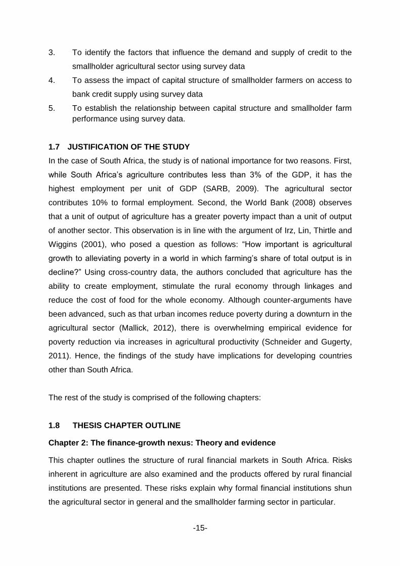
1.7 JUSTIFICATION OF THE STUDY

In the case of South Africa, the study is of national importance for two reasons. First,

while South Africa‟s agriculture contributes less than 3% of the GDP, it has the

highest employment per unit of GDP (SARB, 2009). The agricultural sector

contributes 10% to formal employment. Second, the World Bank (2008) observes

that a unit of output of agriculture has a greater poverty impact than a unit of output

of another sector. This observation is in line with the argument of Irz, Lin, Thirtle and

Wiggins (2001), who posed a question as follows: “How important is agricultural

growth to alleviating poverty in a world in which farming‟s share of total output is in

decline?” Using cross-country data, the authors concluded that agriculture has the

ability to create employment, stimulate the rural economy through linkages and

reduce the cost of food for the whole economy. Although counter-arguments have

been advanced, such as that urban incomes reduce poverty during a downturn in the

agricultural sector (Mallick, 2012), there is overwhelming empirical evidence for

poverty reduction via increases in agricultural productivity (Schneider and Gugerty,

2011). Hence, the findings of the study have implications for developing countries

other than South Africa.

The rest of the study is comprised of the following chapters:

1.8 THESIS CHAPTER OUTLINE

Chapter 2: The finance-growth nexus: Theory and evidence

This chapter outlines the structure of rural financial markets in South Africa. Risks

inherent in agriculture are also examined and the products offered by rural financial

institutions are presented. These risks explain why formal financial institutions shun

the agricultural sector in general and the smallholder farming sector in particular.

-16-

The theoretical underpinnings of the demand for and supply of credit are discussed

in this chapter. It elucidates, among other concepts related to the credit-granting

process, information asymmetry and adverse selection. The supply-leading and

demand-leading financial paradigms are also reviewed.

Chapter 3: Bank finance and agricultural growth: Empirical evidence

The chapter examines theoretical models for agricultural growth and the causal

relationship between increased doses of credit and agricultural output. It further

reviews the theory of agricultural growth and attempts to link it to available empirical

evidence. This is done by analysing the role of government and banks in smallholder

farmer development. A discussion is also included on management interventions

required for smallholder farmers. The study explored the available interventions

necessary to enhance the business management skills of smallholder famers.

Chapter 4: Methodological issues review

The research methods used in the study are discussed in this chapter. This includes

a review of research methodologies used in previous studies in order to determine

the methodology for this study.

Chapter 5: Research design and statistical methods

In this chapter, the empirical research design is articulated. The survey

methodological approach is discussed. The data, data-collection instruments and the

methods of analysis are elucidated in this chapter. The various descriptions of the

research design are outlined, giving the respective merits and demerits of each.

Chapter 6: Hypothesis testing and empirical results: Secondary data

This chapter outlines the results of the secondary data analysis. The long- and short-

run relationship between bank credit and agricultural output is discussed in detail.

Furthermore, the causal relationship between bank credit and agricultural output is

examined.

-17-

Chapter 7: Hypothesis testing and empirical results: Survey data

A discussion of how the survey data were analysed and interpreted is presented in

this chapter. The chapter begins with a presentation of the descriptive and inferential

statistics and multiple regression analysis and concludes with more robust SEM

techniques. The chapter demonstrates the contribution made by this study to the

body of knowledge by suggesting a modified model for agricultural production in

South Africa.

Chapter 8: Discussion of results, conclusion and recommendations

In this chapter, the results from the analysis of both secondary and primary data are

synthesised in order to get a clear understanding of the relationship between bank

credit and agricultural output. The conclusions of the study are presented in this

chapter. A discussion of the contribution made by this study is presented. The

chapter also includes recommendations for further research.

-18-

CHAPTER 2

THE FINANCE-GROWTH NEXUS: THEORY AND

EVIDENCE

2.1 INTRODUCTION

The aim of this chapter is to discuss theoretical and empirical literature on finance,

production and economic growth. It attempts to explain the factors of production in

general and then focuses on the empirical evidence of the impact of credit on output.

Over the past several years, the role of financial development in economic growth

has been a focus of attention and has attracted a large number of theoretical and

empirical studies to investigate the relationship between the two (e.g. Demirgüç-Kunt

& Malsimovic, 1998; Goldsmith, 1969; King and Levine, 1993; McKinnon, 1973;

Rajan and Zingales, 1998; Shaw, 1973). In addition to the growing body of literature

on the determinants of economic growth, this chapter attempts to explore the

following question: “Is finance a precondition for growth?” At a micro level,

particularly in developing countries, some researchers, such as Rioja and Valev

(2004), who studied low-income countries such as Cameroon, India, Philippines and

Sudan; Odhiambo (2007), who studied Tanzania; and Wolde-Rufael (2009), who

studied Kenya, argue that it is still not clear whether (1) finance plays a significant

role as a factor of economic growth, or (2) whether it is economic growth that

stimulates the growth of the financial sector. Accordingly, the finance-growth nexus

still remains an inconclusive empirical issue. This chapter reviews literature on this

debate.

2.2 FINANCIAL DEVELOPMENT AND ECONOMIC GROWTH: THEORETICAL

FRAMEWORK

It is generally accepted that financial markets and institutions channel savings of

surplus units to deficit units, and in so doing foster investment activities. As to

whether this function of financial markets and institutions can foster economic

growth, remains an unresolved empirical question. The first hint that financial

-19-

development can lead to economic growth was put forward by Schumpeter (1911),

who observed that the financial system can be used to channel resources into the

most productive use. However, a few decades later, Robinson (1952) argued that

financial development does not lead to economic growth, but rather follows it. In

other words, the demand for financial services increases as economies grow.

Economic theory predicts that finance promotes economic growth through four

different channels or mechanisms. First, intermediaries ameliorate the information

asymmetry problem (Blackburn, Bose and Capasso, 2005; Blackburn and Hung,

1998; Bose and Cothren, 1996; Diamond, 1984; Morales, 2003). Second, they

increase the efficiency of investments (Greenwood and Jovanovic, 1990). Third, they

enhance investment productivity (Saint-Paul, 1992) by providing liquidity, hence

allowing capital accumulation (Bencivenga and Smith, 1991). Fourth, they allow

human capital formation (De Gregorio and Kim, 2000).

Diamond (1984) emphasises the ability of financial intermediaries to monitor

investment projects cost-effectively, thereby increasing entrepreneurs‟ access to

funds. In the absence of financial intermediaries, monitoring costs would be too large

as to discourage credit to entrepreneurs. Bose and Cothren (1996) demonstrate that

this attribute of financial intermediaries promotes resources allocation that leads to

economic growth.

Through the design of incentive-compatible loan contracts and post-loan monitoring

activities, Blackburn and Hung (1998) demonstrate that financial intermediaries

contribute to economic growth by managing the moral hazard problem. Morales

(2003) observes that monitoring increases project productivity because

entrepreneurs are forced to ensure the success of their projects so that they are able

to pay back loans. There would be a loss of societal resources in the absence of

monitoring by intermediaries (Blackburn et al., 2005).

-20-

Bencivenga and Smith (1991) model the finance-growth nexus by looking at a

financial system dominated by intermediaries, where society owns either liquid or

illiquid assets. They observe that although liquid assets could be less productive

compared to illiquid assets, society prefers liquid assets in order to respond quickly

to emergencies. Financial intermediaries resolve this liquidity mismatch because

they attract deposits from a large number of depositors and create loans. These

loans are used to finance long-term investment projects while at the same time

allowing society access to liquid funds. It is this process that promotes capital

formation, leading to economic growth.

According to Saint-Paul (1992), when entrepreneurs utilise a productive, specialised

technology that poses more risk, they can diversify the risk through financial

markets. Greenwood and Jovanovic (1990) and later Greenwood and Smith (1997)

opined that financial intermediation promotes growth because it allows a higher rate

of return to be earned on capital, and growth in turn provides the means to

implement costly financial structures.

De Gregorio and Kim (2000) observe that financial intermediaries enhance human

capital formation by allowing individuals to access credit to finance their education,

which enables them to specialise in skills useful in economic development. Without

intermediaries, individuals would prefer low-skill jobs, because they cannot afford

tuition fees for high-skill education.

Notwithstanding general consensus on the role of finance in the economy, scholars

differ on the causes of financial development. Some believe the financial system is

exogenously developed by government (e.g. Bencivenga and Smith 1991), while

others believe that it is endogenously developed. Hence, there are disagreements on

the direction of causality between finance and economic growth.

There are at least four views in the literature regarding the relationship between

financial development and economic growth. The four views are that (1) financial

development causes economic growth (Adu, Marbuah and Mensah, 2013; Arestis,

-21-

Demetriades and Luintel, 2001; Dawson, 2008), (2) economic growth leads to

financial development (Blanco, 2009; Chakraborty, 2008; Lucas, 1988; Odhiambo,

2010), (3) economic growth and financial development are complimentary or

bidirectional (De la Fuente and Marín, 1996; Greenwood and Jovanovic, 1990; Khan,

2001; Saint-Paul, 1992) and (4) there is no causality running between economic

growth and financial development at all (Kar, Nazhoglu and Agir, 2011).

The first hypothesis, commonly known as „supply-leading‟, posits that financial

development is a necessary precondition for economic growth (see King and Levine,

1993; Levine and Zevros, 1998; Patrick, 1966; Wolde-Rufael, 2009:1142). Therefore,

following from this view, finance leads and causality flows from financial

development to economic growth. In other words, in the supply-leading

phenomenon, the financial sector precedes and induces real growth by channelling

scarce resources from small savers to large investors according to the relative rate

of return (Estrada, Park and Kamayandi, 2010:43; Odhiambo, 2010:208; Stammer,

1972:324; Yay & Oktayer, 2009:56). According to Patrick (1966:23), supply-leading

finance is “the creation of financial institutions and instruments in advance of

demand for them, in an effort to stimulate economic growth”.

The second hypothesis, referred to as the „demand-following‟ phenomenon, is that

financial development follows economic growth. In other words, economic growth

causes financial markets as well as credit markets to grow and develop. The term

„demand-following‟ refers to the creation of modern financial institutions, financial

assets and liabilities and related financial services in response to the demand for

these services by investors and savers in the real economy (Patrick, 1966:23). In this

case, financial development is seen as a consequence of economic development.

Contrary to the first view, in this case, the development of the real sector is

considered to be more important than the financial sector. According to the demand-

following view, lack of financial growth indicates low demand for financial services.

Using data for 74 economies over the period 1975–2005, Hartmann, Herwartz and

Walle (2012) found that economic growth promotes financial development but not

vice versa, ruling out the popular view that finance drives growth. Their finding is

robust even after grouping samples into different income groups.

-22-

In the third hypothesis, the causal relationship between financial development and

economic growth is bidirectional. Both financial development and economic

development are seen to Granger-cause each other. Saint-Paul (1992)

demonstrates that when innovation increases, so does the demand for financial

services, which in turn leads to financial development. De la Fuente and Marín

(1996) also make the same prediction that growth in the real sector increases

demand for financial services, which in turn raises the return on information-

processing activities by financial intermediaries, and eventually leads to growth of

the financial sector. Greenwood and Jovanovic (1990) observe that growth boosts

finance and finance accelerates growth. Khan (2001) observes that growth enhances

financial development by raising borrowers‟ collateralisable net worth and finance

promotes growth by increasing return on investment. Odeniran and Udeaja

(2010:91) tested the competing finance-growth nexus hypothesis using Granger

causality tests in a VAR framework over the period 1960–2009. Their empirical

results confirmed bidirectional causality between some of the proxies of financial

development and the economic growth variable. Specifically, they observed that in

Nigeria the measures of financial development Granger-cause output. At the same

time, net domestic credit was observed to be equally driven by growth in output, thus

indicating bidirectional causality. These results confirmed earlier studies by Acaravci,

Ozturk and Acaravci (2009:11), whose findings show that for the panels of 24 sub-

Saharan African countries, there is a bidirectional causal relationship between real

GDP per capita and the domestic credit provided by the banking sector.

The fourth hypothesis does not see a causal relationship between financial

development and economic growth. In other words, financial development and

economic growth each have factors peculiar to them that stimulate their growth.

There is scant empirical evidence supporting this hypothesis. For instance, Mihalca‟s

(2007:724) work in Romania showed that there is no relationship between financial

development and economic growth. One of the reasons could be that the weakness

of the financial development has encouraged the inefficient allocation of savings and

led to a negative growth in the real GDP (inverse relationship).

-23-

In a cross-country study, Kar et al. (2011) demonstrated that there is no clear

consensus on the direction of causality between finance and growth in the MENA

countries. The results of the causal relationship differed according to country-specific

characteristics. While in some MENA countries, finance was observed to cause

growth (also supported by Aghion, Howitt and Mayer-Foulkes, 2005), for example in

Israel and Morocco, none of the financial development indicators causes economic

growth in Algeria, Egypt, Iran and Sudan. The authors concluded that an increase in

income level leads to the supply of credit to the private sector, as the causality runs

from economic growth to financial development in 9 out of 15 countries.

These results imply that financial development responds positively to economic

growth. The authors failed to obtain convincing results supporting the view that

financial development is a significant determinant of economic growth in the MENA

countries. Various factors were observed to weaken the influence of financial

development on income growth. Typically, high information and transaction costs

hindered the development of the financial sector. In many MENA countries,

government intervention, particularly in state-owned banks with respect to loan

losses to poorly performing state enterprises, constrains the role of the financial

system in economic growth in these countries. The prevalence of Islamic banking,

which prohibits the charging of interest, may result in the private sector not borrowing

from conventional banks that levy interest. This may hinder financial development.

2.3 FINANCIAL DEVELOPMENT AND ECONOMIC GROWTH: EMPIRICAL

EVIDENCE

Empirical evidence shows that there is support for all the competing hypotheses and

that there is no consensus regarding the direction of causality between financial

development and economic growth (see for instance Ang, 2008; Apergis, Filippidis

and Economidou, 2007; Christopoulos and Tsionas, 2004; Demirgüç-Kunt and

Levine, 2008; Levine, 2005; Luintel, Khan and Theodoridis, 2008; Shan, 2005; Shan

and Jianhong, 2006).

2.3.1 The supply-leading hypothesis

According to Jalil and Ma (2008:68), economic growth is defined as the positive

change in the level of production of goods and services. McKinnon (1973), Shaw

-24-

(1973), Patrick (1966) and Fry (1973) argue that financial development leads to

economic growth. Specifically, Patrick (1966) postulates that the creation of financial

institutions in advance of demand for them should of necessity stimulate growth. In

this way, capital allocation becomes more efficient and incentives for growth are also

provided through the financial system. This view posits that there is a supply-leading

response between financial development and economic growth, and attaches

greater importance to the role played by financial sector development in economic

growth. King and Levine (1993) identified financial development as a precondition for

growth. They argue that higher levels of financial development are strongly

associated with future rates of capital accumulation and future improvements in the

efficiency with which economies employ capital.

To do this, first they examined the strength of the empirical relationship between

long-run real per capita GDP growth and four indicators of the level of financial

sector development. After controlling for initial conditions and other economic

indicators, they found a positive, significant and robust partial correlation between

the average annual rate of real per capita GDP growth and the average level of

financial sector development. Similar results were observed by Jalil and Ma

(2008:61) for China and Pakistan, who tested the hypothesis “financial development

leads to growth” using the deposit liability ratio and credit to private sector as the

indicators of financial growth.

Second, they examined the channels through which financial development and

growth are related. They observed a positive relationship between the rate of

physical capital accumulation and a measure of improvements in economic

efficiency. King and Levine (1993) identified and listed four indicators of financial

development and those of growth, as illustrated in Table 2.1. However, it is

noteworthy that the measurement of financial development constitutes an important

challenge to researchers in their efforts to assess the impact of financial

intermediation on real economic activity.

-25-

Table 2.1: Financial development and economic growth indicators

Indicators of financial development

Indicators of growth

Ratio of the size of the formal financial

intermediary sector to GDP

Real per capita GDP

The importance of banks relative to the

central bank

The rate of physical capital

accumulation

The percentage of credit allocated to private

firms

The ratio of domestic investment to

GDP

The ratio of credit issued to private firms to

GDP

A residual measure of improvements

in the efficiency of physical capital

allocation

(Source: King and Levine, 1993)

An earlier study in Nigeria by Afangideh (1996:80) classifies the indicators of

financial development used in empirical studies into three broad categories:

monetary aggregates, stock market indicators, and structural and institutional

indicators. In addition, Afangideh (1996) identifies the various channels through

which financial development is transmitted to the agricultural sub-sector of the

economy. Further, he investigated the effect of financial development on agricultural

sector investment and output using the three-stage least squares estimation

technique. The results show a positive relationship between financial development

and agricultural output.

Rioja and Valev (2004) examined the link between finance and the various sources

of growth. Specifically, they analysed how financial development affects the sources

of growth and whether the level of economic development matters. Using a large

panel data set of 74 countries for the period 1961–1995, they applied generalised

method of moments (GMM) dynamic panel techniques to deal with the possible

simultaneity of financial development and economic growth and to control for

country-specific effects. They concluded that the effect of finance on growth depends

on the level of economic development. In low-income countries, finance affects

economic growth largely through capital accumulation. In middle-income and

-26-

especially in high-income economies, financial development enhances productivity

growth. It also contributes to physical capital growth, although the effect is somewhat

smaller than in the low-income group. Thus the strong contribution of financial

development to productivity growth only occurs when a country has reached a

certain income level, roughly the middle-income group as defined by Rioja and Valev

(2004).

Stulz (2000:35) brings a different approach to the analysis of the supply-leading

hypothesis. He examined how a country‟s financial structure affects economic

growth through its impact on how corporations raise and manage funds. The

structure of a country‟s financial sector facilitates access to finance by firms from

financial institutions. With a poor financial structure, external financing is too

expensive, so that it is difficult for entrepreneurs to create firms and for these firms to

invest efficiently. Stulz (2000) concluded that financial structures that permit the

development of specialised capital by financial intermediaries are crucial to

economic growth.

2.3.2 Demand-driven hypothesis

Empirical studies that support the demand-driven phenomenon, that is, that

economic growth Granger-causes financial development, include studies by Lucas

(1988), Blanco (2009), Adamopoulos (2010) and Odhiambo (2009, 2010). Blanco

(2009) used a multivariate VAR model to show that in Latin America, economic

growth causes financial development, while rejecting the hypothesis that financial

development Granger-causes economic growth. The author argues that financial

development fails to influence growth, presumably because financial resources are

not being allocated to productive activities. When Calderón and Liu (2003) sought

answers to whether growth causes financial development, pooled data from 109

developing and industrial countries from 1960 to 1994 were used for the analysis.

Their findings were mixed. First, their results were in line with those of Blanco (2009)

to the extent that financial development Granger-causes economic growth,

suggesting that financial deepening in many countries results in a more prosperous

economy. However, after splitting their sample into 87 developing and 22 industrial

countries, they argued further that bidirectional causation also exists, implying that

-27-

financial deepening stimulates economic growth while economic growth propels

financial development.

Chakraborty (2008) demonstrated that economic growth Granger-causes financial

development in India for the period 1996–2005. The study took a three-dimensional

approach by analysing three empirical models. The first model examined the whole

economy. The second model related the growth of the industrial sector to financial

sector development. The final model examined the relationship between the growth

of the service sector to financial sector development. Economic growth was proxied

by the growth rate of GDP at factor cost. The sum of quarterly estimates of GDP for

mining and quarrying, manufacturing, electricity, gas and water supply and the

construction sectors was used to estimate industrial growth rate. To estimate service

sector growth rate, the author aggregated the quarterly estimates of GDP for the

trade, hotels, transport and communication, finance, insurance, real estate and

business services sectors. Financial development was proxied by both banking

sector and stock market development indicators. Thus banking sector development

was measured by total bank credit and financial depth was defined as the ratio of

liquid liabilities to GDP. Stock market development was defined as the total market

capitalisation. For all sectors, the author observed that causality runs from growth to

market capitalisation and not the other way round. For the industrial sector, it was

found that causality runs from the real rate of growth of the industry to market

capitalisation. For the service sector, it was established that causality runs from the

real rate of growth to market capitalisation. Chakraborty (2008) concluded that the

relationship runs from growth to financial development.

For South Africa, Odhiambo (2010) extended the investigation of the causal

relationship between financial development and economic growth by including a third

variable. After incorporating investment, and using the autoregressive distributed

lags (ARDL) bounds testing procedure, he observed that overall economic growth

has a substantial influence on the financial sector development. His results reveal a

unidirectional flow from economic growth to financial development via investment

(see Figure 2.1).

-28-

Figure 2.1: The growth-investment-finance nexus (Source: Author construction)

2.3.3 Bidirectional hypothesis

Shan and Jianhong (2006:197) examined the impact of financial development on

economic growth in China using a Vector Autoregression (VAR) approach. Their

results support the view in the literature that financial development and economic

growth exhibit a two-way causality and therefore do not support the finance-led

growth hypothesis. Wolde-Rufael (2009) re-examined the financial development-

economic growth nexus for Kenya for the period 1966–2005 using the Toda and

Yamamoto (1995) version of the Granger causality test. Conclusions drawn from this

study were consistent with those of Al-Yousif (2002:131), arguing that in three out of

the four proxies for financial development there is a bidirectional causality running

between each of the three proxies of financial development and economic growth.

However, a subsequent analysis using VAR conducted by Ozcan and Ari (2011) in

Turkey disproved the bidirectional hypothesis, instead arguing that according to the

Granger causality test, there is a unidirectional relationship between financial

development and economic growth. The direction of this relationship was found to be

from economic growth to financial development.

Blackburn and Hung (1998:109) use the basic model of growth in the form of the

increasing variety model, one which “lends itself naturally to the study of growth in

open economies”. In their analysis, the authors incorporated a discussion of the

extent to which international considerations influence the growth-financial

development nexus. The authors established (1) a positive, bidirectional relationship

between growth and financial development (also as in Carp, 2012; Marques, Fuinhas

and Marques, 2013) and (2) that between financial and trade liberalisation only the

latter has a positive influence on growth.

-29-

Enisan and Olufisayo (2009) examined seven sub-Saharan countries to determine

the relationship between the stock market and economic growth using the ARDL

bounds test. The sample countries included Cote D‟Ivoire, Egypt, Kenya, Morocco,

Nigeria, South Africa and Zimbabwe. Mixed results were obtained among the sample

countries. Egypt and South Africa showed a one-way causation flowing from stock

market development to economic growth. No sufficient evidence was found to reject

the null hypothesis of no cointegration between stock market development and

economic growth in Cote D‟Ivoire, Kenya, Morocco, Nigeria and Zimbabwe, implying

that in these countries, stock market development does not influence economic

growth. Enisan and Olufisayo (2009) did not test the reverse causal relationship from

economic growth to stock market development.

Demirgüç-Kunt, Feyen and Levine (2013) provide evidence of the relationship

between financial development and economic growth by decomposing financial

development into banking system and stock market. The behaviour of the two

markets is observed as the economy grows. The results show that banks and stock

markets metamorphosise during the process of economic development. As

economies grow, both banking system and financial markets become more

developed. However, it is argued that the association between economic activity and

banking sector development tends to decline. The relationship between economic

growth and stock markets tends to increase. The different relationships are attributed

to the fact that banks offer different services from those offered by securities

exchanges. As economies grow, services provided by stock markets become more

important.

2.3.4 Unidirectional hypothesis

Arguments for a unidirectional relationship between finance and growth include that

of Benhabib and Spiegel (2000). The authors examined whether financial

development affects growth solely through its contribution in „primitives‟ or factor

accumulation rates or whether it has a positive influence on total factor productivity.

The results showed that financial development has a positive correlation with both

rates of investment and total factor productivity growth. Similarly, Beck and Levine

-30-

(2004) analysed the link between stock market and bank development and economic

growth in a panel of 40 countries and 146 observations. The analysis focused on the

long-run relationship using annual panel data over a five-year period. The authors

argue that there is unidirectional causality flowing from financial development to

economic growth. This observation is in line with that of Bencivenga and Smith

(1991), Christopoulos and Tsionas (2004), Blackburn et al. (2005) and Cooray

(2010), who concluded that the development of financial intermediation increases

real growth rates.

Using data from 35 medium- to low-income developing countries, Cooray (2010)

suggested policy measures to increase the size, liquidity and activity of the stock

market to catalyse economic growth. Market capitalisation, market liquidity and the

turnover ratio were used as measures of stock market development. It is argued that

a well-developed stock market should promote growth by stimulating higher savings

and lowering transaction costs, which in turn improves efficient allocation of

resources.

Durham (2002) also analysed the long- and short-run effects of financial market

development proxied by stock market development on growth and investment in

lower-income countries. Using a sample of up to 64 countries for the period 1981–

1998, Durham observed that there is positive relationship between stock market

liberalisation and that it is greater in higher-income countries than in lower-income

countries. The author provides evidence that suggests that stock market

development has a more positive impact on growth for greater levels of per capita

GDP, lower levels of country credit risk and higher levels of legal development.

Christopoulos and Tsionas (2004) fail to support the view that there is a bidirectional

relationship between financial development and growth. For example, they argue

that using time series data may yield unreliable results due to short timespans of

typical data sets. Instead they conducted unit root tests and panel cointegration

analysis and concluded that there is fairly strong evidence in favour of the hypothesis

that long-run causality runs from financial development to growth (see also Kargbo

and Adamu, 2009). They also observe that the relationship is significant, and that

there is no evidence of bidirectional causality. More recently, Bittencourt (2012), who

-31-

investigated the effect of access to finance in stimulating economic growth in four

Latin American countries (1980–2007), confirmed Schumpeter‟s (1911) assertion

that finance enables an entrepreneur to invest in productive activities, and therefore

to promote economic growth. However, economic stability (low interest and inflation

rates) and conducive institutional framework (central bank independence and fiscal

responsibility laws) are seen to be a precondition for the positive influence of finance

on economic growth.

Rachdi and Mbarek (2011) found conflicting relationships between financial

development and economic growth, using a sample of ten countries – six from the

OECD region and four from the MENA countries. Using the ECM approach,

empirical results revealed that causality is bidirectional for the OECD countries and

unidirectional for the MENA countries, in other words, economic growth stimulates

financial development. Similar results were observed by Akinlo and Egbetunde

(2010:17) in Kenya, Chad, South Africa, Sierra Leone and Swaziland.

Although there is convergence on the unidirectional hypothesis, Ozcan and Ari

(2011) fail to confirm the direction of causality, rather suggesting the opposite,

namely that the direction of this relationship is from economic growth to financial

development. These conflicting results further complicate the inconclusive ongoing

debate.

What remain unresolved are the divergent views on the issue of causality between

financial intermediation and growth. The next chapter focuses on the role of finance

in stimulating growth in the agricultural sector.

-32-

CHAPTER 3

BANK FINANCE AND AGRICULTURAL GROWTH:

EMPIRICAL EVIDENCE

3.1 INTRODUCTION

In this chapter, literature on the finance-growth nexus in agriculture is explored. As

the capital structure of firms is dominated by debt and equity, the chapter presents

empirical literature on the impact of equity on the one hand and debt on the other

hand. However, as the aim of this study was to investigate the relationship between

credit and agricultural output, more emphasis was directed towards analysing this

relationship. This chapter also discusses non-financial factors of production, such as

land, climate, labour, technical efficiency and managerial skills, as some of the

factors that influence production in agriculture.

The chapter proceeds as follows. Sub-section 3.2 discusses the interface between

finance and growth in agricultural output. Sub-section 3.3 discusses credit as a factor

of production. Subsection 3.4 discusses non-financial factors that affect agricultural

production.

3.2 FINANCE AND GROWTH IN THE AGRICULTURAL SECTOR

In this section, the relationship between finance and agricultural growth is elucidated.

First, in Sub-section 3.2.1, a review of empirical evidence of the relationship between

capital structure and increase in agricultural production is presented. This is followed

by the demand for agricultural credit in Sub-section 3.2.2.

3.2.1 Capital structure theory and financing costs: an agricultural perspective

The impact of capital structure on firm performance has been widely documented in

the corporate finance literature. The aim of studies reviewed was to estimate an

optimal capital structure; see, for example, Modigliani and Miller (1958), Calvo and

Kumar (1994), Mahmud (2003), Miao (2005) and Leary (2009). In their seminal

-33-

paper, Modigliani and Miller (1958) demonstrated that in the world of perfect capital

markets, finance is irrelevant to investment decisions. However, such view is widely

disputed because the assumption of perfect capital markets cannot be maintained in

the real world (see Hubbard, 1998, for a survey), as market imperfections exist due

to information asymmetry and agency costs. Market imperfections create differences

in the cost of internal and external financing, making the former cheaper than the

latter. Therefore, firms are naturally inclined to use cheaper internal sources of

finance at the first instance to finance their investment. When internal sources are

not enough or exhausted, they resort to the costly external sources of finance. This

is consistent with the pecking order hypothesis of Myers and Majluf (1984).

Fazzari, Hubbard and Petersen (1988) developed a framework to measure the

extent of financing constraints faced by firms. This framework tries to measure the

sensitivity of firm investment to internal cash flow, whereby higher sensitivity is

interpreted as higher financial constraint and lower sensitivity is interpreted as lower

financial constraint. While it is the most widely used framework to measure financing

constraints, it is also highly contested and debated in the literature.

Available literature has covered the manufacturing and service sectors, but an

optimal capital structure remains elusive (Ahmadinia, Afrasiabishani and Hesami,

2012:4). For example, Nosa and Ose (2010:50) conducted an empirical investigation

of the link between debt and corporate performance in Nigeria. They concluded that

debt only is not sufficient to meet funding required for the growth and development of

corporations. Rather, corporations need to be adequately funded by both money and

capital markets, subject to a conducive legal environment for which government has

a responsibility.

To the knowledge of the researcher, there are few studies on the impact of debt or

credit on the performance of farm enterprises. For instance, Barry and Ellinger

(1988:45) observed debt to stimulate growth and vice versa. More recently, Zhengfei

and Lansik (2006:644) used data from Dutch arable farms and demonstrated that

debt has no effect on productivity growth. In Latvia, Bratka and Praulins (2009:144)

concluded that the relationship between debt and farm performance is positive. The

debt-to-asset ratio was observed to be growing as performance increased. Despite

-34-

the importance of lines of credit in the provision of liquidity in the economy, the

absence of data has resulted in limited empirical studies on the role of debt in

financing decisions in agriculture (see Sufi, 2009:1058).

Agricultural performance engrosses many production factors, of which agricultural

credit is one (Kumar et al., 2010:262). Farming requires finance to fund operations,

to acquire capital goods as well as to meet working capital requirements (Bernard,

2009); this has arguably been the largest challenge for farmers, but mostly

smallholder farmers, in South Africa. According to Mitchell et al. (2008:129), in their

study of the Wild Coast spatial development initiative (SDI) for small businesses in

tourism and agriculture, there was a dramatic fall-off in food production due to lack of

funding. They observed that fewer households had bank loans in 2004 than in 1997,

while more were taking loans from loan sharks than from banks. The Wild Coast SDI

is located in the Eastern Cape Province, the second poorest province in South

Africa.

Varghese (2005:318) reports that moneylenders are the most prevalent informal

lenders in India and in many developing countries because they have more

information than banks. He argues that some of the reasons why banks lend less to

farmers include high borrower-monitoring costs, lack of readily saleable collateral

and information constraints. Due to these problems, banks employ dynamic

incentives, for example not re-lending to defaulting borrowers. Those who default

may do so due to uncertain agricultural environments. Available empirical evidence

suggests that smallholder farmers have limited access to bank credit and that credit

is needed for meeting operational requirements (Chisasa and Makina, 2012;

Coetzee et al., 2002; Kirsten and Vink, 2003; Moyo, 2002; Olawale and Garwe,

2010). The link between credit and the performance of farmers is analysed in the

paragraphs that follow.

Examining the relationship between credit and agricultural output lends an

alternative dimension to further understanding the dynamics of capital structure

theory in farming. In his theory of money, Karl Marx identified three basic functions of

money (Lucarelli, 2010:201). First, money is conceived as a unit of account, and

-35-

functions as a measure of value-assigning prices. Marx‟s commodity theory of

money led him to assign gold as a measure of value. Second, money performs the

role as a means of circulation (in other words the modern bank note), which is issued

by private banks and ultimately regulated by the central bank through its reserves of

high-powered money. The third function can be described as the abstract

representation of value, or quite simply „money as money‟. In this perspective, Marx

distinguishes between three types of functions of money: (1) as a store of value (as a

store of value, money acquires intrinsic purchasing power), (2) as a means of

payment or deferred payment in the form of credit and (3) as world money

associated with the means of international payments and reserve assets. This study

focuses on the second function of money.

To understand whether or not credit has an implication for agricultural output, one

must first explore the reasons for credit demand. Previous studies have identified

factors (for example age of the farmer, interest rates, education, farm size and

inputs) that influence the demand for credit (see for example Byiers, Rand, Tarp and

Bentzen, 2010; Melitz and Pardue, 1973; Swain, 2007) and how credit affects output

via these factors (Boni and Zira, 2010; Khan and Hussain, 2011; Turvey, He and Ma,

2012). According to Singh, Kaur and Kingra (2009:313), farmers, in their bid to make

high capital investments to sustain high output rates and incomes for maintaining

their improved living and social standards, borrow from both formal and non-formal

institutional sources. This linkage is discussed in detail in the next section.

3.2.2 The demand for agricultural credit

Turvey et al. (2012:3) opine that understanding the demand for credit is a

prerequisite for setting either credit policies or a path for rural credit reform.

Therefore, the first step would be to enunciate what constitutes the demand for

credit. Byiers et al. (2010:50) point out that those factors that increase firm credit

constraints (in other words that reduce credit supply to a firm) also reduce its

demand for credit and vice versa. To this end, Oni, Amao and Ogbowa (2005), using

the probit model, showed that education, distance to the financial institution, income

of the farmer and use of fertilizer influence the demand for credit among farming

households. Khan and Hussain (2011:312) focused on the factors that affect the

-36-

ratio of formal and informal credit. They argue that this ratio is affected by a variety of

factors. These factors may be divided into demand and supply factors and include

the following:

Inadequate collateral value

The existence of interest rates (interest rates are prohibited in Islam)

Bribes in the formal sector

Distance to the source of credit

Expensive procedures in the informal sector

Education of the farmer

Land value

Experience in farming

Lag in disbursement of loans.

It is necessary at this stage to explain how these factors influence the demand for

credit by farmers. Briggeman, Towe and Morehart (2009:276) observed that the

impact of being credit-constrained significantly lowers production. Furthermore, most

farms and businesses that are credit-constrained tend to operate small-scale farms

or businesses.

3.2.2.1 Level of education of the farmer

Khan and Hussain (2011:312) and Kumar et al. (2010:262) pointed out that the

demand for formal sector loans is positively related to the education of the farmer.

They argue that the documentation involved in obtaining a loan from a formal

institution is convenient for educated farmers. Fatoki and Odeyemi (2010:1423), who

investigated the phenomenon in the context of South Africa, concur. For the less

educated there are challenges that have to be dealt with, such as the problem of

calculation, estimation and valuation of assets, loans and returns. Less educated

farmers usually have less information about available credit schemes and sometimes

the varieties of inputs (which give the highest yields). Khan and Hussain (2011)

argue further that loan officials from the formal sector portray a bad attitude, as they

do not want to serve these illiterate and poor farmers. This usually leads to these

borrowers opting to approach informal lenders, who are characterised by less

strenuous procedures and requirements for loans.

-37-

3.2.2.2 Farm size

The size of the farm plays a significant part in the formal loan-decision process, as it

provides much-needed collateral. In Pakistan, Akram, Hussain, Sial and Hussain

(2008:5) observed that the demand for credit was minimised by unacceptable or

inadequate collateral; land was the most readily acceptable form of collateral and

this prevented a large number of tenants and landless people from participating in

the formal credit markets. Approximately 77% of farmers used agricultural land as

collateral because it was the most acceptable form of collateral by all institutional

lenders. Hussain and Khan (2011) concluded that by increasing the size of the farm

from small-scale to large-scale, the demand for formal credit is enhanced. Similarly,

Byiers et al. (2010:50) used industrial firm surveys to identify the key determinants of

credit demand in Mozambique and commented as follows:

In the case of firm size, this is sensible both from a borrower and a lender point of

view. Small size is related with relatively high transaction costs for holding debt and

lenders have higher monitoring costs. However, this may not be socially optimal

assuming returns to small firm investment is on par with returns in larger firms.

Byiers et al. (2010) concluded that firm size is an important factor for financial

constraints and access to credit. Firm size emerged to be a critically important

determinant of the demand for credit. Bigsten et al. (2003:119) also found that

demand for credit is strongly related to size. However, they fail to reject the

hypothesis that this is related to the heterogeneity of the firms rather than their size.

In the agricultural context, empirical evidence suggests that land is the only collateral

acceptable to institutional sources of credit. Thus, subsistence farmers are left out of

the credit programmes (Akram et al. 2008:302). It is worth noting that in agriculture,

land quality and the size of the operational area are factors that affect the productive

capacity of the farm and imply an increase in the income generated (Swain, 2007:

2691). Although it seems that these factors affect creditworthiness positively, Swain

argues that many formal and some informal lenders make their judgement of the

creditworthiness of households primarily on the basis of the amount of land they

own. This is supported by the fact that the quality of land and the proportion of

irrigated area are statistically insignificant. In this regard, Yaslioglu, Aslan, Kirmikil,

Gundogdu and Arici (2009:327) argued and concluded that in Turkey, the scattered,

-38-

fragmented plots in agricultural areas are one of the major problems preventing

agricultural efficiency. Such inefficiency may also constrain smallholder farmers from

accessing both short- and long-term credit needed for financing working capital and

fixed improvements on the farm and machinery.

3.2.2.3 Distance to the bank

An inverse relationship is observed to exist between the distance to the bank and the

demand for institutional credit. Akram et al. (2008: 300) found the average distance

between rural communities and the bank to be more than 20 km, a clear indication of

backwardness and poverty. Such kind of spatial distribution of branches of formal

credit institutions tends to dampen the demand for credit. However, Swain

(2007:2691) differs and argues that the creditworthiness of the household in the eyes

of the lender is not affected by how far or how near he or she lives. Swain

acknowledges that distance affects the transaction cost of the borrower or the lender

(which is logical).

3.2.2.4 Time lag in disbursement of loan

Once an application for credit has been lodged with the bank, the time taken to

access the loan is very important to the farmer. Akram et al. (2011:312) argues that

the slow processing of loan applications or delayed disbursement not only delays the

sowing and growth of crops, but also raises the cost. On the other hand, timely

disbursement of credit therefore not only helps to reduce cost of credit, but also

enhances returns from agriculture. The speed with which applications are processed

shows that the bank has simplified processes and is efficient.

3.2.2.5 Transaction costs

A farmer is transaction cost-constrained if the non-interest monetary and time costs

associated with application for and administration of loans are sufficiently large that

they lead a farmer to refrain from borrowing (Fletschner, Guirkinger and Boucher,

2010:983). However, it is argued that the most important decision criterion for

borrowing is the interest rate on the loan (Akram et al., 2008: 309). Kshirsagar and

Shah (2005:5) and Khan and Hussain (2011:313) showed that the higher cost of

credit negatively affects the demand for credit from formal financial institutions. This

is particularly so for landless smallholder farmers. They opine that borrowers feel

-39-

less comfortable with informal lending sources due to their high interest rate. On the

other hand, the formal sector loaning agencies charge lower interest rates, but the

total cost may be higher due to the number of visits, bribes and expenditures on

documentation. For instance, in Punjab State of India, Singh et al. (2009:312) found

that on average, approximately 14 trips were made per borrower to get a loan from

commercial banks. Overall, the loan approval took 33 weeks in Punjab State (Patil,

2008:48), which was too long, and therefore borrowers could not rely on this source

of financing. According to Patil (2008:48), “the institutions offer poor quality service

through inadequately manned branches under a mandatory rural branch posting

policy with a short-term stay, which gives little time to the staff to develop knowledge

about the area and the people”. Singh et al. (2009:313) further analysed the cost of

obtaining credit and concluded that in spite of significant increases in institutional

lending, the malpractices prevailing in the system make the borrowing more

cumbersome and costly to the farmer. Therefore, farmers end up resorting to

informal lenders such as cooperatives to get loans (see for instance Ortmann and

King, 2007:219, in South Africa).

The disparities in formal and non-formal institutions in the supply of credit to

agriculture remain cause for concern and require policy intervention. Demand for

credit from formal institutions would increase if household farmer preferences, as

suggested by Singh et al. (2009:315), are given attention (see Table 3.1).

-40-

Table 3.1: Reasons for preference of non-institutional loans

Percentage of respondent farmers (multiple responses)

Farm size

Reason for preference Marginal Small Semi-

medium

Medium Overall

Easy to avail 42.5 46.1 64.7 50.0 51.4

No formality needed 17.2 19.1 18.4 32.9 20.8

No surety and security

needed

14.9 18.3 12.5 17.1 14.1

Low credit limit in

commercial banks

0.0 4.3 5.9 15.8 7.2

No transaction costs 0.0 3.5 8.8 17.1 6.3

No bribe/commission to any

official

2.3 4.4 7.4 9.2 6.3

(Source: Singh et al., 2009:315)

To support this demand, Nwosu, Oguoma, Ben-Chendo and Henri-Ukoha (2010:87)

suggest that because credit is needed for enhanced productivity and agricultural

development (see also Feder, Lau, Lin and Luo, 1990:1151), the government of

Nigeria should give the idea of the credit guarantee scheme support and publicise

the scheme to the beneficiary farmers (particularly small farmers). According to

Nwosu et al. (2010:89), this would help address the poor output of farmers. Similarly,

Kohansal, Ghorbain and Mansoori (2008) recommended that attention should be

given to the revision of policies that influence investment in order to increase output

while at the same time decreasing poverty in the agricultural sector in Iran. In

particular, farm land, number of credit repayment instalments and previous

investment were found to be the most important factors influencing the investment

behaviour of farmers. An increase in these variables by one unit was observed to

positively affect investment. Kohansal et al. (2008:4457) further argue that land

ownership indicates the farmer‟s ability to offer collateral when accessing more credit

for agricultural investment; longer repayment periods offer the farmer an opportunity

to invest in agricultural projects with longer payback periods. Finally, the positive

effect of previous investment on agricultural production demonstrates the farmer‟s

experience in this field, which may facilitate new investment decisions.

-41-

Afangideh (2009:74), using the simulation approach and data from 1970 to 2005

from Nigeria, observed that bank lending has a positive and significant effect on real

gross national saving and real agricultural output. He presents his findings in his

model of agricultural output, which states that “agricultural output should necessarily

be the outcome of economic activity, financial development, credit to the sector and

environmental influence like rainfall in Nigeria”. This model carries some degree of

logic and reasonableness, because there is an independent relationship among the

variables of the model. Supporting this view, Guirkinger and Boucher (2008:295)

concluded that credit constraints lower the value of agricultural output. Similarly,

Olaitan (2006:9) argues that lack of access to economic resources, especially

finance, by both farmers and small to medium enterprises (SMEs) across Nigeria,

continues to retard economic growth. He suggests that there is a need for a critical

examination and the adoption of an approach to avoid declaring smallholder farmers

and SMEs as „endangered species‟.

In a study of Indian agriculture, Sriram (2007:245) argues that “the causality of

agricultural output with increased doses of credit cannot be clearly established”. This

view seems to suggest that the availability of credit to smallholder farmers will not

necessarily result in increased output. This argument confirms earlier findings by

Binswanger and Khandker (1992:39) that the effect of credit to agriculture on output

was not significant. Rather, a strong effect was on increased fertiliser use and private

investment in machines and livestock.

The success story reported by Gow, Shanoyan, Abrahamyan and Alesksandryan

(2006:2) of smallholder farmers in Armenia provides evidence that access to formal

credit does not hold the key to growth in agricultural productivity. The land

redistribution process was not supported by foreign direct investment and therefore

meant that over 300 000 inexperienced, financially distressed subsistence farmers,

operating extremely fragmented plots, relied on a quasi-public third party, the United

States Department of Agriculture Market Assistance Program and agricultural credit

clubs for finance. Ngepah (2009:2), in a comparative study of commercial and small-

scale farmers‟ productivity, found that inequality (in land redistribution) is associated

with slower agricultural productivity. However, land redistribution slightly improves

-42-

productivity (Ngepah, 2010:353). He further suggests the need to strengthen the

human capital (particularly education) of small-scale producers. Ngepah (2010) is

however silent on the importance or lack of finance in general and credit in particular

in enhancing output.

The rate at which the world population is expanding and lessons learnt from the

2008 global financial crisis make it important for research to be conducted on how

farmers can access more bank credit in order to boost productivity. Poor people

spend 50 to 70% of their income on food and have little capacity to adapt as prices

rise and wages for unskilled labour fail to adjust accordingly (Von Braun, 2008:5). In

2007, more than 2 000 farmers in northern Nigeria, with the financial support from

the United States Agency for International Development (USAID), the Gatsby

Foundation and the UK Department for International Development (DFID), recorded

an increase of over 300% in productivity, enhanced income generation and improved

livelihoods of farm families (Singh and Ajeigbe, 2007:158). Although USAID, the

Gatsby Foundation and the DFID are not credit-granting institutions, these results

suggest that smallholder farmers need external financial injections for them to

increase output. Empirical results of Zhengfei and Lansik (2006:654) showed that

long-term debt increases productivity growth. They argue that the fact that family

farms provide a livelihood for the whole family and the full liability associated with the

legal form of proprietorship presumably changes the risk perceptions of the farmer.

This change increases the disciplinary effect of debt. Similarly, Moghaddam

(2010:958) re-examined the efficacy of the M1, M2 and M2 Monetary Service

(Divisia) Index (DM2) for the USA in conjunction with labour and capital in the Cobb-

Douglas production function employing cointegration methodology. The results

confirmed money as a significant input in the cointegrated space encompassing

labour and capital. In addition, the results also demonstrated that the relation

between real output and the most efficient definition of money (cyber cash) may be

stronger than that explained by the traditional paper money (M2). By extension,

Moghaddam (2010) concluded that the cyber cash system enhances production

efficiency even further by making market transactions virtually timeless in a

competitive money market.

-43-

Contributions to the ongoing debate on the impact of bank credit on agricultural

output in the context of South African smallholder farmers have been made by Moyo

(2002), Wynne and Lyne (2003) and Lahiff and Cousins (2005). Wyne and Lyne

(2003:575) concluded that the majority of small-scale commercial poultry producers

in KwaZulu-Natal have significantly lower enterprise growth rates than larger poultry

producers. The lower growth rate of the small-scale commercial poultry producers is

attributable to poor access to credit, high transaction costs and unreliable markets.

This view is shared by Moyo (2002:189), who posits that if small-scale farmers do

not have sufficient capital, they need access to credit.

While credit has arguably been identified as a determinant of the level of smallholder

farm output (for example Kumar et al., 2010:262), technical efficiency and land,

among other factors, have been identified as significant explanatory variables for

agricultural output. In South Africa, studies conducted thus far have not been

exhaustive in explaining the contribution of bank credit to smallholder farm output.

Results of a study of poultry farmers in the KwaZulu-Natal province of South Africa

by Wynne and Lyne (2003:1) confirm those of an earlier study by Kalinda et al.

(1998:598), namely that agricultural credit is recognised as one of the means by

which small-scale farmers can increase their capital base. They argue that

government‟s dominance as a major credit source is largely a reflection of the

reluctance of private financial institutions to invest in rural markets and agricultural

production. In a study conducted by the Central Bank of Nigeria (1976), shortage of

primary production credit was identified as one of the major causes of declining

agricultural production. This shortage was attributed to reluctance by the banks to

provide for real sector activities, especially agricultural production. The reasons

were, inter alia, the following:

Inherent risks associated with agricultural production (so-called agriculture

production risk)

Urban-/semi-urban-based nature of operations of banks

High cost of administration of agricultural loans

Inability of farmers to provide the necessary collateral.

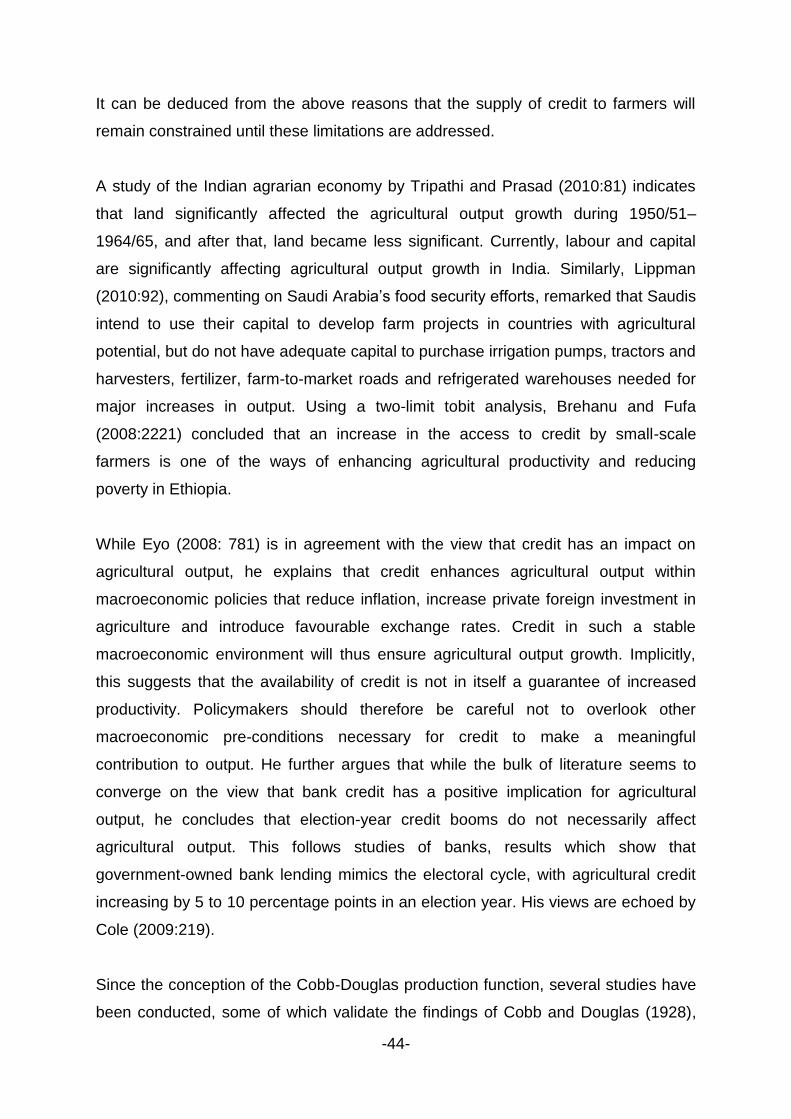
-44-

It can be deduced from the above reasons that the supply of credit to farmers will

remain constrained until these limitations are addressed.

A study of the Indian agrarian economy by Tripathi and Prasad (2010:81) indicates

that land significantly affected the agricultural output growth during 1950/51–

1964/65, and after that, land became less significant. Currently, labour and capital

are significantly affecting agricultural output growth in India. Similarly, Lippman

(2010:92), commenting on Saudi Arabia‟s food security efforts, remarked that Saudis

intend to use their capital to develop farm projects in countries with agricultural

potential, but do not have adequate capital to purchase irrigation pumps, tractors and

harvesters, fertilizer, farm-to-market roads and refrigerated warehouses needed for

major increases in output. Using a two-limit tobit analysis, Brehanu and Fufa

(2008:2221) concluded that an increase in the access to credit by small-scale

farmers is one of the ways of enhancing agricultural productivity and reducing

poverty in Ethiopia.

While Eyo (2008: 781) is in agreement with the view that credit has an impact on

agricultural output, he explains that credit enhances agricultural output within

macroeconomic policies that reduce inflation, increase private foreign investment in

agriculture and introduce favourable exchange rates. Credit in such a stable

macroeconomic environment will thus ensure agricultural output growth. Implicitly,

this suggests that the availability of credit is not in itself a guarantee of increased

productivity. Policymakers should therefore be careful not to overlook other

macroeconomic pre-conditions necessary for credit to make a meaningful

contribution to output. He further argues that while the bulk of literature seems to

converge on the view that bank credit has a positive implication for agricultural

output, he concludes that election-year credit booms do not necessarily affect

agricultural output. This follows studies of banks, results which show that

government-owned bank lending mimics the electoral cycle, with agricultural credit

increasing by 5 to 10 percentage points in an election year. His views are echoed by

Cole (2009:219).

Since the conception of the Cobb-Douglas production function, several studies have

been conducted, some of which validate the findings of Cobb and Douglas (1928),

-45-

while others challenge this model. For example, using the switching regression

model with an endogenous criterion function, Feder et al. (1990:1154) examined the

relationship between credit and productivity in Chinese agriculture. The analysis was

conducted using cross-sectional household-level survey data from a study area in

north-east China. It was observed that based on the estimated coefficients, if every

credit-constrained household in the sample is given additional credit of 17.82 Yuan

(equal to 1% of the average level of liquidity of the credit-constrained households),

the total output of these households may be projected to increase by 201.8 Yuan, or

approximately 0.04% of the total output. Thus, on average, one additional Yuan of

liquidity (credit) would yield 201.08/(17.82 x 48) = 0.235 Yuan of gross value of

output. Feder et al. (1990:1156) concluded that two important factors should be

considered when evaluating the likely impact of agricultural credit expansion. First,

not all farmers are constrained in their farming operations by inadequate credit.

Second, expanded supplies of formal credit will be diverted in part to consumption.

Thus, the likely output effect will be smaller than that which is expected when all

funds are assumed to be used productively.

3.3 CREDIT AS A FACTOR OF PRODUCTION

The use of credit as an independent variable in the agricultural production function in

empirical studies has been challenged (see for example Driscoll, 2004:469 and

Nkurunziza, 2010:489). However, Sial et al. (2011:128) posit that improved seeds

and other inputs such as tractors, fertilizer and biocides that may be purchased using

credit money play an important role in agricultural production and that these can be

directly influenced by the availability of credit.

The inclusion of credit as an explanatory variable in the production function is usually

challenged on the grounds that it does not affect the output directly; rather it has an

indirect effect on output through easing the financial constraints of the producers in

purchasing inputs (Carter, 1989). Carter (1989:19) argues that credit affects

production in the agricultural sector in three ways. First, it encourages efficient

resource allocation by overcoming constraints to purchase inputs and use them

optimally – “this sort of effect would shift the farmer along a given production surface

to a more intensive and more remunerative input combination” (Carter, 1989:19).

-46-

Secondly, if the credit is used to buy a new package of technology, say high-yielding

seed and other unaffordable expensive inputs, it would help farmers to move not

only closer to the production frontier, but also to shift the entire input-output surface.

In this regard it embodies technological change and a tendency to increase the

technical efficiency of the farmers. Finally, credit can also increase the use intensity

of fixed inputs such as land (Kumar, Turvey & Kropp, 2013:15), family labour and

management, persuaded by the „nutrition-productivity link of credit‟ that raises family

consumption and productivity. Carter‟s (1989) reasoning implies that agricultural

credit not only improves management efficiency, but also affects the resource

allocation and profitability.

Gosa and Feher (2010) analysed financial resource implications for agriculture

performance in Romania, taking into account both bank and trade credit. First, direct

bank credit to agriculture was observed to be low, paving the way for the

development of trade credit (supplier‟s credit). Trade credit is a financing alternative

agreed, in case of need, by input beneficiaries (farmers) as well as suppliers.

Second, although trade credit was found to be more expensive than bank credit, it

was seen to be more operative and thus more appealing. It can be inferred from this

analysis that not only is credit required to enhance farmer profitability, as was later

concluded by Gosa and Feher (2010:7), but that the turnaround time for accessing

the credit was also found to be key.

Obilor (2013:91) observed that commercial banks‟ credit to the agricultural sector for

the period 1984–2007 had no significant positive impact on productivity in Nigeria.

However, the researcher noted that the agricultural credit guarantee scheme loan by

purpose led to a significant positive growth in agricultural productivity in Nigeria.

Thus, while generally concurring that credit is a necessary factor in the agricultural

production function, Obilor (2013) emphasises the provision of credit guarantees by

government to lenders. The credit guarantee scheme indirectly acts as security for

the repayment of bank loans advanced to the agricultural sector where loan

repayment may be jeopardised by the risky nature of agricultural production. These

results confirmed those of an earlier study by Ammani (2012) in Nigeria.

-47-

The strategic role of financial credit in accelerating agricultural production in Nigeria

was also analysed by Sogo-Temi and Olubiyo (2004). In general, it was observed

that one of the most important determinants of growth in agricultural output is the

availability of productive credit. However, it was opined that the insignificance of the

parameter estimates could be attributed to diversion of bank credit to non-productive

ventures such as marriage, funeral ceremonies and other social functions. Despite

this setback, several empirical studies concur that credit is an important instrument

that enables farmers to acquire command over the use of working capital, fixed

capital and consumption goods (Sial et al., 2011:7; Siddiqi and Baluch, 2004:161;

Simsir, 2012:362). As agriculture is a multi-product industry, Saleem and Jan

(2011:3) used agricultural gross domestic product (AGDP) as the dependent variable

and agricultural production was assumed to be the function of credit disbursed by

different financial institutions for irrigation purposes, seeds, fertilisers, pesticides,

implementation of tractors and other purposes. Over 80% of the AGDP was

observed to be attributable to total credit supplied.

While supporting the hypothesis that institutional credit has a positive impact on

productivity in agriculture in India, Sidhu et al. (2008:407) argue against the uniform

supply of credit across all regions. Rather, they suggest that region-specific credit

demand patterns must be assessed first, depending on crop patterns and current

inputs and capital requirements in relation to the targeted output growth rate.

Afterwards, a policy framework should be put in place to meet those requirements,

instead of increasing the credit supply uniformly across the regions of the country.

Subsequently, Kumar et al. (2010:259) reported that regional disparities in the

distribution of institutional credit in India seem to have declined over time from 122%

in 2000–2001 to 81% in 2007–2008. However, 81% still remains a significant level,

which demonstrates that the regional disparities in institutional credit flow do exist

and still characterise the rural credit system.

3.4 NON-FINANCIAL FACTORS THAT AFFECT AGRICULTURAL OUTPUT

Turning to nonfinancial factors that influence the level of agricultural output, this

section discusses climate, land, labour and technical efficiency as some of the

factors that influence farm output. These are considered in the following sub-

sections.

-48-

3.4.1 Climate

Erratic rainfall is an inherent characteristic of semi-arid, sub-humid, tropical agro-

ecosystems, limiting landscape productivity (Barron, Enfors, Cambridge and

Moustapha, 2010:543). Farmers have to contend not only with market risks, but also

with environmental factors such as weather (DBSA, 2011). During drought periods,

crops wither before maturity. In times of excess rains, which normally result in floods

and water logging, the yields are poor. According to Rouault and Richard (2003:489),

the eight most severe droughts in the history of South Africa since 1921 occurred in

1926, 1933, 1945, 1949, 1952, 1970, 1982 and 1983 (see also Blignaut,

Ueckermann and Aronson, 2009:61). The total number of wet and dry districts per

decade seems to have increased since the 1960s. Faures, Bernardi and Gommes

(2010:529) argue that harvested area may depend on direct weather factors, for

instance when drought wipes out the crops from a farm, resulting in the harvested

area being smaller than the planted area. On the other hand, yield is very much the

result of the overall health of the plants, which is affected in more or less subtle and

direct ways by weather, starting with sunshine, the driver of photosynthesis, and

water availability from rainfall and irrigation, which defines to which extent plants can

actually make use of available solar energy. In most places, water availability is the

factor that most directly conditions crop yields, and in the areas where water is

plenty, the main limiting factor usually becomes sunshine. Consequently, rainfall can

either have a positive or a negative impact on farm output. For instance, droughts

and too much rain could have a negative impact, while moderate rain could have a

positive impact.

South Africa is characterised by a semi-arid climate. To supplement its water

requirements for agricultural use, irrigation schemes have been set up. Fanadzo et

al. (2010:3516) outlined the history of irrigation schemes in South Africa, focusing on

smallholder irrigation schemes. The development of irrigation schemes started

during the time of the Cape Colony and went through several eras, described as

follows:

The peasant and mission diversion scheme era – occurred in the 19th century in

the Cape Colony. This era was associated with mission activity and the

emergence of African peasantry in the Eastern Cape. The type of irrigation was

mainly river diversion.

-49-

The smallholder canal scheme era – lasted from about 1930 to 1960. The

schemes were primarily aimed at providing African families residing in the

„native or Bantu areas‟ with a full livelihood based on farming. Typically, these

irrigation schemes obtained water from a river by means of a concrete weir, but

schemes using a storage tank were also built.

The homeland era – lasted from about 1960 until about 1990. Irrigation

development during this era was characterised by modernisation, functional

diversification and the centralisation of scheme management (Van Averbeke,

2008, cited in Fanadzo et al., 2010:3517).

The irrigation management transfer and revitalisation era – this is the most

recent and current smallholder irrigation system in South Africa. The

management of the irrigation system was transferred from government to the

farmers. Since then, government withdrew and water user associations were

formed. Similar arrangements are also found in Nigeria; see for instance

Olubode-Awosola, Idowu and Van Schalkwyk (2006:305).

The above discussion demonstrates the importance of rainfall or water as a factor of

production (see also Harris-White, 2008:549–561 and Nair, 2008:61). According to

Nair, “water resources management has been an issue in many African countries

including ineffective functioning of institutions. In addition, the neglect of research

and development and its funding has hindered the growth of the agricultural sector.”

Olubode-Awosola et al. (2006:309) raised interesting findings regarding the

performance of irrigation projects under the Ogun-Oshun River Basin and Rural

Development Authority (O-ORBRDA) in Nigeria. A total of 95.5 and 123 hectares of

irrigated and rain-fed plots respectively were under the care of O-ORBRDA. Several

factors were linked to the low demand for irrigation services. Approximately 55% of

farmers were reported not to be enthusiastic about irrigation services because of

lack of credit facilities, while the rest considered the irrigation charges to be too high.

Other contributory factors to the low demand for irrigation were observed to be

irregular supply of fuel, electricity, deterioration of physical structures, the

dilapidation of canals and worn-out pump stations. What is clear from these findings

is that agricultural output is a function of the availability of water (whether rain-fed or

irrigation) and that farmers who are incapacitated by liquidity constraints are unable

to pay for services necessary for them to maximise production.

-50-

Speranza (2010:629) analysed the impact of the 1999/2000 drought in Kenya. He

observed that drought adversely affected livestock holdings mainly through sales

(76%) and deaths (52%). Livestock holdings generally declined as a result of the

drought. Notable reductions were observed in cattle, goat and poultry holdings.

Unpredictable weather patterns and persistent climate change continue to pose

productivity challenges to agriculture. In South Africa, semi-arid regions such as the

Free State province are characterised by dry weather spells (De Jagger, Potgieter

and Van den Berg, 1998:352), which disadvantage farming activities. To assist

maize producers and other stakeholders in the Free State, a framework for

assessing drought situations has been established. However, such a framework

faces the challenge of defining drought. For example, McKee, Doesken and Kleist

(1993:1) noted that the definition of drought has been a stumbling block for drought

monitoring and analysis. Dozens of drought definitions were reviewed, out of which

six overall categories were identified: meteorological, climatological, atmospheric,

agricultural, hydrologic and water management. What was observed to be common

to all types of drought is that drought is a condition of insufficient moisture caused by

a deficit in precipitation over some time period as well as the impact thereof. It can

be concluded from this discussion, as was observed by Westerberg et al. (2010:314)

in Tanzania, that farmers need to take into account the effect of climate and climate

change in modelling agricultural production.

3.4.2 Land

Land is one of the key factors of production across sectors, including agriculture

(Jaffe and Zeller, 2010:531; Lipmann, 2010:90; McMichael, 2009:235). Historically,

black farming in South Africa has not been supported, while white farming has been

given preferential support through government subsidies and legislation. This

created a highly dualistic agricultural sector, with black farmers cultivating small

pieces of land (Palmer and Sender, 2006:349; Rother, Hall and London, 2008:399)

with insufficient investment or institutional support (Oettle et al., 1998:6).

Complementary to farmer efforts, government needs to formulate policy that makes it

possible for farmers to acquire land to cultivate. As a result, land reform has been a

topical subject around the world (Deininger, Jin and Nagarajan, 2007:16). According

to Udoh (2011:290), restrictive laws pertaining to land use need to be amended to

-51-

make more land available for large-scale agriculture. For example, the historical

imbalances in South Africa require an intervention that will see the transfer of some

amount of land to the previously disadvantaged farmers who operate on very small

farms.

As reported by Graham and Darroch (2001:295), land reform in South Africa took a

two-pronged approach, namely government-assisted land acquisition and land

acquired through private transactions. Households in government-assisted projects

had less tenure security than households that acquired land through private

transactions. Using panel household data from India, together with state-level

variation in the implementation of land reform, Deininger et al. (2007:17) found land

reform to have a positive impact on the accumulation of assets in the form of

physical as well as human capital. It was also observed that land reform leads to

economic growth. Furthermore, Guirkinger and Boucher (2008:36) found that a

positive land reform policy is required as a precondition for alleviating credit

constraints. For instance, the first stage of most financial liberalisation programmes

in Latin America was accompanied by the liberalisation of agricultural land markets

in the form of land titling programmes, investment in land registry institutions and the

elimination of legal impediments for the transfer of land. By instituting these reforms,

credit rationing is reduced as a result of the use of land as collateral.

Mahabile, Lyne and Panin (2005) in Botswana also observed a strong relationship

between farm size and access to credit, arguing that farmers with secure land tenure

(private farms) and larger herds of livestock use more agricultural credit than those

relying on communal grazing land to raise cattle. Investments in fixed improvements

to land and herd productivity were found to be positively related to secure land

tenure via higher levels of liquidity from long-term credit.

Although collateral does not provide a guarantee for accessing credit, it improves the

chances of access. While owning land should help alleviate the credit constraint

(Hertz, 2009:76), where markets for farmland are thin or missing, as they are in

many countries with a socialist background, land is of limited value as collateral. The

size of the land is also an important attribute to be considered (MacLeod, MacDonald

& Van Oudtshoorn, 2008:76). Progress has been made in addressing the land

-52-

problem in South Africa. However, one of the constraints to maximising productivity

is farm size. According to MacLeod et al. (2008:76), many of these farmers will not

be viable due to limited farm size.

3.4.3 The role of government

The role of government in economic management is performed through the

formulation and implementation of economic policy in general and fiscal policy in

particular (Udoh, 2011:285). As recognised by the new growth theory, public

spending is an important factor for self-sustaining productivity gains and long-term

growth. Udoh (2011) argues that government expenditure can contribute to

agricultural growth (and hence poverty alleviation). In South Africa, one way

government can enhance growth in the agricultural sector is by facilitating land

redistribution. Since attaining democracy in 1994, the government of South Africa

has supported farmers through the creation of a land reform process that guaranteed

and increased ownership of land for production (Vink, Tregurtha and Kirsten, 2002).

According to Ngepah (2009:22), there are positive effects of land redistribution

between those with small farms and those with large farms. The effects are

described as negative for large-scale farms and positive for small-scale farms. Prior

to democracy, the government of South Africa assisted farmers through debt

consolidation subsidies (R344 million), crop production loans (R470 million) and

drought relief (R120 million) and acted as a guarantor of consolidated debt of R900

million in the eighties and early nineties (Kirsten and Vink, 2003).

3.4.4 Labour

Labour is an integral variable in the agricultural production function. Various

definitions of labour have been put forward. For example, Baumol and Blinder

(2006:486) define labour input in the production function as the number of hours

worked. Holding other factors constant, output rises as labour inputs increase. For a

given level of technology, Figure 3.1 shows how output (measured by real GDP on

the vertical axis) depends on labour input (measured by hours of work on the

horizontal axis). If a country‟s labour force can supply L0 hours of work when it is fully

employed, then the potential GDP is Y0 (see Point A). If the technology improves, the

production function will shift upward, say to the curve OM, meaning that the same

-53-

amount of labour input will now produce more output. Graphically, potential GDP

increases from Y0 to Y1. However, this view is subject to the law of diminishing

returns (Lipsey and Chrystal, 2004:395). According to the law of diminishing returns,

the increment to total production will eventually fall whenever equal increases of a

variable input are combined with another input of which the quantity is fixed.

Real GDP M

Y1

Y0A K

0 L0 Labour input (hours)

Figure 3.1: The economy‟s production function – effects of better technology (Source: Lipsey and Chrystal, 2004:395)

Zuberi (1989:53) recommends that any strategy designed to increase agricultural

productivity in Pakistan must focus on channelling investment towards human capital

development, with emphasis being placed on both primary and secondary schools.

In the case of South Africa, Fatoki and Odeyemi (2010:133) suggest that educational

institutions should introduce and strengthen entrepreneurial education. They argue

that when learners are oriented into entrepreneurship at an early age, it increases

their probability of success as entrepreneurs. A different view is offered by Dhehibi

and Luchaal (2006:255) for Tunisia. After investigating the patterns of productivity in

Tunisian agriculture, they observed that capital was the most important contributor to

output growth. The variable capital stock was defined as including machinery,

installations and buildings. Labour was in fact found to be the least contributor to

economic growth. Among other empirical work, these studies attempt to provide

answers to the question posed by Cobb and Douglas (1928:140), namely whether “it

may be possible to determine, again within limits, the relative influence upon

production of labour as compared with capital”.

In light of the foregoing, Bratka and Praulins (2009:14) posit that farm profitability is

dependent upon both the amount of the factors of production employed and the

ability to mix these factors such that profitability is maximised. The ability to

-54-

productively combine the factors of production is also crucial. As a result of this

analysis, Bratka and Praulins (2009) hypothesise that some managers are more

successful in maximising profits than others. In Cameroon, Bayemi et al. (2009:907)

found evidence supporting this hypothesis. A study was conducted to evaluate the

impact of management interventions to solve constraints in smallholder dairy farms

of the Western Highlands of Cameroon. A reduction in expenditure and an overall

increase in farm income were observed. The intervention had a positive impact,

which led to poverty alleviation and some farmers acquiring more cows. These

results are consistent with those of Nuthall (2009:413), who posits that “the efficiency

of production from a farm‟s land, labour and capital are critically dependent on the

ability of the farm manager”. Nathall (2009) argues that a farmer‟s exposure to

experiences is a significant factor in ability, as is the farmer‟s management style and

the family influence on early life experience.

The chapter that follows presents methodological issues identified in an empirical

literature survey conducted, paving the way for the formulation of the appropriate

research design for this study. The statistical and econometric models as well as the

variables used in Chapter 6 are guided by the results of the critical analysis of the

various methodologies in Chapter 5.

-55-

CHAPTER 4

METHODOLOGICAL ISSUES REVIEW

4.1 INTRODUCTION

The relationship between finance and growth in the agricultural sector has been

widely researched with varied results. The diverse research results can be traced to

challenges posed by a lack of a harmonised methodological approach. Traditional

and contemporary methodologies have been applied in an attempt to explain the

finance-growth nexus in the context of agriculture. No conclusive results have been

presented that explicitly model the impact of credit on agricultural output. This is

especially true for the case of South Africa. This chapter reviews the methodological

complexities encountered when modelling the impact of credit on agricultural output.

The aim of this chapter is to give an overview of the various methods of measuring

the impact of bank credit on agricultural output that are employed in the literature.

Furthermore, the methods are subjected to a comparative evaluation of their specific

merits and demerits. In the final analysis, the evaluation informs this study of the

most appropriate methodology that can be applied to estimate the impact of credit on

agricultural output in South Africa.

The chapter is structured as follows. Sub-section 4.2 presents a discussion of the

conceptual issues regarding the measurement of agricultural output. Sub-section 4.3

examines the methodological approaches that have been applied to estimate the

impact of bank credit on agricultural output in empirical studies. Sub-section 4.4

presents the dependent and independent variables used in empirical studies. In Sub-

section 4.5 confounding problems and robustness are discussed.

4.2 CONCEPTUAL ISSUES IN MEASURING AGRICULTURAL OUTPUT

Different approaches to measuring agricultural output abound in the literature.

However, studies are neither uniform in their empirical approach nor do they

necessarily draw on the same understanding of the finance-growth nexus in the

agricultural sector. They range from the use of indices to GDP as proxies for

agricultural output. Christensen (1975) presents an intriguing discussion of the

-56-

measurement of productivity in the USA. Index number procedures and value added

versus the gross output approach are some of the measurement techniques

discussed. The conventional approach to the measurement of total factor

productivity involves the computation of an index of total output and an index of all

factor inputs. Total factor productivity is then simply computed as the ratio of the

output index to the input index. Virtually all practitioners adopt this overall framework

(Christensen, 1975:910).

Iqbal et al. (2003) examined the impact of institutional credit on agricultural

production in Pakistan, using AGDP as the proxy for agricultural output. More

recently, Das et al. (2009) analysed the association between agriculture credit and

output in India. In this instance, the AGDP was used as the proxy for agriculture

output. The data for district GDP from agriculture data of major states were

juxtaposed with district-level agricultural credit data (as per place of utilisation). The

(Pearson‟s) correlation coefficients for districts within the states were derived to

indicate the direction and extent of relationship between GDP and credit. The

elasticity of bank credit on GDP was chosen to measure the responsiveness of the

relationship to changes in bank credit to the GDP. Enoma (2010) in Nigeria used the

growth rate of GDP as a proxy for GDP, while Ahmad (2011) in Pakistan defined

agricultural output as „value added‟ measured in million rupees.

Similarly, Udoh (2011) examined the relationship between public expenditure, private

investment and agricultural sector growth in Nigeria. Agricultural output was used as

the dependent variable wherein output was defined as the sum total of crop

production, livestock, forestry and fishing.

Although there appears to be no succinct consensus on the definition of agricultural

output, it is evident from the bulk of empirical evidence that AGDP is the most widely

accepted measurement for agricultural output. This study uses this definition as

provided by the Department of Agriculture, Forestry and Fisheries (DAFF) (RSA,

DAFF, 2012:84). This definition captures all the agricultural activity in South Africa

and was therefore deemed a suitable measurement for agricultural output.

-57-

4.3 METHODOLOGICAL APPROACHES

Several approaches have been adopted to test the impact of credit on agricultural

output. The ordinary least squares (OLS), two-stage least squares, three-stage least

squares and the dynamic panel regression models are some of the approaches

reported in the literature and are discussed in the ensuing sub-sections.

The measurement of agricultural output is fraught with challenges. Therefore,

specification of an appropriate model of agricultural credit and output presents

several econometric difficulties (Das et al., 2009:84). First, time series data on

informal credit do not exist. If expansion of formal credit causes a reduction in

informal credit, a regression of output on formal credit will measure the effect of

expansion of credit net of the effect of reduced informal credit.

The second econometric problem is the joint dependence of output and credit on

other variables such as weather, prices or technology. Credit advanced by formal

lending agencies such as banks is an outcome of both the supply of and demand for

formal credit. The amount of formal credit available to farmers, their credit ration,

enters into their decision to make investments, and to finance and use variable

inputs such as fertiliser and labour. There is, therefore, a joint dependence between

the observed levels of credit used and aggregate output. Das et al. (2009:85)

suggest that a two-stage instrumental variable (IV) procedure can solve this

identification problem.

The third econometric problem arises because formal agriculture lending is not

exogenously given or randomly distributed across space. This means that the banks

will lend more in areas where agricultural opportunities are better, risk is lower, and

hence, chances for loan recovery are higher. An unobserved variable problem thus

arises for the econometric estimation and is associated with unmeasured or

immeasurable region, say district characteristics. This problem can be overcome by

the use of district-level panel data. Assuming exogeneity in the independent

variables may lead to wrong results, as variables such as area under cultivation may

depend on last period‟s output. For instance, an increase/decrease in output in a

particular district at any particular year may lead to the chances of more/less area of

showing in the next year, which increases/decreases the likelihood of higher

-58-

production in the subsequent year. In light of these challenges, Das et al. (2009)

analysed the data using a dynamic panel data analysis with IVs using the Arellano-

Bond regression. To address the problem of endogeneity, the Arellano-Bond

(Arellano & Bond, 1991) GMM estimator adds the lagged value of the endogenous

variables. This makes the endogenous variables pre-determined and, therefore, not

correlated with the error term in the equation.

4.3.1 Ordinary least squares method

According to Stigler (1981:465), the method of least squares is the “automobile of

modern statistical analysis: despite its limitations, occasional accidents, and

incidental pollution, it and its numerous variations, extensions, and related

conveyances carry the bulk of statistical analyses, and are known and valued by

nearly all”. Confirmation of this early observation is available in several empirical

studies conducted in which the Cobb-Douglas production function was estimated

using the OLS method (see for instance Bernard, 2009; Chisasa and Makina, 2013;

Iqbal et al., 2003; Lawal and Abdullahi, 2011; Sial et al., 2011b). A detailed

discussion on OLS is available in Kacapyr (2011:89).

Qureshi and Shah (1992), Iqbal et al. (2003), Sial et al. (2011b) and recently Simsir

(2012) estimated the Cobb-Douglas production function by using the OLS method.

When drawing the correlation matrix, serious problems of multicolinearity were

observed. All the variables were transformed into natural log. The Bruesh-Godfrey

serial autocorrelation Lagrange multiplier (LM) test was conducted in order to test the

presence of severe autocorrelation. When using OLS in time series data, the

problem of non-stationarity may arise. Such problems may be detected by applying

the Augmented Dickey-Fuller or Phillips-Peron tests in order to test for unit roots. In

the majority of cases, non-stationarity is found but may be addressed by taking

differences. The regression equation is re-estimated by adjusting for AR(1) and

MA(1). At this stage, the final model is free from multicolinearity, heteroskedastcity

and autocorrelation. When applied to survey data, the OLS method is seen to be free

of the problems associated with its application to secondary data (see for instance

Lawal and Abdullahi, 2011).

-59-

While the robustness of more recent models discussed herein may not be

underestimated, Iqbal et al. (2003), Sial et al. (2011:128) and Chisasa and Makina

(2013) offer solutions to the problems associated with the application of OLS. They

estimated the Cobb-Douglas production function by using the OLS method. Firstly,

the original production function was estimated. The correlation matrix revealed

serious problems of multicolinearity (ordinarily as would be expected) (Sial et al.

2011:128). Secondly, the Bruesh-Godfrey serial correlation LM test was used to

investigate the presence of serial autocorrelation, after which all the variables were

transformed into natural log of the variable per cultivated hectare. The problem of

autocorrelation persisted as detected by the Bruesh-Godfrey serial correlation test.

The data were subjected to unit root tests using the Augmented Dickey-Fuller,

Phillips-Peron and Kwiatkowski, Phillips, Schmidt and Shin (KPSS) tests and many

variables were observed to be non-stationary. The problem was resolved by first

differencing and observed to be integrated of order zero, I(0), at the 99% significance

level. The regression equation was re-estimated by adjusting for AR(1) and MA(1).

The final model was free from multicolinearity, hetroskedastcity and autocorrelation.

4.3.2 The method of two-stage least squares

Much of the evidence offered in subsection 4.3.1 applied OLS methodologies as

characterised by multiple regression. Maki (2011:36) argues that when the

categories of a model are extended to more than three items, it is necessary to

estimate the model by the simultaneous equation estimation method. To this end,

this sub-section discussed the method of two-stage least squares (2SLS).

As a starting point, it should be noted that there possibly exists the problem of the

presence of „two-way causation‟, which results in a non-zero covariance between the

disturbance term and one (or more) of the independent variables. Applying the OLS

estimation procedure requires one to get rid of this non-zero covariance so that the

equation satisfies the assumptions of the estimated regression model. This is

precisely what 2SLS does (Hendry, 1995:793; Kelejian and Oates, 1981:244). It is a

two-step estimation procedure. The first step „purges‟, or eliminates from the

explanatory variable(s) that part which is correlated with the disturbance term. This

process involves generating a revised set of values for the suspect independent

-60-

variables. These „revised‟ values are no longer correlated with the disturbance term;

therefore the second step is simply to estimate the parameters using the standard

OLS technique.

The 2SLS method was developed independently by Theil (1953) and Basmann

(1957). The method involves two successive applications of OLS. The simultaneity

problem arises because some of the regressors are endogenous and are therefore

likely to be correlated with the disturbance, or error, term. Therefore, a test of

simultaneity is essentially a test of whether an endogenous regressor is correlated

with the error term. If it is, the simultaneity problem exists, in which case alternative

methods to OLS must be found; if no correlation exists, OLS is preferred. The

Hausman‟s specification error test can be used to detect which is the case in a

concrete situation. In the presence of simultaneity, the method of 2SLS will give

estimators that are consistent and efficient (Gujarati, 2003:753).

A detailed review of the advantages and disadvantages is available from Kelejian

and Oates (1981:244), and Bollen (1996, cited in Oczkowski, 2003:1).

In summary, the 2SLS estimation procedure consists of, first, regressing the suspect

dependent variable, Yt, on the exogenous variable It, and using this estimated

equation to generate a new dependent variable, Ŷt. The second step is to replace Yt

by Ŷt in the original equation, and then estimate the equation in the usual way. Under

this procedure, the disturbance term ut* is a slight modification of the original one, ut.

4.3.3 The instrumental variable method

A general method of obtaining consistent estimates of the parameters in

simultaneous equations models is the instrumental variable (IV) method. Broadly

speaking, an IV is a variable that is uncorrelated with the error term but correlated

with explanatory variables in the equation (Maddala, 1992:367). IV techniques,

commonly used in the field of economics, have the potential to remove endogeneity

bias from regression estimates (Crosby, Dowsett, Gennetian and Huston, 2010:3;

Shen, 2006:388). The central strategy in IV estimation is to find a variable, or

„instrument‟, that produces exogenous variation in the predictor of interest; variation

-61-

that can then be used to cleanly estimate the relationship between the predictor and

outcome. The 2SLS is the most common form of IV. While acknowledging that the

2SLS method differs from the IV method in that the ŷs are used as regressors rather

than as instruments, Maddala (1992:373) argues that both the IV and the 2SLS give

identical estimates.

4.3.4 Three-stage least squares

The three-stage least squares (3SLS) estimation technique is the natural extension

of the seemingly unrelated regression (SUR) models. 3SLS involves the application

of GLS estimation to the system of equations, each of which has first been estimated

using 2SLS (Pindyck and Rubenfeld, 1991:310). In the first stage of the process, the

reduced form of the model system is estimated. The fitted values of the endogenous

variables are then used to obtain 2SLS estimates of all the equations in the system.

After calculating the 2SLS parameters, the residuals of each equation are used to

estimate the cross-equation variances and covariances. In the third and final stage of

the estimation process, GLS parameter estimates are obtained.

Pindyck and Rubenfeld (1991) argue that the 3SLS procedure can be shown to yield

more efficient parameter estimates than 2SLS because it takes into account cross-

equation correlation. This confirms an earlier observation by Zellner and Theil

(1962:58) that there is a gain in asymptotic efficiency when compared with 2SLS.

However, the 3SLS method of estimation has not been widely applied in the finance-

growth theory. To evaluate the reliability of the forecasting ability of the 3SLS model,

historical simulation is carried out. Using evaluation criteria such as R2, adjusted R2

and Durbin Watson is not appropriate, as the model is estimated simultaneously. In

historical simulation, the extent to which the estimated model „tracks‟ the economy is

determined. This is important for counter-factual analysis and to see whether the

models effectively evaluate the structure of agricultural production in the economy

(see Enoma, 2010:4; Olofin and Afangideh, n.d.:16).

One major problem that is evident in the use of simultaneous equation systems is

that one or more relations may look alike, making it difficult to separate one from the

others, unless one imposes certain a priori conditions on each of them to distinguish

-62-

one from the others. This is the problem of identification in econometric models

(Tong, Kumar and Huang, 2011:216).

4.3.5 Dynamic panel regression model

Panel data analysis has a long tradition. It was first used in the analysis of variance

(ANOVA) by Fischer in the early 20th century. Panel data analysis involves pooling

cross-section and time series data. When dealing with panel data, also known as

longitudinal or micropanel data, the same cross-sectional unit (say, a family or a firm)

is surveyed over time. In short, panel data consist of both space and time

dimensions, and regression models based on such data are known as panel data

regression models. Panel data are increasingly being used in economic research,

but should be used with caution. The topic of panel data regressions is vast, and

involves some complicated mathematics and statistics. Fortunately, some but not all

of these complications can be alleviated by the use of user-friendly software

packages such as SAS, STATA and EViews, among others. Recently, Arestis et al.

(2010:1481) renewed the debate on the use of panel data and postulate that “there

is a growing concern that panel (and cross-section) regressions neglect

heterogeneity”.

Despite these complications inherent in the use of panel data, there are several

merits of panel data over cross-section or time series data suggested by Gujarati

(2004:637). First, because panel data relate to individuals, firms, states, countries,

and so forth over time, there is bound to be heterogeneity in these units. The

techniques of panel data estimation can take such heterogeneity explicitly into

account by allowing for individual-specific variables. The term „individual‟ is used in a

generic sense to include micro-units such as individuals, firms, states and countries.

Second, by combining time series of cross-section observations, panel data give

“more informative data, more variability, less collinearity among variables, more

degrees of freedom and more efficiency” (Gujarati, 2004:637). Third, by studying

repeated cross-sections of observations, panel data are better suited to study the

dynamics of change. For example, spells of unemployment, job turnover and labour

mobility are better studied with panel data. Fourth, panel data can better detect and

measure effects that simply cannot be observed in pure cross-section or pure time

-63-

series data. Fifth, with panel data it is possible to study more complicated

behavioural models. Phenomena such as economies of scale and technological

change can be better handled by panel data than by pure cross-sectional or pure

time series data. Finally, by making data available for several thousand units, panel

data can minimise the bias that might result if we combine individuals or firms into

broad aggregates.

Despite the numerous advantages cited above, panel data pose several estimation

and inference problems. Because such data involve both cross-section and time

dimensions, problems that plague cross-sectional data (e.g. heterocesdasticity) and

time series data (e.g. autocorrelation) need to be addressed. Additional problems

include cross-correlation in individual units at the same point in time (Gujarati,

2004:662).

There is growing concern that panel and cross-section regressions neglect

heterogeneity. Arestis et al. (2010:1479) contribute to the debate on the use of panel

data regression models. While examining whether financial structure influences

economic growth, they observed that panel estimates, in most cases, do not

correspond to country-specific estimates, and hence may give incorrect inferences

for several countries of the panel.

4.4 DEFINITION OF VARIABLES

Following on the measurement problems discussed in Sub-section 4.3, this section

discusses the dependent and independent variables used in previous empirical

studies. The discussion culminates in the variables identified for this study.

4.4.1 Dependent variables

4.4.1.1 Agricultural output/production

In the literature, the terms „agricultural output‟ and „agricultural production‟ have been

used interchangeably as a representation of the end product of agricultural activity.

This has presented measurement problems as a result. Lawal and Abdullahi

(2011:246) examined the impact of informal agricultural financing on agricultural

production in the rural economy of Kwara State, Nigeria. Using a survey approach,

-64-

agricultural production was proxied by income generated from agricultural produce in

the rural areas and was adopted as the dependent variable. Similarly, Sial et al.

(2011:128) conducted a time series analysis of Pakistan and used AGDP as a proxy

for agricultural production. In an earlier study of Pakistan, Iqbal et al. (2003:472)

estimated the agricultural production function and defined it as representing the

relationship between physical quantities of output and inputs such as land, labour,

capital and quantities of other inputs (e.g. water, fertiliser and pesticides). However,

as agriculture is a multi-product industry, AGDP was used as the dependent variable

and agricultural production was assumed to be a function of water availability,

agricultural labour force, cropped area and agricultural credit. Other important inputs

such as tractors, fertiliser, biocides and improved seeds, which may be purchased

using credit money, were dropped and agricultural credit was directly introduced as

one of the explanatory variables.

Suphannachart and Warr (2011:40) define agricultural output as a contribution to

GDP at constant prices, measured as real value added to the crop sector. Similarly,

Sial et al. (2011:4) used real agricultural gross domestic product (AGRI_PRO) as a

proxy for agricultural production. For Nigeria, Afangideh (1996) postulates that

agricultural output should necessarily be the outcome of economic activity, financial

development and credit to the sector and environmental influence such as rainfall.

Unlike in previous modelling frameworks, annual rainfall was included in the model to

reflect the important role of seasonal rainfall in influencing agricultural output in

Nigeria.

4.4.2 Independent variables

Numerous empirical studies have been carried out on the causal relationship

between credit and output growth in the agricultural sector. Models used to test this

relationship have revealed differences in the estimation process, particularly the

explanatory variables used. For instance, Bernard (2009) applied four explanatory

variables, Enoma (2010) used only three, while Das et al. (2009) used nine (see

Table 4.1 below). Those regressors that have been used most widely are defined in

this section. A summary of the variables used for modeling agricultural output in

previous is presented in Table 4.1 below.

-65-

Table 4.1: Summary of literature review on modelling agricultural output Author Country Dependent variable Explanatory variables Method

Bernard

(2009)

Nigeria Output of major

agricultural commodities

(staples and other

crops)

Bank loans and advances

Government capital expenditure on agriculture

Agriculture credit guarantee scheme

Foreign investment in agriculture

OLS

Ahmad

(2011)

Pakistan Agricultural output

(value added) measured

in terms of million

rupees

Cropped land (ha)

Labour force (m)

Credit disbursed by all institutions (Rm)

Water availability in million acre feet

Dummy variable for bad years

OLS

Iqbal et al.

(2003)

Pakistan AGDP per cultivated ha Institutional credit/ha

Agricultural labour/ha

Farm gate availability of water/ha

Crop intensity (total cropped area/cultivated area)

Dummy variable for bad years

OLS

Enoma

(2010)

Nigeria Agricultural output

growth (GRDP)

Interest rates

Exchange rates

Credit to the agricultural sector

OLS

Das et al.

(2009)

India Per capita agricultural

output in rupees

Per capita total agricultural credit amount outstanding in rupees

Per capita total number of agricultural credit accounts outstanding/one lakh population

Total agricultural area in square metres standardised by population

Rain – absolute deviation from normal rain

Per capita agricultural direct credit amount outstanding in rupees

Per capita agricultural indirect credit amount outstanding in rupees

Per capita number of direct agricultural credit accounts outstanding per one lakh population

Per capita number of indirect agricultural credit accounts outstanding per one lakh population

Panel data

using

Arrelano-

Bond

methodology

Sial et al.

(2011b)

Pakistan AGDP/Cultivated ha Agricultural credit/cultivated ha

Labour force/cultivated ha

Farm gate availability of water/cultivated ha

Cropping intensity, i.e. ratio of total cropped area to cultivated area

Dummy

OLS

Wynne &

Lyne

(2003)

South Africa

Credit Initial size Technology Growth rate

Group (member or non-member) Company (CC or private) Liquidity Wealth (number of vehicles owned) Education of the producer, e.g. diploma Experience Tenure (tribal land or otherwise) Gender Transaction costs Utilities (piped water and electricity) Local market Initial information (from input suppliers or government-extension officers) Operation period Current information (if provided by extension officers or input suppliers) Management (quality created by principal component analysis

Block-

recursive

model based

on survey

data

Source: Compiled by author

-66-

4.4.2.1 Credit

Borrowers demand credit that will be used to reinvest in their businesses and for

which they expect to earn a return. At the same time, lenders or financial

intermediaries supply credit to earn a return when these companies borrow. This

process for extending credit has a multiplier effect on the money supply. This is why

credit is such a powerful driver of economies (Colquitt, 2007:1). The Economist

Dictionary of Economics defines credit as “the use or possession of goods or

services without immediate payment”, and adds that “credit enables a producer to

bridge the gap between the production and the sale of goods” and that “virtually all

exchange in manufacturing, industry and services is conducted on credit”. Various

proxies for credit have been used in empirical studies and are explored below.

In empirical literature, Ammani (2012:47) defines credit as non-equity capital. Lawal

and Abdullahi (2011:244) in Nigeria accounted for credit as the amount received

from moneylenders and the amount received from rotating savings club members.

For Pakistan, Saleem and Jan (2011:1) defined credit as that which is disbursed

from different formal sources for different purposes. Beck, Demirgüç-Kunt, Laeven

and Levine (2008) in a cross-country study, Afangideh (2009) in Nigeria and later

Shabbaz et al. (2011:7) in Pakistan applied financial development proxies by real

loans disbursed to farmers to explain credit in the finance-growth nexus for the

agricultural sector. Das et al. (2009:96) used district-level data on total credit

outstanding and total number of credit accounts for the scheduled commercial

banks. The data were obtained from basic statistical returns of scheduled

commercial banks and the Reserve Bank of India, and these sources of data

provided information on credit amounts outstanding and the total number of

agricultural accounts for direct, indirect and total agricultural credit of scheduled

commercial banks of India. The researcher finds this data to be erratic by accounting

for closing balances. This approach excludes any amounts that may have been

repaid by borrowers from the time when loans were disbursed to the farmers.

Rather, the use of total funds disbursed is a better proxy for credit supplied to

farmers.

-67-

While the use of credit as an independent variable in the agricultural production

function has been challenged (see for example Driscoll, 2004:469 and Nkurunziza,

2010:489), Sial et al. (2011a:128) posit that improved seeds and other inputs such

as tractors, fertilizer and biocides that may be purchased using credit money play an

important role in agricultural production and that these can be directly influenced by

the availability of credit. Carter (1989) gives three reasons why credit should be an

explanatory variable. First, credit availability alleviates liquidity constraints relating to

the purchase of inputs. Second, the technical efficiency of farmers improves if credit

is used to purchase new technology and enables a shift of the production frontier.

Third, the availability of credit increases the intensity of the use of fixed inputs (land,

labour and management) to enhance resource allocation and profitability. Thus we

would expect credit to have a positive impact on agricultural output. Similarly, Kumar

et al. (2010:253) argue that credit is one of the critical inputs for agricultural

development, arguing that credit capitalises farmers to undertake new investments

and/or adopt new technologies.

The relationship between credit and agricultural output is controversial and remains

an empirical issue. However, in this study the coefficient of credit in the agricultural

output model is expected to be positive and statistically significant, as postulated by

Carter (1989), Iqbal et al. (2003), Enoma (2010) and Sial et al. (2011a).

4.4.2.2 Gross capital formation

Capital formation is defined as the inventory (or stock) of plant, equipment and other

productive resources held by a business firm, an individual or some other

organisation (Baumol and Blinder, 2006:399). The process of building up of capital

(capital formation) thus takes place by the process of investing and then using this

capital in production. The growth of the capital stock depends on how much

businesses spend on investment. The process of capital formation is therefore

literally the forming of new capital. The amount that businesses invest depends on

the real interest rate they pay to borrow funds. The lower the real rate of interest, the

more investment there will be.

-68-

Samuelson and Nordhaus (1998:542) postulate that leaders in the growth race

invest 20% of output in capital formation. By contrast, the poorest agrarian countries

are often able to save 5% of the national income.

Butzer, Mundlak and Larson (2010:4) present a three-component series of capital

stock comprising of fixed capital, livestock and tree stock as a proxy for capital

formation. The fixed capital series is constructed based on national account

investment data, using a modification of the perpetual inventory method. The method

requires integration of the investment data to obtain capital stocks. For livestock the

initial data are the number of animals. Values of the individual herds were calculated

and aggregated to obtain the total for the full stock of animals. For tree stock, the

present value of future income derived from the area planted in orchards was

estimated. In South Africa, DAFF (RSA, DAFF, 2012:81) uses the sum of fixed

improvements, tractors, machinery and implements, and change in livestock

inventory as a proxy for gross capital formation in agriculture.

The involvement of capital formation in the agricultural production process justifies its

inclusion as one of the explanatory variables used in this study. The expectation is

that increases in agricultural physical assets should have a positive effect on output.

4.4.2.3 Labour

In the production function, labour is defined as the “physical and mental efforts

provided by people” (Lipsey and Crystal, 2004:131). In the empirical studies

surveyed, labour has been defined as the economically active population in

agriculture (Butzer et al., 2010:13). Boni and Zira (2010:2505) use family labour as a

proxy for the labour variable. The proxy for labour used in this study is the total

employment in the agricultural sector. This figure represents the number of farm

workers and domestic servants in agriculture, hunting, forestry and fishing (RSA,

DAFF, 2012:4). This proxy includes both skilled and unskilled labour. Ideally,

agricultural labour hours would be the appropriate labour variable, but these are not

available. The coefficient of labour in the production function could either be positive

(if labour is efficient) or negative (if labour is not efficient). Izhar and Tariq (2009) in

India used the Cochrane Orcutt regression method and found the coefficient of

-69-

labour to be negative and significant. This implies that labour does not have any

significant impact on agricultural output in India. Similarly, Boni and Zira (2010) also

found that among other factors, family labour revealed a positive and significant

relationship with farm revenue.

Conflicting results were obtained by Ahmad (2011) in Pakistan when using the ARDL

bounds testing procedure. Labour in the agricultural sector was observed to have a

significant role in agricultural production. The t-statistic was highly significant and the

coefficient of labour showed that on average, a 1% increase in labour will increase

agricultural output by 1%, holding other factors constant.

4.4.2.4 Climate risk

Brooks and Adger (2003:4) use numbers of people killed and otherwise affected by

climate-related natural disasters over the final decades of the 20th century as a proxy

for climatic risk. The disaster types that are climatic in nature or that may include a

climatic component fall into the following categories: (i) drought, (ii) epidemic, (iii)

extreme temperature, (iv) famine, (v) flood, (vi) insect infestation, (vii) slide, (viii)

wave and surge, (ix) wild fire and (x) windstorm. The classification and definition of

famines is particularly problematic due to the difficulty of decoupling climatic

influences, particularly drought, from socio-economic causes of such events. This

study uses average annual rainfall data from the South African Weather Service

(SAWS, 2012) as a proxy for the variable rainfall.

According to Rouault and Richard (2003:489) and Blignaut et al. (2009:61), the eight

most severe droughts in the history of South Africa since 1921 occurred in 1926,

1933, 1945, 1949, 1952, 1970, 1982 and 1983. The majority of these episodes of

severe drought were outside the time period 1970–2010, which is the focus of this

study, and hence it was considered imprudent to introduce a dummy variable for

good years and bad years in the production function (see Chisasa and Makina,

2013:391). In essence, save for three years, the period 1970–2010 were good years

with regard to rainfall and visual inspection of the AGDP data series does not show

structural breaks in the three bad years of 1970 and 1982–1983. The coefficient of

-70-

rainfall can either be positive (if rainfall positively affects output) or negative (if too

much rainfall adversely affects output).

Rafiee, Avval and Mohammadi (2010) used water for irrigation as one of the

exogenous variables and found it to have the highest impact (0.52) on apple

production when compared to other factors. A 10% increase in the amount of water

would thus lead to a 5.2% increase in the apple output. In a separate but related

cross-country study, Eberhardt and Teal (2013:932) argue that total factor

productivity is affected by different factors and has different levels of responsiveness

across geographic regions of the world due to agro-climatic diversity. This

observation is consistent with that of Woodhouse (2012), who postulates that water

resources are important, as they are needed to overcome production risks

associated with irregular rainfall. More recently, Beloumi (2014) analysed the impact

of climate change on agricultural output in selected Eastern and Southern African

(EAS) countries during the period 1961–2011, using panel data analysis. Annual

precipitation and annual mean temperature were used as proxies for climate change.

It was observed that precipitation positively affects agricultural production.

Conversely, an increase in annual mean temperature decreases agricultural

production in EAS countries. In a similar and related study, Mandleni and Anim

(2011) investigated factors that influence awareness of climate change among

livestock farmers in the Eastern Cape province of South Africa. Temperatures were

found to be among the significant factors that influence farmer awareness and

adaptation strategies to climate change.

4.5 CONFOUNDING FACTORS AND ROBUSTNESS

Despite its documented weaknesses, previous empirical studies have largely applied

the OLS method to estimate the agricultural production function. In all these cases,

the problem of endogeneity has been overlooked. Izhar and Tariq (2009) estimated

the Cobb-Douglas production function using the OLS method. In recognition of and

in order to minimise the problem of serial autocorrelation, Izhar and Tariq (2009)

applied the Cochrane Orcutt regression method for model estimation. The Cochrane

Orcutt iterative procedure requires the transformation of the regression model to a

form in which the OLS procedure is applicable.

-71-

This study is a departure from previous studies that have largely relied on estimating

the Cobb-Douglas production function. It used the Johansen cointegration test to

establish the long-run relationship between bank credit and agricultural output.

Furthermore, the Engle and Granger causality test was applied to establish the

causal relationship and direction of causality between credit and agricultural output.

The study also recognises that the time series secondary data available from DAFF

(RSA, DAFF, 2012) excludes some of the smallholder farmers. To this end, this

study applied a mixed-methods approach, which no previous studies have done.

This study applied SEM to survey data to suggest an agricultural production model

that best fits the available survey data. One of the weaknesses of the secondary

data analysis in this study is that it does not control for farmers who did not receive

credit. The survey data approach plugs this hole. This study compared results

obtained using secondary data to those of the survey data approach explained by

using SEM, which offers more robust results.

-72-

CHAPTER 5

RESEARCH DESIGN AND STATISTICAL METHODS

5.1 INTRODUCTION

This chapter presents the research design and statistical analysis techniques used in

the study for both the secondary and the primary data. It describes the data sources

and the statistical techniques to test the hypotheses of the study. Several methods

have been suggested in the empirical literature to test the relationship between bank

credit and agricultural output. Similarly, this study adapted different statistical and

econometric approaches and methods to test long- and short-run relationships as

well as the causal relationship between bank credit and agricultural output using

secondary data and augmented by primary data.

After carefully reviewing the varied statistical methods in the literature, Section 5.2

presents the research design. The data sources and collection methods are

presented in Section 5.3. Methodological limitations are highlighted in Section 5.4. In

Section 5.5 methods of secondary data analysis are articulated, followed by analysis

techniques used for survey data in Section 5.6.

5.2 RESEARCH DESIGN

The quantitative research design guided this study, where the emphasis is on the

quantification of variables and statistical controls. The study is described as

quantitative because it used hard data (Neuman, 2006:165) in the form of time series

secondary data and cross-sectional survey data. As the objective of the study was to

determine the relationship between agricultural output and its stated predictor

variables, the research is also classified as quantitative following on Neuman‟s

(2011:165) argument that “quantitative studies rely more on positivist principles and

use a language of variables and hypotheses”. This study tested several hypotheses

discussed in the ensuing sections of this chapter.

-73-

5.3 DATA SOURCES AND COLLECTION METHODS

5.3.1 Secondary data

Secondary data were obtained from the Department of Agriculture, Fisheries and

Forestry (DAFF) of South Africa and the South African Weather Service (SAWS).

The total credit data used in the model consist of that supplied by the Land Bank of

South Africa, commercial banks, agricultural cooperatives, the DAFF, private

persons, other financial institutions and other informal sources (RSA, DAFF,

2012:83).

Consistent with the approach adopted by Iqbal et al. (2003) and Sial et al. (2011b),

the study utilised time series data from 1970 to 2011 to estimate a Cobb-Douglas

function in which AGDP is the dependent variable and credit, agricultural capital

formation, agricultural labour force and rainfall are explanatory or independent

variables.

There are no national statistics that capture credit data specifically for smallholder

farmers. The available farm credit data are provided by DAFF and agricultural

statistics and include farm credit provided by the Land Bank, commercial banks,

agricultural cooperatives, DAFF, other financial institutions, private persons, and

other debt. To address the smallholder credit data deficiency, the researcher

assumed that a large proportion of credit to smallholder farmers largely emanates

from cooperatives, DAFF, private persons and other sources, which include the

Department of Rural Development and Land Reform (DRDLR). DAFF, in

collaboration with DRDLR, provides post-settlement and production loans for new

and upcoming farmers who meet the accessibility criteria (RSA, DAFF, 2010:21). For

the purposes of this study, credit from these sources is considered to be entirely

destined for smallholder farmers.1 According to FinMark Trust (2006), only 2% of

new SMEs are able to access bank credit. Furthermore, Foxcroft, Wood, Kew,

Herrington and Segal (2002) report that 75% of applications for bank credit by new

SMEs are rejected. Hence, it follows that bank credit to smallholder farmers should

1This assumption must be treated with caution because these credit sources are also available to large-scale

farmers. Furthermore, the assumption does not take into account that the Land Bank and commercial banks also

lend a small proportion of their funds to smallholder farmers. Hence, farm credit to smallholder farmers referred to

in this study should be seen as an extrapolated approximation rather than fact.

-74-

be assumed to be a small proportion of banks‟ lending portfolios.

The study acknowledges government initiatives to reform the agricultural sector over

the years. Such initiatives include the creation of the Land Bank, whose mandate is

to channel credit to both small and large farmers. Following poor corporate

governance at the Land Bank (mismanagement, fraud and corruption), this mandate

has not been carried out efficiently (Land Bank, 2010:3). Consequently, the supply of

credit to agriculture has declined significantly. It has almost dried up for smallholder

farmers and was therefore not included in the computation of total credit to

smallholders. This assessment is similar to that of Lahiff and Cousins (2005:128),

who argue that, like DAFF, the Land Bank has ignored targets for the inclusion of

marginalised groups, but rather directed its support to „emerging‟ farmers with

access to credit.

Data for total credit extended to the non-farm private sector and GDP were obtained

from the Statistics South Africa database. Data collected for total domestic credit to

private sector excluded credit to both central and local governments, but included

households. The data were used for conducting a cross-sectional comparative

analysis. The purpose of the comparative analysis was to determine the amount of

credit extended to smallholder farmers as a proportion of total private sector credit,

commercial farmers and GDP. Finally, total farm debt included debt provided by the

Land Bank, commercial banks, agricultural cooperatives, DAFF, other financial

institutions, private persons, and other debt (RSA, DAFF, 2011:87). The Consumer

Price Index data used for this purpose were obtained from the SARB database.

Farm debt figures were deflated by the index of all farming requisites to eliminate the

effect of inflation. This approach was also applied by Coetzee et al. (2002:3).

The labour explanatory variable was based on data from DAFF (RSA, DAFF,

2012:4). Here it was the number of farm employees and domestic servants on farms.

Ideally, agricultural labour hours would be the appropriate labour variable, but these

were not available. The coefficient of labour in the production function could either be

positive (if labour is productive) or negative (if labour is not productive).

-75-

Agricultural capital accumulation (capital formation) that comprises fixed

improvements, purchase of tractors and changes in the inventory of livestock was

included as one of the explanatory variables. The expectation was that increases in

agricultural physical assets should have a positive effect on output. It is noteworthy

that in this study and consistent with Khan et al. (2011) in Pakistan, the variable land

was dropped and replaced with capital formation, which includes fixed improvements

on the land, tractors, machinery and implements. Furthermore, statistics for the

cultivated area in South Africa were not available. In Nigeria, Obilor (2013) also

excluded land as an explanatory variable when modelling agricultural development

preferring to use gross capital formation. The author argued that gross capital

formation consists of the real factors that are applied directly in the production

process. This is contrary to land per cultivated hectare used by Iqbal et al. (2003)

and Sial et al. (2011b).

The agricultural production function has previously been estimated using different

variables and variable measurements. Shah, Khan, Jehanzeb and Khan (2008) in

Pakistan used farm size as a proxy for land, while for the same country, Ahmad

(2011:105) used cropped land in million hectares. Simsir (2012) excluded the

variable of land altogether, offering no explanation for the exclusion.

The secondary data sources used for this study were public data domains. The risk

of using discrepant and biased data was thus mitigated. The researcher used trend

analysis to evaluate trends of credit provision to the farming sector for the period

1970–2011. To facilitate analysis and interpretation, the data cleaning was

performed in a manner that made it suitable for analysis, as recommended by Steyn,

Smit and Strasheim (1994:219).

5.3.2 Survey data

Following on the objectives of this study elucidated in Section 5.2 above and the

dearth of secondary data on smallholder farmers (Chisasa and Makina, 2012, in

South Africa; Lawal and Abdullahi, 2011, in Nigeria; Sidhu et al., 2008, in Punjab), it

was argued by the researcher that only a survey could offer a solution to the data-

deficiency problem. In the absence of secondary data, only a survey could be used

-76-

to extract empirical data from the smallholder farmers required for analysis and

provide plausible answers to the research questions posed by this study in Chapter

1, sub-section 1.5 on page 16. In the majority of cases, no historical data of a time

series nature were available from neither authoritative databases nor the research

respondents themselves. This paved the way for the use of a questionnaire as a

means of collecting the data. As most of the smallholder farmers had no access to

email, the questionnaires were hand-delivered to and collected from the respondents

after completion.

5.3.3 Study area

The survey was carried out in three district municipalities of the North West and two

district municipalities of Mpumalanga provinces of South Africa. Specifically, the

study was carried out in the Dr Modiri Molema, Dr Ruth Mompati Bojanala and Dr

Kenneth Kaunda district municipalities in the North West province. In Mpumalanga

province, the study was conducted in the Gert Sibande and Nkangala district

municipalities. The location of the two provinces on the map of South Africa is

shown as Figure 5.1 below.

Location of North West province Location of Mpumalanga province

Source: http://upload.wikimedia.org/Wikipedia/commons/c/c4/Mpumalanga_in_South_Africa_svg

Figure 5.1: Location of the North West and Mpumalanga provinces

5.3.3.1 North West province

Previously, the North West province (Figure 5.2) formed part of the homelands of the

former Bophuthatswana. Since 1994 when South Africa attained democracy, the

province now comprises of four district municipalities. North West province is slightly

smaller than the US state of Pennsylvania. It is the country‟s fourth smallest province

with a land area of 8.7% of South Africa‟s land area (RSA, DAFF, 2007:39). The

http://www.google.co.za/imgres?q=map+of+north+west+province&hl=en&sa=X&tbo=d&rlz=1R2ADFA_enZA489&biw=1280&bih=835&tbm=isch&tbnid=mJRUoATttMl9EM:&imgrefurl=http://en.wikipedia.org/wiki/North_West_(South_African_province)&docid=01ym_vxtG9mTFM&imgurl=http://upload.wikimedia.org/wikipedia/commons/thumb/f/fc/North_West_in_South_Africa.svg/250px-North_West_in_South_Africa.svg.png&w=250&h=214&ei=fZ8CUYrTI4mShgeyyoHgDw&zoom=1&iact=rc&dur=500&sig=114355229019192531760&page=2&tbnh=143&tbnw=167&start=26&ndsp=31&ved=1t:429,r:30,s:0,i:204&tx=101&ty=51

http://upload.wikimedia.org/wikipedia/commons/c/c4/Mpumalanga_in_South_Africa.svg

http://www.google.co.za/imgres?q=map+of+north+west+province&hl=en&sa=X&tbo=d&rlz=1R2ADFA_enZA489&biw=1280&bih=835&tbm=isch&tbnid=mJRUoATttMl9EM:&imgrefurl=http://en.wikipedia.org/wiki/North_West_(South_African_province)&docid=01ym_vxtG9mTFM&imgurl=http://upload.wikimedia.org/wikipedia/commons/thumb/f/fc/North_West_in_South_Africa.svg/250px-North_West_in_South_Africa.svg.png&w=250&h=214&ei=fZ8CUYrTI4mShgeyyoHgDw&zoom=1&iact=rc&dur=500&sig=114355229019192531760&page=2&tbnh=143&tbnw=167&start=26&ndsp=31&ved=1t:429,r:30,s:0,i:204&tx=101&ty=51

http://upload.wikimedia.org/wikipedia/commons/c/c4/Mpumalanga_in_South_Africa.svg

-77-

surface area of the province is 116 320 km2. It is estimated that approximately 1.55

million people are economically active. Agriculture is of immense importance to the

North West province, contributing approximately 6.2% of the total GDP and 19% of

formal employment (RSA, DAFF, 2007:39). The predominant languages are Tswana

(65.4%), Afrikaans (7.5%) and Xhosa (5.8%).

North West is one of the important food baskets of South Africa. Approximately a

third of South Africa‟s maize comes from this province (RSA, DAFF, 2012:9) (also

see Figure 5.4; the area labels are in Table 5.1). Other main crops are sunflower,

groundnuts, fruit, tobacco, cotton and wheat. Agriculture in the eastern, wetter parts

of the province largely comprises livestock and crop farming, while the semi-arid

central and western parts of the province have livestock and wildlife farming (RSA,

DAFF, 2007:39).

Figure 5.2: Map of North West province municipalities

Table 5.1: Area labels for Figure 5.2 Map key

Name Code Seat Area (km

2)

Population Population density (per

km2)

15–19 Bojanala Platinum District Municipality

DC37 Rustenburg 18 333 1 507 505 82.2

6–9 Dr Kenneth Kaunda District Municipality

DC40 Klerksdorp 14 642 695 933 47.5

1–5 Dr Ruth Segomotsi Mompati District Municipality

DC39 Vryburg 44 017 463 815 10.5

10–14 Dr Modiri Molema District Municipality

DC38 Mafikeng 27 889 842 699 30.2

(Source: Stats SA, 2011)

-78-

5.3.3.2 Mpumalanga province

Mpumalanga means “Place where the sun rises”. The province is a summer rainfall

area divided by the escarpment into the Highveld region with cold frosty winters, and

the Lowveld region with mild winters and a subtropical climate. Agriculture is one of

the largest sectors in Mpumalanga province, contributing 15% of aggregate output in

South Africa. This level of activity is driven by an increasing demand for agricultural

products. Sugar cane, sunflower seed, sorghum, potatoes, onions, cotton and maize

are some of the most widely cultivated crops. Subtropical fruits such as mangoes,

avocadoes, litchis, guavas, bananas, papaya and granadillas are common features

in the province. However, water is a constraint for agricultural production.

Figure 5.3 shows the map of Mpumalanga province while Table 5.2 provides the

area labels. Nkangala District Municipality comprises of 68 towns and 92 villages.

The district shares the western side of its borders with the Gauteng province, the

economic hub of South Africa. The main economic sectors in the district are

electricity generation, manufacturing and mining. These sectors are followed by

community services, trade, finance, transport, agriculture and construction. The

relatively large economies of Steve Tshwete (Middleburg) and Emalahleni (Witbank)

sustain the economy of the Nkangala District to a large extent and are based on the

manufacturing sector.

Figure 5.3: Map of Mpumalanga province municipalities

http://en.wikipedia.org/wiki/File:Map_of_Mpumalanga_with_districts_shaded_and_municipalities_numbered_(2011).svg

-79-

Table 5.2: Area labels for Figure 5.3

Map key

Name Code Seat Area (km

2) Population

(2011) Pop.

density (per

km2)

1–5 Enhlazeni District Municipality

DC32 Nelspruit 27 896 1 688 615 60.5

12–18

Gert Sibande District Municipality

DC30 Secunda 31 841 1 043 194 32.8

6–11 Nkangala District Municipality

DC31 Middleburg 16 758 1 308 129 78.1

(Source: Stats SA, 2011)

5.3.4 Definition of smallholder farmer

Challenges faced by non-farm SMEs are similar to those of smallholder farmers.

While smallholder farmers are generally viewed as belonging to the SME category, a

universally acceptable definition of a smallholder farmer has been contentious. South

African agriculture consists of mainly two categories of farmers – subsistence

(mainly rural areas) and large-scale commercial. According to Kirsten and Van Zyl

(1998:561) and Fanadzo et al. (2010:3515), „small-scale‟ in South Africa is often

equated with backward, non-productive, non-commercial, subsistence agriculture

that is found in rural areas.

On the other hand, white farmers are generally perceived to be large-scale

commercial farmers, who are modern and efficient, using advanced technology.

Kirsten and Van Zyl (1998:561) argue that these generalisations are a

misrepresentation of the facts. They state that almost 25% of all farms in the „white‟

commercial sector cover a land area smaller than 200 hectares and almost 5% are

less than 10 hectares in size. While these farms are small, they are considered to be

„commercial‟ and large-scale, although they should be correctly classified as

smallholder farmers. Kirsten and Van Zyl (1998:564) conclude by defining a

smallholder farmer as “one whose scale of operation is too small to attract the

provision of the services he/she needs to be able to significantly increase his/her

productivity”. The difficulty in defining the term „smallholder‟ is aptly articulated by

Lahiff and Cousins (2005:127):

-80-

There is no standard definition of a smallholder, but the term is generally

used in the South African context for producers who are black and otherwise

distinct from the dominant (and white dominated) large-scale commercial

sector. No clear distinctions can be drawn between categories such as

smallholder, small-scale, subsistence, communal or emergent.

It is clear from the above definition that in the South African context, a smallholder

farmer is viewed as a low-value producer operating on a small piece of land.

Smallholder farmers are constrained in one way or the other, such that seasonal

output is compromised due to limited resources. This is unlike their commercial

farmer counterparts, who are seen as having sufficient resources to carry out

farming businesses profitably. Smallholder farmers are categorised under SMEs due

to their small size and scope of operation. For the purpose of this study, a

smallholder farmer is a farmer whose operations are classified as such by DAFF and

classified as an SME by the Department of Trade and Industry.

5.3.5 Population and sampling procedure

No authentic national records of the population of smallholder farmers were in place

at the time of the survey, a situation consistent with the observation by Babbie and

Mouton (2011:184) that unlike developed countries, researchers in developing

countries (such as South Africa) have more of a struggle to acquire adequate

sampling frames either because extensive information is not available, or because

when it is available, it is erratic. In some cases it only means that more time and

money are required to develop these sample frames. Accordingly, estimates

provided by the provincial presidents of the African Farmers‟ Association of South

Africa (AFASA) in the Mpumalanga and North West provinces were adapted for

sampling purposes. The total population of Mpumalanga province is estimated to be

11 000 smallholder farmers, while that of the North West province is estimated to be

2 400 smallholder farmers. However, for the purpose of this study, only members of

AFASA were included in the study. Mpumalanga has a membership of 1 000 fully

paid-up members, while North West has a total of 1 200 paid-up members. This

delineation is consistent with the recommendation by Babbie and Mouton

(2011:174), who posit that researchers may redefine their populations.

-81-

For the purpose of this study, a total of 500 farmers were selected among the

participating districts. Malik and Mullen (1975:5), Neuman (2006:219) and Babbie

and Mouton (2011) define a sample as a small group of objects or units selected

from a much larger group (the population), such that the researcher can study the

smaller group and produce accurate generalisations about the larger group. Often, a

sample is selected because measurement of the entire population cannot be done.

In addition, Neuman (2006:219) posits that the results of a well-designed, carefully

executed probability sample will produce results that are representative of the entire

population. This study acknowledges the alternative views of Kolb (2008:179) that

the data obtained from a sample population can never provide as accurate an

answer as a census from everyone.

Following on the arguments from empirical evidence for sampling provided by Oni et

al. (2005:77), Okunade, (2007:139), Oladeebo and Oladeebo (2008:60), Grobbler

and Diedericks (2009:8) and Akudugu (2012), multi-stage random sampling was

used in selecting the respondents. The random sampling technique was preferred

because of its advantage of generalisable results that are free from bias (Salkind,

2012:96).

In the first stage, two out of nine provinces in South Africa were randomly selected,

namely the North West and Mpumalanga provinces. These two provinces contribute

substantially to South Africa‟s food reserves, especially with regard to maize

production. Maize is the staple food of South Africa. The two provinces rank second

and third respectively after the Free State province (see Figure 5.4) in maize

production (RSA, DAFF, 2012:9). The Free State was excluded from the study due

to financial limitations. The second stage involved a simple random selection of

municipal districts from each of the two provinces. Three out of four (75%) municipal

districts in the North West were randomly selected and surveyed, while two of the

three (67%) district municipalities in Mpumalanga were randomly selected and

included in the sample. Thus, the Dr Modiri Molema, Dr Ruth Mompati Bojanala and

Dr Kenneth Kaunda district municipalities were selected from the North West. The

Gert Sibande and Nkangala district municipalities were selected from Mpumalanga.

In the last stage, 100 farmers were randomly selected from each of the five districts

-82-

with the aid of the AFASA listing. This sampling procedure follows that of Oni et al.

(2005:77), Okunade (2007:139) and Oladeebo and Oladeebo (2008:60).

Figure 5.4: Maize production per province

(Source: RSA, DAFF, 2012:9)

5.3.6 Questionnaire design

After an extensive literature survey of the subject area and consistent with Mouton

(2001:102), who posits that “most of the existing questionnaires, scales, and tests

accessed by researchers would most likely have been developed for the highly

industrialised countries of Europe and North America”, questions were generated

and a questionnaire drawn up. According to Mouton (2001), such instruments (for

industrialised countries) usually cannot be applied to the South African context

without some adaptation. To the knowledge of the researcher, no previous

questionnaires have been developed that address the research questions and

objectives of this study. Accordingly, a self-administered structured questionnaire

was compiled with 40 closed-ended questions. The questionnaire consisted of five

sections, as follows:

Section A: Farmer‟s demographic characteristics

Section B: Production information

Section C: Financial information

Section D: Borrower attitudes towards borrowing

Section E: Credit demand and credit-rationing variables

0

2000

4000

6000

8000

10000

12000

14000 North West (000 t)

Gauteng (000 t)

Mpumalanga (000 t)

Limpopo (000 t)

KwaZulu-Natal (000 t)

Free State (000 t)

Northern Cape (000 t)

Eastern Cape (000 t)

Western Cape (000 t)

-83-

For the majority of the questions, use was made of the five-point Likert scale. The

first draft questionnaire was reviewed by a statistician from the University of South

Africa (Unisa). The purpose of the review was to eliminate questions that could

potentially not be analysed statistically. In the next stage, the questionnaire was

discussed with an emerging farmer. The purpose of the interview was to test the

ease with which the questions contained in the instrument could be understood by

the respondents. The respondent was asked to confirm whether the ranges of

financial data, for example turnover, the amount of credit accessed, farm size and

level of production, were realistic. These figures were adjusted in line with advice

given by the respondent. The respondent served in several agricultural cooperatives

and DAFF for over 20 years and has sufficient knowledge of the industry to the

extent that his estimates were considered to be realistic. No secondary statistical

data were available to guide the questionnaire design in this regard. The language

used to construct the questions was also adjusted to the level of the respondents‟

anticipated comprehension of the English language without changing the meaning of

the questions.

Two separate interviews were conducted with the first honorary president of AFASA,

who shared his extensive farming experience and working relationship with the

smallholder farming sector spanning over four decades. A detailed description of an

emerging/smallholder farmer was given, defining a smallholder farmer as “any

farmer who was historically disadvantaged, operating on a small piece of land”.

Similar views were expressed by the president of AFASA, Mpumalanga. After

collating the input of the three respondents, the Unisa statistician and the literature

sources, the questionnaire was finalised for validity and reliability tests using the

Cronbach‟s alpha test.

5.3.7 Data collection

Three field workers were identified with the assistance of the two presidents of

AFASA. Those selected were smallholder farmers who were actively involved with

farm activities. On average, each of the field workers had a minimum of 10 years‟

farming experience in the districts in which they conducted the survey. Training was

offered to each of the field workers by the researcher to ensure that they understood

-84-

the research instrument fully. Each of them completed a questionnaire for their own

farming operations, thereby further enhancing the clarity of the research instrument.

Smallholder farmers were selected by the field workers and assistance was provided

by the two presidents of AFASA in their respective provinces. The final sample was

moderated by the researcher in order to eliminate selection bias. To their advantage

was their knowledge of the languages spoken in the areas researched. For example,

the field workers were able to translate English into Tswana and back to English.

Each survey took between 35 and 60 minutes, depending on the level of literacy of

the respondent farmer.

The questionnaires were distributed using own transport (car), as the respondent

farmers were far apart. The survey was conducted during the period from August

2012 to November 2012. During this period, most farmers were on a ploughing break

and were able to spare time to complete the questionnaires. The researcher had an

opportunity to visit some of the smallholder farmers during the survey period as a

quality control measure.

5.4 METHODOLOGICAL LIMITATIONS

Limitations in the methodology relate in the main to the non-availability of accurate

records of the population of the smallholder farmers at both national and provincial

levels. To overcome this hurdle, reliance was placed upon membership registers

obtained from AFASA. The study was also subjected to financial and time resource

constraints and was therefore limited to the Mpumalanga and North West provinces,

two out of nine of South Africa‟s provinces. The study also acknowledges that the

use of the 2SLS and instrumental variables in dealing with the problems of

endogeneity and the interdependence between inputs would have improved the

quality of the results of this thesis.

5.5 METHODS OF SECONDARY DATA ANALYSIS

5.5.1 Descriptive statistics

The first phase of data analysis involves organising the data. Typically, the data are

reduced to one or two descriptive summaries, such as the mean and standard

deviation or correlation, or by visualising the data through various graphical

-85-

procedures such as histograms, frequency distributions and scatter plots.

When analysing time series data, one is particularly interested in what happens to

the variable being observed over time. The purpose is to predict the future behaviour

of this variable. To facilitate analysis and interpretation, the data should be organised

in such a way that it can be represented by means of a table or graph. After

observing the trend of the variables, one establishes the strength of the association

using the correlation coefficient discussed in the ensuing section.

This section presents the socio-economic characteristics of the respondents and

sources of credit for farmers. In the first step, descriptive statistics such as means,

standard deviations, minimum and maximum values and cross-tabulations were

used to describe the data. A further analysis of the data was conducted using non-

parametric tests.

5.5.2 Correlation analysis

As the main objective of this study was to determine the relationship between credit

and agricultural output, the variables used in the regression analysis were subjected

to correlation analysis. A priori, the relationship between credit and agricultural

output is linear and significant. This implies that an increase in credit supply to

farmers will directly result in a linear increase in productivity. The researcher used

the Pearson correlation coefficient to test the association between the variables and

the chi-square test to establish the level of significance of the association. The

presence of correlation paved the way for further analyses such as regression

analysis, which served to determine the impact of predictor variables on the

endogenous variables.

5.5.3 Unit root test

When using OLS in time series data, the problem of non-stationarity may arise.

Furthermore, it is a precondition for time series data to be stationary before

conducting cointegration and Granger causality tests. Such problems may be

detected by applying the Augmented Dickey-Fuller or Phillips-Peron tests in order to

test for unit roots. As the objective of this study was to test the long- and short-run

-86-

relationship between credit and agricultural output using time series data, it was a

precondition of the cointegration test for the data series to be integrated of the order

of 1, that is, I(1) in levels. In the majority of cases, non-stationarity was found but

could be addressed by taking differences. At this stage, the final model was free

from multicolinearity, heteroskedastcity and autocorrelation. AGDP, credit, capital

formation, labour and rainfall are the variables that were subjected to the unit root

test, as they were the ones that were included in the specified long- and short-run

econometric models. This approach followed that of Ahmad (2011), Shahbaz et al.

(2011) and Dritsakis and Adamopoulos (2004).

When applied to survey data, the OLS method is seen to be free from the problems

associated with its application to secondary data (see for instance Lawal and

Abdullahi, 2011). For safety, the survey data was tested for multicolinearity using the

variance inflation factor (VIF), as suggested by Akpan, Patrick, Udoka, Offiong and

Okon (2012), in order to pave the way for multiple regression analysis (Chisasa,

2014).

5.5.4 Analysis of trends of credit to smallholder farmers: Objective 2

The researcher used time series data from 1970 to 2011 to examine bivariate data

sets. The data were collected from SARB, Statistics South Africa and DAFF.

5.5.5 Relationship between credit and agricultural output using the Cobb-

Douglas model: Objective 1 (OLS)

Cobb and Douglas (1928:151), using time series data (1899-1920) hypothesised

production as a function of labour (L) and capital (K). The Cobb-Douglas production

function (as it later became known), is still the most ubiquitous tool in theoretical and

empirical analysis of growth and productivity. It is widely used to represent the

relationship of an output to inputs. Essentially, it considers a simplified view of the

economy in which production output (P) is determined by the amount of labour (L)

involved and the amount of capital (K) invested, resulting in the following equation:

P(L,K) = bLαKβ [5.1]

-87-

where α and β are the output elasticities of labour and capital respectively. These

values are constants determined by available technology. This model has been

subjected to critical analyses since its inception (see for example Samuelson, 1979

and Felipe and Adams, 2005). According to Tan (2008:5), there are concerns over

its application in different industries and time periods. Tan (2008) argues that Cobb

and Douglas were influenced by statistical evidence that appeared to show that

labour and capital shares of total output were constant over time in developed

countries. However, there is doubt over whether constancy over time exists. This

argument is premised on the fact that the nature of the machinery and other capital

goods (the K) differs between time periods and according to what is being produced.

The same applies to the skills of labour (L).

Notwithstanding its weaknesses, the Cobb-Douglas model has attractive

mathematical characteristics, such as highlighting diminishing marginal returns to

either factor of production. It is in this regard that the researcher utilised it in this

study to estimate agricultural output as a function of credit, capital accumulation,

labour and rainfall, an approach applied by Iqbal et al. (2003) and Ahmad (2011) for

Pakistan and Bernard (2009) and Enoma (2010) for Nigeria. Having regard that the

production function is non-linear, the researcher log-transformed the Cobb-Douglas

model to derive the following equation:

lnAGDP = β0 + β1lnCredit + β2 lnLabour + β3 lnCapital accumulation +

β4lnRainfall + εt [5.2]

where:

lnAGDP = log of agricultural gross domestic product measured in million rands;

lnCredit = log of bank credit disbursed from all institutions in million rands;

lnLabour = log of labour force in millions;

lnCapital accumulation = log of annual changes in farm fixed improvements,

machinery and inventory of livestock in million rands

lnRainfall = log of annual rainfall in millilitres;

Β1 – β4= coefficients explaining the partial elasticities of explanatory variables.

These values are constants determined by available technology.

εt = white noise.

-88-

It is noteworthy that in this study, the variable land was dropped and replaced with

capital formation, which includes fixed improvements on the land, tractors,

machinery and implements. It was argued that the variable gross capital formation

consists of the real factors that are applied directly in the production process rather

than land per cultivated hectare used by Iqbal et al. (2003) and Sial et al. (2011b).

5.5.6 Long-run relationship using cointegration test and ECM cointegration

technique

The presence of a long-run relationship among the variables was tested using the

Johansen and Juselius (1990) cointegration method on the variables, which were

found to be integrated of the order of one, viz.: AGDP (Lagdp), rainfall (Lrainfall),

capital formation (Lcapform), labour (Llabour) and credit (Lcredit). When applying the

cointegration approach, the first step is to select the optimum lag length, which was

set at four. The lag length was selected using the LR, FPE, AIC, SC and HQ VAR

lag order selection criteria.

The long-run relationship was estimated with the log-transformed agricultural output

as the dependent variable as follows:

LAGDP = β0 + β1LCAPFORM + β2LCREDIT + β3LLABOUR + β4LRAINFALL +

εt.......................................................................................................................... [5.3]

With a sample spanning the period 1970–2011, a total of 42 observations after

adjustments were included in the analysis.

5.5.7 Error correction model

After determining the presence of a long-run relationship between bank credit and

agricultural output, a VAR model incorporating an error correction model (ECM) is

estimated. A short-run relationship accounting for the three-period lag was

conducted using the equation with differenced variables, as below, in which the ECM

is lagged once.

-89-

∆lagdp = c + β1∆lagdp(-1) + β2d∆lagdp(-2) + β3∆lagdp(-3) + β4∆lcapform +

β5∆lcapform(-1) + β6∆lcapform(-2) + β7∆lagdp(-3) + β8∆lcredit + β9∆lcredit(-1) +

β10∆lcredit(-2) + β11∆lcredit(-3) + β12d∆llabour + β13∆llabour(-1) + β14∆llabour(-2) +

β15∆llabour(-3) + β16∆lrainfall + β17∆lrainfall(-1) + β18∆lrainfall(-2) + β19∆lrainfall(-3) +

β20ECM(-1) + et [5.4]

The Hendry‟s (1986) general-to-specific modelling method was employed for the

parsimonious re-estimation of the basic model in equation [5.4] to sequentially drop

the lagged variables with insignificant coefficients until a preferred model is obtained

for the interpretation of the short-run dynamics (Hendry, 1995). The coefficient of

ECM, which was expected to be negative, measures the speed of adjustment of the

model back to long-run equilibrium after disequilibrium, which occurs in response to

shocks.

5.5.8 Granger causality estimation model

The conventional causality test was conducted to explore the transmission

mechanism between bank credit and agricultural output and other explanatory

variables of output. The conventional Granger causality theorem was first

conceptualised by Wiener (1956) who conceived the idea that if the prediction of one

time series is improved by incorporating the knowledge of a second time series, then

the latter is said to have caused the first. Granger (1969; 1980) later formalised

Wiener‟s idea in the context of linear regression models. Specifically, two auto-

regressive models are fitted to the first time series – with and without including the

second time series – and the improvement of the prediction is measured by the ratio

of the variance of the error terms. A ratio larger than one signifies an improvement,

hence a causal connection. At worst, the ratio is 1 and signifies causal independence

from the second time series to the first.

In its original conception, Granger Causality is limited to the investigation of pairs of

time series. Thus within the bank credit-agricultural output context, the Engle and

Granger (1987) two-step procedure was investigated using the following equations

5.5 and 5.6:

-90-

AGDPt = a + t

N

j

jtj

N

j

jtj AGDPyCreditn

11

[5.5]

Creditt = c + t

N

j

jtj

N

j

jtj CreditAGDP

11

[5.6]

Where: AGDP = agricultural gross domestic product

Credit = bank credit to the agricultural sector

t = time period (1970–2011).

The error terms µ were assumed to be uncorrelated.

The null hypotheses to be tested were:

H1: nj = 0, j = 1, 2, 3..........N meaning that bank credit does not Granger-cause

agricultural output (AGDP).

H2 : αj = 0, j = 1, 2, 3........N meaning that AGDP does not Granger-cause bank

credit.

If the first hypothesis is rejected, it means that bank credit Granger-causes AGDP.

Rejection of the second hypothesis would show that the causality runs from AGDP to

bank credit. If none of the hypothesis is rejected, it would mean that bank credit does

not Granger-cause AGDP and AGDP also does not Granger-cause bank credit,

indicating that the two variables are independent of each other. If all the hypotheses

are rejected, it means there is bidirectional causality between bank credit and AGDP.

Pairwise Granger causality tests among factors influencing AGDP were also

performed.

5.5.9 Innovative accounting approach for testing impulse responses

The VAR model is estimated to provide the basis of the impulse functions to test the

response of one variable to the other of interest. In the estimation, agricultural

output, credit, capital formation and labour were entered as endogenous variables,

while rainfall was entered as an exogenous variable. The impulse response function

tracks the time path of the effect of an innovative shock of an endogenous variable,

for example, on the other endogenous variables, for example agricultural output,

capital formation and labour, whereas the relative importance of innovative shocks is

tested using the variance decomposition method. The generalised forecast error

-91-

variance decomposition approach proposed by Koop, Pesaran and Potter (1996)

and Pesaran and Shin (1999) was employed, because empirical results from this

approach are not sensitive to the order of variables included in the VAR model.

Ender (1995) observed that forecast error variances decomposition allows

inferences to be made regarding the proportion of the movement in a particular time

series due to its own earlier shocks against shocks arising from other variables in the

VAR.

Importantly, the impulse response function and the variance decomposition method

are used to test the feedback and relative effectiveness of causality (Shan, 2005).

Thus the robustness of causality tests can be checked through the innovative

accounting approach that employs the impulse response function and the variance

decomposition method, which give an intuitive insight into the dynamic relationships

among the variables in the VAR. For this study, a 10-year period was considered

sufficient to give credible results from the impulse response function and the

variance decomposition.

The estimated VAR took the following form:

t

k

i

itit VAV

1 [5.7]

Where tV = (LnAGDPt, LnCreditt, LnCapformt, LnLabourt, LnRainfallt),

A1 – Ak are 4 x 4 matrices of coefficients and t is a vector of error terms.

5.6 ANALYSIS OF SURVEY DATA

This section discusses the statistical methods used to test objectives 1 and 3 to 5 of

this study using survey data. The method of analysis was adopted from Makina

(2007) with some modifications. The modification made was the basis of comparison

with previous studies on the factors that influence the demand for and supply of

credit to smallholder farmers in South Africa. Details of the statistical tests are

presented below.

Out of the sample of 500 questionnaires distributed, a total of 362 usable

questionnaires were returned and captured. After capturing, the data were subjected

-92-

to the data-cleaning process, in which all unusable data were removed. The

statistical analysis was carried out using the Statistical Package for Social Science

(SPSS) version 20.

The first of the four objectives of the survey was to determine the impact of bank

credit on the performance of smallholder farmers in South Africa. Secondly, the

study identified factors that influence the demand for credit (Cd) by the smallholder

agricultural sector in South Africa. The third objective was to determine the impact of

capital structure of smallholder farmers on access to bank credit in South Africa.

Finally, it was the objective of the survey to determine the relationship between

capital structure and smallholder farm performance. The appropriate variables

required for analysing these relationships were identified and grouped accordingly.

The data were first subjected to descriptive statistical analysis, non-parametric tests,

multiple regression analysis and SEM for robustness.

5.6.1 Non-parametric tests

Non-parametric tests were used to determine the relationships that exist between the

dependent variable and explanatory variables in the models estimated above.

Significance tests were conducted using the chi-square test statistic. Consistent with

Makina (2007:4), the significance of the chi-square at the 95% confidence level

would indicate that there is variation between the dependent variable and its

predictors. For instance, in the case of the credit demand at the 95% confidence

level, the significance of the chi-square would indicate the strength of the influence

exerted on the demand for credit by smallholder farmers in South Africa by factor

inputs of production (such as fertiliser, seed, and chemicals), equipment, collateral,

transaction costs, capital structure and interest rates.

Further tests were carried out using the ANOVA test. The purpose of this analysis

was to determine the relationship between the independent variables and to test the

stated hypotheses to determine whether there are statistically significant

relationships (Smith and Perks, 2010:16).

-93-

5.6.2 Statistical technique for testing Objective 1

The main objective of this study was to assess the role of bank credit in the

performance of farmers proxied by annual agricultural output. The study therefore

hypothesised that bank credit among other factors of production in the agricultural

production function has no influence on agricultural output. The following null and

alternate hypotheses were postulated:

H0: There is no supported relationship between bank credit and agricultural output.

Ha: There is a supported relationship between bank credit and agricultural output.

From the above hypothesis, the following agricultural production function is stated:

Agricultural output (AO) = f[(credit (C), labour (L), rainfall (R) land (Ld)]


Following on the third objective of the study, as discussed in Chapter 1, Sub-section

1.6, it was hypothesised that there is a positive and significant relationship between

the demand for credit and factor inputs of production (such as fertiliser, seed and

chemicals), equipment, collateral, transaction costs, capital structure and interest

rates. Hypothesis 3 was stated thus:

H0: Factor inputs of production (such as fertiliser, seed and chemicals),

equipment, collateral, transaction costs, capital structure and interest rates do

not influence the demand for credit in the agricultural sector in South Africa.

Ha: Factor inputs of production (such as fertiliser, seed and chemicals),

equipment, collateral, transaction costs, capital structure and interest rates

influence the demand for credit in the agricultural sector in South Africa.

From this hypothesis, the following credit demand function (Cd) was postulated.

Cd = f(fertiliser (F), seed (S), chemicals (C), equipment (E), collateral (Clt),

transaction costs (T), capital structure (CSt), interest rates (I))

-94-

Preliminary descriptive statistics of the selected variables were performed using

frequencies, means and standard deviations. The purpose was to have an

understanding of the characteristics of the respondents. This was followed by a more

robust statistical analysis using non-parametric analysis by applying the chi-square

test and Pearson‟s correlation coefficient. The purpose of the analysis was to test for

the existence of relationships between credit demand and the variables listed herein.


In the fourth scenario, the study hypothesised a positive relationship between capital

structure of smallholder farmers and the supply of credit (Cs) in South Africa.

Variables used to test this relationship were credit accessed as the dependent

variable and collateral, interest rates and income of the borrower (the farmer) as the

explanatory variables. This relationship is represented by the credit supply function

below:

Cs = f(collateral (Clt), interest rates(I), income of the borrower (Y))


In the last scenario, it was hypothesised that there is no positive relationship

between the capital structure of a smallholder farmer and its performance. In this

case, the annual income of the farmer from farming operations (Y) was used as the

proxy for performance while bank credit and equity were used as proxies for capital

structure. The following null and alternate hypotheses were postulated as follows:

H0: Capital structure does not stimulate smallholder farm performance in

South Africa.

Ha: Capital structure stimulates smallholder farm performance in South

Africa.

Drawing from the above hypothesis, the following production function was specified

with capital structure as one of the independent variables.

Agricultural output (AO) = f(capital structure (Cs); labour (L), land (L), rainfall (R)).

-95-

Non-parametric tests were carried out to determine the effect of capital structure on

agricultural output. Furthermore, the relationship between capital structure and farm

performance was tested using structural equation modelling.

5.6.6 Structural equation modelling

After subjecting the data to multiple regression modelling using the OLS method, the

more robust SEM technique was used to test hypotheses 1 to 4 of the study. The

study used SEM to account for the weaknesses of multiple regression such as

multicolinearity and to yield more robust results. The detailed merits and demerits of

using SEM are as articulated below.

The overall objective of SEM is to establish that a model derived from theory has a

close fit to the sample data in terms of the difference between the sample and

model-predicted covariance matrices. Tomer and Pugesek (2003) warn that even if

all the possible indices point to an acceptable model, one can never claim to have

found the true model that has generated the analysed data. SEM is most concerned

with finding a model that does not contradict the data. That is to say, in an empirical

session of SEM, one is typically interested in retaining the proposed model whose

validity is the essence of the null hypothesis. Statistically speaking, when using SEM,

the researcher is usually interested in not rejecting the null hypothesis (Raykov and

Marcoulides, 2000:34).

In SEM, one tests all the relationships in the model (arrows) at one time. Thus, if the

model is correct, one will not reject the hypothesis that the model and observed

covariance matrices are equal. This is a departure from most statistical applications

where one strives to prove findings. Dion (2008:365) postulates that “a conceptual

difference of SEM from regression is that in a regression model the independent

variables are themselves correlated (multi-co linearity) which influences the size of

the coefficients found. In SEM, the interactions amongst these variables are

modelled”. Furthermore, in this study, the maximum likelihood parameter estimation

was chosen ahead of other estimation methods (weighted least squares, 2SLS and

asymptotically distribution-free [ADF]), because the data were normally distributed,

as demonstrated in Chapter 6. It should be noted that OLS methods minimise the

-96-

squared deviations between values of the criterion variable and those predicted by

the model. Maximum likelihood attempts to maximise the likelihood that obtained

values of the criterion variable will be correctly predicted.

To the knowledge of the researcher, no previous empirical studies on the impact of

credit on agricultural output have used SEM. This study extends previous studies

that have largely applied multiple regression of the OLS method. This study used

structural modelling because of the multiple indicators for each of the latent

constructs dictated by theoretical considerations. When presenting the results of the

study, both the hypothesised and final models are presented diagrammatically for

ease of reference, as recommended by Schreiber, Nora, Stage, Barlow and King

(2006:334).

-97-

CHAPTER 6

HYPOTHESIS TESTING AND EMPIRICAL RESULTS:

SECONDARY DATA

6.1 INTRODUCTION

In Chapter 5, the main objectives of this study were articulated, mainly to determine

the impact of bank credit on agricultural output. This chapter presents the results of

the study using secondary data spanning the period 1970 to 2011 in an econometric

model approach. Section 6.2 presents the trends in credit to both the agricultural and

the private sectors, Section 6.3 discusses the data, descriptive statistics and

correlations of the variables used in the analysis. Section 6.4 presents unit root tests,

Section 6.5 presents the estimation of empirical results, Section 6.6 presents the

model estimation for the long-run relationship, while ECM short-run relationship is

discussed in Section 6.7. The pairwise Granger causality test is discussed in Section

6.8. The variance decomposition is discussed in Section 6.9 and the impulse

responses are presented in Section 6.10.

6.2 REVIEW OF CREDIT TRENDS

A trend analysis of log-transformed data series for agricultural gross domestic

product (LAGDP), credit (LCREDIT) and capital formation (LCAPFORM) was

conducted and the results are shown in Figure 6.1 below. In this analysis, capital

formation was defined as including land and capital equipment such as machinery

and tractors. In general, the three variables have trended in the same direction over

the period under review.

-98-

Figure 6.1: Trend of variables over years (Source: EViews 8)

The graph (Figure 6.1) shows quite an insightful trend between AGDP and the

supply of credit extended to the agricultural sector over the years. From 1970 to

1980, the trends of AGDP and the supply of credit were in tandem. However, from

1981 to 1993, the supply of credit trended higher than AGDP. It then trended lower

from 1994 to 1999, briefly switching higher from 2001, and thereafter (since 2002),

the trend of the supply of credit has been lower than that of AGDP.

As observed by Du Randt and Makina (2012), Figure 6.2 below also shows that the

role of commercial banks in agricultural financing has seen an upward trend since

1980. Having been providing just over 20% of the total credit to the sector in 1978,

commercial banks were providing over 67% of the total agricultural credit by 2008.

On the other hand, the role of the Land Bank was increasing during the same period

until 2002, when it reached a peak, providing 28% of total credit to the agricultural

sector. After 2002 there was a sharp decline in the role of the Land Bank in the

sector and by 2008 it provided just over 7% of the total credit to the sector.

According to figures on agricultural financing, made available by the Agricultural

Business Chamber in 2011, commercial banks contributed 75% towards agricultural

financing in South Africa, while the Land Bank‟s 30% share in 2000 has fallen to 8%.

The fall in the share of credit by the Land Bank may be attributed to high default

rates in its portfolio.

The role of agricultural co-operatives was on an upward trend up to 1990, having

risen from just over 19% in 1978 to a peak of over 23% in 1990. However, after 1990

0

5

10

15

20

25

30

35P

erc

en

tag

e

Years

LAGDP

LCREDIT

LCAPFORM

-99-

their role has declined by half and has stabilised at that level. The decline in the role

of agricultural co-operatives was due to the dismantling of their control of marketing

boards that regulated prices in the agricultural sector-. Other debt providers of

agricultural credit, shown in Figure 6.2, which include discount houses, merchant

banks, insurance companies, pension funds, trust companies, other monetary

institutions, non-monetary banks and trust assets as well as participating mortgage

bonds, had a declining role over the years. The source of finance from the

Department of Agriculture has been minimal over the years and has become

insignificant (less than 1%) by 2008.

Figure 6.2: Debt distribution by financial institutions (Source: Calculations based on data from DAFF [RSA, DAFF, 2009])

6.2.1 Ratio of total farm credit to GDP

Farm credit averaged approximately 11% of the GDP between 1986 and 1992. It

plunged to below 2% from 1993 to 1997. From 1998 to 2009, the ratio recovered

slightly and hovered at just over 2% of the GDP. It is clear that the proportion of total

farm credit to GDP fell significantly from 1993 to the 2000s. This happened when the

contribution of agriculture to GDP largely remained unchanged; it averaged around

4% from 1986 to 1992 and barely 3% from 1993 to 2009 (RSA, DAFF, 2009:20). As

the analysis of the reasons behind the plunge of farm credit to GDP is beyond the

scope of the research reported in this study, the researcher could only assume that

the downward trend that started in 1993 could be partly attributed to increased

political uncertainty, which resulted in a decrease in the confidence level in the

agricultural sector.

-100-

6.2.2 Ratio of farm credit to total private sector credit

Figure 6.3 depicts the trend in the amount of credit extended to the agricultural

sector in the two and a half decades ending in 2011. The agricultural sector received

low supplies of credit relative to total credit to all sectors. The ratio of farm credit to

total private credit has been on a sharp decline since 1986. It declined from 45% in

1986 to a mere 5% by 2009. A downward trend is observed largely because banks

and non-bank lenders channelled credit to mortgage financing. For example, interest

earned from mortgage bonds, which constituted 35% (1999: 35.6%) of total interest

income in 2000, continued to be the largest component of income (SARB, 2000:52).

Figure 6.3: Ratio of farm credit to total private credit (Source: Chisasa & Makina, 2012)

Similarly, the trend of the ratio of smallholder farm credit to GDP remained subdued

in the period under review. Before 1992, the ratio of smallholder farm credit to GDP

was a small fraction below 6%. After 1992, the ratio nose-dived and barely breached

the 1% mark as a proportion of the GDP.

0

5

10

15

20

25

30

35

40

45

50

FCr/TPCr (%)

-101-

6.2.3 Trends in smallholder credit and commercial farm credit

A comparative analysis of total credit extended to smallholder farmers relative to that

extended to commercial farmers revealed that smallholder farmers receive far lower

credit than their commercial farm counterparts. While credit to the large-scale sector

shows an upward trend, credit to the smallholder sector has remained stagnant. The

gap has continued to widen since 1986, with no sign that the two will ever converge.

This is despite the complementary role the two sub-sectors should be playing in the

attempt to alleviate hunger, poverty and unemployment in South Africa. For example,

the formal agricultural sector employs approximately 700 000 workers, including

seasonal and contract workers, while the smallholder sector provides full-time

employment to at least one million households (RSA, DAFF, 2010:20). It is for this

reason that the economic contribution of the smallholder farmers cannot be

underestimated.

6.3 DESCRIPTIVE STATISTICS AND CORRELATION ANALYSIS

Time series data for the period 1970 to 2011 were used in this study. Data were

obtained from the annual reports of DAFF (RSA, DAFF, 2012). All the data were at

current prices. Descriptive statistics in Table 6.1 below show that AGDP recorded a

minimum output of R861.0 m and a maximum of R63 984.0 m between 1970 and

2011. The mean output was R20 227.48 m against a background of increases in

factor inputs as depicted by minima and maxima in Table 6.1 above. For instance,

capital formation (CAPFORM) averaged R3 443.07 (n = 42) while the minimum and

maximum investments in capital equipment were R162.2 m and R12 138.3 m

respectively for the period under review. Credit grew from a low of R1 402.0 m to a

high of R79 364.0 m (5.560%). Similarly, labour, which had a mean of 1 144.78 m,

also recorded an increase from a low of 624.0 m to a high of 2 239.2 m employees.

Rainfall averaged 560 mm, with a low of 266 mm and a high of 868 mm. Using

nominal data, all variables portrayed variability (standard deviation) below the mean .

-102-

Table 6.1: Descriptive statistics

AGDP CAPFORM CREDIT LABOUR RAINFALL

Mean 20 227.48 3 443.071 20 413.90 1 144.786 560.3114

Median 12 694.00 1 929.050 16 410.00 1 123.450 580.8786

Maximum 63 984.00 12 138.30 79 364.00 2 239.200 867.8568

Minimum 861.0000 162.2000 1 402.000 624.0000 265.5729

Std. dev. 19 973.50 3 439.532 19 459.72 289.4856 135.1556

Skewness 0.933626 1.101458 1.357864 1.091572 -0.240611

Kurtosis 2.661209 3.057842 4.419733 6.335724 2.583535

Jarque-Bera 6.302462 8.498328 16.43393 27.81304 0.708782

Probability 0.042799 0.014276 0.000270 0.000001 0.701600

Sum 849 554.0 144 609.0 857 383.7 48 081.00 23 533.08

Sum sq. dev. 1.64E+10 4.85E+08 1.55E+10 3435877.0 748948.2

Observations 42 42 42 42 42

(Source: EViews 8)

Results of the correlation analysis in Table 6.2 below support a positive and

significant correlation between [1] agricultural output and capital formation, [2]

agricultural output and credit and [3] capital formation and credit (p ˂ 0.05). Labour

and rainfall were both found to be negatively correlated with agricultural output. The

relationship between capital formation and credit was observed to be positive and

significant, suggesting that an increase in credit supplied would lead to an increase

in capital formation, holding other factors constant. The direction of causality is

presented in Sub-section 6.8 below. However, both labour and rainfall show a

negative and significant relationship. The correlation between credit and labour and

credit and rainfall was found to be negative and significant.

-103-

Table 6.2: Correlation matrix

Covariance analysis: Ordinary

Sample: 1970 2011

Included observations: 42

Correlation

Probability LAGDP LCAPFORM LCREDIT LLABOUR LRAINFALL

LAGDP 1.000000

-----

LCAPFORM 0.984073*** 1.000000

0.0000 -----

LCREDIT 0.984349*** 0.958758*** 1.000000

0.0000 0.0000 -----

LLABOUR -

0.856210***

-0.874739*** -

0.849131***

1.000000

0.0000 0.0000 0.0000 -----

LRAINFALL -

0.399814***

-0.310944*** -

0.385615***

0.265925 1.000000

0.0087 0.0450 0.0117 0.0887 -----

Note: ***,** and * denote significance at 1.5 and 10% levels, respectively.

(Source: EViews 8)

6.4 UNIT ROOT TESTS

Time series data used in this study were first subjected to stationarity tests. The

variables agricultural output, capital formation, farm credit, labour and rainfall are

presented graphically and all show stochastic trends (see figures 6.4a–e below).

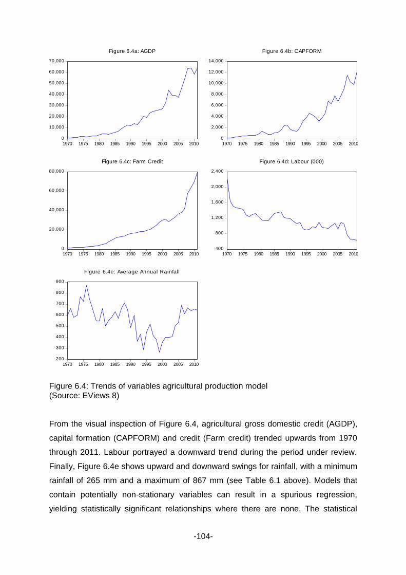
-104-

0

10,000

20,000

30,000

40,000

50,000

60,000

70,000

1970 1975 1980 1985 1990 1995 2000 2005 2010

Figure 6.4a: AGDP

0

2,000

4,000

6,000

8,000

10,000

12,000

14,000

1970 1975 1980 1985 1990 1995 2000 2005 2010

Figure 6.4b: CAPFORM

0

20,000

40,000

60,000

80,000

1970 1975 1980 1985 1990 1995 2000 2005 2010

Figure 6.4c: Farm Credit

400

800

1,200

1,600

2,000

2,400

1970 1975 1980 1985 1990 1995 2000 2005 2010

Figure 6.4d: Labour (000)

200

300

400

500

600

700

800

900

1970 1975 1980 1985 1990 1995 2000 2005 2010

Figure 6.4e: Average Annual Rainfall

Figure 6.4: Trends of variables agricultural production model (Source: EViews 8)

From the visual inspection of Figure 6.4, agricultural gross domestic credit (AGDP),

capital formation (CAPFORM) and credit (Farm credit) trended upwards from 1970

through 2011. Labour portrayed a downward trend during the period under review.

Finally, Figure 6.4e shows upward and downward swings for rainfall, with a minimum

rainfall of 265 mm and a maximum of 867 mm (see Table 6.1 above). Models that

contain potentially non-stationary variables can result in a spurious regression,

yielding statistically significant relationships where there are none. The statistical

-105-

significance obtained from standard regression techniques with non-stationary

variables may be due to their trending over time, rather than a meaningful causal

relationship between them. It is therefore important to determine the order of

integration of all the variables used in econometric analysis, as this will determine

the correct estimation technique to use.

Data were log-transformed to stabilise variances and induce normality of errors in

the OLS regression. As it is a precondition for time series data to be stationary

before conducting Granger causality tests, unit root tests were carried out using the

Augmented Dickey-Fuller and Phillips and Perron tests, which hypothesise the

presence of a unit root, and the Kwiatkowski, Phillips, Schmidt and Shin (KPSS) test,

which argues for the no unit root hypothesis. Testing both unit root hypothesis and

stationarity hypothesis helps to distinguish the series that appear to be stationary,

from those that have a unit root, and those for which the information contained in the

data is not sufficient, to confirm whether series are stationary or non-stationary due

to the presence of a unit root (Syczewska, n.d.). In levels, all variables were

integrated of order one I(1). In differences, all the variables were observed to be

integrated of order zero I(0) and hence the variables were transformed into

difference form in subsequent analysis, as the null of no unit root was rejected by the

KPSS unit root test. Both the Augmented Dickey-Fuller and the Phillips and Perron

tests failed to reject the hypothesis of the presence of a unit root in the time series

data. Table 6.3 below summarises the unit root tests.

- 106 -

Table 6.3: Results of unit root tests Variable Augmented Dickey-Fuller

Order of

integration

Phillips & Perron Order of

integration

Kwiatkowski, Phillips, Schimdt and Shin

Level with

intercept

Order of

integration

1st difference

with intercept

Level with

intercept

Order of

integration

1st

difference

with

intercept

Level

with

intercept

Order of

integration

1st

difference

with

intercept

Order of

integration

LAGDP -1.8030 I(1) -6.0807***

I(0) -4.7255***

I(0) -6.6847***

I(0) 0.8057 I(1) 0.4228**

I(0)

LRAINFALL -2.4661 I(1) -9.1026***

I(0) -2.4395

I(1) -9.0840***

I(0) 0.2830***

I(0) 0.1869***

I(0)

LCREDIT -1.0458 I(1) -3.8213***

I(0) -1.4349 I(1) -3.0228**

I(0) 0.7858 I(1) 0.1460***

I(0)

LLABOUR -1.9335

I(1) -6.4241***

I(0) -2.1976 I(1) -6.1396***

I(0) 0.7857 I(1) 0.1231***

I(0)

LCAPFORM -1.2017 I(1) -6.5084***

I(0) -2.1537 I(1) -4.7498***

I(0) 0.2830 I(1) 0.1979***

I(0)

Note: ***, ** and * denote significance at 1, 5 and 10% levels, respectively.

(Source: EViews 8)

- 107 -

6.5 ESTIMATION OF EMPIRICAL RESULTS: COINTEGRATION TEST

Figure 6.5 below plots series of the variables agricultural output, credit, labour,

rainfall and capital formation and provides strong visual evidence that the variables

in the agricultural output model are indeed cointegrated. This graphical output

implies that an increase in the variable agricultural output responds positively to

increases in rainfall, labour force, credit and capital formation in the long-run. The

Cobb-Douglas production function has been used to provide similar evidence

(Chisasa and Makina, 2013). Further analysis of cointegration was conducted and

reported below, as Koop (2000:156) warns that “visual examinations of graphs

should not be considered as substitutes for a statistical test!”

5

10

15

20

25

30

35

40

45

1970 1975 1980 1985 1990 1995 2000 2005 2010

LAGDP LCAPFORM LCREDIT

LLABOUR LRAINFALL

Figure 6.5: Co-trending variables of agricultural production (Source: EViews 8)

The presence of a long-run relationship among the variables was tested using the

Johansen and Juselius (1990) cointegration method on the variables, which were

found to be integrated of the order of one, viz.: AGDP (LAGDP), rainfall (Lrainfall),

capital formation (Lcapform), labour (Llabour) and credit (Lcredit). When applying

the cointegration approach, the first step is to select the optimum lag length, which

was set at three, based on the sequential modified likelihood ratio (LR) test statistic,

-108-

final prediction error (FPE), Akaike information criterion (AIC), Schwartz information

criterion (SC) and Hannan-Quinn information criterion (HQ) and was set at three

allowing for the cointegration test.

The Johansen Trace cointegration test shows that there are three integrating

equations at the 95% confidence level (p-value ˂ 0.05), suggesting that credit,

rainfall, labour, capital formation and agricultural output are cointegrated. Both the

trace statistic and the Max-Eigen statistic are higher than the Eigenvalue. These

results confirm that in the long run, bank credit, labour, capital formation, rainfall and

agricultural output are cointegrated. The results are presented in Tables 6.4 and 6.5

below:

Table 6.4: Trace statistics Unrestricted cointegration rank test (trace)

Hypothesised no. of CEs Eigenvalue Trace statistic

None*

0.784945 127.0105

At most 1*

0.602603 68.60969

At most 2* 0.437802 33.54259

At most 3 0.230796 11.65837

At most 4 0.043429 1.687203

Trace test indicates three cointegrating equations at the 0.05 level

(Source: EViews 8) Table 6.5: Max-Eigen statistics Hypothesised no. of CEs Eigenvalue Max-Eigen statistic

None*

0.784945 58.40078

At most 1*

0.602603 35.06710

At most 2* 0.437802 21.88422

At most 3 0.230796 9.971166

At most 4 0.043429 1.687203

Max-Eigenvalue test indicates three cointegrating equations at the 0.05 level

(Source: EViews 8)

6.6 MODEL ESTIMATION FOR THE LONG-RUN RELATIONSHIP

The long-run relationship was estimated with the log-transformed agricultural output

as the dependent variable. With a sample spanning the period 1970–2011, the data

were analysed using the method of least squares. A total of 42 observations after

adjustments were included in the analysis. The results are presented in Table 6.6

below.

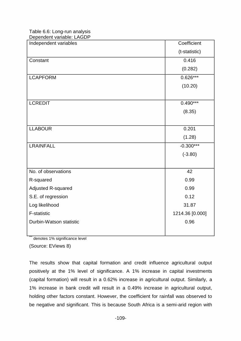
-109-

Table 6.6: Long-run analysis Dependent variable: LAGDP

Independent variables Coefficient

(t-statistic)

Constant 0.416

(0.282)

LCAPFORM 0.626***

(10.20)

LCREDIT 0.490***

(8.35)

LLABOUR 0.201

(1.28)

LRAINFALL -0.300***

(-3.80)

No. of observations

R-squared

Adjusted R-squared

S.E. of regression

Log likelihood

F-statistic

Durbin-Watson statistic

42

0.99

0.99

0.12

31.87

1214.36 [0.000]

0.96

*** denotes 1% significance level

(Source: EViews 8)

The results show that capital formation and credit influence agricultural output

positively at the 1% level of significance. A 1% increase in capital investments

(capital formation) will result in a 0.62% increase in agricultural output. Similarly, a

1% increase in bank credit will result in a 0.49% increase in agricultural output,

holding other factors constant. However, the coefficient for rainfall was observed to

be negative and significant. This is because South Africa is a semi-arid region with

-110-

only 28% of the country receiving more than 600 mm of rainfall (Food and

Agricultural Organisation, 2006). Its water requirements for agricultural purposes are

supplemented by irrigation. In times of excess rains, crops are waterlogged resulting

in poor output. During drought periods, crops wither resulting in poor harvests. The

Durbin-Watson statistic was lower than the benchmark indicating autocorrelation.

6.7 THE ERROR CORRECTION MODEL (ECM)

In the preceding section, it has been shown that the variables in the agricultural

production function have a long-run relationship and are thus cointegrated. This

suggests that one can estimate an ECM. Of course, in the short run, there may be

disequilibrium. The error term can be treated as the „equilibrium error‟. Gujarati and

Porter (2009) suggest that the error term can be used to tie the short-run behaviour

of the dependent variable to its long-run value. The error correction mechanism

(ECM), first used by Sargan and later popularised by Engle and Granger, corrects for

disequilibrium. Furthermore, the Granger representation theorem states that if two

variables X and Y are cointegrated, the short-run relationship between the two can

be expressed as the ECM.

Taking into account the coefficients of the variables in Equation [5.2], the model is

re-estimated as follows:

LAGDP = 0.416 + 0.626*LCAPFORM + 0.490*LCREDIT + 0.201*LLABOUR -

0.300*LRAINFALL + ECT................................................................................... [6.1].

Generating the ECM from Equation [6.1] above yields the following relationship:

ECM = LAGDP - 0.416-0.626*LCAPFORM-0.490*LCREDIT-0.201*LLABOUR-

0.300*LRAINFALL.............................................................................................. [6.2].

The model for agricultural output was re-estimated, taking into account the ECM in

order to understand the short-run behaviour of agricultural output and its factors of

production. The method of least squares was applied to 41 observations (after

adjustments).

The results show that capital formation influences agricultural output positively. The

relationship is also significant at the 1% level of confidence. The error correction

-111-

term also portrays the apriori negative sign and is significant at the 1% confidence

level. However, labour, credit and rainfall are observed to be insignificant with

negative coefficients. The statistical information, though, indicates that this might not

be a good model, as some of the explanatory variables are not significant (e.g. the p-

values for the coefficients on DLCREDIT, DLLABOUR and DLRAINFALL all imply

insignificance at the 5% level. This raises the issue of lag length selection (Koop,

2000:151). Just as the ARDL model has lags of the dependent and independent

variables, the ECM may also have lags. These were introduced and the model was

re-estimated. The model estimation took into account the three-period lag for each of

the variables and is presented as follows:

The method of least squares was once again used to analyse the lagged data. The

residuals were included in the following regression (in lagged form) as presented in

Table 6.7 below. The model was estimated using OLS.

-112-

Table 6.7: ECM regression results after parsimonious exercise

Independent variables Coefficient (t-statistic)

Constant 0.104*** (3.65)

∆LAGDP(-3) 0.323** (2.258)

∆LAGDP(-4) 0.130 (-1.380)

∆LCAPFORM 0.635*** (8.54)

∆LCAPFORM(-1) -0.207*** (-3.52)

∆LCAPFORM(-3) 0.167* (1.95)

∆LCREDIT(-3) -0.304* (-1.75)

∆LLABOUR(-1) -0.217 (-1.59)

∆LRAINFALL -0.254*** (-3.67)

ECM(-1) -0.646*** (-5.08)

R-squared Adjusted R-squared S.E. of regression Log likelihood F-statistic Durbin-Watson statistic

0.79 0.72 0.06 55.62

11.64 [0.000] 1.71

***, **, * Respectively significant at 1%, 5% and 10% level

(Source: EViews 8)

The ECM(-1) has a significantly negative coefficient meaning that agricultural GDP

rapidly adjusts to short term disturbances in the sector. There is no room for

tardiness in the agricultural sector. Disturbances occasioned by poor or low rainfall

will be rapidly compensated for by the application of irrigation facility. The absence of

institutional credit will be immediately replaced by availability of other credit facilities

from non-institutional sources. There is no room for possible non-application of

intermediate inputs such as seeds, fertilizers, chemicals, harvesting facilities, etc.

In the short run current capital formation is associated with a positive significant

increase in agricultural GDP. On the other hand, capital formation in the previous two

years is observed to impact negatively on agricultural GDP. These results are

-113-

consistent with the observation by Wolf (1991:566) who postulates that new capital is

more productive than old capital per unit of expenditure, a phenomenon called the

“vintage effect.” Previous employments of capital amount to unutilised capital in the

agricultural sector and as such contribute negatively to agricultural GDP.

Credit in previous periods has a significant negative impact on agricultural GDP in

the short run. In the long run we have observed that credit has a positive impact.

Therefore, the negative impact in the short run could be a result of several factors

peculiar to the South African context. First, it could be the result of the short-term

nature of credit to farmers whereby banks may require them to repay loans even

before harvesting and selling their produce. Thus a mismatch between production

and repayment cycles would adversely affect output. Second, it could be the result of

high interest rates charged on loans to farmers by virtue of sector having a longer

production period as compared with other sectors. Third, the negative impact in the

short run could be the result of the uncertain nature of agricultural output whose risks

include, among others, uncertain prices, high input costs, climatic conditions, etc.

Notwithstanding the negative impact in the short term, the adjustment process to

positive equilibrium position is rapid and evidenced with a highly significant negative

ECM(-1).

Labour in the previous period is negatively associated with agricultural GDP in the

short term. This is expected in the South African context because of inflexible labour

laws characterised by high unionisation that have adverse effect on productivity.

The short run results appear to be unique for the South African agricultural sector.

To the knowledge of the researcher, the few studies that have attempted to

investigate the short run effect on the sector were undertaken in Pakistan. One study

by Sial (2011) that utilised time series data from 1973-2009 (37 years) observed no

significant short run effects. Another study by Shahbaz et al. (2011) that utilised time

series data from 1971-2011 (41 years) observed significant positive effects with

respect to labour. However, unlike in South Africa where deviations from equilibrium

are rapidly corrected (by 65% per year), in Pakistan deviations in the short run

towards the long run are corrected by 11.86% per year. The researchers attribute

-114-

this slow adjustment to equilibrium to the high cost of agricultural production in

Pakistan.

6.8 GRANGER CAUSALITY TEST

A causality test was conducted to explore the transmission mechanism between

bank credit and agricultural output and other explanatory variables of output. Thus

within the bank credit-agricultural output context, the Engle and Granger (1987) two-

step procedure was investigated. To achieve this the following hypotheses were

postulated:

H0: Bank credit (credit) does not Granger-cause agricultural output (AGDP).

Ha: Bank credit (credit) Granger-causes agricultural output (AGDP).

H0: AGDP does not Granger-cause bank credit.

Ha: AGDP Granger causes bank credit.

Table 6.8 exhibits the results of the pairwise Granger causality tests among the

variables AGDP, bank credit, capital formation, labour and rainfall. The lag length

was selected using the LR, FPE, AIC, SC and HQ VAR lag order selection criteria.

At lag length 1, the p-value is less than 5% (0.0154) and the null hypothesis was

rejected, while the alternate hypothesis was accepted.

The results reveal the presence of unidirectional causality flowing from bank credit

(Credit) to AGDP at a 95% level of significance, thus confirming the apriori

expectations. There is no evidence of reverse causality. Also observed is

unidirectional causality from (1) AGDP to capital formation, (2) AGDP to labour, (3)

capital formation to credit and (4) capital formation to labour, and a bi-directional

causality between credit and labour. The results confirm those of Simsir (2012).

-115-

Table 6.8: Pairwise Granger causality results Null hypothesis Obs. Lags F-statistic Probability Results

∆LCapform does not Granger-cause

∆LAGDP

39 1 1.42641 0.2402 H0 is not

rejected

∆LAGDP does not Granger-cause

∆LCapform

39 1 5.35040 0.0265** H0 is rejected

∆LCredit does not Granger-cause

∆LAGDP

39 1 6.46505 0.0154** H0 is rejected


∆LCredit

39 1 0.01942 0.8899 H0 is not rejected

∆Llabour does not Granger-cause

∆LAGDP

39 1 4.46534 0.4995 H0 is not

rejected


∆Llabour

39 1 7.65170 0.0089*** H0 is rejected

∆Lcredit does not Granger-cause

∆Lcapform

39 1 2.24937 0.1424 H0 is not

rejected

∆Lcapform does not Granger-cause

DLcredit

39 1 4.18942 0.0480** H0 is rejected

∆Llabour does not Granger-cause

∆Lcredit

39 1 4.19920 0.0478** H0 is rejected

∆Lcredit does not Granger-cause

∆Llabour

39 1 3.90529 0.0558* H0 is rejected

***, **, * Respectively significant at 1%, 5% and 10% level

(Source: EViews 8)

6.9 VARIANCE DECOMPOSITION

6.9.1 Variance decomposition of agricultural output

Agricultural output is 55.6% described by its innovative shocks. The contribution of

credit to agricultural output is 37.6%, while that of capital formation and labour is

3.7% and 3.1% respectively. These results are presented in Table 6.9 below.

-116-

Table 6.9: Variance decomposition of LAGDP

Period S.E. LAGDP LCREDIT LCAPFORM LLABOUR

1 0.116265 100.0000 0.000000 0.000000 0.000000

2 0.151247 96.71277 0.840888 0.153539 2.292798

3 0.169814 94.14943 1.119375 1.765536 2.965658

4 0.179253 90.05841 2.912013 4.049113 2.980461

5 0.187648 84.63703 7.506783 4.775659 3.080527

6 0.197474 78.12424 14.05062 4.368554 3.456586

7 0.208810 71.39396 20.79216 4.036739 3.777136

8 0.220721 65.30376 27.00480 3.983445 3.707992

9 0.232644 60.07055 32.63196 3.918279 3.379216

10 0.244519 55.57561 37.63363 3.716859 3.073899

Source: EViews 8

6.9.2 Variance decomposition of credit

Agricultural output contributes 9.4% to credit. Credit, through its innovative shocks,

contributes 86.5% to itself. The contribution of capital formation and labour to credit

is minimal at slightly over 2% for both. The results are presented in Table 6.10

below.

Table 6.10: Variance decomposition of LCREDIT


1 0.067322 1.609273 98.39073 0.000000 0.000000

2 0.107184 0.671294 99.11773 0.042810 0.168164

3 0.139561 0.449236 98.75362 0.612888 0.184255

4 0.167347 1.047048 96.71792 2.100361 0.134675

5 0.190768 2.390338 94.35354 3.100411 0.155709

6 0.210181 3.970838 92.39592 3.180457 0.452786

7 0.226786 5.459846 90.68206 2.837994 1.020096

8 0.241369 6.815380 89.09329 2.505436 1.585890

9 0.254122 8.103402 87.68359 2.282623 1.930385

10 0.265167 9.360445 86.47045 2.125811 2.043295

(Source: EViews 8)

-117-

6.9.3 Variance decomposition of capital formation

Agricultural output explains capital formation by 54.6%, and 28.9% of capital

formation is explained through its innovative shocks. The contribution of credit to

capital formation is 11.6%, while that of labour is 4.9%. Detailed results are

presented in Table 6.11 below.

Table 6.11: Variance decomposition of capital formation


1 0.174029 51.59884 3.843623 44.55753 0.000000

2 0.243330 64.29079 2.546676 32.54094 0.621591

3 0.266641 69.54190 2.145581 27.51033 0.802194

4 0.283381 65.44865 1.965684 29.97616 2.609506

5 0.295699 61.35609 2.755592 32.66931 3.219007

6 0.302503 59.60169 4.440397 32.86935 3.088571

7 0.308444 58.43056 6.195375 31.67501 3.699062

8 0.314995 57.11138 7.785941 30.52581 4.576872

9 0.321056 55.83989 9.499836 29.69819 4.962085

10 0.326569 54.57665 11.62350 28.89455 4.905300

(Source: EViews 8)

6.9.4 Variance decomposition of labour

Table 6.12 below shows that 60.7% of labour is explained by itself through its

innovative shocks. Agricultural output explains labour by 17%. The contribution of

credit and capital formation to labour is 13.6% and 8.7% respectively.

-118-

Table 6.12: Variance decomposition of labour


1 0.081162 0.557314 7.632200 0.244594 91.56589

2 0.111511 3.300919 16.17923 0.242196 80.27766

3 0.125651 8.146589 16.49229 2.845786 72.51534

4 0.133110 11.27635 15.08706 6.242244 67.39434

5 0.136988 13.52758 14.24598 8.174336 64.05210

6 0.139225 15.26448 13.90068 8.797543 62.03730

7 0.140829 16.34133 13.77140 8.856884 61.03038

8 0.141897 16.82690 13.69004 8.878160 60.69590

9 0.142465 16.97939 13.60026 8.728296 60.69205

10 0.142756 16.99704 13.56344 8.692791 60.74673

(Source: EViews 8)

Notably, the contribution of credit to agricultural output (37.6%) is substantial.

Compared to its contribution to labour (13.6%) and to capital formation (11.6%), the

impulse response innovations confirm the pivotal role of credit in agricultural output.

6.10 IMPULSE RESPONSES

There is a positive response in agricultural growth due to innovations in bank credit

from Period 1 to Period 10. The same is observed for labour, save for Period 10,

where the response is negative due to innovations in labour. There is a positive

response in agricultural growth due to innovations in capital formation from Period 1

to Period 2, followed by a negative response from Period 3 to Period 6 and then a

positive response thereafter.

There is a negative response in bank credit due to innovations in agricultural output

from Period 1 to Period 2, followed by a positive response in subsequent periods.

This suggests unidirectional causality between agricultural output and credit. Mixed

responses are observed for capital formation and labour. Credit is positively affected

by shocks in capital formation in all periods. There is a negative response in labour

due to innovations or shocks in credit from Period 1 to Period 4. Figure 6.6 below

depicts these responses.

-119-

-.10

-.05

.00

.05

.10

.15

1 2 3 4 5 6 7 8 9 10

Response of LAGDP to LAGDP

-.10

-.05

.00

.05

.10

.15

1 2 3 4 5 6 7 8 9 10

Response of LAGDP to LCREDIT

-.10

-.05

.00

.05

.10

.15

1 2 3 4 5 6 7 8 9 10

Response of LAGDP to LCAPFORM

-.10

-.05

.00

.05

.10

.15

1 2 3 4 5 6 7 8 9 10

Response of LAGDP to LLABOUR

-.10

-.05

.00

.05

.10

.15

1 2 3 4 5 6 7 8 9 10

Response of LCREDIT to LAGDP

-.10

-.05

.00

.05

.10

.15

1 2 3 4 5 6 7 8 9 10

Response of LCREDIT to LCREDIT

-.10

-.05

.00

.05

.10

.15

1 2 3 4 5 6 7 8 9 10

Response of LCREDIT to LCAPFORM

-.10

-.05

.00

.05

.10

.15

1 2 3 4 5 6 7 8 9 10

Response of LCREDIT to LLABOUR

-.2

-.1

.0

.1

.2

.3

1 2 3 4 5 6 7 8 9 10

Response of LCAPFORM to LAGDP

-.2

-.1

.0

.1

.2

.3

1 2 3 4 5 6 7 8 9 10

Response of LCAPFORM to LCREDIT

-.2

-.1

.0

.1

.2

.3

1 2 3 4 5 6 7 8 9 10

Response of LCAPFORM to LCAPFORM

-.2

-.1

.0

.1

.2

.3

1 2 3 4 5 6 7 8 9 10

Response of LCAPFORM to LLABOUR

-.10

-.05

.00

.05

.10

1 2 3 4 5 6 7 8 9 10

Response of LLABOUR to LAGDP

-.10

-.05

.00

.05

.10

1 2 3 4 5 6 7 8 9 10

Response of LLABOUR to LCREDIT

-.10

-.05

.00

.05

.10

1 2 3 4 5 6 7 8 9 10

Response of LLABOUR to LCAPFORM

-.10

-.05

.00

.05

.10

1 2 3 4 5 6 7 8 9 10

Response of LLABOUR to LLABOUR

Response to Cholesky One S.D. Innov ations ± 2 S.E.

Figure 6.6: Impulse responses

(Source: EViews 8)

-120-

CHAPTER 7

HYPOTHESES TESTING AND EMPIRICAL RESULTS:

SURVEY DATA

7.1 INTRODUCTION

This chapter presents the survey results of the study. First, the socio-economic

characteristics of the respondents are discussed using frequencies and descriptive

statistics. Chi-square tests were used to measure associations of variables used to

test the postulated hypotheses. Objectives 1, 3, 4 and 5 of the study and the results

of the respective hypotheses tested therefrom are presented next. Objective 2 traces

the trends in the supply of credit to farmers using time series secondary data and

was accordingly excluded from this chapter. Thus, the section analysed the impact of

bank credit on agricultural output, the relationship between capital structure and

access to bank credit by smallholder farmers, as well as the link between capital

structure and the performance of smallholder farmers. Finally, the section presents

the best model fit for agricultural output using SEM.

7.2 VALIDITY AND RELIABILITY TESTS

The questionnaire used for this study was subjected to validity and reliability tests

using confirmatory factor analysis (CFA) and Cronbach‟s alpha to determine its

appropriateness. The purpose was to eliminate questions that were found not to be

reliable and valid when compared to the Cronbach‟s alpha value. To test the validity

of the dimensions used in the questionnaire, factor analysis was performed to

determine whether the individual questions load onto (or contribute to) the

dimensions listed in the questionnaire. There are two types of factor analysis,

namely exploratory factor analysis (EFA) and CFA. EFA attempts to discover the

nature of the constructs influencing a set of responses, while CFA tests whether a

specified set of constructs is influencing responses in a predicted way (DeCoster,

1998; Hurley et al., 1997). For the purposes of this study, CFA was adapted,

because unlike EFA, CFA produces many goodness-of-fit measures for model

-121-

evaluation (Albright and Park, 2009). Using the principal component analysis (PCA)

and the Varimax with Kaiser normalisation rotation method, the results of the factor

analysis for all the constructs are presented in Table 7.1 below.

7.2.1 Validity test: Confirmatory factor analysis

Table 7.1 depicts the results of Bartlett‟s test for sphericity, the Kaiser-Meyer-Olkin

(KMO) value and the communalities. The KMO value of 0.746 is reasonable to

conduct a factor analysis. The p-value of Bartlett‟s test (p = 0.000), which is below

0.05, is significant at the 99% confidence level. This result indicates that the

correlations structure is significantly strong enough for performing a factor analysis

on the items.

Table 7.1 KMO and Bartlett‟s test

KMO and Bartlett’s test

KMO measure of sampling adequacy 0.746

Bartlett‟s test of sphericity Approx. chi-square 666.129

df 36

Sig. 0.000

(Source: SPSS 21)

The communalities indicate the extent to which an individual item correlates with the

rest of the items in the construct. Items with low communalities (less than 0.3) were

candidates for elimination, as recommended by Hosany, Ekinci and Uysal (2006).

Using the PCA method of extraction, the communalities for all nine items in Table 7.2

are observed to be reasonable.

-122-

Table 7.2 Communalities

Communalities

Initial Extraction

Q7 1.000 0.659

Q10 1.000 0.716

Q15 1.000 0.611

Q18 1.000 0.503

Q19 1.000 0.618

Q23 1.000 0.489

Q24 1.000 0.583

Q27 1.000 0.671

Q28 1.000 0.676

Extraction method: PCA

(Source: SPSS 21)

Table 7.3 below shows that a 61.42% (highlighted in blue) cumulative variance is

attributed to three factors, namely financial information of the farmer, production

information and the borrower‟s attitude towards borrowing. All three factors have

Eigenvalues greater than 1 (shaded in green). The loading factors of an item indicate

the extent to which an individual item „loads‟ onto a factor (which represents three

loading factors, as shown in Table 7.3).

Table 7.3: The cumulative variance explained for by the factors Total variance explained

Component Initial Eigenvalues Extraction sums of squared loadings Rotation sums of squared

loadings

Total % of

variance

Cumulative

%

Total % of

variance

Cumulative

%

Total % of

varianc

e

Cumulati

ve %

1 2.908 32.310 32.310 2.908 32.310 32.310 2.627 29.193 29.193

2 1.553 17.253 49.564 1.553 17.253 49.564 1.501 16.674 45.867

3 1.067 11.855 61.418 1.067 11.855 61.418 1.400 15.551 61.418

4 0.803 8.917 70.335

5 0.689 7.652 77.987

6 0.597 6.633 84.620

7 0.504 5.595 90.215

8 0.460 5.106 95.320

9 0.421 4.680 100.000


(Source: SPSS 21)

-123-

A further analysis was carried out using the scree plot. Figure 7.1 below shows the

scree plot results. Taking into account the different criteria, the decision was made to

extract three factors.

7.3 INTERPRETATION OF FACTOR LOADINGS

Figure 7.1 below shows the factor loadings for the three extracted factors. The

loading of an item shows the extent to which an item contributes to the factor. A

value close to 1 indicates that an item that loads highly on a specific factor. A loading

of 0.400 can be considered meaningful (Lee, Lee and Wicks, 2004). Upon

investigating the items and their factor loadings, it was decided to re-specify the

factor model, including all items with a factor loading above 0.400, which is

considered important. The researcher felt that items with loadings above 0.400

would be meaningful in measuring the dependent variables in the hypothesised

models. The individual questions could now be allocated to each of the three factors

according to their individual factor loadings. These three factors should then form the

dimensions in the questionnaire (see Table 7.4 below).

Figure 7.1: The scree plot (Source: SPSS 21)

-124-

Table 7.4: Factor loadings Rotated component matrix

a

Component

1 2 3

Q19 What were the average total current assets (cash and debtors) available after paying

current liabilities?

0.78

2

Q15 Please indicate your household income in Rands for the previous season. 0.77

3

Q18 Please indicate your family‟s estimated total assets at the beginning of the last

agricultural season (2011/2012).

0.70

7

Q24 What was the family‟s net worth at the beginning of the last agricultural season? 0.70

3

Q23 What were the average monthly expenses? 0.60

0

Q28 Local banks will provide loans to agriculture even when there is a downturn in the

agricultural economy.

0.80

8

Q27 Loan products from my local bank are flexible enough to meet my ability to repay

when I sell my products/at harvest.

0.80

6

Q10 How many hours do you spend on the farm per hectare per person per day? 0.82

6

Q7 Please indicate the size of your land in hectares. 0.78

4


Rotation method: Varimax with Kaiser normalisationa

a Rotation converged in five iterations

(Source: SPSS 21)

7.4 RELIABILITY TEST: CRONBACH’S ALPHA

The questionnaire was subjected to the reliability test using the Cronbach‟s alpha. In

this test, an item analysis was performed on the questions construct by construct to

determine the Cronbach‟s alpha values. The Cronbach‟s alpha value was an

important measure of the reliability of the questionnaire. Its value generally increases

when the correlations between the questions of the questionnaire increase. The

alpha value can lie between negative infinity and 1 (-∞ ˂ α ˂ 1). Three decision

criteria guide the interpretation of Cronbach‟s alpha as follows:

For a value above 0.8, reliability is considered good.

For a value between 0.6 and 0.8, reliability is considered acceptable.

For a value below 0.6, reliability is considered unacceptable (Cronbach, 1951;

De Souza & Dick, 2009).

To ensure that the rotated components (factors) are not correlated with each other,

the orthogonal rotation method was selected ahead of the oblique method. The

-125-

orthogonal method is preferred in cases where further modelling such as regression

will be done. The most recommended orthogonal method is the Varimax (Kaiser,

1958), which was applied in this study. Table 7.5 presents the summary reliability

statistics for all the constructs in the research instrument.

Table 7.5: Reliability statistics

Factor/Construct Cronbach‟s alpha

Factor 1: Financial information 0.775

Factor 2: Production information 0.518

Factor 3: Borrower attitudes towards borrowing 0.565

(Source: SPSS 21)

7.4.1 Factor 1: Financial information

For the construct Financial information, the overall Cronbach‟s alpha was observed

to be 0.775 (0.8 when rounded off) and was therefore considered acceptable (see

Table 7.3 above) when compared to the minimum threshold Cronbach‟s alpha of 0.8.

In the case where the alpha of an individual item is higher than the overall alpha

value, any such items will be excluded. This results in an increase of the overall

alpha. Table 7.6 shows the individual item alphas for this construct. None of them

has a negative or very low (0.10) correlation with the total; therefore all the questions

of the construct were retained.

-126-

Table 7.6: Item-total statistics: Factor 1 – Financial information Item-total statistics

Question Scale mean if

item deleted

Scale variance if

item deleted

Corrected

item-total

correlation

Cronbach‟

s alpha if

item

deleted

Q15 Please indicate your household income

in rands for the previous season.

7.53 12.782 0.608 0.714

Q18 Please indicate your family‟s total

assets at the beginning of the last

agricultural season (2011/2012).

7.40 12.462 0.504 0.754

Q19 What were the average total current

assets (cash and debtors) available

after paying current liabilities?

7.53 13.308 0.560 0.731

Q23 What were the average monthly

expenses?

7.27 13.644 0.500 0.750

Q24 What was the family‟s net worth at the

beginning of the last agricultural

season?

7.51 12.849 0.585 0.722

(Source: SPSS 21)

7.4.2 Factor 2: Production information

The construct Production information, containing eight items, had a Cronbach‟s

alpha of 0.518. Tables 7.3 and 7.7 show the reliability tests of the construct and the

individual items respectively. Although the Cronbach‟s alpha for the construct was

below the threshold (0.6), counter-arguments available in empirical literature suggest

and justify consideration for constructs with a Cronbach‟s alpha of 0.5 (Chin, 1998;

Fornell and Larcker, 1981; Su and Yang, 2010). All the individual alpha statistics

were below the Cronbach‟s alpha of the construct, had positive values and were

accordingly included in the analysis.

Table 7.7: Item-total statistics – Factor 2: Production information Item-total statistics

Scale mean if

item deleted

Scale variance

if item deleted

Corrected

item-total

correlation

Cronbach‟s

alpha if item

deleted

Q7 Please indicate the size of your

land in hectares.

2.70 1.298 0.358 .

Q10 How many hours do you spend

on the farm per hectare per day?

3.22 2.008 0.358 .

(Source: SPSS 21)

-127-

7.4.3 Factor 3: Borrower attitudes towards borrowing

An analysis of the Borrower attitudes towards borrowing construct, containing seven

questions, and confirmed reliability, with an overall Cronbach‟s alpha of 0.565. Three

out of the seven questions were „yes/no‟ questions and were therefore excluded from

the analysis. The individual item alphas were neither negative nor more than the

overall alpha and were therefore retained. Tables 7.3 and 7.8 depict the reliability

results for the construct.

Table 7.8: Item-total statistics – Factor 3: Borrower attitudes towards borrowing Item-total statistics

Scale mean if

item deleted

Scale variance

if item deleted

Corrected item-

total correlation

Cronbach‟s alpha

if item deleted

Q27 Loan products from my

local bank are flexible

enough to meet my ability

to repay when I sell my

products/at harvest.

3.29 1.324 0.394 .

Q28 Local banks will provide

loans to agriculture even

when there is a downturn

in the agricultural

economy.

3.06 1.339 0.394 .

(Source: SPSS 21)

7.4.4 Factor 4: Credit demand and credit-rationing variables

The final reliability test was performed for the construct Credit demand and credit-

rationing variables. The construct failed the reliability test. However, the questions

making up the construct were deemed useful for the final analysis and were retained.

This is in line with the argument offered by Singelis, Triandis, Bhawuk and Gelfand

(1995), namely that several scores with relatively low alphas will give more valid

information than fewer scores with high alphas. The authors further argue that this is

especially the case when a large number of people are assessed, because errors of

measurement tend to average over subjects, and the inaccurate scores of any one

subject have little significance for the research.

7.5 DESCRIPTIVE STATISTICS

The study first analysed the demographic characteristics of the respondents. The

respondents were asked to indicate their age. The purpose was to determine the age

-128-

concentration and establish the patterns of interest in farming as a business. Figure

7.2 below shows that the majority of the respondents were between 31 and 50 years

old (71.5%; n = 362), while only 12.5% (n = 362) were over 50 years old. This shows

that the bulk of the respondents are still in their active and productive age group. It is

also encouraging to note that some of the respondent farmers (16%; n = 362) are

younger than 30 years of age.

Figure 7.2: Age distribution of farmers (Source: SPSS 21)

Married farmers constituted 48.6% of the sample (n = 362). This suggests that

farming is taken seriously for the purpose of generating income for taking care of the

family. What is worrying, though, is that while 39.6% (n = 362) received high school

education, only 4.7% (n = 362) had received tertiary education (Figure 7.3). The

majority either did not go to school (14.7%; n = 362) or had received only primary

school education (37.4%; n = 362). As anticipated, the majority (65.3%; n = 362) of

the respondents were male.

16%

71.50%

12.50%

Younger than 30

31-50

Older than 50

-129-

Figure 7.3: Level of education (Source: SPSS 21)

Most of the farmers (72.2%; n = 362) operate on relatively small pieces of land of up

to 20 hectares, suggesting that farm size could be a constraint to their quest to grow.

The respondents were asked to indicate the factors that limit them from borrowing

from banks. Distance from the bank and high interest rates were cited as the major

impediments to borrowing (Figure 7.4). On the other hand, the farmers indicated the

need for inputs such as fertiliser, seed and pesticides, payment of wages for workers

and irrigation equipment as key drivers for credit demand.

Figure 7.4: Q40. The following factors limit me from borrowing from banks (Source: SPSS 21)

Level of education0.00%

20.00%

40.00%

Did not go toschool

Primary school High school Tertiaryeducation

14.70%

37.40% 39.60%

4.70% Level of education

62.7%

40.8%

38.2%

25.1%

24.0%

19.4%

13.0%

13.0%

11.0%

10.4%

8.7%

3.2%

0.0% 10.0% 20.0% 30.0% 40.0% 50.0% 60.0% 70.0%

High interest rates

Long and difficult application procedure

Might lose assets pledged as security

High transaction costs

Fear of application being turned down

Long time taken to approve loans

Distance to the bank

Long time taken to disburse loans

Lack of collateral

Do not need a loan

Bad customer service

Payment of bribe

%

%

-130-

7.6 CORRELATION ANALYSIS

The correlation coefficients between variables were determined construct by

construct. For the factors that influence agricultural production construct, Table 7.9

below shows that there is positive correlation between the size of land and labour (ρ

= 0.358), land size and family labour (ρ = 0.117), land size and non-family labour (ρ =

0.148) and land size and agricultural output for the previous cropping season (ρ =

0.220). Furthermore, the type of farming practised by the farmer was observed to be

significantly correlated to the size of family labour involved with the farming

enterprise (ρ = 0.233).

Table 7.9: Pearson correlation: Factors that influence agricultural production Correlations

Q7 Q9 Q10 Q11 Q12 Q14

Q7 Pearson correlation 1 -0.069 0.358** 0.117

* 0.148

** 0.220

**

Sig. (2-tailed) 0.191 0.000 0.027 0.005 0.000

Q9 Pearson correlation 1 0.233** -0.009 0.080 -0.013

Sig. (2-tailed) 0.000 0.858 0.130 0.802

Q10 Pearson correlation 1 0.139** 0.094 0.140

**

Sig. (2-tailed) 0.008 0.076 0.007

Q11 Pearson correlation 1 0.206** 0.201

**

Sig. (2-tailed) 0.000 0.000

Q12 Pearson correlation 1 0.296**

Sig. (2-tailed) 0.000

Q14 Pearson correlation 1

Sig. (2-tailed)

** Correlation is significant at the 0.01 level (2-tailed).

* Correlation is significant at the 0.05 level (2-tailed).

Q7: Please indicate the size of your land in hectares.

Q9: I practise the following type of farming.

Q10: How many hours do you spend on the farm per hectare per person per day?

Q11: How many family members work on the farm?

Q12: Please indicate how many non-family members work on the farm.

Q14: What is your gross agricultural output in rands for the last agricultural season?

(Source: SPSS 21)

The Pearson correlation matrix for the construct Financial information is presented in

Table 7.10 below. All variables in this construct were found to be statistically

significant and positive. For instance, household income was observed to be

positively correlated with both short-term and long-term credit, suggesting that an

increase in credit supply to smallholder farmers positively influences the level of

household income. Furthermore, the ratio of agricultural income to total family

-131-

income showed a positive and significant relationship with both short-term and long-

term credit.

Table 7.10: Pearson Correlation matrix: Financial information

Correlations

Q15 Q16 Q17 Q18 Q19 Q20 Q21 Q22 Q23 Q24

Q15 Pearson

correlation

1 0.524** 0.411

** 0.452

** 0.479

** 0.349

** 0.185

** 0.263

** 0.407

** 0.449

**

Sig. (2-

tailed)

0.000 0.000 0.000 0.000 0.000 0.000 0.000 0.000 0.000

Q16 Pearson

correlation

0.524** 1 0.607

** 0.290

** 0.294

** 0.268

** 0.234

** 0.364

** 0.363

** 0.335

**

Sig. (2-

tailed)

0.000 0.000 0.000 0.000 0.000 0.000 0.000 0.000 0.000

Q17 Pearson

correlation

0.411** 0.607

** 1 0.245

** 0.346

** 0.259

** 0.294

** 0.365

** 0.387

** 0.317

**

Sig. (2-

tailed)

0.000 0.000 0.000 0.000 0.000 0.000 0.000 0.000 0.000

Q18 Pearson

correlation

0.452** 0.290

** 0.245

** 1 0.452

** 0.346

** 0.228

** 0.259

** 0.285

** 0.341

**

Sig. (2-

tailed)

0.000 0.000 0.000 0.000 0.000 0.000 0.000 0.000 0.000

Q19 Pearson

correlation

0.479** 0.294

** 0.346

** 0.452

** 1 0.349

** 0.324

** 0.335

** 0.304

** 0.428

**

Sig. (2-

tailed)

0.000 0.000 0.000 0.000 0.000 0.000 0.000 0.000 0.000

Q20 Pearson

correlation

0.349** 0.268

** 0.259

** 0.346

** 0.349

** 1 0.263

** 0.252

** 0.359

** 0.430

**

Sig. (2-

tailed)

0.000 0.000 0.000 0.000 0.000 0.000 0.000 0.000 0.000

Q21 Pearson

correlation

0.185** 0.234

** 0.294

** 0.228

** 0.324

** 0.263

** 1 0.397

** 0.353

** 0.287

**

Sig. (2-

tailed)

0.000 0.000 0.000 0.000 0.000 0.000 0.000 0.000 0.000

Q22 Pearson

correlation

0.263** 0.364

** 0.365

** 0.259

** 0.335

** 0.252

** 0.397

** 1 0.394

** 0.350

**

Sig. (2-

tailed)

0.000 0.000 0.000 0.000 0.000 0.000 0.000 0.000 0.000

Q23 Pearson

correlation

0.407** 0.363

** 0.387

** 0.285

** 0.304

** 0.359

** 0.353

** 0.394

** 1 0.530

**

Sig. (2-

tailed)

0.000 0.000 0.000 0.000 0.000 0.000 0.000 0.000 0.000

Q24 Pearson

correlation

0.449** 0.335

** 0.317

** 0.341

** 0.428

** 0.430

** 0.287

** 0.350

** 0.530

** 1

Sig. (2-

tailed)

0.000 0.000 0.000 0.000 0.000 0.000 0.000 0.000 0.000


(Source: SPSS 21)

An analysis of the Borrower attitudes towards borrowing construct portrayed

positively significant correlations between variables. The Pearson correlation

-132-

coefficient for the relationship between the different types of credit instruments and

the variable family culture is to borrow as little as possible (ρ = 0.008) was found to

be insignificant, suggesting that when the family culture is to minimise borrowing,

credit providers and policy makers need to roll out educational programmes geared

towards motivating farmers to tap into the benefits of financial intermediation in

growth initiatives. The summary statistics for this construct are presented in Table

7.11.

Table 7.11: Pearson correlation matrix: Borrower attitudes towards borrowing

Correlations

Q26 Q27 Q28 Q29 Q30 Q31 Q32

Q26 Pearson correlation 1 0.003 0.082 0.018 -0.064 0.082 0.189**

Sig. (2-tailed)

0.954 0.117 0.734 0.223 0.118 0.000

N 362 362 362 362 362 362 362

Q27 Pearson correlation 0.003 1 0.394** -0.133

* 0.008 0.109

* 0.215

**


0.000 0.011 0.878 0.038 0.000

N 362 362 362 362 362 362 362

Q28 Pearson correlation 0.082 0.394** 1 -0.141

** 0.182

** 0.162

** 0.185

**

Sig. (2-tailed) 0.117 0.000

0.007 0.000 0.002 0.000

N 362 362 362 362 362 362 362

Q29 Pearson correlation 0.018 -0.133* -0.141

** 1 -0.089 -0.082 -0.205

**

Sig. (2-tailed) 0.734 0.011 0.007

0.092 0.118 0.000

N 362 362 362 362 362 362 362

Q30 Pearson correlation -0.064 0.008 0.182** -0.089 1 -0.049 -0.051

Sig. (2-tailed) 0.223 0.878 0.000 0.092

0.357 0.334

N 362 362 362 362 362 362 362

Q31 Pearson correlation 0.082 0.109* 0.162

** -0.082 -0.049 1 0.230

**

Sig. (2-tailed) 0.118 0.038 0.002 0.118 0.357

0.000

N 362 362 362 362 362 362 362

Q32 Pearson correlation 0.189** 0.215

** 0.185

** -0.205

** -0.051 0.230

** 1

Sig. (2-tailed) 0.000 0.000 0.000 0.000 0.334 0.000

N 362 362 362 362 362 362 362


*. Correlation is significant at the 0.05 level (2-tailed).

(Source: SPSS 21)

Finally, the analysis of the construct Credit demand and credit-rationing variables

was based on four variables, which had passed the reliability and validity test. The

amount of credit received, collateral offered by the borrowers and interest rates were

-133-

observed to have a significant and positive correlation. Table 7.12 presents the

summary statistics for the relationship between variables making up this construct.

Table 7.12: Pearson correlation matrix: Credit demand and credit-rationing variables

Correlations

Q34 Q35 Q36 Q37

Q34 Pearson correlation 1 -0.165** -0.030 -0.086

Sig. (2-tailed)

0.002 0.572 0.103

N 362 362 362 362

Q35 Pearson correlation -0.165** 1 -0.035 0.240

**


0.505 0.000

N 362 362 362 362

Q36 Pearson correlation -0.030 -0.035 1 0.030

Sig. (2-tailed) 0.572 0.505

0.566

N 362 362 362 362

Q37 Pearson correlation -0.086 0.240** 0.030 1

Sig. (2-tailed) 0.103 0.000 0.566

N 362 362 362 362


(Source: SPSS 21)

7.7 HYPOTHESES TESTING

Hypotheses 1 through 4 were tested using the Pearson chi-square test. In each

case, descriptive statistics are presented and discussed, followed by a bivariate

correlation analysis. Further tests of the hypotheses were carried out using SEM for

robustness.

7.7.1 Testing Hypothesis 1

The first objective of this study was to empirically determine the impact of bank credit

on agricultural output in South Africa. Following on this objective, the following

hypothesis was postulated:

H0: There is no supported relationship between bank credit and agricultural

output (b = 0).

-134-

7.7.1.1 Descriptive statistics

From Table 7.13 below, the average total valid observations summed to n = 362. An

analysis of the descriptive statistics revealed that the respondents attain agricultural

output of between R50 000 and R60 000 annually (mean score = 3.22). This level of

performance is supported by land sizes averaging 16–20 hectares. Both short-term

and long-term credit were in the range of R35 000 to R110 000. With labour hours

per person per day dedicated to the farm on a day-to-day basis, it appears less

convincing that the resources dedicated to the farm by the respondents are sufficient

to maximise production, particularly given land sizes of 11 to 20 hectares.

Table 7.13: Descriptive statistics Mean Standard deviation N

Agricultural output (AO) 1.59 1.034 362

Land 3.22 1.417 362

Labour 2.7 1.139 362

Short-term credit 1.76 1.275 362

Long-term credit 1.65 1.279 362

Rainfall 504.36 129.383 362

(Source: SPSS 21)

7.7.1.2 Bivariate correlation analysis: Chi-square test

Table 7.14 below presents the chi-square test results for bivariate correlations

between the predictor variables and agricultural output in Hypothesis 1. All the

predictor variables were observed to have significant association with agricultural

output (p < 0.05).

Table 7.14: Pearson chi-square test between predictors and agricultural output

Item no. Relationship Value df Chi-sq

1 Land size 38.242 20 0.008***

2 Short-term debt 70.931 25 0.000***

3 Long-term debt 111.907 25 0.000**

*; **; *** denotes significance at 1%, 5% and 10% respectively.

(Source: SPSS 21)

-135-

7.8 TESTING HYPOTHESIS 2

The second objective of the survey was to determine the factors that influence the

demand for credit by smallholder farmers in South Africa. Following on this objective,

the following hypothesis was postulated.

H0: Factor inputs of production such as fertiliser, seed, and chemicals DO NOT

influence the demand for credit in the agricultural sector in South Africa.


Table 7.15 shows that the respondents received one loan in the previous season

(mean = 1.65). Borrowers offer personal property as collateral for the credit received.

Other factors observed to influence borrowing are interest rates, the need for liquidity

to pay workers, level of education and family culture. The respondents were found to

have attained a level of education of between primary and high school (mean =

3.55). The variables family culture is to borrow as little as possible (mean = 3.10) and

lack of tangible collateral are presumed to be the reason why farmers access few

loans.

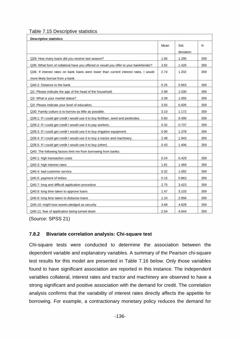
-136-

Table 7.15 Descriptive statistics

Descriptive statistics

Mean Std.

deviation

N

Q29: How many loans did you receive last season? 1.65 1.295 359

Q35: What form of collateral have you offered or would you offer to your bank/lender? 3.92 1.426 359

Q36: If interest rates on bank loans were lower than current interest rates, I would

more likely borrow from a bank.

2.74 1.202 359

Q40.2: Distance to the bank. 0.25 0.663 359

Q1: Please indicate the age of the head of the household. 2.99 1.030 359

Q2: What is your marital status? 2.09 1.055 359

Q3: Please indicate your level of education. 3.55 0.926 359

Q30: Family culture is to borrow as little as possible. 3.10 1.172 359

Q39.1: If I could get credit I would use it to buy fertiliser, seed and pesticides. 0.60 0.490 359

Q39.2: If I could get credit I would use it to pay workers. 0.32 0.737 359

Q39.3: If I could get credit I would use it to buy irrigation equipment. 0.90 1.378 359

Q39.4: If I could get credit I would use it to buy a tractor and machinery. 2.48 1.943 359

Q39.5: If I could get credit I would use it to buy (other) 0.43 1.406 359

Q40: The following factors limit me from borrowing from banks:

Q40.1: high transaction costs 0.24 0.429 359

Q40.3: high interest rates 1.81 1.469 359

Q40.4: bad customer service 0.32 1.092 359

Q40.5: payment of bribes 0.15 0.863 359

Q40.7: long and difficult application procedure 2.75 3.423 359

Q40.8: long time taken to approve loans 1.47 3.103 359

Q40.9: long time taken to disburse loans 1.10 2.956 359

Q40.10: might lose assets pledged as security 3.68 4.828 359

Q40.11: fear of application being turned down 2.54 4.644 359

(Source: SPSS 21)

7.8.2 Bivariate correlation analysis: Chi-square test

Chi-square tests were conducted to determine the association between the

dependent variable and explanatory variables. A summary of the Pearson chi-square

test results for this model are presented in Table 7.16 below. Only those variables

found to have significant association are reported in this instance. The independent

variables collateral, interest rates and tractor and machinery are observed to have a

strong significant and positive association with the demand for credit. The correlation

analysis confirms that the variability of interest rates directly affects the appetite for

borrowing. For example, a contractionary monetary policy reduces the demand for

-137-

credit, while an expansionary monetary policy increases the appetite for credit by

borrowers. Tight collateral requirements diminish credit demand and vice versa.

Finally, the desire to mechanise farming operations has a positive impact on the

demand for credit by farmers.

Table 7.16: Pearson chi-square test: Credit demand and credit-rationing variables

Item no. Relationship Value df Chi-sq

1 Collateral and credit demand 116.505 20 0.000***

2 Interest rates and credit demand 29.137 20 0.085*

3 Tractor and machinery and credit demand 13.173 5 0.022**

4 Lack of collateral and credit demand 11.208 5 0.047**


(Source: SPSS 21)


The third objective of the survey was to determine the impact of capital structure of

smallholder farmers on access to bank credit supply in South Africa. A dummy

variable was introduced. The variable 0 was assigned for those who did not receive

credit, otherwise 1. The following null and alternate hypotheses were postulated.

Ho = Capital structure does not influence access to credit by smallholder

farmers in South Africa.


Table 7.17 shows that the majority (241, or 89.4%) of the respondents received less

than R100 000 credit during the last agricultural season, 9.6% (29) received between

R100 001 and R150 000, while only 10.6% (35) accessed over R150 000 (see

Figure 7.5). In light of the escalating input prices and average land size of over 15

hectares, these credit facilities are insufficient to run the farming business profitably.

-138-

Table 7.17: Descriptive statistics Question Mean Std.

deviation N

Q34 How much credit did you receive last season?

1.38 0.877 362

Q15 Please indicate your household income in Rands for the previous season.

1.78 1.172 362

Q24 What was the family‟s net worth at the beginning of the last agricultural season?

1.80 1.189 362

Q35 What form of collateral have you offered or would you offer to your bank/lender?

3.93 1.423 362

(Source: SPSS 21)

Figure 7.5: How much credit did you receive last season? (Source: SPSS 21)

The land size distribution is shown in Figure 7.6 below.

Figure 7.6: Please indicate the size of your land in hectares (Source: SPSS 21)

˂5ha, 44, 23%

˂5ha, 25, 13%

˂5ha, 38, 20%

˂5ha, 50, 26%

˂5ha, 34, 18%

-139-

Table 7.18 below shows that access to credit has a positive relationship with capital

structure (proxied by debt and equity), income and collateral. The Pearson

correlation coefficient is significant (one-tailed) for all variables. These results are

confirmed by the chi-square test presented in Table 7.19, which shows that all

variables have a strong association at a 95% confidence level (p ˂ 0.05). Therefore,

it can be concluded that farmers with a high income hold collateral and have low

gearing, and have a high probability of accessing credit from banks and other similar

credit suppliers.

Table 7.18: Pearson correlation matrix Q34 Q15 Q21b_Q22b Q24 Q35

Pearson correlation Q34 1.000 0.300 0.223 0.279 -0.165

Q15 0.300 1.000 0.176 0.449 -0.207

Q21b_Q22b 0.223 0.176 1.000 0.264 -0.414

Q24 0.279 0.449 0.264 1.000 -0.255

Q35 -0.165 -0.207 -0.414 -0.255 1.000

Sig. (1-tailed) Q34 . 0.000 0.000 0.000 0.001

Q15 0.000 . 0.000 0.000 0.000

Q21b_Q22b 0.000 0.000 . 0.000 0.000

Q24 0.000 0.000 0.000 . 0.000

Q35 0.001 0.000 0.000 0.000 .

N Q34 362 362 362 362 362

Q15 362 362 362 362 362

Q21b_Q22b 362 362 362 362 362

Q24 362 362 362 362 362

Q35 362 362 362 362 362

Q34: How much credit did you receive last season?

Q15: Please indicate your household income in rands for the previous season.

Q21b_Q:22b: Capital structure

Q24: What was the family‟s net worth at the beginning of the last agricultural season?

Q35: What form of collateral have you offered or would you offer to your bank/lender?

(Source: SPSS 21)

Table 7.19: Chi-square tests between credit accessed and predictors Item no. Relationship Pearson chi-square

Value df Assmp. Sig (s-sided)

1 Collateral and credit accessed 75.779 16 000***

2 Capital structure and credit accessed 41.646 4 000***

3 Net worth and credit accessed 66.920 16 000***

4 Collateral and credit accessed 42.284 16 000***


(Source: SPSS 21)


The fourth and final objective of the survey was to determine the relationship

between capital structure and smallholder farm performance. The following null

hypothesis was postulated.

-140-

H0: Capital structure does not stimulate smallholder farm performance in

South Africa.


Table 7.20 below shows that on average, the farmers own approximately three

hectares of land on which they practise their farming business (mean = 3.22).

Furthermore, workers spend between six and eight hours working on the farm daily

(mean = 2.7 hours). The variable capital structure was not included in the

computation of descriptive statistics, as it comprises of binary responses of 0

(ungeared) and 1 (geared).

Table 7.20: Descriptive statistics

Descriptive statistics

N Minimum Maximum Mean Std. deviation

Q7 362 1 5 3.22 1.417

Q10 362 1 5 2.70 1.139

Rainfall 362 360 620 504.36 129.383

(Source: SPSS 21)

7.10.2 Correlation analysis

Table 7.21 below presents the correlation matrix for the variables in the estimated

model. The purpose is to establish the strength of the relation between two variables.

For correlation, the hypothesis of no significant correlation between smallholder farm

performance and explanatory variables (land, labour, rainfall and capital structure)

was tested.

-141-

Table 7.21: Correlation matrix

Q14 Q7 Q10 Q21b_Q22b Q24 Rainfall

Pearson correlation Q14 1.000 0.220 0.140 0.238 0.352 0.079

Q7 0.220 1.000 0.358 0.208 0.254 0.063

Q10 0.140 0.358 1.000 0.097 0.088 0.054

Q21b_Q22b 0.238 0.208 0.097 1.000 0.264 0.063

Q24 0.352 0.254 0.088 0.264 1.000 0.021

Rainfall 0.079 0.063 0.054 0.063 0.021 1.000

Sig. (1-tailed) Q14 . 0.000 0.004 0.000 0.000 0.066

Q7 0.000 . 0.000 0.000 0.000 0.116

Q10 0.004 0.000 . 0.032 0.048 0.152

Q21b_Q22b 0.000 0.000 0.032 . 0.000 0.117

Q24 0.000 0.000 0.048 0.000 . 0.344

Rainfall 0.066 0.116 0.152 0.117 0.344 .

N Q14 362 362 362 362 362 362

Q7 362 362 362 362 362 362

Q10 362 362 362 362 362 362

Q21b_Q22b 362 362 362 362 362 362

Q24 362 362 362 362 362 362

Rainfall 362 362 362 362 362 362

Q14: What is your gross agricultural output in rands for the last agricultural season (2011/2012)?

Q7: Please indicate the size of your land in hectares.

Q10: How many hours do you spend on the farm per hectare per person per day?

Q21b_Q22b: Capital structure

Q24: What was the family‟s net worth at the beginning of the last agricultural season?

(Source: SPSS 21)

With sample size (n = 362), all variables were found to be positively correlated with

smallholder farm performance proxied by annual output. The relationship is also

significant (p ˂ 0.05). The null was therefore rejected.

The variables were subjected to further tests for association using the Pearson chi-

square test. The results of the bivariate correlation analysis are shown in Table 7.22

below. All the predictor variables are observed to have a positive and significant

association with agricultural output.

-142-

Table 7.22: Chi-square tests between agricultural output and predictors

Item no. Relationship Pearson chi-square

Value df Assmp. Sig (s-sided)

1 Farm size and agricultural output 38.242 20 008***

2 Labour (hours) and agricultural output 57.729 20 000***

3 Capital structure and agricultural output 23.450 16 000***

4 Family net worth and agricultural output 84.521 16 000***

5 Family net worth and agricultural output 4.447 5 0.487


(Source: SPSS 21)

The correlations discussed above have highlighted the presence of associations

between agricultural output and its predictor variables, access to credit and its

determinants, and the effect of capital structure on access to credit and agricultural

output. These relationships have portrayed overlaps and interrelationships among

the specified variables. In the next section, these relationships are subjected to more

robust analyses, using SEM for robustness.

7.11 STRUCTURAL EQUATION MODELLING

This section presents results for each of the hypotheses postulated from these

objectives using SEM with AMOS Version 22. AMOS offers two distinct advantages.

Firstly, its graphical user interface is quite intuitive, and secondly, it has been merged

since 2000 into the most popular statistical software package for social sciences

(SPSS) (Nokelainen, n.d.). The overall objective of SEM is to establish that a model

derived from theory has a close fit to the sample data in terms of the difference

between the sample and model-predicted covariance matrices. However, Tomer and

Pugesek (2003) warn that even if all the possible indices point to an acceptable

model, one can never claim to have found the true model that has generated the

analysed data. SEM is most concerned with finding a model that does not contradict

the data. That is to say, in an empirical session of SEM, one is typically interested in

retaining the proposed model whose validity is the essence of the null hypothesis.

Statistically speaking, when using SEM, the researcher is usually interested in not

rejecting the null hypothesis (Raykov and Marcoulides, 2000:34).

-143-

In SEM, all the relationships in the model (arrows) are tested at one time. Therefore,

if the model is correct, one will not reject the hypothesis that the model and observed

covariance matrices are equal. This is a departure from most statistical applications

where one strives to prove findings. Dion (2008:365) postulates that “a conceptual

difference of SEM from regression is that in a regression model the independent

variables are themselves correlated (multi-co linearity) which influences the size of

the coefficients found. In SEM, the interactions amongst these variables are

modelled”. Furthermore, in this study, the maximum likelihood parameter estimation

was chosen ahead of other estimation methods (weighted least squares, 2SLS and

ADF, because the data were normally distributed. It should be noted that OLS

methods minimise the squared deviations between values of the criterion variable

and those predicted by the model. Maximum likelihood attempts to maximise the

likelihood that obtained values of the criterion variable will be correctly predicted.

To the knowledge of the researcher, no previous empirical studies on the impact of

credit on agricultural output have used SEM. This study extends previous studies

that have largely applied multiple regression of the OLS method. This study used

structural modelling because of the multiple indicators for each of the latent

constructs dictated by theoretical considerations. The results for Objective 1 are

presented below. In each case, both the hypothesised and final models are

presented diagrammatically for ease of reference (Schreiber et al., 2006:334).

7.11.1 Goodness-of-model-fit indices

The reporting done here follows the guidance of Schreiber et al. (2006), who provide

a basic set of guidelines and recommendations for information that should be

included in CFA and SEM. However, as a point of departure, the researcher must

first conduct a chi-square test of association of the predictor variables and the

endogenous variables. Table 7.23 below presents summarised chi-square test

results for models 1–5 summarised in their functional form as follows:

Model 1: Agricultural output (AO) = f[(credit (C), labour (L), rainfall (R) land (Ld)]

-144-

Model 2: Cd = f(fertiliser (F), seed (S), chemicals (C), equipment (E), collateral

(Clt), transaction costs (T), capital structure (CSt), interest rates (I))

Model 3: Cs = f(collateral (Clt), interest rates(I), income of the borrower

(Y))

Model 4: Agricultural output (AO) = f(capital structure (Cs); labour (L), land (L),

rainfall (R)).

Model 5: Agricultural output (AO) = f (land size (LS); short-term debt (STD); long-

term debt (LTD); household income (HI); family networth (FN): access to credit

(ACVolume)

Table 7.23: Chi-square test for models 1–5

Chi-sq. df p-value Remark

Model 1 (Objective 1) 0.000 0 Cannot be computed Poor fit




Model 5: (Proposed model) 129.502 11 0.000 Poor fit

(Source: SPSS 21)

Furthermore, fit indices were used to inform the researcher how closely the data fit

the model. Table 7.24 presents for the most widely used indices. They are the chi-

square value (CMIN), Goodness of Fit Index (GFI), Tucker-Lewis Index (TLI),

comparative fit index (CFI), parsimony-adjusted fit index (PCFI), root mean square

error of approximation (RMSEA), normed fit index (NFI) and the p of close fit

(PCLOSE). All the structural equation models reported in this section follow the

decision criteria set out in Table 7.24 below.

-145-

Table 7.24: Interpretation of model fit indices

Index Recommended value

CMIN ˂ 0.05

GFI ≥ 0.95 (not generally recommended).

TLI values close to 1 indicate a very good fit)

CFI (values close to 1 indicate a very good fit)

PCFI Sensitive to model size

RMSEA ˂ 0.06 to 0.08 with confidence interval.

NFI (values close to 1 indicate a very good fit); indices less than 0.9

can be improved substantially.

PCLOSE ˂ 0.05

(Source: Author construction)

7.11.2 Model 1: Agricultural output

The hypothesised SEM for agricultural output is presented in Figure 7.7 below.

Within the context of structural modelling, exogenous variables represent those

constructs that exert an influence over other constructs under study and are not

influenced by other factors in the quantitative model. Those constructs identified as

endogenous are affected by exogenous and other endogenous variables in the

model. This model hypothesises that agricultural output (AOutput) is predicted by

land size (LS), labour (LH), short-term debt (STD), long-term debt (LTD) and rainfall.

Rainfall and labour were observed to have the lowest predictive power of agricultural

output (0.05) each and were therefore excluded from further analysis. The single-

headed arrows represent causal relationships between explanatory variables and the

dependent variable, while double-headed arrows represent covariances between

explanatory variables.

-146-

Figure 7.7: Model 1: Impact of credit on agricultural output (Source: AMOS 21)

7.11.3 Maximum likelihood estimates

The regression model that forms part of the SEM process confirmed that there are

relationships between most variables, which are consistent with theory. The path

coefficients presented in Table 7.25 below are positive and significant at 5% (p ˂

0.05). While previous studies have shown total credit to be positively and

significantly related to agricultural output, this study breaks credit into its short-term

and long-term components. It is observed that long-term credit has a higher

contribution to agricultural output (0.189 or approximately 19%) than short-term

credit (0.120 or 12%). These results are in line with Patil‟s (2008) recommendations

for a long-term credit policy for Indian smallholder farmers. Similarly, a one-unit

increase in land size is observed to lead to a 10% increase in agricultural output,

holding other factors constant. The contribution of the variable land to agricultural

output, though significant, is observed to command the lowest direct effect. These

results confirm the theory of production.

-147-

Table 7.25: Regression weights (group number 1 – default model) Estimate S.E. C.R. P

Agricultural output (Q14) <--- Short-term debt (Q21) 0.120 0.044 2.736 0.006

Agricultural output (Q14) <--- Land size (Q7) 0.100 0.037 2.710 0.007

Agricultural output (Q14) <--- Long-term debt (Q22) 0.189 0.043 4.376 ***

(Source: AMOS 21)

Table 7.26 shows the simple correlations between exogenous variables. Both short-

term credit and long-term credit have a strong correlation with land size (p ˂ 0.05).

Similarly, short-term credit and long-term credit have a strong bidirectional

correlation.

Table 7.26: Covariances (group number 1 – default model) Estimate S.E. C.R. P

Land size (Q7) <--> Short-term credit (Q21) 0.452 0.098 4.626 ***

Land size (Q7) <--> Long-term credit (Q22) 0.355 0.097 3.665 ***

Short-term credit (Q21) <--> Long-term credit (Q22) 0.646 0.092 7.015 ***

(Source: AMOS 21)

The results for the hypothesised Model 1 showed that labour and rainfall were

insignificant in explaining agricultural output. Land size (β = 0.14), short-term credit (β

= 0.15) and long-term debt (β = 0.23) explain approximately 15% (R2 = 0.145) of the

agricultural output model depicted in Figure 7.8 below. Table 7.27 below is

illustrative. In keeping with the SEM methodology, rainfall and labour were not

retained for modelling agricultural output using SEM. The final model is presented as

Figure 7.9 below.

Table 7.27 Squared multiple correlations (R2) (group number 1 – default model)

Estimate

Agricultural output (Q14)

0.145

(Source: AMOS 21)

-148-

Figure 7.8: Model 1a: Impact of credit on agricultural output (Source: AMOS 21)

Where:

AOutput: is the endogenous variable agricultural output

LS: Land size

STD: Short-term credit

LTD: Long-term credit

(LS, STD and LTD are unobserved, exogenous variables)

e1: Error term

Chi-square, root mean square error of approximation (RMSEA), the Tucker-Lewis

Index (TLI) and the Comparative Fit Index (CFI) were used to determine the

goodness of fit for Model 1 above. The results are presented below.

7.11.4 Chi-square test for the re-estimated SEM 1

According to Schreiber et al. (2006:327), if a model has been modified and

reanalysed, one should provide evidence that the modified model is statistically

superior to the original model with a chi-square test and fit indexes. Tomer and

-149-

Pugesek (2003) postulate that ᵡ2 is one of the most widely used statistics for

assessing goodness of fit of a model. This statistic is an assessment of the

magnitude of difference between the initial observed covariance matrix and the

reproduced matrix. The probability level (p-value) that is associated with ᵡ2 indicates

whether the difference between the reproduced matrix is significant or not.

A significant ᵡ2 test states that the difference between the two matrices is due to

sampling error or variation. Typically, researchers are interested in a non-significant

ᵡ2 test. This indicates that the observed matrix and the reproduced are not

statistically different, therefore indicating a good fit of the model to the data.

However, the ᵡ2 test suffers from several weaknesses, including a dependence on

sample size and vulnerability to departures from multivariate normality. Raykov and

Marcoulides (2000) suggest that a researcher should examine a number of fit criteria

in addition to the ᵡ2 value to assess the fit of the proposed model.

The chi-square test results depicted in Table 7.23 above fails to confirm that the

model fits the data being observed. The probability level was found to be significant

(p ˂ 0.05). To verify these results and cognisant of the weaknesses of the chi-square

test statistic elucidated above, further and more robust tests were applied using

goodness-of-fit indices.

7.11.5 Model fit for SEM 1 using goodness-of-fit indices

The main objective of this study was to test the relationship between bank credit and

agricultural output. All the indices confirm that all the sample data fit the model

significantly: CMIN = 0.00, GFI = 1.00, TLI = 0.00, CFI = 1.00, PCFI = 0.00, NFI =

1.00 and PCLOSE = 0.00 (see Table 7.28 below). Only RMSEA showed a poor

model fit; however, as the majority of indices confirmed a good model fit, the results

of the RMSEA index were discarded, and consistent with Schreiber et al. (2010:327),

it was concluded that the model fits the data being tested.

-150-

Table 7.28: SEM 1 fit indices

Index Recommended

value Output Remark

CMIN ˂ 0.05 0.000 Very good

GFI ≥ 0.95 (not generally

recommended)

1.000 Very good

TLI values close to

1 indicate a very

good fit)

0.000 Good

CFI (values close to

1 indicate a very

good fit)

1.000 Very good

PCFI Sensitive to model

size

0.000 Very good

RMSEA ˂ 0.06 to 0.08 with

confidence interval

0.255 Insignificant,

therefore poor

model fit

NFI (values close to

1 indicate a very

good fit);

indices less than 0.9

can be improved

substantially

1.000 Very good

PCLOSE ˂ 0.05 0.000 Very good

(Source: AMOS 21)

7.12 MODEL 2: DEMAND FOR CREDIT

Objective 3 of the study sought to determine the socio-economic factors that

influence the demand for credit by smallholder farmers in South Africa. Accordingly,

the following hypothetical structural equation model (Figure 7.9) was derived and the

covariances among the explanatory variables thereof estimated. Both the dependent

and explanatory variables are defined in Table 7.29 below.

-151-

Table 7.29: Definition of variables

Variable Definition

Q39 Purpose of credit demanded

Q40 Factors limiting credit demand

Q35 Collateral offered to the lender

Q36 Interest rate charged by the lender

Q1 Age of the farmer in years

Q2 Marital status of the farmer

Q3 Highest level of education of the farmer

Q30 Family culture towards borrowing

Q29 Number of loans received by the farmer in the previous farming season


Figure 7.9: Model 2: Determinants of demand for credit (Source: AMOS 21)

-152-

When disaggregated data series for the variables purpose of credit demanded (Q39)

and factors limiting the demand for credit (Q40) were included in the analysis,

missing values were observed and the data could therefore not be analysed. To

overcome this problem, both Q39 and Q40 were collapsed and included in the

analysis, as depicted in Figure 7.9 above, showing the estimated SEM.

The results show that the combined effect of the variable Q39 and Q40 yields a

negative impact on the demand for credit. This is in contrast with results from

previous studies, in which it was observed that the sub-questions/variables for Q39

and Q40 were positive and significant. The model was re-estimated and subjected to

goodness-of-model-fit tests. The model failed the chi-square test, implying that the

model does not explain the data. The chi-square test results for Model 2 are

presented in Table 7.23. The chi-square test statistic shows a lack of good model fit

(p ˂ 0.05). In this case the researcher failed to reject the null that the explanatory

variables do not predict the dependent variable. These results conform to the

recommendations of Tomer and Pugesek (2003), who posit that a non-significant

chi-square test statistic indicates that the observed matrix and the reproduced matrix

are not statistically different, thus indicating a good fit of the model to the data.

Therefore, Figure 7.10 depicts the final model for the demand for credit by

smallholder farmers in South Africa. All model variables are defined in Table 7.30.

-153-

Figure 7.10: Model 2a: Determinants of demand for credit (Source: AMOS 21)


Variable Definition of variable

IE Denotes the farming inputs and capital equipment to be purchased

FC Family culture is not to borrow

Collateral Collateral offered by the farmer to the lender

EF Denotes economic factors that influence the demand for credit

ACValue Denotes the credit accessed by the farmer in the previous season

e1 Denotes the error term



Regression weights for the model variables were computed and are presented in

Table 7.31 below. Farming inputs and capital equipment, family culture and collateral

were observed to have a significant relationship with the demand for credit (p ˂

0.05). However, the coefficients were negative, indicating a negative influence on the

demand for credit (collateral = -0.151; inputs and capital equipment = -0.375; family

culture = -0.120). An interesting and otherwise unique finding in this analysis is that

-154-

family culture has a negative and significant influence on the demand for credit (p <

0.05). Farming inputs such as fertiliser, seed and pesticides, wages for workers and

capital equipment were found to have a negative and significant influence on the

demand for credit. This suggests that smallholder farmers mainly rely on equity

finance, as family culture is seen to negatively influence borrowing. Collateral, which

in empirical literature is observed to impede access to credit by smallholder farmers,

is confirmed to have a negative influence on the demand for credit. In other words,

as credit providers emphasise on borrowers providing collateral, this tends to

diminish the demand for credit, because most smallholder farmers have no assets

suitable for assigning as collateral.

Table 7.31: Regression weights (group number 1 – default model)

Estimate S.E. C.R. P

Access to credit (Q29) <--- Collateral (Q35) -0.151 0.047 -3.233 0.001

Access to credit (Q29) <--- Economic factors (Q40) 0.127 0.065 1.953 0.051

Access to credit (Q29) <--- Inputs and equipment (Q39) -0.375 0.156 -2.405 0.016

Access to credit (Q29) <--- Family culture (Q30) -0.120 0.058 -2.072 0.038

Estimate = estimated path coefficient (prediction) for arrows in the model (Garson, 2010) SE = standard error CR = critical ratio (estimate divided by its standard error [Garson, 2010:4]) (˃ 1.96 = significant at 0.05 level (Garson 2009:22; 2010:4) P = probability value (˂ 0.05 = significant on the 0.001 level *** [Garson 2009])

(Source: AMOS 21)

Table 7.32 below shows the bi-directional correlations between dimensions. The

relationship between family culture towards borrowing and economic factors such as

interest rates is observed to be positive and significant with a p-value below 0.05 at

the 0.001 (two-tailed) level. The relationship between family culture towards

borrowing and economic factors (interest rates) was also found to be strongly

significant with a p-value below 0.05, also at the 0.001 (two-tailed) level. Family

culture towards borrowing and inputs and capital equipment were found to be weakly

significant at 0.1 with a p-value greater than 0.05. The causal relationships between

collateral and family culture towards borrowing, economic factors and inputs and

capital equipment were all observed to be insignificant with p-values greater than

0.05. Furthermore, the relationship between collateral and family culture towards

borrowing was found to be negative.

-155-


Inputs and equipment (Q39) <--> Family culture (Q30) 0.056 0.032 1.759 0.079

Family culture (Q30) <--> Economic factors (Q40) 0.299 0.079 3.793 ***

Family culture (Q30) <--> Collateral (Q35) -0.088 0.088 -1.000 0.317

Economic factors (Q40) <--> Collateral (Q35) 0.081 0.094 0.866 0.387

Inputs and equipment (Q39) <--> Collateral (Q35) 0.017 0.039 0.435 0.664

Inputs and equipment (Q39) <--> Economic factors (Q40) 0.365 0.039 9.359 ***

(Source: AMOS 21)

Finally, Table 7.33 below shows that approximately 5.1% of the demand for credit

model is explained by the predictor variables in the model shown as Figure 7.10

above.

Table 7.33: Squared multiple correlations (group number 1 – default model)

Estimate

Access to credit (Q29)

0.051

(Source: AMOS 21)

The chi-square test results discussed above (Table 7.23) have rejected the null

hypothesis of a good fit for Model 2. In keeping with Schreiber et al. (2006), more

robust tests were applied using goodness-of-fit indices. For Model 2, the demand for

credit was proxied by 0 for the respondents who did not apply for credit and 1 for

those who applied. Table 7.34 presents the indices used to analyse the SEM fit

(CMIN = 0.00, CFI = 1.00, PCFI = 0.00, NFI = 1.00 and PCLOSE = 0.00). Those

values indicate a good fit between the hypothesised model and the observed data.

Only RMSEA = 0.215 showed a poor model fit; however, as the majority of indices

confirmed a good model fit, the RMSEA index was discarded. Figure 7.11 below

shows the final model for Hypothesis 2.

-156-


Index Recommended value Output Remark



recommended)

1.000 Very good

TLI values close to 1

indicate a very good fit)

0.000 Good

CFI (values close to 1


1.000 Very good

PCFI Sensitive to model size 0.000 Very good


confidence interval

0.215 Insignificant,

therefore no

model fit

NFI (values close to 1

indicate a very good fit);

indices less than 0.9

can be improved

substantially

1.000 Very good


(Source; AMOS 21)

7.13 MODEL 3: ACCESS TO CREDIT BY SMALLHOLDER FARMERS

The fourth objective of the study was to determine the impact of capital structure of

smallholder farmers on access to bank credit supply in South Africa. In this instance,

a dummy variable was introduced for capital structure. Respondents who accessed

credit were represented by 1 (one) and those who did not by 0 (zero). Responses 2–

5 (representing the scale of credit accessed by loan size) for questions 21 and 22

were first combined and transformed to 1, while response 1 was transformed to zero

in order to generate a binary response system. Both questions 21 and 22 for credit

accessed were combined, as they relate to short-term and long-term credit

respectively. The purpose of combining the two questions was to determine the

aggregate leverage effect on access to credit. The following structural equation

model (Figure 7.11) was hypothesised:

-157-

Figure 7.11: Model 3: Impact of capital structure on access to credit (Source: AMOS 21)

In this structural equation model, it was hypothesised that access to bank credit by

smallholder farmers (ACVolume) in South Africa is a function of the family‟s net

worth (FN), household income (HI), collateral, capital structure (CS) and ratio of

agricultural income to total family income (RAIFI). Family net worth, collateral and

the ratio of agricultural income to total family income were observed to have weak

explanatory power towards access to bank credit by smallholder farmers. To this

end, they were excluded from further analysis. The final path diagram and parameter

estimates are shown in Figure 7.12 below.

-158-

Figure 7.12: Model 3a: Impact of capital structure on access to credit (Source: AMOS 21)

Interpreting the regression coefficients, capital structure (CS) has the highest impact

on access to credit (ACVolume) in volume terms (estimate of 0.15), explaining

26.1% of the variance. Household income (HI) (estimate of 0.21) explains 15.6% of

the variance. Both capital structure and household income are significant with p-

value less than 5% (p ˂ 0.05). Similarly, family net worth (FN) is observed to have a

positive and significant impact on access to credit (estimate of 0.15), explaining

10.8% of the variance. Table 7.35 below is illustrative.


Access to credit (Q34) <--- Capital structure (Q21b_Q22b) 0.261 0.090 2.909 0.004

Access to credit (Q34) <--- Household Income (Q15) 0.156 0.041 3.794 ***

Access to credit (Q34) <--- Family net worth (Q24) 0.108 0.041 2.613 0.009

(Source: AMOS 21)

In Table 7.36 below, the covariances between the exogenous variables are

presented. All the relationships are positive and significant with p-values below 0.05

at the 0.001 (two-tailed) levels. The strongest causal relationship is seen between

household income and family net worth (estimate of 0.625). This confirms the theory

that the dimensions are to a large extent correlated.

-159-

Table 7.36: Covariances (group number 1 – default model)


Household income (Q15) <--> Capital structure (Q21b_Q22b) 0.103 0.031 3.301 ***

Household income (Q15) <--> Family net worth (Q24) 0.625 0.080 7.789 ***

Capital structure (Q21b_Q22b) <--> Family net worth (Q24) 0.156 0.032 4.856 ***

(Source: AMOS 21)

Table 7.37 shows that approximately 13.6% of access to credit by smallholder

farmers is explained by household income, capital structure and family networth.

Table 7.37: Squared multiple correlations (group number 1 – default model)

Estimate

Access to credit (Q34)

0.136

(Source: AMOS 21)

The SEM was re-estimated using three predictor variables, which are household

income (HI), capital structure (CS) and family net worth (FN). The results of the final

model for Objective 4 are presented in Table 7.38. All indices, save for RMSEA,

confirm the goodness of fit of the model, thus confirming the predictive power of the

independent variables listed in the model for access to bank credit by smallholder

farmers in South Africa (CMIN = 0.000, GFI = 1.000, TLI = 0.000, CFI = 1.000, PCFI

= 0.000, RMSEA = 0.269, NFI = 1.000 and PCLOSE = 0.000).

-160-




GFI ≥ 0.95 (not generally recommended) 1.000 Very good

TLI values close to 1 indicate a very good fit) 0.000 Good

CFI (values close to 1 indicate a very good fit) 1.000 Very good


RMSEA ˂ 0.06 to 0.08 with confidence interval. 0.269 Insignificant,

therefore no

model fit

NFI (values close to 1 indicate a very good

fit); indices less than 0.9 can be improved

substantially

1.000 Very good


(Source: AMOS 21)

7.14 MODEL 4: IMPACT OF CAPITAL STRUCTURE ON FARM PERFORMANCE

The fifth and final objective of this study was to determine the relationship between

capital structure and smallholder farm performance. Following on this objective, it is

hypothesised that capital structure does not influence the level of farm performance.

The first step was to develop a model based on theory, time, logic and previous

research, as recommended by Quirk, Keith and Quirk (2001). In this model,

agricultural output (AOutput) is argued to be a function of land size (LS), labour (L),

capital structure (CS) and rainfall. The hypothesised structural equation model is

depicted in Figure 7.13 below and the summary variable definitions provided in Table

7.39.

As in the preceding models, AMOS was used to analyse the effects of capital

structure on farm performance proxied by farm output in this study. AMOS is a latent

variable structural equations program that assists in developing and testing a

theoretical model (Quirk et al., 2002). Although there are four variables in the model,

the main variable of concern was the path from capital structure to agricultural

-161-

output. The fit of the model was then examined using the chi-square test statistic and

goodness-of-fit indices.

Figure 7.13: Model 4: Impact of capital structure on farm performance (Source: AMOS 21)


Variable Definition of variable

AOutput Denotes gross agricultural output for the previous season in rands

LS Denotes the size of the farming area in hectares

LH Denotes labour hours spent on the farm

CS Denotes the capital structure of the farming enterprise

Rainfall Denotes average annual rainfall

e1 Denotes the error term

Source: Compiled by author.


The regression model shown in Table 7.40 below confirmed the presence of causal

relationships between the endogenous variable agricultural output (AOutput) and the

exogenous variables land size (LS) and capital structure (CS). Both causal

relationships are significant with p-values indicated by *** on the 0.001 level (two-

tailed). Two asterisks (**) would indicate a p-value for the 0.1 level (10%), and one

-162-

asterisk (*) would indicate a p-value for the 0.05 level (5%) (Garson, 2009:60). Only

one intercorrelation (covariance) was observed from the analysis.


Agricultural output (Q14) <--- Land size (Q7) 0.130 0.037 3.465 ***

Agricultural output (Q14) <--- Capital structure (Q21b_Q22b) 0.418 0.107 3.916 ***

(Source: AMOS 21)

Table 7.41 below depicts the strongly significant intercorrelation between land size

and capital structure with a p-value below 0.05 at the 0.001 (two-tailed) level. All the

other paths linking exogenous variables (see Figure 7.13) were found to be

insignificant and therefore excluded from the final model depicted in Figure 7.14

below.

Figure 7.14: Model 4a: Impact of capital structure on farm performance (Source: AMOS 21)

-163-

Table 7.41: Covariances (group number 1 – default model)


Land size (Q7) <--> Capital structure (Q21b_Q22b) 0.146 0.038 3.871 ***

(Source: AMOS 21)

Table 7.42 shows that approximately 8.7% of agricultural output is attributable capital

structure and land size.

Table 7.42 Squared multiple correlations (group number 1 – default model)

Estimate

Agricultural output (Q14)

0.087

(Source: AMOS 21)

Results of the chi-square test show no model fit, with p ˂ 0.05. As the chi-square test

is often criticised for weaknesses of sample error or bias, this result was not

considered conclusive and further analysis was conducted using fit indices. After

excluding the variables labour and rainfall (which were found to be insignificant) from

the hypothesised structural equation, agricultural output was observed to be

influenced by capital structure and land size. In other words, the mix of debt and

equity significantly determines the level of smallholder farm performance, holding

other factors constant. Therefore, the hypothesis that capital structure does not

influence smallholder farm output could not be accepted. The reported model fit

indexes confirm these results, as they satisfy the goodness-of-fit criteria for the

estimated model. The model fit summary statistics are shown in Table 7.43 (CMIN =

0.000, GFI = 1.000, TLI = 0.000, CFI = 1.000, PCFI = 0.000 and NFI = 1.000). Only

RMSEA shows a poor model fit (RMSEA = 0.206).

-164-





recommended)

1.000 Very good

TLI values close to 1


0.000 Good

CFI (values close to 1


1.000 Very good



confidence interval

0.206 Poor model fit

NFI (values close to 1

indicate a very good fit);

indices less than 0.9 can

be improved substantially

1.000 Very good


(Source: Amos 21)

7.15 MODEL 5: PROPOSED MODEL FOR AGRICULTURAL OUTPUT

The focus of SEM is on estimating relationships among hypothesised latent

constructs. Furthermore, SEM allows researchers to test theoretical propositions

regarding how constructs are theoretically linked and the directionality of significant

relationships (Schreiber et al., 2008). As the main objective, this study attempted to

determine the relationship between bank credit and agricultural output. While

modelling agricultural output, several interrelationships were examined using SEM.

Figure 7.15 presents the hypothesised structural equation model informed by results

of the chi-square tests performed above for objectives 1, 3, 4 and 5 of the study.

In Model 5, attention was on the overall relationships linking the different dimensions

of the four models discussed in the sections above, namely agricultural output,

demand for credit, access to credit and the influence of capital structure on

agricultural output. The purpose was to derive an overall model for agricultural output

-165-

embracing relationships to the extent that the model fit indices would indicate an

acceptable model.

Figure 7.15: Model 5a: Hypothesised final SEM for agricultural output (Source: AMOS 21)

After the preliminary analysis of the hypothesised model shown in Figure 7.15

above, the predictor variables land size, short-term credit, long-term credit,

household income, family net worth and access to credit were retained. All the

insignificant paths were trimmed, starting with those with the highest p-value. Both

the direct and indirect effects of the exogenous variables on the endogenous

variable were measured. The final path diagram and parameter estimates for Model

5 are shown in Figure 7.16 below.

-166-

Figure 7.16: Best fit proposed SEM for agricultural output (Source: AMOS 21)


When interpreting the regression model with agricultural output as the endogenous

variable, long-term debt was observed to have the highest impact (estimate of 0.19)

on agricultural output, explaining 15.1% of the variance and a coefficient of

determination (R2) of 11.6%. On the other hand, short-term debt portrayed a lower

impact (estimate of 0.15) on agricultural output, explaining 11.9% of the variance.

When combined, short-term credit and long-term credit explain 27% of the variance.

Land size was found to have an impact on agricultural output (estimate of 0.13),

explaining 9.2% of the variance. Overall, long-term debt, short-term debt and land

size explain 36.2% of the variance.

The number of loans accessed, proxied by access to credit by volume (estimate

0.13), explains 15.4% of the variance. The results also show that household income

(estimate 0.22) and family net worth (estimate 0.18), when combined, explain 29.7%

of the variance (household income = 16%; family net worth = 13.3%) in access to

-167-

credit in volume terms. In another dimension, it was observed that agricultural output

has a positive impact on the value of loans/credit received by smallholder farmers

(estimate 0.15) and it explains 19.1% of the variance.

The causal relationships reported in the regression model are all significant, with p-

values greater than 0.05. The significance level is also shown by three stars (***) on

the 0.001 level (two-tailed). Both household income and family net worth portray an

indirect effect on agricultural output through an intermediating factor (access to

credit). The indirect contributions are computed below:

Indirect effect of family net worth = Path coefficient of family net worth to Access to

credit x Path coefficient of Access to credit to Agricultural output

= 0.18 x 0.13

= 0.0234

Indirect effect of household income (HI) = Path coefficient of Household income to

access to credit x Path coefficient of Access to credit to Agricultural output

= 0.22 x 0.13

= 0.0286

The indirect effect of family net worth and that of household income on agricultural

output were found to be 2.34% and 2.86% respectively.

The intercorrelations in Table 7.44 below are significant, with p-values below 0.05 at

the 0.001 (two-tailed) level. These results are consistent with theory that the

dimensions are for the most part intercorrelated to a great extent. All variables in the

model (see Table 7.45 below) were observed to covary significantly (p ˂ 0.05).

-168-


Access to credit (Q34) <--- Household income (Q15) 0.164 0.041 3.952 ***

Access to credit (Q34) <--- Family net worth (Q24) 0.133 0.041 3.261 0.001

Agricultural output (Q14) <--- Long-term debt (Q22) 0.151 0.043 3.532 ***

Agricultural output (Q14) <--- Short-term debt (Q21) 0.119 0.043 2.727 0.006

Agricultural output (Q14) <--- Land size (Q7) 0.092 0.037 2.517 0.012

Agricultural output (Q14) <--- Access to credit (Q34) 0.154 0.057 2.675 0.007

Access to credit (Q29) <--- Agricultural output (Q14) 0.191 0.066 2.908 0.004

(Source: AMOS 21)


Household income (Q15) <--> Family net worth (Q24) 0.625 0.080 7.789 ***

Long-term debt (Q22) <--> Family net worth (Q24) 0.531 0.085 6.277 ***

Short-term debt (Q21) <--> Family net worth (Q24) 0.434 0.083 5.249 ***

Land size (Q7) <--> Family net worth (Q24) 0.426 0.091 4.673 ***

Long-term debt (Q22) <--> Household income (Q15) 0.392 0.081 4.824 ***

Short-term debt (Q21) <--> Household income (Q15) 0.276 0.080 3.457 ***

Household income (Q15) <--> Land size (Q7) 0.378 0.089 4.224 ***

Long-term debt (Q22) <--> Short-term debt (Q21) 0.646 0.092 7.015 ***

Long-term debt (Q22) <--> Land size (Q7) 0.355 0.097 3.665 ***

Short-term debt (Q21) <--> Land size (Q7) 0.452 0.098 4.626 ***

(Source: AMOS 21)

Table 7.46 shows that approximately 14% (R2 = 0.145) of agricultural output is

directly explained by land size, short-term debt, long-term debt. Furthermore,

household income and family networth influence agricultural output via the number of

loans received by farmers from banks. The volume of credit received is shown as a

function of household income and family networth (approximately 12%). Finally,

about 2% of the value of credit received by farmers is influenced by the farmer‟s

output (R2 = 0.023).

Table 7.46: Squared multiple correlations (group number 1 – default model) Estimate

Access to credit (Q34) 0.116

Agricultural output (Q14) 0.145

Access to credit (Q29) 0.023

(Source: AMOS 21)

-169-

The summary model fit indices (Table 7.47) also confirm the goodness of fit of the

proposed structural equation model for gross agricultural output. Based on the

saturated model, CMIN = 0.00, GFI = 1.00, CFI = 1.00. Only RMSEA shows a poor

model fit with a result of 0.173. The study proposes the Joseph‟s agricultural

production growth model for South Africa, particularly the smallholder farm sector. In

summary, gross agricultural output is argued to be a function of land size, both short-

term and long-term debt, household income and net worth.




GFI ≥ 0.95 (not generally recommended) 1.000 Very good

TLI values close to 1 indicate a very

good fit)

0.000 Good

CFI (values close to 1 indicate a very

good fit)

1.000 Very good


RMSEA ˂ 0.06 to 0.08 with confidence interval 0.206 Poor model fit

NFI (values close to 1 indicate a very

good fit); indices less than 0.9 can be

improved substantially

1.000 Very good


(Source: AMOS 21) This empirical study has shown that a new agricultural output model can be compiled

that would explain the factors that could have an impact on agricultural output, on the

one hand, and increasing access to credit, on the other. This model, which is

presented as Model 5a, is depicted in figures 7.14 and 7.15 above.

The model of agricultural output indicates that three main factors, namely land size,

short-term debt and long-term debt, would directly contribute to agricultural output

ceteris paribus. Household income and family net worth are argued to indirectly

contribute to agricultural output through access to credit. Land size, short-term debt,

-170-

long-term debt, household income and family income are mostly intercorrelated,

which shows that all these factors would have some influence on agricultural output.

Output of the path analysis showed that land and both short-term and long-term

credit have a positive and significant influence on agricultural output. A 1% increase

in land size will result in a 13% increase in agricultural output. In the same vein, a

1% increase in short-term credit yields output growth of 15%. A 1% increase in long-

term credit results in a 19% growth in agricultural output.

Household income and family net worth were observed to have an indirect effect on

agricultural output through the mediating variable (indirect effect) credit received.

Furthermore, a reverse causal relationship is evident with gross agricultural output

having a direct effect on access to credit. A 1% increase in agricultural output

increases the probability of smallholder farmer access to bank credit by 15%. The

coefficient of determination, R2 of 0.14 (14%) confirms that the endogenous variable

gross agricultural output is explained significantly by the latent constructs listed in the

structural equation model depicted as Figure 7.16.

These results imply that providers of credit must first look to disbursing more long-

term credit than short-term credit in view of its higher contribution to agricultural

output than is the case with short-term credit. Evidence from previous empirical

studies omits the categorisation of credit into its short-term and long-term classes

and the respective contributions of the two classes of credit by term to maturity. This

study argues that when giving credit to farmers, the classification of credit paves the

way for more efficient allocation of credit by aligning the type of assets financed to

the term of the credit facility, the identification of appropriate collateral

commensurate with loan term as well as near-precise risk pricing. The longer the

term of the loan, the higher the default probability. Therefore this calls for a higher

risk premium and collateral with a stable value. Furthermore, the study argues that

access to credit can be enhanced by increasing household income and family net

worth, as both variables improve the creditworthiness of borrowers. The reverse

causal effect of agricultural output on the value of loans accessed by farmers was

also found to be significant (p ˂ 0.05).

-171-

This chapter has shown that agricultural output for smallholder farmers influenced by

access to both short- and long-term credit. Furthermore, the size of the farm land,

family networth and household income all determine the level of agricultural output

for smallholder farmers in South Africa. The next chapter presents a discussion and

synthesis of the results, the contribution of this study to the body of knowledge and

the conclusion.

-172-

CHAPTER 8

DISCUSSION OF RESULTS, CONCLUSION AND

RECOMMENDATIONS

8.1 INTRODUCTION

The finance-growth nexus has received wide attention in previous empirical studies.

Whether finance influences growth or vice versa is a relationship that has not been

conclusively dealt with in the literature, despite its extensive coverage. This is

particularly so when attempting to account for this relationship at sector level in

general, and specifically the agricultural sector. Furthermore, advances have been

extended supporting the hypothesis of a bi-directional causal relationship. In this

case, it is argued that credit causes growth and at the same time growth causes

credit. Finally, an argument for no causality was postulated. This study therefore

applied the finance-growth theories using both primary and secondary data to

validate or invalidate claims by smallholder farmers that lack of access to credit is

the reason for their poor performance, as reported in various studies.

The purpose of this study was to empirically determine the impact of bank credit on

agricultural output in South Africa. The study was motivated by the poor performance

of smallholder farmers, who cite credit constraints as the reason for their persistently

poor growth rate. In South Africa, formal agriculture can be traced to 1652, when the

Dutch East India Company arrived at the Cape of Good Hope (now Cape Town), and

established what was meant to be a watering point and source of fresh produce for

sailors en route to India. Today, agriculture is a key sector, contributing 3% to the

annual GDP. Furthermore, with rising unemployment, the agricultural sector is seen

to have prospects for creating employment and improving the standard of living of

South Africa and the region. This study therefore argues that an increase in the

amount of credit to farmers will increase their productive capacity via increases in

inputs, capital equipment and hence technical efficiency, holding other factors

constant.

-173-

From the hypothesis enunciated above, several research questions were posed,

which culminated in the major research objective to determine the relationship

between bank credit and agricultural output. The study acknowledges that agriculture

is a multifactor business of which land, labour, capital and rainfall constitute key

factors in the agricultural production function. Literature on this subject revealed

several other relationships linking with the main research objective. To this end, the

relationship between capital structure and agricultural output was tested. This was

cognisant of the fact that some of the farmers use a mix of equity and debt to finance

their operations. If debt were to be used, it was found pertinent to test the factors that

influence the demand for credit by smallholder farmers. A further question that had to

be answered was whether capital structure influences access to credit by

smallholder farmers. The study also analysed trends in credit supply to smallholder

farmers, as they are the most vulnerable sub-sector due to their perceived bad risk

profile by credit providers. Furthermore, the study sought to establish the presence

of both a short-run and a long-run relationship between credit and agricultural output.

Another question that had to be answered from the study is whether there is a causal

relationship between bank credit and agricultural output, and if so, the direction of

causality. All these research objectives guided the methodology that was to be used

to answer the research questions.

To test the postulated hypotheses, the study used both primary and secondary data.

The purpose of the two-pronged approach was to account for the dearth in data on

smallholder farmers in South Africa. At the time of conducting the study, a national

register for all smallholder farmers did not exist, paving the way for reliance on

provincial records obtained from smallholder farmers‟ associations. The purpose of

this approach was to ensure that the study yields robust and reliable results. Thus

the study analysed secondary data for the period 1970–2011 and survey data

collected during 2013 from the sampled provinces of Mpumalanga and North West.

From the ensuing prelude, the objectives are summarised accordingly. Firstly, the

study sought to test the relationship between bank credit and agricultural output

using econometric methods. Secondly, the study analysed the trends in the supply of

credit to the agricultural sector when compared to the private sector. Thirdly, the

study tested the factors that influence the demand for credit by smallholder farmers

-174-

using a survey approach. Fourthly, the study tested the impact of capital structure on

smallholder farm performance. Finally, the study tested the relationship between

capital structure and access to bank credit by smallholder farmers in South Africa.

The rest of the chapter is structured as follows. Sub-section 8.2 summarises the

empirical results. Sub-section 8.3 presents the survey results and Sub-section 8.4

presents a discussion of the contribution of the study to the body of knowledge. Sub-

section 8.5 presents the conclusion of the study. The limitations of the study are

outlined in Sub-section 8.6. In Sub-section 8.7, recommendations and suggestions

for further research are provided.

8.2 DISCUSSION OF EMPIRICAL RESULTS

8.2.1 Relationship between bank credit and agricultural output

The relationship between finance and growth has been documented extensively in

the literature, with conflicting results. To a large extent, there are studies that have

found finance to stimulate growth, while others have argued that economic growth

leads financial development. Several observations are reported in this section that

explain the relationship between credit and agricultural output in South Africa.

Although studies have been conducted at a macro level explaining the finance-

growth nexus, none that are known to the researcher have focused on this

relationship at a sectoral level. This study investigated the long-run and short-run

relationship between capital formation, bank credit, labour, rainfall and growth in the

agricultural sector.

8.2.2 Cointegration results

The Johansen Trace cointegration test shows that there are three integrating

equations at the 95% confidence level (p-value = 0.05), suggesting that credit,

rainfall, labour, capital formation and agricultural output are cointegrated. Both the

trace statistic and the Max-Eigen statistic are higher than the Eigenvalue, thereby

confirming that in the long run, bank credit, labour, capital formation, rainfall and

agricultural output are cointegrated.

-175-

The results show that capital formation and credit influence agricultural output

positively at the 1% level of significance. A 1% increase in capital investments

(capital formation) will result in a 0.63% increase in agricultural output. These results

support the argument by Rajni (2013) that capital formation is the core of economic

development and development is not possible without adequate capital resources.

Similarly, a 1% increase in bank credit will result in a 0.49% increase in agricultural

output, holding other factors in the model constant. Similar results were obtained by

Bashir et al. (2010), Ahmad (2011) and Chisasa and Makina (2013) for South Africa

using the Cobb-Douglas model.

Rainfall is observed to have a negative and significant relationship with agricultural

output at a 1% level of significance. Therefore a 1% increase in rainfall will result in a

0.30% decline in agricultural output. The impact of rainfall on agricultural output can

be positive or negative. For example, during drought periods, crops wither before

maturity. In times of excess rains, which normally result in floods and waterlogging,

the yields are poor (DBSA, 2010). South Africa is characterised by a semi-arid

climate and therefore supplements its water requirements for agricultural use

through irrigation (Fanadzo et al., 2010), while excess rainfall, which may lead to

flooding or waterlogging, may be dealt with by using drainage systems.

While the low Durbin-Watson statistic and the high R-squared suggest serial

correlation and non-stationarity of variables, the long-run results largely resemble

those of Chisasa and Makina (2013), who utilised differenced variables and

corrected for serial correlation for the same set of data. However, the purpose of

estimating the long-run equation is to enable computing of the error correction term

to be used as an input variable for the short-run ECM that utilised differenced

variables.

8.2.3 ECM short-run results

The results of the parsimonious regression analysis demonstrated that the ECM(-1)

term has a significantly negative coefficient, meaning that AGDP rapidly adjusts to

short-term disturbances in the sector. There is no room for tardiness in the

agricultural sector. Disturbances occasioned by poor or low rainfall will be rapidly

compensated for by the application of irrigation facilities. The absence of institutional

-176-

credit will be immediately replaced by availability of other credit facilities from non-

institutional sources. There is no room for possible non-application of intermediate

inputs such as seeds, fertilizers, chemicals, harvesting facilities, and so forth.

In the short run, current capital formation is associated with a positive significant

increase in AGDP. On the other hand, capital formation in the previous three years is

observed to have a negative impact on AGDP. These results are consistent with the

observation by Wolf (1991:566), who postulates that new capital is more productive

than old capital per unit of expenditure, a phenomenon called the „vintage effect‟.

Previous employments of capital (such as previous year‟s employment and the one

before that) amount to unutilised capital in the agricultural sector and as such

contribute negatively to AGDP.

Credit in the current period and in the previous periods has a significant negative

impact on AGDP in the short run. In the long run, it was observed that credit has a

positive impact. Therefore, the negative impact in the short run could be a result of

several factors peculiar to the South African context. First, it could be the result of

the short-term nature of credit to farmers, whereby banks may require them to repay

loans even before harvesting and selling their produce. Thus a mismatch between

production and repayment cycles would adversely affect output. Second, it could be

the result of high interest rates charged on loans to farmers by virtue of the sector

having a longer production period as compared to other sectors. Third, the negative

impact in the short run could be the result of the uncertain nature of agricultural

output of which risks include, among others, uncertain prices, high input costs and

climatic conditions. Notwithstanding the negative impact in the short term, the

adjustment process to positive equilibrium position is rapid and evidenced with a

highly significant negative ECM (-1).

Labour is negatively associated with AGDP in the short term. This is expected in the

South African context because of inflexible labour laws characterised by high

unionisation, which have adverse effects on productivity.

The short-run results appear to be unique for the South African agricultural sector.

To the researcher‟s knowledge, the few studies that have attempted to investigate

-177-

the short-run effect on the sector were undertaken in Pakistan. One study by Sial et

al. (2011), which utilised time series data from 1973 to 2009 (37 years), observed no

significant short-run effects. Another study by Shahbaz et al. (2011), which utilised

time series data from 1971 to 2011 (41 years), observed significant positive effects

with respect to current capital formation and credit in the previous period and a

significant negative effect with respect to labour. However, unlike in South Africa,

where deviations from equilibrium are rapidly corrected (by 100% per year), in

Pakistan deviations in the short run towards the long run are corrected by 11.86%

per year. The researcher attributes this slow adjustment to equilibrium to the high

cost of agricultural production in Pakistan.

8.2.4 Granger causality results

Pairwise conventional Granger causality tests among the variables AGDP, bank

credit, capital formation and labour were performed. The results revealed the

presence of unidirectional causality flowing from bank credit to AGDP, thus

confirming the apriori expectations. There was no evidence of reverse causality. This

means that increasing credit supply to farmers will cause an increase in agricultural

production, holding other factors constant. These results are consistent with the

long-run relationship and those of Sial et al. (2011) for Pakistan. However, for South

Africa this result is in conflict with the macroeconomic level results, which show a

demand-leading relationship, in other words a unidirectional causality from economic

growth to financial development (Odhiambo, 2010). Thus, Granger causality at

sectoral level is not necessarily the same as that at macroeconomic level. Also

observed were unidirectional causality from (1) AGDP to capital formation, (2) AGDP

to labour, (3) capital formation to credit and (4) capital formation to labour, and a bi-

directional causality between credit and labour. These results are largely as

expected and consistent with those of Simsir (2012) and Ahmad (2011).

8.3 SURVEY RESULTS

To account for the dearth of time series secondary data for smallholder farmers, a

survey approach was adopted for examining the influence of short-term credit, long-

term credit, land size, labour and rainfall on agricultural output. The chi-square test

results for bivariate correlations between the agricultural output and predictor

-178-

variables were observed to be significant (p < 0.05). However, when applying

structural equation modelling, only land size, short-term credit and long-term credit

were found to significantly influence agricultural output. These results correlate with

those obtained when using the time series secondary data discussed above.

The results of this study have demonstrated that smallholder farmers need credit to

improve their output. A 1% increase in short-term credit will result in a 0.14%

increase in agricultural output, holding other factors constant. Furthermore, a 1%

increase in long-term credit will result in a 0.23% increase in output. These results

suggest that smallholder farmers need more long-term credit facilities. The long-term

credit may be utilised to purchase capital equipment required to mechanise farming

operations. These may be in the form of tractors, irrigation equipment and combine

harvesters. On the other hand, short-term credit is required to purchase inputs such

as improved seed varieties for improved technical efficiency, fertiliser and pesticides,

and to pay wages and salaries. The results of this study are in line with those of

Kohansal et al. (2008), who investigated the effect of credit accessibility of farmers

on agricultural investment. Using a Logit model, the authors observed a strong

relationship between access to credit, increased profitability of the farmer and

poverty reduction in the agricultural sector. Similarly, Gosa and Feher (2010) found

trade credit to enhance the competitiveness and profitability of farmers in Romania.

Al Rjoub and Al-Rabbaie (2010) examined whether changes in the level of credit

supply by banks in Jordan would affect output. As with other empirical studies

discussed above and Adewale (2014), results showed a positive and statistically

significant correlation between bank credit and output growth.

Land has also been observed to make a significant contribution to production and its

positive coefficient suggests that a 1% increase in land size will result in a 0.12%

increase in farm output. These results correlate with those of Feder et al. (1990),

who concluded that the quantity of land is an important and statistically significant

determinant of output supply for constrained and unconstrained households in

Chinese agriculture.

Both labour and rainfall were observed to be insignificant. However, their coefficients

were positive, suggesting that they are vital factors in the agricultural production

-179-

function. Similar results were observed by Ehikioya and Mohammed (2013) in

Nigeria.

8.3.1 Factors influencing the demand for credit

Farm inputs (fertiliser, seed and pesticides) and capital equipment were found to be

an important predictor of credit demand by smallholder farmers in South Africa. The

path coefficient is positive (0.180), implying that a 1% increase in the amount of input

requirements will lead to a 0.180% increase in the demand for credit, holding other

factors constant. These results confirmed apriori expectations. Similar results were

obtained by Oni et al. (2005), who argue that the use of fertiliser influences the

demand for credit among households. Furthermore, Nwosu et al. (2010:87)

commented that “since credit is needed for enhanced productivity and agricultural

development, the Government of Nigeria should give the idea of the credit guarantee

scheme support and publicise the scheme to the beneficiary farmers”. The author

argued that this initiative will help address the poor output of farmers in Nigeria.

As hypothesised, in this study, interest rates were found to influence the demand for

credit negatively and significantly at 5%. This implies that when interest rates rise,

the demand for credit decreases and vice versa. Similar results were obtained by

Shah et al. (2008) in a case study of selected villages in Pakistan‟s district Chitral.

Furthermore, Khan and Hussain (2011), in a case study of the demand for formal

and informal credit by cotton growers in Bahalpur, Pakistan, identified transaction

costs as having a negative impact on the demand for credit. The authors found that

the high cost of loaning negatively affects the demand for credit from formal sector

credit agencies.

While farm size was found to positively influence the demand for credit, its

contribution was observed to be insignificant. This study argues that the size of the

farm fails to influence credit demand due to lack of title to ownership, rendering it

unfit for use as collateral for credit demanded. This finding is in line with that of

Gaisina (2011), who argues that the underdeveloped land market in Kazakhstan

makes formal credit institutions very cautious about accepting agricultural land as

collateral. However, the results of the present study contradict those of Amao (2013),

-180-

who found farm size to have a positive and significant relationship with the demand

for credit farmers in Nigeria.

Gender, irrigation equipment, tractors and machinery, and labour were all found to

be insignificant predictors of the demand for credit by smallholder farmers. However,

their relationship with the demand for credit was found to be positive.

8.3.2 Relationship between capital structure and access to credit

In the fourth objective, the study analysed the impact of capital structure on access

to credit in the agricultural sector. Empirical studies conducted for capital structure as

an explanatory variable for access to credit are abound for non-agricultural firms. For

instance, Horton (1957:139) argues that “an increase in indebtedness is most likely

to occur on farms with a substantial cushion of owner equity, that is, farms with low

financial leverage”. Lenders are inclined to extend credit to borrowers with low

gearing. On the other hand, if a farm has a small equity cushion, or if asset and

income deflation are unusually severe, an increase in loan default and hence

foreclosures will transform creditor interests into owner equities. This study

contributes to the literature in this economic sub-sector.

8.3.3 Impact of capital structure on the performance of smallholder farmers

In the final objective, the study examined the extent to which capital structure

influences performance in farming businesses proxied by seasonal output. From the

review of related literature, capital structure has been observed to influence the

performance and hence the value of the firm (Ebrati, Emadi, Balasang and Safari,

2013; Fosu, 2013). Since Modigliani and Miller‟s (1958; 1963) seminal work, later

referred to as the irrelevancy theory, several empirical studies have observed capital

structure to positively and significantly influence firm performance depending on

whether a firm has high or low financial leverage. However, Soumadi and Hayajneh

(2012) demonstrated for firms in Jordan that capital structure is negatively

associated with firm performance. Furthermore, they found no significant difference

in the impact of capital structure on firm performance between firms with low

leverage and those with high leverage. Similar results were reported by Salim and

Yadav (2012) for Malaysian listed companies. More precisely, the authors observed

-181-

a negative relationship to subsist between firm performance, measured by return on

equity, and short-term debt, long-term debt and total debt.

While much work has been done to explain the relationship between capital structure

and firm performance, studies that focus on the impact of capital structure on farm

performance are scant. In this study, the researcher argues that the performance of

agricultural farms is a function of land size and capital structure and that the

relationship is significant. It is argued further that farmers need large pieces of land

to cultivate in order to increase their output. This finding is in line with that of

Schneider and Gugerty (2011), who argue that initial asset endowments, and land

assets in particular, are significant determinants of households‟ ability to access and

effectively use productivity-enhancing knowledge and technologies. The availability

of long-term debt enables farmers to purchase land and capital equipment required

for farming operations. Furthermore, access to short-term debt enhances access to

farming inputs and other working capital requirements. The total debt available to

farmers provides tax shield opportunities, thereby reducing the overall cost of funds,

taking into account the high agency costs of equity emphasised by Jensen and

Meckling (1976) when compared to debt. The results of the current study contradict

those of Salim and Yadav (2012), who posit that for the plantation sector, short-term

debt and long-term-debt have a negative and significant influence on the

performance of the farm.

8.4 CONTRIBUTION OF THE STUDY

Empirical evidence of the impact of bank credit on agricultural output has been

reported in the literature, but most of it has excluded South Africa. For instance,

Izhar and Tariq (2009) examined the impact of institutional credit on aggregate

agricultural production in India, Boni and Zira (2010) analysed the relationship

between credit supply and farm revenue in India, Ahmad (2011) and Sial et al.

(2011) looked at the role of credit in the agricultural sector in Pakistan. Most recently,

Obilor (2013) evaluated the impact of commercial banks‟ credit on agricultural

development in Nigeria.

-182-

Wynne and Lyne (2003), the only notable exception, identified factors that limit the

growth of small-scale commercial poultry enterprises in the KwaZulu-Natal province

of South Africa. The purpose of Wynne and Lyne‟s study was essentially limited to

identifying factors that hinder success among poultry farmers in KwaZulu-Natal,

rather than their impact on poultry output. The present study closes this gap, first by

emphasising South Africa and secondly by evaluating the contribution of the

individual factors to agricultural output. While Wynne and Lyne (2003) used a sample

of 123 poultry farmers, the present study drew its results from 362 respondents from

two provinces (Mpumalanga and North West), three times the sample used by

Wynne and Lyne. The sample used in the present study was not limited to one

agricultural activity as in Wynne and Lyne, but covered both crop cultivation and

animal husbandry – the combination of which is key to the alleviation of hunger,

poverty, food insecurity and unemployment. The results of this study are consistent

with those from other developing countries (India, Nigeria and Pakistan).

In the literature there are mixed results on the link between credit and agricultural

output growth. Some authors argue that credit leads to growth in agricultural output.

Others view growth as one of the factors that influence credit supply, thus growth

leads and credit follows. By and large, studies have not endeavoured to establish the

short-run impact of agricultural credit on output. They are generally limited in

establishing the long-run relationship between credit and agricultural output and thus

present a research gap in this respect.

This study contributes to the existing body of literature by focusing on the finance-

growth nexus at sectoral level as a departure from extant literature that has focused

on the macroeconomic level. Using South African data, the study investigated the

causal relationship between the supply of credit and agricultural output as well as

whether the two are cointegrated and have a short-run relationship.

The study found that bank credit and agricultural output are cointegrated. Using

ECM, the results show that, in the short run, bank credit has a negative impact on

agricultural output, reflecting the uncertainties of institutional credit in South Africa.

However, the ECM coefficient shows that the supply of agricultural credit rapidly

adjusts to short-term disturbances, indicating that there is no room for tardiness in

-183-

the agricultural sector. The absence of institutional credit will be immediately

replaced by the availability of other credit facilities from non-institutional sources.

Conventional Granger causality tests show unidirectional causality from (1) bank

credit to agricultural output growth, (2) agricultural output to capital formation, (3)

agricultural output to labour, (4) capital formation to credit and (5) capital formation to

labour, and a bidirectional causality between credit and labour. Noteworthy and

significant for South Africa is that for the agricultural sector, the direction of causality

is from finance to growth, in other words supply-leading, whereas at the

macroeconomic level, the direction of causality is from economic growth to finance,

in other words demand-leading.

Applying an SEM approach to survey data of smallholder farmers, the positive

relationship between bank credit and agricultural output observed from analysis of

secondary data was confirmed.

8.5 CONCLUSION

The economy of South Africa depends mainly on agriculture and agricultural-related

activities. Lack of access to credit has retarded the growth of farm production,

especially for smallholder farmers. Credit constraints, especially for smallholder

farmers, have been reported in the literature (Chisasa and Makina, 2012; Coetzee et

al., 2002; Moyo, 2007). This study concludes that the supply of credit to agriculture

still remains insufficient in relation to the level of demand. This has been illustrated

by an analysis of trends in credit to both the private sector and the agricultural sector

for the period 1970–2011.

Several empirical studies have demonstrated the impact of credit on agricultural

output to be positive and significant (Bernard, 2009; Iqbal et al., 2003; Sial et al.,

2011). The purpose of this study was to empirically determine the impact of bank

credit on agricultural output in South Africa using the Cobb-Douglas production

function. The results of this study were consistent with those of other empirical

studies. The study has demonstrated that bank credit and agricultural output has a

short-run relationship and is cointegrated. The study concludes that an increase in

the credit supply to farmers will increase farm output, holding other factors constant.

-184-

More long-term credit must be channelled towards farmers to enable them to buy

equipment and machinery. This stems from the observation that long-term credit

contributes more to agricultural output than short-term credit. Nevertheless, short-

term credit still remains necessary for financing working capital.

8.6 LIMITATIONS OF THE STUDY

As the main objective, the study sought to determine the factors that influence the

performance of farmers proxied by seasonal agricultural output. Both secondary and

primary data were used. Several limitations characterised this study.

The first limitation stems from the fact that secondary data obtained from DAFF were

used for time series analysis. However, the study acknowledged that the data may

not have sufficiently captured smallholder farmers. To deal with this problem, a

survey approach was adopted to account for smallholder farmers. The survey was

limited to two provinces out of nine, mainly due to time and financial resource

constraints. However, the sampled provinces were considered sufficient to

generalise the results.

The second limitation is associated with the non-availability of borrower-specific data

on the amount of credit accessed from the bank. This was mainly attributed to

confidentiality reasons. Interesting results would have been obtained had such data

been available. To circumvent this challenge, the study used survey data, which

used ranges of the amount of credit accessed rather than exact amounts on a five-

point Likert scale.

The third limitation is that no authentic records were available of the number of

smallholder farmers neither in the country nor in the sampled provinces. This hurdle

was overcome by relying on registers of provincial farmers‟ associations. For this

purpose, AFASA was quite helpful.

The fourth limitation is that the survey excluded commercial farmers who were

assumed not to be credit-constrained. Commercial farmers have collateral, are better

managed and have more access to credit than smallholder farmers.

-185-

Finally, the study acknowledges the problem of endogeneity, that is, credit, inputs

and agricultural output are jointly determined variables. Furthermore, when using

survey data the issue of unobserved heterogeneity is found to be a potential

problem.

8.7 RECOMMENDATIONS AND SUGGESTIONS FOR FURTHER STUDY

This study recommends an increase in the supply of both short-term and long-term

credit to farmers, particularly smallholder farmers. Short-term credit is required to

finance working capital, while long-term credit is used to purchase capital equipment

and machinery. This study has demonstrated that long-term credit contributes more

to agricultural output than short-term credit. Capital accumulation, which was also

found to be significant, must also be considered. For instance, this study established

that the combined effect of credit (0.6%) and capital accumulation (0.4%) gives

constant returns to scale, meaning that doubling the two inputs will double

agricultural output. The partial elasticities for labour and rainfall were observed to be

negative but insignificant. Furthermore, the financing of capital equipment must be

prioritised due to its higher contribution to agricultural output.

Land size was also observed to contribute significantly to agricultural output. In this

regard, it is also recommended that the implementation of pro-poor land reform

policies be expedited in order to increase agricultural output flowing from increased

stocks of land under agricultural use. Furthermore, title to land will enhance the

collateral position of the farmers and increased access to credit, especially from

formal lenders such as commercial banks.

Household income and family net worth were observed to be factors that positively

influence access to credit by smallholder farmers surveyed. This study recommends

educational programmes that emphasise both business and financial management if

savings are to be achieved.

For the survey component, this study was limited to smallholder farmers in the

Mpumalanga and North West provinces. As a result, a large population of farmers

-186-

was excluded from the analysis, mainly due to time and financial resource

constraints. An extension of this study to other provinces is recommended. For

instance, the Free State is the largest maize-producing province in the country. It

would be interesting to see how its inclusion in the study would influence the results.

Bank credit and its impact on agricultural output was the main variable under study.

The marketing of the produce was excluded from this study, yet it plays an integral

part in the cash flows and sustainable growth of the farmers. Marketing opportunities

and threats warrant investigation.

The study acknowledges that the supply of credit to smallholder farmers, especially

smallholder farmers, has been limited due to high default risk probabilities. To this

end, further research is recommended to unearth models for managing default risk in

agricultural portfolios. Empirical evidence is sparse for emerging markets (see, for

example, Bandyophandhyay, 2007 for India) and there is none for South Africa.

This study found family culture not to borrow to negatively and significantly influence

borrowing by smallholder farmers. Because credit has been proven to be important

for growth in agricultural output, further research is required to determine the causes

of the non-borrowing culture. No studies have been done to capture this behavioural

aspect of the credit demand function.

-187-

BIBLIOGRAPHY

Acaravci, S.K., Ozturk, I. & Acaravci, A. 2009. Financial development and economic

growth: Literature survey and empirical evidence from sub-Saharan African

countries. South African Journal of Economic and Management Sciences,

12(1):11–27.

Adamopoulos, A. 2010. Financial development and economic growth: An empirical

analysis for Ireland. International Journal of Economic Sciences and Applied

Research, 3(1):750–88.

Adewale, A.R. 2014. Financial regulation, credit consumption and economic growth:

An analysis of the National Credit Act in South Africa. The Journal of Applied

Business Research, 30(2):367–378.

Adu, G., Marbuah, G. & Mensah, J.T. 2013. Financial development and economic

growth in Ghana: Does the measure of financial development matter? Review

of Development Finance, 3(4):192–203.

Afangideh, U.J. 2009. Financial development and agricultural investment in Nigeria:

Historical simulation approach. Journal of Economic and Monetary

Integration, 9(1):74–97.

Aghion, P., Howitt, P. & Mayer-Foulkes, D. 2005. The effect of financial development

on convergence: Theory and evidence. The Quarterly Journal of Economics,

120(1):173–222.

Ahmad, A.D. & Wahid, A.N.M. 2011. Financial structure and economic growth link in

African countries: A panel cointegration analysis. Journal of Economic

Studies, 38(3):331–357.

Ahmad, N. 2011. Impact of institutional credit on agricultural output: A case study of

Pakistan. Theoretical and Applied Economics, 10(563):99–120.

-188-

Ahmadinia, H., Afrasiabishani, J. & Hesami, E. 2012. A comprehensive review of

capital structure theories. The Romanian Economic Journal, XV(45):3–26.

Akinboade, O.A. & Makina, D. 2006. Financial sector development in South Africa,

1970–2002. Journal of Studies in Economics and Econometrics, 30(1):101–

128.

Akinlo, A.E. & Egbetunde, A.E. 2010. Financial development and economic growth:

The experience of 10 sub-Saharan African countries revisited. The Review of

Finance and Banking, 2(1):17–28.

Akpan, S.B., Patrick, I.V., Udoka, S.J., Offiong, E.A. & Okon, U.E. 2012.

Determinants of credit access and demand among poultry farmers in Akwa

Ibom State, Nigeria. SDI Paper Template Version 1.6. Available from:

http//sciencedomain.org/uploads/1366 [Accessed 20 May 2014].

Akram, W., Hussain, Z., Sial, M.H. & Hussain, I. 2008. Agricultural credit constraints

and borrowing behaviour of farmers in Rural Punjab. European Journal of

Scientific Research, 23(2):294–304.

Akudugu, M.A. 2012. Estimation of the determinants of credit demand by farmers

and supply by rural banks in Ghana‟s Upper East Region. Asian Economic

and Social Society, 2(2):189–200.

Albright, J.J. & Park, H.M. 2009. Confirmation factor analysis using Amos, LISREL,

Mplus, SAS/STAT CALIS. Working paper. The University Information

Technology Services (UITS) Center for Statistical and Mathematical

Computing, Indiana University. Available from:

http://www.indiana.edu/~statmath/stat/all/cfa/index.html [Accessed 12-01-

2014].

http://www.indiana.edu/~statmath/stat/all/cfa/index.html

-189-

Al Rjoub, S.A.M. & AL-Rabbaie, A. 2010. Does bank lending affect output? Evidence

from an emerging market. International Research Journal of Finance and

Economics, 46:63–70.

Al-Yousif, Y.K. 2002. Financial development and economic growth: Another look at

the evidence from developing countries. Review of Financial Economics,

11:131–150.

Amao, J. O. (2013). Determinants of credit demand among arable crop farmers in

Odo-Otin Local Government Area of Osun State, Nigeria. American Journal-

Eurasian Journal of Agricultural and Environmental Science, 13(10): 1382-

1389.

Ammani, A.A. 2012. An investigation into the relationship between agricultural

production and formal credit supply in Nigeria. International Journal of

Agriculture and Forestry, 2(1):46–52.

Ang, J.B. 2008. What are the mechanisms linking financial development and

economic growth in Malaysia? Economic Modelling, 25:38–53.

Apergis, N., Filippidis, I. & Economidou, C. 2007. Financial deepening and economic

growth linkages: A panel data analysis. Review of World Economics,

143(1):179–198.

Arellano, M. & Bond, S.R. 1991. Some tests of specification for panel data: Monte

Carlo evidence and an application to employment equations. Review of

Economic Studies, 58:277–297.

Arestis, P., Demetriades, P.O. & Luintel, K.B. 2001. Financial development and

economic growth: The role of stock markets. Journal of Money, Credit &

Banking, 33(1):16–41.

-190-

Arestis, P., Luintel, A.D. & Luintel, K.B. 2010. Financial structure and economic

growth: Evidence from time series. Applied Financial Economics, 20:1479–

1492.

Ayadi, R. & Arbak, E. 2013. Financial development, bank efficiency and economic

growth across the Mediterranean. MEDPRO Technical Report No. 30/March.

Aye, G.C. 2013. Causality between financial deepening, economic growth and

poverty in Nigeria. The Business Management Review, 3(3):1–12.

Babbie, E. & Mouton, J. 2011. The practice of social science research. South African

edition. City: Oxford University Press.

Baiphethi, M.N. & Jacobs, P.T. 2009. The contribution of subsistence farming to food

security in South Africa. Agrekon, 48(4):459–482.

Barron, J., Enfors, E., Cambridge, H. & Moustapha, A.M. 2010. Coping with rainfall

variability: Dry spell mitigation and implication on landscape water balances in

small-scale farming systems in semi-arid Niger. Water Resources

Development, 26(4):543–559.

Barry, P.J. & Ellinger, P.N. 1988. Credit scoring, loan pricing, and farm business

performance. Western Journal of Agricultural Economics, 14(1):45–55.

Bashir, M.K., Mehmood, Y. & Hassan, S. 2010. Impact of agricultural credit on

productivity of wheat crop: Evidence from Lahore, Punjab, Pakistan. Pakistan

Journal of Agricultural Science, 47(4):405–409.

Basmann, R.L. 1957. A generalised classical method of linear estimation of

coefficients in a structural equation. Econometrica, 25:77–83.

-191-

Battese, G.E. 1992. Frontier production functions and technical efficiency: A survey

of empirical applications in agricultural economics. Agricultural Economics,

7(3):187–208.

Baumol, W.J. & Blinder, A.S. 2006. Economics: Principles and policy. Tenth edition.

New York: Thompson South-Western.

Bayemi, P.H., Webb, E.C., Ndambi, A., Ntam, F. & Chinda, V. 2009. Impact of

management interventions on smallholder dairy farms of the western

highlands of Cameroon. Tropical Animal Health and Production, 41:907–912.

Beck, T., Demirguc-Kunt, A., Laeven, L. & Levine, R. 2008. Finance, firm size, and

growth. Journal of Money, Credit and Banking, 40(7):1379–1390.

Beck, T. & Levine, R. 2004. Stock markets, banks, and growth: Panel evidence.

Journal of Banking & Finance, 28(3):423–442.

Belloumi, M. (2014). Investigating the impact of climate change on agricultural

production in Eastern and Southern African Countries. African Growth and

Development Policy Working Paper No. 0003. [Online] Available from

http://www.agrodep.org/sites/default/files/AGRODEPWP0003.pdf [Accessed

on 2014-02-10].

Bencivenga, V.R. & Smith, B.D. 1991. Financial intermediation and endogenous

growth. The Review of Economic Studies, 58(2):195–209.

-192-

Benhabib, J. & Spiegel, M.M. 2000. The role of financial development in growth and

investment. Journal of Economic Growth, 5(4):341–360.

Bernard, O.A. 2009. An empirical analysis of credit supply and agricultural output in

Nigeria. Available from: http://www.scribd.com/doc/23834331/Credit-SS-Agric-

Output [Accessed 10 July 2012].

Bigsten, A., Collier, P., Dercon, S., Fafchamps, M., Gauthier, B., Gunning, J.W.,

Oduro, A., Oostendorp, R., Patillo, C., Soderbom, M., Teal, F. & Zeufack, A.

2003. Credit constraints in manufacturing enterprises in Africa. Journal of

African Economies, 12(1):104–125.

Binswanger, H. & Khandker, S. 1992. The impact of formal finance on the rural

economy of India. World Bank working paper series no. WPS0949.

Bittencourt, M. 2012. Financial development and economic growth in Latin America:

Is Schumpeter right? Journal of Policy Modeling, 34(3):341–355.

Blackburn, K., Bose, N. & Capasso, S. 2005. Financial development, financing

choice and economic growth. Review of Development Economics, 9(2):135–

149.

Blackburn, K. & Hung, V.T.Y. 1998. A theory of growth, financial development and

trade. Economica, 65(257):107–124.

Blades, D., Ferreira, F.H.G. & Lugo, M.A. 2011. The informal economy in developing

countries: An introduction. Review of Income and Wealth, Series 57, Special

issue, S1–S7.

Blanco, L. 2009. The finance-growth link in Latin America. Southern Economic

Journal, 76(1):224–248.

http://www.scribd.com/doc/23834331/Credit-SS-Agric-

http://www.scribd.com/doc/23834331/Credit-SS-Agric-

-193-

Blignaut, J., Ueckermann, L. & Aronson, J. 2009. Agriculture production‟s sensitivity

to changes in climate change in South Africa. South African Journal of

Science, 105:61–67.

Boni, P.G. & Zira, Y.D. 2010. Credit supply and resource productivity among farmers

group link to banks in Adamawa State, Nigeria. African Journal of Agricultural

Research, 5(18):2504–2509.

Bose, N. & Cothren, R. 1996. Equilibrium loan contracts and endogenous growth in

the presence of asymmetric information. Journal of Monetary Economics,

38(2):363–376.

Bratka, V. & Praulins, A. 2009. Efficiency of borrowed capital in Lativian agricultural

holdings. Economics and Management, 14:138–144.

Brehanu, A. & Fufa, B. 2008. Repayment rate of loans from semi-formal financial

institutions among small-scale farmers in Ethiopia: Two-limit Tobit analysis.

The Journal of Socio Economics, 37:2221–2230.

Briggeman, B.C., Towe, C.A. & Morehart, M.J. 2009. Credit constraints: Their

existence, determinants, and implications for US farm and nonfarm sole

proprietorships. American Journal of Agricultural Economics, 91(1):275–289.

Brooks, N. & Adger, W.N. 2003. Country level risk measures of climate-related

natural disasters and implications for adaptation to climate change. Working

paper 26, Tyndall Centre for Climate Change Research. Norwich, UK.

Butzer, R., Mundlak, Y. & Larson, D. 2010. Measures of fixed capital in agriculture.

World Bank policy research working paper no. 5472.

Byiers, B., Rand, J., Tarp, F. & Bentzen, J. 2010. Credit demand in Mozambican

manufacturing. Journal of International Development, 22(1):37–55.

-194-

Calderón, C. & Liu, L. 2003. The direction of causality between financial

development and economic growth. Journal of Development Economics,

72(1):321–334.

Calvo, G.A. & Kumar, M.S. 1994. Money demand, bank credit, and economic

performance in former socialist economies. IMF Staff Papers, 41(2):314–349.

Caporale, G.M., Rault, C., Sova, R. & Sova, A. 2009. Financial development and

economic growth: Evidence from ten new EU members. Discussion paper no.

940. West London: German Institute for Economic Research.

Carp, L. 2012. Can stock market development boost economic growth? Empirical

evidence from emerging markets in Central and Eastern Europe. Procedia

Economics and Finance, 3(0):438–444.

Carter, M.R. 1989. The impact of credit on peasant productivity and differentiation in

Nicaragua. Journal of Development Economics, 31:13–36.

Chakraborty, I. 2008. Does financial development cause economic growth? The

case of India. South Asia Economic Journal, 9(1):109–139.

Chin, W.W. 1998. Issues and opinions on structural equation modeling. Management

Information Systems Quarterly, 22(1):vii–xvi.

Chisasa, J. 2014. Determinants of demand for credit by smallholder farmers: Survey

results from South Africa. (Unpublished). Accepted for publication in

International Journal of Economic Policy in Emerging Markets.

Chisasa, J. & Makina, D. 2012. Trends in credit to smallholder farmers in South

Africa. International Business and Economics Research Journal, 11(7):771–

784.

-195-

Chisasa, J. & Makina, D. 2013. Bank credit and agricultural output in South Africa: A

Cobb-Douglas empirical analysis. International Business and Economics

Research Journal, 12(4):387–398.

Christensen, L.R. 1975. Concepts and measurement of agricultural productivity.

American Journal of Agricultural Economics, 57(5):910–915.

Christopoulos, D.K. & Tsionas, E.G. 2004. Financial development and economic

growth: Evidence from panel unit root cointegration tests. Journal of

Development Economics, 73:55–74.

Cobb, C.W. & Douglas, P.H. 1928. A theory of production. The American Economic

Review, 18(1):139–165.

Coetzee, G., Meyser, F. & Adam, H. 2002. The financial position of South African

agriculture, Department of Agricultural Economics, Extension and Rural

Development. Working paper. Pretoria: University of Pretoria.

Cole, S. 2009. Fixing market failures or fixing elections? Agricultural credit in India.

American Economic Journal: Applied Economics, 1(1):219–250.

Colquitt, J. 2007. Risk management: How to avoid lending disasters and maximise

earnings. New York: McGraw-Hill.

Cooray, A. 2010. Do stock markets lead to economic growth? Journal of Policy

Modeling, 32(4):448–460.

Cronbach, L.J. 1951. Coefficient alpha and internal structure of tests. Psychometrika,

16(3):297–334.

-196-

Crosby, D.A., Dowsett, C.J., Gennetian, L.A. & Huston, A.C. 2010. A tale of two

methods: Comparing regression and instrumental variables estimates of the

effects of preschool child care type on the subsequent externalizing behaviour

of children in low-income families. Developmental Psychology, 46(5):1030–

1048.

Das, A., Senapati, M. & John, J. 2009. Impact of agricultural credit on agriculture

production: An empirical analysis in India. Reserve Bank of India Occasional

Papers, 30(2):75–107.

Dawson, P. 2008. Financial development and economic growth in developing

countries. Progress in Development Studies, 8(4):325–331.

DBSA (Development Bank of Southern Africa). 2011. Annual report. Available from:

http://www.dbsa.org [Accessed 3 March 2014].

DeCoster, J. 1998. Overview of factor analysis. Available from: http://www.stat-

help.com/notes.html [Accessed on 31 March 2014].

De Gregorio, J. & Kim, S. 2000. Credit markets with differences in abilities:

Education, distribution, and growth. International Economic Review,

41(3):579–607.

Deininger, K., Jin, S. & Nagarajan, H.K. 2007. Land reforms, poverty reduction, and

economic growth: Evidence from India. World Bank policy research paper no.

WPS4448.

De Jagger, J.M., Potgieter, A.B. & Van den Berg, W.J. 1998. Framework for

forecasting the extent and severity of drought in maize in the Free State

province of South Africa. Agricultural Systems, 57(3):351–365.

http://www.stat-help.com/notes.html

http://www.stat-help.com/notes.html

-197-

De La Fuente, A. & Marín, J. 1996. Innovation, bank monitoring, and endogenous

financial development. Journal of Monetary Economics, 38(2):269–301.

Demirgüç-Kunt, A., Feyen, E. & Levine, R. 2013. The evolving importance of banks

and securities markets. The World Bank Economic Review, 27(3):476–490.

Demirguc-Kunt, A. & Levine, R. 2008. Finance and economic opportunity. World

Bank Policy Research Working Paper 4468. http://www-

wds.worldbank.org/servlet/WDSContentServer/WDSP/IB/2008/01/07/0001583

49_20080107113310/Rendered/PDF/wps4468.pdf

Demirgüç-Kunt, A. & Maksimovic, V. 1998. Law, finance, and firm growth. The

Journal of Finance, LIII(6):2107–2137.

De Souza, Z. & Dick, G.N. 2009. Disclosure of information by children in social

networking – Not just a case of “you show me yours and I‟ll show you mine”.

International Journal of Information Management, 29:255–261.

Dhehibi, B. & Lachaal, L. 2006. Empirical evidence of productivity growth in Tunisian

agriculture: 1961–2000. African Development Review, 18(2):248–257.

Diamond, D.W. 1984. Financial intermediation and delegated monitoring. The

Review of Economic Studies, 51(3):393–414.

Dion, P.A. 2008. Interpreting structural equation modeling results: A reply to Martin

and Cullen. Journal of Business Ethics, 83:365–368.

Driscoll, J.C. 2004. Does bank lending affect output? Evidence from the US states.

Journal of Monetary Economics, 51:451–471.

Dritsakis, N. & Adamopoulos, A. 2004. Financial development and economic growth

in Greece: An empirical investigation with Granger causality analysis.

International Economic Journal, 18(4):547–559.

-198-

Du Randt, R. & Makina, D. 2012. An appraisal of agricultural financing models in

South Africa. Paper presented at the Southern African Finance Association

Conference, 18–20 January, Cape Town.

Durham, J.B. 2002. The effects of stock market development on growth and private

investment in lower-income countries. Emerging Markets Review, 3:211–232.

Eberhardt, M. & Teal, F. (2013). No mangoes in the Tundra: Spatial heterogeneity in

agricultural productivity analysis. Oxford Bulletin of Economics and Statistics,

75(6): 914-939.

Ebrati, M.R., Emadi, F., Balasang, R.S. & Safari, G. 2013. The impact of capital

structure on firm performance: Evidence from Tehran Stock Exchange.

Australian Journal of Basic and Applied Sciences, 7(4):1–8.

Ehikioya, I. L. & Mohammed, I. (2013). Commercial bank credit accessibility and

sectoral output performance in a deregulated financial market economy:

Empirical evidence from Nigeria. Journal of Finance and Bank Management,

1(2): 36-59.

Ender, W. 1995. Applied econometric time series. New York: Wiley.

Engle, R.F. & Granger, C.W.J. 1987. Co-integration and error correction: Estimation

and testing. Econometrica, 55(2):251–276.

Enisan, A.A. & Olufisayo, A.O. 2009. Stock market development and economic

growth: Evidence from seven sub-Sahara African countries. Journal of

Economics and Business, 61:162–171.

Enoma, A. 2010. Agricultural credit and economic growth in Nigeria: An empirical

analysis. Business and Economics Journal, 14:1–7.

-199-

Estrada, G., Park, D. & Kamayandi, A. 2010. Financial development and economic

growth in Asia. ADB working paper no. 233.

Eyo, E.O. 2008. Macroeconomic environment and agricultural sector growth in

Nigeria. World Journal of Agricultural Sciences, 4(6):781–786.

Fanadzo, M., Chiduza, C. & Mnkeni, P.N.S. 2010. Overview of smallholder irrigation

schemes in South Africa: Relationship between farmer crop management

practices and performance. African Journal of Agricultural Research

5(25):3514–3523.

FAO (Food and Agriculture Organization of the United Nations). 2010. White maize:

A traditional food grain in developing countries. Available from:

http://www.fao.org/docrep/w2698e03.htm [Accessed on 20 February 2011].

Fatoki, O. & Odeyemi, A. 2010. Which new small and medium size enterprises in

South Africa have access to bank credit? International Journal of Business

Management, 5(10):128–136.

Faures, J.M., Bernardi, M. & Gommes, R. 2010. There is no such thing as an

average: How farmers manage uncertainty related to climate and other

factors. Water Resources Development, 26(4):523–542.

Fazzari, S.M., Hubbard, R.G. & Petersen, B.C. 1988. Financing constraints and

corporate investment. Brookings Papers on Economic Activity, 1:141–195.

Feder, G., Lau, L.J., Lin, J.Y. & Luo, X. 1990. The relationship between credit and

productivity in Chinese agriculture: A microeconomic model of disequilibrium.

American Journal of Agricultural Economics, 72(5):1151–1157.

Feinstein, C.H. 2005. An economic history of South Africa: Conquest, discrimination

and development. Cambridge: Cambridge University Press.

http://www.fao.org/docrep/w2698e03.htm

-200-

Felipe, J. & Adams, F.G. 2005. A theory of production. The estimation of the Cobb-

Douglas function: A retrospective view. Eastern Economic Journal, 31(3):427–

445.

FinMark Trust. 2006. FinScope Small Business Survey Report. Available from:

http://www.finmarktrust.org.za [Accessed on 13 September 2011].

Fletschner, D., Guirkinger, C. & Boucher, S. 2010. Risk, credit constraints and

financial efficiency in Peruvian agriculture. Journal of Development Studies,

46(6):981–1002.

Fornell, C. & Larcker, D.F. 1981. Evaluating structural equation models with

unobservable variables and measurement error. Journal of Marketing

Research, 18(1):39–50.

Fosu, S. 2013. Capital structure, product market competition and firm performance:

Evidence from South Africa. The Quarterly Review of Economics and

Finance, 53:140–151.

Foxcroft, M., Wood, W., Kew, K., Herrington, M. & Segal, N. 2002. Global

Entrepreneurship Monitor Report. Available from:

http://www.gbs.nct.ac.za/gbswebbb/userfiles/gemsouthafrica2000pdf

[Accessed on 13 September 2011].

Fry, M.J. 1973. Manipulating demand for money. In M. Parkin (ed.). Essays in

modern economics. London: Longman, 257-399.

Gaisina, S. (2011). Credit policies for Kazakhstani agriculture. Central Asian Survey,

30(2): 257-274.

Garson, D. 2010. Regression analysis, from Statnotes: Topics in multivariate

analysis GD Garson - 2010 - … ://faculty. chass. ncsu. edu/garson/

http://www.finmarktrust.org.za)/

http://www.gbs.nct.ac.za/gbswebbb/userfiles/gemsouthafrica2000pdf)

-201-

Garson, D. 2009. Logistic regression with SPSS. Publication Administration

programme. North Carolina State University.

Goldsmith, R.W. 1969. Financial structure and development. New Haven, CT: Yale

University Press.

Gosa, V. & Feher, A. 2010. Financial resource implications on agriculture results.

Lucrari Stintifice Seria I, 12(3):7–14.

Gow, H.R., Shanoyan, A., Abrahamyan, L. & Alesksandryan, M. 2006. Agricultural

production credit clubs in Armenia: Facilitating investment through market

linkages, social capital and micro-credit. Agricultural Finance Review, 66(2):

316-329.

Graham, A.W. & Darroch, M.A.G. 2001. Relationship between the mode of land

redistribution, tenure security and agricultural credit use in Kwa-Zulu Natal.

Development Southern Africa, 18(3):295–308.

Granger, C.W.J. 1980. Testing for causality: a personal view point. Journal of

Economic Dynamics and Control, 2:329-352.

Granger, C.W.J. 1969. Investigating causal relations by econometric models and

cross-special methods. Econometrica, 3:424-438.

Greenwood, J. & Jovanovic, B. 1990. Financial development, growth, and the

distribution of income. Journal of Political Economy, 98(5, Part 1):1076–1107.

Greenwood, J. & Smith, B.D. 1997. Financial markets in development, and the

development of financial markets. Journal of Economic Dynamics and

Control, 21(1):145–181.

Grobler, P.A. & Diedericks, H. 2009. Talent management: An empirical study of

-202-

selected South African Hotel groups. Southern African Business Review,

13(3):1–27.

Guirkinger, C. & Boucher, S.R. 2008. Credit constraints and productivity in Peruvian

agriculture. The Journal of the International Association of Agricultural

Economics, 39:295–308.

Gujarati D.N. 2004. Basic econometrics. Fourth edition. New York: McGraw-Hill.

Gujarati DN (2003). Basic econometrics (4th ed). New York: McGraw-Hill.

Gujarati, D.N. & Porter, D.C. 2009. Basic econometrics. Fifth edition. New York:

McGraw-Hill.

Hartmann, M., Herwartz, H. & Walle, Y.M. 2012. Where enterprise leads, finance

follows: In-sample and out-of-sample evidence on the causal relation between

finance and growth. Economics Bulletin, 32(1):871–882.

Hendry, D.F. 1995. Dynamic econometrics: Advanced texts in econometrics. New

York: Oxford University Press.

Hertz, T. 2009. The effect of nonfarm income on income in Bulgarian family farming.

Agricultural Economics, 40:161–176.

Horton, D.C. 1957. The role of credit in the capital structure of agriculture. Available

from: http://www.nber.org/chapters/c2709 [Accessed on 30-06-2013].

Hosany, S., Ekinci, Y. & Uysal, M. 2006. Destination image and destination

personality: An application of branding theories to tourism places. Journal of

Business Research, 59:638–642.

Hubbard, R.G. 1998. Capital-market imperfections and investment. Journal of

Economic Literature, XXXVI:193–225.

http://www.nber.org/chapters/c2709

-203-

Hurley, A.E., Scandura, T.A., Schriesheim, C.A., Brannick, M.T., Seers, A.,

Vandenberg, R.J. & Williams, L.J. 1997. Exploratory and confirmatory factor

analysis: Guidelines, issues and alternatives. Journal of Organisational

Behaviour, 18:667–683.

Iqbal, M., Ahmad, M. & Abbas, K. 2003. The impact of institutional credit on

agricultural production in Pakistan. The Pakistan Development Review, 42(4,

Part II):469–485.

Irz, X., Lin, L., Thirtle, C. & Wiggins, S. 2001. Agricultural productivity growth and

poverty alleviation. Development Policy Review, 19(4):449–466.

Izhar, A. & Tariq, M. 2009. Impact of institutional credit on aggregate agricultural

production in India during post reform period. MPRA paper no. 17075.

Available from: http://mpra.ub.uni-muenchen.de/17075/ [Accessed on 20-10-

2013].

Jaffe, M. & Zeller, M. 2010. Land regulations and agricultural production: The case of

Cuba‟s cattle sector. Post-Communist Economies, 22(4):531–545.

Jalil, A. & Ma, Y. 2008. Financial development and economic growth: Time series

evidence from Pakistan and China. Journal of Economic Cooperation,

29(2):29–67.

Jensen, M. & Meckling, W. 1976. Theory of the firm: Managerial behaviour, agency

costs and capital structure. Journal of Financial Economics, 3:11–25.

Johansen, S. & Juselius, K. 1990. Maximum likelihood estimation and inference on

cointegration – with application to the demand for money. Oxford Bulletin of

Economics and Statistics, 52:169–210.

Kacapyr, E. 2011. Introductory econometrics for undergraduates: A student’s guide

to the basics. New York: ME Sharpe.

http://mpra.ub.uni-muenchen.de/17075/

-204-

Kaiser, H.F. 1958. The Varimax criterion for analytic rotation in factor analysis.

Psychometrica, 23(3):187–200.

Kalinda, T.H., Shute, J.C. & Filson, G.C. 1998. Access to agricultural extension,

credit and markets among small-scale farmers in southern Zambia.

Development Southern Africa, 4:589–608.

Kar, M., Nazhoglu, S. & Agir, H. 2011. Financial development and economic growth

nexus in the MENA countries: Bootstrap panel granger causality analysis.

Economic Modelling, 28:689–693.

Kargbo, S.M. & Adamu, P.A. 2009. Financial development and economic growth in

Sierra Leone. West African Journal of Monetary and Economic Integration,

9(2):30–61.

Keene, J. 1995. South Africa in World War II: A pictorial history. Cape Town: Human

& Rousseau.

Kelejian, H.H. & Oates, W.E. 1981. Introduction to econometrics: Principles and

applications. New York: Harper & Row.

Khan, A. 2001. Financial development and economic growth. Macroeconomic

Dynamics, 5(3):413–433.

Khan, R.E.A. & Hussain, T. 2011. Demand for formal and informal credit in

agriculture: A case study of cotton growers in Bahawalpur. Interdisciplinary

Journal of Contemporary Research in Business, 2(10):308–314.

King, R.G. & Levin, R. 1993. Finance and growth: Schumpeter might be right. The

Quarterly Journal of Economics, August, 717–737.

-205-

Kirsten, J. & Vink, N. (2003). Policy Module South Africa. Presented under

the Roles of Agriculture Project in International Conference on the 20-22

October 2003 Rome, Italy. Agricultural and Development Economics Division,

Food and Agriculture Organization of the United Nations

Kirsten, J.F. & Van Zyl, J. 1998. Defining small-scale farmers in the South African

context. Agrekon, 37(4):560–571.

Kohansal, M.R., Ghorbani, M, & Mansoori, H. 2008. Effect of credit accessibility of

farmers on agricultural investment and investigation of policy options in

Khorasan-Razavi Province. Journal of Applied Sciences, 8(23):4455–4459.

Kolb, B. 2008. Marketing research: A practical approach. London: Sage.

Koop, G. 2000. Analysis of economic data. Chichester: Wiley.

Koop, G., Pesaran, M.H. & Potter, S.M. 1996. Impulse response analysis in

nonlinear multivariate models. Journal of Econometrics, 74: 119-147.

Kshirsagar, K.G. & Shah, D. 2005. Rural credit delivery in Maharashtra: Experience

with formal and informal lending institutions. Econ WPA No. 051204. Available

from: http://www.repec.org [Accessed on 1 June 2012].

Kumar, A., Singh, K.M. & Sinha S. 2010. Institutional credit to agricultural sector in

India: Status, performance and determinants. Agricultural Economics

Research Review, 23:223–264.

Kumar, C.S., Turvey, C.G. & Kropp, J.D. 2013. The impact of credit constraints on

farm households: Survey results from India and China. Applied Economic

Perspectives and Policy, 00(00): 1–20.

Lahiff, E. & Cousins, B. 2005. Smallholder agriculture and land reform in South

Africa. Institute of Development Studies Bulletin, 36(2):127–131.

-206-

Land Bank. 2010. Annual report. Available from: http://www.landbank.co.za/

[Accessed on 21 August 2011].

Lawal, W.A. & Abdullahi, I.B. 2011. Impact of informal agricultural financing on

agricultural production in the rural economy of Kwara State, Nigeria.

International Journal of Business and Social Science, 2(19):241–248.

Leary, M.T. 2009. Bank loan supply, lender choice, and corporate capital structure.

The Journal of Finance, LXIV(3):1143–1185.

Lee, C., Lee, Y. & Wicks, B.E. 2004. Segmentation of festival motivation by

nationality and satisfaction. Tourism Management, 25:61–70.

Levine, R. 2005. Finance and growth: Theory and evidence. In P. Aghion & S.N.

Durlauf (eds.). Handbook of economic growth. Stanford, CA, USA: Kenneth

Arrow, Stamford University, 1-1822.

Levine, R. & Zevros, S. 1998. Stock markets, banks and economic growth. American

Economic Review, 88:537–558.

Lippman, T.W. 2010. Saudi Arabia‟s quest for “food security”. Middle East Policy,

XVII(1):90–98.

Lipsey, R.G. & Chrystal, K.A. 2004. Economics. Tenth edition. New York: Oxford

University Press.

Lucarelli, B. 2010. Marxian theories of money, credit and crisis. Capital and Class,

34(2):199–214.

Lucas, R.E. Jr. 1988. On the mechanics of economic development. Journal of

Monetary Economics, 22:3–42.

Luintel, K.B., Khan, M. & Theodoridis, K. 2008. Financial structure and economic

growth. Journal of Development Economics, 86:181–200.

http://www.landbank.co.za/)

-207-

MacCLeod, N.D., MacDonald, C.D. & Van Oudtshoorn, F.P. 2008. Challenges for

emerging livestock farmers in Limpopo province, South Africa. African Journal

of Range and Forage Science, 25(2):71–77.

Maddala, G.S. 1992. Introduction to econometrics. Second edition. New York:

Macmillan.

Mahabile, M., Lyne, M.C. & Panin, A. 2005. An empirical analysis of factors affecting

the productivity of livestock in Southern Botswana. Agrekon, 44(1):99–117.

Mahmud, M. 2003. The relationship between economic growth and capital structure

of listed companies: Evidence of Japan, Malaysia and Pakistan. The Pakistan

Development Review, 42(4):727–750.

Maki, A. 2011. Introduction to estimating economic models. New York: Routledge.

Makina, D. 2007. Survey of profile of migrant Zimbabweans in South Africa: A pilot

study. Available from:

www.idasa.org.za/gbOutputFiles.asp?WriteContent=Y&RID=1994 [Accessed

on 30 April 2013].

Makina, D. 2009. Recovery of the financial sector and building financial

inclusiveness. United Nations Development Programme. Comprehensive

Economic Recovery in Zimbabwe working paper series. Working paper no. 5.

Mallick, S.K. 2012. Disentangling the poverty effects of sectoral output, prices and

policies in India. South and South-West Asia Development Papers 1202.

Available from: www.sswa.unescap.org/meeting/documents [Accessed on 9

June 2014].

Mandleni, B. & Anim, F.D.K. 2011. Climate change awareness and decision on

adaptation measures by livestock farmers in South Africa. Journal of

Agricultural Science, 3(3):258–268.

-208-

Marques, L.M., Fuinhas, J.A. & Marques, A.C. 2013. Does stock market cause

economic growth? Portuguese evidence of economic regime change.

Economic Modelling, 32:316–324.

McKee, T.B., Doesken, N.J. & Kleist, J. 1993. The relationship of drought frequency

and duration to time scales. Paper presented at the Eighth Conference on

Applied Climatology, 17–22 January, Anaheim, CA.

McKinnon, R.I. 1973. Money and capital in economic development. Washington, DC:

The Brookings Institution.

Melitz, J. & Pardue, M. 1973. The demand and supply of commercial bank loans.

Journal of Money, Credit and Banking, 5(2):669–692.

Miao, J. (2005). Optimal capital structure and industry dynamics. The Journal of

Finance, LX(6): 2621-–2659.

Mihalca, G. 2007. The relationship between financial development and economic

growth in Romania. Paper presented at the 2nd Central European Conference

in Regional Science, 10-13 October, Faculty of Economics, Technical

University of Kosice, Novy Smokovec.

Mishkin, F.S. 1992. The economics of money, banking and financial markets.

Second edition. New York: Amazon.

Mitchell, S., Andersson, N., Ngxowa, N. & Merhi, M. 2008. A community-based

impact assessment of the Wild Coast spatial development initiative, 1997–

2004. Development Southern Africa 25(1):119–132.

Modigliani, F. & Miller, M.H. 1958. The cost of capital, corporate finance and the

theory of investment. The American Economic Review, 48(3):261–297.

Modigliani, F. & Miller, M. 1963. Corporate income taxes and cost of capital: A

correction. American Economic Review, 53:443–553.

-209-

Moghaddam, M. 2010. Co-integrated money in the production function – evidence

and implications. Applied Economics, 42:957–963.

Morales, M.F. 2003. Financial intermediation in a model of growth through creative

destruction. Macroeconomic Dynamics, 7(3):363–393.

Mouton, J. 2001. How to succeed in your master’s & doctoral studies: A South

African guide and resource book. Pretoria: Van Schaik.

Moyo, S. 2002. Using market research to inform product development: The case of

small farmer financial products in South Africa. Agrekon, 41(2):189–194.

Mudhara, M. 2010. Agrarian transformation in smallholder agriculture in South Africa:

A diagnosis of bottlenecks and public policy options. Conference paper

presented at „Overcoming inequality and structural poverty in South Africa:

Towards inclusive growth and development‟, 20–22 September,

Johannesburg.

Mudyazvivi, E. & Maunze, S. (2008). Developing viable business with smallholders

through local service providers – the case of banana (Musa spp.) value chain

development in Zimbabwe. Paper presented at the International Conference

on Banana and Plantain in Africa: Harnessing International Partnerships to

Increase Research Impact.

Myers, S.C. & Majluf, N.S. 1984. Corporate financing and investment decisions when

firms have information that investors do not have. Journal of Financial

Economics, 13(2):187–221.

Nair, R.D. 2008. Food security in Africa: Challenges and interventions. The Icfai

Journal of Agricultural Economics, 1:61–76.

-210-

Neuman, W.L. 2006. Social research methods: Qualitative and quantitative

approaches. Sixth edition. London: Pearson Education.

Ngepah, N. 2009. Inequality, agricultural production and poverty: With focus on

large-scale/small-scale sugarcane farms in South Africa. Working paper

series. University of Cape Town, South Africa: Centre of Evaluation for Global

Action.

Ngepah, N. 2010. Inequality, agricultural production and poverty: With focus on

large-scale/small-scale sugarcane farms in South Africa. African Journal of

Agricultural and Resource Economics, 6(1):353–371.

Nkurunziza, J.D. 2010. The effect of credit on growth and convergence of firm size in

Kenyan manufacturing. The Journal of Trade and Economic Development,

19(3):465–494.

Nokelainen, P. (N.d.). Structural equation modeling with AMOS. Available from:

http://www15.uta.fi/arkisto/aktk/lectures/sem_en/pdf/sem_exercise_v2.5.pdf

[Accessed on 22-10-2013].

Nosa, O.A. & Ose, E.D. 2010. Capital structure and corporate performance in

Nigeria: An empirical investigation. AAU Journal of Management Sciences,

1(1):43–52.

Nuthall, P. 2009. Modelling the origins of managerial ability in agricultural production.

The Australian Journal of Agricultural and Resource Economics, 53:413–436.

Nwosu, F.O., Oguoma, N.N.O., Ben-Chendo, N.G. & Henri-Ukoha, A. 2010. The

agricultural credit guarantee scheme: Its roles, problems and prospects in

Nigeria‟s quest for agricultural development. Researcher, 2(2):87–90.

http://www15.uta.fi/arkisto/aktk/lectures/sem_en/pdf/sem_exercise_v2.5.pdf

-211-

Obilor, S.I. 2013. The impact of commercial banks‟ credit to agriculture on

agricultural development in Nigeria: An econometric analysis. International

Journal of Business, Humanities and Technology, 3(1):85–94.

Oczkowski, E. 2003. Two-stage least squares (2SLS) and structural equation models

(SEM). Available from: http://csusap.csu.edu.au/~eoczkows/home.htm


Odeniran, S.O. & Udeaja, E.A. 2010. Financial sector development and economic

growth: Empirical evidence from Nigeria. Economic and Financial Review,

48(3):91–124.

Odhiambo, N. 2011. Financial intermediaries versus financial markets: A South

African experience. International Business and Economics Research Journal,

10(2):77–84.

Odhiambo, N.M. 2007. Supply-leading versus demand-following hypothesis:

Empirical evidence from three SSA countries. African Development Review,

19(2):254–279.

Odhiambo, N.M. 2010. Finance-investment-growth nexus in South Africa: An ARDL-

bounds testing procedure. Economic Change Restructuring, 43(3):205–219.

Oettle, N., Fakir, S., Wentzel, W., Giddings, S. & Whiteside, M. 1998. Encouraging

sustainable smallholder agriculture in South Africa. Agricultural Services

Reform in Southern Africa Available from http://www.eldis.org/fulltext/rsa.pdf


Okunade, E.O. 2007. Accessibility of agricultural credit inputs to women farmers of

Isoya Rural Development Project. Research Journal of Agriculture and

Biological Sciences, 3(3):138–142.

http://csusap.csu.edu.au/~eoczkows/home.htm

-212-

Oladeebo, J.O. & Oladeebo, O.E. 2008. Determinants of loan repayment among

smallholder farmers in Ogbomoso agricultural zone of Oyo State, Nigeria.

Journal of Social Sciences, 17(1):59–62.

Olaitan, M.A. 2006. Finance for small and medium enterprises: Nigeria‟s agricultural

credit guarantee scheme fund. Journal of International Farm Management,

3(2):1–9.

Olawale, F. & Garwe, D. 2010. Obstacles to the growth of new SMEs in South Africa:

A principal component analysis approach. African Journal of Business

Management 4(5):729–738.

Olofin, S.O. & Afangideh, U.J. (N.d.). Financial structure and economic growth in

Nigeria: A macroeconomic approach. Available from:

http://www.africametrics.org/documents/conference08/day2/session5/olofin_af

angideh.pdf [Accessed on 20 March 2013].

Olubode-Awosola, O.O., Idowu, E.O. & Van Schalkwyk, H.D. 2006. Assessing

irrigation projects performance for sustainable irrigation policy reform.

Irrigation and Drainage Systems, 20:303–315.

Oni, O.A., Amao, J.O. & Ogbowa, O. 2005. Determinants of credit demand among

rural farming household in Ose local government: Ondo State of Nigeria.

Journal of Financial Management and Analysis, 18(2):76–80.

Ortmann, G.F. & King, R.P. 2007. Agricultural cooperatives II: Can they facilitate

access of small-scale farmers in South Africa to input and product markets?

Agrekon, 46(2):219–244.

Ozcan, B. & Ari, A. 2011. An empirical analysis of relationship between financial

development and economic growth: The Turkish case. Business and

Economics Research Journal, 2(1):121–142.

-213-

Ozturk, I. 2007. Foreign direct investment-growth nexus: A review of the recent

literature. International Journal of Applied Econometrics and Quantitative

Studies, 4(2): 79-98.

Palmer, K. & Sender, J. 2006. Prospects of on-farm self-employment and poverty

reduction: An analysis of the South African income and expenditure survey

2000. Journal of Contemporary African Studies, 24(3):347–376.

Pameroy, C. & Jacob, S. 2004. From mangos to manufacturing: Uneven

development and its impact on social well-being in the Dominican Republic.

Social Indicators Research, 65(1):73–107.

Patil, B.V. 2008. Agricultural indebtedness: Crises and revival. Economic and

Political Weekly, 43(5), 2–8 February:47–52.

Patrick, H.T. 1966. Financial development and economic growth in developing

countries. Economic Development and Cultural Change, 14(2):174–189.

Pesaran, H.H. & Shin, Y. 1999. Generalised impulse response analysis in linear

multivariate models. Economics Letters, 58: 17-29.

Pindyck, R.S. & Rubinfeld, D.L. 1991. Econometric models & economic forecasts.

Third edition. New York: McGraw-Hill.

Quirk, K.J., Keith, T.Z. & Quirk, J.T. 2001. Employment during high school and

student achievement: Longitudinal analysis of national data. The Journal of

Educational Research, 95(1):4–10.

Qureshi, S., Nubi, I. & Faruqee, R. 1996. Rural finance for growth and poverty

alleviation. World Bank policy research working paper no. 1593.

Qureshi, S. K. & Shah, A. (1992). A critical review of rural credit policy in Pakistan.

The Pakistan Development Review, 31(4): 781-801.

-214-

Rachdi, H. & Mbarek, H.B. 2011. The causality between financial development and

economic growth: Panel data cointegration and GMM system approaches.

International Journal of Economics and Finance, 3(1):143–151.

Rafiee, S., Avval, S. H. M. & Mohammadi, A. (2010). Modelling and sensitivity

analysis of energy inputs for apple production in Iran. Energy, 35: 3301-3306.

Rajan, R. & Zingales, L. 1998. Financial dependence and growth. American

Economic Review, 88(3):559–586.

Rajni, P. (2013). Linkages between export, import and capital formation in India.

International Research Journal of Social Sciences, 2(3): 16-19.

Ramakrishna, G. & Rao, S.V. 2012. The long run relationship between savings and

investment in Ethiopia: A cointegration and ECM approach. Developing

Country Studies, 2(4):1–7.

Raykov, T. & Marcoulides, G.A. 2000. A method for comparing completely

standardised solutions in multiple groups. Structural Equation Modeling,

7:292–308.

Rioja, F. & Valev, N. 2004. Does one size fit all? A re-examination of the finance and

growth relationship. Journal of Development Economics, 74(2):429–447.

Rioja, F. & Valev, F. 2009. Finance and the sources of growth at various stages of

economic development. Economic Inquiry, 42(1):127–140.

Robinson, J. 1952. The generalisation of the general theory in the rate of interest

and other essays. London: McMillian.

-215-

Rother, H., Hall, R. & London, L. 2008. Pesticide use among emerging farmers in

South Africa: Contributing factors and stakeholder perspectives. Development

Southern Africa, 25(4):399–424.

Rouault, J. & Richard, Y. 2003. Intensity and spatial extension of drought in South

Africa at different time scales. Water SA, 29(4):489–500.

RSA, DAFF (Republic of South Africa, Department of Agriculture, Forestry and

Fisheries). 2009. Abstract of agricultural statistics. Available from:

http://www.daff.gov.za [Accessed on 19 August 2011].









http://www.daff.gov.za [Accessed on 29 January 2013].


Fisheries). 2013. Economic review of the South African agriculture. Available

from: http://www.daff.gov.za [Accessed on 9 June 2014].

RSA, DoT (Republic of South Africa, Department of Transport). 2007. Annual report.

Available from:

http://www.transport.gov.za/siteimgs/Annual%20Report%2007-08.pdf

[Accessed on 10 September 2011].

RSA, South Africa. South African Weather Service. (2012). Available from:

http://www.weathersa.co.za/ [Accessed: 28-02-2014].

http://www.daff.gov.za)/

http://www.daff.gov.za)/

http://www.daff.gov.za/

http://www.daff.gov.za/

-216-

Saint-Paul, G. 1992. Technological choice, financial markets and economic

development. European Economic Review, 36(4): 763–781.

Saleem, M.A. & Jan, F.A. 2011. The impact of agricultural credit on agricultural

productivity in Dera Ismail Khan (District). European Journal of Business

Management, 3(2):1–7.

Salim, M. & Yadav, R. 2012. Capital structure and firm performance: Evidence from

Malaysian Listed Companies. Procedia – Social and Behavioral Sciences,

65:156–166.

Salkind, N.J. 2012. Exploring research. Eighth edition. Thousand Oaks, CA: Pearson

Education.

Samuelson, P.A. 1979. Paul Douglas‟s measurement of production functions and

marginal productivities. Journal of Political Economy, 87(5): 923–39.

Samuelson, P.A. & Nordhaus, W.D. 1998. Economics. 16th edition. Boston, MA:

Irwin/McGraw-Hill.

SARB (South African Reserve Bank). 2000. Annual report. Available from:

http://www.resbank.co.za/Lists/News%20and%20Publications/Attachments/46

66/Annual%20Report%202010-11.pdf [Accessed on 30 August 2011].

SARB (South African Reserve Bank). 2009. Annual report – 2009. Available from:

https://www.resbank.co.za/Lists/News%20and%20Publications/Attachments/4

011/Annual+Report+2008.pdf [Accessed on 30 August 2011].



66/Annual%20Report%202010-11.pdf [Accessed on 30 August 2011].

http://www.resbank.co.za/Lists/News%20and%20Publications/Attachments/4666/Annual%20Report%202010-11.pdf

http://www.resbank.co.za/Lists/News%20and%20Publications/Attachments/4666/Annual%20Report%202010-11.pdf

-217-



88/AER%202011.pdf [Accessed on 28 February 2014].


https://www.resbank.co.za/Lists/News%20and%20Publications/Attachments/5

081/Annual%20Report%20Full2012.pdf [Accessed on 24-08-2013].

Schneider, K. & Gugerty, M.K. 2011. Agricultural productivity and poverty reduction:

Linkages and pathways. The Evans School Review, 1(1):56–74.

Schreiber, J.B., Nora, A., Stage, F.K., Barlow, E.A. & King, J. 2006. Reporting

structural equation modeling and confirmatory factor analysis results: A

review. The Journal of Educational Research, 99(6):323–338.

Schumpeter, J. (1934). The Theory of Economic Development. New York, Harvard

University Press.

Schumpeter, J.A. 1911. The theory of economic development. Cambridge, MA:

Harvard University Press.

Shah, K., Khan, H., Khan, J. & Khan, Z. 2008. Impact of agricultural credit on farm

productivity and income of farmers in mountainous agriculture in Northern

Pakistan: A case study of selected villages in District Chitral. Sarhad Journal

of Agriculture, 24(4):713–718.

Shahbaz, M., Shabbir, S.M. & Butt, M.S. 2011. Effect of financial development on

agricultural development on agricultural growth in Pakistan: New extensions

from bounds test to level relationships and granger causality tests. MPRA

paper no. 34162. Available from: http://mpra.ub.uni-muenchen.de/34162/


https://www.resbank.co.za/Lists/News%20and%20Publications/Attachments/5081/Annual%20Report%20Full2012.pdf

https://www.resbank.co.za/Lists/News%20and%20Publications/Attachments/5081/Annual%20Report%20Full2012.pdf


-218-

Shan, J. 2005. Does financial development lead economic growth? A vector auto-

regression appraisal. Applied Economics, 37(12):1353–1367.

Shan, J. & Jianhong, Q. 2006. Does financial development „lead‟ economic growth?

The case of China. Annals of Economics and Finance, 1:197–216.

Shaw, E. 1973. Financial deepening in economic development. London: Oxford

University Press.

Shen, J. 2006. A simultaneous estimation of environmental Kuznets curve: Evidence

from China. China Economic Review, 17:383–394.

Sial, M.H., Awan, M.S. & Waqas, M. 2011a. Institutional credit and agricultural

production nexus. MPRA paper no. 30392. Available from: http://mpra.ub.uni-

muenchen.de/30932/ [Accessed on 26-06-2013].

Sial, M.H., Awan, M.S. & Waqas, M. 2011b. Role of institutional credit on agricultural

production: A time series analysis of Pakistan. International Journal of

Economics and Finance, 3(2):126–132.

Siddiqi, M.W.M. & Baluch, K.N. 2004. Institutional credit: A policy tool for

enhancement of agricultural income of Pakistan. International Research

Journal of Arts & Humanities, 37:157–174.

Sidhu, R.S.S, Vatta, K. & Kaur, A. 2008. Dynamics of institutional agricultural credit

and growth in Punjab: Contribution and demand-supply gap. Agricultural

Economics Research Review, 21:407–414.

Simar, L. & Wilson, P. 2007. Estimation and inference in two-stage, semi-parametric

models of production process. Journal of Econometrics, 136(1):31–64.

Simsir, N.C. 2012. An econometric analysis of the relationships between economic

growth and agricultural credits for pro-poor growth in Turkey. International

Journal of Social Sciences and Humanity Studies, 4(2):355–364.



-219-

Singelis, T.M., Triandis, H.C., Bhawuk, D.P.S. & Gelfand, M.J. 1995. Horizontal and

vertical dimensions of individualism and collectivism: A theoretical and

measurement refinement. Cross-Cultural Research. Available from:

http://ccr.sagepub.com/content/29/3/240 [Accessed on 18 July 2014].

Singh, B.B. & Ajeigbe, H. 2007. Improved cowpea-cereals-based cropping systems

for household food security and poverty reduction in West Africa. Journal of

Crop Improvement, 19(1/2):157–172.

Singh, S., Kaur, M. & Kingra, H.S. 2009. Inadequacies of institutional agricultural

credit system in Punjab State. Agricultural Economics Research Review,

22:309–318.

Smith, E.E. & Perks, S. 2010. Perceptual study of the impact of green practice

implementation on business functions. Southern African Business Review,

14(3):1–29.

Sogo-Temi, J.S. & Olubiyo, S.O. 2004. The role of agricultural credit in the

development of agricultural sector: The Nigerian case. African Review of

Money, Finance and Banking, 101–116.

Soumadi, M.M. & Hayajneh, O.S. 2012. Capital structure and corporate

performance: Empirical study on the public Jordanian shareholdings firms

listed in the Amman Stock Market. European Scientific Journal, 8(22):173–

189.

South African Government Information. (n.d.) Year. A short history of South Africa.

Available from: http://www.info.gov.za/aboutsa/history.htm#early_inhabitants

[Accessed on 9 June 2012].

-220-

Speranza, C.I. 2010. Drought coping and adaptation strategies: Understanding

adaptations to climate change in agro-pastoral livestock production in

Mukueni District, Kenya. European Journal of Development Research,

22(5):623–642.

Sriram, M.S. 2007. Productivity of rural credit: A review of issues and some recent

literature. International Journal of Rural Management, 3:245-268.

Stammer, D. 1972. Financial development and economic growth in underdeveloped

countries: Comment. Economic Development and Cultural Change,

20(2):318–325.

Stats SA (Statistics South Africa). 2010. Concepts and definitions for Statistics

South Africa Version 3. Available at:

http://www.statssa.gov.za/inside_statssa/standardisation/Concepts_and_Defin

itions_%20StatsSAV3.pdf) [Accessed on 26 October 2011].

Stats SA (Statistics South Africa). 2011. Municipal fact sheet. Available at:

http://Statssa.gov.za/census2011/products/census_2011_fact_sheet.pdf

[Accessed on 26 October 2011].

Stats SA (Statistics South Africa). 2014. Statistical release, P0441. Gross domestic

product. Available from:

http://Statssa.gov.za/publications/P0441/P04412ndQuarter2014.pdf

[Accessed on 15 October 2014].

Steyn, A.G.W., Smit, C.F. & Strasheim, C. 1994. Modern statistics in practice.

Pretoria: Van Schaik.

Stigler, S.M. 1981. Gauss and the invention of Least Squares. The Annals of

Statistics, 9(3):465–474.

Stulz, R.M. 2000. Financial structure, corporate finance and economic growth.

International Review of Finance, 1(1):11–38.

http://www.statssa.gov.za/inside_statssa/standardisation/Concepts_and_Definitions_%20StatsSAV3.pdf

http://www.statssa.gov.za/inside_statssa/standardisation/Concepts_and_Definitions_%20StatsSAV3.pdf

http://statssa.gov.za/census2011/products/census_2011_fact_sheet.pdf

-221-

Sufi, A. 2009. Bank lines of credit in corporate finance: An empirical analysis. The

Review of Financial Studies, 22(3):1057–1088.

Suphannachart, W. & Warr, P. 2011. Research and productivity in Thai agriculture.

The Australian Journal of Agricultural and Resources Economics, 55:35–52.

Swain, R.B. 2007. The demand and supply of credit for households. Applied

Economics, 39:2681–2692.

Taha, Z., Anis, O. & Hassen, S. 2013. Banking intermediation and economic growth:

Some evidence from MENA countries. Advances in Management and Applied

Economics, 3(4):51–57.

Tan, B.H. 2008. Cobb-Douglas production function. Available from:

http://docents.fe.unl.pt/~jamador/Macro/cob-douglas.pdf [Accessed on 29 July

2012].

Temple, J. 2010. Aggregate production functions, growth economics, and the part-

time tyranny of identity: A reply to Felipe and McCombie. International Review

of Economics, 24(6):685–692.

Theil, H. 1953. Repeated least-squares applied to complete equation systems. The

Hague: The Central Planning Bureau.

Toda, H.Y. & Yamamoto, T. 1995. Statistical inference in vector autoregressions with

possibly integrated processes. Journal of Econometrics, 66:225–250.

Tomer, A. & Pugesek, B.H. 2003. Guidelines for the implementation and publication

of structural equation models. In: B.H. Pugesek, A. Tomer & A. von Eye

(eds.). Structural equation modeling: Applications in ecological and

evolutionary biology. Cambridge: Cambridge University Press.

-222-

Tong, H., Kumar, T.H. & Huang, Y. 2011. Developing econometrics. West Sussex:

Wiley.

Tripathi, A. & Prasad, A.R. 2010. An overview of agrarian economy of India:

Performance and determinants. Journal of Agricultural Economics, VII(2):62–

82.

Turvey, C.G., He, G. & Ma, J. 2012. Farm credit and credit demand elasticities in

Shaanxi and Gansu, People‟s Republic of China. China Economic Review

(2012). doi:10.1016/j.chieco.2012.05.004

Udoh, E. 2011. An examination of public expenditure, private investment and

agricultural sector growth in Nigeria: Bounds testing approach. International

Journal of Business and Social Science, 2(13), Special Issue:285–292.

Varghese, A. 2005. Bank-moneylender linkage as an alternative to bank competition

in rural credit markets. Oxford Economic Papers 57(2):315–335.

Vink, N., Tregurtha, N. & Kirsten, J. (2002). South Africa‟s changing agricultural

trade regime, paper presented to Trade and Industrial Policy Strategies

Annual Forum 2002, Muldersdrift, September 17-18.

Von Braun, J. 2008. Food and financial crises: Implications for agriculture and the

poor. International Research Institute Food Policy Report: 1–17. Available

from: http://books.google.com [Accessed on 29 June 2010].

Westerberg, L., Holmgren, K., Borjeson, L., Hakansson, N.T., Lualumaas, V., Ryner,

M. & Oberg, H. 2010. The development of the ancient irrigation system at

Engaruka, northern Tanzania: Physical and societal factors. The

Geographical Journal, 176(4):304–318.

Wiener, N. 1956. The theory of production. Modern Mathematics for Engineers,

1:125-139.

-223-

Wolf, E. N. (1991). Capital formation and productivity convergence over the long

term. American Economic Journal, 81(3): 565-579.

Wolde-Rufael, Y. 2009. Re-examining the financial development and economic

growth nexus in Kenya. Economic Modelling, 26:1140–1146.

Woodhouse, P. (2012). New investment, old challenges. Land deals and the water

constraint in African agriculture. The Journal of Peasant Studies, 39(3-4): 777-

794.

World Bank Development Report. 2008. Agriculture for development. Available from:

https://

http://web.worldbank.org/WBSITE/EXTERNAL/EXTDEC/EXTRESEARCH/EX

TWDRS/0,,contentMDK:23062293~pagePK:478093~piPK:477627~theSitePK

:477624,00.html [Accessed on 31 September 2013].

Wynne, A.T. & Lyne, M.C. 2003. An empirical analysis of factors affecting the growth

of small-scale poultry enterprises in KwaZulu-Natal. Development Southern

Africa, 20(5):563–577.

Yaslioglu, E., Aslan, S.T.A., Kirmikil, M., Gundogdu, K.S. & Arici, I. 2009. Changes in

farm management and agricultural activities and their effect on farmers‟

satisfaction from land consolidation: The case of Bursa-Karacabey, Turkey.

European Planning Studies, 17(2):327–340.

Yay, G. & Oktayer, A. 2009. Financial development and economic growth: A

comparative analysis. Romanian Journal of Economic Forecasting, 3:56–74.

Yucel, F. 2009. Causal relationships between financial development, trade openness

and economic growth: The case of Turkey. Journal of Social Sciences,

5(1):33–42.

Zellner, A. & Theil, H. 1962. Three-stage least squares: Simultaneous equations.

Econometrica, 30(1): 54-78.

-224-

Zhengfei, G. & Lansik, A.O. 2006. The source of productivity growth in Dutch

agriculture: A perspective of finance. American Journal of Economics,

88(3):644–656.

Zuberi, A.H. 1989. Production function, institutional credit and agricultural

development in Pakistan. The Pakistan Development Review, 28(1):43–56.

-225-

LIST OF APPENDICES

Appendix 1: Research instrument

Resp. no.

- Determinants of demand for formal and informal credit by smallholder farmers in South Africa -

Dear respondent Thank you for your willingness to participate in this survey. The purpose of the survey is to determine the factors that influence the demand for credit for your farming business. The survey should not take more than 30 minutes to complete. This is an anonymous and confidential survey. You cannot be identified and the answers you provide will be used for academic research purposes only.

Please answer all the questions by placing a cross () in the appropriate block. There

are no right or wrong answers.

A. Farmer’s demographic characteristics

Q1 Please indicate the age of the head of the household.

20–30 1

31–40 2

41–50 3

Over 50 4

Q2 What is your marital status?

Single 1

Married 2

Widowed 3

Divorced 4

Separated 5

-226-

Q3 Please indicate your level of education.

University graduate in agriculture 1

College graduate in agriculture 2

National Senior Certificate 3

Primary school 4

Did not go to school 5

Q4. Please indicate the number of your family members.

1–3 1

4–6 2

7–10 3

Over 10 4

Q5 Please indicate your gender.

Male 1

Female 2

Q6 What is the type of ownership (legal form) of your farm?

Sole proprietor 1

Leasehold 2

Communal 3

Renting 4

Partnership 5

B PRODUCTION INFORMATION Q7 Please indicate the size of your land in hectares.

Less than 5 ha 1

5–10 ha 2

11–15 ha 3

16–20 ha 4

21 ha and above 5

-227-

Q8 The type of soil on my farm is:

Sandy 1

Clay 2

Sweet grass 3

Sour grass 4

Q9 I practise the following type of farming:

Conventional 1

Organic 2

Q10 How many hours do you spend on the farm per hectare per person per day?

Less than 2 1

3–5 2

6–8 3

9–11 4

More than 11 5

Q11 How many family members work on the farm?

Less than 2 1

3–5 2

6–8 3

9–10 4

More than 10 5

Q12 Please indicate how many non-family members work on the farm.

Less than 5 1

6–10 2

11–15 3

16–20 4

More than 20 5

-228-

Q13 Which of the following crops and/or animals do you produce?

Maize 1

Rice 2

Wheat 3

Cattle 4

Goats 5

Sheep 6

Other (specify) 7

Q14 What is your gross agricultural output in Rands for the last agricultural season?

Less than 50 000 1

50 001–60 000 2

60 001–70 000 3

70 001–80 000 4

80 001 and above 5

-229-

C FINANCIAL INFORMATION

Q15 Please indicate your household income in Rands for the previous season.

10 000–15 000 1

15 001–20 000 2

20 001–25 000 3

25 001–30 000 4

30 001 and above 5

Q16 Please indicate the ratio of agricultural income to total family income (%).

Less than 5% 1

6% – 8% 2

9% – 10% 3

11% – 12% 4

Over 12% 5

Q17 What proportion of household income were you able to save last year?

None 1

<5% 2

5% – 10% 3

11% – 15% 4

16% – 20% 5

21% and above 6

Q18 Please indicate your family‟s estimated total assets at beginning of the last agricultural season (2011/2012).

10 000–20 000 1

20 001–30 000 2

30 001–40 000 3

40 001–50 000 4

Over 50 000 5

-230-

Q19 What were the average total current assets (cash and debtors) available after paying current liabilities?

30 000–40 000 1

40 001–45 000 2

45 001–50 000 3

50 001–55 000 4

55 001 and above 5

Q20 Please indicate the estimated value of fixed assets.

Less than 50 000

50 001–60 000

60 001–70 000

70 001–80 000

80 001 and above

Q21 Please indicate your total short-term debt.

None 1

Less than 35 000 2

35 001–40 000 3

40 001–45 000 4

45 001–50 000 5

50 001 and above 6

Q22 Please indicate your total long-term debt.

None 1

Less than 110 000 2

110 001–120 000 3

120 001–130 000 4

130 001–140 000 5

140 001 and above 6

Q23 What were the average monthly expenses?

Less than 2 000 1

2 001–4 000 2

4 001–6 000 3

6 001–8 000 4

8 001 and above 5

-231-

Q24 What was the family‟s net worth at the beginning of the last agricultural season?

Less than 10 000 1

10 001–15 000 2

15 001–20 000 3

20 001–25 000 4

Over 25 000 5

Q25 The following factors negatively affect my output.

Lack of access to credit 1

Lack of adequate land 2

Lack of inputs 3

Lack of expertise 4

Insufficient water 5

Lack of extension services 6

Lack of equipment 7

Other (specify): 8

D BORROWER ATTITUDES TOWARDS BORROWING Q26 Are you a member of a union?

Yes 1

No 2

Q27 Loan products from my local bank are flexible enough to meet my ability to

repay when I sell my products/at harvest.

Strongly agree 1

Agree 2

Neutral 3

Disagree 4

Strongly disagree 5

Q28 Local banks will provide loans to agriculture even when there is a downturn in

the agricultural economy.

Strongly agree 1

Disagree 2

Neutral 3

Agree 4

Strongly disagree 5

-232-

Q29 How many loans did you receive last season?

Did not apply 1

1 2

2 3

3 4

More than 3 5

Loan application declined 6

Q30 Family culture is to borrow as little as possible.

Strongly disagree 1

Disagree 2

Neutral 3

Moderately agree 4

Strongly agree 5

Q31 Prefer to borrow from a friend or relative.

Sometimes 1

Not at all 2

Q32 Do not like to be indebted to a bank.

Sometimes 1

Not at all 2

E CREDIT DEMAND AND CREDIT RATIONING VARIABLES Q33 Which bank/institution did you borrow from?

Absa 1

Nedbank 2

Standard 3

FNB 4

Land bank 5

Stokvel 6

Cooperative 7

Microfinance institution 8

Peer farmers 9

Government 10

Other (specify) 11

-233-

Q34 How much credit did you receive last season?

Less than 100 000 1

100 001–150 000 2

150 001–200 000 3

200 001–250 000 4

250 001 and over 5

Q35 What form of collateral have you offered or would you offer to your

bank/lender?

Mortgage bond over farm land and buildings

1

Notarial bond over movable assets 2

Guarantee (specify) 3

Personal property 4

None 5

Q36 If interest rates on bank loans were lower than current interest rates I would

more likely borrow from a bank.

Strongly disagree 1

Agree 2

Neutral 3

Agree 4

Strongly agree 5

Q37 If I was offered a larger loan at the same interest rate, I would borrow more.

Strongly agree 1

Agree 2

Neutral 3

Disagree 4

Strongly disagree 5

Q38 If I could get adequate credit from a bank I would:

Leave agriculture and start a business

1

Remain in agriculture and expand 2

Remain in agriculture and start new business

3

Address pressing family needs 4

Other (specify) 5

-234-

Q39 If I could get credit I would use it to buy:

Fertiliser, seed, pesticides 1

Pay workers 2

Irrigation equipment 3

Tractor and machinery 4

Other (specify) 5

Q40 The following factors limit me from borrowing from banks.

High transaction costs 1

Distance to the bank 2

High interest rates 3

Bad customer service 4

Payment of bribe 5

Lack of collateral 6

Long and difficult application procedure 7

Long time taken to approve loans 8

Long time taken to disburse loans 9

Might lose assets pledged as security 10

Fear of application being turned down 11

Do not need a loan 12

Thank you for completing the survey. I appreciate your assistance.

-235-

College of Economic and Management Sciences

Appendix 2: Informed consent for participation in an academic research study

Dept. of Finance, Risk Management and Banking

AN EMPIRICAL STUDY OF THE IMPACT OF BANK CREDIT ON AGRICULTURAL OUTPUT IN SOUTH AFRICA

Research conducted by:

Mr. J. Chisasa Cell: 073 293 4365

Dear Respondent You are invited to participate in an academic research study conducted by Joseph Chisasa, a Doctoral student from the Department Finance, Risk Management and Banking at the University of South Africa. The purpose of the study is first, to determine the factors that influence the demand and supply of credit to the smallholder farmers in South Africa. Secondly the study seeks to determine the impact of capital structure of smallholder farmers on access to bank credit supply in South Africa. Please note the following:

This study involves an anonymous survey. Your name will not appear on the questionnaire and the answers you give will be treated as strictly confidential. You cannot be identified in person based on the answers you give.

Your participation in this study is very important to me. You may, however, choose not to participate and you may also stop participating at any time without any negative consequences.

Please answer the questions in the attached questionnaire as completely and honestly as possible. This should not take more than 30 minutes of your time

The results of the study will be used for academic purposes only and may be published in an academic journal. I will provide you with a summary of our findings on request.

Please contact my promoter, Professor D. Makina on tel. 012 429-4832 or via e-mail at [email protected] if you have any questions or comments regarding the study.

Please sign the form to indicate that:

You have read and understand the information provided above.

You give your consent to participate in the study on a voluntary basis.

___________________________ ___________________ Respondent’s signature Date

joseph chisasa - Unisa Institutional Repository

Documents

Transcript of joseph chisasa - Unisa Institutional Repository