5 sensitivity analysis an applied approach

� � � � � � � � � � �

Sensitivity Analysis: An Applied Approach

In this chapter, we discuss how changes in an LP’s parameters affect the optimal solution. This

is called sensitivity analysis. We also explain how to use the LINDO output to answer ques-

tions of managerial interest such as “What is the most money a company would be willing to

pay for an extra hour of labor?” We begin with a graphical explanation of sensitivity analysis.

5.1 A Graphical Introduction to Sensitivity Analysis

Sensitivity analysis is concerned with how changes in an LP’s parameters affect the op-

timal solution.

Reconsider the Giapetto problem of Section 3.1:

max z � 3x1 � 2x2

s.t. 2x1 � x2 � 100 (Finishing constraint)

s.t. s.t. 2x1 � x2 � 80 (Carpentry constraint)

s.t. s.t. x1 � x2 � 40 (Demand constraint)

s.t. 2 �x1, x2 � 0

where

x1 � number of soldiers produced per week

x2 � number of trains produced per week

The optimal solution to this problem is z � 180, x1 � 20, x2 � 60 (point B in Figure 1),

and it has x1, x2, and s3 (the slack variable for the demand constraint) as basic variables.

How would changes in the problem’s objective function coefficients or right-hand sides

change this optimal solution?

Graphical Analysis of the Effect of a Change in an Objective Function Coefficient

If the contribution to profit of a soldier were to increase sufficiently, then it seems rea-

sonable that it would be optimal for Giapetto to produce more soldiers (that is, s3 would

become nonbasic). Similarly, if the contribution to profit of a soldier were to decrease suf-

ficiently, then it would become optimal for Giapetto to produce only trains (x1 would now

be nonbasic). We now show how to determine the values of the contribution to profit for

soldiers for which the current optimal basis will remain optimal.

Let c1 be the contribution to profit by each soldier. For what values of c1 does the cur-

rent basis remain optimal?

Currently, c1 � 3, and each isoprofit line has the form 3x1 � 2x2 � constant, or

x2 � ��3

2

x1� � �

con

2

stant�

and each isoprofit line has a slope of ��3

2�. From Figure 1, we see that if a change in c1

causes the isoprofit lines to be flatter than the carpentry constraint, then the optimal so-

lution will change from the current optimal solution (point B) to a new optimal solution

(point A). If the profit for each soldier is c1, the slope of each isoprofit line will be ��c

21�.

Because the slope of the carpentry constraint is �1, the isoprofit lines will be flatter than

the carpentry constraint if ��c

21� � �1, or c1 2, and the current basis will no longer be

optimal. The new optimal solution will be (0, 80), point A in Figure 1.

If the isoprofit lines are steeper than the finishing constraint, then the optimal solution

will change from point B to point C. The slope of the finishing constraint is �2. If ��c

21�

�2, or c1 � 4, then the current basis is no longer optimal and point C, (40, 20), will

be optimal. In summary, we have shown that (if all other parameters remain unchanged)

the current basis remains optimal for 2 � c1 � 4, and Giapetto should still manufacture

20 soldiers and 60 trains. Of course, even if 2 � c1 � 4, Giapetto’s profit will change.

For instance, if c1 � 4, then Giapetto’s profit will now be 4(20) � 2(60) � $200 instead

of $180.

Graphical Analysis of the Effect of a Change in a Right-Hand Side on the LP’s Optimal Solution

A graphical analysis can also be used to determine whether a change in the right-hand

side of a constraint will make the current basis no longer optimal. Let b1 be the number

of available finishing hours. Currently, b1 � 100. For what values of b1 does the current

basis remain optimal? From Figure 2, we see that a change in b1 shifts the finishing con-

straint parallel to its current position. The current optimal solution (point B in Figure 2)

228 C H A P T E R 5 Sensitivity Analysis: An Applied Approach

40

60

80

D

C

A

B

Finishing constraint

Slope = –2

Demand constraint

Carpentry constraint

Slope = –1

32

Isoprofit line z = 120

Slope = –

x2

x1

20

20 40 60

100

80

F I G U R E 1

Analysis of Range ofValues for Which c1

Remains Optimal inGiapetto Problem

is where the carpentry and finishing constraints are binding. If we change the value of b1,

then as long as the point where the finishing and carpentry constraints are binding re-

mains feasible, the optimal solution will still occur where the finishing and carpentry con-

straints intersect. From Figure 2, we see that if b1 > 120, then the point where the fin-

ishing and carpentry constraints are both binding will lie on the portion of the carpentry

constraint below point D. Note that at point D, 2(40) � 40 � 120 finishing hours are used.

In this region, x1 � 40, and the demand constraint for soldiers is not satisfied. Thus, for

b1 � 120, the current basis will no longer be optimal. Similarly, if b1 80, then the car-

pentry and finishing constraints will be binding at an infeasible point having x1 0, and

the current basis will no longer be optimal. Note that at point A, 0 � 80 � 80 finishing

hours are used. Thus (if all other parameters remain unchanged), the current basis remains

optimal if 80 � b1 � 120.

Note that although for 80 � b1 � 120, the current basis remains optimal, the values

of the decision variables and the objective function value change. For example, if 80 �

b1 � 100, then the optimal solution will change from point B to some other point on the

line segment AB. Similarly, if 100 � b1 � 120, then the optimal solution will change from

point B to some other point on the line BD.

As long as the current basis remains optimal, it is a routine matter to determine how

a change in the right-hand side of a constraint changes the values of the decision vari-

ables. To illustrate the idea, let b1 � number of available finishing hours. If we change b1

to 100 � , then we know that the current basis remains optimal for �20 � � 20.

Note that as b1 changes (as long as �20 � � 20), the optimal solution to the LP is

still the point where the finishing-hour and carpentry-hour constraints are binding. Thus,

if b1 � 100 � , we can find the new values of the decision variables by solving

2x1 � x2 � 100 � and x1 � x2 � 80

5 . 1 A Graphical Introduction to Sensitivity Analysis 229

40

60

80

D

C

A

B

Finishing constraint b1 = 120

Demand constraint

Isoprofit line z = 120

Carpentry constraint

x2

x1

20

20 40 60

100

80



F I G U R E 2

Range of Values onFinishing Hours for

Which Current BasisRemains Optimal in

Giapetto Problem

This yields x1 � 20 � and x2 � 60 �. Thus, an increase in the number of available

finishing hours results in an increase in the number of soldiers produced and a decrease

in the number of trains produced.

If b2 (the number of available carpentry hours) equals 80 � , then it can be shown

(see Problem 2) that the current basis remains optimal for �20 � � 20. If we change

the value of b2 (keeping �20 � � 20), then the optimal solution to the LP is still the

point where the finishing and carpentry constraints are binding. Thus, if b2 � 80 � ,

the optimal solution to the LP is the solution to

2x1 � x2 � 100 and x1 � x2 � 80 �

This yields x1 � 20 � and x2 � 60 � 2, which shows that an increase in the amount

of available carpentry hours decreases the number of soldiers produced and increases the

number of trains produced.

Suppose b3, the demand for soldiers, is changed to 40 � . Then it can be shown (see

Problem 3) that the current basis remains optimal for � �20. For in this range, the

optimal solution to the LP will still occur where the finishing and carpentry constraints

are binding. Thus, the optimal solution will be the solution to

2x1 � x2 � 100 and x1 � x2 � 80

Of course, this yields x1 � 20 and x2 � 60, which illustrates an important fact. Consider

a constraint with positive slack (or positive excess) in an LP’s optimal solution; if we

change the right-hand side of this constraint in the range where the current basis remains

optimal, then the optimal solution to the LP is unchanged.

Shadow Prices

As we will see in Sections 5.2 and 5.3, it is often important for managers to determine how

a change in a constraint’s right-hand side changes the LP’s optimal z-value. With this in

mind, we define the shadow price for the ith constraint of an LP to be the amount by which

the optimal z-value is improved—increased in a max problem and decreased in a min prob-

lem—if the right-hand side of the ith constraint is increased by 1. This definition applies

only if the change in the right-hand side of Constraint i leaves the current basis optimal.

For any two-variable LP, it is a simple matter to determine each constraint’s shadow

price. For example, we know that if 100 � finishing hours are available (assuming the

current basis remains optimal), then the LP’s optimal solution is x1 � 20 � and x2 �

60 � . Then the optimal z-value will equal 3x1 � 2x2 � 3(20 � ) � 2(60 � ) �

180 � . Thus, as long as the current basis remains optimal, a one-unit increase in the

number of available finishing hours will increase the optimal z-value by $1. So the shadow

price of the first (finishing hours) constraint is $1.

For the second (carpentry hours) constraint, we know that if 80 � carpentry hours

are available (and the current basis remains optimal), then the optimal solution to the

LP is x1 � 20 � and x2 � 60 � 2. Then the new optimal z-value is 3x1 � 2x2 �

3(20 � ) � 2(60 � 2) � 180 � . So a one-unit increase in the number of finishing

hours will increase the optimal z-value by $1 (as long as the current basis remains

optimal). Thus, the shadow price of the second (carpentry hour) constraint is $1.

We now find the shadow price of the third (demand) constraint. If the right-hand side

is 40 � , then (as long as the current basis remains optimal) the optimal values of the

decision variables remain unchanged. Then the optimal z-value will also remain un-

changed, which shows that the shadow price of the third (demand) constraint is $0. It turns

out that whenever the slack or excess variable for a constraint is positive in an LP’s opti-

mal solution, the constraint will have a zero shadow price.


Suppose that the current basis remains optimal as we increase the right-hand side of

the ith constraint of an LP by bi. ( bi 0 means that we are decreasing the right-hand

side of the ith constraint.) Then each unit by which Constraint i’s right-hand side is in-

creased will increase the optimal z-value (for a max problem) by the shadow price. Thus,

the new optimal z-value is given by

(New optimal z-value) � (old optimal z-value) � (Constraint i’s shadow price) bi (1)

For a minimization problem,

(New optimal z-value) � (old optimal z-value) � (Constraint i’s shadow price) bi (2)

For example, if 95 carpentry hours are available, then b2 � 15, and the new z-value is

given by

New optimal z-value � 180 � 15(1) � $195

We will continue our discussion of shadow prices in Sections 5.2 and 5.3.

Importance of Sensitivity Analysis

Sensitivity analysis is important for several reasons. In many applications, the values of

an LP’s parameters may change. For example, the prices at which soldiers and trains are

sold or the availability of carpentry and finishing hours may change. If a parameter

changes, then sensitivity analysis often makes it unnecessary to solve the problem again.

For example, if the profit contribution of a soldier increased to $3.50, we would not have

to solve the Giapetto problem again, because the current solution remains optimal. Of

course, solving the Giapetto problem again would not be much work, but solving an LP

with thousands of variables and constraints again would be a chore. A knowledge of sen-

sitivity analysis often enables the analyst to determine from the original solution how

changes in an LP’s parameters change its optimal solution.

Recall that we may be uncertain about the values of parameters in an LP. For exam-

ple, we might be uncertain about the weekly demand for soldiers. With the graphical

method, it can be shown that if the weekly demand for soldiers is at least 20, then the op-

timal solution to the Giapetto problem is still (20, 60) (see Problem 3 at the end of this

section). Thus, even if Giapetto is uncertain about the demand for soldiers, the company

can be fairly confident that it is still optimal to produce 20 soldiers and 60 trains.

P R O B L E M SGroup A

5 . 1 A Graphical Introduction to Sensitivity Analysis 231

1 Show that if the contribution to profit for trains isbetween $1.50 and $3, the current basis remains optimal. Ifthe contribution to profit for trains is $2.50, then what wouldbe the new optimal solution?

2 Show that if available carpentry hours remain between60 and 100, the current basis remains optimal. If between60 and 100 carpentry hours are available, would Giapettostill produce 20 soldiers and 60 trains?

3 Show that if the weekly demand for soldiers is at least20, then the current basis remains optimal, and Giapettoshould still produce 20 soldiers and 60 trains.

4 For the Dorian Auto problem (Example 2 in Chapter 3),

a Find the range of values on the cost of a comedy adfor which the current basis remains optimal.

b Find the range of values on the cost of a football adfor which the current basis remains optimal.

c Find the range of values for required HIW exposuresfor which the current basis remains optimal. Determinethe new optimal solution if 28 � million HIW expo-sures are required.

d Find the range of values for required HIM exposuresfor which the current basis remains optimal. Determine

5.2 The Computer and Sensitivity Analysis

If an LP has more than two decision variables, the range of values for a right-hand side

(or objective function coefficient) for which the current basis remains optimal cannot be

determined graphically. These ranges can be computed by hand calculations (see Section

6.3), but this is often tedious, so they are usually determined by packaged computer pro-

grams. In this section, we discuss the interpretation of the sensitivity analysis information

on the LINDO output.

To obtain a sensitivity report in LINDO, select Yes when asked (after solving LP) whether

you want a Range analysis. To obtain sensitivity report in LINGO, go to Options and select

Range (after solving LP). If this does not work, then go to Options and choose the General

Solver tab. Then go to Dual Computations and select the Ranges and Values option.

Winco sells four types of products. The resources needed to produce one unit of each and

the sales prices are given in Table 2. Currently, 4,600 units of raw material and 5,000 la-

bor hours are available. To meet customer demands, exactly 950 total units must be pro-

duced. Customers also demand that at least 400 units of product 4 be produced. Formu-

late an LP that can be used to maximize Winco’s sales revenue.

Solution Let xi � number of units of product i produced by Winco.

max z � 4x1 � 6x2 � 7x3 � 8x4

s.t. 2x1 � 3x2 � 4x3 � 7x4 � 950

s.t. 2x1 � 3x2 � 4x3 � 7x4 � 400

s.t. 2x1 � 3x2 � 4x3 � 7x4 � 4,600

s.t. 3x1 � 4x2 � 5x3 � 6x4 � 5,000

s.t. 3 �4 �5 �6x1, x2, x3, x4 � 0

the new optimal solution if 24 � million HIM expo-sures are required.

e Find the shadow price of each constraint.

f If 26 million HIW exposures are required, determinethe new optimal z-value.

5 Radioco manufactures two types of radios. The onlyscarce resource that is needed to produce radios is labor. Atpresent, the company has two laborers. Laborer 1 is willingto work up to 40 hours per week and is paid $5 per hour.Laborer 2 will work up to 50 hours per week for $6 perhour. The price as well as the resources required to buildeach type of radio are given in Table 1.

Letting xi be the number of Type i radios produced eachweek, Radioco should solve the following LP:

max z � 3x1 � 2x2

s.t. 2x1 � 2x2 � 40s.t. s.t. 2x1 � 2x2 � 50s.t. 2 �2x1, x2 � 0

a For what values of the price of a Type 1 radio wouldthe current basis remain optimal?

b For what values of the price of a Type 2 radio wouldthe current basis remain optimal?


Winco Products 1E X A M P L E 1

c If laborer 1 were willing to work only 30 hours perweek, then would the current basis remain optimal? Findthe new optimal solution to the LP.

d If laborer 2 were willing to work up to 60 hours perweek, then would the current basis remain optimal? Findthe new optimal solution to the LP.

e Find the shadow price of each constraint.

TA B L E 1

Radio 1 Radio 2

Resource ResourcePrice ($) Required Price ($) Required

25 Laborer 1: 22 Laborer 1:1 hour 2 hours

Laborer 2: Laborer 2:2 hours 2 hours

Raw material Raw materialcost: $5 cost: $4

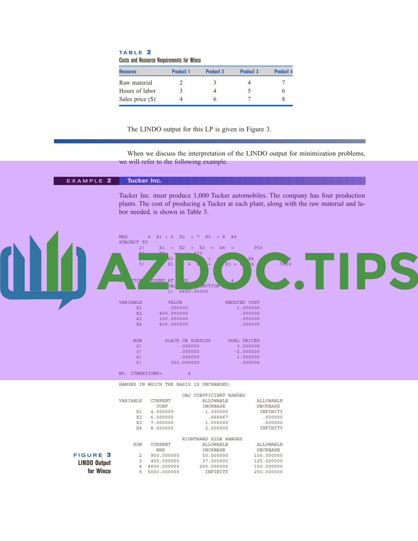
The LINDO output for this LP is given in Figure 3.

When we discuss the interpretation of the LINDO output for minimization problems,

we will refer to the following example.

Tucker Inc. must produce 1,000 Tucker automobiles. The company has four production

plants. The cost of producing a Tucker at each plant, along with the raw material and la-

bor needed, is shown in Table 3.

5 . 2 The Computer and Sensitivity Analysis 233

Tucker Inc.E X A M P L E 2

TA B L E 2

Costs and Resource Requirements for Winco

Resource Product 1 Product 2 Product 3 Product 4

Raw material 2 3 4 7

Hours of labor 3 4 5 6

Sales price ($) 4 6 7 8

MAX 4 X1 + 6 X2 + 7 X3 + 8 X4

SUBJECT TO

2) X1 + X2 + X3 + X4 = 950

3) X4 >= 400

4) 2 X1 + 3 X2 + 4 X3 + 7 X4 <= 4600

5) 3 X1 + 4 X2 + 5 X3 + 6 X4 <= 5000

END

LP OPTIMUM FOUND AT STEP 4

OBJECTIVE FUNCTION VALUE

1) 6650.00000

VARIABLE VALUE REDUCED COST

X1 .000000 1.000000

X2 400.000000 .000000

X3 150.000000 .000000

X4 400.000000 .000000

ROW SLACK OR SURPLUS DUAL PRICES

2) .000000 3.000000

3) .000000 -2.000000

4) .000000 1.000000

5) 250.000000 .000000

NO. ITERATIONS= 4

RANGES IN WHICH THE BASIS IS UNCHANGED:

OBJ COEFFICIENT RANGES

VARIABLE CURRENT ALLOWABLE ALLOWABLE

COEF INCREASE DECREASE

X1 4.000000 1.000000 INFINITY

X2 6.000000 .666667 .500000

X3 7.000000 1.000000 .500000

X4 8.000000 2.000000 INFINITY

RIGHTHAND SIDE RANGES

ROW CURRENT ALLOWABLE ALLOWABLE

RHS INCREASE DECREASE

2 950.000000 50.000000 100.000000

3 400.000000 37.000000 125.000000

4 4600.000000 250.000000 150.000000

5 5000.000000 INFINITY 250.000000

F I G U R E 3

LINDO Output for Winco

The autoworkers’ labor union requires that at least 400 cars be produced at plant 3;

3,300 hours of labor and 4,000 units of raw material are available for allocation to the

four plants. Formulate an LP whose solution will enable Tucker Inc. to minimize the cost

of producing 1,000 cars.

Solution Let xi � number of cars produced at plant i. Then, expressing the objective function in

thousands of dollars, the appropriate LP is

min z � 15x1 � 10x2 � 9x3 � 7x4

s.t. 2x1 � 3x2 � 4x3 � 5x4 � 1000

s.t. 2x1 � 3x2 � 4x3 � 5x4 � 400

s.t. 2x1 � 3x2 � 4x3 � 5x4 � 3300

s.t. 3x1 � 4x2 � 5x3 � 6x4 � 4000

s. t. 2� 4� 5� 6x1, x2, x3, x4 � 0

The LINDO output for this LP is given in Figure 4.

Objective Function Coefficient Ranges

Recall from Section 5.1 that (at least in a two-variable problem) we can determine the

range of values for an objective function coefficient for which the current basis remains

optimal. For each objective function coefficient, this range is given in the OBJECTIVE

COEFFICIENT RANGES portion of the LINDO output. The ALLOWABLE INCREASE

(AI) section indicates the amount by which an objective function coefficient can be in-

creased with the current basis remaining optimal. Similarly, the ALLOWABLE DE-

CREASE (AD) section indicates the amount by which an objective function coefficient

can be decreased with the current basis remaining optimal. To illustrate these ideas, let ci

be the objective function coefficient for xi in Example 1. If c1 is changed, then the cur-

rent basis remains optimal if

�� 4 � � � c1 � 4 � 1 � 5

If c2 is changed, then the current basis remains optimal if

5.5 � 6 � 0.5 � c2 � 6 � 0.666667 � 6.666667

We will refer to the range of variables of ci for which the current basis remains optimal

as the allowable range for ci. As discussed in Section 5.1, if ci remains in its allowable

range then the values of the decision variables remain unchanged, although the optimal

z-value may change. The following examples illustrate these ideas.


TA B L E 3

Cost and Requirements for Producing a Tucker

CostPlant (in Thousands of Dollars) Labor Raw Material

1 15 2 3

2 10 3 4

3 19 4 5

4 17 5 6

a Suppose Winco raises the price of product 2 by 50¢ per unit. What is the new opti-

mal solution to the LP?

b Suppose the sales price of product 1 is increased by 60¢ per unit. What is the new op-

timal solution to the LP?

c Suppose the sales price of product 3 is decreased by 60¢. What is the new optimal so-

lution to the LP?

Solution a Because the AI for c2 is $0.666667, and we are increasing c2 by only $0.5, the cur-

rent basis remains optimal. The optimal values of the decision variables remain unchanged

(x1 � 0, x2 � 400, x3 � 150, and x4 � 400 is still optimal). The new optimal z-value may

be determined in two ways. First, we may simply substitute the optimal values of the de-

cision variables into the new objective function, yielding

New optimal z-value � 4(0) � 6.5(400) � 7(150) � 8(400) � $6,850

Another way to see that the new optimal z-value is $6,850 is to observe the only differ-

ence in sales revenue: Each unit of product 2 brings in 50¢ more in revenue. Thus, total

revenue should increase by 400(.50) � $200, so

New z-value � original z-value � 200 � $6,850

5 . 2 The Computer and Sensitivity Analysis 235

Interpretation of Objective Function Coefficients Sensitivity AnalysisE X A M P L E 3

MIN 15 X1 + 10 X2 + 9 X3 + 7 X4

SUBJECT TO

2) X1 + X2 + X3 + X4 = 1000

3) X3 >= 400

4) 2 X1 + 3 X2 + 4 X3 + 5 X4 <= 3300

5) 3 X1 + 4 X2 + 5 X3 + 6 X4 <= 4000

END

LP OPTIMUM FOUND AT STEP 3

OBJECTIVE FUNCTION VALUE

1) 11600.0000

VARIABLE VALUE REDUCED COST

X1 400.000000 .000000

X2 200.000000 .000000

X3 400.000000 .000000

X4 .000000 7.000000

ROW SLACK OR SURPLUS DUAL PRICES

2) .000000 -30.000000

3) .000000 -4.000000

4) 300.000000 .000000

5) .000000 5.000000

NO. ITERATIONS= 3

RANGES IN WHICH THE BASIS IS UNCHANGED:

OBJ COEFFICIENT RANGES

VARIABLE CURRENT ALLOWABLE ALLOWABLE

COEF INCREASE DECREASE

X1 15.000000 INFINITY 3.500000

X2 10.000000 2.000000 INFINITY

X3 9.000000 INFINITY 4.000000

X4 7.000000 INFINITY 7.000000

RIGHTHAND SIDE RANGES

ROW CURRENT ALLOWABLE ALLOWABLE

RHS INCREASE DECREASE

2 1000.000000 66.666660 100.000000

3 400.000000 100.000000 400.000000

4 3300.000000 INFINITY 300.000000

5 4000.000000 300.000000 200.000000

F I G U R E 4

LINDO Output for Tucker

b The AI for c1 is 1, so the current basis remains optimal, and the optimal values of the

decision variables remain unchanged. Because the value of x1 in the optimal solution is

0, the change in the sales price for product 1 will not change the optimal z-value—it will

remain $6,650.

c For c3, AD � .50, so the current basis is no longer optimal. Without resolving the

problem by hand or on the computer, we cannot determine the new optimal solution.

Reduced Costs and Sensitivity Analysis

The REDUCED COST portion of the LINDO output gives us information about how

changing the objective function coefficient for a nonbasic variable will change the LP’s

optimal solution. For simplicity, let’s assume that the current optimal bfs is nondegener-

ate (that is, if the LP has m constraints, then the current optimal solution has m variables

assuming positive values). For any nonbasic variable xk, the reduced cost is the amount

by which the objective function coefficient of xk must be improved before the LP will have

an optimal solution in which xk is a basic variable. If the objective function coefficient of

a nonbasic variable xk is improved by its reduced cost, then the LP will have alternative

optimal solutions—at least one in which xk is a basic variable, and at least one in which

xk is not a basic variable. If the objective function coefficient of a nonbasic variable xk is

improved by more than its reduced cost, then (barring degeneracy) any optimal solution

to the LP will have xk as a basic variable and xk � 0. To illustrate these ideas, note that

in Example 1 the basic variables associated with the optimal solution are x2, x3, x4, and

s4 (the slack for the labor constraint). The nonbasic variable x1 has a reduced cost of $1.

This implies that if we increase x1’s objective function coefficient (in this case, the sales

price per unit of x1) by exactly $1, then there will be alternative optimal solutions, at least

one of which will have x1 as a basic variable. If we increase x1’s objective function coef-

ficient by more than $1, then (because the current optimal bfs is nondegenerate) any op-

timal solution to the LP will have x1 as a basic variable (with x1 � 0). Thus, the reduced

cost for x1 is the amount by which x1 “misses the optimal basis.” We must keep a close

watch on x1’s sales price, because a slight increase will change the LP’s optimal solution.

Let’s now consider Example 2, a minimization problem. Here the basic variables as-

sociated with the optimal solution are x1, x2, x3, and s3 (the slack variable for the labor

constraint). Again, the optimal bfs is nondegenerate. The nonbasic variable x4 has a re-

duced cost of 7 ($7,000), so we know that if the cost of producing x4 is decreased by 7,

then there will be alternative optimal solutions. In at least one of these optimal solutions,

x4 will be a basic variable. If the cost of producing x4 is lowered by more than 7, then

(because the current optimal solution is nondegenerate) any optimal solution to the LP

will have x4 as a basic variable (with x4 � 0).

Right-Hand Side Ranges

Recall from Section 5.1 that we can determine (at least for a two-variable problem) the

range of values for a right-hand side within which the current basis remains optimal. This

information is given in the RIGHTHAND SIDE RANGES section of the LINDO output.

To illustrate, consider the first constraint in Example 1. Currently, the right-hand side of

this constraint (call it b1) is 950. The current basis remains optimal if b1 is decreased by

up to 100 (the allowable decrease, or AD, for b1) or increased by up to 50 (the allowable

increase, or AI, for b1). Thus, the current basis remains optimal if


5 sensitivity analysis an applied approach

Documents

Transcript of 5 sensitivity analysis an applied approach