5 Equations of State and Phase Equilibria
126
5 Equations of State and Phase Equilibria A PHASE IS THE PART OF A SYSTEM that is uniform in physical and chemical properties, homogeneous in composition, and separated from other, coexisting phases by definite boundary surfaces. The most important phases occurring in petroleum production are the hydrocarbon liquid phase and gas phase. Water is also commonly present as an additional liquid phase. These can coexist in equilibrium when the variables describing change in the entire system remain constant in time and position. The chief variables that determine the state of equilibrium are system temperature, system pressure, and composition. The conditions under which these different phases can exist are a matter of consider- able practical importance in designing surface separation facilities and developing compo- sitional models. These types of calculations are based on the following two concepts, equilibrium ratios and flash calculations, which are discussed next. Equilibrium Ratios As indicated in Chapter 1, a system that contains only one component is considered the simplest type of hydrocarbon system. The word component refers to the number of molec- ular or atomic species present in the substance. A single-component system is composed entirely of one kind of atom or molecule. We often use the word pure to describe a single- component system. The qualitative understanding of the relationship that exists between temperature, T, pressure, p , and volume, V, of pure components can provide an excellent basis for understanding the phase behavior of complex hydrocarbon mixtures. In a multicomponent system, the equilibrium ratio, K i , of a given component is defined as the ratio of the mole fraction of the component in the gas phase, y i , to the mole 331
-
Upload
independent -
Category
Documents
-
view
2 -
download
0
Transcript of 5 Equations of State and Phase Equilibria

5
Equations of State and Phase Equilibria
A PHASE IS THE PART OF A SYSTEM that is uniform in physical and chemical properties,homogeneous in composition, and separated from other, coexisting phases by definiteboundary surfaces. The most important phases occurring in petroleum production are thehydrocarbon liquid phase and gas phase. Water is also commonly present as an additionalliquid phase. These can coexist in equilibrium when the variables describing change in theentire system remain constant in time and position. The chief variables that determine thestate of equilibrium are system temperature, system pressure, and composition.
The conditions under which these different phases can exist are a matter of consider-able practical importance in designing surface separation facilities and developing compo-sitional models. These types of calculations are based on the following two concepts,equilibrium ratios and flash calculations, which are discussed next.
Equilibrium Ratios
As indicated in Chapter 1, a system that contains only one component is considered thesimplest type of hydrocarbon system. The word component refers to the number of molec-ular or atomic species present in the substance. A single-component system is composedentirely of one kind of atom or molecule. We often use the word pure to describe a single-component system. The qualitative understanding of the relationship that exists betweentemperature, T, pressure, p , and volume, V, of pure components can provide an excellentbasis for understanding the phase behavior of complex hydrocarbon mixtures.
In a multicomponent system, the equilibrium ratio, Ki, of a given component isdefined as the ratio of the mole fraction of the component in the gas phase, yi , to the mole
331
Ahmed_ch5.qxd 12/21/06 2:05 PM Page 331
fraction of the component in the liquid phase, xi. Mathematically, the relationship isexpressed as
(5–1)
where
Ki = equilibrium ratio of component iyi = mole fraction of component i in the gas phasexi = mole fraction of component i in the liquid phase
At pressures below 100 psia, Raoult’s and Dalton’s laws for ideal solutions provide asimplified means of predicting equilibrium ratios. Raoult’s law states that the partial pres-sure, pi, of a component in a multicomponent system is the product of its mole fraction inthe liquid phase, xi , and the vapor pressure of the component, pvi:
pi = xipvi (5–2)
where
pi = partial pressure of a component i, psiapvi = vapor pressure of component i, psiaxi = mole fraction of component i in the liquid phase
Dalton’s law states that the partial pressure of a component is the product of its mole frac-tion in the gas phase, yi, and the total pressure of the system, p:
pi = yi p (5–3)
where p = total system pressure, psia.At equilibrium and in accordance with the previously cited laws, the partial pressure
exerted by a component in the gas phase must be equal to the partial pressure exerted bythe same component in the liquid phase. Therefore, equating the equations describing thetwo laws yields the following:
xi pvi = yi p
Rearranging the preceding relationship and introducing the concept of the equilibriumratio gives
(5–4)
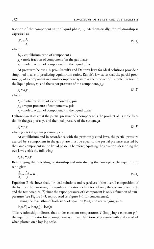
Equation (5–4) shows that, for ideal solutions and regardless of the overall composition ofthe hydrocarbon mixture, the equilibrium ratio is a function of only the system pressure, p,and the temperature, T, since the vapor pressure of a component is only a function of tem-perature (see Figure 1–3, reproduced as Figure 5–1 for convenience).
Taking the logarithm of both sides of equation (5–4) and rearranging gives
log(Ki) = log(pvi) – log(p)
This relationship indicates that under constant temperature, T (implying a constant pvi),the equilibrium ratio for a component is a linear function of pressure with a slope of –1when plotted on a log-log scale.
yx
pp
Ki
ii= =vi
Kyxi
i
i
=
332 equations of state and pvt analysis
Ahmed_ch5.qxd 12/21/06 2:05 PM Page 332
equations of state and phase equilibria 333
FIG
UR
E 5
–1Va
por
pres
sure
char
t for
hyd
roca
rbon
com
pone
nts.
Sour
ce: G
PSA
Eng
inee
ring
Dat
a Bo
ok, 1
0th
ed. T
ulsa
, OK
: Gas
Pro
cess
ors
Supp
liers
Ass
ocia
tion,
198
7. C
ourt
esy
of th
e G
as P
roce
s-so
rs S
uppl
iers
Ass
ocia
tion.
Ahmed_ch5.qxd 12/21/06 2:05 PM Page 333
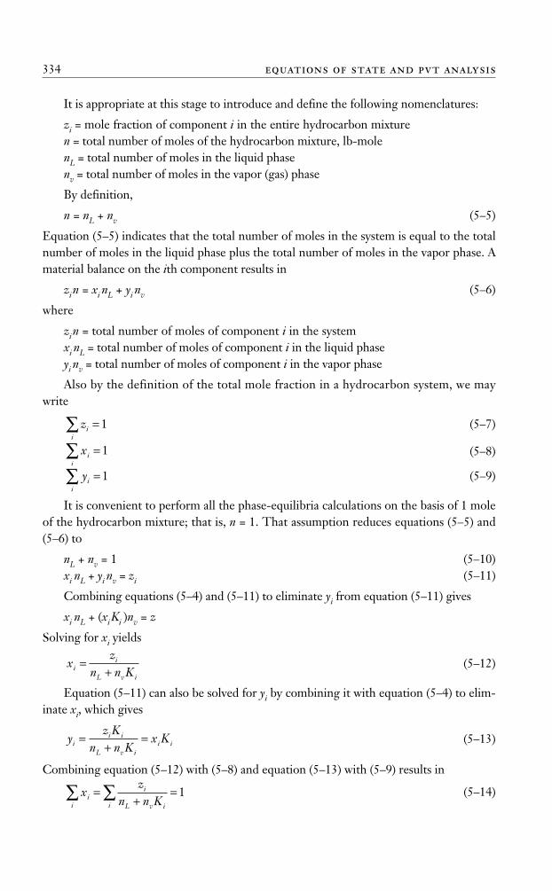
It is appropriate at this stage to introduce and define the following nomenclatures:
zi = mole fraction of component i in the entire hydrocarbon mixturen = total number of moles of the hydrocarbon mixture, lb-molenL = total number of moles in the liquid phasenv = total number of moles in the vapor (gas) phase
By definition,
n = nL + nv (5–5)
Equation (5–5) indicates that the total number of moles in the system is equal to the totalnumber of moles in the liquid phase plus the total number of moles in the vapor phase. Amaterial balance on the ith component results in
zin = xi nL + yi nv (5–6)
where
zin = total number of moles of component i in the systemxi nL = total number of moles of component i in the liquid phaseyi nv = total number of moles of component i in the vapor phase
Also by the definition of the total mole fraction in a hydrocarbon system, we maywrite
(5–7)
(5–8)
(5–9)
It is convenient to perform all the phase-equilibria calculations on the basis of 1 moleof the hydrocarbon mixture; that is, n = 1. That assumption reduces equations (5–5) and(5–6) to
nL + nv = 1 (5–10)xi nL + yi nv = zi (5–11)
Combining equations (5–4) and (5–11) to eliminate yi from equation (5–11) gives
xi nL + (xiKi )nv = z
Solving for xi yields
(5–12)
Equation (5–11) can also be solved for yi by combining it with equation (5–4) to elim-inate xi, which gives
(5–13)
Combining equation (5–12) with (5–8) and equation (5–13) with (5–9) results in
(5–14)xz
n n Kii
i
L v ii∑ ∑= +
=1
yz K
n n Kx Ki
i i
L v ii i=
+=
xz
n n Kii
L v i
=+
yii∑ =1
xii∑ =1
zii∑ =1
334 equations of state and pvt analysis
Ahmed_ch5.qxd 12/21/06 2:05 PM Page 334
(5–15)
Since
then
Rearranging gives
Replacing nL with (1 – nv) yields
(5–16)
This set of equations provides the necessary phase relationships to perform volumetricand compositional calculations on a hydrocarbon system. These calculations are referredto as flash calculations, as described next.
Flash Calculations
Flash calculations are an integral part of all reservoir and process engineering calculations.They are required whenever it is desirable to know the amounts (in moles) of hydrocarbonliquid and gas coexisting in a reservoir or a vessel at a given pressure and temperature.These calculations also are performed to determine the composition of the existing hydro-carbon phases.
Given the overall composition of a hydrocarbon system at a specified pressure andtemperature, flash calculations are performed to determine the moles of the gas phase, nv,moles of the liquid phase, nL, composition of the liquid phase, xi, and composition of thegas phase, yi. The computational steps for determining nL, nv, yi, and xi of a hydrocarbonmixture with a known overall composition of zi and characterized by a set of equilibriumratios, Ki, are summarized in the following steps.
Step 1 Calculate nv. Equation (5–16) can be solved for the number of moles of the vaporphase nv by using the Newton-Raphson iteration technique. In applying this iterative tech-nique, do the following.
Assume any arbitrary value of nv between 0 and 1, such as nv = 0.5. A good assumedvalue may be calculated from the following relationship:
nv = A/(A + B)
where
A = z Ki ii
−( )⎡⎣ ⎤⎦∑ 1
f nz K
n Kvi i
v ii
( )( )
( )=
−− +
=∑ 11 1
0
z Kn n K
i i
L V ii
( )−+
=∑ 10
z Kn n K
zn n K
i i
L v ii
i
L v ii+−
+=∑ ∑ 0
y xii
ii
∑ ∑− = 0
yz K
n n Kii
i i
L v ii∑ ∑= +
=1
equations of state and phase equilibria 335
Ahmed_ch5.qxd 12/21/06 2:05 PM Page 335
B =
These expressions could yield a starting value for nv, providing that the values of the equilib-rium ratios are accurate. Note that the assumed value of nv must be between 0 and 1; that is,0 < nv < 1.
Evaluate the function f (nv) as given by equation (5–16) using the assumed (old) value of nv:
If the absolute value of the function f (nv) is smaller than a preset tolerance, such as10–6, then the assumed value of nv is the desired solution.
If the absolute value of f (nv) is greater than the preset tolerance, then a new value of(nv)new is calculated from the following expression:
with the derivative f '(nv) as given by
where (nv)n is the new value of nv to be used for the next iteration.This procedure is repeated with the new value of nv until convergence is achieved, that
is, when
|f (nv )| ≤ eps
or
|(nv )new – (nv )| ≤ eps
in which eps is a selected tolerance, such as eps = 10–6.
Step 2 Calculate nL. The number of moles of the liquid phase can be calculated by apply-ing equation (5–10) to give
nL + nv = 1
or
nL = 1 – nv
Step 3 Calculation of xi. Calculate the composition of the liquid phase by applying equa-tion (5–12):
Step 4 Calculation of yi. Determine the composition of the gas phase from equation (5–13):
yz K
n n Kx Ki
i i
L v ii i=
+=
xz
n n Kii
L v i
=+
′ =−−− +
⎧⎨⎩
⎫⎬⎭
∑f nz K
n Kvi i
v ii
( )( )
[ ( ) ]1
1 1
2
2
( )( )( )
n nf nf nv v
v
vnew = −
′
f nz K
n Kvi i
v ii
( )( )
( )=
−− +∑ 1
1 1
zKi
ii
11−
⎛⎝⎜
⎞⎠⎟
⎡
⎣⎢
⎤
⎦⎥∑
336 equations of state and pvt analysis
Ahmed_ch5.qxd 12/21/06 2:05 PM Page 336

EXAMPLE 5–1
A hydrocarbon mixture with the following overall composition is flashed in a separator at50 psia and 100°F:
COMPONENT ziC3 0.20i-C4 0.10n-C4 0.10i-C5 0.20n-C5 0.20C6 0.20
Assuming an ideal solution behavior, perform flash calculations.
SOLUTION
Step 1 Determine the vapor pressure pvi from the Cox chart (Figure 5–1) and calculate theequilibrium ratios using equation (5–4). The results are shown below.
COMPONENT zi pvi at 100°F Ki = pvi/50C3 0.20 190 3.80i-C4 0.10 72.2 1.444n-C4 0.10 51.6 1.032i-C5 0.20 20.44 0.4088n-C5 0.20 15.57 0.3114C6 0.20 4.956 0.09912
Step 2 Solve equation (5–16) for nv using the Newton-Raphson method:
ITERATION nv f(nv)0 0.08196579 3.073(10–2)1 0.1079687 8.894(10–4)2 0.1086363 7.60(10–7)3 0.1086368 1.49(10–8)4 0.1086368 0.0
to give nv = 0.1086368.
Step 3 Solve for nL:
nL = 1 – nv
nL = 1 – 0.1086368 = 0.8913631
Step 4 Solve for xi and yi to yield
yi = xi Ki
xz
n n Kii
L v i
=+
( )( )( )
n nf nf nv n v
v
v
= −′
equations of state and phase equilibria 337
Ahmed_ch5.qxd 12/21/06 2:05 PM Page 337
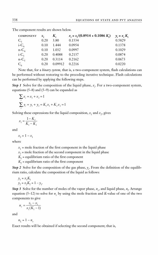
The component results are shown below.
COMPONENT zi Ki xi = zi/(0.8914 + 0.1086 Ki) yi = xi KiC3 0.20 3.80 0.1534 0.5829i-C4 0.10 1.444 0.0954 0.1378n-C4 0.10 1.032 0.0997 0.1029i-C5 0.20 0.4088 0.2137 0.0874n-C5 0.20 0.3114 0.2162 0.0673C6 0.20 0.09912 0.2216 0.0220
Note that, for a binary system, that is, a two-component system, flash calculations canbe performed without restoring to the preceding iterative technique. Flash calculationscan be performed by applying the following steps.
Step 1 Solve for the composition of the liquid phase, xi. For a two-component system,equations (5–8) and (5–9) can be expanded as
Solving these expressions for the liquid composition, x1 and x2, gives
and
x2 = 1 – x1
where
x1 = mole fraction of the first component in the liquid phasex2 = mole fraction of the second component in the liquid phaseK1 = equilibrium ratio of the first componentK2 = equilibrium ratio of the first component
Step 2 Solve for the composition of the gas phase, yi. From the definition of the equilib-rium ratio, calculate the composition of the liquid as follows:
y1 = x1K1
y2 = x2K2 = 1 – y1.
Step 3 Solve for the number of moles of the vapor phase, nv, and liquid phase, nl. Arrangeequation (5–12) to solve for nv by using the mole fraction and K-value of one of the twocomponents to give
and
nL = 1 – nv
Exact results will be obtained if selecting the second component; that is,
nz x
x Kv =−−
1 1
1 1 1( )
xK
K K12
1 2
1=
−−
y y y K x K xii∑ = + = + =1 2 1 1 2 2 1
x x xii∑ = + =1 2 1
338 equations of state and pvt analysis
Ahmed_ch5.qxd 12/21/06 2:05 PM Page 338
and
nL = 1 – nv
where
z1 = mole fraction of the first component in the binary systemx1 = mole fraction of the first component in the liquid phasez2 = mole fraction of the second component in the binary systemx2 = mole fraction of the second component in the liquid phaseK1 = equilibrium ratio of the first componentK2 = equilibrium ratio of the second component
The equilibrium ratios, which indicate the partitioning of each component between theliquid phase and gas phases, as calculated by equation (5–4) in terms of vapor pressure andsystem pressure, proved inadequate. The basic assumptions behind equation (5–4 ) are that:
• The vapor phase is an ideal gas as described by Dalton’s law.
• The liquid phase is an ideal solution as described by Raoult’s law.
The combination of assumptions is unrealistic and results in inaccurate predictions ofequilibrium ratios at high pressures.
Equilibrium Ratios for Real Solutions
For a real solution, the equilibrium ratios are no longer a function of the pressure andtemperature alone but also the composition of the hydrocarbon mixture. This observationcan be stated mathematically as
Ki = K( p, T, zi )
Numerous methods have been proposed for predicting the equilibrium ratios ofhydrocarbon mixtures. These correlations range from a simple mathematical expression toa complicated expression containing several compositional dependent variables. The fol-lowing methods are presented: Wilson’s correlation, Standing’s correlation, the conver-gence pressure method, and Whitson and Torp’s correlation.
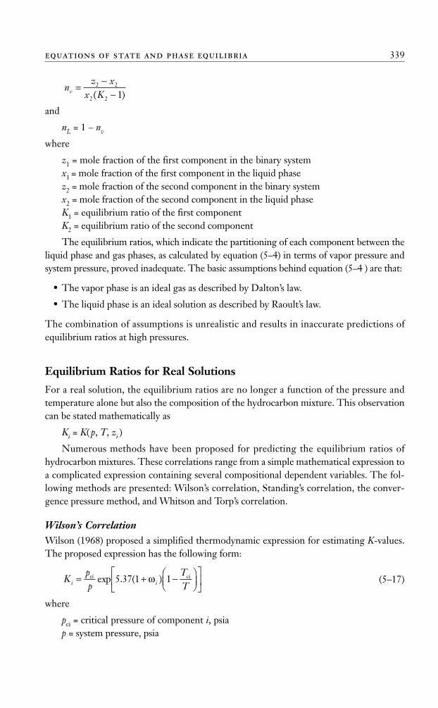
Wilson’s CorrelationWilson (1968) proposed a simplified thermodynamic expression for estimating K-values.The proposed expression has the following form:
(5–17)
where
pci = critical pressure of component i, psiap = system pressure, psia
Kpp
TTi i= + −⎛
⎝⎜⎞⎠⎟
⎡
⎣⎢
⎤
⎦⎥
ci ciexp . ( )5 37 1 1ω
nz x
x Kv =−−
2 2
2 2 1( )
equations of state and phase equilibria 339
Ahmed_ch5.qxd 12/21/06 2:05 PM Page 339
Tci = critical temperature of component i, °RT = system temperature, °R
This relationship generates reasonable values for the equilibrium ratio when applied atlow pressures.
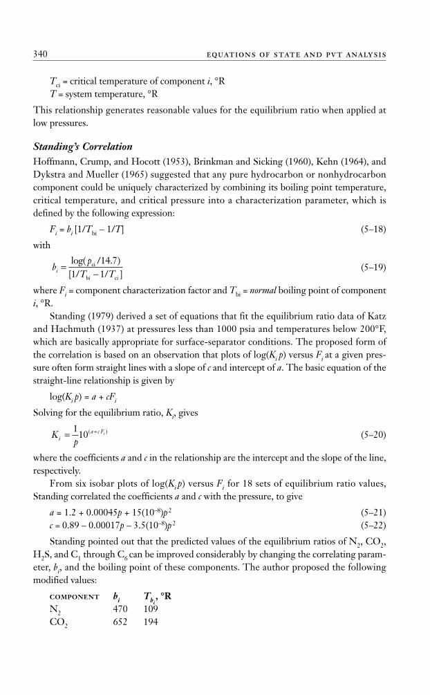
Standing’s CorrelationHoffmann, Crump, and Hocott (1953), Brinkman and Sicking (1960), Kehn (1964), andDykstra and Mueller (1965) suggested that any pure hydrocarbon or nonhydrocarboncomponent could be uniquely characterized by combining its boiling point temperature,critical temperature, and critical pressure into a characterization parameter, which isdefined by the following expression:
Fi = bi [1/Tbi – 1/T] (5–18)
with
(5–19)
where Fi = component characterization factor and Tbi = normal boiling point of componenti, °R.
Standing (1979) derived a set of equations that fit the equilibrium ratio data of Katzand Hachmuth (1937) at pressures less than 1000 psia and temperatures below 200°F,which are basically appropriate for surface-separator conditions. The proposed form ofthe correlation is based on an observation that plots of log(Ki p) versus Fi at a given pres-sure often form straight lines with a slope of c and intercept of a. The basic equation of thestraight-line relationship is given by
log(Ki p) = a + cFi
Solving for the equilibrium ratio, Ki, gives
(5–20)
where the coefficients a and c in the relationship are the intercept and the slope of the line,respectively.
From six isobar plots of log(Ki p) versus Fi for 18 sets of equilibrium ratio values,Standing correlated the coefficients a and c with the pressure, to give
a = 1.2 + 0.00045p + 15(10–8)p2 (5–21)c = 0.89 – 0.00017p – 3.5(10–8)p2 (5–22)
Standing pointed out that the predicted values of the equilibrium ratios of N2, CO2,H2S, and C1 through C6 can be improved considerably by changing the correlating param-eter, bi, and the boiling point of these components. The author proposed the followingmodified values:
COMPONENT bi Tbi, °R
N2 470 109CO2 652 194
Kpi
a c Fi= +110( )
bp
T Ti = −log( / . )
[ / / ]ci
bi ci
14 71 1
340 equations of state and pvt analysis
Ahmed_ch5.qxd 12/21/06 2:05 PM Page 340
COMPONENT bi Tbi, °R
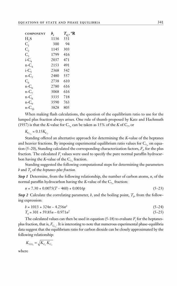
H2S 1136 331C1 300 94C2 1145 303C3 1799 416i-C4 2037 471n-C4 2153 491i-C5 2368 542n-C5 2480 557C6 2738 610n-C6 2780 616n-C7 3068 616n-C8 3335 718n-C9 3590 763n-C10 3828 805
When making flash calculations, the question of the equilibrium ratio to use for thelumped plus fraction always arises. One rule of thumb proposed by Katz and Hachmuth(1937) is that the K-value for C7+ can be taken as 15% of the K of C7, or
KC7+= 0.15KC7
Standing offered an alternative approach for determining the K-value of the heptanesand heavier fractions. By imposing experimental equilibrium ratio values for C7+ on equa-tion (5–20), Standing calculated the corresponding characterization factors, Fi, for the plusfraction. The calculated Fi values were used to specify the pure normal paraffin hydrocar-bon having the K-value of the C7+ fraction.
Standing suggested the following computational steps for determining the parametersb and Tb of the heptanes-plus fraction.
Step 1 Determine, from the following relationship, the number of carbon atoms, n, of thenormal paraffin hydrocarbon having the K-value of the C7+ fraction:
n = 7.30 + 0.0075(T – 460) + 0.0016p (5–23)
Step 2 Calculate the correlating parameter, b, and the boiling point, Tb, from the follow-ing expression:
b = 1013 + 324n – 4.256n2 (5–24)Tb = 301 + 59.85n – 0.971n2 (5–25)
The calculated values can then be used in equation (5-18) to evaluate Fi for the heptanes-plus fraction, that is, FC7+
. It is interesting to note that numerous experimental phase-equilibriadata suggest that the equilibrium ratio for carbon dioxide can be closely approximated by thefollowing relationship:
where
K K KCO C C2 2=
1
equations of state and phase equilibria 341
Ahmed_ch5.qxd 12/21/06 2:05 PM Page 341
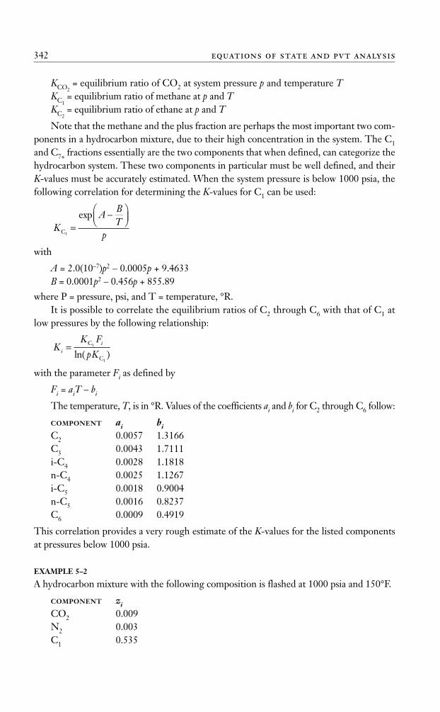
KCO2= equilibrium ratio of CO2 at system pressure p and temperature T
KC1= equilibrium ratio of methane at p and T
KC2= equilibrium ratio of ethane at p and T
Note that the methane and the plus fraction are perhaps the most important two com-ponents in a hydrocarbon mixture, due to their high concentration in the system. The C1
and C7+ fractions essentially are the two components that when defined, can categorize thehydrocarbon system. These two components in particular must be well defined, and theirK-values must be accurately estimated. When the system pressure is below 1000 psia, thefollowing correlation for determining the K-values for C1 can be used:
with
A = 2.0(10–7)p2 – 0.0005p + 9.4633B = 0.0001p2 – 0.456p + 855.89
where P = pressure, psi, and T = temperature, °R.It is possible to correlate the equilibrium ratios of C2 through C6 with that of C1 at
low pressures by the following relationship:
with the parameter Fi as defined by
Fi = aiT – bi
The temperature, T, is in °R. Values of the coefficients ai and bi for C2 through C6 follow:
COMPONENT ai biC2 0.0057 1.3166C3 0.0043 1.7111i-C4 0.0028 1.1818n-C4 0.0025 1.1267i-C5 0.0018 0.9004n-C5 0.0016 0.8237C6 0.0009 0.4919
This correlation provides a very rough estimate of the K-values for the listed componentsat pressures below 1000 psia.
EXAMPLE 5–2
A hydrocarbon mixture with the following composition is flashed at 1000 psia and 150°F.
COMPONENT ziCO2 0.009N2 0.003C1 0.535
KK F
pKii= C
C
1
1ln( )
KA
BT
pC1=
−⎛⎝⎜
⎞⎠⎟
exp
342 equations of state and pvt analysis
Ahmed_ch5.qxd 12/21/06 2:05 PM Page 342
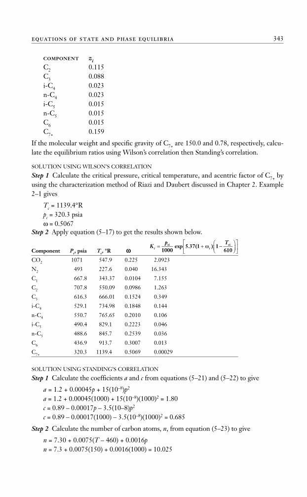
COMPONENT ziC2 0.115C3 0.088i-C4 0.023n-C4 0.023i-C5 0.015n-C5 0.015C6 0.015C7+ 0.159
If the molecular weight and specific gravity of C7+ are 150.0 and 0.78, respectively, calcu-late the equilibrium ratios using Wilson’s correlation then Standing’s correlation.
SOLUTION USING WILSON’S CORRELATION
Step 1 Calculate the critical pressure, critical temperature, and acentric factor of C7+ byusing the characterization method of Riazi and Daubert discussed in Chapter 2. Example2–1 gives
Tc = 1139.4°Rpc = 320.3 psia ω = 0.5067
Step 2 Apply equation (5–17) to get the results shown below.
Component Pc, psia Tc, °R ωωCO2 1071 547.9 0.225 2.0923
N2 493 227.6 0.040 16.343
C1 667.8 343.37 0.0104 7.155
C2 707.8 550.09 0.0986 1.263
C3 616.3 666.01 0.1524 0.349
i-C4 529.1 734.98 0.1848 0.144
n-C4 550.7 765.65 0.2010 0.106
i-C5 490.4 829.1 0.2223 0.046
n-C5 488.6 845.7 0.2539 0.036
C6 436.9 913.7 0.3007 0.013
C7+ 320.3 1139.4 0.5069 0.00029
SOLUTION USING STANDING’S CORRELATION
Step 1 Calculate the coefficients a and c from equations (5–21) and (5–22) to give
a = 1.2 + 0.00045p + 15(10–8)p2
a = 1.2 + 0.00045(1000) + 15(10–8)(1000)2 = 1.80c = 0.89 – 0.00017p – 3.5(10–8)p2
c = 0.89 – 0.00017(1000) – 3.5(10–8)(1000)2 = 0.685
Step 2 Calculate the number of carbon atoms, n, from equation (5–23) to give
n = 7.30 + 0.0075(T – 460) + 0.0016pn = 7.3 + 0.0075(150) + 0.0016(1000) = 10.025
Kp T
i i= + −⎛⎝⎜
⎞⎠⎟
⎡
⎣⎢
⎤
⎦⎥
ci ci
10005 37 1 1
610exp . ( )ω
equations of state and phase equilibria 343
Ahmed_ch5.qxd 12/21/06 2:05 PM Page 343
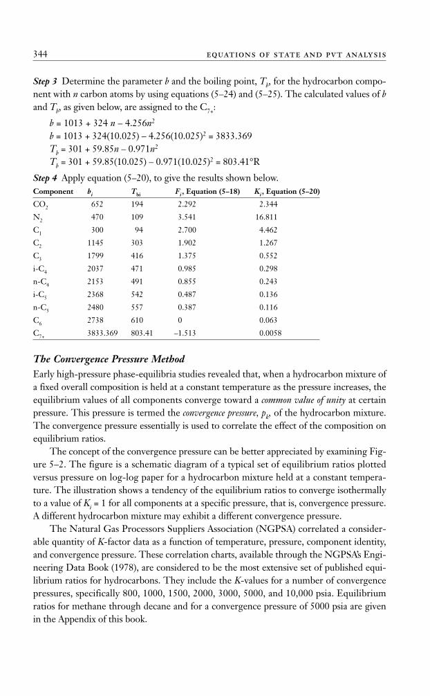
Step 3 Determine the parameter b and the boiling point, Tb, for the hydrocarbon compo-nent with n carbon atoms by using equations (5–24) and (5–25). The calculated values of band Tb, as given below, are assigned to the C7+:
b = 1013 + 324 n – 4.256n2
b = 1013 + 324(10.025) – 4.256(10.025)2 = 3833.369Tb = 301 + 59.85n – 0.971n2
Tb = 301 + 59.85(10.025) – 0.971(10.025)2 = 803.41°R
Step 4 Apply equation (5–20), to give the results shown below.Component bi Tbi Fi , Equation (5–18) Ki , Equation (5–20)
CO2 652 194 2.292 2.344
N2 470 109 3.541 16.811
C1 300 94 2.700 4.462
C2 1145 303 1.902 1.267
C3 1799 416 1.375 0.552
i-C4 2037 471 0.985 0.298
n-C4 2153 491 0.855 0.243
i-C5 2368 542 0.487 0.136
n-C5 2480 557 0.387 0.116
C6 2738 610 0 0.063
C7+ 3833.369 803.41 –1.513 0.0058
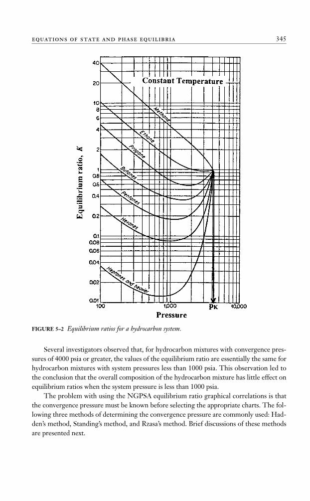
The Convergence Pressure MethodEarly high-pressure phase-equilibria studies revealed that, when a hydrocarbon mixture ofa fixed overall composition is held at a constant temperature as the pressure increases, theequilibrium values of all components converge toward a common value of unity at certainpressure. This pressure is termed the convergence pressure, pk, of the hydrocarbon mixture.The convergence pressure essentially is used to correlate the effect of the composition onequilibrium ratios.
The concept of the convergence pressure can be better appreciated by examining Fig-ure 5–2. The figure is a schematic diagram of a typical set of equilibrium ratios plottedversus pressure on log-log paper for a hydrocarbon mixture held at a constant tempera-ture. The illustration shows a tendency of the equilibrium ratios to converge isothermallyto a value of Ki = 1 for all components at a specific pressure, that is, convergence pressure.A different hydrocarbon mixture may exhibit a different convergence pressure.
The Natural Gas Processors Suppliers Association (NGPSA) correlated a consider-able quantity of K-factor data as a function of temperature, pressure, component identity,and convergence pressure. These correlation charts, available through the NGPSA’s Engi-neering Data Book (1978), are considered to be the most extensive set of published equi-librium ratios for hydrocarbons. They include the K-values for a number of convergencepressures, specifically 800, 1000, 1500, 2000, 3000, 5000, and 10,000 psia. Equilibriumratios for methane through decane and for a convergence pressure of 5000 psia are givenin the Appendix of this book.
344 equations of state and pvt analysis
Ahmed_ch5.qxd 12/21/06 2:05 PM Page 344
Several investigators observed that, for hydrocarbon mixtures with convergence pres-sures of 4000 psia or greater, the values of the equilibrium ratio are essentially the same forhydrocarbon mixtures with system pressures less than 1000 psia. This observation led tothe conclusion that the overall composition of the hydrocarbon mixture has little effect onequilibrium ratios when the system pressure is less than 1000 psia.
The problem with using the NGPSA equilibrium ratio graphical correlations is thatthe convergence pressure must be known before selecting the appropriate charts. The fol-lowing three methods of determining the convergence pressure are commonly used: Had-den’s method, Standing’s method, and Rzasa’s method. Brief discussions of these methodsare presented next.
equations of state and phase equilibria 345
FIGURE 5–2 Equilibrium ratios for a hydrocarbon system.
Ahmed_ch5.qxd 12/21/06 2:05 PM Page 345

Hadden’s MethodHadden (1953) developed an iterative procedure for calculating the convergence pressureof the hydrocarbon mixture. The procedure is based on forming a “binary system” thatdescribes the entire hydrocarbon mixture. One component in the binary system is selectedas the lightest fraction in the hydrocarbon system, and the other is treated as a “pseudo-component” that lumps together all the remaining fractions. The binary system conceptuses the binary system convergence pressure chart, shown in Figure 5–3, to determine thepk of the mixture at the specified temperature.
The equivalent binary system concept employs the following steps for determiningthe convergence pressure.
Step 1 Estimate a value for the convergence pressure.
Step 2 From the appropriate equilibrium ratio charts, read the K-values of each compo-nent in the mixture by entering the charts with the system pressure and temperature.
Step 3 Perform flash calculations using the calculated K-values and system composition.
Step 4 Identify the lightest hydrocarbon component that constitutes at least 0.1 mol% inthe liquid phase.
Step 5 Convert the liquid mole fraction to weight fraction.
Step 6 Exclude the lightest hydrocarbon component, as identified in step 4, and normalizethe weight fractions of the remaining components.
Step 7 Calculate the weight average critical temperature and pressure of the lumped com-ponents (pseudo-component) from the following expressions:
T w Tii
pc ci==∑ *
2
346 equations of state and pvt analysis
FIGURE 5–3 Convergence pressures for binary systems.Source: GPSA Engineering Data Book, 10th ed. Tulsa, OK: Gas Processors Suppliers Association, 1987. Courtesy of theGas Processors Suppliers Association.
Ahmed_ch5.qxd 12/21/06 2:05 PM Page 346
where
wi* = normalized weight fraction of component iTpc = pseudo-critical temperature, °Rppc = pseudo-critical pressure, psi
Step 8 Enter into Figure 5–3 the critical properties of the pseudo component and tracethe critical locus of the binary consisting of the light component and the pseudo compo-nent.
Step 9 Read the new convergence pressure (ordinate) from the point at which the locuscrosses the temperature of interest.
Step 10 If the calculated new convergence pressure is not reasonably close to the assumedvalue, repeat steps 2 through 9.
Note that, when the calculated new convergence pressure is between values for whichcharts are provided, interpolation between charts might be necessary. If the K-values donot change rapidly with the convergence pressure, then the set of charts nearest to the cal-culated pk may be used.
Standing’s MethodStanding (1977) suggested that the convergence pressure could be roughly correlated lin-early with the molecular weight of the heptanes-plus fraction. Whitson and Torp (1981)expressed this relationship by the following equation:
pk = 60MC7+– 4200 (5–26)
where MC7+is the molecular weight of the heptanes-plus fraction.
Rzasa’s MethodRzasa, Glass, and Opfell (1952) presented a simplified graphical correlation for predictingthe convergence pressure of light hydrocarbon mixtures. They used the temperature and theproduct of the molecular weight and specific gravity of the heptane-plus fraction as correlat-ing parameters. A graphical illustration of the proposed correlation is shown in Figure 5–4.
The graphical correlation is expressed mathematically by the following equation:
(5–27)
where
(M)C7+= molecular weight of C7+
(γ)C7+= specific gravity of C7+
T = temperature, in °Ra1–a3 = coefficients of the correlation with the following values:
a1 = 6124.3049a2 = –2753.2538a3 = 415.42049
p M aM
k ii
= − + +=∑2381 8542 46 341487
1
3
. . [ ]( )
γγ
CC
7+
77+
T
i
−⎡
⎣⎢
⎤
⎦⎥460
p w pii
pc ci==∑ *
2
equations of state and phase equilibria 347
Ahmed_ch5.qxd 12/21/06 2:05 PM Page 347
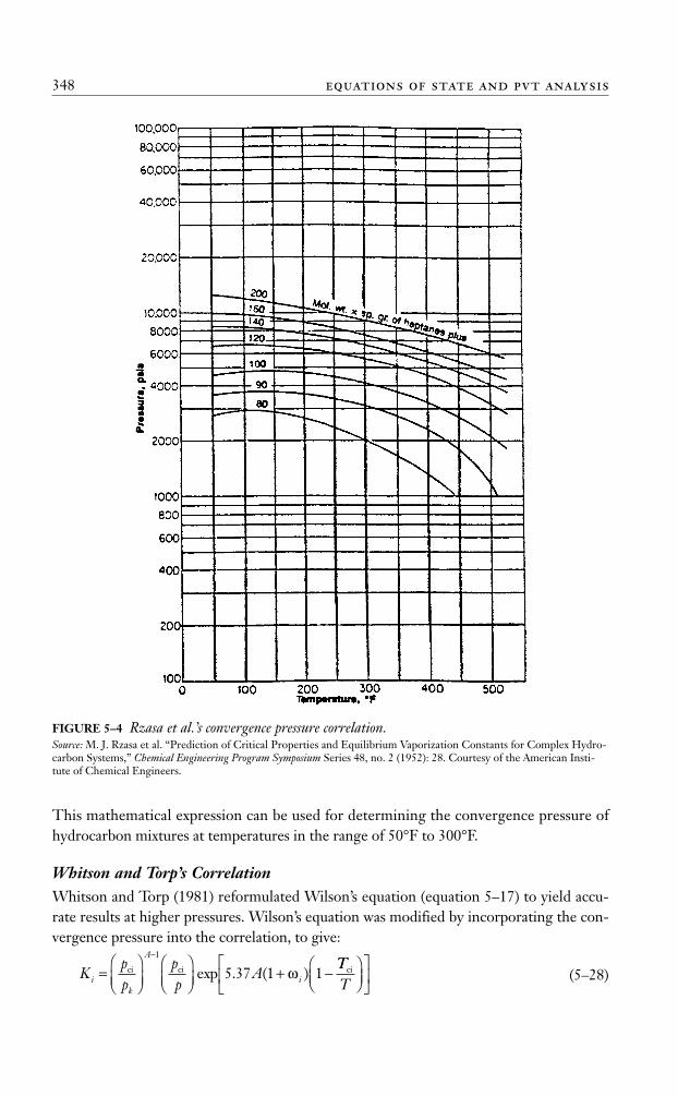
This mathematical expression can be used for determining the convergence pressure ofhydrocarbon mixtures at temperatures in the range of 50°F to 300°F.
Whitson and Torp’s CorrelationWhitson and Torp (1981) reformulated Wilson’s equation (equation 5–17) to yield accu-rate results at higher pressures. Wilson’s equation was modified by incorporating the con-vergence pressure into the correlation, to give:
(5–28)Kpp
pp
Aik
A
i=⎛⎝⎜
⎞⎠⎟
⎛⎝⎜
⎞⎠⎟
+ −−
ci ci
1
5 37 1 1exp . ( )ωTTT
ci⎛⎝⎜
⎞⎠⎟
⎡
⎣⎢
⎤
⎦⎥
348 equations of state and pvt analysis
FIGURE 5–4 Rzasa et al.’s convergence pressure correlation.Source: M. J. Rzasa et al. “Prediction of Critical Properties and Equilibrium Vaporization Constants for Complex Hydro-carbon Systems,” Chemical Engineering Program Symposium Series 48, no. 2 (1952): 28. Courtesy of the American Insti-tute of Chemical Engineers.
Ahmed_ch5.qxd 12/21/06 2:05 PM Page 348
with
wherep = system pressure, psigpk = convergence pressure, psigT = system temperature, °Rωi = acentric factor of component i
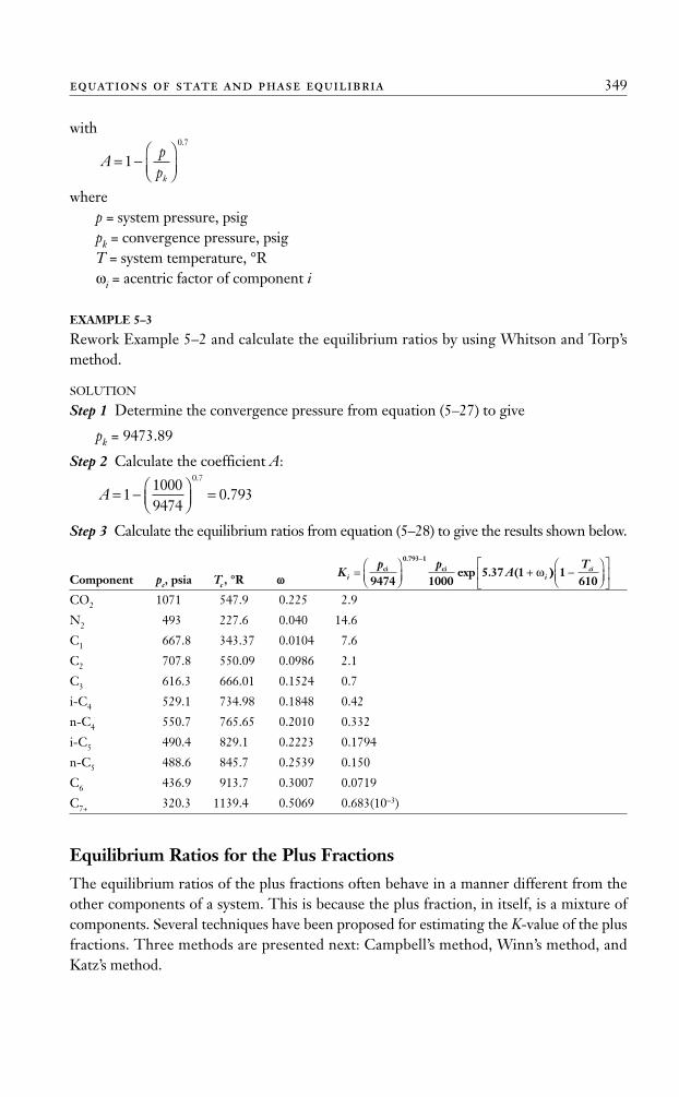
EXAMPLE 5–3
Rework Example 5–2 and calculate the equilibrium ratios by using Whitson and Torp’smethod.
SOLUTION
Step 1 Determine the convergence pressure from equation (5–27) to give
pk = 9473.89
Step 2 Calculate the coefficient A:
Step 3 Calculate the equilibrium ratios from equation (5–28) to give the results shown below.
Component pc, psia Tc , °R ωω
CO2 1071 547.9 0.225 2.9
N2 493 227.6 0.040 14.6
C1 667.8 343.37 0.0104 7.6
C2 707.8 550.09 0.0986 2.1
C3 616.3 666.01 0.1524 0.7
i-C4 529.1 734.98 0.1848 0.42
n-C4 550.7 765.65 0.2010 0.332
i-C5 490.4 829.1 0.2223 0.1794
n-C5 488.6 845.7 0.2539 0.150
C6 436.9 913.7 0.3007 0.0719
C7+ 320.3 1139.4 0.5069 0.683(10–3)
Equilibrium Ratios for the Plus Fractions
The equilibrium ratios of the plus fractions often behave in a manner different from theother components of a system. This is because the plus fraction, in itself, is a mixture ofcomponents. Several techniques have been proposed for estimating the K-value of the plusfractions. Three methods are presented next: Campbell’s method, Winn’s method, andKatz’s method.
Kp p
Ai i=⎛⎝⎜
⎞⎠⎟
+−
ci ci
9474 10005 37 1
0 793 1.
exp . ( ω )) 1610
−⎛⎝⎜
⎞⎠⎟
⎡
⎣⎢
⎤
⎦⎥
Tci
A = − ⎛⎝⎜
⎞⎠⎟
=110009474
0 7930 7.
.
Appk
= −⎛⎝⎜
⎞⎠⎟
10 7.
equations of state and phase equilibria 349
Ahmed_ch5.qxd 12/21/06 2:05 PM Page 349
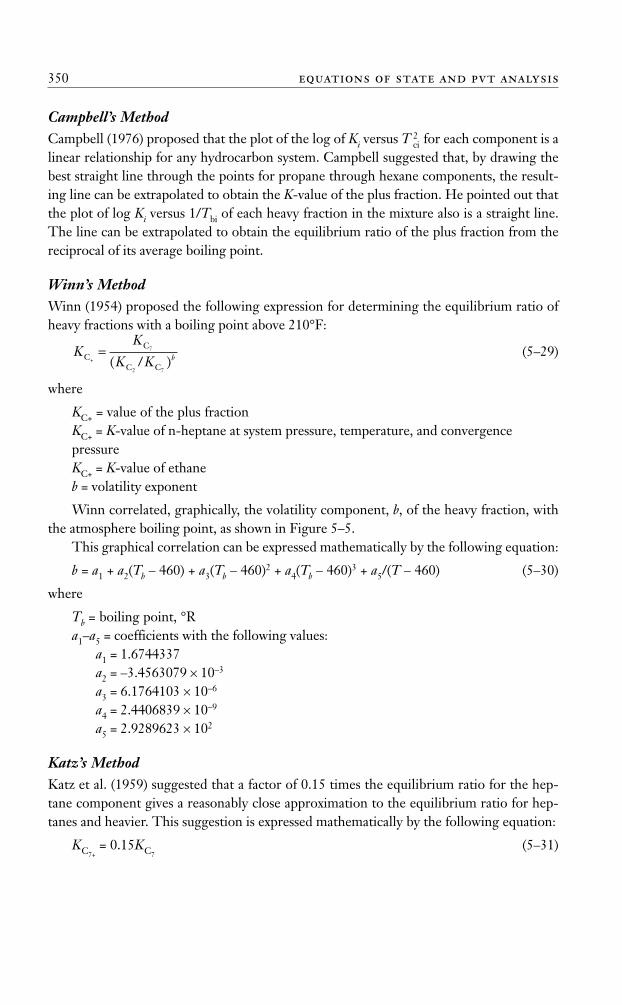
Campbell’s MethodCampbell (1976) proposed that the plot of the log of Ki versus T 2
ci for each component is alinear relationship for any hydrocarbon system. Campbell suggested that, by drawing thebest straight line through the points for propane through hexane components, the result-ing line can be extrapolated to obtain the K-value of the plus fraction. He pointed out thatthe plot of log Ki versus 1/Tbi of each heavy fraction in the mixture also is a straight line.The line can be extrapolated to obtain the equilibrium ratio of the plus fraction from thereciprocal of its average boiling point.
Winn’s MethodWinn (1954) proposed the following expression for determining the equilibrium ratio ofheavy fractions with a boiling point above 210°F:
(5–29)
where
KC+ = value of the plus fractionKC+ = K-value of n-heptane at system pressure, temperature, and convergencepressureKC+ = K-value of ethaneb = volatility exponent
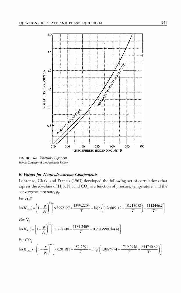
Winn correlated, graphically, the volatility component, b, of the heavy fraction, withthe atmosphere boiling point, as shown in Figure 5–5.
This graphical correlation can be expressed mathematically by the following equation:
b = a1 + a2(Tb – 460) + a3(Tb – 460)2 + a4(Tb – 460)3 + a5/(T – 460) (5–30)
where
Tb = boiling point, °Ra1–a5 = coefficients with the following values:
a1 = 1.6744337a2 = –3.4563079 × 10⁻³
a3 = 6.1764103 × 10⁻⁶
a4 = 2.4406839 × 10⁻⁹
a5 = 2.9289623 × 10²
Katz’s MethodKatz et al. (1959) suggested that a factor of 0.15 times the equilibrium ratio for the hep-tane component gives a reasonably close approximation to the equilibrium ratio for hep-tanes and heavier. This suggestion is expressed mathematically by the following equation:
KC7+= 0.15KC7
(5–31)
KK
K K bCC
C C+
7
2 7
=( / )
350 equations of state and pvt analysis
Ahmed_ch5.qxd 12/21/06 2:05 PM Page 350
K-Values for Nonhydrocarbon ComponentsLohrenze, Clark, and Francis (1963) developed the following set of correlations thatexpress the K-values of H2S, N2, and CO2 as a function of pressure, temperature, and theconvergence pressure, pk.
For H2S
For N2
For CO2
ln( ) ..
.
Kpp Tk
CO2= −⎛⎝⎜
⎞⎠⎟
− −1 7 0201913152 7291
0 6
lln( ) .. .
pT T
1 88969741719 2956 644740 69
2− +⎛⎝⎜
⎞⎠⎟⎟
⎡⎣⎢
⎤⎦⎥
ln( ) ..
.
Kpp Tk
N2= −⎛⎝⎜
⎞⎠⎟
− −1 11 2947481184 2409
0 4
00 90459907. ln( )p⎡⎣⎢
⎤⎦⎥
ln( ) ..
.
Kpp Tk
H S2= −⎛⎝⎜
⎞⎠⎟
+1 6 39921271399 2204
0 8
−− +⎛⎝⎜
⎞⎠⎟−ln( ) .
. .p
T0 76885112
18 215052 1112446 222T
⎡⎣⎢
⎤⎦⎥
equations of state and phase equilibria 351
FIGURE 5–5 Volatility exponent.Source: Courtesy of the Petroleum Refiner.
Ahmed_ch5.qxd 12/21/06 2:05 PM Page 351
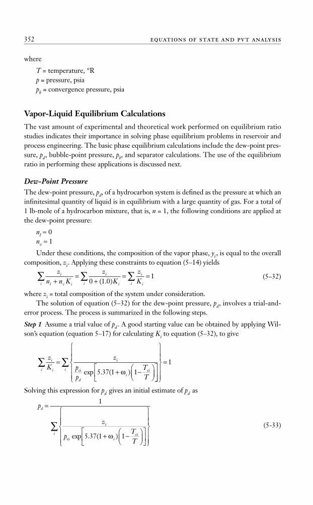
where
T = temperature, °Rp = pressure, psiapk = convergence pressure, psia
Vapor-Liquid Equilibrium Calculations
The vast amount of experimental and theoretical work performed on equilibrium ratiostudies indicates their importance in solving phase equilibrium problems in reservoir andprocess engineering. The basic phase equilibrium calculations include the dew-point pres-sure, pd, bubble-point pressure, pb, and separator calculations. The use of the equilibriumratio in performing these applications is discussed next.
Dew-Point PressureThe dew-point pressure, pd, of a hydrocarbon system is defined as the pressure at which aninfinitesimal quantity of liquid is in equilibrium with a large quantity of gas. For a total of1 lb-mole of a hydrocarbon mixture, that is, n = 1, the following conditions are applied atthe dew-point pressure:
nl ≈ 0nv ≈ 1
Under these conditions, the composition of the vapor phase, yi , is equal to the overallcomposition, zi. Applying these constraints to equation (5–14) yields
(5–32)
where zi = total composition of the system under consideration.The solution of equation (5–32) for the dew-point pressure, pd, involves a trial-and-
error process. The process is summarized in the following steps.
Step 1 Assume a trial value of pd . A good starting value can be obtained by applying Wil-son’s equation (equation 5–17) for calculating Ki to equation (5–32), to give
Solving this expression for pd gives an initial estimate of pd as
(5-33)
p
z
pTT
d
i
i
=
+ −⎛⎝⎜
⎞⎠⎟
⎡
⎣⎢
⎤
⎦⎥
⎧
⎨⎪
1
5 37 1 1ciciexp . ( )ω
⎪⎪
⎩⎪⎪
⎫
⎬⎪⎪
⎭⎪⎪
∑i
zK
zpp
TT
i
ii
i
di
∑ =+ −⎛
⎝⎜⎞⎠⎟
⎡
⎣⎢
⎤ci ciexp . ( )5 37 1 1ω⎦⎦⎥
⎧
⎨⎪⎪
⎩⎪⎪
⎫
⎬⎪⎪
⎭⎪⎪
=∑i
1
zn n K
zK
zK
i
l v ii
i
ii
i
ii+=
+= =∑ ∑ ∑0 1 0
1( . )
352 equations of state and pvt analysis
Ahmed_ch5.qxd 12/21/06 2:05 PM Page 352
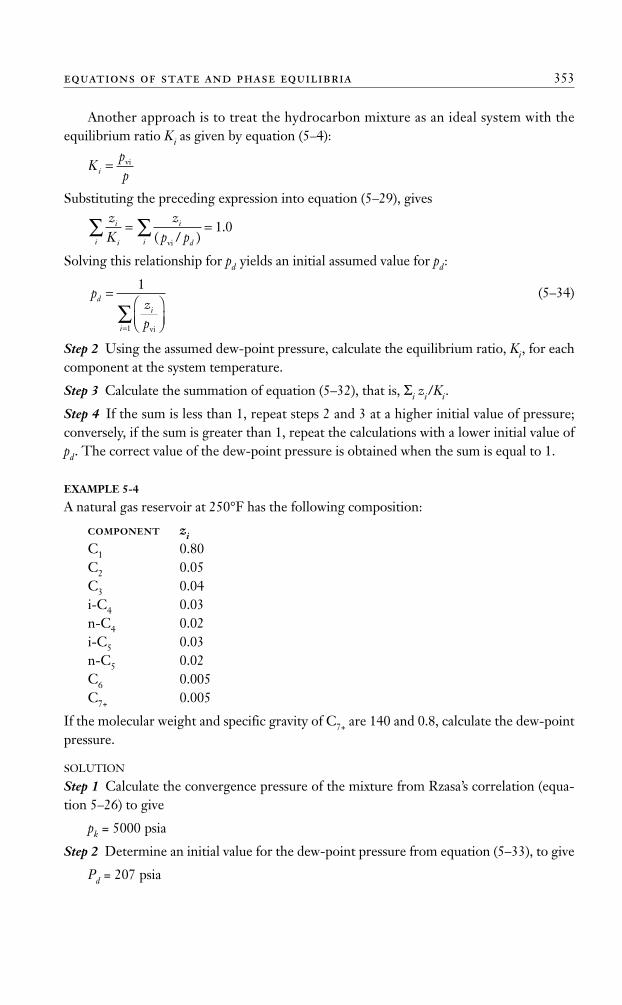
Another approach is to treat the hydrocarbon mixture as an ideal system with theequilibrium ratio Ki as given by equation (5–4):
Substituting the preceding expression into equation (5–29), gives
Solving this relationship for pd yields an initial assumed value for pd:
(5–34)
Step 2 Using the assumed dew-point pressure, calculate the equilibrium ratio, Ki, for eachcomponent at the system temperature.
Step 3 Calculate the summation of equation (5–32), that is, Σi zi/Ki.
Step 4 If the sum is less than 1, repeat steps 2 and 3 at a higher initial value of pressure;conversely, if the sum is greater than 1, repeat the calculations with a lower initial value ofpd. The correct value of the dew-point pressure is obtained when the sum is equal to 1.
EXAMPLE 5-4
A natural gas reservoir at 250°F has the following composition:
COMPONENT ziC1 0.80C2 0.05C3 0.04i-C4 0.03n-C4 0.02i-C5 0.03n-C5 0.02C6 0.005C7+ 0.005
If the molecular weight and specific gravity of C7+ are 140 and 0.8, calculate the dew-pointpressure.
SOLUTION
Step 1 Calculate the convergence pressure of the mixture from Rzasa’s correlation (equa-tion 5–26) to give
pk = 5000 psia
Step 2 Determine an initial value for the dew-point pressure from equation (5–33), to give
Pd = 207 psia
pzp
di
i
=⎛⎝⎜
⎞⎠⎟=
∑1
1 vi
zK
zp p
i
ii
i
di
= =∑ ∑ ( / ).
vi
1 0
Kppi =vi
equations of state and phase equilibria 353
Ahmed_ch5.qxd 12/21/06 2:05 PM Page 353
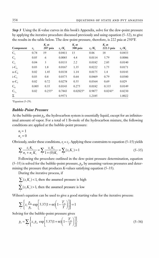
Step 3 Using the K-value curves in this book’s Appendix, solve for the dew-point pressureby applying the iterative procedure discussed previously and using equation (5–32), to givethe results in the table below. The dew-point pressure, therefore, is 222 psia at 250°F.
Ki at Ki at Ki at Component zi 207 psia zi /Ki 300 psia zi /Ki 222.3 psia zi /Ki
C1 0.78 19 0.0411 13 0.06 18 0.0433
C2 0.05 6 0.0083 4.4 0.0114 5.79 0.0086
C3 0.04 3 0.0133 2.2 0.0182 2.85 0.0140
i-C4 0.03 1.8 0.0167 1.35 0.0222 1.75 0.0171
n-C4 0.02 1.45 0.0138 1.14 0.0175 1.4 0.0143
i-C5 0.03 0.8 0.0375 0.64 0.0469 0.79 0.0380
n-C5 0.02 0.72 0.0278 0.55 0.0364 0.69 0.029
C6 0.005 0.35 0.0143 0.275 0.0182 0.335 0.0149
C7+ 0.02 0.255* 0.7843 0.02025* 0.9877 0.0243* 0.8230
Σ 0.9571 1.2185 1.0022
*Equation (5–29).
Bubble-Point PressureAt the bubble-point pb, the hydrocarbon system is essentially liquid, except for an infinites-imal amount of vapor. For a total of 1 lb-mole of the hydrocarbon mixture, the followingconditions are applied at the bubble-point pressure:
nl ≈ 1nv ≈ 0
Obviously, under these conditions, xi = zi. Applying these constraints to equation (5–15) yields
(5–35)
Following the procedure outlined in the dew-point pressure determination, equation(5–35) is solved for the bubble-point pressure, pb, by assuming various pressures and deter-mining the pressure that produces K-values satisfying equation (5–35).
During the iterative process, if
Wilson’s equation can be used to give a good starting value for the iterative process:
Solving for the bubble-point pressure gives
(5–36)p z pTTb i= + −⎛
⎝⎜⎞⎠⎟
⎡
⎣⎢
⎤
⎦⎥
⎧⎨⎪
⎩⎪ci
ciexp . ( )5 37 1 1ω⎫⎫⎬⎪
⎭⎪∑
i
zpp
TTi
b
ci ciexp . ( )5 37 1 1+ −⎛⎝⎜
⎞⎠⎟
⎡
⎣⎢
⎤
⎦⎥
⎧⎨⎪
⎩⎪
⎫ω ⎬⎬
⎪
⎭⎪=∑
i
1
( ) ,z Kii
i∑ >1 then the assumed pressure is low
( ) ,z Kii
i∑ <1 then the assumed pressure is high
z Kn n K
z KK
z Ki i
l v ii
i i
iii
ii+
=+
= =∑ ∑ ∑1 01
( )( )
354 equations of state and pvt analysis
Ahmed_ch5.qxd 12/21/06 2:05 PM Page 354
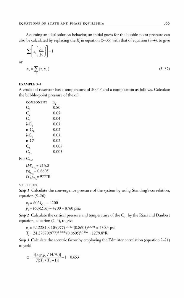
Assuming an ideal solution behavior, an initial guess for the bubble-point pressure canalso be calculated by replacing the Ki in equation (5–35) with that of equation (5–4), to give
or
(5–37)
EXAMPLE 5–5
A crude oil reservoir has a temperature of 200°F and a composition as follows. Calculatethe bubble-point pressure of the oil.
COMPONENT xiC1 0.80C2 0.05C3 0.04i-C4 0.03n-C4 0.02i-C5 0.03n-C5 0.02C6 0.005C7+ 0.005
For C7+,
(M)C7+= 216.0
(γ)C7+= 0.8605
(Tb )C7+= 977°R
SOLUTION
Step 1 Calculate the convergence pressure of the system by using Standing’s correlation,equation (5–26):
pk = 60MC7+– 4200
pk = (60)(216) – 4200 = 8760 psia
Step 2 Calculate the critical pressure and temperature of the C7+ by the Riazi and Daubertequation, equation (2–4), to give
pc = 3.12281 × 10⁹(977)–2.3125(0.8605)2.3201 = 230.4 psiTc = 24.27870(977)0.58848(0.8605)0.3596 = 1279.8°R
Step 3 Calculate the acentric factor by employing the Edmister correlation (equation 2–21)to yield
ω =−
− =3 14 70
7 11 0 653
[log( / . )][( / )]
.p
T Tc
c b
p z pb ii
=∑ ( )vi
zppi
bi
vi⎛⎝⎜
⎞⎠⎟
⎡
⎣⎢
⎤
⎦⎥ =∑ 1
equations of state and phase equilibria 355
Ahmed_ch5.qxd 12/21/06 2:05 PM Page 355
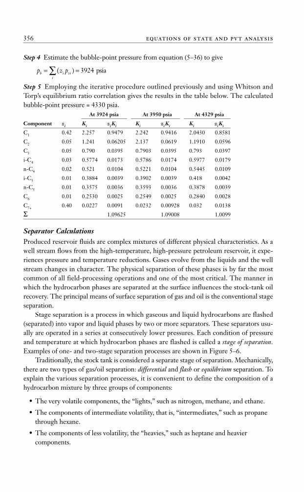
Step 4 Estimate the bubble-point pressure from equation (5–36) to give
Step 5 Employing the iterative procedure outlined previously and using Whitson andTorp’s equilibrium ratio correlation gives the results in the table below. The calculatedbubble-point pressure = 4330 psia.
At 3924 psia At 3950 psia At 4329 psia
Component zi Ki ziKi Ki ziKi Ki ziKi
C1 0.42 2.257 0.9479 2.242 0.9416 2.0430 0.8581
C2 0.05 1.241 0.06205 2.137 0.0619 1.1910 0.0596
C3 0.05 0.790 0.0395 0.7903 0.0395 0.793 0.0397
i-C4 0.03 0.5774 0.0173 0.5786 0.0174 0.5977 0.0179
n-C4 0.02 0.521 0.0104 0.5221 0.0104 0.5445 0.0109
i-C5 0.01 0.3884 0.0039 0.3902 0.0039 0.418 0.0042
n-C5 0.01 0.3575 0.0036 0.3593 0.0036 0.3878 0.0039
C6 0.01 0.2530 0.0025 0.2549 0.0025 0.2840 0.0028
C7+ 0.40 0.0227 0.0091 0.0232 0.00928 0.032 0.0138
Σ 1.09625 1.09008 1.0099
Separator CalculationsProduced reservoir fluids are complex mixtures of different physical characteristics. As awell stream flows from the high-temperature, high-pressure petroleum reservoir, it expe-riences pressure and temperature reductions. Gases evolve from the liquids and the wellstream changes in character. The physical separation of these phases is by far the mostcommon of all field-processing operations and one of the most critical. The manner inwhich the hydrocarbon phases are separated at the surface influences the stock-tank oilrecovery. The principal means of surface separation of gas and oil is the conventional stageseparation.
Stage separation is a process in which gaseous and liquid hydrocarbons are flashed(separated) into vapor and liquid phases by two or more separators. These separators usu-ally are operated in a series at consecutively lower pressures. Each condition of pressureand temperature at which hydrocarbon phases are flashed is called a stage of separation.Examples of one- and two-stage separation processes are shown in Figure 5–6.
Traditionally, the stock tank is considered a separate stage of separation. Mechanically,there are two types of gas/oil separation: differential and flash or equilibrium separation. Toexplain the various separation processes, it is convenient to define the composition of ahydrocarbon mixture by three groups of components:
• The very volatile components, the “lights,” such as nitrogen, methane, and ethane.
• The components of intermediate volatility, that is, “intermediates,” such as propanethrough hexane.
• The components of less volatility, the “heavies,” such as heptane and heaviercomponents.
p z pb i vii
= =∑ ( ) 3924 psia
356 equations of state and pvt analysis
Ahmed_ch5.qxd 12/21/06 2:05 PM Page 356
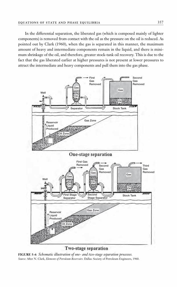
In the differential separation, the liberated gas (which is composed mainly of lightercomponents) is removed from contact with the oil as the pressure on the oil is reduced. Aspointed out by Clark (1960), when the gas is separated in this manner, the maximumamount of heavy and intermediate components remain in the liquid, and there is mini-mum shrinkage of the oil, and therefore, greater stock-tank oil recovery. This is due to thefact that the gas liberated earlier at higher pressures is not present at lower pressures toattract the intermediate and heavy components and pull them into the gas phase.
equations of state and phase equilibria 357
GasGas
GasGas
Gas Zone
Gas Zone
Oil Zone
Oil Zone
Oil
Oil
OilOil
Oil
Gas
ReservoirLiquidProduced
ReservoirLiquidProduced
Well
Well
FirstGasRemoved
First GasRemoved
SecondGasRemoved
SecondGasRemoved
ThirdGasRemoved
Separator Stock Tank
Stock TankSecondStage Separator
First StageSeparator
FIGURE 5–6 Schematic illustration of one- and two-stage separation processes.Source: After N. Clark, Elements of Petroleum Reservoirs. Dallas: Society of Petroleum Engineers, 1960.
Ahmed_ch5.qxd 12/21/06 2:05 PM Page 357
In the flash (equilibrium) separation, the liberated gas remains in contact with the oiluntil its instantaneous removal at the final separation pressure. A maximum proportion ofintermediate and heavy components are attracted into the gas phase by this process, andthis results in maximum oil shrinkage and, therefore, lower oil recovery.
In practice, the differential process is introduced first in field separation, when gas orliquid is removed from the primary separator. In each subsequent stage of separation, theliquid initially undergoes a flash liberation followed by a differential process as actual sep-aration occurs. As the number of stages increases, the differential aspect of the overall sep-aration becomes greater.
The purpose of stage separation then is to reduce the pressure on the produced oil insteps so that more stock-tank oil recovery results.
Separator calculations are basically performed to determine
• Optimum separation conditions: separator pressure and temperature.
• Composition of the separated gas and oil phases.
• Oil formation volume factor.
• Producing gas/oil ratio.
• API gravity of the stock-tank oil.
Note that, if the separator pressure is high, large amounts of light components remainin the liquid phase at the separator and are lost along with other valuable components tothe gas phase at the stock tank. On the other hand, if the pressure is too low, largeamounts of light components are separated from the liquid, and they attract substantialquantities of intermediate and heavier components. An intermediate pressure, called theoptimum separator pressure, should be selected to maximize the oil volume accumulationin the stock tank. This optimum pressure also yields
• A maximum in the stock-tank API gravity.
• A minimum in the oil formation volume factor (i.e., less oil shrinkage).
• A minimum in the producing gas/oil ratio (gas solubility).
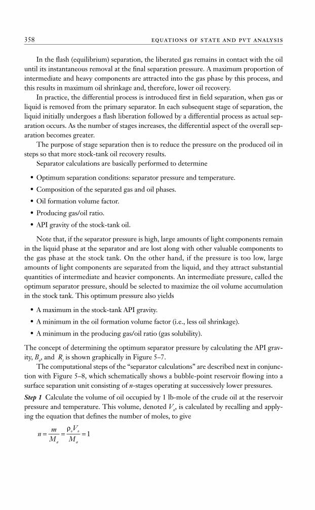
The concept of determining the optimum separator pressure by calculating the API grav-ity, Bo, and Rs is shown graphically in Figure 5–7.
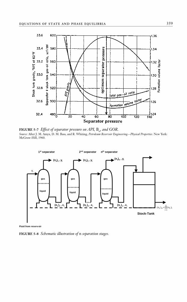
The computational steps of the “separator calculations” are described next in conjunc-tion with Figure 5–8, which schematically shows a bubble-point reservoir flowing into asurface separation unit consisting of n-stages operating at successively lower pressures.
Step 1 Calculate the volume of oil occupied by 1 lb-mole of the crude oil at the reservoirpressure and temperature. This volume, denoted Vo, is calculated by recalling and apply-ing the equation that defines the number of moles, to give
nm
M
V
Ma
o o
a
= = =ρ
1
358 equations of state and pvt analysis
Ahmed_ch5.qxd 12/21/06 2:05 PM Page 358
equations of state and phase equilibria 359
FIGURE 5–7 Effect of separator pressure on API, Bo, and GOR.Source: After J. M. Amyx, D. M. Bass, and R. Whiting, Petroleum Reservoir Engineering—Physical Properties. New York:McGraw-Hill, 1960.
Fluid from reservoir
gas
liquid
1st separator
(nv)1 , yi
(nL)1 , xi
gas
liquid
2nd separator
(nv)2 , yi
(nL)2 , xi
gas
liquid
nth separator
(nv)n , yi
(nL)n , xi
Stock-Tank
zi
i
n
iLstL nn )()(
1∏=
=
FIGURE 5–8 Schematic illustration of n separation stages.
Ahmed_ch5.qxd 12/21/06 2:05 PM Page 359
Solving for the oil volume gives
(5–38)
where
m = total weight of 1 lb-mole of the crude oil, lb/moleVo = volume of 1 lb-mole of the crude oil at reservoir conditions, ft3/moleMa = apparent molecular weightρo = density of the reservoir oil, lb/ft3
Step 2 Given the composition of the feed stream, zi, to the first separator and the operat-ing conditions of the separator, that is, separator pressure and temperature, calculate theequilibrium ratios of the hydrocarbon mixture.
Step 3 Assuming a total of 1 mole of the feed entering the first separator and using thepreceding calculated equilibrium ratios, perform flash calculations to obtain the composi-tions and quantities, in moles, of the gas and the liquid leaving the first separator. Desig-nating these moles as (nL)1 and (nv)1, the actual number of moles of the gas and the liquidleaving the first separation stage are
[nv1]a = (n)(nv)1 = (1) (nv)1
[nL1]a = (n) (nL)1 = (1) (nL)1
where [nv1]a = actual number of moles of vapor leaving the first separator and [nL1]a =actual number of moles of liquid leaving the first separator.
Step 4 Using the composition of the liquid leaving the first separator as the feed for thesecond separator, that is, zi = xi, calculate the equilibrium ratios of the hydrocarbon mix-ture at the prevailing pressure and temperature of the separator.
Step 5 Based on 1 mole of the feed, perform flash calculations to determine the composi-tions and quantities of the gas and liquid leaving the second separation stage. The actualnumber of moles of the two phases then is calculated from
[nv2]a = [nL1]a(nv)2 = (1)(nL)1(nv)2
[nL2]a = [nL1]a(nL)2 = (1)(nL)1(nL)2
where
[nv2]a, [nL2]a = actual moles of gas and liquid leaving separator 2(nv)2, (nL)2 = moles of gas and liquid as determined from flash calculations
Step 6 The previously outlined procedure is repeated for each separation stage, includingthe stock-tank storage, and the calculated moles and compositions are recorded. The totalnumber of moles of gas given off in all stages then are calculated as
( ) ( ) ( ) ( ) ( ) ( ) (n n n n n n nv t va i vi
n
L v L L= = + +=∑ 1
11 2 1 )) ( ) . . . ( ) . . ( ) ( )2 3 1 1n n n nv L L n v n+ + −.
VM
oa
o
=ρ
360 equations of state and pvt analysis
Ahmed_ch5.qxd 12/21/06 2:05 PM Page 360
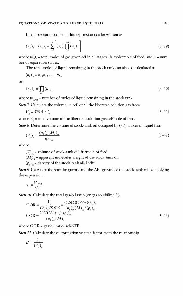
In a more compact form, this expression can be written as
(5–39)
where (nv)t = total moles of gas given off in all stages, lb-mole/mole of feed, and n = num-ber of separation stages.
The total moles of liquid remaining in the stock tank can also be calculated as
(nL)st = nL1nL2 . . . nLn
or
(5–40)
where (nL)st = number of moles of liquid remaining in the stock tank.
Step 7 Calculate the volume, in scf, of all the liberated solution gas from
Vg = 379.4(nv)t (5–41)
where Vg = total volume of the liberated solution gas scf/mole of feed.
Step 8 Determine the volume of stock-tank oil occupied by (nL)st moles of liquid from
(5–42)
where
(Vo )st = volume of stock-tank oil, ft3/mole of feed(Ma)st = apparent molecular weight of the stock-tank oil(ρo )st = density of the stock-tank oil, lb/ft3
Step 9 Calculate the specific gravity and the API gravity of the stock-tank oil by applyingthe expression
Step 10 Calculate the total gas/oil ratio (or gas solubility, Rs):
(5–43)
where GOR = gas/oil ratio, scf/STB.
Step 11 Calculate the oil formation volume factor from the relationship
BV
Voo
o
=( )st
GOR st
st st
=2130 331. ( ) ( )
( ) ( )n
n Mv t o
L
ρ
GORst s
= =V
Vn
ng
o
v t
L( ) / .( . )( . )( )( )5 6155 615 379 4
tt st st( ) / ( )M oρ
γρ
oo=
( ).
st
62 4
( )( ) ( )
( )V
n Mo
L a
ost
st st
st
=ρ
( ) ( )n nL L ii
n
st ==∏
1
( ) ( ) ( ) ( )n n n nv t v v i L jj
i
i
n
= +⎡
⎣⎢
⎤
⎦⎥
=
−
=∏∑1
1
1
2
equations of state and phase equilibria 361
Ahmed_ch5.qxd 12/21/06 2:05 PM Page 361
Combining equations (5–38) and (5–42) with the preceding expression gives
(5–44)
where
Bo = oil formation volume factor, bbl/STBMa = apparent molecular weight of the feed(Ma)st = apparent molecular weight of the stock-tank oilρo = density of crude oil at reservoir conditions, lb/ft3
The separator pressure can be optimized by calculating the API gravity, GOR, and Bo
in the manner just outlined at different assumed pressures. The optimum pressure corre-sponds to a maximum in the API gravity and a minimum in gas/oil ratio and oil formationvolume factor.
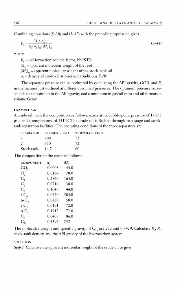
EXAMPLE 5–6
A crude oil, with the composition as follows, exists at its bubble-point pressure of 1708.7psia and a temperature of 131°F. The crude oil is flashed through two-stage and stock-tank separation facilities. The operating conditions of the three separators are:
SEPARATOR PRESSURE, PSIA TEMPERATURE, °F
1 400 722 350 72Stock tank 14.7 60
The composition of the crude oil follows:
COMPONENT zi MiCO2 0.0008 44.0N2 0.0164 28.0C1 0.2840 164.0C2 0.0716 30.0C3 0.1048 44.0i-C4 0.0420 584.0n-C4 0.0420 58.0i-C5 0.0191 72.0n-C5 0.1912 72.0C6 0.0405 86.0C7+ 0.3597 252
The molecular weight and specific gravity of C7+ are 252 and 0.8429. Calculate Bo, Rs,stock-tank density, and the API gravity of the hydrocarbon system.
SOLUTION
Step 1 Calculate the apparent molecular weight of the crude oil to give
BMn Mo
a o
o L a
=( )
( ) ( )ρ
ρst
st st
362 equations of state and pvt analysis
Ahmed_ch5.qxd 12/21/06 2:05 PM Page 362
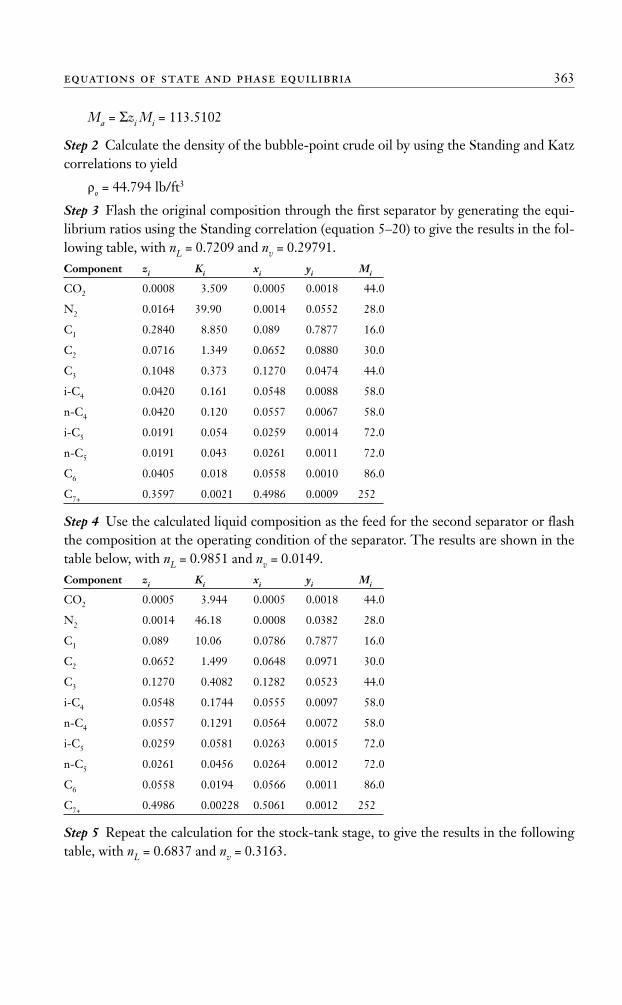
Ma = Σzi Mi = 113.5102
Step 2 Calculate the density of the bubble-point crude oil by using the Standing and Katzcorrelations to yield
ρo = 44.794 lb/ft3
Step 3 Flash the original composition through the first separator by generating the equi-librium ratios using the Standing correlation (equation 5–20) to give the results in the fol-lowing table, with nL = 0.7209 and nv = 0.29791.Component zi Ki xi yi Mi
CO2 0.0008 3.509 0.0005 0.0018 44.0
N2 0.0164 39.90 0.0014 0.0552 28.0
C1 0.2840 8.850 0.089 0.7877 16.0
C2 0.0716 1.349 0.0652 0.0880 30.0
C3 0.1048 0.373 0.1270 0.0474 44.0
i-C4 0.0420 0.161 0.0548 0.0088 58.0
n-C4 0.0420 0.120 0.0557 0.0067 58.0
i-C5 0.0191 0.054 0.0259 0.0014 72.0
n-C5 0.0191 0.043 0.0261 0.0011 72.0
C6 0.0405 0.018 0.0558 0.0010 86.0
C7+ 0.3597 0.0021 0.4986 0.0009 252
Step 4 Use the calculated liquid composition as the feed for the second separator or flashthe composition at the operating condition of the separator. The results are shown in thetable below, with nL = 0.9851 and nv = 0.0149.Component zi Ki xi yi Mi
CO2 0.0005 3.944 0.0005 0.0018 44.0
N2 0.0014 46.18 0.0008 0.0382 28.0
C1 0.089 10.06 0.0786 0.7877 16.0
C2 0.0652 1.499 0.0648 0.0971 30.0
C3 0.1270 0.4082 0.1282 0.0523 44.0
i-C4 0.0548 0.1744 0.0555 0.0097 58.0
n-C4 0.0557 0.1291 0.0564 0.0072 58.0
i-C5 0.0259 0.0581 0.0263 0.0015 72.0
n-C5 0.0261 0.0456 0.0264 0.0012 72.0
C6 0.0558 0.0194 0.0566 0.0011 86.0
C7+ 0.4986 0.00228 0.5061 0.0012 252
Step 5 Repeat the calculation for the stock-tank stage, to give the results in the followingtable, with nL = 0.6837 and nv = 0.3163.
equations of state and phase equilibria 363
Ahmed_ch5.qxd 12/21/06 2:05 PM Page 363
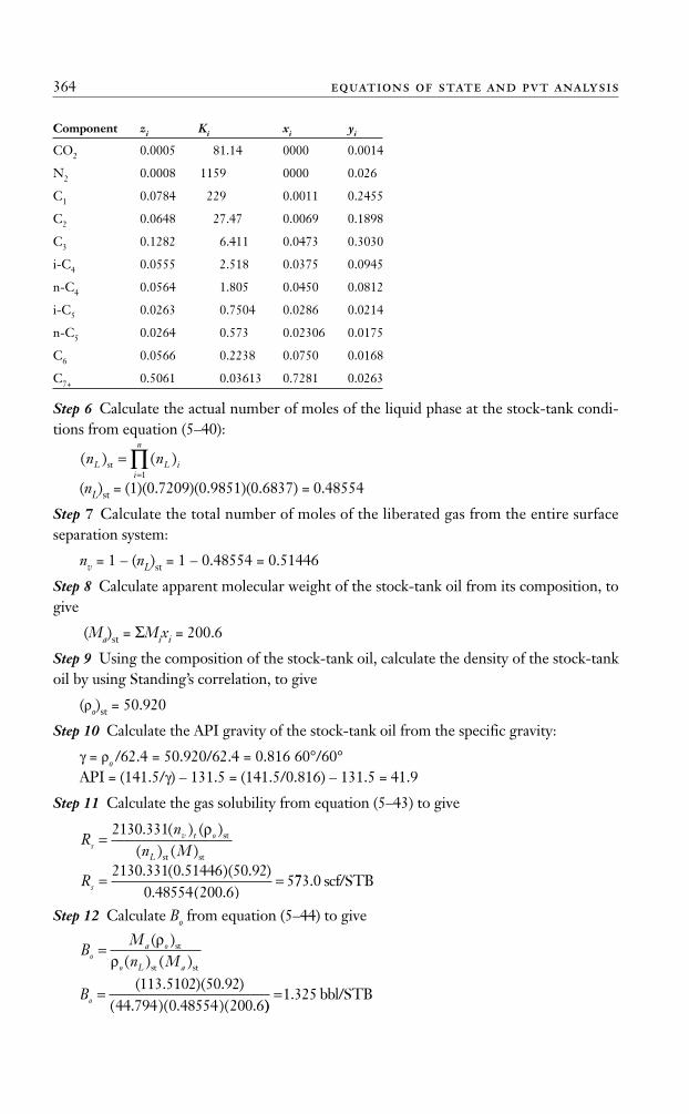
Component zi Ki xi yi
CO2 0.0005 81.14 0000 0.0014
N2 0.0008 1159 0000 0.026
C1 0.0784 229 0.0011 0.2455
C2 0.0648 27.47 0.0069 0.1898
C3 0.1282 6.411 0.0473 0.3030
i-C4 0.0555 2.518 0.0375 0.0945
n-C4 0.0564 1.805 0.0450 0.0812
i-C5 0.0263 0.7504 0.0286 0.0214
n-C5 0.0264 0.573 0.02306 0.0175
C6 0.0566 0.2238 0.0750 0.0168
C7+ 0.5061 0.03613 0.7281 0.0263
Step 6 Calculate the actual number of moles of the liquid phase at the stock-tank condi-tions from equation (5–40):
(nL)st = (1)(0.7209)(0.9851)(0.6837) = 0.48554
Step 7 Calculate the total number of moles of the liberated gas from the entire surfaceseparation system:
nv = 1 – (nL)st = 1 – 0.48554 = 0.51446
Step 8 Calculate apparent molecular weight of the stock-tank oil from its composition, togive
(Ma)st = ΣMixi = 200.6
Step 9 Using the composition of the stock-tank oil, calculate the density of the stock-tankoil by using Standing’s correlation, to give
(ρo)st = 50.920
Step 10 Calculate the API gravity of the stock-tank oil from the specific gravity:
γ = ρo /62.4 = 50.920/62.4 = 0.816 60°/60°API = (141.5/γ) – 131.5 = (141.5/0.816) – 131.5 = 41.9
Step 11 Calculate the gas solubility from equation (5–43) to give
Step 12 Calculate Bo from equation (5–44) to give
Bo =( . )( . )
( . )( . )( .113 5102 50 92
44 794 0 48554 200 6)).=1 325 bbl/STB
BMn Mo
a o
o L a
=( )
( ) ( )ρ
ρst
st st
Rs = =2130 331 0 51446 50 92
0 48554 200 65
. ( . )( . ). ( . )
773 0. scf/STB
Rn
n Msv t o
L
=2130 331. ( ) ( )
( ) ( )ρ st
st st
( ) ( )n nL L ii
n
st ==∏
1
364 equations of state and pvt analysis
Ahmed_ch5.qxd 12/21/06 2:05 PM Page 364
To optimize the operating pressure of the separator, these steps should be repeatedseveral times under different assumed pressures and the results, in terms of API, Bo, and Rs,should be expressed graphically and used to determine the optimum pressure.
Equations of State
An equation of state (EOS) is an analytical expression relating the pressure, p, to the tem-perature, T, and the volume, V. A proper description of this PVT relationship for realhydrocarbon fluids is essential in determining the volumetric and phase behavior of petro-leum reservoir fluids and predicting the performance of surface separation facilities; thesecan be described accurately by equations of state. In general, most equations of state requireonly the critical properties and acentric factor of individual components. The main advan-tage of using an EOS is that the same equation can be used to model the behavior of allphases, thereby assuring consistency when performing phase equilibria calculations.
The best known and the simplest example of an equation of state is the ideal gas equa-tion, expressed mathematically by the expression
(5–45)
where V = gas volume in ft3 per 1 mole of gas, ft3/mol.This PVT relationship is used to describe the volumetric behavior only of real hydro-
carbon gases at pressures close to the atmospheric pressure for which it was experimen-tally derived.
The extreme limitations of the applicability of equation (5–45) prompted numerousattempts to develop an equation of state suitable for describing the behavior of real fluidsat extended ranges of pressures and temperatures.
A review of recent developments and advances in the field of empirical cubic equa-tions of state are presented next, along with samples of their applications in petroleumengineering. Four equations of state are discussed here, those by van der Waals, Redlich-Kwong, Soave-Redlich-Kwong, and Peng-Robinson.
Van der Waals’s Equation of StateIn developing the ideal gas EOS, equation (5–45), two assumptions were made:
1. The volume of the gas molecules is insignificant compared to both the volume of thecontainer and distance between the molecules.
2. There are no attractive or repulsive forces between the molecules or the walls of thecontainer.
Van der Waals (1873) attempted to eliminate these two assumptions in developing anempirical equation of state for real gases. In his attempt to eliminate the first assumption,van der Waals pointed out that the gas molecules occupy a significant fraction of the vol-ume at higher pressures and proposed that the volume of the molecules, denoted by theparameter b, be subtracted from the actual molar volume, V, in equation (5–45), to give
pRTV
=
equations of state and phase equilibria 365
Ahmed_ch5.qxd 12/21/06 2:05 PM Page 365
where the parameter b is known as the covolume and considered to reflect the volume ofmolecules. The variable V represents the actual volume in ft3 per 1 mole of gas.
To eliminate the second assumption, van der Waals subtracted a corrective term,denoted by a/V 2, from this equation to account for the attractive forces between mole-cules. In a mathematical form, van der Waals proposed the following expression:
(5–46)
where
p = system pressure, psiaT = system temperature, °RR = gas constant, 10.73 psi-ft3/lb-mole, °RV = volume, ft3/molea = “attraction” parameterb = “repulsion” parameter
The two parameters, a and b, are constants characterizing the molecular properties ofthe individual components. The symbol a is considered a measure of the intermolecularattractive forces between the molecules. Equation (5–46) shows the following importantcharacteristics:
1. At low pressures, the volume of the gas phase is large in comparison with the volumeof the molecules. The parameter b becomes negligible in comparison with V and theattractive forces term, a/V2, becomes insignificant; therefore, the van der Waals equa-tion reduces to the ideal gas equation (equation 5–45).
2. At high pressure, that is, p→ ∞, the volume, V, becomes very small and approachesthe value b, which is the actual molecular volume, mathematically given by
The van der Waals or any other equation of state can be expressed in a more general-ized form as follows:
(5–47)
where the repulsion pressure term, prepulsion, is represented by the term RT/(V – b), and theattraction pressure term, pattraction, is described by a/V 2.
In determining the values of the two constants, a and b, for any pure substance, vander Waals observed that the critical isotherm has a horizontal slope and an inflection pointat the critical point, as shown in Figure 5–9. This observation can be expressed mathemat-ically as follows:
(5–48)∂∂⎡
⎣⎢
⎤
⎦⎥ =
2
2 0p
VT pc c,
∂∂⎡⎣⎢
⎤⎦⎥
=pV T pc c,
0
p p p= −repulsion attraction
lim ( )p
V p b→∞
=
pRT
V ba
V=
−− 2
pRT
V b=
−
366 equations of state and pvt analysis
Ahmed_ch5.qxd 12/21/06 2:05 PM Page 366
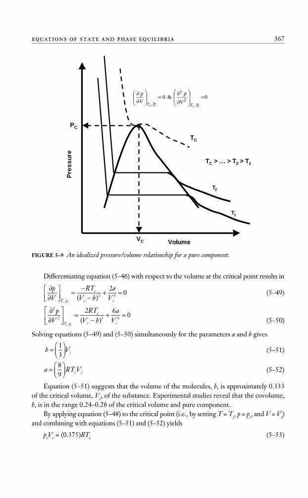
Differentiating equation (5–46) with respect to the volume at the critical point results in
(5–49)
(5–50)
Solving equations (5–49) and (5–50) simultaneously for the parameters a and b gives
(5–51)
(5–52)
Equation (5–51) suggests that the volume of the molecules, b, is approximately 0.333of the critical volume, Vc, of the substance. Experimental studies reveal that the covolume,b, is in the range 0.24–0.28 of the critical volume and pure component.
By applying equation (5–48) to the critical point (i.e., by setting T = Tc, p = pc, and V = Vc)and combining with equations (5–51) and (5–52) yields
pcVc = (0.375)RTc (5–53)
a RT Vc c= ⎛⎝⎜⎞⎠⎟
89
b Vc= ⎛⎝⎜⎞⎠⎟
13
∂∂⎡
⎣⎢
⎤
⎦⎥ =
−+ =
2
2 3 4
2 60
pV
RTV b
aV
T p
c
c cc c,
( )
∂∂⎡⎣⎢
⎤⎦⎥
=−−
+ =pV
RTV b
aVT p
c
c cc c, ( )2 3
20
equations of state and phase equilibria 367
o
Volume
Pre
ss
ure
VC
PC
TC
T1
T2
TC > … > T2 > T1
0&0,
2
2
,
=⎟⎟⎠
⎞⎜⎜⎝
⎛
∂∂=⎟⎟⎠
⎞⎜⎜⎝
⎛∂∂
PcTcPcTc
V
p
V
p
FIGURE 5–9 An idealized pressure/volume relationship for a pure component.
Ahmed_ch5.qxd 12/21/06 2:05 PM Page 367
Equation (5–53) shows that, regardless of the type of the substance, the van der WaalsEOS produces a universal critical gas compressibility factor, Zc, of 0.375. Experimental studiesshow that Zc values for substances range between 0.23 and 0.31.
Equation (5–53) can be combined with equations (5–51) and (5–52) to give more con-venient and traditional expressions for calculating the parameters a and b, to yield
(5–54)
(5–55)
where
R = gas constant, 10.73 psia-ft3/lb-mole-°Rpc = critical pressure, psiaTc = critical temperature, °RΩa = 0.421875Ωb = 0.125
Equation (5–46) can also be expressed in a cubic form in terms of the volume, V, asfollows:
Rearranging gives
(5–56)
Equation (5–56) usually is referred to as the van der Waals two-parameter cubic equationof state. The term two-parameter refers to parameters a and b. The term cubic equation ofstate implies an equation that, if expanded, would contain volume terms to the first, sec-ond, and third powers.
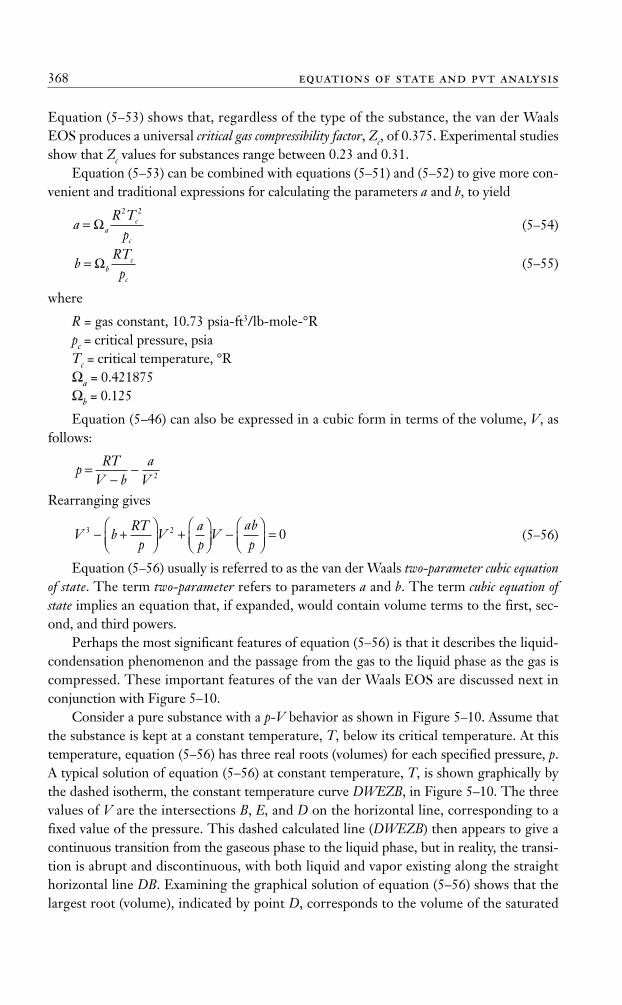
Perhaps the most significant features of equation (5–56) is that it describes the liquid-condensation phenomenon and the passage from the gas to the liquid phase as the gas iscompressed. These important features of the van der Waals EOS are discussed next inconjunction with Figure 5–10.
Consider a pure substance with a p-V behavior as shown in Figure 5–10. Assume thatthe substance is kept at a constant temperature, T, below its critical temperature. At thistemperature, equation (5–56) has three real roots (volumes) for each specified pressure, p.A typical solution of equation (5–56) at constant temperature, T, is shown graphically bythe dashed isotherm, the constant temperature curve DWEZB, in Figure 5–10. The threevalues of V are the intersections B, E, and D on the horizontal line, corresponding to afixed value of the pressure. This dashed calculated line (DWEZB) then appears to give acontinuous transition from the gaseous phase to the liquid phase, but in reality, the transi-tion is abrupt and discontinuous, with both liquid and vapor existing along the straighthorizontal line DB. Examining the graphical solution of equation (5–56) shows that thelargest root (volume), indicated by point D, corresponds to the volume of the saturated
V bRT
pV
ap
Vabp
3 2 0− +⎛⎝⎜
⎞⎠⎟
+⎛⎝⎜⎞⎠⎟−⎛⎝⎜
⎞⎠⎟=
pRT
V ba
V=
−− 2
bRTpb
c
c
= Ω
aR T
pac
c
= Ω2 2
368 equations of state and pvt analysis
Ahmed_ch5.qxd 12/21/06 2:05 PM Page 368
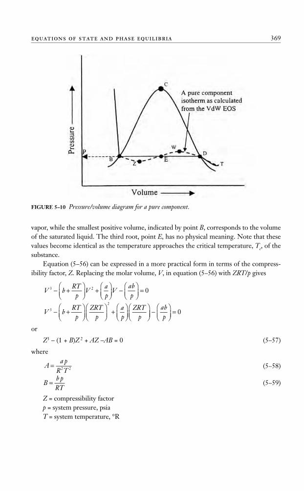
vapor, while the smallest positive volume, indicated by point B, corresponds to the volumeof the saturated liquid. The third root, point E, has no physical meaning. Note that thesevalues become identical as the temperature approaches the critical temperature, Tc, of thesubstance.
Equation (5–56) can be expressed in a more practical form in terms of the compress-ibility factor, Z. Replacing the molar volume, V, in equation (5–56) with ZRT/p gives
or
Z3 – (1 + B)Z 2 + AZ –AB = 0 (5–57)
where
(5–58)
(5–59)
Z = compressibility factorp = system pressure, psiaT = system temperature, °R
Bb pRT
=
Aa p
R T= 2 2
V bRT
pZRT
pap
ZRTp
3
2
− +⎛⎝⎜
⎞⎠⎟⎛⎝⎜
⎞⎠⎟+⎛⎝⎜⎞⎠⎟⎛⎝⎜
⎞⎠⎟⎟−⎛⎝⎜
⎞⎠⎟=
abp
0
V bRT
pV
ap
Vabp
3 2 0− +⎛⎝⎜
⎞⎠⎟
+⎛⎝⎜⎞⎠⎟
−⎛⎝⎜
⎞⎠⎟=
equations of state and phase equilibria 369
FIGURE 5–10 Pressure/volume diagram for a pure component.
Ahmed_ch5.qxd 12/21/06 2:05 PM Page 369
Equation (5–57) yields one real root∗ in the one-phase region and three real roots inthe two-phase region (where system pressure equals the vapor pressure of the substance). Inthe two-phase region, the largest positive root corresponds to the compressibility factor of thevapor phase, Zv, while the smallest positive root corresponds to that of the liquid phase, ZL.
An important practical application of equation (5–57) is density calculations, as illus-trated in the following example.
EXAMPLE 5–7
A pure propane is held in a closed container at 100°F. Both gas and liquid are present. Cal-culate, using the van der Waals EOS, the density of the gas and liquid phases.
SOLUTION
Step 1 Determine the vapor pressure, pv, of the propane from the Cox chart. This is theonly pressure at which two phases can exist at the specified temperature:
pv = 185 psi
Step 2 Calculate parameters a and b from equations (5–54) and (5–55), respectively:
and
Step 3 Compute the coefficients A and B by applying equations (5–58) and (5–59),respectively:
Step 4 Substitute the values of A and B into equation (5–57), to give
Step 5 Solve the above third-degree polynomial by extracting the largest and smallest rootsof the polynomial using the appropriate direct or iterative method, to give
Zv = 0.72365ZL = 0.07534
Step 6 Solve for the density of the gas and liquid phases using equation (2–17):
ρg v
pMZ RT
= = =( )( . )
( . )( . )( )185 44 0
0 72365 10 73 56011 87 3. lb/ft
Z Z Z3 21 044625 0 179122 0 007993 0− + − =. . .
Z B Z AZ AB3 21 0− + + − =( )
Bb pRT
= = =( . )( )( . )( )
.1 4494 18510 73 560
0 044625
Aa p
R T= = =2 2 2 2
34 957 4 18510 73 560
0 17( , . )( )( . ) ( )
. 99122
bRT
pbc
c
= = =Ω 0 12510 73 666
616 31 4494.
. ( ).
.
aR T
pac
c
= = =Ω2 2 2 2
0 42187510 73 666
616 334.
( . ) ( ).
,9957 4.
370 equations of state and pvt analysis
*In some super critical regions, equation (5–57) can yield three real roots for Z. From the three real roots, thelargest root is the value of the compressibility with physical meaning.
Ahmed_ch5.qxd 12/21/06 2:05 PM Page 370
and
The van der Waals equation of state, despite its simplicity, provides a correct descrip-tion, at least qualitatively, of the PVT behavior of substances in the liquid and gaseousstates. Yet, it is not accurate enough to be suitable for design purposes.
With the rapid development of computers, the equation-of-state approach for calcu-lating physical properties and phase equilibria proved to be a powerful tool, and muchenergy was devoted to the development of new and accurate equations of state. Theseequations, many of them a modification of the van der Waals equation of state, range incomplexity from simple expressions containing 2 or 3 parameters to complicated formscontaining more than 50 parameters. Although the complexity of any equation of statepresents no computational problem, most authors prefer to retain the simplicity found inthe van der Waals cubic equation while improving its accuracy through modifications.
All equations of state generally are developed for pure fluids first and then extended tomixtures through the use of mixing rules. These mixing rules are simply means of calculat-ing mixture parameters equivalent to those of pure substances.
Redlich-Kwong’s Equation of StateRedlich and Kwong (1949) demonstrated that, by a simple adjustment of the van derWaals’s attraction pressure term, a/V2, and explicitly including the system temperature,they could considerably improve the prediction of the volumetric and physical propertiesof the vapor phase. Redlich and Kwong replaced the attraction pressure term with a gen-eralized temperature dependence term, as given in following form:
(5–60)
in which T is the system temperature, in °R.Redlich and Kwong noted that, as the system pressure becomes very large, that is, p→∞,
the molar volume, V, of the substance shrinks to about 26% of its critical volume, Vc, regard-less of the system temperature. Accordingly, they constructed equation (5–60) to satisfy thefollowing condition:
b = 0.26Vc (5–61)
Imposing the critical point conditions (as expressed by equation 5–48) on equation(5–60) and solving the resulting two equations simultaneously, gives
(5–62)aR T
pac
c
= Ω2 2 5.
∂∂⎡
⎣⎢
⎤
⎦⎥ =
2
2 0p
VT pc c,
∂∂⎡⎣⎢
⎤⎦⎥
=pV T pc c,
0
pRT
V ba
V V b T=
−−
+( )
ρL L
pMZ RT
= = =( )( )
( . )( . )( )185 44
0 07534 10 73 56017..98 3lb/ft
equations of state and phase equilibria 371
Ahmed_ch5.qxd 12/21/06 2:05 PM Page 371
(5–63)
where Ωa = 0.42747 and Ωb = 0.08664.Equating equation (5–63) with (5–61) gives
or
(5–64)
Equation (5–64) shows that the Redlich-Kwong EOS produces a universal criticalcompressibility factor (Zc) of 0.333 for all substances. As indicated earlier, the critical gascompressibility ranges from 0.23 to 0.31 for most of the substances.
Replacing the molar volume, V, in equation (5–60) with ZRT/p and rearranging gives
Z3 – Z2 + (A – B – B2)Z – AB = 0 (5–65)where
(5–66)
(5–67)
As in the van der Waals EOS, equation (5–65) yields one real root in the one-phaseregion (gas-phase region or liquid-phase region) and three real roots in the two-phaseregion. In the latter case, the largest root corresponds to the compressibility factor of thegas phase, Zv, while the smallest positive root corresponds to that of the liquid, ZL.
EXAMPLE 5–8
Rework Example 5–7 using the Redlich-Kwong equation of state.
SOLUTION
Step 1 Calculate the parameters a, b, A, and B.
Step 2 Substitute the parameters A and B into equation (5–65) and extract the largest andthe smallest roots, to give
Z3 – Z2 + (A – B – B2)Z – AB = 0Z3 – Z2 + 0.1660384Z – 0.0061218 = 0Largest root: Zv = 0.802641Smallest root: ZL = 0.0527377
Bb pRT
= = =( . )( )( . )( )
.1 0046 18510 73 560
0 03093
Aa p
R T= =2 2 5 2 2 5
914 110 1 18510 73 560. .
( , . )( )( . ) ( )
== 0 197925.
bRTpb
c
c
= = =Ω 0 0866410 73 666
616 31 0046.
( . )( ).
.
aR T
pac
c
= = =Ω2 2 5 2 2 5
0 4274710 73 666
616 3
. .
.( . ) ( )
.9914 110 1, .
Bb pRT
=
Aa p
R T= 2 2 5.
p V RTc c c= 0 333.
0 26. VRTpc b
c
c
= Ω
bRTpb
c
c
= Ω
372 equations of state and pvt analysis
Ahmed_ch5.qxd 12/21/06 2:05 PM Page 372
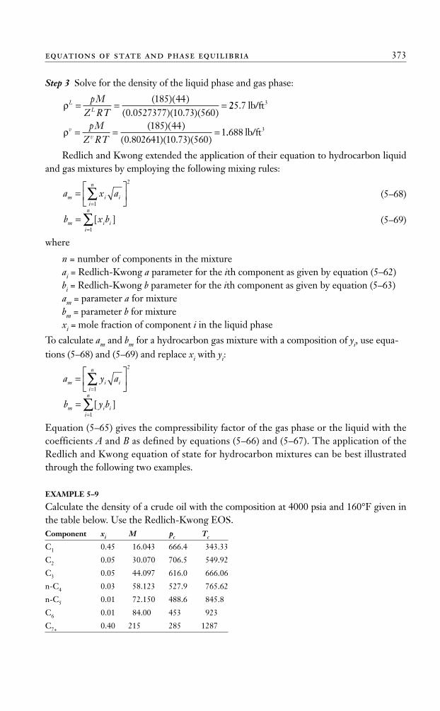
Step 3 Solve for the density of the liquid phase and gas phase:
Redlich and Kwong extended the application of their equation to hydrocarbon liquidand gas mixtures by employing the following mixing rules:
(5–68)
(5–69)
where
n = number of components in the mixtureai = Redlich-Kwong a parameter for the ith component as given by equation (5–62)bi = Redlich-Kwong b parameter for the ith component as given by equation (5–63)am = parameter a for mixturebm = parameter b for mixturexi = mole fraction of component i in the liquid phase
To calculate am and bm for a hydrocarbon gas mixture with a composition of yi, use equa-tions (5–68) and (5–69) and replace xi with yi:
Equation (5–65) gives the compressibility factor of the gas phase or the liquid with thecoefficients A and B as defined by equations (5–66) and (5–67). The application of theRedlich and Kwong equation of state for hydrocarbon mixtures can be best illustratedthrough the following two examples.
EXAMPLE 5–9
Calculate the density of a crude oil with the composition at 4000 psia and 160°F given inthe table below. Use the Redlich-Kwong EOS.Component xi M pc Tc
C1 0.45 16.043 666.4 343.33
C2 0.05 30.070 706.5 549.92
C3 0.05 44.097 616.0 666.06
n-C4 0.03 58.123 527.9 765.62
n-C5 0.01 72.150 488.6 845.8
C6 0.01 84.00 453 923
C7+ 0.40 215 285 1287
b y bm i ii
n
==∑[ ]
1
a y am i ii
n
=⎡⎣⎢
⎤⎦⎥
=∑
1
2
b x bm i ii
n
==∑[ ]
1
a x am i ii
n
=⎡⎣⎢
⎤⎦⎥
=∑
1
2
ρvv
pMZ RT
= = =( )( )
( . )( . )( )185 44
0 802641 10 73 5601..688 3lb/ft
ρLL
pMZ RT
= = =( )( )
( . )( . )( )185 44
0 0527377 10 73 560225 7 3. lb/ft
equations of state and phase equilibria 373
Ahmed_ch5.qxd 12/21/06 2:05 PM Page 373
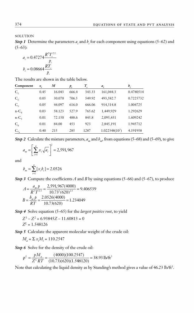
SOLUTION
Step 1 Determine the parameters ai and bi for each component using equations (5–62) and(5–63):
The results are shown in the table below.Component xi M pc Tc ai bi
C1 0.45 16.043 666.4 343.33 161,044.3 0.4780514
C2 0.05 30.070 706.5 549.92 493,582.7 0.7225732
C3 0.05 44.097 616.0 666.06 914,314.8 1.004725
n-C4 0.03 58.123 527.9 765.62 1,449,929 1.292629
n-C5 0.01 72.150 488.6 845.8 2,095,431 1.609242
C6 0.01 84.00 453 923 2,845,191 1.945712
C7+ 0.40 215 285 1287 1.022348(107) 4.191958
Step 2 Calculate the mixture parameters, am and bm, from equations (5–68) and (5–69), to give
and
Step 3 Compute the coefficients A and B by using equations (5–66) and (5–67), to produce
Step 4 Solve equation (5–65) for the largest positive root, to yield
Z3 – Z2 + 6.93845Z – 11.60813 = 0ZL = 1.548126
Step 5 Calculate the apparent molecular weight of the crude oil:
Ma = Σ xiMi = 110.2547
Step 6 Solve for the density of the crude oil:
Note that calculating the liquid density as by Standing’s method gives a value of 46.23 lb/ft3.
ρL aL
pMZ RT
= =( )( . )
( . )( )( .4000 100 2547
10 73 620 1 544812038 93 3
).= lb/ft
Bb pRT
m= = =2 0526 400010 73 620
1 234049. ( )
. ( ).
Aa p
R Tm= = =2 2 5 2 2 5
2 591 967 400010 73 620
9. .
, , ( ). ( )
..406539
b x bm i ii
n
= ==∑[ ] .
1
2 0526
a x am i ii
n
=⎡⎣⎢
⎤⎦⎥ =
=∑
1
2
2 591 967, ,
bRTpi
c
c
= 0 08664.
aR T
pic
c
= 0 472742 2 5
..
374 equations of state and pvt analysis
Ahmed_ch5.qxd 12/21/06 2:05 PM Page 374
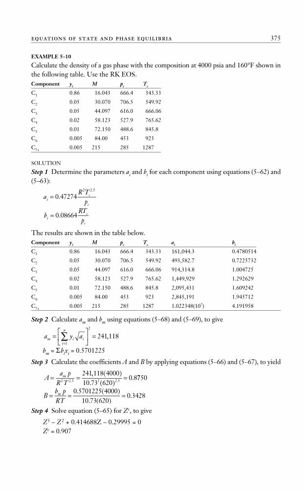
EXAMPLE 5–10
Calculate the density of a gas phase with the composition at 4000 psia and 160°F shown inthe following table. Use the RK EOS.Component yi M pc Tc
C1 0.86 16.043 666.4 343.33
C2 0.05 30.070 706.5 549.92
C3 0.05 44.097 616.0 666.06
C4 0.02 58.123 527.9 765.62
C5 0.01 72.150 488.6 845.8
C6 0.005 84.00 453 923
C7+ 0.005 215 285 1287
SOLUTION
Step 1 Determine the parameters ai and bi for each component using equations (5–62) and(5–63):
The results are shown in the table below.Component yi M pc Tc ai bi
C1 0.86 16.043 666.4 343.33 161,044.3 0.4780514
C2 0.05 30.070 706.5 549.92 493,582.7 0.7225732
C3 0.05 44.097 616.0 666.06 914,314.8 1.004725
C4 0.02 58.123 527.9 765.62 1,449,929 1.292629
C5 0.01 72.150 488.6 845.8 2,095,431 1.609242
C6 0.005 84.00 453 923 2,845,191 1.945712
C7+ 0.005 215 285 1287 1.022348(107) 4.191958
Step 2 Calculate am and bm using equations (5–68) and (5–69), to give
bm = Σbixi = 0.5701225
Step 3 Calculate the coefficients A and B by applying equations (5–66) and (5–67), to yield
Step 4 Solve equation (5–65) for Zv, to give
Z3 – Z2 + 0.414688Z – 0.29995 = 0Zv = 0.907
Bb pRT
m= = =0 5701225 4000
10 73 6200 3428
. ( ). ( )
.
Aa p
R Tm= = =2 2 5 2 2 5
241 118 400010 73 620
0 8. .
, ( ). ( )
. 7750
a y am i ii
n
=⎡⎣⎢
⎤⎦⎥ =
=∑
1
2
241 118,
bRTpi
c
c
= 0 08664.
aR T
pic
c
= 0 472742 2 5
..
equations of state and phase equilibria 375
Ahmed_ch5.qxd 12/21/06 2:05 PM Page 375

Step 5 Calculate the apparent molecular weight and density of the gas mixture:
Ma =ΣyiMi = 20.89
Soave-Redlich-Kwong Equation of State and Its ModificationsOne of the most significant milestones in the development of cubic equations of state wasthe report by Soave (1972) of a modification in the evaluation of the parameter a in the at-traction pressure term of the Redlich-Kwong equation of state (equation 5–60). Soave re-placed the term (a/T0.5) in equation (5–60) with a more general temperature-dependent term,denoted by aα(T), to give
(5–70)
where α(T) is a dimensionless factor that becomes unity when the reduced temperature, Tr, =1; that is, α(Tc) = 1 when T/Tc = 1. Soave used vapor pressures of pure components todevelop a generalized expression for the temperature correction parameter α(T). At sys-tem temperatures other than the critical temperature, the correction parameter α(T) isdefined by the following relationship:
(5–71)Soave correlated the parameter m with the acentric factor, ω, to give
m = 0.480 + 1.574ω – 0.176ω2 (5–72)
where
Tr = reduced temperature, T/Tc
ω = acentric factor of the substanceT = system temperature, °R
For simplicity and convenience, the temperature-dependent term αα(T ) is re-placed by the symbol αα for the remainder of this chapter.
For any pure component, the constants a and b in equation (5–70) are found by impos-ing the classical van der Waals’s critical point constraints (equation 5–48), on equation(5–70) and solving the resulting two equations:
(5–73)
(5–74)where Ωa and Ωb are the Soave-Redlich-Kwong (SRK) dimensionless pure componentparameters and have the following values:
Ωa = 0.42747Ωb = 0.08664
bRTpb
c
c
= Ω
aR T
pac
c
= Ω2 2
α( )T m Tr= + −( )⎡⎣
⎤⎦1 1
2
pRT
V ba T
V V b=
−−
+α( )
( )
ρv av
pMZ RT
= =( )( . )
( . )( )( . )4000 20 89
10 73 620 0 907==13 85 3. lb/ft
376 equations of state and pvt analysis
Ahmed_ch5.qxd 12/21/06 2:05 PM Page 376
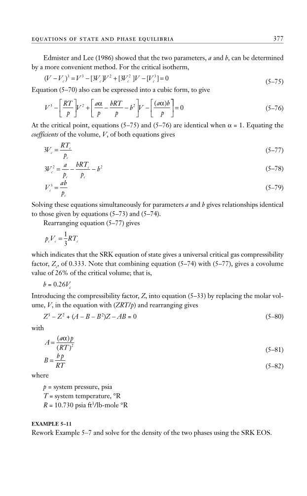
Edmister and Lee (1986) showed that the two parameters, a and b, can be determinedby a more convenient method. For the critical isotherm,
(5–75)Equation (5–70) also can be expressed into a cubic form, to give
(5–76)
At the critical point, equations (5–75) and (5–76) are identical when α = 1. Equating thecoefficients of the volume, V, of both equations gives
(5–77)
(5–78)
(5–79)
Solving these equations simultaneously for parameters a and b gives relationships identicalto those given by equations (5–73) and (5–74).
Rearranging equation (5–77) gives
which indicates that the SRK equation of state gives a universal critical gas compressibilityfactor, Zc, of 0.333. Note that combining equation (5–74) with (5–77), gives a covolumevalue of 26% of the critical volume; that is,
b = 0.26Vc
Introducing the compressibility factor, Z, into equation (5–33) by replacing the molar vol-ume, V, in the equation with (ZRT/p) and rearranging gives
Z3 – Z2 + (A – B – B2)Z – AB = 0 (5–80)
with
(5–81)
(5–82)where
p = system pressure, psiaT = system temperature, °RR = 10.730 psia ft3/lb-mole °R
EXAMPLE 5–11
Rework Example 5–7 and solve for the density of the two phases using the SRK EOS.
Bb pRT
=
Aa pRT
= ( )( )α
2
p V RTc c c= 13
Vabpc
c
3 =
3 2 2Vap
bRTp
bcc
c
c
= − −
3VRTpc
c
c
=
VRT
pV
ap
bRTp
b Va b
p3 2 2−⎡
⎣⎢
⎤
⎦⎥ + − −
⎡
⎣⎢
⎤
⎦⎥ −
⎡
⎣⎢
α α( ) ⎤⎤
⎦⎥ = 0
( ) [ ] [ ] [ ]V V V V V V V Vc c c c− = − + − =3 3 2 2 33 3 0
equations of state and phase equilibria 377
Ahmed_ch5.qxd 12/21/06 2:05 PM Page 377
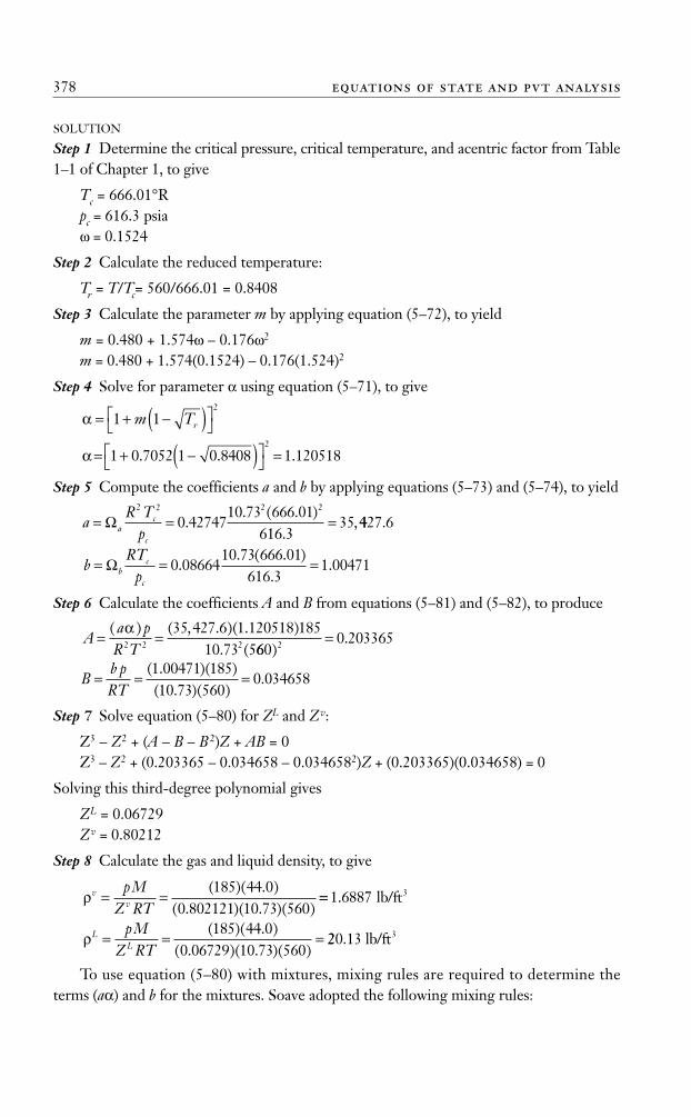
SOLUTION
Step 1 Determine the critical pressure, critical temperature, and acentric factor from Table1–1 of Chapter 1, to give
Tc = 666.01°Rpc = 616.3 psiaω = 0.1524
Step 2 Calculate the reduced temperature:
Tr = T/Tc= 560/666.01 = 0.8408
Step 3 Calculate the parameter m by applying equation (5–72), to yield
m = 0.480 + 1.574ω – 0.176ω2
m = 0.480 + 1.574(0.1524) – 0.176(1.524)2
Step 4 Solve for parameter α using equation (5–71), to give
Step 5 Compute the coefficients a and b by applying equations (5–73) and (5–74), to yield
Step 6 Calculate the coefficients A and B from equations (5–81) and (5–82), to produce
Step 7 Solve equation (5–80) for ZL and Zv:
Z3 – Z2 + (A – B – B2)Z + AB = 0Z3 – Z2 + (0.203365 – 0.034658 – 0.0346582)Z + (0.203365)(0.034658) = 0
Solving this third-degree polynomial gives
ZL = 0.06729Zv = 0.80212
Step 8 Calculate the gas and liquid density, to give
To use equation (5–80) with mixtures, mixing rules are required to determine theterms (aα) and b for the mixtures. Soave adopted the following mixing rules:
ρLL
pMZ RT
= = =( )( . )
( . )( . )( )185 44 0
0 06729 10 73 560220 13 3. lb/ft
ρvv
pMZ RT
= =( )( . )
( . )( . )( )185 44 0
0 802121 10 73 560==1 6887. lb/ft3
Bb pRT
= = =( . )( )( . )( )
.1 00471 18510 73 560
0 034658
Aa pR T
= =( ) ( , . )( . )
. (α2 2 2
35 427 6 1 120518 18510 73 5660
0 2033652).=
bRT
pbc
c
= = =Ω 0 0866410 73 666 01
616 31 00471.
. ( . ).
.
aR T
pac
c
= = =Ω2 2 2 2
0 4274710 73 666 01
616 335.
. ( . ).
,4427 6.
α= + −( )⎡⎣
⎤⎦ =1 0 7052 1 0 8408 1 120518
2
. . .
α = + −( )⎡⎣
⎤⎦1 1
2
m Tr
378 equations of state and pvt analysis
Ahmed_ch5.qxd 12/21/06 2:05 PM Page 378
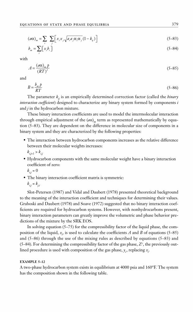
(5–83)
(5–84)
with
(5–85)
and
(5–86)
The parameter kij is an empirically determined correction factor (called the binaryinteraction coefficient) designed to characterize any binary system formed by components iand j in the hydrocarbon mixture.
These binary interaction coefficients are used to model the intermolecular interactionthrough empirical adjustment of the (aα)m term as represented mathematically by equa-tion (5–83). They are dependent on the difference in molecular size of components in abinary system and they are characterized by the following properties:
• The interaction between hydrocarbon components increases as the relative differencebetween their molecular weights increases:ki,j+1 > ki,j
• Hydrocarbon components with the same molecular weight have a binary interactioncoefficient of zero:ki,j = 0
• The binary interaction coefficient matrix is symmetric:ki,j = kj,i
Slot-Petersen (1987) and Vidal and Daubert (1978) presented theoretical backgroundto the meaning of the interaction coefficient and techniques for determining their values.Graboski and Daubert (1978) and Soave (1972) suggested that no binary interaction coef-ficients are required for hydrocarbon systems. However, with nonhydrocarbons present,binary interaction parameters can greatly improve the volumetric and phase behavior pre-dictions of the mixture by the SRK EOS.
In solving equation (5–75) for the compressibility factor of the liquid phase, the com-position of the liquid, xi, is used to calculate the coefficients A and B of equations (5–85)and (5–86) through the use of the mixing rules as described by equations (5–83) and(5–84). For determining the compressibility factor of the gas phase, Zv, the previously out-lined procedure is used with composition of the gas phase, yi , replacing xi.
EXAMPLE 5–12
A two-phase hydrocarbon system exists in equilibrium at 4000 psia and 160°F. The systemhas the composition shown in the following table.
Bb pRT
m=
Aa pRT
m=( )( )α
2
b x bm i ii
= ⎡⎣ ⎤⎦∑
( ) ( )a x x a a kmi
i j i j i j ijj
α α α= −⎡⎣
⎤⎦∑ ∑ 1
equations of state and phase equilibria 379
Ahmed_ch5.qxd 12/21/06 2:05 PM Page 379
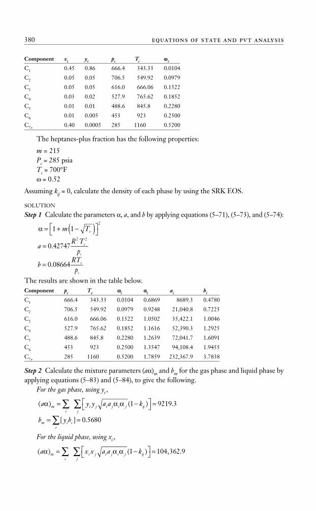
Component xi yi pc Tc ωω i
C1 0.45 0.86 666.4 343.33 0.0104
C2 0.05 0.05 706.5 549.92 0.0979
C3 0.05 0.05 616.0 666.06 0.1522
C4 0.03 0.02 527.9 765.62 0.1852
C5 0.01 0.01 488.6 845.8 0.2280
C6 0.01 0.005 453 923 0.2500
C7+ 0.40 0.0005 285 1160 0.5200
The heptanes-plus fraction has the following properties:
m = 215Pc = 285 psiaTc = 700°Fω = 0.52
Assuming kij = 0, calculate the density of each phase by using the SRK EOS.
SOLUTION
Step 1 Calculate the parameters α, a, and b by applying equations (5–71), (5–73), and (5–74):
The results are shown in the table below.Component pc Tc ωωi ααi ai bi
C1 666.4 343.33 0.0104 0.6869 8689.3 0.4780
C2 706.5 549.92 0.0979 0.9248 21,040.8 0.7225
C3 616.0 666.06 0.1522 1.0502 35,422.1 1.0046
C4 527.9 765.62 0.1852 1.1616 52,390.3 1.2925
C5 488.6 845.8 0.2280 1.2639 72,041.7 1.6091
C6 453 923 0.2500 1.3547 94,108.4 1.9455
C7+ 285 1160 0.5200 1.7859 232,367.9 3.7838
Step 2 Calculate the mixture parameters (aα)m and bm for the gas phase and liquid phase byapplying equations (5–83) and (5–84), to give the following.
For the gas phase, using yi ,
For the liquid phase, using xi ,
( ) ( ) , .a x x a a kmi
i j i j i j ijj
α α α= −⎡⎣
⎤⎦ =∑ ∑ 1 104 362 9
b y bm i ii
= =∑[ ] .0 5680
( ) ( ) .a y y a a kmi
i j i j i j ijj
α α α= −⎡⎣
⎤⎦ =∑ ∑ 1 9219 3
bRTp
c
c
= 0 08664.
aR T
pc
c
= 0 427472 2
.
α = + −( )⎡⎣
⎤⎦1 1
2
m Tr
380 equations of state and pvt analysis
Ahmed_ch5.qxd 12/21/06 2:05 PM Page 380
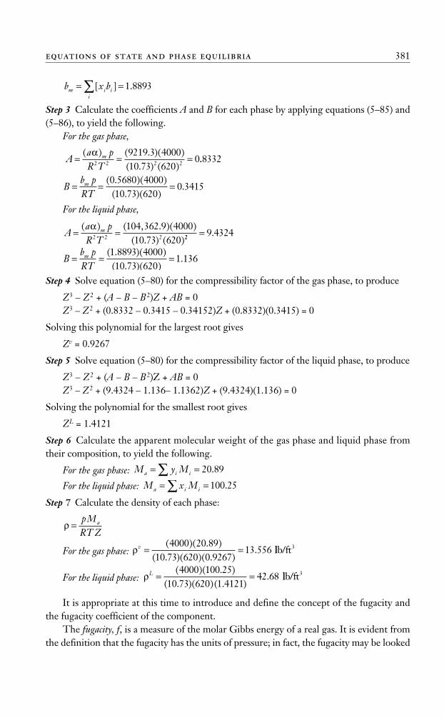
Step 3 Calculate the coefficients A and B for each phase by applying equations (5–85) and(5–86), to yield the following.
For the gas phase,
For the liquid phase,
Step 4 Solve equation (5–80) for the compressibility factor of the gas phase, to produce
Z3 – Z2 + (A – B – B2)Z + AB = 0Z3 – Z2 + (0.8332 – 0.3415 – 0.34152)Z + (0.8332)(0.3415) = 0
Solving this polynomial for the largest root gives
Zv = 0.9267
Step 5 Solve equation (5–80) for the compressibility factor of the liquid phase, to produce
Z3 – Z2 + (A – B – B2)Z + AB = 0Z3 – Z2 + (9.4324 – 1.136– 1.1362)Z + (9.4324)(1.136) = 0
Solving the polynomial for the smallest root gives
ZL = 1.4121
Step 6 Calculate the apparent molecular weight of the gas phase and liquid phase fromtheir composition, to yield the following.
For the gas phase:
For the liquid phase:
Step 7 Calculate the density of each phase:
For the gas phase:
For the liquid phase:
It is appropriate at this time to introduce and define the concept of the fugacity andthe fugacity coefficient of the component.
The fugacity, f, is a measure of the molar Gibbs energy of a real gas. It is evident fromthe definition that the fugacity has the units of pressure; in fact, the fugacity may be looked
ρL = =( )( . )
( . )( )( . ).
4000 100 2510 73 620 1 4121
42 68 llb/ft3
ρv = =( )( . )
( . )( )( . ).
4000 20 8910 73 620 0 9267
13 556 llb/ft3
ρ =pMRT Z
a
M x Ma i i= =∑ 100 25.
M y Ma i i= =∑ 20 89.
Bb pRT
m= = =( . )( )( . )( )
.1 8893 400010 73 620
1 136
Aa pR T
m= =( ) ( , . )( )
( . ) ( )α2 2 2
104 362 9 400010 73 620 22 9 4324= .
Bb pRT
m= = =( . )( )
( . )( ).
0 5680 400010 73 620
0 3415
Aa pR T
m= = =( ) ( . )( )
( . ) ( )α2 2 2 2
9219 3 400010 73 620
0..8332
b x bm i ii
= =∑[ ] .1 8893
equations of state and phase equilibria 381
Ahmed_ch5.qxd 12/21/06 2:05 PM Page 381
on as a vapor pressure modified to correctly represent the tendency of the molecules from onephase to escape into the other. In a mathematical form, the fugacity of a pure component isdefined by the following expression:
(5–87)
where
f o = fugacity of a pure component, psiap = pressure, psiaZ = compressibility factor
The ratio of the fugacity to the pressure, f/p, called the fugacity coefficient, Φ, is calcu-lated from equation (5–87) as
Soave applied this generalized thermodynamic relationship to equation (5–70) todetermine the fugacity coefficient of a pure component, to give
(5–88)
In practical petroleum engineering applications, we are concerned with the phasebehavior of the hydrocarbon liquid mixture, which at a specified pressure and temperature,is in equilibrium with a hydrocarbon gas mixture at the same pressure and temperature.
In a hydrocarbon multicomponent mixture, the component fugacity in each phase isintroduced to develop a criterion for thermodynamic equilibrium. Physically, the fugacityof a component i in one phase with respect to the fugacity of the component in a secondphase is a measure of the potential for transfer of the component between phases. Thephase with the lower component fugacity accepts the component from the phase with ahigher component fugacity. Equal fugacities of a component in the two phases results in azero net transfer. A zero transfer for all components implies a hydrocarbon system in ther-modynamic equilibrium. Therefore, the condition of the thermodynamic equilibrium canbe expressed mathematically by
(5–89)
where
f vi = fugacity of component i in the gas phase, psi
f Li = fugacity of component i in the liquid phase, psi
n = number of components in the system
The fugacity coefficient of component i in a hydrocarbon liquid mixture or hydrocar-bon gas mixture is a function of the system pressure, mole fraction, and fugacity of thecomponent. The fugacity coefficient is defined as:
For a component i in the gas phase: (5–90)Φ iv i
v
i
fy p
=
f f i niv
iL= ≤ ≤, 1
ln ln( ) ln( ) lnfp
Z Z BAB
Z BZ
o⎛⎝⎜
⎞⎠⎟= = − − − −
+⎡⎣⎢
⎤⎦
Φ 1 ⎥⎥
fp
Zp
dpo
o
p= = −⎛
⎝⎜⎞⎠⎟
⎡
⎣⎢
⎤
⎦⎥∫Φ exp
1
f pZ
pdpo
o
p=
−⎛⎝⎜
⎞⎠⎟
⎡
⎣⎢
⎤
⎦⎥∫exp
1
382 equations of state and pvt analysis
Ahmed_ch5.qxd 12/21/06 2:05 PM Page 382
For a component i in the liquid phase: (5–91)
where Φvi = fugacity coefficient of component i in the vapor phase and ΦL
i = fugacity coef-ficient of component i in the liquid phase.
It is clear that, at equilibrium ( f Li = f v
i ), the equilibrium ratio, Ki, as previously definedby equation (5–1), that is, Ki = yi /xi , can be redefined in terms of the fugacity of compo-nents as
(5–92)
Reid, Prausnitz, and Sherwood (1987) defined the fugacity coefficient of component iin a hydrocarbon mixture by the following generalized thermodynamic relationship:
(5–93)
where
V = total volume of n moles of the mixtureni = number of moles of component iZ = compressibility factor of the hydrocarbon mixture
By combining the above thermodynamic definition of the fugacity with the SRK EOS(equation 5–70), Soave proposed the following expression for the fugacity coefficient ofcomponent i in the liquid phase:
(5–94)
where
(5–95)
(5–96)
Equation (5–94) also is used to determine the fugacity coefficient of component in thegas phase, Φv
i , by using the composition of the gas phase, yi, in calculating A, B, Zv, andother composition-dependent terms; that is,
where
It is important to note that, in solving the cubic Z-factor equation for hydrocarbonmixtures, one or three real roots may exist. When three roots exist with different values
( ) ( )a y y a a km i j i j i j ijji
α α α= −⎡⎣
⎤⎦∑∑ 1
Ψ i j i j i j ijj
y a a k= −⎡⎣
⎤⎦∑ α α ( )1
ln( )
ln( )( )
ΦΨ
iv i
v
m
v ib Zb
Z BAB a
( ) = −− − − ⎛
⎝⎜⎞⎠⎟
1 2α mm
i
mv
bb
BZ
−⎡
⎣⎢
⎤
⎦⎥ +⎡
⎣⎢⎤⎦⎥
ln 1
( ) ( )a x x a a km i j i j i j ijji
α α α= −⎡⎣
⎤⎦∑∑ 1
Ψ i j i j i j ijj
x a a k= −⎡⎣
⎤⎦∑ α α ( )1
ln ln( )
ln( )fx p
b Zb
Z BiL
iiL i
L
m
L⎛⎝⎜
⎞⎠⎟= ( ) = −
− − −Φ1 AA
B abb
BZ
i
m
i
mL
⎛⎝⎜⎞⎠⎟
−⎡
⎣⎢
⎤
⎦⎥ +⎡
⎣⎢⎤⎦⎥
21
Ψ( )
lnα
ln( )Φ ii
VRTpn
RTV
dV= ⎛⎝⎜
⎞⎠⎟
∂∂
−⎛⎝⎜
⎞⎠⎟
⎡
⎣⎢
⎤
⎦⎥ −
∞
∫1
lln( )Z
Kf x pf y pi
iL
i
iv
i
iL
iv= =
[ / ( )][ / ( )]
ΦΦ
Φ iL i
L
i
fx p
=
equations of state and phase equilibria 383
Ahmed_ch5.qxd 12/21/06 2:05 PM Page 383
that are denoted as ZLargest, ZMiddle, and ZSmallest, the middle root, ZMiddle, always is discardedas a nonphysical value or meaning. However, the choice of the correct root between theremaining two roots is not a priori and the correct root is chosen as the one with the low-est normalized Gibbs energy function, g*. The normalized Gibbs energy function, g*, isdefined in terms of the composition of the system and the individual component fugacityin the system; mathematically, it is defined by
Normalized Gibbs energy for gas:
Normalized Gibbs energy for liquid:
Therefore, assume that a liquid phase with a composition of xi has multiple Z-factorroots; the middle root is discarded automatically, and the remaining two are designated ZL1
and ZL2. To select the correct root, calculate the normalized Gibbs energy function using
the two remaining roots:
In which the fugacity f Li is determined from equation (5–94) using the two remaining
roots, ZL1 and ZL2:
If g*ZL1< g*ZL2
then ZL1is chosen as the correct root; otherwise, ZL2
is chosen.It should be pointed out that the partial Gibbs free energy plays an equally important
role in determining the equilibrium of mixtures. The partial Gibbs energy is given thename chemical potential, μi , as defined by
The chemical potential, μi, essentially is a quantity that measures how much energy acomponent brings to a mixture. As was defined mathematically, this property can be usedto measure the change of Gibbs free energy, G, in the system with the change in theamount of substance i as a constant: pressure, p; temperature, T; and amount of othercomponents, nj, where ni is the amount of component i in the mixture and i ≠ j. In a mix-ture, the normalized Gibbs free energy, g, is not the same in both phases because theircompositions are different. Instead, the criterion for equilibrium is that the total Gibbsfree energy, G, is at minimum with respect to all transfers of components from one phaseto another at constant pressure and temperature; that is
∂ = −⎡⎣ ⎤⎦∂ =G ni i iμ μgas liquid 0
μ ii p T n
Gn
j
=∂∂⎛⎝⎜
⎞⎠⎟ , ,
( ) exp( )
ln( )f z xb Z
bZ B
ABi
LL i
i L
mL1
22
1= +
−⎧⎨⎩
− − − ⎛⎝⎝⎜⎞⎠⎟
−⎡
⎣⎢
⎤
⎦⎥ +
⎡
⎣⎢
⎤
⎦⎥⎫⎬⎪
⎭
21
2
Ψ i
m
i
m Labb
BZ( )
lnα ⎪⎪
( ) exp( )
ln( )f z x pb Z
bZ B
ABi
LL i
i L
mL1
11
1= +
−⎧⎨⎩
− − − ⎛⎛⎝⎜⎞⎠⎟
−⎡
⎣⎢
⎤
⎦⎥ +
⎡
⎣⎢
⎤
⎦⎥⎫⎬⎪2
11
Ψ i
m
i
m Labb
BZ( )
lnα ⎭⎭⎪
g x fZ i iL
i
n
L 21
* ln( )==∑
g x fZ i iL
i
n
L11
* ln( )==∑
g x fi iL
i
n
Liquid* ln( )=
=∑
1
g y fi iv
i
n
gas* ln( )=
=∑
1
384 equations of state and pvt analysis
Ahmed_ch5.qxd 12/21/06 2:05 PM Page 384
This criterion implies that, at equilibrium, the chemical potential of each component μi
has the same value in each phase:
The chemical potential of component i is related to the activity âi by
with
where
âi = activity of component i in mixture at p and Tμo
i = chemical potential of pure of component i at p and Tf o
i = fugacity of pure component i at p and Tfi = fugacity of component i in mixture at p and T
Modifications of the SRK EOSTo improve the pure component vapor pressure predictions by the SRK equation of state,Groboski and Daubert (1978) proposed a new expression for calculating parameter m ofequation (5–72). The proposed relationship, which originated from analyzing extensiveexperimental data for pure hydrocarbons, has the following form:
(5–97)
Sim and Daubert (1980) pointed out that, because the coefficients of equation (5–97)were determined by analyzing vapor pressure data of low-molecular-weight hydrocarbons,it is unlikely that equation (5–97) will suffice for high-molecular-weight petroleum frac-tions. Realizing that the acentric factors for the heavy petroleum fractions are calculatedfrom an equation such as the Edmister correlation or the Lee and Kesler correlation, theauthors proposed the following expressions for determining parameter m:
• If the acentric factor is determined using the Edmister correlation, then(5–98)
• If the acentric factor is determined using the Lee and Kesler correction, then(5–99)
Elliot and Daubert (1985) stated that the optimal binary interaction coefficient, kij,would minimize the error in the representation of all the thermodynamic properties of amixture. Properties of particular interest in phase-equilibrium calculations include bubble-point pressure, dew-point pressure, and equilibrium ratios. The authors proposed a set ofrelationships for determining interaction coefficients for asymmetric mixtures∗ that containmethane, N2, CO2, and H2S. Referring to the principal component as i and other fractionsas j, Elliot and Daubert proposed the following expressions:
m i i= + −0 315 1 60 0 166 2. . .ω ω
m i i= + −0 431 1 57 0 161 2. . .ω ω
m = + −0 48508 1 55171 0 15613 2. . .ω ω
affi
i
io=
μ μi io
iRT a= + ln( ˆ )
μ μgas liquidi i=
equations of state and phase equilibria 385
∗An asymmetric mixture is defined as one in which two of the components are considerably different in theirchemical behavior. Mixtures of methane with hydrocarbons of 10 or more carbon atoms can be considered asym-metric. Mixtures containing gases such as nitrogen or hydrogen are asymmetric.
Ahmed_ch5.qxd 12/21/06 2:05 PM Page 385
For N2 systems,kij = 0.107089 + 2.9776k∞
ij (5–100)
For CO2 systems,kij = 0.08058 – 0.77215k∞
ij – 1.8404(k∞ij ) (5–101)
For H2S systems,kij = 0.07654 + 0.017921k∞
ij (5–102)
For methane systems with compounds of 10 carbons or more,kij = 0.17985 + 2.6958k∞
ij + 10.853(k∞ij )
2 (5–103)where
(5–104)
and
(5–105)
The two parameters, ai and bi, of equation (5–105) were defined previously by equations(5–73) and (5–74).
The major drawback in the SRK EOS is that the critical compressibility factor takes onthe unrealistic universal critical compressibility of 0.333 for all substances. Consequently,the molar volumes typically are overestimated; that is, densities are underestimated.
Peneloux, Rauzy, and Freze (1982) developed a procedure for improving the volumet-ric predictions of the SRK EOS by introducing a volume correction parameter, ci, into theequation. This third parameter does not change the vapor/liquid equilibrium conditionsdetermined by the unmodified SRK equation, that is, the equilibrium ratio Ki, but it mod-ifies the liquid and gas volumes. The proposed methodology, known as the volume transla-tion method, uses the following expressions:
(5–106)
(5–107)
where
VL = uncorrected liquid molar volume (i.e., VL = ZLRT/p), ft3/moleVv = uncorrected gas molar volume Vv = ZvRT/p, ft3/moleV L
corr= corrected liquid molar volume, ft3/moleV v
corr = corrected gas molar volume, ft3/molexi = mole fraction of component i in the liquid phaseyi = mole fraction of component i in the gas phase
The authors proposed six schemes for calculating the correction factor, ci, for eachcomponent. For petroleum fluids and heavy hydrocarbons, Peneloux and coworkers sug-gested that the best correlating parameter for the volume correction factor ci is the Rackettcompressibility factor, ZRA. The correction factor then is defined mathematically by thefollowing relationship:
ci = 4.43797878(0.29441 – ZRA)Tci /pci (5–108)
V V y cv vi i
icorr = −∑ ( )
V V x cL Li i
icorr = −∑ ( )
ε ii
i
ab
=0 480453.
kiji j
i j
∞ =− −( )ε ε
ε ε
2
2
386 equations of state and pvt analysis
Ahmed_ch5.qxd 12/21/06 2:05 PM Page 386
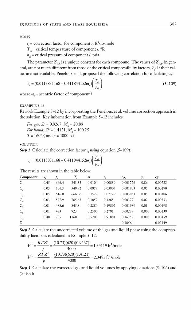
where
ci = correction factor for component i, ft3/lb-moleTci = critical temperature of component i, °Rpci = critical pressure of component i, psia
The parameter ZRA is a unique constant for each compound. The values of ZRA, in gen-eral, are not much different from those of the critical compressibility factors, Zc. If their val-ues are not available, Peneloux et al. proposed the following correlation for calculating ci:
(5–109)
where ωi = acentric factor of component i.
EXAMPLE 5–13
Rework Example 5–12 by incorporating the Peneloux et al. volume correction approach inthe solution. Key information from Example 5–12 includes:
For gas: Zv = 0.9267, Ma = 20.89For liquid: ZL = 1.4121, Ma = 100.25T = 160°F, and p = 4000 psi
SOLUTION
Step 1 Calculate the correction factor ci using equation (5–109):
The results are shown in the table below.Component xi pc Tc ωωi ci cixi yi ciyi
C1 0.45 666.4 343.33 0.0104 0.00839 0.003776 0.86 0.00722
C2 0.05 706.5 549.92 0.0979 0.03807 0.001903 0.05 0.00190
C3 0.05 616.0 666.06 0.1522 0.07729 0.003861 0.05 0.00386
C4 0.03 527.9 765.62 0.1852 0.1265 0.00379 0.02 0.00253
C5 0.01 488.6 845.8 0.2280 0.19897 0.001989 0.01 0.00198
C6 0.01 453 923 0.2500 0.2791 0.00279 0.005 0.00139
C7+ 0.40 285 1160 0.5200 0.91881 0.36752 0.005 0.00459
Σ 0.38564 0.02349
Step 2 Calculate the uncorrected volume of the gas and liquid phase using the compress-ibility factors as calculated in Example 5–12.
Step 3 Calculate the corrected gas and liquid volumes by applying equations (5–106) and(5–107):
VRT Z
pL
L
= = =( . )( )( . )
.10 73 620 1 4121
40002 3485 ft3 //mole
VRT Z
pv
v
= = =( . )( )( . )
.10 73 620 0 9267
40001 54119 ft33 /mole
cTpi i= +⎛⎝⎜
⎞⎠⎟
( . . )0 0115831168 0 411844152ω ci
ci
cTpi i= +⎛⎝⎜
⎞⎠⎟
( . . )0 0115831168 0 411844152ω ci
ci
equations of state and phase equilibria 387
Ahmed_ch5.qxd 12/21/06 2:05 PM Page 387
Step 4 Calculate the corrected compressibility factors:
Step 5 Determine the corrected densities of both phases:
As pointed out by Whitson and Brule (2000), when the volume shift is introduced tothe EOS for mixtures, the resulting expressions for fugacity are
and
This implies that the fugacity ratios are unchanged by the volume shift:
Peng-Robinson’s Equation of State and Its ModificationsPeng and Robinson (1976a) conducted a comprehensive study to evaluate the use of theSRK equation of state for predicting the behavior of naturally-occurring hydrocarbon sys-tems. They illustrated the need for an improvement in the ability of the equation of stateto predict liquid densities and other fluid properties, particularly in the vicinity of the crit-ical region. As a basis for creating an improved model, Peng and Robinson (PR) proposedthe following expression:
where a, b, and α have the same significance as they have in the SRK model, and parame-ter c is a whole number optimized by analyzing the values of the terms Zc and b/Vc as ob-tained from the equation. It is generally accepted that Zc should be close to 0.28 and b/Vc
pRT
V ba
V b cb=
−−
+ −α
( )2 2
f
f
f
fiL
iv
iL
iv
( )( ) =
( )modified
modified
original
(( )original
f f cp
RTiv
iv
i( ) = ( ) −⎡
⎣⎢
⎤
⎦⎥modified original
exp
f f cp
RTiL
iL
i( ) = ( ) −⎡
⎣⎢
⎤
⎦⎥modified original
exp
ρL = =( )( . )
( . )( )( . ).
4000 100 2510 73 620 1 18025
51 077 3lb/ft
ρv = =( )( . )
( . )( )( . ).
4000 20 8910 73 620 0 91254
13 7677 3lb/ft
ρ =pMRT Z
a
Z Lcorr = =
( )( . )( . )( )
.4000 1 962927
10 73 6201 18025
Z vcorr = =
( )( . )( . )( )
.4000 1 517710 73 620
0 91254
V V y cv vi i
icorr ft= − = − =∑ ( ) . . .1 54119 0 02349 1 5177 33 /mole
V V x cL Li i
icorr f= − = − =∑ ( ) . . .2 3485 0 38564 1 962927 tt /mole3
388 equations of state and pvt analysis
Ahmed_ch5.qxd 12/21/06 2:05 PM Page 388
should be approximately 0.26. An optimized value of c = 2 gives Zc = 0.307 and (b/Vc) =0.253. Based on this value of c, Peng and Robinson proposed the following equation ofstate (commonly referred to as PR EOS):
(5–110)
Imposing the classical critical point conditions (equation 5–48) on equation (5–110)and solving for parameters a and b yields
(5–111)
(5–112)
where
Ωa = 0.45724Ωb = 0.07780
This equation predicts a universal critical gas compressibility factor, Zc, of 0.307, com-pared to 0.333 for the SRK model. Peng and Robinson also adopted Soave’s approach forcalculating parameter α:
(5–113)
where m = 0.3796 + 1.54226ω – 0.2699ω2.Peng and Robinson (1978) proposed the following modified expression for m that is
recommended for heavier components with acentric values ω > 0.49:
m = 0.379642 + 1.48503ω – 0.1644ω2 + 0.016667ω3 (5–114)
Rearranging equation (5–110) into the compressibility factor form, gives
Z3 + (B – 1)Z2 + (A – 3B2 – 2B)Z – (AB – B2 – B3) = 0 (5–115)
where A and B are given by equations (5–81) and (5–82) for pure component and by equa-tions (5–85) and (5–86) for mixtures; that is,
with
EXAMPLE 5–14
Using the composition given in Example 5–12, calculate the density of the gas phase andliquid phase by using the Peng-Robinson EOS. Assume kij = 0. The components aredescribed in the following table.
b x bm i ii
=∑[ ]
( ) ( )a x x a a km i j i j i j ijji
α α α= −⎡⎣
⎤⎦∑∑ 1
Bb pRT
m=
Aa pRT
m=( )( )α
2
α = + −( )⎡⎣
⎤⎦1 1
2
m Tr
bRTpb
c
c
= Ω
aR T
pac
c
= Ω2 2
pRT
V ba
V V b b V b=
−−
+ + −α
( ) ( )
equations of state and phase equilibria 389
Ahmed_ch5.qxd 12/21/06 2:05 PM Page 389
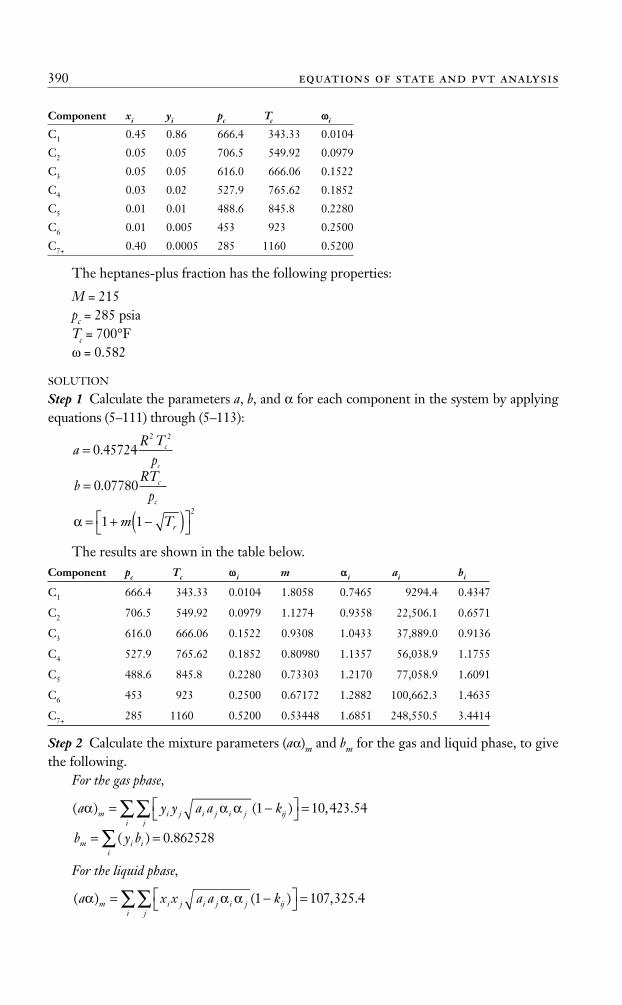
Component xi yi pc Tc ωωi
C1 0.45 0.86 666.4 343.33 0.0104
C2 0.05 0.05 706.5 549.92 0.0979
C3 0.05 0.05 616.0 666.06 0.1522
C4 0.03 0.02 527.9 765.62 0.1852
C5 0.01 0.01 488.6 845.8 0.2280
C6 0.01 0.005 453 923 0.2500
C7+ 0.40 0.0005 285 1160 0.5200
The heptanes-plus fraction has the following properties:
M = 215pc = 285 psiaTc = 700°Fω = 0.582
SOLUTION
Step 1 Calculate the parameters a, b, and α for each component in the system by applyingequations (5–111) through (5–113):
The results are shown in the table below.Component pc Tc ωω i m αα i ai bi
C1 666.4 343.33 0.0104 1.8058 0.7465 9294.4 0.4347
C2 706.5 549.92 0.0979 1.1274 0.9358 22,506.1 0.6571
C3 616.0 666.06 0.1522 0.9308 1.0433 37,889.0 0.9136
C4 527.9 765.62 0.1852 0.80980 1.1357 56,038.9 1.1755
C5 488.6 845.8 0.2280 0.73303 1.2170 77,058.9 1.6091
C6 453 923 0.2500 0.67172 1.2882 100,662.3 1.4635
C7+ 285 1160 0.5200 0.53448 1.6851 248,550.5 3.4414
Step 2 Calculate the mixture parameters (aα)m and bm for the gas and liquid phase, to givethe following.
For the gas phase,
For the liquid phase,
( ) ( ) , .a x x a a km i j i j i j ijji
α α α= −⎡⎣
⎤⎦ =∑∑ 1 107 325 4
b y bm i ii
= =∑ ( ) .0 862528
( ) ( ) , .a y y a a km i j i j i j ijji
α α α= −⎡⎣
⎤⎦ =∑∑ 1 10 423 54
α = + −( )⎡⎣
⎤⎦1 1
2
m Tr
bRT
pc
c
= 0 07780.
aR T
pc
c
= 0 457242 2
.
390 equations of state and pvt analysis
Ahmed_ch5.qxd 12/21/06 2:05 PM Page 390

Step 3 Calculate the coefficients A and B, to give the following.For the gas phase,
For the liquid phase,
Step 4 Solve equation (5–115) for the compressibility factor of the gas and liquid phases,to give
Z3 + (B – 1)Z2 + (A – 3B2 – 2B)Z – (AB – B2 – B3) = 0
For the gas phase:Substituting for A = 0.94209 and B = 0.30669 in the above equation gives
Z3 + (B – 1)Z2 + (A – 3B 2 – 2B)Z – (AB – B2 – B3) = 0Z3 + (0.30669 – 1)Z2 + [0.94209 – 3(0.30669)2 – 2(0.30669)]Z – [(0.94209)(0.30669)
– (0.30669)2 – (0.30669)3] = 0
Solving for Z gives
Zv = 0.8625
For the liquid phase:Substituting A = 9.700183 and B = 1.020078 in equation (5–115) gives
Z3 + (B – 1)Z2 + (A – 3B 2 – 2B)Z – (AB – B2 – B3) = 0Z3 + (1.020078 – 1)Z2 + [(9.700183) – 3(1.020078)2 – 2(1.020078)]Z
– [(9.700183)(1.020078) – (1.020078)2 – (1.020078)3] = 0
Solving for Z gives
ZL = 1.2645
Step 5 Calculate the density of both phases.Density of the vapor phase:
Density of the liquid phase:
ρL aL
pMZ RT
=
ρv = =( )( . )
( . )( )( . ).
4000 20 8910 73 620 0 8625
14 566 llb/ft3
ρv av
pMZ RT
=
Bb pRT
m= = =( . )( )
( . )( ).
1 696543 400010 73 620
1 0200778
Aa pR T
m= =( ) ( , . )( )
( . ) ( )α2 2 2
107 325 4 400010 73 620 22 9 700183= .
Bb pRT
m= = =( . )( )
( . )( ).
0 862528 400010 73 620
0 306699
Aa pR T
m= =( ) ( , . )( )
( . ) ( )α2 2 2
10 423 54 400010 73 620 22 0 94209= .
b x bm i ii
= =∑ ( ) .1 696543
equations of state and phase equilibria 391
Ahmed_ch5.qxd 12/21/06 2:05 PM Page 391
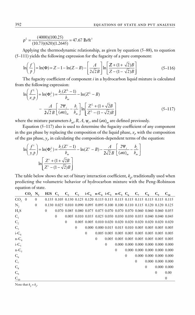
Applying the thermodynamic relationship, as given by equation (5–88), to equation(5–111) yields the following expression for the fugacity of a pure component:
(5–116)
The fugacity coefficient of component i in a hydrocarbon liquid mixture is calculatedfrom the following expression:
(5–117)
where the mixture parameters bm, B, A, ψi , and (aα)m are defined previously.Equation (5–117) also is used to determine the fugacity coefficient of any component
in the gas phase by replacing the composition of the liquid phase, xi, with the compositionof the gas phase, yi, in calculating the composition-dependent terms of the equation:
The table below shows the set of binary interaction coefficient, kij, traditionally used whenpredicting the volumetric behavior of hydrocarbon mixture with the Peng-Robinsonequation of state.
CO2 N2 H2S C1 C2 C3 i-C4 n-C4 i-C5 n-C5 C6 C7 C8 C9 C10
CO2 0 0 0.135 0.105 0.130 0.125 0.120 0.115 0.115 0.115 0.115 0.115 0.115 0.115 0.115
N2 0 0.130 0.025 0.010 0.090 0.095 0.095 0.100 0.100 0.110 0.115 0.120 0.120 0.125
H2S 0 0.070 0.085 0.080 0.075 0.075 0.070 0.070 0.070 0.060 0.060 0.060 0.055
C1 0 0.005 0.010 0.035 0.025 0.050 0.030 0.030 0.035 0.040 0.040 0.045
C2 0 0.005 0.005 0.010 0.020 0.020 0.020 0.020 0.020 0.020 0.020
C3 0 0.000 0.000 0.015 0.015 0.010 0.005 0.005 0.005 0.005
i-C4 0 0.005 0.005 0.005 0.005 0.005 0.005 0.005 0.005
n-C4 0 0.005 0.005 0.005 0.005 0.005 0.005 0.005
i-C5 0 0.000 0.000 0.000 0.000 0.000 0.000
n-C5 0 0.000 0.000 0.000 0.000 0.000
C6 0 0.000 0.000 0.000 0.000
C7 0 0.000 0.000 0.000
C8 0 0.000 0.000
C9 0 0.00
C10 0
Note that kij = kji.
1 21 2
Z BZ B
v
vln
(( )+ +− −
⎡
⎣⎣⎢⎢
⎤
⎦⎥⎥
ln ln( )( )
ln( )fy p
b Zb
Z BAv
iiL i
v
m
v⎛⎝⎜
⎞⎠⎟= =
−− − −Φ
122 2
2B a
bb
i
m
i
m
Ψ( )α
−⎡
⎣⎢
⎤
⎦⎥
A−22 2
2 1 21 2B a
bb
Z BZ B
i
m
i
m
L
L
Ψ( )
ln(( )α
−⎡
⎣⎢
⎤
⎦⎥
+ +− −
⎡
⎣⎣⎢⎢
⎤
⎦⎥⎥
ln ln( )( )
ln( )fx p
b Zb
Z BL
iiL i
L
m
L⎛⎝⎜
⎞⎠⎟= =
−− −Φ
1
ln ln( ) ln( ) lnfp
Z Z BA
B
⎛⎝⎜⎞⎠⎟= = − − − −
⎡
⎣⎢⎢
⎤
⎦⎥⎥
Φ 12 2
ZZ BZ B+ +− −
⎡
⎣⎢⎢
⎤
⎦⎥⎥
( )( )1 21 2
ρL = =( )( . )
( . )( )( . ).
4000 100 2510 73 620 1 2645
47 67 llb/ft3
392 equations of state and pvt analysis
Ahmed_ch5.qxd 12/21/06 2:05 PM Page 392
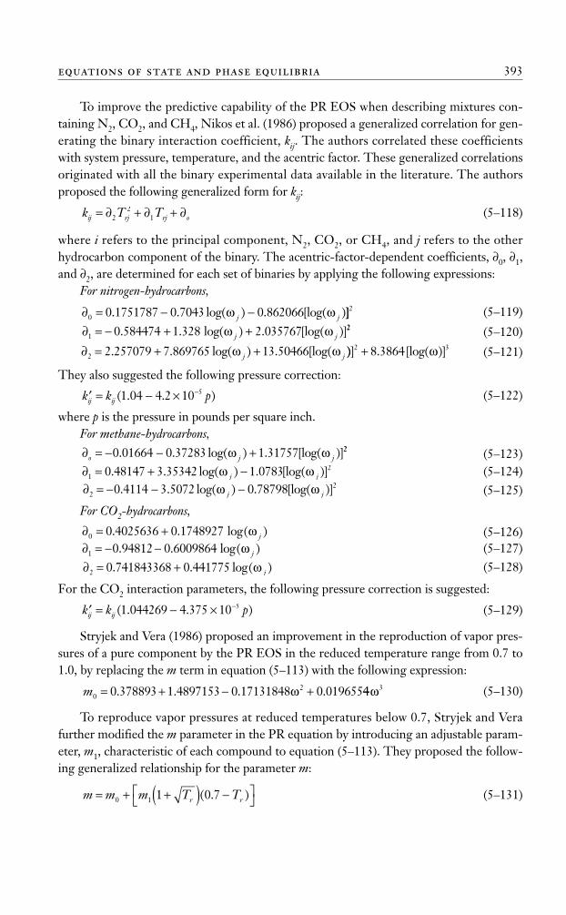
To improve the predictive capability of the PR EOS when describing mixtures con-taining N2, CO2, and CH4, Nikos et al. (1986) proposed a generalized correlation for gen-erating the binary interaction coefficient, kij. The authors correlated these coefficientswith system pressure, temperature, and the acentric factor. These generalized correlationsoriginated with all the binary experimental data available in the literature. The authorsproposed the following generalized form for kij:
(5–118)
where i refers to the principal component, N2, CO2, or CH4, and j refers to the otherhydrocarbon component of the binary. The acentric-factor-dependent coefficients, ∂0, ∂1,and ∂2, are determined for each set of binaries by applying the following expressions:
For nitrogen-hydrocarbons,
(5–119)
(5–120)
(5–121)
They also suggested the following pressure correction:
(5–122)
where p is the pressure in pounds per square inch.For methane-hydrocarbons,
(5–123)(5–124)(5–125)
For CO2-hydrocarbons,
(5–126)(5–127)(5–128)
For the CO2 interaction parameters, the following pressure correction is suggested:
(5–129)
Stryjek and Vera (1986) proposed an improvement in the reproduction of vapor pres-sures of a pure component by the PR EOS in the reduced temperature range from 0.7 to1.0, by replacing the m term in equation (5–113) with the following expression:
(5–130)
To reproduce vapor pressures at reduced temperatures below 0.7, Stryjek and Verafurther modified the m parameter in the PR equation by introducing an adjustable param-eter, m1, characteristic of each compound to equation (5–113). They proposed the follow-ing generalized relationship for the parameter m:
(5–131)m m m T Tr r= + +( ) −⎡⎣
⎤⎦0 1 1 0 7( . )
m020 378893 1 4897153 0 17131848 0 019655= + − +. . . .ω 44 3ω
′ = − × −k k pij ij ( . . )1 044269 4 375 10 5
∂ = +2 0 741843368 0 441775. . log( )ω j
∂ = − −1 0 94812 0 6009864. . log( )ω j
∂ = +0 0 4025636 0 1748927. . log( )ω j
∂ = − − −220 4114 3 5072 0 78798. . log( ) . [log( )]ω ωj j
∂ = + −120 48147 3 35342 1 0783. . log( ) . [log( )]ω ωj j
∂ = − − +o j j0 01664 0 37283 1 31757. . log( ) . [log( )]ω ω 22
′ = − × −k k pij ij ( . . )1 04 4 2 10 5
∂ = + +2 2 257079 7 869765 13 50466. . log( ) . [log(ω ωj j ))] . [log( )]2 38 3864+ ω∂ = − + +1 0 584474 1 328 2 035767. . log( ) . [log( )]ω ωj j
22
∂ = − −0 0 1751787 0 7043 0 862066. . log( ) . [log( )ω ωj j ]]2
k T Tij rj rj o= ∂ + ∂ + ∂22
1
equations of state and phase equilibria 393
Ahmed_ch5.qxd 12/21/06 2:05 PM Page 393
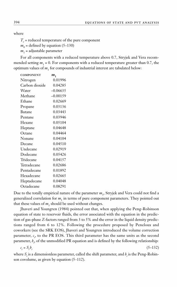
where
Tr = reduced temperature of the pure componentm0 = defined by equation (5–130)m1 = adjustable parameter
For all components with a reduced temperature above 0.7, Stryjek and Vera recom-mended setting m1 = 0. For components with a reduced temperature greater than 0.7, theoptimum values of m1 for compounds of industrial interest are tabulated below:
COMPONENT m1Nitrogen 0.01996Carbon dioxide 0.04285Water –0.06635Methane –0.00159Ethane 0.02669Propane 0.03136Butane 0.03443Pentane 0.03946Hexane 0.05104Heptane 0.04648Octane 0.04464Nonane 0.04104Decane 0.04510Undecane 0.02919Dodecane 0.05426Tridecane 0.04157Tetradecane 0.02686Pentadecane 0.01892Hexadecane 0.02665Heptadecane 0.04048Octadecane 0.08291
Due to the totally empirical nature of the parameter m1, Stryjek and Vera could not find ageneralized correlation for m1 in terms of pure component parameters. They pointed outthat these values of m1 should be used without changes.
Jhaveri and Youngren (1984) pointed out that, when applying the Peng-Robinsonequation of state to reservoir fluids, the error associated with the equation in the predic-tion of gas-phase Z-factors ranged from 3 to 5% and the error in the liquid density predic-tions ranged from 6 to 12%. Following the procedure proposed by Peneloux andcoworkers (see the SRK EOS), Jhaveri and Youngren introduced the volume correctionparameter, ci, to the PR EOS. This third parameter has the same units as the secondparameter, bi, of the unmodified PR equation and is defined by the following relationship:
ci = Si bi (5–132)
where Si is a dimensionless parameter, called the shift parameter, and bi is the Peng-Robin-son covolume, as given by equation (5–112).
394 equations of state and pvt analysis
Ahmed_ch5.qxd 12/21/06 2:05 PM Page 394
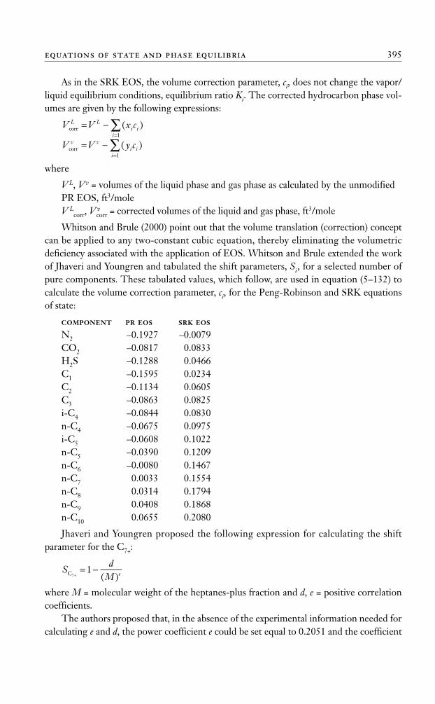
As in the SRK EOS, the volume correction parameter, ci, does not change the vapor/liquid equilibrium conditions, equilibrium ratio Ki. The corrected hydrocarbon phase vol-umes are given by the following expressions:
where
V L, Vv = volumes of the liquid phase and gas phase as calculated by the unmodifiedPR EOS, ft3/moleV L
corr, Vvcorr = corrected volumes of the liquid and gas phase, ft3/mole
Whitson and Brule (2000) point out that the volume translation (correction) conceptcan be applied to any two-constant cubic equation, thereby eliminating the volumetricdeficiency associated with the application of EOS. Whitson and Brule extended the workof Jhaveri and Youngren and tabulated the shift parameters, Si, for a selected number ofpure components. These tabulated values, which follow, are used in equation (5–132) tocalculate the volume correction parameter, ci, for the Peng-Robinson and SRK equationsof state:
COMPONENT PR EOS SRK EOS
N2 –0.1927 –0.0079CO2 –0.0817 0.0833H2S –0.1288 0.0466C1 –0.1595 0.0234C2 –0.1134 0.0605C3 –0.0863 0.0825i-C4 –0.0844 0.0830n-C4 –0.0675 0.0975i-C5 –0.0608 0.1022n-C5 –0.0390 0.1209n-C6 –0.0080 0.1467n-C7 0.0033 0.1554n-C8 0.0314 0.1794n-C9 0.0408 0.1868n-C10 0.0655 0.2080
Jhaveri and Youngren proposed the following expression for calculating the shiftparameter for the C7+:
where M = molecular weight of the heptanes-plus fraction and d, e = positive correlationcoefficients.
The authors proposed that, in the absence of the experimental information needed forcalculating e and d, the power coefficient e could be set equal to 0.2051 and the coefficient
Sd
M eC71
+= −
( )
V V y cv vi i
icorr = −
=∑ ( )
1
V V x cL Li i
icorr = −
=∑ ( )
1
equations of state and phase equilibria 395
Ahmed_ch5.qxd 12/21/06 2:05 PM Page 395
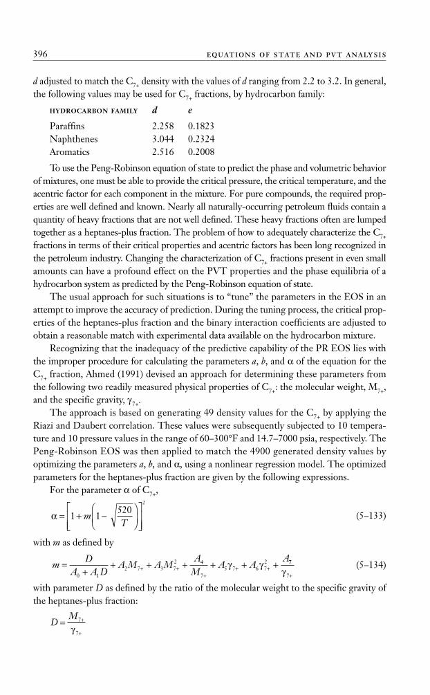
d adjusted to match the C7+ density with the values of d ranging from 2.2 to 3.2. In general,the following values may be used for C7+ fractions, by hydrocarbon family:
HYDROCARBON FAMILY d e
Paraffins 2.258 0.1823Naphthenes 3.044 0.2324Aromatics 2.516 0.2008
To use the Peng-Robinson equation of state to predict the phase and volumetric behaviorof mixtures, one must be able to provide the critical pressure, the critical temperature, and theacentric factor for each component in the mixture. For pure compounds, the required prop-erties are well defined and known. Nearly all naturally-occurring petroleum fluids contain aquantity of heavy fractions that are not well defined. These heavy fractions often are lumpedtogether as a heptanes-plus fraction. The problem of how to adequately characterize the C7+
fractions in terms of their critical properties and acentric factors has been long recognized inthe petroleum industry. Changing the characterization of C7+ fractions present in even smallamounts can have a profound effect on the PVT properties and the phase equilibria of ahydrocarbon system as predicted by the Peng-Robinson equation of state.
The usual approach for such situations is to “tune” the parameters in the EOS in anattempt to improve the accuracy of prediction. During the tuning process, the critical prop-erties of the heptanes-plus fraction and the binary interaction coefficients are adjusted toobtain a reasonable match with experimental data available on the hydrocarbon mixture.
Recognizing that the inadequacy of the predictive capability of the PR EOS lies withthe improper procedure for calculating the parameters a, b, and α of the equation for theC7+ fraction, Ahmed (1991) devised an approach for determining these parameters fromthe following two readily measured physical properties of C7+: the molecular weight, M7+,and the specific gravity, γ7+.
The approach is based on generating 49 density values for the C7+ by applying theRiazi and Daubert correlation. These values were subsequently subjected to 10 tempera-ture and 10 pressure values in the range of 60–300°F and 14.7–7000 psia, respectively. ThePeng-Robinson EOS was then applied to match the 4900 generated density values byoptimizing the parameters a, b, and α, using a nonlinear regression model. The optimizedparameters for the heptanes-plus fraction are given by the following expressions.
For the parameter α of C7+,
(5–133)
with m as defined by
(5–134)
with parameter D as defined by the ratio of the molecular weight to the specific gravity ofthe heptanes-plus fraction:
DM
= +
+
7
7γ
mD
A A DA M A M
AM
A AA
=+
+ + + + + ++ ++
+ +0 1
2 7 3 72 4
75 7 6 7
2γ γ 77
7γ +
α = + −⎛
⎝⎜⎞
⎠⎟⎡
⎣⎢⎢
⎤
⎦⎥⎥
1 1520
2
mT
396 equations of state and pvt analysis
Ahmed_ch5.qxd 12/21/06 2:05 PM Page 396
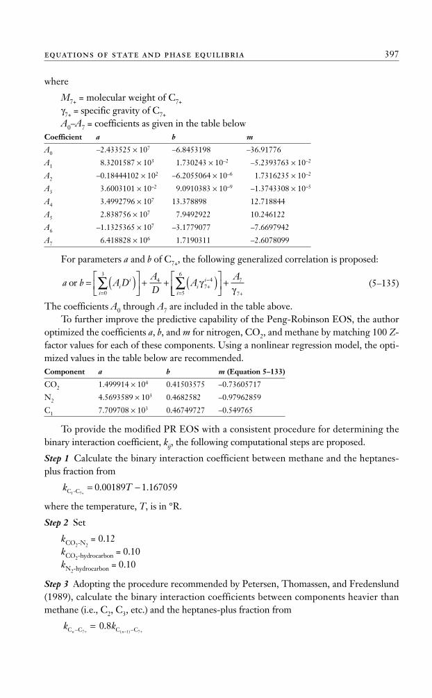
where
M7+ = molecular weight of C7+
γ7+ = specific gravity of C7+
A0–A7 = coefficients as given in the table belowCoefficient a b m
A0 –2.433525 × 10⁷ –6.8453198 –36.91776
A1 8.3201587 × 10³ 1.730243 × 10⁻² –5.2393763 × 10⁻²
A2 –0.18444102 × 10² –6.2055064 × 10⁻⁶ 1.7316235 × 10⁻²
A3 3.6003101 × 10⁻² 9.0910383 × 10⁻⁹ –1.3743308 × 10⁻⁵
A4 3.4992796 × 10⁷ 13.378898 12.718844
A5 2.838756 × 10⁷ 7.9492922 10.246122
A6 –1.1325365 × 10⁷ –3.1779077 –7.6697942
A7 6.418828 × 10⁶ 1.7190311 –2.6078099
For parameters a and b of C7+, the following generalized correlation is proposed:
(5–135)
The coefficients A0 through A7 are included in the table above.To further improve the predictive capability of the Peng-Robinson EOS, the author
optimized the coefficients a, b, and m for nitrogen, CO2, and methane by matching 100 Z-factor values for each of these components. Using a nonlinear regression model, the opti-mized values in the table below are recommended.Component a b m (Equation 5–133)
CO2 1.499914 × 10⁴ 0.41503575 –0.73605717
N2 4.5693589 × 10³ 0.4682582 –0.97962859
C1 7.709708 × 10³ 0.46749727 –0.549765
To provide the modified PR EOS with a consistent procedure for determining thebinary interaction coefficient, kij, the following computational steps are proposed.
Step 1 Calculate the binary interaction coefficient between methane and the heptanes-plus fraction from
where the temperature, T, is in °R.
Step 2 Set
kCO2-N2= 0.12
kCO2-hydrocarbon = 0.10kN2-hydrocarbon = 0.10
Step 3 Adopting the procedure recommended by Petersen, Thomassen, and Fredenslund(1989), calculate the binary interaction coefficients between components heavier thanmethane (i.e., C2, C3, etc.) and the heptanes-plus fraction from
k kn nC C C C− −+ − +
=7 1 7
0 8.( )
k TC -C1 7+= −0 00189 1 167059. .
a b A DAD
Aii
ii
i
i
or = ( )⎡⎣⎢
⎤⎦⎥ + + ( )⎡
=+−
=∑ ∑
0
34
74
5
6
γ⎣⎣⎢
⎤⎦⎥ +
+
A7
7γ
equations of state and phase equilibria 397
Ahmed_ch5.qxd 12/21/06 2:05 PM Page 397
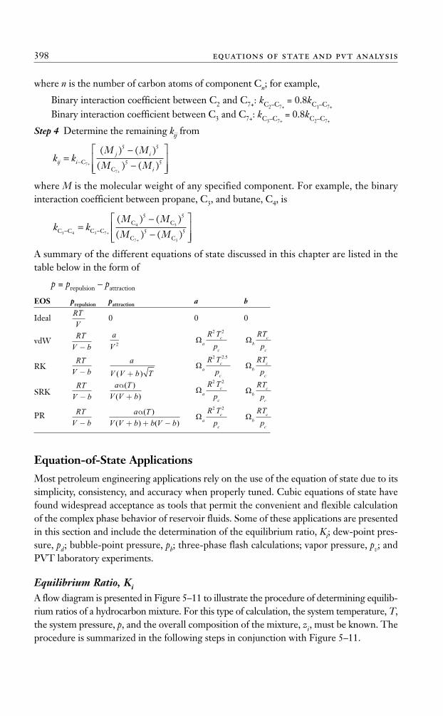
where n is the number of carbon atoms of component Cn; for example,
Binary interaction coefficient between C2 and C7+: kC2–C7+= 0.8kC1–C7+
Binary interaction coefficient between C3 and C7+: kC3–C7+= 0.8kC2–C7+
Step 4 Determine the remaining kij from
where M is the molecular weight of any specified component. For example, the binaryinteraction coefficient between propane, C3, and butane, C4, is
A summary of the different equations of state discussed in this chapter are listed in thetable below in the form of
p = prepulsion – pattraction
EOS prepulsion pattraction a b
Ideal 0 0 0
vdW
RK
SRK
PR
Equation-of-State Applications
Most petroleum engineering applications rely on the use of the equation of state due to itssimplicity, consistency, and accuracy when properly tuned. Cubic equations of state havefound widespread acceptance as tools that permit the convenient and flexible calculationof the complex phase behavior of reservoir fluids. Some of these applications are presentedin this section and include the determination of the equilibrium ratio, Ki; dew-point pres-sure, pd; bubble-point pressure, pb; three-phase flash calculations; vapor pressure, pv; andPVT laboratory experiments.
Equilibrium Ratio, Ki
A flow diagram is presented in Figure 5–11 to illustrate the procedure of determining equilib-rium ratios of a hydrocarbon mixture. For this type of calculation, the system temperature, T,the system pressure, p, and the overall composition of the mixture, zi, must be known. Theprocedure is summarized in the following steps in conjunction with Figure 5–11.
Ωbc
c
RTp
Ωac
c
R Tp
2 2a TV V b b V b
α( )
( ) ( )+ + −RT
V b−
Ωbc
c
RTp
Ωac
c
R Tp
2 2a TV V b
α( )
( )+RT
V b−
Ωbc
c
RTp
Ωac
c
R Tp
2 2 5.a
V V b T( )+
RTV b−
Ωbc
c
RTp
Ωac
c
R Tp
2 2aV 2
RTV b−
RTV
k kM M
M MC C C CC C
C C3 4 3 7
4 3
7 3
5 5
5 5− −=−−
⎡
⎣+
+
( ) ( )
( ) ( )⎢⎢⎢
⎤
⎦⎥⎥
k kM M
M Mij ij i
i
=−−
⎡
⎣⎢⎢
⎤
⎦⎥⎥
− +
+
CC
7
7
5 5
5 5
( ) ( )
( ) ( )
398 equations of state and pvt analysis
Ahmed_ch5.qxd 12/21/06 2:05 PM Page 398
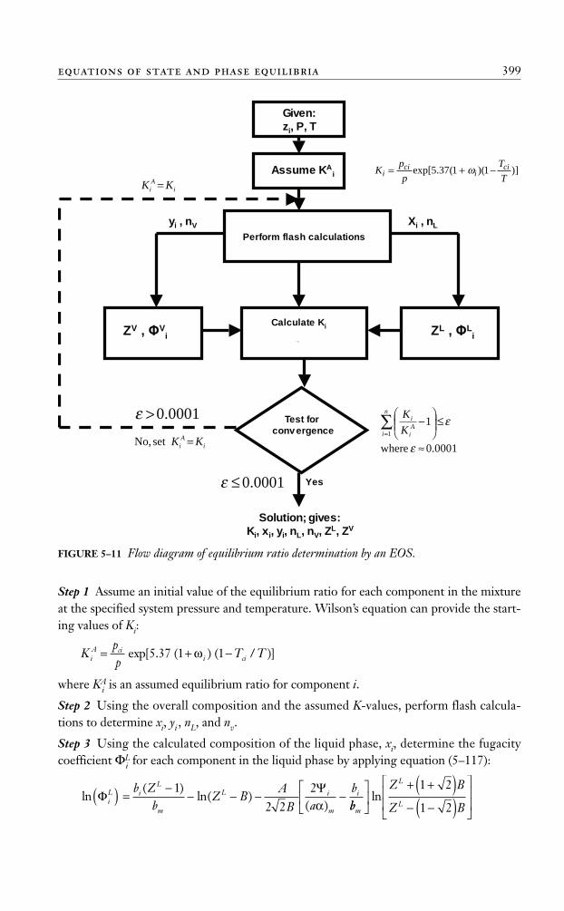
Step 1 Assume an initial value of the equilibrium ratio for each component in the mixtureat the specified system pressure and temperature. Wilson’s equation can provide the start-ing values of Ki:
where KAi is an assumed equilibrium ratio for component i.
Step 2 Using the overall composition and the assumed K-values, perform flash calcula-tions to determine xi, yi , nL, and nv.
Step 3 Using the calculated composition of the liquid phase, xi, determine the fugacitycoefficient ΦL
i for each component in the liquid phase by applying equation (5–117):
ln( )
ln( )( )
ΦΨ
iL i
L
m
L i
m
ib Zb
Z BA
B ab( ) = −
− − − −1
2 22α bb
Z B
Z Bm
L
L
⎡
⎣⎢
⎤
⎦⎥
+ +( )− −( )
⎡
⎣
⎢⎢
⎤
⎦
⎥⎥
ln1 2
1 2
Kpp
T TiA ci
i ci= + −exp[ . ( ) ( / )]5 37 1 1ω
equations of state and phase equilibria 399
)]1)(1(37.5exp[T
T
p
pK ci
ici
i −+= ω
Given:
zi, P, T
Assume KAi
Perform flash calculations
Xi , nL
ZL , Li
yi , nV
ZV , Vi
Calculate Ki
vi
Li
iKΦΦ=
Test for
convergence
0001.0where
11
≈
≤⎟⎟⎠
⎞⎜⎜⎝
⎛−∑
=
ε
εn
iAi
i
KK0001.0>ε
0001.0≤ε Yes
iAi KK =setNo,
iAi KK =
Solution; gives:
Ki, xi, yi, nL, nV, ZL, ZV
FIGURE 5–11 Flow diagram of equilibrium ratio determination by an EOS.
Ahmed_ch5.qxd 12/21/06 2:05 PM Page 399
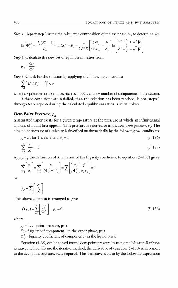
Step 4 Repeat step 3 using the calculated composition of the gas phase, yi , to determine Φvi .
Step 5 Calculate the new set of equilibrium ratios from
Step 6 Check for the solution by applying the following constraint:
where ε = preset error tolerance, such as 0.0001, and n = number of components in the system.If these conditions are satisfied, then the solution has been reached. If not, steps 1
through 6 are repeated using the calculated equilibrium ratios as initial values.
Dew-Point Pressure, pd
A saturated vapor exists for a given temperature at the pressure at which an infinitesimalamount of liquid first appears. This pressure is referred to as the dew-point pressure, pd. Thedew-point pressure of a mixture is described mathematically by the following two conditions:
yi = zi, for 1 ≤ i ≤ n and nv = 1 (5–136)
(5–137)
Applying the definition of Ki in terms of the fugacity coefficient to equation (5–137) gives
or
This above equation is arranged to give
(5–138)
where
pd = dew-point pressure, psiaf v
i = fugacity of component i in the vapor phase, psiaΦ L
i = fugacity coefficient of component i in the liquid phase
Equation (5–35) can be solved for the dew-point pressure by using the Newton-Raphsoniterative method. To use the iterative method, the derivative of equation (5–138) with respectto the dew-point pressure, pd, is required. This derivative is given by the following expression:
f pf
pdiv
iL
i
n
d( ) =⎡
⎣⎢
⎤
⎦⎥ − =
=∑ Φ1
0
pf
div
iL
i
n
=⎡
⎣⎢
⎤
⎦⎥
=∑ Φ1
zk
z zi
ii
ni
iL
iv
i
ni
i
⎡
⎣⎢⎤
⎦⎥ =
⎡
⎣⎢
⎤
⎦⎥ =
= =∑ ∑
1 1 ( / )Φ Φ ΦLLiv
i d
fz p
⎛⎝⎜
⎞⎠⎟
⎡
⎣⎢⎢
⎤
⎦⎥⎥=∑ 1
zK
i
ii
n ⎡
⎣⎢
⎤
⎦⎥ =
−∑ 1
1
K Ki iA
i
n
/ −⎡⎣ ⎤⎦ ≤=∑ 1
2
1
ε
K iiL
iv=
ΦΦ
ln( )
ln( )( )
ΦΨ
iL i
v
m
v i
m
ib Zb
Z BA
B ab( ) = −
− − − −1
2 22α bb
Z B
Z Bm
v
v
⎡
⎣⎢
⎤
⎦⎥
+ +( )− −( )
⎡
⎣
⎢⎢
⎤
⎦
⎥⎥
ln1 2
1 2
400 equations of state and pvt analysis
Ahmed_ch5.qxd 12/21/06 2:05 PM Page 400
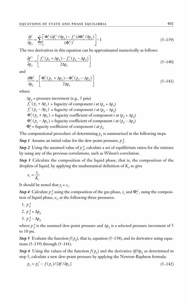
(5–139)
The two derivatives in this equation can be approximated numerically as follows:
(5–140)
and
(5–141)
where
Δpd = pressure increment (e.g., 5 psia)= fugacity of component i at (pd + Δpd)= fugacity of component i at (pd – Δpd)= fugacity coefficient of component i at (pd + Δpd)= fugacity coefficient of component i at (pd – Δpd)
ΦLi = fugacity coefficient of component i at pd
The computational procedure of determining pd is summarized in the following steps.
Step 1 Assume an initial value for the dew-point pressure, p Ad .
Step 2 Using the assumed value of p Ad , calculate a set of equilibrium ratios for the mixture
by using any of the previous correlations, such as Wilson’s correlation.
Step 3 Calculate the composition of the liquid phase, that is, the composition of thedroplets of liquid, by applying the mathematical definition of Ki, to give
It should be noted that yi = zi.
Step 4 Calculate p Ad using the composition of the gas phase, zi and ΦL
i , using the composi-tion of liquid phase, xi , at the following three pressures:
1. p Ad
2. p Ad + Δpd
3. p Ad – Δpd
where p Ad is the assumed dew-point pressure and Δpd is a selected pressure increment of 5
to 10 psi.
Step 5 Evaluate the function f ( pd), that is, equation (5–138), and its derivative using equa-tions (5–139) through (5–141).
Step 6 Using the values of the function f ( pd) and the derivative ∂f/∂pd as determined instep 5, calculate a new dew-point pressure by applying the Newton-Raphson formula:
(5–142)p p f p f pd dA
d d= − ∂ ∂( )/ [ / ]
xzKi
i
i
=
Φ ΔiL
d dp p( )−Φ Δi
Ld dp p( )+
f p piv
d d( )− Δf p pi
vd d( )+ Δ
∂∂
=+ − −⎡
⎣⎢
⎤
⎦⎥
Φ Φ Δ Φ ΔΔ
iL
d
iL
d d iL
d d
dpp p p p
p( ) ( )
2
∂∂
=+ − −⎡
⎣⎢
⎤
⎦⎥
fp
f p p f p pp
v
d
iv
d d iv
d d
d
( ) ( )Δ ΔΔ2
∂∂
=∂ ∂ − ∂ ∂⎡
⎣⎢
⎤fp
f p f p
d
iL
iv
d iv
iL
d
iL
Φ ΦΦ
( / ) ( / )( )2
⎦⎦⎥ −
=∑ 1
1i
n
equations of state and phase equilibria 401
Ahmed_ch5.qxd 12/21/06 2:05 PM Page 401
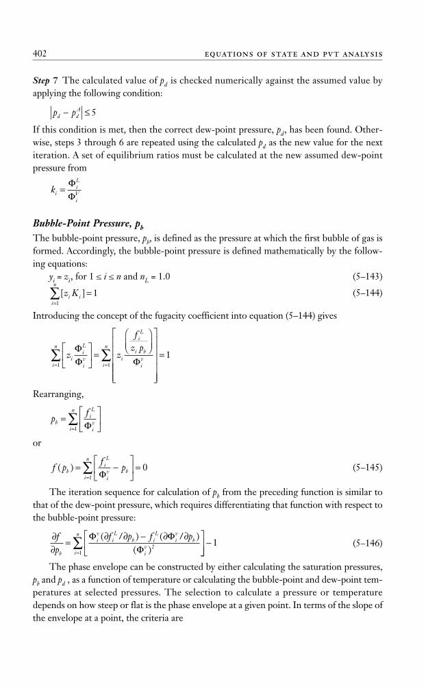
Step 7 The calculated value of pd is checked numerically against the assumed value byapplying the following condition:
If this condition is met, then the correct dew-point pressure, pd, has been found. Other-wise, steps 3 through 6 are repeated using the calculated pd as the new value for the nextiteration. A set of equilibrium ratios must be calculated at the new assumed dew-pointpressure from
Bubble-Point Pressure, pb
The bubble-point pressure, pb, is defined as the pressure at which the first bubble of gas isformed. Accordingly, the bubble-point pressure is defined mathematically by the follow-ing equations:
yi = zi, for 1 ≤ i ≤ n and nL = 1.0 (5–143)
(5–144)
Introducing the concept of the fugacity coefficient into equation (5–144) gives
Rearranging,
or
(5–145)
The iteration sequence for calculation of pb from the preceding function is similar tothat of the dew-point pressure, which requires differentiating that function with respect tothe bubble-point pressure:
(5–146)
The phase envelope can be constructed by either calculating the saturation pressures,pb and pd , as a function of temperature or calculating the bubble-point and dew-point tem-peratures at selected pressures. The selection to calculate a pressure or temperaturedepends on how steep or flat is the phase envelope at a given point. In terms of the slope ofthe envelope at a point, the criteria are
∂∂
=∂ ∂ − ∂ ∂⎡
⎣⎢
⎤fp
f p f p
b
iv
iL
b iL
iv
b
iv
Φ ΦΦ
( / ) ( / )( )2
⎦⎦⎥ −
=∑ 1
1i
n
f pf
pbiL
iv b
i
n
( ) = −⎡
⎣⎢
⎤
⎦⎥ =
=∑ Φ
01
pf
biL
iv
i
n
=⎡
⎣⎢
⎤
⎦⎥
=∑ Φ1
z z
fz p
iiL
iv
i
n
i
iL
i b
iv
ΦΦ Φ
⎡
⎣⎢
⎤
⎦⎥ =
⎛⎝⎜
⎞⎠⎟
⎡
⎣
⎢⎢⎢
=∑
1 ⎢⎢⎢
⎤
⎦
⎥⎥⎥⎥⎥
==∑i
n
1
1
[ ]z Ki ii
n
==∑ 1
1
kiiL
iV=ΦΦ
p pd dA− ≤ 5
402 equations of state and pvt analysis
Ahmed_ch5.qxd 12/21/06 2:05 PM Page 402
• Calculate the bubble-point or dew-point pressure if
• Calculate the bubble-point or dew-point temperature if
Three-Phase Equilibrium CalculationsTwo- and three-phase equilibria occur frequently during the processing of hydrocarbonand related systems. Peng and Robinson (1976b) proposed a three-phase equilibrium cal-culation scheme of systems that exhibit a water-rich liquid phase, a hydrocarbon-rich liq-uid phase, and a vapor phase.
In applying the principle of mass conversation to 1 mole of a water-hydrocarbon in athree-phase state of thermodynamic equilibrium at a fixed temperature, T, and pressure, p,gives
nL + nw + nv = 1 (5–147)nLxi + nwxwi + nv yi = zi (5–148)
(5–149)
where
nL, nw, nv = number of moles of the hydrocarbon-rich liquid, the water-rich liquid,and the vapor, respectivelyxi, xwi, yi = mole fraction of component i in the hydrocarbon-rich liquid, the waterrich liquid, and the vapor, respectively
The equilibrium relations between the compositions of each phase are defined by thefollowing expressions:
(5–150)
and
(5–151)
where
Ki = equilibrium ratio of component i between vapor and hydrocarbon-rich liquidKwi = equilibrium ratio of component i between the vapor and water-rich liquidΦL
i = fugacity coefficient of component i in the hydrocarbon-rich liquidΦv
i = fugacity coefficient of component i in the vapor phaseΦw
i = fugacity coefficient of component i in the water-rich liquid
Ky
xi i
w
ivwi
wi
= =ΦΦ
Kyxi
i
i
iL
iv= =
ΦΦ
x x y zi i ii
n
i
n
i
n
i
n
= = = ====∑∑∑∑ wi 1
111
∂∂
≈−−
>ln( )ln( )
ln( ) ln( )ln( ) ln( )
pT
p pT T
2 1
2 1
20
∂∂
≈−−
<ln( )ln( )
ln( ) ln( )ln( ) ln( )
pT
p pT T
2 1
2 1
2
equations of state and phase equilibria 403
Ahmed_ch5.qxd 12/21/06 2:05 PM Page 403
Combining equations (5–147) through (5–151) gives the following conventional non-linear equations:
(5–152)
(5–153)
(5–154)
Assuming that the equilibrium ratios between phases can be calculated, these equationsare combined to solve for the two unknowns, nL and nv, and hence xi, xwi, and yi. The natureof the specific equilibrium calculation is what determines the appropriate combination ofequations (5–152) through (5–154). The combination of these three expressions then canbe used to determine the phase and volumetric properties of the three-phase system.
There are essentially three types of phase behavior calculations for the three-phasesystem: bubble-point prediction, dew-point prediction, and flash calculation. Peng andRobinson (1980) proposed the following combination schemes of equations (5–152)through (5–154).
For the bubble-point pressure determination,
and
Substituting equations (5–152) through (5–154) in this relationships gives
(5–155)
and
(5–156)
For the dew-point pressure,
x yiii
wi − =∑∑ 0
g n nz K
n K n K K K KL wi i
L i w i i i
( , )( ) ( / )
=− + − +
⎡
⎣⎢
⎤
⎦1 wi⎥⎥ − =∑
i
1 0
f n nz K K
n K n K K KL wi i
L i w i i
( , )( / )
( ) ( / )=
−− + −
11
wi
wi ++⎡
⎣⎢
⎤
⎦⎥ =∑ K ii
0
yii∑⎡⎣⎢
⎤⎦⎥− =1 0
x xii i∑ ∑− =wi 0
yz K
n K nKK
K Ki
i
i i
L i wi
i i=∑ =
− + −⎛⎝⎜
⎞⎠⎟+
⎡
⎣
⎢⎢
1 1( )wi
⎢⎢⎢⎢
⎤
⎦
⎥⎥⎥⎥⎥
==∑i 1
1
xz K K
n K nKK
Ki
i i
L i wi
i
wiwi
wi
=∑ =
− + −⎛⎝⎜
⎞⎠⎟
1 1
( / )
( ) ++
⎡
⎣
⎢⎢⎢⎢⎢
⎤
⎦
⎥⎥⎥⎥⎥
==∑
K ii
11
xz
n K nKK
K Ki
i
i
L i wi
i i=∑ =
− + −⎛⎝⎜
⎞⎠⎟+
⎡
⎣
⎢⎢⎢⎢1 1( )
wi⎢⎢
⎤
⎦
⎥⎥⎥⎥⎥
==∑ 1
1i
404 equations of state and pvt analysis
Ahmed_ch5.qxd 12/21/06 2:05 PM Page 404
Combining with equations (5–152) through (5–154) yields
(5–157)
and
(5–158)
For flash calculations,
or
(5–159)
and
(5–160)
Note that, in performing any of these property predictions, we always have twounknown variables, nL and nw, and between them, two equations. Providing that the equi-librium ratios and the overall composition are known, the equations can be solved simulta-neously using the appropriate iterative technique, such as the Newton-Raphson method.The application of this iterative technique for solving equations (5–159) and (5–160) issummarized in the following steps.
Step 1 Assume initial values for the unknown variables nL and nw.
Step 2 Calculate new values of nL and nw by solving the following two linear equations:
where f (nL, nw) = value of the function f (nL, nw) as expressed by equation (5–159) and g(nL, nw) = value of the function g(nL, nw) as expressed by equation (5–160).
The first derivative of these functions with respect to nL and nw is given by the follow-ing expressions:
( / )( )( / )
[ ( ) (∂ ∂ =
− − −− +
f nz K K K K
n K n Kwi i i i
L i w
11
wi
ii i ii K K K/ ) ]wi − +⎧⎨⎩
⎫⎬⎭=
∑ 21
( / )( )
[ ( ) ( / )∂ ∂ =
− −− + − +
f nz K
n K n K K KLi i
L i w i i
11
2
wi KK ii ]21
⎧⎨⎩
⎫⎬⎭=
∑
nn
nn
f n f ng n
L
w
L
w
L w
L
⎡
⎣⎢⎤
⎦⎥ =
⎡
⎣⎢⎤
⎦⎥ −
∂ ∂ ∂ ∂∂ ∂
new / // ∂∂ ∂
⎡
⎣⎢
⎤
⎦⎥⎡
⎣⎢
⎤
⎦⎥
−
g nf n ng n nw
L w
L w/( , )( , )
1
g n nz K K
n K n K K K KL wi i
L i w i i i
( , )/
( ) ( / )=
− + − +⎡ wi
wi1⎣⎣⎢
⎤
⎦⎥ − =∑
i
1 0 0.
f n nz K
n K n K K K KL wi i
L i w i i i
( , )( )
( ) ( / )=
−− + − +
⎡ 11 wi⎣⎣
⎢⎤
⎦⎥ =∑
i
0
xi
wi∑⎡⎣⎢
⎤⎦⎥− =1 0
x yii
ii
∑ ∑− = 0
g n nz
n K n K K K KL wi
L i w i i ii
( , )( ) ( / )
=− + − +
⎡
⎣⎢
⎤
⎦⎥1 wi
∑∑ − =1 0
f n nz K K
n K n K K KL wi i
L i w i i
( , )( / )
( ) ( /=
−− + −
1 11
wi
wi )) +⎡
⎣⎢
⎤
⎦⎥ =∑ K ii
0
xii∑⎡⎣⎢
⎤⎦⎥− =1 0
equations of state and phase equilibria 405
Ahmed_ch5.qxd 12/21/06 2:05 PM Page 405
Step 3 The new calculated values of nL and nw then are compared with the initial values. Ifno changes in the values are observed, then the correct values of nL and nw have been ob-tained. Otherwise, the steps are repeated with the new calculated values used as initial values.
Peng and Robinson (1980) proposed two modifications when using their equation ofstate for three-phase equilibrium calculations. The first modification concerns the use ofthe parameter α as expressed by equation (5–113) for the water compound. Peng andRobinson suggested that, when the reduced temperature of this compound is less than0.85, the following equation is applied:
(5–161)where Trw is the reduced temperature of the water component; that is, Trw = T/Tcw.
The second important modification of the PR EOS is the introduction of alternativemixing rules and new interaction coefficients for the parameter (aα). A temperature-dependent binary interaction coefficient was introduced into the equation, to give:
(5–162)
where τij = temperature-dependent binary interaction coefficient and xwi = mole fractionof component i in the water phase.
Peng and Robinson proposed graphical correlations for determining this parameterfor each aqueous binary pair. Lim et al. (1984) expressed these graphical correlationsmathematically by the following generalized equation:
(5–163)
where
T = system temperature, °RTci = critical temperature of the component of interest, °Rpci = critical pressure of the component of interest, psiapcj = critical pressure of the water compound, psia
Values of the coefficients a1, a2, and a3 of this polynomial are given in the table below forselected binaries.Component i a1 a2 a3
C1 0 1.659 –0.761
C2 0 2.109 –0.607
C3 –18.032 9.441 –1.208
n-C4 0 2.800 –0.488
n-C6 49.472 –5.783 –0.152
τij aTT
pp
aTT
=⎡
⎣⎢
⎤
⎦⎥⎡
⎣⎢⎢
⎤
⎦⎥⎥+
⎡
⎣⎢
⎤1
2 2
2ci
ci
cj ci ⎦⎦⎥⎡
⎣⎢⎢
⎤
⎦⎥⎥+
pp
aci
cj3
( ) [ ( ) ( )].a x x a ai j i j ijji
α α α τwater wi wj= −∑∑ 0 5 1
αw T= + −[ . . ( )].1 0085677 0 82154 1 0 5 2rw
( / )( )( / )
[ ( ) (∂ ∂ =
− −− +
g nz K K K K K
n K nwi i i i
L i w
wi wi
1 KK K K Ki i ii / ) ]wi − +⎧⎨⎩
⎫⎬⎭=
∑ 21
( / )( / )( )
[ ( ) ( /∂ ∂ =
− −− +
g nz K K K
n K n K KLi i i
L i w i
wi 11 wwi − +
⎧⎨⎩
⎫⎬⎭=
∑ K Ki ii ) ]21
406 equations of state and pvt analysis
Ahmed_ch5.qxd 12/21/06 2:05 PM Page 406
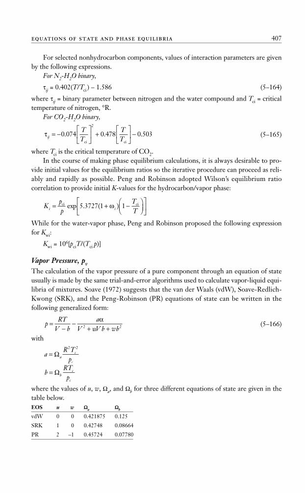
For selected nonhydrocarbon components, values of interaction parameters are givenby the following expressions.
For N2-H2O binary,
τij = 0.402(T/Tci ) – 1.586 (5–164)
where τij = binary parameter between nitrogen and the water compound and Tci = criticaltemperature of nitrogen, °R.
For CO2-H2O binary,
(5–165)
where Tci is the critical temperature of CO2.In the course of making phase equilibrium calculations, it is always desirable to pro-
vide initial values for the equilibrium ratios so the iterative procedure can proceed as reli-ably and rapidly as possible. Peng and Robinson adopted Wilson’s equilibrium ratiocorrelation to provide initial K-values for the hydrocarbon/vapor phase:
While for the water-vapor phase, Peng and Robinson proposed the following expressionfor Kwi:
Kwi = 106[pciT/(Tci p)]
Vapor Pressure, pv
The calculation of the vapor pressure of a pure component through an equation of stateusually is made by the same trial-and-error algorithms used to calculate vapor-liquid equi-libria of mixtures. Soave (1972) suggests that the van der Waals (vdW), Soave-Redlich-Kwong (SRK), and the Peng-Robinson (PR) equations of state can be written in thefollowing generalized form:
(5–166)
with
where the values of u, w, Ωa, and Ωb for three different equations of state are given in thetable below.EOS u w ΩΩa ΩΩb
vdW 0 0 0.421875 0.125
SRK 1 0 0.42748 0.08664
PR 2 –1 0.45724 0.07780
bRTpb
c
c
= Ω
aR T
pac
c
= Ω2 2
pRT
V ba
V V b wb=
−−
+ +α
2 2μ
Kpp
TTi i= + −⎛
⎝⎜⎞⎠⎟
⎡
⎣⎢
⎤
⎦⎥
ci ciexp . ( )5 3727 1 1ω
τij
TT
TT
= −⎡
⎣⎢
⎤
⎦⎥ +
⎡
⎣⎢
⎤
⎦⎥ −0 074 0 478 0 503
2
. . .ci ci
equations of state and phase equilibria 407
Ahmed_ch5.qxd 12/21/06 2:05 PM Page 407

Soave introduced the reduced pressure, pr, and reduced temperature, Tr, to these equa-tions, to give
(5–167)
(5–168)
and
(5–169)
where
pr = p/pc
Tr = T/Tc
In the cubic form and in terms of the Z-factor, the three equations of state can be writ-ten as
vdW: Z3 – Z2(1 + B) + ZA – AB = 0SRK: Z3 – Z2 + Z(A – B – B2) – AB = 0PR: Z3 – Z2 (1 – B) + Z(A – 3B2 – 2B ) – (AB – B2 – B2) = 0
And the pure component fugacity coefficient is given by
vdW:
SRK:
PR:
A typical iterative procedure for the calculation of pure component vapor pressure atany temperature, T, through one of these EOS is summarized next.
Step 1 Calculate the reduced temperature; that is, Tr = T/Tc.
Step 2 Calculate the ratio A/B from equation (5–169).
Step 3 Assume a value for B.
Step 4 Solve the selected equation of state, such as SRK EOS, to obtain ZL and Z, that is,smallest and largest roots, for both phases.
Step 5 Substitute ZL and Zv into the pure component fugacity coefficient and obtainln( f o/p) for both phases.
Step 6 Compare the two values of f/p. If the isofugacity condition is not satisfied, assume anew value of B and repeat steps 3 through 6.
Step 7 From the final value of B, obtain the vapor pressure from equation (5–168):
ln ln( ) lnfp
Z Z BA
B
Zo⎛⎝⎜
⎞⎠⎟= − − − −
⎛
⎝⎜
⎞
⎠⎟
+ +( )1
2 2
1 2 BB
Z B− −( )⎡
⎣
⎢⎢
⎤
⎦
⎥⎥1 2
ln ln( ) lnfp
Z Z BAB
BZ
o⎛⎝⎜
⎞⎠⎟= − − − − ⎛
⎝⎜⎞⎠⎟
+⎛⎝⎜
⎞⎠
1 1 ⎟⎟
ln ln( )fp
Z Z BAZ
o⎛⎝⎜
⎞⎠⎟= − − − −1
AB T
a
b r
=⎛⎝⎜
⎞⎠⎟
ΩΩ
α
Bb p
RTp
Tbr
r
= = Ω
Aa pR T
pTa
r
r
= =α α2 2 Ω
408 equations of state and pvt analysis
Ahmed_ch5.qxd 12/21/06 2:05 PM Page 408
Solving for pv gives
Simulation of Laboratory PVT Data by Equations of State
Before attempting to use an EOS-based compositional model in a full-field simulationstudy, it is essential the selected equation of state is capable of achieving a satisfactorymatch between EOS results and all the available PVT test data. It should be pointed outthat an equation of state generally is not predictive without tuning its parameters to matchthe relevant experimental data. Several PVT laboratory tests were presented in Chapter 4and are repeated here for convenience to illustrate the procedure of applying an EOS tosimulate these experiments, including
• Constant-volume depletion.
• Constant-composition expansion.
• Differential liberation.
• Flash separation tests.
• Composite liberation.
• Swelling tests.
• Compositional gradients.
• Minimum-miscibility pressure.
Constant-Volume Depletion TestA reliable prediction of the pressure depletion performance of a gas-condensate reservoir isnecessary in determining reserves and evaluating field-separation methods. The predictedperformance is also used in planning future operations and studying the economics of proj-ects for increasing liquid recovery by gas cycling. Such predictions can be performed withaid of the experimental data collected by conducting constant-volume-depletion (CVD)tests on gas condensates. These tests are performed on a reservoir fluid sample in such amanner as to simulate depletion of the actual reservoir, assuming that retrograde liquidappearing during production remains immobile in the reservoir.
The CVD test provides five important laboratory measurements that can be used in avariety of reservoir engineering predictions:
1. Dew-point pressure.
2. Composition changes of the gas phase with pressure depletion.
3. Compressibility factor at reservoir pressure and temperature.
4. Recovery of original in-place hydrocarbons at any pressure.
pBT p
vr c
b
=Ω
Bp p
Tbv c
r
= Ω( / )
equations of state and phase equilibria 409
Ahmed_ch5.qxd 12/21/06 2:05 PM Page 409
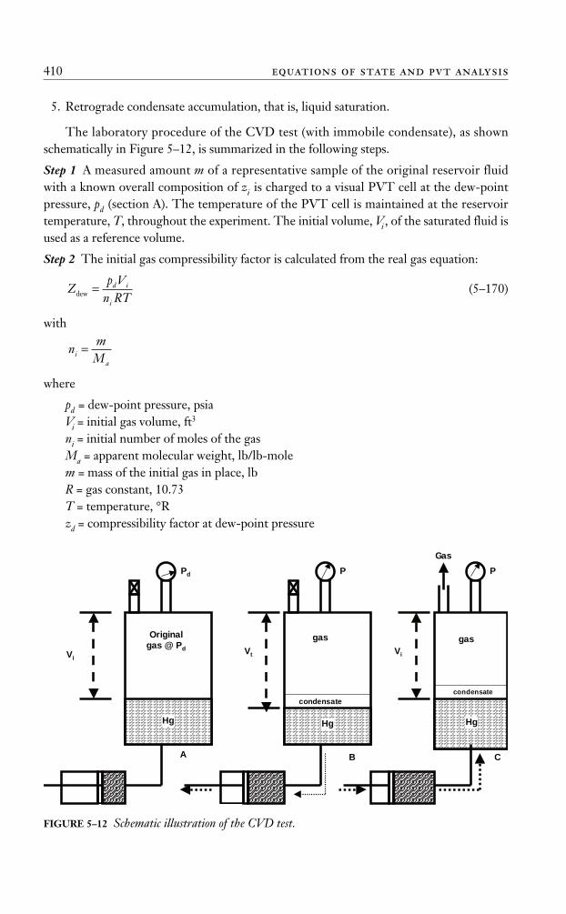
5. Retrograde condensate accumulation, that is, liquid saturation.
The laboratory procedure of the CVD test (with immobile condensate), as shownschematically in Figure 5–12, is summarized in the following steps.
Step 1 A measured amount m of a representative sample of the original reservoir fluidwith a known overall composition of zi is charged to a visual PVT cell at the dew-pointpressure, pd (section A). The temperature of the PVT cell is maintained at the reservoirtemperature, T, throughout the experiment. The initial volume, Vi , of the saturated fluid isused as a reference volume.
Step 2 The initial gas compressibility factor is calculated from the real gas equation:
(5–170)
with
where
pd = dew-point pressure, psiaVi = initial gas volume, ft3
ni = initial number of moles of the gasMa = apparent molecular weight, lb/lb-molem = mass of the initial gas in place, lbR = gas constant, 10.73T = temperature, °Rzd = compressibility factor at dew-point pressure
nm
Mia
=
Zp V
n RTd i
idew =
410 equations of state and pvt analysis
Hg
Original
gas @ Pd
Pd P
condensate
P
gas
ViVt
gas
condensate
Gas
Vi
A CB
Hg Hg
FIGURE 5–12 Schematic illustration of the CVD test.
Ahmed_ch5.qxd 12/21/06 2:05 PM Page 410
with the gas initially in place as expressed in standard units, scf, given by
G = 379.4ni (5–171)
Step 3 The cell pressure is reduced from the saturation pressure to a predetermined level,p. This can be achieved by withdrawing mercury from the cell, as illustrated in Figure5–12, section B. During the process, a second phase (retrograde liquid) is formed. Thefluid in the cell is brought to equilibrium and the total volume, Vt , and volume of the ret-rograde liquid, VL, are visually measured. This retrograde volume is reported as a percentof the initial volume, Vi:
This value can be translated into condensate saturation in the presence of water saturation by
So = (1 – Sw)SL/100
Step 4 Mercury is reinjected into the PVT cell at constant pressure p while an equivalentvolume of gas is removed. When the initial volume, Vi, is reached, mercury injectionceases, as illustrated in Figure 5–12, section C. The volume of the removed gas is meas-ured at the cell conditions and recorded as (Vgp)p,T . This step simulates a reservoir produc-ing only gas, with retrograde liquid remaining immobile in the reservoir.
Step 5 The removed gas is charged to analytical equipment, where its composition, yi , isdetermined and its volume is measured at standard conditions and recorded as (Vgp)sc. Thecorresponding moles of gas produced can be calculated from the expression:
(5–172)
where np = moles of gas produced and (Vgp)sc = volume of gas produced measured at stan-dard conditions, scf.
Step 6 The compressibility factor of the gas phase at cell pressure and temperature is cal-culated by
(5–173)
where
Combining equations (5–172) and (5–173) and solving for the compressibility factor Z gives
(5–174)
Another property, the two-phase compressibility factor, also is calculated. The two-phase Z-factor represents the total compressibility of all the remaining fluid (gas and retrograde liq-uid) in the cell and is computed from the real gas law as
Zp V
RT Vp T=
379 4. ( )
( ),gp
gp sc
VRT n
pp
ideal =
ZVV
V
Vp T= =actual
ideal
gp
ideal
( ) ,
nV
p =( )
.gp sc
379 4
SVVL
L
i
=⎛⎝⎜
⎞⎠⎟100
equations of state and phase equilibria 411
Ahmed_ch5.qxd 12/21/06 2:05 PM Page 411
(5–175)
where
(ni – np ) = represents the remaining moles of fluid in the cellni = initial moles in the cellnp = cumulative moles of gas removed
Step 7 The volume of gas produced as a percentage of gas initially in place is calculated bydividing the cumulative volume of the produced gas by the gas initially in place, both atstandard conditions:
(5–176)
Equivalently as
This experimental procedure is repeated several times, until a minimum test pressure isreached, after which the quantity and composition of the gas and retrograde liquid remain-ing in the cell are determined.
This test procedure also can be conducted on a volatile oil sample. In this case, thePVT cell initially contains liquid, instead of gas, at its bubble-point pressure.
Simulation of the CVD Test by EOSIn the absence of the CVD test data on a specific gas-condensate system, predictions ofpressure-depletion behavior can be obtained by using any of the well-established equa-tions of state to compute the phase behavior when the composition of the total gas-condensate system is known. The stepwise computational procedure using the Peng-Robinson EOS as a representative equation of state now is summarized in conjunctionwith the flow diagram shown in Figure 5–13.
Step 1 Assume that the original hydrocarbon system with a total composition zi occupiesan initial volume of 1 ft3 at the dew-point pressure pd and system temperature T:
Vi = 1
Step 2 Using the initial gas composition, calculate the gas compressibility factor Zdew atthe dew-point pressure from equation (5–115):
Z3 + (B – 1)Z2 + (A – 3B2 – 2B)Z – (AB – B2 – B3) = 0
Step 3 Calculate the initial moles in place by applying the real gas law:
(5–177)
where pd = dew-point pressure, psi, and Zdew = gas compressibility factor at the dew-pointpressure.
np
Z RTid=
( )( )1
dew
%( )
Gn
npp
i
=⎡
⎣⎢⎢
⎤
⎦⎥⎥
∑original
100
%( )
GV
Gp =⎡
⎣⎢⎢
⎤
⎦⎥⎥
∑ gp sc 100
ZpV
n n RTi
i ptwo-phase = −( )( )
412 equations of state and pvt analysis
Ahmed_ch5.qxd 12/21/06 2:05 PM Page 412
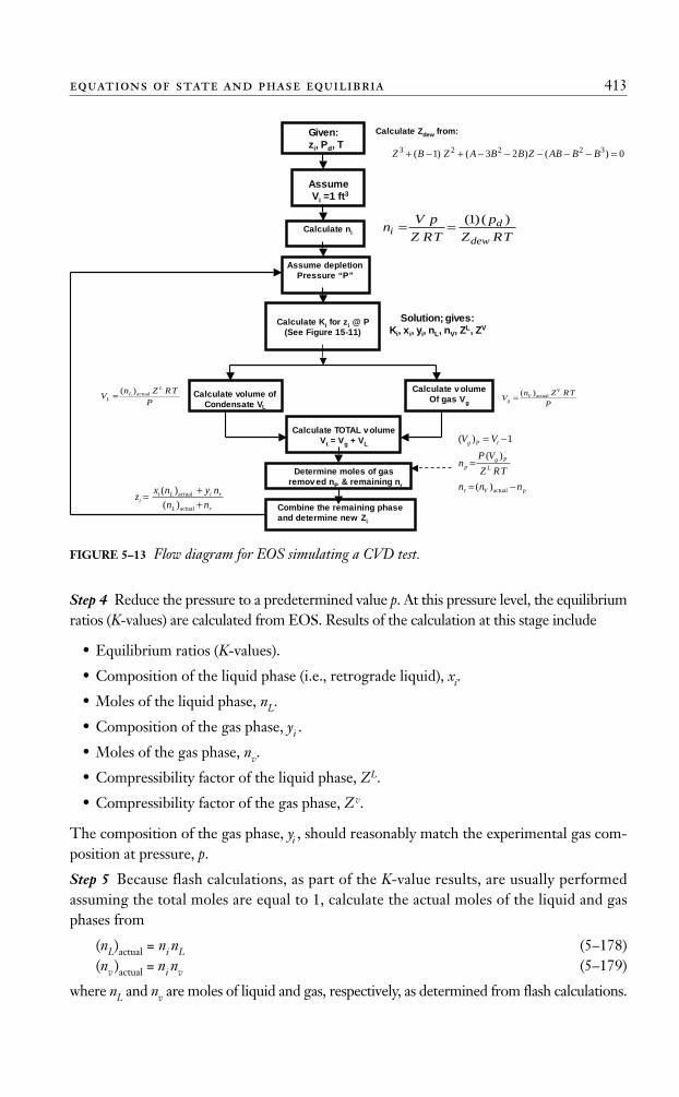
Step 4 Reduce the pressure to a predetermined value p. At this pressure level, the equilibriumratios (K-values) are calculated from EOS. Results of the calculation at this stage include
• Equilibrium ratios (K-values).
• Composition of the liquid phase (i.e., retrograde liquid), xi.
• Moles of the liquid phase, nL.
• Composition of the gas phase, yi .
• Moles of the gas phase, nv.
• Compressibility factor of the liquid phase, ZL.
• Compressibility factor of the gas phase, Zv.
The composition of the gas phase, yi , should reasonably match the experimental gas com-position at pressure, p.
Step 5 Because flash calculations, as part of the K-value results, are usually performedassuming the total moles are equal to 1, calculate the actual moles of the liquid and gasphases from
(nL)actual = ni nL (5–178)(nv )actual = ni nv (5–179)
where nL and nv are moles of liquid and gas, respectively, as determined from flash calculations.
equations of state and phase equilibria 413
PTRZn
VL
LL
actual)(=
TRZ
p
TRZ
pVn
dew
di
)()1(==
PTRZn
VV
Vg
actual)(=
Given:
zi, Pd, T
Assume
Vi =1 ft3
Calculate ni
Calculate Zdew from:
Assume depletion
Pressure “P”
Calculate Ki for zi @ P
(See Figure 15-11)
Solution; gives:
Ki, xi, yi, nL, nV, ZL, ZV
Calculate volume
Of gas Vg
Calculate volume of
Condensate VL
Calculate TOTAL volume
Vt = Vg + VL
Determine moles of gas
removed nP & remaining nrpVr
LPg
p
tPg
nnn
TRZ
VPn
VV
−=
=
−=
actual)(
)(
1)(
Combine the remaining phase
and determine new Zi
rL
riLii nn
nynxz
++=
actual
actual
)()(
0)()23()1( 32223 =−−−−−+−+ BBABZBBAZBZ
FIGURE 5–13 Flow diagram for EOS simulating a CVD test.
Ahmed_ch5.qxd 12/21/06 2:05 PM Page 413
Step 6 Calculate the volume of each hydrocarbon phase by applying the expression
(5–180)
(5–181)
where
VL = volume of the retrograde liquid, ft3/ft3
Vg = volume of the gas phase, ft3/ft3
ZL, Zv = compressibility factors of the liquid and gas phaseT = cell (reservoir) temperature, °R
Since Vi = 1, then
SL = (VL)100
This value should match the experimental value if the equation of state is properly tuned.
Step 7 Calculate the total volume of fluid in the cell:
Vt = VL + Vg (5–182)
where Vt = total volume of the fluid, ft3.
Step 8 Since the volume of the cell is constant at 1 ft3, remove the following excess gasvolume from the cell:
(Vgp)p,T = Vt – 1 (5–183)
Step 9 Calculate the number of moles of gas removed:
(5–184)
Step 10 Calculate cumulative gas produced as a percentage of gas initially in place bydividing cumulative moles of gas removed, by the original moles in place:
Step 11 Calculate the two-phase gas deviation factor from the relationship:
(5–185)
Step 12 Calculate the remaining moles of gas (nv )r by subtracting the moles produced (np)from the actual number of moles of the gas phase (nv )actual:
(nv )r = (nv )actual – np (5–186)
Step 13 Calculate the new total moles and new composition remaining in the cell byapplying the molal and component balances, respectively:
ni = (nL)actual + (nv )r , (5–187)
(5–188)zx n y n
nii L i v r
i
=+( ) ( )actual
Zp
n n RTi ptwo-phase = −
( )( )( )
1
%( )
( )G
n
npp
i
=⎡
⎣⎢⎢
⎤
⎦⎥⎥
∑original
100
np∑
np V
Z RTpp T
v=( ) ,gp
Vn Z RT
pgv
v
=( )actual
Vn Z RT
pLL
L
=( )actual
414 equations of state and pvt analysis
Ahmed_ch5.qxd 12/21/06 2:05 PM Page 414
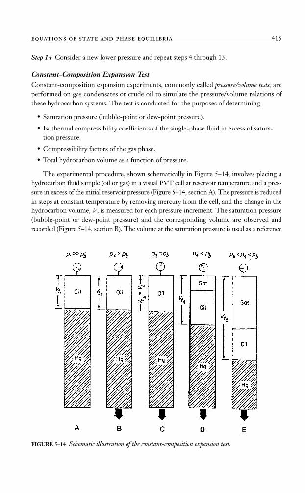
Step 14 Consider a new lower pressure and repeat steps 4 through 13.
Constant-Composition Expansion TestConstant-composition expansion experiments, commonly called pressure/volume tests, areperformed on gas condensates or crude oil to simulate the pressure/volume relations ofthese hydrocarbon systems. The test is conducted for the purposes of determining
• Saturation pressure (bubble-point or dew-point pressure).
• Isothermal compressibility coefficients of the single-phase fluid in excess of satura-tion pressure.
• Compressibility factors of the gas phase.
• Total hydrocarbon volume as a function of pressure.
The experimental procedure, shown schematically in Figure 5–14, involves placing ahydrocarbon fluid sample (oil or gas) in a visual PVT cell at reservoir temperature and a pres-sure in excess of the initial reservoir pressure (Figure 5–14, section A). The pressure is reducedin steps at constant temperature by removing mercury from the cell, and the change in thehydrocarbon volume, V, is measured for each pressure increment. The saturation pressure(bubble-point or dew-point pressure) and the corresponding volume are observed andrecorded (Figure 5–14, section B). The volume at the saturation pressure is used as a reference
equations of state and phase equilibria 415
FIGURE 5–14 Schematic illustration of the constant-composition expansion test.
Ahmed_ch5.qxd 12/21/06 2:05 PM Page 415
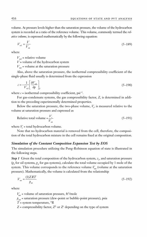
volume. At pressure levels higher than the saturation pressure, the volume of the hydrocarbonsystem is recorded as a ratio of the reference volume. This volume, commonly termed the rel-ative volume, is expressed mathematically by the following equation:
(5–189)
where
Vrel = relative volumeV = volume of the hydrocarbon systemVsat = volume at the saturation pressure
Also, above the saturation pressure, the isothermal compressibility coefficient of thesingle-phase fluid usually is determined from the expression
(5–190)
where c = isothermal compressibility coefficient, psi–1.For gas-condensate systems, the gas compressibility factor, Z, is determined in addi-
tion to the preceding experimentally determined properties.Below the saturation pressure, the two-phase volume, Vt , is measured relative to the
volume at saturation pressure and expressed as
Relative total volume = (5–191)
where Vt = total hydrocarbon volume.Note that no hydrocarbon material is removed from the cell, therefore, the composi-
tion of the total hydrocarbon mixture in the cell remains fixed at the original composition.
Simulation of the Constant Composition Expansion Test by EOSThe simulation procedure utilizing the Peng-Robinson equation of state is illustrated inthe following steps.
Step 1 Given the total composition of the hydrocarbon system, zi, and saturation pressure(pb for oil systems, pd for gas systems), calculate the total volume occupied by 1 mole of thesystem. This volume corresponds to the reference volume Vsat (volume at the saturationpressure). Mathematically, the volume is calculated from the relationship
(5–192)
where
Vsat = volume of saturation pressure, ft3/molepsat = saturation pressure (dew-point or bubble-point pressure), psiaT = system temperature, °RZ = compressibility factor, ZL or Zv depending on the type of system
VZ RTpsat
sat
=( )1
VV
t
sat
cV
Vp
T
= −∂∂
⎡
⎣⎢
⎤
⎦⎥
1
rel
rel
VV
Vrelsat
=
416 equations of state and pvt analysis
Ahmed_ch5.qxd 12/21/06 2:05 PM Page 416
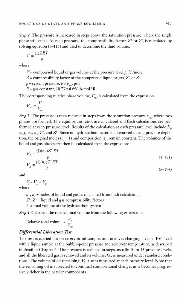
Step 2 The pressure is increased in steps above the saturation pressure, where the singlephase still exists. At each pressure, the compressibility factor, ZL or Zv, is calculated bysolving equation (5–115) and used to determine the fluid volume.
where
V = compressed liquid or gas volume at the pressure level p, ft3/moleZ = compressibility factor of the compressed liquid or gas, ZL or Zv
p = system pressure, p > psat, psiaR = gas constant; 10.73 psi ft3/ lb-mol °R
The corresponding relative phase volume, Vrel, is calculated from the expression
Step 3 The pressure is then reduced in steps below the saturation pressure psat, where twophases are formed. The equilibrium ratios are calculated and flash calculations are per-formed at each pressure level. Results of the calculation at each pressure level include Ki,xi, yi, nL, nv, Z
v, and ZL. Since no hydrocarbon material is removed during pressure deple-tion, the original moles (ni = 1) and composition, zi, remain constant. The volumes of theliquid and gas phases can then be calculated from the expressions
(5–193)
(5–194)and
Vt = VL + Vg
where
nL, nv = moles of liquid and gas as calculated from flash calculationsZL, Zv = liquid and gas compressibility factorsVt = total volume of the hydrocarbon system
Step 4 Calculate the relative total volume from the following expression:
Relative total volume =
Differential Liberation TestThe test is carried out on reservoir oil samples and involves charging a visual PVT cellwith a liquid sample at the bubble-point pressure and reservoir temperature, as describedin detail in Chapter 4. The pressure is reduced in steps, usually 10 to 15 pressure levels,and all the liberated gas is removed and its volume, Gp, is measured under standard condi-tions. The volume of oil remaining, VL, also is measured at each pressure level. Note thatthe remaining oil is subjected to continual compositional changes as it becomes progres-sively richer in the heavier components.
VV
t
sat
Vn Z RT
pgv
v
=( )( )1
Vn Z RT
pLL
L
=( )( )1
VV
Vrelsat
=
VZ RTp
=( )1
equations of state and phase equilibria 417
Ahmed_ch5.qxd 12/21/06 2:05 PM Page 417
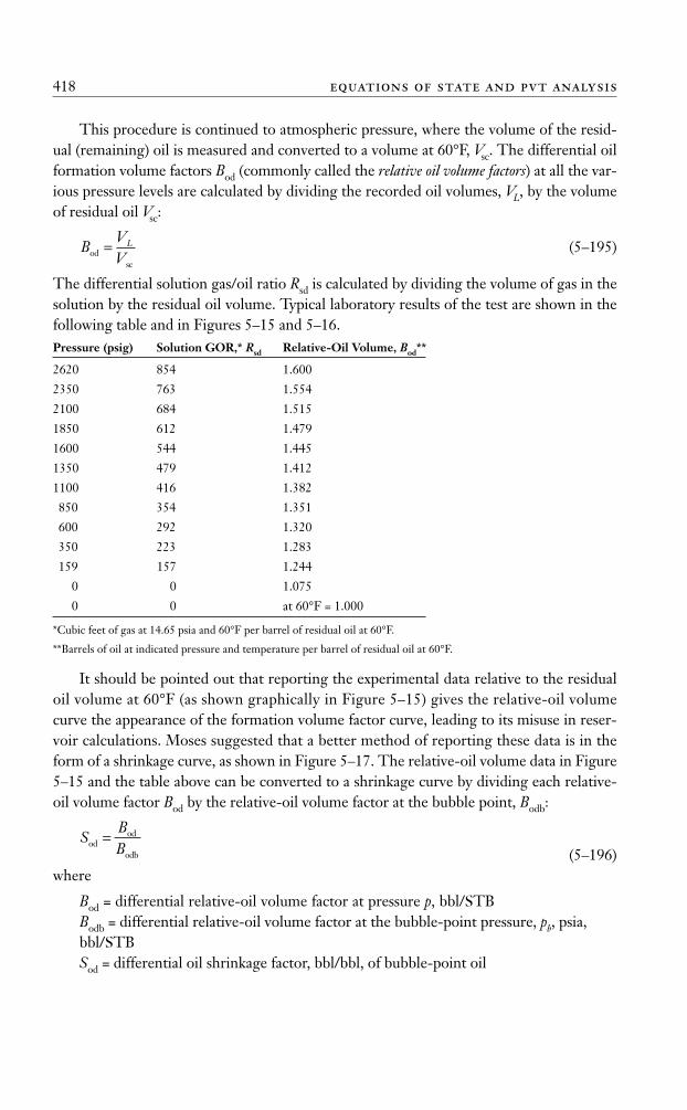
This procedure is continued to atmospheric pressure, where the volume of the resid-ual (remaining) oil is measured and converted to a volume at 60°F, Vsc. The differential oilformation volume factors Bod (commonly called the relative oil volume factors) at all the var-ious pressure levels are calculated by dividing the recorded oil volumes, VL, by the volumeof residual oil Vsc:
(5–195)
The differential solution gas/oil ratio Rsd is calculated by dividing the volume of gas in thesolution by the residual oil volume. Typical laboratory results of the test are shown in thefollowing table and in Figures 5–15 and 5–16.Pressure (psig) Solution GOR,* Rsd Relative-Oil Volume, Bod**
2620 854 1.600
2350 763 1.554
2100 684 1.515
1850 612 1.479
1600 544 1.445
1350 479 1.412
1100 416 1.382
850 354 1.351
600 292 1.320
350 223 1.283
159 157 1.244
0 0 1.075
0 0 at 60°F = 1.000
*Cubic feet of gas at 14.65 psia and 60°F per barrel of residual oil at 60°F.
**Barrels of oil at indicated pressure and temperature per barrel of residual oil at 60°F.
It should be pointed out that reporting the experimental data relative to the residualoil volume at 60°F (as shown graphically in Figure 5–15) gives the relative-oil volumecurve the appearance of the formation volume factor curve, leading to its misuse in reser-voir calculations. Moses suggested that a better method of reporting these data is in theform of a shrinkage curve, as shown in Figure 5–17. The relative-oil volume data in Figure5–15 and the table above can be converted to a shrinkage curve by dividing each relative-oil volume factor Bod by the relative-oil volume factor at the bubble point, Bodb:
(5–196)where
Bod = differential relative-oil volume factor at pressure p, bbl/STBBodb = differential relative-oil volume factor at the bubble-point pressure, pb, psia,bbl/STBSod = differential oil shrinkage factor, bbl/bbl, of bubble-point oil
SBBod
od
odb
=
BVV
Lod
sc
=
418 equations of state and pvt analysis
Ahmed_ch5.qxd 12/21/06 2:05 PM Page 418
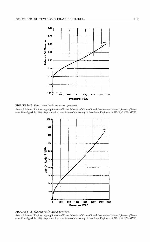
equations of state and phase equilibria 419
FIGURE 5–15 Relative-oil volume versus pressure.Source: P. Moses, “Engineering Applications of Phase Behavior of Crude Oil and Condensate Systems,” Journal of Petro-leum Technology (July 1980). Reproduced by permission of the Society of Petroleum Engineers of AIME, © SPE-AIME.
FIGURE 5–16 Gas/oil ratio versus pressure.Source: P. Moses, “Engineering Applications of Phase Behavior of Crude Oil and Condensate Systems,” Journal of Petro-leum Technology (July 1980). Reproduced by permission of the Society of Petroleum Engineers of AIME, © SPE-AIME.
Ahmed_ch5.qxd 12/21/06 2:05 PM Page 419
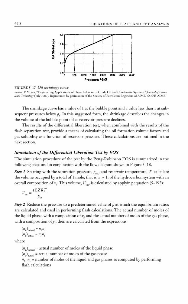
The shrinkage curve has a value of 1 at the bubble point and a value less than 1 at sub-sequent pressures below pb. In this suggested form, the shrinkage describes the changes inthe volume of the bubble-point oil as reservoir pressure declines.
The results of the differential liberation test, when combined with the results of theflash separation test, provide a means of calculating the oil formation volume factors andgas solubility as a function of reservoir pressure. These calculations are outlined in thenext section.
Simulation of the Differential Liberation Test by EOSThe simulation procedure of the test by the Peng-Robinson EOS is summarized in thefollowing steps and in conjunction with the flow diagram shown in Figure 5–18.
Step 1 Starting with the saturation pressure, psat, and reservoir temperature, T, calculatethe volume occupied by a total of 1 mole, that is, ni = 1, of the hydrocarbon system with anoverall composition of zi. This volume, Vsat, is calculated by applying equation (5–192):
Step 2 Reduce the pressure to a predetermined value of p at which the equilibrium ratiosare calculated and used in performing flash calculations. The actual number of moles ofthe liquid phase, with a composition of xi, and the actual number of moles of the gas phase,with a composition of yi, then are calculated from the expressions
(nL)actual = ni nL
(nv)actual = ni nv
where
(nL)actual = actual number of moles of the liquid phase(nv)actual = actual number of moles of the gas phasenL, nv = number of moles of the liquid and gas phases as computed by performingflash calculations
VZ RTpsat
sat
=( )1
420 equations of state and pvt analysis
FIGURE 5–17 Oil shrinkage curve.Source: P. Moses, “Engineering Applications of Phase Behavior of Crude Oil and Condensate Systems,” Journal of Petro-leum Technology (July 1980). Reproduced by permission of the Society of Petroleum Engineers of AIME, © SPE-AIME.
Ahmed_ch5.qxd 12/21/06 2:05 PM Page 420
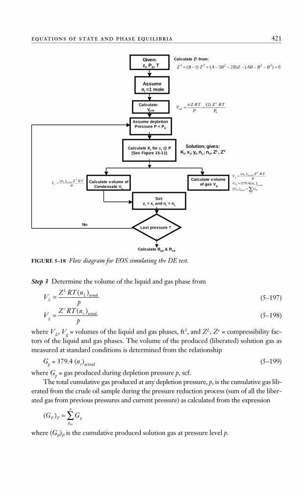
Step 3 Determine the volume of the liquid and gas phase from
(5–197)
(5–198)
where VL, Vg = volumes of the liquid and gas phases, ft3, and ZL, Zv = compressibility fac-tors of the liquid and gas phases. The volume of the produced (liberated) solution gas asmeasured at standard conditions is determined from the relationship
Gp = 379.4 (nv)actual (5–199)
where Gp = gas produced during depletion pressure p, scf.The total cumulative gas produced at any depletion pressure, p, is the cumulative gas lib-
erated from the crude oil sample during the pressure reduction process (sum of all the liber-ated gas from previous pressures and current pressure) as calculated from the expression
where (GP)P is the cumulative produced solution gas at pressure level p.
( )G GP P pp
p
=∑sat
VZ RT n
pg
vv=
( )actual
VZ RT n
pL
LL=
( )actual
equations of state and phase equilibria 421
PTRZn
VL
LL
actual)(=
b
L
sat PTRZ
PTRZn
V)1(==
∑=
=
=
=
1
actual
actual
)(
)(4.379
)(
iPtotalP
VP
VV
g
GG
nGP
TRZnV
Given:
zi, Pb, T
Assume
ni =1 mole
Calculate:
Vsat
Calculate ZL from:
Assume depletion
Pressure P < Pb
Calculate Ki for zi @ P
(See Figure 15-11)
Solution; gives:
Ki, xi, yi, nL, nV, ZL, ZV
Calculate volume
of gas Vg
Calculate volume of
Condensate VL
Set:
zi = xi and ni = nL
Last pressure ?No
Calculate Bod & Rsd
0)()23()1( 32223 =−−−−−+−+ BBABZBBAZBZ
FIGURE 5–18 Flow diagram for EOS simulating the DE test.
Ahmed_ch5.qxd 12/21/06 2:05 PM Page 421

Step 4 Assume that all the equilibrium gas is removed from contact with the oil. This canbe achieved mathematically by setting the overall composition, zi, equal to the composi-tion of the liquid phase, xi, and setting the total moles equal to the liquid phase:
zi = xi
ni = (nL)actual
Step 5 Using the new overall composition and total moles, steps 2 through 4 are repeated.When the depletion pressure reaches the atmospheric pressure, the temperature is changedto 60°F and the residual-oil volume is calculated. This residual-oil volume, calculated byequation (5–197), is referred to as Vsc. The total volume of gas that evolved from the oil andproduced (GP)Total is the sum of the all-liberated gas including that at atmospheric pressure:
Step 6 The calculated volumes of the oil and removed gas then are divided by the resid-ual-oil volume to calculate the relative-oil volumes (Bod) and the solution GOR at all theselected pressure levels from
(5–200)
Flash Separation TestsFlash separation tests, commonly called separator tests, are conducted to determine thechanges in the volumetric behavior of the reservoir fluid as the fluid passes through the sep-arator (or separators) and then into the stock tank. The resulting volumetric behavior isinfluenced to a large extent by the operating conditions, that is, pressures and temperaturesof the surface separation facilities. The primary objective of conducting separator tests,therefore, is to provide the essential laboratory information necessary for determining theoptimum surface separation conditions, which in turn maximize the stock-tank oil produc-tion. In addition, the results of the test, when appropriately combined with the differentialliberation test data, provide a means of obtaining the PVT parameters (Bo, Rs, and Bt)required for petroleum engineering calculations. The laboratory procedure of the flash sep-aration test involves the following steps.
Step 1 The oil sample is charged into a PVT cell at reservoir temperature and its bubble-point pressure.
Step 2 A small amount of the oil sample, with a volume of (Vo )pb, is removed from thePVT cell at constant pressure and flashed through a multistage separator system, witheach separator at a fixed pressure and temperature. The gas liberated from each stage (sep-arator) is removed and its volume and specific gravity measured. The volume of theremaining oil in the last stage (stock-tank condition) is recorded as (Vo )st.
Step 3 The total solution gas/oil ratio and the oil formation volume factor at the bubble-point pressure are then calculated:
RVsd
sc
remaining gas insolution= =
( . )( ) ( .5 615 5 6115)[( ) ( ) ]G GV
P P PTotal
sc
−
BVV
Lod
sc
=
( ).
G GP Pp
Totalsat
=∑14 7
422 equations of state and pvt analysis
Ahmed_ch5.qxd 12/21/06 2:05 PM Page 422
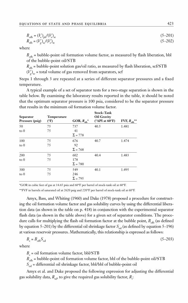
Bofb = (Vo )pb/(Vo )st (5–201)Rsfb = (Vg )sc/(Vo )st (5–202)
where
Bofb = bubble-point oil formation volume factor, as measured by flash liberation, bblof the bubble-point oil/STBRsfb = bubble-point solution gas/oil ratio, as measured by flash liberation, scf/STB(Vg )sc = total volume of gas removed from separators, scf
Steps 1 through 3 are repeated at a series of different separator pressures and a fixed temperature.
A typical example of a set of separator tests for a two-stage separation is shown in thetable below. By examining the laboratory results reported in the table, it should be notedthat the optimum separator pressure is 100 psia, considered to be the separator pressurethat results in the minimum oil formation volume factor.
Stock-Tank Separator Temperature Oil Gravity Pressure (psig) (°F) GOR, Rsfb* (°API at 60°F) FVF, Bofb**
50 75 737 40.5 1.481to 0 75 41
Σ = 778
100 75 676 40.7 1.474to 0 75 92
Σ = 768
200 75 602 40.4 1.483to 0 75 178
Σ = 780
300 75 549 40.1 1.495to 0 75 246
Σ = 795
*GOR in cubic feet of gas at 14.65 psia and 60°F per barrel of stock-tank oil at 60°F.
**FVF in barrels of saturated oil at 2620 psig and 220°F per barrel of stock-tank oil at 60°F.
Amyx, Bass, and Whiting (1960) and Dake (1978) proposed a procedure for construct-ing the oil formation volume factor and gas solubility curves by using the differential libera-tion data (as shown in the table on p. 418) in conjunction with the experimental separatorflash data (as shown in the table above) for a given set of separator conditions. The proce-dure calls for multiplying the flash oil formation factor at the bubble point, Bofb (as definedby equation 5–201) by the differential oil shrinkage factor Sod (as defined by equation 5–196)at various reservoir pressures. Mathematically, this relationship is expressed as follows:
Bo = BofbSod (5–203)
where
Bo = oil formation volume factor, bbl/STBBofb = bubble-point oil formation volume factor, bbl of the bubble-point oil/STBSod = differential oil shrinkage factor, bbl/bbl of bubble-point oil
Amyx et al. and Dake proposed the following expression for adjusting the differentialgas solubility data, Rsd, to give the required gas solubility factor, Rs:
equations of state and phase equilibria 423
Ahmed_ch5.qxd 12/21/06 2:05 PM Page 423
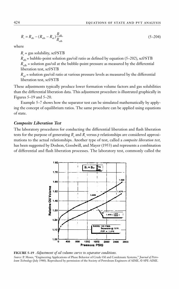
(5–204)
where
Rs = gas solubility, scf/STBRsfb = bubble-point solution gas/oil ratio as defined by equation (5–202), scf/STBRsdb = solution gas/oil at the bubble-point pressure as measured by the differentialliberation test, scf/STBRsd = solution gas/oil ratio at various pressure levels as measured by the differentialliberation test, scf/STB
These adjustments typically produce lower formation volume factors and gas solubilitiesthan the differential liberation data. This adjustment procedure is illustrated graphically inFigures 5–19 and 5–20.
Example 5–7 shows how the separator test can be simulated mathematically by apply-ing the concept of equilibrium ratios. The same procedure can be applied using equationsof state.
Composite Liberation TestThe laboratory procedures for conducting the differential liberation and flash liberationtests for the purpose of generating Bo and Rs versus p relationships are considered approxi-mations to the actual relationships. Another type of test, called a composite liberation test,has been suggested by Dodson, Goodwill, and Mayer (1953) and represents a combinationof differential and flash liberation processes. The laboratory test, commonly called the
R R R RBBs = − −sfb sdb sd
ofb
odb
( )
424 equations of state and pvt analysis
FIGURE 5–19 Adjustment of oil volume curve to separator conditions.Source: P. Moses, “Engineering Applications of Phase Behavior of Crude Oil and Condensate Systems,” Journal of Petro-leum Technology (July 1980). Reproduced by permission of the Society of Petroleum Engineers of AIME, © SPE-AIME.
Ahmed_ch5.qxd 12/21/06 2:05 PM Page 424
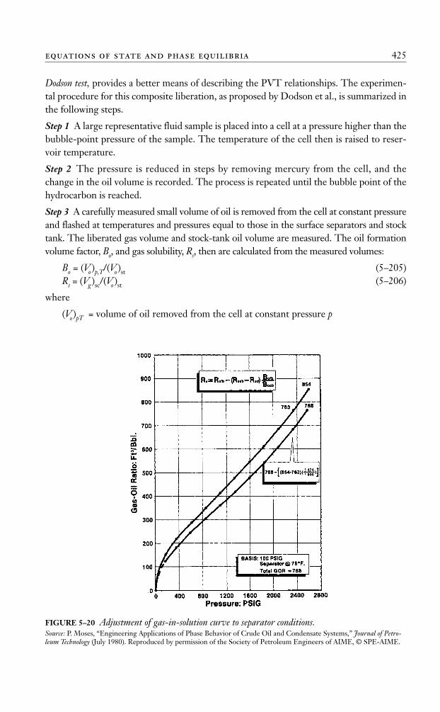
Dodson test, provides a better means of describing the PVT relationships. The experimen-tal procedure for this composite liberation, as proposed by Dodson et al., is summarized inthe following steps.
Step 1 A large representative fluid sample is placed into a cell at a pressure higher than thebubble-point pressure of the sample. The temperature of the cell then is raised to reser-voir temperature.
Step 2 The pressure is reduced in steps by removing mercury from the cell, and thechange in the oil volume is recorded. The process is repeated until the bubble point of thehydrocarbon is reached.
Step 3 A carefully measured small volume of oil is removed from the cell at constant pressureand flashed at temperatures and pressures equal to those in the surface separators and stocktank. The liberated gas volume and stock-tank oil volume are measured. The oil formationvolume factor, Bo, and gas solubility, Rs, then are calculated from the measured volumes:
Bo = (Vo )p,T/(Vo )st (5–205)Rs = (Vg )sc/(Vo )st (5–206)
where
(Vo )pT = volume of oil removed from the cell at constant pressure p
equations of state and phase equilibria 425
FIGURE 5–20 Adjustment of gas-in-solution curve to separator conditions.Source: P. Moses, “Engineering Applications of Phase Behavior of Crude Oil and Condensate Systems,” Journal of Petro-leum Technology (July 1980). Reproduced by permission of the Society of Petroleum Engineers of AIME, © SPE-AIME.
Ahmed_ch5.qxd 12/21/06 2:05 PM Page 425
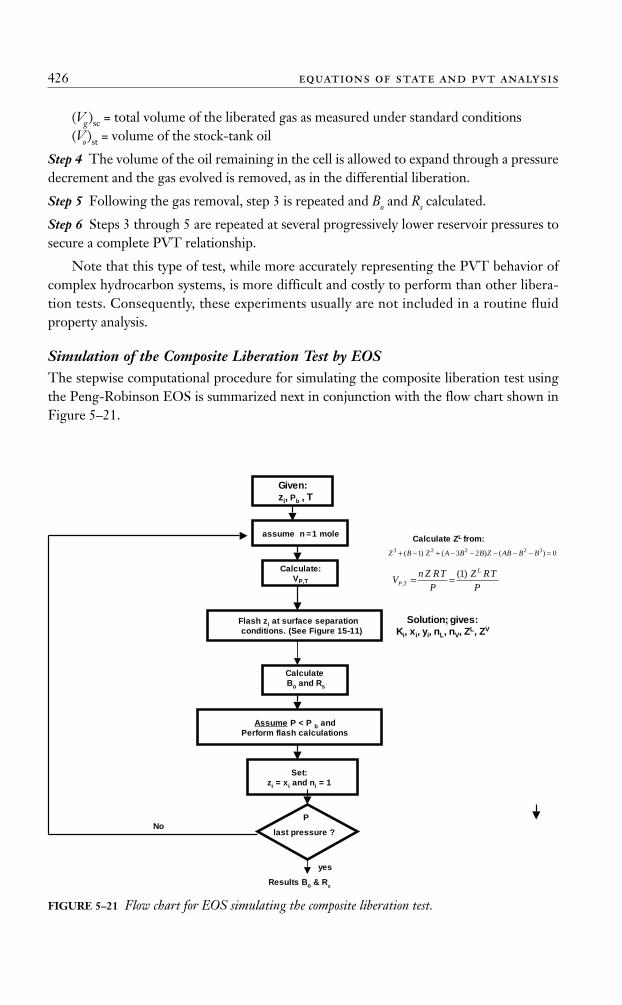
(Vg )sc = total volume of the liberated gas as measured under standard conditions(Vo )st = volume of the stock-tank oil
Step 4 The volume of the oil remaining in the cell is allowed to expand through a pressuredecrement and the gas evolved is removed, as in the differential liberation.
Step 5 Following the gas removal, step 3 is repeated and Bo and Rs calculated.
Step 6 Steps 3 through 5 are repeated at several progressively lower reservoir pressures tosecure a complete PVT relationship.
Note that this type of test, while more accurately representing the PVT behavior ofcomplex hydrocarbon systems, is more difficult and costly to perform than other libera-tion tests. Consequently, these experiments usually are not included in a routine fluidproperty analysis.
Simulation of the Composite Liberation Test by EOSThe stepwise computational procedure for simulating the composite liberation test usingthe Peng-Robinson EOS is summarized next in conjunction with the flow chart shown inFigure 5–21.
426 equations of state and pvt analysis
0)()23()1( 32223 =−−−−−+−+ BBABZBBAZBZ
Given:
zi, Pb , T
Assume P < P b and
Perform flash calculations
Calculate:
VP,T
Calculate ZL from:
Flash zi at surface separation
conditions. (See Figure 15-11)
Solution; gives:
Ki, xi, yi, nL, nV, ZL, ZV
Calculate
Bo and Rs
Set:
zi = xi and ni = 1
last pressure ?No
Results Bo & Rs
assume n =1 mole
yes
P
PTRZ
PTRZn
VL
TP
)1(, ==
FIGURE 5–21 Flow chart for EOS simulating the composite liberation test.
Ahmed_ch5.qxd 12/21/06 2:05 PM Page 426

Step 1 Assume a large reservoir fluid sample with an overall composition of zi is placed ina cell at the bubble-point pressure, pb, and reservoir temperature, T.
Step 2 Remove 1 lb-mole ni = 1, of the liquid from the cell and calculate the correspon-ding volume at pb and T by applying the Peng-Robinson EOS to estimate the liquid com-pressibility factor, ZL:
(5–207)
where (Vo )p,T = volume of 1 mole of the oil, ft3.
Step 3 Flash the resulting volume (step 2) at temperatures and pressures equal to those inthe surface separators and stock tank. Designating the resulting total liberated gas volume(Vg )sc and the volume of the stock-tank oil (Vo )st, calculate the Bo and Rs by applying equa-tions (5–205) and (5–206), respectively:
Bo = (Vo )p,T /(Vo )st
Rs = (Vg )sc/(Vo )st
Step 4 Set the cell pressure to a lower pressure level, p, and using the original compositionzi, generate the Ki values through the application of the PR EOS.
Step 5 Perform flash calculations based on zi and the calculated ki values.
Step 6 To simulate the differential liberation step of removing the equilibrium liberated gasfrom the cell at constant pressure, simply set the overall composition, zi, equal to the mole frac-tion of the equilibrium liquid, xi, and the bubble-point pressure, pb, equal to the new pressure level, p.Mathematically, this step is summarized by the following relationships:
zi = xi
pb = p
Step 7 Repeat steps 2 through 6.
Swelling TestsSwelling tests should be preformed if a reservoir is to be depleted under gas injection or adry gas cycling scheme. The swelling test can be conducted on gas condensate or crude oilsamples. The purpose of this laboratory experiment is to determine the degree to whichthe proposed injection gas will dissolve in the hydrocarbon mixture. The data that can beobtained during a test of this type include
• The relationship of saturation pressure and volume of gas injected.
• The volume of the saturated fluid mixture compared to the volume of the originalsaturated fluid.
The test procedure, as shown schematically in Figure 5–22, is summarized in the follow-ing steps.
Step 1 A representative sample of the hydrocarbon mixture with a known overall compo-sition, zi, is charged to a visual PVT cell at saturation pressure and reservoir temperature.
( )( )
,VZ RTpo p T
L
b
=1
equations of state and phase equilibria 427
Ahmed_ch5.qxd 12/21/06 2:05 PM Page 427
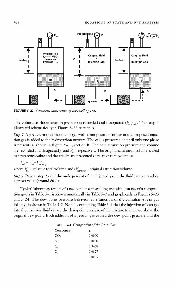
The volume at the saturation pressure is recorded and designated (Vsat)orig. This step isillustrated schematically in Figure 5–22, section A.
Step 2 A predetermined volume of gas with a composition similar to the proposed injec-tion gas is added to the hydrocarbon mixture. The cell is pressured up until only one phaseis present, as shown in Figure 5–22, section B. The new saturation pressure and volumeare recorded and designated ps and Vsat, respectively. The original saturation volume is usedas a reference value and the results are presented as relative total volumes:
Vrel = Vsat/(Vsat)orig
where Vrel = relative total volume and (Vsat)orig = original saturation volume.
Step 3 Repeat step 2 until the mole percent of the injected gas in the fluid sample reachesa preset value (around 80%).
Typical laboratory results of a gas-condensate swelling test with lean gas of a composi-tion given in Table 5–1 is shown numerically in Table 5–2 and graphically in Figures 5–23and 5–24. The dew-point pressure behavior, as a function of the cumulative lean gasinjected, is shown in Table 5–2. Note by examining Table 5–1 that the injection of lean gasinto the reservoir fluid caused the dew-point pressure of the mixture to increase above theoriginal dew point. Each addition of injection gas caused the dew-point pressure and the
428 equations of state and pvt analysis
Hg
Original Fluid
(gas or oil) @
saturation
Pressure Psat
Psat P(Psat)new
i.e. Pb or Pd
(Vsat)origVt
Original Fluid
+
Injection Gas
Injection gas
(Vsat)new
A CB
Original Fluid
+
Injection Gas
Hg Hg
FIGURE 5–22 Schematic illustration of the swelling test.
TABLE 5–1 Composition of the Lean GasComponent yi
CO2 0.0000
N2 0.0000
C1 0.9468
C2 0.0527
C3 0.0005
Ahmed_ch5.qxd 12/21/06 2:05 PM Page 428
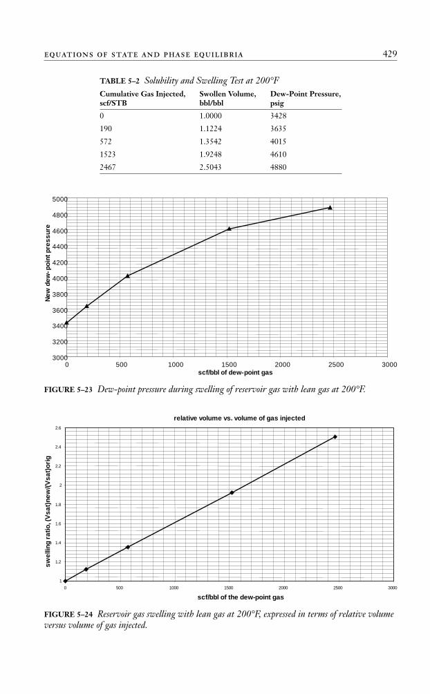
equations of state and phase equilibria 429
TABLE 5–2 Solubility and Swelling Test at 200°FCumulative Gas Injected, Swollen Volume, Dew-Point Pressure, scf/STB bbl/bbl psig
0 1.0000 3428
190 1.1224 3635
572 1.3542 4015
1523 1.9248 4610
2467 2.5043 4880
3000
3200
3400
3600
3800
4000
4200
4400
4600
4800
5000
0 500 1000 1500 2000 2500 3000
scf/bbl of dew-point gas
Ne
wd
ew
-p
oin
tp
res
su
re
FIGURE 5–23 Dew-point pressure during swelling of reservoir gas with lean gas at 200°F.
relative volume vs. volume of gas injected
1
1.2
1.4
1.6
1.8
2
2.2
2.4
2.6
0 500 1000 1500 2000 2500 3000
scf/bbl of the dew-point gas
sw
ellin
gra
tio
,(V
sa
t)n
ew
/(V
sa
t)o
rig
FIGURE 5–24 Reservoir gas swelling with lean gas at 200°F, expressed in terms of relative volumeversus volume of gas injected.
Ahmed_ch5.qxd 12/21/06 2:05 PM Page 429
430 equations of state and pvt analysis
relative volume (swollen volume) to increase. The dew point increased from 3428 to 4880psig and relative total volume from 1 to 2.5043 after the final addition, as shown in Figures5–23 and 5–24, respectively.
Simulation of the Swelling Test by EOSThe simulation procedure of the swelling test by the PR EOS is summarized in the fol-lowing steps.
Step 1 Assume the hydrocarbon system occupies a total volume of 1 bbl at the saturationpressure, ps, and reservoir temperature, T. Calculate the initial moles of the hydrocarbonsystem from the following expression:
where ni = initial moles of the hydrocarbon systempsat = saturation pressure, that is, pb or pd, depending on the type of the hydrocarbonsystem, psiaZ = gas or liquid compressibility factor
Step 2 Given the composition yinj of the proposed injection gas, add a predetermined volume(as measured in scf) of the injection gas to the original hydrocarbon system and calculate thenew overall composition by applying the molal and component balances, respectively:
nt = ni + ninj,
with
where ninj = total moles of the injection gasVinj = volume of the injection gas, scf(zsat)i = mole fraction of component i in the saturated hydrocarbon system
Step 3 Using the new composition, zi, calculate the new saturation pressure, pb or pd, usingthe Peng-Robinson EOS as outlined in this chapter.
Step 4 Calculate the relative total volume (swollen volume) by applying the relationship
where Vrel = swollen volume and psat = saturation pressure.
Step 5 Steps 2 through 4 are repeated until the last predetermined volume of the lean gasis combined with the original hydrocarbon system.
VZn RT
pt
relsat
=5 615.
nV
injinj=
379 4.
zy n z n
nii i
t
=+inj inj sat( )
np
Z RTi =5 615. sat
Ahmed_ch5.qxd 12/21/06 2:05 PM Page 430
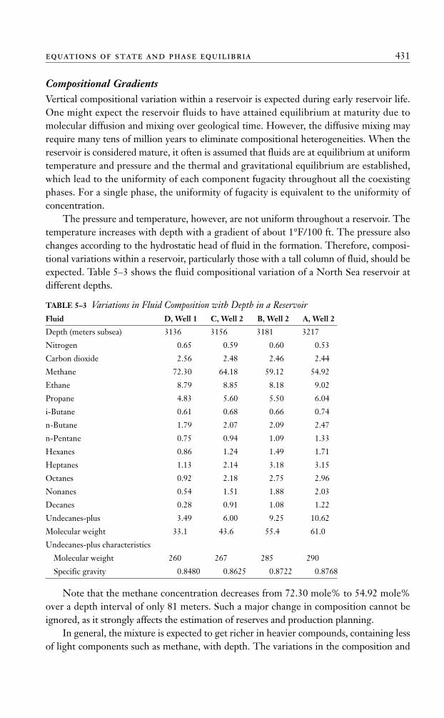
Compositional GradientsVertical compositional variation within a reservoir is expected during early reservoir life.One might expect the reservoir fluids to have attained equilibrium at maturity due tomolecular diffusion and mixing over geological time. However, the diffusive mixing mayrequire many tens of million years to eliminate compositional heterogeneities. When thereservoir is considered mature, it often is assumed that fluids are at equilibrium at uniformtemperature and pressure and the thermal and gravitational equilibrium are established,which lead to the uniformity of each component fugacity throughout all the coexistingphases. For a single phase, the uniformity of fugacity is equivalent to the uniformity ofconcentration.
The pressure and temperature, however, are not uniform throughout a reservoir. Thetemperature increases with depth with a gradient of about 1°F/100 ft. The pressure alsochanges according to the hydrostatic head of fluid in the formation. Therefore, composi-tional variations within a reservoir, particularly those with a tall column of fluid, should beexpected. Table 5–3 shows the fluid compositional variation of a North Sea reservoir atdifferent depths.
TABLE 5–3 Variations in Fluid Composition with Depth in a ReservoirFluid D, Well 1 C, Well 2 B, Well 2 A, Well 2
Depth (meters subsea) 3136 3156 3181 3217
Nitrogen 0.65 0.59 0.60 0.53
Carbon dioxide 2.56 2.48 2.46 2.44
Methane 72.30 64.18 59.12 54.92
Ethane 8.79 8.85 8.18 9.02
Propane 4.83 5.60 5.50 6.04
i-Butane 0.61 0.68 0.66 0.74
n-Butane 1.79 2.07 2.09 2.47
n-Pentane 0.75 0.94 1.09 1.33
Hexanes 0.86 1.24 1.49 1.71
Heptanes 1.13 2.14 3.18 3.15
Octanes 0.92 2.18 2.75 2.96
Nonanes 0.54 1.51 1.88 2.03
Decanes 0.28 0.91 1.08 1.22
Undecanes-plus 3.49 6.00 9.25 10.62
Molecular weight 33.1 43.6 55.4 61.0
Undecanes-plus characteristics
Molecular weight 260 267 285 290
Specific gravity 0.8480 0.8625 0.8722 0.8768
Note that the methane concentration decreases from 72.30 mole% to 54.92 mole%over a depth interval of only 81 meters. Such a major change in composition cannot beignored, as it strongly affects the estimation of reserves and production planning.
In general, the mixture is expected to get richer in heavier compounds, containing lessof light components such as methane, with depth. The variations in the composition and
equations of state and phase equilibria 431
Ahmed_ch5.qxd 12/21/06 2:05 PM Page 431
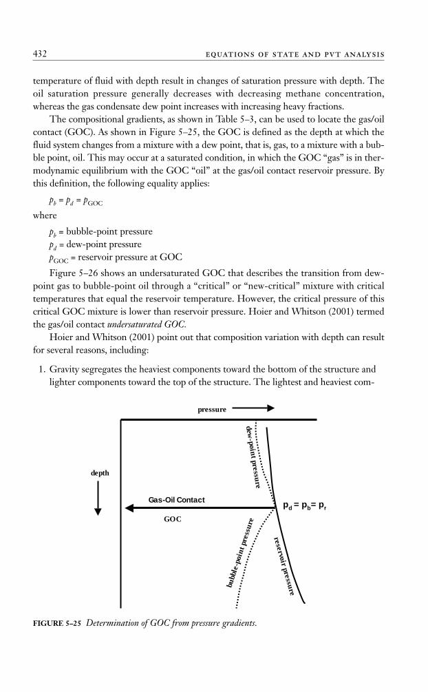
432 equations of state and pvt analysis
temperature of fluid with depth result in changes of saturation pressure with depth. Theoil saturation pressure generally decreases with decreasing methane concentration,whereas the gas condensate dew point increases with increasing heavy fractions.
The compositional gradients, as shown in Table 5–3, can be used to locate the gas/oilcontact (GOC). As shown in Figure 5–25, the GOC is defined as the depth at which thefluid system changes from a mixture with a dew point, that is, gas, to a mixture with a bub-ble point, oil. This may occur at a saturated condition, in which the GOC “gas” is in ther-modynamic equilibrium with the GOC “oil” at the gas/oil contact reservoir pressure. Bythis definition, the following equality applies:
pb = pd = pGOC
where
pb = bubble-point pressurepd = dew-point pressurepGOC = reservoir pressure at GOC
Figure 5–26 shows an undersaturated GOC that describes the transition from dew-point gas to bubble-point oil through a “critical” or “new-critical” mixture with criticaltemperatures that equal the reservoir temperature. However, the critical pressure of thiscritical GOC mixture is lower than reservoir pressure. Hoier and Whitson (2001) termedthe gas/oil contact undersaturated GOC.
Hoier and Whitson (2001) point out that composition variation with depth can resultfor several reasons, including:
1. Gravity segregates the heaviest components toward the bottom of the structure andlighter components toward the top of the structure. The lightest and heaviest com-
dew-poin
t pressure
bubb
le-p
oint
pre
ssur
e
reservoir pressure
GOC
pressure
depth
Gas-Oil Contactpd = pb= pr
FIGURE 5–25 Determination of GOC from pressure gradients.
Ahmed_ch5.qxd 12/21/06 2:05 PM Page 432
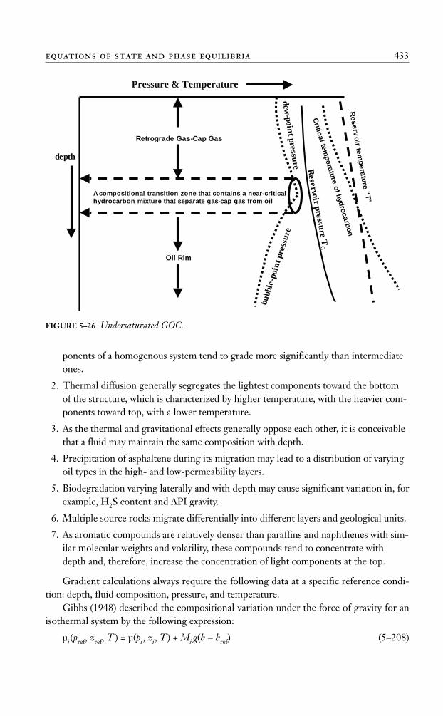
ponents of a homogenous system tend to grade more significantly than intermediateones.
2. Thermal diffusion generally segregates the lightest components toward the bottomof the structure, which is characterized by higher temperature, with the heavier com-ponents toward top, with a lower temperature.
3. As the thermal and gravitational effects generally oppose each other, it is conceivablethat a fluid may maintain the same composition with depth.
4. Precipitation of asphaltene during its migration may lead to a distribution of varyingoil types in the high- and low-permeability layers.
5. Biodegradation varying laterally and with depth may cause significant variation in, forexample, H2S content and API gravity.
6. Multiple source rocks migrate differentially into different layers and geological units.
7. As aromatic compounds are relatively denser than paraffins and naphthenes with sim-ilar molecular weights and volatility, these compounds tend to concentrate withdepth and, therefore, increase the concentration of light components at the top.
Gradient calculations always require the following data at a specific reference condi-tion: depth, fluid composition, pressure, and temperature.
Gibbs (1948) described the compositional variation under the force of gravity for anisothermal system by the following expression:
μi (pref, zref, T ) = μ(pi, zi, T ) + Mi g(h – href) (5–208)
equations of state and phase equilibria 433
dew-poin
t pressure
bubb
le-p
oint
pre
ssur
e
Reservoir pressu
re TC
Pressure & Temperature
depth
A compositional transition zone that contains a near-critical
hydrocarbon mixture that separate gas-cap gas from oil
Retrograde Gas-Cap Gas
Oil Rim
Re
se
rvo
irte
mp
era
ture
“T”
Critic
al
tem
pe
ratu
reo
fh
yd
roc
arb
on
FIGURE 5–26 Undersaturated GOC.
Ahmed_ch5.qxd 12/21/06 2:05 PM Page 433
with i = 1, 2, . . ., N,where
μi = chemical potential of component ihref = reference depthpref = pressure at reference depthMi = molecular weight of component ip = pressure at depth hzi = mole fraction of component i at depth hN = total number of components
This condition represents N equations with the constraint that the sum of the molefraction at depth h, zi(h), must equal 1:
(5–209)
The main objective is to determine the composition of fluid zi(h) and pressure p(h) at aspecified depth, h.
Whitson and Belery (1994) point out that combining the mechanical/equilibriumcondition, that is,
(5–210)
with equation (5–208) guarantees automatic satisfaction of the condition
(5–211)
where ρ(h) = fluid density at depth h and g = acceleration due to gravity.The chemical potential essentially is a quantity that measures how much energy a
component brings to a mixture. It can be expressed in terms of fugacity by the followingexpression:
(5–212)
whereR = constantfi = fugacity of component i at p, Tf o
i = fugacity of component i at a reference stateμo
i = chemical potential of component i at a reference state
The term between the two brackets usually drops out in most of the calculations.Combining equation (5–208) with (5–212) gives
(5–213)
For convenience, defining
fi(pref, zref, T ) = fi(href)fi(p, z, T ) = fi(h)
ln ( , , ) ln ( , , )(
f p z T f p z TgM h
i ii
ref ref⎡⎣ ⎤⎦ = ⎡⎣ ⎤⎦ +−−
−h
RTref )
1
μ μi i io
ioRT f RT f= + −⎡⎣ ⎤⎦ln( ) ln( )
p h p h h g dhh
h
( ) ( ) ( )= + ⎡⎣ ⎤⎦∫ref
ref
ρ
dpdh
g= −ρ
z hii
N
( ) .==∑ 1 0
1
434 equations of state and pvt analysis
Ahmed_ch5.qxd 12/21/06 2:05 PM Page 434
equation (5–213) can be written as
(5–214)
where
R = gas constant, 10.73 psi-ft3/lb-mol °RT = temperature, °RMi = molecular weight, lbm/lb-mol
It should be pointed out that, when calculating the fugacity using the SRK or PR EOS,the volume-translation method must be used in the fugacity expression; that is,
(5–215)
where ci = component-dependent volume shift parameter.Equation (5–215) suggests that compositional grading becomes more significant when
the mixture is composed of molecules with widely different molecular weights. This is ofparticular significance in oil systems with large concentrations of heavy components suchas asphaltenes. It should be pointed out that the heavy ends generally are reported aspseudo components or groups, each composed of several compounds characterized by anassigned fixed average molecular weight. When compositional grading occurs, the con-centration of compounds within each pseudo component changes and the use of a fixedvalue of molecular weight reduces the reliability of the predicted results.
Whitson and Belery (1994) and Whitson and Brule (2000) presented an efficient algo-rithm for solving equation (5–214). The methodology is summarized in the following steps.
Step 1 Using the composition, zref, at the reference depth, href, calculate the reference feedfugacity, fi (pref, Tref). Note that each fugacity value must be corrected using the volumeshift parameter; that is,
Step 2 Calculate the gravity-corrected fugacity (pref, Tref) from
Whitson and his coauthors point out that (pref, Tref) needs to be made only once.
Step 3 Assume the composition and pressure at depth h, that is, zi(h) and p(h). The initialestimates can be simply
zi(h) = zi(href)
and
p(h) = p(href)
Step 4 Calculate fugacities of the composition estimate, zi, at the pressure estimate, p.
�f i
�f p T f p TM h h
i ii( ) ( , ) exp( )
ref ref ref refref, =
− −1444RT
⎡
⎣⎢
⎤
⎦⎥
�f i
f p Tc p
RTii( , ) expref ref
−⎛⎝⎜
⎞⎠⎟
( ) ( ) expf fc p
RTi ii
modified orginial=−⎛⎝⎜
⎞⎠⎟
f h f hM h h
RTi ii( ) ( ) exp( )
=− −⎡⎣⎢
⎤⎦⎥
refref
144
equations of state and phase equilibria 435
Ahmed_ch5.qxd 12/21/06 2:05 PM Page 435
Step 5 Calculate the following two parameters as defined by Whitson and his coworkers:
where Yi is termed the mole number.
Step 6 Calculate the fugacity ratio correction from
Step 7 Update mole numbers using the following expression:
Using the method of successive substitution with four iterations (initially λ = 1), followedby accelerated successive substitution with λ as given by
with
where n is the iteration number, that is, n = 4.
Step 8 Calculate the composition at depth h, that is, z(n+1) from Y n+1i , using
Step 9 Update the reservoir pressure estimated depth, h, using a Newton-Raphson estimate:
where
Step 10 Check for convergence using the criterion
Iterate until convergence is achieved.
lnYz
i
ii
N ⎛⎝⎜
⎞⎠⎟
⎡
⎣⎢
⎤
⎦⎥ <
=
−∑1
2
410
∂∂=
∂ ∂⎡
⎣⎢
⎤
⎦⎥
=∑Q
pY R
f pf p zi i
i
ii
N ( / )( , )1
p pQ
Q pn n
n
n+ = −
∂ ∂1
( / )
zY
Yi
i
ii
n=
=∑
1
b R Rin
in
i
N
= ⎡⎣ ⎤⎦− −
=∑ ln( ) ln( )1 1
1
a R Rin
in
i
N
= ⎡⎣ ⎤⎦−
=∑ ln( ) ln( )1
1
λ =+a
a b
Y Y Rin
in
in+ = ⎡⎣ ⎤⎦
1 λ
Rf p z
f p z Yi
i
ii
i
N=⎡
⎣⎢
⎤
⎦⎥
=∑
� ( , )( , )ref ref 1
1
Q p z Yii
N
( , ) = −=∑1
1
Y zf p z
f p zii i
i
i
=⎡
⎣⎢
⎤
⎦⎥ =
� ( , )( , )
, , .ref ref . .1 ,, N
436 equations of state and pvt analysis
Ahmed_ch5.qxd 12/21/06 2:05 PM Page 436
Step 11 After finding the composition, z(h), and pressure, p(h), a phase-stability test asproposed by Michelsen (1984) must be made to establish that the solution is valid. A validsolution has a single phase that is thermodynamically stable. An unstable solution indicatesthat the calculated z and p will split into two or more phases, thereby making the solutioninvalid.
Whitson and Brule (2000) point out that, if the gradient solution is unstable, then thestability-test composition should be used to reinitialize the gradient calculation. The start-ing pressure for the new gradient calculation can be pref or, preferably, the converged pres-sure from the gradient calculation that led to the instable solution.
It should be noted that, when tuning an EOS to match a variety of experimental dataon hydrocarbon samples taken from different depths and within a certain range of tem-peratures, the resulting tuned EOS generally is capable of predicting the PVT propertiesand the compositional gradient within that range of the temperatures; that is, it can inter-polate and generate accurate PVT and compositional fluid data at temperatures withinthat range. However, the degree accuracy usually decreases when extrapolating outsidethe range of temperatures used in tuning the selected EOS. This attributed to the factthat equation-of-state’s parameter, a(T), is a highly dependent temperature parameter.This is evident when using the EOS to locate the gas/oil contact using different referencepoints, that is, Tref, pref, (zi)ref, each will not predict the same GOC.
The ternary diagram (as defined in Chapter 1 and shown in Figure 1–32) with equilat-eral triangles defines the compositional boundaries that separate different types of hydro-carbon systems. This diagram can be conveniently used to approximate the location of theGOC from compositional gradients. Figure 5–27 shows the compositional gradient of fivefields and illustrates the transition from gas to oil as the compositional gradients cross theboundary between the condensate gas cap and volatile oil. For example, Figure 5–27shows the changes in the composition of the Orocual field hydrocarbon system as it ap-proaches the boundary that separates the gas from oil. The composition at the boundarycan be read as
C1 + N2 = 70.0 mol%C2–C6, CO2 = 17.5 mol%C7+ = 12.5 mol%
Figures 5–28 through 5–30 show the compositional variations of C1 + N2, C2–C6,CO2, and C7+ as function of depth, respectively, of the Orocual hydrocarbon system.Entering these graphs with composition of the transition mixtures gives an approxima-tion of the GOC at 13,500 ft. Plotting the composition gradient as a function of depth isa linear form worth investigating.
Minimum Miscibility Pressure Several schemes for predicting MMP based on the equation-of-state approach have beenproposed. Benmekki and Mansoori (1988) applied the PR EOS with different mixing rulesthat were joined with a newly formulated expression for the unlike three-body interactions
equations of state and phase equilibria 437
Ahmed_ch5.qxd 12/21/06 2:05 PM Page 437
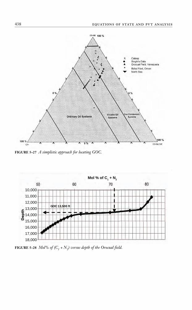
438 equations of state and pvt analysis
FIGURE 5–27 A simplistic approach for locating GOC.
GOC 13,500 ft
10,000
11,000
12,000
13,000
14,000
15,000
16,000
17,000
18,000
Mol % of C1 + N
2
FIGURE 5–28 Mol% of (C1 + N2) versus depth of the Orocual field.
Ahmed_ch5.qxd 12/21/06 2:05 PM Page 438
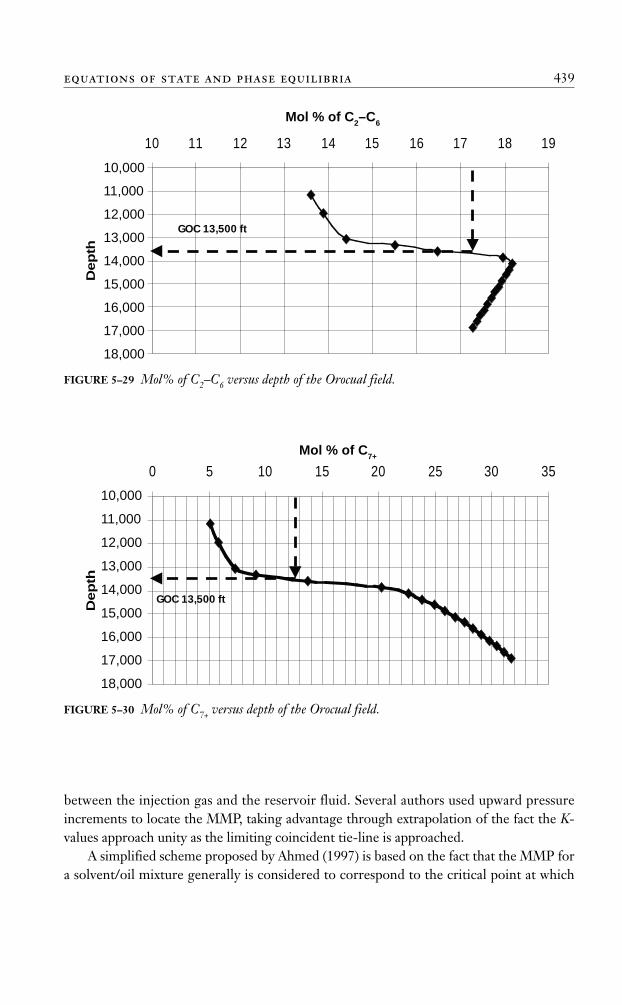
between the injection gas and the reservoir fluid. Several authors used upward pressureincrements to locate the MMP, taking advantage through extrapolation of the fact the K-values approach unity as the limiting coincident tie-line is approached.
A simplified scheme proposed by Ahmed (1997) is based on the fact that the MMP fora solvent/oil mixture generally is considered to correspond to the critical point at which
equations of state and phase equilibria 439
10000
11000
12000
13000
14000
15000
16000
17000
18000
10 11 12 13 14 15 16 17 18 19
Mol %of C2-C6
Dep
th
GOC 13,500 ft
Mol % of C2–C
6
10,000
11,000
12,000
13,000
14,000
15,000
16,000
17,000
18,000
FIGURE 5–29 Mol% of C2–C6 versus depth of the Orocual field.
10000
11000
12000
13000
14000
15000
16000
17000
18000
0 5 10 15 20 25 30 35
Mol %of C7+
Dep
th
GOC 13,500 ft
10,000
11,000
12,000
13,000
14,000
15,000
16,000
17,000
18,000
Mol % of C7+
FIGURE 5–30 Mol% of C7+ versus depth of the Orocual field.
Ahmed_ch5.qxd 12/21/06 2:05 PM Page 439
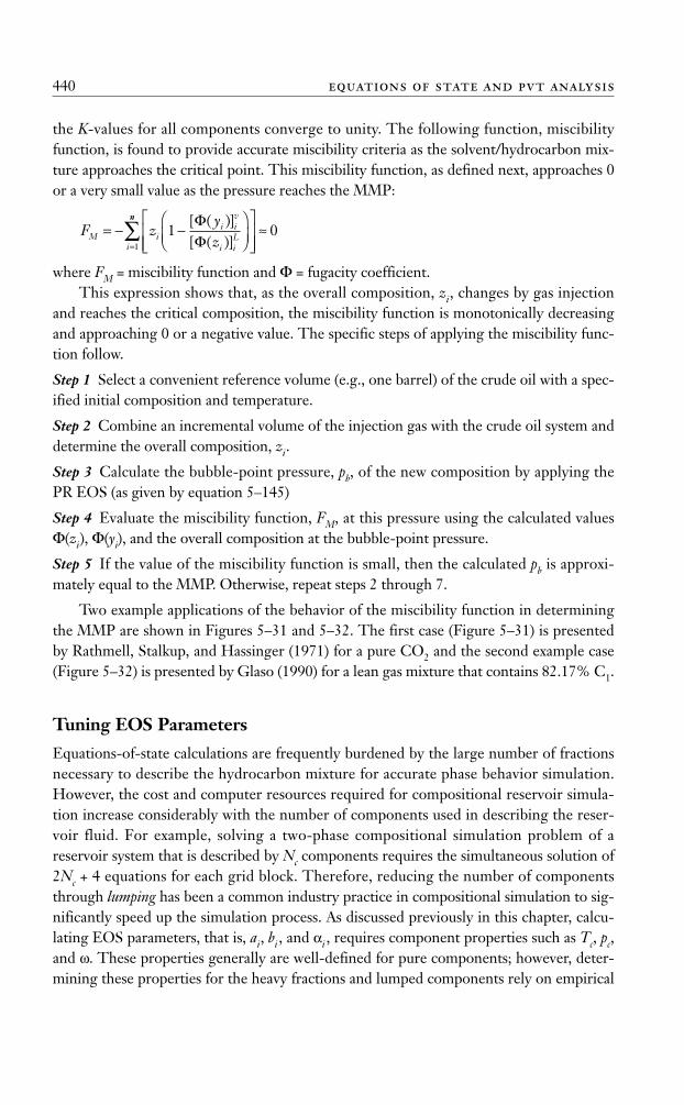
the K-values for all components converge to unity. The following function, miscibilityfunction, is found to provide accurate miscibility criteria as the solvent/hydrocarbon mix-ture approaches the critical point. This miscibility function, as defined next, approaches 0or a very small value as the pressure reaches the MMP:
where FM = miscibility function and Φ = fugacity coefficient.This expression shows that, as the overall composition, zi, changes by gas injection
and reaches the critical composition, the miscibility function is monotonically decreasingand approaching 0 or a negative value. The specific steps of applying the miscibility func-tion follow.
Step 1 Select a convenient reference volume (e.g., one barrel) of the crude oil with a spec-ified initial composition and temperature.
Step 2 Combine an incremental volume of the injection gas with the crude oil system anddetermine the overall composition, zi.
Step 3 Calculate the bubble-point pressure, pb, of the new composition by applying thePR EOS (as given by equation 5–145)
Step 4 Evaluate the miscibility function, FM, at this pressure using the calculated valuesΦ(zi), Φ(yi), and the overall composition at the bubble-point pressure.
Step 5 If the value of the miscibility function is small, then the calculated pb is approxi-mately equal to the MMP. Otherwise, repeat steps 2 through 7.
Two example applications of the behavior of the miscibility function in determiningthe MMP are shown in Figures 5–31 and 5–32. The first case (Figure 5–31) is presentedby Rathmell, Stalkup, and Hassinger (1971) for a pure CO2 and the second example case(Figure 5–32) is presented by Glaso (1990) for a lean gas mixture that contains 82.17% C1.
Tuning EOS Parameters
Equations-of-state calculations are frequently burdened by the large number of fractionsnecessary to describe the hydrocarbon mixture for accurate phase behavior simulation.However, the cost and computer resources required for compositional reservoir simula-tion increase considerably with the number of components used in describing the reser-voir fluid. For example, solving a two-phase compositional simulation problem of areservoir system that is described by Nc components requires the simultaneous solution of2Nc + 4 equations for each grid block. Therefore, reducing the number of componentsthrough lumping has been a common industry practice in compositional simulation to sig-nificantly speed up the simulation process. As discussed previously in this chapter, calcu-lating EOS parameters, that is, ai, bi , and αi , requires component properties such as Tc, pc,and ω. These properties generally are well-defined for pure components; however, deter-mining these properties for the heavy fractions and lumped components rely on empirical
F zyzM i
i iv
i iL
i
= − −⎛⎝⎜
⎞⎠⎟
⎡
⎣⎢⎢
⎤
⎦⎥⎥=
11
[ ( )][ ( )]ΦΦ
nn
∑ ≈ 0
440 equations of state and pvt analysis
Ahmed_ch5.qxd 12/21/06 2:05 PM Page 440
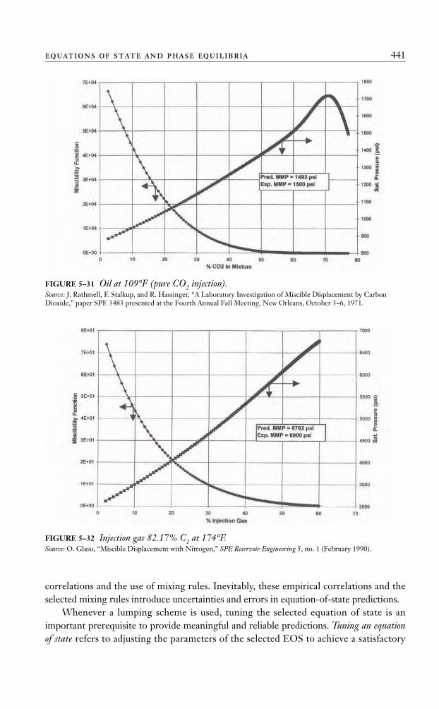
correlations and the use of mixing rules. Inevitably, these empirical correlations and theselected mixing rules introduce uncertainties and errors in equation-of-state predictions.
Whenever a lumping scheme is used, tuning the selected equation of state is animportant prerequisite to provide meaningful and reliable predictions. Tuning an equationof state refers to adjusting the parameters of the selected EOS to achieve a satisfactory
equations of state and phase equilibria 441
FIGURE 5–31 Oil at 109°F (pure CO2 injection).Source: J. Rathmell, F. Stalkup, and R. Hassinger, “A Laboratory Investigation of Miscible Displacement by CarbonDioxide,” paper SPE 3483 presented at the Fourth Annual Fall Meeting, New Orleans, October 3–6, 1971.
FIGURE 5–32 Injection gas 82.17% C1 at 174°F.Source: O. Glaso, “Miscible Displacement with Nitrogen,” SPE Reservoir Engineering 5, no. 1 (February 1990).
Ahmed_ch5.qxd 12/21/06 2:05 PM Page 441
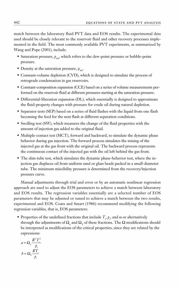
match between the laboratory fluid PVT data and EOS results. The experimental dataused should be closely relevant to the reservoir fluid and other recovery processes imple-mented in the field. The most commonly available PVT experiments, as summarized byWang and Pope (2001), include:
• Saturation pressure, psat, which refers to the dew-point pressure or bubble-pointpressure.
• Density at the saturation pressure, ρsat.
• Constant-volume depletion (CVD), which is designed to simulate the process ofretrograde condensation in gas reservoirs.
• Constant-composition expansion (CCE) based on a series of volume measurements per-formed on the reservoir fluid at different pressures starting at the saturation pressure.
• Differential-liberation expansion (DL), which essentially is designed to approximatethe fluid-property changes with pressure for crude oil during natural depletion.
• Separator tests (SEP) based on a series of fluid flashes with the liquid from one flashbecoming the feed for the next flash at different separation conditions.
• Swelling test (SW), which measures the change of the fluid properties with theamount of injection gas added to the original fluid.
• Multiple-contact test (MCT), forward and backward, to simulate the dynamic phasebehavior during gas injection. The forward process simulates the mixing of theinjected gas at the gas front with the original oil. The backward process representsthe continuous contact of the injected gas with the oil left behind the gas front.
• The slim-tube test, which simulates the dynamic phase-behavior test, where the in-jection gas displaces oil from uniform sand or glass beads packed in a small-diametertube. The minimum miscibility pressure is determined from the recovery/injectionpressure curve.
Manual adjustments through trial and error or by an automatic nonlinear regressionapproach are used to adjust the EOS parameters to achieve a match between laboratoryand EOS results. The regression variables essentially are a selected number of EOSparameters that may be adjusted or tuned to achieve a match between the two results,experimental and EOS. Coats and Smart (1986) recommend modifying the followingregression variables, that is, EOS parameters:
• Properties of the undefined fractions that include Tc, pc, and ω or alternativelythrough the adjustments of Ωa and Ω b of these fractions. The Ωmodifications shouldbe interpreted as modifications of the critical properties, since they are related by theexpressions:
bRTpb
c
c
= Ω
aR T
pac
c
= Ω2 2
442 equations of state and pvt analysis
Ahmed_ch5.qxd 12/21/06 2:05 PM Page 442
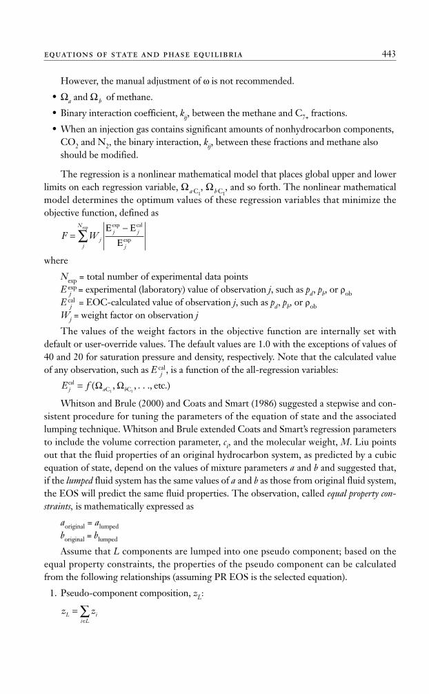
However, the manual adjustment of ω is not recommended.
• Ωa and Ω b of methane.
• Binary interaction coefficient, kij, between the methane and C7+ fractions.
• When an injection gas contains significant amounts of nonhydrocarbon components,CO2 and N2, the binary interaction, kij, between these fractions and methane alsoshould be modified.
The regression is a nonlinear mathematical model that places global upper and lowerlimits on each regression variable, Ω a C1
, Ω b C1, and so forth. The nonlinear mathematical
model determines the optimum values of these regression variables that minimize theobjective function, defined as
where
Nexp = total number of experimental data pointsE exp
j = experimental (laboratory) value of observation j, such as pd, pb, or ρob
E calj = EOC-calculated value of observation j, such as pd, pb, or ρob
Wj = weight factor on observation j
The values of the weight factors in the objective function are internally set withdefault or user-override values. The default values are 1.0 with the exceptions of values of40 and 20 for saturation pressure and density, respectively. Note that the calculated valueof any observation, such as E cal
j , is a function of the all-regression variables:
Whitson and Brule (2000) and Coats and Smart (1986) suggested a stepwise and con-sistent procedure for tuning the parameters of the equation of state and the associatedlumping technique. Whitson and Brule extended Coats and Smart’s regression parametersto include the volume correction parameter, ci, and the molecular weight, M. Liu pointsout that the fluid properties of an original hydrocarbon system, as predicted by a cubicequation of state, depend on the values of mixture parameters a and b and suggested that,if the lumped fluid system has the same values of a and b as those from original fluid system,the EOS will predict the same fluid properties. The observation, called equal property con-straints, is mathematically expressed as
aoriginal = alumped
boriginal = blumped
Assume that L components are lumped into one pseudo component; based on theequal property constraints, the properties of the pseudo component can be calculatedfrom the following relationships (assuming PR EOS is the selected equation).
1. Pseudo-component composition, zL:
z zL ii L
=∈∑
E fj a bcal
C C . ., etc.= ( , , . )Ω Ω1 1
F W jj j
jj
N
=−
∑Ε ΕΕ
exp
exp
exp cal
equations of state and phase equilibria 443
Ahmed_ch5.qxd 12/21/06 2:05 PM Page 443
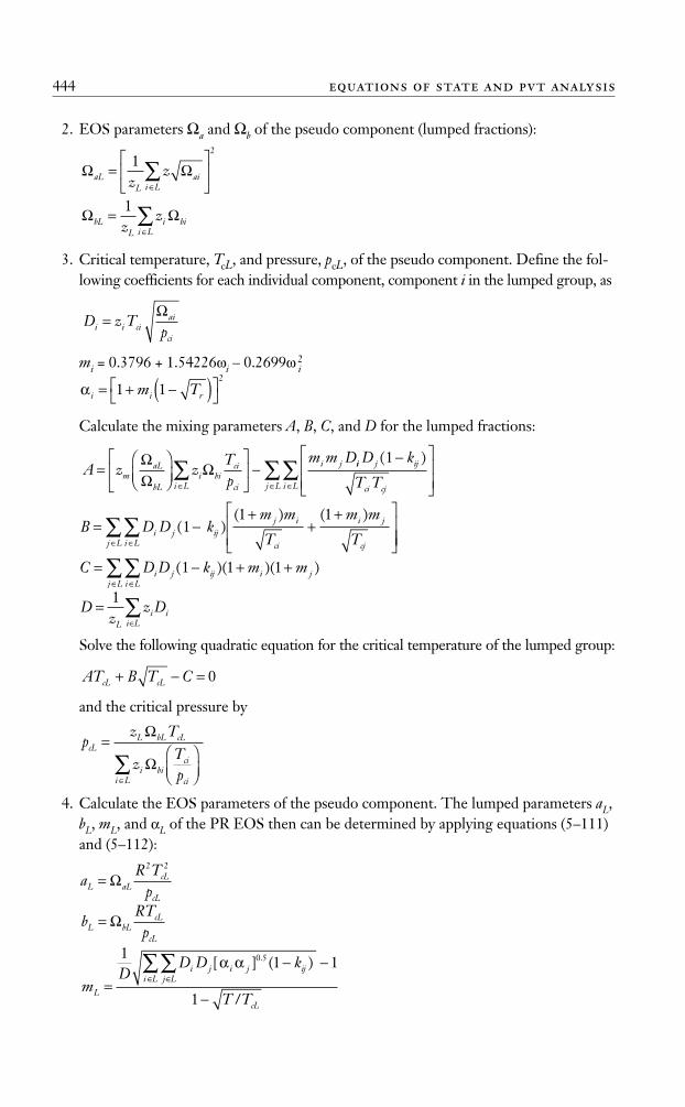
2. EOS parameters Ωa and Ωb of the pseudo component (lumped fractions):
3. Critical temperature, TcL, and pressure, pcL, of the pseudo component. Define the fol-lowing coefficients for each individual component, component i in the lumped group, as
mi = 0.3796 + 1.54226ωi – 0.2699ω 2i
Calculate the mixing parameters A, B, C, and D for the lumped fractions:
Solve the following quadratic equation for the critical temperature of the lumped group:
and the critical pressure by
4. Calculate the EOS parameters of the pseudo component. The lumped parameters aL,bL, mL, and αL of the PR EOS then can be determined by applying equations (5–111)and (5–112):
mD
D D k
T TL
i j i j ijj Li L
cL
=− −
−∈∈∑∑1
1 1
1
0 5[ ] ( )
/
.α α
bRTpL bL
cL
cL
= Ω
aR T
pL aLcL
cL
= Ω2 2
pz T
zTp
cLL bL cL
i bici
cii L
=⎛⎝⎜
⎞⎠⎟∈
∑Ω
Ω
AT B T CcL cL+ − = 0
Dz
z DL
i ii L
=∈∑1
C D D k m mi j ij i ji Lj L
= − + +∈∈∑∑ ( )( )( )1 1 1
B D D km m
T
m m
Ti j ijj i
ci
i j
cj
= −+
++⎡
⎣⎢⎢
⎤
⎦⎥( )
( ) ( )1
1 1
⎥⎥∈∈∑∑i Lj L
A z zTp
m m Dm
aL
bLi
i Lbi
ci
ci
i j=⎛⎝⎜
⎞⎠⎟
⎡
⎣⎢
⎤
⎦⎥ −
∈∑Ω
ΩΩ ii j ij
ci cji Lj L
D k
T T
( )1−⎡
⎣⎢⎢
⎤
⎦⎥⎥∈∈
∑∑
α i i rm T= + −( )⎡⎣
⎤⎦1 1
2
D z Tpi i ci
ai
ci
=Ω
Ω ΩbLL
i bii Lz
z=∈∑1
Ω ΩaLL
aii Lz
z=⎡
⎣⎢
⎤
⎦⎥
∈∑1
2
444 equations of state and pvt analysis
Ahmed_ch5.qxd 12/21/06 2:05 PM Page 444
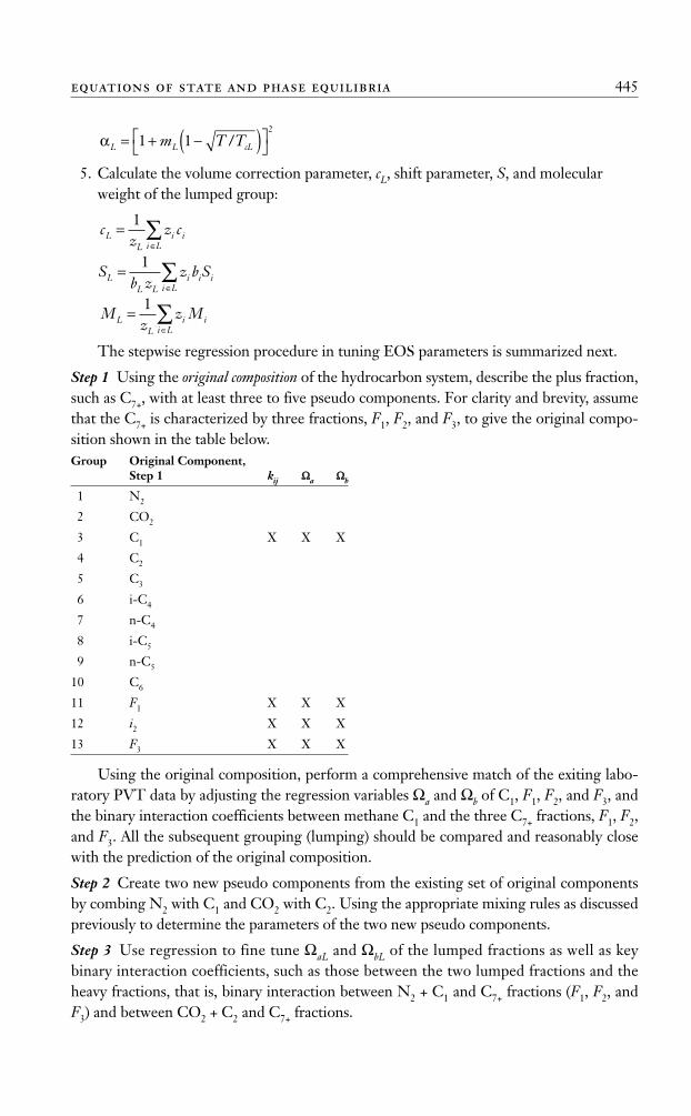
5. Calculate the volume correction parameter, cL, shift parameter, S, and molecularweight of the lumped group:
The stepwise regression procedure in tuning EOS parameters is summarized next.
Step 1 Using the original composition of the hydrocarbon system, describe the plus fraction,such as C7+, with at least three to five pseudo components. For clarity and brevity, assumethat the C7+ is characterized by three fractions, F1, F2, and F3, to give the original compo-sition shown in the table below.Group Original Component,
Step 1 kij ΩΩa ΩΩb
1 N2
2 CO2
3 C1 X X X
4 C2
5 C3
6 i-C4
7 n-C4
8 i-C5
9 n-C5
10 C6
11 F1 X X X
12 i2 X X X
13 F3 X X X
Using the original composition, perform a comprehensive match of the exiting labo-ratory PVT data by adjusting the regression variables Ωa and Ωb of C1, F1, F2, and F3, andthe binary interaction coefficients between methane C1 and the three C7+ fractions, F1, F2,and F3. All the subsequent grouping (lumping) should be compared and reasonably closewith the prediction of the original composition.
Step 2 Create two new pseudo components from the existing set of original componentsby combing N2 with C1 and CO2 with C2. Using the appropriate mixing rules as discussedpreviously to determine the parameters of the two new pseudo components.
Step 3 Use regression to fine tune ΩaL and ΩbL of the lumped fractions as well as keybinary interaction coefficients, such as those between the two lumped fractions and theheavy fractions, that is, binary interaction between N2 + C1 and C7+ fractions (F1, F2, andF3) and between CO2 + C2 and C7+ fractions.
Mz
z MLL
i ii L
=∈∑1
Sb z
z b SLL L
i i ii L
=∈∑1
cz
z cLL
i ii L
=∈∑1
αL L cLm T T= + −( )⎡⎣
⎤⎦1 1
2
/
equations of state and phase equilibria 445
Ahmed_ch5.qxd 12/21/06 2:05 PM Page 445
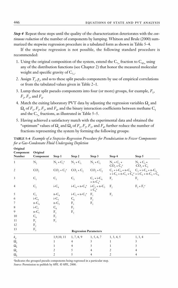
Step 4 Repeat these steps until the quality of the characterization deteriorates with the con-tinuous reduction of the number of components by lumping. Whitson and Brule (2000) sum-marized the stepwise regression procedure in a tabulated form as shown in Table 5–4.
If the stepwise regression is not possible, the following standard procedure isrecommended:
1. Using the original composition of the system, extend the C7+ fraction to C45+ usingany of the distribution functions (see Chapter 2) that honor the measured molecularweight and specific gravity of C7+.
2. Assign Tc, pc, and ω to these split pseudo components by use of empirical correlationsor from the tabulated values given in Table 2–1.
3. Lump these split pseudo components into four (or more) groups, for example, F1,F2, F3, and F4.
4. Match the exiting laboratory PVT data by adjusting the regression variables Ωa andΩb of F1, F2, F3, and F4, and the binary interaction coefficients between methane C1
and the C7+ fractions, as illustrated in Table 5–5.
5. Having achieved a satisfactory match with the experimental data and obtained the“optimum” values of Ωa and Ωb of F1, F2, F3, and F4, further reduce the number offractions representing the system by forming the following groups:
446 equations of state and pvt analysis
TABLE 5–4 Example of a Stepwise-Regression Procedure for Pseudoization to Fewer Componentsfor a Gas-Condensate Fluid Undergoing Depletion OriginalComponent OriginalNumber Component Step 1 Step 2 Step 3 Step 4 Step 5
1 N2 N2 + C1a N2 + C1 N2 + C1 N2 + C1 + N2 + C1 +
CO2 + C2a CO2 + C2
2 CO2 CO2 + C2a CO2 + C2 CO2 + C2 C3 + i-C4 + n-C4 C3 + i-C4 + n-C4
+ i-C5 + n-C5 + C6a + i-C5 + n-C5 + C6
3 C1 C3 C3 C3 + i-C4 F1 F1+ n-C4
a
4 C2 i-C4 i-C4 + n-C4a i-C5 + n-C5 F2 F2 + F3
a
+ C6a
5 C3 n-C4 i-C5 + n-C5a F1 F3
6 i-C4 i-C5 C6 F2
7 n-C4 n-C5 F1 F3
8 i-C5 C6 F2
9 n-C5 F1 F3
10 C6 F2
11 F1 F3
12 F2
13 F3 Regression Parameters
kij 1,9,10, 11 1, 7, 8, 9 1, 5, 6, 7 1, 3, 4, 5 1, 3, 4Ωa 1 4 3 1 3Ωb 1 4 3 1 3Ωa 2 5 4 2 4Ωb 2 5 4 2 4
aIndicates the grouped pseudo components being regressed in a particular step.Source: Permission to publish by SPE. © SPE, 2000.
Ahmed_ch5.qxd 12/21/06 2:05 PM Page 446
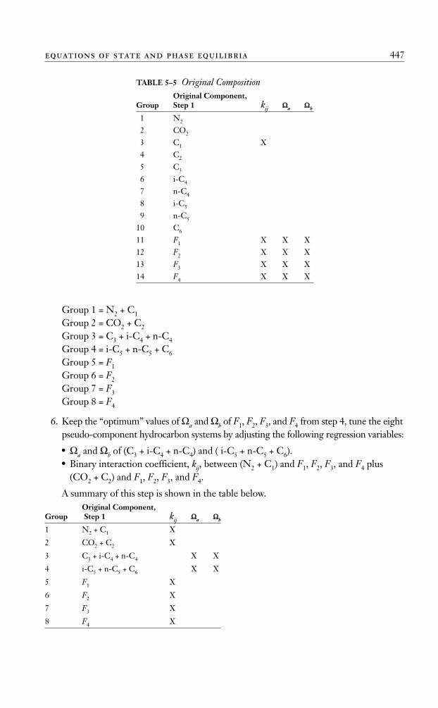
equations of state and phase equilibria 447
Group 1 = N2 + C1
Group 2 = CO2 + C2
Group 3 = C3 + i-C4 + n-C4
Group 4 = i-C5 + n-C5 + C6
Group 5 = F1
Group 6 = F2
Group 7 = F3
Group 8 = F4
6. Keep the “optimum” values of Ωa and Ωb of F1, F2, F3, and F4 from step 4, tune the eightpseudo-component hydrocarbon systems by adjusting the following regression variables:
• Ωa and Ωb of (C3 + i-C4 + n-C4) and ( i-C5 + n-C5 + C6).• Binary interaction coefficient, kij, between (N2 + C1) and F1, F2, F3, and F4 plus
(CO2 + C2) and F1, F2, F3, and F4.
A summary of this step is shown in the table below.Original Component,
Group Step 1 kij ΩΩa ΩΩb
1 N2 + C1 X
2 CO2 + C2 X
3 C3 + i-C4 + n-C4 X X
4 i-C5 + n-C5 + C6 X X
5 F1 X
6 F2 X
7 F3 X
8 F4 X
TABLE 5–5 Original CompositionOriginal Component,
Group Step 1 kij ΩΩa ΩΩb
1 N2
2 CO2
3 C1 X 4 C2
5 C3
6 i-C4
7 n-C4
8 i-C5
9 n-C5
10 C6
11 F1 X X X 12 F2 X X X 13 F3 X X X 14 F4 X X X
Ahmed_ch5.qxd 12/21/06 2:05 PM Page 447
As pointed out in Chapter 4, the Lohrenz, Bray, and Clark (LBC) viscosity correlationhas become a standard in compositional reservoir simulation. When observed viscosity dataare available, values of the coefficients a1–a5 in equation (4–86) and the critical volume of C7+ areadjusted and used as tuning parameters until a match with the experimental data isachieved. These adjustments are performed independent of the process of tuning equation-of-state parameters to match other PVT data. The key relationships of the LBC viscositymodel follow:
where
a1 = 0.1023a2 = 0.023364a3 = 0.058533a4 = –0.040758a5 = 0.0093324
Original Fluid Composition from a Sample Contaminated with Oil-Based Mud
As pointed out by Gozalpour et al. (2002), hydrocarbon-based fluids (natural or syntheticoils) generally are used in oil-base mud (OBM). Because these fluids are soluble in thereservoir fluid, they can render the fluid analysis limited in value. Contamination with anoil-based mud filtrate could affect reservoir fluid properties such as
• Saturation pressure.
• Formation volume factor.
• Gas/liquid ratio.
• Stock-tank liquid density.
Determination of the original fluid composition from the analysis of a contaminated sam-ple is feasible, but isolating the properties of the reservoir fluid free from contamination isnot easily accomplished. Despite the recent improvements in sampling reservoir fluids,obtaining a contamination-free formation fluid is a major challenge, particularly in open-hole wells. Therefore, modeling techniques are required, along with the laboratory stud-ies, to determine the composition and PVT properties of the uncontaminated fluid.
Because collecting a reservoir fluid sample is expensive and accurate reservoir fluidproperties are needed in reservoir development, it is highly desirable to determine accu-rate composition and phase behavior for the reservoir fluid from contaminated samples.
ρ
ρ
r
i i ciii
n
ox M V x V
=
+⎛
⎝
⎜⎜
⎞
⎠
⎟⎟+ +
+
=∉
∑ [( )] C C
C
77
7
1
MMa
μ μob = ++ + + + −o r r r ra a a a a[ ] .1 2 3
24
35
4 4 0 0001ρ ρ ρ ρξmm
448 equations of state and pvt analysis
Ahmed_ch5.qxd 12/21/06 2:05 PM Page 448
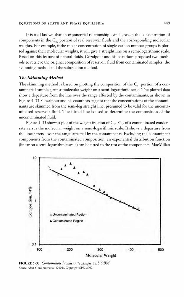
equations of state and phase equilibria 449
It is well known that an exponential relationship exits between the concentration ofcomponents in the C8+ portion of real reservoir fluids and the corresponding molecularweights. For example, if the molar concentration of single carbon number groups is plot-ted against their molecular weights, it will give a straight line on a semi-logarithmic scale.Based on this feature of natural fluids, Gozalpour and his coauthors proposed two meth-ods to retrieve the original composition of reservoir fluid from contaminated samples: theskimming method and the subtraction method.
The Skimming MethodThe skimming method is based on plotting the composition of the C8+ portion of a con-taminated sample against molecular weight on a semi-logarithmic scale. The plotted datashow a departure from the line over the range affected by the contaminants, as shown inFigure 5–33. Gozalpour and his coauthors suggest that the concentrations of the contami-nants are skimmed from the semi-log straight line, presumed to be valid for the unconta-minated reservoir fluid. The flitted line is used to determine the composition of theuncontaminated fluid.
Figure 5–33 shows a plot of the weight fraction of C10–C30 of a contaminated conden-sate versus the molecular weight on a semi-logarithmic scale. It shows a departure fromthe linear trend over the range affected by the contaminants. Excluding the contaminantcomponents from the contaminated composition, an exponential distribution function(linear on a semi-logarithmic scale) can be fitted to the rest of the components. MacMillan
FIGURE 5–33 Contaminated condensate sample with OBM.Source: After Gozalpour et al. (2002). Copyright SPE, 2002.
Ahmed_ch5.qxd 12/21/06 2:05 PM Page 449
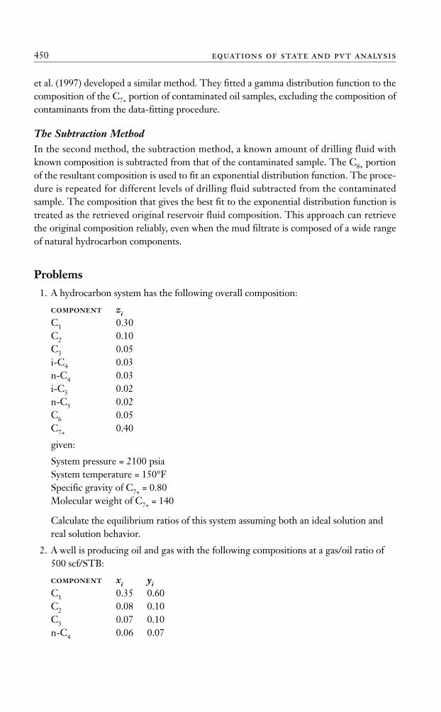
et al. (1997) developed a similar method. They fitted a gamma distribution function to thecomposition of the C7+ portion of contaminated oil samples, excluding the composition ofcontaminants from the data-fitting procedure.
The Subtraction MethodIn the second method, the subtraction method, a known amount of drilling fluid withknown composition is subtracted from that of the contaminated sample. The C8+ portionof the resultant composition is used to fit an exponential distribution function. The proce-dure is repeated for different levels of drilling fluid subtracted from the contaminatedsample. The composition that gives the best fit to the exponential distribution function istreated as the retrieved original reservoir fluid composition. This approach can retrievethe original composition reliably, even when the mud filtrate is composed of a wide rangeof natural hydrocarbon components.
Problems
1. A hydrocarbon system has the following overall composition:
COMPONENT ziC1 0.30C2 0.10C3 0.05i-C4 0.03n-C4 0.03i-C5 0.02n-C5 0.02C6 0.05C7+ 0.40
given:
System pressure = 2100 psiaSystem temperature = 150°FSpecific gravity of C7+ = 0.80Molecular weight of C7+ = 140
Calculate the equilibrium ratios of this system assuming both an ideal solution andreal solution behavior.
2. A well is producing oil and gas with the following compositions at a gas/oil ratio of500 scf/STB:
COMPONENT xi yiC1 0.35 0.60C2 0.08 0.10C3 0.07 0.10n-C4 0.06 0.07
450 equations of state and pvt analysis
Ahmed_ch5.qxd 12/21/06 2:05 PM Page 450
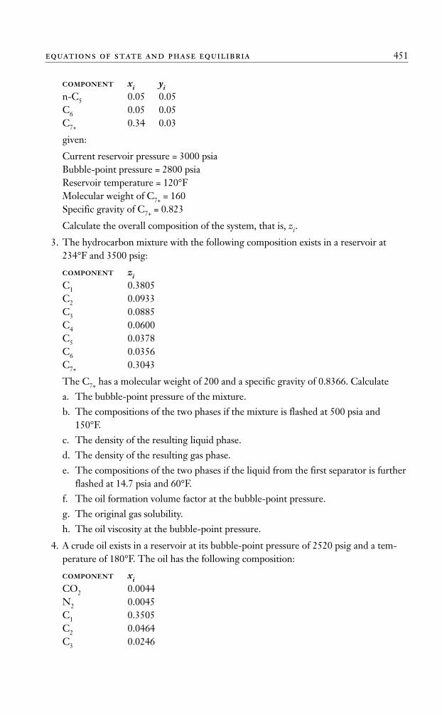
COMPONENT xi yin-C5 0.05 0.05C6 0.05 0.05C7+ 0.34 0.03
given:
Current reservoir pressure = 3000 psiaBubble-point pressure = 2800 psiaReservoir temperature = 120°FMolecular weight of C7+ = 160Specific gravity of C7+ = 0.823
Calculate the overall composition of the system, that is, zi.
3. The hydrocarbon mixture with the following composition exists in a reservoir at234°F and 3500 psig:
COMPONENT ziC1 0.3805C2 0.0933C3 0.0885C4 0.0600C5 0.0378C6 0.0356C7+ 0.3043
The C7+ has a molecular weight of 200 and a specific gravity of 0.8366. Calculatea. The bubble-point pressure of the mixture.b. The compositions of the two phases if the mixture is flashed at 500 psia and
150°F.c. The density of the resulting liquid phase.d. The density of the resulting gas phase.e. The compositions of the two phases if the liquid from the first separator is further
flashed at 14.7 psia and 60°F.f. The oil formation volume factor at the bubble-point pressure.g. The original gas solubility.h. The oil viscosity at the bubble-point pressure.
4. A crude oil exists in a reservoir at its bubble-point pressure of 2520 psig and a tem-perature of 180°F. The oil has the following composition:
COMPONENT xiCO2 0.0044N2 0.0045C1 0.3505C2 0.0464C3 0.0246
equations of state and phase equilibria 451
Ahmed_ch5.qxd 12/21/06 2:05 PM Page 451
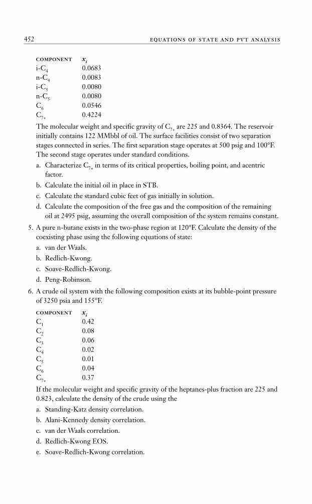
452 equations of state and pvt analysis
COMPONENT xii-C4 0.0683n-C4 0.0083i-C5 0.0080n-C5 0.0080C6 0.0546C7+ 0.4224
The molecular weight and specific gravity of C7+ are 225 and 0.8364. The reservoirinitially contains 122 MMbbl of oil. The surface facilities consist of two separationstages connected in series. The first separation stage operates at 500 psig and 100°F.The second stage operates under standard conditions.a. Characterize C7+ in terms of its critical properties, boiling point, and acentric
factor.b. Calculate the initial oil in place in STB.c. Calculate the standard cubic feet of gas initially in solution.d. Calculate the composition of the free gas and the composition of the remaining
oil at 2495 psig, assuming the overall composition of the system remains constant.
5. A pure n-butane exists in the two-phase region at 120°F. Calculate the density of thecoexisting phase using the following equations of state:a. van der Waals.b. Redlich-Kwong.c. Soave-Redlich-Kwong.d. Peng-Robinson.
6. A crude oil system with the following composition exists at its bubble-point pressureof 3250 psia and 155°F.
COMPONENT xiC1 0.42C2 0.08C3 0.06C4 0.02C5 0.01C6 0.04C7+ 0.37
If the molecular weight and specific gravity of the heptanes-plus fraction are 225 and0.823, calculate the density of the crude using thea. Standing-Katz density correlation.b. Alani-Kennedy density correlation.c. van der Waals correlation.d. Redlich-Kwong EOS.e. Soave-Redlich-Kwong correlation.
Ahmed_ch5.qxd 12/21/06 2:05 PM Page 452
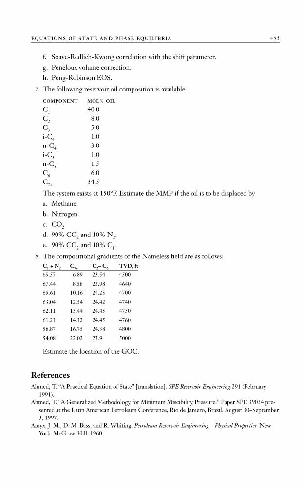
equations of state and phase equilibria 453
f. Soave-Redlich-Kwong correlation with the shift parameter.g. Peneloux volume correction.h. Peng-Robinson EOS.
7. The following reservoir oil composition is available:
COMPONENT MOL% OIL
C1 40.0C2 8.0 C3 5.0 i-C4 1.0 n-C4 3.0 i-C5 1.0n-C5 1.5C6 6.0C7+ 34.5
The system exists at 150°F. Estimate the MMP if the oil is to be displaced bya. Methane.b. Nitrogen.c. CO2.d. 90% CO2 and 10% N2.e. 90% CO2 and 10% C1.
8. The compositional gradients of the Nameless field are as follows:C1 + N2 C7+ C2– C6 TVD, ft
69.57 6.89 23.54 4500
67.44 8.58 23.98 4640
65.61 10.16 24.23 4700
63.04 12.54 24.42 4740
62.11 13.44 24.45 4750
61.23 14.32 24.45 4760
58.87 16.75 24.38 4800
54.08 22.02 23.9 5000
Estimate the location of the GOC.
ReferencesAhmed, T. “A Practical Equation of State” [translation]. SPE Reservoir Engineering 291 (February
1991).Ahmed, T. “A Generalized Methodology for Minimum Miscibility Pressure.” Paper SPE 39034 pre-
sented at the Latin American Petroleum Conference, Rio de Janiero, Brazil, August 30–September3, 1997.
Amyx, J. M., D. M. Bass, and R. Whiting. Petroleum Reservoir Engineering—Physical Properties. NewYork: McGraw-Hill, 1960.
Ahmed_ch5.qxd 12/21/06 2:05 PM Page 453
Benmekki, E., and G. Mansoori. “Minimum Miscibility Pressure Prediction with EOS.” SPE ReservoirEngineering (May 1988).
Brinkman, F. H., and J. N. Sicking. “Equilibrium Ratios for Reservoir Studies.” Transactions of theAIME 219 (1960): 313–319.
Campbell, J. M. Gas Conditioning and Processing. Campbell Petroleum Series, vol. 1. Norman, OK:Campbell, 1976.
Clark, N. Elements of Petroleum Reservoirs. Dallas: Society of Petroleum Engineers, 1960. Coats, K., and G. Smart. “Application of Regression-Based EOS PVT Program to Laboratory Data.”
SPE Reservoir Engineering (May 1986).Dake, L. P. Fundamentals of Reservoir Engineering. Amsterdam: Elsevier Scientific Publishing Com-
pany, 1978.Dodson, C., D. Goodwill, and E. Mayer. “Application of Laboratory PVT Data to Engineering Prob-
lems.” Journal of Petroleum Technology (December 1953).Dykstra, H., and T. D. Mueller. “Calculation of Phase Composition and Properties for Lean-or
Enriched-Gas Drive.” Society of Petroleum Engineers Journal (September 1965): 239–246. Edmister, W., and B. Lee. Applied Hydrocarbon Thermodynamics, vol. 1, 2nd ed. Houston: Gulf Publish-
ing Company, 1986, p. 52.Elliot, J., and T. Daubert. “Revised Procedure for Phase Equilibrium Calculations with Soave Equa-
tion of State.” Industrial Engineering and Chemical Process Design Development 23 (1985): 743–748.Gibbs, J. The Collected Works of J. Willard Gibbs. New Haven, CT: Yale University Press, 1948.Glaso, O. “Miscible Displacement with Nitrogen.” SPE Reservoir Engineering 5, no. 1 (February
1990).Gozalpour, F., et al. “Predicting Reservoir Fluid Phase and Volumetric Behavior from Samples Conta-
minated with Oil-Based Mud.” SPE Reservoir Evaluation and Engineering (June 2002).Graboski, M. S., and T. E. Daubert. “A Modified Soave Equation of State for Phase Equilibrium Cal-
culations, 1. Hydrocarbon System.” Industrial Engineering and Chemical Process Design Development17 (1978): 443–448.
Hadden, J. T. “Convergence Pressure in Hydrocarbon Vapor-Liquid Equilibria.” Chemical Engineer-ing Progress Symposium Series 49, no. 7 (1953): 53.
Hoffmann, A. E., J. S. Crump, and R. C. Hocott. “Equilibrium Constants for a Gas-Condensate Sys-tem.” Transactions of the AIME 198 (1953): 1–10.
Hoier, L., and C. Whitson. “Compositional Gradient—Theory and Practice.” SPE Reservoir Evalua-tion and Engineering (December 2001).
Jhaveri, B. S., and G. K. Youngren. “Three-Parameter Modification of the Peng-Robinson Equationof Sate to Improve Volumetric Predictions.” Paper SPE 13118, presented at the SPE Annual Tech-nical Conference, Houston, September 16–19, 1984.
Katz, D. L., and K. H. Hachmuth. “Vaporization Equilibrium Constants in a Crude Oil-Natural GasSystem.” Industrial Engineering and Chemistry 29 (1937): 1072.
Katz, D., et al. Handbook of Natural Gas Engineering. New York: McGraw-Hill, 1959.Katz, D., et al. “Overview of Phase Behavior of Oil and Gas Production.” Journal of Petroleum Technol-
ogy (June 1983): 1205–1214. Kehn, D. M. “Rapid Analysis of Condensate Systems by Chromatography.” Journal of Petroleum Tech-
nology (April 1964): 435–440.Lim, D., and T. Ahmed. “Calculation of Liquid Dropout for Systems Containing Water.” Paper SPE
13094, presented at the 59th Annual Technical Conference of the SPE, Houston, September16–19, 1984.
Lohrenze, J., G. Clark, and R. Francis. “A Compositional Material Balance for Combination DriveReservoirs.” Journal of Petroleum Technology (November 1963).
MacMillian, D, et al. How to Obtain Reservoir Fluid Properties from an Oil Sample Contaminated withSynthetic Drilling Mud. SPE paper 38852. Richardson, TX: Society of Petroleum Engineers, 1997.
454 equations of state and pvt analysis
Ahmed_ch5.qxd 12/21/06 2:05 PM Page 454
Michelson, M. “Collection of Critical Points and Phase Boundaries in the Critical Region.” FluidPhase Equilibria 16 (1984).
NGPSA. Engineering Data Book. Tulsa, OK: National Gas Producers Suppliers Association, 1978.Nikos, V., et al. “Phase Behavior of Systems Comprising North Sea Reservoir Fluids and Injection
Gases.” Journal of Petroleum Technology (November 1986): 1221–1233.Pedersen, K., P. Thomassen, and A. Fredenslund. “Phase Equilibria and Separation Processes.”
Report SEP 8207, Institute for Kemiteknik, Denmark Tekniske Hojskole, July 1982.Pedersen, K., P. Thomassen, and A. Fredenslund. “Characterization of Gas Condensate Mixtures.” In
Advances in Thermodynamics. New York: Taylor and Francis, 1989.Peneloux, A., E. Rauzy, and R. Freze. “A Consistent Correlation for Redlich-Kwong-Soave Volumes.”
Fluid Phase Equilibria 8 (1982): 7–23.Peng, D., and D. Robinson. “A New Two Constant Equation of State.” Industrial Engineering and
Chemistry Fundamentals 15, no. 1 (1976a): 59–64.Peng, D., and D. Robinson. “Two and Three Phase Equilibrium Calculations for Systems Containing
Water.” Canadian Journal of Chemical Engineering 54 (1976b): 595–598.Peng, D., and D. Robinson. The Characterization of the Heptanes and Their Fractions. Research Report
28. Tulsa, OK: Gas Producers Association, 1978.Peng, D., and D. Robinson. “Two and Three Phase Equilibrium Calculations for Coal Gasification
and Related Processes.” ACS Symposium Series no. 133, Thermodynamics of Aqueous Systemswith Industrial Applications, 1980.
Rathmell, J., F. Stalkup, and R. Hassinger. “ A Laboratory Investigation of Miscible Displacement byCarbon Dioxide.” Paper SPE 3483 presented at the Fourth Annual Fall Meeting, New Orleans,October 3–6, 1971.
Redlich, O., and J. Kwong. “On the Thermodynamics of Solutions. An Equation of State. Fugacitiesof Gaseous Solutions.” Chemical Reviews 44 (1949): 233–247.
Reid, R., J. M. Prausnitz, and T. Sherwood. The Properties of Gases and Liquids, 4th ed. New York:McGraw-Hill, 1987.
Rzasa, M. J., E. D. Glass, and J. B. Opfell “Prediction of Critical Properties and Equilibrium Vapor-ization Constants for Complex Hydrocarbon Systems.” Chemical Engineering Progress, SymposiumSeries 48, no. 2 (1952): 28.
Sim, W. J., and T. E. Daubert. “Prediction of Vapor-Liquid Equilibria of Undefined Mixtures.” Indus-trial Engineering and Chemical Process Design Development 19, no. 3 (1980): 380–393.
Slot-Petersen, C. “A Systematic and Consistent Approach to Determine Binary Interaction Coeffi-cients for the Peng-Robinson Equation of State.” Paper SPE 16941, presented at the 62nd AnnualTechnical Conference of the SPE, Dallas, September 27–30, 1987.
Soave, G., “Equilibrium Constants from a Modified Redlich-Kwong Equation of State.” ChemicalEngineering and Science 27 (1972): 1197–1203.
Standing, M. B. Volumetric and Phase Behavior of Oil Field Hydrocarbon Systems. Dallas: Society of Petro-leum Engineers of AIME, 1977.
Standing, M. B. “A Set of Equations for Computing Equilibrium Ratios of a Crude Oil/Natural GasSystem at Pressures Below 1,000 psia.” Journal of Petroleum Technology (September 1979): 1193–1195.
Stryjek, R., and J. H. Vera. “PRSV: An Improvement Peng-Robinson Equation of State for PureCompounds and Mixtures.” Canadian Journal of Chemical Engineering 64 (April 1986): 323–333.
Van der Waals, J. D. “On the Continuity of the Liquid and Gaseous State.” Ph.D. dissertation, Sigth-off, Leiden, 1873.
Vidal, J., and T. Daubert. “Equations of State—Reworking the Old Forms.” Chemical Engineering andScience 33 (1978): 787–791.
Whitson, C., and P. Belery. “Composition of Gradients in Petroleum Reservoirs.” Paper SPE 28000presented at the University of Tulsa/SPE Centennial Petroleum Engineering Symposium, Tulsa,OK, August 29–31, 1994.
equations of state and phase equilibria 455
Ahmed_ch5.qxd 12/21/06 2:05 PM Page 455
Whitson, C. H., and M. R. Brule. Phase Behavior. Richardson, TX: SPE, 2000.Whitson, C. H., and S. B. Torp. “Evaluating Constant Volume Depletion Data.” Paper SPE 10067,
presented at the SPE 56th Annual Fall Technical Conference, San Antonio, October 5–7, 1981.Wilson, G. “A Modified Redlich-Kwong EOS, Application to General Physcial Data Calculations.”
Paper 15C, presented at the Annual AIChE National Meeting, Cleveland, May 4–7, 1968.Winn, F. W. “Simplified Nomographic Presentation, Hydrocarbon Vapor-Liquid Equilibria.” Chemi-
cal Engineering Progress, Symposium Series 33, no. 6 (1954): 131–135.
456 equations of state and pvt analysis
Ahmed_ch5.qxd 12/21/06 2:05 PM Page 456