ELSEVIER

THEO CHEM

Journal of Molecular Structure (Theochem) 424 (1998) 237-247

3D weighting of molecular descriptors for QSPWQSAR by the method of ideal symmetry (MIS).

1. Application to boiling points of alkanes

Andrey Toropova, Alla Toropovab, Temur Ismailovb, Danail Bonchevc’d3*

‘Institute of Polymer Chemistry and Physics, Academy of Sciences, Tashkent 700122, Uzbekistan

bTashkent State University, Tashkent 700095, Uzbekistan

‘Texas A&M University. Galveston, TX 77553.1675. USA

‘Assen Zlatarov University Burgas 8010, Bulgaria

Received 4 November 1996; revised 19 March 1997; accepted 4 April 1997

Abstract

The method of ideal symmetry (MIS), developed recently, presents molecules as systems of mutually repulsing atoms connected by covalent bonds of constant length. In this paper we have used MIS optimized geometry to define a vertex 3D weight as a metric analogue of the vertex distance sum in molecular graphs. These 3D weights were used as a substitute for the vertex degrees in several well known topological (2D) indices, thus producing a series of 3D-weighted molecular descriptors. The novel indices were tested in calculating the boiling points of a series of 73 C3-C9 alkanes and showed generally a better performance than the original 2D indices. The best l-, 2-, and 3-variable linear regression models incorporated 3D zero-order molecular connectivity with correlation coefficients of 0.9892, 0.9961, and 0.9986, and standard deviations of 5.97, 3.64, and

2.17”C, respectively. The approach was further validated by correlations with four other properties of alkanes (heats of formation, heats of vaporization, heats of atomization, and molar volume). The potential of the proposed 3D weighting of topological indices for QSPWQSAR studies was thus demonstrated. 0 1998 Elsevier Science B.V.

Keywords: 3D molecular descriptors; 3D atomic weights; Method of ideal symmetry; QSPR; Alkane properties

1. Introduction

Topological and information-theoretic indices have

been widely applied to quantitative structure- property (QSPR) and structure-activity relationships

(QSAR) of chemical compounds [ l-101. By describing important details of molecular structure, these indices produce models that fit experimental data fairly well.

* Corresponding author. Fax: 001409 740 4429; e-mail: bonchevd

@tamug.tamu.edu

In attempting to further improve such models, a variety of steric, topographical, and other 3D indices have been added to the numerous topological (2D) molecular descriptors [ 1 l- 181. Such methods view the molecules as graphs embedded in certain spatial lattices. Many of the existing graph-theoretic schemes

have been modified in this manner. The topographic indices of RandiC [ 14- 161, for example, embed mole- cular graphs in a hexagonal grid, and make use of the metric distances in this idealized lattice. Such an approach does distinguish between stereoisomers,

0166-1280/98/$19.00 0 1998 Elsevier Science B.V. All rights reserved PII SO166-1280(97)00151-6

238 A. Toropov et al./Journal of Molecular Structure (Theochem) 424 (1998) 237-247

lC /H /H /H

c-c-c c - c - c c - c - c C-C-H

/ / / /

C C H H

Rl R4 Rl R4

/ / R2-C-C + c-c-

/ /

R3 R6

which is not possible within the 2-dimensional

description. Perhaps the major improvement resulting

from 3D molecular descriptors is that they account for ‘through-space’ interactions whereas the topological indices are based on ‘through-bonds’ interactions. However, this difference in the physical meaning of

the 2D and 3D indices should not be overestimated. The relatively high correlation between the corre-

sponding pairs of such molecular descriptors rather indicates that they only mirror to a different extent the two types of interaction which cannot be clearly separated. An effective 3D descriptor is the 3D Wiener index, developed in Bulgaria and Croatia [ 17,181, which is calculated from the interatomic

distances, taken from experiment or calculated after quantum chemical geometry optimization. This index outperforms its widely used 2D counterpart in correlations with various properties and biological activities (see, for example, [33]).

In this paper, the potential improvement of QSPR

(and QSAR) by accounting for the three-dimensional structure of molecules is approached in a different way. A ‘3D weight’, based on the metric distances between atoms in a preferable molecular conformation, can be ascribed to many of the known graph-theoretic and information-theoretic indices. The key feature of our modeling is the presentation of the molecule as a system

of mutually repulsing atoms, keeping constant the length of each bond. This concept of molecular simula- tion was termed the “method of ideal symmetry” (MIS) [19,20]. The MIS method manifests some simi- larity to the approaches that proceed from the intra- molecular repulsion of valence electron pairs [21,22]. The MIS-based 3D-weighting procedure was applied in this study to five topological indices and tested against the boiling points and other properties of alkanes.

/ / R5 ---> R2 - C - C - R5

/ /

R3 R6

2. The method

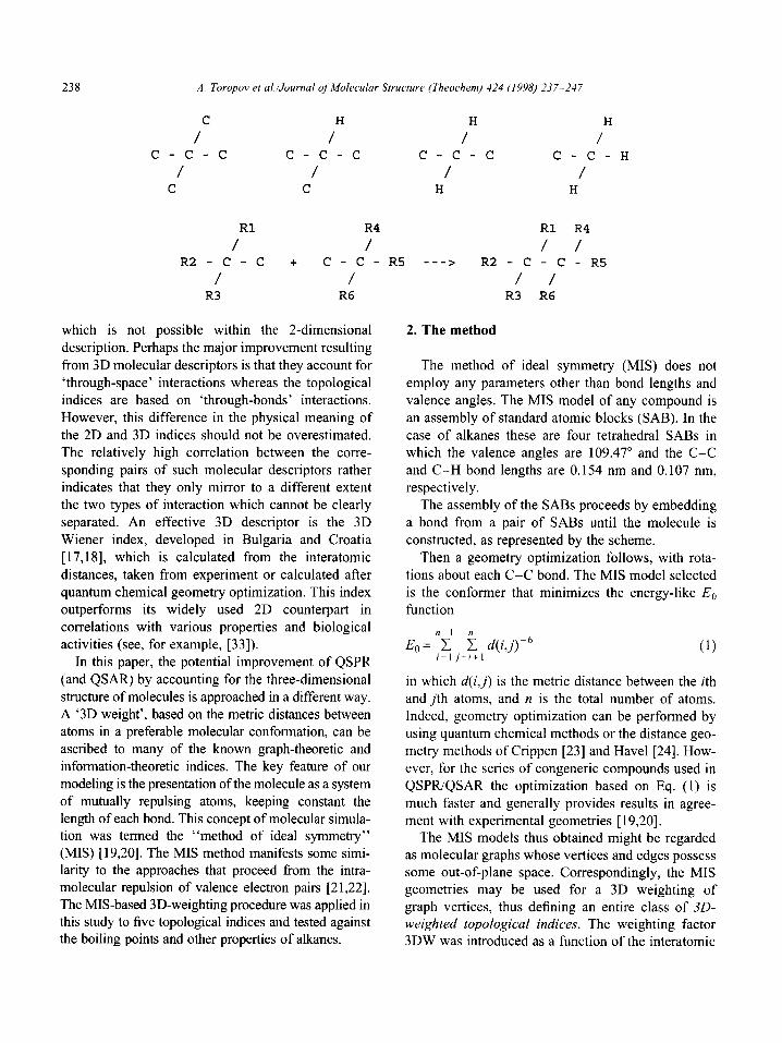
The method of ideal symmetry (MIS) does not employ any parameters other than bond lengths and

valence angles. The MIS model of any compound is an assembly of standard atomic blocks (SAB). In the case of alkanes these are four tetrahedral SABs in which the valence angles are 109.47” and the C-C and C-H bond lengths are 0.154 nm and 0.107 nm, respectively.

The assembly of the SABs proceeds by embedding a bond from a pair of SABs until the molecule is

constructed, as represented by the scheme. Then a geometry optimization follows, with rota-

tions about each C-C bond. The MIS model selected is the conformer that minimizes the energy-like E,, function

in which d(i,j) is the metric distance between the ith and jth atoms, and n is the total number of atoms. Indeed, geometry optimization can be performed by using quantum chemical methods or the distance geo- metry methods of Crippen [23] and Have1 [24]. How- ever, for the series of congeneric compounds used in QSPWQSAR the optimization based on Eq. (1) is

much faster and generally provides results in agree- ment with experimental geometries [ 19,201.

The MIS models thus obtained might be regarded as molecular graphs whose vertices and edges possess some out-of-plane space. Correspondingly, the MIS geometries may be used for a 3D weighting of graph vertices, thus defining an entire class of 3D- weighted topological indices. The weighting factor 3DW was introduced as a function of the interatomic

A. Toropov et al./Journal of Molecular Structure (Theochem) 424 (1998) 237-247 239

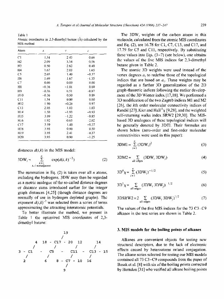
Table 1

Atomic coordinates in 2,3-dimethyl butane (A) calculated by the

MIS method

Atom x J’ z

Cl 1.54 2.43 0.66

H2 2.09 3.34 0.56

H3 0.50 2.62 0.48

H4 1.67 2.03 1.65

c5 2.05 1.40 -0.37

H6 1.69 1.67 -1.35

C? 0.00 0.00 0.00

H8 -0.36 -1.01 0.00

H9 PO.36 0.51 -0.87

HI0 -0.36 0.50 0.88

Cl1 1.54 0.00 0.00

H12 1.90 -0.26 0.97

Cl3 2.05 -1.02 -1.03

H14 1 so -1.93 -0.93

H15 3.09 -1.22 -0.85

H16 1.92 -0.63 -2.02

Cl7 3.59 I .40 -0.37

H18 3.95 0.90 0.50

H19 3.95 2.41 -0.37

H20 3.95 0.90 -1.25

distances d(i,k) in the MIS model:

3DW,= 5 exp(d(i, k)-*) (2) k#i

k. i nonadjacent

The summation in Eq. (2) is taken over all n atoms,

including the hydrogens. 3DW may then be regarded as a metric analogue of the so-called distance degrees or distance sums introduced earlier for the integer graph distances [4,25] (though distance degrees are normally of use in hydrogen depleted graphs). The exponent d(iJm2 was selected from a series of terms approximating the attracting interatomic potentials.

To better illustrate the method, we present in

Table 1 the optimized MIS coordinates of 2,3- dimethyl butane:

19

/

I4 18 - Cl7 / - 20 / 12 14 /

3 - Cl - c5 - Cl1 - Cl3 - 15

/ / / /

2 6 8 - C7 - 10 16

/

9

The 3DW; weights of the carbon atoms in this

molecule, calculated from the atomic MIS coordinates

and Eq. (2), are 16.78 for Cl, C7, C13, and C17, and 17.79 for CS and Cl 1, respectively. By substituting

these values into Eqs. (3-7) (see below), one obtains the values of the five MIS indices for 2,3-dimethyl

butane given in Table 2. The atomic 3D weights were used instead of the

vertex degrees a, to redefine those of the topological indices that are based on ai. These weights may be regarded as a further 3D generalization of the 2D

graph-theoretic indices following the earlier develop- ment of the 3D Wiener index [ 17,181. We performed a

3D modification of the two Zagreb indices Ml and M2 [26], the kth order molecular connectivity indices of

Randic [27], Kier and Hall k~ [9,28], and the weighted self-returning walks index SRW2 [29,30]. The MIS- based 3D analogues of these topological indices will

be generally denoted by 3DTI. Their formulas are shown below (zero-order and first-order molecular connectivities were used in this paper):

3DMl= ~~, (3DWi)2 (3)

3DM2= 2 (3DWi 3DWj) all edges

(4)

3D”x = i; (3DW,) - “* (5)

~D’x= C (3DWi 3DWj)~“” (6) all edges

3DSRW2=2 2 (3DWi 3DWj)“2 all edges

(7)

The values of the five MIS indices for the 73 C3-C9 alkanes in the test series are shown in Table 2.

3. MIS models for the boiling points of alkanes

Alkanes are convenient objects for testing new

structural descriptors, due to the lack of electronic effects caused by heteroatoms orland conjugation. The alkane series selected for testing our MIS models contained all 73 C3-C9 compounds from the paper of Basak et al. [8] with six of the boiling points corrected by Herndon [3 l] who verified all alkane boiling points

240 A. Toropov et al./Journal of Molecular Structure (Theochem) 424 (1998) 237-247

Table 2

Values of the five MIS indices defined by Eqs. (3)-(7)

No. Compound 3D”x 3D’x 3DM1 3DM2 3DSRW2

1 c3

2 2M-C3

3 n-C4

4 2,2-MMC3

5 2M-C4

6 n-C5

7 2,2-MMC4

8 2,3-MMC4

9 2M-C5

IO 3M-C5

ii n-C6

12 2,2,3-~MMC4

13 2,2-MMC5

14 3,3-MMC5

I5 2,3-MMC5

16 2,4-MMCS

17 2M-C6

18 3M-C6

19 3E-~CS

20 n-C7

21 2,2,3,3-MMMMC4

22 2,2,3-MMMC5

23 2,3,3-MMMC5

24 2,2,4-MMMCS

25 2,2-MMC6

26 3,3-MMC6

27 3,3-MECS

28 2,3,4-MMMCS

29 2,3-MMC6

30 2,3-MEC5 31 2,4-MMC6

32 2,5-MMC6

33 2-MC7

34 3-MC7

35 4-MC7

36 3-EC6

37 n-C8

38 2,2,3,3-MMMMC5

39 2.2,3,4-~~MMMC5

40 2,2,3-MMMC6

41 2,2,3-MMEC5

42 2,3,3,4&MMMMCS

43 2,3,3-MMMC6

44 2,3,3-MMEC5

45 2,2,4,4-MMMMCS

46 2~2,4-MMMC4 47 2,4,4-MM~C6

48 2,2,5-MMMC6

49 4,4-MMC7

50 3,3-EEC5

51 2,3,4-MEMCS

52 2,3,5-MMMC6

53 2.3-MEC6

1.1210 0.2763 154 104 28.9

1.2320 0.2791 445 346 64.4

1.2370 0.2841 438 334 63.3

I .3420 0.2806 966 813 114.1

I .3460 0.2858 953 783 112.0

1.3520 0.2903 936 760 110.3

1.4480 0.2859 1771 1530 174.9

1.4510 0.2877 1759 1510 173.8

1.4570 0.2916 1728 1471 171.5

I .4550 0.2905 1740 1483 172.2

1.4620 0.2950 1704 1437 169.5

1.5480 0.2882 2933 2602 249.9

1.5540 0.29 I2 2888 2548 247.3 1.5500 0.2898 2918 2575 248.5 I .5540 0.2920 2886 2534 246.6

1.5570 0.2932 2864 2514 245.6

I .5620 0.2962 2827 2464 243. I 1.5590 0.2950 2846 2484 244.1

1.5570 0.2939 2865 2503 245.1

1 S660 0.2989 2796 2420 241.0

I .6420 0.2892 4518 4101 338.9 I .6470 0.2923 4461 4018 335.4

1.6450 0.291 I 4482 4034 336.0

I .6490 0.293 I 4438 399s 334.4

I xi540 0.2958 4383 3924 331.4

1.6500 0.294 1 4429 3970 333.4

1.6460 0.2927 4461 4007 334.9

1.6480 0.2934 4446 3986 334.1

1.6540 0.2962 4384 3913 331.0

1.6500 0.2946 4424 3954 332.7

I.6540 0.2963 4379 3908 330.8

1.6580 0.2977 4344 3872 329.2

1.6610 0.2999 4304 3816 326.9 I .6590 0.2988 4330 3845 328.1

I .6560 0.2985 4336 3853 328.4

1.6560 0.2975 4360 3878 329.5 I .6650 0.3020 4266 3763 324.6 1.7350 0.2925 6532 5989 437.7

1.7360 0.2937 6502 5940 435.9 1.7420 0.2962 6414 5838 432.2 1.7390 0.2950 6459 5887 434.0 1.7350 0.293 I 6522 596 I 436.7 1.7400 0.2956 6443 5864 433.1 1.7360 0.2939 6507 5932 435.6 I .7320 0.2918 6577 6013 438.6 1.7430 0.2963 6410 5834 432.0 1.7410 0.2959 6430 5850 432.6 1.7460 0.2977 6360 5780 430.0 1.7450 0.2975 6379 5790 430.4 1.7370 0.2946 6499 5904 434.6 1.7400 0.2957 6447 5858 432.9 1.7450 0.2977 6372 5780 430.0 1.7420 0.2964 6421 S833 432.0

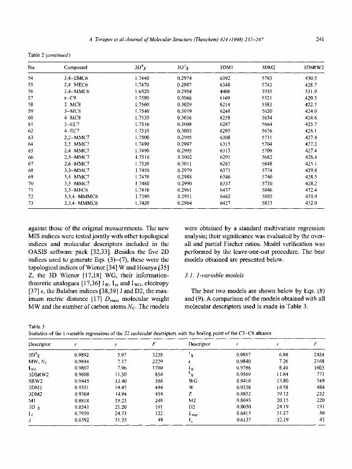
A. Toropov et al/Journal of Molecular Structure (Theochem) 424 (1998) 237-247 241

Table 2 (continued)

No. Compound 3D”x 3D’x 3DMl 3DM2 3DSRW2

54 3,4-EMC6 1.7440 0.2974

55 2,4&MEC6 1.7470 0.2987

56 3,4--MMC6 1.6520 0.2954

57 n-C9 1.7590 0.3046

58 2&MC8 1.7560 0.3029

59 3-MC8 1.7540 0.3019

60 4-MC8 1.7530 0.3016

61 3-EC7 1.7510 0.3008

62 4-EC7 1.7510 0.3005

63 2,2-MMC7 1.7500 0.2995

64 2,3-MMC7 1.7490 0.2997

65 2,4&MMC7 1.7490 0.2995

66 2,5pMMC7 1.7510 0.3002

67 2,6-MMC7 1.7530 0.30 I 1

68 3,3pMMC7 1.7450 0.2979

69 3,4&MMC7 1.7470 0.2988

70 3,5pMMC7 1.7480 0.2990

71 3,3pMEC6 1.7410 0.2961

72 3,3,4-MMMC6 1.7390 0.295 1

73 2,3,4-MMMC6 1.7420 0.2964

6392

6348

4406

6169

6214

6248

6258

6295

6308

6315

6313

6291

6261

6371

6337

6437

6462

6427

5793 430.5

5743 428.7

3935 331.9

5521 420.3

5583 422.7

5620 424.0

5634 424.6

5664 425.7

5676 426.1

5711 427.4

5704 427.2

5709 427.4

5682 426.4

5648 425.1

5774 429.8

5740 428.5

5730 428.2

5846 432.4

5885 433.9

5833 432.0

against those of the original measurements. The new

MIS indices were tested jointly with other topological indices and molecular descriptors included in the OASIS software pack [32,33]. Besides the five 2D indices used to generate Eqs. (3)-(7), these were the topological indices of Wiener [34] W and Hosoya [35] Z, the 3D Wiener [ 17,181 WG, their information-

theoretic analogues [17,36] Iw, I,, and Iwo, electropy [37] E, the Balaban indices [38,39] J and D2, the max- imum metric distance [ 171 D,,,, molecular weight MW and the number of carbon atoms NC. The models

were obtained by a standard multivariate regression

analysis; their significance was evaluated by the over- all and partial Fischer ratios. Model verification was

performed by the leave-one-out procedure. The best models obtained are presented below.

3.1. l-variable models

The best two models are shown below by Eqs. (8) and (9). A comparison of the models obtained with all molecular descriptors used is made in Table 3.

Table 3

Statistics of the l-variable regressions of the 22 molecular descriptors with the boiling point of the C3-C9 alkanes

Descriptor r s F Descriptor r s F

3D’X 0.9892 5.97

MW, Nc 0.9844 7.17

Iwo 0.9807 7.96

3DSRW2 0.9608 11.30

SRW2 0.9445 13.40

3DM 1 0.935 1 14.45

3DM2 0.9304 14.94

Ml 0.8818 19.23

3D’X 0.8541 21.20

lz 0.7950 24.73

J 0.6392 31.35

3238 ‘X 2229 E

1790 Iw

854 OX

586 WG 494 W

458 2

248 M2

191 D2

122 L nlax

49 1,

0.9857 6.88 2424

0.9840 7.26 2168

0.9786 8.40 1603

0.9569 11.84 771

0.9410 13.80 549

0.9338 14.58 484

0.8832 19.12 252

0.8693 20.15 220

0.8050 24.19 131

0.6415 31.27 50

0.6137 32.19 43

242 A. Toropov et d/Journal of Molecular Structure (Theochem) 424 (1998) 237-247

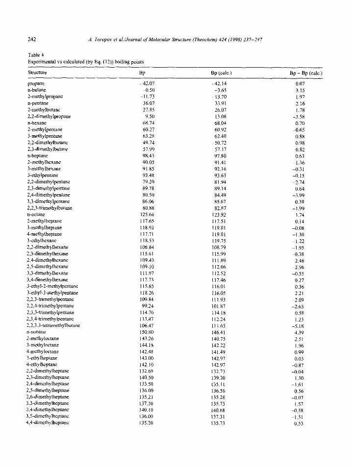
Table 4

Experimental vs calculated (by Eq. (12)) boiling points

Structure BP Bp (talc.) Bp - Bp (talc.)

propane n-butane

2-methylpropane

n-pentane

2-methylbutane

2,2_dimethylpropane

n-hexane

Z-methylpentane

3-methylpentane

2,2-dimethylbutane

2,3_dimethylbutane

n-heptane

2-methylhexane

3-methylhexane

3-ethylpentane

2,2_dimethylpentane

2,3_dimethylpentane

2,4_dimethylpentane

3,3_dimethylpentane

2,2,3kmethylbutane

n-octane

2-methylheptane

3-methylheptane

4-methylheptane

3-ethylhexane

2,2_dimethylhexane

2,3-dimethylhexane

2,4_dimethylhexane

2,5-dimethylhexane

3,3_dimethylhexane

3,4-dimethylhexane

3-ethyl-2-methylpentane

3-ethyl-3-methylpentane

2,2,3_trimethylpentane

2,2,4_trimethylpentane

2,3,3_trimethylpentane

2,3,4_trimethylpentane

2,2,3,3_tetramethylbutane

n-nonane

2-methyloctane

3-methyloctane

4-methyloctane

3-ethylheptane

4-ethylheptane

2,2_dimethylheptane

2,3_dimethylheptane

2,4-dimethylheptane

2,5-dimethylheptane

2,6-dimethylheptane

3,3-dimethylheptane

3,4_dimethylheptane

3,5-dimethylheptane

4,4_dimethylheptane

-42.07 -42.14 0.07 -0.50 -3.65 3.15

-11.73 -13.70 1.97

36.07 33.91 2.16 27.85 26.07 1.78

9.50 13.08 -3.58 68.74 68.04 0.70 60.27 60.92 -0.65 63.28 62.40 0.88 49.14 50.72 -0.98 57.99 57.17 0.82 98.43 97.80 0.63 90.05 91.41 -1.36 91.85 92.16 -0.3 1 93.48 93.63 -0.15 79.20 81.94 -2.74 89.78 89.14 0.64 80.50 84.49 -3.99 86.06 85.67 0.39 80.88 82.87 -1.99

125.66 123.92 1.74 117.65 117.51 0.14 118.93 119.01 -0.08 117.71 119.01 -1.30 118.53 119.75 -1.22 106.84 108.79 -1.95 115.61 115.99 -0.38 109.43 111.89 -2.46 109.10 112.06 -2.96 111.97 112.52 -0.55 117.73 117.46 0.27 115.65 116.01 -0.36 118.26 116.05 2.2 1 109.84 111.93 -2.09 99.24 101.87 -2.63

114.76 114.18 0.58 113.47 112.24 1.23 106.47 111.65 -5.18 150.80 146.41 4.39 143.26 140.75 2.51 144.18 142.22 1.96 142.48 141.49 0.99 143.00 142.97 0.03 142.10 142.97 -0.87 132.69 132.73 -0.04 140.50 139.20 1.30 133.50 135.11 -1.61 136.00 136.56 -0.56 135.21 135.28 -0.07 137.30 135.73 1.57 140.10 140.68 -0.58 136.00 137.31 -1.31 135.20 135.73 -0.53

A. Toropov et al./Journal of Molecular Structure (Theochem) 424 (1998) 237-247 243

Table 4 (continued)

Structure BP Bp (talc.) Bp - Bp (talc.)

3-ethyl-2-methylhexane 138.00 139.95 -1.95 4-ethyl-2-methylhexane 133.80 136.58 -2.78 3-methyl-3-ethylhexane 140.60 139.27 1.33 3-ethyl-4-methylhexane 140.40 141.23 -0.83 2,2,3_trimethylhexane 133.60 135.14 -1.54 2,2,4&methylhexane 126.54 127.09 -0.55 2,2,5_trimethylhexane 124.08 126.54 -2.46 2,3,3_trimethylhexane 137.68 137.39 0.29 2,3,4_trimethylhexane 139.00 137.66 1.34 2,3,5_trimethylhexane 131.34 132.81 -1.47 2,4,4_trimethylhexane 130.65 129.34 1.31 3,3,4_trimethylhexane 140.46 139.60 0.86 3,3_diethylpentane 146.17 143.00 3.17 2,2-dimethyl-3-ethylpentane 133.83 135.89 -2.06 2,3-dimethyl-3-ethylpentane 142.00 140.93 I .07 2.4-dimethyl-3-ethylpentane 136.72 136.20 0.52 2,2,3,3_tetramethylpentane 140.27 139.86 0.41 2,2,3,4_tetramethylpentane 133.01 131.39 1.62 2,2,4,4-tetramethylpentane 122.28 112.70 9.58 2,3,3,4-tetramethylpentane 141.55 139.06 2.49

Bp (“C) = 279.25( 2 4.91)3D0x - 348.94( k 8.08) Bp(“C)=34.35( t- 2.18)‘~+25.43( ? 2.12)Iw

n=73, r=0.9892, s=5.97, s’=6.18, F=3238 (8)

Bp (=C)=59.11( + 1.20)+ 104.51( k 4.41) (9)

n=73, r=0.9857, s=6.88, s/=7.23, F=2424

Here Y is the correlation coefficient, s the standard deviation, s’ the averaged standard deviation of the leave-one-out procedure, and F the Fischer ratio.

As seen, the 3D”x MIS index outperforms all other

indices tested. Four of the five MIS indices show better statistics than their 2D analogues, the exception being Randic’s connectivity index lx, the champion of the topological indices.

- 130.44( t 3.34) (11)

n=73, r=0.9953, s=3.96, s/=4.18, F=3722

The next three best models included the Randic mol- ecular connectivity lx with 3D Wiener index WG (r =

0.9951, s = 4.07, s’ = 4.28, F = 3520), the Zagreb M2 index in combination with the 3D’x index (r = 0.9947, s = 4.21, s’ = 4.36, F = 3289) and molecular weight

MW combined with the information-theoretic analogue of the Hosoya index I, (r = 0.9946, s = 4.27, s’ = 4.54,

F = 3199).

Once again, the best model included the 3D”x MIS index. The leave-one-out procedure produced exactly the same averaged correlation coefficients and averaged standard deviations s’ that are only slightly larger than those of the basic models.

3.2. 2-variable models

Bp (“C) = 244.87( -c 4.32)3D0x + 27.02( ? 2.45)1,

-336.47( + 5.05) (10)

n=73, r=0.9961, s=3.63, s/=3.80, F=4428

3.3. 3-variable models

Bp (“C)= 727.26( + 20.76)3D”x

- 19.46( + 0.91)3DSRW2

+ 7.99( + 0.39)M2 - 779.42( 2 20.08) (12)

n=73, r=0.9986, s=2.17, s’=2.50, F=8340

244

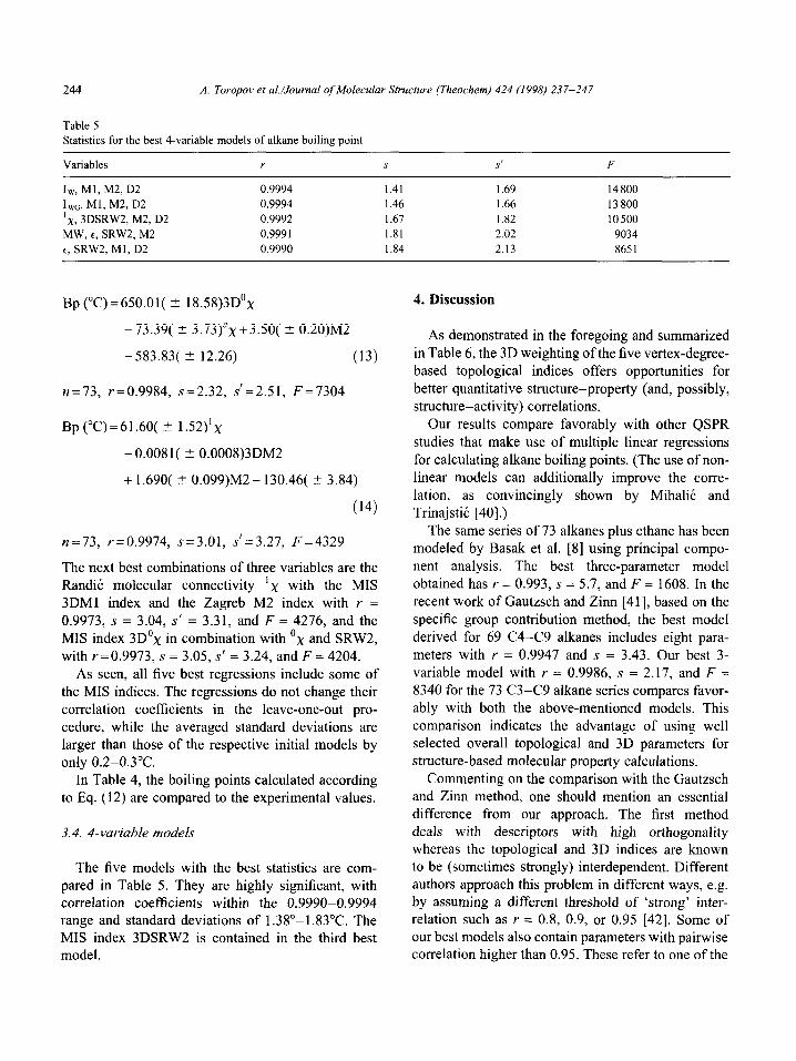
Table 5

A. Toropov et aL/Journal of Molecular Structure (Theochem) 424 (1998) 23 7-247

Statistics for the best 4-variable models of alkane boiling point

Variables r S S’ F

I,,,, Ml, M2, D2 0.9994 1.41 1.69 14 800

Iwo, Ml, M2, D2 0.9994 1.46 I .66 13 800

‘x, 3DSRW2, M2, D2 0.9992 I .61 I .82 10500

MW, E, SRWZ, M2 0.9991 1.81 2.02 9034

E, SRW2, Ml, D2 0.9990 1.84 2.13 865 1

Bp (“C) = 650.01( t- 1 8.58)3D”x

-73.39( t 3.73)Ox+3

-583.83( ? 12.26)

n=73, r=0.9984, s=2.32, s’=2.51, F=7304

50( ? 0.20)M2

(13)

Bp (“C)=61.60( ? 1.52)‘~

- 0.008 l( + O.O008)3DM2

+ 1.690( -t O.O99)M2- 130.46( +- 3.84)

(14)

n=73, r=0.9974, s=3.01, s/=3.27, F=4329

The next best combinations of three variables are the RandiC molecular connectivity ‘x with the MIS 3DMl index and the Zagreb M2 index with r =

0.9973, s = 3.04, S’ = 3.3 1, and F = 4276, and the MIS index 3D”x in combination with Ox and SRW2,

with r=0.9973, s = 3.05, s’ = 3.24, and F = 4204. As seen, all five best regressions include some of

the MIS indices. The regressions do not change their correlation coefficients in the leave-one-out pro- cedure, while the averaged standard deviations are larger than those of the respective initial models by only 0.2-0.3”C.

In Table 4, the boiling points calculated according to Eq. (12) are compared to the experimental values.

3.4. I-variable models

The five models with the best statistics are com- pared in Table 5. They are highly significant, with correlation coefficients within the 0.9990-0.9994 range and standard deviations of 1.38”-1.83”C. The MIS index 3DSRW2 is contained in the third best model.

4. Discussion

As demonstrated in the foregoing and summarized in Table 6, the 3D weighting of the five vertex-degree- based topological indices offers opportunities for better quantitative structure-property (and, possibly, structure-activity) correlations.

Our results compare favorably with other QSPR studies that make use of multiple linear regressions for calculating alkane boiling points. (The use of non- linear models can additionally improve the corre- lation, as convincingly shown by Mihalic and Trinajstic [40].)

The same series of 73 alkanes plus ethane has been modeled by Basak et al. [8] using principal compo- nent analysis. The best three-parameter model obtained has r = 0.993, s = 5.7, and F = 1608. In the recent work of Gautzsch and Zinn [41], based on the specific group contribution method, the best model derived for 69 C4-C9 alkanes includes eight para- meters with r = 0.9947 and s = 3.43. Our best 3-

variable model with r = 0.9986, s = 2.17, and F =

8340 for the 73 C3-C9 alkane series compares favor- ably with both the above-mentioned models. This comparison indicates the advantage of using well selected overall topological and 3D parameters for structure-based molecular property calculations.

Commenting on the comparison with the Gautzsch and Zinn method, one should mention an essential difference from our approach. The first method deals with descriptors with high orthogonality whereas the topological and 3D indices are known to be (sometimes strongly) interdependent. Different authors approach this problem in different ways, e.g. by assuming a different threshold of ‘strong’ inter- relation such as r = 0.8, 0.9, or 0.95 [42]. Some of our best models also contain parameters with pairwise correlation higher than 0.95. These refer to one of the

A. Toropov et al/Journal of Molecular Structure (Theochem) 424 (1998) 237-247 245

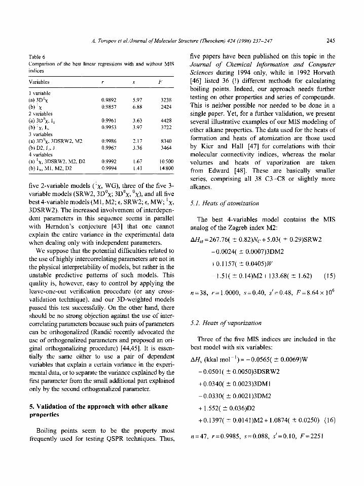
Table 6

Comparison of the best linear regressions with and without MIS

indices

Variables

1 variable

(a) 3D’x

(b) ‘x 2 variables

(a) 3D0x, 1,

(b) ‘x, 1, 3 variables

(a) 3D”x. 3DSRW2, M2

(b) D2, I,, J 4 variables

(a) ‘x, 3DSRW2, M2, D2

(b) I,, Ml, M2, D2

r s F

0.9892 5.97 3238

0.9857 6.88 2424

0.996 1 3.63 4428

0.9953 3.97 3722

0.9986 2.17 8340

0.9967 3.36 3464

0.9992 1.67 10500

0.9994 1.41 14800

five 2-variable models (lx, WG), three of the five 3- variable models (SRW2, 3D”x; 3D”x, Ox), and all five best 4-variable models (Ml, M2; E, SRW2; E, MW; lx, 3DSRW2). The increased involvement of interdepen-

dent parameters in this sequence seems in parallel with Hemdon’s conjecture [43] that one cannot explain the entire variance in the experimental data when dealing only with independent parameters.

We suppose that the potential difficulties related to the use of highly intercorrelating parameters are not in the physical interpretability of models, but rather in the unstable predictive patterns of such models. This

quality is, however, easy to control by applying the leave-one-out verification procedure (or any cross- validation technique), and our 3D-weighted models

passed this test successfully. On the other hand, there should be no strong objection against the use of inter- correlating parameters because such pairs of parameters can be orthogonalized (Randic recently advocated the

use of orthogonalized parameters and proposed an ori- ginal orthogonalizing procedure) [44,45]. It is essen- tially the same either to use a pair of dependent variables that explain a certain variance in the experi- mental data, or to separate the variance explained by the

first parameter from the small additional part explained only by the second orthogonalized parameter.

5. Validation of the approach with other alkane properties

Boiling points seem to be the property most frequently used for testing QSPR techniques. Thus,

five papers have been published on this topic in the

Journal of Chemical Information and Computer

Sciences during 1994 only, while in 1992 Horvath

[46] listed 36 (!) different methods for calculating boiling points. Indeed, our approach needs further testing on other properties and series of compounds.

This is neither possible nor needed to be done in a single paper. Yet, for a further validation, we present

several illustrative examples of our MIS modeling of

other alkane properties. The data used for the heats of formation and heats of atomization are those used by Kier and Hall [47] for correlations with their molecular connectivity indices, whereas the molar

volumes and heats of vaporization are taken from Edward [48]. These are basically smaller series, comprising all 38 C3-C8 or slightly more

alkanes.

5.1. Heats of atomization

The best 4-variables model contains the MIS analog of the Zagreb index M2:

AHa, =267.76( -+ 0.82)Nc +5.03( + 0.29)SRW2

-0.0024( 2 O.O007)3DM2

+0.1157( -t 0.0405)W

-1.51( -+ 0.14)M2+133.68( 2 1.62) (15)

n=38, r=l.OOOO, s=O.40, s’=O.48, F=8.64x lo6

5.2. Heats of vaporization

Three of the five MIS indices are included in the best model with six variables:

AH, (kkal mol-‘)= -0.0565( ? 0.0069)W

- 0.0501( ? O.O050)3DSRW2

+ 0.0340( 5 O.O023)3DMl

- 0.0330( + O.O021)3DM2

+ 1.552( + O.O36)D2

+0.1397( ? O.O141)M2+ 1.0874( 5 0.0250) (16)

n=47, r=0.9985, s=O.O88, s’=O.lO, F=2251

246 A. Toropov et al./Journal of Molecular Structure (Theochem) 424 (1998) 237-247

5.3. Heats offormation

The 2-variable model with the best statistics incor-

porates the RandiC first-order connectivity index and

its zero-order MIS counterpart:

AH” (kkal mol- ‘) = 98.77( t 3.46)3D”x

- 11.23( -+ 0.76)*x-70.58( 2 3.02) (17)

n=38, r=0.9964, s=O.62, s’=O.70, F=2422

5.4. Molar volumes

The same zero-order MIS connectivity index was found to be the parameter that correlated best with

molar volumes:

VM (ml mole’)= 155.29( -C 3.38)3D”x

-95.13( 2 5.52) (18)

n=46, r-=0.9897, s=2.50, s’=2.62, F=2104

Models (15- 18) as well as many others not shown here, confirm our finding for boiling points that the studied 3D analogues of some of the most frequently used 2D indices are always among the parameters included in the best regression equations. In the light of the above we may conclude that our MIS models (based on intramolecular atom-atom repulsion) could compete well, in the simulation and modeling of molecular properties, with other QSPW QSAR methods.

Acknowledgements

The comments made by W.C. Herndon (El Paso)

are highly appreciated. D. Bonchev was supported by the Robert Welch Foundation, Texas. A. Toropov gratefully acknowledges the support of the Vostok Innovation Company (D.V. Rikov, President).

References

[l] A.T. Balaban, 1. Motoc, D. Bonchev, 0. Mekenyan, Topics

Curr. Chem. 114 (1983) 21.

[2] N. Trinajstic, Chemical Graph Theory, 2nd edn, CRC Press, Boca Raton, FL, 1992.

[3] M. Randic. N. Trinajstic, J. Mol. Struct. 300 (1993) 551.

[4] D. Bonchev, N. Trinajstic, lnt. J. Quantum Chem. Symp. 16

(1982) 463.

[5] D. Bonchev, Information-Theoretic Indices for Charac-

terization of Chemical Structures, Research Studies Press,

Chichester, UK, 1983.

[6] P.G. Seybold, M. May, U.A. Bagal, J. Chem. Educ. 64 (1987)

515.

[7] S.C. Basak, G.J. Niemi, G.D. Veith, J. Math. Chem. 4 (1990)

185.

[8] S.C. Basak, G.J. Niemi, G.D. Veith, J. Math. Chem. 7 (1991)

243.

[9] L.B. Kier, L.H. Hall, Molecular Connectivity in Chemistry

and Drug Research, Academic Press, New York, 1976; Mole-

cular Connectivity in Structure-Activity Analysis, Research

Studies Press, Chichester, UK, 1986.

[lo] 0. Mekenyan, S.C. Basak, in D. Bonchev, 0. Mekenyan (Eds.)

Graph Theoretical Approaches to Chemical Reactivity,

Khmer Academic, Dordrecht, The Netherlands, 1994, p, 221.

[ 111 A.T. Balaban, A. Chiriac, 1. Motoc, Z. Simon, Steric Fit in

QSAR, Lecture Notes in Chemistry, No. 15, Springer, Berlin,

1980.

[ 121 M. Randic, J. Math. Chem. 9 (1992) 97.

[13] A.R. Katritzky, E.V. Gordeeva, J. Chem. Inf. Comput. Sci. 33 (1993) 835.

[14] M. Randic, lnt. J. Quantum Chem. Symp. 15 (1988) 201.

[l5] M. Randic, J. Chem. Inf. Comput. Sci. 34 (1994) 277.

[ 161 M. Randic, J. Chem. Inf. Comput. Sci. (in press).

[17] 0. Mekenyan, D. Peitchev, D. Bonchev, N. Trinajstic. 1.

Bangov, Drug Design 36 (1986) 176.

[18] B. Bogdanov, S. Nikolic, N. Trinajstic, J. Math. Chem. 3

( 1989) 299.

[19] A.A. Toropov, B.G. lshakov, R.A. Muftahov, T. lsmailov,

A.T. Mamadalimov, Russ. J. Phys. Chem. 66 (1992) 1074.

[20] A.A. Toropov, A.F. Toropova, R.A. Muftahov, T. Jsmailov,

A.G. Muftahov, Russ. J. Phys. Chem. 68 (1994) 577.

[21] R.J. Gillespie, Molecular Geometry. Addison-Wesley, New

York, 1972.

[22] D.L. Keppert, Inorganic Stereochemistry, Springer, New

York, 1972.

[23] G.M. Crippen, AS. Smellie, J.W. Peng, J. Chem. lnf. Comput.

Sci. 28 (1988) 125.

[24] T.F. Havel, in: Encyclopedia of NMR, Wiley, New York,

1995.

[25] D. Bonchev, A.T. Balaban, 0. Mekenyan, J. Chem. lnf. Com-

put. Sci. 20 (1980) 106.

[26] 1. Gutman, B. RuSEic, N. Trinajstic, C.W. Wilcox Jr, J. Chem.

Phys. 69 (1975) 3399.

[27] M. Randic, J. Am. Chem. Sot. 97 (1975) 6609.

[28] L.B. Kier, L.H. Hall, W.J. Murray, M. Randic, J. Pharm. Sci. 64 (1975) 1971.

[29] D. Bonchev, L.B. Kier, J. Math. Chem. 9 (1992) 75.

[30] D. Bonchev, X. Liu, D.J. Klein, Croat. Chem. Acta 66 (1993) 141.

[3 I] W.C. Herndon (private communication).

[32] 0. Mekenyan, S. Karabunarliev, D. Bonchev, Comput. Chem. 14 (1990) 193.

A. Toropov et al./Journaf of Mofecdar Structure (Theochem) 424 (1998) 237-247 247

1331 D. Bonchev, CF. Mountain, W.A. Seitz, A.T. Baiaban, 1. [42] L.M. Egolf, M.D. Wessel, P.C. Jurs, J. them. inf. Comput.

Med. Chem. 36 (I 993) 1562. Sci. 34 (1994) 941.

[34] H. Wiener, J. Am. Chem. Sot., 69 (1947) 17; 69 (1947) 2636.

1351 H. Hosoya, Bull. Chem. Sot. Jpn 44 (1971) 2332.

[36] D, Bonchev, N. Trinajstii-, J. Chem. Phys. 67 (1977) 45 17.

[37] W.Y. Yee, K. Sakamoto, Y.J. I’Haya, Rep. Univ. Electro-

comm., 27 (1976) 53; K. Sakamoto, W.Y. Yee, Y.J.

l’Haya, Rep. Univ. Electra-comm., 27 (1977) 227.

[38] A.T. Balaban, Chem. Phys. Lett. 89 (1982) 399.

[39] A.T. Balaban, Theor. Chim. Acta 53 (1979) 355.

[40] Z. Mihalic, N. Trinajstic, J. Chem. Educ. 69 (1992) 701.

[41] R. Gautzsch. P. Zinn, J. Chem. Inf. Comput. Sci. 34 (1994)

791.

1431 WC. Hemdon (private co~unication).

1441 M. Rand%, J. Chem. Inf. Comput. Sci. 31 (1991) 31 I.

[45] M. Randif, New J. Chem. 15 (1991) 517.

[46] A.L. Horvath, Molecular Design: Chemical Structure Genera-

tion from the Properties of Pure Organic Compounds, Elsevier,

Amsterdam, 1992.

[47] L.B. Kier, L.H. Hall, Molecular Connectivity in Stmcture-

Activity Analysis. Research Studies Press, Chichester, UK,

1986.

[48] J.T. Edward, Can. J. Chem. 60 (1982) 480.