SPE 165960

3-D Numerical Investigation of Subsurface Flow in Anisotropic Porous Media using Multipoint Flux Approximation Method Ardiansyah Negara, SPE, Amgad Salama, Shuyu Sun, SPE, King Abdullah University of Science and Technology

Copyright 2013, Society of Petroleum Engineers This paper was prepared for presentation at the SPE Reservoir Characterisation and Simulation Conference and Exhibition held in Abu Dhabi, UAE, 16–18 September 2013. This paper was selected for presentation by an SPE program committee following review of information contained in an abstract submitted by the author(s). Contents of the paper have not been reviewed by the Society of Petroleum Engineers and are subject to correction by the author(s). The material does not necessar ily reflect any position of the Society of Petroleum Engineers, its officers, or members. Electronic reproduction, distribution, or storage of any part of this paper without the written consent of the Society of Petroleum Engineers is prohibited. Permission to reproduce in print is restricted to an abstract of not more than 300 words; illustrations may not be copied. The abstract must contain conspicuous acknowledgment of SPE copyright.

Abstract

Anisotropy of hydraulic properties of subsurface geologic formations is an essential feature that has been established as a

consequence of the different geologic processes that they undergo during the longer geologic time scale. With respect to

petroleum reservoirs, in many cases, anisotropy plays significant role in dictating the direction of flow that becomes no longer

dependent only on the pressure gradient direction but also on the principal directions of anisotropy. Furthermore, in complex

systems involving the flow of multiphase fluids in which the gravity and the capillarity play an important role, anisotropy can

also have important influences.

Therefore, there has been great deal of motivation to consider anisotropy when solving the governing conservation laws

numerically. Unfortunately, the two-point flux approximation of finite difference approach is not capable of handling full

tensor permeability fields. Lately, however, it has been possible to adapt the multipoint flux approximation that can handle

anisotropy to the framework of finite difference schemes. In multipoint flux approximation method, the stencil of

approximation is more involved, i.e., it requires the involvement of 9-point stencil for the 2-D model and 27-point stencil for

the 3-D model. This is apparently challenging and cumbersome when making the global system of equations.

In this work, we apply the equation-type approach, which is the experimenting pressure field approach that enables the

solution of the global problem breaks into the solution of multitude of local problems that significantly reduce the complexity

without affecting the accuracy of numerical solution. This approach also leads in reducing the computational cost during the

simulation.

We have applied this technique to a variety of anisotropy scenarios of 3-D subsurface flow problems and the numerical results

demonstrate that the experimenting pressure field technique fits very well with the multipoint flux approximation method.

Furthermore, the numerical results explicitly emphasize that anisotropy could not be ignored for the proper model of

subsurface flow.

1. Introduction

The description of a porous medium as a continuum greatly simplifies the governing laws. This has been because field

variables are now describe continuous functions of space and time leading the governing laws to be written as a set of partial

differential equations. This has only been possible provided it is feasable to finding a representative volume for upscaling and

the satisfaction of certain length scale constraints (Salama and Van Geel 2008a-b). It has been suggested based on

experimental arguments that all the geometrical complexities of real porous media is replaced by one parameter that relates the

pressure gradient vector and the fluid flux vector. Apparently, since early experiments have been conducted on homogeneous

sand filter, Darcy 1856 suggested that this parameter is a mer scalar quantity. This implies that, in such media, both the

hydraulic gradient vector and the flux vector are coincident. Lately, it has been realized that this situation is not always true

and there are cases in which both vectors are not coincident. This suggests that the hydraulic conductivity parameter could be

more complex than just a mer scalar and could possess directional dependence (i.e., anisotropic). For long time, geological

processes in the subsurface have caused the rock formations to be geometrically complex in such a way the hydraulic

properties of reservoir rocks are, mostly, heterogeneous and anisotropic. This anisotropy plays significant role in dictating the

direction of the flow that becomes no longer dependent only on the pressure gradient but also on the principal directions of

2 SPE 165960

anisotropy. In anisotopic porous media, several properties of reservoir rocks (e.g., permeability, thermal conductivity, etc.)

vary with respect to the direction. To take anisotropy of the hydraulic conductivity into account, it has been proposed that it

should be treated as a tensor rather than a scalar. Apparently, this imposes several difficulties to the numerical solution to the

set of governing equations. That is traditional finite difference techniques (the so-called two-point flux approximation) is not

capable of handeling but diagonal tensor.

Recently, a method has been designed based on the finite volume formulation to enable the modeling of flow and transport in

anisotropic porous media, which is called multipoint flux approximation (MPFA). From the name it is clear that several points

are involved in calculating the flux as opposed to only two points. This method has been grown as a class of mixed finite

element technique, Wheeler and Yotov 2006, Osman et al. 2012 and also as a class of finite volume technique, Avatsmark,

1998. Several studies discussed the implementation of MPFA in fluid flow problems in anisotropic porous media and others

(e.g., heat conduction problems, Salama et al. 2013). This includes Aavatsmark et al. 1998, Aavatsmark 2002, and Edwards

and Rogers 1998. In Aavatsmark et al. 1998, two subclasses of MPFA, i.e., MPFA O- and U-methods are introduced. Further

details of discussion in Aavatsmark et al. 1998 involve on how to dealing with inactive cells and flow barriers in anisotropic

reservoirs. Aavatsmark et al. 1998 has demonstrated that the numerical results involving MPFA method fit very well with

numerical results produced by the commercial ECLIPSE reservoir simulator. In the other paper, Aavatsmark 2002 discussed

the discretization and implementation of MPFA O-method with surface midpoints as continuity points on quadrilateral grids.

Aavatsmark 2002 has shown a comparison between MPFA and TPFA in the simulation results in which the considerable

errors appear when using TPFA methods. In addition, Edwards and Rogers 1998 presented a family of nine flux continuous

based on the finite volume scheme that is applicable for the diagonal and full discontinuous tensor coefficients of pressure

equations. Edwards and Rogers 1998 have also demonstrated the existence of an error produced by the classical five-point

stencil scheme (TPFA) due to the ignorance of the off-diagonal elements in the tensor. The off-diagonal elements of the tensor

equation could not be ignored since these give a strong impact on the variation of the pressure field.

MPFA method requires more point stencil in the approximation, i.e., 9-point stencil in the 2-D problem and 27-point stencil in

the 3-D problem. If the flow model is solved by constructing the pressure equation from the substitution of Darcy’s law into

the mass conservation equation then this is apparently challenging and cumbersome in the sense of constructing the global

system of equations because the expression of pressure equation would be very large when it is discretized. We tackle this

issue by implementing the equation-type approach (or the experimenting pressure field approach) that has been introduced by

Sun et al. 2012. The equation-type approach enables to obtain the numerical solution without extra mathematical

manipulations. In other words, the reduction of number of governing equations is no longer needed. The solution of the global

problem breaks into the solution of multitude of local problems that significantly reduce the complexity without affecting the

accuracy of the numerical results. This technique separates the physics and the solver parts of the problems in such a way it

enables the code to be more robust with maintaining the ease of implementation.

The motivation of this paper is to investigate the subsurface flow in anisotropic porous media by applying the MPFA method

and the experimenting pressure field approach. We employ the MPFA in the framework of finite difference scheme and we

expect to gain a robust code that produces accurate numerical results by applying both techniques. The paper is organized into

several sections as follows: section 2 presents the mathematical model of fluid flow in porous medium particularly single-

phase flow model. Section 3 explains the fundamental concept of MPFA method particularly MPFA O-method. Section 4

contains the explanation of equation-type approach that is applied to solve the fluid flow model. Section 5 demonstrates two

numerical experiments and the discussion of the results. Finally we end up with the conclusions in section 6.

2. Mathematical model

The governing equations of fluid flow in porous medium are given by the combination of physical principles, i.e., the

conservation of mass and Darcy’s law. The former describes the principle of conservation of some physical quantity, which is

the mass inflow and outflow are equal when the fluid crosses a certain region. In this work, we consider single-phase flow

model in which the mass conservation equation is given by

q

t

u Eq. 1

where ϕ is the porosity, ρ is the density of the fluid, q is the sink/source, is the divergence operator, and u is the Darcy

velocity defined as

p z

K

u g Eq. 2

SPE 165960 3

Darcy’s law expresses the linear relationship between the total volumetric flow rate and the pressure gradient. In Eq.2, K is the

full permeability tensor, p is the fluid pressure, µ is the fluid viscosity, ρ is the fluid density, g is the gravitational acceleration,

z is the depth, and is the gradient operator, , ,

T

x y z

. Here, the full permeability tensor is represented as a

second-order tensor by

xx xy xz

yx yy yz

zx zy zz

K K K

K K K

K K K

K Eq. 3

Unlike a zeroth-order tensor in which the value is a single number (scalar) for any dimension or first-order tensor in which the

value is characterized by three numbers (vector) for three dimensions, in a second-order tensor, there are nine numbers that is

represented by a matrix as shown in Eq. 3. In the full permeability tensor, the main diagonal elements show the magnitude of

permeability with respect to the principal directions whereas the off-diagonal elements describe the magnitude with respect to

the arbitrary combination of principal directions (Hassanpour et al. 2010). These off-diagonal elements contribute to the flow

direction to be different from the linear potential gradient of pressure for instance the xyK element contributes to the flow in

the x-direction due to the pressure gradient in the y-direction, etc. As a second-order tensor, the full permeability is assumed to

be symmetric and positive definite.

In this work, the domain is defined as cube and bounded by the boundaries. The boundary conditions associated to the

governing equations (Eqs. 1 and 2) are the Dirichlet boundary ( D ) and the Neumann boundary ( N ):

,

,

B D

B N

p p

u

x

u n x Eq. 4

Here n is the outward unit normal vector on the boundary, Bp is the given pressure on D and Bu is the imposed velocity on

N .

3. Multipoint flux approximation method

There are a variety of MPFA methods for instance MPFA-O method (Aavatsmark 1996; Edwards and Rogers 1998), the

MPFA-U method (Aavatsmark and Eigestad 2006), the MPFA L-method (Aavatsmark et al. 2008; Cao et al 2009), and the

MPFA Z-method (Nordbotten and Eigestad 2005). In this paper, we discuss only the MPFA O-method (later, simply called

MPFA) since it will be implemented into the model. Compared to the TPFA, the MPFA methods increase the accuracy of the

solution particularly in the case of non-orthogonal grids or anisotropy that requires more flux stencil.

(a) (b)

Figure 1. The 2-D (a) and 3-D (b) interaction regions.

4 SPE 165960

As the MPFA method has been outlined in the literature (Aavatsmark 2002; Wolff et al. 2011), the fundamental concept of

MPFA is the following: the MPFA O-method uses the midpoint of the interface for the linear variation and continuity of

pressure gradient. The linear pressure gradient is constructed based on the cell-centered pressure and the interface pressure. In

the 2-D problem, the MPFA method builds the interaction region (dashed line) that is centered on the four adjacent cells as

seen in Figure 1a. In this case, there are four fluxes need to be calculated in each interaction region in which each flux is

approximated by

i i

i

f t

Eq. 5

where it and i are the transmissibility coefficient and the potential gradient (in this work is the pressure gradient) at the center

of the cell-i, respectively. The set depends on the dimension of the considered problem in which in the 2-D problem, the set

involves 6 cells whereas in the 3-D problem, the set involves 18 cells. Like the TPFA, the fluxes are conserved locally

by assuming the inflow and outflow fluxes are equal. To explain more detail the method, let’s consider an example based on

Figure 1a on how to calculate the flux,

xx xy

ij i ij i i ik i

xx xy

j j ij j jl j

f t p p t p p

t p p t p p

Eq. 6a

and

yy yx

ik i ik i i ij i

yy yx

k k ik k kl k

f t p p t p p

t p p t p p

Eq. 6b

We approach fjk and fkl in the same way. Each flux involves two adjacent cells to be considered as expressed in Eq. 6. The

transmissibility coefficient includes the hydraulic conductivity or permeability and the grids information. From each

interaction region, we would obtain four systems of equations that need to be solved locally. In 3-D problem, the interaction

region involves eight adjacent cells as shown in Figure 1b. The black node represents the center of each cell; so each subcube

represents one-eighth of a cell. There are 12 interface fluxes in each interaction region. We present the details of numerical

discretization based on the MPFA in the framework of finite difference method and how to obtain the 12 fluxes in each

interaction region in 3-D problem (see the Appendix).

4. The experimenting pressure field approach

As mentioned earlier, the MPFA stencil is much more complex than that for the simple two-point flux approximation. For

example, in 2-D problems, each flux component requires six pressure values in the surrounding six cells and in 3-D problems

it requires 18 pressure values in the surrounding 18 cells. Likewise, the divergence operator over a cell requires nine pressure

values in the surrounding nine cells in 2-D problems and 27 pressure values from 27 cells in 3-D problems. Apparently this is

cumbersome and prone to errors in calculating these terms and in coding them in the matrix of coefficients. In this work, we

use a technique that has been recently published by Sun et al. 2012, which the matrix of coefficients is generated automatically

within the solver routine. In this technique, a set of experimenting pressure fields are applied to the governing equations from

which the velocity field is evaluated and the divergence of the velocity field is determined. Since none of these pressure fields

are the correct one, the divergence will not be correct (e.g., in divergence free problems it will not be zero). Now the

experimenting pressure fields are designed such that the residual, which is the difference between the divergence given the

experimenting field and the correct one determines the entries of the matrix of coefficients. The number of required

experimenting pressure fields equals the number of cells, which is large particularly for larger problems. In other words, in the

original work of Sun et al. 2012, they loop over m × n pressure fields (where m and n are the number of segments in x-and y-

directions) to generate the matrix of coefficients and one more pressure field for the boundary conditions. Apparently this is

inefficient particularly for time dependent problems in which the matrix of coefficients is updating with time. In this work, the

testing pressure fields are generated only three times, which clearly reduce significantly the time required to construct the

matrix of coefficients. In other words, only three testing pressure fields are designed to generate the global matrix. For

completeness, in this section we highlight the essence of this approach. Consider the steady state mass conservation equation

for the flow of an incompressible fluid in porous media without source/sink term. This equation is written simply as

u 0 Eq. 7

SPE 165960 5

If the gravity is lumped into the pressure, we obtain Darcy’s law as

p

Ku Eq. 8

Suppose that the pressure field is known, then the velocity field could be obtained using the Darcy’s law and if we substitute

into Eq. 7, we find a divergence free solution. However, if the pressure is not the correct one, we will not get a divergence free

system. The residual that is the difference between the true divergence value and the calculated one may be defined as

p

R 0 u Eq. 9

Substituting Darcy’s law into the conservation of mass law, one obtains

p u K Eq. 10

In matrix form this equation may be written as

Ap u[ ] Eq.11

Therefore, for the ith

testing pressure field we have

i

ip Ap 0 u Eq. 12

Now if pi is chosen to be 1 in the i

th cell and zeros elsewhere, one could obtain the entries of the i

th column of the coefficient

matrix and likewise until the matrix is populated. Furthermore, the boundary condition has to be incorporated as shown in Sun

et al. 2012 using additional pressure field where the pressure in all the cells is zero. As explained earlier this requires m × n + 1

experimenting pressure fields which is, apparently, inefficient. However, one notices that the cell in which the pressure is one

affects the flux in only the neighbouring four cells. This implies that one could design the testing pressure field in which the

cells where the pressure is one alternate every two cells and significantly reduce the CPU time. The algorithm of the equation-

type approach is as follows:

1) Given any pressure field, we calculate the velocity at the midpoint interface by solving Eq. 8 along the entire domain. In

this step, we implement the MPFA method simultaneously.

2) Calculate the divergence in each cell in the domain based on the obtained velocity from step 1.

3) Calculate the function of pressure or the residual as defined in Eq. 9.

4) Construct the matrix of coefficient A and the right hand side, u , of Eq. 11 then solve it to obtain the correct solution

for the pressure field.

5) Calculate the correct velocity based on the correct pressure field.

5. Numerical experiments

This section presents two numerical experiments and comparison between the numerical results produced by MPFA and TPFA

methods. We perform the numerical experiments with different types of cases and boundary conditions to show the subsurface

flow phenomena in anisotropic and isotropic porous media. The 3-D single-phase flow model is considered. The domain of

each numerical experiment is discretized into 50 × 50 × 50 cells. The porosity of the porous medium is assumed to be 0.20.

The fluid density and viscosity are taken as 1000 kg/m3 and 1 centipoise (cP), respectively. We refer the full permeability

tensor model to Renard et al. 2001. The comparison between anisotropic and isotropic problems is importance in the sense of

demonstrating the effect of anisotropy to the variation of pressure and flow directions. We will also see that the experimenting

pressure field approach has been successfully implemented into all considered numerical experiments in this work.

Numerical experiment 1

In the first numerical experiment, we consider a case in which the domain has the Dirichlet (pressure) boundary condition on

the boundaries of y-direction. The pressure in one boundary side is higher than the other boundary. Meanwhile, the boundaries

in the other principal directions are defined as the Neumann (no flow) boundary conditions. Figures 2a-b illustrate the pressure

field in the anisotropic and isotropic porous media, respectively. From these two figures we may see a significant difference in

the sense of pressure field variation.

6 SPE 165960

(a) (b)

Figure 2. The pressure fields in anisotropic (a) and isotropic (b) cases: numerical experiment 1.

Figure 2a clearly demonstrates the presence of anisotropy, in this case, causing more variation of pressure field distribution.

The pressure field variation field appears in the simulation since we involve the full tensor elements including the off-diagonal

elements in the flow model. The off-diagonal elements induce the existence of cross-flow in such a way they affects the

pressure field for instance the skew of the pressure distribution in the x-z plane as shown in Figure 3a. If we consider only the

main diagonal element of the permeability tensor or consider the permeability as a scalar, we would not have the anisotropy

effect because the pressure gradient only exists along the principal directions. Figure 3b shows the uniform distribution of

pressure gradient in the isotropic case.

(a) (b)

Figure 3. The x-z cross section of pressure fields in anisotropic (a) and isotropic (b) cases: numerical experiment 1.

Numerical experiment 2

In the second numerical experiment, we consider a problem in which there is an injection from the top of the domain. We

impose the Dirichlet (pressure) boundary condition on the boundaries of y-direction and the Neumann (no-flow) boundary

conditions on the boundaries of x-and z-directions. We set equal pressure values in each Dirichlet boundary. Again, from the

simulation, we notice a clear difference for two difference cases as illustrated by Figures 4a-b. In the case of anisotropy

(Figure 4a), the injected fluid impacts the pressure field distribution tends to the direction of perpendicular to the boundaries

that are defined as pressure. Similarly, in the isotropic case, the injected fluid affects the pressure field distribution to the same

direction, however, with less impact region than the anisotropic one. These two comparison results indicate that the anisotropy

property of the reservoir rocks contributes in controlling the variation of pressure field distribution. From the numerical results

we may see by the ignoring of anisotropy property of the material, the pressure field has uniform distribution (Figure 5b);

otherwise, the pressure field distribution is skewed in a particular direction in which the permeability is more dependent on the

principal direction (Figure 5a).

SPE 165960 7

(a) (b)

Figure 4. The x-z cross section of pressure fields in anisotropic (a) and isotropic (b) cases: numerical experiment 2.

(a) (b)

Figure 5. The x-z cross section of pressure fields in anisotropic (a) and isotropic (b) cases: numerical experiment 2.

6. Conclusions

The method of MPFA and the experimenting pressure field methods have been applied to study the problem of flow in 3-D

anisotropic porous medium domain. The numerical results have demonstrated that the MPFA performs well to model the flow

in porous medium that has anisotropy property. In this work, we use the MPFA in the framework of cell-centered finite

difference, which is generally easy to implement. This apparently enlarges the scope of finite differences by considering

anisotropic media. Furthermore, the experimenting pressure field approach has shown to significantly simplify calculations. In

this approach the global matrix of coefficients is constructed automatically within the solver routine, thereby greatly

facilitating the coding.

8 SPE 165960

References

Aavatsmark, I., Barkve, T., Boe, O., and Mannseth, T. 1996. Discretization on non-orthogonal, quadrilateral grids for

inhomogeneous anisotropic media. Journal of Computational Physics, 127: 2-14.

Aavatsmark, I. 2002. An introduction to multipoint flux approximations for quadrilateral grids. Computational Geosciences,

6(3-4): 405-432.

Aavatsmark, I., and Eigestad, G. T. 2006. Numerical convergence of the MPFA O-method and U-method for general

quadrilateral grids. International Journal for Numerical Methods in Fluids. 51(9-10): 939-961.

Aavatsmark, I., Eigestad G. T., Mallison, B. T., and Nordbotten, J. M. 2008. A compact multipoint flux approximation method

with improved robustness. Numerical Methods for Partial Differential Equations. 24(5): 1329-1360.

Cao, Y., Helmig, R., and Wohlmuth, B. 2009. Geometrical interpretation of the multipoint flux approximation L-method.

International Journal for Numerical Methods in Fluids. 60(11): 1173-1199.

Edwards, M. G., and Rogers, C. F. 1998. Finite volume discretization with imposed flux continuity for the general tensor

pressure equation. Computational Geosciences, 2(4): 259-290.

Hassanpour, R. M., Manchuk, J. G., Leuangthong, O., and Deutsch, C. V. 2010. Calculation of permeability tensors for

unstructured gridblocks. Journal of Canadian Petroleum and Technology, 49(10): 65-74.

Nordbotten, J., and Eigestad, G. T. 2005. Discretization on quadrilateral grids with improved monotonicity properties. Journal

of Computational Physics, 203(2): 744-760.

Osman, H., Salama, A., Sun, S., and Bao, K. 2012, A finite difference, multipoint flux numerical approach to flow in porous

media: numerical examples. Porous Media and Its Applications in Science, Engineering, and Industry: 4th

International

Conference, AIP Conference Proceeding, 1453: 217-222.

Renard, P., Genty, A., and Stauffer, F. 2001. Laboratory determination of the full permeability tensor. Journal of Geophysical

Research, 106(B11): 26443-26452.

Salama, A., and Van Geel, P. J. 2008a. Flow and solute transport in saturated porous media: 1. The continuum hypothesis,

Journal of Porous Media, 11(4): 403-413.

Salama, A. and Van Geel, P. J. 2008b. Flow and solute transport in saturated porous media: 2. Violating the continuum

hypothesis, Journal of Porous Media, 11(5): 421-441.

Salama, A., Sun, S., and El-Amin, M. F. 2013. A multipoint flux approximation of the steady-state heat conduction equation in

anisotropic media.The ASME Journal of Heat Transfer, 135(4): 041302(1)-(6).

Sun, S., Salama, A., and El-Amin, M. F. 2012. An equation-type approach for the numerical solution of the partial differential

equations governing transport phenomena in porous media. Procedia Computer Science, 9: 661-669.

Wheeler, M., and Yotov, I. 2006. A multipoint flux mixed finite element method, SIAM Journal on Numerical Analysis, 44(5):

2082–2106.

Wolff, M., Flemisch, B., Helmig, R., and Aavatsmark, I. Treatment of tensorial relative permeabilities with multipoint flux

approximation. International Journal of Numerical Analysis and Modeling, 9(3): 725-744.

SPE 165960 9

Appendix

Figure A-1. The 3-D interaction region.

Figure A-2. The velocity field in the interaction region.

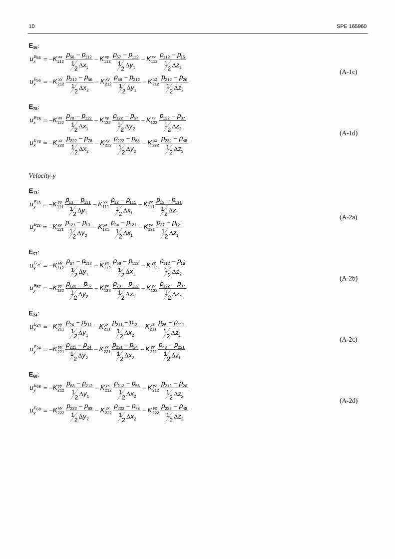
For the details on how the MPFA method works, let’s discretize Eq. 2 to obtain the velocity in all principal directions:

Velocity-x

E12:

13 111 15 11112 11112111 111 111

1 1 1

26 111211 12 24 21112211 211 211

2 1 1

1 1 12 2 2

1 1 12 2 2

E xx xy xz

x

E xx xy xz

x

p p p pp pu K K K

x y z

p pp p p pu K K K

x y z

(A-1a)

E34:

34 121 121 13 37 12134121 121 121

1 2 1

221 34 48 221221 2434221 221 221

2 2 1

1 1 12 2 2

1 1 12 2 2

E xx xy xz

x

E xx xy xz

x

p p p p p pu K K K

x y z

p p p pp pu K K K

x y z

(A-1b)

x

y

z

x

y

z

p111 p211

p121 p221

p112 p212

p122 p222

E1 E2

E3 E4

E5

E6

E7 E8

10 SPE 165960

E56:

56 112 57 112 112 1556112 112 112

1 1 2

212 56 68 212 212 2656212 212 212

2 1 2

1 1 12 2 2

1 1 12 2 2

E xx xy xz

x

E xx xy xz

x

p p p p p pu K K K

x y z

p p p p p pu K K K

x y z

(A-1c)

E78:

78 122 122 57 122 3778122 122 122

1 2 2

222 78 222 68 222 4878222 222 222

2 2 2

1 1 12 2 2

1 1 12 2 2

E xx xy xz

x

E xx xy xz

x

p p p p p pu K K K

x y z

p p p p p pu K K K

x y z

(A-1d)

Velocity-y

E13:

13 111 15 11112 11113111 111 111

1 1 1

121 13 34 121 37 12113121 121 121

2 1 1

1 1 12 2 2

1 1 12 2 2

E yy yx yz

y

E yy yx yz

y

p p p pp pu K K K

y x z

p p p p p pu K K K

y x z

(A-2a)

E57:

57 112 56 112 112 1557112 112 112

1 1 2

122 57 78 122 122 3757122 122 122

2 1 2

1 1 12 2 2

1 1 12 2 2

E yy yx yz

y

E yy yx yz

y

p p p p p pu K K K

y x z

p p p p p pu K K K

y x z

(A-2b)

E24:

26 21124 211 211 1224211 211 211

1 2 1

221 34 48 221221 2424221 221 221

2 2 1

1 1 12 2 2

1 1 12 2 2

E yy yx yz

y

E yy yx yz

y

p pp p p pu K K K

y x z

p p p pp pu K K K

y x z

(A-2c)

E68:

68 212 212 56 212 2668212 212 212

1 2 2

222 68 222 78 222 4868222 222 222

2 2 2

1 1 12 2 2

1 1 12 2 2

E yy yx yz

y

E yy yx yz

y

p p p p p pu K K K

y x z

p p p p p pu K K K

y x z

(A-2d)

SPE 165960 11

Velocity-z

E15:

15 111 13 11112 11115111 111 111

1 1 1

112 15 56 112 57 11215112 112 112

2 1 1

1 1 12 2 2

1 1 12 2 2

E zz zx zy

z

E zz zx zy

z

p p p pp pu K K K

z x y

p p p p p pu K K K

z x y

(A-3a)

E37:

37 121 34 121 121 1337121 121 121

1 1 2

122 37 78 112 122 5737122 122 122

2 1 2

1 1 12 2 2

1 1 12 2 2

E zz zx zy

z

E zz zx zy

z

p p p p p pu K K K

z x y

p p p p p pu K K K

z x y

(A-3b)

E26:

26 211 211 12 24 21126211 211 211

1 2 1

212 26 212 56 68 21226212 212 212

2 2 1

1 1 12 2 2

1 1 12 2 2

E zz zx zy

z

E zz zx zy

z

p p p p p pu K K K

z x y

p p p p p pu K K K

z x y

(A3-c)

E48:

48 221 221 34 221 2448221 221 221

1 2 2

222 48 222 78 222 6848222 222 222

2 2 2

1 1 12 2 2

1 1 12 2 2

E zz zx zy

z

E zz zx zy

z

p p p p p pu K K K

z x y

p p p p p pu K K K

z x y

(A3-d)

Here, E represents a subcell or subcube so that E12 implies two subcells or subcubes-1 and 2 with an interface between them, 12E

xu is the velocity in the x-direction at the interface between subcells-1 and-2, and 12p is the pressure at the interface between

subcells-1 and-2, etc. From these discretizations, we obtain 24 equations that include the velocities, the cell-centered pressures,

and the interface pressures as unknown variables. Through the mathematical manipulation, we eliminate the interface

pressures such that we end up only with 12 equations and the remaining unknown variables are the velocities and the cell-

centered pressure. These 12 equations are written in the matrix form as follows

R C u p (A-4)

Here, R is the inverse of hydraulic conductivity or permeability, K-1

,

11 12 13

21 22 23

31 32 33

1

2

R R R

R R R R

R R R

(A-5)

where

111 1 211 2

121 1 221 2

11

112 1 212 2

122 1 212 2

0 0 0

0 0 0

0 0 0

0 0 0

xx xx

xx xx

xx xx

xx xx

R x R x

R x R xR

R x R x

R x R x

(A-6a)

12 SPE 165960

111 1 211 2

121 1 221 212

112 1 212 2

122 1 222 2

0 0

0 0

0 0

0 0

xy xy

xy xy

xy xy

xy xy

R x R x

R x R xR

R x R x

R x R x

(A-6b)

111 1 211 2

121 1 221 213

112 1 212 2

122 1 222 1

0 0

0 0

0 0

0 0

xy xy

xy xy

xy xy

xy xy

R x R x

R x R xR

R x R x

R x R x

(A-6c)

111 1 121 2

211 1 221 221

112 1 122 2

212 1 222 2

0 0

0 0

0 0

0 0

yx yx

yx yx

yx yx

yx yx

R y R y

R y R yR

R y R y

R y R y

(A-6d)

111 1 121 2

211 1 221 2

22

112 1 122 2

212 1 222 2

0 0 0

0 0 0

0 0 0

0 0 0

yy yy

yy yy

yy yy

yy yy

R y R y

R y R yR

R y R y

R y R y

(A-6e)

111 1 121 2

211 1 221 223

112 1 122 2

212 1 222 2

yz yz

yz yz

yz yz

yz yz

R y R y

R y R yR

R y R y

R y R y

(A-6f)

111 1 112 2

211 1 212 231

121 1 122 2

221 1 222 2

0 0

0 0

0 0

0 0

zx zx

zx zx

zx zx

zx zx

R z R z

R z R zR

R z R z

R z R z

(A-6g)

R32

=

R111

zy Dz1

0 R112

zy Dz2

0

0 R211

zy Dz1

0 R212

zy Dz2

R121

zy Dz1

0 R122

zy Dz2

0

0 R221

zy Dz1

0 R222

zy Dz2

é

ë

êêêêêê

ù

û

úúúúúú

(A-6h)

111 1 112 2

211 1 212 2

33

121 1 122 2

221 1 222 2

0 0 0

0 0 0

0 0 0

0 0 0

zz zz

zz zz

zz zz

zz zz

R z R z

R z R zR

R z R z

R z R z

(A-6i)

SPE 165960 13

C is the matrix of coefficient,

1 1 0 0 0 0 0 0

0 0 1 1 0 0 0 0

0 0 0 0 1 1 0 0

0 0 0 0 0 0 1 1

1 0 1 0 0 0 0 0

0 1 0 1 0 0 0 0

0 0 1 0 1 0 0 0

0 0 0 1 0 1 0 0

1 0 0 0 1 0 0 0

0 1 0 0 0 1 0 0

0 0 1 0 0 0 1 0

0 0 0 1 0 0 0 1

C

(A-7)

u is the vector of unknowns velocities,

34 56 78 13 57 68 15 26 37 4812 24T

E E E E E E E E E EE E

x x x x y y y y z z z zu u u u u u u u u u u u

u (A-8)

and p is the vector of unknown pressures,

111 211 121 221 112 212 122 222

Tp p p p p p p p p (A-9)

We use Eq. A-4 to obtain the solution for the the velocities in each node by constructing the local matrix as the following

12 8 12 12 12 18 1

8 8 8 12 8 112 1

= C R

D N b

0p

u (A-10)

Here, C and R are the same matrices as shown earlier whereas D and N are the matrices related to the Dirichlet and Neumann

boundaries and b is a vector that contains the value of the boundaries. The matrices D and N are derived from a diagonal

matrix, which its diagonal elements determined from two vectors,

diag

A D Ndiag

0

0 (A-11)

where

1 2 3 4 5 6 7 8

T (A-12)

1 2 3 4 5 6 7 8 9 10 11 12

T (A-13)

The elements of vector- will have value of one if the subcell of interest represents pressure; otherwise, the elements are zero.

Similarly, the elements of vector- will have value of one if the subcell of interest represents velocity; otherwise, the elements

are zero. Initially, the size of matrix A is 20 × 20; however, its size is reduced to be 8 × 20 after the zero rows eliminated.

Despite the pressure belong to the unknown variable; in this case, we only take the solution for the velocity whereas the

solution for pressure obtained from Eq. 11 in section 4. The velocity obtained from this step is the velocity that is located in a

node. Then, we return back to obtain the velocity in the interface (as the framework of finite difference method) by averaging

the four adjacent velocities in each interface.