ARTICLE IN PRESS

0098-3004/$ - se

doi:10.1016/j.ca

�Correspondfax: +3902644

E-mail addr

Computers & Geosciences 34 (2008) 351–372

www.elsevier.com/locate/cageo

3D fold and fault reconstruction with an uncertainty model: Anexample from an Alpine tunnel case study

Andrea Bistacchia,�, Matteo Massironib, Giorgio V. Dal Piazb, Giovanni Dal Piazc,Bruno Monopolic, Alessio Schiavoc, Giovanni Toffolonc

aDipartimento di Geologia, Universita di Milano Bicocca, Piazza della Scienza 4, 20126 Milano, ItalybDipartimento di Geologia, Universita di Padova, Via Giotto 1, 35137 Padova, Italy

cConsorzio Ferrara Ricerche, Universita di Ferrara, Via Savonarola, 9, 44100 Ferrara, Italy

Received 21 November 2006; received in revised form 5 March 2007; accepted 15 April 2007

Abstract

In order to improve the railway connection between Austria and Italy, a base tunnel, extending from Fortezza to

Innsbruck (57 km), is under study. The design corridor crosscuts a large and strongly tectonized section of the Eastern

Alpine chain, characterized by complex metamorphic and igneous lithology and polyphase structures developed under

ductile to brittle deformation conditions. In order to model the sub-surface geology of the area, surface and sub-surface

geological data have been integrated in a spatial database. 3D geological models of the Italian part of the corridor have

been constructed on the basis of this data using two approaches. The first is a more traditional approach, involving the

reconstruction of several parallel and intersecting cross-sections. It has been implemented using ArcGISs software with

custom-developed scripts that enable one to automatically project structural data, collected at the surface and along

boreholes, onto cross-sections. The projection direction can be controlled and is based on structural trends obtained from a

detailed statistical analysis of orientation data. Other ArcGISs scripts enable linking of the network of crosscutting

profiles and help to secure their consistency. The second approach involves the compilation of a true 3D geological model

in gOcads. As far as time efficiency and visualization are concerned, the second approach is more powerful. The basic

structural geology assumptions, however, are similar to those applied in the first approach. In addition to the 3D model,

compilation scripts (ArcGISs and gOcads) have been developed, which allow estimation of the uncertainties in the depth

extrapolation of structures observed at the surface or along boreholes. These scripts permit the assignment of each

projected structural element (i.e., geological boundaries, faults and shear zones) to a parameter estimating reliability. Basic

differences between ‘‘data-driven’’ interpolation and ‘‘knowledge-based’’ extrapolation of geological features at depth are

also discussed and consequences for the uncertainty estimates of 3D geological models are evaluated.

r 2007 Elsevier Ltd. All rights reserved.

Keywords: Structural geology; 3D modeling; GIS; gOcad; Tunneling; Uncertainty estimation; Brenner; Eastern Alps

e front matter r 2007 Elsevier Ltd. All rights reserved

geo.2007.04.002

ing author. Tel.: +390264482093;

82073.

ess: andrea.bistacchi@unimib.it (A. Bistacchi).

1. Introduction and motivation

3D geological models that are based on fielddata aim at predicting geological conditions atdepth, but are strongly affected by different sources

.

ARTICLE IN PRESSA. Bistacchi et al. / Computers & Geosciences 34 (2008) 351–372352

of uncertainty. These sources include the overallstructural and stratigraphic complexity of the site,the required depth of the prediction, topography,regional attitude of geological structures and thecontinuity of bedrock outcrops.

Traditionally, sub-surface models are based on anetwork of cross-sections, sometimes constructedusing sound quantitative structural geology meth-odologies, but more often designed by hand usinggeological insight and millimeter paper. This kind ofgeological model is difficult to implement, andhence rather unreliable, in complex poly-deformedareas. In such sites, no regional structural trend canbe defined to orient the cross-sections with properangular relationships to underlying structures (seeRamsay and Huber, 1987, p. 366, for a discussionon how to orient cross-sections with respects tostructural trends).

On the other hand, true 3D geological modelingsoftware, such as gOcads, permits escaping manylimitations of the 2D approach and in recent yearssuch packages have boosted their capability fortreating complex multi-deformed structures. Hence,the application of these modeling techniques isbecoming more and more convenient and useful,improving the quality of the predictions and theease of developing models for a structural geologistwith average computer skills.

The uncertainty associated with every kind ofgeological model of the sub-surface can be reduced,but not eliminated, by (1) a correct ‘‘genetic’’understanding of the origin and developmentof the stratigraphy and geological structures and(2) the usage of rigorous projection techniques thatmust reflect tectonic processes recognized in the field(Ramsay and Huber, 1987; de Kemp, 1998;Bistacchi et al., 2004a). The last point is veryimportant, especially when sub-surface geologicalstructures are extrapolated from geological andstructural observations collected at the Earth’ssurface. As will be shown in this paper, extrapola-tion of geological structures at depths below that ofthe available information poses totally differentproblems to interpolation within the spatial domainspanned by the relevant data (including field data,boreholes and seismics).

In projects sensitive to sub-surface geologicalconditions, such as tunneling or mining projects,the uncertainty in a geological model can lead tofinancial and human risks and inappropriatedesign decisions. For instance, in tunneling projectsin mountain areas, an understanding of ductile

deformations might be important for predicting thelithology along the tunnel, whilst brittle deforma-tion studies could be more important when dealingwith mechanical and hydrogeological conditions.Although deep boreholes, in spite of their highcosts, can provide local cross-checks, they are notsufficient for validating large and deep models.Hence, after having reduced the geological uncer-tainties to a minimum by applying proper modelingtechniques, it is important to reconstruct the spatialdistribution of residual uncertainty in order toevaluate the associated design risk and, if necessary,plan new investigations in areas where the un-certainty is unacceptable.

In this field of application, 3D modeling softwarestill has very limited capabilities. For instance ingOcads, the only kind of ‘‘structural uncertainties’’that can be dealt with are those depending on thevelocity function used for the time-to-depth conver-sion of seismic data. Having recognized thislimitation, Tacher et al. (2006) proposed a proce-dure for estimating uncertainties for geologicalmodels based on field data. Unfortunately, theirapproach can only account for simple geometries,such as gently folded layers, which can be repre-sented with 2.5D models.

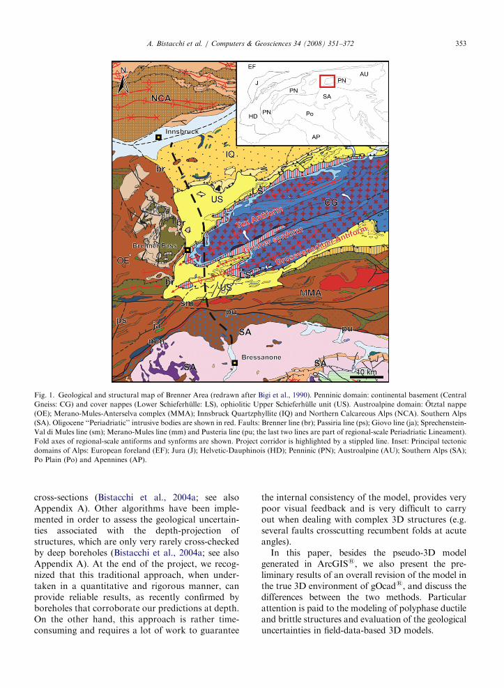
The case discussed in the paper concerns thestudy for a 57 km railway tunnel, which will even-tually connect the town of Fortezza (north ofBressanone) in Italy to Innsbruck in Austria. Thedesign corridor covers a large and strongly tecto-nized section of the Eastern Alps (Fig. 1), which willbe crossed by a tunnel that for long sections will beas deep as 1.5 km. During a project funded by anEU research grant and by BBT SE (the Italia-n–Austrian railway company in charge of theproject), a large body of new geological andstructural data were collected in the field. On theItalian side of the design corridor, these data consistof detailed geological maps at 1:10,000, or even1:5000 scale, about 3000 structural measurementstations, petrographic and microstructural analyses,and other measurements. On the other hand, nogeophysical data regarding the bedrock have beenacquired during the project. As a result of ourresearch project, a traditional pseudo-3D geologicalmodel was developed via a dense network ofinterconnected vertical and horizontal cross-sec-tions. We developed custom projection algorithms,mainly in ArcGISs, in order to (1) reconstruct thecross-sections by means of structural criteria and(2) ensure the internal consistency of this network of

ARTICLE IN PRESS

Fig. 1. Geological and structural map of Brenner Area (redrawn after Bigi et al., 1990). Penninic domain: continental basement (Central

Gneiss: CG) and cover nappes (Lower Schieferhulle: LS), ophiolitic Upper Schieferhulle unit (US). Austroalpine domain: Otztal nappe

(OE); Merano-Mules-Anterselva complex (MMA); Innsbruck Quartzphyllite (IQ) and Northern Calcareous Alps (NCA). Southern Alps

(SA). Oligocene ‘‘Periadriatic’’ intrusive bodies are shown in red. Faults: Brenner line (br); Passiria line (ps); Giovo line (ja); Sprechenstein-

Val di Mules line (sm); Merano-Mules line (mm) and Pusteria line (pu; the last two lines are part of regional-scale Periadriatic Lineament).

Fold axes of regional-scale antiforms and synforms are shown. Project corridor is highlighted by a stippled line. Inset: Principal tectonic

domains of Alps: European foreland (EF); Jura (J); Helvetic-Dauphinois (HD); Penninic (PN); Austroalpine (AU); Southern Alps (SA);

Po Plain (Po) and Apennines (AP).

A. Bistacchi et al. / Computers & Geosciences 34 (2008) 351–372 353

cross-sections (Bistacchi et al., 2004a; see alsoAppendix A). Other algorithms have been imple-mented in order to assess the geological uncertain-ties associated with the depth-projection ofstructures, which are only very rarely cross-checkedby deep boreholes (Bistacchi et al., 2004a; see alsoAppendix A). At the end of the project, we recog-nized that this traditional approach, when under-taken in a quantitative and rigorous manner, canprovide reliable results, as recently confirmed byboreholes that corroborate our predictions at depth.On the other hand, this approach is rather time-consuming and requires a lot of work to guarantee

the internal consistency of the model, provides verypoor visual feedback and is very difficult to carryout when dealing with complex 3D structures (e.g.several faults crosscutting recumbent folds at acuteangles).

In this paper, besides the pseudo-3D modelgenerated in ArcGISs, we also present the pre-liminary results of an overall revision of the model inthe true 3D environment of gOcads, and discuss thedifferences between the two methods. Particularattention is paid to the modeling of polyphase ductileand brittle structures and evaluation of the geologicaluncertainties in field-data-based 3D models.

ARTICLE IN PRESSA. Bistacchi et al. / Computers & Geosciences 34 (2008) 351–372354

2. Geological setting

2.1. Regional framework

The Alps originated by subduction and closure ofthe Mesozoic Tethyan ocean (Cretaceous–Eocene)and subsequent collision between the Europeanpassive continental margin and the Adriatic(African) active plate margin (Dal Piaz et al.,2003, and refs. therein). This geodynamic evolutiongenerated a collisional wedge that in the EasternAlps (Fig. 1) consists, from top to bottom, of (1) theAdria-derived Austroalpine continental basementand cover nappe system; (2) the Penninic systemexposed in the Tauern window, including (2a) theophiolite-bearing Upper Schieferhulle nappe and(2b) the underlying Europe-derived Tux-Grossve-nediger-Zillertal continental basement (CentralGneiss) and Permian-Mesozoic cover nappes (Low-er Schieferhulle). To the south, the Austroalpine–-Penninic wedge is laterally juxtaposed to the Adria-vergent Southern Alps (3) along the Periadriaticfault system, which, during the Oligocene, was apreferential channel for the rise and crustal empla-cement of magmas from mantle sources (post-collisional magmatism; 4).

The Penninic nappe stack exposed in the WesternTauern window is characterized, at a regional scale,by two E–W trending antiforms (Grossvenediger-Zillertal to the S and Tux to the N), where cores ofgneissic granitoids (Central Gneiss) and minorparaschists (Altes Dach) are separated by a narrowsynform (Greiner syncline) with ophiolitic andcontinental cover units (Upper and LowerSchieferhulle, respectively; Sander, 1929; Lammereret al., 1981; De Vecchi and Baggio, 1982; Lam-merer, 1986; Fig. 1) The penetrative foliationsassociated with the synform itself were afterwardsinvolved in a polyphase shear zone (Greiner shearzone; e.g. Selverstone, 1988, 1993; Steffen et al.,2001). In addition, the southern edge of the Tauernwindow is characterized by an overturned contactwhere the Upper Schieferhulle nappe lies over theAustroalpine units exposed to the south of thewindow. All these folds of the Penninic nappe stackare the product of Alpine ductile deformationsdeveloped under different metamorphic conditions.

To the west, the Central Gneiss and related coverunits (Lower Schieferhulle) disappear beneath theophiolitic Upper Schieferhulle, composed of domi-nant carbonaceous to terrigenous calcschists ofLate Jurassic–Early Cretaceous age and minor

metamorphic ophiolites (mainly greenschist faciesmetabasalts and rare serpentinite slices). This‘‘telescopic’’ disappearance was traditionally inter-preted to be the result of the gentle westward plungeof the two antiformal hinges (e.g. Bigi et al., 1990;Selverstone et al., 1995). In contrast, De Vecchi andBaggio (1982) explained this situation with a top-down-to-the-west tectonic transport alongNNE–SSW trending normal faults.

The collisional Penninic nappe stack is over-printed by a pervasive greenschist to amphibolitefacies metamorphism (Tauernkrystallisation ofSander, 1911) of Late Eocene–Early Oligocene age(Thoni, 1999, and refs. therein). Locally subduction-related blueschist facies metamorphism is preserved,as evidenced by scattered mineral–textural relics(core of Na-amphiboles, pseudomorphs after law-sonite; Selverstone et al., 1984; Selverstone, 1985;Selverstone and Spear, 1985).

The Oligocene post-collisional magmatism isdocumented in the study area by the granodioriticto tonalitic Rensen pluton (intruded within theAustroalpine basement), the Mules tonalitic ‘‘la-mella’’ (a sheet-like body intruded along thePusteria Fault, part of the Periadriatic system) andsome andesitic dykes (intruded in the Austroalpinebasement and Upper Schieferhulle calcschists),which yield Rb/Sr age on micas of 32–30Ma (Borsiet al., 1972, 1978; Muller et al., 2001; Mancktelowet al., 2001; Fig. 1).

2.2. Ductile deformation history

Our structural analysis allows us to infer theductile deformation history for this part of theTauern Window that partly differs from reconstruc-tions made by Selverstone (Selverstone, 1985, 1988,1993; Selverstone et al., 1993) and Lammerer(1990). The ductile regional architecture of this areais the final result of at least three Alpine deforma-tion phases (D1, D2 and D3), which can berecognized at the meso-scale and are well recordedin the Lower and Upper Schieferhulle, whilst themore competent Central Gneiss generally showsfewer penetrative foliations (Bistacchi et al., 2003).

In oceanic and continental cover sequences, phaseD1 is characterized by a S1 foliation locally pre-served in low-strain domains (with respect to thesubsequent deformations), generally correspondingto fold hinges. It is most likely that D1 is the onlypenetrative foliation in the Central Gneiss at theregional scale.

ARTICLE IN PRESSA. Bistacchi et al. / Computers & Geosciences 34 (2008) 351–372 355

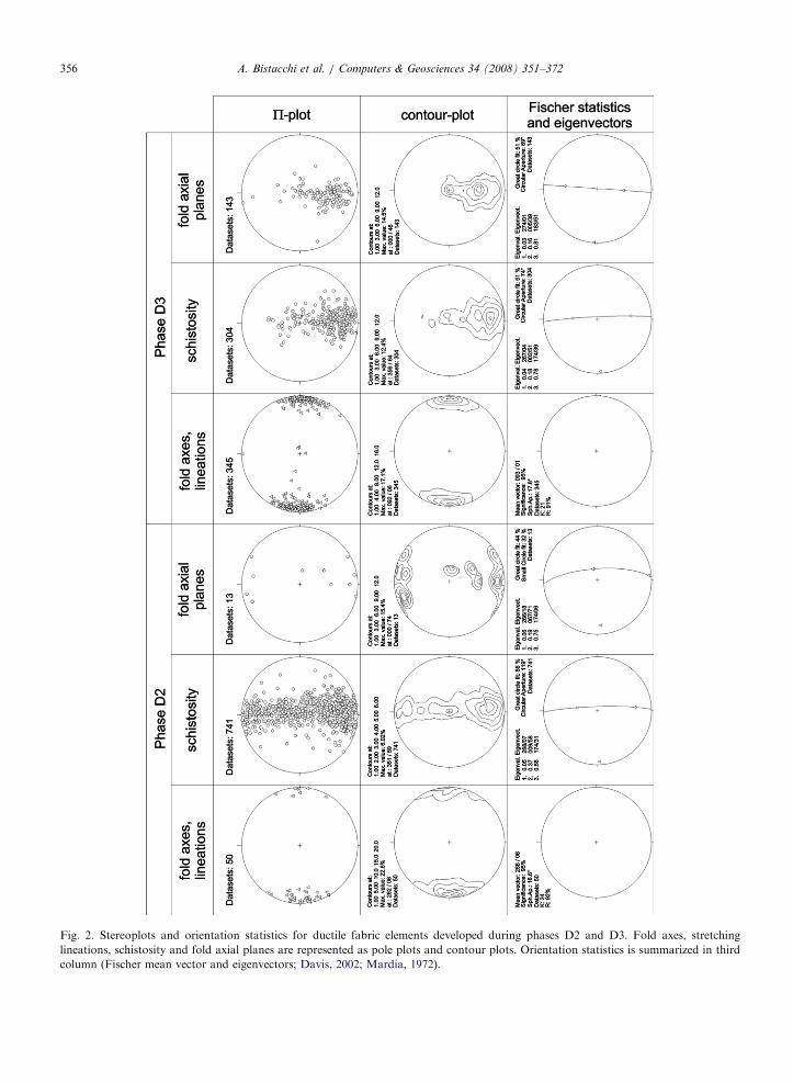
Foliation S2 dominates at the regional scale inLower and Upper Schieferhulle and is characterizedby mineral assemblages generated at amphibolite/high-temperature greenschist facies conditions andby E–W sub-horizontal stretching lineationsmarked by kyanite, hornblende and stretched lithicor quartz pebbles in some metaconglomerates.During this tectono-metamorphic event, an almostcomplete transposition of all lithological andtectonic boundaries has been accomplished. D2folds always show isoclinal geometries that arecharacterized by sub-horizontal E–W axes (Figs. 2and 3).

After phase D2, a static growth of biotite(Tauernkrystallisation, Sander, 1911) together withkyanite and hornblende produced characteristic‘‘Garbenschiefer’’ (sheafs schist, after the arrange-ment of elongated hornblende prisms), which can befound all over the Lower Schieferhulle.

Phase D3 results in meso- and megascopic openfolds showing E–W sub-horizontal axes andN-dipping axial planes (Fig. 2). S3 foliation,showing greenschist facies mineral assemblages,developed only locally in calcschists of the Greinersyncline (Vizze valley), and to the South, at theoverturned boundary between the Upper Schiefer-hulle unit and the Austroalpine basement. TheD3 E–W sub-horizontal stretching lineation ischaracterized by kyanite and hornblende micro-boudinage.

2.3. Ductile– brittle deformation history

Ductile–brittle SC shear bands with a sinistraltranscurrent to sinistral transtensive activity havebeen found all along the E–W trending Pennini-c–Austroalpine boundary zone characterized by S3foliation. This foliation is crosscut by some Oligo-cene dykes showing evidence of the same sinistralshearing. These findings agree with the observationsof Mancktelow et al. (2001).

The sinistral structures along E–W trends areoverprinted by dextral ductile–brittle shear bandskinematically consistent with the top-to-the-westextension recorded in greenschist facies mylonites ofthe Brenner detachment and associated shear bands.From the early Miocene onward, this is thekinematics that drives the Penninic unit denudationalong the Brenner low-angle detachment andthe eastward extrusion of the Tauern window(Selverstone, 1988; Behrmann, 1988; Ratschbacheret al., 1991).

2.4. Brittle deformation history

Structural analysis along the westernmost end ofthe Pusteria Fault (part of the Periadriatic Linea-ment) revealed a first deformation phase character-ized by sinistral transtension along E–W faults. Thisphase is followed by the well-known dextraltranspressional activity consistent with the eastwardescape at the footwall of the Brenner detachment(Mancktelow et al., 2001; Ratschbacher et al., 1991)Both tectonic regimes were developed under brittleconditions along the Pusteria fault, but the age ofthe first phase is not yet well understood.

A major WNW–ESE shear zone, known as the‘‘Sprechenstein-Val di Mules fault system’’, con-nects the Brenner detachment to the Pusteria line(Bistacchi et al., 2003, 2004b). This fault system canbe followed from the Sprechenstein castle (south ofthe Vipiteno alluvial plain), through the MulesValley, where it displaces the Pusteria fault, to theValles Valley, where it is evidenced by a widecataclastic horizon inside the Bressanone granite.The dextral offset of the Sprechenstein-Val di Mulesfault can be estimated in 4.5 km in the northernsector, where it cuts the Austroalpine–UpperSchieferhulle boundary. Toward the South, thedisplacement decreases to 2 km where it is parti-tioned among multiple faults showing thick fault-rock horizons (gouge and cataclasites).

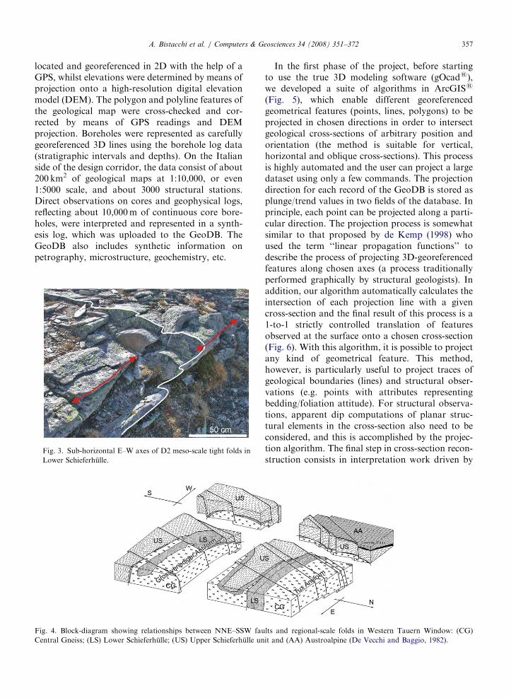
In the westernmost Tauern Window, the Tux andGrossvenediger-Zillertal antiforms are pervasivelydissected by steep NNE–SSW and NE–SW trendingfaults, which also cut the Southern AustroalpineMerano-Mules unit and the Oligocene Rensenpluton. At the meso- and mega-scale, D2 and D3fold axes follow an E–W, sub-horizontal trend. Theprogressive westward deepening of the folded nappestack (the structurally deeper units are well exposedto the east, but progressively disappear to the west)is due to this penetrative system of west dippingnormal faults, defining a ‘‘staircase’’ structurealready envisaged by De Vecchi and Baggio (1982)(Fig. 4).

3. 3D geological modeling

Geological modeling for the sector betweenFortezza (N of Bressanone) and the Italy–Austriapolitical boundary was carried out taking intoaccount structural data and detailed geologicalmaps organized in a geological database (GeoDB)implemented in ArcGISs. Structural stations were

ARTICLE IN PRESS

Fig. 2. Stereoplots and orientation statistics for ductile fabric elements developed during phases D2 and D3. Fold axes, stretching

lineations, schistosity and fold axial planes are represented as pole plots and contour plots. Orientation statistics is summarized in third

column (Fischer mean vector and eigenvectors; Davis, 2002; Mardia, 1972).

A. Bistacchi et al. / Computers & Geosciences 34 (2008) 351–372356

ARTICLE IN PRESSA. Bistacchi et al. / Computers & Geosciences 34 (2008) 351–372 357

located and georeferenced in 2D with the help of aGPS, whilst elevations were determined by means ofprojection onto a high-resolution digital elevationmodel (DEM). The polygon and polyline features ofthe geological map were cross-checked and cor-rected by means of GPS readings and DEMprojection. Boreholes were represented as carefullygeoreferenced 3D lines using the borehole log data(stratigraphic intervals and depths). On the Italianside of the design corridor, the data consist of about200 km2 of geological maps at 1:10,000, or even1:5000 scale, and about 3000 structural stations.Direct observations on cores and geophysical logs,reflecting about 10,000m of continuous core bore-holes, were interpreted and represented in a synth-esis log, which was uploaded to the GeoDB. TheGeoDB also includes synthetic information onpetrography, microstructure, geochemistry, etc.

Fig. 3. Sub-horizontal E–W axes of D2 meso-scale tight folds in

Lower Schieferhulle.

Fig. 4. Block-diagram showing relationships between NNE–SSW fau

Central Gneiss; (LS) Lower Schieferhulle; (US) Upper Schieferhulle un

In the first phase of the project, before startingto use the true 3D modeling software (gOcads),we developed a suite of algorithms in ArcGISs

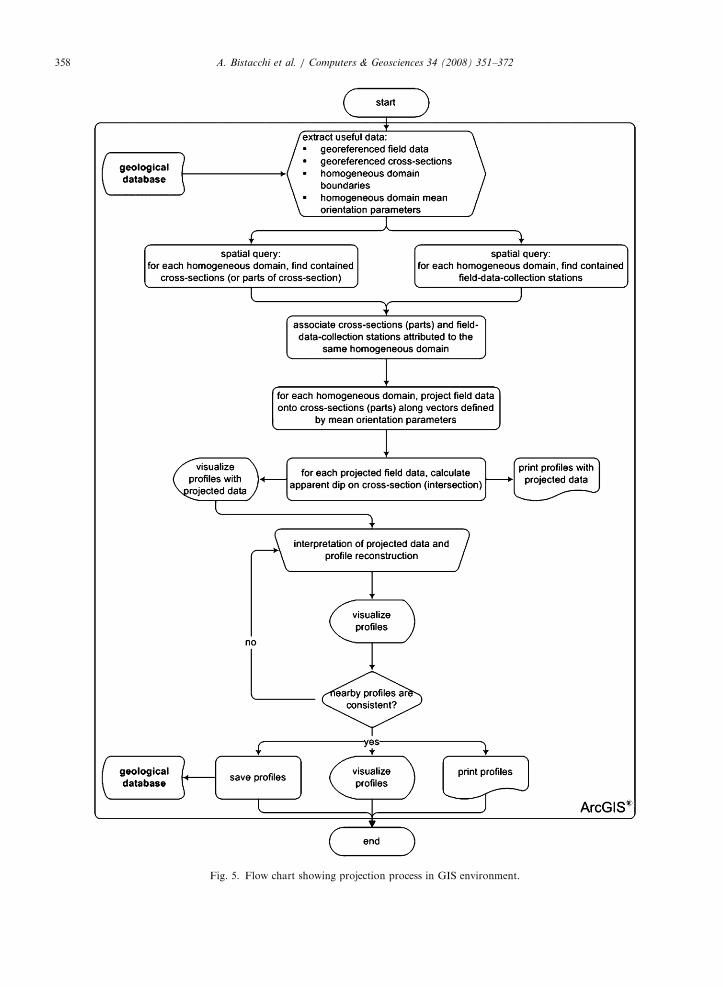
(Fig. 5), which enable different georeferencedgeometrical features (points, lines, polygons) to beprojected in chosen directions in order to intersectgeological cross-sections of arbitrary position andorientation (the method is suitable for vertical,horizontal and oblique cross-sections). This processis highly automated and the user can project a largedataset using only a few commands. The projectiondirection for each record of the GeoDB is stored asplunge/trend values in two fields of the database. Inprinciple, each point can be projected along a parti-cular direction. The projection process is somewhatsimilar to that proposed by de Kemp (1998) whoused the term ‘‘linear propagation functions’’ todescribe the process of projecting 3D-georeferencedfeatures along chosen axes (a process traditionallyperformed graphically by structural geologists). Inaddition, our algorithm automatically calculates theintersection of each projection line with a givencross-section and the final result of this process is a1-to-1 strictly controlled translation of featuresobserved at the surface onto a chosen cross-section(Fig. 6). With this algorithm, it is possible to projectany kind of geometrical feature. This method,however, is particularly useful to project traces ofgeological boundaries (lines) and structural obser-vations (e.g. points with attributes representingbedding/foliation attitude). For structural observa-tions, apparent dip computations of planar struc-tural elements in the cross-section also need to beconsidered, and this is accomplished by the projec-tion algorithm. The final step in cross-section recon-struction consists in interpretation work driven by

lts and regional-scale folds in Western Tauern Window: (CG)

it and (AA) Austroalpine (De Vecchi and Baggio, 1982).

ARTICLE IN PRESS

Fig. 5. Flow chart showing projection process in GIS environment.

A. Bistacchi et al. / Computers & Geosciences 34 (2008) 351–372358

ARTICLE IN PRESS

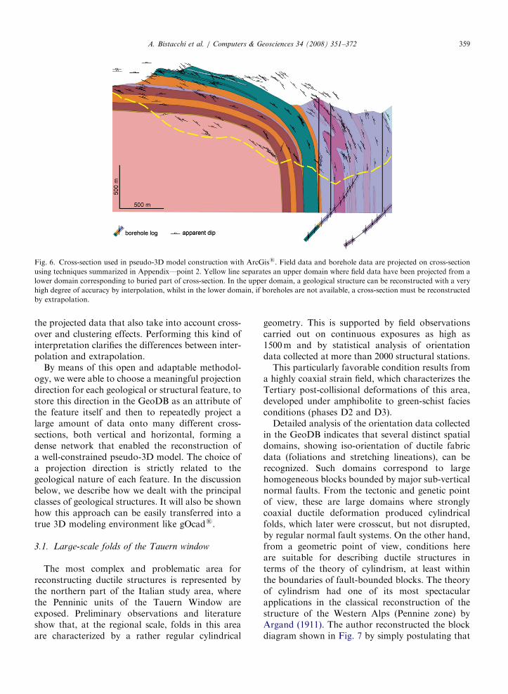
Fig. 6. Cross-section used in pseudo-3D model construction with ArcGiss. Field data and borehole data are projected on cross-section

using techniques summarized in Appendix—point 2. Yellow line separates an upper domain where field data have been projected from a

lower domain corresponding to buried part of cross-section. In the upper domain, a geological structure can be reconstructed with a very

high degree of accuracy by interpolation, whilst in the lower domain, if boreholes are not available, a cross-section must be reconstructed

by extrapolation.

A. Bistacchi et al. / Computers & Geosciences 34 (2008) 351–372 359

the projected data that also take into account cross-over and clustering effects. Performing this kind ofinterpretation clarifies the differences between inter-polation and extrapolation.

By means of this open and adaptable methodol-ogy, we were able to choose a meaningful projectiondirection for each geological or structural feature, tostore this direction in the GeoDB as an attribute ofthe feature itself and then to repeatedly project alarge amount of data onto many different cross-sections, both vertical and horizontal, forming adense network that enabled the reconstruction ofa well-constrained pseudo-3D model. The choice ofa projection direction is strictly related to thegeological nature of each feature. In the discussionbelow, we describe how we dealt with the principalclasses of geological structures. It will also be shownhow this approach can be easily transferred into atrue 3D modeling environment like gOcads.

3.1. Large-scale folds of the Tauern window

The most complex and problematic area forreconstructing ductile structures is represented bythe northern part of the Italian study area, wherethe Penninic units of the Tauern Window areexposed. Preliminary observations and literatureshow that, at the regional scale, folds in this areaare characterized by a rather regular cylindrical

geometry. This is supported by field observationscarried out on continuous exposures as high as1500m and by statistical analysis of orientationdata collected at more than 2000 structural stations.

This particularly favorable condition results froma highly coaxial strain field, which characterizes theTertiary post-collisional deformations of this area,developed under amphibolite to green-schist faciesconditions (phases D2 and D3).

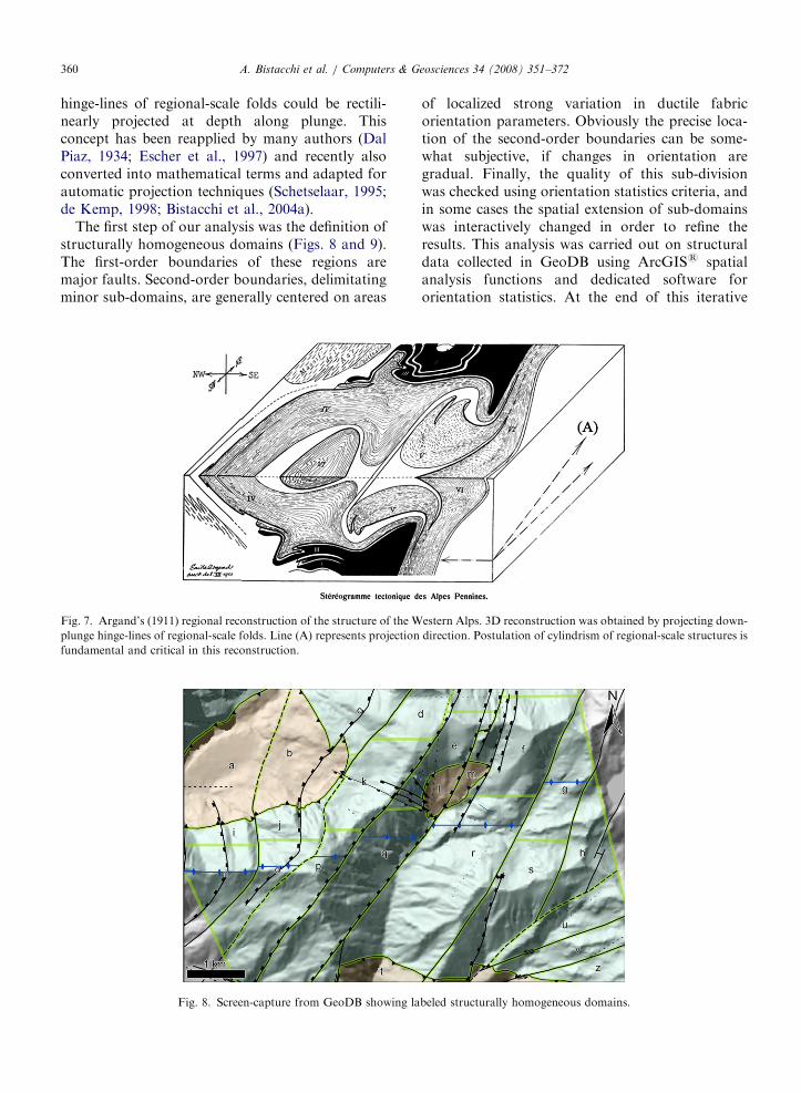
Detailed analysis of the orientation data collectedin the GeoDB indicates that several distinct spatialdomains, showing iso-orientation of ductile fabricdata (foliations and stretching lineations), can berecognized. Such domains correspond to largehomogeneous blocks bounded by major sub-verticalnormal faults. From the tectonic and genetic pointof view, these are large domains where stronglycoaxial ductile deformation produced cylindricalfolds, which later were crosscut, but not disrupted,by regular normal fault systems. On the other hand,from a geometric point of view, conditions hereare suitable for describing ductile structures interms of the theory of cylindrism, at least withinthe boundaries of fault-bounded blocks. The theoryof cylindrism had one of its most spectacularapplications in the classical reconstruction of thestructure of the Western Alps (Pennine zone) byArgand (1911). The author reconstructed the blockdiagram shown in Fig. 7 by simply postulating that

ARTICLE IN PRESSA. Bistacchi et al. / Computers & Geosciences 34 (2008) 351–372360

hinge-lines of regional-scale folds could be rectili-nearly projected at depth along plunge. Thisconcept has been reapplied by many authors (DalPiaz, 1934; Escher et al., 1997) and recently alsoconverted into mathematical terms and adapted forautomatic projection techniques (Schetselaar, 1995;de Kemp, 1998; Bistacchi et al., 2004a).

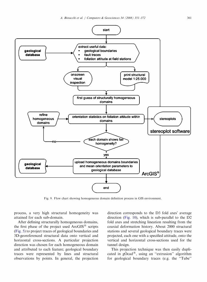
The first step of our analysis was the definition ofstructurally homogeneous domains (Figs. 8 and 9).The first-order boundaries of these regions aremajor faults. Second-order boundaries, delimitatingminor sub-domains, are generally centered on areas

Fig. 7. Argand’s (1911) regional reconstruction of the structure of the W

plunge hinge-lines of regional-scale folds. Line (A) represents projection

fundamental and critical in this reconstruction.

Fig. 8. Screen-capture from GeoDB showing la

of localized strong variation in ductile fabricorientation parameters. Obviously the precise loca-tion of the second-order boundaries can be some-what subjective, if changes in orientation aregradual. Finally, the quality of this sub-divisionwas checked using orientation statistics criteria, andin some cases the spatial extension of sub-domainswas interactively changed in order to refine theresults. This analysis was carried out on structuraldata collected in GeoDB using ArcGISs spatialanalysis functions and dedicated software fororientation statistics. At the end of this iterative

estern Alps. 3D reconstruction was obtained by projecting down-

direction. Postulation of cylindrism of regional-scale structures is

beled structurally homogeneous domains.

ARTICLE IN PRESS

Fig. 9. Flow chart showing homogeneous domain definition process in GIS environment.

A. Bistacchi et al. / Computers & Geosciences 34 (2008) 351–372 361

process, a very high structural homogeneity wasattained for each sub-domain.

After defining structurally homogeneous domains,the first phase of the project used ArcGISs scripts(Fig. 5) to project traces of geological boundaries and3D-georeferenced structural data onto vertical andhorizontal cross-sections. A particular projectiondirection was chosen for each homogeneous domainand attributed to each feature; geological boundarytraces were represented by lines and structuralobservations by points. In general, the projection

direction corresponds to the D3 fold axes’ averagedirection (Fig. 10), which is sub-parallel to the D2fold axes and stretching lineation resulting from thecoaxial deformation history. About 2000 structuralstations and several geological boundary traces wereprojected, each one with a specified attitude, onto thevertical and horizontal cross-sections used for thetunnel design.

This projection technique was then easily dupli-cated in gOcads, using an ‘‘extrusion’’ algorithmfor geological boundary traces (e.g. the ‘‘Tube’’

ARTICLE IN PRESS

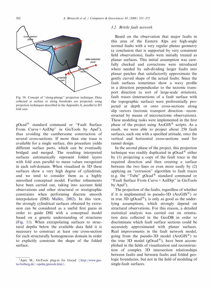
Fig. 10. Concept of ‘‘along-plunge’’ projection technique. Data

collected at surface or along boreholes are projected, using

projection techniques described in the Appendix A, parallel to D3

fold axis.

A. Bistacchi et al. / Computers & Geosciences 34 (2008) 351–372362

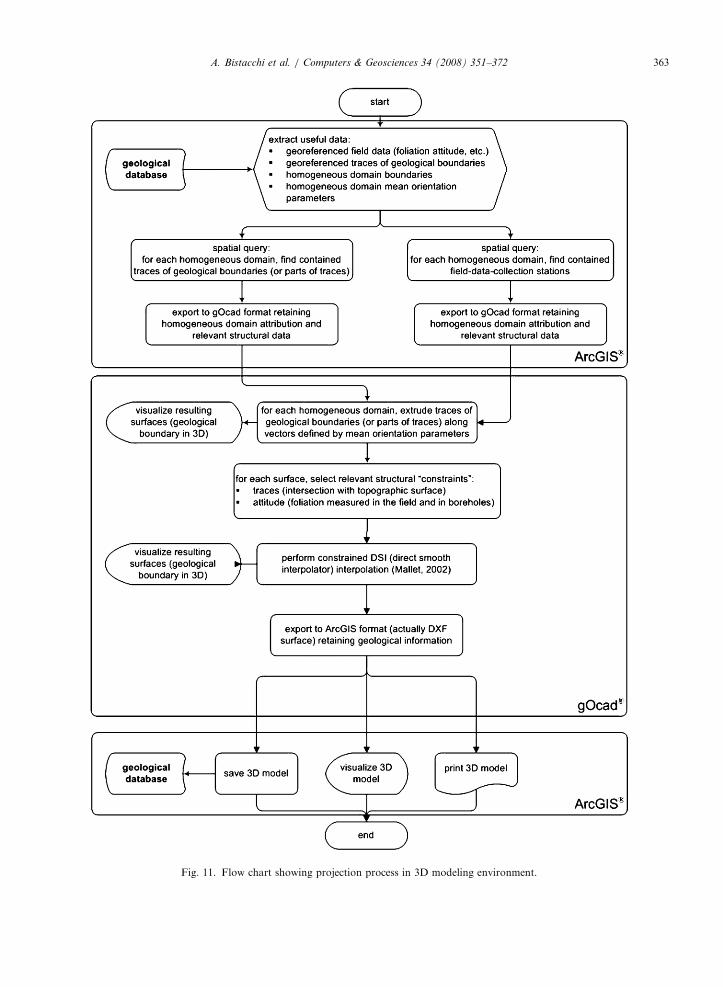
gOcads standard command or ‘‘Fault SurfaceFrom Curve+AziDip’’ in GisTools by Apel1),thus avoiding the cumbersome construction ofseveral cross-sections. If more than one trace isavailable for a single surface, this procedure yieldsdifferent surface parts, which can be eventuallybridged and merged. The resulting interpretedsurfaces automatically represent folded layerswith fold axes parallel to mean values recognizedin each sub-domain. When visualized in 3D thesesurfaces show a very high degree of cylindrism,and we tend to consider them as a highlysmoothed conceptual model. Further refinementshave been carried out, taking into account fieldobservations and other structural or stratigraphicconstraints when performing discrete smoothinterpolation (DSI) Mallet, 2002). In this view,the strongly cylindrical surfaces obtained by extru-sion can be considered as a useful first guess inorder to guide DSI with a conceptual modelbased on a genetic understanding of structures(Fig. 11). When extrapolating surfaces to struc-tural depths below the available data field it isnecessary to construct at least one cross-sectionfor each structurally homogeneous domain in orderto explicitly constrain the shape of the foldedsurface.

1Apel, M., GisTools plug-in for Gocad /http://www.geo.

tu-freiberg.de/�apelm/gistools.htmS.

3.2. Brittle fault network

Based on the observation that major faults inthis area of the Eastern Alps are high-anglenormal faults with a very regular planar geometry(a conclusion that is supported by very consistentfield observations), faults were initially treated asplanar surfaces. This initial assumption was care-fully checked and corrections were introducedwhere needed by sub-dividing larger faults intoplanar patches that satisfactorily approximate thegently curved shape of the actual faults. Since thefault surfaces sometimes show a wavy profilein a direction perpendicular to the tectonic trans-port direction (a sort of large-scale striation),fault traces (intersections of a fault surface withthe topographic surface) were preferentially pro-jected at depth or onto cross-sections alongslip vectors (tectonic transport direction—recon-structed by means of microtectonic observations).These modeling tasks were implemented in the firstphase of the project using ArcGISs scripts. As aresult, we were able to project about 250 faultsurfaces, each one with a specified attitude, onto thevertical and horizontal cross-sections used fortunnel design.

In the second phase of the project, this projectiontechnique was readily duplicated in gOcads eitherby (1) projecting a copy of the fault trace in therequired direction and then creating a surfacebetween the two lines or even more easily by (2)applying an ‘‘extrusion’’ algorithm to fault traces(e.g. the ‘‘Tube’’ gOcads standard command or‘‘Fault Surface From Curve+AziDip’’ in GisToolsby Apel1).

The projection of the faults, regardless of whetherif it is implemented in pseudo-3D (ArcGISs) orin true 3D (gOcads), is only as good as the under-lying assumptions, which strongly depend onstructural observations. For this reason, a detailedstatistical analysis was carried out on orienta-tion data collected in the GeoDB in order todiscriminate which fault surface sections could beaccurately approximated with planar surfaces.Real improvements in the fault network model,going from the pseudo-3D model (ArcGISs) tothe true 3D model (gOcads), have been accom-plished in the fields of visualization and reconstruc-tion of complex 3D intersection relationshipsbetween faults and between faults and folded geo-logic boundaries, but not in the field of modeling ofsingle-fault surfaces.

ARTICLE IN PRESS

Fig. 11. Flow chart showing projection process in 3D modeling environment.

A. Bistacchi et al. / Computers & Geosciences 34 (2008) 351–372 363

ARTICLE IN PRESSA. Bistacchi et al. / Computers & Geosciences 34 (2008) 351–372364

3.3. Intrusive bodies of the periadriatic lineament

Some magmatic bodies exposed along the Peria-driatic fault system show primary intrusive bound-aries, whose projection at depth can be consideredunreliable due to their irregular geometry. Forinstance, the intrusive boundary of the Rensen calc-alkaline pluton is characterized by structures typicalof a shallow intrusion with evidence of stoping, suchas inclusion of roof pendants in the magmatic body,a dense networks of dikes, etc. This boundary showsvery irregular and poorly predictable geometries atthe map scale (1:10,000). Without any independentinformation on their behavior at depth (geophysics,

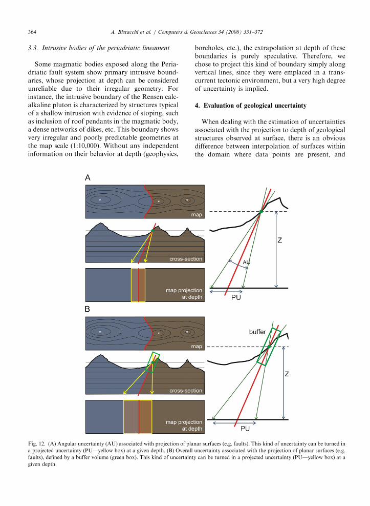
Fig. 12. (A) Angular uncertainty (AU) associated with projection of pla

a projected uncertainty (PU—yellow box) at a given depth. (B) Overall

faults), defined by a buffer volume (green box). This kind of uncertaint

given depth.

boreholes, etc.), the extrapolation at depth of theseboundaries is purely speculative. Therefore, wechose to project this kind of boundary simply alongvertical lines, since they were emplaced in a trans-current tectonic environment, but a very high degreeof uncertainty is implied.

4. Evaluation of geological uncertainty

When dealing with the estimation of uncertaintiesassociated with the projection to depth of geologicalstructures observed at surface, there is an obviousdifference between interpolation of surfaces withinthe domain where data points are present, and

nar surfaces (e.g. faults). This kind of uncertainty can be turned in

uncertainty associated with the projection of planar surfaces (e.g.

y can be turned in a projected uncertainty (PU—yellow box) at a

ARTICLE IN PRESS

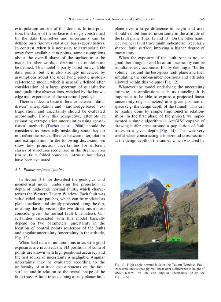
Fig. 13. High-angle normal fault in the Tauern Window. Fault

trace (red line) is strongly rectilinear over a difference in height of

about 600m. Pin line and angular uncertainty (AU): see

Fig. 12(A).

A. Bistacchi et al. / Computers & Geosciences 34 (2008) 351–372 365

extrapolation outside of this domain. In interpola-tion, the shape of the surface is strongly constrainedby the data themselves and uncertainty can bedefined on a rigorous statistical basis (geostatistics).In contrast, when it is necessary to extrapolate faraway from available data points, some assumptionsabout the overall shape of the surface must bemade. In other words, a deterministic model mustbe defined. This model is partly based on availabledata points, but it is also strongly influenced byassumptions about the underlying genetic geologi-cal–tectonic model, which is generally defined afterconsideration of a large spectrum of quantitativeand qualitative observations, weighed by the knowl-edge and experience of the structural geologist.

There is indeed a basic difference between ‘‘data-driven’’ interpolation and ‘‘knowledge-based’’ ex-trapolation, and uncertainty should be evaluatedaccordingly. From this perspective, attempts atestimating extrapolation uncertainties using geosta-tistical methods (Tacher et al., 2006) should beconsidered as potentially misleading since they donot reflect the basic difference between interpolationand extrapolation. In the following discussion, weshow how projection uncertainties for differentclasses of structures recognized in the Brenner area(thrust, fault, folded boundary, intrusive boundary)have been evaluated.

4.1. Planar surfaces (faults)

In Section 3.1, we described the geological andgeometrical model underlying the projection atdepth of high-angle normal faults, which charac-terizes the Western Tauern Window. Each fault wassub-divided into patches, which can be modeled asplanar surfaces and simply projected along the dip,or along the slip vector (the two directions almostcoincide, given the normal fault kinematics). Un-certainties associated with this model basicallydepend on two parameters: uncertainty in thelocation of control points (outcrops of the fault)and angular uncertainty (uncertainty in the attitude,Fig. 12).

When field data in mountainous areas with goodexposures are involved, the 3D positions of controlpoints are known with high positional accuracy andthe first source of uncertainty is negligible. Angularuncertainty may be evaluated according to theuniformity of attitude measurements on the faultsurface, and in relation to the overall shape of thefault trace. A fault trace defining a truly planar fault

plane over a large difference in height and areashould exhibit limited uncertainty in the attitude ofthe fault plane (Figs. 12 and 13). On the other hand,a curvilinear fault trace might indicate an irregularlyshaped fault surface, implying a higher degree ofuncertainty.

When the exposure of the fault zone is not sogood, both angular and location uncertainty can besimultaneously accounted for by defining a ‘‘buffervolume’’ around the best-guess fault plane and thensimulating the end-member positions and attitudesallowed within this volume (Fig. 12).

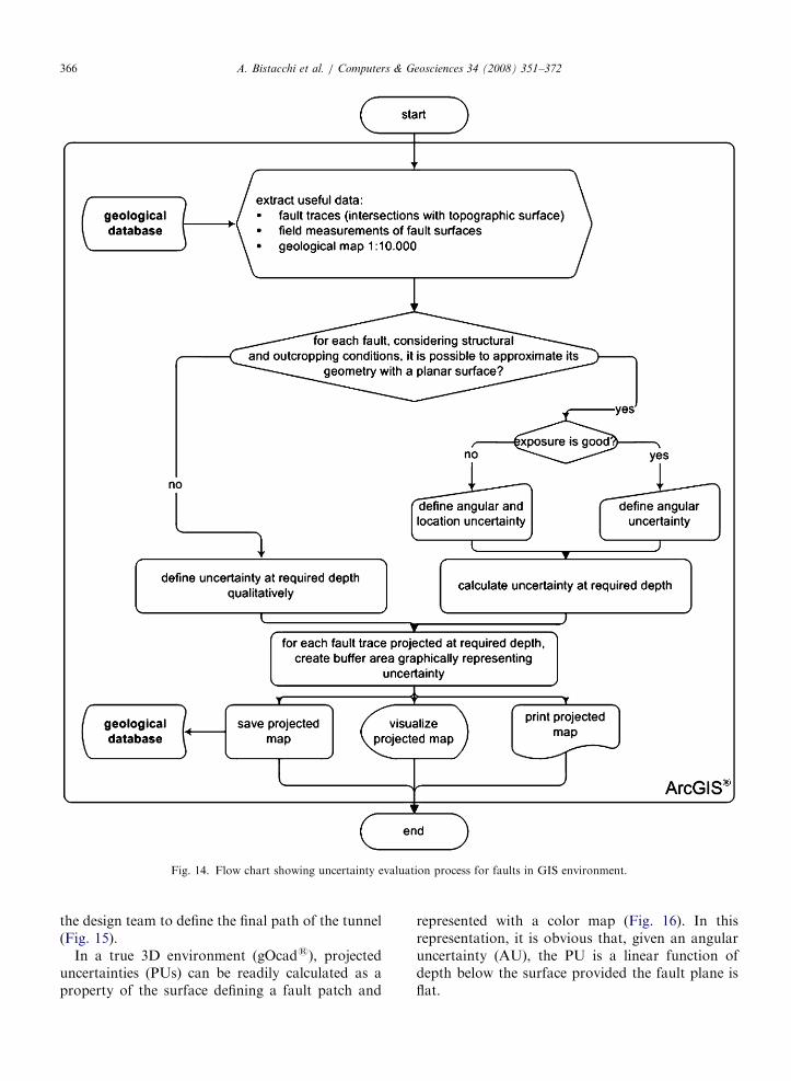
Whatever the model underlying the uncertaintyestimate, in applications such as tunneling it isimportant to be able to express a projected linearuncertainty (e.g. in meters) at a given position inspace (e.g. the design depth of the tunnel). This canbe readily done by simple trigonometric relation-ships. In the first phase of the project, we imple-mented a simple algorithm in ArcGISs capable ofdrawing buffer areas around a population of faulttraces at a given depth (Fig. 14). This was veryuseful when constructing a horizontal cross-sectionat the design depth of the tunnel, which was used by

ARTICLE IN PRESS

Fig. 14. Flow chart showing uncertainty evaluation process for faults in GIS environment.

A. Bistacchi et al. / Computers & Geosciences 34 (2008) 351–372366

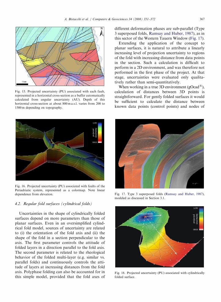
the design team to define the final path of the tunnel(Fig. 15).

In a true 3D environment (gOcads), projecteduncertainties (PUs) can be readily calculated as aproperty of the surface defining a fault patch and

represented with a color map (Fig. 16). In thisrepresentation, it is obvious that, given an angularuncertainty (AU), the PU is a linear function ofdepth below the surface provided the fault plane isflat.

ARTICLE IN PRESS

Fig. 15. Projected uncertainty (PU) associated with each fault,

represented in a horizontal cross-section as a buffer automatically

calculated from angular uncertainty (AU). Depth of this

horizontal cross-section at about 800ma.s.l. varies from 200 to

1500m depending on topography.

Fig. 16. Projected uncertainty (PU) associated with faults of the

Periadriatic system, represented as a colormap. Note linear

dependence from elevation. Fig. 17. Type 3 superposed folds (Ramsay and Huber, 1987),

modeled as discussed in Section 3.1.

Fig. 18. Projected uncertainty (PU) associated with cylindrically

folded surface.

A. Bistacchi et al. / Computers & Geosciences 34 (2008) 351–372 367

4.2. Regular fold surfaces (cylindrical folds)

Uncertainties in the shape of cylindrically foldedsurfaces depend on more parameters than those ofplanar surfaces. Even in an oversimplified cylind-rical fold model, sources of uncertainty are relatedto (i) the orientation of the fold axis and (ii) theshape of the fold in a section perpendicular to theaxis. The first parameter controls the attitude offolded layers in a direction parallel to the fold axis.The second parameter is related to the rheologicalbehavior of the folded multi-layer (e.g. similar vs.parallel folds) and continuously controls the atti-tude of layers at increasing distances from the foldaxis. Polyphase folding can also be accounted for inthis simple model, provided that the fold axes of

different deformation phases are sub-parallel (Type3 superposed folds, Ramsay and Huber, 1987), as inthis sector of the Western Tauern Window (Fig. 17).

Extending the application of the concept toplanar surfaces, it is natural to attribute a linearlyincreasing level of projection uncertainty to regionsof the fold with increasing distance from data pointsin the section. Such a calculation is difficult toperform in a 2D environment, and was therefore notperformed in the first phase of the project. At thatstage, uncertainties were evaluated only qualita-tively rather than semi-quantitatively.

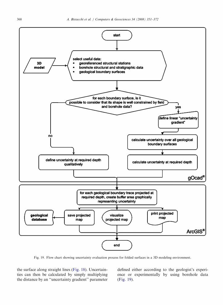
When working in a true 3D environment (gOcads),calculation of distances between 3D points isstraightforward. For gently folded surfaces it wouldbe sufficient to calculate the distance betweenknown data points (control points) and nodes of

ARTICLE IN PRESS

Fig. 19. Flow chart showing uncertainty evaluation process for folded surfaces in a 3D modeling environment.

A. Bistacchi et al. / Computers & Geosciences 34 (2008) 351–372368

the surface along straight lines (Fig. 18). Uncertain-ties can then be calculated by simply multiplyingthe distance by an ‘‘uncertainty gradient’’ parameter

defined either according to the geologist’s experi-ence or experimentally by using borehole data(Fig. 19).

ARTICLE IN PRESSA. Bistacchi et al. / Computers & Geosciences 34 (2008) 351–372 369

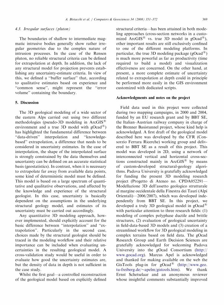
4.3. Irregular surfaces (pluton)

The boundaries of shallow to intermediate mag-matic intrusive bodies generally show rather irre-gular geometries due to the complex nature ofintrusion processes. In the case of the Rensenpluton, no reliable structural criteria can be definedfor extrapolation at depth. In addition, the lack ofany structural model for projection prevents estab-lishing any uncertainty-estimate criteria. In view ofthis, we defined a ‘‘buffer surface’’ that, accordingto qualitative estimates based on experience and‘‘common sense’’, might represent the ‘‘errorvolume’’ containing the boundary.

5. Discussion

The 3D geological modeling of a wide sector ofthe eastern Alps carried out using two differentmethodologies (pseudo-3D modeling in ArcGISs

environment and a true 3D model with gOcads)has highlighted the fundamental difference between‘‘data-driven’’ interpolation and ‘‘knowledge-based’’ extrapolation, a difference that needs to beconsidered in uncertainty estimates. In the case ofinterpolation, the shape of the interpolated surfaceis strongly constrained by the data themselves anduncertainty can be defined on an accurate statisticalbasis (geostatistics). In contrast, when it is necessaryto extrapolate far away from available data points,some kind of deterministic model must be defined.This model is based on a large spectrum of quanti-tative and qualitative observations, and affected bythe knowledge and experience of the structuralgeologist. In this case, uncertainty is basicallydependent on the assumptions in the underlyingstructural geology model, and estimates of itsuncertainty must be carried out accordingly.

Any quantitative 3D modeling approach, how-ever implemented, should explicitly account for thebasic difference between ‘‘interpolation’’ and ‘‘ex-trapolation’’. Particularly in the second case,choices made by the structural geologist should betraced in the modeling workflow and their relativeimportance can be included when evaluating un-certainties in the resulting geological model. Across-validation study would be useful in order toevaluate how good the uncertainty estimates are,but the density of data in depth is not sufficient inthe case study.

Whilst the first goal—a controlled reconstructionof the geological model based on explicitly defined

structural criteria—has been attained in both mode-ling approaches (cross-section networks in a custo-mized ArcGISs vs. true 3D model in gOcads),other important results are still exclusively confinedto one of the different modeling platforms. Inparticular, the true 3D modeling package (gOcads)is much more powerful as far as productivity (timerequired to build a model) and visualizationeffectiveness are concerned. On the other hand, atpresent, a more complete estimate of uncertaintyrelated to extrapolation at depth could in principlebe performed more easily in the GIS environmentcustomized with dedicated scripts.

Acknowledgments and notes on the project

Field data used in this project were collectedduring two mapping campaigns, in 2000 and 2004,funded by an EU research grant and by BBT SE,the Italian–Austrian railway company in charge ofthe Brenner Basistunnel project, whose kind help isacknowledged. A first draft of the geological modeldescribed here was developed by the CFR (Con-sorzio Ferrara Ricerche) working group and deliv-ered to BBT SE as a result of this project. Thismodel was developed in 2D, using a network ofinterconnected vertical and horizontal cross-sec-tions constructed mainly in ArcGISs by meansof custom-developed structural-geology algori-thms. Padova University is gratefully acknowledgedfor funding the present 3D modeling researchproject (Progetto di Ateneo no. CPDA052291—Modellazione 3D dell’assetto geologico strutturaleal margine occidentale della Finestra dei Tauri (AlpiOrientali)—2006/2007), which was developed inde-pendently from BBT SE. In this project, wedeveloped a truly 3D geological model in gOcads

with particular attention to three research fields: (1)modeling of complex polyphase ductile and brittlestructures, (2) evaluation of geological uncertaintyin field-data-based 3D models and (3) creation of astreamlined workflow for 3D geological modeling incomplex terrains based on field data. The gOcadResearch Group and Earth Decision Sciences aregratefully acknowledged for welcoming PadovaUniversity into the gOcad Consortium (http://www.gocad.org). Marcus Apel is acknowledgedand thanked for making available on the web theGisTools plug-in for gOcads (http://www.geo.tu-freiberg.de/�apelm/gistools.htm). We thankErnst Schetselaar and an anonymous reviewerwhose insightful comments substantially improved

ARTICLE IN PRESSA. Bistacchi et al. / Computers & Geosciences 34 (2008) 351–372370

this manuscript. We thank Simon Crowhurst for therevision of the English text and useful scientificdiscussions.

Appendix A. Tools for extrapolation in 3D of

structural elements

In the following, we deal with the main points ofprojection and uncertainty estimate techniques. Thesource code of ArcGiss and gOcads scripts has notbeen included because it is very specific to the geo-logical database structure, and, even if it canadapted to other projects, it would be very hard tounderstand the code without the database itself,which cannot be published for confidentiality issues.

A.1. Building a pseudo-3D model with a network of

consistent interconnected cross-sections

The basic condition for building a pseudo-3Dmodel using 2D GIS tools was realized by setting upa system of (almost entirely) automatically inter-connected reference frames, which ensures thegeometrical coherence of geological objects recon-structed in map view and in cross-sections.

The solution to this problem lies in setting up aglobal reference frame in the map view (the UTMWGS84 coordinate system in the case studied), andone local reference frame for each cross-section.Local reference frames can be defined arbitrarily,even for oblique (non-vertical) cross-sections, but aconvenient frame for vertical cross-sections hasbeen realized by establishing (1) a vertical axis,using the same elevation value as the map view (notransformation needed from map to cross-section)and (2) a horizontal axis corresponding to thedistance measured from the origin of the cross-section along its map trace. The coordinate trans-formation for the horizontal axis could be given byPythagoras’ theorem:

xcs ¼

ffiffiffiffiffiffiffiffiffiffiffiffiffiffiffiffiffiffiffiffiffiffiffiffiffiffiffiffiffiffiffiffiffiffiffiffiffiffiffiffiffiffiffiffiffiffiffiffiðxm � xoÞ

2þ ðym � yoÞ

2

q,

where xcs is the horizontal coordinate in the cross-section frame, xm, ym are map coordinates and xo, yo

is the vertex (origin) of the trace of the cross-section.Alternatively, if we take the trace of cross-

sections in the map view as m-shapefiles, we canobtain the distance from the cross-section originby linear referencing (also referred to as dyna-mic segmentation; ESRI, 2004). In this case,location is directly given in terms of position, or

measurement, along a linear feature (the map traceof the cross-section). Apart from being moreintuitive, linear referencing is already implementedin ArcGISs and is more flexible, since it can be alsoapplied to curved cross-sections. The only require-ment is that traces of cross-sections must be definedconsistently with oriented polylines, starting fromthe origin of the local cross-section reference frame.

A.2. Projection of structural elements along

arbitrary lines

In order to reconstruct cross-sections with thehighest accuracy and efficiency, it is important to beable to project onto arbitrary cross-sections, andalong arbitrary vectors, structural elements definedon the geological map (data collection stations,traces of geological boundaries or faults, etc.) oralong boreholes (e.g. dipmeter data). From a 3Dgeometry point of view, this is just a problem offinding the intersection between a vector (originat-ing from the object to be projected) and a plane(the cross-section).

A straight line through a given point is para-metrically defined as

x ¼ xo þ l

sin t cosð�pÞ

cos t cosð�pÞ

sinð�pÞ

�������

�������, (1)

where xo,is the origin point (vectors in bold), l is aparameter measuring the distance from xo, and tand p are trend and plunge, respectively.

The equation of a plane through a given point is

x ¼ xo þ g

sinðd� p=2Þ

cosðd� p=2Þ

0

�������

�������þ m

sin d cosð�jÞ

cos d cosð�jÞ

sinð�jÞ

�������

�������, (2)

where xo is the origin point (vectors in bold), g and mare along-strike and along-dip distance parameters,and d and j are dip direction and dip, respectively.

The intersection between the projection line andthe cross-section plane can be easily found bysolving for parameters l, g and m, the linear systemof equations obtained by combining (1) and (2) andthen substituting l in (1).

A.3. Link objects

Coordinates in different reference frames—mapand cross-sections—are stored and automaticallyupdated in the geological database of control points

ARTICLE IN PRESSA. Bistacchi et al. / Computers & Geosciences 34 (2008) 351–372 371

used to ensure coherence between the differentspaces. These points can also carry attributes relatedto the geological, structural and geometric proper-ties of the geological model. They can therefore beused to transfer properties between the map spaceand different cross-section reference frames. Forinstance, attitude measurements collected on out-crops can be projected onto cross-sections, and theprojected link point can carry information aboutstrike, dip, apparent dip, phase of deformation,kinematics, etc. In the same way, attributes of faultsurfaces, such as attitude, kinematics or uncertainty,can be transferred between the trace of a fault inthe map view and the corresponding trace in across-section.

A.4. Evaluation of linear uncertainty

In a simple form, location uncertainty forgeological objects can be treated as a linear functionof distance from data points (points in space wherelocation is perfectly known). The gradient of thisfunction is the uncertainty gradient and could bedefined according to different projection models,based on a predictive structural model. Forinstance, in the case represented in Fig. 12, theuncertainty gradient is the tangent of angularuncertainty. This property is evaluated for eachfault, according to structural data collected in thefield, attributed to the ‘‘fault’’ object in thegeological database and eventually used to calculatethe linear uncertainty where required (e.g. at a givendepth along a given cross-section).

References

Argand, E., 1911. Les nappes de recouvrement des Alpes

Pennines et leurs prolongements structuraux (Nappes of the

Pennine Alps and their structural projection). Matiere Carte

Geologique Suisse 31, 1–26.

Behrmann, J.H., 1988. Crustal scale extension in a convergent

orogen: the Sterzing-Steinach mylonite zone in the Eastern

Alps. Geodynamica Acta 2, 63–73.

Bigi, G., Castellarin, A., Coli, M., Dal Piaz, G.V., Sartori, R.,

Scandone, P., Vai, G.B., 1990. Structural Model of Italy,

sheet 1, C.N.R., Progetto Finalizzato Geodinamica, SELCA

Firenze.

Bistacchi, A., Dal Piaz, G.V., Dal Piaz, G., Martinotti, G.,

Massironi, M., Monopoli, B., Schiavo, A., 2003. Carta

geologica e note illustrative del transetto Val di Vizze-

Fortezza (Alpi Orientali). Memorie di Scienze Geologiche-

Padova 55, 169–188.

Bistacchi, A., Dal Piaz, G.V., Dal Piaz, G., Massironi, M.,

Monopoli, B., Schiavo, A., 2004a. Brenner Basistunnel: 3D

geological modeling and reliability estimates. In: Proceedings

of the 32nd International Geological Congress, Firenze, Italy,

Abs. vol., Part 1, Abs. 9–1, p. 63.

Bistacchi, A., Dal Piaz, G.V., Dal Piaz, G., Massironi, M.,

Monopoli, B., Schiavo, A., 2004b. Structural constraints to

western Tauern window tectonic evolution. In: Proceedings of

the 32nd International Geological Congress, Firenze, Italy,

Abs. vol., Part 1, Abs. 49–17, p. 248.

Borsi, S., Del Moro, A., Ferrara, G., 1972. Eta radiometriche

delle rocce intrusive del Massiccio di Bressanone-Ivigna-

Monte Croce (Alto Adige) (Radiometric ages of intrusive

rocks in the Bressanone-Ivigna-Monte Croce massif (Alto

Adige)). Bollettino della Societa Geologica Italiana 91,

387–406.

Borsi, S., Del Moro, A., Sassi, F.P., Zipoli, G., 1978. On the age

of the periadriatic Rensen Massif (Eastern Alps). Neues

Jahrbuch Fur Geologie Und Palaontologie Monatshefte 5,

267–272.

Dal Piaz, G.B., 1934. Studi geologici sull’Alto Adige orientale e

regioni limitrofe (Geological studies on Eastern Alto Adige

and neighbouring regions). Memorie degli Istituti di Geologia

e Mineralogia dell’Universita di Padova 10, 1–242.

Dal Piaz, G.V., Bistacchi, A., Massironi, M., 2003. Geological

outline of the Alps. Episodes 26 (3), 174–179.

Davis, J.C., 2002. Statistics and Data Analysis in Geology, third

ed. Wiley, New York, NY, 638pp.

de Kemp, E.A., 1998. Three-dimensional projection of curvilinear

geological features through direction cosine interpolation of

structural field observations. Computers & Geosciences 24,

269–284.

De Vecchi, G.P., Baggio, P., 1982. The Pennine zone of the

Vizze region in the western Tauern window (Italian eastern

Alps). Bollettino della Socita Geologica Italiana 101,

89–116.

Escher, A., Hunziker, J.C., Marthaler, M., Masson, H., Sartori,

M., Steck, A., 1997. Geologic framework and structural

evolution of the Western Swiss–Italian Alps. In: Pfiffner,

O.A., Lehner, P., Heitzman, P.Z., Mueller, S., Steck, A.

(Eds.), Deep Structure of the Swiss Alps—Results from NRP

20. Birkhaueser AG, Basel, pp. 326–337.

ESRI, 2004. ArcGIS Users’ Manual. ESRI, Redlands, CA.

Lammerer, B., 1986. Das Autochthon im westlichen Tauernfen-

ster (The autochthonous in the Western Tauern Window).

Jahrbuch der Geologischen Bundesanstalt Wien 129, 51–67.

Lammerer, B., 1990. Wege durch Jahrmillionen—Geologische

Wanderungen zwischen Brenner und Gardasee (Travelling

across Millions of Years—Geological Excursions between the

Brenner and the Garda Lake). Tappeiner Verlag, Bozen and

Verlag J. Berg, Munchen, 224pp.

Lammerer, B., Schmidt, K., Stadler, R., 1981. Zur Stratigraphie

und Genese der penninisches Gesteinen der Sudwestlichen

Tauernfenster. Neues Jahrbuch fuer Geologie und Palaeon-

tologie (11), 678–696.

Mallet, J.L., 2002. Geomodeling. Oxford University Press, Inc.,

New York, NY, 624pp.

Mancktelow, N., Stockli, D.F., Grollimund, B., Muller, W.,

Fugenschuh, B., Viola, G., Seward, D., Villa, I.M., 2001. The

DAV line and Periadriatic fault system in the Eastern Alps

south of the Tauern window. International Journal of Earth

Sciences 90, 593–622.

Mardia, K.V., 1972. Statistics of Orientation Data. Academic

Press, London, 357pp.

ARTICLE IN PRESSA. Bistacchi et al. / Computers & Geosciences 34 (2008) 351–372372

Muller, W., Prosser, G., Mancktelow, N., Villa, I.M.,

Kelley, S.P., Viola, G., Oberli, F., 2001. Geochronological

constraints on the evolution of the Periadriatic fault system

(Alps). International Journal of Earth Sciences 90, 623–653.

Ramsay, J.G., Huber, M., 1987. The Techniques of Modern

Structural Geology. Folds and Fractures, vol. 2. Academic

Press, London, 391pp.

Ratschbacher, L., Frisch, W., Linzer, H.G., Merle, O., 1991.

Lateral extrusion in the Eastern Alps. Part 2: structural

analyses. Tectonics 10, 257–271.

Sander, B., 1911. Geologische Studien am Westende der Hohen

Tauern (Geological studies in the Western Hohen Tauern).

Denkschriften der Kaiserlichen Akademie der Wissenschaften,

Wien 82, 257–320.

Sander, B., 1929. Erlauterungen zur geologischen Karte des

Brixner und Meraner Gebietes (Comments on the geo-

logical map of the Brixen and Meran region). Der Schlern

16, 1–111.

Schetselaar, E.M., 1995. Computerized field-data capture and

GIS analysis for generation of cross sections in 3-D

perspective views. Computers & Geosciences 21 (5), 687–701.

Selverstone, J., 1985. Petrologic constraints on imbrication,

metamorphism and uplift in the WS Tauern-window, Eastern

Alps. Tectonics 4, 687–704.

Selverstone, J., 1988. Evidence for east–west crustal extension in

the Eastern Alps: implications for the unroofing history of the

Tauern window. Tectonics 7, 87–105.

Selverstone, J., 1993. Micro- to macroscale interaction between

deformational and metamorphic processes, Tauern window,

Eastern Alps. Schweizerische Mineralogische und Petrogra-

phische Mitteilungen 73 (2), 229–239.

Selverstone, J., Spear, F.S., 1985. Metamorphic P–T paths from

pelitic schists and greenstones from the south–west Tauern

window, eastern Alps. Journal of Metamorphic Geology 3,

439–465.

Selverstone, J., Frank, S., Spear, F.S., Franz, G., Morteani, G.,

1984. High-pressure metamorphism in the SW Tauern

window, Austria: P–T paths from hornblende-kyanite-

staurolite schists. Journal of Petrology 25, 501–531.

Selverstone, J., Franz, G., Thomas, S., Getty, S., 1993. Fluid

variability in 2GPa eclogites as an indicator of fluid behavior

during subduction. Contributions to Mineralogy and Petrol-

ogy 112, 341–357.

Selverstone, J., Axen, G.J., Bartley, J.M., 1995. Fluid inclusion

constraints on the kinematics of footwall uplift beneath the

Brenner Line normal fault, eastern Alps. Tectonics 14, 264–278.

Steffen, K., Selverstone, J., Brearley, A., 2001. Episodic weakening

and strengthening during synmetamorphic deformation of a

deep crustal shear zone in the Alps. In: Holdsworth, R.,

Strachan, R., Magloughlin, J., Knipe, R. (Eds.), The Nature

and Tectonic Significance of Fault ZoneWeakening, Geological

Society of London Special Publication, vol. 186, pp. 141–156.

Tacher, L., Pomian-Srzednicki, I., Parriaux, A., 2006. Geological

uncertainties associated with 3-D subsurface models. Com-

puters & Geosciences 32, 212–221.

Thoni, M., 1999. A review of geochronological data from the

Eastern Alps. Schweizerische Mineralogische und Petrogra-

phische Mitteilungen 79 (1), 209–230.