2D Coda and Direct-Wave Attenuation Tomography in Northern Italy

by Paola Morasca, Kevin Mayeda, Rengin Gök, W. Scott Phillips, and Luca Malagnini

Abstract A 1D coda method was proposed by Mayeda et al. (2003) in order toobtain stable seismic source moment-rate spectra using narrowband coda envelopemeasurements. That study took advantage of the averaging nature of coda wavesto derive stable amplitude measurements taking into account all propagation,site, and S-to-coda transfer function effects. Recently, this methodology wasapplied to microearthquake data sets from three subregions of northern Italy (i.e.,western Alps, northern Apennines, and eastern Alps). Because the study regions weresmall, ranging between local-to-near-regional distances, the simple 1D path assump-tions used in the coda method worked very well. The lateral complexity of this regionwould suggest, however, that a 2D path correction might provide even better results ifthe data sets were combined, especially when paths traverse larger distances and com-plicated regions. The structural heterogeneity of northern Italy makes the region idealto test the extent to which coda variance can be reduced further by using a 2D Qtomography technique. The approach we use has been developed by Phillips et al.(2005) and is an extension of previous amplitude ratio techniques to remove sourceeffects from the inversion. The method requires some assumptions, such as isotropicsource radiation, which is generally true for coda waves. Our results are comparedagainst direct S-wave inversions for 1=Q and results from both share very similarattenuation features that coincide with known geologic structures. We compare ourresults with those derived from direct waves as well as some recent results fromnorthern California obtained by Mayeda et al. (2005) that tested the same tomo-graphic methodology applied in this study to invert for 1=Q. We find that 2D codapath corrections for this region significantly improve upon the 1D corrections, incontrast to California where only a marginal improvement was observed. We attributethis difference to stronger lateral variations in Q for northern Italy relative toCalifornia.

Introduction

The goal of seismic monitoring, whether at local or re-gional distances, is to locate events and derive their sourceparameters accurately. At regional distances, the problem iscompounded because of very sparse station distribution withpaths that often traverse complicated structures. The 1D codamethodology introduced by Mayeda et al. (2003) for eventsalong the Dead Sea fault demonstrate that coda waves allowfor more stable results than using direct waves. Subsequentsuccessful applications have been documented in California,Turkey, and Italy. In spite of lateral complexity, coda wavesaverage over path and source variability. In Italy, this ap-proach was successfully applied to the western Alps (Mor-asca, Mayeda, Malagnini, et al., 2005), the eastern Alps(Malagnini et al., 2004), and the northern Apennines (Mor-asca, Mayeda, Gök, et al., 2005), where the simple 1Dradially symmetric path assumptions were sufficient to de-scribe the regional scale complexity. However, the extension

of this methodology to a larger and more laterally complexarea including all three previously mentioned regions couldrequire 2D path corrections. For example, Mayeda et al.(2005) used northern California broadband data and foundthat though 2D corrections improved over 1D, the changewas surprisingly small and 1D corrections performed verywell. The application of a tomographic approach to studythe attenuation in northern Italy will allow us to better under-stand the influence of the different structures on the averageattenuation observed in the region. In fact, the presence ofanomalies, such as the Ivrea body, is well known in thisregion (Kissling, 1993; Di Stefano et al., 1999). It is alsocrucial to understand the detailed propagation effects forfuture accurate seismic hazard prediction.

Another purpose of this study is to improve the qualityof the source spectra derived analyzing both coda and directwaves corrected using the 2D attenuation models. This will

1936

Bulletin of the Seismological Society of America, Vol. 98, No. 4, pp. 1936–1946, August 2008, doi: 10.1785/0120070089

allow for more accurate estimation of source parameters suchas seismic moment (M0) and radiated energy (ER). Reliableestimates of such parameters make it possible to analyze thescaled energy ( ~e is equal to ER=M0) to understand the dy-namics of the earthquake rupture process over a broad rangeof event sizes. In fact, the way that earthquake radiated en-ergy scales with event size is still debated in the scientificcommunity (e.g., Mayeda and Walter, 1996; Ide and Beroza,2001; Izutani and Kanamori, 2001; Morasca, Mayeda,Malagnini, et al., 2005; Mayeda et al., 2007) because ofthe difficulties in energy estimation due to the strong in-fluence of the attenuation and propagation effects, especiallyfor small events (Ide and Beroza, 2001; Izutani and Kana-mori, 2001).

To study the 2D attenuation effects, some authors(e.g., Campillo et al., 1993; Phillips et al., 2001) have esti-mated the attenuation by analyzing different phase amplituderatios in order to remove source effects. There are also tech-niques that allow for the elimination of both source and siteeffects using two-station spectral ratios (e.g., Chun et al.,1987; Shih et al., 1994; Fan and Lay, 2002, 2003), with thelimit that a collinear alignment of event and receiver pairs isrequired.

Another amplitude ratio tomography method has beendeveloped by Phillips et al. (2005), which provides for highresolution Q images with the advantage of reducing thenumber of terms in the inversion. By assuming that the dis-tance dependence for coda envelope and direct amplitudescan be described using the same form (i.e., Q and geometri-cal spreading), Mayeda et al. (2005) successfully tested this

method using early coda measured in northern California.Several studies (Wagner, 1997, 1998) showed that the earlycoda has very similar back azimuths to the direct arrival andit is only the late coda that seems to be truly random. Thismeans that a tomographic approach is appropriate whenusing early coda.

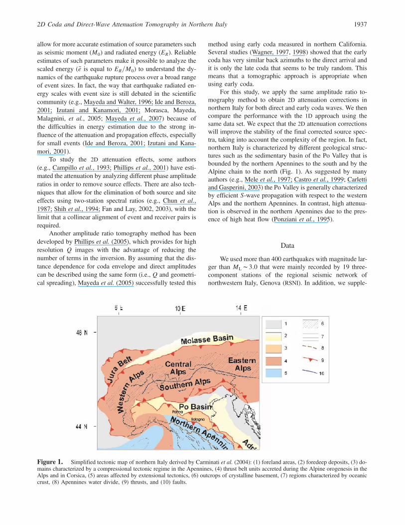
For this study, we apply the same amplitude ratio to-mography method to obtain 2D attenuation corrections innorthern Italy for both direct and early coda waves. We thencompare the performance with the 1D approach using thesame data set. We expect that the 2D attenuation correctionswill improve the stability of the final corrected source spec-tra, taking into account the complexity of the region. In fact,northern Italy is characterized by different geological struc-tures such as the sedimentary basin of the Po Valley that isbounded by the northern Apennines to the south and by theAlpine chain to the north (Fig. 1). As suggested by manyauthors (e.g., Mele et al., 1997; Castro et al., 1999; Carlettiand Gasperini, 2003) the Po Valley is generally characterizedby efficient S-wave propagation with respect to the westernAlps and the northern Apennines. In contrast, high attenua-tion is observed in the northern Apennines due to the pres-ence of high heat flow (Ponziani et al., 1995).

Data

We used more than 400 earthquakes with magnitude lar-ger than ML ∼ 3:0 that were mainly recorded by 19 three-component stations of the regional seismic network ofnorthwestern Italy, Genova (RSNI). In addition, we supple-

Figure 1. Simplified tectonic map of northern Italy derived by Carminati et al. (2004): (1) foreland areas, (2) foredeep deposits, (3) do-mains characterized by a compressional tectonic regime in the Apennines, (4) thrust belt units accreted during the Alpine orogenesis in theAlps and in Corsica, (5) areas affected by extensional tectonics, (6) outcrops of crystalline basement, (7) regions characterized by oceaniccrust, (8) Apennines water divide, (9) thrusts, and (10) faults.

2D Coda and Direct-Wave Attenuation Tomography in Northern Italy 1937

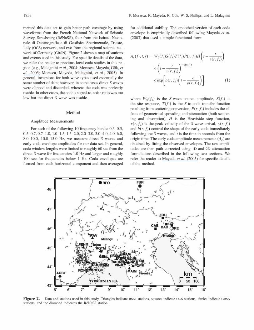
mented this data set to gain better path coverage by usingwaveforms from the French National Network of SeismicSurvey, Strasbourg (RéNaSS), four from the Istituto Nazio-nale di Oceanografia e di Geofisica Sperimentale, Trieste,Italy (OGS) network, and two from the regional seismic net-work of Germany (GRSN). Figure 2 shows a map of stationsand events used in this study. For specific details of the data,we refer the reader to previous local coda studies in this re-gion (e.g., Malagnini et al,, 2004; Morasca, Mayeda, Gök, etal., 2005; Morasca, Mayeda, Malagnini, et al., 2005). Ingeneral, inversions for both wave types used essentially thesame number of data; however, in some cases direct S waveswere clipped and discarded, whereas the coda was perfectlyusable. In other cases, the coda’s signal-to-noise ratio was toolow but the direct S wave was usable.

Method

Amplitude Measurements

For each of the following 10 frequency bands: 0.3–0.5,0.5–0.7, 0.7–1.0, 1.0–1.5, 1.5–2.0, 2.0–3.0, 3.0–4.0, 4.0–6.0,8.0–10.0, 10.0–15.0 Hz, we measure direct S waves andearly coda envelope amplitudes for our data set. In general,coda window lengths were limited to roughly 60 sec from thedirect S wave for frequencies 1.0 Hz and larger and roughly100 sec for frequencies below 1 Hz. Coda envelopes areformed from each horizontal component and then averaged

for additional stability. The smoothed version of each codaenvelope is empirically described following Mayeda et al.(2003) that used a simple functional form:

Ac�fi; t; r� � W0�fi�S�fi�T�fi�P�r; fi�H�t � r

v�r; fi�

�

�t � r

v�r; fi�

��γ�r;fi�

× exp�b�r; fi�

�t � r

v�r; fi�

��; (1)

where W0�fi� is the S-wave source amplitude, S�fi� isthe site response, T�fi� is the S-to-coda transfer functionresulting from scattering conversion, P�r; fi� includes the ef-fects of geometrical spreading and attenuation (both scatter-ing and absorption), H is the Heaviside step function,v�r; fi� is the peak velocity of the S-wave arrival, γ�r; fi�and b�r; fi� control the shape of the early coda immediatelyfollowing the S waves, and t is the time in seconds from theorigin time. The early coda amplitude measurements (Ac) areobtained by fitting the observed envelopes. The raw ampli-tudes are then path corrected using 1D and 2D attenuationformulations described in the following two sections. Werefer the reader to Mayeda et al. (2005) for specific detailsof the method.

Figure 2. Data and stations used in this study. Triangles indicate RSNI stations, squares indicate OGS stations, circles indicate GRSNstations, and the diamond indicates the RéNaSS station.

1938 P. Morasca, K. Mayeda, R. Gök, W. S. Phillips, and L. Malagnini

1D Path Corrections

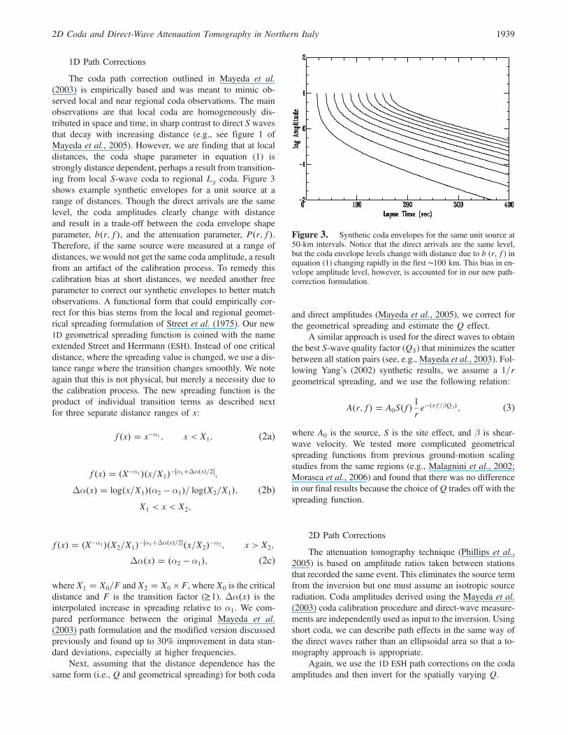
The coda path correction outlined in Mayeda et al.(2003) is empirically based and was meant to mimic ob-served local and near regional coda observations. The mainobservations are that local coda are homogeneously dis-tributed in space and time, in sharp contrast to direct S wavesthat decay with increasing distance (e.g., see figure 1 ofMayeda et al., 2005). However, we are finding that at localdistances, the coda shape parameter in equation (1) isstrongly distance dependent, perhaps a result from transition-ing from local S-wave coda to regional Lg coda. Figure 3shows example synthetic envelopes for a unit source at arange of distances. Though the direct arrivals are the samelevel, the coda amplitudes clearly change with distanceand result in a trade-off between the coda envelope shapeparameter, b�r; f�, and the attenuation parameter, P�r; f�.Therefore, if the same source were measured at a range ofdistances, we would not get the same coda amplitude, a resultfrom an artifact of the calibration process. To remedy thiscalibration bias at short distances, we needed another freeparameter to correct our synthetic envelopes to better matchobservations. A functional form that could empirically cor-rect for this bias stems from the local and regional geomet-rical spreading formulation of Street et al. (1975). Our new1D geometrical spreading function is coined with the nameextended Street and Herrmann (ESH). Instead of one criticaldistance, where the spreading value is changed, we use a dis-tance range where the transition changes smoothly. We noteagain that this is not physical, but merely a necessity due tothe calibration process. The new spreading function is theproduct of individual transition terms as described nextfor three separate distance ranges of x:

f�x� � x�α1 ; x < X1; (2a)

f�x� � �X�α1��x=X1���α1�Δα�x�=2�;

Δα�x� � log�x=X1��α2 � α1�= log�X2=X1�;X1 < x < X2;

(2b)

f�x� � �X�α1��X2=X1���α1�Δα�x�=2��x=X2��α2 ; x > X2;

Δα�x� � �α2 � α1�; (2c)

where X1 � X0=F and X2 � X0 × F, where X0 is the criticaldistance and F is the transition factor (≥1). Δα�x� is theinterpolated increase in spreading relative to α1. We com-pared performance between the original Mayeda et al.(2003) path formulation and the modified version discussedpreviously and found up to 30% improvement in data stan-dard deviations, especially at higher frequencies.

Next, assuming that the distance dependence has thesame form (i.e., Q and geometrical spreading) for both coda

and direct amplitudes (Mayeda et al., 2005), we correct forthe geometrical spreading and estimate the Q effect.

A similar approach is used for the direct waves to obtainthe best S-wave quality factor (QS) that minimizes the scatterbetween all station pairs (see, e.g., Mayeda et al., 2003). Fol-lowing Yang’s (2002) synthetic results, we assume a 1=rgeometrical spreading, and we use the following relation:

A�r; f� � A0S�f�1

re��πf=βQβ�; (3)

where A0 is the source, S is the site effect, and β is shear-wave velocity. We tested more complicated geometricalspreading functions from previous ground-motion scalingstudies from the same regions (e.g., Malagnini et al., 2002;Morasca et al., 2006) and found that there was no differencein our final results because the choice ofQ trades off with thespreading function.

2D Path Corrections

The attenuation tomography technique (Phillips et al.,2005) is based on amplitude ratios taken between stationsthat recorded the same event. This eliminates the source termfrom the inversion but one must assume an isotropic sourceradiation. Coda amplitudes derived using the Mayeda et al.(2003) coda calibration procedure and direct-wave measure-ments are independently used as input to the inversion. Usingshort coda, we can describe path effects in the same way ofthe direct waves rather than an ellipsoidal area so that a to-mography approach is appropriate.

Again, we use the 1D ESH path corrections on the codaamplitudes and then invert for the spatially varying Q.

Figure 3. Synthetic coda envelopes for the same unit source at50-km intervals. Notice that the direct arrivals are the same level,but the coda envelope levels change with distance due to b (r, f) inequation (1) changing rapidly in the first ∼100 km. This bias in en-velope amplitude level, however, is accounted for in our new path-correction formulation.

2D Coda and Direct-Wave Attenuation Tomography in Northern Italy 1939

The following amplitude ratio formulation was applied:

Aij � ⟨Aij⟩j � Si � ⟨Sj⟩j

� �Pkdxijkαk � ⟨Pkdxijkαk⟩j� log10�e�;(4)

where A is log10 spreading corrected amplitude, i, j, and kindices are site, source, and path discretization, respectively,S is the log10 site term, dx are the path lengths through adiscretized region of the Earth, α is the discretized attenu-ation coefficient (αk � ω=2Qkc), and Pk are the ray-pathsums. The ratio is taken between the single value and theaverage for the same event j; consequently, the source ratiois zero. We obtain a linear system of equations and solveusing sparse matrix methods. Smoothing constraints areapplied to the attenuation model to avoid artifacts due tonoise, and the site term’s sum is assumed to be zero. Weobtained a tomography image for each frequency band ina range between 0.3 and 15 Hz for coda and direct wavesseparately.

At this point, we have four different cases that need to beanalyzed:

1. Direct-wave amplitudes path corrected using 1D attenua-tion parameters;

2. Coda-wave amplitudes path corrected using 1D attenua-tion parameters;

3. Direct-wave amplitudes path corrected using 2D attenua-tion parameters;

4. Coda-wave amplitudes path corrected using 2D attenua-tion parameters.

For each of these four sets of path-corrected amplitudes,source spectra are computed following the approach used byMayeda et al. (2003).

Attenuation Tomography Results

For each frequency band in the range of 0.3–15 Hz, weimaged quality factor variations with respect to an averagecomputed over the region. Figure 4 shows Q tomographyresults for all the frequency bands for the direct waves whileFigure 5 displays the results obtained for the coda-wavesanalysis. In all cases, we used pixel dimensions of 0.1°.Results are presented as difference in percentages fromthe average Q (green) for each frequency. The averageQ�⟨Q⟩� value is reported in the bottom of each plot and in-creases with increasing frequency for both wave types.

We observe that both wave types exhibit low attenuationin the southern part of the western Alps that coincides withthe area characterized by the massifs. This anomaly is ob-servable starting from 0.7 to 1.0 Hz for the direct waves andfrom 1.5 to 2.0 Hz for coda waves. Eva et al. (1991) obtainedsimilar results in their study analyzing coda Q variations

focusing on this restricted area. In addition, a large low Qarea to the north is observed for both direct and codaanalysis. In this case, the anomaly is observable at all fre-quencies, but with slightly different lateral extent. Exceptfor very low and high frequencies, the anomalous area seemsto narrow around the Ivrea body, known as a shallow sliceof mantle (Kissling, 1993; Di Stefano et al., 1999). Thepresence of this body seems to have important effects suchas the production of a positive Bouguer anomaly (Vernantet al., 2002). Moreover, in the same zone, an extinction ofLg waves was observed by Campillo et al. (1993) over a widefrequency range. Their results confirm our findings becausethe authors explain this attenuation effect as a result of stronglateral heterogeneity of the surface geology, which is char-acterized by interwoven mantle and crustal rocks. Theyinterpret the wide range of frequency in which the extinctionis observable as due to variable scale-length heterogeneitieswithin the area.

Figures 4 and 5 also show a high Q zone in correspon-dence with the Po Plain, extending to the very northern partof the Apennines, close to Parma (see Fig. 1). As for the highQ zone of the northernmost part of the Apennines, an in-terpretation is not simple given the complex geological set-ting and geometric crustal relationships. In fact, the northernApennines’ front is buried under the Po Plain sediments andthe Po Plain is the foreland basin of both the Alps and Apen-nines (Doglioni, 1993). This complexity might be the originof strong lateral heterogeneity in the crust where we observea high attenuation anomaly related to this buried front. It isclear that the anomaly we observe in this area is not a resultof artifacts correlated to the adopted methodology or to thedata and station distribution because other studies show ananomalous propagation of waves within this region. In fact,Ciaccio and Chiarabba (2002) observed a shallow high ve-locity anomaly in the same area and interpreted that as aneffect of heterogeneity due to uplifted Mesozoic carbona-ceous rocks. Moreover, a recent study of Margheriti et al.(2006) highlights a seismic anisotropy in this area findinga shear-wave splitting effect that the authors relate to thepresence of fluid-saturated microcracks aligned or openedby the prevailing stress field.

Tests with synthetic data have been conducted to revealinherent limitations in resolution and possible artifacts due toevent-station geometry and chosen parameterization. Foreach frequency band, we performed checkerboard tests toverify what could and could not be resolved. In all cases,the results look very similar to each other except at the lowestbands for which we needed to use a larger grid size. Figure 6shows example results for a representative range of fre-quency bands. The low and high attenuation input cell valuesvary as a function of frequency, in accordance to what weobserve in the real data. We recognize, however, that highQ regions will not be well resolved due to smoothing ofadjacent low Q regions. The accurate recovery of high Qis known to be an issue because of smoothing constraintson 1=Q, but our derived model still fits the data well, and

1940 P. Morasca, K. Mayeda, R. Gök, W. S. Phillips, and L. Malagnini

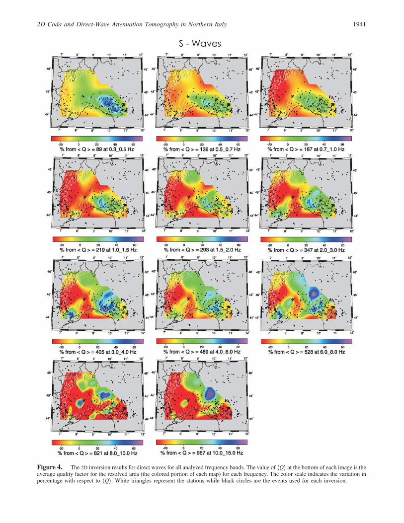
Figure 4. The 2D inversion results for direct waves for all analyzed frequency bands. The value of ⟨Q⟩ at the bottom of each image is theaverage quality factor for the resolved area (the colored portion of each map) for each frequency. The color scale indicates the variation inpercentage with respect to ⟨Q⟩. White triangles represent the stations while black circles are the events used for each inversion.

2D Coda and Direct-Wave Attenuation Tomography in Northern Italy 1941

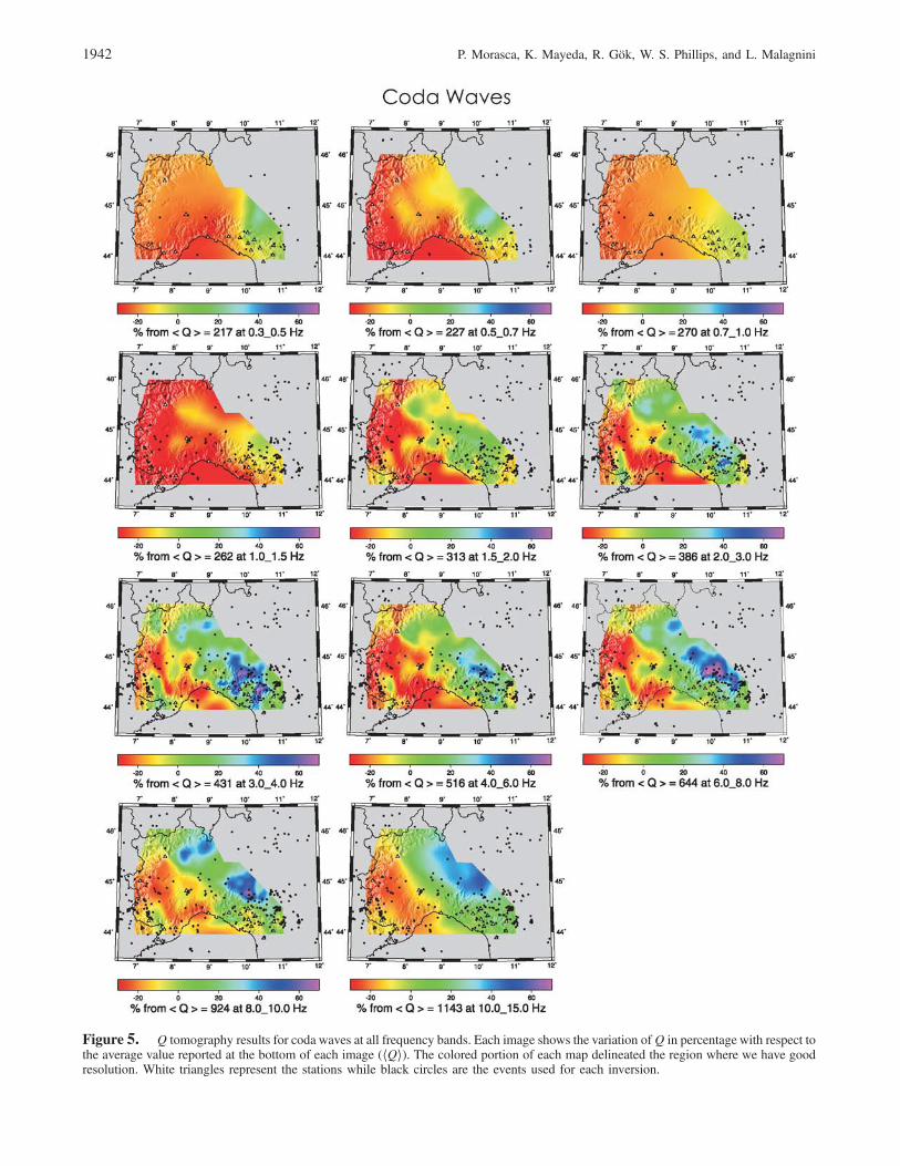
Figure 5. Q tomography results for coda waves at all frequency bands. Each image shows the variation ofQ in percentage with respect tothe average value reported at the bottom of each image (⟨Q⟩). The colored portion of each map delineated the region where we have goodresolution. White triangles represent the stations while black circles are the events used for each inversion.

1942 P. Morasca, K. Mayeda, R. Gök, W. S. Phillips, and L. Malagnini

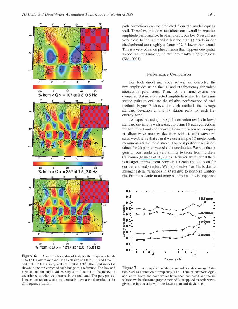
path corrections can be predicted from the model equallywell. Therefore, this does not affect our overall interstationamplitude performance. In other words, our lowQ results arevery close to the input value but the high Q pixels in ourcheckerboard are roughly a factor of 2–3 lower than actual.This is a very common phenomenon that happens due spatialsmoothing, thus making it difficult to resolve high Q regions(Xie, 2005).

Performance Comparison

For both direct and coda waves, we corrected theraw amplitudes using the 1D and 2D frequency-dependentattenuation parameters. Then, for the same events, wecompared distance-corrected amplitude scatter for the samestation pairs to evaluate the relative performance of eachmethod. Figure 7 shows, for each method, the averagestandard deviation among 37 station pairs for each fre-quency band.

As expected, using a 2D path correction results in lowerstandard deviations with respect to using 1D path correctionsfor both direct and coda waves. However, when we compare2D direct-wave standard deviation with 1D coda-waves re-sults, we observe that even if we use a simple 1D model, codameasurements are more stable. The best performance is ob-tained for 2D path-corrected coda amplitudes. We note that ingeneral, our results are very similar to those from northernCalifornia (Mayeda et al., 2005). However, we find that thereis a larger improvement between 1D coda and 2D coda forour current study region. We hypothesize that this is due tostronger lateral variations in Q relative to northern Califor-nia. From a seismic monitoring standpoint, this is important

Figure 6. Result of checkerboard tests for the frequency bands0.3–0.5 Hz where we have used a cell size of 1:0 × 1:0°, and 1.5–2.0and 10.0–15.0 Hz using cells of 0:50 × 0:50°. The input model isshown in the top corner of each image as a reference. The low andhigh attenuation input values vary as a function of frequency, inaccordance to what we observe in the real data. The polygon de-lineates the region where we generally have a good resolution forall frequency bands.

Figure 7. Averaged interstation standard deviation using 37 sta-tion pairs as a function of frequency. The 1D and 2D methodologiesapplied to direct and coda waves have been compared and the re-sults show that the tomographic method (2D) applied on coda wavesgives the best results with the lowest standard deviations.

2D Coda and Direct-Wave Attenuation Tomography in Northern Italy 1943

because it shows that some regions can benefit significantlyfrom 2D coda path calibrations.

Source Spectra

For all four cases, the path-corrected amplitudesare used to compute source spectra. Further frequency-dependent site and S-to-coda transfer function correctionswere derived using the procedure outlined by Mayeda et al.(2003). Likewise for the direct-wave amplitudes, we appliedsimilar corrections to remove site effects and derive absolutesource spectra. An example of the 24 November 2002Mw 5.1 event is plotted in Figure 8, where gray and blackcurves are the station and average source spectra, respec-tively. The scatter observed for the different cases reflectsthe results presented in Figure 7. As expected, source spectraderived from coda measurements are much less scatteredthan those computed from the direct waves, and the moststable results are obtained for coda measurements whenwe use the 2D attenuation corrections.

Discussion and Conclusions

For the same data set and stations, we estimated the at-tenuation effects for both coda and direct S waves using anew 2D tomography approach (Phillips et al., 2005) as wellas performed a comparison with the 1D method outlined byMayeda et al. (2003). For the coda wave analysis we focusedon the early coda because, as many studies demonstrated(e.g., Wagner, 1997, 1998), the late coda consists of multiplescattered energy that samples a larger volume of the propa-gation medium, more so than the early coda and the directwaves. This means that the early coda path effects could beroughly approximated to the direct waves and used in atraditional direct-wave tomographic approach.

Attenuation tomography revealed lateral complexityfor northern Italy that comprises the Alps–Apenninesjunction zone and the foredeep basin (Po Plain) of bothchains. Our results consistently show the same trend fordifferent frequency bands and for both coda and directwaves, though lateral coda attenuation is smoother, espe-

Figure 8. Example of moment-rate spectra obtained for the 24 November 2002 Mw 5:1 event. Gray curves are the individual stationspectra while black curves represent the averages. Stations are situated at a variety of azimuths and distances. As expected, direct wavesresults are more scattered then coda waves for both 1D and 2D methods, consistent with the finding shown in Figure 7.

1944 P. Morasca, K. Mayeda, R. Gök, W. S. Phillips, and L. Malagnini

cially for high and low frequencies. This effect is expectedbecause of the averaging nature of coda waves and is con-sistent with observations by Mayeda et al. (2005) for north-ern California.

A low attenuation area is observed in the southern partof the western Alps, in agreement with results by Eva et al.(1991) who focused their coda Q study in this small zone ofwestern Alps characterized by the presence of crystallinemassifs. To the north of this zone, in the western Alps, a largelow Q anomaly is observed in correspondence with the Ivreabody, in good agreement with an Lg extinction observed inthe same area by Campillo et al. (1993). Campillo et al.(1993) suggest that the blockage of Lg across the westernAlps as being due to the effect of low Q from the presenceof strong heterogeneity of the crust. The large range of fre-quency in which the anomaly is observed indicates a variablescale length of the heterogeneity. Our results also show highQ under the Po Plain, the largest alluvial basin of northernItaly. This region has a complex geological and structuralsetting because the thrust fronts of the northern Apennineare buried by variable thickness, quaternary alluvium (Pieriand Groppi, 1998), which might cause the anomalous propa-gation. The behavior within this region is confirmed byother studies indicating the presence of velocity (Ciaccioand Chiarabba, 2002) and seismic (Margeriti et al., 2006)anomalies.

The attenuation results obtained from the tomographyhave been used to derive source spectra. We compared directand coda waves using 1D and 2D attenuation corrections, andwe demonstrated that the 2D method provides more stableresults than the 1D approach for the same phase. However,when we compare direct and coda waves, we notice that thesimple 1D attenuation corrections applied to coda measure-ments are significantly better than direct S waves correctedfor 2D attenuation. The same conclusion was reached byMayeda et al. (2005) for northern California. Because thestudy area is relatively small and limited in data, we planto add more events and stations from other networks toenlarge the study area to better understand the relation-ship between attenuation and geological structures for thebroader region.

Acknowledgments

The authors wish to thank the RSNI network staff for the careful net-work management and data collection that made this work possible. Wewishto thank the OGS, Trieste, for kindly providing some data from their seismicnetwork. The helpful suggestions of two anonymous reviewers and of theeditor Hiroshi Kawase helped us to improve this manuscript. K. Mayeda wassupported under Weston Geophysical Subcontract Number GC19762NGDand AFRL Contract Number FA8718-07-C-0010. This work performedunder the auspices of the U.S. Department of Energy by Lawrence Liver-more National Laboratory under Contract Number DE-AC52-07NA27344,UCRL-JRNL-235660

References

Campillo, M., B. Feignier, M. Bouchon, and N. Béthoux (1993). Attenua-tion of crustal waves across the alpine range, J. Geophys. Res. 98,no. B2, 1987–1996.

Carletti, F., and P. Gasperini (2003). Lateral variations of seismic intensityattenuation in Italy, Geophys. J. Int. 155, 839–856.

Carminati, E., C. Dogliosi, and D. Scrocca (2004). Alps vs Apennines,in Geology of Italy, U. Crescenti, S. D’Offizi, S. Merlini and L. Sacchi(Editors), special volume of the Italian Geological Society for the In-ternational Geological Congress 32, Italian Geological Society, Flor-ence, 141–151.

Castro, R. R., M. Mucciarelli, G. Monachesi, F. Pacor, and R. Berardi(1999). A review of nonparametric attenuation functions computedfor different regions of Italy, Ann. Geofis. 42, 735–748.

Chun, K.-Y., G. F. West, R. J. Kokoski, and C. Samson (1987), A noveltechnique for measuring Lg attenuation: results from eastern Canadabetween 1 to 10 Hz, Bull. Seismol. Soc. Am. 77, 398–419.

Ciaccio, M. G., and C. Chiarabba (2002). Tomographyc models and seismo-tectonics of the Reggio Emilia region, Italy, Tectonophysics 344,261–276.

Di Stefano, R., C. Chiarabba, F. Lucente, and A. Amato (1999). Crustaland uppermost mantle structure in Italy from the inversion ofP-wave arrival times: geodynamic implications, Geophys. J. Int. 139,483–498.

Doglioni, C. (1993). Some remarks on the origin of foredeeps, Tectono-physics 228, 1–20.

Eva, C., M. Cattaneo, P. Augliera, and M. Pasta (1991). Regional coda Qvariations in the western Alps (northern Italy), Phys. Earth Planet.Inter. 67, 76–86.

Fan, G., and T. Lay (2003), Strong Lg wave attenuation in the Northernand Eastern Tibetan Plateau measured by a two-station/two-eventstacking method, Geophys. Res. Lett. 30, no. 10 1530, doi 10.1029/2002GL016211.

Fan, G.-W., and T. Lay (2002). Characteristics of Lg attenuation in theTibetan Plateau, J. Geophys. Res. 107, no. 10, 2256, doi 10.1029/2001JB000804.

Ide, S., and G. C. Beroza (2001), Does apparent stress vary with earthquakesize? Geophys. Res. Lett. 28, 3349–3352.

Izutani, Y., and H. Kanamori (2001), Scale-dependence of seismic energy-to-moment ratio for strike-slip earthquakes in Japan, Geophys. Res.Lett. 28, 4007–4010.

Kissling, E. (1993). Deep structure of the Alps—what do we really know?,Phys. Earth Planet. Inter. 79, 87–112.

Malagnini, L., A. Akinci, R. G. Herrmann, N. A. Pino, and L. Scognamiglio(2002). Characteristics of the ground motion in Friuli (northeasternItaly), Bull. Seismol. Soc. Am. 94, no. 4, 1343–1352.

Malagnini, L., K. Mayeda, A. Akinci, and P. Bragato (2004). Esti-mating absolute site effects, Bull. Seismol. Soc. Am. 94, no. 4,1343–1352.

Margheriti, L., M. F. Ferulano, and M. Di Bona (2006). Seismic an-isotropy and its relation with crustal structure and stress field inthe Reggio Emilia region (northern Italy), Geophys. J. Int. 167,1035–1043.

Mayeda, K., and W. R. Walter (1996). Moment, energy, stress drop, andsource spectra of western United States earthquakes from regionalcoda envelopes, J. Geophys. Res. 101, 11,195–11,208.

Mayeda, K., A. Hofstetter, J. L. O’Boyle, and W. R. Walter (2003). Stableand transportable regional magnitudes based on coda-derived moment-rate spectra, Bull. Seismol. Soc. Am. 93, 224–239.

Mayeda, K., L. Malagnini, and W. R. Walter (2007). A new spectral ratiomethod using narrow band coda envelopes: evidence for non-self-similarity in the Hector Mine sequence, Geophys. Res. Lett., 34,L11303, doi 10.1029/2007GL030041.

Mayeda, K., L. Malagnini, W. S. Phillips, W. R. Walter, and D. Dreger(2005). 2-D or not 2-D, that is the question: a northern California test,Geophys. Res. Lett. 32, L12301, doi 10.1029/2005GL022882.

2D Coda and Direct-Wave Attenuation Tomography in Northern Italy 1945

Mele, G., A. Rovelli, D. Seber, and M. Barazangi (1997) Shear wave at-tenuation in the lithosphere beneath Italy and surrounding regions: tec-tonic implications, J. Geophys. Res. 102, no. B6, 11,863–11,875.

Morasca, P., L. Malagnini, A. Akinci, and D. Spallarossa (2006).Ground motion scaling in the western Alps, J. Seism. 10, no. 3,315–333.

Morasca, P., K. Mayeda, L. Malagnini, and W. R Walter (2005). Coda de-rived source spectra, moment magnitudes, and energy-moment scalingin the western Alps, Geophys. J. Int. 160, no. 1, 263–275.

Morasca, P., K. Mayeda, R. Gök, L. Malagnini, and C. Eva (2005). Abreak in self-similarity in the Lunigiana-Garfagnana region (northernApennines), Geophys. Res. Lett. 32, no. 22, L22301 doi 10.1029/2005GL024443.

Phillips, W. S., H. E. Hartse, and J. T. Rutledge (2005). Amplitude ratiotomography for regional phase Q, Geophys. Res. Lett. 32, no 21,L21301, doi 10.1029/2005GL023870.

Phillips, W. S., H. E. Hartse, S. R. Taylor, A. A. Velasco, and G. E. Randall(2001). Application of regional phase amplitude tomography to seis-mic verification, Pure Appl. Geophys. 158, 1189–1206.

Pieri, M., and G. Groppi (1998). Pubblicazione 414, Subsurface geologicalstructure of the Po Plain, P. F. Geodin. C. N. R., 1–23.

Ponziani, F., R. De Franco, G. Minelli, G. Biella, C. Federico, and G. Pialli(1995). Crustal shortening and duplication of the Moho in the northernApennines: a view from seismic reflection data, Tectonophysics 252,391–418.

Shih, X. R., K.-Y. Chun, and T. Zhu (1994). Attenuation of 1–6s Lgwaves inEurasia, Geophys. Res. 99, no. B12, 23,859–23,874.

Street, R. L., R. Herrmann, and O. Nuttli (1975). Spectral characteristics ofthe Lg wave generated by central United States earthquakes, Geophys.J. R. Astr. Soc. 41, 51–63.

Vernant, P., F. Masson, R. Bayer, and A. Paul (2002). Sequential inversion oflocal earthquake traveltimes and gravity anomaly—the example of thewestern Alps, Geophys. J. Int. 150, 79–90.

Wagner, G. S. (1997). Regional wave propagation in southern Californiaand Nevada: observations from a three-component seismic array, J.Geophys. Res. 102, no. B4, 8285–8312.

Wagner, G. S. (1998). Local wave propagation near the San Jacinto faultzone, southern California: observations from a three-component seis-mic array, Bull. Seismol. Soc. Am. 103, 7231–7246.

Xie, J. (2005). On the inadequacy of stochastic modeling of regional Lgwave spectra (Abstract S43C-05), Eos Trans. AGU 86, no. 52 (FallMeet. Suppl.), S43C-05.

Yang, X. (2002). A numerical investigation of Lg geometrical spreading,Bull. Seismol. Soc. Am. 92, 3067–3079.

Università di GenovaViale Benedetto XV5, 16132 Genova, Italy

(P.M.)

Weston Geophysical Corporation181 Bedford StreetSuite 1Lexington, Massachusetts 02420

(K.M.)

Lawrence Livermore National Laboratory7000 East AvenueLivermore, California 94550

(R.G.)

Los Alamos National LaboratoryP.O. Box 1663Los Alamos, New Mexico 87545

(W.S.P.)

Istituto Nazionale di Geofisica e VulcanologiaVia di Vigna Murata, 605Rome, Italy 00143

(L.M.)

Manuscript received 19 April 2007

1946 P. Morasca, K. Mayeda, R. Gök, W. S. Phillips, and L. Malagnini