2D CFD Modelling Of H –Darrieus Wind Turbine and Its ...

International Journal of Emerging Technologies in Engineering Research (IJETER)

Volume 4, Issue 8, August (2016) www.ijeter.everscience.org

ISSN: 2454-6410 ©EverScience Publications 79

2D CFD Modelling Of H –Darrieus Wind Turbine

and Its Optimization for Performance Enhancement

Komal Rawat1, Hina Akhtar1, Anirudh Gupta2, Ravi Kumar 3 1

PG Scholar, Department of Mechanical Engineering, BTKIT, Dwarahat, India. 2

Associate Professor, Department of Mechanical Engineering, BTKIT, Dwarahat, India. 3

Assistant Professor, Department of Mechanical Engineering, BTKIT, Dwarahat, India.

Abstract – In the present paper 2D CFD model of H-Darrieus

Wind Turbine has been developed. The model was implemented

in ANSYS Fluent solver to predict wind turbines performance and

optimize its geometry. As the RANS Turbulence Modeling plays a

strategic role for the prediction of the flow field around wind

turbines, different Turbulence Models were tested. The results

demonstrate the good capabilities of the Transition SST

turbulence model compared to the classical fully turbulent

models. The computational domain was structured with a rotating

ring mesh and the unsteady solver was used to capture the

dynamic stall phenomena and unsteady rotational effects. Both

grid and time step were optimized to reach independent solutions.

Particularly a high quality 2D mesh was obtained using the

ANSYS Meshing tool while a Sliding Mesh Model was used to

simulate rotation. .Coefficient of lift and drag were calculated at

different values of attack. Main parameter that is monitored in

this study is the Tip Speed Ratio (TSR) . Thus, an optimum value

of TSR is obtained at which the turbine gives maximum power.

Index Terms – H-Darrieus Wind Turbine; CFD; Transition

Turbulence Modeling; URANS; VAWT performance

prediction,TSR.

Abbreviations - VAWT (Vertical Axis Wind

Turbine),𝐂𝐥(coefficient of lift) , 𝐂𝐝(coefficient of

drag, 𝐂𝐦(coefficient of moment),TSR(Tip Speed Ratio).

1. INTRODUCTION

Vertical Axis Wind Turbines (VAWTs) are becoming ever

more important in wind power generation thanks to its

compactness and adaptability for domestic installations.

However, it is well known that VAWTs have lower efficiency,

above all if compared to HAWTs. To improve VAWTs

performance, industries and researchers are trying to optimize

the design of the rotors. Some numerical codes like Vortex

Method or Multiple Stream tube Mode have been developed to

predict VAWTs performance and optimize efficiency but they

do not provide information on the wakes and they use semi

empirical equations to predict effects like tip vortex and

dynamic stall.[1]

As it is known, CFD resolves the fluid dynamic equations and

it is certainly more realistic than the 1D models but there are

many other problematic issues like stall and turbulence

modeling, unsteady rotational effects and long computation

time. Some works were found in scientific literature [3-8]

regarding the application of CFD modeling on VAWTs. The

problem in general was the power overestimation due to the

arduous prediction of stall phenomena using fully turbulent

RANS models for low Reynolds numbers.

Simulations were performed on a AMD processor having 8

cores with 12 GB RAM providing a processing speed of 3.5

GHz. A parallel computing technique was implemented in

ANSYS Fluent solver with 6 to 7 processor cores being used at

once.

In this paper, the strategy of generating a 2D CFD model to

predict H-Darrieus rotors performance and solve such issues is

presented.NACA0021 symmetrical airfoil with a three bladed

rotor is chosen for the study.

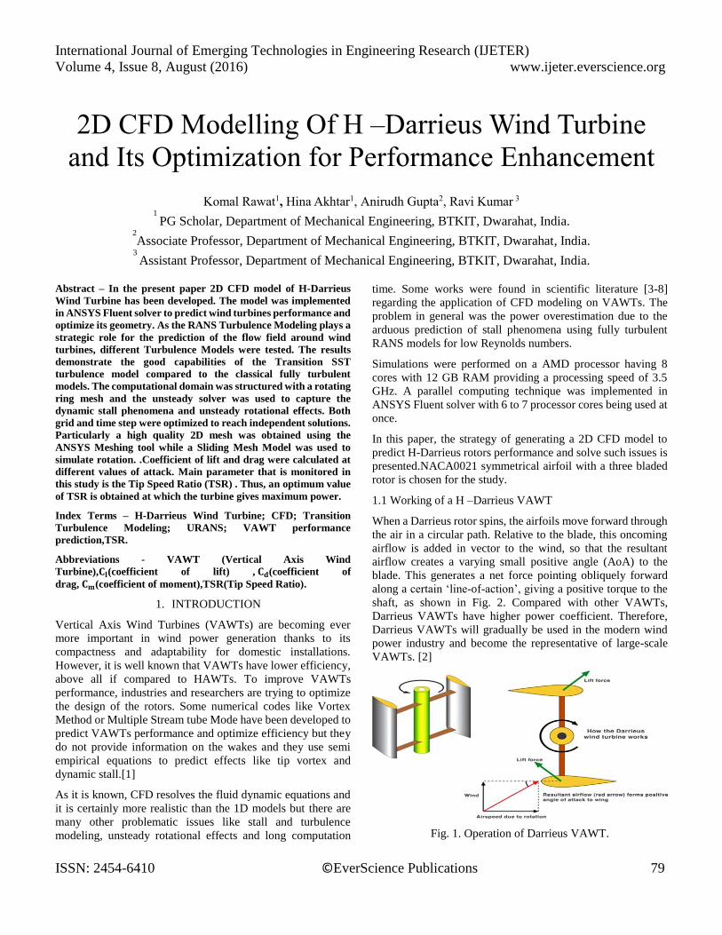
1.1 Working of a H –Darrieus VAWT

When a Darrieus rotor spins, the airfoils move forward through

the air in a circular path. Relative to the blade, this oncoming

airflow is added in vector to the wind, so that the resultant

airflow creates a varying small positive angle (AoA) to the

blade. This generates a net force pointing obliquely forward

along a certain ‘line-of-action’, giving a positive torque to the

shaft, as shown in Fig. 2. Compared with other VAWTs,

Darrieus VAWTs have higher power coefficient. Therefore,

Darrieus VAWTs will gradually be used in the modern wind

power industry and become the representative of large-scale

VAWTs. [2]

Fig. 1. Operation of Darrieus VAWT.




1.2 Computational Domain Generation and Optimization

Modelling the right Computational Domain is one of the most

important task that can be done to simplify the model

description or when done in the other way a much simpler or a

much complex design can complicate things and make the

simulation much more time consuming and costly also at the

same time. The mesh can be taken into account as one of the

most important parameter in deciding on a mesh independent

solution. The advanced turbulence model used in this study

requires very fine mesh near the wall region having a Y + value

less than 1.

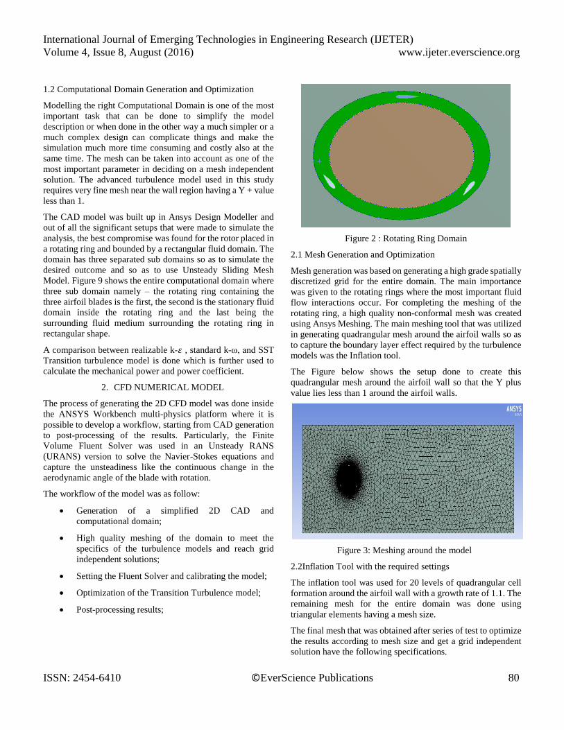
The CAD model was built up in Ansys Design Modeller and

out of all the significant setups that were made to simulate the

analysis, the best compromise was found for the rotor placed in

a rotating ring and bounded by a rectangular fluid domain. The

domain has three separated sub domains so as to simulate the

desired outcome and so as to use Unsteady Sliding Mesh

Model. Figure 9 shows the entire computational domain where

three sub domain namely – the rotating ring containing the

three airfoil blades is the first, the second is the stationary fluid

domain inside the rotating ring and the last being the

surrounding fluid medium surrounding the rotating ring in

rectangular shape.

A comparison between realizable k-𝜀 , standard k-ω, and SST

Transition turbulence model is done which is further used to

calculate the mechanical power and power coefficient.

2. CFD NUMERICAL MODEL

The process of generating the 2D CFD model was done inside

the ANSYS Workbench multi-physics platform where it is

possible to develop a workflow, starting from CAD generation

to post-processing of the results. Particularly, the Finite

Volume Fluent Solver was used in an Unsteady RANS

(URANS) version to solve the Navier-Stokes equations and

capture the unsteadiness like the continuous change in the

aerodynamic angle of the blade with rotation.

The workflow of the model was as follow:

Generation of a simplified 2D CAD and

computational domain;

High quality meshing of the domain to meet the

specifics of the turbulence models and reach grid

independent solutions;

Setting the Fluent Solver and calibrating the model;

Optimization of the Transition Turbulence model;

Post-processing results;

Figure 2 : Rotating Ring Domain

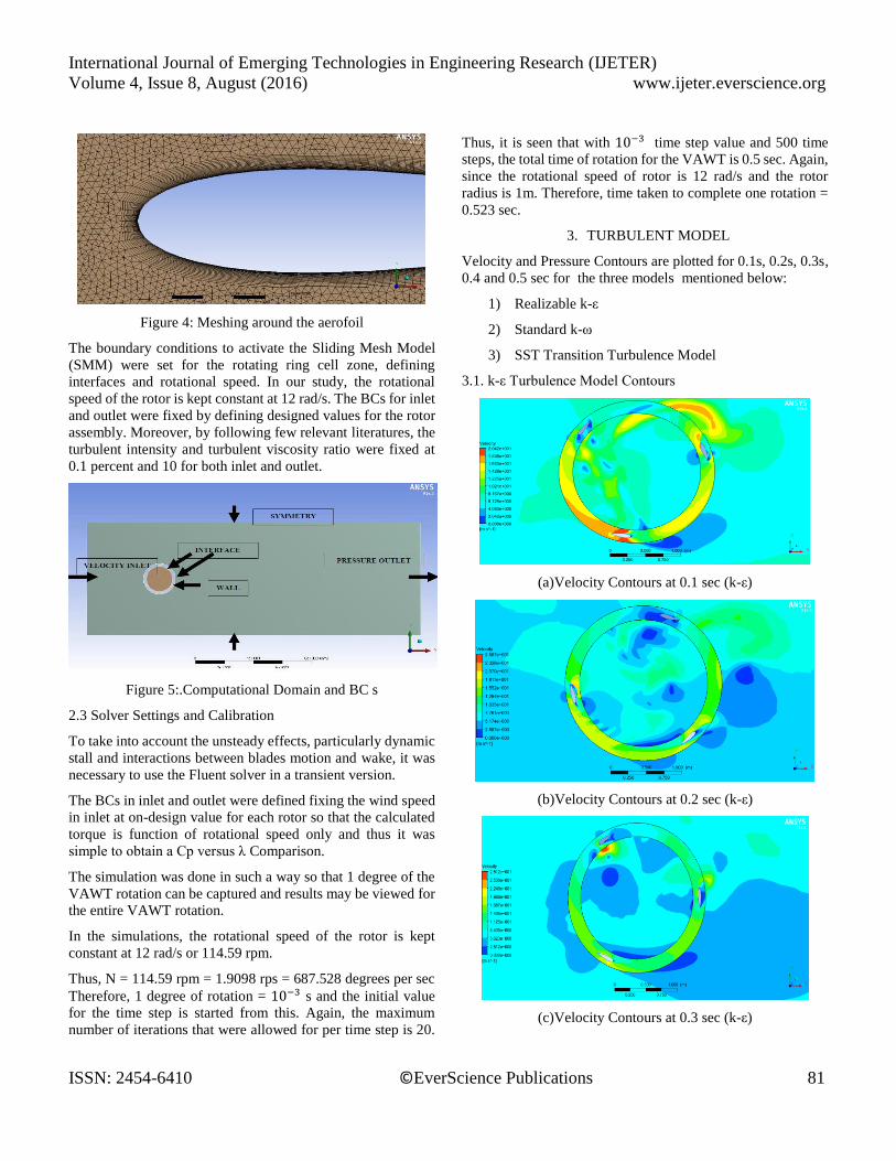
2.1 Mesh Generation and Optimization

Mesh generation was based on generating a high grade spatially

discretized grid for the entire domain. The main importance

was given to the rotating rings where the most important fluid

flow interactions occur. For completing the meshing of the

rotating ring, a high quality non-conformal mesh was created

using Ansys Meshing. The main meshing tool that was utilized

in generating quadrangular mesh around the airfoil walls so as

to capture the boundary layer effect required by the turbulence

models was the Inflation tool.

The Figure below shows the setup done to create this

quadrangular mesh around the airfoil wall so that the Y plus

value lies less than 1 around the airfoil walls.

Figure 3: Meshing around the model

2.2Inflation Tool with the required settings

The inflation tool was used for 20 levels of quadrangular cell

formation around the airfoil wall with a growth rate of 1.1. The

remaining mesh for the entire domain was done using

triangular elements having a mesh size.

The final mesh that was obtained after series of test to optimize

the results according to mesh size and get a grid independent

solution have the following specifications.




Figure 4: Meshing around the aerofoil

The boundary conditions to activate the Sliding Mesh Model

(SMM) were set for the rotating ring cell zone, defining

interfaces and rotational speed. In our study, the rotational

speed of the rotor is kept constant at 12 rad/s. The BCs for inlet

and outlet were fixed by defining designed values for the rotor

assembly. Moreover, by following few relevant literatures, the

turbulent intensity and turbulent viscosity ratio were fixed at

0.1 percent and 10 for both inlet and outlet.

Figure 5:.Computational Domain and BC s

2.3 Solver Settings and Calibration

To take into account the unsteady effects, particularly dynamic

stall and interactions between blades motion and wake, it was

necessary to use the Fluent solver in a transient version.

The BCs in inlet and outlet were defined fixing the wind speed

in inlet at on-design value for each rotor so that the calculated

torque is function of rotational speed only and thus it was

simple to obtain a Cp versus λ Comparison.

The simulation was done in such a way so that 1 degree of the

VAWT rotation can be captured and results may be viewed for

the entire VAWT rotation.

In the simulations, the rotational speed of the rotor is kept

constant at 12 rad/s or 114.59 rpm.

Thus, N = 114.59 rpm = 1.9098 rps = 687.528 degrees per sec

Therefore, 1 degree of rotation = 10−3 s and the initial value

for the time step is started from this. Again, the maximum

number of iterations that were allowed for per time step is 20.

Thus, it is seen that with 10−3 time step value and 500 time

steps, the total time of rotation for the VAWT is 0.5 sec. Again,

since the rotational speed of rotor is 12 rad/s and the rotor

radius is 1m. Therefore, time taken to complete one rotation =

0.523 sec.

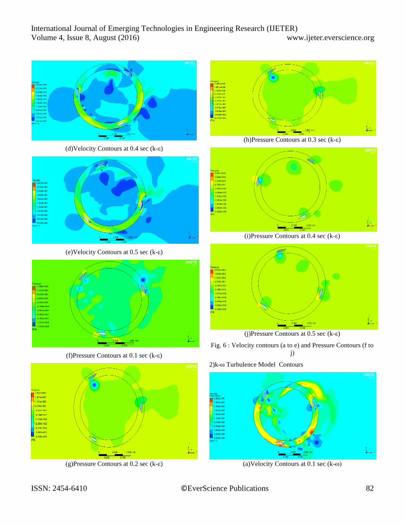
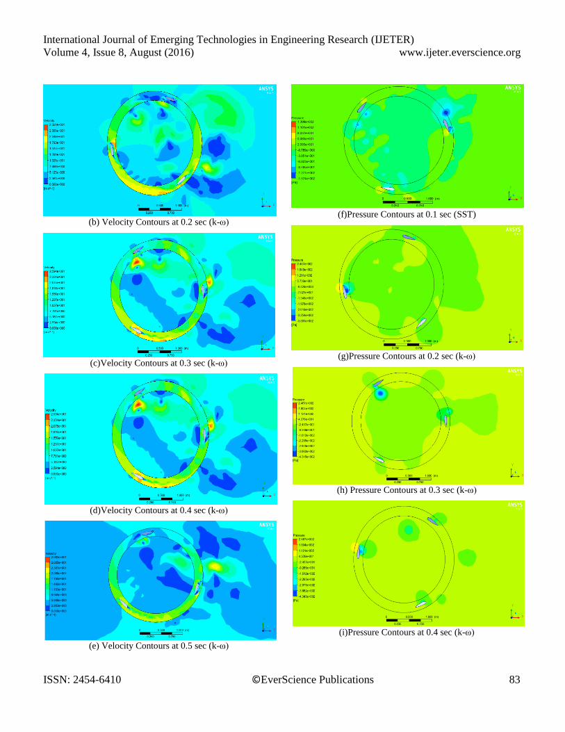
3. TURBULENT MODEL

Velocity and Pressure Contours are plotted for 0.1s, 0.2s, 0.3s,

0.4 and 0.5 sec for the three models mentioned below:

1) Realizable k-ε

2) Standard k-ω

3) SST Transition Turbulence Model

3.1. k-ε Turbulence Model Contours

(a)Velocity Contours at 0.1 sec (k-ε)

(b)Velocity Contours at 0.2 sec (k-ε)

(c)Velocity Contours at 0.3 sec (k-ε)




(d)Velocity Contours at 0.4 sec (k-ε)

(e)Velocity Contours at 0.5 sec (k-ε)

(f)Pressure Contours at 0.1 sec (k-ε)

(g)Pressure Contours at 0.2 sec (k-ε)

(h)Pressure Contours at 0.3 sec (k-ε)

(i)Pressure Contours at 0.4 sec (k-ε)

(j)Pressure Contours at 0.5 sec (k-ε)

Fig. 6 : Velocity contours (a to e) and Pressure Contours (f to

j)

2)k-ω Turbulence Model Contours

(a)Velocity Contours at 0.1 sec (k-ω)




(b) Velocity Contours at 0.2 sec (k-ω)

(c)Velocity Contours at 0.3 sec (k-ω)

(d)Velocity Contours at 0.4 sec (k-ω)

(e) Velocity Contours at 0.5 sec (k-ω)

(f)Pressure Contours at 0.1 sec (SST)

(g)Pressure Contours at 0.2 sec (k-ω)

(h) Pressure Contours at 0.3 sec (k-ω)

(i)Pressure Contours at 0.4 sec (k-ω)




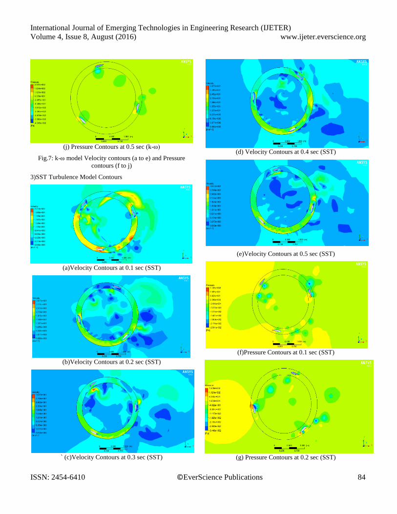
(j) Pressure Contours at 0.5 sec (k-ω)

Fig.7: k-ω model Velocity contours (a to e) and Pressure

contours (f to j)

3)SST Turbulence Model Contours

(a)Velocity Contours at 0.1 sec (SST)

(b)Velocity Contours at 0.2 sec (SST)

` (c)Velocity Contours at 0.3 sec (SST)

(d) Velocity Contours at 0.4 sec (SST)

(e)Velocity Contours at 0.5 sec (SST)

(f)Pressure Contours at 0.1 sec (SST)

(g) Pressure Contours at 0.2 sec (SST)




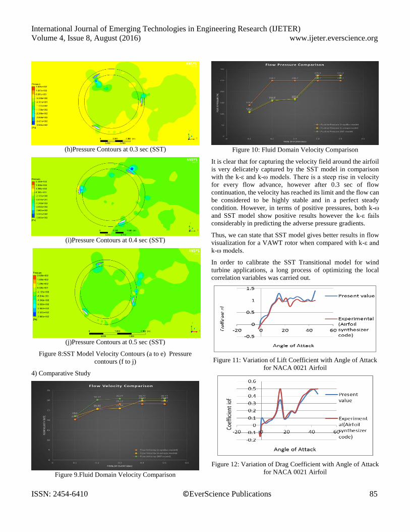
(h)Pressure Contours at 0.3 sec (SST)

(i)Pressure Contours at 0.4 sec (SST)

(j)Pressure Contours at 0.5 sec (SST)

Figure 8:SST Model Velocity Contours (a to e) Pressure

contours (f to j)

4) Comparative Study

Figure 9.Fluid Domain Velocity Comparison

Figure 10: Fluid Domain Velocity Comparison

It is clear that for capturing the velocity field around the airfoil

is very delicately captured by the SST model in comparison

with the k-ε and k-ω models. There is a steep rise in velocity

for every flow advance, however after 0.3 sec of flow

continuation, the velocity has reached its limit and the flow can

be considered to be highly stable and in a perfect steady

condition. However, in terms of positive pressures, both k-ω

and SST model show positive results however the k-ε fails

considerably in predicting the adverse pressure gradients.

Thus, we can state that SST model gives better results in flow

visualization for a VAWT rotor when compared with k-ε and

k-ω models.

In order to calibrate the SST Transitional model for wind

turbine applications, a long process of optimizing the local

correlation variables was carried out.

Figure 11: Variation of Lift Coefficient with Angle of Attack

for NACA 0021 Airfoil

Figure 12: Variation of Drag Coefficient with Angle of Attack

for NACA 0021 Airfoil




The coefficient of Drag predicted by the Fluent Solver shows

under fitting with respect to the experimental data for most of

the angle of attack values and thus makes the assumption pretty

complicated. However, the error percentage in this case is also

not large and thus the model can be considered stable for these

angle of attack values.

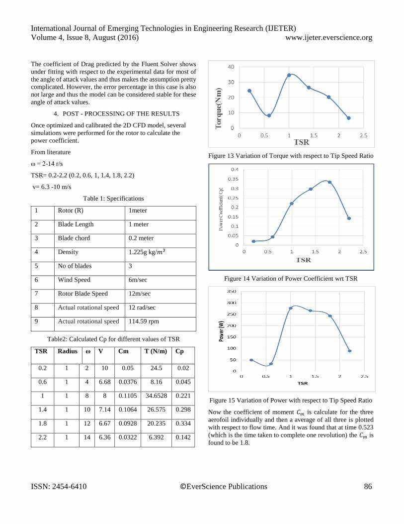
4. POST - PROCESSING OF THE RESULTS

Once optimized and calibrated the 2D CFD model, several

simulations were performed for the rotor to calculate the

power coefficient.

From literature

ω = 2-14 r/s

TSR= 0.2-2.2 (0.2, 0.6, 1, 1.4, 1.8, 2.2)

v= 6.3 -10 m/s

Table 1: Specifications

1 Rotor (R) 1meter

2 Blade Length 1 meter

3 Blade chord 0.2 meter

4 Density 1.225g kg/𝑚3

5 No of blades 3

6 Wind Speed 6m/sec

7 Rotor Blade Speed 12m/sec

8 Actual rotational speed 12 rad/sec

9 Actual rotational speed 114.59 rpm

Table2: Calculated Cp for different values of TSR

TSR Radius ω V Cm T (N/m) Cp

0.2 1 2 10 0.05 24.5 0.02

0.6 1 4 6.68 0.0376 8.16 0.045

1 1 8 8 0.1105 34.6528 0.221

1.4 1 10 7.14 0.1064 26.575 0.298

1.8 1 12 6.67 0.0928 20.235 0.334

2.2 1 14 6.36 0.0322 6.392 0.142

Figure 13 Variation of Torque with respect to Tip Speed Ratio

Figure 14 Variation of Power Coefficient wrt TSR

Figure 15 Variation of Power with respect to Tip Speed Ratio

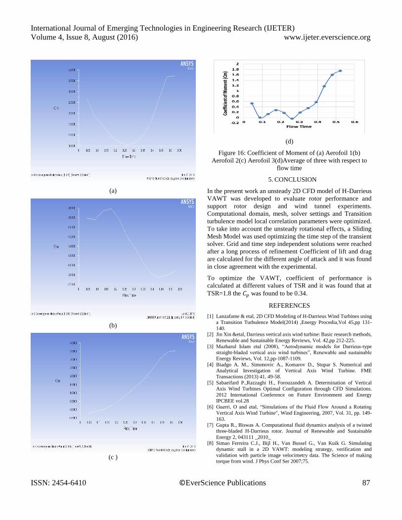
Now the coefficient of moment 𝐶𝑚 is calculate for the three

aerofoil individually and then a average of all three is plotted

with respect to flow time. And it was found that at time 0.523

(which is the time taken to complete one revolution) the 𝐶𝑚 is

found to be 1.8.




(a)

(b)

(c )

(d)

Figure 16: Coefficient of Moment of (a) Aerofoil 1(b)

Aerofoil 2(c) Aerofoil 3(d)Average of three with respect to

flow time

5. CONCLUSION

In the present work an unsteady 2D CFD model of H-Darrieus

VAWT was developed to evaluate rotor performance and

support rotor design and wind tunnel experiments.

Computational domain, mesh, solver settings and Transition

turbulence model local correlation parameters were optimized.

To take into account the unsteady rotational effects, a Sliding

Mesh Model was used optimizing the time step of the transient

solver. Grid and time step independent solutions were reached

after a long process of refinement Coefficient of lift and drag

are calculated for the different angle of attack and it was found

in close agreement with the experimental.

To optimize the VAWT, coefficient of performance is

calculated at different values of TSR and it was found that at

TSR=1.8 the 𝐶𝑝 was found to be 0.34.

REFERENCES

[1] Lanzafame & etal, 2D CFD Modeling of H-Darrieus Wind Turbines using

a Transition Turbulence Model(2014) ,Energy Procedia,Vol 45,pp 131-

140. [2] Jin Xin &etal, Darrieus vertical axis wind turbine: Basic research methods,

Renewable and Sustainable Energy Reviews, Vol. 42,pp 212-225.

[3] Mazharul Islam etal (2008), “Aerodynamic models for Darrieus-type straight-bladed vertical axis wind turbines”, Renewable and sustainable

Energy Reviews, Vol. 12,pp-1087-1109.

[4] Biadgo A. M., Simonovic A., Komarov D., Stupar S. Numerical and Analytical Investigation of Vertical Axis Wind Turbine. FME

Transactions (2013) 41, 49-58.

[5] Sabaeifard P.,Razzaghi H., Forouzandeh A. Determination of Vertical

Axis Wind Turbines Optimal Configuration through CFD Simulations.

2012 International Conference on Future Environment and Energy

IPCBEE vol.28 [6] Guerri, O and etal, “Simulations of the Fluid Flow Around a Rotating

Vertical Axis Wind Turbine", Wind Engineering, 2007, Vol. 31, pp. 149-

163. [7] Gupta R., Biswas A. Computational fluid dynamics analysis of a twisted

three-bladed H-Darrieus rotor. Journal of Renewable and Sustainable

Energy 2, 043111 _2010_ [8] Simao Ferreira C.J., Bijl H., Van Bussel G., Van Kuik G. Simulating

dynamic stall in a 2D VAWT: modeling strategy, verification and

validation with particle image velocimetry data. The Science of making torque from wind. J Phys Conf Ser 2007;75.

2D CFD Modelling Of H –Darrieus Wind Turbine and Its ...

Documents

Transcript of 2D CFD Modelling Of H –Darrieus Wind Turbine and Its ...