28 GHz Indoor Model Calibration

Application Note

Products:

➢ Consultix 5G; mmWave CW Transmitter

➢ iBwave design SW

➢ PCTEL HBflex; mmWave scanner

mmWave bands have been conceived as the most likely candidates to enable the ultra-high-speed of

5G networks. And due to the confined propagation characteristics of such bands, it is obvious that

dedicated indoor networks are becoming a must in 5G.

CW model calibration is a vital step during indoor radio planning to reflect the actual material

characteristics, tune propagation models and overcome uncertainties or risky assumptions. Hence, it’s a common practice to avoid an underperforming design and to prevent over-designs which lead to

unnecessary extra network cost.

This application note describes the field setup and procedures to perform indoor CW testing and

model calibration using “Consultix-5G” CW transmitter, “PCTEL HBflex” scanner as the test equipment

and “iBwave Design “as the planning tool.

Copyright© 2020 Consultix

All Rights Reserved

No part of this guide may be produced or transmitted in any form or by any means

without prior written consent of Consultix.

Trademarks

Consultix is a trademark of Consultix Company. All other trademarks mentioned in this

document are the property of their respective holders.

About iBwave

iBwave Solutions, the standard for converged indoor network planning, is the power

behind great in-building wireless experience, enabling billions of end users and devices

to connect inside a wide range of venues. As the global industry reference, iBwave

software solutions allow for smarter planning, design and deployment of any project

regardless of size, complexity or technology. Along with innovative software, the

company is recognized for world class support in 90 countries, the industry's most

comprehensive components database and a well-established certification program. For

more information.

About PCTEL

PCTEL, Inc. provides Performance Critical Telecom technology solutions. The company is

a leading global supplier of antennas and wireless network testing solutions.

PCTEL’s precision antennas are deployed in small cells, enterprise Wi-Fi access points,

fleet management and transit systems. The vendor offers in-house design, testing, radio

integration, and manufacturing capabilities. PCTEL’s test and measurement

tools improve the performance of wireless networks globally, with a focus on LTE, public

safety, and emerging 5G technologies. Network operators, neutral hosts, and

equipment manufacturers rely on PCTEL scanning receivers and testing solutions to

analyze, design, and optimize their networks.

Contents Introduction .................................................................................................................................................. 4

5G planning challenges ............................................................................................................................. 5

Test Setup ..................................................................................................................................................... 6

Procedures .................................................................................................................................................... 8

Test Preparations ...................................................................................................................................... 8

Notes before starting your test............................................................................................................. 8

Test Routes............................................................................................................................................ 8

Wall Material Realities .......................................................................................................................... 9

Measurements ........................................................................................................................................ 10

Transmitter ......................................................................................................................................... 10

Receiver ............................................................................................................................................... 10

CW Output .............................................................................................................................................. 18

Calibration Steps ..................................................................................................................................... 19

Calibrated model ..................................................................................................................................... 25

Conclusion (Statistical Results) ............................................................................................................... 29

General Remarks on the Calibration Process ......................................................................................... 33

Annex 1: Practical Tips (factors affecting CW Test Accuracy) ..................................................................... 35

Transmitter/receiver accuracy ............................................................................................................ 35

Test antennas ...................................................................................................................................... 35

Interference on channel ...................................................................................................................... 35

Test Route ........................................................................................................................................... 35

Data Averaging .................................................................................................................................... 35

Receiver settings ................................................................................................................................. 35

Test Cables .......................................................................................................................................... 36

Connectors .......................................................................................................................................... 36

Tripods ................................................................................................................................................ 37

Warm Up ............................................................................................................................................. 37

Body Blockage ..................................................................................................................................... 38

CW Signal BW ...................................................................................................................................... 38

Sampling Points ................................................................................................................................... 39

Annex # 2: References ................................................................................................................................ 40

Introduction Several countries have started to allocate mmWave bands for 5G services. And segments such as the 24-

29 GHz, the 37-40 GHz and 64-71 GHz are considered the frontier spectrum for 5G services. Each

country is currently adopting one or some of these bands, however in general the allocations of this

spectrum and bandwidth made the 5G service possible.

The emerging categories of services have diverse requirements in terms of bandwidth, speed, latency

and mobility. However, the challenge with mmWave spectrum is that the wavelengths are much shorter

than low GHz bands and thus they imply different propagation characteristics and new kinds of

interaction with the environment.

Higher propagation losses, lower building penetration, stronger reflections and significant scattering are

some of the forms of such different propagation behavior. And these factors together with the emerging

application requirements bring some challenges when it comes to radio planning.

Infrastructure cost is a prime factor in 5G network deployment. And coverage is more opportunistic

when it comes to higher bands such as mmWave. The thing that requires densification of RAN elements.

Hence, Consultix as the leader of CW test equipment in cooperation with iBwave as the prime tool for

indoor planning software analyze here how to optimize your design based on real measurements to

efficiently deploy a 5G network that meets its KPI's.

The key in this cycle is to collect measurements easily and effectively then to process them based on the

best practice of the planning tool.

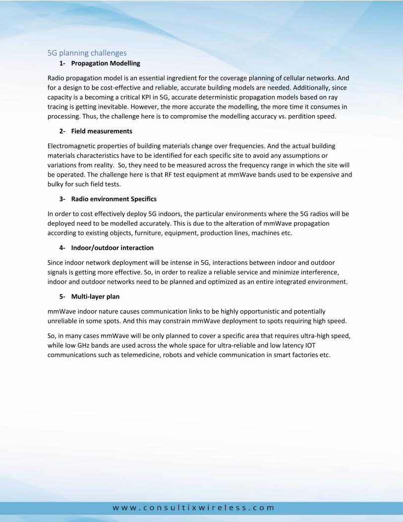
5G planning challenges

1- Propagation Modelling

Radio propagation model is an essential ingredient for the coverage planning of cellular networks. And

for a design to be cost-effective and reliable, accurate building models are needed. Additionally, since

capacity is a becoming a critical KPI in 5G, accurate deterministic propagation models based on ray

tracing is getting inevitable. However, the more accurate the modelling, the more time it consumes in

processing. Thus, the challenge here is to compromise the modelling accuracy vs. perdition speed.

2- Field measurements

Electromagnetic properties of building materials change over frequencies. And the actual building

materials characteristics have to be identified for each specific site to avoid any assumptions or

variations from reality. So, they need to be measured across the frequency range in which the site will

be operated. The challenge here is that RF test equipment at mmWave bands used to be expensive and

bulky for such field tests.

3- Radio environment Specifics

In order to cost effectively deploy 5G indoors, the particular environments where the 5G radios will be

deployed need to be modelled accurately. This is due to the alteration of mmWave propagation

according to existing objects, furniture, equipment, production lines, machines etc.

4- Indoor/outdoor interaction

Since indoor network deployment will be intense in 5G, interactions between indoor and outdoor

signals is getting more effective. So, in order to realize a reliable service and minimize interference,

indoor and outdoor networks need to be planned and optimized as an entire integrated environment.

5- Multi-layer plan

mmWave indoor nature causes communication links to be highly opportunistic and potentially

unreliable in some spots. And this may constrain mmWave deployment to spots requiring high speed.

So, in many cases mmWave will be only planned to cover a specific area that requires ultra-high speed,

while low GHz bands are used across the whole space for ultra-reliable and low latency IOT

communications such as telemedicine, robots and vehicle communication in smart factories etc.

Test Setup Transmitter Side

The transmitter setup comprises the elements listed in the table and illustrated in figure 1 below

Ser. Item Designation

1 CW Transmitter Consultix 5G transmitter (25 to 28.5 GHz)

2 RF Test Cable Low Loss cable (2.4 dB/m @ 28 GHz)

3 Test Antenna 3 dBi omni-directional antenna (model Consultix C5G-Acc-OA3)

4 Tripod 2-meter non-metal tripod

• The transmitter can be tied to the tripod or placed on any other holder.

• The test antenna to be monted on the tripod using the provided mounting kit as shown below.

• The test cable is firmly connected to the transmitter and the antenna.

• The AC/DC adapter of the transmitter to be connected to AC Main supply

Figure 1 mmWave CW transmitter setup

Receiver Side

The receiver setup comprises the following elements:

1- PCTEL scanner: HBFlex

2- Low Loss cable (2.4 dB/m @ 28 GHz)

3- 3 dBi omni-directional antenna

4- Battery pack

5- USB Cable

6- PCTEL Software: SeeHawk Touch

Figure 2 PCTEL HBflex Scanner setup

Figure 3 PCTEL HBflex scanner Backpack

Procedures

Test Preparations

Notes before starting your test

1- The environment has to be checked that the channel is clear prior to starting the test. So, the

receiver has to read something close to noise levels while the transmitter is off.

2- After assembling the transmitter and receiver setups, a 3m check up has to take place to verify

the signal integrity across all elements. And this indicates that all cables and antennas are

integrated properly. Receiving something around -60 dBm is reasonable in this test.

3- Remember during your walk test that the log shouldn’t include pause/resume jumps across

walls and corridors, as these results include erratic interpolated values.

4- You can pass on the same point multiple times.

Test Routes

Walk test routes should be identified prior to commencing the test. Here we identified 4 different routes

with 4 different transmitter positions as shown in figure 4.

Figure 4: Defining 4 transmitter locations for the 4 walk test routes

And measurement routes to be drafted before starting the walk test as shown below.

Figure 5 Drafting a Walk Test Route

Wall Material Realities

Importing the wrong type of wall material may significantly affect prediction accuracy. It is

recommended to visually inspect the prediction map and compare it with the CW data taken during the

site survey. If the signal delta is consistently high along a stretch of a wall, it is possible that the wrong

type of wall was imported.

• Wall types need to be defined on the layout; which one is concrete and which one is steel etc.

• Its recommended to verify wall types during the site visit.

• We will perform material loss measurement for different wall material (if there are many types,

user may pick the most common two or three types).

• This test should be done on the same test frequency. And the receiver location to be fixed for 2-

minute duration (in a separate file)

• The exact distance from wall will be 1.5 m as shown in the figure

Figure 6 Verifying wall types

Measurements

Transmitter

5- The transmitter frequency is set to 28.002 GHz and the output power to 16 dBm.

6- The actual antenna Hight is noted down and here it is 2.015 m

Receiver

1- Select Indoor from the Mode dropdown to perform Indoor tests.

2- Customize legends by Technology and Metrics

3- Indoor Measurement selection

• From the listed Protocol list select NR. From the Band list Select the desired Band.

• Sampling rate to be at least 60 samples/s

• Click on Selected Channels to pick a Channel/Frequency.

• Check the desired channels and Click OK.

4- Map Setup-Select measurement to plot on Indoor Map

Select Measurement and Metric to be displayed

5- Selecting Indoor Image

Select Floor Plan using the following options:

• Load a Tab File; Load an already created tab file.

• Load and Register an Image; Register a saved Image using SeeHawk Touch Registration.

• Capture and Register an Image File; Take a picture on the fly and register.

• Recent TAB file; Show last used TAB file.

6- Test Files – Indoor Map Image Registration

• Images must be registered to have collected data available to be displayed on the image (Tab

files are generated in this process)

• Select image to be loaded in for data collection

Select image to be loaded in for data collection, tap image to show reference line, select one end of line

and hold until line is active as shown below

Then, drag edges to size ruler line, tap and set scale (meters or feet)

Test Files – Indoor Map Manual Registration

Manual Registration allows for the user to input coordinate information\geocode in image

7- Indoor Mode Data Collection

Place marker at starting point, Record and begin walk test

8- Indoor Mode- Delete Last Marker

Route is displayed according to the legend. And measurements are spread between markers. If

there is an error in placing a marker, it can deleted.

9- Indoor Mode-File Name

Once route is completed, hit the Stop button and save file

10- Test Files

Provides Playback, and a Quick View of a collected measurement, FTP Queue and ability to

Delete or Rename files. Walk test data will be in the Drive/Walk tab.

11- Export Data Using Collect

• Data can be exported using SeeHawk Collect or Autoexport.

• Copy files from SeeHawk Touch to a PC. If using SeeHawk Collect, copy files in the Documents

folder. Select Drive>Right Click>Export.

• Select csv and click next. Click on Start export. Data will be saved in .csv format in the drive data

folder.

12- Export Data Using Autoexport

• Start SeeHawk AutoExport by double clicking on the SeeHawk AutoExport icon in the Windows

tray menu, or from Start Menu under All Programs → PCTEL, RF Solutions Group → SeeHawk

AutoExport.

• Right click on the tray icon for options to view activity log, change settings, view about

information, or exit the program.

• Create Source and Target Folders and assign path here.

• Copy paste the test files in the Source Folder. Autoexport will automatically process and convert

the data to a csv file.

CW Output

The exported CSV file will contain the required basic information that will be used for model calibration

as shown below

Figure 7 Walk Test Result files; CSV

Figure 8 Walk Test Drawing Results

Calibration Steps

The following steps are will be followed in order to perform calibration in iBwave Design

1) Import the survey data

2) Under the Prediction Tab, go to Calibrate

3) In the Calibration Window, go to Manage Models tab and click on + sign to create a new calibration model

4) Follow the 4 steps as indicated below to create a new model

5) Once the model is created, you need to assign it to the corresponding antenna in order to perform prediction using this created model. To do this, go to Assign Tab.

6) In Assign Models Tab, select the created model and assign it to the corresponding Antenna

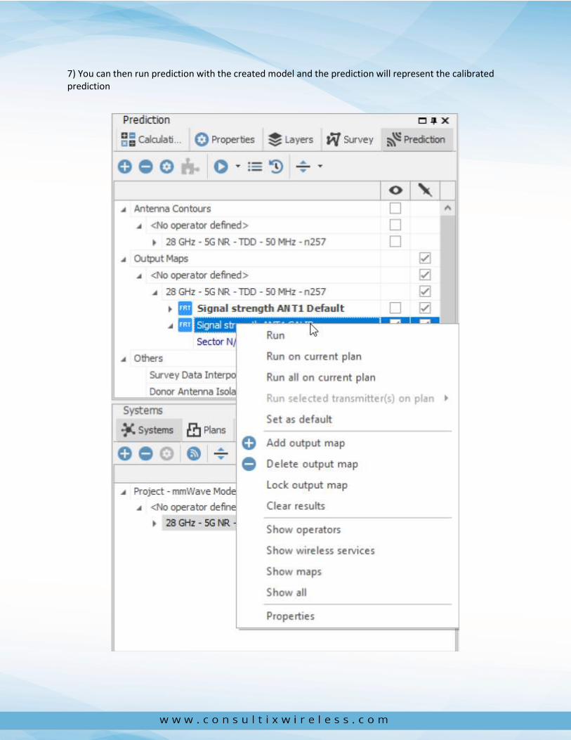
7) You can then run prediction with the created model and the prediction will represent the calibrated prediction

Calibrated model

The layout of the office space with 4 antenna locations is shown below:

Figure 9 Layout Plan for 4 locations of the CW Transmitter

We did two steps in data post processing. First, we removed fast fading by averaging the receive data

every 0.2 meters, which is 20 wavelengths. Second, we eliminated the data that was too far away from

antenna. After that, the CW data looks as illustrated in the next figures.

CW Data for Antenna 1

CW Data for Antenna 2

CW Data for Antenna 3

CW Data for Antenna 4

When we started analyzing the data, we noticed the following:

1) The Non-Line of Sight data behind Drywall walls was predicted to be much lower than the measured.

When comparing similar materials, we noticed that Drywall has much higher penetration loss than

plaster sheetrock - light. We decided to replace drywall with plaster sheetrock light everywhere in the

floorplan.

2) The predicted data behind wood wall near antenna 2 was much lower than the measured data. When

comparing similar materials, we noticed that wood has much higher penetration loss than chip board.

We decided to replace the wood with chip board.

The layout with the new materials is shown below:

Figure 10 Material Update of the layout Plan

After we replaced the materials, we started looking into uncalibrated prediction and whether changing

propagation constants γ1 – γ3 would help increase accuracy. We decided to change γ2 and γ3 to 2.2

instead of 2.4.

Conclusion (Statistical Results)

The final statistics for default and calibrated prediction for all 4 antenna locations are presented in the

following section:

Statistical Results for Antenna 1

We see that calibrated results are about the same as default results. This is because we do not have Line

of Sight data. To improve the calibrated model, we need a mix of LOS and NLOS data.

Statistical Results for Antenna 2

Accuracy is better for calibrated data. Also, default accuracy is better than for Antenna 1. We also have

plenty of LOS data.

Statistical Results for Antenna 3

Again, calibrated results show improvement over uncalibrated results because we have LOS data.

Statistical Results for Antenna 4

As was the case with Antenna 2 and 3, we see significant improvement in calibrated data. There is

plenty of LOS data as well.

General Remarks on the Calibration Process

• Mean and absolute mean error values are similar for antenna 3. This is also the case for antenna 4. Because the mean error is positive and the two errors are similar, the measured data is almost always

higher than the predicted data. In other words, iBwave prediction for antenna 3 and 4 is consistently

more pessimistic than the measured data.

• When we had to decide which data to keep and which to eliminate, we looked into two things: Is the data duplicate? For antenna 2, we had LOS data taken in two ways going away from the antenna

from right to left, and then backwards, going from left to right. When we examined the data more

closely, we saw that data points taken at the same location but in opposite direction had different

values. Sometimes, that difference is up to 10 dB. This is a problem for calibration, because we have two

very different values at the same location. Ideally, we would need to average out that data out before

calibration. But if there is no plenty of time to do that, user can only keep one of the two sets, and

eliminate the other. This improved default and calibrated accuracy. The area where we reduced the

number of points by eliminating duplicate points is shown below:

Figure 11 Data Elimination for Antenna Location 2

Is the data far away and NLOS? For antenna 4 we had data that was behind a corner after a long

corridor, to the right of the antenna. We decided to keep only a few meters behind the corner and

delete the rest. We also deleted points in the upper left area, in the corridor parallel to LOS corridor.

Deleting those points improved default and calibrated accuracy.

Figure 12 Data Elimination for Antenna Location 3

In retrospect, the default prediction absolute error is in the 4.5-5.5 dB range. The standard deviation is

in the 3.5 – 6.2 dB range. This is consistent with what we saw at lower frequencies. While it is true that

we had to fine tune the floorplan material modeling (by replacing the high penetration loss material

with lower penetration loss material).

What we learned from this measurement campaign is that inner walls should be modeled as plaster

sheetrock - light and chip board, and not as drywall and wood.

Finally, we learned that 28 GHz signal propagates through typical office walls/barriers better than

expected. We had to adjust propagation constants γ2 and γ3 to reflect on that

Annex 1: Practical Tips (factors affecting CW Test Accuracy)

Transmitter/receiver accuracy

• Use calibrated equipment

• Make sure your RF equipment is maintained and operated as instructed by its vendor

• Use a transmitter with a screen to know the setting values during the test

• Visually check your testers, antennas and cables for any defect in the RF connectors.

Test antennas

• Preferably the transmitter antenna to be the same type of the actual one of that site

• Make sure there are no obstructions around the test antennas

• Care must be taken to hold the receiver antenna at an average person’s height

• Place the transmitter antenna as close as possible to the intended installation position,

orientation and Hight. Usually a tripod or a mast with a variable hight is a very helpful tool for

this function.

Interference on channel

• Prior to your test, make sure the RF environment along the whole test path is clear from

interference on the same channel that will be used for testing

Test Route

• The measurement route must be well selected and planned prior to conducting the test.

• It should represent the areas to be served and a special attention must be given to areas close

to windows on the sides of the building.

• Avoid testing in a close proximity to the transmitter as this saturates your receiver and provides

false results.

Data Averaging

• Averaging always yields to more reliable estimate of the local average power independent of the

test signal bandwidth and mitigates fluctuations over a small area due to multipath fading.

• Some collection tools have data averaging algorithm, make sure you recognize if this is the case

with your tool and configure its parameters adequately.

• If you will do averaging manually pay attention if its linear averaging or dB averaging. dB

averaging tends to deemphasize the large variations from the mean, whereas linear averaging

may be significantly skewed by one or two extreme values

Receiver settings

If you are using a spectrum analyzer rather than a CW receiver/scanner, special attention should be

given when setting its parameters to avoid inaccurate readings:

• The same transmitter frequency is to be chosen as the central frequency of the spectrum

analyzer

• The span of your spectrum analyzer to be adequately wider than the test signal. However, too

wide span affects frequency accuracy.

• Reference Level should be configured relevant to the expected power levels along the test path.

• Recognize the type of detectors of your tester whether RMS, Peak or Quasi peak detector and

select it as per your measurement needs and the post processing procedures.

• Select a relevant channel bandwidth if you are using the “channel power measurement” mode.

• Make sure your analyzer is in normal settings without any offsets.

Usually most of these setting considerations are not required when using a more specialized CW

receiver or a radio scanner.

Test Cables

Cable losses are very significant at this band. For example, here we have the attenuation curve of

one of Consultix typical accessories which is the flexible 3 ft cable .

As can be seen, losses at low GHz bands are around 0.5 dB while the curve reaches around 2.5 dB at

28 GHz. This means that almost half the power is lost. So, attention should be paid to the used

cables and other accessories.

Connectors

Consultix 5G transmitter and its setup have K type connector (2.9mm). Users have to take care not

to use SMA cables/adapters. SMA is a kind of connectors which are practical up to 26 GHz while K

type works up to 46 GHz or more. They are mechanically compatible, but their dimensions are not

exactly the same. The inner diameter of the external conductor of the coaxial structure is 2.92 mm

for the K connector while it is 4.13 mm for the SMA connector. In addition the dielectric material

isn't the same:

SMA --> teflon

K --> air

So they are not electrically compatible.

Tripods

In general, metal objects close to the test antenna cause pattern deformation by some dB’s. Which in turn reflects in the measurement accuracy. And metal objects should be kept at least few lambda

from the antenna neighborhood to not cause practical pattern distortion.

So, usually for test purposes, a non-metal tripod or a mast is mandatory.

Warm Up

Warming up is always a good idea before any activity. And the same applies to RF measurements.

All RF devices have resistance and capacitance whose electrical properties change with

temperature. For the measurement equipment to be able to properly operate and provide accurate

and consistent results, these instruments must warm up and stabilize thermally.

Body Blockage

Care should be given to the receiver antenna placement. Sometimes, especially in CW walk-testing,

users ignore the right antenna placement of the receiver. For example, it might happen that they

hold it in their hands and so on.

Please note that field experience and statistical modelling indicated that body blockage at mmWave

could reach around 8 dB. Hence, the location of the mmWave antenna is critical during walk testing.

And user has to maintain the receiver antenna height at least above the human body.

CW Signal BW

CW signal is unmodulated, hence theoretically it has no BW. Practically you can see it as just few Hz.

And using such a narrow signal is intentional in order to keep the receiver noise floor at minimal and

thus maximizing the measurement distance. On the other side, another important tip here is to

open the RBW of the scanner to tolerate signal drifts due to any reasons.

100 KHz is very fair scanner RBW at mmWave bands, however before testing, user has to check that

the RF environment is clear across those 100 KHz. You can verify this by checking that your receiver

is not picking any interferer while the transmitter is off.

Sampling Points

Attention should be paid to sampling points in terms of quantity and quality. And this is explained

here:

Figure # 1 below represents the ideal scenario. The user here captured an adequate number of

samples and calibrated his propagation model to produce the solid curve.

Figure # 2 is what happens to the plot when insufficient number of samples is taken. The calibrated

plot tends to higher values at most of the points.

Figure # 3 illustrates the case when the samples represent only areas close to the transmitter. So,

the plot is extrapolated along its extension and tends to values lower than the ideal curve. And the

same in curve # 4.

And finally in the last curve, when noise floor clipping takes place, the calibration plot is false as well.

Figure 13 Calibrated model vs different sampling manners

Annex # 2: References

Consultix, IBS Testing Pocket Guide Part 1. IBS Pocket Guide 2019

Consultix, Indoor Designer Checklist. Technical Article. 2020

iBwave, Fast Ray Tracing. White Paper. 2013

iBwave, Instructions for Calibration Process. Manual. 2020

PCTEL, SeeHawk Touch Setup. Instructions. 2020

Alejandro Aragón-Zavala, Indoor wireless communications: From Theory to Implementation. John Wiley &

Sons, Ltd. 2017

Microwave Journal, mmWave Channel Modelling with Diffuse Scattering in an Office Environment. Online

Article. 2019

Ranplan, 5G NR Network Planning. White Paper. 2019

Huawei, Indoor 5G Networks. White Paper. 2018

Ericsson, Bringing 5G Networks Indoor. White Paper. 2019

S. A. Busari, S. Mumtaz, S. Al-Rubaye and J. Rodriguez, "5G Millimeter-Wave Mobile Broadband:

Performance and Challenges," in IEEE Communications Magazine, vol. 56, no. 6, pp. 137-143, June 2018,

doi: 10.1109/MCOM.2018.1700878.

iBwave, Analysis of CW Measurements @ 28 GHz taken by Consultix. Online Blog. 2020

Consultix, 6 Factors affect CW Test Accuracy. Application note. 2019

About Consultix Consultix is a leading vendor of portable RF test

equipment. The company is remarkably known

for its comprehensive portfolio of RF analyzers,

CW equipment and monitoring solutions

serving the Small cells and DAS market

worldwide

Find us:

133, St. 17, Mohammed Farid Axis, 11835 New Cairo Egypt.

+2 02 25647370 info@consultixwireless.com