248566.pdf - Office of Justice Programs

The author(s) shown below used Federal funds provided by the U.S. Department of Justice and prepared the following final report: Document Title: Developing Guidelines for the Application of

Multivariate Statistical Analysis to Forensic Evidence

Author(s): Ruth Waddell Smith, David R. Foran, Victoria L.

McGuffin Document No.: 248566 Date Received: January 2015 Award Number: 2011-DN-BX-K560 This report has not been published by the U.S. Department of Justice. To provide better customer service, NCJRS has made this Federally-funded grant report available electronically.

Opinions or points of view expressed are those of the author(s) and do not necessarily reflect

the official position or policies of the U.S. Department of Justice.

Developing Guidelines for the Application of Multivariate Statistical Analysis

to Forensic Evidence

Final Technical Report

Ruth Waddell Smith1, David R. Foran1, and Victoria L. McGuffin2

1Forensic Science Program and 2Department of Chemistry

Michigan State University

East Lansing, MI 48824

Award Number: 2011-DN-BX-K560

Office of Justice Programs

National Institute of Justice

Department of Justice

This project was supported by Award No. 2011-DN-BX-K560 awarded by the National Institute of Justice, Office

of Justice Programs, U.S. Department of Justice. The opinions, findings, and conclusions or recommendations

expressed are those of the authors and do not necessarily reflect those of the

Department of Justice.

This document is a research report submitted to the U.S. Department of Justice. This report has not been published by the Department. Opinions or points of view expressed are those of the author(s)

and do not necessarily reflect the official position or policies of the U.S. Department of Justice.

i

Abstract

Recommendation 3 in the 2009 National Academy of Sciences’ National Research

Council report “Strengthening Forensic Science in the United States: A Path Forward”

highlighted the lack of statistical comparison of forensic evidence. Multivariate statistical

procedures have potential as a means to overcome this deficiency by providing an additional tool

for analysts to use in such comparisons. However, these procedures are not widely implemented

in forensic laboratories. The purpose of this research was to investigate and demonstrate

application of multivariate statistical procedures to forensically relevant data and highlight the

advantages and limitations that must be considered for these procedures to be used in forensic

investigations.

To be as realistic and as practical as possible, three separate and diverse data sets were

generated. The first contained chromatographic data of ignitable liquid reference standards and

simulated fire debris samples, the second contained spectral data of controlled substance

reference standards and simulated street samples, and the third contained ribosomal RNA gene

sequence data of bacteria in soil samples from different habitats. For each data set, statistical

procedures were used to associate or classify samples to the corresponding reference standard.

The chromatographic and spectral data sets were initially probed using principal

components analysis (PCA) and hierarchical cluster analysis (HCA). These two procedures are

exploratory in nature and are used to identify patterns in the data, enabling association of similar

samples with distinction from different samples. Both procedures are based on the principle of

distance measurements in multidimensional space and hence, in theory, the same association and

differentiation of samples within a data set will be achieved irrespective of procedure used.

However, PCA reduces the dimensionality of the data set, retaining the most important

information while in HCA, all dimensions are retained and expressed. While there are

advantages and disadvantages for each procedure, in this particular application, greater success

in associating the simulated sample to the appropriate reference standard was achieved using

HCA.

The same two data sets were further probed using two classification procedures: soft

independent modeling of class analogy (SIMCA) and k-nearest neighbors (k-NN). SIMCA has

theoretical advantages in using statistical models for the classification and not forcing

classification. However, for this particular application, the development of representative models



ii

was challenging and limited the success of SIMCA. In contrast, the k-NN procedure is based on

the proximity of samples to reference standards in multidimensional space rather than statistical

models. Although k-NN forces classification, the simulated samples were more successfully

classified according to appropriate reference standard using this procedure rather than SIMCA.

The sequencing data were analyzed with PCA and nonmetric multidimensional scaling

(NMDS). While both procedures are based on similar principles, NMDS is better suited to

nonparametric data. Similar to PCA, NMDS reduces the dimensions of the data set for easier

interpretation. Differentiation among the habitats was possible based on the gene sequence data;

however, NMDS was able to cluster replicate samples of each soil within standard error whereas,

only mild association of replicates was possible using PCA.

Aspects of this research have been disseminated to the wider forensic community through

poster and oral presentations, which have been given by both graduate students in the Forensic

Science Program at Michigan State University and the PIs. Three manuscripts are in preparation

(one for each data type) and tutorials outlining the application, interpretation, and considerations

for these data analysis procedures are currently being developed.



iii

Table of Contents

Abstract ............................................................................................................................................ i

Executive Summary ........................................................................................................................ 1

1. Introduction ................................................................................................................................. 9

2. Theory ....................................................................................................................................... 14

2.1 Data Pretreatment Procedures ............................................................................................ 14

2.2 Exploratory Procedures ...................................................................................................... 19

2.3 Classification Procedures ................................................................................................... 35

3. Materials and Methods .............................................................................................................. 39

3.1 Chromatographic Data ....................................................................................................... 39

3.2 Spectral Data ...................................................................................................................... 42

3.3 Gene Sequence Data ........................................................................................................... 44

4. Results and Discussion ............................................................................................................. 49

4.1 Chromatographic Data ....................................................................................................... 49

4.2 Spectral Data .................................................................................................................... 120

4.3 Gene Sequence Data ......................................................................................................... 145

5. Conclusions ............................................................................................................................. 158

6. References ............................................................................................................................... 164

7. Dissemination of Results ........................................................................................................ 169



1

Executive Summary

The 2009 National Academy of Sciences’ National Research Council report

“Strengthening Forensic Science in the United States: A Path Forward” was instrumental in

highlighting current deficiencies in the practice of forensic science across the country. Among

the thirteen recommendations made in the report, one in particular identified the limitations in

forensic evidence comparisons and called for “the development and establishment of quantifiable

measures of the reliability and accuracy of forensic analyses” and the “development of

quantifiable measures of uncertainty in the conclusions of forensic analyses.”1 Throughout the

report, the current methods for nuclear DNA analysis were highlighted as the gold standard.

With this type of evidence, DNA profiles from a questioned source are generated using advanced

analytical instrumentation, and then compared to a known sample or database of DNA profiles.

This comparison can provide the likelihood that the particular DNA profile occurred by random

chance, which in turn can be used to express an error rate associated with the comparison.

Similar statistical procedures are not currently employed for other evidence comparisons.

In trace evidence and controlled substance analysis, submitted samples are analyzed using gas

chromatography-mass spectrometry and infrared spectroscopy, among other techniques. The data

generated by these instruments are complex, containing hundreds, even thousands of variables.

Despite the complexity, comparisons of the resulting chromatograms and spectra between a

questioned sample and a reference standard are currently based on visual assessment, which

naturally introduces some subjectivity. In an effort to minimize such subjectivity, a more

statistical-based comparison is necessary. The complex chromatographic and spectral data are

ideal candidates for multivariate statistical procedures. These procedures compare all variables

simultaneously to identify patterns in the data that can be used to associate similar samples and

discriminate different samples.

Forensic analysis of soil samples is typically based on a physical and chemical

assessment of the soil, which are class characteristics. However, analysis of the microbial

population of the soil has the potential to create a ‘microbial fingerprint’ to associate soils from

similar habitats while discriminating those from different habitats. In the microbial genomics

field, soils are analyzed using next generation sequencing, which routinely generates over

100,000 sequences. Again, this type of data lends itself to analysis using multivariate statistical

procedures.



2

The purpose of the proposed research was to investigate the applicability of a selection of

multivariate statistical procedures for the analysis and comparison of forensically relevant data.

The selected procedures are widely used and reported in other scientific fields such as analytical

chemistry or microbial studies, but are not yet tried and tested specifically for forensic evidence

applications. Therefore, a second intention of the research was to highlight considerations and

current limitations with regard to the implementation of these procedures. Finally, the third

intention was to produce a document that describes the theory, application, and interpretation of

results for these procedures using forensically relevant evidence as the model data. This

document could serve as a resource for forensic laboratories considering implementation of such

statistical procedures.

The first step in the research was to generate suitable data sets for statistical analysis.

Three distinct data sets that represented different types of data encountered in forensic analyses

were generated. The first data set contained chromatographic data of ignitable liquid reference

standards and simulated fire debris samples. The second set contained spectral data of controlled

substance reference standards and simulated street samples, and the third set contained ribosomal

RNA gene sequence data of bacteria in soil samples collected from different habitats.

Although all three data sets contained thousands of variables, there were distinct

differences between the chemical data (i.e., the chromatographic and spectral data) and the

biological (i.e., gene sequencing) data. First, the chromatographic and spectral data consisted of

continuous variables while the gene sequencing data contained discrete variables. Second, the

former data sets were assumed to follow a normal distribution while the gene sequencing data

were nonparametric in nature. As a result, different statistical procedures were applied according

to the distribution of the data, thus for clarity, the chromatographic and spectral data sets are

discussed separately from the gene sequence data throughout this report.

Similar procedures were applied to the chromatographic and spectral data sets to

investigate association of the simulated samples to the appropriate reference standard, and

distinction of the simulated samples from all other reference standards in the data set. Although

both data sets contained approximately 3,500 variables, the chromatographic data were more

complex and hence, much of the investigative aspect of the research focused on this particular set

to provide a test of the robustness of the procedures applied.



3

While the focus of the research was the application of statistical procedures, data

pretreatment prior to analysis is an important consideration for data collected using instrumental

techniques and over a prolonged time period. Variance that is non-chemical in nature can exist in

such data as a result of random fluctuations in noise, differences in the mass or volume of sample

analyzed, and fluctuations in the parameters used for the analysis (e.g., carrier gas flow rate or

variations in oven temperature in gas chromatography). When present in a data set, these non-

chemical sources of variance can be identified by the statistical procedures as chemical

differences among the samples. As such, it is important to minimize or eliminate non-chemical

variance to ensure data analysis results are meaningful.

To address this consideration, various pretreatment procedures were applied to the data

and the effect of each was assessed. For the chromatographic data, retention time alignment,

normalization, and scaling were investigated. Two different alignment algorithms were

considered (peak-match and correlation optimized warping) and for each algorithm, various user-

defined parameters were compared. For this particular data set, alignment was not necessary,

primarily because reference standards and simulated samples were analyzed using the same

instrument and column and over a relatively short time period. However, this will not always be

true in forensic laboratories and hence, it is important to visually assess the data to determine the

need for retention time alignment.

Three normalization procedures were investigated (constant sum, constant maximum, and

constant vector length) for this data set. Normalization was necessary to improve precision of

replicates; however, no one procedure offered improvement for all standards in the data set. This

was primarily due to both the complexity of the data and the chemical diversity among the

reference standards. Hence, it was necessary to reach a compromise in which all data were

subjected to constant sum normalization prior to data analysis. Scaling procedures (autoscaling

and Pareto scaling) were also investigated. For this pretreatment, there was no improvement in

replicate precision compared to the unscaled data as all the data were of similar magnitude.

Pretreatment for the spectral data set focused on normalization to take into account

variation among samples as a result of day-to-day instrument variation. Again, three different

normalization procedures (constant sum, constant vector length, and standard normal variate)

were assessed based on the improvement in precision of replicate spectra. For these data, the

standard normal variate procedure proved optimal and was used for all subsequent analyses.



4

Following the investigation of data pretreatment procedures, two different types of

statistical procedures (exploratory and classification) were investigated for the chromatographic

and spectral data sets. Exploratory procedures identify patterns in the data with no prior

knowledge of the identity of any samples or even standards in the data set. Three exploratory

procedures (Pearson product-moment correlation, principal components analysis, and

hierarchical cluster analysis) were initially applied to investigate association of the simulated

samples to the appropriate reference standard with distinction from all other standards.

Pearson product-moment correlation (PPMC) offers a pairwise comparison of samples (in

this case, simulated sample compared to reference standard) resulting in a single number (the

correlation coefficient) that indicates the degree of similarity between the two. However, through

analysis of the chromatographic data set, a number of limitations for this particular application

were highlighted. Firstly, the coefficient is calculated on a point-by-point basis between the two

samples. Chromatograms of the simulated samples contained interference compounds (e.g.,

interference compounds from debris substrates or cutting agents in street samples) that were not

present in the reference standards. These additional peaks lowered the coefficient, resulting in

only weak to moderate correlation between the simulated samples and the corresponding

reference standard. Further, while the comparison of a sample and standard can be represented

by a single number, the number of coefficients calculated for a given data set increases with the

square of the number of samples. Comparison of a single sample with each standard in a

reference collection can generate a large number of coefficients, which makes comparison and

investigation of the coefficients particularly time consuming. Hence, PPMC coefficients were

not investigated further beyond the chromatographic data set due to these limitations.

The chromatographic and spectral data sets were separately subjected to principal

components analysis (PCA). This procedure reduces the dimensionality of the data set by

identifying and maintaining the major sources of variance. Complex data can be represented in a

smaller number of dimensions without losing discriminatory information. Results from PCA are

most commonly displayed in the form of scores and loadings plots. The scores plot is a scatter

plot that represents the similarities and differences within the data set; that is, samples that are

chemically similar are positioned closely in the scores plot and separately from those that are

chemically distinct. Loadings plots are used to identify those variables that contribute to the



5

variance described by each principal component and can be useful in explaining the positioning

of samples on the scores plot.

For each data set, PCA was initially performed on the reference standards alone,

generating scores and loadings plots. Scores were calculated for the simulated samples using the

eigenvectors for the standards and then projected onto the original scores plot. Performing PCA

in this manner has the advantage of minimizing or eliminating contributions from sample

interference compounds (e.g., debris substrates or cutting agents) as only those compounds

present in the reference standards contribute to the scores calculated for the samples. Further,

association and discrimination in the scores plot was assessed using two additional metrics

(Euclidean distance and PPMC coefficients) to provide a more objective method to interpret the

scores plot.

Association of simulated samples to the corresponding reference standard using PCA was

of limited success for both data sets. For the chromatographic data, simulated fire debris samples

containing liquids that were chemically distinct from other reference standards were

appropriately associated. However, for the remaining samples, clear association to one reference

standard was not possible. Additionally, the success of association was dependent on the nature

of the substrate interference compounds. For the spectral data, simulated samples were

successfully associated to the corresponding reference standard in the presence of low levels of

cutting agent. However, as the percentage of cutting agent present increased, successful

association became limited, with fewer samples associated successfully.

The final exploratory procedure considered was hierarchical cluster analysis (HCA). This

procedure is often considered complementary to PCA; that is, HCA assesses similarity among

samples in a data set while PCA identifies differences in the form of variance among samples.

The output from HCA is a dendrogram which displays clusters of similar samples, along with the

similarity level at which the clusters form, with higher similarity level indicating greater

similarity.

Cluster analysis was performed separately on each data set to again assess association of

simulated samples to the appropriate reference standard. While the actual similarity level at

which the simulated samples clustered with the reference standards varied, the simulated samples

clustered first with the corresponding reference standard before clustering to any other standard.

This was true for both the chromatographic and spectral data sets. Further, in most cases,



6

exclusive clusters were formed; that is, the cluster contained the simulated sample and the

appropriate reference standards only. There were some exceptions to this in the chromatographic

data set in which certain simulated fire debris samples formed clusters with a group containing

more than one reference standard. However, this overlap in clustering was due to the high degree

of chemical similarity among these particular reference standards.

This research indicated that HCA had greater potential than PCA for these applications.

Despite apparent differences in mode of operation (HCA is based on similarity while PCA is

based on variance), both procedures are founded on the same basis; that is, the distance between

samples and references standards in multidimensional space. Hence, both procedures should

theoretically yield similar results in terms of association and discrimination. However, probing

these results is considerably simpler using HCA as all dimensions are retained and accounted for

in the resulting dendrogram. In contrast, typically only the first few principal components

(dimensions) are retained and assessed in the PCA scores and loadings plots. To achieve the

same association and discrimination as HCA, all principal components must be considered.

However, this is no small undertaking as n-1 principal components are calculated, where n is the

number of samples or variables, whichever is smaller. Further, as only two or three dimensions

can be readily visualized, probing additional principal components would require plotting

numerous scores plots. Not only would this be extremely time consuming, but subsequent

interpretation and comparison of all the resulting plots would become arduous.

While exploratory procedures have the advantage of not requiring any knowledge of the

data set, the limitation is that only association (or differentiation) of samples is possible based on

patterns in the data. In contrast, classification procedures require knowledge of pre-defined

groups within the data set. Samples are subsequently classified according to one of the

previously defined groups. Two classification procedures (soft independent modeling of class

analogy and k-nearest neighbors) were used to investigate classification of simulated samples to

the appropriate reference standard with distinction from all other standards.

The soft independent modeling of class analogy (SIMCA) approach develops statistical

models for the pre-defined groups in the data set and then uses these models to classify the ‘new’

samples (in this case, the simulated samples). Models are developed using PCA and hence,

SIMCA can be considered an extension of PCA. Through this investigation for both the

chromatographic and spectral data sets, multiple iterations of model development were



7

conducted. Initial models that contained only the reference standards were not sufficiently

representative of the data to be classified and hence, no classification was possible.

The greatest success in classification using SIMCA was achieved with models that

included not only the reference standards but also the burned substrate or cutting agent (for the

chromatographic and spectral data, respectively), as well as replicates of the simulated samples.

For both data sets, the most successful classification was achieved at the 99.9% confidence level;

however, it should be noted that higher confidence levels are least rigorous when association is

considered, as is the case here. Not all simulated samples were classified and in each case, the

lack of classification was attributed to differences in abundance between the simulated samples

to be classified and those included in the model. Hence, despite being more representative of the

data to be classified, the models were too specific, to the extent that differences in abundance

prevented classification.

In contrast to SIMCA, the k-nearest neighbors (k-NN) approach to classification requires

no model building; instead, known groups and ‘new’ samples are considered at the same time,

with the ‘new’ sample being classified according to the group to which it is positioned most

closely in the multidimensional space. As a result, k-NN can be considered an extension of HCA

in that sample distances are calculated and groupings are based on close proximity. Using this

procedure, classification of the simulated samples was considerably more successful. Further,

samples previously misclassified using SIMCA were correctly classified using k-NN.

For the classification procedures, k-NN was deemed to be more promising for this

application than the SIMCA approach. Despite being a ‘hard’ procedure that forces

classification, greater success in classification was achieved using k-NN. In contrast, SIMCA is

based on the development of representative PCA models. Classification success improved with

the inclusion of the substrate (for chromatographic data) or cutting agent (for spectral data) in the

models; however, this is a practical limitation in forensic laboratories as the substrate or cutting

agent may not be readily known. Thus, the development of suitable models that are

representative of the data without being too specific is challenging and a major limitation

particularly in forensic applications of this nature.

The gene sequence data set included over 100,000 sequences for ten soil samples that

were collected from three different habitats (marsh, woodlot, and yard). Extensive data

processing was necessary before statistical analysis. Processing was performed using the mothur



8

open source software, which is designed to facilitate sequence processing from next generation

sequencing platforms. As errors in sequencing are possible, much of the pretreatment involved

the removal of possibly erroneous sequences. In addition, repetitive sequences were removed to

reduce the dataset and allow for faster processing.

Unlike the spectral and chromatographic data, this data set was not assumed to be

normally distributed and hence, along with PCA, nonmetric multidimensional scaling (NMDS)

was also investigated. This procedure makes no assumptions regarding the distribution of the

data and is commonly used for the analysis and interpretation of gene sequence data. The gene

sequence data were analyzed using both procedures and the results from each were compared.

Biological replicates were associated and samples from different habitats were

distinguished using both PCA and NMDS. However, between the two procedures, there was a

difference in the ability to cluster replicate samples. Using PCA, there was more spread among

replicates, which would indicate that the replicates were not as similar biologically as

anticipated. However, PCA is a parametric procedure, making an assumption that the data are

normally distributed. Because of this assumption, the relationships in the data can be

misrepresented. In contrast, NMDS makes no assumptions regarding the distribution of the data

and using this procedure, replicate samples were more closely clustered (within standard error),

revealing the close nature of the replicate samples and the differences among the habitats. As a

result, NMDS was more suitable for the analysis of the gene sequence data.

While preliminary in nature and despite using relatively small data sets, this research has

highlighted some important considerations and limitations for the application of multivariate

statistical procedures in forensic evidence comparisons. Overall, HCA and k-NN were deemed to

be more appropriate for these types of data. However, it must be emphasized that these

procedures should only be considered as a supplemental tool to aid analysts in their comparison

and interpretation of evidence. This research is considered only a very initial step in the

investigation of multivariate statistical procedures in forensic evidence comparisons and future

research using larger, more representative data sets (e.g., through collaboration with forensic

laboratories to access case samples), as well as investigating additional procedures, is warranted.

This research has been disseminated through poster and oral presentations at regional and

national forensic science conferences, as well as at national analytical chemistry conferences.

Three graduate students conducted different aspects of this research in partial fulfillment of the



9

requirements for the Master’s degree in Forensic Science. Additionally, three initial manuscripts

are in preparation (one for each data type) for journal submission, with another two manuscripts

planned focusing on the relationship between the two exploratory procedures and the two

classification procedures, respectively. Further dissemination of this research is currently

underway, with the development of a series of tutorials that demonstrate application of these

procedures to forensically relevant data. The first in the series focuses on data pretreatment and

exploratory procedures, using the chromatographic and spectral data sets to illustrate application

of the procedures and interpretation of the results obtained. The second planned tutorial will

focus on classification procedures and, according to the success of these, a third will be

considered that focuses on statistical procedures for discrete data.

1. Introduction

1.1 Statement of the Problem

The 2009 report of the National Academy of Sciences’ National Research Council (NRC)

entitled Strengthening Forensic Science in the United States: a Path Forward”, highlighted

various deficiencies in the current state of forensic science in this country.1 Thirteen

recommendations were made to address these deficiencies among which the “development of

quantifiable measures of uncertainty in the conclusions of forensic analyses” was one. This was

illustrated using mass spectra of controlled substances as an example. The report stated that such

comparisons are based on “identification of peaks on a spectrum that appear at frequencies

consistent with the controlled substance and that stand out above background noise.” Despite

using an objective method for analysis (commonly gas chromatography-mass spectrometry),

interpretation of the resulting data is subjective, based on visual assessment of the complex

spectral patterns. It is cases such as this where a statistical evaluation of the comparison between

a questioned and known sample is necessary, but is currently lacking in routine forensic

laboratory analyses.

Although the data generated in many forensic analyses (e.g., chromatograms, infrared

spectra, mass spectra, etc.) is complex, such data can still be assessed, using multivariate

statistical procedures to assess the significance of a ‘match’ between a questioned sample and a

known reference standard. These procedures are either based on, or are extensions of, univariate

statistical tests such as F-tests and Student’s t-tests. The difference is the simultaneous



10

comparison of multiple variables, an approach that is ideally suited for the statistical evaluation

of data containing thousands of variables, as is typically the case with chromatographic and

spectral data.

Multivariate statistical procedures have been used in many different branches of science;

hence, they are widely accepted and have been peer-reviewed and published, meeting important

requirements of the Daubert ruling*. Despite this, such procedures are not routinely utilized or

embraced in forensic science2, although they certainly have the potential to meet the

recommendation in the NRC report that called for “quantifiable measures of uncertainty in the

conclusions of forensic analyses.”

1.2 Literature Review

Multivariate statistical procedures are widely used in analytical chemistry for the

comparison of complex data, and the same procedures are directly applicable to data generated

from the analysis of forensic evidence.3, 4 Although the NRC report highlighted a lack of

statistical evaluation of forensic data in routine casework, these procedures have actually been

applied in forensic research, although not in a systematic and comparative manner on different

types of data.

The potential of multivariate statistical procedures in fire debris analysis to address the

issues of liquid evaporation and substrate contributions has been demonstrated. Sandercock and

DuPasquier analyzed 35 gasoline samples obtained from 24 different service stations using gas

chromatography.5 Using principal components analysis (PCA) and linear discriminant analysis

based on the C0-C2 naphthalene range in the chromatogram, the gasoline samples were classified

into 32 groups. Using the same statistical procedures, the authors later reported association of

evaporated gasoline (4 different evaporation levels) to the unevaporated counterpart.6 Tan et al.

used both PCA and a soft independent modeling of class analogy (SIMCA) approach to

successfully classify 51 ignitable liquids according to chemical class.7 Baerncopf et al.

conducted a study in which correlation coefficients and PCA were used to associate a liquid

extracted from simulated fire debris samples to the original liquid, despite evaporation of the

liquid and the presence of substrate contributions.8 Continuing this work with the consideration

of a different substrate, Prather et al. also included hierarchical cluster analysis (HCA), as well as

* Daubert et al. v. Merrell Dow Pharmaceuticals (509 US 579 (1993))



11

PCA and correlation coefficients to investigate association of fire debris samples to the

appropriate reference standard.9 Turner and Goodpaster investigated the effect of microbial

degradation on the identification of ignitable liquid residues in soil samples, using PCA to

identify degradation trends over time.10 Waddell et al. reported a method to identify and classify

ignitable liquids in fire debris using a combination of PCA, linear discriminant analysis, and

quadratic discriminant analysis, with all statistical analyses performed on total ion spectra rather

than chromatographic data.11

Multivariate statistical procedures have also been reported in the controlled substances

discipline, particularly for profiling purposes. Klemenc demonstrated association of heroin

samples according to production batch using a combination of HCA, PCA, and k-nearest

neighbors (k-NN).12 Chan et al. assessed trace elements present in street samples of heroin, using

PCA to identify links among samples based on the elements present.13 Weyermann et al. used

correlation procedures to successfully associate MDMA (‘ecstasy’) samples from the same

production batch with discrimination from samples produced in different batches.14 Bodnar

Willard et al. demonstrated the use of both PCA and HCA to differentiate the plant material,

Salvia divinorum, from other Salvia species based on the presence of the hallucinogenic

compound, salvinorin A.15 The statistical procedures were subsequently used to associate

different plant samples adulterated with salvinorin A to S. divinorum.16 Further applications of

similar statistical procedures in the analysis of controlled substances were reviewed by NicDaéid

and Waddell.17

For DNA analysis, statistical methods for estimating a likelihood ratio (the odds that the

evidence originated from the suspect over the odds that it originated from someone else) are well

established. However, DNA data without population statistics are a different matter. Multivariate

statistical procedures have been proposed for complex data sets such as those produced in high

throughput sequencing18 and terminal restriction fragment length polymorphism.19 Lenz and

Foran used similar methods for analysis of mock forensic soil samples.20 Hedman et al.

examined the information garnered from multiple characteristics of DNA electropherograms

(e.g., peak height, peak balance) from different DNA polymerases using a PCA approach.21 In

general however, multivariate statistical measures have not been widely used by forensic

biologists, although their use has been proposed.22



12

A variety of statistical procedures have been applied to DNA analysis of the microbial

content of soil. Such studies have often focused on analyzing the 16S rRNA gene via various

assays (e.g., denaturing gradient gel electrophoresis, terminal restriction fragment length

polymorphism analysis, or next generation sequencing). The types of statistical procedures

employed range from ordination methods like canonical correspondence analysis23, 24 to cluster

analysis methods, including HCA.25, 26 Each method has its own advantages and disadvantages27

with the mode of analysis chosen usually corresponding to the type of data being analyzed.

Among the exploratory methods commonly used for soil microbe analysis are PCA and

multidimensional scaling (MDS). Dollhopf et al., Girvan et al., and McCaig et al. utilized PCA

in conjunction to analyze bacterial community structure of environmental soil samples.28-30 All

incorporated additional statistical procedures including Kohonen self-organizing maps, HCA,

and canonical variate analysis, respectively. Additionally, each group applied these statistical

measures to different types of data (e.g., Dollhopf et al. and Girvan et al. conducted terminal

restriction fragment length polymorphism analysis, while McCaig et al. sequenced 16S rRNA

clones that were analyzed using denaturing gradient gel electrophoresis).28-30

The majority of researchers who used MDS analyzed their data with nonmetric

multidimensional scaling (NMDS). Fierer et al., Nagy et al., and Phillippot et al. used this

procedure to understand the populations of bacteria in the habitats being studied.31-33 Like the

PCA examples, the laboratories used different experimental techniques, and had additional

statistical analyses accompanying their NMDS results. Further occurrences of PCA and NMDS,

as well as other ordinal or cluster analyses, are common in the literature for the statistical

analysis of soil bacterial communities.34-39

A substantial body of research has been conducted in the Forensic Biology Laboratory at

Michigan State University studying the bacterial composition of soil in a forensic context.

Spatiotemporal factors influencing bacterial populations have been investigated using terminal

restriction fragment length polymorphism analysis of all bacteria coupled with analysis of

variance (ANOVA) and MANOVA, which is the multivariate version of ANOVA.40 The

heterogeneity as well as temporal changes of bacterial populations were analyzed within five

habitats. Lenz et al. took a different approach for the spatiotemporal profiling of bacterial

populations of the same five locations.20 While terminal restriction fragment length

polymorphism analysis was still employed; the rhizobial recA gene was targeted rather than all



13

bacterial populations. The resulting profiles were analyzed using NMDS in an attempt to

differentiate the habitats.

Although various pretreatment and statistical procedures have been reported in the

literature for the association and classification of different forensic evidence types, including

footwear impressions,41, 42 toolmarks,43, 44 ballistics,45 and questioned documents,46-48 as well as

the others discussed above, there exists no systematic evaluation of such procedures for the

different types of data. In many cases, these procedures are conducted on pre-selected variables

(e.g., specific impurities in controlled substance samples), which could result in a loss of

potentially discriminating variables. A variety of different pretreatment procedures are applied to

the same data types, but with no comparison of the effects of different pretreatments on

subsequent association and discrimination. To become more widely used in forensic science,

these procedures must be demonstrated, evaluated, and documented, providing an essential

resource for forensic laboratories. The principal aim of the research presented here was to meet

this need.

1.3 Rationale for Research

The purpose of the research detailed here was to investigate the utility of multivariate

statistical procedures to address Recommendation 3 in the NRC report, with specific application

to forensically relevant data. Three diverse data sets were generated, each containing reference

standards and simulated samples. All data sets were probed using both exploratory and

classification procedures. Exploratory procedures were used to assess association of samples to

the corresponding reference standard, with no prior knowledge of the data set. Classification

procedures were used to classify the samples to the known reference standards. Tutorials were

developed that document the application of each procedure, along with the advantages,

limitations, and other considerations. These tutorials are intended as a resource for forensic

laboratories interested in implementing statistical procedures as an additional tool for the

comparison of evidence.



14

2. Theory

2.1 Data Pretreatment Procedures

2.1.1 Chromatographic Data

For chromatographic data, pretreatment procedures are necessary to remove instrumental

sources of variance among samples. In gas chromatography, non-chemical sources of variance

can result from differences in injection volume (particularly when samples are injected manually

rather than by using an autosampler), fluctuations in mobile phase flow rate and oven

temperature, as well as degradation of the stationary phase that occurs over time. All of these

parameters vary with each injection, leading to differences in chromatograms that are not

chemical in nature.

Data pretreatment essentially minimizes or eliminates these non-chemical differences to

ensure that in subsequent data analysis, differences identified among samples are chemical in

nature and not artifacts of the analytical system or methodology. Numerous pretreatment

procedures are available but, for chromatographic data, the more commonly applied procedures

include background correction, smoothing, retention time alignment, and normalization.

Background correction can be used to minimize low frequency noise originating from drift in the

background signal, as well as to subtract, or remove, peaks present in the background.

Smoothing is used to minimize noise in the chromatograms, thereby improving peak shape and

increasing the signal-to-noise ratio. Retention time alignment may be necessary to account for

shifts in retention time of the same compound that are due to instrumental drift. Finally,

normalization procedures are used to account for small differences in peak abundance among

samples that are a result of differences in the volume of sample injected/mass of sample

analyzed.

2.1.1.1 Background Subtraction and Smoothing

As the eventual aim of this research is to provide data analysis methods that can may be

incorporated into forensic laboratories, the data pretreatment procedures ideally should use

software that is already available or easily accessible to laboratories. The operating software for

the instrument used in this research (Agilent ChemStation, version E.01.00.237) incorporates a



15

background subtraction and a smoothing algorithm that require minimal user input and hence,

both were used in this research.

The background subtraction function in the operating software subtracts the mass

spectrum of a selected compound or region in the chromatogram from all scans in the total ion

chromatogram (TIC). Caution should be exercised when performing this function to ensure that

chemically relevant ions are not removed from the TIC. In such cases, the abundance of the ions

in the sample compound would be reduced, resulting in a spectrum that is not truly representative

of the compound.

The smoothing function in the instrument software applies a Savitzky-Golay algorithm to

the TIC. This algorithm applies a least-squares polynomial fit to sections (windows) of the

chromatogram containing a specified number of data points.49 Second- or third-order polynomial

functions are typically used as the shape of these functions most closely resembles the ideal

Gaussian shape of chromatographic peaks. It should be noted that the even-numbered

polynomial order and the next highest odd-numbered order will yield the same results; that is,

applying a second or third order polynomial will result in the same degree of smoothing.50

The number of data points within each window should be less than the number of data

points across a peak for smoothing to be effective. Beginning at the start of the chromatogram,

the polynomial is fit to the specified number of data points. The central data point in the window

is replaced with the value predicted by solving the polynomial. The algorithm moves forward by

one data point and the process is repeated, replacing the value of the new central point with the

value predicted by the polynomial. After smoothing, the resulting chromatograms should be

visually inspected to ensure an appropriate degree of smoothing has been applied. It should be

noted that the first few and last few data points in a chromatogram will not be smoothed as these

points will never be in the center of a window. However, modifications to the algorithm are

available that enable smoothing of all data points in the chromatogram.51 The Savitzky-Golay

algorithm is also susceptible to over-smoothing, which can result in a lower signal-to-noise ratio

and a loss of peak resolution.

2.1.1.2 Retention Time Alignment

Retention time alignment is often necessary for chromatographic data to correct for small

shifts in retention time that occur over time as a result of mobile phase flow rate fluctuation,



16

oven temperature fluctuation, and stationary phase degradation, among others. Chromatographic

data should therefore be assessed to determine the extent of retention time drift and the need for

alignment. In this research, two different retention time algorithms were investigated: a peak-

match algorithm52 and a correlation optimized warping algorithm.53, 54

Both algorithms align chromatograms to a user-selected target chromatogram. Options

for the target chromatogram include randomly selecting a chromatogram from the data set, or

generating either an average chromatogram or a concensus chromatogram. As the target

chromatogram should ideally contain all compounds in the data set to be aligned, the random

target is only suitable for data sets that contain samples of the same type. An average target

chromatogram can be generated by averaging the abundance of each variable across all samples

in the data set. The resulting chromatogram contains all peaks in the sample set; however,

mathematically averaging in this manner can lead to artificial peak broadening. A concensus

target can be generated by combining aliquots of each sample into a single solution that is then

analyzed under the same conditions as all samples in the data set. However, depending on the

sample set in question, the consensus solution may be so complex that baseline resolution is not

achieved thus compromising the ability to appropriately align chromatographic peaks.

The peak-match algorithm investigated in this research aligns peak maxima in the sample

and target chromatograms.52 Prior to alignment, a baseline correction is performed by subtracting

a baseline offset from each chromatogram. The offset is estimated for each chromatogram by

linear regression of the last few points of the chromatogram, which only account for noise. The

next step is the identification of peaks in each sample chromatogram. To do this, the first

derivative of the chromatogram is estimated and the difference in abundance between

consecutive data points is determined. The leading edge of a peak is identified when the

difference in abundance exceeds the peak identification threshold, which in this research, is set

as five times the standard deviation of the baseline noise. On identifying a leading edge, the

algorithm then searches for a zero crossing, which indicates the tailing edge of the peak. Through

interpolation, the retention time at which this zero crossing occurs is determined, rounded to the

next nearest integer, and added to a table of retention times being generated for that

chromatogram. This is done for all chromatograms, including the target, generating a list of

retention times at which peaks occur in each chromatogram.



17

Each sample chromatogram in turn is then compared to the target chromatogram,

assessing where peak maxima occur. To do this, a user-defined window is defined and peaks

present in this window in both the sample and target chromatograms are considered a match. The

retention time axis is then interpolated to include or exclude data points so that the apex of the

peak in the sample chromatogram occurs at the same retention time as the apex of the

corresponding peak in the target chromatogram. In cases where a peak is identified in the sample

chromatogram but is not present in the target, or vice versa, there is no interpolation of the

retention time axis. As a result, this algorithm can align chromatograms that contain a different

number of peaks. When using this algorithm, caution must be exercised in the choice of window

size: if the window is too small, there will be difficulty in aligning peaks but if the window size

is too large, there is the danger of aligning peaks in the sample to a neighboring, rather than the

corresponding, peak in the target.

The correlation optimized warping algorithm aligns sections of a sample chromatogram

to corresponding sections in the target chromatogram.53, 54 In this case, the optimal alignment

parameters are determined by calculating correlation coefficients between the corresponding

sections of the sample and target chromatograms. There are two user-defined variables that must

be specified in this algorithm. The first is the segment size (s) which determines the number of

sections the chromatograms will be divided into for alignment. It should be noted that the

definition of segment size can vary depending on the software used for the alignment. In some

software programs, the segment size is the number of data points per section while in others, the

segment size is the actual number of segments that the chromatogram is divided into. The second

user-defined variable is the warp (w) which corresponds to the number of data points by which a

segment in the sample chromatogram can be stretched or compressed to align with the

appropriate section in the target chromatogram.

To perform the alignment, the algorithm begins by assessing the last segments in the

sample and target chromatograms and applying warps from –w to +w. As an example, with a

warp of 1, there are three possibilities for alignment: 1 data point is subtracted from the segment

(equivalent to –w), no data points are added or subtracted, or 1 data point is added to the segment

(equivalent to +w). Thus, for a segment containing 75 data points, applying a warp of 1 results in

three segments: one segment contains 74 data points, one contains 75, and the third contains 76

data points. In the first and last cases, where the segment is compressed or stretched, data points



18

are interpolated so that the number of data points in the segment remains the same as the number

in the corresponding section in the target chromatogram. Local correlation coefficients are then

calculated to assess the effect of each warp on alignment of the section to the target

chromatogram. Although all coefficients are stored, the warp that offers the highest correlation is

retained and the algorithm moves onto the next segment in the chromatogram.

The whole process is repeated for the remaining segments, working from the end of the

chromatogram to the beginning and, in each case, calculating local correlation coefficients for

each warp and segment combination. A global correlation coefficient is then calculated from the

sum of the local correlation coefficients. This is done for all combinations of local correlation

coefficients and the combination resulting in the highest global correlation is deemed the optimal

warp and segment size for alignment.

2.1.1.3 Normalization and Scaling

Normalization procedures are applied to all variables in a sample and are used to

eliminate variation due to differences in signal intensity as a result of differences in the volume

or mass of sample analyzed, as well as differences in instrument response. A variety of

normalization procedures are available according to the nature of the data under investigation.

For the chromatographic data in this research, three normalization procedures were investigated:

constant sum, constant maximum, and constant vector length.55

For the constant sum normalization procedure, the value of all variables in the

chromatogram is summed and then the value of each variable is divided by that sum. Following

this normalization, the sum of all variables in a given sample equals one. For the constant

maximum normalization procedure, all variables in the chromatogram are divided by the

abundance of the maximum variable in the chromatogram. This is analogous to mass spectral

data in which each ion is expressed as a proportion of the base peak. Following this

normalization, the maximum value in each chromatogram equals one and the values of all other

variables ranges from zero to one.56 For the constant vector length normalization procedure, the

value of each variable is divided by the square root of the sum of the squares of all variables in

the chromatogram.10

In addition to normalization, the effect of scaling was also investigated. Whereas

normalization procedures are applied to all variables in a sample, scaling procedures are applied



19

to individual variables across all samples in the data set. Two scaling procedures were

investigated: autoscaling and Pareto scaling. For both scaling procedures, the first step is to mean

center the data by subtracting the mean of each variable across the data set from the

corresponding variable in each sample. To autoscale, each mean-centered variable is divided by

the standard deviation of the variable across the data set while to Pareto scale, each mean-

centered variable is divided by the square root of the standard deviation. As the mean of an

autoscaled data set is zero, with a standard deviation equal to one, all variables have similar

variance and hence, are more equally weighted for comparison. However, autoscaling tends to

increase the importance of noise. This problem is somewhat overcome in Pareto scaling, in

which the scaled data more closely resemble the original data.57 Scaling is not always necessary

but does offer advantages for data sets in which sample responses are of different magnitudes.

2.1.2 Spectral Data

2.1.2.1 Normalization

The spectral data were subjected to three normalization procedures: constant sum,

constant vector length, and the standard normal variate (SNV) normalization. Both constant sum

and constant vector length normalization procedures were discussed previously with reference to

the chromatographic data and were applied to the spectral data in a similar manner. The SNV

procedure is commonly applied to spectral data to eliminate or minimize variance as a result of

differences in effective path length. Such differences can originate from differences in the

particle size or thickness of the sample analyzed, as well as differences in the instrument optics.58

The SNV procedure is similar to autoscaling although is applied to all variables in a sample,

rather than across all variables in the data set as is the case in autoscaling. Thus, the mean value

of all variables in the sample is subtracted from the value of each individual variable, then

divided by the standard deviation of all variables. SNV is termed a “weighted normalization” as

not all variables have equal contribution. Instead, those variables that show greater deviation

from the mean of the sample have greater weighting.

2.2 Exploratory Procedures

Exploratory procedures are statistical procedures in which no prior knowledge about the

data set is necessary. As such, exploratory procedures can be a useful first step in the analysis of



20

complex data containing hundreds of variables, such as the chromatographic and spectral data

considered in this research. Exploratory procedures have great utility in a forensic setting as they

allow differences among complex data to be more easily visualized. Three different exploratory

procedures were investigated in this research: Pearson product-moment correlation, cluster

analysis, and principal components analysis. The first two procedures assess similarity among

samples while the latter identifies the sources of greatest variance among samples.

2.2.1 Pearson Product-Moment Correlation Coefficients

Pearson product-moment correlation (PPMC) coefficients provide a method to compare

samples in a pairwise manner to assess the correlation, or similarity. As such, coefficients can be

calculated between two chromatograms or spectra (e.g., reference standard and questioned

sample) to assess the correlation between the two. In this case, each data point is a variable and

the two chromatograms or spectra are compared on a point-by-point basis, using Equation 1.

n

i

n

i

ii

n

i

ii

yx

yyxx

yyxx

r

1 1

22

1

, (1)

where rx,y is the correlation coefficient between chromatogram (or spectrum) x and y, ix

and iy represent the abundance of variable i in chromatogram (or spectrum) x and y ,

respectively, while x and y represent the average abundance of all variables in the

chromatogram (or spectrum) of x and y , respectively.

Correlation coefficients range in value from -1.00 to +1.00. Coefficients of ±1.00 indicate

perfect similarity between the two samples being compared, with the sign indicating positive or

negative correlation. Coefficients in the range ±0.80-0.99 represent strong correlation between

the two samples, coefficients from ±0.50-0.79 represent moderate correlation, coefficients less

than ±0.49 represent weak correlation, and coefficients close to 0.00 indicate no correlation.59



21

2.2.2 Principal Components Analysis

Principal component analysis (PCA) is a procedure used to highlight relationships among

samples that may otherwise be difficult to observe due to the complexity of the data.3 Using

PCA, a complex data set (such as chromatographic or spectral data) is reduced to a few principal

components that represent the greatest contributions to variance among the samples. As a result,

the most discriminatory variables are identified and maintained whereas those that are

uninformative are eliminated. This reduction in the dimensionality of the data set is useful as it

allows patterns in the complex data to be more readily observed.

In PCA, the data set is represented in n-dimensional space, where n is the number of

variables. For example, the chromatograms generated in this research each contain

approximately 3,600 data points—each of these data points is a variable. In PCA, latent axes,

known as principal components (PCs), are defined and the samples are projected onto the new

axes. The first principal component (PC1) is the axis that maximizes the variance of the

projected samples. This projected value is known as the score and hence, PC1 maximizes the

variance of the scores. The second principal component (PC2) is positioned orthogonally to PC1

and accounts for the next greatest variance of the scores. Subsequent PCs follow this rule; that is,

each is orthogonal to the preceding PC and accounts for next greatest source of variance.

The first step in PCA is to calculate a covariance matrix for the data set. Covariance is a

measure of the correlation between two random variables and is calculated using Equation 2:

𝐶𝑜𝑣(𝑥, 𝑦) =∑ (𝑥𝑖−𝑥)(𝑦𝑖−𝑦)𝑛

𝑖=1

𝑛−1 (2)

For chromatographic or spectral data, ix and iy in Equation 2 represent the abundance of

variable i in chromatogram (or spectrum) x and y , respectively, x and y represent the average

abundance of all variables in the chromatogram (or spectrum) of x and y , respectively, and n is

the number of dimensions (or variables). Note that the data are mean-centered during the process

of calculating the covariance.

A matrix is then generated showing the covariance of all pairwise combinations in the

data set. As an example, a data set with three dimensions (x, y, and z) would result in the

following 3 x 3 covariance matrix:



22

[

cov(𝑥, 𝑥) cov(𝑥, 𝑦) cov(𝑥, 𝑧)cov(𝑦, 𝑥) cov(𝑦, 𝑦) cov(𝑦, 𝑧)cov(𝑧, 𝑥) cov(𝑧, 𝑦) cov(𝑧, 𝑧)

]

The covariance matrix shown above is symmetrical about the main diagonal as cov(x, y)

is equivalent to cov(y, x). For PCA, this covariance matrix should be square: if this condition is

not met, additional zeros must be added to generate such a matrix.

Eigenanalysis of the covariance matrix is then performed to generate eigenvectors and

corresponding eigenvalues. An eigenvector is a unit vector that can be multiplied by the data

matrix to yield a vector that is a multiple of the original unit vector. The corresponding

eigenvalue is the factor by which the eigenvector differs from the original matrix. For a data set

containing n dimensions, n eigenvectors are defined and each has an associated eigenvalue that

corresponds to the amount of variance described by that eigenvector. The eigenvectors are

ranked in order of highest to lowest eigenvalues. The eigenvector with the largest associated

eigenvalue is the first principal component (PC1) which, by definition, accounts for the

maximum variance in the scores of the data. The eigenvector with the next greatest eigenvalue is

the second principal component (PC2) and accounts for the next greatest variance in the data set.

Theoretically, the maximum number of PCs that can be calculated for a given data set is equal to

n-1 where n is the number of samples or the number of data points, whichever is smaller. A plot

of the variance accounted for against principal component (known as a Scree plot) can be used to

determine the number of principal components that are necessary to adequately describe the data.

Ideally, the first few principal components should account for 80-90% of the total variance,

indicating that the structure of the data is represented adequately. Thus, a data set of n

dimensions can be described in substantially fewer PCs, while still retaining the underlying

patterns in the data.

The two outputs from PCA that are typically used for data interpretation are scores and

loadings plots. The score for each sample on PC1 is calculated by multiplying the mean-centered

data for the sample by the eigenvector for PC1 and summing the product. Scores for the samples

on additional PCs are calculated in a similar manner, multiplying by the corresponding

eigenvector. The scores for each sample on two (or three) PCs can then be plotted to generate a

scores plot. Samples that are chemically similar have similar scores and, therefore, are positioned



23

closely in the scores plot. In contrast, chemically different samples have dissimilar scores and

such samples are positioned distinctly in the scores plot.

Loadings plots are used to identify the variables contributing to the variance described by

the PCs and are obtained by plotting the relevant eigenvectors. For chromatographic data, the

eigenvectors for each principal component can be plotted against retention time while for

spectral data, the eigenvectors can be plotted against wavenumber. In this way, each of the

variables contributing to the variance can be identified. These variables are those that are

responsible for the association and discrimination of the samples and hence, positioning of

samples in the scores plot can be explained with reference to the appropriate loadings plots.

While the scores plot provides a graphical representation of association and

discrimination among samples in the data set, the interpretation can be somewhat subjective,

based on visual assessment of sample positioning in the plot. In this research, Euclidean distance

and PPMC coefficients were subsequently employed where necessary to provide a quantitative

assessment of the scores plot.

The Euclidian distance was calculated for pairwise comparisons of samples to reference

standards. The distance was calculated based on the mean scores of the sample and standard on

the first four principal components (Equation 3) and hence, the calculated distance represents the

numerical distance between the sample and standard on the scores plot.

𝑑(𝑆𝑎𝑚, 𝑆𝑡𝑑) = √(𝑃𝐶1𝑆𝐴𝑀 − 𝑃𝐶1𝑆𝑇𝐷)2 + (𝑃𝐶2𝑆𝐴𝑀 − 𝑃𝐶2𝑆𝑇𝐷)2 + (𝑃𝐶3𝑆𝐴𝑀 − 𝑃𝐶3𝑆𝑇𝐷)2 + (𝑃𝐶4𝑆𝐴𝑀 − 𝑃𝐶4𝑆𝑇𝐷)2 (3)

where d(Sam, Std) is the Euclidean distance between the sample and reference standard,

PC1SAM, PC2SAM, PC3SAM, and PC4SAM, are the average scores of the sample on PC1, PC2, PC3,

and PC4, respectively and PC1STD, PC2STD, PC3STD, and PC4STD are the average scores of the

reference standard on PC1, PC2, PC3, and PC4, respectively. Association between a sample and

standard is represented by a short Euclidean distance whereas, longer distances indicate no

association between the sample and standard. However, the point at which two sample distances

are short enough to be considered associated or long enough to be considered distinct from one

another is not statistically defined.

Pearson product-moment correlation coefficients were also used to assess association of

samples and standards based on the PCA scores. For this purpose, coefficients were calculated



24

using the loadings of the sample and standard (i.e., the product of the mean-centered data and the

eigenvector for the appropriate PC). By calculating coefficients in this manner, the sample and

standard can be compared based on the variance described by the relevant PC.

2.2.3 Hierarchical Cluster Analysis

Cluster analysis also assesses similarity of samples, similar to PPMC coefficients;

however, cluster analysis is not limited to pairwise comparisons of data. In agglomerative

hierarchical cluster analysis (HCA), all samples are initially considered as individual groups,

each containing one sample.60, 61 Distances between samples are measured using one of many

available distance measurements, although the Euclidean distance (Equation 4) is commonly

used.

𝑑𝐴𝐵 = √(∑ (𝑥𝐴𝑖 − 𝑥𝐵𝑖𝑛𝑖=1 )2 (4)

where dAB is the Euclidean distance between samples A and B, xAi and xBi are the

coordinates of samples A and B, respectively in dimension i, and n is the total number of

dimensions.

After calculating distances between pairs of samples, the two samples separated by the

shortest distance are linked to form a new group. The process of calculating distances among

samples is repeated; however, from this stage on, the distance of the sample to groups containing

more than one sample must be calculated. Different linkage methods are available to do this. In

the single linkage method, the distance between the sample and the nearest sample within each

group is calculated (Figure 1A). In the complete linkage method, the distance between the

sample and the farthest sample within each group is calculated (Figure 1B) while in the average

linkage method, the distance between the sample and the average point in each group is

calculated Figure 1C). In each case, the sample joins the group to which the calculated distance



25

Figure 1. Linkage methods in hierarchical cluster analysis (A) single linkage, (B) complete

linkage, and (C) average linkage. Euclidean distance is calculated between members of each

cluster as shown.

Cluster 1 Cluster 2

A

Cluster 1 Cluster 2

B

Cluster 1 Cluster 2

C



26

is shortest. It should be noted that if the data set contains distinct groups of samples, then choice

of linkage method should not change the groupings observed.

The process of calculating distances and linking groups continues until all samples are

members of a single groups. The grouping of samples is commonly displayed as a dendrogram in

which the horizontal axis represents the similarity among samples. This similarity is based on the

distance measured between two samples compared to the maximum distance between any two

samples in the data set (Equation 5).

𝑆𝐴𝐵 = 1 −𝑑𝐴𝐵

𝑑𝑚𝑎𝑥 (5)

where SAB and dAB are the similarity and Euclidean distance, respectively, between

samples A and B, and dmax is the maximum Euclidean distance between any two samples in the

data set. Thus, a similarity of 1 indicates identical samples while a similarity of 0 indicates

dissimilar samples.

Dendrograms from HCA provide a method in which similarities among samples can be

readily visualized (an advantage over PPMC coefficients), while also providing a metric to

compare the degree of similarity among samples. However the similarity index is relative to the

population being tested; that is, the two least similar samples in the data set will have a similarity

index of 0 and the similarity index of all other samples will be calculated relative to this. As a

result, even if two samples have some degree of similarity, the similarity index between the two

may be 0 if all other samples in the set are more similar. Furthermore, while similarities among

samples are highlighted in HCA, no information is given regarding the variables that are most

similar among the samples. Thus, it is often useful to perform another exploratory procedure,

namely principal components analysis.

2.2.4 Multidimensional Scaling

Similar to PCA and HCA, multidimensional scaling (MDS) is an exploratory procedure

used to understand and visualize the patterns or structure of complex data sets. The goal of MDS

is to orient data in a low-dimensional multidimensional space where each data point represents a

single sample and the spread of the data represents, as closely as possible, the originally imputed

(dis)similarities, also referred to as proximities.62, 63 Data inputted into MDS takes the form of a



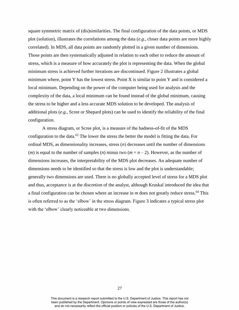
27

square symmetric matrix of (dis)similarities. The final configuration of the data points, or MDS

plot (solution), illustrates the correlations among the data (e.g., closer data points are more highly

correlated). In MDS, all data points are randomly plotted in a given number of dimensions.

Those points are then systematically adjusted in relation to each other to reduce the amount of

stress, which is a measure of how accurately the plot is representing the data. When the global

minimum stress is achieved further iterations are discontinued. Figure 2 illustrates a global

minimum where, point Y has the lowest stress. Point X is similar to point Y and is considered a

local minimum. Depending on the power of the computer being used for analysis and the

complexity of the data, a local minimum can be found instead of the global minimum, causing

the stress to be higher and a less accurate MDS solution to be developed. The analysis of

additional plots (e.g., Scree or Shepard plots) can be used to identify the reliability of the final

configuration.

A stress diagram, or Scree plot, is a measure of the badness-of-fit of the MDS

configuration to the data.62 The lower the stress the better the model is fitting the data. For

ordinal MDS, as dimensionality increases, stress (σ) decreases until the number of dimensions

(m) is equal to the number of samples (n) minus two (m = n – 2). However, as the number of

dimensions increases, the interpretability of the MDS plot decreases. An adequate number of

dimensions needs to be identified so that the stress is low and the plot is understandable;

generally two dimensions are used. There is no globally accepted level of stress for a MDS plot

and thus, acceptance is at the discretion of the analyst, although Kruskal introduced the idea that

a final configuration can be chosen where an increase in m does not greatly reduce stress.64 This

is often referred to as the ‘elbow’ in the stress diagram. Figure 3 indicates a typical stress plot

with the ‘elbow’ clearly noticeable at two dimensions.



28

Figure 2. Graph illustrating the concept of local and global minimum with regards to stress.

Position Y indicates the global minimum having the lowest stress for the entire graph. Position X

is similar to Y and is considered a local minimum. Multidimensional scaling aims to attain the

global minimum when plotting the data.

0

40

-3 6

Stre

ss

Iteration

Y

X



29

Figure 3. Typical stress plot. Stress is high in one dimension followed by a large decrease at two

dimensions. Stress continues to decrease into higher dimensionality, though not appreciably,

creating the elbow, after which little additional information is gained.

0

0.7

0 1 2 3 4 5

Raw

Str

ess

Dimensions



30

In this research, Kruskal’s Stress-1 was calculated for all plots using Equation 6,

Stress-1 = σ1 = √∑[𝑓(𝑝𝑖𝑗)− 𝑑𝑖𝑗 (𝐗)]2

∑ 𝑑𝑖𝑗2 (𝐗)

(6)

where f is a representation function that establishes the MDS model, pij is the proximity for point

i,j, and dij (X) is the corresponding distance in the MDS solution X.62 The stress is expected to

decrease as the number of dimensions increases. Any deviation from this expectation would

indicate errors in the way MDS is plotting the data. Figure 4 is an example of such a stress plot.

The raw stress is extremely low for all dimensions; however, the increase in stress from one to

three dimensions would call the final configuration into question. Logically this should not

happen and the MDS plot can be disregarded as being erroneous.

Another test for the acceptability of stress at a given dimension was described by Spence,

who proposed that random stress, or stress produced by random data for a given number of

samples and dimensions, could be approximated using Equation 7,65

σ1 = 0.001[a0 + a1m + a2n + a3 ln(m) + a4 √ln (𝑛)] (7)

where a0 = -524.25, a1 = 33.8, a2 = -2.54, a3 = -307.26, and a4 = 588.35. This estimation of

random stress is accurate for the range n = 10 – 60 and m = 1 – 15. Random stress can be used as

a null hypothesis for the acceptance of the MDS plot with relation to its associated stress

diagram.



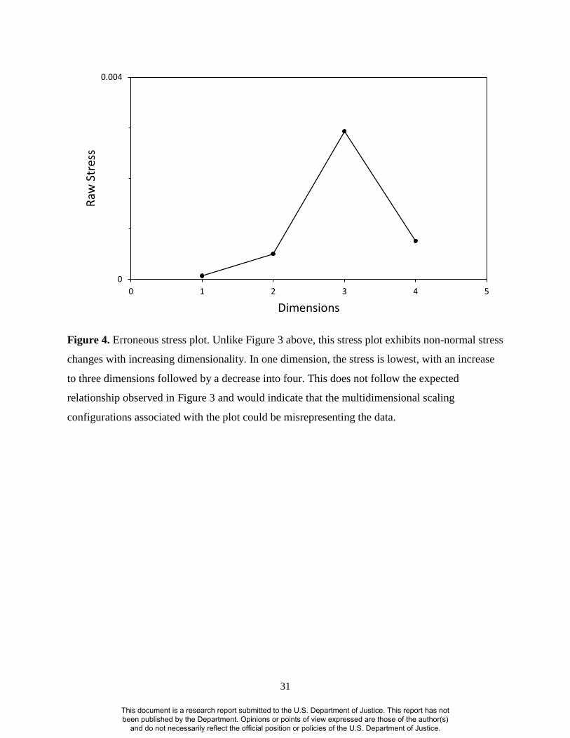
31

Figure 4. Erroneous stress plot. Unlike Figure 3 above, this stress plot exhibits non-normal stress

changes with increasing dimensionality. In one dimension, the stress is lowest, with an increase

to three dimensions followed by a decrease into four. This does not follow the expected

relationship observed in Figure 3 and would indicate that the multidimensional scaling

configurations associated with the plot could be misrepresenting the data.

0

0.004

0 1 2 3 4 5

Raw

Str

ess

Dimensions



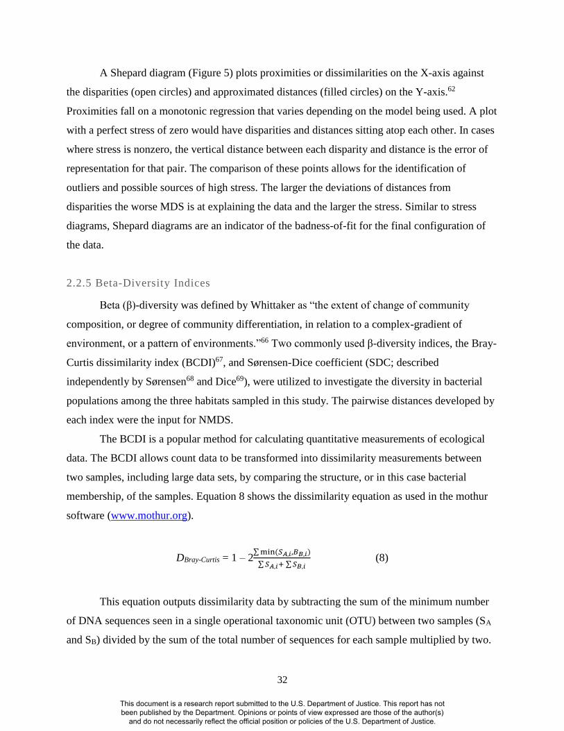
32

A Shepard diagram (Figure 5) plots proximities or dissimilarities on the X-axis against

the disparities (open circles) and approximated distances (filled circles) on the Y-axis.62

Proximities fall on a monotonic regression that varies depending on the model being used. A plot

with a perfect stress of zero would have disparities and distances sitting atop each other. In cases

where stress is nonzero, the vertical distance between each disparity and distance is the error of

representation for that pair. The comparison of these points allows for the identification of

outliers and possible sources of high stress. The larger the deviations of distances from

disparities the worse MDS is at explaining the data and the larger the stress. Similar to stress

diagrams, Shepard diagrams are an indicator of the badness-of-fit for the final configuration of

the data.

2.2.5 Beta-Diversity Indices

Beta (β)-diversity was defined by Whittaker as “the extent of change of community

composition, or degree of community differentiation, in relation to a complex-gradient of

environment, or a pattern of environments.”66 Two commonly used β-diversity indices, the Bray-

Curtis dissimilarity index (BCDI)67, and Sørensen-Dice coefficient (SDC; described

independently by Sørensen68 and Dice69), were utilized to investigate the diversity in bacterial

populations among the three habitats sampled in this study. The pairwise distances developed by

each index were the input for NMDS.

The BCDI is a popular method for calculating quantitative measurements of ecological

data. The BCDI allows count data to be transformed into dissimilarity measurements between

two samples, including large data sets, by comparing the structure, or in this case bacterial

membership, of the samples. Equation 8 shows the dissimilarity equation as used in the mothur

software (www.mothur.org).

DBray-Curtis = 1 – 2∑ min(𝑆𝐴,𝑖,𝐵𝐵,𝑖)

∑ 𝑆𝐴,𝑖+ ∑ 𝑆𝐵,𝑖 (8)

This equation outputs dissimilarity data by subtracting the sum of the minimum number

of DNA sequences seen in a single operational taxonomic unit (OTU) between two samples (SA

and SB) divided by the sum of the total number of sequences for each sample multiplied by two.



http://www.mothur.org/

33

Figure 5. A sample Shepard diagram with low stress and good association of disparities and

distances. The closer the association of the filled circles (representing approximated distances)

and open circles (representing disparities) the better multidimensional scaling is representing

these data. This Shepard diagram shows very close relationship between the two using a

polynomial monotonic function.

0.0

2.0

0.0 0.2 0.4 0.6 0.8 1.0

Dis

par

ity/

Dis

tan

ce

Dissimilarity

Disparities Distances



34

This process is conducted for each pair of samples until all pairwise comparisons have

been made. Note that comparing A to B and B to A will result in the same dissimilarity

measurement, so the final matrix is square symmetric.

The SDC is similar to the BCDI; however, the SDC compares the dissimilarity between

two samples through community membership. Equation 9 shows the dissimilarity calculation as

used in the mothur software.

DSørenson = 1 – 2𝑆AB

𝑆𝐴+ 𝑆𝐵 (9)

This equation outputs dissimilarity data by subtracting double the number of shared OTUs

between the samples (SAB) divided by the sum of the total number of OTUs in each sample.

Unlike the BCDI, the SDC only considers the number of OTUs in common, not the number of

sequences in each shared OTU, making it possible to obtain different measures of dissimilarity

between the two. The final result from SDC analysis will also be a square symmetric matrix.



35

2.3 Classification Procedures

Classification procedures are supervised statistical procedures that are used to assign

unclassified (e.g., questioned) samples to previously defined groups (e.g., reference standards).

Typically, these procedures require prior knowledge of the data set (e.g., identities of reference

standards); however, when this is not the case, exploratory procedures such as those described in

the previous section can be used to identify natural groups of samples in the data set. These

clusters then constitute the pre-defined groups for classification. Two classification procedures

were investigated in this research: soft independent modeling of class analogy (SIMCA) and k-

nearest neighbors (k-NN).

Both the SIMCA and k-NN approaches to classification are based on similarity; that is,

questioned samples are members of the class to which they lie closest to in the measurement

space. In both procedures, known samples (e.g., reference standards) in the data set are used to

develop and optimize the classification model. This model is subsequently used to classify

questioned samples. The k-NN approach is an example of a ‘hard’ classification procedure,

meaning that classification is forced such that all questioned samples will be classified to one of

the known classes. In contrast, SIMCA is a ‘soft’ classification procedure which means that

classification is not forced. As a result, a questioned sample may be considered a member of one

class, more than one class, or no classes at all.

2.3.1 Soft Independent Modeling of Class Analogy

In the SIMCA approach to classification, PCA is used to develop independent models for

each of the assigned classes and the optimal number of PCs is maintained in the model.55, 61, 70, 71

A cross-validation procedure can be used to determine the appropriate number of principal

components to retain in each model. To do this, the data set is firstly divided into a training set

and a test set, ensuring that the test set contains samples from each of the known classes in the

training set. The optimal number of principal components is initially set to 1 and using this

model, an appropriate sample in the test set is fit to the corresponding model. The residuals are

calculated for the fit of the sample to the model. The procedure is repeated, this time setting the

optimal number of principal components to 2. As before, appropriate samples are fit to the

relevant model and residuals are calculated. The procedure is repeated, and the number of

principal components that minimizes the residuals is the optimal number of principal



36

components that should be retained in the model. It should be noted that due to the independent

nature of the modeling, the optimal number of PCs will not necessarily be the same for all

classes.

Once PCA models have been developed for each class, questioned samples can be

classified. Scores for the questioned sample are calculated and projected onto the PCA model for

the first class to assess the goodness-of-fit. The variance of the residuals for the questioned

sample when fit using this model is calculated using Equation 10, along with the variance of the

residuals for members of the class, which is calculated using Equation 11.

𝑠𝑓𝑖𝑡2 = ∑

(𝑒𝑖𝑗)2

𝑃−𝐹

𝑃𝑗=1 (10)

𝑠𝑐𝑙𝑎𝑠𝑠2 = ∑ ∑

(𝑒𝑖𝑗)2

(𝑃−𝐹)(𝑁−𝐹−1)𝑃𝑗=1

𝑁𝑖=1 (11)

where 𝑠𝑓𝑖𝑡2 is the residual variance of the sample fit to the class, 𝑠𝑐𝑙𝑎𝑠𝑠

2 is the residual variance of

the model class, 𝑒𝑖𝑗are the calculated residuals, P is the dimensionality of the data, F is the

number of principal components retained in the model, and N is the number of samples in the

class.

An F-test is then used to compare the variance of the residuals. In cases where 𝑠𝑓𝑖𝑡2 is

significantly different from 𝑠𝑐𝑙𝑎𝑠𝑠2 , the questioned sample is not well described by the model and

is not considered a member of that class. In contrast, where 𝑠𝑓𝑖𝑡2 and 𝑠𝑐𝑙𝑎𝑠𝑠

2 are not significantly

different, then the model adequately describes the questioned sample and the sample is

considered a member of the class. This procedure is repeated for each of the pre-defined classes,

assessing the fit of the questioned sample in each case. It should also be noted that as the F-test

can be conducted at different confidence levels, the probability of class membership at different

confidence levels can also be assigned.

2.3.2 k-Nearest Neighbors

In the k-NN procedure, classification is based on the proximity of a questioned sample to

its nearest neighbors in the measurement space.55, 61, 71 Samples in the training set are firstly



37

assigned to known classes and the Euclidean distance between all pairs of samples is calculated

according to Equation 12.

𝑑𝑥𝑦 = [∑ (𝑥𝑗 − 𝑦𝑗)2𝑚

𝑗=1 ]1

2⁄

(12)

where dxy is the Euclidean distance between data vectors x and y, xj and yj are the values

of the variable j in data vectors x and y, respectively, and m is the number of variables in the data

set.

The k samples that are closest (i.e., have the shortest Euclidean distance) to the

questioned sample are considered the nearest neighbors, where k is a user-defined integer. The

questioned sample is considered a member of the class to which the majority of the k-nearest

neighbors belong. The optimal number of neighbors to consider in the classification is

determined during the model development phase. To do this, classification of known samples in

the training set is assessed using different k values for the classification. The optimal k value

occurs where there is correct classification and no misclassifications of the known samples.

However, as k increases, the kth nearest neighbor is not necessarily close to the known sample in

the measurement space.

To prevent ambiguity in classification, k is typically an odd number. However, where this

is not the case and the questioned sample has an equal number of nearest neighbors to two or

more classes, the accumulated Euclidean distances can be considered. The questioned sample is

subsequently considered a member of the class to which there is the lowest accumulated

distance.

As k-NN is a ‘hard’ classification procedure, all samples will be classified to one class

only. However, as the classification is forced, the sample may not actually be a good fit for that

class or group. To assess the goodness-of-fit, the distance of the sample to the nearest neighbor

in the class is calculated and then compared to the spread or variance of that class. To estimate

the spread of the class, the distance among all pairs of samples in the class is firstly determined,

then the average of the smallest distance of each sample to all others is calculated. The

goodness-of-fit, G, of a new sample is then calculated using Equation 13.



38

𝐺𝑖 =𝑑𝑖−𝒅𝒒

𝑠(𝒅𝒒) (13)

where di is the distance of sample i to the nearest neighbor in the group, dq is a vector of the

smallest distance of each sample in the group to all others, and s(dq) is the standard deviation of

the vector.

The goodness-of-fit is calculated for all samples to all groups and compared to a

threshold value at a given confidence level. Goodness-of-fit values close to the threshold level of

a class can indicate that the sample is not truly likely to be a member of that class.71



39

3. Materials and Methods

3.1 Chromatographic Data

3.1.1 Reference Standards and Simulated Fire Debris Samples

Reference standards from four classes defined by ASTM International were selected

(Table 1) and diluted 1:10 (v/v) in methylene chloride72. Diluted liquids were spiked onto

separate kimwipes (approximately 4 cm x 4 cm), placed in nylon bags that contained one-fourth

of an activated carbon strip, and subjected to a passive headspace extraction for 4 hours at 80 °C.

Following extraction, the carbon strips were eluted with 200 µL methylene chloride and

analyzed by GC-MS using the instrument parameters shown in Table 2. Three extracts were

prepared for each reference standard and each extract was analyzed in triplicate to give a total of

nine chromatograms for each standard.

Table 1. Ignitable liquid reference standards.

ASTM class Definition Representative

liquids Abbreviation*

Representative

chromatogram

Gasoline

C3- and C4-

alkylbenzenes and

various aliphatic

compounds

Gasoline 3

(Meijer)

Gasoline 4

(Marathon)

Gasoline 5 (BP)

GS3

GS4

GS5

Appendix 1A

Appendix 1B

Appendix 1C

Isoparaffinic

products

Branched chain; cyclic

alkanes and n-alkanes

insignificant or absent

Paint thinner

Upholstery &

fabric protector

PTH

UFP

Appendix 1D

Appendix 1E

Naphthenic

paraffinic

products

Branched chain and

cyclic alkanes; n-alkanes

insignificant or absent

Marine fuel

stabilizer

MFS

Appendix 1F

Petroleum

distillate

products

Homologous series of n-

alkanes in Gaussian

distribution; less

significant isoparaffinic,

cycloparaffinic, and

aromatic compounds

Lamp oil

Torch fuel

Charcoal lighter

Diesel

Kerosene

LMP

TFL

CHL

DSL

KER

Appendix 1G

Appendix 1H

Appendix 1I

Appendix 1J

Appendix 1K

* These abbreviations are used throughout the remainder of the report.



40

Table 2. GC-MS instrument parameters.

Injection

250 °C

1 µL

Pulsed splitless (15 psi for 0.25 s)

Carrier gas Ultra-high purity helium, 1 mL/min

Column 5% diphenyl-95% dimethyl polysiloxane

30 m x 0.25 mm i.d. x 0.25 µm

Oven temperature

program

40 °C, hold for 3 min

10 °C/min to 280 °C, hold for 4 min

Transfer line

temperature 280 °C

Ionization mode Electron, 70 eV

Scan range 50-550 Da

Scan rate 2.91 scans/s

Two sets of simulated fire debris samples were prepared. The first set (Set 1) contained

eight liquids (paint thinner, upholstery protector, marine fuel stabilizer, lamp oil, torch fuel,

charcoal lighter, diesel, and kerosene) spiked onto a carpet and carpet padding substrate. Due to

the diverse chemical nature, Set 1 was used to investigate the potential of each of the statistical

procedures. The second set (Set 2) contained four liquids (each from different ASTM classes)

spiked onto an oil-finished red oak hardwood flooring substrate.

To prepare the fire debris samples, separate samples of each substrate were spiked with

the appropriate diluted ignitable liquid reference standard (spike volumes ranged from 100-175

µL for the carpet and carpet padding substrate and from 50-125 µL for the oil-finished wood

substrate). For the carpet and carpet padding substrate, a propane blowtorch was applied to the

sample for 30 s and the sample was allowed to burn for a further 90 s before being extinguished

using an overturned beaker. For the oil-finished wood substrate, the torch was applied for 30 s

before the sample was extinguished in a similar manner. Each sample was extracted using the

passive-headspace procedure and then analyzed by GC-MS following the same procedures as for

the reference standards. For each substrate/reference standard combination, three samples were

prepared in this manner and each extract was analyzed in triplicate, yielding a total of 9

chromatograms for each simulated fire debris sample.

3.1.2 Chromatographic Data Pretreatment

Standard operating procedures for the data pretreatment procedures are included in

Appendix 2 and a summary of each procedure is given below.



41

Because the reference standards and fire debris samples were extracted in nylon bags, a

major compound in the bags (caprolactam) was present at varying abundance in the resulting

total ion chromatograms (TICs). The background subtraction function in the instrument

operating software (Agilent ChemStation version E.01.00.237, Agilent Technologies) was used

to remove the caprolactam peak from each chromatogram, before the smoothing function in the

operating software was applied.

A target chromatogram for retention time alignment was generated from the TICs of the

reference standards. The random number function in Microsoft Excel was used to randomly

select three TICs per reference standard and the average abundance of each variable in the

selected TICs was calculated to generate the target. The peak-match algorithm was performed in

Matlab (version R2010b, The Mathworks Inc., Natick MA) following the procedure described by

Johnson et al., investigating window sizes of 3, 5, and 752. A correlation optimized warping

algorithm was performed in The Unscrambler X (version 10.2, Camo Software Inc., Woodbridge

NJ), investigating segment sizes of 120, 80, 60, and 40 with warp sizes of 2 and 4 data points.

Following alignment, a total of eleven aligned data sets were generated and each was visually

inspected to assess the need for retention time alignment.

Total ion chromatograms were then subjected to three separate normalization procedures:

constant sum normalization, constant maximum normalization, and constant vector length

normalization. The normalized data sets were subsequently autoscaled and Pareto scaled.

Principal components analysis was then performed separately on each data set (including the

non-normalized data) and the resulting scores plots were used to assess association of replicates

of each reference standard as well as discrimination of chemically different reference standards.

3.1.3 Chromatographic Data Analysis

Standard operating procedures for the data analysis procedures are included in Appendix

2 and a summary of each procedure is given below.

After preliminary assessment of the data, the appropriate pretreatment procedures were

applied to the full data set (reference standards and simulated fire debris samples in Set 1).

PPMC coefficients were calculated for pairwise comparisons of the standards, as well as for

comparisons of the simulated fire debris to the corresponding standard. Coefficients were

calculated using the data analysis add-in in Microsoft Excel. Principal components analysis was



42

performed in Matlab (version R2010b, The Mathworks Inc., Natick MA) while HCA was

performed in Pirouette (version 4.0, Infometrix Inc., Bothell, WA). Both exploratory procedures

were used to investigate association of reference standards in the same ASTM class,

differentiation of standards in chemically different classes, and association of the simulated fire

debris samples to the corresponding reference standard.

Classification procedures were also performed to investigate the ability to successfully

classify the ignitable liquid present in each of the simulated fire debris samples. SIMCA was

performed in The Unscrambler X (Camo Software Inc.), using a random cross-validation

procedure to validate the models, and k-NN was performed in Pirouette (Infometrix Inc.). For

both procedures, the reference standards were used as the initial training set and classification of

the simulated fire debris samples according to ignitable liquid present was investigated.

3.2 Spectral Data

3.2.1 Reference Standards and Simulated Street Samples

Reference standards of d-amphetamine sulfate, d-methamphetamine hydrochloride,

codeine, morphine sulfate, barbital sodium salt, and phenobarbital were purchased from Sigma-

Aldrich (St. Louis, MO) and used as purchased. Reference standards of N-methyl-3,4-

methylenedioxamphetamine (MDMA) hydrochloride, (+)-N-ethyl-3,4-

methylenedioxyamphetamine (MDEA) hydrochloride, and heroin were purchased from

Cerilliant Corporation (Round Rock, TX) and also used as received. The data set of reference

standards is summarized in Table 3. All standards were individually homogenized in a mortar

and pestle prior to analysis by infrared spectroscopy.

Selected reference standards were mixed with caffeine to prepare simulated street

samples. Specifically, amphetamine, methamphetamine, MDMA, MDEA, codeine, and barbital

were mixed with caffeine (Eastman Kodak Co., Rochester, NY) to give controlled

substance/caffeine ratios of 80/20 and 50/50, by mass. Throughout the remainder of this report,

these simulated samples are referred to as “80/20” and “50/50”, respectively, to indicate the

composition of the sample mixture. The simulated samples were individually homogenized in a

mortar and pestle prior to analysis.



43

Table 3. Controlled substance reference standards.

Controlled substance

class

Representative

substances Abbreviation

Representative

spectrum

Amphetamines

Amphetamine

MDEA

MDMA

Methamphetamine

AMPH

MDEA

MDMA

METH

Appendix 3A

Appendix 3B

Appendix 3C

Appendix 3D

Barbiturates Barbital

Phenobarbital

BARB

PHEN

Appendix 3E

Appendix 3F

Opiates

Codeine

Heroin

Morphine

CODE

HERO

MORP

Appendix 3G

Appendix 3H

Appendix 3I

Reference standards and simulated samples were analyzed using a Perkin Elmer

Spectrum One Fourier-transform infrared (FTIR) spectrometer, equipped with an attenuated total

reflectance (ATR) sampling accessory. On each day of analysis, the zinc-selenide crystal was

initially cleaned with acetone and a contamination check was performed and a background

spectrum was collected. A portion of the relevant standard or sample mixture was placed on the

crystal and approximately 80-85 units of pressure were applied. Four scans were collected for

each spectrum over the wavenumber range 4000-650 cm-1, with a resolution of 4 cm-1. The

crystal and pressure anvil were cleaned again with acetone between samples and a new

background was collected after every six samples.

The set of standards and samples was analyzed in a similar manner a total of nine times.

Spectra were background corrected and smoothed using the automated functions in the

instrument software (Spectrum version 5.0.1, Perkin Elmer), then exported as .ascii files into

Microsoft Excel. For each data collection day, the average of the three spectra collected for each

standard or sample mixture was generated and used in subsequent data analysis.

3.2.2 Spectral Data Pretreatment



The spectra generated and exported into Excel were in transmittance mode and prior to

data analysis, the spectra were transformed into absorbance mode. Following transformation,

spectra of the reference standards were subjected to three normalization procedures: constant

sum normalization, constant maximum normalization, and SNV normalization. All calculations



44

for the normalization procedures were performed in Microsoft Excel. To assess the effect of

normalization, PCA (Matlab, The Mathworks) was performed separately on the non-normalized

data and each normalized data set. The resulting scores plots were used to assess association of

replicates of each reference standard, as well as discrimination of the chemically different

reference standards.

3.2.3 Spectral Data Analysis



The normalized spectra of the reference standards were then subjected to PCA (Matlab,

The Mathworks) and HCA (Pirouette, Infometrix Inc.) as initial exploratory data analysis

procedures. The resulting scores plot and dendrogram were used to assess association of

standards of the same controlled substance class and differentiation of the classes. Both statistical

procedures were repeated, this time including the simulated street samples in the data set. The

resulting plots were used to investigate association of each simulated sample to the

corresponding reference standard and controlled substance class.

Both SIMCA (The Unscrambler, Camo Software Inc.) and k-NN (Pirouette Infometrix

Inc.) were performed, using the reference standards as the initial training set and investigating

classification of the simulated street samples according to the appropriate controlled substance.

3.3 Gene Sequence Data

3.3.1 Sample Collection and Preparation

3.3.1.1 Sample Collection

Soil samples were collected from three locations in the Fenner Nature Center in Lansing,

MI (Table 4). The sampling locations represent three distinct habitats: a yard, a marsh, and a

wooded area. GPS coordinates were taken for each site. Soil was collected using a gardening

spade, which was washed with water between collections, and the collected soil was stored in a

freezer at -20°C within an hour of collection. Three soil samples less than a meter apart were

collected from each site and were used as biological replicates and labeled 1 – 3. A mixture

(1:1:1) of the yard samples (Ymix) was also processed.



45

Table 4. Sampling sites and corresponding GPS coordinates

Site name Abbreviation GPS coordinates

Fenner Nature Center, Yard Y N 42° 42.65' W 84° 30.92'

Fenner Nature Center, Marsh M N 42° 42.00' W 84° 31.15'

Fenner Nature Center, Soil S N 42° 42.43' W 84° 30.59'

3.3.1.2 DNA Extraction

Micropipette tips and tubes were UV irradiated in a Spectrolinker XL-1500 UV

Crosslinker (Spectronic Corporation Lincoln, NE) for 5 min (~ 2.5 J/cm2). DNA was extracted

from soil samples using a PowerSoil® DNA Isolation Kit (MoBio Carlsbad, CA) with two minor

modifications: an additional wash was conducted after step 16 by adding 500 μL of 70% ethanol

and centrifuged for 30 s at 10,000 x g, and DNA was eluted using 100 μL of solution C6 that had

been heated to 55°C. Reagent blanks were processed with every extraction.

3.3.1.3 PCR Amplification of 16S Hypervariable Regions 4 -6

Reagents suitable for UV irradiation and all micropipette tips and tubes were UV

irradiated for two or more rounds of 5 min. Hypervariable regions 4 – 6 of bacterial 16S rRNA

genes were amplified with universal bacterial primers (Table 5). A PCR master mix was

generated, with final concentrations of 1X AmpliTaq Gold buffer (Life Technologies Carlsbad,

CA) 2.5 mM MgCl2, 0.2 mM nucleotide triphosphates, 1.2 μL of the 10 μM forward primer, 0.4

μg/μL bovine serum albumin, and 3U AmpliTaq Gold (Life Technologies). Master mix was

aliquoted into ten PCR tubes to a final volume of 51.6 μL per tube. Six microliters of each soil

DNA extract was added to an aliquot, along with 1.2 μL of one of the 10 μM reverse primers

(each reverse primer, while identical in binding region, had a unique DNA barcode that was used

for downstream analysis). Each 60 μL reactions was mixed, then equally aliquoted into three

PCR tubes, with a goal of avoiding stochastic sampling of template DNA. DNAs were amplified

on an 2720 thermocycler (Life Technologies) under the conditions noted in Table 6, for 30

cycles. Identical 20 μL reactions were combined into a 60 μL pool and 5 μL was electrophoresed

on a 1% agarose gel with ethidium bromide visualization.



46

Table 5. Primer sequences.

Forward

or

reverse

Adaptor sequence Barcode Binding sequence

Forward CCTATCCCCTGTGTGCCTTGGCAGTCTCAG CCAGCAGCYGCGGTAAN

Reverse

A1 CCATCTCATCCCTGCGTGTCTCCGACTCAG AATGGTAC CGACRRCCATGCANCACCT

Reverse

A2 CCATCTCATCCCTGCGTGTCTCCGACTCAG TCTCCGTC CGACRRCCATGCANCACCT

Reverse

A3 CCATCTCATCCCTGCGTGTCTCCGACTCAG AACCTGGC CGACRRCCATGCANCACCT

Reverse

A4 CCATCTCATCCCTGCGTGTCTCCGACTCAG ACGAAGTC CGACRRCCATGCANCACCT

Reverse

A5 CCATCTCATCCCTGCGTGTCTCCGACTCAG TTCGTGGC CGACRRCCATGCANCACCT

Reverse

A6 CCATCTCATCCCTGCGTGTCTCCGACTCAG AACACAAC CGACRRCCATGCANCACCT

Reverse

A7 CCATCTCATCCCTGCGTGTCTCCGACTCAG TTCTTGAC CGACRRCCATGCANCACCT

Reverse

A8 CCATCTCATCCCTGCGTGTCTCCGACTCAG TCCAAGTC CGACRRCCATGCANCACCT

Reverse

A9 CCATCTCATCCCTGCGTGTCTCCGACTCAG TTCGCGAC CGACRRCCATGCANCACCT

Reverse

A10 CCATCTCATCCCTGCGTGTCTCCGACTCAG CCGGTCGC CGACRRCCATGCANCACCT

Table 6. PCR cycling parameters

PCR step Temperature (°C) Time (s)

Initial Heating 94 600

Denaturation 94 30

Annealing 60 45

Extension 72 60

Final Extension 72 120

3.3.1.4 PCR Product Purification

Forty microliters of the remaining pooled amplification reactions was purified using

Agencourt® AMPure® XP (Beckman Coulter Brea, CA). The bottle containing the beads was

vortexed briefly and 30 μL was aliquoted into a 1.5 ml micro-centrifuge tube. DNA was added

and the mixture was vortexed and incubated at room temperature for 15 min. The beads were

bound to a MagnaRack™ (Life Technologies) for a minimum of five min. The supernatant was

aspirated from the beads and discarded. Undisturbed beads were washed with 500 μL 70%

ethanol for 30 s. The supernatant was again aspirated and the beads were washed an additional

time. Beads were then dried on the magnet for 30 min at 37°C. DNA was eluted by adding 100

μL of 10 mM Tris, pH 8 and vortexing the tubes for at least 10 s. The tubes were returned to the



47

magnet and beads were bound for at least five min. Supernatant was aspirated away from the

pellet and saved in a 1.5 mL micro-centrifuge tube.

3.3.1.5 PCR Quantification and Equimolar Pooling

Purified PCR product was quantified using a Quant-iT™ dsDNA High-Sensitivity Assay

Kit (Life Technologies) following the manufacturer’s protocol. The ten quantified samples were

pooled so that 25 ng of DNA from each was in the final pool and brought to a final concentration

of 1 ng/μL.

3.3.1.6 Sequencing Purified PCR Product

The pooled DNAs were sequenced on a Roche GS Junior 454 Sequencer following the

manufacturer’s protocols using a titanium emPCR kit (Lib-L), sequencing kit, and PicoTiter

plate kit (Roche, San Francisco, CA).

3.3.2 Gene Sequence Data Pretreatment

Sequencing data output for the 454 sequencer was processed using open-source mothur

software.73 The program input codes and explanations for processing sequence data, along with a

sample file, are given in Appendix 4A. Bacterial sequences were also classified using the SILVA

bacterial reference alignment provided on the mothur website with input codes given in

Appendix 4B.

3.3.3 Gene Sequence Data Analysis

Two statistical procedures were used to analyze the biological data: PCA and nonmetric

MDS. The OTU's data used for PCA are described at the end of Appendix 4A. PCA was

performed using Matlab (version R2010b, The Mathworks).

Pairwise comparisons used for NMDS are described in Appendix 4C. Square

dissimilarity matrices developed from BCDI and SDC were input into Addinsoft XLSTAT Pro

expansion for Microsoft Excel. NMDS was run, using the Scaling by Majorizing a Complicated

Function (SMACOF) algorithm, for four dimensions with 500 iterations, each stopping at a

convergence of 0.00001. Two dimensional MDS plots were analyzed along with Shepard

diagrams and stress plots, the latter of which were compared against the null hypothesis random



48

stress plot described by Spence (1979). If the Kruskal’s stress was less than random stress, the

MDS plots were accepted at that dimension. MDS plots were further accepted with Kruskal’s

stress for two dimensions lower than 0.1. Finally, standard error bars were applied to all MDS

plots.



49

4. Results and Discussion

4.1 Chromatographic Data

Exemplar chromatograms of the ignitable liquid reference standards and simulated fire

debris samples are included in Appendix 1.

4.1.1 Retention Time Alignment

The aligned data sets were visually compared to assess the alignment of replicates of each

reference standard. No single algorithm or alignment parameters improved alignment for all

standards in the data set; however, in general, the correlation optimized warping algorithm

improved alignment compared to the peak-match algorithm. This is primarily due to differences

in the operation of the algorithms. The peak-match algorithm aligns the apex of the peaks but, as

a result, the leading and tailing edges of the peaks can be misaligned as the algorithm shifts the

peak to align the apex (Figure 6). The extent of misalignment of the edges of the peak is

therefore dependent on the window size used in the algorithm. In contrast, the correlation

optimized warping algorithm aligns the leading edge or tailing edge of the peak with the result

that the apexes may not be well-aligned. For the data set of reference standards, there were more

instances of misaligned peaks with the peak-match algorithm than with the correlation optimized

warping algorithm.

However, when compared to the unaligned reference standards, neither algorithm offered

substantial improvements. The reference standards were analyzed over a relatively short time

period during which there was no major instrument maintenance. Consequently, there was little

instrument drift with the result that the TICs were generally aligned and further retention time

alignment of the reference standards was not deemed necessary.



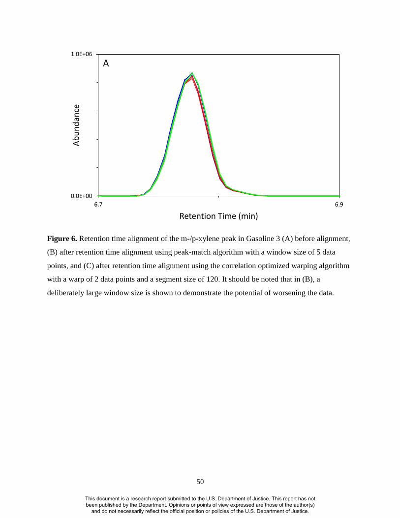
50

Figure 6. Retention time alignment of the m-/p-xylene peak in Gasoline 3 (A) before alignment,

(B) after retention time alignment using peak-match algorithm with a window size of 5 data

points, and (C) after retention time alignment using the correlation optimized warping algorithm

with a warp of 2 data points and a segment size of 120. It should be noted that in (B), a

deliberately large window size is shown to demonstrate the potential of worsening the data.

0.0E+00

1.0E+06

6.7 6.9

Ab

un

dan

ce

Retention Time (min)

A



51

Figure 6 contd. Retention time alignment of the m-/p-xylene peak in Gasoline 3 (A) before

alignment, (B) after retention time alignment using peak-match algorithm with a window size of

5 data points, and (C) after retention time alignment using the correlation optimized warping

algorithm with a warp of 2 data points and a segment size of 120. It should be noted that in (B), a


0.0E+00

1.0E+06

6.7 6.9

Ab

un

dan

ce


B



52

Figure 6 contd. Retention time alignment of the m-/p-xylene peak in Gasoline 3 (A) before

alignment, (B) after retention time alignment using peak-match algorithm with a window size of

5 data points, and (C) after retention time alignment using the correlation optimized warping

algorithm with a warp of 2 data points and a segment size of 120. It should be noted that in (B), a


0.0E+00

1.0E+06

6.7 6.9

Ab

un

dan

ce


C



53

Sets 1 and 2 of the simulated fire debris samples were collected over a longer time period

(approximately 12 months). Replicates of each sample were well aligned and were also well

aligned to the reference standards, despite the time duration between collection of the standards

and samples. As a result, no retention time alignment was actually necessary for these data sets.

The need for retention time alignment will depend on the time period over which the data

are collected as well as the state of the instrument during that time. Thus, for each data set, a

visual assessment should initially be conducted to assess the need for retention time alignment.

4.1.2 Normalization and Scaling

The non-aligned reference standards were subsequently normalized using three

normalization procedures (constant sum, constant maximum, and constant vector length

normalization), which were applied to each sample chromatogram.

Figure 7 illustrates the general effects of normalization, focusing on the C12 peak in

replicate chromatograms of the kerosene standard. With no normalization (Figure 7A), there is

spread among the replicates in both the baseline and the peak maxima. Following constant sum

normalization, there is less spread in the abundance of the baseline; however, spread in the peak

maxima remains (Figure 7B). Following constant maximum normalization, there is less spread in

the peak maxima but spread remains in the baseline (Figure 7C). Constant vector length

normalization is similar to constant sum normalization in that there is spread in the peak maxima

but an improvement in the baseline spread (Figure 7D).



54

Figure 7. Section of chromatogram for kerosene replicates corresponding to C12 peak after (A)

no normalization, (B) constant sum normalization, (C) constant maximum normalization, and

(D) constant vector length normalization.

0.0E+00

7.0E+05

12.35 12.55

Ab

un

dan

ce


A

0.0E+00

1.0E-02

12.35 12.55

No

rmal

ized

Ab

un

dan

ce


B



55

Figure 7 contd. Section of chromatogram for kerosene replicates corresponding to C12 peak after

(A) no normalization, (B) constant sum normalization, (C) constant maximum normalization,

and (D) constant vector length normalization.

0.0E+00

1.2E+00

12.35 12.55

No

rmal

ized

Ab

un

dan

ce


C

0.0E+00

1.0E+05

12.35 12.55

No

rmal

ized

Ab

un

dan

ce


D



56

The normalization procedures were further assessed using PCA and the resulting scores

plots were assessed (Figure 8). The first two principal components account for approximately 50-

60% of the variance in the data set, depending on the normalization procedure used. However,

with no normalization (Figure 8A), there is substantial spread among replicates of each standard,

which is sufficient to prevent adequate differentiation of four of the standards: upholstery

protector and paint thinner (both isoparaffinic class) and charcoal lighter and lamp oil (both

petroleum distillate class). There is an improvement in the close positioning of replicates

following normalization, although this improvement is greater for the constant sum and constant

maximum normalization procedures compared to constant vector length (Figures 8B and C

compared to D). To quantify this improvement, the relative standard deviation in the scores of

replicates of each standard in the first two principal components was calculated (Tables 7 and 8).



57

Figure 8. Scores plots for ignitable liquid reference standards (A) no normalization, (B) constant

sum normalization, (C) constant maximum normalization, and (D) constant vector length

normalization. Abbreviations for each standard are defined in Table 1.

PC

2 (

19

.8%

)

PC1 (42.0%)

GS3 GS4 GS5 PTH UHR MFS LMP TFL CHL DSL KER

A



58

Figure 8 contd. Scores plots for ignitable liquid reference standards (A) no normalization, (B)

constant sum normalization, (C) constant maximum normalization, and (D) constant vector

length normalization Abbreviations for each standard are defined in Table 1.

PC

2 (

19

.8%

)

PC1 (40.6%)

GS3 GS4 GS5 PTH UFP MFS LMP TFL CHL DSL KER

C



59

Table 7. Relative standard deviation of scores on the first principal component (PC1) for non-

normalized and normalized ignitable liquid reference standards.

Reference

standard

Relative standard deviation on PC1

Non-normalized Constant sum Constant

maximum

Constant vector

length

GS3 5.0 0.8 2.4 4.2

GS4 6.2 1.3 3.4 4.4

GS5 13.9 1.5 5.0 11.3

PTH 26.7 1.1 3.1 1.8

UFP 2.9 2.5 0.3 6.6

MFS 1.9 2.2 7.9 0.5

LMP 1.2 0.9 0.8 2.5

TFL 6.8 61.8 11.3 7.7

CHL 6.1 1.8 2.2 6.1

DSL 7.3 1.9 2.0 5.0

KER 8.6 53.8 5.0 5.5 Abbreviations for each reference standard are listed in Table 1.

Table 8. Relative standard deviation of scores on the second principal component (PC2) for non-

normalized and normalized ignitable liquid reference standards.

Reference

standard


Non-normalized Constant sum Constant

maximum

Constant vector

length

GS3 7.7 2.0 4.4 5.0

GS4 11.8 2.9 6.6 6.7

GS5 115.9 3.0 10.2 27.2

PTH 8.8 4.7 0.7 9.7

UFP 7.5 3.4 0.7 9.6

MFS 3.2 0.2 1.1 1.6

LMP 1.4 0.4 0.6 3.2

TFL 62.8 1.4 0.3 9.2

CHL 9.6 6.2 0.4 8.0

DSL 13.2 1.4 1.9 20.0

KER 16.1 1.5 45.9 1.9 Abbreviations for each reference standard are listed in Table 1.



60

Normalization improves association of replicates compared to the non-normalized data,

as indicated by the generally lower relative standard deviations in the normalized data. However,

due to the chemical diversity of the reference standards in this data set, no single normalization

procedure is optimal for all standards; rather, the optimal procedure depends on the chemical

complexity of the standard. Constant maximum normalization favors standards that are relatively

simple, with no areas of unresolved compounds (e.g., paint thinner and upholstery & fabric

protector). In contrast, constant sum normalization favors more complex standards that contain

unresolved compounds (e.g., diesel and kerosene). When compared to these two normalization

procedures, the constant vector length normalization procedure offers no additional advantages.

The effect of normalization on subsequent data analysis is apparent in the PCA scores

plots shown in Figure 8. There is clear improvement in the association of replicates of each

standard after normalization; however, the positioning of the reference standards on the scores

plots varies according to the normalization procedure. In constant sum normalization, the

upholstery protector is distinguished from the other reference standards on PC1 (Figure 8B). This

is a relatively simple standard with few compounds but following this normalization, the

abundance of each of these compounds is substantially increased such that they dominate the

data set. As a result, the compounds are weighted heavily in the loadings plot for the first

principal component, meaning that they are the most influential in the positioning of the

standards in the scores plot (Figure 9A).

In contrast, with constant maximum normalization, the diesel and kerosene reference

standards are distinguished from the other standards. Diesel and kerosene are the most complex

standards in the data set and both contain substantial areas of unresolved compounds. Following

constant maximum normalization, the lower abundance normal alkanes in these liquids become

more dominant and, as the later-eluting alkanes are only present in diesel and kerosene, it is these

alkanes that dominate the data set, as indicated in the PC1 loadings plot (Figure 9B).

Following constant vector length normalization, there is distinction of the gasoline

standards, as well as two of the petroleum distillate standards (torch fuel and lamp oil) on PC1.

The corresponding loadings plot (Fig 9C) is dominated by compounds from gasoline, torch fuel,

and lamp oil. As a result, there is little distinction of the remaining standards that includes

isoparaffinic and naphthenic paraffinic standards, as well as petroleum distillates, which form a

group positioned close to zero on both PC1 and PC2.



61

Figure 9. Loadings plot of PC1 after (A) constant sum normalization, (B) constant maximum

normalization, and (C) constant vector length normalization.

Load

ings

PC

1


ACompounds from

Upholstery & Fabric Protector



62

Figure 9 contd. Loadings plot of PC1 after (A) constant sum normalization, (B) constant

maximum normalization, and (C) constant vector length normalization.

Load

ings

PC

1


C Compounds fromGasoline

Compounds fromLamp Oil and Torch Fuel



63

While these results indicate the need for normalization, the actual procedure selected will

vary depending on the chemical nature of the data set. The effects of normalization can be

evaluated using the procedures demonstrated here (i.e., visual assessment of chromatograms,

PCA scores plots, and relative standard deviation of scores for sets of replicates on each PC). In

constant sum normalization, an assumption is made that a given volume of sample has the same

instrument response, irrespective of the sample identity. However, this means that for samples

containing relatively few compounds, constant sum normalization will substantially increase the

abundance and hence, the contribution, of these compounds. Constant maximum normalization

can also skew the relative abundance of compounds that otherwise would be a factor in

distinguishing the samples. As indicated above, the diverse nature of this data set does not lend

itself to a single normalization procedure; however, constant sum normalization yielded

improvements in the relative standard deviation of scores for sets of replicates for the majority of

the reference standards and hence, was selected for subsequent investigation.

The constant sum normalized data set was scaled, using both autoscaling and Pareto

scaling. The scaled data sets were then subjected to PCA and the resulting scores plots were

assessed (Figure 10 and Table 9) in a similar manner as described above.

Similar to normalization, no single scaling procedure is optimal for all standards. In fact,

while Pareto scaling improves the close positioning of replicates on both PCs compared to

autoscaling, the improvement is not as great as that observed for the non-scaled data. For these

data, scaling is not necessary as the abundance of each chromatogram is similar in magnitude. In

cases where the data set contains samples collected using different techniques such that the

instrument responses are on different scales, then scaling will become more important. Hence,

for this diverse and complex data set, scaling does not offer further advantages. As a result, all

subsequent data analysis procedures were conducted using constant sum normalized, non-scaled

data.



64

Figure 10. Scores plots for data set of reference standards after constant sum normalization and

(A) no scaling, (B) autoscaling, (C) Pareto scaling. Abbreviations for each standard are defined

in Table 1.

PC

2 (

22

.9%

)

PC1 (29.4%)


A



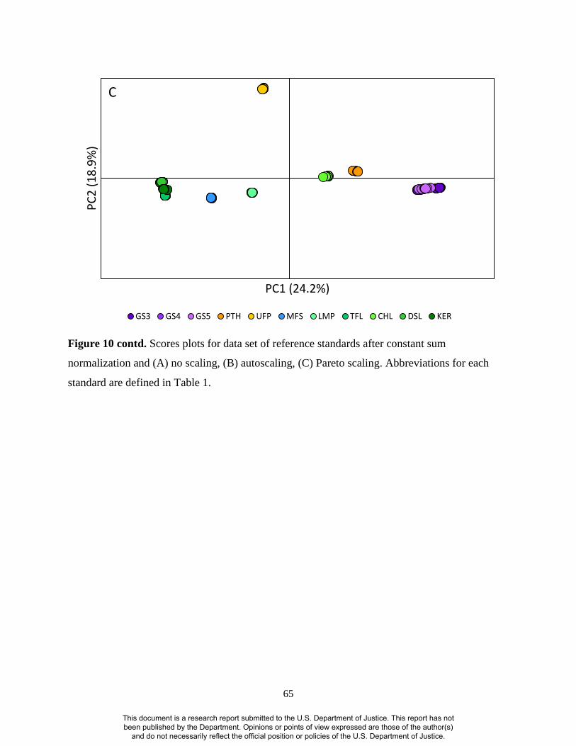
65

Figure 10 contd. Scores plots for data set of reference standards after constant sum

normalization and (A) no scaling, (B) autoscaling, (C) Pareto scaling. Abbreviations for each

standard are defined in Table 1.

PC

2 (

18

.9%

)

PC1 (24.2%)


C



66

Table 9. Relative standard deviation of scores on the first two principal components (PC1 and

PC2) for constant sum normalized non-scaled and scaled ignitable liquid reference standards.

Relative standard deviation on PC1 Relative standard deviation on PC2

Reference

standard Non-scaled Autoscaled

Pareto

scaled Non-scaled Autoscaled

Pareto

scaled

GS3 0.8 1.2 1.1 2.0 3.6 3.5

GS4 1.3 1.0 1.9 2.9 7.4 3.8

GS5 1.5 2.4 2.5 3.0 7.0 3.9

PTH 1.1 1.5 2.9 4.7 2.7 5.0

UFP 2.5 0.9 2.2 3.4 7.2 0.5

MFS 2.2 1.8 0.5 0.2 2.1 0.5

LMP 0.9 6.0 1.1 0.4 5.4 0.3

TFL 61.8 15.4 0.2 1.4 3.9 0.3

CHL 1.8 2.5 4.4 6.2 6.3 19.2

DSL 1.9 12.1 0.8 1.4 14.1 9.9

KER 53.8 5.4 1.3 1.5 12.3 2.8 Abbreviations for each reference standard are listed in Table 1.



67

4.1.3 Pearson Product-Moment Correlation Coefficients

PPMC coefficients were firstly calculated for pairwise comparisons of TICs of the

reference standards (Table 10). Mean PPMC coefficients indicate strong correlation for

replicates of each reference standard, with r ≥ 0.97. Theoretically, coefficients for replicates

should equal 1.0; however, in this study, the calculated coefficients take into account extraction

and instrument replicates. The strong correlation among replicates indicates acceptable precision

in both the extraction and analysis procedures.

Within the gasoline class, there is strong correlation among the reference standards, as

expected due to the high similarity in chemical composition. There is no correlation between the

two isoparaffinic reference standards (r = -0.017). Liquids in this class contain branched alkanes;

however, the paint thinner and upholstery & fabric protector included here contain branched

alkanes with different carbon number ranges. For the petroleum distillate class, there is moderate

correlation between torch fuel and kerosene (r = 0.539) and between diesel and kerosene (r =

0.726), which is primarily due to an overlap in the range of normal alkanes present. There is

weak to no correlation for all other comparisons (i.e., between reference standards from different

classes), as expected due to the differences in chemical composition.

PPMC coefficients were also calculated among replicates of both the 50% evaporated

standards and the 90% evaporated standards (Tables 11 and 12). Strong correlation is observed

for all comparisons, again indicating the acceptable precision in the extraction and analysis

procedures. The evaporated standards were also compared to the unevaporated standards and the

calculated PPMC coefficients are summarized in Tables 13 and 14.



68

Table 10. Mean PPMC coefficient ± standard deviation for pairwise comparisons of reference standards within and between ASTM

classes.

Mean PPMC coefficient ± standard deviation

Class Gasoline Isoparaffinic NapPar Petroleum Distillate

Reference

standard GS3 GS4 GS5 PTH UFP MFS LMP TFL CHL DSL KER

GS3 0.998 ±

0.002

GS4 0.938 ±

0.020

0.996 ±

0.004

GS5 0.944 ±

0.013

0.957 ±

0.010

0.993 ±

0.006

PTH 0.098

±0.010

0.015 ±

0.013

0.119 ±

0.013

0.984 ±

0.016

UFP -0.016 ±

0.002

-0.002 ±

0.002

-0.016 ±

0.002

-0.017 ±

0.001

0.991 ±

0.008

MFS 0.014 ±

0.004

0.061 ±

0.007

0.044 ±

0.009

0.068 ±

0.005

-0.041 ±

0.001

0.999 ±

0.001

LMP 0.017 ±

0.003

0.039 ±

0.005

0.039 ±

0.005

0.083 ±

0.005

-0.020 ±

0.001

0.337 ±

0.003

0.999 ±

0.001

TFL -0.019 ±

0.001

-0.008 ±

0.002

-0.007 ±

0.003

-0.014 ±

0.000

-0.021 ±

0.001

0.343 ±

0.006

0.251 ±

0.004

0.997 ±

0.003

CHL 0.091 ±

0.005

0.113 ±

0.003

0.120 ±

0.006

0.158 ±

0.009

-0.018 ±

0.001

0.078 ±

0.003

0.312 ±

0.053

0.025±

0.005

0.969 ±

0.057

DSL -0.093 ±

0.002

-0.091 ±

0.003

-0.086 ±

0.003

-0.076 ±

0.002

-0.074 ±

0.001

0.024 ±

0.014

-0.017 ±

0.004

0.265 ±

0.016

-0.081 ±

0.004

0.996 ±

0.004

KER -0.028 ±

0.004

-0.008 ±

0.007

-0.004 ±

0.008

-0.027 ±

0.003

-0.052 ±

0.001

0.283 ±

0.016

0.189 ±

0.018

0.539 ±

0.023

-0.032 ±

0.016

0.726 ±

0.034

0.995 ±

0.004 Abbreviations for each reference standard are listed in Table 1.

NapPar indicates naphthenic paraffinic.

For comparisons of the same reference standard, mean PPMC coefficient calculated based on 36 pairwise comparisons.

For comparisons of different reference standards, mean PPMC coefficient calculated based on 81 pairwise comparisons.

Light grey shading indicates mean PPMC coefficients for extraction replicates of the same reference standard.

Dark grey shading indicates mean PPMC coefficients for reference standards in the same ASTM class.



69

Table 11. Mean PPMC coefficient ± standard deviation for pairwise comparisons of replicates of

50% evaporated standards.

Reference standard Mean PPMC coefficient ± standard deviation

50GS3 0.995 ± 0.005

50GS4 0.993 ± 0.006

50GS5 0.989 ± 0.009

50PTH 0.991 ± 0.009

50UFP 0.987 ± 0.014

50MFS 0.999 ± 0.001

50LMP 0.998 ± 0.001

50TFL 0.996 ± 0.003

50CHL 0.995 ± 0.003

50DSL 0.981 ± 0.018

50KER 0.992 ± 0.008 Abbreviations for each reference standard are listed in Table 1.

Mean PPMC coefficient calculated based on 36 replicates of each standard.

Table 12. Mean PPMC coefficient ± standard deviation for pairwise comparisons of replicates of

90% evaporated standards.

Reference standard Mean PPMC coefficient ± standard deviation

90GS3 0.997 ± 0.002

90GS4 0.983 ± 0.027

90GS5 0.998 ± 0.001

90PTH 0.970 ± 0.026

90UFP 0.996 ± 0.002

90CHL 0.987 ± 0.014

90DSL 0.993 ± 0.006

90KER 0.993 ± 0.006 Abbreviations for each reference standard are listed in Table 1.

Mean PPMC coefficient calculated based on 36 replicates of each standard.



70

Table 13. Mean PPMC coefficient ± standard deviation for pairwise comparisons of 50% evaporated standards to the unevaporated

standards.


Class Gasoline Isoparaffinic NapPara Petroleum Distillate

Reference


50GS3 0.963 ±

0.010

0.983 ±

0.013

0.939 ±

0.013

0.123 ±

0.011

-0.021 ±

0.001

0.041 ±

0.005

0.033 ±

0.003

-0.012 ±

0.001

0.111 ±

0.004

-0.095 ±

0.003

-0.018 ±

0.006

50GS4 0.802 ±

0.032

0.948 ±

0.020

0.880 ±

0.023

0.179 ±

0.013

-0.027 ±

0.001

0.117 ±

0.011

0.067 ±

0.004

0.008 ±

0.004

0.123 ±

0.004

-0.083 ±

0.006

0.020 ±

0.010

50GS5 0.821 ±

0.036

0.953 ±

0.021

0.915 ±

0.025

0.151 ±

0.014

-0.025 ±

0.001

0.100 ±

0.010

0.069 ±

0.006

0.011 ±

0.004

0.141 ±

0.003

-0.075 ±

0.005

0.026 ±

0.010

50PTH 0.080 ±

0.007

0.128 ±

0.009

0.098 ±

0.009 0.951 ±

0.018

-0.017 ±

0.000

0.091 ±

0.003

0.120 ±

0.004

-0.007 ±

0.001

0.130 ±

0.006

-0.073 ±

0.002

-0.016 ±

0.004

50UFP -0.017 ±

0.002

-0.022 ±

0.002

-0.018 ±

0.002

-0.019 ±

0.001 0.962 ±

0.028

-0.045 ±

0.002

-0.022 ±

0.000

-0.023 ±

0.001

-0.020 ±

0.001

-0.082 ±

0.002

-0.057 ±

0.002

50MFS -0.017 ±

0.002

0.010 ±

0.005

0.003 ±

0.006

-0.019 ±

0.001

-0.029 ±

0.003 0.928 ±

0.005

0.204 ±

0.004

0.372 ±

0.004

0.006 ±

0.002

0.087 ±

0.013

0.312 ±

0.014

50LMP 0.007 ±

0.002

0.028 ±

0.004

0.029 ±

0.005

0.050 ±

0.003

-0.021 ±

0.001

0.382 ±

0.004 0.976 ±

0.002

0.316 ±

0.004

0.271 ±

0.048

0.018 ±

0.005

0.238 ±

0.018

50TFL -0.022 ±

0.001

-0.017 ±

0.001

-0.014 ±

0.002

-0.024 ±

0.001

-0.019 ±

0.001

0.242 ±

0.008

0.109 ±

0.002 0.930 ±

0.015

-0.005 ±

0.002

0.318 ±

0.018

0.606 ±

0.020

50CHL 0.058 ±

0.006

0.077 ±

0.007

0.084 ±

0.008

0.118 ±

0.010

-0.017 ±

0.001

0.124 ±

0.004

0.313 ±

0.015

0.048 ±

0.004 0.902 ±

0.052

-0.058 ±

0.005

0.068 ±

0.016

50DSL -0.085 ±

0.003

-0.097 ±

0.003

-0.091 ±

0.003

-0.066 ±

0.002

-0.053 ±

0.002

-0.161 ±

0.009

-0.066 ±

0.001

0.011 ±

0.033

-0.078 ±

0.003

0.779 ±

0.026

0.348 ±

0.067

50KER -0.073 ±

0.001

-0.077 ±

0.002

-0.072 ±

0.002

-0.060 ±

0.002

-0.049 ±

0.001

0.016 ±

0.027

-0.018 ±

0.013

0.401 ±

0.043

-0.062 ±

0.004

0.831 ±

0.021 0.831 ±



Mean PPMC coefficient calculated based on 81 pairwise comparisons.



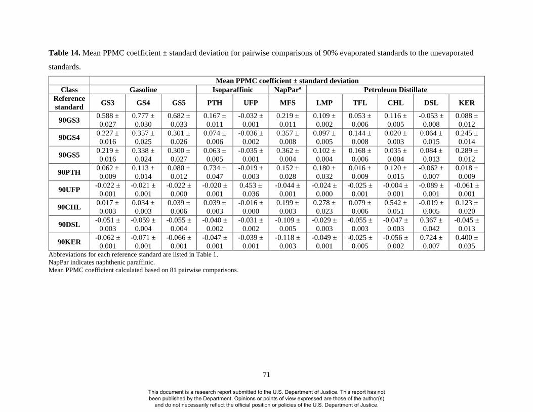
71

Table 14. Mean PPMC coefficient ± standard deviation for pairwise comparisons of 90% evaporated standards to the unevaporated

standards.


Class Gasoline Isoparaffinic NapPara Petroleum Distillate

Reference


90GS3 0.588 ±

0.027

0.777 ±

0.030

0.682 ±

0.033

0.167 ±

0.011

-0.032 ±

0.001

0.219 ±

0.011

0.109 ±

0.002

0.053 ±

0.006

0.116 ±

0.005

-0.053 ±

0.008

0.088 ±

0.012

90GS4 0.227 ±

0.016

0.357 ±

0.025

0.301 ±

0.026

0.074 ±

0.006

-0.036 ±

0.002

0.357 ±

0.008

0.097 ±

0.005

0.144 ±

0.008

0.020 ±

0.003

0.064 ±

0.015

0.245 ±

0.014

90GS5 0.219 ±

0.016

0.338 ±

0.024

0.300 ±

0.027

0.063 ±

0.005

-0.035 ±

0.001

0.362 ±

0.004

0.102 ±

0.004

0.168 ±

0.006

0.035 ±

0.004

0.084 ±

0.013

0.289 ±

0.012

90PTH 0.062 ±

0.009

0.113 ±

0.014

0.080 ±

0.012

0.734 ±

0.047

-0.019 ±

0.003

0.152 ±

0.028

0.180 ±

0.032

0.016 ±

0.009

0.120 ±

0.015

-0.062 ±

0.007

0.018 ±

0.009

90UFP -0.022 ±

0.001

-0.021 ±

0.001

-0.022 ±

0.000

-0.020 ±

0.001

0.453 ±

0.036

-0.044 ±

0.001

-0.024 ±

0.000

-0.025 ±

0.001

-0.004 ±

0.001

-0.089 ±

0.001

-0.061 ±

0.001

90CHL 0.017 ±

0.003

0.034 ±

0.003

0.039 ±

0.006

0.039 ±

0.003

-0.016 ±

0.000

0.199 ±

0.003

0.278 ±

0.023

0.079 ±

0.006

0.542 ±

0.051

-0.019 ±

0.005

0.123 ±

0.020

90DSL -0.051 ±

0.003

-0.059 ±

0.004

-0.055 ±

0.004

-0.040 ±

0.002

-0.031 ±

0.002

-0.109 ±

0.005

-0.029 ±

0.003

-0.055 ±

0.003

-0.047 ±

0.003

0.367 ±

0.042

-0.045 ±

0.013

90KER -0.062 ±

0.001

-0.071 ±

0.001

-0.066 ±

0.001

-0.047 ±

0.001

-0.039 ±

0.001

-0.118 ±

0.003

-0.049 ±

0.001

-0.025 ±

0.005

-0.056 ±

0.002

0.724 ±

0.007

0.400 ±






72

In Tables 13 and 14, strong correlations are highlighted in bold. The 50% evaporated

standards are strongly correlated to the corresponding unevaporated standard and only weakly

correlated (at most) to all other standards. There are some exceptions to this generalization.

Firstly, each 50% evaporated gasoline standard is also strongly correlated to the other two

unevaporated gasoline standards. This is expected due to the highly similar chemical

composition among the three gasoline standards. Secondly, the 50% evaporated diesel standard

is only moderately correlated to the unevaporated diesel reference standard. This lower than

expected correlation is primarily due to the loss of the early eluting aromatic compounds as a

result of evaporation. However, when the standard deviation is also taken into account, the 50%

evaporated diesel standards are strongly correlated to the unevaporated standard. And thirdly, the

50% evaporated kerosene standard is moderately correlated to the unevaporated diesel reference

standard. These two liquids have a similar distribution of normal alkanes and, even with

evaporation, sufficient overlap remains to indicate a moderate correlation between these two

liquids.

The 90% evaporated standards are generally only moderately to weakly correlated to the

corresponding unevaporated standard, primarily due to the substantial difference in chemical

composition at this advanced stage of evaporation. Chromatograms of the paint thinner standards

are shown in Figure 11 as an example. In the unevaporated standard (Figure 11A), C7- and C8-

branched alkanes are present, eluting between 8.5 and 9.4 minutes; however, at the 90%

evaporation level, these compounds are no longer present (Figure 11B). As correlation

coefficients are calculated on a point-by-point basis, the presence of compounds in one

chromatogram but not the other, as is the case here, lowers the coefficient.

Finally, the utility of PPMC coefficients to indicate correlation between fire debris

samples and the corresponding reference standards was investigated using Set 1 of the simulated

fire debris samples. This set consisted of eight ignitable liquids spiked onto a carpet and carpet

padding substrate, then burned. Coefficients were calculated for pairwise comparisons of each

fire debris sample to the unevaporated, 50% evaporated, and 90% evaporated standards (Table

15).



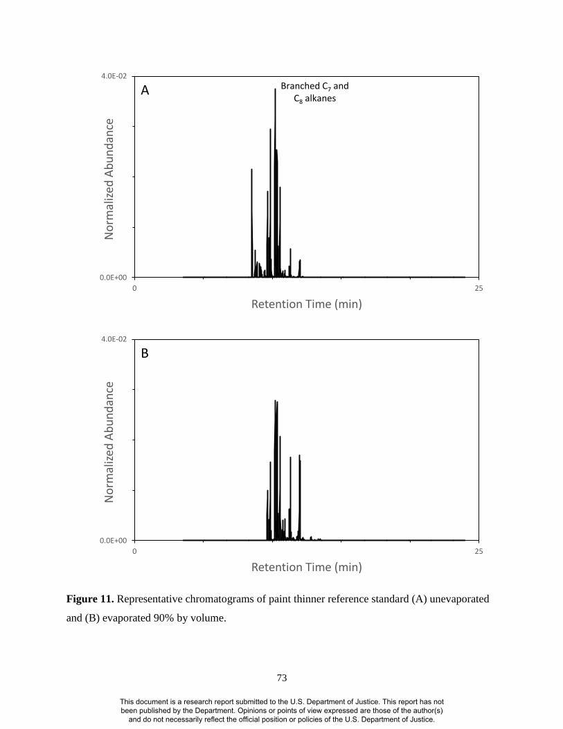
73

Figure 11. Representative chromatograms of paint thinner reference standard (A) unevaporated

and (B) evaporated 90% by volume.

0.0E+00

4.0E-02

0 25

No

rmal

ized

Ab

un

dan

ce


Branched C7 and C8 alkanes

A

0.0E+00

4.0E-02

0 25

No

rmal

ized

Ab

un

dan

ce


B



74

Table 15. Mean PPMC coefficient ± standard deviation for pairwise comparisons of simulated

fire debris (carpet and carpet padding substrate) to corresponding reference standard.

Reference

standard

Mean PPMC coefficient for comparison of standards and simulated fire debris on

carpet and carpet padding (CPT) substrate

PTH

CPT

UFP

CPT

MFS

CPT

LMP

CPT

TFL

CPT

CHL

CPT

DSL

CPT

KER

CPT

GS3 0.060 ±

0.013

-0.008 ±

0.002

0.015 ±

0.005

0.022 ±

0.010

-0.003 ±

0.002

0.062 ±

0.021

0.030 ±

0.005

0.063 ±

0.008

50GS3 0.073 ±

0.016

-0.015 ±

0.002

0.030 ±

0.005

0.032 ±

0.011

0.006 ±

0.002

0.076 ±

0.023

0.037 ±

0.006

0.072 ±

0.009

90GS3 0.093 ±

0.015

-0.029 ±

0.002

0.136 ±

0.018

0.077 ±

0.009

0.094 ±

0.007

0.081 ±

0.013

0.085 ±

0.015

0.151 ±

0.014

GS4 0.085 ±

0.020

-0.016 ±

0.002

0.041 ±

0.007

0.033 ±

0.011

0.008 ±

0.003

0.078 ±

0.022

0.045 ±

0.007

0.083 ±

0.009

50GS4 0.101 ±

0.021

-0.022 ±

0.002

0.075 ±

0.011

0.050 ±

0.012

0.031 ±

0.004

0.087 ±

0.020

0.061 ±

0.010

0.108 ±

0.012

90GS4 0.035 ±

0.005

-0.029 ±

0.005

0.232 ±

0.029

0.059 ±

0.012

0.190 ±

0.007

0.028 ±

0.009

0.142 ±

0.024

0.217 ±

0.015

GS5 0.072 ±

0.016

-0.009 ±

0.003

0.035 ±

0.007

0.041 ±

0.008

0.017 ±

0.005

0.085 ±

0.025

0.047 ±

0.008

0.093 ±

0.011

50GS5 0.087 ±

0.019

-0.020 ±

0.001

0.068 ±

0.010

0.062 ±

0.009

0.043 ±

0.006

0.098 ±

0.024

0.060 ±

0.010

0.114 ±

0.013

90GS5 0.035 ±

0.004

-0.019 ±

0.002

0.248 ±

0.030

0.080 ±

0.017

0.244 ±

0.006

0.040 ±

0.008

0.161 ±

0.026

0.254 ±

0.018

PTH 0.597 ±

0.184

-0.015 ±

0.001

0.012 ±

0.005

0.035 ±

0.007

-0.007 ±

0.001

0.108 ±

0.028

0.018 ±

0.005

0.034 ±

0.005

50PTH 0.596 ±

0.170

-0.016 ±

0.001

0.024 ±

0.006

0.058 ±

0.010

0.004 ±

0.002

0.101 ±

0.018

0.021 ±

0.005

0.044 ±

0.005

90PTH 0.513 ±

0.125

-0.020 ±

0.002

0.072 ±

0.019

0.101 ±

0.028

0.036 ±

0.013

0.091 ±

0.015

0.034 ±

0.011

0.076 ±

0.015

UFP -0.021 ±

0.001 0.735 ±

0.046

-0.034 ±

0.001

-0.022 ±

0.001

-0.028 ±

0.001

-0.023 ±

0.001

-0.031 ±

0.002

-0.035 ±

0.001

50UFP -0.023 ±

0.001 0.773 ±

0.041

-0.037 ±

0.002

-0.024 ±

0.001

-0.030 ±

0.001

-0.025 ±

0.001

-0.033 ±

0.003

-0.037 ±

0.001

90UFP -0.002 ±

0.001 0.388 ±

0.032

-0.034 ±

0.002

-0.024 ±

0.002

-0.030 ±

0.001

-0.017 ±

0.002

-0.031 ±

0.002

-0.036 ±

0.001

MFS 0.032 ±

0.002

-0.038 ±

0.003 0.514 ±

0.049

0.195 ±

0.045

0.355 ±

0.008

0.092 ±

0.005

0.179 ±

0.032

0.281 ±

0.019

50MFS -0.022 ±

0.005

-0.037 ±

0.001 0.441 ±

0.043

0.110 ±

0.033

0.341 ±

0.007

0.018 ±

0.010

0.160 ±

0.028

0.244 ±

0.016

LMP 0.047 ±

0.003

-0.014 ±

0.003

0.169 ±

0.019 0.660 ±

0.095

0.304 ±

0.018

0.460 ±

0.023

0.115 ±

0.020

0.341 ±

0.029

50LMP 0.029 ±

0.004

-0.015 ±

0.003

0.192 ±

0.021 0.637 ±

0.096

0.353 ±

0.017

0.424 ±

0.016

0.135 ±

0.023

0.365 ±

0.029

TFL -0.020 ±

0.001

-0.028 ±

0.001

0.133 ±

0.016

0.137 ±

0.030 0.536 ±

0.024

0.053 ±

0.006

0.198 ±

0.032

0.338 ±

0.023

50TFL -0.028 ±

0.001

-0.028 ±

0.001

0.074 ±

0.012

0.053 ±

0.016 0.578 ±

0.028

0.000 ±

0.005

0.191 ±

0.031

0.325 ±

0.022



75

CHL 0.117 ±

0.025

-0.014 ±

0.002

0.051 ±

0.009

0.335 ±

0.072

0.128 ±

0.017 0.396 ±

0.142

0.042 ±

0.010

0.179 ±

0.031

50CHL 0.088 ±

0.018

-0.017 ±

0.001

0.084 ±

0.013

0.340 ±

0.065

0.185 ±

0.017 0.334 ±

0.102

0.053 ±

0.011

0.203 ±

0.025

90CHL 0.029 ±

0.004

-0.018 ±

0.000

0.159 ±

0.023

0.159 ±

0.023

0.265 ±

0.028 0.194 ±

0.040

0.077 ±

0.013

0.230 ±

0.029

DSL -0.089 ±

0.003

-0.088 ±

0.003

-0.009 ±

0.015

-0.034 ±

0.013

0.181 ±

0.021

-0.077 ±

0.016 0.094 ±

0.028

0.125 ±

0.017

50DSL -0.080 ±

0.004

-0.073 ±

0.004

-0.122 ±

0.008

-0.079 ±

0.004

-0.071 ±

0.017

-0.092 ±

0.007 -0.043 ±

0.021

-0.066 ±

0.019

90DSL -0.049 ±

0.004

-0.044 ±

0.004

-0.081 ±

0.006

-0.081 ±

0.006

-0.070 ±

0.004

-0.059 ±

0.005 -0.066 ±

0.010

-0.082 ±

0.006

KER -0.035 ±

0.004

-0.053 ±

0.002

0.168 ±

0.026

0.155 ±

0.045

0.562 ±

0.033

0.062 ±

0.018

0.250 ±

0.043 0.417 ±

0.033

50KER -0.061 ±

0.004

-0.052 ±

0.002

-0.021 ±

0.016

-0.025 ±

0.012

0.228 ±

0.048

-0.051 ±

0.015

0.127 ±

0.033 0.165 ±

0.029

90KER -0.059 ±

0.002

-0.055 ±

0.001

-0.090 ±

0.004

-0.090 ±

0.004

-0.058 ±

0.005

-0.068 ±

0.004

-0.024 ±

0.014 -0.042 ±



In Table 15, mean PPMC coefficients representing correlation between the simulated fire

debris samples and the corresponding reference standards are highlighted in bold. For each fire

debris sample, the highest correlation is observed between the sample and corresponding

standard although in most cases, only a weak to moderate correlation is observed. For the

majority of the fire debris samples, the chromatograms contain some characteristic compounds

from the ignitable liquid, along with additional compounds (styrene, trichloropropane, and

biphenyl) from the carpet and carpet padding substrate. The presence of compounds from the

liquids enables some degree of correlation with the appropriate standard. However, as PPMC

coefficients are calculated on a point-by-point basis, the presence of the additional compounds

from the substrate lowers the coefficient.

For the fire debris sample containing diesel, there is no correlation to any of the

corresponding standards. Chromatograms of this particular sample show none of the

characteristic diesel compounds, namely the Gaussian shaped distribution of normal alkanes

(Figure 12) that would be expected. As a result, there is little to no correlation between this fire

debris sample and the corresponding standards.



76

Figure 12. Representative chromatograms of diesel reference standard (A) unevaporated, (B)

50% evaporated, and (C) simulated fire debris containing diesel on a carpet and carpet padding

substrate.

0.0E+00

6.0E-03

0 25

No

rmal

ized

Ab

un

dan

ce


A

C9

C10C11

C12

C13

C14

C15

C16

C17

C18

C19

C20C21

0.0E+00

2.0E-02

0 25

No

rmal

ized

Ab

un

dan

ce


B



77

Figure 12 contd. Representative chromatograms of diesel reference standard (A) unevaporated,

(B) 50% evaporated, and (C) simulated fire debris containing diesel on a carpet and carpet

padding substrate.

0.E+00

2.E-02

0 5 10 15 20 25

No

rmal

ized

Ab

un

dan

ce


C StyreneTrichloropropane

Biphenyl



78

Pearson product-moment correlation coefficients were also calculated for pairwise

comparisons of the reference standards with simulated fire debris samples containing the oil-

finished wood flooring substrate (Set 2, coefficients summarized in Table 16).

Table 16. Mean PPMC coefficient ± standard deviation for pairwise comparisons of simulated

fire debris (oil-finished wood flooring substrate) to corresponding reference standard.

Reference

standard

Mean PPMC coefficient ± standard deviation for comparison of

standards and simulated fire debris on oil-finished wood (OWD)

substrate

PTH OWD TFL OWD DSL OWD

GS3 0.116 ± 0.013 0.058 ± 0.009 0.066 ± 0.013

50GS3 0.151 ± 0.012 0.081 ± 0.009 0.100 ± 0.015

90GS3 0.227 ± 0.004 0.137 ± 0.010 0.213 ± 0.007

GS4 0.170 ± 0.013 0.093 ± 0.009 0.118 ± 0.015

50GS4 0.211 ± 0.010 0.120 ± 0.006 0.164 ± 0.013

90GS4 0.103 ± 0.013 0.115 ± 0.030 0.199 ± 0.012

GS5 0.153 ± 0.016 0.082 ± 0.008 0.102 ± 0.017

50GS5 0.198 ± 0.012 0.113 ± 0.005 0.152 ± 0.016

90GS5 0.094 ± 0.011 0.111 ± 0.043 0.200 ± 0.012

PTH 0.332 ± 0.008 0.188 ± 0.020 0.253 ± 0.013

50PTH 0.348 ± 0.006 0.188 ± 0.016 0.263 ± 0.012

90PTH 0.333 ± 0.032 0.161 ± 0.019 0.252 ± 0.029

UFP -0.035 ± 0.001 -0.032 ± 0.003 -0.050 ± 0.004

50UFP -0.039 ± 0.001 -0.035 ± 0.004 -0.055 ± 0.004

90UFP -0.022 ± 0.002 -0.023 ± 0.006 -0.043 ± 0.003

MFS 0.240 ± 0.025 0.276 ± 0.101 0.467 ± 0.020

50MFS 0.057 ± 0.018 0.179 ± 0.112 0.327 ± 0.023

LMP 0.609 ± 0.061 0.437 ± 0.105 0.584 ± 0.031

50LMP 0.559 ± 0.056 0.442 ± 0.125 0.592 ± 0.032

TFL 0.086 ± 0.014 0.445 ± 0.233 0.412 ± 0.027

50TFL -0.012 ± 0.007 0.345 ± 0.215 0.300 ± 0.021

CHL 0.368 ± 0.053 0.216 ± 0.024 0.249 ± 0.037

50CHL 0.323 ± 0.036 0.196 ± 0.024 0.239 ± 0.021

90CHL 0.195 ± 0.029 0.128 ± 0.037 0.187 ± 0.010

DSL -0.151 ± 0.007 0.015 ± 0.067 0.082 ± 0.036

50DSL -0.148 ± 0.004 -0.098 ± 0.018 -0.061 ± 0.049

90DSL -0.091 ± 0.005 -0.080 ± 0.010 -0.133 ± 0.013

KER 0.034 ± 0.018 0.231 ± 0.140 0.342 ± 0.026

50KER -0.119 ± 0.006 0.088 ± 0.096 0.176 ± 0.041

90KER -0.106 ± 0.002 -0.082 ± 0.004 -0.035 ± 0.034 Abbreviations for each reference standard are listed in Table 1.




79

For fire debris samples containing paint thinner and diesel, the highest correlation is

observed for pairwise comparison to the lamp oil reference standard, albeit only a moderate

correlation in both cases. Debris samples containing paint thinner are only weakly correlated to

the corresponding reference standard while there is no correlation between the diesel-containing

debris samples and the appropriate reference standards. For the torch fuel-containing debris

samples, weak correlation (0.445) is observed for comparison to the torch fuel reference

standard, although a similar correlation (0.442) is also observed for the 50% evaporated lamp oil

standard. Similarity of the debris samples to lamp oil is based on the substrate interference

compounds from the oil-finished wood; that is, the range of normal alkanes from the substrate

(C9-C12) is similar to that observed in the lamp oil standard. As a consequence, the presence of

interference compounds from the debris results in apparent similarity of the fire debris samples

to one particular reference standard.

These results indicate that PPMC coefficients are of limited utility in assessing similarity

between reference standards and simulated fire debris samples as coefficients are calculated on a

point-by-point basis. For the carpet and carpet padding substrate, interference compounds do not

correspond to any compounds present in the liquids and hence, the presence of such compounds

lowers the coefficient. For the oil-finished wood substrate, interference compounds correspond

to those present in some of the reference standards and hence, their presence increases similarity

to those standards. Additionally, and irrespective of substrate, the greater the extent of burning,

fewer compounds characteristic of the liquid remain in the debris, further lowering the

coefficient when compared to the reference standard.


Principal components analysis was initially performed on the pretreated reference

standards and the scores plot of PC1 and PC2 is shown in Figure 13.



80

Figure 13. Scores plot of PC1 versus PC2 for ignitable liquid reference standards. Each

reference standard was analyzed in replicate (n=9) and each standard is represented by a different

color in the plot. Abbreviations for each standard are defined in Table 1.

PC

2 (

22

.9%

)

PC1 (29.4%)




81

The first two PCs account for 52% of the variance among the reference standards.

Replicates of each standard are closely positioned in the scores plot and three groups of the

standards are apparent. The first contains the three gasoline standards, the second contains the

upholstery and fabric protector standard, and the third group contains the remaining standards.

This positioning can be explained with reference to the loadings plots, which are shown in Figure

14 for the first two principal components.

The loadings plot for PC1 (Figure 14A) is dominated by the branched C5- and C7-alkanes

that are present in the upholstery protector standard. This is an artifact of the normalization

procedure, which results in a substantial increase in abundance of these compounds. These

compounds are weighted positively in the loadings plot for both PC1 and PC2, which results in

the positive positioning of this standard on these two PCs. The C3- and C4-alkylbenzenes that are

present in gasoline are weighted negatively in the loadings plot for PC1 and positively in the

loadings plot for PC2. As a result, the gasoline standards are positioned negatively on PC1 and

positively on PC2 in the scores plot.

The remaining standards are positioned negatively on both PC1 and PC2 in the scores

plot, albeit close to zero in both cases. The normal alkanes C11-C14 are weighted negatively in the

loadings for PC2 (Figure 14B). The petroleum distillate standards all contain these four normal

alkanes, resulting in the negative positioning of these standards on PC2 in the scores plot. Paint

thinner and marine fuel stabilizer are also positioned negatively on PC2 in the scores plot, which

is due to some of the compounds present in these standards being weighted negatively on PC2 in

the loadings plot.

For further discrimination of the reference standards, it is necessary to consider additional

principal components, particularly as the first two account for only 52% of the variance in the

data set. The third and fourth principal components account for an additional 30.3% of the

variance, resulting in 82.6% of the total variance described by the first four PCs. The scores plot

of PC3 versus PC4 is shown in Figure 15, with the loadings plots for each of these PCs shown in

Figure 16.



82

Figure 14. Loadings plot of (A) PC1 and (B) PC2 for ignitable liquid reference standards.

Load

ings

PC

1


A Branched C5-C7 alkanes

C2-alkylbenzenes

C3-alkylbenzenes

C4-alkylbenzenesToluene

Load

ings

PC

1


B

BranchedC5-C7 alkanes

C2-alkylbenzenes

C3-alkylbenzenes

C4-alkylbenzenes

C11

C12C13

C14



83

Figure 15. Scores plot of PC3 versus PC4 for ignitable liquid reference standards. Each



PC

4 (

12

.6%

)

PC3 (17.7%)




84

Figure 16. Loadings plot of (A) PC3 and (B) PC4 for ignitable liquid reference standards.

Load

ings

PC

3


A Branched C7 and C8 alkanes

C11

C12

C13

C14

Load

ings

PC

4


BC11

C13

C10



85

The loadings plot for PC3 (Figure 16A) is dominated by branched C7- and C8-alkanes,

which are weighted positively, and C11-C14 normal alkanes that are weighted negatively. The

branched alkanes are the major compounds present in the paint thinner reference standard while

the C11-C14 normal alkanes are the major compounds in the torch fuel reference standard. As a

result, the third principal component further distinguishes these two standards from the others,

with paint thinner positioned positively, and torch fuel positioned negatively, on PC3 (Figure

15).

The loadings plot for PC4 (Figure 16B) is dominated by C10 and C11 normal alkanes,

which are weighted positively, and C13, which is weighted negatively. While all three of these

normal alkanes are present in the petroleum distillate standards, the C10 and C11 normal alkanes

are the major compounds in charcoal lighter, resulting in the very positive positioning of this

standard on PC4 and facilitating distinction of this standard from the other petroleum distillates.

Similarly, C13 is the dominant compound in torch fuel, resulting in the very negative positioning

of this standard on PC4 and again, enabling distinction from the other petroleum distillate

standards.

Therefore, the variance described by the first principal component distinguishes the

upholstery protector reference standard from the remaining standards. The second principal

component distinguishes gasoline, while the third distinguishes paint thinner and torch fuel, and

the fourth further distinguishes the petroleum distillate reference standards. Hence, while the

variance described by each PC progressively decreases, important information is still contained

and PCA of a diverse data set should not be limited to consideration of only the first two

principal components.

Principal components analysis was repeated, including the 50% and 90% evaporated

reference standards in the data set to investigate association of these standards to the

corresponding unevaporated standard. The resulting scores plot for the first two principal

components is shown in Figure 17 and the corresponding loadings plots are shown in Figure 18.



86

Figure 17. Scores plot of PC1 versus PC2 for unevaporated and evaporated ignitable liquid

reference standards. Each reference standard was analyzed in replicate (n=9) and each standard is

represented by a different color in the plot. Unevaporated standards are shown as circles, 50%

evaporated as triangles, and 90% evaporated as squares. Abbreviations for each standard are

defined in Table 1.

PC

2 (

17

.5%

)

PC1 (22.4%)

GS3 GS4 GS5 PTH UFP MFS LMP TFL CHL DSL

KER 50GS3 50GS4 50GS5 50PTH 50UFP 50MFS 50LMP 50TFL 50CHL

50DSL 50KER 90GS3 90GS4 90GS5 90PTH 90UFP 90CHL 90DSL 90KER



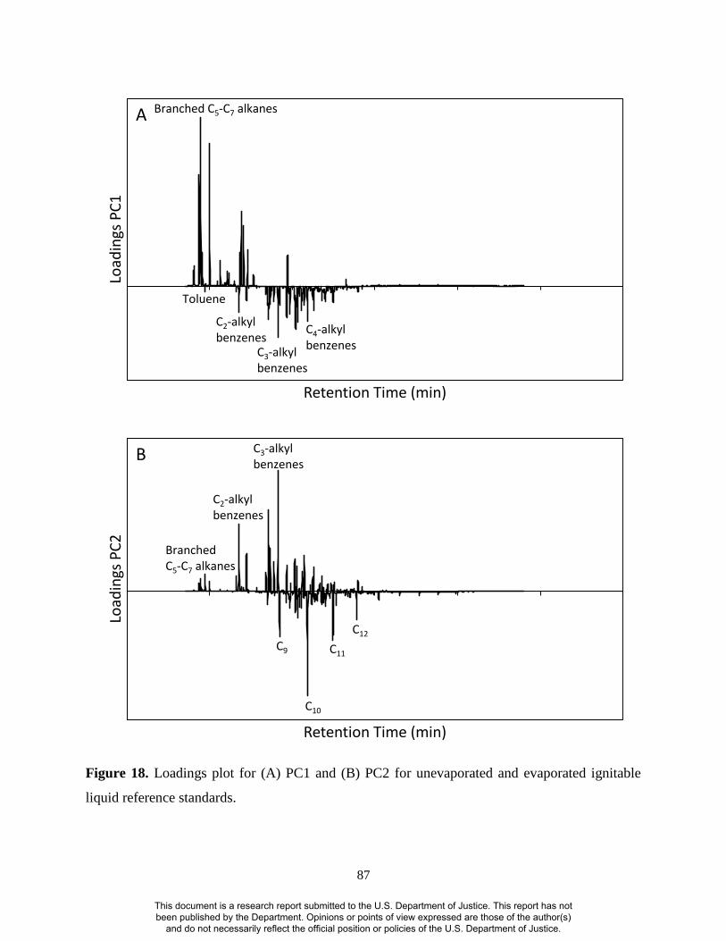
87

Figure 18. Loadings plot for (A) PC1 and (B) PC2 for unevaporated and evaporated ignitable

liquid reference standards.

Load

ings

PC

1


A Branched C5-C7 alkanes

Toluene

C2-alkylbenzenes

C3-alkylbenzenes

C4-alkylbenzenes

Load

ings

PC

2


B

Branched C5-C7 alkanes

C2-alkylbenzenes

C3-alkylbenzenes

C9

C10

C11

C12



88

The general positioning of standards on the scores plot is similar to that observed

previously for PCA of the unevaporated standards only (compare Figure 17 to Figure 13); that is,

the first principal component distinguishes the upholstery protector standards from the others. It

is important to note that in general, the evaporated standards are positioned closely to the

unevaporated counterparts on PC1, while the second principal component distinguishes the

standards based on evaporation level. However, some exceptions do exist, including the 90%

evaporated upholstery protector standard and the 90% evaporated gasoline standards.

Replicates of the 90% evaporated upholstery protector standard are positioned less

positively on PC1 than the corresponding 50% evaporated and unevaporated standards. The

branched alkanes present in this liquid are weighted positively in the PC1 loadings plot (Figure

18A). However, due to their volatility, these compounds are no longer present in the 90%

evaporated standard. As a result, there are fewer compounds with a positive weighting on PC1

and consequently, a less positive score on this PC for the 90% evaporated standard compared to

the 50% evaporated and unevaporated standards.

Replicates of the 90% evaporated gasoline are positioned more negatively on PC2 than

the 50% and unevaporated counterparts. Toluene and the C2-alkylbenzenes, which are the more

volatile compounds present in gasoline, are weighted positively in the PC2 loadings plot (Figure

18B). As evaporation progresses, the abundance of these volatile compounds decreases (Figure

19) and at the 90% evaporation level, toluene and ethylbenzene (the first eluting C2-

alkylbenzene) are no longer present, while the xylenes (the remaining C2-alkylbenzenes) are

present at very low abundance. Hence, there are fewer compounds with a positive contribution,

which results in a less positive score for the 90% evaporated standards on PC2.

The 90% evaporated Gasoline 3 standard is positioned more positively on PC2 than the

90% evaporated standards of Gasolines 4 and 5. This effect is due to the higher abundance of

1,2,4-trimethylbenzene in Gasoline 3 compared to the other two gasolines (Figure 20). This

compound is weighted positively in the PC2 loadings plot and hence, the higher abundance in

Gasoline 3 results in a more positive score on PC2 for this standard compared to the other two

90% evaporated gasoline standards.



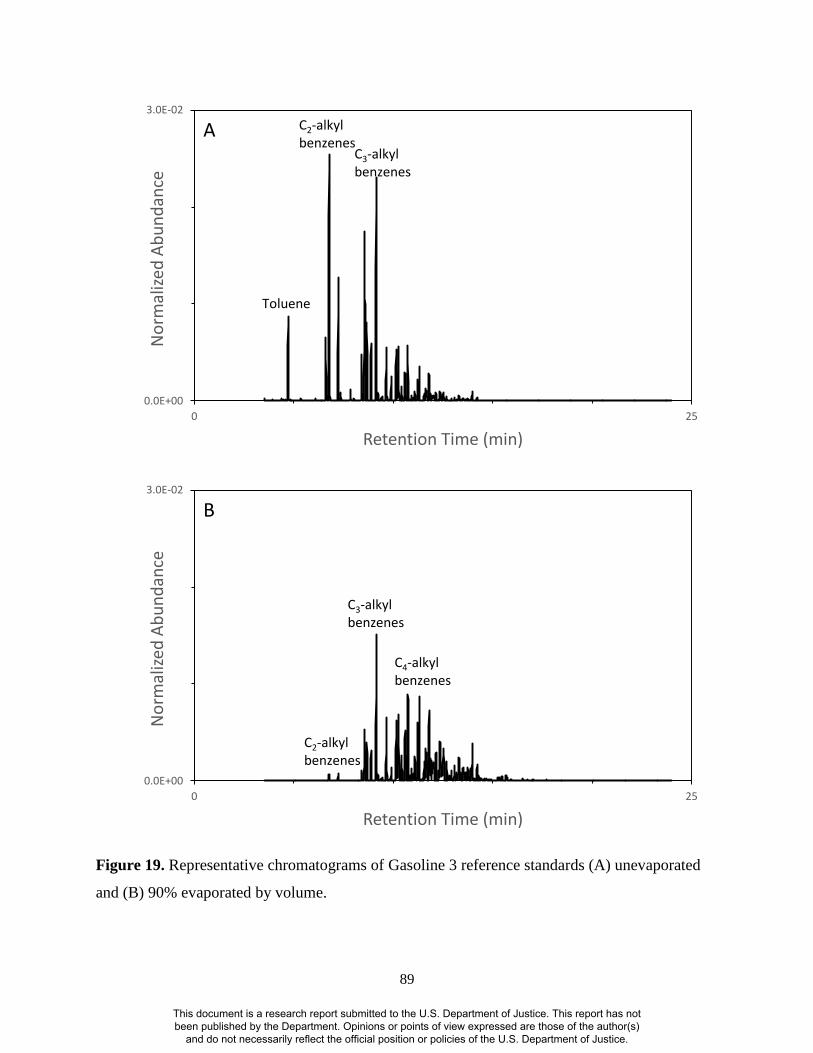
89

Figure 19. Representative chromatograms of Gasoline 3 reference standards (A) unevaporated

and (B) 90% evaporated by volume.

0.0E+00

3.0E-02

0 25

No

rmal

ized

Ab

un

dan

ce


A

Toluene

C2-alkylbenzenes

C3-alkylbenzenes

0.0E+00

3.0E-02

0 25

No

rmal

ized

Ab

un

dan

ce


B

C2-alkylbenzenes

C3-alkylbenzenes

C4-alkylbenzenes



90

Figure 20. Representative chromatograms of 90% evaporated by volume gasoline reference

standards (A) Gasoline 3 and (B) Gasoline 4.

0.0E+00

3.0E-02

0 25

No

rmal

ized

Ab

un

dan

ce


A

1,2,4-trimethylbenzene

0.0E+00

3.0E-02

0 25

No

rmal

ized

Ab

un

dan

ce


B

1,2,4-trimethylbenzene



91

The evaporated charcoal lighter standards have more negative scores on PC2 than the

unevaporated standard (Figure 17). Charcoal lighter contains the normal alkanes C9-C12, which

are all weighted negatively in the PC2 loadings plot (Figure 18B). As evaporation progresses, the

abundance of C9 and C10 decreases and in fact, C9 is no longer present in the 90% evaporated

standard (Figure 21). However, C11 and C12 become more concentrated as evaporation

progresses. The higher abundance of C11 and C12 in the evaporated standards increases the

negative contribution of these compounds on PC2 with the result that the evaporated standards

have a more negative score on PC2 than the unevaporated counterparts.

Association of simulated fire debris samples to the appropriate reference standard was

also assessed using PCA. Again, this was initially assessed using Set 1 of the simulated fire

debris samples (carpet and carpet padding substrate). PCA was performed on only the reference

standards and the resulting eigenvectors were used to calculate scores for the fire debris samples,

which were then projected onto the scores plot. To calculate scores, the mean-centered data for

the sample is multiplied by the eigenvector for PC1 and the product is summed across all

variables to generate the score for the sample on PC1. The procedure is repeated, multiplying the

mean-centered data by the eigenvector for subsequent PCs (generating the loadings for the

sample) and summing the product to generate the score for the sample on those PCs.

Performing PCA in this manner theoretically eliminates contributions from the substrate

(i.e., interference compounds inherent to the substrate and/or produced during burning) as the

eigenvectors are generated based on the reference standards. This means that the positioning of

the fire debris samples on the scores plot is affected only by compounds present in the liquid as

these compounds are also present in the reference standards. As a result, association and

discrimination of the fire debris samples are due to compounds from the ignitable liquids

remaining in the sample, rather than any contributions from the substrate.

To be more representative of the way in which forensic laboratories may implement this

procedure, replicates of one simulated sample at a time were projected onto the scores plot.

Examples of the resulting scores plots are shown in Figure 22 for the simulated fire debris

samples containing paint thinner, torch fuel and diesel.



92

Figure 21. Representative chromatograms of charcoal lighter reference standards (A)

unevaporated and (B) 90% evaporated by volume.

0.0E+00

5.0E-02

0 25

No

rmal

ized

Ab

un

dan

ce


A

C9

C10

C11

C12

0.0E+00

5.0E-02

0 25

No

rmal

ized

Ab

un

dan

ce


B

C10

C11

C12

C13



93

Figure 22. Scores plot of PC1 versus PC2 for the ignitable liquid reference standards and

simulated fire debris sample containing carpet and carpet padding and (A) paint thinner, (B)

torch fuel, and (C) diesel. Each reference standard was analyzed in replicate (n=9) and each

standard is represented by a different color in the plot. Unevaporated standards are shown as

circles, 50% evaporated as triangles, and 90% evaporated as squares. Simulated fire debris

samples were analyzed in triplicate and are shown as black diamonds with red outlines.

Abbreviations for each standard are defined in Table 1.

PC

2 (

17

.5%

)

PC1 (22.4%)


50GS3 50GS4 50GS5 50PTH 50UFP 50MFS 50LMP 50TFL 50CHL 50DSL 50KER

90GS3 90GS4 90GS5 90PTH 90UFP 90CHL 90DSL 90KER CPTPTH

A



94








PC

2 (

17

.5%

)

PC1 (22.4%)



90GS3 90GS4 90GS5 90PTH 90UFP 90CHL 90DSL 90KER CPTTFL

B



95








PC

2 (

17

.5%

)

PC1 (22.4%)



90GS3 90GS4 90GS5 90PTH 90UFP 90CHL 90DSL 90KER CPTDSL

C



96

In terms of associating the fire debris samples to the corresponding standard, visual

assessment of the scores plots is limited. The success of association is dependent on the extent of

burning and hence, the compounds characteristic of the liquid that remain in the fire debris

samples. For this particular data set, some fire debris samples associate well to the corresponding

standard (e.g., upholstery protector, torch fuel, paint thinner, etc.) as reference standards of these

liquids are already well discriminated from the others. However, in other cases, association to the

corresponding standard is not possible, particularly for the debris samples containing marine fuel

stabilizer, diesel, and kerosene. Each of these samples is positioned closely to a group containing

the marine fuel stabilizer, diesel, and kerosene reference standards although clear association to

one liquid over the other two is not possible, even with the consideration of additional principal

components. This is likely due to the overlap in compounds present in the unresolved section of

the chromatogram between approximately 10 and 13 min.

To further assess positioning of the simulated fire debris samples on the scores plots, two

additional metrics were used: Euclidean distance measurement and PPMC coefficients, which

were calculated using the eigenvectors and mean-centered data (see section 2.2.2 for more

details). For the simulated fire debris samples containing paint thinner, upholstery and fabric

protector, marine fuel stabilizer, and lamp oil, the shortest Euclidean distance was to the

corresponding standard. However, for fire debris samples containing torch fuel, charcoal lighter,

diesel, and kerosene, the shortest distance was to the marine fuel stabilizer standard.

For the second metric, the absolute mean PPMC coefficient for the first four principal

components was calculated for pairwise comparisons of each simulated fire debris sample to all

reference standards (Table 17).



97

Table 17. Absolute mean PPMC coefficient calculated using the first four principal components

to assess association of simulated fire debris (carpet and carpet padding substrate) to reference

standards.

Reference

standard

Absolute mean PPMC coefficient based on first four principal components

PTH

CPT

UFP

CPT

MFS

CPT

LMP

CPT

TFL

CPT

CHL

CPT

DSL

CPT

KER

CPT

GS3 0.290 0.356 0.374 0.239 0.306 0.270 0.354 0.365

50 GS3 0.305 0.367 0.389 0.248 0.318 0.277 0.367 0.379

90 GS3 0.387 0.403 0.504 0.309 0.357 0.350 0.474 0.415

GS4 0.304 0.364 0.383 0.242 0.309 0.273 0.361 0.369

50 GS4 0.328 0.372 0.411 0.254 0.317 0.277 0.385 0.371

90 GS4 0.641 0.625 0.871 0.325 0.478 0.395 0837 0.641

GS5 0.285 0.359 0.362 0.232 0.304 0.266 0.343 0.364

50 GS5 0.294 0.364 0.364 0.232 0.308 0.264 0.343 0.370

90 GS5 0.630 0.615 0.867 0.319 0.540 0.392 0.848 0.688

PTH 0.760 0.468 0.556 0.200 0.267 0.308 0.535 0.405

50 PTH 0.763 0.475 0.574 0.217 0.285 0.359 0.549 0.440

90 PTH 0.747 0.474 0.586 0.322 0.337 0.435 0.554 0.480

UFP 0.423 0.914 0.510 0.246 0.368 0.272 0.489 0.402

50 UFP 0.450 0.945 0.547 0.255 0.381 0.280 0.524 0.415

90 UFP 0.552 0.759 0.698 0.245 0.367 0.330 0.668 0.495

MFS 0.674 0.662 0.971 0.297 0.568 0.490 0.916 0.732

50 MFS 0.639 0.652 0.950 0.306 0.596 0.460 0.908 0.738

LMP 0.202 0.216 0.203 0.871 0.311 0.721 0.211 0.436

50 LMP 0.199 0.221 0.243 0.850 0.399 0.718 0.255 0.520

TFL 0.361 0.362 0.463 0.288 0.747 0.335 0.571 0.637

50 TFL 0.371 0.373 0.474 0.250 0.784 0.300 0.582 0.644

CHL 0.345 0.343 0.340 0.417 0.234 0.270 0.372 0.287

50 CHL 0.354 0.368 0.368 0.274 0.222 0.182 0.411 0.303

90 CHL 0.351 0.335 0.326 0.247 0.214 0.190 0.370 0.292

DSL 0.679 0.688 0.954 0.328 0.641 0.472 0.979 0.794

50 DSL 0.676 0.697 0.951 0.315 0.539 0.481 0.936 0.721

90 DSL 0.674 0.698 0.950 0.308 0.520 0.488 0.917 0.702

KER 0.582 0.594 0.836 0.363 0.857 0.464 0.955 0.914

50 KER 0.605 0.627 0.858 0.340 0.716 0.402 0.950 0.809

90 KER 0.668 0.693 0.943 0.310 0.522 0.481 0.920 0.706 Abbreviations for each reference standard are listed in Table 1.


CPT indicates carpet and carpet padding substrate.

In Table 17, coefficients indicating correlation to corresponding standards are shown in

bold. For fire debris samples containing upholstery and fabric protector, lamp oil, and kerosene,

the highest coefficient, indicating strong correlation, is obtained for comparisons to the

corresponding standards. For the paint thinner fire debris sample, the highest coefficient is also

obtained for comparison to the corresponding standard but in this case, a moderate rather than



98

strong correlation is indicated. The debris sample containing torch fuel is strongly correlated to

the kerosene reference standards but only moderately correlated to the appropriate reference

standard. Debris samples containing marine fuel stabilizer and diesel are each strongly correlated

to both the marine fuel stabilizer and diesel reference standards. However, the higher coefficient

is observed between the fire debris and the corresponding standard indicating greater similarity.

Finally, the debris sample containing charcoal lighter is not strongly correlated to any reference

standard.

Principal components analysis was also performed on fire debris samples in Set 2 which

contained an oil-finished hardwood flooring substrate (Figure 23). Separate samples of the

substrate were spiked with paint thinner, torch fuel, and diesel, then burned, extracted and

analyzed following procedures described previously. For this particular substrate, dominant

interference compounds are the normal alkanes C9-C12. These compounds are also present in the

petroleum distillate standards and hence, for this particular substrate, the substrate compounds do

contribute to positioning of the fire debris samples on the scores plot.

In each of the scores plots, the fire debris samples are positioned most closely to the

marine fuel stabilizer reference standard (Figure 23). This was verified with Euclidean distance

calculations using the first four principal components: in each case, the shortest Euclidean

distance is between the fire debris sample and the marine fuel stabilizer standard (0.022, 0.006,

and 0.006 for debris containing paint thinner, torch fuel, and diesel, respectively).

To further assess positioning on the scores plots, PPMC coefficients were calculated

using the eigenvectors for each PC (Table 18). The paint thinner fire debris samples are only

weakly correlated to the corresponding standards while the torch fuel fire debris samples are

moderately correlated to the corresponding standard. However, torch fuel fire debris samples are

more strongly correlated to the diesel and kerosene reference standards, most likely due to the

normal alkane substrate interference compounds. Fire debris containing diesel is strongly

correlated to the corresponding standards although these samples are also strongly correlated to

marine fuel stabilizer and kerosene reference standards, primarily due to the substrate

interference compounds.



99


simulated fire debris sample containing oil-finished hardwood flooring (A) paint thinner, (B)






PC

2 (

17

.5%

)

PC1 (22.4%)



90GS3 90GS4 90GS5 90PTH 90UFP 90CHL 90DSL 90KER PTHWD

A



100

Figure 23 contd. Scores plot of PC1 versus PC2 for the ignitable liquid reference standards and







PC

2 (

17

.5%

)

PC1 (22.4%)



90GS3 90GS4 90GS5 90PTH 90UFP 90CHL 90DSL 90KER TFLWD

B



101

Figure 23 contd. Scores plot of PC1 versus PC2 for the ignitable liquid reference standards and







PC

2 (

17

.5%

)

PC1 (22.4%)



90GS3 90GS4 90GS5 90PTH 90UFP 90CHL 90DSL 90KER DSLTWD

C



102

Table 18. Absolute mean PPMC coefficient calculated using the first four principal components

to assess association of simulated fire debris (oil-finished wood substrate) to reference standards.

Reference standard

Absolute mean PPMC coefficient based on first four principal

components

PTH

OWD

TFL

OWD

DSL

OWD

GS3 0.211 0.276 0.331

50 GS3 0.230 0.283 0.344

90 GS3 0.333 0.307 0.456

GS4 0.231 0.276 0.340

50 GS4 0.261 0.273 0.367

90 GS4 0.442 0.519 0.767

GS5 0.206 0.278 0.324

50 GS5 0.225 0.276 0.321

90 GS5 0.430 0.522 0.759

PTH 0.350 0.349 0.524

50 PTH 0.388 0.371 0.550

90 PTH 0.431 0.400 0.570

UFP 0.349 0.365 0.442

50 UFP 0.361 0.363 0.476

90 UFP 0.353 0.428 0.627

MFS 0.565 0.662 0.901

50 MFS 0.497 0.642 0.867

LMP 0.534 0.312 0.263

50 LMP 0.542 0.397 0.357

TFL 0.452 0.688 0.461

50 TFL 0.431 0.621 0.441

CHL 0.218 0.309 0.345

50 CHL 0.274 0.337 0.387

90 CHL 0.291 0.326 0.359

DSL 0.509 0.704 0.904

50 DSL 0.529 0.648 0.893

90 DSL 0.540 0.625 0.879

KER 0.432 0.741 0.823

50 KER 0.405 0.740 0.843

90 KER 0.530 0.622 0.879 Abbreviations for each reference standard are listed in Table 1.


OWD indicates oil-finished wood substrate.

In Table 18, coefficients indicating correlation to corresponding standards shown in bold

font. Irrespective of the substrate (carpet and carpet padding or oil-finished wood), PCA is

limited for this particular application. These limitations remain despite performing PCA in a

manner that theoretically eliminates or minimizes contributions from the substrate interference



103

compounds and despite taking into account additional PCs that explain more of the variance in

the data set.


Initially, HCA was performed on only the ignitable liquid reference standards to assess

the ability to cluster according to ASTM class, using the Euclidean distance measurement and

three common linkage methods (single, complete, and average). The resulting dendrograms are

shown in Figure 24 and a summary of the clustering is given in Table 19.

Table 19. Similarity level at which replicates and liquids within each ASTM class cluster.

Reference standard

Similarity level (%) of clusters

Euclidean distance

Single linkage

Euclidean distance

Complete linkage

Euclidean distance

Average linkage

GS3 96.4 95.6 95.9

GS4 96.5 94.4 95.2

GS5 90.3 89.9 90.7

Gasoline 88.3 79.9 83.0

PTH 95.4 93.0 94.0

UFP 92.7 90.9 92.0

Isoparaffinic 30.7 0.0 0.0

MFS 98.6 98.5 98.5

LMP 99.2 98.4 98.9

TFL 98.1 96.8 97.3

CHL 89.2 90.0 89.4

DSL 98.1 97.4 97.7

KER 97.9 97.8 97.8

Petroleum distillate 41.5 32.4 35.0 Abbreviations for each liquid are listed in Table 1.



104

Figure 24. Hierarchical cluster analysis of ignitable liquid reference standards using Euclidean

distance and (A) single linkage, (B) complete linkage, and (C) average linkage. Abbreviations

for each standard are defined in Table 1.



105

Figure 24 contd. Hierarchical cluster analysis of ignitable liquid reference standards using

Euclidean distance and (A) single linkage, (B) complete linkage, and (C) average linkage.




106

Figure 24 contd. Hierarchical cluster analysis of ignitable liquid reference standards using





107

In general, the linkage method used does not drastically influence the clusters formed for

this data set. For all three methods, replicates of each ignitable liquid reference standard form

distinct clusters at similarity levels greater than 90%. Further, replicates are clustered before

forming clusters with other standards, indicating that replicates are more similar to each other

than to those of other standards, as expected.

The linkage method also does not greatly influence the similarity level at which standards

in the same ASTM class are clustered, with the exception of the isoparaffinic class. In this

instance, there is 31% similarity between upholstery protector and paint thinner using the single

linkage method but 0% similarity using the complete linkage and average linkage methods.

Despite being in the same class, these two standards are very different in chemical composition,

containing branched alkanes with a different carbon number range. In cluster analysis, the

similarity levels are calculated relative to the data set under consideration: as a result, there will

always be two samples that have 0% similarity. Given the prior knowledge of this particular data

set, upholstery protector is the most dissimilar and therefore, the clustering afforded by the

complete and average linkage methods is not unexpected.

For all three linkage methods, the petroleum distillate reference standards are clustered at

relatively low similarity levels (ranging from 32-42%). Again, given the prior knowledge of this

data set, the lower similarity levels are not unexpected. The five reference standards in this class

all contain normal alkanes although the identity and number of the alkanes varies. Among the

petroleum distillates, diesel and kerosene are the most similar, both containing a similar range of

unresolved compounds and with a wide range of normal alkanes (C10-C20 in diesel and C10-C17 in

kerosene). These two standards are clustered at similarity levels of 81.8%, 82.9%, and 82.1%

using single, complete, and average linkage methods, respectively.

The cluster analysis results indicate that, in a chemically diverse data set such as this, the

choice of linkage method does not greatly influence the clusters obtained. While all three

methods could easily be used in subsequent data analysis, for simplicity and clarity, only one

linkage method was selected for further consideration. The single linkage method is analogous to

the k-nearest neighbors classification procedure, with k (i.e., the number of neighbors for

classification) equal to 1. As these data were also subjected to k-nearest neighbors, the single

linkage method was selected.



108

Cluster analysis was repeated, including the evaporated standards in the data set. The

similarity level at which replicates of each reference standard are clustered is summarized in

Table 20. The similarity levels at which the evaporated standards cluster with the corresponding

non-evaporated standard are summarized in Table 21.

Table 20. Similarity level of replicates of each reference standard.

Reference standard Similarity level (%)of

replicates Reference standard

Similarity level (%)of

replicates

GS3 95.2 LMP 96.7

50 GS3 92.4 50 LMP 97.5

90 GS3 96.3

TFL 96.0

GS4 95.4 50 TFL 94.2

50 GS4 92.6

90 GS4 96.6 CHL 59.3

50 CHL 91.1

GS5 88.7 90 CHL 87.9

50 GS5 91.7

90 GS5 97.0 DSL 98.1

50 DSL 94.8

PTH 89.1 90 DSL 93.4

50 PTH 89.2

KER 96.9

UFP 87.4 50 KER 95.7

50 UFP 90.3 90 KER 93.6

MFS 98.0

50 MFS 97.2 Abbreviations for each liquid are listed in Table 1.

Replicates of each standard cluster at high similarity irrespective of evaporation level,

with the exception of unevaporated charcoal lighter for which replicates only cluster at 59.3%

similarity. For this liquid, one replicate was slightly misaligned compared to the other eight

replicates. As a result, this replicate clustered to the others at the slightly lower similarity level.

When this replicate is excluded, the remaining replicates of the unevaporated charcoal lighter

reference standard cluster at a similarity level of 96.3%.



109

Table 21. Similarity level at which evaporated standards cluster with corresponding

unevaporated standard.

Unevaporated reference

standard

Similarity level (%) of cluster formation with corresponding

evaporated standard

50% evaporated standard 90% evaporated standard

GS3 85.3 81.0

GS4 90.9 67.3

GS5 85.3 67.3

PTH 76.1 --

UFP 80.1 --

MFS 82.5 --

LMP 84.6 --

TFL 74.9 --

CHL 59.3 44.7

DSL 82.5 65.3

KER 85.8 77.9 Abbreviations for each liquid are listed in Table 1.

For those standards for which there are only two levels of evaporation (unevaporated and

50% evaporated), the unevaporated and evaporated standards cluster at high similarity levels

(75% and higher). Additionally, these clusters are formed first, prior to forming clusters with any

other standard. For those standards for which there are three evaporation levels, the 50%

evaporated standard clusters with the unevaporated standard first, and then to the 90%

evaporated standard. However, these clusters tend to include reference standards of other liquids.

For example, the unevaporated and 50% evaporated diesel standards cluster at 82.5% similarity.

These standards then cluster not with the 90% evaporated diesel but instead, with a cluster

containing the unevaporated and 50% evaporated kerosene standards. Similarly, unevaporated

gasoline 5 clusters with a group containing the corresponding 50% evaporated standard along

with the unevaporated and 50% evaporated standards of gasolines 3 and 4.

To assess association of simulated fire debris samples to the corresponding reference

standards, cluster analysis was repeated using Set 1 of the fire debris samples. As before,

replicates of one fire debris sample at a time were included with the reference standards for

analysis. This method of conducting HCA was deemed more relevant to the way in which

forensic laboratories could perform similar analyses in the future. In all cases, HCA was

performed using Euclidean distance and single linkage. All dendrograms are shown in Appendix

5 and the results of cluster analysis are summarized in Table 22.



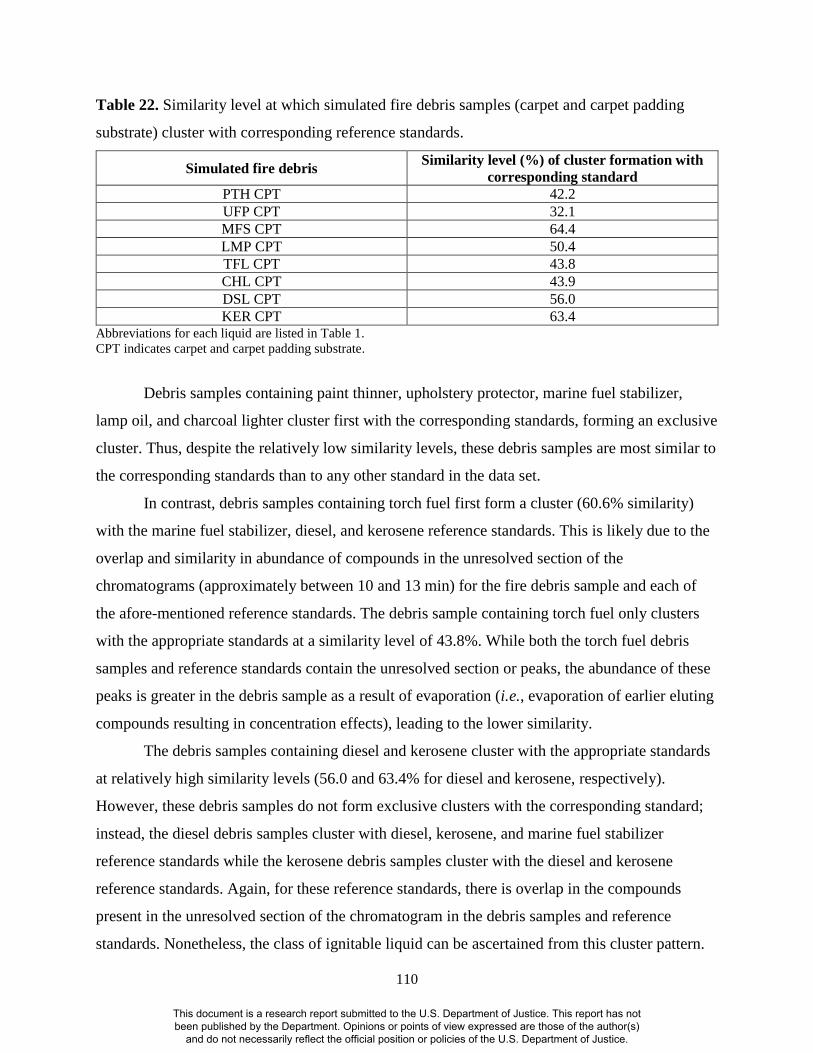
110

Table 22. Similarity level at which simulated fire debris samples (carpet and carpet padding

substrate) cluster with corresponding reference standards.

Simulated fire debris Similarity level (%) of cluster formation with

corresponding standard

PTH CPT 42.2

UFP CPT 32.1

MFS CPT 64.4

LMP CPT 50.4

TFL CPT 43.8

CHL CPT 43.9

DSL CPT 56.0

KER CPT 63.4 Abbreviations for each liquid are listed in Table 1.


Debris samples containing paint thinner, upholstery protector, marine fuel stabilizer,

lamp oil, and charcoal lighter cluster first with the corresponding standards, forming an exclusive

cluster. Thus, despite the relatively low similarity levels, these debris samples are most similar to

the corresponding standards than to any other standard in the data set.

In contrast, debris samples containing torch fuel first form a cluster (60.6% similarity)

with the marine fuel stabilizer, diesel, and kerosene reference standards. This is likely due to the

overlap and similarity in abundance of compounds in the unresolved section of the

chromatograms (approximately between 10 and 13 min) for the fire debris sample and each of

the afore-mentioned reference standards. The debris sample containing torch fuel only clusters

with the appropriate standards at a similarity level of 43.8%. While both the torch fuel debris

samples and reference standards contain the unresolved section or peaks, the abundance of these

peaks is greater in the debris sample as a result of evaporation (i.e., evaporation of earlier eluting

compounds resulting in concentration effects), leading to the lower similarity.

The debris samples containing diesel and kerosene cluster with the appropriate standards

at relatively high similarity levels (56.0 and 63.4% for diesel and kerosene, respectively).

However, these debris samples do not form exclusive clusters with the corresponding standard;

instead, the diesel debris samples cluster with diesel, kerosene, and marine fuel stabilizer

reference standards while the kerosene debris samples cluster with the diesel and kerosene

reference standards. Again, for these reference standards, there is overlap in the compounds

present in the unresolved section of the chromatogram in the debris samples and reference

standards. Nonetheless, the class of ignitable liquid can be ascertained from this cluster pattern.



111

Set 2 of the simulated fire debris samples (paint thinner, torch fuel, and diesel on an oil-

finished wood flooring) was also subjected to HCA. As before, replicates of one fire debris

sample at a time were included with the reference standards for analysis and in all cases, HCA

was performed using Euclidean distance and single linkage. The three simulated fire debris

samples all first form clusters with a larger group that contains the diesel and kerosene reference

standards, albeit at different similarity levels (52.3% for simulated fire debris containing paint

thinner, 44.2% for fire debris containing torch fuel, and 61.8% for fire debris containing diesel).

In all cases, the presence of the normal alkanes in the substrate (from the oil finish) increases

similarity to the petroleum distillate standards, resulting in the clustering observed. As noted

previously, the diesel simulated fire debris sample does not resemble the diesel reference

standard and hence, the apparent high similarity observed in clustering is due to the presence of

the interference compounds from the substrate (C9-C12).

For the oil-finished wood substrate, the use of HCA is more limited than observed

previously for the carpet and carpet padding substrate. Samples and reference standards are

clustered based on similarities in chemical composition. For the carpet and carpet padding

substrate, the interference compounds (styrene, trichloropropane, and biphenyl) are not present in

the reference standards. Hence, clustering of these samples is based on the compounds present in

the liquid, resulting in successful association of the debris samples and reference standards. In

contrast, the substrate interference compounds (C9-C12) in the oil-finished wood are also present

in the petroleum distillate reference standards. As a result, clustering of these debris samples is

based on similarity of the interference compounds, resulting in association of the fire debris

samples to the kerosene and diesel standards first.

It is interesting to note the agreement between cluster analysis and principal components

analysis: that is, positioning of simulated samples in the PCA scores plot corresponds to

clustering observed in the HCA dendrogram. Cluster analysis is often considered to assess

similarity while, in contrast, PCA is considered to assess differences (i.e., variance) among

samples in a data set. However, both procedures are based on distance measurements in

multidimensional space. In fact, the dendrogram output from HCA includes all dimensions

whereas, scores plots from PCA typically include only a few dimensions that account for the

majority of the variance. Thus, in comparing the outputs from both procedures, the dendrogram

is actually more representative of the full data set. The implication of this difference becomes



112

apparent in the classification procedures which are discussed in the following sections (4.1.6 and

4.1.7).


To begin investigating the SIMCA approach, Set 1 of the simulated fire debris samples

(carpet and carpet padding substrate) was again used. In the first iteration, statistical models were

developed based on the isoparaffinic and petroleum distillate ignitable liquid classes as these

were the two classes represented in the fire debris samples in this data set. The isoparaffinic

model contained the two isoparaffinic reference standards at all three evaporation levels (i.e.,

unevaporated, 50%, and 90% evaporated) while the petroleum distillate model contained all

evaporation levels available for these reference standards. Both models were generated by PCA

of the appropriate data set. For the isoparaffinic class, four principal components were included

in the model, accounting for 98.2% of the variance, while for the petroleum distillate model, six

principal components were included, accounting for 97.0% of the variance. This highlights one

of the advantages of the SIMCA method: the number of principal components included in a

model does not have to be the same for all models in the data set. As a result, the number of PCs

selected is tailored to adequately describe the variance in that model.

Classification of the simulated fire debris samples was subsequently performed using the

generated models. However, with these two models, none of the fire debris samples were

classified at any of the confidence levels investigated (95, 99, 99.5, and 99.9%). The lack of

classification is primarily a result of the models not adequately describing the data to be

classified; that is, the simulated fire debris samples contain interference compounds (i.e., styrene,

trichloropropane, and biphenyl) from the substrate that are not described by the models.

In the second SIMCA iteration, the burned substrate with no ignitable liquid present was

included in the PCA models. For the isoparaffinic class, five principal components were included

in the model, accounting for 98.2% of the variance, while for the petroleum distillate model,

seven principal components were included, accounting for 97.4% of the variance. In both cases,

the contributions of the substrate compounds were taken into account as compounds from the

substrate contributed to the principal components included in the model.

Using these two models, some degree of classification of the simulated fire debris

samples was possible. At the 95% confidence level (α = 0.05), only two extracts of the fire debris



113

containing upholstery protector are correctly classified. At the 99.9% confidence level

(representing α = 0.001), there is greater success in classification. Fire debris samples containing

paint thinner and upholstery protector are correctly classified in the isoparaffinic class while

samples containing lamp oil and torch fuel are correctly classified in the petroleum distillate

class. Thus, the rate of successful classification increases as confidence level increases. At first,

this may seem counter-intuitive but in fact, higher confidence levels are less rigorous for

association. To illustrate, the area under a normal distribution density curve is shown in Figure

25 for two sample populations, A and B. At lower confidence levels (e.g., 95%), the distribution

is narrow but broadens as confidence level increases. Therefore, there is greater chance of

association as confidence level increases due to broadening of the distribution.

While there is greater success in classification at higher confidence levels, there is also an

increase in the rate of multiple classifications. At the 99.9% confidence level, simulated fire

debris samples containing charcoal lighter, diesel, and kerosene, are correctly classified as

petroleum distillates but are also misclassified as isoparaffinics. Upon closer inspection, the

chromatograms of these samples are all dominated by the substrate interference compounds, with

less contribution from the compounds contained in the liquid (Appendix 1). As both class models

now contain the substrate, the high contribution of substrate compounds in these fire debris

samples means that classification to both models occurs. In contrast, chromatograms of the fire

debris samples that are correctly classified (i.e., paint thinner, upholstery protector, lamp fuel,

and torch fuel) are dominated by compounds from the liquid itself, with less contribution from

the substrate compounds.

A final iteration of SIMCA was performed in which replicates of one simulated fire

debris sample were also included in the model, along with the reference standards and burned

substrate. For the isoparaffinic class, six principal components were included in the model,

accounting for 98.7% of the variance, while for the petroleum distillate model, seven principal

components were included, accounting for 95.9% of the variance. Classification success is

enhanced with this addition to the models, as summarized in Table 23.



114

Figure 25. Normal distribution density curves for two sample populations for confidence levels

from 95% to 99.9%.

95.0%

98.0%

99.0%

99.9 %

4 43 32 211 04 43 32 211 0

95.0%

98.0%

99.0%

99.9%

4 3 2 1 0 1 2 3 44 3 2 1 0 1 2 3 4

No

rmal

ized

Am

plit

ud

e

Number of Standard Deviations

Population A Population B



115

Table 23. Summary of classification of simulated fire debris samples (carpet and carpet padding

substrate) with inclusion of reference standards, substrate, and simulated fire debris in model.

Simulated fire debris Classification at the following confidence levels

95% 99% 99.9%

PTH CPT Extract 2 NC NC ISO

PTH CPT Extract 3 ISO ISO ISO

UFP CPT Extract 2 ISO ISO ISO

UFP CPT Extract 3 NC ISO ISO

MFS CPT Extract 1 NC PET PET



LMP CPT Extract 1 PET PET PET

LMP CPT Extract 2 PET PET PET

TFL CPT Extract 2 PET PET PET

TFL CPT Extract 3 PET PET PET

CHL CPT Extract 2 PET PET PET

CHL CPT Extract 3 NC PET PET

DSL CPT Extract 1 PET PET PET

DSL CPT Extract 3 PET PET PET

KER CPT Extract 1 PET PET PET

KER CPT Extract 2 PET PET PET Abbreviations for each liquid are listed in Table 1.


NC indicates Not classified.

ISO indicates Isoparaffinic.

PET indicates Petroleum distillate.

At the 95% confidence level, all samples are correctly classified, with the exception of

one extract each of fire debris containing paint thinner, upholstery protector, and charcoal lighter.

Upon further inspection of the chromatograms for these samples, all have a high abundance of

the interference compounds, particularly trichloropropane, compared to the other extracts. At the

highest confidence level (99.9%), all simulated fire debris samples are correctly classified

although at this level, the sample containing marine fuel stabilizer (a naphthenic paraffinic

liquid) is also classified as a petroleum distillate. However, this liquid is chemically similar to

the petroleum distillates in the common unresolved portion of the chromatogram, as discussed

previously.

With models that include fire debris samples, classification is more successful. However,

the models are now so specific that even differences in abundance of the compounds from the

liquid can prevent correct classification. In model building, a compromise must be reached

between models that do not adequately describe the data (e.g., the first models here that include



116

the standards only) and models that are too specific (e.g., the final models that include simulated

fire debris samples). For fire debris analysis, appropriate model generation is challenging as the

nature of the substrate will change, as will the abundance of compounds in any liquid present.

Thus, from a practical aspect, SIMCA may be limited for the classification of ignitable liquids

present in fire debris samples.

Simulated fire debris samples prepared using the oil-finished wood substrate were also

subjected to SIMCA in a similar manner. That is, in the first iteration, PCA models were

generated for the isoparaffinic and petroleum distillate classes including only the appropriate

reference standards in each model. With these models, classification was limited with only three

of the nine fire debris samples correctly classified at the 99% confidence level and higher.

For the second iteration of SIMCA, PCA models for each class also included the burned

oil-finished wood substrate (Table 24). While a greater number of fire debris samples are

classified using these models, there is also an increase in the number of double classifications.

Table 24. Summary of classification of simulated fire debris samples (oil-finished wood flooring

substrate) with inclusion of reference standards and burned substrate in model.

Simulated fire

debris

Classification at the following confidence levels

95% 99% 99.5% 99.9%

PTH OWD

Extract 1 ISO; PET ISO; PET ISO; PET ISO; PET

PTH OWD

Extract 2 NC ISO; PET ISO; PET ISO; PET

PTH OWD


TFL OWD

Extract 1 NC NC NC NC

TFL OWD

Extract 2 NC NC NC NC

TFL OWD

Extract 3 PET PET PET PET

DSL OWD

Extract 1 PET PET ISO; PET ISO; PET

DSL OWD

Extract 2 PET ISO; PET ISO; PET ISO; PET

DSL OWD

Extract 3 PET PET PET ISO; PET

Abbreviations for each liquid are listed in Table 1.



ISO indicates Isoparaffinic; PET indicates Petroleum distillate.

ISO; PET indicates sample classified as both isoparaffinic and petroleum distillate.



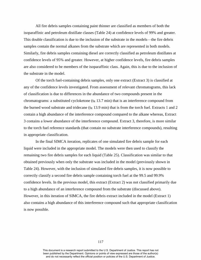
117

All fire debris samples containing paint thinner are classified as members of both the

isoparaffinic and petroleum distillate classes (Table 24) at confidence levels of 99% and greater.

This double classification is due to the inclusion of the substrate in the models—the fire debris

samples contain the normal alkanes from the substrate which are represented in both models.

Similarly, fire debris samples containing diesel are correctly classified as petroleum distillates at

confidence levels of 95% and greater. However, at higher confidence levels, fire debris samples

are also considered to be members of the isoparaffinic class. Again, this is due to the inclusion of

the substrate in the model.

Of the torch fuel-containing debris samples, only one extract (Extract 3) is classified at

any of the confidence levels investigated. From assessment of relevant chromatograms, this lack

of classification is due to differences in the abundance of two compounds present in the

chromatograms: a substituted cycloketone (tR 13.7 min) that is an interference compound from

the burned wood substrate and tridecane (tR 13.9 min) that is from the torch fuel. Extracts 1 and 2

contain a high abundance of the interference compound compared to the alkane whereas, Extract

3 contains a lower abundance of the interference compound. Extract 3, therefore, is more similar

to the torch fuel reference standards (that contain no substrate interference compounds), resulting

in appropriate classification.

In the final SIMCA iteration, replicates of one simulated fire debris sample for each

liquid were included in the appropriate model. The models were then used to classify the

remaining two fire debris samples for each liquid (Table 25). Classification was similar to that

obtained previously when only the substrate was included in the model (previously shown in

Table 24). However, with the inclusion of simulated fire debris samples, it is now possible to

correctly classify a second fire debris sample containing torch fuel at the 99.5 and 99.9%

confidence levels. In the previous model, this extract (Extract 2) was not classified primarily due

to a high abundance of an interference compound from the substrate (discussed above).

However, in this iteration of SIMCA, the fire debris extract included in the model (Extract 1)

also contains a high abundance of this interference compound such that appropriate classification

is now possible.



118

Table 25. Summary of classification of simulated fire debris samples (oil-finished wood

substrate) with inclusion of reference standards, burned substrate, and simulated fire debris in

model.

Simulated fire

debris

Classification at the following confidence levels

95% 99% 99.5% 99.9%

PTH OWD


PTH OWD


TFL OWD

Extract 2 NC NC PET PET

TFL OWD

Extract 3 PET PET PET PET

DSL OWD

Extract 1 PET PET ISO; PET ISO; PET

DSL OWD

Extract 2 PET ISO; PET ISO; PET ISO; PET

Abbreviations for each liquid are listed in Table 1.



ISO indicates Isoparaffinic; PET indicates Petroleum distillate.

ISO; PET indicates sample classified as both isoparaffinic and petroleum distillate.

For both substrates, some degree of classification of simulated fire debris samples is

possible. However, development of representative models is challenging, requiring models that

are sufficiently representative without being too specific. In this research, classification to any

extent was only possible with inclusion of at least the burned substrate in the models. For

practical applications in a forensic laboratory, this is a major limitation, particularly for fire

debris analysis as, in many cases, the identity of the substrate will not be known or easily

identifiable.


The k-nearest neighbors (k-NN) classification procedure differs from SIMCA in a

number ways. Firstly, k-NN is a ‘hard’ classification, meaning that each sample will be classified

into one, and only one, class. While this prevents samples being classified into more than one

class (previously observed using SIMCA, section 4.1.6), the risk of misclassification remains as

all samples are forced to be members of a class. Secondly, the SIMCA procedure is based on

statistical models that must be representative of the samples to be classified for the actual

classification to be accurate. However, as discussed in the previous section, this requirement is a



119

limitation for classification of ignitable liquids in fire debris. In contrast, k-NN does not require

model development; instead, the full data set is considered and classification is based on distance

of the samples to the standards in multidimensional space.

All reference standards were used in the training set to investigate the appropriate number

of nearest neighbors (k) to use for classification. For k = 1 through to k = 10 (all integer values

investigated), every reference standard was classified correctly, indicating that any value k could

be used for the subsequent classification. However, lower k values are more prone to

misclassification if outliers are present in the data set and/or the classes are not sufficiently

distinct. To avoid any potential problems, k = 5 was initially used for classification.

Using this number of neighbors, the simulated samples in Set 1 (carpet and carpet

padding substrate) are correctly classified according to ASTM class, with only one exception:

one extract of simulated fire debris containing paint thinner is classified as a petroleum distillate.

This particular extract was consistently misclassified using SIMCA primarily due to the high

abundance of substrate interference compounds and low abundance of compounds characteristic

of the liquid. It is interesting to note that simulated fire debris containing diesel is correctly

classified using k-NN whereas, these samples were not exclusively classified using SIMCA due

to the high abundance of substrate compounds coupled with the low abundance of compounds

from diesel itself. It should also be noted that the k-NN classification of the simulated samples

was repeated using k = 1, 3, 7, and 9, with the same classification results being returned

irrespective of the number of neighbors used for classification.

Set 2 of the simulated fire debris samples (oil-finished wood substrate) was also

subjected to k-NN. Classification was performed using k = 1, 3, 5, 7, and 9 and in each case, the

same classification was obtained. That is, the simulated fire debris samples containing paint

thinner are misclassified as naphthenic paraffinic while the debris samples containing torch fuel

and diesel are correctly classified as petroleum distillates. Misclassification of the paint thinner is

likely due to the unresolved region in the chromatogram that occurs over a similar retention time

range, along with the presence of later-eluting compounds in the same range, as observed in the

marine fuel stabilizer (the only naphthenic paraffinic in the data set) reference standard.

Despite the afore-mentioned misclassifications, k-NN was demonstrated to be more

successful and hence, have greater potential, for the analysis of fire debris. As discussed

previously, generating the necessary SIMCA models that are sufficiently representative without



120

being too specific is challenging, especially for fire debris applications. As the k-NN approach is

not model-based, these limitations are not a factor and hence, this approach is worthy of further

investigation and validation.

4.2 Spectral Data

Exemplar spectra of the controlled substance reference standards and simulated street

samples are included in Appendix 3.

4.2.1 Normalization

The spectral data for the controlled substance reference standards were normalized using

three different procedures: constant sum, constant vector length, and SNV normalization. The

non-normalized and normalized data sets were individually subjected to PCA to assess the effect

of normalization on the association of replicates of each standard and the distinction of different

standards. The resulting scores plots are shown in Figure 26.

For the non-normalized data, there is substantial spread among replicates of each

standard on both PC1 and PC2 (Figure 26A). As a result of the spread, there are no distinct

clusters of any of the standards such that association and discrimination is not possible. Similar

trends are observed for the data after normalization to constant sum (Figure 26B) and after

normalization to constant vector length (Figure 26C). In contrast, for the SNV-normalized data,

replicates of each standard are closely positioned in the scores plot (Figure 26D) and clear

differentiation among the three classes of controlled substances (amphetamines, opiates, and

barbiturates) is possible.

To quantify the improvement in clustering of the replicates, the relative standard

deviation of the scores on both PC1 and PC2 was calculated for each reference standard (Tables

26 and 27). On PC1, there is improved precision among replicates of all reference standards as

indicated by the low relative standard deviations. This trend is also true for PC2, with the

exception of replicates of MDEA, MDMA, methamphetamine, and phenobarbital. For these

standards, precision of replicates is improved using the other normalization procedures.

However, in general, the RSDs obtained for these standards after SNV normalization are



121

Figure 26. Scores plot for controlled substance reference standards with (A) no normalization,

(B) constant sum normalization, (C) constant vector length normalization and (D) standard

normal variate normalization. Abbreviations for each standard are defined in Table 3.

PC

2 (

17

.8%

)

PC1 (38.7%)

AMPH BARB CODE HERO MDEA MDMA METH MORP PHEN CAFF

A



122

Figure 26 contd. Scores plot for controlled substance reference standards with (A) no

normalization, (B) constant sum normalization, (C) constant vector length normalization and (D)

standard normal variate normalization. Abbreviations for each standard are defined in Table 3.

PC

2 (

17

.6%

)

PC1 (39.0%)


C



123

comparable to those RSDs obtained using the other normalization procedures. Hence, for all

subsequent data analysis, the reference standards were normalized using the SNV procedure.

Table 26. Relative standard deviation of scores on the first principal component (PC1) for non-

normalized and normalized controlled substance reference standards.

Reference

standard


Non- normalized Constant sum Constant vector

length

Standard normal

variate

Amphetamine 25.2 0.4 0.4 0.4

Barbital 5.5 12.8 6.4 0.9

Codeine 336.5 660.8 342.8 4.8

Heroin 3076.0 1588.1 672.1 20.8

MDEA 169.1 63.4 170.2 1.7

MDMA 245.4 130.7 247.5 2.1

Methamphetamine 56.1 341.1 55.6 4.1

Morphine 57.6 45.4 57.7 6.5

Phenobarbital 3.1 14.3 3.7 1.1

Caffeine 1.6 19.0 2.0 0.9

Table 27. Relative standard deviation of scores on the second principal component (PC2) for

non-normalized and normalized controlled substance reference standards.

Reference

standard


Non-normalized Constant sum Constant vector

length

Standard normal

variate

Amphetamine 62.4 29.6 58.6 2.3

Barbital 41.3 29.8 41.0 11.0

Codeine 221.8 1349.8 255.6 1.6

Heroin 80.3 50.6 77.2 2.9

MDEA 4.1 14.0 3.7 6.5

MDMA 3.9 29.5 4.9 10.6

Methamphetamine 4.8 12.3 5.0 5.8

Morphine 70.1 48.6 67.4 2.7

Phenobarbital 42.2 36.9 41.6 40.3

Caffeine 2225.2 988.3 2448.2 6.2


Principal components analysis was initially performed on the SNV-normalized reference

standards and the scores plot of PC1 and PC2 is shown in Figure 27.



124

Figure 27. Scores plot of PC1 versus PC2 for controlled substance reference standards. Each



PC

2 (

20

.3%

)

PC1 (33.6%)




125

The first two PCs account for 54% of the variance among the reference standards.

Replicates of each standard are closely positioned and three groups of the standards are apparent.

The first contains standards in the amphetamine class, the second contains standards in the

opiates class, and the third contains the two barbiturate standards. The caffeine standard is

positioned closely to the barbiturate standards, most notably on PC1. Hence, although the first

two principal components only describe 54% of the variance in the data set, this is sufficient to

distinguish the reference standards.

The majority of the positively-weighted contributions in the PC1 loadings plot (Figure

28A) result from the barbital, phenobarbital, and caffeine reference standards and hence, these

three standards are positioned positively on PC1 in the scores plot (Figure 27). The majority of

the negatively-weighted contributions result from the amphetamine, MDEA, MDMA, and

methamphetamine reference standards. As a result, the amphetamine class of standards is

positioned negatively on PC1 in the scores plot (Figure 27). Thus, the first principal component

essentially distinguishes the barbiturate and amphetamine classes.

The majority of the positively-weighted contributions in the PC2 loadings plot (Figure

28B) result from the opiate class of standards and hence, this class is positioned positively on

PC2 in the scores plot (Figure 27). The majority of the negatively-weighted contributions result

from the MDEA, MDMA, methamphetamine, and caffeine standards. As a result, these four

standards are positioned negatively on PC2 in the scores plot (Figure 27).

The two barbiturate standards have an equal number of positive and negative

contributions on PC2 but barbital is positioned negatively while phenobarbital is positioned

positively on this PC. This is explained with reference to the loadings (the product of the mean-

centered data and the PC2 eigenvector). For barbital, there are more negative loadings than

positive across all variables with the result that the score (the sum of the loadings) is negative. In

contrast, for phenobarbital, there are more positive loadings than negative, resulting in a positive

score on this PC.



126

Figure 28. Loadings plot of (A) PC1 and (B) PC2 for controlled substance reference standards.

-0.1

-0.08

-0.06

-0.04

-0.02

0

0.02

0.04

0.06

0.08

0.1

Wavenumber (cm-1)

Load

ings

PC

1A

-0.1

-0.08

-0.06

-0.04

-0.02

0

0.02

0.04

0.06

0.08

0.1

Wavenumber (cm-1)

Load

ings

PC

2

B



127

To investigate association of simulated street samples to the corresponding controlled

substance reference standard, scores were calculated for the samples and then projected onto the

scores plot, following the procedure described previously (section 4.1.4). The scores plot with

the 80/20 samples (80 parts controlled substance/20 parts caffeine, by mass) projected is shown

in Figure 29 while the plot with the 50/50 samples (50 parts controlled substance/50 parts

caffeine, by mass) projected is shown in Figure 30. Within a forensic laboratory, it is more likely

that a single case sample would be included with the reference standards for PCA rather than

multiple samples as shown here. However, as scores for each sample are calculated using the

relevant mean-centered data and the eigenvectors generated for the standards, the positioning of

individual samples does not change if only one sample is included in the data set. For these

reasons, additional scores plots showing the reference standards with the inclusion of one

simulated sample at a time are not shown here.

The 80/20 samples are positioned more positively on PC1 than the reference standards,

with a shift toward the caffeine standard. This shift is primarily due to the additional presence of

two absorptions (1694 and 1649 cm-1) from caffeine that are present in the simulated samples.

These two absorptions have positive contributions to the PC1 eigenvector, resulting in the

positive shift observed.

The 80/20 samples are positioned more closely to the respective standard on PC2, albeit

slightly more negatively. This is also primarily due to the presence of the two absorbance bands

resulting from caffeine, which have a negative contribution on PC2. The exceptions to this are

the samples containing codeine for which there is a greater negative shift on PC2 compared to

the standard. For these particular samples, the absorptions from caffeine mask two of the

absorptions from codeine. Accordingly, there is less contribution from the controlled substance

and a greater shift toward caffeine. Despite the shifts observed on PC2, association of the 80/20

samples to the respective standards is possible on this principal component.



128

Figure 29. Scores plot of PC1 versus PC2 for the controlled substance reference standards and

simulated street samples containing 80 parts controlled substance/20 parts caffeine, by mass.

Each reference standard was analyzed in replicate (n=9) and each standard is represented by a

different color in the plot. Reference standards are shown as circles and simulated samples are

shown as triangles, with the color corresponding to the controlled substance present.


PC

2 (

20

.3%

)

PC1 (33.6%)

AMPH BARB CODE HERO MDEA MDMA METH MORP

PHEN CAFF 80AMPH 80BARB 80CODE 80MDEA 80MDMA 80METH



129

Figure 30. Scores plot of PC1 versus PC2 for the controlled substance reference standards and

simulated street samples containing 50 parts controlled substance/50 parts caffeine, by mass.

Each reference standard was analyzed in replicate (n=9) and each standard is represented by a

different color in the plot. Reference standards are shown as circles and simulated samples are

shown as squares with the color corresponding to the controlled substance present. Abbreviations

for each standard are defined in Table 3.

PC

2 (

20

.3%

)

PC1 (33.6%)

AMPH BARB CODE HERO MDEA MDMA METH MORP

PHEN CAFF 50AMPH 50BARB 50CODE 50MDEA 50MDMA 50METH



130

Similar trends are observed for the 50/50 simulated samples; that is, the samples have

similar scores on PC2 as the corresponding standards but have more positive scores on PC1 due

to the contributions from caffeine. However, as the caffeine content of the 50/50 samples is

greater, the shift on PC1 is more apparent than for the 80/20 samples. This greater shifts prevents

confident association of the 50/50 samples to the corresponding reference standard.

To provide a more quantitative assessment of the scores plot, Euclidean distances and

PPMC coefficients were calculated between each simulated sample and all reference standards

(Tables 28 and 29). Quantitative assessment of both scores plots was performed; however, due to

the large shifts observed in the scores plot for the 50/50 samples, quantitative assessment

provided no additional information. Hence, only quantitative assessment of association of the

80/20 samples and reference standards is discussed below. Additionally, as discrimination was

possible based on the first two principal components, Euclidean distances and PPMC coefficients

were calculated using only these two PCs.

Table 28. Euclidean distance between simulated street samples and reference standards

calculated based on scores for first two principal components.

Reference

standard

Euclidean distance between reference standard and simulated sample

containing

Amphetamine Barbital Codeine MDEA MDMA Methamphetamine

Amphetamine 7.86 68.78 38.88 32.05 31.76 53.33

Barbital 58.81 2.46 31.63 50.51 47.39 54.91

Codeine 18.93 55.73 21.67 42.02 39.75 62.82

Heroin 24.83 47.83 13.89 42.56 39.80 61.97

MDEA 25.52 61.96 43.97 10.62 13.13 28.01

MDMA 23.12 61.97 42.67 11.66 13.67 30.24

Methamphetamine 45.65 70.06 60.39 22.10 25.31 18.64

Morphine 20.28 62.90 28.81 46.53 44.60 67.85

Phenobarbital 57.30 10.90 27.54 53.68 50.37 61.09

Caffeine 61.41 9.97 38.18 47.76 45.03 47.92

In Table 28, the shortest Euclidean distance for each comparison is highlighted in bold. In

general, the shortest distance is observed between the sample and the corresponding reference

standard and in each case, this distance is approximately half the next greatest distance. The

exceptions are the samples containing codeine, MDEA, and MDMA. For codeine, the shortest

distance is to the heroin reference standard, while the next shortest distance is to the codeine

standard. For the simulated samples containing MDEA and MDMA, there is little difference in



131

the distance calculated between the sample and both the MDEA and MDMA reference standards.

That is, it is not possible to associate the samples to the corresponding reference standard; rather,

the samples are equally associated to both MDEA and MDMA.

Table 29. Absolute mean PPMC coefficient calculated using the first two principal components

to assess association of simulated street samples to controlled substance reference standards.

Reference

standard

Absolute mean PPMC coefficient based on first two principal components

for comparison of reference standard and samples containing

Amphet-

amine Barbital Codeine MDEA MDMA

Metham-

phetamine

Amphetamine 0.936 0.636 0.152 0.129 0.260 0.299

Barbital 0.500 0.955 0.134 0.246 0.111 0.067

Codeine 0.349 0.460 0.515 0.300 0.523 0.547

Heroin 0.086 0.320 0.189 0.186 0.263 0.634

MDEA 0.112 0.510 0.494 0.828 0.545 0.195

MDMA 0.193 0.416 0.606 0.609 0.694 0.220

Methamphetamine 0.179 0.279 0.516 0.212 0.156 0.810

Morphine 0.675 0.517 0.234 0.247 0.341 0.629

Phenobarbital 0.565 0.705 0.232 0.252 0.044 0.141

Caffeine 0.333 0.782 0.320 0.031 0.237 0.311

In Table 29, coefficients indicating correlation between samples and corresponding

standards are shown in bold. For each simulated sample, the highest coefficient is observed for

comparison to the corresponding reference standard and in general, strong correlation is

indicated. Exceptions are the simulated street samples containing MDMA and codeine. For

MDMA, the highest coefficient is observed for comparison of the simulated sample to the

reference standard; however, only a moderate correlation is indicated. For the simulated sample

containing codeine, only a moderate correlation is observed between the simulated sample and

reference standard. In addition, higher coefficients are observed for the codeine simulated sample

and the MDMA and methamphetamine reference standards.

From the scores plot (Figure 29) and the Euclidean distances calculated (Table 28), clear

association of the samples containing MDEA and MDMA to their respective standards is not

possible, with each sample being equally associated to both standards. However, when

calculating PPMC coefficients based on the first two principal components, association of these

samples to the corresponding reference standard is indicated (Table 29), based on the highest

coefficients. It should be noted that the sample containing MDEA is moderately correlated to the



132

MDMA standard while the sample containing MDMA is moderately correlated to the MDEA

standard.


Cluster analysis was initially performed on the controlled substance reference standards

only, using three different linkage methods (single, complete, and average linkage). The

corresponding dendrograms are shown in Figure 31 and a summary of the clustering obtained

using each linkage method is given in Table 30.

Table 30. Similarity level at which replicates and controlled substances within each class cluster.

Similarity level (%) of clusters

Reference standard Euclidean distance

Single linkage

Euclidean distance

Complete linkage

Euclidean distance

Average linkage

Amphetamine 95.4 92.6 94.6

MDEA 94.3 89.2 91.0

MDMA 91.2 87.3 88.8

Methamphetamine 91.9 89.1

Amphetamines 9.8 2.6 12.7

Codeine 94.1 94.2 94.7

Heroin 95.4 94.0 95.2

Morphine 90.6 86.2 87.7

Opiates 16.2 20.6 21.3

Barbital 94.5 94.8 94.9

Phenobarbital 96.4 94.9 95.8

Barbiturates 14.3 37.1 30.2

Caffeine 91.1 83.8 87.7

There are no substantial differences in the clusters formed using the three linkage

methods. In all cases, replicates of each reference standard form clusters at similarity levels

greater than 87%. Furthermore, replicates form clusters before forming clusters with other

reference standards. In general, controlled substances in the same class cluster first before

clustering with standards in other classes. The exception to this is the amphetamine reference

standard which, irrespective of linkage method, forms a cluster with morphine and codeine

before clustering with the other amphetamine-type stimulants.



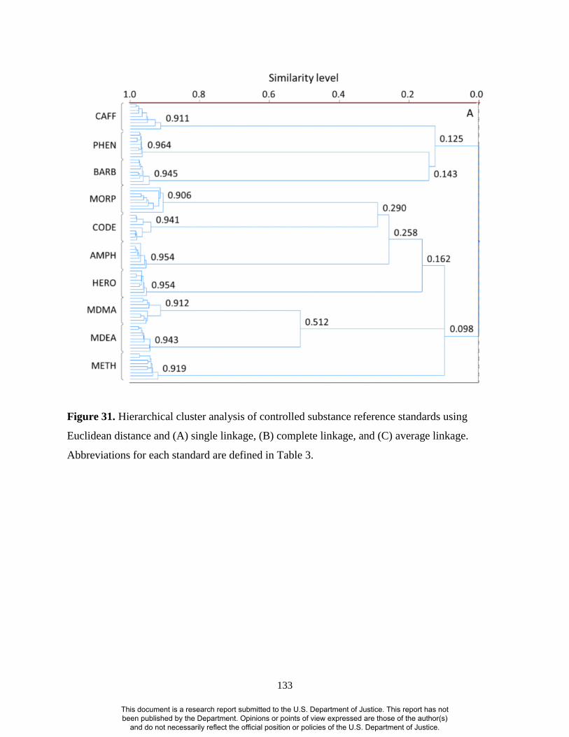
133

Figure 31. Hierarchical cluster analysis of controlled substance reference standards using





134

Figure 31 contd. Hierarchical cluster analysis of controlled substance reference standards using





135

Figure 31 contd. Hierarchical cluster analysis of controlled substance reference standards using





136

However, the similarity level at which amphetamine clusters with morphine and codeine

is relatively low (25.8%, 30.8%, and 30.5% for single, complete, and average linkage methods,

respectively). Due to the similarities in the clusters formed, any of the three linkage methods

could be used in subsequent data analysis. For the purposes of this research, the single linkage

method was again selected as this method is analogous to the k-NN classification method, as

discussed previously.

To investigate association of simulated street samples to the appropriate reference

standards, HCA was repeated including one simulated sample at a time with the reference

standards. All dendrograms are shown in Appendix 6 and a summary of the results is given in

Table 31.

Table 31. Similarity level at which simulated samples cluster with corresponding reference

standard.

Simulated street sample containing Similarity level (%) of cluster formation with

corresponding standard

Amphetamine, 80/20 75.0

Amphetamine, 50/50 45.1

Barbital, 80/20 73.7

Barbital, 50/50 45.4

Codeine, 80/20 51.5

Codeine, 50/50 47.8

MDEA, 80/20 77.6

MDEA, 50/50 53.5

MDMA, 80/20 62.1

MDMA, 50/50 2.3

Methamphetamine, 80/20 58.2

Methamphetamine, 50/50 0.0 80/20 indicates samples containing 80 parts controlled substance and 20 parts caffeine.

50/50 indicates samples containing 50 parts controlled substance and 50 parts caffeine.

Using HCA, association of the 80/20 samples to the respective standard is possible. All

samples form clusters with the standards first, before forming subsequent clusters. Hence,

despite only 51.5% similarity between the 80/20 codeine sample and respective standard, this

sample is most similar to the codeine reference standard than to any other standard in the data

set. A similar general trend is observed for the 50/50 samples: although similarity levels are

around 45%, the simulated samples are most similar to the respective standards than any other

standard or sample in the data set. However, there are notable exceptions to this trend. The 50/50



137

simulated sample containing barbital first clusters with caffeine (at a similarity level of 59.3%)

before clustering with the barbital standard (at a similarity level of 45.4%). Despite first

clustering with the cutting agent, this simulated sample is still most similar to the barbital

standard than to any other reference standard in the data set. The 50/50 samples containing

MDMA and methamphetamine are also both most similar to caffeine (50.0% and 56.5%,

respectively). However, in this instance, these samples first form clusters with other standards

and only cluster to the appropriate standard at very low similarity levels (2.3% and 0.0% for

MDMA and methamphetamine, respectively).


Initially, PCA models were developed for each reference standard; however, when the

optimal number of PCs (1) in each model are maintained, none of the 80/20 simulated samples

are classified at any of the confidence levels investigated (α = 0.25 to 0.001). In each model, the

first principal component accounts for 97-100% of the variance in the data set. As a result, the

models are too specific which prevents classification of the simulated samples. In cases such as

this, the next step would typically be to include more principal components in the models to

better describe data. However, for these data, no advantage is gained in doing this as the

subsequent PCs describe a negligible proportion of the variance.

To more adequately describe the data, simulated samples were included in the PCA

models. Each model therefore contained the appropriate controlled substance reference

standards, caffeine, and four of the nine corresponding simulated samples. Exceptions to this

were the models for codeine and MDEA, for which three simulated samples were included in the

model. All PCA models retained one PC (which accounted for 99.1-99.5% variance), except

codeine for which the optimal number of PCs was three (which accounted for 99.9% variance).

With these models, classification of the 80/20 simulated samples is possible at different

confidence levels, as summarized in Table 32.

With the exception of simulated samples containing codeine and MDEA, classification

ability improves as confidence level increases. However, and as discussed previously, higher

confidence levels are less rigorous with regards to association and hence, the observed trend is not

unexpected. All classified samples are exclusively classified; that is, none are also considered a

member of additional classes, indicating sufficient discrimination among the defined classes.



138

However, for codeine, only one of the two samples is correctly classified while interestingly, no

MDEA samples are classified at any confidence level.

Table 32. Summary of classification of 80/20 simulated samples with inclusion of reference

standards and selected simulated samples in model.

Simulated samples

containing

Samples classified (%) at the following confidence levels

95% 99% 99.9%

Amphetamine, 80/20 80 100 100

Barbital, 80/20 80 80 100

Codeine, 80/20 50 50 50

MDEA, 80/20 0 0 0

MDMA, 80/20 80 80 100

Methamphetamine,

80/20 60 100 100


For each model, four corresponding simulated samples were also included, with the exception of codeine and MDEA,

for which three simulated samples were included.

For classification, five simulated samples were available for each controlled substance, with the exception of codeine,

for which two simulated samples were available, and MDEA, for which three simulated samples were available.

Spectra of the codeine and MDEA simulated samples were overlaid to highlight any

substantial differences among the spectra that may explain the lack of classification. Slight

differences in abundance are apparent, especially in the wavenumber range 1720-1620 cm-1

(shown as inset in Figure 32) which corresponds to absorptions from caffeine. For codeine, the

intensity of these absorptions in the classified sample (sample number 5) is within the range

defined by the samples included in the model (sample numbers 1, 2, and 3). However, sample

number 4, which is not classified, has the lowest absorption intensity, indicating that the codeine

model is too specific such that differences in abundance prevent classification.

For MDEA, the intensity of the absorption in the three simulated samples that are

classified (sample numbers 4, 5, and 6) lies within the range defined by the other three simulated

samples that were included in the model (sample numbers 1, 2, and 3). Hence, the differences in

intensity that are apparent are unlikely to contribute to the lack of classification of the MDEA

simulated samples. However, the lack of classification indicates that the MDEA models is not

sufficiently representative of the data. It should be noted that in models for the other controlled

substances, four simulated samples are included, leaving five samples for classification.



139

Figure 32. Overlay of spectra of simulated samples containing 80 parts MDEA/20 parts caffeine

by mass.

-1.0E+00

0.0E+00

1.0E+00

2.0E+00

3.0E+00

4.0E+00

5.0E+00

6.0E+00

7.0E+00

8.0E+00

9.0E+00

6504000

Wavenumber (cm-1)

80MDEA_1 80MDEA_2 80MDEA_3 80MDEA_4 80MDEA_5 80MDEA_6

No

rmal

ized

Ab

sorb

ance

15001800



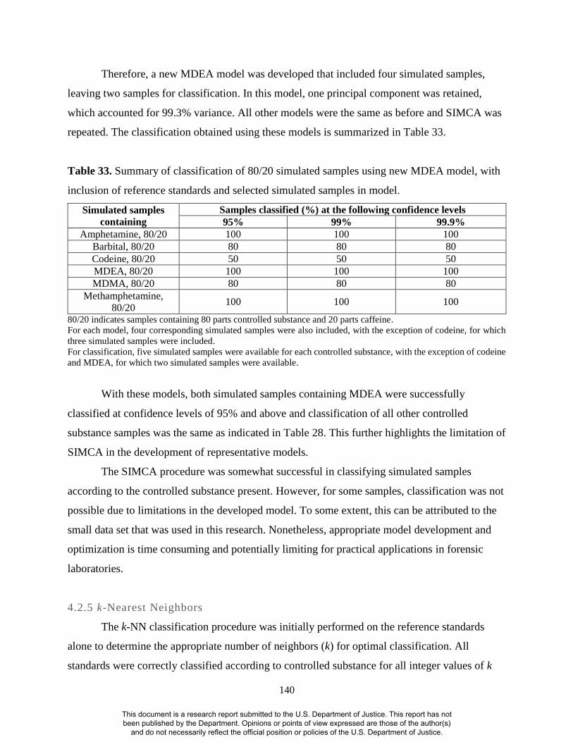
140

Therefore, a new MDEA model was developed that included four simulated samples,

leaving two samples for classification. In this model, one principal component was retained,

which accounted for 99.3% variance. All other models were the same as before and SIMCA was

repeated. The classification obtained using these models is summarized in Table 33.

Table 33. Summary of classification of 80/20 simulated samples using new MDEA model, with

inclusion of reference standards and selected simulated samples in model.

Simulated samples

containing

Samples classified (%) at the following confidence levels

95% 99% 99.9%

Amphetamine, 80/20 100 100 100

Barbital, 80/20 80 80 80

Codeine, 80/20 50 50 50

MDEA, 80/20 100 100 100

MDMA, 80/20 80 80 80

Methamphetamine,

80/20 100 100 100


For each model, four corresponding simulated samples were also included, with the exception of codeine, for which

three simulated samples were included.

For classification, five simulated samples were available for each controlled substance, with the exception of codeine

and MDEA, for which two simulated samples were available.

With these models, both simulated samples containing MDEA were successfully

classified at confidence levels of 95% and above and classification of all other controlled

substance samples was the same as indicated in Table 28. This further highlights the limitation of

SIMCA in the development of representative models.

The SIMCA procedure was somewhat successful in classifying simulated samples

according to the controlled substance present. However, for some samples, classification was not

possible due to limitations in the developed model. To some extent, this can be attributed to the

small data set that was used in this research. Nonetheless, appropriate model development and

optimization is time consuming and potentially limiting for practical applications in forensic

laboratories.


The k-NN classification procedure was initially performed on the reference standards

alone to determine the appropriate number of neighbors (k) for optimal classification. All

standards were correctly classified according to controlled substance for all integer values of k



141

from 1 to 10. Hence, any value k could be used for classification. With k = 5, all 80/20 samples

are correctly classified to the appropriate reference standard, with one exception: one simulated

sample containing codeine is classified as caffeine. Figure 33 shows the spectrum of this

particular simulated sample, along with representative spectra of caffeine and the codeine

reference standard. Absorptions from caffeine (e.g., 1692 cm-1, 1643 cm-1 and the range 1480-

1430 cm-1) dominate the spectrum of this sample, resulting in the misclassification. The

dominance of the caffeine absorptions in this spectrum indicate poor homogeneity of this

simulated sample, most likely a result of inadequate mixing prior to collecting the spectrum.

The 50/50 simulated samples were also classified using the k-NN procedure. However,

due to the increased proportion of cutting agent in these samples, classification is not as

successful as previously, with a total of 38 misclassifications. In each case, the samples are

misclassified as the cutting agent rather than the appropriate controlled substance.



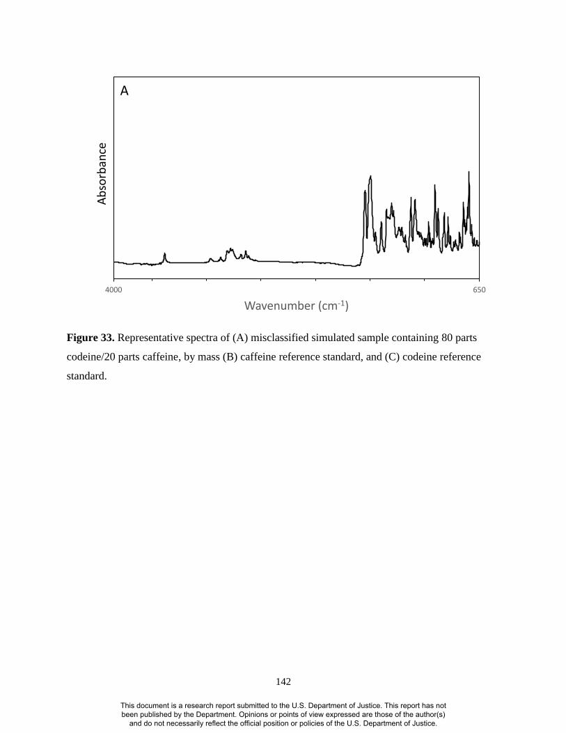
142

Figure 33. Representative spectra of (A) misclassified simulated sample containing 80 parts

codeine/20 parts caffeine, by mass (B) caffeine reference standard, and (C) codeine reference

standard.

-2.0E+00

-2.0E+00

-1.9E+00

-1.9E+00

-1.8E+00

-1.8E+00

6504000

Wavenumber (cm-1)

Ab

sorb

ance

A



143

Figure 33 contd. Representative spectra of (A) misclassified simulated sample containing 80

parts codeine/20 parts caffeine, by mass (B) caffeine reference standard, and (C) codeine

reference standard.

-2.0E+00

-2.0E+00

-1.9E+00

-1.9E+00

-1.8E+00

-1.8E+00

-1.7E+00

-1.7E+00

-1.6E+00

-1.6E+00

-1.5E+00

6504000

Wavenumber (cm-1)

Ab

sorb

ance

B



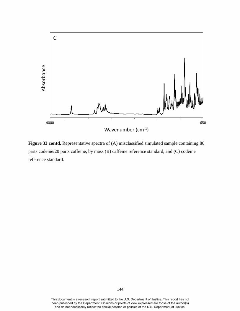
144

Figure 33 contd. Representative spectra of (A) misclassified simulated sample containing 80

parts codeine/20 parts caffeine, by mass (B) caffeine reference standard, and (C) codeine

reference standard.

-2.0E+00

-2.0E+00

-1.9E+00

-1.9E+00

-1.8E+00

-1.8E+00

-1.7E+00

-1.7E+00

-1.6E+00

-1.6E+00

-1.5E+00

6504000

Wavenumber (cm-1)

Ab

sorb

ance

C



145

4.3 Gene Sequence Data

4.3.1 Amplification and Quantification

All samples exhibited strong amplification around 650 basepairs with minor product

occasionally surrounding the brightest band and primer dimer (Figure 34). The exact length of

the region amplified can vary based on the bacteria present in the soils and these minor products

are likely species with either longer or shorter regions. Quantification revealed DNA

concentrations ranging from 19.82 – 24.14 ng/mL with a standard curve R2 value of 0.9982.

Figure 34. PCR amplicons compared against DNA ladder showing strong amplification at the

appropriate size.

4.3.2 Mothur Processing

At the end of processing the sequencing data with the mother software, the number of

sequences in each group ranged from 1843 – 3147 (Table 34) with an average of 2533 sequences

per group. The number of sequences varied because the subsample command in mothur was not

utilized, allowing all the data to be analyzed. Furthermore, the sequences were sorted into 11,853

OTUs at the unique cutoff level for PCA analysis. Mothur clusters sequences at a variety of

cutoffs, or distances, with higher cutoffs sorting less similar sequences into the same OTU. The

unique cutoff level was used as it gave the greatest degree of separation among the sequences.

This cutoff maintains that each OTU has identical sequences, which allows for a direct count of

that clade.



146

Table 34. Unique DNA sequences per soil extract after processing with mother software

Sample Number of unique sequences

Marsh 1 (M1) 2921

Marsh 2 (M2) 3147

Marsh 3 (M3) 2486

Woodlot 1 (W1) 2266

Woodlot 2 (W2) 1843

Woodlot 3 (W3) 2607

Yard 1 (Y1) 2127

Yard 2 (Y2) 2713

Yard 3 (Y3) 2822

Yard Mixture (Ymix) 2424

4.3.3 Bacterial Classification

Sequences were classified with mothur software using the SILVA bacterial reference file,

allowing identification of each OTU. The 11,853 OTUs were first catalogued into 42 class level

taxonomies and the abundance of each is shown in Figure 35. Over 90% of the total bacterial

abundance is found within nine classes for most samples. Further, all of the samples have similar

compositions of the seven most prevalent classes. Therefore, the vast majority of the variability

of taxonomies exists in the last 5 – 10% of the total abundance, and 25 of the 42 classes

identified exist in the remaining 5% of the total abundance (Figure 36). The large number of

relatively rare bacterial classes demonstrates the diversity in each habitat even at low levels, and

has the potential to act as the ‘fingerprint’ region of the data.



147

Figure 35. Bacterial classes found in each sample displayed as a percentage of total number of sequences found in that phylogeny.

0% 10% 20% 30% 40% 50% 60% 70% 80% 90% 100%

M1

M2

M3

W1

W2

W3

Y1

Y2

Y3

Ymix

Abundance

Sam

ple

Actinobacteria

Sphingobacteria

Alphaproteobacteria

Acidobacteria

Betaproteobacteria

Deltaproteobacteria

Gammaproteobacteria

Planctomycetacia

Spartobacteria

Phycisphaerae

Flavobacteria

Bacilli

Holophagae

Clostridia

Anaerolineae

Gemmatimonadetes

Chlamydiae

Nitrospira

Caldilineae

Verrucomicrobiae

Opitutae

Thermomicrobia

Chlorobia

Chloroplast

Fibrobacteria

Bacteroidia

Erysipelotrichi

Mollicutes

Thermodesulfobacteria

Thermales

Acidimethylosilex

Chrysiogenetes

Spirochaetes

Chloroflexi

Acaryochloris

Synergistia

Brasilonema

Deferribacteres

Deinococcales

Fusobacteria

Lentisphaeria

Epsilonproteobacteria



148

Figure 36. Subset of bacterial classes found in each sample displayed as a percentage of total number of sequences found in that

phylogeny. These classes account for less than 5% of the total abundance shown in Figure 35.

0% 10% 20% 30% 40% 50% 60% 70% 80% 90% 100%

M1

M2

M3

W1

W2

W3

Y1

Y2

Y3

Ymix

Abundance

Sam

ple

Nitrospira

Caldilineae

Verrucomicrobiae

Opitutae

Thermomicrobia

Chlorobia

Chloroplast

Fibrobacteria

Bacteroidia

Erysipelotrichi

Mollicutes

Thermodesulfobacteria

Thermales

Acidimethylosilex

Chrysiogenetes

Spirochaetes

Chloroflexi

Acaryochloris

Synergistia

Brasilonema

Deferribacteres

Deinococcales

Fusobacteria

Lentisphaeria

Epsilonproteobacteria



149


PCA was performed on the sequence data segregated into OTUs. The scores plot for the

first two principal components, which account for 55% of the variance in the data set, is shown

in Figure 37. Samples from different habitats are readily distinguished in the scores plot;

however, there is some spread among replicates of each sample type. This is due to the

nonparametric nature of these data, as well as the variable number of sequences in each OTU.

The corresponding loadings plot is shown in Figure 38, in which OTUs that contribute

most to the variance in the data set are labeled. It should be noted that the majority of OTUs are

positioned close to the origin, indicating that they contribute little to the variance. These OTUs

generally only contain a few sequences with a majority containing only a single sequence. These

singular sequences could result from sequencing error and belong to a larger group of sequences

in a different OTU or be a rare sequence identifying a unique species in each habitat.

Generally OTUs with the greatest number of sequences contribute the most to the

variance among samples, with the majority of sequences for that OTU found in one or two of the

habitats sampled (Table 35). The marsh samples tend to have high levels of sequences in OTUs

in which the yard and woodlot samples have few or no sequences (e.g., OTUs 13, 40, 70, and

119) and vice versa. This variation in sequences indicates a microbiota difference between the

marsh samples and the woodlot and yard sites. Additionally, while some sequences (e.g., OTUs

1, 3, 6, 8, and 11) occur in both the woodlot and yard samples, there are also some instances

where sequences exist in one or other of these habitats. For the OTUs where both habitats

contain sequences, the number of sequences varies from being similar (e.g., OTUs 1, 3, and 8) to

being very different.



150

Figure 37. Scores plot of PC1 versus PC2 for gene sequence data from samples collected from

three different habitats: marsh (M), woodlot (W), and yard (Y).

PC

2 (

16

.2%

)

PC1 (38.9%)

M1 M2 M3 W1 W2 W3 Y1 Y2 Y3 Ymix



151

Figure 38. Loadings plot of PC1 versus PC2 for gene sequence data from samples collected

from three different habitats. Each data point represents a different OTU that contains identical

sequences. OTUs contributing most to the variance are labeled.

PC

2 (

16

.2%

)

PC1 (38.9%)

OTU 4

OTU 8 OTU 3

OTU 70

OTU 40

OTU 13

OTU 119

OTU 89OTU 6

OTU 17

OTU 28OTU 11

OTU 1



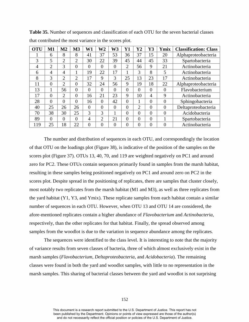
152

Table 35. Number of sequences and classification of each OTU for the seven bacterial classes

that contributed the most variance in the scores plot.

OTU M1 M2 M3 W1 W2 W3 Y1 Y2 Y3 Ymix Classification: Class

1 6 8 8 41 37 53 36 37 15 20 Alphaproteobacteria

3 5 2 2 30 22 39 45 44 45 33 Spartobacteria

4 2 3 0 0 0 0 2 56 9 21 Actinobacteria

6 4 4 1 19 22 17 1 3 8 5 Actinobacteria

8 3 2 2 17 9 3 25 13 23 17 Actinobacteria

11 0 2 0 32 24 56 9 19 18 22 Alphaproteobacteria

13 1 56 0 0 0 0 0 0 0 0 Flavobacterium

17 0 2 0 16 21 23 9 10 4 9 Actinobacteria

28 0 0 0 16 0 42 0 1 0 0 Sphingobacteria

40 25 26 26 0 0 0 0 2 0 0 Deltaproteobacteria

70 38 30 25 3 3 1 0 0 0 0 Acidobacteria

89 0 0 0 4 2 21 0 0 0 1 Spartobacteria

119 25 18 22 0 0 0 0 0 0 0 Actinobacteria

The number and distribution of sequences in each OTU, and correspondingly the location

of that OTU on the loadings plot (Figure 38), is indicative of the position of the samples on the

scores plot (Figure 37). OTUs 13, 40, 70, and 119 are weighted negatively on PC1 and around

zero for PC2. These OTUs contain sequences primarily found in samples from the marsh habitat,

resulting in these samples being positioned negatively on PC1 and around zero on PC2 in the

scores plot. Despite spread in the positioning of replicates, there are samples that cluster closely,

most notably two replicates from the marsh habitat (M1 and M3), as well as three replicates from

the yard habitat (Y1, Y3, and Ymix). These replicate samples from each habitat contain a similar

number of sequences in each OTU. However, when OTU 13 and OTU 14 are considered, the

afore-mentioned replicates contain a higher abundance of Flavobacterium and Actinobacteria,

respectively, than the other replicates for that habitat. Finally, the spread observed among

samples from the woodlot is due to the variation in sequence abundance among the replicates.

The sequences were identified to the class level. It is interesting to note that the majority

of variance results from seven classes of bacteria, three of which almost exclusively exist in the

marsh samples (Flavobacterium, Deltaproteobacteria, and Acidobacteria). The remaining

classes were found in both the yard and woodlot samples, with little to no representation in the

marsh samples. This sharing of bacterial classes between the yard and woodlot is not surprising



153

as they are only separated on PC2 (Figure 37) and are much more similar to each other than to

the marsh samples.

As previously mentioned, these data do not meet the data linearity assumption PCA

requires. The spread of the data points on the scores plot among replicate samples is evidence of

this. Despite this, the three habitats can be satisfactorily distinguished from each other, although

more appropriate and informative statistics may be available using a statistical procedure that

does not make any assumptions regarding the linearity of the data.

4.3.5 Nonmetric Multidimensional Scaling

Two 10 x 10 square matrices of pairwise comparisons were used as the starting point for

NMDS analysis generated by the BCDI or SDC algorithms using the mother software. The stress

plots of comparative stresses (Figure 39, and Appendix 7A) diagram the change in stress as

dimensionality increases. For both indices, a single dimension plot fails to meet the requirements

of the stress null hypothesis and is considered random noise; however, for dimensions greater

than one, the stress for each NMDS plot is below random stress and is accepted as accurately

fitting the data.65 The ‘elbow’ in the stress plot at two dimensions indicates that the NMDS

configuration can be interpreted in two dimensions with minimal additional information gained

as the number of dimensions increases. Furthermore, the extremely low stress at two dimensions

(3.634x10-4 and 5.197x10-4 in Figure 39 and in Appendix 7A respectively) supports an accurate

portrayal of these data in the NMDS plot.



154

Figure 39. Plot of Kruskal’s stress (red line) vs. Spence’s random stress (black line) for Bray-

Curtis dissimilarity data across four dimensions.

0

0.6

1 2 3 4

Raw

Str

ess

Dimensions

Random Stress Kruskal's Stress



155

The Shepard diagrams (Figure 40 and Appendix 7B) demonstrate a very high correlation

between disparity and distance, indicating an accurate representation of these data in the NMDS

plots. For NMDS, the rank-order between the disparities and proximities must be maintained and

are plotted in a monotonic function, positively if the inputted distances are dissimilarities.62 The

staircase shape of the function in the Shepard diagrams is typical of NMDS.

Soil extracts from each habitat were analyzed on a two dimensional NMDS plot (Figure

41 and Appendix 7C) with standard error bars applied. Both BCDI and SDC show complete

separation of the three habitats, with clustering of replicate samples within standard error. The

clusters of replicate samples appear to dissociate from each other equidistantly. The tight

clustering of replicate samples in the final configurations is expected based on analysis of the

stress plots and Shepard diagrams. As mentioned previously, the low stress and high correlation

of distances to disparities provides confidence that the NMDS plot is accurately representing the

data.

These results show that multidimensional scaling is capable of modeling complex

nonparametric data. This is evident from the NMDS plots and low stress associated with them.

The replicate samples for each site cluster closely and within standard error, with all three

habitats differentiated for both diversity indices. Of the two procedures, NMDS is more powerful

than PCA for describing these data and is the more appropriate statistical procedure for soil

analysis.



156

Figure 40. Shepard diagram plotting Bray-Curtis dissimilarities against the disparities/distances

observed on the nonmetric multidimensional scaling (NMDS) plot. This strong correlation

between the two indicates that NMDS has represented the rank-order of these data accurately.

0.0

1.4

0.0 0.2 0.4 0.6 0.8 1.0

Dis

par

ity/

Dis

tan

ce

Dissimilarity

Disparities Distances



157

Figure 41. Nonmetric multidimensional scaling plot of ten samples in two dimensions with

standard error bars for Bray-Curtis Index.

M1

M2M3

W1

W2 W3

Y1

Y2Y3

Ymix

Dim

ensi

on

2

Dimension 1



158

5. Conclusions

5.1 Summary of Findings

The purpose of this research was to investigate the utility of multivariate statistical

procedures, specifically for forensic applications. While similar procedures are commonly used

in different scientific disciplines, they are not widely used in forensic science. Therefore, this

research aimed to further investigate the application of multivariate statistical procedures for

forensic evidence comparisons to highlight both the potential of these procedures and the

challenges associated with their implementation.

The first part of the research involved generating data sets to which the statistical

procedures would subsequently be applied. Three different data sets were generated, each

corresponding to different evidence types commonly generated by forensic laboratories. The

chromatographic data set was composed of ignitable liquid reference standards and simulated

fire debris samples that were prepared using different household substrates. This data set was

chemically diverse and complex in nature, containing over 3,500 variables. The spectral data set

was composed of controlled substance reference standards along with simulated street samples

containing controlled substances cut with caffeine. Although this data set contained a similar

number of variables (3,350 variables) as the chromatographic data set, the spectral data was less

complex in nature. Finally, the biological data set was composed of soil bacteria sequence data

from different habitat types. These data contained discrete variables, rather than the continuous

variables that were present in the chromatographic and spectral data sets. Thus, the data sets in

this work not only represented common types of data generated in forensic laboratories, they also

ranged in complexity and included both continuous and discrete variables.

Chemical data sets were subjected to pretreatment procedures prior to data analysis. Such

procedures are used to minimize or eliminate sources of variance that result from instrumental

factors rather than from the samples themselves. It is important that these sources of variance are

reduced before data analysis otherwise differences identified among samples will be a remnant

of the analytical procedure rather than truly chemical in nature. For the chromatographic data,

several pretreatment procedures were applied with normalization offering the greatest effect on

improving replicate precision. For the spectral data, the commonly applied SNV normalization

procedure was deemed optimal when compared to two other normalization procedures.



159

However, for the more chemically diverse chromatographic data, no one normalization

procedure universally improved precision of all replicates.

Exploratory procedures were then investigated with the aim of associating the simulated

chemical samples to the corresponding reference standard. Pearson product-moment correlation

(PPMC) coefficients provide a single number that represents the correlation between two

complex samples, which can simplify comparisons. While a single number representing the

comparison of complex data containing thousands of variables is advantageous, the use of PPMC

coefficients for this particular application is limited for a number of reasons. First, coefficients

are calculated on a pairwise basis and hence, the number of coefficients calculated for a given

data set increases with the square of the number of samples. Depending on the size of the data set

under consideration, this can make the comparison of a large data set time-consuming. Second,

the coefficient is calculated on a point-by-point basis for the two samples being compared. This

means that peaks present in one sample but not the other (as is the case for the simulated samples

and reference standards considered here) will result in a lower coefficient. And third, the range

of coefficients representing each correlation strength is relatively wide (e.g., any coefficient in

the range ±0.8-1 indicates strong correlation).

The chromatographic and spectral data sets were further analyzed using principal

components analysis (PCA) and hierarchical cluster analysis (HCA), both of which offer several

advantages over PPMC coefficients. Firstly, neither are limited to pairwise comparisons of

samples; instead, all samples are considered simultaneously which makes analysis of a large data

set substantially less time consuming. In contrast to PPMC coefficients, these procedures also

provide a graphical representation of the similarities and differences in the data set in the form of

the scores plot in PCA and the dendrogram in HCA.

Principal components analysis is used to identify sources of variance in a data set while

HCA measures similarity among samples in the data set. However, it is important to note that

despite this apparent difference in operation, both procedures are based on distance

measurements among samples in multidimensional space. In PCA, though, typically only the

first few dimensions (which account for the greatest variance) are retained and examined in the

scores plots. In contrast, the dendrogram generated in HCA retains all dimensions rather than a

select few. As a result, in this research, there was greater success in associating simulated

samples to reference standards using HCA.



160

Nonetheless, PCA does offer an advantage in that the variables contributing to the

association and differentiation in the data set can be identified through interrogation of the

loadings plots. However, interpretation of the PCA scores plot is based on visual assessment and

therefore, without additional evaluation metrics (such as Euclidean distance measurements or

PPMC coefficients calculated using the principal component eigenvectors), it could be argued

that there is some subjectivity in interpretation. In contrast, while HCA does not identify the

variables contributing to the clustering, a numerical measure of the degree of association is

inherent in the procedure.

Finally for the chemical data, the use of classification procedures was investigated, with

the aim of classifying the simulated samples according to the appropriate reference standard with

statistical confidence. Two such procedures were investigated: soft independent modeling of

class analogy (SIMCA) and k-nearest neighbors (k-NN). These two procedures were selected for

this initial investigation due to their relationship with the exploratory procedures previously

investigated. That is, classification using SIMCA is based on the development of PCA models

while k-NN is analogous to HCA.

Despite both procedures affording classification, again there are inherent differences in

the manner in which the classification is performed. For SIMCA, classification is based on PCA

models that are developed for pre-defined groups in the data set, which in this research meant

performing PCA on the reference standards. However, the development of representative models

is challenging. For both the chromatographic and spectral data sets, classification of the

simulated samples was not possible when models were developed using only the reference

standards. This is mainly because the models did not account for the substrate or cutting agent

(for the chromatographic and spectral data sets, respectively). Limited classification was possible

when simulated samples were included in the model; however, the models were now so specific

that misclassifications arising from differences in abundance were apparent.

In contrast, the k-NN procedure is not based on true model development. Instead, for

each classification to be performed, the reference standards and samples are re-subjected to the

k-NN procedure. Samples are classified with the reference standards to which they are positioned

most closely in the multidimensional space. While a perceived limitation is the forced

classification of samples, the success rate of k-NN in this research was greater than for SIMCA.



161

This was attributed to the nature of operation in that classification is based on similarity of the

sample to the set of reference standards rather than model development.

The gene sequence data were also subjected to data pretreatment to remove artificial

sources of variation. For these data, erroneous and repetitive sequences were removed prior to

statistical analysis using PCA and nonmetric multidimensional scaling (NMDS). Like PCA and

HCA, NMDS reduces the complexity of the data, in this case over 100,000 sequences, into two

or three dimensions. NMDS has advantages over PCA and HCA in that it is designed to

accurately represent nonparametric data. However, NMDS is limited in its capability to identify

the variables that are responsible for the variation observed in the final configuration of the data.

Though NMDS is wanting in this respect, association of biological replicates was improved

using this procedure compared to PCA. Although distinction of soil habitats was also possible

using PCA, the natural variability within the bacterial populations hindered PCA from closely

associating replicate samples together. All in all, NMDS was the more appropriate procedure to

distinguish soil from the three different habitats, while closely associating the replicate samples.

5.2 Implications for policy and practice

This research indicates potential for the application of multivariate statistical procedures

in the comparison of forensic evidence. It should be emphasized though that these procedures are

not intended to replace analysts; instead, the statistical procedures should be viewed as an

additional tool available to aid analysts in their comparisons. For the relatively small data sets

considered here, greater success in association and classification of simulated samples was

achieved using HCA and k-NN, indicating that these two procedures are worthy of further

investigation, using larger data sets and incorporating real case samples rather than laboratory-

simulated samples. For data that are nonparametric in nature, NMDS offers a suitable alternative

to PCA as an exploratory procedure.

While further investigation is warranted, many challenges remain before such procedures

could be routinely implemented in a forensic laboratory setting. Firstly, this research has

demonstrated the need for data pretreatment procedures. At the same time, it also demonstrated

that the actual procedures applied are not only dependent on the type of data in question, but also

must be optimized for each data set. This poses some limitations for forensic laboratories as



162

optimization lengthens the time necessary for analysis and comparison of evidence and the final

selection of the procedures applied can be subjective.

In terms of application of statistical procedures, there are again a number of

considerations. Replicate measurements of samples and standards are necessary for statistical

soundness although this may not be viable in forensic laboratories due to caseloads and sample

backlogs. Application of the statistical procedures will also require substantial investment by the

laboratory in the form of both hardware and software. Higher-end computers that are dedicated

to statistical analysis, rather than also controlling instruments, are desirable. And, after

purchasing the software package, there are costs associated with license renewals and technical

support. Additional investment is also necessary to provide analysts with sufficient training for

the implementation and interpretation of these procedures. Given the limited operating budgets

most forensic laboratories are faced with, equipping the laboratory with such hardware and

software is unlikely to be prioritized.

Presenting the results of these procedures in court yields additional challenges. Statistical

procedures are often considered to be objective in nature; however, there is some degree of

subjectivity in the selection of analysis parameters. For example, how many principal

components should be considered in PCA? Which linkage and distance measurements should be

used in HCA? How does the sample classification change if the SIMCA models are modified?

How does the sample classification change if the number of nearest neighbors in the k-NN

procedure is altered? How does the abundance estimator affect clustering in NMDS? While these

questions can be answered, the answers depend on the data set in question again, necessitating

additional steps and investigations during the analysis.

5.3 Future work

This research has generated three very rich data sets that will continue to be investigated

and disseminated. For the chromatographic data, only the total ion chromatograms were used as

the first stage in the statistical assessment. However, for each reference standard and simulated

sample, extracted ion profiles of characteristic compound classes can be generated from the data

that have already been collected. The next step in the continued investigation of statistical

procedures will be to examine the effect of using extracted ion profiles rather than the total ion

chromatogram for the association and classification of simulated fire debris samples.



163

As discussed previously, the two exploratory procedures considered are related in their

mode of operation (based on distance measurements in the multidimensional space).

Additionally, the classification procedures investigated can be considered an extension of the

exploratory procedures. These relationships will be further investigated following the expansion

of the chromatographic and spectral data sets through analysis of additional samples. According

to the success of these investigations, contact will be made with the Michigan State Police

Forensic Science Division in an attempt to procure similar chromatographic and spectral data

from case samples to further investigate the statistical procedures.

The gene sequence data will continue to be investigated both through addition of new

habitats, and with additional multivariate statistical procedures. As discussed earlier, a multitude

of statistics have been used to analyze this type of data. Those commonly found within the

literature (e.g., NMDS, PCA, and HCA), as well as additional procedures that allow statistical

classification will be investigated. Applying several statistical procedures to the sequence data

will enable a more thorough understanding of the relationships among the three habitats, as well

as a measure of the probative value of each statistical procedure.

In addition to the three manuscripts that are expected from this work (section 7.2), two

tutorials that demonstrate the application of selected procedures are in preparation. The first

tutorial focuses on chromatographic data while the second focuses on spectral data. Both present

relevant statistical theory, as well as interpretation of the results. Graduate students in the

Forensic Science Program at Michigan State University are currently working through the

tutorials to identify and correct deficiencies. Once complete, these tutorials will be disseminated

via a link on the Forensic Chemistry website (www.forchem.msu.edu). As our research in this

area continues, additional tutorials will be prepared and disseminated in a similar manner.



http://www.forchem.msu.edu/

164

6. References

1. Strengthening Forensic Science in the United States: A Path Forward. The National

Academies Press: Washington DC, 2009.

2. Curran, J. M. Is forensic science the last bastion of resistance against statistics? Science &

Justice 2013, 53 (3), 251-252.

3. Morgan, S. L.; Bartick, E. G., Discrimination of forensic analytical chemical data using

multivariate statistics. In Forensic analysis on the cutting edge, Blackledge, R. D., Ed.;

John Wiley & Sons, Ltd.: Hoboken, NJ, 2007; pp. 333-74.

4. Brereton, R. G. Chemometrics. Applications of Mathematics and Statistics to Laboratory

Systems. Ellis Horwood: Chichester, 1990.

5. Sandercock, P. M. L.; Du Pasquier, E. Chemical fingerprinting of unevaporated automotive

gasoline samples. Forensic Science International 2003, 134, 1-10.

6. Sandercock, P. M. L.; Du Pasquier, E. Chemical fingerprinting of gasoline 2. Comparison

of unevaporated and evaporated automotive gasoline samples. Forensic Science

International 2004, 140, 43-59.

7. Tan, B.; Hardy, J. K.; Snavely, R. E. Accelerant classification by gas chromatography/mass

spectrometry and multivariate pattern recognition. Analytica Chimica Acta 2000, 422, 37-

46.

8. Baerncopf, J. M.; McGuffin, V. L.; Waddell Smith, R. Association of ignitable liquid

residues to neat ignitable liquids in the presence of matrix interferences using chemometric

procedures. Journal of Forensic Sciences 2011, 56 (1), 70-81.

9. Prather, K. R.; McGuffin, V. L.; Waddell Smith, R. Effect of evaporation and matrix

interferences on the association of simulated ignitable liquid residues to the corresponding

liquid standard. Forensic Science International 2012, 222 (1-3), 242-251.

10. Turner, D. A.; Goodpaster, J. V. The effects of season and soil type on microbial

degradation of gasoline residues from incendiary devices. Analytical and Bioanalytical

Chemistry 2013, 405 (5), 1593-1599.

11. Waddell, E. E.; Song, E. T.; Rinke, C. N.; Williams, M. R.; Sigman, M. E. Progress toward

the determination of correct classification rates in fire debris analysis. Journal of Forensic

Sciences 2013, 58 (4), 887-896.

12. Klemenc, S. In common batch searching of illicit heroin samples - evaluation of data by

chemometrics methods. Forensic Science International 2001, 115 (1-2), 43-52.

13. Chan, K. W.; Tan, G. H.; Wong, R. C. S. Investigation of trace inorganic elements in street

doses of heroin. Science & Justice 2013, 53 (1), 73-80.

14. Weyermann, C.; Marquis, R.; Delaporte, C.; Esseiva, P.; Lock, E.; Aalberg, L. et al. Drug

intelligence based on MDMA tablets data I. Organic impurities profiling. Forensic Science

International 2008, 177, 11-16.

15. Willard, M. A. B.; McGuffin, V. L.; Waddell Smith, R. Forensic analysis of Salvia

divinorum using multivariate statistical procedures. Part I: discrimination from related

Salvia species. Analytical and Bioanalytical Chemistry 2012, 402 (2), 833-842.

16. Willard, M. A. B.; McGuffin, V. L.; Waddell Smith, R. Forensic analysis of Salvia

divinorum using multivariate statistical procedures. Part II: association of adulterated

samples to S. divinorum. Analytical and Bioanalytical Chemistry 2012, 402 (2), 843-850.

17. NicDaeid, N.; Waddell, R. J. H. The analytical and chemoemtric procedures used to profile

illicit drug seizures. Talanta 2005, 67, 280-5.



165

18. Trosvik, P.; Skanseng, B.; Jakobsen, K. S.; Stenseth, N. C.; Naes, T.; Rudi, K. Multivariate

analysis of complex DNA sequence electropherograms for high-throughput quantitative

analysis of mixed microbial populations. Applied and Environmental Microbiology 2007,

73 (15), 4975-4983.

19. Abdo, Z.; Schuette, U. M. E.; Bent, S. J.; Williams, C. J.; Forney, L. J.; Joyce, P. Statistical

methods for characterizing diversity of microbial communities by analysis of terminal

restriction fragment length polymorphisms of 16S rRNA genes. Environmental

Microbiology 2006, 8 (5), 929-938.

20. Lenz, E. J.; Foran, D. R., Bacterial profiling of soil using genus-specific markers and

multidimensional scaling. Journal of Forensic Sciences 2010, 55 (6), 1437-1442.

21. Hedman, J.; Nordgaard, A.; Rasmusson, B.; Ansell, R.; Radstrom, P. Improved forensic

DNA analysis through the use of alternative DNA polymerases and statistical modeling of

DNA profiles. Biotechniques 2009, 47 (5), 951-958.

22. Krane, D. E.; Bahn, V.; Balding, D.; Barlow, B.; Cash, H.; Desportes, B. L. et al. Time for

DNA disclosure. Science 2009, 326 (5960), 1631-1632.

23. Grayston S. J.; Wang S.; Cambell C. D.; Edwards A. C. Selective influence of plant species

on microbial diversity in the rhizoshpere. Soil Biology and Biochemistry 1998, 30, 369-

378.

24. Marschner, P.; Yang, C.; Lieberei, R.; Crowley, D. E. Soil and plant specific effects on

bacterial community composition in the rhizosphere. Soil Biology and Biochemistry 2001,

33, 1437-14445.

25. Boon, N.; Windt, W. D.; Verstaete, W.; Top, E. M. Evaluation of nested PCR-DGGE

(denaturing gradient gel electrophoresis) with group-specific 16S rRNA primers for the

analysis of bacterial communities from different wastewater treatment plants. FEMS

Microbiology Ecology 2002, 39, 101-112.

26. Fantroussi, S. E.; Verschuere, L.; Verstraete, W.; Top, E. M. Effect of phenylurea

herbicides on soil microbial communities estimated by analysis of 16S rRNA gene

fingerprints and community-level physiological profiles. Applied and Environmental

Microbiology 1999, 65, 982-988.

27. Lengendre, P.; Lengendre, L. Numerical ecology. Elsevier: Oxford, England, 2012.

28. Dollhopf, S. I.; Hashsham, S. A.; Tiedje, J. M. Interpreting 16S rDNA T-RFLP data:

Application of self-organizing maps and principal component analysis to describe

community dynamics and convergence. Microbiology Ecology 2001, 42, 495-505.

29. Girvan, M. S.; Bullimore, J.; Pretty, J. N.; Osborn, A. M.; Ball, A. S. Soil type is the

primary determinant of the composition of the total active bacterial communities in arable

soils. Applied and Environmental Microbiology 2003, 69, 1800-1809.

30. McCaig, A. E.; Glover, L. A.; Prosser, J. I. Numerical analysis of grassland bacterial

community structure under different land management regimens by using 16S ribosomal

DNA sequence data and denaturing gradient gel electrophoresis banding patterns. Applied

and Environmental Microbiology 2001, 67, 4554-4559.

31. Fierer, N.; Jackson, R. B. The diversity and biogeography of soil bacterial communities.

Proceedings of the National Academy of Sciences 2006, 103, 626-631.

32. Nagy, M. L.; Pérez, A.; Garcia-Pichel, F. The prokaryotic diversity of biological soil crusts

in the Sonoran Desert (Organ Pipe Cactus National Monument, AZ). FEMS Microbiology

Ecology 2004, 54, 233-245.



166

33. Philippot, L.; Bru, D.; Saby, N. P. A.; Čuhel, J.; Arrouays, D.; Šimek, M. et al. Spatial

patterns of bacterial taxa in nature reflect ecological traits of deep branches of the 16S

rRNA bacterial tree. Environmental Microbiology 2009, 11, 3096-3104.

34. Hughes, J. B.; Hellmann, J. J.; Ricketts, T. H. Counting the uncountable: Statistical

approaches to estimating microbial diversity. Applied and Environmental Microbiology

2001, 67, 4399-4406.

35. Roesch, L. F. W.; Fulthorpe, R. R.; Riva, A.; Casella, F.; Hawdin, A. K. M.; Kent, A. D.

et al. Pyrosequencing enumerates and contrasts soil microbial diversity. ISME Journal

2007, 1, 283-290.

36. Gans, J.; Wolinsky, M.; Dunbar, J. Computational improvements reveal great bacterial

diversity and high metal toxicity in soil. Science 2005, 309, 1387-1390.

37. Chu, H.; Fierer, N.; Lauber, C. L.; Caporaso, J. G.; Knight, R.; Grogan, P. Soil bacterial

diversity in the arctic is not fundamentally different from that found other biomes.

Environmental microbiology 2010, 12, 2998-3006.

38. Dunbar, J.; Barns, S. M.; Ticknor, L. O. Emperical and theoretical bacterial diversity in

four Arizona soils. Applied and Environmental Microbiology 2002, 68, 3035-3045.

39. Lauber, C. L.; Hamady, M.; Knight, R.; Fierer, N. Pyrosequencing-based assessment of

soil pH as a predictor of soil bacterial community structure at the continental scale. Applied

and Environmental Microbiology 2009, 75, 5111-5120.

40. Meyers, M. S.; Foran, D. R. Spatial and temporal influences on bacterial profiling of soil

samples. Journal of Forensic Sciences 2008, 53, 652-660.

41. Petraco, N. D. K.; Gambino, C.; Kubic, T. A.; Olivio, D.; Petraco, N. Statistical

discrimination of footwear: A method for the comparison of accidentals on shoe outsoles

inspired by facial recognition techniques. Journal of Forensic Sciences 2010, 55 (1), 34-

41.

42. Sheets, H. D.; Gross, S.; Langenburg, G.; Bush, P. J.; Bush, M. A. Shape measurement

tools in footwear analysis: A statistical investigation of accidental characteristics over time.

Forensic Science International 2013, 232 (1-3), 84-91.

43. Petraco, N. D. K.; Shenkin, P.; Speir, J.; Diaczuk, P.; Pizzola, P. A.; Gambino, C.; Petraco,

N. Addressing the National Academy of Sciences' challenge: A method for statistical

pattern comparison of striated tool marks. Journal of Forensic Sciences 2012, 57 (4), 900-

911.

44. Chumbley, L. S.; Morris, M. D.; Kreiser, M. J.; Fisher, C.; Craft, J.; Genalo, L. J. et al.

Validation of tool mark comparisons obtained using a quantitative, comparative, statistical

algorithm. Journal of Forensic Sciences 2010, 55 (4), 953-961.

45. Gerules, G.; Bhatia, S. K.; Jackson, D. E. A survey of image processing techniques and

statistics for ballistic specimens in forensic science. Science & Justice 2013, 53 (2), 236-

250.

46. Egan, W. J.; Morgan, S. L.; Bartick, E. G.; Merrill, R. A.; Taylor, H. J. Forensic

discrimination of photocopy and printer toners. II. Discriminant analysis applied to infrared

reflection-absorption spectroscopy. Analytical and Bioanalytical Chemistry 2003, 376 (8),

1279-1285.

47. Egan, W. J.; Galipo, R. C.; Kochanowski, B. K.; Morgan, S. L.; Bartick, E. G.; Miller, M.

L. et al. Forensic discrimination of photocopy and printer toners. III. Multivariate statistics

applied to scanning electron microscopy and pyrolysis gas chromatography/mass

spectrometry. Analytical and Bioanalytical Chemistry 2003, 376 (8), 1286-1297.



167

48. Thanasoulias, N. C.; Parisis, N. A.; Evmiridis, N. P. Multivariate chemometrics for the

forensic discrimination of blue ball-point pen inks based on their vis spectra. Forensic

Science International 2003, 138 (1-3), 75-84.

49. Savitzky, A.; Golay, M. J. E. Smoothing + differentiation of data by simplified least

squares procedures. Analytical Chemistry 1964, 36 (8), 1627-&.

50. Barak, P. Smoothing and differentiation by an adaptive-degree polynomial filter.

Analytical Chemistry 1995, 67 (17), 2758-2762.

51. Gorry, P. A. General least-squares smoothing and differentiation by the convolution

(Savitzky-Golay) method. Analytical Chemistry 1990, 62 (6), 570-573.

52. Johnson, K. J.; Wright, B. W.; Jarman, K. H.; Synovec, R. E. High-speed peak matching

algorithm for retention time alignment of gas chromatographic data for chemometric

analysis. Journal of Chromatography A 2003, 996, 141-155.

53. Nielsen, N. P. V.; Carstensen, J. M.; Smedsgaard, J. Aligning of single and multiple

wavelength chromatographic profiles for chemometric data analysis using correlation

optimised warping. Journal of Chromatography A 1998, 805 (1-2), 17-35.

54. Tomasi, G.; van den Berg, F.; Andersson, C. Correlation optimized warping and dynamic

time warping as preprocessing methods for chromatographic data. Journal of

Chemometrics 2004, 18, 231-241.

55. Varmuza, K.; Filzmoser, P. Introduction to multivariate statistical analysis in

chemometrics. CRC Press: Boca Raton, FL, 2009.

56. Moreda-Pineiro, A.; Marcos, A.; Fisher, A.; Hill, S. J. Evaluation of the effect of data pre-

treatment procedures on classical pattern recognition and principal components analysis:

A case study for the geographical classification of tea. Journal of Environmental

Monitoring 2001, 3 (4), 352-360.

57. van den Berg, R. A.; Hoefsloot, H. C. J.; Westerhuis, J. A.; Smilde, A. K.; van der Werf,

M. J. Centering, scaling, and transformations: improving the biological information content

of metabolomics data. Bmc Genomics 2006, 7.

58. Miller, C. E. Chemometrics in Process Analytical Technology (PAT). In Process

Analytical Technology: Spectroscopic Tools and Implementation Strategies for the

Chemical and Pharmaceutical Industries; Bakeev, K. A., Ed. John Wiley & Sons, Ltd.:

Chichester, England, 2010; p 372.

59. Devore, J. L. Probability and statistics for engineering and the sciences. 3rd Ed.; Duxbury

Press: Belmont, CA, 1991.

60. Miller, J. N.; Miller, J. C. Statistics and chemometrics for analytical chemistry. Pearson

Prentice Hall: Harlow, England, 2000.

61. Brereton, R. G. Applied chemometrics for scientists. Wiley: Hoboken, New Jersey, 2007.

62. Borg, I.; Groenen, P. J. F. Modern multidimensional scaling: Theory and applications.

Springer: New York., 2005.

63. Cox, T. F. Multidimensional scaling. Chapman & Hall: Boca Raton, Florida, 2001.

64. Kruskal, J. B. Multidimensional scaling by optimizing goodness of fit to a nonmentric

hypothesis. Psychometrika 1964, 29, 1-27.

65. Spence, I. A simple approximation for random rankings stress values. Multivariate

Behavioral Research 1979, 14, 355-365.

66. Whittaker, R. H. Vegetation of the Siskiyou mountains, Oregon and California. Ecological

Monographs 1960, 30, 279-338.



168

67. Bray, J. R.; Curtis, J. T. An ordination of the upland forest communities of southern

Wisconsin. Ecological Monographs 1957, 4, 325-349.

68. Sørensen, T. A method of establishing groups of equal amplitude in plant sociology base

on similarity of species and its application to analyses of the vegetation on Danish common.

Biologiske Skrifter. K. Danske videnskabernes Selskab, 1948, 5, 1-34.

69. Dice, L. R. Measures of the amount of ecologic association between species. Ecology 1945,

26, 297-302.

70. Lavine, B. K. Signal Processing and Data Analysis. In Practical Guide to Chemometrics;

Haswell, S. J., Ed.; Marcel Dekker: New York, 1992; pp 225-227.

71. Multivariate Data Analysis. Pirouette User Guide. Version 4.0. Infometrix Inc.: Bothell,

WA.

72. ASTM E 1618-11. Standard test method for ignitable liquid residues in extracts from fore

debris samples by gas chromatography-mass spectrometry. ASTM International: West

Conshohocken, PA, 2011.

73. Scloss, P. D.; Westcott, S. L.; Ryabin, T.; Hall, J.R.; Hartmann, M.; Hollister, E. B. et al.

Introducing mothur: Open-source, platform-independent, community-supported software

for describing and comparing microbial communities. Applied and Environmental

Microbiology 2009, 75, 7537-7541.



169

7. Dissemination of Results

7.1 Presentations resulting from this work

DeJarnette AT, McGuffin VL, Waddell Smith R. Principal Components Analysis and Hierarchical

Cluster Analysis for the Identification of Ignitable Liquids in Simulated Fire Debris. Oral

presentation at the 65th Annual Meeting of the American Academy of Forensic Sciences,

Washington DC. February 2013.

Hopkins JM, Foran DR. Multivariate Statistical Evaluation of Bacterial rRNA16S V4-V6

Sequencing to Identify Soil Evidence. Poster presentation at the 65th Annual Meeting of the

American Academy of Forensic Sciences, Washington DC. February 2013. Winner of the

Emerging Forensic Scientist Award.

McIlroy JW, McGuffin VL, Waddell Smith R. Applications of Multivariate Statistics in Forensic

Science. Oral presentation at the Pittsburgh Conference on Analytical Chemistry and Applied

Spectroscopy, Philadelphia PA. March 2013.

DeJarnette AT, McGuffin VL, Waddell Smith R. Investigation of Soft Independent Modeling of

Class Analogy for the Classification of Ignitable Liquids in Simulated Fire Debris. Poster

presentation at the Pittsburgh Conference on Analytical Chemistry and Applied Spectroscopy,

Philadelphia PA. March 2013.

Geiger JL, McGuffin VL, Waddell Smith R. Classification Procedures for Identification of

Ignitable Liquids in Fire Debris. Poster presentation at the 42nd Annual Meeting of the Midwestern

Association of Forensic Scientists, Dayton OH. October 2013.

DeJarnette AT, Waddell Smith R. Multivariate Statistical Procedures for the Identification of

Controlled Substances in Simulated Street Samples. Abstract accepted for oral presentation at the

66th Annual Meeting of the American Academy of Forensic Sciences, Seattle WA. February 2014.



170

7.2 Publications resulting from this work

Planned

Theses

A Statistical Investigation of Bacterial Populations using the 16S rRNS Gene to Understand

Habitat, Temporal, and Spatial Variability in a Forensic Context. James M. Hopkins, MS Thesis.

Comparison of Exploratory and Classification Procedures to Identify Ignitable Liquid Residues

in Fire Debris Analysis. Andrew T. DeJarnette, MS Thesis.

Manuscripts

Next Generation Sequencing coupled with Multivariate Statistical Evaluation of Bacterial 16S

rRNA to Identify Soil Evidence. J.M. Hopkins and D. R. Foran. In preparation for submission to

Journal of Forensic Sciences.

Comparison of Multivariate Statistical Procedures for the Classification of Controlled Substance

Samples. A.T. DeJarnette and R. Waddell Smith. In preparation for submission to Journal of

Forensic Sciences.

Exploratory and Classification Data Analysis Procedures for the Identification of Ignitable

Liquids in Simulated Fire Debris. A.T. DeJarnette, J.L. Geiger, V.L. McGuffin, and R. Waddell

Smith. In preparation for submission to Analytical and Bioanalytical Chemistry.



248566.pdf - Office of Justice Programs

Documents

Transcript of 248566.pdf - Office of Justice Programs