2018-jot-fall.pdf - Aramco Americas
76
-
Upload
khangminh22 -
Category
Documents
-
view
0 -
download
0
Transcript of 2018-jot-fall.pdf - Aramco Americas

www.saudiaramco.com/jot
www.saudiaramco.com/jot

Fall 2018
THE SAUDI ARAMCO JOURNAL OF TECHNOLOGYA quarterly publication of the Saudi Arabian Oil CompanyJournal of Technology
Saudi Aramco
Contents
Evaluating and Implementing a New Pillar Fracturing Technology Using Local Sand for Proppants in the Middle East 2Dr. Fakuen F. Chang, Naresh K. Purusharthy, Mohamed Khalifa, and Dr. Raed Rahal
Development of Scaling Resistant Coatings for High Temperature Sour Gas Service 9Dr. Lawrence Kool, Dr. Qiliang Wang, Dr. Nidal A. Ghizawi, Dr. Fauken F. Chang, and Hui Zhu
Impact of Water Chemistry on Crude Oil-Brine-Rock Interfaces: A New Insight on Carbonate Wettability from Cryo-BIB-SEM 17Dr. Ahmed Gmira, Dr. Dongkyu Cha, Dr. Sultan M. Al-Enezi, and Dr. Ali A. Yousef
Determining Effective Mixture Viscosities in Oil-Water Flows for Downhole Oil Field Operations 24Dr. Chidrim E. Ejim and Dr. Jinjiang Xiao
CO2 Foam Rheology: Effect of Surfactant Concentration, Shear Rate and Injection Quality 31Dr. Zuhair A. Al-Yousif, Dr. Sunil L. Kokal, Amin M. Al-Abdulwahab, and Dr. Ayrat Gizzatov
Detection of Signs Leading to Stuck Pipe Incidents and the Way toward Automation 39Abrar A. Alshaikh, Mohammed K. Al-Bassam, Salem H. Al-Gharbi, and Dr. Abdullah S. Al-Yami
A New NMR-based Height Saturation Model of a Low Permeability Carbonate Reservoir 49Dr. Ahmad M. Al-Harbi, Dr. Gabor G. Hursan, Dr. Hyung T. Kwak, and Jun Gao
Distributed Fiber Optic Sensing: A Technology Review for Upstream Oil and Gas Applications 60Frode Hveding and Dr. Ahmed Y. Bukhamseen

2 FALL 2018 SAUDI ARAMCO JOURNAL OF TECHNOLOGY
ABSTRACT
Using local natural silica sand as a proppant can significantly reduce costs as hydraulic fracturing activities increase in the Middle East. Though natural sand resources in the region are abundant, they are mechanically weaker than the typical prop-pants necessary to fracture deep gas reservoirs. Using chemicals to bind sand grains to form competent pillars within a hydrau-lic fracture can help sustain conductibility at high closure stress and prevent mobilization of the crushed fines. A laboratory study demonstrated that this approach can generate stable and highly conductive channels with a near infinite fracture conduc-tivity. A field trial of such technology was performed.
Careful evaluation was performed on many gas wells to select a candidate based on the plain strain modulus and other petrophysical parameters. Before the primary fracturing treat-ment, a diagnostic fracture injection test and minifrac were conducted to calibrate rock properties used in the fracturing design. The proppant was placed by pulsed pumping to render proppant pillars of resin bonded local sand. Among the pil-lars are wide channels through which the reservoir fluid can be effectively produced. The post-fracturing treatment flow back sample analysis showed neither proppant nor fines produc-tion. The field test results indicated that this technique, which was being performed for the first time in the Middle East, can be a viable means to enhance productivity in low permeability formations.
This article describes the experimental study to evaluate the feasibility of using low-cost raw sand in combination with a pil-lar fracturing technique to fracture high stress formations. The engineering approach for design, implementation, and assess-ment of such a technique in a gas reservoir is also presented.
INTRODUCTION
Fracturing is a primary technique used worldwide for stimu-lating oil and gas wells, both in conventional reservoirs and unconventional resources. With an increasing focus on deep and tight gas exploration and production, both cost-effective-ness and uncompromised productivity are extremely important to unlock the economics of these plays. Technologies to achieve these objectives include a combination of the proper chemicals
and materials with novel engineering designs.Hydraulic fracturing in tight gas reservoirs requires pump-
ing significant amounts of high strength ceramic or bauxite proppants that can withstand high closure stress, and therefore, maintain fracture conductivity. As fracturing activity increases, cost-effectiveness becomes a key driver for the continuous growth of the market. Silica sand is a low-cost material that is an abundantly available natural resource. Being able to widely apply such material for fracturing can significantly improve the economic viability of the treatment. Several research and development and engineering initiatives have been performed to achieve this goal1. This article documents one such initiative related to the investigation of using weak Saudi Arabian local sand combined with resin chemicals to determine the feasibility of fracturing with this low-cost material.
To improve the performance of fracturing treatments using weak local sand, a non-cured resin system that coats the sand just before it is introduced to the fracturing fluid was used. Inside the fracture this resin allows the building of aggregated pillars that have the propping strength necessary to withstand high closure stress and allow highly conductive flow paths to form around the sand aggregates. In addition to providing support against fracture closure, the resin bonded sand pillars are more ductile at the grain contact points. Therefore, crush-ing becomes less severe, and even if crushed fines occur, they tend to be confined within the cured resin network instead of becoming mobilized. These mechanisms enable the fracturing of deep gas wells to be accomplished using this low-cost material2.
Laboratory studies show that the local sand in its raw state can be significantly crushed at 5,000 psi and higher; however, when resin coating is applied to form consolidated pillars, the pillar strength is sufficient to withstand closure stresses greater than 12,000 psi. Parallel testing using commercial high-strength proppants (HSPs) indicated comparable performance. The efflu-ent contained almost no fines from the crushed particles. The conductivity remained near infinite, indicating flow channels are propped open effectively, even at high closure stress. The pillar fracturing design method was executed in the Middle East using HSPs. The resin coating process has been regularly used on loca-tion, so its methods for implementation have matured opera-tionally. Laboratory test results showed that replacing the HSP with local sand performs equally well, but at a much lower cost.
Evaluating and Implementing a New Pillar Fracturing Technology Using Local Sand for Proppants in the Middle East
Dr. Fakuen F. Chang, Naresh K. Purusharthy, Mohamed Khalifa, and Dr. Raed Rahal

SAUDI ARAMCO JOURNAL OF TECHNOLOGY FALL 2018 3
EXPERIMENTAL
A thorough laboratory study was conducted to help engineer the process necessary to implement the local sand, which is intrinsically weak, into fracturing field treatments on high-stress formations. The experiments were designed to: (1) optimize strength of the aggregated pillars by addressing the bonding mechanism between the sampled sand and resin to identify for-mulations to render strong and resilient structures capable of surviving closure stress at downhole temperatures; (2) evaluate conductivity through the aggregates and channels to determine engineering parameters for designing the fracturing treatment; and (3) determine fracture conductivity as a function of closure stress and fines prevention under cyclic stress.
Laboratory Evaluation of Pillar Fracturing Technology
Rectangular shaped strips of cured resin with 20/40-mesh local sand were prepared by mixing the resin with sand and then curing them at 275 °F for 12 hours. Various concentrations of the resin were mixed with 11 g of sand to prepare a 1” × 5” strip — using a mold — and then cured, Fig. 1. The cured strip was placed inside an API cell for conductivity testing, leaving space for channels on both sides within the test cell chamber between two pistons. The cell was then placed into a Dake® press, plumbed, confined, and then the pistons applied stress to 2,000 psi. The test cell temperature was increased to 300 °F, and 2% potassium chloride (KCl) brine was pumped continuously through the chamber at 2 mL/min. After 24 hours, closure stress was increased to the desired level for 48 hours while main-taining a continuous brine flow. Conductivity was measured intermittently.
Unconfined Compressive Strength
Figure 2a shows one pillar of 1” diameter and 3” length that was created with resin cured coated 20/40-mesh local sand, and Fig. 2b shows one pillar that was created with resin cured coated 20/40-mesh HSP sand — in a brass cell at 275 °F for 12 hours. The surfaces at both the ends of the pillars were made uniform using sandpaper. Then, the unconfined compres-sive strength (UCS) of these pillars was determined using an INSTRON® press.
Cyclic Testing Procedure
A 100-ton Dake® press was used for applying the experimental closure stress on the channels enclosed in the API conductiv-ity cell. The API conductivity cell with channel setup using the resin and 20/40-mesh sand cured in a rectangular strip shape was loaded into the Dake® press, a closure stress of 1,000 psi was maintained for 12 hours, and a 2% KCl brine flow rate of 2 mL/min was applied while maintaining the temperature at 300 °F.
After 12 hours at 1,000 psi and 300 °F, the closure stress was increased to 8,000 psi and allowed to stabilize for 1 hour at a flow rate of 2 mL/min. Then, the flow rate was increased to 80 mL/min and the conductivity was measured. This flow rate was
Fig. 1. A resin cured 20/40-mesh local sand pillar loaded on a conductivity measurement slab.
Fig. 2. Resin cured cores of: (a) 20/40-mesh local sand, and (b) 20/40-mesh HSP sand.
Fig. 3. Stress cycles applied during the fracture conductivity measurements.
Fig. 1. A resin cured 20/40-mesh local sand pillar loaded on a conductivity measurement slab.
Fig. 2. Resin cured cores of: (a) 20/40-mesh local sand, and (b) 20/40-mesh HSP sand.
Fig. 1. A resin cured 20/40-mesh local sand pillar loaded on a
Fig. 2. Resin cured cores of: (a) 20/40-mesh local sand, and (b)
Fig. 3. Stress cycles applied during the fracture
Fig. 3. Stress cycles applied during the fracture conductivity measurements.
Fig. 1. A resin cured 20/40-mesh local sand pillar loaded on a
Fig. 2. Resin cured cores of: (a) 20/40-mesh local sand, and (b) 20/40-
Fig. 3. Stress cycles applied during the fracture conductivity measurements.
ba

4 FALL 2018 SAUDI ARAMCO JOURNAL OF TECHNOLOGY
maintained for six stress cycles, and the temperature was main-tained at 300 °F. The first stress cycle was completed by decreas-ing the closure stress to 5,500 psi, and after achieving a stable closure stress of 5,500 psi, increasing again to 8,000 psi. At the end of six such stress cycles in approximately 1 hour, the con-ductivity was measured again at 80 mL/min and recorded.
Figure 3 depicts the stress cycles applied for the fracture con-ductivity measurements. The same test was repeated for two other flow rates: 150 mL/min and 250 mL/min.
The effluent during the conductivity measurement was fil-tered for measuring the fines generated, if any.
Results
For the local sand to be considered as a viable product for propping hydraulic fractures, the API crush strength and phys-ical appearance characteristics were first measured. Table 1 compares the properties of the sands from several sources.
It was observed that the local sand showed high fines gener-ation beginning at low closure stress, compared to conventional white and brown sands. The “A Sand” 20/40-mesh that showed superior properties among the local sands tested was selected for further testing.
UCS measurements were performed on local sand and resin aggregates at room temperature. Various resin-to-sand mass ratios were used to optimize the formulation for rendering the highest strength. Figure 4 shows the high, medium, and low resin-to-sand mass ratio results. For 30/50-mesh, the sand pil-lar formed by resin coated sand was actually stronger than the HSP pillar when a low resin-to-proppant ratio was used. Subse-quently, for the 20/40-mesh, the sand pillars were stronger than the HSP pillars at all levels of resin-to-proppant ratios. Figure 4 results also show the higher the resin-to-sand mass ratio,
the higher the UCS of the aggregate can be formed. This indi-
cates that in a resin consolidated pillar, the overall load-bearing
capacity is dominated by the resin matrix and the bonding
strength between the resin and the sand or proppant grains
rather than the intrinsic strength of the grains. This allows
using weaker grains to create pillars for fracturing as long as
the bonding strength is sufficient.
The formulation that produced the highest UCS was the A
Sand 20/40-mesh pillar, formed by a high resin-to-sand mass
ratio. This formulation was selected to perform a modified3
conductivity channel measurement to evaluate its durability
for maintaining conductivity and preventing fines production
at 10,000 psi and 12,000 psi closure stress and 300 °F. The
results of the modified API conductivity testing with the pillar
as the proppant medium showed that the conductivity remained
constant at 22,132 md-ft and 11,498 md-ft at 10,000 psi and
12,000 psi, respectively.
PropertyA Sand
20/40-meshD Sand
20/40-meshA Sand
16/30-meshD Sand
16/30-meshD Sand
30/50-mesh
Northern White Sand 20/40-mesh
Brown Sand 20/40-mesh
Specific gravity
2.64 2.63 — — 2.65 2.65 2.65
Acid solubility (%)
3.76 0.55 2.22 1.11 0.55 0.6-0.7 0.9
Krumbein sphericity
0.64 0.72 0.77 0.73 0.65 0.7-0.9 0.64
Krumbein roundness
0.70 0.71 0.66 0.6 0.68 0.7-0.9 0.62
Crush Resistance Test (% fines)
1,000 psi — 0.3 — — 0.51 — —
2,000 psi 1.3 1.5 3.3 4.7 1.18 0.7 0.7
3,000 psi — 5.4 — — 3.56 — 2.0
4,000 psi 10.5 17.1 22.9 26.1 6.71 1.6 6.7
5,000 psi — — — — 15.67 2.6 —
6,000 psi 24.5 — 37.0 39.4 — — —
Table 1. A comparison of the properties of the sand — size and crush resistance properties
Property
A Sand 20/40-mesh
D Sand 20/40-mesh
A Sand 16/30-mesh
D Sand 16/30-mesh
D Sand 30/50-mesh
Northern White Sand 20/40-mesh
Specific gravity 2.64 2.63 — — 2.65 2.65 Acid solubility (%) 3.76 0.55 2.22 1.11 0.55 0.6-0.7 Krumbein sphericity 0.64 0.72 0.77 0.73 0.65 0.7-0.9 Krumbein roundness 0.70 0.71 0.66 0.6 0.68 0.7-0.9 Crush Resistance Test (% fines) 1,000 psi — 0.3 — — 0.51 — 2,000 psi 1.3 1.5 3.3 4.7 1.18 0.7 3,000 psi — 5.4 — — 3.56 — 4,000 psi 10.5 17.1 22.9 26.1 6.71 1.6 5,000 psi — — — — 15.67 2.6 6,000 psi 24.5 — 37.0 39.4 — —
Table 1. A comparison of the properties of the sand —
Fig. 4. UCS comparison for local sand and HSP vs. conventional proppants at room temperature.

SAUDI ARAMCO JOURNAL OF TECHNOLOGY FALL 2018 5
Evaluation of conductivity performance under cyclic stress showed that a pillar of A Sand 20/40-mesh with a lower resin-to-sand mass ratio sustained conductivity of 60% to 80% after experiencing six complete stress cycles, Fig. 5.
Further testing using A Sand 20/40-mesh with a medium res-in-to-sand mass ratio showed a loss of conductivity when the number of cycles increased. The regained conductivity declined below 30% after 18 cycles, though the absolute conductivity was still high at greater than 10,000 md-ft, Fig. 6.
Post-test aggregate survivability investigations showed that the resin consolidated sand aggregate remained at the center of the fracture, leaving clear channels on both sides of the pillar, Fig. 7. The aggregates and channel were determined to be intact after the test. No fines generation occurred during the conduc-tivity measurements. The observed conductivity reduction after the stress cycles was caused by a reduction of fracture width as the pillar deformed plastically; however, the channels remained open without fines plugging. Therefore, the overall conductivity was still high, even after a 75% fracture width reduction.
CASE STUDY
The pillar fracturing treatment was conducted in a sandstone gas reservoir having a bottom-hole static temperature of 263 °F. The vertical well was planned to be fractured across a 20 ft per-forated interval. To properly evaluate the suitability of the can-didate well and determine the merit of the resin consolidated pil-lar fracturing technique, the treatment was designed to include: (1) an injection test, step rate test, minifrac, and flow back after minifrac to measure the gas flow rate; and (2) the primary prop-pant fracturing treatment followed by flow back to measure the post-fracturing gas flow rate.
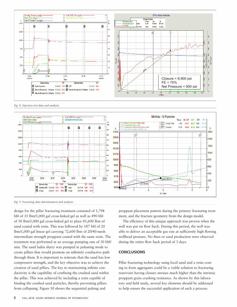
Fracturing operations began with an injection test being pumped using a total volume of 58 barrels (bbl) of treated water at a stable rate of 16 bbl/min. The breakdown pressure was observed at approximately 5,330 psi, Fig. 8, and pressure decline analysis estimated a reservoir permeability of approxi-mately 0.06 md.
The fracture data determination was later performed with approximately 350 bbl of 35 lbm/1,000 gal cross-linked fluid flushed with 212 bbl of 20 lbm/1,000 gal linear gel at a pump rate of 30 bbl/min. A high-definition temperature survey was performed to evaluate the fracture height growth and calibrate the pressure match accordingly. Figure 9 shows the treating pressure and fracture data analysis result.
After deliberate pressure matching and model calibra-tion, the primary pillar fracturing treatment was redesigned to meet specific design parameter requirements. The new
Fig. 5. Sustained conductivity channel using an A Sand 20/40-mesh consolidated pillar with a lower concentration of resin-to-sand mass.
Fig. 6. Sustained conductivity of the medium resin-to-sand concentration pillar fracturing channels as a function of stress cycling.
Fig. 5. Sustained conductivity channel using an A Sand 20/40-mesh consolidated pillar with a lower concentration of resin-to-sand mass.
Fig. 5. Sustained conductivity channel using an A Sand 20/40-mesh consolidated pillar with a lower concentration of resin-to-sand mass.
Fig. 6. Sustained conductivity of the medium resin-to-sand concentration pillar fracturing channels as a function of stress cycling.
Fig. 6. Sustained conductivity of the medium resin-to-sand concentration pillar fracturing channels as a function of stress cycling.
Fig. 7. Aggregate survivability investigation, showing the post-test results (right).
Initial aggregate Loading of cell Post-test analysis
Fig. 7. Aggregate survivability investigation, showing the post-test results (right).
6 FALL 2018 SAUDI ARAMCO JOURNAL OF TECHNOLOGY
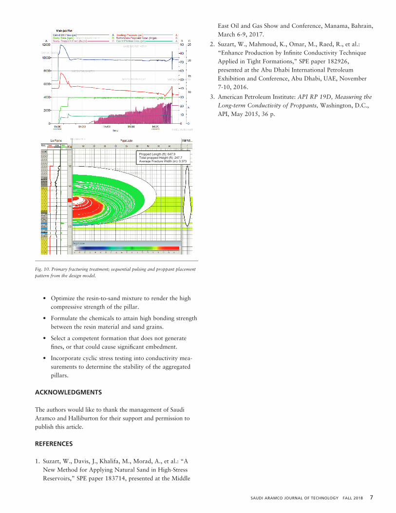
design for the pillar fracturing treatment consisted of 1,798 bbl of 35 lbm/1,000 gal cross-linked gel as well as 490 bbl of 30 lbm/1,000 gal cross-linked gel to place 81,600 lbm of sand coated with resin. This was followed by 187 bbl of 20 lbm/1,000 gal linear gel carrying 72,600 lbm of 20/40-mesh intermediate strength proppant coated with the same resin. The treatment was performed at an average pumping rate of 30 bbl/min. The sand laden slurry was pumped in pulsating mode to create pillars that would promote an infinitely conductive path through them. It is important to reiterate that the sand has low compressive strength, and the key objective was to achieve the creation of sand pillars. The key to maintaining infinite con-ductivity is the capability of confining the crushed sand within the pillar. This was achieved by including a resin capable of binding the crushed sand particles, thereby preventing pillars from collapsing. Figure 10 shows the sequential pulsing and
proppant placement pattern during the primary fracturing treat-ment, and the fracture geometry from the design model.
The efficiency of this unique approach was proven when the well was put on flow back. During this period, the well was able to deliver an acceptable gas rate at sufficiently high flowing wellhead pressure. No fines or sand production were observed during the entire flow back period of 3 days.
CONCLUSIONS
Pillar fracturing technology using local sand and a resin coat-ing to form aggregates could be a viable solution to fracturing reservoirs having closure stresses much higher than the intrinsic proppant grain crushing resistance. As shown by this labora-tory and field study, several key elements should be addressed to help ensure the successful application of such a process:
Fig. 9. Fracturing data determination and analysis.
Fig. 7. Aggregate survivability investigation, showing the post-test results (right).
Fig. 8. Injection test data and analysis.
Fig. 9. Fracturing data determination and analysis.
Closure = 8,900 psi FE = 75% Net Pressure = 900 psi
Fig. 7. Aggregate survivability investigation, showing the post-test results (right).
Fig. 8. Injection test data and analysis.
Fig. 9. Fracturing data determination and analysis.
Closure = 8,900 psi FE = 75% Net Pressure = 900 psi
- .
Fig. 8. Injection test data and analysis.
Fig. 9. Fracturing data determination and analysis.
Closure = 8,900 psi FE = 75% Net Pressure = 900 psi
Fig. 8. Injection test data and analysis.
- .
Fig. 8. Injection test data and analysis.
Fig. 9. Fracturing data determination and analysis.
Closure = 8,900 psi FE = 75% Net Pressure = 900 psi
SAUDI ARAMCO JOURNAL OF TECHNOLOGY FALL 2018 7
• Optimize the resin-to-sand mixture to render the high compressive strength of the pillar.
• Formulate the chemicals to attain high bonding strength between the resin material and sand grains.
• Select a competent formation that does not generate fines, or that could cause significant embedment.
• Incorporate cyclic stress testing into conductivity mea-surements to determine the stability of the aggregated pillars.
ACKNOWLEDGMENTS
The authors would like to thank the management of Saudi Aramco and Halliburton for their support and permission to publish this article.
REFERENCES
1. Suzart, W., Davis, J., Khalifa, M., Morad, A., et al.: “A New Method for Applying Natural Sand in High-Stress Reservoirs,” SPE paper 183714, presented at the Middle
East Oil and Gas Show and Conference, Manama, Bahrain, March 6-9, 2017.
2. Suzart, W., Mahmoud, K., Omar, M., Raed, R., et al.: “Enhance Production by Infinite Conductivity Technique Applied in Tight Formations,” SPE paper 182926, presented at the Abu Dhabi International Petroleum Exhibition and Conference, Abu Dhabi, UAE, November 7-10, 2016.
3. American Petroleum Institute: API RP 19D, Measuring the Long-term Conductivity of Proppants, Washington, D.C., API, May 2015, 36 p.
Fig. 10. Primary fracturing treatment; sequential pulsing and proppant placement pattern from the design model.
Fig. 10. Primary fracturing treatment; sequential pulsing and proppant placement pattern from the design model.
Propped Length (ft): 647.9 Total propped Height (ft): 247.7 Average Fracture Width (in): 0.373
Fig. 10. Primary fracturing treatment; sequential pulsing and proppant placement pattern from the design model.
Propped Length (ft): 647.9 Total propped Height (ft): 247.7 Average Fracture Width (in): 0.373

8 FALL 2018 SAUDI ARAMCO JOURNAL OF TECHNOLOGY
BIOGRAPHIES
Dr. Fakuen “Frank” F. Chang is the focus area champion for Productivity Enhancement in the Production Technology Team of Saudi Aramco’s Exploration and Petroleum Engineering Center – Advanced Research Center (EXPEC ARC).
Prior to joining Saudi Aramco in September 2012, he worked at Schlumberger for 16 years. Before that, Frank was at Stimlab for 4 years. He has developed many products and technologies dealing with sand control, fracturing, acidizing and perforating.
Frank is an inventor and recipient of 23 granted U.S. patents, and he is the author of more than 40 Society of Petroleum Engineers (SPE) technical papers.
Frank received his B.S. degree in Mineral and Petroleum Engineering from the National Cheng Kung University, Tainan City, Taiwan; his M.S. degree in Petroleum Engineering from the University of Louisiana at Lafayette, Lafayette, LA; and his Ph.D. degree in Petroleum Engineering from the University of Oklahoma, Norman, OK.
Naresh K. Purusharthy is a Gas Production Engineer working for the Southern Area Production Engineering Department, located in ‘Udhailiyah. He has extensive experience in well stimulation (fracturing and acidizing), intervention (coiled tubing, e-line, and
slick line), well integrity, completions and workover. Prior to joining Saudi Aramco in September 2013,
Naresh worked for Cairn Energy in India for 5 years as a Petroleum Engineer. Prior to that, he worked for BJ Services focusing mostly on stimulation.
Naresh so far has authored four Society of Petroleum Engineers (SPE) technical papers, and has additional publications in other technical forums.
He received his M.S. degree in Petroleum Engineering from St. Petersburg Mining University, St. Petersburg, Russia.
Mohamed Khalifa is currently the Halliburton Stimulation Technical Lead in Saudi Arabia. Upon joining Halliburton, he began his career working in production enhancement in operations, and worked his way up from Stimulation Engineer to Senior
Account Representative. Mohamed has extensive experience in production engineering, petrophysics, well analysis and stimulation evaluation, in both onshore and offshore wells.
He has 15 years of experience in stimulation and well completions, including conventional and unconventional hydraulic fracturing, hybrid fracturing, high rate water fracturing, fracpac, acid fracturing, carbonate acid stimulation, sandstone acid stimulation, pinpoint stimulation for vertical and horizontal wells, AccessFrac and conductor fracture.
Mohamed received his B.S. degree in Mechanics and Evaluation Engineering from Cairo University of Technology, Cairo, Egypt.
Dr. Raed Rahal is a Principal Scientist for Production Enhancement at the Halliburton Dhahran Technology Center, Saudi Arabia. He is currently managing a production enhancement technology portfolio of fluids and additives for oil field applications in
Saudi Arabia. Raed is an upstream oil and gas professional with a diversified technical background in well stimulation techniques and chemicals, including hydraulic fracturing, acidizing, and sand and water control chemicals. Prior to joining Halliburton in 2013, he had over 10 years of commendable experience in the area of nanotechnology, sol gel chemistry, photocatalysis, nanoparticles design, and surface functionalization.
Raed received both his M.S. and Ph.D. degrees in Material Science from Claude Bernard University, Lyon, France.
During his career, Raed has published more than 25 papers and has been awarded four patents.

SAUDI ARAMCO JOURNAL OF TECHNOLOGY FALL 2018 9
ABSTRACT
Iron sulfide scaling is one of the primary causes of impairment of gas production in deep sour reservoirs in Saudi Arabia. The wells are typically acid fractured and completed with carbon steel tubing. The combination of corrosion of tubes caused by hydrogen sulfide (H2S) and iron dissolved from the tubes during the acidizing process at high temperature, though inhib-ited, leads to significant scaling issues. This scale in tubulars can cause significant production losses and restricts well access for surveillance and intervention operations. A fundamental solution, therefore, is required to prevent iron sulfide scale for-mation and deposition along downhole tubulars. One cost-ef-fective approach to mitigating scaling in downhole tubing is to develop high performance coatings for carbon steel tubing. This article describes the development of novel coating materials and methods and evaluation of their effectiveness in preventing iron sulfide scale.
INTRODUCTION
Scaling of production tubing1 is the primary reason2 for loss of gas production3 in deep sour reservoirs in Saudi Arabia. These wells are completed with carbon steel production tubing. The primary component of the scale is iron sulfide, with iron ions generated by hydrogen sulfide (H2S) and acid attacks of the steel during acid treatment. The iron sulfide scale can cause significant production losses and restricts access to the well for surveillance and intervention. A fundamental solution to this scaling problem is required. Our approach was to develop cost-effective, high performance coatings for the inner surface of the carbon steel production tubing.
EXPERIMENTAL PROCEDURE
A high-pressure, high temperature (HPHT) autoclave facility with rotating cage and sour gas capability was established in laboratories for safely handling H2S gas exposure of coated and uncoated test coupons to simulate field conditions. It was cru-cial that strictly anoxic conditions be maintained in the auto-clave after loading to assure that only iron(II) sulfide (FeS) scal-ing occurred, without any possibility of oxidation.
This apparatus was used to screen T95 steel coupons under conditions where uncoated coupons rapidly developed FeS scales from the direct reaction of steel with H2S under HPHT conditions in synthetic brine — having a similar composition of the Saudi Arabian field. Once baseline conditions were estab-lished, coupons completely coated on all sides with various coating formulations were subjected to the same environment to probe their resistance to direct attack by HPHT H2S and to indirect scaling caused by externally produced FeS.
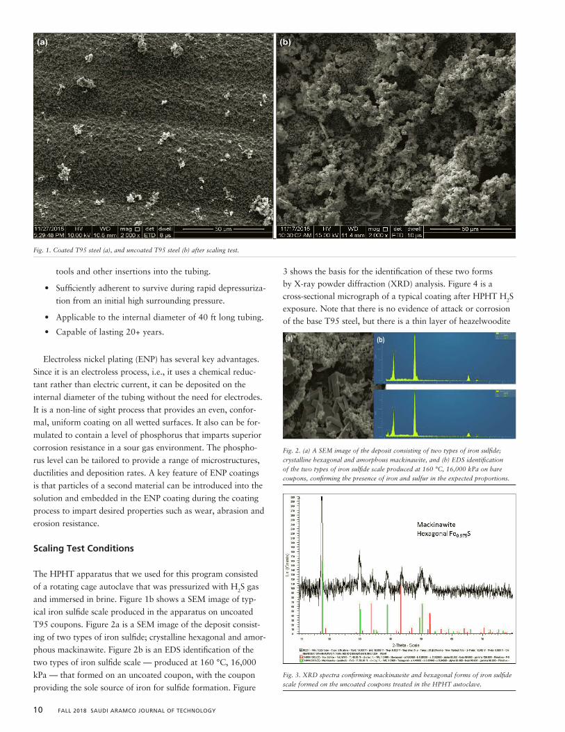
The equipment setup allows each experiment to test five coating formulations and one uncoated control sample. In every case, the control coupon scaled heavily and shed signifi-cant amounts of suspended FeS into the brine. This suspended FeS was then re-deposited on the five coated coupons (visible as white clusters in Fig. 1a). After testing, the coupons were thoroughly rinsed in running deionized water to dislodge any loosely adherent solids, then air-dried, and weighed to deter-mine the extent to which they had lost or gained weight. They were then examined by scanning electron microscope (SEM), energy dispersive X-ray spectroscopy (EDS), and X-ray fluores-cence to rank their anti-scaling performance. These data were used to make a down selection of the best anti-scaling coatings for these conditions.
RESULTS
Types of Coatings Tested
Our initial hypothesis was that if we were to develop a coating that was resistant to corrosion by H2S, then this coating should not only prevent the formation of FeS via corrosion of the steel, but also prevent deposition of preformed FeS owing to the lack of a driving force for adhesion. Prevention of the formation of corrosion products on the metal surface was expected to minimize scale initiation. In addition to being unreactive with respect to corrosion, the coatings need to have the following attributes:
• Nonstick with respect to scalant species, e.g., complex oxides, carbonates and sulfides.
• Wear and abrasion resistant to survive damage from
Development of Scaling Resistant Coatings for High Temperature Sour Gas Service
Dr. Lawrence Kool, Dr. Qiliang Wang, Dr. Nidal A. Ghizawi, Dr. Fauken F. Chang, and Hui Zhu
10 FALL 2018 SAUDI ARAMCO JOURNAL OF TECHNOLOGY
tools and other insertions into the tubing.
• Sufficiently adherent to survive during rapid depressuriza-
tion from an initial high surrounding pressure.
• Applicable to the internal diameter of 40 ft long tubing.
• Capable of lasting 20+ years.
Electroless nickel plating (ENP) has several key advantages.
Since it is an electroless process, i.e., it uses a chemical reduc-
tant rather than electric current, it can be deposited on the
internal diameter of the tubing without the need for electrodes.
It is a non-line of sight process that provides an even, confor-
mal, uniform coating on all wetted surfaces. It also can be for-
mulated to contain a level of phosphorus that imparts superior
corrosion resistance in a sour gas environment. The phospho-
rus level can be tailored to provide a range of microstructures,
ductilities and deposition rates. A key feature of ENP coatings
is that particles of a second material can be introduced into the
solution and embedded in the ENP coating during the coating
process to impart desired properties such as wear, abrasion and
erosion resistance.
Scaling Test Conditions
The HPHT apparatus that we used for this program consisted
of a rotating cage autoclave that was pressurized with H2S gas
and immersed in brine. Figure 1b shows a SEM image of typ-
ical iron sulfide scale produced in the apparatus on uncoated
T95 coupons. Figure 2a is a SEM image of the deposit consist-
ing of two types of iron sulfide; crystalline hexagonal and amor-
phous mackinawite. Figure 2b is an EDS identification of the
two types of iron sulfide scale — produced at 160 °C, 16,000
kPa — that formed on an uncoated coupon, with the coupon
providing the sole source of iron for sulfide formation. Figure
3 shows the basis for the identification of these two forms by X-ray powder diffraction (XRD) analysis. Figure 4 is a cross-sectional micrograph of a typical coating after HPHT H2S exposure. Note that there is no evidence of attack or corrosion of the base T95 steel, but there is a thin layer of heazelwoodite
Fig. 1. Coated T95 steel (a), and uncoated T95 steel (b) after scaling test.
Fig. 2. (a) A SEM image of the deposit consisting of two types of iron sulfide;amorphous mackinawite, and (b) EDS identification of the two types of iron sulfide°C, 16,000 kPa on bare coupons, confirming the presence of iron and sulfur in the
(a) (b)
(a) (b)
Fig. 2. (a) A SEM image of the deposit consisting of two types of iron sulfide; crystalline hexagonal and amorphous mackinawite, and (b) EDS identification of the two types of iron sulfide scale produced at 160 °C, 16,000 kPa on bare coupons, confirming the presence of iron and sulfur in the expected proportions.
Fig. 3. XRD spectra confirming mackinawite and hexagonal forms of ironuncoated coupons treated in the HPHT autoclave.
Fig. 3. XRD spectra confirming mackinawite and hexagonal forms of iron sulfide scale formed on the uncoated coupons treated in the HPHT autoclave.
Fig. 1. Coated T95 steel (a), and uncoated T95 steel (b) after scaling test.
Fig. 2. (a) A SEM image of the deposit consisting of two types of iron sulfide; crystalline hexagonal and amorphous mackinawite, and (b) EDS identification of the two types of iron sulfide scale produced at 160 °C, 16,000 kPa on bare coupons, confirming the presence of iron and sulfur in the expected proportions.
(a) (b)
(a) (b)
Fig. 1. Coated T95 steel (a), and uncoated T95 steel (b) after scaling test.

SAUDI ARAMCO JOURNAL OF TECHNOLOGY FALL 2018 11
(Ni3S2) deposited on the top of the ENP coating surface.
Note that in each set of experiments, six coupons were
included in the rotating cage, five with experimental coatings
and one with no coating (bare T95). We have found that
uncoated coupons always form copious quantities of FeS scale
— as confirmed by EDS and XRD spectroscopy — and lose
weight during exposure owing to the reaction of H2S with the
steel to form FeS, then some loss of adhesion and suspension
of FeS and re-deposition on the autoclave walls and the five
coated coupons to varying degrees, depending upon the affin-
ities of FeS for the coating surfaces. We confirmed by SEM,
EDS and XRD analysis of metallographic cross-sections of rep-
resentative coatings that the FeS deposited on the coated cou-
pons did not form from corrosion of the coupons. Our analy-
ses detected only coating components, with no FeS embedded
within or beneath the coatings.
Several criteria were considered to differentiate the candidate
coatings. These were:
1. Mass gain caused by accumulation of FeS on the coated
samples.
2. Macroscopic visual inspection of the samples after treat-
ment to rank changes in color, uniformity of color, and
integrity of the coating.
3. SEM examination of the morphologies of any accumulated
scale.
4. EDS and XRD analyses of the treated surfaces to identify
scalant species.
Coating Screening Results
Figure 5 shows some representative coupons before and after
HPHT H2S exposure to the scaling conditions previously
described. Note that uncoated coupons — included in each
cage set of six — always formed a heavy, black iron sulfide
deposit, while none of the coated samples formed the black
deposit. There were some minor, but macroscopically notice-able, changes in color, owing to the formation — to varying degrees — of Ni3S2 upon HPHT reaction of H2S with nickel in the coatings. Note that the formation of Ni3S2 appears to be beneficial, owing to its fine microstructure, apparent tenacity and slow growth rate. In addition, Ni3S2 has a very low affin-ity for attachment of FeS. Ultimate down selection to the best anti-scaling coating was based upon a combination of the lack of adhesion of scale to the surface, formation of a slow grow-ing, microcrystalline, protective Ni3S2 scale and good abrasive wear performance.
Figure 6 compares the hydrophobicity of the coatings prior to exposure to HPHT H2S. The hydrophobicity is measured by the contact angle measurement using the ASTM D7334 proce-dure. The contact angle greater than 90° indicates a hydropho-bic surface. In general, when the contact angle exceeds 120°, the surface is considered super hydrophobic. Most coatings are either hydrophobic or superhydrophobic4, which is expected to correlate with nonstick behavior with respect to water-soluble scale5.
Selection of Highest Rank Coating Candidates for in-Depth Evaluation
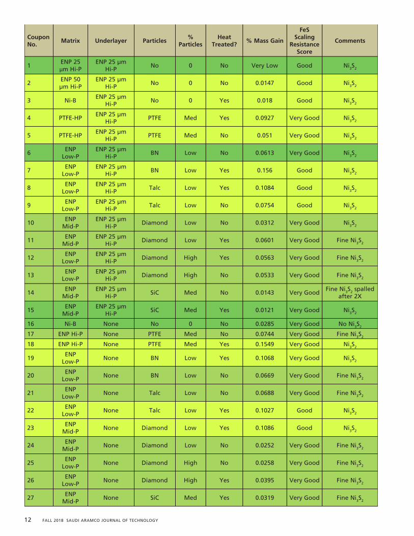
Table 1 shows the results of the initial HPHT screening exper-iments on coated coupons. The coatings are ranked by color, with dark green being the most promising coatings, light green
Fig. 4. A typical coating after HPHT H2S exposure showing an absence of corrosion of the T95 substrate.
Coating layer: High phosphorous *0.002” Measured total thickness: ~41 m
Fig. 4. A typical coating after HPHT H2S exposure showing an absence of corrosion of the T95 substrate.
Fig. 5. Representative images of test coupons before and after HPHT H2S autoclave exposure.
Fig. 5. Representative images of test coupons before and after HPHT H2S
Fig. 6. of Coatings, Substrates and Pigments by Advancing Contact Angle Measurement). DLC is a carbon, included for comparison.
Con
tact
Ang
le (D
eg)
Sample Code
Afte
r
B
efor
e
Streamax #30 #07 #08 #09 #10 #11 #12 #13 #14 Bare Coupons
Fig. 5. Representative images of test coupons before and after HPHT H2S autoclave exposure.
Fig. 6. of Coatings, Substrates and Pigments by Advancing Contact Angle Measurement). DLC is a carbon, included for comparison.
Con
tact
Ang
le (D
eg)
Sample Code
Afte
r
B
efor
e
Streamax #30 #07 #08 #09 #10 #11 #12 #13 #14 Bare Coupons
Fig. 6. Contact angle measured for all coatings (ASTM D7334: Standard Practice for Surface Wettability of Coatings, Substrates and Pigments by Advancing Contact Angle Measurement). DLC is a diamond-like carbon, included for comparison.
12 FALL 2018 SAUDI ARAMCO JOURNAL OF TECHNOLOGY
Coupon No.
Matrix Underlayer Particles%
ParticlesHeat
Treated?% Mass Gain
FeS Scaling
Resistance Score
Comments
1ENP 25 µm Hi-P
ENP 25 µm Hi-P
No 0 No Very Low Good Ni3S2
2ENP 50 µm Hi-P
ENP 25 µm Hi-P
No 0 No 0.0147 Good Ni3S2
3 Ni-BENP 25 µm
Hi-PNo 0 Yes 0.018 Good Ni3S2
4 PTFE-HPENP 25 µm
Hi-PPTFE Med Yes 0.0927 Very Good Ni3S2
5 PTFE-HPENP 25 µm
Hi-PPTFE Med No 0.051 Very Good Ni3S2
6ENP
Low-PENP 25 µm
Hi-PBN Low No 0.0613 Very Good Ni3S2
7ENP
Low-PENP 25 µm
Hi-PBN Low Yes 0.156 Good Ni3S2
8ENP
Low-PENP 25 µm
Hi-PTalc Low Yes 0.1084 Good Ni3S2
9ENP
Low-PENP 25 µm
Hi-PTalc Low No 0.0754 Good Ni3S2
10ENP
Mid-PENP 25 µm
Hi-PDiamond Low No 0.0312 Very Good Ni3S2
11ENP
Mid-PENP 25 µm
Hi-PDiamond Low Yes 0.0601 Very Good Fine Ni3S2
12ENP
Low-PENP 25 µm
Hi-PDiamond High Yes 0.0563 Very Good Fine Ni3S2
13ENP
Low-PENP 25 µm
Hi-PDiamond High No 0.0533 Very Good Fine Ni3S2
14ENP
Mid-PENP 25 µm
Hi-PSiC Med No 0.0143 Very Good
Fine Ni3S2 spalled after 2X
15ENP
Mid-PENP 25 µm
Hi-PSiC Med Yes 0.0121 Very Good Ni3S2
16 Ni-B None No 0 No 0.0285 Very Good No Ni3S2
17 ENP Hi-P None PTFE Med No 0.0744 Very Good Fine Ni3S2
18 ENP Hi-P None PTFE Med Yes 0.1549 Very Good Ni3S2
19ENP
Low-PNone BN Low Yes 0.1068 Very Good Ni3S2
20ENP
Low-PNone BN Low No 0.0669 Very Good Fine Ni3S2
21ENP
Low-PNone Talc Low No 0.0688 Very Good Fine Ni3S2
22ENP
Low-PNone Talc Low Yes 0.1027 Good Ni3S2
23ENP
Mid-PNone Diamond Low Yes 0.1086 Good Ni3S2
24ENP
Mid-PNone Diamond Low No 0.0252 Very Good Fine Ni3S2
25ENP
Low-PNone Diamond High No 0.0258 Very Good Fine Ni3S2
26ENP
Low-PNone Diamond High Yes 0.0395 Very Good Fine Ni3S2
27ENP
Mid-PNone SiC Med Yes 0.0319 Very Good Fine Ni3S2
SAUDI ARAMCO JOURNAL OF TECHNOLOGY FALL 2018 13
as promising coatings, and yellow, less promising. We assigned
these rankings based upon several factors: % mass gain, as a
measure of FeS deposition, SEM examination of FeS morphol-
ogy on the surface, contact angle, and Ni3S2 microstructure.
The mass gain measurements included a combination of weight
gain from Ni3S2 growth and re-deposition onto coated coupons
of iron sulfide dislodged from the uncoated coupon. Note that
every coated coupon performed better than the uncoated con-
trol coupons, which turned black during HPHT exposure and
lost mass, owing to the detachment of FeS corrosion products
that redeposited to varying degrees on other coupons immersed
in the same brine solution — clearly visible as isolated clusters
previously shown in Fig. 1a.
The mass decrease of uncoated (control) coupons was typi-
cally 0.2% to 0.3%. The mass increase of the coated coupons
provided a direct indication of the degree to which exogenously
formed FeS adheres to the coating surfaces. Mass gains of the
various coated coupons, exposed under identical conditions,
can be compared directly as a way of ranking the coatings.
Again, these mass gains represent a combination of the mass
increase associated with Ni3S2 formation and FeS accumulation.
These two sources of mass gain can be differentiated by closely
comparing the SEM images of FeS deposits that are clearly visi-
ble (vide infra).
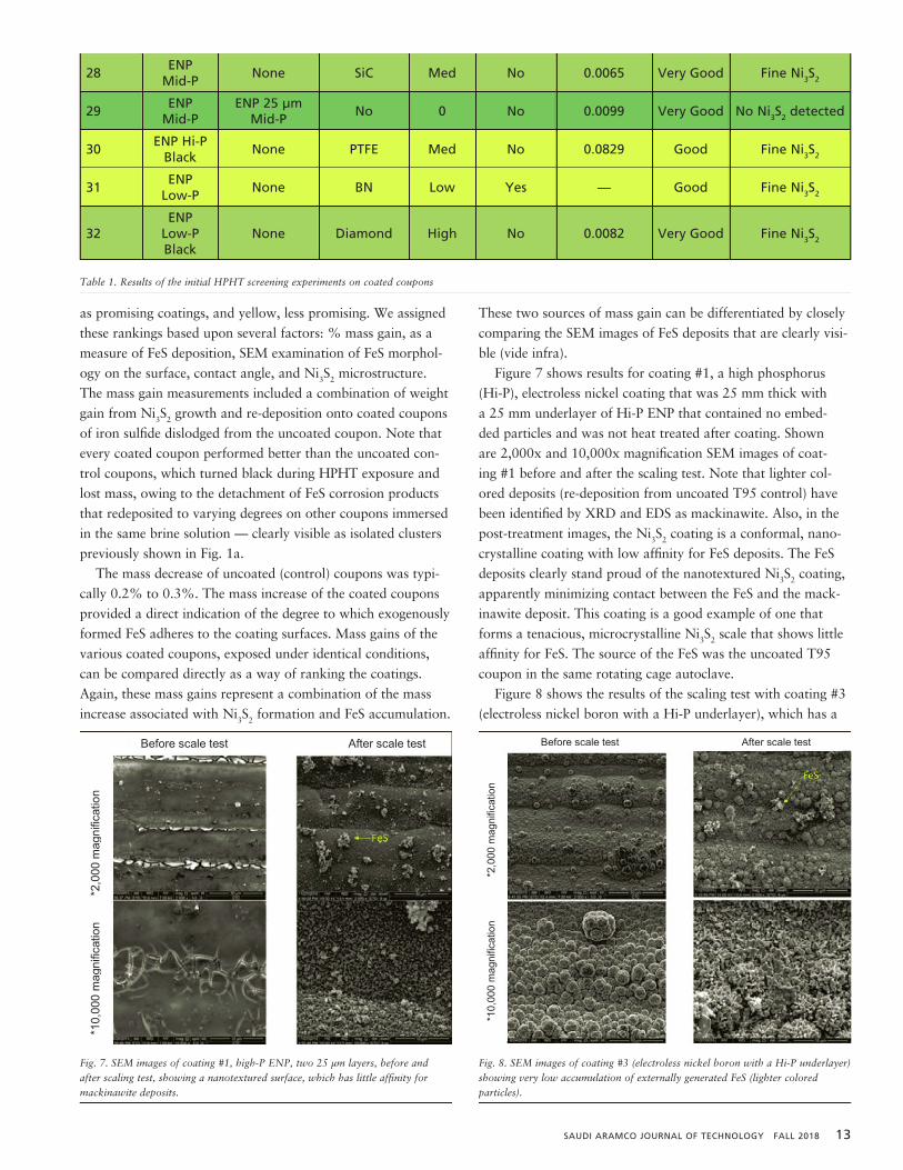
Figure 7 shows results for coating #1, a high phosphorus
(Hi-P), electroless nickel coating that was 25 mm thick with
a 25 mm underlayer of Hi-P ENP that contained no embed-
ded particles and was not heat treated after coating. Shown
are 2,000x and 10,000x magnification SEM images of coat-
ing #1 before and after the scaling test. Note that lighter col-
ored deposits (re-deposition from uncoated T95 control) have
been identified by XRD and EDS as mackinawite. Also, in the
post-treatment images, the Ni3S2 coating is a conformal, nano-
crystalline coating with low affinity for FeS deposits. The FeS
deposits clearly stand proud of the nanotextured Ni3S2 coating,
apparently minimizing contact between the FeS and the mack-
inawite deposit. This coating is a good example of one that
forms a tenacious, microcrystalline Ni3S2 scale that shows little
affinity for FeS. The source of the FeS was the uncoated T95
coupon in the same rotating cage autoclave.
Figure 8 shows the results of the scaling test with coating #3
(electroless nickel boron with a Hi-P underlayer), which has a
Table 1. Results of the initial HPHT screening experiments on coated coupons
28ENP
Mid-PNone SiC Med No 0.0065 Very Good Fine Ni3S2
29ENP
Mid-PENP 25 µm
Mid-PNo 0 No 0.0099 Very Good No Ni3S2 detected
30ENP Hi-P
BlackNone PTFE Med No 0.0829 Good Fine Ni3S2
31ENP
Low-PNone BN Low Yes — Good Fine Ni3S2
32ENP
Low-P Black
None Diamond High No 0.0082 Very Good Fine Ni3S2
25 ENP Low-P None Diamond High No 0.0258 Very Good Fine Ni3S2
26 ENP Low-P None Diamond High Yes 0.0395 Very Good Fine Ni3S2
27 ENP Mid-P None SiC Med Yes 0.0319 Very Good Fine Ni3S2
28 ENP Mid-P None SiC Med No 0.0065 Very Good Fine Ni3S2
29 ENP Mid-P
ENP 25 m Mid-P
No 0 No 0.0099 Very Good No Ni3S2 detected
30 ENP Hi-P Black None PTFE Med No 0.0829 Good Fine Ni3S2
31 ENP Low-P None BN Low Yes — Good Fine Ni3S2
32 ENP
Low-P Black
None Diamond High No 0.0082 Very Good Fine Ni3S2
Table 1. Results of the initial HPHT screening experiments on coated coupons
Fig. 7. SEM images of coating #1, high-P ENP, two 25 m layers, before and after scaling test, showing a nanotextured surface, which has little affinity for mackinawite deposits.
Before scale test After scale test
*10,
000
mag
nific
atio
n
*
2,00
0 m
agni
ficat
ion
Fig. 7. SEM images of coating #1, high-P ENP, two 25 µm layers, before and after scaling test, showing a nanotextured surface, which has little affinity for mackinawite deposits.
Fig. 8. SEM images of coating #3 (electroless nickel boron with a Hi-accumulation of externally generated FeS (lighter colored particles).
Before scale test After scale test
Before scale test After scale test
*1
0,00
0 m
agni
ficat
ion
*2,
000
mag
nific
atio
n
Fig. 8. SEM images of coating #3 (electroless nickel boron with a Hi-P underlayer) showing very low accumulation of externally generated FeS (lighter colored particles).

14 FALL 2018 SAUDI ARAMCO JOURNAL OF TECHNOLOGY
unique surface microstructure (microspheroids). This structure
results in a very high contact angle, > 140°, which appears to
correlate with extremely low accumulation of externally gener-
ated FeS. Note the continuous coverage of the spheroids with
tenacious nanocrystalline Ni3S2. This combination of micro-
spheroids covered with nanocrystalline Ni3S2 feature affords a
superhydrophobic, nonstick surface. Although sample #1 shows
an excellent anti-FeS deposition characteristic, the higher con-
tact angle measured in sample #3 may deliver even better non-
stick properties than sample #1. It is therefore worth further
testing for its overall performance.
For comparison, coating #8 contains embedded talc particles
in a Low-P ENP matrix, Fig. 9. The anti-stick properties of this
coating are not as good as other coatings, as is evident from the
larger sized clusters and relatively high concentration of depos-
ited mackinawite particles.
Extended Testing of Down Selected Coatings
Screening of the anti-scaling performance of 30+ coatings led
to a down selection of six coatings for closer scrutiny. These
coatings were those numbered 1, 2, 3, 15, 16, and 29 in Table
1. Coupons 2 and 3 were down selected because we were inter-
ested in looking more closely at the lack of heat treatment in
coating #2, and the uniquely hydrophobic electroless nickel
boron (ENB) coating. Additional, fresh coupons were coated
and these were subjected to repeated HPHT scaling conditions.
We focused on the evolution of Ni3S2 crystal morphologies
grown on the selected coatings to learn more about how the
robustness of the scale might vary among the coatings. In addi-
tion to these HPHT scaling tests, the coatings, with and with-
out Ni3S2, were subjected to explosive decompression testing
(EDT) and abrasive loop wear testing.
Figure 10 shows SEM images of coating #3 after two
successive scaling tests. This coating is particularly anti-stick
with respect to FeS. This observation is consistent with it being
one of the more hydrophobic coatings, as was established in the
contact angle measurements. We speculate that this enhanced
hydrophobicity is related to the nano-nodular microstructure
of the surface, which makes it difficult for FeS deposits to
achieve sufficient contact with the surface to adhere. Note that
nanocrystalline Ni3S2 also grows on the ENB surface, but with
a finer microstructure than what is observed with ENP. This
Ni3S2 deposit conforms nicely to the underlying nodular ENB
surface, indicating that good adhesion can be expected.
Coating Adhesion Testing
We expected all the down selected coatings to have strong
adhesion to their T95 substrates based on previous experi-
ence with electroless nickel coatings, which are known to have
a metallurgical bond between the coating and the substrate.
This bonding is further promoted during heat treatment of the
coating, which causes inter-diffusion of the coating and sub-
strate, or diffusion bonding. This expectation was borne out
in the HPHT H2S exposures (vide supra), in which only one
sample (#14), showed minor spallation of the Ni3S2 layer after
two cycles of exposure. The spalling of the Ni3S2 layer could
cause re-exposure of the metal to the H2S downhole and there-
fore losing its corrosion and scale protection functionality.
Nevertheless, we carried out adhesion testing by means of an
EDT, which was devised and carried out by a local university
in Shanghai. In addition to the adhesion of the applied coat-
ings, we were even more curious about how tenacious the Ni3S2
would be in the EDT. The EDT apparatus includes two liquid
layers: (1) a bottom aqueous brine layer, and (2) a top layer
that is a mixture of kerosene and toluene.
The experimental sequence of soaking in brine for 17 hours
. accumulation of externally generated FeS (lighter colored particles).
Fig. 9. SEM images of coating #8 (ENP, Low-P plus talc, heat treated) before and after exposure.
Before scale test After scale test
*1
0,00
0 m
agni
ficat
ion
*2,0
00 m
agni
ficat
ion
Fig. 9. SEM images of coating #8 (ENP, Low-P plus talc, heat treated) before and after exposure.
Fig. 10. SEM images of coating #3 (25 m high photos ENP underlayer with 25 boron overlayer, heat treated at 350 °C) after one and two scale tests.
After the first scale test After the second scale test
*1
0,00
0 m
agni
ficat
ion
*2,0
00 m
agni
ficat
ion
Fig. 10. SEM images of coating #3 (25 µm high photos ENP underlayer with 25 µm ENB overlayer, heat treated at 350 °C) after one and two scale tests.

SAUDI ARAMCO JOURNAL OF TECHNOLOGY FALL 2018 15
at 2 MPa, heating for 3½ hours at 150 °C, boosting over 2 minutes to 56 MPa, holding at 150 °C at 56 MPa and sudden decompression in 2.3 seconds, was conducted on the down selected coatings. Note that five of the coupons (2, 3, 15, 29, and 31) had previously been exposed at HPHT in the scal-ing rig and had robust coatings of Ni3S2 developed over mul-tiple HPHT cycles in the rotating cage autoclave. After EDT, the coupons were examined by SEM and showed spallation of neither the original coating nor exposed coating having Ni3S2 overlayers.
CONCLUSIONS
A total of 32 different coatings have been tested in a rotating cage apparatus under HPHT H2S atmosphere. Six coupons were tested in each batch: five coated and one uncoated T95 steel coupon. All the coatings prevented corrosive formation of FeS scale, in contrast to the bare coupons, which scaled heav-ily with FeS. The uncoated coupons lost mass during treat-ment because the steel was consumed to form FeS scale and a fraction of the scale formed lost adhesion in the rapidly stirred autoclave, re-depositing, to varying degrees, on the other five coupons.
The electroless nickel phosphorus and ENB coatings formed a tenacious, microcrystalline to nanocrystalline Ni3S2 scale that showed very low affinity for FeS adhesion. The iron sulfide and Ni3S2 scales were characterized by EDS and XRD analyses. Contact angle measurements of the tested coatings indicated that most are hydrophobic, and some were superhydrophobic.
Based upon these initial screening results, we down selected a set of six coatings for further evaluation. We have also con-ducted explosive decompression as a gauge of coating adhesion, as well as abrasion testing to differentiate the down selected coatings. We will be looking at extended exposure times in high temperature sour gas wells to gauge the growth rate and sur-face morphology of the protective Ni3S2 scale and evaluate the anti-scaling performance.
ACKNOWLEDGMENTS
The authors would like to thank the management of Saudi Aramco and General Electric for their support and permission to publish this article. The authors would also like to acknowl-edge the participation of the following coauthors who par-ticipated in the design of the experiments described and the interpretation of the results: Dennis Gray, Raul Rebak, Limin Wang, Dalong Zhong, and Hai Chang (GE Global Research), Tao Chen, Qiwei Wang, Noel Ginest, and Jawad I. Tammar (Saudi Aramco).
REFERENCES
1. Crabtree, M., Eslinger, D., Fletcher, P., Miller, M., et al.: “Fighting Scale: Removal and Prevention,” Oilfield
Review, Vol. 11, Issue 3, October 1999, pp. 30-45.
2. Brondel, D., Edwards, R., Hayman, A., Hill, D., et al.: “Corrosion in the Oil Industry,” Oilfield Review, Vol. 6, Issue 2, April 1994, pp. 4-18.
3. Popoola, L.T., Grema, A.S., Latinwo, G.K., Gutti, B., et al.: “Corrosion Problems during Oil and Gas Production and its Mitigation,” International Journal of Industrial Chemistry, Vol. 4, Issue 1, September 2013, pp. 4-35.
4. Law, K-Y.: “Definitions for Hydrophilicity, Hydro- phobicity, and Superhydrophobicity: Getting the Basics Right,” The Journal of Physical Chemistry Letters, Vol. 5, Issue 4, February 2014, pp. 686-688.
5. Subramanyam, S.B., Azimi, G. and Varanasi, K.K.: “Designing Lubricant Impregnated Textured Surfaces to Resist Scale Formation,” Advanced Materials Interfaces, Vol. 1, Issue 2, April 2014.
BIOGRAPHIES
Dr. Lawrence Kool joined the research staff at the GE Global Research Center in 1999 as a Senior Research Chemist, and now works as a Senior Inorganic Chemist. He has been responsible for the development and global implementation of
environmentally friendly chemical processes that are used in services technologies for gas turbine and aircraft engine components. Lawrence developed selective methods for removing environmental coatings from superalloy components while causing no damage to the underlying substrate.
He joined the GRC after spending four years at GE Superabrasives, where he developed and implemented — in Ohio and Ireland — environmentally benign chemical processes for manufacturing man-made diamonds from metallic catalysts.
Before joining GE, Lawrence was an Assistant Professor of Chemistry at Boston College, where he taught organic, inorganic and organometallic chemistry at both the undergraduate and graduate levels. His research group focused on the development of organoplatinum catalysts for the activation of C-H bonds, the catalytic partial oxidation of methane, and novel organometallic complexes of group IV transition metals. In addition to his work at GE, Lawrence was an Adjunct Professor of Chemistry at Siena College, where he taught inorganic chemistry.
He holds over 50 patents and has more than 50 technical papers published in peer-reviewed publications.
Lawrence received his B.S. degree in Chemistry from University of Michigan, Ann Arbor, MI, and his Ph.D. degree in Chemistry from University of Massachusetts, Amherst, MA.

16 FALL 2018 SAUDI ARAMCO JOURNAL OF TECHNOLOGY
Dr. Qiliang “Luke” Wang completed his postdoctoral training with Prof. Mason Tomson at the Brine Chemistry Consortium at Rice University, Houston, TX, where he explored mineral scales solubility and the kinetics of precipitation in oil
production systems, iron sulfide formation and inhibition, and mild steel corrosion in a newly designed anoxic plug flow reactor. Later, Luke worked at the GE Global Research — Oil & Gas Technology Center in Oklahoma City, as a Lead Research Engineer until November 2017. Now, his research interest is in the area of the Industrial Internet of Things of flow assurance management (organic and inorganic depositions control).
In 2001, Luke received his B.S. degree in Applied Chemistry from Dalian Polytechnic University, Dalian, China, and in 2010, he received his Ph.D. degree in Environmental Science and Engineering from Gwangju Institute of Science and Technology, Gwangju, South Korea.
Dr. Nidal A. Ghizawi joined GE in Saudi Arabia in February 2015 as the Technology & Innovation Director, leading the GE Saudi Technology & Innovation Center based at the Dhahran Techno Valley. He started with GE in 2005 as a Principal
Engineer in compressor aerodynamics in Greenville, South Carolina. In 2006, Nidal moved to GE Oil & Gas in Qatar as Engineering Manager to recruit and develop a team of engineers based at the GE Advanced Technology & Research Center (GEATRC) in the Qatar Science & Technology Park. From 2010 to early 2015, he worked with GE Global Research, leading the Energy and Propulsion Programs at GEATRC in Qatar.
Prior to joining GE, Nidal worked for eight years at AlliedSignal’s automotive division (previously Garrett Corporation) in Los Angeles, CA, as a Principal Engineer, where he focused on the aeromechanical design of turbochargers for passenger and commercial vehicles.
Nidal received his B.S. degree in Mechanical Engineering from University of Baghdad, Baghdad, Iraq, his M.S. degree in Mechanical Engineering from University of Jordan, Amman, Jordan, and his Ph.D. degree in Aerospace Engineering from University of Cincinnati, Cincinnati, OH.
Dr. Fakuen “Frank” F. Chang is the focus area champion for Productivity Enhancement in the Production Technology Team of Saudi Aramco’s Exploration and Petroleum Engineering Center – Advanced Research Center (EXPEC ARC).
Prior to joining Saudi Aramco in September 2012, he worked at Schlumberger for 16 years. Before that, Frank was at Stimlab for 4 years. He has developed many products and technologies dealing with sand control, fracturing, acidizing and perforating.
Frank is an inventor and recipient of 23 granted U.S. patents, and he is the author of more than 40 Society of Petroleum Engineers (SPE) technical papers.
Frank received his B.S. degree in Mineral and Petroleum Engineering from the National Cheng Kung University, Tainan City, Taiwan; his M.S. degree in Petroleum Engineering from the University of Louisiana at Lafayette, Lafayette, LA; and his Ph.D. degree in Petroleum Engineering from the University of Oklahoma, Norman, OK.
Hui Zhu started her career in 2006 when she joined the GE Global Research Center. Some of the main research projects that Hui has been involved in include: the study of rheological properties of coal slag under high temperature, anti-foulant
coating development in heat exchangers, and anti-corrosion coating development for overhead pipelines in an oil refinery.
In 2006, she received her M.S. degree in Inorganic Chemistry and Materials from East China University of Science and Technology, Shanghai, China.

SAUDI ARAMCO JOURNAL OF TECHNOLOGY FALL 2018 17
ABSTRACT
There is increasing evidence that SmartWater Flooding through the tuning of injection water chemistry and ionic composition, has a significant impact on the recovered oil, but the exact underlying mechanism by which this occurs is not well under-stood, and is supposed to be caused by complex interactions occurring at the fluid-fluid and fluid-rock interfaces. Most of the laboratory studies reported so far have been focused on characterization of an oil-brine-rock system and wettability alteration at microscale and macroscale using classic measure-ments, including contact angle, interfacial tension, nuclear magnetic resonance, zeta potential, and coreflooding.
Subsequently, those techniques depend strongly on rock het-erogeneities, roughness and fluids distribution inside the pores. Therefore, a direct visualization at pore scale is needed to iden-tify fluids distribution in situ, wettability state at pore scale, and wettability alteration by injection water composition tuning. We used broad ion beam (BIB) slope cutting in combination with a scanning electron microscope (SEM) under cryogenic conditions (cryo-BIB-SEM) to study oil-brine-rock interfaces. Direct imaging at the nanoscale level allows investigation of the porosity, in situ preserved fluids, and combined with energy dis-persive X-ray spectroscopy (EDS), identify crude oil and brine distribution, and quantifies the wettability state by measuring the contact angle at pore level.
In this study, we compare carbonate rock samples that have been aged in crude oil and saturated with high and low ionic strength brines. In both samples, we investigate oil and brine distribution in the carbonate porous matrix. Results show that ion milling at cryogenic conditions allows the preparation of a large smooth cross section. The presence of pinning points contribute to the hydrocarbon adherence to the carbonate rock surface. SEM images indicate that in the presence of high ionic strength brine, large trapped oil patches have an elongated shape, following the rock surface morphology. Meanwhile, the oil droplets have a pseudo-spherical shape in the presence of low ionic strength brine, in addition to a distinct boundary between the oil and brine phase. Statistical analysis of the in situ contact angle and oil-brine-rock interface demonstrate the sensitivity of cryo-BIB-SEM approach to sub-micron scale wet-tability alteration caused by ionic strength variations.
INTRODUCTION
Enhancing oil recovery in carbonate reservoirs by adjusting
the ionic composition of the injected water has recently been
widely investigated, and has proven its efficiency at laboratory
and field scales. This ongoing extensive work is mainly driven
by attractive economics during the implementation phase com-
pared to other enhanced oil recovery techniques. There is a
consensus that salinity and ionic formulation dramatically affect
the oil-brine carbonate rock system, and wettability alteration
is believed to be the main driving factor based on the abundant
literature that describes the potential mechanisms involved in
tuned water injection.
Findings from laboratory studies supported by some field
tests have shown the favorable effects of diluted seawater on
oil recovery in carbonate reservoirs1-4. Those fundamental stud-
ies pointed out the undesirable effect of monovalent ions (Na+
and Cl-) and the key role of multivalent ions (Ca2+, Mg2+, and
SO42-) along with connectivity enhancement between micropores
and macropores caused by anhydrite dissolution5. Al Geer et al.
(2016)6, 7 demonstrated the sensitivity of oil-brine interfacial ten-
sion and contact angle measurements to ionic composition in an
attempt to decouple the effect of individual single ions. Al Otaibi
and Yousef (2015)8 described a zeta potential measurement on
carbonates, the contribution of individual ions and SmartWater
Flooding recipes in altering the rock surface charges, which is
considered a key mechanism in rock wettability alteration.
The ionic composition of the injected water was also found
responsible for affecting the rheological properties at the oil-
brine interface, where ions valency, brine salinity, pH, and
aging, contribute strongly to modify interfacial rheology and
oil-brine interactions9, 10. All the above studies pointed out that
wettability alteration is strongly affecting the petrophysical
properties at the centimeter to micrometer scale of a reservoir
rock, such as the distribution of fluids, fluid saturation and fluid
flow in porous media. The responsible mechanisms for this
wettability alteration are not well understood at the pore scale.
Therefore, nanometer scale exploration and direct sub-micron
visualization are needed to investigate fluid-rock interfaces, con-
tact lines, contact angles, and fluids distribution in the complex
rock porosity matrix.
Impact of Water Chemistry on Crude Oil-Brine-Rock Interfaces: A New Insight on Carbonate Wettability from Cryo-BIB-SEM
Dr. Ahmed Gmira, Dr. Dongkyu Cha, Dr. Sultan M. Al-Enezi, and Dr. Ali A. Yousef

18 FALL 2018 SAUDI ARAMCO JOURNAL OF TECHNOLOGY
A novel way to visualize the distribution of oil and water in situ is to freeze the liquid-bearing rock, fracture it, and examine the exposed fracture surface with a scanning electron micro-scope (SEM); this process showed promising results in the early 1980s11, 12. Sutanto et al. (1990)13 started investigating sand-stone wettability alteration using cryogenic SEM (cryo-SEM) and identified oil and water locations inside the exposed pore space and illuminated the mechanisms of oil-water displace-ment in strongly water wet and mixed wet sandstones. Robin et al. (1995)14 have shown, by using the analytical possibilities of cryo-SEM — topographic contrast, chemical contrast, and local elemental analysis by X-ray spectrometry — coupled with cryo-genic conditions, that it is possible to differentiate brine from oil to visualize fluid distribution and local wettability.
Desbois et al. (2013)15 implemented a broad ion beam (BIB) polisher into a SEM at cryogenic temperature, which allowed for the first time, the observation of pore and grain details of preserved fluid and reservoir rocks and in situ oil-water-rock contacts with nanometer resolution. Cha et al. (2015)16 revealed for the first time the in situ distribution of mono and diva-lent ions around oil droplets and the effect of water salinity on the interfacial layer thickness using a cryo-high resolution transmission electron microscope and a cryo-SEM. Schmatz et al. (2015)17 used a cryo-SEM extended by energy dispersive X-ray spectroscopy (EDS) chemical analysis to study reser-voir sandstone, saturated with oil and brine. They observed the non-wetting oil phase separated from quartz surfaces by a thin brine film, but also direct contacts between oil and rock at pinning points. A recent feasibility study by Schmatz et al. (2017)18 demonstrated the effect of variation of the flooding brine chemistry on the in situ fluid distribution in limestone at a nanometer scale. They have presented for the first time, a new generation of the cryo-BIB-SEM method, in which all prepa-ration and analyzing steps are performed in separated devices that are connected in a closed cryogenic and vacuum workflow. Cryo-SEM, in combination with high resolution EDS mapping, allowed the quantification of oil droplet size, length of oil-rock interfaces, and a pseudo-2D contact angle in the presence of brine and oil.
In this article, we present a nanoscale approach to the wet-tability characterization of carbonate rocks using the cryo-BIB-SEM method in an attempt to identify phase distribution — oil and brine — and pores from the BIB-SEM images. We compare carbonate rock samples aged in crude oil and exposed to brines with high and low ionic strength to assess pore connectivity, oil and brine distribution, oil-rock contact areas, as well as an esti-mation of the 2D in situ contact angle directly inferred from the SEM images segmentation.
METHODOLOGY
Carbonate rock samples were initially saturated with connate water (capillary imbibition) for 24 hours at room condition, and followed by an imbibition with crude oil in a desiccator at
low vacuum for a few days. After that, samples were aged in brine with two different ionic strengths for a few days. Table 1 lists the composition of both brines used.
The cryo-BIB-SEM procedure allows for the preparation of a representative high quality cross section (mm2), using a SEM, and an argon ion beam at cryogenic temperatures to study car-bonate rock pores filled with crude oil and brine. Saturated rocks were plunged in frozen, and stirred in slushy nitrogen to minimize the formation of ice crystals, known as the Leiden-frost effect19. Frozen samples were attached in a sample holder with an ion milling resistant mask (titanium), and cut with a diamond blade saw under cryogenic conditions. Samples were then transferred from the nitrogen bath to a cryo-preparation chamber, using a transfer device, at cryogenic and vacuum conditions.
Frozen samples were sputter coated with a 10 nm thick layer of tungsten to prevent charging effects and transferred to the SEM sample cryo-stage, ready for BIB cutting at cryogenic conditions. The in situ BIB cross-sectioning unit is used as described by Desbois et al. (2013)15, three argon ion beams are channeled across the titanium mask to produce a sharp edged beam for a flat cross-sectioning surface. After BIB milling, the whole cross section was investigated using secondary electrons and back scattered electron (BSE) detectors. Simultaneously, EDS mappings were conducted for identification of the chemical ele-ments and distribution across the carbonate rock porous matrix. Large areas of the rock’s cross section were imaged, providing mosaic maps compiled from up to hundreds of single images at high resolution. Statistical analysis provides contact angle distri-bution, estimation of the rock matrix, oil and brine distribution and also morphological insights on the oil-brine-rock interface.
RESULTS AND DISCUSSIONS
The cryo-BIB-SEM provides a large cross section area (few mm2), smooth and damage-free. High resolution imaging, com-bined with chemical mapping, allowed for the identification of existing phases (rock, oil and brine) and their distribution within the pore space. Imaging large areas of the cross sec-tion at high resolution required stitching systematically high
Brine 1 Brine 2
Na+ 18,240 9,120
Mg2+ 2,110 1,055
Ca2+ 650 325
SO42- 4,290 2,145
Cl- 32,200 16,100
HCO3- 120 60
pH 6.8 7.6
Total Dissolved Solids (ppm)
57,610 28,805
Table 1. Composition of the injected brines
SAUDI ARAMCO JOURNAL OF TECHNOLOGY FALL 2018 19
resolution single captured images to mosaic images. BSEs, sec-ondary electrons, and EDS map mosaics were compiled from up to 100 single images (1,024 × 768 pixel, 20% overlap) cap-tured simultaneously at 15 kX magnification with 20 nm pixel resolution. The locations for the high resolution mosaic maps were selected from cross section overviews, captured and com-piled in a similar way as the high resolution mosaics, but at lower magnification.
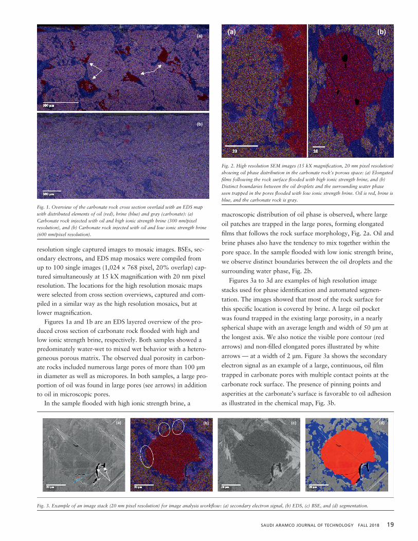
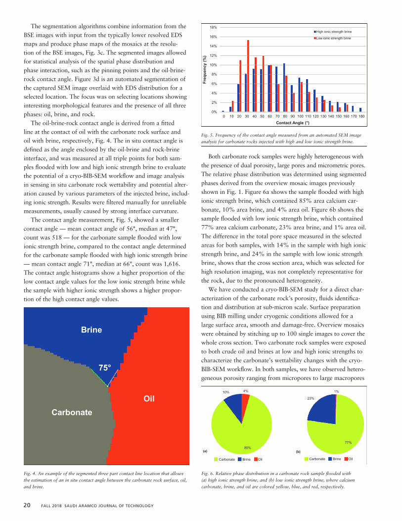
Figures 1a and 1b are an EDS layered overview of the pro-duced cross section of carbonate rock flooded with high and low ionic strength brine, respectively. Both samples showed a predominately water-wet to mixed wet behavior with a hetero-geneous porous matrix. The observed dual porosity in carbon-ate rocks included numerous large pores of more than 100 µm in diameter as well as micropores. In both samples, a large pro-portion of oil was found in large pores (see arrows) in addition to oil in microscopic pores.
In the sample flooded with high ionic strength brine, a
macroscopic distribution of oil phase is observed, where large
oil patches are trapped in the large pores, forming elongated
films that follows the rock surface morphology, Fig. 2a. Oil and
brine phases also have the tendency to mix together within the
pore space. In the sample flooded with low ionic strength brine,
we observe distinct boundaries between the oil droplets and the
surrounding water phase, Fig. 2b.
Figures 3a to 3d are examples of high resolution image
stacks used for phase identification and automated segmen-
tation. The images showed that most of the rock surface for
this specific location is covered by brine. A large oil pocket
was found trapped in the existing large porosity, in a nearly
spherical shape with an average length and width of 50 µm at
the longest axis. We also notice the visible pore contour (red
arrows) and non-filled elongated pores illustrated by white
arrows — at a width of 2 µm. Figure 3a shows the secondary
electron signal as an example of a large, continuous, oil film
trapped in carbonate pores with multiple contact points at the
carbonate rock surface. The presence of pinning points and
asperities at the carbonate’s surface is favorable to oil adhesion
as illustrated in the chemical map, Fig. 3b.
Fig. 1. Overview of the carbonate rock cross section overlaid with an EDS map with distributed elements of oil (red), brine (blue) and gray (carbonate): (a) Carbonate rock injected with oil and high ionic strength brine (300 nm/pixel resolution), and (b) Carbonate rock injected with oil and low ionic strength brine (600 nm/pixel resolution).
Fig. 2. High resolution SEM images (15 kX magnification, 20 nm pixel resolution) showing oil phase distribution in the carbonate rock’s porous space: (a) Elongated films following the rock surface flooded with high ionic strength brine, and (b) Distinct boundaries between the oil droplets and the surrounding water phase seen trapped in the pores flooded with low ionic strength brine. Oil is red, brine is blue, and the carbonate rock is gray.
Fig. 3. Example of an image stack (20 nm pixel resolution) for image analysis workflow: (a) secondary electron signal, (b) EDS, (c) BSE, and (d) segmentation.
Fig. 2. High resolution SEM images (15 kXdistribution in the carbonate rock’s porous space: (a)with high ionic strength brine, and (b) Distinctwater phase seen trapped in the pores flooded with lowthe carbonate rock is gray. Fig. 3. Example of an image stack (20 nm pixelelectron signal, (b) EDS, (c) BSE, and (d) segmentation.
20 µm
20 µm
(a) (b)
(a)
(c)
2020
Fig. 1. Overview of the carbonate rock cross section overlaid with an EDS map with distributed elements of oil (red), brine (blue) and gray (carbonate): (a) Carbonate rock injected with oil and high ionic strength brine (300 nm/pixel resolution), and (b) Carbonate rock injected with oil and low ionic strength brine (600 nm/pixel resolution).
(b)
(a)
300 μm
300 μm
Fig. 2. High resolution SEM images (15 kX magnification, 20 nm pixel resolution) showing oil phase distribution in the carbonate rock’s porous space: (a) Elongated films following the rock surface flooded with high ionic strength brine, and (b) Distinct boundaries between the oil droplets and the surrounding water phase seen trapped in the pores flooded with low ionic strength brine. Oil is red, brine is blue, and the carbonate rock is gray.
20 µm
20 µm
(a) (b)
(a)
(c) (d)
(b)
Fig. 2. High resolution SEM images (15 kX magnification, 20 nm pixel resolution)distribution in the carbonate rock’s porous space: (a) Elongated films following thewith high ionic strength brine, and (b) Distinct boundaries between the oil droplets andwater phase seen trapped in the pores flooded with low ionic strength brine. Oil is red,the carbonate rock is gray. Fig. 3. Example of an image stack (20 nm pixel resolution) for image analysiselectron signal, (b) EDS, (c) BSE, and (d) segmentation.
20 µm
20 µm
(a) (b)
(a)
(c) (d)
(b)
Fig. 2. High resolution SEM images (15 kX magnification, 20 nm pixel resolution)distribution in the carbonate rock’s porous space: (a) Elongated films following thewith high ionic strength brine, and (b) Distinct boundaries between the oil dropletswater phase seen trapped in the pores flooded with low ionic strength brine. Oil isthe carbonate rock is gray. Fig. 3. Example of an image stack (20 nm pixel resolution) for image analysiselectron signal, (b) EDS, (c) BSE, and (d) segmentation.
20 µm
20 µm
(a) (b)
(a)
(c) (d)
(b)
20 μm 20 μm 20 μm 20 μm
20 FALL 2018 SAUDI ARAMCO JOURNAL OF TECHNOLOGY
The segmentation algorithms combine information from the BSE images with input from the typically lower resolved EDS maps and produce phase maps of the mosaics at the resolu-tion of the BSE images, Fig. 3c. The segmented images allowed for statistical analysis of the spatial phase distribution and phase interaction, such as the pinning points and the oil-brine-rock contact angle. Figure 3d is an automated segmentation of the captured SEM image overlaid with EDS distribution for a selected location. The focus was on selecting locations showing interesting morphological features and the presence of all three phases: oil, brine, and rock.
The oil-brine-rock contact angle is derived from a fitted line at the contact of oil with the carbonate rock surface and oil with brine, respectively, Fig. 4. The in situ contact angle is defined as the angle enclosed by the oil-brine and rock-brine interface, and was measured at all triple points for both sam-ples flooded with low and high ionic strength brine to evaluate the potential of a cryo-BIB-SEM workflow and image analysis in sensing in situ carbonate rock wettability and potential alter-ation caused by various parameters of the injected brine, includ-ing ionic strength. Results were filtered manually for unreliable measurements, usually caused by strong interface curvature.
The contact angle measurement, Fig. 5, showed a smaller contact angle — mean contact angle of 56°, median at 47°, count was 518 — for the carbonate sample flooded with low ionic strength brine, compared to the contact angle determined for the carbonate sample flooded with high ionic strength brine — mean contact angle 71°, median at 66°, count was 1,616. The contact angle histograms show a higher proportion of the low contact angle values for the low ionic strength brine while the sample with higher ionic strength shows a higher propor-tion of the high contact angle values.
Both carbonate rock samples were highly heterogeneous with the presence of dual porosity, large pores and micrometric pores. The relative phase distribution was determined using segmented phases derived from the overview mosaic images previously shown in Fig. 1. Figure 6a shows the sample flooded with high ionic strength brine, which contained 85% area calcium car-bonate, 10% area brine, and 4% area oil. Figure 6b shows the sample flooded with low ionic strength brine, which contained 77% area calcium carbonate, 23% area brine, and 1% area oil. The difference in the total pore space measured in the selected areas for both samples, with 14% in the sample with high ionic strength brine, and 24% in the sample with low ionic strength brine, shows that the cross section area, which was selected for high resolution imaging, was not completely representative for the rock, due to the pronounced heterogeneity.
We have conducted a cryo-BIB-SEM study for a direct char-acterization of the carbonate rock’s porosity, fluids identifica-tion and distribution at sub-micron scale. Surface preparation using BIB milling under cryogenic conditions allowed for a large surface area, smooth and damage-free. Overview mosaics were obtained by stitching up to 100 single images to cover the whole cross section. Two carbonate rock samples were exposed to both crude oil and brines at low and high ionic strengths to characterize the carbonate’s wettability changes with the cryo-BIB-SEM workflow. In both samples, we have observed hetero-geneous porosity ranging from micropores to large macropores
Fig. 4. An example of the segmented three part contact line location that allows thesitu contact angle between the carbonate rock surface, oil, and brine.
75°
Oil
Brine
Carbonate
Fig. 4. An example of the segmented three part contact line location that allows the estimation of an in situ contact angle between the carbonate rock surface, oil, and brine.
Fig. 5. Frequency of the contact angle measured from an automated SEM image analysis for carbonate rocks injected with high and low ionic strength brine.
0%
2%
4%
6%
8%
10%
12%
14%
16%
18%
0 10 20 30 40 50 60 70 80 90 100 110 120 130 140 150 160 170 180
Freq
uenc
y (%
)
Contact Angle (°)
High ionic strength brine
Low ionic strength brine
Fig. 5. Frequency of the contact angle measured from an automated SEM image analysis for carbonate rocks injected with high and low ionic strength brine.
Fig. 6. Relative phase distribution in a carbonate rock sample flooded with (a) high ionic strength brine, and (b) low ionic strength brine, where calcium carbonate, brine, and oil are colored yellow, blue, and red, respectively.
(a)
10% 4% 1%
23%
77% 85%
Carbonate Brine Oil
Carbonate Brine Oil
(b) (a)
Fig. 6. Relative phase distribution in a carbonate rock sample flooded with (a) high ionic strength brine, and (b) low ionic strength brine, where calcium carbonate, brine, and oil are colored yellow, blue, and red, respectively.

SAUDI ARAMCO JOURNAL OF TECHNOLOGY FALL 2018 21
with more than 100 µm in length. The experimental protocol aimed to prepare samples with a mixed wet initial state to study the cryo-BIB-SEM protocol to the variation in injected brine ionic strength. The two selected cross sections were not repre-sentative of the carbonate rock due to the heterogeneity in place, differences in estimated porosity and oil distribution.
The saturation protocol followed for the sample’s prepara-tion consisted of capillary imbibition of brine, then oil imbibi-tion at low vacuum pressure, and finally a spontaneous flood with brine at low and high ionic strength brines. It is likely that the saturation protocol did not affect the small pores as oil imbibition will require a higher entry pressure. Subsequently, the large number of selected locations gives a fair statistical analysis and an idea about the oil-brine-rock interfaces and chemical variations that occur at the nanoscale level. At high ionic strength, a macroscopic distribution of large oil patches trapped in large pores was observed in an elongated shape that follows the rock surface curvature. Oil and brine phases were also observed to mix together while there are distinct boundar-ies between the oil and brine phases in the rock sample flooded with low ionic strength brine. In situ contact angles were esti-mated using an automated images segmentation.
As previously shown in Fig. 5, the contact angles of oil-brine-rock with low ionic strength brine were lower than those estimated for the carbonate rock sample flooded with high ionic strength brine. This indicates a higher water-wet character when using low ionic strength brine in agreement with previous studies3, 20. Oil droplets were also observed to have an affinity for asperities, considered as pinning points that contribute to oil adherence at the carbonate rock surface.
The contact angle estimation from image segmentation could be influenced by various parameters causing an overestimation of the contact angle due to the size of image pixels, oil droplets, and pores. A post-filtration was applied manually to all the selected locations to exclude the large curvatures and pinning points at the interface that contribute to the contact angle overestimation. Segmentation of images provided a statistical analysis of the in situ contact angle and results show a relatively less oil wet rock surface for the sample flooded with low ionic strength brine com-pared to the one flooded with high ionic strength brine.
At this stage, the presented feasibility study shows the poten-tial of cryo-BIB to prepare a suitable surface area for high res-olution imaging and SEM imaging combined with automated segmentation could potentially provide new insights of the oil-brine-rock interface at nano and sub-micron scale, identify trapped phases inside the porous matrix, and quantify the dis-tribution of the different phases. The cryo-BIB-SEM method also allows a statistical evaluation of the 2D contact angle and the oil-brine-rock interfaces.
CONCLUSIONS
We presented a cryo-BIB-SEM feasibility study to investigate the oil-brine-rock interface at a sub-micron scale and investigate
the sensitivity toward variations of the injected brine ionic strength. The following conclusions can be drawn based on the initial imaging analysis:
• Ion milling at cryogenic conditions allows the prepara-tion of a smooth rock cross section, free of damages, thereby providing access to the trapped fluids in carbon-ate porosity.
• Existing dual porosity influences the oil and brine dis-tribution in the porous matrix as a large amount of oil droplets were located in the largest pores in addition to a small portion of oil located in microporosity.
• Tendency of oil to adhere to the carbonate rock surface is emphasized by the presence of pinning points.
• Differences of oil and brine phase distribution were observed in low and high ionic strength brines.
• A 2D contact angle statistical analysis shows the sen-sitivity of the cryo-BIB-SEM technique to sub-micron scale chemical variations at the oil-brine-rock interface.
ACKNOWLEDGMENTS
The authors would like to thank the management of Saudi Aramco for their support and permission to publish this article. The authors would also like to thank Dr. Joyce Schmatz from Microstructure and Pores GmbH, Germany, for her valuable discussions.
This article was presented at the SPE EOR Conference at Oil and Gas West Asia, Muscat, Oman, March 26-28, 2018.
REFERENCES
1. Yousef, A.A., Al-Saleh, S., Al-Kaabi, A.U. and Al-Jawfi, M.S.: “Laboratory Investigation of Novel Oil Recovery Method for Carbonate Reservoirs,” SPE paper 137634, presented at the Canadian Unconventional Resources and International Petroleum Conference, Calgary, Alberta, Canada, October 19-21, 2010.
2. Yousef, A.A., Al-Saleh, S.H. and Al-Jawfi, M.S.: “SmartWater Flooding for Carbonate Reservoirs: Salinity and Role of Ions,” SPE paper 141082, presented at the SPE Middle East Oil and Gas Show and Conference, Manama, Bahrain, September 25-28, 2011.
3. Yousef, A.A., Al-Saleh, S.H. and Al-Jawfi, M.S.: “Improved/Enhanced Oil Recovery from Carbonate Reservoirs by Tuning Injection Water Salinity and Ionic Content,” SPE paper 154076, presented at the SPE Improved Oil Recovery Symposium, Tulsa, Oklahoma, April 14-18, 2012.
4. Yousef, A.A. and Ayirala, S.C.: “Optimization Study of a Novel Water-Ionic Technology for SmartWater Flooding Application in Carbonate Reservoirs,” Oil and Gas
Facilities, Vol. 3, Issue 5, October 2014, pp. 72-82.

22 FALL 2018 SAUDI ARAMCO JOURNAL OF TECHNOLOGY
5. Yi, Z. and Sharma, H.K.: “Improving Waterflood Recovery Efficiency in Carbonate Reservoirs through Salinity Variations and Ionic Exchanges: A Promising Low-Cost ‘Smart Waterflood’ Approach,” SPE paper 161631, presented at the Abu Dhabi International Petroleum Conference and Exhibition, Abu Dhabi, UAE, December 11-14, 2012.
6. Al Geer, M.A., Gmira, A., Al-Enezi, S.M. and Yousef, A.A.: “A New Insight on the Impact of Individual Ions on Fluid/Fluid Interactions and SmartWater Recovery,” SPE paper 179779, presented at the SPE EOR Conference at Oil and Gas West Asia, Muscat, Oman, March 21-23, 2016.
7. Al Geer, M.A., Gmira, A., Al-Enezi, S.M. and Yousef, A.A.: “Impact of Individual Ions on Oil/Brine/Rock Interface: A Macroscopic Insight on Wettability Alteration,” SPE paper 183202, presented at the Abu Dhabi International Petroleum Exhibition and Conference, Abu Dhabi, UAE, November 7-10, 2016.
8. Al-Otaibi, M.B. and Yousef, A.A.: “The Impact of Dissolved Species on the Reservoir Fluids and Rock Interactions in Carbonates,” SPE paper 177983, presented at the SPE Saudi Arabia Section Annual Technical Symposium and Exhibition, al-Khobar, Saudi Arabia, April 21-23, 2015.
9. Gmira, A., Al-Enezi, S.M. and Yousef, A.A.: “Ions Dependent Stability of Stearic Acid Langmuir Monolayers: An Insight of Oil/Water Interface in SmartWater Flood,” SPE paper 183855, presented at the SPE Middle East Oil & Gas Show and Conference, Manama, Bahrain, March 6-9, 2017.
10. Gmira, A., Al-Enezi, S.M. and Yousef, A.A.: “Interfacial Rheology at the Crude Oil/Brine Interface: A Microscopic Insight of SmartWater Flood,” poster presented at the 19th European Symposium on Improved Oil Recovery, Stavanger, Norway, April 24-27, 2017.
11. Schwartz, D.E.: “Scanning Electron Microscope — Cold Stage: Viewing Fluid Saturated Reservoir Rock,” SPE paper 9248, presented at the SPE Annual Fall Technical Conference and Exhibition, Dallas, Texas, September 21-24, 1980.
12. Pescheck, P.S., Davis, H.T. and Scriven, L.E.: “Cold Stage Scanning Electron Microscopy of Crude Oil and Brine in Rock,” Scanning Electron Microscopy, Vol. 1, January 1981, pp. 515-524.
13. Sutanto, E., Davis, H.T. and Scriven, L.E.: “Liquid Distributions in Porous Rock Examined by Cryo Scanning Electron Microscopy,” SPE paper 20518, presented at the SPE Annual Technical Conference and Exhibition, New Orleans, Louisiana, September 23-26, 1990.
14. Robin, M., Rosenberg, E. and Fassi-Fihri, O.: “Wettability Studies at the Pore Level: A New Approach by Use of Cryo-SEM,” SPE Formation Evaluation, Vol. 10, Issue 1, March 1995, pp. 11-19.
15. Desbois, G., Urai, J.L., Perez-Willard, F., Radi, Z., et al.: “Argon Broad Ion Beam Tomography in a Cryogenic Scanning Electron Microscope: A Novel Tool for the Investigation of Representative Microstructures in Sedimentary Rocks Containing Pore Fluid,” Journal of Microscopy, Vol. 249, Issue 3, January 2016, pp. 215-235.
16. Cha, D.K., Al-Otaibi, M.B. and Yousef, A.A.: “Visualization and Distribution of Ions at Fluids-Rock Interfaces: Angstrom Scale Study,” SPE paper 174676, presented at the SPE Asia Pacific Enhanced Oil Recovery Conference, Kuala Lumpur, Malaysia, August 11-13, 2015.
17. Schmatz, J., Urai, J.L., Berg, S. and Ott, H.: “Nanoscale Imaging of Pore-Scale Fluid-Fluid-Solid Contacts in Sandstone,” Geophysical Research Letters, Vol. 42, Issue 7, April 2015, pp. 2189-2195.
18. Schmatz, J., Klaver, J., Jiang, M. and Urai, J.L.: “Nanoscale Morphology of Brine/Oil/Mineral Contacts in Connected Pores of Carbonate Reservoirs: Insights on Wettability from Cryo-BIB-SEM,” SPE Journal, Vol. 22, Issue 5, October 2017, pp. 1374-1384.
19. Zhang, S. and Gogos, G.: “Film Evaporation of a Spherical Droplet over a Hot Surface: Fluid Mechanics and Heat/Mass Transfer Analysis,” Journal of Fluid Mechanics, Vol. 222, January 1991, pp. 543-563.
20. Austad, T., Shariatpanahi, S.F., Strand, S., Black, C.J.J., et al.: “Conditions for a Low-Salinity Enhanced Oil Recovery (EOR) Effect in Carbonate Oil Reservoirs,” Energy & Fuels, Vol. 26, Issue 1, 2011, pp. 569-575.
SAUDI ARAMCO JOURNAL OF TECHNOLOGY FALL 2018 23
BIOGRAPHIES
Dr. Ahmed Gmira is a Petroleum Sci-entist with the SmartWater Team of Saudi Aramco’s Exploration and Petro-leum Engineering Center – Advanced Research Center (EXPEC ARC). His main interests are enhanced oil recov-ery, SmartWater Flooding, fluids-fluids
interfaces and fluids-rocks interfaces.Ahmed joined Saudi Aramco in April 2015. Prior to
this, he worked as a Research Scientist in the Schlumberger Research Centers in Dhahran, Saudi Arabia, and in Rio de Janeiro, Brazil. He also worked as a Research Fellow in a postdoctoral position with the Department of Physics at the Norwegian University of Science and Technology, Trond-heim, Norway.
Ahmed received his Ph.D. degree in Physico-Chemistry from the University of Orléans, Orléans, France.
Dr. Dongkyu Cha joined Saudi Aramco in 2013 as a Petroleum Engi-neer with Saudi Aramco’s Exploration and Petroleum Engineering Center – Advanced Research Center (EXPEC ARC). His current interests are on fundamental research for defining and
understanding of fluid-fluid and fluid-rock interactions at molecular scale.
Prior to Dong’s current position, he was a Research Scientist at the King Abdullah University of Science and Technology’s imaging core lab as a Transmission Electron Microscopy, Scanning Electron Microscopy and Focused Ion Beam Specialist. Dong has published more than 70 technical papers as a first author/coauthor, and has filed two patents.
He received his Ph.D. degree in Material Science and Engineering from the University of Texas at Dallas, Richardson, TX.
Dr. Sultan M. Al-Enezi is a Petroleum Engineering Specialist and the cham-pion of the SmartWater Focus Area with the Reservoir Engineering Tech-nology Division of Saudi Aramco’s Exploration and Petroleum Engineering Center – Advance Research Center
(EXPEC ARC). His research interests include enhanced oil recovery, digital rock physics, petrophysics, and fluid flow in porous media.
Sultan is an active member of the Society of Petroleum Engineers (SPE), and has participated as co-chair, session chair, technical committee member, and discussion leader in various international SPE events.
He received his B.S. degree in Industrial Chemistry from King Fahd University of Petroleum and Minerals (KFUPM), Dhahran, Saudi Arabia. Sultan also received his M.S. and Ph.D. degrees in Petroleum and Natural Gas Engineering from Pennsylvania State University, University Park, PA.
Dr. Ali A. Al-Yousef is a Senior Petro-leum Engineering Consultant and Chief Technologist of the Reservoir Engineer-ing Technology Division in Saudi Aramco’s Upstream Advanced Research Center. He has more than 24 years of experience in upstream
research and technology. Since joining Saudi Aramco, Ali has been involved in applied research projects on improved oil recovery (IOR), waterflooding and enhanced oil recovery (EOR). He played a pivotal role in planning, developing and implementing the EOR roadmap for the company.
Ali is currently leading more than 50 EOR scientists, engineers, and technicians. Those EOR researchers are ded-icated to development of various EOR processes, including SmartWater Flooding, carbon dioxide and chemical EOR technologies, as well as other novel processes with the clear target of meeting Saudi Aramco’s objective. He was the impetus for Saudi Aramco’s SmartWater Flooding revolu-tion: a patented award-winning technology. In 2011, this technology won the ADIPEC Award for Innovation and Technology. Its implementation is the industry’s first multi-well pilot of SmartWater Flooding.
In 2016, Ali was the recipient of the prestigious Society of Petroleum Engineers (SPE) IOR Pioneer Award for his pio-neering contributions made to the advancement of recovery technologies in the field of IOR/EOR. He also received the very prestigious award of The Custodian of the Two Holy Mosques Prize for Inventors and Talents in 2017.
Ali has written over 60 technical papers and reports and has more than eight granted patents. He is currently an active member of SPE and has chaired several SPE workshops and forums, helped organize several petroleum engineering related conferences, and taught courses on IOR/EOR and waterflooding.
Ali received his B.S. degree in Chemical Engineering from King Fahd University of Petroleum and Minerals (KFUPM), Dhahran, Saudi Arabia, and his M.S. and Ph.D. degrees, both in Petroleum Engineering, from the University of Texas at Austin, Austin, TX.
24 FALL 2018 SAUDI ARAMCO JOURNAL OF TECHNOLOGY
ABSTRACT
In downhole oil field operations that involve pumping oil and water, information on mixture viscosity is important to fur-ther understand the performance of the downhole production equipment. This study presents a method for determining the effective absolute viscosity of oil-water mixtures by applying fluid mechanics’ first principles to data representative of down-hole production measurements. Knowledge of effective abso-lute viscosity in upstream and downstream oil field operations is essential to extend equipment life and optimize production operations.
A 7” 26 lb/ft pipe and a 3½” 9.20 lb/ft pipe, typically used as casing and tubing, respectively, in field operations were installed in an oil-water flow loop. The volume flow rates during the tests varied from 2,000 barrels per day (bpd) to 12,000 bpd, representative of target field production rates. The tests were performed at different inclinations to represent varying well deviation angles. For each oil and water flow rate, the corresponding pressure drop measurements across a fully developed section of the flow were measured. Using fun-damental hydraulic relationships, the effective absolute viscos-ities of the oil-water mixtures were determined.
The results showed that as water cut varied, the effective mixture absolute viscosity also changed, and in some cases this was substantial. The highest effective absolute viscosity of 500 centipoise (cP) occurred at the mixture flow rate corresponding to 2,000 bpd and 40% water cut. In general, mixture flow rates of 2,000 bpd and water cuts between 40% and 60% consis-tently showed the highest effective absolute mixture viscosities, which varied between 160 cP to 500 cP. For water cuts outside the 40% to 60% range, the effective absolute viscosities were about 120 cP and less. These results indicate that the effective mixture viscosity is about two and close to three orders of mag-nitude of pure oil and pure water viscosities, respectively. The results also suggest that certain flow rates and water cuts sig-nificantly affect the viscosity of oil-water flows.
Other results showed that for a given mixture flow rate, the effective viscosities were about the same order of magnitude for the different inclinations. This indicates that the well devi-ation angle has minimal or negligible influence on the effec-tive mixture’s absolute viscosity. From the combined results
the technique used in this study provides additional insight to ascertain the effective viscosity of oil-water mixtures during field operations. This study highlights the importance of hav-ing the capability to determine the effective absolute viscosity of oil-water mixtures during oil field production operations. The methodology is simple and has the advantage of easy integration into a flow measurement system. Such systems are beneficial tools for reservoir engineers, production engineers and field operators in general, for making appropriate produc-tion modifications during operations, to increase asset life and maximize hydrocarbon recovery.
INTRODUCTION
Oil and water are some of the reservoir fluids produced from downhole to the surface in many oil and gas field operations. In some cases, the oil and water may be separated down-hole with only the oil produced to the surface and the water re-injected back into the reservoir. Subsequently, either due to capacity handling, or complex completion layout, not all operators utilize downhole oil-water separators. Instead, during production, the oil and water have to be produced to the surface as a liquid-liquid mixture, where the oil and water are either separated at the well site or transported to a pro-cessing facility further downstream, where the separation pro-cess occurs.
Electric submersible pumps (ESPs) are a type of artificial lift method used in the oil and gas industry to either lift reservoir fluids from dead wells, or boost production from naturally flowing wells. ESPs operate favorably when pumping pure liquids, e.g., water or oil, or liquid with very low gas content. Depending on the proportions of oil and water, or water cut, from the reservoir, the viscosity of oil-water mixtures can vary substantially. A phenomenon known as phase inversion occurs when the mixture flow changes from a continuous water to continuous oil, or vice versa. At the point of phase inversion, the viscosity of the mixture is significantly higher than the viscosity of pure oil or pure water.
Under such flow conditions, the performance of the ESP, such as the head developed by the pump, degrades consid-erably and any attempt to increase the flow rate or head by adjusting motor conditions can lead to motor overload and
Determining Effective Mixture Viscosities in Oil-Water Flows for Downhole Oil Field Operations
Dr. Chidrim E. Ejim and Dr. Jinjiang Xiao
SAUDI ARAMCO JOURNAL OF TECHNOLOGY FALL 2018 25
potential failure of the ESP system. Current ESP installa-tions are equipped with downhole sensors that can measure parameters such as intake and discharge pressure, intake and discharge temperature, motor vibration, motor oil and wind-ing temperature, as well as motor current. Estimating the oil-water mixture viscosity downhole is desirable to give the operator additional information on the downhole flow condi-tion the ESP is operating in, and subsequently setup a series of remedial or operational actions to mitigate against poten-tial failure of the ESP system, thereby increasing operational efficiency.
Previous studies on viscosities of solutions are present in the literature, which show relationships between the contin-uous and dispersed phases within the mixture1. Other stud-ies have involved experimental work on oil-water flows in horizontal pipelines, in which the ultimate objective was to develop a viscosity prediction model for this type of flow2. Additional studies on the effect of mixing intensity on oil-wa-ter mixture viscosities at different temperatures have also been performed3, in which the inversion point was observed to occur at about 35% water cut. Some studies have been under-taken on predicting viscosities in oil-water mixtures using an intelligent model4. The researchers reported a very good fit of the model to the laboratory data. Yet some other work was done by measuring oil-water viscosity variation with water cut at atmospheric pressure under different temperatures and shear rates, where a modified viscosity correlation was developed5.
Li et al. (2016)5 observed an inversion point at 20% water cut. In the above studies, given the various potential water cuts that phase inversion can occur, it is evident that a single model to determine the effective viscosity of oil and water mixtures may not be fully transferable to all oil-water systems due to the complex flow regimes inherent in these mixtures. A method to determine the effective viscosity of oil-water mixtures downhole has to be on a case-by-case basis. A direct measurement method will be very beneficial to field operators as it provides production viscosity information representative of downhole fluid characteristics from a specific well.
Such a method is discussed in this work, which also looks into the effect of oil-water mixture flow rates on the effective oil-water mixture viscosity. The work also shows the effect of flow conduit inclination angle on the effective oil-water mix-ture viscosity. The information from such direct measurements can be used by the operator to make proper adjustments to field equipment during production operations to further extend the life of the equipment and also improve the overall operating economics of the field asset.
BACKGROUND THEORY
Viscosity estimation requires an understanding of the pressure drop of the flow through pipes or annular conduits. From elementary fluid mechanics, it can be shown from the first
principle that the total pressure drop in a fluid flowing in a conduit can be given as:
∆𝑝𝑝𝑡𝑡 = 𝜌𝜌𝜌𝜌𝜌𝜌 sin 𝜃𝜃 + 𝑓𝑓𝑓𝑓𝐷𝐷ℎ
𝜌𝜌𝑉𝑉2
2 (1)
𝑉𝑉 = 𝑄𝑄0.25𝜋𝜋(𝐷𝐷𝑂𝑂
2 −𝐷𝐷𝑖𝑖2)
1√𝑓𝑓 = −0.86 𝑙𝑙𝑙𝑙 (
𝜀𝜀 𝐷𝐷ℎ⁄3.7 + 2.51
𝑅𝑅𝑅𝑅√𝑓𝑓) (2)
𝑅𝑅𝑅𝑅 = 4𝜌𝜌𝑄𝑄𝜋𝜋𝜋𝜋𝐷𝐷ℎ
(3)
1√𝑓𝑓 = 𝐴𝐴 − (𝐵𝐵−𝐴𝐴)2
𝐶𝐶−2𝐵𝐵+𝐴𝐴 (4)
𝐴𝐴 = −2.0 𝑙𝑙𝑙𝑙𝜌𝜌10 (𝜀𝜀 𝐷𝐷ℎ⁄3.7 + 12
𝑅𝑅𝑅𝑅) (5)
𝐵𝐵 = −2.0 𝑙𝑙𝑙𝑙𝜌𝜌10 (𝜀𝜀 𝐷𝐷ℎ⁄3.7 + 2.51𝐴𝐴
𝑅𝑅𝑅𝑅 ) (6)
𝐶𝐶 = −2.0 𝑙𝑙𝑙𝑙𝜌𝜌10 (𝜀𝜀 𝐷𝐷ℎ⁄3.7 + 2.51𝐵𝐵
𝑅𝑅𝑅𝑅 ) (7)
𝑄𝑄𝑚𝑚 = 𝑄𝑄𝑜𝑜 + 𝑄𝑄𝑤𝑤 (8)
𝜌𝜌𝑚𝑚 = 𝛼𝛼𝑜𝑜𝜌𝜌𝑜𝑜 + 𝛼𝛼𝑤𝑤𝜌𝜌𝑤𝑤 (9)
𝜌𝜌𝑚𝑚 = 𝑄𝑄𝑜𝑜𝑄𝑄𝑤𝑤+𝑄𝑄𝑜𝑜
𝜌𝜌𝑜𝑜 + 𝑄𝑄𝑤𝑤𝑄𝑄𝑤𝑤+𝑄𝑄𝑜𝑜
𝜌𝜌𝑤𝑤 (10)
(1)
In Eqn. 1, the first term on the right-hand side represents the pressure drop due to gravitational acceleration, whereas the second term is the pressure drop due to friction and expressed as the Darcy-Weisbach equation. The parameters in Eqn. 1 are defined as: ∆pt = total pressure drop, ρ = fluid density, g = acceleration due to gravity, L = distance across which the pressure drop occurred, θ = inclination angle of the conduit from the horizontal, f = friction factor, V = average fluid velocity across the conduit, and Dh = hydraulic diameter of the conduit.
For a general case of flow through conduits with internal and outer diameters of Di and Do, respectively, and volume flow rate, Q, the velocity,
∆𝑝𝑝𝑡𝑡 = 𝜌𝜌𝜌𝜌𝜌𝜌 sin 𝜃𝜃 + 𝑓𝑓𝑓𝑓𝐷𝐷ℎ
𝜌𝜌𝑉𝑉2
2 (1)
𝑉𝑉 = 𝑄𝑄0.25𝜋𝜋(𝐷𝐷𝑂𝑂
2 −𝐷𝐷𝑖𝑖2)
1√𝑓𝑓 = −0.86 𝑙𝑙𝑙𝑙 (
𝜀𝜀 𝐷𝐷ℎ⁄3.7 + 2.51
𝑅𝑅𝑅𝑅√𝑓𝑓) (2)
𝑅𝑅𝑅𝑅 = 4𝜌𝜌𝑄𝑄𝜋𝜋𝜋𝜋𝐷𝐷ℎ
(3)
1√𝑓𝑓 = 𝐴𝐴 − (𝐵𝐵−𝐴𝐴)2
𝐶𝐶−2𝐵𝐵+𝐴𝐴 (4)
𝐴𝐴 = −2.0 𝑙𝑙𝑙𝑙𝜌𝜌10 (𝜀𝜀 𝐷𝐷ℎ⁄3.7 + 12
𝑅𝑅𝑅𝑅) (5)
𝐵𝐵 = −2.0 𝑙𝑙𝑙𝑙𝜌𝜌10 (𝜀𝜀 𝐷𝐷ℎ⁄3.7 + 2.51𝐴𝐴
𝑅𝑅𝑅𝑅 ) (6)
𝐶𝐶 = −2.0 𝑙𝑙𝑙𝑙𝜌𝜌10 (𝜀𝜀 𝐷𝐷ℎ⁄3.7 + 2.51𝐵𝐵
𝑅𝑅𝑅𝑅 ) (7)
𝑄𝑄𝑚𝑚 = 𝑄𝑄𝑜𝑜 + 𝑄𝑄𝑤𝑤 (8)
𝜌𝜌𝑚𝑚 = 𝛼𝛼𝑜𝑜𝜌𝜌𝑜𝑜 + 𝛼𝛼𝑤𝑤𝜌𝜌𝑤𝑤 (9)
𝜌𝜌𝑚𝑚 = 𝑄𝑄𝑜𝑜𝑄𝑄𝑤𝑤+𝑄𝑄𝑜𝑜
𝜌𝜌𝑜𝑜 + 𝑄𝑄𝑤𝑤𝑄𝑄𝑤𝑤+𝑄𝑄𝑜𝑜
𝜌𝜌𝑤𝑤 (10)
, and Dh = Do – Di.In fluid literature6, the friction factor is typically expressed
by the Colebrook-White equation, as shown in Eqns. 2 and 3:
∆𝑝𝑝𝑡𝑡 = 𝜌𝜌𝜌𝜌𝜌𝜌 sin 𝜃𝜃 + 𝑓𝑓𝑓𝑓𝐷𝐷ℎ
𝜌𝜌𝑉𝑉2
2 (1)
𝑉𝑉 = 𝑄𝑄0.25𝜋𝜋(𝐷𝐷𝑂𝑂
2 −𝐷𝐷𝑖𝑖2)
1√𝑓𝑓 = −0.86 𝑙𝑙𝑙𝑙 (
𝜀𝜀 𝐷𝐷ℎ⁄3.7 + 2.51
𝑅𝑅𝑅𝑅√𝑓𝑓) (2)
𝑅𝑅𝑅𝑅 = 4𝜌𝜌𝑄𝑄𝜋𝜋𝜋𝜋𝐷𝐷ℎ
(3)
1√𝑓𝑓 = 𝐴𝐴 − (𝐵𝐵−𝐴𝐴)2
𝐶𝐶−2𝐵𝐵+𝐴𝐴 (4)
𝐴𝐴 = −2.0 𝑙𝑙𝑙𝑙𝜌𝜌10 (𝜀𝜀 𝐷𝐷ℎ⁄3.7 + 12
𝑅𝑅𝑅𝑅) (5)
𝐵𝐵 = −2.0 𝑙𝑙𝑙𝑙𝜌𝜌10 (𝜀𝜀 𝐷𝐷ℎ⁄3.7 + 2.51𝐴𝐴
𝑅𝑅𝑅𝑅 ) (6)
𝐶𝐶 = −2.0 𝑙𝑙𝑙𝑙𝜌𝜌10 (𝜀𝜀 𝐷𝐷ℎ⁄3.7 + 2.51𝐵𝐵
𝑅𝑅𝑅𝑅 ) (7)
𝑄𝑄𝑚𝑚 = 𝑄𝑄𝑜𝑜 + 𝑄𝑄𝑤𝑤 (8)
𝜌𝜌𝑚𝑚 = 𝛼𝛼𝑜𝑜𝜌𝜌𝑜𝑜 + 𝛼𝛼𝑤𝑤𝜌𝜌𝑤𝑤 (9)
𝜌𝜌𝑚𝑚 = 𝑄𝑄𝑜𝑜𝑄𝑄𝑤𝑤+𝑄𝑄𝑜𝑜
𝜌𝜌𝑜𝑜 + 𝑄𝑄𝑤𝑤𝑄𝑄𝑤𝑤+𝑄𝑄𝑜𝑜
𝜌𝜌𝑤𝑤 (10)
(2)
∆𝑝𝑝𝑡𝑡 = 𝜌𝜌𝜌𝜌𝜌𝜌 sin 𝜃𝜃 + 𝑓𝑓𝑓𝑓𝐷𝐷ℎ
𝜌𝜌𝑉𝑉2
2 (1)
𝑉𝑉 = 𝑄𝑄0.25𝜋𝜋(𝐷𝐷𝑂𝑂
2 −𝐷𝐷𝑖𝑖2)
1√𝑓𝑓 = −0.86 𝑙𝑙𝑙𝑙 (
𝜀𝜀 𝐷𝐷ℎ⁄3.7 + 2.51
𝑅𝑅𝑅𝑅√𝑓𝑓) (2)
𝑅𝑅𝑅𝑅 = 4𝜌𝜌𝑄𝑄𝜋𝜋𝜋𝜋𝐷𝐷ℎ
(3)
1√𝑓𝑓 = 𝐴𝐴 − (𝐵𝐵−𝐴𝐴)2
𝐶𝐶−2𝐵𝐵+𝐴𝐴 (4)
𝐴𝐴 = −2.0 𝑙𝑙𝑙𝑙𝜌𝜌10 (𝜀𝜀 𝐷𝐷ℎ⁄3.7 + 12
𝑅𝑅𝑅𝑅) (5)
𝐵𝐵 = −2.0 𝑙𝑙𝑙𝑙𝜌𝜌10 (𝜀𝜀 𝐷𝐷ℎ⁄3.7 + 2.51𝐴𝐴
𝑅𝑅𝑅𝑅 ) (6)
𝐶𝐶 = −2.0 𝑙𝑙𝑙𝑙𝜌𝜌10 (𝜀𝜀 𝐷𝐷ℎ⁄3.7 + 2.51𝐵𝐵
𝑅𝑅𝑅𝑅 ) (7)
𝑄𝑄𝑚𝑚 = 𝑄𝑄𝑜𝑜 + 𝑄𝑄𝑤𝑤 (8)
𝜌𝜌𝑚𝑚 = 𝛼𝛼𝑜𝑜𝜌𝜌𝑜𝑜 + 𝛼𝛼𝑤𝑤𝜌𝜌𝑤𝑤 (9)
𝜌𝜌𝑚𝑚 = 𝑄𝑄𝑜𝑜𝑄𝑄𝑤𝑤+𝑄𝑄𝑜𝑜
𝜌𝜌𝑜𝑜 + 𝑄𝑄𝑤𝑤𝑄𝑄𝑤𝑤+𝑄𝑄𝑜𝑜
𝜌𝜌𝑤𝑤 (10)
(3)
where, is the absolute roughness of the wetted pipe wall, Re is the Reynolds Number, and μ is the absolute viscosity of the fluid.
To obtain the absolute viscosity using Eqns. 2 and 3 requires knowledge of the friction factor, f. The f equation is of an implicit form, and therefore, the f cannot be solved for explicitly; however, Asker et al. (2014)7 reviewed a number of f relationships for flow in pipes. They found that one of the correlations with the best result is that by Serghides (1984)8, which is valid for all Re and relative roughness ( /Dh), and has a percent error of 10-4%. The Serghides equation is shown in Eqns. 4 to 7:
∆𝑝𝑝𝑡𝑡 = 𝜌𝜌𝜌𝜌𝜌𝜌 sin 𝜃𝜃 + 𝑓𝑓𝑓𝑓𝐷𝐷ℎ
𝜌𝜌𝑉𝑉2
2 (1)
𝑉𝑉 = 𝑄𝑄0.25𝜋𝜋(𝐷𝐷𝑂𝑂
2 −𝐷𝐷𝑖𝑖2)
1√𝑓𝑓 = −0.86 𝑙𝑙𝑙𝑙 (
𝜀𝜀 𝐷𝐷ℎ⁄3.7 + 2.51
𝑅𝑅𝑅𝑅√𝑓𝑓) (2)
𝑅𝑅𝑅𝑅 = 4𝜌𝜌𝑄𝑄𝜋𝜋𝜋𝜋𝐷𝐷ℎ
(3)
1√𝑓𝑓 = 𝐴𝐴 − (𝐵𝐵−𝐴𝐴)2
𝐶𝐶−2𝐵𝐵+𝐴𝐴 (4)
𝐴𝐴 = −2.0 𝑙𝑙𝑙𝑙𝜌𝜌10 (𝜀𝜀 𝐷𝐷ℎ⁄3.7 + 12
𝑅𝑅𝑅𝑅) (5)
𝐵𝐵 = −2.0 𝑙𝑙𝑙𝑙𝜌𝜌10 (𝜀𝜀 𝐷𝐷ℎ⁄3.7 + 2.51𝐴𝐴
𝑅𝑅𝑅𝑅 ) (6)
𝐶𝐶 = −2.0 𝑙𝑙𝑙𝑙𝜌𝜌10 (𝜀𝜀 𝐷𝐷ℎ⁄3.7 + 2.51𝐵𝐵
𝑅𝑅𝑅𝑅 ) (7)
𝑄𝑄𝑚𝑚 = 𝑄𝑄𝑜𝑜 + 𝑄𝑄𝑤𝑤 (8)
𝜌𝜌𝑚𝑚 = 𝛼𝛼𝑜𝑜𝜌𝜌𝑜𝑜 + 𝛼𝛼𝑤𝑤𝜌𝜌𝑤𝑤 (9)
= 𝑄𝑄𝑜𝑜 + 𝑄𝑄𝑤𝑤
(4)
where:
∆𝑝𝑝𝑡𝑡 = 𝜌𝜌𝜌𝜌𝜌𝜌 sin 𝜃𝜃 + 𝑓𝑓𝑓𝑓𝐷𝐷ℎ
𝜌𝜌𝑉𝑉2
2 (1)
𝑉𝑉 = 𝑄𝑄0.25𝜋𝜋(𝐷𝐷𝑂𝑂
2 −𝐷𝐷𝑖𝑖2)
1√𝑓𝑓 = −0.86 𝑙𝑙𝑙𝑙 (
𝜀𝜀 𝐷𝐷ℎ⁄3.7 + 2.51
𝑅𝑅𝑅𝑅√𝑓𝑓) (2)
𝑅𝑅𝑅𝑅 = 4𝜌𝜌𝑄𝑄𝜋𝜋𝜋𝜋𝐷𝐷ℎ
(3)
1√𝑓𝑓 = 𝐴𝐴 − (𝐵𝐵−𝐴𝐴)2
𝐶𝐶−2𝐵𝐵+𝐴𝐴 (4)
𝐴𝐴 = −2.0 𝑙𝑙𝑙𝑙𝜌𝜌10 (𝜀𝜀 𝐷𝐷ℎ⁄3.7 + 12
𝑅𝑅𝑅𝑅) (5)
𝐵𝐵 = −2.0 𝑙𝑙𝑙𝑙𝜌𝜌10 (𝜀𝜀 𝐷𝐷ℎ⁄3.7 + 2.51𝐴𝐴
𝑅𝑅𝑅𝑅 ) (6)
𝐶𝐶 = −2.0 𝑙𝑙𝑙𝑙𝜌𝜌10 (𝜀𝜀 𝐷𝐷ℎ⁄3.7 + 2.51𝐵𝐵
𝑅𝑅𝑅𝑅 ) (7)
𝑄𝑄𝑚𝑚 = 𝑄𝑄𝑜𝑜 + 𝑄𝑄𝑤𝑤 (8)
𝜌𝜌𝑚𝑚 = 𝛼𝛼𝑜𝑜𝜌𝜌𝑜𝑜 + 𝛼𝛼𝑤𝑤𝜌𝜌𝑤𝑤 (9)
(5)
∆𝑝𝑝𝑡𝑡 = 𝜌𝜌𝜌𝜌𝜌𝜌 sin 𝜃𝜃 + 𝑓𝑓𝑓𝑓𝐷𝐷ℎ
𝜌𝜌𝑉𝑉2
2 (1)
𝑉𝑉 = 𝑄𝑄0.25𝜋𝜋(𝐷𝐷𝑂𝑂
2 −𝐷𝐷𝑖𝑖2)
1√𝑓𝑓 = −0.86 𝑙𝑙𝑙𝑙 (
𝜀𝜀 𝐷𝐷ℎ⁄3.7 + 2.51
𝑅𝑅𝑅𝑅√𝑓𝑓) (2)
𝑅𝑅𝑅𝑅 = 4𝜌𝜌𝑄𝑄𝜋𝜋𝜋𝜋𝐷𝐷ℎ
(3)
1√𝑓𝑓 = 𝐴𝐴 − (𝐵𝐵−𝐴𝐴)2
𝐶𝐶−2𝐵𝐵+𝐴𝐴 (4)
𝐴𝐴 = −2.0 𝑙𝑙𝑙𝑙𝜌𝜌10 (𝜀𝜀 𝐷𝐷ℎ⁄3.7 + 12
𝑅𝑅𝑅𝑅) (5)
𝐵𝐵 = −2.0 𝑙𝑙𝑙𝑙𝜌𝜌10 (𝜀𝜀 𝐷𝐷ℎ⁄3.7 + 2.51𝐴𝐴
𝑅𝑅𝑅𝑅 ) (6)
𝐶𝐶 = −2.0 𝑙𝑙𝑙𝑙𝜌𝜌10 (𝜀𝜀 𝐷𝐷ℎ⁄3.7 + 2.51𝐵𝐵
𝑅𝑅𝑅𝑅 ) (7)
𝑄𝑄𝑚𝑚 = 𝑄𝑄𝑜𝑜 + 𝑄𝑄𝑤𝑤 (8)
𝜌𝜌𝑚𝑚 = 𝛼𝛼𝑜𝑜𝜌𝜌𝑜𝑜 + 𝛼𝛼𝑤𝑤𝜌𝜌𝑤𝑤 (9)
𝜌𝜌𝑚𝑚 = 𝑄𝑄𝑜𝑜𝑄𝑄𝑤𝑤+𝑄𝑄𝑜𝑜
𝜌𝜌𝑜𝑜 + 𝑄𝑄𝑤𝑤𝑄𝑄𝑤𝑤+𝑄𝑄𝑜𝑜
𝜌𝜌𝑤𝑤 (10)
(6)
∆𝑝𝑝𝑡𝑡 = 𝜌𝜌𝜌𝜌𝜌𝜌 sin 𝜃𝜃 + 𝑓𝑓𝑓𝑓𝐷𝐷ℎ
𝜌𝜌𝑉𝑉2
2 (1)
𝑉𝑉 = 𝑄𝑄0.25𝜋𝜋(𝐷𝐷𝑂𝑂
2 −𝐷𝐷𝑖𝑖2)
1√𝑓𝑓 = −0.86 𝑙𝑙𝑙𝑙 (
𝜀𝜀 𝐷𝐷ℎ⁄3.7 + 2.51
𝑅𝑅𝑅𝑅√𝑓𝑓) (2)
𝑅𝑅𝑅𝑅 = 4𝜌𝜌𝑄𝑄𝜋𝜋𝜋𝜋𝐷𝐷ℎ
(3)
1√𝑓𝑓 = 𝐴𝐴 − (𝐵𝐵−𝐴𝐴)2
𝐶𝐶−2𝐵𝐵+𝐴𝐴 (4)
𝐴𝐴 = −2.0 𝑙𝑙𝑙𝑙𝜌𝜌10 (𝜀𝜀 𝐷𝐷ℎ⁄3.7 + 12
𝑅𝑅𝑅𝑅) (5)
𝐵𝐵 = −2.0 𝑙𝑙𝑙𝑙𝜌𝜌10 (𝜀𝜀 𝐷𝐷ℎ⁄3.7 + 2.51𝐴𝐴
𝑅𝑅𝑅𝑅 ) (6)
𝐶𝐶 = −2.0 𝑙𝑙𝑙𝑙𝜌𝜌10 (𝜀𝜀 𝐷𝐷ℎ⁄3.7 + 2.51𝐵𝐵
𝑅𝑅𝑅𝑅 ) (7)
𝑄𝑄𝑚𝑚 = 𝑄𝑄𝑜𝑜 + 𝑄𝑄𝑤𝑤 (8)
𝜌𝜌𝑚𝑚 = 𝛼𝛼𝑜𝑜𝜌𝜌𝑜𝑜 + 𝛼𝛼𝑤𝑤𝜌𝜌𝑤𝑤 (9)
𝜌𝜌𝑚𝑚 = 𝑄𝑄𝑜𝑜𝑄𝑄𝑤𝑤+𝑄𝑄𝑜𝑜
𝜌𝜌𝑜𝑜 + 𝑄𝑄𝑤𝑤𝑄𝑄𝑤𝑤+𝑄𝑄𝑜𝑜
𝜌𝜌𝑤𝑤 (10)
(7)
With the f expression obtained from Eqns. 4 to 7, and sub-stituting this into Eqn. 1, together with all the other variables known during testing, the absolute viscosity of the fluid can be determined.
These equations can be extended to systems involving the flow of oil and water to estimate the absolute viscosity of the
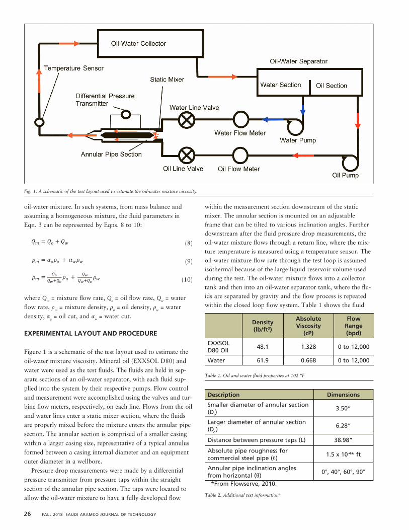
26 FALL 2018 SAUDI ARAMCO JOURNAL OF TECHNOLOGY
oil-water mixture. In such systems, from mass balance and
assuming a homogeneous mixture, the fluid parameters in
Eqn. 3 can be represented by Eqns. 8 to 10:
∆𝑝𝑝𝑡𝑡 = 𝜌𝜌𝜌𝜌𝜌𝜌 sin 𝜃𝜃 + 𝑓𝑓𝑓𝑓𝐷𝐷ℎ
𝜌𝜌𝑉𝑉2
2 (1)
𝑉𝑉 = 𝑄𝑄0.25𝜋𝜋(𝐷𝐷𝑂𝑂
2 −𝐷𝐷𝑖𝑖2)
1√𝑓𝑓 = −0.86 𝑙𝑙𝑙𝑙 (
𝜀𝜀 𝐷𝐷ℎ⁄3.7 + 2.51
𝑅𝑅𝑅𝑅√𝑓𝑓) (2)
𝑅𝑅𝑅𝑅 = 4𝜌𝜌𝑄𝑄𝜋𝜋𝜋𝜋𝐷𝐷ℎ
(3)
1√𝑓𝑓 = 𝐴𝐴 − (𝐵𝐵−𝐴𝐴)2
𝐶𝐶−2𝐵𝐵+𝐴𝐴 (4)
𝐴𝐴 = −2.0 𝑙𝑙𝑙𝑙𝜌𝜌10 (𝜀𝜀 𝐷𝐷ℎ⁄3.7 + 12
𝑅𝑅𝑅𝑅) (5)
𝐵𝐵 = −2.0 𝑙𝑙𝑙𝑙𝜌𝜌10 (𝜀𝜀 𝐷𝐷ℎ⁄3.7 + 2.51𝐴𝐴
𝑅𝑅𝑅𝑅 ) (6)
𝐶𝐶 = −2.0 𝑙𝑙𝑙𝑙𝜌𝜌10 (𝜀𝜀 𝐷𝐷ℎ⁄3.7 + 2.51𝐵𝐵
𝑅𝑅𝑅𝑅 ) (7)
𝑄𝑄𝑚𝑚 = 𝑄𝑄𝑜𝑜 + 𝑄𝑄𝑤𝑤 (8)
𝜌𝜌𝑚𝑚 = 𝛼𝛼𝑜𝑜𝜌𝜌𝑜𝑜 + 𝛼𝛼𝑤𝑤𝜌𝜌𝑤𝑤 (9)
𝜌𝜌𝑚𝑚 = 𝑄𝑄𝑜𝑜𝑄𝑄𝑤𝑤+𝑄𝑄𝑜𝑜
𝜌𝜌𝑜𝑜 + 𝑄𝑄𝑤𝑤𝑄𝑄𝑤𝑤+𝑄𝑄𝑜𝑜
𝜌𝜌𝑤𝑤 (10)
(8)
∆𝑝𝑝𝑡𝑡 = 𝜌𝜌𝜌𝜌𝜌𝜌 sin 𝜃𝜃 + 𝑓𝑓𝑓𝑓𝐷𝐷ℎ
𝜌𝜌𝑉𝑉2
2 (1)
𝑉𝑉 = 𝑄𝑄0.25𝜋𝜋(𝐷𝐷𝑂𝑂
2 −𝐷𝐷𝑖𝑖2)
1√𝑓𝑓 = −0.86 𝑙𝑙𝑙𝑙 (
𝜀𝜀 𝐷𝐷ℎ⁄3.7 + 2.51
𝑅𝑅𝑅𝑅√𝑓𝑓) (2)
𝑅𝑅𝑅𝑅 = 4𝜌𝜌𝑄𝑄𝜋𝜋𝜋𝜋𝐷𝐷ℎ
(3)
1√𝑓𝑓 = 𝐴𝐴 − (𝐵𝐵−𝐴𝐴)2
𝐶𝐶−2𝐵𝐵+𝐴𝐴 (4)
𝐴𝐴 = −2.0 𝑙𝑙𝑙𝑙𝜌𝜌10 (𝜀𝜀 𝐷𝐷ℎ⁄3.7 + 12
𝑅𝑅𝑅𝑅) (5)
𝐵𝐵 = −2.0 𝑙𝑙𝑙𝑙𝜌𝜌10 (𝜀𝜀 𝐷𝐷ℎ⁄3.7 + 2.51𝐴𝐴
𝑅𝑅𝑅𝑅 ) (6)
𝐶𝐶 = −2.0 𝑙𝑙𝑙𝑙𝜌𝜌10 (𝜀𝜀 𝐷𝐷ℎ⁄3.7 + 2.51𝐵𝐵
𝑅𝑅𝑅𝑅 ) (7)
𝑄𝑄𝑚𝑚 = 𝑄𝑄𝑜𝑜 + 𝑄𝑄𝑤𝑤 (8)
𝜌𝜌𝑚𝑚 = 𝛼𝛼𝑜𝑜𝜌𝜌𝑜𝑜 + 𝛼𝛼𝑤𝑤𝜌𝜌𝑤𝑤 (9)
𝜌𝜌𝑚𝑚 = 𝑄𝑄𝑜𝑜𝑄𝑄𝑤𝑤+𝑄𝑄𝑜𝑜
𝜌𝜌𝑜𝑜 + 𝑄𝑄𝑤𝑤𝑄𝑄𝑤𝑤+𝑄𝑄𝑜𝑜
𝜌𝜌𝑤𝑤 (10)
(9)
𝐷𝐷ℎ 2
𝑉𝑉 = 𝑄𝑄0.25𝜋𝜋(𝐷𝐷𝑂𝑂
2 −𝐷𝐷𝑖𝑖2)
1√𝑓𝑓 = −0.86 𝑙𝑙𝑙𝑙 (
𝜀𝜀 𝐷𝐷ℎ⁄3.7 + 2.51
𝑅𝑅𝑅𝑅√𝑓𝑓) (2)
𝑅𝑅𝑅𝑅 = 4𝜌𝜌𝑄𝑄𝜋𝜋𝜋𝜋𝐷𝐷ℎ
(3)
1√𝑓𝑓 = 𝐴𝐴 − (𝐵𝐵−𝐴𝐴)2
𝐶𝐶−2𝐵𝐵+𝐴𝐴 (4)
𝐴𝐴 = −2.0 𝑙𝑙𝑙𝑙𝜌𝜌10 (𝜀𝜀 𝐷𝐷ℎ⁄3.7 + 12
𝑅𝑅𝑅𝑅) (5)
𝐵𝐵 = −2.0 𝑙𝑙𝑙𝑙𝜌𝜌10 (𝜀𝜀 𝐷𝐷ℎ⁄3.7 + 2.51𝐴𝐴
𝑅𝑅𝑅𝑅 ) (6)
𝐶𝐶 = −2.0 𝑙𝑙𝑙𝑙𝜌𝜌10 (𝜀𝜀 𝐷𝐷ℎ⁄3.7 + 2.51𝐵𝐵
𝑅𝑅𝑅𝑅 ) (7)
𝑄𝑄𝑚𝑚 = 𝑄𝑄𝑜𝑜 + 𝑄𝑄𝑤𝑤 (8)
𝜌𝜌𝑚𝑚 = 𝛼𝛼𝑜𝑜𝜌𝜌𝑜𝑜 + 𝛼𝛼𝑤𝑤𝜌𝜌𝑤𝑤 (9)
𝜌𝜌𝑚𝑚 = 𝑄𝑄𝑜𝑜𝑄𝑄𝑤𝑤+𝑄𝑄𝑜𝑜
𝜌𝜌𝑜𝑜 + 𝑄𝑄𝑤𝑤𝑄𝑄𝑤𝑤+𝑄𝑄𝑜𝑜
𝜌𝜌𝑤𝑤 (10)
(10)
where Qm = mixture flow rate, Qo = oil flow rate, Qw = water
flow rate, ρm = mixture density, ρo = oil density, ρw = water
density, αo = oil cut, and αw = water cut.
EXPERIMENTAL LAYOUT AND PROCEDURE
Figure 1 is a schematic of the test layout used to estimate the
oil-water mixture viscosity. Mineral oil (EXXSOL D80) and
water were used as the test fluids. The fluids are held in sep-
arate sections of an oil-water separator, with each fluid sup-
plied into the system by their respective pumps. Flow control
and measurement were accomplished using the valves and tur-
bine flow meters, respectively, on each line. Flows from the oil
and water lines enter a static mixer section, where the fluids
are properly mixed before the mixture enters the annular pipe
section. The annular section is comprised of a smaller casing
within a larger casing size, representative of a typical annulus
formed between a casing internal diameter and an equipment
outer diameter in a wellbore.
Pressure drop measurements were made by a differential
pressure transmitter from pressure taps within the straight
section of the annular pipe section. The taps were located to
allow the oil-water mixture to have a fully developed flow
within the measurement section downstream of the static mixer. The annular section is mounted on an adjustable frame that can be tilted to various inclination angles. Further downstream after the fluid pressure drop measurements, the oil-water mixture flows through a return line, where the mix-ture temperature is measured using a temperature sensor. The oil-water mixture flow rate through the test loop is assumed isothermal because of the large liquid reservoir volume used during the test. The oil-water mixture flows into a collector tank and then into an oil-water separator tank, where the flu-ids are separated by gravity and the flow process is repeated within the closed loop flow system. Table 1 shows the fluid
Fig. 1. A schematic of the test layout used to estimate the oil-water mixture viscosity.
Density (lb/ft3)
Absolute Viscosity
(cP)
Flow Range (bpd)
EXXSOL D80 Oil
48.1 1.328 0 to 12,000
Water 61.9 0.668 0 to 12,000
Table 1. Oil and water fluid properties at 102 °F
Description Dimensions
Smaller diameter of annular section (Di)
3.50”
Larger diameter of annular section (Do)
6.28”
Distance between pressure taps (L) 38.98”
Absolute pipe roughness for commercial steel pipe ()
1.5 x 10⁻⁴* ft
Annular pipe inclination angles from horizontal ()
0°, 40°, 60°, 90°
*From Flowserve, 2010.
Table 2. Additional test information9
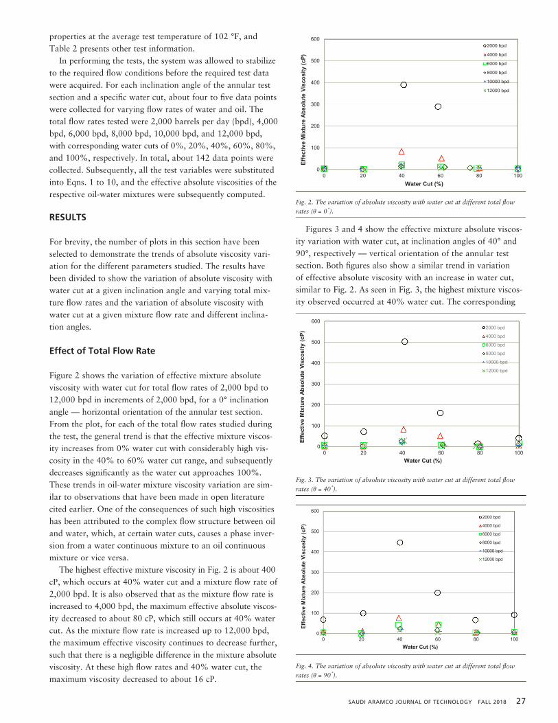
SAUDI ARAMCO JOURNAL OF TECHNOLOGY FALL 2018 27
properties at the average test temperature of 102 °F, and Table 2 presents other test information.
In performing the tests, the system was allowed to stabilize to the required flow conditions before the required test data were acquired. For each inclination angle of the annular test section and a specific water cut, about four to five data points were collected for varying flow rates of water and oil. The total flow rates tested were 2,000 barrels per day (bpd), 4,000 bpd, 6,000 bpd, 8,000 bpd, 10,000 bpd, and 12,000 bpd, with corresponding water cuts of 0%, 20%, 40%, 60%, 80%, and 100%, respectively. In total, about 142 data points were collected. Subsequently, all the test variables were substituted into Eqns. 1 to 10, and the effective absolute viscosities of the respective oil-water mixtures were subsequently computed.
RESULTS
For brevity, the number of plots in this section have been selected to demonstrate the trends of absolute viscosity vari-ation for the different parameters studied. The results have been divided to show the variation of absolute viscosity with water cut at a given inclination angle and varying total mix-ture flow rates and the variation of absolute viscosity with water cut at a given mixture flow rate and different inclina-tion angles.
Effect of Total Flow Rate
Figure 2 shows the variation of effective mixture absolute viscosity with water cut for total flow rates of 2,000 bpd to 12,000 bpd in increments of 2,000 bpd, for a 0° inclination angle — horizontal orientation of the annular test section. From the plot, for each of the total flow rates studied during the test, the general trend is that the effective mixture viscos-ity increases from 0% water cut with considerably high vis-cosity in the 40% to 60% water cut range, and subsequently decreases significantly as the water cut approaches 100%. These trends in oil-water mixture viscosity variation are sim-ilar to observations that have been made in open literature cited earlier. One of the consequences of such high viscosities has been attributed to the complex flow structure between oil and water, which, at certain water cuts, causes a phase inver-sion from a water continuous mixture to an oil continuous mixture or vice versa.
The highest effective mixture viscosity in Fig. 2 is about 400 cP, which occurs at 40% water cut and a mixture flow rate of 2,000 bpd. It is also observed that as the mixture flow rate is increased to 4,000 bpd, the maximum effective absolute viscos-ity decreased to about 80 cP, which still occurs at 40% water cut. As the mixture flow rate is increased up to 12,000 bpd, the maximum effective viscosity continues to decrease further, such that there is a negligible difference in the mixture absolute viscosity. At these high flow rates and 40% water cut, the maximum viscosity decreased to about 16 cP.
Figures 3 and 4 show the effective mixture absolute viscos-ity variation with water cut, at inclination angles of 40° and 90°, respectively — vertical orientation of the annular test section. Both figures also show a similar trend in variation of effective absolute viscosity with an increase in water cut, similar to Fig. 2. As seen in Fig. 3, the highest mixture viscos-ity observed occurred at 40% water cut. The corresponding
Fig. 2. The variation of absolute viscosity with water cut at different total flow rates ( = 0).
Fig. 3. The variation of absolute viscosity with water cut at different total flow rates ( = 40).
0
100
200
300
400
500
600
0 20 40 60 80 100
Effe
ctiv
e M
ixtu
re A
bsol
ute
Visc
osity
(cP)
Water Cut (%)
2000 bpd
4000 bpd
6000 bpd
8000 bpd
10000 bpd
12000 bpd
0
100
200
300
400
500
600
0 20 40 60 80 100
Effe
ctiv
e M
ixtu
re A
bsol
ute
Visc
osity
(cP)
Water Cut (%)
2000 bpd
4000 bpd
6000 bpd
8000 bpd
10000 bpd
12000 bpd
Fig. 2. The variation of absolute viscosity with water cut at different total flow rates (θ = 0˚).
Fig. 2. The variation of absolute viscosity with water cut at different total flow rates ( = 0).
Fig. 3. The variation of absolute viscosity with water cut at different total flow rates ( = 40).
0
100
200
300
400
500
600
0 20 40 60 80 100
Effe
ctiv
e M
ixtu
re A
bsol
ute
Visc
osity
(cP)
Water Cut (%)
2000 bpd
4000 bpd
6000 bpd
8000 bpd
10000 bpd
12000 bpd
0
100
200
300
400
500
600
0 20 40 60 80 100
Effe
ctiv
e M
ixtu
re A
bsol
ute
Visc
osity
(cP)
Water Cut (%)
2000 bpd
4000 bpd
6000 bpd
8000 bpd
10000 bpd
12000 bpd
Fig. 3. The variation of absolute viscosity with water cut at different total flow rates (θ = 40˚).
Fig. 4. The variation of absolute viscosity with water cut at different total flow rates ( = 90).
0
100
200
300
400
500
600
0 20 40 60 80 100
Effe
ctiv
e M
ixtu
re A
bsol
ute
Visc
osity
(cP)
Water Cut (%)
2000 bpd
4000 bpd
6000 bpd
8000 bpd
10000 bpd
12000 bpd
500
600
(cP)
0 Degrees
40 Degrees
60 Degrees
Fig. 4. The variation of absolute viscosity with water cut at different total flow rates (θ = 90˚).
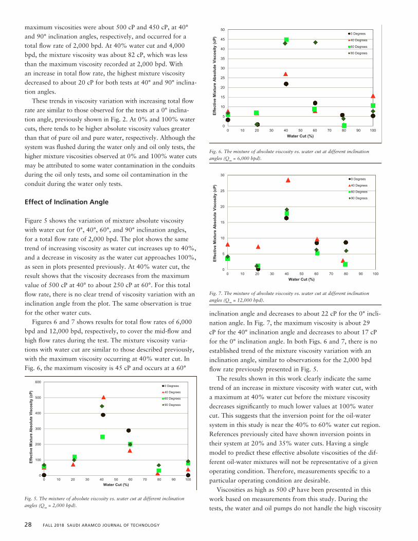
28 FALL 2018 SAUDI ARAMCO JOURNAL OF TECHNOLOGY
maximum viscosities were about 500 cP and 450 cP, at 40° and 90° inclination angles, respectively, and occurred for a total flow rate of 2,000 bpd. At 40% water cut and 4,000 bpd, the mixture viscosity was about 82 cP, which was less than the maximum viscosity recorded at 2,000 bpd. With an increase in total flow rate, the highest mixture viscosity decreased to about 20 cP for both tests at 40° and 90° inclina-tion angles.
These trends in viscosity variation with increasing total flow rate are similar to those observed for the tests at a 0° inclina-tion angle, previously shown in Fig. 2. At 0% and 100% water cuts, there tends to be higher absolute viscosity values greater than that of pure oil and pure water, respectively. Although the system was flushed during the water only and oil only tests, the higher mixture viscosities observed at 0% and 100% water cuts may be attributed to some water contamination in the conduits during the oil only tests, and some oil contamination in the conduit during the water only tests.
Effect of Inclination Angle
Figure 5 shows the variation of mixture absolute viscosity with water cut for 0°, 40°, 60°, and 90° inclination angles, for a total flow rate of 2,000 bpd. The plot shows the same trend of increasing viscosity as water cut increases up to 40%, and a decrease in viscosity as the water cut approaches 100%, as seen in plots presented previously. At 40% water cut, the result shows that the viscosity decreases from the maximum value of 500 cP at 40° to about 250 cP at 60°. For this total flow rate, there is no clear trend of viscosity variation with an inclination angle from the plot. The same observation is true for the other water cuts.
Figures 6 and 7 shows results for total flow rates of 6,000 bpd and 12,000 bpd, respectively, to cover the mid-flow and high flow rates during the test. The mixture viscosity varia-tions with water cut are similar to those described previously, with the maximum viscosity occurring at 40% water cut. In Fig. 6, the maximum viscosity is 45 cP and occurs at a 60°
inclination angle and decreases to about 22 cP for the 0° incli-
nation angle. In Fig. 7, the maximum viscosity is about 29
cP for the 40° inclination angle and decreases to about 17 cP
for the 0° inclination angle. In both Figs. 6 and 7, there is no
established trend of the mixture viscosity variation with an
inclination angle, similar to observations for the 2,000 bpd
flow rate previously presented in Fig. 5.
The results shown in this work clearly indicate the same
trend of an increase in mixture viscosity with water cut, with
a maximum at 40% water cut before the mixture viscosity
decreases significantly to much lower values at 100% water
cut. This suggests that the inversion point for the oil-water
system in this study is near the 40% to 60% water cut region.
References previously cited have shown inversion points in
their system at 20% and 35% water cuts. Having a single
model to predict these effective absolute viscosities of the dif-
ferent oil-water mixtures will not be representative of a given
operating condition. Therefore, measurements specific to a
particular operating condition are desirable.
Viscosities as high as 500 cP have been presented in this
work based on measurements from this study. During the
tests, the water and oil pumps do not handle the high viscosity
Fig. 4. The variation of absolute viscosity with water cut at different total flow rates ( = 90).
Fig. 5. The mixture of absolute viscosity vs. water cut at different inclination angles (Qm = 2,000 bpd).
0
100
200
300
400
500
600
0 20 40 60 80 100
Effe
ctiv
e M
ixtu
re A
bsol
ute
Visc
osity
(cP)
Water Cut (%)
2000 bpd
4000 bpd
6000 bpd
8000 bpd
10000 bpd
12000 bpd
0
100
200
300
400
500
600
0 10 20 30 40 50 60 70 80 90 100
Effe
ctiv
e M
ixtu
re A
bsol
ute
Visc
osity
(cP)
Water Cut (%)
0 Degrees
40 Degrees
60 Degrees
90 Degrees
Fig. 5. The mixture of absolute viscosity vs. water cut at different inclination angles (Qm = 2,000 bpd).
Fig. 6. The mixture of absolute viscosity vs. water cut at different inclination angles (Qm = 6,000 bpd).
Fig. 7. The mixture of absolute viscosity vs. water cut at different inclination angles (Qm = 12,000 bpd).
0
5
10
15
20
25
30
35
40
45
50
0 10 20 30 40 50 60 70 80 90 100
Effe
ctiv
e M
ixtu
re A
bsol
ute
Visc
osity
(cP)
Water Cut (%)
0 Degrees
40 Degrees
60 Degrees
90 Degrees
0
5
10
15
20
25
30
0 10 20 30 40 50 60 70 80 90 100
Effe
ctiv
e M
ixtu
re A
bsol
ute
Visc
osity
(cP)
Water Cut (%)
0 Degrees
40 Degrees
60 Degrees
90 Degrees
Fig. 6. The mixture of absolute viscosity vs. water cut at different inclination angles (Qm = 6,000 bpd).
Fig. 6. The mixture of absolute viscosity vs. water cut at different inclination angles (Qm = 6,000 bpd).
Fig. 7. The mixture of absolute viscosity vs. water cut at different inclination angles (Qm = 12,000 bpd).
0
5
10
15
20
25
30
35
40
45
50
0 10 20 30 40 50 60 70 80 90 100
Effe
ctiv
e M
ixtu
re A
bsol
ute
Visc
osity
(cP)
Water Cut (%)
0 Degrees
40 Degrees
60 Degrees
90 Degrees
0
5
10
15
20
25
30
0 10 20 30 40 50 60 70 80 90 100
Effe
ctiv
e M
ixtu
re A
bsol
ute
Visc
osity
(cP)
Water Cut (%)
0 Degrees
40 Degrees
60 Degrees
90 Degrees
Fig. 7. The mixture of absolute viscosity vs. water cut at different inclination angles (Qm = 12,000 bpd).
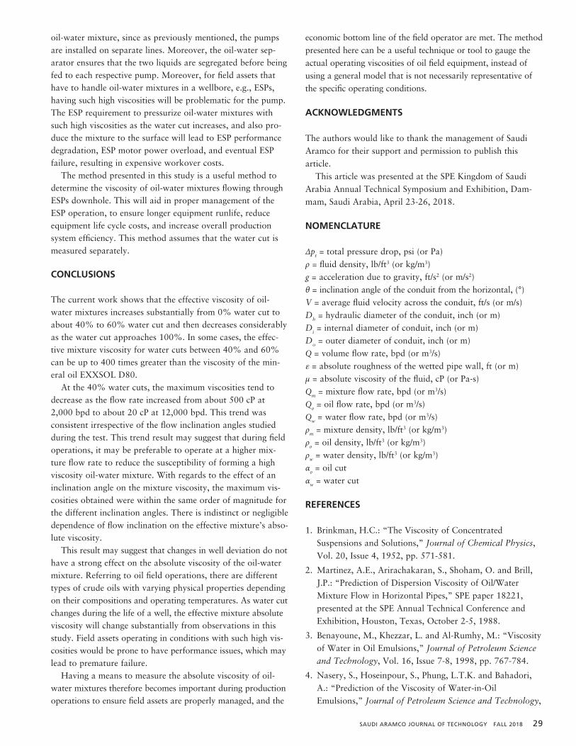
SAUDI ARAMCO JOURNAL OF TECHNOLOGY FALL 2018 29
oil-water mixture, since as previously mentioned, the pumps are installed on separate lines. Moreover, the oil-water sep-arator ensures that the two liquids are segregated before being fed to each respective pump. Moreover, for field assets that have to handle oil-water mixtures in a wellbore, e.g., ESPs, having such high viscosities will be problematic for the pump. The ESP requirement to pressurize oil-water mixtures with such high viscosities as the water cut increases, and also pro-duce the mixture to the surface will lead to ESP performance degradation, ESP motor power overload, and eventual ESP failure, resulting in expensive workover costs.
The method presented in this study is a useful method to determine the viscosity of oil-water mixtures flowing through ESPs downhole. This will aid in proper management of the ESP operation, to ensure longer equipment runlife, reduce equipment life cycle costs, and increase overall production system efficiency. This method assumes that the water cut is measured separately.
CONCLUSIONS
The current work shows that the effective viscosity of oil- water mixtures increases substantially from 0% water cut to about 40% to 60% water cut and then decreases considerably as the water cut approaches 100%. In some cases, the effec-tive mixture viscosity for water cuts between 40% and 60% can be up to 400 times greater than the viscosity of the min-eral oil EXXSOL D80.
At the 40% water cuts, the maximum viscosities tend to decrease as the flow rate increased from about 500 cP at 2,000 bpd to about 20 cP at 12,000 bpd. This trend was consistent irrespective of the flow inclination angles studied during the test. This trend result may suggest that during field operations, it may be preferable to operate at a higher mix-ture flow rate to reduce the susceptibility of forming a high viscosity oil-water mixture. With regards to the effect of an inclination angle on the mixture viscosity, the maximum vis-cosities obtained were within the same order of magnitude for the different inclination angles. There is indistinct or negligible dependence of flow inclination on the effective mixture’s abso-lute viscosity.
This result may suggest that changes in well deviation do not have a strong effect on the absolute viscosity of the oil-water mixture. Referring to oil field operations, there are different types of crude oils with varying physical properties depending on their compositions and operating temperatures. As water cut changes during the life of a well, the effective mixture absolute viscosity will change substantially from observations in this study. Field assets operating in conditions with such high vis-cosities would be prone to have performance issues, which may lead to premature failure.
Having a means to measure the absolute viscosity of oil- water mixtures therefore becomes important during production operations to ensure field assets are properly managed, and the
economic bottom line of the field operator are met. The method presented here can be a useful technique or tool to gauge the actual operating viscosities of oil field equipment, instead of using a general model that is not necessarily representative of the specific operating conditions.
ACKNOWLEDGMENTS
The authors would like to thank the management of Saudi Aramco for their support and permission to publish this article.
This article was presented at the SPE Kingdom of Saudi Arabia Annual Technical Symposium and Exhibition, Dam-mam, Saudi Arabia, April 23-26, 2018.
NOMENCLATURE
∆pt = total pressure drop, psi (or Pa)ρ = fluid density, lb/ft3 (or kg/m3)g = acceleration due to gravity, ft/s2 (or m/s2)θ = inclination angle of the conduit from the horizontal, (°)V = average fluid velocity across the conduit, ft/s (or m/s)Dh = hydraulic diameter of the conduit, inch (or m)Di = internal diameter of conduit, inch (or m)Do = outer diameter of conduit, inch (or m)Q = volume flow rate, bpd (or m3/s) = absolute roughness of the wetted pipe wall, ft (or m)μ = absolute viscosity of the fluid, cP (or Pa-s)Qm = mixture flow rate, bpd (or m3/s)Qo = oil flow rate, bpd (or m3/s)Qw = water flow rate, bpd (or m3/s)ρm = mixture density, lb/ft3 (or kg/m3)ρo = oil density, lb/ft3 (or kg/m3)ρw = water density, lb/ft3 (or kg/m3)αo = oil cutαw = water cut
REFERENCES
1. Brinkman, H.C.: “The Viscosity of Concentrated Suspensions and Solutions,” Journal of Chemical Physics, Vol. 20, Issue 4, 1952, pp. 571-581.
2. Martinez, A.E., Arirachakaran, S., Shoham, O. and Brill, J.P.: “Prediction of Dispersion Viscosity of Oil/Water Mixture Flow in Horizontal Pipes,” SPE paper 18221, presented at the SPE Annual Technical Conference and Exhibition, Houston, Texas, October 2-5, 1988.
3. Benayoune, M., Khezzar, L. and Al-Rumhy, M.: “Viscosity of Water in Oil Emulsions,” Journal of Petroleum Science
and Technology, Vol. 16, Issue 7-8, 1998, pp. 767-784.
4. Nasery, S., Hoseinpour, S., Phung, L.T.K. and Bahadori, A.: “Prediction of the Viscosity of Water-in-Oil Emulsions,” Journal of Petroleum Science and Technology,

30 FALL 2018 SAUDI ARAMCO JOURNAL OF TECHNOLOGY
Vol. 34, Issue 24, 2016, pp. 1972-1977.
5. Li, C., Huang, Q., Ma, S. and Ji, C.: “An Experimental Study on the Viscosity of Water-in-Oil Emulsions,” Journal of Dispersion Science and Technology, Vol. 37, Issue 3, 2016, pp. 305-316.
6. Streeter, V.L., Wylie, E.B. and Bedford, K.W.: Fluid Mechanics, 1st edition, McGraw-Hill, 1983, 752 p.
7. Asker, M., Targut, O.E. and Coban, M.T.: “A Review of non-Iterative Friction Factor Correlations for the Calculation of Pressure Drop in Pipes,” Journal of Science and Technology, Vol. 4, Issue 1, June 2014, pp. 1-8.
8. Serghides, T.K.: “Estimate Friction Factor Accurately,” Chemical Engineering, Vol. 91, Issue 5, March 1984, pp. 63-64.
9. Heald, C.C.: Cameron Hydraulic Data, 19th edition, Flowserve Corporation, U.S.A., 2002.
BIOGRAPHIES
Dr. Chidirim E. Ejim is a Petroleum Engineer working in the artificial lift focus area within the Production Technology Team of Saudi Aramco’s Exploration and Petroleum Engineering Center – Advanced Research Center (EXPEC ARC). Prior
to joining Saudi Aramco in 2014, Chidirim spent over 7 years with Schlumberger’s Artificial Lift Segment, working on surface horizontal pumping systems; downhole pump design, development and testing; multiphase production systems; as well as downhole gas separator/gas handler testing and analysis.
He received his B.Eng. degree (Honors) from the University of Malta, Msida, Malta; his M.S. degree from the University of Waterloo, Ontario, Canada; and his Ph.D. degree from the University of Alberta, Edmonton, Canada, all in Mechanical Engineering.
Dr. Jinjiang Xiao is a Petroleum Engineering Consultant working in Saudi Aramco’s Exploration and Petroleum Engineering Center – Advanced Research Center (EXPEC ARC). He is currently the focus area champion for artificial lift.
Prior to joining Saudi Aramco in 2003, Jinjiang spent 10 years with Amoco and later BP-Amoco, working on multiphase flow, flow assurance and deepwater production engineering.
He received both his M.S. and Ph.D. degrees in Petroleum Engineering from the University of Tulsa, Tulsa, OK.
SAUDI ARAMCO JOURNAL OF TECHNOLOGY FALL 2018 31
ABSTRACT
Injecting carbon dioxide (CO2) into oil reservoirs has the potential to enhance oil recovery and sequester CO2 under-ground. While CO2 injection has been successful, a major challenge facing this technique is enhancing volumetric sweep efficiency. Some of the factors that contribute to this challenge are the low density and viscosity of injected gas relative to reservoir fluids. The use of foam is one of the most promis-ing techniques used to increase the apparent viscosity of CO2, thereby improving volumetric sweep efficiency.
Increasing the CO2 viscosity by using surfactants has the po-tential to mitigate some of the challenges associated with CO2 injection projects. The objective of this work is to investigate the effect of various surfactants on CO2 foam viscosity. Four surfactants, three commercial and one developed in-house, were used to evaluate the foam generation and rheological properties of CO2 foams at high-pressure, high temperature (HPHT). Dy-namic foam viscosity measurements were conducted in a special foam rheology apparatus with supercritical CO2 (sc-CO2) under high-pressure (3,200 psi), high temperature (210 °F), and salin-ity conditions. The foam was generated by injecting sc-CO2 and a surfactant at different concentrations (0.20 wt%, 0.50 wt%, and 1.00 wt%), shear rates (10 s-1 to 600 s-1), and qualities (70%, 85%, and 90%).
The results indicate that all surfactants were able to generate good quality foam at HPHT. The foam viscosity increases with surfactant concentration. All foams exhibited a shear thinning behavior, with foam viscosity decreasing when increasing shear rates. In general, the highest viscosity for each surfactant was re-ported at the lowest shear rates. The results also showed that the foam quality has an impact on foam viscosity for some cases.
The highest foam viscosities for surfactant 2 were achieved at 85% quality; however, the quality had no significant impact on foam viscosity for surfactant 3.
INTRODUCTION
Carbon dioxide (CO2) is a great injectant for enhanced oil re-covery of light conventional oils — for environmental, tech-nical, and economic reasons. The major advantages of CO2 include lower miscibility pressures, swelling of crude oil, and
lowering its viscosity1. It has two major disadvantages: (1) An
unfavorable viscosity or mobility ratio that produces inefficient
oil displacement by causing fingering of the CO2 owing to fron-
tal instability, and (2) Gravity override within the reservoir due
to the low density of supercritical CO2 (sc-CO2)2-4.
These factors lead to poor sweep efficiency. Some of the fac-
tors that contribute to this challenge are the low density and
viscosity of injected gas compared with the resident fluids in
reservoirs5-7. Several methods have been tried to resolve this is-
sue. The most common techniques are: Water alternating gas; in
situ generation of foam/emulsion; and adding thickening agents
to increase the CO2 viscosity6, 8-12. The use of foam is one of the
most promising techniques to increase the apparent viscosity of
the CO2, thereby improving volumetric sweep efficiency13, 14.
Surfactants are the main chemicals used to generate and sta-
bilize foams. Different parameters might affect foam generation
and stabilization, including surfactant type and concentration,
shear rate, gas volume (quality), and experimental conditions.
Foam generation and stabilization at harsh reservoir conditions,
such as high reservoir temperature, high salinity conditions,
reaction with reservoir fluids — mainly crude oil — and sur-
factant adsorption to the rock minerals, are very difficult and
complex15-21. The use of sc-CO2 in the foam generation process
is a major challenge. This is attributed to the fact that CO2 has
weak van der Waals forces and a lack of permanent dipole mo-
ment. Consequently, the CO2 philic tail is a poor solvent for
high molecular weight and polar solutes. In such a case, insta-
bility of foam can occur either in the form of flocculation or
coalescence of foam bubbles. Based on the work that has been
accomplished in this area, only a few surfactants can stabilize
CO2 brine foam/emulsion22-24.
The objective of this work is to investigate the effect of var-
ious surfactants on CO2 foam rheology. Four surfactants, in-
cluding commercial and in-house developed, were used to
evaluate the foam generation and rheological properties of CO2
foams at high-pressure, high temperature (HPHT), and salinity
conditions. This work is a preliminary step to select potential
surfactants for foam generation as a technique to improve the
volumetric sweep efficiency during CO2 injection.
CO2 Foam Rheology: Effect of Surfactant Concentration, Shear Rate and Injection Quality
Dr. Zuhair A. Al-Yousif, Dr. Sunil L. Kokal, Amin M. Al-Abdulwahab, and Dr. Ayrat Gizzatov

32 FALL 2018 SAUDI ARAMCO JOURNAL OF TECHNOLOGY
MATERIALS
The commercially available 30 wt% active blend of laurami-dopropylamine oxide and myristamidopropylamine oxide sur-factants in water (Ammonyx® LMDO) and the 43 wt% active cocoamidopropyl hydroxysultaine surfactant in water (Petro-step® SB) used in this study were from the Stepan Company (Northfield, IL), and another commercial foaming agent was provided by a local vendor. The last surfactant formulation described in this work was developed in-house.
Table 1 lists the surfactants with their commercial names used in this study. The water used in this study was field injec-tion water with a total dissolved solids content of 57,000 ppm, a density of 1.01 g/mL, and a viscosity of 0.291 centipoise (cP), both values are at 90 °C. The brine was prepared by dissolv-ing various types of salts in deionized water. The details of the brine composition used are provided in Table 2. The gas used for foam generation is CO2 with 99.5% purity.
METHODOLOGY
Measured amounts of as-supplied surfactant stock solution were di-rectly dissolved in calculated amounts of high salinity water to prepare — 0.20 wt%, 0.50 wt%, and 1.00 wt% — active surfactant solutions. Rheol-ogy experimentations were designed and performed on a custom-made HPHT foam loop rheometer, Fig. 1. This instrument has a visualization sapphire window cell and a capillary steel tube loop to measure rheology under dynamic conditions. Foam studies were performed with sc-CO2
under high-pressure (3,200 psi), high temperature, (210 °F), and salinity conditions. Shear rates applied to measure foam viscosity ranged from 10-600 s-1 and volume (quality) of sc-CO2 used for different measurements was 70%, 85%, and 90%.
The rheometer was first calibrated using Newtonian fluids with known values. The procedure involved placing the foam-ing agent — surfactant in high salinity water — and allowed to equilibrate in the cell. The sc-CO2 is then introduced and equilibrates until the desired temperature and pressure is reached. The mixture was circulated in the capillary loop to ensure mix-ing and formation of the foam. Sample viscosities were then measured at different shear rates. The quality parameters of the foam was calculated from the volume of gas to the foaming agent ratio. A similar procedure was repeated for all samples reported in this study.
When studying fluid rheological properties, it is important to characterize shear stress (
𝜏𝜏 𝛾𝛾 𝜇𝜇𝑎𝑎𝑎𝑎𝑎𝑎𝑎𝑎𝑎𝑎𝑎𝑎𝑎𝑎𝑎𝑎 𝜇𝜇𝑎𝑎𝑎𝑎𝑎𝑎𝑎𝑎𝑎𝑎𝑎𝑎𝑎𝑎𝑎𝑎 = 𝜏𝜏
𝛾𝛾 (1) 𝜏𝜏 = 𝐷𝐷 ∆𝑃𝑃
4𝐿𝐿 (2) 𝛾𝛾 = 8 𝑉𝑉
𝐷𝐷 (3)
) and shear rate (
𝜏𝜏 𝛾𝛾 𝜇𝜇𝑎𝑎𝑎𝑎𝑎𝑎𝑎𝑎𝑎𝑎𝑎𝑎𝑎𝑎𝑎𝑎 𝜇𝜇𝑎𝑎𝑎𝑎𝑎𝑎𝑎𝑎𝑎𝑎𝑎𝑎𝑎𝑎𝑎𝑎 = 𝜏𝜏
𝛾𝛾 (1) 𝜏𝜏 = 𝐷𝐷 ∆𝑃𝑃
4𝐿𝐿 (2) 𝛾𝛾 = 8 𝑉𝑉
𝐷𝐷 (3)
) to estimate the fluid’s apparent viscosity,
𝜏𝜏 𝛾𝛾 𝜇𝜇𝑎𝑎𝑎𝑎𝑎𝑎𝑎𝑎𝑎𝑎𝑎𝑎𝑎𝑎𝑎𝑎 𝜇𝜇𝑎𝑎𝑎𝑎𝑎𝑎𝑎𝑎𝑎𝑎𝑎𝑎𝑎𝑎𝑎𝑎 = 𝜏𝜏
𝛾𝛾 (1) 𝜏𝜏 = 𝐷𝐷 ∆𝑃𝑃
4𝐿𝐿 (2) 𝛾𝛾 = 8 𝑉𝑉
𝐷𝐷 (3)
. Foam is classified as non-Newtonian fluid whose apparent viscosity is shear rate dependent. The apparent viscosity of the generated foam was measured as follows:
𝜏𝜏 𝛾𝛾 𝜇𝜇𝑎𝑎𝑎𝑎𝑎𝑎𝑎𝑎𝑎𝑎𝑎𝑎𝑎𝑎𝑎𝑎 𝜇𝜇𝑎𝑎𝑎𝑎𝑎𝑎𝑎𝑎𝑎𝑎𝑎𝑎𝑎𝑎𝑎𝑎 = 𝜏𝜏
𝛾𝛾 (1) 𝜏𝜏 = 𝐷𝐷 ∆𝑃𝑃
4𝐿𝐿 (2) 𝛾𝛾 = 8 𝑉𝑉
𝐷𝐷 (3)
(1)
𝜏𝜏 𝛾𝛾 𝜇𝜇𝑎𝑎𝑎𝑎𝑎𝑎𝑎𝑎𝑎𝑎𝑎𝑎𝑎𝑎𝑎𝑎 𝜇𝜇𝑎𝑎𝑎𝑎𝑎𝑎𝑎𝑎𝑎𝑎𝑎𝑎𝑎𝑎𝑎𝑎 = 𝜏𝜏
𝛾𝛾 (1) 𝜏𝜏 = 𝐷𝐷 ∆𝑃𝑃
4𝐿𝐿 (2) 𝛾𝛾 = 8 𝑉𝑉
𝐷𝐷 (3)
(2)
𝜏𝜏 𝛾𝛾 𝜇𝜇𝑎𝑎𝑎𝑎𝑎𝑎𝑎𝑎𝑎𝑎𝑎𝑎𝑎𝑎𝑎𝑎 𝜇𝜇𝑎𝑎𝑎𝑎𝑎𝑎𝑎𝑎𝑎𝑎𝑎𝑎𝑎𝑎𝑎𝑎 = 𝜏𝜏
𝛾𝛾 (1) 𝜏𝜏 = 𝐷𝐷 ∆𝑃𝑃
4𝐿𝐿 (2) 𝛾𝛾 = 8 𝑉𝑉
𝐷𝐷 (3)
(3)
where D is the tube diameter, ∆P is the differential pressure across the foam loop, L is the tube length, and V is the velocity.
RESULTS AND DISCUSSION
As previously mentioned, this study examines the impact of sur-factant concentration, foam quality and shear rate on the vis-cosity of generated foam at HPHTs. The results indicate that
Surfactant Commercial Name
Surfactant 1 Ammonyx® LMDO
Surfactant 2 Petrostep® SB
Surfactant 3Foaming agent provided
by local vendor
Surfactant 4 Nano-surfactant
Table 1. List of surfactants
Salt Concentration (mg/L)
NaCl 41,041.45
CaCl2·2H2O 2,384.27
MgCl2·6H2O 17,644.88
Na2SO4 6,343.19
NaHCO3 165.22
Table 2. Brine composition used
Surfactant Commercial Name Surfactant 1 Ammonyx® LMDO Surfactant 2 Petrostep® SB Surfactant 3 Foaming agent provided by local vendor Surfactant 4 Nano-surfactant (in-house)
Table 1. List of surfactants
Table 2. Brine composition used
Fig. 1. Schematic of the custom-made HPHT foam loop rheometer.
Salt Concentration (mg/L) NaCl 41,041.45 CaCl2·2H2O 2,384.27 MgCl2·6H2O 17,644.88 Na2SO4 6,343.19 NaHCO3 165.22
Fig. 1. Schematic of the custom-made HPHT foam loop rheometer.

SAUDI ARAMCO JOURNAL OF TECHNOLOGY FALL 2018 33
all four surfactants were able to generate foams at experimen-
tal conditions, Figs. 2a to 2d. The foam viscosity increases with
surfactant concentration. All foams exhibited shear thinning
behavior, whereas the foam viscosity decreases with increas-
ing shear rates. The results also showed that the foam quality
has an impact on the foam viscosity for surfactant 2, where the
highest foam viscosities were achieved at 85% quality. More
details about the effect of each parameter on the viscosity of
foam will be presented separately.
Foam Texture
Foam texture is an important parameter for determining foam
strength and viscosity. Foam texture, also known as bubble
density, is defined as bubble size or the number of lamellae per unit volume. There is an inverse relationship between bub-ble density and bubble size. The foam’s apparent viscosity is strongly dependent on foam texture. Studies found that smaller bubbles result in higher apparent viscosity of foam13, 14, 25. Fig-ures 3a and 3b show the foam bubbles for surfactant 2 and sur-factant 4 generated at 0.20 wt% concentration, 70% quality, and 30 s-1 shear rate. As shown in Fig. 3a, foam bubbles are smaller for surfactant 2 than for surfactant 4. Consequently, the apparent viscosity measured for surfactant 2 was higher than that for surfactant 4 at the same conditions, 18.45 cP and 6.50 cP, respectively.
Also, a comparison was made for surfactant 2 and surfac-tant 3 at 0.50 wt% concentration, 90% quality, and 10 s-1 shear rate, Figs. 4a and 4b, respectively. Surfactant 3, Fig. 4b,
Fig. 2. Foam generated at HPHT: (a) surfactant 1, (b) surfactant 2, (c) surfactant 3, and (d) surfactant 4.
Fig. 3. Foam generated at 0.20 wt% concentration, 70% quality, and 30 s-1 shear rate: (a) surfactant 2, and (b) surfactant 4.
Fig. 4. Foam generated at 0.50 wt% concentration, 90% quality, and 10 s-1 shear rate: (a) surfactant 2, and (b) surfactant 3.
Fig. 2. Foam generated at HPHT: (a) surfactant 1, (b) surfactant 2, (c) surfactant 3, and (d) surfactant 4.
Fig. 3. Foam generated at 0.20 wt% concentration, 70% quality, and 30 s-1 shear rate: (a) surfactant 2, and (b) surfactant 4.
(a) (b)
(c) (d)
(a) (b)
-1 shear rate: (a) surfactant 2,
(b)
(d)
(b)
a
b
and (b) surfactant 3.
0
20
40
60
80
50 100 200
Visc
osity
(cP)
0.2 wt% 0.5 wt%
(a) (b)
Fig. 4. Foam generated at 0.50 wt% concentration, 90% quality, and 10 s-1 shear rate: (a) surfactant 2, and (b) surfactant 3.
(a) (b)
a
b
Fig. 2. Foam generated at HPHT: (a) surfactant 1, (b) surfactant 2, (c) surfactant 3, and (d) surfactant 4.
Fig. 3. Foam generated at 0.20 wt% concentration, 70% quality, and 30 s-1 shear rate: (a) surfactant 2, and (b) surfactant 4.
(a) (b)
(c) (d)
(a) (b)
Fig. 2. Foam generated at HPHT: (a) surfactant 1, (b) surfactant 2, (c) surfactant 3, and (d) surfactant 4.
Fig. 3. Foam generated at 0.20 wt% concentration, 70% quality, and 30 s-1 shear rate: (a) surfactant 2, and (b) surfactant 4.
(a) (b)
(c) (d)
(a) (b)
Fig. 2. Foam generated at HPHT: (a) surfactant 1, (b) surfactant 2, (c) surfactant 3, and (d) surfactant 4.
Fig. 3. Foam generated at 0.20 wt% concentration, 70% quality, and 30 s-1 shear rate: (a) surfactant 2, and (b) surfactant 4.
(a) (b)
(c) (d)
(a) (b)
Fig. 2. Foam generated at HPHT: (a) surfactant 1, (b) surfactant 2, (c) surfactant 3, and (d) surfactant 4.
Fig. 3. Foam generated at 0.20 wt% concentration, 70% quality, and 30 s-1 shear rate: (a) surfactant 2, and (b) surfactant 4.
(a) (b)
(c) (d)
(a) (b)
a b c d

34 FALL 2018 SAUDI ARAMCO JOURNAL OF TECHNOLOGY
generated foam with relatively smaller bubbles than that of sur-factant 2, Fig. 4a. The measured apparent viscosity for surfac-tant 2 was 15 cP, while for surfactant 3, it was 33 cP.
Effect of Concentration
The effect of surfactant concentration on foam viscosity was evaluated for all four surfactants. The results clearly indicate that the concentration of surfactant is critical to generate vis-cous foam. For surfactant 1, the effect of surfactant concentra-tion was evaluated at 0.20 wt% and 0.50 wt%, and at different shear rates. As shown in Fig. 5, the increase of surfactant con-centration from 0.20 wt% to 0.50 wt% produced at least seven times higher viscosity foam. This magnitude becomes higher as the shear rate increases. Similarly, the effect of the surfactant concentration was evaluated at 0.20 wt% and 0.50 wt%, and at different shear rates for surfactant 2. As shown in Fig. 6, the viscosity doubles as the surfactant concentration increases from
0.20 wt% to 0.50 wt%.
For surfactant 3, the effect of the surfactant concentration was
studied using 0.50 wt% and 1.00 wt% samples. Similar to the
previous surfactants, the results showed that as the surfactant
concentration increases, the foam viscosity increases, Fig. 7.
The same behavior was reported for surfactant 4, with the
surfactant concentration and viscosity being directly propor-
tional. This behavior is depicted in Fig. 8. Increasing the sur-
factant concentration enhances the formation of micelle at the
CO2 brine interface, reduces the interfacial tension, and en-
hances the foam generation process.
Effect of Quality
In general, the volume of injected gas to the total volume of in-
jected fluids (quality) is a very important parameter influencing
the foam generation and rheology. If the quality is too low, gas
droplets are spherical and dispersed. In such cases, the foam
will be weak and the viscosity will be very close to that of the
foaming agent. Likewise, if the quality is too high, the aqueous
film (lamellae) will be very thin and easy to collapse; or there
might be no sufficient volume of foaming agent to form lamel-
lae. As a result, the viscosity will be similar to that of the in-
jected gas. The definition of low and high quality depends on
the selected material and experimental conditions.
The effect of gas volume on the foam viscosity was evalu-
ated for surfactant 2 and surfactant 3. The results showed that
the injection quality is a critical parameter for foam generation
for some cases, and therefore, determines the viscosity of the
Fig. 4. Foam generated at 0.50 wt% concentration, 90% quality, and 10 s-1 shear rate: (a) surfactant 2, and (b) surfactant 3.
Fig. 5. The effect of surfactant 1 concentration on foam viscosity.
Fig. 6. The effect of surfactant 2 concentration on foam viscosity.
0
20
40
60
80
50 100 200
Visc
osity
(cP)
Shear Rate (s-1)
0.2 wt% 0.5 wt%
0
10
20
30
40
50 200 600
Visc
osity
(cP)
Shear Rate (s-1)
0.2 wt% 0.5 wt%
(a) (b)
Fig. 5. The effect of surfactant 1 concentration on foam viscosity.
Fig. 6. The effect of surfactant 2 concentration on foam viscosity.
Fig. 7. The effect of surfactant 3 concentration on foam viscosity.
0
10
20
30
40
50
50 200 600
Visc
osity
(cP)
Shear Rate (s-1)
0.5 wt% 1 wt%
Fig. 7. The effect of surfactant 3 concentration on foam viscosity.
Fig. 8. The effect of surfactant 4 concentration on foam viscosity.
Fig. 9. The effect of gas volume on the foam viscosity for surfactant 2.
0
10
20
30
50 200 600
Visc
osity
(cP)
Shear Rate (s-1)
0.2 wt% 0.5 wt%
0
20
40
60
80
50 100 200
Visc
osity
(cP)
Shear Rate (s-1)
70% 85% 90%
Fig. 8. The effect of surfactant 4 concentration on foam viscosity.
Fig. 9. The effect of gas volume on the foam viscosity for surfactant 2.
0
20
40
60
80
50 100 200
Visc
osity
(cP)
Shear Rate (s-1)
70% 85%
Fig. 9. The effect of gas volume on the foam viscosity for surfactant 2.
Fig. 4. Foam generated at 0.50 wt% concentration, 90% quality, and 10 s-1 shear rate: (a) surfactant 2, and (b) surfactant 3.
Fig. 5. The effect of surfactant 1 concentration on foam viscosity.
Fig. 6. The effect of surfactant 2 concentration on foam viscosity.
0
20
40
60
80
50 100 200
Visc
osity
(cP)
Shear Rate (s-1)
0.2 wt% 0.5 wt%
0
10
20
30
40
50 200 600
Visc
osity
(cP)
Shear Rate (s-1)
0.2 wt% 0.5 wt%
(a) (b)

SAUDI ARAMCO JOURNAL OF TECHNOLOGY FALL 2018 35
generated foam. For surfactant 2, the effect of quality was con-
ducted at two qualities: 70%, and 85%. The results showed
that the highest foam viscosities were produced when the foam
quality was 85%. The tests were repeated at different shear
rates, and all results confirmed this conclusion. This is, as men-
tioned earlier, due to either the lack of foaming agent or the
weak foam generated, which might break down easily. Figure 9
shows the results of this case.
The effect of quality on the foam viscosity was also evaluated
at three qualities: 70%, 85%, and 90% for surfactant 3. The re-
sults, as plotted in Fig. 10, showed that quality had no significant
impact on the foam viscosity. As mentioned earlier, the impact of
quality on the foam rheology is material and experimental con-
ditions dependent. The results reported for the two tested mate-
rials, surfactant 2 and surfactant 3, support this hypothesis.
Effect of Shear Rate
Foam is classified as a non-Newtonian fluid, whose apparent
viscosity is shear rate dependent. Based on the foaming agent
and shear rates, foam can exhibit either a shear thickening or a
shear thinning behavior. In this study, the role of the shear rate
on foam strength was examined by measuring the foam viscos-
ity at various conditions, different concentrations and qualities,
for all listed surfactants. Even though the effect of shear rate on
foam viscosity was previously seen in Figs. 5 to 10, this section
will present the effect of shear rate for specific cases. In general,
the results of all tested surfactants exhibited a shear thinning
behavior since their viscosity values decrease as shear rates in-crease. Figure 11 shows the effect of shear rates on the foam’s apparent viscosity for surfactant 3 at 0.5 wt% concentration and at 85% and 90% quality.
The effect of shear rates on the foam’s apparent viscosity for surfactants 1, 2, and 4, is depicted in Fig. 12. All cases exhib-ited the same behavior, as the shear rate increases, the foam’s apparent viscosity decreases.
The viscosity of brine and CO2 at experimental conditions, 3,200 psi, and 100 °C are 0.218 cP and 0.041 cP, respectively. Based on viscosity measurements, the four surfactants at all sce-narios were able to generate foams with a higher viscosity than that of CO2 and water.
CONCLUSIONS
Four surfactants, developed commercially and in-house, were used to evaluate the foam generation and rheological properties of CO2 foams at HPHT, and salinity conditions. Dynamic foam viscosity measurements were conducted in a special foam rhe-ology apparatus with sc-CO2 under high-pressure (3,200 psi), high temperature (210 °F), and salinity conditions. The foam was generated by injecting sc-CO2 and surfactant at different concentrations (0.20 wt%, 0.50 wt%, and 1.00 wt%), shear rates (10 s-1 to 600 s-1), and qualities (70%, 85%, and 90%).
Based on the foam rheology tests:
1. The results indicated that all four surfactants were able to generate foams at the tested conditions.
2. The foam viscosity is strongly dependent on the experimen-tal parameters, including the surfactant concentration, the shear rate, and to some extent, the quality.
3. The foam viscosity increases with surfactant concentration. This effect was very obvious with all tested surfactants. For example, the increase of surfactant concentration from 0.20 wt% to 0.50 wt%, for surfactant 1, produced viscos-ity foam that was at least seven times higher.
4. The results showed that the injection quality is a crucial parameter for foam generation for some cases, and there-fore, the viscosity of generated foam. For surfactant 2, the
Fig. 10. The effect of gas volume on the foam viscosity for surfactant 3.
Fig. 11. The effect of shear rates on the foam’s apparent viscosity for surfactant 3 at 0.5 wt% concentration, and at 85% and 90% quality.
Fig. 12. The effect of shear rates on the foam’s apparent viscosity for surfactant 1, surfactant 2, and surfactant 4.
0
5
10
15
20
25
30
50 100
Visc
osity
(cP)
Shear Rate (s-1)
70% 85% 90%
0
10
20
30
40
50
0 50 100 150 200 250
Visc
osity
(cP)
Shear Rate (s-1)
90% 85%
0
30
60
90
120
0 100 200 300
Visc
osity
(cP)
Shear Rate (s-1)
Surfactant 1 Surfactant 2 Surfactant 4
Fig. 10. The effect of gas volume on the foam viscosity for surfactant 3.
Fig. 10. The effect of gas volume on the foam viscosity for surfactant 3.
Fig. 11. The effect of shear rates on the foam’s apparent viscosity for surfactant 3 at 0.5 wt% concentration, and at 85% and 90% quality.
0
5
10
15
20
25
30
50 100
Visc
osity
(cP)
Shear Rate (s-1)
70% 85% 90%
0
10
20
30
40
50
0 50 100 150 200 250
Visc
osity
(cP)
Shear Rate (s-1)
90% 85%
Fig. 11. The effect of shear rates on the foam’s apparent viscosity for surfactant 3 at 0.5 wt% concentration, and at 85% and 90% quality.
Fig. 12. The effect of shear rates on the foam’ssurfactant 4.
0
30
60
90
120
0 100 200 300
Visc
osity
(cP)
Shear Rate (s-1)
Surfactant 1 Surfactant 2 Surfactant 4
Fig. 12. The effect of shear rates on the foam’s apparent viscosity for surfactant 1, surfactant 2, and surfactant 4.

36 FALL 2018 SAUDI ARAMCO JOURNAL OF TECHNOLOGY
highest viscosities were reported at 85% quality and the lowest at 90% quality. This is not the case for surfactant 3, for which the quality had no significant impact on the foam’s viscosity.
5. The results also found that shear rate had an inverse rela-tionship with the foam viscosity.
6. The four surfactants, at various conditions, were able to increase the CO2 viscosity 25 to 2,000 fold.
ACKNOWLEDGMENTS
The authors would like to thank the management of Saudi Ar-amco for their support and permission to publish this article. Special thanks go to Othman Swaie and Abdulkaream Alga-drah for their help with the experimental work.
This article was presented at the SPE Kingdom of Saudi Ara-bia Annual Technical Symposium and Exhibition, Dammam, Saudi Arabia, April 23-26, 2018.
REFERENCES
1. Dong, M., Huang, S. and Srivastava, R.: “Effect of Solution Gas in Oil on CO2 Minimum Miscibility Pressure,” Journal of Canadian Petroleum Technology, Vol. 39, Issue 11, November 2000, pp. 53-61.
2. Enick, R.M., Holder, G.D. and Morsi, B.I.: “A Thermody-namic Correlation for the Minimum Miscibility Pressure in CO2 Flooding of Petroleum Reservoirs,” SPE Reservoir Engineering, Vol. 3, Issue 1, February 1988, pp. 81-92.
3. Christensen, J.R., Stenby, E.H. and Skauge, A.: “Review of WAG Field Experience,” SPE paper 39883, presented at the International Petroleum Conference and Exhibition of Mexico, Villahermosa, Mexico, March 3-5, 1998.
4. Bayraktar, Z. and Kiran, E.: “Miscibility, Phase Separation, and Volumetric Properties in Solutions of Poly(Dimethylsiloxane) in Supercritical Carbon Dioxide,” Journal of Applied Polymer Science, Vol. 75, Issue 11, March 2000, pp. 1397-1403.
5. Campbell, B.T. and Orr Jr., F.M.: “Flow Visualization for CO2/Crude Oil Displacements,” Society of Petroleum Engineers Journal, Vol. 25, Issue 5, October 1985, pp. 665-678.
6. Chakravarthy, D., Muralidharan, V., Putra, E. and Schechter, D.S.: “Application of X-ray CT for Investigation of CO2 and WAG Injection in Fractured Reservoirs,” presentation CIPC 2004-232, presented at the Canadian International Petroleum Conference, Calgary, Alberta, Canada, June 8-10, 2004.
7. Masalmeh, S.K., Hillgartner, H., Al-Mjeni, R.A.M. and Jin, X.: “Simultaneous Injection of Miscible Gas and Polymer (SIMGAP) to Improve Oil Recovery and Sweep Efficiency from Layered Carbonate Reservoirs,” SPE paper
129645, presented at the SPE EOR Conference at Oil & Gas West Asia, Muscat, Oman, April 11-13, 2010.
8. Dandge, D.K. and Heller, J.P.: “Polymers for Mobility Control in CO2 Floods,” SPE paper 16271, presented at the SPE International Symposium on Oil Field Chemistry, San Antonio, Texas, February 4-6, 1987.
9. Heller, J.P.: “CO2 Foams in Enhanced Oil Recovery,” in Foams: Fundamentals and Applications in the Petroleum Industry, Chapter 5, Vol. 242, October 1994, pp. 201-234.
10. Dalland, M. and Hanssen, J.E.: “Enhanced Foams for Efficient Gas Influx Control,” SPE paper 37217, presented at the International Symposium on Oil Field Chemistry, Houston, Texas, February 18-21, 1997.
11. Enick, R.M.: “A Literature Review of Attempts to Increase the Viscosity of Dense Carbon Dioxide,” Department of Chemical and Petroleum Engineering, University of Pittsburgh, Pittsburgh, Pennsylvania, October 1998, 48 p.
12. Enick, R.M., Beckman, E.J. and Hamilton, A.: “Inexpensive CO2 Thickening Agents for Improved Mobility Control of CO2 Floods,” report prepared for the U.S. Department of Energy, National Energy Technology Laboratory, June 2009, 166 p.
13. Kovscek, A.R. and Radke, C.J.: “Fundamentals of Foam Transport in Porous Media,” in Foams: Fundamentals and Applications in the Petroleum Industry, Chapter 3, Vol. 242, October 1994, pp. 115-163.
14. Falls, A.H., Hirasaki, G.J., Patzek, T.W., Gauglitz, D.A., et al.: “Development of a Mechanistic Foam Simulator: The Population Balance and Generation by Snap-Off,” SPE Reservoir Engineering, Vol. 3, Issue 3, August 1988, pp. 884-892.
15. Figdore, P.E.: “Adsorption of Surfactants on Kaolinite: NaCl vs. CaCl2 Salt Effects,” Journal of Colloid and Interface Science, Vol. 87, Issue 2, June 1982, pp. 500-517.
16. Al-Hashim, H.S., Celik, M.S., Oskay, M.M. and Al-Yousef, H.Y.: “Adsorption and Precipitation Behavior of Petroleum Sulfonates from Saudi Arabian Limestone,” Journal of Petroleum Science and Engineering, Vol. 1, Issue 4, October 1988, pp. 335-344.
17. Mannhardt, K., Schramm, L.L. and Novosad, J.J.: “Effect of Rock Type and Brine Composition on Adsorption of Two Foam-Forming Surfactants,” SPE Advanced Technology Series, Vol. 1, Issue 1, April 1993, pp. 212-218.
18. Grigg, R.B. and Bai, B.: “Sorption of Surfactant Used in CO2 Flooding onto Five Minerals and Three Porous Media,” SPE paper 93100, presented at the SPE International Symposium on Oil Field Chemistry, The Woodlands, Texas, February 2-4, 2005.
SAUDI ARAMCO JOURNAL OF TECHNOLOGY FALL 2018 37
19. Al-Yousef, Z.A., Almobarky, M.A. and Schechter, D.S.: “Enhancing the Stability of Foam by the Use of Nanoparticles, Energy & Fuels, Vol. 31, Issue 10, 2017, pp. 10620-10627.
20. Almobarky, M.A., Al-Yousef, Z.A. and Schechter, D.S.: “A Comparison between Two Anionic Surfactants or Mobility Control of Supercritical CO2 in Foam-Assisted Miscible EOR,” CMTC paper 486486, presented at the Carbon Management Technology Conference, Houston, Texas, July 17-20, 2017.
21. Al-Yousef, Z.A., Almobarky M.A. and Schechter, D.S.: “Surfactant and a Mixture of Surfactant and Nanoparticles Stabilized CO2/Brine Foam for Gas Mobility Control and Enhanced Oil Recovery,” CMTC paper 486622, presented at the Carbon Management Technology Conference, Houston, Texas, July 17-20, 2017.
22. Bartscherer, K.A., Minier, M. and Renon, H.: “Microemulsions in Compressible Fluids — A Review,” Fluid Phase Equilibria, Vol. 107, Issue 1, May 1995, pp. 93-150.
23. Eastoe, J., Dupont, A., Paul, A., Steytler, D.C., et al.: “Design and Performance of Surfactants for Carbon Dioxide,” Chapter 19, Supercritical Carbon Dioxide in ACS Symposium Series, Vol. 860, August 2003, pp. 285-308.
24. Johnston, K.P. and Da Rocha, S.R.P.: “Colloids in Supercritical Fluids over the Last 20 Years and Future Directions, The Journal of Supercritical Fluids, Vol. 47, Issue 3, January 2009, pp. 523-530.
25. Al-Yousef, Z.A., Almobarky M.A. and Schechter, D.S.: “The Effect of Nanoparticle Aggregation on Surfactant Foam Stability,” Journal of Colloid and Interface Science, Vol. 511, February 2018, pp. 365-373.

38 FALL 2018 SAUDI ARAMCO JOURNAL OF TECHNOLOGY
BIOGRAPHIES
Dr. Zuhair A. Al-Yousif joined Saudi Aramco as a Petroleum Engineer in August 2008. Since that time, he has worked in a variety of departments within Saudi Aramco. The emphasis of Zuhair’s work has been on enhanced oil recovery (EOR) projects.
He is currently leading the gravity override mitigation and the gas mobility control research, and contributing to high-impact projects within the area of carbon dioxide EOR, which has received international recognition.
Zuhair is a member of the Society of Petroleum Engineers (SPE). He has authored and coauthored numerous technical papers, including peer-reviewed articles, and filed several patent applications.
In 2008, Zuhair received his B.S. degree in Petroleum Engineering from King Fahd University of Petroleum and Minerals (KFUPM), Dhahran, Saudi Arabia. He then received his M.S. degree in 2012 and his Ph.D. degree in 2017, both in Petroleum Engineering from Texas A&M University, College Station, TX.
Dr. Sunil L. Kokal is a Principal Professional and a Focus Area Champion of enhanced oil recovery (EOR) on the Reservoir Engineering Technology team of Saudi Aramco’s Exploration and Petroleum Engineering Center – Advanced
Research Center (EXPEC ARC). Since joining Saudi Aramco in 1993, he has been involved in applied research projects on EOR/improved oil recovery, reservoir fluids, hydrocarbon phase behavior, crude oil emulsions and production-related challenges. Currently Sunil is leading a group of scientists, engineers and technicians in efforts to develop a program for carbon dioxide EOR and to conduct appropriate studies and field demonstration projects. Prior to joining Saudi Aramco, he worked at the Petroleum Recovery Institute, Calgary, Canada.
Sunil is a member of the Society of Petroleum Engineers (SPE), and he is a Registered Professional Engineer and a member of the Association of Professional Engineers, Geologists and Geophysicists of Alberta, Canada.
He has written over 100 technical papers. Sunil has served as an associate editor for the Journal of Petroleum Science and Engineering and for SPE’s Reservoir Evaluation and Engineering Journal, and he earlier served on the Editorial Review Board of the Journal of Canadian Petroleum Technology.
He is the recipient of the prestigious 2016 SPE Honorary Member Award, the 2012 SPE DeGolyer Distinguished Service Medal, the 2011 SPE Distinguished Service Award, the 2010 SPE Regional Technical Award for Reservoir Description & Dynamics, and the 2008 SPE Distinguished Member Award for his services to the society. Sunil also served as a SPE Distinguished Lecturer during 2007-2008. Currently he is the Chair of the SPE Distinguished Lecturer Committee.
In 1982, Sunil received his B.S. degree in Chemical Engineering from the Indian Institute of Technology, New Delhi, India, and in 1987, he received his Ph.D. degree in Chemical Engineering from the University of Calgary, Calgary, Alberta, Canada.
Amin M. Al-Abdulwahab joined Saudi Aramco in 2012, after his graduation from Saudi Aramco’s Industrial Training Center. Currently, he is working as a Technician in the Reservoir Engineering Technology Division with the Carbon Dioxide
Enhanced Oil Recovery (CO2 EOR) Group within the Exploration and Petroleum Engineering Center – Advanced Research Center (EXPEC ARC). Amin has been involved in the CO2 gravity override mitigation project. He performs all regular routine and research lab work with high- pressure, high temperature equipment. Amin also conducts experiments on minimum miscibility pressure and oil swelling tests, and performs surfactant and nanoparticle screening tests.
Dr. Ayrat Gizzatov is a Research Scientist in the Reservoir Engineering Technology Division at the Aramco Research Center – Boston. Since joining the Boston team in 2015, he has been extensively involved in developing low-cost chemicals and
technologies for applications in improved oil recovery. Ayrat is also evaluating the integration of microfluidics screening technologies to facilitate processes involved in the development of field chemicals.
He is a member of the Society of Petroleum Engineers (SPE), and serves as a Young Professionals Chairperson in the New York and New England Section. Ayrat has authored and coauthored seven high-impact peer-reviewed publications and more than 20 conference presentations.
He received his B.S. degree in Chemistry from Fatih University, Istanbul, Turkey, and his Ph.D. degree in Chemistry from Rice University, Houston, TX.

SAUDI ARAMCO JOURNAL OF TECHNOLOGY FALL 2018 39
ABSTRACT
The earlier a stuck pipe incident is predicted and mitigated, the higher the chance of success in freeing the pipe or avoid-ing severe sticking. Time is crucial in such cases as an improper reaction to a stuck pipe incident can easily make it worse. In this work, a novel and practical model was developed using real-time drilling data to automatically detect leading signs of stuck pipe during drilling operations and to communicate the observations and alerts — sufficiently ahead of time — to the rig crew for avoidance, or to initiate remediation actions.
The model uses key drilling parameters to detect abnormal trends that are identified as leading signs to stuck pipe. The parameters and patterns used in building the system were iden-tified from published literature and historical data, and reports of stuck pipe incidents. The model is designed to be imple-mented in the real-time drilling data portal to provide an alarm system for all oil and gas rigs based on the observed abnormal-ities. The alarm is to be populated in the real-time environment and communicated to the rig crew in a timely manner to ensure optimal results, giving them more time to prevent or remediate a potential stuck pipe incident.
Testing the model on several wells showed promising results as anomalies were detected early in time before the actual stuck pipe incidents were reported. It further facilitated a better understanding of the underlying physics principles and provided awareness of stuck pipe occurrence. It improved monitoring and interpreting the drilling data streams. Beside such pipe signs, the model helped to detect signs of other impeding prob-lems in the downhole conditions of the wellbore, the drilling equipment, and the sensors.
The model exceptionally uses the robustness of data along with the physics-based analysis of stuck pipe. This hybrid model has shown effective detection of the signs observed by experts ahead of time and has helped to provide enhanced stuck pipe prediction and risk assessment.
INTRODUCTION
Stuck pipe occurs routinely in drilling operations with various levels of severity due to the combined effect of reservoir proper-ties, engineering design factors, and rig crew intervention. These
factors include and are not limited to: formation lithology, pore pressure, well profile, drilling mud properties, borehole size, bottom-hole assembly (BHA) configuration, still pipe time, and rig crew experience. Stuck pipe is a typical unscheduled event during drilling operations, but it is especially problematic as it accounts for at least 25% of the nonproductive time, which is equivalent to an annual cost of 2 rig years1. This cost would be even more crucial when the drilling operations are carried out offshore. In addition to lost time and the rig daily rate, stuck pipe incidents often come with remedial associated costs such as lost tools, fishing costs, and/or sidetracking costs. Each of which comes with several cost categories, as in the case of side-tracking where the expenditures are associated with casing, cementing, drilling mud, logging, site preparations, and so on2.
When a pipe is stuck, the mechanism and cause of sticking need to be identified to execute the corresponding freeing pro-cedures and remediation measures. Freeing the drillstring can take less than an hour in minor cases, and it can last days in severe sticking cases — if freed at all. The sooner the stuck pipe mechanism of the incident is identified, the faster the correct response can be taken, and the higher the chance of freeing the pipe3. In fact, 50% of stuck pipe cases become free within 4 hours, while less than 10% become free after 4 hours, Fig. 14. If this statistic tells us something, it is the critical influence of time in the freeing procedure. In a worst-case scenario, when freeing the pipe becomes unsuccessful, the drilling engineer needs to
Detection of Signs Leading to Stuck Pipe Incidents and the Way toward Automation
Abrar A. Alshaikh, Mohammed K. Al-Bassam, Salem H. Al-Gharbi, and Dr. Abdullah S. Al-Yami
Fig. 1. Time is crucial to stuck pipe remediation, as less than 10% of stuck pipes are
50%
10%
40%
Free within 4 hrs Free after 4 hrs Cannot free
Fig. 1. Time is crucial to stuck pipe remediation, as less than 10% of stuck pipes are freed after 4 hours4.

40 FALL 2018 SAUDI ARAMCO JOURNAL OF TECHNOLOGY
consider an alternative plan of action and proceed with a side-tracking operation, adding additional costs to the drilling plan.
By understanding the mechanisms of sticking and their leading signs, one can also predict the sticking ahead of time according to the signs and trends produced during the drilling operations. This type of prediction, if done effectively, can give the rig crew more chance to avoid serious stuck pipe incidents. In this article, the mechanisms of stuck pipe, the conventional practices and techniques of preventing, diagnosing, and remedi-ating such incidents, the identified leading signs and symptoms of stuck pipe, and the previously published work in the area of predicting stuck pipe occurrences are reviewed. A model for real-time automated detection of abnormalities in the drilling data is also presented as an approach to predict stuck pipe inci-dents. The results of the model’s validation tests are presented and discussed from both the data and physics perspectives.
STUCK PIPE MECHANISMS, PREVENTION, AND REMEDIATION
The drillstring is considered stuck when it cannot be retrieved from the wellbore, despite the ability or inability to lower it downhole, rotate it, or to circulate. In other words, as long as the drillstring cannot be pulled out of the hole using the max-imum allowable tensile strength of the drillstring, it is consid-ered stuck. This is because of the different types of sticking, e.g., in case of differential sticking, circulation is usually not interrupted, and in case of key seating, typically the down movement of the pipe remains possible during the incident4. That being so, stuck pipe incidents are usually classified accord-ing to their sticking mechanism, i.e., the force or the means that prevents pulling the drillstring out of the hole, to three broad categories. These are: (1) pack off and bridging, (2) wellbore geometry, and (3) differential sticking.
Mechanical sticking, due to either pack off, bridging, or
wellbore geometry, is responsible for almost 68% to 70% of the stuck pipe incidents while the remaining 30% to 32% is accounted for by differential sticking1. It is very common to have a stuck pipe after loss circulation during drilling through a lost zone as the drilling fluid fails to transport the cuttings off the bottom, causing pack off. It is also common for the pipe to
Fig. 1. Time is crucial to stuck pipe remediation, as less than 10% of stuck pipes are
Fig. 2. The three most common stuck pipe incidents by type of sticking4.
Free within 4 hrs Free after 4 hrs Cannot free
26%
42%
32%
Pack off Hole Geometry Differential Sticking
Fig. 2. The three most common stuck pipe incidents by type of sticking4.
Fig. 3. A short list of the most common activities prior to stuck pipe incidents.
Mechanism Causes
Mechanical sticking
Packoff and bridging
Poor hole cleaning
Wellbore instability Junk in the hole Fractures and faults
Wellbore geometry
Dogleg Keyseats Stiff assembly Micro-dogleg
Ledges Squeezing formation Undergauge hole
Differential sticking Differential pressure Table 1. A summary of the different mechanisms and causes of stuck pipe4
0%
5%
10%
15%
20%
25%
30%
Prob
abili
ty o
f Stu
ck P
ipe
Occ
uran
ce
Fig. 3. A short list of the most common activities prior to stuck pipe incidents.
Mechanism Causes
Mechanical sticking
Pack off and bridging
Poor hole cleaning
Wellbore instability
Chemically stressed shale
Mechanically stressed shale
Unconsolidated sands
Junk in the hole
Fractures and faults
Wellbore geometry
Dogleg
Keyseats
Stiff assembly
Micro-dogleg
Ledges
Squeezing formation
Undergauge hole
Differential sticking Differential pressure
Table 1. A summary of the different mechanisms and causes of stuck pipe4
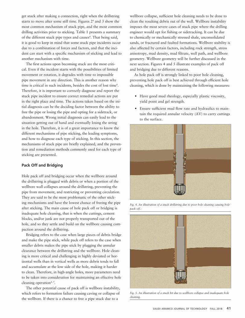
SAUDI ARAMCO JOURNAL OF TECHNOLOGY FALL 2018 41
get stuck after making a connection, right when the drillstring starts to move after some still time. Figures 24 and 3 show the most common mechanism of stuck pipe, and the most common drilling activities prior to sticking. Table 1 presents a summary of the different stuck pipe types and causes4. That being said, it is good to keep in mind that some stuck pipe incidents occur due to a combination of forces and factors, and that the inci-dent can start with a specific mechanism of sticking and lead to another mechanism with time.
The first actions upon becoming stuck are the most criti-cal. Even if the incident starts with the possibilities of limited movement or rotation, it degrades with time to impossible pipe movement in any direction. This is another reason why time is critical in such incidents, besides the cost of lost time4. Therefore, it is important to correctly diagnose and report the stuck pipe incident to ensure correct remedial actions are put in the right place and time. The actions taken based on the ini-tial diagnosis can be the deciding factor between the ability to free the pipe or losing the pipe and opting for a sidetrack, or abandonment. Wrong initial diagnosis can easily lead to the situation getting out of hand and eventually losing the string in the hole. Therefore, it is of a great importance to know the different mechanisms of pipe sticking, the leading symptoms, and how to diagnose each type of sticking. In this section, the mechanisms of stuck pipe are briefly explained, and the preven-tion and remediation methods commonly used for each type of sticking are presented.
Pack Off and Bridging
Hole pack off and bridging occur when the wellbore around the drillstring is plugged with debris or when a portion of the wellbore wall collapses around the drillstring, preventing the pipe from movement, and restricting or preventing circulation. They are said to be the most problematic of the other stick-ing mechanisms and have the lowest chance of freeing the pipe after sticking. The main cause of hole pack off or bridging is inadequate hole cleaning, that is when the cuttings, cement blocks, and/or junk are not properly transported out of the hole, and so they settle and build on the wellbore causing com-paction around the drillstring.
Bridging refers to the case when large pieces of debris bridge and make the pipe stick, while pack off refers to the case when smaller debris makes the pipe stick by plugging the annular clearance between the drillstring and the wellbore. Hole clean-ing is more critical and challenging in highly deviated or hor-izontal wells than in vertical wells as more debris tends to fall and accumulate at the low side of the hole, making it harder to clean. Therefore, in high-angle holes, more parameters need to be taken into consideration for maintaining an effective hole cleaning operation4, 5.
The other potential cause of pack off is wellbore instability, which refers to formation failure causing caving or collapse of the wellbore. If there is a chance to free a pipe stuck due to a
wellbore collapse, sufficient hole cleaning needs to be done to clean the resulting debris out of the well. Wellbore instability imposes the most severe cases of stuck pipe where the drilling engineer would opt for fishing or sidetracking. It can be due to chemically or mechanically stressed shale, unconsolidated sands, or fractured and faulted formations. Wellbore stability is also affected by certain factors, including rock strength, stress anisotropy, mud density, mud filtrate, well path, and wellbore geometry. Wellbore geometry will be further discussed in the next section. Figures 4 and 5 illustrate examples of pack off and bridging due to different reasons.
As hole pack off is strongly linked to poor hole cleaning, preventing hole pack off is best achieved through efficient hole cleaning, which is done by maintaining the following measures:
• Have good mud rheology, especially plastic viscosity, yield point and gel strength.
• Ensure sufficient mud flow rate and hydraulics to main-tain the required annular velocity (AV) to carry cuttings to the surface.
Fig. 4. An illustration of a stuck drillstring due to poor hole cleaning causing
Fig. 5. An illustration of a stuck bit due to wellbore collapse and inadequate
Fig. 4. An illustration of a stuck drillstring due to poor hole cleaning causing hole pack off.
Fig. 4. An illustration of a stuck drillstring due to poor hole cleaning
Fig. 5. An illustration of a stuck bit due to wellbore collapse and
Fig. 5. An illustration of a stuck bit due to wellbore collapse and inadequate hole cleaning.

42 FALL 2018 SAUDI ARAMCO JOURNAL OF TECHNOLOGY
• Ensure reciprocating and rotating of the drillpipe while circulating the hole clean.
• Ensure eccentricity of the pipe, making sure that the pipe is placed in the center of the wellbore to ensure having similar AVs around the drillstring.
• Control the rate of penetration to ensure that the drill-ing process is not creating more cutting and solids than the mud system can carry and dispose of.
• Plan regular wiper trips as they clean the hole, wipe swelling clays, and ream problematic sections.
An important indicator of the efficiency of hole cleaning is the carrying capacity index (CCI), which was developed by Robinson and Morgan (2004)6 and is calculated using the fol-lowing equation:
𝐶𝐶𝐶𝐶𝐶𝐶 = 𝐾𝐾∗𝐴𝐴𝐴𝐴∗𝑀𝑀𝑀𝑀
400,000 (1) 𝐾𝐾 = (511)1−𝑛𝑛(𝑃𝑃𝑃𝑃 + 𝑌𝑌𝑃𝑃) (2) 𝑛𝑛 = 3.22 log (2 𝑃𝑃𝐴𝐴+𝑌𝑌𝑃𝑃
𝑃𝑃𝐴𝐴+𝑌𝑌𝑃𝑃 ) (3)
(1)
where AV is the annular velocity in ft/min, MW is the mud weight in ppg, and K is the consistency index calculated using the following equation:
𝐶𝐶𝐶𝐶𝐶𝐶 = 𝐾𝐾∗𝐴𝐴𝐴𝐴∗𝑀𝑀𝑀𝑀
400,000 (1) 𝐾𝐾 = (511)1−𝑛𝑛(𝑃𝑃𝑃𝑃 + 𝑌𝑌𝑃𝑃) (2) 𝑛𝑛 = 3.22 log (2 𝑃𝑃𝐴𝐴+𝑌𝑌𝑃𝑃
𝑃𝑃𝐴𝐴+𝑌𝑌𝑃𝑃 ) (3)
(2)
where PV and YP are the plastic viscosity and the yield point in the Bingham Plastic model, respectively, and n is the power law index defined by the following equation:
𝐶𝐶𝐶𝐶𝐶𝐶 = 𝐾𝐾∗𝐴𝐴𝐴𝐴∗𝑀𝑀𝑀𝑀
400,000 (1) 𝐾𝐾 = (511)1−𝑛𝑛(𝑃𝑃𝑃𝑃 + 𝑌𝑌𝑃𝑃) (2) 𝑛𝑛 = 3.22 log (2 𝑃𝑃𝐴𝐴+𝑌𝑌𝑃𝑃
𝑃𝑃𝐴𝐴+𝑌𝑌𝑃𝑃 ) (3)
(3) Robinson and Morgan (2004)6 concluded that the best hole
cleaning is observed when the CCI = 1 and poor hole cleaning is observed when the CCI = 0.1.
As for remediation hole pack off, certain steps can be consid-ered to free the pipe:
• Attempt first to ensure good mud circulation, and regain circulation in case of losses.
• Apply downward force until circulation starts.
• Attempt to rotate the drillstring.
• In case of high inclination wells, spotting a low viscous followed by a weighted pill. The low viscosity pill will disturb the flow across the cuttings bed and then the weighted pill will carry the cuttings to the surface.
• In case of low inclination wells, only the use of a weighted pill will be needed to carry the cuttings to the surface.
Wellbore Geometry
The second category of stuck pipe to be discussed involves well-bore geometry. This category includes the cases where sticking
happens as a result of a conflict between the wellbore shape and the BHA configuration. Specifically, it occurs when the BHA is moved up or down into the area of the wellbore with the misconfigured shape. This can happen due to several reasons, which Mitchell (2011)4 has broken down into four categories. These are: (1) doglegs, (2) ledges, (3) undergauge holes, and (4) squeezing formations; such as salts, marls, and plastic shales.
Doglegs represent the majority of wellbore geometry stick-ing, as they can lead to further sticking problems such as key-seats, ledges, or drillstring failure due to high torque and side load. They can also lead to trouble related to cementing, run-ning casing, logging, and even production equipment failure. It is worthwhile to note that doglegs also increase the risk of other types of sticking, be it differential or pack off. Figure 6 illustrates how a keyseat can be cut into a dogleg. Several key-seats resulted from high dogleg severity, high pipe tension and rotation, and long rotating time.
In his book, Mitchell (2011)4 also points out another type of stuck pipe, which is “stiff assembly sticking.” It usually occurs while drilling directional wells, Fig. 7. In case of a severe
Fig. 6. An illustration of how a keyseat cuts
Fig. 7. An illustration of drillstring getting stuck.
Fig. 6. An illustration of how a keyseat cuts into a dogleg causing a stuck drillstring.
Fig. 6. An illustration of how a keyseat cuts
Fig. 7. An illustration of drillstring getting stuck.
Fig. 7. An illustration of side loads induced by forcing the assembly into the dogleg, leading to the drillstring getting stuck.
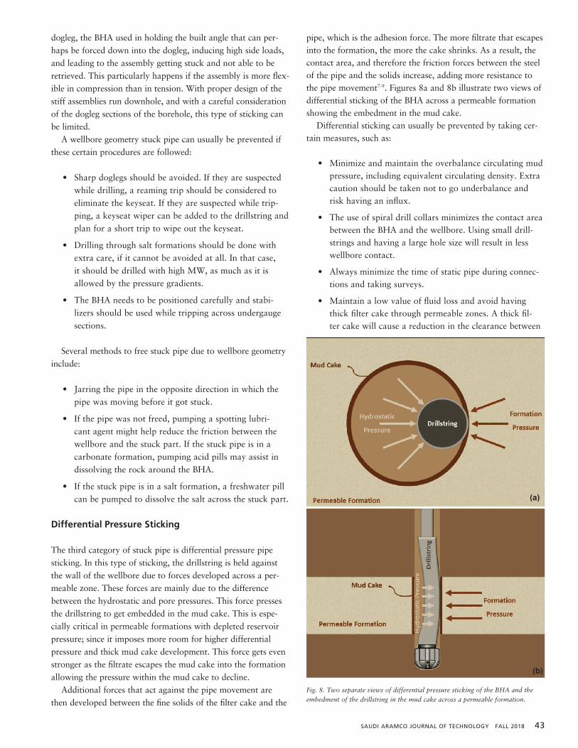
SAUDI ARAMCO JOURNAL OF TECHNOLOGY FALL 2018 43
dogleg, the BHA used in holding the built angle that can per-haps be forced down into the dogleg, inducing high side loads, and leading to the assembly getting stuck and not able to be retrieved. This particularly happens if the assembly is more flex-ible in compression than in tension. With proper design of the stiff assemblies run downhole, and with a careful consideration of the dogleg sections of the borehole, this type of sticking can be limited.
A wellbore geometry stuck pipe can usually be prevented if these certain procedures are followed:
• Sharp doglegs should be avoided. If they are suspected while drilling, a reaming trip should be considered to eliminate the keyseat. If they are suspected while trip-ping, a keyseat wiper can be added to the drillstring and plan for a short trip to wipe out the keyseat.
• Drilling through salt formations should be done with extra care, if it cannot be avoided at all. In that case, it should be drilled with high MW, as much as it is allowed by the pressure gradients.
• The BHA needs to be positioned carefully and stabi-lizers should be used while tripping across undergauge sections.
Several methods to free stuck pipe due to wellbore geometry include:
• Jarring the pipe in the opposite direction in which the pipe was moving before it got stuck.
• If the pipe was not freed, pumping a spotting lubri-cant agent might help reduce the friction between the wellbore and the stuck part. If the stuck pipe is in a carbonate formation, pumping acid pills may assist in dissolving the rock around the BHA.
• If the stuck pipe is in a salt formation, a freshwater pill can be pumped to dissolve the salt across the stuck part.
Differential Pressure Sticking
The third category of stuck pipe is differential pressure pipe sticking. In this type of sticking, the drillstring is held against the wall of the wellbore due to forces developed across a per-meable zone. These forces are mainly due to the difference between the hydrostatic and pore pressures. This force presses the drillstring to get embedded in the mud cake. This is espe-cially critical in permeable formations with depleted reservoir pressure; since it imposes more room for higher differential pressure and thick mud cake development. This force gets even stronger as the filtrate escapes the mud cake into the formation allowing the pressure within the mud cake to decline.
Additional forces that act against the pipe movement are then developed between the fine solids of the filter cake and the
pipe, which is the adhesion force. The more filtrate that escapes into the formation, the more the cake shrinks. As a result, the contact area, and therefore the friction forces between the steel of the pipe and the solids increase, adding more resistance to the pipe movement7-9. Figures 8a and 8b illustrate two views of differential sticking of the BHA across a permeable formation showing the embedment in the mud cake.
Differential sticking can usually be prevented by taking cer-tain measures, such as:
• Minimize and maintain the overbalance circulating mud pressure, including equivalent circulating density. Extra caution should be taken not to go underbalance and risk having an influx.
• The use of spiral drill collars minimizes the contact area between the BHA and the wellbore. Using small drill-strings and having a large hole size will result in less wellbore contact.
• Always minimize the time of static pipe during connec-tions and taking surveys.
• Maintain a low value of fluid loss and avoid having thick filter cake through permeable zones. A thick fil-ter cake will cause a reduction in the clearance between
Fig. 8. Two separate views of differential pressure sticking of the BHA anddrillstring in the mud cake across a permeable formation.
(a)
(b)
Fig. 8. Two separate views of differential pressure sticking of the BHA and the embedment of the drillstring in the mud cake across a permeable formation.
44 FALL 2018 SAUDI ARAMCO JOURNAL OF TECHNOLOGY
the wellbore and the BHA and will lead to differential sticking.
• Keep circulating to remove high solids from the mud to minimize the thickness of the filter cake. The filter cake is recommended to be thin, hard and impermeable.
Conventionally, a differential stuck pipe can be recovered following a few basic points4, 10:
• The first action is to increase the flow rate and apply maximum torque. The high mud flow rate will help to remove the filter cake from the BHA.
• The pipe should be jarred down. If not able to jar the pipe, the pipe should be slumped down. In differential sticking, the pipe should not be jarred up or pulled up because this will only increase the contact area between the filter cake and the BHA.
• If the above action did not succeed, then the reduction of MW should be considered to reduce the overbalance causing the differential sticking. Extra caution should be taken when reducing the MW so as to not get a kick, which could lead to a dangerous blowout.
• If the reduction of MW is not successful, or too dan-gerous to attempt, then spotting fluids to reduce the friction between the filter cake and the BHA should be considered. This may also be used simultaneously with the reduction of MW.
STUCK PIPE PREDICTION
Throughout the last few decades, following the best practices for stuck pipe avoidance has proven to be very effective in reducing stuck pipe incidents. Several major oil and gas compa-nies have adopted initiatives for preventing stuck pipe, formed task forces to mitigate this problem, and have reached the same conclusion. Results of their investigations indicate that focusing effort on engineering an operational training; ensuring adequate hole cleaning, ensuring use of optimal BHA and fluid designs, and following best remediation practices, have shown signif-icant improvement in reducing stuck pipe incidents. Despite such improvements, stuck pipes continues to be a leading cause of nonproductive time and a major expense during drilling operations today1, 11.
Two potential solutions to minimize stuck pipe incidents are either of a drilling fluids approach, or of a drilling automation approach. In the first approach, which was presented in the previous section, the options are to optimize your drilling pro-cesses proactively such as by improving hole cleaning efficiency, controlling mud cake, and reducing loss circulation by optimiz-ing the drilling fluids. The automation approach, however, is consistent of the hardware part; i.e., the sensors, and the soft-ware part; e.g., the algorithms. This approach, when very well
developed and utilized, can become very accurate and robust in preventing or mitigating stuck pipe incidents.
Many studies published in the literature have utilized data based on statistical analysis techniques, with a goal for track-ing stuck pipe probability. One of the earliest works is by Hempkins et al. (1987)12, which uses the discriminant analysis technique to classify the wells statistically, into mechanical, differential, or not stuck wells. Several other studies followed Hempkins’ work, basing their work on the multivariate dis-criminant analysis method and improving on it13-15. Subsequent work has presented several other techniques such as artificial neural network (ANN)16, 17, the adaptive neuro fuzzy inference system18, 19, and support vector regression3, 20 to build similar stuck pipe classifiers or give stuck pipe probabilities using a large set of drilling data as an input.
Another approach using the combination of automation and human knowledge in mitigating drilling problems has been pre-sented by Sadlier et al. (2013)21 and Ferreira et al. (2015)22. The model uses pattern recognition incorporated in an automated decision support tool. This tool provides real-time case-based reasoning to assess the risk and mitigate stuck pipe incidents in collaboration with an expert. The tool uses case-based reason-ing to match the real-time patterns with historical analogous cases where the same problem occurred. This allows providing automated recommendations for corrective actions based on the recognized patterns and the historical match. The experts are to collaborate in a timely manner with the decision support tool to provide guidance in mitigating the problem.
The third approach published in the literature uses analytical models, such as torque and drag, or hydraulics models, in identi-fying potential drilling problems. These models are usually based on the initial well plan, and the resulted predictions from the model are used during drilling operations for comparison with the actual parameters. In 2016, Salminen et al. (2017)23 have pre-sented a methodology using the same analytical model, but with improved reliability by including more parameters as factors in assessing stuck pipe risk. They have also incorporated this with the detection of specific patterns in the data that were identified as leading indicators of stuck pipe from historical cases.
METHODOLOGY
Careful monitoring of drilling and tripping trends is crucial to a successful drilling operation. The approach discussed in this article focuses on real-time detection of leading signs of stuck pipe incidents using the combination of pattern recognition in the drilling data and the physics of stuck pipe presented ear-lier. This integration is meant to ensure the reliability of the automated detective model. The drilling data and the trends of abnormalities implemented in the model were identified based on analysis of historical data of stuck pipe cases as well as the expert’s knowledge in the underlying principles for each type of stuck pipe. The model is designed to be implemented in the real-time drilling data environment to provide an alarm system
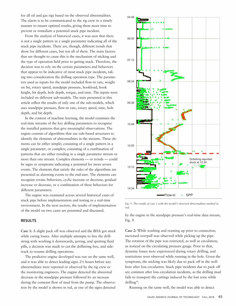
SAUDI ARAMCO JOURNAL OF TECHNOLOGY FALL 2018 45
for all oil and gas rigs based on the observed abnormalities. The alarm is to be communicated to the rig crew in a timely manner to ensure optimal results, giving them more time to prevent or remediate a potential stuck pipe incident.
From the analysis of historical cases, it was seen that there is not a single pattern in a single parameter indicating all of the stuck pipe incidents. There are, though, different trends that show for different cases, but not all of them. The main factors that are thought to cause this is the mechanism of sticking and the type of operation held prior to getting stuck. Therefore, the decision was to rely on the certain parameters and behaviors that appear to be indicative of most stuck pipe incidents, tak-ing into consideration the drilling operation type. The parame-ters used as inputs for the model included flow-in rate, weight on bit, rotary speed, standpipe pressure, hookload, hook height, bit depth, hole depth, torque, and time. The inputs were included on different sub-models. The tests presented in this article reflect the results of only one of the sub-models, which uses standpipe pressure, flow-in rate, rotary speed, time, hole depth, and bit depth.
In the context of machine learning, the model examines the real-time streams of the key drilling parameters to recognize the installed patterns that give meaningful observations. The engine consists of algorithms that use rule-based structures to identify the elements of abnormalities in the streams. These ele-ments can be either simple; consisting of a single pattern in a single parameter, or complex; consisting of a combination of patterns that are either trending in a single parameter stream or more than one stream. Complex elements — or trends — could be signs or symptoms indicating a potential for more severe events. The elements that satisfy the rules of the algorithms are presented as alarming events to the end-user. The elements can recognize erratic behaviors, cyclic increase or decrease, gradual increase or decrease, or a combination of these behaviors for different parameters.
The engine was examined across several historical cases of stuck pipe before implementation and testing in a real-time environment. In the next section, the results of implementation of the model on two cases are presented and discussed.
RESULTS
Case 1: A slight pack off was observed and the BHA got stuck while curing losses. After multiple attempts to free the drill-string with working it downwards, jarring, and spotting fluid pills, a decision was made to cut the drillstring free, and side-track to resume drilling operations.
The predictive engine developed was run on the same well, and it was able to detect leading signs 2½ hours before any abnormalities were reported or observed by the rig crew or the monitoring engineers. The engine detected the abnormal decrease in the standpipe pressure followed by an increase during the constant flow of mud from the pump. The observa-tion by the model is shown in red, as one of the signs detected
by the engine in the standpipe pressure’s real-time data stream, Fig. 9.
Case 2: While washing and reaming up prior to connection, increased overpull was observed while picking up the pipe. The rotation of the pipe was restricted, as well as circulation, as noticed on the circulating pressure gauge. Prior to that, dynamic losses were experienced during rotary drilling, and restrictions were observed while running in the hole. Given the symptoms, the sticking was likely due to pack off in the well-bore after loss circulation. Stuck pipe incidents due to pack off are common after loss circulation incidents, as the drilling mud fails to transport the cuttings induced by the lost zone while drilling24.
Running on the same well, the model was able to detect
Fig. 9. The results of case 1 with the model’s observed abnormalities
04:48
06:00
07:12
08:24
09:36
10:48
12:00
13:12
14:24
Flow-in SPP
Drillstring reported stuck at 12:30
Fig. 9. The results of case 1 with the model’s observed abnormalities marked in red.
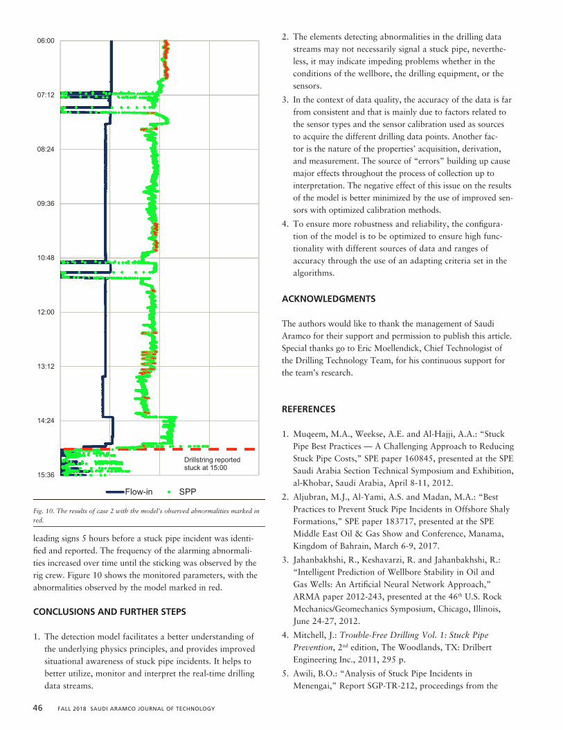
46 FALL 2018 SAUDI ARAMCO JOURNAL OF TECHNOLOGY
leading signs 5 hours before a stuck pipe incident was identi-fied and reported. The frequency of the alarming abnormali-ties increased over time until the sticking was observed by the rig crew. Figure 10 shows the monitored parameters, with the abnormalities observed by the model marked in red.
CONCLUSIONS AND FURTHER STEPS
1. The detection model facilitates a better understanding of the underlying physics principles, and provides improved situational awareness of stuck pipe incidents. It helps to better utilize, monitor and interpret the real-time drilling data streams.
2. The elements detecting abnormalities in the drilling data streams may not necessarily signal a stuck pipe, neverthe-less, it may indicate impeding problems whether in the conditions of the wellbore, the drilling equipment, or the sensors.
3. In the context of data quality, the accuracy of the data is far from consistent and that is mainly due to factors related to the sensor types and the sensor calibration used as sources to acquire the different drilling data points. Another fac-tor is the nature of the properties’ acquisition, derivation, and measurement. The source of “errors” building up cause major effects throughout the process of collection up to interpretation. The negative effect of this issue on the results of the model is better minimized by the use of improved sen-sors with optimized calibration methods.
4. To ensure more robustness and reliability, the configura-tion of the model is to be optimized to ensure high func-tionality with different sources of data and ranges of accuracy through the use of an adapting criteria set in the algorithms.
ACKNOWLEDGMENTS
The authors would like to thank the management of Saudi Aramco for their support and permission to publish this article. Special thanks go to Eric Moellendick, Chief Technologist of the Drilling Technology Team, for his continuous support for the team’s research.
REFERENCES
1. Muqeem, M.A., Weekse, A.E. and Al-Hajji, A.A.: “Stuck Pipe Best Practices — A Challenging Approach to Reducing Stuck Pipe Costs,” SPE paper 160845, presented at the SPE Saudi Arabia Section Technical Symposium and Exhibition, al-Khobar, Saudi Arabia, April 8-11, 2012.
2. Aljubran, M.J., Al-Yami, A.S. and Madan, M.A.: “Best Practices to Prevent Stuck Pipe Incidents in Offshore Shaly Formations,” SPE paper 183717, presented at the SPE Middle East Oil & Gas Show and Conference, Manama, Kingdom of Bahrain, March 6-9, 2017.
3. Jahanbakhshi, R., Keshavarzi, R. and Jahanbakhshi, R.: “Intelligent Prediction of Wellbore Stability in Oil and Gas Wells: An Artificial Neural Network Approach,” ARMA paper 2012-243, presented at the 46th U.S. Rock Mechanics/Geomechanics Symposium, Chicago, Illinois, June 24-27, 2012.
4. Mitchell, J.: Trouble-Free Drilling Vol. 1: Stuck Pipe Prevention, 2nd edition, The Woodlands, TX: Drilbert Engineering Inc., 2011, 295 p.
5. Awili, B.O.: “Analysis of Stuck Pipe Incidents in Menengai,” Report SGP-TR-212, proceedings from the
Fig. 10. The results of case 2 with the model’s observed abnormalities marked in red.
06:00
07:12
08:24
09:36
10:48
12:00
13:12
14:24
15:36
Flow-in SPP
Drillstring reported stuck at 15:00
Fig. 10. The results of case 2 with the model’s observed abnormalities marked in red.
SAUDI ARAMCO JOURNAL OF TECHNOLOGY FALL 2018 47
42nd Workshop on Geothermal Reservoir Engineering, Stanford, California, February 13-15, 2017, 12 p.
6. Robinson, L. and Morgan, M.: “Effect of Hole Cleaning on Drilling Rate and Performance,” AADE paper 04-DF-HO-42, presented at the American Association of Drilling Engineers Drilling Fluids Conference, Houston, Texas, April 6-7, 2004.
7. Dupriest, F.E., Elks, W.C. and Ottesen, S.: “Design Methodology and Operational Practices Eliminate Differential Sticking,” SPE Drilling & Completion, Vol. 26, Issue 1, March 2011, pp. 115-123.
8. Helmic, W.E. and Longley, A.J.: “Pressure Differential Sticking of Drill Pipe and How It Can Be Avoided or Relieved,” paper API-57-055, presented at the Drilling and Production Practice, New York, New York, January 1, 1957.
9. Outmans, H.D.: “Mechanics of Differential Pressure Sticking of Drill Collars,” Petroleum Transactions, AIME, Vol. 213, 1958, pp. 265-274.
10. Heitmann, N. and Burgos, E.C.: “Freeing Differential Stuck Pipe with Nitrogen Reduces Significantly Lost- In-Hole Drill Strings,” SPE paper 173168, presented at the SPE/IADC Drilling Conference and Exhibition, London, England, March 17-19, 2015.
11. Yarim, G., Uchytil, R.J., May, R.B., Trejo, A., et al.: “Stuck Pipe Prevention — A Proactive Solution to an Old Problem,” SPE paper 109914, presented at the SPE Annual Technical Conference and Exhibition, Anaheim, California, November 11-14, 2007.
12. Hempkins, W.B., Kingsborough, R.H., Lohec, W.E. and Nini, C.J.: “Multivariate Statistical Analysis of Stuck Drillpipe Situations,” SPE Drilling Engineering, Vol. 2, Issue 3, September 1987, pp. 237-244.
13. Biegler, M.W. and Kuhn, G.R.: “Advances in Prediction of Stuck Pipe Using Multivariate Statistical Analysis,” SPE paper 27529, presented at the SPE/IADC Drilling Conference, Dallas, Texas, February 15-18, 1994.
14. Howard, J.A. and Glover, S.B.: “Tracking Stuck Pipe Probability While Drilling,” SPE paper 27528, presented at the SPE/IADC Drilling Conference, Dallas, Texas, February 15-18, 1994.
15. Shoraka, S.A.R., Shadizadeh, S.R. and Shahri, M.P.: “Prediction of Stuck Pipe in Iranian South Oil Fields Using Multivariate Statistical Analysis,” SPE paper 151076, presented at the Nigeria Annual International Conference and Exhibition, Abuja, Nigeria, July 30- August 3, 2011.
16. Miri, R., Sampaio, J.H.B., Afshar, M. and Lourenco, A.: “Development of Artificial Neural Networks to Predict Differential Pipe Sticking in Iranian Offshore Oil Fields,” SPE paper 108500, presented at the International Oil Conference and Exhibition in Mexico, Veracruz, Mexico,
June 27-30, 2007.
17. Siruvuri, C., Nagarakanti, S. and Samuel, R.: “Stuck
Pipe Prediction and Avoidance: A Convolutional Neural
Network Approach,” SPE paper 98378, presented at the
IADC/SPE Drilling Conference, Miami, Florida, February
21-23, 2006.
18. Murillo, A., Neuman, J. and Samuel, R.: “Pipe Sticking
Prediction and Avoidance Using Adaptive Fuzzy Logic
Modeling,” SPE paper 120128, presented at the SPE
Production and Operations Symposium, Oklahoma City,
Oklahoma, April 4-8, 2009.
19. Naraghi, M.E., Ezzatyar, P. and Jamshidi, S.: “Prediction
of Drilling Pipe Sticking by Active Learning Method
(ALM),” Journal of Petroleum and Gas Engineering, Vol.
4, Issue 7, November 2013, pp. 173-183.
20. Chamkalani, A., Shahri, M.P. and Poordad, S.: “Support
Vector Machine Model: A New Methodology for Stuck
Pipe Prediction,” SPE paper 164003, presented at the SPE
Unconventional Gas Conference and Exhibition, Muscat,
Oman, January 28-30, 2013.
21. Sadlier, A., Says, I. and Hanson, R.: “Automated
Decision Support to Enhance While Drilling Decision
Making: Where Does it Fit within Drilling Automation?”
SPE paper 163430, presented at the SPE/IADC Drilling
Conference and Exhibition, Amsterdam, the Netherlands,
March 5-7, 2013.
22. Ferreira, A.P.L.A., Carvalho, D.J.L., Rodrigues, R.M.,
Schnell, D.M., et al.: “Automated Decision Support and
Expert Collaboration Avoid Stuck Pipe and Improve
Drilling Operations in Offshore Brazil Subsalt Well,”
OTC paper 25838, presented at the Offshore Technology
Conference, Houston, Texas, May 4-7, 2015.
23. Salminen, K., Cheatham, C., Smith, M. and Valiulin,
K.: “Stuck Pipe Prediction by Use of Automated
Real-Time Modeling and Data Analysis,” SPE Drilling
& Completion, Vol. 32, Issue 3, September 2017, pp.
184-193.
24. Nugroho, W.A., Hermawan, S. and Lazuardi, B.H.:
“Problem Mitigation in Geothermal Drilling, Case Studies
of Stuck Pipe and Lost Circulation,” Report SGP-TR-212,
proceedings from the 42nd Workshop on Geothermal
Reservoir Engineering, Stanford, California, February
13-15, 2017, 10 p.

48 FALL 2018 SAUDI ARAMCO JOURNAL OF TECHNOLOGY
BIOGRAPHIES
Abrar A. Alshaikh is a Petroleum Engineer with Saudi Aramco’s Drilling Technology Team of the Exploration and Petroleum Engineering Center – Advanced Research Center (EXPEC ARC). She has worked on several research and development projects,
mainly in the area of drilling optimization and automation. Abrar has filed one patent and published several
technical papers. Currently, she is on an assignment working as a Drilling Engineer with the Exploration and Oil Drilling Engineering Department.
Abrar received her B.S. degree in Petroleum Engineering from Texas A&M University, College Station, TX.
Mohammed K. Al-Bassam joined Saudi Aramco in 2015 as a Petroleum Engineer working in the advanced drilling tools focus area of the Drilling Technology Team in the Exploration and Petroleum Engineering Center – Advanced Research Center (EXPEC
ARC). His experience includes work on several research projects related to big data analytics and automation for data acquisition and engineering optimization.
Mohammed completed a one-year assignment working as a Drilling Engineer in the Exploration and Oil Drilling Engineering Department followed by a six-month assignment with the Northern Area Oil Drilling Department working as a Drilling Foremen in the Fadhili and Abu Hadriya oil fields.
He has published several technical papers and has one filed patent.
Mohammed received his B.S. degree in Mechanical Engineering from Northeastern University, Boston, MA.
Salem H. Al-Gharbi is Drilling Data Scientist with Saudi Aramco’s Drilling Technology Team at the Exploration and Petroleum Engineering Center – Advanced Research Center (EXPEC ARC). He has over 15 years of experience in the domain of advance
application development, targeting reservoir engineering, exploration, drilling engineering, operations and real-time challenges.
Salem was appointed as the technical leader for Saudi Aramco’s Drilling Ahead of Bit smart initiative; he is also one of the founders of the Society of Petroleum Engineers (SPE) Drilling Uncertainty Prediction International Technical Section (DUPTS). Salem has participated in multiple local and international events as a committee member or key speaker in the domain of artificial intelligent and machine learning in the drilling domain. He also has authored several publications and holds several patents in this field.
Salem received his M.S. degree in Computer Science from King Fahd University of Petroleum and Minerals
(KFUPM), Dhahran, Saudi Arabia, and his M.S. degree in Petroleum Engineering from Heriot-Watt University, Edinburgh, U.K.
Dr. Abdullah S. Al-Yami is a Petroleum Engineer with Saudi Aramco’s Drilling Technology Team at the Exploration and Petroleum Engineering Center – Advanced Research Center (EXPEC ARC). He has 18 years of experience with Saudi
Aramco and previously worked in different positions, including as a Lab Scientist and Drilling Engineer, conducting research related to drilling engineering.
Abdullah has received several awards during his career, including Saudi Aramco’s Research and Development Center (R&DC) Innovation Award and its Successful Field Application Award for his research work. He also received Saudi Aramco’s EXPEC ARC Effective Publications Award. A member of the Society of Petroleum of Engineers (SPE), Abdullah was awarded the 2009 SPE Outstanding Technical Editor Award for his work on the SPE Drilling and Completion Journal. He also received the 2014 SPE Regional (Middle East, North Africa and South Asia) Drilling Engineering Award and the 2015 CEO Saudi Aramco Excellence Award. In 2016, Abdullah received Oil & Gas Middle East Award “highly commended” recognition in the category of internal control valve (ICV) Strategy of the Year for his efforts in developing drilling products utilizing a local resources strategy.
He is a coauthor of the textbook Underbalanced Drilling: Limits and Extremes; has 13 granted U.S. patents and more than 30 filed patents; and has more than 60 publications to his credit, all in the area of drilling and completions.
Abdullah received his B.S. degree in Chemistry from Florida Institute of Technology, Melbourne, FL; his M.S. degree in Petroleum Engineering from King Fahd University of Petroleum and Minerals (KFUPM), Dhahran, Saudi Arabia; and his Ph.D. degree in Petroleum Engineering from Texas A&M University, College Station, TX.
SAUDI ARAMCO JOURNAL OF TECHNOLOGY FALL 2018 49
ABSTRACT
Formation evaluation studies suggest that high in the hydro-carbon column, the resistivity logs can precisely quantify fluid saturation due to the large contrast in the resistivities of hydro-carbon-bearing and water-bearing formations. In the transition zone where water and oil reside in more or less equal volumes, the determination of hydrocarbon saturation by resistivity value becomes challenging. Some of these intervals exhibit low resis-tivity pay (LRP) characteristics where resistivity-based log anal-ysis predicts high water saturation, yet they can produce little or no water cut.
Conventional log-based saturation and rock quality evalua-tion in a low permeability carbonate reservoir is difficult due to the lack of the input measurement sensitivity to pore size and the amount of pore filling fluids. Pore size information pro-vided by nuclear magnetic resonance (NMR) logs from this LRP provides good sensitivity, but it needs to be calibrated for quantitative use. The objective of this study is to determine a height-based bulk volume irreducible (HBVI) cutoff to dis-tinguish and quantify the amounts of reservoir fluids across a wellbore using NMR logs.
The procedure consists of a two-part workflow. The first part describes the acquisition of a database that includes high-quality laboratory NMR and capillary pressure meas- urements to determine the pore aspect ratio and the effect of temperature on the formation’s NMR properties using core samples from the target reservoir. These measurements are then used to underpin the mathematical description of the HBVI cutoff as a function of displacement pressure that is translated to a height above the free water level. The second part of the workflow is a well log processing scheme where the new formula is implemented to calculate a continuous fluid saturation profile across the well using NMR logs.
The laboratory measurements suggest a good agreement between the capillary pressure and NMR T
2 measurements. Both data sets indicate a well sorted pore size distribution. The T2 relaxation time increases with temperature, which is then considered in the downhole implementation of the HBVI model. The NMR-based saturation log is consistent with wire-line formation test observations and mercury injection capil-lary pressure (MICP) based saturation height modeling results
in a LRP reservoir.The results of this study suggest that the laboratory calibra-
tion and NMR log processing workflows described herein pro-vide a viable alternative for the calculation of fluid saturations in complex reservoirs where the conventional log-based satura-tion evaluation faces uncertainties.
INTRODUCTION
Formation evaluation studies suggest that high in the hydro-carbon column, the distribution of fluids in the pore network yields a simple and straightforward correlation between for-mation resistivity fluid saturation as described first by Archie’s breakthrough article in 19421. In the transition zone, where the amounts of oil and water become comparable, the relation-ship between resistivity and saturation is less accurate2. In cer-tain formations, the water phase forms electrical shortcuts that lead to low resistivity in formations that still contain significant volumes of producible hydrocarbons2. Such a pay interval is known as low resistivity pay (LRP). The issue of LRP is evident in some sandstones due to mainly shaliness3, 4 and in carbonates due to mainly microporosity5-9.
Microporous carbonates may contain large amounts of connate water, yet produce dry or nearly dry oil. The resistiv-ity contrast between these pay zones and water-bearing for-mations becomes small10. The resulting loss of sensitivity in conventional log-based saturation evaluation poses risks to reservoir development in these formations at or near the tran-sition zone and warrants alternative solutions, one of which is discussed in this article.
Nuclear magnetic resonance (NMR) tools uniquely measure the amount of fluids within a porous rock and characterizes the strength of their interaction with the pore surface. Downhole NMR logging enabled new reservoir description techniques for porosity and rock quality analysis11. One of these techniques is the determination of irreducible water saturation using an NMR cutoff that is obtained by laboratory desaturation of core samples with a single desaturation pressure representing maximum reservoir height. The advantage of this technique is that the NMR cutoff12 usually remains consistent within major lithology types while it is independent of formation resistivity properties.
A New NMR-based Height Saturation Model of a Low Permeability Carbonate Reservoir
Dr. Ahmad M. Al-Harbi, Dr. Gabor G. Hursan, Dr. Hyung T. Kwak, and Jun Gao

50 FALL 2018 SAUDI ARAMCO JOURNAL OF TECHNOLOGY
Motivated by a good agreement between NMR T2 distribu-tion logs and mercury injection capillary pressure (MICP) pore throat distributions in multiple cored wells from a low perme-ability carbonate reservoir, the current study extends the NMR cutoff approach to a multitude of displacement pressures cov-ering a wide range that includes the transition zone in addition to the irreducible condition. Combined with fluid displacement pressure in a given well, the height-based NMR cutoff can be conveniently used for the calculation of water saturation. The practical advantages of the technique reported herein are sum-marized as:
1. It is independent of formation resistivity.
2. It is easily implemented within the existing NMR interpreta-tion software.
3. The method works in horizontal and vertical wells without any modification.
This article describes the laboratory procedures to acquire supporting data for the height-based cutoff method and the results of said analysis for 15 microporous samples that under-pins the mathematical model of the height-based NMR T2 cut-off. The final section discusses the results of the new procedure applied on NMR well log data.
METHOD AND PROCEDURE
Material
Fifteen 1.5” diameter core plug samples from a low permeabil-ity carbonate reservoir were prepared for the tests. All of the 1.5” core plugs were cut in half creating 30 plugs, in which nine halves were used in the MICP study while the other nine halves were used in the height saturation modeling study. Synthetic water related to the depth’s interval used for the investigation — 206,056 mg/L total dissolved solids — was prepared based on the detailed water composition presented in Table 1. The brine was filtered through a 0.45 micron filter for test use.
Magnetic Resonance Imaging (MRI) based Capillary Pressure
The main objective of this study is to confirm the apparent rela-tionship of pore size information provided by NMR and capil-lary pressure, and to develop a model linking capillary-bound water volume and capillary pressure, resulting in a height-based saturation model.
To confirm the relationship of pore size information from the NMR and capillary pressure, accurate capillary pressure curves are required for each sample. Capillary pressure is typ-ically measured in the laboratory by using mercury injection, porous plate, or centrifugation techniques13. The porous plate method is considered the most direct and accurate method. This method takes a long time since each capillary pressure point requires an equilibrium time that can take weeks or months14. The mercury injection method is fast and can reach very high capillary pressures. The method is destructive and uses a non-representative fluid (mercury).
A common compromise between porous plate and mercury injection is centrifugation15. This method uses reservoir fluids and decreases the equilibrium time by using high centrifugal forces. The inlet saturation must be computed using an approx-imate solution that is known to cause errors16.
A more recent method14 for measuring capillary pressure employing a centrifuge and a new quantitative magnetic res-onance imaging (MRI) method for measuring fluid saturation were demonstrated to work for different rock systems. The capillary pressure is calculated from the Hassler and Brunner equation (Eqn. 1) at each radial position in the rock:
𝑃𝑃𝐶𝐶(𝑟𝑟) =12 ∆𝜌𝜌𝜔𝜔
2(𝑟𝑟22 − 𝑟𝑟2) (1) ∆𝜌𝜌 𝜔𝜔
𝑃𝑃𝐶𝐶 = 𝑃𝑃𝑒𝑒 (𝑆𝑆𝑤𝑤−𝑆𝑆𝑤𝑤𝑤𝑤1−𝑆𝑆𝑤𝑤𝑤𝑤
)−1
𝜆𝜆⁄ (2) 𝑆𝑆𝑤𝑤 𝑆𝑆𝑤𝑤𝑤𝑤 𝑃𝑃𝑒𝑒 𝜆𝜆
𝑆𝑆𝑤𝑤 = (1 − 𝑆𝑆𝑤𝑤𝑤𝑤) (𝑃𝑃𝐶𝐶𝑃𝑃𝑒𝑒)−𝜆𝜆
+ 𝑆𝑆𝑤𝑤𝑤𝑤 (3)
𝑇𝑇2𝑐𝑐𝑐𝑐𝑐𝑐𝑐𝑐𝑐𝑐𝑐𝑐 = (𝑇𝑇2𝑚𝑚𝑚𝑚𝑚𝑚 − 𝑇𝑇2𝑚𝑚𝑤𝑤𝑚𝑚) (𝑃𝑃𝐶𝐶𝑃𝑃𝑒𝑒)−𝜆𝜆
+ 𝑇𝑇2𝑚𝑚𝑤𝑤𝑚𝑚 (4) ℎ = 144𝑃𝑃𝐶𝐶
∆𝜌𝜌 (5)
𝑇𝑇2𝑐𝑐𝑐𝑐𝑐𝑐𝑐𝑐𝑐𝑐𝑐𝑐 = (𝑇𝑇2𝑚𝑚𝑚𝑚𝑚𝑚 − 𝑇𝑇2𝑚𝑚𝑤𝑤𝑚𝑚) (ℎℎ𝑒𝑒)−𝜆𝜆
+ 𝑇𝑇2𝑚𝑚𝑤𝑤𝑚𝑚 (6) 𝐸𝐸𝑟𝑟𝑟𝑟𝐸𝐸𝑟𝑟 = ∑(log(𝑇𝑇2𝑐𝑐𝑐𝑐𝑐𝑐𝑐𝑐𝑐𝑐𝑐𝑐−𝑚𝑚𝑒𝑒𝑚𝑚𝑚𝑚𝑐𝑐𝑚𝑚𝑒𝑒𝑚𝑚) − log(𝑇𝑇2𝑐𝑐𝑐𝑐𝑐𝑐𝑐𝑐𝑐𝑐𝑐𝑐−𝑐𝑐𝑚𝑚𝑐𝑐𝑐𝑐𝑐𝑐𝑐𝑐𝑚𝑚𝑐𝑐𝑒𝑒𝑚𝑚))
2
ℎ = 𝑃𝑃𝐶𝐶𝑚𝑚−𝑤𝑤 × 𝜎𝜎𝑜𝑜−𝑤𝑤
𝜎𝜎𝑎𝑎−𝑤𝑤× 144𝑐𝑐𝑐𝑐𝑚𝑚𝑐𝑐
∆𝜌𝜌𝑜𝑜−𝑤𝑤 (8)
𝜎𝜎𝑐𝑐−𝑤𝑤 𝜎𝜎𝑚𝑚−𝑤𝑤
(1)
where
𝑃𝑃𝐶𝐶(𝑟𝑟) =12 ∆𝜌𝜌𝜔𝜔
2(𝑟𝑟22 − 𝑟𝑟2) (1) ∆𝜌𝜌 𝜔𝜔
𝑃𝑃𝐶𝐶 = 𝑃𝑃𝑒𝑒 (𝑆𝑆𝑤𝑤−𝑆𝑆𝑤𝑤𝑤𝑤1−𝑆𝑆𝑤𝑤𝑤𝑤
)−1
𝜆𝜆⁄ (2) 𝑆𝑆𝑤𝑤 𝑆𝑆𝑤𝑤𝑤𝑤 𝑃𝑃𝑒𝑒 𝜆𝜆
𝑆𝑆𝑤𝑤 = (1 − 𝑆𝑆𝑤𝑤𝑤𝑤) (𝑃𝑃𝐶𝐶𝑃𝑃𝑒𝑒)−𝜆𝜆
+ 𝑆𝑆𝑤𝑤𝑤𝑤 (3)
𝑇𝑇2𝑐𝑐𝑐𝑐𝑐𝑐𝑐𝑐𝑐𝑐𝑐𝑐 = (𝑇𝑇2𝑚𝑚𝑚𝑚𝑚𝑚 − 𝑇𝑇2𝑚𝑚𝑤𝑤𝑚𝑚) (𝑃𝑃𝐶𝐶𝑃𝑃𝑒𝑒)−𝜆𝜆
+ 𝑇𝑇2𝑚𝑚𝑤𝑤𝑚𝑚 (4) ℎ = 144𝑃𝑃𝐶𝐶
∆𝜌𝜌 (5)
𝑇𝑇2𝑐𝑐𝑐𝑐𝑐𝑐𝑐𝑐𝑐𝑐𝑐𝑐 = (𝑇𝑇2𝑚𝑚𝑚𝑚𝑚𝑚 − 𝑇𝑇2𝑚𝑚𝑤𝑤𝑚𝑚) (ℎℎ𝑒𝑒)−𝜆𝜆
+ 𝑇𝑇2𝑚𝑚𝑤𝑤𝑚𝑚 (6) 𝐸𝐸𝑟𝑟𝑟𝑟𝐸𝐸𝑟𝑟 = ∑(log(𝑇𝑇2𝑐𝑐𝑐𝑐𝑐𝑐𝑐𝑐𝑐𝑐𝑐𝑐−𝑚𝑚𝑒𝑒𝑚𝑚𝑚𝑚𝑐𝑐𝑚𝑚𝑒𝑒𝑚𝑚) − log(𝑇𝑇2𝑐𝑐𝑐𝑐𝑐𝑐𝑐𝑐𝑐𝑐𝑐𝑐−𝑐𝑐𝑚𝑚𝑐𝑐𝑐𝑐𝑐𝑐𝑐𝑐𝑚𝑚𝑐𝑐𝑒𝑒𝑚𝑚))
2
ℎ = 𝑃𝑃𝐶𝐶𝑚𝑚−𝑤𝑤 × 𝜎𝜎𝑜𝑜−𝑤𝑤
𝜎𝜎𝑎𝑎−𝑤𝑤× 144𝑐𝑐𝑐𝑐𝑚𝑚𝑐𝑐
∆𝜌𝜌𝑜𝑜−𝑤𝑤 (8)
𝜎𝜎𝑐𝑐−𝑤𝑤 𝜎𝜎𝑚𝑚−𝑤𝑤
is the density difference between wetting and non-wetting fluid.
𝑃𝑃𝐶𝐶(𝑟𝑟) =12 ∆𝜌𝜌𝜔𝜔
2(𝑟𝑟22 − 𝑟𝑟2) (1) ∆𝜌𝜌 𝜔𝜔
𝑃𝑃𝐶𝐶 = 𝑃𝑃𝑒𝑒 (𝑆𝑆𝑤𝑤−𝑆𝑆𝑤𝑤𝑤𝑤1−𝑆𝑆𝑤𝑤𝑤𝑤
)−1
𝜆𝜆⁄ (2) 𝑆𝑆𝑤𝑤 𝑆𝑆𝑤𝑤𝑤𝑤 𝑃𝑃𝑒𝑒 𝜆𝜆
𝑆𝑆𝑤𝑤 = (1 − 𝑆𝑆𝑤𝑤𝑤𝑤) (𝑃𝑃𝐶𝐶𝑃𝑃𝑒𝑒)−𝜆𝜆
+ 𝑆𝑆𝑤𝑤𝑤𝑤 (3)
𝑇𝑇2𝑐𝑐𝑐𝑐𝑐𝑐𝑐𝑐𝑐𝑐𝑐𝑐 = (𝑇𝑇2𝑚𝑚𝑚𝑚𝑚𝑚 − 𝑇𝑇2𝑚𝑚𝑤𝑤𝑚𝑚) (𝑃𝑃𝐶𝐶𝑃𝑃𝑒𝑒)−𝜆𝜆
+ 𝑇𝑇2𝑚𝑚𝑤𝑤𝑚𝑚 (4) ℎ = 144𝑃𝑃𝐶𝐶
∆𝜌𝜌 (5)
𝑇𝑇2𝑐𝑐𝑐𝑐𝑐𝑐𝑐𝑐𝑐𝑐𝑐𝑐 = (𝑇𝑇2𝑚𝑚𝑚𝑚𝑚𝑚 − 𝑇𝑇2𝑚𝑚𝑤𝑤𝑚𝑚) (ℎℎ𝑒𝑒)−𝜆𝜆
+ 𝑇𝑇2𝑚𝑚𝑤𝑤𝑚𝑚 (6) 𝐸𝐸𝑟𝑟𝑟𝑟𝐸𝐸𝑟𝑟 = ∑(log(𝑇𝑇2𝑐𝑐𝑐𝑐𝑐𝑐𝑐𝑐𝑐𝑐𝑐𝑐−𝑚𝑚𝑒𝑒𝑚𝑚𝑚𝑚𝑐𝑐𝑚𝑚𝑒𝑒𝑚𝑚) − log(𝑇𝑇2𝑐𝑐𝑐𝑐𝑐𝑐𝑐𝑐𝑐𝑐𝑐𝑐−𝑐𝑐𝑚𝑚𝑐𝑐𝑐𝑐𝑐𝑐𝑐𝑐𝑚𝑚𝑐𝑐 ℎ = 𝑃𝑃𝐶𝐶𝑚𝑚−𝑤𝑤 × 𝜎𝜎𝑜𝑜−𝑤𝑤
𝜎𝜎𝑎𝑎−𝑤𝑤× 144𝑐𝑐𝑐𝑐𝑚𝑚𝑐𝑐
∆𝜌𝜌𝑜𝑜−𝑤𝑤 (8)
𝜎𝜎𝑐𝑐−𝑤𝑤 𝜎𝜎𝑚𝑚−𝑤𝑤
is the rotational speed around the rota-tional axis, r2 and r are the distance from the center of the rota-tional axis, Fig. 1.
The calculated capillary pressure together with the satura-tion, as measured by MRI at each position, directly produces a capillary pressure curve14. Figure 2 shows a typical example of the MRI capillary pressure curve.
Salt Concentration (mg/L)
Sodium Chloride (NaCl) 187,667
Calcium Chloride (CaCl2.2H2O)
13,293
Magnesium Chloride (MgCl2.6H2O)
3,562
Potassium Chloride (KCl) 550
Sodium Bicarbonate (NaHCO3)
2,236
Sodium Sulfate (Na2SO4) 2,675
Table 1. Salt concentration of the water used to prepare synthetic brine
Fig. 1. Schematic diagram of a core plug sample spinning in a centrifuge.
21.1 psi
52.1 psi
Inlet Face
Outlet Face
Core Plug at 100% SW ω
r2
r
r1
Fig. 1. Schematic diagram of a core plug sample spinning in a centrifuge.
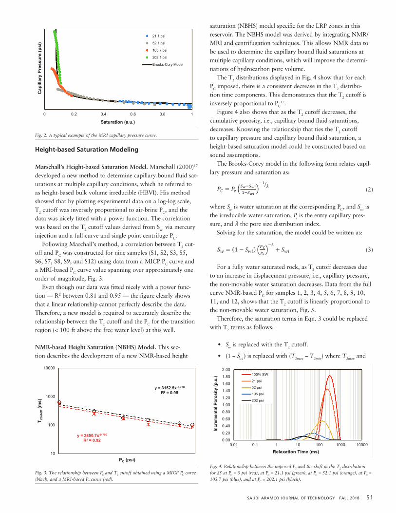
SAUDI ARAMCO JOURNAL OF TECHNOLOGY FALL 2018 51
Height-based Saturation Modeling
Marschall’s Height-based Saturation Model. Marschall (2000)17 developed a new method to determine capillary bound fluid sat-urations at multiple capillary conditions, which he referred to as height-based bulk volume irreducible (HBVI). His method showed that by plotting experimental data on a log-log scale, T2 cutoff was inversely proportional to air-brine PC, and the data was nicely fitted with a power function. The correlation was based on the T2 cutoff values derived from Swi via mercury injection and a full-curve and single-point centrifuge PC.
Following Marchall’s method, a correlation between T2 cut-off and PC was constructed for nine samples (S1, S2, S3, S5, S6, S7, S8, S9, and S12) using data from a MICP PC curve and a MRI-based PC curve value spanning over approximately one order of magnitude, Fig. 3.
Even though our data was fitted nicely with a power func-tion — R2 between 0.81 and 0.95 — the figure clearly shows that a linear relationship cannot perfectly describe the data. Therefore, a new model is required to accurately describe the relationship between the T2 cutoff and the PC for the transition region (< 100 ft above the free water level) at this well.
NMR-based Height Saturation (NBHS) Model. This sec-tion describes the development of a new NMR-based height
saturation (NBHS) model specific for the LRP zones in this reservoir. The NBHS model was derived by integrating NMR/MRI and centrifugation techniques. This allows NMR data to be used to determine the capillary bound fluid saturations at multiple capillary conditions, which will improve the determi-nations of hydrocarbon pore volume.
The T2 distributions displayed in Fig. 4 show that for each PC imposed, there is a consistent decrease in the T2 distribu-tion time components. This demonstrates that the T2 cutoff is inversely proportional to PC
17.Figure 4 also shows that as the T2 cutoff decreases, the
cumulative porosity, i.e., capillary bound fluid saturations, decreases. Knowing the relationship that ties the T2 cutoff to capillary pressure and capillary bound fluid saturation, a height-based saturation model could be constructed based on sound assumptions.
The Brooks-Corey model in the following form relates capil-lary pressure and saturation as:
𝑃𝑃𝐶𝐶(𝑟𝑟) =12 ∆𝜌𝜌𝜔𝜔
2(𝑟𝑟22 − 𝑟𝑟2) (1) ∆𝜌𝜌 𝜔𝜔
𝑃𝑃𝐶𝐶 = 𝑃𝑃𝑒𝑒 (𝑆𝑆𝑤𝑤−𝑆𝑆𝑤𝑤𝑤𝑤1−𝑆𝑆𝑤𝑤𝑤𝑤
)−1
𝜆𝜆⁄ (2) 𝑆𝑆𝑤𝑤 𝑆𝑆𝑤𝑤𝑤𝑤 𝑃𝑃𝑒𝑒 𝜆𝜆
𝑆𝑆𝑤𝑤 = (1 − 𝑆𝑆𝑤𝑤𝑤𝑤) (𝑃𝑃𝐶𝐶𝑃𝑃𝑒𝑒)−𝜆𝜆
+ 𝑆𝑆𝑤𝑤𝑤𝑤 (3)
𝑇𝑇2𝑐𝑐𝑐𝑐𝑐𝑐𝑐𝑐𝑐𝑐𝑐𝑐 = (𝑇𝑇2𝑚𝑚𝑚𝑚𝑚𝑚 − 𝑇𝑇2𝑚𝑚𝑤𝑤𝑚𝑚) (𝑃𝑃𝐶𝐶𝑃𝑃𝑒𝑒)−𝜆𝜆
+ 𝑇𝑇2𝑚𝑚𝑤𝑤𝑚𝑚 (4) ℎ = 144𝑃𝑃𝐶𝐶
∆𝜌𝜌 (5)
𝑇𝑇2𝑐𝑐𝑐𝑐𝑐𝑐𝑐𝑐𝑐𝑐𝑐𝑐 = (𝑇𝑇2𝑚𝑚𝑚𝑚𝑚𝑚 − 𝑇𝑇2𝑚𝑚𝑤𝑤𝑚𝑚) (ℎℎ𝑒𝑒)−𝜆𝜆
+ 𝑇𝑇2𝑚𝑚𝑤𝑤𝑚𝑚 (6) 𝐸𝐸𝑟𝑟𝑟𝑟𝐸𝐸𝑟𝑟 = ∑(log(𝑇𝑇2𝑐𝑐𝑐𝑐𝑐𝑐𝑐𝑐𝑐𝑐𝑐𝑐−𝑚𝑚𝑒𝑒𝑚𝑚𝑚𝑚𝑐𝑐𝑚𝑚𝑒𝑒𝑚𝑚) − log(𝑇𝑇2𝑐𝑐𝑐𝑐𝑐𝑐𝑐𝑐𝑐𝑐𝑐𝑐−𝑐𝑐𝑚𝑚𝑐𝑐𝑐𝑐𝑐𝑐𝑐𝑐𝑚𝑚𝑐𝑐𝑒𝑒𝑚𝑚))
2
ℎ = 𝑃𝑃𝐶𝐶𝑚𝑚−𝑤𝑤 × 𝜎𝜎𝑜𝑜−𝑤𝑤
𝜎𝜎𝑎𝑎−𝑤𝑤× 144𝑐𝑐𝑐𝑐𝑚𝑚𝑐𝑐
∆𝜌𝜌𝑜𝑜−𝑤𝑤 (8)
𝜎𝜎𝑐𝑐−𝑤𝑤 𝜎𝜎𝑚𝑚−𝑤𝑤 𝜃𝜃 ∆𝜌𝜌𝑐𝑐−𝑤𝑤 𝜆𝜆
(2)
where Sw is water saturation at the corresponding PC, and Swi is the irreducible water saturation, Pe is the entry capillary pres-sure, and
𝑃𝑃𝐶𝐶(𝑟𝑟) =12 ∆𝜌𝜌𝜔𝜔
2(𝑟𝑟22 − 𝑟𝑟2) (1) ∆𝜌𝜌 𝜔𝜔
𝑃𝑃𝐶𝐶 = 𝑃𝑃𝑒𝑒 (𝑆𝑆𝑤𝑤−𝑆𝑆𝑤𝑤𝑤𝑤1−𝑆𝑆𝑤𝑤𝑤𝑤
)−1
𝜆𝜆⁄ (2) 𝑆𝑆𝑤𝑤 𝑆𝑆𝑤𝑤𝑤𝑤 𝑃𝑃𝑒𝑒 𝜆𝜆
𝑆𝑆𝑤𝑤 = (1 − 𝑆𝑆𝑤𝑤𝑤𝑤) (𝑃𝑃𝐶𝐶𝑃𝑃𝑒𝑒)−𝜆𝜆
+ 𝑆𝑆𝑤𝑤𝑤𝑤 (3)
𝑇𝑇2𝑐𝑐𝑐𝑐𝑐𝑐𝑐𝑐𝑐𝑐𝑐𝑐 = (𝑇𝑇2𝑚𝑚𝑚𝑚𝑚𝑚 − 𝑇𝑇2𝑚𝑚𝑤𝑤𝑚𝑚) (𝑃𝑃𝐶𝐶𝑃𝑃𝑒𝑒)−𝜆𝜆
+ 𝑇𝑇2𝑚𝑚𝑤𝑤𝑚𝑚 (4) ℎ = 144𝑃𝑃𝐶𝐶
∆𝜌𝜌 (5)
𝑇𝑇2𝑐𝑐𝑐𝑐𝑐𝑐𝑐𝑐𝑐𝑐𝑐𝑐 = (𝑇𝑇2𝑚𝑚𝑚𝑚𝑚𝑚 − 𝑇𝑇2𝑚𝑚𝑤𝑤𝑚𝑚) (ℎℎ𝑒𝑒)−𝜆𝜆
+ 𝑇𝑇2𝑚𝑚𝑤𝑤𝑚𝑚 (6) 𝐸𝐸𝑟𝑟𝑟𝑟𝐸𝐸𝑟𝑟 = ∑(log(𝑇𝑇2𝑐𝑐𝑐𝑐𝑐𝑐𝑐𝑐𝑐𝑐𝑐𝑐−𝑚𝑚𝑒𝑒𝑚𝑚𝑚𝑚𝑐𝑐𝑚𝑚𝑒𝑒𝑚𝑚) − log(𝑇𝑇2𝑐𝑐𝑐𝑐𝑐𝑐𝑐𝑐𝑐𝑐𝑐𝑐−𝑐𝑐𝑚𝑚𝑐𝑐𝑐𝑐𝑐𝑐𝑐𝑐𝑚𝑚𝑐𝑐𝑒𝑒𝑚𝑚))
2 (7)
ℎ = 𝑃𝑃𝐶𝐶𝑚𝑚−𝑤𝑤 × 𝜎𝜎𝑜𝑜−𝑤𝑤
𝜎𝜎𝑎𝑎−𝑤𝑤× 144𝑐𝑐𝑐𝑐𝑚𝑚𝑐𝑐
∆𝜌𝜌𝑜𝑜−𝑤𝑤 (8)
𝜎𝜎𝑐𝑐−𝑤𝑤 𝜎𝜎𝑚𝑚−𝑤𝑤 𝜃𝜃 ∆𝜌𝜌𝑐𝑐−𝑤𝑤 𝜆𝜆
the pore size distribution index.Solving for the saturation, the model could be written as:
𝑃𝑃𝐶𝐶(𝑟𝑟) =12 ∆𝜌𝜌𝜔𝜔
2(𝑟𝑟22 − 𝑟𝑟2) (1) ∆𝜌𝜌 𝜔𝜔
𝑃𝑃𝐶𝐶 = 𝑃𝑃𝑒𝑒 (𝑆𝑆𝑤𝑤−𝑆𝑆𝑤𝑤𝑤𝑤1−𝑆𝑆𝑤𝑤𝑤𝑤
)−1
𝜆𝜆⁄ (2) 𝑆𝑆𝑤𝑤 𝑆𝑆𝑤𝑤𝑤𝑤 𝑃𝑃𝑒𝑒 𝜆𝜆
𝑆𝑆𝑤𝑤 = (1 − 𝑆𝑆𝑤𝑤𝑤𝑤) (𝑃𝑃𝐶𝐶𝑃𝑃𝑒𝑒)−𝜆𝜆
+ 𝑆𝑆𝑤𝑤𝑤𝑤 (3)
𝑇𝑇2𝑐𝑐𝑐𝑐𝑐𝑐𝑐𝑐𝑐𝑐𝑐𝑐 = (𝑇𝑇2𝑚𝑚𝑚𝑚𝑚𝑚 − 𝑇𝑇2𝑚𝑚𝑤𝑤𝑚𝑚) (𝑃𝑃𝐶𝐶𝑃𝑃𝑒𝑒)−𝜆𝜆
+ 𝑇𝑇2𝑚𝑚𝑤𝑤𝑚𝑚 (4) ℎ = 144𝑃𝑃𝐶𝐶
∆𝜌𝜌 (5)
𝑇𝑇2𝑐𝑐𝑐𝑐𝑐𝑐𝑐𝑐𝑐𝑐𝑐𝑐 = (𝑇𝑇2𝑚𝑚𝑚𝑚𝑚𝑚 − 𝑇𝑇2𝑚𝑚𝑤𝑤𝑚𝑚) (ℎℎ𝑒𝑒)−𝜆𝜆
+ 𝑇𝑇2𝑚𝑚𝑤𝑤𝑚𝑚 (6) 𝐸𝐸𝑟𝑟𝑟𝑟𝐸𝐸𝑟𝑟 = ∑(log(𝑇𝑇2𝑐𝑐𝑐𝑐𝑐𝑐𝑐𝑐𝑐𝑐𝑐𝑐−𝑚𝑚𝑒𝑒𝑚𝑚𝑚𝑚𝑐𝑐𝑚𝑚𝑒𝑒𝑚𝑚) − log(𝑇𝑇2𝑐𝑐𝑐𝑐𝑐𝑐𝑐𝑐𝑐𝑐𝑐𝑐−𝑐𝑐𝑚𝑚𝑐𝑐𝑐𝑐𝑐𝑐𝑐𝑐𝑚𝑚𝑐𝑐𝑒𝑒𝑚𝑚))
2
ℎ = 𝑃𝑃𝐶𝐶𝑚𝑚−𝑤𝑤 × 𝜎𝜎𝑜𝑜−𝑤𝑤
𝜎𝜎𝑎𝑎−𝑤𝑤× 144𝑐𝑐𝑐𝑐𝑚𝑚𝑐𝑐
∆𝜌𝜌𝑜𝑜−𝑤𝑤 (8)
𝜎𝜎𝑐𝑐−𝑤𝑤 𝜎𝜎𝑚𝑚−𝑤𝑤 𝜃𝜃 ∆𝜌𝜌𝑐𝑐−𝑤𝑤 𝜆𝜆
(3)
For a fully water saturated rock, as T2 cutoff decreases due to an increase in displacement pressure, i.e., capillary pressure, the non-movable water saturation decreases. Data from the full curve NMR-based PC for samples 1, 2, 3, 4, 5, 6, 7, 8, 9, 10, 11, and 12, shows that the T2 cutoff is linearly proportional to the non-movable water saturation, Fig. 5.
Therefore, the saturation terms in Eqn. 3 could be replaced with T2 terms as follows:
• Sw is replaced with the T2 cutoff.
• (1-Swi) is replaced with (T2max – T2min) where T2max and
Fig. 1. Schematic diagram of a core plug sample spinning in a centrifuge.
Fig. 2. A typical example of the MRI capillary pressure curve.
0 0.2 0.4 0.6 0.8 1
Cap
illar
y Pr
essu
re (p
si)
Saturation (a.u.)
21.1 psi
52.1 psi
105.7 psi
202.1 psi
Brooks-Cory Model
Fig. 2. A typical example of the MRI capillary pressure curve.
Fig. 3. The relationship between PC and T2 cutoff obtained using a MICP PC curve (black) and a MRI-based PC curve (red).
y = 3152.5x-0.778
R² = 0.95
y = 2850.7x-0.796
R² = 0.92
10
100
1000
10000
T 2cu
toff
(ms)
PC (psi)
2.00100% SW
Fig. 3. The relationship between PC and T2 cutoff obtained using a MICP PC curve (black) and a MRI-based PC curve (red).
Fig. 4. Relationship between the imposed PC and the shift in the T2 distribution for S5 at PC = 0 psi (red), at PC = 21.1 psi (green), at PC = 52.1 psi (orange), at PC = 105.7 psi (blue), and at PC = 202.1 psi (black).
Fig. 3. The relationship between PC and T2 cutoff obtained using a MICP PC curve (black)based PC curve (red).
Fig. 4. Relationship between the imposed PC and the shift in the T2 distribution for S5 at PCat PC = 21.1 psi (green), at PC = 52.1 psi (orange), at PC = 105.7 psi (blue), and at PC =
y = 3152.5x-0.778
R² = 0.95
y = 2850.7x-0.796
R² = 0.92
10
100
1000
10000
T 2cu
toff
(ms)
PC (psi)
0.00
0.20
0.40
0.60
0.80
1.00
1.20
1.40
1.60
1.80
2.00
0.01 0.1 1 10 100 1000 10000
Incr
emen
tal P
oros
ity (p
.u.)
Relaxation Time (ms)
100% SW
21 psi
52 psi
105 psi
202 psi

52 FALL 2018 SAUDI ARAMCO JOURNAL OF TECHNOLOGY
T2min are defined in Fig. 6, using S11 as an example.
• Swi is replaced with T2min.
For the studied samples, it is assumed that any incremental
porosity with T2 relaxation time less than 10 mSec, Fig. 6, will
not be produced for an air-brine PC range up to ~200 psi.
Therefore, Eqn. 3 takes the following form:
𝑃𝑃𝐶𝐶(𝑟𝑟) =12 ∆𝜌𝜌𝜔𝜔
2(𝑟𝑟22 − 𝑟𝑟2) (1) ∆𝜌𝜌 𝜔𝜔
𝑃𝑃𝐶𝐶 = 𝑃𝑃𝑒𝑒 (𝑆𝑆𝑤𝑤−𝑆𝑆𝑤𝑤𝑤𝑤1−𝑆𝑆𝑤𝑤𝑤𝑤
)−1
𝜆𝜆⁄ (2) 𝑆𝑆𝑤𝑤 𝑆𝑆𝑤𝑤𝑤𝑤 𝑃𝑃𝑒𝑒 𝜆𝜆
𝑆𝑆𝑤𝑤 = (1 − 𝑆𝑆𝑤𝑤𝑤𝑤) (𝑃𝑃𝐶𝐶𝑃𝑃𝑒𝑒)−𝜆𝜆
+ 𝑆𝑆𝑤𝑤𝑤𝑤 (3)
𝑇𝑇2𝑐𝑐𝑐𝑐𝑐𝑐𝑐𝑐𝑐𝑐𝑐𝑐 = (𝑇𝑇2𝑚𝑚𝑚𝑚𝑚𝑚 − 𝑇𝑇2𝑚𝑚𝑤𝑤𝑚𝑚) (𝑃𝑃𝐶𝐶𝑃𝑃𝑒𝑒)−𝜆𝜆
+ 𝑇𝑇2𝑚𝑚𝑤𝑤𝑚𝑚 (4) ℎ = 144𝑃𝑃𝐶𝐶
∆𝜌𝜌 (5)
𝑇𝑇2𝑐𝑐𝑐𝑐𝑐𝑐𝑐𝑐𝑐𝑐𝑐𝑐 = (𝑇𝑇2𝑚𝑚𝑚𝑚𝑚𝑚 − 𝑇𝑇2𝑚𝑚𝑤𝑤𝑚𝑚) (ℎℎ𝑒𝑒)−𝜆𝜆
+ 𝑇𝑇2𝑚𝑚𝑤𝑤𝑚𝑚 (6) 𝐸𝐸𝑟𝑟𝑟𝑟𝐸𝐸𝑟𝑟 = ∑(log(𝑇𝑇2𝑐𝑐𝑐𝑐𝑐𝑐𝑐𝑐𝑐𝑐𝑐𝑐−𝑚𝑚𝑒𝑒𝑚𝑚𝑚𝑚𝑐𝑐𝑚𝑚𝑒𝑒𝑚𝑚) − log(𝑇𝑇2𝑐𝑐𝑐𝑐𝑐𝑐𝑐𝑐𝑐𝑐𝑐𝑐−𝑐𝑐𝑚𝑚𝑐𝑐𝑐𝑐𝑐𝑐𝑐𝑐𝑚𝑚𝑐𝑐𝑒𝑒𝑚𝑚))
2 (7)
ℎ = 𝑃𝑃𝐶𝐶𝑚𝑚−𝑤𝑤 × 𝜎𝜎𝑜𝑜−𝑤𝑤
𝜎𝜎𝑎𝑎−𝑤𝑤× 144𝑐𝑐𝑐𝑐𝑚𝑚𝑐𝑐
∆𝜌𝜌𝑜𝑜−𝑤𝑤 (8)
𝜎𝜎𝑐𝑐−𝑤𝑤 𝜎𝜎𝑚𝑚−𝑤𝑤 𝜃𝜃 ∆𝜌𝜌𝑐𝑐−𝑤𝑤 𝜆𝜆
(4)
By substituting the following relationship between PC and the
height above the free water level (
𝑃𝑃𝐶𝐶(𝑟𝑟) =12 ∆𝜌𝜌𝜔𝜔
2(𝑟𝑟22 − 𝑟𝑟2) (1) ∆𝜌𝜌 𝜔𝜔
𝑃𝑃𝐶𝐶 = 𝑃𝑃𝑒𝑒 (𝑆𝑆𝑤𝑤−𝑆𝑆𝑤𝑤𝑤𝑤1−𝑆𝑆𝑤𝑤𝑤𝑤
)−1
𝜆𝜆⁄ (2) 𝑆𝑆𝑤𝑤 𝑆𝑆𝑤𝑤𝑤𝑤 𝑃𝑃𝑒𝑒 𝜆𝜆
𝑆𝑆𝑤𝑤 = (1 − 𝑆𝑆𝑤𝑤𝑤𝑤) (𝑃𝑃𝐶𝐶𝑃𝑃𝑒𝑒)−𝜆𝜆
+ 𝑆𝑆𝑤𝑤𝑤𝑤 (3)
𝑇𝑇2𝑐𝑐𝑐𝑐𝑐𝑐𝑐𝑐𝑐𝑐𝑐𝑐 = (𝑇𝑇2𝑚𝑚𝑚𝑚𝑚𝑚 − 𝑇𝑇2𝑚𝑚𝑤𝑤𝑚𝑚) (𝑃𝑃𝐶𝐶𝑃𝑃𝑒𝑒)−𝜆𝜆
+ 𝑇𝑇2𝑚𝑚𝑤𝑤𝑚𝑚 (4) ℎ = 144𝑃𝑃𝐶𝐶
∆𝜌𝜌 (5)
𝑇𝑇2𝑐𝑐𝑐𝑐𝑐𝑐𝑐𝑐𝑐𝑐𝑐𝑐 = (𝑇𝑇2𝑚𝑚𝑚𝑚𝑚𝑚 − 𝑇𝑇2𝑚𝑚𝑤𝑤𝑚𝑚) (ℎℎ𝑒𝑒)−𝜆𝜆
+ 𝑇𝑇2𝑚𝑚𝑤𝑤𝑚𝑚 (6) 𝐸𝐸𝑟𝑟𝑟𝑟𝐸𝐸𝑟𝑟 = ∑(log(𝑇𝑇2𝑐𝑐𝑐𝑐𝑐𝑐𝑐𝑐𝑐𝑐𝑐𝑐−𝑚𝑚𝑒𝑒𝑚𝑚𝑚𝑚𝑐𝑐𝑚𝑚𝑒𝑒𝑚𝑚) − log(𝑇𝑇2𝑐𝑐𝑐𝑐𝑐𝑐𝑐𝑐𝑐𝑐𝑐𝑐−𝑐𝑐𝑚𝑚𝑐𝑐𝑐𝑐𝑐𝑐𝑐𝑐𝑚𝑚𝑐𝑐𝑒𝑒𝑚𝑚))
2 (7)
ℎ = 𝑃𝑃𝐶𝐶𝑚𝑚−𝑤𝑤 × 𝜎𝜎𝑜𝑜−𝑤𝑤
𝜎𝜎𝑎𝑎−𝑤𝑤× 144𝑐𝑐𝑐𝑐𝑚𝑚𝑐𝑐
∆𝜌𝜌𝑜𝑜−𝑤𝑤 (8)
𝜎𝜎𝑐𝑐−𝑤𝑤 𝜎𝜎𝑚𝑚−𝑤𝑤 𝜃𝜃 ∆𝜌𝜌𝑐𝑐−𝑤𝑤 𝜆𝜆
):
𝑃𝑃𝐶𝐶(𝑟𝑟) =12 ∆𝜌𝜌𝜔𝜔
2(𝑟𝑟22 − 𝑟𝑟2) (1) ∆𝜌𝜌 𝜔𝜔
𝑃𝑃𝐶𝐶 = 𝑃𝑃𝑒𝑒 (𝑆𝑆𝑤𝑤−𝑆𝑆𝑤𝑤𝑤𝑤1−𝑆𝑆𝑤𝑤𝑤𝑤
)−1
𝜆𝜆⁄ (2) 𝑆𝑆𝑤𝑤 𝑆𝑆𝑤𝑤𝑤𝑤 𝑃𝑃𝑒𝑒 𝜆𝜆
𝑆𝑆𝑤𝑤 = (1 − 𝑆𝑆𝑤𝑤𝑤𝑤) (𝑃𝑃𝐶𝐶𝑃𝑃𝑒𝑒)−𝜆𝜆
+ 𝑆𝑆𝑤𝑤𝑤𝑤 (3)
𝑇𝑇2𝑐𝑐𝑐𝑐𝑐𝑐𝑐𝑐𝑐𝑐𝑐𝑐 = (𝑇𝑇2𝑚𝑚𝑚𝑚𝑚𝑚 − 𝑇𝑇2𝑚𝑚𝑤𝑤𝑚𝑚) (𝑃𝑃𝐶𝐶𝑃𝑃𝑒𝑒)−𝜆𝜆
+ 𝑇𝑇2𝑚𝑚𝑤𝑤𝑚𝑚 (4) ℎ = 144𝑃𝑃𝐶𝐶
∆𝜌𝜌 (5)
𝑇𝑇2𝑐𝑐𝑐𝑐𝑐𝑐𝑐𝑐𝑐𝑐𝑐𝑐 = (𝑇𝑇2𝑚𝑚𝑚𝑚𝑚𝑚 − 𝑇𝑇2𝑚𝑚𝑤𝑤𝑚𝑚) (ℎℎ𝑒𝑒)−𝜆𝜆
+ 𝑇𝑇2𝑚𝑚𝑤𝑤𝑚𝑚 (6) 𝐸𝐸𝑟𝑟𝑟𝑟𝐸𝐸𝑟𝑟 = ∑(log(𝑇𝑇2𝑐𝑐𝑐𝑐𝑐𝑐𝑐𝑐𝑐𝑐𝑐𝑐−𝑚𝑚𝑒𝑒𝑚𝑚𝑚𝑚𝑐𝑐𝑚𝑚𝑒𝑒𝑚𝑚) − log(𝑇𝑇2𝑐𝑐𝑐𝑐𝑐𝑐𝑐𝑐𝑐𝑐𝑐𝑐−𝑐𝑐𝑚𝑚𝑐𝑐𝑐𝑐𝑐𝑐𝑐𝑐𝑚𝑚𝑐𝑐𝑒𝑒𝑚𝑚))
2 (7)
ℎ = 𝑃𝑃𝐶𝐶𝑚𝑚−𝑤𝑤 × 𝜎𝜎𝑜𝑜−𝑤𝑤
𝜎𝜎𝑎𝑎−𝑤𝑤× 144𝑐𝑐𝑐𝑐𝑚𝑚𝑐𝑐
∆𝜌𝜌𝑜𝑜−𝑤𝑤 (8)
𝜎𝜎𝑐𝑐−𝑤𝑤 𝜎𝜎𝑚𝑚−𝑤𝑤 𝜃𝜃 ∆𝜌𝜌𝑐𝑐−𝑤𝑤 𝜆𝜆
(5)
where
𝑃𝑃𝐶𝐶(𝑟𝑟) =12 ∆𝜌𝜌𝜔𝜔
2(𝑟𝑟22 − 𝑟𝑟2) (1) ∆𝜌𝜌 𝜔𝜔
𝑃𝑃𝐶𝐶 = 𝑃𝑃𝑒𝑒 (𝑆𝑆𝑤𝑤−𝑆𝑆𝑤𝑤𝑤𝑤1−𝑆𝑆𝑤𝑤𝑤𝑤
)−1
𝜆𝜆⁄ (2) 𝑆𝑆𝑤𝑤 𝑆𝑆𝑤𝑤𝑤𝑤 𝑃𝑃𝑒𝑒 𝜆𝜆
𝑆𝑆𝑤𝑤 = (1 − 𝑆𝑆𝑤𝑤𝑤𝑤) (𝑃𝑃𝐶𝐶𝑃𝑃𝑒𝑒)−𝜆𝜆
+ 𝑆𝑆𝑤𝑤𝑤𝑤 (3)
𝑇𝑇2𝑐𝑐𝑐𝑐𝑐𝑐𝑐𝑐𝑐𝑐𝑐𝑐 = (𝑇𝑇2𝑚𝑚𝑚𝑚𝑚𝑚 − 𝑇𝑇2𝑚𝑚𝑤𝑤𝑚𝑚) (𝑃𝑃𝐶𝐶𝑃𝑃𝑒𝑒)−𝜆𝜆
+ 𝑇𝑇2𝑚𝑚𝑤𝑤𝑚𝑚 (4) ℎ = 144𝑃𝑃𝐶𝐶
∆𝜌𝜌 (5)
𝑇𝑇2𝑐𝑐𝑐𝑐𝑐𝑐𝑐𝑐𝑐𝑐𝑐𝑐 = (𝑇𝑇2𝑚𝑚𝑚𝑚𝑚𝑚 − 𝑇𝑇2𝑚𝑚𝑤𝑤𝑚𝑚) (ℎℎ𝑒𝑒)−𝜆𝜆
+ 𝑇𝑇2𝑚𝑚𝑤𝑤𝑚𝑚 (6) 𝐸𝐸𝑟𝑟𝑟𝑟𝐸𝐸𝑟𝑟 = ∑(log(𝑇𝑇2𝑐𝑐𝑐𝑐𝑐𝑐𝑐𝑐𝑐𝑐𝑐𝑐−𝑚𝑚𝑒𝑒𝑚𝑚𝑚𝑚𝑐𝑐𝑚𝑚𝑒𝑒𝑚𝑚) − log(𝑇𝑇2𝑐𝑐𝑐𝑐𝑐𝑐𝑐𝑐𝑐𝑐𝑐𝑐−𝑐𝑐𝑚𝑚𝑐𝑐𝑐𝑐𝑐𝑐𝑐𝑐𝑚𝑚𝑐𝑐𝑒𝑒𝑚𝑚))
2 (7)
ℎ = 𝑃𝑃𝐶𝐶𝑚𝑚−𝑤𝑤 × 𝜎𝜎𝑜𝑜−𝑤𝑤
𝜎𝜎𝑎𝑎−𝑤𝑤× 144𝑐𝑐𝑐𝑐𝑚𝑚𝑐𝑐
∆𝜌𝜌𝑜𝑜−𝑤𝑤 (8)
𝜎𝜎𝑐𝑐−𝑤𝑤 𝜎𝜎𝑚𝑚−𝑤𝑤 𝜃𝜃 ∆𝜌𝜌𝑐𝑐−𝑤𝑤
is the density difference between the
wetting and nonwetting phase, so Eqn. 4 then
becomes:
𝑃𝑃𝐶𝐶(𝑟𝑟) =12 ∆𝜌𝜌𝜔𝜔
2(𝑟𝑟22 − 𝑟𝑟2) (1) ∆𝜌𝜌 𝜔𝜔
𝑃𝑃𝐶𝐶 = 𝑃𝑃𝑒𝑒 (𝑆𝑆𝑤𝑤−𝑆𝑆𝑤𝑤𝑤𝑤1−𝑆𝑆𝑤𝑤𝑤𝑤
)−1
𝜆𝜆⁄ (2) 𝑆𝑆𝑤𝑤 𝑆𝑆𝑤𝑤𝑤𝑤 𝑃𝑃𝑒𝑒 𝜆𝜆
𝑆𝑆𝑤𝑤 = (1 − 𝑆𝑆𝑤𝑤𝑤𝑤) (𝑃𝑃𝐶𝐶𝑃𝑃𝑒𝑒)−𝜆𝜆
+ 𝑆𝑆𝑤𝑤𝑤𝑤 (3)
𝑇𝑇2𝑐𝑐𝑐𝑐𝑐𝑐𝑐𝑐𝑐𝑐𝑐𝑐 = (𝑇𝑇2𝑚𝑚𝑚𝑚𝑚𝑚 − 𝑇𝑇2𝑚𝑚𝑤𝑤𝑚𝑚) (𝑃𝑃𝐶𝐶𝑃𝑃𝑒𝑒)−𝜆𝜆
+ 𝑇𝑇2𝑚𝑚𝑤𝑤𝑚𝑚 (4) ℎ = 144𝑃𝑃𝐶𝐶
∆𝜌𝜌 (5)
𝑇𝑇2𝑐𝑐𝑐𝑐𝑐𝑐𝑐𝑐𝑐𝑐𝑐𝑐 = (𝑇𝑇2𝑚𝑚𝑚𝑚𝑚𝑚 − 𝑇𝑇2𝑚𝑚𝑤𝑤𝑚𝑚) (ℎℎ𝑒𝑒)−𝜆𝜆
+ 𝑇𝑇2𝑚𝑚𝑤𝑤𝑚𝑚 (6) 𝐸𝐸𝑟𝑟𝑟𝑟𝐸𝐸𝑟𝑟 = ∑(log(𝑇𝑇2𝑐𝑐𝑐𝑐𝑐𝑐𝑐𝑐𝑐𝑐𝑐𝑐−𝑚𝑚𝑒𝑒𝑚𝑚𝑚𝑚𝑐𝑐𝑚𝑚𝑒𝑒𝑚𝑚) − log(𝑇𝑇2𝑐𝑐𝑐𝑐𝑐𝑐𝑐𝑐𝑐𝑐𝑐𝑐−𝑐𝑐𝑚𝑚𝑐𝑐𝑐𝑐𝑐𝑐𝑐𝑐𝑚𝑚𝑐𝑐𝑒𝑒𝑚𝑚))
2 (7)
ℎ = 𝑃𝑃𝐶𝐶𝑚𝑚−𝑤𝑤 × 𝜎𝜎𝑜𝑜−𝑤𝑤
𝜎𝜎𝑎𝑎−𝑤𝑤× 144𝑐𝑐𝑐𝑐𝑚𝑚𝑐𝑐
∆𝜌𝜌𝑜𝑜−𝑤𝑤 (8)
𝜎𝜎𝑐𝑐−𝑤𝑤 𝜎𝜎𝑚𝑚−𝑤𝑤 𝜃𝜃 ∆𝜌𝜌𝑐𝑐−𝑤𝑤 𝜆𝜆
(6)
where
𝑃𝑃𝐶𝐶(𝑟𝑟) =12 ∆𝜌𝜌𝜔𝜔
2(𝑟𝑟22 − 𝑟𝑟2) (1) ∆𝜌𝜌 𝜔𝜔
𝑃𝑃𝐶𝐶 = 𝑃𝑃𝑒𝑒 (𝑆𝑆𝑤𝑤−𝑆𝑆𝑤𝑤𝑤𝑤1−𝑆𝑆𝑤𝑤𝑤𝑤
)−1
𝜆𝜆⁄ (2) 𝑆𝑆𝑤𝑤 𝑆𝑆𝑤𝑤𝑤𝑤 𝑃𝑃𝑒𝑒 𝜆𝜆
𝑆𝑆𝑤𝑤 = (1 − 𝑆𝑆𝑤𝑤𝑤𝑤) (𝑃𝑃𝐶𝐶𝑃𝑃𝑒𝑒)−𝜆𝜆
+ 𝑆𝑆𝑤𝑤𝑤𝑤 (3)
𝑇𝑇2𝑐𝑐𝑐𝑐𝑐𝑐𝑐𝑐𝑐𝑐𝑐𝑐 = (𝑇𝑇2𝑚𝑚𝑚𝑚𝑚𝑚 − 𝑇𝑇2𝑚𝑚𝑤𝑤𝑚𝑚) (𝑃𝑃𝐶𝐶𝑃𝑃𝑒𝑒)−𝜆𝜆
+ 𝑇𝑇2𝑚𝑚𝑤𝑤𝑚𝑚 (4) ℎ = 144𝑃𝑃𝐶𝐶
∆𝜌𝜌 (5)
𝑇𝑇2𝑐𝑐𝑐𝑐𝑐𝑐𝑐𝑐𝑐𝑐𝑐𝑐 = (𝑇𝑇2𝑚𝑚𝑚𝑚𝑚𝑚 − 𝑇𝑇2𝑚𝑚𝑤𝑤𝑚𝑚) (ℎℎ𝑒𝑒)−𝜆𝜆
+ 𝑇𝑇2𝑚𝑚𝑤𝑤𝑚𝑚 (6) 𝐸𝐸𝑟𝑟𝑟𝑟𝐸𝐸𝑟𝑟 = ∑(log(𝑇𝑇2𝑐𝑐𝑐𝑐𝑐𝑐𝑐𝑐𝑐𝑐𝑐𝑐−𝑚𝑚𝑒𝑒𝑚𝑚𝑚𝑚𝑐𝑐𝑚𝑚𝑒𝑒𝑚𝑚) − log(𝑇𝑇2𝑐𝑐𝑐𝑐𝑐𝑐𝑐𝑐𝑐𝑐𝑐𝑐−𝑐𝑐𝑚𝑚𝑐𝑐𝑐𝑐𝑐𝑐𝑐𝑐𝑚𝑚𝑐𝑐𝑒𝑒𝑚𝑚))
2 (7)
ℎ = 𝑃𝑃𝐶𝐶𝑚𝑚−𝑤𝑤 × 𝜎𝜎𝑜𝑜−𝑤𝑤
𝜎𝜎𝑎𝑎−𝑤𝑤× 144𝑐𝑐𝑐𝑐𝑚𝑚𝑐𝑐
∆𝜌𝜌𝑜𝑜−𝑤𝑤 (8)
𝜎𝜎𝑐𝑐−𝑤𝑤 𝜎𝜎𝑚𝑚−𝑤𝑤 𝜃𝜃 ∆𝜌𝜌𝑐𝑐−𝑤𝑤 𝜆𝜆
e is the height above the free water level
corresponding to the capillary entry pressure.
To generate a height-based saturation curve,
Eqn. 6 can be used to fit a full curve of PC (or
𝑃𝑃𝐶𝐶(𝑟𝑟) =12 ∆𝜌𝜌𝜔𝜔
2(𝑟𝑟22 − 𝑟𝑟2) (1) ∆𝜌𝜌 𝜔𝜔
𝑃𝑃𝐶𝐶 = 𝑃𝑃𝑒𝑒 (𝑆𝑆𝑤𝑤−𝑆𝑆𝑤𝑤𝑤𝑤1−𝑆𝑆𝑤𝑤𝑤𝑤
)−1
𝜆𝜆⁄ (2) 𝑆𝑆𝑤𝑤 𝑆𝑆𝑤𝑤𝑤𝑤 𝑃𝑃𝑒𝑒 𝜆𝜆
𝑆𝑆𝑤𝑤 = (1 − 𝑆𝑆𝑤𝑤𝑤𝑤) (𝑃𝑃𝐶𝐶𝑃𝑃𝑒𝑒)−𝜆𝜆
+ 𝑆𝑆𝑤𝑤𝑤𝑤 (3)
𝑇𝑇2𝑐𝑐𝑐𝑐𝑐𝑐𝑐𝑐𝑐𝑐𝑐𝑐 = (𝑇𝑇2𝑚𝑚𝑚𝑚𝑚𝑚 − 𝑇𝑇2𝑚𝑚𝑤𝑤𝑚𝑚) (𝑃𝑃𝐶𝐶𝑃𝑃𝑒𝑒)−𝜆𝜆
+ 𝑇𝑇2𝑚𝑚𝑤𝑤𝑚𝑚 (4) ℎ = 144𝑃𝑃𝐶𝐶
∆𝜌𝜌 (5)
𝑇𝑇2𝑐𝑐𝑐𝑐𝑐𝑐𝑐𝑐𝑐𝑐𝑐𝑐 = (𝑇𝑇2𝑚𝑚𝑚𝑚𝑚𝑚 − 𝑇𝑇2𝑚𝑚𝑤𝑤𝑚𝑚) (ℎℎ𝑒𝑒)−𝜆𝜆
+ 𝑇𝑇2𝑚𝑚𝑤𝑤𝑚𝑚 (6) 𝐸𝐸𝑟𝑟𝑟𝑟𝐸𝐸𝑟𝑟 = ∑(log(𝑇𝑇2𝑐𝑐𝑐𝑐𝑐𝑐𝑐𝑐𝑐𝑐𝑐𝑐−𝑚𝑚𝑒𝑒𝑚𝑚𝑚𝑚𝑐𝑐𝑚𝑚𝑒𝑒𝑚𝑚) − log(𝑇𝑇2𝑐𝑐𝑐𝑐𝑐𝑐𝑐𝑐𝑐𝑐𝑐𝑐−𝑐𝑐𝑚𝑚𝑐𝑐𝑐𝑐𝑐𝑐𝑐𝑐𝑚𝑚𝑐𝑐𝑒𝑒𝑚𝑚))
2 (7)
ℎ = 𝑃𝑃𝐶𝐶𝑚𝑚−𝑤𝑤 × 𝜎𝜎𝑜𝑜−𝑤𝑤
𝜎𝜎𝑎𝑎−𝑤𝑤× 144𝑐𝑐𝑐𝑐𝑚𝑚𝑐𝑐
∆𝜌𝜌𝑜𝑜−𝑤𝑤 (8)
𝜎𝜎𝑐𝑐−𝑤𝑤 𝜎𝜎𝑚𝑚−𝑤𝑤 𝜃𝜃 ∆𝜌𝜌𝑐𝑐−𝑤𝑤 𝜆𝜆
)
vs. T2 cutoff. To generate the T2 cutoff curve, the workflow in Fig. 7 is followed. The model error was calculated and then minimized to find the optimal solution (fit) using the “log Sw least squared fit” function given by:
𝑃𝑃𝐶𝐶(𝑟𝑟) =12 ∆𝜌𝜌𝜔𝜔
2(𝑟𝑟22 − 𝑟𝑟2) (1) ∆𝜌𝜌 𝜔𝜔
𝑃𝑃𝐶𝐶 = 𝑃𝑃𝑒𝑒 (𝑆𝑆𝑤𝑤−𝑆𝑆𝑤𝑤𝑤𝑤1−𝑆𝑆𝑤𝑤𝑤𝑤
)−1
𝜆𝜆⁄ (2) 𝑆𝑆𝑤𝑤 𝑆𝑆𝑤𝑤𝑤𝑤 𝑃𝑃𝑒𝑒 𝜆𝜆
𝑆𝑆𝑤𝑤 = (1 − 𝑆𝑆𝑤𝑤𝑤𝑤) (𝑃𝑃𝐶𝐶𝑃𝑃𝑒𝑒)−𝜆𝜆
+ 𝑆𝑆𝑤𝑤𝑤𝑤 (3)
𝑇𝑇2𝑐𝑐𝑐𝑐𝑐𝑐𝑐𝑐𝑐𝑐𝑐𝑐 = (𝑇𝑇2𝑚𝑚𝑚𝑚𝑚𝑚 − 𝑇𝑇2𝑚𝑚𝑤𝑤𝑚𝑚) (𝑃𝑃𝐶𝐶𝑃𝑃𝑒𝑒)−𝜆𝜆
+ 𝑇𝑇2𝑚𝑚𝑤𝑤𝑚𝑚 (4) ℎ = 144𝑃𝑃𝐶𝐶
∆𝜌𝜌 (5)
𝑇𝑇2𝑐𝑐𝑐𝑐𝑐𝑐𝑐𝑐𝑐𝑐𝑐𝑐 = (𝑇𝑇2𝑚𝑚𝑚𝑚𝑚𝑚 − 𝑇𝑇2𝑚𝑚𝑤𝑤𝑚𝑚) (ℎℎ𝑒𝑒)−𝜆𝜆
+ 𝑇𝑇2𝑚𝑚𝑤𝑤𝑚𝑚 (6) 𝐸𝐸𝑟𝑟𝑟𝑟𝐸𝐸𝑟𝑟 = ∑(log(𝑇𝑇2𝑐𝑐𝑐𝑐𝑐𝑐𝑐𝑐𝑐𝑐𝑐𝑐−𝑚𝑚𝑒𝑒𝑚𝑚𝑚𝑚𝑐𝑐𝑚𝑚𝑒𝑒𝑚𝑚) − log(𝑇𝑇2𝑐𝑐𝑐𝑐𝑐𝑐𝑐𝑐𝑐𝑐𝑐𝑐−𝑐𝑐𝑚𝑚𝑐𝑐𝑐𝑐𝑐𝑐𝑐𝑐𝑚𝑚𝑐𝑐𝑒𝑒𝑚𝑚))
2
ℎ = 𝑃𝑃𝐶𝐶𝑚𝑚−𝑤𝑤 × 𝜎𝜎𝑜𝑜−𝑤𝑤
𝜎𝜎𝑎𝑎−𝑤𝑤× 144𝑐𝑐𝑐𝑐𝑚𝑚𝑐𝑐
∆𝜌𝜌𝑜𝑜−𝑤𝑤 (8)
𝜎𝜎𝑐𝑐−𝑤𝑤 𝜎𝜎𝑚𝑚−𝑤𝑤 𝜃𝜃 ∆𝜌𝜌𝑐𝑐−𝑤𝑤 𝜆𝜆
𝑃𝑃𝐶𝐶(𝑟𝑟) =12 ∆𝜌𝜌𝜔𝜔
2(𝑟𝑟22 − 𝑟𝑟2) (1) ∆𝜌𝜌 𝜔𝜔
𝑃𝑃𝐶𝐶 = 𝑃𝑃𝑒𝑒 (𝑆𝑆𝑤𝑤−𝑆𝑆𝑤𝑤𝑤𝑤1−𝑆𝑆𝑤𝑤𝑤𝑤
)−1
𝜆𝜆⁄ (2) 𝑆𝑆𝑤𝑤 𝑆𝑆𝑤𝑤𝑤𝑤 𝑃𝑃𝑒𝑒 𝜆𝜆
𝑆𝑆𝑤𝑤 = (1 − 𝑆𝑆𝑤𝑤𝑤𝑤) (𝑃𝑃𝐶𝐶𝑃𝑃𝑒𝑒)−𝜆𝜆
+ 𝑆𝑆𝑤𝑤𝑤𝑤 (3)
𝑇𝑇2𝑐𝑐𝑐𝑐𝑐𝑐𝑐𝑐𝑐𝑐𝑐𝑐 = (𝑇𝑇2𝑚𝑚𝑚𝑚𝑚𝑚 − 𝑇𝑇2𝑚𝑚𝑤𝑤𝑚𝑚) (𝑃𝑃𝐶𝐶𝑃𝑃𝑒𝑒)−𝜆𝜆
+ 𝑇𝑇2𝑚𝑚𝑤𝑤𝑚𝑚 (4) ℎ = 144𝑃𝑃𝐶𝐶
∆𝜌𝜌 (5)
𝑇𝑇2𝑐𝑐𝑐𝑐𝑐𝑐𝑐𝑐𝑐𝑐𝑐𝑐 = (𝑇𝑇2𝑚𝑚𝑚𝑚𝑚𝑚 − 𝑇𝑇2𝑚𝑚𝑤𝑤𝑚𝑚) (ℎℎ𝑒𝑒)−𝜆𝜆
+ 𝑇𝑇2𝑚𝑚𝑤𝑤𝑚𝑚 (6) 𝐸𝐸𝑟𝑟𝑟𝑟𝐸𝐸𝑟𝑟 = ∑(log(𝑇𝑇2𝑐𝑐𝑐𝑐𝑐𝑐𝑐𝑐𝑐𝑐𝑐𝑐−𝑚𝑚𝑒𝑒𝑚𝑚𝑚𝑚𝑐𝑐𝑚𝑚𝑒𝑒𝑚𝑚) − log(𝑇𝑇2𝑐𝑐𝑐𝑐𝑐𝑐𝑐𝑐𝑐𝑐𝑐𝑐−𝑐𝑐𝑚𝑚𝑐𝑐𝑐𝑐𝑐𝑐𝑐𝑐𝑚𝑚𝑐𝑐𝑒𝑒𝑚𝑚))
2 (7)
ℎ = 𝑃𝑃𝐶𝐶𝑚𝑚−𝑤𝑤 × 𝜎𝜎𝑜𝑜−𝑤𝑤
𝜎𝜎𝑎𝑎−𝑤𝑤× 144𝑐𝑐𝑐𝑐𝑚𝑚𝑐𝑐
∆𝜌𝜌𝑜𝑜−𝑤𝑤 (8)
𝜎𝜎𝑐𝑐−𝑤𝑤 𝜎𝜎𝑚𝑚−𝑤𝑤 𝜃𝜃 ∆𝜌𝜌𝑐𝑐−𝑤𝑤 𝜆𝜆
(7)
The reason for selecting this error function is because for capillary pressure like the curve data, the data is nonlinear and is exponential in nature.
Fig. 5. The relationship between the T2 cutoff and non-movable water saturation.
Fig. 6. NMR T2 distribution of S11 at 100% Sw.
y = 515.28x + 67.27R² = 0.87
0
100
200
300
400
500
600
700
800
0 0.2 0.4 0.6 0.8 1 1.2
T 2cu
toff
(ms)
Non-Movable Water Saturation (a.u.)
10.65 psi19.65 psi30.00 psi40.38 psi47.84 psi75.95 psi185.27 psi
0
0.2
0.4
0.6
0.8
1
1.2
1.4
1.6
1.8
2
0.01 0.1 1 10 100 1000 10000
Incr
emen
tal P
oros
ity (p
.u.)
T2 Relaxation Time (ms)
T2min T2max
Fig. 5. The relationship between the T2 cutoff and non-movable water saturation.
Fig. 6. NMR T2 distribution of S11 at 100% Sw.
0
0.2
0.4
0.6
0.8
1
1.2
1.4
1.6
1.8
2
0.01 0.1 1 10 100 1000 10000
Incr
emen
tal P
oros
ity (p
.u.)
T2 Relaxation Time (ms)
T2min T2max
Fig. 6. NMR T2 distribution of S11 at 100% Sw.
Fig. 7. Steps followed to generate a height-based saturation curve.
NMR Parameter Saturation ProfileT2 by
CPMG1 SequenceSpatial T2 by
SE-SPI2 Sequence
Recycling Delay (s) 7,500 7,500 7,500
Echo Delay (s) — 59 59
Total Number of Echo Train — 42,373 42,369
Number of Scan 16 16 16
Field of View (cm) 6 — 6
Number of Steps — — 64
Maximum Gradient Strength (gauss/cm) 70 — 70
(1) CPMG: Carr-Purcell-Meiboom-Gill (2) SE-SPI: Spin-Echo Single Point Imaging
Table 2. Important parameters used for all NMR/MRI measurements using the 2 MHz NMR instrument

SAUDI ARAMCO JOURNAL OF TECHNOLOGY FALL 2018 53
Centrifuge Displacement and NMR/MRI Measurements
A centrifuge system, from CoreLab, was used in this study for air-brine displacement tests. The NMR measurements before and after using the centrifuge were conducted using the 2 MHz GeoSpec Oxford Geospec2 with 1D gradient. Table 2 lists important parameters used for all NMR/MRI measurements.
The general procedure for an air-water displacement test using the centrifuge and NMR measurements is as follows:
1. Protect the core plug’s integrity by using heat shrink tubes.
2. Saturate the selected core plugs with connate water under vacuum and then apply 2,000 psi pressure to make sure the core samples are fully saturated with connate water.
3. Conduct NMR base measurements (T2, spatial T2, and satu-ration profile) at room temperature.
4. Centrifuge the core sample at room temperature and desired desaturation pressure for 6 hours.
5. Conduct NMR measurements (T2 and saturation profile) at room temperature.
Temperature Effect on NMR T2 Relaxation
It is known that reliable, in situ nuclear spin relaxation meas- urements must be calibrated with laboratory experiments per-formed on core plugs. The laboratory data are usually collected at room temperature as is the case in this study, whereas res-ervoir temperatures can be as high as 100 °C. Previous studies of the temperature dependence of NMR relaxation of water in natural rocks showed either a weak and negligible effect18 or an anomalous temperature dependence19, 20. The tempera-ture dependence of the NMR T2 relaxation should therefore be investigated for the core plug samples of this study. Three core plug samples (S13, S14, and S15) were selected for this study.
The main procedure for the temperature dependence test is as follows:
1. Clean and dry the core plug sample.
2. Take the dry weight of the core plug sample.
3. Saturate the selected core plug samples with connate water under vacuum conditions and then apply pressure of 2,000 psi to make sure the core samples are fully saturated with connate water.
4. Seal the core plug sample with a heating shrink tube and Teflon solid disks to prevent fluid loses during handling and testing.
5. Submerge the core plug sample in a sealed bottle filled with synthetic formation brine.
6. Place the bottle with the sample inside the incubator. Set the temperature of the incubator at 25 °C for 8 hours.
7. Take out the sample and immediately conduct a NMR T2
measurement.
8. Place the bottle with the sample inside the incubator. Raise the temperature of the incubator to 95 °C for 8 hours.
9. Take out the sample and immediately conduct a NMR T2 measurement.
RESULTS AND DISCUSSIONS
NMR T2 and Spatial T2 Measurements at 100% Sw
Figure 8 shows the NMR T2 distribution of all samples used in this study. The figure also shows that the selected samples have in general uniform and narrow pore size distributions. The NMR
Fig. 7. Steps followed to generate a height-based saturation curve.
Fig. 8. NMR T2 distributions of the samples used in this study.
0
0.5
1
1.5
2
2.5
3
0.01 0.1 1 10 100 1000 10000
Incr
emen
tal P
oro
sity
(p
.u.)
T2 Relaxation Time (ms)
with brine.
, and saturation
profiling).
starting low to high speeds. each
Generate spatial T2cutoff for each
saturation profile by comparing T2 spatial and
saturation profiles.
Convert PC to height above
free water level.
Calculate PC along length of core sample for
each centrifugation using Eqn. 1.
Plot all Tcurves in
samethen useto fit the
Step 2
Fig. 8. NMR T2 distributions of the samples used in this study.
Fig. 9. Spatial T2 distributions along the length of S7 (a), and S8 (b).

54 FALL 2018 SAUDI ARAMCO JOURNAL OF TECHNOLOGY
porosity is in good agreement with routine helium porosity.The results from the NMR T2 spatial showed that the major-
ity of the selected samples have uniform pore size distribution along the length of the core samples, similar to S7 in Fig. 9a. S8, on the other hand, showed nonuniform T2 distribution, i.e., pore size distribution, Fig. 9b. In addition, the profiles at 100% Sw showed that the majority of the samples have uniform porosity along the length of the core samples — similar to S7 in Fig. 9a — except for S2, S3, S6, S7, and S11, which displayed spatial porosity nonuniformity similar to S8 in Fig. 9b.
Figure 10 shows the MRI measured profiles at 100% Sw for S7 and S8.
Temperature Effect on NMR T2 Relaxation
Figures 11a, 11b, and 11c, and Table 3 show the results from the temperature effect on the NMR T2 relaxation for the three core plug samples — S13, S14, and S15 — that were fully satu-rated with synthetic formation brine. NMR T2 relaxation mea-sured at 25 °C was compared against the NMR T2 relaxation measured at 95 °C. The figures clearly show that the NMR T2 relaxation of the samples will experience a shift toward the lon-ger T2 relaxation times under reservoir temperature (95 °C). The percentage change in the logarithmic mean of T2 was used to adjust the T2 cutoff values measured at a lab temperature of 25 °C. The average percentage change in the logarithmic mean of the T2 (25 °C vs. 95 °C) of the three samples is 54.93%.
MRI-based Capillary Pressure
Table 4 presents the fitting parameters of the Brooks-Corey capillary pressure model (Eqn. 2) for S1 to S12. The fitting of capillary pressure data was performed by using GIT software.
The equivalent air-brine capillary pressure from the MICP was consistent with the MRI-based capillary pressure, Fig. 12. The MRI-based capillary pressure method seems to undercall the capillary pressure for the saturation region above irreduc-ible saturation. There are a few possible explanations for this behavior in the studied samples:
1. MICP was conducted on the sister plugs of the samples used for the NMR study. Therefore, the sister plug samples could have some discrepancy in both rock properties and rock homogeneity.
2. The MRI-based capillary pressure method utilizes centrif-ugation to initiate saturation profiles at different desatura-tion pressures. The capillary pressure measurements using
Sample No.
T2 Log Mean (mSec) Percentage Change in T2 Log Mean
(mSec)25 °C 95 °C
13 167.61 254.46 51.82
14 131.45 196.72 49.65
15 123.33 201.42 63.31
Table 3. Results from the temperature effect on NMR T2 relaxation
Fig. 11. Temperature effect on NMR T2 distribution for S13 (a), S14 (b), and S15 (c).
Fig. 10. MRI measured profiles for S7 (black) and S8 (red) at 100% Sw.
-2 -1.5 -1 -0.5 0 0.5 1 1.5 2
Position in Field of View (cm)
0
0.5
1
1.5
2
2.5
3
3.5
0.01 0.1 1 10 100 1000 10000
Incr
emen
tal P
oros
ity (p
.u.)
T2 Relaxation Time (ms)25 C 95 C
(a)
Fig. 11. Temperature effect on NMR T2 distribution for S13 (a), S14 (b), and S15 (c).
0
0.5
1
1.5
2
2.5
3
0.01 0.1 1 10 100 1000 10000
Incr
emen
tal P
oros
ity (p
.u.)
T2 Relaxation Time (ms)25 C 95 C
0
0.5
1
1.5
2
2.5
0.01 0.1 1 10 100 1000 10000
Incr
emen
tal P
oros
ity (p
.u.)
T2 Relaxation Time (ms)25 C 95 C
(b)
(c)
Fig. 10. MRI measured profiles for S7 (black) and S8 (red) at 100% Sw.
-2 -1.5 -1 -0.5 0 0.5 1 1.5 2
Poro
sity
(p.u
.)
Position in Field of View (cm)
Fig. 10. MRI measured profiles for S7 (black) and S8 (red) at 100% Sw.

SAUDI ARAMCO JOURNAL OF TECHNOLOGY FALL 2018 55
centrifugation is based on the assumption that the capillary pressure is zero (Sw = 100%) at the far end of the core sam-ple from the center of the centrifugation. This assumption usually cannot be satisfied in practice. There are some other measures that can be applied during centrifugation to min-imize the experimental error from not satisfying the zero capillary pressure condition. The most appropriate of these measures is the use of a Teflon disk at the bottom of the sample, which was applied in this study.
3. MICP uses a standard mercury air contact angle of 480° that was obtained on a smooth standard rock’s surface. In reality, the pore surface of our samples is not smooth, and could be different from one sample to another. Therefore, the use of the standard mercury air contact angle could be a source of error causing the aforementioned discrepancy between the two capillary pressure measurement methods.
Most of the samples showed a mismatch of the capillary pressure curves near the region of irreducible saturation. This is caused by our sample’s integrity condition, which mandates the use of maximum centrifuge speed of about 6,500 rpm (~200 psi) to avoid damaging the core sample. Therefore, for some
samples, the irreducible saturation was not reached. Another reason for this mismatch could be the result of using a sister plug as previously mentioned.
For each saturation profile the capillary pressure was com-puted using the Hassler and Brunner equation at each point and plotted with the saturation percent to create a capillary pressure curve. Figure 13 shows the MRI measured profiles for S7 before and after centrifugation at a different P
C. The saturation profiles acquired at different centrifuge speeds were plotted on the same curve to expand the range and the reso-lution of the capillary pressure curve. Fluid redistribution was noticed in some samples for the saturation profiles acquired at the highest desaturation pressures, marked by green and orange curves in Fig. 13. Figure 13 also shows that a fluid redistribution took place at a position in the field of view of 1.5 cm. This could contribute to the mismatch between the capillary pressures obtained by MRI and MICP for the irre-ducible saturation region.
In summary, since the MRI-based capillary pressure method is reasonably comparable to the MICP method, we can now proceed to construct the NBHS model for our samples.
Sample No. Swi (a.u.) Pe (psi) λ Error
1 0.05 9.44 1.97 4.42 × 10⁻⁵
2 0.03 5.92 1.45 8.32 × 10⁻⁵
3 0.01 10.81 1.75 7.7 × 10⁻⁵
4 0.05 10.57 1.74 9.9 × 10⁻⁶
5 0.04 12.04 1.59 4.64 × 10⁻⁶
6 0.06 7.67 1.78 4.64 × 10⁻⁵
7 0.07 10.12 1.94 3.59 × 10⁻⁵
8 0.03 9.79 1.10 2.07 × 10⁻⁵
9 0.07 13.72 2.26 2.22 × 10⁻⁵
10 0.08 18.85 2.02 0.13
11 0.03 12.53 1.33 5.14 × 10⁻⁷
12 0.09 21.76 2.18 0.02
Table 4. Results from fitting the Brooks-Corey capillary pressure model to the experimental data for the selected samples
Fig. 12. The MRI-based air-brine capillary pressure vs. the equivalent air-brine PC from the MICP.
Fig. 13. MRI measured profiles for S7 before and after centrifugation at a different PC.
0 0.2 0.4 0.6 0.8 1
Cap
illar
y Pr
essu
re (p
si)
Saturation (a.u.)
21.1 psi
52.1 psi
105.7 psi
202.1 psi
Brooks.Cory Model
MICP: Equivalent Air-Brin
-2 -1.5 -1 -0.5 0 0.5 1 1.5 2
Poro
sity
(p.u
.)
Position in Field of View (cm)202.1 psi 105.7 psi 52.1 psi 21.1 psi 0 psi
Fig. 12. The MRI-based air-brine capillary pressure vs. the equivalent air-brine PC
from the MICP.
Fig. 13. MRI measured profiles for S7 before and after centrifugation at a different PC.
Fig. 12. The MRI-based air-brine capillary pressure vs. the equivalent air-brine PC from the
Fig. 13. MRI measured profiles for S7 before and after centrifugation at a different PC.
0 0.2 0.4 0.6 0.8 1
Cap
illar
y P
ress
ure
(psi
)
Saturation (a.u.)
21.1 psi
52.1 psi
105.7 psi
202.1 psi
Brooks.Cory Model
MICP: Equivalent Air-Brin
-2 -1.5 -1 -0.5 0 0.5 1 1.5 2
Por
osity
(p.u
.)
Position in Field of View (cm)202.1 psi 105.7 psi 52.1 psi 21.1 psi 0 psi

56 FALL 2018 SAUDI ARAMCO JOURNAL OF TECHNOLOGY
The NBHS Model
The NBHS model was derived by integrating NMR, MRI and centrifugation techniques as previously explained. This allowed the NMR data to be used to determine the capillary bound fluid saturations at multiple elevations from the free water level.
To fit the experimental data with the NBHS model, air-wa-ter PC was converted to the reservoir height (h) above the free water level using Eqn. 8:
𝑃𝑃𝐶𝐶(𝑟𝑟) =12 ∆𝜌𝜌𝜔𝜔
2(𝑟𝑟22 − 𝑟𝑟2) (1) ∆𝜌𝜌 𝜔𝜔
𝑃𝑃𝐶𝐶 = 𝑃𝑃𝑒𝑒 (𝑆𝑆𝑤𝑤−𝑆𝑆𝑤𝑤𝑤𝑤1−𝑆𝑆𝑤𝑤𝑤𝑤
)−1
𝜆𝜆⁄ (2) 𝑆𝑆𝑤𝑤 𝑆𝑆𝑤𝑤𝑤𝑤 𝑃𝑃𝑒𝑒 𝜆𝜆
𝑆𝑆𝑤𝑤 = (1 − 𝑆𝑆𝑤𝑤𝑤𝑤) (𝑃𝑃𝐶𝐶𝑃𝑃𝑒𝑒)−𝜆𝜆
+ 𝑆𝑆𝑤𝑤𝑤𝑤 (3)
𝑇𝑇2𝑐𝑐𝑐𝑐𝑐𝑐𝑐𝑐𝑐𝑐𝑐𝑐 = (𝑇𝑇2𝑚𝑚𝑚𝑚𝑚𝑚 − 𝑇𝑇2𝑚𝑚𝑤𝑤𝑚𝑚) (𝑃𝑃𝐶𝐶𝑃𝑃𝑒𝑒)−𝜆𝜆
+ 𝑇𝑇2𝑚𝑚𝑤𝑤𝑚𝑚 (4) ℎ = 144𝑃𝑃𝐶𝐶
∆𝜌𝜌 (5)
𝑇𝑇2𝑐𝑐𝑐𝑐𝑐𝑐𝑐𝑐𝑐𝑐𝑐𝑐 = (𝑇𝑇2𝑚𝑚𝑚𝑚𝑚𝑚 − 𝑇𝑇2𝑚𝑚𝑤𝑤𝑚𝑚) (ℎℎ𝑒𝑒)−𝜆𝜆
+ 𝑇𝑇2𝑚𝑚𝑤𝑤𝑚𝑚 (6) 𝐸𝐸𝑟𝑟𝑟𝑟𝐸𝐸𝑟𝑟 = ∑(log(𝑇𝑇2𝑐𝑐𝑐𝑐𝑐𝑐𝑐𝑐𝑐𝑐𝑐𝑐−𝑚𝑚𝑒𝑒𝑚𝑚𝑚𝑚𝑐𝑐𝑚𝑚𝑒𝑒𝑚𝑚) − log(𝑇𝑇2𝑐𝑐𝑐𝑐𝑐𝑐𝑐𝑐𝑐𝑐𝑐𝑐−𝑐𝑐𝑚𝑚𝑐𝑐𝑐𝑐𝑐𝑐𝑐𝑐𝑚𝑚𝑐𝑐𝑒𝑒𝑚𝑚))
2 (7)
ℎ = 𝑃𝑃𝐶𝐶𝑚𝑚−𝑤𝑤 × 𝜎𝜎𝑜𝑜−𝑤𝑤
𝜎𝜎𝑎𝑎−𝑤𝑤× 144𝑐𝑐𝑐𝑐𝑚𝑚𝑐𝑐
∆𝜌𝜌𝑜𝑜−𝑤𝑤 (8)
𝜎𝜎𝑐𝑐−𝑤𝑤 𝜎𝜎𝑚𝑚−𝑤𝑤 𝜃𝜃 ∆𝜌𝜌𝑐𝑐−𝑤𝑤 𝜆𝜆
(8)
where
𝑃𝑃𝐶𝐶(𝑟𝑟) =12 ∆𝜌𝜌𝜔𝜔
2(𝑟𝑟22 − 𝑟𝑟2) (1) ∆𝜌𝜌 𝜔𝜔
𝑃𝑃𝐶𝐶 = 𝑃𝑃𝑒𝑒 (𝑆𝑆𝑤𝑤−𝑆𝑆𝑤𝑤𝑤𝑤1−𝑆𝑆𝑤𝑤𝑤𝑤
)−1
𝜆𝜆⁄ (2) 𝑆𝑆𝑤𝑤 𝑆𝑆𝑤𝑤𝑤𝑤 𝑃𝑃𝑒𝑒 𝜆𝜆
𝑆𝑆𝑤𝑤 = (1 − 𝑆𝑆𝑤𝑤𝑤𝑤) (𝑃𝑃𝐶𝐶𝑃𝑃𝑒𝑒)−𝜆𝜆
+ 𝑆𝑆𝑤𝑤𝑤𝑤 (3)
𝑇𝑇2𝑐𝑐𝑐𝑐𝑐𝑐𝑐𝑐𝑐𝑐𝑐𝑐 = (𝑇𝑇2𝑚𝑚𝑚𝑚𝑚𝑚 − 𝑇𝑇2𝑚𝑚𝑤𝑤𝑚𝑚) (𝑃𝑃𝐶𝐶𝑃𝑃𝑒𝑒)−𝜆𝜆
+ 𝑇𝑇2𝑚𝑚𝑤𝑤𝑚𝑚 (4) ℎ = 144𝑃𝑃𝐶𝐶
∆𝜌𝜌 (5)
𝑇𝑇2𝑐𝑐𝑐𝑐𝑐𝑐𝑐𝑐𝑐𝑐𝑐𝑐 = (𝑇𝑇2𝑚𝑚𝑚𝑚𝑚𝑚 − 𝑇𝑇2𝑚𝑚𝑤𝑤𝑚𝑚) (ℎℎ𝑒𝑒)−𝜆𝜆
+ 𝑇𝑇2𝑚𝑚𝑤𝑤𝑚𝑚 (6) 𝐸𝐸𝑟𝑟𝑟𝑟𝐸𝐸𝑟𝑟 = ∑(log(𝑇𝑇2𝑐𝑐𝑐𝑐𝑐𝑐𝑐𝑐𝑐𝑐𝑐𝑐−𝑚𝑚𝑒𝑒𝑚𝑚𝑚𝑚𝑐𝑐𝑚𝑚𝑒𝑒𝑚𝑚) − log(𝑇𝑇2𝑐𝑐𝑐𝑐𝑐𝑐𝑐𝑐𝑐𝑐𝑐𝑐−𝑐𝑐𝑚𝑚𝑐𝑐𝑐𝑐𝑐𝑐𝑐𝑐𝑚𝑚𝑐𝑐𝑒𝑒𝑚𝑚))
2 (7)
ℎ = 𝑃𝑃𝐶𝐶𝑚𝑚−𝑤𝑤 × 𝜎𝜎𝑜𝑜−𝑤𝑤
𝜎𝜎𝑎𝑎−𝑤𝑤× 144𝑐𝑐𝑐𝑐𝑚𝑚𝑐𝑐
∆𝜌𝜌𝑜𝑜−𝑤𝑤 (8)
𝜎𝜎𝑐𝑐−𝑤𝑤 𝜎𝜎𝑚𝑚−𝑤𝑤 𝜃𝜃 ∆𝜌𝜌𝑐𝑐−𝑤𝑤 𝜆𝜆
is the interfacial tension between the oil and water at reservoir conditions (38.5 dyn/cm),
𝑃𝑃𝐶𝐶(𝑟𝑟) =12 ∆𝜌𝜌𝜔𝜔
2(𝑟𝑟22 − 𝑟𝑟2) (1) ∆𝜌𝜌 𝜔𝜔
𝑃𝑃𝐶𝐶 = 𝑃𝑃𝑒𝑒 (𝑆𝑆𝑤𝑤−𝑆𝑆𝑤𝑤𝑤𝑤1−𝑆𝑆𝑤𝑤𝑤𝑤
)−1
𝜆𝜆⁄ (2) 𝑆𝑆𝑤𝑤 𝑆𝑆𝑤𝑤𝑤𝑤 𝑃𝑃𝑒𝑒 𝜆𝜆
𝑆𝑆𝑤𝑤 = (1 − 𝑆𝑆𝑤𝑤𝑤𝑤) (𝑃𝑃𝐶𝐶𝑃𝑃𝑒𝑒)−𝜆𝜆
+ 𝑆𝑆𝑤𝑤𝑤𝑤 (3)
𝑇𝑇2𝑐𝑐𝑐𝑐𝑐𝑐𝑐𝑐𝑐𝑐𝑐𝑐 = (𝑇𝑇2𝑚𝑚𝑚𝑚𝑚𝑚 − 𝑇𝑇2𝑚𝑚𝑤𝑤𝑚𝑚) (𝑃𝑃𝐶𝐶𝑃𝑃𝑒𝑒)−𝜆𝜆
+ 𝑇𝑇2𝑚𝑚𝑤𝑤𝑚𝑚 (4) ℎ = 144𝑃𝑃𝐶𝐶
∆𝜌𝜌 (5)
𝑇𝑇2𝑐𝑐𝑐𝑐𝑐𝑐𝑐𝑐𝑐𝑐𝑐𝑐 = (𝑇𝑇2𝑚𝑚𝑚𝑚𝑚𝑚 − 𝑇𝑇2𝑚𝑚𝑤𝑤𝑚𝑚) (ℎℎ𝑒𝑒)−𝜆𝜆
+ 𝑇𝑇2𝑚𝑚𝑤𝑤𝑚𝑚 (6) 𝐸𝐸𝑟𝑟𝑟𝑟𝐸𝐸𝑟𝑟 = ∑(log(𝑇𝑇2𝑐𝑐𝑐𝑐𝑐𝑐𝑐𝑐𝑐𝑐𝑐𝑐−𝑚𝑚𝑒𝑒𝑚𝑚𝑚𝑚𝑐𝑐𝑚𝑚𝑒𝑒𝑚𝑚) − log(𝑇𝑇2𝑐𝑐𝑐𝑐𝑐𝑐𝑐𝑐𝑐𝑐𝑐𝑐−𝑐𝑐𝑚𝑚𝑐𝑐𝑐𝑐𝑐𝑐𝑐𝑐𝑚𝑚𝑐𝑐𝑒𝑒𝑚𝑚))
2 (7)
ℎ = 𝑃𝑃𝐶𝐶𝑚𝑚−𝑤𝑤 × 𝜎𝜎𝑜𝑜−𝑤𝑤
𝜎𝜎𝑎𝑎−𝑤𝑤× 144𝑐𝑐𝑐𝑐𝑚𝑚𝑐𝑐
∆𝜌𝜌𝑜𝑜−𝑤𝑤 (8)
𝜎𝜎𝑐𝑐−𝑤𝑤 𝜎𝜎𝑚𝑚−𝑤𝑤 𝜃𝜃 ∆𝜌𝜌𝑐𝑐−𝑤𝑤 𝜆𝜆
is the interfacial tension between the air and brine at laboratory conditions (73 dyn/cm),
𝑃𝑃𝐶𝐶(𝑟𝑟) =12 ∆𝜌𝜌𝜔𝜔
2(𝑟𝑟22 − 𝑟𝑟2) (1) ∆𝜌𝜌 𝜔𝜔
𝑃𝑃𝐶𝐶 = 𝑃𝑃𝑒𝑒 (𝑆𝑆𝑤𝑤−𝑆𝑆𝑤𝑤𝑤𝑤1−𝑆𝑆𝑤𝑤𝑤𝑤
)−1
𝜆𝜆⁄ (2) 𝑆𝑆𝑤𝑤 𝑆𝑆𝑤𝑤𝑤𝑤 𝑃𝑃𝑒𝑒 𝜆𝜆
𝑆𝑆𝑤𝑤 = (1 − 𝑆𝑆𝑤𝑤𝑤𝑤) (𝑃𝑃𝐶𝐶𝑃𝑃𝑒𝑒)−𝜆𝜆
+ 𝑆𝑆𝑤𝑤𝑤𝑤 (3)
𝑇𝑇2𝑐𝑐𝑐𝑐𝑐𝑐𝑐𝑐𝑐𝑐𝑐𝑐 = (𝑇𝑇2𝑚𝑚𝑚𝑚𝑚𝑚 − 𝑇𝑇2𝑚𝑚𝑤𝑤𝑚𝑚) (𝑃𝑃𝐶𝐶𝑃𝑃𝑒𝑒)−𝜆𝜆
+ 𝑇𝑇2𝑚𝑚𝑤𝑤𝑚𝑚 (4) ℎ = 144𝑃𝑃𝐶𝐶
∆𝜌𝜌 (5)
𝑇𝑇2𝑐𝑐𝑐𝑐𝑐𝑐𝑐𝑐𝑐𝑐𝑐𝑐 = (𝑇𝑇2𝑚𝑚𝑚𝑚𝑚𝑚 − 𝑇𝑇2𝑚𝑚𝑤𝑤𝑚𝑚) (ℎℎ𝑒𝑒)−𝜆𝜆
+ 𝑇𝑇2𝑚𝑚𝑤𝑤𝑚𝑚 (6) 𝐸𝐸𝑟𝑟𝑟𝑟𝐸𝐸𝑟𝑟 = ∑(log(𝑇𝑇2𝑐𝑐𝑐𝑐𝑐𝑐𝑐𝑐𝑐𝑐𝑐𝑐−𝑚𝑚𝑒𝑒𝑚𝑚𝑚𝑚𝑐𝑐𝑚𝑚𝑒𝑒𝑚𝑚) − log(𝑇𝑇2𝑐𝑐𝑐𝑐𝑐𝑐𝑐𝑐𝑐𝑐𝑐𝑐−𝑐𝑐𝑚𝑚𝑐𝑐𝑐𝑐𝑐𝑐𝑐𝑐𝑚𝑚𝑐𝑐𝑒𝑒𝑚𝑚))
2 (7)
ℎ = 𝑃𝑃𝐶𝐶𝑚𝑚−𝑤𝑤 × 𝜎𝜎𝑜𝑜−𝑤𝑤
𝜎𝜎𝑎𝑎−𝑤𝑤× 144𝑐𝑐𝑐𝑐𝑚𝑚𝑐𝑐
∆𝜌𝜌𝑜𝑜−𝑤𝑤 (8)
𝜎𝜎𝑐𝑐−𝑤𝑤 𝜎𝜎𝑚𝑚−𝑤𝑤 𝜃𝜃 ∆𝜌𝜌𝑐𝑐−𝑤𝑤 𝜆𝜆
is the oil-water contact angle at reservoir conditions (71°), and
𝑃𝑃𝐶𝐶(𝑟𝑟) =12 ∆𝜌𝜌𝜔𝜔
2(𝑟𝑟22 − 𝑟𝑟2) (1) ∆𝜌𝜌 𝜔𝜔
𝑃𝑃𝐶𝐶 = 𝑃𝑃𝑒𝑒 (𝑆𝑆𝑤𝑤−𝑆𝑆𝑤𝑤𝑤𝑤1−𝑆𝑆𝑤𝑤𝑤𝑤
)−1
𝜆𝜆⁄ (2) 𝑆𝑆𝑤𝑤 𝑆𝑆𝑤𝑤𝑤𝑤 𝑃𝑃𝑒𝑒 𝜆𝜆
𝑆𝑆𝑤𝑤 = (1 − 𝑆𝑆𝑤𝑤𝑤𝑤) (𝑃𝑃𝐶𝐶𝑃𝑃𝑒𝑒)−𝜆𝜆
+ 𝑆𝑆𝑤𝑤𝑤𝑤 (3)
𝑇𝑇2𝑐𝑐𝑐𝑐𝑐𝑐𝑐𝑐𝑐𝑐𝑐𝑐 = (𝑇𝑇2𝑚𝑚𝑚𝑚𝑚𝑚 − 𝑇𝑇2𝑚𝑚𝑤𝑤𝑚𝑚) (𝑃𝑃𝐶𝐶𝑃𝑃𝑒𝑒)−𝜆𝜆
+ 𝑇𝑇2𝑚𝑚𝑤𝑤𝑚𝑚 (4) ℎ = 144𝑃𝑃𝐶𝐶
∆𝜌𝜌 (5)
𝑇𝑇2𝑐𝑐𝑐𝑐𝑐𝑐𝑐𝑐𝑐𝑐𝑐𝑐 = (𝑇𝑇2𝑚𝑚𝑚𝑚𝑚𝑚 − 𝑇𝑇2𝑚𝑚𝑤𝑤𝑚𝑚) (ℎℎ𝑒𝑒)−𝜆𝜆
+ 𝑇𝑇2𝑚𝑚𝑤𝑤𝑚𝑚 (6) 𝐸𝐸𝑟𝑟𝑟𝑟𝐸𝐸𝑟𝑟 = ∑(log(𝑇𝑇2𝑐𝑐𝑐𝑐𝑐𝑐𝑐𝑐𝑐𝑐𝑐𝑐−𝑚𝑚𝑒𝑒𝑚𝑚𝑚𝑚𝑐𝑐𝑚𝑚𝑒𝑒𝑚𝑚) − log(𝑇𝑇2𝑐𝑐𝑐𝑐𝑐𝑐𝑐𝑐𝑐𝑐𝑐𝑐−𝑐𝑐𝑚𝑚𝑐𝑐𝑐𝑐𝑐𝑐𝑐𝑐𝑚𝑚𝑐𝑐𝑒𝑒𝑚𝑚))
2 (7)
ℎ = 𝑃𝑃𝐶𝐶𝑚𝑚−𝑤𝑤 × 𝜎𝜎𝑜𝑜−𝑤𝑤
𝜎𝜎𝑎𝑎−𝑤𝑤× 144𝑐𝑐𝑐𝑐𝑚𝑚𝑐𝑐
∆𝜌𝜌𝑜𝑜−𝑤𝑤 (8)
𝜎𝜎𝑐𝑐−𝑤𝑤 𝜎𝜎𝑚𝑚−𝑤𝑤 𝜃𝜃 ∆𝜌𝜌𝑐𝑐−𝑤𝑤 𝜆𝜆
is the density difference between oil (41.52 lb/ft3) and water (65.86 lb/ft3) at reservoir conditions.
Figure 14 shows the NBHS model fit to the experimental data for one sample, and that the NBHS model was able to pre-cisely model the changes in T2 cutoff with the height above the
free water level. The he in Table 5 varies from 4.65 ft (S2) to
15.11 ft (S12), while
𝜃𝜃 ∆𝜌𝜌𝑐𝑐−𝑤𝑤 𝜆𝜆 varies from 1.42 (S8) to 2.06 (S6). The
model fit error rate varies between 0.02 (S4) and 0.36 (S2), and
is found in most cases to increase with heterogeneity — spatial
porosity as depicted by the saturation profile at initial satura-
tion — of the sample.
LOG EXAMPLE
Figure 15 shows the application of the height-based variable
cutoff model on NMR logs acquired from the studied well
Fig. 14. The NBHS model fit to the experimental data.
0 200 400 600 800 1000
Hei
ght A
bove
FW
L (f
t)
T2 cutoff (ms)
21.1 psi
52.1 psi
105.7 psi
202.1 psi
NBHS Model
Fig. 14. The NBHS model fit to the experimental data.
Sample No.
T2 Maximum (ms) T2 Minimum (ms) he (ft) λ Error Rate
1 1,122.02 141.2 6.74 1.77 0.14
2 1,122.02 125.89 4.65 1.73 0.36
3 707.95 100 8.87 1.92 0.11
4 707.95 100 9.3 2.05 0.02
5 1,000 89.13 8.38 1.59 0.07
6 1,122.02 125 6.92 2.06 0.25
7 891.25 100 6.9 1.54 0.27
8 1,778.28 79.43 5.31 1.42 0.27
9 707.94 89.13 9.39 1.65 0.10
10 562.34 79.43 15.96 1.99 0.15
11 1,122.02 70.79 8.24 1.44 0.16
12 562.34 79.43 15.11 1.58 0.04
Table 5. The results from fitting the NBHS model to the experimental data for the selected samples
Fig. 15. Track 1: Comparison of fluid saturation calculations using conventional resistivity logsNMR logs using a height-based variable T2 cutoff described by the NBHS model (orange), and MICP measurements on core plugs (magenta dots). Track 2: Fractional fluid flow measurements observed during wireline formation test pump out measurements. Track 3: NMR T2 spectrum with thevariable T2 cutoff.
X150
X100
X050 Sw (Resistivity)
Sw (NMR-SHM)
Sw (from Pc data)
OIL WATER
WFT PUMPOUT
FRACTIONAL FLUID FLOW
NMR T2 SPECTRUM
HEIGHT-BASED NMR T2 CUTOFF
FLUID SATURATION
DEPTH
X200
Fig. 15. Track 1: Comparison of fluid saturation calculations using conventional resistivity logs (black), NMR logs using a height-based variable T2 cutoff described by the NBHS model (orange), and MICP measurements on core plugs (magenta dots). Track 2: Fractional fluid flow measurements observed during wireline formation test pump out measurements. Track 3: NMR T2 spectrum with the height-based variable T2 cutoff.
SAUDI ARAMCO JOURNAL OF TECHNOLOGY FALL 2018 57
where the logging program included conventional and NMR logs, and wireline formation testing. The NMR T2 spectrum is shown in Track 3 along with the height-based variable cutoff where prior information on the free water level from nearby wells has been in good consistency with the formation pressure gradient observations in this well.
In Track 1 is a comparison between water saturations cal-culated from conventional resistivity logs (black), the new NMR log-based saturation model (orange) and MICP data (magenta dots), converted to reservoir conditions using prior information on reservoir fluid densities, interfacial tension and a fluid-surface contact angle. The NMR-based saturation model is in excellent agreement with the MICP-based satura-tion calculation, commonly considered as the ground truth for the reservoir description. Track 2 shows fractional fluid pro-duction at six wireline formation test pump outs. The MICP and NMR-based saturation models are consistent with fluid production percentages.
CONCLUSIONS
This article presents a two-step NMR calibration and log pro-cessing workflow to calculate fluid saturation in a low per-meability carbonate formation where resistivity interpretation is challenging. First, a series of laboratory measurements was performed on 15 core samples from the transition zone of the target reservoir to calibrate NMR responses to capillary pres-sure data. Special care was taken to account for the effect of temperature for implementation to downhole measurements. Second, a model was developed to enumerate fluid satura-tion using a variable NMR T2 cutoff as a function of dis-placement pressure that is related to the height above the free water level. This model was implemented for the processing of downhole NMR logs to obtain a continuous fluid satura-tion profile across a wellbore. The following conclusions were drawn from this study:
1. A new, specifically customized equation was developed to model the HBVI cutoff in the LRP zones of a low permeabil-ity carbonate reservoir.
2. NMR-based capillary pressure data demonstrated good agreement with MICP-based capillary pressure data. This allowed the NMR relaxation spectrum to be calibrated with capillary pressure data at various reservoir displacement pressures.
3. The NMR T2 relaxation of the samples obtained at lab tem-perature (25 °C) shifted toward longer T2 relaxation times under reservoir temperature (95 °C). The average percentage change in the logarithmic mean of T2 (25 °C vs. 95 °C) of the three samples is 54.93%.
4. The results of log-based saturation modeling are in excellent agreement with capillary pressure-based saturation calcula-tions and are consistent with fractional fluid flow observed
by wireline formation test pump out measurements.
5. Once the method is calibrated, the log processing workflow requires a basic NMR log only. The stand-alone NMR-based procedure is a good complement to saturation model-ing based on other log measurements.
6. In view of considering the directional insensitivity of NMR measurements, the workflow is applicable for both vertical and horizontal wells without any modification.
ACKNOWLEDGMENTS
The authors would like to thank the management of Saudi Aramco for their support and permission to publish this arti-cle. Special thanks go to Mustafa Al Satrawi and Badr Al Zahrani from Saudi Aramco EXPEC ARC for conducting the experiments.
This article was presented at the SPE Kingdom of Saudi Arabia Annual Technical Symposium and Exhibition, Dammam, Saudi Arabia, April 23-26, 2018.
REFERENCES
1. Archie, G.E.: “The Electrical Resistivity Log as an Aid in Determining Some Reservoir Characteristics,” Transactions
of the AIME, Vol. 146, Issue 1, December 1942, pp. 54-62.
2. Griffiths, R. and Carnegie, A.: “Evaluation of Low Resistivity Pay in Carbonates? A Breakthrough,” paper presented at the SPWLA 47th Annual Logging Symposium, Veracruz, Mexico, June 4-7, 2006.
3. Murphy, R.P. and Owens, W.W.: “A New Approach for Low-Resistivity Sand Log Analysis,” Journal of Petroleum
Technology, Vol. 24, Issue 11, November 1972, pp. 1302-1306.
4. Tanner, H.L.: “Evaluation of Low-Resistivity Cased Off Reserves Using the Shale Compensated Chlorine Log,” SPE
Formation Evaluation, Vol. 2, Issue 3, September 1987, pp. 284-288.
5. Azer, S.R. and Borai, A.M.: “An Overview of the Formation Evaluation of Recent Discoveries in the Thamama, Arab, and Araej Reservoirs, Offshore Abu Dhabi,” SPE paper 15744, presented at the Middle East Oil Show, Bahrain, March 7-10, 1987.
6. Worthington, P.F.: “Recognition and Development of Low-Resistivity Pay,” SPE paper 38035, presented at the SPE Asia Pacific Oil and Gas Conference and Exhibition, Kuala Lumpur, Malaysia, April 14-16, 1997.
7. Dixon, J.R. and Marek, B.F.: “The Effect of Bimodal Pore Size Distribution on Electrical Properties of Some Middle Eastern Limestones,” SPE paper 20601, presented at the SPE Annual Technical Conference and Exhibition, New Orleans, Louisiana, September 23-26, 1990.

58 FALL 2018 SAUDI ARAMCO JOURNAL OF TECHNOLOGY
8. Petricola, M.J.C. and Watfa, M.: “Effect of Microporosity in Carbonates: Introduction of a Versatile Saturation Equation,” SPE paper 29841, presented at the Middle East Oil Show, Bahrain, March 11-14, 1995.
9. Marzouk, I., Takezaki, H. and Miwa, M.: “Geologic Controls on Wettability of Carbonate Reservoirs, Abu Dhabi, UAE,” SPE paper 29883, presented at the Middle East Oil Show, Bahrain, March 11-14, 1995.
10. Parker, A.R. and Rudd, J.M.: “Understanding and Modeling Water Free Production in Transition Zones: A Case Study,” SPE paper 59412, presented at the SPE Asia Pacific Conference on Integrated Modeling for Asset Management, Yokohama, Japan, April 25-26, 2000.
11. Dunn, K-J., Bergman, D.J. and LaTorraca, G.A.: Nuclear Magnetic Resonance: Petrophysical and Logging Applications, Vol. 32, 1st edition, Elsevier, 2002, 312 p.
12. Timur, A.: “Effective Porosity and Permeability of Sandstones Investigated through Nuclear Magnetic Resonance Principles,” paper presented at the SPWLA 9th Annual Logging Symposium, New Orleans, June 23-26, 1968.
13. Dullien, F.A.L.: Porous Media: Fluid Transport and Pore Structure, Academic Press, 2012, 574 p.
14. Green, D.P., Gardner, J.S., Balcom, B.J., McAloon, M., et al.: “Comparison Study of Capillary Pressure Curves Obtained Using Traditional Centrifuge and Magnetic Resonance Imaging Techniques,” SPE paper 110518, presented at the SPE Symposium on Improved Oil Recovery, Tulsa, Oklahoma, April 20-23, 2008.
15. Hassler, G.L. and Brunner, E.: “Measurement of Capillary Pressures in Small Core Samples,” Transactions of the AIME, Vol. 160, Issue 1, December 1945, pp. 114-123.
16. O’Meara Jr., D.J., Hirasaki, G.J. and Rohan, J.A.: “Centrifuge Measurements of Capillary Pressure: Part 1 — Outflow Boundary Condition,” SPE Reservoir Engineering, Vol. 7, Issue 1, February 1992, pp. 133-142.
17. Marschall, D.M.: “HBVI: An NMR Method to Determine BVI as a Function of Reservoir Capillarity,” paper presented at the SPWLA 41st Annual Logging Symposium, Dallas, Texas, June 4-7, 2000.
18. Latour, L.L., Kleinberg, R.L. and Sezginer, A.: “Nuclear Magnetic Resonance Properties of Rocks at Elevated Temperatures,” Journal of Colloid and Interface Science, Vol. 150, Issue 2, May 1992, pp. 535-548.
19. Godefroy, S., Korb, J-P., Fleury, M. and Bryant, R.G.: “Surface Nuclear Magnetic Relaxation and Dynamics of Water and Oil in Macroporous Media,” Physical Review E, Vol. 64, Issue 2, August 2001.
20. Korb, J-P., Hodges, M.W., Gobron, T. and Bryant, R.G.: “Anomalous Surface Diffusion of Water Compared to Aprotic Liquids in Nanopores,” Physical Review.
E, Statistical Physics, Plasmas, Fluids, and Related Interdisciplinary Topics, Vol. 60, Issue 3, September 1999, pp. 3097-3106.
SAUDI ARAMCO JOURNAL OF TECHNOLOGY FALL 2018 59
BIOGRAPHIES
Dr. Ahmad M. Al-Harbi is a Petroleum Engineer in the Pore Scale Physics Group of the Reservoir Engineering Technology Division in Saudi Aramco’s Exploration and Petroleum Engineering Center – Advanced Research Center (EXPEC
ARC). His current research focus is seeking solutions for ultimate recovery from Saudi Arabian reservoirs by acquiring deeper understandings of fluid dispersion, pore connectivity, and fluid-rock interaction in porous media.
Ahmad has 15 years of experience in the oil industry with Saudi Aramco. He has been involved with various enhanced oil recovery (EOR) research projects, such as chemical EOR.
In 2001, Ahmad received his B.S. degree in Chemical Engineering from King Fahd University of Petroleum and Minerals (KFUPM), Dhahran, Saudi Arabia, and in 2013, he received his Ph.D. degree in Petroleum Engineering from the University of Calgary, Calgary, Alberta, Canada.
Dr. Gabor G. Hursan is a Petrophysicist in Saudi Aramco’s Reservoir Description and Simulation Department. He is Saudi Aramco’s focal point for nuclear magnetic resonance (NMR) well logging and formation evaluation. Previously,
Gabor worked as a Scientist and Project Leader on NMR technology development at Baker Hughes for 10 years.
He has published several papers and patents, teaches classes in NMR logging and is a reviewer for technical publications. Gabor is a member of the Society of Petroleum Engineers (SPE) and the Society of Petrophysicists and Well Log Analysts (SPWLA).
He received his M.S. degree in Geophysical Engineering from the University of Miskolc, Miskolc, Hungary, and his Ph.D. degree in Geophysics from the University of Utah, Salt Lake City, UT.
Dr. Hyung T. Kwak joined Saudi Aramco in April 2010 as a Petroleum Engineer with Saudi Aramco’s Exploration and Petroleum Engineering Center – Advance Research Center (EXPEC ARC). He had been a member of Pore Scale
Physics focus area (2010 to 2012) and SmartWater Flooding focus area (2013 to 2014) of the Reservoir Engineering Technology Division. Currently, Hyung is a focus area champion of the Pore Scale Physics focus area. His main research focus is seeking deeper understanding of fluid-rock interaction in pore scale of the Kingdom’s reservoirs.
Since joining Saudi Aramco in 2010, Hyung has been involved with various improved oil recovery and enhanced oil recovery (EOR) research projects, such as SmartWater Flooding, carbon dioxide EOR, and chemical EOR. Prior
to joining Saudi Aramco, Hyung was a Research Scientist at Baker Hughes, with a main area of research related to nuclear magnetic resonance (NMR)/magnetic resonance imaging technology.
In 1996, Hyung received a B.S. degree in Chemistry from the University of Pittsburgh, Pittsburgh, PA, and in 2001, he received his Ph.D. degree in Physical Chemistry from Ohio State University, Columbus, Ohio.
Before moving into the oil and gas industry, Hyung was involved — as a postdoctoral fellow for 2 years — in a project developing the world’s largest wide bore superconducting magnet NMR spectrometer, 900 MHz, at the National High Magnetic Field Laboratory.
He has 100+ publications, including peer-reviewed articles and patents.
Jun Gao joined Saudi Aramco in October 2015 and is currently working in Saudi Aramco’s Exploration and Petroleum Engineering Center – Advanced Research Center (EXPEC ARC) as a Petroleum Scientist with the Reservoir
Engineering Technology Division. Prior to joining Saudi Aramco, he worked as a Research Scientist on multiple advanced enhanced oil recovery (EOR) studies for oil companies at Tomographic Imaging and Porous Media Laboratory (TIPM lab) in Perm Inc. and the University of Calgary. Prior to that, Jun worked as a Petroleum Engineer on national chemical EOR research projects at the Geological Scientific Research Institute, Shengli Oil Field Company, and China Petroleum & Chemical Corporation (Sinopec).
He has over 25 years of research experience in special core analysis and EOR, including chemical, thermal, and carbon dioxide techniques, assisted by imaging technologies such as X-ray computer tomography and nuclear magnetic resonance imaging.
Jun received his B.S. degree in Physics from Shandong University, Shandong, China, his B.Eng. degree in Petroleum Engineering from the China University of Petroleum (East China), Qingdao, China, and his M.S. degree in Petroleum Engineering from the University of Calgary, Calgary, Alberta, Canada.
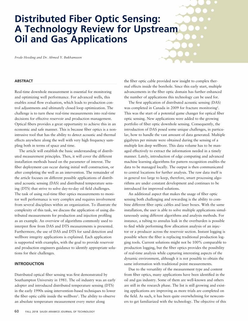
60 FALL 2018 SAUDI ARAMCO JOURNAL OF TECHNOLOGY
ABSTRACT
Real-time downhole measurement is essential for monitoring and optimizing well performance. For advanced wells, this enables zonal flow evaluation, which leads to production con-trol adjustments and ultimately closed loop optimization. The challenge is to turn these real-time measurements into real-time decisions for effective reservoir and production management. Optical fibers provides a great opportunity to achieve this in an economic and safe manner. This is because fiber optics is a non-intrusive tool that has the ability to detect acoustic and thermal effects anywhere along the well with very high frequency sam-pling both in terms of space and time.
The article will establish the basic understanding of distrib-uted measurement principles. Then, it will cover the different installation methods based on the parameter of interest. The fiber deployment can occur during initial well construction, or after completing the well as an intervention. The remainder of the article focuses on different possible applications of distrib-uted acoustic sensing (DAS) and distributed temperature sens-ing (DTS) that strive to solve day-to-day oil field challenges. The task of using real-time fiber optics measurements to moni-tor well performance is very complex and requires involvement from several disciplines within an organization. To illustrate the complexity of this task, we discuss the application of using dis-tributed measurements for production and injection profiling as an example. An overview of algorithms commonly used to interpret flow from DAS and DTS measurements is presented. Furthermore, the use of DAS and DTS for sand detection and wellbore integrity applications is explained. Each application is supported with examples, with the goal to provide reservoir and production engineers guidance to identify appropriate solu-tions for their challenges.
INTRODUCTION
Distributed optical fiber sensing was first demonstrated by Southampton University in 1981. The oil industry was an early adopter and introduced distributed temperature sensing (DTS) in the early 1990s using intervention-based techniques to lower the fiber optic cable inside the wellbore1. The ability to observe an absolute temperature measurement every meter along
the fiber optic cable provided new insight to complex ther-mal effects inside the borehole. Since this early start, multiple advancements in the fiber optic domain has further enhanced the number of applications this technology can be used for.
The first application of distributed acoustic sensing (DAS) was completed in Canada in 2009 for fracture monitoring2. This was the start of a potential game changer for optical fiber optic sensing. New applications were added to the growing portfolio of fiber optic downhole sensing. Consequently, the introduction of DAS posed some unique challenges, in particu-lar, how to handle the vast amount of data generated. Multiple gigabytes per minute were obtained during the sensing of a multiple km deep wellbore. This data volume has to be man-aged effectively to extract the information needed in a timely manner. Lately, introduction of edge computing and advanced machine learning algorithms for pattern recognition enables the data to be managed locally. The output is then communicated to central locations for further analysis. The raw data itself is in general too large to keep, therefore, smart processing algo-rithms are under constant development and continues to be introduced for improved solutions.
An additional aspect that makes the usage of fiber optic sensing both challenging and rewarding is the ability to com-bine different fiber optic cables and laser boxes. With the same installation, the user is able to solve multiple applications simul-taneously using different algorithms and analysis methods. For instance, a tubing to annulus leak in the overburden is possible to find while performing flow allocation analysis of an injec-tor or a producer across the reservoir section. Instant logging is possible where the fiber is replacing traditional production log-ging tools. Current solutions might not be 100% comparable to production logging, but the fiber optics provides the possibility of real-time analysis while capturing interesting aspects of the dynamic environment, although it is not possible to obtain the same information with traditional point measurements.
Due to the versatility of the measurement type and content from fiber optics, many applications have been identified in the oil and gas industry. Some of them are well-known and others are still in the research phase. The list is still growing and exist-ing applications are improving as more trials are completed on the field. As such, it has been quite overwhelming for newcom-ers to get familiarized with the technology. The objective of this
Distributed Fiber Optic Sensing: A Technology Review for Upstream Oil and Gas Applications
Frode Hveding and Dr. Ahmed Y. Bukhamseen
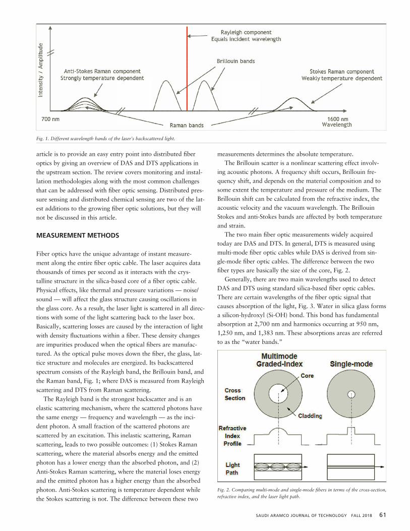
SAUDI ARAMCO JOURNAL OF TECHNOLOGY FALL 2018 61
article is to provide an easy entry point into distributed fiber optics by giving an overview of DAS and DTS applications in the upstream section. The review covers monitoring and instal-lation methodologies along with the most common challenges that can be addressed with fiber optic sensing. Distributed pres-sure sensing and distributed chemical sensing are two of the lat-est additions to the growing fiber optic solutions, but they will not be discussed in this article.
MEASUREMENT METHODS
Fiber optics have the unique advantage of instant measure-ment along the entire fiber optic cable. The laser acquires data thousands of times per second as it interacts with the crys-talline structure in the silica-based core of a fiber optic cable. Physical effects, like thermal and pressure variations — noise/sound — will affect the glass structure causing oscillations in the glass core. As a result, the laser light is scattered in all direc-tions with some of the light scattering back to the laser box. Basically, scattering losses are caused by the interaction of light with density fluctuations within a fiber. These density changes are impurities produced when the optical fibers are manufac-tured. As the optical pulse moves down the fiber, the glass, lat-tice structure and molecules are energized. Its backscattered spectrum consists of the Rayleigh band, the Brillouin band, and the Raman band, Fig. 1; where DAS is measured from Rayleigh scattering and DTS from Raman scattering.
The Rayleigh band is the strongest backscatter and is an elastic scattering mechanism, where the scattered photons have the same energy — frequency and wavelength — as the inci-dent photon. A small fraction of the scattered photons are scattered by an excitation. This inelastic scattering, Raman scattering, leads to two possible outcomes: (1) Stokes Raman scattering, where the material absorbs energy and the emitted photon has a lower energy than the absorbed photon, and (2) Anti-Stokes Raman scattering, where the material loses energy and the emitted photon has a higher energy than the absorbed photon. Anti-Stokes scattering is temperature dependent while the Stokes scattering is not. The difference between these two
measurements determines the absolute temperature. The Brillouin scatter is a nonlinear scattering effect involv-
ing acoustic photons. A frequency shift occurs, Brillouin fre-quency shift, and depends on the material composition and to some extent the temperature and pressure of the medium. The Brillouin shift can be calculated from the refractive index, the acoustic velocity and the vacuum wavelength. The Brillouin Stokes and anti-Stokes bands are affected by both temperature and strain.
The two main fiber optic measurements widely acquired today are DAS and DTS. In general, DTS is measured using multi-mode fiber optic cables while DAS is derived from sin-gle-mode fiber optic cables. The difference between the two fiber types are basically the size of the core, Fig. 2.
Generally, there are two main wavelengths used to detect DAS and DTS using standard silica-based fiber optic cables. There are certain wavelengths of the fiber optic signal that causes absorption of the light, Fig. 3. Water in silica glass forms a silicon-hydroxyl (Si-OH) bond. This bond has fundamental absorption at 2,700 nm and harmonics occurring at 950 nm, 1,250 nm, and 1,383 nm. These absorptions areas are referred to as the “water bands.”
Fig. 1. Different wavelength bands of the laser’s backscattered light.
Fig. 1. Different wavelength bands of the laser’s backscattered light.
Fig. 2. Comparing multi-mode and single-mode fibers in terms of the cross-the laser light path.
Fig. 2. Comparing multi-mode and single-mode fibers in terms of the cross-section, refractive index, and the laser light path.

62 FALL 2018 SAUDI ARAMCO JOURNAL OF TECHNOLOGY
INSTALLATION METHODS
There are three main methods for getting the fiber optic cable into the wellbore, where it is exposed to the variations in tem-perature and noise during production or injection3. These meth-ods are permanent installations, semi-permanent installations, and intervention-based service.
Permanent installation is obtained by strapping a fiber optic cable outside the casing and cementing it in place, Fig. 4a. The fiber can then be used to observe the heat being generated during cement curing, and thereby give indications of the height
of cement and also its potential quality. In addition, since the fiber is directly coupled to the sand face, it will be able to pro-vide valuable information about production related effects if it is placed across the reservoir. Other applications like vertical seismic profiling and geological subsidence can also be detected with this fiber placement using the right combination of laser box and fiber optic cable.
In a semi-permanent installation, the fiber optic cable is strapped outside a tubing and is exposed to the annulus between the tubing and the casing, Fig. 4b. If the tubing is pulled out, the fiber will also be removed. Normally, this instal-lation limits the fiber to be in the upper completion only above the production packer. Although it is possible to also include the fiber in the lower completion, it is a complex process and not commonly utilized. This installation can be particularly useful for tubing to annulus leak detection. In populated areas, and with ground water protection in mind, it is very useful to obtain integrity information in real-time without having to open and enter a well.
Both of these methods require a higher capital cost and lower operational cost. Subsequently, the main advantage with these methods is that the user is able to acquire instant down-hole logging without accessing the wellbore simply by attach-ing either a DAS or DTS laser box (or both) to the fiber optic cable(s) available at the surface.
The third method involves running fiber optics downhole as an intervention-based service. This method can be very useful
Fig. 3. The “water bands” plotted in an attenuation vs. wavelength plot to show common wavelengths that causes absorption of the light.
Fig. 4. Different methods to install a fiber optic line in the wellbore.
Fig. 3. The “water bands” plotted in an attenuation vs. wavelength plot to show common wavelengths that causes absorption of the light.
Fig. 4. Different methods to install a fiber optic line in the wellbore.
Fig-4a Fig-4b Fig-4c(a) (b) (c)
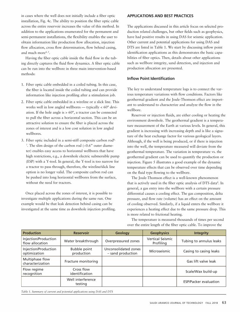
SAUDI ARAMCO JOURNAL OF TECHNOLOGY FALL 2018 63
in cases where the well does not initially include a fiber optic installation, Fig. 4c. The ability to position the fiber optic cable across the entire reservoir increases the value of this method. In addition to the applications enumerated for the permanent and semi-permanent installations, the flexibility enables the user to obtain information like production flow allocation, injection flow allocation, cross flow determination, flow behind casing, and much more4, 5.
Having the fiber optic cable inside the fluid flow in the tub-ing directly captures the fluid flow dynamics. A fiber optic cable can be run into the wellbore in three main intervention-based methods:
1. Fiber optic cable embedded in a coiled tubing. In this case, the fiber is located inside the coiled tubing and can provide information like injection profiling after a stimulation job.
2. Fiber optic cable embedded in a wireline or a slick line. This works well in low angled wellbores — typically < 60° devi-ation. If the hole angle is > 60°, a tractor can be connected to pull the fiber across a horizontal section. This can be an attractive solution to ensure the fiber is placed across the zones of interest and is a low cost solution in low angled wellbores.
3. Fiber optic included in a semi-stiff composite carbon rod6,
7. The slim design of the carbon rod (~0.6” outer diame-ter) enables easy access to horizontal wellbores that have high restrictions, e.g., a downhole electric submersible pump (ESP) with a Y-tool. In general, the Y-tool is too narrow for a tractor to pass through, therefore, the wireline/slick line option is no longer valid. The composite carbon rod can be pushed into long horizontal wellbores from the surface, without the need for tractors.
Once placed across the zones of interest, it is possible to investigate multiple applications during the same run. One example would be that leak detection behind casing can be investigated at the same time as downhole injection profiling.
APPLICATIONS AND BEST PRACTICES
The applications discussed in this article focus on selected pro-duction related challenges, but other fields such as geophysics, have had positive results in using DAS for seismic application. Other current and potential applications for using DAS and DTS are listed in Table 1. We start by discussing inflow point identification applications as this demonstrates the basic capa-bilities of fiber optics. Then, details about other applications such as wellbore integrity, sand detection, and injection and production allocation are presented.
Inflow Point Identification
The key to understand temperature logs is to connect the var-ious temperature variations with flow conditions. Factors like geothermal gradient and the Joule-Thomson effect are import-ant to understand to characterize and analyze the flow in the wellbore.
Reservoir or injection fluids, are either cooling or heating the environment downhole. The geothermal gradient is a tempera-ture measurement of the Earth at various levels. In general, this gradient is increasing with increasing depth and is like a signa-ture of the heat exchange factor for various geological layers. Although, if the well is being produced, or if there is injection into the well, the temperature measured will deviate from the geothermal temperature. The variation in temperature vs. the geothermal gradient can be used to quantify the production or injection. Figure 5 illustrates a good example of the dynamic temperature effects that can be observed over time depending on the fluid type flowing to the wellbore.
The Joule-Thomson effect is a well-known phenomenon that is actively used in the fiber optic analysis of DTS data8. In general, a gas entry into the wellbore with a certain pressure differential causes a cooling effect. The gas composition, delta pressure, and flow rate (volume) has an effect on the amount of cooling observed. Similarly, if a liquid enters the wellbore it experiences a heating effect due to the same pressure drop. This is more related to frictional heating.
The temperature is measured thousands of times per second over the entire length of the fiber optic cable. To improve the
Production Reservoir Geology Geophysics Integrity
Injection/Production flow allocation
Water breakthrough Overpressured zonesVertical Seismic
ProfilingTubing to annulus leaks
Injection/Production optimization
Bubble point production
Unconsolidated zones – sand production
Microseismic Casing to casing leaks
Multiphase flow characterization
Fracture monitoring Gas lift valve leak
Flow regime recognition
Cross flow identification
Scale/Wax build-up
Well interference testing
ESP/Packer evaluation
Table 1. Summary of current and potential applications using DAS and DTS

64 FALL 2018 SAUDI ARAMCO JOURNAL OF TECHNOLOGY
signal to noise ratio and increase the temperature resolution, it is normal to stack the readings over a period of time, Fig. 69. The advantage of stacking the data is that the temperature resolution improves. The disadvantage with too long of stack-ing is that the small variations in temperature could be missed. For instance, gas can enter the wellbore in squirts instead of a steady flow. The local cooling effect would be visible only in a short period of time before potential liquid coming from below heats up the area again.
The second measurement gaining more popularity in this domain is the DAS. DAS is capable of measuring both the amplitude and the frequency of sound waves downhole, or noise as it is normally called. Noise logging is not a new tech-nology in the oil industry and was first introduced in the early 1950s for leak detection. In Stein et al. (1972)10 a method of using acoustics to establish maximum sand free production was described. McKinley et al. (1973)11 presented work to charac-terize the noise amplitude and frequency spectrum for flow of air and water across a small orifice with certain pressure drops. When DAS was introduced, it opened up for all the classic noise logging methods in addition to much more. The ability to
listen to noise along the entire fiber optic cable establishes an opportu-nity to capture the dynamic vari-ations caused by flow downhole. And not just that; sound effects of fracturing in neighboring wells, leak detection behind casing, sub-seis-mic events caused by overpressured zones, and much more, can be ana-lyzed with DAS. A number of these applications will be discussed later.
With fiber optic across the reser-voir, it is possible to capture infor-mation about the various areas of production all the time. In other words, the fiber has the ability to observe all parts of the well, all the
time. Conversely, traditional wireline-based production log-ging provides a point measurement and has to be moved up and down a wellbore to map the different production zones. For example, a point measurement method could not track a moving slug as it moves up the well. Having the ability to observe the entire wellbore simultaneously, with spatial resolu-tions lower than a meter, enables a new level of dynamic infor-mation. There are several ongoing research projects to further improve the understanding of DAS and DTS.
Wellbore Integrity
Dealing with live hydrocarbons can be a challenge unless there are measures in place to handle it properly. Multiple barriers are installed to secure a safe production environment. In case of a downhole leak, it is important to identify the leak loca-tion and what kind of leak it is. There are multiple wellbore integrity scenarios that can take advantage of distributed fiber optics, such as: tubing to annulus leak (tubing to casing leak), flow behind casing (casing to casing leak), gas lift valve leak (plugged vs. active), and leaks around packers and the casing shoe. In addition, other challenges like high-pressure zones in the overburden that receives injection fluid from a nearby injec-tor, can be monitored with distributed data.
In the first scenario, the tubing to casing leak, the leak is identified by a pressure buildup in the annulus. Depending on the severity of the leak, the pressure is bled off regularly to avoid unsafe pressure level; however, identifying the source of the leak can be a challenge. Fiber optics have been used suc-cessfully for this task several times. The ability of fiber optic to sense the entire length of the fiber simultaneously makes it possible to identify the source of the leak, or multiple sources, within the time it takes to bleed off the annulus pressure.
Both semi-permanent fiber optic and intervention-based fiber optic can solve this challenge quite effectively. Normally, even if only annulus A (between the tubing and first casing) has a pressure buildup, it is good to perform a health check
Fig. 6. Achieving improved DTS resolution with averaging temperature values over longer periods of time. Longer fiber optic cables require more stacking for improved resolution9.
Fig. 6. Achieving improved DTS resolution with averaging temperature values over longer periods of time. Longer fiber optic cables require more stacking for improved resolution9.
Fig. 5. Dynamic well flow conditions, including the cooling and warming effects that are easily captured by DTS8.
Temperature (oF)M
easu
red
Dis
tan
ce (
feet
)

SAUDI ARAMCO JOURNAL OF TECHNOLOGY FALL 2018 65
between other casings as well. With fiber optics across the sens-ing area, we start by keeping everything shut-in for some time to establish a baseline. This baseline could last for 2 to 3 hours to ensure fluids have stabilized. Then, annulus C is bled off as quickly as possible while keeping the tubing, annulus A and B completely shut-in. The speed of bleeding off is important as we want to aggravate the potential flow or leak as much as possible to sense it. The only noise source now is the movement of fluid in the annulus, in particular if there is a leak at a cer-tain point. After bleeding down to low pressure, the sequence can be repeated depending on the rate of pressure buildup. The same operation should be repeated for annulus A and B. Typically, you can spend a few hours on the buildup and a few hours on the bleed down. The whole operation can take up to 24 hours to complete, Fig. 7.
Sand Detection
Unconsolidated reservoirs pose big challenges when it comes to sand production. Erosion of downhole and surfaces pipes can lead to catastrophic results. Fiber optic data is ideal to observe multiple zones at the same time. This enables the user to observe exactly the conditions when sand production starts. The well can be tuned to obtain maximum sand-free produc-tion. The key here is to distinguish formation sand ingress from other noisy phenomena in the well, such as fluid flow and back-ground noise.
To accomplish that, the data has to go through rigorous test-ing to classify the noise pattern from DAS as sand production. Thiruvenkatanathan et al. (2016)12 have performed some long-term tests in multiphase flow loops with multiple vendors to be able to positively identify the sand signature. Once the acoustic fingerprint of sand production has been empirically derived, a model was constructed with the understanding of the underly-ing physics.
After establishing confidence in the models, data were col-lected from a well with known sand production problems. The
data from this well was processed to filter out frequencies asso-ciated with background flow and instrumentation noise. The resulting signal was referred to as a “sand log” after averaging through time across the whole reservoir section. When time-depth DAS measurements are monitored over long periods of time, it is possible to track the transport of sand particles from the inflow point all the way to the surface. Figure 8 indicates consistency between the time that the sand slug hits the surface and a peak at the surface flow line acoustic sensor.
Injection Profiling
An injection profile is something the fiber optic cable is able to resolve quite nicely. Two main methods are used to determine the injection profile: (1) hot slug tracking, and (2) warm back analysis. The hot slug method consists of tracking the move-ment of a slug at a different temperature than the surrounding fluid. Normally, in an injector well, this slug is generated by shutting in the well for a period of time and letting the tem-perature in the well increase toward the geothermal gradient. In the cased off section above the reservoir, the temperature profile is not affected by cold fluid previously injected and the temperature moves quite fast toward the original geothermal gradient. If the well has already been on injection for some period of time, the reservoir has cooled down to a lower tem-perature just because of a constant feed of colder fluid.
After an initial shut-in period to obtain a stable reference geothermal gradient, the well is put on injection. The hot slug is visible both on DAS and DTS and moves down with the speed of the fluid. On a depth time-based plot, the slope angle of the slug equals the flow velocity. If we assume that the top section takes some injected fluid volume, the remaining fluid available for zones below it will be less. In other words, the slug veloc-ity will slow down. So, for a hot slug tracking, the slope of the host slug front will be directly related to the amount of fluid lost in every injection zone.
The warm back method is considered more preferable for
Fig. 7. A DAS waterfall plot in a wellbore integrity application to track gas leaking from a source in annulus A5.
Fig. 7. A DAS waterfall plot in a wellbore integrity application to track gas leaking from a source in annulus A5.
Fig. 8. A surface coincides with the time of the slug arrival to the surface5.
Fig. 9. The tDAS waterfall plot with noise amplitudes — noise amplitude plot into production (green) and no producti
Fig. 8. A DAS waterfall plot showing sand slug movement up the wellbore. Peaks in acoustic noise in the surface coincides with the time of the slug arrival to the surface5.
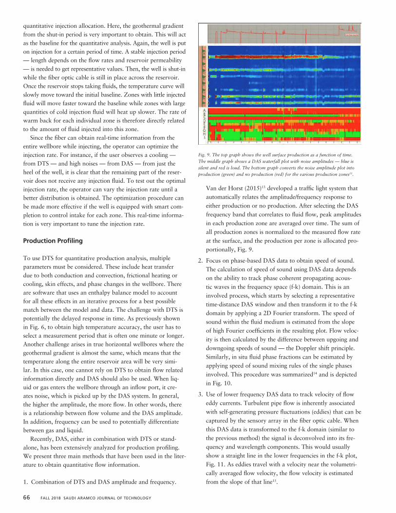
66 FALL 2018 SAUDI ARAMCO JOURNAL OF TECHNOLOGY
quantitative injection allocation. Here, the geothermal gradient from the shut-in period is very important to obtain. This will act as the baseline for the quantitative analysis. Again, the well is put on injection for a certain period of time. A stable injection period — length depends on the flow rates and reservoir permeability — is needed to get representative values. Then, the well is shut-in while the fiber optic cable is still in place across the reservoir. Once the reservoir stops taking fluids, the temperature curve will slowly move toward the initial baseline. Zones with little injected fluid will move faster toward the baseline while zones with large quantities of cold injection fluid will heat up slower. The rate of warm back for each individual zone is therefore directly related to the amount of fluid injected into this zone.
Since the fiber can obtain real-time information from the entire wellbore while injecting, the operator can optimize the injection rate. For instance, if the user observes a cooling — from DTS — and high noises — from DAS — from just the heel of the well, it is clear that the remaining part of the reser-voir does not receive any injection fluid. To test out the optimal injection rate, the operator can vary the injection rate until a better distribution is obtained. The optimization procedure can be made more effective if the well is equipped with smart com-pletion to control intake for each zone. This real-time informa-tion is very important to tune the injection rate.
Production Profiling
To use DTS for quantitative production analysis, multiple parameters must be considered. These include heat transfer due to both conduction and convection, frictional heating or cooling, skin effects, and phase changes in the wellbore. There are software that uses an enthalpy balance model to account for all these effects in an iterative process for a best possible match between the model and data. The challenge with DTS is potentially the delayed response in time. As previously shown in Fig. 6, to obtain high temperature accuracy, the user has to select a measurement period that is often one minute or longer. Another challenge arises in true horizontal wellbores where the geothermal gradient is almost the same, which means that the temperature along the entire reservoir area will be very simi-lar. In this case, one cannot rely on DTS to obtain flow related information directly and DAS should also be used. When liq-uid or gas enters the wellbore through an inflow port, it cre-ates noise, which is picked up by the DAS system. In general, the higher the amplitude, the more flow. In other words, there is a relationship between flow volume and the DAS amplitude. In addition, frequency can be used to potentially differentiate between gas and liquid.
Recently, DAS, either in combination with DTS or stand-alone, has been extensively analyzed for production profiling. We present three main methods that have been used in the liter-ature to obtain quantitative flow information.
1. Combination of DTS and DAS amplitude and frequency.
Van der Horst (2015)13 developed a traffic light system that automatically relates the amplitude/frequency response to either production or no production. After selecting the DAS frequency band that correlates to fluid flow, peak amplitudes in each production zone are averaged over time. The sum of all production zones is normalized to the measured flow rate at the surface, and the production per zone is allocated pro-portionally, Fig. 9.
2. Focus on phase-based DAS data to obtain speed of sound. The calculation of speed of sound using DAS data depends on the ability to track phase coherent propagating acous-tic waves in the frequency space (f-k) domain. This is an involved process, which starts by selecting a representative time-distance DAS window and then transform it to the f-k domain by applying a 2D Fourier transform. The speed of sound within the fluid medium is estimated from the slope of high Fourier coefficients in the resulting plot. Flow veloc-ity is then calculated by the difference between upgoing and downgoing speeds of sound — the Doppler shift principle. Similarly, in situ fluid phase fractions can be estimated by applying speed of sound mixing rules of the single phases involved. This procedure was summarized14 and is depicted in Fig. 10.
3. Use of lower frequency DAS data to track velocity of flow eddy currents. Turbulent pipe flow is inherently associated with self-generating pressure fluctuations (eddies) that can be captured by the sensory array in the fiber optic cable. When this DAS data is transformed to the f-k domain (similar to the previous method) the signal is deconvolved into its fre-quency and wavelength components. This would usually show a straight line in the lower frequencies in the f-k plot, Fig. 11. As eddies travel with a velocity near the volumetri-cally averaged flow velocity, the flow velocity is estimated from the slope of that line15.
.
Fig. 9. The tDAS waterfall plot with noise amplitudes — noise amplitude plot into production (green) and no producti
Fig. 9. The top graph shows the well surface production as a function of time. The middle graph shows a DAS waterfall plot with noise amplitudes — blue is silent and red is loud. The bottom graph converts the noise amplitude plot into production (green) and no production (red) for the various production zones11.

SAUDI ARAMCO JOURNAL OF TECHNOLOGY FALL 2018 67
CONCLUSIONS
As with other technologies in the industry, fiber optics mon-itoring systems have been progressively evolving. Nowadays, the different types of measurement can be collected continu-ously with time and distance, and with high measurement fidel-ity. Due to its relatively low cost and the wide distance range it
covers, distributed fiber optic systems are viewed as an attrac-
tive monitoring option for all well types. With the increasing
data flow, new algorithms have been developed and demon-
strated on the field to assist with real-time decisions and deliver
value from the system. With the recent advancement in compu-
tational modeling, more emphasis should be placed on machine
learning, automation, and data driven models, which work
quite well with the high data flow rate in DAS applications.
In this article, we have discussed the basic working princi-
ples of distributed fiber optics and how to deploy the fiber in
the well. Careful system design should be performed to place
the fiber in the region of interest, depending on the desired
application. Despite presenting several working applications
here, many industry experts believe that we have not unlocked
the full potential of the value that DAS and DTS promises to
deliver.
ACKNOWLEDGMENTS
The authors would like to thank the management of Saudi
Aramco for their support and permission to publish this article.
This article was presented at the SPE Kingdom of Saudi
Arabia Annual Technical Symposium and Exhibition,
Dammam, Saudi Arabia, April 23-26, 2018.
Fig. 10. Speed of sound calculation steps involving a f-k slope line fitting and Doppler shift velocity estimation.
Fig. 10. Speed of sound calculation steps involving a f-k slope line fitting and Doppler shift velocity estimation.
Fig. 11. Frequency wavenumber plot that results after applying 2D Fourier transform to DAS data. Convection velocity is shown as a straight line in the lower frequencies.
≈ 2 GB / min
Sampling at 10 kHzSa
mpl
ing
ever
y 1.
5’
Build SoS profile2D Fourier Transform
-0.15 -0.1 -0.05 00
200
400
600
800
1000
Wavenumber (1/ft)
Freq
uenc
y (H
z)
0 0.05 0.10
200
400
600
800
1000
Wavenumber (1/ft)
1 1.5 2
x 104
20
30
40
50
60
70
Slope (ft/s)
Inte
gral
Val
ue
1 1.5 2
x 104
20
40
60
80
100
Slope (ft/s)
200
160
120
80
40
0
200
160
120
80
40
0
Line fitting
-0.15 -0.1 -0.05 00
200
400
600
800
1000
Wavenumber (1/ft)
Freq
uenc
y (H
z)
0 0.05 0.10
200
400
600
800
1000
Wavenumber (1/ft)
1 1.5 2
x 104
20
30
40
50
60
70
Slope (ft/s)In
tegr
al V
alue
1 1.5 2
x 104
20
40
60
80
100
Slope (ft/s)SOS_down = 2940 (ft/s) SOS_up = 2976 (ft/s)1.9 1.9 3.73.7
Fig. 11. Frequency wavenumber plot that results after applying 2D Fourier transform to DAS data. Convection velocity is shown as a straight line in the lower frequencies.
68 FALL 2018 SAUDI ARAMCO JOURNAL OF TECHNOLOGY
REFERENCES
1. Hurtig, E., Schrotter, J., Grosswig, S., Kuhn, K., et al.: “Borehole Temperature Measurements Using Distributed Fiber Optic Sensing,” paper presented at the International Conference on Industrial Uses of Geothermal Energy, Reykjavik, Iceland, September 2-4, 1992.
2. Molenaar, M.M., Hill, D.J., Webster, P., Dinad, E., et al.: “First Downhole Application of Distributed Acoustic Sensing for Hydraulic Fracturing Monitoring and Diagnostics,” SPE paper 140561, presented at the SPE Hydraulic Fracturing Technology Conference, The Woodlands, Texas, January 24-26, 2011.
3. Al Shoaibi, S., Kechichian, R., Mjeni, R., Al Rajhi, S., et al.: “Implementing Fiber Optics Distributed Sensing as a Key Surveillance Tool,” SPE paper 183535, presented at the Abu Dhabi International Petroleum Exhibition and Conference, Abu Dhabi, UAE, November 7-10, 2016.
4. Danardatu, H., Gregersen, S.H.H., Alterrn, E. and Pellegrini, I.: “Data Acquisition and Processing of Carbon Rod Conveyed DTS and DAS in Very Long Horizontal Wells: First Trial in North Sea Danish Sector,” SPE paper 170663, presented at the SPE Annual Technical Conference and Exhibition, Amsterdam, the Netherlands, October 27-29, 2014.
5. Hveding, F. and Porturas, F.: “Integrated Applications of Fiber Optic Distributed Acoustic and Temperature Sensing,” SPE paper 177222, presented at the SPE Latin American and Caribbean Petroleum Engineering Conference, Quito, Ecuador, November 18-20, 2015.
6. Hansen, H., Wilberg, T.K., Stokkeland, K., Male, P.T., et al.: “Successful Deployments of a New Well Intervention Methodology in Horizontal Wellbores,” SPE paper 121459, presented at the SPE/ICoTA Coiled Tubing and Well Intervention Conference and Exhibition, The Woodlands, Texas, March 31-April 1, 2009.
7. Gardner, N., Hveding, F. and Sambrook, R.: “Distributed Fiber Optic Technologies Drive New Intervention Applications,” Journal of Petroleum Technology, Vol. 67, Issue 1, January 2015, pp. 36-40.
8. Wang, X., Lee, J., Thigpen, B., Vachon, G.P., et al.: “Modeling Flow Profile Using Distributed Temperature Sensor (DTS) System,” SPE paper 111790, presented at the Intelligent Energy Conference and Exhibition, Amsterdam, the Netherlands, February 25-27, 2008.
9. Sensornet home page (www.sensornet.co.uk): “Sentinel DTS Data Sheet,” 2 p.
10. Stein, N., Kelly, J., Baldwin, W.F. and McNeely, W.E.: “Sand Production Determined from Noise Measurements,” Journal of Petroleum Technology, Vol. 24, Issue 7, July 1972, pp. 803-806.
11. McKinley, R.M. Bower, F.M. and Rumble, R.C.: “The Structure and Interpretation of Noise from Flow behind Cemented Casing,” Journal of Petroleum Technology, Vol. 25, Issue 3, March 1973, pp. 329-338.
12. Thiruvenkatanathan, P., Langnes, T., Beaumont, P., White, D., et al.: “Downhole Sand Ingress Detection Using Fiber Optic Distributed Acoustic Sensors,” SPE paper 183329, presented at the Abu Dhabi International Petroleum Exhibition and Conference, Abu Dhabi, UAE, November 7-10, 2016.
13. van der Horst, J.: “Recent Advances in Fiber Optic Technology for In-Well Production and Injection Profiling,” IPTC paper 18563, presented at the International Petroleum Technology Conference, Doha, Qatar, December 6-9, 2015.
14. Bukhamsin, A. and Horne, R.: “Cointerpretation of Distributed Acoustic and Temperature Sensing for Improved Smart Well Inflow Profiling,” SPE paper 180465, presented at the Western Regional Meeting, Anchorage, Alaska, May 23-26, 2016.
15. Da Silva, M.F., Muradov, K.M., Davies, D.R.: “Review, Analysis and Comparison of Intelligent Well Monitoring Systems,” SPE paper 150195, presented at the Intelligent Energy International Conference and Exhibition, Utrecht, the Netherlands, March 27-29, 2012.

SAUDI ARAMCO JOURNAL OF TECHNOLOGY FALL 2018 69
BIOGRAPHIES
Frode Hveding joined the Production Technology Team of Saudi Aramco’s Exploration and Petroleum Engineering Center – Advanced Research Center (EXPEC ARC) in August 2015. His work focuses mainly on flow measurements using
lasers and fiber optics. Frode has 23 years of experience in the oil industry.
His main areas of expertise are distributed fiber optics for downhole applications, production logging and formation evaluation, advanced data acquisition from both wireline and logging while drilling, and the active use of real-time information for wellbore placement and geosteering.
Frode received his M.S. degree in Petroleum Technology from the Norwegian University of Science and Technology, Trondheim, Norway.
Dr. Ahmed Y. Bukhamseen is a Petroleum Engineer working with the Production Technology Team of Saudi Aramco’s Exploration and Petroleum Engineering Center – Advanced Research Center (EXPEC ARC). His extensive experience includes reservoir
engineering, production operations and completions research and development. Ahmed’s current research activities cover smart well completions, production optimization, fiber optic sensing and multiphase flow metering.
He has published several technical papers and holds three patents.
Ahmed received his B.S. degree from the Colorado School of Mines, Golden, CO, and both his M.S. and Ph.D. degrees from Stanford University, Stanford, CA, all in Petroleum Engineering.

70 FALL 2018 SAUDI ARAMCO JOURNAL OF TECHNOLOGY
SUBSCRIPTION ORDER FORM
To begin receiving the Saudi Aramco Journal of Technology at no charge, please complete this form.
Please print clearly.
Name _____________________________________________________________________________________________________________________________________________________________________________________________________________________________________________
Title __________________________________________________________________________________________________________________________________________
Organization _______________________________________________________________________________________________________________________________
Address _____________________________________________________________________________________________________________________________________
City __________________________________________________________________________________________________________________________________________
State/Province ______________________________________________________________________________________________________________________________
Postal code _________________________________________________________________________________________________________________________________
Country _____________________________________________________________________________________________________________________________________
E-mail address _____________________________________________________________________________________________________________________________
Number of copies _________________________________________________________________________________________________________________________
TO ORDER
By phone/email:
Saudi Aramco Corporate Communication Support Department JOT [email protected]
By mail:
Saudi Aramco Corporate Communication Support Department JOT Distribution Box 5000Dhahran 31311Saudi Arabia
Current issues, select back issues and multiple copies of some issues are available upon request.
The Saudi Aramco Journal of Technology is published by the Saudi Aramco Corporate Communication Support Department, Saudi Arabian Oil Company, Dhahran, Saudi Arabia.

SAUDI ARAMCO JOURNAL OF TECHNOLOGY FALL 2018 71
GUIDELINES FOR SUBMITTING AN ARTICLE TO THE SAUDI ARAMCO JOURNAL OF TECHNOLOGY
These guidelines are designed to simplify and help standardize submissions. They need not be followed rigorously. If you have additional questions, please feel free to contact us at CCSD. Our address and phone numbers are listed on page 70.
Length
Varies, but an average of 2,500-3,500 words, plus illustrations/photos and captions. Maximum length should be 5,000 words. Articles in excess will be shortened.
What to send
Send text in Microsoft Word format via email or on disc, plus one hard copy. Send illustrations/photos and captions separately but concurrently, both as email or as hard copy (more information follows under file formats).
Procedure
Notification of acceptance is usually within three weeks after the submission deadline. The article will be edited for style and clarity and returned to the author for review. All articles are subject to the company’s normal review. No paper can be published without a signature at the manager level or above.
Format
No single article need include all of the following parts. The type of article and subject covered will determine which parts to include.
Working title
Abstract
Usually 100-150 words to summarize the main points.
Introduction
Different from the abstract in that it “sets the stage” for the content of the article, rather than telling the reader what it is about.
Main body
May incorporate subtitles, artwork, photos, etc.
Conclusion/summary
Assessment of results or restatement of points in introduction.
Endnotes/references/bibliography
Use only when essential. Use author/date citation method in the main body. Numbered footnotes or endnotes will be converted. Include complete publication information. Standard is The Associated Press Stylebook, 52nd ed. and Webster’s New World College Dictionary, 5th ed.
Acknowledgments
Use to thank those who helped make the article possible.
Illustrations/tables/photos and explanatory text
Submit these separately. Do not place in the text. Positioning in the text may be indicated with placeholders. Initial submission may include copies of originals; however, publication will require the originals. When possible, submit both electronic versions, printouts and/or slides. Color is preferable.
File formats
Illustration files with .EPS extensions work best. Other acceptable extensions are .TIFF, .JPEG and .PICT.
Permission(s) to reprint, if appropriate
Previously published articles are acceptable but can be published only with written permission from the copyright holder.
Author(s)/contributor(s)
Please include a brief biographical statement.
Submission/Acceptance Procedures
Papers are submitted on a competitive basis and are evaluated by an editorial review board comprised of various department managers and subject matter experts. Following initial selection, authors whose papers have been accepted for publication will be notified by email.
Papers submitted for a particular issue but not accepted for that issue will be carried forward as submissions for subsequent issues, unless the author specifically requests in writing that there be no further consideration. Papers previously published or presented may be submitted.
Submit articles to:
EditorThe Saudi Aramco Journal of TechnologyC-11B, Room AN-1080North Admin Building #175Dhahran 31311, Saudi Arabia Tel: +966-013-876-0498Email: [email protected]
Submission deadlines
Issue Paper submission deadline Release date
Spring 2019 November 14, 2018 March 31, 2019Summer 2019 February 13, 2019 June 30, 2019Fall 2019 May 15, 2019 September 30, 2019Winter 2019 August 1, 2019 December 31, 2019

72 FALL 2018 SAUDI ARAMCO JOURNAL OF TECHNOLOGY
NOTES:
____________________________________________________________________________________________________________________________________________________________________________________________________________________________________________________________________________________
____________________________________________________________________________________________________________________________________________________________________________________________________________________________________________________________________________________
____________________________________________________________________________________________________________________________________________________________________________________________________________________________________________________________________________________
____________________________________________________________________________________________________________________________________________________________________________________________________________________________________________________________________________________
____________________________________________________________________________________________________________________________________________________________________________________________________________________________________________________________________________________
____________________________________________________________________________________________________________________________________________________________________________________________________________________________________________________________________________________
____________________________________________________________________________________________________________________________________________________________________________________________________________________________________________________________________________________
____________________________________________________________________________________________________________________________________________________________________________________________________________________________________________________________________________________
____________________________________________________________________________________________________________________________________________________________________________________________________________________________________________________________________________________
____________________________________________________________________________________________________________________________________________________________________________________________________________________________________________________________________________________
____________________________________________________________________________________________________________________________________________________________________________________________________________________________________________________________________________________
____________________________________________________________________________________________________________________________________________________________________________________________________________________________________________________________________________________
____________________________________________________________________________________________________________________________________________________________________________________________________________________________________________________________________________________
____________________________________________________________________________________________________________________________________________________________________________________________________________________________________________________________________________________
____________________________________________________________________________________________________________________________________________________________________________________________________________________________________________________________________________________
____________________________________________________________________________________________________________________________________________________________________________________________________________________________________________________________________________________
____________________________________________________________________________________________________________________________________________________________________________________________________________________________________________________________________________________
____________________________________________________________________________________________________________________________________________________________________________________________________________________________________________________________________________________
____________________________________________________________________________________________________________________________________________________________________________________________________________________________________________________________________________________
____________________________________________________________________________________________________________________________________________________________________________________________________________________________________________________________________________________
____________________________________________________________________________________________________________________________________________________________________________________________________________________________________________________________________________________
____________________________________________________________________________________________________________________________________________________________________________________________________________________________________________________________________________________
____________________________________________________________________________________________________________________________________________________________________________________________________________________________________________________________________________________
____________________________________________________________________________________________________________________________________________________________________________________________________________________________________________________________________________________
____________________________________________________________________________________________________________________________________________________________________________________________________________________________________________________________________________________
____________________________________________________________________________________________________________________________________________________________________________________________________________________________________________________________________________________
____________________________________________________________________________________________________________________________________________________________________________________________________________________________________________________________________________________
____________________________________________________________________________________________________________________________________________________________________________________________________________________________________________________________________________________
____________________________________________________________________________________________________________________________________________________________________________________________________________________________________________________________________________________