Center of Excellence for Explosive Detection, Mitigation and Response

A Department of Homeland Security

Center of Excellence

University of Rhode Island (URI);

California Institute of Technology Purdue University

New Mexico State University University of Illinois

Florida International University Hebrew University, Jerusalem Israel

Weizmann Institute of Science

Fifth Annual Report

July 2012-July 2013

DHS agreement number: 2008-ST-061-ED0002

Table of Contents

Introduction 5

Characterization Factors Influencing TATP and DADP Formation (Part 2) Jimmie Oxley & James Smith (URI)

8

Factors Influencing TATP and DADP Formation (Part 3) Jimmie Oxley & James Smith (URI)

45

Characterization of HME Steve Son (Purdue)

54

Detonation Failure Characterization of HME Steve Son (Purdue)

66

Hot dense liquid TNT decomposition Ronnie Kosloff (Hebrew UJI)

90

Enhanced Sensitivity of Condensed Phase Nitroaromatic Explosives Ronnie Kosloff (Hewbrew UJI) & Yehuda Zeiri (BGU)

119

Development of Simulants of Hydrogen Peroxide Based Explosives for use by Canine and IMS Detectors Jose Almirall (FIU)

158

Calibration of PSPME Using Controlled Vapor Generation Followed by IMS Detection Jose Almirall (FIU)

161

Detection Optical Chemical Sensors using Nanocomposites from Porous Silicon Photonic Crystals & Sensory Polymers William Euler (URI)

181

Fluorescent Species Formed by the Reaction of Trinitroaromatics with N,N-Demethylformamide and Peroxide William Euler (URI)

189

A Fluorometric Sensing Array for the Detection of Military Explosives and IED MaterialsWilliam Euler (URI)

219

Light Trapping to Amplify Metal Enhanced Fluorescence with Application for Sensing TNT

226

William Euler (URI)

A Persistent Surveillance Technique for the Detection of Explosives and Explosive Precursors Otto Gregory (URI)

234

Solution-Based Direct Readout SERS Method for Detection Radha Narayanan (URI)

303

Solution-based Direct Readout Surface Enhanced Raman Spectroscopic Detection of Ultra-Low Levels of Thiamin with Dogbone Shaped Gold Nanoparticles Radha Narayanam (URI)

310

Gold Nanorods as Surface Enhanced Raman Spectroscopy Substrates for Sensitive and Selective Detection of Ultra-Low Levels of Dithiocarbamate Pesticides Radha Narayanam (URI)

316

Nanocantilever Chemical Vapor Sensors Coated with Localized Rubbery and Glassy Polymer Brush Films Nate Lewis (Cal Tech)

322

Supplementary Information 349

Mitigation Development of Structural Steel with Higher Blast Resistance H. Ghonem (URI)

354

Time-dependent Deformation of Low Carbon Steel at Elevated Temperatures H. Ghonem and Otto Gregory

365

Simulation of Viscoplastic Deformation of Low Carbon Steel Structures at Elevated Temperatures H. Ghonem (URI)

375

Deformation Criterion of Low Carbon Steel Subjected to High Speed Impacts H. Ghonem, C-E. Rousseau and Otto Gregory

384

Deformation Characteristics of Low Carbon Steel Subjected to Dynamic Impact LoadingH. Ghonem, C-E. Rousseau and Otto Gregory

391

Self-Healing Concrete Arijit Bose (URI)

401

Polyurea/Polyurethane Microcapsules Based Self Healing Concrete Arijit Bose (URI)

404

Structural Response to Non-ideal Explosions J. E. Shepherd (California Institute of Technology)

524

Experimental Investigation of Blast Mitigation for Target Protection Steve Son (Purdue University)

529

Self Healing Materials for Autonomic Mitigation of Blast Damage Nancy R. Sottos (U of Illinois)

554

Stress Attenuation by Means of Particulates C-E. Rouseau

566

Development of Novel Composite Materials & Structures for Blast Mitigation Arun Shukla (URI)

574

Center of Excellence Explosives

Fifth Annual Report The goal of this CoE in Explosives is to mitigate the worldwide explosive threat, both

today and in the future. To reach that goal, URI has maintained four thrust areas Characterization, Detection, Mitigation, and Education. In addition, one project was designated as Engage to Excellence (E-2-E).

Characterization For the present and near term, studies in the thrust area are aimed at physical

characterization of novel explosives and explosives signatures, along with determination of thermal stability and sensitivity. This information is available to the community within weeks by publication on the URI Explosive Database, journal publication, and classes. Beyond that is the need to understand the mechanism of material formation and destruction with the goal of hindering or facilitating these events. Looking to the future we believe it is high priority to identify and prioritize the list of potential threats. Therefore, we are taking two approaches to identifying potential explosives—a comprehensive theoretical approach which involves prediction of physical properties and hazards and an experimental approach. Enhanced sample collection is addressed both by an experimental approach based on microextraction for the capture of extremely small quantities of the volatile compounds and a survey of potential materials using atomic force microscopy (1.1 - 1.8).

Detection Progress continues towards development of sensors that are sensitive, selective and able

to detect trace levels of explosives. A number of novel sensors are being developed. The sensors employ two orthogonal spectral techniques; surface enhanced Raman scattering (SERS) and metal enhanced fluorescence (MEF). Due to the light absorbing properties of TNT and its quenching capabilities the MEF component was shown to be particularly sensitive to TNT. Another approach is detecting explosive vapors via use of a nanocantilever. The response of these sensors is due to two mechanisms; one that affects mass accumulation to the sensor and another that affects its stiffness. Modeling studies suggest that the response of the nanocantilever to vapor appears to be due more by change in the sensor spring constant rather than accumulation of mass. Also investigated are nanoparticle chemiresistor sensors. Applications of organic capping groups impart electrical conductivity to the films on these sensors. Shaper-less” standoff remote detection from distance of up to 50 meters has been demonstrated using femptosecond pulses shaped by a photonic crystal filter. The fundamental behavior of ions in ion mobility spectrometers (IMS) continues to be studied. To this end a kinetic dual shutter IMS with a gas chromatograph interface was constructed. This instrument successfully characterized ion lifetimes, energies, and kinetics of decomposition of gas phase ions of energetic materials. Studies are in progress on as many explosives in the nitro-alkane and nitro-aromatic family as possible (2.1 - 2.10)

Mitigation In the mitigation thrust area approach is diverse from technologies that mitigate the effect of the blast to new sandwich compounds and functionally graded materials that more readily withstand blast. New metrics of assessing material stress as well as non-ideal explosive events are under

development. Already to the commercialization stage are techniques for manufacturing self-healing materials polymers and cements (3.1 - 3.12).

Engage to Excellence An outstanding success has been achieved in our E-2-E project —the development of a new steel with a significantly high blast resistance. This has been accomplished through a systematic numerical/analytical/experimental approach carried out by Professor Hamouda Ghonem and his research group over four years of funding. First, they established metrics for rating the residual strength of steel under post blast conditions. For this purpose, they built an advanced gas gun capable of delivering a blast pressure of 25 GPa at 1000 m/s. Joining this unique gas gun with Split-Hopkinson Pressure Bar and ECAP severe plastic deformation system, blast testing of steel with different microstructures and compositions could be routinely accomplished in the URI-Mechanics of Materials Research lab. These testing facilities coupled with numerical simulation techniques are used to develop pre-strained steel with a blast resistance up to 12 GPa of blast pressure as opposed to that of present steels which is best assessed as 4 GPa. These efforts in the DHS Center have been assisted by FM Global and US Steel. The application significance of this steel is its potential in retrofitting of tunnels and doming of nuclear reactors with a steel fiber mesh to act as self-sustained blast protection shields. (3.1 – 3.5)

Education Our work in this field to date is as follows. Each University project in the Center supports one or more graduate students. This is their best learning experience. Undergraduates are also supported on the projects as their class schedules permit. In addition, URI has a traveling magic shows for elementary and junior high students. For three summers we hosted Minority Scholars and for the last four summers we have hosted high school science teachers. In the summer of 2012 our Center supported eight high school teachers to conduct research at University of Rhode Island (URI). Four teachers of physics were placed in URI engineering departments; and another four, in the URI chemistry department. The teachers worked fulltime for 8-10 weeks. They were required to prepare a poster and give a brief presentation of their work at the end of their tenure. The purpose of this program is to provide high school teachers with an opportunity to gain research experiences they can take back to the classrooms. In the calendar year 2012 seventeen professional classes were offered, providing training for over 300 professionals with new titles (red on Table) offered every year. Also new in 2012 were week-long courses with lecture and labs (marked in green on the following Table) most of them aimed at the TSA explosive specialists. Since May we have offered 4 weeks of such classes and trained 48 TSA explosive specialists as well as NYPD forensic lab personnel. The next NYPD class will be offered next week.

Class DATES # Class 2009 # Class 2010 #students Class 2011 #students Class 2012 #studentsStumpneck Feb 17-19 30 APL Fundamenta Feb 4-6 10 Fundamentals Edwards A Jan 19-21 26 Terrorism Apr 26-27 18 Stability Jan 18-19 16Pic -Managers April 23 21 Picatinny Hazards Feb 17-19 26 Fundamentals Picatinny Feb 1-3 25 Fundamentals a May 3-5 37 Air Blast Feb 14-16 10APL JHU Apr 29-May 1 30 Picatinny Combu Feb 22-23 29 Hazards Ottawa, CA Feb 3-5 13 Combustion May 9-10 18 Fundamentals Feb 27-29 25URI May 6-8 38 Picatinny Protoco Apr 23-24 20 Fundamentals ABQ Feb 17-19 9 Insensitive Mun May 10-11 26 Nanoenergetics Mar 12-13 15Kansas City Plant Jul 15-19 6 Pic Air Blast Apr 27-29 19 Hazards ABQ Feb 17-19 11 Det'n & DDT June 7-9 20 Firing Trains Ap 10-12 13Andrews Materials Aug 11-14 32 Pic HE Material C May 12-14 16 Warheads Picatinny Feb 24-26 26 Mat'l Response July 21-22 15 Fundamentals Ap 24-25 42

Indian Head Aug 18-22 30 Picatinny Fundam June 23-25 22 Materials Response, CA Mar 22-23 15 Protocols Aug 2-3 16 Fundamentals May 1-3 38Picatinny Protocol Sep 22-23 25 URI Fundamenta May 5-7 44 Air Blast Ottawa, CA Mar 24-26 13 Det'n & DDT Sept 6-8 35 Warhead Mech, May 8-10 13Picatinny Fundame Sep 24-26 23 Valcartier May 26-28 17 Terrorism Issues April 25-26 40 Dynamic Diagn Sep 28-29 15 NYPD Analysis May 7-18 9

Pic Diagonstics Oct 20-21 24 Crane, IN Jun 1-3 16 Safety Protocols Ap 28-29 25 TOTAL 200 TSA BAO May 21-25 24Picatinny Fundame Oct 22-24 24 Picatinny DDT Jul 28-30 23 Fundamentals May 4-6 26 Fundamentals July 17-18 18DHS Fundamental Nov 24-26 20 Picatinny Aug 3-4 16 Nanomaterials May 25-26 20 Dugway July 7-10 7Picatinny Analysis Dec 2-3 23 Ottawa Sep 8-10 16 Pyrotechnics June 7-11 28 TSA BAO Aug 20-24 22

TOTAL 326 Materials Respon Sep 29-30 23 Fundamentals July 26-28 24 Pic Protocols Sept 10-11 12Components Oct 27-29 25 HE Materials Characteriz Sept 16-18 19 TSA BAO Sept 17-21 22Environmental Nov 4-5 26 Unintended Ignition Oct 20-22 19 Warheads, Alb. Nov. 6-8 25

TOTAL 348 TOTAL 339 Standoff Detection Dec 12-13, 18

TOTALS 329

1

Factors Influencing Triacetone Triperoxide (TATP) and Diacetone Diperoxide (DADP) Formation: Part 2

Jimmie C. Oxley*; James L. Smith; Lucus Steinkamp; Guang Zhang

aUniversity of Rhode Island, Chemistry Department 51 Lower College Road

Kingston, RI 02881 *joxley@chm.uri.edu

Abstract A comprehensive mechanistic study regarding acetone peroxides reveals that water has a

profound effect on the formation of the solid cyclic peroxides, TATP and DADP. The

identification and rate of occurrence of reaction intermediates as well as compositions of the

final products offer explanation for previously reported results indicating that acid type and

hydrogen peroxide concentration affect the acid catalyzed reaction between acetone and

hydrogen peroxide. A kinetics study of the decomposition of TATP revealed the effects of water

and alcohols. They generally retard conversion of TATP to DADP and leads to complete

decomposition of TATP by acid. A mechanism is proposed for the production of TATP and

DADP.

Keywords: Triacetone triperoxide (TATP), Diacetone diperoxide (DADP), Product Formation,

Product Decomposition, Mechanism, Kinetics

2

1. Introduction

Organic peroxides are often used as polymerization catalysts or bleaching agents [1-3].

However, a few with high ratios of peroxide functionality to ketone have found use as illicit

explosives [4]. We have previously reported attempts to prevent synthesis of TATP in

improvised settings [5]. That work pointed out a need for a detailed mechanistic study. Some of

the questions of interest in TATP formation/destruction were conditions under which TATP and

DADP form, mechanisms of formation and destruction and whether DADP could be formed

directly or only through a TATP intermediate. These questions were addressed by identifying

intermediates by gas chromatography/mass spectrometry (GC/MS), liquid chromatography/mass

spectrometry (LC/MS) at high mass resolution and 1H/13C nuclear magnetic resonance

spectroscopy (NMR). Intermediates were monitored during formation and destruction

experiments to elucidate mechanisms.

2. Experimental Section

2.1 Reagents and Chemicals

HPLC-grade solvents, deuterated acetone (99.8 wt% d), and acids trifluoroacetic (99 wt%),

nitric (70wt%), hydrochloric (37 wt%) and sulfuric (98wt%) were obtained from Fisher

Scientific; deuterated acetonitrile, from Cambridge Isotopes Lab. Syntheses of TATP and

DADP were previously reported [5]. For synthesis of deuterium-labeled TATP d6 acetone was

used. Precipitates were filtered, rinsed with water, dried under aspiration 30 minutes and re-

crystallized in methanol. Final products were analyzed by GC/MS, GC/uECD, 1H NMR and 13C

NMR. Anhydrous hydrogen peroxide was prepared by dissolving 20 g of L-serine in 20 mL 65

wt% hydrogen peroxide.6 To confirm its concentration, the hydrogen peroxide was dissolved in

acetonitrile (ACN) and titrated with 0.25N potassium permanaganate.

3

2.2 GC/MS Method

An Agilent 6890 gas chromatograph with 5973 mass selective detector (GC/MS) was used with

inlet in splitless mode at 110°C, with purge flow 20 mL/min at 0.5 min, total helium flow of 24.1

mL/min and a Varian VF-200MS column (15m, 0.25 mm inner diameter, 0.25 µm film) under

constant helium flow (1.5 mL/min). Oven temperature was held at 40°C for 2 minutes, ramped

10°C/min to 70°C, then 20°C/min to 220°C; post-run oven was held 3 min at 310°C. Transfer

line, MS detector source, and quadrupole were held at 150°C, 150°C, and 106°C, respectively.

Chemical ionization used anhydrous ammonia.

2.2.1 TATP Formation (GC/MS): All reagents were chilled to 0oC. Hydrogen peroxide (HP)

(67 wt%, 0.47 g, 9.3 mmol) in 10 mL acetonitrile was stirred in a round bottom flask while

sulfuric acid (0.95 g, 96.5 wt%, 9.3 mmol) and then acetone (0.54 g. 9.3 mmol) were added

dropwise. Periodically, 100 uL of the solution was removed, placed in 1 mL CH2Cl2, and rinsed

with 3 wt% sodium bicarbonate. Organic layer was dried over MgSO4 and analyzed by GC/MS.

2.2.2 Effect of water (GC/MS): Acetone and HP were mixed and chilled to 0°C. Water was

mixed with sulfuric or hydrochloric acid, chilled to 0°C, and added dropwise to the acetone/HP

mixture keeping the temperature below 5°C. The ratio of HP:acetone:acid was maintained at

1:1:1 (8.6 mmol). Once all acid was added the mixture was removed from the ice water bath and

allowed to stir at room temperature 24 hours; resulting products were analyzed by GC/MS.

2.2.3 TATP Destruction (GC/MS): TATP (100 mg) was place in a 40 mL vial; and 5 mL

solvent, added. In a second 40 mL vial 200 uL 96.5 wt% sulfuric acid was added to a solvent/

water mix of total volume 5 mL. Both vials were equilibrated at 45°C. Once equilibrated, the

two solutions were mixed. At intervals 100 uL aliquots were removed, quenched as above

(2.2.1) and analyzed by GC/MS. TATP and DADP were quantified by external calibration.

4

2.2.4 Acetone Exchange Reactions (GC/MS): TATP was stirred at room temperature with 2.6

mmol sulfuric acid in aqueous ethanol spiked with d6 acetone (16.4 mmol). After 24 hours the

TATP had not completely dissolved, but a small aliquot of solution were analyzed by GC/MS for

acetone exchange by identification of presence or absence of deuterium containing fragments.

Similar experiments involving ACN, methanol or chloroform/TFA as solvent were conducted.

2.3 LC/MS Method

Certain experiments identified intermediates by liquid chromatography/mass spectrometry at

high mass resolution (LC/MS). The Thermo Scientific Exactive Orbitrap MS was operated in

positive ion mode using atmospheric pressure chemical ionization (APCI). Decomposition was

minimized during analysis by setting the vaporizer at 175°C and capillary at 125°C. Discharge

current was 5 μA; the sheath gas and auxiliary gas operated at 25 and 10 arbitrary units,

respectively. The LC was ramped from 70/30 methanol/ammonium acetate (4mM) in water to

15/85 methanol/ ammonium acetate (4 mM) in 5.5 minutes followed by a 30 second hold. The

eluent was returned to 70/30 methanol/ ammonium acetate and held for 4 minutes. Resolution

was set to high (50,000 at 2 Hz), and the maximum injection time was 250 ms.

2.3.1 TATP Formation (LC/MS): Acetone and HP (67 wt%) mixtures were prepared as molar

ratios of 1:1, 2:1 and 1:2 and held at room temperature (r.t.) without stirring. For LC/MS

analysis 100 uL of each mixture was diluted to 1 mL with methanol.

2.3.2 d6-Acetone Insertion into Proteo-TATP (LC/MS): At room temperature, stirred solution

of TATP (222mg, 1.0 mmols) and d6-acetone (75µL, 1.0 mmols) in 10 mL ACN, methanol or

chloroform was added trifluoroacetic acid (TFA, 150µL, 2.0 mmols). Every 24 hours, 0.5mL of

the mixture was removed and diluted to 1.5mL total volume for LC/MS analysis.

5

2.4 Nuclear Magnetic Resonance (NMR) Method

A Bruker Avance III nuclear magnetic resonance (NMR) spectrometer with 7.1 Tesla magnet

was used for all NMR experiments. Kinetic experiments, at 15°C (288K), monitored 1H-spectra

every 5 minutes (including scanning time) for up to 17 hours or daily for up to four days.

Following the kinetics experiments, the samples were neutralized with excess sodium

bicarbonate and either diluted by the identical solvent, sans-deuterium, and analyzed by GC/MS

or returned to an NMR tube for subsequent analysis. 2-D NMR experiments: HSQC (hetero-

nuclear single quantum coherence) and HMBC (heteronuclear multi-bond coherence) were

performed. The 1H (300 MHz) and 13C (75 MHz) chemical shifts corresponding to all species

present in the formation and decomposition of TATP reaction mixtures were obtained. NMR

samples were then analyzed by GC/MS.

2.4.1 Formation of TATP/DADP (NMR): In a 10 mL vial, HP (1 mL, 65 wt%, 24.6 mmols) was

mixed with acetone (1.9 mL, 25.8 mmols); 100 µL of the mixture was transferred into an NMR

tube with 1.2 mL CD3CN. Trifluoroacetic acid (TFA) (20-80 µL, 0.26-1.04 mmols) and trace of

tetramethylsilane (TMS for calibration and quantification) were added.

2.4.2 Decomposition of TATP or DADP (NMR): TATP (45 mg, 0.2 mmols) was dissolved in

deuterated solvent (0.6 mL CD2Cl2, 1.0 mL CDCl3 or 1.2 mL CD3CN), transferred to 5mm NMR

tube, and acid added [TFA (20-100 µL, 0.26-1.3 mmols), sulfuric (10-20 µL, 0.18-0.36 mmols)

or hydrochloric acid (10 µL, 0.12 mmols)]. DADP (29mg, 0.2 mmols) dissolved in CDCl3 (1mL)

was decomposed with TFA (60-100µL, 0.78-1.3mmols) or sulfuric acid (10µL, 0.18 mmols).

2.4.3 Acetone Exchange Without Acid (NMR): In 5 mm NMR tubes with 100µL CH2Cl2,

TATP (111 mg, 0.5 mM) and 1 mL d6-acetone or d18-TATP (120 mg, 0.5 mM), 0.9 mL acetone,

and 100 µL d6 acetone (for lock) were sealed and stored at room temperature for a week.

6

2.4.4 Acetone Exchange Reactions (NMR): To d18-TATP (48mg, 0.2mmols) in 1.2 mL CD3CN

or 1.0 mL CDCl3 was added 50 µL (0.68 mmols) or 40 µL (0.55 mmols) acetone, respectively.

The solution was transferred to an NMR tube and TFA (20-40µL, 0.26-0.52 mmols) was added.

2.4.5 1,3-Dichloroacetone insertion into Proteo-TATP and d18-TATP (NMR): A tenth

millimole TATP (22 mg) or d18-TATP (25 mg) was dissolved in 1.2 mL CD3CN; 1,3-

dichloroacetone, 1,1-dichloroacetone (42 mg, 0.3 mmols) or monochloroacetone (27 µL, 0.3

mmols) was added, and the solution placed in a 5mm NMR tube. TFA (40 µL, 0.54 mmols) was

added.

3.0 Results and Discussion

3.1 Formation of TATP with acid

Previous studies have shown that the best yield of TATP is obtained from a 1:1 mole ratio of

acetone and hydrogen peroxide [5,7]. When using an acid catalyst such as hydrochloric or

sulfuric acid a white precipitate is quickly formed that can be washed and re-crystallized yielding

high purity TATP, DADP or a mixture of the two [5,8]. To fully understand the mechanism of

TATP and DADP formation it was necessary to conduct experiments using a co-solvent that

would prevent precipitation from solution and not interfere with the analysis of the products and

intermediates. Using GC/MS and NMR, TATP, DADP and intermediate species were observed

and monitored over time. Figure 1 shows the progress of a typical reaction under highly acidic

conditions by monitoring TATP and DADP by GC/MS. Initially the concentration of TATP

rises sharply while that of DADP rises more gradually and levels off. The newly formed TATP

undergoes decomposition in the presence of 1 molar equivalent of acid while DADP does not.

Under less acidic conditions (3.5:3.5:1 HP:acetone:sulfuric acid) TATP concentration reached a

maximum, remained constant for several days, and then gradually decreased as DADP

7

concentration continually increased. DADP is the final product if TATP cannot precipitate from

solution. In agreement with NMR data, upon increasing the amount of acid added, a faster rise

to equilibrium was observed as well as a higher equilibrium concentration of TATP in solution.

The decomposition of TATP also occurred more rapidly with increased amounts of acid, and

water, itself, had an effect. Figure 2 shows that when the molar ratios of acetone, hydrogen

peroxide and acid are kept constant (9.3 mmol) added water and reduced acid slows the rate of

formation of both TATP and DADP and appears to suppress DADP formation more

significantly. With minimal water present the rate of formation for TATP and DADP are at a

maximum although TATP is still the major product observed early in the reaction.

<Figure 1> <Figure 2> 3.2 Formation of TATP with no acid

GC/MS analysis of the products when 70 wt% hydrogen peroxide (HP) and acetone were mixed

highlighted the importance of the ratios. When HP was in excess 5:1 over acetone more TATP

was produced than DADP. When the ratio of HP to acetone was adjusted from 5:1 to 1:1 and

then to 1:5, the total amount of solid product decreased and the amount of DADP increased

relative to TATP. The reaction between HP (70 wt%) and acetone without acid was monitored

for up to 14 days. A number of peaks appeared in 1H NMR and 13C spectra as well as in GC/MS

chromatogram/spectra. Assignments of intermediates by NMR and GC/MS are given in Table 1.

Acetone and 70% HP were combined in ratios 1:1, 1:10 (mostly HP) and 10:1 (excess acetone )

in 0.6 mL d3 acetonitrile and monitored by 1H NMR and 13C NMR for 14 days. The relative

reaction progress in terms of proton resonances (as large, medium, small or tiny peaks) is given

in the right columns of Table 1. On day zero there were two prominent methyl resonances in the

8

1H NMR (Table 1): one at 2.1 ppm, assigned to the methyl protons of acetone and the other at

1.38 ppm attributed to 2-hydroxy-2-hydroperoxypropane (I) (Figure 3 shows structures of

intermediates) [9]. The acetone resonance shifted to slightly higher ppm with moderate to

excessive amounts of HP. This was taken as evidence for protonation of acetone by HP. By day

4 the 1:1 and 10:1 HP:acetone (i.e. moderate to large amounts of HP) samples exhibited an

additional methyl resonance at 1.44 ppm in 1H NMR which was assigned to a dimeric species

where two molecules of acetone were linked by a peroxide functionality. By that time the

protonated acetone species had decreased substantially with increasing reaction intermediates.

The larger chemical shift range of the 13C NMR spectrum offered better peak separation

with changes in carbon functionality. On day zero for the sample with excess acetone,

resonances were observed at 24 ppm in the methyl region and 102 ppm in the carbonyl region.

These were assigned to species with hydroxy terminal groups. On day zero of the samples with

excess HP, peaks were seen at 20 ppm in the methyl region and at 109 ppm in the carbonyl

region. These were assigned to species with terminal hydroperoxy groups. In the 13C NMR

spectrum of the sample of 1:1 HP:acetone, the resonance associated with the methyl groups of 2-

hydroxy-2-hydroperoxypropane (I) and the 2,2-dihydroperoxypropane (II) were observed at 20

and 24 ppm, respectively, as well as in the carbonyl region at 102 and 109, respectively. With

daily monitoring, new 13C resonances were observed in the methyl region: four between 20-21

ppm and three between 24-25 ppm. One at ~21 ppm is known to be TATP. On day zero 2-

hydroxy-2-hydroperoxypropane (I) was at a maximum but diminished over time. The 13C

resonances of TATP (107.8 ppm CO) and DADP (108.7 ppm CO) did not become discernible

until day 5, although their presence was detected on day 1 using GC/MS (Table 1).

9

In order to validate proton and carbon assignments, 2D NMR experiments were

performed: HSQC (heteronuclear single quantum coherence) correlated to methyl and

heteronuclear multi-bond coherence (HMBC) correlated to carbonyls. Chemical ionization

GC/MS analyses, with ammonia reagent gas, were performed on the aged NMR solutions to

confirm assignments of NMR resonances. Reasonable NMR resonances with corresponding

masses, relative abundance of species, and chemical intuition were used to formulate

assignments shown in Table 1.

<Table 1> We had shown that solutions of acetone/HP without added acid contained several intermediates,

and LC/MS confirmed the presence of longer chain oligomers and cyclic species (Fig. 3) [10].

Species with terminal peroxide functionalities are favored, and increasing amount of HP

enhances their formation. Only TATP and DADP precipitated under reaction conditions where

acid was present and when no co-solvent was employed. In the absence of acid, solid TATP

precipitated when the samples were aged at room temperature for up to two months. The

asymmetric peroxides and longer chain oligomers were not observed by GC/MS, but using

LC/MS they were observed in trace amounts.

<Figure 3> 3.3 Acetone Exchange in TATP

Experiments were conducted to determine if a new molecule of acetone could insert into an

intact TATP ring. Deuterated acetone (d6-acetone) was stirred with h18-TATP and monitored

daily for seven days by GC/MS. Similarly, d18-TATP was monitored in h6-acetone by 1H NMR,

typically for days; afterwards the solution was examined by GC/MS. GC/MS results indicated 1,

2, and 3 molecules of d6-acetone were incorporated into h18-TATP and 1 or 2 molecules of d6-

10

acetone into h12-DADP in the presence of acid (Table 2). However, when no acid was added,

1H NMR indicated no insertion of acetone; the proton resonances of the methyl groups in h18-

TATP (1.43 ppm) showed no decrease in intensity though followed for 7 days in d6-acetone.

Likewise the resonance of h6-acetone (2.1 ppm) containing dissolved d18- TATP indicated no

decrease in intensity over a 7 day period. Without acid, neither exchange nor synthesis of fresh

TATP nor DADP was observed.

Exchange studies with chlorinated acetone were performed. d18-Substituted TATP or

proteo-TATP was stirred with 1,3-dichloroacetone in ACN with a five-fold excess of TFA.

GC/MS analysis after d18 TATP and TFA had been stirred with dichloroacetone in ACN 17 hr

showed d12 DADP, 1,3-dichloroacetone, and dichloro-TATP. While d12-DADP was formed,

presumably from opening of the d18 TATP-ring, no chloro-substitution into DADP was observed.

Furthermore, the GC/MS fragmentation pattern as well as the quartet in the 1H NMR spectrum

suggested only singly substituted TATP(i.e.1,3-dichloroacetone) was formed. Neither

tetrachloro-DADP nor hexachloro-TATP was observed, suggesting their formation may be

sterically hindered. Interestingly, no incorporation of 1,1 dichloroacetone nor monochloro-

acetone was observed (1H, 13C, GC/MS) even in the presence of acid (Table 3). Nevertheless, the

observation of dichloro-substituted TATP indicates ring opening and re-closing does occur.

<Table 2> 3.4 Rate of TATP Formation

1H NMR was used to monitor the one–to-one reaction of acetone and HP (25 mmol each) at

15oC using 20, 40 or 80 uL of trifluoroacetic acid (TFA) (0.27, 0.54, 1.07 mmol). The reaction

was monitored by taking spectra every 5 minutes (including scan time) for up to 17 hours (1020

min) (Figure 4 shows typical NMR data). After 200 minutes the methyl protons of TATP were

11

clearly visible (as opposed to three days without acid). DADP protons only were barely visible

after 800 minutes and were still faint at 1.35 and 1.79 ppm in the 1020 minute spectrum. The

most abundant intermediates in the acid catalyzed reactions observed by NMR and GC/MS were

2,2-dihydroperoxypropane (II) and 2,2’-dihydroperoxy-2,2’-diisopropylperoxide (V). Although

2-hydroxy-2-hydroperoxypropane (I) was most abundant when there was no acid catalyst,

formation of 2,2-dihydroperoxypropane (II) was favored under acidic conditions [7,11]. TATP

formation was greatly accelerated by addition of acid; yet acid also caused TATP decomposition,

as evident from following 1H NMR resonance of TATP (1.42 ppm) when treated with various

volumes of TFA (Figure 5). Monitoring TATP formation reactions by GC/MS showed the effect

of the strength of acid as well as type of acid used. Compared to a mixture of acetone and HP

with no added acid, concentrated sulfuric acid greatly enhanced the rate of formation of TATP as

well as its decomposition to DADP. Reducing the concentration of the sulfuric acid, while

maintaining a 1 molar equivalent acid, slowed TATP formation and significantly inhibited its

decomposition to DADP. This observation suggested that water played a role. Concentrated HCl

contains significantly more water than concentrated H2SO4. When water was added to sulfuric

acid so that the water content in the acetone/HP mix was the same as when HCl was used, the

rates of TATP formation with either acid were comparable. Use of nitric acid did not result in

the same observed rate of formation, but nitric acid is the weakest of the strong acids used in

these experiments. Use of weak acids such as citric acid and TFA resulted in dramatically slower

rates of TATP formation (Fig. 6), although TFA was still capable of decomposing TATP.

<Figure 4>

<Figure 5>

12

3.5 Effect of Water

Previously reported results indicate that a change in the concentration of acid and hydrogen

peroxide can dramatically affect the outcome of TATP syntheses [5]. Dilute reagents result in

poor yield of solid products, and concentrated reagents in the presence of higher acid loadings

result in increased DADP formation. Water appears to play an important role in the synthesis. In

an attempt to understand how water affects DADP versus TATP formation, several syntheses

were attempted using 30 wt% and 50 wt% HP, acetone and concentrated sulfuric or hydrochloric

acid. The ratios of the three reagents were maintained at 1:1:1 (8.6 mmol scale), but excess

water, over that contributed by the reagents, was added (Table 3, Fig. 6). At the lowest levels of

added water, the white solid formed was 100% DADP. At the highest levels of added water, the

white solid precipitating was 100% TATP [12]. When the acid added was HCl, only a small

amount of DADP was observed; this is attributed to the large amount of water (63wt%) in HCl.

This phenomenon can be explained by the tendency of 2-hydroxy-2-hydroperoxypropane to

disproportionate to 2,2-dihydroperoxypropane (II) and acetone in aqueous media [9]. The

formation of the dihydroperoxy species appears to be a key step in TATP formation.

<Table 3>

<Figure 6>

3.6 Effect of Solvent and Temperature

To probe whether order of reactant addition had an effect on formation of TATP vs. DADP, it

was varied (Table 4). The final precipitates, as well as in-situ products, were monitored by

extracting aliquots of the reaction at intervals during reagent addition and analyzing by GC/MS.

There were no notable differences in the final products obtained regardless of whether the acid

was added first to the acetone, to the HP, or to both together (cf. exp. 1 to 3, Table 4) [8]. Only

13

when acid was the last reagent added did the reaction proceed slow enough for an intermediate,

2,2’-dihydroperoxy-2,2’-diisopropylperoxide (V) to be observed along with both cyclic

peroxides (exp. 3); otherwise, only the cyclic peroxide(s) were seen. The final product of the

hydrogen peroxide/acetone mixture varied markedly with solvent; acetonitrile favored formation

of DADP at 0oC, while alcohols favored TATP (cf. exp.1 with 1*, Table 4). The effect of

temperature has been discussed by others without agreement [8,11,13]. Generally, TATP is

favored at lower temperatures, but the effect of temperature can be manipulated by other factors

such as solvent. While DADP was the major solid product in ACN at 0oC, at lower temperatures

even in ACN, TATP was favored (cf. 1 to 1’ and 3 to 3’, Table 4). When TFA was substituted

for sulfuric acid (exp 1”) no precipitate formed within the same time interval as previous

reactions (~30 minutes).

<Table 4> 3.7 Rate of TATP Decomposition

The decomposition of TATP by acid in CD3CN or CDCl3 was monitored by 1H NMR. In ACN

and CDCl3 decomposition of TATP was pseudo-first order and formed DADP and acetone

(Table 5). Quantifying TATP formation kinetics was more difficult due to formation of a number

of intermediates, but initial formation rates of TATP in ACN are estimated in Table 5. Data

suggests that at very high concentrations of acid, TATP is destroyed as fast as it is formed, and

destruction of TATP in ACN leads to the formation of DADP (Tables 4 & 6). As TATP

decomposed to DADP and acetone, other intermediates could be observed by 1H NMR in d3-

ACN. In ACN, 2,2’-dihydroperoxy-2,2’-diisopropylperoxide (V) and 2,2-dihydroperoxypropane

(II) were observed as intermediates, whereas in CDCl3 only 2,2’-dihydroperoxy-2,2’-

14

diisoproylperoxide (V) was observed. NMR and MS data suggests these intermediates are

identical to those observed in formation experiments (Table 1).

<Table 5> Table 6 emphasizes the effect of water and solvent on TATP decomposition. Not only did water

slow the decomposition, but it also appeared to retard conversion of TATP to DADP. Table 6

shows the pseudo first-order rate constants for TATP destruction in ACN and various alcohols.

When concentrated sulfuric acid was added to a TATP ACN solution, the rate of disappearance

of TATP was very high, and DADP was the end product. With added water the reaction was

slowed significantly, and only trace amounts of DADP were observed. When concentrated

sulfuric acid was added to a TATP alcohol solution, the destruction of TATP was slower than in

neat ACN, and only trace amounts of DADP were observed. Destruction of TATP was slower in

alcohols with greater reactivity towards concentrated sulfuric acid, i.e. isopropanol or t-butanol.

Methanol showed the highest rate of TATP destruction followed by ethanol, n-propanol and

isopropanol. When t-butanol was used, an anomalous effect was observed. The reaction

proceeded very quickly to a mixture of TATP and DADP and ceased. The decomposition of

TATP by 37 wt% HCl generated some DADP, but the amount was very small compared with

other acids (TFA SA) and chlorinated acetone species were detected.

<Table 6> 3.8 Mechanism A proposed mechanism for the production of TATP and DADP is given in Figure 7. In a

reaction between HP and acetone without acid catalyst, 2-hydroxy-2-hydroperoxypropane (I)

was observed in high quantities soon after mixing. When acid was added 2,2-dihydroperoxy-

propane (II) was the primary species observed shortly after mixing [11]. Symmetric species,

15

where two acetones are linked by a peroxide linkage, 2,2’-dihydroxy-2,2’-diisopropylperoxide

(III) and 2,2’-dihydroperoxy-2,2’-diisopropylperoxide (V) were also observed, but at later

reaction times. The asymmetric species similar to 2-hydroxy-2’-hydroperoxy-2,2’-

diisopropylperoxide (IV) were not directly observed by NMR or GC/MS and only trace amounts

were observed using LC/MS. We speculate that when these are formed the hydroxyl group

exchanges with a hydroperoxy group, or they rapidly convert to DADP and TATP, respectively

[7]. The effect of water is apparent at this point. When water content is low, 2-hydroxy-2-

hydroperoxypropane (I) can be protonated facilitating formation of (IV) and a pathway to

cyclization forming DADP. When water content is high, disproportionation of (I) becomes

favored resulting in the formation of the dihydroperoxy species (II) and, ultimately, the

formation of TATP [9]. Under high water conditions, water, itself, is protonated; and the overall

reaction proceeds more slowly. Alcohol solvents also become involved in this competition for

protonation. Formation reactions performed in methanol or ethanol under highly acidic

conditions produced almost 100% TATP versus the same reactions performed in acetonitrile

which produced 90 to 98% DADP (Table 4).

Destruction of TATP results in the formation of 2,2’-dihydroperoxy-2,2’-diisopropyl

peroxide (V) and acetone [14]. Depending upon the solvent used 2,2-dihydroperoxypropane (II)

may also be observed. Under destruction conditions, the presence of water or alcohol retards

TATP loss and prevents the formation of DADP. The retarding effect of water and alcohol can

be attributed to the intermediate species competing with the solvent for protonation. The lack of

DADP formation can be attributed to the solubility of the intermediates in more polar and protic

solvents. Under mildly acidic conditions the opening of the TATP ring is reversible and

16

incorporation of a new acetone molecule is possible, or decomposition to DADP may occur,

explaining the presence of deuterated DADP in addition to deuterated TATP.

<Figure 7>

4.0 Conclusions

We have reported that the synthesis of TATP is achieved in best yield by use of a 1 to 1 molar

ratio of HP to acetone with modest amounts of acid (10-50 mole %). However, acid catalyzes

TATP synthesis and decomposition, especially at high acid levels. Herein we examine the

intermediates of the acetone/HP reaction and the rates of formation and destruction of TATP and

postulate a mechanistic pathway. The oxidation of acetone by HP occurs whether or not acid is

added; it is dramatically slower without acid, taking weeks and months to precipitate TATP and

DADP [15] Other linear and even cyclic peroxides have been observed in the reaction solution,

but only TATP and DADP precipitate out due to their low solubility in aqueous media. If an

organic solvent is present, TATP does not precipitate out of solution and, in the presence of acid,

converts to DADP. Whether or not acid is present as soon as HP and acetone are mixed 2-

hydroxy-2-hydroperoxypropane (I) forms. This then proceeds to form 2-hydroxy-2’-

hydroperoxy-2,2’-diisopropylperoxide (IV) (the precursor to DADP) or 2,2’-dihydroperoxy-2,2’-

diisopropylperoxide (V) (the precursor to TATP) depending on whether water content in the

reaction mix is low or high, respectively. Water, which comes into the reaction via the acid and

the HP, slows the formation of TATP and DADP, DADP most dramatically. Indeed, the same

effect is observed when alcohol, which like water is susceptible to protonation, is added to the

reaction mixture.

Under nearly anhydrous conditions sulfuric acid and trifluoroacetic acid decompose

TATP in a pseudo first-order fashion to DADP. Under mildly acidic conditions the TATP ring

17

opens to form 2,2’-dihydroperoxy-2,2’-diisopropylperoxide (V) and acetone; this may re-cyclize

with a new acetone molecule or further decompose to DADP and other smaller molecules. This

point is important for the formation and destruction of TATP. Under destruction conditions it

confirms that the process does not proceed to any appreciable extent via radical intermediates.

The presence of the dihydroperoxy intermediates observed during destruction or under milder

insertion conditions can only be rationalized by an ionic mechanism where acetone is removed

leaving hydroperoxy species [14]. The presence of completely substituted TATP also implies

one of two things: the TATP molecule opens and equilibrium with the intermediates is

reestablished or the ring continues to open and reclose allowing all acetone molecules to be

replaced with their deuterated counterparts. Both these possibilities seem reasonable; which

dominates may depend upon the solvent. Regarding formation, the insertion of acetone seems to

indicate that (V) reacts with acetone to form the asymmetric hydroxy hydroperoxy trimeric

species, prior to cyclizing to TATP. This supports the claim that the asymmetric species are

short-lived intermediates leading to the cyclic peroxide products.

18

5. References 1. Graham, S.R., Hodgson, R., Vechot, L., Essa, M.I., Calorimetric Studies on The Thermal Stability of Methyl Ethyl Ketone Peroxides (MEKP) Formulations., Process Safety and Environmental Protection, 2011, 89, 424-433.

2. Lin, Y.F., Tseng, J.M., Wu, T.C., Shu, C.M., Effects of Acetone on Methyl Ethyl Ketone Peroxide Runaway Reaction., Journal of Hazardous Materials, 2008, 153, 1071-77.

3. Jia, X., Wu, Y., Liu, P., Effects of Flour Bleaching Agent on Mice Liver Antioxidant Status and ATPases., Environmental Toxicology and Pharmacology, 2011, 31, 479-484.

4. Encyclopedia of Explosives and Related Items Vol 1 Fedoroff, Ed; Picatinny Arsenal, NJ 1960 A41 and Vol 7, Kaye, Ed; Picatinny Arsenal, NJ 1975 H79 5. Oxley, J.C.; Smith, J.L.; Bowden, P.; Ryan Rettinger “Factors Influencing TATP and DADP Formation: Part I” Propellants, Explosives, Pyrotechnics, submitted

6. Wolanov Y., Ovadia, L., Churakov, A. V., Medvedev, A. G., Novotortsev, V. M., Prikhodchenko, P. V., Preparationof Pure Hydrogen Peroxide and Anhydrous Peroxide Solutions From Crystalline Serine Perhydrate. Tetrahedron, 2010, 66, 5130-5133.

7. McCullough, Ketone-Derived Peroxides. Part 1. Synthetic Methods. J. Chem. Res. Synopses, 1980, 2, 601-627.

8. Matyas, R., Pachman, J., Study of TATP: Influence of Reaction Conditions on Product Composition., Propellants, Explosives, Pyrotechnics, 2010, 35, 31-37.

9. Sauer, M.C.V., Edwards, J.O., “Reactions of Acetone and Hydrogen Peroxide. I. The Primary Adduct,” J. Phys. Chem., 1971, 75, 3004-3011. ibid Reactions of Acetone and Hydrogen Peroxide. II. Higher Adducts., J. Phys. Chem., 1972, 76, 1283-1287. 10. Sigman, M.E., Clark, C.D., Caiano, T., Mullen, R., Analysis of Triacetone Triperoxide (TATP) and TATP Synthetic Intermediates By Electrospray Ionization Mass Spectrometry., Rapid Communication in Mass Spectrometry, 2008, 22, 84-90.

11. Story, P. R., Lee, B., Bishop, C. E., Denson, D. D., Busch, P., Macrocyclic Synthesis. II. Cyclohexanone Peroxides., J. Org. Chem., 1970, 35, 3059-3062.

12. Sanderson, J. R., Zeiler, A. G., Wilterdink, R. J., An Improved Synthesis of Dicyclohexylidene Diperoxide., J. Org. Chem., 1975, 40, 2239-2241.

13. Pena, A. J., Pacheco-Londoño, L. P., Figueroa, J., Rivera-Montalvo, L. A., Román-Velazquez ,F. R., Hernández-Rivera, S. P., Characterization and Differentiation of High Energy Cyclic Organic Peroxides by GC/FT-IR, GC-MS, FT-IR and Raman Microscopy., Proc. Of SPIE, 5778, 347-358.

19

14. Armitt, D., Zimmermann, P., Ellis-Steinborn, S., Gas Chromotography/Mass Spectrometry Analysis of Triacetone Triperoxide (TATP) Degradation Products., Rapid Commun. Mass Spectrom., 2008, 22, 950-958.

15. Wilson, S.A.; Brady, J.E.; Smith, J.L.; Oxley, J.C. The Risk of Mixing Dilute Hydrogen Peroxide and Acetone Solutions J of Chemical Health & Safety, 2012, 19(2), 27-33.

20

List of Figures

Figure 1. GC/MS Data 1:1:1 (9.3 mmol) of 65%HP to acetone to 96.5% sulfuric acid at 0oC Figure 2. GC/MS data shows effect of varying the mole ratio of acid and the concentration of acid and hydrogen peroxide. Increasing the water content slows the rate of formation of TATP. Figure 3. Products of HP/acetone reaction as observed by LC/MS Figure 4. Formation of TATP followed by 1H NMR using 40 uL TFA Figure 5. Formation of TATP followed by 1H NMR 20, 40, & 80 uL TFA Figure 6. Rate of TATP Formation with 8.6 mmol each HP-Acetone-Acid vs Water Figure 7. Mechanism for Synthesis of TATP and DADP

21

Figure 1

Figure 1. GC/MS Data 1:1:1 (9.3 mmol) of 65%HP to acetone to 96.5% sulfuric acid at 0oC

22

Figure 2

Figure 2. GC/MS data shows effect of varying the mole ratio of acid and the concentration of acid and hydrogen peroxide. Increasing the water content slows the rate of formation of TATP.

23

Figure 3

Figure 3. Products of HP/acetone reaction as observed by LC/MS

24

Figure 4

0

1

2

3

4

5

6

7

8

9

0 100 200 300 400 500 600 700 800 900

Inte

gral

Time (minutes)

acetone

2,2-dihydroperoxypropane

2,2'-dihydroperoxy-2,2'-diisopropylperoxide

TATP

Figure 4. Formation of TATP followed by 1H NMR using 40 uL TFA

25

Figure 5

0

1

2

3

4

5

6

7

0 200 400 600 800 1000

Inte

gral

Time ( minutes)

80 uL TFA

40 uL TFA

20 uL TFA

Figure 5. Formation of TATP followed by 1H NMR 20, 40, & 80 uL TFA

26

Figure 6

Figure 6. Rate of TATP Formation with 8.6 mmol each HP-Acetone-Acid vs Water

0

5

10

15

20

25

30

35

40

45

97% H2SO4 64% H2SO4 HCl HNO3 Citric TFA No acid

mg/

mL T

ATP

2 hours 4 hours

24 hours 96 hours

1.7 26.4 29.7 12.9 0.55 mmol H2O

0

5

10

15

20

25

30

35

40

45

97% H2SO4 64% H2SO4 HCl HNO3 Citric TFA No acid

mg/

mL T

ATP

2 hours 4 hours

24 hours 96 hours

1.7 26.4 29.7 12.9 0.55 mmol H2O

27

Figure 7

Figure 7. Mechanism for Synthesis of TATP and DADP

High [acid] low [water]

+H2O

C

O

H3CCH3

O

C

CH3

OOH

H3C

C

H3C CH3

O

H O O H

H+

HO

C

OOH

H3C CH3

HO

C

O

H3CCH3

O

C

CH3

OH

H3C

HO

C

O

H3CCH3

O

C

CH3

OOH

H3C

HP

H3C

C

CH3

O O

O O

C

H3C CH3

HP

HOO

C

OOH

H3C CH3

HOC

OOH

H3C CH3

HOO

C

O

H3CCH3

O

C

CH3

OOH

H3C

HOO

C

O

H3CCH3

O

C

CH3

O

H3C

O

C

CH3

OH

H3C

H O O H

H+

OO

C

O

OC

O

O

C

CH3H3C

CH3

CH3

H3C

H3C

aceto

ne

+ H2O

acetone

+ H2O

+ H2O

HP

I

II

III

IV

V

DADP

TATP

HOC

OOH

H3C CH3

No acid required

Acid andhigh [water]

Acid

Acid andhigh [water]

Hig

h a

cid

low

wat

er

Acid andhigh [water]

Acid andhigh [water]

Acid andhigh [water]

Low [water]

28

List of Tables Table 1: GC/MS & NMR Assignments for Various Products of Acetone/HP reaction Table 2: Acid catalyzed insertion of labeled acetone into TATP Table 3: Acetone, HP, Acid, 1:1:1 (8.6 mmol each) & Varied H2O Table 4: GC/MS Analysis of Cyclic Peroxide Products vs HP/Acetone Reaction Conditions Table 5: First order rate constants obtained from 1H NMR at 288K following destruction of 45mg (0.203 mmol) TATP with acid or TATP formation from 100 uL acetone & HP (1.36mmol; 1:1 ratio) & TFA in 1.2mL d3-CH3CN Table 6: GC/MS monitoring of TATP (100 mg, 045 mol) + H2SO4 (96.5 wt%, 200 uL, 3.6 mmol)

29

Table 1: GC/MS & NMR Resonance Assignments & Relative Abundance by Days of Reaction

1:1 HP:acetone no acid, in acetonitrile CI mass spectrum ( 1H NMR 13C NMR 13C NMR Relative NMR abundance on day

mass amount (CH3) ppm (CH3) ppm (CO) ppm 0 1 3 5 7 10 12 14

I 2,2-hydroxy hydroperoxy propane 92.1 s 1.38 24.2 102.4 L L M M S S S SII 2,2-dihydroperoxy propane 108.1 m 1.38 20.2 109.4 M L L L L L L LIII 2,2'-dihydroxy-2,2'-diisopropyl peroxide 150.2 m 1.44 24.66 102.5 T S S S S S S SIV 2,2'-hydroxy hydroperoxy-2,2'-diisopropyl peroxide 166.2 -- uncertain

V 2,2'-dihydroperoxy-2,2'-diisopropyl peroxide 182.2 l 1.44 20.5 109 T M M M L L L LTATP (3,3,6,6,9,9-hexamethyl-1,2,4,5,7,8-hexoxonane) 222.2 vary 1.42 20.97 107.8 T S S S S S S SDADP (3,3,6,6-tetramethyl-1,2,4,5-tetroxonane) 148.2 vary 1.35, 1.79 20.8, 21.1 108.7 T T T S Sacetone 2.1 31 209 L L L L L L L Ldihydroxy trimer 224.3 shydroxy hydroperoxy trimer 240.3 --dihydroperoxy trimer 256.3 m* CI with NH3, M+1, M+18 were observed & for compound I M+35.

L = large; M = medium; S= small; T= tiny

30

Table 2: Acid catalyzed insertion of labeled acetone into TATP Labeled Acetone Insertio

Experiment

h0-acetone + d18-TATP

on of TATP at 15°C for 17 hours

SolventmL

Solvent Acid µL Acid mmols Acid

mg TATP

mmol TATP

Ratio Acid:TATP

h6-Acetone + d18-TATP 288K

CD3CN 1.2 TFA 30,40 0.40,0.54 48 0.20 2.0, 2.7

µL Acetone

mmols acetone

Ratio acetone: TATP Analysis TATP DADP

50 0.68 3.40 1H-NMR insertion insertion

h0-acetone + d18-TATP CDCl3 1.0 TFA 20,30 0.27,0.40 48 0.20 1.3,2.0 40 0.54 2.72 1H-NMR insertion insertion

h0-acetone + d18-TATP

d0-acetone + h18-TATP

d6-Acetone + h18-TATP

d6 & h6

acetone 1.0 none 0 0 120 0.50 --

d6-Acetone + h18-TATP Reaction for 7 days 298K

d6

acetone 1.0 none 0 0 111 0.50 --acetone+ water or EtOH 10 sulfuric 140 2.6 222 1.0 2.6

900 12.2 24.5

1H-NMR LC/MS no insertion 7 days no insertion 7 days

1000 13.6 27.2

1H-NMR LC/MS no insertion 7 days no insertion 7 days

1200 16.4 16.4 GC/MSd6TATP, TATP after

24 hr

d12 DADP, d6 DADP & DADP+other in

48h

d6-Acetone + h18-TATP

CH3OH, ACN, or CHCl3 10 TFA 150 2.01 222 0.92 2.2 75 1.02 1.1 LC/MS

d6, d12, d18 TATP observed

insertion, d12 DADP major, d6 DADP but

no parent ion

1,3 dichloro acetone + d18-TATP

1,3 dichloro acetone + h18-TATP

1,1 dichloro acetone + h18-TATP

monochloro acetone + h18 TATP

1,3 dichloro acetone + h18-TATP

ChloroAcetone + d18 & h18-TATP 288K (dichloroacetone is a solid)

CD3CN 1.2 TFA 40 0.54 22 0.10 5.4

CD3CN 1.2 TFA 40 0.54 22 0.10 5.4

CD3CN 1.2 TFA 40 0.54 22 0.10 5.4

CD3CN 1.2 TFA 40 0.54 22 0.10 5.4

CD3CN 1.2 none 0 0 22 0.10 0

42 mg 0.33 3.3

1H-NMR & GC/MS 1 dichloro in TATP no insertion

42 mg 0.33 3.3

1H-NMR & GC/MS 1 dichloro in TATP no insertion

42 mg 0.33 3.3 GC/MS no insertion no insertion

27 0.33 3.3 GC/MS no insertion no insertion

42 mg 0.33 3.3 GC/MS no insertion no insertion

31

Table 3: Acetone, HP, Acid, 1:1:1 (8.6 mmol each) & Varied H2O Acetone (0.5 g), HP, Acid (1:1:1) (8.6 mmol each) water (mL) yield (mg) % yield % TATP % DADP

50% HP (0.586 g), 96.5% H2SO4 (0.876g)0.25 308 48.3 0 1000.5 246 38.6 7.6 92

0.75 348 54.6 81 191 378 59.3 100 0

30% HP (0.976 g), 96.5% H2SO4 (0.876g)218 34 11 89

0.25 140 22 72 280.5 265 42 72 28

0.75 161 25 89 1130% HP (0.976 g), 37% HCl (0.85g)

92.1 14 81 00.25 98.7 15 83 00.5 92.2 14 87 0

0.75 99.3 16 94 0

32

Table 4: GC/MS Analysis of Cyclic Peroxide Products vs HP/Acetone Reaction Conditions

Order of Reactant Addition Conditions crude in situ % Final Product analysisexp HP (66.8%) acetone sulfuric acid (96.5%) solvent temp yield products TATP DADP GC

(repeat) 2.7g,54mmol 3.0g, 51mmol 10.4g, 102mmol ACN (mL)oC gram

1 (3) 1 3 2 30 0 2.6 TATP/DADP -- 98 uECD

2 (2) 3 1 2 30 0 3.1 DADP -- 100 uECD

3 (1) 2 1 3 30 0 3.1 TATP/dimer/DADP -- 87 MS

2' 3 1 2 30 -20 3.0 TATP/DADP 7 77 MS

1' 1 3 2 30 -25 3.3 TATP/dimer/DADP 67 22 MS

1.5g,26mmol 1.5g, 26mmol 5.24g, 51mmol

3' 2 1 3 15 -40 1.7 TATP/dimer/DADP 93 1 MS

1* 1 3 2 15 EtOH 0 1.0 n/a 98 -- uECD

1* 1 3 2 15 MeOH 0 0.8 n/a 100 -- MS

1' 1 3 2 15 -40 1.8 TATP/DADP 90 1 MS

1" 1 3 2 TFA (99%,5.8g) 15 ACN 0 dimer->TATP, DADP no ppt

33

Table 5: First order rate constants obtained from 1H NMR at 288K following destruction of 45mg (0.203 mmol) TATP with acid or TATP formation from 100 uL acetone & HP (1.36mmol; 1:1 ratio) & TFA in 1.2mL d3-CH3CN

TATP Formation & Destruction Monitored by 1H NMR

Acid uLmmol acid Rate Constant (s-1)

Decomposition of TATP (45mg, 0.2 mmol) in Chloroform

TFA 30 0.392 1.50E-05TFA 40 0.522 1.83E-05TFA 60 0.784 6.67E-05TFA 80 1.045 2.48E-04SA 10 0.188 2.17E-05SA 15 0.281 3.00E-05SA 20 0.375 6.17E-05Decomposition of TATP (45 mg, 0.2mmol) in Acetonitrile

TFA 60 0.784 1.17E-05TFA 100 1.306 3.50E-05Decomposition of DADP (29 mg) in Chloroform

SA 10 0.188 3.67E-05Formation of TATP (45mg, 0.2mmol) in Acetonitrile

TFA 20 0.261 1.75E-04TFA 40 0.522 4.83E-04TFA 80 1.045 4.83E-04

34

Table 6: GC/MS monitoring of TATP (100 mg, 045 mol) + H2SO4 (96.5 wt%, 200 uL, 3.6 mmol)

GC/MS monitoring of TATP Decomposition (298K)TATP (100 mg, 045 mmol) + H2SO4 (96.5wt%, 200 uL, 3.6 mmo

Solvent (10 mL) k (sec-1) ResultAcetonitrile 2.41E-03 DADP

90:10 acetonitrile:water 1.81E-04 no DADP80:20 acetonitrile:water 4.74E-05 no DADP70:30 acetonitrile:water 1.82E-05 no DADP

Methanol 1.98E-03 no DADP90:10 methnaol:water 2.13E-04 no DADP80:20 methanol:water 2.96E-04 no DADP

Ethanol 6.43E-04 no DADP90:10 ethanol:water 8.63E-05 no DADP80:20 ethanol:water 1.46E-04 no DADP70:30 ethanol:water 2.00E-04 no DADP

n-propanol 2.96E-04 no DADP90:10 n-propanol:water 1.72E-05 no DADP

isopropanol 8.86E-05 no DADP90:10 isopropanol:water 2.88E-05 no DADP80:20 isopropanol:water 1.01E-04 no DADP70:30 isopropanol:water 6.96E-05 no DADP

t-butanol n/a DADP/TATP90:10 t-butanol:water n/a DADP/TATP

*Reaction in t- butanol quickly converted some of the TATP to DADP but further change in concentrations was not observed. **Reaction in neat ACN used only 20 uL acid F

35

36

Factors Influencing Triacetone Triperoxide (TATP) and Diacetone Diperoxide (DADP) Formation: Part 3

Jimmie C. Oxley*; James L. Smith; Joseph E. Brady, IV; Lucus Steinkamp

aUniversity of Rhode Island, Chemistry Department 51 Lower College Road

Kingston, RI 02881 *joxley@chm.uri.edu

Abstract Acid catalyzes the formation of triacetone triperoxide (TATP) from acetone and

hydrogen peroxide, but acid also destroys TATP, and, under certain conditions, converts it to diacetone diperoxide (DADP). Strong acid reacts so quickly with TATP that it can explode. We found that the use of dilute acid reduces the rate of decomposition almost too much for the purpose of gentle destruction. However, combining the use of weak acid with slightly solvated TATP made the destruction of TATP proceed at a reasonable rate. The variables of acid type, concentration, solvent and ratios thereof have been explored, along with kinetics, in an attempt to provide a safe fieldable technique for gently destroying this homemade primary explosive. 1. Introduction

The hazardous nature of peroxides is well established; however, those with multiple peroxide functionalities, such as triacetone triperoxide (TATP), diacetone diperoxide (DADP), or hexamethylene triperoxide diamine (HMTD), can be explosive (Fig. 1). They are impractical as explosives and are not used by legitimate military groups because they are too shock and heat sensitive. They are attractive to terrorists because synthesis is straightforward, requiring only a few easily obtained ingredients. Peroxide explosives were employed as initiators by would-be-bombers Ahmed Ressam (Dec. 1999), Richard Reid (Dec. 2001), and Umar Abdulmutallab (Dec 2009). They also have proven to be effective as the main charges in Palestinian bombs and the July 2005 London bombs. This paper discusses methods to gently degrade peroxide explosives chemically, at room temperature.

Currently, the safest way to dispose of illegal explosives is to blow-in-place. This procedure keeps law enforcement from handling and transporting highly sensitive materials. However, because the peroxide explosives are frequently found in high-population density areas, blow-in-place protocols are impractical. In recent years there have been many examples of finds of illicit explosives where law enforcement went to extreme measures to destroy on the premises. For example, in November 2010 at a rented house in Escondido, CA was found “the largest amount of certain homemade explosives ever found in a single U.S. location. Nearly every room was packed with piles of explosive material….six mason jars with highly unstable hexamethylene triperoxide diamine, or HMTD….” Controlled burn of the house was deemed the only safe way to handle the disposal.1

The goal of this work was to find a safe, effective, field-usable method for destroying TATP. Few publications have addressed this issue; two have suggested copper and tin salts to effect destruction at elevated temperature; 2,3 one used mineral acids and elevated temperature.4 These articles were used as the starting point in a search for a room-temperature, chemical destruction method for peroxides. We sought an all-liquid chemical solution that could be

sprayed over solid peroxide stashes or in which peroxide saturated materials could be immersed and the peroxide would quiescently be destroyed within hours without further handling. We sought a chemical solution that could destroy either TATP or HMTD so that the white illicit explosive would not require prior characterization. At a lab-scale of milligrams we found concentrated sulfuric acid effectively destroyed TATP; however, on scale-up to even 1 gram, the heat released in the reaction caused a violent and rapid release of energy, perhaps detonation.5

TATP is made by the reaction of acetone and hydrogen peroxide. Under the right

conditions those two reagents slowly form TATP at room temperature.6,8 However, when synthesis of TATP is desired, the controlled addition of acid is used. With too much acid or too high a temperature the reaction can form mainly DADP, or the heat of the reaction of TATP with acid can initiate detonation. Herein we explore the region where acid can be used to affect quiescent decomposition of TATP. This work mainly focuses on the destruction of 0.5 g or 3g quantities of solid TATP, but kinetics are also reported on solutions of TATP. Field tests were also performed on 500g quantities of TATP and 500mg of HMTD.

2.0 Experimental Section 2.1 Synthesis of TATP and DADP TATP and DADP were prepared in our laboratory.7-9 TATP was prepared by stirring 7 g 50% hydrogen peroxide and 5.8 grams acetone in a cold bath (< -5°C) while 0.5 mL of HCl (18% m/m) was slowly added. The mixture was held at -14°C overnight (14-18 hours). Water was added to the mixture; it was filtered; and the precipitate was rinsed with copious amounts of water. Crude yield was 5 g (67.6%) with melting point 88-92°C; recrystallization from hot methanol yielded a white, finely divided crystalline product, melting point 94-95°C.

DADP was prepared by adding concentrated sulfuric acid (10.7 g, 96%, 105 mmol) with stirring to a cold (< 3°C) acetonitrile solution of hydrogen peroxide (3.00 g, 70%, 62 mmol). Acetone (2.9 g, 50 mmol) and acetonitrile (10 mL) were combined and chilled (~ 0oC). The acetone mixture was added drop-wise to the hydrogen peroxide mixture while the temperature was maintained between -4 and 4°C, and the mixture was allowed to stir for 90 minutes, during which time a white precipitate formed. The precipitate was collected by vacuum filtration and rinsed with copious amounts of cold water. The crude solid (2.9 g, 76% yield) had a melting point of 131-132°C and was recrystallized from ethyl acetate. 2.2 Destruction of TATP For the destruction, 500 mg (2.25 mmol) of the recrystallized TATP was placed in clear 40 mL glass vials and moisten with 0.5, 1, 2, or 4 mL solvent. This was followed by addition of 0.5, 1, 2, 3, 4, 5, 9 mL of acids in varying concentrations. More than 600 individual experiments were performed. All mixtures were allowed to react at room temperature uncovered for 2-24 h before extraction with 10 mL dichloromethane (solubility of TATP at room temperature ~ 1g/4mL), rinsing with 3 mL distilled water followed by 3 mL of 1% Na2CO3. The organic layer was dried over anhydrous magnesium sulfate and analyzed via gas chromatography with mass selective detector (GC/MS). Each analytical run began with a series of five or more authentic TATP samples ranging in concentration from 10-10,000 μg/mL. These samples were used to monitor instrument response and plot a calibration curve. An Agilent 6890 GC with Agilent 5973i MSD detector was used. The inlet was operated with a 5:1 split at 150°C. The column was an HP-5MS (30m x 0.25mm x 250μm), operated in constant flow mode with a flow rate of 1.5 mL/min and average velocity of 45 cm/sec. The

transfer line for the GC to the MS was held at 250°C for the duration of the run. The oven was held at 50°C for two minutes before ramping to 200°C at a rate of 10°C/min. The MS had a solvent delay of 2 minutes and scanned from 14-500 m/z. 2.3 Kinetics for Destruction of TATP Solutions of TATP (5 mL) were measured into 40 mL screw-top vials. In a separate vial solutions of acid and solvent (5 mL total) were measured. The solutions were equilibrated at the experimental temperature. in a water bath or GC oven. After equilibration, the 5 mL solution of acid was poured into the 5mL TATP solution, and the mixture was held at constant temperature for the duration of the experiment. At recorded time intervals, an aliquot of the reaction mixture was removed by syringe, placed in a separate 15 mL vial containing dicholormethane (DCM), rinsed with 2 to 3 mL of 3% NaHCO3, followed by a rinse with distilled water, removing the aqueous layer each time. The organic layer was dried over a small amount of MgSO4 (anhydrous) and transferred to a GC vial for quantification of remaining TATP. For destruction of solid TATP with aqueous acid 5 mg TATP was placed into a 16 mL screw cap vial; and 1 mL acid, added. At recorded intervals the reaction was quenched by addition of ~3 mL 3 wt% sodium bicarbonate followed by 5 mL DCM. The aqueous layer was discarded; a second rinse with bicarbonate was performed; and a third with distilled water. The organic layer was dried over anhydrous magnesium sulfate and analyzed by GC/MS.

To quantify TATP an Agilent 6890 gas chromatograph with 5973 mass selective detector (GC/MS) was used. The inlet temperature was 110°C and total flow of 24.1 mL/min (helium carrier gas). Inlet was operated in splitless mode, with a purge flow of 20 mL/min at 0.5 minutes. A 15 m Varian VF-200MS column with 0.25 mm inner diameter and 0.25 µm film thickness was operated under constant flow condition at 1.5 mL/min. The oven program was initial temperature of 40°C with a 2 minutes hold followed by a 10°C/min ramp to 70°C, a 20°C/min ramp to 220°C and a post-run at 310°C for 3 minutes. The transfer line temperature was 250°C and the mass selective detector source and quadrupole temperatures were 230°C and 150°C, respectively. Electron impact ionization was used. 2.4 Heat Release Heat released during the reaction of acid on dissolved TATP was measured using a Thermal Hazards Technologies micro-calorimeter. To calibrate the instrument two amber GC vials containing 1 mL reagent alcohol were placed in the sample and reference positions of the instrument. In calibration mode the number of pulses was set to 3; the pulse size, to 300 mJ; the pulse interval, to 300 seconds; and the lead time, to 30 seconds; samples were stirred at 200 rpm. To determine the heat of mixing between sulfuric acid and reagent alcohol, the instrument was set to collection mode with an experimental duration of 1000 seconds. A modified acid injection method was designed to accommodate the corrosive nature of strong acids. A glass capillary syringe needle was attached to a 1 mL plastic syringe. The syringe was primed to remove excess air and reduce dead volume, and the desired mass of acid was pulled into the syringe. Once a stable baseline was achieved, data collection began followed by manual injection of acid into alcohol. To determine heat released during the reaction between acid and TATP, the steps described above were followed using 1 mL of a 40 mg/mL TATP/ alcohol solution in the sample position and an experimental duration of 50,000 seconds. 2.5 Product ID The type and concentration of acid used to destroy TATP determined the progress of reaction and the reaction products. Experiments, in duplicate, were conducted to examine the effect of acid type. TATP (500 mg) and 1 mL of 50% water/alcohol were combined (the alcohol

was ethanol or isopropanol). To this mixture was added 2 mL of sulfuric acid (65%), hydrochloric acid (36%), nitric acid (70%), phosphoric acid (85%), methanesulfonic acid (99%), boron trifluoride (48% in diethyl ether), trifluoroacetic acid (99%), or perchloric acid (99%). WARNING In one experiment, addition of nitric acid resulted in a violent fuming reaction. The mixtures were allowed to react for 3 hours before extracting as described above. Products were identified by comparing the mass spectra to authentic samples of TATP and DADP or by spectral matching to the NIST database. The relative amounts of each material in solution are expressed as a percentage of the total chromatographic signal. 3.0 Results & Discussion Relative rates of TATP Decomposition with Acid: Mineral acid, an inexpensive liquid applied as a spray or mist, could be the perfect field approach to destroying TATP. However, the addition of some concentrated acids to solid TATP (3 g) resulted in detonation (3 mL 80% or 98% sulfuric) or violent decomposition (98% sulfuric with alcohol-wet or diesel-wet TATP) while with more dilute acid the reaction appeared non-existent. To avoid the potentially violent reactions, experiments were designed to screen different solvent and acid combinations. TATP destruction did not occur with bases, but many acids, even BF3, destroyed TATP to some extent. A survey of acids was performed, both with alcohol wetted TATP (Table 1) and with neat TATP (Table 2). Note that decomposition is faster with HCl than with H2SO4, though the molar concentrations were roughly the same, and decomposition is much faster in solution with lower concentrations of acid than is necessary to decompose the solid (Table 3). Table 1: Percent alcohol-wet TATP remaining (from 0.5 g) after acid treatment [TATP DADP031213] (1:2 is solvent to acid ratio)

Solvent MeSO3H HClO4

HCl 36%

H2SO4

65%HNO3

70%TFA

CF3CO2H BF3 H3PO4 CH3CO2H

3h IPA EtOH 50%

1:2 0%

1:2 0%

1:2 9-0%

1:2 37-30%

1:2 0%

1:2 1-0%

1:2 0%

1:2 83-75%

2:2, 2:3 100%

24h toluene1:0.5 43%

1:0.5 violent

0.5:2 36%

0.5:1 73%

1:0.5 0%

pKa -13 -8 -6.3 -3 -1.64 0.23 2.15 4.75 Table 2: Decomposition Rate Constant of Solid TATP (5 mg) at 22oC with 1 mL aqueous acid [TATP DADP031213]

H2SO4 wt% k(sec-1) HCl wt% k(sec-1) HNO3 wt% k(sec-1) HClO4 wt% k(sec-1)16M 89 7.1E-0314M 82 1.9E-03 13M 60 1.8E-0212M 74 8.8E-04 12M 37 1.4E-0310M 64 1.9E-04 10M 32 2.6E-04 10M 49 2.4E-03 9.3M 61 7.9E-038.1M 54 9.8E-05 8.8M 28 1.8E-04 8.1M 41 1.5E-04 8.4M 58 1.7E-034.7M 34 2.7E-05 5.4M 18 1.3E-05

Table 3: Decomposition Rate Constants for Dissolved TATP with Aqueous Acid rate(mg/s) = k*solubility [Excel TATP DADP031213]

TA

TP

(m

g)

Aci

d (3

.7 m

mol

)

Sol

vent

(10

mL)

k (s

-1)

Sol

ubili

ty (

mg/

mL)

Rat

e (m

g/se

c)

TA

TP

(m

g)

Aci

d (3

.7 m

mol

)

Sol

vent

(10

mL)

k (s

-1)

Sol

ubili

ty (

mg/

mL)

Rat

e (m

g/se

c)

100 97%* Acetonitrile (ACN)

1.4E-01 125 1.8E+01 100 97% Ethanol (EtOH)

6.4E-04 143 9.2E-02

100 97%90:10

ACN:H2O1.8E-04 105 1.9E-02 100 97%

90:10 EtOH:H2O

8.6E-05 123 1.1E-02

100 97%80:20

ACN:H2O4.7E-05 49 2.3E-03 100 97%

80:20 EtOH:H2O

1.5E-04 76.9 1.1E-02

100 97%70:30

ACN:H2O1.8E-05 44 8.0E-04 100 97%

70:30 EtOH:H2O

2.0E-04 51.4 1.0E-02

7.5 97%50:50

ACN:H2O7.4E-05 11.1 8.2E-04 7.5 97%

50:50 EtOH:H2O

3.0E-04 13.2 4.0E-03

7.5 37% Acetonitrile 2.0E-04 125 2.5E-02 100 97% n-propanol (n-PrOH)

3.0E-04 188 5.6E-02

7.5 37%50:50

ACN:H2O9.9E-05 11.1 1.1E-03 100 97%

90:10 n-PrOH:H2O

1.7E-05 141 2.4E-03

7.5 18% Acetonitrile 4.8E-04 125 6.0E-02 100 97% Isopropanol (i-PrOH)

8.9E-05 217 1.9E-02

7.5 18%50:50

ACN:H2O1.1E-04 11.1 1.2E-03 100 97%

90:10 i-PrOH:H2O

2.9E-05 155 4.5E-03

7.5 97% Methanol (MeOH)

5.2E-04 35.7 1.9E-02 100 97%80:20

i-PrOH:H2O2.3E-05 109 2.5E-03

7.5 97%50:50

MeOH:H2O5.6E-05 1.45 8.0E-05 100 97%

70:30 i-PrOH:H2O

7.0E-05 69 4.8E-03

7.5 65% Methanol 4.7E-05 35.7 1.7E-03 7.5 97%50:50

i-PrOH:H2O2.5E-04 24.0 6.0E-03

7.5 65%50:50

MeOH:H2O5.3E-05 1.45 7.7E-05 100 97% Methanol 2.0E-03 80 1.6E-01

7.5 35% Methanol 6.7E-05 35.7 2.4E-03 100 97%90:10

MeOH:H2O2.1E-04 57.6 1.2E-02

7.5 35%50:50

MeOH:H2O3.7E-05 1.45 5.3E-05 100 97%

80:20 MeOH:H2O

3.0E-04 33.3 9.9E-03

7.5 37% Methanol 1.7E-04 35.7 6.0E-03 7.5 97%60:40

MeOH:H2O8.8E-04 12.7 1.1E-02

7.5 37%50:50

MeOH:H2O5.8E-05 1.45 8.4E-05 7.5 97%

50:50 MeOH:H2O

9.7E-04 5.99 5.8E-03

7.5 18% Methanol 2.4E-04 35.7 8.6E-03 100 97% t-butanol (t-BuOH)

7.5 18%50:50

MeOH:H2O6.3E-05 1.45 9.1E-05 100 97%

90:10 t-BuOH:H2O

*20 uL 96.5wt% H2SO4 [18.2M] 65%= 65wt% H2SO4 [10.2M] 37% = 37 wt% HCl [12.2M]97% = 96.5wt% H2SO4 [18.2M] 35%= 35wt% H2SO4 [4.5M] 18% = 18wt% HCl [5.4M]

Temperature 22C Temperature 45C

acid reacts preferentially with t-butanol

We previously noted that water content affected the ratio of TATP/DADP precipitates when synthesizing TATP.8 Now we note water effects the rate of decomposition as well as the decomposition products. Water, entering the reaction with the acid, and in some cases with the solvent, slows the rate of TATP decomposition (Table 3). Solubility is part of the effect. While TATP was soluble in the alcohols and acetonitrile used it is essentially insoluble in water, yet the acid can more freely dissociate in water. The highest observed decomposition rate constant was for TATP in acetonitrile with no water, and in that solvent TATP converted to DADP. This

conversion was not observed in alcohol solvents, nor when water was added to acetonitrile. Furthermore, use of an alcohol solvent or addition of water markedly slowed the decomposition of TATP. Similar observations were noted when using alcohols as co-solvents in TATP formation reactions.8 The rate of TATP decomposition was dependent on the type of alcohol. TATP decomposed faster in primary alcohols (MeOH > EtOH > n-PrOH) than in isopropanol, a secondary alcohol. Tertiary butyl alcohol reacts preferentially with acid rather than TATP forming 2,2,4,6,6-pentamethyl-3-heptene, a condensation product of alcohol with sulfuric acid.

The rate constants for TATP decomposition in alcohol are at a maximum in pure alcohol but pass through a minimum as the amount of water increases. The formation of alcohol/water complexes were shown to have a significant impact upon protonation of organic acids and bases and is attributed to preferential solubility by water or the organic solvent depending on the nature of the substance.10-12 Table 3 shows the solubility of TATP in the various solvents. If rate (mg/sec) were calculated from the product of the rate constant and solubility (assuming solvent-wetted solid TATP maintains a film of saturated solution), the decreased solubility negates (Table 3, far right columns) the effect of increasing rate constants with increasing water content. We found that TATP reacted violently with concentrated sulfuric acid, but decomposed extremely slowly when the concentration was diluted to 65wt%. As an alternative to using strong acid to decompose TATP, partial dissolution of the TATP was used. TATP is soluble in most organic solvents, but complete dissolution of large quantities found in the field would be impractical. Instead of attempting to dissolve TATP, just enough solvent to wet the TATP was applied. The dissolved TATP surface layer was available for faster decomposition than the solid TATP so that more dilute aqueous acid could cause its decomposition without instant explosion. In addition, the solvent may have served as somewhat of a heat sink. Postulating a coating effect for the organic solvent means that volume of the organic liquid as well as surface area of the TATP must be considered in any attempt to scale-up these reactions.

0"25%&remaining&

25"50%&remaining&

50"100%&remaining&

%"water" %"alcohol"

%"acid"

50/50 acid:alcohol

80%

60%

40%

20%

50/50 acid:water

80%

80%

60%

60%

40%

40%

20%

20% 50/50 water:alcohol

% H2SO4

% water % alcohol

0"25%&remaining&

25"50%&remaining&

50"100%&remaining&

Field&study&(EtOH)&

Field&study&(i"PrOH)&

%"water" %"alcohol"

%"acid"

Successful field trial, 100g TATP, EtOH, HCl

Successful field trial, 100g TATP, i-PrOH, HCl

50/50 acid:alcohol

80%

60%

40%

20%

20%

40%

50/50 acid:water

60%

80%

20% 40% 60% 80% 50/50 water:alcohol

% HCl

% water % alcohol

Fig. 1: Ternary diagram of destruction of 500 mg TATP wetted with alcohol (ethanol or i-propanol), water and acid (left H2SO4, 24hr; or right HCl, 7 hr). [ternary ppt] Figure 1 represents attempts to decompose 500 mg TATP using the method outlined in section 2.2. The ternary diagrams express the percentage by weight of water, alcohol and acid present in the experiments. Note that the percentage does not represent the concentration of solvent or acid added but is the percentage after all components in the composition are accounted for. Success was defined as 0-25% of the TATP remained after sitting together overnight (17 to 24 hours). Some important trends emerge which support the kinetics experiments where TATP decomposed in solution. Hydrochloric acid appears to be more effective at decomposing TATP than sulfuric

acid. Increased amounts of water, reduced quantities of organic solvent and reduced amounts of acid slow the decomposition to an extent that decomposition overnight was incomplete (i.e. more than 50% TATP remaining). Using acetone, ethylene glycol, and ethyl acetate as the wetting agents, similar trends were observed. Hydrochloric acid is more effective than sulfuric acid; more water reduced the rate of decomposition, while more solvent and more acid increased that rate. Using sulfuric acid with ethylene glycol wetting-agent, did not destroy TATP; probably because of the reactivity of ethylene glycol with sulfuric acid. Although TATP was soluble in i-octane, toluene and diesel (Table 4), many of these experiments failed to destroy TATP, possibly due to the immiscibility of the aqueous acids with these solvents. Table 4: Milliliters Solvent Required to Dissolve 100 mg TATP at Room Temperature

acetone diesel EtAc i-octane toluene EtOH(100%) EtOH(50%) i-PrOH i-PrOH(50%) water

average 1.0 3.0 1.2 2.1 0.8 3.0 62.2 3.8 40.2sd 0.5 1.0 0.2 0.5 0.2 0.8 7.4 1.2 3.5

rsd(%) 44 33 14 23 20 26 12 33 9

14-16 ppm6

Products

TATP was observed to convert to DADP in pure acetonitrile or chloroform (Table 3). When water or other protic species were present, DADP formation was not favored. Not every acid was compatible with the organic solvent used. The addition of methylsulfonic acid (MSA), BF3, or HClO4 resulted in instant and violent boiling of the solutions, and the solutions quickly turned from white to brownish-black. GC/MS analysis of the resulting extracts gave only a weak signal, suggesting that TATP had decomposed to relatively small molecules such as acetone and other smaller intermediate that volatilized away.8,13 DADP was formed to some extent by most of the acids, but acid was applied in molar excess, which favors conversion of TATP to DADP.8,14 Since all reactions were allowed to progress at room temperature for the same length of time, (3 hours), the amount of DADP observed was directly related to the rate of TATP decomposition in each acid. Minor amounts of species tentatively identified as peroxo-acetone species (Table 5) were observed. DADP is also decomposed by the acid but at a much slower rate than TATP.

Table 5: Conversion of TATP (2.25mmol,500 mg) to DADP Alcohol in 3h at 25oC [TATP DADP031213]

acid pKa conc M mmol TATP DADPR-OOH's peroxy

Other Products

conc HCl (36%) -6 12 24 0-20% 2-5% 0.7-2% chlorinated acetones (73-97%)conc HNO3 (70%) -1.64 16 32 0.1-0.2% 81-92% 0.1-0.5% R-ONO, R-ONO2 (8-17%)

conc TFA (98%) 0.23 13 26 0.1-1% 99-100% 0.1-0.2% none identifiedH2SO4 (65%) -3.6 10 24 47-48% 48-50% 2-5% none identified

H3PO4 2.15 15 29 83-87% 13-17% 0.2-2% none identified

HCl destruction of TATP produced various chlorinated acetones (1,1-dichloroacetone, 1,1,1-trichloroacetone, 1,3-dichloroacetone, and 1,1,3,3-tetrachloroacetone) and little (2-5%) DADP. It is possible that in the highly oxidizing reaction environment chloroacetones and peroxy fragments may have resulted from DADP decomposition.13 On the other hand a direct decomposition route from TATP to the chloroacetones cannot be ruled out. We have reported the insertion of chloroacetone into TATP under less oxidizing conditions.8 Although the primary decomposition product of nitric acid (70%) on TATP was DADP, methyl nitrate and a fragment

!5#

0#

5#

10#

15#

20#

5# 10005# 20005# 30005# 40005#

mW

#

$me#(seconds)#

kJ/mol TATPHCl 595 585

H2SO4 692 684

HNO3 697 702

assigned as an organic nitrite were observed. The presence of methyl nitrate suggests that a radical decomposition pathway, as previously suggested.15 Decomposition Mechanism All the strong acids decompose TATP, but rates (Table 1) and final products (Table 5) differ. If a protic species, e.g. water or alcohol, is present with TATP, is protonated then attacked at the peroxide group. If no water is present, the conjugate base of the acid, e.g. chloride or nitrate attacks the hydroperoxy end of the opened TATP. Acetone is lost and DADP is formed. Figure 3 illustrates these alternate routes. The formation of chlorinated acetones and nitrate esters (Table 5) supports this hypothesis.

OO

O

OO

O

H+

HOO O O O O

OH

H

O

+

OHOO O OOH2+

OH

H

OOH2+HOO

+ H2O2+

O

O

+ 2 H2O2 + H+

A-

O

O O

O+

O

+ AOH

Anhydrous conditions

Hydrous conditions

A-

H2O

Fig. 3: TATP Decomposition by Acid with and without Water Present

Calorimetry: During calorimetry experiments when 65 wt% H2SO4 was added to (40 mg/mL) alcohol solutions of TATP, no reaction was observed until the solution was raised to 50oC. At that temperature the reaction started within a few minutes. The experiment was repeated using 80 wt% sulfuric acid. Within a few minutes heat release was visible and after about 11 hours it appeared to be complete. Duplicate experiments were run using sulfuric, hydrochloric and nitric acids taking care to deliver similar quantities of water while delivering the same number of moles of acid because previous work had shown that water affects the formation and destruction of TATP8. Under the same conditions hydrochloric acid resulted in a faster reaction but with less heat released overall than tests using nitric or sulfuric acid. Figure 4 shows the calorimetry traces and the heat release observed for each of the duplicate experiments.

Fig. 4: Calorimetry trace acid added to ethanol (1 mL) solution of 40 mg TATP[TATPuRC.ppt]

Scaleup When the 500 mg tests were scaled to 3 g TATP wetted with 3 g alcohol, the acid (3mL) was added remotely. When the acid was concentrated HCl (36%), the decomposition went quiescently; when it was 90% sulfuric acid, the reaction was violent (see Figure 5). Scaling to 100 g of TATP, 100 mL of solvent was used and 400 mL hydrochloric acid (see labeled data points in Figure 1). The alcohol was added to a 4 L beaker containing the TATP; the TATP absorbed this amount of solvent without noticeable wetting. The acid was added all at once, remotely (in an outdoor area). Results are shown in Table 6. Scaling up further will require carefully maintaining a balance between the wetting solvent, the acid, and the volume of TATP.

Table 6: TATP (100g) Destruction Tests

date solvent solvent mL acid acid mL time to destruction

12/14/10 acetone 50% HCl 36%12/14/10 EtOH 50% 200 HCl 36% 400 20 min4/21/11 IPA 50% 200 HCl 36% 400 2h 20 min4/21/11 IPA 50% 100 HCl 36% 400 3 h

Fig. 5 TATP (3g) violently reacting with acid Conclusions TATP can be destroyed quiescently under certain conditions. Using aqueous acids alone may result in a successful decomposition attempt, but the rate of decomposition is unreasonably slow when concentrations are low and becomes exponentially faster as the concentration of acid increases. This is problematic since the exothermic decomposition could potentially go into thermal runaway and lead to detonation. For example, concentrated sulfuric acid (>80 wt%) successful decomposed small quantities (< 50 mg) of TATP but caused detonation of a larger quantity (> 3g).

The key to controlling the acid destruction of TATP is maintaining a balance between the wetting solvent, the acid, and the water brought in with the acid and with the solvent. It is the uncontrolled release of heat during TATP destruction that results in explosion. In employing a wetting solvent, it must be one in which TATP has some solubility and the chosen acid is miscible. There is a balance among the solvent, water and acid that can be visualized in the ternary diagrams (Fig. 1). The organic solvent/wetting agent makes a thin layer of solvated TATP accessible to the acid. Depending on the solvent, it may or may not support dissociation of the acid. The water ameliorates the solubility of TATP in the solvent, but it ensures dissociation of the acid. Water slows the decomposition of TATP, but slows its conversion to DADP more so. The balance among constituents is illustrated in ternary diagrams (Fig. 1). Generally, systems which successfully destroyed TATP overnight were one-to-one water-to-solvent or two-to-one. Both water and the solvent could be considered to supply a heat sink for TATP decomposition.

The ternary diagrams (Fig 1) suggest that the optimum ratio of water, solvent and acid may vary depending on the acid. TATP decomposes faster with hydrochloric acid and nitric acid than with sulfuric of about comparable molarity. The same decomposition mechanism is postulated (Fig. 3), but the attack of the different conjugate bases on the hydroperoxy end results

in different decomposition products. We prefer using hydrochloric acid when gentle destruction of TATP is desired though it reacts faster than sulfuric acid, the heat release is significantly lower. Hydrochloric acid and alcohol wetting agent have gently destroyed TATP on the 100 gram scale. Prediction of the actual outcome is still challenging since there are numerous potential variables that cannot be accounted for in a laboratory setting, but this work serves as a guideline for decomposing TATP when blowing-in-place or transporting to a remote location is not a viable option. It is recommended that addition of chemicals be done remotely. References 1. KTLA News 11:53 a.m. PST, Dec 11, 2010 & . Feb 2, 2011 CBS 8 (KFMB) 2. Bellamy, A.J.“Triacetone Triperoxide: Its Chemical Destruction” J. Forensic Sci., 1999, 44(3),603-8. 3. Costantini, M. “Destruction of Acetone Peroxides” U.S. Patent 5,003,109; Mar. 26, 1991. 4. Matyas, R. “Chemical Decomposition of Triacetone Triperoxide and Hexamethylene triperoxide diamide Nitrem Symposium, Pardubice, CZ, 2004, 241-247. 5. Oxley, J.C.; Smith, J.L.; Huang, J.; Luo, W. “Destruction of Peroxide Explosives” J Forensic Sci. 2009, 54(5), 1029-1033. 6. Oxley, J.C.; Wilson, S.A.; Brady, J.E. Smith, J.L.; “Risk of Mixing Dilute Hydrogen Peroxide and Acetone Solutions” J Chemical Health & Safety 2012, 19(2), 27-33. 7. Oxley, J.C.; Smith, J.L.; Bowden, P.; Ryan Rettinger “Factors Influencing TATP and DADP Formation: Part I,” Propellants, Explosives, Pyrotechnics, accepted 8. Oxley, J.C.; Smith, J.L.; Steinkamp, L.; Zhang, G. “Factors Influencing TATP and DADP Formation: Part II,” Propellants, Explosives, Pyrotechnics, submitted. 9. McCullough, K.J.; Morgan, A.R.; Nonhebel, D.C.; Pauson, P.L., Ketones-derived Peroxides. Part. I. Synthetic Methods. J. Chem. Res. Synop. 1981, 2, 34-36. 10. Canals, I.; Portal, J. A.; Bosch, E.; Roses, M. Retention of Ionizaable Compounds on HPLC. 4. Mobile-Phase pH Measurement in Methanol/Water. Anal. Chem., 2000, 72, 1802-1809. 11. Rived, F.; Canals, I.; Bosch, E.; Roses, M. Acidity in Methanol-Water. Analytical Chimica Acta, 2001, 439, 315-333. 12. Katz, E. D.; Ogan, K.; Scott, R. P. W. Distribution of A Solute Between Two Phases. Journal of Chromatography, 1986, 352, 67-90. 13. Armitt, D.; Zimmerman, P.; Ellis-Steinborner, S. “Gas chromatography/mass spectrometry analysis of triacetone triperoxide (TATP) degradation products” Rapid Communications in Mass Spectrometry, 2008, 22(7), 950-958. 14. Matyas, R.; Pachman, J.; Ang, H.-G. “Study of TATP: Spontaneous Transformation of TATP to DADP” Propellants, Explosives and Pyrotechnics 2008, 33, 89-91 15. Oxley, J.C.; Smith, J.L.; Chen, H.; Cioffi, E. “Decomposition of Multi-Peroxidic Compounds: Part II: Hexamethylene Triperoxide Diamine (HMTD)” Thermochemica Acta 2002, 388(1-2), 215-225.

Characterization of Homemade Explosives (HMEs)

S. F. Son (PI), L. J. Groven, R. S. Janesheski, P. J. Renslow, and D. E. Kittell School of Mechanical Engineering, Purdue University

West Lafayette, Indiana

April, 2013

1. Objectives The goal of this experimental work is to characterize homemade explosives (many are often non-ideal explosives) on a small-scale. The need of characterized explosives that could be used in threats has seen an increase due to the constituent materials used and relatively low costs that allow terrorist to obtain and use them. In contrast to military and DOE explosives the characterization of these materials is severely lacking. A significant challenge is there is an insignificant amount of experimental data available due to the large-scale setup that is required for characterization. The main restraint is due to the large critical diameters needed to sustain a steady detonation in a non-ideal explosive. We are developing and performing small-scale experiments (grams) in tubes with small diameters relative to the expected critical diameter and anticipating unsteady detonations that are likely to fail in many cases. Using microwave interferometry, a highly time resolved profile of the location of the detonation front is measured. The failure dynamics measured with the interferometer allows for the characterization of the non-ideal explosive over a wide parameter space (from overdriven to failure). A simulation of the experimental results is being pursued using CTH, a shock physics hydrocode, to calibrate a reaction model of the non-ideal explosive. The small-scale nature of the experiment allows for various parameters to be changed quickly that include chemical composition, non-ideal explosive density, and confiner thickness. The final goal of this work is to demonstrate that the calibrated model obtained from the small-scale experiment calibration is able to predict the results of large-scale experiment. Specifically, our goals this period are to: 1) Characterize a wider variety of AN-based HMEs on a small-scale. 2) Develop higher fidelity data analysis techniques (wavelet decomposition). 3) Compare experimental data to CTH simulations. We were also able to secure grant for a $5000 computer to do these simulations from Zink Corporation. 2. Summary

A unique method for characterizing HME explosives on a small-scale has been achieved and extended to more materials (see Fig. 2.1). This experiment has also been successful at evaluating the relative detonability of different mixtures with only a few grams of material. Successful experiments have been performed using the microwave interferometer to measure the detonation front’s position profile of non-ideal explosives. Different compositions of AN with either diesel fuel, mineral oil, or sugar have been used as non-ideal explosives. The failure dynamics between the compositions were measurably different. The amount of fuel in the non-ideal explosive affected the distance the detonation was able to sustain itself as well as the rate at which it decreased in velocity and eventually reached complete failure. Experiments showed different failure dynamics among a single composition when the thickness of the confinement was changed. It was seen that lateral losses of energy occur in the thin-walled confiners and reduces the reaction zones ability to sustain the detonation. The thick-walled confiner sees minimal deformation, which allows for the much slower rate of deceleration of the detonation front as it is failing.

This year we applied this to a wide variety of additional AN-based explosives and will add to this data set in the remaining time. We have also greatly improved the experiment by eliminating noise issues to a significant extent and applied state of the art data analysis using wavelet decomposition. This has shown significant improvement in the data quality. Modeling of the non-ideal explosives is well underway using CTH. Working simulations have been developed and parameters are currently being tuned to fit the experimental data. Once the data has been fit, the calibrated model will then be compared to results reported from large scale experiments. We have identified a material that has sufficient large scale data and also an existing CTH model. We will be applying the experiment and model to this material.

Figure 2.1. Drawing of the confiner in units of inches (upper left); packed confiner instrumented and ready for testing (upper right); sealed frag box and detonation event is occurring (bottom).

3. Accomplishments

Our specific accomplishments this period are summarized below: a. Improved the quality of the data collected and the analysis technique (wavelet). b. Showed that for ANFO made from Kinepak, 2wt.% FO has the slowest detonation failure

(strongest propagation) than 4, 5, and 10wt.% FO. o Kinepak is packaged with small amount of paraffin wax and this might explain why

stoichiometric 5wt.% FO has a faster detonation failure. c. Results indicate that for a fixed confinement and diameter, different fuel mass percents determine

when the detonation will fail. o Until failure under these conditions all samples have nearly identical frequency (velocity

and position) histories. d. Systematically tested 6 AN-based HMEs using our technique. e. Observed that wavelet technique has the ability to determine point of detonation failure and

potentially shock decoupling.

f. Found that ideal explosive (Primasheet) experimental data matches best with PETN EOS and burn model in CTH.

g. Demonstrated that CTH can predict a detonation failure location paving the way for experiment validation with TATB (a non-ideal explosive that is well-characterized).

h. Obtained a $5000 grant for the purchase of a computer to do these calculations.

4. Details

The following reviews much of the recent work accomplished. A chapter and journal article, from this funding, will also be sent with this report.

4.1 Data collection and wavelet transforms

Using a battery pack to power the microwave interferometer and by carefully shielding the experiment through equipment placement and metal foils, the quality of the experimental data was improved as shown in Figure 4.1.

Figure 4.1. Clean data after switching to the battery pack (left) and original data plus filtering result (right). Instead of using the quadrature method – which relies on taking the inverse tangent of two noisy signals – a wavelet analysis was selected to calculate the instantaneous frequency of the primary signal without any need to filter the data. Instantaneous frequency is related to the speed of the propagating wave by the equation, = ,

where the wavelength, , is related to the average dielectric constant that the microwave signal sees as it travels down the waveguide and into the ideal and non-ideal explosives. It is approximately constant but has a discontinuity as the leading shock passes from the ideal to the non-ideal explosive. If is constant then the leading shock position may be found from simple integration = 2 . Because integration is used instead of differentiation, the position data has improved resolution; hence unlike the other technique numerical differentiation of experimental data is avoided. A wavelet transform can extracted instantaneous frequencies (linearly related to velocity of the wave) and do it more effectively than a short time Fourier transform (STFT). Wavelet transforms utilizes mother wavelet basis functions that must be carefully adjusted so that the desired frequency-time resolution is achieved. An example of a normalized scalogram (method of displaying wavelet transform output) for an ANFO test is shown below in Figure 4.2.

Figure 4.2. Time-frequency wavelet transform data for 10wt.% ANFO shown in a normalized scalogram; additional settings were used to enhance the level of detail in the transition region from the ideal to the non-ideal explosive. Wavelet transforms have the ability to provide high-fidelity resolution and may be capable of detecting quick and subtle changes to shock velocity, such as a potential velocity hiccups during the transition between the ideal and non-ideal explosive. For characterizing the strength of the detonation in different compositions of non-ideal explosives, this analysis technique is effective. Shown below in Figure 4.3 are velocity/frequency profiles for 2, 4/5, and 10 wt.% ANFO for both wavelet and quadrature analyses (see also Figure 4.4). Using quadrature there is not much distinction between the different cases, while in the frequency-time plots it is clear to see that 2wt.% ANFO has the strongest detonation. This is in some ways unexpected because the stoichiometric ratio for ANFO is closer to 5wt.%. One possible explanation is that the AN used (Kinepak) has a light coating of paraffin wax, which might also react as fuel.

Figure 4.3. Comparison of wavelet analysis technique (left) to the quadrature analysis (right). Note: frequency is proportional to true velocity; however, the constant of proportionality is discontinuous and has not been calibrated past the shock decoupling point. 1.5 MHz corresponds roughly to 4000 m/s.

Figure 4.4. Frequency (directly related to velocity) data corresponding to 2, 4, and 10wt.% ANFO shown for the whole duration of the test (ideal and non-ideal explosives). 4.2 AN-based explosives with alternate fuels A total of six different fuels were mixed at stoichiometric conditions that were calculated for pure AN: glycine, diesel, paraffin, urea, citric acid, and sugar. All fuels are relatively accessible to terrorists and could easily be incorporated into improvised, non-ideal explosives. In small quantities, the sensitivities of these mixtures are very low and this is shown in Table 1; average post experiment sample lengths are also shown in Table 4.1. Figures 4.5 to 4.8 summarize the results obtained. From the results it is observed that there are only subtle differences between each of the stoichiometric fuels. It is difficult to determine a shock decoupling point, but it is possible to rank these combinations in order of strongest to weakest detonation according to frequency (velocity) and the post experiment confiner lengths. From each of the metrics applied we can summarize these results as follows: By Confiner Length: Glycine > Diesel > Urea & Citric Acid > Paraffin > Sugar By Unreacted Explosive Length: Diesel > Glycine & Citric Acid > Paraffin > Urea > Sugar By Velocity (Frequency): Glycine > Diesel > Paraffin > Urea > Citric Acid > Sugar Our results do indicate that a variety of fuels with AN can be used with only minor changes in detonation properties. Table 4.1. Stoichiometric fuel wt.%, measured sensitivity, and post experiment sample lengths for AN-based explosives. Sensitivity limits are the maximum available stimuli for each test, respectively.

Fuel Stoic. Fuel wt.%

BAM Friction

Test

ESD Sensitivity

Drop Weight Impact

Est. Length of Confiner Bottom to Failure Point (cm)

Avg. Length of Unreacted

Material (cm) Glycine 17.25 > 360 N > 1.02 J > 213 cm 2.87 1.63 Diesel 5.56 > 360 N > 1.02 J > 213 cm 3.05 1.55 Paraffin 5.47 > 360 N > 1.02 J > 213 cm 3.51 1.83 Urea 20.01 > 360 N > 1.02 J > 213 cm 3.48 1.98 Citric Acid 22.58 > 360 N > 1.02 J > 213 cm 3.48 1.63 Sugar 15.12 > 360 N > 1.02 J > 213 cm 3.63 2.13

Figure 4.5. Post experiment images of the sample confiners with fuel type and wt.% indicated. 2wt.% diesel is included as a comparison because it has shown the strongest detonation during the testing.

Figure 4.6. Overview of the microwave signal recorded for the different stoichiometric AN-based explosives.

8

Figure 4.7. Frequency (velocity) data for stoichiometric combinations of AN-based explosives. Only one leg of the quadrature signal was needed to produce these curves.

Figure 4.8. Detail for the detonation failure region shown in Figure 3. From the results it is observed that there are only subtle differences between each of the stoichiometric fuels. It is difficult to determine a shock decoupling point, but it is possible to rank these combinations in order of strongest to weakest detonation according to frequency (velocity) and the post experiment confiner lengths.

9

4.3 CTH simulation results Simulating the experiment in CTH requires an initiation mechanism and a robust model for each explosive. Explosives models are composed of an equation of state for both the detonation products and unreacted explosive as well as an expression for the chemical kinetics within the reaction zone. Calibration of these models is not trivial and few models exist for non-ideal explosives, especially over the wide variety of chemical formulations and material properties. As a first step, a model was built for the RP-502 detonator and then a pre-built model was selected to best match the detonation speed of the ideal explosive (Primasheet). Simulation output is shown in Figure 4.9 and calibration curves in Figure 4.10. The best available model for the ideal explosive is PETN (Primasheet 1000 is composed of nominally 63% PETN by mass).

10

Figure 4.9. Simulation output of the RP-502 detonator initiating a ¼-inch dia. confiner packed with a mock-up of the ideal explosive.

Figure 4.10. Simulation and experimental data for the shock front position throughout the ideal explosive; several different pre-build explosive models in CTH have been tested to simulate Primasheet 1000. Having calibrated and developed a working model for the detonator and the ideal explosive, no suitable model was available for the AN-based compositions. In attempting to simulate detonation failure, PBX 9502 (a TATB based explosive) was selected because of its non-ideal nature and well-established EOS. In an unconfined configuration, it was found that PBX 9502 fails to propagate a detonation for charge diameters between 6-7mm. The detonation failure is marked by a decoupling of the shock wave with the reaction zone, and this is depicted in Figure 4.11. In order to illustrate how CTH can simulate detonation failure and produce comparable results to those obtained from the experiment, the position of the pressure, reaction, and temperature fronts for a confined and unconfined cylinder of PBX 9502 is shown below in Figure 4.12.

Figure 4.1Images sho

Figure 4.1unconfined

5. Studen

David E. K

We leveraSandia Fe

11. Detonationow how the che

12. Simulated d PBX 9502 (4

nts Supported

Kittell

aged a Fellowellowship.

failure in an uemical reaction

position data 4mm dia.).

d

wship student,

unconfined 6mn front thicken

for the leadin

P. J. Renslow

mm dia. Cylinds and separates

ng pressure, re

w, who is a S

der of PBX 95s from the lead

eaction, and te

andia Nationa

502 initiated byding shock.

emperature fro

al Laboratory

y an ideal expl

onts in confine

y employee on

11

losive.

ed and

n a

Fig. 5.1.

6. Confer• P

be 7. Future Our future

8. Appen

David Kittel

rence & Jouraper submittee submitted w

e Directions

directions are a. Implem

decoupb. Compl

o o o o o

c. Obtain stoichio

d. Increasdifferen

e. Obtain

dix: Paper in

l (standing) a

rnal Publicated for publicawith this repor

summarized ament shock pinpling. ete AN-based

Sugar Citric Acid Urea Glycine Paraffin

experimentalometry (NOT use the thin wances between cexperimental d

n review and

and Peter Ren

tions ation (in reviert.

as follows: ns with fiber o

explosives usin

results for Ausing Kinepak

alled confiner chemical formudata for TATB

d published c

nslow perform

ew). We have

optics to calibr

ng the followin

ANFO with d) to look for mdiameter to slulations.

B in order to va

hapter are se

ming a HME c

e also publish

rate signal thro

ng fuels at vari

different particmore trends to blow down deto

alidate simulati

ent in separa

characterizatio

hed a book ch

ough detonatio

ious stoichiome

cle sizes / sizbe correlated wonation failure

ion output from

ate files.

on experimen

apter. Both w

on failure and

etries for:

ze distributionwith wavelet ane and accentua

m CTH.

12

nt.

will

shock

ns and nalysis ate the

For Peer Review Only

DETONATION FAILURE CHARACTERIZATION OF HOME MADE

EXPLOSIVES Journal: Propellants, Explosives, Pyrotechnics

Manuscript ID: Draft

Wiley - Manuscript type: Full Paper

Date Submitted by the Author: n/a

Complete List of Authors: Janesheski, Robert; Purdue University, School of Mechanical Engineering Groven, Lori; Purdue University, School of Mechanical Engineering Son, Steven; Purdue University, School of Mechanical Engineering

Keywords: ammonium nitrate, homemade explosives, microwave interferometry, detonation failure, shockwave

Wiley - VCH

Propellants, Explosives, Pyrotechnics

For Peer Review Only

F u l l P a p e r

1

DOI: 10.1002/prep.201((full DOI will be filled in by the editorial staff))

DETONATION FAILURE CHARACTERIZATION OF HOME MADE EXPLOSIVES

Robert S. Janesheski, Lori J. Groven, and Steven F. Son[a] Abstract: Typically characterizing home made explosives (HMEs) requires many large scale experiments, which is prohibitive given the large number of materials in use. A small scale experiment has been developed to characterize HMEs such as ammonium nitrate-fuel oil mixtures. A microwave interferometer is applied to small scale confined transient experiments, yielding time resolved characterization of a failing detonation that is initiated with an ideal explosive booster charge. Experiments were performed with ammonium nitrate and two fuel compositions (diesel fuel and mineral oil). It was observed that the failure dynamics were influenced by factors such as the chemical composition, confiner thickness, and applied shock wave strength. Thin steel walled confiners with 0.71 mm wall thickness experienced detonation failure and decoupling of the shock wave from the reaction zone. Confiners with a wall thickness of 34.9 mm showed a decrease in propagation speed and a steady reactive wave was achieved. Varying the applied shock strength by using an attenuator showed corresponding changes in the initial overdriven reactive wave velocity in the HMEs. The distance to detonation failure was also shown to depend on the attenuator length when thin wall confinement was used. This experimental method is shown to be repeatable and can be performed with little required material (about 2 grams). The data obtained could be useful to model development and validation, as well as quantifying detonability of materials.

Keywords: home made explosives, ammonium nitrate, microwave interferometry, detonation failure, shockwave

1 Introduction There is a strong need for characterizing, modelling, and understanding home made explosives (HMEs) as their availability and low cost makes them terrorist accessible [1-5]. In order to more adequately mitigate and respond to these threats, characterization coupled with modelling of HMEs has become of the utmost importance. Presently, the lack of detailed experimental data has limited the development of reactive models for HMEs. This is especially challenging because of the wide variety in HME compositions and typically expensive, large scale experiments currently applied.

A large critical diameter is a characteristic associated with many HMEs due to a thick reaction zone. An explosive with a large critical diameter is also termed a non-ideal high explosive. Ammonium nitrate (AN), a typical HME component, has a critical diameter of 100 mm when confined in a steel tube that is loosely packed [6]. When fuel is added to AN, it has been shown that the critical diameter can vary from 10 mm with fine AN particles to 50 mm with course AN particles [7]. It is evident that many parameters such as AN particle size, confiner diameter, packing, and confiner thickness have an effect on the detonability of HMEs [2-4]. However, the wide range of HME compositions makes large scale characterization of every composition prohibitive.

A steady detonation experiment is the conventional approach for detonation property measurement such as velocity, reaction zone length, and detonation front curvature [5]. Producing a steady detonation with a HME requires a large amount of material, on the order of kilograms, in order to satisfy the critical diameter constraint. It is evident that small scale experiments are highly desirable and the ability

to assess detonability with small samples is also a critical need.

Transient data also provides rich data sets for model validation. The large scale required to sustain a detonation in HMEs has also made it a challenge to perform transient measurements, such as deflagration to detonation transition (DDT) [8] or shock initiation [9]. Shock initiation measurements have been used for the calibration of parameters for reaction models [9], such as Forest-Fire [10] and ignition and growth [11], typically used for ideal explosives.

The data available involving transient measurement during a reactive wave transition (including detonation failure) for HMEs is very limited. However, some work has been performed to fit equation of state (EOS) parameters for HMEs using high pressure x-ray diffraction and gas gun-driven plate impact experiments [12]. Reaction and growth modelling parameters have also been measured with HMEs by using a hybrid Hopkinson bar experiment (modified plate impact experiment) [13]. The need for an experimental technique to study the transient dynamics of a HME remains, especially if the experiment can span a wide parameter space. A small scale transient experiment would be especially useful to modellers and could provide valuable qualitative insight as well.

Microwave interferometry has been used as a non-intrusive measurement for burning rates of propellants [14] and for the study of the detonation of ideal

[a] RS Janesheski, LJ Groven, SF Son School of Mechanical Engineering Purdue University 500 N. Allison Rd., West Lafayette IN 47907 E-mail: sson@purdue.edu

Page 1 of 23

Wiley - VCH

Propellants, Explosives, Pyrotechnics

123456789101112131415161718192021222324252627282930313233343536373839404142434445464748495051525354555657585960

For Peer Review Only

DETONATION FAILURE CHARACTERIZATION OF HOME MADE EXPLOSIVES

2

explosives including tetryl [15], trinitrotoluene (TNT), Pentolite, Amatol, and even Tritonal (an alumininized explosive) [16]. Low power microwaves have been used to develop interference signals produced from reflection off of the reactive wave front. The position and velocity of the reactive wave can then be calculated non-intrusively from the interference signal. The spatial and temporal resolution of the technique is dependent on the wavelength of the microwave system. Over the years, the technique has been refined and wavelengths have decreased from 3 cm [16] to 2 mm [17] resulting in increased accuracy. It also has been shown that a single experiment can measure the regression rate of propellants as a function of pressure [18] in a slowly pressurizing experiment. Since the technique is applicable to both deflagration and detonation, it has also been used to characterize the highly transient deflagration-to-detonation transition (DDT) of ideal explosives [8]. Therefore, this diagnostic tool could be applied to detonation failure in HMEs.

It is noted here for clarity that the term “detonation” is only applicable to a steady reactive wave involving a shock. Here, we use the term “detonation failure” to refer to the transient reactive wave process where the reaction zone decouples from the leading shock wave. We use the term “reactive wave” to refer to the transient front observed.

The objective of this work is to develop a small scale experiment to characterize HMEs in a detonation failure experiment using a microwave interferometer. This could provide a broad range of parameter space for model validation or calibration, as well as provide a quick screening tool and increase the understanding of the reactive dynamics. Material composition, various confinement properties, and leading shock strength can also be investigated to quantify the effects on the failing detonation through HMEs.

2 EXPERIMENTAL PROCEDURE 2.1 Materials and Equipment The HMEs used in this work consisted of ammonium nitrate (AN) mixed with various fuels. KinepakTM ammonium nitrate produced by SEC, Orica Manufacturing Company, was used. Sizing of the AN was conducted with a Malvern Mastersizer with hexane as the dispersing medium. The material is trimodal with a mean volume diameter of ~200 µm and d(50) of ~175 µm. Various weight percentages of diesel and mineral oil were mixed with AN as the fuels of interest. In these experiments, 2 to 2.5 g of HME was required. The HME mixtures characterized in this work include AN with 2, 5 and 10 wt.% diesel fuel as well as AN with 2 and 15 wt.% mineral oil. The explosives were pressed within the confiner in increments to yield uniform density throughout the length of the sample. Depending on the compositions being pressed, 0.25 g increments were pressed to lengths that ranged from 5 to 10 mm. Samples ranged

from 60% TMD for compositions with 2 wt.% fuel up to 70% TMD for compositions with 15 wt.% fuel. Approximately 1.9 g of Primasheet 1000 (an ideal explosive with 63% PETN qualified to MIL-PRF-46676) was used to develop a steady detonation into the HME. A Teledyne Risi, Inc. RP-502 detonator was used to initiate the detonation in the Primasheet.

Three confinement conditions were used that included very weak confinement (polypropylene tube with a wall thickness of 0.2 mm and I.D. of 6.95 mm), thin-wall confinement (304 stainless steel tube with 0.71 mm wall thickness and I.D. of 6.53 mm) and thick-wall confinement (1018 steel tube with a wall thickness of 34.9 mm and I.D. of 6.35 mm). To study the effect of applied shock strength leading into the HMEs, poly(methyl methacrylate) (PMMA) attenuators with thicknesses ranging from 1 to 8 mm were used.

A custom built microwave interferometer was used to produce time-resolved position measurements of the reactive front, or shock wave. The microwave system produced microwaves with a frequency of 35 GHz and a free space vacuum wavelength of 8.6 mm. The output signal from the microwave interferometer was recorded with a 500 MHz sampling rate using a Tektronix DPO4034 Digital Oscilloscope. Microwave transmission to the sample was made possible by an expendable 6.35 mm O.D. cylindrical TeflonTM waveguide. The location of the reactive wave within the confiners was verified with a fiber optic system consisting of patch cables (Thorlabs, Inc. M34L02) having a 600 µm core diameter and DET10A photo-detectors (Thorlabs, Inc.) with a 1 ns rise time.

2.2 Experimental Configuration The experimental configuration within the confiner is shown in Fig. 1. Detonation begins with the detonator initiating a steady detonation through the ideal explosive. When present, a PMMA attenuator transmits a shock wave to the HME. The baseline configuration is to have no PMMA attenuator. When the attenuator was omitted, the ideal and HMEs were placed together to allow for the steady detonation developed by the ideal explosive to transition to the HME. Due to the inner diameter of the confiner being below the critical diameter for the HME, the initial overdriven reactive wave weakens and decelerates in the HME. <Figure 1>

The waveguide was placed on the opposite end of the detonator in the confiner tube as shown in Fig. 2. The explosives and PMMA attenuator are dielectric mediums, allowing for transmission of the microwave signal from the waveguide. Reflection of the microwave signal occurs with the presence of a dielectric discontinuity caused by an ionizing reaction zone or a shock wave [19, 20]. A fiber optic cable was located at the interface of the detonator/ideal explosive to trigger the oscilloscope. A second fiber optic cable was placed at the ideal/HME interface. A

Page 2 of 23

Wiley - VCH

Propellants, Explosives, Pyrotechnics

123456789101112131415161718192021222324252627282930313233343536373839404142434445464748495051525354555657585960

For Peer Review Only

DETONATION FAILURE CHARACTERIZATION OF HOME MADE EXPLOSIVES

3

third location was either at 1.5 cm away from the ideal/non-ideal interface into the HME for in situ interference signal calibration or at the end of the confiner to verify that a reactive wave was sustained through the entire length of the HME.

<Figure 2>

2.3 Microwave Interferometry Technique As previously mentioned microwaves are partially reflected off of the reactive wave, a shock wave, or other dielectric discontinuity. The reflected signal is mixed with the reference signal to produce an interference signal.

The frequency of the interference signal is proportional to the velocity. The position can be determined using the zero-axis crossing method [19] with

( )

( )2

I N tx tλ

=, (1)

where x is the position, λI is the wavelength of the interference signal through the medium, and N is the number wavelengths present at a specified time. The spatial resolution is limited to half the wavelength of the interference signal. The interference signal advancing in phase by 2π indicates that the reactive wave has advanced in position a distance equivalent to the wavelength of the interference signal.

Higher spatial resolution can be obtained between each zero-axis crossing using the quadrature method [21]. The microwave interferometer can be designed to output a second signal shifted 90 degrees from the interference signal using a quadrature mixer. The two output signals are then combined to calculate the position using,

1 2

1

( )( ) tan4 ( )I V tx t

V tλπ

−=, (2)

where V1 is the interference signal and V2 is the 90 degree shifted interference signal. The arctangent function is pieced together to yield a continuous position.

In practice the raw data from each experiment was also filtered and normalized before Eqn. 2 was applied. Low–pass and high pass filters were implemented using MATLAB® to reduce the low frequency shifts that were observed and remove high frequency noise. Normalization of the signal from -1 to 1 also allows for an improved visual representation of the frequency (reactive wave front velocity) as a function of time.

Each method requires knowledge of the wavelength of the interference signal for the material being measured. This could be calculated from dielectric constant values, however here this was calibrated in situ using fiber optic cables at two known locations of the medium. The wavelength is found using

2

IL xN N

λ = =, (3)

where L is the total distance the microwave travels from one fiber optic cable to the next, N is the number of wavelengths that are present in the interference signal between the time the fiber optics were triggered, and x is the length between the fiber optic cables. The number of wavelengths present can be found by producing a Lissajous diagram with both quadrature signals between the time intervals indicated by the fiber optics. Since both signals are in quadrature, one full revolution of the data in the Lissajous curve represents advancement in phase by one wavelength. Fractions of a wavelength are then calculated by calculating the phase angle of an incomplete revolution for more accuracy.

A numerical differentiation method by Fast Fourier Transform (FFT) [22] was used to calculate the velocity of the front from position measurements. This method reduces error produced during numerical differentiation associated with experimental data.

2.4 Numerical Predictions The Chapman-Jouguet (C-J) pressures were predicted for a range of compositions using CHEETAH 6.0 with the standard equation of state product library [23]. Compositions for investigation were selected based on the predicted C-J pressure; assuming that the failure dynamics of these HMEs would correlate to the predicted C-J pressures and detonation energy. A density of 100% of the theoretical was assumed.

3 Results and Discussion The results from a typical test are shown first and the analysis steps illustrated. Figure 3 shows raw data (top) and the filtered/normalized data of the interference signal (bottom) for an experiment with AN/10 wt.% diesel fuel. The signal prior to t=0 is the measurement of the detonation front as it propagates through the ideal explosive. It is seen in the normalized data (bottom of Fig. 3) that a constant frequency is present during this time, representing a steady detonation through the ideal explosive. <Figure3> At t=0, the shock reaches the HME. The frequency of the interference signal then decreases as a function of time, capturing the reactive wave front slowing as the detonation fails.

The position and velocity of the front is calculated and shown in Fig. 4 with the position (top) and the velocity (bottom). A constant slope of the position (top of Fig. 4 at early times) as well as a nearly constant velocity (bottom of Fig. 4) is shown through the ideal explosive prior to t=0, as expected. At t=0, the

Page 3 of 23

Wiley - VCH

Propellants, Explosives, Pyrotechnics

123456789101112131415161718192021222324252627282930313233343536373839404142434445464748495051525354555657585960

For Peer Review Only

DETONATION FAILURE CHARACTERIZATION OF HOME MADE EXPLOSIVES

4

measured position no longer has a constant slope as a function of time. A concave-down curve is seen indicating a decelerating reactive wave as a function of time. A decelerating reactive wave is also evident in the bottom plot of Fig. 4 (velocity) as the reactive wave slows. This trend shows the non-ideal reactive wave weakening during propagation through the sample. The plots in Fig. 4 illustrate the ability of microwave interferometry to measure the entire dynamic process.

<Figure4>

3.1 Verification It is important to verify that measurements made using the microwave interferometer with HMEs were indeed of a reactive wave front and not of a shock or compaction wave of the material. To distinguish between a signal produced by reflection from a decoupled shock wave and a reactive wave, experiments with an inert material were also considered.

Data was collected using a thick-walled confiner with compositions consisting of non-iodized table salt/2 wt.% mineral oil (inert) and AN/2 wt.% mineral oil (HME) for comparison. The interference signal produced from the salt/2 wt.% mineral oil is shown in the top of Fig. 5. The amplitude of the interference signal stays approximately constant for the duration of the measurement. When compared to the signal for AN/2 wt.% mineral oil there is a clear difference; the amplitude does not remain constant and increases generally as a function of time as shown in Fig. 5 (bottom). <Figure 5> It was previously noted that the amplitude of the interference signal has no effect on the measurement of position. However, the amplitude can provide an indication of whether a decoupled (inert) shock wave or reactive wave is causing the reflection of the microwave signal as there is a generally a difference in the interference signal amplitude of an inert material and HME. Previous work has shown that for inert material the reflections due to a shock wave produced constant amplitudes and are caused by dielectric discontinuities from compaction (density changes) [19]. It has also been shown that in reflections from a reactive wave the signal amplitude will tend to steadily increase due to ionization effects [20]. The increasing amplitude indicates that a reaction is occurring within the HME.

The higher frequency signal of the HME in Fig. 5 also indicates that the wave is traveling at a faster rate compared to the shock wave within the inert material. The amplitude of the interference signal cuts off much sooner in time for the signal from the HME when compared to the inert material because the end of the confiner is reached much sooner. Fiber optic cables placed near the end of the confiner indicated that a

reaction zone was present as emitted light was measured. As anticipated, no emission of light was recorded with the inert material (top of Fig. 5). A few oscillations of the interference signal are seen after the fiber optic triggers for AN/2 wt.% mineral oil, which occurred due to the waveguide being forced out of the confiner as the reactive wave reached the end of the HME. However, beyond the end of the tube the data is not relevant.

3.2 Experimental Accuracy All subsequent results reported are only of the HME as the steady detonation leading to the attenuator or HME interface for each experiment was the same. Four experiments were performed using thin wall confiners with each composition of 2 and 10 wt.% diesel fuel to determine the accuracy of the microwave interferometry method during detonation failure. The mean position along with the standard deviation of AN/2 wt.% diesel fuel is shown in Fig.6. Maximum standard deviations calculated were +/-1.1 mm for AN/2 wt.% diesel fuel and +/-2.5 mm for AN/10 wt.% diesel fuel. It is noted that the standard deviation was observed to be the largest near the end of the HME’s position record. The increased standard deviation can be explained by the method used to calculate the position from the interference signal. Specifically, the advancement in position of the front calculated for each time step compounds error, which therefore results in maximum deviation occurring near the end of the measurement. <Figure 6>

3.3 Thin-walled Confinement with AN/Diesel Compositions A typical position vs. velocity result with AN/2 wt.% diesel fuel is shown in Fig. 7. Two distinct slopes are observed. The initial slope is the weakening of the overdriven reactive wave as it travels through the AN/2 wt.% diesel fuel composition. The second velocity slope is less steep. The location of the interception of the two slopes is defined as the location at which the reactive wave fails and measurement of a decoupled shock wave begins. The location is indicated in Fig. 7. This is analogous to analysis of shock initiation to determine run-to-detonation, and here this could perhaps be termed a run-to-failure measure. It is not meant to be a precise measure of the point of failure, but rather is a systematic way to obtain a single parameter from an experiment. This value and the entire position-time trace are useful for model comparison. The velocity oscillation may correspond to a pulsating, failing detonation (reactive wave). It is noted that once the shock wave decouples from the reaction, two microwave signals will be reflected and measured by the interferometer (one of reflection off of the reaction front and the other off of the shock wave). We do see some indications of this in the data, however

Page 4 of 23

Wiley - VCH

Propellants, Explosives, Pyrotechnics

123456789101112131415161718192021222324252627282930313233343536373839404142434445464748495051525354555657585960

For Peer Review Only

DETONATION FAILURE CHARACTERIZATION OF HOME MADE EXPLOSIVES

5

the current method of processing the data did not allow for extracting the reaction front data from the mixed interference signal. Perhaps future work could analyze these results in order to separate the two signals and allow the relative velocities between the decaying reaction front and the shock wave to be determined although this is not a trivial task because after the shock the dielectric constant increases because the bed density is higher, effectively changing the wavelength. <Figure 7>

The stoichiometric mixture of AN/diesel fuel was

calculated to consist of 5.56 wt.% diesel fuel. Predictions using CHEETAH, shown in Fig. 8, indicate that the C-J energy is largest at the stoichiometric composition (near 5 wt.% diesel fuel). A higher C-J energy correlates to larger detonation energy available to support a reactive wave. The additional energy released from the stoichiometric mixture should allow for the reaction front to be sustained further through the HME.

<Figure8>

Measurements of the location within the HME

where detonation fails and decoupling of the shock wave occurs (run-to-failure distance) are shown for compositions of AN with 2, 5, and 10 wt.% diesel fuel in Table 1 for thin wall confiners. It is shown in Table 1 that the mixture consisting of AN/5 wt.% diesel sustained a reactive wave the furthest into the HME. It is shown that the fuel lean (2 wt.% diesel) and fuel rich (10 wt.% diesel) were not able to sustain the reactive wave through the tube. Consequently, we see that they run-to-failure. Measurements appear to be consistent with the idea that higher calculated C-J pressures (or energy) tends to lead to a longer run-to-failure distance.

<Table 1> For failed propagations, unreacted HME was recovered and was observed to be compacted due to the shock wave. The recovered samples after the experiments verified that the detonation failed in the HME. Obviously, deflagration also failed as would be expected for these materials in this configuration. All thin wall confinement experiments were consistent with complete failure. When the reactive wave fails the shock wave decouples and decreases in speed without the energy from the reaction zone, eventually weakening to the point where no deformation of the thin-wall confiner occurs. An example of a recovered thin walled steel confiner is shown in Fig. 9. <Figure 9> The remaining lengths of the recovered confiners were measured and were approximately 3.9, 4.0, and 4.4

cm long for AN with 2, 5, and 10 wt.% diesel fuel respectively. The recovered confiners show that deformation occurred further through the confiners for mixtures closest to stoichiometric. It is noted that these measurements are approximate and the microwave interferometer measurements are viewed as being more reliable.

3.4 Thin-walled Confinement with AN/Mineral Oil Compositions A similar relationship was seen when diesel fuel was replaced with mineral oil (MO). Velocity slope intercepts were used to determine the location of the reactive wave failure (run-to-failure) in the same way previously shown for AN/diesel fuel. Increasing the fuel percentage decreased how far the failing detonation could sustain itself through the HME, shown in Fig. 10. <Figure 10> The AN/2 wt.% MO composition sustained the reactive front through 3.9 cm of HME while the AN/15 wt.% composition only sustained the reactive front for 2.5 cm, as shown in Table 2. Assuming that mineral oil is similar in composition to diesel fuel, it was shown that a mixture closer to the stoichiometric composition (2 wt.% MO) sustained the reactive wave further, much like what was previously observed for diesel fuel. <Table 2>

3.5 Various Confinement Conditions with AN/2 wt.% Mineral Oil Different failure dynamics are observed when the material composition is held constant and the confinement conditions are changed. Figure 11 shows the reactive front velocity as it travels through AN/2 wt.% mineral oil for various confinement conditions. The condition emulating no confinement (thin plastic tube) showed deceleration of the overdriven reactive front much more rapidly when compared to the other confinement conditions. The radial loss of energy is greatest with conditions of little confinement and the failing reactive wave does not continue beyond 2 cm of the HME. The difference in the failure dynamics for different confinement is due to energy loss from the reaction zone. In the thin wall confiners, there are more significant lateral losses due to plastic deformation and expansion. With sizing of the HME below the critical diameter, the energy loss due to plastic deformation of the confiner can surpass the amount of energy supplied to the leading shock by the reaction zone. The reactive front weakens until the reactive wave can no longer be sustained and the shock wave decouples from the reaction zone.

Page 5 of 23

Wiley - VCH

Propellants, Explosives, Pyrotechnics

123456789101112131415161718192021222324252627282930313233343536373839404142434445464748495051525354555657585960

For Peer Review Only

DETONATION FAILURE CHARACTERIZATION OF HOME MADE EXPLOSIVES

6

Unlike with thin wall confinement, the velocity of the thick wall confiner never dropped below 1000 m/s. The transition zone for a decoupled shock wave seen with the thin wall confiners was not evident with the thick wall confiners. This indicates that although the reactive wave is weakening, with a decreasing velocity, complete failure never occurs for thick walled confiners although the propagation speed is far from CJ, as might be expected.

The amount of deformation that occurs within the thick wall confiner should depend on the amount of energy lost from the reaction zone. Energy is required to result in expansion of the confiner. Measuring the amount of deformation that occurred after the HME reactive front would verify whether or not a reactive front (approaching a steady detonation) occurred through the entire length of the confiner.

<Figure 11>

The thick-wall confiners were cut in half to produce

one side that would allow for the measurement of the inner diameter, as seen in the bottom of Fig. 12, to determine the expansion from the original diameter of 6.35 mm occurred. Inner diameter measurements (top of Fig. 12) showed that a coupled reactive wave occurred through the entire length of AN/2 wt.% mineral oil, as the measured I.D. never dropped below 6.46 mm. The fiber optic cable placed at the end of the HME in the thick wall confiner was also triggered indicating that a luminous reaction occurred through the entirety of the sample.

Previous work has shown that energy lost due to expansion of the confiner can be distributed in front of the detonation by pressure waves when the sound speed of the confiner is larger than the velocity of the explosive [24]. The speed of sound for steel is 5790 m/s [25]. The reactive wave front velocities measured in this work propagated at values below the sound speed of the steel confiners, allowing for the energy lost due to deformation of the confiners to be distributed in front of the detonation front. The transported energy into the walls could of course have an effect on the reactive wave velocity. It was also shown by Jackson et al. [24] that when energy transport within the confiner occurs, increasing the confiner thickness increases the detonation velocity of ammonium nitrate-fuel oil. In this work, increasing confinement thickness showed a similar trend as the sustainment of the reactive wave was shown to increase. Consequently, simulations of these data should certainly account for confiner wall thickness and wall material properties.

<Figure 12>

3.6 Effect of Attenuator Thickness with AN/2 wt. % Diesel Fuel Experiments were performed using PMMA attenuators in thin and thick wall confiners with various attenuator thicknesses. These experiments allow for examination

of the transient dynamics as applied shock strength is varied. The strength of the shock wave transmitted to the HME (AN/2 wt.% diesel fuel) is dependent on the thickness of the attenuator. Thicker attenuators result in weaker applied shock waves. The weaker shock waves should lower initial reactive wave velocities in the HMEs. Associated with the weaker shock waves across the attenuator is an increase in curvature to the reaction front that leads to a two-dimensional shock initiation. However, this complexity is still acceptable for the purpose of these experiments due to the ability of simulations to replicate two-dimensional reaction zone curvature for rate law calibration. The use of an attenuator can also allow for the run-to-failure distance to be obtained as a function of attenuation when thin wall confiners are used, similar to “Pop-plots” for shock initiation.

3.6.1 Thick wall Confinement

Using thick wall confinement with AN/2 wt.% diesel fuel, attenuators 2, 4, and 8 mm thick were used along with a base case without attenuation. As shown in Fig. 13, the velocity without an attenuator produced a higher initial wave velocity. Using the 2 mm thick attenuator reduced the initial reactive wave velocity, but the deceleration is seen to be similar to the deceleration without an attenuator. Increasing the attenuator thickness to 4 mm showed very little difference compared to the 2 mm case. It could be expected that a lower initiating reactive wave velocity would be observed with a slightly thicker attenuator. However, the additional 2 mm thickness of the attenuator may not have as large of an effect on the leading shock strength compared to just the effect of having the presence of the attenuator of any thickness due to impedance mismatching effects. With a doubling of the attenuator thickness to 8 mm from 4 mm, the largest decrease in initiating reactive wave velocity is seen. However, the deceleration of the reactive wave in all three cases has a common slope indicating that the dynamics occurring (specifically the losses in energy to deformation of the confiner walls) are similar. The key difference is that the initial reactive wave velocity is dependent on the incoming shock wave strength (attenuator thickness), which was expected.

Results for all cases show a nearly steady wave velocity near 2000 m/s (Fig. 13). The steady detonation velocity was calculated using CHEETAH to be 1865 m/s for AN/2 wt.% diesel. With the thick wall confinement, a steady wave may therefore be sustainable. The fiber optic cables placed at the end of the confiners indicated that a reactive wave propagated through the entire HME sample. Consequently, there was no recovery of unreacted HME for any of the thick wall confinement experiments.

Page 6 of 23

Wiley - VCH

Propellants, Explosives, Pyrotechnics

123456789101112131415161718192021222324252627282930313233343536373839404142434445464748495051525354555657585960

For Peer Review Only

DETONATION FAILURE CHARACTERIZATION OF HOME MADE EXPLOSIVES

7

<Figure 13>

3.6.2 Thin wall Confinement

Experiments were also conducted in thin wall confiners. Attenuators of different thicknesses (0, 1, 4, and 8 mm) were used with a HME composition of AN/2 wt.% diesel fuel. Decreased leading reactive wave velocities were observed with thicker attenuators similar to thick wall confinement experiments. The deceleration of the reaction front was similar between each case, with the difference in leading velocity proportional to the transmitted shock strength. As observed in previous results with thin wall confinement, complete failure of the reactive wave occurred along with the decoupling of a shock wave. A run-to-failure (RTF) distance is observed to depend on the attenuator thickness (leading shock strength), as shown in Fig. 14. The case without an attenuator was able to sustain the reaction the furthest through the HME, while the cases with attenuation showed a linear relationship between the RTF distance and the attenuator thickness. The RTF plot could be beneficial for calibrating a model of AN/2 wt.% diesel fuel in a thin wall confiner. Again, the large drop from no attenuator to a thin attenuator is attributed to impedance mismatch effects. <Figure 14>

4 Conclusion A unique method has been developed to

characterize the failure dynamics of HMEs with small sample sizes. The experimental work presented could be used for calibration of models using hydrocodes such as Sandia’s CTH [26] or other shock physics code. The calibrated models could then be compared to large scale data for validation. If successful, it would show that this small scale experimental technique can be used for the characterization of HMEs and still be valid for large scale configurations. Regardless, this experiment is useful for improving the understanding of detonation failure in HMEs.

Experiments have been performed using AN with diesel fuel and mineral oil. High resolution spatial measurements of the position and velocity were attained indicating factors such as chemical composition, confiner thickness, and initiating shock wave strength all affect the detonation failure dynamics. Thin wall experiments showed that stoichiometric compositions sustained a coupled reactive wave (approaching a steady detonation) further through the HMEs. Various confinement conditions used with AN/2 wt.% mineral oil showed how confinement had an effect on sustaining a coupled reactive wave (approaching a steady detonation) through a HME. Complete failure of the detonation was accompanied by a decoupling shock

wave with thin wall confinement. It was shown that the thick wall confiner sustained the reactive wave through the entire length of HME by limiting the lateral loss of energy compared to the thin wall confiners and likely propagating energy ahead of the shock wave. Many other combinations of materials can also now be quicly and conveniently be considered.

The strength of the shock wave transmitted to the HME corresponded to the resulting initial reactive wave speed. In thin wall confinement, it was shown that the run-to-failure distance increased as the attenuator length decreased. Higher initiating shock strengths yielded additional energy for sustaining the reactive wave further into the HME. This experimental technique shows potential to reduce the time and cost required to dynamically characterize HMEs and rapidly characterize a variety of materials and confinement conditions over a broad parameter space. It is a useful tool for assessing the detonability of HMEs with only a few grams of material.

Acknowledgements This project was funded by the Department of

Homeland Security through the Center of Excellence for Explosive Detection, Mitigation, and Response under award number 080409/0002251. Discussions with Dr. Blaine Asay were also very useful.

References [1] W. M. Howard, L. E. Fried, P. C. Souers, Modeling

of Non-Ideal Aluminized Explosives, AIP Conference Proceedings, 2000, 505.1 p. 389.

[2] A. Miyake, H. Echigoya, H. Kobayashi, T. Ogawa, K. Katoh, S. Kubota, Y. Wada, Non-Ideal Detonation Properties of Ammonium Nitrate and Activated Carbon Mixtures, Int. J. Mod. Phys. B. 2008, 22.9-11, p. 1319-1324.

[3] S. I. Jackson, C. B. Kiyanda, M. Short, Experimental Observations of Detonation in Ammonium-nitrate-fuel-oil (ANFO) Surrounded by a High-sound-speed, Shockless, Aluminum Confiner, Proceedings of the Combustion Institute, 2011, 33.2 p. 2219-2226.

[4] A. Miyake, K. Takahara, T. Ogawa, Y. Ogata, Y. Wada, H. Arai, Influence of Physical Properties of Ammonium Nitrate on the Detonation Behavior of ANFO, Journal of Loss Prevention in the Process Industries, 2001, 14.6, p. 533–538.

[5] F. W. Sandstrom, R. L. Abernathy, M. G. Leone, M. L. Banks, Diameter Effect and Detonation Front Curvature of Ideal and Non-ideal Explosives, AIP Conference Proceedings, 2000, 505 p. 825-828.

[6] B. M. Dobratz, LLNL handbook of explosives, Report UCRL-52997, Lawrence Livermore National Laboratory, Livermore, CA, USA, 1981 (updated 1985).

[7] C. H. Johansson, P. A. Persson, in: Detonics of High Explosives, Academic Press, London, 1970.

[8] N. J. Burnside, S. F. Son, B. W. Asay, P. M. Dickson, Deflagration to Detonation Experiments

Page 7 of 23

Wiley - VCH

Propellants, Explosives, Pyrotechnics

123456789101112131415161718192021222324252627282930313233343536373839404142434445464748495051525354555657585960

For Peer Review Only

DETONATION FAILURE CHARACTERIZATION OF HOME MADE EXPLOSIVES

8

in Granular HMX, 1997 Joint Army, Navy, NASA, Air Force (JANNAF) CS/propulsion systems hazards subcommittee meeting, West Palm Beach, FL, USA, 1997.

[9] E. L. Lee, C. M. Tarver, Phenomenological Model of Shock Initiation in Heterogeneous Explosives, Phys. Fluids., 1980, 23, p. 2362–272.

[10] R. Menikoff, M. S. Shaw, Review of the Forest fire Model for High Explosives, Combustion Theory and Modeling, 2008, 12.3 p. 569-604.

[11] R. Menikoff, M. S. Shaw, Reactive Burn Models and Ignition & Growth Concept, EPJ Web of Conferences, 2010, 10, p. 00003.

[12] D. L. Robbins, S. A. Sheffield, D. M. Dattelbaum, N. Velisavljevic, D. B. Stahl, Equation of State of Ammonium Nitrate, AIP Conference Proceedings, 2009, 1195, p. 552–555.

[13] E. J. Cart, R. H. Granholm, V. S. Joshi, H. W. Sandusky, R. J. Lee, Measurement of Ignition and Reaction Parameters in Non-Ideal Energetic Materials, AIP Conference Proceedings, 2006, 845 p. 1045–1048.

[14] V. S. Bozic, D. D. Blagojevic, B. A. Anicin, Measurement System for Determining Solid Rocket Propellant Burning Rate using Reflection Microwave Interferometry, J. Propulsion and Power, 1997, 13.4, p. 457-462.

[15] G. F. Cawsey, J. L. Farrands, S. Thomas, Observations of Detonation in Solid Explosives by Microwave Interferometry, Proceedings - Royal Society. Mathematical, Physical and Engineering Sciences, 1958, 248.1255 p. 499-521.

[16] M. A. Cook, R. L. Doran, G. J. Morris, Measurement of Detonation Velocity by Doppler Effect at 3-centimeter Wavelength, J. Appl. Phys., 1955, 26.4, p. 426-428.

[17] V. E. Zarko, D. V. Vdovin, V.V. Perov, Methodical Problems of Solid-Propellant Burning-rate Measurements Using Microwaves, Comb. Explosion, and Shock Waves, 2000, 36.1, p. 62-71.

[18] B. A. Anicin, B. Jojic, D. Blagojeciv, M. Adzic, V. Milosavljevic, Flame Plasma and the Microwave Determination of Solid-Propellant Regression Rates, Combust. Flame, 1986, 64.3 p. 309-319.

[19] A. D. Krall, B. C. Glancy, H. W. Sandusky, Microwave Interferometry of Shock Waves .1. Unreacting Porous-media, J. Appl. Phys., 1993, 74.10, p. 6322-6327.

[20] B. C. Glancy, A. D. Krall and H. W. Sandusky, Microwave Interferometry of Shock Waves .2. Reacting Porous-media, J. Appl. Phys., 1993, 74.10, p. 6328-6334.

[21] N. Burnside, Deflagration to Detonation Transition in Granular HMX, MS thesis, Brigham Young University, Provo, UT, USA, 1999.

[22] R. D. Levie, S. Sarangapani, P. Czekaj, Numerical Differentiation by Fourier Transformation as Applied to Electrochemical Interfacial Tension Data, Anal. Chem., 1978, 50, p. 110-115.

[23] L. E. Fried, W. M. Howard, P. C. Souers, Cheetah 6.0 User’s Manual, Lawrence Livermore National Laboratory, Livermore, CA, USA, 2010.

[24] S. I. Jackson, C. B. Kiyanda, M. Short, Precursor Detonation Wave Development in ANFO Due to Aluminum Confinement, 14th International Detonation Symposium, Coeur d’Alene, Idaho, USA, 2009.

[25] CRC Handbook of Chemistry and Physics, 90th ed., CRC Press, Boca Raton, FL., 2009.

[26] D. A. Crawford, A. L. Brundage, E. N. Harstad, E. S. Hertel, Jr., R. G. Schmitt, S. C. Schumacher, J. S. Simmons, CTH User’s Manual and Input Instruction, Sandia National Laboratories, Albuquerque, NM, USA, 2011.

Page 8 of 23

Wiley - VCH

Propellants, Explosives, Pyrotechnics

123456789101112131415161718192021222324252627282930313233343536373839404142434445464748495051525354555657585960

For Peer Review Only

F u l l P a p e r C . A u t h o r , B . C o a u t h o r

9

Tables

TABLE 1. Failure position and velocity measured at the location of the velocity slope intercepts for various AN/diesel fuel compositions.

Diesel Fuel (wt.%) Position (cm) Velocity (m/s) 2 2.7 760 5 3.2 850

10 2.9 640

TABLE 2. Failure position and velocity measured at the location of the velocity slope intercepts for various AN/mineral oil compositions.

Mineral Oil (wt.%) Position (cm) Velocity (m/s) 2 3.9 910

15 2.5 980

Page 9 of 23

Wiley - VCH

Propellants, Explosives, Pyrotechnics

123456789101112131415161718192021222324252627282930313233343536373839404142434445464748495051525354555657585960

For Peer Review Only

FIG. 1. Cross-section of confiner showing location of the detonator, ideal explosive, non-ideal explosive, PMMA attenuator, waveguide, and fiber optics.

282x211mm (72 x 72 DPI)

Page 10 of 23

Wiley - VCH

Propellants, Explosives, Pyrotechnics

123456789101112131415161718192021222324252627282930313233343536373839404142434445464748495051525354555657585960

For Peer Review Only

FIG. 2. Schematic of the experimental configuration. 1189x841mm (150 x 150 DPI)

Page 11 of 23

Wiley - VCH

Propellants, Explosives, Pyrotechnics

123456789101112131415161718192021222324252627282930313233343536373839404142434445464748495051525354555657585960

For Peer Review Only

FIG. 3. Raw interference signal (top) and normalized signal (bottom) of detonation through ideal explosive transitioning to AN/10 wt.% diesel (t = 0).

142x50mm (300 x 300 DPI)

Page 12 of 23

Wiley - VCH

Propellants, Explosives, Pyrotechnics

123456789101112131415161718192021222324252627282930313233343536373839404142434445464748495051525354555657585960

For Peer Review Only

FIG. 4. Position (top) and velocity (bottom) of detonation through ideal explosive transitioning to AN/10 wt.% diesel (t = 0).

76x65mm (600 x 600 DPI)

Page 13 of 23

Wiley - VCH

Propellants, Explosives, Pyrotechnics

123456789101112131415161718192021222324252627282930313233343536373839404142434445464748495051525354555657585960

For Peer Review Only

FIG. 5. Interference signal produced due to reflection through salt/2 wt.% mineral oil (top) and AN/2 wt.% mineral oil (bottom).

282x211mm (72 x 72 DPI)

Page 14 of 23

Wiley - VCH

Propellants, Explosives, Pyrotechnics

123456789101112131415161718192021222324252627282930313233343536373839404142434445464748495051525354555657585960

For Peer Review Only

FIG. 6. Result showing the detonation velocity of the detonation front through AN/2 wt.% diesel fuel in thin-wall confiners.

76x65mm (600 x 600 DPI)

Page 15 of 23

Wiley - VCH

Propellants, Explosives, Pyrotechnics

123456789101112131415161718192021222324252627282930313233343536373839404142434445464748495051525354555657585960

For Peer Review Only

FIG. 7. Wave velocity as a function of position through AN/2 wt.% diesel fuel. 76x65mm (600 x 600 DPI)

Page 16 of 23

Wiley - VCH

Propellants, Explosives, Pyrotechnics

123456789101112131415161718192021222324252627282930313233343536373839404142434445464748495051525354555657585960

For Peer Review Only

FIG. 8. C-J energy predictions for AN/diesel mixtures at various compositions (100% TMD) using CHEETAH 6.0.

76x65mm (600 x 600 DPI)

Page 17 of 23

Wiley - VCH

Propellants, Explosives, Pyrotechnics

123456789101112131415161718192021222324252627282930313233343536373839404142434445464748495051525354555657585960

For Peer Review Only

FIG. 9. Recovered thin-walled confiner after detonation of a non-ideal explosive fails.

Page 18 of 23

Wiley - VCH

Propellants, Explosives, Pyrotechnics

123456789101112131415161718192021222324252627282930313233343536373839404142434445464748495051525354555657585960

For Peer Review Only

FIG. 10. Results showing the velocity of the detonation front through non-ideal explosives with various mineral oil compositions in thin-wall confiners.

76x65mm (600 x 600 DPI)

Page 19 of 23

Wiley - VCH

Propellants, Explosives, Pyrotechnics

123456789101112131415161718192021222324252627282930313233343536373839404142434445464748495051525354555657585960

For Peer Review Only

FIG. 11. Results between no confinement, thick confinement, and thin wall confiner using AN/2 wt.%

mineral oil showing the velocity as a function of position through the non-ideal explosive. 76x65mm (600 x 600 DPI)

Page 20 of 23

Wiley - VCH

Propellants, Explosives, Pyrotechnics

123456789101112131415161718192021222324252627282930313233343536373839404142434445464748495051525354555657585960

For Peer Review Only

FIG. 12. Measurement of the I.D. of the recovered thick wall confiner (top) where x=0 is the location that the detonation transfers to the non-ideal explosive along with the cross-section of the thick-wall confiner cut

in half used to measure the inner diameter I.D. (bottom). 87x85mm (600 x 600 DPI)

Page 21 of 23

Wiley - VCH

Propellants, Explosives, Pyrotechnics

123456789101112131415161718192021222324252627282930313233343536373839404142434445464748495051525354555657585960

For Peer Review Only

FIG. 13. Results showing velocity of a detonation front through AN/2 wt.% diesel fuel with various

attenuator thicknesses to alter the overdriven shock strength in thick-wall confiners. 76x65mm (600 x 600 DPI)

Page 22 of 23

Wiley - VCH

Propellants, Explosives, Pyrotechnics

123456789101112131415161718192021222324252627282930313233343536373839404142434445464748495051525354555657585960

For Peer Review Only

FIG. 14. Run to failure as a function of attenuator thickness in a thin steel wall confiner for AN/2 wt.% diesel fuel.

282x211mm (72 x 72 DPI)

Page 23 of 23

Wiley - VCH

Propellants, Explosives, Pyrotechnics

123456789101112131415161718192021222324252627282930313233343536373839404142434445464748495051525354555657585960

1

Hot dense liquid TNT decomposition: Fragmentation, kinetics and carbon clusters formation

Naomi Rom1, Barak Hirshberg1, Yehuda Zeiri3,4, D. Furman1, Sergey V. Zybin2, William A.

Goddard III2, and Ronnie Kosloff1

1Fritz Haber Research Center for Molecular Dynamics, Hebrew University, Jerusalem 91904, Israel 2Materials and Process Simulation Center, 139-74, California Institute of Technology, Pasadena, California 91125, USA, 3Bio-medical Engineering, Ben Gurion University, Beer-Sheva 84105, Israel 4Division of Chemistry, NRCN, P.O. Box 9001 Beer-Sheva 84190, Israel Abstract – The thermal decomposition mechanism of hot, dense liquid TNT was studied using reactive force field (ReaxFF) molecular dynamics simulations. The decomposition was analyzed from the initial stage through carbon-clusters and stable gaseous production. The density and temperature dependence of these reactions, activation energies and fragments production was studied in details. The initial decomposition reaction is density and temperature dependent: In general, a unimolecular C-N bond scission is dominant at the lower densities (producing NO2), whereas dimer formation and decomposition to TNT derivatives and smaller gaseous fragments prevails at higher compressions. The carbon-clustering is enhanced when density is increased, while initial gaseous fragments formation is suppressed. Temperature rise, on the other hand, speeds up the production of both clusters and gaseous products. The activation energy for the initial decomposition stage of liquid TNT is ~10 kcal/mole lower than the corresponding gas phase value. Finally, a simple linear growth kinetic model is suggested for describing the clustering process, and gives a very good agreement to simulation results.

Index Terms— TNT, liquid, heat up, compression, Arrhenius, kinetics, fragments, detonation, soot, clusters.

1 INTRODUCTION

Trinitrotoluene (C7N3O6H5) is an insensitive high explosive (HE) that has wide applications both in industry and military. Due to its low melting point (80oC), it can be easily poured to obtain various shapes, or mixed with other materials. Upon heating above its melting point, TNT melts and reacts as a liquid, therefore studying the properties of liquid TNT are of importance. Density functional theory (DFT) calculations of TNT unimolecular decomposition along three main reaction routes were performed in [1]. The initial reactions that were studied are:

1. NO2 homolysis. 2. C-H alpha attack, leading to the formation of 2,4-dinitro-anthranil and water molecule

release. 3. NO2-ONO rearrangement.

The detailed chemical mechanisms and the species created along these reaction paths were presented in [1], as well as the free energies and enthalpies in the temperature range 300K-3500K. At room temperature, the kinetically and thermodynamically favorable unimolecular path is the C-H alpha attack, whereas at 3500K the NO2 homolysis is dominant. The calculated activation free energies for the reactions 1-3 at 300K are 43.8, 37.7 and 54.9 kcal/mole, whereas at 3500K the corresponding values are -90.6, 60.8, 60.1 kcal/mole [1].

2

The decomposition of liquid TNT under hydrostatic compression as a function of density is studied at high temperatures using LAMMPS molecular dynamics simulation package [2] with ReaxFF potentials [3, 4] and LG dispersion correction [5]. The evolution of fragments that are formed during the decomposition process of liquid TNT is presented, and the corresponding reaction kinetics is evaluated. As shown below, the initial decomposition reaction path of hot liquid TNT depends on the compression and temperature conditions. Similarly, density dependent initial decomposition mechanisms were seen in the ReaxFF molecular dynamics (MD) simulations of hot, dense liquid nitromethane [6]. Due to the low oxygen content of TNT, soot is formed upon TNT reaction/explosion, as observed in experiments [7]. The formation of soot is common to other HE nitroaromatic substances, such as TATB, and was obtained in previous ReaxFF-MD simulations [8]. The present liquid TNT simulations demonstrate this behavior as well, where large, carbon-rich clusters are formed as the decomposition reaction proceeds. An analysis of the clusters production process and a suggestion of a kinetic model that describes the coagulation mechanism are given for the various conditions studied. The computational approach is described in Section 2, and the results of the simulations are presented in Section 0. The decay of liquid TNT at high temperatures and compressions is shown and analyzed, starting at the initial decomposition, followed by intermediate fragments formation and finally stable products formation. The clusters analysis and the kinetic model are presented in Section 4, and the conclusions are summarized in Section 5.

2 COMPUTATIONAL APPROACH

The molecular dynamics code that was used in the present liquid TNT simulation with ReaxFF potentials [3, 4] is LAMMPS [2], with LG-corrected potentials [5]. The potential parameters are given in the Supporting Information. In Section 2.1, the enthalpy change calculated with these ReaxFF potentials is compared to DFT values, for two TNT unimolecular decomposition paths.

The ReaxFF-MD simulation cell includes 288 TNT molecules (6048 atoms). The liquid sample preparation, the type of simulations and the decomposition reactions and kinetic analysis are similar to the scheme applied and outlined in details in Ref. 6, excluding the clusters analysis and kinetic modeling (not relevant to NM decomposition). Thus, only the main points that are typical to the present liquid TNT simulations are mentioned in the sections below.

2.1 Single TNT molecule decomposition

The decomposition paths of a single TNT molecule were studied intensively using DFT (see for example [1], [9]. Two unimolecular reactions of TNT were chosen here as study cases for the enthalpy change values calculated using ReaxFF potentials in LAMMPS: 1. C7N3O6H5 (TNT) → C7N3O6H5 (ortho-nitril (ONO)-TNT, see FIG. 1). 2. C7N3O6H5 (TNT) → C7N2O4H5 + NO2 (NO2 homolysis). The enthalpy change in these reactions is obtained from the potential energy (PE) difference at 0K, between the initial TNT molecule and the energy minimized products. The enthalpy change obtained using ReaxFF potentials is -1.2 and 61.4 kcal/mole, and the DFT results at 298K are -6.6 (-8.1) and 57.0 (58.0) kcal/mole in Ref. [9] ([1]), respectively. The ReaxFF parameters can be further optimized for improved description of TNT decomposition energetics, however this is not within the scope of this paper. The activation energies calculated for the above reactions are 55 and 44 kcal/mole, respectively [1]. Another decomposition path of TNT molecule in the gas phase is the intra-molecular

3

hydrogen atom attack, which results in H2O release. Its calculated activation energy is 43 kcal/mole [1], which is similar to the TNT unimolecular C-N bond break barrier. In Section 3.3 the activation energy of the initial decomposition step of TNT is calculated.

2.2 Sample preparation

The unitcell used for the liquid TNT simulation cell preparation is CSD_CIF_ZZZMUC01[910], with a, b, c = 14.991, 6.077, 20.017 Å (see FIG. 2). First, a 3x6x2 expanded crystal supercell was created and its energy was minimized (see FIG. 3, l.h.s). The supercell has 288 molecules, with a, b, c = 44.730, 36.204, 39.360 Å. Thereafter, the following procedure was applied:

• The supercell volume was increased by 45%, then its energy was minimized, resulting in an optimized geometry.

• The obtained supercell was heated to 500K (well above the TNT melting point - 354K) and thermalized for 10ps.

• The hot cell was heavily compressed (NPT simulation at 1 GPa and 500K, for 30 ps). • Cooling and decompression was applied (NPT simulation at 1atm and 400K, for 30ps).

The calculated mass density of the liquefied sample at the end of the simulation was 1.444gr/cm3 (a, b, c = 47.2714, 38.2609, 41.5961Å), in excellent agreement with the measured density at 373oK: 1.443 gr/cm3 [11].

• The liquid cell was then thermalized (NVT simulation at T=400K, for 2 ps). • Finally the system state was relaxed (NVE simulation, for 1ps). A typical liquid supercell

is shown in FIG. 3 and FIG. 4 (r.h.s). The time step used in the simulation steps described above was 0.25 fs. The radial distribution functions (RDF) for the liquid and the solid at 1 atm are presented in FIG. 5. The liquid RDF has smoothed and smeared peaks that are characteristic of a liquid phase. However, some order is preserved in the liquid RDF in the vicinity of the crystal sharp peaks as shown in FIG. 6.

FIG. 2: TNT orthorhombic unitcell [910].

→

FIG. 1: NO2 → ONO (nitro-nitril) rearrangement in TNT molecule.

4

FIG. 3: Energy-minimized TNT Crystal supercell (left) vs. liquid simulation cell (right) at 1atm, 400K.

FIG. 4: As FIG. 3, but from a different direction. Some order remains in the liquid cell.

FIG. 5: Radial distribution function for TNT molecules in the solid (left) and liquid (right) phases. Distance units are Å.

0 5 10 150

0.05

0.1

0.15

0.2

TNT SOLID (1 atm, 300K)

g(r

)

r (A)0 5 10 15

0

0.05

0.1

0.15

0.2

TNT LIQUID (1 atm, 400K)

g(r

)

r (A)

5

FIG. 6: Comparison between the radial distribution function for TNT solid (300K) and liquid (400K). Distance units

are Å

2.3 Liquid compression

In order to obtain liquid at various compressions, the liquid sample prepared by the process described above (at 400K and 1atm) was volumetrically compressed by the desired amount. Then, the compressed liquid cell energy was minimized, until equilibrium positions were obtained. Finally, each compressed liquid cell was thermalized using NVT simulation at 400K, for 5 ps. It is important to note that none of the TNT molecules decomposed during these initial state preparation stages. The liquid TNT densities obtained are shown in Table 1, corresponding to ambient density, 15% and 30% compression at 400K. The temperatures used in the heat up simulations are 1800K, 2250K, 2750K, and 3500K.

Table 1: Densities, volumes and compressions of the heat up simulation cells. Mass density [gr/cm3] Cell volume, V [Å3] Compression, V/V0

1.444 75233 1 1.699 63948 0.85 2.063 52663 0.7

2.4 Heat up simulations

Liquid TNT heat up simulations were carried out in two stages: Initially, the sample at a fixed density was heated rapidly (within 100 fs, using time step 0.1 fs) from the initial liquid temperature of 400K to the desired temperature (Tf). Then, NVT simulations were carried out at Tf until the final decomposition products were obtained. The values of Tf used are: 1800K, 2250K, 2700K, and 3500K.

The rapid heating is carried out on a time scale similar to that of a detonation wave passing through the simulation cell (~500 fs). The measured detonation velocity of liquid TNT with initial density 1.472 gr/cm3 is 6.633 ± 0.012 km/sec [12], and the Chapman Jouguet pressure is 182 ± 12 kbar [13]. The time step used in the NVT simulations was 0.25 fs (the energy conservation is similar for simulations with 0.1 and 0.25 fs timesteps). The simulations length varied between 100-200 ps, depending on the reaction rate.

2.5 Thermal kinetic analysis

Fragments formation along the liquid TNT decomposition path is analyzed using an internal

0 5 10 150

0.05

0.1

0.15

0.2

TNT SOLID vs LIQUID (1 atm)

g(r

)

r (A)

SOLIDLIQUID

6

code from the LAMMPS package [2] in the following regimes: - Initial decomposition (endothermic stage). - Intermediate reactions and products (exothermic stage). - Final products formation:

o Gaseous products: H2O, CO2, N2, H2, NH3, CO and OH. o Soot (large clusters).

The calculation of liquid TNT decomposition thermal rate constants for the initial and intermediates stages, and for the gaseous products formation stage were calculated using the formalism outlined in our previous study of liquid NM [6]. The soot formation kinetic analysis was made using a linear growth model, as described in Section 4.3.

3 RESULTS: GASEOUS FRAGMENTS FORMATION AND THERMAL RATE CONSTANTS

In this chapter the decay of liquid TNT and the gaseous products formed in ReaxFF-MD simulations at extreme conditions are presented. Thermal rate constants are computed for the decomposition reaction at the initial and intermediate stages from the TNT decay (k1) and the potential energy decay (k2), respectively. In particular, the influence of pressure and temperature on the above is studied.

3.1 Liquid TNT initial decay

The time evolution of the amount of TNT molecules, normalized by the initial number of 288 molecules, is presented in FIG. 7, for the different temperatures. The initial, rapid heating stage is not shown in these plots, and it was verified that no decomposition occurred during this period. As seen, the decomposition rate increases when density (compression) increases. The reaction rate increase with compression is expected if the decomposition dynamics is dominated by inter-molecular processes. In contrast, the increase of liquid TNT decomposition rate due to temperature rise is expected both in unimolecular and bi-molecular reactions, since the probability to overcome energy barriers is higher at elevated temperatures. These findings are further discussed in Section 3.4, in relation to the fragments formation at the various conditions.

FIG. 7: TNT decay vs. simulation time for various densities and.

3.2 Pressure and potential energy evolution

The time evolution of the total pressure and potential energy as a function of density (see Table 1) is presented in FIG. 8 and FIG. 9. Generally, the pressure increases with temperature and compression. In all cases, the pressure profiles reach an asymptotic limit, but with low (0 and

0 10 20 30 40 50 60 70 80 90 1000

0.1

0.2

0.3

0.4

0.5

0.6

0.7

0.8

0.9

1

C7H

5N

3O

6 (TNT) decay

time (psec)

TN

T(t

)/T

NT

(t=

0)

d0 1800K

1.3d0 1800K

d0 T2250K

1.15d0 2250K

1.3d0 T2250K

d0 T2700K1.15d0 T2700K

1.3d0 T2700K

d0 T3500K

1.15d0 3500K

1.3d0 T3500K

0 2 4 6 8 10 12 14 16 18 200

0.1

0.2

0.3

0.4

0.5

0.6

0.7

0.8

0.9

1

C7H

5N

3O

6 (TNT) dcay

time (psec)

TN

T(t

)/T

NT

(t=

0)

7

15%) compression the pressure increases toward the asymptotic value, whereas it decreases as it approach the asymptotic value with 30% compression. This different trend can be explained, as will be demonstrated below in Section 4, by the following reasoning: At low compression, the decomposition of TNT results in the production of large amount of gaseous products. However, at high compression, large clusters are formed, slowing down the gaseous products formation, resulting in a lower pressure.

FIG. 8: Pressure as a function of time for various temperatures and compressions.

The variation of the system PE during the decomposition process is presented in FIG. 9. Although the simulations are carried out at a constant temperature (and kinetic energy), energy is consumed and released during the simulation due to chemical bond rupture and formation. The calculated PE profile can be divided into two parts: A short increasing part, which is related to the endothermic initial decomposition step, and a decreasing part, related to the exothermic reactions that take place following the initial part. The influence of compression on the PE profile is demonstrated in FIG. 9. For all temperature values examined, the asymptotic potential energy value reduces as the compression increases. This means that the final products are more stable at high compressions. This result can be explained by a more effective and complete decomposition of liquid TNT at these high pressures. A second observation is that the energy released (calculated as the difference between the asymptotic value of PE and the barrier energy) is larger at high compressions. In addition, at each temperature shown in FIG. 9, the PE reaches its maximal and asymptotic values faster as compression increases. This is in agreement with the liquid TNT decay rate increase as compression rises (see FIG. 7). The temperature dependence of the PE is presented in FIG. 10 for 30% compression. It is clear that the completion of the liquid TNT decomposition is faster at

0 10 20 30 40 50 60-2

0

2

4

6

8

10

12

14

16

181800K

time (psec)

P(G

Pa)

d0

1.3d0

0 10 20 30 40 50 600

2

4

6

8

10

12

14

16

182250K

time (psec)P

(GP

a)

d0

1.15d0

1.3d0

0 10 20 30 40 50 600

2

4

6

8

10

12

14

16

182700K

time (psec)

P(G

Pa)

d0

1.15d0

1.3d0

0 10 20 30 40 50 602

4

6

8

10

12

14

16

183500K

time (psec)

P(G

Pa)

d0

1.15d0

1.3d0

8

higher temperatures. The energy release in the exothermic part of the PE is similar at all temperatures studied, with only ~2% variation between the lowest and highest temperatures.

FIG. 9: Potential energy vs. simulation time for various densities, plotted separately per constant temperature

simulation (1800-3500K). tmax is the PE maximum, separating between the endothermic and exothermic stages in the decomposition reaction of liquid TNT. Energy units are kcal/mole, where “mole” here refers to a

mole of simulation cells1.

1 In order to change energy units to kcal/mole of TNT molecules, the values in the plots should be divided by 288 (number of molecules/cell).

0 10 20 30 40 50 60

-7.4

-7.2

-7

-6.8

-6.6

-6.4

x 105 1800K

time (psec)

Pot

. E

nerg

y (k

cal/m

ole)

d0

1.3d0

0 10 20 30 40 50 60

-7.4

-7.2

-7

-6.8

-6.6

-6.4

x 105 2250K

time (psec)

Pot

. E

nerg

y (k

cal/m

ole)

d0

1.15d0

1.3d0

0 10 20 30 40 50 60

-7.4

-7.2

-7

-6.8

-6.6

-6.4

x 105 2700K

d0

1.15d0

1.3d0

0 10 20 30 40 50 60

-7.4

-7.2

-7

-6.8

-6.6

-6.4

x 105 3500K

time (psec)

Pot

. E

nerg

y (k

cal/m

ole)

d0

1.15d0

1.3d0

tmax

9

FIG. 10: PE at 30% compression for various temperatures.

3.3 Decomposition reactions rate constants: k1 and k2

Rate constants for the initial (k1) and intermediate (k2) decomposition stages were calculated by the procedure described in [6]. The first step in the analysis is finding tmax, the time when the maximum value of PE is reached (see FIG. 9). k1 is obtained by fitting an exponential decay function to the TNT decay curve in the range [t0,tmax], where t0 is the time when decomposition begins (note that t0 does not necessarily resemble the time when the fast heating ends). The value of k2 is obtained by fitting an exponential decay function to the PE decay in the range [tmax,tend], where tend denotes the time when all the TNT molecules decomposed. As seen in FIG. 11, tmax decreases with increased compression and temperature, in correlation with the increase of the reaction rate.

FIG. 11: PE maximum time vs. temperature for various densities. At the lower temperatures PE has a flat top (see FIG. 9) and the accuracy of tmax is reduced.

0 10 20 30 40 50 60 70 80 90

-7.6

-7.4

-7.2

-7

-6.8

-6.6

-6.4

x 105 30% compression

time (psec)

Pot

. E

nerg

y (k

cal/m

ole)

1800K

2250K2700K

3500K

1800 2000 2200 2400 2600 2800 3000 3200 3400 36000

5

10

15

t max

(ps

ec)

T(K)

d0

1.15d01.3d0

10

Arrhenius plots of the rate constants for the initial and intermediate decomposition stages of liquid TNT are shown in FIG. 12. The Arrhenius parameters for k1 and k2 are summarized in Table 2 and Table 3, respectively. Both reaction rates increase for higher values of temperature and compression, at the studied ranges. However, it is seen that the activation energy (Ea1) of the initial decomposition stage is similar for ambient density and 15% compression cases (the latter is higher by only ~4%), while for 30% compression Ea1 is lower by ~10%. This non-monotonic behavior can be explained by an initial decomposition mechanism change that occurs when compression increases from lower compressions to 30%. This point will be further discussed in Section 3.4. The activation energies obtained for the initial decomposition stage of liquid TNT, at all studied compressions, are lower from the lowest TNT molecule decomposition activation energy in the gas phase (~37.7 kcal/mole for the C-H alpha attack reaction [1]).

FIG. 12: Arrhenius plots (shown is reaction time, τ = 1/k) for liquid TNT decomposition: (1)

initial, endothermic stage (k1, full lines); (2) exothermic reactions stage (k2, dashed lines), for various densities, in the temperature range 2250K-3500K.

Table 2: Arrhenius parameters fitted to TNT exponential decay rates, [, ], over [t0, tmax] time interval for various initial compressions (see the corresponding densities in Table

1). Temperature range used: 2250K-3500K Compression, V/V0 ln(A0[sec-1]) Ea [kcal/mole]

1 33.7 35.8 0.85 34.1 37.3 0.7 33.8 32.7

Table 3: Arrhenius parameters fitted to Potential Energy exponential decay rate, [, ],

over [tmax, tend] time interval for various initial compressions. Temperature range used: 2250K-3500K.

Compression, V/V0 ln(A0[sec-1]) Ea [kcal/mole] 1 29.2 24.0

0.85 28.8 20.5 0.7 29.2 20.5

0.3 0.32 0.34 0.36 0.38 0.4 0.42 0.44 0.46-30

-29

-28

-27

-26

-25

-24

-23

ln[ τ

(s)

]

1000/T (1/K)

C7H5O6N3

d0

1.15d0

1.3d0

11

An effective overall first order decay rate of liquid TNT can be obtained by fitting an exponential decay function to the whole range of TNT decomposition [t0, tend]. The Arrhenius plot is shown in FIG. 13, compared to the TNT decay rate fitted in the range [t0, tmax]. The Arrhenius parameters for this effective decay rate are presented in Table 4. The effective decay rate is higher than the one obtained with the endothermic-stage-only, in all compressions, as can be expected when additional reactions contribute and speed up the TNT decay. In addition, the non-monotonic activation energy change with compression seen in the endothermic-stage-only case (Table 2) is absent in the effective first order decay rate constant (Table 4). This can be understood as the latter is less sensitive to a possible mechanism change in the initial decomposition stage, or to a non-monotonic reactant decay curve. In the case of liquid NM [6], the activation energy calculated in the range [t0, tmax] was higher by up to 12% from the one calculated between [t0, tend] for densities above 30% compression. This is related to a change in the initial decomposition mechanism of NM decay when compression increases, which is averaged out when the exponential function fit to the reactant decay is done over the whole decomposition period. Table 4: Arrhenius parameters fitted to TNT exponential decay rates, [, ], over the

region [t0,tend] for various initial compressions. Temperatures range: 2250K-3500K. Compression, V/V0 ln(A0[sec-1]) Ea [kcal/mole]

1 33.4 34.0 0.85 33.5 33.7 0.7 33.6 31.4

FIG. 13: Arrhenius plots (shown is reaction time, τ = 1/k) for liquid TNT initial decomposition

(k1) for two cases: exponential fit is carried out in the region [t0,tmax] (dotted lines, +) and [t0,tend] (full lines, o), for various densities in the temperature range 2250K-3500K.

An estimate of the temperatures for which liquid TNT decomposition rates are in the vicinity of k1=1Hz (τ=1sec) is made by interpolating the Arrhenius plot (FIG. 12). The temperatures obtained are 530K, 550K and 490K for 0, 15% and 30% compressions, respectively. This implies that when confined TNT is heated to temperatures above ~500K (where TNT is a liquid) it starts to decompose within a time scale of approximately 1 sec. Similarly, for k1=0.001Hz the

0.3 0.32 0.34 0.36 0.38 0.4 0.42 0.44 0.46-29.5

-29

-28.5

-28

-27.5

-27

-26.5

-26

-25.5

ln[ τ

(s)

]

1000/T (1/K)

C7H5O6N3

d0

1.15d0

1.3d0

12

corresponding interpolated reaction temperatures are 675K, 690K, 615K for 0, 15% and 30% compressions.

3.4 Fragments analysis: Initial and intermediate reactions

The fragments formed in the heat up simulations of liquid TNT were obtained using the fragments analysis code supplied in LAMMPS [2]. The fragments are identified according to the bond order calculated for each pair of atoms with ReaxFF potentials, and the bond order cutoff used in BondFrag (see Supplementary Materials). The stable products and soot that are produced at later stages of the simulation are analyzed separately in Section 4. The initial fragments formed are presented for ambient density and 30% compression at various temperatures in FIG. 14 - FIG. 19. Only the fragments that reach > 2% of the initial amount of TNT molecules (288) during the simulations are shown. Several observations that can be deduced from the plots are:

• At T=1800K, the initial decomposition step involves TNT-dimer (C14H10O12N6) creation followed by its instant decomposition, producing the fragments NO2, C7H5O5N3 and

C7H5O5N2 (see the initial fragmentation in FIG. 14). The amount of these fragments is similar for some period, indicating that they are formed concurrently, via the dimer decomposition reaction. The amount of dimers is very low, which means that its stability is low at 1800K. Note that the length of the correlation between the fragments creation depends on the density: At ambient density this decomposition route lasts for ~25 psec (FIG. 14, l.h.s.), whereas with 30% compression the correlation is interrupted after ~2.5 psec (FIG. 14, r.h.s.). The correlation ends when other reactions initiate, interfere and compete with this initial reaction path. In FIG. 15, additional initial fragments are shown (TNT derivatives and NO). At the higher compressions, the fragments variety and amount increase.

• At ambient density and temperature > 1800K: The initial reaction is a unimolecular decomposition of a TNT molecule via C-N bond scission (see FIG. 16 and FIG. 17, green and cyan colored lines). After some delay, the TNT-dimer (C14H10O12N6) is formed and decomposes, via the route described above, to the fragments NO2, C7H5O5N3 and

C7H5O5N2 (see FIG. 16 and FIG. 17, green red and black colored lines). • At 30% compression:

o 3500K > T > 1800K: Initially the TNT-dimer is formed (see FIG. 16). Then, it decomposes to various TNT and TNT-dimer derivatives and smaller fragments. The major small molecular fragments formed at this stage are NO2 (of which only a small part is created by a unimolecular C-N bond break in a TNT molecule) and NO, and the dominant TNT derivative is C7H5O5N3. As temperature increases, the variety of derivatives increases.

o At T~3500K: The unimolecular decomposition via C-N bond scission becomes energetically favored at this high temperature and density, and begins the decomposition process of liquid TNT under these conditions. It is closely followed by the dimer creation and decomposition reactions as well as other TNT derivatives formation.

As described in Section 3.3, the activation energies for the initial decomposition stage of liquid TNT demonstrate a non monotonic behavior when compression increases beyond 15% (see Table 2). The fragments analysis discussed above supports this behavior for T ≥2250K: The

13

initial decomposition reaction of ambient and moderate densities liquid TNT (≤15% compression; fragments for this case are not shown) is the unimolecular C-N bond scission, whereas for high compressions (≥30%), below 3500K, the decomposition begins with TNT dimer formation and decomposition, accompanied by NO2 release. Apparently, the activation energy for the latter initial decomposition process is lower by ~10%. Comparing the behavior of liquid and gas TNT, it is seen that the unimolecular NO2 scission is a common initial decomposition mechanism for both gas phase and liquid TNT at lower compressions (≤15%) and T>1800K. However, at lower temperatures the initial decomposition processes in the gas phase is the C-H alpha attack [1], whereas for liquid TNT the dimer formation and decomposition is favored (at all compressions studied). In addition, in contrast to the gas phase and low density liquid TNT initial reactions, the initial decomposition path of 30% compressed liquid TNT in the range 3500K>T>1800K is dimer formation and decomposition.

FIG. 14: A comparison between the initial fragments created at ambient density and 30% compression at

1800K.

FIG. 15: Additional fragments at 1800K for ambient density (left) and 30% compression (right).

0 5 10 15 20 25 30 35 40 45 500

0.02

0.04

0.06

0.08

0.1

0.12

0.14

0.16

0.18

0.2

Fra

gmen

ts #

time (ps)

d0 T1800K

C14H10O12N6

O2NC7H5O5N2

C7H5O5N3

tmax

0 5 10 15 20 25 300

0.02

0.04

0.06

0.08

0.1

0.12

0.14

Fra

gmen

ts #

time (ps)

1.3d0 T1800K

C14H10O12N6

O2NC7H5O5N3

C7H5O5N2

tmax

0 5 10 15 20 25 300

0.02

0.04

0.06

0.08

0.1

0.12

Fra

gmen

ts #

time (ps)

d0 T1800K

C14H10O12N6O2N

C7H5O4N2

C14H10O10N5

C7H5O5N2C7H5O5N3

C7H4O6N3

C7H6O6N3

ONtmax

0 5 10 15 20 25 300

0.02

0.04

0.06

0.08

0.1

0.12

0.14

Fra

gmen

ts #

time (ps)

1.3d0 T1800K

C14H10O12N6O2N

C7H5O5N3

C7H5O5N2

C7H5O7N3C7H4O6N3

C7H6O6N3

C7H4O5N3

ONtmax

14

FIG. 16: A comparison between the initial fragments created at ambient density and 30% compression at 2250K.

FIG. 17: Blow up of FIG. 16 for ambient density liquid TNT at 2250K, focusing on the initial decomposition reactions: 1. Unimolecular NO2 release; 2. TNT dimer decomposition, producing C7H5O5N2, C7H5O5N3 and

NO2.

FIG. 18: A comparison between the initial fragments created at ambient density and 30% compression at 2700K.

0 5 10 15 20 25 300

0.05

0.1

0.15

0.2

0.25

0.3

0.35

0.4F

ragm

ents

#

time (ps)

d0 T2250K

O2NC7H5O4N2

C14H10O10N5

C7H5O5N2C7H5O5N3

C7H6O6N3

C7H4O6N3

ONtmax

0 0.5 1 1.5 2 2.5 3 3.5 4 4.5 50

0.02

0.04

0.06

0.08

0.1

0.12

0.14

0.16

0.18

0.2

Fra

gmen

ts #

time (ps)

1.3d0 T2250K

C14H10O12N6C7H4O6N3

C7H6O6N3

C7H5O5N3

O2NC14H10O10N5

C7H5O7N3

ON

C7H5O5N2C7H5O4N2

tmax

0 0.5 1 1.5 2 2.5 3 3.5 4 4.5 50

0.02

0.04

0.06

0.08

0.1

0.12

0.14

0.16

0.18

0.2

Fra

gmen

ts #

time (ps)

d0 T2250K

O2NC7H5O4N2

C14H10O10N5

C7H5O5N2C7H5O5N3

C7H6O6N3

C7H4O6N3

ONtmax

0 0.5 1 1.5 2 2.5 30

0.05

0.1

0.15

0.2

0.25

0.3

0.35

0.4

0.45

Fra

gmen

ts #

time (ps)

d0 T2700K

C7H5O4N2

O2NC14H10O12N6

C7H5O5N2

ON

C7H4O6N3

C7H5O5N3HO

tmax

0 0.5 1 1.5 2 2.5 3 3.5 4 4.5 50

0.05

0.1

0.15

0.2

0.25

Fra

gmen

ts #

time (ps)

1.3d0 T2700K

O2NC7H5O4N2

C7H5O7N3

C7H5O5N3

C14H10O12N6ON

C7H6O6N3

C7H4O6N3

C7H5O5N2HO

tmax

15

FIG. 19: A comparison between the initial fragments created at ambient density and 30% compression at 3500K. In FIG. 20 the production of NO2 and NO is shown for ambient density (left) and for 30% compression (right) at the various temperatures. At all conditions, first NO2 is formed, thereafter NO. It can be seen that temperature speeds up these small fragments formation, while compression suppresses it. This tendency is in agreement with the enhanced clustering that takes place at high densities, along with reduction in gaseous fragments production, as will be shown in the clusters analysis in Section 4.

FIG. 20: NO and NO2 formation at ambient density (left) and 30% compression, at various temperatures.

3.5 Final products analysis: Formation and asymptotic amounts

The main final gaseous products obtained in the thermal decomposition of liquid TNT are: N2, H2, H2O, CO2, CO, NH3 and OH. In

Table 5 these fragments asymptotic amounts are given at 3500K. These products evolution with time is shown in FIG. 21 at various temperatures and densities. The final amounts of H2O and N2 are not very sensitive to the liquid compression (see FIG. 22). On the other hand, the amount of CO2 and CO reduces with increasing hydrostatic pressure, due to the density-enhanced carbon-clustering (see Section 4). The temperature increase improves the OH and CO production. The asymptotic amount of the stable gaseous products at various densities, at 3500K, is presented in FIG. 22, in comparison to measured values [15]. A good agreement is obtained for

0 0.5 1 1.5 2 2.5 30

0.1

0.2

0.3

0.4

0.5

0.6

0.7

0.8F

ragm

ents

#

time (ps)

d0 T3500K

C7H5O4N2

O2NC7H4O6N3

C7H6O6N3

C7H5O5N3

C14H10O10N5

ON

C7H5O5N2HO2N

tmax

0 0.5 1 1.5 2 2.5 30

0.05

0.1

0.15

0.2

0.25

0.3

0.35

0.4

0.45

0.5

Fra

gmen

ts #

time (ps)

1.3d0 T3500K

O2NC7H5O4N2

C14H10O12N6

C7H5O5N2C7H5O5N3

C7H5O7N3

C7H4O6N3

C14H10O10N5C7H6O6N3

HO

ONtmax

0 5 10 15 20 25 300

0.1

0.2

0.3

0.4

0.5

0.6

0.7

0.8

0.9Ambient density

ON - 1800K

O2N - 1800KON - 2250K

O2N - 2250K

ON - 2700K

O2N - 2700KON - 3500K

O2N - 3500K

0 5 10 15 20 25 300

0.1

0.2

0.3

0.4

0.5

0.6

0.7

0.8

0.930% compression

O2N 1800K

ON 1800KO2N 2250K

ON 2250K

O2N 2700K

ON 2700KO2N 3500K

ON 3500K

16

N2 and H2O. The amount of carbon containing gases (CO and CO2) differs from the measured values (which are higher than the calculated ones), and so do H2, NH3 and OH. This difference is related to the production of soot during the liquid TNT decomposition and the accuracy of this process description by the ReaxFF potentials. The clusters formation directly influences the amount of carbon-containing gases produced, and also the amount of hydrogen-containing gases, as the later depend on the trapping (or caging) of hydrogen atoms within the clusters.

Table 5: Final gaseous products asymptotic amounts, at 3500K and various densities. The

values are normalized with respect to the initial amount of TNT molecules. Fragment Ambient

density 15% compression

30% compression

OH 0.13 0.18 0.27 H2 0.19 0.07 0.03 H2O 1.57 1.72 1.66 CO 0.55 0.29 0.09 N2 1.21 1.27 1.25 CO2 0.27 0.23 0.15 NH3 - - 0.04

0 20 40 60 80 100 120 140 160 180 2000

0.5

1

1.5

time (ps)

Fra

gmen

ts #

d0 T2250K

HOH2O

CO

CO2

N2H2

0 20 40 60 80 100 120 140 160 180 2000

0.2

0.4

0.6

0.8

1

1.2

1.4

1.6

1.8

2

time (ps)

Fra

gmen

ts #

1.3d0 T2250K

HO

H2O

N2CO2

CO

0 10 20 30 40 50 60 70 80 90 1000

0.2

0.4

0.6

0.8

1

1.2

1.4

1.6

time (ps)

Fra

gmen

ts #

d0 T2700K

HOH2O

CO

H2

CO2N2

0 10 20 30 40 50 60 70 80 90 1000

0.2

0.4

0.6

0.8

1

1.2

1.4

1.6

1.8

2

time (ps)

Fra

gmen

ts #

1.3d0 T2700K

HO

H2O

COCO2

N2

H2

17

FIG. 21: Final gaseous products creation (solid lines) at various temperatures, for ambient

density and 30% compression.

FIG. 22: Final gaseous procuts amount as a function of density, for liquid TNT

decomposition (left). Also shown are (right) the measured fragments amounts (stars) from confined experiments [15].

4 RESULTS: SOOT FORMATION

Carbon clusters formation under pressure in general, and during detonation of high explosives in particular, has been the topic of several theoretical and experimental studies in the past years [8, 16-22]. This soot formation is important as it may have a significant effect on the detonation performance of different explosives, especially ones with negative oxygen balance [8]. Despite the interest, the microscopic details of carbon clustering are yet to be resolved. To the best of our knowledge, this is the first microscopic study of the carbon coagulation process in a hot dense liquid explosive. In order to study the time dependent clustering in liquid TNT, the time evolution of the average molecular weight (AMW) of clusters with a number of carbon atoms (C) above a minimal value n (C≥n) is analyzed. The AMW is defined as follows: ( ; ) = 1 ∑ ( )∈∑ ( )∈

Where N0 is the initial number of TNT molecules in the simulation cell (288), MWi is the molecular weight of fragment i and Ni(t) is the number of fragments of type i at a given time, t.

0 10 20 30 40 50 60 70 80 90 1000

0.2

0.4

0.6

0.8

1

1.2

1.4

1.6

1.8

time (ps)

Fra

gmen

ts #

d0 T3500K

HO

H2O

COH2

N2

CO2

0 10 20 30 40 50 60 70 80 90 1000

0.2

0.4

0.6

0.8

1

1.2

1.4

1.6

1.8

2

time (ps)

Fra

gmen

ts #

1.3d0 T3500K

HO

H2O

CO2H2

CO

N2

H3N

1.4 1.5 1.6 1.7 1.8 1.9 2 2.10

0.2

0.4

0.6

0.8

1

1.2

1.4

1.6

1.8

density(gr/cm3)

Fra

gmen

ts #

3500K

OH

H2

H2O

CON2

CO2

H3N

1.4 1.5 1.6 1.7 1.8 1.9 2 2.10

0.2

0.4

0.6

0.8

1

1.2

1.4

1.6

1.8

2

density(gr/cm3)

Fra

gmen

ts #

3500K

H2H2O +OH

CO

N2

CO2H3N

* Ornellas Exp. data for TNT solid (confined)

18

The temporal dependence of the AMW during the simulation at 2250K is shown in FIG. 23, for the cases C≥0, C≥7, C≥14 and C≥21, and two densities (ambient and 30% compression). In all plots below, the AMW is normalized to the weight of a single TNT molecule. The C≥0 case corresponds to averaging the MW of all carbon-containing fragments in the simulation cell, at each time step. The AMW for C≥7, C≥14 and C≥21 is calculated by averaging over the MW of fragments with at least 7, 14, and 21 carbon atoms (corresponding to TNT molecules and their derivatives, TNT dimers and their derivatives, and trimers and their derivatives, accordingly). Each type of AMWs provides both unique and complementary information:

• The AMW of all carbon-containing fragments (C≥0) in the simulation cell decreases as a function of time, due to the formation of many small carbon containing products (see Section 3.4).

• The time dependence of the AMW of all fragments with C≥7 initially decreases, due to the detachment of small fragments (e.g., NO2 and OH) from the original TNT molecules. Thereafter (at ~10 ps, in the case shown in FIG. 23 at ambient density), the AMW starts to increase, due to initiation of carbon clustering. This process is density/pressure and temperature dependent, as shown below.

• For AMW with larger clusters (C≥14, C≥21) it is seen that they are starting to form at some time, tform>0, and they continue to grow as the simulation progresses. As can be expected, tform is shorter as the minimal cluster size in the AMW calculation is smaller. Once they are formed, the clusters grow in a similar fashion regardless of their size.

It appears that the clusters grow in a step-wise fashion (see in FIG. 23 the dashed lines marking the steps in AMW for C≥14 at ambient density). At each step, the clusters grow by approximately a single TNT molecule. This observation will serve as the basis for the kinetic model presented in the following section. FIG. 23 also shows (r.h.s.) the time evolution of the AMW for 30% compression. A detailed analysis of the pressure influence on the carbon clustering is discussed in Section 4.2. A few observations can be made here: Until ~20 psec, the temporal change of AMW is similar to the ambient density case for C≥0, C≥7, C≥14, and C≥21 (see enlarged plot in FIG. 24). However, unlike the ambient density results, at 30% compression the AMW for C≥7, C≥14, and C≥21 begins to oscillate after clustering begins. In addition, the AMW for C≥0 and 30% compression shows a non monotonic decay starting at ~20 psec as well (see insert plot in FIG. 24). The oscillations are caused by the instability of the large clusters formed, which can be an artifact of the numerical fragments analysis algorithm (not using time-window to average over unstable fragments).

19

FIG. 23: Average molecular weight (AMW) as a function of time, for fragments with at least C carbon atoms, where C≥0, C≥7, C≥14 and C≥21. The liquid TNT simulations were done at 2250K for ambient density (l.h.s.)

and for 30% compression (r.h.s.).

FIG. 24: A blow up of FIG. 23 for 30% compression at 2250K, emphasizing the initial steps of liquid TNT

decomposition and clustering. The inner panel shows results for C≥0 on a different scale, for clarity. In order to have a complete understanding of carbon clustering it is important to analyze the effect of pressure and temperature on the clusters’ growth. It is possible that different pressure and temperature conditions accelerate or decelerate the clustering, or might even result in different mechanisms governing the overall clustering process.

4.1 Temperature effect on clustering

FIG. 25 (l.h.s.) shows the effect of temperature on the AMW at ambient density, for the C≥0 and C≥7 cases. In the former, it is seen that the temperature accelerates the decay in the overall AMW, as expected. For the C≥7 case, the following is observed:

20

• Initially the AMW decays faster and to smaller values as temperature increases. This can be explained by the fact that as temperature increases, more TNT molecules have enough kinetic energy to overcome the decomposition barrier.

• At later times, it is seen that temperature increase speeds up the clusters formation. In addition, larger clusters are formed at a given time as temperature increases.

This temperature dependence can be understood by the increased mobility of the clusters at high temperatures, which allows them to diffuse and react faster. The above temperature effect on clustering is observed at higher densities as well, as can be seen in FIG. 25 (r.h.s.) for the 30% compression case and C≥7. However, the initial decay of the AMW for C≥7, due to the decomposition of TNT molecules to smaller gaseous fragments, is almost negligible, even at the higher temperatures (see FIG. 26). This suggests that compression suppresses the detachment of small fragments, while clustering becomes favorable. The increased cluster formation is also seen for C≥14 and C≥21 (not shown). As explained above, the oscillations that appear in the decay of the AMW for C≥0 at 30% compression originate from the numerical instability of the clusters formed at that stage.

FIG. 25: AMW as a function of time at ambient density (l.h.s.) and 30% compression (r.h.s.) at 2250K, 2700K

and 3500K. The results in the main and internal panels are for C≥7 and C≥0, respectively.

FIG. 26: A blow up of FIG. 25 for 30% compression in the vicinity of the initial decay for C≥7.

21

4.2 Pressure effect on clustering

The AMW dependence on compression (C≥0 and C≥7) is plotted in FIG. 27 for 2250K (l.h.s.) and 3500K (r.h.s.). For C≥0 (inner panels) at both temperatures (2250K, 3500K) it is seen that the AMW reduces monotonically with time for the lower densities (ambient density and 15% compression). However, for 30% compression a non-monotonic behavior is observed. The later behavior is correlated with the instability of clusters discussed above. It seems that the influence of compression on the decay is not significant in the case of C≥0. This density dependence differs from the one seen in Section 3.1 for the liquid TNT molecules decay (see FIG. 7), where the decay speeds up with compression. At both temperatures and C≥7 the clustering is enhanced as density rises: The clusters are formed sooner and reach a higher AMW value, at any given time. As mentioned above, the initial AMW decay for C≥7 is suppressed when the density increases (see FIG. 28).

FIG. 27: AMW as a function of time at 2250K (l.h.s.) and 3500K (r.h.s.) for three compression ratios: ambient

density, 15% and 30% compression. The results in the main and the internal panels are for C≥7 and C≥0, respectively.

FIG. 28: A blow up of FIG. 27 showing the density dependence of the AMW with C≥7 in the vicinity of the

initial decay, for 2250K (l.h.s.) and 3500K (r.h.s.).

22

4.3 Kinetic Analysis

A possible mechanism to describe the cluster growth shown in FIG. 23, during liquid TNT decomposition, is a step-wise mechanism, where the cluster size increases by approximately the MW of a single TNT molecule at each step. Such a linear growth model is applied below for the carbon clustering in hot liquid TNT decomposition. The model denotes the building block of the different clusters produced as A1, which is defined as all fragments with 6≤C≤8 carbon atoms. Generally, Ai is defined as a fragment with 7i-1≤C≤7i+1 carbon atoms, where 1≤i≤6 (i is an integer). ki is the rate constant for the reaction between Ai and A1, producing Ai+1. The kinetic model for the initial five clustering reactions is represented by the following equations: A + A →A A + A →A A + A →A A + A →A A + A →A The kinetic model suggested produces a set of differential equations that cannot be solved analytically. In order to fit this kinetic model to the liquid TNT simulations results, the following numerical scheme is used:

• An initial guess for the rate constants in the above clustering reactions is made. • The set of five differential equations is numerically solved [14], producing the temporal

variation of Ai(t). • A least-squares fitting to the MD simulation results is performed only for the three

smallest clusters (A1, A2 and A3), as for i≥4 Ai~0 is obtained, and the clusters A1, A2, and A3 are insensitive to the values of A4-A6.

The quality of fitness of the model, R2, is evaluated by: R = 1 − ∑ −,∑ −,

Where / [ ] is the number of fragments Ai at time tj, obtained from the kinetic model result (m) or the MD simulation (s). is the time average of for a given Ai. In FIG. 29 and FIG. 30, the linear growth model results are compared to the simulations results for ambient density at 2250K and 3500K, and for 30% compression at 2250K, respectively. It is seen that in general there is a good agreement between the model and the simulation results for the clusters A1-A3. In particular, the agreement is very good at ambient density (at both temperatures shown in FIG. 29), and is reasonable for the higher compression, which may indicate that a more complex clustering mechanism takes place as density increases. This agreement shows that the carbon clustering reactions and kinetics in hot, dense liquid TNT can be fairly described by the simple linear cluster growth model suggested here.

23

FIG. 29: The temporal evolution of clusters A1, A2, A3 concentration (with 6≤C≤8, 13≤C≤15, 20≤C≤22,

respectively) at ambient density, in the MD simulation (dashed lines) and in the linear growth kinetic model (full lines). Two temperatures are shown: 2250K (l.h.s.) and 3500K (r.h.s.).

FIG. 30: As FIG. 29, for results at 2250K and 30% compression.

The rate constants k1-k3 obtained for various temperatures and compressions are shown in Table 6. As expected, increasing the temperature and pressure speeds up the clusters formation rate.

Table 6: Rate constants and error estimates calculated with the linear growth kinetic model at various conditions.

T [K] V/V0 k3 [s-1M-1] k2 [s

-1M-1] k1 [s-1M-1] R2

2250 1 0.0507 0.0171 0.0017 0.992700 1 0.1571 0.0525 0.0049 0.993500 1 0.6925 0.2111 0.0246 0.982250 0.85 0.0517 0.0205 0.0023 0.982250 0.7 0.1109 0.0395 0.0047 0.98

5 CONCLUSIONS

The thermal decomposition of hot, dense liquid TNT was studied using ReaxFF-MD simulations with LAMMPS code. The process was analyzed starting from the initial, endothermic stage, through clusters formation, and reaching stable gaseous products.

0 50 100 150 2000

1

2

3

4

5

6

7

Time [ps]

Co

nce

ntr

atio

n [M

]

A1

A2

A3

0 5 10 15 20 250

1

2

3

4

5

6

7

Time [ps]

Co

nce

ntr

atio

n [M

]

A1

A2

A3

0 10 20 30 40 500

2

4

6

8

10

Time [ps]

Co

nce

ntr

atio

n [M

]

A1

A2

A3

0 50 100 150 2000

0.2

0.4

0.6

0.8

1

Time [ps]

Co

nce

ntr

atio

n [M

]

A1

A2

A3

0 5 10 15 20 250

0.2

0.4

0.6

0.8

1

Time [ps]

Co

nce

ntr

atio

n [M

]

A1

A2

A3

0 10 20 30 40 500

0.5

1

1.5

2

Time [ps]

Co

nce

ntr

atio

n [M

]

A1

A2

A3

24

A density dependence of the liquid TNT decomposition mechanism was observed: • Initial reaction: The initial decomposition of ambient density liquid TNT begins with C-N

bond scission (NO2 release), whereas the dominant initial step of compressed liquid TNT is TNT dimer formation and decomposition to TNT derivatives.

• Clusters formation: Carbon clustering increases while the small gases production is suppressed when the pressure and density rise.

The density dependent initial decomposition path has an imprint on the density dependent activation energy. The latter is ~10 kcal/mole lower than the lowest gas phase unimolecular TNT decomposition activation energy. The temperature also influences the reaction path: At low temperatures (1800K), the dimer formation and decomposition is the dominant initial decomposition path for all compressions studied. As temperature increases, the initial reaction path is determined by the liquid density, as described above. In addition, the temperature rise speeds up both the clustering reactions and the small fragments formation. A linear growth kinetic model was suggested for the clustering process. The model was shown to be in a very good agreement with the simulation results at low compression, and in reasonable agreement for 30% compression and 3500K. At higher densities a more complex model may be required for describing the clustering in liquid TNT. The stable gases production was calculated and compared with experimental data. A good agreement was obtained for N2 and H2O. The amount of carbon-containing gases (CO and CO2) is under estimated in the simulations. The hydrogen-containing gases (H2 and NH3) are also lacking with respect to measurements, but to a lesser extent. This difference is attributed to the inaccurate description of the soot production process in the simulations, since the ReaxFF potentials were not trained for the clustering phenomena, yet.

25

6 REFERENCES

1. COHEN, R.; ZEIRI, Y.; WURZBERG, E.; KOSLOFF, R. J. PHYS. CHEM. A 2007, 111, 11074. 2. LAMMPS PACKAGE REFERENCE… 3. VAN DUIN, A. C. T.; DASGUPTA, S.; LORANT, F.; GODDARD, W.A. J. PHYS. CHEM. A 2001, 105, 9396. 4. VAN DUIN, A. C. T.; STRACHAN, A.; STEWMAN, S.; ZHANG, Q. S.; XU, X.; GODDARD, W. A. J. PHYS.

CHEM. A 2003, 107, 3803. 5. SERGEY LG CORRECTION PAPER… 6. ROM, N; ZYBIN, S. V.; VAN DUIN, A. C. T.; GODDARD, W. A. III; ZEIRI, Y.; KATZ, G.; KOSLOFF, R. J.

PHYS. CHEM A 2011, 115, 10181. 7. TNT SOOT FORMATION PAPR (EXP) 8. ZHANG, L.; ZYBIN, S. V.; VAN DUIN, A. C. T.; DASGUPTA, S.; GODDARD, W. A.; KOBER, E. M. J.

PHYS. CHEM. A 2009, 113, 10619. 9. CHEN, X. F.; LIU, J. F.; MENG, Z. H; HAN, K. L. THEOR CHEM ACC 2010, 127, 327. 10. TNT UNITCELL DATA WAS OBTAINED FROM THE CAMBRIDGE CRYSTALLOGRAPHIC DATA CENTRE,

FILE TNT.CIF, DATA_CSD_CIF_ZZZMUC01 (OBTAINED AT ROOM TEMPERATURES 283-303K): CARPER, W.R.; DAVIS, L.P.; EXTINE, M.W., J. PHYS. CHEM., 1982, 86, 459.

11. LLNL EXPLOSIVES HANDBOOK – PROPERTIES OF CHEMICAL EXPLOSIVES AND EXPLOSIVE

SIMULATIONS, P. 241, 8-33. 12. GARN, W.B., J. CHEM. PHYS., 1959, 30, 819. 13. DAVIS, W. C., CRAIG, B. G., RAMSAY, J. B., PHYS. OF FLUIDS, 1965, 8, 2169. 14. MATLAB REFERENCE 15. ORNELLAS, D. L. J. PHYS. CHEM. 1968, 72, 2390. 16. VIECELLI, J. A. AND GLOSLI, J. N. S.L. : J. CHEM. PHYS., 2002, 117, 11352. 17. PHYS. CHEM. A, 2009, 112, 10619. 18. CHEVROT, G. , SOLLIER, A. AND PINEAU, N. S.L. : J. CHEM. PHYS., 2012, 136, 084506. 19. PINEAU, N. , SOULARD, L. , LOS, J.H. AND FASOLINO, A. S.L. : J. CHEM. PHYS., 2008, 129, 024708. 20. LU, Y. , ZHU, Z. AND LIU Z. S.L. : CARBON, 2003, 42, 361. 21. MCENNIS, C. , DIKMELIK, Y. AND SPICER, J. B. S.L. : APPLIED SURFACE SCIENCE, 2007, 254, 557. 22. EMELIANOV, A. AND EREMIN, A. S.L. : SHOCK WAVES, 2010, VOL. 20, P. 491.

26

7 SUPPORTING INFORMATION

7.1 Cutoff.dic

# Interesting name. This file contains # the bond-order cut off for each # pair of ReaxFF elements C N 0.3 C C 0.55 C O 0.65 C H 0.4 O O 0.65 N O 0.40 O H 0.4 H H 0.55 H N 0.55 N N 0.55

7.2 ReaxFF parameters

Reactive MD-force field nitramines (RDX/HMX/TATB/PETN): Strachan, A.; et al. Phys. Rev. Lett. 2003, 91, 098301

39 ! Number of general parameters 50.0000 !Overcoordination parameter 9.4514 !Overcoordination parameter 30.0000 !Valency angle conjugation parameter 216.4305 !Triple bond stabilisation parameter 12.4838 !Triple bond stabilisation parameter 0.0000 !C2-correction 1.0701 !Undercoordination parameter 7.5000 !Triple bond stabilisation parameter 11.9083 !Undercoordination parameter 13.3822 !Undercoordination parameter -10.4637 !Triple bond stabilization energy 0.0000 !Lower Taper-radius 10.0000 !Upper Taper-radius 2.8793 !Not used 33.8667 !Valency undercoordination 3.5895 !Valency angle/lone pair parameter 1.0563 !Valency angle 2.0384 !Valency angle parameter 6.1431 !Not used 6.9290 !Double bond/angle parameter 0.0283 !Double bond/angle parameter: overcoord 0.0570 !Double bond/angle parameter: overcoord -2.4837 !Not used 5.8374 !Torsion/BO parameter 10.0000 !Torsion overcoordination 1.8820 !Torsion overcoordination -1.2327 !Conjugation 0 (not used) 2.1861 !Conjugation 1.5591 !vdWaals shielding

27

0.0100 !Cutoff for bond order (*100) 5.2216 !Valency angle conjugation parameter 3.4021 !Overcoordination parameter 38.5241 !Overcoordination parameter 2.1533 !Valency/lone pair parameter 0.5000 !Not used 20.0000 !Not used 5.0000 !Molecular energy (not used) 2.0000 !Version number 6.5560 !Valency angle conjugation parameter 4 ! Nr of atoms; cov.r; valency;a.m;Rvdw;Evdw;gammaEEM;cov.r2;# alfa;gammavdW;valency;Eunder;Eover;chiEEM;etaEEM;n.u. cov r3;Elp;Heat inc.;n.u.;n.u.;n.u.;n.u. ov/un;val1;n.u.;val3,vval4 C 1.3742 4.0000 12.0000 1.9684 0.1723 0.8712 1.2385 4.0000 9.4606 2.1346 4.0000 31.0823 79.5548 5.7254 6.9235 0.0000 1.2104 0.0000 183.7012 5.7419 33.3951 11.9957 0.8563 0.0000 -2.8983 2.5000 1.0564 4.0000 2.9663 0.0000 0.0000 0.0000 0.0001 1.9255 H 0.6867 1.0000 1.0080 1.3525 0.0616 0.8910 -0.1000 1.0000 9.3858 5.0013 1.0000 0.0000 121.1250 3.8446 10.0839 1.0000 -0.1000 0.0000 58.4228 3.8461 3.2540 1.0000 1.0698 0.0000 -15.7683 2.1504 1.0338 1.0000 2.8793 0.0000 0.0000 0.0000 0.0001 1.4430 O 1.3142 2.0000 15.9990 1.9741 0.0880 0.8712 1.1139 6.0000 10.2186 7.7719 4.0000 29.5271 116.0768 8.5000 7.1412 2.0000 0.9909 14.9473 69.2812 9.1371 1.6258 0.1863 0.9745 0.0000 -3.5965 2.5000 1.0493 4.0000 2.9225 0.0000 0.0000 0.0000 623.8417 1.7500 N 1.2450 3.0000 14.0000 1.9951 0.1088 1.0512 1.1911 5.0000 9.9303 7.8431 4.0000 32.4758 100.0000 6.7768 6.8035 2.0000 1.0636 0.1045 128.0119 2.1604 2.9464 2.5181 0.9745 0.0000 -4.0959 2.0047 1.0183 4.0000 2.8793 0.0000 0.0000 0.0000 1240.001 1.8300 10 ! Nr of bonds; Edis1;LPpen;n.u.;pbe1;pbo5;13corr;pbo6 pbe2;pbo3;pbo4;Etrip;pbo1;pbo2;ovcorr 1 1 141.9346 113.4487 67.6027 0.1554 -0.3045 1.0000 30.4515 0.4283 0.0801 -0.2113 8.5395 1.0000 -0.0933 6.6967 1.0000 0.0000 1 2 163.6889 0.0000 0.0000 -0.4525 0.0000 1.0000 6.0000 0.5921 12.1053 1.0000 0.0000 1.0000 -0.0097 8.6351 0.0000 0.0000 2 2 169.8421 0.0000 0.0000 -0.3591 0.0000 1.0000 6.0000 0.7503 9.3119 1.0000 0.0000 1.0000 -0.0169 5.9406 0.0000 0.0000 1 3 164.0476 117.4881 72.1261 -0.6031 -0.1795 1.0000 14.9755 0.5413 1.2626 -0.3063 7.0000 1.0000 -0.1588 4.5000 0.0000 0.0000 3 3 110.4748 155.6441 40.0000 0.1150 -0.1054 1.0000 28.5221 0.2000 0.9590 -0.2635 8.5715 1.0000 -0.1007 6.8548 1.0000 0.0000 1 4 130.7147 175.2276 97.2523 -0.0368 -0.4942 1.0000 26.7545 0.5133 0.3296 -0.3653 7.0000 1.0000 -0.1171 5.1025 1.0000 0.0000 3 4 85.4950 114.0081 70.1453 0.5778 -0.1070 1.0000 16.6611 0.2339 0.3474 -0.1948 8.3762 1.0000 -0.1089 5.8148 1.0000 0.0000 4 4 157.7518 67.1322 160.9732 -0.5869 -0.1824 1.0000 12.0000 0.7136 0.8204 -0.1657 10.6490 1.0000 -0.0967 4.5976 1.0000 0.0000 2 3 224.3076 0.0000 0.0000 -0.6280 0.0000 1.0000 6.0000 1.0000 5.0050 1.0000 0.0000 1.0000 -0.0512 5.1982 0.0000 0.0000 2 4 212.1772 0.0000 0.0000 -0.3585 0.0000 1.0000 6.0000 0.3316 10.4316 1.0000 0.0000 1.0000 -0.0658 6.4545 0.0000 0.0000

28

6 ! Nr of off-diagonal terms; Ediss;Ro;gamma;rsigma;rpi;rpi2 1 2 0.0464 1.8296 10.1311 1.0029 -1.0000 -1.0000 2 3 0.0375 1.7275 10.8037 0.8813 -1.0000 -1.0000 2 4 0.0509 1.7672 10.4261 0.9990 -1.0000 -1.0000 1 3 0.1036 1.8869 9.5668 1.3590 1.1099 1.1534 1 4 0.1971 1.7356 10.0734 1.2754 1.2113 1.1172 3 4 0.0535 1.6709 10.8180 1.2968 1.1416 1.0167 42 ! Nr of angles;at1;at2;at3;Thetao,o;ka;kb;pv1;pv2 1 1 1 74.0317 32.2712 0.9501 0.0000 0.1780 10.5736 1.0400 1 1 2 70.6558 14.3658 5.3224 0.0000 0.0058 0.0000 1.0400 2 1 2 76.7339 14.4217 3.3631 0.0000 0.0127 0.0000 1.0400 1 2 2 0.0000 0.0000 6.0000 0.0000 0.0000 0.0000 1.0400 1 2 1 0.0000 3.4110 7.7350 0.0000 0.0000 0.0000 1.0400 2 2 2 0.0000 27.9213 5.8635 0.0000 0.0000 0.0000 1.0400 1 1 3 65.3104 6.3897 7.5000 0.0000 0.2000 10.0000 1.8525 3 1 3 71.9855 28.5708 6.4252 0.0000 0.2000 0.0000 1.8525 1 1 4 65.8892 45.0000 1.6598 0.0000 0.2000 10.0000 1.8525 3 1 4 73.1057 25.8227 4.2145 0.0000 0.2000 0.0000 1.8525 4 1 4 65.8759 40.9838 2.4369 0.0000 0.2000 0.0000 1.8525 2 1 3 56.3039 17.3681 5.3095 0.0000 0.9110 0.0000 1.0400 2 1 4 71.5505 11.1820 3.7129 0.0000 0.9110 0.0000 1.0400 1 2 4 0.0000 0.0019 6.3000 0.0000 0.0000 0.0000 1.0400 1 3 1 72.3642 37.8942 1.1566 0.0000 0.7472 0.0000 1.2639 1 3 3 90.0000 45.0000 0.5719 0.0000 0.7472 0.0000 1.2639 1 3 4 70.4313 14.4055 7.1593 0.0000 0.7472 0.0000 1.2639 3 3 3 83.8833 23.3345 2.3433 -10.0000 0.7472 0.0000 1.2639 3 3 4 84.0407 45.0000 1.0695 0.0000 0.7472 0.0000 1.2639 4 3 4 73.9966 24.4410 5.2760 0.0000 0.7472 0.0000 1.2639 1 3 2 89.1394 37.0874 0.3849 0.0000 3.0000 0.0000 1.2618 2 3 3 80.7068 5.0854 5.7151 0.0000 3.0000 0.0000 1.2618 2 3 4 76.0238 45.0000 0.8637 0.0000 3.0000 0.0000 1.2618 2 3 2 82.3474 13.5165 3.4896 0.0000 0.3596 0.0000 1.3307 1 4 1 68.4330 19.3525 2.1625 0.0000 1.7325 0.0000 1.0440 1 4 3 86.2893 37.5587 1.2660 0.0000 1.7325 0.0000 1.0440 1 4 4 74.2404 12.0547 7.5000 0.0000 1.7325 0.0000 1.0440 3 4 3 78.5566 43.8492 1.3351 -26.1471 1.7325 40.0000 1.0440 3 4 4 77.4239 33.7297 1.7944 -0.9193 1.7325 0.0000 1.0440 4 4 4 64.9107 17.5558 7.5000 0.0000 1.7325 0.0000 1.0440 1 4 2 90.0000 32.0540 0.7195 0.0000 0.5355 0.0000 2.5279 2 4 3 84.1185 45.0000 1.3826 0.0000 0.5355 0.0000 2.5279 2 4 4 78.7133 24.6250 3.8202 0.0000 0.5355 0.0000 2.5279 2 4 2 56.3036 14.1532 3.3914 0.0000 0.2000 0.0000 2.1689 1 2 3 0.0000 0.0019 6.0000 0.0000 0.0000 0.0000 1.0400 1 2 4 0.0000 0.0019 6.0000 0.0000 0.0000 0.0000 1.0400 1 2 5 0.0000 0.0019 6.0000 0.0000 0.0000 0.0000 1.0400 3 2 3 0.0000 0.0019 6.0000 0.0000 0.0000 0.0000 1.0400 3 2 4 0.0000 0.0019 6.0000 0.0000 0.0000 0.0000 1.0400 4 2 4 0.0000 0.0019 6.0000 0.0000 0.0000 0.0000 1.0400 2 2 3 0.0000 0.0019 6.0000 0.0000 0.0000 0.0000 1.0400 2 2 4 0.0000 0.0019 6.0000 0.0000 0.0000 0.0000 1.0400 17 ! Nr of torsions;at1;at2;at3;at4;;V1;V2;V3;V2(BO);vconj;n.u;n 1 1 1 1 0.0000 48.4194 0.3163 -8.6506 -1.7255 0.0000 0.0000 1 1 1 2 0.0000 63.3484 0.2210 -8.8401 -1.8081 0.0000 0.0000 2 1 1 2 0.0000 45.2741 0.4171 -6.9800 -1.2359 0.0000 0.0000 0 1 2 0 0.0000 0.0000 0.0000 0.0000 0.0000 0.0000 0.0000 0 2 2 0 0.0000 0.0000 0.0000 0.0000 0.0000 0.0000 0.0000

29

0 1 3 0 -0.0002 85.8794 0.3236 -3.8134 -2.0000 0.0000 0.0000 0 2 3 0 0.0000 0.1000 0.0200 -2.5415 0.0000 0.0000 0.0000 0 3 3 0 -0.9667 116.4743 0.0002 -4.9422 0.0000 0.0000 0.0000 0 1 4 0 -0.0069 150.0000 0.4891 -7.4921 -2.0000 0.0000 0.0000 0 2 4 0 0.0000 0.1000 0.0200 -2.5415 0.0000 0.0000 0.0000 0 3 4 0 1.6745 56.6301 -0.0008 -4.5064 -2.0000 0.0000 0.0000 0 4 4 0 1.1253 75.3447 0.0080 -9.0000 -2.0000 0.0000 0.0000 0 1 1 0 0.0930 18.5962 0.0002 -9.0000 -1.0000 0.0000 0.0000 4 1 4 4 -2.0000 20.8732 -1.5000 -9.0000 -2.0000 0.0000 0.0000 1 1 3 3 -0.0002 21.5452 0.1727 -9.0000 -2.0000 0.0000 0.0000 1 3 3 1 0.0002 79.3777 -1.5000 -5.2139 -2.0000 0.0000 0.0000 3 1 3 3 -1.3476 22.4932 1.5000 -9.0000 -2.0000 0.0000 0.0000 4 ! Nr of hydrogen bonds;at1;at2;at3;Rhb;Dehb;vhb1 3 2 3 2.0000 -5.0000 3.0000 3.0000 3 2 4 1.7753 -5.0000 3.0000 3.0000 4 2 3 1.3884 -5.0000 3.0000 3.0000 4 2 4 1.6953 -4.0695 3.0000 3.0000

Enhanced Sensitivity of Condensed Phase Nitroaromatic Explosives: 2,4,6-trinitrotoluene as a model system aDavid Furman, aRonnie Kosloff, aFaina Dubnikova, bSergey V. Zybin, bWilliam A. Goddard III, aNaomi Rom, aBarak Hirshberg and *c,dYehuda Zeiri

aFritz Haber Research Center for Molecular Dynamics, Institute of Chemistry, Hebrew University of Jerusalem, Jerusalem 91904, Israel bMaterials and Process Simulation Center, California Institute of Technology, Pasadena, California 91125 cBiomedical Engineering, Ben Gurion University, Beer-Sheva 94105, Israel dDivision of Chemistry, NRCN, P.O. Box 9001, Beer-Sheva 84190, Israel

ABSTRACT

A thermal decomposition study of nitroaromatic high explosives based on 2,4,6-trinitrotoluene

(TNT) is carried out using reactive molecular dynamics (MD) and electronic structure (DFT)

calculations. Dramatic differences with increased decomposition sensitivity of the solid phase

compared to an isolated molecule are observed. The activation energy of the homolysis

decomposition pathway is reduced by ~23 kcal/mol. The reactive MD simulations suggested that

bimolecular processes dominate the decomposition process. We then used DFT calculations to

study a variety of possible bimolecular pathways. Indeed we discovered bimolecular mechanisms

leading to a barrier ~23 kcal/mol lower than for the gas phase unimolecular decomposition. The

new mechanisms involve (1) a TNT molecule that had lost an H atom from its aromatic ring that

promotes breaking an adjacent C-NO2 bond leading to a new C≡C cis benzyne type bond, and

(2) Intermolecular H-transfer from the methyl group of one TNT molecule to a NO2 group on an

adjacent TNT molecule and the subsequent formation of HONO and NO products. It is

suggested that these mechanisms are responsible for the increased sensitivity observed for

condensed phase nitroaromatic explosives as compared to their gas phase sensitivity. The

thermal decomposition is simulated using reactive MD up to 400 ps to characterize its kinetics

and thermodynamics. In addition, the mechanism and rates of carbon cluster formation are

addressed and shown to be composed primarily of sp2 carbon, clusters of aromatic rings. It is

predicted that these carbon rich clusters are formed in nanosecond timescales, in good agreement

to experiments. The pathways discussed here are believed to dominate also the initial

decomposition of many aromatic ring based explosives in the condensed phase.

1 Introduction

The technology of chemical explosives is heavily dependent on safe handling. The first

industrial production and use of Nitroglycerine by the Noble family in 1863 led to several

accidental initiations. Improvement in the science and technology of chemical explosives led to

enhanced performance and safety in handling. Nevertheless, considerable uncertainties remain in

knowledge of basic properties of many high explosives including the simplest ones. Important

characteristics include the thermal decomposition mechanism, the kinetic and thermodynamic

properties and the resultant intermediates and final stable products. Understanding these topics

can assist in systematic predictions of new high energy molecules, influence feasibility of large-

scale synthesis, and lead to a predictive capability based on structure-function relationships.

One of the most important parameters of an explosive is its initiation sensitivity, which in turn

depends on complex multiscale phenomena1,2,3,4. It has been known that initiation can occur

following minute energy input, much less than that needed for deflagration to occur. Thus, the

concept of localized energy regions ("hot spots") was conceived. The hot spot based mechanisms

currently accepted are collapse of voids and the shearing of surfaces in the solid5,6. It is clear,

though, that chemical reaction kinetics play an important role in the initiation sequence. A slower

kinetically regulated rate-controlling step can desensitize the energetic material. The rate at

which these slower events take place during the initiation sequence defines the sensitivity of an

explosive.

The present study focuses on nitroaromatic compounds such as 2,4,6-trinitrotoluene (TNT),

1,3,5-trinitrobenzene (TNB) and 1,3,5-triamino-2,4,6-trinitrobenzene (TATB) which are all

crystalline secondary high explosives. These materials are widespread in civilian and military

applications due to their low impact sensitivities.

Recently, numerous experimental7,8,9,10 and theoretical11,2,12,13 studies were aimed at

understanding the initiation mechanisms and detonation properties of high explosives. A number

of different experimental techniques have been used, each with its advantages and limitations,

leading to discrepancies between reported values of activation energy and rate constants.

Moreover, different levels of accuracy in electronic structure calculations show markedly

different results14,15 and thus invalidate the direct comparison between such studies.

Particular attention should be given to the dramatic differences apparent in reported activation

energies for condensed as opposed to the gas phases of some common high explosives. It is well

known that the decomposition of some explosives is pressure dependent11,16,17. This implies that

one should expect noticeable differences between the gas phase and condensed phase reactions.

It is intriguing that some types of explosives show no difference in activation energy, whereas

others decompose up to 10 times faster in the condensed phase. Maksimov18 proposed that

intermolecular H-transfer is responsible for the increased decomposition rate of molten TNT in

contrast to nitrate esters and nitramines, whose decomposition is faster in the gas phase.

Furthermore, in a series of isothermal decompositions in dilute supercritical solutions, Minier et

al.19 found that the rate-controlling step for nitrobenzene and p-nitrotoluene is probably an

intermolecular H-transfer. The bimolecular path is also supported by the works of Davis et al.20

with some evidence for intermolecular H-transfer reactions for shock-induced reactions in

nitroaromatic compounds. However, this contradicts the works of Brill and James10,21 and

others22,23 claiming the dominant rate-controlling step in nitroaromatic explosives is a

unimolecular C-NO2 homolysis reaction.

Based on reactive MD simulations and DFT calculations we propose and verify bimolecular

chemical routes of initiation in condensed phase nitroaromatic explosives. We show that labile

hydrogen atoms on the aromatic ring substituents or on the ring itself are mainly responsible for

the difference in activation energies between the condensed and gas phases of nitroaromatic high

explosives. It is also suggested that this sensitization does not occur in the gas phase and it does

not contribute to other types of explosives in the condensed phase including nitramines and

nitrate esters. Finally, this study sheds light on later stages of the decomposition process

including production of intermediates as well as final stable gases and carbon rich particulates

for aromatic explosives in contrast to only small volatile molecules in the case of non-aromatic

explosives.

As a model high explosive we have chosen TNT to represent the class of nitroaromatic

explosives. TNT molecules consist of a toluene moiety with three NO2 groups replacing three of

the H atoms on the ring. Consequently, there are two types of H atoms: three hydrogen atoms of

the methyl group and two remaining hydrogen atoms connected to the aromatic ring. The solid

TNT unit cell and typical single crystal structures are illustrated in Fig. 1. This study describes a

series of molecular dynamics simulations utilizing the reactive force field, ReaxFF-lg, as

implemen

calculatio

material

molecula

processes

detonatio

The re

the vario

descriptio

section 4

of the th

provides

Figure 1: (

2 Compu

2.1 Reax

The re

as shown(1)

nted in the

ons using th

compressio

ar dynamics

s occurring

on. The resul

est of the pa

ous comput

on of the ma

4 presents an

hermodynam

a short sum

left) Unit cell o

utational De

xFF-lg Reacti

eactive force

n in equation=+

simulation

he Gaussian

on (1800-35

simulations

at these ex

lts are comp

aper is organ

ational meth

ajor decomp

n analysis of

mics and kin

mary of mai

of o-2,4,6-trini

etails

ive Force Fie

e field Reax

n (1) + ++

package LA

0925 packag

500K and

s we gain in

treme condi

ared to prev

nized as foll

hods used

position mech

final decom

netics of the

in results and

itrotoluene and

eld

xFF-lg 27 part

++

AMMPS24 t

ge. By emp

0-30% volu

sight into th

itions charac

iously publi

lows: section

in this stud

hanisms as e

mposition pro

e thermal d

d draws conc

d (right) non-co

titions the sy

+ +

together wit

loying broad

lumetric com

he complex

cterizing the

shed26 DFT

n 2 will des

dy; section

elucidated b

oducts; sectio

decompositio

clusions.

ompressed supe

ystem energy

+ +

th density f

d ranges of

mpression)

set of physi

e reaction z

investigatio

scribe the tec

3 is devote

by DFT and M

on 5 is devot

on process;

er cell consisti

y into a sum

+

functional th

f temperature

in the rea

cal and chem

zone during

ons.

chnical deta

ed to a det

MD calculat

ted to descri

lastly, secti

ing of 288 mol

m of contribu

+

heory

e and

active

mical

TNT

ails of

tailed

tions;

iption

ion 6

ecules

utions

Generally, the total energy of the system consists of three types: covalent bond order-dependent

terms (bonds, angles and torsions), electrostatic forces and van der Waals interactions between

all atomic pairs27.

The covalent part is mainly responsible for the reactivity of the force field, describing

instantaneous bond formation and rupture events as smooth functions of the interatomic

separations for σ, π, and ππ bonds. (2) ′ = + + = exp p rrσ + exp p rrπ+ exp p rrππ

The bond order, BO'ij, in equation (2) is calculated on-the-fly and consecutively corrected with

under- and over-coordination terms to attain the correct valency. In addition, ReaxFF-lg accounts

for polarization effects by using a geometry-dependent charge equilibration scheme. All

parameters are optimized to reproduce QM data. In the present study the nitramines-trained force

field was used with low gradient correction for dispersion interactions. The long range correction

factor is responsible for a proper description of vdW and London forces between molecules and

has been shown to be important in molecular solids. The parameterization is based on a large

number of ab-initio QM calculations of nitramine and nitroaromatic high energy compounds

both at ambient and at extreme conditions28,29,11,30.

We briefly describe here the correction method presented extensively elsewhere27. The proposed

method adds a correction factor to the original ReaxFF total energy expression31 (Eq. 1) in order

to keep the fitted parameters intact, while adding the ability to train a new set of correction

parameters so to predict a correct density and heat of sublimation for energetic materials such as

PETN, TATB, NM and RDX compared to experimental results. The new energy term introduced

is the low-gradient energy term of the form:

(3) = − ,+,

Where rij is the interatomic distance, Reij is the interatomic equilibrium vdW distance and Clg,ij is

the dispersion energy correction parameter for atomic pair i and j.

Although no TNT-specific training was performed, we have ensured that major single molecule

unimolecular decomposition pathways and energetics are reproduced with high accuracy

compared to previously reported DFT results26,32,33 indicating the applicability of the ReaxFF-lg

force field to nitroaromatic (TATB, TNT) and nitroaminic (RDX, HMX, NM) energetic

materials. The obtained crystal density of TNT at ambient conditions was 1.49 gr/cm3 compared

to the experimental density of 1.65 gr/cm3. This indicates that the dispersion correction should be

increased.

2.2 Reactive Molecular Dynamics of TNT at Extreme Conditions

An initially non-compressed (Vo) super cell of 288 molecules (6048 atoms) was generated

using orthorhombic TNT unit cell (see fig. 1) obtained from the Cambridge Crystallographic

Data Centre 34. The super cell was created by multiplying the a, b and c cell vectors by 3, 6 and 2

respectively to form a cubic shaped super cell. Energy minimization using the conjugate gradient

method was employed until convergence of potential energy was reached. Subsequent

thermalization with the Berendsen thermostat at 300K for 5ps using a 25fs damping constant was

carried out to thermalize the system at room temperature. In order to relax excess pressure

another 5ps of isobaric-isothermal (NPT) relaxation was performed using Nose-Hoover barostat

at 1atm and 300K with 50fs and 250fs damping constants for temperature and pressure

respectively. By the end of this stage we have obtained the relaxed initial super cell (with V0 =

7.2x103 Å3 and crystal density of 1.49 gr/cm3). This initial super cell was used to generate the

volumetrically compressed super cells. By shortening lattice parameters for each compressed

super cell, we have obtained the 0.9V0, 0.8V0 and 0.7V0 super cells corresponding to 10%, 20%

and 30% compression. We have checked that no artificial bond breaking occurred at this stage.

To further decrease any artificial stress, the group of compressed super cells was evolved

through the micro canonical ensemble (NVE) for an additional 5 ps to get a fully relaxed set of

super cells to be used in the decomposition simulation.

The target temperatures at 1800K, 2250K, 2500K, 3000K and 3500K were reached by rapid

heating during 100fs. The rapid heating was imposed by rescaling the atomic velocities and

maintaining target temperature using a Berendsen thermostat during the rest of the simulation.

Simulation length varied in the range 80-400ps depending on temperature. Lower temperatures

needed longer simulation time to achieve chemical equilibrium. The time steps used during

thermalization and the rapid heating steps were kept at 0.25fs and 0.1fs respectively. Small time

step is essential in reactive simulations where chemical transformations occur and a chemical

bond's vibrational frequency is accounted for. During each simulation bond formation and

rupture events were monitored. Each possible atomic pair was assigned different cutoff distances

to properly identify chemical species. The full set of force field parameters and cutoffs can be

found in the supporting information.

2.3 DFT calculations

The calculations were carried out using the Gaussian-09 package25. The PBE1PBE hybrid

density functional (also known as PBE0)35,35b was used in conjunction with the Dunning

correlation consistent polarized valence double ξ (cc-pVDZ) basis set36. The PBE1PBE

functional yields reliable results and is quite economic in computational time requirements for

rather large molecular systems as those discussed. The vibrational analysis of the structures was

performed at the same level of theory in order to reliably characterize the optimized structures

either as local minima or transition states. All the calculated frequencies, the zero point energies

and the thermal energies correspond to harmonic approximation. The calculations of intrinsic

reaction coordinates (IRC) using internal coordinates were performed in order to examine

whether the transition states under consideration connect the expected reactants and products.

These calculations were performed for all the transition states at the PBE1PBE level of theory.

The basis set used was the same as that used for the stationary point optimizations.

3 Initial Decomposition Mechanisms

The basic mechanisms that govern TNT decomposition were elucidated recently using

extensive density functional theory calculations26,32. It was suggested that only unimolecular

reactions are kinetically accessible during the passage of a shock wave (~6900 m/s) through a

characteristic length scale of a unit cell of TNT (10-20Å) 37,38,39 and that ring fission does not

take place until most of the attached substituents are removed10,40. Three major decomposition

routes were proposed as the initiating agents of detonation, depending upon temperature and

pressure conditions. Starting with –[C(CH3)-C(NO2)-CH-C(NO2)-CH-C(NO2)]-, we found26

(1) C-NO2 homolytic cleavage followed by subsequent C-NO2 steps forming eventually three

NO2(g) molecules and a triradical intermediate –[C(CH3)-C(·)-CH-C(·)-CH-C(·)]-,

(C7H5O4N2)

(2) C-H attack on the nitro substituent to form 2,4-dinitro-anthranil (DNAn, C7H3O5N3) and

water and

(3) Nitro-Nitrite (C-NO2 C-ONO) rearrangement followed by O-NO homolytic cleavage and

release of NO(g) for each of the three NO2 substituents.

It was suggested that above 1700K the dominant pathway is the C-NO2 homolytic cleavage while

the other pathways are negligible.

To assess the influence of bulk environment on the thermal decomposition simulations were

carried out at temperatures in the range: 1800K-3500K and compressions: 0-30% for the solid

slab with periodic conditions. Fig. 2 shows the time evolution of the major species during the

initial TNT decomposition for low and high temperature and pressure conditions.

Figure 22: Initial decomposition intermediates following TNT thermal initiation

Fig. 2 shows that the most dominant step of decomposition in all the temperature and

compression ranges is cleavage of the NO2 substituent with production of the highly reactive -

[C(CH3)-C(·)-CH-C-(NO2)-CH-C(NO2)]-, radical (C7H5O4N2) in agreement with DFT results26.

We also find the di- and tri-radicals formed following the 2nd and 3rd NO2 cleavages though in a

much lesser amount (not shown for clarity). NO begins to appear shortly after NO2 is produced

with significant amounts at high temperatures simultaneously with the formation of the TNT

radical, –[C(CH3)-C(NO2)-CH-C(NO2)-CH-C(O)]-, (C7H5O5N2). According to DFT and

ReaxFF-lg calculations both routes become more exergonic at high temperatures. Water

molecules and 2,4-dinitro-anthranil (C7H3O5N3) appear as products at a later stage and evolve

with a slower rate.

The ReaxFF-lg simulations predict formation of TNT dimers very early in the decomposition

with increasing amounts and rates for increased compressions. Their formation and evolution

together with bigger clusters is elaborated in section 4.2. Various other radicals are produced

during the initial decomposition steps, for example: The bimolecular formation of TNT radicals

lacking a hydrogen atom (C7H4O6N3) and some with an extra hydrogen atom (C7H6O6N3). We

also observe the unimolecular HONO elimination path leading to C7H4O4N2 at the higher

temperatures; however, it is occurring at later stages and with a relatively low intensity. It is clear

that the initial steps of condensed phase TNT decomposition are a complex set of bimolecular

reactions.

4 Stable products in the Solid Chemical Decomposition

4.1 Stable Final Detonation Gases

The final amounts of the stable gases, normalized by the initial number of TNT molecules, are

shown in Fig. 3. Both N2 and H2O are relatively insensitive to the wide range of applied

temperature and compression values, while the combustion gases, CO and CO2, seem to behave

differently. As the temperature increases the amount of CO2 diminishes while more CO is

produced. We also noticed that higher compressions reduce the production of these gases,

suggesting that oxygen is trapped in carbon clusters as will be discussed in section 4.2.

Generally, higher temperatures and compressions enhance the production rate of all species. A

detailed kinetic study will be presented in section 5.

Figure 33: Normalized populations of stable final detonation gases

We compare the final populations for T=3500K and d=1.49 gr/cm3 (V=V0), where most

secondary reactions reached equilibrium, to available experimental results of calorimetric bomb

experiments41 of TNT with a density d=1.53 gr/cm3 conducted in vacuum confined environment.

Post detonation analysis identified the main detonation gaseous species to be N2, H2O, CO, and

CO2 with relative amounts of 1.32, 1.60, 1.98, and 1.25 respectively. The MD data show that the

N2 and H2O produced in the MD simulation agrees well with the corresponding experimental

values, however, CO and CO2 deviate quite notably. One should be aware that the experimental

measurements of detonation are performed after isentropic expansion and subsequent cooling of

the released gases, whereas our results are obtained in NVT ensemble conditions which

characterize the reaction zone of the detonation wave. We assume that by performing additional

expansion of the systems a higher degree of combustion will be achieved, as was also suggested

in a study of TATB detonation12. This is further supported by our carbon clusters analysis

described below.

4.2 Carbon Clusters

Nitroaromatic explosives such as TNT and TATB are known to produce large quantities of

soot and carbonaceous clusters.12, 42,43 Recent theoretical studies demonstrated the effect of phase

transitions in these clusters, occurring during detonation, to be significant to the explosive

performance. Victorov et al. claimed that the graphite-diamond phase transition during TNT

detonation wave is responsible for the invalidity of the Chapman Jougeout (CJ) theory for this

explosive44 since chemical equilibrium implied by the CJ theory is inconsistent with the findings

that the carbon phase change doesn't follow the equilibrium phase diagram. Moreover,

experimental data indicates that sp2-bonded graphitic solid is present as detonation soot45; in

contrary to the equilibrium CJ assumption where the carbon phase in the reaction zone is

expected to be sp3-bonded with a diamond structure. To elucidate the initial steps of cluster

formation we followed both the kinetics and variation in carbon hybridization during the

simulations in all temperature and pressure conditions. The average number of carbon atoms in

large product molecules, ⟨ ⟩, was monitored for all species containing over 100 carbon atoms.

Each cluster was weighted by its frequency of appearance at any given time to properly represent

relative contribution as is shown in Eq. 4. These results are presented in Fig. 4.

(4)⟨ ⟩ = ∑ ( ) ∙ ( )∙ ( )

Figure 44: Average number of carbon atoms in a cluster with a size of 100 and above carbon atoms. Dashed lines show addition and subtraction of one standard deviation value.

We noticed (See Fig. 1 in supplementary material) that in the group of carbon clusters having

less than 100 atoms, there were ~7 carbon atoms in a species for V=V0 at 1800K for the full

simulation period. At higher temperatures (3500K) there was a rapid reduction to ~4 carbons

with initially ~7 carbons in a species. At high compressions we noticed a sharp increase to ~14

carbon atoms in a species (dimer) and their subsequent disappearance in favor of molecules that

contain 2 to 3 carbon atoms. This behavior demonstrates the rapid formation of dimers of TNT

molecules and their involvement in the following decomposition steps. This is supported by our

findings in section 4.1 and by Rom et al.33. These relatively small carbon clusters grow into

larger clusters as is shown in Fig. 4 where clusters containing over 100 carbon atoms are time-

averaged. Inspection of these results clearly shows that high compressions favor production of

larger clusters at a higher rate. In addition, the scatter in the data indicates a transient nature of

the clusters. While temperature seems to have a minor influence on the stability of the clusters,

we see that they become more stable at high compressions. However, from the kinetic point of

view, we find that at 1800K clusters begin to appear at a much later stage than at 3500K.

Moreover, the clusters begin to form before the complete decomposition of parent TNT

molecules which in all cases undergoes dimerization and agglomeration mechanisms.

Figure 55: Elemental ratio for clusters with: (top) < 100 carbon atoms and (bottom) > 100 carbon atoms

The data presented in Fig. 5 show the ratio of H, N and O atoms with respect to C atoms in the

clusters. The upper row plots belong to clusters having less than 100 carbon atoms. They clearly

indicate the uptake of O, N and H atoms into the clusters at high compressions and their stability

during the simulation. Interestingly, at high compressions Oxygen is the most abundant species

in these clusters with a relative amount of ~ 1.5 times that of carbon itself. Clearly, this behavior

is attributed to the production of CO and CO2 as the main carbon containing gaseous species

during the simulations. However, clusters with over 100 carbon atoms are primarily composed of

carbon with oxygen being the second abundant atom. These results clearly indicate that a slow

reduction in the amount of H, N and O atoms content in the clusters takes place, but significant

amounts of oxygen and hydrogen are still trapped in these clusters even at the end of the

simulations. The oxygen trapped in these clusters is incapable of further oxidizing them into CO

and CO2 because of the high stability of the clusters in the simulated constant temperature and

volume (NVT) conditions. A similar result was recently obtained for shocked and thermally

initiated TATB43,12.

Figure 66: Hybridization of all carbon atoms in the system

To further analyze the bonding nature of carbon in the detonation products, we monitored the

hybridization of the carbon atoms in the simulation for the 3500K and 1800K cases for both

uncompressed and highly compressed super cells. The system begins with 288 TNT molecules;

each one contains 6 sp2 carbons and 1 sp3 carbon, thus making a total of 1728 sp2 carbons and

288 sp3 carbons in the initial state of the system. The decomposition of the aromatic benzene

rings expected to lead to a decrease in the number of sp2 carbons and an increase in the number

of sp3 carbons associated with the formation of intermediates and final volatile carbon containing

molecules. At later stages of the simulations we witness a slow increase in the number of sp2

carbon atoms that is consistent with the formation of graphite-like carbon clusters. The increase

in sp carbons is mainly associated with the production of CO2 and CO that start to form after ~5

ps at T=3500K and ~100ps at T=1800K (Fig. 3 top).

At the final stage of the simulation for the highly compressed state (0.7V0) most of the

carbon is in the form of carbon clusters with an average size of ~1800 carbon atoms (Fig. 4

bottom) in sp2 hybridization suggesting that the soot is mainly graphite like material. Higher

compression and temperature seem to favor production of sp3 carbon clusters implying a

preference of diamond-like structures. According to recent experimental detonation

measurements46 of pure TNT and TNT/RDX mixtures, the condensed carbon phase exhibited a

complex composition, made up of nano diamonds, graphite and amorphous phases. Generally,

1800K

3500K

the mixture exhibited a larger content of sp3 carbon (ultrafine diamond). In addition, an X-ray

photoelectron spectroscopy analysis showed that only ~12% of the detonation soot in a

TNT/RDX (50/50) in N2 environment is actually in a diamond phase and that graphite accounts

for ~71%. Our results for the 3500K and 0.7V0 conditions reveal a sp3:sp2 ratio of 1:6 in

accordance with the experimentally measured values. It is known that TNT reaction zone is

characterized by a very high electrical conductivity47 ,48. Two possible mechanisms for this

anomalous effect were proposed to be (a) thermal emission of electrons from sp2 carbon

complexes and (b) the contact electrical conduction in the presence of carbon complexes

dispersed in the large sp2 matrix formed in the soot. Thus, our calculations provide further

indirect evidence for the possibility of electrical conductivity during the detonation of TNT by

graphitic carbon complexes.

5 Kinetics and Thermodynamics of Decomposition

5.1 Stable Gaseous Species

The variation of potential energy along the simulation of the system is related to the changes

occurring during the decomposition process11,12,31. Hence, evidence for endothermic and

exothermic stages is clearly noticeable. The time evolution of the potential energy for the various

systems examined is shown in Fig. 7.

Figure 77: Thermal decomposition potential energy curves for lowest (1800K) and highest (3500K) temperatures for

non-compressed (V0) and 30% compressed (0.7V0) TNT super cell

Inspection of Fig. 7 reveals that in all cases the first stage in the decomposition process is

endothermic. This stage corresponds to energy transfer from translational into vibrational modes

of TNT molecules and followed by initiation of the decomposition that involves bond rupture.

The maximum obtained in the potential energy profile marks the commencement of exothermic

reactions and the formation of a large variety of intermediate species and final products. The

time dependence of the potential energy profile starting at the potential energy maximum is fitted

to a decaying exponential function U(t;T,P) to extract kinetic and thermodynamic parameters of

the exothermic stage in the decomposition process. The exponential function used for the fitting

is shown in Eq. 5:

(5) ( ; , ) = + ∆ ∙ − − In Eq. 5 U0 is the asymptotic potential energy of the system (kcal/mol), ΔQ is the exothermicity

(cal/g), τexo is the inverse reaction rate (ps) and tmax (ps) is the time when the maximum in the

potential energy is obtained ("induction time"). To extract the global endothermic reactions rate

constant (τendo), a 1st order rate model (Eq. 6) was fitted to the TNT decomposition curves (Fig. 3)

from t=0 up to t=tmax. Here, N0 is the initial amount of TNT molecules. The fit quality was high

(R2 > 0.99) and is indicative of a dominant unimolecular channel during the period between t=0

and t=tmax. However, as will be demonstrated below, the very initiation of TNT in the condensed

phase follows bimolecular reactions which subsequently promote the C-NO2 unimolecular

cleavage. The parameters obtained in these fits are presented in Table 1 in the supplementary

material. (6)N(t) = ∙ − We observed that temperature variation plays a major role in the kinetics of both stages. The rate

of the exothermic stage becomes 40 times faster for the non-compressed case when temperature

is increased from 1800K to 3500K, and an 80-fold faster kinetics is observed for endothermic

stage of TNT decomposition. Compression of the bulk has also a significant effect. For example,

20% volumetrically compressed TNT exhibits a 60% faster exothermic products evolution at

1800K, suggesting that both stages in TNT decomposition are pressure dependent in the

compression range examined. The calculated heat released during the exothermic step of

compressed crystals, ∆Q, varies in the range 1091.7–1606.7 cal/g where for a density of d=1.49

gr/cm3 (V=V0) it is in the range 1091–1304 cal/g. The experimental data yield ∆Q values in the

range 900–930 cal/g49 (for d=1.605 g/cm3 ,T=500-600K), 950 cal/g50 (for d=1.654 g/cm3 T=470–

600K), and 1082–1128 cal/g for d=1.66 gr/cm3 in vacuum confined experiments41. These values

are in good agreement with our results.

To investigate temperature and pressure dependence of the rate constant one can consider the

total differential:

(7)d = − + − The partial derivatives are easily evaluated using the 1st law of thermodynamics, = ++ together with the Arrhenius relation51 = A .

(8) (1) = − ; = −∆ ‡ According to Eq. 8, increase in pressure results in faster reaction rates only if the change in

activation volume is negative. Conversely, a positive change in activation volume implies a

decrease in the reaction rate for increasing pressure. Hence, a unimolecular reaction is expected

to have a positive change in activation volume, while a bimolecular reaction will exhibit a

negative activation volume52,53.

Plotting the logarithm of inverse reaction rate as a function of average pressure, one can extract

the volume of activation, ∆V‡, from the slope. The calculated average pressures for each

compression and temperature and the calculated activation volumes are presented in Table 1.

Table 1: Average pressures and volumes of activation during decomposition

Average pressure (GPa) 1800K

Average pressure (GPa) 2500K

V0 3.04 4.29

0.9V0 4.38 5.94

0.8V0 6.70 8.28

0.7V0 10.53 13.04

∆V‡ (cm3/mol)

Endo Exo Endo Exo

-1.94 -2.69 -2.55 -1.66

As can be seen in Table 2 all the changes in activation volumes are negative as is expected from

the decreasing magnitudes of the inverse rate constants for increasing compression. The rate

constants for both endothermic and exothermic stages represent a complex mixture of many

reactions that occur in parallel. According to the calculated values of ∆V‡ both stages are (at

least) bimolecular in contrast to the DFT results where a unimolecular rate determining step was

suggested for the initial endothermic stage. We could not find any experimental measurements of

activation volumes of TNT, however, some data are reported for HMX, RDX and

Nitromethane16,54,55. These are: -5.6 cm3/mol for α-RDX (for 478-508K and 1.3-2.1GPa), +3.89

cm3/mol for β-RDX (for 508K and 3-7GPa), and +4.1 cm3/mol (for β-HMX at 558-573K and 3-

8GPa). Nitromethane exhibits complex kinetics with several pressure dependent mechanism

changes11,56,57 and includes both positive and negative volumes of activation58. Our calculated

values seem to be close in magnitude to the reported values of nitramine explosives and suggest

that the global condensed phase TNT thermal decomposition is at least a bimolecular process.

This finding is also supported by the initial stages of decomposition presented in Fig. 2 where

dimerization and radical formation reactions are found to occur concurrently with NO2 cleavage.

Recently, Zhang et al12 used ReaxFF to study the thermal decomposition of both β-HMX and

TATB. They found that both TATB and β-HMX decompositions are pressure dependent in the

range 0-50% compression. Increasing pressure results in a decreased rate of β-HMX

decomposition, but leads to an increase in the decomposition rate of TATB. Since TATB and

TNT are structurally similar, one would expect them to behave similarly, as is found in here. The

activation energies for both stages of the decomposition process were calculated and are

presented in Fig. 8.

Figure 88: Arrhenius plots for the endothermic (left) and exothermic stages (right) of decomposition. Extrapolations

for experimental results of Robertson et al.59 (548-583K EG study) , Zinn et al60 (571-763K TTX study) and

Beckmann et al.22 (518-542K IDSC study) are also shown.

The ReaxFF-lg predicted activation energies are in excellent agreement with experimental

values, although there is a clear discrepancy in the values of the pre-exponential factors, which

are up to 2 orders of magnitude larger in the simulations (units: s-1). Possible reason for this

discrepancy in pre-factor values is that the simulation cell (6048 atoms) is relatively small and

the simulation time scales are relatively short due to computational cost. In addition, surfaces,

grain boundaries, and defects are not included in our model. These limitations may prevent full

coverage of the phase space for the decomposition process. Besides, additional possible routes

can exist at high temperatures and pressures (including charge transfer and excited states) that

might lead to complex kinetic behavior including autocatalysis10, which could invalidate the

comparison to extrapolated low temperature measurements. Nonetheless, the slopes of the linear

regression analysis allow extracting the activation energies for the stages of the decomposition

process at each material compression. These are summarized in Table 2.

Table 2: Activation energies and pre-factors for both stages of TNT thermal decomposition

Stage Super cell Ea

(kcal/mol)

ln[A (s-1)]

Endothermic V0 35.0 33.6

0.9V0 32.0 33.1

0.8V0 30.4 33.1

0.7V0 29.9 33.2

Zinn et al. 41.4 30.4

Robertson et al. 34.4 26.3

Exothermic V0 27.8 30.0

0.9V0 25.7 29.8

0.8V0 23.1 29.5

0.7V0 20.7 29.3

Beckmann et al. 29.4 22.8

The activation energies represent an effective rate-limiting step for both endothermic and

exothermic stages of TNT decomposition. There is a good agreement between the calculated

activation energies and the experimental data from different sources and measurement methods.

However, DFT calculations for a single TNT molecule unimolecular decomposition predict for

C-NO2 bond rupture an activation energy which is higher by ~23 kcal/mol26,32 than the values

described above. Inspection of Fig. 2 clearly shows that the initial stage of TNT decomposition

involves a dominant NO2 production, as predicted by the DFT calculation; however, the large

discrepancy in the predicted activation energies is unclear. Moreover, the negative ∆V‡ values

obtained above suggests that a bimolecular mechanism is responsible for the endothermic stage,

also in contradiction with the DFT predictions. An analogous behavior is observed for TATB, a

similar nitroaromatic. Some of the reported activation energies for a single molecule of TATB

(C-NO2 bond dissociation energy) lie in the range 69.4-77.2 kcal/mol61,62, while reported

activation energies in the condensed phase lie in the range 42.0-60.0 kcal/mol63. However, in the

case of RDX, HMX and PETN, three high explosives representing the nitramine and nitrate ester

classes, the gas and condensed phases share the same activation energy. The data of activation

energies for variety of systems is presented in Table 4. Surprisingly, 1,3,5-trinitrobenzene

(TNB), a nitroaromatic explosive, similar in structure to TATB and TNT, with a missing NH2 or

a CH3 group, is also characterized by similar activation energies in both phases.

Table 3: Global activation energies of condensed phase nitroaromatic, nitramine and nitrate ester high explosives and unimolecular DFT energy barriers for NO2 cleavage

Family Aromatic Non-aromatic

∆E‡ (kcal/mol)

TATB TNT

TNB RDX PETN HMX

Gas phase DFT results

69.461, 77.262

61.7 64.061, 67.764

41.5 46.5 42.862

Condensed phase Experimental results

60.05 ; 59.165 ; 42.063

34.459, 43.447, 41.460

67.3±0.810 47.163, 53.666

41.83 -62.8667,9

48.4768 ; 52.769

∆(∆ E‡) +19.6 +21.8 -1.45 -8.8 -5.8 -5.5

A possible explanation for this behavior is proposed and tested by further DFT calculations. The

condensed phase allows the formation of a large amount of radical fragments during its initial

steps via bimolecular pathways, which in turn can promote further decomposition in a chain-like

reaction, whereas in the gas phase this is not likely to occur. We noticed that a major

intermediate radical species is a TNT molecule lacking one hydrogen atom (C7H4O6N3) on the

aromatic ring or on the methyl group as was seen in Fig. 2. These species are produced very

early in the decomposition, reach a maximum value and then decrease to zero, as these radicals

are rapidly consumed by the decomposition process. Thus, we focused on two possible

bimolecular decomposition channels consistent with the above findings:

(1) Homolytic cleavage of NO2 from a TNT molecule missing an aromatic hydrogen

resulting in a neutral radical

(2) Methylic H-transfer to an NO2 group on a TNT molecule by an adjacent TNT molecule

In the first case the resultant ortho bond cleavage energy was found to be ~23 kcal/mol lower

(BDE=38.3 kcal/mol) than the corresponding value for an intact TNT molecule1,2. The H

abstraction promotes breaking the adjacent C-NO2 bond due to the formation of a new C≡C cis

benzyne type bond. This value is very close to the reported experimental values and our solid

TNT ReaxFF-lg calculations (29.9-35.0 kcal/mol). We note that although the reaction for H

abstraction from the aromatic ring is quite endothermic (BDE=112.5 kcal/mol) in the

unimolecular gas phase case, it could still serve as an initiating and sensitizing channel for C-

NO2 homolysis and further radical production in the hot and dense environment characterizing

TNT reaction zone.

In the second case, we identified three possible routes with significantly lower activation barriers

compared to the gas phase (Scheme 1 and Table 2 in the supplementary material). The first step

involves methylic H-transfer to an NO2 group (Ea=43.0 kcal/mol) to form

C6H2(NO2)2(NOOH)CH3- and C6H2(NO2)3CH2

-. Subsequently, the former leads to the formation

of HONO and 2,4-dinitrotoluene radical (C6H2(NO2)2CH3•) via 2 transition states (TS2=38.0

kcal/mol and TS3=42.3 kcal/mol). Alternatively, the parent molecule can undergo an

isomerization reaction (route 2) to produce NO and 4-methyl-4,5-dinitrophenol

(C6H2(NO2)2(OH)CH3). Another possibility (route 3) is to begin from C6H2(NO2)3CH2- to form

NO and C6H2(NO2)(O)CH2 with a slightly higher barrier of TS5=47.7 kcal/mol. The calculated

activation energies for the different routes are lower by ~20 kcal/mol compared to the gas phase

NO2 unimolecular decomposition channel. Thus, it is asserted that gas phase TNT decomposition

is a unimolecular stage where the dominant reaction is the C-NO2 homolytic cleavage, whereas

the condensed phase decomposition is a more complex set of few steps in which bimolecular

routes assist further NO2 production from reactive intermediate radicals. The second route,

namely, intermolecular hydrogen transfer, is only possible if available hydrogen atoms are

present on the ring substituents (-CH3, -NH2). Hence, although TNB is a very similar aromatic

explosive to TNT and TATB, its decomposition is not likely to proceed via the above routes but

instead lead primarily to unimolecular C-NO2 homolysis step as evidenced by the similar

activation energies for the gas and condensed phases. For non-aromatic explosives, such as RDX

and PETN, that have no available hydrogen atoms the decomposition proceeds via unimolecular

channels, namely homolytic cleavage of the weakest bond (∆E‡(O-NO2)=46.5 kcal/mol and ∆E‡

(N-

NO2)=41.5 kcal/mol). Therefore, possible bimolecular routes discussed above, such as abstraction

of hydrogen atoms and further NO2 release, become irrelevant as bimolecular reactions are

generally much slower. The full set of total energies for all transition states and intermediates

including para reactions is included (Table 3 in the supporting information).

It is interesting to compare the above findings with possible ionic species that could be

responsible for electronic excited state and ionic initiation mechanisms. Recently, Wang et al. 70

suggested that an intramolecular H-transfer from CH3 to an ortho NO2 group in TNT is

facilitated by ionization and leads to a decrease in activation energy of ~20 kcal/mol. It was

additionally suggested by Kuklja et al.13 that electronic excitation promoted by lattice defects is a

possible initiation mechanism in explosive solids. Thus, to assess the effects of ionization on the

decomposition of TNT and related compounds, we calculated the activation energy for the

unimolecular C-NO2 cleavage channel of the radical cation and anion species. We find that

ionization lowers the TNT molecule activation barrier by ~27 kcal/mol, similar to the routes

discussed above. We also find that unlike TNT, the explosives RDX and PETN are prone to

immediate decomposition (ΔE‡ ~ 0 kcal/mol) following ionization except for a cationic RDX

with ΔE‡ =19.4 kcal/mol. This implies that the aromaticity of nitroaromatic explosives maintains

the stability of the ionic intermediates and neutral radicals and is also an important aspect for the

stability of detonation carbon complexes as is further discussed in Section 5.2.

5.2 Carbon Clusters

In order to shed light on the initial rate of carbon clustering in TNT detonation we have

calculated rates of formation of carbon clusters found in the simulations. Inspection of Fig. 4

shows that the clustering process is characterized by a rapid stage followed by a slow stage. To

quantify the initial rates of formation of carbon clusters (τ1, NC0,1), we fitted the time evolution

plots of the average number of carbon atoms in clusters containing over 100 carbon atoms (Fig.

4) to a simple exponential rate low (Eq. 9), where ⟨ ⟩ is the average initial amount of carbon

atoms in a cluster.

(9)⟨ ⟩( ) = ⟨ ⟩ We stress that our simulations are probably too short to describe the clustering phenomena

observed at timescales close to the end of a detonation42,71,72, and obviously do not describe the

isentropic expansion of the products because of the constant volume conditions in our

simulations. Nevertheless, we can gain important insight into longer timescale phenomena

occurring at the reaction zone of the detonation wave. Thus, we fit Eq. 6 to the time dependent

atomic ratio plot O/C for the case of 0.7V0 in Fig. 5 to extract the rate constant for the slow stage

(τ2, NC0,2) of carbon clustering. We choose to follow the oxygen ratio since its relative amount is

the largest compared to hydrogen and nitrogen. We have chosen the highly compressed case

(0.7V0) to represent the reaction zone of TNT. The fitting parameters are listed in Table 4.

Table 4: Fitted kinetic parameters for carbon clustering process at 0.7V0

T (K) τ1 (ps) N0,1 (atoms) τ2 (ps) N0,2 (ratio)

1800 11.79 2.77 3590.61 0.64

3500 2.38 84.88 368.35 0.55

As can be seen from the rate constants, the initial clustering process is characterized by

timescales of tens of picoseconds, whereas the longer rate leads to hundreds and thousands of

picoseconds of condensation process. We calculate the time needed to attain a cluster that is

mainly composed of carbon atoms with low level of impurities of O, N and H by extracting the

time needed to attain a cluster with an O/C ratio of 0.1 from Eq. 6 and using the τ2 and N0,2 rate

constants. We obtain this time to be 1.05 ns for 3500K and 10.89 ns for 1800K; both are much

longer than our simulations. We note that a recent theoretical study73 of carbon nucleation and

growth processes of model carbon systems under pressure at temperatures of 2000-5000K and

densities 0.95-3.80 gr/cm3 showed that the timescales associated with carbon condensation

reactions are on the order of tens of nanoseconds, in good agreement with our results, and a

similar result (10-7-10-8 s) was suggested by van Thiel and Ree45 for detonation of TNT.

6 Summary and Conclusions

A comprehensive study based on ReaxFF-lg reactive molecular dynamics and DFT calculations

was conducted to understand some major discrepancies in the reported mechanisms of thermal

decomposition of nitroaromatic high explosives. TNT was used as a model aromatic explosive in

the present study. It was found that the activation energy associated with thermal decomposition

of condensed phase TNT is ~23 kcal/mol lower than the one expected based on values for the

gas phase decomposition. This enhanced sensitivity of the solid exists also in the case of other

nitroaromatic high explosives, provided they have labile hydrogen atoms on the aromatic ring or

on its substituents. For example, thermal decomposition of condensed phase TATB has an

activation energy lower by ~19 kcal/mol than expected based on the decomposition of a gas

phase molecule. On the other hand, for explosives like TNB, RDX and PETN the activation

energies in the condensed phase are almost identical to those of single molecule decomposition.

It has been shown that this behavior is due to new bimolecular reaction channels present in the

condensed phase nitroaromatic explosives which promote and sensitize the unimolecular C-NO2

cleavage channel, including intermolecular H-transfer routes with lower activation barriers

compared to the gas phase. The crystalline structure is not essential for these bimolecular routes

to be operational as is evident by the fact that liquid TNT exhibits very similar activation energy

for thermal decomposition as the solid.38 This findings is in contrast to previous assumptions of

unimolecular decomposition of condensed phase TNT. Furthermore, the stability of the aromatic

ring, even as a radical, is the main reason for the formation of large, high carbon content, clusters

in the case of TNT, TNB and TATB. The sp2 nature of the carbon atoms in the post detonation

clusters suggest that they are mainly formed by aromatic ring agglomeration. The rate of

formation of these clusters was shown to be in the range 0.3-10 ns, in good agreement with

experimental data. This behavior is also in contrast to that of RDX, HMX and PETN where the

thermal decomposition produces a variety of highly reactive radicals that mostly end in the form

of stable products typically with sp3 hybridization and a much smaller amount of carbon clusters

produced.

7 Acknowledgments

SZ and WAG were supported by the US ONR (N0014-12-1-0538 and N00014-09-1-0634). RK

and YZ acknowledge partial support of The Center of Excellence for Explosives Detection,

Mitigation and Response, Department of Homeland Security.

8 References

1. Ershov, A. P., Ionization During Detonation of Solid Explosives. Fizika Goreniya i Vzryva 1974, 11, 938-945. 2. van Duin, A. C.; Zeiri, Y.; Dubnikova, F.; Kosloff, R.; Goddard, W. A., 3rd, Atomistic-scale simulations of the initial chemical events in the thermal initiation of triacetonetriperoxide. J Am Chem Soc 2005, 127 (31), 11053-62. 3. Tarver, C. M., What is a shock wave to an explosive molecule? In 12th American Physical Society Topical Conference, Atlanta, GA., 2001. 4. S. M. Walley, J. E. F. a. M. W. G., Crystal Sensitivities of Energetic Materials. Materials Science and Technology 2006, 22, 402-413. 5. Tarver, C. M.; Chidester, S. K.; Nichols, A. L., Critical conditions for impact- and shock-induced hot spots in solid explosives. Journal of Physical Chemistry 1996, 100 (14), 5794-5799. 6. An, Q.; Liu, Y.; Zybin, S. V.; Kim, H.; Goddard, W. A., Anisotropic Shock Sensitivity of Cyclotrimethylene Trinitramine (RDX) from Compress-and-Shear Reactive Dynamics. Journal of Physical Chemistry C 2012, 116 (18), 10198-10206. 7. da Silva, G.; Nakamura, N. M.; Iha, K., Kinetic Study of the Thermal Decomposition of Pentaerythritol-Tetranitrate (Petn). Quimica Nova 2008, 31 (8), 2060-U160. 8. Chovancova, M.; Zeman, S., Study of initiation reactivity of some plastic explosives by vacuum stability test and non-isothermal differential thermal analysis. Thermochimica Acta 2007, 460 (1-2), 67-76. 9. Lee, J. S.; Hsu, C. K.; Chang, C. L., A study on the thermal decomposition behaviors of PETN, RDX, HNS and HMX. Thermochimica Acta 2002, 392, 173-176. 10. Brill, T. B.; James, K. J., Kinetics and mechanisms of thermal decomposition of nitroaromatic explosives. Chemical Reviews 1993, 93 (8), 2667-2692. 11. Rom, N.; Zybin, S. V.; van Duin, A. C.; Goddard, W. A.; Zeiri, Y.; Katz, G.; Kosloff, R., Density-Dependent Liquid Nitromethane Decomposition: Molecular Dynamics Simulations Based on ReaxFF. J Phys Chem A 2011, 115 (36), 10181-202. 12. Zhang, L.; Zybin, S. V.; van Duin, A. C.; Dasgupta, S.; Goddard, W. A., 3rd; Kober, E. M., Carbon cluster formation during thermal decomposition of octahydro-1,3,5,7-tetranitro-1,3,5,7-tetrazocine and 1,3,5-triamino-2,4,6-trinitrobenzene high explosives from ReaxFF reactive molecular dynamics simulations. J Phys Chem A 2009, 113 (40), 10619-40. 13. Kuklja, M. M.; Aduev, B. P.; Aluker, E. D.; Krasheninin, V. I.; Krechetov, A. G.; Mitrofanov, A. Y., Role of electronic excitations in explosive decomposition of solids. Journal of Applied Physics 2001, 89 (7), 4156-4166. 14. Wu, Z. Q.; Kalia, R. K.; Nakano, A.; Vashishta, P., Vibrational and thermodynamic properties of beta-HMX: A first-principles investigation. J Chem Phys 2011, 134 (20). 15. Byrd, E. F. C.; Scuseria, G. E.; Chabalowski, C. F., An ab initio study of solid nitromethane, HMX, RDX, and CL20: Successes and failures of DFT. J Phys Chem B 2004, 108 (35), 13100-13106.

16. Miller, P. J.; Block, S.; Piermarini, G. J., Effects of Pressure on the Thermal-Decomposition Kinetics, Chemical-Reactivity and Phase-Behavior of Rdx. Combustion and Flame 1991, 83 (1-2), 174-184. 17. Piermarini, G. J.; Block, S.; Miller, P. J., Effects of Pressure on the Thermal-Decomposition Rates, Chemical-Reactivity and Phase-Behavior of Hmx, Rdx and Nitromethane. Chemistry and Physics of Energetic Materials 1990, 309, 391-412. 18. Maksimov, Y. Y., Thermal Dissociation of Aromatic Polynitro Compounds in Vapors. Zhurnal Fizicheskoi Khimii 1972, 46 (7), 1726-&. 19. L. M. Minier, K. R. B. a. J. C. O., Role of Intermolecular Reactions in Thermolysis of Aromatic Nitro Compounds in Supercritical Aromatic Solvents. J. Org. Chem. 1991, 56, 3306-3314. 20. L. L. Davis, K. R. B., Reactions of Organic Compounds in Explosive-Driven Shock Waves. J. Phys. Chem. 1996, 100, 18775-18783. 21. James, T. B. B. a. K. J., Thermal Decomposition of Energetic Materials. 62. Reconciliation of the Kinetics and Mechanisms of TNT on the Time Scale from Microseconds to Hours. J. Phys. Chem. 1993, (97), 8759-8763. 22. Beckmann, J. W.; Wilkes, J. S.; Mcguire, R. R., 2,4,6-Trinitrotoluene Thermal-Decomposition - Kinetic-Parameters Determined by Isothermal Differential Scanning Calorimetry Technique. Thermochimica Acta 1977, 19 (1), 111-118. 23. Stevenson, C. D. G., P. M.; Batz, M. L., Evidence of Carbenes in the Explosion Chemistry of Nitroaromatic Anion Radicals. J. Org. Chem. 1996, (61), 5948. 24. (a) Steve, P., Fast Parallel Algorithms for Short-Range Molecular Dynamics. Journal of Computational Physics 1995, 117 (1), 1-19; (b) LAMMPS. http://lammps.sandia.gov. 25. Frisch, M. J. T., G. W.; Schlegel, H. B.; Scuseria, G. E.; Robb, M. A.; Cheeseman, J. R.; Scalmani, G.; Barone, V.; Mennucci, B.; Petersson, G. A.; Nakatsuji, H.; Caricato, M.; Li, X.; Hratchian, H. P.; Izmaylov, A. F.; Bloino, J.; Zheng, G.; Sonnenberg, J. L.; Hada, M.; Ehara, M.; Toyota, K.; Fukuda, R.; Hasegawa, J.; Ishida, M.; Nakajima, T.; Honda, Y.; Kitao, O.; Nakai, H.; Vreven, T.; Montgomery, Jr., J. A.; Peralta, J. E.; Ogliaro, F.; Bearpark, M.; Heyd, J. J.; Brothers, E.; Kudin, K. N.; Staroverov, V. N.; Kobayashi, R.; Normand, J.; Raghavachari, K.; Rendell, A.; Burant, J. C.; Iyengar, S. S.; Tomasi, J.; Cossi, M.; Rega, N.; Millam, N. J.; Klene, M.; Knox, J. E.; Cross, J. B.; Bakken, V.; Adamo, C.; Jaramillo, J.; Gomperts, R.; Stratmann, R. E.; Yazyev, O.; Austin, A. J.; Cammi, R.; Pomelli, C.; Ochterski, J. W.; Martin, R. L.; Morokuma, K.; Zakrzewski, V. G.; Voth, G. A.; Salvador, P.; Dannenberg, J. J.; Dapprich, S.; Daniels, A. D.; Farkas, Ö.; Foresman, J. B.; Ortiz, J. V.; Cioslowski, J.; Fox, D. J. Gaussian 09, Revision A.1, 2009. 26. Cohen, R.; Zeiri, Y.; Wurzberg, E.; Kosloff, R., Mechanism of thermal unimolecular decomposition of TNT (2,4,6-trinitrotoluene): a DFT study. J Phys Chem A 2007, 111 (43), 11074-83. 27. Liu, L.; Liu, Y.; Zybin, S. V.; Sun, H.; Goddard, W. A., ReaxFF-lg: Correction of the ReaxFF Reactive Force Field for London Dispersion, with Applications to the Equations of State for Energetic Materials. J Phys Chem A 2011, 115 (40), 11016-22. 28. Strachan, A.; van Duin, A. C.; Chakraborty, D.; Dasgupta, S.; Goddard, W. A., 3rd, Shock waves in high-energy materials: the initial chemical events in nitramine RDX. Phys Rev Lett 2003, 91 (9), 098301. 29. Brower, L. L. D. a. K. R., Shock-Initiation Chemistry of Nitroarenes. In The 10th American Physical Society Topical Conference on Shock Compression of Condensed Matter, Amhrest, Massachusetts, 27 Jul - 1 Aug 1997; pp 699-702. 30. Zhou, T. T.; Huang, F. L., Effects of defects on thermal decomposition of HMX via ReaxFF molecular dynamics simulations. J Phys Chem B 2011, 115 (2), 278-87. 31. Strachan, A.; Kober, E. M.; van Duin, A. C.; Oxgaard, J.; Goddard, W. A., Thermal decomposition of RDX from reactive molecular dynamics. J Chem Phys 2005, 122 (5), 54502. 32. Chen, X.-F.; Liu, J.-F.; Meng, Z.-H.; Han, K.-L., Thermal unimolecular decomposition mechanism of 2,4,6-trinitrotoluene: a first-principles DFT study. Theoretical Chemistry Accounts: Theory, Computation, and Modeling (Theoretica Chimica Acta) 2010, 127 (4), 327-344.

33. Rom, N., Hirshberg, B., Zeiri, Y., Furman, D., Zybin, S.V, Goddard III, W.A, and Kosloff, R., Hot Dense Liquid TNT Decomposition: Fragmentation, Kinetics and Carbon Clusters Formation. In prep. 2013. 34. Cambridge Crystallographic Data Centre. http://www.ccdc.cam.ac.uk. 35. (a) Perdew, J. P.; Burke, K.; Ernzerhof, M., Generalized gradient approximation made simple (vol 77, pg 3865, 1996). Phys Rev Lett 1997, 78 (7), 1396-1396; (b) Adamo, C.; Barone, V., Toward reliable density functional methods without adjustable parameters: The PBE0 model. Journal of Chemical Physics 1999, 110 (13), 6158-6170. 36. Dunning, T. H., Gaussian-Basis Sets for Use in Correlated Molecular Calculations .1. The Atoms Boron through Neon and Hydrogen. Journal of Chemical Physics 1989, 90 (2), 1007-1023. 37. Carper, W. R.; Davis, L. P.; Extine, M. W., Molecular-Structure of 2,4,6-Trinitrotoluene. Journal of Physical Chemistry 1982, 86 (4), 459-462. 38. Golovina, N. I.; Titkov, A. N.; Raevskii, A. V.; Atovmyan, L. O., Kinetics and Mechanism of Phase-Transitions in the Crystals of 2,4,6-Trinitrotoluene and Benzotrifuroxane. Journal of Solid State Chemistry 1994, 113 (2), 229-238. 39. Vrcelj, R. M.; Sherwood, J. N.; Kennedy, A. R.; Gallagher, H. G.; Gelbrich, T., Polymorphism in 2-4-6 trinitrotoluene. Crystal Growth & Design 2003, 3 (6), 1027-1032. 40. Singh, G.; Kapoor, I. P. S.; Mannan, S. M.; Tiwari, S. K., Studies on energetic compounds Part XI: Preparation and thermolysis of polynitro organic compounds. J Hazard Mater 1999, 68 (3), 155-178. 41. Ornellas, D. L., Calorimetric Determination of the Heat and Products of Detonation for Explosives: October 1961 to April 1982. 1982, (UCRL-52821). 42. Chevrot, G.; Sollier, A.; Pineau, N., Molecular dynamics and kinetic study of carbon coagulation in the release wave of detonation products. Journal of Chemical Physics 2012, 136 (8). 43. Manaa, M. R.; Reed, E. J.; Fried, L. E.; Goldman, N., Nitrogen-Rich Heterocycles as Reactivity Retardants in Shocked Insensitive Explosives. J Am Chem Soc 2009, 131 (15), 5483-5487. 44. Victorov, S. B.; Gubin, S. A., A double-front structure of detonation wave as the result of phase transitions. Shock Waves 2006, 15 (2), 113-128. 45. Vanthiel, M.; Ree, F. H., Properties of Carbon Clusters in Tnt Detonation Products - Graphite-Diamond Transition. Journal of Applied Physics 1987, 62 (5), 1761-1767. 46. Chen, P. W.; Huang, F. L.; Yun, S. R., Characterization of the condensed carbon in detonation soot. Carbon 2003, 41 (11), 2093-2099. 47. Satonkina, A. P. E. a. N. P., Investigation of the Reaction Zone in Heterogeneous Explosives Substances Using an Electrical Conductivity Method. Combustion, Explosion and Shock Waves 2009, 45 (2), 205-210. 48. Hayes, B., On the Electrical Conductivity in Detonation Products. In Proc. 4th Symp. (Int.) on Detonation (White Oak, 1965), Office of Naval Research, Washington (1967): 1967; pp 595-601. 49. Tarver, C. M.; McGuire, R. R.; Lee, E. L.; Wrenn, E. W.; Brein, K. R., The thermal decomposition of explosives with full containment in one-dimensional geometries. Symposium (International) on Combustion 1979, 17 (1), 1407-1413. 50. Wemhoff, A. P.; Hsieh, H. TNT Prout-Tompkins Kinetics Calibration with PSUADE; UCRL-TR-230194; TRN: US200722%%967; 2007; pp Medium: ED; Size: PDF-file: 40 pages; size: 1.1 Mbytes. 51. Eyring, H., The Activated Complex in Chemical Reactions. J Chem Phys 1935, 3 (2), 107-115. 52. Luft, G.; Recasens, F.; Velo, E., Chapter 3 Kinetic properties at high pressure. In Industrial Chemistry Library, Bertucco, A.; Vetter, G., Eds. Elsevier: 2001; Vol. Volume 9, pp 65-140. 53. Jenner, G., High-pressure mechanistic delineation based on activation volumes. Journal of Physical Organic Chemistry 2002, 15 (1), 1-13. 54. Bulusu, S. N.; North Atlantic Treaty Organization. Scientific Affairs Division., Chemistry and physics of energetic materials. Kluwer Academic ;

Sold and distributed in the U.S.A. and Canada by Kluwer Academic: Dordrecht ; Boston

Norwell, MA, U.S.A., 1990; p x, 764 p. 55. Peiris, S. M., Static compression of energetic materials. Springer: New York, 2008. 56. Piermarini, G. J.; Block, S.; Miller, P. J., Effects of Pressure on the Thermal-Decomposition Kinetics and Chemical-Reactivity of Nitromethane. Journal of Physical Chemistry 1989, 93 (1), 457-462. 57. Citroni, M.; Bini, R.; Pagliai, M.; Cardini, G.; Schettino, V., Nitromethane Decomposition under High Static Pressure. Journal of Physical Chemistry B 2010, 114 (29), 9420-9428. 58. Svatopluk Zeman, T. A., Zdenek Friedl, Xue-Hai Ju, Accounts of the New Aspects of Nitromethane Initiation Reactivity. Central European Journal of Energetic Materials 2009, 6 (1), 119-133. 59. Robertson, A. J. B., Trans. Faraday Soc. 1948, (48). 60. Zinn, J., Rogers, R. N., Thermal Initiation of Explosives. Journal of Physical Chemistry 1962, 66 (12), 2646-2653. 61. Rice B. M. , S. S., Owens F. J. , Density functional calculations of bond dissociation energies for NO2 scission in some nitroaromatic molecules. Journal of Molecular Structure (Theochem) 2002, 583, 69-72. 62. Wu, C. J., Fried, L. E., First-Principles Study of High Explosive Decomposition Energetics. In Eleventh International Detonation Symposium, Snowmass, CO, 1998. 63. McGuire R. R., T. C. M., Chemical Decomposition Models for the Thermal Explosion of Confined HMX, TATB, RDX and TNT Explosives. In Seventh Symposium (International) on Detonation; Naval Surface Weapons Center NSWC MP Annapolis, MD, 1981; p 56. 64. Pexa, M.; Friedl, Z., Characterization of C-NO2 Bonds in Nitroaromatic Compounds: A Bond Disproportionation Approach. Central European Journal of Energetic Materials 2010, 7 (2), 131-144. 65. Rogers, R. N.; Janney, J. L.; Ebinger, M. H., Kinetic-Isotope Effects in Thermal Explosions. Thermochimica Acta 1982, 59 (3), 287-298. 66. Cottrell, T. L.; Graham, T. E.; Reid, T. J., The thermal decomposition of nitromethane. Transactions of the Faraday Society 1951, 47 (0), 584-590. 67. Ng, W. L.; Field, J. E.; Hauser, H. M., Study of Thermal-Decomposition of Pentaerythritol Tetranitrate. Journal of the Chemical Society-Perkin Transactions 2 1976, (6), 637-639. 68. Tarver, C. M.; Tran, T. D., Thermal decomposition models for HMX-based plastic bonded explosives. Combustion and Flame 2004, 137 (1-2), 50-62. 69. Gibbs, R. T., Popolato, A., LASL explosive property data. University of California: 1980. 70. Wang, B.; Wright, D.; Cliffel, D.; Haglund, R.; Pantelides, S. T., Ionization-Enhanced Decomposition of 2,4,6-Trinitrotoluene (TNT) Molecules. Journal of Physical Chemistry A 2011, 115 (28), 8142-8146. 71. Viecelli, J. A.; Ree, F. H., Carbon clustering kinetics in detonation wave propagation. Journal of Applied Physics 1999, 86 (1), 237-248. 72. Vitello, P., Fried, L.E., Glaesemann, K.R., Souers, C., Kinetic modeling of slow energy release in non-ideal carbon rich explosives. In Thirteenth Symposium (International) on Detonation, Norfolk, 2006; pp 465–475. 73. Pineau, N.; Soulard, L.; Los, J. H.; Fasolino, A., Theoretical study of the nucleation/growth process of carbon clusters under pressure. Journal of Chemical Physics 2008, 129 (2).

Supporting Information

Figure 1: Average number of carbon atoms in a cluster containing up to 100 carbon atoms. Dashed lines show addition and subtraction of one standard deviation value.

Table 51: Parameters obtained by fitting an exponential function to the Potential energy time evolution curve for second stage decomposition (exothermic decay phase) and 1st order rate model to TNT decomposition curves (endothermic step)

T

(K)

Super cell

volume

τexo

(ps)

∆Q

(cal/g)

tmax

(ps)

U0

(kcal/mol)

τendo

(ps)

1800 256.0 -1304.0 49.8 -2688.4 42.9

2250 41.3 -1144.0 8.0 -2580.1 7.1

2500 V0 22.0 -1092.58 5.3 -2553.3 3.0

3000 10.3 -1091.7 1.7 -2508.0 0.9

3500 5.6 -1095.8 0.7 -2459.5 0.4

1800 165.1 -1280.8 21.2 -2658.0 30.0

2250 34.2 -1191.4 5.2 -2589.4 6.8

2500 0.9 V0 17.7 -1125.8 3.2 -2555.1 2.3

3000 8.6 -1129.4 1.3 -2513.8 0.9

3500 5.0 -1121.2 0.7 -2465.1 0.4

1800 101.0 -1266.6 11.8 -2639.3 21.5

2250 25.6 -1274.9 3.4 -2597.4 3.7

2500 0.8 V0 13.3 -1170.1 2.8 -2561.3 1.9

3000 7.4 -1184.9 0.8 -2520.7 0.7

3500 4.3 -1119.9 0.5 -2467.5 0.3

1800 60.9 -1250.42 8.4 -2629.4 11.4

2250 18.4 -1370.2 2.4 -2591.1 3.0

2500 0.7 V0 10.1 -1244.0 2.3 -2560.9 1.4

3000 5.6 -1514.8 0.8 -2517.3 0.5

3500 3.8 -1606.7 0.04 -2466.2 0.3

Scheme 11. Total energies (kcal/mol) for ortho TNT protonation (top part) and decomposition routes of NO2-protonated TNT (C6H2(NO2)2(NOOH)CH3

-) and TNT with a removed methylic hydrogen (C6H2(NO2)3CH2-)

(bottom part)

H3C

N

N

N

OO

O

O

OO

H H2C

N

N

N

OO

O

O

OO

H3C

N

N

N

OO

O

O

OO

H3C

N

N

N

OO

O

O

OO

+

H3C

N

N

N

OO

O

O

OHO

H2C

N

N

N

OO

O

O

OO

+

TS1

TNT + TNT C6H2(NO2)2(NOOH)CH3.

+ C6H2(NO2)3CH2.

H3C

N

N

N

O

O

O

O

OH

O

C6H2(NO2)2(NOOH)CH3.

H3C

N

N

N

O

O

O

O

OHO

H3C

N

N

N

O

O

O

O

HOO

H3C

N

N

N

O

O

O

O

HOO

H3C

N

N

O

O

O

O

+ ONOH

0.0

TS238.0

C6H2(NO2)2(ONOH)CH3.

TS342.3

8.4

38.5

H3C

N

N

N

O

O

O

O

OHO

TS4

45.4

H3C

N

N

O

O

O

O

HO-20.7

+ NO.

C6H2(NO2)2(OH)CH3 + NO.

H2C

N

N

N

O

O

O

O

O

O

0.0

TS547.7

-6.0TS6-1.5

H2C

N

N

N

O

O

O

O

O

O

H2C

N

N

N

O

O

O

O

O

O

C6H2(NO2)3CH2.

C6H2(NO2)2(ONO)CH2.

H2C

N

N

N

O

O

O

O

O

O

H2C

N

N

O

O

O

OO

+ NO.

C6H2(NO2)2(O)CH2 + NO.

-4.9

Route 2 Route 1

Route 3

Table 2. Energy barriers and reaction energies, Functional: PBE1PBE, basis set: cc-pVDz, energy values in kcal/mol

Reaction ΔE# / ΔEreact

TNT…TNT → TS1 → C6H2(NO2)2 (NOOH)CH3

• + C6H2(NO2)3CH2• 43.0 / 43.6

C6H2(NO2)2 (NOOH)CH3

• (ortho) C6H2(NO2)2 (NOOH)CH3

• → TS2 → C6H2(NO2)2 (ONOH)CH3• 38.0 / 8.4

C6H2(NO2)2 (ONOH)CH3• → TS3 → C6H2(NO2)2 CH3

• + ONOH 33.9 / 30.1 C6H2(NO2)2 (NOOH)CH3

• → TS4 → C6H2(NO2)2 (OH)CH3 +NO• 45.4 / -20.7 C6H2(NO2)2 (NOOH)CH3

• (para) C6H2(NO2)2 (NOOH)CH3

• → TS2 → C6H2(NO2)2 (ONOH)CH3• 44.2 / 10.2

C6H2(NO2)2 (ONOH)CH3• → TS3 → C6H2(NO2)2 CH3

• + ONOH 35.1 / 34.3 C6H2(NO2)2 (NOOH)CH3

• → TS4 → C6H2(NO2)2 (OH)CH3 +NO• 47.8 / -15.8 C6H2(NO2)3 CH2

• (ortho) C6H2(NO2)3 CH2

• → TS5 → C6H2(NO2)2(ONO) CH2• 47.7 / -6.0

C6H2(NO2)2(ONO) CH2• → TS6 → C6H2(NO2)2(O) CH2 + NO• 4.4 / 1.1

C6H2(NO2)3 CH2• (para)

C6H2(NO2)3 CH2• → TS5 → C6H2(NO2)2(O) CH2 + NO• 54.3 / -0.4

Table 3. DFT values of activation energies of NO2 cleavage from TNT, RDX and PETN. For TNT ortho and para positions of NO2 group are with respect to CH3 group. For RDX the positions are with respect to removed H atom. Asterisk denotes a change in total energy (=bond dissociation energy) in cases where no transition state was found. -No Hm/ar indicates a methylic/aromatic hydrogen deficient molecule

Case ∆E‡ (kcal/mol) ortho / para

#1 TNT TNT• + NO2• 61.7* / 67.8*

#2 TNT•+ TNT+ + NO2• 34.4 / 42.1

#3 TNT•- TNT- + NO2• 59.2 / 66.4

#4 TNT-noHm TNT + •TNT_noHm + NO2• 59.0 / 89.4*

#5 TNT-noHar TNT + •TNT_noHar + NO2• 38.3 / 44.8

#6 RDX RDX• + NO2• 41.5*

#7 RDX•+ RDX+ + NO2• 19.4

#8 RDX•- RDX- + NO2• -0.1

#9 RDX•-noH RDX-noH + NO2• 2.1 / 29.4

#10 PETN PETN• + NO2• 46.5*

#11 PETN•+ PETN+ + NO2• 0.1

#12 PETN•- PETN- + NO2• 0.3

#13 PETN•-noH PETN•-noH (A) + NO2• -0.3

#14 PETN•-noH PETN•-noH (B) + NO2• 20.9

For cases #13 and #14: (A) refers to NO2 cleavage from the same chain where H is absent and (B) refers to a cleavage from a different chain

ReaxFF-lg force field parameters used in this study: 39 ! Number of general parameters 50.0000 !Overcoordination parameter 9.4514 !Overcoordination parameter 30.0000 !Valency angle conjugation parameter 216.4305 !Triple bond stabilisation parameter 12.4838 !Triple bond stabilisation parameter 0.0000 !C2-correction 1.0701 !Undercoordination parameter 7.5000 !Triple bond stabilisation parameter 11.9083 !Undercoordination parameter 13.3822 !Undercoordination parameter -10.4637 !Triple bond stabilization energy 0.0000 !Lower Taper-radius 10.0000 !Upper Taper-radius 2.8793 !Not used 33.8667 !Valency undercoordination 3.5895 !Valency angle/lone pair parameter 1.0563 !Valency angle 2.0384 !Valency angle parameter 6.1431 !Not used 6.9290 !Double bond/angle parameter 0.0283 !Double bond/angle parameter: overcoord 0.0570 !Double bond/angle parameter: overcoord -2.4837 !Not used 5.8374 !Torsion/BO parameter 10.0000 !Torsion overcoordination 1.8820 !Torsion overcoordination -1.2327 !Conjugation 0 (not used) 2.1861 !Conjugation 1.5591 !vdWaals shielding 0.0100 !Cutoff for bond order (*100) 5.2216 !Valency angle conjugation parameter 3.4021 !Overcoordination parameter 38.5241 !Overcoordination parameter 2.1533 !Valency/lone pair parameter 0.5000 !Not used 20.0000 !Not used 5.0000 !Molecular energy (not used) 2.0000 !Version number 6.5560 !Valency angle conjugation parameter 4 ! Nr of atoms; cov.r; valency;a.m;Rvdw;Evdw;gammaEEM;cov.r2;# alfa;gammavdW;valency;Eunder;Eover;chiEEM;etaEEM;n.u. cov r3;Elp;Heat inc.;n.u.;n.u.;n.u.;n.u. ov/un;val1;n.u.;val3,vval4 C 1.3742 4.0000 12.0000 1.9684 0.1723 0.8712 1.2385 4.0000 9.4606 2.1346 4.0000 31.0823 79.5548 5.7254 6.9235 0.0000 1.2104 0.0000 183.7012 5.7419 33.3951 11.9957 0.8563 0.0000 -2.8983 2.5000 1.0564 4.0000 2.9663 0.0000 0.0000 0.0000 0.0001 1.9255

H 0.6867 1.0000 1.0080 1.3525 0.0616 0.8910 -0.1000 1.0000 9.3858 5.0013 1.0000 0.0000 121.1250 3.8446 10.0839 1.0000 -0.1000 0.0000 58.4228 3.8461 3.2540 1.0000 1.0698 0.0000 -15.7683 2.1504 1.0338 1.0000 2.8793 0.0000 0.0000 0.0000 0.0001 1.4430 O 1.3142 2.0000 15.9990 1.9741 0.0880 0.8712 1.1139 6.0000 10.2186 7.7719 4.0000 29.5271 116.0768 8.5000 7.1412 2.0000 0.9909 14.9473 69.2812 9.1371 1.6258 0.1863 0.9745 0.0000 -3.5965 2.5000 1.0493 4.0000 2.9225 0.0000 0.0000 0.0000 623.8417 1.7500 N 1.2450 3.0000 14.0000 1.9951 0.1088 1.0512 1.1911 5.0000 9.9303 7.8431 4.0000 32.4758 100.0000 6.7768 6.8035 2.0000 1.0636 0.1045 128.0119 2.1604 2.9464 2.5181 0.9745 0.0000 -4.0959 2.0047 1.0183 4.0000 2.8793 0.0000 0.0000 0.0000 1240.001 1.8300 10 ! Nr of bonds; Edis1;LPpen;n.u.;pbe1;pbo5;13corr;pbo6 pbe2;pbo3;pbo4;Etrip;pbo1;pbo2;ovcorr 1 1 141.9346 113.4487 67.6027 0.1554 -0.3045 1.0000 30.4515 0.4283 0.0801 -0.2113 8.5395 1.0000 -0.0933 6.6967 1.0000 0.0000 1 2 163.6889 0.0000 0.0000 -0.4525 0.0000 1.0000 6.0000 0.5921 12.1053 1.0000 0.0000 1.0000 -0.0097 8.6351 0.0000 0.0000 2 2 169.8421 0.0000 0.0000 -0.3591 0.0000 1.0000 6.0000 0.7503 9.3119 1.0000 0.0000 1.0000 -0.0169 5.9406 0.0000 0.0000 1 3 164.0476 117.4881 72.1261 -0.6031 -0.1795 1.0000 14.9755 0.5413 1.2626 -0.3063 7.0000 1.0000 -0.1588 4.5000 0.0000 0.0000 3 3 110.4748 155.6441 40.0000 0.1150 -0.1054 1.0000 28.5221 0.2000 0.9590 -0.2635 8.5715 1.0000 -0.1007 6.8548 1.0000 0.0000 1 4 130.7147 175.2276 97.2523 -0.0368 -0.4942 1.0000 26.7545 0.5133 0.3296 -0.3653 7.0000 1.0000 -0.1171 5.1025 1.0000 0.0000 3 4 85.4950 114.0081 70.1453 0.5778 -0.1070 1.0000 16.6611 0.2339 0.3474 -0.1948 8.3762 1.0000 -0.1089 5.8148 1.0000 0.0000 4 4 157.7518 67.1322 160.9732 -0.5869 -0.1824 1.0000 12.0000 0.7136 0.8204 -0.1657 10.6490 1.0000 -0.0967 4.5976 1.0000 0.0000 2 3 224.3076 0.0000 0.0000 -0.6280 0.0000 1.0000 6.0000 1.0000 5.0050 1.0000 0.0000 1.0000 -0.0512 5.1982 0.0000 0.0000 2 4 212.1772 0.0000 0.0000 -0.3585 0.0000 1.0000 6.0000 0.3316 10.4316 1.0000 0.0000 1.0000 -0.0658 6.4545 0.0000 0.0000 6 ! Nr of off-diagonal terms; Ediss;Ro;gamma;rsigma;rpi;rpi2 1 2 0.0464 1.8296 10.1311 1.0029 -1.0000 -1.0000 2 3 0.0375 1.7275 10.8037 0.8813 -1.0000 -1.0000 2 4 0.0509 1.7672 10.4261 0.9990 -1.0000 -1.0000 1 3 0.1036 1.8869 9.5668 1.3590 1.1099 1.1534 1 4 0.1971 1.7356 10.0734 1.2754 1.2113 1.1172 3 4 0.0535 1.6709 10.8180 1.2968 1.1416 1.0167 42 ! Nr of angles;at1;at2;at3;Thetao,o;ka;kb;pv1;pv2 1 1 1 74.0317 32.2712 0.9501 0.0000 0.1780 10.5736 1.0400 1 1 2 70.6558 14.3658 5.3224 0.0000 0.0058 0.0000 1.0400 2 1 2 76.7339 14.4217 3.3631 0.0000 0.0127 0.0000 1.0400 1 2 2 0.0000 0.0000 6.0000 0.0000 0.0000 0.0000 1.0400 1 2 1 0.0000 3.4110 7.7350 0.0000 0.0000 0.0000 1.0400 2 2 2 0.0000 27.9213 5.8635 0.0000 0.0000 0.0000 1.0400

1 1 3 65.3104 6.3897 7.5000 0.0000 0.2000 10.0000 1.8525 3 1 3 71.9855 28.5708 6.4252 0.0000 0.2000 0.0000 1.8525 1 1 4 65.8892 45.0000 1.6598 0.0000 0.2000 10.0000 1.8525 3 1 4 73.1057 25.8227 4.2145 0.0000 0.2000 0.0000 1.8525 4 1 4 65.8759 40.9838 2.4369 0.0000 0.2000 0.0000 1.8525 2 1 3 56.3039 17.3681 5.3095 0.0000 0.9110 0.0000 1.0400 2 1 4 71.5505 11.1820 3.7129 0.0000 0.9110 0.0000 1.0400 1 2 4 0.0000 0.0019 6.3000 0.0000 0.0000 0.0000 1.0400 1 3 1 72.3642 37.8942 1.1566 0.0000 0.7472 0.0000 1.2639 1 3 3 90.0000 45.0000 0.5719 0.0000 0.7472 0.0000 1.2639 1 3 4 70.4313 14.4055 7.1593 0.0000 0.7472 0.0000 1.2639 3 3 3 83.8833 23.3345 2.3433 -10.0000 0.7472 0.0000 1.2639 3 3 4 84.0407 45.0000 1.0695 0.0000 0.7472 0.0000 1.2639 4 3 4 73.9966 24.4410 5.2760 0.0000 0.7472 0.0000 1.2639 1 3 2 89.1394 37.0874 0.3849 0.0000 3.0000 0.0000 1.2618 2 3 3 80.7068 5.0854 5.7151 0.0000 3.0000 0.0000 1.2618 2 3 4 76.0238 45.0000 0.8637 0.0000 3.0000 0.0000 1.2618 2 3 2 82.3474 13.5165 3.4896 0.0000 0.3596 0.0000 1.3307 1 4 1 68.4330 19.3525 2.1625 0.0000 1.7325 0.0000 1.0440 1 4 3 86.2893 37.5587 1.2660 0.0000 1.7325 0.0000 1.0440 1 4 4 74.2404 12.0547 7.5000 0.0000 1.7325 0.0000 1.0440 3 4 3 78.5566 43.8492 1.3351 -26.1471 1.7325 40.0000 1.0440 3 4 4 77.4239 33.7297 1.7944 -0.9193 1.7325 0.0000 1.0440 4 4 4 64.9107 17.5558 7.5000 0.0000 1.7325 0.0000 1.0440 1 4 2 90.0000 32.0540 0.7195 0.0000 0.5355 0.0000 2.5279 2 4 3 84.1185 45.0000 1.3826 0.0000 0.5355 0.0000 2.5279 2 4 4 78.7133 24.6250 3.8202 0.0000 0.5355 0.0000 2.5279 2 4 2 56.3036 14.1532 3.3914 0.0000 0.2000 0.0000 2.1689 1 2 3 0.0000 0.0019 6.0000 0.0000 0.0000 0.0000 1.0400 1 2 4 0.0000 0.0019 6.0000 0.0000 0.0000 0.0000 1.0400 1 2 5 0.0000 0.0019 6.0000 0.0000 0.0000 0.0000 1.0400 3 2 3 0.0000 0.0019 6.0000 0.0000 0.0000 0.0000 1.0400 3 2 4 0.0000 0.0019 6.0000 0.0000 0.0000 0.0000 1.0400 4 2 4 0.0000 0.0019 6.0000 0.0000 0.0000 0.0000 1.0400 2 2 3 0.0000 0.0019 6.0000 0.0000 0.0000 0.0000 1.0400 2 2 4 0.0000 0.0019 6.0000 0.0000 0.0000 0.0000 1.0400 17 ! Nr of torsions;at1;at2;at3;at4;;V1;V2;V3;V2(BO);vconj;n.u;n 1 1 1 1 0.0000 48.4194 0.3163 -8.6506 -1.7255 0.0000 0.0000 1 1 1 2 0.0000 63.3484 0.2210 -8.8401 -1.8081 0.0000 0.0000 2 1 1 2 0.0000 45.2741 0.4171 -6.9800 -1.2359 0.0000 0.0000 0 1 2 0 0.0000 0.0000 0.0000 0.0000 0.0000 0.0000 0.0000 0 2 2 0 0.0000 0.0000 0.0000 0.0000 0.0000 0.0000 0.0000 0 1 3 0 -0.0002 85.8794 0.3236 -3.8134 -2.0000 0.0000 0.0000 0 2 3 0 0.0000 0.1000 0.0200 -2.5415 0.0000 0.0000 0.0000 0 3 3 0 -0.9667 116.4743 0.0002 -4.9422 0.0000 0.0000 0.0000 0 1 4 0 -0.0069 150.0000 0.4891 -7.4921 -2.0000 0.0000 0.0000 0 2 4 0 0.0000 0.1000 0.0200 -2.5415 0.0000 0.0000 0.0000 0 3 4 0 1.6745 56.6301 -0.0008 -4.5064 -2.0000 0.0000 0.0000 0 4 4 0 1.1253 75.3447 0.0080 -9.0000 -2.0000 0.0000 0.0000 0 1 1 0 0.0930 18.5962 0.0002 -9.0000 -1.0000 0.0000 0.0000 4 1 4 4 -2.0000 20.8732 -1.5000 -9.0000 -2.0000 0.0000 0.0000

1 1 3 3 -0.0002 21.5452 0.1727 -9.0000 -2.0000 0.0000 0.0000 1 3 3 1 0.0002 79.3777 -1.5000 -5.2139 -2.0000 0.0000 0.0000 3 1 3 3 -1.3476 22.4932 1.5000 -9.0000 -2.0000 0.0000 0.0000 4 ! Nr of hydrogen bonds;at1;at2;at3;Rhb;Dehb;vhb1 3 2 3 2.0000 -5.0000 3.0000 3.0000 3 2 4 1.7753 -5.0000 3.0000 3.0000 4 2 3 1.3884 -5.0000 3.0000 3.0000 4 2 4 1.6953 -4.0695 3.0000 3.0000 Cutoff of bond orders used for post-analysis of molecular species: C N 0.3 C C 0.55 C O 0.65 C H 0.4 O O 0.65 N O 0.40 O H 0.4 H H 0.55 H N 0.55 N N 0.55

Development of Simulants of Hydrogen Peroxide Based Explosives for use by Canine and IMS Detectors

José Almirall, Ph.D., Department of Chemistry and Biochemistry and International Forensic Research Institute, Florida International University, Miami, FL

I. Objective

The objective of this effort is to develop an improved field instrument system for the detection of explosive odors based on ion mobility spectrometry (IMS). The PI and co-workers have previously described the composition of the volatile and semi-volatile chemical compounds that are characteristic of several drugs of abuse and chemical explosives in order to assist the design and application of canine detection training aids. The PI has also developed pre-concentration and sampling devices based on Solid Phase Microextraction (SPME) for the capture of extremely small quantities of the volatile compounds (on the order of ng) for subsequent detection using IMS using an in-house developed interface (patent pending). The current effort investigates home-made explosives (HME) detection, particularly explosives based on hydrogen peroxide (HP). This proposal aims to characterize the odor signatures of a set of samples from HP-based explosives, some of which will be provided by the University of Rhode Island Center of Excellence, in order to improve the detection of this threat using IMS instruments. The existing large installed base of > 12,000 IMS instruments make this technology viable as a crime scene detection tool and the already proven use of detection canine teams also makes this approach a viable alternative to instrumental detectors. The project team will continue to characterize the odor signature compounds of HP-based explosives and provide the chemical data to the URI center collaborators. The results will also be used to target compounds that can be used for 1) IMS detection and 2) canine detection. The identification of these compounds will assist future researchers interested in detection of HP-based explosives. Additionally, the effort will continue to develop a planar-SPME device specifically designed and optimized to extract the volatile odor signature compounds associated with HP-based explosives. Finally, the existing IMS operating parameters will be investigated to work towards an unambiguous identification of the target compounds of the HP-based explosives by coupling an IMS instrument with a mass spectrometer of high sensitivity to better investigate the composition of the ion swarms in the IMS experiment. An already existing ESI-IMS-MS instrument in our laboratory will be used in this research along with the

more traditional techniques of SPME-GC-MS and SPME-IMS already developed in our lab.

II. Accomplishments A manuscript describing the results of the analysis of TATP using PSPME coupled to IMS was published in a very good quality analytical chemistry journal (attached).

W Fan, M Young, J Canino, J Smith, J Oxley, and JR Almirall*, Fast Detection of Triacetone Triperoxide (TATP) from Headspace using Planar Solid Phase Microextraction (PSPME) Coupled to an IMS Detector, Anal. and Bio. Chem. 2012, DOI 10.1007/s00216-012-5878-x.

A second manuscript describing a novel calibration strategy for adsorption of volatiles using a vaporjet generator was submitted to the same journal (JABC) and the reviewers requested minor changes to the manuscript. The revised manuscript was recently submitted for consideration. The manuscript is entitled:

M Young, W Fan, and JR Almirall*, Calibration of Planar Solid Phase Microextraction (PSPME) Using Controlled Vapor Generation Followed by Ion Mobility Spectrometry (IMS) Detection, Anal. and Bio. Chem. 2013, submitted.

A third manuscript has been completed and will be submitted before the end of April 2013. The manuscript is entitled:

W. Fan and JR Almirall, Fast detection of explosives by using capillary microextractor of volatiles (CMV) coupled with gas chromatography – mass spectrometer (GC-MS).

III. Students Supported Mimy Young: PhD in Chemistry Wen Fan: PhD in Chemistry

IV. Conference Presentations

, Anna Raeva, “Development of Receiver Operating Characteristic (ROC) Curves Mimy Youngfor Explosives Detection for Different Sampling and Detection Techniques.” Gordon Research Conferen 2013, May 26-31, 2013 (Les Diablerets, Switzerland).

Anna Raeva Wen Fan, Mimy Young and Jose Almirall, Determination of true and false positive explosives detection rates using planar solid phase microextraction (PSPME) non-contact sampling coupled to ion mobility spectrometry (IMS), Trace Explosives Detection Conference

(TED), April 18-12, 2013, Philadelphia, PA.

Fast Detection of Peroxide Explosives Using Planar , Mimy Young and Jose Almirall “Wen FanSolid Phase Microextraction (PSPME) Coupled to Ion Mobility Spectrometers (IMS)” 2013

Florida International University Scholarly Forum, Mar 25-26, 2013, Miami, FL

, Wen Fan and Jose Almirall "Evaluation and Comparison of Planar Solid Phase Mimy YoungMicroextraction (PSPME) with Other Substrates for Headspace Sampling of Cocaine and MDMA Coupled to Ion Mobility Spectrometry." FIU Scholarly Forum, March 25-26, 2013

(Miami, FL).

Fast Detection of Peroxide Explosives Using Planar “ , Mimy Young and Jose AlmirallWen FanSolid Phase Microextraction (PSPME) Coupled to Ion Mobility Spectrometers (IMS)” Second

Annual Forensic Science Symposium, Mar 14-15, 2013, Miami, FL

Fast Detection of Peroxide Explosives Using Planar “ , Mimy Young and Jose AlmirallWen FanSolid Phase Microextraction (PSPME) Coupled to Ion Mobility Spectrometers (IMS)”

International Society of Ion Mobility Spectrometry Conference, July 22-26, 2012, Orlando, FL

, Wen Fan and Jose Almirall "Evaluation and Comparison of Planar Solid Phase Mimy YoungMicroextraction (PSPME) with Other Substrates for Headspace Sampling of Cocaine and MDMA Coupled to Ion Mobility Spectrometry." International Conference on Ion Mobility

Spectrometry, July 22-26, 2012 (Orlando, FL).

April 2012. Field Detection of Hydrogen Peroxide Based Explosives Using SPME-GC-MS and PSPME-IMS, Department of Homeland Security Center of Excellence at the University of Rhode Island, Providence, RI (PA, Invited Oral)

March 2012. Rapid Instrumental Detection of Explosives and Drugs in the Field, in New Developments in Forensic Chemistry for use at the Crime Scene and in the Laboratory Symposium, Pittsburgh Conference, Orlando, FL (PA, Invited Oral and Symposium Organizer)

February 2012. Field Detection of Drugs and Explosives by SPME-IMS and PSPME-IMS, Forensic Science Without Borders Symposium - NIJ Grantees Meeting, American Academy of Forensic Sciences Meeting, Atlanta, GA (PA, Invited Oral)

September 2011. NFSTC Technology Transition Workshop; PSPME for the Analysis of Drugs and Explosives, Largo, FL (PA, Workshop Organizer)

June 2011. Performance Evaluation and Calibration of Planar Solid Phase Microextraction (PSPME) Using Vapors of Standards Followed by Ion Mobility Spectrometry (IMS) Detection, Gordon Research Conference on the Analysis of Illicit Substances, Lucca, Italy (PA, Poster)

June 2011. Headspace Profiling of Volatile Compounds from Explosives Using Planar Solid Phase Microextraction (PSPME) Followed by Ion Mobility Spectrometer (IMS) Detection Gordon Research Conference on Illicit Substances, Lucca, Italy (SP, Poster)

June 2011. Fast Detection of Triacetone Triperoxide (TATP) from Headspace using Planar Solid Phase Microextraction (PSPME) Coupled to an Ion Mobility Spectrometer Detector, Gordon Research Conference on Illicit Substances, Lucca, Italy (SP, Poster)

Commercialization Efforts:

The developed PSPME technology has been licensed to Field Forensics Inc.

.in 2012 ®and marketed as FAST )http://www.fieldforensics.com(

1

Calibration of Planar Solid Phase 1

Microextraction (PSPME) Using Controlled 2

Vapor Generation Followed by Ion Mobility 3

Spectrometry (IMS) Detection 4

Mimy Young, Wen Fan, and Jose R. Almirall* 5 6

Department of Chemistry and Biochemistry and International 7 Forensic Research Institute, Florida International University, 8

11200 SW 8th St. OE 116A, 9 Miami, FL 33199, USA 10

almirall@fiu.edu 11 12

Abstract Planar solid phase microextraction (PSPME) is used as a sampling and preconcentration 13 device for the extraction of volatile chemical compounds found in the headspace above illicit 14 drugs and explosives. The PSPME calibration was accomplished by delivering very small 15 quantities (~ 90 pg) of target analytes onto a heated ceramic to deliver a controlled amount of the 16 standards, in the gas phase, for subsequent collection by the PSPME device. The planar disk 17 geometry allows for the use of commercially available ion mobility spectrometry (IMS) 18 instruments to be used as a detector without further modification. Several volatile chemical 19 compounds found in the headspace above explosives such as diphenylamine (DPA), ethyl 20 centralite (EC), 2,4,6-trinitrotoluene (TNT), 2,4-dinitrotoluene (2,4-DNT) and triacetone 21 triperoxide (TATP) as well as vapors associated with the illicit drugs cocaine (methyl benzoate) 22 and 3,4-methylenedioxymethamphetamine (MDMA) (piperonal) were used to determine the 23 extraction recoveries and the limits of detection of the PSPME coupled with IMS. Limits of 24 detection (LOD) for vapors of explosives TNT, DNT, DPA, and EC using a PSPME substrate as 25 well as vapors associated to illicit drugs methyl benzoate and piperonal resulted in the sub-26 nanogram to nanogram range (0.5 – 24 ng for explosives and 3 – 14 ng for illicit drugs). 27 Extraction recovery of the PSPME varied from ~7 to ~24% depending on the analyte of interest. 28

Keywords Planar solid phase microextraction (PSPME), Ion mobility spectrometer (IMS), 29 explosives, vapor calibration, piezoelectric microdrop printing technology 30

31

* Corresponding Author 32

2

Introduction 1

Solid-phase microextraction (SPME) has proven to be a sensitive method for 2

sampling and preconcentration of a wide range of volatile and semi-volatile target 3

analytes in a wide range of applications [1-3] when coupled to a gas 4

chromatograph inlet. Our group has previously reported the utility of sol-gel 5

polydimethylsiloxane (PDMS) coated disks, referred to as planar solid phase 6

microextraction (PSPME), as a sampling and preconcentration device and coupled 7

to the inlet of an ion mobility spectrometer [4,5], offering non-contact vapor 8

preconcentration, rather than direct swabbing of residues offering lower false 9

positive in high throughput environments. The PSPME disk geometry has been 10

shown [6] to offer surface area increases (> 15,000X) over the widely accepted 11

solid-phase microextraction resulting in significant improvements in extraction 12

performance and lower sampling times for the same conditions [3,7,8]. The use 13

of this planar disk geometry allows commercial off-the-shelf (COTS) ion mobility 14

spectrometry (IMS) instruments to be used as detectors of the extracted target 15

volatiles without further modification. 16

In order to evaluate the performance of the PSPME device, a means of 17

generating reliable amounts of standards is required. Calibration and quantitation 18

methods for solid phase microextraction (SPME) have been proposed [9,10] as a 19

non-exhaustive extraction due to the low sample volume [9,11], where the phase 20

volume of the SPME fiber is negligible. The improved sensitivity in detectors 21

also increases the demand for sub-nanoliter microdispensing chemical assays and 22

vapor generation. A vapor generator that can accurately deliver trace amounts of 23

volatile organic compounds (VOCs) of explosives and illicit drugs into the 24

headspace will be used to calibrate the newly developed PSPME preconcentration 25

devices. 26

Great efforts have been made to generate consistent vapors of various 27

compounds for landmine determination [12], environmental chemical monitoring 28

[13], explosives detection [14-17] and sensor calibration [18] through the past 29

decades. One technique such as Controlled Odor Mimic Permeation Systems 30

(COMPS) uses a thin plastic film to release vapors generated from the solid 31

compounds into the headspace at a fixed rate [19,20]. Another technique has been 32

developed especially for explosives with low vapor pressure, such as 1,3,5-33

trinitroperhydro-1,3,5-triazine (RDX), 2,4,6-trinitrotoluene (TNT) and 34

3

pentaerythritol tetranitrate (PETN) [21]. This explosive vapor generation device 1

has proven to be suitable for generating controlled vapor for explosive analysis at 2

elevated temperatures for low vapor pressure explosives; however, the device 3

requires a large amount of explosive solids to perform the calibration. 4

Piezoelectric nozzles, a similar technology to that used in ink-jet printers, have 5

been used for precise picoliter volume depositions on a surface [18]. Uniform-6

sized microdrops with well-defined trajectories and known amounts of volume 7

can be delivered by the user in amounts as low as 1 drop to a rapid, steady stream 8

of drops at will [22]. The drop volume can be determined by gravimetric methods 9

as well as by imaging the droplet morphology and dispensing dynamics [23,24]. 10

Various piezoelectric delivery devices are currently commercially available for 11

the evaluation of trace detectors in part-per-trillion levels using liquid standards; 12

however, in order to appropriately evaluate a vapor collecting device, a calibrator 13

for generating and extracting vapors is needed. A home-built design by 14

Verkouteren et al. [18,25] from the National Institute of Standards and 15

Technology (NIST) utilizes the technology of the piezoelectric microdispenser 16

with a heated ceramic plate for generating precisely controlled amounts of vapors. 17

Similar to the technology at NIST, a commercial instrument developed by 18

MicroFab Technologies also allows users to generate precise amount of vapors for 19

research purposes. The heating element is set to a temperature above the boiling 20

points of the solvent and the analytes of interest in order to generate the analyte 21

vapors. 22

In this study, a commercial piezoelectric trace vapor generator was used to 23

deliver picoliter quantities of target analyte mass in the form of a vapor, allowing 24

precise control of known amounts of vapors to be released and subsequently 25

extracted by the PSPME, for the evaluation of the mass calibration and extraction 26

performance of vapors in PSPME devices coupled to ion mobility spectrometry 27

(IMS) systems. Compounds of interest include explosives such as 2,4,6-28

trinitrotoluene (TNT) and triacetone triperoxide (TATP) as well as volatile 29

chemical markers found in smokeless powders such as 2,4-dinitrotoluene (2,4-30

DNT), diphenylamine (DPA) and ethyl centralite (EC). These volatile chemical 31

compounds provide the identification of smokeless powders which are typically 32

used as improvised explosives [26] and will be used as a model for explosives 33

detection. Reduced mobility, boiling points and vapor pressures for the 34

4

compounds of interest are listed in Table 1. Signature volatile vapors associated 1

with the illicit drugs cocaine (methyl benzoate) and MDMA (piperonal) were also 2

targeted as volatile chemical markers associated to the illicit drug [27,28]. This 3

evaluation and calibration method can also assist in the fabrication of training aids 4

of illicit drugs and explosives for detector canines. 5

Experimental 6

Instrumentation 7

A Jetlab® 4 (MicroFab Technologies Inc., Plano, Texas) Microdrop printing 8

instrument was used to deliver picoliter volumes of standard solutions on a 9

PSPME device. The VaporJet Calibrator (MicroFab Technologies Inc., Plano, 10

Texas) vapor generator was used to deliver very small quantities of target analyte 11

mass in the form of a vapor, collected by a PSPME device at the opening of the 12

chamber. Both instruments utilize piezoelectric orifice nozzles for delivery of 13

picoliter volumes of standard solutions. For the microdrop printing experiments 14

performed on the JetLab® 4, a 60-µm piezoelectric orifice device was used 15

whereas the vapor generator was configured with a 40-µm piezoelectric orifice 16

nozzle. Microdrop printing conditions were optimized by using 2-butanol as the 17

solvent to generate reproducible droplets with similar sizes and velocities. In 18

order to properly produce droplets, the fluid was flush with the orifice face by 19

adjusting the backpressure and fluid reservoir. Moreover, the bipolar waveform 20

conditions were also adjusted in order to produce consistent droplets, in which the 21

volume of the droplets was calculated by using the volume of a sphere. This was 22

performed by obtaining several images of the jetting solution in continuous mode 23

using a strobed light-emitting diode (LED) and CCD, measuring the diameter by 24

the number of pixels per mm, as described previously [10]. The average drop 25

volume was observed to be 133 ± 20 pL for the liquid-generating technology and 26

72 ± 20 pL for the vapor-generating technology. Other operating conditions of the 27

vapor generator include the temperature of the heating element which was chosen 28

depending on the solvents’ and analytes’ boiling point in order to deliver 29

reproducible microdrops without degradation. The boiling points of most of the 30

analytes exceed 100 °C, greater than that of the solvent; however, the vapor 31

pressure of most compounds is sufficiently high at the selected elevated 32

5

temperature resulting in primarily existing as vapors in the chamber with minor 1

analyte decomposition. Optimization of flow rate was performed for this 2

instrument; however, a flow rate 50 mL min−1 was chosen to accommodate the 3

instrument’s two physical configurations. Furthermore, the frequency of droplets 4

dispensed was held constant at 300 Hz. 5

Two different physical configurations of the vapor generator instrument were 6

evaluated to optimize the performance for vapor production and collection. The 7

original configuration arranges the microdrop nozzle to generate the microdrops 8

vertically (Figure 1 (a)). A modified configuration was also used in which placed 9

the chamber at a 90° angle where the microdrop nozzle generated microdrops 10

horizontally in order for the vapors to exit from the top of the jetting device 11

(Figure 1 (b)) as proposed in similar technology developed at NIST [18]. Due to 12

the configuration modification, higher droplet velocity was required in the new 13

setup in order to successfully target the droplets onto the heating element, 14

resulting in smaller drop volume. Drop volume for the microdrops produced 15

using the original physical configuration was calculated to be 0.025 ± 0.003 µL s-1 16

and the modified physical configuration was calculated to have a drop volume of 17

0.018 ± 0.003 µL s-1. 18

An IONSCAN®-LS (Smiths Detection, Warren, NJ) ion mobility 19

spectrometer was used for the detection of the explosive vapors collected by the 20

PSPME device in either the positive mode or the negative mode. An Itemiser 2 21

IMS (GE Securities, Wilmington, MA) was used for the analysis of the volatile 22

chemical signatures associated with cocaine and MDMA, methyl benzoate and 23

piperonal, respectively, due to the requirement of lower drift tube temperature[2] 24

(80 °C) for the targeting compounds. The IMS operating conditions for both 25

commercial instruments are shown in Table 2. 26

Materials and methods 27

A planar solid phase microextraction (PSPME) device is an acid-cured glass filter 28

that is spin-coated (Laurell Technologies Co., North Wales, PA) with a sol-gel 29

solution prepared as previously described [5]. The liquid and vapors were 30

deposited onto the PSPME device in triplicates followed by thermal desorption 31

into an IMS system. The compounds detected were quantified by using standard 32

solutions (TATP solution from AccuStandard, New Haven, CT; TNT solution 33

6

from Cerilliant, Round Rock, TX; DPA, EC, piperonal and 2,4-DNT solid 1

powders from Sigma-Alrich, St. Louis, MO, and Alfa Aesar, Ward Hill, MA; and 2

methyl benzoate (99%) obtained from Aldrich Chemical Company, Inc., 3

Milwaukee, WI). 2-Butanol (99%, Alrich Chemical Company Co., Inc., 4

Milwaukee, WI) and methanol of optima grade (Fisher Scientific, Fair Lawn, NJ) 5

were used as the solvents for dilution. 6

The calibration solutions for both technologies were prepared using the 7

certified standard solutions mentioned above and diluted to concentrations 8

ranging from 10-500 ng µL-1 in 2-butanol. Other standards in solid form were 9

prepared by dissolving 50 mg with 5 mL of 2-butanol and then further diluting the 10

solution into the desired concentrations. The calibration experiments were 11

performed in triplicates to determine the precision of the delivery. 12

A known amount of target analyte was deposited onto a PSPME surface by 13

triggering known amounts of droplets with known concentration, followed by 14

detection using an IMS. Due to the large solvent (2-butanol) interference 15

responses observed in the GE Itemiser 2 IMS instrument, microdrop printing 16

calibration was performed at higher concentrations for methyl benzoate and 17

piperonal (1000 ng µL-1) to prevent competitive ionization [4,10,29]. 18

Vapor quantitative analysis required a period of continuous jetting onto the 19

inserted ceramic heater for establishing consistent droplet generation using the 20

optimized waveform and equilibrium headspace system in the chamber. The 21

vapors exited through the chamber with the assistance of an air flow (10-50 mL 22

min-1) and then were collected using the PSPME device positioned at the opening 23

of the chamber. The amount of vapors generated was determined by jetting at a 24

known frequency for a given time period. 25

26

Results and Discussion 27

VaporJet Optimization 28

Dose versus continuous mode 29

The vapor-generating technology allows two jetting modes, dose mode and 30

continuous mode. Dose mode generates a burst of microdrops onto the heating 31

element and the microdrops are heated and evaporated by a user-defined 32

7

temperature profile. This operation mode allows a preprogrammed temperature 1

gradient for evaporation of the solvent (Tevap) and analyte (Tvap) separately which 2

is beneficial for detectors that are sensitive to the analyte solvent. The other 3

mode, continuous mode, vaporizes the droplets in a continuous manner where the 4

heater is set at a constant temperature. A calibration curve was developed in the 5

dose mode using a 100 ng µL-1 TNT solution with different extraction times in 6

comparison to the continuous mode using a 10 ng uL-1 TNT solution (Figure 2). 7

Based on the results, the dose mode was inadequate for the evaluation purpose 8

because of the high RSD observed between experiments in comparison to the 9

RSD values observed in the continuous mode (dose mode resulted with an RSD 10

range of 3-16 whereas continuous mode resulted with a RSD range of 1-13). The 11

poor precision could be caused by co-evaporation of analytes and solvent and loss 12

of signal to the chamber surrounding during the vapor generation period. In 13

addition, constant emission of target odors is required for the simulation of 14

concealed contraband. Thus, experiments thereafter were conducted using the 15

continuous mode. 16

Steady-state delivery 17

When using the VaporJet in the continuous mode, a constant delivery of the 18

analyte onto the PSPME device depends on the equilibrium established in the 19

system chamber. A five second extraction was performed at different elapsed 20

times to evaluate when the system reaches a steady state, determined to be after 21

30 minutes of continuous jetting. 22

Effect of flow rate 23

Air flow is utilized for the assistance of generated vapors to exit from the 24

chamber. The effect of air flow rates on amount delivered on the PSPME device 25

was monitored by collecting the vapors at the exiting chamber of the vapor 26

generator at different time periods followed by detection with an IMS instrument. 27

Air flow rates of 10, 30, and 50 mL min-1 were used to optimize the amount of 28

analyte (TNT) delivered (Figure 3). The optimum air flow rate to efficiently 29

assist the vapors to exit from the generating region was determined to be 30 mL 30

min-1 since increased flow rates did not result with further improvement in signal. 31

As a result, a minimum flow rate of 30 mL min-1 is required for the maximum 32

8

amount of vapors to exit the chamber. For these studies, a flow rate of 50 mL 1

min-1 was used to keep the flow rates consistent based on the instrument’s 2

physical configuration. 3

VaporJet chamber orientation 4

The physical configuration of the vapor generating instrument was modified by 5

turning the chamber in such a way that the thermal vapors exit the chamber from 6

the desired position (top) rather than the side as done in the original configuration. 7

This configuration was used in previous studies by Verkouteren et al. [25] and a 8

comparison study of the two configurations was investigated. 9

With the modified physical configuration, the velocity of the microdrop 10

generation is increased for the microdrops traveling horizontally to come into 11

contact with the heated ceramic plate and successfully generate vapors. The 12

increase in velocity of the microdrops resulted in greater volume and mass of the 13

analyte delivered on the PSPME compared to the similar extraction time 14

performed as using the original configuration. Figure 4 shows the response 15

curves of TNT on the PSPME using the two different configurations. Although 16

the intensity detected was greater for the modified physical configuration of the 17

vapor generator when extracting the vapors for the same amount of time, the 18

amount of vapors generated in the generating region was also greater for the 19

modified physical configuration. Comparing both configurations shows that the 20

instrument performs similarly regardless which configuration is applied. 21

Accordingly, the following experiments were conducted in the original physical 22

configuration of the vapor generating instrument. 23

PSPME Desorption Profiles of Volatile Chemical Compounds 24

Limit of detection for explosives and their associated volatile compounds 25

Extraction curves of the explosive vapors were generated by extracting the vapors 26

at different times. The amount of analyte vapors generated by the instrument was 27

determined by calculating the total volume of the microdrops generated from the 28

dispenser at a constant jetting frequency for different extraction times. The 29

response curve was used to calculate the limit of detection (LOD) as well as the 30

precision in the form of relative standard deviation (RSD). The limits of detection 31

9

for TNT and 2,4-DNT vapors by the vapor generator were noted to be 2.3 ng with 1

an RSD of ~7% and 3.7 ng with an RSD of ~10%, respectively. 2

One desorption was inadequate to completely desorb the DPA and EC when 3

extracted by PSPME due to the presence and alarm for these analytes after 4

subsequent desorption. Multiple desorption of the PSPME allowed for semi-5

quantitative analysis of the vapors collected via PSPME. As a result, the limit of 6

detection of DPA was 24 ng with RSD value of 12%; the limit of detection for EC 7

was 0.5 ng with a RSD of 8%. 8

Although the vapor generating instrument was capable of producing 9

reproducible vapors for most explosives, this technique is not suitable for 10

thermally labile compounds such as TATP [30]. A comparison of the IMS 11

response curves observed for manually delivering liquid standard solutions of 12

varying concentrations of TATP onto the PSPME and vapors collected on the 13

PSPME via the generated vapors is shown in Figure 5 (a). Decomposition is 14

evident on the IMS plasmagram for vapor extractions using the vapor generator, 15

resulting in decreased signal for similar vapor extraction technique performed by 16

depositing the same amount of TATP in a closed system and extracted for 5 17

minutes (Figure 5 (b)). Furthermore, the ions observed in the IMS instrument 18

result in a signal with a different drift time and detection window (6.73 ms) as 19

well as a more pronounced unidentified decomposition signal (~7.85 ms). 20

Limits of detection for illicit drugs and their associated volatile signatures 21

Methyl benzoate and piperonal, the volatile chemical compounds associated with 22

cocaine and MDMA were detected using a different commercial IMS instrument 23

due to user accessibility to be able to modify the drift tube temperature without 24

further modification. Desorption profiles of each analyte were obtained using the 25

vapor generator and the limits of detection for these two analytes were observed 26

as 14 ng (RSD 2%) and 2.8 ng (RSD 10%) for methyl benzoate and piperonal, 27

respectively. 28

In summary, the limits of detection calculated from the generated vapors are 29

higher compared to the liquid standards delivered on the PSPME by microdrop 30

printing which is due to the limitation of only extracting the vapors of the analyte 31

of interest rather than absolute deposition of analyte on the PSPME device. Also, 32

some loss associated with the instrument design could incorporate to the increased 33

10

detection limits. However, the vapor generator has proven to produce 1

reproducible results with low RSD values (Table 3) from triplicates with the 2

average values of less than 12%. The use of piezoelectric microdrop vapor 3

printing device allows for the determination of the limits of detection of the 4

vapors generated from an explosive or illicit substance by PSPME followed by 5

IMS detection. 6

PSPME extraction performance evaluation 7

Calibration curves of the analytes of interest were also generated by using the 8

microdrop generating technology or direct microliter spiking in order to determine 9

the extraction performance of an analyte by PSPME, which is defined as the mass 10

detected divided by the mass available. The use of a microdispenser for delivery 11

of picoliter volumes of analyte allows for a more accurate response of the analyte 12

with no or little interferences caused by solvents [10]. A summary of the limits of 13

detection and RSD values obtained from the microdrop printing are shown in 14

Table 3. The PSPME extraction performance varies for each analyte due to the 15

analyte-phase chemistry selectivity [31]. The coating of the PSPME is a sol-gel 16

based PDMS [5,32] which is widely used for general applications as well as 17

detection of volatile components in explosives and drugs [1,2]. The evaluated 18

extraction performances for the analytes of interest are summarized in Table 3 as 19

well. For most of the analytes associated with explosives, the extraction 20

performance was observed to be ~20%, while diphenylamine showed a much 21

lower recovery (7%) for the first desorption. The lower recovery of the analyte 22

could be caused by the higher partitioning coefficient (K) between the sample and 23

the PSPME coating resulting in lower recovery of the analyte [31,33] as well as 24

loss of analyte between multiple desorption since subsequent desorption were 25

required to fully desorb all the adsorbed DPA and EC vapors. Furthermore, 26

extraction performance for TNT using the two different physical configurations of 27

the instrument allowed further evaluation of the physical configurations of the 28

instrument. Using the original configuration, the recovery of TNT was 29

determined to be ~18% which was slightly higher compared to the modified 30

physical configuration (~15%) recovery of TNT. Thus, similarly to the previous 31

conclusions, both physical configuration for vapor generation of this instrument 32

will result in similar results and the original configuration can be used for further 33

11

PSPME evaluation studies. For signature compounds associated with illicit drugs, 1

the extraction efficiencies were much higher than the previous calculated 2

extraction efficiencies of explosives and their volatile signature compounds, 3

~51% for methyl benzoate and ~80% for piperonal. Calibration curves produced 4

by direct spiking of standard solutions on the PSPME surface using a micropipette 5

resulted in decreased responses due to competitive ionization between analytes 6

and solvent [4,10,29] which suppressed the analyte signal. Vapor extractions 7

were done in the presence of very low amount of solvents, which did not suffer 8

from signal suppression. Calibration for methyl benzoate and piperonal were also 9

performed with the microdrop printer using higher concentration solutions onto a 10

PSPME device, resulting in fewer interferences observed from the solvent. From 11

the observed extraction efficiencies for explosives and illicit drugs, the enhanced 12

surface area and phase volume of the PSPME has shown to decrease the sampling 13

time, providing approximately twenty fold increase in extraction performance in 14

comparison to the commercial SPME [5]. 15

Conclusions 16

Microdrop dispensing devices were used to deliver picoliter quantities of target 17

analyte mass in the form of a vapor and liquid for the calibration and 18

characterization of the planar solid phase microextraction (PSPME) device. 19

Steady-state delivery of analytes in the gaseous phase was achieved after 30 20

minutes of continuous generation of vapors, and the optimum analyte delivery 21

was obtained at minimum gas flow delivery rate of 30 mL min-1. Modifications 22

of the vapor generator were performed in order to allow for the generated vapors 23

to exit from above the generating region in order to simulate vapors of explosives. 24

Since this physical configuration required a faster speed for the microdrops 25

generated, larger volumes were produced and similar microdrop generation 26

efficiencies were obtained for the modified configuration in comparison to the 27

original design. 28

The PSPME devices have been proven to be a universal pre-concentrator for 29

different headspace volatiles above explosives and illicit drugs. By using liquid 30

standards, the PSPME devices were calibrated by vapor generation to deliver 31

precise amounts of the analytes in the form of vapor onto the PSPME surfaces 32

followed by IMS detection. Once the steady state has been reached, the amounts 33

12

of the headspace compounds extracted on the PSPME devices are directly 1

proportional to the extraction time. The PSPME extraction efficiencies were 2

determined for TNT, DNT, DPA and EC ranging from ~7 to ~24% and for methyl 3

benzoate and piperonal were ~51% and ~80%, respectively. The explosive TATP 4

is a thermally labile chemical and decomposes on the ceramic plate during the 5

vapor generation process; as a result, the extraction performance for this analyte 6

was not obtained in this experiment. 7

In conclusion, the PSPME devices were calibrated using a piezoelectric 8

microdrop printing instrument and evaluated using a vapor generating instrument 9

for different headspace compounds related to both explosives and illicit drugs. 10

The high surface area and phase volume of allow higher capacity for the 11

adsorption of the volatile compounds onto the PSPME surface, resulting in higher 12

extraction efficiencies, as low as ~7% for DPA and as high as ~24% for 2,4-DNT, 13

with low limits of detections ranging as low as ~ 0.5 ng for EC and a maximum of 14

~ 24 ng for DPA. 15

16

Acknowledgements 17

The authors would like to thank Dr. Bogdan Antohe for providing the instrument as well as for 18 helpful discussions. This project was supported by a research grant award from the University of 19 Rhode Island and the Dept. of Homeland Security Center of Excellence at the University of Rhode 20 Island. The opinions, findings, and conclusions or recommendations expressed in this publication 21 are those of the authors and do not necessarily reflect those of the Department of Homeland 22 Security. 23

24

13

Tables and Figures 1

Table 1 Analytes of interest listed with their reduced mobility (Ko), boiling point and vapor 2 pressure (data from MSDS and references [3,19,34]). 3

Chemical Structure Ko

(cm2V−1s−1

)

b.p. (°C)

Vapor pressure (Torr at

20-25 °C)

2,4,6-Trinitrotoluene

1.45 280 3.0 x 10-6

2,4-Dinitrotoluene

1.57 300 2.1 x 10-4

Triacetone triperoxide

2.57 97 5.2 x 10-2

Diphenylamine

1.61 302 2.2 x 10-4

14

Ethyl centralite

1.24 325 6.0 x 10-6

Methyl benzoate

1.55 199 2.5 x 10-1

Piperonal

1.51 264 1.0 x 10-2

1 2

Figure 1 Original configuration of the VaporJet Calibrator (a) and modified physical configuration 3 of the VaporJet Calibrator (b). 4

5

Table 2 Operating conditions for the IMS instruments used in the experiments. 6

Air Flow Vapor Generation

Heating element

Jetting device

Air Flow

Vapor Generation

Heating

element

Jetting device

(a) (b)

15

IMS operating conditions Smiths Detection IONSCAN®-LS GE Itemiser 2 IMS

Polarity Positive (+) Negative (-) Positive (+) Positive (+)

Desorber temperature (°C) 250 300 150 197

Drift tube temperature (°C) 235 115 80 190

Sample flow (mL min−1) 200 500 500 1000

Drift flow (mL min−1) 300 350 350 250

Reagent gas Nicotinamide Hexachloromethane Nicotinamide None

Compounds detected DPA, TATP, EC 2,4-DNT, TNT Piperonal Methyl

benzoate

1

2 Figure 2 Response curves of TNT in IMS using the dose mode and continuous mode in triplicates. 3 Different amounts of drops of 100 ppm TNT solution (in 2-butanol) were jetted onto the heating 4 element with the programmed profile: Tbase = 25 °C, Tevap = 50 °C, Tvap =150 °C, Tclean =300 °C. 5

6 7

16

1 Figure 3 Air flow rate effects on the amounts of analyte delivered (N=3). 2

3

4 Figure 4 PSPME desorption profiles for TNT using two different VaporJet physical 5 configurations (N=3). 6

7

17

1 2 3 4

Figure 5 (a) PSPME desorption profiles for TATP from VaporJet vapor extractions and manually

(a)

(b)

18

spiking liquid TATP solutions unto the PSPME surface (N=3); (b) IMS plasmagrams of TATP

from vapor extractions from liquid deposition on a closed system and VaporJet vapor extractions.

1

Table 3 Limits of detection and precision (as RSD, %) for explosives and illicit drugs from vapor 2 and liquid calibrations (N=3). (*) Denotes analyte that required calibrations using manual liquid 3 delivery of standards solution using a micropipette. 4

RSD (%) Extraction Performance (%)

Technique Compound LOD (ng) Range Average Average

Vapor generation TNT 2.3 1-14 7.3 18

2,4-DNT 3.7 2-22 9.7 24

DPA 24 5-21 12 7

TATP 17 1-15 7.6 n/a

EC 0.5 1-15 7.5 19

Methyl benzoate

14 1-4 1.7 51

Piperonal 2.8 2-18 9.5 80

Microdrop printing or manual liquid standard deliver using a micropipette(*)

TNT 0.37 4-50 15

2,4-DNT 0.53 6-30 17

DPA 10 3-16 10

TATP* 1.0 6-17 11

EC 0.4 5-56 22

Methyl benzoate*

0.5 1-22 9.7

Piperonal 4.0 4-21 12

5 6 7

8

19

References 1

1. Lai H, Leung A, Magee M, Almirall J (2010) Identification of volatile chemical signatures from 2 plastic explosives by SPME-GC/MS and detection by ion mobility spectrometry. Anal Bioanal 3 Chem 396 (8):2997-3007. 4 2. Lai H, Guerra P, Joshi M, Almirall JR (2008) Analysis of volatile components of drugs and 5 explosives by solid phase microextraction-ion mobility spectrometry. Journal of Separation 6 Science 31 (2):402-412. 7 3. Lai H, Corbin I, Almirall J (2008) Headspace sampling and detection of cocaine, MDMA, and 8 marijuana via volatile markers in the presence of potential interferences by solid phase 9 microextraction–ion mobility spectrometry (SPME-IMS). Anal Bioanal Chem 392 (1):105-113. 10 4. Gura S, Guerra-Diaz P, Lai H, Almirall JR (2009) Enhancement in sample collection for the 11 detection of MDMA using a novel planar SPME (PSPME) device coupled to ion mobility 12 spectrometry (IMS). Drug Testing and Analysis 1 (7):355-362. 13 5. Guerra-Diaz P, Gura S, Almirall JR (2010) Dynamic Planar Solid Phase Microextraction−Ion 14 Mobility Spectrometry for Rapid Field Air Sampling and Analysis of Illicit Drugs and Explosives. 15 Analytical Chemistry 82 (7):2826-2835. 16 6. Fan W, Young M, Canino J, Smith J, Oxley J, Almirall J (2012) Fast detection of triacetone 17 triperoxide (TATP) from headspace using planar solid-phase microextraction (PSPME) coupled to 18 an IMS detector. Anal Bioanal Chem 403 (2):401-408. 19 7. Perr JM, Furton KG, Almirall JR (2005) Gas chromatography positive chemical ionization and 20 tandem mass spectrometry for the analysis of organic high explosives. Talanta 67 (2):430-436. 21 8. Joshi M, Delgado Y, Guerra P, Lai H, Almirall JR (2009) Detection of odor signatures of 22 smokeless powders using solid phase microextraction coupled to an ion mobility spectrometer. 23 Forensic Science International 188 (1-3):112-118. 24 9. Ai J (1997) Headspace Solid Phase Microextraction. Dynamics and Quantitative Analysis 25 before Reaching a Partition Equilibrium. Analytical Chemistry 69 (16):3260-3266. 26 10. Gura S, Joshi M, Almirall J (2010) Solid-phase microextraction (SPME) calibration using 27 inkjet microdrop printing for direct loading of known analyte mass on to SPME fibers. Anal 28 Bioanal Chem 398 (2):1049-1060. 29 11. Pawliszyn J (2002) Chapter 13 Solid phase microextraction. In: Pawliszyn J (ed) 30 Comprehensive Analytical Chemistry, vol 37. Elsevier, pp 389-477. 31 12. Kapoor JC, Kannan GK (2007) Landmine Detection Technologies to Trace Explosive Vapour 32 Detection Techniques. Defence Science Journal 57 (6):797-810. 33 13. Rana P, Kannan GK, Bhalla R, Kapoor JC (2003) Standardisation of a Vapour Generator for 34 Calibration of Environmental Monitoring Instruments. Defence Science Journal 53 (4 ):415-423. 35 14. Eiceman GA, Preston D, Tiano G, Rodriguez J, Parmeter JE (1997) Quantitative calibration of 36 vapor levels of TNT, RDX, and PETN using a diffusion generator with gravimetry and ion 37 mobility spectrometry. Talanta 45 (1):57-74. 38 15. Davies JP, Blackwood LG, Davis SG, Goodrich LD, Larson RA (1993) Design and calibration 39 of pulsed vapor generators for 2,4,6-trinitrotoluene, cyclo-1,3,5-trimethylene-2,4,6-trinitramine, 40 and pentaerythritol tetranitrate. Analytical Chemistry 65 (21):3004-3009. 41 16. Moorman M, Robinson A, Manginell RP, Tappan AS, Linker K Microfabricated Chip for 42 Calibration of Field Instruments. In: Technologies for Homeland Security, 2007 IEEE Conference 43 on, 16-17 May 2007 2007. pp 34-38. 44 17. Zhang G, Pitchimani R, Weeks BL (2008) A simple and flexible thin film evaporating device 45 for energetic materials. Review of Scientific Instruments 79 (9):096102-096103. 46 18. Verkouteren RM, Gillen G, Taylor DW (2006) Piezoelectric trace vapor calibrator. Review of 47 Scientific Instruments 77 (8):085104-085104-085106. 48 19. Harper RJ, Almirall JR, Furton KG (2005) Identification of dominant odor chemicals 49 emanating from explosives for use in developing optimal training aid combinations and mimics for 50 canine detection. Talanta 67 (2):313-327. 51 20. Macias MS, Guerra-Diaz P, Almirall JR, Furton KG (2010) Detection of piperonal emitted 52 from polymer controlled odor mimic permeation systems utilizing Canis familiaris and solid phase 53 microextraction-ion mobility spectrometry. Forensic Science International 195 (1-3):132-138. 54 21. Bonnot K, Bernhardt P, Hassler D, Baras C, Comet M, Keller Vr, Spitzer D (2010) Tunable 55 Generation and Adsorption of Energetic Compounds in the Vapor Phase at Trace Levels: A Tool 56 for Testing and Developing Sensitive and Selective Substrates for Explosive Detection. Analytical 57 Chemistry 82 (8):3389-3393. 58

20

22. Lee ER (2003) Microdrop generation. CRC Press, Boca Raton. 1 23. Verkouteren RM, Verkouteren JR (2009) Inkjet Metrology: High-Accuracy Mass 2 Measurements of Microdroplets Produced by a Drop-on-Demand Dispenser. Analytical Chemistry 3 81 (20):8577-8584. 4 24. Wu HC, Hwang WS, Lin HJ (2004) Development of a three-dimensional simulation system 5 for micro-inkjet and its experimental verification. Materials Science and Engineering A 373 (1-6 2):268-278. 7 25. Verkouteren M, Staymates M, Fletcher R, MacCrehan B, Staymates J, Anderson J, Najarro M, 8 Brewer T, Gillen G The NIST Inkjet Trace Explosives Vapor Generator. In: Trace Explosive 9 Detection Workshop, Portland, Oregon, 2011. 10 26. Joshi M, Rigsby K, Almirall JR (2011) Analysis of the headspace composition of smokeless 11 powders using GC–MS, GC-µECD and ion mobility spectrometry. Forensic Science International 12 208 (1):29-36. 13 27. Furton KG, Hong YC, Hsu YL, Luo T, Rose S, Walton J (2002) Identification of Odor 14 Signature Chemicals in Cocaine Using Solid-Phase Microextraction-Gas Chromatography and 15 Detector-Dog Response to Isolated Compounds Spiked on U.S. Paper Currency. Journal of 16 Chromatographic Science 40 (3):147-155. 17 28. Lorenzo N, Wan T, Harper R, Hsu Y-L, Chow M, Rose S, Furton K (2003) Laboratory and 18 field experiments used to identify Canis lupus var. familiaris active odor signature chemicals from 19 drugs, explosives, and humans. Anal Bioanal Chem 376 (8):1212-1224. 20 29. Eiceman G, Karpas Z (2005) Ion mobility spectrometry. 2 edn. CRC Press, Boca Raton. 21 30. Oxley JC, Smith JL, Chen H (2002) Decomposition of a Multi-Peroxidic Compound: 22 Triacetone Triperoxide (TATP). Propellants, Explosives, Pyrotechnics 27 (4):209-216. 23 31. Wilson CL, Pawliszyn J (2002) Comprehensive analytical chemistry. Elsevier. 24 32. Guerra P, Lai H, Almirall JR (2008) Analysis of the volatile chemical markers of explosives 25 using novel solid phase microextraction coupled to ion mobility spectrometry. Journal of 26 Separation Science 31 (15):2891-2898. 27 33. Gorecki T (1997) Effect of Sample Volume on Quantitative Analysis by Solid-phase 28 MicroextractionPart 1. Theoretical Considerations. Analyst 122 (10):1079-1086. 29 34. Oxley JC, Smith JL, Shinde K, Moran J (2005) Determination of the Vapor Density of 30 Triacetone Triperoxide (TATP) Using a Gas Chromatography Headspace Technique. Propellants, 31 Explosives, Pyrotechnics 30 (2):127-130. 32 33 34

Optical Chemical Sensors using Nanocomposites from Porus Silicon Photonic Crystals and Sensory Polymers. William Euler, URI

Accomplishments

1. Reactivity of TNT and other nitroaromatics in various solvents

To determine optimal sensing environments for explosives, several solvent systems were investigated, including tetrahydrofuran (THF), methanol (MeOH), and dimethylformamide (DMF). In all cases it was discovered that a reaction that could be used for optical sensing could be invoked and in all cases water was a critical component to inducing formation of the chromophore.

An investigation of the reaction of amine bases with TNT in THF and MeOH showed that there were several products possible, as shown in Scheme 1.

Both 1H formation

direct detfor ethyl only the spectroscdeproton

attributed

A kineticMeOH. F

the form

equilibriuis 2 ordeproducts

When TNused as tthat residwith obsehydroxid

centered

To help structure

C1 σ-add

Figurethyla311+G

NMR and n could occ

tection via Namine, butydeprotonatio

copy showednation of the

d to the σ-ad

c study was uFor the react

ation of TN

um constanters of magnhave the sam

NT is exposthe solvent. dual water inerved rate co

de ion. Altho

σ-adduct ap

support thes are shown

ducts, C3 σ-

TNT

re 1. Conveamine (EA). G** basis fu

visible absocur, dependin

NMR spectroyl amine, anon of the md that the pre methyl gr

dduct. This w

undertaken ttion of TNT

NT – and the

s and ΔGo fonitude faster me stability

sed to amineHowever, inn the nominonstants 3 –

ough the mec

ppears to pro

se conclusioin Figure 1.

adducts, and

–

rged structuGeometry o

unctions.

S

orption specng upon sol

oscopy of a d diethylam

methyl group rimary chromoup but the

was true in b

to better undwith hydrox

σ-adduct, T

or the reactiothat the de

in THF whil

e bases no rn THF or M

nally solvent– 4 orders ofchanistic det

oceed by add

ons, a comp. All of the a

d charge-tran

C1 TN

ures for threeoptimization

cheme 1

ctroscopy shlvent and co

small amoumine when th

could be demophoric proere also was

oth THF and

derstand the rxide, absolut

TNT-OH–. T

on between Teprotonation le the TNT –

reaction wasMeOH, reacti

s was actingf magnitude tails are yet

dition to TNT

putational stuamine bases

nsfer (CT) co

NT-EA

e examples os were done

howed that boncentration

unt of the C1he solvent wetected in thoduct was ths a second

d MeOH.

reactivity ofte rate const

The rate con

TNT and OHn reaction fo– anion is slig

s observed wion proceedeg catalyticalllarger than to be confir

T –.

udy was doallowed con

omplexes w

of reaction pe using the H

both acid-ba conditions.

1 σ-adduct cwas THF. Hohe NMR spehe TNT – anproduct for

f TNT with btants could b

nstants were

H–: formatioor both solvghtly more s

when the dred readily. Ily to promoobserved wh

rmed, the for

ne. A few onverged stru

with compara

C3 TNT-E

products betwHartee-Fock

ase and σ-ad For the am

ould be obseowever, in Mectra. The vnion formed rmed, which

bases in THFbe determine

used to esti

n of the σ-advents but thestable in MeO

ry, neat baseIt was discovote deprotonahen reactingrmation of th

of the conveuctures for T

able energies

EA

ween TNT amethod and

dduct mines,

erved MeOH

isible from

h was

F and ed for

imate

dduct e two OH.

e was vered ation,

g with he N-

erged TNT –,

s. The

and 6-

thermodynamic energies of the different reactions showed that in the gas phase formation of σ-adducts was similar in energy to the deprotonaton of TNT when the base was hydroxide or

methoxide. For the amine bases, none of the reactions were favorable, but the formation of the σ-adducts was less disfavored than deprotonation in the gas phase.

A study was done looking at the effect of solvation by simulating a changing dielectric environment for each reaction. In the case of reaction with hydroxide or methoxide, an

increasing dielectric constant reduced the spontaneity of both the deprotonation and σ-adduct formation reactions but never to the point of being disfavored. A more dramatic result was seen with the amine bases. As noted above, in the gas phase all reactions between TNT and amines were disfavored but at higher dielectric constants these reactions become favorable. For example,

for reaction with ethylamine, when the dielectric constant exceeds ~5, both deprotonation and σ-

adduct formation becomes spontaneous with the C1 σ-adduct being most favored. ΔE continues to become more negative to a dielectric constant of ~20 and then levels off. The computional results parallel the experimental observations surprisingly well.

When the solvent system was DMF, no added base was required to observe a reaction. Addition of a crystal of TNT to DMF leads to immediate color formation. The visible spectra for the reactions of TNT and trinitrobenzene (TNB) are shown in Figure 2. The role of water is demonstrated by the increase of intensities of the spectral bands with added water. Analysis of

the visible and fluorescence spectra showed that deprotonation and σ-adduct formation was

observed for reaction with TNT but only σ-adduct formation occurred for TNB (as necessary, since TNB has no acidic protons).

Figure 2. Initial and final absorbance spectra from trinitroaromatics titrated with water in DMF: (a) 7×10-5 M TNB in DMF; (b) TNB + 30 μL H2O in DMF; (c) 1.1×10-4 M TNT in DMF; (d) TNT + 30 μL H2O in DMF.

In the DMF solvent system it was discovered that the s-adduct between the trinitroaromatics and DMF was fluorescent, an unexpected result. Deconvolution of the spectra showed that the

emission arises from both OH– and DMF σ-adducts (B in Scheme 1). This leads to the exciting possibility of developing sensors based on the fluorescence of TNT products directly, rather than the indirect methods currently used.

2. Fluorescent arrays for detection of explosives.

A series of common and inexpensive fluorophores were examined to determine their reactivity with a suite of explosives and common impurities found in explosives. The goal was to develop a sensor array that could be used to detect the explosive analytes at a trace level while using pattern recognition techniques to provide unambiguous identification of the detected species. Thus, as series of rhodamine dyes were used as the fluorophores, with the emission maxima spanning the entire visible region. Figure 4 shows the results. Every analyte shows a different pattern of response for the set of fluorophores used. An unexpected result was that some fluorophore/analyte combinations showed fluorescent enhancements rather than the more typical quenching response. Quantum computations were able to help explain the fluorescent enhancements. In most cases where enhancement was observed, the highest occupied molecular orbital (HOMO) of the analyte or analyte reaction product was of nearly the same energy as the lowest unoccupied molecular orbital (LUMO) of the fluorophore. This leads to a resonance condition that allows population of the fluorophore excited state directly from the analyte ground state.

Figure 3. Initial and final emission spectra from trinitroaromatics titrated with water in DMF: (a) 7×10-5 M TNB in DMF; (b) TNB + 30 μL H2O in DMF; (c) 1.1×10-4 M TNT in DMF; (d) TNT + 30 μL H2O in DMF. TNB spectra normalized at 650 nm, TNT spectra normalized at 591 nm.

Figure 4. Emission difference spectra for the exposure of explosive analytes to selected fluorophores in DMF solution, normalized to the initial emission maximum. Blue spectra indicate the observed quenching of emission, red spectra indicate the observed enhancement of emission, and black spectra indicate minimal change in emission.

3. Fluorescence enhancement using polymer thin films

All of the previously described results pertain to solutions. Ultimately, a sensor that can detect TNT and other explosives in the gas phase is the desired goal. The design plan was to use the fluorophore array described above on a solid substrate and test this against explosive vapors. To further improve the sensitivity, the sensor array was to be designed to take advantage of a technique reported in the literature known as metal enhanced fluorescence (MEF). A MEF structure has a substrate coated with silver or gold nanoparticles, a few nm thick dielectric layer (typically SiO2), and then the fluorophore. The surface plasmon resonance of the Ag or Au layer provides an electric field enhancement to the fluorophore, which leads to an emission enhancement, typically of about 50.

When preparing the MEF structure we decided to try using a polymer for the dielectric layer, since this would be easier and cheaper to make. To our surprise, the observed fluorescent enhancements were significantly larger than reported in the literature. An example of this is shown in Figure 5. Several different polymers were examined and all showed varying degrees of enhancement. The ordinate in Fig. 5 is the enhancement factor observed based on the intensity of the fluorophore emission with no Ag layer and no dielectric layer. Enhancements about 10 times of those seen with normal MEF were observed.

Figure 5. Emission spectra of Rhodamine 6G coated on different polymers cast on a porous Si/Ag substrate. All spectra are normalized to the spectrum with no Ag and no polymer, p-Si/Rh6G (solid line). MEF samples were: no polymer, p-Si/Ag/Rh6G (long dashed); p-Si/Ag/PMMA/Rh6G (short dashes); p-Si/Ag/PVDF/Rh6G (dotted); and p-Si/Ag/co-polymer/Rh6G (dot-dashed). The inset shows the p-Si/Rh6G and p-Si/Ag/Rh6G spectra multiplied by 10.

To test if this enhancement could be used for explosives detection, a sample was made using a fluorophore that is known to quench upon exposure to gas phase TNT, MEH-PPV. The results of this are shown in Figure 6. Two interesting results were observed. First, while an enhancement was seen for MEH-PPV, it was much smaller than observed for Rhodamine 6G, the fluorophore used to obtain the data in Fig. 5. More positively, the time constant for the quenching of the TNT was reduced by an order of magnitude for the MEF structure. The reason for both of these effects is unknown. However, the initial data does show that it is possible to concurrently improve the sensitivity of the measurement and do so in a shorter time.

Publications

1. Christopher A. Latendresse, Syrena C. Fernandes, Sangmin You, Hui Qi Zhang, William B. Euler, “Fluorescent Species Formed by Reaction Trinotroaromatics with N,N-Dimethylformamide and Hydroxide,” J. Phys. Chem. A 2013, 117, 324 – 332

2. Meredith A. Matoian, Richard Sweetman, Emily C. Hall, Shayna Albanese, William B. Euler, Light Trapping to Amplify Metal Enhanced Fluorescence with Application for Sensing TNT,” J. Fluoresc., 2013, accepted pending corrections.

3. Christopher A. Latendresse, Syrena C. Fernandes, Sangmin You, Hui Qi Zhang, William B. Euler, “A Fluorometric Sensing Array for the Detection of Military Explosives and IED Materials,” Anal. Methods, 2013, under review.

Figure 6. Quenching of MEH-PPV at λmax (598 nm) upon exposure to TNT. Black

circles – flat Si/MEH-PPV; black line – exponential fit with half-life = 19 s; green

triangle – p-Si/Ag/co-polymer/ MEH-PPV; green line – exponential fit with half-life

2 s. Intensities are normalized to the flat-Si/MEH-PPV value at t = 0 s.

4. Christopher A. Latendresse, Syrena C. Fernandes, Sangmin You, William B. Euler, “Comparing the Roles of Hydroxide and Amines in Reactions with TNT,” J. Am. Chem. Soc., 2013, to be submitted.

5. Christopher A. Latendresse, William B. Euler, “Relative Thermodynamics of TNT Reactions Commonly Used for Sensor Applications: Computational Modeling in vacuo and in Solution,” J. Am. Chem. Soc., 2013, to be submitted.

Students

Ph.D. Christopher A. Latendresse, May, 2013

M.S. Emily C. Hall, May 2013; Meredith A. Matoian, May 2013.

B.S. Shayna Albanese, December, 2013; Syrena C. Fernandes, May 2013; Alessandra Lonardo, May 2013; Courtney McGowan, May 2013; Sangmin You, May 2016; Hui Qi Zhang, May 2014.

1

Fluorescent Species Formed by the Reaction of

Trinitroaromatics With N,N-Dimethylformamide and

Hydroxide

Christopher A. Latendresse, Syrena C. Fernandes, Sangmin You, Hui Qi Zhang, and William B.

Euler*

University of Rhode Island Department of Chemistry, 51 Lower College Road, Kingston, RI

02881, USA

ABSTRACT

Trinitrobenzene (TNB) and trinitrotoluene (TNT) react in N,N-dimethylformamide (DMF) to

form multiple species in solution. Despite structural similarities, electronic spectra show that the

reactivity is different for TNB and TNT. In addition to reaction with the DMF solvent, residual

water in nominally dry DMF generates sufficient hydroxide for reaction with TNB and TNT.

Multiple sigma adducts are formed and observed to be fluorescent, which has not been

previously reported. Both TNB and TNT show the capacity to form sigma adducts with

hydroxide and DMF, while methyl hydrogens of TNT can be deprotonated by hydroxide.

KEYWORDS: trinitrobenzene (TNB); trinitrotoluene (TNT); Meisenheimer complex.

2

1. Introduction

Common reactions of nitroaromatic molecules are of interest to the scientific community,

especially for the application of explosive detection. Many products of these reactions have

absorbances in the visible range, which allow for a multitude of detection approaches including

colorimetry1,2 and fluorescence methods.3-8 2,4,6-Trinitrotoluene (TNT) and 1,3,5-

trinitrobenzene (TNB) are perhaps the most studied of the nitroaromatic family, having the

highest electron deficiency in their pi system from their three nitro groups; this leaves them the

most susceptible to nucleophilic attack, thereby converting the original species with no visible

absorbance features to a vibrantly colorful product (commonly referred to as a "Meisenheimer

complex"). While TNT and TNB share this type of reactivity, TNT also has acidic hydrogens

that can be abstracted to form the TNT anion (TNT–).9-12 Since both TNT products have

absorbances in similar locations in the visible range,9,10 and basicity and nucleophilicity tend to

go hand in hand, it is a precarious process to be able to differentiate TNT sigma adducts from

TNT–.

It is commonly believed that nitroaromatics and their nucleophilic substitution products

are not fluorescent, and therefore additional mechanisms need to be imposed in order to address

their sensing using a fluorescence method. Many sensors rely on the fluorescence quenching of

a reporter molecule, where the emission of a selected fluorophore decreases as a function of

interacting with an explosive analyte. This process may result from either dynamic or static

quenching, but is most often observed as a combination of both mechanisms.13-18 Since

quenching decreases the observed signal as a function of addition of analyte, these collective

mechanisms are commonly referred to as "turn-off" mechanisms.

3

Another typical approach utilizes absorbance features of an analyte in a resonance energy

transfer mechanism (RET). In this mechanism, the excited state of a donor molecule is

deactivated by the transfer of energy across space to an acceptor molecule, promoting it to its

excited state. Since the mechanism does not necessitate direct contact between donor and

acceptor, a sensor developed using RET has the capacity to be more sensitive. If the acceptor is

emissive, then the observation is ratiometric with a decrease of donor emission concurrent with

an increase in acceptor emission; otherwise, the observation is just a quenching of the donor's

emission. Because many explosive analytes do not have visible absorbance features or react

under the same conditions, this is also touted as a selectivity parameter to differentiate

nitroaromatics. Many proposals in the literature3,6-8 use the visible absorbance features of

nitroaromatic products to justify their use as a RET acceptor, but since these products lack

emissive features the sensing remains a "turn-off" mechanism.

We describe herein the observation of fluorescence emission from TNT and TNB

products formed in N,N-dimethylformamide (DMF), without addition of any strong base or

nucleophile. The competing equilibria are complicated. TNT is observed to react with OH–

(present from the trace water in nominally dry DMF) forming the non-emissive TNT– or an

emissive sigma adduct with DMF or OH–. TNB also shows the ability to form emissive sigma

adducts with either DMF or OH–. In addition, the emission of TNT adducts may give a long

desired method to clarify their abundance from that of TNT–. This is the first description of

these products as being emissive, with evidence of the formation of products through a reaction

with DMF. This work also demonstrates the need to understand the role of even trace amounts

of water in working TNT sensors.

4

2. Materials and Methods

2.1. Materials. TNB was purchased from Fisher Scientific wetted with ca. 40% water

with 98.0% purity. Concentrations of TNB solution were thus calculated using a value of 60%

TNB solid by mass. TNT was obtained from Drs. Jimmie Oxley and James Smith and was used

without further purification. DMF (≥99.5%) was purchased from Fisher Scientific and used as

received. H2O (HPLC grade) was purchased from Sigma and used as received. Aqueous 0.1 M

NaOH and HCl solutions were purchased from Anachemia.

2.2. Absorbance and Fluorescence Measurements. Absorbance spectra were obtained

between 300 and 800 nm on a Perkin-Elmer Lambda 900 UV/Vis/NIR spectrophotometer.

Fluorescence spectra were obtained with a Horiba Fluorolog-3, Xe arc lamp excitation source, 3

nm excitation and emission slits for TNB, 5 nm excitation and emission slits for TNT, 0.1 sec

integration time, and ambient temperature. TNB and TNT titration emission scans were excited

at 446 nm, while additional samples were investigated using excitations every 10 nm from 350 to

600 nm. TNB and TNT excitation scans were monitored at an emission wavelength of 550 and

700 nm.

2.3. Peak Fitting Method. The commercially available software PeakFit© and

SigmaPlot© were employed to fit emission spectra to constituent peaks. Initially, spectra were

fit with an increasing number of Gaussian peaks with vibrationally related maxima, FWHM (full

width at half maximum), and peak intensity until a consistent set of peaks were obtained for each

individual spectrum in a given titration. After this, a global fit was undertaken upon all related

spectra at the same time using the average initial parameters as a starting point. Converged fits

were obtained without unrealistic or inconsistent parameters to support chemical mechanisms.

5

2.4. Computational Analysis. Spartan '10 computational software19 was used to propose

the relative absorbance maxima for the isomers of [TNT-OH]–. Structures were optimized at the

HF/6-311+G** level without imaginary vibrational frequencies. TDDFT energies and

absorbance spectra were calculated using the converged structures at the B3LYP/6-311+G**

level.

3. Results and Discussion

3.1. UV/Vis Absorption

The addition of a few crystals of TNB or TNT into DMF rapidly generates colorful

products visible to the naked eye. To monitor these products, a 7×10-5 M solution of TNB and a

1.1×10-4 M TNT solution were prepared in DMF and immediately observed using absorbance

and fluorescence spectroscopy. The initial absorbance spectrum for the TNB solution (Figure

1a) shows maxima at 452 nm and 523 nm, reminiscent of other "Meisenheimer" type adducts

reported in literature with a narrow feature around 420 nm and a broader set of features around

500 nm.9,10

6

Figure 1. Initial and final absorbance spectra from trinitroaromatics titrated with water in DMF: (a) 7×10-5 M TNB in DMF; (b) TNB + 30 μL H2O in DMF; (c) 1.1×10-4 M TNT in DMF; (d) TNT + 30 μL H2O in DMF.

Only two possible products are expected to be formed by TNB, which are sigma adducts with

DMF or OH– (TNB-DMF and [TNB-OH]–, respectively - see Scheme 1); the absorbance changes

observed suggest an equilibrium between the DMF adduct and the hydroxide adduct with free

TNB. Titration of water to the TNB solution was done in increments of 5 μL. The initial

concentration of water in the TNB solutions was 6×10-4 M due to the availability as a wetted

solid, whereas TNT was not pre-wetted. While the autoionization constant of water in DMF is

not available, we estimate the initial [OH–] in the TNB solutions to be on the order of 10-10 M

using Kw in pure water as an approximation. The initial [OH–] in the TNT solutions will be less

than this, as the same amount of water is not carried in by solid addition. Titration of water gives

evidence of a tight isosbestic point at 318 nm early in the titration and a second isosbestic point

at 475 nm later in the titration (see Supplementary Information, Fig. S1). Addition of water

decreases the initial absorbance features at higher wavelengths while increasing the new features

at lower wavelengths; after 30 μL of water are added, new maxima are observed at 438 nm and

514 nm. This likely indicates the indirect conversion of the TNB-DMF adduct to the [TNB-

OH]– adduct. The isosbestic point that is well defined at 318 nm represents the loss of UV

features of TNB in solution with the rise of an absorbance peak from [TNB-OH]–. The late

forming isosbestic point at 475 nm shows a decrease in absorbance at higher wavelengths from

the loss of TNB-DMF while features at lower wavelength increase from the generation of [TNB-

OH]–; the late isosbestic point formation may be resultant from a third species that completely

disappears after the second addition of water - this may be a dinitrobenzene impurity in the TNB

7

or a charge-transfer complex that goes below limits of detection. TNB CT complexes have been

reported in the literature, with maxima ranging from the UV to the violet end of the visible

spectrum.20

To help confirm our assignments, we monitored the absorbance of the TNB solution with

the addition of 5 μL of 0.1 M NaOH/H2O and the addition of 5 μL of 0.1 M HCl/H2O. Figure 2a

shows the absorbance increase from the addition of NaOH and the decrease from the addition of

HCl.

Figure 2. (a) Absorbance spectra and (b) emission spectra resultant from 7×10-5 M TNB in DMF ( ); + 5 μL of 0.1 M NaOH/H2O ([OH–]/[TNB] = 3.6) ( ); + 5 μL of 0.1 M HCl/H2O ([H+]/[TNB] = 3.6) ( ). Samples were excited at 446 nm. The addition of NaOH increases the concentration of [TNB-OH]– in solution, increasing the initial absorbance and emission spectra. The addition of HCl decreases the concentration of [TNB-OH]–, leaving TNB-DMF as the only observed absorbing and emitting species in the visible range. The insets show the lower intensity features closer to baseline.

8

The initial spectral shape is retained with the NaOH addition, supporting that the initial spectrum

is at least in part resultant from the formation of [TNB-OH]–. There is a small shift in the

absorbance maximum, initially observed at 450 nm shifting to 440 nm. This indicates that there

is another absorbing species involved. The addition of HCl helps to clarify this spectrum, as it

removes OH– from solution. Two very weak signals are retained after the acidification, as seen

in the inset on Figure 2a. We attribute these features to be from the TNB-DMF adduct, since

there is still an overwhelming amount of DMF available that is not protonated. These

experiments support our assignments of the generation of [TNB-OH]– and TNB-DMF in our

titration of water into TNB/DMF solution.

The addition of TNT to DMF shows a very different absorbance spectrum (Figure 1c),

suggesting different products. Maxima for this initial spectrum are observed at 375 nm, 509 nm,

529 nm, and 645 nm. Since TNT has acidic methyl protons whereas TNB does not, it is not

surprising that this absorbance spectrum has been previously attributed to TNT–;9-12 in this

particular system, hydroxide from ambient water is likely acting as the Brønsted-Lowry base.

The addition of water leads to the observation of isosbestic points at 339 nm, 414 nm, and 451

nm (see Supplementary Information Fig. S2), suggesting the contribution of only two absorbing

species. This can be explained through the loss of TNT– and the increase in [TNT-OH]–, while

there is little evidence here to suggest a DMF adduct. If there is a DMF sigma adduct, it either

has a low molar absorptivity or the concentration is much lower than that of the corresponding

hydroxide adduct. In similar fashion to our TNB experiments, we added 5 μL of 0.1 M

NaOH/H2O and 5 μL of 0.1 M HCl/H2O to our TNT solution to help confirm our spectral

assignments. Figure 3a shows the absorbance growth of the TNT/DMF solution with the

addition of NaOH, and the decrease of the absorbance spectrum with the addition of HCl.

9

Figure 3. (a) Absorbance spectra and (b) emission spectra resultant from 1.1×10-4 M TNT in DMF ( ); + 5 μL of 0.1 M NaOH/H2O ([OH–]/[TNT] = 2.3) ( ); + 5 μL of 0.1 M HCl/H2O ([H+]/[TNT] = 2.3) ( ). Samples were excited at 446 nm. The addition of NaOH increases the concentration of [TNT-OH]– in solution, increasing the initial absorbance and emission spectra. The addition of HCl decreases the concentration of [TNT-OH]–, leaving TNT-DMF as the only observed absorbing and emitting species in the visible range. The insets show the lower intensity features closer to baseline.

As expected, the addition of NaOH created more TNT–, increasing the absorbance but retaining

nearly the same spectral shape throughout the visible range. The new feature at 443 nm comes

from the generation of [TNT-OH]–, where the growth in the water titration occurred. Addition of

HCl obliterated the initial absorbance spectrum; this is consistent with the initially observed

product being TNT–, which is fully protonated as the solution is acidified. The inset on Figure

3a shows the baseline, where there is a very small absorbance component remaining. This may

indicate a small amount of TNT-DMF that is not affected by HCl addition. Again, these

10

experiments have helped to support our original assessment that OH– from the water titration is

responsible for the absorbance changes, forming both TNT– and [TNT-OH]– and possibly TNT-

DMF. Overall, the absorbance spectra indicate sigma adduct formation for both TNB and TNT

along with acid-base reactivity for TNT. The proposed reaction products are summarized in

Scheme 1.

11

Scheme 1. Proposed reactions of TNB/TNT with DMF or OH–.

NO2

NO2

O2N O2N

NO2

NO2

+

N

O H

CH3H3CO N

H

CH3

CH3

NO2

NO2

O2N O2N

NO2

NO2

+ OH

OH

NO2

NO2

O2N O2N

NO2

NO2

+ OH

CH3 H3C

6

54

3

2

1 NO2

NO2

O2N O2N

NO2

NO2

+ OH

CH3

7CH2

OH

TNB-DMF

[TNB-OH]-

[TNT-OH]- C1

TNT-

NO2

NO2

O2N O2N

NO2

NO2

+ OH

CH3CH3

[TNT-OH]- C3

OH

NO2

NO2

O2N O2N

NO2

NO2

+

N

O H

CH3H3CO N

H

CH3

CH3

TNT-DMF

CH3CH3

12

3.2. Emission & Excitation Spectra of TNB Products

Emission spectra were collected for both systems before and after each addition of water

in the titration. In the case of TNB, the samples were excited at 446 nm in an effort to observe

possible emissions from each species. Figure 4 shows the emission spectra for the initial

addition of TNB into DMF and also after the addition of 30 μL H2O. The initial spectrum has a

maximum at 650 nm, which decreases as water is added (see Supplementary Information, Fig.

S3), while a new maximum is observed at 586 nm, which increases with the addition of water.

In correlation to the absorbance spectra, the initial emission spectrum represents major features

of the TNB-DMF adduct, which then gives way to the [TNB-OH]– adduct. The previously

discussed NaOH and HCl additions support this assignment. Figure 2b shows the emission

spectra of the TNB/DMF samples with the addition of NaOH and HCl, excited at 446 nm. We

observe increase in emission at 591 nm for TNB + NaOH, indicating this feature to be resultant

of the formation of [TNB-OH]–. This feature overwhelms the spectrum, such that the original

feature at 637 nm can no longer be seen. The addition of HCl to the TNB/DMF solution causes a

decrease in emission at higher energy, but an increase in emission beyond 600 nm. Combined

with our assessment of the absorbance spectra, this indicates the loss of [TNB-OH]– concurrent

with the increase in TNB-DMF. This is likely the result of the reversion of [TNB-OH]– back to

free TNB, which then shifts the TNB-DMF formation equilibrium forward.

13

Figure 4. Initial and final emission spectra from trinitroaromatics titrated with water in DMF: (a) 7×10-5 M TNB in DMF; (b) TNB + 30 μL H2O in DMF; (c) 1.1×10-4 M TNT in DMF; (d) TNT + 30 μL H2O in DMF. TNB spectra normalized at 650 nm, TNT spectra normalized at 591 nm.

In an effort to understand the exchange between the emissive species in the titration, a

separate pair of samples were prepared with identical concentration of nitroaromatic and water as

the final point in the titration. These samples were allowed to equilibrate for one hour before

obtaining emission and excitation data. Both sets of emission spectra were fit to a modeled set of

Gaussian peaks, based on initial parameters from selective excitation of individual products; the

TNB and TNT samples show a unique excitation spectrum for emission at 550 nm and evidence

of a separate species at 700 nm emission (see Figure 5).

14

Figure 5. Excitation spectra from trinitroaromatics with water in DMF: 7×10-5 M TNB + 30 μL H2O in DMF (a) 550 nm emission, (b) 700 nm emission; 1.1×10-4 M TNT + 30 μL H2O in DMF (c) 550 nm emission, (d) 700 nm emission.

Excitation maxima for the TNB solution are observed at 433 nm and 515 nm for 550 nm

emission and 448 nm, 527 nm and 575 nm for 700 nm emission. This corresponds well to the

absorbance features described previously, where [TNB-OH]– absorbance and excitation features

are blue-shifted relative to TNB-DMF. The maximum observed for TNB-DMF at 527 nm may

have slight overlap from a [TNB-OH]– emission contribution at 700 nm. Figure 6a shows the

[TNB-OH]– emission spectrum resultant from 390 nm excitation of the TNB sample, indicating

that three Gaussian peaks were required for a proper fit. As expected, the emission spectrum is

similar in shape only to the lower energy features in the excitation spectrum; this indicates that

all emission is occurring from the first electronic excited state.

15

Figure 6. Emission spectra of OH– adducts fit with a three Gaussian spectrum for initial modeling parameters: (a) 7×10-5 M TNB + 30 μL water in DMF, 390 nm excitation; (b) 1.1×10-4 M TNT in DMF + 30 μL water, 370 nm excitation. Scatter points represent raw emission data, dashed lines represent constituent Gaussian peaks, and solid lines represent the sum of the Gaussian peaks for the overall modeled spectrum.

The TNB-DMF emission spectrum was observed using an excitation of 600 nm, as seen in

Figure 7a modeled with two Gaussian peaks. These sets of peaks were used as initial parameters

in the establishment of the overall model, fitting both species' spectra at the same time. An

intensity ratio was held between peaks in the same spectrum, normalizing one intensity to the

highest energy feature. Since emission generally occurs through transition from the ground

vibrational state of the first electronic excited state to an excited vibrational excited state in the

ground electronic excited state, the energy spacing between peaks in the same spectrum should

16

indicate a vibrational mode for the ground state of an emitting species. Due to this, a vibronic

energy parameter was included in the equation, separating the peak maxima equally, for partial

validation of data fitting. The complete set of parameters accounting for each emissive species

in our model can be found in Table 1. The model's equation can be found in Supplementary

Information.

Figure 7. Emission spectra of DMF adducts fit with a two Gaussian spectrum for initial modeling parameters: (a) 7×10-5 M TNB + 30 μL water in DMF, 600 nm excitation; (b) 1.1×10-4 M TNT in DMF + 30 μL water, 600 nm excitation. Scatter points represent raw emission data, dashed lines represent constituent Gaussian peaks, and solid lines represent the sum of the Gaussian peaks for the overall modeled spectrum.

17

Table 1. Fitting parameters for TNB/TNT emission product spectra.

Intensity

Ratio (a.u.)

Peak max

(cm-1)

FWHM

(cm-1)

Vibronic Energy

(cm-1)

[TNB-OH]-

a1 1* λ1 17496 ± 7 FWHM1 640 ± 10 ν1 990 ± 10

a2 0.89 ± 0.02 16510 ± 10 FWHM2 850 ± 10

a3 0.49 ± 0.01 15530 ± 20 FWHM3 1220 ± 10

TNB-DMF a4 1* λ2 15370 ± 30 FWHM4 626 ± 3 ν2 1000 ± 30

a5 0.76 ± 0.02 14370 ± 40 FWHM5 900 ± 20

[TNT-OH]- C1

a1 1* λ1 17317 ± 6 FWHM1 530 ± 30 ν1 770 ± 30

a2 1.04 ± 0.03 16550 ± 30 FWHM2 710 ± 40

a3 0.48 ± 0.02 15780 ± 60 FWHM3 1220 ± 40

TNT-DMF a4 1* λ2 15390 ± 10 FWHM4 440 ± 20 ν2 630 ± 20

a5 2.8 ± 0.9 14760 ± 20 FWHM5 1190 ± 60

[TNT-OH]- C3 a6 1* λ3 17930 ± 20 FWHM6 499 ± 3 N/A

*Normalized in fitting equation

In the assigned [TNB-OH]– spectrum, the energy difference between the two modeled

peaks is 990 cm-1, while the difference in the TNB-DMF spectrum is 1000 cm-1. These energies

may represent out of plane ring bending modes, formed by the nucleophilic attack. To verify

that these modeling parameters are valid, the TNB fitting model was applied to emission data

with varying excitation wavelengths. Figure 8a shows emission data excited from 410 to 450 nm

with the TNB model overlaid on the raw data. The model clearly applies well to data collected

across a range of excitation wavelengths that excite each species in varying quantities.

18

Figure 8. Emission spectra of trinitroaromatics with water in DMF as a function of excitation wavelength (410 to 450 nm excitation): (a) 7×10-5 M TNB + 30 μL water in DMF; (b) 1.1×10-4 M TNT in DMF + 30 μL water. Scatter points represent raw emission data, and lines represent the fit resultant from each established model.

Figure 9 shows emission spectra for the individual species fit to the initial, middle, and final

point of the water titration. The two modeled species' spectra fit the overall spectrum very well

throughout the titration, indicating the decrease of TNB-DMF relative to [TNB-OH]–. The entire

set of TNB titration spectra with the model fitting can be found in the Supplementary

Information (Figure S4). Using these modeled fits, the area under each species' spectrum was

calculated at each titration point.

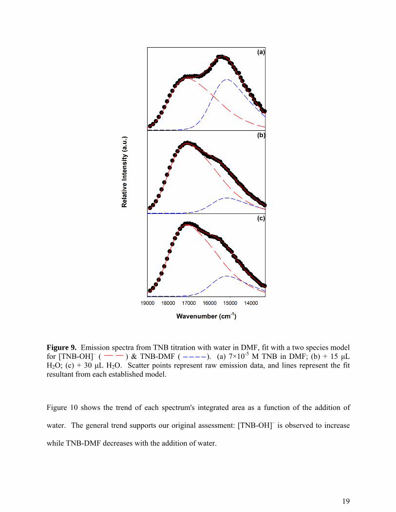
19

Figure 9. Emission spectra from TNB titration with water in DMF, fit with a two species model for [TNB-OH]– ( ) & TNB-DMF ( ). (a) 7×10-5 M TNB in DMF; (b) + 15 μL H2O; (c) + 30 μL H2O. Scatter points represent raw emission data, and lines represent the fit resultant from each established model.

Figure 10 shows the trend of each spectrum's integrated area as a function of the addition of

water. The general trend supports our original assessment: [TNB-OH]– is observed to increase

while TNB-DMF decreases with the addition of water.

20

Figure 10. Normalized modeled emission spectrum area as a function of increasing concentration of water.

3.3. Excitation and Emission Spectra of TNT Products

For TNT, the emission spectra of the titration do not show a great deal of shape change

(see Supplementary Information S5). Figure 4 shows the normalized emission of the initial TNT

solution and after the addition of 30 μL water, excited at 446 nm. These two spectra appear to be

superimposable, however the excitation data in Figure 5 refutes the existence of only one

species. In similar fashion to the TNB data, two distinctly different excitation spectra are

acquired using 550 nm emission and 700 nm emission. As previously mentioned, the methyl

21

group on TNT gives additional reactions that TNB cannot exhibit, so identification of emissive

species requires caution. Since the emission intensity increases (Supplementary Information Fig.

S5) while the absorbance of TNT– is decreasing, TNT– cannot be the emissive species. Also, the

established TNT– absorbance spectrum9,10 has absorbance at lower energy beyond 700 nm; this

rules out TNT– emitting at higher energy wavelengths. These emission spectra show similarity to

the products that are formed from TNB, which does not have the ability to be deprotonated. In

addition, Figure 5 shows that the excitation spectra are similar for [TNB-OH]– and the TNT

product after adding 30 μL of water; with an observed emission at 550 nm, excitation maxima

are observed at 424 nm and 526 nm. This supports that this excitation spectrum belongs to one

of the possible [TNT-OH]– species. Features similar to TNB-DMF are seen for the excitation

spectrum at 700 nm emission, with maxima around 460 nm and 590 nm, but are not as

pronounced relative to the hydroxide sigma adduct features. Figure 3b shows the emission

spectra from the aforementioned addition of NaOH and HCl to the TNT/DMF solution. The

addition of NaOH causes a sizable increase in emission at 603 nm, too large of a change to be

consistent with the more modest increase in the absorbance of TNT–. Instead, this is consistent

with the magnitude of the absorbance increase seen for [TNT-OH]–. The addition of HCl to the

TNT/DMF solution eliminates the [TNT-OH]– emission signal, again by removing hydroxide

from the formation equilibrium. The inset on Figure 3b shows a component of the original

emission that remains around 655 nm after the acidification, which is consistent with the

analogous formation of a DMF adduct, TNT-DMF.

To further understand the TNT reactions, the emission data was also modeled using the

same approach as described above. Figure 6b shows the emission spectrum resultant from 370

nm excitation, where only [TNT-OH]– is excited. The outcome was a three peak spectrum with

22

slight differences from the [TNB-OH]– model, which was not able to reasonably fit all spectra in

the titration by itself even when allowing for relaxation of initial parameters. TNT-DMF

emission peaks were initially fit using a 600 nm excitation (see Figure 7b), and subsequently

iterated with the [TNT-OH]– parameters to establish an overall model. It became obvious that

there was an additional emitting feature for several reasons. First, the emission maximum

appears to shift to higher energy as the excitation shifts to higher energy (see Figure 8b), which

was not observed for TNB. Also, the initial fits for [TNT-OH]– and TNT-DMF were unable to

account for all of the observed emission data collected between samples excited at varying

wavelengths, even when the parameters were allowed to change dramatically. The addition of

one extra Gaussian peak at a higher energy maximum than [TNT-OH]– was able to globally

satisfy all data without drastically altering the initial [TNT-OH]– and TNT-DMF fits. The

complete equation for the TNT model can be found in the Supplementary Information.

The existence of a third species seems to go against the observation of tight isosbestic

points, which typically indicate only two absorbing species in solution. TNT– and [TNT-OH]–

are well established and clearly evident here. TNT-DMF has been observed through

fluorescence, and supported through analogous chemistry to the formation of TNB-DMF. As a

third contributing species, we cannot ascertain the magnitude of TNT-DMF's molar absorptivity

nor its quantum yield. The addition of another [TNT-OH]– species appears to cloud this even

further; however, there are systems that may exhibit isosbestic points with three contributing

species. Such a situation can arise in a system with absorbance contributions from a Lewis acid

with two binding sites and one Lewis base, where the free acid and each form of the adduct

absorb in the same range with different molar extinction coefficients.21 In our case, TNT acts as

the Lewis acid, which has two binding sites (C1 & C3 - see numbering for TNT carbons in

23

Scheme 1). While TNT does not absorb in the visible range, TNT– does; the three products of

the reaction of TNT with hydroxide (TNT–, [TNT-OH]– C1, and [TNT-OH]– C3) should therefore

still show isosbestic points if TNT-DMF is at or below absorbance detection limits. The

question arises as to which form of [TNT-OH]– belongs to which modeled spectrum. While Fyfe

et. al. previously described [TNT-OCH3]– C3 as the only observable sigma adduct via 1H NMR,9

we cannot appropriately correlate this to our measurements without knowing how significantly

the sterics affect methoxide attack versus hydroxide attack. We also do not know each species'

molar absorptivity and quantum yield. If we estimate that both [TNT-OH]– species have molar

absorptivities and quantum yields on the same order of magnitude, then the three peak emission

spectrum that we initially fit plausibly belongs to [TNT-OH]– C1. Also, TDDFT UV-Vis

calculations may support this assignment by projecting the C3 adduct as having higher energy

transitions (Supplementary Information Fig. S6). Absorbance computations at the B3LYP/6-

311+G**//HF/6-311+G** level suggest that the HOMO/LUMO gap for the C1 sigma adduct is

of lower energy than the C3 form. If each hydroxide sigma adduct has a similar Stokes shift, this

would assign the higher energy, single peak emission spectrum to [TNT-OH]– C3. The TDDFT

calculated absorbance spectrum shows that the maximum for [TNT-OH]– C3 is at about 25 nm

shorter wavelength than [TNT-OH]– C1 while the fit emission spectra show a 21 nm difference,

giving some quantitative support for the assignments.

Figure 11 shows the initial emission spectrum of the TNT/DMF solution, the addition of

15 μL of water, and addition of 30 μL of water. All spectra in this titration fit well using our

established model (full titration fitting can be found in Supplementary Information Fig. S7). The

converged parameters for the TNT product emission spectra model can be found in Table 1. The

vibronic energy for [TNT-OH]– C1 is 770 cm-1 and 630 cm-1 for TNT-DMF; these energies may

24

represent ring bending modes in each respective species. The integrated area of each spectrum

as a function of water addition is found in Figure 10. Unlike the trend for TNB, all emissive

species are observed to grow as more water is added to the system. This could be an indication

that TNT-DMF formation requires [TNT-OH]– C3 as an intermediate with a subsequent SN2 step.

Figure 11. Emission spectra from TNT titration with water in DMF, fit to a three species model for [TNT-OH]– C1 ( ), TNT-DMF ( ), and [TNT-OH]– C3 ( ). (a) 1.1×10-4 M TNT in DMF; (b) + 15 μL H2O; (c) + 30 μL H2O.

25

4. Conclusions

In summary, we have shown that TNB has the capacity to form two sigma adducts in

DMF, [TNB-OH]– and TNB-DMF, as shown in Scheme 1. Absorbance data for TNB/DMF

solutions supports the existence of two species that absorb in the region expected for sigma

adducts. Further investigation into excitation and emission data supports the two species. The

development of a multi-Gaussian model (with parameters given in Table 1) clarifies the relative

quantities of emission from each species, showing the two to be linked by equilibrium. The

methyl group of TNT causes different reactivity than TNB. TNT has the ability to form four

products in DMF (Scheme 1), leading to spectral differences and similarities which require

careful analysis to discern. The major absorbing species, TNT–, is shown to be non-emissive.

Absorbance features consistent with sigma adducts of TNT are observed to grow as a function of

water addition. The three possible sigma adducts, [TNT-OH]– C1, [TNT-OH]– C3, and TNT-

DMF, all exhibit excitation and emission features that have distinct similarity to their TNB

counterparts. A multi-Gaussian model was also established to differentiate the TNT sigma

adducts' relative emission (Table 1), showing that all grow together as a function of added water.

This is not observed for the TNB sigma adducts, and implies different mechanisms for DMF

sigma adduct formation.

This is the first report of fluorescent emission from Meisenheimer adducts of TNB and

TNT, with both nitroaromatics capable of nucleophilic attack by hydroxide and the less sterically

hindered TNB capable of attack by DMF. All reactions show significant changes within

minutes, which allow these reactions to be further explored in the context of sensor development.

The emissions may be able to be enhanced by using a resonance energy transfer from a donor

26

fluorophore with a long excited state lifetime to these adducts as acceptors; this could further

amplify this form of a "turn-on" mechanism. Alternatively, a solid state sensor capable of

capturing these nitroaromatics through stronger nucleophilic attack may be able to serve in a

facile turn-on approach. Future work should compare dinitrotoluene (DNT) emission

characteristics to those described here. DNTs are common impurities in TNT, but since DNTs

have a much higher vapor pressure than TNT they will each deliver similar amounts in the vapor

phase to a sensor. Depending on the relative equilibrium constants for each adduct formation

and their relative quantum yield, it may be found that DNTs are more observable in this capacity.

In addition, the different reactivity between TNT and TNB means that caution must be used

when using TNB as a surrogate for TNT in the development and testing of TNT sensors.

Finally, this work shows that TNT sensors are expected to perform differently under wet or

humid conditions than under dry conditions. Water can react with nitroaromatics even at trace

levels.

ASSOCIATED CONTENT

Supporting Information.

UV/Vis Absorbance spectra, excitation and emission spectra of trinitroaromatics in DMF with

water titration. This material is available free of charge via the Internet at http://pubs.acs.org.

AUTHOR INFORMATION

Corresponding Author

*Email: weuler@chm.uri.edu

27

Notes

The authors declare no competing financial interest.

ACKNOWLEDGMENT

We would like to gratefully acknowledge Drs. Jimmie Oxley and James Smith for providing us

with TNT. We also thank the Department of Homeland Security ALERT Center for funding.

ABBREVIATIONS

TNB, trinitrobenzene; TNT, trinitrotoluene; DMF, N,N-dimethylformamide.

REFERENCES

(1) Jiang, Y.; Zhao, H.; Zhu, N.; Lin, Y.; Yu, P.; Mao, L. Angew. Chem. Int. Ed. 2008,

47, 8601-8604.

(2) Üzer, A.; Erçağ, E.; Apak, R. For. Sci. Int. 2008, 239-243.

(3) Xia, Y.; Song, L.; Zhu, C. Anal. Chem. 2011, 83, 1401-1407.

(4) Chen, Y.; Chen, Z.; He, Y.; Lin, H.; Sheng, P.; Liu, C.; Luo, S.; Cai, Q.

Nanotechnology 2010, 21, 125502-125507.

(5) Tu, R.; Liu, B.; Wang, Z.; Gao, D.; Wang, F.; Fang, Q.; Zhang, Z. Anal. Chem. 2008,

80, 3458-3465.

28

(6) Gao, D.; Wang, Z.; Liu, B.; Ni, L.; Wu, M.; Zhang, Z. Anal. Chem. 2008, 80, 8545-

8553.

(7) Fang, Q.; Geng, J.; Liu, B.; Gao, D.; Li, F.; Wang, Z.; Guan, G.; Zhang, Z. Chem. Eur. J.

2009, 15, 11507-11514.

(8) Zhang, K.; Zhou, H.; Mei, Q.; Wang, S.; Guan, G.; Liu, R.; Zhang, J.; Zhang, Z. J.

Am. Chem. Soc. 2011, 133, 8424-8427.

(9) Fyfe, C.; Malkiewich, C.; Damji, S.; Norris, A. J. Am. Chem. Soc. 1976, 98, 6983-6988.

(10) Bernasconi, C. J. Org. Chem. 1971, 36, 1671-1679.

(11) Shipp, K.; Kaplan, L. J. Org. Chem. 1966, 31, 857-861.

(12) Buncel, E.; Norris, A.; Russell, K.; Tucker, R. J. Am. Chem. Soc. 1972, 94, 1646-1649.

(13) Lakowicz, J.R. Principles of Fluorescence Spectroscopy, third ed., Springer

Science, New York, 2006.

(14) Rahman, M.; Harmon, H.J. Spectrochimica Acta A 2006, 65, 901-906.

(15) Olley, D.A.; Wren, E.J.; Vamvounis, G.; Fernee, M.J.; Wang, X.; Burn, P.L.;

Meredith, P.; Shaw, P.E. Chem. Mater. 2011, 23, 789-794.

(16) Algarra, M.; Campos, B.B.; Miranda, M.S.; Esteves da Silva, J.C.G. Talanta, 2011,

83, 1335-1340.

(17) Thomas III, S.W.; Joly, G.D.; Swager, T.M. Chem. Rev. 2007, 107, 1339-1386.

29

(18) Shi, G.H.; Shang, Z.B.; Wang, Y.; Jin, W.J.; Zhang, T.C. Spectrochimica Acta A 2008,

70, 247-252.

(19) Spartan '10; Wavefunction, Inc.: Irvine, CA, 2010. Version 1.1.0.

(20) Foster, R.; Mackie, R.K. J. Chem. Soc. 1962, 3843-3844.

(21) Drago, R.S. Physical Methods for Chemists, second ed., Saunders College Publishing,

New York, 1992.

TOC GGraphic

30

Journal Name

Cite this: DOI: 10.1039/c0xx00000x

www.rsc.org/xxxxxx

Dynamic Article Links

ARTICLE TYPE

This journal is © The Royal Society of Chemistry [year] [journal], [year], [vol], 00–00 | 1

A Fluorometric Sensing Array for the Detection of Military Explosives and IED Materials Christopher A. Latendresse a, Syrena C. Fernandes a, Sangmin You a, Hui Qi Zhang a, and William B. Euler*a

Received (in XXX, XXX) Xth XXXXXXXXX 20XX, Accepted Xth XXXXXXXXX 20XX 5

DOI: 10.1039/b000000x

A fluorometric sensing array was developed to detect and discern common military explosives and materials used in improvised explosive devices (IEDs). Xanthene-based fluorophores were chosen as reporter molecules and were exposed to explosive analytes in DMF solution. Unique responses were observed for each analyte, with the strongest observed responses resultant from trinitrobenzene (TNB) or 10

trinitrotoluene (TNT) addition. Evidence for substantial electron transfer (ET) between TNB and TNT products and fluorophores was observed. Computational results indicate that anionic trinitroaromatic products are likely donating electrons to cationic fluorophores, leading to an observed enhancement of their emission.

Introduction 15

With the rise in domestic and international terroristic events in the past decade, the scientific community has been pushed by the need to develop rapid and sensitive means of detection of explosive analytes. Explosive sensors have been developed based on a number of methods of detection, including 20

colorimetry,1,2 fluorescence,3-9 mass spectrometry,10-12 electrochemical,13-15 and Surface Enhanced Raman Scattering (SERS),16-18 among others. Sensitivity and selectivity remain at the heart of an effective sensor, and while many sensors are able to claim one, most 25

cannot achieve both. Fluorescence sensing benefits from the inherently high sensitivity of contemporary fluorescence instrumentation, which can achieve attomolar detection for molecules with high quantum yields in solution.19 Additionally, detection limits may be improved by another order of magnitude 30

using metal enhanced fluorescence.20,21 Selectivity, although difficult to achieve using a single interactive sensor, can be induced by the use of a sensor array where multiple sensors can be exposed to the same analyte stream and their responses observed together. This “fingerprint” can be read as a function of 35

a specific analyte; whereas one of the sensors may not be able to discern one analyte from another, it is unlikely that two analytes will interact with the multitude of sensors in the exact same fashion. Perhaps surprisingly, the rhodamine family has not been well 40

explored in the field of explosive detection. Meaney & coworkers investigated the fluorescence quenching of common fluorophores including Rhodamine 6G against nitrobenzene, 4-nitrotoluene and 2,6-dinitrotoluene, but did not explore more contemporarily relevant analytes.9 Rhodamines have notoriety as 45

being very strong fluorophores, and were therefore selected to

test as fluorescence reporters against explosive analytes. Rhodamines also have the advantage of possessing visible range excitations and emissions that are not subject to interference by absorbance bands of explosive analytes. The rhodamines 50

investigated in this study were Rhodamine 560 Chloride (Rh560), Rhodamine 6G (Rh6G), Sulforhodamine B (SRhB), Rhodamine 640 Perchlorate (Rh640), Sulforhodamine 640 (SRh640), Rhodamine 700 (Rh700) and Rhodamine 800 (Rh800). Fluorescein 548 (Fl548) was also included, as another represent-55

ative xanthene derivative with a high quantum yield. The structures of the selected fluorophores can be found in Supplementary Information Fig. S1. The analytes exposed to the aforementioned fluorophores were selected based on current military relevance: trinitrobenzene (TNB), trinitrotoluene (TNT), 60

cyclotrimethylenetrinitramine (RDX), and cyclotetramethylene-tetranitramine (HMX) are common military grade secondary explosives; pentaerythritoltetranitrate (PETN) and triacetone-triperoxide (TATP) have been used in improvised explosive devices (IEDs) and large scale terrorist events over the past two 65

decades due to their relatively simple synthesis and high output;10,11,22 and 2,3-dinitrotoluene (2,3-DNT), 2,4-dinitrotoluene (2,4-DNT), 2,6-dinitrotoluene (2,6-DNT), 3,4-dinitrotoluene (3,4-DNT), 2-nitrotoluene (2-NT) and 4-nitrotoluene (4-NT) are common impurities in crude and refined 70

TNT due to incomplete nitration.23 Due to the much higher vapor pressures and saturated vapor densities of DNTs and NTs relative to TNT, these species may serve as useful analytes for the implication of TNT sensing. The structures of the explosive analytes can be found in Supplementary Information Fig. S2. 75

Experimental section Chemicals and materials

2 | Journal Name, [year], [vol], 00–00 This journal is © The Royal Society of Chemistry [year]

DMF (≥99.5%) was purchased from Fisher Scientific and used as received. Rh560, Fl548, Rh640, SRh640, Rh700, and Rh800 were purchased from Exciton (Dayton, Ohio) and used as received. Rh6G (99%) was purchased from Acros and used as received. SRhB was purchased from Lambda Physik and used as 5

received. TNT, TATP, PETN, HMX, and RDX were obtained from Drs. Jimmie Oxley and James Smith and were used without further purification. TNB was purchased from Fisher Scientific wetted with ca. 40% water with 98.0% purity; 2,3-DNT (99%), 2,6-DNT (98%), and 3,4-DNT (99%) were purchased from 10

Aldrich; 2,4-DNT (95%) was purchased from Alfa Aesar; and 2-NT (99%) and 4-NT (99%) were purchased from Acros. All were used as received.

Apparatus and Procedure

Fluorophore solutions in DMF were created and diluted to a 15

maximum visible range absorbance of 0.1 abs. units. Solutions of Rh700 and Rh800 were acidified with trifluoroacetic acid (TFA) to prevent photobleaching prior to use. Absorbance data (PerkinElmer Lambda900 UV/Vis/NIR spectrophotometer) and emission data (Horiba Fluorolog-3, Xe arc lamp excitation) were 20

obtained before and after the addition of a few crystals of solid explosive, or the addition of a small drop in the case of 2-NT(l). Excitation and emission slits were used between 2 and 5 nm, but did not vary between initial and final spectra acquisitions.

Computational Analysis 25

Spartan '10 computational software24 was used to propose the relative absorbance maxima for the isomers of [TNT-OH]–. Structures were optimized at the HF/6-311+G** level without imaginary vibrational frequencies. TDDFT energies and absorbance spectra were calculated using the converged 30

structures at the B3LYP/6-311+G** level.

Results and Discussion Solutions of fluorophores were prepared in DMF, with absorbance and emission spectra acquired before and after the addition of explosive analyte. Figure 1 shows the absorbances 35

characterizing the initial fluorophore solutions, spanning the visible range. In similar fashion, Figure 2 shows the normalized emission spectra from each initial fluorophore solution, spanning from 530 nm to 800 nm. Pairing absorbance and emission measurements together allows for determination of possible 40

interactions between fluorophore and analyte, as both ground state and excited state profiles are examined. Figure 3 shows the output of the sensing array, as indicated by emission difference spectra. Note that the ordinate axis for TNB and TNT interactions are set to 100% change in emission. All 45

others are zoomed to 10% for clarity, with a select few zoomed to 40% marked by "× ¼." The trinitroaromatics, TNB and TNT, both show very strong observed quenching. This is in large part due to the products which they form in DMF, reacting with hydroxide generated by trace amounts of water. Others have 50

previously described the absorbance properties25-28 and recently we have described the emission properties of these products;29 both of these factors complicate the observations made here as added variables. TNB and TNT are capable of nucleophilic attack by hydroxide and DMF; in addition, TNT is capable of 55

60

Fig. 1 Absorbance overlay of selected fluorophores in DMF, normalized 65

to visible absorbance maximum. Listed in order of decreasing energy maximum, the fluorophores are Rh560 ( ), Fl548 ( ), Rh6G ( ), SRhB ( ), Rh640 ( ), SRh640 (

), Rh700 ( ), Rh800 ( ).

70

75

80

Fig. 2 Emission overlay of selected fluorophores in DMF, normalized to 85

emission maximum. Listed in order of decreasing energy maximum, the fluorophores are Rh560 ( ), Fl548 ( ), Rh6G (

), SRhB ( ), Rh640 ( ), SRh640 (), Rh700 ( ), Rh800 ( ).

deprotonation by hydroxide. The resulting strong absorbance 90

features can be seen in Supplementary Information Figs. S3-S6. Consistently, these products are diminished in the observations with Rh700 and Rh800, as these solutions were slightly acidified to inhibit photobleaching during analysis. Since the product formation is reliant on hydroxide in solution, acidification 95

removes hydroxide and shifts the equilibria back towards free TNT or TNB. The formation of these products serves to complicate the interactions with the fluorophores in solution, due to their inner filter effect and possible ground state interactions. Both of these factors will be discussed in greater detail later in the 100

paper. PETN, RDX, and HMX are all nitroaliphatics, which show a mixture of quenches and enhancements through interactions with the sensing fluorophores. There is no observed change in any fluorophore's absorbance upon these exposures (see Figs. S3-S6), 105

implying that emission changes are only resultant from excited state interactions. Emission decreases are likely resultant from dynamic mechanisms. Increases in emission may result from interactions that either decrease the lifetime of the excited state,

Journal Name

Cite this: DOI: 10.1039/c0xx00000x

www.rsc.org/xxxxxx

Dynamic Article Links

ARTICLE TYPE

This journal is © The Royal Society of Chemistry [year] [journal], [year], [vol], 00–00 | 3

Fig./Scheme XX Caption

5

10

15

20

25

30

35

40

45

X

50

55

60

Fig. 3 Emission difference spectra for the exposure of explosive analytes to selected fluorophores in DMF solution, normalized to the initial emission maximum. Blue spectra indicate the observed quenching of emission, red spectra indicate the observed enhancement of emission, and black spectra indicate minimal change in emission. Full absorbance and emission spectra can be found in Supplementary Information Figs. S3-S6.

65

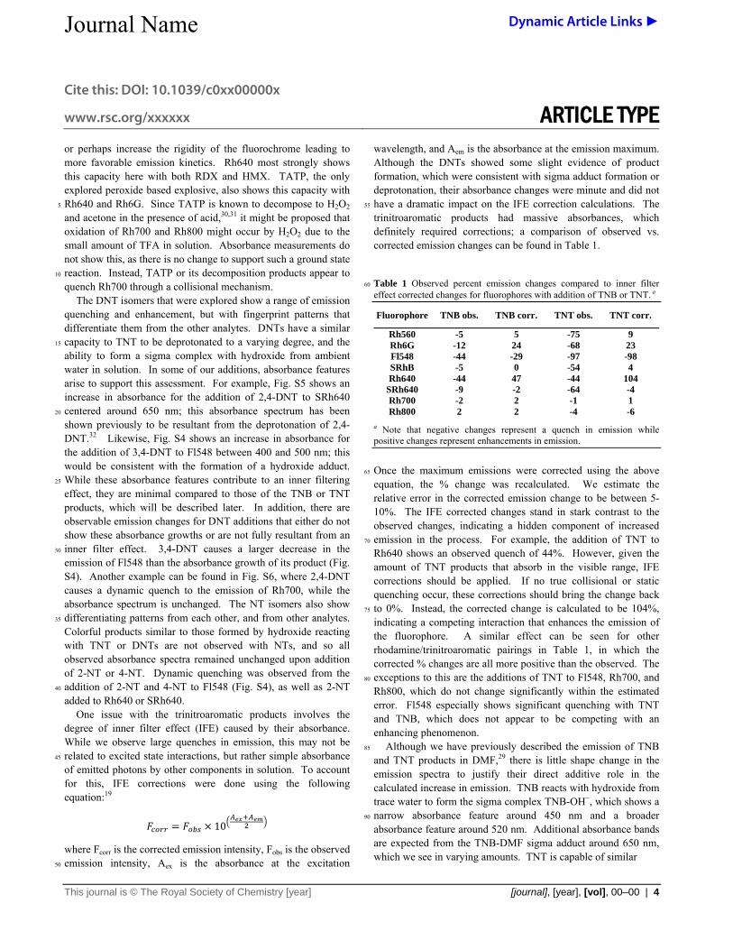
Journal Name

Cite this: DOI: 10.1039/c0xx00000x

www.rsc.org/xxxxxx

Dynamic Article Links

ARTICLE TYPE

This journal is © The Royal Society of Chemistry [year] [journal], [year], [vol], 00–00 | 4

or perhaps increase the rigidity of the fluorochrome leading to more favorable emission kinetics. Rh640 most strongly shows this capacity here with both RDX and HMX. TATP, the only explored peroxide based explosive, also shows this capacity with Rh640 and Rh6G. Since TATP is known to decompose to H2O2 5

and acetone in the presence of acid,30,31 it might be proposed that oxidation of Rh700 and Rh800 might occur by H2O2 due to the small amount of TFA in solution. Absorbance measurements do not show this, as there is no change to support such a ground state reaction. Instead, TATP or its decomposition products appear to 10

quench Rh700 through a collisional mechanism. The DNT isomers that were explored show a range of emission quenching and enhancement, but with fingerprint patterns that differentiate them from the other analytes. DNTs have a similar capacity to TNT to be deprotonated to a varying degree, and the 15

ability to form a sigma complex with hydroxide from ambient water in solution. In some of our additions, absorbance features arise to support this assessment. For example, Fig. S5 shows an increase in absorbance for the addition of 2,4-DNT to SRh640 centered around 650 nm; this absorbance spectrum has been 20

shown previously to be resultant from the deprotonation of 2,4-DNT.32 Likewise, Fig. S4 shows an increase in absorbance for the addition of 3,4-DNT to Fl548 between 400 and 500 nm; this would be consistent with the formation of a hydroxide adduct. While these absorbance features contribute to an inner filtering 25

effect, they are minimal compared to those of the TNB or TNT products, which will be described later. In addition, there are observable emission changes for DNT additions that either do not show these absorbance growths or are not fully resultant from an inner filter effect. 3,4-DNT causes a larger decrease in the 30

emission of Fl548 than the absorbance growth of its product (Fig. S4). Another example can be found in Fig. S6, where 2,4-DNT causes a dynamic quench to the emission of Rh700, while the absorbance spectrum is unchanged. The NT isomers also show differentiating patterns from each other, and from other analytes. 35

Colorful products similar to those formed by hydroxide reacting with TNT or DNTs are not observed with NTs, and so all observed absorbance spectra remained unchanged upon addition of 2-NT or 4-NT. Dynamic quenching was observed from the addition of 2-NT and 4-NT to Fl548 (Fig. S4), as well as 2-NT 40

added to Rh640 or SRh640. One issue with the trinitroaromatic products involves the degree of inner filter effect (IFE) caused by their absorbance. While we observe large quenches in emission, this may not be related to excited state interactions, but rather simple absorbance 45

of emitted photons by other components in solution. To account for this, IFE corrections were done using the following equation:19 = × 10

where Fcorr is the corrected emission intensity, Fobs is the observed emission intensity, Aex is the absorbance at the excitation 50

wavelength, and Aem is the absorbance at the emission maximum. Although the DNTs showed some slight evidence of product formation, which were consistent with sigma adduct formation or deprotonation, their absorbance changes were minute and did not have a dramatic impact on the IFE correction calculations. The 55

trinitroaromatic products had massive absorbances, which definitely required corrections; a comparison of observed vs. corrected emission changes can be found in Table 1.

Table 1 Observed percent emission changes compared to inner filter 60

effect corrected changes for fluorophores with addition of TNB or TNT. a

Fluorophore TNB obs. TNB corr. TNT obs. TNT corr.

Rh560 -5 5 -75 9 Rh6G -12 24 -68 23 Fl548 -44 -29 -97 -98 SRhB -5 0 -54 4 Rh640 -44 47 -44 104

SRh640 -9 -2 -64 -4 Rh700 -2 2 -1 1 Rh800 2 2 -4 -6

a Note that negative changes represent a quench in emission while positive changes represent enhancements in emission.

Once the maximum emissions were corrected using the above 65

equation, the % change was recalculated. We estimate the relative error in the corrected emission change to be between 5-10%. The IFE corrected changes stand in stark contrast to the observed changes, indicating a hidden component of increased emission in the process. For example, the addition of TNT to 70

Rh640 shows an observed quench of 44%. However, given the amount of TNT products that absorb in the visible range, IFE corrections should be applied. If no true collisional or static quenching occur, these corrections should bring the change back to 0%. Instead, the corrected change is calculated to be 104%, 75

indicating a competing interaction that enhances the emission of the fluorophore. A similar effect can be seen for other rhodamine/trinitroaromatic pairings in Table 1, in which the corrected % changes are all more positive than the observed. The exceptions to this are the additions of TNT to Fl548, Rh700, and 80

Rh800, which do not change significantly within the estimated error. Fl548 especially shows significant quenching with TNT and TNB, which does not appear to be competing with an enhancing phenomenon. Although we have previously described the emission of TNB 85

and TNT products in DMF,29 there is little shape change in the emission spectra to justify their direct additive role in the calculated increase in emission. TNB reacts with hydroxide from trace water to form the sigma complex TNB-OH−, which shows a narrow absorbance feature around 450 nm and a broader 90

absorbance feature around 520 nm. Additional absorbance bands are expected from the TNB-DMF sigma adduct around 650 nm, which we see in varying amounts. TNT is capable of similar

This journal is © The Royal Society of Chemistry [year] Journal Name, [year], [vol], 00–00 | 5

5

Fig. 4 Normalized absorbance overlay of fluorophores in DMF, 10

compared with the normalized emission of TNB products. Listed in order of decreasing energy maximum, the fluorophores are (a) Rh560 (

), (b) Fl548 ( ), (c) Rh6G ( ), (d) SRhB (), (e) Rh640 ( ), (f) SRh640 ( ), (g) Rh700 (), (h) Rh800 ( ). The emission spectrum (i), given by 15

the thicker line width, is a composite of the emission of TNB-OH− and TNB-DMF formed in the addition of TNB to DMF solution.

chemistry, by forming two possible TNT-OH− adduct isomers, as well as a DMF adduct; both have been shown to be emissive. TNT is also capable of being deprotonated by OH−, forming 20

TNT−, but this species is not emissive. One plausible conclusion is that the increase results from resonance energy transfer (RET). This would reslt from the excited states of a trinitroaromatic product to donate energy to the fluorophore acceptor, populating their excited states leading to 25

greater emission. Additionally, it appears that the addition of TNT leads to a greater enhancement than the TNB counterparts. While we cannot address RET efficiencies here without knowing the relative amount of each species and lifetimes, it is interesting to note the consistently higher response to TNT. To further 30

investigate the possibility of RET between trinitroaromatic products and the fluorophores, the absorbance spectra of the fluorophore acceptors is compared to the emission spectrum of TNB product donors in DMF solution in Figure 4. The emission spectrum is comprised of two components, TNB-35

OH− and TNB-DMF, which emit at a maximum around 580 nm and 650 nm respectively.29 The emission spectrum overlaps best with the absorbance spectra of Rh700 and Rh800, which do not exhibit enhancement when exposed to TNB in DMF. Also, the similar absorbance spectra of Rh640 and SRh640 but different 40

response to TNB do not make sense in the context of RET shown here. In a RET mechanism, it would be expected that both Rh640 and SRh640 would show enhancements, which are not observed. In addition, the concentrations of each species in solution are on the order of 10-3 M, which would make the average distance 45

between molecules greater than 100 Å. Given the strong distance dependence in a RET mechanism, this distance is higher than the typical Förster distance exhibited by similar molecules.19 The poor correlation of the spectral bands of the fluorophores and TNB products and the large intramolecular distances suggest that 50

RET is not the enhancement mechanism. Other possibilities for an enhanced fluorescence are charge transfer (CT) or electron transfer (ET) mechanisms. A CT complex may be formed if the HOMOs of the TNB or TNT products are close enough in energy to the LUMOs of the sensing 55

60

Fig. 5 HOMO/LUMO diagram for energy comparison between sensing fluorophores, trinitroaromatics, and trinitroaromatic products. Relative energies were computed at the B3LYP/6-311+G**//HF/6-311+G** level 65

in vacuum at 298.15 K and 1 atm. Arrows are shown to designate the HOMO.

fluorophores, for a small amount of overlap to occur. If either of the TNB or TNT products have HOMOs of high energy relative to the LUMOs of the fluorophores, ET may justify the enhanced 70

excited state population and subsequent enhanced emission of the fluorophores. To help in our assignment of the mechanism of enhanced emission, molecular orbital energies were calculated. Figure 5 shows the calculated relative energies of the HOMO and LUMO for TNB, TNB-OH−, TNT, TNT-OH−, TNT−, and the 75

sensing fluorophores. It is clear that there is a dramatic difference between the frontier orbital energies of the free trinitroaromatics, with the transient anionic products (TNT− and the OH− adducts) being of much higher energy. The trinitroaromatic products have HOMOs 80

so high in energy that they are very close to the energy of the LUMOs of some of the modeled fluorophores (eg. Fl548, SRh640). This gives plausibility to the formation of a CT complex where the products may donate to the fluorophore. The HOMOs of TNB and TNT are reasonably close in energy to the 85

LUMOs of several of the fluorophores, which indicates the possibility of a trinitroaromatic:fluorophore CT complex formation. However, the energy of this transition would be greater than the HOMO/LUMO gap of all of the fluorophores, suggesting that the CT band would not be in the visible range but 90

rather in the UV. Since the formation of any CT complex would lead to a spectral shift, yet no shift is observed, no significant CT complex formation is occurring. Photo-induced electron transfer (PET) is unlikely to play a role in our observations in the context of these calculations. 95

Typically, PET causes a quench in emission if electron density is transferred to or away from a fluorophore, as this can lead to structural and lifetime changes.19 Emission enhancements can be justified through disruption of PET mechanisms, but since our initial solution is comprised of only the fluorophore in DMF this 100

also seems unlikely. The only way that this might be conceived is if DMF is initially quenching the fluorophores, and that the displacement of DMF by explosive molecules in solvation leads to an observed enhancement. Given the relatively low quantity of analyte added relative to the overwhelming amount of DMF 105

solvent, the small addition cannot account for the magnitude of enhancement observed. In the context of a ground state ET mechanism, TNB and TNT have the lowest calculated HOMO energy of all of the modeled species. This feature as well as their electron deficient character 110

6 | Journal Name, [year], [vol], 00–00 This journal is © The Royal Society of Chemistry [year]

makes it unlikely that the free trinitroaromatics would donate electrons to the fluorophores. The anionic products have a much higher calculated HOMO energy however, making them more likely electron donors. Fl548 and SRh640 have LUMOs that are slightly higher in energy than the HOMOs of TNT− and the OH− 5

adducts, making them poor candidates as electron acceptors. The calculated LUMO of SRhB is lower but still close in energy to the HOMO of the anionic products (within 0.3 eV); this is likely an insufficient energy gap to cause significant ET at ambient temperatures. Rh6G and Rh640 have LUMOs of very similar 10

energy (-5.39 and -5.13 eV respectively), which are about 2.4 eV lower than the HOMO of TNB-OH−. Since these two fluorophores show the greatest enhancement with TNB and TNT addition in solution and their relative LUMO energies to TNB-OH− are strikingly similar, electron transfer appears to be the 15

most probable mechanism. The difference in energy is substantial enough to occur without significant reversibility. Rh560, Rh700, and Rh800 have LUMOs of lower energy than Rh6G and Rh640. Rh560 shows a calculated enhancement that is within the estimated error of our approach, and with a LUMO 20

that is 3 eV lower than the HOMO of TNB-OH− the magnitude of the enhancement might be expected to be higher. The correlation of the relative enhancements is beyond the scope of our calculations here, however Rh560 is likely to follow the trend of enhancement shown by Rh6G and Rh640. Rh700 and Rh800 25

have a difference of about 2.8 eV, but an electron transfer is hindered by the lack of OH− adduct formation in the acidified solution. In these cases, only slight changes in emission are observed after IFE calculations. It is also interesting to note that the three enhanced fluorophores (Rh560, Rh6G, Rh640) happen 30

to all be cationic, whereas the remaining fluorophores (excluding Rh700 and Rh800 for aforementioned reasons) are either neutral in charge or anionic. It is easy to conceive the possible formation of an ion pair between the cationic fluorophores and the anionic trinitroaromatic products. This driving force would bring the 35

species in close proximity to allow ET to occur, without the limitations of diffusion and collision in solution.

Conclusion We have investigated a sensing array based on highly fluorescent molecules in DMF solution that shows promise for the detection 40

of explosive analytes. In addition to typical collisional or static quenching, inner filter effect corrections indicate an ET component, which increases the emission of at least two of the fluorescent reporters (Rh6G and Rh640). The findings of ET may have an impact on pre-existing RET based sensors, as the 45

emission of the fluorophores in this study was observed to enhance. The capability of trinitroaromatic products to be involved in ET may influence existing sensors that rely on TNB or TNT as a RET disruptor, leading to a competitive ET mechanism that would decrease the effectiveness of the sensor by 50

diminishing an observed quench in emission. Further studies will be undertaken to expand the set of fluorescent reporter molecules and quantify the interactions with the most significant emission change, as well as experiments to give additional clarification of the ET with trinitroaromatic products. 55

Notes and references a University of Rhode Island, Department of Chemistry, 51 Lower College Road, Kingston, RI, USA. Fax: XX XXXX XXXX; Tel: 401 874 5090; E-mail: weuler@chm.uri.edu 60

† Electronic Supplementary Information (ESI) available: absorbance and emission spectra for all fluorphore/analyte combinations. See DOI: 10.1039/b000000x/ 1 Y. Jiang, H. Zhao, N. Zhu, Y. Lin, P. Yu, and L. Mao, Angew. Chem.

Int. Ed., 2008, 47, 8601. 65

2 A. Üzer, E. Erçağ, and R. Apak., For. Sci. Int., 2008, 239. 3 Y. Xia, L. Song, and C. Zhu, Anal. Chem., 2011, 83, 1401. 4 Y. Chen, Z. Chen, Y. He, H. Lin, P. Sheng, C. Liu, S. Luo, and Q.

Cai, Nanotechnology, 2010, 21, 125502. 5 R. Tu, B. Liu, Z. Wang, D. Gao, F. Wang, Q. Fang, and Z. Zhang, 70

Anal. Chem., 2008, 80, 3458. 6 D. Gao, Z. Wang, B. Liu, L. Ni, M. Wu, and Z. Zhang, Anal. Chem.,

2008, 80, 8545. 7 Q. Fang, J. Geng, B. Liu, D. Gao, F. Li, Z. Wang, G. Guan, and Z.

Zhang, Chem. Eur. J., 2009, 15, 11507. 75

8 K. Zhang, H. Zhou, Q. Mei, S. Wang, G. Guan, R. Liu, J. Zhang, and Z. Zhang, J. Am. Chem. Soc., 2011, 133, 8424.

9 M. S. Meaney and V. L. McGuffin, Anal. Chim. Acta, 2008, 610, 57. 10 Y. Takada, Y. Suzuki, H. Nagano, M. Sugiyama, E. Nakajima, M.

Sugaya, Y. Hashimoto, and M. Sakairi, IEEE Sensors, 2012, 12, 80

1673. 11 J. Kozole, J. Tomlinson-Phillips, J. R. Stairs, J. D. Harper, S. R.

Lukow, R. T. Lareau, H. Boudries, H. Lai, and C. S. Brauer, Talanta, 2012, 99, 799.

12 P. Sulzer, F. Petersson, B. Agarwal, K. H. Becker, S. Jürschik, T. D. 85

Märk, D. Perry, P. Watts, and C. A. Mayhew, Anal. Chem., 2012, 84, 4161.

13 P. K. Sekhara, E. L. Broshaa, R. Mukundana, K. L. Linkerb, C. Brusseaub, and F. H. Garzona, J. Haz. Mat., 2011, 190, 125.

14 M. Y. Ho, N. D’Souza, and P. Migliorato, Anal. Chem., 2012, 84, 90

4245. 15 R. L. Marple and W. R. LaCourse, Anal. Chem., 2005, 77, 6709. 16 X. Liua, L. Zhaob, H. Shenb, H. Xub, and L. Lua, Talanta, 2011, 83,

1023. 17 T. Demeritte, R. Kanchanapally, Z. Fan, A. K. Singh, D. Senapati, M. 95

Dubey, E. Zakarb, and P. C. Ray, Analyst, 2012, 137, 5041. 18 P. R. Sajanlal and T. Pradeep, Nanoscale, 2012, 4, 3427. 19 J. R. Lakowicz, Principles of Fluorescence Spectroscopy, third ed.,

Springer Science, New York, 2006. 20 Y. Wang, Z. Li, H. Li, M. Vukib, D. Xua, and H. Y. Chen, 100

Biosensors and Bioelectronics, 2012, 32, 76. 21 H. Li, C. Y. Chen, X. Wei, W. Qiang, Z. Li, Q. Cheng, and D. Xu,

Anal. Chem., 2012, 84, 8656. 22 W. Fan, M. Young, J. Canino, J. Smith, J. Oxley, and J. R. Almirall,

Anal. Bioanal. Chem., 2012, 403, 401. 105

23 Military Explosives, Dept. of the Army Technical Manual, updated 1990.

24 Spartan '10; Wavefunction, Inc.: Irvine, CA, 2010. Version 1.1.0. 25 C. Fyfe, C. Malkiewich, S. Damji, and A. Norris, J. Am. Chem. Soc.,

1976, 98, 6983. 110

26 C. Bernasconi, J. Org. Chem., 1971, 36, 1671. 27 K. Shipp and L. Kaplan, J. Org. Chem., 1966, 31, 857. 28 E. Buncel, A. Norris, K. Russell, and R. Tucker, J. Am. Chem. Soc.,

1972, 94, 1646. 29 C. A. Latendresse, S. C. Fernandes, S. You, H. Q. Zhang, and W. B. 115

Euler, J. Phys. Chem. A., 2013, 117, 324. 30 H. Lin and K. S. Suslick, J. Am. Chem. Soc., 2010, 132, 15519. 31 J. C. Oxley, J. L. Smith, and H. Chen, Prop., Explos., Pyro., 2002,

27, 209. 32 E. J. Olson, T. T. Xiong, C .J. Cramer, and P. Bühlmann, J. Am. 120

Chem. Soc., 2011, 133, 12858. 125

This journal is © The Royal Society of Chemistry [year] Journal Name, [year], [vol], 00–00 | 7

Table of Contents graphic 5

ON N

CO2H

CH2

NO2

NO2

O2N

e– donation

enhanced emission

1

Light Trapping to Amplify Metal Enhanced

Fluorescence with Application for Sensing TNT

Meredith A. Matoian, Richard Sweetman, Emily C. Hall, Shayna Albanese, William B.

Euler*

Department of Chemistry, University of Rhode Island, 51 Lower College Road, Kingston, RI 02881

E-mail: weuler@chm.uri.edu.

Abstract

Metal Enhanced Fluorescence (MEF) typically produces enhancement factors of 10 to 50. By using a polymer

layer as the dielectric spacer enhancements as high as 1600 can be observed. The effect occurs with a variety of

different polymers and substrates, all of which act to trap light in the dielectric layer. This allows the fabrication

of sensors with improved sensitivity as demonstrated for detection of trinitrotoluene (TNT).

Keywords: enhanced fluorescence, polymer layer, light trapping, TNT sensing

Introduction

Exploitation of the plasmon properties of metal nanoparticles is currently of interest.

Coupling the electric field created by a plasmon to a molecule on the surface can lead to

significant intensity increases in Raman spectra (surface enhanced Raman spectra, SERS) and

in fluorescent spectra (metal enhanced fluorescence spectra, MEF).1-8 For SERS, typical

enhancements can be 106 or greater while for MEF the enhancements are more modest,

typically 101 – 102. We have been interested in using fluorescence methods for the detection

of explosives.9 A porous silicon (p-Si) substrate is used as the substrate for the fluorophore,

which increases the surface area available to the analyte, thereby increasing the sensitivity.

We presumed that adding a metal layer to the porous layer the sensitivity could be further

improved by taking advantage of MEF. Optimized MEF structures require a dielectric layer

between the metal and the fluorophore and when we used a polymer as the dielectric the

enhancements increased to 102 – 103.

2

We report here that using a polymer layer between a fluorophore and substrate provides an

enhanced emission for a variety of polymers and substrates, including those that do not

include a metal layer. The enhancement appears to arise from the ability of the dielectric

layer to also act as a light trapping layer, i.e., the light makes a number of bounces between

the substrate layer and the fluorophore layer, thereby being confined to the polymer layer.

When the substrate contains a layer of silver nanoparticles the MEF effect is amplified

cooperatively by the polymer effect. We exploit this effect to demonstrate improved

sensitivity for the detection of trinitrotoluene (TNT).

Experimental Section

Silver coated porous silicon substrates, p-Si/Ag, were created by electrochemical etching9

and reduction of silver nitrate solution on the freshly etched pores.10 Flat silicon wafers (p-

type <100>, Silicon Quest International) were first cut down to a 4 cm by 4 cm size and

mounted in a Teflon etching chamber. An aqueous HF solution (100:100:90 H2O: EtOH:

HF) was poured over the wafer immediately before current was applied. Constant current

was applied by a Keithley 2635A SYSTEM sourcemeter using 25 mA/cm2 current for 190

seconds. The resulting p-Si had pores with approximately 10 micron diameter.9 Freshly

etched p-Si samples were then submerged in a 50 mM AgNO3 solution for 14 min. A chosen

polymer was spin-cast on the p-Si/Ag wafer at a rate of 1200 rpm for 45 seconds

(acceleration rate 1296 /s/s), followed by drying in a 60 oC oven for 2 min to evaporate

residual solvent. Polymer solutions used were 2 % w/v polyvinylidene difluoride, PVDF, in

90/10 (v/v) acetone/dimethyl formamide (DMF) mixture, 3 % w/v [(CH2CF2)0.65-

(CHFCF2)0.35]x, co-polymer, in acetone/DMF, and 5 % w/v polymethylmethacrylate, PMMA,

in toluene. 30 µL of the selected fluorophore (6.0×10–4 M of rhodamine 6G, Rh6G, dissolved

in ethanol or 6.5×10–4 M methoxy-ethylhexyloxypolyphenylenevinylene, MEH-PPV,

dissolved in methylene chloride), was applied to the p-Si/Ag/polymer samples and allowed to

dry in air to complete the MEF substrates. For samples on flat Si or glass, the same coating

procedure for the polymers and fluorophores was followed. The average area of the sample

was 3.5 cm2; using the densities of the fluorophores this gave an estimated thickness of 20

nm for Rh6G and 40 nm for MEH-PPV. Substrates were mounted on glass slides to fit the

solid sample holder for the Horiba Fluorolog-3 instrument for fluorescence measurements

and care was taken to ensure that the same spot was sampled in every measurement. The

incidence angle was set to 55o from perpendicular, which was determined to provide the

3

maximum response. For all measurements reported here, the slit width was set to 1 nm for

both the excitation and emission monochromators. Reflection spectra were obtained using an

Ocean Optics spectrometer with a reflectance probe at 90o incidence from the sample.

Results and Discussion

Figure 1 shows the emission spectra for rhodamine 6G (Rh6G) on several different substrates

designed with a typical MEF structure, i.e. substrate, Ag nanoparticle layer, dielectric layer,

and fluorophore. When Rh6G is placed directly on p-Si a weak luminescence is observed

with a maximum at 555 nm. When a layer of Ag nanoparticles (~100 – 200 nm thick islands,

as estimated by AFM) is placed between the fluorophore and the p-Si the emission intensity

increases by a factor of 3, which is typical for MEF with no dielectric layer. Using a

transparent polymer as the dielectric spacer, giving a structure of p-Si/Ag/polymer/Rh6G,

leads to dramatic enhancements, as shown in Fig. 1 (the spectra are referenced to the

maximum of the p-Si/Rh6G sample). These are significantly increased compared to what is

usually observed in MEF and is especially unusual since the polymer layers are ~10 – 20

times thicker than the usual dielectric layers used in MEF structures. There are also shifts of

the wavelength maximum that are not typically seen in MEF.

Wavelength (nm)

540 560 580 600 620 640

Em

issi

on

In

ten

sity

(a.

u.)

0

100

200

300

400

500

560 600 640

PMMA

PVDF

co-polymer no polymer × 10

no Ag ×10

Figure 1. Emission spectra of Rhodamine 6G coated on different polymers cast on a porous Si/Ag substrate. All

spectra are referenced to the spectrum with no Ag and no polymer, p-Si/Rh6G (solid line). MEF samples were:

no polymer, p-Si/Ag/Rh6G (long dashed); p-Si/Ag/PMMA/Rh6G (short dashes); p-Si/Ag/PVDF/Rh6G (dotted);

and p-Si/Ag/co-polymer/Rh6G (dot-dashed). The inset shows the p-Si/Rh6G and p-Si/Ag/Rh6G spectra

multiplied by 10. Excitation was at 521 nm and 1 nm slits were used for both the excitation and emission

monochromator.

4

Figure 2. Emission spectra of Rhodamine 6G coated on different polymers cast on a glass substrate (upper) and

a flat Si substrate (lower). All spectra are referenced to the spectrum with no polymer (solid line). PMMA (short

dashes), PVDF (dotted), and co-polymer (dot-dashed). Excitation was at 521 nm and 1 nm slits were used for

both the excitation and emission monochromator.

To test the effect of different substrates, Rh6G was deposited onto polymers spin-cast onto a

glass slide and a flat Si wafer. Neither of these substrates contained Ag, yet substantial

enhancements were observed as shown in Figure 2. Even with a glass slide substrate there is

a modest enhancement, by as much as a factor of ~35 for PVDF. When the substrate is flat

Si, again with no Ag, the polymers lead to enormous enhancements, as high as 1600 for 0.3

μm thick co-polymer film. On the flat Si substrate there also is noticeable shift of the

emission maximum, ranging from 560 nm for PMMA, 550 nm for PVDF, and 540 nm for the

co-polymer. When Fabry-Perot modes are coupled to a plasmon resonance the absorption

maximum can shift11 and this should affect the emission maximum similarly. However, the

flat Si is a semiconductor and is not expected to support a plasmon resonance in the visible

region. Further, the observation of some enhancement on a glass substrate rules out any

coupling to a plasmon resonance. Another possible explanation for the shift in the emission

maxima is the difference in the polarity of each of the polymers. Environmental polarity is

5

often observed to shift emission maxima in solution and that may contribute to the observed

wavelength shift here, as well.

Figure 3 shows the emission spectra for different substrates all spin-cast with a ~0.3 μm

PVDF film, normalized to Rh6G on glass with no polymer. When the substrate is glass, flat

Si, or p-Si the enhancements are all comparable, ~400, relative to the glass substrates,

glass/Rh6G. The enhancement more than doubles when Ag is deposited on the p-Si. This

shows that the plasmon induced enhancement and the polymer amplification are cooperative.

Wavelength (nm)

540 560 580 600 620 640

Em

issi

on

In

ten

sit

y (a

.u.)

0

100

200

300

400

500

600glass no polymer layerPVDF on glassPVDF on porous SiPVDF on flat SiPVDF on porous Si/Ag

Figure 3. Emission spectra of Rhodamine 6G cast on PVDF with different substrates. All spectra are referenced

to Rhodamine 6G cast on glass with no polymer layer (solid line). PVDF on glass (long dashes), PVDF on

porous Si (dots), PVDF on flat Si (short dashes), PVDF on Ag coated porous Si (dot-dashed line). Excitation

was at 521 nm and 1 nm slits were used for both the excitation and emission monochromator.

One possible explanation for the observed enhancement effect is that the Rh6G is dissolved

into the polymer layer when it is deposited. If this were to happen, then there would be less

self-quenching from Rh6G and an enhancement. This seems unlikely, however, because the

solvent used to dissolve the Rh6G, ethanol, does not dissolve the polymers used here.

Reflection spectra for the various layered structures were measured, as shown in Figure 4.

The effect of simply depositing Rh6G onto the substrate is shown in Fig. 4A using flat Si as

the reference (using Si as the reference removed the large contribution arising from the Si

reflectivity). In the absence of Rh6G, p-Si shows a fringing pattern resulting from the pore

structure (~ 2 μm thick) but the fringing largely disappears when the Ag layer is added,

6

indicating that the light does not pass through to the p-Si layer. The p-Si shows a resonance at

450 nm while the p-Si/Ag substrate shows minimal reflection throughout the visible region.

Upon addition of Rh6G, reflection drops considerably in all cases and does not show any

feature that could be assigned to the absorption maximum expected for Rh6G at 521 nm. The

featureless response is assigned to diffuse reflection of the rough Rh6G surface since the

Rh6G layer is too thin (20 – 40 nm) to exhibit a fringing pattern. Fig. 4B shows the reflection

spectra of different polymers, with no Rh6G, coated onto p-Si/Ag. The polymers, which are

all transparent, all reduce the reflectivity compared to the bare p-Si/Ag, showing that the

polymers trap the light within the polymer layer of the structure.

Figure 4. A. Reflection spectra of flat Si substrate (black solid line), flat Si substrate coated with Rhodamine 6G

(red solid line), porous Si substrate (black dashed line), porous Si substrate coated with Rhodamine 6G (red

dashed line), Ag coated porous Si substrate (black dotted line), and Ag coated porous Silicon substrate coated

with Rhodamine 6G (red dotted line). B. Reflection spectra of Ag coated porous Si (solid line), ~310 nm

PMMA on Ag/p-Si (dashed line), ~470 nm PVDF on Ag/p-Si (dotted line), and ~150 nm co-polymer on Ag/p-

Si.

To test the utility of the enhanced fluorescent signal, samples were prepared using MEH-

PPV on flat Si and p-Si/Ag/co-polymer substrates to be used for TNT sensing. MEH-PPV has

been previously shown to be effectively quenched by nitroaromatics,9 while Rh6G has not

been shown to interact with TNT in the gas phase. The p-Si/Ag/co-polymer/MEH-PPV

7

structure showed a fluorescence enhancement compared to flat-Si/MEH-PPV, but the

enhancement at the emission maximum (598 nm) was only about 2.5 times. It is not clear

why the enhancement is so much less than observed with Rh6G, but may be related to the

overlap of the excitation wavelength (495 nm) and the resonance observed in the p-Si. Some

of the excitation light is undoubtedly lost into the tail of the p-Si absorption.

Figure 5 shows the effect of exposing flat-Si/MEH-PPV and p-Si/Ag/co-polymer/MEH-PPV

samples to TNT. The decay of the emission maximum is plotted as a function of exposure

time to vapors of TNT (formed from the natural vapor pressure of TNT at room temperature,

which is in the ppb range12). Both samples exhibit a quenching of about 60 % of the initial

signal in less than 100 s. For comparison, MEH-PPV coated onto p-Si also shows about a 60

% quench but requires ~300 s to reach this value. Notably, in the p-Si/Ag/co-polymer/MEH-

PPV sample this quenching occurs significantly faster: the half-life for the flat-Si/MEH-PPV

sample is 19 s while the half-life for the p-Si/Ag/co-polymer/MEH-PPV sample is only 2 s,

nearly an order of magnitude improvement.

Exposure Time (s)

0 50 100 150 200 250 300

Inte

nsi

ty a

t λ m

ax

0.5

1.0

1.5

2.0

2.5 flat-Si/MEH-PPV 596 nm t½ = 19 s

p-Si/Ag/co-polymer/MEH-PPV 593 nm t½ = 2 s

Figure 5. Quenching of MEH-PPV at max (598 nm) upon exposure to TNT. Black circles – flat Si/MEH-PPV;

black line – exponential fit with half-life = 19 s; green triangle – p-Si/Ag/co-polymer/ MEH-PPV; green line –

exponential fit with half-life 2 s. Intensities are referenced to the flat-Si/MEH-PPV value at t = 0 s.

Conclusions

In conclusion, we have shown that by adding a light trapping layer to a MEF structure can

increase the fluorescence signal intensity by a factor of several hundred to over 1000. Further,

when the light trapping layer is used in a TNT sensor, the exposure time to reach maximum

8

quenching is reduced, an important quality required for improved sensors. Work to better

understand the influence all of the parameters in the structures is underway.

Acknowledgment

We gratefully acknowledge the ALERT Center of Excellence sponsored by the Department of Homeland

Security for funding this work.

References

1. Geddes CD, Lakowicz JR (2002) Metal-Enhanced Fluorescence. J Fluoresc 12:121 – 129.

2. Geddes CD, Cao H, Gryczynski I, Gryczynski Z, Fang J, Lakowicz JR (2003) Metal-Enhanced Fluorescence

(MEF) Due to Silver Colloids on a Planar Surface: Potential Applications of Indocyanine Green to in Vivo

Imaging. J Phys Chem A 107:3443 – 3449.

3. Parfenov A, Gryzcynski I, Malicka J, Geddes CD, Lakowicz JR (2003) Enhanced Fluorescence from

Fluorophores on Fractal Silver Surfaces. J Phys Chem B 107:8829 – 8833.

4. Lakowicz JR (2005) Radiative decay engineering 5: metal-enhanced fluorescence and plasmon emission.

Anal Biochem 337:171 – 194.

5. Aslan K, Leonenko Z, Lakowicz JR, Geddes CD (2005) Fast and Slow Deposition of Silver Nanorods on

Planar Surfaces: Application to Metal-Enhanced Fluorescence. J Phys Chem B 109:3157 – 3162.

6. Deng W, Goldys EM (2012) Plasmonic Approach to Enhanced Fluorescence for Applications in

Biotechnology and the Life Sciences. Langmuir 28:10152 – 10163.

7. Gill R, Tian L, Somerville WRC, Le Ru EC, van Amerongen H, Subramanian V (2012) Silver Nanoparticle

Aggregates as Highly Efficient Plasmonic Antennas for Fluorescent Enhancement. J Phys Chem C 116:16687 –

16693.

8. Guzatov DV, Vaschenko SV, Stankevich VV, Lunevich AY, Glukhov YF, Gaponenko SV (2012) Plasmonic

Enhancement of Molecular Fluorescence near Silver Nanoparticles: Theory, Modeling, and Experiment. J Phys

Chem C 116:10723 – 1073.

9. Levitsky IA, Euler WB, Tokranova N, Rose A (2007) Flourescent Polymer – Porous Silicon Microcavity

Devices for Explosives Detection. Appl Phys Lett 90:041904/1 – 041904/3.

10. Zeiri L, Rechav K, Porat Z, Zeiri Y (2012) Silver Nanoparticles Deposited on Porous Silicon as a Surface-

Enhanced Raman Scattering (SERS) Active Substrate. Appl Spec 66:294 – 299

11. Saison-Francioso O, Lévêque G, Akjouj A, Pennec Y, Djafari-Rouhani B, Szunerits S, Boukherroub R

(2012) Plasmonic Nanoparticles Array for High-Sensitivity Sensing: A Theoretical Investigation. J Phys Chem

C 116:17819 – 17827.

12. Oxley, JC, Smith, JL, Luo, W, Brady, J (2009) Determining the Vapor Pressures of Diacetone Diperoxide

DADP), and Hexamethylene Triperoxide Diamine (HMTD). Propel. Explos. Pyrotech. 34: 539 – 543.

Persistent Surveillance of Explosives and Explosive Precursors Using an Orthogonal Sensor Platform

Professor Otto J. Gregory Department of Chemical Engineering

University of Rhode Island

Objective: Airports, subways and major transportation hubs have long been targets for terrorists intent on deploying improvised explosive devices or IED’s. As such, the early detection of explosives at trace levels for screening purposes or for the direct intervention of potential threats continues to be a priority for the Department of Homeland Security. In response to this very real need, we are developing an orthogonal sensor platform that can uniquely identify threat molecules at trace levels. Using a continuous, passive detection system that exhibits both high sensitivity and selectivity for nitrogen and non-nitrogen based explosives without generating false positives continues to be our primary goal in this project. The ability to detect energetic materials such as TATP at trace concentrations in confined spaces by deploying sensors or sensor arrays that could "sniff" for explosives in relatively confined spaces is particularly important in venues that threaten public safety. We have seen many examples of terrorist acts over the past decade where the early detection of explosives and their precursors could have alerted the travelling public to such potential threats. Compounding the problem is the fact that most of explosives and energetic materials have extremely low vapor pressure. Towards that end, we have successfully detected TATP, ammonium nitrate, 2,6-DNT and diacetone diperoxide (DADP) at trace levels using our sensor platforms and we continue to broaden our range of threat molecules that can be detected.

Project Summary: Our initial focus was the detection of TATP and its precursors at trace levels, which was later expanded to include 2,6-DNT, urea and ammonium nitrate. Since the peroxide based compounds are generally harder to detect than the nitrogen based compounds used in many IED’s and that there are some more mature technologies for the detection of nitrogen based explosives, we focused our initial efforts on the compounds related to TATP. We developed a small footprint, robust sensor platform that can reliably detect TATP at the single part per million level without multi-pass and pre-concentration steps. Our thermodynamic based sensor can continuously monitor the environment for explosives and explosive precursors by measuring the heat affect (heat generated or absorbed) associated with the interaction between a catalyst and a target molecule. The technique employs a digital control system which enables a microheater coated with a catalyst, to be thermally scanned over a selected temperature range and the electrical power difference due to catalytic activity (power difference between the target molecule and an inert reference) is measured similar to that in a microcalorimeter.

By minaturizing the sensor platform using MEMS technology, arrays of microheater sensors each coated with different catalysts specifically “tuned” for different threat molecules, it will be possible to uniquely identify target molecules of interest, without false positives. Provided that the energetic materials have sufficient vapor pressure, our thermodynamic based sensor is ideally suited for this purpose. Early indications were that unique signature to threat molecules such as TATP were a result of the catalytic

decomposition of the TATP, since we did not see any evidence of acetone in the output signal of our sensor and the signature closely tracked that of hydrogen peroxide. Further evidence of catalytic decomposition of TATP was provided by the Smith Oxley group at URI, who found that under ambient conditions, TATP decomposes primarily into acetone. Therefore, we believe that the catalytic decomposition of TATP actually provides a more specific reaction “tag” than first thought. Furthermore, the signature generated from our sensor will be used to uniquely characterize target molecules of interest when incorporated into a sensor array comprised of different catalysts, which can further minimize false positives.

To separate the sensor signals of H2O2 from TATP, a combinatorial chemistry approach was employed to enhance catalyst selectivity. Combinatorial catalyst libraries were created by “doping” metals such as platinum, palladium and copper into different metal oxides including ZnO, SnO2, In2O3 and WO. The library based on Pd-SnO2 was the most promising from this point of view and we demonstrated that the nanocomposite catalyst based on Pd-SnO2 could dramatically improve the selectivity and sensitivity of TATP over that of H2O2.

To achieve lower detection limits without sacrificing its excellent selectivity, our thermodynamic sensor platform was combined with a conductometric sensor platform to form an orthogonal sensor that can simultaneously interrogate catalysts exposed to explosive vapors. In doing so, a certain redundancy can be built into the sensor that can reduce the frequency of false positives, a major concern with any passive detection system. As a result of this work, we have successfully identified a number of explosives including 2,6-DNT, ammonia nitrate and TATP using multiple orthogonal sensors.

We have also continued to develop a microelectromechanical system (MEMS) version of the orthogonal sensor to miniaturize its footprint and thus, improve its response time, selectivity and sensitivity. The MEMs version of the sensor will also lower the power requirements, which is beneficial for continuous monitoring purposes should make it compatible for wireless networking capabilities. The smaller footprint also provides the possibility of creating sensor arrays with multiple catalysts and configurations.

Accomplishments:! The development of sensor platforms, which could reliably detect those explosives commonly used in IED’s as initiators or the main explosive such as TATP and its precursors, was the primary goal of our research. Since TATP’s precursors (acetone, hydrogen peroxide and a strong acid) are readily available and its preparation is relatively simple, TATP is the explosive of choice for many terrorists. Unlike other explosives, TATP contains neither metallic elements nor nitro groups, and therefore, has no significant absorption in the ultraviolet region and does not fluoresce, making it very difficult to detect with conventional spectroscopy techniques. However, TATP has relatively high vapor pressure and sublimes readily at room temperature, which makes it ideal for vapor phase detection such as ours. Towards that end, we have identified various metal oxide catalysts and developed sensor protocols, as shown in Figure 1(a) and Figure 2) for the detection of TATP at the ppm level.

Figure 1. Photograph of our two sensor platforms developed for detection of explosives and explosive precursors: (a) thermodynamic sensor platform, (b) orthogonal sensor platform and (c) MEMS platform.

Figure 2. Schematic of thermodynamic sensor platform showing the top view (left) and expanded view (right) of catalyst (1), alumina layer (2), nickel micro-heater (3) and alumina substrate (4).

Figure 3. Apparatus used as testbed for the detection of explosive vapors and explosive precursors using a micro-calorimetric sensor.

The response of our sensor to TATP using a number of different catalysts is shown in Figure 4. Here, the responses to 0.685 µg/mL TATP as a function of temperature using several catalysts including WO3–TiO2, V2O5, SnO2−x, Nb2O3 and ZnO were measured. Each of the five metal oxide catalysts show a unique response as a function of temperature, with features ranging from almost no peak response for Nb2O3 to well defined peak responses for ZnO. Since we demonstrated that we can detect hydrogen peroxide at comparable levels using the same metal oxide catalysts, we compared the TATP and peroxide responses to determine if the TATP was decomposing in the vicinity of the microheater as it was being detected. Based on the responses of V2O5 and SnO catalysts to TATP and peroxide, it appears that the response of each catalyst to these target molecules occurs at the same temperature and that the signatures have a similar

(a) (b)

(c)

(2)

(1)

(3)

(4)

peak intensity and shape.

From Figure 5, it can be seen that the relative response to acetone is considerably greater than that of H2O2, which was consistent with other investigations using thermodynamic based gas sensors for detection. These studies support our findings that significant exothermic heat effects are observed for hydrocarbons. Not only is the magnitude of the response to acetone for Cu2O significantly greater than that of hydrogen peroxide but it is also of opposite sign, which implies that the sensitivity of our thermodynamic sensor platform to acetone is significantly greater than that of the other products derived from the decomposition of TATP. The fact that there is a sign change in the response signal for this catalyst, adds to the uniqueness of the signature which will ultimately lead to fewer false positives.

Figure 4. Response of various catalysts to 0.685 ug/mL TATP as a function of temperature.

Figure 5. Response of Cu2O catalyst to acetone and hydrogen peroxide.

We also focused our efforts throughout this research on catalyst development, which was an integral part of the overall sensor project. Even though we successfully demonstrated a thermodynamic based sensor that was capable of detecting TATP at trace levels, we wanted to improve the selectivity between TATP and hydrogen peroxide. Therefore, we incorporated palladium nanoparticles into a SnO2 catalyst to improve both the sensitivity and selectivity to H2O2 over TATP. A Pd-SnO2 nano-composite catalyst containing 8 wt.% Pd yielded the greatest selectivity (H2O2 relative to TATP) as shown in Figure 6. Not only was the selectivity to TATP increased using this approach but the sensitivity to TATP was also increased by more than 60% and the sensitivity to H2O2 was increased by more than 160%. As a reference, the selectivity improvement relative to urea was also demonstrated in Figure 6 and a series of concentration tests were completed to determine the effect of concentration of TATP in the vapor phase on the response of a Pd-SnO2 nanocomposite catalyst. These results are shown in Figure 7. SEM and TEM micrographs of a Pd-SnO2 nanocomposite catalyst containing 12 wt.% Pd is shown in Figure 8. Microscopy was used to determine the palladium loading in the Pd-SnO2 nanocomposite catalyst that was developed for optimum selectivity and sensitivity.

Figure 6. Selectivity of various Pd doped SnO2 catalysts to H2O2, TATP and UREA.

Figure 7. Effect of TATP concentration on the response to Pd-SnO2 sensor (8 wt.% Pd)

Figure 8. SEM (a) and TEM (b) micrographs of a SnO2 catalyst with a 12 wt% palladium.

We have also pursued new sensor templates that will ultimately reduce the frequency of false positives, a major concern with any passive detection scheme. Our approach to mitigate false positives was to combine multiple sensor platforms to yield a more unique signature or sensor response. By combining a thermodynamic platform with a conductometric platform, we could effectively interrogate our catalysts (simultaneously) in a single sensor by relying on these very different sensing mechanisms. Most conductometric sensors are highly sensitive to oxidizing and reducing species, but other than that difference, target molecules are not easily identified. Thus, conductometric sensors on their own merit have relatively poor selectivity. Thermodynamic based sensors, however, have much greater selectivity, since target molecules react with a particular catalyst, the sensor can accurately measure these heat effects associated with decomposition and/or decomposition products. Based on this idea, a conductometric platform was successfully paired with a thermodynamic platform to establish an orthogonal sensor, as shown in Figure 1(b) and Figure 9. The orthogonal sensor provides additional redundancy to mitigate false positives and at the same time lowered the detection limit for target molecules.

Figure 9. Schematic of orthogonal sensors showing the top view (left) and expanded views (right) of oxide catalyst layer (1), nickel electrodes (2), alumina layer (3), alumina sputtered film (4), nickel microheater (5) and alumina substrate (6).

Figure 10 shows the response of an orthogonal sensor to 0.5 ppm 2,6-DNT using a ZnO catalyst at 410 °C. 2,6-DNT was introduced into system at the 60 second mark and was exposed for 360 seconds as shown in Figure 10 (horizontal axis). Both thermodynamic and conductometric signals indicated a large, rapid response (response time of less than 10 seconds), but appeared to have different time constants: i.e. compared to the conductometric response, thermodynamic response took longer to reach equilibrium. Additional testing of the orthogonal sensor using a SnO2 catalyst to DNT as a function of vapor concentration was conducted to study the effect of vapor concentration, on recovery time as shown in Figure 11. The thermodynamic response was linear with respect to DNT vapor concentration whereas the conductometric response remained reasonably large as DNT vapor concentration was decreased.

Figure 10. Thermodynamic sensor response (blue) and conductometric sensor response (red) to 2, 6-DNT at 410 °C: ZnO catalyst was simultaneously interrogated using two different platforms in orthogonal sensor.

Figure 11. Response of a SnO2 orthogonal sensor to different concentrations of 2, 6-DNT in the vapor phase at 410 °C.

The conductometric signal of SnO2 to ammonia nitrate, DNT and TATP vapor as a function of temperature is shown in Figure 12. Sensor response of ammonia nitrate was proportional to temperature and leveled off at high temperatures (>350°C), whereas the TATP signal exhibits a steady response at all temperatures investigated. Sensor response to 2, 6-DNT showed similar behavior (as TATP) but a shallow peak was observed at 280 °C. The differences of response signals were due to the differences in vapor pressure, functional groups and molecular structures of each explosive molecules.

Cond

uctometric

,respon

se,(%

),

We have also developed a microelectrochemical (MEMS) based sensor platform that utilizes our novel thermodynamic and conductometric platform on a much smaller scale. A suspended membrane MEMS sensor is being developed both at URI and NUWC to replace the existing solid-state sensor (Figure 1c and Figure 13). Several versions of the device have been fabricated and tested. They show more than a 60% and 90% reduction in power requirement relative to the existing solid-state sensors. Based on our most recent fabrication results, we have reduced the size of the micro-heater platform even further and in the process reduced its thermal mass and power consumption. To fabricate a sensor with the desired characteristics, a silicon wafer was etched to form a thin suspended membrane onto which the microheaters and catalyst are deposited. With this size reduction comes a reduction in power requirements relative to our current sensor platform, leading to an increase in sensitivity to the target molecules of interest and a decrease in response time. The smaller footprints achieved with the MEMS platform also creates the possibility of forming microarrays of sensors; i.e. sensor arrays containing many different catalysts, which will increase selectivity and sensitivity for target explosives while eliminating false positives. Due to the ease of integration, the ability to form large sensor arrays in a fast responding, single pass continuous detection system is feasible. The MEMS platform developed at URI is shown in Figure 1 (c) and has considerable potential for commercialization.

Finally, the most critical part of our detection system for "sniffing" explosives is the acquisition, reduction, and signal processing of the raw data collected from our measurements. When an inert is passed over the sensor, a baseline electrical analog response was generated. When the sensor is exposed to the target molecule, a signal corresponding to the heat effect is measured and recorded. That is, the analog signal is sampled using an A/D converter and the data stored in a text file. To efficiently analyze this data, a graphical user interface (GUI) using MATLAB was developed. This MATLAB code performs the data reduction function. The acquired digitized data typically has over 100,000 sampling points per run. The GUI digitally samples the data and reduces this to between 100 and 2000 data points. It also enables the user to perform some graphical manipulation of the data. Once stored, the data can be easily analyzed or plotted using a broad array of mathematical and graphical tools. A second GUI was developed using MATLAB to perform signal processing. This program loads the original data, reduced data, or reduced data that has been truncated. The data can be digitally

Figure 12. Conductometric sensor response to ammonia nitrate (blue), 2,6-DNT (red) and TATP (green) as a function of temperature using a SnO2 catalsyt.

!

filtered to minimize random noise either using automatic or manual selection controls depending on user input. The program also enables the user to calculate and subtract out any signal drift either automatically or manually. Our high school chemistry and physics teacher, Mr. Anthony Fascia, was largely responsible for this task, which was successfully integrated into our working sensor platform.

!

Figure 13. Left is the top view of a URI MEMS sensor and on the right is a side view illustrating the layers including: (A) pyrex glass, (B) silicon wafer with an KOH etched cavity on the underside, (C) platinum microheater, (D) Type K thermocouple, (E) silicon dioxide dielectric layer, (F) platinum conductometric electrodes and (G) a metal oxide catalyst layer placed over the coils of the microheater.

5. Students Supported

Undergraduate Students Supported:

Chemical Engineering Bisola B. Bruno;

Chemical Engineering Ben Jacques

Chemical Engineering Kelly Waterman

Chemical Engineering Caitlin Hurley

Chemical Engineering Dennis Belov

Chemical Engineering Matin Amani

Electrical Engineering Fabian Sierra

!Top$View$

Graduate Students Supported:

Yun Chu; Chemical Engineering PhD

Dan Mallin; Chemical Engineering MS

Carson Pryde; Chemical Engineering MS

Tom Hilfer; Chemical Engineering MS

Matthew Priest; Chemical Engineering MS

Agust Cote III Electrical Engineering MS

6.Transition Partners

SensorTech, Inc., Savannah, GA and NUWC Middletown, RI

Naval Undersea Warfare Center, Middletown, RI

FLIR-Nomadics, Stillwater, OK

7. Publications / Patents

Y. Chu, D. Mallin, M. Amani, M. Platek, and O.J. Gregory, “Detection of Explosives using Orthogonal Sensor”, submitted to IEEE Sensors.

Y. Chu, D. Mallin, M. Amani, M. Platek, and O.J. Gregory, “Detection of Peroxides Using Pd/SnO2 Nanocomposite Catalysts”, Sensors and Actuators B Chemical in press.

M. Amani, Y. Chu, K. Waterman, C. Hurley, M. Platek and O.J. Gregory, “Detection of Triacetone Triperoxide (TATP) Using a Thermodynamic Based Gas Sensor”, Sensors and Actuators B: Chemical, Vol. 162, p.7-13 (2012).

K. Maciejewski, Y. Sun, O. J. Gregory and H. Ghonem, “Time-dependent Deformation of Low Carbon Steel at Elevated Temperatures”, Materials Science and Engineering: A, Volume 534, p.147–156 (2012).

W. Visser, Y. Sun, O. Gregory, G. Plume, C-E. Rousseau, H. Ghonem, “Deformation characteristics of low carbon steel subjected to dynamic impact loading”, Material Science and Engineering A, 528, p. 7857– 7866 (2011).

O.J. Gregory, H. Ghonem, M.J. Platek, J. Oxley, J. Smith, M. Downey, C. Cummiskey and E. Bernier, “Microstructural Characterization of Pipe Bomb Fragments”, Materials Characterization, Vol.61, No. 3, p.347-354, (2010).

“A Thermodynamic Based Gas Sensor for the Detection of TATP”, O.J. Gregory, M. Platek, M. Amani and A. Cote, URI Patent disclosure filed 2011.

“An Orthogonal Sensor for the Detection of Explosives”, O.J. Gregory, M. Platek, M. Amani, Daniel Mallin, and Yun Chu, URI Patent disclosure filed 2012.

8.Presentations:

RICC Research to Resilience 2012, Northeastern Univ., Boston, MA, Sep. 2012, “Detection of Explosives Using Multi-technique Sensor”, Y. Chu, D. Mallin, B. Bruno, O.J. Gregory

221st

Electrochemical Society Meeting, Seattle, Washington, May 2012, “Catalyst Development for Thermodynamic Based Gas Sensors Using Combinatorial Chemistry”, Y. Chu, C. Hurley, C. Pryde, M. Amani, M.Platek and O.J. Gregory.

RICC Research 2 Reality 2011, Northeastern Univ, Boston, MA, Oct 2011, “Thermodynamic Based Sensors for the Detection of Explosives and Explosive Precursors”, O.J. Gregory

219th Electrochemical Society Meeting, May 2011, Montreal, Canada, “Detection of TATP Using Thermodynamic Based Gas Sensors with Metal Oxide Catalysts”, Y. Chu, K. Waterman, C. Hurley, M. Amani and O.J. Gregory.

IMPLAST 2010-Society of Experimental Mechanics (SEM), Providence, RI, October 2010, “Deformation Criterion of Low Carbon Steel Subjected to High Speed Impacts”, W. Visser, G. Plume, C.E. Rousseau, O. Gregory and H. Ghonem. Microscopy and Microanalysis 2010, Portland , OR, “Characterization of Pipe Bomb Fragments using Optical Microscopy and Scanning Electron Microscopy”, M.J. Platek, O. J. Gregory, T. Duarte, H. Ghonem, J. Oxley, J. Smith, E. Bernier.

Sensors and Actuators B 162 (2012) 7– 13

Contents lists available at SciVerse ScienceDirect

Sensors and Actuators B: Chemical

journa l h o mepage: www.elsev ier .com/ locate /snb

Detection of triacetone triperoxide (TATP) using a thermodynamic based gassensor

Matin Amania,b, Yun Chua, Kellie L. Watermana, Caitlin M. Hurleya, Michael J. Platekb, Otto J. Gregorya,!

a Department of Chemical Engineering, University of Rhode Island, Kingston, RI 02881, USAb Department of Electrical Engineering, University of Rhode Island, Kingston, RI 02881, USA

a r t i c l e i n f o

Article history:Received 31 July 2011Received in revised form22 September 2011Accepted 6 November 2011Available online 17 November 2011

Keywords:Gas sensorTATPHydrogen peroxideSputteringMetal oxide

a b s t r a c t

Triacetone triperoxide (TATP) is commonly used in improvised explosive devices (IEDs) due to its rel-atively simple preparation and readily available precursors. In this study, a small footprint gas sensorutilizing metal oxide catalysts was fabricated and tested, which is capable of detecting the heat of reac-tion during the catalytic decomposition of TATP. Due to its relatively high vapor pressure compared toother explosives, TATP is an ideal target molecule for this type of gas sensor. TATP and its decompo-sition products, hydrogen peroxide and acetone were successfully detected using this thermodynamicbased sensor platform. Each tested catalyst exhibited a specific response at a given temperature andthe detection limit of TATP was determined to be in the range of parts per million. X-ray photoelectronspectroscopy (XPS) was employed to study the oxidation state of selected catalysts prior to and afterexposure to the target gases. Morphology of the catalysts in the as-deposited and tested condition wasfollowed using scanning electron microscopy (SEM).

© 2011 Elsevier B.V. All rights reserved.

1. Introduction

Triacetone triperoxide (TATP) has been widely used in IEDs byterrorists, since its precursors (acetone, hydrogen peroxide and astrong acid) are readily available and its preparation is relativelysimple. For example, in 2001 a suicide bomber targeted AmericanAirlines with a TATP trigger [1] and it is also believed that TATPwas used in the 2005 London subway bombings. Consequently, thereliable detection of TATP using a portable, small footprint sensorcontinues to draw interest, however, relatively few studies havebeen published to date.

Unlike many other explosives, TATP contains neither metallicelements nor nitro groups, and therefore, has no significantabsorption in the ultraviolet region and does not fluoresce [2]. Thismakes it very difficult to detect with conventional spectroscopytechniques, especially when combined with its instability andmolecular structure. Specifically, the presence of peroxide bondsmakes the TATP molecule sensitive to extreme shock, heat andfriction, but at the same time this makes it degrade readily. TATPis typically a crystalline solid compound at low temperatures butsublimes readily at room temperature, which makes it an idealmaterial for vapor phase detection. Several studies have beenpublished on detecting TATP, including ion mobility spectra (IMS)combined with Raman spectrometry, mass spectrometry (MS),

! Corresponding author. Tel.: +1 401 874 2085.E-mail address: gregory@egr.uri.edu (O.J. Gregory).

nuclear magnetic resonance (NMR), fluorescence spectroscopy andabsorption spectroscopy [3–8]. Each of these detection methodshas limitations, which include slow responses and/or low sensi-tivity [2], and all these techniques require large scale analyticalinstrumentation which is very difficult to implement at venueswhere a portable or hand held device is required. TATP analysis byhigh performance liquid chromatography has been touted as animproved technique, coupled with UV irradiation and electrochem-ical detection [9], but it still requires considerable analysis timeand is not suitable for in situ monitoring under field conditions.Finally, all these techniques are based on the detection of solidTATP and often involve swabbing techniques, thus cannot be usedfor continuous in situ monitoring. More recently, sensor platformsbased on colorimetric sensor arrays have been developed whichhave detection limits as low 2 ppb [10]; however, this methodis based on a one-time use, swabbing technique, and cannot beused for continuous real time detection. Capua et al. have alsorecently demonstrated a multisensory array capable of detectingppb quantities of TATP vapor continuously, in real time [11].

Metal oxide based gas sensors have been extensively studiedand have been implemented in several commercial applications,such as O2 and CO detection in internal combustion engine exhaustsystems as well as the detection of other toxic, inflammable gasessuch as NH3, NO2, SO2 and H2 at concentrations as low as 1 ppm[12,13]. These sensor platforms also offer several advantages, suchas compatibility with conventional CMOS processing, low cost andsmall dimensions, but have been criticized for their lack of longterm stability and poor selectivity. The majority of these platforms

0925-4005/$ – see front matter © 2011 Elsevier B.V. All rights reserved.doi:10.1016/j.snb.2011.11.019

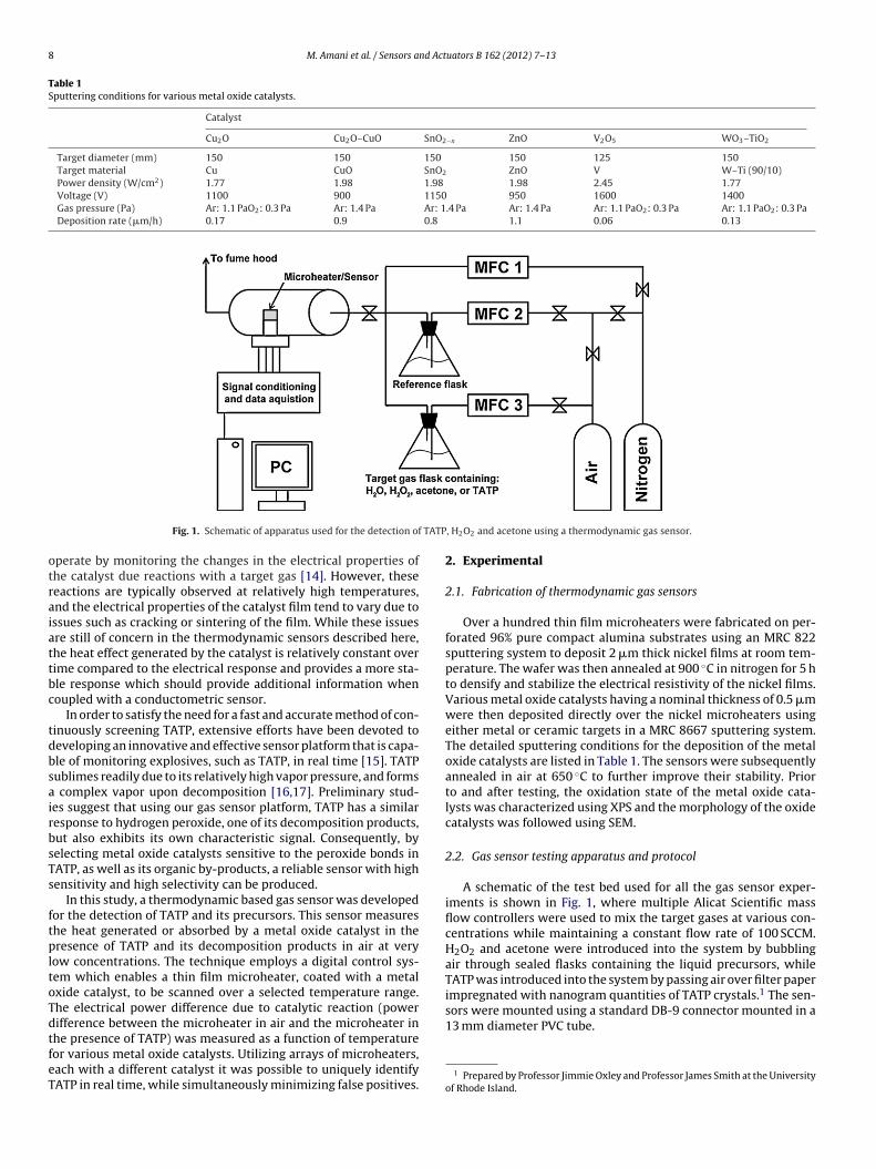
8 M. Amani et al. / Sensors and Actuators B 162 (2012) 7– 13

Table 1Sputtering conditions for various metal oxide catalysts.

Catalyst

Cu2O Cu2O–CuO SnO2!x ZnO V2O5 WO3–TiO2

Target diameter (mm) 150 150 150 150 125 150Target material Cu CuO SnO2 ZnO V W–Ti (90/10)Power density (W/cm2) 1.77 1.98 1.98 1.98 2.45 1.77Voltage (V) 1100 900 1150 950 1600 1400Gas pressure (Pa) Ar: 1.1 PaO2: 0.3 Pa Ar: 1.4 Pa Ar: 1.4 Pa Ar: 1.4 Pa Ar: 1.1 PaO2: 0.3 Pa Ar: 1.1 PaO2: 0.3 PaDeposition rate (!m/h) 0.17 0.9 0.8 1.1 0.06 0.13

Fig. 1. Schematic of apparatus used for the detection of TATP, H2O2 and acetone using a thermodynamic gas sensor.

operate by monitoring the changes in the electrical properties ofthe catalyst due reactions with a target gas [14]. However, thesereactions are typically observed at relatively high temperatures,and the electrical properties of the catalyst film tend to vary due toissues such as cracking or sintering of the film. While these issuesare still of concern in the thermodynamic sensors described here,the heat effect generated by the catalyst is relatively constant overtime compared to the electrical response and provides a more sta-ble response which should provide additional information whencoupled with a conductometric sensor.

In order to satisfy the need for a fast and accurate method of con-tinuously screening TATP, extensive efforts have been devoted todeveloping an innovative and effective sensor platform that is capa-ble of monitoring explosives, such as TATP, in real time [15]. TATPsublimes readily due to its relatively high vapor pressure, and formsa complex vapor upon decomposition [16,17]. Preliminary stud-ies suggest that using our gas sensor platform, TATP has a similarresponse to hydrogen peroxide, one of its decomposition products,but also exhibits its own characteristic signal. Consequently, byselecting metal oxide catalysts sensitive to the peroxide bonds inTATP, as well as its organic by-products, a reliable sensor with highsensitivity and high selectivity can be produced.

In this study, a thermodynamic based gas sensor was developedfor the detection of TATP and its precursors. This sensor measuresthe heat generated or absorbed by a metal oxide catalyst in thepresence of TATP and its decomposition products in air at verylow concentrations. The technique employs a digital control sys-tem which enables a thin film microheater, coated with a metaloxide catalyst, to be scanned over a selected temperature range.The electrical power difference due to catalytic reaction (powerdifference between the microheater in air and the microheater inthe presence of TATP) was measured as a function of temperaturefor various metal oxide catalysts. Utilizing arrays of microheaters,each with a different catalyst it was possible to uniquely identifyTATP in real time, while simultaneously minimizing false positives.

2. Experimental

2.1. Fabrication of thermodynamic gas sensors

Over a hundred thin film microheaters were fabricated on per-forated 96% pure compact alumina substrates using an MRC 822sputtering system to deposit 2 !m thick nickel films at room tem-perature. The wafer was then annealed at 900 "C in nitrogen for 5 hto densify and stabilize the electrical resistivity of the nickel films.Various metal oxide catalysts having a nominal thickness of 0.5 !mwere then deposited directly over the nickel microheaters usingeither metal or ceramic targets in a MRC 8667 sputtering system.The detailed sputtering conditions for the deposition of the metaloxide catalysts are listed in Table 1. The sensors were subsequentlyannealed in air at 650 "C to further improve their stability. Priorto and after testing, the oxidation state of the metal oxide cata-lysts was characterized using XPS and the morphology of the oxidecatalysts was followed using SEM.

2.2. Gas sensor testing apparatus and protocol

A schematic of the test bed used for all the gas sensor exper-iments is shown in Fig. 1, where multiple Alicat Scientific massflow controllers were used to mix the target gases at various con-centrations while maintaining a constant flow rate of 100 SCCM.H2O2 and acetone were introduced into the system by bubblingair through sealed flasks containing the liquid precursors, whileTATP was introduced into the system by passing air over filter paperimpregnated with nanogram quantities of TATP crystals.1 The sen-sors were mounted using a standard DB-9 connector mounted in a13 mm diameter PVC tube.

1 Prepared by Professor Jimmie Oxley and Professor James Smith at the Universityof Rhode Island.

M. Amani et al. / Sensors and Actuators B 162 (2012) 7– 13 9

A digital control system employing a LabView program was usedto heat the microheaters to a series of predetermined set pointtemperatures. These temperatures were selected using the tem-perature coefficient of resistance (TCR) of the nickel film, whichwas independently calibrated. After the sensor reached equilib-rium at each temperature set point, the total power dissipationwas recorded for a period of 75 s. The average amount of heat gen-erated or absorbed by the catalyst in the presence of the target gaswas calculated as the power required to maintain the sensor at aconstant temperature, as well as the percent response which wasthe fraction of total power generated by the catalyst. These testswere conducted using both a dynamic pulsed gas scheme, wherethe sensor is initially run in air, followed by 2 min in various con-centrations of the target gas, and then run in air again, withoutchanging temperature. Static testing was also performed by deter-mining the power dissipation in air at each temperature, coolingthe sensor to room temperature and running again in the targetgas at the same temperatures. Using the static test protocol, thesensitivity of electronics and drift in the resistance of the thin filmmicroheaters allow for power differences greater than 8 mW to bereliably detected, while the dynamic response technique allows forpower differences as low as 1 mW to be reliably detected.

3. Results and discussion

3.1. Chemical characterization

The oxidation states of the copper oxide catalysts prepared fromceramic and metallic targets were determined by XPS (Fig. 2). InFig. 2, the Cu 2p spectra of those copper oxide films preparedby reactive sputtering in an Ar/O2 plasma from a metallic target(dashed line) were compared to copper oxide films prepared bysputtering in an Ar plasma from a CuO target (solid line). The sig-nificant difference between the spectra is that the films preparedfrom ceramic targets contain satellite peaks which are typicallyfound 7–10 eV above the main peaks associated with the copper2p3/2 and 2p1/2 electrons, respectively for Cu2+ compounds, andcorrespond to shake-up electrons with 2p3d9 character [18]. Inthis film, the copper 2p3/2 and 2p1/2 peaks were found at 929.65and 949.15 eV (Cu+), respectively; furthermore, curve fitting of themain 2p3/2 peak revealed a second peak with lower amplitude at

Fig. 2. XPS spectra of Cu2O films prepared by sputtering in an Ar/O2 plasma froma metal target and CuO–Cu2O films prepared by sputtering in an Ar plasma from aCuO target.

Fig. 3. XPS spectra of stoichiometric SnO2 films prepared by sputtering in an Ar/O2

plasma from a ceramic target and non-stoichiometric SnO2!x films prepared bysputtering in an Ar plasma from a SnO2 target.

Fig. 4. XPS spectra of (a) ZnO and (b) V2O5 films.

10 M. Amani et al. / Sensors and Actuators B 162 (2012) 7– 13

Fig. 5. SEM micrographs of (a) CuO–Cu2O after testing, Cu2O (b) before and (c) after testing and (d) V2O5, (e) ZnO and (f) SnO2!x after testing.

931 eV (Cu2+). The broadening of the 2p3/2 peak towards higherbinding energies combined with the presence of the satellite peakssuggests that these copper oxide films prepared by sputtering fromceramic targets in an Ar plasma have mixed oxidation states [19].On the other hand, by sputtering in Ar/O2 plasma from a metal tar-get, a narrow 2p3/2 peak at 929.65 eV was observed and no satellitepeaks were present, in the spectra indicating that the film is largelycomposed of Cu2O. Non-stoichiometric SnO2!x films were also pre-pared by sputtering from an oxide target in an argon plasma. A1.12 eV shift in both the O 1s and the Sn 3d peaks was observedrelative to those peaks for a SnO2 reference film, as shown in Fig. 3.This is consistent with the shift typically described in the literature,for SnO [20]. Fig. 4 shows the XPS spectra of the 3d and 2p electronsin (a) ZnO and (b) V2O5. The Zn 2p3/2 and 2p1/2 peaks were found at1022.65 eV and 1045.5 eV, respectively. In the spectra for vanadium

oxide, the 2p3/2 and 2p1/2 core levels were found at 514.25 eV and520.65 eV, respectively, both of which are in agreement with thosevalues typically observed in ZnO and V2O5 films [21,22]. Moreover,no significant shifting of these peaks was observed after testing ata maximum temperature of 650 "C.

3.2. Structural characterization

Fig. 5 shows the microstructure of several oxide catalysts sput-tered from metallic and ceramic targets in different Ar/O2 partialpressures. CuO–Cu2O films with mixed oxidation states, were sput-tered from a ceramic target in argon plasma, and show surfacesdevoid of any fine structure. They also exhibit relatively smoothrounded protuberances with minimal surface area, typical of anas-sputtered film (Fig. 5a). However, the Cu2O films reactively

M. Amani et al. / Sensors and Actuators B 162 (2012) 7– 13 11

Fig. 6. Percent response in 8 ppm TATP and 9 ppm H2O2 as a function of temperature for (a) tin oxide and (b) tungsten oxide catalysts, measured using the static testingapproach.

sputtered from a metallic target in Ar/O2 mixtures, exhibited amicrocrystalline surface morphology within the rounded protuber-ances of the as-deposited films, unlike those films prepared from aceramic target (Fig. 5b). When this catalyst surface was exposed tovarious target gases, including H2O2 and TATP at a high tempera-ture, there was no apparent change in the fine microstructure butinstead an increase in the cluster/grain size was observed (Fig. 5c).The reactively sputtered V2O5 catalysts prepared from a metallicvanadium target in an Ar/O2 plasma (Fig. 5d), revealed the forma-tion of acicular needles as well as a very fine fibrous morphology ornano-hair on the surface of the sensor. The surface area of these veryfine microstructural features, associated with reactively sputteredfilms produced from metallic targets, was estimated to be orders ofmagnitude greater than that of typical sputtered film morphology.SnO2!x and ZnO films were also deposited from a ceramic targetby sputtering in an argon plasma (Fig. 5e and f), and a morphologymore similar to that of sputtered CuO–Cu2O (Fig. 5a) was observed.In the case of SnO2!x, some micro-cracking of the films due to ther-mal stress due to high temperature testing became apparent overtime.

3.3. Gas sensing properties

The responses of a tin oxide catalyst and a tungsten oxide cat-alyst to TATP and hydrogen peroxide are shown in Fig. 6. Here,the percent response to 8 ppm TATP and 9 ppm H2O2 as a functionof temperature were measured using the static testing approach. Aprecipitous drop in the response for tin oxide occurs until a temper-ature of 300 "C, at which point the response increases dramaticallyas a function of temperature. We believe this is due to the decom-position of TATP by the catalyst, for which the response peaks at400 "C. It should be noted that the response for hydrogen perox-ide using the same catalyst has a similar behavior and tracks theTATP response closely. The response of a tungsten oxide catalyst toTATP and hydrogen peroxide is shown in Fig. 6b and has very dif-ferent characteristics than that of tin oxide. No significant responsewas observed at temperatures below 380 "C, at which point theresponse then increased dramatically until a maxima was observedat 460 "C. As was the case for the tin oxide catalyst, the response ofthe sensor to H2O2 was very similar and closely tracks the TATPresponse. In both cases the response to hydrogen peroxide waslarger in magnitude as might be expected since the decomposition

of the TATP is not complete during the test cycle and the startingconcentration of TATP is 8 ppm whereas the starting concentrationof H2O2 is 9 ppm.

The gas sensor response to TATP using a number of differentcatalysts is shown in Fig. 7. Here, the response to 8 ppm TATPas a function of temperature using several catalysts includingWO3–TiO2, V2O5, SnO2!x, Nb2O3 and ZnO was measured usingthe static testing approach. Each of the five oxide catalysts showa unique response as a function of temperature, and show fea-tures ranging from almost no peak response for Nb2O3 to welldefined peaks for ZnO. Due to the catalytic decomposition ofTATP, it is expected that the target gas consists not only of amixture of air and TATP vapor, but also contains some H2O2vapor. To verify this, several experiments were undertaken toinvestigate if TATP is indeed decomposing into H2O2 in the vicinityof the catalyst, which is not the primary decomposition productbased on a number of related studies. For example, Oxley andSmith [16,17] have determined that acetone and not hydrogen

Fig. 7. Response as a function of temperature using several catalysts to detect TATP(8 ppm) including WO3–TiO2, V2O5, SnO2!x and ZnO, measured using the statictesting approach.

12 M. Amani et al. / Sensors and Actuators B 162 (2012) 7– 13

Fig. 8. Response of (a) CuO–Cu2O and (b) Cu2O in acetone and H2O2 at 330 !C.

peroxide is the predominant decomposition product of highpurity TATP in air and they have measured the activation energyand determined the decomposition kinetics for the degradationof TATP.

Fig. 9. Response of SnO2"x in several concentrations of (a) acetone and (b) H2O2 at415 !C.

Fig. 8 shows the response of a CuO–Cu2O and Cu2O catalyst to8 ppm acetone and H2O2 at 330 !C after a 2-min exposure to thetarget gas. From this figure it can be seen that the relative responseto acetone is considerably greater than that of H2O2, which is con-sistent with other investigations using thermodynamic based gassensors for detection [23]. These studies support our findings thatsignificant exothermic heat effects are observed for hydrocarbons.Not only is the magnitude of the response to acetone for bothCuO–Cu2O and Cu2O significantly greater than that of hydrogenperoxide but it is also of opposite sign, which implies that thesensitivity of the thermodynamic sensor platform to acetone is sig-nificantly greater than that of the other gaseous products derivedfrom the decomposition of TATP. Furthermore, this figure indicatesthat CuO–Cu2O (Fig. 8a) is a more selective catalyst for hydrogenperoxide than that of Cu2O (Fig. 8b), since both a smaller heat ofreaction in the presence of acetone and a more negative heat ofreaction for H2O2 were observed. All of this suggests that theseresults can be further improved upon by tailoring the sputteringconditions and thus, the oxidation state of the catalyst films. Theeffect of acetone and H2O2 concentration on the magnitude of theresponse using tin oxide as the catalyst is shown in Fig. 9, wherethe temperature was held constant at 415 !C (maximum sensitiv-ity to H2O2 and TATP shown in Fig. 6a). Again the responses are ofopposite sign, and it was found that the TATP response tracks thatof hydrogen peroxide, which can be readily detected at concentra-tions as low as 3.5 ppm. Based on the results presented in Fig. 9, weshould also be able to reliably detect low levels of acetone in the gasstream generated by the decomposition of TATP. Since we do notsee any evidence of acetone in the output signal, we can concludethat the TATP is detected as hydrogen peroxide. However, it has alsobeen extensively cited in the literature [16,17] that under ambientconditions TATP primarily decomposes into acetone. Therefore, webelieve that we are sensing the catalytic decomposition of TATP,which is a much more specific reaction than the decomposition ofTATP to acetone in air ambient, and this specific mechanism shouldhelp mitigate false positives using this sensor platform.

4. Conclusion

A small footprint, thermodynamic based gas sensor capableof detecting TATP at ppm levels in air under ambient conditionswas demonstrated. This robust sensor platform has the potentialof exhibiting the necessary sensitivity, selectivity and responsetime to be used for the continuous monitoring of TATP and its

M. Amani et al. / Sensors and Actuators B 162 (2012) 7– 13 13

precursors. This would be particularly important in closed spacedvenues where the public may be exposed to potential threats fromIEDs employing TATP as the triggering device. A number of metaloxide catalysts were able to detect TATP using the thermodynamicbased gas sensor described within. We have shown that TATP vaporat concentrations of 8 ppm in air can be detected readily usingSnO2!x and ZnO catalysts, and its peroxide and acetone precursorswere able to be detected at even lower concentrations. Based on ourpreliminary results, arrays of microheater sensors can be fabricatedusing multiple catalysts and combining the characteristic responsecurves to uniquely identify the target molecules of interest. Inaddition, the current thermodynamic detection scheme can easilybe integrated into an existing micro-hotplate based MEMS metaloxide gas sensing platforms by modifying the heater electronics andadding a mass flow controller to eliminate hydrodynamic effects.This can add a second independent variable to minimize false posi-tives and improve long term stability in existing gas sensor systems.

Acknowledgements

The authors wish to thank the Department of Homeland Secu-rity Center of Excellence for Explosives Detection, Mitigation andResponse and Sensor Tech, Savannah, GA for support of this work.The authors also thank Prof. Jimmy Oxley and Prof. James Smith atthe University of Rhode Island for preparation of the TATP samplesused throughout the study. The authors would like to acknowledgeUS Patent #7,329,389 B2, “Sensor Device and Method for Qualita-tive and Quantitative Analysis of Gas Phase Substances”, Feb. 12,2008, Michael L. Horovitz and Karl L. Anderson upon which someof the preliminary work was based.

References

[1] F. Dubnikova, R. Kosloff, Y. Zeiri, Z. Karpas, Novel approach to the detection oftriacetone triperoxide (TATP), its structure and its complexes with ions, J. Phys.Chem. A 106 (19) (2002) 4951–4956.

[2] I. Cotte-Rodriguez, H. Chen, R.G. Cooks, Rapid trace detection of triacetonetriperoxide (TATP) of complexation detections of desorption electrospray ion-ization, Chem. Commun. 5 (2006) 953–955.

[3] G.A. Buttigieg, A.K. Knight, S. Denson, C. Pommier, M.B. Denton, Characteri-zation of the explosive triacetone triperoxide and detection by ion mobilityspectrometry, Forensic Sci. Int. 135 (2003) 53–59.

[4] R. Rasanen, M. Nousiainen, K. Parakorpi, M. Sillanpaa, L. Polari, O. Anttalainen,M. Utriainen, Determination of gas phase triacetone triperoxide with aspirationion mobility spectrometry and gas chromatography–mass spectrometry, Anal.Chim. Acta 623 (2008) 59–65.

[5] J. Wilkinson, C.T. Konek, J.S. Moran, E.M. Witko, T.M. Korter, Terahertz absorp-tion spectrum of triacetone triperoxide (TATP), Chem. Phys. Lett. 478 (2009)172–174.

[6] A. Stambouli, A. El Bouri, T. Bouayoun, M.A. Bellimam, Headspace GC/MS detec-tion of TATP traces in post-explosion debris, Forensic Sci. Int. 146S (2004)S191–S194.

[7] C. Mullen, A. Irwin, B.V. Pond, D.L. Huestis, M.J. Coggiola, H. Oser, Detection ofexplosives and explosives-related compounds by single photon laser ionizationtime-of-flight mass spectrometry, Anal. Chem. 78 (2006) 3807.

[8] C. Shen, J. Li, H. Han, H. Wang, H. Jiang, Y. Chu, Triacetone triperoxide using lowreduced-field proton transfer reaction mass spectrometer, Int. J. Mass Spec-trom. 285 (2009) 100–103.

[9] R.S. Ladbeck, U. Karst, Determination of triacetone triperoxide in ambient air,Anal. Chem. 482 (2003) 183–188.

[10] H. Lin, K.S. Suslick, A colorimetric sensor array for detection of triacetone triper-oxide vapor, J. Am. Chem. Soc. 132 (2010) 15519–15521.

[11] E. Capua, R. Cao, C.N. Sukenik, R. Naaman, Detection of triacetone triperox-ide (TATP) with an array of sensors based on non-specific interactions, Sens.Acuators B 140 (2009) 122–127.

[12] N. Barsan, D. Koziej, U. Weimar, Metal oxide-based gas sensor research: howto? Sens. Actuators B 121 (2007) 18–35.

[13] N.L. Hung, H. Kim, S.K. Hong, D. Kim, Enhancement of CO gas sensing propertiesof ZnO thin films deposited on self-assembled Au nanodots, Sens. Actuators B151 (2010) 127–132.

[14] G. Eranna, B. C/Joshi, D.P. Runthala, R.P. Gupta, Oxide materials for developmentof integrated gas sensors: a comprehensive review, Crit. Rev. Solid State Mater.Sci. 29 (2004) 111–188.

[15] W.H. Zhang, W.D. Zhang, L.Y. Chen, Highly sensitive detection of explosivetriacetone triperoxide by an In2O3 sensor, Nanotechnology 21 (2010) 315502.

[16] J.C. Oxley, J.L. Smith, K. Shinde, J. Moran, Determination of the vapor den-sity of triacetone triperoxide (TATP) using a gas chromatography headspacetechnique, Propellants Explos. Pyrotech. 30 (2) (2005) 127–130.

[17] J.C. Oxley, J.L. Smith, H. Chen, Decomposition of a multi-peroxidic compound:triacetone triperoxide (TATP), Propellants Explos. Pyrotech. 27 (4) (2002)209–216.

[18] W.Y. Yang, W.G. Kim, S.W. Rhee, Radio frequency sputter deposition of singlephase cuprous oxide using Cu2O as a target material and its resistive switchingproperties, Thin Solid Films 517 (2008) 967–971.

[19] C.I. Pearce, R.A.D. Pattrick, D.J. Vaughan, C.M.B. Henderson, G. van der Laan,Copper oxidation state in chalcopyrite: mixed Cu d9 and d10 characteristics,Geochimica 70 (2006) 4635–4642.

[20] S. Hwang, Y.Y. Kim, J.H. Lee, D.K. Seo, J.Y. Lee, H.K. Cho, Irregular electrical con-duction types in tin oxide thin films induced by nanoscale phase separation,Journal of the American Ceramic Society 95 (1) (2012) 324–332.

[21] S. Uthanna, T.K. Subramanyam, B.S. Naidu, G.M. Rao, Structure–composition–property dependence of reactive magnetron sputtered ZnO thin films, Opt.Mater. 19 (4) (2002) 461–469.

[22] G. Silversmit, D. Depla, H. Poelman, G.B. Marin, R. Gryse, Determinationof the V2P XPS binding energies for different vanadium oxide oxidationstates (V5+ to V0+), J. Electron Spectrosc. Relat. Phenom. 135 (2–3) (2004)167–175.

[23] E. Vereshchaginam, R.A.M. Wolters, J.G.E. Gardeniers, Measurement of reactionheats using a polysilicon based microcalorimetric sensor, Sens. Actuators A 169(2) (2011) 308–316.

Biographies

Matin Amani received his B.S. degree in electrical engineering at URI in 2011, andis currently working on his B.S. degree in chemical engineering and M.S. degree inelectrical engineering. His research interests include oxide thermoelectrics, nano-materials, sensors for harsh environments and gas sensors.

Yun Chu received his M.S. degree in chemistry from Beihang University in 2008. He iscurrently working on his Ph.D. in chemical engineering at URI. His research interestsinclude gas sensors and materials discovery using combinatorial chemistry.

Kellie L. Waterman received her B.S. degree in chemical engineering in 2011, andis in processes of obtaining her M.S. degree at WPI.

Caitlin M. Hurley is a senior undergraduate student studying chemical engineeringat URI.

Michael J. Platek received his B.S degree in physics from Indiana University ofPA (1984) and M.S. degree in physics from Wesleyan University (Middletown, CT)(1986). He is the laboratory manager for the URI Sensors and Sensors TechnologyPartnership. His interests include fabrication as well as characterization of nano-materials, development of gas sensors, bio-sensors and MEMS.

Otto J. Gregory received his B.S. degrees in chemical engineering and ocean engi-neering and his M.S. degree in chemical engineering from URI, in 1975 and 1977,respectively and his Ph.D. in engineering from Brown University in 1984. He is cur-rently Distinguished Engineering Professor at URI and Director of the URI Sensorsand Surface Technology Partnership. Dr. Gregory has published over 80 peer-reviewed journal articles and filed 25 US patents. His work has largely focused onsensors for harsh environments, wide bandgap semiconductors and chemical sen-sors, and has been funded by the gas turbine engine industry, NASA, DOE, Air Force,NSF and DHS.

Author's personal copy

Microstructural characterization of pipe bomb fragments

Otto Gregorya,⁎, Jimmie Oxleyc, James Smithc, Michael Plateka, Hamouda Ghonemb,Evan Bernierc, Markus Downeya, Christopher CumminskeyaSensors and Surface Technology Partnership Forensic Science PartnershipaDepartment of Chemical Engineering, University of Rhode Island, Kingston, RI, 02881, USAbDepartment of Mechanical Engineering, University of Rhode Island, Kingston, RI, 02881, USAcDepartment of Chemistry, University of Rhode Island, Kingston, RI, 02881, USA

A R T I C L E D A T A A B S T R A C T

Article history:Received 22 May 2009Received in revised form17 December 2009Accepted 22 December 2009

Recovered pipe bomb fragments, exploded under controlled conditions, have beencharacterized using scanning electron microscopy, optical microscopy and microhardness.Specifically, this paper examines themicrostructural changes in plain carbon-steel fragmentscollected after the controlled explosion of galvanized, schedule 40, continuously welded, steelpipes filled with various smokeless powders. A number of microstructural changes wereobserved in the recovered pipe fragments: deformation of the soft alpha-ferrite grains,deformation of pearlite colonies, twin formation, bands of distorted pearlite colonies, slipbands, and cross-slip bands. These microstructural changes were correlated with the relativeenergy of the smokeless powder fillers. The energy of the smokeless powderwas reflected in areduction in thickness of the pipe fragments (due to plastic strain prior to fracture) and anincrease in microhardness. Moreover, within fragments from a single pipe, there was a radialvariation inmicrohardness,with themicrohardness at theouterwall being greater than that atthe inner wall. These findings were consistent with the premise that, with the high energyfillers, extensive plastic deformation and wall thinning occurred prior to pipe fracture.Ultimately, the information collected from this investigation will be used to develop adatabase, where the fragment microstructure andmicrohardness will be correlated with typeof explosive filler and bomb design. Some analyses, specifically wall thinning andmicrohardness, may aid in field characterization of explosive devices.

© 2009 Elsevier Inc. All rights reserved.

Keywords:Pipe bombHigh strain rate loadingSteel microstructure

1. Introduction

In the United States, pipe bombs are a common improvisedexplosive device. Construction is straightforward, and bothmetal and plastic pipes are readily available. Many of the pipefillers are propellants which may include black powder,smokeless powder, photo and fireworks powder, and evenmatch heads which can be purchased without special permit[1]. Over the years, law enforcement has developed robustprotocols for processing bomb scenes and analytical proce-dures for identifying explosive residue, but chemical residue is

not always recovered [2,3]. Generally, the recovered fragmentsare intermixed with a host of metal shards and debrischaracteristic of the chaotic scene of an explosion. A wealthof forensic information remains unexploited in terms of“metallurgical evidence” found in each pipe fragment. Suchevidence is embodied in changes in the microstructure andmicrohardness of the pipe fragments. Metallurgical changes inarmor steels have been extensively studied in order toestimate explosive loadings [4]. The degree of shock loadingin plain carbon steel is reflected by pearlite and ferrite graindeformation, twinning, and slip band formation [5]. This study

M A T E R I A L S C H A R A C T E R I Z A T I O N 6 1 ( 2 0 1 0 ) 3 4 7 – 3 5 4

⁎ Corresponding author. Department of Chemical Engineering, 16 Greenhouse Rd, Kingston, RI, 02881, USA. Tel.: +1 401 874 2085.E-mail address: gregory@egr.uri.edu (O. Gregory).

1044-5803/$ – see front matter © 2009 Elsevier Inc. All rights reserved.doi:10.1016/j.matchar.2009.12.017

ava i l ab l e a t www.sc i enced i r ec t . com

www.e l sev i e r . com/ loca te /matcha r

Author's personal copy

attempts to correlate such microstructural features found inrecovered steel pipe bomb fragments with the power andquantity of the propellant used, as well as other character-istics of the initial device [6]. The characterization included theapplication of quantitative stereology techniques to study themicrostructural changes that occur in plain carbon-steel pipesdue to high strain rate deformation and variations in micro-hardness obtained under different loading conditions. Acorrelation between pipe fragment microstructure, micro-hardness, and wall thinning with the pipes propellant fillermay provide clues concerning the relative nature of thepropellant in cases where chemical residue is not recovered.

2. Experimental

2.1. Materials/Methods

Commercially available, continuouslywelded, schedule 40 steelpipes [2 in. I.D. by 12 in. long (5 cm!30.5 cm)] were used in thisinvestigation. These galvanized AISI 1030 steel pipes nominallycontain 0.3% carbon by weight and trace amounts of otherimpurities. Standard end caps were used at both ends of thethreaded pipes and the pipes were usually initiated in a verticalorientation, with the detonator threaded through a hole drilledin the top end cap. To contain the fragments, pipes wereinitiated in 55-gallon (208.14 L) drums which were mostly filledwith either sand or ground cornhusks. A cardboard sleeve wasplaced around the vertical pipe to ensure there was no directcontact between thepipeand thedrumfiller. Pipeswere filled tovolume (i.e. pour density) with black powder or one of thefollowing smokelesspowders:WC870 (DB); IMR-PB (SB); RedDot(DB); Winchester Action Pistol (DB); Bullseye (DB); where SB andDB indicate single (nitrocellulose) or double-base (nitrocelluloseand nitroglycerin) powder, respectively. An improvised formu-lationmadeof sodiumchlorate andaluminumchips as found inpaintwas also tested. Nitromethane, a high explosive,was usedas a reference material. (Ref. [7] contains additional detailsrelated to the experimental procedure used here.)

Over 60 pipes were shot under the controlled conditionsdescribed above, and on average 87% of the pipe material wasrecovered. An effort was made to separate end cap pieces fromthose of the main body of the pipe, such that only thosefragments from themain body of the pipe were selected for themicrostructural analysis. Fragments from the end capswere notused in this study because they, and the threaded portion of thesteel pipe, were already work hardened prior to use (Fig. 1).

2.2. Pipe Thinning

The extent of plastic deformation prior to fracture was deter-mined by measuring the wall thickness of the fragments in theradial direction using Vernier calipers and comparing thesemeasurements to those from thewall of an unexploded pipe. Nospecial sample preparation was necessary to make thesemeasurements; thus, it may be a field-adaptable technique. Bycomparing the ratio of the fragment wall thickness to that of thewall thickness of an unexploded pipe (Eq. (1)), the engineeringradial strain, or plastic strain, prior to fracture was estimated [8].A total of 10–40 fragments were analyzed, at least four wall

thicknessmeasurementsper fragment, for each typeof energeticfiller. The seam region of the pipe was avoided because seamedges exhibited less ductility and the reduction inwall thicknesswas less pronounced than in other locations.

!a0–af "= a0 = εp !1"

where

a0 initial wall thickness (unexploded)=4.15 mmaf final wall thickness (exploded)!p plastic strain.

2.3. Microhardness

AWilsonmicrohardness testerwith a 200 g loadwas used for allmicrohardness measurements. The measurements were madeacross the through-thickness of the wall of as-received frag-ments. This provided considerable insight into the extent ofwork hardening in the individual fragments as a function ofradial position. The procedure required that a series of indenta-tions be made across the fragment through-thickness followedby a measurement of the length of each indentation (L). In thisway, theKnoophardnessnumber (HK)wasdetermined fromtheindenter load and the indentation length using the equation [9]:

HK = 14229*!P= L2" !2"

where

P applied load (g)L length of indentation in (μm).

2.4. Microscopy

Recovered pipe fragments were prepared for examination byscanning electron microscopy (SEM) and optical microscopyusing standard metallographic preparation techniques [5]. AJEOL JSM5900LV SEM equipped with an energy dispersive X-rayanalyzer (EDX) was used at magnifications between 200 and5000! to determine the fine microstructural features and thesize of the microhardness indentations. The fragments weresectioned using a water soluble oil-cooled diamond saw so thatthey would fit into a standard 1.25-inch (3.18 cm) diametermetallurgicalmount. The fragmentswere cut in such away thatthe cross section of the pipewall could be viewed. The sectionedfragments were mounted in an Extec® two-part epoxy andpolished using Extec® silicon carbide polishing discs. Succes-sively finer grit papers were used, starting with 120 grit paperand progressing to 240, 400, 600 and 1200 grit paper. Afterlapping on the 1200 grit paper, the samples were polished with3.0μm and 0.3μm Extec® alumina slurries. To reveal the finalmicrostructure, the fragments were etched for 30–90s in nital(1 vol.% nitric acid (50–70%)/95 vol% absolute ethanol).

A reflection lightmicroscope (NikonOptifont 100)withbright-field illumination was used for all optical microscopies. Opticalmicrographs were captured using a Nikon Digital Sight DS-Fi1high definition (5-megapixel CCD) color camera head with a DS-L2 controller operated by Nikon's NIS-Elements (version F2.20)

348 M A T E R I A L S C H A R A C T E R I Z A T I O N 6 1 ( 2 0 1 0 ) 3 4 7 – 3 5 4

Author's personal copy

software. Depending on the specific microstructural featurebeing analyzed, quantitative stereology was performed atmagnifications of 20!, 50!, 100! or 200! [5]. A Sun Sparkworkstation running Princeton Gamma Tech (PGT) softwarewas used to collect and analyze the images. The extent of plasticdeformation in the !-ferrite grains and pearlite colonies, asmeasured by the aspect ratio in the digitally storedmicrographs,was quantified utilizing the PGT metallography module. Defor-mation of the pearlite colonies was selected to follow thedeformation trends instead of the !-ferrite grains because thedark pearlite colonies were more readily distinguished by thesoftware than the light ferrite grains.

3. Results and Discussion

3.1. Thinning

Considerable thinning of the pipe wall was usually observed.Average fragment wall thickness is shown in Fig. 2, along withthe associated plastic strain. Reduction in wall thickness wascaused by plastic deformation that occurred prior to the ruptureof the pipematerial during explosion [10]. As the pressure wavepropagated through the pipe, thematerial at the inner wall wasplaced in compression. This caused the material in the outerwall to expand (deform) biaxially and, as a result, the pipebecame thinner and eventually ruptured. This plastic deforma-tion prior to fracture increased as the power of each pipe bombdevice increased. For example, black powder, the least powerfulpropellant in the study, caused the least plastic deformationprior to fracture. The fragments collected from explosions usingblack powder showed a 25% reduction in thickness, whereaspipes exploded with Bullseye smokeless powder, the mostpowerful propellant used, showed 61% reduction in wallthickness (Fig. 2).

3.2. Microscopy

Examination of pipe fragments using microscopy revealedspecific detail on the extent of plastic deformation and thedevelopment of characteristic features in the steel micro-structure. Fig. 3 shows the microstructure of an as-received(unexploded) steel pipe which was purposely over-etched(15 vol.% nital). Notice the visible boundaries of the !-ferritegrains (light phase) and the pearlite colonies (dark phase). It isevident from these micrographs that the individual grains areequiaxed, having approximately the same length and width.Scanning electron microscopy was used to observe the finestructure of the pearlite colonies. These colonies consist ofalternating plates or lamellae of !-ferrite and cementite (Fe3C)

Fig. 2 – Changes in measured wall thickness of pipe bombfragments as a function of filler (propellant) energy. Notecorresponding plastic deformation prior to fracture.

Fig. 1 – Photographs of pipe bomb fragments collected under controlled conditions: a.) Bullseye endcap detonation b.) Bullseyeendcapdetonation c.) Bullseye center detonationd.) Bullseye center detonation. Onaverage 87%of the pipematerialwas collected.

349M A T E R I A L S C H A R A C T E R I Z A T I O N 6 1 ( 2 0 1 0 ) 3 4 7 – 3 5 4

Author's personal copy

which are responsible for the scattering of visible light andresulting dark contrast of the colonies in the optical micro-graphs (Fig. 4).

Fig. 5 showsamicrographof a fragment collected fromapipefilled with black powder. The pearlite colonies and !-ferritegrains are visibly deformed and elongated in thedirection of theapplied strain. As the power of the propellant filler increased,the deformation of the pearlite became more pronounced.This trend is shown in Fig. 6 for an improvised formulation ofNaClO3/Al. To quantify the extent of pearlite deformation, theaverage aspect ratio of the pearlite colonies from the variouspipe bomb fragments was determined. An aspect ratio close toone represents features that are very symmetrical or equiaxed.The as-received pipe seen in Fig. 3 had average pearlite aspectratios closer to 2 than1. The aspect ratios of thepearlite coloniescorrelate well with the observed plastic deformation prior topipe fracture. As expected, the more powerful fillers yieldedlarger pearlite aspect ratios (Fig. 7).

In the fragments collected from pipes using high-powerfillers, twinningwas observed alongwith elongation of both the!-ferrite grains and pearlite colonies. These characteristicswere observed for Winchester Action Pistol 44, Red Dot, IMR-PB, Bullseye, and nitromethane as shown in Figs. 8, 9.A–9.C,10.A–10.B, 11.A–11.C, and 12.A–12.B respectively. Normally,plastic deformation in body-centered cubic (BCC) metaloccurs by slip, but deformation twins can occur in BCCmetalsand alloys at very low temperatures or at very high strainrates [10,11]. Therefore, the high-power propellants musthave produced sufficiently high shock loading (pressurewaves) within the walls of the pipe, prior to fracture, to

Fig. 3 – Optical micrograph of “as-received” plain carbon-steelpipe (transverse view — 500!). The dark phase is pearlitecolonies and the light phase is !-ferrite grains. Grainboundariesare clearly visibledue toover-etchingof thesample(15% nital).

Fig. 4 – SEM micrograph of pearlite colony lamella in a steelpipe (5000!). The light phase is cementite (Fe3C) and the darkphase is!-ferrite. [The lamella appears as a solid black phasein lower magnification micrographs as its structureencourages light scattering.]

Fig. 5 – Optical micrograph of a recovered steel pipe bombfragment with black powder used as the filler (transverseview — 200!). Note the deformation (elongation) of thepearlite (dark phase) and subsequent change in aspect ratioassociated with the pearlite and !-ferrite relative to theas-received pipe (Fig. 4).

Fig. 6 – Optical micrograph of a recovered steel pipe bombfragment with NaClO3/Al used as the filler (200!). Note thedeformation of the pearlite (dark phase).

350 M A T E R I A L S C H A R A C T E R I Z A T I O N 6 1 ( 2 0 1 0 ) 3 4 7 – 3 5 4

Author's personal copy

induce twin plane formation in the steel pipe. The twindensity was relatively low in most instances where twinswere observed, due to random orientation of the pearlitecolonies in the starting material. When high-power, highexplosive fillers such as nitromethane were employed in thisstudy, additional microstructural features were observed.The pearlite colonies were extremely distorted in continuousbands which extended well beyond a single grain or colony(Figs. 12.A–12.B). Fig. 12.A also reveals the presence ofintersecting slip bands, or cross-slip bands, in the steeldetonated with nitromethane.

A qualitative representation of the various threshold energylevels associated with the different propellants is shown inFig. 13. Low-power propellant fillers, such as black powder,released enough energy to deform both the !-ferrite grains andpearlite colonies. Higher-power fillers, such as Winchester or

RedDot, showed twin formation in addition to elongation of thepearlite colonies. In the most powerful devices, for example,employing IMR, Bullseye or nitromethane, the pearlite colonies

Fig. 7 – Relative plastic deformation of pearlite colonies incollected pipe bomb fragments prior to fracture, as evidencedby the changes in aspect ratio. Note the variation in aspectratio as a function of filler (propellant) power.

Fig. 8 – Optical micrograph of a recovered pipe bomb fragmentwithWinchester 44 used as the filler (transverse view— 200!).Note the deformation of the pearlite (dark phase) aswell as thepresence of twins in the microstructure.

Fig. 9.A – Optical micrograph of a recovered steel pipe bombfragment with Red Dot used as the filler (transverseview— 100!). Note the heavily deformed pearlite (dark phase).9.B. Optical micrograph of a recovered steel pipe bombfragment with Red Dot used as the filler (transverseview— 200!). Note the heavily deformed pearlite (dark phase)as well as the presence of twins in the microstructure.9.C. Optical micrograph of a recovered steel pipe bombfragment with Red Dot used as the filler (transverse view—500!). Expanded view of twinning and deformed pearlite.

351M A T E R I A L S C H A R A C T E R I Z A T I O N 6 1 ( 2 0 1 0 ) 3 4 7 – 3 5 4

Author's personal copy

were severely distorted and formed continuous bands extend-ing beyond a single ferrite grain or pearlite colony. Fragmentanalysis from the pipe bomb detonated with the only highexplosive, nitromethane, showed a significant number of slipbands.

3.3. Microhardness

The observed microstructural changes were accompanied bywork hardening of the steel during the high strain rateconditions. The energy of the pressure wave created by thepropellant was partially dissipated by the pipe material in theform of work hardening; i.e. the metal at the inner wall wascompressed into the outer wall material. Microhardness testresults were consistent with the degree of plastic deformationas determined from the physical thinning of the pipe fragmentwalls. Larger Knoop hardness values were associated withfragments produced from high-power propellants. Every filler

used produced consistent Knoop hardness numbers withstandard deviations less than 20 for the five points tested atthe three locations tested; inside, middle and outside pipewall. This result correlates well with the pearlite aspect ratios

Fig. 10.A – Optical micrograph of a recovered steel pipe bombfragment with IMR used as the filler (transverse view— 200!).Note thedeformationof thepearlite (darkphase) and its overalldistortion in continuous bands. 10.B. Optical micrograph of arecovered steel pipe bomb fragmentwith IMRused as the filler(transverse view— 200!). Note the deformation of the pearlite(dark phase) as well as the presence of twins in themicrostructure.

Fig. 11.A – Optical micrograph of a recovered steel pipe bombfragment with Bullseye used as the filler (transverseview — 200!). Note the heavily deformed pearlite (darkphase) and its overall distortion in continuous bands, as wellas the presence of twins in the microstructure. 11.B. Opticalmicrograph of a recovered steel pipe bomb fragment withBullseye used as the filler (transverse view — 500!). Note theheavily deformed pearlite (dark phase) as well as thepresence of twins in the microstructure. 11.C. Opticalmicrograph of a recovered steel pipe bomb fragment withBullseye used as the filler (transverse view — 500!). Note theheavily deformed pearlite (dark phase) as well as thepresence of twins in the microstructure.

352 M A T E R I A L S C H A R A C T E R I Z A T I O N 6 1 ( 2 0 1 0 ) 3 4 7 – 3 5 4

Author's personal copy

determined from quantitative stereology, where more power-ful explosive devices showed greater pearlite deformation(larger aspect ratios) and greater work hardening (microhard-ness numbers). A radial variation in microhardness was alsoobserved i.e. microhardness numbers measured at the outerwall of the pipe fragments were typically larger than thosemeasured at the inner wall. Fig. 14 illustrates the change inmicrohardness as a function of propellant energy and radialposition. The work hardening was caused by the propagationof the pressure wave through the pipe wall and was enhancedby the compression of thematerial from the inner to the outerwall. Thus, the observedwork hardening is greater at the outerwall than the inner wall of the pipe.

Fig. 12.A – Optical micrograph of a recovered steel pipe bombfragmentwithnitromethaneusedas thepropellant (transverseview — 200!). Note the heavily deformed pearlite (dark phase)as well as the presence of slip bands and twins in themicrostructure. 12.B. Optical micrograph of a recovered steelpipe bomb fragment with nitromethane used as the propellant(transverse view— 200!). Note the heavily deformed pearlite(dark phase) as well as the presence of slip bands and twins inthe microstructure.

Fig. 13 – Microstructural changes observed in pipe bomb fragments collected after detonation.

Fig. 14 –Microhardness variations of pipe bomb fragments asa function of radial position; i.e. microhardness variationswithin the wall of exploded pipes. Note the variation inmicrohardness with propellant energy.

353M A T E R I A L S C H A R A C T E R I Z A T I O N 6 1 ( 2 0 1 0 ) 3 4 7 – 3 5 4

Author's personal copy

4. Conclusions

More powerful, faster burning, propellants produced moreplastic deformation in steel pipe bombs prior to fracture thanlower power propellants. This can be shown by quantitativestereology and microhardness analysis of the pipe fragmentsrecovered after the explosion. As the power of the propellantfiller increased, the extent of work hardening in the pipefragments also increased, as measured by microhardness. Aradial variation in microhardness was observed, with largerKnoop Hardness values at the outer pipe wall than at the innerwall of the pipe fragments. Moreover, the recovered pipefragments exhibited four distinct changes in microstructure,which also showed a strong correlation with the power of thepropellant. The microstructural changes observed in the post-blast pipe fragments include (1) deformation of !-ferrite grainsandpearlite colonies as evidencedby changes in aspect ratio, (2)twin formation, (3) distortion of pearlite colonies in continuousbands, and (4) formation of cross-slip bands. Quantitativestereology revealed that the average aspect ratio of the pearlitecolonies in the recovered fragments increased with increasingfiller energy. This trendwas consistentwith theworkhardeningeffect determined from microhardness measurements of thefragments.

R E F E R E N C E S

[1] Arson and Explosives Incidents Report; Bureau of Alcohol,Tobacco, and Firearms: Dept. of Treasury: Washington D.C.,1997.

[2] A Guide for Explosion and Bombing Scene Investigation;J181869; U.S. Department of Justice: June, 2000.

[3] 25 Ways to Fight Terrorism. Prism — American Society ofEngineering Education Journal Feb., 2002, p 27.

[4] Raftenberg MN, Krause CD. Metallographic observations ofarmor steel specimens from plates perforated by shapedcharge jets. Int J Imp Eng 1999;23:757–70.

[5] Vander-Voort GF. Metallography, principles and practices.New York: McGraw Hill Book Co; 1984.

[6] Walsh GA, Inal OT, Romero VD. A potential metallographictechnique for the investigation of pipe bombings. J Forens Sci2003;48(5):945–60.

[7] Oxley JC, Smith JL, Resende E, Rogers E, Strobel RA, Bender EC.Improvised explosive devices: pipe bombs. J For Sci2001;46(3):87–110.

[8] MockW, Holt WH. Fragmentation behavior of Armco Iron andHF-1 steel explosive-filled cylinders. J Appl Phys1983;54(5):2350.

[9] ASTM E384-00 Test Method for Microindentation Hardness ofMaterials, American Society for Testing and MaterialsInternational, Volume 03.01, W. Conshohocken, PA, 2003.

[10] Reed-Hill RE. Physical metallurgy principles. 3rd ed. Boston,MA: PWS Publishing Co; 1994.

[11] Callister WD. Materials science and engineering, anintroduction. 6th ed. Hoboken, NJ: John Wiley and Sons; 1999.

354 M A T E R I A L S C H A R A C T E R I Z A T I O N 6 1 ( 2 0 1 0 ) 3 4 7 – 3 5 4

*Corresponding author. Tel.:+1 401 874 2085. E-mail Address: gregory@egr.uri.edu (O.J.Gregory)

Detection of Peroxides Using Pd/SnO2 Nanocomposite Catalysts

Yun Chu1, Daniel Mallin1, Matin Amani1, 2,

Michael J. Platek2, and Otto J. Gregory1*

Department of Chemical Engineering, University of Rhode Island, Kingston, RI 02881, USA1 Department of Electrical Engineering, University of Rhode Island, Kingston, RI 02881, USA2

TATP is one of the most frequently used peroxide based explosives in improvised

explosive devices (IED’s) by terrorists. While TATP and its precursors have previously

been detected at the ppm level using a thermodynamic gas sensor platform, most of the

catalysts considered for this platform exhibited relatively poor selectivity between

hydrogen peroxide and TATP. Transition metals were reported of the capability to

improve the sensitivity of metal oxide based gas sensor by modifying the surface energy

state of the metal oxide. Therefore, combinatorial chemistry techniques were employed to

screen catalysts with various compositions for micro-calorimetric sensor arrays that will

ultimately reduce false positives. These nanocomposite catalysts were prepared by

incorporating palladium nanoparticles of different loadings in a SnO2 matrix, such that

improved sensitivity and selectivity could be achieved in a single thermodynamic sensor

platform. SEM and TEM were employed to study morphology of the catalyst. Oxidation

state and crystal structures were identified using XPS and XRD separately.

Key Words: Gas sensor, TATP, hydrogen peroxide, sputtering, SnO2, Pd

2

I. Introduction

TATP is a hydrogen peroxide-based compound commonly used as an initiator in

improvised explosive devices (IED’s) employing PETN and other high explosives due to its ease

of manufacture from available precursors and simple preparation [1]. The detection of TATP

using bench-scale analytical instrumentation has been readily demonstrated. Specifically, mass

spectrometry [2, 3, 4], terahertz absorption spectrometry [5], ion mobility spectrometry [4, 6] and

fluorescence spectroscopy [7], exhibit both adequate sensitivity and stability for detection

purposes. However, the aforementioned techniques are somewhat limited for field use since they

cannot be adapted in a small footprint sensor platform and are not capable of continuous

monitoring. This is due in part to the cost, complexity, analysis time and sample preparation

associated with these more traditional analytical tools. A low cost, small footprint sensor that

exhibits adequate speed, selectivity and sensitivity without false positives is highly desired for

field use where continuous monitoring is warranted.

Many investigators have reported on gas sensors employing metal oxide catalysts in a

variety of sensor platforms. For example, these catalysts have been used to detect trace levels of

toxic gases such as CO, H2S, H2 and NOx [8]. However, a vast majority of the gas sensors

employing metal oxide catalyst respond to changes in the electrical properties of the catalyst

during exposure to the target gas which can include changes in electrical conductivity or

dielectric constant of the metal oxide [10, 11], changes in work function [12, 13] and changes in

optical properties of the metal oxide [15, 16]. A number of researchers have also reported that

the sensitivity of metal oxide based sensors can be enhanced by a direct exchange of electrons

between the oxide semiconductor and heavy metals such as Pd, Au, and Pt. The addition of such

metals increases the rate of specific reactions on the surface of oxide crystals due to spill-over

3

effects or through modification of surface energy states [18, 19]. However, one major

disadvantage of the metal oxide gas sensors, as well as all other types of solid-state gas sensors,

is their poor selectivity caused by their inability to distinguish between complex target molecules

[9]. In a previous study, we demonstrated a gas sensor which was capable of detecting TATP via

catalytic decomposition to form hydrogen peroxide. However, these sensors exhibited little or no

selectivity between TATP and hydrogen peroxide, making them prone to false positives when

other peroxides may exist in the ambient.

In the present study we utilized combinatorial chemistry techniques to screen potential

catalysts for enhanced selectivity using a thermodynamic gas sensor platform. The

thermodynamic sensor platform employs a digital control system to measure the heat effect

associated with the interaction of a target gas molecule with a catalyst deposited onto the surface

of a microheater. The heat effect of the catalyst-coated microheater is monitored by thermal

scanning from room temperature to 500˚C. These characteristic heat affects are measured as the

target molecules including TATP, H2O2 and acetone were passed over the active sensor element.

In this paper, the controlled addition of palladium to a SnO2 matrix was used to systematically

enhance both the sensitivity and selectivity of TATP over H2O2.

II. Experimental

2.1 Sensor fabrication and characterization

Thin film nickel micro-heaters having a nominal thickness of 4.5 μm were deposited onto

a laser-perforated alumina substrate using a MRC 822 sputtering system. The nickel

microheaters were annealed in flowing nitrogen at 900°C for 5 hours to improve the electrical

stability and eliminate point defects as a result of the sputtering process. A 1µm thick alumina

layer was then deposited over the nickel microheaters to prevent direct electrical shorts between

4

the Ni heating element and the catalyst layer. The alumina layer was also used to prevent

possible interactions with oxygen and other gases present in the atmosphere. A SnO2/Pd

nanocomposite film was then deposited onto the isolated microheater surface which served as the

catalyst support. A cutaway view of the various layers comprising the sensor is shown in Figure

1. The nanocomposite catalyst was deposited onto arrays of microheater sensors in an MRC

8667 sputtering machine by co-sputtering from simultaneously energized SnO2 and Pd targets.

This produced a large number of essentially different catalysts with a continuously varying,

spatially dependent chemistry. Palladium loadings ranged from 2 wt.% to 25 wt.% in the

nanocomposite. Following deposition, the films were annealed at 550°C in an air ambient to

promote crystallization and further stabilize the catalysts. The chemical composition and

morphology of these catalysts were characterized using scanning electron microscopy (SEM)

equipped with energy dispersive x-ray spectroscopy (EDS). The catalysts were also characterized

using x-ray diffraction (XRD) and x-ray photoelectron spectroscopy (XPS). Pure tin oxide films

were also prepared as catalysts for comparison purposes using the deposition conditions

presented in reference [19].

2.2 Testing apparatus and protocol

The flow rate of inert gas (dry air) and target gas was precisely metered into the test

chamber using two mass flow controllers and a digital flowmeter, which produced a constant

mass flow and allowed precise control over the target gas and inert gas mixtures delivered to the

testbed. The desired vapor phase concentration of TATP (e.g. 0.68 µg/ml) was achieved by

passing a carrier gas over a piece of filter paper impregnated with high purity TATP crystals

maintained at room temperature. When the target molecules were derived from liquid-based

chemical solutions such as H2O, or acetone in deionized water, air was bubbled through the flask

5

containing dilute solutions to establish an equilibrium partial pressure in the vapor phase. A

schematic of the test bed used to evaluate sensor performance is shown in Figure 2.

Catalytic response was determined by measuring the heat affect associated with the

interaction of the target molecules with a catalyst using a dynamic testing protocol. The catalyst

coated microheater was heated to a series of predetermined temperature set points by controlling

the electrical resistance of the microheater, measured via the four point probe method. The

temperature coefficient of resistance of the nickel microheater was independently calibrated and

verified prior to each test. Gas delivery system and data acquisition system were computer

controlled using LabView software. After reaching each target set point temperature, the sensor

was allowed to equilibrate for 360 seconds under constant inert gas flow. The target gas was then

introduced into the test chamber for 180 seconds and then the reference gas was introduced for

180 seconds before the microheater was ramped to the next temperature set point. The power

required to maintain the sensor at a particular temperature was recorded after the target gas was

introduced and this temperature was maintained until the start of next step increase in

temperature. The heat effect at each temperature set point was measured as by taking the

difference in power required to maintain the temperature in the presence of the target gas and the

power required to maintain the temperature in the presence of the inert gas. Prior to measuring

the sensor response, the background power or drift was subtracted from the sensor response.

Typically, all responses smaller than ±1.0 mW were considered background noise, which was

due to small variations in the target and inert gas flow rates, drift in the nickel microheaters and

other sources of electrical noise.

III. Results and Discussion

3.1 Chemical characterization and surface morphology

6

Catalysts incorporating palladium nanoparticles in a tin oxide matrix were characterized

by XRD, in both the as-deposited and annealed condition (Figure 3). All of the nanocomposite

catalysts, regardless of composition were amorphous in the as-deposited condition and

crystalline or partially crystalline after subsequent annealing. Peaks corresponding to the rutile

form of SnO2 were observed in the XRD patterns of the annealed films with no preferred

orientation or texture evident. A uniform 2θ shift of (0.01Å) was also observed for the SnO2

diffraction peaks relative to the literature value, which was likely caused by substitutional defects

[20]. The oxidation states of the nanocomposite catalysts after exposure to hydrogen peroxide

and TATP were characterized using XPS. As shown in Figure 4, the XPS spectrum of pure SnO2

and Pd doped SnO2 exhibited the same Sn 3d5 core level peak at 486.5 eV, suggesting that tin

was present in +4 oxidation states in both specimens. Pure SnO2 contains +2 state tin as indicated

by the lower intensity and slight shifting of the main peak. The Pd 3d5 peaks in the 2.2 wt.%

nanocomposite were observed at 336.4 eV and 337.5 eV respectively, which is in good

agreement with literature values corresponding to palladium in the +2 and +4 states [20-24]. The

composition (at.%) was estimated to be 0.17:0.83 based on the peak area. As the palladium

doping level was increased to 12 wt.%, metallic palladium started to phase separate and the

composition of PdO2:PdO:Pd became 0.084:0.723:0.193. When the palladium doping level

reached 32 wt.%, the metallic component became dominant while the PdO2 peak disappeared

along with the PdO peak. This is because palladium single crystals are more difficult to oxidize

and the palladium particles in the SnO2 are easier to oxidize [22]. This finding is in good

agreement with the disappearance of the palladium (220) peak indicated in XRD pattern of the

nanocomposite. Finally, the catalyst morphology was followed by both SEM and TEM and is

shown in Figure 5. While most of the as-deposited films were featureless, as might be expected

7

with an amorphous film, extensive micro-cracking was observed in the catalysts after annealing.

This was attributed to the large volume change associated with crystallization of the

nanocomposite. In addition, as the palladium content in the nanocomposite was increased, the

density of micro-cracks diminished and eventually disappeared from the microstructure when

palladium loadings greater than 25 wt.% were realized. EDS analysis was used in conjunction

with TEM to determine the chemistry of the dark spherical particles observed in the SnO2 matrix.

These palladium particles had an average diameter of 20 nm, and EDS confirmed the presence of

palladium in the SnO2 matrix.

3.2 Gas sensing characteristics

Baseline experiments using an un-doped SnO2 catalyst at several temperature set points

in the presence of 0.68 µg/ml TATP were conducted. Figure 6 illustrates the “off-on-off”

protocol used for each run. At temperatures below 240°C, a slightly exothermic reaction was

observed at the surface of the SnO2 catalyst. However, as the temperature was increased, the

reaction tended to be endothermic and peaked at 420˚C. Accompanying the change in sign of the

response was a change in the reaction kinetics, which was apparent from the reduced response

time for the exothermic reaction when compared to the endothermic sensor response. Such sign

changes are very telling with respect to the uniqueness of the sensor response or signature and

along with the magnitude of response can alleviate false positives.

When similar tests were performed using pure SnO2, the palladium doped catalysts

showed very different behavior (response versus temperature curves) when exposed to H2O2

compared to TATP as shown in Figure 7. The sensor clearly had a response to TATP at low

temperature (185°C – 275°C) and reached maximum at 390°C. However, the catalyst exhibited

little or no response to H2O2 until 275°C, where a peak response at 455°C was observed. A series

8

of concentration tests, shown in Figure 8, was performed in both H2O2 and TATP to determine

the sensitivity and detection limit of the sensor.

Figure 9 shows the magnitude of the heat effect observed in a number of nanocomposite

catalysts as a function of palladium loading in the presence of 0.68 µg/ml TATP and 0.225 µg/ml

H2O2. At palladium loadings less than 8 wt.%, the sensors exhibit a relatively poor response

compared to the un-doped SnO2 catalysts. However, at higher palladium loadings, there was a

substantial increase in sensor response, which abruptly decreased when more than 12 wt.% Pd

was incorporated into the film. Catalysts with even higher palladium loadings showed almost no

response to TATP and H2O2. While there was a substantial improvement in the maximum

response to the two target molecules at a 12 wt.% palladium loading, the selectivity between

these two target molecules was also significantly improved. A nanocomposite catalyst with a 8

wt.% palladium loading yielded the greatest selectivity (H2O2 relative to TATP) while a 12 wt.%

palladium loading yielded the greatest sensitivity as shown in Figure 9.

IV. Discussion

4.1 Effect of palladium doping rate

The role of Pd in the promotion of sensing ability of metal oxides was discussed in

literatures [25-34]. However, variables including doping method [25, 26], loading concentration

[26, 27], working temperature [28] and species of analytic gases [29-32] all played important

roles in varying its functioning mechanism. In this study, stoichiometric SnO2 without addition

of dopants exhibited higher sensitivity to oxidizing vapors such as H2O2 and TATP compared

with non-stoichiometric SnO2. At low Pd loading, Pd atoms diffused uniformly into SnO2 matrix

and formed two possible types of bond: (1) a strong Pd-Sn alloy metallic bond which was

9

suggested in literature [33] and (2) Pd-O and O-Pd-O ionic bond which were conformed in XPS.

The first type of bond reduced the amount of active SnO2 molecules in unit surface area while

the second type of bond seized oxygen atoms from stoichiometric SnO2 leaving non-

stoichiometric SnO2. This explains the decrease of sensitivity from 0 - 8 wt.% palladium loading.

As Pd loading increased, oxygen molecules diffused into the catalyst during annealing processes

were insufficient for Pd atoms to form O-Pd-O bonds which caused a disappearance of PdO2

peak as indicated by XPS in Figure 4(b). Instead, Pd metallic clusters with relatively small size

encapsulated in PdO-SnO2 molecules were formed resulting in the increase of Pd metallic peak

[33]. Meanwhile, Sn peak remained a single state as stoichiometric SnO2 by sharing oxygen

atoms from PdO as indicated by XPS in Figure 4(a). This uniform stoichiometric SnO2 lead to

the maximum sensitivity of Pd-SnO2 sensor at 12 wt.%. When Pd loading continued increasing,

the size of Pd cluster increased resulting in a large Pd metallic peak and the active space of SnO2

were greatly occupied, which caused the second decrease of the sensitivity of the sensors.

4.2 Protocol of TATP identification

As indicated in Figure 9, SnO2 with 12 wt.% palladium doping rate provided the

maximum sensitivity to both TATP and H2O2 at 395°C. Thus this 12 wt.% Pd:SnO2 sensor was

selected and maintained at 410°C as an early warning indicator. Once the sensor was triggered

by an unknown vapor and received positive signal, further measures were taken to identify the

species of such suspicious vapor. The sensor would then be scanned at various temperature

setpoint ranged from 150°C to 450°C to collect a profile of signal intensity as a function of

temperature. Significant differences between H2O2 response and TATP response are their

different positive trigger point and their temperature range of peak response, which can be used

to detect TATP from H2O2. The Pd:SnO2 nanocomposite with 5 wt.% and 8 wt.% palladium

10

loading were also employed for the reason that the sensor with 5 wt.% palladium loading only

responses to TATP but shows no signal to H2O2 while the one with 8 wt.% palladium loading

does the opposite. These two sets of sensors provided a certain redundancy in response which

helped mitigate false positives.

V. Conclusion

Palladium-tin oxide combinatorial libraries were fabricated by co-sputtering from metal

palladium and SnO2 targets to screen catalysts for the optimal selectivity to TATP. Tin was

present in largely the Sn4+ state while palladium was present in both the Pd2+ and Pd4+ oxidation

state. Compared with a pure SnO2 catalyst, several unique features in the response versus

temperature curves were observed for the catalysts that were doped with palladium, which

greatly improved the magnitude of responses to both TATP and H2O2. Sensors with various

palladium doping levels also exhibited very different characteristics to the target molecules: the

catalyst with an 8 wt.% palladium loading yielded the greatest selectivity while a 12 wt.%

palladium loading provided maximum sensitivity.

Acknowledgements

The authors wish to thank the Department of Homeland Security Center of Excellence for

Explosives Detection, Mitigation and Response and Sensor Tech, Savannah GA for support of

this work. The authors also thank Prof. Jimmy Oxley and Prof. James Smith at the University of

Rhode Island for preparation of the TATP samples used throughout the study.

11

References

1F. Dubnikova, R. Kosloff, Y. Zeiri, Z. Karpas, “Novel approach to the detection of triacetone

triperoxide (TATP), its structure and its complexes with ions”, J. Phys. Chem. A 106 (19) (2002)

4951–4956.

2I. Cotte-Rodriguez, H. Chen, R. G. Cooks, “Rapid trace detection of triacetone triperoxide

(TATP) of complexation detections of desorption electrospray ionization”, Chemical

Communications, 12 January, 2006

3G. A. Buttigieg, A. K. Knight, S. Denson, C. Pommier, M. B. Denton, “Characterization of the

explosive triacetone triperoxide and detection by ion mobility spectrometry”, Forensic Science

International 135 (2003) 53-59

4R. Rasanen, M. Nousiainen, K. Parakorpi, M. Sillanpaa, L. Polari, O. Anttalainen, M. Utriainen,

“Determination of gas phase triacetone triperoxide with aspiration ion mobility spectrometry and

gas chromatography-mass spectrometry”, Analytica Chimica Acta, 623 (2008) 59-65

5J. Wilkinson, C. T. Konek, J. S. Moran, E. M. Witko, T. M. Korter, “Terahertz absorption

spectrum of triacetone triperoxide (TATP)”, Chemical Physics Letters, 478 (2009) 172-174

6A. Stambouli, A. El Bouri, T. Bouayoun, M. A. Bellimam, “Headspace GC/MS detection of

TATP traces in post-explosion debris”, Forensic Science International, 146S (2004) S191-S194

7C. Mullen, A. Irwin, B. V. Pond, D. L. Huestis, M. J. Coggiola, H. Oser, “Detection of

explosives and explosives-related compounds by single photon laser ionization time-of-flight

mass spectrometry”, Anal. Chem. 78 (2006) 3807.

8C. Shen, J. Li, H. Han, H. Wang, H. Jiang, Y. Chu, “Triacetone triperoxide using low reduced-

field proton transfer reaction mass spectrometer”, International Journal of Mass Spectrometry,

285 (2009) 100-103

12

9R. S. Ladbeck, U. Karst. “Determination of triacetone triperoxide in ambient air”, Anal. Chem.

482 (2003) 183-188

10N. Barsan, D. Koziej, U. Weimar. “Metal oxide-based gas sensor research: How to?”, Sens.

Actuators, B, 121 (2007) 18-35.

11N. L. Hung, H. Kim, S. K. Hong, D. Kim. “Enhancement of CO gas sensing properties of ZnO

thin films deposited on self-assembled Au nanodots”, Sens. Actuators, B, 151 (2010) 127-132.

12G. Eranna, B. C/ Joshi, D. P. Runthala, R. P. Gupta. “Oxide materials for development of

integrated gas sensors: A comprehensive review”, Crit. Rev. Solid State Mater. Sci., 29 (2004)

111-188.

13W. H. Zhang, W. D. Zhang, L. Y. Chen. “Highly sensitive detection of explosive Triacetone

triperoxide by an In2O3 sensor”, Nanotechnol., 21 (2010) 315502.

14J. C. Oxley, J. L. Smith, K. Shinde, J. Moran. “Determination of the Vapor Density of

Triacetone Triperoxide (TATP) Using a Gas Chromatography Headspace Technique”,

Propellants Explos. Pyrotech., 30 [2] (2005) 127-130.

15J. C. Oxley, J. L. Smith, H. Chen. “Decomposition of a Multi-Peroxidic Compound: Triacetone

Triperoxide (TATP)”, Propellants Explos. Pyrotech., 27 [4] (2002) 209-216.

16W. Y. Yang, W. G. Kim, S. W. Rhee. “Radio frequency sputter deposition of single phase

cuprous oxide using Cu2O as a target material and its resistive switching properties”, Thin Solid

Films, 517 (2008) 967-971.

17C. I. Pearce, R. A. D. Pattrick, D. J. Vaughan, C. M. B. Henderson, G. van der Laan. “Copper

oxidation state in chalcopyrite: Mixed Cu d9 and d10 characteristics”, Geochimica, 70 (2006)

4635-4642.

13

18E. Vereshchaginam, R. A. M. Wolters, J. G. E. Gardeniers. “Measurement of reaction heats

using a polysilicon based microcalorimetric sensor”, Sens. Actuators, A , In press.

19M. Amani, Y. Chu, K. L. Waterman, C. M. Hurley, M. J. Platek, O. J. Gregory. “Detection of

triacetone triperoxide (TATP) using a thermodynamic based gas sensor”, Sens. Actuators B,

162(2012)7-13.

20T. Zhang, L. Liu, Q. Qi, S. Li, G. Lu. “Development of microstructure In/Pd-doped SnO2

sensor for low level CO detection”, Sensors and Actuators B, 139 (2009) 287-291.

21V. Jimenez, J. Espinos, A. Gonzalez-Elipe. “Effect of texture and annealing treatments in SnO2

and Pd/SnO2 gas sensor materials”, Sensors and Actuators B, 61(1999)23-32.

22T. Skala, K. Veltruska, M. Moroseac, I. Matolinova, A. Cirera, V. Matolin. “Redox process of

Pd-SnO2 system”, Surface Science 566-568(2004)1217-1221.

23R. Tan, Y. Guo, J. Zhao, Y. Li, T. Xu, W. Song. “Synthesis, characterization and gas-sensing

properties of Pd-doped SnO2 nano particles”, Trans. Nonferrous Met. Soc. China 21(2011)1568-

1573.

24Y. Shen, T. Yamazaki, Z. Liu, D. Meng, T. Kikuta, N. Nakatani, M. Saito, M. Mori.

“Microstructure and H2 gas sensing properties of undoped and Pd-doped SnO2 nanowires”,

Sensors and Actuators B, 135(2009)524-529.

25C.B. Lim, S. Oh. “Microstructure evolution and gas sensitivities of Pd-doped SnO2-based

sensor prepared by three different catalyst-addition process”, Sensors and Actuators B 30 (1996)

223-231.

26S. Matsushima, T. Maekawa, J. Tamaki, N. Miura, N. Yamazoe. “New methods for supporting

palladium on a tin oxide gas sensor”, Sensors and Actuators B, 9 (1992) 71-78.

14

27M. Yuasa, T. Masaki, T. Kida, K. Shimanoe, N. Yamazoe. “Nano-sized PdO loaded SnO2

nanoparticles by reverse micelle method for highly sensitive CO gas sensor”, Sensors and

Actuators B, 136 (2009) 99-104.

28L. Liu, T. Zhang, S. Li, L. Wang, T. Tian. “Preparation, characterization, and gas-sensing

properties of Pd-doped In2O3 nanofibers”, Materials Letters, 63 (2009) 1975-1977.

29N. Yamazoe, K. Kurokawa, T. Seiyama. “Effects of additives on semiconductor gas sensor”,

Sensors and Actuators, 4 (1983) 283-289.

30G. Tournier, C. Pijolat, R. Lalauze, B. Patissier. “Selective detection of CO and CH4 with gas

sensors using SnO2 doped with palladium”, Sensors and Actuators B, 26-27 (1995) 24-28.

31Y.C. Lee, H. Huang, O.K. Tan, M.S. Tse. “Semiconductor gas sensor based on Pd doped SnO2

nanorod thin films”, Sensors and Actuators B 132 (2008) 239-242.

32Y. Zhang, Q. Xiang, J. Xu, P. Xu, Q. Pan, F. Li. “Self-assemblies of Pd nanoparticles on the

surfaces of single crystal ZnO nanowires for chemical sensors with enhanced performances”,

Journal of Material Chemistry, 19 (2009) 4701-4706.

33N. Tsud, V. Johanek, I. Stara, K. Veltruska, V. Matolin. “XPS, ISS and TPD of Pd-Sn

interactions on Pd-SnOx systems”, Thin Solid Films 391 (2001) 204-208

34J.Choia, I. Hwanga, S. Kima, J. Parkb, S. Parkb, U. Jeongc, Y. Kangd, J. Leea. “Design of

selective gas sensor using electrospun Pd doped SnO2 hollow nanofibers”, Sensors and Actuators

B, 150 (2010) 191-199

15

List of Figures

Fig. 1 Schematic of microsensor, showing the top view (a) and expanded view (b) of catalyst

layer (1), alumina passivation layer (2), nickel microheater (3) and alumina substrate (4).

Fig. 2 Apparatus used for the detection of TATP, H2O2 and acetone using a micro-calorimetric

sensor.

Fig. 3 XRD patterns of as-deposited (a) and annealed films with (b) 8 wt.% loading Pd (1), 2.5

wt.% loading Pd (2), and 1 wt.% loading Pd (3) in the Pd:SnO2 nanocomposite catalyst.

Fig. 4 XPS spectra of Sn 3d doublet for Pd doped and undoped SnO2 (a), and Pd 3d doublet

corresponding to 2.2 wt.% loading Pd, 12 wt.% loading Pd and 38 wt.% loading Pd in the

PdSnO2 nanocomposite(b).

Fig. 5 SEM (a) and TEM (b) micrographs of as-annealed nanocomposite catalyst with a 12 wt.%

palladium loading.

Fig. 6 Response of micro-calorimetric sensor to 0.68µg/ml TATP using an SnO2 catalyst

thermally scanned to various temperature set points.

Fig. 7 Response of a 12 wt.% Pd nanocomposite catalyst to 0.225 µg/ml H2O2 (a) and 0.68µg/ml

TATP (b).

Fig. 8 Response of a 12 wt.% Pd nanocomposite to H2O2 (a) and TATP (b) as a function of

concentration in the vapor phase.

Fig. 9 Response and selectivity of Pd:SnO2 nanocomposite catalyst with various Pd loadings to

H2O2 and TATP.

16

Fig. 1 Schematic of microsensor, showing the top view (a) and expanded view (b) of catalyst

layer (1), alumina passivation layer (2), nickel microheater (3)and alumina substrate (4).

17

Fig. 2 Apparatus used for the detection of TATP, H2O2 and acetone using a micro-calorimetric

sensor.

18

Fig. 3 XRD patterns of as-deposited (a) and annealed films with (b) 8 wt.% loading Pd (1), 2.5

wt.% loading Pd (2), and 1 wt.% loading Pd (3) in the Pd:SnO2 nanocomposite catalyst.

19

Fig. 4 XPS spectra of Sn 3d doublet for Pd doped and undoped SnO2 (a), and Pd 3d doublet

corresponding to 2.2 wt.% loading Pd, 12 wt.% loading Pd and 38 wt.% loading Pd in the

PdSnO2 nanocomposite(b).

20

Fig. 5 SEM (a) and TEM (b) micrographs of as-annealed nanocomposite catalyst with a 12 wt.%

palladium loading.

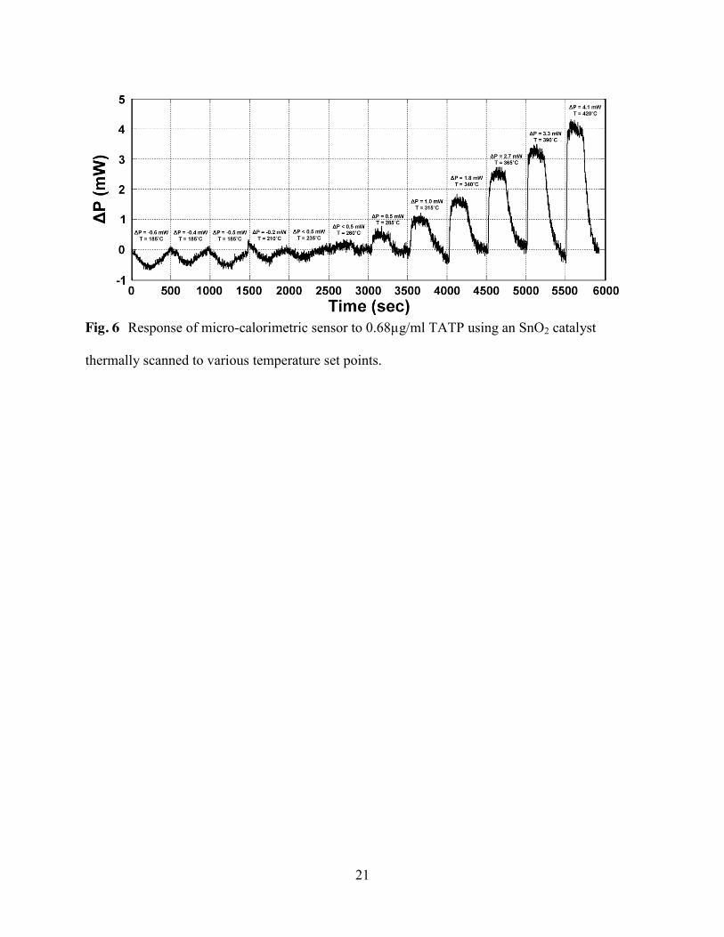
21

Fig. 6 Response of micro-calorimetric sensor to 0.68µg/ml TATP using an SnO2 catalyst

thermally scanned to various temperature set points.

22

Fig. 7 Response of a 12 wt.% Pd nanocomposite catalyst to 0.225 µg/ml H2O2 (a) and

0.68µg/ml TATP (b).

23

Figure 8. Response of a 12 wt.% Pd nanocomposite to H2O2 (a) and TATP (b) as a function of

concentration in the vapor phase at 395°C.

24

Fig. 9 Response and selectivity of Pd:SnO2 nanocomposite catalyst with various Pd loadings to

H2O2 and TATP at 395°C.

25

Author Biographies

Yun Chu received his B.S. degree in chemistry in Beijing University of Aeronautics and Astronautics in 2008. He is currently working on his Ph.D. in chemical engineering at University of Rhode Island (URI). His research interests include gas sensors, MEMS and catalyst development using nano-materials. Caitlin M. Hurley received her B.S. degree in chemical engineering and a B.A. degree in French language from the URI in 2012. She is currently working on her Ph.D. at the Institute National Polytechnique de Toulouse through the Commissariat à l'Energie Atomique located in Saclay, France. Matin Amani received B.S. degrees in electrical and biomedical engineering at URI in 2011, and his B.S. degree in chemical engineering and M.S. degree in electrical engineering in 2012. He is currently working on his Ph.D. in electrical engineering at Oregon State University through the Army Research Laboratory. His research interests include graphene electronics, MIM tunnel diodes, sensors for harsh environments, and gas sensors. Michael J. Platek received his B.S degree in physics from Indiana University of PA (1984) and M.S. degree in physics from Wesleyan University (Middletown, CT) (1986). He is the laboratory manager for the URI Sensors and Sensors Technology Partnership. His interests include fabrication as well as characterization of nano-materials, development of gas sensors, bio-sensors and MEMS. Alan J. Davis received his B.S. in Physics and Electrical Engineering, the M.S. degree in Electrical Engineering from the University of Massachusetts, Dartmouth, MA and Ph.D. in Electrical Engineering from the URI, Kingston in 1983, 1985 and 2000, respectively. Dr. Davis is currently employed by the Naval Undersea Warfare Center (NUWC) in Newport, RI. His research interests include MEMS devices/modeling, high speed ROIC development, sigma-delta modulation and mixed signal integrated circuits. Otto J. Gregory received his B.S. degrees in chemical engineering and ocean engineering and his M.S. degree in chemical engineering from URI, in 1975 and 1977, respectively and his Ph.D. in engineering from Brown University in 1984. He is currently Distinguished Engineering Professor at URI and Director of the URI Sensors and Surface Technology Partnership. Dr. Gregory has published over 80 peer-reviewed journal articles and filed 25 US patents. His work has largely focused on sensors for harsh environments, wide bandgap semiconductors and chemical sensors, and has been funded by the gas turbine engine industry, NASA, DOE, Air Force, NSF and DHS.

Detection of Explosives Using Orthogonal Sensors

Yun Chu1, Daniel Mallin1, Matin Amani2, Bisolar Bruno1, Otto J. Gregory1* Department of Chemical Engineering, University of Rhode Island, Kingston, RI 028811

Abstract: An orthogonal detection system comprised of two independent sensing platforms integrated into a single sensor was recently developed to detect trace levels of explosives including TATP, DNT and ammonium nitrate in the vapor phase. The orthogonal sensor consists of a thermodynamic based sensing platform, which measures the heat effect associated with the interaction of specific target molecules with various metal oxide catalyst (ZnO and SnO2) and a conductometric sensing platform which monitors the electrical conductivity changes of the same catalyst when exposed to the explosive molecules. The experimental results to date indicated that the combined orthogonal sensor was effective in identifying explosives at the ppb level. At the same time, it also provided a certain redundancy in sensor response to help mitigate false positives. The sensor output typically exhibited a linear response as a function of target molecule concentration. XPS was employed to confirm the oxidation state of metal oxides used as catalysts, which were a function of deposition and post deposition heat treatments.

Key words: Thermodynamic, conductometric, explosive detection, metal oxide

1. Introduction

The detection of explosive compounds is a highly significant task for military, industrial and

public security purposes. Yet since different types of explosives are composed of various of

chemicals and functional groups (e.g. -NO2, -ONO2, -NH2, -[O-O]-, etc.)[1, 2] and since many of

such compounds have extremely low vapor pressures [2-5], their detection is a complicated task.

Conventional analytical instruments (e.g. infra-red spectroscopy, fluorescence spectroscopy,

mass spectroscopy, Terahertz spectroscopy and Raman Spectroscopy) [6-13] have shown

excellent reliability and selectivity to trace levels of explosives, especially to explosives

containing nitro groups. However, these techniques suffer from limitations like complicated

sample preparation, high cost of maintenance, the requirement of skilled operator and the

incapability of in situ monitoring. Additionally, well trained canines can react to particular

chemicals or even a combination of many smells that make up an explosive[14, 15], but dogs

also require extensive training, high maintenance costs, are incapable of working long hours and

due to many variables, lack reliability. As a result, an easy to operate, low cost and portable

electronic “nose” with continuous and fast screening, high selectivity and sensitivity is needed

for explosive detection.

Conductometric gas sensors based on measuring the conductivity changes of semiconducting

metal oxides have been widely studied by researchers and scientists due to their excellent gas

sensing capability and sensitivity under atmospheric conditions. Metal oxides materials (SnO,

SnO2, In2O3, WO3, TiO2, ZrO2, etc.) have demonstrated excellent sensitivity toward trace level,

simple gas molecules (H2O, CO, O2, O3, H2, SO2, NO2, etc.) or even complex explosive

compounds [16-21]. The changes in resistivity of metal oxides occur at the adsorption or reaction

process of gases on the surface of film, where the free charge carriers are transferred from the

semiconductor to the target gas or vice versa. Gases of the same type, either acceptor gases or

donor gases, will cause similar characteristic changes in resistivity, which makes it difficult to

determine the interaction at gas/solid interface. Thus, this poor selectivity, due to its sensing

mechanism, is a major defect that impedes the application of conductometric sensors [19, 22-25].

In our previous study, a thin film thermodynamic gas sensor which measures the catalytic

reaction heat of target gases with relatively high selectivity among different peroxide based

compounds and sensitivity to part per million level was demonstrated [26]. To further improve

its sensitivity without sacrificing selectivity to different chemical compounds, the

thermodynamic sensing platform was combined with conductometric approach. Using these two

complimentary techniques simultaneously provides a certain redundancy in response that

mitigated the detection of false positives. In this paper, Tin dioxide and zinc oxide were

employed to exhibit the sensing ability of this new platform.

2. Experimental

2.1 Fabrication of the combined sensor

Photolithography processes were used to form film patterns shown in Figure 1 onto a 6mm *

5.1mm * 0.5mm alumina substrate. Nickel thin-film micro-heaters with a thickness of 4.5 µm

were sputtered using a MRC 822 sputtering system, followed by a nitrogen annealing process to

improve electrical stability of the film. A 1 µm alumina insulation layer and 5 µm alumina

coating were employed as the passivation layers to prevent the nickel micro-heaters from direct

exposure to the gas molecules present in the surrounding atmosphere and prevent electrical

shorts to the marginally conductive catalysts. Nickel electrodes were then deposited to supply

constant current through metal oxide catalysts and measure the resistivity change. Metal oxide

catalysts (e.g. SnO2, ZnO, In2O3, etc.) were subsequently deposited using a MRC 8667 sputtering

system in argon. The catalysts were then annealed at 500°C in nitrogen for 5 hours, densifying

the film and eliminating point defects, and then in nitrogen/oxygen atmosphere (volume ratio of

90:10) for 10 minutes to form a stoichiometric metal oxide rich surface over a non-stoichiometric

film, for the reason that stoichiometric sensor exhibited maximum sensitivity in thermodynamic

signals while conductometric sensor required high conductivity of the film. The oxidation states

of the metal oxide as a function of deposition and post deposition heat treatment were studied

using X-ray photoelectron spectroscopy (XPS).

2.2 Sensing procedure and data acquisition

A schematic diagram of sensing apparatus is shown in Figure 2. The flow rate of

reference gas (dry air) and target gas was precisely metered into the test chamber using two mass

flow controllers and a digital flowmeter, which produced a constant mass flow and allowed

precise control over the target gas and reference gas mixtures delivered to the sensor. The desired

concentration of explosive molecules was achieved by mixing the carrier gas passing over

explosive crystals in target source chamber and reference gas at designed flow rate ratios.

Catalytic response and resistivity behavior were measured using a dynamic testing

protocol. The catalyst coated microheater was heated to a series of predetermined temperature set

points by controlling the electrical resistance of the microheater and correlating to a calibration

curve based on its TCR. Electrical power was used to maintain the temperature while switching

from an inert gas to target gas. Change in power was recorded to determine the heat effect

associated with the interaction between the explosive molecules and the catalyst.

Thermodynamic response was then analyzed by compiling the power differences at different

temperature setpoints. Conductivity changes of the catalyst layer were measured simultaneously

using a four-point probe method by supplying constant current through metal oxide catalyst

while recording voltage applied. The gas delivery system and data acquisition system were

computer controlled using LabView software.

Thermodynamic and conductometric response were analyzed by compiling each power

signal and resistivity change at different temperature setpoints. After reaching each desired

temperature, the sensor was allowed to reach equilibrium for 360 seconds under constant

reference gas flow. The target gas was introduced next into the test chamber for 300 seconds, and

then switched back to reference gas for another 240 seconds to study the recovery ability of the

sensor before the microheater was ramped to the next temperature setpoint. The power change

required to maintain the sensor at a particular temperature and resistivity change of

semiconductor in presence of target gas were recorded for the entire step. Prior to calculate the

sensor response, the reference base line and electrical signal drift were subtracted from the

sensor response. Typically, all responses smaller than ±5% were considered background noise,

which was due to small variations in the target and inert gas flow rates, drift in the nickel

microheaters and other sources of electrical noise. Sensor responses to explosive vapors as a

function of target gas concentration were also conducted to study the sensitivity, detection limit,

response and recovery time.

3. Results

3.1 Analysis of oxidation state

Oxidation states of catalysts as a function of deposition and post deposition heat

treatments were characterized by XPS as shown in Figure 3. Position 1, 2 and 3 represent as

annealed surface, approximately 200Å from surface and 600Å from surface of the catalyst,

separately. From Figure 3(b), Zn 2p doublets can be observed indicating multiple oxidation

states exist at surface of ZnO catalyst due to the annealing processes. Also Zn 2p3/2 peaks at

position 2 and 3 shift to lower binding energy and appear sharper compared to one at position

one, indicating a uniform non-stoichiometric ZnO1-X state. This assumption was confirmed in

Figure 3(c) by the disappearance of a ZnO secondary peak at 3s and 3p states and the increase of

3d intensity as a function of sampling position, which verified the transition in oxidation state.

3.2 Explosive sensing characteristics

Figure 4 showed a typical orthogonal signal generated from SnO2 and ZnO separately in

presence of 2, 6-DNT. The sensor was pre-stabilized at 410°C for 15 minutes before data

recording. DNT was then introduced into system by 60th second for 360 seconds as shown along

the horizontal axis. SnO2 exhibited the fastest thermodynamic response time of less than 5

seconds whereas its conductometric signal took longest time to reach equilibrium and didn’t

exhibit clear transition steps when switching gases. However, both thermodynamic and

conductometric signal completely recovered to the origin within 5 minutes. Both thermodynamic

and conductometric signal of ZnO demonstrated a rapid response time of less than 10 seconds.

However, both signals took longer time to reach equilibrium and recover, compared with SnO2.

The difference of response and recovery time between the two sensing platforms was caused by

their sensing mechanism. Thermodynamic platform was measuring the decomposition heat effect

which initiated instantly as target gas molecules interact with the surface of catalyst. As new

target gas molecules was engaged to decompose, previous molecules had already been depleted.

This forms a dynamic equilibrium where reaction rate is the rate-controlling step.

Conductometric platform was measuring the charge carrier concentration which was varied by

donating or accepting extra charge carriers when target gas adsorbed onto the surface of catalyst

and desorbed from the surface. This process also forms a dynamic equilibrium where in this case

adsorption rate is the rate-controlling step. Since chemical reaction rate is of magnitude faster

than physical adsorption, thermodynamic signal exhibit a faster response and recover time

compared with thermodynamic signal.

Orthogonal responses of SnO2 to 2,6-DNT as a function of DNT vapor concentration at

410°C was shown in Figure 5. Thermodynamic response showed an excellent linear relationship

to DNT vapor concentration while conductometric response remained a considerable response

magnitude as DNT vapor concentration decreased. Both responses were considered effective and

were repeatable when the vapor concentration was diluted into 0.2 ppm.

The conductometric signal of SnO2 and ZnO to ammonia nitrate, DNT and TATP vapor

as a function of temperature is shown in Figure 6. Response magnitude of both catalysts to

ammonia nitrate is proportional to temperature at low-mid range and levels off or even decreases.

at high temperature range (>350°C), while TATP signal exhibits a steady intensity along all

temperature range. 2, 6-DNT shows a similar behavior as TATP but a shallow peak at medium

temperature range of 280°C. These differences of response signature were caused by the

differences of vapor pressure, functional groups and molecular structures between each explosive

molecule. As a result, all three explosives exhibited their unique orthogonal response signature,

which could be used as their characteristic curve in identification of explosives and mitigate false

positives.

4 Conclusion

An orthogonal explosive sensing system comprised of two independent sensor platforms

was developed and tested. A fast response and recover time was observed in concentration tests,

which also demonstrated spare capacity of detection limit in conductometric sensor platform.

The sensor output showed a linear relationship to concentration of target vapor concentrations.

The experimental results suggested that both sensor platform demonstrated reliable responses to

TATP, ammonium nitrate and 2,6-DNT and formed unique signal-temperature curves of each

explosive vapor.

References

[1] K. G. Furton, L. J. Meyers, “The scientific foundation and efficacy of the use of canines as

chemical detectors for explosives”, Talanta 54 (2001) 487.

[2] S. Singh, “Sensors—An effective approach for the detection of explosives”, Journals of

Hazardous Materials 144 (2007) 15-28

[3] J. C. Oxley, J. L. Smith, K. Shinde, J. Moran, “Determination of the Vapor Density of

Triacetone Triperoxide (TATP) Using A Gas Chromatography Headspace Technique,”

Propellants, Explosives, Pyrotechnics, 30 (2005), 127.

[4] P. A. Pella, “Measurement of the Vapor Pressure of TNT, 2,4-DNT, 2,6-DNT and EGDN,”

Journal of Chemical Thermodynamics, 1977, 9(4), 301

[5] B. C. Dionne, D. P. Roundbehler, E. K. Achter, J. R. Hobbs, D. H. Fine, “Vapor Pressure of

Explosives,” Journal of Energetic Materials, 1986, 4, 447.

[6] M. W. Todd, R. A. Provencal, T. G. Owano, B. A. Paldus, A. Kachanov, K. L. Vodopyanov,

M. Hunter, S. L. Coy, J. I. Steinfeld, J. T. Arnold, “Application of mid-infrared cavity-ringdown

spectroscopy to trace explosives vapor detection using a broadly tunable (6-8 µm) optical

parametric oscillator”, Applied Physics B, 75 (2002) 367-376.

[7] K. J. Albert, D. R.Walt, “High speed fluorescence detection of explosive like vapors”,

Analytical Chemistry, 72 (2000) 1947-1955.

[8] Z. Takats, I. Cotte-Rodriguez, N. Talaty, H. Chen, R. G. Cooks, “Direct, trace level detection

of explosives on ambient surfaces by desorption electrospray ionization mass spectrometry”,

Chemical Communications, 2005, 1950-1952.

[9] Y. Zhang, X. Ma, S. Zhang, C. Yang, O. Zheng, X. Zhang, “Direct detection of explosives on

solid surfaces by low temperature plasma desorption mass spectrometry”, Analyst, 134 (2009)

176-181.

[10] M. C. Kemp, “Explosive Detection by Terahertz Spectroscopy- A Bridge Too Far?”

Terahertz Science and Technology, IEEE, 1 (2011) 282-292.

[11] M. R. Leahy-Hoppa, M. J. Fitch, R. Osiander, “Terahertz spectroscopy techniques for

explosives detection”, Analytical and Bioanalytical Chemistry, 395 (2009) 247-257.

[12] I. E. Hayward, T. E. Kirkbride, D. N. Batchelder, R. J. Lacey, “Use of a Fiber Optic Probe for the Detection and Identification of Explosive Materials by Raman Spectroscopy”, Journal of Forensic Sciences, 40 (1995) 883-334.

[13] M. Gaft, L. Nagli, “UV gated Raman spectroscopy for standoff detection of explosives”,

Optical Materials, 30 (2008) 1739-1746.

[14] J. S. Caygilla, F. Davisa, S. P. J. Higson, “Current trends in explosive detection techniques,” Talanta, 88 (2012) 14-29.

[15] I. Gazit, J. Terkel, “Explosive detection by sniffer dogs following strenuous physical activity” Applied Animal Behavior Science, 81 (2003) 149–161.

[16] N. Barsan, D. Koziej, U. Weimar, “Metal oxide-based gas sensor research: How to?”

Sensors and Actuators B, 121 (2007)18-35

[17]!T. Seiyama, A. Kato, K. Fujiishi, M. Nagatani, “A New detector for gaseous components

using semiconductive thin films,” Analytical Chemistry, 34 (1962) 1502-1503.

[18] J. Barkauskas, “Investigation of conductometric humidity sensors”, Talanta, 44(1997)1107-

1112.

[19] G. Korotcenkov, B.K. Cho, “Ozone measuring: what can limit application of SnO2-based

conductometric gas sensor?” Sensors and Actuators B, 161(2012)28-44.

[20] S. S. Symanski, S. Bruckenstein, “Conductometric sensor for parts per billion sulfur dioxide

determination”, Analytical Chemistry, 58 (1986) 1771-1777.

[21] A. Dutta, S.Basu, “Modified metal-insulator-metal (M-I-M) hydrogen gas sensors based on

zinc oxide,” Journal of Materials Science: Materials in Electronics, 6 (1995) 415-418.

[22] P. Massok, M. Loesch, D. Bertrand, “Comparison for the between two Figaro sensors (TGS

813 and TGS 842) for the detection of methane, in terms of selectivity and long-term stability”,

Sensors and Actuators B 25 (1995) 525-528.

[23] G. Korotcenkov, B.K. Cho, “Instability of metal oxide based conductometric gas sensors

and approaches to stability improvement (short survey)”, Sensors and Actuators B, 156 (2011)

527-538.

[24] A. C. Romain, J. Nicolas, “Long term stability of metal oxide-based gas sensors for E-nose

environmental applications: an overview”, Sensors and Actuators B 146 (2010) 502-506.

[25] I. Sayago, J. Gutierrez, L. Ares, J. I. Robla, M. C. Horrilo, J. Getino, J. Rino, J. A. Agapito,

“Long-term reliability of sensors for detection of nitrogen oxides”, Sensors and Actuators B, 26

(1995) 56-58.

[26] M. Amani, Y. Chu, K. L. Waterman, C. M. Hurley, M. J. Platek, O. J. Gregory. “Detection

of triacetone triperoxide (TATP) using a thermodynamic based gas sensor”, Sensors and

Actuators B, 162(2012)7-13.

Author Biographies

Yun Chu received his B.S. degree in chemistry in Beijing University of Aeronautics and Astronautics in 2008. He is currently working on his Ph.D. in chemical engineering at University of Rhode Island (URI). His research interests include gas sensors, MEMS and catalyst development using nano-materials.

Daniel M. Mallin received his B.S. degree in chemical engineering from URI in 2012. He is currently working on his M.S. degree in chemical engineering at URI. His research interests include gas sensors, MEMS and catalyst development using nano-materials.

Matin Amani received B.S. degrees in electrical and biomedical engineering at URI in 2011, and his B.S. degree in chemical engineering and M.S. degree in electrical engineering in 2012. He is currently working on his Ph.D. in electrical engineering at Oregon State University through the Army Research Laboratory. His research interests include graphene electronics, MIM tunnel diodes, sensors for harsh environments, and gas sensors.

Otto J. Gregory received his B.S. degrees in chemical engineering and ocean engineering and his M.S. degree in chemical engineering from URI, in 1975 and 1977, respectively and his Ph.D. in engineering from Brown University in 1984. He is currently Distinguished Engineering Professor at URI and Director of the URI Sensors and Surface Technology Partnership. Dr. Gregory has published over 80 peer-reviewed journal articles and filed 25 US patents. His work has largely focused on sensors for harsh environments, wide bandgap semiconductors and chemical sensors, and has been funded by the gas turbine engine industry, NASA, DOE, Air Force, NSF and DHS.

List of Figures

Figure 1. Schematic of orthogonal sensor showing the top view (left) and expanded views (right)

of the metal oxide catalyst layer (1), nickel electrodes (2), alumina coatings (3-4), nickel

microheater (5) and alumina substrate (6).

Figure 2. Apparatus used for TATP, 2,6-DNT and ammonia nitrate detection using orthogonal

sensor.

Figure 3. X-ray photoelectron spectra (XPS) results of ZnO catalyst. 3(a) indicates the sampling

position in a cross-section diagram of catalyst; Zn 2p states were shown in 3(b) and 3s, 3p and 3d

states in 3(c).

Figure 4. Thermodynamic response (blue) and conductometric response (red) to 2, 6-DNT at

410 °C taken simultaneously with SnO2 (left) and ZnO (right) orthogonal sensor.

Figure 5. Orthogonal response of SnO2 (where conductometric response is presented in red and

thermodynamic response in blue) as a function of 2,6-DNT vapor concentration (black dashed

line) at 410°C.

Figure 6. Conductometric response of SnO2 (left) and ZnO (right) orthogonal sensor to ammonia

nitrate (blue), 2,6-DNT (red) and TATP (green) as a function of temperature.

Figure 1. Schematic of orthogonal sensor showing the top view (left) and expanded views (right) of the metal oxide catalyst layer (1), nickel electrodes (2), alumina coatings (3-4), nickel microheater (5) and alumina substrate (6).

Figure 2. Apparatus used for TATP, 2,6-DNT and ammonia nitrate detection using orthogonal sensor.

Figure 3. X-ray photoelectron spectra (XPS) results of ZnO catalyst. 3(a) indicates the sampling position in a cross-section diagram of catalyst; Zn 2p states were shown in 3(b) and 3s, 3p and 3d states in 3(c).

(a)!

(b)!

(c)!Position!1!Position!2!Position!3!

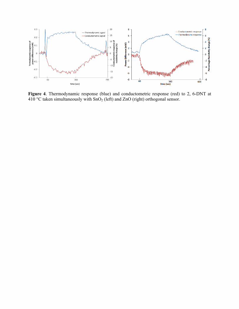
Figure 4. Thermodynamic response (blue) and conductometric response (red) to 2, 6-DNT at 410 °C taken simultaneously with SnO2 (left) and ZnO (right) orthogonal sensor.

Figure 5. Orthogonal response of SnO2 (where conductometric response is presented in red and thermodynamic response in blue) as a function of 2,6-DNT vapor concentration (black dashed line) at 410°C.

Figure 6. Conductometric response of SnO2 (left) and ZnO (right) orthogonal sensor to ammonia nitrate (blue), 2,6-DNT (red) and TATP (green) as a function of temperature.

ZnO!SnO2!

Dr. Radha Narayanan April 12, 2013

Solution Based Direct Readout SERS Method for Detection of Ultra-Low Levels of

Explosives In Complex Matrices Objective The overall objective of my research is to use nanoparticles of different shapes as colloidal SERS substrates for a direct readout and solution-based detection of ultra-low levels of different explosives in different matrices Summary We have synthesized dogbone shaped gold nanoparticles of two different sizes. The surface plasmon band of the nanoparticles red-shifts with increasing size of the dogbone shaped gold nanoparticles. We have successfully acquired the SERS spectra for nitrobenzenethiol in water and obtained the calibration curve. We have successfully acquired the SERS spectra of nitrobenzenethiol in other complex matrices such as Sprite and hairspray. Accomplishments

• Successfully synthesized two different sizes of dogbone shaped gold nanoparticles

• Obtained the UV-Visible spectra of the two sizes of dogbone shaped gold nanoparticles

• Acquired the SERS spectra of nitrobenzenethiol in water • Obtained the calibration curve of nitrobenzenethiol in water • Acquired the SERS spectra of nitrobenzenethiol in Sprite and hairspray

Details The dogbone shaped gold nanoparticles is synthesized using the seed-mediated growth method which consists of two steps: preparation of the gold nanoparticle seeds and growth of the seeds in a growth solution. Systematic variation of the concentration of the different components as well as a variety of different synthetic parameters results in gold nanoparticles of different shapes and sizes. We have synthesized two different sizes of dogbone shaped gold nanoparticles. Figure 1 and 2 show the TEM image and size distribution plot for two different sizes of dogbone shaped gold nanoparticles.

Figure 1. TEM image and size distribution plot of the smaller dogbone shaped gold nanoparticles. Figure 2. TEM image and size distribution plot of the larger dogbone shaped gold nanoparticles. We have obtained the UV-Visible spectra of the two different types of dogbone shaped gold nanoparticles. It was observed that the larger dogbone shaped gold nanoparticles result in a higher SPR lambda max which would result in higher SERS enhancements compared to the smaller dogbone shaped gold nanoparticles. Figure 3 and 4 show the UV-Visible spectra of the two types of dogbone shaped gold nanoparticles.

0 10 20 30 40 50 60 700

1

2

3

4

5

6

7

8

9

Pe

rcen

t o

f N

ano

par

ticl

es (

%)

Size of Nanoparticles (nm)

Average Size = 43 + 13 nmb

b

0 10 20 30 40 50 60 70 80 900

1

2

3

4

5

6

7

Per

cen

t o

f N

ano

par

ticl

es (

%)

Size of Nanoparticles (nm)

Average SIze =65 + 15 nm

Figure 3. UV-Visible spectra of the smaller dogbone shaped gold nanoparticles Figure 4. UV-Visible spectra of the larger dogbone shaped gold nanoparticles We have obtained the SERS spectra of different concentrations of nitrobenzenethiol in water using the larger dogbone shaped gold nanoparticles. Figure 5 shows the SERS spectra of nitrobenzenethiol in water that we have obtained. Figure 6 shows the calibration curve that we have generated for nitrobenzene in water. We also have obtained SERS spectra of nitrobenzenethiol in other complex matrices that would be present in passengers travelling in an airplane. Figure 7 shows the SERS spectra of nitrobenzenethiol in Sprite and Figure 8 shows the SERS spectra of nitrobenzenethiol in hairspray.

400 500 600 700 800 9000.0

0.2

0.4

0.6

0.8

1.0

Ab

so

rba

nc

e

Wavelength (nm)

UV-Vis Spectrum of Dogbone Shaped Gold Nanoparticles

SPR λmax = 671 nm

300 400 500 600 700 800 9000.00

0.25

0.50

0.75

1.00

1.25

1.50

Ab

sorb

anc

e

Wavelength (nm)

SPR λmax = 758 nm

Figure 5. SERS spectra of nitrobenzenethiol in water using the dogbone shaped gold nanoparticles as solution based SERS substrates

Figure 6. Calibration curve of nitrobenzenethiol in water

Figure 7. SERS spectra of nitrobenzenethiol in Sprite as the matrice

Figure 8. SERS spectra of nibrobenzenethiol in hairspray

Students Supported

Benjamin Saute—Ph.D. student

Allison Alix—undergraduate student Transition Partners None. Publications 1. Saute, B.; Narayanan.R, “Solution-Based Direct Readout Surface Enhanced Raman

Spectroscopic (SERS) Detection of Ultra-Low Levels of Thiram with Dogbone-Shaped Gold Nanoparticles”, Analyst, 2011, 136(3), 527-532.

2. Saute, B.; Premasiri, R., Ziegler, L, Narayanan, R., “Gold Nanorods as Surface Enhanced Raman Spectroscopy Substrates for Sensitive and Selective Detection of

Ultra-Low Levels of Dithiocarbamate Pesticides”, Analyst, 2012, 137(21), 5082-5087.

Prsentations 1. URI Explosives Workshop Poster Session, October 7-9, 2009, Kingston, RI, Poster,

“Metal Nanoparticles of Different Shapes as Colloidal Substrates for Solution-Based SERS Detection of Environmental Pollutants and Explosives”, Benjamin Saute, Nicole Cook, and Radha Narayanan

2. DHS Center Review, March 24-25, 2011, Poster, “Nanotechnology for Detection of Ultralow Levels of Explosives”, Benjamin Saute and Radha Narayanan

3. DHS Center Review, April 4-5, 2012, Kingston, RI, Oral, “SERS Detection of Explosives with Au Nanoparticles”, Radha Narayanan

PAPER www.rsc.org/analyst | Analyst

Dow

nloa

ded

by U

nive

rsity

of

Uta

h on

27

Dec

embe

r 20

10Pu

blis

hed

on 2

9 N

ovem

ber

2010

on

http

://pu

bs.r

sc.o

rg |

doi:1

0.10

39/C

0AN

0059

4KView Online

Solution-based direct readout surface enhanced Raman spectroscopic (SERS)detection of ultra-low levels of thiram with dogbone shaped gold nanoparticles

Benjamin Saute and Radha Narayanan*

Received 1st August 2010, Accepted 4th November 2010

DOI: 10.1039/c0an00594k

We report the use of two different sizes of dogbone shaped gold nanoparticles as colloidal substrates for

surface enhanced Raman spectroscopy (SERS) based detection of ultra-low levels of thiram,

a dithiocarbamate fungicide. We demonstrate the ability to use a solution based, direct readout SERS

method as a quantitative tool for the detection of ultra-low levels of thiram. The two different sizes of

dogbone shaped gold nanoparticles are synthesized by using the seed-mediated growth method and

characterized by using UV-visible spectroscopy and transmission electron microscopy (TEM). The

smaller dogbone shaped nanoparticles have an average size of 43 13 nm. The larger dogbone shaped

gold nanoparticles have an average size of 65 15 nm. The nanoparticle concentration is 1.25 1011

nanoparticles per mL for the smaller dogbone shaped gold nanoparticles and is 1.13 1011

nanoparticles per mL for the larger dogbone shaped gold nanoparticles. Different concentrations of

thiram are allowed to bind to the two different sizes of dogbone shaped gold nanoparticles and the

SERS spectra are obtained. From the calibration curve, the limit of detection for thiram is 43.9 6.2

nM when the smaller dogbone shaped gold nanoparticles are used as colloidal SERS substrates In the

case of the larger dogbone shaped gold nanoparticles, the limit of detection for thiram is 11.8 3.2 nM.

The lower limit of detection obtained by using the larger dogbone shaped gold nanoparticles as

colloidal substrates is due to the lightning rod effect, higher contributions from the electromagnetic

enhancement effect, and larger number of surface sites for thiram to bind.

Introduction

Surface-enhanced Raman scattering (SERS) was discovered in

1977 by Van Duyne1 and by Creighton.2 SERS is a phenomenon

in which there are greatly enhanced Raman signals when Raman

scattering molecules are placed very near or attached onto metal

substrates or metal nanoparticles. While of long standing funda-

mental importance,3–6 its potential as a quantitative analytical tool

has only recently begun to take place.7–10 Some types of quanti-

tative applications of SERS are biological sensing,5,11–23 environ-

mental monitoring,16,24 trace analysis,24 and explosive and

contaminant detection.5,24–26 The ability to use SERS as a quanti-

tative analytical tool reflects advances in the ability to reproduc-

ibly synthesize and manipulate the size and shape of gold and

silver nanoparticles.

The EPA have set maximum concentration limit (MCL) of

<1 ng mL1 for pollutants present in water. As a result, it is

necessary to be able to detect ultra-low levels of pesticides,

insecticides, fungicides, and other environmental pollutants.

SERS has been used for the detection of different types of

environmental pollutants.27–30 SERS has also been used for the

detection of polychlorinated biphenyls (PCBs).27–29 Different

types of pesticides27–34 have also been detected by using SERS. In

addition, SERS has been used for the detection of fungicides.35–38

It is worth noting that in many of these studies, SERS is used

qualitatively for identification of the different pollutants, PCBs,

Department of Chemistry, University of Rhode Island, 51 Lower CollegeRoad, Kingston, RI, 02881, USA. E-mail: rnarayanan@chm.uri.edu;Fax: +1 401-874-5072; Tel: +1 401-874-2298

This journal is ª The Royal Society of Chemistry 2010

pesticides and fungicides as well as structural studies on the

binding process. In our paper, we use SERS as a quantitative

analytical tool for detecting ultra-low levels of thiram, which is

a dithiocarbamate fungicide.

SERS has traditionally been conducted with gold and silver

substrates as well as colloidal gold and silver nanoparticles. It has

been recently shown that using cubic, block, and dogbone shaped

gold nanoparticles result in 100 times higher SERS enhance-

ments of 4-mercaptobenzoic acid compared to spherical gold

nanoparticles.39 This SERS enhancement has been attributed

to the lightning rod effect in which there is greater amount of

localized electromagnetic fields at the corners and edges of the

nanoparticles.39

We show that we can use two different sizes of dogbone shaped

gold nanoparticles as colloidal SERS substrates for quantitative

detection of ultralow levels of thiram, which is a dithiocarbamate

fungicide. In this paper we demonstrate the ability to use a

solution based, direct readout SERS method as a quantitative

tool for the detection of ultra-low levels of thiram. In our

method, we use two different sizes of dogbone shaped gold

nanoparticles as colloidal SERS substrates for a solution based

direct readout SERS based detection of ultra-low levels of

thiram. Thiram has a disulfide bond which spontaneously breaks

upon exposure to the gold nanoparticles and binds to the

nanoparticles through the Au–S bond, which is the gold thiolate

bond. It was observed that there is a lower limit of detection

when the larger dogbone shaped gold nanoparticles are used as

colloidal SERS substrates. Different sources that give rise to

higher enhancements will also be discussed in the paper.

Analyst

Dow

nloa

ded

by U

nive

rsity

of

Uta

h on

27

Dec

embe

r 20

10Pu

blis

hed

on 2

9 N

ovem

ber

2010

on

http

://pu

bs.r

sc.o

rg |

doi:1

0.10

39/C

0AN

0059

4KView Online

Experimental

Synthesis of two different sizes of dogbone shaped gold

nanoparticles

The smaller dogbone shaped gold nanoparticles were synthesized

by a slightly modified seed mediated growth method reported

previously.40–42 This synthesis consists of two distinct steps:

preparation of the nanoparticle seeds and preparation of the

nanoparticle growth solution. To prepare the seeds, 250 mL of

0.01 M HAuCl4 is added to a solution containing 4.75 mL

deionized water and 5 mL of 0.2 M CTAB. Next, 600 mL of ice-

cold 0.01 M NaBH4 is added to the solution, acting as a rapid

reducing agent. The seed solution is allowed to age for approx-

imately one hour. After the seed is aged, the growth solution is

prepared. The growth solution consists of 95 mL of 0.1 M

CTAB, 800 mL of 0.01 M AgNO3, 5 mL of 0.01 M HAuCl4,

550 mL of 0.1 M ascorbic acid, and 120 mL of the previously

prepared seed solution. After the growth solution is prepared, the

jar is left undisturbed overnight to allow the nucleation and

growth process to occur. The resulting nanoparticle solution

appears navy blue. In the case of the synthesis of larger dogbone

shaped nanoparticles, the same type of seed mediated growth

method was used and 0.25 M ascorbic acid is used in the growth

solution instead of 0.1 M ascorbic acid.

UV-visible spectroscopic characterization

The two different sizes of dogbone shaped gold nanoparticles

were characterized by using UV-visible spectroscopy to deter-

mine the surface plasmon band lmax of the nanoparticles. The

two different sizes of dogbone shaped nanoparticles were filtered

by using a 0.22 micron PVDF syringe filter. Two mL of the

dogbone shaped gold nanoparticles were placed into a quartz

cuvette and placed in the sample holder of the Agilent 8453 diode

array UV-visible spectrophotometer. The smaller dogbone sha-

ped nanoparticles have a surface plasmon band lmax of 671 nm

and the larger dogbone shaped nanoparticles have a surface

plasmon band lmax of 758 nm.

Transmission electron microscopic characterization

TEM characterization allows for determination of the size and

shape distributions of our gold nanoparticles. The different sizes

of dogbone shaped gold nanoparticles are filtered in the same

way as the UV-vis sample preparation. The nanoparticles are

then centrifuged twice at 12 000 rpm for 10 minutes each time.

This removes excess CTAB that is present in solution. One drop

of the filtered and centrifuged nanoparticles is spotted on the

TEM grid.

Fig. 1 TEM image of the smaller dogbone shaped gold nanoparticles (a)

and size distribution histogram of the nanoparticles (b).

Size distribution analysis

The UTHSCSA ImageTool for Windows—Version 3 image

analysis software was used to determine the size distributions of

the two different sizes of dogbone shaped gold nanoparticles.

The Distance tool in the Analysis pull-down menu is used to

measure the number of pixels in the scale bar of the TEM image.

Based on the number of pixels for the fixed size associated with

the scale bar and measuring the number of pixels for 200

Analyst

nanoparticles in several TEM images, the size of the dogbone

shaped gold nanoparticles can be calculated by dividing the

number of pixels for the nanoparticles by the number of pixels of

the scale bar and multiplying by the fixed size associated with the

scale bar of the TEM image. We then plotted the histogram of

% dogbone shaped gold nanoparticles vs. nanoparticle size and

obtained a Gaussian fit to the histogram. From the Gaussian fit,

we can determine the average size and standard deviation of the

dogbone shaped gold nanoparticles.

Surface enhanced Raman spectroscopy (SERS)

The SERS spectra of thiram were obtained by using a Raman

Systems R-3000QE Raman spectrometer. The laser excitation

wavelength is 785 nm. One mL of the dogbone shaped gold

nanoparticles with thiram bound to it is placed in a cuvette. The

cuvette is placed in the self-contained dark chamber. The L cap is

used since these are solution samples that are being analyzed. A

30 second integration time is used for acquisition of the SERS

spectra. The SERS spectra are acquired in the range from 200 to

1800 cm1.

Results and discussion

There are a few papers in the literature which report the SERS

spectra for thiram and discuss the binding modes to silver

colloids and gold films.43–45 In addition, there has been a paper in

which the authors have made assignments of the SERS bands

associated with thiram when it is bound to silver colloids.35 We

have developed a solution-based direct readout SERS method

for quantitative detection of ultralow levels of thiram, which is

a dithiocarbamate fungicide. Two different sizes of dogbone

shaped gold nanoparticles have been used as colloidal SERS

substrates for the detection of thiram.

Synthesis of the two different sizes of dogbone shaped gold

nanoparticles

We have synthesized two different sizes of dogbone shaped gold

nanoparticles by using the seed-mediated growth method

described previously.40–42 Fig. 1 shows a representative TEM

image of the smaller dogbone shaped gold nanoparticles as well

as the size distribution histogram with the average size of the

particles. The size distributions were determined by using the

ImageTool software. The smaller dogbone shaped gold nano-

particles have an average size of 43 13 nm. The concentration

This journal is ª The Royal Society of Chemistry 2010

Fig. 2 UV-visible spectrum showing the surface plasmon band lmax of

the smaller dogbone shaped gold nanoparticles.

Fig. 4 UV-visible spectrum showing the surface plasmon band lmax of

the larger dogbone shaped gold nanoparticles.

Table 1 Table of the SERS bands associated with thirama

SERS band Assignment35

339 (vw) d (S]CS), d (CSS)486 (vw) d (CH3NC), n (C]S)556 (m) n (SS)755 (vw) —928 (m) n (CH3N), n (C]S)1139 (m) r (CH3), n (CN)1379 (vs) d s(CH3), n (CN)1444 (m) d as(CH3)1508 (m) r (CH3), n (CN)

a s ¼ strong, w ¼ weak, m ¼ medium, sh ¼ shoulder, v ¼ very, n ¼stretching, d ¼ deformation, r ¼ rocking.

Dow

nloa

ded

by U

nive

rsity

of

Uta

h on

27

Dec

embe

r 20

10Pu

blis

hed

on 2

9 N

ovem

ber

2010

on

http

://pu

bs.r

sc.o

rg |

doi:1

0.10

39/C

0AN

0059

4KView Online

of the smaller dogbone shaped nanoparticles is calculated to be

1.25 1011 nanoparticles per mL. We have also characterized the

smaller dogbone shaped gold nanoparticles by using UV-visible

spectroscopy to characterize the surface plasmon band lmax. It

can be seen in Fig. 2 that the smaller dogbone shaped gold

nanoparticles have a lmax of 671 nm.

TEM images and size distribution plots were also obtained

for the larger dogbone shaped gold nanoparticles. Fig. 3 shows

a representative TEM image of the larger dogbone shaped gold

nanoparticles as well as the size histogram with the average size

of the nanoparticles. The larger dogbone shaped gold nano-

particles have an average size of 65 15 nm. The concentration

of the larger dogbone shaped gold nanoparticles is calculated

to be 1.13 1011 nanoparticles per mL. We have also used

UV-visible spectroscopy to obtain the surface plasmon band

lmax. It can be seen in Fig. 4 that the larger dogbone shaped gold

nanoparticles have a surface plasmon band lmax of 758 nm.

The dogbone shaped gold nanoparticles are much more

attractive as colloidal SERS substrates compared to the spherical

gold nanoparticles since the dogbone shaped gold nanoparticles

have surface plasmon bands (671 nm and 758 nm) that are

in greater resonance to the laser excitation wavelength,. The

spherical gold nanoparticles have surface plasmon band in the

range between 520 and 560 nm, which are not in good resonance

to the laser excitation wavelength. The larger dogbone shaped

gold nanoparticles have a surface plasmon band lmax which is in

greater resonance to the laser excitation wavelength than that of

the smaller dogbone shaped gold nanoparticles. As a result, we

Fig. 3 TEM image of the larger dogbone shaped gold nanopartic

This journal is ª The Royal Society of Chemistry 2010

would expect to obtain higher SERS signals using the larger

dogbone shaped gold nanoparticles compared to the smaller

dogbone shaped gold nanoparticles. This is discussed in more

detail later on in the paper.

SERS bands of thiram

There has been a previous study where the SERS spectrum of

thiram has been obtained in which the assignments of the

different bands has been determined.35 Table 1 shows the SERS

peaks that we observe when the thiram is bound to the dogbone

les (a) and size distribution histogram of the nanoparticles (b).

Analyst

Fig. 5 Example of a SERS spectrum of thiram bound to dogbone

shaped gold nanoparticles.

Fig. 6 Raw SERS spectra (a) and SERS calibration curve of SERS

intensity with 30 second integration time as a function of the thiram

concentration obtained by using the smaller dogbone shaped gold

nanoparticles as colloidal SERS substrates (b).

Dow

nloa

ded

by U

nive

rsity

of

Uta

h on

27

Dec

embe

r 20

10Pu

blis

hed

on 2

9 N

ovem

ber

2010

on

http

://pu

bs.r

sc.o

rg |

doi:1

0.10

39/C

0AN

0059

4KView Online

shaped gold nanoparticles and Fig. 5 shows an example of the

SERS bands observed when thiram binds to the nanoparticles.

There are many peaks in the SERS spectrum of thiram. The

strongest peak is at 1379 cm1 which is the CN stretching mode

and symmetric CH3 deformation mode. Since this is the strongest

peak in the SERS spectra, this is the band we use for monitoring

the SERS intensity as a function of the thiram concentration.

The asymmetric CH3 deformation mode occurs at 1444 cm1.

The CN stretching mode also occurs at 1508 cm1 as well as the

rocking CH3 mode. The CN stretching mode and rocking CH3

mode also occurs at 1139 cm1. The stretching CH3N and C]S

modes occur at 928 cm1. The peak at 556 cm1 is associated with

the SS stretching mode. The peak at 486 cm1 is due to the

CH3NC deformation and C]S stretching modes. The S]CS

deformation and the CSS deformation occur at 339 cm1.

SERS calibration curve

Thiram is a dithiocarbamate fungicide which has a disulfide

bond. It is known that there is cleavage of the disulfide bond

upon exposure to gold nanoparticles or gold substrates.46 When

the disulfide bond in thiram breaks, it can bind to the dogbone

shaped gold nanoparticles via the gold thiolate bond. Different

concentrations of thiram are added to the dogbone shaped gold

nanoparticles and allowed to bind overnight. The SERS spectra

were obtained in triplicate sets for different concentrations of

thiram that is covalently bound to the smaller dogbone shaped

gold nanoparticles. Fig. 6 shows a representative raw SERS

spectra as well as the calibration curve of the SERS intensity as

a function of the thiram concentration obtained by using the

smaller dogbone shaped gold nanoparticles. The error bars

represent the standard deviation of the average Raman intensity

(counts per 30 s) obtained with three sets of SERS measurement.

It can be seen from the linear fit that the SERS measurements are

reproducible. The limit of detection (LOD) is determined by first

calculating the minimum distinguishable signal which is the

average signal of the blank + 3 times the standard deviation of

the blank. The minimum distinguishable signal is then plugged

into the best-fit equation of the calibration curve to calculate the

limit of detection. The limit of detection obtained for thiram by

using the smaller dogbone shaped gold nanoparticles is 43.9 6.2 nM.

Fig. 7 shows a representative set of raw SERS spectra from

triplicate sets as well as the calibration curve of the SERS

Analyst

intensity as a function of the thiram concentration obtained by

using the larger dogbone shaped gold nanoparticles. The error

bars represent the standard deviation of the average Raman

intensity (countsper 30 s) obtained with three sets of SERS

measurement. It can be seen from the linear fit that the SERS

measurements are reproducible. In the case of the larger dogbone

shaped Au nanoparticles, the limit of detection is 11.8 3.2 nM.

Using the larger dogbone shaped Au nanoparticles as colloidal

SERS substrates results in 3.7 lower limit of detection. Several

sources that give rise to the higher SERS enhancements are

discussed in the next section.

Sources of higher SERS activities

It has been previously shown that cubic, block, and dogbone

shaped gold nanoparticles result in 100 higher SERS

enhancements for 4-mercaptobenzoic acid compared to spherical

nanoparticles.39 In the case of these nanoparticles, the higher

SERS enhancements are attributed to the lightning rod effect.

The two types of dogbone shaped gold nanoparticles that we

have synthesized have a similar concentration in which the

smaller nanoparticles have a concentration of 1.25 1011

nanoparticles per mL and the larger dogbone shaped gold

nanoparticles have a concentration of 1.13 1011 nanoparticles

per mL. In the case of our smaller dogbone shaped gold nano-

particles, the source of the SERS enhancement is due to the

This journal is ª The Royal Society of Chemistry 2010

Fig. 7 Raw SERS spectra (a) and SERS calibration curve of SERS

intensity with 30 second integration time as a function of the thiram

concentration obtained by using the larger dogbone shaped gold nano-

particles as colloidal SERS substrates (b).

Dow

nloa

ded

by U

nive

rsity

of

Uta

h on

27

Dec

embe

r 20

10Pu

blis

hed

on 2

9 N

ovem

ber

2010

on

http

://pu

bs.r

sc.o

rg |

doi:1

0.10

39/C

0AN

0059

4KView Online

lightning rod effect in which there are greater electromagnetic

fields at the corners and edges of the nanoparticles. In the case of

the larger dogbone shaped gold nanoparticles, in addition to the

lightning rod effect, there are much greater contributions from

the electromagnetic enhancement effect since the surface plas-

mon band lmax is 758 nm which is close to the laser excitation

wavelength of 785 nm. This gives rise to some of the higher SERS

enhancement that is observed. Also, since the surface area of the

larger dogbone shaped gold nanoparticles (6276.07 nm2) is larger

than the surface area of the smaller dogbone shaped gold

nanoparticles (5175.85 nm2) more thiram can bind to the nano-

particle surface resulting in some of the higher enhancements

that is observed. Overall, there are higher SERS enhancements

and lower limits of detection for thiram observed for the larger

dogbone shaped gold nanoparticles. The sources that contribute

to the higher SERS enhancements and lower limits of detection

observed for the larger dogbone shaped gold nanoparticles are

lightning rod effect, surface plasmon band lmax being in much

greater resonance to the laser excitation wavelength resulting in

greater contributions from the electromagnetic enhancement

effect, and more surface sites for thiram to bind to the nano-

particle surface due to a higher surface area.

Conclusions

We have developed a quantitative analytical solution-based

direct readout SERS method for detection of thiram which is

This journal is ª The Royal Society of Chemistry 2010

a dithiocarbamate fungicide. Two different sizes of dogbone

shaped gold nanoparticles are used as colloidal SERS substrates

for SERS based detection of thiram. It is observed that using

larger dogbone shaped gold nanoparticles results in lower limits

of detection compared to using the smaller dogbone shaped gold

nanoparticles. The lower limits of detection observed for the

larger dogbone shaped gold nanoparticles could be attributed to

the lightning rod effect, surface plasmon band lmax being in

much greater resonance to the laser excitation wavelength, and

more surface sites for thiram to bind. There are higher contri-

butions in the SERS intensities from the electromagnetic

enhancement effect.

Acknowledgements

We thank Dr Richard Kingsley at the Electron Microscopy

Facility for assistance in acquiring the TEM images. We thank

the University of Rhode Island start-up funds, RI-INBRE Pilot

Program, as well as the Society for Analytical Chemists of

Pittsburgh starter grant for funding of this work.

References

1 D. L. Jeanmaire and R. P. VanDuyne, Surface Raman spectro-electrochemistry. Part I. Heterocyclic, aromatic, and aliphatic aminesadsorbed on the anodized silver electrode, J. Electroanal. Chem.,1977, 84, 1.

2 M. G. Albrecht and J. A. Creighton, Anomalously intense Ramanspectra of pyridine at a silver electrode, J. Am. Chem. Soc., 1977,99, 5215.

3 M. Moskovits, Surface-enhanced Raman spectroscopy. A briefperspective, Top. Appl. Phys., 2006, 103, 1.

4 J. A. Dieringer, A. D. McFarland, N. C. Shah, D. A. Stuart,A. V. Whitney, C. R. Yonzon, M. A. Young, X. Zhang andR. P. Van Duyne, Surface enhanced Raman spectroscopy: newmaterials, concepts, characterization tools, and applications,Faraday Discuss., 2006, 132, 9.

5 C. L. Haynes, A. D. McFarland and R. P. VanDuyne, Surface-enhanced Raman spectroscopy, Anal. Chem., 2005, 77(17), 338A–346A.

6 M. Moskovits, Surface-enhanced Raman spectroscopy: a briefretrospective, J. Raman Spectrosc., 2005, 36(6–7), 485.

7 W. E. Smith, K. Faulds and D. Graham, Quantitative surface-enhanced resonance Raman spectroscopy for analysis, Top. Appl.Phys., 2006, 103, 381.

8 C. L. Haynes, C. R. Yonzon, X. Zhang and R. P. VanDuyne, Surface-enhanced Raman sensors: early history and the development ofsensors for quantitative biowarefare agent and glucose detection,J. Raman Spectrosc., 2005, 36(6–7), 471.

9 S. C. Pinzaru, I. Pavel, N. Leopold and W. Kiefer, Identification andcharacterization of pharmaceuticals using Raman and surface-enhanced Raman scattering, J. Raman Spectrosc., 2004, 35(5), 338.

10 T. Vo-Dinh, SERS chemical sensors and biosensors: new tools forenvironmental and biological analysis, Sens. Actuators, B, 1995,B29(1–3), 183.

11 K. Faulds, W. E. Smith and D. Graham, DNA detection by surfaceenhanced resonance Raman scattering (SERRS), Analyst, 2005,130(8), 1125–1131.

12 A. E. Grow, L. L. Wood, J. L. Claycomb and P. A. Thompson, Newbiochip technology for label-free detection of pathogens and theirtoxins, J. Microbiol. Methods, 2003, 53(2), 221–233.

13 K. Kneipp, H. Kneipp, I. Itzkan, R. R. Dasari and M. S. Feld,Surface-enhanced Raman scattering and biophysics, J. Phys.:Condens. Matter, 2002, 14(18), R597–R624.

14 A. G. Ryder, Surface enhanced Raman scattering for narcoticdetection and applications to chemical biology, Curr. Opin. Chem.Biol., 2005, 9(5), 489–493.

15 Z. Q. Tian, Surface-enhanced Raman spectroscopy: advancementsand applications, J. Raman Spectrosc., 2005, 36(6–7), 466–470.

Analyst

Dow

nloa

ded

by U

nive

rsity

of

Uta

h on

27

Dec

embe

r 20

10Pu

blis

hed

on 2

9 N

ovem

ber

2010

on

http

://pu

bs.r

sc.o

rg |

doi:1

0.10

39/C

0AN

0059

4KView Online

16 T. Vo-Dinh, Surface-enhanced Raman spectroscopy using metallicnanostructures, TrAC, Trends Anal. Chem., 1998, 17(8–9), 557–582.

17 T. Vo-Dinh, D. L. Stokes, in Surface-Enhanced Raman scattering(SERS) for Biomedical Diagnostics, 2003, pp 64/1–64/39.

18 T. Vo-Dinh, F. Yan and D. L. Stokes, Plasmonics-basednanostructures for surface-enhanced Raman scattering bioanalysis,Methods Mol. Biol., 2005, 300, 255–283, Protein Nanotechnology.

19 S. Xu, X. Ji, W. Xu, B. Zhao, X. Dou, Y. Bai and Y. Ozaki, Surface-enhanced Raman scattering studies on immunoassay, J. Biomed. Opt.,2005, 10(3), 031112.

20 W. E. Doering, M. E. Piotti, M. J. Natan and R. G. Freeman, Adv.Mater., 2007, 19(20), 3100.

21 R. G. Freeman, W. E. Doering, I. D. Walton, S. G. Penn, G. Davis,F. Wong and M. J. Natan, Proc. SPIE, 2005, 5705, 114.

22 S. P. Mulvaney, M. D. Musick, C. D. Keating and M. J. Natan,Langmuir, 2003, 19(11), 4784.

23 M. El-Kouedi, C. D. Keating, Nanobiotechnology, 2004, p. 429.24 G. A. Baker and D. S. Moore, Progress in plasmonic engineering of

surface-enhanced Raman-scattering substrates toward ultra-traceanalysis, Anal. Bioanal. Chem., 2005, 382(8), 1751–1770.

25 K. M. Spencer, J. M. Sylvia, P. J. Marren, J. F. Bertone andS. D. Christesen, Surface-enhanced Raman spectroscopy forhomeland defense, Proc. SPIE, 2004, 5269, 1–8, Chemical andBiological Point Sensors for Homeland Defense.

26 W. E. Smith, P. C. White, C. Rodger and G. Dent, Raman andsurface enhanced resonance Raman scattering: applications inforensic science, Pract. Spectrosc., 2001, 28, 733–748, Handbook ofRaman Spectroscopy.

27 A. M. Alak and D. Tuan Vo, Surface-enhanced Raman spectrometryof chlorinated pesticides, Anal. Chim. Acta, 1988, 206(1–2), 333–337.

28 S. Bonora, M. Di Foggia and M. Iafisco, SERS in the analysis ofpesticides (triazinic herbicides), Chim. Ind., 2008, 90(10), 98–100.

29 C. J. Lee, H. J. Kim, M. R. Karim and M. S. Lee, Surface-enhancedRaman spectroscopy of ethephone adsorbed on silver surface, Bull.Korean Chem. Soc., 2006, 27(4), 545–548.

30 D. Lee, S. Lee, G. H. Seong, J. Choo, E. K. Lee, D.-G. Gweon andS. Lee, Quantitative analysis of methyl parathion pesticide ina polydimethylsiloxane microfluidic channel using confocal surface-enhanced Raman spectroscopy, Appl. Spectrosc., 2006, 60(4), 373–377.

31 V. Lee and S. Farquharson, SERS sample vials based on sol–gelprocess for trace pesticide analysis, Proc. SPIE, 2001, 4206, 140–146, Photonic Detection and Intervention Technologies for SafeFood.

32 J. Qiao, G. Zheng and F. Li, Determination of trace pesticide in waterby surface enhanced Raman spectroscopy, Huaxue Tongbao, 2006,69(6), 462–464.

33 C. Shende, A. Gift, F. Inscore, P. Maksymiuk and S. Farquharson,Inspection of pesticide residues on food by surface-enhanced raman

Analyst

spectroscopy, Proc. SPIE, 2004, 5271, 28–34, Monitoring FoodSafety, Agriculture, and Plant Health.

34 C. S. Shende, F. Inscore, A. Gift, P. Maksymiuk and S. Farquharson,Analysis of pesticides on or in fruit by surface-enhanced Ramanspectroscopy, Proc. SPIE, 2004, 5587, 170–176, Nondestructivesensing for food Safety, Quality, and Natural Resources.

35 J. S. Kang, S. Y. Hwang, C. J. Lee and M. S. Lee, SERS ofdithiocarbamate pesticides adsorbed on silver surface; thiram, Bull.Korean Chem. Soc., 2002, 23(11), 1604–1610.

36 M. S. Kim, J. S. Kang, S. B. Park and M. S. Lee, Surface-enhancedRaman spectroscopy of quinomethionate adsorbed on silvercolloids, Bull. Korean Chem. Soc., 2003, 24(5), 633–637.

37 S. Sanchez-Cortes, C. Domingo, J. V. Garcia-Ramos andJ. A. Aznarez, Surface-enhanced vibrational study (SEIR andSERS) of dithiocarbamate pesticides on gold films, Langmuir, 2001,17(4), 1157–1162.

38 S. Sanchez-Cortes, M. Vasina, O. Francioso and J. V. Garcia-Ramos,Raman and surface-enhanced Raman spectroscopy of dithio-carbamate fungicides, Vib. Spectrosc., 1998, 17(2), 133–144.

39 C. J. Orendorff, A. Gole, T. K. Sau and C. J. Murphy, Surface-enhanced Raman spectroscopy of self-assembled monolayers:sandwich architecture and nanoparticle shape dependence, Anal.Chem., 2005, 77(10), 3261–3266.

40 L. Gou and C. J. Murphy, Fine-tuning the shape of gold nanorods,Chem. Mater., 2005, 17(14), 3668–3672.

41 C. J. Murphy, T. K. Sau, A. M. Gole, C. J. Orendorff, J. Gao, L. Gou,S. E. Hunyadi and T. Li, Anisotropic metal nanoparticles: synthesis,assembly, and optical applications, J. Phys. Chem. B, 2005, 109(29),13857–13870.

42 T. K. Sau and C. J. Murphy, Room temperature, high-yield synthesisof multiple shapes of gold nanoparticles in aqueous solution, J. Am.Chem. Soc., 2004, 126(28), 8648–8649.

43 A. Torreggiani, Z. Jurasekova, M. D’Angelantonio, M. Tamba,J. V. Garcia-Ramos and S. Sanchez-Cortes, Fabrication of Agnanoparticles by 1-irradiation: application to surface-enhancedRaman spectroscopy of fungicides, Colloids Surf., A, 2009, 339,60–67.

44 S. Sanchez-Cortes, M. Vasina, O. Francioso and J. V. Garcia-Ramos,Raman and surface-enhanced Raman spectroscopy of dithio-carbamate fungicides, Vib. Spectrosc., 1998, 17, 133–144.

45 S. Sanchez-Cortes, C. Domingo, J. V. Garcia-Ramos and J. A. Aznarez,Surface-enhanced vibrational study (SEIR and SERS) ofdithiocarbamate pesticides on gold films, Langmuir, 2001, 17, 1157–1162.

46 H. A. Biebuyck and G. M. Whitesides, Interchange betweenmonolayers on gold formed from unsymmetrical disulfides andsolutions of thiols: evidence for sulfur-sulfur bond cleavage by goldmetal, Langmuir, 1993, 9(7), 1766–1770.

This journal is ª The Royal Society of Chemistry 2010

Dynamic Article LinksC<Analyst

Cite this: Analyst, 2012, 137, 5082

www.rsc.org/analyst PAPER

Dow

nloa

ded

by U

nive

rsity

of

Rho

de I

slan

d on

12/

04/2

013

14:3

8:06

. Pu

blis

hed

on 0

3 Se

ptem

ber

2012

on

http

://pu

bs.r

sc.o

rg |

doi:1

0.10

39/C

2AN

3604

7KView Article Online / Journal Homepage / Table of Contents for this issue

Gold nanorods as surface enhanced Raman spectroscopy substrates forsensitive and selective detection of ultra-low levels of dithiocarbamatepesticides

Benjamin Saute, Ranjith Premasiri, Lawrence Ziegler and Radha Narayanan*

Received 31st July 2012, Accepted 3rd September 2012

DOI: 10.1039/c2an36047k

We report the use of gold nanorods as solution-based SERS substrates for the detection of ultralow-

levels of three different dithiocarbamate fungicides: thiram, ferbam and ziram. Gold nanorods are

attractive to use as SERS substrates due to the ability to tune the surface plasmon resonance of the

nanoparticles to the laser excitation wavelength of the Raman spectrometer equipped with a 785 nm

diode laser. The gold nanorods are synthesized using a seed-mediated growth method and characterized

using UV-Visible spectroscopy, zeta potential, and TEM. The gold nanorods have an aspect ratio of

2.19 0.21 and have an average length of 37.81 4.83 nm. SERS spectra are acquired at different

concentrations of each fungicide and calibration curves are obtained by monitoring the intensity of the

band arising from the n(C–N) stretching mode coupled to the symmetric d(CH3) motion. The limits of

detection and limits of quantitation are obtained for each fungicide. The limits of detection are 11.000.95 nM, 8.00 1.01 nM, and 4.20 1.22 nM for thiram, ferbam, and ziram respectively. The limits of

quantitation are 34.43 0.95 nM, 25.61 1.01 nM, and 12.94 1.22 nM for thiram, ferbam, and

ziram respectively. It can be seen that the three different dithiocarbamates can be detected in the low

nM range based on the limits of detection that are achieved.

Introduction

Dithiocarbamates are a subclass of carbamate pesticides that are

widely used as insecticidal agents on food crops in the US and

abroad.1 Quantitative determination of trace quantities of

dithiocarbamates is necessary in order to mitigate potential

human exposure via pesticide residues left on inadequately

washed food items as well as groundwater contamination from

agricultural runoff. The focus of this research is on the devel-

opment of a sensitive and selective sensing platform based on

surface enhanced Raman spectroscopy (SERS) in conjunction

with multivariate cluster-based data analysis techniques for the

sensitive and selective determination of structurally similar

dithiocarbamate fungicides, namely, thiram, ferbam and ziram.

Data clustering analysis coupled to the output from SERS

analysis has been shown to enable the discrimination between

similar spectra for bacterial diagnostics2–4 and as such, the

application of the technique to the analysis of thiram, ferbam,

and ziram allows for trace-level quantitative determination as

well as unambiguous identification of unknown species from

comparison with previously constructed SERS libraries.

The frequencies and relative intensities of SERS vibrational

bands are sensitive to the nature of the substrate. Gold

Department of Chemistry, University of Rhode Island, Kingston, RI, USA,02881. E-mail: rnarayanan@chm.uri.edu; Fax: +1 401-874-5072; Tel: +1401-874-2298

5082 | Analyst, 2012, 137, 5082–5087

nanostructures have been explored extensively as SERS

substrates due to their unique size dependent optical and elec-

tronic properties.5–8 Of these unique properties of nanoscale gold

particles, localized surface plasmon resonance is one of the most

widely exploited properties for sensing applications. Excitation

of localized surface plasmons (conduction band electrons located

at the surface of a nanoparticle) by an external electromagnetic

field results in strong light scattering, the appearance of intense

absorption bands, and an increase in the magnitude of the local

electromagnetic field by several orders of magnitude.9 Surface

plasmon resonance has been exploited to construct a variety of

chemical sensors for analytes including biomolecules,10 explo-

sives,11 chemical warfare simulants,12 and environmental

pollutants.13

Surface enhanced Raman spectroscopy (SERS)14 is a technique

that utilizes the enormous enhancement of the local electric field

around a nanoparticle generated by surface plasmon resonance.

Since its discovery in 1974,15 significant research has been con-

ducted toward investigating the mechanism of the enhancement

process. It is widely accepted in the literature that SERS operates

via two distinct mechanisms.16 The electromagnetic enhancement

is considered to be the dominant enhancement process and is a

direct result of the amplification of the local electromagnetic field

due to localized surface plasmon resonance. The other mechanism

underlying SERS enhancement is the chemical enhancement

where the excitation of adsorbate electrons creates charge transfer

This journal is ª The Royal Society of Chemistry 2012

Fig. 1 Chemical structures of dithiocarbamate pesticides analyzed.

Dow

nloa

ded

by U

nive

rsity

of

Rho

de I

slan

d on

12/

04/2

013

14:3

8:06

. Pu

blis

hed

on 0

3 Se

ptem

ber

2012

on

http

://pu

bs.r

sc.o

rg |

doi:1

0.10

39/C

2AN

3604

7K

View Article Online

states between the metal substrate and an adsorbed molecule.17,18

These charge transfer states contribute more strongly to the

observed Raman scattering intensity than do adsorbate molecules

in their native ground states. The sensitivity afforded by such

significant increases in signal intensity makes SERS well suited for

a wide variety of analytical applications including detecting

anthrax biomarkers,12 in vitro19 and in vivo20 glucose monitoring,

monitoring of heterogeneous catalytic reactions21 and detection of

explosive compounds.22

One of the major challenges involved with establishing a SERS

based analytical method involves fabricating and optimizing the

SERS-active substrate. Typically, nanostructures composed of

silver and gold are used as SERS substrates due to the fact that

these metals can support localized surface plasmon resonance

located in the visible region of the spectrum.23 Although

substrates composed of silver nanoparticles are often used in

SERS applications,24 gold nanoparticles display several advan-

tageous characteristics including resistance to surface oxidation

as well as a red-shifted surface plasmon resonance.25 The shifting

of the surface plasmon resonance to lower frequencies is

advantageous because it allows for the use of lower energy

Raman excitation sources. Lower energy excitation reduces the

risk of analyte photobleaching26 and photodegradation27 and

allows for the use of inexpensive, commercially available diode

laser sources in the red and NIR spectral region.

Previously, our group has demonstrated an analytical method

for the quantitative detection of the dithiocarbamate pesticide

thiram in solution using SERS.28 In this study, we used dog bone

shaped gold nanoparticles stabilized by the cationic surfactant

hexadecyltrimethylammonium bromide (CTAB) as SERS

substrates. The substrate was characterized by UV-Vis spec-

troscopy and found to have a surface plasmon resonance located

at 671 nm, significantly off-resonance with our instrumental

excitation wavelength of 785 nm. These substrates were used to

construct a solution based SERS calibration curve and the limit

of detection of thiram was calculated to be 43.9 6.2 nM. From

this work we hypothesized that utilizing substrates with surface

plasmon resonance matching the 785 nm instrumental excitation

wavelength should allow for the highest possible enhancement of

the local electromagnetic field around the particle and therefore,

the lowest possible limits of detection.

Among the various gold nanostructures that have been

reported in the literature, gold nanorods are attractive as SERS

substrates because the surface plasmon resonance frequency can

be tuned as a function of the aspect ratio.29 Typically, gold

nanorods are synthesized in the presence of CTAB, a cationic

surfactant which assists in the formation of the nanorods by

forming micellar templates in solution.30 While the presence of

CTAB during nanorod formation is crucial, it remains strongly

bound to the surface of the nanorods after synthesis and

competes with analytes for binding sites. Reducing the amount of

surface bound CTAB is necessary to optimize binding between

the analyte and the substrate surface. Cui et al.31 have published

a method for removing surface bound CTAB through treatment

of the nanorod solution with HCl at elevated temperatures and

we have utilized this method to produce highly active gold

nanorod SERS substrates.

In this work, we present the development of an analytical

method for the trace analysis of dithiocarbamate pesticides

This journal is ª The Royal Society of Chemistry 2012

utilizing SERS. We have expanded the target analytes to include

ferbam and ziram, two dithiocarbamate pesticides with struc-

tural similarity to thiram. Utilizing CTAB-removed gold nano-

rods as SERS substrates, we present limits of detection and

quantitation for the three target analytes and compare these

values to the maximum residue tolerances established by the

EPA. In addition to quantitative analysis, we utilize a second

derivative based principle component analysis (PCA) clustering

technique32 to show how the SERS spectra of these closely

related fungicides may be readily identified when compared to a

previously generated library (Fig. 1).

Experimental

Gold nanorod synthesis

Gold nanorods were prepared using established synthetic

protocols.33 Briefly, a seed solution is prepared composed of

250 mL [0.01 M] HAuCl4, 7.5 mL [0.1 M] CTAB, 1.65 mL H2O

and reduced by the addition of 600 mL ice-cold [0.01 M] NaBH4.

This solution was allowed to age for one hour while the growth

solution is prepared consisting of 47.5 mL [0.1 M] CTAB, 400 mL

[0.01 M] AgNO3, 2.5 mL [0.01 M] HAuCl4, and 275 mL [0.1 M]

ascorbic acid. Addition of 60 mL of the aged seed solution initi-

ates nanorod growth which is allowed to proceed overnight.

The as-synthesized gold nanorods were purified and surface

bound CTAB removed using protocols established by Cui et al.31

Excess CTAB on the surface of the nanorods was removed by

centrifuging the nanorod solution at 8000 rpm for 10 minutes,

removing the supernatant liquid, and redispersing the collected

solid in deionized water. 3.2 mL [10 M] HCl per mL of particles

was added and the solution was heated at 60 C with stirring for 3

hours to remove surface bound CTAB. The particles were again

centrifuged at 8000 rpm for 10 minutes, the supernatant liquid

removed, and the remaining solid was redispersed in deionized

water.

Characterization of HCl-treated gold nanorods

UV-Vis absorption measurements were acquired using an

Agilent 8453 spectrophotometer in plastic cuvettes with 1 cm

path length. A Malvern Zetasizer Nano series dynamic light

scattering instrument in a dip cell configuration with a plastic

cuvette was used to obtain zeta potential measurements. Trans-

mission electron microscopy was performed using a JEOL JEM-

2100 TEM operating at 200 kV at 40 000 magnification.

SERS sample preparation and instrumentation

One mL of the centrifuged HCl-treated gold nanorod solution

was used as the SERS substrate. A known quantity of 10 mM

Analyst, 2012, 137, 5082–5087 | 5083

Dow

nloa

ded

by U

nive

rsity

of

Rho

de I

slan

d on

12/

04/2

013

14:3

8:06

. Pu

blis

hed

on 0

3 Se

ptem

ber

2012

on

http

://pu

bs.r

sc.o

rg |

doi:1

0.10

39/C

2AN

3604

7K

View Article Online

analyte stock solution in acetonitrile was added to the substrate

and the system was mixed for one hour to allow binding between

the analyte and substrate. After binding, SERS measurements

were acquired using a Raman Systems R-3000QE system

equipped with a 785 nm diode laser excitation source. The

excitation light is delivered by a fiber optic probe equipped with a

fiber Bragg grating for wavelength isolation. The same fiber optic

probe is used to collect the Raman scattered light which is

directed to an ultra high sensitive dispersive grating spectrometer

and focused on a cooled back-thinned 2D CCD array detector.

‘‘Barcode’’ principle component analysis

The PCA approach employed here to uniquely distinguish and

identify the SERS spectra of these three fungicides that exhibit

very similar SERS spectra was previously developed for the

detection and identification of vegetative bacterial cells and has

been shown to result in enhanced specificity relative to more

standard PCA treatments.18 Briefly, the observed SERS spectra

are Fourier filtered to remove the high frequency noise. The

normalized filtered SERS spectra are converted to a barcode, i.e.

a series of zeros and ones, based on the sign of the second

derivative of the SERS spectrum as a function of Raman

frequency. A minimum value, typically at10% of the maximum

second derivative value is used as a threshold for the zero (one)

assignment. These so-called barcodes are the inputs to a PCA

treatment that is carried out with Matlab software routines. The

clusters that result from this barcode PCA approach result in

improved effective reproducibility and specificity. Identification

results from group membership in a barcode PCA cluster. This

procedure minimizes background variability while maximizing

the more robust spectral features, regions of peaks and valleys, in

the observed vibrational spectra.18

Fig. 3 UV-Vis absorption spectrum of HCl-treated gold nanorods.

Results and discussion

The main focus of this research was to utilize gold nanorod

substrates for the investigation of the limits of detection and

quantitation of three structurally similar dithiocarbamate pesti-

cides in solution. Upon synthesis, the gold nanorod substrate was

subjected to treatment with HCl at 60 C in order to remove as

Fig. 2 TEM micrograph and size

5084 | Analyst, 2012, 137, 5082–5087

much surface bound CTAB as possible. In order to assess the

effectiveness of CTAB removal, zeta potential measurements

were made both before and after HCl treatment. Zeta potential

can be used to qualitatively assess the stability of the nano-

particle solution by measuring the surface charge on the

particle.34 Zeta potential values of 40 mV indicate that there is

sufficient charge on the surface of the particle to ensure that the

solution does not experience aggregation. The value of the zeta

potential for the gold nanorod solution was 43 mV immediately

following synthesis, indicative of a highly stable substrate solu-

tion and 33.4 mV immediately following HCl treatment. This

decrease in zeta potential indicates that the overall stability of the

substrate solution decreased as a result of HCl treatment and

that this decrease in substrate solution stability suggests that

there was a decrease in the amount of stabilizing CTAB on the

surface of the particle. The decrease in the amount of CTAB

present on the particle surface was not sufficient to cause particle

aggregation, and the particles remained stable over the course of

several days. A decrease in the amount of surface bound CTAB

increases the number of free binding sites on the substrate which

serves to increase the sensitivity of the SERS method.

Fig. 2 is a TEM image showing the size and shape of the

synthesized gold nanorods. The synthesis is successful in

producing the desired nanorod shape in high yields with minimal

spherical impurities. From this TEM image, we determine the

size distribution to be Gaussian with an average nanorod length

distribution of gold nanorods.

This journal is ª The Royal Society of Chemistry 2012

Dow

nloa

ded

by U

nive

rsity

of

Rho

de I

slan

d on

12/

04/2

013

14:3

8:06

. Pu

blis

hed

on 0

3 Se

ptem

ber

2012

on

http

://pu

bs.r

sc.o

rg |

doi:1

0.10

39/C

2AN

3604

7K

View Article Online

along the longitudinal axis of 37.81 4.83 nm. Additionally, the

aspect ratio is calculated to be 2.19 0.21. The length of the

longitudinal axis is an important parameter when characterizing

the gold nanorod substrate because of the sensitivity of the

surface plasmon resonance to the size and shape of the substrate.

The ability to tune this resonance is paramount to high SERS

intensity and, as such, is one of the most important character-

istics of an effective SERS substrate.

As can be seen in Fig. 3, the surface plasmon resonance of the

synthesized gold nanorod substrate displays two absorption

Fig. 4 Surface enhanced Raman spectrum of thiram and calibration curve

represent the standard deviation of three identical measurements.

Fig. 5 SERS spectrum of ferbam and corresponding calibration curve. Calib

measurements.

Fig. 6 SERS spectrum of ziram and corresponding calibration curve. Calibr

measurements.

This journal is ª The Royal Society of Chemistry 2012

features. The strong feature centered at 778 nm is due to the

resonant propagation of surface plasmons along the longitudinal

axis and is highly tunable with the substrate aspect ratio. The

weaker absorption feature centered around 540 nm is charac-

teristic of surface plasmons propagating along the transverse axis

as well as spherical gold nanoparticle impurities. The Raman

spectrometer utilized in this research is equipped with a 785 nm

excitation source and as such, it is desirable to synthesize a

substrate with surface plasmon resonance located as close as

possible to the instrumental excitation wavelength. This ensures

of SERS intensity vs. concentration (nM). Calibration curve error bars

ration curve error bars represent the standard deviation of three identical

ation curve error bars represent the standard deviation of three identical

Analyst, 2012, 137, 5082–5087 | 5085

Table 1 Analytical figures of merit for the quantitative SERS detection of thiram, ferbam, and ziram

Fungicide R2 Limit of detection Limit of quantitation EPA tolerance

Thiram 0.99872 11.00 0.95 nM 34.43 0.95 nM 16.6 mMFerbam 0.99893 8.00 1.01 nM 25.61 1.01 nM 9.6 mMZiram 0.99073 4.20 1.22 nM 12.94 1.22 nM 22.9 mM

Fig. 7 (A) Principle component analysis (PCA) plot (PC2 vs. PC3)

resulting from SERS spectra of ferbam, thiram and ziram in the

concentration range of 700–900 nM, (B) analogous PCA 2D plot

resulting from SERS spectra of ferbam, thiram and ziram in the

concentration range of 700–900 nM based on the second derivative

barcode analysis procedure.18 2D contours correspond to successive

standard deviations for each cluster distribution.

Dow

nloa

ded

by U

nive

rsity

of

Rho

de I

slan

d on

12/

04/2

013

14:3

8:06

. Pu

blis

hed

on 0

3 Se

ptem

ber

2012

on

http

://pu

bs.r

sc.o

rg |

doi:1

0.10

39/C

2AN

3604

7K

View Article Online

that conditions for surface plasmon resonance are fulfilled for the

maximum number of particles and maximizes the magnitude of

the local electric field near the surface of the particle responsible

for the SERS effect. Optimizing the surface plasmon resonance

of the substrate to the instrumental excitation energy should

maximize the observed SERS intensity and afford the lowest

detection limits for our analytes of interest. In addition to the

surface plasmon resonance location of 778 nm, the UV-Vis

absorption spectrum in Fig. 3 shows a narrow absorption band

indicating a highly monodisperse substrate morphology.

Fig. 4 shows raw SERS spectra of different concentrations of

thiram and the linear calibration curve constructed by moni-

toring the intensity of the strong 1377 cm1 spectral feature as a

function of analyte concentration. An in-depth analysis and

assignment of the SERS bands of thiram and ziram adsorbed

onto gold and silver colloidal films has been previously reported

by Sanchez-Cortes et al.35 The monitored band at 1377 cm1 is

likely due to the n(C–N) stretching coupled to the symmetric

d(CH3) motion and was chosen as the calibration band due to its

strong intensity. Fig. 4 shows the SERS spectra (A) and cali-

bration curve (B) obtained for thiram. Similarly, the SERS

spectra and calibration curve of ferbam and ziram are shown in

Figs. 5 and 6 respectively. Superficially, the spectra for the three

dithiocarbamate pesticide analytes show little difference due to

their structural similarity and lead to the inference that the

orientation of the analyte molecule on the gold nanorod surface

is similar for all three pesticides. A 1998 study by Sanchez-Cortes

et al.36 proposes that upon exposure to a silver nanoparticle sol

substrate, spontaneous cleavage of the disulfide bond of thiram

occurs producing a dimethyldithiocarbamate ion which assem-

bles onto the substrate surface in a bidentate configuration.

Similarly, ferbam and ziram undergo spontaneous cleavage of

their metal–sulfur bond to produce the dimethyldithiocarbamate

ion which then assembles on the substrate surface. Because these

degradation processes produce identical dimethyldithiocarba-

mate ions, the SERS spectra for the three compounds appear

very similar. Any differences in the spectra are assumed to be due

to non-degraded analyte molecules adsorbing onto the substrate

surface in a monodentate configuration.

Calibration curves were constructed by monitoring the inten-

sity of the spectral feature located at 1377 cm1 as a function of

analyte concentration. In order to correct for variations in

instrumental noise, the background signal at 1048 cm1 was

subtracted from each spectrum. The background-corrected

intensity at 1377 cm1 was plotted against the analyte concen-

tration at a minimum of 7 different analyte concentration values.

Each point on the calibration curve represents the average value

of three identical measurements with error bars representing the

standard deviation for each set of measurements.

Table 1 displays calculated limits of detection, limits of

quantitation, the correlation coefficient (R2) for each calibration

5086 | Analyst, 2012, 137, 5082–5087

curve, and the maximum residue tolerance of each pesticide

determined by the US Environmental Protection Agency.37

Limits of detection are calculated by first determining the

minimum distinguishable signal using the following expression:

Sm ¼ Sbl þ ksbl

where Sm is the minimum distinguishable signal, Sbl is the Raman

signal generated by a blank measurement of the nanorod

This journal is ª The Royal Society of Chemistry 2012

Dow

nloa

ded

by U

nive

rsity

of

Rho

de I

slan

d on

12/

04/2

013

14:3

8:06

. Pu

blis

hed

on 0

3 Se

ptem

ber

2012

on

http

://pu

bs.r

sc.o

rg |

doi:1

0.10

39/C

2AN

3604

7K

View Article Online

substrate in the absence of the analyte at 1377 cm1, k is the

proportionality constant, and sbl is the standard deviation of k

blank measurements. In the case of the limit of detection, the k

value is 3, and in the case of the limit of quantitation, the k value

is 10. The concentration value is determined by substituting the

minimum distinguishable signal to the best fit equation of the

calibration curve to determine the limits of detection.

In addition to the sensitivity provided by this SERS approach,

fungicide specificity for these three closely related compounds can

also be attained by exploiting multivariate data analysis tech-

niques. The results of a principle components analysis (PCA) for

SERS spectra of ziram, ferbam, and thiram are shown in Fig. 7A.

Three SERS spectra at 700 nM, 800 nM, and 900 nM for each of

these three compounds were the input vectors for this PCA

analysis. PC2 vs. PC3 is plotted in this figure. These PCs are found

to exhibit the most significant variance for a two dimensional plot.

The contour rings are the corresponding two dimensional stan-

dard deviations for each of the cluster distributions. These

fungicide concentrations for the samples analyzed here are all

below the minimum current EPA tolerances. Although good

clustering is evident in this figure, the clusters corresponding to

ziram and ferbam are partially overlapping (Fig. 7A) and thus this

spectra based PCA approach could not unequivocally distinguish

these two compounds. However, when the inputs to the PCA

analysis are the barcodes based on the sign of the second deriva-

tives of the SERS spectra,18 all three compounds may be

unequivocally distinguished based on the separation of their PCA

clusters as shown in Fig. 7B. As seen in this figure, the barcode

treatment results in ziram and ferbam clusters separating, as

judged by the 3 standard deviation contours, in contrast to the

spectra inputs (Fig. 7A), at least for this sample dataset. Thus, in

addition to high sensitivity, multivariate data analysis can be used

to distinguish which of these fungicides are present at environ-

mentally relevant concentrations.

Conclusion

We report a solution-based analytical method for the quantita-

tive determination of three dithiocarbamate pesticides (thiram,

ferbam and ziram) in solution utilizing surface enhanced Raman

spectroscopy (SERS). Gold nanorods were chosen as SERS

substrates due to the ability to easily tune the localized surface

plasmon resonance to be in resonance with the instrumental

excitation frequency. This solution-based SERS method is highly

sensitive with limits of detection in the low ppb range for each

investigated fungicide and specificity can be provided by multi-

variate data analysis techniques. The demonstrated sensitivity

coupled with molecule specific structural information afforded

by Raman spectroscopy makes this an ideal method for the

analysis of dithiocarbamate fungicides.

This journal is ª The Royal Society of Chemistry 2012

References

1 EPA, U. S., U. S. Government Printing Office, Washington D.C.,2001.

2 I. Patel, W. Premasiri, D. Moir and L. Ziegler, J. Raman Spectrosc.,2008, 39, 1660.

3 R. Jarvis, A. Brooker and R. Goodacre, Faraday Discuss., 2006, 132,281.

4 R. Jarvis and R. Goodacre, Anal. Chem., 2004, 76, 40.5 W. Rechberger, A. Hohenau, A. Leitner, J. Krenn, B. Lamprecht and

F. Aussnegg, Opt. Commun., 2003, 220, 137.6 P. Jain, K. Lee, I. El-Sayed and M. El-Sayed, J. Phys. Chem. B, 2006,

110, 7238.7 D. Hernandez-Santos, M. Gonzalez-Garcia and A. Costa-Garcia,

Electroanalysis, 2002, 14, 1225.8 M. Castandeda, S. Alegret and A. Merkoci, Electroanalysis, 2007, 19,

743.9 E. Hutter and J. Fendler, Adv. Mater., 2004, 16, 1685.

10 M. Mrksich, G. Sigal and G. Whitesides, Langmuir, 1995, 11, 4383.11 M. Riskin, R. Tel-Vered, O. Lioubashevski and I. Willner, J. Am.

Chem. Soc., 2009, 131, 7368.12 X. Zhang, M. Young, O. Lyandres and R. Van Duyne, J. Am. Chem.

Soc., 2005, 127, 4484.13 K. Gobi, M. Sasaki, Y. Shoyama and N. Mirua, Sens. Actuators, B,

2003, 89, 137.14 P. L. Stiles, J. A. Dieringer, N. C. Shah and R. P. Van Duyne, Annu.

Rev. Anal. Chem., 2008, 1, 601.15 J. MacQuillan, J. Jendra and P. Fleischmann, Chem. Phys. Lett.,

1974, 26, 163.16 K. Kelly, E. Coronado, L. Zhao and G. Schatz, J. Phys. Chem. B,

1987, 107, 668.17 S. Morton and L. Jensen, J. Am. Chem. Soc., 2009, 131, 4090.18 S. Saikin, Y. Chu, D. Rappoport, K. Crozier and A. Aspuru-Guzik, J.

Phys. Chem. Lett., 2010, 1, 2740.19 D. Stuart, C. Yonzon, X. Zhang, O. Lyandres and N. Shah, Anal.

Chem., 2005, 77, 4013.20 D. Stuart, J. Yuen, N. Shah, O. Lyandres and C. Yonzon, Anal.

Chem., 2006, 78, 7211.21 S. Knudu, M. Mandal, S. Ghosh and T. Pal, Science, 2004, 272, 134.22 J. Sylvia, J. Janni, J. Klein and K. Spencer, Anal. Chem., 2000, 72,

5834.23 A. Moores and F. Goettmann, New J. Chem., 2006, 30, 1121.24 W. Doering and S. Nie, J. Phys. Chem. B, 2002, 106, 311.25 K. Lee and M. El-Sayed, J. Phys. Chem. B, 2006, 110, 19220.26 E. Ru, M. Meyer and P. Etchegoin, J. Phys. Chem. B, 2006, 110, 1944.27 K. Myli and V. Grassian, J. Phys. Chem., 1994, 98, 6237.28 B. Saute and R. Narayanan, Analyst, 2011, 136, 527.29 B. Nikoobahkt, J. Wang and M. El-Sayed, Chem. Phys. Lett., 2002,

366, 17.30 P. Sisco, A. Alkilany, J. Huang, S. Boulos, J. Yang, D. Chernal,

L. Thompson and C. Murphy, Curr. Opin. Colloid Interface Sci.,2011, 16, 128.

31 Z. Wang, S. Zong, J. Yang, C. Song, J. Li and Y. Cui, Biosens.Bioelectron., 2010, 1, 241.

32 W. Premasiri, Y. Gebregziabher and L. Ziegler, Appl. Spectrosc.,2011, 65, 493.

33 C. Johnson, E. Dujardin, S. Davis, C. Murphy and S. Mann, J.Mater. Chem., 2002, 12, 1765.

34 T. Kim, K. Lee, M. Gong and S. Joo, Langmuir, 2005, 21, 9524.35 J. Aznarez, J. Garcia-Ramos, C. Domingo and S. Sanchez-Cortes,

Langmuir, 2001, 17, 1157.36 S. Sanchez-Cortes, M. Vasina, O. Francioso and J. Garcia-Ramos,

Vib. Spectrosc., 1998, 17, 133.37 EPA, US Government Printing Office, Washington DC, 2004.

Analyst, 2012, 137, 5082–5087 | 5087

Nanocantilever Chemical Vapor Sensors Coated with Localized Rubbery

and Glassy Polymer Brush Films: Sensing Changes in Stiffness

Heather C. McCaig, Edward B. Myers, Derrick Chi, Bruce S. Brunschwig, Nate S. Lewis, and

Michael L. Roukes

DRAFT 3 101612

Abstract (250 words)

Highly-miniaturized chemical vapor detection systems, capable of near laboratory-quality

analysis, could potentially be deployed widely, for applications in security, environmental

monitoring, and disease biomarker detection on exhaled breath. Nanocantilever chemical vapor

sensors, when coated with sorptive films, are ideal for such systems because of their ultra-small

footprint, high sensitivity, and rapid response time. The deposition of well-controlled sorptive

films is critical for optimizing sensor performance and enables the study of complex sensor

response mechanisms. Towards this end, thick, uniform, and localized polymer films of

poly(methyl methacryalte), poly(methyl acrylate), and poly(n-butyl methacryate) were grown onto

nanocantilevers via surface initiated atom transfer radical polymerization (SI-ATRP). Upon

exposure to a series of chemical vapors at a concentration of 0.02 P/PO (where P is the partial

pressure and PO is the saturated vapor pressure) the relative frequency shifts (∆f/fO) of SI-ATRP

polymer coated nanocantilevers were on the order of 5 – 200 x 105, two orders of magnitude

greater than calculated frequency shift due to mass-loading alone. To determine what section of

the nanocantilever contributed the greatest portion of the observed response, polymer films were

localized, by a chromium masking and passivation scheme, to selected regions of the

nanocantilevers. Vapor sorption on the clamped end resulted in much stronger responses than

vapor sorption on the tip, indicating that stiffness change, rather than mass-loading, is the

predominant response mechanism. This information could be the key to improving future design

and coating parameters for resonant nanocantilever sensors.

Introduction (<1000 words, no heading)

Purpose and significance of work. Put into context of other work. Cite reviews rather than do

complete lit rev.

Nanoscale chemical vapor sensors are an essential component of highly-miniaturized

chemical detection systems.1 Such systems have the potential to bring real-time, laboratory

quality analysis to handheld devices, impacting fields as diverse as environmental monitoring,

homeland security, and medical diagnostics.2 A number of microscale chemical vapor sensors

that are compatible with the constraints of miniaturized detection systems have been

investigated, including chemiresistors,3-7 carbon nanotube chemicapacitors,8, 9 surface acoustic

wave (SAW) devices,1, 10, 11 organic thin film transistors,12 metal oxide nanowires,13 and

microcantilevers (static and resonating).14-18 Of these, resonant nanocantilevers, and other

nanoelectromehcanical systems (NEMS), have been shown to be extremely sensitive to changes

in mass,19-21 and are able to detect mass loading on the attogram (10-18 g) scale in ambient

conditions.22

The response mechanisms governing the behavior of NEMS sensors have been the

subject of intense study,23 and while experimentally observed shifts in resonance frequency are

often attributed to mass loading, changes in the sensor’s spring constant, especially when the

thickness of the sorbed material is close to that of the nanocantilever, also contribute to frequency

shifts. In particular, the effect of the modulus of the absorbate on nanocantilever resonant

frequency has been observed upon the absorption of self assembled monolayers (SAMs),24

protein,24 and bacterial cells,25 as well as upon the patterning of gold films on cantilevers.26

Similarly, the positive shifts in resonance frequency of gelatin-coated V-shaped microcantilevers

upon exposure to water vapor has been attributed to stiffening of the gelatin film.27 Previously,

polymers have been deposited on nanocantilevers by dropcasting,22, 28(ref cantilever array paper)

however, the resulting films were too thin, non-uniform, and irreproducible to draw conclusions

about the polymer film’s influence on sensor behavior.

One critical challenge that must be overcome to determine the effects of polymer films on

the behavior of nanocantilever chemical vapor sensors is the development of a method to coat

nanocantilevers, and other NEMS, with thick, uniform, and localized polymer films. Well-defined

films composed of polymer brushes can be grown directly from substrates using surface initiated

polymerization.29 Polymer brushes are formed when polymer chains are tethered to a substrate

in sufficient density that the chains are forced to stretch away from the surface, forming an

anisotropic film resembling the upright fibers of a carpet. Previously, polymer brushes have been

grown on static microcantilevers, and the deflection of the sensors used to detect phenomena

such as changes in solvent quality,30, 31 pH,31 and temperature,31, 32 as well as the presence of

glucose in solution,33 and of saturated toluene vapor in nitrogen.34 Recently, a thick, uniform film

of poly(methyl methacrylate) (PMMA) has been grown directly from the surface of nanocantilever

sensors via surface initiated atom transfer radical polymerization (SI-ATRP).(Nano letters paper)

Upon exposure to chemical vapors the SI-ATRP PMMA-coated nanocantilever exhibited strong

positive shifts in resonance frequency, demonstrating that mass loading, which induces a

decrease in the resonant frequency, was not the dominant response mechanism. However,

these studies did not examine other underlying mechanistic questions remain such as whether

mass-loading would be the dominant response mechanism for a nanocantilever coated with a

rubbery polymer, and what sections of the nanocantilever would be the most sensitive to the

sorption of vapor molecules.

In this study, surface initiated atom transfer radical polymerization (SI-ATRP) was used to

grow thick, uniform films of two rubbery polymers, poly(methyl acrylate) (PMA), and poly(n-butyl

methacrylate) (PBMA) on resonant nanocantilever chemical vapor sensors, which were then

exposed to a series of chemical vapors. The response behavior of the nanocantilevers coated

with rubbery polymers was compared to that of nanocantilevers coated with SI-ATRP grown films

of the glassy polymer, PMMA, and thereafter compared to the calculated frequency shifts

expected from mass-loading. Both the direction of the observed frequency shifts and the

response time of the sensors were strongly influenced by whether the polymer film was rubbery

or glassy.

The importance of stiffness change as a response mechanism was further shown when

polymer films were localized to specific sections of the nanocantilever sensors through a

chromium masking and passivation scheme to determine which part of the structure was

responsible for the experimentally observed responses of the unmasked nanocantilevers. This

work has revealed that nanocantilevers coated with SI-ATRP grown films respond to chemical

vapors primarily through changes in stiffness, rather than via mass-loading. The importance of

stiffness change as a response mechanism therefore should inform the design and coating of

nanocantilevers for sensing applications.

RESULTS AND DISCSSION

I broke up results and discussion into subsections, with results sections first and discussion

sections second

SI-ATRP Polymer Films on Unmasked Nanocantilevers

SI-ATRP was used to grow films of PMMA (88 nm thick), PMA (110 nm thick), and PBMA

(108 nm thick) on nanocantilever sensors, as shown in Figure 1. The thickness of the polymer

brush films on the nanocantilevers was determined using scanning electron microscopy (SEM).

Ellipsometry was also used to measure the thickness of PMMA and PBMA films grown on flat

substrates (silicon wafer with a 30 nm gold film on top of a 10 nm chromium adhesion layer), but

that technique was not used for PMA because of that film’s greater surface roughness. The

roughness of the PMA film was attributed to a lower polymer chain graft density compared to the

PMMA and PBMA films because, previously, polymer film dimpling has been observed upon the

drying and collapse of the brush, which lead to the formation pinned micelles on the surface,

composed of a number polymer chains.35, 36 PMMA is a glassy polymer (bulk Tg = 105 °C), while

PMA (bulk Tg = 5 °C) and PBMA (bulk Tg = 15 °C) are rubbery at the operating temperature of

the nanocantilever (approximately 30 °C).37 Briefly, the polymer films were grown by first forming

a self assembled monolayer (SAM) of Bis(2-[2’-bromoisobutyryloxy]ethyl)disulfide (BiBOEDS), an

ATRP polymerization initiator, which spontaneously binds to the gold via the disulfide. The

polymerization conditions were such that no sacrificial initiator (unbound initiator in the solution)

was necessary to control the reaction, so polymerization only occurred on the gold, BiBOEDS-

functionalized surface. The PMMA and PBMA were grown at room temperature for 10 h and 20

h, respectively, while the PMA film was grown at 50 °C for 48 h, as detailed in the Methods

section. An elevated temperature was necessary for the reaction to proceed, but increasing the

reaction temperature further was undesirable because the thiol bond labile above 60 °C, which

can result in chain termination due to thiol desorption.38 Dropcast polymer films of PMMA, PMA,

and PBMA were also applied to nanocantilevers for comparison to the corresponding SI-ATRP

polymer films.

The self-sensing piezoresistive nanocantilevers used in this study were 2.5 μm long

bilayer structures of silicon nitride (100 nm thick) with the top layer comprising a 30 nm gold film,

over a 10 nm chromium adhesion layer. The gold was used as an etch mask in fabrication and

then for the actuation of vibration and the readout of the frequency during sensor operation.22

Bare nanocantilevers had an average resonance quality factor (Q) of 120 in ambient conditions,

which remained unchanged within the standard deviation of the initial Q when coated with a 2-10

nm dropcast polymer film, with 10 nm being approximately the maximum film thickness possible

for a dropcast film. Figure S1, in the Supplementary Information, shows that nanocantilevers

coated with an SI-ATRP grown PMMA film (SI-PMMA) had an average Q of 100, while

nanocantilevers with an SI-ATRP grown PMA film (SI-PMA) had an average Q of 90, and

nanocantilevers coated with an SI-ATRP grown PBMA film (SI-PBMA) had an average Q of 50.

Three to eight cantilevers with each coating were used to calculate the average Q.

Response of Unmasked Nanocantilever to Chemical Vapors

Nanocantilever sensors were exposed to 400 s pulses of a series of chemical vapors at

0.02 P/Po (where P is the partial pressure and Po the saturated vapor pressure) in a background

of laboratory air (1.10 ± 0.15 ppth water vapor). The chemical vapors were selected to include

non-polar, polar, aromatic, and halogenated compounds. The resonant frequencies of

nanocantilevers were tracked using a phase-locked loop (PLL), enabling the real-time

measurement of frequency shifts due to the sorption of chemical vapors.22 Bare nanocantilevers

and nanocantilevers coated with dropcast films of PMMA, PMA, and PBMA were tested along

with nanocantilevers coated with SI-PMMA, SI-PMA, and SI-PBMA, as shown in Figure 2. The

responses of nanocantilevers coated with dropcast PMA and PBMA are not shown for clarity, but

they were on the same order of magnitude of the responses of nanocantilevers with the dropcast

PMMA (D-PMMA) film. All nanocantilevers coated with SI-ATRP grown polymer films exhibited

responses to all of the chemical vapors. Nanocantilevers coated with the glassy SI-PMMA

exhibited positive shifts in resonance frequency when exposed to polar vapors, as previously

described,(my Nano Letters paper) while the nanocantilevers coated with SI-PMA and SI-PBMA

exhibited negative frequency shifts upon exposure to all chemical vapors.

The response time of nanocantilevers coated with SI-ATRP grown polymer films was

determined as the time necessary for the sensor to reach 90% of its equilibrium response upon

exposure to 0.02P/Po of each tested vapor. Sensors coated with SI-PMA and SI-PBMA

responded to all vapors within 50 s, while SI-PMMA coated nanocantilevers responded within 50

s for non-polar vapors, but required up to 1700 - 2600 s to reach 90% of equilibrium when

exposed to polar vapors (Figure 3). The linearity of the sensor responses with respect to the

concentration of toluene, isopropanol, and ethyl acetate was also tested in the range of 0.005 –

0.08 P/PO. Unlike SI-PMMA,(REF Nano Letters) nanocantilevers coated with both SI-PMA and

SI-PBMA responded linearly to 400 s pulses of each chemical vapor. Nanocantilevers coated

with SI- PMA and SI-PBMA also responded linearly to chloroform vapor, which induced the

largest responses of any the vapor set.

Modeling of the Frequency Shift Caused by Mass Loading

To model the NEMS frequency shifts due to analyte mass loading, it was assumed that

the polymer uniformly coats the top surface of the NEMS, with the additional mass absorbed into

the polymer calculated according to the partition coefficient of each polymer/vapor pair.

Partition coefficients were derived from the frequency shifts of quartz crystal microbalances

(QCMs) coated with SI-ATRP grown polymer films. The resulting mass-induced frequency shifts

were calculated using an analytical elastic continuum model for the polymer-coated cantilever;

further details appear in the Methods section. The calculated relative frequency shifts (∆f/fO) due

to mass loading for a nanocantilever coated with 100 nm SI-PMMA ranged from -0.47 to -3.8 x

10-5 for hexane and chloroform, respectively, for SI-PMA -0.06 to -0.20 x 10-5 for heptane and

chloroform, respectively, and for SI-PBMA -0.06 to -0.89 x 10-5 for heptane and chloroform,

respectively. The comparison of calculated and experimental relative frequency shifts is

presented in Table 1.

Chromium Masked Nanocantilevers

Nanocantilevers with an additional masking layer of chromium on top of the gold surface

were fabricated to study the effects of localizing SI-ATRP polymer films to sections of the

nanocantilever structure. The chromium mask was applied to the nanocantilever tip (Cr-tip), legs

and base (Cr-legs), or only base (Cr-base) via an additional electron-beam lithography step

conducted prior to the nanocantilever release etch step. Additionally, prior to formation of the

polymerization BiBOEDS SAM, the chromium was passivated with a SAM of n-hexylphosphonic

acid. Without this treatment, significant polymer film growth (>10 nm) was measured on flat

chromium surfaces via ellipsometry, and was visible in SEM images of chromium-masked

cantilevers. Chromium passivation was tested by comparing the ratio of the thickness of an SI-

PMMA brush film grown on flat gold and passivated-chromium substrates. All substrate-pairs for

comparison studies underwent identical SAM formation steps, and were exposed to

polymerization conditions together in the same reaction vial to minimize any differences in

processing. The ratio of the thickness of the SI-PMMA films on gold and passivated-chromium

substrates was measured as 20:1 by ellipsometry. When the n-hexylphosphonic acid SAM was

formed prior to conducting SI-ATRP on chromium-masked nanocantilevers, no polymer was

visible on the chromium-masked regions of the nanocantilevers while smooth, translucent

polymer films have grown on the exposed gold, as shown in Figure 4. A similar high specificity of

film growth was also observed for SI-PBMA (Figure 5), but SI-PMA was unable to be sufficiently

localized to the gold for use in this study. The SI-PMMA films on the chromium-masked

nanocantilevers was 74 nm thick, with the SI-PBMA films were 63 nm thick. Upon coating the

chromium-masked nanocantilevers with SI-ATRP polymer films, the average shift in resonance

frequency was within the standard deviation of the average resonance frequency of the uncoated

nanocantilevers, though there was a slight increase in the average resonance frequency of the

Cr-tip and Cr-base sensors (polymer grown on the clamped end), and a slight decrease in the

resonance frequency of the Cr-legs sensors (polymer grown on the free end).

Chromium-masked nanocantilevers with SI-PMMA (Figure 6) and SI-PBMA (Figure 7)

films were exposed to 400 s pulses of a series of chemical vapors at 0.02 P/Po, with the sensor

responses of single, representative cantilevers. At least three nanocantilevers of each chromium-

masking geometry and polymer coating were tested, and the representative chromium-masked

sensors were from a single fabrication and polymerization batch to minimize processing

differences. Chromium-masked nanocantilevers without polymer films responded to the chemical

vapors similarly to bare, unmasked nanocantilevers. Of the chromium-masked nanocantilevers

with an SI-PMMA film, the Cr-tip sensors responded more strongly than the Cr-legs and the Cr-

base sensors. Of the Cr-masked nanocantilevers with an SI-PBMA, the responses of the Cr-legs

sensor were weaker than the Cr-tip and Cr-base sensors.

The Contribution of Stiffness to the Experimental Resonant Frequency Shifts

The calculated frequency shifts due to mass-loading were one to two orders of magnitude

smaller than the frequency shifts observed during vapor exposure experiments, indicating that

another mechanism must be responsible for the remainder of sensor responses. Additionally,

because mass-loading decreases the resonance frequency, the positive shifts in resonance

frequency observed for SI-PMMA coated sensors must be due to different response mechanism.

The resonant frequency of a nanocantilever is a function of the mass and stiffness, where the

change in relative frequency can be described by,

eff

eff

O Mm

kk

ff

22

Δ−Δ=Δ

(1)

where ∆f is the change in frequency, fO is the fundamental resonance frequency, k is the spring

constant, Δk is the change in spring constant, Meff is the NEMS effective mass, and Δmeff is the

change in effective mass.27 Since mass-loading cannot account for the experimentally observed

frequency shifts, the vapor sorption into the polymer films must be changing the spring constant

of the nanocantilever, either stiffening the sensor, as with SI- PMMA coated nanocantilevers, or

softening the sensor, as with SI-PMA and SI-PBMA coated nanocantilevers. Previously, the

frequency shifts of micro- and nanocantilever sensors, which could not be explained by mass

loading, have been attributed to changes in sensor stiffness, as detailed in the introduction,

though further study is required to develop a complete understanding of underlying causes of

these changes in spring constant.

These results are a reminder that caution must be employed whenever mass-loading

occurring on a micro- or nanoresonator is calculated directly from measured frequency shift.

Changes in spring constant should be taken into account when one or more continuous

monolayers of vapor molecules are adsorbed on the sensor surface (as occurs with the bare

nanocantilevers), or when the nanocantilever is coated with a continuous polymer film.39

Effect of Polymer Glass Transition Temperature on Sensor Behavior

The glass transition temperature (Tg) of a polymer denotes the temperature at which the

material undergoes a phase change from a glassy state to a rubbery state. Below the Tg, the

polymer is in a glassy state in which the polymer chains are locked into a single configuration,

unable to easily move past each other, leading to a stiff material with a slow diffusion constant.

Conversely, the rubbery state is characterized by significantly increased chain mobility, a softer

bulk material, and an increased diffusion coefficient for vapor molecules. The polymers PMMA

and PMA were chosen for this comparison study because of they represented chemically similar,

but physically different sorptive materials, with PMMA being glassy and PMA being rubbery at 30

°C. The only chemical difference between PMA and PMMA is that PMMA has a single extra

methyl group per monomer, which prevents the PMMA polymer chains from easily slipping past

each other and is responsible for PMMA’s greater Tg. A second rubbery polymer, PBMA, was

included in these experiments because it was determined that PMA was a poor candidate for

localized polymerization procedure. PBMA has a greater affinity toward non-polar analytes than

PMMA or PMA due to the n-butyl group in each monomeric unit of the polymer.

When chemical vapors sorb into the polymer films, changes occur in film properties such

as thickness and Young’s modulus, both of which are affected polymer chain orientation.

Comparing the responses of the SI-ATRP PMMA and SI-ATRP PMA coated nanocantilevers to

chemical vapors, it is seen that the affect of the penetrant vapor molecules on sensor response is

dependent on whether the polymer brush is glassy or rubbery. For a glassy polymer, the

configuration of the chains in the polymer brush is locked, so a small number of penetrant

molecules may cause the film to stiffen like a swollen gel. In contrast, the individual chains of the

rubbery polymers are able to slide past each other, allowing the chains to accommodate the

penetrant molecules, which may be plasticizing the film. Given the high Young’s modulus of

silicon nitride of (~110 GPa) vs. those of the polymers (measured by atomic force microscopy

(AFM) nanoindentation as 8 GPa for a 150 nm dry PMMA brush40 and 50-60 MPa for 50 nm dry

PMA brush35). Further work, such as nanoindentation of polymer brush films during exposure to

chemical vapors, is required to elucidate any changes occurring in Young’s modulus.

While nanocantilevers coated with rubbery SI-PMA and SI-PBMA films had lower Q

values than cantilevers coated with dropcast PMMA and SI-PMMA films, this reduction in Q did

not negatively impact the sensor responses to chemical vapors at the concentrations tested. For

applications requiring trace detection, the choice of polymer film thickness must be balanced to

maximize vapor capture while retaining a sufficient Q to measure small shifts in resonance

frequency in order to optimize the minimum detectable level (MDL).

Nanocantilevers coated with rubbery polymer films of SI-PMA and SI-PBMA responded

quickly to chemical vapors because the diffusion of vapor molecules in rubbery polymers is

Fickian, as the relative mobility of the penetrant molecules is slower than the polymer chain

mobility.41 Unlike rubbery polymers, glassy polymers such as PMMA are known to exhibit non-

Fickian diffusion characterized by a delayed relaxation of the polymer chains (two stage sorption),

which can greatly increase the time required for the film to reach a new equilibrium state.42-45

Due to the slow chain relaxation, glassy polymers can also exhibit history effects, such that the

order of chemical vapor exposures can impact the shape and magnitude of an individual

response. Given that sensor response magnitude of cantilevers coated glassy and rubbery

polymer films is similar, rubbery polymer films are preferred due to their faster response time.

Localization of Polymer Films on Nanocantilever Sensors

This work demonstrates a method for highly selective deposition of localized polymer

films on nanostructures post-fabrication, protecting the polymer from potentially damaging

processing steps such as plasma etches. High quality polymer films are essential for vapor

detection, especially for the discrimination between vapors where an array of sensors coated with

a variety of chemically distinct polymer films is employed,46 and to study the response

mechanisms behind the observed frequency shifts. The localization of the polymer film directs

the absorption of chemical vapors to the sensor, or the most sensitive part of the sensor, rather

than allowing a portion of the vapor molecules to be lost by absorption on non-sensitive areas,

which would be detrimental for a trace detection application. This bottom up technique is

amenable to wafer-scale production and adaptation to other surface initiated polymerization

techniques.29 While PMMA and PBMA were successfully localized to the gold regions of the

nanocantilever, the PMA brush grew on the chromium mask as well. It is believed the failure of

the chromium passivation was due to desorption of the n-hexylphosphonic acid SAM during the

48 hr, 50 °C PMA polymerization reaction. Chromium was chosen for the masking layer because

of its adherence to gold and its resistance to the plasma etch used to release the nanocantilevers

from the substrate. A number of passivation SAMs were tested including multiple silanes,

carboxylic acids, and phosphonic acids, with n-hexyl phosphonic acid exhibiting superior

performance compared to all other SAMs tested. Phosphonic acid SAMs have been studied

previously on titania47 and alumina,48 and it has also been shown that alkane thiols and alkane

carboxylic acid SAMs can be formed simultaneously on adjacent gold and alumina surfaces.49 By

first protecting the chromium regions with the n-hexyl phosphonic acid SAM, subsequent

exposure to BiBOEDS resulted in the initiator self assembling only on the bare gold surface.

The responses of nanocantilevers coated with localized polymer films indicate that vapor

sorption on the legs and base of the sensors is the primary source of the observed frequency

shifts. For chromium masked nanocantilevers coated with SI-ATRP PMMA, the Cr-Tip sensors

responded more strongly to chemical vapors than the Cr-Legs or Cr-Base sensors. Additionally,

of the chromium masked nanocantilevers coated with SI-ATRP PBMA, the Cr-Legs sensors

produced weak responses to chemical vapors compared to the Cr-Tip and Cr-Base sensors.

Modeling of the shape of the nanocantilever’s fundamental resonance mode showed that mass-

loading from vapor absorption on the sensor’s legs had only a weak effect on resonant frequency;

a hundred times smaller than mass loading on the tip. Conversely, changes in sensor stiffness

have the greatest affect on resonant frequency if they occur near the clamped end of the

nanocantilever where the majority of the bending occurs.

CONCLUSION

Resonant nanocantilevers have a number of desirable qualities necessary for

incorporation into highly miniaturized chemical vapor detection systems, including their small size,

extreme sensitivity, and adaptability to various chemical targets. There has been a need for a

method to deposit thick, uniform polymer films on nanocantilevers to both enhance vapor sorption

and to develop a thorough understanding of the mechanisms behind the observed sensor

responses. The challenge of depositing high-quality polymer films was overcome using SI-ATRP,

and was demonstrated by growing approximately 100 nm thick films of PMMA, PMA, and PBMA

on nanocantilevers. Nanocantilevers were exposed to a series of seven non-polar and polar

chemical vapors to test their response speed and magnitude. While nanocantilevers coated with

the glassy SI-PMMA film exhibited positive shifts in resonant frequency upon exposure to polar

vapors, sensors coated with the rubbery SI-PMA and SI-PBMA films exhibited negative shifts in

resonance frequency for both non-polar and polar vapors. The responses of nanocantilevers

coated with all SI-ATRP grown polymer films were one to two orders of magnitude larger than

expected by mass loading alone, and were attributed to the stiffening or softening of the polymer

films. Nanocantilevers coated with SI-PMA and SI-PBMA responded to all vapors within 50 s, but

nanocantilevers coated with SI-PMMA required up to 2600 s to respond to polar vapors.

Additionally, the bottom-up nature of SI-ATRP enabled the localization of polymer films to chosen

sections of each nanocantilever by using a chromium mask, passivated with a n-hexylphosphonic

acid SAM, which restricted the self assembly of the BiBOEDS polymerization initiator to the

uncovered gold surface. Nanocantilevers were fabricated with three different mask geometries,

Cr-tip, Cr-legs, and Cr-base, to determine what are of the sensor was the most sensitive to vapor

sorption. Localization of the polymer film was achieved for SI-PMMA and SI-PBMA, but not for

SI-PMA due to the elevated temperature and long polymerization time required to grow a film a

sufficiently thick film. Nanocantilevers with the Cr-legs mask and both SI-PMMA and SI-PBMA

films exhibited reduced responses to chemical vapors compared to nanocantilevers with Cr-tip

and Cr-base masks. The sensor responded maximally when vapor sorption occurred on the legs

and base of the sensors, providing further evidence that changes in nanocantilever spring

constant dominate the observed responses. These results show that for resonant nanocantilevers

coated with thick, continuous polymer films, both vapor sorption and bending at the clamped end

must be maximized to enhance sensitivity. Additionally, localized polymer coating could be

applied in trace detect situations where mass loading and stiffening would compete to impede

sensitivity. By coating nanocantilever chemical vapor sensors with rubbery polymer brush films,

the sensors respond rapidly and strongly to changes in stiffness, making it a competitive

technology for incorporation into highly-miniaturized detections systems. Furthermore, this work

can be applied to all resonant NEMS sensors, enabling localization of target binding to specific

areas on the resonator, enabling quantitative mass-loading calculation from frequency shifts, and

maximizing resonator sensitivity by preventing the activation of competing response mechanisms.

METHODS

Cantilevers Fabrication

The fabrication of silicon nitride nanocantilevers with integrated piezoresistive readouts

has been described in detail previously.22, 50 Briefly, cantilever and bondpad shapes were

patterned with electron beam lithography onto a 100 nm thick SiN layer on a silicon substrate,

followed by gold film deposition, and then liftoff. Dry plasma etching was then used to release the

cantilevers. The gold overlayer served as both etch mask during fabrication and later as a

piezoresistive transducer.51 Chromium masked nanocantilevers were fabricated by first defining

the bondpad and nanocantilever in gold, followed by a second electron beam lithography step to

define the chromium areas, again followed by resist liftoff and then a release etch.

Nanocantilevers had a typical fundamental resonance frequency of 10-12 MHz and quality (Q)

factors of 120 in ambient conditions. Unmasked nanocantilevers had a capture area of 1.5 μm2.

Resonance was actuated thermoelastically.52 Nanocantilever sensors were operated with home-

built, LabView controlled, electronics51 which tracked each sensor’s resonance frequency using

parallel, independent phase-locked loops.

Surface chemistry

Materials

Methyl methacrylate (MMA), methyl acrylate (MA), and n-butyl methacrylate (BMA) (all

containing 10-100 ppm MEHQ inhibitor), HQ/MEHQ inhibitor removal column packing,

poly(methyl methacrylate) (PMMA; Tg = 105 °C; MW = 35,000; ρ = 1.20 g/mL), poly(methyl

acrylate) (PMA; Tg = 5 °C; MW = 40,000; ρ = 1.22 g/mL), and poly(n-butyl methacrylate) (PBMA;

Tg = 15 °C; MW = 180,000; ρ = 1.07 g/mL) were purchased from Scientific Polymer Products,

Inc. Bis(2-[2’-bromoisobutyryloxy]ethyl)disulfide (BiBOEDS) (>90%) was purchased from ATRP

Solutions. Methanol (anhydrous, 99.8%), n,n,n’,n”,n”-pentamethyldiethylenetriamine (PMDETA),

copper (I) bromide (CuBr) (98%), copper (II) bromide (CuBr2) (99.999%), and 2,2’-bypyridyl (2-

bipy) (>99%) were purchased from Aldrich. CuBr was purified by stirring with glacial acetic acid

for 24 hrs at room temperature, followed by rinsing with ethanol and diethyl ether, and then drying

overnight in vacuum. Purified CuBr was stored in a vacuum desiccator until use. Absolute

ethanol was purchased from Decon Laboratories, Inc. Regent grade hexane, heptane, toluene,

ethyl acetate, chloroform, tetrahydrofuran, and isopropanol were purchased from VWR, and were

used to produce analyte vapors. All chemicals were used as received unless otherwise stated.

Ultrapure, deionized water (18 MΩ/cm) was used for all syntheses. All QCMs and the QCM

actuator were purchased from International Crystal Manufactures (ICM, Inc.)

Formation of SAMs

Solutions for SAM formation were prepared in 20 ml scintillation vials, consisting of 5 mM

n-hexylphosphonic acid or BiBOEDS in absolute ethanol. Typically, each vial contained 2.5 – 5

mL of solution, which was sufficient to fully immerse the substrate. Solutions were stored in the

dark to prevent potential degradation of the SAM forming molecules, particularly of the BiBOEDS,

due to UV light.

Flat gold substrates were fabricated by evaporation of 30 nm gold film on silicon over a

10 nm chromium adhesion layer. Flat chromium substrates were fabricated by evaporation of a

30 nm chromium film on silicon, and were stored in air such that a native oxide was formed. All

flat substrates, nanocantilevers, and QCMs were first thoroughly washed with hexane, acetone,

tetrahydrofuran, and absolute ethanol, and then dried with compressed air. Organic

contaminants were removed using an 8 min ozone plasma etch (XX machine), followed by rinsing

with deionized water (18 MΩ/cm), thorough drying with compressed air, and immediate

immersion in the pre-prepared ethanol solution of either n-hexylphosphonic acid or BiBOEDS. To

aid in the handling of the delicate QCMs, a sample holder consisting of an NMR tube cap with a

slit cut with a razor blade was employed. A single QCM was slid into the slit, so that the cap

could be handled with tweezers (see Supplemental Information for a photograph of the QCM

holder).

Substrates were soaked in each solution for at least 36 h to ensure the formation of an

ordered SAM. Substrates were then rinsed with absolute ethanol and dried with compressed air.

Substrates were characterized and then either immersed in a second SAM-formation solution or

immediately prepared for use in a polymerization reaction. Unmasked nanocantilevers were not

immersed in the n-hexylphosphonic acid solution.

ATRP of PMMA

Polymerization of MMA was conducted by water-accelerated SI-ATRP.53 Neat MMA was

first passed through an inhibitor removal column. The purified MMA was either used immediately,

or was stored in sealed vials that were placed in a freezer until use. A two necked round bottom

flask was charged with 7.5 mg purified MMA, 6 mL methanol, and 1.5 mL deionized water. The

flask was sealed with septa and then the solution sonicated while sparging with nitrogen or argon

for 45 min. The catalyst components, 258 mg of CuBr and 114 mg 2-bipy, were then added to

the solution, which was then simultaneously sonicated and sparged for 30-45 min until the

catalyst dissolved. Substrates were suspended with a flat alligator clip in a 20 mL scintillation vial

equipped with a small stir bar and a septum. The clip was attached to a wire that was sufficiently

long to bend over the rim of the vial, and was held in place with the septum. The vial was purged

with nitrogen or argon for at least 45 min before introduction of the solution. The reaction solution

was transferred via syringe from the round bottom flask to the vial containing the suspended

substrate to prevent contact with oxygen. The reaction was allowed to proceed at room

temperature with stirring and a constant inert gas purge. At the desired time (e.g. 20 h for a 90

nm thick film) the substrate was removed and thoroughly rinsed with tetrahydrofuran, methanol,

and absolute ethanol.

ATRP of PMA

Polymerization of MA was conduced by bulk SI-ATRP,54 and the reaction parameters

adjusted from the original publication such that polymer growth occurred at 50 °C to prevent

desorption of the BiBOEDS SAM. MA was first passed through an inhibitor removal column. A

round bottom flask was charged with 23 g MA (excess to account for evaporation during the long

polymerization) and 432 mg PMDETA. The flask was sealed with a septum, and then the solution

was sonicated while sparging with argon for 1 h. A large test tube fitted with a magnetic stir bar

was charged with 257 mg CuBr and 15 mg CuBr2. The substrate was suspended in the test tube

with a flat clip that was wired to a metal needle. The needle was pierced through the septum

which was then used to seal the test tube, allowing the substrate height to be controlled (see

Supplemental Information for a photograph of the set up). The pointed tip of the needle was

wrapped in parafilm to seal it and to prevent accidental injury and prevent oxygen contamination.

Substrate suspension allowed the solution to be stirred without damaging the substrate. The tube

was purged continuously with argon. The test tube was maintained at 50 °C by emersion in an oil

bath for the duration of the reaction. The sparged solution was transferred to the test tube using a

syringe. Care was taken to prevent solution from contacting the substrate, which was kept

suspended above the liquid. After stirring the solution for 1 h at 50 °C to dissolve the catalyst, the

substrate was lowered into the reaction solution. The reaction was allowed to proceed for 48 hrs,

which resulted in a 100 nm thick PMA film. The solution was exposed to air to stop the

polymerization. Substrates were rinsed with chloroform, methanol, and absolute ethanol.

ATRP of PBMA

Polymerization of BMA was conducted by water accelerated SI-ATRP.55 Neat BMA was

first passed through an inhibitor removal column, and then used immediately. A two necked

round bottom flask was charged with 10 mL purified BMA, 9 mL isopropanol, and 1 mL deionized

water. The flask was sealed with septa and then the solution sonicated while sparging with argon

for 45 min. The catalyst components, 52 mg of CuBr and 127 mg 2-bipy, were then added to the

solution, which was then simultaneously sonicated and sparged until the catalyst dissolved (30-45

min). The remainder of the reaction proceeded as for ATRP of PMMA, with a typical reaction

time of 12 h producing a 100 nm thick PBMA film.

Dropcast Polymer Films

Polymer solutions for creating dropcast films on nanocantilevers were made by first

making a concentrated solution by sonicating approximately 100 mg polymer in 20 mL toluene

until the polymer beads were dissolved, which was then diluted 5 mM. A 10 μL micropipette was

used to apply a 1.5 μL droplet of the dilute PMMA solution to the chip containing nanocantilever

sensors, which was allowed to evaporate naturally. This dropcasting procedure resulted in 2-10

nm thick polymer films.

Characterization

Films were characterized using ellipsometry and scanning electron microscopy (SEM).

Polymer film thickness was measured with a Gaertner L166C ellipsometer, equipped with HeNe

(633 nm wavelength) laser, at a 70° angle of incidence. The optical constants of the flat gold

substrates were measured prior to formation of the initiator SAM. Both initiator SAM and polymer

film thickness were measured. The refractive index both the n-hexylphosphonic acid and

BiBOEDS SAMs was assumed to be 1.46. The refractive index of PMMA assumed to be 1.49,

the index of PMA to be 1.48, and the index of PBMA to be 1.48, based on values provided by

Scientific Polymer Products, Inc for bulk polymers. The thickness of the initiator SAM measured

between 0-2 Å. SEM (ZEISS 1550 VP FESEM) was used to verify the quality of nanocantilever

fabrication and the quality of the SI-ATRP grown polymer films.

Vapor Exposure Experiments

The nanocantilevers were exposed to analyte vapors using an automated vapor delivery

system controlled by LabView.56 At least three sensors of each type (e.g. unmasked

nanocantilevers with dropcast PMMA films, Cr-legs nanocantilevers with SI-BPMA films) were

tested. The analytes (hexane, toluene, heptane, ethyl acetate, chloroform, tetrahydrofuran, and

isopropanol) were delivered at a concentrations of 0.005-0.08 P/Po (partial pressure divided by

saturated vapor pressure), and each exposure consisted of 70 s of pure carrier gas, 400 s of

analyte vapor exposure, followed by 630 s of carrier gas to purge the system. For single

concentration experiments, a run consisted of five exposures to each analyte at 0.02 P/Po. For

linearity experiments, five exposures per concentration per analyte were delivered in the order

0.03, 0.01, 0.048, 0.005, 0.08, and 0.02 P/Po to prevent possible hysteresis from affecting

linearity profile. The response times of the nanocantilevers were determined by running the

sensors “open-loop” and measuring the error signal, rather than tracking the resonance frequency

with a PLL,28 The nanocantilevers were housed in a brass chamber with an internal volume of

100 mL. Between one and four sensors were tested in each experimental run, and all sensors

were broken in prior to data collection by multiple exposures to each analyte over a period of 12-

24 h. Temperature was not controlled, but was stable at 21 ± 1 °C.

Nanocantilever Sensor Data Analysis

Nanocantilever frequency data was corrected for baseline drift prior to extraction of

sensor responses using OriginLab (Version 7.5). The baseline-corrected frequency data was

then imported into MATLAB (Mathworks, Version R22008b) and the sensor responses extracted

using custom scripts. Baseline noise was computed as the standard deviation of drift-corrected

baseline frequency over a period of 10 s prior to sensor response. Signal to noise ratio was

calculated conservatively as the average response divided by three times the baseline noise.

Nanocantilever sensor response data reported in figures and tables were recorded from single,

representative sensors. Some variation was observed between individual sensors of each type,

but it did not distort the reported trends.

Determination of Partition Coefficients (could move this to SI)

Partition coefficients (K=) were determined by measuring the mass uptake of PMMA films

applied to quartz crystal microbalances (QCMs). Each QCM was cleaned with hexane, acetone,

and methanol before measurement of its initial resonance frequency, FO,i. Polymer films were

prepared either by spraycoating the QCM with a solution of PMMA, PMA, or PBMA in

tetrahydrofuran (160 mg / 20 mL) using an airbrush, or by SI-ATRP, as described above. All

coated QCMs were stored in a closed, but not sealed, container for at least 24 hrs after film

formation to aid evaporation of any solvent trapped in the films. Before data collection QCMs

were broken-in by exposing them to a randomized series of vapor exposures for 12-18 hrs.

QCMs were exposed to analyte vapors with an automated vapor delivery system.56 Five

exposures of the seven vapors at each of the five concentrations (P/Po = 0.01, 0.02. 0.04, 0.06,

0.08) were conducted in an order randomized for both analyte identify and concentration. After

an initial purge of 500 s, each exposure was 400 s in duration, with a 700 s purge between

exposures. The change in resonance frequency due to polymer coating, ∆Fpolymer, was calculated

as the difference of the resonance frequency before and after coating. The frequency change

due to each vapor exposure, ∆Fanalyte, was calculated as the difference in frequency between the

QCM during exposure relative to the baseline frequency. The baseline frequency was calculated

as the average frequency during the 20 s prior to the specific vapor exposure, and the frequency

during exposure was calculated as the average frequency between 350 and 398 s after the

exposure had begun.

The calculation of the partition coefficient from the QCM frequency shift data has been

described previously.57 Briefly, first a line with a forced zero is fitted versus concentration data.

The slope of this fit is then converted into a partition coefficient by,

atmpolymerWeq PFM

RTmKΔ

=610*ρ

(2)

Where R is the ideal gas constant (1 atm mol-1 K-1), ρ is the density (g mL-1) of the polymer, T is

the temperature (K), m is the slop of ∆Fanalyte versus concentration (Hz/ppth in air), MW is the

molecular weight (g mol-1) of the analyte, ∆Fpolymer (Hz) is the frequency shift due to polymer

coating, and Patm is the atmospheric pressure (atm). The density of PMMA used in the Keq

calculations was 1.20 g/mL for QCMs with both spraycoated and SI-ATRP grown films.

Modeling

As described above, the fractional frequency shift is related to the effective mass of the resonator.

Rewriting Eqn. (XX), we find

.2 eff

eff

O mMff Δ=Δ (3)

The change in effective mass caused by analyte absorption is position-dependent, as molecules

absorbed closer to the cantilever base participate less in resonant motion and so have a smaller

inertial effect. This dependence is directly related to the resonance mode shape as follows:

),()()( 2 xxmxmeff φδδ = (4)

where δm(x) is the differential mass absorbed at position x along the length of the cantilever, and

φ2(x) is the normalized mode shape function.58 δm(x) is derived from the measured partition

coefficient:

.)()( xxARTPMK

xm Weq ∂=ρ

δ (5)

Here P is the partial analyte vapor pressure delivered to the device (typically 0.02 x saturation

vapor pressure) and A(x) is the cross-sectional area of the polymer at length position x. To

determine the effective mass ∆meff added to a portion of the cantilever (e.g., the legs only or the

head only), Eqn. (XX) was integrated over the respective length. The mode shape function was

determined by modeling the cantilever head and legs as connected elastic beam segments59 and

solving the resulting differential equations using a Mathematica script.

SUPPLEMENTARY INFORMATION

Tabulated response data for chromium-masked nanocantilevers, tabulated partition

coefficient values for polymer films, nanocantilever resonance quality factors, sensor linearity,

and the change in fO upon coating of chromium-masked nanocantilevers with SI-ATRP grown

polymer films is available.

FIGURES

Figure 1: SEM images of unmasked nanocantilevers: as fabricated (a), coated with 88 nm SI-

PMMA (b), coated with 110 nm SI-PMA (c), and coated with 108 nm SI-PBMA (d).

NOTE: ACS Nano wants lineart figure in eps format (1200 dpi), which does no import well into

Word, so gifs have been substituted in this manuscript.

Figure 2: Responses of unmasked nanocantilevers to 400 sec pulses of a series of chemical

vapors at a concentration of 0.02 P/Po. Nanocantilevers coated with glassy SI-PMMA responded

positively to polar vapors, while nanocantilevers coated with rubbery SI-PMA and SI-PBMA

responded negatively to all vapors.

Figure 3: Nanocantilevers coated with rubbery SI-PMA and SI-PBMA responded to all vapors

within 50 s, while nanocantilevers coated with glassy SI-PMMA required long exposures to reach

equilibrium with polar vapors.

Figure 4: SEM images of unsuspended chromium-masked nanocantilevers before and after

selectively coating the exposed gold with SI-PMMA: Cr-tip before (a) after (b) polymerization, Cr-

base before (c) and after (d) polymerization, and Cr-legs after (e) polymerization, where the

smooth translucent PMMA film is visible on the exposed gold, while the chromium-masked legs

remain bare.

Figure 5: SEM images of chromium-masked nanocantilevers with localized films of SI-PBMA on

the exposed gold regions: Cr-tip (a), Cr-legs (b), and Cr-base (c).

Figure 6: Responses of chromium-masked nanocantilevers coated with localized films of glassy

SI-PMMA to a series of chemical vapors presented at 0.02 P/Po. Cr-tip nanocantilevers showed

the greatest responses and Cr-legs nanocantilevers showed the smallest responses, indicating

that mass-loading does not dominate the response.

Figure 7: Responses of chromium-masked nanocantilevers coated with localized films of rubbery

SI-PBMA to a series of chemical vapors presented at 0.02 P/Po. Cr-tip nanocantilevers exhibit

much smaller responses than Cr-legs and Cr-base nanocantilevers, indicating that vapor sorption

on the clamped end is essential for strong responses,

Table 1: Comparison of Experimentally Measured Frequency Shifts and Calculated Frequency

Shifts Due to Mass Loading for Unmasked Nanocantilever Sensors

Responses of Nanocantilevers: ∆f/fO x 105

Vapor SI-PMMA SI-PMA SI-PBMA

Experimental Calculated Experimental Calculated Experimental Calculated

Hexane -5.30 ± 0.26 -0.47 - 3.32 ± 1.59 -0.13 -46.45 ± 1.08 -0.13

Toluene 2.37 ± 0.54 -1.07 -9.21 ± 0.99 -0.14 -69.67 ± 1.31 -0.20

Heptane -3.96 ± 0.21 -0.28 -2.72 ± 0.85 -0.06 -38.55 ± 0.86 -0.07

Ethyl acetate 59.80 ± 2.65 -0.61 -14.22 ± 0.78 -0.16 -63.57 ± 0.75 -0.43

Chloroform 27.40 ± 3.95 -3.80 -45.14 ± 1.72 -0.20 -208.12 ± 4.40 -0.89

Isopropanol 18.60 ± 1.03 -0.23 -4.10 ± 2.28 -0.06 -16.55 ± 1.59 -0.18

Tetrahydrofuram 15.80 ± 1.13 -0.78 -17.75 ± 1.13 -0.13 -85.40 ± 2.56 -0.24

REFERENCES

1. Lewis, P. R.; Manginell, P.; Adkins, D. R.; Kottenstette, R. J.; Wheeler, D. R.; Sokolowski, S. S.; Trudell, D. E.; Byrnes, J. E.; Okandan, M.; Bauer, J. M.; Manley, R. G.; Frye-Mason, C., Recent advancements in the gas-phase MicroChemLab. Sensors Journal, IEEE 2006, 6 (3), 784-795. 2. Rock, F.; Barsan, N.; Weimar, U., Electronic nose: Current status and future trends. Chemical Reviews 2008, 108 (2), 705-725. 3. Covington, E.; Bohrer, F. I.; Xu, C.; Zellers, E. T.; Kurdak, C., Densely integrated array of chemiresistor vapor sensors with electron-beam patterned monolayer-protected gold nanoparticle interface films. Lab Chip 2010, 10 (22), 3058-3060. 4. Lu, C. J.; Steinecker, W. H.; Tian, W. C.; Oborny, M. C.; Nichols, J. M.; Agah, M.; Potkay, J. A.; Chan, H. K. L.; Driscoll, J.; Sacks, R. D.; Wise, K. D.; Pang, S. W.; Zellers, E. T., First-generation hybrid MEMS gas chromatograph. Lab Chip 2005, 5 (10), 1123-1131. 5. Albert, K. J.; Lewis, N. S.; Schauer, C. L.; Sotzing, G. A.; Stitzel, S. E.; Vaid, T. P.; Walt, D. R., Cross-reactive chemical sensor arrays. Chemical Reviews 2000, 100 (7), 2595-2626. 6. Ibañez, F. J.; Gowrishetty, U.; Crain, M. M.; Walsh, K. M.; Zamborini, F. P., Chemiresistive vapor sensing with microscale films of gold monolayer protected clusters. Analytical chemistry 2006, 78 (3), 753-761. 7. Jian, R. S.; Huang, R. X.; Lu, C. J., A micro GC detector array based on chemiresistors employing various surface functionalized monolayer-protected gold nanoparticles. Talanta 2012, 88, 160-167. 8. Snow, E. S.; Perkins, F. K.; Houser, E. J.; Badescu, S. C.; Reinecke, T. L., Chemical Detection with a Single-Walled Carbon Nanotube Capacitor. Science 2005, 307 (5717), 1942-1945. 9. Robinson, J. A.; Snow, E. S.; Perkins, F. K., Improved chemical detection using single-walled carbon nanotube network capacitors. Sens. Actuator A-Phys. 2007, 135 (2), 309-314. 10. Grate, J. W., Acoustic wave microsensor arrays for vapor sensing. Chemical Reviews 2000, 100 (7), 2627-2647. 11. Grate, J. W.; Rose-Pehrsson, S. L.; Venezky, D. L.; Klusty, M.; Wohltjen, H., Smart sensor system for trace organophosphorus and organosulfur vapor detection employing a temperature-controlled array of surface acoustic wave sensors, automated sample preconcentration, and pattern recognition. Analytical chemistry 1993, 65 (14), 1868-1881. 12. Wang, L.; Fine, D.; Dodabalapur, A., Nanoscale chemical sensor based on organic thin-film transistors. Applied Physics Letters 2004, 85 (26), 6386-6388. 13. Chen, P. C.; Ishikawa, F. N.; Chang, H. K.; Ryu, K.; Zhou, C., A nanoelectronic nose: a hybrid nanowire/carbon nanotube sensor array with integrated micromachined hotplates for sensitive gas discrimination. Nanotechnology 2009, 20 (12), 8. 14. Pinnaduwage, L. A.; Ji, H. F.; Thundat, T., Moore's law in homeland defense: An integrated sensor platform based on silicon microcantilevers. IEEE Sens. J. 2005, 5 (4), 774-785. 15. Lavrik, N. V.; Sepaniak, M. J.; Datskos, P. G., Cantilever transducers as a platform for chemical and biological sensors. Review of Scientific Instruments 2004, 75 (7), 2229-2253. 16. Lang, H. P.; Baller, M. K.; Berger, R.; Gerber, C.; Gimzewski, J. K.; Battiston, F. M.; Fornaro, P.; Ramseyer, J. P.; Meyer, E.; Güntherodt, H. J., An artificial nose based on a micromechanical cantilever array. Anal. Chim. Acta 1999, 393 (1-3), 59-65. 17. Chapman, P. J.; Vogt, F.; Dutta, P.; Datskos, P. G.; Devault, G. L.; Sepaniak, M. J., Facile Hyphenation of Gas Chromatography and a Microcantilever Array Sensor for Enhanced Selectivity. Analytical chemistry 2006, 79 (1), 364-370. 18. Datar, R.; Kim, S.; Jeon, S.; Hesketh, P.; Manalis, S.; Boisen, A.; Thundat, T., Cantilever Sensors: Nanomechanical Tools for Diagnostics. Mrs Bulletin 2009, 34 (6), 449-454. 19. Yang, Y. T.; Callegari, C.; Feng, X. L.; Ekinci, K. L.; Roukes, M. L., Zeptogram-scale nanomechanical mass sensing. Nano Lett. 2006, 6 (4), 583-586. 20. Chiu, H. Y.; Hung, P.; Postma, H. W. C.; Bockrath, M., Atomic-Scale Mass Sensing Using Carbon Nanotube Resonators. Nano Lett. 2008, 8 (12), 4342-4346. 21. Jensen, K.; Kim, K.; Zettl, A., An atomic-resolution nanomechanical mass sensor. Nat. Nanotechnol. 2008, 3 (9), 533-537.

22. Li, M.; Tang, H. X.; Roukes, M. L., Ultra-sensitive NEMS-based cantilevers for sensing, scanned probe and very high-frequency applications. Nat. Nanotechnol. 2007, 2 (2), 114-120. 23. Eom, K.; Park, H. S.; Yoon, D. S.; Kwon, T., Nanomechanical resonators and their applications in biological/chemical detection: Nanomechanics principles. Phys. Rep.-Rev. Sec. Phys. Lett. 2011, 503 (4-5), 115-163. 24. Tamayo, J.; Ramos, D.; Mertens, J.; Calleja, M., Effect of the adsorbate stiffness on the resonance response of microcantilever sensors. Applied Physics Letters 2006, 89 (22), 3. 25. Ramos, D.; Tamayo, J.; Mertens, J.; Calleja, M.; Zaballos, A., Origin of the response of nanomechanical resonators to bacteria adsorption. Journal of Applied Physics 2006, 100 (10), 3. 26. Lee, D.; Kim, S.; Jung, N.; Thundat, T.; Jeon, S., Effects of gold patterning on the bending profile and frequency response of a microcantilever. Journal of Applied Physics 2009, 106 (2), 024310. 27. Thundat, T.; Chen, G. Y.; Warmack, R. J.; Allison, D. P.; Wachter, E. A., Vapor Detection Using Resonating Microcantilevers. Analytical chemistry 1995, 67 (3), 519-521. 28. Li, M.; Myers, E. B.; Tang, H. X.; Aldridge, S. J.; McCaig, H. C.; Whiting, J. J.; Simonson, R. J.; Lewis, N. S.; Roukes, M. L., Nanoelectromechanical Resonator Arrays for Ultrafast, Gas-Phase Chromatographic Chemical Analysis. Nano Lett. 2010, 10 (10), 3899-3903. 29. Barbey, R.; Lavanant, L.; Paripovic, D.; Schuwer, N.; Sugnaux, C.; Tugulu, S.; Klok, H. A., Polymer Brushes via Surface-Initiated Controlled Radical Polymerization: Synthesis, Characterization, Properties, and Applications. Chemical Reviews 2009, 109 (11), 5437-5527. 30. Bumbu, G. G.; Wolkenhauer, M.; Kircher, G.; Gutmann, J. S.; Berger, R., Micromechanical cantilever technique: A tool for investigating the swelling of polymer brushes. Langmuir 2007, 23 (4), 2203-2207. 31. Abu-Lail, N. I.; Kaholek, M.; LaMattina, B.; Clark, R. L.; Zauscher, S., Micro-cantilevers with end-grafted stimulus-responsive polymer brushes for actuation and sensing. Sensors and Actuators B-Chemical 2006, 114 (1), 371-378. 32. Bradley, C.; Jalili, N.; Nett, S. K.; Chu, L. Q.; Forch, R.; Gutmann, J. S.; Berger, R., Response Characteristics of Thermoresponsive Polymers Using Nanomechanical Cantilever Sensors. Macromol. Chem. Phys. 2009, 210 (16), 1339-1345. 33. Chen, T.; Chang, D. P.; Liu, T.; Desikan, R.; Datar, R.; Thundat, T.; Berger, R.; Zauscher, S., Glucose-responsive polymer brushes for microcantilever sensing. J. Mater. Chem. 2010, 20 (17), 3391-3395. 34. Bumbu, G. G.; Kircher, G.; Wolkenhauer, M.; Berger, R.; Gutmann, J. S., Synthesis and characterization of polymer brushes on micromechanical cantilevers. Macromol. Chem. Phys. 2004, 205 (13), 1713-1720. 35. Lemieux, M.; Minko, S.; Usov, D.; Stamm, M.; Tsukruk, V. V., Direct measurement of thermoelastic properties of glassy and rubbery polymer brush nanolayers grown by "grafting-from" approach. Langmuir 2003, 19 (15), 6126-6134. 36. Koutsos, V.; van der Vegte, E. W.; Hadziioannou, G., Direct view of structural regimes of end-grafted polymer monolayers: A scanning force microscopy study. Macromolecules 1999, 32 (4), 1233-1236. 37. Scientific Polymer Products, Inc. 38. Saha, S.; Bruening, M. L.; Baker, G. L., Facile Synthesis of Thick Films of Poly(methyl methacrylate), Poly(styrene), and Poly(vinyl pyridine) from Au Surfaces. Acs Applied Materials & Interfaces 2011, 3 (8), 3042-3048. 39. Liu, T.; Pihan, S.; Roth, M.; Retsch, M.; Jonas, U.; Gutmann, J. S.; Koynov, K.; Butt, H. J.; Berger, R., Frequency Response of Polymer Films Made from a Precursor Colloidal Mono layer on a Nanomechanical Cantilever. Macromolecules 2012, 45 (2), 862-871. 40. Tranchida, D.; Sperotto, E.; Chateauminois, A.; Schönherr, H., Entropic Effects on the Mechanical Behavior of Dry Polymer Brushes During Nanoindentation by Atomic Force Microscopy. Macromolecules 2011, 44 (2), 368-374. 41. Felder, R. M.; Huvard, G. S.; Fava, R. A., 17. Permeation, Diffusion, and Sorption of Gases and Vapors. In Methods in Experimental Physics, Academic Press: 1980; Vol. Volume 16, Part C, pp 315-377. 42. Berens, A. R.; Hopfenberg, H. B., Diffusion of organic vapors at low concentrations in glassy PVC, polystyrene, and PMMA. Journal of Membrane Science 1982, 10 (2–3), 283-303.

43. Sanopoulou, M.; Petropoulos, J. H., Systematic Analysis and Model Interpretation of Micromolecular Non-Fickian Sorption Kinetics in Polymer Films. Macromolecules 2001, 34 (5), 1400-1410. 44. Ferrari, M.-C.; Piccinini, E.; Giacinti Baschetti, M.; Doghieri, F.; Sarti, G. C., Solvent-Induced Stresses during Sorption in Glassy Polycarbonate: Experimental Analysis and Model Simulation for a Novel Bending Cantilever Apparatus. Industrial & Engineering Chemistry Research 2008, 47 (4), 1071-1080. 45. De Angelis, M. G.; Sarti, G. C., Solubility of Gases and Liquids in Glassy Polymers. Annual Review of Chemical and Biomolecular Engineering 2011, 2 (1), 97-120. 46. Lewis, N. S., Comparisons between mammalian and artificial olfaction based on arrays of carbon black-polymer composite vapor detectors. Accounts of Chemical Research 2004, 37 (9), 663-672. 47. Gawalt, E. S.; Avaltroni, M. J.; Koch, N.; Schwartz, J., Self-Assembly and Bonding of Alkanephosphonic Acids on the Native Oxide Surface of Titanium. Langmuir 2001, 17 (19), 5736-5738. 48. Goetting, L. B.; Deng, T.; Whitesides, G. M., Microcontact Printing of Alkanephosphonic Acids on Aluminum: Pattern Transfer by Wet Chemical Etching. Langmuir 1999, 15 (4), 1182-1191. 49. Laibinis, P. E.; Hickman, J. J.; Wrighton, M. S.; Whitesides, G. M., Orthogonal Self-Assembled Monolayers: Alkanethiols on Gold and Alkane Carboxylic-Acids on Alumina. Science 1989, 245 (4920), 845-847. 50. Yang, Y. T.; Ekinci, K. L.; Huang, X. M. H.; Schiavone, L. M.; Roukes, M. L.; Zorman, C. A.; Mehregany, M., Monocrystalline silicon carbide nanoelectromechanical systems. Applied Physics Letters 2001, 78 (2), 162-164. 51. Bargatin, I.; Myers, E. B.; Arlett, J.; Gudlewski, B.; Roukes, M. L., Sensitive detection of nanomechanical motion using piezoresistive signal downmixing. Applied Physics Letters 2005, 86 (13), 3. 52. Bargatin, I.; Kozinsky, I.; Roukes, M. L., Efficient electrothermal actuation of multiple modes of high-frequency nanoelectromechanical resonators. Applied Physics Letters 2007, 90 (9), 3. 53. Jones, D. M.; Huck, W. T. S., Controlled surface-initiated polymerizations in aqueous media. Adv. Mater. 2001, 13 (16), 1256-1259. 54. Matyjaszewski, K.; Miller, P. J.; Shukla, N.; Immaraporn, B.; Gelman, A.; Luokala, B. B.; Siclovan, T. M.; Kickelbick, G.; Vallant, T.; Hoffmann, H.; Pakula, T., Polymers at interfaces: Using atom transfer radical polymerization in the controlled growth of homopolymers and block copolymers from silicon surfaces in the absence of untethered sacrificial initiator. Macromolecules 1999, 32 (26), 8716-8724. 55. Xu, C.; Wu, T.; Drain, C. M.; Batteas, J. D.; Fasolka, M. J.; Beers, K. L., Effect of block length on solvent response of block copolymer brushes: Combinatorial study with block copolymer brush gradients. Macromolecules 2006, 39 (9), 3359-3364. 56. Severin, E. J.; Doleman, B. J.; Lewis, N. S., An investigation of the concentration dependence and response to analyte mixtures of carbon black/insulating organic polymer composite vapor detectors. Analytical Chemistry 2000, 72 (4), 658-668. 57. Briglin, S. M.; Freund, M. S.; Tokumaru, P.; Lewis, N. S., Exploitation of spatiotemporal information and geometric optimization of signal/noise performance using arrays of carbon black-polymer composite vapor detectors. Sensors and Actuators B-Chemical 2002, 82 (1), 54-74. 58. Hanay, M. S.; KelberS; Naik, A. K.; ChiD; HentzS; Bullard, E. C.; ColinetE; DuraffourgL; Roukes, M. L., Single-protein nanomechanical mass spectrometry in real time. Nat Nano 2012, 7 (9), 602-608. 59. Timoshenko, S.; Young, D. H.; Weaver, W., Vibration Problems in Engineering. 4 ed.; Wiley: New York, 1974.

Nanocantilever Chemical Vapor Sensors Coated with Localized Rubbery and Glassy Polymer Brush Films: Sensing Changes in Stiffness

Supplementary Information

Figure S1: The resonance quality factor is changes little upon coating nanocantilevers with D-PMMA and SI-PMMA films, but decreases when the nanocantilevers are coated with rubbery SI-PMA and SI-PBMA films.

Figure S2: Linearity of sensor responses with respect to vapor concentration for unmasked nanocantilever coated with SI-PBMA (a), SI-PMA (b), and SI-PMMA (c).

Figure S3: Average change in resonance frequency upon coating chromium-masked cantilevers with SI-ATRP grown polymer films.

Figure S4: Linearity of sensor responses with respect to vapor concentration for chromium-masked nanocantilevers coated with localized SI-PMMA films.

Figure S5: Linearity of sensor responses with respect to vapor concentration for chromium-masked nanocantilevers coated with localized SI-PBMA films.

Table S1: Relative frequency shifts of chromium-masked nanocantilevers coated with localized SI-PMMA films exposed to vapors at 0.02 P/PO.

Responses of Nanocantilevers: ∆f/fO x 105 Vapor Cr-Tip Cr-Legs Cr-Base Hexane -7.78 ± 0.99 -1.79 ± 0.31 -5.19 ± 1.18

Toluene 0.82 ± 0.72 -1.03 ± 0.39 -3.57 ± 0.37

Heptane -7.17 ± 0.87 -1.11 ± 0.193 -4.99 ± 0.53

Ethyl acetate 42.50 ± 0.79 6.25 ± 0.25 19.96 ± 0.35

Chloroform 39.25 ± 0.54 -3.02 ± 0.36 -2.20 ± 1.47

Isopropanol 13.96 ± 3.67 2.13 ± 0.18 6.19 ± 1.00

Tetrahydrofuram 16.58 ± 0.94 0.42 ± 0.17 1.52 ± 0.52

Table S2: Relative frequency shifts of chromium-masked nanocantilevers coated with localized SI-PBMA films exposed to vapors at 0.02 P/PO.

Responses of Nanocantilevers: ∆f/fO x 105

Vapor Cr-Tip Cr-Legs Cr-Base Hexane -33.24 ± 1.88 -1.93 ± 1.00 -36.72 ± 0.94

Toluene -42.90 ± 0.58 -2.95 ± 0.51 -48.11 ± 1.38

Heptane -27.81 ± 2.26 -1.46 ± 0.58 -27.95 ± 0.27

Ethyl acetate -44.09 ± 1.52 0.27 ± 0.56 -47.46 ± 1.40

Chloroform -140.80 ± 1.36 -11.80 ± 0.19 -139.87 ± 4.92

Isopropanol -18.49 ± 1.77 -0.39 ± 0.66 -15.81 ± 2.57

Tetrahydrofuram -66.07 ± 2.07 -7.06 ± 0.46 -64.24 ± 3.10

Table S3: Partition coefficients for dropcast and SI-ATRP grown polymer films.

Partition Coefficients (Keq)Vapor Bulk PMMA SI-PMMA Bulk PMA SI-PMA Bulk PBMA SI-PBMA

Hexane 105 40 56 41 165 145

Toluene 525 375 220 256 2047 2014

Heptane 308 90 160 76 362 384

Ethyl acetate 108 280 47 102 438 399

Chloroform 46 200 19 44 875 853

Isopropanol 1037 350 593 106 400 446

Tetrahydrofuram 57 115 21 57 402 376

Annual Report (April 2013)

Development of Structural Steel with Higher Blast Resistance: Influence of Cold Rolling, Pearlite Volume Fraction and Grain Size

Hamouda Ghonem

Mechanics of Materials Research Laboratory Department of Mechanical, Industrial and Systems Engineering

University of Rhode Island, Kingston RI 028821 ghonem@egr.uri.edu

Prepared for: DHS Center of Excellence for Explosive Detection, Mitigation and Response

Objectives

The research work in the Mechanics of Materials Research Laboratory (MMRL), as part of the blast

mitigation group of the DHS Center of Excellence, focuses on identifying deformation and damage mechanisms of the reinforcing low carbon steel (LCS) phase of civil structures subjected to blast loadings. For this purpose, an extensive program has been carried out to examine various microstructure factors which influence the dynamic behavior, as well as, post-impact performance of LCS. These include prior deformation (by cold rolling), second phase particles (variation of pearlite volume fraction by heat treatment) and grain size (grain refinement through sever plastic deformation).

The first task in this work has dealt with identification of the deformation mechanisms in LCS

associated with plate impacts. This has been achieved through the use of a light gas gun (designed and built in the MMRL as part of the DHS program). Results of this work have provided knowledge of the two rate controlling mechanisms, slip and mechanical twinning, and their relation with blast severity. In conjunction with this work, the critical stress required for twin initiation has been identified through the use of a Split Hopkinson Pressure Bar apparatus (SHPB, designed and built in the MMRL as part of the DHS program) at cryogenic temperatures. This critical stress has been implemented in a numerical model in order to predict twin volume fraction (TVF) as a function of impact pressure. TVF is shown to increase with impact pressure and post-impact testing has shown an increase in TVF is associated with a decrease in residual life. Furthermore, the critical twinning stress has also been explicitly modeled as a function of prior deformation by cold rolling of the as-received LCS which is shown to suppress twin formation during plate impact experiments and increase the critical stress twinning. Results of this work conclude that post-impact performance of LCS measured in terms of residual life, can be significantly improved by prior cold rolling.

The second task of this work has examined the role of second phase particles, in particular the volume

fraction of pearlite colonies, on the relative significance of the thermal and athermal stress components in relation to the overall flow behavior of the material. This has been achieved through a series of high strain rate tests carried out on the SHPB over temperatures ranging from 20 to 650°C. Results of this work have been analyzed in terms of thermal and athermal flow stress components for both the as-received LCS (9% pearlite volume fraction) and heat treated LCS (0% pearlite volume fraction). The thermal stress component, a function of only temperature and strain rate, arises from the interaction of dislocations with short range barriers, (phonons, forest dislocations, dislocation jogs and kinks and Peierls-Narbarro resistance to dislocation motion) is shown to be independent of pearlite volume fraction. On the other hand, the athermal stress component, which arises from the interaction of dislocations with long range barriers (grain boundaries, precipitates, second phase particles) is strongly influenced by the pearlite volume fraction, a second phase particle of the LCS studied. A decrease in pearlite volume fraction decreases the athermal stress component. The athermal component is a function of strain and as stated,

micro structural parameters. The total flow stress is the summation of the thermal and athermal stress components, which is also shown a decrease with the decrease in pearlite volume fraction. These results point out to a route for optimizing the pearlite volume fraction of the LCS in order to increase its flow resistance under dynamic loading conditions.

The third part of this work aims at determining the influence of grain size on the evolution of the flow

stress components under dynamic impact loading. For this, the constitutive behavior of the athermal stress component, developed previously as an explicit function of strain and pearlite volume fraction, will be examined as a function of the grain size. In order to achieve this goal, the coarse grain LCS (40-50μm) will be subjected to severe plastic deformation (SPD) to produce ultra-fine grain (UFG) LCS (10-1μm). The dynamic response of UFG steel will then be examined following the approach used in the second task described above. The SPD process to refine the steels grain size is achieved through the use of an equal channel angular press (ECAP). For this purpose, an ECAP die has been designed and built to produce UFG steel bars with up to a 1 inch cross section. These bars, with different grain size, will be used to generate specimens which will be tested dynamically using the available gas gun and SHPB. The outcome of the research work in this task is to identify the optimum grain size and pearlite volume fraction to achieve the highest possible impact load resistance of LCS.

A brief review of the three research tasks mentioned above and their major outcomes are described in

the following sections. This is followed by a list of publications and conferences, and students supported in this program. Also, attached are the papers published as part of this program.

Summary of Research

This section provides an overview and major outcomes of the three tasks examined by the MMRL group during the period 2012-2013.

Task I: Role of Cold Rolling on Impact Resistance

As mentioned above, work in this task has dealt with identification of the deformation mechanisms in LCS associated with plate impact using a light gas gun. An important result of the work performed within the frame work of this task, in the past two years, is that the high strain rate deformation of LCS occurs by two processes; dislocation slip and mechanical twinning (see Figure 1a). Furthermore, it was established that as the impact stress is increased, the volume fraction of twins increases. This increase in TVF is shown to be detrimental to the overall fracture energy during post-impact loading, as the twin boundaries play a significant role in crack propagation direction. One method, cold rolling (pre-straining), which has been shown to suppress twin nucleation, can be easily implemented into steel manufacturing processes. An inherent feature in the cooling process after hot rolling I-beams is a heterogeneous distribution of dislocations. By implementing a final cold rolling procedure into the manufacturing process, a network of mobile dislocations can be homogeneously dispersed throughout the substructure. It is shown in the current work that the plastic deformation taking place during high impact loading, in prior cold rolled material, is accommodated entirely by dislocation slip in a uniform fashion, as shown in Figure 1b. The cold rolling processes is quantified in terms of the amount of pre-strain from the original condition, i.e. the change in thickness relative to the original thickness.

A set of plate impact tests were completed at room temperature on 1% and 20% pre-strained samples. As shown in Figure 2, similar TVFs are produced in the 1% pre-strained material as in the as-received steel, but this requires double the impact stress. This will be shown to be a result of an increase in the stress required to nucleate, rather than a change in the twin growth process.

Figure 1:plate impahas been present.

Figure 2:the as-rec

Figure 3:solid blueas-receiveFor a givmode.

(a)

: (a) Scanninact, showing pre-strained

: Twin volumeived, 1%, an

: Slip stress ae and solid blaed LCS, respeven temperatu

)

ng electron mthe presence to 1% and d

me fraction asnd 20% pre-st

and twin stresack lines are tectively, and ture condition

Str

ess

(M

Pa)

1

1

Tw

in V

olu

me

Fra

ctio

n (%

)

micrograph ofof mechanica

deformed by

s a function otrained LCS.

ss as a functiothe minimumthe dashed re

n, the lowest

0 200200

400

600

800

1000

1200

25 μm

Im

0 2 40

2

4

6

8

10

12

14As-Recie1% Pre-20% Pre

the as-receiv

al twins. (b) San 11GPa p

f impact stres

on of tempera

m stress required line is the m

stress (slip

Temperature (400 600

As-Receive3% Pre-StrAs-Receive

(b)

mpact Stress (GP

4 6 8 1

evedStrained

e-Strained

ved, hot rolleScanning elecplate impact,

ss during room

ature, at a strred to deformminimum streor twin) defi

K)800 1000

ed Slip Stressrained Slip Stressed Twin Stress

Pa)

10 12 14

ed LCS deforctron microgrshowing no

m temperatur

rain rate of 1.m slip in the 3%ess required ffines the dom

rmed by an 1raph of LCS w

mechanical

re plate impac

6x103 s-1. No% pre-straine

for twin nucleminant deform

25 μm

11GPa which twins

cts for

ote the ed and eation. mation

Tests twinning specimenswith strainyield stren

Figure 4:lines corrstrain rate

The r

electron mstress requ

As shlow strainLCS defoshows somstrain hardand a largand disloc

Figure 5:1520 s-1 a

(a)

at -196°C (7stress and ths at strain raten rate and is ngth as shown

: Typical streespond to the

es are indicate

recovered spemicroscopy touired for twin

hown in Figurn rate to that oormed at low me evidence tdening at the

ger range of prcation density

: Typical optiand (b) 6010 s

Str

ess

(MP

a)

1

1

1

)

7K) using thehe level of pres ranging frohigher for th

n in Figure 3.

ess-strain cure as-received ed in the legen

ecimens fromo determine in nucleation isre 5, the as-reof slip and twtemperature wthat dynamic higher rates.

re-strain utilizy. These resul

ical micrograps-1.

0.00 0.05600

800

1000

1200

1400

e SHPB are pre-strain. Theom 8x102 up

he 3% pre-stra

rves of LCS tLCS and the

nd.

m these tests wf mechanicals determinedeceived LCS

winning at higwhere no twirecovery is p The data frozing a relationlts are shown

phs of as-rece

Strain (mm/mm

0.10 0.15

60 μm

performed in ese tests wereto 7x103 s-1. Fained specime

tested at -196e blue lines c

were sectionel twins are obfor the corresdisplays a cl

gher strain ratins are presenpresent and coom these testsn between prein Figure 7.

eived LCS de

m)

0.20 0.25

(b)

n order to detee done on asFigure 4 showen coinciding

6°C (77K) uscorrespond to

ed and examinbserved (see Fsponding stralear transitionte. This is notnt at either strould be a posss was then exe-strain and c

eformed at -19

As-Receiv1520 s-1

6010 s-1

6025 s-1

3% Pre-Str1607 s-1

3388 s-1

6093 s-1

ermine the rels-received anws that the flog with the inc

sing the SHPo the 3% pre-

ned using opFigure 5 and

ain rate. n from pure st evident in thrain rate. In asible explana

xtrapolated to corresponding

96°C (77K) a

ved

rained

lationship betnd 3% pre-strow stress incrcrease in the

PB. Note the -strained LCS

ptical and scad 6). From thi

slip deformathe 3% pre-straddition, Figuation for the la

higher straing material har

at strain rates

60 μm

tween rained reases initial

black S. The

anning is, the

tion at rained ure 6b ack of n rates rdness

of (a)

Figure 6:of (a) 118

Figure 7:ranging fr

From strained mdelay the 105 s-1. Thin a homoselecting regions ofof deformThereforeFurther teof the mat

T

model to pa journal

(a)

: Typical opti87 s-1 and (b) 6

: Critical strerom 0% (as-re

Figure 7 it ismaterial is suf

onset and redhe absence ofogeneous unifmaterials for

f high stress cmation throughe, cold rollinesting is beingterial in terms

The work despredict twin vpaper which

)

ical microgra6093 s-1.

ss required foeceived LCS)

s clear that thfficient to prevduce the avaif the twins duform fashion wr applicationsconcentration hout the mateg can be useg conducted ts of energy to

cribed abovevolume fracti

h is submitted

Crit

ical

Tw

in S

tres

s (G

Pa)

aphs of 3% pr

or twin nucle) to 5%, as ind

he initial incrvent twin nuclable energy

uring plate impwithout locals where impaby introducin

erial, making ed as an effeo validate the

o failure and c

e including fuion as a func

d to the Journ

102 103

0

5

10

15

200%1%3%5%

60 μm

re-strained LC

ation as a fundicated in the

rease in twinncleation in lowto grow twinpacts of cold ized high streact or explosng a homogenstress analys

fective meanse effectivenescrack initiatio

full details ofction of impanal Material S

Strain Rate (s-1)

104 105

(b)

CS deformed

nction of strae legend.

ning stress bew temperatur

ns in the strainrolled LCS in

ess regions. Tsive loading cneous substrusis and designs of improvinss of cold rollon.

f the deformaact load and pScience and E

)

106 107

d at -196°C (7

ain rate for pr

etween as-recre SHPB testinn rate range fnfers that def

This is an impcould be intr

ucture allows n more feasibng dynamic ling on the po

ation mechapre-straining Engineering

77K) at strain

re-strain cond

ceived and 1%ng, or significfor plate impaformation devportant aspect roduced. Redfor a uniform

ble and predicimpact resist

ost-impact int

nisms and re is documenin April 2013

60 μm

n rates

ditions

% pre-cantly acts at velops when

ducing m state ctable. tance. tegrity

elated ted in 3.

Task II:

The fidentify tcompletedthermal arate and iNabarro, independelong rangparameterfraction an

The eby examin102 to 104

coarse graand a LCSremoval oreceived mlength of microstrucooling an

Figure 8:light regiregions ar

Typicand 9b fothat for thhand, sho

Resulcomponenand 10b, fthe pearlit16% decrrelationsh

(a)

Role of Pear

flow stress othe role of pd using a SHnd athermal. is a resultant forest disloc

ent of temperge barriers inr, in the casend grain size.

explicit role oning flow stre4s-1 and testinained low carS comprised oof pearlite inmaterial, seentime and thecture. This mnd its microst

: Scanning elons are pearlre spheriodize

cal stress-straior the heat trehe same strainws that for thlts of these tents in both thfor the as-recte colonies, hrease in the

hip with pearli

)

rlite Colonies

f LCS is exapearlite colonHPB. The flo

The thermal of dislocatio

cations, dislocrature and strncluding grae of LCS, is.

of pearlite voless parameterng temperaturrbon steel, coof speriodized

the latter mn in Figure 8en quickly qumaterial is thtructure is sho

lectron microlite colonies)ed carbides lo

in curves geneated materialn rate, the flowhe same tempeests have bee

he as-receivedeived and hea

have no affect athermal stite volume fra

s on Dynami

amined withinies on the dow stress is

component ions interactiocation jogs arain rate, is cain boundaries governed b

lume fractionrs generated ures of 20, 300omposed of αd carbides dis

material was a8a, is broughtuenched in anhen heated toown in Figure

ograph of the ) and (b) heaocated along b

nerated from l. The effect ow stress decreerature, the flen analyzed td and heated mat treated LCSt on the thermtress componaction is illus

25 μm

c Flow Stres

n a range ofdynamic flowgenerally anis viewed asns with short

and kinks. Thconsidered to es, precipitatby micro-stru

on the dynamusing a series0, 500 and 6α-ferrite and pspersed withinachieved by at to 750°C, ju

n ice-brine wao 720°C, helde 8b.

(a) as-receiv

at treated LCboundaries).

SHPB testingof temperatureases as the telow stress incrto identify anmaterials. ThS, respectivel

mal stress. Onnent with thtrated in Figu

(b)

s

f strain rates w stress. Testnalyzed in ter

solely depenrt range barriehe athermal be a result o

tes and seconuctural param

mic response s of SHPB te50°C. The mpearlite phasen a ferrite maa two-stage hust above theater solution,d for 2 hour

ved LCS (darS (dark regio

g are shown ire on LCS is emperature inreases as the

nd compare the thermal strly. These figu

n the other hanhe removal oure 11.

and temperating in the drms of two bndent on tempers includingcomponent oof dislocationnd phase pa

meters such a

of LCS has ests, at strain materials studie having a 9%atrix and 0% pheat treatmene austenizing, resulting a frs, followed b

rk regions areons are ferrit

in Figure 9a shown in Fig

ncreases. Figustrain rate inc

the thermal aresses are shoures indicate tnd, Figures 1of the pearl

ature conditiodynamic regimbasic componperature and

g phonons, Peof stress, whn interactionsarticles. The as pearlite vo

been characterates rangingied are as-rec% volume frapearlite phase

nt in which thg temperature ferrite-fine peby a slow fu

e ferrite grainte grains and

for the as-recgure 9c, indicure 9d, on thecreases.

and athermalown in Figurethat the remo0c and 10d shite colonies.

25 μm

ons to me is nents; strain

eierls-ich is s with latter

olume

erized g from ceived action, e. The he as- for a earlite urnace

ns and d light

ceived cating

e other

stress es 10a val of how a

This

Figure 9: Stress-strain curves for (a) as-received LCS and (b) heat treated LCS at various strain rates and temperatures. Stress-strain curve for as-received LCS at (c) a constant temperature of 20°C, showing stress increases with the increase in strain rate and (d) at a constant strain rate of 2.4x103 s-1, showing that stress decreases with the increase in temperature.

Figure 10: The normalized thermal stress versus temperature for the (a) as-received and (b) heat treated LCS for different strain values (indicated in the legend). The normalized athermal stress versus strain for the (c) as-received and (d) heat treated LCS.

Temperature (K)

200 300 400 500 600 700 800 900 1000

Nor

m. T

herm

al S

tres

s (M

Pa

)

-100

0

100

200

300

400

500

600

7002%5%10%15%20%25%

Temperature (K)

200 300 400 500 600 700 800 900 1000

Nor

m. T

herm

al S

tres

s (M

Pa

)

-100

0

100

200

300

400

500

6002%5%10%15%20%25%

True Strain (mm/mm)

0.00 0.05 0.10 0.15 0.20 0.25 0.30

No

rm. A

the

rma

l Str

ess

(M

Pa)

0

50

100

150

200

250

300

True Strain (mm/mm)

0.00 0.05 0.10 0.15 0.20 0.25 0.30

No

rm. A

the

rma

l Str

ess

(M

Pa)

0

50

100

150

200

250

(a) (b)

(c) (d)

True Strain (mm/mm)

0.00 0.05 0.10 0.15 0.20 0.25 0.30

Tru

e S

tre

ss (

MP

a)

0

200

400

600

800

10001.4E3s-1 - 20C2.4E3s-1 - 20C5.4E3s-1 - 20C1.4E3s-1 - 300C2.4E3s-1 - 300C5.4E3s-1 - 300C1.4E3s-1 - 500C2.4E3s-1 - 500C5.4E3s-1 - 500C1.4E3s-1 - 650C2.4E3s-1 - 650C

True Strain (mm/mm)

0.00 0.05 0.10 0.15 0.20 0.25 0.30

Tru

e S

tre

ss (

MP

a)

0

200

400

600

800

1000

12007.2E2s-1 - 20C1.5E3s-1 - 20C2.5E3s-1 - 20C7.2E2s-1 - 300C1.5E3s-1 - 300C2.5E3s-1 - 300C7.2E2s-1 - 500C1.5E3s-1 - 500C2.5E3s-1 - 500C7.2E2s-1 - 650C1.5E3s-1 - 650C2.5E3s-1 - 650C

True Strain (mm/mm)

0.00 0.05 0.10 0.15 0.20 0.25

Flo

w S

tres

s (M

Pa)

400

500

600

700

800

900

1.4E3s-1

2.4E3s-1

5.4E3s-1

Increase instrain rate

True Strain (mm/mm)

0.00 0.05 0.10 0.15 0.20 0.25F

low

Str

ess

(MP

a)300

400

500

600

700

800

900

20οC300οC500οC650οC

Increase intemperature

(a) (b)

(c) (d)

Figure 11: The athermal stress as a function of pearlite volume fraction, where the 0% and 9% pearlite volume fractions correspond to the heat treated and as-received LCS, respectively.

Furthermore, a constitutive flow model based on the linear summation of thermal and athermal stress components is developed. Results of the dynamic stress strain tests shown above were utilized to identify the model parameters. The model outcomes in terms of flow stress-strain relationship for different temperatures and strain rates are generated and plotted in Figure 12 which shows close correlation with experimental results.

Figure 12: Typical stress-strain curves for (a) as-received LCS at 20°C and 500°C at a strain rate of 1.4x103 s-1 and (b) heat treated LCS at 300C at strain rates of 7.2x102 s-1 and 2.5x103 s-1, as indicated in the plot legends, for experimental tests and the corresponding numerical simulations. These illustrates the models ability to capture the sensitivity due to variation in strain rate, temperature and pearlite volume fraction.

The work described above including full details of the dynamic flow constitutive behavior of the LCS as a function of pearlite volume fraction (0%, 9%, 20% and 60%) is documented in a journal paper which is submitted to the Journal Material Science and Engineering in April 2013.

Task III: Role of Grain Size on Dynamic Flow Stress

This study focuses on identifying explicitly the relationship between the athermal component of the dynamic flow stress and grain size. This knowledge will allow the development of more accurate constitutive flow equations capable of predicting the material deformation response under dynamic loading. The experimental portion of this work will be achieved by developing ultra-fine grained (UFG) LCS by sever plastic deformation (SPD). An SPD approach, with the ability to transition to large scale production, is the equal channel angular pressing (ECAP) which consists of two main components: a 100 ton hydraulic press and a high strength ECAP die with a 90° angle channel (see Figure 13). This channel

True Strain (mm/mm)

0.00 0.05 0.10 0.15 0.20 0.25

Tru

e S

tre

ss (

MP

a)

0

200

400

600

800

Model, 20οC, 1.4x103 s-1

Experimental, 20οC, 1.4x103 s-1

Model, 500οC, 1.4x103 s-1

Experimental, 500οC, 1.4x103 s-1

True Strain (mm/mm)

0.00 0.05 0.10 0.15 0.20 0.25

Tru

e S

tres

s (M

Pa)

0

200

400

600

800

Model, 300οC, 7.2x102 s-1

Experimental, 300οC, 7.2x102 s-1

Model, 300οC, 2.5x103 s-1

Experimental, 300οC, 2.5x103 s-1

(a) (b)

Volume Fraction of Pearlite (%)

0 2 4 6 8 10 12

Ath

erm

al S

tres

s (M

Pa)

280

300

320

340

360

380

is built tocaused byorganizedgrained L

Figure 13channel Eextrusion

The grotation orefined grbillet willductility. ductility cThis procthus recov

This t

stress beh

Resea

steel to prbetween t• Dynam• Ather

receiv• A hea

0% pe• Flow

accept eithery traversing d in sub grainCS bar (40-5

3: (a) UFC faECAP die. (bduring the SP

grain refinemeof the billet durains that arel show an inIn order to

characteristicess will removering much o

task work is havior of LCS

arch efforts hrovide an incrthe period of Amic deformatrmal and theved coarse graat treatment pearlite volumstress behavi

r a billet withthe channel,

n structures. T0 μm) to an u

acility establisb) A cross-sePD process.

ent, using theuring each pae evenly distrncrease in yioptimize the s, a post-ECA

ove residual stof the origina

currently unS as a functio

have been marease in its ovAugust 2012-tion of LCS isrmal componain LCS rocess is carre fraction or of LCS is

(a)

h a 1 x 1 inchin multiple

The aim of thultra fine grain

shed at the Mectional view

e ECAP proceass. This rotatributed througield strength,

post-ECAP'AP annealingtresses existin

al ductility, wi

nderway and on of grain siz

Acco

de in order toverall blast res-April 2013:s studied utilinents of flow

ried out to rem

determined a

h or 0.5 x 0.5 passes, resulhe current exn size (10-1 μ

MMRL consis

of the ECA

essing techniqtion will resulgh the thickn

a decrease ed material, g procedure hng in the matith a limited l

it is expectedze be written

omplishment

o improve upsistance. The

izing recentlyw stress and

move pearlite

s an explicit f

(b)

inch cross selts in heavilyxperimental wμm).

sting of a 100AP die illustra

que, requires lt in a final mness. It is expin the hardefor improved

has been devterial and alloloss of the gra

d that a journand submitte

ts

pon the manufollowing acc

y designed andmodel param

structure from

function of pe

ection. The exy formed diswork is to ref

0 ton hydrauliating the dire

several passemicrostructurepected that th

ening coefficid strength w

vised and wilow for a moreains refineme

nal paper oned by June 30

ufacturing lowcomplishmen

d built SHPBameters are d

m LCS, resul

earlite volum

xtreme shear slocation netwfine a 6 in3 c

ic press with ection of the

es with a spee that has equhe refined grient and a lo

while still retall be implemee equilibrated ent.

the dynamic0, 2013.

w carbon strunts have been

determined fo

lting in a LCS

e fraction

strain works coarse

a 90° billet

ecified uiaxed rained oss of aining ented.

d state,

c flow

uctural made

or as-

S with

• Athermal and thermal components of flow stress and model parameters of coarse grain as-received (9% pearlite volume fraction) and heat treated (0% pearlite volume fraction) LCS are determined from experimental dynamic stress-strain curves obtained using SHPB

• Flow stress behavior of LCS is successfully modeled as an explicit function of pearlite volume fraction

• A processing path is realized for optimized LCS with improved dynamic impact resistance by tailoring pearlite volume fraction via heat treatments

List of Publications Journal Publications • K. Maciejewski, Y. Sun, O. Gregory and H. Ghonem, “Time-Dependent Deformation of Low Carbon

Steel at Elevated Temperatures,” J Material Science and Engineering A, Volume 534, 2012, 147-156. (pdf attached)

• Y. Sun, K. Maciejewski, H. Ghonem, “Simulation of Viscoplastic Deformation of Low Carbon Steel Structures at Elevated Temperatures,” J Materials Engineering and Performance, Volume 21, Issue 7, 2012, 1151-1159. (pdf attached)

• W. Visser, Y. Sun, O. Gregory, G. Plume, C-E. Rousseau, H. Ghonem, “Deformation Characteristics of Low Carbon Steel Subjected to Dynamic Impact Loading,” Material Science and Engineering A, Volume 528, Issue 27, October 2011, 7857-7866. (pdf attached)

• J. Spirdione, K. Maciejewski, H. Ghonem, “Role of Pearlitic Colonies to the High Strain Rate Response of Low Carbon Steel at Elevated Temperatures,” J Material Science and Engineering A, April 2013. (submitted)

• W. Visser, J. Spirdione, K. Maciejewski, H. Ghonem, “Deformation Twinning in Cold Rolled Low Carbon Steel,” J Material Science and Engineering A, April 2013. (submitted)

Conferences

• J. Spirdione, W. Visser, K. Maciejewski, H. Ghonem, “Significance of Pearlite Colonies on Dynamic Deformation of Low Carbon Steel,” Material Science and Technology Conference, David L. Lawrence Convention Center, Pittsburgh, PA, October 10, 2012.

• W. Visser, J. Spirdione, K. Maciejewski, H. Ghonem, “Effects of Pre-Strain on Impact Deformation Mechanisms of Low Carbon Steel,” Material Science and Technology Conference, David L. Lawrence Convention Center, Pittsburgh, PA, October 10, 2012.

• W. Visser, Y. Sun, H. Ghonem, “Twin Influence on Post-Impact Deformation of Low Carbon Steel,” SEM Annual Conference and Exposition on Experimental and Applied Mechanics, Mohegan Sun, Uncasville, CT, June 16, 2011.

• W. Visser, G. Plume, C. Rousseau, O. Gregory, H. Ghonem, “Deformation Criterion of Low Carbon Steel Subjected to High Speed Impacts,” Proceedings of the IMPLAST 2010 Conference, Society for Experimental Mechanics, Inc., Providence, RI, October 14, 2010. (pdf attached)

• K. Maciejewski, Y. Sun, O. Gregory, H. Ghonem, "Deformation and Hardening Characteristics of Low Carbon Steel at Elevated Temperature," Material Science and Technology Conference, David L. Lawrence Convention Center, Pittsburgh, PA, October 8, 2008.

Students Supported • Kimberly Maciejewski, PhD Candidate • Justin Spirdione, Masters Student • William Visser, PhD Candidate

T

Ka

b

a

ARRAA

KLSNSMHF

1

rdralpaoTaicoetfn

0d

Materials Science and Engineering A 534 (2012) 147– 156

Contents lists available at SciVerse ScienceDirect

Materials Science and Engineering A

jo ur n al hom epage: www.elsev ier .com/ locate /msea

ime-dependent deformation of low carbon steel at elevated temperatures

imberly Maciejewskia, Yaofeng Suna, Otto Gregoryb, Hamouda Ghonema,∗

Department of Mechanical Engineering and Applied Mechanics, University of Rhode Island, Kingston, RI 02881, USADepartment of Chemical Engineering, University of Rhode Island, Kingston, RI 02881, USA

r t i c l e i n f o

rticle history:eceived 20 November 2010eceived in revised form 26 August 2011ccepted 10 November 2011vailable online 30 November 2011

eywords:ow carbon steeltructural steelon linear kinematic hardening

a b s t r a c t

This paper focuses on the microstructure and deformation properties of structural steel at elevated tem-peratures. The amounts and morphology of carbides present were monitored as a function of thermalexposure parameters. It was observed that as the temperature approaches the ferrite-austenite phasetransformation (727 C), considerable diffusion of cementite plates and abnormal grain growth occurs. Aviscoplastic constitutive model has been employed to simulate the flow behavior of the steel. Monotonicand cyclic tests were carried out to determine the kinematic and isotropic hardening parameters requiredfor full identification of the model variables. Results of the model were compared with those obtainedexperimentally. The material parameters were shown to be sensitive to the microstructure and temper-ature. Variation in carbide amounts and morphology in the post thermal exposed specimens result in

train rate sensitivityicrostructureigh temperatureinite element

differences in the kinematic hardening, as compared to the as received material. Furthermore, the tem-perature sensitivity of the isotropic hardening is indicated by the presence a cyclic hardening/softeningtransition in the temperatures 600–700 C. Validity of the model in capturing time dependent behavior ofthe structural steel is examined using a sequentially coupled thermal-stress finite element analysis of sin-gle steel beam. Results of this simulation are discussed in terms of effects of temperature and strain-ratesensitivity on the material’s viscoplastic deformation response.

© 2011 Elsevier B.V. All rights reserved.

. Introduction

Accurate characterization and simulation of the deformationesponse of structural steel is an important concern in establishing aamage criterion for the design of civil structures. In general, designequirements to resist thermal exposures resulting from direct firere thought of in the context of life safety and not in terms ofife-cycle performance. On the other hand, post-thermal exposureerformance criteria for such structures may require serviceabilitynd reuse. Under this condition, structure designs must be basedn the ability of the structure to provide optimum fire resistance.his can be achieved through the utilization of the material plasticnd viscoplastic response in a manner as to not compromise thentegrity of the entire structure. The current state of knowledgeoncerning the deformation behavior of loaded structures focusesn the final state of the structure rather than the detailed knowl-dge of the transient effects leading to the progressive failure of

he structure. The lack of this knowledge is due to the fact thatailure events under thermal exposure are a highly coupled phe-omenon. That depends in large on the mechanical and thermal

∗ Corresponding author. Tel.: +1 401 874 2909; fax: +1 401 874 2925.E-mail address: ghonem@egr.uri.edu (H. Ghonem).

921-5093/$ – see front matter © 2011 Elsevier B.V. All rights reserved.oi:10.1016/j.msea.2011.11.053

properties of the reinforcing phase. In almost all existing criticalfacilities, and for years to come, structural low carbon steel is theprime reinforcing material. The variations in the loading rate asso-ciated with thermally exposed structure can alter the plastic flowcharacteristics of the steel. In addition, thermal exposure can reachtemperature levels capable of introducing significant changes inthe steel’s microstructure and mechanical properties.

The mechanical behavior of various metals and alloys can bequite complex at high temperature where interactions of time-and temperature-dependent processes take place. The generalapproach to simulate steel response under fire conditions is theuse of power law stress–strain equations [1]. Other studies [2] havemodeled the deterioration in the material strength with increas-ing temperature by a set of nonlinear stress–strain–temperaturerelationships using a Ramberg–Osgood equation in which creepeffects are implicitly included. This model includes the temperaturedependent nonlinear material behavior, variations in temperaturedistributions both along and across each steel member within astructure, as well as, the effects of thermal strains and residualstresses. These types of strain-rate independent plasticity formulas,do not account for the interactive effects of plasticity and viscous

flow, hardening or load rate sensitivity occurring under combinedload and temperature environment, see for example, the work ofOutinen et al. [3] on structural steel S355 and Makelainen et al. onhigh-strength structural steel S420M [1]. Another approach is the

1 ce and Engineering A 534 (2012) 147– 156

usecfasTotlaptee

tflheditaepaacfatousv

2

h0rmrcistatttttccwptadaa

Fig. 1. Micrographs of (a) as received low carbon steel and a specimen heat treated

48 K. Maciejewski et al. / Materials Scien

se of a continuously nonlinear stress–strain curves applied to sub-egments with different temperatures. The average temperature ofach subsegment is used to determine the appropriate stress–strainurve, and its average strain is used to find a tangent modulusrom this curve. This approach, in addition to the requirement of

monotonic stress–strain database at varying temperatures andtrain rates, is difficult to integrate within a complex structure [4].an et al. [5] have incorporated strain reversal into their modelingf steel structures, allowing one to analyze steel frames subjectedo unloading or cooling of the structure. The program can ana-yze steel frames subjected either to increasing external loads atmbient temperature or constant external loads at elevated tem-erature. The factors affecting the structural behavior at elevatedemperature include temperature-dependent material nonlin-arity, geometric nonlinearity, thermal gradient, and the creepffect.

The work presented in this paper aims at describing the struc-ural steel behavior under thermal exposure in terms of a unifiedow formulation that takes into consideration the evolution ofardening features of the steel as a function of temperature andxposure time. These formulations, that couple the time depen-ent plastic response, are based on an internal state variable model

ncorporating kinematic and isotropic hardening variables. Thus,he model is capable of describing the material response under vari-ble strain rate conditions. The first part of this paper explores thevolution of microstructure as a function of both time and tem-erature. This metallurgical study is aimed at investigating themount and morphology of the iron carbide phase and grain size as

function of exposure time and temperature. Understanding theseharacteristics will lead to critical post thermal exposure conditionsor mechanical testing. Mechanical tests carried out at post thermalnd elevated temperatures for identification of the model parame-ers will be described in the second part of this paper. The third partf the paper will describe various numerical applications including,niaxial simulations in one dimensional strain-controlled loadingcenarios and a finite element model of a single beam exposed toarying temperature and loading scenarios.

. Material characterization

The material used in this study is A572 grade 50 steel whichas the following nominal composition (in wt%): 0.23 max Carbon,.005–0.05 Columbium, 1.35 max Manganese, 0.04 max Phospho-us, 0.40 max Silicon, 0.05 max Sulfur, 0.01–0.15 Vanadium, 0.015ax Nitrogen, iron remaining [6]. The microstructure of the as-

eceived steel is typical of normalized steel, consisting of pearliteolonies and alpha-ferrite equiaxed grains, as seen in Fig. 1a. Anmportant factor influencing time dependent deformation of theteel is the morphological changes in the grain size and carbides ofhe starting material. Evolution of microstructure was monitoreds a function of temperature, ranging from 300 C to 700 C, andime, from 0 to 200 min. The upper temperature level was selectedo be below the ferrite-austenite phase transformation tempera-ure of 727 C, thus upon quenching the heat treated specimen,he microstructure will remain as a ferrite-cementite microstruc-ure. The heat treatments were carried out in air environment usingoupons measuring 0.75 in. × 0.75 in. × 0.03 in. The treatment pro-edure was performed in a vertical furnace in which each specimenas heated at an average rate of 105 C/min to the desired tem-erature followed by quenching in ice salt water bath followinghe various exposure times. Microstructural features were evalu-

ted using quantitative stereology techniques. The grain size wasetermined using the mean intercept method [7] and is reporteds a mean intercept length. The volumetric percent of pearlite waslso calculated as a function of temperature and exposure time.

at 300 C, (b) 600 C and (c) 700 C for 200 min (all samples are etched for 5 s with5 vol% nital).

Results of these heat treatment experiments showed that at tem-peratures in the range of 300–727 C, iron carbide can change froma plate-like habit or lamella (Fig. 1a), as in the case of pearlite, toa spherodized habit (Fig. 1b and c), depending on thermal expo-sure conditions. Fig. 2a shows that the volume percent of pearlitein samples exposed to temperatures 600 C and below did notnotably vary from the as received condition. Analysis of the 700 Csamples, while indicated the presence of the alpha-ferrite grains,shows that the volume of pearlite colonies decreased to around2%. Furthermore, Fig. 2a shows that for the same temperature theexposure time does not have a significant effect in the amount ofpearlite (the points at 700 C are plotted for exposure times greaterthan 1 min). Depending on time and temperature carbon particles

go into solution, thus decreasing the amount of pearlite coloniespresent. Scanning electron microscopy was used to observe the-ses grains at a higher magnification as shown in Fig. 1b and c.

K. Maciejewski et al. / Materials Science and Engineering A 534 (2012) 147– 156 149

50 10 00 15 20 00

Gra

in S

ize

(mic

rom

eter

s)

40

50

60

70

80

90

10020°C, 300°C, 500°C, 600° C700°C

50 10 00 15 20 00

Gra

in S

ize

(mic

rom

eter

s)

40

50

60

70

80

90

10020°C, 300°C, 500°C, 6 00°C700°C

Exposure Time (minutes ) Exposure Time (minutes )500 100 150 200

Vol

% P

earli

te

0

2

4

6

8

10

12

14

1620°C, 300°C, 500°C, 600°C700°C

(a () b)

F e. (a)

p ion co

So

ta6smiAtsfd

caetoscstia

3

Tdllkamcm˝p

˝

wr

ig. 2. The effects of temperature and time on volume percent pearlite and grain sizoints at 700 C are plotted for exposure times greater than 1 min, the 0 min condit

ome grains heat treated at 600 C and 700 C showed evidencef spherodization.

The heat treatments did not result in significant grain growth atemperature exposures below 600 C, as seen in Fig. 2b. The aver-ge grain size following thermal exposures at 300 C, 500 C, and00 C is fairly steady around about 50 m. These results are con-istent with those observed by Gayle et al. [8], which did not showicrostructural changes at or below 500 C. At There is an increase

n the grain size for the longer exposure times for the 700 C sample.t 700 C, however, the average grain size increased with exposure

ime showing an average size of 74 m. The 700 C specimens alsohow evidence of a bimodal distribution which generally resultsrom the pinning of grain boundaries by impurities thus preventingiffusion across boundaries [9,10].

The results described above, indicate that the thermal exposuresan be grouped into three categories. The first category includes thes-received, 300 C and 500 C, which represents the condition ofquiaxed grains with pearlite colonies. The second category belongso the 600 C condition which shows pearlite colonies and evidencef spherodization. The third category is limited to the 700 C whichhows spherodized particles of carbon with the absence of pearliteolonies and a bimodal grain size. As a result, modeling of the con-titutive behavior of the material under consideration will focus onhe three conditions; as received, 600 C and 700 C. The first steps to outline the viscoplastic model which will be applied in thisnalysis. This is described in the following section.

. Non-linear kinematic hardening model

Several unified material constitutive models exist in literature.hese models account for the combined effects of plastic and creepeformation response by including terms that account for the evo-

ution of isotropic and kinematic hardening parameters during theoading history of the material, see refs. [11–14]. The non-linearinematic hardening model applied in the current work has thedvantage that it requires the determination of a limited number ofaterial variables and accounts for deformation recovery and thus

apable of modeling the strain-rate sensitivity of the material. Theodel is formulated on the assumption that a viscoplastic potential,, exists in the stress space. A particular form of the viscoplastic

otential is given as [15]:

= Kexp

(˛⟨

v⟩n+1

)(1)

˛(n + 1) K

here K, n, and are material parameters that characterize theate sensitivity. To describe the viscoplastic behavior, the concept

Exposure time vs. volume percent pearlite, and (b) exposure time vs. grain size. Therresponds to the as received material.

of time-dependent overstress or viscous stress is used. This is givenas:

v = | − X| − R − k (2)

The variable signifies the applied stress tensor and k is a temper-ature dependent material constant representing the initial size ofthe elastic domain. R and X are hardening variables correspondingto isotropic stress or drag stress and kinematic stress or back stresstensor. The relation between the plastic flow and the viscoplasticpotential is determined by means of the normality rule [12,13,16]:

εp =⟨

v

K

⟩n

exp

(˛⟨

v

K

⟩n+1)

sign( − X) (3)

The rules governing the evolution of the kinematic and the isotropichardening variables are described below. Here it should be men-tioned that the low carbon steel under consideration, as will bedetailed later, exhibits strain rate sensitivity which is important inloading scenarios involving variable force distributions arising fromthermal distributions [17]. As such, it is necessary to incorporaterecovery terms into the hardening laws. The kinematic hardeningterm, measured by the back stress X, is expressed as a sum of alinear, X2, and non-linear, X1, time-dependent term [18,19];

X = X1 + X2 (4)

The general forms of back stress including strain hardening,dynamic recovery and static recovery terms are written as[15,20,21]:

X1 = C1(a1εp − X1|εp|) − ˇ1|X1|r1−1X1 (5)

X2 = C2(a2εp − X2|εp|) − ˇ2|X2|r2−1X2 (6)

where C, a, ˇ, and r are material-dependent parameters.The slow evolution of microstructure associated with cyclic

hardening or softening of the material can be described by theisotropic hardening variable, R, which is the difference in the satu-ration position after a loading cycle and that corresponding to themonotonic loading for the same plastic strain. This is governed bythe following relationships:

R = b(Q − R)|εp| (7)

Q = Qmax(1 − e−q) (8)

q = max(|εp|, q) (9)

where Q and b are the limiting values of the isotropic hardening

variable. Q is the saturation limit of R, while the constant, b, is atemperature and material-dependent parameter describing howfast R reaches Q. This latter parameter can be either a positivevalue, indicating cyclic hardening, or a negative value, indicating

150 K. Maciejewski et al. / Materials Science and Engineering A 534 (2012) 147– 156

Strain (mm/mm)-0.009 -0.006 -0.003 0.000 0.003 0.006 0.009

Stre

ss (M

Pa)

-600

-400

-200

0

200

400

600

Strain (mm/mm)-0.004 -0.002 0.000 0.002 0.004

Stre

ss (M

Pa)

-600

-400

-200

0

200

400

600

Strain (mm/mm)-0.006 -0.003 0.000 0.003 0.006

Stre

ss (M

Pa)

-600

-400

-200

0

200

400

600

(d)

(e) (f)

Strain (mm/mm)0.000 0.005 0.010 0.015 0.020

Stre

ss (M

Pa)

0

100

200

300

400

500

Strain (mm/mm)0.000 0.005 0.010 0.015 0.020

Stre

ss (M

Pa)

0

100

200

300

400

500

Strain (mm/mm)0.000 0.005 0.010 0.015 0.020

Stre

ss (M

Pa)

0

100

200

300

400

500

(a b)

(c)

Strain (mm/mm)-0.009 -0.006 -0.003 0.000 0.003 0.006 0.009

Stre

ss (M

Pa)

-600

-400

-200

0

200

400

600

Strain (mm/mm)-0.004 -0.002 0.000 0.002 0.004

Stre

ss (M

Pa)

-600

-400

-200

0

200

400

600

Strain (mm/mm)-0.006 -0.003 0.000 0.003 0.006

Stre

ss (M

Pa)

-600

-400

-200

0

200

400

600

(d)

(e) (f)

Strain (mm/mm)0.000 0.005 0.010 0.015 0.020

Stre

ss (M

Pa)

0

100

200

300

400

500

Strain (mm/mm)0.000 0.005 0.010 0.015 0.020

Stre

ss (M

Pa)

0

100

200

300

400

500

Strain (mm/mm)0.000 0.005 0.010 0.015 0.020

Stre

ss (M

Pa)

0

100

200

300

400

500

(a () b)

(c)

Fig. 3. Comparison between experimental (Symbol) and numerical (Solid line) monotonic stress–strain curves for (a) as received, (b) post-600 C thermal exposure, and (c)p arisonr d) as r

cmp

4

GtoTwdafqr

ost-700 C thermal exposure low carbon steel tested at room temperature. Companges for low carbon steel for the following test conditions at room temperature, (

yclic softening. Qmax is the maximum value of Q, and q is theaximum strain achieved during loading, which memorizes the

revious plastic strain range [22].

. Experimental determination of model constants

A series of strain-controlled tests were carried out on A572rade 50 Low Carbon Steel, at both room and high temperature,

o determine the various material parameters described above inrder to fully identify the non-linear kinematic hardening model.he testing was performed on cylindrical hourglass type specimensith an overall length of 4.5 in., a gage length of 1 in. and a gageiameter of 0.4375 in. The mechanical testing was carried out using

servo hydraulic test machine, equipped with a heat induction unitor the high temperature tests. The strain was measured with auartz rod extensometer. A monotonic test is carried out, at a strainate of 5 × 10−6 s−1, to determine the modulus, E, and yield stress,

between experimental and numerical cyclic stress–strain loops at various straineceived, (e) post-600 C thermal exposure, (f) post-700 C thermal exposure.

k, of the material. Results of this rate at various loading conditionsare shown in Figs. 3a–c and 4a.

A series of strain-controlled fully reversed cyclic stress–straintests (R = −1) are performed, until peak stress saturation is reached,at a strain rate of 5 × 10−6 s−1. The strain range of these tests variedfrom ±0.2% to ±1% strain. The cyclic stress–strain curves at varioustest conditions are shown in Figs. 3d–f and 4b, c. These loops areemployed to generate the isotropic and kinematic hardening, aswell as, viscosity and recovery parameters, which are describedbelow.

4.1. Isotropic hardening parameters

The slow internal changes described by isotropic stress occurs

over a large number of cycles and is a function of accumulated plas-tic strain, corresponding to the difference in the maximum stress ofthe current cycle and the maximum stress of the first loop associ-ated with the monotonic stress–strain curve. Assuming the increase

K. Maciejewski et al. / Materials Science and

Strain (mm/mm)-0.006 -0.003 0.000 0.003 0.006

Stre

ss (M

Pa)

-80

-60

-40

-20

0

20

40

60

80

Strain (mm/mm)-0.006 -0.004 -0.002 0.000 0.00 2 0.004 0.006

Stre

ss (M

Pa)

-400

-200

0

200

400

(b)

(c)

Strain (mm/mm )0.000 0.002 0.00 4 0.006 0.00 8 0.010

Stre

ss (M

Pa)

0

100

200

300

400

500300°C500°C600°C700°C

(a)

Fig. 4. Comparison between experimental (Symbol) and numerical (Solid line)monotonic stress–strain curves for (a) as received tested at high temperatures. Com-parison between experimental and numerical cyclic stress–strain loops at variousstrain ranges for as received low carbon steel tested at (b) 300 C and (c) 700 C.

Q (M

Pa)

Log p (mm/mm)0.0001 0.001 0.01 0.1 1

R/Q

(Dim

ensi

onle

ss)

0.0

0.2

0.4

0.6

0.8

1.0

1.2 = 0.3% = 0.5% = 1.4%

(a)

Q (M

Pa)

Log p (mm/mm)0.0001 0.001 0.01 0.1 1

R/Q

(Dim

ensi

onle

ss)

0.0

0.2

0.4

0.6

0.8

1.0

1.2 = 0.3% = 0.5% = 1.4%

(a)

Fig. 5. (a) Fit of Eq. (10) (Solid line) to experimental (Symbol) R/Q vs. log accumulated plast(Symbol) Q vs. q for low carbon steel for at 300 C.

Engineering A 534 (2012) 147– 156 151

in maximum stress, M, occurs only due to isotropic hardening,R, the following relationship can be determined, see Nouailhas[15,23]:

R

Q= M − M0

MS − M0= (1 − e−bp) (10)

where M, MS, M0 correspond to the maximum stress of cycleM, the maximum stress of the saturated cyclic loop and the firstloop respectively. The accumulated plastic strain, p, is defined byp = |εp| = 2Nεp. N is the number of cycles and εp is the sum of plas-tic strain in tension and compression. The material parameter, b,is determined by fitting of the above equation to the experimen-tal R/Q vs. p data as shown below in Fig. 5a for high temperaturetest conditions at 300 C. Qmax and in Eq. (8) are calculated byfitting this equation to the experimental Q vs. q data as shownin Fig. 5b. Where Qmax = MS − M0 and q is the maximum strainachieved during loading, in this case q = εp/2.

4.2. Kinematic hardening parameters

For each strain range, the hardening of the material in the firstcycle of the cyclic stress–strain loops is assumed to be related tothe kinematic hardening only and the accumulated plastic strain pis equal to the plastic strain εp. The kinematic stress correspondsto the center of the linear part of the first reversible cyclic loop ateach strain range. As discussed earlier kinematic stress is expressedas the sum of two terms, each a function of plastic strain throughintegration of Eqs. (5) and (6) X can be represented as follows:

X = a1(1 − e−C1εp ) + a2(1 − e−C2εp ) (11)

where ai, the asymptotic value of Xi, and Ci, the rate at which Xireaches ai, are obtained from curve fitting of experimental X vs. εp

data as shown below in Fig. 6.

4.3. Viscous stress parameters

To describe the time-dependent viscous stress terms, n and K,a strain-controlled monotonic stress-relaxation test is performed.A typical relaxation test at 300 C is shown in Fig. 7a. During theperiods of holding at a constant total strain, the stress as a function

of time is acquired, as shown in Fig. 7b. Under constant strain con-ditions during hold time, the plastic strain rate can be written asεp = − /E. Where the stress rate is determined from the stress vs.hold time graph shown in Fig. 7b and E is the modulus.

q (mm/mm)0.000 0.001 0.002 0.0030

20

40

60

80

100

(b)

q (mm/mm)0.000 0.001 0.002 0.0030

20

40

60

80

100

(b)

ic strain for low carbon steel for at 300 C. (b) Fit of Eq. (8) (Solid line) to experimental

152 K. Maciejewski et al. / Materials Science and

p (mm/mm)

0.000 0.001 0.002 0.003 0.00 4

X (M

Pa)

0

20

40

60

80

100

120X1X2X

Fig. 6. Fit of Eq. (11) (Lines) to experimental (Symbol) kinematic stress vs. plasticstrain for low carbon steel at 300 C.

Fig. 7. Comparison of experimental (Symbol) and numerical (Solid line) (a) relax-ation stress vs. strain curve and (b) relaxation stress vs. hold time at constant strainvalues for low carbon steel at 300 C. (c) Fit of Eq. (13) (Solid line) to experimental(Symbol) log viscous stress vs. log plastic strain rate for low carbon steel at 300 C.

Engineering A 534 (2012) 147– 156

The viscous stress can be expressed in terms of plastic strain rateby rearranging the equation for plastic flow, given by Eq. (3), to theform:

log( − i) = 1n

log(

−

E

)+ log K (12)

For arbitrary values of i, one can plot log v vs. log εp. The param-eters n and K are determined from fitting the linear part of thecurve (Fig. 7c). An average of n and K is taken for different val-ues of εt. The material constant, ˛, is taken to be the saturationlimit of viscous stress for high plastic strain rates. This constant isdetermined by fitting Eq. (3) to the experimental viscous stress vs.plastic strain rate at a high plastic strain rate. The low strain ratesare captured by the time-dependent behavior of the material. Themost sensitive terms reflecting the lower strain rates are the staticrecovery terms in Eqs. (5) and (6), these are discussed in the nextparagraph.

4.4. Recovery parameters

As discussed earlier, the kinematic stress includes a dynamicand static recovery terms expressed by the last two parts in Eqs.(5) and (6); respectively. The dynamic recovery term representsprocesses for by passing or penetrating barriers at comparable ratesand occurs during deformation. The material constants for dynamicrecovery are defined in Eq. (11). On the other hand, the static recov-ery describes the microstructural rearrangement in the absenceof deformation. It is a temperature and time-dependent functionrepresenting climb or diffusion-assisted processes for the relief ofstress fields. The static recovery term requires the knowledge of theparameters, ˇi and ri in Eqs. (5) and (6). For this purpose, the backstress can be expressed by rearranging Eq. (2) to the form:

X(t) = (t) − R − k − v (13)

where (t) is the linear portion of the experimental stress vs. timecurve from Fig. 7b (at large values of time) and the terms R, k, andv, are constants with respect to time at a constant value of plas-tic strain. The time-dependent back stress can also be obtained byintegrating Eqs. (5) and (6) with respect to time. Assuming a linearrecovery term (r1 = r2 = 1), the integration yields:

X(t) =C1a1|εp|

C1|εp| + ˇ1(1 − e−(C1|εp|+ˇ1)t)

+C2a2|εp|

C2|εp| + ˇ2(1 − e−(C2|εp|+ˇ2)t) (14)

By plotting X(t) using Eq. (13) and curve fitting the plot to Eq. (14),initial estimate of the parameters ˇ1 and ˇ2 which along with r1and r2, are optimized with stress–strain data at various strain rates[24].

The material parameter determination procedure, describedabove, has been applied at two post-thermal exposure conditions(specimens tested at 20 C that has seen prior thermal exposure at600 C and 700 C for 200 min and quenched). These will be termedhere as post-thermal exposure tests, as well as, as received steel attemperatures ranging from 20 to 700 C (these will be termed hightemperature tests). The material parameters for each condition inthese two categories are listed in Table 1.

5. Simulation and validation of the model

Modeling was achieved by carrying out a simultaneous integra-tion of the set of viscoplastic constitutive Eqs. (2)–(9) describedabove and using the material constants listed in Table 1. The modelapplication to different loadings including post thermal exposure

K. Maciejewski et al. / Materials Science and Engineering A 534 (2012) 147– 156 153

Table 1Material parameters for A572 Grade 50 low carbon steel tested at 20 C that has seen prior thermal exposure at 600 C and 700 C for 200 min and quenched, and as receivedsteel tested at temperatures ranging from 20 C to 700 C.

Thermal history Post 600 C Post 700 C 20 C 300 C 500 C 600 C 700 C

E (GPa) 196 196 188 172 127 93 58k (MPa) 101 101 100 71 27 11 3a1 (MPa) 120 150 137 96 54 36 22C1 1411 1411 1411 1411 1411 1411 1411a2 (MPa) 820 1120 1864 1753 1111 566 175C2 1.15 1.15 1.15 1.15 1.15 1.15 1.15b 78 78 78 78 78 78 78Qmax (MPa) 113 113 86 78 31 1 -10 1447 1447 1447 1447 1447 1447 1447n 14 14 14 14 14 14 14K (MPa) 351 351 155 349 304 227 107˛ 5.50E+06 5.50E+06 5.50E+06 5.00E+06 1.00E+05 4.50E+00 9.90E−01ˇ1 (Pa2.58) 1.00E−21 1.00E−21 1.00E−21 9.90E−20 1.00E−15 1.00E−15 1.00E−15ˇ2 (Pa2.15) 4.60E−26 4.60E−26 4.60E−26 2.10E−16 1.00E−12 1.00E−12 1.00E−12r 2.58 2.58 2.58 2.58 2.58 2.58 2.58

asshsrltaaethcesmTwdtarittbmcpt

iaapt6cfdp

scm

This two dimensional model has been utilized to describe thecombined effects of temperature and rate sensitivity on a singlesteel beam. The simulation of a single steel beam was performedusing a commercial finite element program ABAQUS. The geometry

Table 2Parameters in Eq. (15) for temperature-dependent material constants, E, k, a1, a2,Qmax, K, ˛, ˇ1, and ˇ2.

Constant A T0 C0 B

E 187,850.1 742 187,743.8 2.8k 100.6 520.8 99.6 2.3a1 137.4 621.3 137.5 1.6a2 1830.5 619.1 1864.3 3.9Q 97.7 558 86.1 4.1

1

r2 2.15 2.15 2.15

nd high temperatures conditions are compared with the corre-ponding experimental curves, see Figs. 3a–c and 4a. These resultshow that the outcomes of the employed non linear kinematicardening model is in good agreement with the experimentaltress–strain curves. It is clear from this comparison that the modelesults do not capture the lüders phenomena with an upper andower yield as seen in the experimental curves at room tempera-ure, see Fig. 3a. The two post thermal exposure conditions testedt room temperature (Fig. 3b and c) show an increase in hardenings compared to the as received condition. This increase is appar-nt in the material constants in which the asymptotic values ofhe kinematic hardening parameters (constant a2 in Table 1) areigher for the post thermal exposure conditions. These variationsan be explained by the fact that the steel specimens that have beenxposed to 600 C and 700 C for 200 min microstructures revealedpherodization indicating more carbon solute atoms in the ferriteatrix, which would act as short range barriers for dislocations.

his microstructure also revealed a bimodal grain size distribution,here the grain boundaries would act as long range barriers forislocations which would in turn reflect on the hardening charac-eristic of the microstructure. In addition to the monotonic testingt room temperature, high temperature tests are performed andesults are shown in Fig. 4a. This figure shows that the harden-ng, as indicated by the tangential slope of the curve, decreases asemperature increases. This trend reaches a limit at 700 C wherehe material shows a perfect plastic response. One can relate thisehavior to the dissolution of the pearlite colonies which are theain hardening phase in the material. It should be noted that the

ondition of spherodization would not be present at high tem-erature, this would only occur during the quenching from highemperature.

Furthermore, fully reversed strain-controlled loading case stud-es were simulated and compared to those obtained experimentallys shown in Figs. 3d–f and 4b, c. The peak stresses for all conditionsgree well between the numerical and experimental curves. Thelastic strain ranges agree better at lower temperature conditionshan higher temperature conditions. Between the temperatures of00 C and 700 C there is a transition between cyclic hardening andyclic softening behavior as the sign of the Qmax parameter changesrom positive to negative (see Table 1). This could be attributed toissolution of pearlite colonies at 700 C; the lack of a hardeninghase results in cyclic softening.

Case studies for monotonic strain-controlled loading at variabletrain rates ranging from 5E−7 to 5E−4 s−1 were performed andompared to those obtained experimentally as seen in Fig. 8. Theodel can illustrate both strain rate independent and dependent

2.15 2.15 2.15 2.15

behavior. At 300 C the low carbon steel is strain rate indepen-dent. Above this temperature, the low carbon steel is increasinglystrain rate sensitive. The recovery terms become more influen-tial at higher temperatures. The saturation of the stress vs. straincurve at high strain rates is captured by the material parameter,˛, which decreases with increasing temperature (see Table 1). Thegood agreement between the slow strain rates at the varying tem-peratures is greatly influenced by the static recovery terms. Table 1shows that the terms ˇ1 and ˇ2 increase with temperature. Thus,there is more recovery at higher temperature.

Generally for all cases, the non-linear kinematic hardeningmodel is capable of modeling low carbon steel. It cannot only cap-ture the effects of variable loading, but also variable temperatureconditions.

6. Applications

The one dimensional internal state variable (ISV) model previ-ously described has been extended to a two dimensional UMATsubroutine, incorporating temperature-dependent material con-stants. These temperature-dependent constants consist of E, k, a1,a2, Qmax, K, ˛, ˇ1, and ˇ2. The formula used to fit the temperature-dependent material constants is given as:

C = A × tanh

(−(

T

T0

)B)

+ C0 (15)

where C is the fitted material constant and T is the temperature, A,B, T0, and C0, are fitting parameters which are listed in Table 2.

max

K 351.7 720.1 351.5 5.4˛ 5.50E+06 437.3 5.50E+06 6.4ˇ1 −1.00E−15 443 2.70E−27 18.8ˇ2 −1.00E−12 443 3.20E−24 18.8

154 K. Maciejewski et al. / Materials Science and Engineering A 534 (2012) 147– 156

Strain (mm/mm)0.000 0.002 0.004 0.006 0.008 0.010

Stre

ss (M

Pa)

0

50

100

150

200

5e-5 s-1

5e-6 s-1

5e-7 s-1

Strain (mm/mm)0.000 0.002 0.004 0.006 0.008 0.010

Stre

ss (M

Pa)

0

20

40

60

80

5e-6 s-1

5e-7 s-1

Strain (mm/mm)0.000 0.002 0.004 0.006 0.008 0.010

Stre

ss (M

Pa)

0

100

200

300

400

500

5e-6 s-1

5e-5 s-1

5e-4 s-1

Strain (mm/mm)0.000 0.005 0.010 0.015 0.020 0.025

Stre

ss (M

Pa)

0

50

100

150

200

250

300

5e-4 s-1

5e-6 s-1

5e-7 s-1

(a) (b)

(c () d)

Strain (mm/mm)0.000 0.002 0.004 0.006 0.008 0.010

Stre

ss (M

Pa)

0

50

100

150

200

5e-5 s-1

5e-6 s-1

5e-7 s-1

Strain (mm/mm)0.000 0.002 0.004 0.006 0.008 0.010

Stre

ss (M

Pa)

0

20

40

60

80

5e-6 s-1

5e-7 s-1

Strain (mm/mm)0.000 0.002 0.004 0.006 0.008 0.010

Stre

ss (M

Pa)

0

100

200

300

400

500

5e-6 s-1

5e-5 s-1

5e-4 s-1

Strain (mm/mm)0.000 0.005 0.010 0.015 0.020 0.025

Stre

ss (M

Pa)

0

50

100

150

200

250

300

5e-4 s-1

5e-6 s-1

5e-7 s-1

(a) (b)

(c () d)

F c strec

mcmidTofcupapb

mamFsr

ig. 8. Comparison of experimental (Symbol) and numerical (Solid line) monotonionditions at (a) 300 C, (b) 500 C, (c) 600 C, and (d) 700 C.

odels were built in ABAQUS/CAE. The two dimensional UMATode for the ISV model was written and employed for the steelaterial. A single steel beam model, seen in Fig. 9, was built to

llustrate effects of loading rate and temperature on the beameflection. The two-dimensional beam is 3 m long and 0.2 m high.he elements are all plain strain elements. Each element has a sizef 0.1 m long, 0.02 m high. The beam was fixed at both ends. Uni-orm temperature field was applied to the beam. Two temperatureases, 300 C and 700 C, were studied. Uniform pressure rampingp with time was also applied on the beam. Two study cases ofressure ramping rate were investigated. They are 1.5 MPa/minnd 0.15 MPa/min. A combination of 2 temperature cases and 2ressure ramping rates makes 4 simulation cases using single steeleam model.

Four simulation cases were run using the single steel beamodel, and their beam deflections were output for comparative

nalysis. The four curves in Fig. 10 show the evolution of theaximum beam deflections along with the ramping pressure.

ig. 10a shows the beam deflections from 2 simulation cases at theame temperature of 300 C but at two different pressure rampingates; Fig. 10b from another 2 simulation cases at the temperature

Fig. 9. Single steel

ss–strain curves at multiple strain rates for low carbon steel for the following test

700 C. Low carbon steel exhibits both temperature and strain ratedependence. Fig. 10 emphasizes these dependencies. At elevatedtemperatures the strength increasingly degrades, as shown inFig. 10c by the degradation of the peak stress. Fig. 10c also showsthat the strain rate sensitivity increases with increasing tempera-ture. Below a critical temperature, between 300 C and 500 C, thesteel is rate-independent, while above this value, the steel is ratedependent. This shows the importance of a model which exhibitstemperature and strain rate-dependencies.

At the temperature 300 C (Fig. 10a), the beam deflection is notdependent on the pressure ramping rate, however it shows thedependence of pressure ramping rate at the temperature 700 C(Fig. 10b). The comparison accounts for the effect of strain-rate sen-sitivity on structural deformation. It is implied that 300 C is belowthe transition temperature of the material strain-rate sensitivity,and 700 C is above that (as implied in Fig. 10c). If we comparethe beam deflections under the same pressure load but at the twodifferent temperatures, it is obvious that the beam deflection is

larger at the higher temperature 700 C. The higher temperaturereduces the strength of the material steel or the stiffness of the steelbeam.

beam model.

K. Maciejewski et al. / Materials Science and

Pressure load (MPa)86420

Def

lect

ion

(mm

)

0

5

10

15

20

251.5 MPa/min0.15 MPa/min

Temperature = 300°C

(a)

Pressure load (MPa)0.0 0.5 1.0 1.5 2.0 2.5 3.0

Def

lect

ion

(mm

)

020406080

100120140160180

1.5 MPa/min0.15 MPa/min

Temperature = 700°C

(b)

Absolute Temperature (°K)400 600 800 1000

Pea

k S

tress

(MP

a)

0

100

200

300

400

Temperature (°C)

0 200 400 600 800

5e-4 s-1

5e-5 s-1

5e-6 s-1

5e-7 s-1

2.5e-7 s-1

(c)

Pressure load (MPa)86420

Def

lect

ion

(mm

)

0

5

10

15

20

251.5 MP a/min0.15 MPa/min

Temperature = 300°C

(a)

Pressure load (MPa)0.0 0.5 1.0 1.5 2.0 2.5 3.0

Def

lect

ion

(mm

)

020406080

100120140160180

1.5 MPa/min0.15 MPa/min

Temperature = 700°C

(b)

Absolute Temperature (°K)400 600 800 1000

Pea

k S

tress

(MP

a)

0

100

200

300

400

Temperature (°C)

0 200 400 600 800

5e-4 s-1

5e-5 s-1

5e-6 s-1

5e-7 s-1

2.5e-7 s-1

(c)

Fig. 10. Beam deflection vs. pressure load at two loading rates at (a) 300 C and (b)700 C. (c) Experimental (Symbol) and curve fit to an Arrhenius equation (Solid lines)o

7

ttCbf2eatis

[

f temperature and strain rate dependency of peak stress at a tensile strain 0.5%.

. Summary and conclusions

The work in this paper has examined the microstructure varia-ions and deformation response of the low carbon steel subjectedo post thermal exposure and elevated temperature conditions.hanges in the grain size as well as amounts and morphology of car-ides present were monitored as a function of temperature, rangingrom room temperatures up to 700 C for exposure times up to00 min. Furthermore, a viscoplastic constitutive model has beenmployed to simulate the flow behavior of the steel in the temper-

ture ranges mentioned above and a series of monotonic and cyclicests were carried out to determine the parameters required for fulldentification of the model variables. The main conclusions of thistudy can be summarized as follows:

[

[[

Engineering A 534 (2012) 147– 156 155

1. The grain size, measuring 50 m, did not show changes forall thermal exposure conditions below 600 C. The 600 C and700 C specimens show evidence of a bimodal distribution. Theas received material and those that have been heat treated attemperatures 600 C and below, show no changes in the amountof pearlite colonies present while the condition at 700 C showsthe absence of pearlite colonies. In addition, spherodized par-ticles of carbon have been observed at specimens exposed to600 C and 700 C.

2. An Internal State Variable model, incorporating temperature-dependent material constants, static and dynamic recoveryterms, based on non-linear kinematic hardening formulationsto describe the viscoplastic flow behavior of low carbon struc-tural steel under variable thermal conditions has been examined.Validity of the fully formulated constitutive model has beenestablished through comparison with corresponding experi-mental results.

3. Monotonic and cyclic tests were performed at both room tem-perature and high temperature in order to provide data todetermine material dependent parameters for a non-linearkinematic hardening model. The material parameters areshown to be not only responsive to variations in tempera-ture, but microstructure as well. Microstructure sensitivity isseen through differences in the kinematic hardening for themechanical testing at room temperature which suggest that thespherodized carbide particles and bimodal grain size distributionin the post thermal exposed specimens act as barriers for dislo-cations. Furthermore, between the temperatures of 600 C and700 C there is a transition between cyclic hardening and cyclicsoftening behavior, thus indicating the temperature sensitivityof the isotropic hardening.

4. The temperature and rate sensitivity of low carbon steel hasbeen examined using a finite element analysis of a steel-beam. This has been implemented with a sequentially coupledthermal-stress analysis under variable loading and temperaturescenarios. The predicted deformation shows that it is necessaryto consider the time-dependent plastic deformation in the steel-beam subjected to elevated temperature.

Acknowledgments

This work has been funded by FM Global and the Departmentof Homeland Security Center of Excellence: Explosives Detection,Mitigation, and Response at the University of Rhode Island.

References

[1] P. Makelainen, J. Outinen, J. Kesti, Journal of Constructional Steel Research 48(1998) 47–57.

[2] H.A. Saab, D.A. Nethercot, Engineering Structures 13 (1991) 371–382.[3] J. Outinen, J. Kesti, P. Makelainen, Journal of Constructional Steel Research 42

(3) (1997) 161–169.[4] S.R. Najjar, I.W. Burgess, Engineering Structures 18 (1) (1996) 77–89.[5] K.H. Tan, S.K. Ting, Z.F. Huang, Journal of Structural Engineering 128 (1) (2002)

105–114.[6] J. Cattan, Steel Industry Embraces A992, Modern Steel Construction, 1999.[7] G.F. Vander Voort, Metallography Principles and Practice, McGraw-Hill, New

York, USA, 1984.[8] F.W. Gayle, R.J. Fields, W.E. Luecke, S.W. Banovic, T. Foecke, C.N. McCowan, D.J.

McColskey, T.A. Siewert, Mechanical and Metallurgical Analysis of StructuralSteel, NIST NCSTAR 1-3, Federal Building and Fire Safety Investigation of theWorld Trade Center Disaster, 2005, September.

[9] W.D. Callister Jr., Materials Science and Engineering an Introduction, 7th ed.,John Wiley and Sons, Inc., York, PA, USA, 2007.

10] G.E. Dieter, Mechanical Metallurgy, McGraw-Hill, USA, 1986.

11] D.C. Stouffer, L.T. Dame, Inelastic Deformation of Metals Models, Mechanical

Properties and Metallurgy, John Wiley and Sons, Inc., New York, 1996.12] M. Yaguchi, Y. Takahashi, JSME International Journal Series A 42 (1) (1999).13] J.L. Chaboche, G. Rousselier, Transactions of the ASME, Journal of Pressure Ves-

sel Technology 105 (1983) 123–133.

1 ce and

[

[[[

[

[[

[

[

56 K. Maciejewski et al. / Materials Scien

14] J.L. Chaboche, G. Rousselier, Transactions of the ASME, Journal of Pressure Ves-sel Technology 105 (1983) 159–164.

15] D. Nouailhas, International Journal of Plasticity 5 (1989) 501–520.16] J.L. Chaboche, International Journal of Plasticity 5 (1989) 247–302.17] Y.C. Wang, T. Lennon, D.B. Moore, Journal of Constructional Steel Research 35

(1995) 291–322.18] J.L. Chaboche, K. Dang Van, G. Cordier, Proceedings of the Fifth International

Conference on SMIRT, Div. L, Berlin, Germany, 1979.19] J.L. Chaboche, International Journal of Plasticity 7 (1991) 661–678.20] W. Prager, Journal of Applied Physics 20 (3) (1949) 235–241.

[

[

Engineering A 534 (2012) 147– 156

21] P.J. Armstrong, C.O. Frederick, A Mathematical Representation of the MultiaxialBauschinger Effect, Berkeley Nuclear Laboratories, Report RD/B/N731, 1996.

22] A.S. Zaki, H. Ghonem, Proceeding of the ASME 2000 Design, Reliability,Stress Analysis and Failure Prevention Conference, Baltimore, Maryland, USA,September 10–13, 2000.

23] D. Nouailhas, Proceedings of the Second International Conference on Constitu-tive Laws for Engineering Materials: Theory and Application, Tuscon, Arizona,USA, January 5–8, 1987, pp. 717–724.

24] J. Lemaitre, J.L. Chaboche, Mechanics of Solid Materials, Cambridge UniversityPress, Cambridge, United Kingdom, 1990.

Simulation of Viscoplastic Deformation of Low CarbonSteel Structures at Elevated Temperatures

Y. Sun, K. Maciejewski, and H. Ghonem

(Submitted November 19, 2010; in revised form June 17, 2011)

The deformation response of a low carbon structural steel subjected to high temperature simulating fireconditions is generated using a viscoplastic material constitutive model which acknowledges the evolution ofthe material hardening parameters during the loading history. The material model is implemented in anABAQUS subroutine (UMAT) which requires the determination of the material constants as a function oftemperature. Both the temperature dependency and strain-rate sensitivity of the material parameters havebeen examined by the analysis of a single steel beam and a steel-framed structure subjected to temperaturesranging from 300 to 700 C. Sequentially coupled thermal-stress analysis is applied to a structure undersimulated fire condition. Results of this analysis show that above a transitional temperature, the defor-mation of the steel is strain-rate dependent. The combined effect of heat flux and loading rate on thecomplex deformation of a two-story steel structure is examined and the significance of employing aviscoplastic material model is discussed.

Keywords finite element analysis, hardening, internal statevariables, strain-rate sensitivity, structural steel, visco-plasticity

1. Introduction

With the advancement of computation technology, engineerstend to adopt more advanced thermal and mechanical simulationtechniques to assess the safety and reliability of engineeringstructures. Advanced numerical analysis allows less simplifica-tions or assumptions for the description of material constitutivebehavior, geometric modeling, real boundary conditions andloading, hence leading to a more realistic prediction of the stress/deformation in the studied engineering structure. For example, thedeformation response prediction of steel-framed structures underfire conditions was done based on an elasto-plastic beam-columnformulation (Ref 1, 2); the non-uniform profile of temperatureacross section of frame members was considered in Ref 3; thecreep strain model was included in the simulation of steel framesin fire (Ref 4); nonlinear analyses for three-dimensional steelframes in fire was presented in Ref 5, 6, but without taking intoaccount the strain-rate sensitivity of the steel material at elevatedtemperature and nonlinear temperature distribution both acrosssection of steel frames and along length of beam column.

In this study, viscoplastic constitutive equations (Ref 7, 8) areused to describe the nonlinear behavior of low carbon steel atelevated temperatures. The material parameters in the visco-plastic constitutive equations are modeled as a function oftemperature and implemented in ABAQUS subroutine UMAT.

The UMAT code is verified by the simulation of tensile tests ofmonotonic displacement loading at different temperatures andof a fatigue test of cyclic displacement loading. The simulationof single steel beam is conducted to show the effect of loadingrate and temperature on the beam deflection. Furthermore,sequentially coupled thermal-stress simulation technique isemployed in the finite element analysis of a three-dimensionalsteel-framed structure. Transient heat transfer analysis is firstconducted to obtain the temperature distribution on the steelframes as a function of time. Nodal temperature results fromheat transfer analysis are then transferred for structural responseanalysis. The main focus of this article is to study the influenceof the mechanical behaviors of the steel material on thedeformation response of steel structures.

2. Viscoplastic Constitutive Equations

The model described in this section is based on unifiedconstitutive equations in the manner developed by Chabocheand Rousselier (Ref 7, 9). This model formulated on theassumption that a viscoplastic potential, X, exists in the stressspace. A particular form of the viscoplastic potential is (Ref 8):

X ¼ K

aðnþ 1Þ exp arv

K

D Enþ1 ; ðEq 1Þ

where K, n, and a are material parameters that characterizethe rate sensitivity. To describe the viscoplastic behavior, theconcept of time-dependent overstress or viscous stress, rv, isused. This is given as:

rv ¼ Jðr X Þ R k; ðEq 2Þ

where the tensor X represents the kinematic hardening stress,R and k are scalar variables corresponding to the isotropichardening stress and the initial yield stress, respectively, andJ(rX), is Von Mises second invariant defined by:

Y. Sun, K. Maciejewski, and H. Ghonem, Mechanics of MaterialsResearch Laboratory, Department of Mechanical Engineering andApplied Mechanics, University of Rhode Island, Kingston, RI 02881.Contact e-mail: ghonem@egr.uri.edu.

JMEPEG (2012) 21:1151–1159 ASM InternationalDOI: 10.1007/s11665-011-0023-0 1059-9495/$19.00

Journal of Materials Engineering and Performance Volume 21(7) July 2012—1151

Jðrij XijÞ ¼3

2ðr0ij X 0ijÞ : ðr0ij X 0ijÞ

1=2

ðEq 3Þ

where r¢ and X¢ are the deviatoric parts of the applied stresstensor, r, and the back stress tensor, X, respectively. The sca-lar k is a temperature-dependent material constant representingthe initial size of the elastic domain. Throughout this develop-ment, the total strain is partitioned into an elastic componentand an inelastic component. The unified viscoplastic equationsincorporate the plastic and creep components simultaneouslyin an inelastic or viscoplastic strain component denoted by epthroughout the rest of this article (Ref 7, 9, 10). The relationbetween plastic flow and the viscoplastic potential is deter-mined by means of the normality rule:

dep ¼@X@rij¼ dp

3

2

ðr0ij X 0ijÞJ2ðr0ij X 0ijÞ

; ðEq 4Þ

where the dp is the accumulated plastic strain rate, which isgiven in terms of effective plastic strain as:

dp ¼ 2

3depdep

1=2

¼ J2ðr X Þ R k

K

n

exp aJ2ðr X Þ R k

K

nþ1 !

ðEq 5Þ

The kinematic hardening terms, measured by the back stressX, describes the internal changes during each inelastic transient.Two terms of back stress describing the phenomena of theBauschinger effect will be considered here. The first term, Xij

1, isthe short-range hardening effect, which is a fast saturatedvariable. The second term, Xij

2, is a quasi-linear variabledescribing the long-range hardening effect. Hence, the backstress is defined as:

Xij ¼ X 1ij þ X 2

ij ðEq 6Þ

where each term is described by a general form as (Ref 7, 8):

_X iij ¼ ci

2

3ai _e

pij X i

ij _p

bi JðX i

ijÞ

ri1

X iij ðEq 7Þ

The first term describes the strain hardening as a function ofX, plastic strain rate and accumulated plastic strain rate. Thesecond term represents processes for bypassing or penetratingbarriers at comparable rates and is termed dynamic recovery.The third term, which is strongly temperature dependent,describes the time-recovery or static-recovery as a function ofX. c, a, b, and r are material-dependent parameters and J(Xij) isthe second invariant of Xij.

The slow evolution of microstructure associated with cyclichardening or softening of the material can be described by theisotropic hardening variable, R, which is the difference in thesaturation position after a loading cycle and that correspondingto the monotonic loading for the same plastic strain. This isgoverned by the following equations:

_R ¼ bðQ RÞ _p ðEq 8Þ

Q ¼ Qmax 1 elqð Þ ðEq 9Þ

q ¼ maxðjepj; qÞ ðEq 10Þ

where Q and b are the limiting values of the isotropic harden-ing variable. Q is the saturation limit of R while the constant,

b, is a temperature and material-dependent parameter describ-ing how fast R reaches Q. This latter parameter can be eithera positive value, indicating cyclic hardening, or a negativevalue, indicating cyclic softening. Qmax is the maximum valueof Q, and q is the maximum strain achieved during loading,which memorizes the previous plastic strain range (Ref 11).

3. Models Material Parameters

The material employed in this study is A572 Grade 50 LowCarbon Steel and its microstructure which is shown in Fig. 1,includes pearlite colonies and a-ferrite equiaxed grains. Theaverage grain size is 53 lm (ASTM 5). Volume fraction of thepearlite phase is 10%.

A series of strain-controlled tests were carried out on the as-received steel, at both room and high temperature, to determinethe various material parameters described above in order tofully identify the nonlinear kinematic hardening model. Themechanical testing was carried out using a servo hydraulic testmachine, equipped with a heat induction coil for the hightemperature tests. The strain was measured with a quartz rodextensometer.

A monotonic test is carried out, to determine the modulus,E, and yield stress, k, of the material. Results of this rate atvarious loading conditions are shown in Fig. 2(a). A series ofstrain-controlled fully reversed cyclic stress-strain tests (fatiguestress ratio = 1) are performed at strain ranges varying from±0.2% to ±1% strain. A typical cyclic stress-strain curve at300 C is shown in Fig. 2(b). These loops are employed togenerate the isotropic and kinematic hardening, as well as,viscosity and recovery parameters.

The isotropic hardening parameter, b, is determined from theevolution of the peaks of the cyclic stress-strain curves(Fig. 2b) Qmax and l are calculated from the difference in thepeak stress of the first cycle and the saturated cycle as afunction of the maximum plastic strain achieved during loading(Ref 8, 11–13). The kinematic stress corresponds to the centerof the linear part of the first reversible cyclic loop at each strain

Fig. 1 Optical micrograph of as-received A572 Grade 50 steeletched for 5 s in 5 vol.% nital. The microstructure is typical of nor-malized steel, consisting of pearlite colonies (dark phase) and a-fer-rite (light phase) equiaxed grains. The pearlite colonies have avolume fraction of 10% and the grain size is 53 lm (ASTM 5)

1152—Volume 21(7) July 2012 Journal of Materials Engineering and Performance

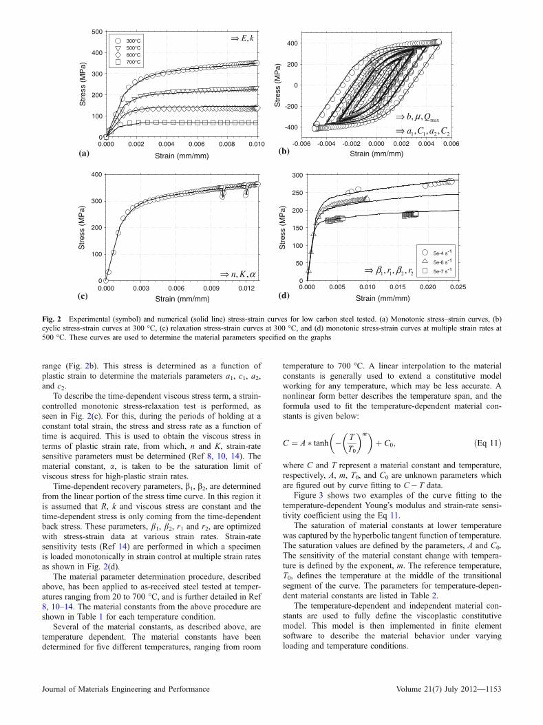
range (Fig. 2b). This stress is determined as a function ofplastic strain to determine the materials parameters a1, c1, a2,and c2.

To describe the time-dependent viscous stress term, a strain-controlled monotonic stress-relaxation test is performed, asseen in Fig. 2(c). For this, during the periods of holding at aconstant total strain, the stress and stress rate as a function oftime is acquired. This is used to obtain the viscous stress interms of plastic strain rate, from which, n and K, strain-ratesensitive parameters must be determined (Ref 8, 10, 14). Thematerial constant, a, is taken to be the saturation limit ofviscous stress for high-plastic strain rates.

Time-dependent recovery parameters, b1, b2, are determinedfrom the linear portion of the stress time curve. In this region itis assumed that R, k and viscous stress are constant and thetime-dependent stress is only coming from the time-dependentback stress. These parameters, b1, b2, r1 and r2, are optimizedwith stress-strain data at various strain rates. Strain-ratesensitivity tests (Ref 14) are performed in which a specimenis loaded monotonically in strain control at multiple strain ratesas shown in Fig. 2(d).

The material parameter determination procedure, describedabove, has been applied to as-received steel tested at temper-atures ranging from 20 to 700 C, and is further detailed in Ref8, 10–14. The material constants from the above procedure areshown in Table 1 for each temperature condition.

Several of the material constants, as described above, aretemperature dependent. The material constants have beendetermined for five different temperatures, ranging from room

temperature to 700 C. A linear interpolation to the materialconstants is generally used to extend a constitutive modelworking for any temperature, which may be less accurate. Anonlinear form better describes the temperature span, and theformula used to fit the temperature-dependent material con-stants is given below:

C ¼ A tanh T

T0

m þ C0; ðEq 11Þ

where C and T represent a material constant and temperature,respectively, A, m, T0, and C0 are unknown parameters whichare figured out by curve fitting to C T data.

Figure 3 shows two examples of the curve fitting to thetemperature-dependent Youngs modulus and strain-rate sensi-tivity coefficient using the Eq 11.

The saturation of material constants at lower temperaturewas captured by the hyperbolic tangent function of temperature.The saturation values are defined by the parameters, A and C0.The sensitivity of the material constant change with tempera-ture is defined by the exponent, m. The reference temperature,T0, defines the temperature at the middle of the transitionalsegment of the curve. The parameters for temperature-depen-dent material constants are listed in Table 2.

The temperature-dependent and independent material con-stants are used to fully define the viscoplastic constitutivemodel. This model is then implemented in finite elementsoftware to describe the material behavior under varyingloading and temperature conditions.

Strain (mm/mm)

0.000 0.002 0.004 0.006 0.008 0.010

Str

ess

(MP

a)

0

100

200

300

400

500300°C500°C600°C700°C

,E k⇒

Strain (mm/mm)-0.006 -0.004 -0.002 0.000 0.002 0.004 0.006

Str

ess

(MP

a)

-400

-200

0

200

400

max

1 1 2 2

, ,

, , ,

b Q

a C a C

μ⇒⇒

(b)(a)

Strain (mm/mm)

0.000 0.003 0.006 0.009 0.012

Str

ess

(MP

a)

0

100

200

300

400

, ,n K α⇒

Strain (mm/mm)

0.000 0.005 0.010 0.015 0.020 0.025S

tres

s (M

Pa)

0

50

100

150

200

250

300

5e-4 s-1

5e-6 s-1

5e-7 s-11 1 2 2, , ,r rβ β⇒

(d)(c)

Fig. 2 Experimental (symbol) and numerical (solid line) stress-strain curves for low carbon steel tested. (a) Monotonic stress–strain curves, (b)cyclic stress-strain curves at 300 C, (c) relaxation stress-strain curves at 300 C, and (d) monotonic stress-strain curves at multiple strain rates at500 C. These curves are used to determine the material parameters specified on the graphs

Journal of Materials Engineering and Performance Volume 21(7) July 2012—1153

4. Validation of UMAT Code

The viscoplastic constitutive equations have been imple-mented into ABAQUS through a subroutine UMAT. A finiteelement model of uniaxial fatigue specimen was built tosimulate the experimental tensile and fatigue tests. A compar-ison of experimental and numerical stress-strain curves is usedto examine the implementation of the simulation model. Aquarter 3D finite element model is shown in Fig. 4. The

diameter of the cylindrical specimen is 6.35 mm and the gagelength is 10 mm. The block element with eight nodes was usedto mesh the geometry model. Nodes on the bottom plane werefixed in vertical direction, and symmetry boundary conditionswere applied to the nodes on two side planes. To simulate thetensile tests, nodes on the top plane were subjected to adisplacement ramping from 0 to 0.1 mm within 2000 s. Foursimulation cases were done by assigning four different uniformtemperatures to the whole model. The predicted stress-straincurves are shown in Fig. 5 and compared with the experimentalresults which show good agreement.

The quarter cylinder model was also used for the simulationof a fatigue test at 300 C. A cyclic displacement loading (seeFig. 6a) was applied to the nodes on the top plane.

The magnitude of applied displacement equals the value thatthe gage length of the model times the strain that the elementwas subjected to. The displacement loading shows three strainranges, ±0.2%, ±0.3%, and ±0.4%. Four cycles were rununder strain range ±0.2%, six cycles under strain range ±0.3%,and three cycles under strain range ±0.4%. The cyclic test ofthree strain ranges used the same loading strain rate of59 106 mm/mm/s. The period of one cycle under strainrange ±0.2% is 1600, 2400 s under strain range ±0.3%, and3200 s under strain range ±0.4%. The element stresses invertical direction were output and plotted with the strains in the

Table 1 Material parameters for as-received A572 Grade 50 low carbon steel tested at temperatures rangingfrom 20 to 700 C

Temperature 20 C 300 C 500 C 600 C 700 C

E, GPa 188 172 127 93 58k, MPa 100 71 27 11 3a1, MPa 137 96 54 36 22C1 1411 1411 1411 1411 1411a2, MPa 1864 1753 1111 566 175C2 1.15 1.15 1.15 1.15 1.15b 78 78 78 78 78Qmax, MPa 86 78 31 1 10l 1447 1447 1447 1447 1447n 14 14 14 14 14K, MPa 155 349 304 227 107a 5.5E+06 5.0E+06 1.0E+05 4.5E+00 9.9E01b1, Pa

2.58 1.0E21 9.9E20 1.0E15 1.0E15 1.0E15b2, Pa

2.15 4.6E26 2.1E16 1.0E12 1.0E12 1.0E12r1 2.58 2.58 2.58 2.58 2.58r2 2.15 2.15 2.15 2.15 2.15

Temperature (°C)0 100 200 300 400 500 600 700

E (

MP

a)

0

5e+4

1e+5

2e+5

2e+5

ExperimentalCurve Fit

Temperature (°C)0 100 200 300 400 500 600 700

Qm

ax (

MP

a)

-20

0

20

40

60

80

100

ExperimentalCurve Fit

(b)(a)

Fig. 3 Modeling of temperature-dependent material constants. (a) Youngs modulus and (b) isotropic hardening coefficient, Qmax

Table 2 Parameters in Eq 11 for temperature-dependentmaterial constants

Constant A T0 C0 m

E 187850.1 742.0 187743.8 2.8k 100.6 520.8 99.6 2.3a1 137.4 621.3 137.5 1.6a2 1830.5 619.1 1864.3 3.9Qmax 97.7 558.0 86.1 4.1K 351.7 720.1 351.5 5.4a 5.5E+06 437.3 5.5E+06 6.4b1 1.0E15 443.0 2.7E27 18.8b2 1.0E12 443.0 3.2E24 18.8

1154—Volume 21(7) July 2012 Journal of Materials Engineering and Performance

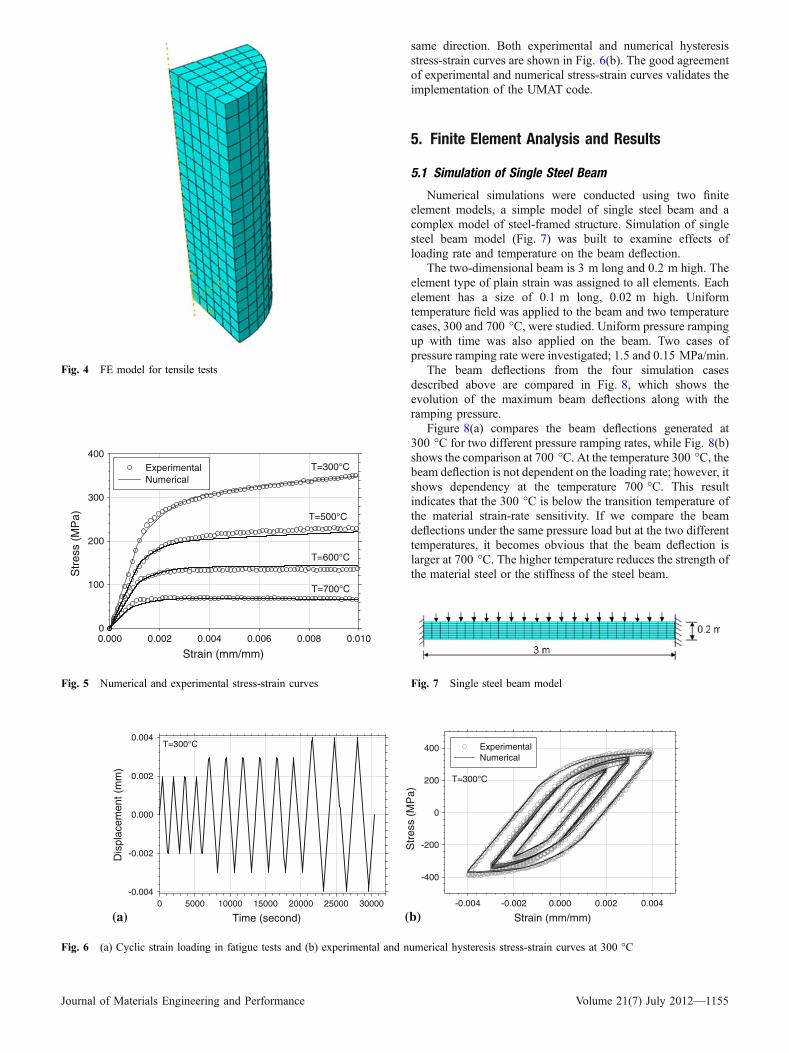
same direction. Both experimental and numerical hysteresisstress-strain curves are shown in Fig. 6(b). The good agreementof experimental and numerical stress-strain curves validates theimplementation of the UMAT code.

5. Finite Element Analysis and Results

5.1 Simulation of Single Steel Beam

Numerical simulations were conducted using two finiteelement models, a simple model of single steel beam and acomplex model of steel-framed structure. Simulation of singlesteel beam model (Fig. 7) was built to examine effects ofloading rate and temperature on the beam deflection.

The two-dimensional beam is 3 m long and 0.2 m high. Theelement type of plain strain was assigned to all elements. Eachelement has a size of 0.1 m long, 0.02 m high. Uniformtemperature field was applied to the beam and two temperaturecases, 300 and 700 C, were studied. Uniform pressure rampingup with time was also applied on the beam. Two cases ofpressure ramping rate were investigated; 1.5 and 0.15 MPa/min.

The beam deflections from the four simulation casesdescribed above are compared in Fig. 8, which shows theevolution of the maximum beam deflections along with theramping pressure.

Figure 8(a) compares the beam deflections generated at300 C for two different pressure ramping rates, while Fig. 8(b)shows the comparison at 700 C. At the temperature 300 C, thebeam deflection is not dependent on the loading rate; however, itshows dependency at the temperature 700 C. This resultindicates that the 300 C is below the transition temperature ofthe material strain-rate sensitivity. If we compare the beamdeflections under the same pressure load but at the two differenttemperatures, it becomes obvious that the beam deflection islarger at 700 C. The higher temperature reduces the strength ofthe material steel or the stiffness of the steel beam.

Fig. 4 FE model for tensile tests

Strain (mm/mm) 0.000 0.002 0.004 0.006 0.008 0.010

Str

ess

(MP

a)

0

100

200

300

400Experimental Numerical

T=300°C

T=500°C

T=600°C

T=700°C

Fig. 5 Numerical and experimental stress-strain curves

Time (second)0 5000 10000 15000 20000 25000 30000

Dis

plac

emen

t (m

m)

-0.004

-0.002

0.000

0.002

0.004T=300°C

Strain (mm/mm)-0.004 -0.002 0.000 0.002 0.004

Str

ess

(MP

a)

-400

-200

0

200

400 ExperimentalNumerical

T=300°C

(b)(a)

Fig. 6 (a) Cyclic strain loading in fatigue tests and (b) experimental and numerical hysteresis stress-strain curves at 300 C

Fig. 7 Single steel beam model

Journal of Materials Engineering and Performance Volume 21(7) July 2012—1155

5.2 Simulation of Steel-Framed Structure Under FireCondition

Finite element analysis of steel-framed structures under firecondition uses a sequentially coupled thermal-stress analysis(Ref 15). In this analysis, a transient heat transfer analysis isfirst performed to obtain temperature distribution history, andthen a stress/deformation analysis is conducted to obtainstructural deformation. Nodal temperatures are calculated in thetransient heat transfer analysis and stored as a function of timein the heat transfer result file. The stress analysis uses the samegeometry model with the same meshing as the heat transferanalysis. The temperature fields for the stress analysis arecoupled with temperature results from transient heat transferanalysis.

A three-dimensional model of a multi-story structure wasbuilt, the dimensions of which are shown in Fig. 9.

The structure has two cells with eight box-shape columnsand eight I-shape beams. Each column is 12 m high and eachbeam is 15 m long. The dimensions of the column and beamcross sections are shown in Fig. 9. We consider the beams andcolumns to be integral. Eight-node block elements were used tomesh the structure as shown in Fig. 10.

The element size is 0.5 m in longitude direction of beam andcolumn, and <0.04 m in their transverse direction. The totalnumber of elements is 19,136.

5.2.1 Heat Transfer Analysis. The finite element modelwas first employed to conduct transient heat analysis. Thematerial properties required for heat transfer analysis are shownin Table 3.

The element type was set as DC3D8 for heat transfer analysis.The room temperature 25 C was assigned to the steel-framestructure as the initial condition. A surface heat flux of 16 kW/m2

was applied on the bottom plane of one beam in the first floor, and24 kW/m2 on the side plane of its connected column in order tosimulate the appearance of a fire in the cell (see Fig. 11).

The heat transfer duration is 1 h. The calculated tempera-tures at all nodes and at different time are stored in the outputfile of heat transfer analysis. The output frequency of nodaltemperatures is 0.2 Hz.

Figure 12 shows the temperature distribution after 1 h ofheat transfer. The non-uniform temperatures across the sectionsof steel frames were observed.

The higher temperature occurred to the positions near thesurface where external heat flux was applied. Within 1 h, the

Pressure load (MPa)

0 2 4 6 8

Def

lect

ion

(mm

)

0

5

10

15

20

25

1.5 MPa/min0.15 MPa/min

Temperature = 300°C

Pressure load (MPa)0.0 0.5 1.0 1.5 2.0 2.5 3.0

Def

lect

ion

(mm

)

0

20

40

60

80

100

120

140

160

180

1.5 MPa/min0.15 MPa/min

Temperature = 700°C

(b)(a)

Fig. 8 Beam deflection at two loading rates (a) at temperature 300 C and (b) at temperature 700 C

Fig. 9 FE model of a 3D steel-framed structure under fire condition

1156—Volume 21(7) July 2012 Journal of Materials Engineering and Performance

heat spread was confined in the mid cell of the first floor.Positions far away from the surface where the heat flux came inalmost maintained their initial temperature of 25 C. Figure 13and 14 show the temperature history at seven points on theheated beams and columns cross sections, respectively.

The temperature at the monitored positions increases withtime since the continuous heat flow increase the thermal energyof the structure. For the beam, the temperatures at points B1and B2 are higher than those at points B3, B4, and B5, andmuch higher than those at points B6 and B7. For the column,the temperatures at points C1 and C2 are higher than those atpoints C3, C4, and C5, and much higher than those at C6 andC7. Although B1 and B2 are on the same heat flux surface,their temperatures are different. The temperature at B1 is higherthan that at B2 because the position B2 is nearer to the web,which is the heat transfer path.

5.2.2 Stress/Deformation Analysis. In the stress/defor-mation analysis, the element type was changed from heattransfer type to stress analysis type C3D8, while the geometry

remained the same. The developed UMAT was used as thematerial model. The four columns were fixed at their roots. Auniform pressure was applied on all beams and temperaturefield was assigned to the whole structure. The simulationconsists of three loading steps. The first step is to increase theuniform pressure from 0 to 0.04 MPa in 10 s, while keepingthe temperature constant at 25 C. In the second step, themaximum pressure loading is maintained and the temperaturefield is coupled with the results obtained from the transient heattransfer analysis, and hence the duration of step 2 is 60 min. Inthe third step, both the pressure and temperature distribution inthe structure is held constant for 30 min. Therefore, staticstress/deformation analysis was performed with a time periodof 90 min plus 10 s. The maximum time increment is 0.5 s.The control setting for the nonlinear effect of large displace-ment was activated in the simulation. The displacement, strain,and stress results along with time were output from the stressanalysis.

The final deformation of the three-dimensional two-storystructure from the stress analysis using the viscoplasticconstitutive model, discussed above, was examined. Amongthe four beams of the first floor, the beam subjected to the heatflux deflected more than other beams as expected. Figure 15shows the deflection history of two beams at the first floor (seeFig. 10).

The heated beam refers to the beam which had the heatflux applied to it, and the non-heated beam is a beamneighboring the heated beam. In the 10 s of load step 1, thedeflections of the two beams increase quickly due to theincreasing pressure load. In this step, the two beams achievedthe same amount of deflection due to geometrical symmetry,the same loading condition, and uniform structural temper-ature. In load step 2, the deflection of the heated beam doesnot increase at the beginning although its temperaturesincrease. It is concluded that the beams deflection starts toincrease when the applied load/stress becomes larger than thestrength of the beam. The applied load did not change but thebeams strength degraded with the increase of temperature.When the strength of the heated beam degraded below itsstress level, the inelastic strain occurred as shown in Fig. 16,and the beams deflection started to increase slowly initiallyand then faster with the continuously increasing of the beamstemperature.

Fig. 10 Meshing of FE model of 3D steel-framed structure

Table 3 Material properties for heat transfer analysis

Mass density Thermal conductivity Specific heat

7800 kg/m3 50 J/m2 C 470 W/kg C

Fig. 11 Surface heat flux as thermal loading applied to the structure

Journal of Materials Engineering and Performance Volume 21(7) July 2012—1157

In load step 3, the applied loading and the temperaturedistribution did not change (actually the applied stress relaxed asshown in Fig. 16), but the heated beams deflection continued to

increase. The deflection increase in load step 3 was attributed tothe creep deformation (that is, material strain-rate sensitivity) atelevated temperatures, which can be shown in Fig. 16.

Fig. 12 The final temperature distribution in the structure

Time (seconds)

0 1000 2000 3000

Tem

pera

ture

(°C

)

0

200

400

600

B1B2B3 B4B5B6B7

B1 B2

B3 B4

B6 B7 B5

Fig. 13 Temperature history of seven points on the beams cross section

Time (seconds)

0 1000 2000 3000

Tem

pera

ture

(o C

)

0

200

400

600C1 C2C3 C4C5 C6C7

C1

C2 C3C4

C5

C6

C7

Fig. 14 Temperature history of seven points on the columns cross section

1158—Volume 21(7) July 2012 Journal of Materials Engineering and Performance

6. Conclusions

The work in this article describes a viscoplastic constitutivemodel that has been employed to simulate the flow behavior ofstructural steel A572 Grade 50 steel at elevated temperatures.The material constants of the model have been fitted as afunction of temperature, thus allowing the implementation ofthe corresponding constitutive equations in a UMAT subroutineof the ABAQUS platform The validation of the UMAT hasbeen carried out by comparing the experimental data with thoseobtained from the numerical simulations under the sameapplied load conditions. The finite element analysis of athree-dimensional steel-framed structure under fire conditionhas been performed using a simulation strategy of sequentiallycoupled thermal-stress analysis. The general conclusions of thisstudy can be listed as follows:

1. The nonlinear material behavior of the low carbon struc-tural steel at elevated temperatures can be captured by uni-fied constitutive equations, which consist of a nonlinearkinematic hardening model and a hyperbolic function forthe modeling of temperature-dependent material constants.

2. The steel shows a transition temperature for the time-dependent plastic deformation. The strain-rate sensitivitytransition is indicated by the trend of temperature-depen-dent material constants.

3. The heat transfer analysis of the 3D steel-frame structureshows the temperature distributed nonlinearly across thesections of the steel frame and along the length of beamsand columns.

4. As the temperature increases, large bending or bucklingdeformation could occur to the steel-frame structure as aresult of the degradation of the materials strength belowthe applied stress level.

5. The time-dependent material behavior contributes to thestructures bending or bucking when the applied tempera-ture is higher than the strain-rate sensitivity transitiontemperature.

References

1. J.Y. Liew, L.K. Tang, T. Holmaas, and Y.S. Choo, Advanced Analysisfor the Assessment of Steel Frames in Fire, J. Constr. Steel Res., 1998,47, p 19–45

2. P. Makelainen, J. Outinen, and J. Kesti, Fire Design Model forStructural Steel S420M Based Upon Transient-State Tensile TestResults, J. Constr. Steel Res., 1998, 48, p 47–57

3. G.Q. Li and S.C. Jiang, Prediction to Nonlinear Behavior of SteelFrames Subjected to Fire, Fire Saf. J., 1999, 32, p 347–368

4. Y.C. Wang, T. Lennon, and D.B. Moore, The Behavior of Steel FramesSubject to Fire, J. Constr. Steel Res., 1995, 35, p 291–322

5. P. Kumar, V.V. Nukala, and D.W. White, A Mixed Finite Element forThree-Dimensional Nonlinear Analysis of Steel Frames, Comput.Methods Appl. Mech. Eng., 2004, 193, p 2507–2545

6. S.R. Najjar and I.W. Burgess, A Nonlinear Analysis for Three-Dimensional Steel Frames in Fire Conditions, Eng. Struct., 1996,18(1), p 77–89

7. J.L. Chaboche and G. Rousselier, On the Plastic and ViscoplasticConstitutive Equations—Part I: Ruled Developed with Integral Vari-able Concept, Trans. ASME J. Press. Vessel Technol., 1983, 105,p 123–133

8. D. Nouailhas, Unified Modeling of Cyclic Viscoplasticity: Applicationto Austenitic Stainless Steels, Int. J. Plast., 1989, 5, p 501–520

9. J.L. Chaboche and G. Rousselier, On the Plastic and ViscoplasticConstitutive Equations—Part II: Application of Integral VariableConcepts to the 316 Stainless Steel, Trans. ASME J. Press. VesselTechnol., 1983, 105, p 159–164

10. J.L. Chaboche, Constitutive Equations for Cyclic Plasticity and CyclicViscoplasticity, Int. J. Plast., 1989, 5, p 247–302

11. A.S. Zaki and H. Ghonem, Modeling the Ratcheting Phenomenon in anAustenitic Steel at Room Temperature, Proceeding of the ASME 2000Design, Reliability, Stress Analysis and Failure Prevention Conference(Baltimore, MA), 2000

12. K. Maciejewski, Y. Sun, O. Gregory, and H. Ghonem, Deformation andHardening Characteristics of Low Carbon Steel at Elevated Temper-ature, Material Science and Technology Conference and Exhibition(Pittsburgh, PA), October 2008

13. D. Nouailhas, A Viscoplastic Modelling Applied to Stainless SteelBehavior, Proceedings of the Second International Conference onConstitutive Laws for Engineering Materials: Theory and Application,January 5–8 (Tuscon, AZ), 1987, p 717–724

14. J. Lemaitre and J.L. Chaboche, Mechanics of Solid Materials,Cambridge University Press, Cambridge, 1990

15. ABAQUS Inc. ABAQUS Standard Users Manual, 6.6 ed., 2006

Time (minutes)0 20 40 60 80 100

Def

lect

ion

(mm

)

0

10

20

30

40

50

Midspan of heated beamMidspan of nonheated beam

Fig. 15 The deflection history at the midspan of the heated andnon-heated beams

Time (minutes)0 20 40 60 80 100

Str

ain

(mm

/mm

)

0.0000

0.0001

0.0002

0.0003

0.0004

0.0005

Str

ess

(MP

a)

0

10

20

30

40

50

60

Strain at heated beam midspanStress at heated beam midspan

Fig. 16 Strain and stress history at the midspan of the heated beam

Journal of Materials Engineering and Performance Volume 21(7) July 2012—1159

Deformation Criterion of Low Carbon Steel Subjected to High Speed Impacts

W. Visser, G. Plume, C-E. Rousseau, O. Gregory*, H. Ghonem 92 Upper College Road, Kingston, RI 02881

Department of Mechanical Engineering *Department of Chemical Engineering

University of Rhode Island Abstract A study has been carried out to examine effects of blast loading on the microstructure deformation response of A572 Grade 50 low carbon structural steel. Symmetrical planar impact experiments have been carried out using a single stage gas gun to drive projectiles to velocities between 200 and 500 m/sec resulting in low to moderate shock loading of disc type steel specimens. Longitudinal stress histories of the impacted specimens were captured at the back face of the loaded specimens with the use of manganin gages. A constitutive model was employed to numerically simulate the particle velocity at the impact surface as well the pressure distribution across the specimens as a function of impact duration. An analytical approach utilizing a deformation model was used to link twin volume fraction to blast severity. Post-mortem analysis was carried out on the impacted specimens with the use of optical and scanning microscopy in order to correlate the severity of the impacts with development of twinning within the microstructure. A comparison between the analytically calculated and experimentally measured twin volume fraction was used to optimize the material and deformation models and establish a correlation between impact pressure and deformation response of the steel under examination. Introduction Impact loading of steel is a subject that has been studied widely for structural applications and material characterization. It has been established that high strain rate loading of steel will result in a change of both microstructural and mechanical properties which individually affect the residual life of the material. Vast amounts of research has been done in order to assess blast loading and deformation effects, much of it being on steel as it is a primary reinforcing phase of structures. Research in blast analysis, while in general utilizes the finite element technique to provide solutions for the dynamic response of the structures [1], requires implementation of microstructure constitutive models is required to accurately capture changes in mechanical properties during high strain rate loading. In order to replicate the pressure profile and high strain rate deformation caused by explosive loading and recover large intact specimens, various techniques exist of which Field et al. [2] provide a detailed review. To achieve the highest velocities, above 1km/s, two and three stage gas guns are used. These techniques are typically used for obtaining Hugonoit curves, measuring spall strength, post-impact mechanical testing, and measuring phase change, the latter of which is the concern of the work presented herein. The phase change of the material is of particular interest in material investigation and has been incorporated into analytical modeling in order to predict deformation response. De Resseguier and Hallouin [3] studied iron disks of different thickness submitted to shock loading by means high-power laser pulses. Post shock studies of the iron microstructure revealed significant twin formation. Using a constitutive twinning model proposed by Johnson and Rohde [4] accurate predictions of twin volume fraction and elastic-plastic response of the material have been made. Johnson and Rohde [4] proposed a mathematical model to describe deformation by slip and twinning based upon the laws of mass and momentum conservation. Plate impact experiments were used to examine shock-loaded iron and analytically predict twin volume fraction in recovered specimens as a function of impact stress. The objective of this study is to establish the effect of moderate shock loading up to strain rates of 105 s-1, on the microstructure deformation mechanisms of low carbon steel. This objective will be achieved by identifying a deformation criterion based on microstructure response to blast loading. This will be examined by subjecting discs of low carbon steel to high velocity impact loading using a light gas gun. Impact specimens will be analyzed

Proceedings of the IMPLAST 2010 ConferenceOctober 12-14 2010 Providence, Rhode Island USA

© 2010 Society for Experimental Mechanics, Inc.

by measurement of microstructural variations and mechanical properties. Attempts will be made to study the deformation pattern in steel using material and deformation models. Results of this analysis will be linked with the experimental work in order to asses the validity of the approach. In this paper, we present the experimental procedure used to impact the steel specimens and experimental observations of microstructure. In addition, numerical methods and analytical modeling of dynamic deformation based on slip and twinning are described, and results are compared with experimental findings. Material and Experimental Procedure

The as received microstructure of A572 grade 50 low carbon steel is body center cubic structure which consists of primarily -ferrite phase with colonies of pearlite; Figure 1. Preparation of all specimens was done by mechanical polishing to 1 micron and chemical etching using 5% nital solution for 8 seconds. [5]

60 m60 m

Figure 1. Micrograph of as received A572 grade 50 structural steel. This material was prepared into round discs by electro discharge machining (EDM) and tested by subjecting it to different impact loads using a single stage light gas gun. A series of five plate impact experiments have been carried out using a single stage light gas gun. Fixed back conditions were employed in order to minimize energy loss and provide means for recovering post impact specimens. Figure 2 provides an illustration of the experimental gas gun and target set up. The projectile measurements are 31.75mm diameter and 3mm thick, while the target disk and backing plate measurements are 57.15mm diameter and 6mm thick. The target dimensions allowed for tensile specimens to be machined from deformed specimens for post impact mechanical testing.

Figure 2. Photograph of a.) the experimental light gas gun and b.) the target and fixed back holder Projectile velocities ranging from 200 to 500 m/sec were measured using two lasers which were mounted perpendicular to the projectile and in front of the target. Input pressure was used to control projectile velocities and magnitude of impact loads. Longitudinal stress histories were recorded using manganin stress gauges bonded centrally between the back surface of the target disk and a steel backing plate. Figure 3 shows a typical stress vs. time record obtained from the back surface of the target disk during an impact.

Stress Gauge

Target

Velocity Lasers

Gas GunGas Gun barrel

Pressure Chamber a b

0

2

4

6

8

0.0 0.5 1.0 1.5 2.0 2.5 3.0Time (micro sec)

Nor

mal

Str

ess

(GPa

)

405 m/s Impact

Figure 3. Impact Stress recorded with manganin gauge at the back surface of target disk during a 405 m/s impact The curve from figure 3 will be compared to numerical results and used as a reference for optimizing simulation parameters. As a reference, particle velocity profiles of the target impact surface will be used as an input into analytical constitutive equations.

Experimental Results

Post impact target specimens revealed plastic deformation in the impacted area and back surface as well as increase in total diameter. The area of impact was discolored suggesting a large and rapid increase in temperature on the front surface during impact; Figure 4.

Figure 4. Impacted steel target specimen and deformed projectile

Specimen surfaces were ground flat using a surface grinder under coolant, and polished and etched. Optical microscopy was conducted on post impact test specimens and the results show the presence of mechanical twins within the -ferrite grains; see Figure 5. Micrographs of the cross-section just below the impact surface showed a lack of twins, which is evidence that temperature rise was high enough to suppress twin formation in the contact region.

37.15 mm dia. 57.15 mm dia.

3 mm6 mm

Figure 5. Example of optical micrographs of post impact steel specimens a.) 7 GPa peak stress yielding 3.4% twins, b.) 9 GPa peak stress yielding 4.3% twins.

Results of these optical micrographs show that all of the twins are of lenticullar shape, which is indicative of the mechanism by which the twins form. The majority of the grains have parallel twins extending between grain boundaries. However, there are also large amounts of twin-twin interaction in which twins terminate at other twins, or continue through the intersections, which suggests formation on multiple planes. Volume fraction of the twins was calculated using ASTM E562-05, standard test method involving systematic manual point count method. This count provides an average estimation of twin volume fraction which was correlated to impact stress, as illustrated in Figure 6. Figure 6 and Figure 8 show that twin volume fraction and macro hardness are both positively correlated to impact stress.

50.00

51.00

52.00

53.00

54.00

55.00

56.00

0 2 4 6 8 10

Impact Stress (Gpa)

Roc

kwel

l HR

A (6

0)

Figure 6. Post-impact macro hardness as a function of impact stress

The increase in hardness, which indicates an increase in yield strength of the material, can be attributed to strain hardening, as described by Maciejewski [5], and to twin-matrix interfaces, which provide additional barriers for further dislocation slip. There may exist a unique relationship between the twinning and hardness properties, however since hardness also increases in the absence of twinning, no attempt has been made from this study to examine the unique relationship between hardness and twinning. Numerical and Analytical Analysis

Finite element simulation using Abaqus dynamic explicit analysis was used to model plate impacts. Simulation of impact conditions provides knowledge of impact wave parameters as well as a description of the blast related stress distribution within the impacted steel. Inputs parameters for boundary and loading conditions are obtained from experimental procedures. From the simulation, the longitudinal stress distribution is matched with experimental stresses recorded. Once good correlation exists between numerical and experimental outputs, particle velocity history at the impact surface is extracted from numerical results and used as an input for

60 m60 m60 m60 ma b

analytical modeling of twin volume fraction as a function of impact loading. In order to obtain stress histories in accordance with experimental results, parameters for a rate dependent model were required. The built in Johnson-Cook material model [6] was used to express the equivalent Von-Mises tensile flow stress as a function of the equivalent plastic strain, strain rate, and temperature. Values for constants were optimized using a room temperature stress-strain curve of the as received material [5]. Numerical stress history of the target specimen during impact show comparable profiles to experimental impact results. In this profile, three important components which must be captured accurately, pressure rise time, impact duration, and maximum stress, all exhibit good fits with experimental data. Figure 7 shows a numerically generated stress profile during impact at the back surface of the target specimen compared with experimental results.

0

2

4

6

8

10

0 0.5 1 1.5 2 2.5time (micro seconds)

Nor

mal

Str

ess

(GPa

)

ExpNum

Figure 7. Experimental and numerical stress history at the back of the target specimen.

Cross slip and dislocation coalescence proposed by Sleeswyk provides a basis for a mechanistic model governing twin formation and has been confirmed by Mahajan [8]. The model proposed by Johnson and Rohde [4] incorporates slip and twinning mechanisms described [7,8] and accurately calculates twin volume fraction of low carbon b.c.c. steel for the given loading conditions. In order to analytically predict twin volume fractions, a modified form of a model based on the work of Johnson and Rohde [4] was applied here. Lenticullar shape of twins suggests formation by progressive shear of the lattice [7] in which slip must be present in order for twin formation to occur [8]. Johnson and Rohde [4] examined shock-loaded iron in order to analytically predict twin volume fraction in recovered specimens. They state that twin formation is based upon proportional shear of the lattice rather than local shuffling of the atoms and twin formation is preceded by corresponding dislocation multiplication. The assumptions and observation from this study are described in the constitutive model in which total plastic strain is composed of both dislocation slip and deformation twinning, and the twin volume fraction and growth rate are functions of corresponding shear stress. The dynamic response and deformation twinning of low carbon steel under impact loading is described by the laws of mass and momentum conservation. Analytical twin volume fractions were calculated using this model for each impact condition using a critical shear stress criterion. An average bulk material value was determined and compared to experimental results; see Figure 8.

0

0.5

1

1.5

2

2.5

3

3.5

4

4.5

5

0 2 4 6 8 10Impact Stress (Gpa)

Twin

Vol

ume

Frac

tion

(%)

Exper

Model

Figure 8. Comparison of experimentally measured and analytically computed twin volume fraction as a function

of impact stress. Analytical model predictions show similar trends to experimental measurements for the given stress range. The linearity of the experimental and calculated data in Figure 8 apparently deviates from this trend at higher stresses as the twins begin to saturate in the material, or other deformation mechanisms begin to play a role. While the relationship between impact stress and twin volume fraction may be satisfied within the given conditions, shear banding and phase transformation have been observed to occur at extremely high pressures [9,10], and the criteria may no longer be valid. Further study of the material at higher stresses and strain rates are needed to develop the relationship further and set limits for its accuracy. Conclusions The objective of the study is to present a correlation between high rate impact and microstructure variation of low carbon steel. Five plate impact experiments were carried out and post impact microscopy shows deformation mechanisms occurring during shock loading of low carbon b.c.c. steel. The coupling of numerical simulations and the analytical constitutive model act as a tool for defining impact history and predicting post-impact microstructure. Results of this study can be briefly summarized as follows:

1. Impact experiments indicated that slip and mechanical twinning are two competing deformation mechanisms occurring during high rate loading of b.c.c. low carbon steel.

2. A direct and unique relationship between impact stress and volume fraction of twins has been experimentally established.

3. Microscopic observations of lenticullar deformation twins formed on multiple planes within each grain indicate the twinning mechanism. This formation mechanism was used as a basis for selection of an analytical model aiming at predicting twin volume fraction.

4. The analytical model incorporates both slip and twinning mechanisms and accurately calculated twin volume fraction. This model was coupled with a rate dependent model implemented into numerical procedures and was capable of capturing deformation response and twin formation during impacts for the given stress range.

Acknowledgements This project has been fully funded by the Department of Homeland Security Center of Excellence: Explosives Detection, Mitigation, and Response at the University of Rhode Island. References 1. Liew. “Survivability of steel frame structures subject to blast and fire.” Journal of Constructional Steel Research. 64 (2008) 854-866.

2. Field, Walley, Proud. “Review of experimental techniques for high rate deformation and shock studies.” International Journal of Impact Engineering. 30 (2004) 725-775. 3. De Resseguier, Hallouin. "Stress relaxation and precursor decay in laser shock-loaded iron." J. Appl. Phys. 84.4 (1998) 1932-38. 4. Johnson, Rohde. "Dynamic deformation twinning in shock-loaded iron." J. Appl. Phys. 42.11 (1971) 4171-82. 5. Maciejewski, Sun, Gregory, Ghonem. “Time-Dependent Deformation of Low Carbon Steel at Elevated Temperature.” (Submitted for Publication) 6. Johnson, Cook. “A constitutive model and data for metals subjected to large strains, high strain rates and high temperatures.” In: Proceedings of the Seventh International Symposium on Ballistic, La Hague, Netherlands. (1983) 541–547. 7. Wasilewski. “Mechanism of bcc twinning: Shear or shuffle?” Metallurgical Transactions. 1 (1970) 2641-2643. 8. Mahajan. “Interrelationship between slip and twinning in B.C.C. crystals.” Acta Metallurgica. 23 (1975) 671-684. 9. Dougherty, Cerreta, Pfeif, Trujillo, Gray. "The impact of peak shock stress on the microstructure and shear behavior of 1018 steel." Acta Materialia 55 (2007): 6356-6364. 10. Firrao. ”Mechanical twins in 304 stainless steel after small-charge explosions.” Materials Science and Engineering. A 424 (2006) 23-32.

Di

Wa

b

a

ARRAA

KLSITP

1

fbairmpudmc

diett

0d

Materials Science and Engineering A 528 (2011) 7857– 7866

Contents lists available at ScienceDirect

Materials Science and Engineering A

jo ur n al hom epage: www.elsev ier .com/ locate /msea

eformation characteristics of low carbon steel subjected to dynamicmpact loading

. Vissera, Y. Suna, O. Gregoryb, G. Plumea, C-E. Rousseaua, H. Ghonema,∗

Department of Mechanical Engineering, University of Rhode Island, Kingston, RI 02881, USADepartment of Chemical Engineering, University of Rhode Island, Kingston, RI 02881, USA

r t i c l e i n f o

rticle history:eceived 26 November 2010eceived in revised form 19 May 2011ccepted 23 June 2011vailable online 29 June 2011

eywords:ow carbon steelhockmpact loading

a b s t r a c t

The effects of impact loading on changes in microstructure have been studied in low carbon steel. Low tomoderate shock loading tests have been carried out on steel specimens using a single stage gas gun withprojectile velocities ranging from 200 to 500 m/s. Stress history at the back face of the target specimenand projectile velocity prior to impact were recorded via manganin stress gauges and velocity lasers,respectively. A Johnson–Cook constitutive material model was employed to numerically simulate thematerial behavior of low carbon steel during impact and obtain the particle velocity at the impact surfaceas well the pressure distribution across the specimens as a function of impact duration. An analyticalapproach was used to determine the twin volume fraction as a function of blast loading. The amountof twinning within the -ferrite phase was measured in post-impact specimens. A comparison between

winningost-impact

experimental and numerical stress histories, and analytical and experimental twin volume fraction wereused to optimize the material and deformation models and establish a correlation between impact pres-sure and deformation response of the steel under examination. Strain rate controlled tensile tests werecarried out on post-impact specimens. Results of these tests are discussed in relation to the effects ofimpact loading on the yield and ultimate tensile strength as well as the hardening and strain energycharacteristics.

. Introduction

Impact loading of steel is a subject that has been studied widelyor structural applications and material characterization. It haseen established that high strain rate loading of steel will result in

change of both microstructural and mechanical properties whichndividually affect the residual life of the material. Vast amounts ofesearch has been done in order to assess blast loading and defor-ation effects, much of it being on steel as it is a primary reinforcing

hase of structures. Research in blast analysis, while in generaltilizes the finite element technique to provide solutions for theynamic response of the structures [1], requires implementation oficrostructure constitutive models required to accurately capture

hanges in mechanical properties during high strain rate loading.In order to replicate the pressure profile and high strain rate

eformation caused by explosive loading and recover intact spec-mens suitable for further testing and analysis, various techniques

xist of which Field et al. [2] provide a detailed review. Some basicechniques which are of main concern to material characteriza-ion are drop weight testing, split Hopkins pressure bar, Taylor

∗ Corresponding author. Tel.: +1 401 874 2909; fax: +1 401 874 2925.E-mail address: ghonem@egr.uri.edu (H. Ghonem).

921-5093/$ – see front matter © 2011 Elsevier B.V. All rights reserved.oi:10.1016/j.msea.2011.06.069

© 2011 Elsevier B.V. All rights reserved.

impacts, plate impacts, and explosive loading. While SHPB testsproduce elastic–plastic wave propagation, the maximum strainrates achieved are typically in the range of 104 s−1. Plate impacttests are often used to replicate explosive loading due to the factthat the strain rates, greater than 104, and planar shock wavesachieved clearly simulate that of explosive shock wave loading.During plate impacts at high velocities, a state of one-dimensionalstrain is produced until lateral release waves from the edge of theprojectile and target specimen reach the center of the impact area.To achieve the highest velocities, above 1 km/s, two and three stagegas guns are used. These techniques are typically used for obtainingHugonoit curves, measuring spall strength, post-impact mechani-cal testing, and measuring phase change, the latter of which is theconcern of the work presented herein.

An important aspect in the post-impact analysis of materi-als is the phase change of the microstructure, which is generallyincorporated into analytical modeling in order to predict deforma-tion response. Recent studies, by Gregory et al. [3], of recoveredpipe bomb fragments provided basis for characterization of plaincarbon-steel subject to high rate deformation. They observed met-

allurgical variations of the steel in order to estimate explosiveloading severity. It was found that explosive loading resulted inelongation in grains in both the -ferrite and pearlite phases,intersecting slip bands and cross slip, as well as mechanical twin

7 nd En

fwiitttctldwBFtDnPtJt[aaststiaotaotsTtod

dassscmPsooWorodsuccesTMk

order to minimize energy loss and provide means for recover-ing post-impact specimens; Fig. 2c provides a schematic of theexperimental set up. The projectile measurements are 31.75 mmdiameter and 3 mm thick, while the target disk and backing plate

858 W. Visser et al. / Materials Science a

ormation. Firrao et al. [4] subjected stainless steel to plane shockave loading by means of spherical plastic explosives with vary-

ng charge weights and varying charge-target distances. Changesn microstructure on the impact surface included oxidations, par-ial melting at grain boundaries, isolated slip bands, and mechanicalwins in areas around fragment impact points. Changes through thehickness of the specimen were limited to mechanical twins in dis-ontinuous layers bordering the exposed surface, but never acrosshe entire thickness. Through X-ray analysis it was found that dis-ocation density remains unchanged, proving that deformation byislocation slip, and subsequently plastic yielding, was not reached,hich is also evident through measurement of thickness variations.ased upon observed twinning and estimated explosive pressures,irrao et al. [4] were able to calculate critical stress required forwinning, and proved that twin nucleation occurs prior to yielding.e Resseguier and Hallouin [5] studied iron disks of different thick-ess submitted to shock loading by means high-power laser pulses.ost-shock studies of the iron microstructure revealed significantwin formation. Using a constitutive twinning model proposed byohnson and Rohde [6] accurate predictions of twin volume frac-ion and elastic–plastic response of the material have been made5,7]. They used plate impacts to examine shock-loaded iron andnalytically predict twin volume fraction in recovered specimenss a function of impact stress. Atroshenko et al. [8] examined thetrengthening properties of materials, including copper, aluminum,itanium, and steel, due to spherical loading by means of explo-ives, and uniaxial loading using a light gas gun. The strength ofhe material was measured as a function of distance from thempact using microhardness measurements. In all materials exceptluminum, microstructure refinement and increases in hardnessccurred. Smida and Bosansky [9] provide experimental and frac-ographical analysis of ferritic structural steel in order to provide

correlation between the role of deformation twins and modef fracture. Tensile and Charpy impact tests were carried out andhe occurrence of deformation twins on the fracture surface weretudied. Murr et al. [10] observed profuse mechanical twinning inantalum when subjected to shock wave deformation of magni-udes up to 45 GPa. From post-impact testing, shock hardening wasbserved which have been attributed to twins as barriers to plasticeformation.

Deformation in BCC materials by means of shock loading isescribed as being composed of the competing mechanisms of slipnd twinning. Murr et al. [10] rationalize that critical twinningtress is highly dependent upon and directly proportional to thetacking-fault energy. Their work examined twin formation duringhock loading and twinning effect on the post-shock mechani-al response of Tantalum. Murr et al. found that twinning wasore predominant at the impact surface than at the back surface.

ost-shock testing consisted of quasi-static and dynamic compres-ion tests as well as microhardness measurements. The rationalef slip–twinning transition was explained through experimentalbservations and a mechanistic model proposed by Armstrong andorthington. A model was presented to predict the critical thresh-

ld stress for twin initiation which is based upon the Swegle–Gradyelationship, grain-size and temperature. Meyers et al. [11,12] rec-gnize the fact that twin initiation and growth is closely tied toislocation motion which is highly strain rate and temperatureensitive. They note that twinning can have two significant effectspon plastic deformation; it increases the work hardening rate byreating more barriers, effectively subdividing the grains, and itontributes to plastic deformation due to twinning shear. Mey-rs briefly describes the effects of strain rate, temperature, grain

ize, texture, and stress state effects upon twinning nucleation.he model used is based upon a similar theory for FCC material inurr’s study of Tantalum [10], in which dislocation pile-ups are a

ey aspect to twin nucleation. Equations for critical shear stress for

gineering A 528 (2011) 7857– 7866

twining are presented for BCC, FCC, and HCP materials, all of whichare dependent upon strain rate, temperature, and the Hall–Petchrelation for grain size. They describe that the twins per grain is afunction of stress which is independent of temperature and strainrate and the amount of twins will increase monotonically withincreasing stress. The evident common aspect in all these works isthe twin formation in steel during high strain rate loading. A corre-lation, however, does not exist between blast conditions, i.e. strainrate and stress state, and twin volume fraction, from which a uniquecriteria defining material integrity can be established. This criterionis the objective of this study. For this purpose, the effect of blastloading up to strain rates of 105 s−1, on the microstructure defor-mation mechanisms of low carbon steel will be examined. Discsof low carbon steel were subjected to high velocity impact loadingusing a light gas gun. Impact specimens were analyzed by mea-surement of microstructural variations and mechanical properties.Attempts are made to study the deformation pattern in steel usingmaterial and deformation models. Results of this analysis are linkedwith the experimental work in order to assess the validity of theapproach. Prediction of impact loading conditions will be achievedthrough a relationship between twin volume fraction and impactstress history and linked to post-impact mechanical properties. Anexperimental procedure was used to impact low carbon steel speci-mens and experimental observations of microstructure. In addition,numerical methods used and means of obtaining accurate resultsare described. An analytical model of dynamic deformation basedupon slip and twinning is described and results are compared withexperimental findings.

2. Material and experimental procedure

The as received microstructure of the low carbon steel, asshown in Fig. 1, consists of primarily -ferrite phase with coloniesof pearlite. The pearlite colonies are made of ferrite and Fe3Ccementite lamellas; Fig. 1. Average grain size is 50 m with 9%volume fraction of the pearlite phase. Tensile tests of as receivedmaterial showed yield strength of the material to be 348 MPaat 0.2% offset at room temperature with a Young’s modulus of197 GPa. Preparation of all specimens was done by mechanicalpolishing to 1 m and chemical etching using 5% nital solution.This material was prepared into round discs by electro dischargemachining and tested by subjecting it to different impact loadsusing a single stage light gas gun. A series of five plate impactexperiments have been carried out using a single stage light gasgun; Fig. 2a. Fixed back conditions, Fig. 2b, were employed in

Fig. 1. Optical Micrograph of as received A572 grade 50 structural steel. Lightergrains are -ferrite, and darker grains are pearlite.

W. Visser et al. / Materials Science and Engineering A 528 (2011) 7857– 7866 7859

atus f

mdd

utpoamo

ietpt

Fig. 2. (a.) Photograph of experimental gas gun. (b.) Fixed back appar

easurements are 57.15 mm diameter and 6 mm thick. The targetimensions allowed for tensile specimens to be machined fromeformed specimens for possible mechanical testing.

Projectile velocities ranging from 200 to 500 m/s were measuredsing two lasers which were mounted perpendicular to the projec-ile and in front of the target. Input pressure was used to controlrojectile velocities and magnitude of impact loads. Input pressuref Helium gas was used to control projectile velocities and achiev-ble stress levels. Longitudinal stress histories were recorded usinganganin stress gauges bonded centrally between the back surface

f the target disk and a steel backing plate.Typical results of normal stress versus time curves are shown

n Fig. 3, for the five different impact velocities. These curves, gen-rated from data recorded from the back surface of the impactedarget disk, are characterized by four distinct features; the elastic

recursor, the plastic wave, the peak stress level and duration, andhe unloading wave. The Hugonoit elastic limit, HEL, which is the

Fig. 3. Impact stress data recorded at the back surface of target disk.

or plate impact tests. (c.) Schematic of gas gun and target apparatus.

amplitude of the initial elastic wave, is related to the shear stress,, through the relation:

HEL = 2[

1 −

1 − 2

](1)

where is Poisson’s ratio. From the impact stress–time histories,the elastic limit for all curves is reached at 1 GPa. A HEL of 1 GPacorresponds to a 0.285 GPa maximum resolved shear stress, and forshear stress greater than this, it is suggested that dislocation slipaccommodates plastic deformation [6].

The time between impact and that at which the stress gauge atthe back surface begins to register the elastic wave can be estimatedusing the velocity of the elastic precursor. The wave speed of theelastic precursor, CElastic, is described as [13]:

CElastic =

√E(1 − )

(1 + )(1 − 2)(2)

where E, and are the elastic modulus and material density, respec-tively. Using the calculated elastic wave speed with a 6 mm thickspecimen, the elastic wave will reach the back surface in 1.03 s. Ifthe projectile and target are of the same material, identical waveswill simultaneously propagate in both. The projectile will stay incontact with the specimen until the elastic wave in the projectilereflects off of the free surface and returns to the contact surface. Theprojectile and target will remain in contact for the time duration,tContact, determined as [13]:

tContact = 2LP

CElastic(3)

where LP is the projectile thickness. Since the projectile is half thethickness of the target specimen, they will separate in the sametime the elastic wave reaches the back of the target, at 1.03 s.

Each of the stress–time curves shown in Fig. 3 will be comparedto that obtained numerically as will be detailed in a later section,

for the same impact condition and will be used as a reference forobtaining particle velocity at the impact surface. Simulated par-ticle velocity of the target impact surface will be used as an inputinto analytical constitutive equations formulated as the basis of the

7860 W. Visser et al. / Materials Science and Engineering A 528 (2011) 7857– 7866

F peak sa ns.

Jf

3

twitwaswsst

awtlofcsalh

satreat

4

cvm

TP

material constants to characterize the strain hardening behaviorof the material; C is the material constant to describe the strainrate effect; m is the material constant to describe the temperaturedependency. Values for material constants, Table 2, were optimized

ig. 4. Example of optical micrographs of post-impact steel specimens: (a.) 7 GPa

re -ferrite, and darker grains are pearlite; black arrows indicate deformation twi

ohnson and Rohde, in order to calculate twin volume fraction as aunction of local shear stress and time.

. Experimental results

Post-impact target specimens show that plastic deformationook place in the impacted area and back surface as accompaniedith an increase in total diameter of the target disk. The area of

mpact was discolored suggesting a large and rapid increase inemperature on the front surface during impact. Specimen surfacesere ground flat using a surface grinder under coolant, and polished

nd etched. Optical microscopy was conducted on post-impact testpecimens and the results show the presence of mechanical twinsithin the -ferrite grains; see Fig. 4. Micrographs of the cross-

ection just below the impact surface showed a lack of twins, whichuggests that the temperature rise was high enough to suppresswin formation in the contact region.

Results of these optical micrographs show that all of the twinsre of lenticullar shape, which is indicative of the mechanism byhich the twins form. The majority of the grains have parallel

wins extending between grain boundaries. However, there are alsoarge amounts of twin–twin interaction in which twins terminate atther twins, or continue through the intersections, which suggestsormation on multiple planes [14]. Volume fraction of the twins wasalculated using ASTM E562-05, standard test method involvingystematic manual point count method [15]. This count providesn average estimation of twin volume fraction which was corre-ated to impact stress, as shown in Table 1. Fig. 5 shows that macroardness is also positively correlated to impact stress.

The increase in hardness, which indicates an increase in yieldtrength of the material, can be attributed to strain hardening [16],nd to presence of twin–matrix interfaces, which provide addi-ional barriers for further dislocation slip. There may exist a uniqueelationship between the twinning and hardness properties, how-ver, since hardness also increases in the absence of twinning, nottempt has been made in this study to examine the unique rela-ionship between hardness and twinning.

. Numerical and analytical analysis

The analysis of the impact process will be carried out first byalculating the particle velocity for each impact condition. Thiselocity will then be utilized to calculate the corresponding defor-ation field and corresponding twin volume fraction.

able 1eak impact stress and measured twin volume fraction.

Impact stress (GPa) 0.00 4.34 7.05 7.63 7.30 8.90Mean twin Vf (%) 0.00 1.93 3.38 3.73 4.05 4.16

tress yielding 3.4% twins, (b.) 9 GPa peak stress yielding 4.3% twins. Lighter grains

4.1. Particle velocity simulation

Dynamic-explicit finite element simulation was used to modelplate impacts. Simulation of impact conditions provides knowl-edge of impact wave parameters as well as a description of theblast related stress distribution within the impacted steel. Inputparameters for boundary and loading conditions are obtained fromexperimental procedures. From the simulation, the longitudinalstress distribution is matched with experimental stresses recorded.Once good correlation exists, particle velocity at the impact sur-face is extracted from numerical results and used as an inputfor analytical modeling of twin volume fraction as a function ofimpact loading. In order to obtain stress histories in accordancewith experimental results, parameters for a rate dependent modelwere required. For this purpose, the Johnson–Cook (JC) constitutivemodel [17] was used to express the equivalent Von-Mises tensileflow stress as a function of the equivalent plastic strain, strain rate,and temperature. This stress is expressed as [13,17]:

= (A + Bεn)︸ ︷︷ ︸Strain hardening

[1 + C ln

(ε

ε0

)]︸ ︷︷ ︸

Strain rate effect

[1 −

(T − Tr

Tm − Tr

)m]

︸ ︷︷ ︸Temperature dependency

(4)

where is the Von-Mises tensile flow stress, which is the appliedstress in the loading direction for the uniaxial tensile test case;ε is the equivalent plastic strain, which equals the strain in theloading direction for the uniaxial tensile test case; A, B and n are

Fig. 5. Post-impact macro hardness (measured in Rockwell A scale with a majorload of 60 kg) as a function of impact stress.

W. Visser et al. / Materials Science and Engineering A 528 (2011) 7857– 7866 7861

Table 2Material properties and JC model constants for use in finite element simulation.

Young’s modulus Poisson’s ratio Density Inelastic heat fraction Specific heat

200 GPa 0.3 7850 kg/m3 0.864 0.465 kJ/(kg K)

A B C n m

umF

puyitaiaeapsttat

sp

Fc

Fv

348 900 0.032

sing a room temperature stress––strain curve of the as receivedaterial obtained from the work of Maciejewski et al. [16]; see

ig. 6.Once the parameters for Eq. (4) are optimized, simulation of the

late impact is preceded. To obtain comparable HEL during sim-lation, the constant A is adjusted from the static to the dynamicield strength of the material. In this simulation, symmetry of thempacted test specimen permits simulation of only one quarter ofhe specimen, as illustrated in Fig. 7a; however, model boundarynd loading conditions replicate that of the actual experiment, asllustrated in Fig. 7b. Step time period was 3 s and included adi-batic heating effects. The model was symmetrically bounded ondges to prevent rotation and translation on the cross-sectionalreas. The displacement and rotation of the surface of the backinglate was fixed in the axial direction corresponding to experimentaletup. The temperature of the parts and the velocity of the projec-ile were defined as a predefined field. The mesh is standard hexype element CD38R with 12,416 and 1,848 elements in the targetnd flyer plate, respectively, and is approximately 1 mm × 1 mm on

he surface and refined to 0.375 mm in the axial direction.

Numerical stress history of the target specimen during impacthows comparable profiles to experimental impact results. In thisrofile, three important components which must be captured accu-

ig. 6. Stress–strain curve of as received material plotted with JC model output. Theurve was obtained at room temperature with a strain rate of 50−6 s−1.

ig. 7. (a.) Quarter plate model of axis-symmetrical target disk, and (b.) predefinedelocity field imposed on projectile and fixed back boundary conditions on target.

0.434 1

rately, pressure rise time, impact duration, and maximum stress, allexhibit good fit with experimental data. Fig. 8 shows numericallygenerated stress profiles during impact at the back surface of thetarget specimen compared with experimental results.

Results show good correlation between rise time, peak stress,and HEL amplitude. Linear and quadratic bulk viscosity parametersin the dynamic explicit step were adjusted in order to reduce noisein the numerical solution. Furthermore, the linear and quadraticbulk viscosity parameters damp high frequency ringing and smearthe shock front across several elements to prevent collapse underhigh velocity gradients. Once good agreement between numeri-cal and experimental stress–time curves is achieved, the simulatedmaximum particle velocity at the front surface of the specimencan be used as an input for calculation of twin volume fraction.An approach to carry out these calculations is described in thefollowing section.

4.2. Twin volume fraction calculation

The twin region can be simply described as an area of stackingfaults enclosed by partial dislocations. Two ways in which thiscan occur are discussed by Wasilewski [18]. Wasilewski suggeststhat twins can form by progressive shear of the parent lattice orby a close atomic shuffle within the lattice, both of which willend in the same arrangement within the twinning planes; Fig. 9.Twinning by progressive shear of the parent lattice will produce ashear offset, of which plastic deformation results, Fig. 9a, while alocal rearrangement or shuffle will produce no shear offset, Fig. 9b.It is assumed that formation of the twin by homogeneous shearwill produce a shear offset equal to kh, where k is the strengthof the simple shear, also known as the twinning shear, and h isthe average thickness of the twin lamella. For bcc crystals thetwinning is most readily formed on the 1 1 2 planes in the(1 1 1) direction which has a twinning shear equal to 1/

√2 [6].

The two modes can be distinguished by observation of the shapeof the twins formed. Twins by shear will be lenticullar in shapewhile those created by shuffle will be prismatic [18]. Based uponthe characteristic lenticular shape of the twins formed in thisstudy, they are assumed to be produced by progressive shearof the parent lattice, as in opposition to the theory of atomicshuffle.

From the works of Wasilewski [18] and Johnson and Rohde [6],it is inherent that twins form by local rearrangement of atomsresulting in a shear offset, as opposed to local shuffling. In orderto analytically predict twin volume fraction, these two points areconsidered and a modified form of a deformation model based onthe work of Johnson and Rohde [6] was therefore applied here. Thisdeformation model incorporates slip and twinning mechanismspreviously described [18–20] and will be used to calculate twinvolume fraction in the material for the given loading conditions.The assumptions and observation from these previous studies aredescribed in the constitutive model in which total plastic strain is

composed of both dislocation slip and deformation twinning, andthe twin volume fraction and growth rate are functions of cor-responding shear stress. The dynamic response and deformationtwinning of low carbon steel under impact loading is described by

7862 W. Visser et al. / Materials Science and Engineering A 528 (2011) 7857– 7866

data m

ta

wtip

w

P

a

wε

ε

d

F[

Fig. 8. Experimental (solid line) and numerical (dashed line) stress history

he laws of mass and momentum conservation, which are writtens:

0

2

∂

∂t+ ∂u

∂X= 0 (5)

0∂u

∂t+ ∂

∂X= 0 (6)

here 0 is initial density, is an evolved density, and u is par-icle velocity during impact at time t at a distance of X from thempact surface. The stress, , component can be defined by a contactressure P, and shear stress , and is expressed as:

= P + 43

(7)

here

= (C + Su)u (8)

nd

˙ = (εt − 2 ) (9)

here is shear modulus, C and S are wave speed constants, andt is total strain in the wave direction and is given by:

t = 1 − 0

(10)

is the plastic shear strain on the plane of maximum shear stressescribed as the summation of slip and twinning strains:

= s + tw (11)

ig. 9. (a.) Twin formation by progressive shear of the parent lattice, and (b.) twin formed

18].

atching for two impact cases. Graph legends pertain to projectile velocity.

Plastic strain due to twinning, and that due to slip are expressedas:

tw = k( − ˛0) (12)

s = 12

εt − 2k − ˛0 − s

(13)

respectively, where k is twinning shear, is the volume fraction oftwins, ˛0 is initial twin volume fraction, and s is the shear stressrequired for slip. Volume fraction of twinned material is given by:

˛ =(

˛1/m0 + 1

tc

∫ t

0

v() dt

)m

(14)

where tc is characteristic time, which is a constant controlling therate of twin density, and m = 3 is for growth of twins both throughthe thickness and radial directions. The dimensionless growth rateof twins, (), is expressed as:

v() =

T− 1 ≥ T (15)

where T is shear stress required for twinning. This set of equa-tions provides a method of calculating twin volume fraction as afunction of shear stress. The results of this model in terms of aver-age twin volume fraction versus impact stress are compared with

experimental results, and are shown in Fig. 10.

Analytical model predictions show similar trends to experimen-tal measurements for the given stress range. The linearity of theexperimental and calculated data in Fig. 10 apparently deviates

by successive alternating “shuffle” of atoms by sequence +a/6[1 1 1], −a/6[1 1 1], 0

W. Visser et al. / Materials Science and Engineering A 528 (2011) 7857– 7866 7863

Fv

ftttsolsd

5

otawasFhutadm

2r

F

ig. 10. Comparison of experimentally measured and analytically computed twinolume fraction within -ferrite grains as a function of impact stress.

rom this trend at higher stresses as the twin volume fraction seemso saturate in the material, or other deformation mechanisms begino dominate. While the relationship between impact stress andwin volume fraction may be satisfied within the given conditions,hear banding and phase transformation have been observed toccur at extremely high pressures [4,21], and the criteria may noonger be valid. Further study of the material at higher stresses andtrain rates are underway by the authors in order to extend theeformation criterion and set limits for its applicability.

. Post-impact residual strength

The influence of twin volume fraction on the residual strengthf the material is examined through strain rate controlled mono-onic tensile tests and has been compared to the response of thes-received condition. For this purpose, post-impact steel discsere ground and polished flat to a nominal thickness of 3 mm

nd cut into dog-bone specimens. Geometry and dimensions of thepecimen as being cut from the impacted disc are illustrated inig. 11. Testing was carried out at room temperature using a servoydraulic mechanical test system and strain values were recordedsing a knife edge extensometer mounted in the gauge section ofhe test specimen. Testing of as-received material was carried outt two strain rates; 10−5/s and 20−5/s. Results show no strain rateependency at this rate and temperature. All post-impact speci-

ens were tested at 20−5/s.It was observed that as-received specimens began necking at

0% strain, while the post-impact specimens began necking in theange of 10–20%, depending on the impact stress history. Engineer-

ig. 11. Tensile specimen (3 mm thick) cut from impact region 2, of target disk 1.

Fig. 12. Stress–strain curves of as-received material tested at strain rates of 10−5/sand 20−5/s.

ing stress–strain curves for the as-received material are presentedin Fig. 12. These curves show clear upper and lower yield points,Lüders extension [22] and serrated plastic flow resembling char-acteristics of Portevin–Le Châtlier effects [23]. Despite the serratedcharacteristics, the amplitude of serration is minimal in compari-son to the magnitude of the general stress level, and is consideredinsignificant in the overall analysis of the curves. Engineeringstress–strain curves of the post-impact tensile specimens, catego-rized by impact velocity and volume fraction of twins, are presentedin Fig. 13.

Post-impact mechanical response of the material showed anincrease in yield strength and slight increase in the ultimatestrength, and a decrease in the work hardening. A comparisonbetween yield and UTS for different twin volume fractions isshown in Fig. 14.

This figure shows that as twin volume fraction increases, theyield stress approaches the ultimate strength of the material. Theconvergence of these curves indicates that the plastic hardeningcharacteristics are becoming less prominent. Figs. 14 and 15 sug-gest that an increase in twin volume fraction results in a decrease inthe ability of the material to store defects during post-impact plas-tic deformation, which is represented by the loss in work hardening[21] and in the loss of available strain energy up to UTS. Further-more, quantitative and qualitative interpretation of mechanismsgoverning elastic–plastic response and instability of the mate-rial can be made by comparing the as-received and post-impactstress–strain characteristics.

The as-received and the post-impact stress–strain curves bothexhibit serrated flow characteristics which have been observed andreported in low carbon and stainless steels [22,24]. Post-impactspecimens lack an upper and lower yield point and are charac-terized by presence of serrations. These serrations can occur inthe event of an increase in dislocation density or velocity or both[25]. This increase can be attributed to dislocations within defor-mation bands locking and unlocking and can be distinguishedby three different profiles; type-A, type-B, and type-C [25,26], asillustrated in Fig. 16. Type-A serrations are characterized by peri-odically spaced yield points which increase in size and spacingwith further straining. This process is controlled by the forma-tion and propagation of deformation bands along the gauge section[26]. Increases in stress are due to large solute atmospheres whichprevent unpinning of dislocations, while the creation of new dislo-cations suddenly decreases the stress. Each successive deformationband requires higher stress to activate. Type-B serrations are char-acterized by quickly fluctuating peaks and valleys lying along the

general level of the stress–strain curve. In this case, in contrast totype-A, the serrations are the result of the propagation of defor-mation bands rather than formation of new bands. In order tomaintain the applied strain rate, an increase in dislocation density,

7864 W. Visser et al. / Materials Science and Engineering A 528 (2011) 7857– 7866

Fig. 13. Stress–strain curves of post-impact steel specimens. Graph legends pertain to

fraction. Inset graph shows detailed view of serration characteristics.

Fig. 14. Ultimate tensile strength and yield stress of post-impact tensile specimensas a function of twin volume fraction.

Fig. 15. Residual strain energy ratio versus twin volume fraction. The ratio is inreference to the as-received condition with no twins. Strain energy is measured asarea under the curve up to strain at UTS.

projectile velocities at which the steel was impacted and resultant twin volume

and in turn, a decrease in average dislocation velocity results insegregation of solute atoms. The slow moving dislocations becomelocked rapidly until the stress increases and breaks the disloca-tion free again, thus allowing the band to propagate. This processcontinues within the deformation band until it has run throughthe entire gauge section or has encountered another band [25].Type-C serrations are characterized by distinct yield drops occur-ring below the general level of the stress–strain curve. This processis controlled by unlocking of pinned dislocations. Inhomogeneousdeformation due to stress concentrations created at barriers, suchas grain or twin boundaries, result in localized regions of a higherstrain rate. This creates additional drag on the atmosphere of dis-locations and in turn, frees dislocations and reduces the stress.The sudden availability of mobility decreases the average disloca-tion velocity in the deformation band and sets up a condition forsolute atoms to relock the dislocations and repetition of the process[25].

The type-C load drops, as well as the general softening behav-ior characterizing the post-impact stress–strain curves can beattributed to Sleeswyk’s emissary dislocation mechanism [28]. AsFig. 4b shows, several of the twins, while lenticullar shaped, haveblunted ends. This is evidence that the twinning shear is accom-modated by slip in the matrix [24]. The incoherent twin boundarycan be schematically visualized in Fig. 17. During tensile testing,slip in the matrix can emanate from available dislocations whichmake up the incoherent twin boundary; Fig. 17(a). This disloca-tion boundary supports a high energy configuration surroundingthe twin. As further straining continues, the matrix accommodatesplastic deformation by slip of these dislocations upon dissociationof every third dislocation:

16

[1 1 1] → 12

[1 1 1] − 13

[1 1 1]

as shown in Fig. 17(b). A 1/2 [1 1 1] total dislocation glides awayfrom the twin, leaving behind a 1/3 [1 1 1] complementary dislo-

cation, and drastically lowers the configuration energy. Thus, asfurther plastic deformation continues, the energy is reduced locallyallowing for dislocation pile-ups to break through the twin bound-ary, as can be seen in the stress reduction of Fig. 13c. If the matrix is

W. Visser et al. / Materials Science and Engineering A 528 (2011) 7857– 7866 7865

Fig. 16. Typical segments of a stress–strain profile with (a.) type-A, (b.) type-B, and (c.) type-C serrations.

F pla[

ntaftic

rcta

Foss

ig. 17. (a.) Incoherent twin boundary composed of twinning dislocations on 1 1 224].

ot able to accommodate the shear, then a crack may develop in thewin boundary region. The cracking can be seen in Fig. 18, as theyre formed both along the ferrite–pearlite interface, and within theerrite grains [27], both which occur parallel to the twinning direc-ion. This suggests that the presence of twins in the microstructurenfluences the not only the elastic–plastic response, but also theharacteristics of the failure mechanism.

The as-received tensile curves show type-B serrations occur-

ing from the onset of yield through the entire plastic stress–strainurve. Post-impact specimens with less than 4% twins also exhibitype-B serrated flow with a random minority of type-C load drops,s shown in detail in the inset of Fig. 13a. Fig. 13b shows, as the

ig. 18. SEM micrograph of necked region in post-impact tensile specimen. Crackingccurred along the ferrite–pearlite and twinning interfaces during post-impact ten-ile testing. All of the cracks within this region are oriented in the twinning direction,uggesting that twins play a role during fracture.

nes, and (b.) dissociation of twinning dislocation as the matrix accommodates slip

volume fraction of twins increases to 4%, the stress–strain curvetransitions from type-B to type-C serrations upon further straining[25]. A detailed view of the type-B to type-C transition is shownin the inset of Fig. 13b. Although this transition is after the UTS,it still acts as an indication that twin interactions are becoming adominant mechanism for locking mobile dislocations. As the vol-ume fraction of twins increases further, as shown in Fig. 13c, themajority of the serrations are of type-C.

Since type-C serrations occur from unlocking of pinned dislo-cations, the transition from B to C could suggest that the materialhas reached a point where all stored dislocations are locked updue to the presence of twinned regions [21]. During post-impactstraining, the networks of locked dislocations between twinnedregions break free, causing successive load drops. This change instress–strain characteristics suggests that the material has transi-tioned to a point of instability when 4% or more twins exist in themicrostructure.

6. Conclusions

The objective of the study is to present a correlation betweenhigh rate impact and microstructure variation of low carbon steel.Five plate impact experiments were carried out and post-impactmicroscopy shows deformation mechanisms occurring duringshock loading of low carbon b.c.c. steel. The coupling of numericalsimulations and the analytical constitutive model acts as a tool fordefining impact history and predicting post-impact microstructure.Results of this study can be briefly summarized as follows:

1. A direct and unique relationship between impact stress and vol-ume fraction of twins has been experimentally established.

2. Microscopic observation of impact specimens indicate that slipand mechanical twinning are two competing deformation mech-anisms occurring during high rate loading of low carbon steel.The lenticullar shape of the twins indicates that the twin forma-tion mechanism is by progressive shear of the parent lattice. Asimpact stress increases, another twinning plane becomes active,and results in large amounts of intergranular twin–twin inter-actions.

3. Based on microscopic observations, an analytical twinningmodel aiming at predicting twin volume fraction incorporat-ing both slip and twinning mechanisms has been applied andshown to accurately calculate twin volume fraction. This model

was coupled with a rate dependent model implemented intonumerical procedures and was capable of capturing deforma-tion response and twin formation during impacts for the givenstress range.

7 nd En

4

5

6

A

SR

R

[[[

[[[

[

[

[[[[

[[

[

[

866 W. Visser et al. / Materials Science a

. Quantitative analysis of the post-impact stress–strain curvesclearly shows an increase in both yield and ultimate strength,which indicates an increase in stored dislocations in themicrostructure as a result of impact loading. However, whilethe yield and UTS both benefit from shock loading, the avail-able strain energy is drastically reduced; up to 87%. If this trendis extrapolated further, it will show that the yield and ultimatetensile strength converge, thus eliminating available energy.

. It is apparent that as the shock loading is increased, new twin-ning planes are activated. Qualitative analysis provides insightinto the dislocation-twinning interaction during plastic defor-mation. Low impacted specimens reveal small fluctuations instress–strain response representing that of type-B serrations. Athigher impact levels, the presence of multiple twinning planesand twin–twin interactions results in the transition of type-Bserrations to type-C load drops during plastic deformation. Thissuggests that twin–twin interactions play a significant role incontrolling plastic deformation, which is responsible for insta-bility within the microstructure.

. The twins play an important role in the direction of crackingduring failure. They provide new interfaces at which cracks mayinitiate and propagate, and also control the direction of crackpropagation.

cknowledgment

This project has been funded by the Department of Homelandecurity Center of Excellence: Explosives Detection, Mitigation, andesponse at the University of Rhode Island.

eferences

[1] J.Y. Richard Liew, Journal of Constructional Steel Research 64 (2008)854–866.

[[

[

gineering A 528 (2011) 7857– 7866

[2] J.E. Field, S.M. Walley, W.G. Proud, H.T. Goldrein, C.R. Siviour, InternationalJournal of Impact Engineering 30 (2004) 725–775.

[3] O. Gregory, J. Oxley, J. Smith, M. Platek, H. Ghonem, E. Bernier, M. Downey, C.Cumminskey, Materials Characterization 61 (3) (2010) 347–354.

[4] D. Firrao, P. Matteis, G. Scavino, G. Ubertalli, M.G. Ienco, G. Pellati, P. Piccardo,M.R. Pinasco, E. Stagno, R. Montanari, M.E. Tata, G. Brandimarte, S. Petralia,Materials Science and Engineering A 424 (2006) 23–32.

[5] T. De Resseguier, M. Hallouin, Journal of Applied Physics 84 (4) (1998)1932–1938.

[6] J.N. Johnson, R.W. Rohde, Journal of Applied Physics 42 (11) (1971) 4171–4182.[7] J.W. Taylor, Journal of Applied Physics 36 (10) (1965) 3146–3150.[8] S.A. Atroshenko, N.S. Naumova, S.A. Novikov, International Journal of Impact

Engineering 33 (2006) 62–67.[9] T. Smida, J. Bosansky, Materials Science and Engineering A 287 (2000)

107–115.10] L.E. Murr, M.A. Meyers, Acta Materialia 45 (1) (1997) 157–175.11] M.A. Meyers, O. Vöhringer, V.A. Lubarda, Acta Materialia 49 (2001) 4025–4039.12] M.A. Meyers, D.J. Benson, O. Vöhringer, B.K. Kad, Q. Xue, H.-H. Fu, Materials

Science and Engineering A 322 (2002) 194–216.13] V. Panov, Ph.D. Thesis, Cranfield University, 2005.14] S. Mahajan, Metallurgical Transactions A 12A (1981) 379–386.15] L. Jiang, J. Jonas, R. Mishra, A. Luo, A. Sachdev, S. Godet, Acta Materialia 55 (2007)

3899–3910.16] K. Maciejewski, Y. Sun, O. Gregory, H. Ghonem, International Journal of Steel

and Iron Research (2011), in press.17] G.R. Johnson, W.H. Cook, Proceedings of the Seventh International Symposium

on Ballistic, La Hague, Netherlands, 1983, pp. 541–547.18] R.J. Wasilewski, Metallurgical Transactions 1 (1970) 2641–2643.19] J.W. Christian, S. Mahajan, Progress in Materials Science 39 (1995) 1–157.20] S. Mahajan, Acta Metallurgica 23 (1975) 671–684.21] L.M. Dougherty, E.K. Cerreta, E.A. Pfeif, C. Trujillo, G.T. Gray, Acta Materialia 55

(2007) 6356–6364.22] E. Pink, S. Kumar, Materials Science and Engineering A 201 (1995) 58–64.23] K. Renard, S. Ryelandt, P.J. Jacques, Materials Science and Engineering A 527

(2010) 2969–2977.24] Reed-Hill, E. Robert, Physical Metallurgy Principles, 2nd ed., Nostran, New York,

1973, pp. 611–660.25] D. Fahr, Analysis of stress–strain behavior of type 316 stainless steel, ORNL/TM-

4292, 1973, Oak Ridge National Laboratory Report.26] P. Rodriguez, Bulletin of Material Science 6 (4) (1984) 653–663.27] N. Narasaiah, K.K. Ray, Materials Science and Engineering A 392 (2005)

269–277.28] A.W. Sleeswyk, Acta Metallurgica 10 (1962) 803–812.

Arijit 1. O

h

2. Sencapsolutihydro

Figure

t Bose; Univ

Objective: Deealing concr

ummary: Popsulated in cion is releaseoxide to form

e 1. Conceptua

versity of Rh

evelop a clasrete

olyurethane mconcrete. Uped into the cm a C-S-H g

l framework fo

Self-He

hode Island

ss of concret

microcapsulon crack init

crack by capiel that partia

or developmen

ealing Concr

te that has au

es containintiation, the cillary action,ally heals the

t of self-healin

rete

utonomous h

ng a sodium scapsules brea, and reacts we crack.

ng concrete.

healing prop

silicate solutak. The sodiwith availab

perties – self-

tion are ium silicateble calcium

f-

Figure 2. Overall concept used in this study.

3. Accomplishments: (i) Samples with capsules located only in regions where concrete experiences

tension recover flexural strength more (58% versus 25%) after initial damage than in samples where capsules are distributed throughout.

Figure 3. Flexural strength recovery after taking sample to point of incipient failure, then waiting 7 days after which the same sample is retested.

(ii) Water containing capsules appear to be as efficient as those containing sodium silicate solution (iii) Capsules do not break during mixing, but only upon crack initiation. These experiments are detailed in the attached MS thesis by Svenja Reinke. (iv) Currently fabricating capsules that are loaded with magnetic particles and calcium nitrite, a strong anti-corrosion agent. These particles will migrate to rebars upon application of an axially directed current to the rebars. This is the MS thesis topic for Lennart Kleinfeldt. 4. Students Supported: Svenja Reinke, Lennart Kleinfeldt

5. Transition Partners: CEMEX – Brugg, Switzerland 6. Publications: (i) Self-healing Concrete, M. Pelletier, T. Bhattacharya, A. Bose, submitted to

Journal of Concrete Research, in review (2013). (ii) Optimization of Autonomous Healing Properties of Concrete Using

Microcapsules with Healing Agents, S. Reinke, L. Lozeau, A. Shukla, R. Brown, A. Bose, Journal of Concrete Research, to be submitted (2013)

7. Presentations (i) Self-healing Concrete, S. Reinke, T. Bhattacharya, A. Shukla, R. Brown, A. Bose,

DHS Center Annual Review, Kingston, April 2012.

POLYUREA/POLYURETHANE MICROCAPSULES BASED

SELF HEALING CONCRETE

BY

SVENJA KRISTIN REINKE

A DISSERTATION SUBMITTED IN PARTIAL FULFILLMENT OF THE

REQUIREMENTS FOR THE DEGREE OF

MASTER OF SCIENCE

IN

CHEMICAL ENGINEERING

UNIVERSITY OF RHODE ISLAND

2012

Library Rights Statement

In presenting this thesis in partial fulfillment of the requirements for an advanced

degree at the University of Rhode Island, I agree that the Library shall make it freely

available for inspection. I further agree that permission for copying, as provided for

by the Copyright Law of the United States (Title 17, U.S. Code), of the thesis for

scholarly purposes may be granted by the Librarian. It is understood that any copying

or publication of this thesis for financial gains shall not be allowed without my written

permission.

I hereby grant permission to the University of Rhode Island Library to use my

thesis for scholarly purposes.

_________________________

Signature

_________________________

Date

MASTER OF YOUR DEGREE THESIS

OF

SVENJA KRISTIN REINKE

APPROVED:

Thesis Committee:

Major Professor__________________________________

__________________________________

__________________________________

__________________________________ DEAN OF THE GRADUATE SCHOOL

UNIVERSITY OF RHODE ISLAND 2012

iii

ABSTRACT

In self healing concrete, the propagation of cracks in the material is prevented by

embedded microcapsules containing an aqueous self healing agent. By adding an

encapsulated aqueous solution the effect of autonomous healing of concrete is

increased. Microscope studies lead to the conclusion that the capsules do not break

upon the mixing process in the mortar production and the solution is released upon

cracking. Moreover, reflective microscope tests with colored capsules inside mortars

have shown that the capsules release their content when cracks occur. The water reacts

with unreacted calcium-hydroxide and calcium silicate particles which are present in

concrete and forms a CSH gel which seals the crack. Thus, a large portion of strength

can be recovered. The self healing technology has been improved by selective capsule

distribution to achieve a recovery of up to 58 %. SEM images gave first insights into

how the capsules appear inside a concrete like environment. Calcium nitrite containing

capsules are working well for corrosion inhibition, by releasing calcium nitrite as a

protective layer around the reinforcement bars. The presented technology is an

important contribution to the development of smart, high-performance construction

materials.

iv

ACKNOWLEDGMENTS

It is a pleasure to thank those who made this thesis and my experience at the

University of Rhode Island possible. I owe my deepest gratitude to Prof. Arijit Bose.

This thesis would not have been accomplished without my major professor Arijit

Bose. I am heartily thankful for the encouragement, guidance and support from the

initial to the final level. I appreciated that I always got the feeling that I can rely on

you as a scientific expert and on your never ending support. I also would like to thank

Prof. Arno Kwade who has been an inspiration and guidance throughout my entire

university time. Dankeschön dafür, dass Sie mich bei all meinen universitären

Projekten durchgehend mit großem Engagement unterstützt haben.

Furthermore, I would like to thank Triparna Bhattacharyya who introduced me

into the topic of self healing concrete, life at the University of Rhode Island and the

department of chemical engineering and made her support available in a number of

ways. I am also strongly indebted to Lindsay Lozeau who helped me enormously and I

know that without her this work combined with my industrial experience would have

not been possible. I like to thank Nicholas Heeder for his endurance in helping me

with the mechanical testing.

I like to deeply thank Prof. Richard Brown and Prof. Arun Shukla for their

support and several discussions. I like to mention Amitesh Saha, Hari Katepalli and

Indrani Chakraborty who helped me if possible.

v

I like to thank Sigrid Berka, Prof. Stefan Scholl, Prof. Michael Greenfield and

Anne-Kathrin Kaiser from the international office of the Technical University

Braunschweig for helping me with making my little American dream true.

I am thankful for my friends in Germany and all the new ones I met during my

studies. You helped a lot in making this experience unforgettable and I appreciate that

you are there for me in good and in challenging times.

I would have not been able to manage my life and be the person I am without the

love and support of my family and Marcel. I owe you my deepest thank you for your

support and for letting me go to find myself and to explore the wide world in

Braunschweig, Edinburgh and finally in Rhode Island far away from home. Ich danke

Euch von ganzem Herzen und mit all meiner Liebe. Ich bin sehr froh, dass es Euch

gibt!

vi

TABLE OF CONTENTS

ABSTRACT ................................................................................................................... 1

TABLE OF CONTENTS .............................................................................................. vi

LIST OF FIGURES ...................................................................................................... ix

LIST OF DIAGRAMS .................................................................................................. xi

CHAPTER 1 .................................................................................................................. 1

INTRODUCTION ......................................................................................................... 1

CHAPTER 2 .................................................................................................................. 4

REVIEW OF LITERATURE ........................................................................................ 4

2.1 Introduction into Concrete Science ...................................................................... 4

2.1.1 Historical Overview ....................................................................................... 5

2.1.2 Introduction into Cement Science ................................................................. 6

2.1.3 Weaknesses and Strengths of Concrete Materials ....................................... 12

2.1.4 Flexural Strength of Reinforced Concrete ................................................... 13

2.2 Techniques for Self healing in Cementitious Materials ..................................... 17

2.3 Encapsulation Methods ...................................................................................... 20

CHAPTER 3 ................................................................................................................ 25

METHODOLOGY ....................................................................................................... 25

3.1 Production .......................................................................................................... 26

3.1.1 Polyurea/Polyurethane Microcapsules ......................................................... 26

3.1.2 Mortar Samples ............................................................................................ 30

3.2 Characterization .................................................................................................. 33

3.3 Performance ........................................................................................................ 35

3.3.1 Determination of Recovery in Flexural Strength ......................................... 35

vii

3.3.2 Corrosion Test ............................................................................................. 36

CHAPTER 4 ................................................................................................................ 38

FINDINGS ................................................................................................................... 38

4.1 Production .......................................................................................................... 38

4.1.1 Water Capsules ............................................................................................ 38

4.1.2 Calcium Nitrite Capsules ............................................................................. 41

4.1.3 Sodium Silicate Capsules ............................................................................ 41

4.2 Characterization .................................................................................................. 44

4.2.1 Capsules ....................................................................................................... 45

4.2.2 Characterization of Mortar Samples ............................................................ 57

4.3 Performance ........................................................................................................ 61

4.3.1 Water Capsules as Reference ....................................................................... 61

4.3.2 Capsule Distribution inside Mortar Samples ............................................... 63

4.3.3 Recovery of Mortar Samples with PEG Capsules ....................................... 66

4.3.4 Sodium Silicate as Self healing agent .......................................................... 67

4.3.5 Corrosion Test ............................................................................................. 70

CHAPTER 5 ................................................................................................................ 76

CONCLUSION ............................................................................................................ 76

APPENDICES ............................................................................................................. 80

REFERENCES ............................................................................................................. 80

POSTERS ................................................................................................................. 86

LITERATURE REVIEW FOR PELLETIER [6] AND BHATTACHARYYA [7] 87

VALIDATION OF SET-UP FOR CORROSION MEASUREMENT .................. 102

BIBLIOGRAPHY ...................................................................................................... 104

viii

LIST OF TABLES

Table 2.1: Risk and probability of corrosion dependent on open circuit potential ...... 16

Table 2.2: schematic summary of influence of monomer on shell parameters, taken

from [29] ...................................................................................................................... 24

Table 3.1: Overview over chemicals used for encapsulation 28

Table 3.2: Composition of solutions O1, O2 and W1 to prepare approximately 20 ml

of capsules .................................................................................................................... 29

Table 3.3: Variations in monomer chemistry to standard method ............................... 29

Table 3.4: Solutions for chemical stability test ............................................................ 34

Table 3.5: Tests to obtain high yield of sodium silicate capsules ................................ 42

Table 3.6: Tests for altering (lowering) pH of sodium silicate solution ...................... 43

Table 4.1: Tests to obtain high yield of sodium silicate capsules 42

Table 4.2: Tests for altering (lowering) pH of sodium silicate solution ...................... 43

Table 4.3: Optical microscope images for stability test of capsules without PEG ...... 50

Table 4.4: Optical microscope images for stability test of capsules without PEG ...... 51

Table 4.5: Optical microscope images for stability test of capsules with PEG ........... 52

Table 4.6: Optical microscope images for stability test of capsules with PEG ........... 53

Table 4.7: Optical microscope images for shake test to check mechanical stability of

different kinds of capsules ........................................................................................... 55

Table A.1: Results compression strength, data taken from Bhattacharyya [7] 88

Table A.2: Results for validation of corrosion set-up ................................................ 103

ix

LIST OF FIGURES

Figure 2.1: Schematic of cement production ................................................................. 7

Figure 2.2: Schematic of changes in the components and their amounts with increasing

temperature, source [16]................................................................................................. 9

Figure 2.3: Stresses in concrete for flexural loading with and without reinforcement

bars ............................................................................................................................... 14

Figure 2.4: Cross section of flexural loaded bar with a rectangular cross section ....... 15

Figure 2.5: Principle of microcapsule based self healing concrete .............................. 19

Figure 3.1: Overview of mechanism on the basis of recovery of strength ................. 25

Figure 3.2: Sketch of capsule preparation .................................................................... 27

Figure 3.3: Set-up of graded samples with capsules placed where tension acts .......... 31

Figure 3.4: Set-up of corrosion samples ...................................................................... 32

Figure 3.5: Set-up of three point bend test for mortar samples .................................... 36

Figure 3.6: Set-up of corrosion experiment with mortar samples ................................ 37

Figure 4.1: Emulsion without monomer, no capsule formation and with no catalyst

(the capsules are very fragile based on their stability is shown in 4.2.1.4) ................. 39

Figure 4.2: PEG test on wall formation with different Polyethylene glycols as second

monomer and PEG dioleate as second surfactant ........................................................ 40

Figure 4.3: Optical microscopy images of capsules with different aqueous contents . 46

Figure 4. 4: Microscopy images of capsules containing pure water ............................ 46

Figure 4.5: Fluorescence images in comparison with optical microscopy, with water

soluble color ................................................................................................................. 47

x

Figure 4.6: Optical microscopy images of capsules inside wet mortar after mortar

preparation including mixing ....................................................................................... 56

Figure 4.7: Images of cracked area with colored capsules, done with reflective

microscope ................................................................................................................... 58

Figure 4.8: SEM images of capsules inside mortar samples at different magnifications

...................................................................................................................................... 59

Figure 4.9: Images taken with reflective microscope of steel wires in different mortar

samples taken after corrosion test ................................................................................ 75

Figure A.1: SEM images of polyurea/polyrethane microcapsules made by interfacial

polymerization [7] ....................................................................................................... 98

Figure A.2: Set-up corrosion test, M. Pelletier [6] ....................................................... 99

xi

LIST OF DIAGRAMS

Diagram 4.1: XRD results for dry capsules ................................................................. 48

Diagram 4.2: XRD of mortar samples with and without capsules ............................... 60

Diagram 4.3: Recovery of flexural strengths of mortar samples with sodium silicate

and water capsules........................................................................................................ 62

Diagram 4.4: Load at first failure for graded and non-graded water as well as sodium

silicate capsules dependent on total amount of capsules in mortar samples ................ 63

Diagram 4.5: Load at second failure for graded and non-graded water as well as

sodium silicate capsules dependent on total amount of capsules in mortar samples ... 64

Diagram 4.6: Recovery of flexural strength with comparison of graded and non-graded

mortar samples, plotted in dependence of total amount of capsules in mortar sample 65

Diagram 4.7: Recovery of flexural strength of capsules with pure water content ....... 67

Diagram 4.8: Recovery of flexural strength for mortar samples with graded sodium

silicate capsules, non-graded and non-graded with sodium silicate/calcium nitrite

capsules ........................................................................................................................ 68

Diagram 4.9: Overview of recovery for different mortar samples with capsules with a

core of sodium silicate, water and combination of calcium nitrite and sodium silicate

based on amount of capsules ........................................................................................ 69

Diagram 4.10: Corrosion of steel wires in different solutions ..................................... 71

Diagram 4.11: Circuit potential for a) plain steel wire, mortar sample b) without

capsules, c) calcium nitrite and sodium silicate capsules and d) and e) calcium nitrite

capsules in different concentrations ............................................................................. 73

xii

Diagram A.1: Compressive strength in dependence for reference samples without

capsules and with 2 vol% capsules, data taken from Bhattacharyya [7] ..................... 87

Diagram A.2: Dynamic strength tested with Split Hopkinson pressure bar, data taken

from Bhattacharyya [7] ................................................................................................ 90

Diagram A.3: Maximum load at three point bend test for samples with different

amounts of capsules, data taken from [6, 7]................................................................. 91

Diagram A.4: Recovery of flexural strength at different capsule loadings from 0 vol%

to 6 vol%, data taken from [6, 7] ................................................................................. 92

Diagram A.5: Mass change due to water absoprion tested by Bhattacharyya [7] after

compression and without compression ........................................................................ 94

Diagram A.6: Potential progress in dependence of time for samples with 2 vol %

sodium silicte capsules and for reference samples without any capsules, diagram has

been taken from [6] and been adapted ....................................................................... 100

Diagram A.7: Validation lines for corrosion set-up, comparison of determined voltage

of set-up and voltage measured with calibrated voltmeter ......................................... 102

1

CHAPTER 1

INTRODUCTION

The demands for construction materials increase constantly and improvement of

existing materials is required in order to fulfill the needs of the future to provide high-

performance, smart and environmental friendly solutions for buildings and

infrastructure, among others. Cementitious materials are the most widely used

construction materials worldwide [1]. Furthermore, Jonkers [2] predicts that concrete,

a cement based material, will continue to be the most important building material for

infrastructure. Concrete is used extensively for its high compressive strength [3]. It

can withstand compressive load well but fails easily under tension [4]. Reinforcement

bars are added to the concrete structure to increase the tensile strength [5]. It is well

known that tiny cracks on the surface of the concrete make the whole structure

vulnerable due to water ingress. This in turn results in corrosion of the steel

reinforcement bars which are used to support the construction to better withstand

tensile load. This leads to a reduction of the lifespan of a concrete structure and repairs

can cost time and money. Moreover, it is often very difficult to gain access to the

structure where repairs are needed. In self healing concrete, the propagation of cracks

is prevented [6]. Thus, self healing concrete has a huge significance in everyday life to

make infrastructure and housing safer and longer lasting by protecting the material

from damage due to weather and cyclic loadings. Furthermore, by increasing the

lifetime of the construction, less concrete has to be produced, resulting in both lower

2

emission of CO2 and saving natural resources and energy as well as lessening the

economic impact from regular maintenance and repair. The production of concrete is

very energy consuming. The implementation of self healing concrete on a large scale

is of high interest of the industry. The self healing approach presented in this work is

based on embedded microcapsules containing a healing agent. The agent is released

when a crack causes the capsules to rupture. The healed material recovers a large

portion of its original flexural strength [6, 7]. But more needs to be known about the

properties of the capsules and about the self healing mechanism. In order to implement

and improve the technology it is essential to find out how the interfacial

polymerization works to develop a production method for large yield of capsules

containing specific healing agents. Moreover, it is investigated how the distribution of

capsules within the concrete sample affects strength and recovery. Graded samples

with selective capsules distribution are prepared and tested for flexural strength and

recovery. Samples under flexural stress fail at the opposite side of loading and

capsules are needed where failure occurs in order to self heal the concrete structure.

This way the self healing can be realized with fewer capsules in total. It has been

observed that capsules can reduce the initial strength as they act as stress

concentrators. By adding less capsules in total but with a selective distribution it is

going to be examined if the self healing can be improved. Additionally, encapsulation

of different healing agents and their ability to inhibit corrosion will also be tested. This

work provides important information about the capsule production, its scale-up,

characterization of the capsules and their properties inside concrete like materials and

the performance of the capsules as a self healing product and a corrosion inhibitor.

3

Thus, it gives a good foundation for the implementation of microcapsule based self

healing concrete.

4

CHAPTER 2

REVIEW OF LITERATURE

This section gives a short introduction into the science of concrete and presents

common self healing approaches for concrete materials. Microcapsule based self

healing concrete is emphasized. Therefore, the general mechanism of encapsulation

via interfacial polymerization is also introduced. For a more detailed description of

concrete science Mindess et al. [8] is recommended. More information about self

healing mechanisms is given in [9], and the mechanisms of encapsulation are

described in [10].

2.1 Introduction into Concrete Science

Concrete is an artificial construction material composed of a binding material

with embedded particles or aggregates. It develops its properties by hydration of the

cement [17]. The Latin word “concretus” means “to grow together”. The binder is a

mixture of hydraulic cement and water. According to the British standard [17] cement

can be defined as a hydraulic binder, which means it is a “finely ground inorganic

material which, when mixed with water, forms a paste which sets and hardens by

means of hydration reactions and processes and which, after hardening, retains its

strength and stability even under water”. Additionally, coarse and fine aggregates such

as sand and gravel and optional admixtures are added to the cement plus water to form

5

concrete [12, 15, 17]. Admixtures are materials added during the mixing process of

concrete in small amounts compared to the mass of cement to change and optimize the

properties of the fresh or hardened concrete. Aggregates are granular mineral materials

put into concrete. They can be natural, artificial or recycled. The water/cement ratio

which is the ratio of water present in the fresh concrete and not absorbed by the

aggregates and the cement content by mass in fresh concrete is an important parameter

for strength development of concrete. A mixture of just water, cement and optional

admixtures is named cement paste. By adding sand, thus a material composed of

cementitious binder, fine aggregated, water and admixtures, mortar is made. Concrete

is mortar with aggregates. [17]

2.1.1 Historical Overview

The use of cementitious materials goes back many years BC. Felder-

Casagrande et al [11] date the first use of mortar back to 22,600 years ago. They come

to the conclusion that mortar was already used in Turkey 22,600 years ago based on a

14C measurement. Nevertheless, Felder-Casagrande et al admit that the historic

determined period of the sample would be 10.000 years ago [11]. Nevertheless, it is

known that the Egyptians built the pyramids with gypsum mortar in 3000 BC [12].

They already prepared systems of uniting blocks and stones with a mortar out of sand

and a cementitious material similar to present concrete solutions [13]. Gypsum is

calcium sulfate with two molecules of crystallized water CaSO4•2H2O [12]. The

Greeks conducted further development of cement and the Romans were finally able to

built very durable structures out of a material similar to concrete [12, 13]. They also

6

used milk and animal blood for additives. It was not known how to make high quality

mortar the following years until the end of the Middle Ages [12, 13]. The word

“cement” turns up first in the Middle Ages in Batman Uppon Bartholome’s book “De

Proprietatibus Rerum”: “Lyme is called calx, & is a stone burnt; by meddeling thereof

with sand and with water, cement is made” [14]. John Smeaton discovered hydraulic

lime in 1756 [12]. According to him his discovery is an “artificial stone” similar in

strength and durability as Portland stone [15]. Bry Higgins patented the use of

hydraulic cement for external use of mortar and James Parker made a patent for

natural hydraulic cement, Parker cement, in the 18th century [12]. Further development

has been done including Joseph Aspdin’s patent of Portland cement [12], which is

made by calcinations of chalky lime and fine ground clays, and Isaac Johnson’s

discovery of manufacturing tricalcium silicate (C3S), cement as we know it today, in

the 19th century. Portland cement is the cement used today. It is made according to the

patent of Joseph Aspdin. The beginning of the 20th century is characterized by

improvement of cement manufacturing and further development of additives and

admixtures. [12 - 16]

2.1.2 Introduction into Cement Science

The paragraph gives an overview for a better understanding of the concepts

and characteristics of cement and the hydration process. It starts with the production of

cement wherein the main components of cement are introduced. Then, the basic

7

concepts of the hydration process which is essential for the characteristic strength of

cementitious materials are presented.

2.1.2.1 Production of Portland Cement

Concrete gets a strong solid by the cement which is a hydraulic binder. It is a

material used to bind particles together whereby the fine inorganic cement particles

form a paste which sets and hardens when mixed with water because of chemical

reactions [13]. Cement is made out of clinker. The raw materials: steel ore, clay and

limestone in the right proportions make the clinker and this is then the main

component of cement [13].

Figure 2.1: Schematic of cement production

8

Thus, cement is composed of common materials: sand, lime and water [16]. Figure 2.1

gives a general overview over the steps in the cement production. First of all, the raw

materials have to be prepared: the big particles from the limestone and clay quarry are

crushed into smaller and homogenous particles, same for the steel ore. According to

Aïtcin [18] the first grinding is essential to favor the solid/solid reactions inside the

kiln at 1450°C which results in the formation of alite, belite, and the interstitial phase.

The main components of the raw materials of the cement production are: calcium

carbonate (CaCO3), silica (SiO2), aluminum oxide (Al2O3) and ferric oxide (FeO3).

The next step is the production of clinker. Clinker is mainly made of hydraulic

calcium silicates ((CaO)3SiO2 and (CaO)2SiO2), tricalcium aluminate ((CaO)3Al2O3)

and tetracalcium aluminoferrate ((CaO)4Al2O3Fe2O3) [13, 16] whereby calcium

silicates and calcium aluminate dominate the structure of cement [16].

Table 2.1: Chemical abbreviations of cement components

Component name Composition Abbreviation

Calcium oxide (lime) CaO C

Silicon dioxide (silica) SiO2 S

Aluminum oxide (alumina) Al2O3 A

Steel (III) oxide Fe2O3 F

Calcium silicate hydrate gel (CaO)x • SiO2 • yH2O CSH

Tricalcium silicates (CaO)3SiO2 C3S

Dicalcium silicates (CaO)2SiO2 C2S

Tricalcium aluminate (CaO)3Al2O3) C3A

Tetracalcium aluminoferrate (CaO)4Al2O3FeO3 C4AF

The chemical compositions mentioned have common abbreviation in cement

technology which are presented in table 2.1. The process of making clinker is called

9

“pyroprocessing” and the main component is the rotating kiln where the raw materials

are heated up to a temperature of around 1450°C and burnt [18]. Figure 2.2 illustrates

the change of components and their amounts in the clinker with increasing time and

temperature [16].

Figure 2.2: Schematic of changes in the components and their amounts with increasing temperature, source [16]

The raw components are slowly decomposed. Calcium carbonate CaCO3 reacts to

form calcium oxide CaO and carbon dioxide CO2. The calcium oxide reacts further to

dicalcium silicate C2S which becomes tricalcium silicate C3S at higher temperatures

of over 1250°C. Additionally, there is formation of liquid aluminate and Ettringite at

10

about 1450°C. This pyroprocess is the most energy and money consuming step in the

cement production as high temperatures are needed. To finally get Portland cement

gypsum, calcium sulfate dihydrate, is added to the clinker and the mixture is ground.

According to Aïtcin [18] the second grinding is needed to activate the reactivity of the

clinker. Ordinary Portland cement only contains Portland clinker and gypsum [18].

Other kinds of Portland cement have additional components such as fly ash or slag.

The properties like chemical structure, particle size and quantity and proportion,

respectively of the synthetic materials, calcium silicates, tricalcium aluminate and

tetracalcium ferroaluminate give the cement its properties [12, 13, 16, 18].

2.1.2.2. Hydration process

The hydration process is the chemical conversion of the powder cement in

combination of water into a stone like solid. The hydration reaction goes through

different states whereby heat is generated. The first phase of the hydration process is

called pre-induction period and is short [16]. When water is added to the cement, part

of the cement grains dissolve and there is formation of compounds in solution. More

precisely, it is the dissolution of C3S. Thus, the oxygen ions on the surface of the C3S

lattice react with the water to form hydroxide ions which are combined with calcium

ions. This leads to the dissolution of material from the C3S [16]. The chemical

reactions in the first phase of hydration are [16]:

O2- (lattice) + H+

(aq) → OH- (aq) (1)

2OH- (aq) + Ca2+ (aq) ←→ Ca(OH)2 (aq) (2)

Meanwhile, silicates from the lattice dissolve according to the following:

11

SiO44- (lattice) + nH+

(aq) → HhSiO4 (hn)-

(aq) (3)

The dissolved components are forming a ‘CSH’ gel:

2 (3CaO • SiO2) (s) + 6H2O (aq) → 3CaO • 2SiO2 • 3H2O (s) + 3Ca(OH)2 (aq) (4)

The reason why gypsum is added to the clinker in Portland cement is to slow

down this first phase in order to avoid rapid setting of the cement. The gypsum works

by the formation of aluminate and sulfoaluminate phases, the so-called Ettringite

phase, in a reaction with gypsum and tricalcium aluminate [16]. It is formed until the

saturation concentration is reached. The following period, the induction period, is

characterized by a slowdown of the reaction. The exact reasons for the slowdown are

not well known [16]. One hypothesis is that the CSH layer rapidly covers the surface

of the dissolving C3S. The layer gets more permeable over time and the reaction

accelerates after this period [16]. Another reason could be the saturation of the mixture

or supersaturating of the solution with calcium hydroxide as well as formation of two

types of CSH [16]. The third phase is the acceleration stage where nucleation and

growth of the hydration products and rapid hydration of C3S followed by slowly

hydration of C2S [16]. The C3S reacts to form calcium hydroxide and a CSH gel on

the surface of the cement particle. The hydration of C3A continues and the ferrite

phase reacts with C3A which leads to formation of crystals and an interconnected

network. Further information about the theories of the second period can be found in

literature, e.g. [16, 13]. The higher the concentration of solid hydration products, the

slower the reaction is due to diffusion limitation. Nevertheless, the hydration process

and the gel formation continue for weeks [16]. After 28 days 85-90% of the maximum

12

strength is reached. The hydration products lead to stiffness, setting and hardening of

the cementitious material over time. Heat is generated in the hydration process,

especially in the first few days. Concrete with early strength usually heats up more

which has to be kept in mind and either used as an advantage or needs to be limited

[17]. As the hardened material is lower in volume compared to fresh concrete

shrinkage occurs which can lead to the development of cracks which has to be

avoided. [12, 16]

2.1.3 Weaknesses and Strengths of Concrete Materials

A list of weaknesses and strengths of concrete is given in Gambhir [3]. It is

pointed out that concrete is widely used in construction because it is most economical

in the long run compared to other engineering materials. Besides, concrete mainly

consists of locally available materials. Moreover, concrete is cheap and fire resistant

and develops high compressive strength. Concrete is durable and can be as hard as

natural stone from which it got its name: artificial stone. In combination with steel

reinforcement bars it can be used in numerous applications. An important property of

cement is its hydraulicity; thus, the ability to set and remain insoluble under water [15]

without weakening for a long time. Concrete can be easily formed in different shapes

and sizes thanks to its flowability before hardening [3, 4, 13] and the molds can be

reused after the concrete has solidified. In wet state concrete can be pumped and easily

sprayed on as well as filled into fine cracks to repair tiny cracks. As a construction

material concrete does not need surface treatment unless special requirements are

13

wished such as water repellent concrete. And usually concrete requires easy and little

maintenance if not cracked [3]. On the other hand, a main weakness is that concrete

has low tensile strength. Steel reinforcement bars, fibers or meshes are used to

increase the tensile strength of the concrete structure. But if cracks are developed and

water can penetrate through the concrete towards the steel reinforcement bars,

corrosion happens and weakens the concrete structure. Cracks can also develop due to

freeze and thaw cycles, drying shrinkage or moisture movement because fresh

concrete shrinks on drying and hardened concrete expands on wetting. Additionally,

contraction and expansion occur due to temperature changes which can lead to cracks.

Consequently, cracks should be avoided or repaired to increase the performance of the

concrete structure. But external repair is often costly and difficult. [3, 12]

2.1.4 Flexural Strength of Reinforced Concrete

As seen in figure 2.3 compression and tension is acting in a concrete sample

stressed by flexural loading like in a three point bend test. Because concrete has such

low tensile strength but good compressive strength it fails due to the tension.

Figure 2.3:

Ten

flexural lo

concrete st

concrete c

side. Neve

reinforcem

19 MPa [6

over 150 M

of its comp

strength co

steel reinfo

improve th

Stresses in con

nsion is actin

ad is applied

tructure to in

an usually c

ertheless, it i

ment bars. Th

6, Appendix]

MPa [12]. W

pressive stre

oncrete [12].

orcement ba

he stability o

ncrete for flex

ng in the opp

d is compres

ncrease the t

arry the serv

s important

he mortar us

]. Ultra-high

Whereas the te

ength for nor

. Steel has te

ars, fibers or

of the concre14

xural loading w

posite side o

ssed. Steel re

tensile streng

vice load eve

that the conc

ed in this pr

h-strength co

ensile streng

rmal-strength

ensile streng

meshes can

ete structure.

with and with

of loading, w

einforcemen

gth and to av

en if there ar

crete is still

roject has a c

ncrete can h

gth of concre

h concrete an

gth of some h

take some o

. The steel re

hout reinforce

whereas the s

nt bars are ad

void failure.

re some crac

able to prote

compressive

have compre

ete is usually

and even low

hundreds of

of the tensile

einforcemen

ment bars

side where th

dded to the

Reinforced

cks on the ten

ect the

strength of

ssive strengt

y only about

wer for high-

MPa [25]. T

e strength to

nt bars provid

he

nsion

up to

th

t 1/10

Thus,

de

the tensile

environme

section.

Figure 2.4:

The cross

are directly

with

with the w

stresses ar

gravity of

the half of

the top pa

due to tens

2.1.5 Corr

strength for

ent for the st

Cross section

section of a

y dependent

width (w), he

re acting and

the cross sec

f the height

art of the sam

sion, thus on

rosion of Re

r the concret

eel against c

of flexural loa

flexural load

t on the coor

∙

∙ 312

eight (h) and

d is called th

ction. For sp

h/2. As a co

mple compre

n the bottom

einforcemen15

e structure w

chemical des

aded bar with

ded bar is sh

dinate z as s

d momentum

he neutral ax

pecimen with

onclusion, at

ession durin

part.

nt Bars

whereas the c

struction wh

h a rectangula

hown in figu

shown in equ

m MB. The z-

xis. The neu

h rectangula

t the bottom

ng flexural lo

concrete giv

hich is shown

r cross section

ure 2.4. The i

uation 1.

-axis is in th

utral axis lie

ar cross secti

m part tension

oading and t

ves the protec

n in the next

n

internal stres

he plane whe

s in the cent

ions this axis

n is acting a

the concrete

ctive

sses

(1)

(2)

ere no

ter of

s is at

and in

e fails

16

Under normal conditions the concrete is highly alkaline at a pH of 13.0 to 13.8,

and ordinary steel reinforcement bars are surrounded by a nanometer thick protective

layer to protect it from corrosion. The high alkalinity results mainly out of calcium

hydroxide formed during the hydration process. The passive layer principally consists

of iron ions and is formed spontaneously. The protective layer can be destroyed by

carbonation of concrete or by the presence of chloride ions. If calcium hydroxide

reacts with carbon dioxide from the environment calcium carbonate is formed which

leads to a decrease of pH and the protective alkaline nature is changed. This process is

called carbonation. Thus, carbonation is the neutralization of alkalinity of concrete by

carbon dioxide of the atmosphere. At a pH of around 9 the passive film is no longer

stable. Chloride ions at high concentrations at the surface of the reinforcement bars

can locally destroy the passive layer. Corrosion occurs if the protective layer is

destroyed and water and oxygen are at the surface of the reinforcement bars. The

degree of corrosion can be determined by measuring the open circuit potential using a

gel-filled epoxy calomel reference electrode. Table 2.1 shows the risk and probability

of corrosion dependent on the open circuit potential. [25, 26]

Table 2.1: Risk and probability of corrosion dependent on open circuit potential [26]

Open circuit potential

[mV]

Risk of corrosion Probability of risk of

corrosion

> -125 > -200 Low 10 %

-126 to -275 -350 to -200 Intermediate corrosion risk

< -276 < -350 High <90%

< -426 < -500 Severe corrosion

17

2.2 Techniques for Self healing in Cementitious Materials

The ability to heal, regenerate and repair, respectively without any further

external treatment is called self healing [19]. Various self healing mechanisms can be

observed in nature such as the self healing phenomena of damaged tree skins or that

human wounds heal themselves [1]. Even cementitious materials show autonomous

healing of cracked areas. To enhance the autonomous self healing mechanism

different self healing approaches are examined including fiber, bacteria and

microcapsule based self healing concrete. This section serves as a short introduction

into the different approaches. A more detailed summary of the work done on

microcapsule based self healing concrete is given in the appendix and encapsulation

methods are presented in chapter 2.3 based on the review by Kondo [20].

According to Jonkers [2] microcracks, which are cracks up to 0.2 mm do

generally not directly impair the safety and strength of a concrete construction.

Moreover, it can be seen that the microcracks heal themselves to a certain degree

which is called ‘autonomous’ healing. Jonkers explains the autonomous healing of

cementitious materials with non-reacted cement particles in the concrete matrix which

react with water penetrating through the cracks resulting in closure of the microcracks.

A CSH gel similar to the one formed during hydration (which has been discussed in

paragraph 2.1.2.2) is formed and seals the microcrack. Based on the state of the art the

autonomous healing of cementitious materials can additionally be explained with

formation of calcium carbonate or calcium hydroxide, blocking the cracks by particles

or the swelling of the CSH gel and therefore the expansion of the hydrated

18

cementitious matrix [1]. The self healing products such as presented in this paragraph

are inspired by biologic systems [21]. They increase the effect of autonomous healing

and the recovery of strength by healing upon trigger like load or heat, etc.

One approach is to use hollow fibers to store healing agents. The fibers are

embedded in the concrete matrix. In theory, the fibers, which are e.g. out of glass, are

brittle and break upon cracking, release the healing agent, seal the crack and therefore,

inhibit the propagation of the cracks. Alkali-silica solutions and epoxy resins have

been used as healing agent in the work by Mihashi [22]. The mechanism of storing

and releasing the healing agent upon cracking has been proven and the approach has

been shown as feasible. Another approach of self healing concrete is embedding of

bacteria and nutrients into the concrete which seal the crack by microbiological

precipitation of calcium carbonate whereas the bacterial cell membrane acts as the

nucleation site [1]. As soon as cracks occur and water penetrates through the material

the bacteria spores are activated and the bacteria consume calcium lactate which has

been put in encapsulated form inside the concrete. The bacteria spores can stay in the

concrete for more than 200 years without being destroyed. They germinate and grow

upon contact with water. Thereby, it produces insoluble limestone which seals the

crack. According to Jonkers [2] one disadvantage is that the cost for the described self

healing approach is about the double of that of conventional concrete. Nevertheless,

Jonkers justifies the technology with the decreased maintenance costs and

consequently savings in the long term. Another disadvantage is that the clay pellets

with the self healing agent uses 20% of the volume and as this volume is usually filled

with harde

convention

A n

a healing a

prevent the

group [21]

microcaps

[7] is show

water and

to capillary

Figure 2.5:

The sodium

similar pro

given in pa

er aggregates

nal concrete

new approac

agent and rel

e propagatio

] who started

ule based se

wn in figure

are ruptured

y forces the

Principle of m

m silicate re

operties to ce

aragraph 2.1

s the concret

. [1, 2]

ch is to intro

lease their co

on of the crac

d using micr

elf healing co

2.5. The emb

d upon crack

solution is r

microcapsule b

acts with cal

ement. A det

1.2.2. The ca

19

te is about 25

duce microc

ontent upon

cks. The app

ocapsules fo

oncrete prop

bedded micr

k formation. T

released into

based self heal

lciumhydrox

tailed descri

apsule based

5% weaker i

capsules into

crack forma

proach is bas

or self healin

posed by Pell

rocapsules c

They release

the microcr

ling concrete

xide to CSH

iption of CSH

self healing

in compress

o the concret

ation to seal

sed on the w

ng polymers.

letier [6] and

contain sodiu

e the healing

rack [6, 7].

gel which h

H gel forma

g concrete ha

ion than

te which con

microcracks

work by the S

. The princip

d Bhattachar

um silicate a

g agent and d

hardens and h

ation in ceme

as been

ntain

s and

Sottos

ple of

ryya

and

due

has

ent is

20

investigated at the University of Rhode Island and is followed up in this work.

Pelletier [6] started exploring sodium silicate as a self healing agent and proposed an

encapsulation method based on interfacial polymerization and the work of Frère [23]

and Saihi [24] on encapsulating aqueous solutions. Furthermore, it has been

investigated by Pelletier [6] in how far the embedded sodium silicate solution capsules

can increase the self healing effect and if it can be used as a corrosion inhibitor.

Bhattacharyya [7] did further tests on the ability of partial strength recovery at

flexural, dynamic as well as compressive load and the influence of capsule amount in

a mortar samples as well as the influence of capsule size. The recovery of the flexural

strength increases with increasing capsule loading but the initial load decreases due to

the addition of capsules [6]. With the introduction of capsules weakness points are

added to the concrete structure. Furthermore, preliminary tests with sodium silicate

capsules as corrosion inhibitor on iron wires have been conducted. The results which

have been a basis for this work can be found in the appendix. Detailed information are

also given in the thesis by Pelletier [6] and Bhattacharyya [7].

2.3 Encapsulation Methods

Microcapsules, which are small spheres with a diameter of around 1 μm to

several hundred μm, can be formed using various methods. In general, it is first

needed to disperse the core material into a continuous phase (this process is the

emulsification) and secondly, a wall material has to be formed around the dispersed

droplets (the microencapsulation process). A general division is made between

21

physical and chemical methods for encapsulation. Physical methods include spray

drying, fluidized bed coating, spinning disk and solvent evaporation among others [10,

20]. The starting point for physical methods is a polymer and solely shape formation

takes place. On the other hand, suspension and emulsion polymerization as well as

dispersion and interfacial polymerization are chemical encapsulation methods. The

chemical methods are characterized by having prepolymers or monomers as a starting

point which chemically reacts to a polymer shell at the interface between the two

phases of the dispersion. Chemical methods are described in more detail as they are

used because of their easy adaption to a wide variety of applications and because of

the fact that a chemical encapsulation method is used in this work. [20, 10]

One way of polymer formation to prepare capsules is emulsion

polymerization. In that process the monomer is added drop wise to the stirred

polymerization medium containing the core material and an emulsifier. Primary nuclei

are formed in the aqueous medium and polymer molecules are produced. However,

according to Dubey et al [10] lipophilic materials are more suitable for encapsulation

with this technique. But the advantage is that the technique is easy to adapt for capsule

sizes of just some nanometers up to millimeters. [10]

Interfacial polymerization uses the fact that compounds having active

hydrogen atoms such as –OH, -NH and –SH dissolved in an aqueous phase can react

with polyacid chlorides or polyisocyanates which are dissolved in an organic phase.

The reaction takes place at the interface of these two phases and this leads to

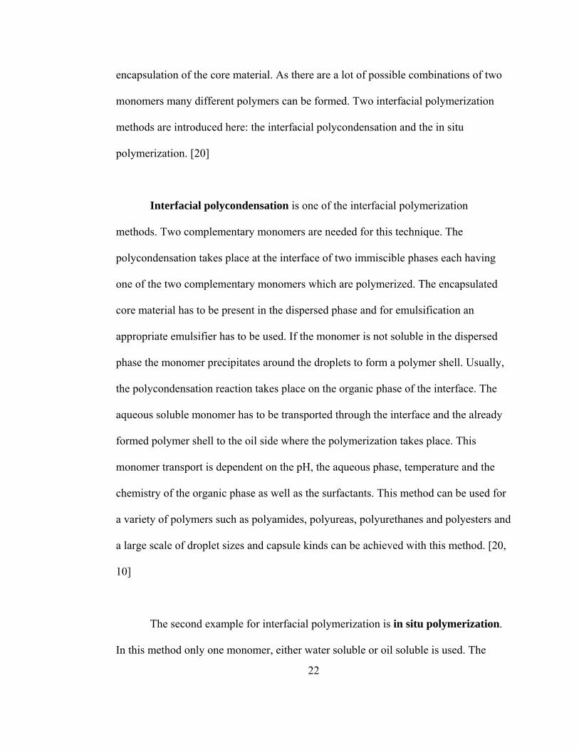
22

encapsulation of the core material. As there are a lot of possible combinations of two

monomers many different polymers can be formed. Two interfacial polymerization

methods are introduced here: the interfacial polycondensation and the in situ

polymerization. [20]

Interfacial polycondensation is one of the interfacial polymerization

methods. Two complementary monomers are needed for this technique. The

polycondensation takes place at the interface of two immiscible phases each having

one of the two complementary monomers which are polymerized. The encapsulated

core material has to be present in the dispersed phase and for emulsification an

appropriate emulsifier has to be used. If the monomer is not soluble in the dispersed

phase the monomer precipitates around the droplets to form a polymer shell. Usually,

the polycondensation reaction takes place on the organic phase of the interface. The

aqueous soluble monomer has to be transported through the interface and the already

formed polymer shell to the oil side where the polymerization takes place. This

monomer transport is dependent on the pH, the aqueous phase, temperature and the

chemistry of the organic phase as well as the surfactants. This method can be used for

a variety of polymers such as polyamides, polyureas, polyurethanes and polyesters and

a large scale of droplet sizes and capsule kinds can be achieved with this method. [20,

10]

The second example for interfacial polymerization is in situ polymerization.

In this method only one monomer, either water soluble or oil soluble is used. The

23

reaction takes place at the interface between the organic and the water phases at

elevated temperatures and with help of a catalyst. [20]

Polyurethanes are per definition polymers which contain urethane linkages in

the main polymer chain. Polyurethane can be formed by a reaction between

diisocyanate O=C=N-R and a diol HO-R-OH. Polyesters, polycarbonates and

polyethers are examples for diols. Isocyanates are chemicals with an extremely

reactive group -N=C=O-. An isocyanate with two reactive isocyanate groups is called

diisocyanate. Diisocyanates can be classified into two categories: aromatic and

aliphatic diisocyanates. Diphenylmethanes and toluene diisocyanate belong to the

group of aromatic diisocyanates; whereas, hexamethylene diisocyanate is an example

for an aliphatic diisocyanate. Besides the mentioned reaction using an alcohol to form

polyurethanes, isocyanates can react with an amide to form polyurea. Isocyanate

reacts with water to form an unstable product and the reacts further on to get an amine.

Thus, diisocyanate and water gives polyurea; whereas, the combination of

diisocyanate with polyethylene glycol would form polyurethane. [28]

The chemistry of the monomers strongly influences the properties of the

polyurea/polyurethane shell. Dependent on the monomer chemistry of the isocyanate,

aromatic or aliphatic polyurethanes can be produced. Aromatic polyurethanes are

more susceptible to ultraviolet light but more thermal resistant compared to aliphatic

polyurethanes. But the thermooxidation resistance is mainly influenced by the type of

the long-chain diol. Polyesters are more thermooxidative stable than polyethers. The

hydrolysis

better resis

longer the

Table 2.2: s

Thus, poly

is just the

a schemati

chemistry.

s resistance i

stance than e

chain, the m

chematic sum

yether is mor

opposite the

ic overview

. [29, 30]

s also depen

ester groups.

more phase s

mmary of influ

re phase sep

e higher the p

over the par

24

ndent on the

. And the les

eparated the

ence of monom

arating than

polarity the b

rameters of t

long-chain d

ss polar the d

e polyurethan

mer on shell p

polyester. T

better the oil

the shell dep

diol. Ether g

diol is, whic

ne is.

parameters, ta

The oil and s

l resistance.

pendent on th

groups show

ch means the

aken from [29

solvent resist

Table 2.2 sh

he monomer

a

e

]

tance

hows

r

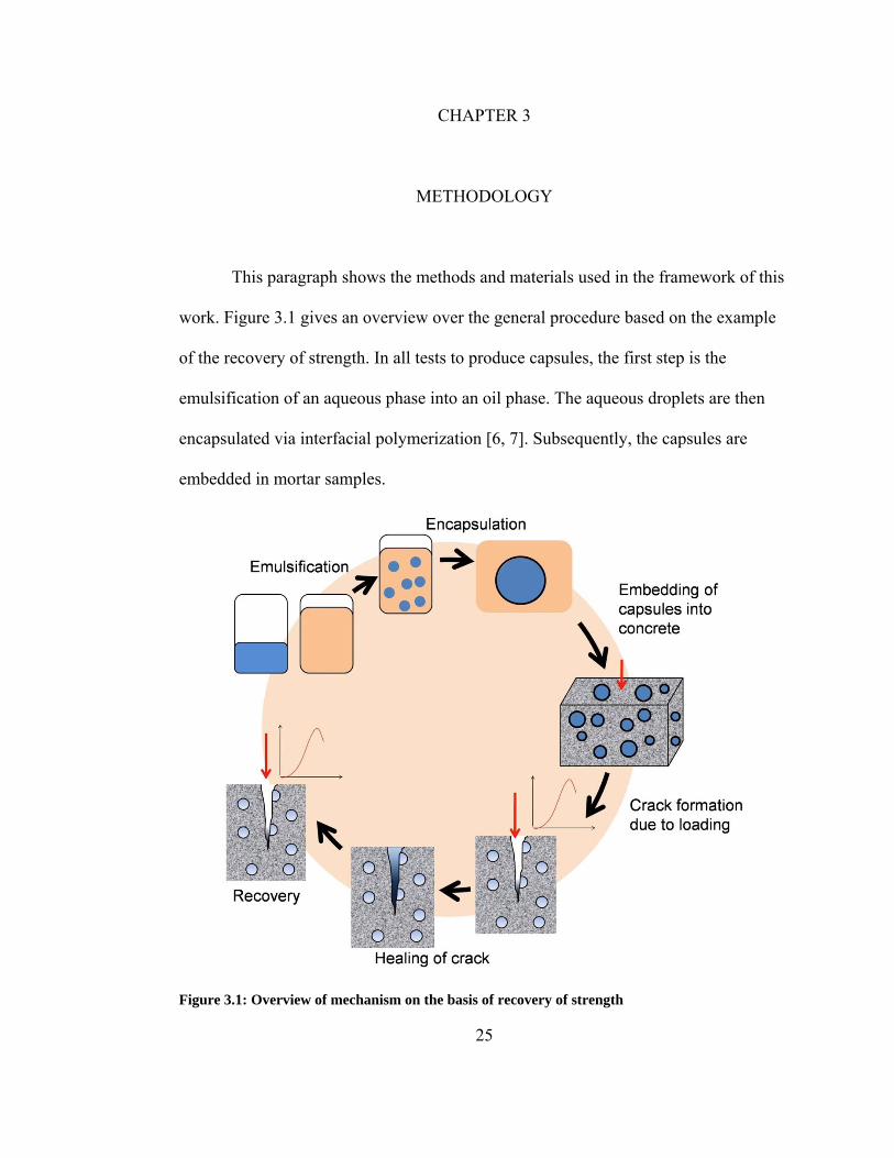
25

CHAPTER 3

METHODOLOGY

This paragraph shows the methods and materials used in the framework of this

work. Figure 3.1 gives an overview over the general procedure based on the example

of the recovery of strength. In all tests to produce capsules, the first step is the

emulsification of an aqueous phase into an oil phase. The aqueous droplets are then

encapsulated via interfacial polymerization [6, 7]. Subsequently, the capsules are

embedded in mortar samples.

Figure 3.1: Overview of mechanism on the basis of recovery of strength

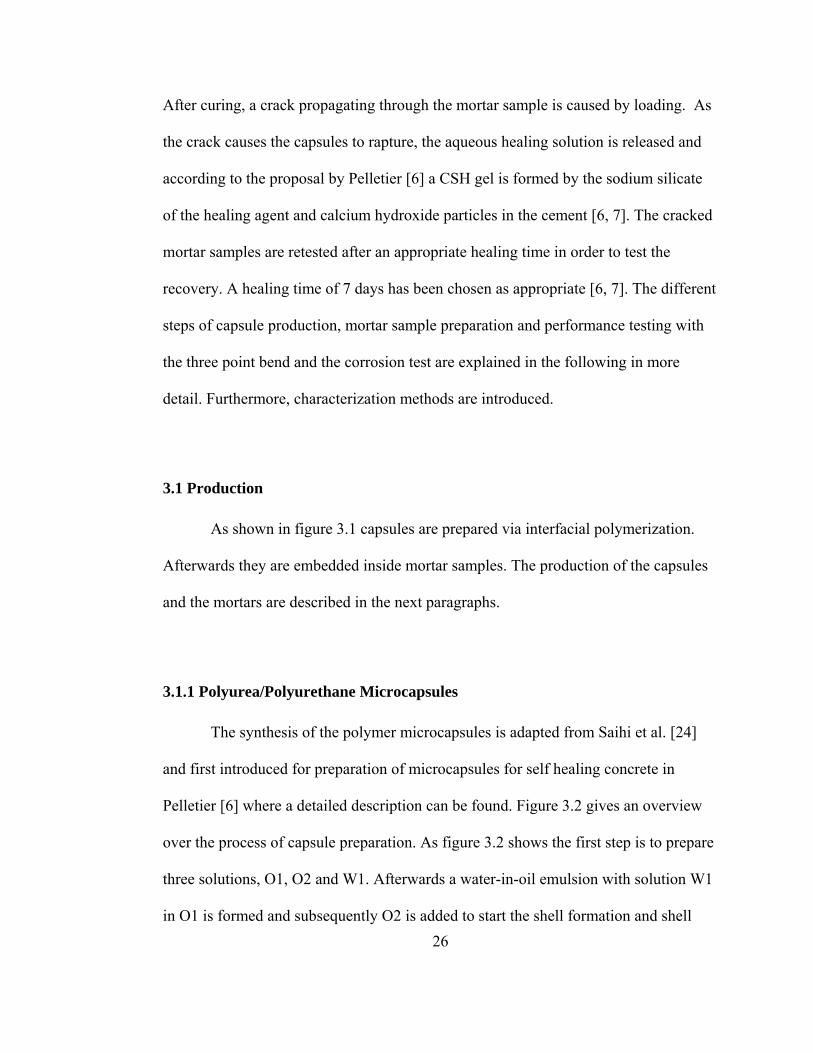
26

After curing, a crack propagating through the mortar sample is caused by loading. As

the crack causes the capsules to rapture, the aqueous healing solution is released and

according to the proposal by Pelletier [6] a CSH gel is formed by the sodium silicate

of the healing agent and calcium hydroxide particles in the cement [6, 7]. The cracked

mortar samples are retested after an appropriate healing time in order to test the

recovery. A healing time of 7 days has been chosen as appropriate [6, 7]. The different

steps of capsule production, mortar sample preparation and performance testing with

the three point bend and the corrosion test are explained in the following in more

detail. Furthermore, characterization methods are introduced.

3.1 Production

As shown in figure 3.1 capsules are prepared via interfacial polymerization.

Afterwards they are embedded inside mortar samples. The production of the capsules

and the mortars are described in the next paragraphs.

3.1.1 Polyurea/Polyurethane Microcapsules

The synthesis of the polymer microcapsules is adapted from Saihi et al. [24]

and first introduced for preparation of microcapsules for self healing concrete in

Pelletier [6] where a detailed description can be found. Figure 3.2 gives an overview

over the process of capsule preparation. As figure 3.2 shows the first step is to prepare

three solutions, O1, O2 and W1. Afterwards a water-in-oil emulsion with solution W1

in O1 is formed and subsequently O2 is added to start the shell formation and shell

growth. W

oil phase,

organic ph

used for en

standard m

stable emu

emulsion.

material. T

F 200 WD

Figure 3.2:

W1 is the aqu

O1, which is

hase with the

ncapsulation

method, the s

ulsion. Tolue

DI water act

The catalyst

D, a cross-lin

Sketch of cap

eous solutio

s a mixture o

e monomer a

n with the sta

surfactants S

ene is taken

ts as the disp

used is dibu

king agent f

sule preparati

27

n which is u

of organic ph

and catalyst n

andard meth

Span 85 and P

as the organ

persed phase

utyl tin dilaur

from BASF,

ion

used as dispe

hase with su

needed for e

od are summ

PEG dioleat

nic continuou

e and as a ba

rate. The sta

as the oil so

ersed phase i

urfactants. O

encapsulation

med up in tab

te are used in

us phase of t

asis of the aq

andard metho

oluble monom

in the contin

2 is a solutio

n. All chemi

ble 3.1. In th

n order to ge

the water-in-

queous core

od uses Baso

mer.

nuous

on of

icals

he

et a

-oil

onat

NB2(B

SStr(A

Pd(A

Dd(A

T(A

MMdd

H

P

Table 3.1: O

Name Basonat F 200 WD BASF)

Span 85 = Sorbitan rioleate Sigma

Aldrich)

PEG dioleate Sigma

Aldrich)

Dibutyltin dilaurate Sigma

Aldrich)

Toluene Sigma

Aldrich)

MDI = Methylene diphenyl diisocyanate

HMDI

PEG

Overview over

Chemical strHMDI: C8H12

C60H108O8

C20H40O4

C32H64O4Sn

C6H5CH3

C15H10N2O2

C8H12N2O2

C2nH4n+2On+1

r chemicals us

ructure 2N2O2

28

ed for encapsu

ulation

FunctMonoaccordBASFcrosslagent compoHMDSurfacmaybemembstructu(accorFTIR Saihi

Secon

Cataly

Solvenemuls

Alternmonomof Bas

Alternmonomof Bas

Wateralternmonom

tion omer, ding to F linking with main onent

DI ctant, e part of brane ure rding to data by et al [24])

nd surfactant

yst

nt for sification

native mer instead sonat

native mer instead sonat

r soluble ative mer

Comments Solvent free polyisocyanatconfidential ingredients

Tests have bewith differentof Span 85: caformation poswithout Span less or more, bquality

Role of PEG dhas not be invin the framewthis work; PEdioleate is usesurfactant accSaihi et al [24

Requirementsphase: Solvento be immiscibwater but moncatalyst and suhave to be solsolvent

First tests with600 show encapsulationas strong as wPEG, further tshould be con

te, BASF

en done t amounts apsule ssible 85, with but poor

dioleate vestigated

work of G ed as 2nd cording to 4]

s for oil nt needs ble with nomer, urfactant luble in

h PEG

n but not without tests

nducted

29

Table 3.2 gives an overview over the amounts used to prepare approximately 20 ml of

water or calcium nitrite capsules.

Table 3.2: Composition of solutions O1, O2 and W1 to prepare approximately 20 ml of capsules

Solution Composition

O1 • 90 ml toluene, • 4.2 ml Span 85, • 2.1 ml PEG dioleate

After preparation of O2 (less solution in total is left)

O2 • 15 ml O1, • 0.6832 ml Basonat, • 0.047 ml Dibutyl tin

dilaurate

W1 • 30 ml DI water, • core material

In this work variations with other monomers, such as methylene diphenyl diisocyanate

(MDI) and hexamethylene diisocyanate (HMDI) instead or in combination with

Basonat are tested. The variations of the standard method tested in this work are

shown in table 3.3.

Table 3.3: Variations in monomer chemistry to standard method

Test Organic phase monomer

Water phase monomer

Comments/Source

Standard method Basonat F 200 WD

- Based on Saihi et al [24] and Pelletier [6]

HMDI as monomer HMDI - Basonat main component is HMDI according to BASF information

MDI as monomer MDI - Based on Saihi et al [24] Basonat and HMDI Basonat and

HMDI - Minimum cross linking

agent needed [23] Basonat and PEG Basonat PEG 400 and

PEG 600 Interfacial polycondensation between two complementary monomers, theory described in section 2.3 and [30]

HMDI and HMDA HMDI HMDA

30

Besides using different diisocyanate monomers, which is the oil soluble monomer and

which leads to in situ polymerization, the influence of a second monomer in the water

phase has been tested. PEG with a molecular weight of 400 and 600 has been tested as

the water soluble monomer complementary to Basonat and a mixture of both PEG

molecular monomers 400 and 600 has been used. Having two complementary

monomers gives interfacial polycondensation with polymerization of the two

complementary polymers like PEG and MDI.

3.1.2 Mortar Samples

The mortar samples are prepared according to the standard procedure of

ASTM C-109 and described in Pelletier [28, 6]. For six 2-inch-cubes 242 ml of DI

water are slowly mixed with 500 g of Portland cement for 30 seconds. After having

added 1375 g of Ottawa Sand C-109 an additional mixing of 30 seconds at slow speed

is carried out and more mixing for 30 seconds on medium speed is realized. The

mixture is set aside for 75 seconds. Meanwhile, the sides of the mixing bowl are

scraped. After an additional mixing time of 60 seconds at medium speed the mixture is

set aside for 75 seconds again. If requested, capsules are added to the mixture and the

final step is to mix for 15 seconds on medium speed. The mortar mixture is filled into

molds. The molds have to be filled equally and it has to be ensured that each mold is

fully filled with mortar. The mortars harden in the molds for 24 hours and are removed

from the molds after 1 day. The samples are submerged into water for 2 days and are

cured for 2

testing can

3.1.2.1 Gr

Gra

figure 3.3.

been place

under tens

but high co

stress. Thu

mortar sam

loading fro

Figure 3.3:

28 days in a

n be conduct

raded Mortar

aded mortar

The capsule

ed in the rest

sion and the t

ompressive s

us, the capsu

mples are 50

om 2 vol% to

Set-up of grad

humid air en

ted after 28 d

r Samples

samples hav

es have been

t of the samp

top part und

strength it fa

ules are place

% filled with

o 6 vol% an

ded samples w

31

nvironment.

days of curin

ve been prep

n placed whe

ple. As expla

der compress

ails in the ten

ed in the bot

h capsule co

d 50% with

with capsules p

Further test

ng time.

pared accord

ere tension o

ained in sect

sion. As conc

nsion part w

ttom part of t

ontaining mo

mortar with

placed where

ts such as thr

ding to the sk

occurs and no

tion 2.1.4 the

crete has low

when loaded b

the mortar s

ortar with dif

hout capsules

tension acts

ree-point ben

ketch shown

o capsules h

e bottom hal

w tensile stre

by flexural

ample. The

fferent capsu

s.

nd

n in

have

lf is

ength

ule

32

Consequently, the total amount of capsules is 1 vol% in the case where the bottom part

is filled with 2 vol% of capsules; it is 2 vol% in total for the 4 vol% of capsules at the

bottom part and 3 vol% in total in the third case with a bottom part of mortar with a

capsule loading of 6 vol% of capsules, respectively. The recovery of flexural strength

of the graded samples is determined with the three-point-bend test which is described

in chapter 3.3.1.

3.1.2.2 Mortar Samples for Corrosion Tests

The mortars for the corrosion samples are prepared according to paragraph

3.1.2 and the ASTM standard C-109 [31]. The first 50% of the molds are filled and

three steel wires are equally put into the mortar. The molds are fully filled afterwards.

Figure 3.4: Set-up of mortar samples for corrosion test

The set-up of the samples is shown in figure 3.4. The steel wires are protected with

duct tape for approximately 1 cm just at the place where the wire is entering the

mortar sample in order to avoid that the wires corrode outside the concrete samples.

The curing of the mortar samples is done as described in paragraph 3.1.2. The samples

33

are cracked with the three point bend test. The crack is induced above the steel wire

through the sample down to the wire. It has to be made sure that the NaCl salt water is

able to penetrate from the surface of the mortar sample to the surface of the wire.

Subsequently, a centrifuge tube which has been cut is tightly attached on top of the

mortar sample the way it is shown in figure 3.4. The tube is sealed to the mortar

sample with rubber sealant. The rubber sealant needs two days to harden. Afterwards,

the entire sample has been covered with duct tape as shown in figure 3.4 on the right

hand side.

3.2 Characterization

Besides the techniques mentioned in the previous paragraphs, other

characterization methods have been used to get information about the nature of the

capsules and their influence on mortar samples. For further information literature

about analytical instruments are recommended, e.g. the “Handbook of Analytical

Instruments” by Khandpur [32]. Various microscope techniques have been used to

investigate the optical properties of the capsules including optical microscopy,

fluorescence microscopy, Scanning Electron Microscopy (SEM) and reflective

microscopy. In order to get information about the crystallinity as well as the impact on

the crystallinity of the capsules on mortar samples X-Ray diffraction (XRD) has been

conducted. XRD is an X-Ray scattering technique and can provide information about

the crystal structure [33]. Mortar samples with and without capsules have been

analyzed to get information about the samples and whether the capsules influence the

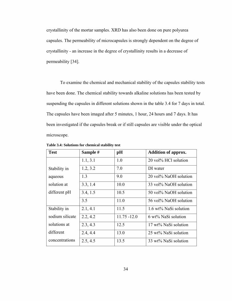
34

crystallinity of the mortar samples. XRD has also been done on pure polyurea

capsules. The permeability of microcapsules is strongly dependent on the degree of

crystallinity - an increase in the degree of crystallinity results in a decrease of

permeability [34].

To examine the chemical and mechanical stability of the capsules stability tests

have been done. The chemical stability towards alkaline solutions has been tested by

suspending the capsules in different solutions shown in the table 3.4 for 7 days in total.

The capsules have been imaged after 5 minutes, 1 hour, 24 hours and 7 days. It has

been investigated if the capsules break or if still capsules are visible under the optical

microscope.

Table 3.4: Solutions for chemical stability test

Test Sample # pH Addition of approx.

Stability in

aqueous

solution at

different pH

1.1, 3.1 1.0 20 vol% HCl solution

1.2, 3.2 7.0 DI water

1.3 9.0 20 vol% NaOH solution

3.3, 1.4 10.0 33 vol% NaOH solution

3.4, 1.5 10.5 50 vol% NaOH solution

3.5 11.0 56 vol% NaOH solution

Stability in

sodium silicate

solutions at

different

concentrations

2.1, 4.1 11.5 1.6 wt% NaSi solution

2.2, 4.2 11.75 -12.0 6 wt% NaSi solution

2.3, 4.3 12.5 17 wt% NaSi solution

2.4, 4.4 13.0 25 wt% NaSi solution

2.5, 4.5 13.5 33 wt% NaSi solution

35

Besides the chemical stability, the mechanical stability of the capsules has

been tested. For the mechanical stability test the capsules are imaged with the optical

microscope. After that, they are exposed to vigorous shaking and they are imaged

again. It is observed if the capsules or emulsion droplets (if no capsule formation took

place) respectively break upon the mechanical stress.

3.3 Performance

The influence of the capsules inside mortar samples and their performance for

self healing purposes and corrosion inhibition has been examined. Additional to the

preliminary tests by Pelletier [6] and Bhattacharyya [7], the influence of capsules on

flexural strength has been tested with focus on the influence of selective capsule

distribution inside the mortar samples and the flexural strength with capsules of

different aqueous agents. By using pure water capsules the contribution of the healing

agent, the sodium silicate powder, has been determined. Furthermore, corrosion tests

have been conducted.

3.3.1 Determination of Recovery in Flexural Strength

The cured mortar samples are loaded with the three-point bend test to measure

the flexural strength. This is the point of incipient failure. If recovery is tested a load is

applied until an initial crack is formed. The samples are healed for 7 days and retested

under the s

strength of

Figure 3.5:

The sampl

tension is

of the appl

as the load

stopped an

known dim

dividing th

3.3.2 Corr

The set-up

corrosion e

A 0.5 M N

and the po

electrode i

same conditi

f the mortar

Set-up of thre

le specimen

acting on the

lied load is k

d drops by an

nd the sampl

mensions of t

he force with

rosion Test

p for the corr

experiment (

NaCl salt solu

otential betw

inside the sa

ions. The thr

samples. Th

ee point bend t

is hold by tw

e bottom sid

kept constan

n amount of

le is removed

the sample t

h dimensions

rosion test is

(a) and phot

ution is fille

een the steel

lt solution is

36

ree-point-be

he set-up can

test for morta

wo supports

de of the sam

nt and the ext

25% of its m

d automatica

the maximum

s of [N] by t

s shown in fi

os of the sam

d in the cent

l wire inside

s measured a

end test was u

n be seen in f

ar samples

and load is a

mple where fa

tension and

maximum lo

ally done by

m load in [Pa

the area [m2]

igure 3.6. Th

mple (c) as w

trifuge tube

e the mortar

and recorded

used to exam

figure 3.5.

applied from

failure occurs

force is mea

oad the appli

y the Instron

a] can be cal

].

he figure has

well as the w

on top of the

sample and

d by a compu

mine the flex

m the top. Th

s first. The s

asured. As so

cation of loa

machine. By

lculated by

s a sketch of

whole set-up

e mortar sam

a reference

uter. The

xural

hus,

speed

oon

ad is

y

f the

(b).

mple

measurem

measured

Figure 3.6:

As a prelim

mortar sam

corrosion t

calcium ni

a)

ment is started

for up to 7 d

Set-up of corr

minary test t

mples is inve

test describe

itrite solution

d as soon as

days.

rosion experim

the corrosion

estigated. Fo

ed above are

n and a 25 w

37

the NaCl wa

ment with mor

n of the steel

or this prelim

tested in 0.5

wt% sodium

ater solution

rtar samples

l wires in dif

minary test, th

5 M salt solu

silicate solu

b)

c)

n is added. T

fferent soluti

he steel wire

ution, 6.25 w

ution.

The potential

ions outside

es used for th

wt% and 12 w

is

he

wt%

38

CHAPTER 4

FINDINGS

4.1 Production

Different aqueous solutions have been encapsulated with the method described

in paragraph 3.1.1 which is based on Pelletier [6], Frère [23] and Saihi et al [24]. Pure

water has been encapsulated to examine the influence of the healing agent on the

recovery and the general impact of capsules inside mortar samples. The influence of

the water capsules are compared to the impact of sodium silicate capsules. Calcium

nitrite dissolved in water was used because of its well known corrosion inhibition

effects.

4.1.1 Water Capsules

The preparation of the water capsules has been conducted based on paragraph

3.1.1. The aqueous phase contained pure DI water solely. The capsules have been

made to get information about the influence of the healing agent, e.g. sodium silicate,

and the contribution of the capsules inside the mortar samples. To investigate the

capsules several microscope techniques have been used among others. The yield was

approximately 20 vol% of the total liquid amount, significantly higher than the yield

for sodium silicate capsules achieved by Pelletier [6] and Bhattacharyya [7]. It was

39

found out that the yield is directly dependent on the amount of emulsion. A higher

yield of emulsion compared to sodium silicate has been achieved with water, calcium

nitrite and with various dyes dissolved in water. Different monomers have been used

for encapsulation. Based on the work of Pelletier [6] Basonat F200 WD, a cross-

linking agent from BASF, has been used as the oil soluble monomer. Besides, tests

with hexamethylene diisocyanate (HMDI) and diphenylmethylen diisocyanate (MDI)

as the oil soluble monomer have been done. But Basonat showed the best quality in

terms of strength and durability of the capsule membrane. Consequently, Basonat has

been used for the encapsulation for the tests described in this framework. It has also

been tried out to produce capsules without any monomer. But as expected and shown

in figure 4.1 on the left no capsules are formed without monomer and just an emulsion

is produced.

Figure 4.1: Emulsion without monomer, no capsule formation and with no catalyst (the capsules are very fragile based on their stability is shown in 4.2.1.4)

Capsules without dibutyltin dilaurate which is used as catalyst were produced.

The image is shown in figure 4.1. A stability test conducted according to section 3.2

(results are discussed in paragraph 4.2.1.4) showed that these capsules break upon

mechanica

polymer sh

of differen

Figure 4.2: and PEG di

Furthermo

completely

fragile cap

PEG in monome

PEG 40

PEG 40water so

al stress. If c

hell is thin a

nt chemical p

PEG test on ioleate as seco

ore, it is assu

y polymerize

psules which

water phaseer, PEG diol

0 as water s

0 and PEG 6oluble mono

apsules brea

and fragile. It

properties.

wall formationd surfactant

umed that po

ed or the thic

h break upon

e as leate as

oluble mono

600 as mer

40

ak in the stab

t could be th

on with differt

lymerization

ckness of the

n low mechan

no

omer PE

noas

bility test it c

hat the capsu

rent Polyethy

n took place

e shell was s

nical stress.

o PEG, no P

EG 600 as w

o PEG, PEGs second surf

can be assum

ules are more

ylene glycols a

but either it

small which

Besides the

PEG dioleate

water soluble

G dioleate factant

med that the

e fragile bec

as second mon

t was not

leads to thin

capsules wi

e monomer

ause

nomer

n and

th

41

Basonat as the only monomer, capsules with PEG as a second monomer have been

produced. PEG at different molecular weights and no PEG nor PEG dioleate at all

have been tested. No significant difference can be seen under the optical microscope

as seen in figure 4.2. As no significant improvement has been observed, the

performance tests have been conducted with the procedure described in paragraph

3.1.1. As shown in paragraph 4.2.1.4 the capsules with no PEG dioleate are fragile and

break easily.

4.1.2 Calcium Nitrite Capsules

The encapsulation of calcium nitrite was successful in different weight ratios

of calcium nitrite. Capsules with an amount of 6.25 wt% and 12 wt% have been made

with a good yield of up to 20 vol% compared to the total amount of liquid (solvent and

water).

4.1.3 Sodium Silicate Capsules

The encapsulation of an aqueous solution of sodium silicate has been

successfully conducted like described in [6] and [7] and shown in figure 3.2.

Nevertheless, it has been found out that the method suggested by Pelletier [6] leads to

a very low yield for sodium silicate capsules.

42

Table 4.1: Tests to obtain high yield of sodium silicate capsules

Approach Justification and source Observation Increase of temperature Increase temperature leads

to better diffusion of

molecules through

membrane [23]

No change

Increase time for polyurea/

polyurethane shell growth

(up to 12 hours)

Increasing time allows

better and entire shell

growth [23]

No change in between hour

0 and 6, after 12 hours

stuck to the ground

Decrease of pH with nitric

acid until ca. pH 10.8

Dependence of yield on

pH has been observed in

preliminary tests,

possibility of lowering as

well as altering pH are

discussed further down in

this paragraph in table 4.2

Higher yield, not as high as

water, CaNi capsules

Using different amounts of

NaSi and also dropping pH

at lower concentrations of

sodium silicate

At low NaSi concentration

(max. 5 wt% of NaSi)

slightly better yield, but

capsules very fragile

Sodium silicate gel

formation, suspending,

dropping pH of NaSi gel in

water to 8-9

Encapsulation didn’t work

out, stuck to ground,

probably too dense and

change of viscosity

Addition of water droplets

at lower pH while shell

growth

No significant change

Use of liquid NaSi instead

of solid NaSi which is

dissolved in DI water

Adding PEG to water,

with/without PEG dioleate

as 2nd surfactant

Formation of polyurethane

via interfacial

condensation possible [23]

Results are described in the

4.1.1 paragraph in more

detail

Addition of more catalyst Catalyst is needed for

polymerization reaction

[23, 24]

Stable droplets observed

which are a good emulsion

or very fragile capsules

Alteration of monomer Various papers such as

[23, 24] show

encapsulation with other

monomers

As described in 4.1.1 it

was possible to encapsulate

with alternative monomers,

but high yield has not been

obtained

43

The yield of capsules is less than 2 vol% based on the total amount of liquid (water

and solvent) whereas the yield with just water and calcium nitrite is up to 20 vol% of

capsules based on the total amount of water and solvent. Table 4.1 sums up the

different tests done in order to obtain a high yield sodium silicate capsule solution.

The observations described in table 4.1 show that it was not possible to obtain sodium

silicate in the same high yield as water and calcium nitrite capsules with the methods

of table 4.1. According to Saihi et al [24] the reaction takes place between the

diisocyanate and the water in the aqueous phase. By adding sodium silicate the pH

increases to 14. Therefore, tests with encapsulation of aqueous solutions at different

pH have been done and showed that the yield decreases at high pH. The pH can be

dropped until a pH of 10.7 before gel formation of the silicate starts. The gel cannot be

encapsulated by the method used. Table 4.2 is a list of experiments done to try to

decrease the pH in order to increase the yield of capsule formation. But as well known

and described in literature, e.g. [35], it is not possible to obtain an aqueous sodium

silicate solution at lower pH than 10.7 without gel formation and the methods

described in table 4.1 and table 4.2 do not show remarkable improvement.

Table 4.2: Tests for altering (lowering) pH of sodium silicate solution

Method Observation

Addition of alcohol (MeOH) in different

amounts and combinations with nitric

acid to drop pH of NaSi solution

MeOH has no effect on pH or gel

formation and as pH drops underneath

10.7 gel formation takes place

Use of liquid sodium silicate in different

concentrations and addition of acid

As soon as pH decreases lower than 10.7

gel formation takes place

44

It has been observed that the emulsification step in the interfacial polymerization is the

leading factor determining the yield of capsules. The shells of the capsules are forming

at the emulsion droplet’s interface [20]. In the case of sodium silicate an equilibrium

of three layers, an oil layer on top, a very small emulsion layer in the middle and a

water layer at the bottom, can be observed. Whereas, with pure water and calcium

nitrite just two layers are formed: An oil layer on top and an emulsion layer at the

bottom. As described in paragraph 2.3 and 3.1.1 the polymer shell forms around the

emulsion droplets. Thus, there is just capsule formation where emulsion is. If the

emulsion layer is small, the yield of capsules is low. Consequently, the yield for

sodium silicate containing capsules is poor. The amount of surfactant [36] and amount

of salt [37] have a crucial effect on the emulsification. Further investigation on how to

increase the emulsification layer and shift the equilibrium to a two phase system with

a high amount of emulsion have to be done in order to obtain high yields of sodium

silicate capsules.

4.2 Characterization

Various characterization methods have been used to obtain information about

the capsules and their properties inside mortar samples. The characterization of the

capsules is presented first, followed by the observations and discussions of properties

of the capsules inside mortar samples.

45

4.2.1 Capsules

The capsules have been mainly examined with focus on their strength.

Microscope techniques have been used for investigation of capsule formation,

stability. Fluorescence microscopy can provide information of chemistry of core

material.

4.2.1.1 Optical Microscope

Figure 4.3 shows optical microscope images of the capsules. It can be seen that

a shell has been formed. The size distribution is large with capsules in the order of up

to 800 microns and very small capsules with a diameter of 10 microns or less. Figure

4.3 shows that capsule formation has been successful with all the different aqueous

solutions tested (pure water, calcium nitrite, sodium silicate and a mixture of sodium

silicate and calcium nitrite). Furthermore, it can be seen that in the case of

encapsulation with sodium silicate (images at bottom of figure 4.3) the capsules float

in residues which are an indication that polymerization also took place in the bulk of

the oil phase as well as at the interface between water droplets and oil. This

observation along with the poor yield supports the fact that due to poor yield of the

emulsification polymerization does not take place just on the interface as the formed

interfacial area is smaller than available monomer for polymerization. Thus, it has to

be investigated how to increase the quantity of the emulsion layer.

Figure 4.3:

Figure 4.4

different m

around the

besides the

Figure 4. 4:

water c

sodium

Optical micro

shows imag

magnification

e water dropl

e major caps

Microscopy i

capsules

m silicate cap

oscopy images

ges of water

ns with focu

lets. Additio

sules.

images of caps

psules

46

s of capsules w

capsules don

us on the she

onally, it can

sules containin

ca

sod

with different a

ne with the o

ll . They sho

n be seen that

ng pure water

alcium nitrit

ium silicate

aqueous conte

optical micr

ow the shell

at small drop

r

te capsules

e/calcium ni

ents

roscope at

formation

lets are form

itrite capsul

med

les

c

The lights

are just im

droplets an

been done

4.2.1.2 Flu

Flu

water-in-o

successful

The experi

capsules u

Figure 4.5:

a) Optic

c) Optical a

seen in the m

magine object

nd whether t

.

uorescence M

uorescent dy

oil emulsion

ly encapsula

iment has be

under the opt

Fluorescence

cal microsco

and Fluoresc

membrane a

ts. In order t

they are wate

Microscopy

ye has been a

has been for

ated. The flu

een conducte

tical microsc

images in com

ope

cence micro

47

are because o

to get inform

er, oil or air

added to the

rmed and tha

uorophor (4,6

ed without h

cope with an

mparison with

b)

oscope d) O

of the light o

mation about

bubbles, flu

water phase

at the whole

6 carboxyflu

healing agent

nd without flu

h optical micro

Fluorescen

Optical and F

of the optical

the nature o

uorescence m

e in order to

amount of w

uorescein) is

t. Figure 4.5

uorescence.

oscopy, with w

nce microsc

Fluorescenc

l microscope

of the small

microscopy h

show that a

water has be

water solub

shows the w

water soluble d

cope

ce microscop

e and

has

een

ble.

water

dye

pe

48

It can be clearly seen that the water phase containing just water soluble fluorophor is

fully encapsulated. No fluorescence could be seen outside capsules. It can be assumed

that just water is encapsulated and the solvent stays outside the capsules.

4.2.1.3 Crystallinity

As the permeability of the capsule membrane is a crucial property for the

application of the capsules as self healing enhancement factors it has been tested. As

described in paragraph 3.2 the permeability is dependent on the degree of crystallinity

of the polymer shell [34].

Diagram 4.1: XRD results for dry capsules

49

Thus, X-Ray diffraction of dry capsules has been done. The result is shown in diagram

4.1. The diagram 4.1 indicates that the capsules are amorphous. There is an indication

for the characteristic peak of polyurethane in the range of 15° < 2Θ < 25° [34] but the

peak partly disappears in the noise. The maximum intensity is with 2 cps not high.

4.2.1.4 Stability of Capsules

To examine the stability of the polyurea and polyurethane microcapsules inside

alkaline solutions tests with capsules with a) produced with the standard method

described in 3.1 (without PEG), and b) with PEG as a second monomer, are dispersed

in alkaline solutions at different pH. The capsules are imaged after 5 minutes, 1 hour,

24 hours and 7 days. The images are shown in table 4.3 to table 4.6. Table 4.3 shows

the images of polyurea capsules which are exposed to aqueous solutions at different

pH for 1 week. The pH of the solution has been adjusted with sodium hydroxide

(NaOH) and hydrogen chloride (HCl). As the capsules are highly hydrophobic they

agglomerate upon exposure to an aqueous solution as seen in table 4.3 if not dispersed

with a dispersant. The capsules are not destroyed even after a week inside the alkaline

solution. Also in comparison to water capsules at pH 7.0 the capsules do not differ in

appearance. But it can be seen that the membrane gets thin compared to the images of

capsules seen in figure 4.1. It could be that the membrane is permeable and

surrounding water gets inside the capsule which leads to swelling of the capsules.

Table 4.3: O

Tab

immersed

table 4.3 it

effect on th

(images w

seen but th

very short

Optical micros

ble 4.4 show

into sodium

t can be clea

he capsules

without capsu

hey are clear

time of 5 m

scope images f

ws polyurea c

m silicate solu

arly seen that

than alkaline

ules are mark

rly broken. It

minutes.

50

for stability te

capsules from

utions at diff

t sodium sili

e water. Afte

ked in red). T

t seems like

est of capsules

m the same b

ferent conce

icate solution

er 1 week th

The remainin

the capsules

s without PEG

batch as in t

ntrations. In

n has a great

here are no c

ng polyurea

s are already

G

table 4.3

n comparison

ter destroyin

apsules anym

shells can b

y affected aft

n to

ng

more

be

fter a

Table 4.4: O

Tab

second mo

be seen tha

inside the

hour but th

capsules. I

Optical micros

ble 4.5 show

onomer) imm

at the capsul

aqueous solu

he capsules a

It is also hard

scope images f

ws the tests d

mersed to alk

les are stable

ution of pH

are not stabl

d to distingu

51

for stability te

done with po

kaline water

e. The micro

1 break after

e anymore. I

uish the imag

est of capsules

olyurethane c

and high ac

oscope image

r 1 hour. Th

It could be th

ge taken afte

s without PEG

capsules (wi

cid water. In

es indicate th

hin shells can

hat very low

er 5 minutes

G

ith PEG as

general, it c

hat the capsu

n be seen aft

w pH destroy

for sample 5

can

ules

er 1

ys the

5.

But as all t

the capsule

Table 4.5: O

Tab

exposed to

sodium sil

It can be s

leading to

the other im

es done with

Optical micros

ble 4.6 show

o sodium sili

licate is more

een that sod

breakage of

ages of samp

h PEG do no

scope images f

ws the polyur

icate solution

e significant

ium silicate

f the polyure

52

ple 5 clearly

ot break at hi

for stability te

rethane caps

ns. It can be

t than the on

solutions at

ethane capsu

y show capsu

igh alkaline

est of capsules

sules from th

clearly seen

ne of the alka

high pH (ov

ules.

ules it can be

solutions.

s with PEG

he same batc

n that the eff

aline solution

ver 12) have

e assumed th

ch as in table

fect of the

n from table

a negative e

hat

e 4.5

e 4.5.

effect

Table 4.6: O

In

to alkaline

after being

exposed to

sodium sil

lower for s

silicate in

capsules. I

Optical micros

summary, it

e solutions bu

g immersed f

o high alkalin

licate capsul

sodium silica

high amount

It seems like

scope images f

can be conc

ut that they a

for at least 7

ne sodium si

es. Because

ate emulsion

ts could lead

e the differen

53

for stability te

cluded that th

are destroye

7 days. Furth

ilicate soluti

in addition t

ns compared

d to breakage

nce between

est of capsules

he capsules

ed in high pH

hermore, the

ions could al

to the fact th

d to water an

e of the poly

the polyurea

s with PEG

do not break

H sodium sili

destruction

lso explain t

hat the amou

nd calcium ni

yurea and po

a (prepared a

k due to expo

icate solutio

of the capsu

the low yield

unt of emulsi

itrite, sodium

olyurethane

according to

osure

ons

ules

d of

ion is

m

o

54

paragraph 3.1) and polyurethane (with PEG as 2nd monomer) on the chemical stability

is not significant.

As an easy and fast determination of the mechanical stability of the capsules a

shake test where the capsules are imaged before and after gently shaking has been

done. Table 4.7 lists the results of the stability test. It can be clearly seen that the

capsules without PEG dioleate but PEG as a second monomer and without any PEG

are very fragile. Shaking leads to breakage of the droplets. In another test, the capsules

have been observed over a time period of over 1 week and no phase separation which

is typical for an emulsion after that time has occurred. A reference sample with an

emulsion has been also tested and consequently it can be assumed that indeed capsule

formation took place.

55

Table 4.7: Optical microscope images for shake test to check mechanical stability of different kinds of capsules

Test Image before shaking Image after shaking normal procedure: there are mechanical stable capsules, only very large capsules break upon hard shaking

No catalyst: images do not allow clear conclusion, it seems like capsule formation but less stable but fragile

no PEG dioleate, with PEG 400: Any reasonably-sized capsules left after the shake tests seem distorted in shape and texture. Capsules are very fragile.

with PEG 600: similar observations as with PEG 400

no PEG dioleate, no PEG: These are not capsules, simply an emulsion. Shaking vigorously only broke the pseudo-capsules

56

The tests indicate that the capsules are fragile upon mechanical stress but membrane

formation took place. The capsules at standard preparation method and the ones

without catalyst seem to be the most stable capsules. It is surprising that it is possible

to get capsules without catalyst. It could be that the polymerization is an auto-

polymerization between the diisocyanate and water where no catalyst is needed.

Further investigation on the chemical reactions taken place when the wall is formed

have to be conducted.

4.2.1.5 Capsules in wet mortar

Figure 4.6 shows capsules in wet mortar after the preparation of mortar. It is

obvious that the capsules are not broken due to the mixing process to repair mortar

samples. Therefore, it can be assumed that the capsules inside the wet mortar samples

are still intact.

Figure 4.6: Optical microscopy images of capsules inside wet mortar after mortar preparation including mixing

57

4.2.2 Characterization of Mortar Samples

In order to examine the self healing mechanism and to show how the

technology works, mortar samples with capsules have been investigated. A main

question to answer is if the capsules are broken or not inside the hardened mortar

samples.

4.2.2.1 Optical Investigation of Capsules inside Mortar Samples

The cracked area of the mortar samples has been investigated with the reflective

microscope. Figure 4.7 shows the images. Circular holes are visible on the surface. To

show if the holes are air or capsules on the surface, capsules with red dye solution

have been imbedded inside the mortar samples. Red dye can be seen and show that the

holes have been capsules and also that the capsules release the dye selective upon

cracking. According to the images of figure 4.7 it can be assumed that the capsules are

not destroyed due to preparation of mortar and that they can release their content upon

cracks.

58

Figure 4.7: Images of cracked area with colored capsules

SEM images of the capsules inside mortar at the cracked area are shown in figure 4.8

59

Figure 4.8: SEM images of capsules inside mortar samples at different magnifications

Figure 4.8 shows two capsules inside mortar at different magnifications. The left side

has images of a capsule with a hole inside. It could be that the capsule broke inside the

mortar due to stress because of hydration or loads while inside the mortar sample or

due to the

capsule wi

4.2.2.2 Cry

Th

been inves

have been

major peak

difference

mortar at s

due to the

Diagram 4.2

impact of th

ith a close up

ystallinity

e influence o

stigated with

examined an

ks are the sa

visible. Thu

such low am

diversity of

2: XRD of mo

he loading of

p of the inne

of the capsul

h X-Ray diffr

nd can be co

ame (location

us, the capsu

mounts of cap

f mortar.

ortar samples w

60

f the crack. T

er shell. Tiny

les on the cr

fraction. Mor

ompared. As

n of peaks ar

ules do not af

psules. The i

with and with

The images o

y cracks in th

rystal structu

rtar samples

s seen in diag

re marked). T

ffect the cry

intensity can

hout capsules

on the right

he shell can

ure of the mo

with and wi

gram 4.2 the

Thus, there i

ystalline struc

n vary from s

show anothe

be seen.

ortar sample

ithout capsu

e location of

is no signific

cture of the

sample to sam

er

s has

ules

f

cant

mple

61

4.3 Performance

The performances of the capsules as a self healing enhancer and as a corrosion

inhibitor are discussed in the following chapter. The determination of self healing

ability is based on the recovery of flexural strength measured with the three point bend

test.

4.3.1 Water Capsules as Reference

In order to get information about the contribution of the presence of capsules

and the contribution of the self healing agent, e.g. sodium silicate, capsules with just

water as the aqueous phase have been prepared and tested. Diagram 4.3 shows the

recovery of flexural strength of mortar samples with different amounts of capsules. It

can be seen that the samples with capsules show better recovery than the control

samples without capsules. As described in paragraph 3.3.1 the samples are loaded until

failure, the load is stopped and the samples are allowed to heal for 7 days until they

are loaded again and the second load of failure is measured. The recovery is

determined by dividing the second maximum load at failure by the first maximum load

at failure. The recovery is measured for different amount of capsules and compared to

the reference samples without any capsules. The samples with sodium silicate inside

the aqueous solution show slightly better recovery. However, due to limited repetitions

and because of the versatility and inhomogeneous nature of concrete inaccuracies can

occur.

62

Diagram 4.3: Recovery of flexural strengths of mortar samples with sodium silicate and water capsules

Therefore, the results should be regarded with caution. Nevertheless, it can be

concluded that the capsules have a positive effect on the recovery of flexural strength

of concrete. And it seems like it is the extra supply of water which leads to better

recovery and not just the sodium silicate. The encapsulated water could be released

upon crack and react with not reacted calcium hydroxide and silicate particles in the

concrete to form a solid CSH gel which heals the crack.

63

4.3.2 Capsule Distribution inside Mortar Samples

As described in paragraph 2.1.4 and 3.1.2.1 the tensile strength acts on the

opposite side of the applied load by flexural loading. As concrete has lower tensile

strength than compressive strength the samples break on the tension side. Thus,

capsules are placed on the bottom side of the mortar samples where cracks occur. As

seen in diagram 4.4 the initial load is decreased compared to the reference samples

without capsules which can be explained with introduction of weakness points by

addition of capsules.

Diagram 4.4: Load at first failure for graded and non-graded water as well as sodium silicate capsules dependent on total amount of capsules in mortar samples

64

But the load at first failure is not dependent on the total amount of capsules in the

sample. The load at first failure is the load before microcracks are developed

deliberately and the agent of the capsules is released. Thus, the number concentration

of capsules does not have a significant influence on the load at first failure. The

healing is initiated after the microcracks rupture the capsules and the capsule content

is released. After the healing period of 7 days the load at second failure is measured

which is shown in diagram 4.5. It can be seen that the second load is higher for the

graded samples with selective distribution of capsules.

Diagram 4.5: Load at second failure for graded and non-graded water as well as sodium silicate capsules dependent on total amount of capsules in mortar samples

65

The loads at second failure divided by the one at first failure gives the recovery. The

recovery of the graded and non-graded samples in dependence of the total amount of

capsules in the mortar samples is shown in diagram 4.6. Samples with water and with

sodium silicate have been examined.

Diagram 4.6: Recovery of flexural strength with comparison of graded and non-graded mortar samples, plotted in dependence of total amount of capsules in mortar sample

As seen in diagram 4.6 the recovery for the graded samples is higher than for the non-

graded samples. The difference is even more drastic at higher total amount of

capsules. This can be explained with an increase in load at second failure shown in

diagram 4.6. It indicates that there is more healing in the graded samples because more

66

of the initial load can be recovered. As discussed before there is no remarkable

difference between the water and sodium silicate samples to allow conclusions about

the influence of the healing agent. It is very probable that as mentioned before the

extra supply of water leads to the enhanced recovery.

4.3.3 Recovery of Mortar Samples with PEG Capsules

The recovery of the flexural strength for the polyurethane capsules made with

PEG as second monomer in comparison to the water capsules in polyurea shell done

with the standard method (without PEG) and the graded samples with water capsules

(without PEG) are depicted in diagram 4.7. As seen in diagram 4.7 the difference

between the capsules with and without PEG is not significant. Consequently, the

recovery does not vary for the capsules with and without PEG. Thus, as expected, the

capsules show very similar behavior in terms of self healing. It is obvious that the

graded samples show significantly better recovery than the non-graded samples. The

difference between graded and non-graded samples has been discussed in paragraph

4.3.2.

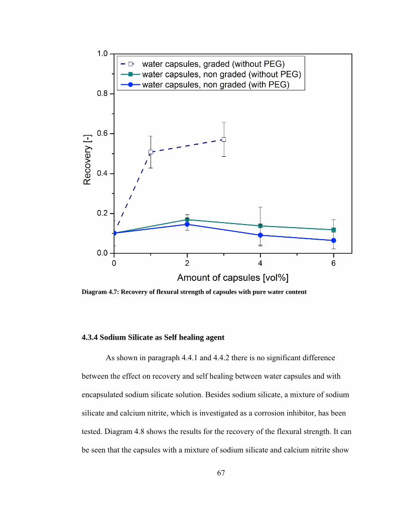
67

Diagram 4.7: Recovery of flexural strength of capsules with pure water content

4.3.4 Sodium Silicate as Self healing agent

As shown in paragraph 4.4.1 and 4.4.2 there is no significant difference

between the effect on recovery and self healing between water capsules and with

encapsulated sodium silicate solution. Besides sodium silicate, a mixture of sodium

silicate and calcium nitrite, which is investigated as a corrosion inhibitor, has been

tested. Diagram 4.8 shows the results for the recovery of the flexural strength. It can

be seen that the capsules with a mixture of sodium silicate and calcium nitrite show

68

less recovery than the sodium silicate capsules. Nevertheless, there is not enough data

available to make conclusions at this point.

Diagram 4.8: Recovery of flexural strength for mortar samples with graded sodium silicate capsules, non-graded and non-graded with sodium silicate/calcium nitrite capsules

As discussed in paragraph 2.1.2.2 the CSH gel is formed by mixing water and cement.

As mentioned in paragraph 2.2 non-reacted calcium hydroxide particles in the

concrete structure can react with water and form a solid and healing CSH gel. By

adding encapsulated water which can be released upon microcracks extra water is

provided which can enhance the autonomous healing of concrete and can be used to

increase the self healing effect.

69

Diagram 4.9: Overview of recovery for different mortar samples with capsules with a core of sodium silicate, water and combination of calcium nitrite and sodium silicate based on amount of capsules

According to the data available the extra water has a positive effect on the self healing

and it is not the dissolved sodium silicate. It can be assumed that there are enough

non-reacted particles inside the concrete which can react later and seal cracks.

Furthermore, it can still be assumed that the formation of a CSH gel leads to the

increase in recovery which supports Pelletier [6] and Bhattacharyya [7] describing the

self healing effect as a formation of CSH gel.

70

4.3.5 Corrosion Test

Calcium nitrite is a well known corrosion inhibitor. The calcium nitrite is

encapsulated and its ability to inhibit corrosion due to cracks in concrete is

investigated inside mortar samples. Prior to the tests the set-up is validated and the

corrosion of the steel wires outside mortar is examined. The steel wires from the

mortars are imaged with a reflective microscope after corrosion to have a closer look

at what happened inside the mortar samples. The results for validation of the new

established set-up can be found in the appendix.

4.3.5.1 Corrosion of Steel Wires outside Mortar

As described in paragraph 3.3.2 a preliminary test to investigate the corrosion

behavior of the steel wires outside mortar is made by exposure of the wires to different

solutions and measurement of the voltage. Table 2.2 lists the risk and probability of

corrosion dependent on open circuit potential. Diagram 4.9 shows the measured circuit

potential for the wires in different solutions with time. It can be seen that there is no

significant difference between the two calcium nitrite solutions. Thus, it seems that a

concentration of 6.25 wt% is already sufficient for the corrosion inhibition effect and

helps to build a protection layer and more calcium nitrite does not have an increase in

corrosion inhibition. The potential of the wire in sodium silicate is in between the ones

with calcium nitrite and NaCl solution. The potential curve of the salt solution of

0.5 M NaCl shows the lowest potential which is associated with severe corrosion.

According to the table severe corrosion takes place at a potential of -0.46 to -0.5 Volts.

It can be seen in diagram 4.9 that the steel wire inside the NaCl salt solution already

shows sev

in low corr

Diagram 4.1

The wire i

corrosion.

corrosion o

corrosion o

inhibitor h

ere corrosion

rosion state

10: Corrosion

n sodium sil

As a conclu

of the steel w

of the steel w

have been co

n after a few

or even less

n of steel wires

licate solutio

usion, diagra

wires wherea

wires. Thus,

onducted and

71

w seconds. Th

for the who

s in different s

on is in betw

am 4.9 implie

as calcium n

further tests

d are present

he wires in c

ole measurem

solutions

ween of interm

es that 0.5 M

nitrite has an

s with the ca

ted in the fol

calcium nitri

ment period o

mediate and

M NaCl leads

n inhibition e

alcium nitrite

llowing.

ite solution s

of 7 hours.

d high risk of

s to severe

effect on the

e as a corros

stay

f

ion

72

4.3.5.2 Corrosion Experiments with Mortar Samples

To investigate the corrosion inhibition of encapsulated calcium nitrite solution

the results of calcium nitrite in different concentrations (d and e) are compared to the

potential of a plain steel wire (a) and mortar samples without capsules (b) , and

calcium nitrite and sodium silicate capsules (c). The mortar samples with the capsules

have been cracked prior to testing to introduce a crack from the surface of the mortar

sample which is exposed to NaCl salt water and the steel wire. After cracking the

samples have been sealed so that the salt water can just enter the mortar from the top

surface of the mortar sample above the wire location. The corrosion test has been

started after the sealing has been set. Figure 3.4 shows the set-up of the mortar

samples for the corrosion test. For starting the test, 0.5 M NaCl has been added to the

cylinder on top of the mortar sample which allowed the salt solution to penetrate

through the mortar sample.

73

Diagram 4.11: Circuit potential for a) plain steel wire, mortar sample b) without capsules, c) calcium nitrite and sodium silicate capsules and d) and e) calcium nitrite capsules in different concentrations

The results for the corrosion experiment according to paragraph 3.3.2 for the

mortar samples with and without capsules are shown in diagram 4.10. It can be clearly

seen that the control sample with the steel wire not embedded in mortar has the highest

negative potential with less than -0.5 V. Thus, according to table 2.1 the wire outside

mortar is severe corroded. The typical circuit potential of steel in NaCl salt water is at

-0.62 V which basically agrees with the results shown in diagram 4.10. A gradual

increase of voltage indicates passive layer formation. It occurs in the mortar samples

but not on the plain wire. The most significant increase is with the sample without

capsules. It could be that because of calcium and silicate molecules naturally available

a)

b) c)

d) e)

a) b) c) d) e)

74

in concrete formation of a small passive layer is formed which is then gradually build

up until the end of the test. It seems like this process needs time. Whereas, with the

capsules this process can happen faster as more calcium nitrite and sodium silicate

molecules, respectively are available upon crack of the capsules. Furthermore, it can

be seen that the best corrosion inhibition can be realized with a pure calcium nitrite

solution. However, the tested concentration changes do not have any differences. The

mixture of sodium silicate and calcium nitrite has a slightly smaller corrosion

inhibition. The results shown in diagram 4.10 are in very good agreement with the

findings of chapter 4.4.5.2.

The steel wires have been investigated with the reflective microscope after the

corrosion test and the images are shown in figure 4.9. It can be seen at the black and/or

brown spots that corrosion took place. Furthermore, it can be seen that the samples for

N3 which are the ones with calcium nitrite capsules show least signs of corrosion. The

image on the bottom right shows that crystals, probably with calcium nitrite formed

around the steel wire. It may have acted as a corrosion inhibitor and therefore the

diagram 4.10 can be explained with formation of a protective layer around the wire.

Figure 4.9: taken after

.

N1: no

N3: 12

Images takencorrosion test

capsules

wt% CaNi

n with reflectt

75

tive microscop

N

N

pe of steel wi

N3: 12 wt%

N2: CaNi, N

ires in differe

CaNi in mor

aSi

ent mortar sa

rtar

amples

76

CHAPTER 5

CONCLUSION

Three main aspects have been examined: The production of capsules with different

aqueous core materials and investigation of the chemistry with a focus on variation and

improvement of capsule properties. Furthermore, the capsules have been characterized with

regard to their properties and stability in and outside of mortars. Finally, the performance based

on the self healing capability and corrosion inhibition has been determined. Emphasis has been

put on the improvement of self healing performance by selective capsule distribution. The results

are an important basis for industrial implementation and improvement of the microcapsule based

enhancement technology for concrete. With the findings a scale-up can be realized and a big step

towards understanding of the interaction of capsules and concrete has been made.

In the production part of this work it was possible to encapsulate pure water, calcium

nitrite and water soluble color as well as fluorescence dye with a large yield and in a scale-up.

Furthermore, an aqueous sodium silicate solution has been successfully encapsulated and it has

been found out that the reason for the poor yield is the emulsification step. Because of the

introduction of sodium silicate salt and the consequently drop in pH a three phase equilibrium

with a small emulsion layer is formed. Further tests have to be conducted to realize a change of

the equilibrium phases towards a two phase equilibrium with a large emulsion layer. It is

assumed that by changing surfactants, the amount of surfactant, salts and temperature it should be

possible to get a high yield of sodium silicate capsules.

77

The capsules have been characterized with focus on the mechanical and chemical stability

whereby they have been observed with a variety of microscope technologies. Additionally their

properties inside mortar have been investigated. First of all, it has been found out that the capsule

production method developed by Pelletier [6] at the University of Rhode Island leads to capsules

with the highest stability and that this method is most suitable for the application of self healing

concrete among all tested methods including the use of different monomers, amounts of

surfactant and catalyst. Nevertheless, encapsulation of aqueous solutions with the standard

method introduced by Pelletier [6] but with different monomers was successful, too. Microscope

studies lead to the conclusion that the capsules do not break upon the mixing process in the

mortar production. Moreover, reflective microscope tests with colored capsules have proofed that

the capsules release their content when cracks occur. SEM images gave first insights into how the

capsules appearance is inside a concrete like environment. Unbroken capsules inside mortars

have been seen under the SEM. More precise data on the stability of the microcapsules could be

gotten by testing the strength of the capsules with a nanoindenter.

The performance of the microcapsules in concrete like materials based on self healing and

corrosion inhibition has been examined. It has been shown that the performance can be improved

by having less microcapsules but with targeted placement and distribution of capsules within the

concrete sample. The graded samples with selective capsules placement showed a recovery of up

to 58% with a total capsule amount of 3 vol% inside the mortar samples. In comparison to that, a

maximum recovery of 31% is achieved with non-graded samples (with a total capsule amount of

6 vol%). Thus, the recovery and consequently the self healing effect can be improved by selective

78

distribution of capsules in the areas where the sample fails and microcracks occurs. Furthermore,

essential information about the technology which leads to the positive effect of increased

recovery has been found. It has been shown that indeed the extra supply of encapsulated water

with or without sodium silicate which can be released upon need lead to a significant better

recovery of strength. It is assumed that by adding encapsulated water which is release when

cracks occur the autonomous healing process is remarkable enhanced. The water reacts with not

reacted calcium-hydroxide and silicate particles which are present in concrete and forms a CSH

gel which seals the cracks. In terms of corrosion inhibition it was found out that calcium nitrite

capsules are working best for corrosion inhibition. Probably by releasing calcium nitrite

protective layer around the steel wires is formed and the corrosion effect is minimized. For easy,

fast and reliable corrosion testing an interface between computer and the physical world has been

established and validated. The validation of the set-up carried out showed that the set-up for

corrosion testing of mortar samples established in the framework of this project is reliable and

can be easily used. The data of up to 8 samples at a time can be logged and saved.

Overall, it can be said that the technology of encapsulated healing and corrosion

inhibition materials can enhance the lifetime of concrete structures. The method of encapsulation

is easy and cheap and therefore very well suitable for concrete industry. As mentioned, further

development on capsule preparation and investigation towards the fully understanding of the

technology and processes carried out while capsules formation and while self healing and

corrosion inhibition have to be done in the future. In order to scale-up the process for industrial

use it is recommended to substitute the toluene with another appropriate solvent which is less

harmful.

79

This work provides an essential basis for the self healing enhancement and corrosion

inhibition of concrete which can provide longer lasting concrete. This would lead to less concrete

production, less repair costs. Therefore, the developed concrete is consequently better in terms of

economic issues and environmental protection.

80

APPENDICES

REFERENCES

1. Introduction:

[1] M. Wu, B. Johannesson, M. Geiker, A review: Self healing in cementitious

materials and engineered cementitious composites as a self healing material,

Construction and Building Materials 28, 571 – 583, 2012

[2] Self healing concrete, Interview with Dr. Henk Jonkers, TU Delft, Ingenia Issue

46, March 2011

[3] M. L. Gambhir, Concrete Technology, third edition, The McGraw-Hill

Companies, Civil Engineering Series, 2004

[4] K. Kovler, N. Roussel, Properties of fresh and hardened concrete, Cement and

Concrete Research, Volume 41, Issue 7, July 2011,Pg 775-792

[5] R. Dodge Woodson, Concrete Structures – Protection, Repair and Rehabilitation,

Butterworth-Heinemann, Elsevier Inc., 2009

[6] M. Pelletier, Self healing Concrete, Master’s thesis, University of Rhode Island,

2010

[7] T. Bhattacharyya, Self healing in Concrete Materials, Master’s thesis, University

of Rhode Island, 2011

81

2. Theoretical background

[8] Mindess, Young, Darwin, Concrete, Prentice Hall, 2003

[9] S. K. Ghosh, Self healing Materials: Fundamentals, Design Strategies, and

Applications, John Wiley & Sons, 2009

[10] R. Dubey, T. C. Shami, K. U. B. Rao, Microencapsulation Technology and

Applications, Defense Science Jornal, Vol. 59, No 1, January 2009, pp. 82 – 95, 2009

2.1 Introduction into Concrete Science

[11] Felder-Casagrande, Wiedemann, Reller, The calcination of limestone –

Studies on the past, the presence and the future of a crucial industrial process, Journal

of Thermal Analysis, Vol. 49, 971 – 978, 1997

[12] Zongjin Li, Advanced concrete Technology, John Wiley & Sons, Inc., 2011

[13] Editor: P. C. Hewlett, Leas’s chemistry of Cement and Concrete, 4th edition,

Butterworth Heinemann, 2001

[14] Batman Uppon Bartholome, His Booke De Proprietatibus Rerum, Imprinted by

Thomas Caft Dwelling by Paules wharfe, London, 1582, found in:

http://books.google.de, last access 06/12/2012, 11:30

[15] J. Aspdin, British Patent #5022, October 21, 1824, found in [16]

82

[16] D. MacLaren, Mary-Ann White, Cement: Its Chemistry and Properties, Journal

of Chemical Education, Vol. 80 No. 6 June 2003

[17] BS 12:1996: Specifications for Portland cement, British standard, 15th edition,

1996 and European Standard EN-206-1: Specification, performance, production and

conformity, 2000

[18] P.C. Aïtcin, Libros del curso “Ingeniería de los Cementantes Hidráulicos”;

Doctorado en Ingeniería de Materiales de Construcción y Estructuras; Cuerpo

académico de Tecnología del Concreto; 2005; p. 608

2.2 Techniques for Self healing in Cementitious Materials

[19] M. Q. Zhang, M.Z. Rong, Self healing Polymer and Polymer Composites,

Practical and Applied Considerations, John Wiley & Sons. Copyright, 2011

[20] T. Kondo, Microcapsules: Their Science and Technology, Part 1. Various

Preparation Methods

[21] N. Sottos, S. White, I. Bond, Introduction: self healing polymers and

composites, J. R. Soc. Interface (2007) 4, 347–348

[22] H. Mihashi H, Y. Kaeko, T. Nishiwaki, K. Otuska, Fundamental study on

development of intelligent concrete characterized by self healing capability for

83

strength, Trans Jpn Concr Inst 2000, 22 (2): 441-50, source not present and reviewed

by author, but cited in [19]

[23] Y. Frère, L. Danicher, P. Gramain, Preparation of Polyurethane microcapsules

by interfacial Polycondensation, Eur. Polym. J. Vol 34, No. 2, pp. 193-199, 1988

[24] D. Saihi, I. Vromn, S.Giraud, S. Bourbigot, Microencapsulation of ammonium

phosphate with a polyurethane shell. Part II. Interfacial polymerization technique,

Reactive & Functional Polymers 66, pp. 1118-1125, 2006

2.3 Microcapsule based Self healing Concrete

[25] L. Bertolini, B. Elsener, P. Pedeferri, R. Polder, Corrosion of Steel in

Concrete, Prevention, Diagnosis, Repair, Wiley-VCH, 2004

[26] H.-W. Song, V. Saraswathy, Corrosion Monitoring of Reinforced Concrete

Structures - A Review. International Journal of Electrochemical Science, 2007. 2: p.

1-28

[27] ASTM C1585-04, Standard Test Method for Measurement of Rate of Absorption

of Water by Hydraulic-Cement Concretes, 2004

[28] M. Ionescu, Chemistry and Technology of Polyols for Polyurethanes, iSmithers

Rapra Publishing, 2005

84

[29] merquinsa, polyurethane types, pdf file found on homepage,

http://www.merquinsa.com/whats/FPPUtypes1.pdf, last access 8/15/2012, 8:42 AM

[30] Wittebecker, E. L., Morgan, P. W., Interfacial Polycondensation. I., Jornal of

Polymer Science, volume XL, 289-297, 1959

3 Methods and Materials

[31] ASTM C-109/C 109-M, Standard Test Method for Compressive Strength of

Hydraulic Cement Mortars (Using 2-in. or [50-mm] Cube Specimens), 2005

[32] R.S. Khandpur, Handbook of Analytical Instruments, McGraw-Hill Handbooks,

2006

[33] B. E. Warren, X-Ray diffraction, Dover publication, 1990

[34] S.K. Yadav, Kartic C. Khilar, A.K. Suresh, Release rates from semi-crystalline

polymer microcapsules formed by interfacial polycondensation, Journal of Membrane

Science 125, 213-218, 1997

4 Results and Discussion

[35] J. Nordström, E. Nilsson, P. Jarvol, M. Nayeri, A. Palmqvist, J. Bergenholtz,

A. Matic, Concentration- and pH-dependence of highly alkaline sodium silicate

solutions, Jornal of Colloid and Interface Science 356, 37-45, 2011

85

[36] B.P. Binks, Emulsion type below and above the CMC in AOT microemulsion

systems, Colloids and Surfaces A: Physicochemical and Engineering Aspects, 71,

167-172, 1993

[37] J. Zhang, L. Li, J. Wang, H. Sun, J. Xu, D. Sun, Double Inversion of

Emulsions Induced by Salt Concentration, Langmuir, 28, 6769-6775, 2012

86

POSTERS

87

LITERATURE REVIEW FOR PELLETIER [6] AND BHATTACHARYYA [7]

Summary of work on capsule based self healing concrete done at the University of

Rhode Island by Pelletier [6] and Bhattacharyya [7]

1. Compressive Strength

Bhattacharyya tested the influence of capsules under compressive load [7]. 2

vol% of capsules have been used filled with an aqueous sodium silicate solution and

have been compared to samples without capsules as a reference. Two tests have been

done. At the first test (Test a) the samples have been compressed and resulting

maximum loads have been measured.

Diagram A.1: Compressive strength in dependence for reference samples without capsules and

with 2 vol% capsules, data taken from Bhattacharyya [7]

88

The maximum load is the load when first failure occurs. At a second test (Test b) the

recovery of flexural strength has been examined. The recovery can be expressed by

the ratio of second load by first load. Therefore, the samples have been loaded until

first failure, have been cured for 7 days and reloaded until final failure. The results are

shown in diagram A.1. Three samples have been tested in each test and the diagram

shows the average values with error bars. The diagram shows that there is no

significant influence of the capsules on the compressive strength of the mortar

samples.

Table A.1: Results compression strength, data taken from Bhattacharyya [7]

Sample

Compressive strength and standard deviation First load

Compressive strength

and standard deviation Second load

[Psi] [MPa] [Psi] [MPa]

Control Compressive strength 2777 19

Standard deviation [%] 403 3

Capsules (2vol%)

Compressive strength 2724 19

Standard deviation [%] 513 4

Control Compressive strength 2522 17 880 6 Standard deviation [%] 330 2 188 1

Capsules (2vol%)

Compressive strength 2507 17 1058 7

Standard deviation [%] 194 1 165 1

There is a slight increase in recovery of strength for the capsule samples with 42.2 %

compared to 34.89 % for the control samples without capsules. Nevertheless, the

difference in the recovery should be regarded with caution as the maximum load

varies from sample to sample as seen in the range of error bars. Additionally, the load

is with over 2500 Psi. Therefore it is very probable that the influence of the capsules

89

cannot be seen at such high loads [7]. Table A.1 gives an overview over the results

Bhattacharyya determined in [Psi].

2. Dynamic Strength

Bhattacharyya also tested the behavior of capsules under dynamic load. The test has

been conducted with a Split Hopkinson pressure bar (SHPB). Mortar samples with a

diameter of 2 inches and a height of 0.5 inch have been prepared. The SHPB is

usually used for ductile materials and not for brittle materials such as concrete.

Nevertheless, a first estimation can be made with the test. The diagram A.2 shows the

results taken from Bhattacharyya [7]. According to the diagram there is no remarkable

difference between the samples containing 2 vol% of capsules and the control samples

without capsules. But the results should be evaluated carefully because first - as

mentioned before - the SPHB is usually used for ductile materials and secondly the

sample size was too small to provide representative predictions of the influence of the

capsules on the dynamic strength. As the capsule amount has just been 2 vol% and the

samples have been small, it is not possible to make sure that the capsules have been

distributed enough to ensure sufficient influence on the dynamic strength of the

mortar samples.

90

Diagram A.2: Dynamic strength tested with Split Hopkinson pressure bar, data taken from

Bhattacharyya [7]

3. Flexural Strength

The flexural strength and the recovery of the flexural strength have been measured

with the three point test which is explained in more detailed in paragraph 3.3. The

mortar samples have been made according to paragraph 3.1. The preparation

procedure is taken from Pelletier [6] and Bhattacharyya [7]. After 28 days of curing

the samples have been stressed until first failure which has been indicated with a rapid

decrease in load dependent on extension of the Instron machine. The failure was not a

final breakage. In contrast, tiny microcracks lead to the abrupt decrease in load and

the samples have not been broken into pieces. The samples have been healed for 7

days whereby they have been stored in a closed plastic bag. They have been stressed

91

again under the same conditions as the first loading. This procedure has been repeated

a second time for samples with a capsule loading of 2 vol%, 4 vol% and 6 vol% after

7 days of healing. By dividing the second by the first maximum load the recovery can

be calculated. The recovery 2 is the 3rd load divided by the 2nd load.

Diagram A.3: Maximum load at three point bend test for samples with different amounts of

capsules, data taken from [6, 7]

Diagram A.3 shows the maximum loads for the initial failure, second loading and the

final failure. It can be seen that the load increases with increasing amount of capsules

from 2 to 6 vol%. The loads for the reference samples without capsules have a higher

92

maximum load. The decrease of load at introduction of capsules in the mortar samples

can be explained with the input of weakness points.

Diagram A.4: Recovery of flexural strength at different capsule loadings from 0 vol% to 6 vol%,

data taken from [6, 7]

Diagram A.4 shows the results for the recovery of the flexural strength. It can be

clearly seen that the recovery increases significantly with increasing capsule loading.

The recovery for no capsules of 12 % can be explained with autonomous healing

which has been discussed in paragraph 2.2. For the samples containing 2 vol% of

capsules the recovery 1 is 23-24%, the samples with 4 vol% capsules has an average

recovery of 27-28% whereas the samples which contained about 6% by volume of the

93

capsules show a recovery of 31% to 34%. Bhattacharyya [7] explained the increase in

recovery with a healing process taken place in the healing period. It is said that the

broken samples release the sodium silicate which leads to formation of the calcium

silicate hydrate (CSH) gel and consequently sealing the crack tip. Thus, according to

Bhattacharyya [7] the samples regain some strength. Furthermore, Bhattacharyya [7]

mentions that as polyurethane acts elastically, the capsules may absorb a small portion

of the load. The recovery 2 does not change significantly with capsules amount which

can be because the sample is broken along the same crack line again and consequently

most of the capsules on that plane have already been broken and have already released

the healing agent [7].

4. Water Absorption

To investigate the effect of capsules on water absorption Bhattacharyya [7]

tested the water absorption by a measurement based on the ASTM C1585-04 [27].

The mortar samples have been prepared and cured for 28 days according to paragraph

3.2. The samples have then been dried in a vacuum chamber for 6 hours at 30°C and

four side faces of the cubic samples have been sealed with ductile tape and the top

side has been loosely covered with Parafilm which has been tied tightly with an elastic

band. The mass of the samples has been measured prior to exposure to water, after

60s, 5min, 10min, 20min, 30min, 60min, 2hr, 3hr, 4hr, 5hr, 6hr, 1day, 2 days, 3 days,

4 days, 5 days, 6 days, a week and 8 days and the change in mass has been

determined.

94

Diagram A.5: Mass change due to water absoprion tested by Bhattacharyya [7] after compression

and without compression

In a second test the samples have been compressed, cured for a week and then the

water absorption has been tested with the method described above. A detailed

description of the test and results can be found in Bhattacharyya [7]. Diagram A.5

shows the mass change due to water absorption after compression and without

compression for the reference samples, mortar samples without capsules, and mortar

samples with 2 vol % of capsules. It can be seen that the samples with capsules absorb

less water compared to the control samples. Bhattacharyya proposed that reduced

porosity is the reason for a reduction in water absorption. The test of water absorption

after compression showed rapid increase in mass due to water absorption for the first

95

10 to 20 minutes and the mass increased until saturation was reached. Bhattacharyya

explained this phenomenon with additional voids due to cracks. It is said that the

capsules containing samples show less water absorption in the end because of

formation of a CSH gel and reduction of porosity and permeability. The reduced

porosity was already proposed as the corrosion inhibitory effect by Pelletier [6]. [7]

5. Capsule Production

Pelletier established a method for encapsulation of an aqueous sodium silicate.

The polyurethane microcapsules with an aqueous sodium silicate solution have been

made via interfacial polymerization. Pelletier [6] developed a method for the

preparation of the polyurethane microcapsules based on Saihi et al [24]. The method

developed by Pelletier [6] is presented below. Paragraph 2.4 gives a better overview

over the theory of interfacial polymerization.

Preparation of Solutions O1, O2, W1

1) Solution O1:

- Measure 90 ml of toluene in a beaker

- Add 4.2 ml of Span 85 and 2.1 ml of PEG dioleate with a pipette

- Stir solution until homogeneous mixture is formed (use e.g. magnet stirrer)

2) Solution O2:

- Take 15 ml of solution O1 with a pipette and put it into another beaker

96

- Add 47 μl of Dibutyltin dilaureate to 15 ml with a pipette, mix solution so that

homogeneous solution is formed

- Add 0.7 ml of Basonat (while mixing; homogeneous solution has to be formed),

the Basonat can be added drop by drop.

- Mix solution O2 until homogeneous mixture is formed

3) Solution W1

- 30 ml water

- If needed: Add water soluble core material (such as sodium silicate, color, calcium

nitrite) to water

Emulsification

Solution O1 is placed on a magnet stirrer and stirring rate is increased to up to 1400

rpm. Do not increase stirrer rate if spilling occurs. Add solution W1 slowly while

mixing. Cover beaker with aluminum foil to avoid spilling and massive evaporation of

toluene. Increase stirrer rate and form emulsion. In general, the higher the stirrer rate,

the smaller the capsules size. The emulsion is visible as a whitish solution. The

formation of emulsion can be checked under the microscope. Stir at high stirring rate

(up to 1400 rpm) for 5 minutes to ensure formation of emulsion.

97

Wall formation

Decrease stirrer rate to 700 rpm. Add solution O2 slowly to mixture and stir at 700

rpm for 10 minutes.

Shell growth

Decrease stirrer rate to 350 rpm and increase temperature to 63°C. Stir emulsion for 4

hours at 63°C.

Test for Capsule Formation

The following fast and easy test shows whether shell formation already took place or

if the liquid is still an emulsion without polymer shell: Place a little drop of solution

on microscope slide. If emulsion breaks it can be seen and a difference can be noticed.

Further analysis if shell formed can be made with optical microscope. Polymer shell

can be usually seen as slightly wrinkled membrane around water droplets. Do droplets

burst easily and fast: shell formation has not taken place entirely. The capsules should

not break if capsule solution is centrifuged at 500 rcf (139 rpm) for 2 minutes.

Washing

Capsules should be at least washed once with toluene to remove surfactants and

residues. After decantation add toluene to capsule solution and centrifuge 2 minutes at

500 rcf. Remove toluene layer at top and do washing step again if necessary. The

washing step should be repeated as long as toluene layer is not transparent and

colorless but yellowish. Washing with another solvent is highly recommended.

Bh

images ar

Figure A.

polymeriza

They show

hand side.

6. Corr

To

into the co

protected.

help of so

aqueous s

tested. A d

hattacharyya

e shown in f

1: SEM im

ation [7]

w an entire c

.

osion Inhib

o increase th

oncrete struc

. Pelletier [6

odium silicat

odium silica

detailed desc

a [7] pictured

figure A.1.

mages of po

capsule on th

ition

e tensile stre

cture. The re

] did prelimi

e capsules. S

ate solution a

cription of th

98

d the microc

lyurea/polyre

he right hand

ength of con

einforcement

inary tests on

Samples with

and referenc

he samples p

capsules und

ethane micro

d side and a

ncrete reinfor

t bars are sus

n the ability

h 2 vol% of

ce samples w

preparation i

er the SEM.

ocapsules ma

broken caps

rcement bars

sceptible to

y of corrosion

f capsules fill

without capsu

is given Pell

The SEM

ade by inter

sule on the le

s are introdu

corrosion if

n inhibition

led with an

ules have be

etier [6].

rfacial

eft

uced

not

with

en

99

Figure A.2: Set-up of corrosion test, set-up used by Pelletier

The set-up Pelletier [6] used can be seen in figure A.2. Pelletier used iron wires to

investigate the corrosion effect. Samples with three iron wires have been put into the

mortar samples as seen in the figure on the right hand side. The mortar samples have

been cracked so that sodium chloride water can penetrate through the sample to get

into contact with the wire. The potential which is an indication for the progress of

corrosion has been measured with a voltmeter. As shown in table 2.1 severe corrosion

happens in the control samples without capsules significantly faster than in the

samples with 2 vol% capsules. Table 2.1 gives an overview over the areas of risk and

classification of corrosion dependent on the open circuit potential [26].

Diagram A

capsules an

been adapt

Three rep

samples. T

decreases

samples w

Pelletier [

samples a

release the

will attrac

Pelletier s

protect it f

A.6: Potential

nd for referen

ted

etitions have

The results a

more rapidl

with 2 vol% o

6] proposed

are stressed d

e healing ag

ct to the posi

stated that th

from corrosi

progress in d

nce samples w

e been made

are shown in

ly for the con

of sodium si

d two mechan

during the th

ent. Consequ

itive ions pre

he formation

ion. Another

100

dependence of

without any ca

e for the sam

n diagram A.

ntrol sample

ilicate capsu

nism of corro

hree point ben

uently, it cou

esent on the

of a passive

r mechanism

f time for sam

apsules, diagr

mples with ca

6 [6]. It can

es without ca

ules.

osion inhibit

nd test and t

uld be that s

metal and d

e film on the

m according t

mples with 2 v

am has been

apsules and f

be seen that

apsules comp

tion. One pr

the capsules

some of the s

eposit on the

surface of t

to Pelletier i

vol % sodium

taken from [6

for the refere

t the potentia

pared to the

roposal is tha

rupture and

sodium silica

e metals surf

the metal wil

is the reduce

silicte

6] and

ence

al

at the

d

ate

face.

ll

ed

101

water transport through the concrete matrix due to reduced porosity, decreased

interconnectivity and healed cracks because of the release of the healing agent. This

would slow down the ingress of chlorides and leads to reduction of the corrosion rate.

[6]

V

Th

paragraph

reference

the mortar

Diagram A

and voltage

The valida

accurate. T

shown in

from 1 is l

Vo

ltag

ed

eter

mie

dw

ith

set

up

[V]

VALIDATIO

he corrosion

h 3.3.2. To in

electrode an

r experiment

A.7: Validation

e measured wi

ation line ca

The set-up h

diagram A.7

less than 1 %

Vo

ltag

e d

eter

mie

d w

ith

set

-up

[V

]

ON OF SET-

is measured

nvestigate th

nd the steel w

ts the new se

n lines for cor

ith calibrated

an be seen in

has 8 channe

7. Additional

% for every c

Voltage

102

-UP FOR CO

d with the set

he degree of c

wire inside th

et-up has to

rrosion set-up

voltmeter

diagram A.

els and all ch

lly, table A.2

channel and

e measured

ORROSION

t-up shown i

corrosion th

he mortar sa

be validated

p, comparison

7. It is visibl

hannels 0-7 a

2 shows that

that the coe

d with voltm

N MEASURE

in figure 3.6

he potential b

amples is me

d.

n of determine

le that the se

are checked.

t the deviatio

efficient of d

meter [V]

vovovovovovovovo

EMENT

6 and describ

between a

easured. Prio

ed voltage of

et-up is very

The results

on of the slo

determination

y = xR² = 1

oltage 0oltage 1oltage 2oltage 3oltage 4oltage 5oltage 6oltage 7

bed in

or to

set-up

y

are

ope

n is

1

103

higher than 0.9999 for all channels. Consequently, it can be said that the system is

reliable.

Table A.2: Results for validation of corrosion set-up

channel slope of validation line deviation of slope from 1 [%] R2 [-]

0 1.0048 0.48 1

1 1.0038 0.38 1

2 1.0031 0.31 1

3 1.0047 0.47 0.9999

4 1.0048 0.48 1

5 1.0032 0.32 1

6 1.0062 0.62 1

7 1.0026 0.26 1

104

BIBLIOGRAPHY

AÏTCIN, P.C., 2005. Libros del curso “Ingeniería de los Cementantes Hidráulicos”; Doctorado en Ingeniería de Materiales de Construcción y Estructuras. Cuerpo académico de Tecnología del Concreto.

ASPDIN, J., 1824. An Improvement in the Mode of Producing an Artificial Stone. Great Britain: .

ASTM C109 / C109M - 11B, 2011. ASTM C109 / C109M - 11b Standard Test Method for Compressive Strength of Hydraulic Cement Mortars (Using 2-in. or [50-mm] Cube Specimens).

BARTHOLOMAEUS, A., 2003. Batman vppon Bartholome his booke De proprietatibus rerum, newly corrected, enlarged and amended: with such additions as are requisite, vnto euery seuerall booke: taken foorth of the most approued authors, the like heretofore not translated in English. Profitable for all estates, as well for the benefite of the mind as the bodie. 1582. Ann Arbor, Michigan: University of Michigan, Digital Library Production Service.

BERTOLINI, L., ELSENER, B., PEDEFERRI, P. and POLDER, R.B., 2003; 2005. Corrosion of Steel in Concrete. Wiley-VCH Verlag GmbH & Co. KGaA

BHATTACHARYYA, T., 2011. Self healing in concrete materials.

BINKS, B.P., 1993. Emulsion type below and above the CMC in AOT microemulsion systems. 71(2), pp. 167.

BLEZARD, R.G., 2003. 1 - The History of Calcareous Cements. Lea's Chemistry of Cement and Concrete (Fourth Edition). 4th edn. Oxford: Butterworth-Heinemann, pp. 1.

BRITISH PATENT, 1996. BS 12:1996, Specifications for Portland Cement. Great Britain.

DUBEY, R., 2009. Microencapsulation Technology and Applications. Defence Science Journal, 59(1).

FELDER-CASAGRANDE, S., WIEDEMANN, H.G. and RELLER, A., 1997. The calcination of limestone — Studies on the past, the presence and the future of a crucial industrial process. Volume 49(2), pp. 971-978.

FRÈRE, Y., DANICHER, L. and GRAMAIN, P., 1998. Preparation of polyurethane microcapsules by interfacial polycondensation. Kidlington, ROYAUME-UNI: Elsevier.

GAMBHIR, M.L., 2004. Concrete Technology. 3rd edn. New Delhi: The McGraw-Hill Companies.

105

GHOSH, S.K., 2008; 2009. Self-Healing Materials: Fundamentals, Design Strategies, and Applications. Self-Healing Materials. Wiley-VCH Verlag GmbH & Co. KGaA, pp. 1-28.

GLASSER, F.P., 2003. 5 - The Burning of Portland Cement. Lea's Chemistry of Cement and Concrete (Fourth Edition). 4th edn. Oxford: Butterworth-Heinemann, pp. 195.

HEWLETT, P., 2004. Lea's Chemistry of Cement and Concrete. forth edn. Oxford UK: Butterworth-Heinemann.

HISTORICAL STANDARD, 2004. ASTM C1585-04 Standard Test Method for Measurement of Rate of Absorption of Water by Hydraulic-Cement Concretes.

IONESCU, M., 2005. Chemistry and Technology of Polyols for Polyurethanes. Shawbury, Shrewsbury, Shropshire, UK: iSmithers Rapra Publishing.

JACKSON, P.J., 2003. 2 - Portland Cement: Classification and Manufacture. Lea's Chemistry of Cement and Concrete (Fourth Edition). 4th edn. Oxford: Butterworth-Heinemann, pp. 25.

JONKERS, H.M., THIJSSEN, A., MUYZER, G., COPUROGLU, O. and SCHLANGEN, E., 2010. Application of bacteria as self-healing agent for the development of sustainable concrete. Ecological Engineering, 36(2), pp. 230.

KHANDPUR, R.S., 2006. Handbook of Analytical Instruments. 1st edn. New York, NY: McGraw-Hill Professional.

KONDO, T., 2001. Microcapsules: Their Science and Technology Part I. Various Preparation Methods. Journal of Oleo Science, 50(1), pp. 1-11.

KOVLER, K. and ROUSSEL, N., 2011. Properties of fresh and hardened concrete. 41(7), pp. 775.

LAWRENCE, C.D., 2003. 4 - The Constitution and Specification of Portland Cements. Lea's Chemistry of Cement and Concrete (Fourth Edition). 4th edn. Oxford: Butterworth-Heinemann, pp. 131.

LI, Z., 2011. Advanced Concrete Technology. John Wiley & Sons, Inc.

MACLAREN, D.C. and WHITE, M.A., 2003. Cement: Its Chemistry and Properties. Journal of chemical education, 80(6), pp. 623.

MACPHEE, D.E. and LACHOWSKI, E.E., 2003. 3 - Cement Components and Their Phase Relations. Lea's Chemistry of Cement and Concrete (Fourth Edition). 4th edn. Oxford: Butterworth-Heinemann, pp. 95.

MERQUINSA, Polyurethane Types.

106

http://www.merquinsa.com/whats/FPPUtypes1.pdf, last access 8/15/2012, 8:42 AM

MIHASHI, H., KANEKO, Y., NISHIWAKI, T. and OTSUKA, K., 2000. Fundamental study on development of intelligent concrete characterized by self-healing capability for Strength. 22, pp. 441-450.

MINDESS, S., YOUNG, J.F. and DARWIN, D., 2002. Concrete. Upper Saddle River, NJ 07458, U.S.A.: Prentice Hall.

NORDSTRÖM, J., NILSSON, E., JARVOL, P., NAYERI, M., PALMQVIST, A., BERGENHOLTZ, J. and MATIC, A., 2011. Concentration- and pH-dependence of highly alkaline sodium silicate solutions. 356(1), pp. 37.

ODLER, I., 2003. 6 - Hydration, Setting and Hardening of Portland Cement. Lea's Chemistry of Cement and Concrete (Fourth Edition). 4th edn. Oxford: Butterworth-Heinemann, pp. 241.

PELLETIER, M.M., 2010. Self-healing concrete.

SAIHI, D., VROMAN, I., GIRAUD, S. and BOURBIGOT, S., 2006. Microencapsulation of ammonium phosphate with a polyurethane shell. Part II. Interfacial polymerization technique. Reactive and Functional Polymers, 66(10), pp. 1118.

SIMS, I. and BROWN, B., 2003. 16 - Concrete Aggregates. Lea's Chemistry of Cement and Concrete (Fourth Edition).4th edn. Oxford: Butterworth-Heinemann, pp. 907.

SONG, H. and SARASWATHY, V., 2007. Corrosion Monitoring of Reinforced Concrete Structures - A Review. 2(1), pp. 1-28.

SOTTOS, N., WHITE, S. and BOND, I., 2007. Introduction: Self-healing polymers and composites. 4, pp. 347-348.

WAGH, S.J., DHUMAL, S.S. and SURESH, A.K., 2009. An experimental study of polyurea membrane formation by interfacial polycondensation. 328(12), pp. 246.

WARREN, B.E., 1990. X-Ray diffraction.

WOODSON, R.D., 2009. Chapter 6 - Materials and methods for repair and rehabilitation. Concrete Structures. Boston: Butterworth-Heinemann, pp. 61.

WU, M., JOHANNESSON, B. and GEIKER, M., 2012. A review: Self-healing in cementitious materials and engineered cementitious composite as a self-healing material. 28(1), pp. 571.

YADAV, S.K., RON, N., CHANDRASEKHARAM, D., KHILAR, K.C., SURESH, A.K. and NADKARNI, V.M., 1996. Polyureas by interfacial polycondensation: Preparation and properties. Journal of Macromolecular Science, Part B, 35(5), pp. 807-827.

107

ZHANG, J., LI, L., WANG, J., SUN, H., XU, J. and SUN, D., 2012. Double Inversion of Emulsions Induced by Salt Concentration. Langmuir, 28(17), pp. 6769-6775.

ZHANG, M.Q. and RONG, M.Z., 2011. Frontmatter. Self-Healing Polymers and Polymer Composites. John Wiley & Sons, Inc., pp. i-xii.

Shepherd URI COE 2012-2013 Annual Report

1

April 5, 2013

Title: Structural Response to Non-ideal Explosions

Sponsor: Department of Homeland Security Science & Technology Directorate (DHS/S&T) Explosives Center of

Excellence (COE) through URI and NEU.

PI: J.E. Shepherd, Student Researchers: J. Damazo

Objective and Summary of Activities in 2012–2013

Gaseous detonation experiments were performed in the Explosion Dynamics Laboratory at the California Institute of Technology to investigate the effect of internal explosions on surrounding structures. Detonations were used as a model to simulate the pressure and heat loadings caused by non-ideal explosions. The overall project objective is to develop the capability to predict the degree of damage induced by a non-ideal explosion in tubes and to investigate methods to mitigate the extent of this damage. The objective of testing in 2012-2013 was to obtain systematic data on pressure, heat transfer, and boundary layer interaction using a range of combustible mixtures. This was accomplished and the work is currently being written up and will form the basis of J. Damazo’s PhD dissertation and subsequent journal articles. We anticipate Damazo’s PhD will be awarded in June 2013.

Highlighted Accomplishments

1. Completed the experimentation in the gaseous detonation tube facility to document visual, pressure, and heat flux measurements for a range of mixture fuels, diluents, and initial pressures.

2. Carried out non-ideal explosion experiments examining the gas dynamics of reflected shock and detonation waves inside tubes with closed end.

3. Applied analytical boundary layer theory to the case of a propagating detonation and compared predictions to heat flux measurements.

4. Used short exposure, high frame-rate schlieren photography to record the first movies of planar reflection of gaseous detonations.

5. Analyzed time-of-arrival signals from pressure and optical measurements and determined the source of the previously documented discrepancies between ideal zero-thickness detonation reflection theory and experiments. Applied a finite-thickness reaction zone model to explain observed reflected wave speeds.

Details

In order to predict damage, pressure and thermal loadings to the structure must be understood sufficiently well to create models that can be incorporated into structural dynamics simulations. In the earlier phases of this project (summarized in Karnesky et al., 2013), we created an idealized pressure load based on one-dimensional gas dynamics and a zero-thickness model of a detonation wave. Experiments on thin-wall tubes and structural simulations with LS-DYNA were used to validate the loading model that described the pressure field before and after detonation reflection from a closed end. Although our model was highly successful in making quantitative predictions of plastic deformation, significant discrepancies between pressure and wave speed were observed. In order to improve the loading model, we needed to understand the sources of these discrepancies, which we initially had attributed as being due to viscous effects, i.e., reflected shock wave-boundary layer interaction, that were neglected in our initial modeling efforts. We also had neglected thermal loads in our initial models and did not have any data to validate proposed thermal models.

Shepherd URI COE 2012-2013 Annual Report

2

For these reasons, we developed new experiments to specifically examine the reflection process in sufficient detail that we could determine thermal loads, viscous interaction effects, and the effect of detonation structure. An extensive set of tests was carried out for incident detonation and shock waves in a variety of test gases using a test fixture instrumented with pressure and heat flux gauges. Because pressure and thermal loads are greatest in locations of wave reflection, the measurement gauges were clustered near an end-wall wall where the waves underwent planar reflection. The experimental facility was designed to allow for optical access to the reflection event. High-speed schlieren images were captured using a Specialised Imaging SIMD16 set to record 16 frames at 750,000 pictures per second (pps) and 20 ns exposure time. With these measurement techniques, the gas dynamics of reflected shock and detonation waves were observed.

The goals of the detonation tube experiments are to measure the wall pressure and heat flux loading caused by either a reflecting shock or detonation wave. To observe this flow, we use a schlieren imaging system to visualize the incident and reflected waves. The speed of the detonation wave is 2-3 km/s implying any visualization system must have exposure times on the order of tens of nanoseconds and a frame-rate on the order of 500,000 frames per second (fps).

The experiments were carried out in the GALCIT detonation tube (Fig. 1), a special-purpose facility which was designed and built at Caltech specifically to carry out experimentation on detonation waves. The facility consists of a 288-mm diameter tube with a special ignition system at one end and square (150 x 150 mm) test section with optical access at the other end. The ignition system uses a combination of electrical (capacitor discharge into an exploding wire) and chemical (a short section of an acetylene-oxygen mixture) energy to create a nearly planar detonation wave. The detonation propagates away from the point of ignition towards the test section at the constant theoretical Chapman—Jouguet (CJ) velocity. The Taylor—Zel’dovich (TZ) expansion wave trails the detonation and gradually brings the fluid to rest. Once the detonation impinges upon the test section’s closed end, a reflected shock wave propagates into the TZ expansion at a non-constant speed. The detonation facility is 7.6 m in length implying that the effects of the TZ expansion are relatively slow so that near the end wall at times immediately following the reflection event, we may approximate the reflected shock as propagating into a steady and spatially uniform flow.

Figure 1. Diagram of experiment used in detonation experiments; the tube and test section are 7.6 m in length.

A “splitter” plate parallel to the horizontal walls and with a sharp leading edge is inserted into the test section to raise the location of the boundary layer into the center of the observation windows. This splitter plate was instrumented with 12 PCB 113B26 pressure transducers and 12 surface junction thermocouples identical to those employed by Sanderson and Sturtevant (Rev Sci Inst 73(7), 2781-7, 2002) for measuring heat flux inside the test section. The thermocouple signals are amplified by a TrikTek Model 205B instrumentation amplifier with a response time of 7.5 µs to a unit step input. The spectral method employed by Sanderson and Sturtevant is used for reducing the heat flux data. A Z-type schlieren system is used to visualize the incident detonation and shock wave reflection. The schlieren system consists of a Photogenic PL1000DRC flashlamp combined with a Specialised Imaging SIMD16 intensified CCD camera. To satisfy the low exposure time, high frame-rate requirement, the SIMD16 was operated with a shutter speed of 20 ns and an intra-frame time of 1.27 µs (corresponding to a frame-rate of approximately 775,000 fps). This allows sixteen images to be taken in quick succession and was used to visualize the incoming detonation and the reflected shock wave for each test.

Stoichioto study thedetonationsidentical into properlyable to exawith a rangdashed blacshock due tdetonation.

Figure 2. Pdashed blac

The schare given cdetonation impinges uThere is a gimages. Foarrival data

ometric hydroge effects of cos of stoichiomnitial conditionsy assess the preamine the wavge associated wck lines. We sto the observed

Pressure data frck lines represe

hlieren video fochronologicallyis initially see

upon this wall great deal of inocusing the anaa. Processing th

gen-oxygen anmposition on t

metric hydrogens were plotted

essure loading ve time-of-arrivwith the rise tim

ee that the chad rise time that

from two experent range of tim

for shot 2152 (ty in left-to-righen to propagatein frame 7. F

nformation regalysis on the whe data in each

nd ethylene-oxythe dynamics on-oxygen at ato illustrate thto the tube waval at each locme of the pressaracterization ois approximat

riments of stoicme characterizi

the red line ofht, top-to-bottoe towards the rames 8-16 tharding the gas wave location

h frame, we are

S

3

ygen mixtures of the reflected

an initial presse repeatability

all as a functioncation and therure signals is pof the arrival tely 10 times lo

chiometric hyding the rise tim

f figure 2) is shom. Each framend-wall locat

hen show the rdynamics of din each imag

e able to determ

Shepherd UR

of various initd shock. Figursure of 25 kPay in the experimn of time and dreby determinplotted for eactime range is eonger than the

drogen-oxygenme for incident

hown in figureme shows the sa

ted at the righreflected shockdetonation reflege, we can commine the wave

RI COE 2012-

tial pressure anre 2 shows prea. Data from

ment. These predistance from re wave speedsh pressure signespecially imporise time assoc

n at an initial pand reflected w

e 3(a). Sixteen ame 30 mm w

ht-edge of the k wave propagection that canmplement the location and q

-2013 Annual

nd dilutions wssure signals ftwo experimeessure signals reflection. Wes. Time-of-arrinal in Fig. 2 asortant for the rciated with the

pressure of 25 kwave arrival.

frames are showide field of vi

frame. The degating back to n be learned fropressure meas

quantify the unc

l Report

were used from two ents with allow us

e are also ival data s vertical reflected incident

kPa. The

own and iew. The etonation

the left. om these surement certainty

due to theCombiningshown in Fdashed linesolid lines c

Udet and t0, Numbers fo

Figure 3. oxygen at aPressure anemployed tdimensiona

Examinwall by thperformed we believe of the detonbe a sharp jreacting shwave is notwave as madimensionadimensionachemical rethe reactioconcentratireacting sh

smearing of g this data withFig. 3(b). Detoes correspond tcorrespond to a

with error baror the specific

(a) Sixteen scan initial press

nd image data ato show that tal reflection mo

ning Fig. 3(b) ahe highly ideal

and the discrethat the sourcenation wave. Tjump in proper

hock wave follt precisely plananifested by thal structure of al model of deteaction and enn zone is teron but the eneock. At the do

the front loch the arrival danation arrival o the one-dimea polynomial f

€

rs, are determinexperiment sho

(a) chlieren imagesure of 25 kPaare combined tthe reflected wodel.

and Table 1, welized zero-thicpancy is far oue of this discrepThe ideal moderties from reaclowed by a finnar and the floe transverse shthe wave (whtonation wave ergy release demed the indu

ergy release is ownstream end

ation because ata obtained frodata are shown

ensional theoryfit to the arrival

Xdet = Udet

Xsh = Ush (t

ned from the down in Figs. 2

s obtained fro

a. Images are rto assemble a dwave speed at

e observe that ckness modelutside of any mpancy is that thel of reflectionctants directly nite-thickness row behind the whock waves (cohich can only b

as a non-reactetermine the st

uction zone ansmall so that tof the inducti

S

4

of the three-om the pressurn in red and re

y described in ol data of the fo

(t0 − t)

t − t0) + 1

2ash

detonation dataand 3 are give

om a single deread left-to-rigdetailed picturethe wall is su

the reflected wof detonation

measurement uhe ideal modeln considers a dto combustionreaction zone.wave is three-dommonly referrbe addressed thting shock folltructure and thnd is a regionthe thermal proon zone, there

Shepherd UR

-dimensional cre signals, we ceflected shockour journal pub

orm

h (t − t0)2

a and Ush and aen in Table 1.

etonation expe

ght, top-to-botte of detonationubstantially fas

wave speed is sreflection. Th

uncertainty. Afl does not consdetonation wavn products. Rea

In addition, adimensional durred to as cellulhrough numerlowed by a zonhickness of then where radicoperties of the e is a narrow z

RI COE 2012-

cellular structucan construct tk arrival data ablication, Karn

ash are fit to th

(b) eriment of stotom. Each framn wave reflectister than predi

substantially unhis is true in fter considerinsider the finite ve that is infinial detonation was observed inue to the instablar structure). S

rical simulationne of chemicale reaction zonecals are increa

gas are those one of large en

-2013 Annual

ure of the detthe space-time are shown in bnesky et al. (20

he reflected sho

oichiometric hyme is 30 mm won. A polynomicted by an id

nder-predicted every experim

ng various possreaction zone sitely thin, appe

waves consist on Fig. 3 the debility of the deSetting aside thn), we considel reaction. Thee. The initial poasing exponenbehind the ininergy release f

l Report

tonation. diagram

blue. The 013). The

ock data.

ydrogen-wide. (b) mial fit is deal one-

near the ment we sibilities, structure earing to of a non-etonation etonation he three-er a one-e rates of ortion of

ntially in itial non-followed

Shepherd URI COE 2012-2013 Annual Report

5

by a slow approach to equilibrium – this is the classical ZND model of detonation structure.

Considering the reflection of the finite-thickness model of the detonation, we observe that immediately after leading shock wave reflects from the wall it will encounter shocked but un-reacted gas. The reaction will occur very quickly behind the reflected shock because the temperature and pressure are already so high within the reaction zone and are increased further by the reflected shock. As a consequence, the induction zone explodes almost instantly when the reflected shock wave moves into it. Approximating the explosion process as a detonation in the shocked but un-reacted gas in the induction zone, we obtain an estimate of the initial reflected shock speed that is in much better agreement with the measured values, as shown in the last column of Table 1.

Mixture p0, kPa Measured Ush, m/s Zero Thickness Ush, m/s Finite Thickness Ush, m/s

H2-O2 25 kPa 1389 ± 6 1049 1393

% difference from experiment: 24.5% 0.3% Table 1. Reflected shock speeds as determined from the experiment, a zero thickness detonation model, and a finite thickness detonation model. The thermodynamic states and wave speeds are found using the Shock and Detonation Toolbox (Browne et al. GALCIT Technical Report FM2006-006, 2008).

Summary

A systematic experimental investigation of detonation reflection has been performed. The pressure and heat flux was measured behind an incident detonation and reflected shock wave for a range of compositions and initial pressures. High-speed schlieren images were obtained showing the interactions of the reflected shock wave with the transverse wave structure as well as the boundary layer set up by the incident detonation. Very minimal disruption of the reflected shock is observed due to interaction with the incident wave boundary layer. The lack of significant reflected shock wave bifurcation verifies earlier results with single images and conclusively rules out shock-wave boundary layer interaction as a significant factor in detonation reflection for a wide range of mixtures. Detailed analysis was carried out on the time-of-arrival data gathered from the pressure signals and schlieren photographs. These measurements confirmed the previously noted mismatch between the reflected shock speed and zero thickness model of detonation reflection. In addition, the data analysis revealed that a very high initial reflected shock velocity and rapid deceleration is responsible for the disagreement between the experimental data and zero-thickness model proposed by Karnesky et al. The high initial reflected shock speed can be explained by considering the finite thickness of the reaction zone and the interaction of the reflected shock wave with the induction zone region, resulting in a rapid explosion of the induction zone region. Modeling this explosion as the detonation of shocked but un-reacted gas as computed with the ZND detonation model yields very good agreement for the initial reflected shock speed.

Publications and Presentations 1. J. Damazo, J. Odell, and J. E. Shepherd. Boundary Layer Profile Behind Gaseous Detonation as it Affects

Reflected Shock Wave Bifurcation. Proceedings of the 42nd AIAA Fluid Dynamics Conference, New Orleans, June 25-28, 2012. (Conference proceedings paper and presentation)

2. J. Damazo and J. E. Shepherd. Planar Reflection of Detonation Waves. Proceedings of the 65th Fall Meeting of the American Physical Society’s Division of Fluid Dynamics, San Diego, November 18-20, 2012. (Conference proceedings paper and presentation)

3. J. Karnesky, J. Damazo, K. Chow-Yee, A. Rusinek, J. E. Shepherd “Plastic Deformation due to Reflected Detonation” International Journal of Solids and Structures, 50:97-110, 2013.

Experimental Investigation of Blast Mitigation for Target Protection

S. F. Sona, A. J . Zakrajseka, E. J . Miklaszewskia, D. E. Kittella, J . L. Wagnerb, D. R. Guildenbecherb aPurdue University, West Lafayette, IN 47906, USA bSandia National Laboratories, Albuquerque, NM 87185, USA

Introduction

Blast waves, whether from conventional munitions or improvised explosive devices, pose a major risk to people and property through-out the world [2]. Engineering methods to protect individuals and structures vary widely due to the diverse range of threats and poten-tial situations. This chapter focuses narrowly on the protection of high-valued structures and other large targets where removal from the threat zone is often impossible. In these situations, methods are needed to dissipate and reflect incoming blast waves and mitigate damage potential.

Any proposed mitigation method must be evaluated for effective-ness, and while steady advances in computational physics have been made in this area, experimentation remains crucial. Therefore, this chapter emphasizes experimental methods for evaluation of blast mitigation, both from a practical and fundamental standpoint. In ad-dition, some of the capabilities of current computational methods are highlighted. The chapter begins with a review of the underlying physics. This is followed by a brief overview of experimental meth-ods. Finally, the remainder of the chapter is dedicated to recent ex-perimental and computational results for a potential configuration involving protective water sheets.

Physics of blast waves

Detonation releases a large amount of energy in a small volume, and in an unconfined gaseous environment, such as air, energy inter-actions quickly give rise to a blast wave expanding in all directions. At a fixed point away from the detonation, a near-instantaneous in-

2

crease in the static pressure is followed by a period of rapid pressure decay. Depending on the conditions of the blast and the distance from the source, the static pressure may eventually fall below at-mospheric. Finally, with sufficient time, pressure equilibrates back to atmospheric.

Figure 1 illustrates a typical blast profile. The initial pressure rise is due to a shock wave whose properties are well approximated us-ing the Rankine-Hugoniot relations [3]. The shock overpressure, Δp, defined as the instantaneous peak static pressure minus the am-bient pressure, typically peaks during the passage of the leading shock. The time period of positive static pressure is defined as the positive pulse duration. The impulse is defined as the area under the pressure curve during the positive pulse duration. Finally, the nega-tive pulse duration and negative impulse are typically much longer and smaller than the positive pulse. Effects of the negative pulse are often assumed negligible for blast mitigation design.

Figure 1: Typical static pressure profile of a blast wave measured at a

fixed point in space.

In general, a lower overpressure and impulse leads to greater blast-wave survivability. Theoretical analyses of blast waves have

Pre

ssur

e

Time

Peak Overpressure

Positive Impulse (Area under Pressure Profile)

Positive Pulse Duration

Negative Impulse (Area Above Pressure Profile)

Negative Pulse DurationTime of

Arrival of Shock

3

been completed by a number of authors, with classic analytic ex-pressions provided by Taylor [4, 5], Sedov [6], and others. In agreement with common experience, all of these analyses show a strong decrease in overpressure and impulse with increasing distance from the source. Therefore, it is clear that an effective defense against the damaging effects of a blast wave is to separate the source of the blast and the target. For this reason, high-value targets, such as the White House, embassies, large ships, and so on, often have es-tablished perimeters with restricted access for individuals and vehi-cles. However, such perimeters cannot be made infinitely large and are particularly challenging to implement for existing structures in urban settings. In some cases adequate standoff distances are simply not possible. For this reason, novel and cost effective methods are needed to protect such structures and their inhabitants. This is the focus of the remainder of the chapter.

Experimental methods

Explosive Field-Tests The literature includes a large number of proposed blast mitiga-

tion methods. Examples include barriers of soil, concrete, foams sprays, polycarbonate, steel, etc. Evaluation of the effectiveness of these methods requires quantification of the change in overpressure and impulse to the target compared to an un-mitigated blast. This is most often achieved via field-tests involving actual explosives, which is the focus of the first half of this section. However, explo-sive blast testing is expensive and lacks repeatability necessary to resolve fundamental phenomena. Diagnostics that can be applied in the field are also limited. For this reason, fundamental investiga-tions of mitigation mechanisms have recently been performed in more controlled environments, such as pressure-driven shock tubes, which is the focus of the second half of this discussion.

At a test range, an explosive charge of known quantity is placed some distance away from a target, and blast loading experiments are conducted with and without the proposed mitigant in-place. Pres-sure transducers are used to measure the overpressure, positive pulse duration, and impulse. The time scales of interest are often on the order of milliseconds to microseconds, during which time the ther-

4

mal and mechanical loading can be significant. Fast pressure trans-ducers are required, which can stand-up to this harsh environment. Among the various commercially available configurations, pressure transducers based on the piezoelectric principle are most often uti-lized. These transducers contain piezoelectric crystals that convert mechanical stress into an electrical signal and are sensitive to rapid changes in overpressure.

To obtain quality measurements, the experimentalist must take care to properly select and configure pressure transducers. In any flow measurement, proper placement and orientation of pressure transducers are crucial. Where the flow is parallel to the sensing surface, the transducer measures the static pressure. In blast meas-urements, this is most often achieved with a ruggedized probe shaped like a pencil with the pointed end facing the incoming blast wave. The design allows the wave to propagate with minimal dis-tortions along the side of the probe, which contains the sensing ele-ment. Alternatively, a pressure transducer may be orientated with its sensing element facing the incoming blast wave. In this orientation, the sensor quantifies the reflected overpressure, which can be related to the incident overpressure assuming idealized shock relations [3]. Regardless of the orientation, additional care must be taken to ensure that measurements are unaffected by mechanical vibrations, thermal stress, and line losses. Industrial transducer suppliers can assist with these issues, which tend to be transducer specific.

In addition to pressure measurements, optical techniques, such as high-speed imaging, Schlieren, and shadowgraphy, have been ap-plied to image the shock waves in an experiment [7]. These tech-niques are equally applicable to shock tube experiments or blast ex-periments.

5

Shock Tube Experiments The shock tube is a basic instrument often used for shock attenua-

tion research relevant to blast mitigation [8-18]. In addition, shock tubes are commonly utilized in aerodynamics [19-23], fluid dynam-ics [24-29], shock physics [30-32], and combustion experiments [33, 34]. As is shown in Fig. 2a, the basic components of a shock tube include a high pressure driver section (region 4) and a low pressure driven section (region 1), which are initially divided by a diaphragm [1]. Upon rupture of the diaphragm (Fig. 2b), a normal shock wave is formed in response to the instantaneous pressure difference be-tween the driver and driven sections. With continuing time, the shock wave propagates downstream resulting in a high-speed, shock-induced flow with velocity u2, which is often utilized in fluid

Figure 2. Illustration of basic shock tube principles. Both the figure and accompanying text are after Anderson [1]: a) initial conditions, b) follow-ing the rupture of the diaphragm, and c) following reflection of the normal

shock from the end-wall.

a)

b)

c)

6

dynamics experiments. Upstream of region 2, a contact surface sep-arates the driver and driven gases. The contact surface moves at a velocity u3 equal to u2. Across the contact surface the pressure is equal, but there is a discontinuity in temperature and entropy. Ex-pansion waves form causing pressure in the driver gas to continu-ously vary between regions 3 and 4. Depending on the initial condi-tions in the shock tube, the expansion waves may propagate to the left or to the right. Eventually, the normal shock will reach the end of the tube resulting in a reflected shock wave as is shown in Fig 2c. To match the end-wall boundary condition, the reflected shock must completely slow the flow in region 5 to a velocity of zero [1]. To ob-tain high temperatures, chemical kinetics experiments are commonly performed in this region of twice-shocked flow.

Many studies have used shock tubes to evaluate the use of porous materials for blast mitigation [8-13]. Several other experiments have measured the effects of compressible foam placed upstream of a wall in the path of a normal shock wave [8-10]. The foam results in a decrease in reflected shock strength, although, importantly, the pressure at the back wall is amplified significantly in comparison to experiments without foam. Tests with rigid porous materials placed upstream of shock tube end-walls also indicate an increase in end-wall pressure compared to the baseline case [11]. However, this in-crease appears to be less than that in deformable foam experiments [10]. In addition, experiments have demonstrated the attenuation of detonation waves traveling along porous walls [12] and walls lined with foams [13].

The use of solid particles for blast mitigation has also been tested in shock tube experiments [14-17], where the general configuration involves placing gas-solid mixtures upstream of incident normal shock waves. Based on the data of Sommerfeld [14], Aizik et al. [15] gave a correlation for shock attenuation in dilute gas-solid mix-tures, which they claimed to be valid for particle volume fractions less than 1%. The use of denser particle mixtures has also been evaluated. For example, streamwise-thin particle curtains with dense particle volume fractions of 20% have resulted in modest shock attenuation [16] and streamwise-thick, granular filters consist-ing of packed particle beds have led to significant shock attenuation [17].

7

Water sheets in the path of normal shock waves have also been tried for mitigation purposes [18]. In comparison to undisturbed shocks, the shocks transmitted through the water sheets were dimin-ished. However, as a result of subsequent compression waves and impinging water droplets, the peak end-wall pressures in experi-ments with water sheets were up to ten times higher than those with-out water and the impulses were up to two times higher [18].

The above discussion demonstrates the complexities and tradeoffs associated with shock attenuation techniques. For example, a reduc-tion in shock strength is often accompanied with an increase in peak pressure that occurs more gradually.

Although many studies have focused on the attenuation of planar shock waves in shock tubes, little work has been aimed at under-standing the physical mechanisms involved in mitigating the ex-panding blast waves associated with real detonations. New data are required to enable effective blast mitigation methods. Towards this end, experiments have been conducted for water sheets subjected to blasts from an explosively driven shock tube, which is the subject of the remainder of this chapter.

Mitigation using unconfined water sheets

As discussed above, an explosion yielding a blast wave can cause catastrophic damage to people and property. To mitigate damage from such an event, a number of investigators have proposed the use of water in various configurations. Water sprays, attached barriers, and sheets could be explored. In this investigation, an unconfined free-flowing water-sheet, with an approximate thickness of 0.3 cm, is experimentally examined using an explosively driven shock tube at three different standoff distances. This differs somewhat from the shock tube experiments described above and is meant to simulate an explosive blast profile. The results presented in this section show that the water-sheet mitigates the initial peak overpressure and im-pulse of the blast. Further insights into the underlying physics are revealed by a numerical simulation using Sandia’s CTH hydrocode [35].

Water is an attractive material for use as a blast mitigant because it is often readily available [36]. Previous investigations have fo-

8

cused on blast mitigation by water sprays or confined masses of wa-ter [36, 37] with mixed success as quantified by the peak overpres-sure and impulse mitigation. An alternative geometry is that of a free-flowing water sheet forming a shield around the object to be protected. A few numerical models have considered this geometry [38, 39], and their results indicate that water sheets may effectively limit the peak overpressure of the blast. However, there are limited experimental data to validate these findings. Meekunnasombat et al. [18] considered liquid layers in a confined vertical shock tube, and their experiments highlighted the advantageous behavior of multiple layers of water. However, it is unclear if their results can be extend-ed to the case of the unconfined water sheet, which is the likely ge-ometry for practical blast mitigation. In addition, Bremond and Vil-lermaux [40] considered the breakup of a thin soap film under normally incident shock loading. However, it is unclear if the physi-cal breakup mechanisms revealed in their investigation can be ex-tended to the thicker water sheets considered here.

The aim of this work is to study the blast mitigating potential as-sociated with a sheet of water. To elucidate the fundamental physics, an experimental investigation is coupled with a numerical model. The following two sections focus on the experimental configuration and results, respectively. Numerical results are presented in subse-quent section. The results presented here form an initial starting point to determine the feasibility of water sheets as a possible blast mitigant.

Experimental configuration for water sheets

Explosively driven shock tube Experiments were conducted in an open field, with an explosively

driven shock tube, and a custom fabricated water sheet generator. A schematic of the experimental configuration is shown in Fig. 3. The explosively driven shock tube is used to produce a relevant laborato-ry size blast wave. Previous work has shown that this configuration yields a blast profile similar to open field explosive tests, and the shock tube directs the energy from the blast in one direction allow-ing for the use of less explosive as compared to a conventional open field explosive test [41, 42].

9

Figure 3. Experimental configuration for investigation of blast loading of

an unconfined water sheet. The out of plane water sheet dimension is roughly 70 cm, while the in plane height is 30 cm. The “X’s” indicate the location of the static pressure gauges which are positioned along the cen-

terline of the shock tube.

In an experiment, the explosively driven shock tube is loaded with 3 grams of Primasheet 1000. Primasheet 1000 is a pentaerythritol tetranitrate (PETN) based plastic explosive consisting of approxi-mately 63% PETN powder. Initiation of the PETN plastic sheet ex-plosive is achieved by a combination of detonation cord (PETN powder) and an explosive bridge wire (EBW) detonator (RP-502 EBW) charged by a firing set, see Fig 3.

The shock tube consists of a detonation chamber and a high ex-plosive chamber. The two chambers are bolted together to protect the cables, test apparatus, and other equipment from the fragments produced by the aluminum detonator cap. A small hole links the two chambers and allows for passage of detonation cord. By chang-ing the distance of the shock tube from the water sheet (defined as the standoff distance), the characteristics of the incident shock wave are altered. Decreasing the standoff distance increases the overpres-sure at the water sheet.

Water sheet generator and pressure gauges A water sheet is generated with a custom fabricated water sheet

generator, operating at a constant flow rate of approximately 56 L/min, producing a sheet approximately 0.3 cm thick. In the ab-

Standoff Distance

Explosively Driven Shock Tube

Water Sheet

Thickness ~ 0.3 cmg

5 cm

15.2 cm

91.4 cm

Primasheet 1000EBW attached to detonation cord

10

sence of blast loading, the sheet is continuous and displays surface perturbations, which likely arise from turbulent or capillary instabili-ties. In an experiment, the incoming blast wave is approximately normal to the water sheet.

Due to space constraints near the water sheet, typical pencil gaug-es cannot be placed at the locations marked in Fig. 3 without disrupt-ing the water flow. Instead, PCB 113A22/113B22 piezoelectric dy-namic pressure sensors were threaded into custom fabricated plates orientated to measure the static pressure of the blast. The experi-mental configuration includes two pressure gauges placed in front and two behind the water sheet, as shown in Fig 3. As the water sheet standoff distance is varied from one experiment to the next, the pressure gauges are repositioned to maintain the distances with re-spect to the water sheet shown in Fig. 3.

Shadowgraphy visualization In select experiments, the shock wave is visualized using the high-

speed shadowgraphy technique described in [43]. Videos are record-ed at 11,494 fps and an exposure of 26 µs using a Vision Research Phantom v7.3 digital high-speed camera and an Oriel 1000 W xenon arc lamp. The field of view is approximately 53 by 53 cm and is recorded on a 171 by 171 pixel region of the CCD.

Water sheet experimental results Experiments were performed at three different standoff distances:

20 cm, 31 cm, and 41 cm (distance from exit of shock tube to water sheet). To verify repeatability, all experiments were performed three times. Further repetition of experimental conditions was cost pro-hibitive, as is often the case in explosive field measurements.

Pressure measurements Figure 4 shows the free field pressure traces taken without the wa-

ter sheet. Additionally, tabulated values for all free field distances measured are shown in Table 1. Figure 5 displays the pressure traces from an experiment with a water sheet at a 31 cm standoff distance. Note the significantly lower peak pressures at distances behind the water sheet (36 and 41 cm). Other standoff distances produce similar results. Table 2 summarizes the pressure measurements after the wa-

11

ter sheets, for all three standoff distances considered. In this table, the peak overpressure is taken as the highest recorded static pressure during the transient experiment. The standard error is calculated be-tween the three experiments performed at each condition.

Figure 4. Free field experimental pressure traces. Numbers indicate the distances in cm between the exit of the shock tube and the pressure gauge.

Figure 5. Pressure trace of a blast test with a water sheet at a 31 cm stand-off distance. Numbers indicate the distances in cm between the exit of the

shock tube and the pressure gauge.

Time (ms)

Pres

sure

(kPa

g)

0.1 0.2 0.3 0.4 0.5 0.6 0.7 0.8 0.9 1 1.1 1.2-80

0

80

160

240

320

400

480

560

640

Time (ms)

Pres

sure

(kPa

g)

0.9 1.2 1.5 1.8 2.1 2.4 2.7 3 3.3 3.6-50

0

50

100

150

200

250

300

350

400

20 cm25 cm36 cm (5 cm after water sheet at 31 cm)41 cm (10 cm after water sheet at 31 cm)

10

15

20

25 31

36 41 46

51

12

Table 1. Free field (no water sheet) experimental shock wave parameters. Uncertainties indicate the standard error.

Pressure Gauge

Standoff Distance

(cm)

Peak Over-pressure

(kPa)

Impulse (kPa-ms)

Positive Pulse (ms)

10 586 ± 29 60 ± 9 0.2 ± 0.1 15 436 ±18 35 ± 8 0.2 ± 0.1 20 389 ±15 32 ± 5 0.3 ± 0.1 25 253 ± 21 32 ± 3 0.3 ± 0.1 31 203 ± 19 19 ± 5 0.2 ± 0.1 36 169 ± 3 19 ± 4 0.3 ± 0.1 41 130 ± 1 18 ± 2 0.3 ± 0.1 46 117 ± 4 18 ± 1 0.4 ± 0.1 51 88 ± 6 12 ± 1 0.3 ± 0.1

Table 2. Initial experimental shock wave parameters 5 and 10 cm after the water sheets. Uncertainties indicate the standard error.

Water Sheet

Standoff Distance

(cm)

5 cm after Water Sheet

Peak Over-pressure

(kPa)

Impulse (kPa-ms)

Positive Pulse (ms)

20 60 ± 8 18 ± 3 0.3 ± 0.1 31 31 ± 4 5 ± 2 0.3 ± 0.1 41 26 ± 5 6 ± 2 0.4 ± 0.1

Water Sheet

Standoff Distance

(cm)

10 cm after Water Sheet

Peak Over-pressure

(kPa)

Impulse (kPa-ms)

Positive Pulse (ms)

20 53 ± 6 12 ± 3 0.3 ± 0.1 31 27 ± 8 4 ± 0.3 0.3 ± 0.1 41 23 ± 3 6 ± 0.4 0.4 ± 0.1

13

Pressure trace after water sheet The experimental results show that the unconstrained free flowing

water sheet significantly reduces the initial overpressure and impulse of the blast. This is best illustrated in Fig. 5. At the 31 cm water-sheet standoff distance the peak overpressure is reduced by 82% and the impulse is reduced by 75% as measured by the pressure gage placed 5 cm behind the water sheet. These results show qualitative agreement with previous work with water shields [38, 39].

The pressures measured downstream of the water sheet also show a somewhat unexpected increase in the pressure at a finite time fol-lowing the passage of an initial shock wave. Some pressure traces showed this rise in the pressure more distinctly. For example, figure 6 highlights the pressures measured downstream of the water sheet at 31 cm. Based on the distances between the measurement points and the delay time between the initial pressure rise, it is found that the initial transmitted wave propagates at approximately sonic con-ditions. The second pressure increase, which occurs sometime after the passage of the sonic wave, travels at subsonic velocity. The source of this behavior is currently not understood. Possible causes may be impact of liquid water on the pressure gauges or passage of high-pressure products released after the sheet fragments.

This phenomena is somewhat similar to the rise in pressure some-times observed during shock wave reflections from porous foams [10]. However, unlike a foam, the water sheet does not contain reg-ular voids. For this reason, wave propagation mechanisms are likely to be distinctly different between the foam and water sheet configu-rations, and more work is needed to understand this phenomena.

14

Figure 6. Pressure trace of gauges 5 and 10 cm behind the water-sheet at a

31 cm standoff distance.

Figure 7. High speed shadowgraphy of a blast loaded water-sheet

at a 31 cm standoff distance.

Shadowgraphy visualization The shock wave interaction with the water-sheet was visualized

using shadowgraphy. Select images from a high-speed shadow-graphy video are shown in Fig. 7, where the flow is right to left. The video is taken without pressure gauges which tend to obstruct the observation of the incident, reflected, and transmitted shock waves.

Time (ms)

Pres

sure

(kPa

g)

0.6 0.9 1.2 1.5 1.8 2.1 2.4 2.7 3 3.3 3.6 3.9-25

0

25

50

75

100

125

150 36 cm (5 cm after water sheet at 31 cm)41 cm (10 cm after water sheet at 31 cm)

Shock WaveWater Sheet Shock Wave

Reflected Shock Wave Transmitted Shock Wave

Shock WaveWater Sheet Shock Wave

Reflected Shock Wave Transmitted Shock Wave

DetonationProducts

15 cm t = 0.9 ms

t = 1.6 mst = 1.3 ms

t = 1.1 ms

3

1

4

2

Initial

Shock

Second

Pressure Rise

15

The reflected wave seen in the third image is due to the impedance differences between the air and water [44]. In the fourth image a weak transmitted shock wave is observed. The disruption of the wa-ter sheet is also seen.

Transmitting/absorbing boundary condition Ghost cell boundary condition

Figure 8. CTH simulation geometry and boundary conditions.

Numerical simulation Exploratory numerical simulations were completed utilizing San-

dia’s hydrocode, CTH. CTH is a multi-material, large deformation, strong shock wave, solid mechanics code developed at Sandia Na-tional Laboratories [35]. In what follows, the CTH model is first val-idated using the free field conditions and is then used to qualitatively study the interaction of the shock wave and water sheet. This is meant to demonstrate what is possible with these types of simula-tions and does not represent a final study. The utility of these types of simulations to interpret the experimental results is demonstrated.

For simplicity, the explosively driven shock tube was not modeled in this study. Rather, an open field charge model was employed; nevertheless, as shown below the model qualitatively captures the physical phenomena. The geometry and boundary conditions are shown in Fig. 8. The model is axisymetric with a spherical open field charge of PETN. The bottom boundary condition is set to allow

85 cm

60 cm

r

Y

Explosive charge

60 cm

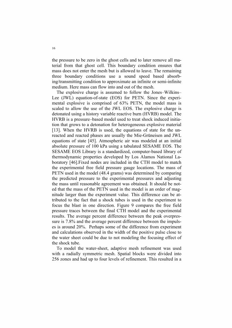
16

the pressure to be zero in the ghost cells and to later remove all ma-terial from that ghost cell. This boundary condition ensures that mass does not enter the mesh but is allowed to leave. The remaining three boundary conditions use a sound speed based absorb-ing/transmitting condition to approximate an infinite or semi-infinite medium. Here mass can flow into and out of the mesh.

The explosive charge is assumed to follow the Jones–Wilkins–Lee (JWL) equation-of-state (EOS) for PETN. Since the experi-mental explosive is comprised of 63% PETN, the model mass is scaled to allow the use of the JWL EOS. The explosive charge is detonated using a history variable reactive burn (HVRB) model. The HVRB is a pressure–based model used to treat shock induced initia-tion that grows to a detonation for heterogeneous explosive material [13]. When the HVRB is used, the equations of state for the un-reacted and reacted phases are usually the Mie-Grüneisen and JWL equations of state [45]. Atmospheric air was modeled at an initial absolute pressure of 100 kPa using a tabulated SESAME EOS. The SESAME EOS Library is a standardized, computer-based library of thermodynamic properties developed by Los Alamos National La-boratory [46].Fixed nodes are included in the CTH model to match the experimental free field pressure gauge locations. The mass of PETN used in the model (48.4 grams) was determined by comparing the predicted pressure to the experimental pressures and adjusting the mass until reasonable agreement was obtained. It should be not-ed that the mass of the PETN used in the model is an order of mag-nitude larger than the experiment value. This difference can be at-tributed to the fact that a shock tubes is used in the experiment to focus the blast in one direction. Figure 9 compares the free field pressure traces between the final CTH model and the experimental results. The average percent difference between the peak overpres-sure is 7.8% and the average percent difference between the impuls-es is around 20%. Perhaps some of the difference from experiment and calculations observed in the width of the positive pulse close to the water sheet could be due to not modeling the focusing effect of the shock tube.

To model the water-sheet, adaptive mesh refinement was used with a radially symmetric mesh. Spatial blocks were divided into 256 zones and had up to four levels of refinement. This resulted in a

17

maximum resolution of 195 microns near any moving interface, re-action zone, or region of steep pressure gradient. Note, results from the adaptive mesh was similar to initial calculations using a fixed Eulerian mesh, except that the water sheet became more jagged dur-ing the later stages of break-up with adaptive meshing.

Liquid water is modeled with the Mie-Grüneisen EOS. The water sheets are assumed to be initially smooth with a thickness of 0.3 cm. Furthermore, the sheets are assumed to be infinite (stretching across CTH domain) to eliminate effects caused by diffraction of the shock wave around the water sheet, and to better isolate the interaction of the shock wave and water sheet. In addition, it should be noted that the CTH models do not include surface tension effects which may play a significant role in the physical breakup process. Because of these simplifications, the simulation results are considered for quali-tative insight into the physical phenomena, rather than quantitative predictions.

Figure 9. Comparison of CTH pressure traces vs. experimental pressure

traces. Numbers indicate the distances in cm between the exit of the shock tube and the pressure gauge.

Figure 10 shows predicted contours of pressure at select time in-tervals. Due to the impendence mismatch at the air-water interface, a significant portion of the initial shock reflects off the water-sheet and

Time (ms)

Pres

sure

(kPa

g)

0.15 0.3 0.45 0.6 0.75 0.9 1.05 1.2-100

0

100

200

300

400

500

600

700

800

CTH pressure gaugesExperimental pressure gauges

10

15

20

25 31

36 41 46 51

18

only a weak shock wave is initially transmitted. Comparison with Fig. 8 reveals many qualitative similarities between simulation and experiment including the reflected wave, transmission of a weak shock wave, and fragmentation of the sheet.

Figure 10. Simulation results showing absolute pressure for shock wave in-

teraction with the water-sheet at the 20 cm standoff distance. (A) initial shock wave reaches the water-sheet, (B) reflection of a shock wave off the

(A)

(B)

(C)

(D)

1 x 105

2 x 105

3 x 105

4 x 105

5 x 105

19

surface of the water-sheet, (C) development of weak transmitted shock wave behind the intact water-sheet, and (D) water-sheet breakup.

Figure 11 shows pressure results from the CTH model at 5 and 10

cm after the water-sheet at a 20 cm standoff distance. This can be qualitatively compared to experimental results presented in Fig 6. Both the experimental and numerical results show the initially transmitted pressure wave. However, the simulation does not cap-ture a distinct second rise in pressure. Note, the pressure fluctua-tions seen in the simulation results, particularly near the centerline, are thought to be a result of water passing through the domain result-ing in an unphysical, numerical artifact. These differences between simulations and experiments highlight the importance of coupled ex-perimental and numerical efforts. Further work is needed to fully understand the experimentally observed pressure profile.

Discussion of water sheet mitigation As discussed by Henderson et al. [44], when a blast wave first

contacts a water-sheet, a large portion of the incident energy is re-flected back towards the source due to the impedance mismatch at the air-water interface. The remaining energy, which is transmitted through the water sheet, forms the observed weak shock wave and the resulting initial pressure rise. For the experimental conditions considered here, the initial blast overpressure is mitigated by as much as 80%. This indicates that a water sheet may be an effective emergency blast mitigant.

20

Figure 11. Comparison between CTH and experimental pressure traces 5 cm after the

water-sheet at a 20 cm standoff distance. However, a second rise in pressure is observed, resulting in a

greater overall peak overpressure behind the water sheet. As dis-cussed above, experimental and numerical results are insufficient to elucidate the source of this behavior and further work is needed. Such work could include investigations in a pressure-driven shock tube as discussed in the first half of this chapter. Such an investiga-tion would be particularly advantageous due to the well-controlled environment and the resulting ability for quantitative optical diag-nostics.

Conclusions Blast loaded objects undergo complex fluid-structure interactions.

These interactions introduce a large range of length-scales and phys-ical phenomena, which complicate first-principle models and numer-ical simulation. For this reason, experimental investigations of blast mitigants are vital to the determination of their effectiveness. In ad-dition, fundamental experimental results can be used to guide model improvements.

This chapter has discussed the most relevant experimental meth-ods, including large-scale blast loading experiments and fundamen-tal shock-tube experiments. In addition, an example investigation of blast mitigation via a water-sheet is presented. Initial results from the experimental investigation reveal significant blast mitigation at certain conditions. However, more work is needed to elucidate the

21

relevant physical phenomena such that predictive models can be de-veloped. This is highlighted by a comparison with numerical simu-lation.

The further development of this, and other blast mitigation meth-ods, requires a three pronged approach. Further blast loading exper-iments are required to identify optimal conditions and quantify ef-fectiveness. Furthermore, fundamental experiments, such as those conducted in pressure-driven shock-tubes, are needed to visualize and quantify the details of the complex interaction of a shock-wave with the proposed mitigant. Finally, these efforts must be closely in-tegrated with numerical simulations to aid in development of predic-tive models. Simulations may possibly be improved with true fluid modeling of the water sheet and full simulation of the shock tube.

Acknowledgements We would like to thank the Department of Homeland Security and

the Center of Excellence for Explosive Detection, Mitigation and Response, Sponsor Award No. 080409/0002251. Additionally, spe-cial thanks to Matthew Massaro and Jesus Mares who assisted with experiments.

Sandia National Laboratories is a multi-program laboratory man-aged and operated by Sandia Corporation, a wholly owned subsidi-ary of Lockheed Martin Corporation, for the U.S. Department of En-ergy's National Nuclear Security Administration under contract DE-AC04-94AL85000.

References

[1] Anderson, J. A., 1990, Modern compressible flow: with historical perspective, Mc-Graw Hill. [2] National Research Council, 1995, Protecting Buildings from Bomb Damage:Transfer of Blast-Effects Mitigation Technologies from Military to Civilian Applications, The National Academies Press. [3] Needham, C. E., 2010, Blast Waves, Springer, Heidelberg.

22

[4] Taylor, G., 1950, "The formation of a blast wave by a very intense explosion. I. Theoritical discussion," Proceedings of the Royal Society of London Series A, Mathematical and Physical Sciences, 201(1065), pp. 159-174. [5] Taylor, G., 1950, "The Formation of a Blast Wave by a Very Intense Explosion. II. The Atomic Explosion of 1945," Proceedings of the Royal Society of London. Series A. Mathematical and Physical Sciences, 201(1065), pp. 175-186. [6] Sedov, L. I., 1959, Similarit and Dimensional Methods in Mechanics, Academic Press, New York. [7] Settles, G. S., 2006, Schlieren and shadowgraph techniques: Visualizing phenomena in transparent media, Springer-Verlag, Berlin. [8] Monti, R., 1970, "Normal shock wave reflection on deformable solid walls," Meccanica, 5(4), pp. 285-296. [9] Gel'fand, B. E., Gubanov, A. V., and Timofeev, E. I., 1983, "Interaction of shock waves in air with a porous screen," Fluid Dynamics, 18(4), pp. 561-566. [10] Skews, B. W., Atkins, M. D., and Seitz, M. W., 1993, "The impact of a shock wave on porous compressible foams," Journal of Fluid Mechanics, 253pp. 245-265. [11] Levy, A., Ben-Dor, G., Skews, B. W., and Sorek, S., 1993, "Head-on collision of normal shock waves with rigid porous materials," Experiments in Fluids, 15(3), pp. 183-190. [12] Radulescu, M. I., and Lee, J. H. S., 2002, "The failure mechanism of gaseous detonations: experiments in porous wall tubes," Combustion and Flame, 131(1–2), pp. 29-46. [13] Teodorczyk, A., and Lee, J. H. S., 1995, "Detonation attenuation by foams and wire meshes lining the walls," Shock Waves, 4(4), pp. 225-236. [14] Sommerfeld, M., 1985, "The unsteadiness of shock waves propagating through gas-particle mixtures," Experiments in Fluids, 3(4), pp. 197-206. [15] Aizik, F., Ben-Dor, G., Elperin, T., Igra, O., Mond, M., and Groenig, H., 1995, "Attenuation law of planar shock waves propagating through dust-gas suspensions," AIAA Journal, 33(5), pp. 953-955.

23

[16] Wagner, J., Beresh, S., Kearney, S., Trott, W., Castaneda, J., Pruett, B., and Baer, M., 2012, "A multiphase shock tube for shock wave interactions with dense particle fields," Experiments in Fluids, 52(6), pp. 1507-1517. [17] Britan, A., Ben-Dor, G., Igra, O., and Shapiro, H., 2001, "Shock waves attenuation by granular filters," International Journal of Multiphase Flow, 27(4), pp. 617-634. [18] Meekunnasombat, P., Oakley, J., Anderson, M., and Bonazza, R., 2006, "Experimental study of shock-accelerated liquid layers," Shock Waves, 15(6), pp. 383-397. [19] Selberg, B., and Nicholls, J., 1968, "Drag coefficient of small spherical particles," AIAA Journal, 6(3), pp. 401-408. [20] Takayama, K., and Itoh, K., 1986, Shock Waves and Shock Tubes; Proceedings of the Fifteenth International Symposium, Sanford University Press. [21] Igra, O., and Takayama, K., 1993, "Shock Tube Study of the Drag Coefficient of a Sphere in a Non-Stationary Flow," Proceedings of the Royal Society of London. Series A: Mathematical and Physical Sciences, 442(1915), pp. 231-247. [22] Jourdan, G., Houas, L., Igra, O., Estivalezes, J.-L., Devals, C., and Meshkov, E. E., 2007, "Drag coefficient of a sphere in a non-stationary flow: new results," Proceedings of the Royal Society A: Mathematical, Physical and Engineering Science, 463(2088), pp. 3323-3345. [23] Wagner, J., Beresh, S., Kearney, S., Pruett, B., and Wright, E., 2011, "Shock Tube Investigation of Unsteady Drag in Shock-Particle Interactions." [24] Haas, J.-F., and Sturtevant, B., 1987, "Interaction of weak shock waves with cylindrical and spherical gas inhomogeneities," Journal of Fluid Mechanics, 181pp. 41-76. [25] Brouillette, M., 2002, "THE RICHTMYER-MESHKOV INSTABILITY," Annual Review of Fluid Mechanics, 34(1), pp. 445-468. [26] Jacobs, J. W., and Krivets, V. V., 2005, "Experiments on the late-time development of single-mode Richtmyer--Meshkov instability," Physics of Fluids, 17(3), pp. 034105. [27] LEINOV, E., MALAMUD, G., ELBAZ, Y., LEVIN, L. A., BEN-DOR, G., SHVARTS, D., and SADOT, O., 2009,

24

"Experimental and numerical investigation of the Richtmyer–Meshkov instability under re-shock conditions," Journal of Fluid Mechanics, 626pp. 449-475. [28] Motl, B., Oakley, J., Ranjan, D., Weber, C., Anderson, M., and Bonazza, R., 2009, "Experimental validation of a Richtmyer--Meshkov scaling law over large density ratio and shock strength ranges," Physics of Fluids, 21(12), pp. 126102. [29] Orlicz, G. C., Balakumar, B. J., Tomkins, C. D., and Prestridge, K. P., 2009, "A Mach number study of the Richtmyer--Meshkov instability in a varicose, heavy-gas curtain," Physics of Fluids, 21(6), pp. 064102. [30] Skews, B. W., 1967, "The shape of a diffracting shock wave," Journal of Fluid Mechanics, 29(02), pp. 297-304. [31] SUN, M., and TAKAYAMA, K., 2003, "Vorticity production in shock diffraction," Journal of Fluid Mechanics, 478pp. 237-256. [32] Tanno, H., Itoh, K., Saito, T., Abe, A., and Takayama, K., 2003, "Interaction of a shock with a sphere suspended in a vertical shock tube," Shock Waves, 13(3), pp. 191-200. [33] Michael, J. V., and Sutherland, J. W., 1986, "The thermodynamic state of the hot gas behind reflected shock waves: Implication to chemical kinetics," International Journal of Chemical Kinetics, 18(4), pp. 409-436. [34] Masten, D. A., Hanson, R. K., and Bowman, C. T., 1990, "Shock tube study of the reaction hydrogen atom + oxygen .fwdarw. hydroxyl + oxygen atom using hydroxyl laser absorption," The Journal of Physical Chemistry, 94(18), pp. 7119-7128. [35] Crawford, D., 2012, CHT Shock Physics, 14 December 2011, http://www.sandia.gov/CTH/. [36] Kailasanath, K., Tatem, P. A., and Mawhinney, J., 2002, "Blast Mitigation Using Water -- A Status Report." [37] Schwer, D., and Kailasanath, K., 2006, "Blast Mitigation by Water Mist (3) Mitigation of Confined and Unconfined Blasts." [38] Cheng, M., Hung, K., and Chong, O., 2005, "Numerical study of water mitigation effects on blast wave," Shock Waves, 14(3), pp. 217-223.

25

[39] Shin, Y. S., Lee, M., Lam, K. Y., and Yeo, K. S., 1998, "Modeling mitigation effects of watershield on shock waves," Shock and Vibration, 5(4), pp. 225-234. [40] BREMOND, N., and VILLERMAUX, E., 2005, "Bursting thin liquid films," Journal of Fluid Mechanics, 524pp. 121-130. [41] Freiwald, D. A., 1972, "Approximate Blast Wave Theory and Experimental Data for Shock Trajectories in Linear Explosive-Driven Shock Tubes," Journal of Applied Physics, 43(5), pp. 2224-2226. [42] Alley, M. D., 2009, "Explosive blast loading experiments for TBI scenarios: Characterization and mitigation," M.S. Thesis, Purdue University, West Lafayette. [43] Settles, G., 2006, "High-speed imaging of shock waves, explosives, and gunshots," American Scientist, 94(1), pp. 22-31. [44] Henderson, L. F., Jia-Huan, M., Akira, S., and Kazuyoshi, T., 1990, "Refraction of a shock wave at an air--water interface," Fluid Dynamics Research, 5(5-6), pp. 337-350. [45] Todd, S. N., Anderson, M. U., and Caipen, T. L., 2011, Springer New York. [46] Lyon, S. P., Johnson, J. D., and Group T-1, SESAME: The Los Alamos National Laboratory equation of state database, 20 November 2011, http://t1web.lanl.gov/doc/SESAME_3Ddatabase_1992.html.

ANNUAL REPORT 2013

Self Healing Materials for Autonomic Mitigation of Blast Damage

Faculty PIs: Nancy R. Sottos and Scott R. White Graduate Student: Jason F. Patrick

Undergraduate Student: Laura K. Richardson

The Beckman Institute for Advanced Science and Technology University of Illinois at Urbana-Champaign

Urbana, IL 61801

Objective This document summarizes research conducted at the University of Illinois at Urbana-Champaign (UIUC) over the past four years, in regards to the development of self-healing materials for autonomic mitigation of blast-induced damage. The goal of this project is to develop self-healing composite systems for mitigation of blast damage over a variety of platforms including civil based infrastructure and aerospace vehicles. The intended outcome of this research will not only address issues directly related to protection and recovery of blast-induced damage but also contribute to scientific advancements in the realm of polymer composites. A concise list of research accomplishments motivated by the aforementioned objectives is provided below: Tasks Accomplished

Prior (Aug. 2009 - July 2010) • Selection of ideal composite sandwich panel system with regards to blast

mitigation performance and realistic integration of self-healing technology.

• Incorporation of bio-inspired microvascular networks into cellular materials to deliver expansive foam healing chemistries suitable for rapid, macro-scale blast damage recovery in polymeric foam sandwich core materials.

(Aug. 2010 - July 2011) • Demonstration of self-healing in a commercial, polyisocyanurate (PIR) foam core

using a 3-pt. Single Edge Notched Bend (SENB) mode-I fracture test under quasi-static loading conditions (Published manuscript [1]).

• Development of “sacrificial fiber” technology for fabrication of microvascular, fiber-reinforced polymer (FRP) composites (Published manuscripts [2, 3]).

(Aug. 2011 - July 2012) • Extension of the patented “sacrificial fiber” vascularization (VaSC) procedure to

encompass conventional 2D woven FRP composite laminate systems.

• Development of a mechanical testing protocol for evaluation of self-healing performance in 2D woven microvascular composites (Manuscript in preparation).

University of Illinois Annual Report

2

Recent (Aug. 2012 - April 2013)

• Demonstration of recovery in interlaminar delamination resistance of 2D woven FRP composites via microvascular delivery of a two-part healing chemistry. (Details I-a).

• Attainment of multiple in-situ self-healing cycles for mode-I fracture repair in vascularized fiber-reinforced composites via active, pressurized fluid delivery (Details I-b, Submitted manuscript [4]).

• Assessment of structural impact of vascularization process on interlaminar fracture resistance in 2D woven composite laminates. (Details II).

Summary Our first milestone was to develop initial specifications for a self-repairing material system based on modern structural requirements for blast resistant composite structures. We completed a comprehensive survey of state-of-the-art materials and potential failure modes for blast resistant composite structures [5-10]. Based on our review of the literature in this area, we identified 3D woven composite sandwich structures as primary candidates for integration of microvascular, self-healing functionality [11-15]. The unique architecture of 3D woven sandwich panels is favorable for seamless integration of current self-healing technology with little impact on initial mechanical properties. Novel composite sandwich panel configurations such as Transonite® make use of 3D woven E-glass composite skins separated by a polymeric foam core and rigidly connected by through thickness fiber insertions. These panels have been shown to withstand 5 lbs of C4 explosive detonated at a mere 3 ft standoff distance. Depending on the through thickness fiber stitching density, primary failure modes after shock loading include delamination of the face sheets from the core, microcracking in the 3D woven composite face sheets, and fracture proliferation throughout the foam core. In our initial work [1], we focused primarily on core damage and the development of a self-healing polymeric foam. Blast events predominantly cause the foam core to fracture, significantly reducing structural stiffness and sandwich efficiency of the composite system [10]. Self-healing of core damage will enable recovery of mechanical integrity and result in enhanced resistance to multiple blast events. Conventional polyurethane (PUR) and polyisocyanurate (PIR) foam cores are condensation materials prepared from organic polyisocyanates, polyols, catalysts, surfactants, and a foaming or blowing agent [16]. In typical foam formulations, the polyisocyanate compound is referred to as Part A whereas the remaining materials constitute Part B. Our strategy was to incorporate a vascular network in a closed-cell PIR foam, whereby Parts A and B were sequestered in separate channels of a 3pt. single edge notch bend (SENB) specimen. Upon quasi-static loading and subsequent crack propagation, the healing agents were released and polymerized on contact to regenerate the foam scaffold. Healing efficiencies in excess of 100% were realized through proper selection of the material system and optimization of delivery parameters. The reactive nature of the PUR foam chemistry provided for rapid healing kinetics, with over 75% recovery in both stiffness and fracture toughness in 1 hr at room temperature. Another attractive feature of this system was the volumetric expansion of the healing chemistry, demonstrating the ability

University of Illinois Annual Report

3

to repair macro-scale fractures comparable to damage induced by blast events. Additionally, multiple damage-healing cycles were attained without sacrifice to healing efficiency or structural integrity. During the second phase of this project, we developed a technique [2,3] for vascularizing (VaSC) fiber-reinforced polymer (FRP) composites to provide a means for circulation of liquid healing agents throughout the structural composite sandwich panel face sheets. This now patented “sacrificial fiber” technology (See Appendix) is capable of producing complex vascular networks in a variety of FRP composite reinforcements, providing a conduit for bioinspired dynamic functionality in a multitude of engineering applications. While the initial VaSC demonstration was performed in 3D woven composites, we decided to first pursue self-healing in more conventional 2D woven FRP laminate systems to gain a deeper understanding of the viscous fluid mixing dynamics and healing reaction kinetics involved. A mechanical evaluation procedure based on mode-I interlaminar delamination in a Double Cantilever Beam (DCB) specimen geometry has been developed to accurately assess healing performance. Through careful selection of a two-part epoxy based healing chemistry, and improved fluid distribution to the fracture plane via pressure-based delivery through interpenetrating networks, multiple damage-healing cycles exceeding 100% recovery have been achieved. Additionally, we have shown the VaSC procedure actually increases interlaminar delamination resistance compared to unvascularized composite laminates. Upon completion of the current research efforts pertaining to self-healing characterization in 2D woven systems, investigation into the damage mechanisms and microvascular based recovery in 3D woven FRP composites subjected to impact will commence. Subsequent work will focus on the total integration of microvascular foam core and composite face sheet components (2D/3D) into a state-of-the-art self-healing structural sandwich panel.

Students Supported

PhD candidate in Civil Engineering at UIUC (emphasis in mechanics & materials)

Jason F Patrick

Senior in Aerospace Engineering at UIUC (interest in structural aircraft design)

Laura K Richardson

University of Illinois Annual Report

4

Transition Partners

Industrial weaving of “sacrificial fibers” to produce 3D non-crimp orthogonal (3WEAVE™) microvascular composite textile

preforms. Melt-spinning of catalyst infused poly(lactic acid) “sacrificial fibers” for vascularizing a wide range of polymeric materials.

Patents 1. Esser-Kahn, H. Dong, P.R. Thakre, J.F. Patrick, N.R. Sottos, J.S. Moore, S.R. White, “Micro-Vascular Materials and Composites for Forming the Materials” US Patent No. 13/416,002 (Published March 14, 2013), UIUC. 2. J.F. Patrick, K.R. Hart, N.R. Sottos, J.S. Moore, S.R. White, “Self-Healing Composite Materials and Micro-Vascular Composites for Forming the Materials” US Patent No. 13/416,002 (Filed December 20, 2012), UIUC. Publications 1. A. Esser-Kahn, P. Thakre, H. Dong, J. Patrick, V. Vlasko-Vlasov, N. Sottos, J. Moore, and S. White, Three-Dimensional Microvascular Fiber-Reinforced Composites, Advanced Materials, 23, 3654-3658 (2011).

2. H. Dong, A. Esser-Kahn, P. Thakre, J. Patrick, N. Sottos, S. White, J. Moore, Chemical Treatment of Poly(lactic acid) Fibers to Enhance the Rate of Thermal Depolymerization, Applied Materials and Interfaces, 4, 503-509 (2012). 3. J. Patrick, N. Sottos, S. White, Microvascular Based Self-Healing Polymeric Foam, Polymer, 53, 4231-4240 (2012). 4. A. King, J. Patrick, N. Sottos, S. White, G. Huff, J. Bernhard, Microfluidically Switched Frequency Reconfigurable Slot Antennas, Submitted to IEEE Antennas and Wireless Propagation Letters (2012). 5. J. Patrick, K. Hart, B. Krull, C. Diesendruck, N. Sottos, S. White, J. Moore, Self- Healing in Fibre Reinforced Composites via Bioinpsired Microvascular Networks, Submitted to Nature Materials (2013). 6. B. Krull, J. Patrick, N. Sottos, S. White, Overhead Automatic Optical Crack Tracking for E-glass Composite Double Cantilever Beam (DCB) Specimens, In Preparation for Experimental Mechanics (2013).

University of Illinois Annual Report

5

Presentations 1. J. Patrick, D.J. Fairfield, N. Sottos, S. White, Microvascular Based Self-Healing Polymeric Foam. 3rd International Conference on Self-healing Materials, Bath, UK, June 2011. 2. J. Patrick, K. Hart, S. White, N. Sottos, J. Moore, Microvascular Based Self-Healing 2D Woven Composites. American Society of Composites 27th Technical Conference, Arlington, TX, October 2012. 3. J. Patrick, K. Hart, B. Krull, C. Diesendruck, J. Moore, N. Sottos, S. White, Self- Healing of Woven Composite Laminates via Bioninspired Microvascular Networks. 4th International Conference on Self-healing Materials, Ghent, BE, June 2013.

Details I-a: Self-healing 2D Woven Microvascular Composites In order to assess microvascular-based healing performance in a 2D woven FRC laminate, the Double Cantilever Beam (DCB) mode-I interlaminar fracture test was selected with relevant experimental parameters depicted in Figure 1a [17-19]. An 8-harness (8H) satin weave (9 oz./yd2, E-glass) fabric reinforcement was chosen due its prevalence in composite structures, and more importantly the stable crack growth resistance (R-curve) behavior (Figure 1b) exhibited during DCB testing under displacement controlled loading [18-20]. The predominantly constant R-curve provides a suitable basis for using the tensile opening (mode-I) strain energy release rate (GI) as a metric to quantify healing efficiency [21, 22] according to:

GI = 3Pδ2ba (1)

where P is the applied load, δ is the load-line displacement, b is specimen width, and a is delamination length (Note: a = a0 + Δa ).

a b Figure 1. (a) Schematic of Double Cantilever Beam (DCB) mode-I fracture specimen; (b) Experimental crack growth resistance (R-curve) behavior for 2D woven 8-harness satin (9 oz./yd2) E-glass composite (Note: fracture along warp direction).

University of Illinois Annual Report

6

DCB samples were quasi-statically loaded under displacement (δ ) control at a rate of 5 mm/min. Illuminating the translucent, E-glass composite samples from below enhanced visual observation of crack propagation using both top and side mounted CCD cameras. Delamination length measurements were determined in 5 mm increments, per ASTM D-5528, from images taken every 1 seconds. Corresponding mode-I strain energy release rates (GI) were calculated according to Equation (1). Based on the success of self-healing in polymer systems via microvascular delivery of a two-part epoxy [11-15], a dual-channel 2D woven fiber-reinforced composite DCB specimen was designed (Figure 2). Equipped with new capabilities in network architecture as a result of the VaSC technology [2], undulating through-thickness microchannels were incorporated via stitching to ensure rupture and fluid release upon interlaminar crack advance. The longitudinally ‘parallel’ channels were placed in close proximity (5mm) to accommodate diffusive mixing of actively delivered (pumped) liquid healing agents. As an extension of the ‘parallel’ design (Figure 3a), a more complex ‘herringbone’ vascular architecture was constructed to further promote in-situ mixing of reactive healing agents and increase delamination recovery (Figure 3b).

a b

Figure 3. Microvascular network configurations investigated (a) Parallel (b) Herringbone;(Top): pre-vascularized composite samples showing embedded 300 µm “sacrificial fibers”;(Middle): idealized two-part liquid healing agent distributions on fractured surfaces; (Bottom):post-vascularized x-ray computed tomographic (µCT) images of liquid gallium-indium fillednetworks revealing internal channel structures (scale bars = 10mm).

a b

Figure 2. (a) Dual channel (red/blue) self-healing microvascular DCB concept; (b) Physicalsample dimensions and layup details for composite fabrication.

University of Illinois Annual Report

7

Details I-b: Multiple Cycles of In-situ Damage Recovery In-situ self-healing tests were conducted by first filling the dual-vascular networks with their respective healing agents (epoxy resin R, amine hardener H) from pressurized reservoirs connected via tubing to micro-dispense tips embedded in the channel orifices. The DCB samples were loaded until the delaminating crack ruptured the first set of vascular channels. Thereafter, the channels were pressurized to deliver a constant total volumetric flow rate (100 µL) of healing agents at a stoichiometric ratio of 2R:1H to the fracture plane. Loading continued as healing agents were concurrently delivered until reaching a preset incremental crack length (Δa), upon which the pressure induced flow was stopped and the sample unloaded (Figure 4).

Healing took place at 30°C for 48 hours with a slight static pressure head on the fluid reservoirs to maintain free-flowing vasculature [11-12]. The sample was then reloaded from the same initial pre-crack length (a0) without pressurized fluid delivery, until the crack front again reached virgin material and pressurized delivery of healing agents was reactivated. Loading continued until reaching the next, preset crack length and again the sample was unloaded and allowed to heal under the same conditions. A total of four loading cycles were conducted for preset incremental crack lengths of: Δa = 30, 50, 70, 95 mm. A representative load-displacement history for all four cycles is shown in Figure 5a. Corresponding healing efficiencies (ηG), or recovery in mode-I strain energy release rate (Figure 5b), was appropriately quantified in this study by [17, 21-23]:

ηG ≡GI

Healed

GIVirgin (2)

Figure 4. In-situ healing agent delivery (a) Overhead optical images of healing agent delivery ina parallel vascularized DCB during loading and crack advance (I-III) (scale bars = 10mm)(b) Representative load-displacement plot for virgin self-healing DCB sample showing typicalfracture behavior at various stages (4a) of in-situ pressurized healing agent delivery.

University of Illinois Annual Report

8

Both sets of data illustrate excellent mechanical recovery in all three cycles of in-situ microvascular based self-healing. Immediately apparent is the increased performance (>100% recovery in virgin strength) of the herringbone vascular network over the parallel configuration due to improved fluid interspersion in the fracture plane (Figure 3). Importantly, the herringbone architecture approaches the maximum values established by pre-mixed, manually repaired tests. Vascularized DCB samples also exhibited a propensity for continued damage-recovery provided that sufficient supply of healing agents remained in external reservoirs. Scanning electron micrographs of the fracture plane from successive regions of an in-situ self-healing DCB sample (herringbone) after three consecutive self-healing cycles are provided in Figure 6. A representative image from a region (Δa = 0-30 mm) experiencing three self-healing events features an accumulation of polymerized, solid material indicated by the presence of raised hackle marks. A lower amount of solid polymer is observed in the two heal cycle region (Δa = 30-50 mm) where underlying, debonded glass fibers are clearly visible. The presence of ruptured glass fibers provides another contribution to damage recovery by increasing the surface area for adhesive bonding of healing agents. Finally, in a representative single heal cycle region (Δa = 50-70 mm), a portion of the fracture surface is overlaid with only partially polymerized healing agents (smooth surface), providing direct evidence for lower healing in regions of close proximity to the crack front.

Figure 5. Self-healing results (a) Representative multiple cycle (48 h, 30°C) load-displacementdata for an in-situ self-healing DCB specimen (herringbone). (b) Average healing efficienciescalculated according to Equation (2) for each vascular pattern at a component delivery ratio of 2-parts epoxy resin (R) to 1-part amine based hardener (H) by volume. (Note: dashed lineindicates average healing efficiency of manually repaired samples with pre-mixed healing agents;vertical error bars represent the standard error from three samples tested).

University of Illinois Annual Report

9

Details II: Effect of Vascularization on Mode-I Fracture Resistance Additionally, the effect of the VaSC process on GI was assessed to ensure no appreciable loss in crack-growth resistance is incurred. Table 1 provides a summary of the results for neat (no channels), treated (VaSC thermal conditions, no channels), and both the parallel and herringbone vascular configurations. The VaSC treated samples show a slight (4%) reduction in GI compared to the neat case, however the parallel and herringbone specimens exhibit a respective 3 and 10% increase over the neat crack-growth resistance. Scanning electron micrographs provided in Figure 7 reveal the fracture resistance mechanisms operative in our self-healing composites. Comparison of the plain, woven 8H satin fabric (7a, left) with a neat composite fracture surface (7b, middle) illustrates the presence of polymer matrix debonding from the E-glass reinforcement during fracture and ruptured fibre-bridging providing supplementary crack growth resistance [19]. Fracture toughness is further enhanced by the presence of vascular inclusions (7c, right) which invoke crack blunting mechanisms previously reported in the literature [24]. Thus, the presences of microvascular networks actually serve to increase the resistance to interlaminar, mode-I fracture over conventional ‘pristine’ composites.

Table 1. Effect of vascularization (VaSC) process on mode-I crack growth resistance

DCB sample type GI (J/m2) Normalized Neat (36 h RT + 2 h 121°C + 3 h 177°C) 488 ± 8.4a 1.00b

Treated (neat + 36 h 200°C @ 12 torr vacuum) 471 ± 11.2 0.96

VaSC – Parallel (treated + channels) 502 ± 3.4 1.03

VaSC – Herringbone (treated + channels) 537 ± 15.1 1.10 a one standard deviation, b by average neat value

Figure 6. Scanning electron micrographs (SEM) from successive regions of an in-situ DCBsample (herringbone - 2R:1H) after three consecutive self-healing cycles (scale bars = 300 µm)(a) Δa = 0 - 30 mm (3 heals); (b) Δa = 30 - 50 mm (2 heals); (c) Δa = 50 - 70 mm (1 heal).

University of Illinois Annual Report

10

While these latest experimental findings mark the first true demonstration of multiple cycles of in-situ microvascular self-healing in a FRC via active delivery of a two-part epoxy, additional research is required to unravel the governing physics and reach full self-healing potential. Current spectroscopic investigations including confocal Raman and fluorescence are being conducted in order to determine fluid interspersion in the fracture plane as a result of varying network configuration and ensuing mixing/degree of polymerization attained. This in-depth characterization study will provide useful information for optimization of future microvascular designs under a variety of composite geometry and loading conditions. More advanced network fabrication procedures to create these optimal, multiscale vascular structures are also being pursued including state-of-the-art 3D printing and laser micromachining techniques [25, 26]. Another ongoing research endeavor is determining the effect of vascular features and/or VaSC processes employed to produce these dynamic composites, on the in-plane mechanical integrity of the native structural material [27]. A series of standardized mechanical tests [28-29] will be conducted in order to develop a comprehensive understanding of the material response. Once the 2D FRC vascular self-healing systems are well understood, our research efforts will move towards developing similar damage-healing protocols for 3D woven microvascular composites subjected to energetic impact. The ultimate goal of our anticipated research and development program is to combine the stand alone microvascular FRC and polymer foam self-healing technologies into a single composite structural sandwich panel capable of unprecedented, autonomic blast protection. REFERENCES

1. J. Patrick, N. Sottos, S. White, Microvascular Based Self-Healing Polymeric Foam, Polymer, 53, 4231-

4240 (2012). 2. A. Esser-Kahn, P. Thakre, H. Dong, J. Patrick, V. Vlasko-Vlasov, N. Sottos, J. Moore, and S. White,

Three-Dimensional Microvascular Fiber-Reinforced Composites, Advanced Materials, 23, 3654-3658 (2011).

3. H. Dong, A. Esser-Kahn, P. Thakre, J. Patrick, N. Sottos, S. White, J. Moore, Chemical Treatment of Poly(lactic acid) Fibers to Enhance the Rate of Thermal Depolymerization, Applied Materials and Interfaces, 4, 503-509 (2012).

4. J. Patrick, K. Hart, B. Krull, C. Diesendruck, J. Moore, N. Sottos, S. White, Self-Healing in Fibre Reinforced Composites via Bioinspired Microvascular Networks, Submitted: Nature Materials (2013).

Figure 7. SEM interlaminar region characterization (a) plain 8H satin E-glass reinforcing fabric(b) neat DCB fracture surface showing fiber-bridging and matrix debonding phenomena; (c)ruptured empty, through-thickness channel along fractured DCB mid-plane (scale bars = 300 µm).

University of Illinois Annual Report

11

5. J. Baucom, M. Zikry. Evolution of Failure Mechanisms in 2D and 3D Woven Composite Systems under Quasi-static Perforation. Journal of Composite Materials, 45, 1651-1674 (2003).

6. J. LeBlanc, A. Shukla, C. Rousseau, A. Bogdanovich. Shock Loading of three-dimensional woven composite materials. Composite Structures, 79, 344-355 (2007).

7. J. Grogan, S. Tekalur, A. Shukla, A. Bogdanovich, A. Coffelt. Ballistic Resistance of 2D and 3D Sandwich Composites. Journal of Sandwich Structures and Materials, 9, 283-302 (2007).

8. J. Patrick, "Fundamental Characteristics of 3-D GFRP Pultruded Sandwich Panels." M.S. Thesis, Department of Civil and Environmental Engineering, North Carolina State University, Raleigh, NC (2007).

9. A. Bogdanovich, M. Mohamed, Three-Dimensional Reinforcements for Composites, SAMPE Journal, 45(6), 2-20 (2009).

10. S. Tekalur, A. Bogdanovich, A. Shukla. Shock loading response of sandwich panels with 3-D woven E-glass composite skins and stitched foam core. Composites Science and Technology, 69, (2009).

11. A. Hamilton, N. Sottos, S. White, Pressurized vascular systems for self-healing materials, Journal of the Royal Society Interface, 9(70), 1020–1028 (2012).

12. A. Hamilton, N. Sottos, S. White, Self-healing of internal damage in synthetic vascular materials, Advanced Materials, 22, 5159–5163 (2010).

13. C. Hansen, S. White, N. Sottos, J. Lewis, Accelerated Self-healing via ternary interpenetrating microvascular networks, Advanced Functional Materials, 21, 4320-4326 (2011).

14. C. Hansen, W. Wu, K. Toohey, N. Sottos, S. White, J. Lewis, Self-healing materials with interpenetrating microvascular networks, Advanced Materials, 21, 4143–4147 (2009).

15. K. Toohey, C. Hansen, N. Sottos, J. Lewis, S. White, N. Sottos, Delivery of two-part self-healing chemistry via microvascular networks, Advanced Functional Materials, 19, 1399–1405 (2009).

16. M. Kapps, S. Buschkamp, The production of rigid polyurethane foam, Technical Report, Bayer Material Science, (2004).

17. M. Kessler, S. White, Self-activated healing of delamination damage in woven composites, Composites A, 32, 683–699 (2001).

18. J. Whitney, C. Browning, W. Hoogsteden, A Double Cantilever Beam Test for Characterizing Mode I Delamination of Composite Materials, Journal of Reinforced Plastics and Composites, 1, 297-313 (1982).

19. ASTM International, ASTM D5528: Standard Test Methods for Mode I Interlaminar Fracture Toughness of Unidirectional Fiber-Reinforced Polymer Matrix Composites (2007).

20. N. Alif, L. Carlsson, L. Boogh, Effect of weave pattern and crack propagation direction on mode I delamination resistance of woven glass and carbon composites, Composites Part B, 29, 603-611 (1998).

21. S. White, N. Sottos, P. Geubelle, J. Moore, M. Kessler, S. Sriram, E. Brown, S. Viswanathan, Autonomic healing of polymer composites, Nature, 409, 794–797 (2001).

22. E. Brown, Use of the tapered double-cantilever beam geometry for fracture toughness measurements and its application to the quantification of self-healing, Strain Analysis for Engineering Design, 46, 167–186 (2011).

23. J. Rule, E. Brown, N. Sottos, S. White, J. Moore, Wax-Protected Catalyst Microspheres for Efficient Self-Healing Materials, Advanced Materials, 17, 205-208 (2005).

24. A. Kousourakis, A. Mouritz, M. Bannister, Interlaminar properties of polymer laminates containing internal sensor cavities. Composite Structures, 75, 610–618 (2006).

25. J. Miller, K. Stevens, M. Tang, B. Baker, D. Nguyen, D. Cohen, E. Toro, A. Chen, P. Galie, X. Yu, R. Chaturvedi, S. Bhatia, C. Chen, Rapid casting of patterned vascular networks for perfusable engineered three-dimensional tissues. Nature Materials, 11, 768–774 (2012).

26. M. Focke, D. Kosse, C. Müller, H. Reinecke, R. Zengerle, F. Stetten, Lab-on-a-Foil: microfluidics on thin and flexible films. Lab on a Chip, 10, 1365–1386 (2010).

27. A. Kousourakis, M. Bannister, A. Mouritz, Tensile and compressive properties of polymer laminates containing internal sensor cavities, Composites A, 39, 1394-1403 (2008).

28. ASTM International, ASTM D3039: Standard Test Methods for Tensile Properties of Polymer Matrix Composite Materials (2008).

29. ASTM International, ASTM D7264: Standard Test Methods for Flexural Properties of Polymer Matrix Composite Materials (2007).

30. A. King, J. Patrick, N. Sottos, S. White, G. Huff, J. Bernhard, Microfluidically Switched Frequency Reconfigurable Slot Antennas, Submitted: IEEE Antennas and Wireless Propagation Letters (2012).

University of Illinois Annual Report

12

APPENDIX The recently patented process (Figure A1) designated ‘Vaporization of Sacrificial Components’ (VaSC), integrates a commercially available biopolymer fiber into existing textile composite reinforcement manufacturing techniques to imbue FRP composites with three-dimensional vasculature. In VaSC a robust, chemically treated [2, 3] thermoplastic monofilament deemed ‘sacrificial fiber’ is directly woven into composite textile reinforcement (Fig. A1a). Upon subsequent epoxy resin infusion (Fig. A1b), vacuum/pressure compaction, and elevated temperature post-curing, the fibers sublimate via thermal depolymerization leaving behind high fidelity, inverse replica vascular features (Fig. A1c). The resulting vascularized composite permits the circulation of fluids (Fig. A1d) through its internal structure, providing a conduit for dynamic functionality. In addition to self-healing capability, vascular composites also accommodate multiphysical properties such as thermal regulation and electromagnetic modulation [30] via a simple substitution of fluids.

The initial VaSC demonstration was performed in 3D woven fiber reinforced composites (FRC), mainly to showcase the commercial practicality and complex geometric possibilities in vascular design [2, 9], although the technique is amendable to a variety of reinforcement architectures.

Figure A1. VaSC fabrication procedure. (a) ‘sacrificial fibers’ (red) woven into glass reinforcing fabric; (b) infiltration of polymer resin into composite preform; (c) matrix solidification and subsequent thermal depolymerization resulting in vascularized structural composite; (d) fluid filled (yellow) microchannels (scale bars = 5 mm). Image from Esser-Kahn et al. [2].

Stress Attenuation by Means of ParticulatesCarl-Ernst Rousseau

Mechanical Engineering; University of Rhode Island

Objective:

The objective of this work is to identify effective means of stress wave mitigation. Traditional shielding techniques have consisted in heavy and voluminous metallic barriers that are effective but cumbersome. The focus has naturally shifted to composites, as they possess lower densities and, though not as sturdy as metals, have resilience capabilities approaching them. The approach associated with composites has also been highly empirical. For instance, consecutive tests performed on two equivalent types of fibrous composites will indicate which on is more appropriate to a specific shielding task. However, what specific aspect of the material’s microstructure ensures this outcome? We endeavor to answer those questions by launching stress waves within these materials and note instances of absorption, reflection, or deflection that reduce or eliminate damage. We aim to do so not only for composites, but also for metals, as we explicitly target the influence of porosity, inclusions, impurities, cell or grain boundaries, and sizes. Finally, complete description of materials for dynamic, stress wave, and shock study or prediction is frequently associated with knowledge of the Hugoniot conditions. For any material, the latter representation is the result of numerous experimental studies. Last year, we had expressed the hope of being able to develop a technique whereby the Hugoniot can be obtained from the amalgamation of data pertaining to a single experiment. We are pleased to report that the success of the first set of experiments concluded in the last month redounded to the credit of our methodology. Consequently, we will soon be able to provide a complete dynamic representation of a material through the medium of two single experiments, where traditionally, several dozens were required by means of the traditional methodologies.

Significance to DHS:

The work performed, its extension and future ramifications are highly relevant to DHS’ aim of protection of infrastructure and citizenry. Indeed full comprehension of mechanisms of failure and of its prevention, will allow engineers working in the security field to base choices on sound scientific grounds, and be better able to combine materials characteristics in order to fabricate more effective shields. Also, experimental techniques developed during the course of this study will allow for the application of speedier and more efficient gathering of experimental outcomes, both for ourselves and others in the broader scientific community who elect to use the techniques we have developed.

Accomplishments:

Within this past year, we have authored two papers associated with this work, one is under review, and three others will be submitted presently. Two conference publications have been accepted and will be presented in June 2013. We have successfully concluded our collaboration

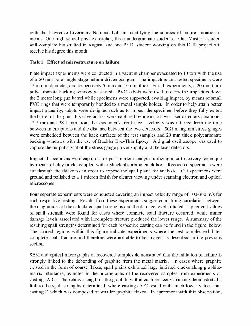
with the Lawrence Livermore National Lab on identifying the sources of failure initiation in metals. One high school physics teacher, three undergraduate students. One Master’s student will complete his studied in August, and one Ph.D. student working on this DHS project will receive his degree this month.

Task 1. Effect of microstructure on failure

Plate impact experiments were conducted in a vacuum chamber evacuated to 10 torr with the use of a 50 mm bore single stage helium driven gas gun. The impactors and tested specimens were 45 mm in diameter, and respectively 5 mm and 10 mm thick. For all experiments, a 20 mm thick polycarbonate backing window was used. PVC sabots were used to carry the impactors down the 2 meter long gun barrel while specimens were supported, awaiting impact, by means of small PVC rings that were temporarily bonded to a metal sample holder. In order to help attain better impact planarity, sabots were designed such as to impact the specimen before they fully exited the barrel of the gun. Flyer velocities were captured by means of two laser detectors positioned 12.7 mm and 38.1 mm from the specimen’s front face. Velocity was inferred from the time between interruptions and the distance between the two detectors. 50Ω manganin stress gauges were embedded between the back surfaces of the test samples and 20 mm thick polycarbonate backing windows with the use of Buehler Epo-Thin Epoxy. A digital oscilloscope was used to capture the output signal of the stress gauge power supply and the laser detectors.

Impacted specimens were captured for post mortem analysis utilizing a soft recovery technique by means of clay bricks coupled with a shock absorbing catch box. Recovered specimens were cut through the thickness in order to expose the spall plane for analysis. Cut specimens were ground and polished to a 1 micron finish for clearer viewing under scanning electron and optical microscopes.

Four separate experiments were conducted covering an impact velocity range of 100-300 m/s for each respective casting. Results from these experiments suggested a strong correlation between the magnitudes of the calculated spall strengths and the damage level initiated. Upper end values of spall strength were found for cases where complete spall fracture occurred, while minor damage levels associated with incomplete fracture produced the lower range. A summary of the resulting spall strengths determined for each respective casting can be found in the figure, below. The shaded regions within this figure indicate experiments where the test samples exhibited complete spall fracture and therefore were not able to be imaged as described in the previous section.

SEM and optical micrographs of recovered samples demonstrated that the initiation of failure is strongly linked to the debonding of graphite from the metal matrix. In cases where graphite existed in the form of coarse flakes, spall plains exhibited large initiated cracks along graphite-matrix interfaces, as noted in the micrographs of the recovered samples from experiments on castings A-C. The relative length of the graphite within each respective casting demonstrated a link to the spall strengths determined, where castings A-C tested with much lower values than casting D which was composed of smaller graphite flakes. In agreement with this observation,

the small surface area shared by the graphite nodules and metal matrix in the ductile cast iron resulted in much higher strength values for this material than found for the gray cast irons. The subsequent coalescence of the initiated microcracks required propagation into the metal matrix to form a completed fracture plane. The small range of strengths exhibited by cast iron D indicates that this process can be completed with minimal additional energy in cases where the spacing between graphite flakes is relatively small. This observation is further supported by considering a SEM micrograph of a recovered sample from casting D impacted at 190 m/s found in the figure below. Within this micrograph graphite of type VII A4 and VII D8 can be noted respectively on the left and right. In the case of the coarse distribution of graphite, the material partially retained its integrity, however, a large spall plane can be noted in the case of the fine distribution. A pearlitic metal matrix is noted to provide an increase in tensile strength through the final stages of spall fracture as indicated by the higher strengths found for casting B in comparison to castings A and C. This observation is in agreement with quasi-static testing of cast irons in literature where it is commonly noted that free ferrite can significantly reduce a castings tensile strength.

Results from this investigation suggest a strong correlation between the magnitudes of calculated spall strengths and the damage level initiated where an increased amount of energy is required to generate completed fracture planes. The morphology of graphite within cast irons has been shown to strongly affect the material’s spall strength. Initiation of spallation is linked to the debonding of graphite from the metal matrix. The subsequent coalescence of initiated cracks into a complete fracture plane is correlated to both the microstructural components of the metal matrix and comparative spacing of the graphite phase. In cases where graphite spacing is relatively small, this process can be completed with minimal additional energy. A metal matrix of pearlite has been linked to increased tensile strength in castings, helping to prevent the coalescence of initiated cracks in the formation of complete spall fracture planes.

Task 2. New method for predicting stress attenuation within materials by ultrasonic means

The ultrasonic pulse-echo immersion technique consists of sending a mechanical pulse in the ultrasonic frequency range to a material and analyzing several echoes reflected from the material in order to calculate the longitudinal wave speed and attenuation coefficient of the material under test.

The mechanical pulse is created by an ultrasonic transducer that is based on the piezoelectric effect of a crystal. The main characteristic of the immersion technique is that the pulse is not transmitted directly from the transducer to the material but rather through a liquid (water, in the present case) in which the solid material is immersed and that acts as a coupler between transducer and material. The material sample is immersed in the liquid and placed perpendicularly to the transducer to facilitate the analysis and calculations.

We will designate the generated wave as (V0), the front wall reflection as (V0’), and the multiple reflections or echoes from back wall of the solid material as (V1), (V2), … (Vn). In the pulse-echo immersion technique, V1 and V2 are used to calculate the longitudinal wave speed and the attenuation coefficient of the material. The magnitudes of these echoes are, based on the assumptions that 1) reflection and transmission of the pulse occur at the water-sample interface, 2) attenuation of the pulse occurs only within the solid material, and 3) the beam is spreading. Variables RA, RB, TA, TB are actually functions representative of the reflection and transmission coefficients of faces A (front) and B (back), respectively, and D is representative of the divergence of the wave. The wave attenuation can thus be expressed as: α = (1/2h) ln [(V1/V2 RA RB (D1/D2)], where h is the material thickness.

The reflection coefficients depend on the impedances of both the material to be tested and the liquid medium. The erroneous assumption frequently made in experimentation is the two media form a perfectly bonded interface. Our experiments have proven that this assumption does not hold, leading to significant errors in the attenuation coefficient calculation. The effect is particularly pronounced for materials that have low affinity to water, such as teflon specimens or urethane-based products frequently used in composites.

In order to resolve the problems associated with the traditional ways of calculating the attenuation coefficient of a material, we have developed a new experimental method that considers the reflection coefficients in both faces to be unknown and possibly different. Traditional means of experimentation, on the other hand incorrectly regard both facial conditions as being identical. Out methodology allows measurement of both reflection and attenuation coefficients simultaneously. The method can be extended to any material and guarantees the correct measurement of attenuation.

The next stage of this research will correlate this “true” attenuation to the material’s internal friction and stress mitigation.

Task 3. Improved methodology for determining material Hugoniot

At present with have just successfully established a methodology for determining material’s Hugoniot based on a set of two experiments. Conventional experimentation requires several dozens tests to establish the dynamic state of a material. Much work needs to be done to refine the methodology, which was initially undertaken by Doctoral Candidate G. Plume. As he received his degree this month, doctoral student M. Goni will undertake those improvements. We, thus propose to continue refining this work for another year as a means of completely establishing dynamic states of novel, mitigating materials.

Doctoral candidate Gifford Plume at work on Task 1.

Master’s recipient Bhaskar Ale at work on the initial stages of Task 2.

Papers Published:

Plume, G., Rousseau, C.-E., April 5, 2012, “Investigation into the Spall Strength of Cast Iron.” International Journal of Nonlinear Science and Numerical Simulations, Vol. 13, Issue 2, pp. 195199, (doi: 10.1515/IJNSNS.2011.098).

Ale, B., Rousseau, C.-E., “Dynamic attenuation and compressive characterization of syntactic foams”, Engineering Materials and Technology, In-Press 2013.

Collaboration

Effect of porosity on the performance of cast iron with Lawrence Livermore National Laboratory

Graduate Students

Gifford Plume (May 2013); Miguel Goni (August 2013); Michael Franzblau (May 2013)

Undergraduate Students

Christian Mejia (May 2014); Jose DeFaria (May 2012); Sameer Saran (May 2014)

Annual Performance Report

2012-2013

Development of Novel Composite Materials & Structures for Blast Mitigation

Arun Shukla1, Nate Gardner2, Payam Fahr2, Emad Makki2, Jefferson Wright2

1 Principal Investigator, Simon Ostrach Professor 2 Students, Dynamic Photomechanics Laboratory Department of Mechanical, Industrial and Systems Engineering University of Rhode Island, Kingston, RI 02881

Submitted to Department of Homeland Security (DHS)

Objective

The current investigations aim to develop novel material systems and sandwich structures that can withstand shock wave (air-blast) loadings and effectively mitigate the blast overpressures. The study also focuses on the response of these material systems and sandwich structures in extreme (temperature) environments.

Summary

A shock tube apparatus was utilized to generate a controlled shock loading on the specimens (Fig. 1a). It has an overall length of 8 m, consisting of a driver, driven and muzzle section. The high-pressure driver section and the low pressure driven section are separated by a diaphragm. By pressurizing the high-pressure section, a pressure difference across the diaphragm is created. When this difference reaches a critical value, the diaphragm ruptures. This rapid release of gas creates a shock wave, which travels down the tube to impart a dynamic loading on the specimen. The driver gas is helium and the driven gas is ambient air.

Fig. 1b shows the detailed dimensions of the muzzle and locations of the specimen and the pressure sensors (PCB102A). The sensors are mounted at the end of the muzzle section to measure the incident pressure and the reflected pressure during the experiment. The final muzzle diameter is 0.076 m (3 in). The distance between the two sensors is 0.160 m and the distance between the second sensor and the end of the muzzle is ~ 0.020 m. The specimen was placed in the supports and positioned close to the end of the muzzle. These support fixtures ensure clamped boundary conditions with a span of 0.203 m (8 in) by 0.203 m (8 in). A typical pressure profile obtained from the transducer closest to the specimen (~ 0.020 m away) can be seen in Fig. 2. It should be noted that both pressure transducers were utilized to obtain the shock wave history, i.e. incident / reflected pressure and incident / reflected velocity. However, only the pressure transducer closest to the specimen was utilized to obtain the pressure applied on the specimen.

The Digital Image Correlation (DIC) technique was also used to measure the full-field, in-plane and out-of-plane displacements. The DIC arrangement is shown in Fig. 3. Initially the camera records an image of the specimen in its un-deformed state. A second picture is then taken after the specimen has deformed. The two images are then compared in order to calculate the in-plane and out-of-plane displacements of the specimen. A random speckle

Fig. 1: Shock tube apparatus

(b) Detail dimensions of the muzzle (a) Shock tube

pattern is applied on the specimen and each speckle is individually tracked in order to obtain the in-plane and out-of-plane displacements.

Accomplishments

Task 1: Dynamic Response of Laminated Safety Glass Panel subjected to Shock Loading under Extreme Environments

Laminated Safety Glass (LSG) is a composite material that combines the unique properties of glass with the benefits of a tough but highly elastic organic material (PVB) interlayer (materials having both advantages of the organic materials such as the light-weight, flexibility and of the inorganic materials such as the high strength, heat-stable, and chemical resistance). The objective of this study is to investigate the blast performance of (LSG) panel, coated with XO-Armor® protective films on both (front / back) faces, and to mitigate the blast loading at extreme environments which was investigated experimentally using the shock tube apparatus. A 3D-Digital Image Correlation (DIC) technique is used to obtain the out-of-plane deflection, in-plane strain developed, and the velocity of the back face, accordingly to understand the failure mechanism during shock wave event. The results show that the coated protective films play a crucial role in the dynamic behavior of (LSG) panels when they are subjected to a blast loading. Effects of temperatures on thermoplastic films will change the mechanical properties, therefore, changing the dynamic response of the glass structure overall. The results indicated that at high temperature the strength of specimen was decreased and accordingly it behaves more ductile. However, for low temperature the panel behaves more brittle where the material strength was increased in this condition. Moreover, the efficiency and energy analyses will be developed to calculate the amount of energies that are absorbed and reflected by the system structure during the blast event.

Task 2: Blast Response of Nano-Scale Core-Shell Rubber (CSR) toughened Sandwich Composites

The dynamic behavior of two types of sandwich composites made of E-Glass Vinyl-Ester (EVE) face sheets and Corecell TM A500 foam was studied using a shock tube apparatus. The core material and thickness, as well as overall specimen dimensions were held constant,

Fig. 2: Typical pressure profile from transducer closest to the specimen

0 1000 2000 3000 4000 50000.0

0.5

1.0

1.5

2.0

2.5

3.0

3.5

4.0

4.5

5.0

P

ress

ure

(MP

a)

Time (μs)

Incident Wave

Reflected Wave

Fig. 3: High-speed photography systems

with the only difference arising in the resin system used during the infusion. The non-coreshell rubber toughened resin system (Non-CSR) consisted of a vinyl-ester resin only; while the CSR toughened resin consisted of the same vinyl-ester resin, but with Kane Ace MX-153 nano-scale coreshell rubber particles added to the mixture. Prior to shock tube testing, the quasi-static and dynamic constitutive behavior of the face sheets (tensile/compressive) and foam (compressive)was evaluated. During the shock tube testing, high-speed photography coupled with the optical technique of Digital Image Correlation (DIC) was utilized to capture the real-time deformation process as well as mechanisms of failure. Post-mortem analysis was also carried out to evaluate the overall blast performance of these configurations. Results indicated that adding nano-scale core-shell rubber (CSR) particles to sandwich composites, aids in dispersing the initial shock wave loading, thus reducing the overall deflection, strain, and velocity and improving the overall blast resistance of the structure.

Task 3: Experimental and Numerical study of Foam Filled Corrugated Core Steel Sandwich Structures Subjected to Blast Loading

In this study, the influence of foam infill on blast resistivity of corrugated steel core sandwich panels was investigated experimentally and numerically through high speed photography and Finite Element Methods, respectively. After verifying the finite element model numerically studies were conducted to investigate the effect of face sheet thickness (1, 3 and 5 mm), corrugated sheet thickness (0.2 mm, 0.6 mm and 1 mm) and boundary conditions (Simple Supported and Encastre supported on sides) on blast performance. Experimental and FEM results were found to be in good agreement with R2 values greater than 0.95. Results showed that the addition of foam infill reduced both the back face deflections and front face deflections by more than 50% at 3 ms after blast loading at a weight expense of only 2.3%. However, increasing face sheet thickness and corrugated sheet thickness decreased the benefit obtained from foam filling in the sandwich structure. Foam infill benefits were more prominent for simple supported edge case than encastre supported edge case.

Task 4: Corrugated Structures to improve Thermal and Blast Mitigation (Collaboration with the University of Connecticut)

Blast loading experiments on corrugated steel sandwich panels were being conducted using a shock tube apparatus configured for extreme temperatures in conjunction with high-speed digital image correlation (DIC) photography. A syntactic filler material was developed to fill the corrugated panels and is being experimentally evaluated in order to understand its contributions in enhancing thermal resistivity and blast response under rapid dynamic loading. Preliminary results show that the syntactic filler material mitigates back-face deformation. Two experimental series were performed for this study. At room temperature, the performance of the filler material was investigated comparing empty and filled panels at a low pressure. High temperature experiments were performed by heating the back face of filled panels to 500˚C. A temperature differential of at least 350˚C was observed over a duration of 20 minutes, at which point a shock load was impinged on the specimen.

Fig.4 (b): LSG-Panel with XO-Armor® Protective

Fig.4 (a): Schematic of Glass Structure System

Details Task 1: Dynamic Response of Laminated Safety Glass Panel subjected to Shock Loading under Extreme Environments

Laminated Safety Glass (LSG) is a composite material that combines the unique properties of glass with the benefits of a tough but highly elastic organic material (PVB) interlayer as shown in (materials having both advantages of the organic materials such as the light-weight, flexibility and of the inorganic materials such as the high strength, heat-stable, and chemical resistance). The objective of this study is to investigate the blast performance of (LSG) panel that is coated with XO-Armor® protective films on both (front / back) faces as shown in (Fig.4(a)), and to mitigate the blast loading at extreme environments were conducted using the shock tube apparatus.

Material Details

As shown in Fig.4 (b), the sandwiched glass panel consists of two clear glass panels made out of soda–lime–silica glass which are bonded by a polyvinyl butyral (PVB) interlayer. This bonding process takes place utilizing heat and pressure treatment. The PVB layer has good bonding strength, is

optically clear and does not diminish the optical properties of the glass panel. The laminated sandwiched glass panel is made by adhering a protective film from XO ARMOR® on both of the outer faces of the sandwiched glass panel. The protective film is 0.279 mm thick and a special adhesive XO® bond was used to adhere the protective film onto both of the faces of the sandwiched glass panel. The specimen is 305 mm long×305 mm wide×7.0 mm thick. According to the ASTM (D-882) standard test method for tensile properties of thin plastic sheeting, a simple test was performed at strain rate of 6x10^-4 (ε/s) to obtain the following physical properties as shown in Table 1.

Fig.5 (a): Thermally insulated enclosure

Fig.5 (a): Thermally insulated enclosure

Fig.5 (b): Heating setup

Modulus of Elasticity (Gpa) 3.5

Yield Strength (Mpa) 85

Ultimate Tensile Strength (Mpa) 181

Elongation (%) 150

Break Strength (lbs/inch) 295

Table 1: Tensile properties of XO ARMOR® protective film.

High and Low Temperature Experimental Setup for Shockwave Loading

Panels are tested at room temperature, at (0 °C, −8 °C) for low temperatures, and at (50 °C, 80 °C) for high temperatures (Gulf Countries). During the experiments, a special environmental chamber is designed to heat up and cool down the panels to required temperatures prior to blast loading. For testing the specimen under high temperature, a thermally insulated enclosure was designed around the support fixture as shown in Fig.5(a).

A heating element was utilized to heat the internal environment and a circulation fan was used to ensure proper air-circulation Fig.5(b). By adjusting the output power of the heating element, various uniform (steady state) temperatures in the heating chamber were achieved.

Lab View software has been used for recording and plotting the temperature-time calibration for both (high / low) setups. To perform the experiment at a steady state temperature of 80 °C, a typical temperature-time plot for a specimen is shown in Fig.6. The specimen was heated for approximately 180 min. and then was subjected to shock-wave loading. In the last 20 Minutes from the calibration process, temperature had a minimal incremental increase (< 1 °C) between the insulated enclosure chamber and the center of the specimen.

Fig.7: Schematic of panel sandwiched between two anti-freeze frozen plastic bags in cooling freezer.

Fig.6: A typical heating calibration plot of 80 °C

For low temperature testing, the specimen was cooled down inside a cooling freezer for about an hour up to a maximum temperature of (-20 °C), where the panel was kept in between and covered by two plastic pages filled with a frozen liquid of an antifreeze (coolant) to continue cooling the entire panel outside the cooling freezer as shown in Fig.7. Once this was achieved, the specimen was quickly moved to the support fixture inside the shock-tube facility and the specimen ready for the blast. The environmental heat will increase the temperature of specimen uniformly, where the panel was held

in room temperature at different periods of time, in order to achieve different specific designed low temperatures as shown in Fig.8.

0 20 40 60 80 100 120 140 160 18020

30

40

50

60

70

80

Time (Min)

Te

mp

era

ture

(°C

)

Fig.9: A typical pressure profiles and there calculated impulses temperatur

Fig.8: A typical cooling calibration plot of -8 °C

Blast Pressures Subjected to Specimen in Shock Tube Experiments

The square flat plate specimens utilized in this experimental study are held under fully clamped boundary conditions prior to blast loading.. The dynamic loading is applied over a central circular area of 76.2 mm in diameter. The diameter of the driver and driven section is 0.15 m. The final muzzle diameter is 0.07 m. Two pressure transducers are mounted at the end of

the muzzle section measure the incident shock pressure and the reflected shock pressure during the experiment. All of the specimens are subjected to the same level of incident pressure in this experiment. A typical pressure profile obtained at the transducer location closer to the specimen is shown in Fig. 9, where the reflected velocity for the panel was about 350 m/s.

Digital Image Correlation (DIC) Analysis

A 3D-Digital Image Correlation (DIC) technique is used to obtain the out-of-plane deflection, in-plane strain developed, and the velocity of the back face, accordingly to understand the failure mechanism during shock wave event. Cameras are Photron SA1 high-speed digital camera and are used at a frame-rate of 20,000 fps with an image resolution of 512× 512 pixels for one second time duration. These cameras are synchronized to make sure that the images and data can be correlated and compared.

Fig.10: Time- out of plane deflection, in-plane strain developed, strain rate, and the velocity of the back face at (room, high, low) temperature

Fig.11: Deflection of the back face during fluid structure interaction time for room, high and low

The deflection on the back face of the specimen during the fluid structure interaction between the gas and the specimen is shown in Fig. 11. The shock wave impinged on the specimen at t=0 μs. Circular deflection contours on the back face begins to appear at t=50 μs showing that the stress wave has

propagated through the specimen. The transient deflection contours on the back face evolve with time. As shown in Fig.11, after a critical time interval (~150–200 μs) the non-uniform loading disappears and a uniform loading is achieved. At high temperature, it takes a longer time for the stress wave to propagate and stabilize due to lower wave speeds resulting in a longer fluid structure interaction time (~200 μs) than that of room and low temperature.

Fig.12: Post-mortem images of samples at (room, high, low) temperature

80 °C

22 °C

-8 °C

The center-point of full-field analysis was chosen and out of plane deflection and in-plane strain data were extracted at this point for better understanding of blast mitigation properties as shown in Fig.10. At (~0–450 μs), specimens at different temperatures had a deflection of 5 mm with about 0.02 ε/s in- plane- strain in such away panels have the same trend of deflection. After this time, the protective film was behaving mechanically at different environments and reaches higher deflections at high temperatures which, results in overall better dynamic response of the glass structure changing behavior. For instant at 80 °C, the laminated sandwich glass panel shows a maximum deflection of 60 mm at t=3ms whereas at room temperature, the specimen has a maximum deflection of 40 mm at the same period of time. So that, the laminated sandwich glass panel did not fail catastrophically and had further deflection according to the required temperature which resulted in higher in-plane strains. However at low temperature, the specimen shows a deflection of only 15 mm with a through hole formation at t=1000 μs, the panel behaves more brittle. In contracts at high temperature, there was no through hole formation and specimens behave more ductile and deflect /absorb more energy. Also, the in-plane strain history for the panel over an extended time at different temperatures is shown Fig. 10. The back face velocity of center point deflection was calculated and the specimen at 80 °C had a maximum velocity of about 13.8 m/s at t=750 μs. Initially the specimen has zero velocity and as the stress wave propagates through the panel structure, the back face center point will deflects until the event ends where the velocity goes to zero again with an extended time of (3 ms) as shown in (Fig.10). Figure 12 indicates that as the temperature increases, the protective film expand more and will absorb more energy.

Task 2: Blast Response of Nano-Scale Core-Shell Rubber (CSR) toughened Sandwich Composites 1. Introduction

Sandwich structures have very important applications in naval and aerospace industry. Due to their construction they have many advantages that include high strength/weight ratio, high stiffness/weight ratio, and energy absorption capabilities. Sandwich structures consist of two thin, stiff face sheets, usually of the same thickness, separated by a lightweight, thicker core. The face sheets carry almost all of the bending and in-plane loads, while the core helps to stabilize the face sheets and defines the flexural stiffness and out-of-plane shear and compressive behavior. When sandwich structures are subjected to high-intensity impulse loadings, such as air blasts, the core materials play a crucial role in the dynamic behavior and overall structural response. Their properties assist in dispersing the mechanical impulse that is transmitted into the structure, and thus protect anything located behind it [1-3].

Common cores are made of metallic and non-metallic honeycombs, cellular foams, balsa wood, PVC, truss and lattice structures. Extensive research exists in the literature regarding the dynamic response of sandwich structures consisting of the various core materials and geometric structures [3-9]. These studies have indicated that advanced sandwich structures can potentially have significant advantages over monolithic plates of equivalent mass in absorbing the blast energy, whether in air or underwater. Apart from the various core materials and structures, the face sheet also plays an important role in the blast mitigation properties of the structure. In fact, the face sheet is the part of the structure which is directly exposed to the blast loading.

For marine applications, fiber-composite (face sheet) materials are commonly based on epoxies and other thermosetting polymers. This is due to the fact that these thermosetting polymers are highly cross- linked resulting in materials which exhibit good elevated temperature resistance and low creep. However, their high cross-link densities cause them to be relatively brittle in nature. This limits their applications as structural materials, as they have a poor resistance to crack initiation and growth. To overcome this deficiency and increase toughness, a commonly used method is the addition of a second dispersed particulate phase (during infusion). This second dispersed particulate phase can either be initially soluble in the epoxy resin and which then phase separates during curing to form or it can be of pre-formed particles. For the phase-separable tougheners, both rubbers (carboxyl-terminated butadiene-acrylonitrile (CBTN) [10, 11]) and thermoplastics [12-14] have been investigated. Pre-formed particles that have been studied include ceramic particles (glass [15, 16], alumina [17], or silica [18,19]), metal particles (aluminum [18]), polymers [20, 21] and core-shell rubber particles [22-27].

The behavior of rubber toughened and core-shell rubber toughened epoxy resin has been extensively studied in the literature [10,11, 22-27]. The core-shell rubber particles consist of two parts, a core which is rubber for impact resistance, and a shell which is a co-polymer compatible with epoxy resin. Note for these investigations, most of these rubber particles were on the micro-scale level. Results of these investigations indicated that the addition of rubber particles to epoxy resins can aid in increasing the fracture toughness, lap shear / T-peel strength, and fatigue resistance, as well as allow for no loss of Tg or thermal

properties (during infusion process), consistent morphology and a wide cure window. Therefore, the addition of rubber particles to current resin systems allows the once-brittle by nature resin to become toughened and subsequently more impact resistant.

Due to the improvement in mechanical properties, these rubber toughened epoxies can be used as the matrices for fiber-reinforced composite systems. However, the addition of these tougheners or pre-formed rubber particles, in the concentrations required to sufficiently enhance the toughness, can significantly increase the viscosity of the matrix resin. Also, conventional pre-formed particles generally have a particle diameter larger than the inter-fiber spacing, and particles are filtered out during infusion. This has led to the development of nano-scale rubber particles [27], defined as rubber particles less than 100 nm in diameter, since these particles will flow between the fibers during infusion [28].

Even though the behavior of rubber toughened epoxy systems has been extensively investigated in the literature, investigations regarding the behavior of glass-fiber reinforced composites and sandwich structures are limited. Therefore, the current study will investigate the influence of nano-scale core-shell rubber (CSR) particles [Kane Ace MX 153] on the behavior and performance of E-glass vinyl-ester (EVE) composite panels and sandwich structures. It will expand upon the authors’ previous work [29-31], for which the blast performance of sandwich composites made of E-Glass Vinyl-Ester (EVE) face sheets and Corecell TM A-series foam was studied. The quasi-static and dynamic constitutive behaviors of the face sheets (both with and without CSR) and foam core material were first studied using a Split Hopkinson Pressure Bar (SHPB) device. The sandwich composites were then fabricated and subjected to shock wave loading generated by a shock tube. Both sandwich composites consisted of identical materials, core thickness and overall dimensions, with the only difference arising in the resin system. The non-coreshell rubber toughened resin system (Non-CSR) consisted of a vinyl-ester resin only; while the CSR toughened resin consisted of the same vinyl-ester resin, but with Kane Ace MX-153 nano-scale coreshell rubber particles added to the mixture. The shock pressure profiles and real-time deformation images were carefully analyzed to reveal the failure mechanisms of these sandwich composites. Digital Image Correlation (DIC) analysis was implemented to investigate the real-time deflection, strain and velocity of the back face of the specimens. Post-mortem analysis was also carried out to evaluate the overall blast performance of these sandwich structures.

2. Material and Specimen

2.1 Skin (Face sheet) and Core Materials

The face sheet materials that were utilized in this study are E-Glass Vinyl Ester (EVE) composites. The woven roving E-glass fibers of the face sheet materials were placed in a quasi-isotropic layout [0/45/90/-45]s. The fibers were made of the .610 kg/m2 areal density plain weave. The resin system used consisted of Ashland Derakane Momentum 8084, Ashland Derakane Momentum 411-200, and Kaneka Kane Ace MX153 (Coreshell Rubber) with the front and back skins (face sheets) consisting of identical layups and materials. Both composite panels consisted of 55% volume fraction of glass (fiber). Fig. 13 shows a schematic of the sandwich composite with skin and core materials.

E-Glass Vinyl Ester Facesheets

Foam Core

Fig. 13: Schematic of sandwich composite with skin and core

Ashland Derakane 8084 is an elastomer modified epoxy vinyl ester resin designed to offer increased adhesive strength, superior resistance to abrasion and severe mechanical stress, while giving greater toughness and elongation. Ashland Derakane 411-200 is an epoxy vinyl ester resin based on Bisphenol-A epoxy that is specifically formulated for use in vacuum infusions. Kaneka Kane Ace MX153is a 33% concentrate coreshell rubber (CSR) toughening agent in unmodified liquid epoxy resin based on Bisphenol-A. The CSR of Kane Ace MX153 is based on a lower Tg rubber component which provides more toughening than standard CSR compositions. MX153 is stable and the CSR remains completely dispersed under normal handling, formulating and curing conditions. Fig. 14 shows an SEM image of nano-scale core-shell rubber particles [27].

Due to the fact that resin viscosity is important during the infusion process (VARTM), the Ashland Derakane Momentum 411-200 was added to the Ashland Derakane Momentum 8084 in order to counteract the high viscosity of the Kaneka Kane Ace MX153. The dynamic viscosities of the Ashland Derakane 8084, 411-200 and Kaneka Kane Ace MX153 are 360 mPa-s (25°C), 210 mPa-s (25°C), and 20,000 mPa-s (50°C), as given from the manufacturer’s data [32-34]. For this investigation a mixture of 48 % Ashland Derakane 8084, 48 % Ashland Derakane 411-200 and 4 % Kaneka Kane Ace MX 153 nano-scale core-shell rubber (CSR) particles was used to fabricate the CSR toughened composite face sheets and sandwich panels.

Core:

Co-Polymer I designed for impact resistance

Shell:

Co-Polymer II designed to be compatible with thermosetting resins

Fig. 14: SEM image of nano-scale core-shell rubber (CSR) particles [27].

Table 2: Quasi-static material properties of foam core [35] and EVE face sheet [29]

The core material used in the present study is CorecellTM A500, which is a styrene acrylonitrile (SAN) foam manufactured by Gurit SP Technologies specifically for marine sandwich composite applications. Table 2 lists important material properties of the foam from the manufacturer’s data [35], as well as the material properties of the face sheet [29]. The material properties of the face sheet and the core materials were determined using proper ASTM standards, D 3410 and D 1621 respectively. The SEM images of the A500 foam cell microstructure can be seen in Fig. 15.

Nominal Density, ρ

(kg/m3)

Compressive Modulus, E

(MPa)

Compressive

Strength, σy

(MPa)

Acoustic Wave Impedance

(kg/m2s)

A500 92 64 0.9 7.7 x 104

E-Glass Vinyl-Ester Composite

1800 13600 [longitudinal]

3900 [transverse] 220

4.9 x 106 [longitudinal]

2.6 x 106 [transverse]

Fig.15: Cell microstructure of A500 foam core layer [35]

A500

100 μm

Fig.16: Specimen design and face sheet configurations

(a) Specimen Schematic (b) A500 foam core (c) Different face sheet material systems; (L) Non-CSR, (R) CSR

2.2 Core-shell Rubber (CSR) Toughened Sandwich Composites

Vacuum Assisted Resin Transfer Molding (VARTM) process was utilized to fabricate the sandwich specimens. During the VARTM process, the sandwich specimens were infused under the same conditions, i.e. temperature, humidity, and vacuum pressure (760 mmHg (1 atm)), with the same volume of resin. The overall dimensions for the samples were approximately 102 mm wide, 254 mm long and 48 mm thick. The foam core itself was approximately 38 mm thick, while the skin thickness was approximately 5 mm.

For the sandwich composites utilized in this study, two different resin systems were used; one configuration utilized a simple vinyl-ester resin system, while the other configuration utilized the same vinyl-ester resin system but with nano-scale core-shell rubber (CSR) toughening. The sandwich composite panels can be seen in Fig. 16. Both configurations consisted of one core layer of foam, A500. Since the core material and thickness, as well as overall specimen dimensions were identical, with the only difference arising in the resin system used during the infusion, the areal density of the two configurations was within 3%, i.e. the areal density of the Non-CSR toughened sandwich composite was 19 kg/m2, and the CSR toughened sandwich composite was 18.5 kg/m2

3. Experimental Setup and Procedure

3.1 Quasi-Static Loading

The quasi-static loading was implemented by a screw- driven testing machine (Instron 5582), as shown in Fig. 17. For the quasi-static tensile and compressive tests on the face sheet materials, the proper ASTM standards for polymer matrix composite materials were used, ASTM D3039/D3039M - 08 (tensile) and ASTM D3410/D3410M - 03 (compressive). The experimental set-up consisted of the Instron 5582 testing machine, an extensometer (25.4 mm gage section) and a data acquisition system, along with a Wheatstone bridge high-strain indicator and oscilloscope (Tektronix TDS 3014). Note for the tensile experiments, two strain gages (C2A-13-250LW-350, Vishay Micro-measurements) were placed on the panels to ensure no shear loading is being applied. These gages were placed longitudinally and centered approximately in the middle of the specimen (length), centered 5 mm from the right and left side. For the compressive tests both gages were placed longitudinally, one gage on each side of the panel (front and back). Specimens were loaded with a constant crosshead rate of 2 mm/min and 1.5 mm/min for the tensile and compressive tests respectively. For the tensile loading, an extensometer was utilized to obtain the exact deformation of the specimen, while under compressive loading the machine compliance was subtracted from the total deformation to obtain the exact deformation of the specimen. Specimen dimensions were approximately 25.4 mm wide, 254 mm long and 5 mm thick (tensile) and 25.4 mm wide, 152 mm long and 5 mm thick (compression). For the transverse compressive loading of the face sheet material, circular specimens with a diameter of approximately 12.7 mm, and thickness of 5 mm were used. Specimens were loaded with a constant crosshead rate of 0.25 mm/min.

For the quasi-static compressive tests of the core material, the proper ASTM standard for rigid cellular plastics (foam) was used, ASTM D1621 – 04a. Specimens were loaded with a constant crosshead rate of 2.5 mm/min. Specimen dimensions were approximately 25.4 mm wide, 25.4 mm long, and approximately 12.7 mm thick.

Fig. 17: Quasi-static experimental set-

(a) Instron 5582 tensile experimental set-up (face sheets) (b) Close up of specimen, along with extensometer and strain gages

(c) Instron 5582compressive experimental set-up (face sheets)

3.2 Drop Weight Impact Tower

The dynamic loading was implemented by a drop weight impact tower apparatus (Instron 9210), as shown in Fig. 18. To investigate the dynamic impact behavior of the face sheets, the proper ASTM standard for polymer matrix composite materials was utilized (ASTM D 7136/D 7136M - 07). The Dynatup 9210 used is outfitted with a medium weight crosshead and is capable of producing 4.6-300 Joules of energy. The maximum impact velocity that can be achieved is 5 m/s. The drop tower is equipped with a data acquisition system. The data acquisition system includes a velocity detector, a piezoelectric tup for measuring loads, a signal conditioning amplifier, and a computer with an A/D board. The velocity detector is capable of measuring impact velocity as well as rebound velocity.

Normally specimens are held within the drop tower enclosure during experiments. To allow the use of an environmental chamber or testing of specimens too large to fit in the enclosure, the 9210 can be modified. Specimens that do not fit in the enclosure can be fixed

Fig. 18: Drop Weight Impact Experimental

(a) Instron Dynatup drop weight tower (b) Simple support fixture

within the support base, outside of the enclosure. A simple support fixture was built that resides in the support base (see Figure 18b). Note the span width between supports is approximately 152 mm, which is identical to the simple support span in the shock loading experiments. The positioning of the specimen outside of the enclosure also allowed the specimen to be oriented in such a way that a high speed photography system could be employed during testing. The use of the high-speed photography system was to ensure proper results, i.e. duration of event (prior to impacting support fixture), no slipping of the specimen, and proper loading (center).

To perform an experiment several steps must be taken. The crosshead mass and drop height must be determined. Given that highest energy output was to be used the cross head was loaded with the maximum weight. All weights are stamped with their mass. The additional mass of the crosshead, reaction plate, reaction plate bolts, tup, tup bolts, and striker were taken into account. The mass of the crosshead, reaction plate and bolts are labeled from the manufacturer. The tup, tup bolt and striker were weighed to determine their mass. Table 3 shows the mass of all components contributing to the impact.

Table 3: Mass of drop-weight components contributing to impact

Both face sheet materials were subjected to approximately 150 J of a low velocity impact with a 25.4 mm (1in) diameter hemispherical striker installed on the tup. Given the impact energy and known mass of the drop weight, the drop height, h, was determined by

Ehmg

= (1)

where E is the desired energy, m is the mass of the drop weight, and g is the acceleration due to gravity.

After the drop height was determined, the drop tower velocity was tested. The specimen was placed in the fixture and the cross head was lowered until it came into contact with the specimen. The velocity sensor must be adjusted so that the velocity flag attached to the crosshead is in line with the bottom of the sensor. With the sensor adjusted, the number indicated on the scale was taken as a datum point and the calculated drop height was set from the datum. The crosshead was raised to the appropriate height and the specimen removed. A velocity test was then completed to ensure that the proper velocity was reached. Impact velocities were checked against a calculated velocity determined by

2v gh= (2)

Before experiments were performed, the data acquisition system was configured. Each tub has a calibration factor that must be input into the software. The system was configured using the correct calibration factor for the 10,000 lb tup. After the calibration factor was entered, the sampling rate was properly chosen. The sampling rate will determine if the entire event is captured. The data acquisition system will record 8192 data points regardless of the sampling rate, therefore it is important to know the duration of the impact event. For the given study, the event duration was approximately 12 ms. A sampling rate of 410kHz was chosen as this corresponds to 20 ms allowing for a proper margin of safety. Figure 19 shows a specimen placed in the simple supports with the hemispherical impactor in contact with the specimen.

Component

Reaction plates and bolts

44 KN (10,000) lb tup and bolt

25.4 mm (1in) hemispherical striker

Crosshead

Weights

Total Mass

Mass (kg) 1.39 0.85 0.31 4.79 11.16 19.5

Fig. 19: Specimen placed in simply-supported conditions for drop weight impact event

3.3 Split Hopkinson Pressure Bar (SHPB)

A Split Hopkinson Pressure Bar (SHPB) is the most common device for measuring dynamic constitutive properties of materials. For the current investigation two different SHPB systems were utilized; solid incident-solid transmission bar for high-impedance materials and a solid incident-hollow transmission bar (Modified SHPB) for low-impedance materials. Due to the low-impedance of CorecellTM foam material, dynamic experiments for the core materials were performed with a modified SHPB device with a hollow transmission bar to increase the transmitted signal intensity. A sketch of the modified SHPB device and typical pulse profiles are given in Fig. 20. It has a 304.8 mm-long striker, 1600 mm-long incident bar and 1447 mm-long transmission bar. All of the bars are made of a 6061 aluminum alloy. The nominal outer diameters of the solid incident bar and hollow transmission bar are 19.05 mm. The hollow transmission bar has a 16.51 mm inner diameter. At the head and at the end of the hollow transmission bar, end caps made of the same material as the bar were press fitted into the hollow tube. By applying pulse shapers, the effect of the end caps on the stress waves can be minimized. The details of the analysis and derivation of equations for analysis of experimental data can be found in ref [36].

Fig. 20: Sketch of modified SHPB device with hollow transmission bar and typical pulse profiles

Hollow Transmission Bar

Foam Specimen

End Cap

Solid Incident Bar

(a) Modified SHPB device (b) Typical pulse profiles

150 300 450 600

-0.6

-0.4

-0.2

0.0

0.2

0.4

0.6

IncidentPulse

TansmittedPulse

IncidentPulse

Str

ain

Gag

e O

utpu

t (v)

Time (μs)

Reflected

P l

Due to the high-impedance of the EVE composite face sheets, dynamic experiments were performed with a normal SHPB device (solid incident-solid transmission). . It has a 203.2 mm-long striker, 1600 mm-long incident bar and 1447 mm-long transmission bar. All of the bars are made of Maraging steel. The nominal outer diameters of the solid incident bar and solid transmission bar are 12.7 mm.

3.4 Shock Tube

The shock tube apparatus used to obtain the controlled dynamic loading is shown in Fig. 21(a). Shock tubes offer the advantages of plane wave fronts, wave parameters that are easily controllable and repeatable, and uniform loading over shock tube muzzle diameter [37]. A complete description of the shock tube and its calibration can be found in ref. [38]. In principle, the shock tube consists of a long rigid cylinder, divided into a high-pressure driver section and a low pressure driven section, which are separated by a diaphragm. By pressurizing the high-pressure driver section, a pressure difference across the diaphragm is created. When this pressure differential reaches a critical value, the diaphragm ruptures. The subsequent rapid release of gas creates a shock wave, which travels down the shock tube to impart shock loading on the specimen at the muzzle end.

When the shock wave impacts the specimen located at the end of the muzzle, the wave is reflected at a higher pressure than that of the incident shock pressure. The theoretical detail on the equations for shock tubes has been previously established in the literature and is briefly discussed in the following section [39]. There are four basic theoretical assumptions which are used to describe the gas flow in shock tube:

1. The gas flow is one-dimensional.

2. The gas is ideal and has constant specific heats.

3. Heat transfer and viscosity effects are neglected.

4. Diaphragm rupture is instantaneous and does not disturb the subsequent gas flow.

Using conservation of energy, mass, and momentum as described by Wright [39], the following relationships for pressure, temperature and density across a shock front can be derived:

22 1

1

2 ( 1)

1

P MP

γ γγ

− −=

+ (3)

2 22 1 1

2 21 1

2 ( 1)( 1) 2

( 1)

T M MT M

γ γ γγ

− − − +=

+ (4)

22 1

21 1

( 1)

( 1) 2

MM

ρ γρ γ

+=

− + (5)

where, P1, T1 and ρ1 , are pressure, temperature and density ahead of the shock front and, P2, T2 and ρ2 , are the pressure, temperature and density behind the shock front, γ is the adiabatic gas constant, and M1 is the mach number of the shock wave relative to the driven gas. The pressure imparted on the specimen can be controlled by varying the above parameters in equations 1, 2, and 3. Different gases, such as nitrogen, and helium, were used in the shock

(c) Detailed dimensions of the muzzle

(a) Shock tube facility at URI

(b) Schematic of shock tube

Fig. 21: Shock tube apparatus

tube and it was found that helium is the most suitable gas to replicate blast loading conditions and also offered the added advantage of repeatability.

The shock tube apparatus utilized in the present study has an overall length of 8 m, consisting of a driver, driven, converging and muzzle section. The diameter of the driver and driven section is 0.15 m. The final muzzle diameter is 0.07 m. Fig. 21(b) shows detailed dimensions and locations of the muzzle, specimen, supports and the pressure sensors (PCB102A). The sensors are mounted at the end of the muzzle section to measure the incident pressure and the reflected pressure during the experiment. The final muzzle diameter is 0.076 m. The distance between the two sensors is 0.160 m and the distance between the second sensor and the end of the muzzle is ~ 0.020 m. The specimen was placed in the supports and

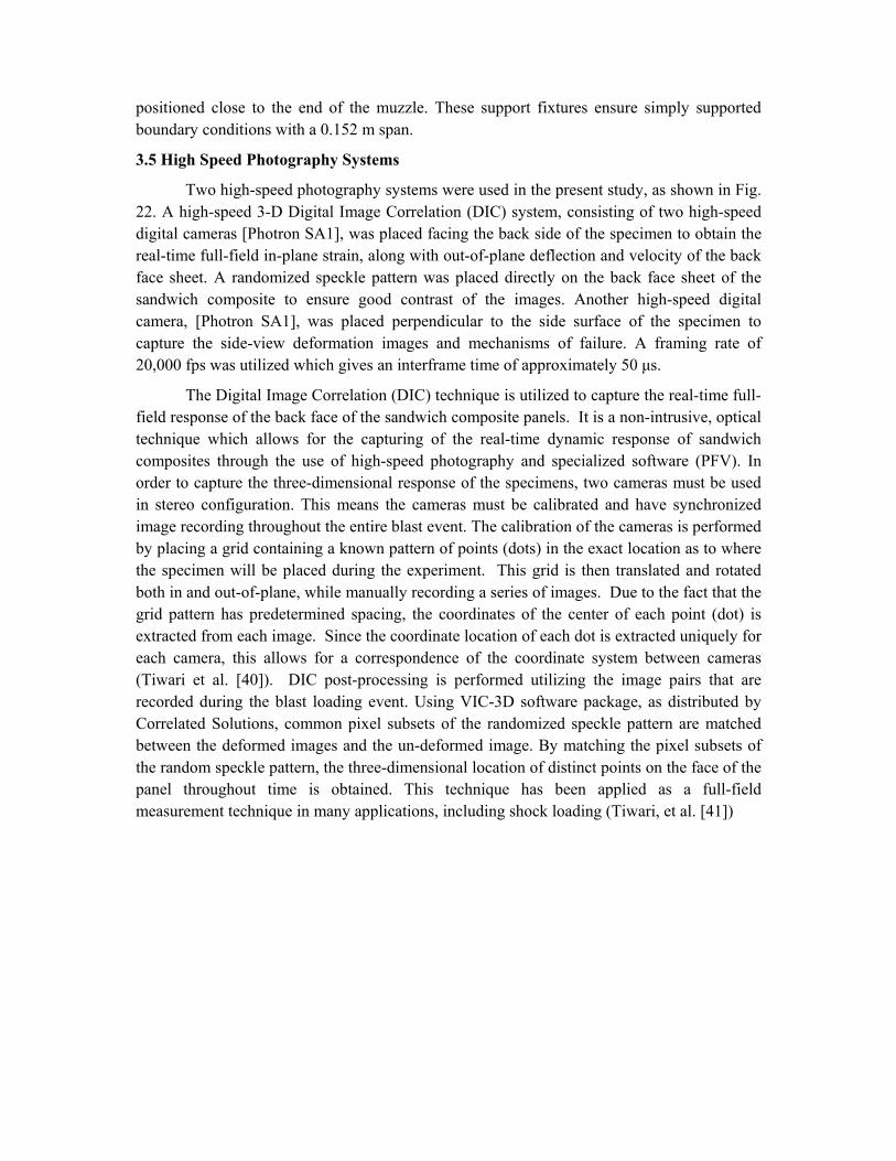
positioned close to the end of the muzzle. These support fixtures ensure simply supported boundary conditions with a 0.152 m span.

3.5 High Speed Photography Systems

Two high-speed photography systems were used in the present study, as shown in Fig. 22. A high-speed 3-D Digital Image Correlation (DIC) system, consisting of two high-speed digital cameras [Photron SA1], was placed facing the back side of the specimen to obtain the real-time full-field in-plane strain, along with out-of-plane deflection and velocity of the back face sheet. A randomized speckle pattern was placed directly on the back face sheet of the sandwich composite to ensure good contrast of the images. Another high-speed digital camera, [Photron SA1], was placed perpendicular to the side surface of the specimen to capture the side-view deformation images and mechanisms of failure. A framing rate of 20,000 fps was utilized which gives an interframe time of approximately 50 μs.

The Digital Image Correlation (DIC) technique is utilized to capture the real-time full-field response of the back face of the sandwich composite panels. It is a non-intrusive, optical technique which allows for the capturing of the real-time dynamic response of sandwich composites through the use of high-speed photography and specialized software (PFV). In order to capture the three-dimensional response of the specimens, two cameras must be used in stereo configuration. This means the cameras must be calibrated and have synchronized image recording throughout the entire blast event. The calibration of the cameras is performed by placing a grid containing a known pattern of points (dots) in the exact location as to where the specimen will be placed during the experiment. This grid is then translated and rotated both in and out-of-plane, while manually recording a series of images. Due to the fact that the grid pattern has predetermined spacing, the coordinates of the center of each point (dot) is extracted from each image. Since the coordinate location of each dot is extracted uniquely for each camera, this allows for a correspondence of the coordinate system between cameras (Tiwari et al. [40]). DIC post-processing is performed utilizing the image pairs that are recorded during the blast loading event. Using VIC-3D software package, as distributed by Correlated Solutions, common pixel subsets of the randomized speckle pattern are matched between the deformed images and the un-deformed image. By matching the pixel subsets of the random speckle pattern, the three-dimensional location of distinct points on the face of the panel throughout time is obtained. This technique has been applied as a full-field measurement technique in many applications, including shock loading (Tiwari, et al. [41])

Fig. 22: High-speed photography set-up (Back-view DIC and side-view)

Real Pattern

Back View 3-D DIC System

Side View Camera

Specimen

Shock Tube

3.6 Experimental Procedure and Parameters

An initial series of experiments was conducted for both configurations and three samples were tested for each. This was followed by a second set of experiments, in which two specimens were tested for each configuration. Two different loading conditions were applied. For the first set of experiments, a simply stacked diaphragm of 5 plies of 10 mil mylar sheets with a total thickness of 1.27 mm was utilized to generate an impulse loading on the specimen with an incident peak pressure of approximately 1.0 MPa, a reflected peak pressure of approximately 5.0 MPa and a wave speed of approximately 1000 m/s. A typical pressure profile obtained from the transducer closest to the specimen (~0.02 m away) can be seen in Fig. 23. It should be noted that both pressure transducers were utilized to obtain the shock wave history, i.e. incident / reflected pressure and incident / reflected velocity. However, only the pressure transducer closest to the specimen was used to obtain the pressure applied on the specimen.

For the second set of experiments, a simply stacked diaphragm of 1 ply of 10 mil mylar sheets with a total thickness of 0.254 mm was utilized to generate an impulse loading on the face sheets only, with an incident peak pressure of approximately 0.3 MPa, a reflected peak pressure of approximately 1 MPa, and a wave speed of approximately 650 m/s. Due to the authors previous work [29-31], the experiments corresponding to the loading conditions with an incident peak pressure of 1.0 MPa will be presented and discussed in detail, while the face sheet experiments corresponding to the lower loading conditions (incident peak pressure 0.3 MPa) will be utilized to better evaluate the performance and failure mechanisms of the sandwich structures.

Fig. 24: Compressive residual strength experimental set-up

(a) Instron 5582 compressive residual strength experimental set-up (pre-damaged face sheets)

(b) Close up of pre-damaged specimen in compressive fixture

Fig. 23: Incident and reflected pressure profile

0

1

2

3

4

5

0 1000 2000 3000 4000 5000

Pres

sure

(MPa

)

Time (microseconds)

Reflected Pulse

Incident Pulse

Reflected Pulse

Incident Pulse

3.7 Residual Compressive Strength Measurements

Following the blast loading experiments, residual strength measurements of the face sheet materials were taken. The compressive strength was chosen as the residual strength parameter for this investigation. It is generally the most severely affected by impact regarding all of the mechanical properties given that the major omde of impact damage is most often delamination. Delamination is extremely detrimental to the residual compressive strength. The equipment used to measure the residual strength consisted of an Instron 5585 screw-driven testing machine, and a special compression fixture, Fig. 24, designed to be similar to that described in [42] and ASTM standard D 7137/ D7137M – 07.

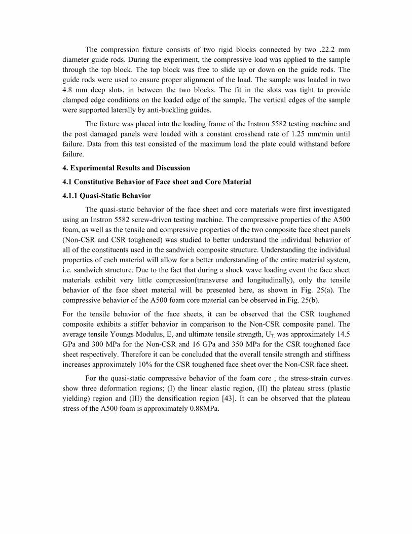
The compression fixture consists of two rigid blocks connected by two .22.2 mm diameter guide rods. During the experiment, the compressive load was applied to the sample through the top block. The top block was free to slide up or down on the guide rods. The guide rods were used to ensure proper alignment of the load. The sample was loaded in two 4.8 mm deep slots, in between the two blocks. The fit in the slots was tight to provide clamped edge conditions on the loaded edge of the sample. The vertical edges of the sample were supported laterally by anti-buckling guides.

The fixture was placed into the loading frame of the Instron 5582 testing machine and the post damaged panels were loaded with a constant crosshead rate of 1.25 mm/min until failure. Data from this test consisted of the maximum load the plate could withstand before failure.

4. Experimental Results and Discussion

4.1 Constitutive Behavior of Face sheet and Core Material

4.1.1 Quasi-Static Behavior

The quasi-static behavior of the face sheet and core materials were first investigated using an Instron 5582 screw-driven testing machine. The compressive properties of the A500 foam, as well as the tensile and compressive properties of the two composite face sheet panels (Non-CSR and CSR toughened) was studied to better understand the individual behavior of all of the constituents used in the sandwich composite structure. Understanding the individual properties of each material will allow for a better understanding of the entire material system, i.e. sandwich structure. Due to the fact that during a shock wave loading event the face sheet materials exhibit very little compression(transverse and longitudinally), only the tensile behavior of the face sheet material will be presented here, as shown in Fig. 25(a). The compressive behavior of the A500 foam core material can be observed in Fig. 25(b).

For the tensile behavior of the face sheets, it can be observed that the CSR toughened composite exhibits a stiffer behavior in comparison to the Non-CSR composite panel. The average tensile Youngs Modulus, E, and ultimate tensile strength, UT, was approximately 14.5 GPa and 300 MPa for the Non-CSR and 16 GPa and 350 MPa for the CSR toughened face sheet respectively. Therefore it can be concluded that the overall tensile strength and stiffness increases approximately 10% for the CSR toughened face sheet over the Non-CSR face sheet.

For the quasi-static compressive behavior of the foam core , the stress-strain curves show three deformation regions; (I) the linear elastic region, (II) the plateau stress (plastic yielding) region and (III) the densification region [43]. It can be observed that the plateau stress of the A500 foam is approximately 0.88MPa.

4.1.2 Drop Weight Impact

Both types of composite panels were subjected to low velocity high mass (LVHM) impact events using an Instron Dynatup 9210 drop weight tower apparatus. The specimens were simply-supported, across a 152 mm span (identical support conditions and span length as in shock tube experiments). The 19.4 kg mass was released from a drop height of 75 cm, achieving a maximum inpact velocity of 3.8 m/s and a total impact energy of ~ 150 J. Load data and velocity data were recorded by a data acquisition system, and the total energy absorbed during the impact event was obtained through the data collected. Fig. 26 shows the total energy absorbed during the 150 J impact event.

Fig. 25: Quasi-static behavior of composite face sheets (tensile) and A500 foam core (compressive)

0

2

4

6

8

10

12

14

16

18

20

0 0.1 0.2 0.3 0.4 0.5 0.6 0.7 0.8 0.9 1

Engi

nee

rin

g St

ress

(M

Pa)

Engineering Strain

Sample 1Sample 2Sample 3Sample 4

(II) Plateau Stress Region (I) Linear Elastic Region

(III) Densification Region

0

50

100

150

200

250

300

350

400

0 0.0025 0.005 0.0075 0.01 0.0125 0.015 0.0175 0.02 0.0225 0.025

Engi

neer

ing

Str

ess

(MPa

)

Engineerin Strain

Non-CSR

CSR

(a) Quasi-static behavior of the different composite face sheets (Non-CSR and CSR)

(b) Quasi-static behavior of the CorecellTM A500 foam

0

5

10

15

20

25

30

0 2000 4000 6000 8000 10000 12000 14000

Ene

rgy

Ab

sorb

ed

(J)

Time (microseconds)

Non-CSR

CSR

Fig. 26: Total energy absorbed for both composite face sheets during drop weight impact event

4.1.3 Split Hopkinson Pressure Bar

The high strain rate behavior of the face sheet and core materials was investigated using a SHPB apparatus. For the dynamic behavior of the face sheet materials, Fig. 27(a), it can be observed

Fig. 27(b) shows the dynamic behavior of the A500 foam core material. Note, the stress-strain curves also show the three deformation regions, as they did under quasi-static loading, even though the densification region is much harder to achieve under dynamic loading conditions. The high strain rate yield stress and plateau (flow) stress of the A500 foam is much higher than its quasi-static yield and plateau stresses, approximately 100% (1.60 MPa and 0.88 MPa respectively). The improvement of the mechanical behavior from quasi-static to high strain-rates in this core material, as well its long stress plateaus, signifies its ability to absorb large amounts of energy under high strain-rate dynamic loading. Therefore, it shows great potential in being used as a core material in sandwich structures subjected to high intensity air blasts

4.2 Blast Response of Core-shell Rubber (CSR) Toughened Sandwich Composites

4.2.1 Real time deformation

The real-time observations of the transient behavior for both types of configurations subjected to shock wave loading are shown in Fig. 28. The shock wave (pressure wave) propagates from the right side of the image to the left side and some detailed deformation mechanisms are pointed out in the figures. It should be noted that the time scheme used to represent the images in each configuration is identical. Therefore for both of the configurations investigated, the images are correlated based on the same time per frame. This

Fig. 27: High strain rate compressive behavior of composite face sheets and A500 foam core

(a) High strain rate behavior of the different composite face sheets (Non-CSR and CSR)

0

100

200

300

400

500

600

700

800

0 0.01 0.02 0.03 0.04 0.05 0.06 0.07 0.08 0.09 0.1

Engi

nee

rin

g St

ress

(MP

a)

Engineering Strain

Sample 1 (1500 1/s)

Sample 2 (1400 1/s)

(b) High strain rate behavior of the CorecellTM A500 foam

0

1

2

3

4

5

6

7

8

9

10

11

12

13

14

0 0.1 0.2 0.3 0.4 0.5 0.6 0.7 0.8 0.9 1

Engi

nee

ring

Str

ess

(M

Pa)

Engineering Strain

Sample 1 (5200 1/s

Sample 2 (5000 1/s)

Fig. 28: High-speed images for (a) Non-CSR and (b) CSR toughened sandwich composites

(a) Non-CSR Toughened

(b) CSR Toughened

Indentation failure Core

Cracking

Core LayerDelamination

SkinDelamination

t = 100 μs t = 400 μs t = 700 μs t = 1000 μs t = 1600 μst = 0 μs

Indentation failure

Core Cracking

Core LayerDelamination

t = 100 μs t = 400 μs t = 700 μs t = 1000 μs t = 1600 μst = 0 μs

4.2.2 Deflection

The mid-point deflection of each sandwich panel and all of its constituents was obtained from the high-speed images and a typical response can be seen in Fig. 29. For both configurations studied, the midpoint deflection of the front face (front skin) and back face (back skin) of the specimen was plotted. For the sandwich composite without core-shell rubber (Non-CSR), as shown in Fig 29 (a), it is evident that at t = 1600 μs the front face deflects to approximately 46 mm, while the back face sheet deflects approximately 35 mm. Therefore the difference between the deflection of the front face and deflection of the back face signifies the total amount of compression observed in the core. Therefore, it can be concluded that the core compressed approximately 11 mm, which is 30% of its original thickness (38 mm).

0

5

10

15

20

25

30

35

40

45

50

0 200 400 600 800 1000 1200 1400 1600 1800

Def

lect

ion

(mm

)

Time (microseconds)

Front Face

Back Face

0

5

10

15

20

25

30

35

40

45

50

0 200 400 600 800 1000 1200 1400 1600 1800

Def

lect

ion

(mm

)

Time (microsecondS)

Front face

Back face

0

5

10

15

20

25

30

35

40

0 200 400 600 800 1000 1200 1400 1600 1800

Defle

ctio

n (m

m)

Time (microseconds)

Non-CSR

CSR

Fig. 29: Mid-point deflections of both configurations

(a) Mid-point deflection of Non-CSR toughened

(b) Mid-point deflection of CSR toughened

(c) Comparison of back face deflections for both configurations

For the core-shell rubber (CSR) toughened sandwich composite, as shown in Fig 29(b), it is evident that at t = 1600 μs the front face deflects to approximately 45 mm, while the back face sheet deflects approximately 32 mm. Therefore the difference between the deflection of the front face and deflection of the back face signifies the total amount of compression observed in the core. Therefore, it can be concluded that the core compressed approximately 12mm, which is 30 % of its original thickness (38 mm).

4.2.3 Digital Image Correlation (DIC) Analysis

Utilizing the Digital Image Correlation (DIC) technique, the full-field deflection (W), in-plane strain (εyy) and particle velocity (dW/dt) of the back face sheet of each configuration were generated. Fig. 30 – Fig. 33 show the full-field results for the back face sheet of both configurations respectively. Fig. 30 shows the full-field out-of-plane deflection (W) during the initial fluid-structure interaction (t ≤ ~ 250 μs, [22]), with an emphasis on the shape of the loading, as indicated by the localized areas of larger deflection. For the Non-CSR toughened sandwich composites, as shown in Fig. 30a, by ~ t = 100 μs, the loading can be observed as a circular region in the center of the back face sheet. For the CSR toughened sandwich composites, as shown in Figures 30b, by t = 100 μs the loading is more dispersed across the back face sheet, resulting in up to two or even three areas of localized deflection (loading). Therefore, it can be concluded that utilizing CSR, and thus introducing nano-scale rubber particles into the composites, aids in dispersing the initial loading on the structure, resulting in up to three areas of localized deflection (loading) on the back face sheets.

Fig. 30: Localized areas of larger deflections (loading) during fluid-structure interaction

(a) Non-CSR toughened t = 50 μs t = 100 μs t = 150 μs

(a) CSR toughened t = 50 μs t = 100 μs t = 150 μs

z

x

y

Fig. 31: Full-field out-of-plane deflection (W) of both configurations

t = 100 μs t = 400 μs t = 700 μs t = 1000 μs t = 1600 μs (a) Non-CSR Toughened

t = 100 μs t = 400 μs t = 700 μs t = 1000 μs t = 1600 μs (b) CSR Toughened

Fig. 31 shows the full-field out-of-plane deflection (W) for both configurations. Note the scale ranges from 0 mm (purple) to 42 mm (red). It is evident from the figure that the back face of both core configurations exhibits limited out-of-plane deflection prior to t = 400 μs. Between t = 400 μs and t = 1600 μs, both of these configurations continue to bend and exhibit deflections. For the sandwich composite with equivalent core layer thickness, as shown in Fig. 31a, it can be observed that at t = 1600 μs, the central region of the panel has deflected approximately 33 mm. When using sandwich composites with equivalent core layer mass (Fig. 31b), it can be seen that at t = 1600 μs, the central region of the panel has deflected approximately 41 mm. Therefore, it can be concluded that when using a core configuration with equivalent layer thickness, the deflection across the central region of the back face sheet is reduced approximately 20%.

z

x

y

Fig. 32: Full-field in-plane strain (εyy) of both configurations

t = 100 μs t = 400 μs t = 700 μs t = 1000 μs t = 1600 μs (a) Non-CSR Toughened

t = 100 μs t = 400 μs t = 700 μs t = 1000 μs t = 1600 μs (b) CSR Toughened

The full-field, in-plane strain (εyy) is shown in Fig 32 for both configurations with a scale of 0 (purple) to .025 (red), or 0% to 2.5% respectively. It can be observed in the figure that the back face of both core configurations exhibits very minimal in-plane strain (εyy) prior to t = 100 μs. Between t = 100 μs and t = 1600 μs, both of these configurations continue bending and the in-plane strain values continue to increase. For the sandwich composite with equivalent core layer thickness, as shown in Fig. 32a, it can be observed that at t = 1600 μs, the central region of the panel exhibits an in-plane strain of approximately .022, or 2.2%. When using sandwich composites with equivalent core layer mass (Fig. 32b), it can be seen that at t = 1600 μs, the central region of the panel exhibits an in-plane strain of approximately .024, or 2.4%. Therefore, it can be concluded that when using a core configuration with equivalent layer thickness, the maximum in-plane strain across the central region of the back face sheet reduced approximately 8%.

Fig. 33: Full-field out-of-plane velocity (dW/dt) of both configurations

t = 100 μs t = 400 μs t = 700 μs t = 1000 μs t = 1600 μs (a) Non-CSR Toughened

t = 100 μs t = 400 μs t = 700 μs t = 1000 μs t = 1600 μs (b) CSR Toughened

z

x

y

Figure 33 shows the full-field out-of-plane velocity (dW/dt) for both configurations. Note the scale ranges from 0 mm/s (purple) to 35,000 mm/s (red), or 0 m/s to 35 m/s. For the sandwich composites with equivalent core layer thickness, as shown in Fig. 33a, the back face exhibits a large out-of-plane velocity (~ 25 % of its maximum) by t = 100 μs. At t = 400 μs, the central region of the back face has reached an out-of-plane velocity of approximately 30 m/s. By t = 700 μs the velocity has reached a maximum value of 31 m/s, and reduced back to approximately 30 m/s. From t = 700 μs and onward, the velocity continues to decrease from 30 m/s to 22 m/s (t = 1000 μs) and finally down to 7 m/s (t = 1600 μs). For the sandwich composites with equivalent core layer mass, as shown in Fig. 27b, the back face exhibits a larger out-of-plane velocity (~40% of its maximum) by t = 100 μs. At t = 400 μs, the central region of the back face has reached an out-of-plane velocity of approximately 31 m/s. By t = 700 μs the velocity has reached a maximum values, 34 m/s, and reduced to 33 m/s. From t = 700 μs and onward, the velocity continues to decrease from 33 m/s to 29 m/s (t = 1000 μs) and finally down to 20 m/s (t = 1600 μs).

Therefore it can be concluded that when using a sandwich composites with equivalent core layer thickness, the maximum back face velocity is approximately 8% smaller than the sandwich composite with equivalent core layer mass. Also note, the velocity of the panel at t = 1600 μs is approximately 65% smaller as well, i.e 20m/s and 7 m/s respectively.

Using the point inspection tool from the Digital Image Correlation (DIC) software, a point directly in the center of the back face of each specimen was chosen. The out-of-plane deflection (W) showed excellent agreement with the results generated utilizing the high-speed images and therefore only the in-plane strain (εyy) and out-of-plane velocity (dW/dt) results are shown. Fig. 34 and Fig. 35 show the in-plane strain and out-of-plane velocity values obtained. Looking at the in-plane strain values (Fig. 34) it can be seen that at t = 1600 μs, the maximum in-plane strain value at the central point of the back face sheet for the sandwich composite with equivalent core layer thickness is approximately 0.0225, or 2.25%. When using a sandwich composite with equivalent core layer mass, it can be seen that at t = 1600 μs, the maximum in-plane strain value at the central point of the back face sheet is approximately 0.0245, or 2.45%. Therefore it can be concluded that when using sandwich composites with equivalent core layer mass, the maximum in-plane strain across the central region of the back face sheet is reduced 8% in comparison to the sandwich composites with equivalent core layer mass.

Fig. 35 shows the out-of-plane velocity (dW/dt) for both configurations. For the sandwich composite with equivalent core layer thickness, the maximum velocity is reached at t = 500 μs and is approximately 31 m/s. For the sandwich composite with equivalent core layer mass, the maximum velocity is reached at approximately the same time, t = 500 μs, but the velocity is larger (34 m/s). Therefore it can be concluded that when using sandwich composites with equivalent core layer mass, the maximum out-of-plane velocity across the central region of the back face sheet is reduced 8% in comparison to the sandwich composites with equivalent core layer mass.

Fig.34: In-plane strain (εyy) of both configurations

0

0.005

0.01

0.015

0.02

0.025

0.03

0 200 400 600 800 1000 1200 1400 1600 1800

In-p

lane

Str

ain

(εyy

)

Time (microseconds)

Non-CSR

CSR

Fig. 35: Out-of-plane velocity (dW/dt) of both configurations

0

5

10

15

20

25

30

35

0 200 400 600 800 1000 1200 1400 1600 1800

Out

-of-

Plan

e V

eloc

ity

(m/s

)

Time (microseconds)

Non-CSR

CSR

In order to provide a more comprehensive understanding on the behavior response of the sandwich panels during the shock wave loading, the individual face sheets were subjected to blast wave loading as well. The Digital Image Correlation (DIC) technique was applied to the facehseet experiments (incident peak pressure 0.3 MPa). For this investigation full-field analysis was also carried out, as well as line-inspection. Since the behavior of the face sheets during the initial fluid structure interaction was similar to that of the sandwich composites, only the line-inspection analysis will be presented here. Utilizing the line-inspection tool from the Digital Image Correlation (DIC) software, a longitudinal line directly in the center of the back face of each specimen was chosen, and the results were extracted, as shown in Fig. 36.

0

10

20

30

40

50

60

70

80

90

100

0 0.1 0.2 0.3 0.4 0.5 0.6 0.7 0.8 0.9 1

Def

lect

ion

(mm

)

Normalized simple-support span length

Non-CSR

CSR

t = 0 µs

t = 800 µs

t = 1600 µs

t = 2400 µs

Fig. 36: Longitudinal line-inspection analysis across central region of back face for both composite face sheet systems

t = 3200 µs

Fig. 37: Residual compressive strength of both types of composite face sheets after being subjected to high intensity blast loading (incident peak pressure 0.3 MPa)

0

5

10

15

20

25

30

35

40

45

50

0 0.005 0.01 0.015 0.02 0.025 0.03

Engi

neer

ing

Stre

ss (M

Pa)

Engineering Strain

CSR Non-CSR

(b) Non-CSR Toughened

(c) CSR Toughened

(a) Residual compressive strengths of both types of composite face sheets

4.2.4 Residual Compressive Strength

After the blast loading event occurred on the face sheets, both types of composite face sheets were subjected to post-blast residual compressive strength measurements. The results of these tests are shown in Fig. 37.

Fig. 38: Visual examination of both composite face sheets after being subjected to 150 J impact

(a) Non-CSR Toughened

(b) CSR Toughened

Fig. 39: Visual examination of both composite face sheets after being subjected to high strain-rate loading (SHPB)

(a) Non-CSR Toughened (b) CSR Toughened

4.2.5 Post-mortem Analysis

After the quasi-static (Drop-weight) and dynamic events (SHPB and Shock Tube) occurred, the damage patterns were visually examined and recorded using a high resolution digital camera and are shown in Fig. 38 - Fig. 41. The damage patterns of both types of composite face sheets subjected to a 150 J drop-weight impact event are shown in Fig. 38.

Fig. 39 shows the damage patterns of composite face sheets subjected to a strain rate of 103 (`5000 1/s) using a Split Hopkinson Pressure Bar apparatus.

Fig. 40: Visual examination of both configurations after being subjected to high intensity blast load (incident peak pressure 1.0 MPa

(a) Non-CSR Toughened

(b) CSR Toughened

Core cracking

DelaminationCore Compression

Fiber Delamination and Cracking

Core cracking

DelaminationCore Compression

Fiber Delamination

Front face sheet (Blast-receiving side) Foam Core Back face sheet

Fig. 41: Visual examination of both composite face sheets after being subjected to

(b) CSR Toughened Composite; (L) Front face sheet, (R) Back face sheet

(a) Non-CSR Toughened Composite; (L) Front face sheet, (R) Back face sheet

The damage patterns of both types of sandwich composite panels subjected to an incident peak pressure of 1.0 MPa, a reflected peak pressure of 5.0 MPa, and an incident velocity of 1000 m/s using the shock tube apparatus are shown in Fig. 40.

Fig. 41 shows the damage patterns of both types of composite face sheets subjected to an incident peak pressure of 0.3 MPa, a reflected peak pressure of 1.0 MPa, and an incident velocity of 650 m/s using the shock tube apparatus.

5. Conclusions

The following is the summary of the investigation:

(1) Core-shell rubber particles (CSR) have a significant effect on the quasi-statci and dynamic behavior of composite materials and sandwich structures. It was observed that the addition of 4% CSR to E-g;lass Vinyl-Ester (EVE) composite face sheets increased the tensile strength (~10%) and drop-weight impact resistance (~10%),. After the dynamic loading, such as SHPB and shock wave loading, the CSR toughened face sheets maintained structural integrity, while the Non-CSR face sheets did not.

(2) The dynamic stress-strain response is significantly higher than the quasi-static response for the CorecellTM A500 foam studied. The increase in the yield strength from quasi-static response to dynamic response, along with the longer stress plateau, indicates that this core material shows great potential in absorbing large amounts of energy.

(3) Two types of sandwich composites were fabricated, one with the addition of nano-scale core-shell rubber (CSR) particles during infusion, and one without (Non-CSR). The core material and thickness, as well as overall specimen dimensions were held constant. Results indicated that the addition of nano-scale core-shell rubber (CSR) particles to the panels allows for an increase in blast performance. By dispersing the initial loading, the CSR toughened sandwich composites exhibit lower amounts of out-of-plane deflection and velocity, as well as in-plane strain, approximately 8%, 12% and 20% respectively.

6. Acknowledgement

The authors kindly acknowledge the financial support provided by Dr. Yapa D. S. Rajapakse, under Office of Naval Research Grant No. N00014-04-1-0268. The authors acknowledge the support provided by the Department of Homeland Security under Cooperative Agreement No. 2008-ST-061-ED0002. Authors thank Gurit SP Technology and Specialty Products Incorporated (SPI) for providing the material as well as Dr. Stephen Nolet and TPI Composites for providing the facility for creating the composites used in this study.

7. References

[1] Xue Z. and Hutchinson JW (2003) Preliminary assessment of sandwich plates subject to blast loads. Int J Mech Sci, 45, 687-705.

[2] Fleck NA and Deshpande VS (2004) The resistance of clamped sandwich beams to shock loading. J Appl Mech, 71, 386-401.

[3] Dharmasena KP, Wadley HNG, Xue Z and Hutchinson JW (2008) Mechanical response of metallic honeycomb sandwich panel structures to high-intensity dynamic loading. Int J Imp Eng, 35 (9), 1063-1074.

[4] Zhu F, Zhao L, Lu G and Wang Z (2008) Deformation and failure of blast loaded metallic sandwich panels – Experimental investigations. Int J Imp Eng, 35 (8), 937-951.

[5] Nurick GN, Langdon GS, Chi Y and Jacob N (2009) Behavior of sandwich panels subjected to intense air blast: part 1- Experiments. Comp Stru, 91 (4), 433 – 441.

[6] Tagarielli VL, Deshpande VS and Fleck NA (2008) The high strain rate response of PVC foams and end-grain balsa wood. Comp B, 39, 83–91.

[7] Radford DD, McShane GJ, Deshpande VS and Fleck NA (2006) The response of clamped sandwich plates with metallic foam cores to simulated blast loading. Int J Sol Struc, 44, 6101-612.

[8] McShane GJ, Deshpande VS, and Fleck NA (2007) The underwater blast resistance of metallic sandwich beams with prismatic lattice cores. J Appl Mech, 74, 352 – 364.

[9] McShane GJ, Radford DD, Deshpande VS and Fleck NA (2006) The response of clamped sandwich plates with lattice cores subjected to shock loading. European J Mech – A: Solids, 25, 215-229.

[10] Kinloch AJ, Shaw SJ, Tod DA, Hunston DL (1983) Deformation and fracture behaviour of a rubber-toughened epoxy: 1. Microstructure and fracture studies. Polymer, 24 (10): 1341- 1354

[11] Yee AF, Pearson RA (1986) Toughening mechanisms in elastomer-modified epoxies Journal of Material Science, 21: 2462-2474

[12] Bucknall CB and Partridge IK (1983) Phase separation in epoxy resins containing polyethersulphone Polymer, 24 (5): 639 – 644

[13] Kinloch AJ, Yuen ML, Jenkins SD (1994) Thermoplastic-toughened epoxy polymers Journal of Material Science 29: 3781-3790

[14] Johnsen BB, Kinloch AJ, Taylor AC (2005) Toughness of syndiotactic polystyrene/epoxy polymer blends: microstructure and toughening mechanisms, Polymer 46: 7352-7369.

[15] Broutman LJ, Sahu S (1971) The effect of interfacial bonding on the toughness of glass filled polymers. Mater Sci Eng, 8: 98-107.

[16] Spanoudakis J, Young RJ (1984) Crack propagation in a glass particle- filled epoxy resin - Part 1, J Mater Sci, 19: 473-486.

[17] McGrath LM, Parnas RS, Lenhart JL, King S (2006) Fracture toughness of alumina-epoxy composites. Poly Mater Sci Eng, Preprints, 94: 683 – 684.

[18] Griffiths R, Holloway D (1970) The fracture energy of some epoxy resin materials, J Mater Sci, 5 (4): 302-307.

[19] Hsieh TH, Kinloch AJ, Masania K, Sohn Lee J, Taylor AC, Sprenger S (2010) The toughness of epoxy polymers and fiber composites modified with rubber microparticles and silica nanoparticles. J Mater Sci, 45: 1193 – 1210.

[20] Dixon DG, Harris SJ, Dempster M, Nicholls P (1998) Effect of PEEK fibers and powder on joints made with high temperature adhesive, J Adhesion, 65 (1- 4): 131-162.

[21] Kinloch AJ, Taylor AC (2002) The toughening of cryanate-ester polymers –Part I – Physical modification using particles, fibers and woven mats. J Mater Sci, 37: 433-460.

[22] Lin KF, Shieh YD (1998) Core-Shell Particles Designed for Toughening the Epoxy Resins: I. Preparation and Characterization of Core-Shell Particles, J Appl Poly Sci, 69: 2069-2078.

[23] Lin KF, Shieh YD (1998) Core-shell particles designed for toughening the epoxy resins: II. Core-shell particle toughened epoxy resins, J Appl Poly Sci, 70: 2313 -2322.

[24] Becu L, Maazouz A, Sautereau and Gerard JF (1997) Fracture behavior of epoxy polymers modified with core-shell rubber particles, Journal of Applied Polymer Science, 65 (12): 2419-2431.

[25] Yan C, Xiao KQ, Ye L, and Mai YW (2002) Numerical and experimental studies on the fracture behavior of rubber toughened epoxy in bulk specimen and laminated composites. Journal of Material Science, 37 (5): 921-927

[26] Giannakopoulos G ,Masania K, and Taylor AC (2011) Toughening of epoxy using core-shell particles. Journal of Material Science, 46 (2): 327-338.

[27] Kaneka Texas Corporation, http://www.kanekatexas.com/MX

[28] Kinloch AJ, Mohammed RD, Taylor AC, Sprenger S and Egan D (2006) The interlaminar toughness of carbon-fibre reinforced plastic composites using ‘hybrid-toughened’ matrices. Journal of Material Science 41(15): 5043-5046.

[29] Gardner N, Wang E, Shukla A (2011) Performance of functionally graded sandwich beams under shock wave loading. Composite Structures, DOI 10.1016/j.compstruct.2011.12.006.

[30] Wang E, Gardner N, Shukla A. The blast resistance of sandwich composites with stepwise graded cores. International Journal of Solids and Structures 2009; 46: 3492-3502.

[31] Gardner N, Wang E, Kumar P, Shukla A. Blast mitigation in a sandwich composite using graded core with polyurea interlayer. Experimental Mechanics 2011. DOI 10.1007/s11340-011-9517-9.

[32] Derakane 8084 Material Data Sheet, www.ashland.com

[33] Derakane 411-200 Material Data Sheet, www.ashland.com

[34] Kaneka Kane Ace MX 153Material Data Sheet, http://www.kanekatexas.com

[35] CorecellTM A-Series Foam Material Data Sheet, http://www.gurit.com/corecell-afoam.aspx. Accessed 20 Sept 2011.

[36] Chen W, Zhang B, Forrestal MJ. A split Hopkinson bar technique for low impedance materials. Experimental Mechanics 1998; 39 (2): 81–85.

[37] Kumar P, LeBlanc J, Stargel D and Shukla A. Effect of plate curvature on blast response of aluminum panels. Impact Engineering 2012; Accepted

[38] LeBlanc J, Shukla A, Rousseau C, Bogdanovich A. Shock loading of three-dimensional woven composite materials. Composite Structures 2007; 79: 344- 355.

[39] Wright J. Shock tubes. New York: John Wiley and Sons Inc, 1961.

[40] V. Tiwari, M.A. Sutton, S.R. McNeill, Assessment of High-speed Imaging Systems for 2D and 3D Deformation Measurements: Methodology Development and Validation, Experimental Mechanics 2007; 47: 561-579.

[41] V. Tiwari, M.A. Sutton, S.R. McNeill, S. Xu, X. Deng, W.L. Fourney, D. Bretall, Application of 3D Image Correlation for Full-Field Transient Plate Deformation Measurements During Blast Loading, International Journal of Impact Engineering 2009; 36; 862-874.

[42] Wu HT and Springer GS. Impact induced stresses, strains, and delaminations caused by impact on composite plates. Journal of Composite Materials 2008; 22: 533

[43] Gibson LJ, Ashby MF. Cellular Solids: Structures and Properties. New York: Pergamon Press, Inc., 1988.

[44] Wang, E. Blast resistance and energy mitigation behavior of sandwich composite materials. Ph.D Dissertation, University of Rhode Island, 2010.

Task 3: Experimental and Numerical study of Foam Filled Corrugated Core Steel Sandwich Structures Subjected to Blast Loading

1. INTRODUCTION

A major consideration in the design of military vehicles is their resistance to explosive blast loading. With the fast development of modern military technology, monolithic plates are continuing to fall behind the desired levels of blast protection. Sandwich structures with cellular solid cores, such as metallic foams and honeycomb structures, have shown superior weight specific stiffness and strength properties compared to their monolithic counterparts in blast resistant structural applications. Their cellular microstructure allows them to undergo large deformation at nearly constant nominal stress and thus absorb more energy [1, 2, 3]. To date, the effect of foam filling on blast mitigation of corrugated core sandwich panels under shock loads has not been fully understood. In this study to clarify the foam infill influences on blast resistivity of corrugated steel core sandwich panels, with and without foam filling, shock tube experiments and Finite Element Method (FEM) were used to investigate the phenomenon. In addition, monolithic face sheets and foam core sandwich panels were tested and analyzed to validate the FEM. More studies were numerically conducted to investigate the effect of face sheet thickness and corrugated sheet thickness under two different boundary conditions, namely simply supported and encastre supported. In order to see the effect of corrugated core rigidity soft, medium, and hard core cases were studied numerically utilizing both filled and empty conditions under blast loading.

In recent years, a number of micro-architectured materials have been developed to use as cores in sandwich panels. These include pyramidal cores [4, 5, 6], diamond celled lattice cores [7], corrugated cores [8], hexagonal honeycomb cores [9], foam cores [10], and square honeycomb cores [11]. The benefits of sandwich construction depend on core topology. Core designs that afford simultaneous crushing and stretching resistance are preferred. One of the most preferred practical core topologies in blast resistant sandwich panel construction is the corrugated metallic core. These cores provide manufacturing advantages, as well as high strength, in both the normal and longitudinal directions of the structures [7, 12, 13].

Sandwich structures have various energy dissipation mechanisms, such as bending and stretching of the face sheet, as well as compression and shear of the core. This is especially pertinent in the case of impulsive loading, wherein the interstices in the metal cellular core can provide adequate space for the large plastic deformation, which is an efficient mechanism to dissipate the energy produced by blast impact [14-17]

During blast loading, the cellular solid core can absorb more than one half of the initial kinetic energy imparted to face sheet of the sandwich plate. This is due to crushing in the early stages of deformation, prior to significant overall bending and stretching, without unduly reducing the separation between the face sheets. High crushing strength and energy absorption per unit mass of the core is therefore important [21].

Wakabayashi et al. conducted experiments that suggest that low-density materials may provide the most effective blast mitigation [24]. In recent years, sandwich structures with strong face sheets and lightweight cores have become central structural components for blast mitigation. Polymeric foams offer unique structural, impact, thermal and acoustic properties, which make them an excellent choice as core materials to obtain low density blast resistive sandwich structures [2, 25] Based on these ideas, a lot of research on blast mitigating layered sandwich structures has been performed in recent years, using foam cores with different wave impedances to minimize shock effect [26, 27, 28].

Studies on metallic sandwich panels subjected to air blasts [17, 8] indicate that sandwich plates with high ductility and high energy absorption capacity per unit areal mass show good performance. Liang et al. [29] and Wei et al. [30] studied the behavior of metallic sandwich cores with varying strengths and found that soft cores (those in which the core is much less stiff then the sandwich panels’ faces) reduce the momentum transferred, thus providing better mitigation for blast loading. For metallic structures, energy absorption in metallic lattice cores is through large scale plasticity, shear and compressive buckling, and eventual tearing of core walls and face sheets [25].

Another possible application of structural foams is for use as a filler material inside cellular metallic core sandwich structures. It is possible to obtain a new sandwich structure by combining these two cores' shock absorption advantages and decrease the transmitted shock load due to differing acoustic impedances. Moreover, foam filling stabilizes the core cell walls against buckling and increases the strength of the core. Vaziri et al. [21] studied two different types of PVC foam filled stainless steel honeycomb and folded core sandwich plates using FEM under various restrictions. They found no clear advantage or disadvantage implemented by foam filling for structural purpose under quasi static and impact loading.

Jhaver R. and Tippur H. [31] investigated syntactic foam filled aluminum honeycomb composites compression response by experimental and computational methods. They obtained considerable increases in elastic modulus and plateau stress through foam filling the honeycomb composites.Murray G. et al. studied polymer filled aluminum honeycomb structures to investigate the filling effect on damping using numerical methods with experimental validations. It was found that high damping improvements in the filled honeycomb explained the significant strain energy in the polymeric infill due to the Poisson’s mismatch between the honeycomb and the infill [32]. Yungwirth et al. showed that low modulus elastomer infill in pyramidal lattice truss metallic core increased the impact energy absorption capacity [33]. Other studies have had success improving the impact resistance of honeycomb cores by fully or partially filling the cells of the honeycomb [34-37].

2. EXPERIMENTAL PROCEDURE

2.1 SPECIMEN PREPARATION

In this study, corrugated steel core sandwich structures were produced with low carbon steel face sheets and galvanized low carbon steel sinusoidal shape corrugations in a four-layer match-up. A schematic of the sandwich panels is shown in Figure 42.

Fig. 42 (a) Corrugated core sheet dimensions (b) Manufacturing procedure of corrugated steel core sandwich structures (c) Final sandwich panel side view.

The face sheets had lateral dimensions of 50.8 x 203.2 x 3.2 mm. The sinusoidal corrugated sheet reference dimensions are shown in Figure 1a. Thickness of the corrugated sheet was 29 gauges (0.44 mm) with galvanization,. The corrugation sheets and the face sheets were bonded to each other with epoxy adhesive G/Flex (West System Inc.). The tensile adhesion strength of this material was 20 MPa . Three different sandwich panel configurations (See Figure 43) were subjected to blast loading with simply supported boundary conditions.

Fig. 43: Schematics of the experimental sandwich panels (a) Empty corrugated steel core sandwich panel (b) Foam filled corrugated steel core sandwich panel (c) Foam core sandwich panel

a b c

31.75 mm

6.35 a) b) c)

2.2 SHOCK LOADING PROCEDURE

A shock tube apparatus was used to generate shock waves with planar wave fronts. A photograph of the shock tube used in these studies can be seen in Figure 44. A typical shock tube produced pressure profile is shown in Figure 45. Two pressure transducers (PCB102A) were mounted at the end of the muzzle section to record the incident and reflected pressure profiles. The first pressure sensor was mounted 20 mm away from the muzzle, and the second was mounted 180 mm away (160 mm separation from the first pressure sensor). The final muzzle inner diameter was 38.1 mm (See Figure 46). The incident peak pressure of the shock wave was chosen to be 5.5 MPa in the current study.

The specimen was placed onto a simply supported boundary condition fixture with a 152.4 mm span. The flat front face of the specimen was set normal to the axis of the shock tube with the face completely covering the muzzle. A diagram of this set up can be seen in Figure 46. At least three specimens of each type were subjected to experiments to ensure repeatability.

A high speed photography system was utilized to capture the motion of the specimens in order to determine their deformation and damage propagation. The lens axis of the camera was set perpendicular to the shock tube as shown in Figure 46. The camera used was a Photron SA1 high-speed digital camera, which has the ability to capture images at a framing rate of 20,000 frames per second with an image resolution of 512x512 pixels for a 3 millisecond time duration.

Fig. 44: Shock tube apparatus Fig. 45: Typical experimental pressure profile [38]

Fig. 46: High speed camera side view deflection measurement

3. NUMERICAL PROCEDURE

Dynamic explicit 3D FEA analyses of the sandwich panels subjected to a blast load were performed using Abaqus/Explicit finite element software . During analysis nonlinear geometry was accounted for, and simulated for a duration of 3 ms . All required field outputs such as displacements, strains, stress, etc., and history outputs such as energy, are defined in this module.

3.1Finite Element Model

A model was created to render simple and encastre supported (along the back face's short edges) corrugated steel core sandwich panels 203 x 50.8 x 25.34 mm, subjected to blast loading. In the model, each layer section was accepted as a homogenous sheet with a prescribed thickness. Corrugated layers are accepted as shells defined by their mid plane. In the model, interactions between the corrugated core and the front and back face sheets are taken as surface-to-surface contacts under the penalty contact method and finite tangential sliding. The shear stress limit is described as 20 MPa.

The sandwich panel was subjected to a pressure-time profile as seen in Figure 47b. This pressure-time profile was taken from the shock tube experiments.

Fig. 47: (a) Shock load distribution function and applied pressure area (b) Applied shock load pressure-time profile (c) FEM model

This shock pressure profile is described in Abaqus software as a tabular data. It was applied to the specimen front face as a non-uniform function (Figure 47c) of area. This variation in shock pressure induced by the shock tube was observed experimentally and validated numerically by Kumar et al. [38]. For FEM simulations, the specimen was symmetrically aligned with the center of the shock tube, and the distance between the supports was fixed at 152.4 mm.

3.2 Material Properties

The material properties of the corrugated steel sheets and face sheets are: elasticity modulus (E) 205 GPa, poisson ratio (ν) 0.29, density (ρ) ) 7.85 g/cm3, and one-dimensional

acoustic wave impedance = . is 3962x104 kg/m2s.

A Johnson Cook material model with strain hardening was applied in Abaqus as the material model. Johnson Cook parameters in the analysis for the material are given in Table 4.

The yield stress is, therefore, expressed as

= + ) 1 + 1 −

where σ is the yield stress at nonzero strain rate, ε is the equivalent plastic strain, ε is the quasi

static strain rate, ε is the equivalent plastic strain rate, and A, B, C, n and m are material constants [39]. θ is the nondimensional temperature ratio and set to zero in this paper.

a) c)

D/3D/3D=38.1

b)

A (MPa) B (MPa) n C m (s-1)

220 499.87 0.228 0.017 0.917 1

Table 4: Johnson Cook Parameters for low carbon steel used in FEM analysis [40]

General purpose humidity cured Polyurethane (PU), of density 0.0446 g/cm3 and Elasticity modulus 0.24 MPa, foam was used. General mechanical properties were found using quasi static compression tests, and high strain rate (3000 /s) properties were found via Split Hopkinson Pressure Bar experiments (See Figure 487) (41) and are shown in Figure 48.

PU foam material shows non-linear, hyperelastic behavior and is extremely compressible. The porosity permits very large volumetric changes. Polyurethane foams under large strains were modeled as compressible hyperelastic solids, if their time dependent mechanical properties and hysteresis are ignored. These materials can deform elastically to large strains, up to 90% strain in compression and are intended for finite strain applications. For PU foams, an Ogden strain energy potential [39] can be applied. In all FE analysis, a Poisson's ratio, ν=0 was used.

Fig. 48: Quasi Static and High-Strain Rate Compression Properties of the Polyurethane Foam

4. EXPERIMENTAL RESULTS AND DISCUSSION

4.1 Applied Pressure and impulses

The average peak value of the shock pressure subjected to specimens was 5.5 MPa. The specimens’ average mass was 616.2 g, 491.9, and 630.4 g for empty corrugated steel core sandwich panels, foam core sandwich panels, and foam filled corrugated steel core sandwich panels respectively. The impulse imparted onto the specimen can be calculated from the detected reflected pressure. These pressure profiles can be considered to be the same as the pressure applied to the plates [42].

0

0.1

0.2

0.3

0.4

0.5

0 0.2 0.4 0.6 0.8 1

En

gin

eeri

ng

Str

ess

(MP

a)

Engineering Strain (-)

Quasi-static

High Strain 3000 1/s

4.2 High Speed Photography Measurements

The real time observations of the deformation of each type of specimen are shown in Figures 49, 51 and 53.

4.3 Empty corrugated steel core sandwich specimen response

The side view history of the empty specimen shows different compression behavior over the entirety of the metallic corrugated core (See Figure 49) during the loading. The beginning of the Back Face Deflection (BFD) occurred 0.25 ms after the initial Front Face Deflection (FFD) of the specimen, which implies a coupled response.

Core compression and bending/stretching stages can be clearly observed by using core compression/time curves. In Figure 12, the core compression variation over time is given for the empty corrugated steel core sandwich panel. It is clearly seen that, from rest to 1.25 ms, core compression increased. After this time, compression of the core remained stable without change, but the front and back faces continued to deflect. This is indicative of the sandwich panel's global bending. The average core compression strain rate increased very quickly up to 1800 1/s at 1.25 ms and then remained stable until the end of the compression stage (See Figure 50).

t=0 ms t=0.5 ms t=1 ms t=1.5 ms t=2 ms t=2.5 ms t=3 ms

Fig. 49: Unfilled corrugated steel core sandwich panel high speed images during shock loading

Fig. 50: Core compression, FFD (Front Face Deflection) and BFD (Back Face Deflection) in empty corrugated steel core sandwich panels.

4.4 Foam Core Sandwich Panels

High speed side view camera images, recording the deflections of foam core sandwich panels, are given in Figure 51. After the shock wave impinged upon the specimen, the weak foam core did not resist the front face motion enough to decrease its velocity until 0.25 ms. As seen in Figure 52, the back face started its motion after this time. This behavior is called "slapping" [18, 19].

0

200

400

600

800

1000

1200

1400

1600

1800

2000

0

5

10

15

20

25

30

35

0.0 0.5 1.0 1.5 2.0 2.5 3.0

Str

ain

Rat

e (1

/s)

Def

lect

ion

(m

m)

Time (ms)

Empty Corrugated Steel Core Sandwich Panel

Core compression FFD BFD strainrate

2 ms 0 ms 0.5 ms 1 ms 1. 5 ms

Fig. 51: High Speed Images of the foam core sandwich specimen

2.5 ms 3 ms

Figure 52.FFD, BFD, Foam Core compression and Strain rate of core in foam core sandwich panels

4.5 Foam Filled Corrugated Steel Core Sandwich Panels

The foam filling caused very large changes in specimen behavior when compared to that of the empty and foam core specimens. This behavior can be seen in Figure 53, which shows high speed side view camera images. Core compression in the foam filled case is decreased when compared to empty and foam core sandwich panels. The BFD starts almost at the same time with FFD. In Figure 54, variations of the velocities of both faces are given. The slope of both the front and back face velocities show the same magnitude, except two durations between 0.5-1 ms and 2-2.5 ms. The front face started deflecting initially, but after only 0.25 ms the BFD began. During the 0.25 ms to 0.75 ms time period core compression can be observed. Between 1 ms and 2 ms the FFD increased more than the BFD, thus causing an increase in the core compression. After this time, both the BFD and FFD started to decrease, and the core decompressed. This reaction occurred over much less time than the empty corrugated steel core and foam core sandwich panels. This shows that even by employing a weak, elastic foam filling the properties of the core increased. In this case, the obtained maximum strain rate in the core was much lower than that of both the empty and foam core cases, and was calculated to be 582 1/s around 2 ms (See Figure 55). The compression percentage at this time was 14.6%. This means that the foam did not exhibit high strain rate behavior in the foam filled corrugated core sandwich panel under blast loading. It is obviously seen that the foam filling increased bending rigidity and core compression strength.

0

500

1000

1500

2000

2500

3000

0

5

10

15

20

25

30

35

40

45

0 0.5 1 1.5 2 2.5 3

Str

ain

Rat

e (1

/s)

Def

lect

ion

(m

m)

Time (ms)

FFD BFD Foam Core Compression Strain Rate

Figure 53. High Speed Images of the fully foam filled corrugated core sandwich specimen

Figure 54. Variations of the velocities of both faces

Fig. 55: FFD, BFD, Core Strain Rate and Core Compression variation after shock loading during captured time period

0

100

200

300

400

500

600

700

0

2

4

6

8

10

12

14

0 0.5 1 1.5 2 2.5 3

Str

ain

Rat

e (1

/s)

Def

lect

ion

(m

m)

Time (ms)

FFD

BFD

Core Compression

Strain Rate

t=1.5 t=1 t=2 ms t=0 t=0.5 ms t=2.5 ms t=3 ms

0

2

4

6

8

10

12

14

16

18

0.00 0.50 1.00 1.50 2.00 2.50 3.00 3.50

Ou

t of

Pla

ne

Vel

ocit

y (m

/s)

Time (ms)

Empty Corrugated Steel Core Sandwich Panel

FRONT FACE

BACK FACE

4.6 Comparison of Experimental Mid Span Deflections of the Sandwich Panels

Figure 56 shows back face and front face mid span deflections. It is clearly seen that both FFD and BFD results of the foam filled corrugated steel core sandwich panel are smaller than the empty and foam core sandwich panels, while its mass exceeds that of the empty sandwich panel by just 2.30%. The benefits of the corrugated steel core sandwich panel and foam core sandwich panels are combined by foam filling of corrugated steel core interstices.

a) b)

Fig. 56: Shock tube experiments' results a) Average Back Face Deflections (BFD) b) Average Front Face Deflections (FFD).

5. NUMERICAL RESULTS AND DISCUSSIONS

5.1 Validation of Numerical Solutions

To verify the material properties, boundary and contact conditions in the FEM were compared to the shock tube experimental results for the face sheet; foam core sandwich panel, empty corrugated steel core sandwich panel, and foam filled corrugated steel core sandwich panels. Comparative results can be seen in Figures 57, 58, 59 and 60.

The Pearson’s correlation coefficient R2 were calculated using equations given in [45] as a means to evaluate the model’s accuracy. The correlation coefficient is a measure of accuracy of the linear relationship between the experimental and predicted data. The predictability of the finite element model over both the front and back faces of the four different experimental designs is shown in Table 5.

Table 5: Predictability of the Model for the Deflection of the Panel Configurations

Face Sheet

Foam Filled Corrugated Steel Core Sandwich Panels

Foam Core Sandwich Panels

Empty Corrugated Steel Core Sandwich Panels

FFD BFD FFD BFD FFD BFD

R2 0.9766 0.9549 0.980 0.980 0.984 0.992 0.9986

0

5

10

15

20

25

30

35

40

0.0 1.0 2.0 3.0

Def

lect

ion

s (m

m)

Time (ms)

Empty Corrugated Steel CoreSandwich Panels BFDFoam Filled Corrugated Steel CoreSandwich Panels BFDFoam Core Sandwich Panels BFD

0

10

20

30

40

50

60

0.0 1.0 2.0 3.0

Def

lect

ion

s (m

m)

Time (ms)

Empty Corrugated Steel CoreSandwich Panels FFDFoam Filled Corrugated Steel CoreSandwich Panels FFDFoam Core Sandwich Panels FFD

The correlation coefficient R2 under all cases is 0.95 or higher, indicating that the trends of both the experimental results and the finite element model are well aligned. All models are accepted with good agreement and can be used to further investigate the influences of the foam and thicknesses of the face sheets and core sheets. See Figures 56-59 for experimental and FEM deflection comparisons.

Fig 57: Experimental and FEM comparisons of Face Sheet a) Face sheet deflections. b) Longitudinal strains

Fig. 58: FEM and Experimental Empty Corrugated Steel Core sandwich specimen a) Front Face Deflection b) Back Face Deflection.

0

0.5

1

1.5

2

0

5

10

15

20

25

0 1 2 3

Pre

ssu

re P

rofi

le (

MP

a)

Def

lect

ion

(m

m)

Time (ms)

Face sheet deflections

Experimental

0.000

0.005

0.010

0.015

0.020

0 1 2 3εx

x (-

)Time (ms)

Face Sheet Strains along longitidunal direction

ExperimentalFEM

0

10

20

30

0.0 1.0 2.0 3.0

Def

lect

ion

s (m

m)

Time (ms)

Empty Corrugated Steel Core Sandwich Panel FFDs

EXPERIMENTALFEM

0

5

10

15

20

25

0.0 1.0 2.0 3.0

Def

lect

ion

s(m

m)

Time (ms)

Empty Corrugated Steel Core Sandwich Panel BFDsEXPERIMENTAL

Fig. 59: FEM and Experimental foam core sandwich specimen a) Front Face Deflection b) Back Face Deflection.

Fig 60: FEM and Experimental Foam Filled corrugated steel core sandwich specimen a) Front Face Deflection b) Back face deflection.

5.2 Investigation of Face Sheet Thickness - Corrugated Core Sheet Thickness and Boundary Conditions effects on Foam Filling Contribution

Face sheet thickness, corrugated steel sheet thickness, and boundary condition effects (see Figure 61) were investigated using FEM simulations. All variables' values are given in Table 6. Sandwich panel length, width, and core thickness are accepted as constants in the FEM simulations as 184.24 x 50.8 x 20.6 mm as well as applied shock pressure. By adding the foam filling, the masses of specimens changed by a very small amount. For example the maximum variation of mass was 3.8% in the 0.2 mm Core Sheet Thickness (CST) and 1 mm Face Sheet Thickness (FST) case. However, by changing FST and CSTs, the mass was increased 4 times in the 5 mm FST - 1 mm CST case as compared to the 1 mm FST - 0.2 mm CST case. Unit mass deflections were calculated for comparison to one another (See Table 7). Totally, 36 runs were performed to understand each of the parameter's influences on the behavior of the sandwich panel.

0

10

20

30

40

0.00 1.00 2.00 3.00

Def

lect

ion

s (m

m)

Time (ms)

Foam Core Sandwich Panel FFDs

EXPERIMENTAL

0

5

10

15

20

25

30

0.00 1.00 2.00 3.00

Def

lect

ion

s (m

m)

Time (ms)

Foam Core Sandwich Panel BFDs

EXPERIMENTAL

0

5

10

15

0 1 2 3

Def

lect

ion

s (m

m)

Time (ms)

Foam Filled Corrugated Steel Core Sandwich Panel FFDs

EXPERIME…

0

5

10

15

0 1 2 3

Def

lect

ion

s (m

m)

Time (ms)

Foam Filled Corrugated Steel Core Sandwich Panel BFDs

FEMEXPERIM…

Table 6. Investigated parameters in FEM simulations of empty and foam filled corrugated steel core sandwich panels.

Boundary Condition Face Sheet Thickness

(mm)

Corrugated Sheet Thickness (mm)

Simple Supported 1, 3, 5 0.2, 0.6, 1

Encastre 1, 3, 5 0.2, 0.6, 1

Table 7.Calculated Masses of FEM models for the empty corrugated steel core sandwich panels

FST

(mm) 1 3 5

CST

(mm) 0.2 0.6 1 0.2 0.6 1 0.2 0.6 1

Empty Sandwich Panel Mass(g)

209 332 462 502 628 754 794 920 1050

Fig. 61: Boundary conditions used in FEM simulations

Simple Supported

Encastre Supported

Face Sheets

Core

U1, U2, U3 =0 UR1, UR2 =0,

U1≠0, U2, U3 =0 UR1, UR2=0, UR3 ≠0

U1, U2, U3, UR1, UR2, UR3=0 at both back face ends

5.3 Front Face Deflections (FFDs)

Figures 62, 63 and 64 show the behavior of the 1, 3 and 5 mm FST sandwich panels under different CST and boundary conditions for the empty corrugated steel core and foam filled corrugated steel core cases.

All FFDs were obtained from the FEM simulations at the front face center point of the specimens. In all these cases, the FFD of the specimens decreased with the incorporation of foam filling. It can be seen from Figures 61, 62 and 63,that the foam filling’s contribution to mitigating FFD and BFD is lessened with the increase of the CST. From these figures, it can be observed that the Simple Supported (SS) sandwich panels show more deflection then Encastre Supported (ES) sandwich panels in all cases.

The foam filling decreased all FFDs, except in the cases of the 1 mm CST, in which cases it became the predominant influence on the core through increased bending resistivity. In these cases the filled and empty specimens’ FFDs are close in both simple and encastre supported boundary conditions.

The foam filling effects on the FFD increased when reducing both the FSTs and CSTs. The biggest FFD reduction due to foam filling was obtained by up to 48%, in the 1 mm FST - 0.6 mm CST case. It can be clearly seen that, by increasing the FST, the foam filling effect is reduced.

Table 8 shows mid span deflection differences in front face unit mass deflections between empty corrugated steel core sandwich panels and foam filled corrugated steel core sandwich panels. In almost all cases the mid span deflection differences were positive. This means that foam filling reduced front face deflection. The differences were very low in some panels, such as 5 mm FST and 1 mm CST, which was the most massive sandwich structure used. These sandwich panels were not affected by foam infill. We can say, by increasing the FSTs and CSTs, that the benefits of the foam infill were reduced. This situation can be explained by the increase in core strength and the increase in the face sheet bending rigidity, which increases the transmitted blast load to the back face without corrugated steel core densification.

Table 8. Front Face Unit Mass Deflection Differences (mm/g) between empty corrugated steel core specimens and foam filled corrugated steel core specimens.

FST

(mm) 1 3 5

CST

(mm) 0.2 0.6 1 0.2 0.6 1 0.2 0.6 1

Time (ms) SS ES SS ES SS ES SS ES SS ES SS ES SS ES SS ES SS ES

0.00 0.000 0.000 0.000 0.000 0.000 0.000 0.000 0.000 0.000 0.000 0.000 0.000 0.000 0.000 0.000 0.000 0.000 0.000

0.30 0.029 0.029 0.012 0.012 0.005 0.005 0.002 0.002 0.001 0.001 0.001 0.001 0.001 0.001 0.000 0.000 0.000 0.000

0.60 0.073 0.072 0.038 0.038 0.013 0.013 0.011 0.011 0.004 0.004 0.002 0.002 0.002 0.002 0.002 0.001 0.000 0.000

0.90 0.091 0.087 0.050 0.049 0.016 0.015 0.025 0.025 0.008 0.008 0.002 0.002 0.003 0.003 0.003 0.003 0.000 0.000

1.20 0.096 0.101 0.061 0.055 0.016 0.015 0.030 0.033 0.010 0.010 0.002 0.001 0.005 0.005 0.003 0.003 0.000 0.000

1.50 0.101 0.097 0.071 0.056 0.015 0.013 0.033 0.040 0.011 0.012 0.003 0.000 0.007 0.007 0.003 0.002 0.000 0.000

1.80 0.107 0.109 0.079 0.057 0.015 0.011 0.035 0.042 0.012 0.014 0.003 -0.001 0.009 0.010 0.004 0.003 0.000 0.000

2.10 0.114 0.104 0.087 0.061 0.016 0.012 0.038 0.042 0.013 0.015 0.002 -0.001 0.011 0.011 0.005 0.004 0.000 0.000

2.40 0.119 0.112 0.099 0.061 0.018 0.015 0.044 0.042 0.013 0.016 0.001 0.000 0.014 0.014 0.005 0.004 0.000 0.000

2.70 0.110 0.108 0.113 0.060 0.022 0.015 0.050 0.042 0.013 0.017 0.001 0.001 0.017 0.017 0.005 0.004 0.000 0.000

3.00 0.098 0.102 0.125 0.058 0.026 0.011 0.058 0.040 0.013 0.018 0.001 0.001 0.020 0.019 0.006 0.003 0.000 0.000

Fig. 62: FFDs depend on CST, BC and Foam filling in 1 mm FST sandwich panels a) CST 0.2 mm b) CST 0.6 mm c) CST 1 mm

Fig. 63: FFDs depend on CST, BC and Foam filling in 3 mm FST sandwich panels a) CST 0.2 mm b) CST 0.6 mm c) CST 1 mm

0.000

0.500

0 1 2 3

Sp

ecif

ic

Def

lect

ion

…

Time (ms)

FST 1 mm, CST 0.2 mmFront Face Deflections

Empty, SS,FST 1 mm,CST 0.2mm, FFD

-0.1000.0000.1000.2000.300

0 1 2 3

Sp

ecif

ic …

Time (ms)

FST 1 mm, CST 0.6 mmFront Face Deflections

Empty,SS, FST1 mm,CST…

0.000

0.100

0 1 2 3

Sp

ecif

ic

Def

lect

ion

…

Time (ms)

FST 1 mm, CST 1 mmFront Face Deflections

Empty, SS,FST 1 mm,CST 1…

0.000

0.050

0.100

0.150

0 1 2 3

Sp

ecif

ic D

efle

ctio

n

(mm

/g)

Time (ms)

FST 3 mm, CST 0.2 mmFront Face Deflections

Empty, SS,FST 1 mm,CST 0.2…

0.000

0.020

0.040

0.060

0 1 2 3

Sp

ecif

ic D

efle

ctio

n

(mm

/g)

Time (ms)

FST 3 mm, CST 0.6 mmFront Face Deflections

Empty,SS, FST 1mm,…

0.000

0.010

0.020

0.030

0.040

0 1 2 3

Sp

ecif

ic …

Time (ms)

FST 3 mm, CST 1 mmFront Face Deflections

Empty,SS, FST1 mm,CST 1…

Fig. 64: FFDs depend on CST, BC and Foam filling in 5 mm FST sandwich panels a) CST 0.2 mm b) CST 0.6 mm c) CST 1 mm

5.4 Back Face Deflections (BFDs)

All of the obtained BFDs from FEM simulations can be seen in Figures 64, 65 and 66. In sandwich panels, and armor in general, the smallest BFD is the premier desirable characteristic in most cases. Table 9 shows BFD differences between empty corrugated steel core sandwich panels and foam filled corrugated steel core sandwich panels under shock loading.

In most of the investigated sandwich panel cases, BFDs were reduced by foam filling. The biggest reduction of BFDs was observed in the 1 mm FST - 0.6 mm CST foam filled sandwich panels. However, in the thickest face sheet condition (FST 5 mm), foam filling did not change the BFDs. The FST and CST increase reduced the influence of the foam infill on mitigating deflection. Encastre boundary conditions produced less BFDs than simple supported in almost all cases.

Table 9: Back face deflection difference between empty corrugated steel core specimen and foam filled corrugated steel core specimens

FST

(mm) 1 3 5

CST

(mm) 0.2 0.6 1 0.2 0.6 1 0.2 0.6 1

Time (ms) SS ES SS ES SS ES SS ES SS ES SS ES SS ES SS ES SS ES

0.00 0.000 0.000 0.000 0.000 0.000 0.000 0.000 0.000 0.000 0.000 0.000 0.000 0.000 0.000 0.000 0.000 0.000 0.000

0.30 -0.002 -0.002 0.000 0.000 0.001 0.001 0.000 0.000 0.000 0.000 0.000 0.000 0.000 0.000 0.000 0.000 0.000 0.000

0.60 -0.005 -0.002 -0.006 -0.004 0.003 0.003 -0.004 -0.004 0.001 0.000 0.001 0.001 0.000 0.000 0.000 0.000 0.000 0.000

0.90 0.015 0.021 0.003 0.005 0.005 0.004 -0.011 -0.009 0.001 0.001 0.002 0.001 -0.001 -0.001 0.000 0.000 0.000 0.000

1.20 0.034 0.027 0.013 0.009 0.006 0.004 -0.008 -0.002 0.002 0.000 0.002 0.000 -0.003 -0.002 0.001 -0.001 0.000 -0.001

1.50 0.043 0.020 0.023 0.012 0.005 0.001 -0.005 0.003 0.002 -0.001 0.002 -0.001 -0.005 -0.002 0.002 -0.001 0.000 -0.001

1.80 0.059 0.021 0.034 0.010 0.006 0.000 -0.001 0.004 0.002 -0.002 0.002 -0.002 -0.006 0.000 0.002 -0.001 0.000 -0.001

2.10 0.069 0.023 0.045 0.009 0.008 0.000 0.004 0.003 0.001 -0.002 0.001 -0.001 -0.005 0.002 0.003 0.000 0.000 0.000

2.40 0.067 0.020 0.056 0.009 0.010 0.001 0.008 0.004 0.000 -0.002 0.001 -0.001 -0.004 0.004 0.003 0.001 0.000 0.000

2.70 0.066 0.019 0.067 0.010 0.012 0.002 0.015 0.003 0.001 -0.002 0.001 0.000 -0.002 0.003 0.004 0.000 0.000 0.000

3.00 0.058 0.025 0.079 0.009 0.014 0.001 0.022 0.003 0.002 -0.002 0.001 -0.001 -0.001 0.003 0.004 0.000 0.000 0.000

0.000

0.010

0.020

0.030

0.040

0 1 2 3

Sp

ecif

ic

Def

lect

ion

(m

m/g

)

Time (ms)

FST 5 mm, CST 0.2 mmFront Face DeflectionsEmpty, SS,FST 1 mm,CST 0.2…

-0.001

0.004

0.009

0 1 2 3

Sp

ecif

ic

Def

lect

ion

(m

m/g

)

Time (ms)

FST 5 mm, CST 0.6 mmFront Face Deflections

Empty,SS, FST 1mm,…

-0.001

0.001

0.003

0.005

0 1 2 3Sp

ecif

ic D

efle

ctio

n

(mm

/g)

Time (ms)

FST 5 mm, CST 1 mmFront Face Deflections

Empty, SS,FST 1 mm,CST 1…

It can be observed from this table that foam filling is more effective in thinner FST core sandwich panels. The biggest reduction in BFD, of 48%, was obtained in 1 mm FST- 0.6 mm CST simple supported case. Furthermore, an increase in the CST caused a reduction of the foam filling effects.

Fig. 65: BFDs depend on CST, BC and Foam filling in 1 mm FST sandwich panels a) CST 0.2 mm b) CST 0.6 mm c) CST 1 mm

Fig. 66: BFDs depend on CST, BC and Foam filling in 3 mm FST sandwich panels a) CST 0.2 mm b) CST 0.6 mm c) CST 1 mm

Fig. 67: BFDs depend on CST, BC and Foam filling in 5 mm FST sandwich panels a) CST 0.2 mm b) CST 0.6 mm c) CST 1 mm

0.000

0.100

0.200

0.300

0.400

0 1 2 3

Sp

ecif

ic D

efle

ctio

n

(mm

/g)

Time (ms)

FST 1 mm, CST 0.2Back Face Deflections

Empty, SS,FST 1 mm,CST 0.2…

0.000

0.050

0.100

0.150

0.200

0.250

0 1 2 3

Sp

ecif

ic D

efle

ctio

n

(mm

/g)

Time (ms)

FST 1 mm, CST 0.6 mmBack Face Deflections

Empty, SS,FST 1 mm,CST 0.6mm, BFD

0.000

0.050

0.100

0.150

0 1 2 3

Sp

ecif

ic D

efle

ctio

n

(mm

/g)

Time (ms)

FST 1 mm, CST 1 mmBack Face Deflections

Empty,SS, FST1 mm,CST…

-0.015

0.005

0.025

0.045

0.065

0.085

0 1 2 3Sp

ecif

ic D

efle

ctio

n

(mm

/g)

Time (mm)

FST 3 mm, CST 0.2 mmBack Face Deflections

Empty, SS,FST 1 mm,CST 0.2mm, BFD

0.000

0.010

0.020

0.030

0.040

0.050

0 1 2 3

Sp

ecif

ic D

efle

ctio

ns

(mm

/g)

Time (ms)

FST 3 mm, CST 0.6 mmBack Face Deflections

Empty,SS, FST 1mm, CST0.6…

0.000

0.010

0.020

0.030

0.040

0.00 1.00 2.00 3.00

Sp

ecif

ic D

efle

ctio

n

(mm

/g)

Time (ms)

FST 3 mm, CST 1 mmBack Face Deflections

Empty,SS, FST 1mm,…

0.000

0.005

0.010

0.015

0.020

0 1 2 3

Sp

ecif

ic D

efle

ctio

n

(mm

/g)

Time (ms)

FST 5 mm, CST 0.2Back Face Deflections

Empty, SS,FST 1 mm,CST 0.2mm, BFD

-0.001

0.001

0.003

0.005

0.007

0.009

0.011

0 1 2 3

Sp

ecif

ic D

efle

ctio

n

(mm

/g)

Time (ms)

FST 5 mm, CST 0.6 mmBack Face Deflections

Empty,SS, FST 1mm, CST0.6 mm,BFD

-0.001

0.001

0.003

0.005

0.007

0.009

0 1 2 3

Sp

ecif

ic D

efle

ctio

n

(mm

/g)

Time (ms)

FST 5 mm, CST 1 mmBack Face Deflections

Empty, SS,FST 1 mm,CST 1mm,BFD

6. CONCLUSIONS

The main scope of this study is to develop a sandwich structure with improved performance under shock loading at room temperatures. To achieve this purpose, metallic corrugated core sandwich panels with polymeric foam filling are developed.

Corrugated metallic core sandwich panels are very good blast resistive sandwich structures. They absorb blast energy due to the plastic deformation of their corrugated cores. However, they are relatively heavy when compared to polymeric foam core sandwich structures. If the weight of the panels can be decreased without reducing blast resistive performance, or performance increased without greatly increasing weight, the materials could be a good alternative in manufacturing, construction, navy, army, and automotive industries. Foam filling inside the cellular metallic core intercedes can be expected to cause some structural benefits, although they are not understood completely. Therefore, this study aimed to discover the effects of foam filling, face sheet thickness, and core cell wall thickness under simple supported and encastre boundary conditions on blast loaded metallic core sandwich panels. Obtained results are summarized as follows:

1) The first behavior of the corrugations before the plastic deformation is elastic buckling and bending. To increase the buckling resistivity and bending rigidity of the corrugations, foam filling are applied between cells. The foams increased the buckling and bending rigidity of the core. Experimental and FEM results show that the foam filling increased the blast resistivity of the sandwich panels.

2) Foam filling decreased FFD and BFDs by more than 50% of the empty corrugated steel core case. The difference between the impedance of the steel and the foam was very big. This causes dissipation and scattering of the shock pressure wave.

3) Strong, soft, and slapping core collapses were observed, and although aspected the hard core of these three had the highest back face deflection of the three. The most rigid core, i.e. the fully foam filled core, showed the least back face deformation. Core compression by the foam infill is reduced up to 77.5%. It is observed that foam infill raised the load carrying capacity of the metallic cellular core and the bending rigidity of the sandwich panel by improving core cell wall buckling resistivity and bending rigidity. This improvement increased the core compression strength.

4) FEM simulations matched very well with the experimental results. The Johnson Cook material model for steels and the Ogden material model for low density closed-cell polyurethane foams can be used in FEM solutions.

5) FEM simulations showed that foam filling effects changed with face sheet thickness, corrugated sheet thickness, and boundary conditions. In all cases, foam filling reduced the front face deflections.

6) Increasing face sheet thickness and corrugated sheet thickness was reduced the foam filling effect in the sandwich structure.

7) The encastre boundary conditions show fewer front face deflections than the simple supported case.

8) In the encastre boundary conditions, the Face Sheet Thickness is more effective than the Corrugated Sheet Thickness This means that the face sheet properties are more dominant than the core properties in fully clamped edge conditions in the metallic core sandwich panels under shock loading.

9) Front face and back face deflections were reduced by foam filling by more than 50% around maximum deflection time, while increasing the mass of the panel by only 2.30%.

REFERENCES

1. Zhu F. and Lu G. A Review of Blast and Impact of Metallic and Sandwich Structures. Electronic Journal of Structural Engineering. Special Issue: Loading on structures. (2007) 92-101.

2. Gibson, L.J., and Ashby, M.F. Cellular solids: structure and properties (2.nd edition), Cambridge University Press, (1997) Cambridge.

3. Hanssen, A.G., Enstock, L., and Langseth, M. Close-range blast loading of aluminium foam panels, International Journal of Impact Engineering (2002) 27:593–618.

4. DharmasenaK. P., Wadley H.N.G., Williams K., XueZ., Hutchinson J. W."Response of metallic pyramidal lattice core sandwich panels to high intensity impulsive loading in air" International Journal Of Impact Engineering (2011) 38:275-289.

5.Dharmasena K.P., Queheillalt D.T. , Wadley H.N.G. , Dudt P. , Chen Y., Knight D.,Evans A.G., Deshpande V.S. Dynamic compression of metallic sandwich structures during planar impulsive loading in water. European Journal Of Mechanics A-Solids (2010) 29 (1): 56-67

6. Wadleya H., Dharmasenaa K., Chen Y., Dudt P., Knight D., Charette R., Kiddy K. Compressive response of multilayered pyramidal lattices during underwater shock loading. International Journal of Impact Engineering (2008) 35(9): 1102-1114

7. Fleck N.A. and Deshpande V.S. The resistance of clamped sandwich beams to shock loading. Journal of applied mechanics, (2004);71:386-401.

8. Xue ZY, Hutchinson JW.A comparative study of impulse-resistant metal sandwich plates.Int J Impact Eng (2004) 30(10):1283-305.

9. Theobald, M. D.; Langdon, G. S.; Nurick, G. N., Pillay S.,Heyns, A.Merrett, R. P. Large inelastic response of unbonded metallic foam and honeycomb core sandwich panels to blast loading. Composite Structures, (2010) 92 (10):2465-2475

10. Langdon G.S., von Klemperer C.J., Rowland B.K., Nurick G.N. The response of sandwich structures with composite face sheets and polymer foam cores to air-blast loading: Preliminary experiments. Engineering Structures (2012) 36:104-112.

11. H.J. Rathbun , D.D. Radford , Z. Xue, M.Y. He, J. Yang , V. Deshpande , N.A. Fleck , J.W. Hutchinson , F.W. Zok, A.G. Evans .Performance of metallic honeycomb-core sandwich beams under shock loading. International Journal of Solids and Structures (2006) 43:1746–1763.

12 . Valdevit L., Wei Z., Mercer C., Zok F.W., Evans A.G. Structural performance of near-optimal sandwich panels

with corrugated cores. International Journal of Solids and Structures (2006) 43(16): 4888-4905.

13 .Qiu, X., Deshpande, V.S., Fleck, N.A. Finite element analysis of the dynamic response of clamped sandwich beams subject to shock loading. Euro. J. Mech. A/Solids (2003)22:801–814.

14. Cui X., Zhao L., Wang Z., Zhao H., Fang D. Dynamic response of metallic lattice sandwich structures to impulsive loading. International Journal of Impact Engineering (2012) 43: 1-5.

15. Evans AG, Hutchinson JW, Ashby MF. Multifunctionality of cellular metal systems. Prog Mater Sci (1998) 43(3):171-221.

16. Hutchinson JW, Xue ZY. Metal sandwich plates optimized for pressure impulses. Int J MechSci 2005;47(4-5):545-569.

17. Xue ZY, Hutchinson JW. Preliminary assessment of sandwich plates subject to blast loads. Int J MechSci 2003;45(4):687-705.

18. Tilbrook M.T., Deshpande V.S. and Fleck N.A. Underwater blast loading of sandwich beams: Regimes of behaviour. International Journal of Solids and Structures, 46(2009) 3209-3221.

19. Tilbrook M.T., Deshpande V.S., Fleck N.A. The impulsive response of sandwich beams:Analytical and numerical investigation of regimes of behaviour. Journa

l of the Mechanics and Physics of Solids, 54 (2006) 2242–2280.

21. Vaziri A., Xue Z. and Hutchinson J.W. Metal Sandwich plates with polymer foam filled cores. Journal of Mechanics of Materials and structures, (2006) 1(1):95-125.

20. Rabczuk T., Kim J.Y., Samaniego E. and T. Belytschko. Homogenization of sandwich structures. Int. J. Numer.Meth.Engng, (2004); 61:1009–1027.

22. Schimizze B., Son S. F., Goel R., Vechart A. P., Young L. An experimental and numerical study of blast induced shock wave mitigation in sandwich structures. (2013) 74 (1):1–9.

23. Zhuang S., Ravichandran G., Grady D.E. An experimental investigation of shock wave propagation in periodically layered composites. Journal of the Mechanics and Physics of Solids.51 (2003) 245 – 265.

24. T. Homae, K. Wakabayashi, T. Matsumura, and Y. Nakayama .Reduction Of Explosion Damage Using Sand Or Water Layer. Shock Compression Of Condensed Matter (2007): Proceedings of the Conference of the American Physical Society Topical Group on Shock Compression of Condensed Matter. Date: 24–29 June 2007. AIP Conf. Proc. 955, pp. 1289-1292; doi:http://dx.doi.org/10.1063/1.2832958 (4 pages), Waikoloa (Hawaii).

25. S. Avachat and M. Zhou. Effect of Face sheet Thickness on Dynamic Response of Composite Sandwich Plates to Underwater Impulsive Loading. Experimental Mechanics (2012) 52(1): 83-93

26. Gardner N., Wang E., Shukla A. Performance of functionally graded sandwich composite beams under shock wave loading. Composite Structures (2012) 94: 1755–1770.

27. Li Y, Ramesh KT, Chin ESC. Dynamic characterization of layered and graded structures under impulsive loading.Int J Solids Struct. (2001);38(34–35):6045–61.

28. Wang E, Gardner N, Shukla A. The blast resistance of sandwich composites with stepwise graded cores. Int J Solids Struct. (2009) 46:3492–502.

29. Liang YM et al. The response of metallic sandwich panels to water blast. J ApplMech Trans Asme (2007) 74(1):81–99.

30. Wei Z et al The resistance of metallic plates to localized impulse. J MechPhys Solid. (2008) 56(5):2074–2091.

31.Jhaver R. and Tippur H.Characterization and modeling of compression behavior of syntactic foam-filled honeycombs. Reinforced Plastics and Composites (2010) 29(21):3185-3196.

32. Murray G., Gandhi F. and Hayden E. Polymer-filled honeycombs to achieve a structural material with appreciable damping. Journal of Intelligent Material Systems and Structures (2012) 23(6):703–718.

33. Yungwirth C. J., Radford D.D., Aronson M., Wadley H.N.G. Experiment assessment of the ballistic response of composite pyramidal lattice truss structures. Composites: Part B 39 (2008) 556–569.

34. Wu, C.L., Weeks, C.A. and Sun, C.T. Improving Honeycomb-Core Sandwich Structures for Impact Resistance, Journal of Advanced Materials (1995) 26(4): 41–47.

35. Resewski, C. and Buchgraber, W.Properties of New Polyimide Foams and Polyimide Foam Filled Honeycomb Composites, Material Wissenschaft und Werkstofftechnik (2003) 34(4): 365–369.

36. Vaidya, U.K., Ulven, C., Pillay, S. and Ricks, H.Impact Damage of Partially Foam-filled Co-injected Honeycomb Core Sandwich Composites, Journal of Composite Materials (2003) 37(7): 611–626.

37. Vaidya, U.K., Kamath, M.V., Mahfuz, H. and Jeelani, S. Low Velocity Impact Response of Resin Infusion Molded Foam filled Honeycomb Sandwich Composites, Journal of Reinforced Plastics and Composites (1998) 17(9): 819–849.

38. Kumar P., LeBlanc J., Stargel D., Shukla A. Effect of plate curvature on blast response of aluminum panels. International Journal of Impact Engineering (2012)46:74-85

39. Abaqus Analysis user manual, Vol. III (Materials), Dassault Systemes Simulia Corp., Providence, RI, USA, 2010.

40.Schever. L. Optional Strain-Rate Forms for the Johnson Cook Constitutive Model and the Role of the Parameter Epsilon 0. 6th European LsDyna User' Conference, Frankenthal 2007, Session Impact, 1-14.

41.Gardner N., Wang E., Kumar P. and Shukla A. Blast Mitigation in a Sandwich Composite Using Graded Core and Polyurea Interlayer. Experimental Mechanics (2012) 52:119–133

42. Jacksonhttp://www.sciencedirect.com/science/article/pii/S1359836810001460 - aff1 M. and Shukla A. Performance of sandwich composites subjected to sequential impact and air blast loading. Composites Part B: Engineering (2011) 42:155–166.

43. Dharmasena K. P., Wadley H.N.G., Williams K., Xue Z., Hutchinson J. W. Response of metallic pyramidal lattice core sandwich panels to high intensity impulsive loading in air. International Journal of Impact Engineering (2011) 38:275-289.

44. Kambouchev N., Radovitzky R. and Noels L. Fluid-Structure Interaction Effects in the Dynamic Response of Free-Standing Plates to Uniform Shock Loading. Journal of Applied Mechanics (2007)74:1042- 1045.

45. Hou QY, Wang JT. A modified Johnson–Cook constitutive model for Mg–Gd–Y alloy extended to a wide range of temperatures. Computational Materials Science (2010) 50:147–152.

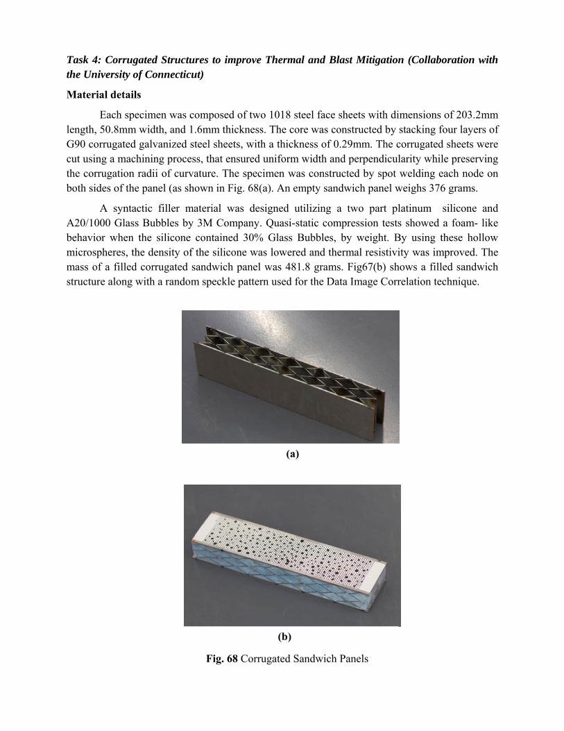
Task 4: Corrugated Structures to improve Thermal and Blast Mitigation (Collaboration with the University of Connecticut)

Material details

Each specimen was composed of two 1018 steel face sheets with dimensions of 203.2mm length, 50.8mm width, and 1.6mm thickness. The core was constructed by stacking four layers of G90 corrugated galvanized steel sheets, with a thickness of 0.29mm. The corrugated sheets were cut using a machining process, that ensured uniform width and perpendicularity while preserving the corrugation radii of curvature. The specimen was constructed by spot welding each node on both sides of the panel (as shown in Fig. 68(a). An empty sandwich panel weighs 376 grams.

A syntactic filler material was designed utilizing a two part platinum silicone and A20/1000 Glass Bubbles by 3M Company. Quasi-static compression tests showed a foam- like behavior when the silicone contained 30% Glass Bubbles, by weight. By using these hollow microspheres, the density of the silicone was lowered and thermal resistivity was improved. The mass of a filled corrugated sandwich panel was 481.8 grams. Fig67(b) shows a filled sandwich structure along with a random speckle pattern used for the Data Image Correlation technique.

Fig. 68 Corrugated Sandwich Panels

(a)

(b)

Real-Tim

The reatransient filled csubjectedshown ipropagatframe to comparedperiod, wmoment b

Onset ofcorrugateapproximfront andfront facback andthe corruback facwas pronof the spfailed dudeflection4.5ms.

The fillevery littlthe entirfiller fromas well primarilythe face specimen

A plot ofto the spaerial denalmost imDuring ththe addedof the fill

me Deforma

al-time obbehavior f

corrugated d to shock in Fig. 69es from thethe left sid

d within the where t=0msbefore shock

f core compred sandwic

mately 1.5md back face

ce sheet defld buckling cugation thatce. By 3.0mnounced alonpecimen andue to shearn, of 17mm

ed corrugatele core comre event. Dm the corruas local fai

y where the sheets. Ma

n had already

f the back fapecimen ovensity of the emmediately whis time, thed mass of thler material.

ation and An

bservations for both em

sandwich wave load

. The shoce right side e and both csame refere

s correspondk loading.

ression in thh panel b

ms, accompae deformatiolected more could be set was joine

ms core comng the centrd several wr effects. M

m, was obt

ed structurempression thDelaminationugation is oblure at the core was joi

aximum defly started to r

ace deflectionerall, the resempty sandwwhereas the e front face ohe filler, eve

F

nalysis

of the mpty and

panels ding are ck wave

of each cases are ence time ds to the

he empty egan by anied by ons. The than the

en along ed to the mpression ral region

welds had Maximum tained by

showed hroughout n of the bserved

welds, ined to lection, of rebound.

n can be seesult for the fwich panel. Tempty corruof the empty

en when norm

Fig. 69 High

12mm, occu

n in Fig 70. filled case hThe back facugation expey specimen dmalized, the

Speed Image

urred around

Because thehas been noce of the fillerienced a brdeflected, coe deflections

es of empty an

d 3.0ms an

e filler materrmalized wied specimenrief delay unompressing s were less w

nd filled spec

nd by 4.5ms

rial added with respect tn began to dentil about 0.2the core. De

with the pres

cimens

s, the

weight to the eflect 25ms. espite sence

Macroscopic Post-Mortem Analysis

Permanent deformation of the corrugated steel sandwich panels were visually inspected and documented using a digital camera, as seen in Fig. 70.

The first series of experiments were performed at room temperature (RT) and a predetermined low pressure (LP) of 1.25-MPa. This was done to understand the performance of both the empty (E) and filled (F) specimens; they have been designated RTLP-E and RTLP-F. The following series compared filled specimens at a higher pressure (HP) of 1.7-MPa, and at both room temperature and a high temperature (HT) of 500˚C.

After experiencing a shock loading the RTLP-E specimen exhibited plastic deformation in the front and back face sheets of 16.7mm and 11.9mm respectively. The core permanently compressed by 8% of its original width in the central region of the specimen. Welds at the outer edges along the central axis showed signs of shearing and core buckling was visible in the central region where the shock impinged on the specimen.

The post-mortem condition of the filled specimens, RTHP-F, RTHP-F, and HTFP-F, showed little signs of core compression; however, plastic deformation was apparent in the face sheets. The RTLP-F specimen showed evidence of delamination of the filler material from the corrugation; however, since the filler is not bonded to the corrugation, it is assumed that this failure mechanism does not contribute to energy dissipation. What the filler does offer is resistance to core buckling and a larger area for applied forces to act. Delamination occurred between the front face sheet and the core via breakage of welds.

The RTHP-F specimen was investigated using higher pressure and endured greater plastic deformation as compared to the low pressure trial. The front face sheet delaminated along its edges, but was still attached at the center. The back face sheet experienced delamination, but this occurred in the central region and was still attached at the edges. Permanent deformation of the front and back face sheets were 15.1mm and 13.5mm, respectively.

Fig. 70 Deflections of filled and unfilled

0 1 2 3 4 5 6 7 80

2

4

6

8

10

12

14

16

18 Empty Filled *

*Normalized with respect to aerial density of empty specimen

Def

lect

ion

(mm

)

Time (ms)

0 5 10 15 200

100

200

300

400

500

Te

mp

era

ture

(°C

)

Time (min)

Back Face Front Face

The HTHP-F specimen was investigated at a higher temperature. The back face of the specimen was heated to ~500˚C (932˚F) for a duration of twenty minutes. The back face temperature reached steady state after six minutes while the front face temperature reached a maximum of ~150˚C (302˚F) before a shock load was applied. Fig. 72 shows a plot of the front and back face temperature profiles during preliminary heating.

During this time a layer of the filler material in contact with the heated face sheet had turned white. This was a result of the silicone decomposes into silica (or silicon dioxide) along with the emission of carbon dioxide and carbon monoxide. The post

mortem specimen showed major deflection and delamination of both front and back face sheets. The corrugated core appeared to be plastically deformed, but was actually held by the welds on the outer edge of the back face sheet, which remained intact. Inner core delamination was present due to a shearing of spot welds.

Fig. 71 Post-mortem images of samples

Fig. 72 Thermal profile of HTHP-F during heating

Fig. 73 Collaborations with Industry

Fig. 74: Novel material systems fabricated with help from Industry

Task 5: Collaboration with Industry / Transition to Customer

Novel material systems and sandwich structures, including but not limited to laminated glass panels, corrugated steel armor, and sandwich composites with a functionally graded foam core (Fig. 73) were designed and fabricated to withstand blast loadings and mitigate blast overpressures. Technical collaboration with XO Armor®, Specialty Products Inc., Gurit SP Technology, 3M Company, and TPI Composites helped in facilitating sample preparation. This effort also aligns with the mission of DHS to transition technology and allow for a unified effort to protect our homeland.

Fig. 75: Students working on shock tube experiments

Students Supported

1. Sandeep Abotula (Ph.D) 2. Nate Gardner (Ph.D) 3. Emad Makki (Ph.D) 4. Jefferson Wright (M.S) 5. Payam Fahr (M.S) 6. Chris Shillings (Undergraduate)

Journal Publications

1. E. Wang, N Gardner and A. Shukla, “The Blast Resistance of Sandwich Composites with Stepwise Graded Cores”, International Journal of Solid and Structures, 46, 3492-3502, 2009.

2. E. Wang and A. Shukla, “Analytical and Experimental Evaluation of Energies during Shock Wave Loading”, International Journal of Impact Engineering, 1188-1196, 2010.

3. M. Jackson, A. Shukla, “Performance of Sandwich Composites Subjected to Sequential Impact and Air Blast Loading”, Composites: Part B, 42, 155–166, 2011.

4. P. Kumar and A. Shukla, "Dynamic Response of Glass Panels Subjected to Shock Loading", Journal of Non-Crystalline Solids, Vol. 357 (24), 3917-3923, 2011.

5. E. Wang, J. Wright and A. Shukla, “Analytical and Experimental Study on the Fluid Structure Interaction During Air Blast Loading", Journal of Applied Physics, Vol. 110, 114901-1 – 114901-12, 2011.

6. N. Gardner, E. Wang, P. Kumar and A. Shukla, “Blast Mitigation in a Sandwich Composite Using Graded Core and Polyurea Interlayer", Experimental Mechanics, Vol. 52,119-133, 2012.

7. N. Gardner, E. Wang and A. Shukla, "Performance of Functionally Graded Sandwich Composite Beams under Shock Wave Loading", Composite Structures, Vol. 94 (5), 1755–1770, 2012

8. E. Wang and A. Shukla, “Blast Performance of Sandwich Composites with In-Plane Compressive Loading”, Experimental Mechanics, Vol. 52, 49-58, 2012.

9. P. Kumar, J. LeBlanc, D. Stargel and A. Shukla, "Effect of Plate Curvature on Blast Response of Aluminum Panels”, International Journal of Impact Engineering,Vol. 46, 74-85, 2012.

10. E. Wang, N. Gardner, S. Gupta and A. Shukla, "Fluid-Structure Interaction and its Effect on the Performance of Composite Structures under Air-Blast Loading", Journal of Multiphysics, Vol. 6(3), 2012

11. “Effect of plate curvature on blast response of carbon composite panels,” with P. Kumar and D. Stargel, Composite Structures, Vol. 99, pp. 19-30, 2013.

Conference Proceedings

1. E. Wang, N. Gardner and A. Shukla, “Experimental Study on the Performance of Sandwich Composites with Stepwise Graded Cores Subjected to a Shock wave Loading”, SEM Annual Conference and Exposition on Experimental and Applied Mechanics, Albuquerque, New Mexico, June 1-4, 2009.

2. N. Gardner, “Blast Performance of Sandwich Composites with Discretely Layered Core”, SEM Annual Conference and Exposition on Experimental and Applied Mechanics, Albuquerque, New Mexico, June 1-4, 2009.

3. S.A. Tekalur, E. Wang, M. Jackson and A. Shukla, “Failure Behavior and Energy Absorption of Sandwich Composites under Dynamic Loading”, SEM Annual Conference and Exposition on Experimental and Applied Mechanics, Albuquerque, New Mexico, June 1-4, 2009.

4. E. Wang and A. Shukla, “Evaluation of Incident, Reflected and Deformation Energies During Blast Experiments”, SEM Annual Conference and Exposition on Experimental and Applied Mechanics, Albuquerque, New Mexico, June 1-4, 2009.

5. N. Gardner and A. Shukla, “The Blast Response of Sandwich Composites With a Functionally Graded Core”, SEM Annual Conference and Exposition on Experimental and Applied Mechanics, Indianapolis, Indiana, June 7-10, 2010.

6. N. Gardner and A. Shukla, “The Blast Response of Sandwich Composites With a Functionally Graded Core and Polyurea Interlayer”, SEM Annual Conference and Exposition on Experimental and Applied Mechanics, Indianapolis, Indiana, June 7-10, 2010.

7. E. Wang and A. Shukla, “The Blast Response of Sandwich Composites with In-Plane Pre-Loading”. SEM Annual Conference and Exposition on Experimental and Applied Mechanics, Indianapolis, Indiana, June 7-10, 2010.

8. P. Kumar and A. Shukla, “Blast Loading Response of Glass Panels”, SEM Annual Conference and Exposition on Experimental and Applied Mechanics, Indianapolis, Indiana, June 7-10, 2010.

9. E. Wang and A. Shukla, “Core Deformation of Sandwich Composites under Blast Loading”, SEM Annual Conference and Exposition on Experimental and Applied Mechanics, Indianapolis, Indiana, June 7-10, 2010.

10. E. Wang and A. Shukla, “Blast Response of Sandwich Composites using Digital Image Correlation Technique”, 9th International Conference on Sandwich Structures (ICSS9), Caltech, Pasadena, California, June 14 - 16, 2010.

11. E. Wang and A. Shukla, “Performance of Pre-Stressed Sandwich Composites Subjected to Shock Wave Loading”, 14th International Conference on Experimental Mechanics (ICEM 14), Poitiers, FRANCE July 4-9, 2010.

12. N. Gardner and A. Shukla, “The Blast Resistance of Sandwich Composites with a Functionally Graded Core and Polyurea Interlayer”, IMPLAST 2010, SEM Fall Conference, Providence, RI, October 12-14, 2010.

13. P. Kumar and A. Shukla, “Dynamic Response of Glass Panels Subjected to Shock Loading", IMPLAST 2010, SEM Fall Conference, Providence, RI, October 12-14, 2010.

14. N. Gardner and A. Shukla, “The Blast Response of Sandwich Composites with Graded Core: Equivalent Core Layer Mass vs. Equivalent Core Layer Thickness”, SEM Annual Conference and Exposition on Experimental and Applied Mechanics, Uncasville, Connecticut, June 13 - 16, 2011.

15. P. Kumar and A. Shukla, “Dynamic Response of Shock Loaded Architectural Glass Panels", SEM Annual Conference and Exposition on Experimental and Applied Mechanics, Uncasville, Connecticut, June 13 - 16, 2011.

16. P. Kumar and A. Shukla, “Effect of Curvature on Shock Loading Response of Aluminum Panels", SEM Annual Conference and Exposition on Experimental and Applied Mechanics, Uncasville, Connecticut, June 13 - 16, 2011.

17. P. Kumar and A. Shukla, “Blast Response of Architectural Glass Panels", SEM Annual Conference and Exposition on Experimental and Applied Mechanics, Uncasville, Connecticut, June 13 - 16, 2011.

18. P. Kumar, D. Stargel and A. Shukla, “Response of Curved Carbon Composite Panels to Shock Loading,” European Conference on Composite Materials, 24-28 June, 2012, Venice, Italy