2006: Scouller, R.C., Snape, I., Stark, J.S. & Gore, D.B. 2006. Evaluation of geochemical methods...

www.elsevier.com/locate/chemosphere

Chemosphere 65 (2006) 294–309

Evaluation of geochemical methods for discrimination ofmetal contamination in Antarctic marine sediments:

A case study from Casey Station

Rebecca C. Scouller, Ian Snape *, Jonathan S. Stark, Damian B. Gore

Australian Antarctic Division, Department of Environment and Heritage, 203 Channel Highway, Kingston, Tasmania 7050, Australia

Received 17 February 2006; accepted 19 February 2006Available online 2 May 2006

Abstract

Detecting anthropogenic metal contamination in regional surveys can be particularly difficult when there is a lack of pre-disturbancedata, especially when trying to differentiate low to moderate levels of contamination from background values. Furthermore, comparisonswith other regional studies are confounded by differing analytical methods used and variations in sediment properties such as grainsize.Several types of geochemical technique, including weak acid partial extraction, strong acid extractions and total digestion have beenused. Attempts have been made to overcome the influence that grainsize has on chemical concentrations in heterogeneous environmentsby analysing the fines, typically the mud fraction (<63 lm), in an attempt to improve the detection of anthropogenic contamination. Herewe compare a weak acid partial extraction using 1 M HCl and total digestion methods for a regional survey of reference and impactedsites in Antarctica using both whole sediment (<2 mm) and mud (<63 lm) fractions. The 1 M partial extraction on whole sediment(<2 mm) most closely distinguished weakly, or moderately, impacted sites from reference locations. It also identified small scalewithin-location spatial variation in metal contamination that the total digest did not detect. Compared with total digests or analysisof the <63 lm fraction alone, this method minimised the possibility of a Type II statistical error in the regional survey – that is, failingto identify a site as being contaminated when it has elevated metal concentrations. To allow inter-regional comparison of sedimentchemistry data from elsewhere in Antarctica, and also more generally, we recommend a 1 M HCl partial extraction on whole sediment(<2 mm).Crown Copyright � 2006 Published by Elsevier Ltd. All rights reserved.

Keywords: Hydrochloric extraction; <2 mm fraction; <63 lm fraction; Metal pollution; Antarctica; Human impacts

1. Introduction

Regional surveys that are designed to detect metal con-tamination in marine sediments are difficult when there areno pre-disturbance records. The most commonly adoptedapproach involves comparing the metal concentrations ofa suitable number of environmentally similar reference orcontrol locations, to locations that are suspected of beingcontaminated. For Antarctica, there are no widely used

0045-6535/$ - see front matter Crown Copyright � 2006 Published by Elsevie

doi:10.1016/j.chemosphere.2006.02.062

* Corresponding author. Tel.: +61 3 62323591; fax: +61 3 62323158.E-mail address: [email protected] (I. Snape).

standards or guidelines and individual national operatorshave begun assessing marine contamination and associatedecological impacts using a variety of methods. Unfortu-nately the use of different sampling and analytical methodsprecludes rigorous inter-regional comparisons of contami-nation or their biological effects. Internationally, severaltypes of geochemical technique have been used: someresearchers have used weak acid partial extraction, othershot or strong acid extractions, or a total digestion. Addi-tionally, various attempts have been made to overcomethe influence that grainsize has on chemical concentrationsin heterogeneous environments. For many regions, tracemetal concentrations increase with decreasing grainsize;

r Ltd. All rights reserved.

mailto:[email protected]

Tab

le1

Met

ho

ds

use

din

oth

erre

gio

nal

surv

eys

inA

nta

rcti

ca

Au

tho

rL

oca

tio

nE

xtra

ctio

nm

eth

od

Gra

insi

zefr

acti

on

Sam

pli

ng

des

ign

Det

ecti

on

of

imp

act

Ala

man

dS

adiq

(199

3)A

nta

rcti

cP

enin

sula

To

tal

dig

est

<0.

5m

mO

pp

ort

un

isti

cra

nd

om

?Y

esK

enn

icu

ttet

al.

(199

5)M

cMu

rdo

So

un

dan

dA

rth

ur

Har

bo

ur

To

tal

dig

est

Wh

ole

sed

imen

t?R

and

om

?Y

esL

enih

anet

al.

(199

0)M

cMu

rdo

So

un

d,

Win

ter

Qu

arte

rsB

ayH

ot

con

c.H

NO

3W

ho

lese

dim

ent?

Tra

nse

ctY

esA

nd

rad

eet

al.

(200

1)P

ott

erC

ove

,K

ing

Geo

rge

Is.

S.

Sh

etla

nd

Is.

Ho

tp

erch

lori

c+

nit

ric

Wh

ole

sed

imen

t?T

ran

sect

No

Co

sma

etal

.(1

994)

Ter

raN

ova

Bay

,R

oss

Sea

To

tal

dig

est

and

sele

ctiv

eex

trac

tio

n<

2m

mp

ow

der

edO

pp

ort

un

isti

cra

nd

om

?N

oC

iara

lli

etal

.(1

998)

Ter

raN

ova

Bay

,R

oss

Sea

To

tal

dig

est?

and

0.5

NH

Cl

<63

lm

and

<2

mm

Op

po

rtu

nis

tic

ran

do

m?

No

Gio

rdan

oet

al.

(199

9)T

erra

No

vaB

ay,

Ro

ssS

eaT

ota

ld

iges

t<

63l

man

d<

2m

mO

pp

ort

un

isti

cra

nd

om

?N

oH

iek

eM

erli

net

al.

(198

9)W

este

rnR

oss

Sea

Was

hed

then

tota

ld

iges

tS

ieve

do

rh

and

pic

ked

Tra

nse

ctN

oR

iva

etal

.(2

004)

Ter

raN

ova

Bay

,R

oss

Sea

To

tal

dig

est

and

0.11

Mac

etic

acid

<63

lm

and

<2

mm

Tra

nse

ctN

o

R.C. Scouller et al. / Chemosphere 65 (2006) 294–309 295

hence the most commonly adopted geochemical methodinvolves separating and analysing the fines, typically the<63 lm or mud fraction, in an attempt to improve thedetection of anthropogenic contamination (Loring, 1991;Loring and Rantala, 1992). Alternatively, where there isa strong relationship between grainsize and metal concen-tration, it is sometimes possible to mathematically correct(normalise) the data. This is either done by normalising ref-erence metals to an empirically derived grainsize dataset, orby using a geochemical surrogate, such as Li or Al, thatrepresents a certain mineral fraction (Loring, 1991; Loringand Rantala, 1992). For Antarctica, and regional surveysin general, a cost-effective chemical survey method isneeded that, as much as possible, targets the bioavailableanthropogenic fraction of metals in the sediment. In thiscontribution we compare the weak acid partial extractionusing 1 M HCl and total digestion methods for a regionalsurvey of reference and impacted sites in Antarctica usingboth whole sediment (<2 mm) and mud (<63 lm)fractions.

1.1. Assessments of metal contamination in Antarcticmarine sediments

It is only relatively recently, since ratification of the Pro-tocol on Environmental Protection to the Antarctic Treatyin 1998 (Madrid Protocol), that Antarctic national opera-tors have been required to cleanup abandoned waste sites.As part of Australia’s commitment to the Protocol, theAustralian Antarctic Program has begun a comprehensiveregional assessment of metal contamination adjacent toabandoned waste sites. Sediments are known to be a sinkfor metal contaminants. They are a crucial link betweencontaminants and impacts on benthic organisms, and sed-iment contamination can be a precursor to impacts at theecosystem level. Hence regional marine surveys to detectmetal contamination from human activities usually concen-trate on sediment assessments.

An aim in this study is to evaluate a number of simplelow-cost approaches that can be used by Australia andother nations to create data for inter-regional compari-sons of contaminants and their impacts. Several regionalsurveys have been undertaken in Antarctica to distinguishcontamination from the background of natural variability(Table 1); unfortunately they all used different techniques,and most used total or strong acid digestions of sedi-ments. In choosing a suitable methodology for the firstbroad-scale regional assessment in the Windmill Islands(Fig. 1), we evaluated chemical approaches that woulddistinguish weak, moderate and heavy contamination,and that might most closely relate to observed biologicalimpacts.

Metal concentrations derived from total digests do notnecessarily provide biologically meaningful data (Agemianand Chau, 1976). Total digests break down all mineralphases within the sediment and are employed because theygenerate highly reproducible data. However such methods

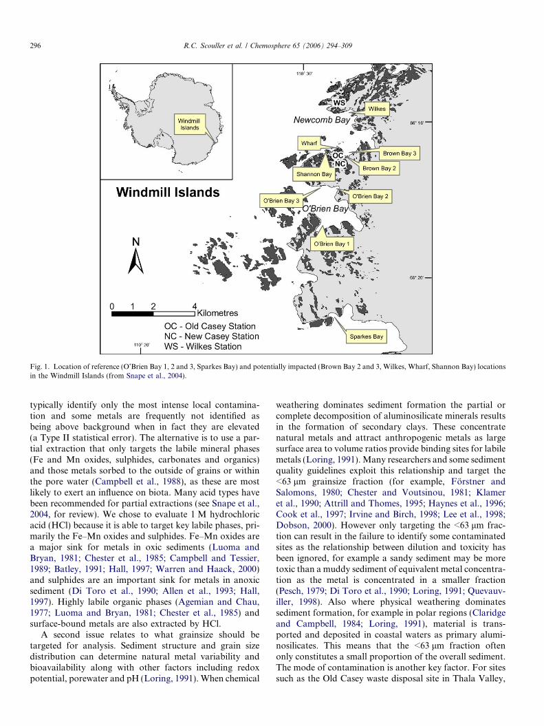
Fig. 1. Location of reference (O’Brien Bay 1, 2 and 3, Sparkes Bay) and potentially impacted (Brown Bay 2 and 3, Wilkes, Wharf, Shannon Bay) locationsin the Windmill Islands (from Snape et al., 2004).

296 R.C. Scouller et al. / Chemosphere 65 (2006) 294–309

typically identify only the most intense local contamina-tion and some metals are frequently not identified asbeing above background when in fact they are elevated(a Type II statistical error). The alternative is to use a par-tial extraction that only targets the labile mineral phases(Fe and Mn oxides, sulphides, carbonates and organics)and those metals sorbed to the outside of grains or withinthe pore water (Campbell et al., 1988), as these are mostlikely to exert an influence on biota. Many acid types havebeen recommended for partial extractions (see Snape et al.,2004, for review). We chose to evaluate 1 M hydrochloricacid (HCl) because it is able to target key labile phases, pri-marily the Fe–Mn oxides and sulphides. Fe–Mn oxides area major sink for metals in oxic sediments (Luoma andBryan, 1981; Chester et al., 1985; Campbell and Tessier,1989; Batley, 1991; Hall, 1997; Warren and Haack, 2000)and sulphides are an important sink for metals in anoxicsediment (Di Toro et al., 1990; Allen et al., 1993; Hall,1997). Highly labile organic phases (Agemian and Chau,1977; Luoma and Bryan, 1981; Chester et al., 1985) andsurface-bound metals are also extracted by HCl.

A second issue relates to what grainsize should betargeted for analysis. Sediment structure and grain sizedistribution can determine natural metal variability andbioavailability along with other factors including redoxpotential, porewater and pH (Loring, 1991). When chemical

weathering dominates sediment formation the partial orcomplete decomposition of aluminosilicate minerals resultsin the formation of secondary clays. These concentratenatural metals and attract anthropogenic metals as largesurface area to volume ratios provide binding sites for labilemetals (Loring, 1991). Many researchers and some sedimentquality guidelines exploit this relationship and target the<63 lm grainsize fraction (for example, Forstner andSalomons, 1980; Chester and Voutsinou, 1981; Klameret al., 1990; Attrill and Thomes, 1995; Haynes et al., 1996;Cook et al., 1997; Irvine and Birch, 1998; Lee et al., 1998;Dobson, 2000). However only targeting the <63 lm frac-tion can result in the failure to identify some contaminatedsites as the relationship between dilution and toxicity hasbeen ignored, for example a sandy sediment may be moretoxic than a muddy sediment of equivalent metal concentra-tion as the metal is concentrated in a smaller fraction(Pesch, 1979; Di Toro et al., 1990; Loring, 1991; Quevauv-iller, 1998). Also where physical weathering dominatessediment formation, for example in polar regions (Claridgeand Campbell, 1984; Loring, 1991), material is trans-ported and deposited in coastal waters as primary alumi-nosilicates. This means that the <63 lm fraction oftenonly constitutes a small proportion of the overall sediment.The mode of contamination is another key factor. For sitessuch as the Old Casey waste disposal site in Thala Valley,


the dispersal mechanism is largely through mobilisation offine particles, including mud but ranging up to about500 lm, rather than being dominated by sorption to mudand clays (Snape et al., 2001; Northcott et al., 2003). In thisscenario, where the bulk of the contamination resides in the63 lm-2 mm fraction, focussing on the <63 lm fractioncould potentially underestimate the extent of contamina-tion.

To discriminate the best geochemical method and grain-size fraction to identify sites known to be biologicallyimpacted in an a posteriori analysis, we identified twoquestions:

Do partial extractions better discriminate between

impacted and reference locations than total digests?

Does chemical analysis of the <63 lm fraction better dis-

criminate between impacted and reference locations than

whole-sediment (<2 mm fraction)?

To test hypotheses based on these questions, we inves-tigated a case study in the Windmill Islands area wherethere are several sources of metal contamination. In a pre-vious publication we examined the effect of extraction timeusing 1 M HCl (Snape et al., 2004), and concluded that a4-h extraction time most effectively targeted the bulk ofanthropogenic metals in sediments. In previous field exper-imental work (Stark et al., 2003a,b,c) we concluded thatsites adjacent to the station were indeed impacted and thatthere is a causal relationship between metal contaminationand observed biological patterns. The overall objectivehere is to ascertain which regional chemical assessmentmethods best identify contaminated sediment in an a pos-teriori analysis, so that we can apply these methods toother sites.

2. Methods

The Windmill Islands cover an area �75 km2 on thecoast of East Antarctica (66�10 0–66�35 0S, 110�10 0–110�50 0E). Human occupation of the Windmill Islandsbegan in 1957 with the construction of Wilkes Station onClark Peninsula. This station was subsequently replacedby ‘Old’ Casey (1969) then ‘New’ Casey (1989) on BaileyPeninsula (Fig. 1). Wilkes and ‘Old’ Casey stations haveassociated waste disposal areas containing an estimated25000 m3 and 2500 m3 of contaminated material respec-tively (Snape et al., 1998; Deprez et al., 1999). Materialdumped at these sites consists of laboratory chemicals,waste from the mechanical workshops and domestic refuse(Snape et al., 2001). Preliminary studies have identified ele-vated metal levels in Thala Valley (Old Casey) and onClark Peninsula near Wilkes (Deprez et al., 1999; Snapeet al., 2001). Metals are known to be elevated in BrownBay adjacent to the Old Casey Station waste disposal site(Stark et al., 2003c).

Other potentially contaminated areas include the wharf,which is the location of fuel transfer from ship to stationand the focal point of all shipping and boating activities;

and Shannon Bay, the receiving environment for the sew-age outfall from Casey Station.

Reference locations were sampled to establish back-ground concentrations. These locations, in O’Brien andSparkes bays, both lie to the south of Newcomb Bay(Fig. 1) and are unlikely to have been affected by humanactivity. They were chosen based on several factors includ-ing ease of access, similar geology and topography, waterdepth and aspect (www.aad.aadc.gov.au).

2.1. Sample collection and preparation

A hierarchical nested sampling design was used for sam-ple collection in the regional survey. This allows for statis-tical analysis of spatial variation at four scales; locations(km), sites (within locations at �100 m scale), plots (withinsites at �10 m scale) and replicate samples taken at �1 mscale (Stark et al., 2003b). In total 11 locations were sam-pled, within Newcomb Bay there were six locations; WilkesBay 97 (W97) and Wilkes Bay 99 (W99), Brown Bay 2(BB2) and Brown Bay 3 (BB3), Shannon Bay (SH) andWharf Bay (WH). Four reference locations within O’BrienBay were sampled; OBB1, OBB2 97, OBB2 98, OBB3 andone reference location within Sparkes Bay (SP) (Fig. 1).

Divers collected the samples from water depths 6–20 musing 5 cm diameter by 15 cm length acid-washed PVC cor-ing tubes pushed �10 cm into the sediment (see Stark et al.,2003b); samples were then emptied into zip-lock plasticbags and stored at �20 �C until sieved. Samples wereallowed to thaw overnight and then wet-sieved with clean,filtered O’Brien Bay seawater (through 0.45 lm cellulosenitrate). Samples were sieved using a polystyrene sieve withnylon mesh, samples were first sieved to <2 mm to removelarge clasts or shells (generally only 1–2% by mass) then analiquot was sieved to <63 lm. Samples were oven dried toconstant weight at 103 �C (e.g. Loring and Rantala, 1992)and stored in Nalgene HDPE bottles.

2.2. Chemical analysis

All plastic and glass labware used for sieving and partialextractions was cleaned for 24 h with 20% (v/v) analyticalgrade HNO3 (69% w/w; BDH) and then soaked for 24 hand triple rinsed in MQ+ water. Teflon containers usedfor partial extractions were cleaned in hot aqua regia for24 h and soaked and triple-rinsed in MQ+ water.

Total metal digests were undertaken following Yu et al.(2001). In brief, 0.1 g of sample was moistened with afew drops of MQ+ water, then digested in 1 ml double dis-tilled concentrated HNO3 (15.4 M) and 1 ml double dis-tilled concentrated HF (29.1 M) in screw-topped Teflonbeakers for 24 h at 130–150 �C, then evaporated to dryness.A second stage of digestion was performed with the addi-tion of 1 ml double distilled concentrated HCl (10.2 M)and 1 ml double distilled concentrated HF, again heatedfor 24 h and then evaporated. Next, 2 ml of double distilledconcentrated HNO3 was added and evaporated to dryness

http://www.aad.aadc.gov.au


then 2 ml MQ+ water and 2 ml double distilled concen-trated HNO3 was refluxed for 4 h before dilution to 2%(v/v) with MQ+ water prior to analysis. Partial extractions(1.0 M HCl for 4 h) were prepared from analytical gradeHCl (32% w/w; Univar) and MQ+ water as described inSnape et al. (2004). All extractions used 1 g of sedimentto 20 ml 1 M HCl solution (1:20 w/v) and were extractedin Teflon containers on an orbital shaker for a period of4 h. Supernatants from the <2 mm fraction samples wereimmediately filtered through 0.45 lm cellulose nitratemembranes (Sartorius) using a Millipore filter unit. The<63 lm digests were filtered using 60 ml syringes and dis-posable 0.45 lm cellulose acetone syringe filter tips. Super-natants were diluted to 100 ml with MQ+ water beforeanalysis by magnetic sector ICP-MS. 12 elements were ana-lysed: Sb, As, Cd, Cr, Cu, Fe, Pb, Mn, Ni, Ag, Sn and Zn,following the method described in Larner et al. (2006) andreferences therein. Briefly, sample solutions were spikedwith 100 lg l�1 In as an internal standard. Multiple batchesof up to 10 samples were typically run in the following order:QC1 100 lg l�1 multi-element solution standard, rinse,NIST CRM, sample batch, CRM (MESS-2, MESS-3 orPACS-2), QC2 100 lg l�1 standard and final rinse. Theorder of CRMs, NIST, and rinse were sometimes varied.In addition, blanks and replicates (�10%) were submittedand analysed as unknowns.

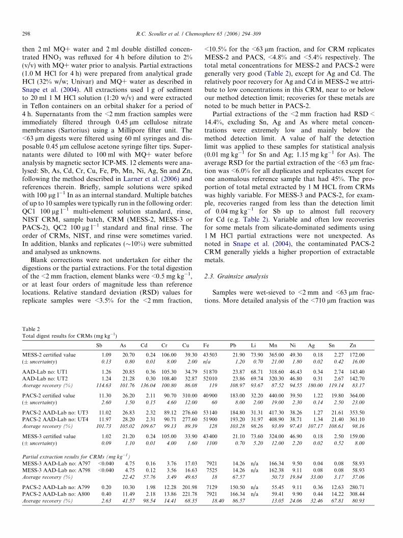
Blank corrections were not undertaken for either thedigestions or the partial extractions. For the total digestionof the <2 mm fraction, element blanks were <0.5 mg kg�1,or at least four orders of magnitude less than referencelocations. Relative standard deviation (RSD) values forreplicate samples were <3.5% for the <2 mm fraction,

Table 2Total digest results for CRMs (mg kg�1)

Sb As Cd Cr Cu

MESS-2 certified value 1.09 20.70 0.24 106.00 39.30(± uncertainty) 0.13 0.80 0.01 8.00 2.00

AAD-Lab no: UT1 1.26 20.85 0.36 105.30 34.79AAD-Lab no: UT2 1.24 21.28 0.30 108.40 32.87Average recovery (%) 114.63 101.76 136.04 100.80 86.08

PACS-2 certified value 11.30 26.20 2.11 90.70 310.00(± uncertainty) 2.60 1.50 0.15 4.60 12.00

PACS-2 AAD-Lab no: UT3 11.02 26.83 2.32 89.12 276.60PACS-2 AAD-Lab no: UT4 11.97 28.20 2.31 90.71 277.60Average recovery (%) 101.73 105.02 109.67 99.13 89.39

MESS-3 certified value 1.02 21.20 0.24 105.00 33.90(± uncertainty) 0.09 1.10 0.01 4.00 1.60

Partial extraction results for CRMs (mg kg�1)

MESS-3 AAD-Lab no: A797 <0.040 4.75 0.16 3.76 17.03MESS-3 AAD-Lab no: A798 <0.040 4.75 0.12 3.56 16.63Average recovery (%) 22.42 57.76 3.49 49.65

PACS-2 AAD-Lab no: A799 0.20 10.30 1.98 12.28 201.98PACS-2 AAD-Lab no: A800 0.40 11.49 2.18 13.86 221.78Average recovery (%) 2.63 41.57 98.54 14.41 68.35

<10.5% for the <63 lm fraction, and for CRM replicatesMESS-2 and PACS, <4.8% and <5.4% respectively. Thetotal metal concentrations for MESS-2 and PACS-2 weregenerally very good (Table 2), except for Ag and Cd. Therelatively poor recovery for Ag and Cd in MESS-2 we attri-bute to low concentrations in this CRM, near to or belowour method detection limit; recoveries for these metals arenoted to be much better in PACS-2.

Partial extractions of the <2 mm fraction had RSD <14.4%, excluding Sn, Ag and As where metal concen-trations were extremely low and mainly below themethod detection limit. A value of half the detectionlimit was applied to these samples for statistical analysis(0.01 mg kg�1 for Sn and Ag; 1.15 mg kg�1 for As). Theaverage RSD for the partial extraction of the <63 lm frac-tion was <6.0% for all duplicates and replicates except forone anomalous reference sample that had 45%. The pro-portion of total metal extracted by 1 M HCL from CRMswas highly variable. For MESS-3 and PACS-2, for exam-ple, recoveries ranged from less than the detection limitof 0.04 mg kg�1 for Sb up to almost full recoveryfor Cd (e.g. Table 2). Variable and often low recoveriesfor some metals from silicate-dominated sediments using1 M HCl partial extractions were not unexpected. Asnoted in Snape et al. (2004), the contaminated PACS-2CRM generally yields a higher proportion of extractablemetals.

2.3. Grainsize analysis

Samples were wet-sieved to <2 mm and <63 lm frac-tions. More detailed analysis of the <710 lm fraction was

Fe Pb Li Mn Ni Ag Sn Zn

43503 21.90 73.90 365.00 49.30 0.18 2.27 172.00n/a 1.20 0.70 21.00 1.80 0.02 0.42 16.00

51870 23.87 68.71 318.60 46.43 0.34 2.74 143.4052010 23.86 69.74 320.30 46.80 0.31 2.67 142.70

119 108.97 93.67 87.52 94.55 180.00 119.14 83.17

40900 183.00 32.20 440.00 39.50 1.22 19.80 364.0060 8.00 2.00 19.00 2.30 0.14 2.50 23.00

53140 184.80 31.31 417.30 38.26 1.27 21.61 353.5051900 193.20 31.97 408.90 38.71 1.34 21.40 361.10

128 103.28 98.26 93.89 97.43 107.17 108.61 98.16

43400 21.10 73.60 324.00 46.90 0.18 2.50 159.001100 0.70 5.20 12.00 2.20 0.02 0.52 8.00

7921 14.26 n/a 166.34 9.50 0.04 0.08 58.937525 14.26 n/a 162.38 9.11 0.08 0.08 58.93

18 67.57 50.73 19.84 33.00 3.17 37.06

7129 150.50 n/a 55.45 9.11 0.36 12.63 280.717921 166.34 n/a 59.41 9.90 0.44 14.22 308.44

18.40 86.57 13.05 24.06 32.46 67.81 80.93

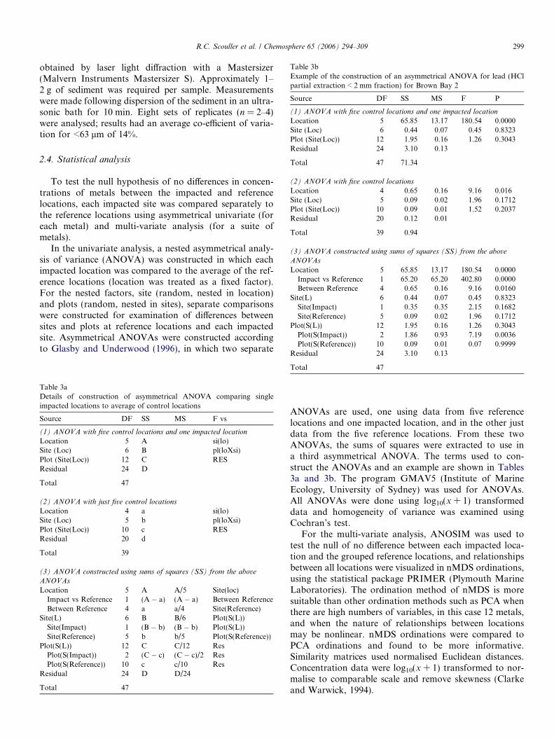
Table 3bExample of the construction of an asymmetrical ANOVA for lead (HClpartial extraction < 2 mm fraction) for Brown Bay 2

Source DF SS MS F P

(1) ANOVA with five control locations and one impacted location

Location 5 65.85 13.17 180.54 0.0000Site (Loc) 6 0.44 0.07 0.45 0.8323Plot (Site(Loc)) 12 1.95 0.16 1.26 0.3043


obtained by laser light diffraction with a Mastersizer(Malvern Instruments Mastersizer S). Approximately 1–2 g of sediment was required per sample. Measurementswere made following dispersion of the sediment in an ultra-sonic bath for 10 min. Eight sets of replicates (n = 2–4)were analysed; results had an average co-efficient of varia-tion for <63 lm of 14%.

Residual 24 3.10 0.13

Total 47 71.34

(2) ANOVA with five control locations

Location 4 0.65 0.16 9.16 0.016Site (Loc) 5 0.09 0.02 1.96 0.1712Plot (Site(Loc)) 10 0.09 0.01 1.52 0.2037Residual 20 0.12 0.01

Total 39 0.94

(3) ANOVA constructed using sums of squares (SS) from the above

ANOVAs

Location 5 65.85 13.17 180.54 0.0000Impact vs Reference 1 65.20 65.20 402.80 0.0000Between Reference 4 0.65 0.16 9.16 0.0160

Site(L) 6 0.44 0.07 0.45 0.8323Site(Impact) 1 0.35 0.35 2.15 0.1682Site(Reference) 5 0.09 0.02 1.96 0.1712

Plot(S(L)) 12 1.95 0.16 1.26 0.3043Plot(S(Impact)) 2 1.86 0.93 7.19 0.0036Plot(S(Reference)) 10 0.09 0.01 0.07 0.9999

Residual 24 3.10 0.13

2.4. Statistical analysis

To test the null hypothesis of no differences in concen-trations of metals between the impacted and referencelocations, each impacted site was compared separately tothe reference locations using asymmetrical univariate (foreach metal) and multi-variate analysis (for a suite ofmetals).

In the univariate analysis, a nested asymmetrical analy-sis of variance (ANOVA) was constructed in which eachimpacted location was compared to the average of the ref-erence locations (location was treated as a fixed factor).For the nested factors, site (random, nested in location)and plots (random, nested in sites), separate comparisonswere constructed for examination of differences betweensites and plots at reference locations and each impactedsite. Asymmetrical ANOVAs were constructed accordingto Glasby and Underwood (1996), in which two separate

Table 3aDetails of construction of asymmetrical ANOVA comparing singleimpacted locations to average of control locations

Source DF SS MS F vs

(1) ANOVA with five control locations and one impacted location

Location 5 A si(lo)Site (Loc) 6 B pl(loXsi)Plot (Site(Loc)) 12 C RESResidual 24 D

Total 47

(2) ANOVA with just five control locations

Location 4 a si(lo)Site (Loc) 5 b pl(loXsi)Plot (Site(Loc)) 10 c RESResidual 20 d

Total 39

(3) ANOVA constructed using sums of squares (SS) from the above

ANOVAs

Location 5 A A/5 Site(loc)Impact vs Reference 1 (A � a) (A � a) Between ReferenceBetween Reference 4 a a/4 Site(Reference)

Site(L) 6 B B/6 Plot(S(L))Site(Impact) 1 (B � b) (B � b) Plot(S(L))Site(Reference) 5 b b/5 Plot(S(Reference))

Plot(S(L)) 12 C C/12 ResPlot(S(Impact)) 2 (C � c) (C � c)/2 ResPlot(S(Reference)) 10 c c/10 Res

Residual 24 D D/24

Total 47

Total 47

ANOVAs are used, one using data from five referencelocations and one impacted location, and in the other justdata from the five reference locations. From these twoANOVAs, the sums of squares were extracted to use ina third asymmetrical ANOVA. The terms used to con-struct the ANOVAs and an example are shown in Tables3a and 3b. The program GMAV5 (Institute of MarineEcology, University of Sydney) was used for ANOVAs.All ANOVAs were done using log10(x + 1) transformeddata and homogeneity of variance was examined usingCochran’s test.

For the multi-variate analysis, ANOSIM was used totest the null of no difference between each impacted loca-tion and the grouped reference locations, and relationshipsbetween all locations were visualized in nMDS ordinations,using the statistical package PRIMER (Plymouth MarineLaboratories). The ordination method of nMDS is moresuitable than other ordination methods such as PCA whenthere are high numbers of variables, in this case 12 metals,and when the nature of relationships between locationsmay be nonlinear. nMDS ordinations were compared toPCA ordinations and found to be more informative.Similarity matrices used normalised Euclidean distances.Concentration data were log10(x + 1) transformed to nor-malise to comparable scale and remove skewness (Clarkeand Warwick, 1994).

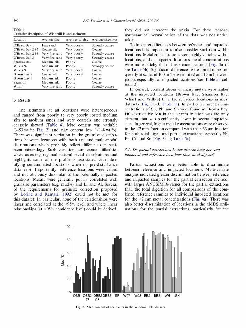
Table 4Grainsize description of Windmill Island sediments

Location Average size Average sorting Average skewness

O’Brien Bay 1 Fine sand Very poorly Strongly coarseO’Brien Bay 2 97 Coarse silt Very poorly CoarseO’Brien Bay 2 98 Very fine sand Very poorly Strongly coarseO’Brien Bay 3 Very fine sand Very poorly Strongly coarseSparkes Bay Medium silt Poorly CoarseWilkes 97 Medium silt Poorly Strongly coarseWilkes 99 Very fine sand Very poorly CoarseBrown Bay 2 Coarse silt Very poorly CoarseBrown Bay 3 Medium silt Poorly CoarseShannon Medium silt Poorly CoarseWharf Very fine sand Poorly Strongly coarse


3. Results

The sediments at all locations were heterogeneousand ranged from poorly to very poorly sorted mediumsilts to medium sands and were coarsely and stronglycoarsely skewed (Table 4). Mud content was variable(3–93 wt.%; Fig. 2) and clay content low (<1–8 wt.%).There was significant variation in the grainsize distribu-tions between locations with both uni and multi-modaldistributions which probably reflect differences in sedi-ment mineralogy. Such variations can create difficultieswhen assessing regional natural metal distributions andhighlights some of the problems associated with iden-tifying contaminated locations when no pre-disturbancedata exist. Importantly, reference locations were variedand not obviously dissimilar to the potentially impactedlocations. Metals were generally poorly correlated withgrainsize parameters (e.g. mud%) and Li and Al. Severalof the requirements for grainsize correction proposedby Loring and Rantala (1992) could not be met forthis dataset. In particular, none of the relationships werelinear and correlated at the >95% level; and where linearrelationships (at <95% confidence level) could be derived,

0

20

40

60

80

100

OBB1 OBB2 97

OBB2 98

OBB3 SP W

Mud

(%

)

Fig. 2. Mud content of sediments

they did not intercept the origin. For these reasons,mathematical normalization of the data was not under-taken.

To interpret differences between reference and impactedlocations it is important to also consider variation withinlocations. Metal concentrations were highly variable withinlocations, and at impacted locations metal concentrationswere more patchy than at reference locations (Fig. 3a–d;see Table 5b). Significant differences were found more fre-quently at scales of 100 m (between sites) and 10 m (betweenplots), especially for impacted locations (see Table 5b col-umn 2).

In general, concentrations of many metals were higherat the impacted locations (Brown Bay, Shannon Bay,Wharf and Wilkes) than the reference locations in mostdatasets (Fig. 3a–d; Table 5a). In particular, greater con-centrations of Sb, Pb, and Sn were found at Brown Bay.HCl-extractable Mn in the <2 mm fraction was the onlyelement that was significantly lower in several impactedsites. In general, higher metal concentrations were observedin the <2 mm fraction compared with the <63 lm fractionfor both total digest and partial extractions, especially Sb,Pb, Cu and Sn (Fig. 3a–d; Table 5a).

3.1. Do partial extractions better discriminate between

impacted and reference locations than total digests?

Partial extractions were better able to discriminatebetween reference and impacted locations. Multi-variateanalysis indicated greater discrimination between referenceand impacted samples for the partial extraction method,with larger ANOSIM R-values for the partial extractionsthan the total digestion for all comparisons of the com-bined reference samples to individual impacted locationsfor the <2 mm metal concentrations (Fig. 4a). There wasalso better discrimination of locations in the nMDS ordi-nations for the partial extractions, particularly for the

97 W98 BB2 BB3 WH SH

in the Windmill Islands area.


<2 mm fraction (Fig. 5). The reference locations also dis-played greater clustering (less variation between samples)in the nMDS ordinations of partial extractions (Fig. 5).In most comparisons using the <63 lm fraction the

Cr

0

5

10

15

20

25

mgk

g-1

Fe

0

5000

10000

15000

20000

25000

mgk

g-1

As

0

10

20

30

40

50

mgk

g-1

Cd

0

1

2

3

4

5

mgk

g-1

Cu

0

10

20

30

40

50

mgk

g-1

Sb

0.0

0.2

0.4

0.6

0.8

1.0

1.2

mgk

g-1

Impacted locationsControl locations

OB1 OB297 OB298OB3 SP W97 W99 BB2 BB3 SH WH

Fig. 3. Metal concentrations of sediments in the Windmill Islands: (a) totextraction < 2 mm fraction; (d) partial extraction < 63 lm fraction.

discrimination between reference and impacted was greaterfor the partial extraction than total digest (Figs. 4b and 5).This effect was most noticeable for the moderately conta-minated sites at Wilkes, the Wharf and Shannon Bay, for

Pb

0

40

80

120

Mn

0

200

400

600

800

1000

Ni

0

2

4

6

8

10

12

Ag

0.0

0.2

0.4

0.6

0.8

1.0

Sn

0

10

20

30

Zn

0

50

100

150

OB1 OB297 OB298 OB3 SP W97 W99 BB2 BB3 SH WH

a

al digest < 2 mm fraction; (b) total digest < 63 lm fraction; (c) partial

Sb

0.0

0.1

0.2

0.3

0.4

0.5

Cd

0.0

0.5

1.0

1.5

2.0

2.5

3.0

Cr

0

4

8

12

16

Cu

0

4

8

12

16

Fe

0

2000

4000

6000

8000

10000

Pb

0

20

40

60Impacted locations

Control locations

Mn

0

50

100

150

200

250

300

350

Ni

0

2

4

6

8

Ag

0.0

0.2

0.4

0.6

Sn

0

2

4

6

8

Zn

0

10

20

30

40

50

As

0

10

20

30

40

50

OB1 OB297 OB298OB3 SP W97 W99 BB2 BB3 SH WH OB1 OB297 OB298 OB3 SP W97 W99 BB2 BB3 SH WH

mgk

g-1m

gkg-1

mgk

g-1m

gkg-1

mgk

g-1m

gkg-1

b

Fig. 3 (continued)


which the R-values increased from quite low to moderatelevels, indicating a greater difference between referencesand these moderately contaminated locations (Fig. 4aand b).

Asymmetrical ANOVAs showed a similar pattern to themulti-variate analysis. In comparisons of impacted to refer-ence locations, there were a greater number of significantdifferences for the partial extractions (in both the <2 mmand <63 lm datasets) than the total digests (Table 5a).For the <2 mm fraction there were 23 significant differencesbetween impacted and reference locations for the partial

extractions but only 14 for the total digests (Table 5a).For the <63 lm fraction there were 13 significant differ-ences between impacted and reference locations for thepartial extraction but only 3 for the total digestion (Table5a).

Partial extractions were also more sensitive in detectingwithin-location variability associated with contamination,which tends to be very patchy as a consequence of the con-taminant dispersal mechanism. In comparisons of siteswithin impacted locations (scale of �100 m), partial extrac-tions had a greater number of significant differences than

Sb

0.0

0.1

0.2

Impacted locations

Control locations

As

0

10

20

30

40

Cd

0

2

4

6

Cr

0

1

2

3

4

5

Cu

0

5

10

15

20

25

Fe

0

1000

2000

3000

4000

5000

6000

Mn

0

5

10

15

Ni

0

2

4

6

8

Ag

0.0

0.1

0.2

0.3

0.4

Sn

0

2

4

6

8

10

12

14

Zn

0

10

20

30

40

50

60

70

Pb

0

20

40

60

80

OB1 OB297 OB298 OBB3 SP W97 W99 BB2 BB3 SH WH OB1 OB297 OB298 OBB3 SP W97 W99 BB2 BB3 SH WH

mgk

g-1m

gkg-1

mgk

g-1m

gkg-1

mgk

g-1m

gkg-1

c

Fig. 3 (continued)


total digestions. For the <2 mm fraction there were 17 vs12 significant differences; for the <63 lm fraction therewere 11 vs 8 significant differences (Table 5b). In compari-sons of plots within sites at impacted locations (scale of�10 m), there were 39 partial vs 36 total significant differ-ences for the <2 mm fraction; and 20 vs 8 significant differ-ences in the <63 lm fraction (Table 5b).

3.2. Does analysis of the whole-sediment (<2 mm) fractionbetter discriminate between impacted and reference locations

than the mud (<63 lm) fraction?

Analysis of the <2 mm fraction was better able to dis-criminate between reference and impacted sites than the<63 lm fraction. In multi-variate analyses, comparisons

Sb

0.00

0.05

0.10

0.15

Impacted locations

Control locations

As

0

10

20

30

40

50

Cr

0.0

1.0

2.0

3.0

Cu

0

4

8

12

mgk

g-1

Fe

0

1000

2000

3000

Pb

0

10

20

30

40

50

Mn

0

5

10

15

Ni

0.0

0.5

1.0

1.5

2.0

2.5

Ag

0.0

0.1

0.2

0.3

0.4

Sn

0

1

2

3

Zn

0

5

10

15

20

25

30

35

Cd

0

1

2

3

OB1 OB297 OB298 OBB3 SP W97 W99 BB2 BB3 SH WH OB1 OB297 OB298 OBB3 SP W97 W99 BB2 BB3 SH WH

mgk

g-1m

gkg-1

mgk

g-1m

gkg-1

mgk

g-1d

Fig. 3 (continued)


of reference sites with impacted sites had greater ANOSIMR-values for the <2 mm fraction, particularly for the par-tial extraction (Fig. 4c and d), and better discriminationin nMDS ordinations (Fig. 5). In particular, the discrimi-nation between the low to moderately contaminated sites(Wilkes, Shannon and Wharf) and the references wasgreater for the <2 mm fraction than the <63 lm fraction(Figs. 4d, 5).

Asymmetrical ANOVAs detected 23 significant differ-ences between impacted and reference locations for theHCl partial extraction <2 mm fraction, and only 13 forthe <63 lm fraction. There were 14 significant differencesfor the total digest <2 mm fraction compared to 3 for the<63 lm fraction (Table 5a).

The <2 mm fraction also revealed a greater degree ofsmall scale heterogeneity in metal concentrations within

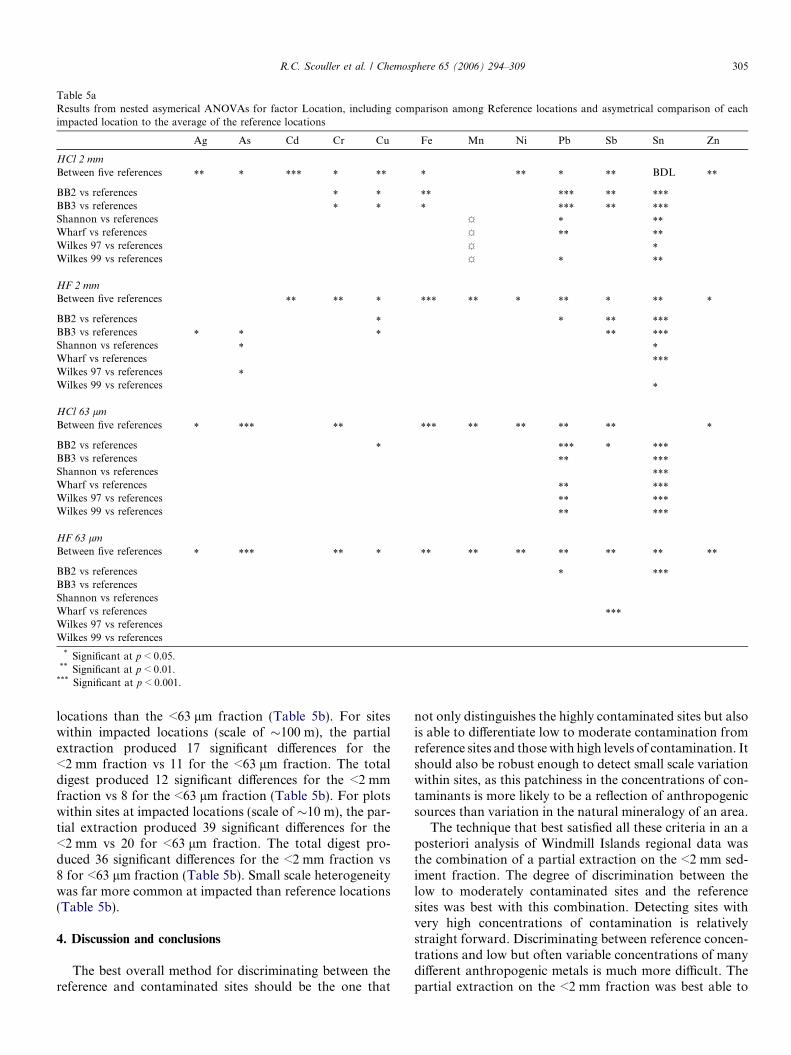
Table 5aResults from nested asymerical ANOVAs for factor Location, including comparison among Reference locations and asymetrical comparison of eachimpacted location to the average of the reference locations

Ag As Cd Cr Cu Fe Mn Ni Pb Sb Sn Zn

HCl 2 mm

Between five references ** * *** * ** * ** * ** BDL **

BB2 vs references * * ** *** ** ***BB3 vs references * * * *** ** ***Shannon vs references * **Wharf vs references ** **Wilkes 97 vs references *Wilkes 99 vs references * **

HF 2 mm

Between five references ** ** * *** ** * ** * ** *

BB2 vs references * * ** ***BB3 vs references * * * ** ***Shannon vs references * *Wharf vs references ***Wilkes 97 vs references *Wilkes 99 vs references *

HCl 63 lm

Between five references * *** ** *** ** ** ** ** *

BB2 vs references * *** * ***BB3 vs references ** ***Shannon vs references ***Wharf vs references ** ***Wilkes 97 vs references ** ***Wilkes 99 vs references ** ***

HF 63 lm

Between five references * *** ** * ** ** ** ** ** ** **

BB2 vs references * ***BB3 vs referencesShannon vs referencesWharf vs references ***Wilkes 97 vs referencesWilkes 99 vs references

* Significant at p < 0.05.** Significant at p < 0.01.

*** Significant at p < 0.001.


locations than the <63 lm fraction (Table 5b). For siteswithin impacted locations (scale of �100 m), the partialextraction produced 17 significant differences for the<2 mm fraction vs 11 for the <63 lm fraction. The totaldigest produced 12 significant differences for the <2 mmfraction vs 8 for the <63 lm fraction (Table 5b). For plotswithin sites at impacted locations (scale of �10 m), the par-tial extraction produced 39 significant differences for the<2 mm vs 20 for <63 lm fraction. The total digest pro-duced 36 significant differences for the <2 mm fraction vs8 for <63 lm fraction (Table 5b). Small scale heterogeneitywas far more common at impacted than reference locations(Table 5b).

4. Discussion and conclusions

The best overall method for discriminating between thereference and contaminated sites should be the one that

not only distinguishes the highly contaminated sites but alsois able to differentiate low to moderate contamination fromreference sites and those with high levels of contamination. Itshould also be robust enough to detect small scale variationwithin sites, as this patchiness in the concentrations of con-taminants is more likely to be a reflection of anthropogenicsources than variation in the natural mineralogy of an area.

The technique that best satisfied all these criteria in an aposteriori analysis of Windmill Islands regional data wasthe combination of a partial extraction on the <2 mm sed-iment fraction. The degree of discrimination between thelow to moderately contaminated sites and the referencesites was best with this combination. Detecting sites withvery high concentrations of contamination is relativelystraight forward. Discriminating between reference concen-trations and low but often variable concentrations of manydifferent anthropogenic metals is much more difficult. Thepartial extraction on the <2 mm fraction was best able to

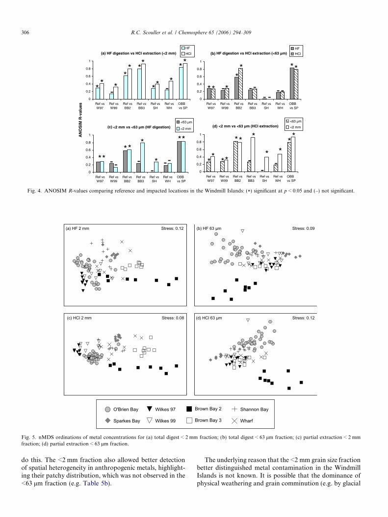
Fig. 4. ANOSIM R-values comparing reference and impacted locations in the Windmill Islands: (*) significant at p < 0.05 and (–) not significant.

Stress: 0.12(a) HF 2 mm

Stress: 0.08(c) HCl 2 mm Stress: 0.12(d) HCl 63 µm

Stress: 0.09(b) HF 63 µm

O'Brien Bay

Sparkes Bay

Wilkes 97

Wilkes 99

Brown Bay 2

Brown Bay 3

Shannon Bay

Wharf

Fig. 5. nMDS ordinations of metal concentrations for (a) total digest < 2 mm fraction; (b) total digest < 63 lm fraction; (c) partial extraction < 2 mmfraction; (d) partial extraction < 63 lm fraction.


do this. The <2 mm fraction also allowed better detectionof spatial heterogeneity in anthropogenic metals, highlight-ing their patchy distribution, which was not observed in the<63 lm fraction (e.g. Table 5b).

The underlying reason that the <2 mm grain size fractionbetter distinguished metal contamination in the WindmillIslands is not known. It is possible that the dominance ofphysical weathering and grain comminution (e.g. by glacial

Table 5bSignificant results from nested asymetrical ANOVAs for factors Site(Location) and Plot(Site)

Significant differences between sites within locations Significant differences between plots within sites

Ag As Cd Cr Cu Fe Mn Ni Pb Sb Sn Zn Ag As Cd Cr Cu Fe Mn Ni Pb Sb Sn Zn

HCl 2 mm

All five references * * *** * ** ** * * ** **

BB2 * ** * *** ** *** ** ** * **BB3 * * * * **Shannon * *** ** * ** *** ***Wharf * * *** * ** ** ** * ** * * *** ** *** ** *** *** *** ** ***Wilkes 97 *** ** * ***Wilkes 99 * *** *** * ** * *** * * ***

HF 2 mm

All five references ** * ** *** ** ** * *

BB2 ** *** ** ** *** * ** ** *** *** *** ***BB3 * ** ** * **Shannon *** * *** ***Wharf * * ** ** ** ** *** *** *** *** *** *** * *** *** ***Wilkes 97 *** * **Wilkes 99 * * *** * * *** * ***

HCl 63 lm

All five references * * *

BB2 * * ** ** ** *** *** ***BB3 ** ** * *** *** *Shannon **Wharf * ** *** *** * ** * ***Wilkes 97 * * *Wilkes 99 * ** ** * ***

HF 63 lm

All five references *

BB2 * * * ** * * ***BB3 * ** ***ShannonWharf ** * **Wilkes 97Wilkes 99 * * **

* Significant at p < 0.05.** significant at p < 0.01.

*** significant at p < 0.001.

R.C

.S

cou

lleret

al.

/C

hem

osp

here

65

(2

00

6)

29

4–

30

9307


processes), rather than extensive chemical dissolution andclay formation, has influenced the distribution of metal con-taminants in the sediment matrix. In this respect our obser-vations might be characteristic of polar and alpinesediments in general, and have less importance in other sed-imentary systems. Alternatively the role of particle-boundcontaminant transport in the Windmill Islands might alsobe a key factor in the greater proportion of metals in the63 lm–2 mm fraction. Comparison of these methods withdata outside of Antarctica and for a range of sediment typeswould be a very useful test of the greater applicability ofusing partial extraction of the <2 mm fraction for regionalcomparisons of metals in marine sediments.

Preliminary work to investigate the relationship betweenthe measures of sediment contamination reported here andbiological uptake, found that the partial extraction sedi-ment chemistry closely correlated with tissue concentra-tions in benthic infauna. Riddle et al. (2003) found thatmetal concentrations in the bivalve Laternula elliptica andthe heart urchins Abatus nimrodi and A. ingens collectedfrom the same reference and impacted sites as the regionalsurvey, correlated with partial extraction sediment data butnot with the total digest data.

In conclusion, we recommend adopting a 4 h 1 M HClpartial extraction on the whole sediment (<2 mm) as aregional survey method for assessing marine metal contam-ination in Antarctica. The method is simple, safe, relativelyquick and reproducible. Compared with total digests oranalysis of the <63 lm fraction alone, this method mini-mises the possibility of a Type II statistical error in theregional survey – that is failing to identify a site as beingcontaminated when it has elevated metal concentrations.

Acknowledgements

This research was supported by the Australian AntarcticScience grant (AAS2201). The authors thank Scott Stark,Martin Riddle, Paul Goldsworthy and Andrew Tabor fromthe AAD; Marc Norman and Phil Robinson from CODESand Ash Townsend from CSL at the University of Tasma-nia; and Ric Morris at the University of Wollongong, fortheir technical assistance, support, editing and scientificcontributions.

References

Agemian, H., Chau, A., 1976. Evaluation of extraction techniques for thedetermination of metals in aquatic sediments. The Analyst 101, 761–767.

Agemian, H., Chau, A.S.Y., 1977. A study of different analyticalextraction methods for non detrital heavy metals in aquatic sediments.Environ. Contamin. Toxicol. 6, 69–82.

Alam, I.A., Sadiq, M., 1993. Metal concentrations in Antarctic sedimentsamples collected during the Trans-Antarctica 1990 Expedition. Mar.Pollut. Bull. 26, 523–527.

Allen, H.F., Fu, G., Deng, B., 1993. Analysis of acid-volatile sulphide(AVS) and simultaneously extracted metals (SEM) for the estimationof potential toxicity in aquatic sediments. Environ. Toxicol. Chem. 12,1441–1453.

Andrade, S., Poblet, A., Scagiola, M., Vodopivez, C., Curtosi, A., Pucci,A., Marcovecchio, J., 2001. Distribution of heavy metals in surfacesediments from an Antarctic marine ecosystem. Environ. Monit.Assess. 66, 147–158.

Attrill, M.J., Thomes, R.M., 1995. Heavy metal concentrations insediment from the Thames Estuary, UK. Mar. Pollut. Bull. 30, 742–744.

Batley, G., 1991. Trace Element Speciation: Analytical Methods andProblems. CRC Press, Inc., Boca Raton.

Campbell, P.G.C., Tessier, A., 1989. Biological availability of metals insediments: analytical approaches. In: Proceedings – InternationalConference on Heavy Metals in the Environment, Geneva, Switzer-land, pp. 516–525.

Campbell, P.G.C., Lewis, A.G., Chapman, P.M., Crowder, A.A.,Fletcher, W.K., Imber, B., Luoma, S.N., Stokes, P.M., Winfrey, M.,1988. Biologically Available Metals in Sediments. National ResearchCouncil Canada, Ottawa, p. 298.

Chester, R., Voutsinou, F.G., 1981. The initial assessment of trace metalpollution in coastal sediments. Mar. Pollut. Bull. 12, 84–91.

Chester, R., Kudoja, W.M., Thomas, A., Towner, J., 1985. Pollutionreconnaissance in stream sediments using non-residual trace metals.Environ. Pollut. 10 (series B), 213–238.

Ciaralli, L., Giordano, R., Lombardi, G., Beccaloni, E., Sepe, A.,Costantini, S., 1998. Antarctic marine sediments: distribution ofelements and textural characters. Microchem. J. 59, 77–88.

Claridge, G.G.C., Campbell, I.B., 1984. Mineral formation duringweathering of dolerite under cold arid conditions in Antarctica. NewZeal. J. Geol. Geop. 27, 537–545.

Clarke, K.R., Warwick, R.M., 1994. Change in Marine Communities: anApproach to Statistical Analysis and Interpretation. Natural Envi-ronment Research Council, U.K., Plymouth Marine Laboratory,Plymouth.

Cook, J.M., Gardner, M.J., Griffiths, A.H., Jessep, M.A., Ravenscroft,J.E., Yates, R., 1997. The comparability of sample digestion tech-niques for the determination of metals in sediments. Mar. Pollut. Bull.34, 637–644.

Cosma, B., Soggia, F., Abelmoschi, M.L., Frache, R., 1994. Determina-tion of trace metals in Antarctic marine sediments from Terra NovaBay – Ross Sea. Int. J. Environ. Anal. Chem. 55, 121–128.

Deprez, P.P., Arens, M., Locher, H., 1999. Identification and assessmentof contaminated sites at Casey Station, Wilkes Land, Antarctica. PolarRec. 35, 299–316.

Di Toro, D.M., Mahoney, J.D., Hansen, K.J., Scott, K.J., Hicks, M.B.,Mayr, S.M., Redmond, M.S., 1990. Toxicity of cadmium in sediments:the role of acid volatile sulphide. Environ. Toxicol. Chem. 9, 1487–1502.

Dobson, J., 2000. Long term trends in trace metals in biota in the forthestuary, Scotland, 1981–1999. Mar. Pollut. Bull. 40, 1214–1220.

Forstner, U., Salomons, W., 1980. Trace element analysis on pollutedsediments, part I: Assessment of sources and intensities. Environ.Technol. Lett. 1, 494–505.

Giordano, R., Lombardi, G., Ciaralli, L., Beccaloni, E., Sepe, A., Ciprotti,M., Costantini, S., 1999. Major and trace elements in sediments fromTerra Nova Bay, Antarctica. Sci. Total Environ. 227, 29–40.

Glasby, T.M., Underwood, A.J., 1996. Sampling to differentiate betweenpulse and press perturbatiuons. Environ. Monit. Assess. 42, 241–252.

Hall, G.E.M., 1997. Determination of trace elements in sediments. In:Mudroch, A., Azcue, J.M., Mudroch, P. (Eds.), Manual of Physico-Chemical Analysis of Aquatic Sediments. Lewis Publishers, BocaRaton.

Haynes, D., Rayment, P., Toohey, D., 1996. Long term variability inpollutant concentrations in coastal marine sediments from Ninety MileBeach, Bass Straight, Australia. Mar. Pollut. Bull. 32, 823–827.

Hieke Merlin, O., Longo Salvador, G., Menegazzo Vitturi, L., Pistolato,M., Rampazzo, G., 1989. Preliminary results on trace elementgeochemistry of sediments from the Ross Sea, Antarctica. Boll.Oceanol. Teor. Appl. VII, 97–108.


Irvine, I., Birch, G.F., 1998. Distribution of heavy metals in surficialsediments of Port Jackson, Sydney, New South Wales. Aust. J. EarthSci. 45, 297–304.

Kennicutt, M.C., McDonald, S.L., Sericano, J.L., Boothe, P., Oliver, J.,Safe, S., Presley, B.J., Liu, H., Wolfe, D., Wade, T.L., Crockett, A.,Bockus, D., 1995. Human contamination of the marine environment –Arthur Harbor and McMurdo Sound, Antarctica. Environ. Sci.Technol. 29, 1279–1287.

Klamer, J., Hegeman, W., Smedes, F., 1990. Comparison of grain sizecorrection procedures for organic micropollutants and heavy metals inmarine sediments. Hydrobiologia 208, 213–220.

Larner, B.L., Seen, A.J., Townsend, A.T., 2006. Comparative study ofoptimised BCR sequential extraction scheme and acid leaching ofelements in the certified reference material NIST 2711. Anal. Chim.Acta 556, 444–449.

Lee, C.-L., Fang, M.-D., Hsieh, M.-T., 1998. Characterization anddistribution of metals in surficial sediments in Southwestern Taiwan.Mar. Pollut. Bull. 36, 464–471.

Lenihan, H.S., Oliver, J.S., Oaken, J.M., Stephenson, M.D., 1990. Intenseand localized benthic marine pollution around McMurdo Station,Antarctica. Mar. Pollut. Bull. 21, 422–430.

Loring, D.H., 1991. Normalization of heavy-metal data from estuarineand coastal sediments. ICES J. Mar. Sci. 48, 101–115.

Loring, D.H., Rantala, R.T.T., 1992. Manual for the geochemicalanalyses of marine sediments and suspended particulate matter.Earth-Sci. Rev. 32, 235–283.

Luoma, S.N., Bryan, G.W., 1981. A statistical assessment of the form oftrace metals in oxidized estuarine sediments employing chemicalextractants. Sci. Total Environ. 17, 165–196.

Northcott, K.A., Snape, I., Connor, M.A., Stevens, G.W., 2003. Watertreatment design for site remediation at Casey Station, Antarctica: sitecharacterisation and particle separation. Cold Reg. Sci. Technol. 37,169–185.

Pesch, C.E., 1979. Influence of three sediment types on copper toxicityto the polychaete Neanthes arenaceodentata. Mar. Biol. 52, 236–245.

Quevauviller, P., 1998. Operationally defined extraction procedures forsoil and sediment analysis I. Standardization. Trends Anal. Chem. 17,289–298.

Riddle, M.J., Scouller, R.C., Snape, I., Stark, J.S., Kratzmann, S.M.,Stark, S.C., King, C.K., Duquesne, S., Gore, D.B., 2003. From

chemical monitoring to biological meaning: extraction techniquesand biological interpretation of sediment chemistry data from theCasey Region. In: Huiskes, A.H.L., Gieskes, W.W.C., Rozema, J.,Schorno, R.M.L., van der Vies, S.M., Wolff, W.J. (Eds.), AntarcticBiology in a Global Context. Backhuys Publishers, Leiden, pp. 285–289.

Riva, S.D., Abelmoschi, M.L., Magi, E., Soggia, F., 2004. The utilizationof the Antarctic environmental specimen bank (BCAA) in monitoringCd and Hg in an Antarctic coastal area in Terra Nova Bay (Ross Sea–Northern Victoria Land). Chemosphere 56, 59–69.

Snape, I., Cole, C., Gore, D., Riddle, M., Yarnall, M., 1998. Apreliminary assessment of contaminants at the abandoned WilkesStation, East Antarctica, with recommendations for establishing anenvironmental management strategy. Australian Antarctic Division,Hobart, p. 69.

Snape, I., Riddle, M.J., Stark, J.S., Cole, C.M., King, C.K., Duquesne, S.,Gore, D.B., 2001. Management and remediation of contaminated sitesat Casey Station, Antarctica. Polar Rec. 37, 199–214.

Snape, I., Scouller, R.C., Stark, S.C., Stark, J.S., Riddle, M.J., Gore,D.B., 2004. Characterisation of the dilute HCl extraction method forthe identification of metal contamination in Antarctic marine sedi-ments. Chemosphere 57, 491–504.

Stark, J.S., Riddle, M.J., Simpson, R.D., 2003a. Human impacts in soft-sediment assemblages at Casey Station, East Antarctica: spatialvariation, taxonomic resolution and data transformation. AustralEcol. 28, 287–304.

Stark, J.S., Riddle, M.J., Snape, I., Scouller, R.C., 2003b. Human impactsin Antarctic marine soft-sediment assemblages: correlations betweenmultivariate biological patterns and environmental variables at CaseyStation. Estuar. Coast. Shelf Sci. 56, 717–734.

Stark, J.S., Snape, I., Riddle, M.J., 2003c. The effects of petroleumhydrocarbon and heavy metal contamination of marine sediments onrecruitment of Antarctic soft-sediment assemblages: a field experimen-tal investigation. J. Exp. Mar. Biol. Ecol. 283, 21–50.

Warren, L.A., Haack, E.A., 2000. Biogeochemical controls on metalbehaviour in freshwater environments. Earth-Sci. Rev., 261–320.

Yu, Z., Robinson, P., McGoldrick, P., 2001. An evaluation of methods forthe chemical decomposition of geological materials for trace elementdetermination using ICP-MS. Geostandards Newslett.: J. Geostan-dards Geoanal. 25, 199–217.

2006: Scouller, R.C., Snape, I., Stark, J.S. & Gore, D.B. 2006. Evaluation of geochemical methods...

Documents

Transcript of 2006: Scouller, R.C., Snape, I., Stark, J.S. & Gore, D.B. 2006. Evaluation of geochemical methods...