
1st International Conference on Machine Control & Guidance
334
ETH Library 1st International Conference on Machine Control & Guidance Proceedings Conference Proceedings Author(s): Ingensand, Hilmar; Stempfhuber, Werner Publication date: 2008 Permanent link: https://doi.org/10.3929/ethz-a-005654221 Rights / license: In Copyright - Non-Commercial Use Permitted This page was generated automatically upon download from the ETH Zurich Research Collection . For more information, please consult the Terms of use .
-
Upload
khangminh22 -
Category
Documents
-
view
1 -
download
0
Transcript of 1st International Conference on Machine Control & Guidance

ETH Library
1st International Conference onMachine Control & GuidanceProceedings
Conference Proceedings
Author(s):Ingensand, Hilmar; Stempfhuber, Werner
Publication date:2008
Permanent link:https://doi.org/10.3929/ethz-a-005654221
Rights / license:In Copyright - Non-Commercial Use Permitted
This page was generated automatically upon download from the ETH Zurich Research Collection.For more information, please consult the Terms of use.

1st International Conference on Machine Control & Guidance
Proceedings
June 24-26, 2008
ETH Zurich, Switzerland
published by:
Hilmar Ingensand und Werner Stempfhuber

These proceedings can be ordered from: [email protected] The authors are responsible for the contents of the papers. The use of contents has to follow the laws of copyright and ownership. The spreading of this document is not allowed! ISBN: 978-3-906467-75-7 © 2008 http://www.geometh.ethz.ch Druck: Reprozentrale, ETH Hönggerberg, Zürich Printed in Switzerland

Preface Over the last two decades, terrestrial and global 3D-measurement sensors in the field of engineering geodesy have seen a significant upturn. Nowadays almost all static sensors contain a kinematic mode. These modern measurement techniques allow determining a trajectory of a moving object within a few centimetres in real time. Additional sensors determine dual slope and bearing parameters. Using calibrated tracking total stations, accuracies within five to ten millimetres can be achieved. Parallel to these new geodetic sensor developments, a broad range of new applications have been created, mostly in the fields of construction, mining and agriculture.
In recent years many guidance and control solutions based on geodetic measurement sensors have become state-of-the-art. Some applications are already introduced in the market, however, many automation tasks are still in a development phase. An overall solution requires close interaction of data acquisition, design data including transformation and conversion, guidance and control processes, documentation, and as-built check. Thus, this represents a great challenge for different fields: engineering geodesy, cybernetics, mechanical and electrical engineering, and applications.
The main scope of the organisers of the 1st International Conference on Machine Control & Guidance (MCG) was to initiate the discussion of these topics among academics, researchers, system and service providers as well as users. Up to now there has not been any conference encompassing all these aspects. This event aims at the creation of a new discussion platform and focuses on the intensification of these world-wide automation ambitions.
The following topics will be discussed and demonstrated:
- 3D-Construction Applications - Kinematic Measurement and Sensor Technology (Local and GNSS Systems) - Agriculture Applications - Data Processing and Acquisition - Control Process and Algorithm
The conference organisers would like to thank all paper and poster contributors; they are confident that many presentations encourage a know-how interchange, bond synergies between the different applications and boost research activities.
Furthermore, the organisers and their team would like to thank the sponsors of the conference, namely
- Leica Geosystems AG - MOBA Mobile Automation AG - RMR Softwareentwicklungsgesellschaft bR - Topcon Europe Positioning B.V. and Fieldwork AG - Trimble Navigation Ltd. - Zoller & Fröhlich GmbH
and the members of the Scientific Committee for their valuable cooperation. Finally, the organisers would like to thank all attendees and interested persons and are sure that the 1st International Conference on Machine Control & Guidance (MCG) will not remain a singular event.
Zurich, June 2008 Werner Stempfhuber Hilmar Ingensand


Inhaltsverzeichnis 3D-Construction Applications – Excavator 9 Heinz-Erich RADER
GPS-based 3D-Monitoring in Surface Mining
11
Fritz SCHREIBER, Peter RAUSCH, Michael DIEGELMANN Use of a Machine Control & Guidance System, Determination of Excavator Performance, Cost Calculation and Protection Against Damaging of Pipes and Cables
21
Nod CLARKE-HACKSTON, Jochen BELZ, Allan HENNEKER Guidance for Partial Face Excavation Machines
31
Kinematic Measurement and Sensor Technology I (Local Systems) 39 Claudia DEPENTHAL
A Time-referenced 4D Calibration System for Kinematic Optical Measuring Systems
41
Holger KIRSCHNER, Werner STEMPFHUBER The Kinematic Potential of Modern Tracking Total Stations - A State of the Art Report on the Leica TPS1200+
51
M. METTENLEITER, N. OBERTREIBER, F. HÄRTL, M. EHM, J. BAUR, C. FRÖHLICH
3D Laser Scanner as Part of Kinematic Measurement Systems
61
Jochen WENDEBAUM, Johannes FLIEDNER, Bernhard MARX, Alfons HORN Local Positioning Systems in Construction Basics, Limitations and Examples of Application
71
Rainer MAUTZ Combination of Indoor and Outdoor Positioning
79
Kinematic Measurement and Sensor Technology II (GNSS Systems) 89 Hans-Jürgen EULER, Joachim WIRTH
Advanced Concept in Multiple GNSS Network RTK Processing
91
Volker SCHWIEGER, Julia HEMMERT Integration of a Multiple-Antenna GNSS System and Supplementary Sensors
103
Patrick Ole NOACK, Thomas MUHR Integrated Controls for Agricultural Applications – GNSS Enabling a New Level in Precision Farming
113
David Eugen GRIMM GNSS Orientation for kinematic applications
121

Agriculture Applications 127 Florian SCHÖLDERLE, Matthias SIEMES, Heiner KUHLMANN 129
Multi Sensor System Requirements for a Position Steered Seed Deposition in Sugar Beet Cultivation for the Generation of a Rectangular Formation
Görres GRENZDÖRFFER, Cornelius DONATH 141
Generation and Analysis of Digital Terrain Models with Parallel Guidance Systems for Precision Agriculture
Henning Jürgen MEYER, Christian RUSCH 151
Self-configuring, Mobile Networks in the Area of Agriculture William KELLAR, Peter ROBERTS, Oliver ZELZER 161
A Self Calibrating Attitude Determination System for Precision Farming using Multiple Low-Cost Complementary Sensors
Dejan ŠEATOVIĆ 169 3D-Object Recognition, Localization and Treatment of Rumex Obtusifolius in its Natural Environment
3D-Construction Applications II 179 Norbert MATTIVI 181
Trimble offers the Connected Construction Site Connecting Office, People and Machines: The New Way to Increase Productivity on Earthmoving and Road Construction Sites
Achiel STURM, Willem VOS 189 New Technologies for Telematics and Machine Control
N. CLARKE-HACKSTON, M. MESSING, E. ULLRICH 199
Geodetic Instrumentation for Use on Machine Bored Tunnels Roland JUNG 211
3D Asphalt Paving of Special Profiles for Comfort Tests at the Example of a New HGV-Test Track.
Data Processing and Data Acquisition 223 Jochen WENDEBAUM, Mats KJELLBERG 225
No Driving in Circles - Improving the Research and Development of Mobile Machinery and Control Systems by Using Advanced Simulation Technology
Ali ZOGHEIB 233
Autonomous Navigation Tool for Real & Virtual Field Robots Gunnar GRÄFE 245
Kinematic 3D Laser Scanning for Road or Railway Construction Surveys

Control Process and Control Algorithm 255 Hansjörg PETSCHKO 257
Universal Developer Platform for Machine Control Applications Alexander BEETZ, Volker SCHWIEGER 263
Integration of Controllers for Filter Algorithms for Construction Machine Guidance H. ALKHATIB, I. NEUMANN, H. NEUNER, H. KUTTERER 273
Comparison of Sequential Monte Carlo Filtering with Kalman Filtering for Nonlinear State Estimation
3D-Construction Applications III 285 Kuno KAUFMANN, Roland ANDEREGG 287
GPS-based Compaction Technology Thomas A. WUNDERLICH, Thomas SCHÄFER, Stefan AUER 297
Passage Simulation of Monorail Suspension Conveyors and Transport Goods for Collision Prevention
Poster Session 305 Hans-Martin ZOGG, David GRIMM 307
Kinematic Surface Analysis by Terrestrial Laser Scanning Manfred JURETZKO, Maria HENNES 315
Monitoring of the spatiotemporal movement of an industrial robot using a laser tracker Th. ENGEL, JJ. STUBY, Ch. GLAUSER, P. GÜLDENAPFEL, M. MANHART, G. SCHELLING, H. INGENSAND 321
Automatic Guidance of Track Laying Machines with Respect to Coordinate Systems Sonja GAMSE, Dušan KOGOJ, Karl FOPPE, Peter WASMEIER, Thomas A. WUNDERLICH, Thomas SCHÄFER 327
Evaluation of linear Kalman filter processing surveying kinematic measurements


3D-Construction Applications – Excavator

1st International Conference on Machine Control & Guidance 2008 11
GPS-based 3D-Monitoring in Surface Mining
Heinz-Erich RADER RMR Softwareentwicklungsgesellschaft (RMR)
[email protected] Abstract RMR has developed a software called GeoCAD-OP for GPS-based machine guidance for wheel-excavators, spreaders and compactors. The 3D-real-time animated software is always divided in a machine and an office application, latter can be used as a control station for any kind of machine. Keywords GPS, machine guidance, wheel excavator, spreader, scanner, compactor, 3D, DTM, digger, open cast mining, mining
1 THE COMPANY RMR exists since 1987 and has theirmain headquarters in Bad Neuenahr-Ahrweiler. Originally she created AutoCAD-applications. They were developed for surveying, street planning and construction as well as for digital terrain models. Since 1995 RMR has used an own AutoCAD-Clone on which the software GeoCAD-OP was developed as a basis, next to AutoCAD. This object-oriented software is the basis for all software which is developed by the RMR and it is today available both on the basis of an own internal CAD and on the AutoCAD basis.
2 GEOCAD-OP AS BASIS OF THE GPS MACHINE CONTROL SOFTWARE
While most manufacturers of machine guidance software are coming from the GPS instrument manufacturers, the reverse way was taken at the RMR. The company currently thinks of GPS devices taking a similar sale way as before the PC e.g. In this way the question which hardware manufacturer builds a GPS device will move more and more into the background in future and the software which binds the devices and makes the devices better usable for the customer will come to the fore. From this thought it is good to develop machine controller programmes on the basis of one software which covers the above listed fields. Therefore the essential components of the software are supposed to be presented shortly in the following chapter.
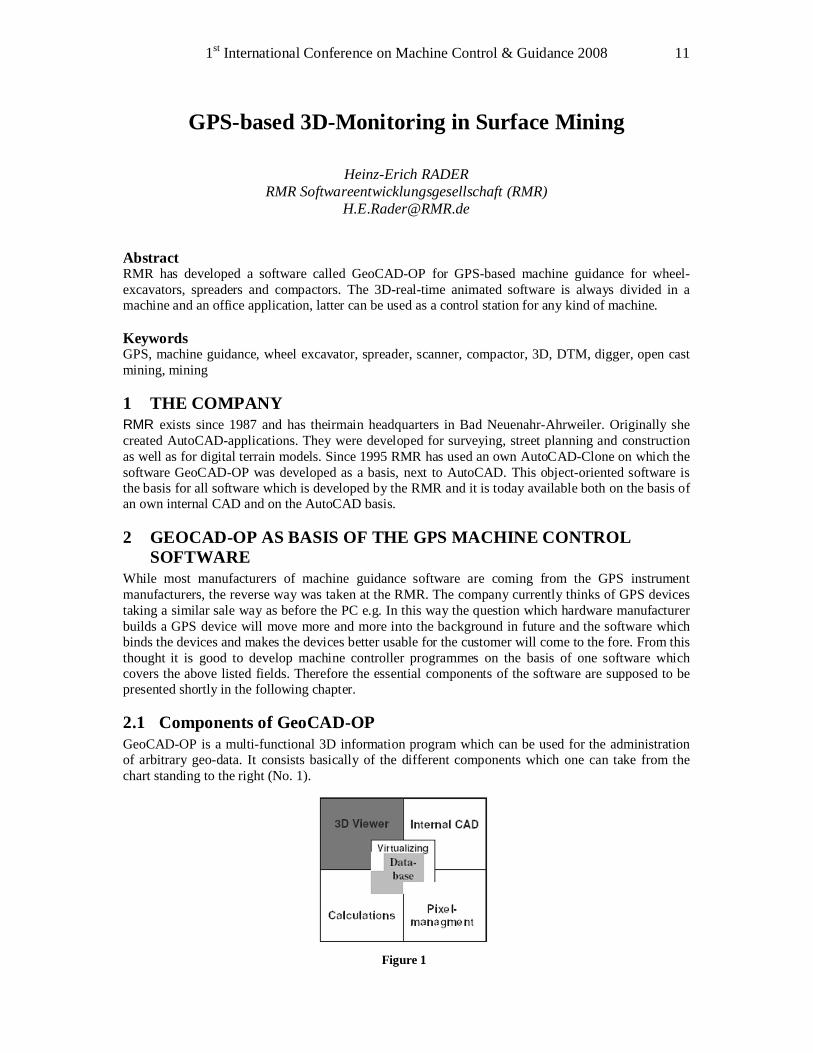
2.1 Components of GeoCAD-OP GeoCAD-OP is a multi-functional 3D information program which can be used for the administration of arbitrary geo-data. It consists basically of the different components which one can take from the chart standing to the right (No. 1).
Figure 1
3D-Construction Applications - Excavator 12
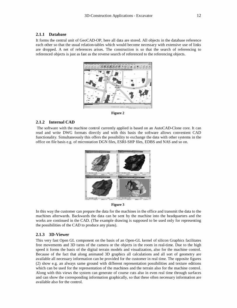
2.1.1 Database It forms the central unit of GeoCAD-OP, here all data are stored. All objects in the database reference each other so that the usual relation-tables which would become necessary with extensive use of links are dropped. A net of references arises. The construction is so that the search of referencing to referenced objects is just as fast as the reverse search of referenced to the referencing objects.
Figure 2
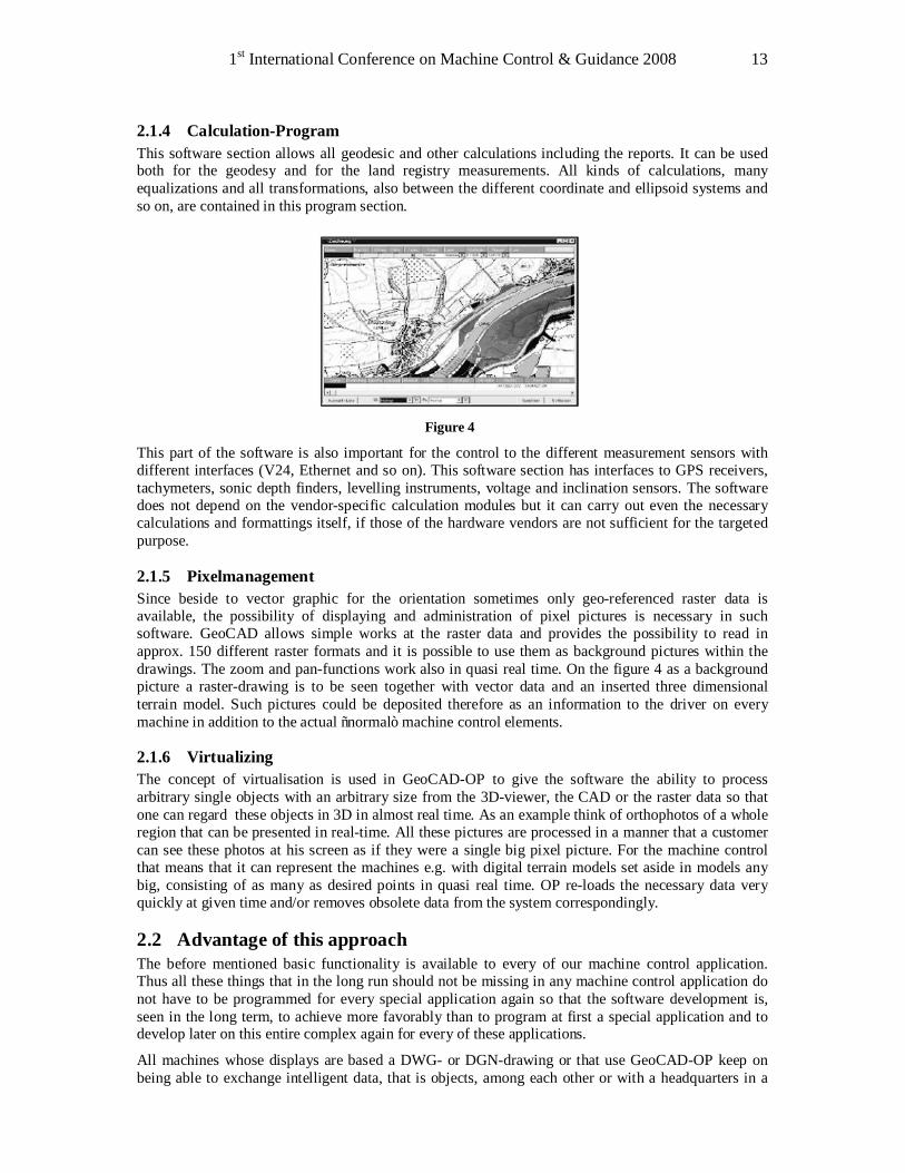
2.1.2 Internal CAD The software with the machine control currently applied is based on an AutoCAD-Clone core. It can read and write DWG formats directly and with this basis the software allows convenient CAD functionality. Simultaneously this offers the possibility to exchange the data with other systems in the office on file basis e.g. of microstation DGN files, ESRI-SHP files, EDBS and NAS and so on.
Figure 3
In this way the customer can prepare the data for the machines in the office and transmit the data to the machines afterwards. Backwards the data can be sent by the machine into the headquarters and the works are continued in the CAD. (The example drawing is supposed to be used only for representing the possibilities of the CAD to produce any plans).
2.1.3 3D-Viewer This very fast Open GL component on the basis of an Open-GL kernel of silicon Graphics facilitates free movements and 3D turns of the camera or the objects in the room in real-time. Due to the high speed it forms the basis of the digital terrain models and visualization, also for the machine control. Because of the fact that along animated 3D graphics all calculations and all sort of geometry are available all necessary information can be provided for the customer in real time. The opposite figures (2) show e.g. an always same ground with different representation possibilities and texture editions which can be used for the representation of the machines and the terrain also for the machine control. Along with this views the system can generate of course cuts also in even real time through surfaces and can show the corresponding information graphically, so that these often necessary information are available also for the control.
1st International Conference on Machine Control & Guidance 2008 13
2.1.4 Calculation-Program This software section allows all geodesic and other calculations including the reports. It can be used both for the geodesy and for the land registry measurements. All kinds of calculations, many equalizations and all transformations, also between the different coordinate and ellipsoid systems and so on, are contained in this program section.
Figure 4
This part of the software is also important for the control to the different measurement sensors with different interfaces (V24, Ethernet and so on). This software section has interfaces to GPS receivers, tachymeters, sonic depth finders, levelling instruments, voltage and inclination sensors. The software does not depend on the vendor-specific calculation modules but it can carry out even the necessary calculations and formattings itself, if those of the hardware vendors are not sufficient for the targeted purpose.
2.1.5 Pixelmanagement Since beside to vector graphic for the orientation sometimes only geo-referenced raster data is available, the possibility of displaying and administration of pixel pictures is necessary in such software. GeoCAD allows simple works at the raster data and provides the possibility to read in approx. 150 different raster formats and it is possible to use them as background pictures within the drawings. The zoom and pan-functions work also in quasi real time. On the figure 4 as a background picture a raster-drawing is to be seen together with vector data and an inserted three dimensional terrain model. Such pictures could be deposited therefore as an information to the driver on every machine in addition to the actual “normal” machine control elements.
2.1.6 Virtualizing The concept of virtualisation is used in GeoCAD-OP to give the software the ability to process arbitrary single objects with an arbitrary size from the 3D-viewer, the CAD or the raster data so that one can regard these objects in 3D in almost real time. As an example think of orthophotos of a whole region that can be presented in real-time. All these pictures are processed in a manner that a customer can see these photos at his screen as if they were a single big pixel picture. For the machine control that means that it can represent the machines e.g. with digital terrain models set aside in models any big, consisting of as many as desired points in quasi real time. OP re-loads the necessary data very quickly at given time and/or removes obsolete data from the system correspondingly.
2.2 Advantage of this approach The before mentioned basic functionality is available to every of our machine control application. Thus all these things that in the long run should not be missing in any machine control application do not have to be programmed for every special application again so that the software development is, seen in the long term, to achieve more favorably than to program at first a special application and to develop later on this entire complex again for every of these applications.
All machines whose displays are based a DWG- or DGN-drawing or that use GeoCAD-OP keep on being able to exchange intelligent data, that is objects, among each other or with a headquarters in a
3D-Construction Applications - Excavator 14
homogeneous, object-oriented and database-based system. In contrary highly specialized applications require new, very specific interfaces here again and again.
Finally it is still to be said that the same software can be used for the indoor work (office) and the available functionality can be controlled through user access control on the machine or in the field work. This reduces the training costs since always the same software is used.
3 THE MACHINE CONTROL SYSTEMS ON BASIS OF GEOCAD-OP On the up to now described software basis applications were developed for 3D-monitoring of the subsequently presented machine types. There are always two modes available, once as software on the machine and once as an office version. The GPS receivers of the companies are selectable (alphabetically without ranking) Leica, Novatel, Topcon and Trimble. Also the tachymeter of the companies Leica and Topcon for the positioning could be operated through the software-interfaces.
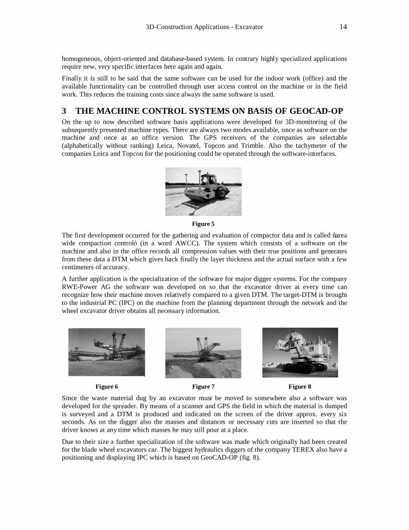
Figure 5
The first development occurred for the gathering and evaluation of compactor data and is called “area wide compaction control” (in a word AWCC). The system which consists of a software on the machine and also in the office records all compression values with their true positions and generates from these data a DTM which gives back finally the layer thickness and the actual surface with a few centimeters of accuracy.
A further application is the specialization of the software for major digger systems. For the company RWE-Power AG the software was developed on so that the excavator driver at every time can recognize how their machine moves relatively compared to a given DTM. The target-DTM is brought to the industrial PC (IPC) on the machine from the planning department through the network and the wheel excavator driver obtains all necessary information.
Figure 6 Figure 7 Figure 8
Since the waste material dug by an excavator must be moved to somewhere also a software was developed for the spreader. By means of a scanner and GPS the field in which the material is dumped is surveyed and a DTM is produced and indicated on the screen of the driver approx. every six seconds. As on the digger also the masses and distances or necessary cuts are inserted so that the driver knows at any time which masses he may still pour at a place.
Due to their size a further specialization of the software was made which originally had been created for the blade wheel excavators car. The biggest hydraulics diggers of the company TEREX also have a positioning and displaying IPC which is based on GeoCAD-OP (fig. 8).
1st International Conference on Machine Control & Guidance 2008 15
3.1 AWCC The AWCC-module also consists of, as any machine software within GeoCAD OP, a machine- and an office part. The sense of this is to be seen in many settings being supposed to be carried out by employees in the indoor work which the drivers should after that not be able to change anymore during their daily work.
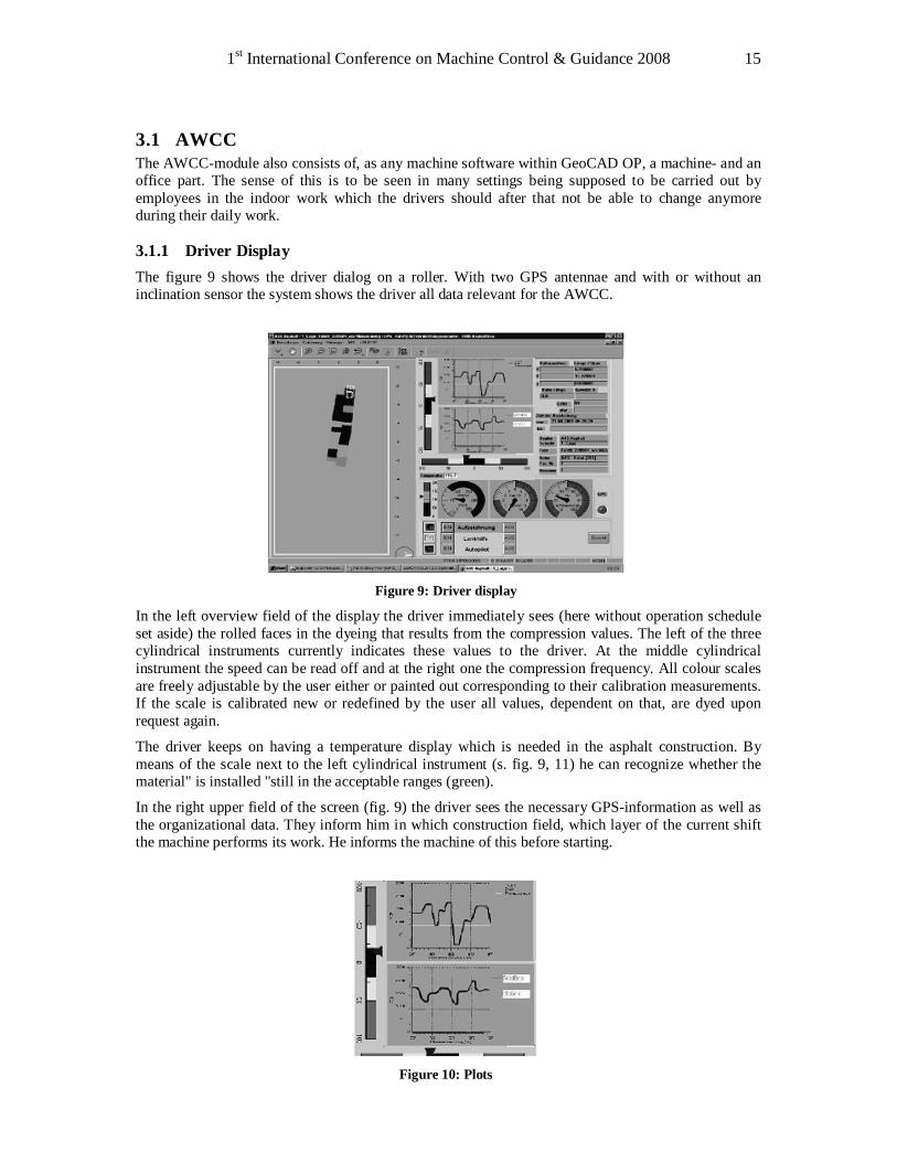
3.1.1 Driver Display The figure 9 shows the driver dialog on a roller. With two GPS antennae and with or without an inclination sensor the system shows the driver all data relevant for the AWCC.
Figure 9: Driver display
In the left overview field of the display the driver immediately sees (here without operation schedule set aside) the rolled faces in the dyeing that results from the compression values. The left of the three cylindrical instruments currently indicates these values to the driver. At the middle cylindrical instrument the speed can be read off and at the right one the compression frequency. All colour scales are freely adjustable by the user either or painted out corresponding to their calibration measurements. If the scale is calibrated new or redefined by the user all values, dependent on that, are dyed upon request again.
The driver keeps on having a temperature display which is needed in the asphalt construction. By means of the scale next to the left cylindrical instrument (s. fig. 9, 11) he can recognize whether the material" is installed "still in the acceptable ranges (green).
In the right upper field of the screen (fig. 9) the driver sees the necessary GPS-information as well as the organizational data. They inform him in which construction field, which layer of the current shift the machine performs its work. He informs the machine of this before starting.
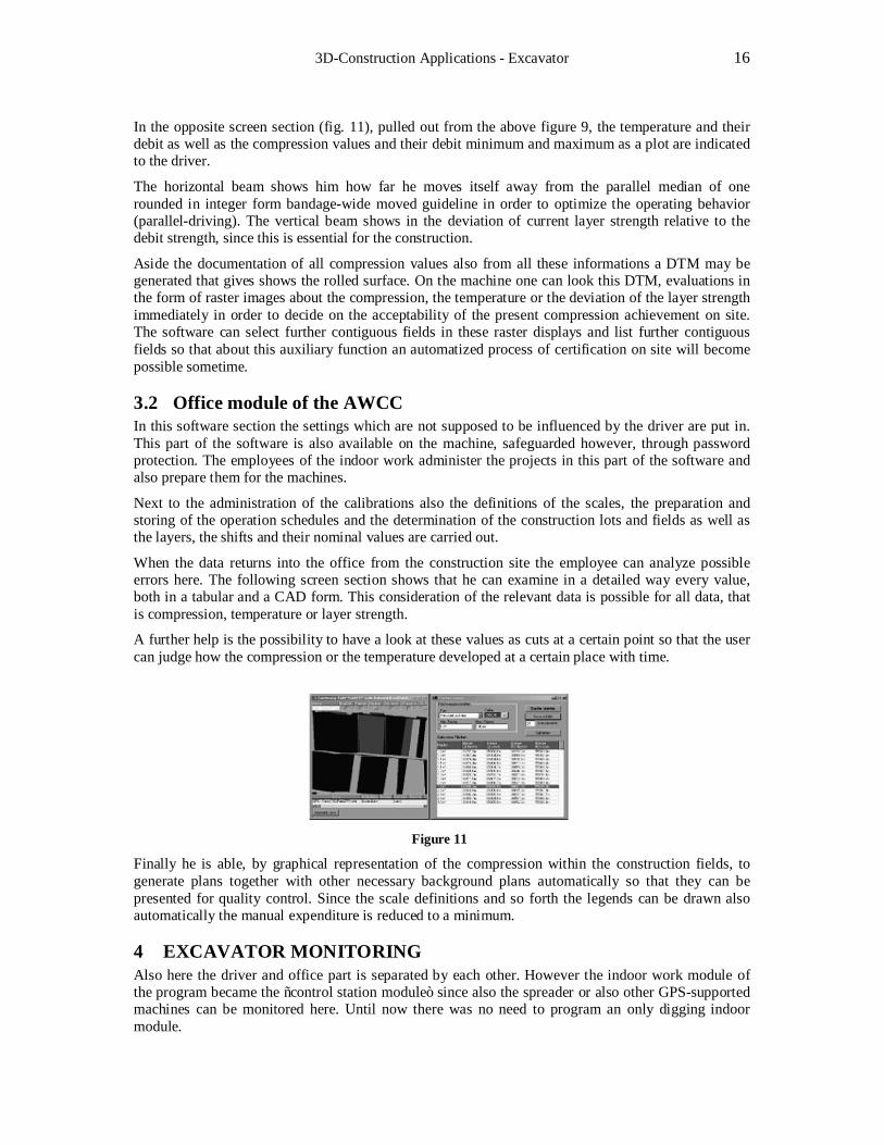
Figure 10: Plots
3D-Construction Applications - Excavator 16
In the opposite screen section (fig. 11), pulled out from the above figure 9, the temperature and their debit as well as the compression values and their debit minimum and maximum as a plot are indicated to the driver.
The horizontal beam shows him how far he moves itself away from the parallel median of one rounded in integer form bandage-wide moved guideline in order to optimize the operating behavior (parallel-driving). The vertical beam shows in the deviation of current layer strength relative to the debit strength, since this is essential for the construction.
Aside the documentation of all compression values also from all these informations a DTM may be generated that gives shows the rolled surface. On the machine one can look this DTM, evaluations in the form of raster images about the compression, the temperature or the deviation of the layer strength immediately in order to decide on the acceptability of the present compression achievement on site. The software can select further contiguous fields in these raster displays and list further contiguous fields so that about this auxiliary function an automatized process of certification on site will become possible sometime.
3.2 Office module of the AWCC In this software section the settings which are not supposed to be influenced by the driver are put in. This part of the software is also available on the machine, safeguarded however, through password protection. The employees of the indoor work administer the projects in this part of the software and also prepare them for the machines.
Next to the administration of the calibrations also the definitions of the scales, the preparation and storing of the operation schedules and the determination of the construction lots and fields as well as the layers, the shifts and their nominal values are carried out.
When the data returns into the office from the construction site the employee can analyze possible errors here. The following screen section shows that he can examine in a detailed way every value, both in a tabular and a CAD form. This consideration of the relevant data is possible for all data, that is compression, temperature or layer strength.
A further help is the possibility to have a look at these values as cuts at a certain point so that the user can judge how the compression or the temperature developed at a certain place with time.
Figure 11
Finally he is able, by graphical representation of the compression within the construction fields, to generate plans together with other necessary background plans automatically so that they can be presented for quality control. Since the scale definitions and so forth the legends can be drawn also automatically the manual expenditure is reduced to a minimum.
4 EXCAVATOR MONITORING Also here the driver and office part is separated by each other. However the indoor work module of the program became the “control station module” since also the spreader or also other GPS-supported machines can be monitored here. Until now there was no need to program an only digging indoor module.
1st International Conference on Machine Control & Guidance 2008 17
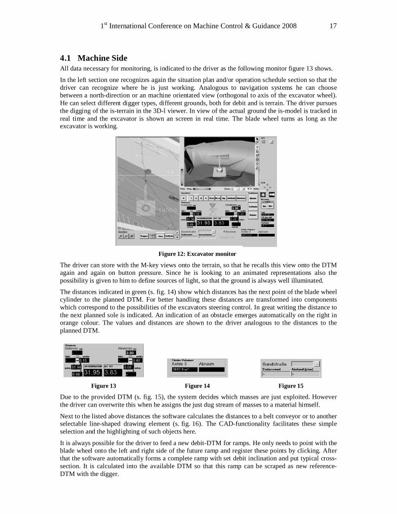
4.1 Machine Side All data necessary for monitoring, is indicated to the driver as the following monitor figure 13 shows.
In the left section one recognizes again the situation plan and/or operation schedule section so that the driver can recognize where he is just working. Analogous to navigation systems he can choose between a north-direction or an machine orientated view (orthogonal to axis of the excavator wheel). He can select different digger types, different grounds, both for debit and is terrain. The driver pursues the digging of the is-terrain in the 3D-l viewer. In view of the actual ground the is-model is tracked in real time and the excavator is shown an screen in real time. The blade wheel turns as long as the excavator is working.
Figure 12: Excavator monitor
The driver can store with the M-key views onto the terrain, so that he recalls this view onto the DTM again and again on button pressure. Since he is looking to an animated representations also the possibility is given to him to define sources of light, so that the ground is always well illuminated.
The distances indicated in green (s. fig. 14) show which distances has the next point of the blade wheel cylinder to the planned DTM. For better handling these distances are transformed into components which correspond to the possibilities of the excavators steering control. In great writing the distance to the next planned sole is indicated. An indication of an obstacle emerges automatically on the right in orange colour. The values and distances are shown to the driver analogous to the distances to the planned DTM.
Figure 13 Figure 14 Figure 15
Due to the provided DTM (s. fig. 15), the system decides which masses are just exploited. However the driver can overwrite this when he assigns the just dug stream of masses to a material himself.
Next to the listed above distances the software calculates the distances to a belt conveyor or to another selectable line-shaped drawing element (s. fig. 16). The CAD-functionality facilitates these simple selection and the highlighting of such objects here.
It is always possible for the driver to feed a new debit-DTM for ramps. He only needs to point with the blade wheel onto the left and right side of the future ramp and register these points by clicking. After that the software automatically forms a complete ramp with set debit inclination and put typical cross-section. It is calculated into the available DTM so that this ramp can be scraped as new reference-DTM with the digger.
3D-Construction Applications - Excavator 18
The accuracy of the blade wheel positions which are achieved via the GPS-system is about approx. 5 cm, x,y and height. The investigations necessary to that were carried out on a stationary device. An investigation of the positions as comparison between such which are determined by pursuit through a tachymeter and such that are supplied GSP-supported is just being carried out.
4.2 Indoor Side The office application is only indirect a GPS-supported application. It is possible to transfer immediately the NMEA-GPS character strings as a stream from the machine into the office and to follow also the machine-sided view of the driver there. But the software concept is, however that all data that are already preprocessed on the machine are sent onto the control-station. In this way there the supervision of all devices, with the possibility to connect to a single machine device, exists. The control-station is described in the last chapter shortly.
5 SPREADER MONITORING The counterpart to the digger is the spreader. It refills all materials that do not roam to the exploitation. The target of the spreadermonitoring is the automatized GPS-supported measuring of each current state of the backfill, the calculation of the poured masses and the comparison of the is-DTM arising so with the planned DTM in real time. From that the necessary views are generated for the spreader driver so that the masses needed for the production of the target-DTM can be poured by him precisely. In a further step the updated plan of the mine is supposed to be generated later automatized by the software.
5.1 Machine Side Unlike the excavator monitoring, an additional definition of points with a measurement device, here a laser scanner, is necessary for the spreader monitoring next to the GPS positioning. It results during this co-ordination in a terrestrial measurement from a system in motion.
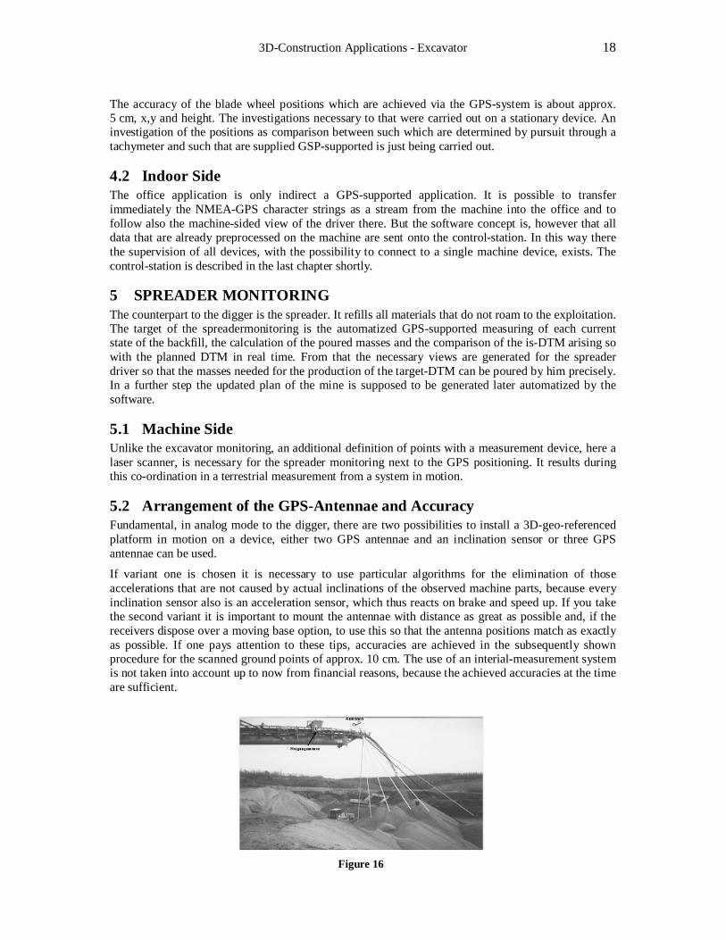
5.2 Arrangement of the GPS-Antennae and Accuracy Fundamental, in analog mode to the digger, there are two possibilities to install a 3D-geo-referenced platform in motion on a device, either two GPS antennae and an inclination sensor or three GPS antennae can be used.
If variant one is chosen it is necessary to use particular algorithms for the elimination of those accelerations that are not caused by actual inclinations of the observed machine parts, because every inclination sensor also is an acceleration sensor, which thus reacts on brake and speed up. If you take the second variant it is important to mount the antennae with distance as great as possible and, if the receivers dispose over a moving base option, to use this so that the antenna positions match as exactly as possible. If one pays attention to these tips, accuracies are achieved in the subsequently shown procedure for the scanned ground points of approx. 10 cm. The use of an interial-measurement system is not taken into account up to now from financial reasons, because the achieved accuracies at the time are sufficient.
Figure 16
1st International Conference on Machine Control & Guidance 2008 19
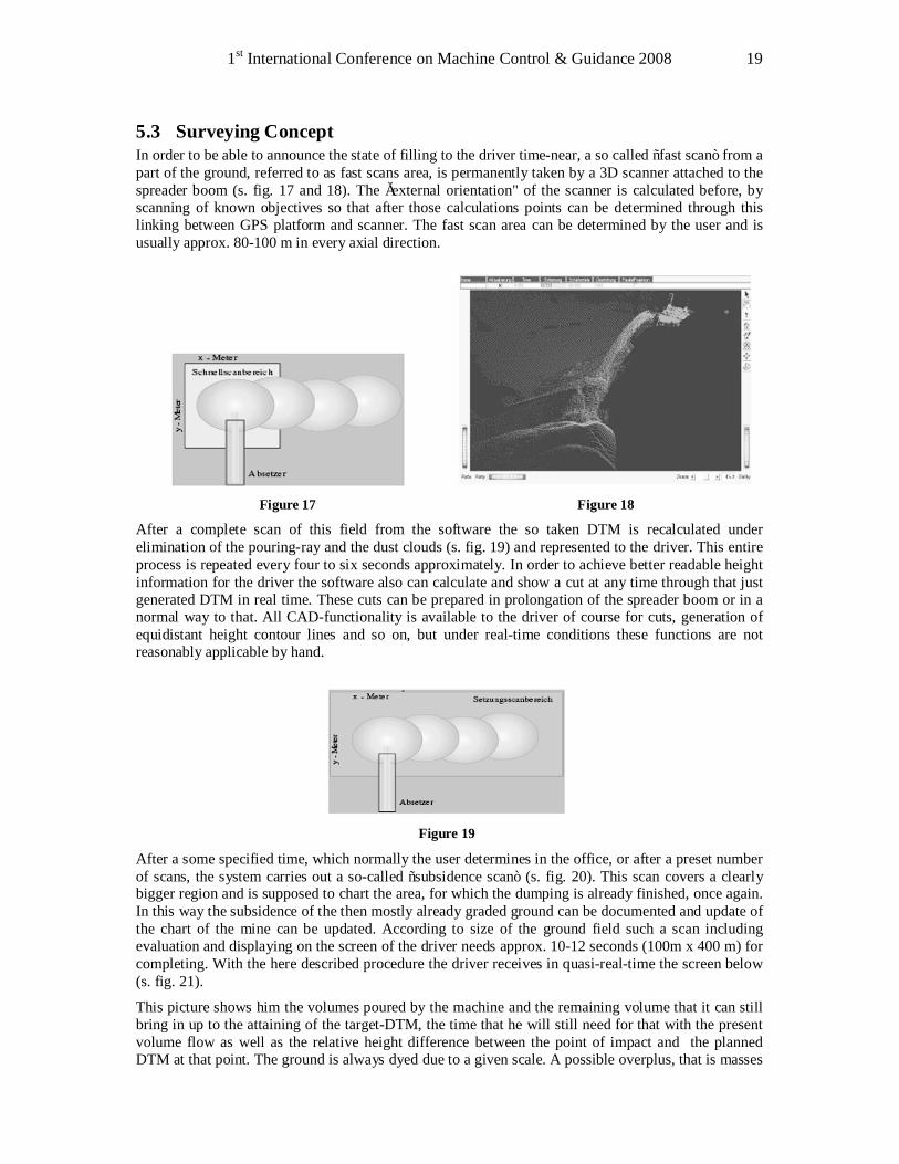
5.3 Surveying Concept In order to be able to announce the state of filling to the driver time-near, a so called “fast scan” from a part of the ground, referred to as fast scans area, is permanently taken by a 3D scanner attached to the spreader boom (s. fig. 17 and 18). The „external orientation" of the scanner is calculated before, by scanning of known objectives so that after those calculations points can be determined through this linking between GPS platform and scanner. The fast scan area can be determined by the user and is usually approx. 80-100 m in every axial direction.
Figure 17 Figure 18
After a complete scan of this field from the software the so taken DTM is recalculated under elimination of the pouring-ray and the dust clouds (s. fig. 19) and represented to the driver. This entire process is repeated every four to six seconds approximately. In order to achieve better readable height information for the driver the software also can calculate and show a cut at any time through that just generated DTM in real time. These cuts can be prepared in prolongation of the spreader boom or in a normal way to that. All CAD-functionality is available to the driver of course for cuts, generation of equidistant height contour lines and so on, but under real-time conditions these functions are not reasonably applicable by hand.
Figure 19
After a some specified time, which normally the user determines in the office, or after a preset number of scans, the system carries out a so-called “subsidence scan” (s. fig. 20). This scan covers a clearly bigger region and is supposed to chart the area, for which the dumping is already finished, once again. In this way the subsidence of the then mostly already graded ground can be documented and update of the chart of the mine can be updated. According to size of the ground field such a scan including evaluation and displaying on the screen of the driver needs approx. 10-12 seconds (100m x 400 m) for completing. With the here described procedure the driver receives in quasi-real-time the screen below (s. fig. 21).
This picture shows him the volumes poured by the machine and the remaining volume that it can still bring in up to the attaining of the target-DTM, the time that he will still need for that with the present volume flow as well as the relative height difference between the point of impact and the planned DTM at that point. The ground is always dyed due to a given scale. A possible overplus, that is masses
3D-Construction Applications - Excavator 20
whose height reach over the height of the target-DTM at that point, are labelled in turn in a specific colour and their mass is indicated.
By one specific program call the driver can calculate a mass balance in the surroundings of the pouring-ray or a chosen point so that he can recognize whether mass is available sufficiently, to produce the debit-DTM through grading.
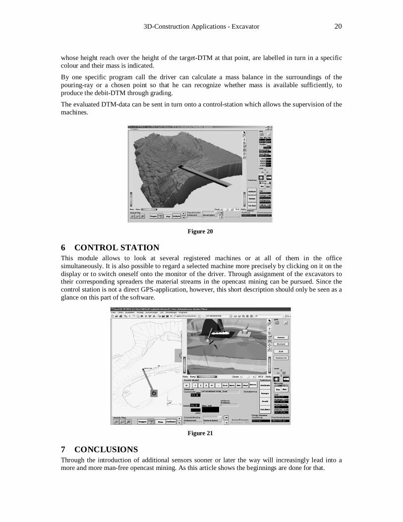
The evaluated DTM-data can be sent in turn onto a control-station which allows the supervision of the machines.
Figure 20
6 CONTROL STATION This module allows to look at several registered machines or at all of them in the office simultaneously. It is also possible to regard a selected machine more precisely by clicking on it on the display or to switch oneself onto the monitor of the driver. Through assignment of the excavators to their corresponding spreaders the material streams in the opencast mining can be pursued. Since the control station is not a direct GPS-application, however, this short description should only be seen as a glance on this part of the software.
Figure 21
7 CONCLUSIONS Through the introduction of additional sensors sooner or later the way will increasingly lead into a more and more man-free opencast mining. As this article shows the beginnings are done for that.

1st International Conference on Machine Control & Guidance 2008 21
Use of a Machine Control & Guidance System, Deter-mination of Excavator Performance, Cost Calculation and
Protection Against Damaging of Pipes and Cables
Fritz SCHREIBER, Peter RAUSCH University of applied sciences Coburg, Germany
Michael DIEGELMANN University of applied sciences Rosenheim, Germany
Abstract The construction industry is confronted with permanent pressure regarding costs due to: • increasing expenses, especially those affecting labor and energy; • shortened schedules for completion of projects; • a highly complex legal system with a growing number of official laws and standards. Possible solutions include efforts to make engineering construction more efficient – i.e. by the introduction of industrial production methods to building practices. It is intended to achieve further improvements of performance. Attention is focused on the earthmoving and road construction areas. The adoption of GPS-referenced machine guidance systems based on a digital terrain model (DTM) can significantly contribute to cost reduction. Much progress has been achieved in these areas in the recent years: the introduction of laser-referenced 1-D machine guidance systems, as well as 3-D machine guidance, tachymetrically referenced and GNSS-based guidance systems for graders, bulldozers and excavators. A DTM-based machine guidance system for excavators using GPS positioning has been developed at the University of Applied Sciences, Coburg, Department of Civil Engineering. Keywords GPS, Digital Terrain Model DTM, Machine Guidance System, LED Bar Display, Productivity (machine performance), Excavator, Tilt Sensor, Encoder
1 INTRODUCTION Why machine guidance? The construction industry is confronted with permanent pressure regarding costs due to: • increasing expenses, especially those pertaining to labor and energy; • shortened schedules for completion of projects; • a highly complex legal system with a growing number of official laws and standards.

3D-Construction Applications - Excavator 22
What can be done to handle the increasing cost pressure? Possible solutions include efforts to make engineering construction work more efficient - that is, to introduce industrial production methods into building practices as a means to achieve further increases in productivity. Techniques of working with DTM-based machine guidance systems will have considerable effects on working practices of construction engineers and surveyors [w.a.07]. This development should be kept in mind when training students.
1.1 History For earthmoving, the surface contours of the construction site of an embankment were visualized to the machine operator by means of profile templates, visors, stakes etc. The visible templates provided the operator with an image of the finished surface and the excavator bucket's edge approaching the grade height ever more accurately. Therefore support by a site worker was required and work was restricted to daylight times. This well known central function must be integrated into a user-friendly machine guidance system. Apart from that it is necessary that the operator gets a three-dimensional image of the work to be done. Nowadays, digital terrain model based machine guidance systems are a suitable resource.
1.2 Basic ideas In the beginning of the development of the DTM-based machine guidance system, it was intended to improve the productivity of construction machines, such as excavators. The excavator was chosen, because it is the geometrically most complicated machine for machine control applications. Possi-bilities to improve the productivity are:
• The improvement of the autonomous operating capabilities of an excavator. The operator of an autonomous, stakeless, operating excavator needs total information of his excavating job.
• The excavator should operate 24 hours a day without the assistance of any worker. • Digging accurately in order to avoid over-excavating. The excavated material has to be moved
only once. A means to realize the 3-D machine guidance system is the GPS-system. The continuous development of the GPS receivers has made them easier to handle, more efficient and has improved the accuracy in the determination of their position.
2 SYSTEM DEVELOPMENT
2.1 System architecture At first, the structure of the machine guidance system was determined. To avoid over-excavation the operator's main information is the difference between the planned depth and the actual depth at the edge of the bucket. This difference is zero, when the planned depth is reached.
1st International Conference on Machine Control & Guidance 2008 23
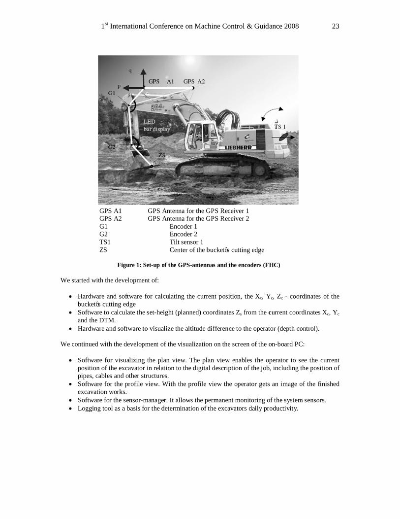
GPS A1 GPS Antenna for the GPS Receiver 1 GPS A2 GPS Antenna for the GPS Receiver 2 G1 Encoder 1 G2 Encoder 2 TS1 Tilt sensor 1 ZS Center of the bucket’s cutting edge
Figure 1: Set-up of the GPS-antennas and the encoders (FHC)
We started with the development of:
• Hardware and software for calculating the current position, the Xc, Yc, Zc - coordinates of the bucket’s cutting edge
• Software to calculate the set-height (planned) coordinates Zs from the current coordinates Xc, Yc and the DTM.
• Hardware and software to visualize the altitude difference to the operator (depth control). We continued with the development of the visualization on the screen of the on-board PC:
• Software for visualizing the plan view. The plan view enables the operator to see the current position of the excavator in relation to the digital description of the job, including the position of pipes, cables and other structures.
• Software for the profile view. With the profile view the operator gets an image of the finished excavation works.
• Software for the sensor-manager. It allows the permanent monitoring of the system sensors. • Logging tool as a basis for the determination of the excavators daily productivity.
3D-Construction Applications - Excavator 24
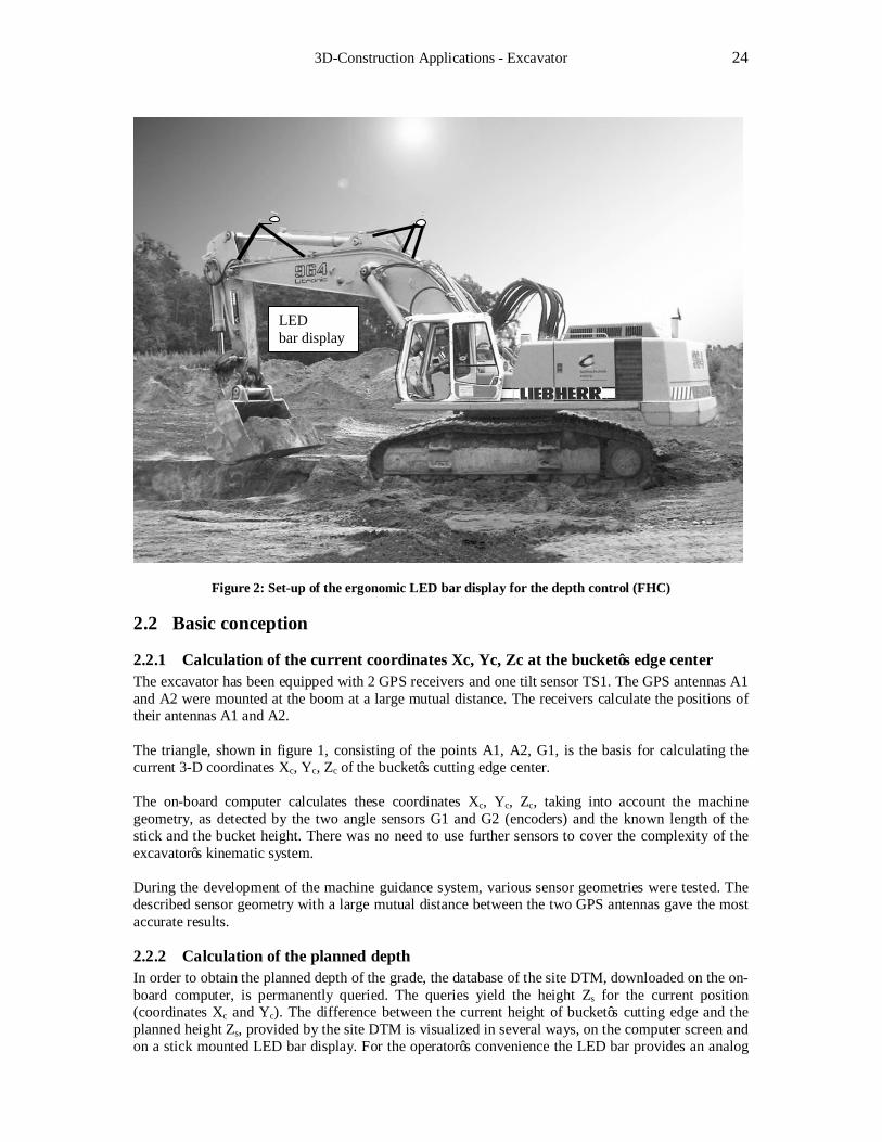
Figure 2: Set-up of the ergonomic LED bar display for the depth control (FHC)
2.2 Basic conception
2.2.1 Calculation of the current coordinates Xc, Yc, Zc at the bucket’s edge center The excavator has been equipped with 2 GPS receivers and one tilt sensor TS1. The GPS antennas A1 and A2 were mounted at the boom at a large mutual distance. The receivers calculate the positions of their antennas A1 and A2. The triangle, shown in figure 1, consisting of the points A1, A2, G1, is the basis for calculating the current 3-D coordinates Xc, Yc, Zc of the bucket’s cutting edge center. The on-board computer calculates these coordinates Xc, Yc, Zc, taking into account the machine geometry, as detected by the two angle sensors G1 and G2 (encoders) and the known length of the stick and the bucket height. There was no need to use further sensors to cover the complexity of the excavator’s kinematic system. During the development of the machine guidance system, various sensor geometries were tested. The described sensor geometry with a large mutual distance between the two GPS antennas gave the most accurate results.
2.2.2 Calculation of the planned depth In order to obtain the planned depth of the grade, the database of the site DTM, downloaded on the on-board computer, is permanently queried. The queries yield the height Zs for the current position (coordinates Xc and Yc). The difference between the current height of bucket’s cutting edge and the planned height Zs, provided by the site DTM is visualized in several ways, on the computer screen and on a stick mounted LED bar display. For the operator’s convenience the LED bar provides an analog
LED bar display
1st International Conference on Machine Control & Guidance 2008 25
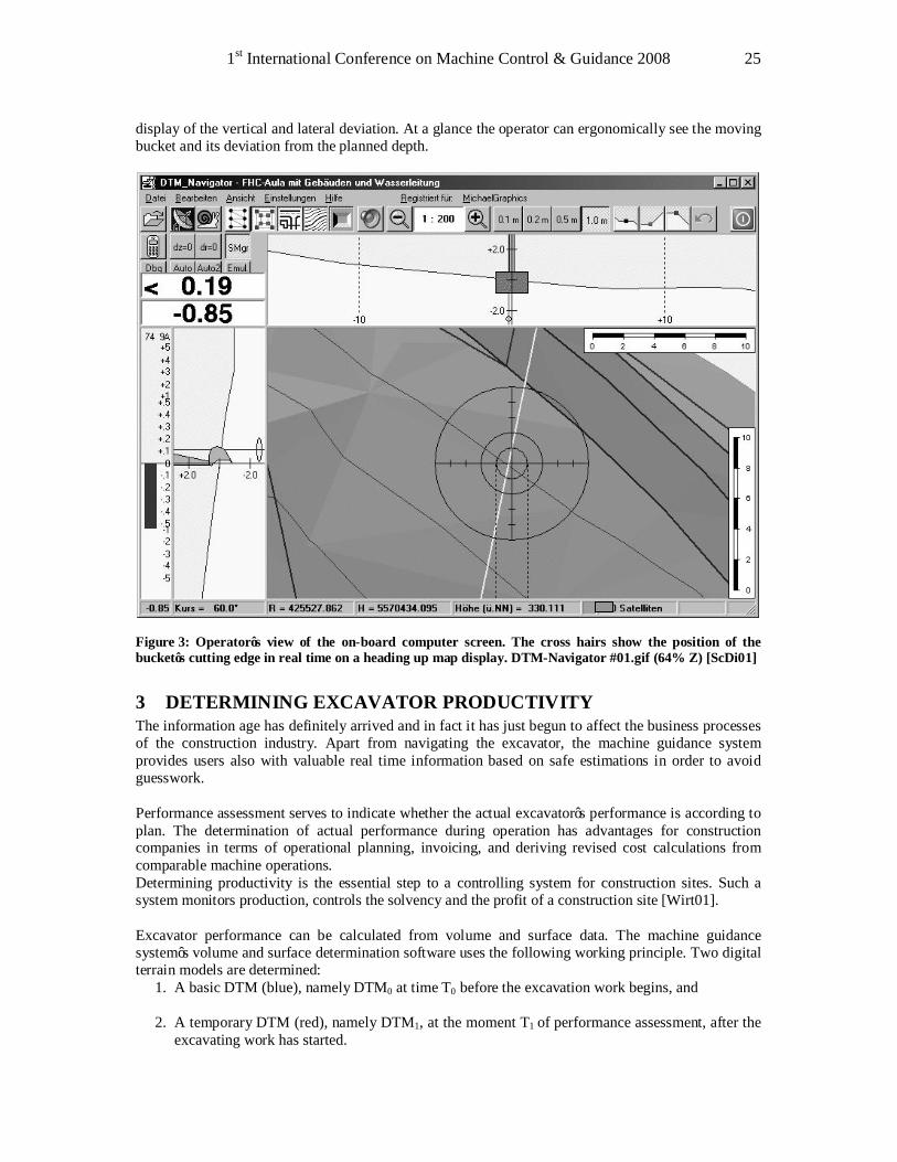
display of the vertical and lateral deviation. At a glance the operator can ergonomically see the moving bucket and its deviation from the planned depth.
Figure 3: Operator’s view of the on-board computer screen. The cross hairs show the position of the bucket’s cutting edge in real time on a heading up map display. DTM-Navigator #01.gif (64% Z) [ScDi01]
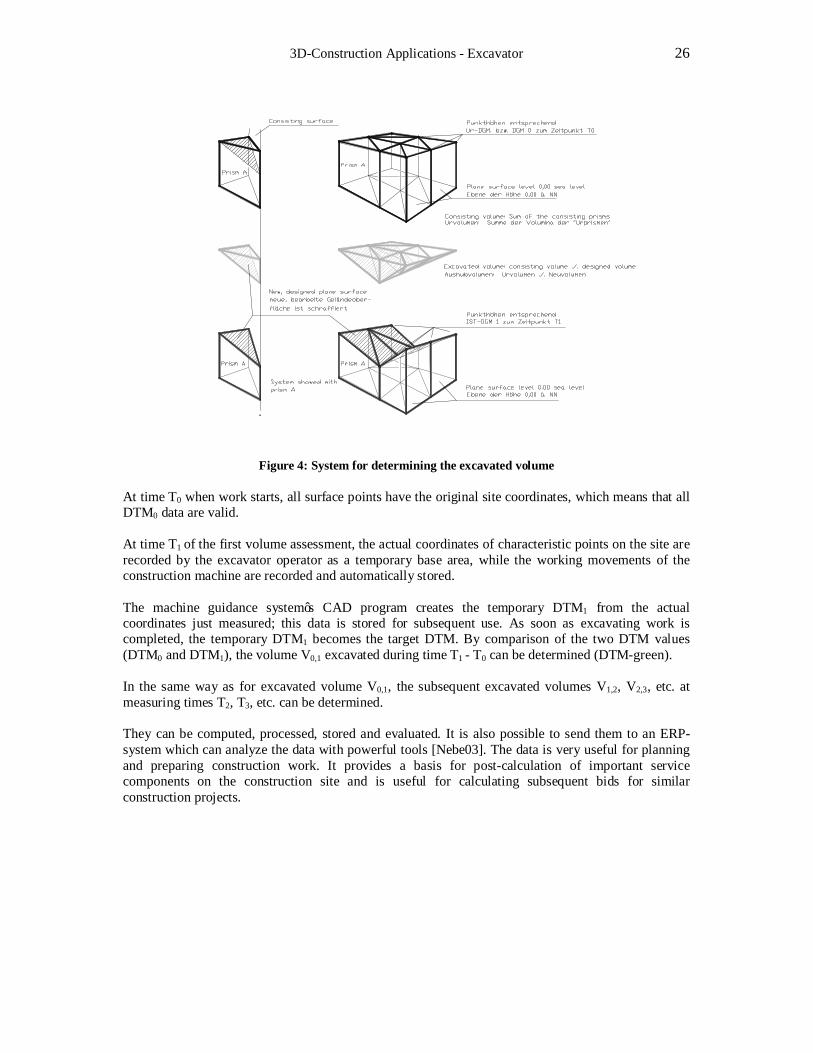
3 DETERMINING EXCAVATOR PRODUCTIVITY The information age has definitely arrived and in fact it has just begun to affect the business processes of the construction industry. Apart from navigating the excavator, the machine guidance system provides users also with valuable real time information based on safe estimations in order to avoid guesswork. Performance assessment serves to indicate whether the actual excavator’s performance is according to plan. The determination of actual performance during operation has advantages for construction companies in terms of operational planning, invoicing, and deriving revised cost calculations from comparable machine operations. Determining productivity is the essential step to a controlling system for construction sites. Such a system monitors production, controls the solvency and the profit of a construction site [Wirt01]. Excavator performance can be calculated from volume and surface data. The machine guidance system’s volume and surface determination software uses the following working principle. Two digital terrain models are determined:
1. A basic DTM (blue), namely DTM0 at time T0 before the excavation work begins, and 2. A temporary DTM (red), namely DTM1, at the moment T1 of performance assessment, after the
excavating work has started.
3D-Construction Applications - Excavator 26
Figure 4: System for determining the excavated volume
At time T0 when work starts, all surface points have the original site coordinates, which means that all DTM0 data are valid. At time T1 of the first volume assessment, the actual coordinates of characteristic points on the site are recorded by the excavator operator as a temporary base area, while the working movements of the construction machine are recorded and automatically stored. The machine guidance system’s CAD program creates the temporary DTM1 from the actual coordinates just measured; this data is stored for subsequent use. As soon as excavating work is completed, the temporary DTM1 becomes the target DTM. By comparison of the two DTM values (DTM0 and DTM1), the volume V0,1 excavated during time T1 - T0 can be determined (DTM-green). In the same way as for excavated volume V0,1, the subsequent excavated volumes V1,2, V2,3, etc. at measuring times T2, T3, etc. can be determined. They can be computed, processed, stored and evaluated. It is also possible to send them to an ERP-system which can analyze the data with powerful tools [Nebe03]. The data is very useful for planning and preparing construction work. It provides a basis for post-calculation of important service components on the construction site and is useful for calculating subsequent bids for similar construction projects.
1st International Conference on Machine Control & Guidance 2008 27
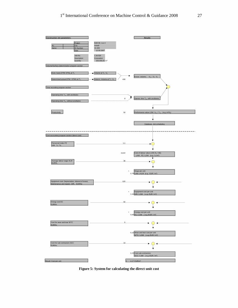
Figure 5: System for calculating the direct unit cost
Equipment cost: Depreciation, interest of invest, 122Maintenance and repairs DIR, EUR/hz
+ Equipment cost per unit2,44 DIR / LSW ( e.g.:EUR / m³)
Energy cost EC 32EUR/hz
+ Energy cost per unit0,64 EC / LSW ( e.g.:EUR / m³)
Cost for wear and tear WTC 5EUR/hz
0,10 Wear and tear cost per unitWTC / LSW ( e.g.:EUR / m³)
Cost for sub contractors SCC 10EUR/hz
0,20 Cost sub-contractorsSCC / LSW ( e.g.:EUR / m³)
Result: Cost per unit Σ 4,17 EUR/m³
Construction site parameters:
Project BAB 96, Los 4NL: City AstadtName: ID-Number 34-456
Date 12.05.2007
Job-No. 1.34.520Description ExcavationQuantity 200.000,00 m³
Volume/Surface determination program section
Exist. basis-DTM: DTM0 at T0 Volume at T0 : V0
Excav.-volume.: V0,1 : V0 - V1
Determined actual-DTM: DTM1 at T1 Determ. Volume at T1 : V1 400
Time recording program section
Operating time T0,1 with ancillaries
8 Operat. time T0,1 with ancillariesOperating time T0,1 without ancillaries
Productivity 50 Performance value LSW: V0,1 / T0,1 (e.g.:m³/hz)
Cost accounting program section (direct cost)
Personnel index PZ 1,1ratio hL / hZ
0,022 Cost of labour value LAW (hL / AE) LAW: PZ / LSW (e.g.: hL/m³)
Average labour wage ALW 36EUR/hL
+ Wage per unit0,79 LAW x ALW (e.g.: EUR / m³)
Results
Database, Job scheduling
3D-Construction Applications - Excavator 28
Use of the calculated excavated volume to determine operating data With the aid of the calculated excavated volume or the surface covered and additional machine operating data, the operating data for the “excavator cost estimation” can be determined. Additional data can be saved and processed in the machine’s computer: details of machine operators’ wages, cost of fuel and related operating materials, cost of the machine itself (depreciation A, interest charges V, and average repair charge rate R), costs of wear and tear, and miscellaneous costs. Regarding all these parameters the excavator’s hourly costs can be divided into separate cost. ERP Interface As we have already mentioned ERP-Systems offer powerful tools to analyze the collected data. Because of that the developer team has implemented an SAP ERP interface. The interface is based on so called Business Application Programming Interfaces (BAPIs). BAPIs allow access to SAP-Business-Objects, which makes it possible to add data to the ERP database. To set up the ERP interface we used the SAP tool “Legacy Systems Migration Workbench” (LSMW). Alternatively we could have used another powerful SAP technology which is called „Exchange Infrastructure“ (XI). The advantages and disadvantages of the tools are discussed in [WiGr03; StOr05; NiFN06]. Due to availability reasons and the fact that XI would have entailed additional license costs we decided to use the LSMW. With the implemented interfaces data collected by the machine guidance system can be transferred to the ERP system. It can be analyzed by the project system, the controlling and the finance component. It is also conceivable to use business intelligence tools for further analysis.
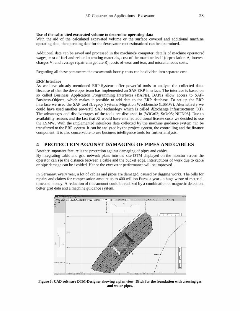
4 PROTECTION AGAINST DAMAGING OF PIPES AND CABLES Another important feature is the protection against damaging of pipes and cables. By integrating cable and grid network plans into the site DTM displayed on the monitor screen the operator can see the distance between a cable and the bucket edge. Interruptions of work due to cable or pipe damage can be avoided. Hence the excavator performance will be improved. In Germany, every year, a lot of cables and pipes are damaged, caused by digging works. The bills for repairs and claims for compensation amount up to 400 million Euros a year - a huge waste of material, time and money. A reduction of this amount could be realized by a combination of magnetic detection, better grid data and a machine guidance system.
Figure 6: CAD software DTM-Designer showing a plan view: Ditch for the foundation with crossing gas and water pipes.

1st International Conference on Machine Control & Guidance 2008 29
Figure 7: Machine guidance software DTM-Navigator. Operator's plan view with gas and water pipes Actual distance: Bucket’s center to the gas pipe: 2,00 m
The DTM-based machine guidance system provides the on-board computer with the 3-D-coordinates of the current local position of the bucket’s cutting edge. It is possible to make the cable and grid network plans available for the on-board computer which enables a superimposed view. With a layer technique, the operator can see the current cable situation and the site plan in a single view. If a collision is imminent, the operator is warned by an audible signal.
5 CONCLUSIONS In this paper a new generation of machine guidance systems is presented. Its additional features are:
• Determination of excavator performance • Protection of cables during excavation work • Possibilities to analyze productivity and costs
This leads to the following benefits: • More accurate schedules and estimates • Less surveying work • Fewer interruptions of work caused by cable and pipe damages, thus saving labor and material
costs
3D-Construction Applications - Excavator 30
ACKNOWLEDGEMENTS We thank the Bavarian Ministry of Science and Education, our cooperating partners and sponsors for their generous support over the years: Liebherr Hydraulikbagger GmbH, Kirchdorf/Germany VOLVO Baumaschinen GmbH, Konz/Germany Zeppelin Baumaschinen GmbH, Garching/Germany STRABAG BauAG, Köln/Munich/Germany Max Boegl Bauunternehmung, Neumarkt/Germany Fraunhofer Institut IIS, Nuremberg/Germany Fujitsu-Siemens GmbH, Nuremberg/Germany Hummel AG, Steckverbindungen, Denzlingen/Germany U.I. Lapp GmbH, Kabelwerk, Stuttgart/Germany
REFERENCES [Nebe03] NEBE, L.: Kennzahlengestütztes Projekt-Controlling in Baubetrieben, Diss., Dortmund, 2003. http://deposit.ddb.de/cgi-bin/dokserv?idn=967845378, last accessed on March 23.
[NiFN06] NICOLESCU, V.; FUNK, B.; NIEMEYER, P.: Entwicklerbuch SAP Exchange Infrastructure SAP Press, Bonn, 2006.
[ScDi01] SCHREIBER, F., DIEGELMANN, M.: Entwicklung eines DGM-basierten Maschinen-führungssystems für Bagger, in: CHESI, G., WEINOLD, T. (Hrsg.): 14. Internationale geodätische Woche Obergurgl, Wichmann, Heidelberg 2007, p. 83-93.
[StOr05] STUMPE, J., ORB, J.: SAP Exchange Infrastructure, SAP Press, Bonn, 2005.
[w.a.07] W. A.: bauma-Trends 2007: Telematik, GPS & Co. in: Computern im Handwerk, Juni/2007, p. 7-10.
[WiGr03] WILLINGER, M.; GRADL, J.: Datenmigration in SAP R/3, SAP Press, Bonn, 2003.
[Wirt01] Wirth, V.: Controlling in der Baupraxis, Kluwer, München, 2003.
1st International Conference on Machine Control & Guidance 2008 31
Guidance for Partial Face Excavation Machines
Nod CLARKE-HACKSTON, Jochen BELZ VMT GmbH
[international, j.belz]@vmt-gmbh.de
Allan HENNEKER Surex Pty Ltd
[email protected] Abstract For the construction of tunnels and other underground structures, extraction of the exact amount of material is of paramount importance both economically and for engineering purposes. In the Sequential Support Method (NATM) immediate (sequential) and smooth support by means of shotcrete, steel arches, lattice girders and rockbolts, either singly or in combination are used; cutting of the precise profile (albeit sometimes of complex geometry) is an integral part of the method. In order to save unnecessary excavation and provide better information to the machine operator, VMT GmbH has developed a system to support precise excavation of the tunnel profile when using roadheaders or other partial face cutting machines. This paper outlines the principles of this system with examples from Australia, Germany, Sweden and Spain and will cite examples of typical savings achieved. Keywords Total Station, Underground, NATM, Profile, Guidance, VMT, Roadheader, Excavator, Bolter.
1 INTRODUCTION Roadheaders were first developed for mechanical excavation of coal in the early 1950’s. Today their application areas have expanded beyond coal mining as a result of continual performance increases brought about by new technological developments and design improvements. The major improvements achieved in the last 50 years consist of: steadily increasing machine weight, size, and cutterhead power, improved design of boom, muck pick-up and loading systems, more efficient cutterhead design, metallurgical developments in cutting bits, advances in hydraulic and electrical systems, and more widespread use of automation and remote control features. All these have led to drastic enhancements in machine cutting capabilities, system availability and service life. Roadheaders are the most widely used underground partial-face excavation machines for soft to medium strength rocks, particularly sedimentary rocks. They are used for both development and production in the soft rock mining industry (i.e. main haulage drifts, roadways, cross-cuts, etc.) particularly in coal, industrial minerals and evaporate rocks. In civil construction, they find extensive use for excavation of tunnels (railway, roadway, sewer, diversion tunnels, etc.) in soft ground conditions, as well as for enlargement and rehabilitation of various underground structures. It is chosen over other possible tunnelling methods principally because of its application advantages which include free excavation area, considerable flexibility in regard to unforeseen changes in geological and hydrological conditions, flexibility in terms of cross-sectional changes, and rapid mobilization with readily available, unsophisticated and relatively inexpensive excavation equipment.
1.1 General All rock and soil has, to a greater or lesser degree, the inherent ability to support itself or stand freely for a certain amount of time. Strong rock can remain free standing for hundreds of years while the
3D-Construction Applications - Excavator 32
self-supporting ability of rocks and soils of weaker types is relatively short-lived and measured in minutes rather than hours, days or years. For the construction of tunnels and other underground structures, extraction of the exact amount of material is of paramount importance both economically and for engineering purposes. In the Sequential Support Method (NATM) where immediate (sequential) and smooth support by means of shotcrete, steel arches, lattice girders and rockbolts, either singly or in combination, are used; cutting of the precise profile (albeit sometimes of complex geometry) is an integral part of the method.
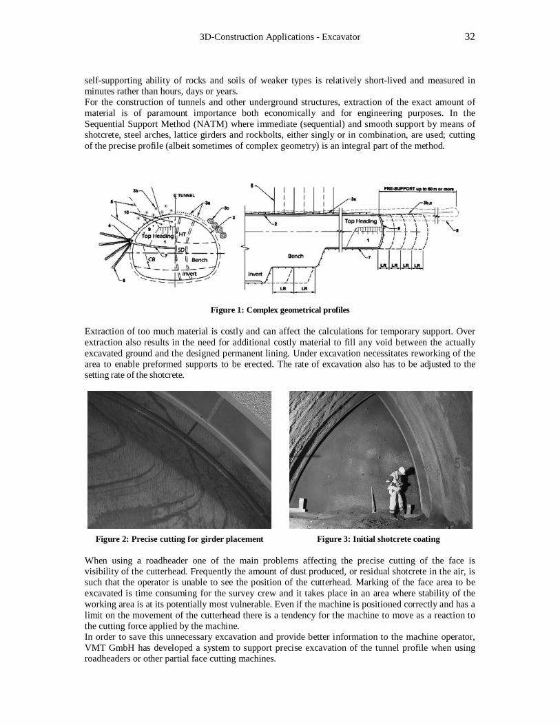
Figure 1: Complex geometrical profiles
Extraction of too much material is costly and can affect the calculations for temporary support. Over extraction also results in the need for additional costly material to fill any void between the actually excavated ground and the designed permanent lining. Under excavation necessitates reworking of the area to enable preformed supports to be erected. The rate of excavation also has to be adjusted to the setting rate of the shotcrete.
Figure 2: Precise cutting for girder placement Figure 3: Initial shotcrete coating When using a roadheader one of the main problems affecting the precise cutting of the face is visibility of the cutterhead. Frequently the amount of dust produced, or residual shotcrete in the air, is such that the operator is unable to see the position of the cutterhead. Marking of the face area to be excavated is time consuming for the survey crew and it takes place in an area where stability of the working area is at its potentially most vulnerable. Even if the machine is positioned correctly and has a limit on the movement of the cutterhead there is a tendency for the machine to move as a reaction to the cutting force applied by the machine. In order to save this unnecessary excavation and provide better information to the machine operator, VMT GmbH has developed a system to support precise excavation of the tunnel profile when using roadheaders or other partial face cutting machines.
1st International Conference on Machine Control & Guidance 2008 33
Figure 4: Poor atmospheric conditions
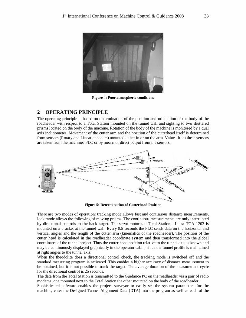
2 OPERATING PRINCIPLE The operating principle is based on determination of the position and orientation of the body of the roadheader with respect to a Total Station mounted on the tunnel wall and sighting to two shuttered prisms located on the body of the machine. Rotation of the body of the machine is monitored by a dual axis inclinometer. Movement of the cutter arm and the position of the cutterhead itself is determined from sensors (Rotary and Linear encoders) mounted either in or on the arm. Values from these sensors are taken from the machines PLC or by means of direct output from the sensors.
Figure 5: Determination of Cutterhead Position There are two modes of operation: tracking mode allows fast and continuous distance measurements, lock mode allows the following of moving prisms. The continuous measurements are only interrupted by directional controls to the back target. The servo-motorized Total Station - Leica TCA 1203 is mounted on a bracket at the tunnel wall. Every 0.5 seconds the PLC sends data on the horizontal and vertical angles and the length of the cutter arm (kinematics of the roadheader). The position of the cutter head is calculated in the roadheader coordinate system and then transformed into the global coordinates of the tunnel project. Thus the cutter head position relative to the tunnel axis is known and may be continuously displayed graphically in the operator cabin, since the tunnel profile is maintained at right angles to the tunnel axis. When the theodolite does a directional control check, the tracking mode is switched off and the standard measuring program is activated. This enables a higher accuracy of distance measurement to be obtained, but it is not possible to track the target. The average duration of the measurement cycle for the directional control is 25 seconds. The data from the Total Station is transmitted to the Guidance PC on the roadheader via a pair of radio modems, one mounted next to the Total Station the other mounted on the body of the roadheader. Sophisticated software enables the project surveyor to easily set the system parameters for the machine, enter the Designed Tunnel Alignment Data (DTA) into the program as well as each of the
3D-Construction Applications - Excavator 34
individual profiles to be excavated. A simple change in the profile icon enables the machine to rapidly change its excavation sequence in line with the project’s requirements
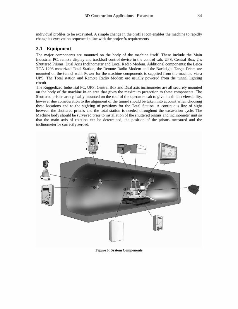
2.1 Equipment The major components are mounted on the body of the machine itself. These include the Main Industrial PC, remote display and trackball control devise in the control cab, UPS, Central Box, 2 x Shuttered Prisms, Dual Axis Inclinometer and Local Radio Modem. Additional components: the Leica TCA 1203 motorized Total Station, the Remote Radio Modem and the Backsight Target Prism are mounted on the tunnel wall. Power for the machine components is supplied from the machine via a UPS. The Total station and Remote Radio Modem are usually powered from the tunnel lighting circuit. The Ruggedized Industrial PC, UPS, Central Box and Dual axis inclinometer are all securely mounted on the body of the machine in an area that gives the maximum protection to these components. The Shuttered prisms are typically mounted on the roof of the operators cab to give maximum viewability, however due consideration to the alignment of the tunnel should be taken into account when choosing these locations and to the sighting of positions for the Total Station. A continuous line of sight between the shuttered prisms and the total station is needed throughout the excavation cycle. The Machine body should be surveyed prior to installation of the shuttered prisms and inclinometer unit so that the main axis of rotation can be determined, the position of the prisms measured and the inclinometer be correctly zeroed.
Figure 6: System Components
1st International Conference on Machine Control & Guidance 2008 35
The Shuttered prisms are standard survey prisms enclosed in a protective housing with a motorized protective shutter. The shutter, activated by the software of the SLS system, is only opened for the duration of the angle and distance measurement to the respective prism. This eliminates confusion of prisms or other reflective objects; it also helps to keep the prism surfaces clean. The individual prisms can be connected by a bus system. A fluid damped dual axis inclinometer for determination of inclination of the roadheader. The damping behaviour of the inclinometer can be adapted to the vibration range of the mounting position; in addition the inclinometer is equipped with a thermometer for temperature compensation. The main computer is a ruggedized industrial PC which is housed in a special Stainless Steel enclosure which is fixed on anti-vibration mounts between the housing and machine body. The mounting location is chosen to give maximum protection for the unit. A UPS is supplied to maintain the appropriate power to the PC in the event of fluctuating power being available from the machine. The PC uses the latest Windows™ Operating system. A remote display for the operator is installed in a prime viewing location in the operators cab. Easy access to functions is via track ball control. A remote USB connector is available for attaching a keyboard for initial data entry and for memory device attachment. The Central Box interfaces between the various sensors of the system and converts these outputs for suitable entry into the Industrial PC. Control signals from the Industrial PC are also converted for transfer to the sensors such as the shuttered prisms. Radio Modems are used to connect the components on the machine with those on the tunnel wall as the use of cables in such a consistently changing working environment would be problematic. The Local Radio Modem is mounted on the machine and effects Wireless Data Communication between SLS-PC and Total Station whilst the Remote Radio Modem is mounted next to the Total Station with clear path for radio signals. Wireless reception is controlled by the SLS-software. The Remote Radio Modem receives the data from the Local Unit and transfers them to the Total Station. In case of power failure it changes automatically into battery mode and sends an alarm signal to the SLS-PC. The principle measurement tool for the SLS-TM system is a Motorized Leica Total Station Model TCA 1203 with Automatic Target Recognition (ATR). Automatic fine pointing to the prisms speeds up measurements and improves productivity. A Standard, round retro-reflective prism is used as a rear backsight target. It is recognised and measured by the ATR target recognition unit of the Total Station and is used to check the bearing of the Total Station. A comparison between the Backsight Target and Total Stations’ positions during each measurement cycle is used to give a warning in case of movement of either outside of any preset limits.
2.2 Software The SLS-TM Roadheader Guidance System provides an automated means to minimize operating expenses, while maximizing the accuracy of cut and minimizing time. This is achieved through use of a highly unique, computer-driven machine operator’s display screen. The easy to use Windows™ software has been carefully configured to make data entry as simple as possible. Initial setup of the system is implemented through the System Editor data entry pages. Input of the Designed Tunnel Alignment (DTA) is achieved through the DTA Editor pages where the DTA, in point coordinate table format can be created from the principle geometric elements that make up the alignment in both Horizontal and Vertical. From the Profile Editor each of the relevant profiles for the project can again be created from the geometric elements that make up the profile. Where multiple profiles are to be excavated in alternating sequence they can all be stored in the main program. When the individual profile is to be excavated its profile is simply called up from the profile editor menu. Access to the various user levels is password protected. Several language options are available as well as Metric and Imperial unit options.
3D-Construction Applications - Excavator 36
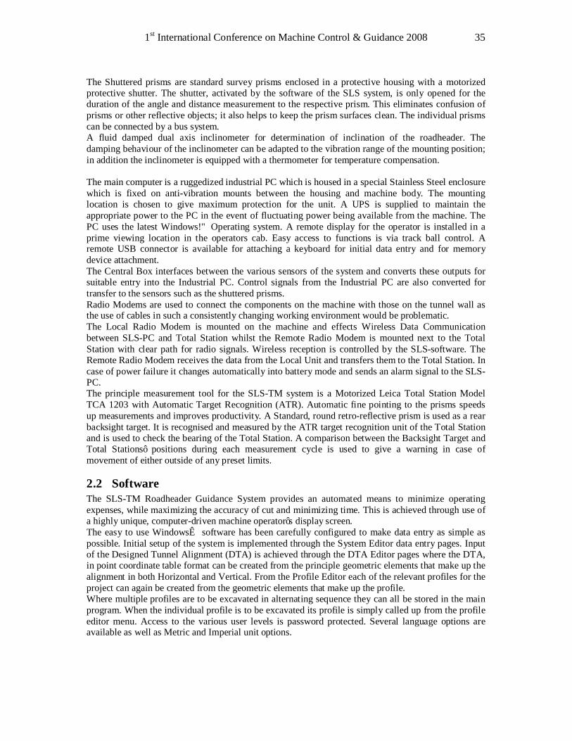
Figure 7: Main operator display
To aid the operator the background of the main graphical display is colour coded to indicate the time interval since the last valid survey reading. Although the measurement cycle can be set to an interval as short as every 20 seconds there may be times when a valid reading cannot be made. When this occurs a change in the background colouring is made to the operators display. The colours for the background are:- § Within initial time interval Grey § Time greater than first preset value Yellow § Time greater than second preset level Red
The typical time intervals being 3 minutes and 6 minutes, and a full dialogue of the survey positions is available from the survey position screens.
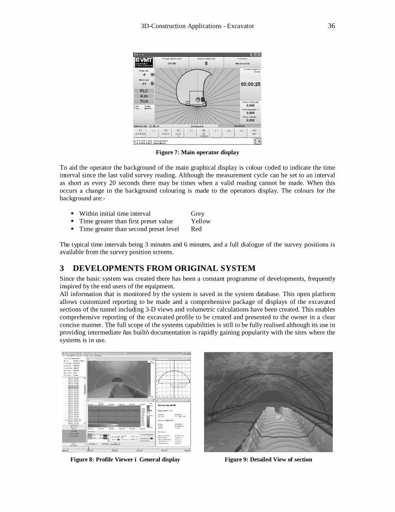
3 DEVELOPMENTS FROM ORIGINAL SYSTEM Since the basic system was created there has been a constant programme of developments, frequently inspired by the end users of the equipment. All information that is monitored by the system is saved in the system database. This open platform allows customized reporting to be made and a comprehensive package of displays of the excavated sections of the tunnel including 3-D views and volumetric calculations have been created. This enables comprehensive reporting of the excavated profile to be created and presented to the owner in a clear concise manner. The full scope of the systems capabilities is still to be fully realised although its use in providing intermediate “as built” documentation is rapidly gaining popularity with the sites where the systems is in use.
Figure 8: Profile Viewer – General display Figure 9: Detailed View of section
1st International Conference on Machine Control & Guidance 2008 37
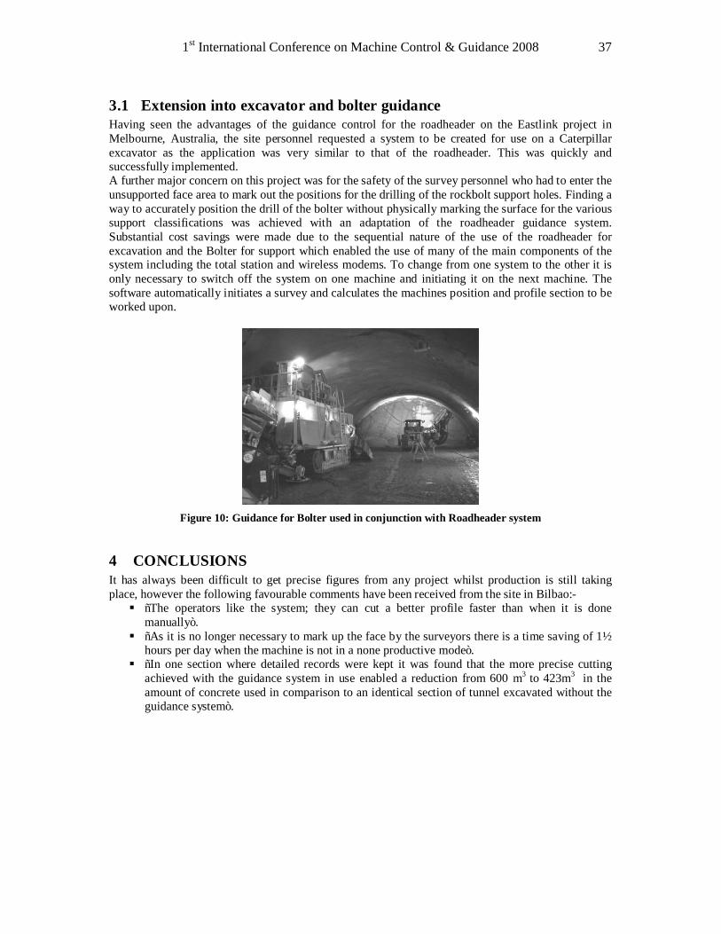
3.1 Extension into excavator and bolter guidance Having seen the advantages of the guidance control for the roadheader on the Eastlink project in Melbourne, Australia, the site personnel requested a system to be created for use on a Caterpillar excavator as the application was very similar to that of the roadheader. This was quickly and successfully implemented. A further major concern on this project was for the safety of the survey personnel who had to enter the unsupported face area to mark out the positions for the drilling of the rockbolt support holes. Finding a way to accurately position the drill of the bolter without physically marking the surface for the various support classifications was achieved with an adaptation of the roadheader guidance system. Substantial cost savings were made due to the sequential nature of the use of the roadheader for excavation and the Bolter for support which enabled the use of many of the main components of the system including the total station and wireless modems. To change from one system to the other it is only necessary to switch off the system on one machine and initiating it on the next machine. The software automatically initiates a survey and calculates the machines position and profile section to be worked upon.
Figure 10: Guidance for Bolter used in conjunction with Roadheader system
4 CONCLUSIONS It has always been difficult to get precise figures from any project whilst production is still taking place, however the following favourable comments have been received from the site in Bilbao:- § “The operators like the system; they can cut a better profile faster than when it is done
manually”. § “As it is no longer necessary to mark up the face by the surveyors there is a time saving of 1½
hours per day when the machine is not in a none productive mode”. § “In one section where detailed records were kept it was found that the more precise cutting
achieved with the guidance system in use enabled a reduction from 600 m3 to 423m3 in the amount of concrete used in comparison to an identical section of tunnel excavated without the guidance system”.

3D-Construction Applications - Excavator 38
REFERENCES Copur, H., Ozdemir, L. and Rostami, J., 1998, Roadheader Applications in Mining and Tunneling. Mining Engineering, Vol. 50, No. 3, pp. 38-4, 1998
Chittenden, N., Müller H., New Developments in Automated Tunnel Surveying Systems. Proceedings ITA World Tunnelling Congress 2004, Singapore, 2004
Sauer, G., 1990 Light at the end of the tunnel. Construction Technology International, March 1990.
Smith, M., 2006 Face Drilling. Reference Editions Ltd for Atlas Copco Rock Drills AB. 2006 Sweden
White, A., 1993 The Installation of Automated Profile Guidance on a Dosco MkIIB Roadheader. Paper Presented at Meeting of The Institution of Mining Engineers, May 13, 1993, Nottingham

Kinematic Measurement and Sensor Technology I (Local Systems)


1st International Conference on Machine Control & Guidance 2008 41
A Time-referenced 4D Calibration System for Kinematic Optical Measuring Systems
Claudia DEPENTHAL*
GIK, University Karlsruhe, Germany [email protected]
Abstract By using kinematic optical measuring systems in spatiotemporal positioning necessarily all involved sensors of the measuring systems have to be synchronized. Otherwise existing dead time and latency in a measuring system will lead to deviations in the space-time position. A time-referenced 4D calibration system is presented for kinematic optical measuring systems, which is qualified for tracking optical measuring systems of any kind. The base of this calibration system is built up by a tiltable rotating arm driven by a rotary direct drive. The rotating arm is supplemented by a further rotary direct drive mounted on a movable tripod. The developed modeling for determinability of a space-time position is based on the theory of quaternions. The fundamental idea of modeling is equivalent to the fact that every measurand of the test item, which is measured at a particular time, could be assigned to an explicit position of the rotating arm. Keywords Kinematic measurements, calibration system, time-referenced, rotating arm
1 INTRODUCTION Kinematic optical measuring systems such as lasertracker, robotic-tacheometer or iGPS are employed for the space-time position determination of moving object points. These kind of measuring systems are multi-sensor systems and for a spatiotemporal positioning all involved sensors have to be synchronized. It is a fact that existing dead time and latency in a measuring system will lead to deviations in space-time position. The development of a 4D calibration system is based on a discrete spatiotemporal position determination. By the calibration system the nominal trajectory is representing by a rotating arm and together with a time referencing every position is known in space and time. With an adequate modeling it is possible to determine the relative time for a measuring result of every mesurand of a test item. In this way the relative time gives information about the measuring point of time. It is also possible to determine dead time or latency from these times. In this paper the basics of the calibration system will be represented as well as a part of the modeling. More details are presented in Depenthal (2008).
2 4D CALIBRATION SYSTEM
2.1 Technical Realization The calibration system is designed by a rotating arm with an arm length of 2m. The arm is rotating in a horizontal or vertical plane and also in planes between both. At the end of the arm a prism or sensor can be fixed and a balance weight on the opposite end. The performance of the prime mover of the rotating arm consists of a rotary direct drive with an integrated rotary encoder. The encoder has a resolution of 0.36" and the grating disk has a reference point, the so-called homepoint, for a defined orientation. After a calibration of the direct drive a measurement uncertainty of Uk=2 = ± 4.0" is achieved (Depenthal, 2006). In addition a function is generated to correct for the bending of the spatial position of the rotating arm. The direct drive can produce velocities up to 10m/s at the arm's end.
Kinematic Measurement and Sensor Technology I (Local Systems) 42
A lasertracker LTD500 (Leica) was used to verify the static accuracy of the rotating arm. In relation to the rotating plane standard deviations are reached as follows: out of plane σ = 17µm, radial σ = 10µm, tangential σ = 9µm. Kinematic measurements until 6m/s exhibit a stable behavior of the rotating arm (Depenthal and Barth, 2007). The length of the rotating arm restricts the angular range of polar measurement systems. To enlarge the horizontal angle, a larger rotation has to be simulated for the measurement system. This can be reached, if the measurement system is mounted on a rotary direct drive. In this way the measuring system performs the same rotation as the direct drive. This second direct drive is mounted on a very stable and heavy tripod. The direct drive has a resolution of 0.22" and after a calibration a measurement uncertainty of Uk=2 = ± 2.3" is achieved.
2.2 Time Referencing Ideally, a kinematic measurement process has to assign an accurate spatiotemporal position to a moving object. In fact there is a difference between the measured spatiotemporal position and the theoretical position. The dimension depends on the measurement system. A time-referenced calibration system has to detect these differences and to enumerate the dimension. The meaning of time referencing is that specific procedures have to be kept at the same point of time on a given time scale. For time referencing only real-time systems can be used. A system is said to be real-time if the total correctness of the result of a real-time data processing depends not only upon its logical correctness, but also upon time in which it is performed (Wörn and Bringschulte, 2005). A real-time system also has to be guarantied a temporal deterministical behavior (Mächtel, 2000). There are two different procedures for time referencing between a calibration system and the test item: external trigger and serial interface. An external trigger is used, if the measuring system has a trigger input interface. The trigger-signal is realized with a function generator, normally using the rising or trailing edge of a rectangular signal as trigger. The quality of the time referencing is only dependent on the edge's quality. The clock rate of the trigger signal must be choosen in that way, that all procedures of the calibration- and measurement system can be closed within one clock rate. The other method of communication is a serial interface. The communication between the two participants – measuring system and calibration system – is made up of requests and replies in terms of the data item. Thereby the trailing edge of each start bit of the data item – request and reply – will be captured. Assuming that the data transfer rate would be 19200 baud, the period between two trailing edges constitutes 103µs so that the trailing edge of the start bit must be captured within this period. The calibration system assigns a position – time and location – to the respective start bit and the result is a spatiotemporal position for every request and reply of a measurement system.
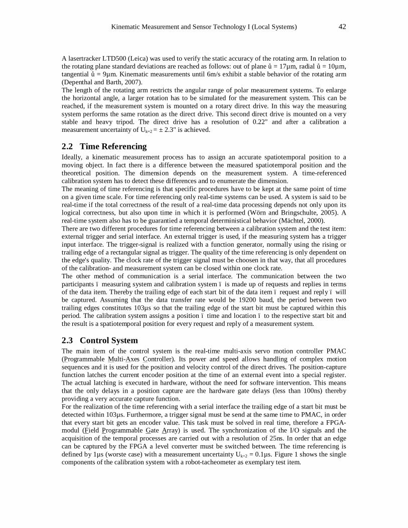
2.3 Control System The main item of the control system is the real-time multi-axis servo motion controller PMAC (Programmable Multi-Axes Controller). Its power and speed allows handling of complex motion sequences and it is used for the position and velocity control of the direct drives. The position-capture function latches the current encoder position at the time of an external event into a special register. The actual latching is executed in hardware, without the need for software intervention. This means that the only delays in a position capture are the hardware gate delays (less than 100ns) thereby providing a very accurate capture function. For the realization of the time referencing with a serial interface the trailing edge of a start bit must be detected within 103µs. Furthermore, a trigger signal must be send at the same time to PMAC, in order that every start bit gets an encoder value. This task must be solved in real time, therefore a FPGA-modul (Field Programmable Gate Array) is used. The synchronization of the I/O signals and the acquisition of the temporal processes are carried out with a resolution of 25ns. In order that an edge can be captured by the FPGA a level converter must be switched between. The time referencing is defined by 1µs (worste case) with a measurement uncertainty Uk=2 = 0.1µs. Figure 1 shows the single components of the calibration system with a robot-tacheometer as exemplary test item.
1st International Conference on Machine Control & Guidance 2008 43
Figure 1: single components of the calibration system
with a robot-tacheometer as exemplary test item
3 KINEMATIC MODELING
3.1 Principle The modeling approach is based on the fact that every measurand of a measuring system is measured at a specific point of time. The time-referenced rotating arm can be assign this specific point of time to an exactly defined rotation angle in respect of the reference position. By known angular velocity and rotation angle it is possible to draw a conclusion for the searched time of the measurand. Kinematic measurements are characterized by existence of no repeated measurements. Therefore every single point of measurement must be examined and the model must bear as unique unknown the rotation angle φ(t) which is assigned to the measurand. The modeling is based on the theory of quaternions, which are given, for example, in Kuipers (1999). A quaternion may be regarded as 4-tupel of real numbers, that is an element of R4. A quaternion is defined as a sum of a scalar part and a vector part, which is an ordinary vector in R3. The multiplication of quaternions is non-commutative. The advantage of using quaternions is the efficient concatenation of multiple rotations. First of all, the radius of the rotating arm will be determined with a static reference measurement due to the higher precision of the measurements in the static mode of the measurement systems. The test item and the calibration system exhibit their own co-ordinate system and a co-ordinate transformation will be calculated using quaternions (Horn, 1987). The aim of modeling is to transfer the co-ordinates of the test item in a function of the angle φ(t). Then the latency of each measurand can be derived. For a clear reference the homepoint of the direct drives are used.
3.2 Spatial Movement with One Rotation In this paper the focus is the description of the modeling for polar measuring systems. The modeling for measuring systems with solely angular or distance measuring are described in Depenthal (2008).
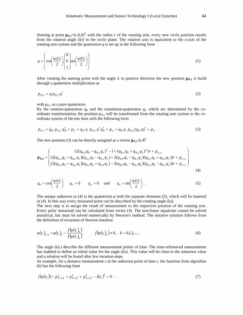
Kinematic Measurement and Sensor Technology I (Local Systems) 44
Starting at point pD,1=(r,0,0)T with the radius r of the rotating arm, every new circle position results from the rotation angle φ(t) in the circle plane. The rotation axis is equivalent to the z-axis of the rotating arm system and the quaternion q is set up in the following form
=
2)(sin
100
,2
)(cos ttq ϕϕ . (1)
After rotating the starting point with the angle φ in positive direction the new position pD,2 is build through a quaternion multiplication as
∗= qpqp DD 1,2, (2) with pD,1 as a pure quaternion. By the rotation-quaternion qR and the translation-quaternion qtr which are determined by the co-ordinate transformation, the position pD,2 will be transformed from the rotating arm system to the co-ordinate system of the test item with the following form
trRDRtrRDRtrRDRP pqqpqqpqqpqqpqpqp +=+=+= ∗∗∗∗ )(1,1,2,2, . (3)
The new position (3) can be directly assigned as a vector pP,2 in R3
+−−−++++−+−+
+++−−=
ztrzxRyRzzRRzRzRzyRxR
ytrzRzRzzRRzxRyRzyRxR
xtrzyRxRzzRR
prqqqqqqqqqqqqqqqqprqqqqqqqqqqqqqqqq
prqqqqqqqq
,,0,,00,0,0,,0,
,0,0,,00,,0,,0,
,2
,0,2
,00,
)))((2))((2()))((2))((2(
))(1)(2(
P,2p
(4)
===
=
2)(sin und 0 0
2)(cos0
tqqqtq zyxϕϕ . (5)
The unique unknown in (4) is the quaternion q with the separate elements (5), which will be inserted in (4). In this way every measured point can be described by the rotating angle φ(t). The next step is to assign the result of measurement to the respective position of the rotating arm. Every polar mesurand can be calculated from vector (4). The non-linear equations cannot be solved analytical, but must be solved numerically by Newton's method. The iterative solution follows from the definition of recursion of Newton iteration
( ) ( ) ( )( )( )( ) ( )( ) ,.....2,1,0 0, ,1 =≠−=+ ktftftf
tt kiki
kikiki ϕ
ϕϕ
ϕϕ &&
(6)
The angle φ(ti) describe the different measurement points of time. The time-referenced measurement has enabled to define an initial value for the angle φ(ti). This value will be close to the unknown value and a solution will be found after few iteration steps. As example, for a distance measurement s at the unknown point of time t1 the function from algorithm (6) has the following form
( )( ) ( ) 021
2,2,
2,2,
2,2,1 =−++= tsppptf ZPYPXPϕ . (7)
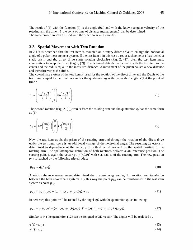
1st International Conference on Machine Control & Guidance 2008 45
The result of (6) with the function (7) is the angle φ(t1) and with the known angular velocity of the rotating arm the time t1 – the point of time of distance measurement – can be determined. The same procedure can be used with the other polar measurands.
3.3 Spatial Movement with Two Rotation In 2.1 it is described that the test item is mounted on a rotary direct drive to enlarge the horizontal angle of a polar measurement system. If the test item – in this case a robot-tacheometer – has locked a static prism and the direct drive starts rotating clockwise (Fig. 2, (1)), then the test item must countersteer to keep the prism (Fig 2, (2)). The acquired data deliver a circle with the test item in the center and the radius equal to the measured distance. A movement of the prism causes a new distance and therefore varies the circle. The co-ordinate system of the test item is used for the rotation of the direct drive and the Z-axis of the test item is equal to the rotation axis for the quaternion q1 with the rotation angle γ(t) at the point of time t
=
2)(sin
100
,2
)(cos1ttq γγ . (8)
The second rotation (Fig. 2, (3)) results from the rotating arm and the quaternion q2 has the same form as (1)
=
2)(sin
100
,2
)(cos2ttq ϕϕ . (9)
Now the test item tracks the prism of the rotating arm and through the rotation of the direct drive under the test item, there is an additional change of the horizontal angle. The resulting trajectory is determined in dependence of the velocity of both direct drives and by the spatial position of the rotating arm. The spatiotemporal definition of both rotations delivers a 4D reference position. The starting point is again the vector pD,1=(r,0,0)T with r as radius of the rotating arm. The new position pD,2 is reached by the following tripleproduct
∗= 2122, qpqp D,D . (10) A static reference measurement determined the quaternion qR and qtr for rotation and translation between the both co-ordinate systems. By this way the point pD,2 can be transformed in the test item system as point pP,2
trRDRtrRDRP qqqpqqqqpqp +=+= ∗∗∗ )( 21,22,2, . (11) In next step this point will be rotated by the angel γ(t) with the quaternion q1 as following
∗∗∗∗∗ +=+== 1131,311211,2112,13, )()( qqqqpqqqqqqqpqqqqpqp trDtrRDRPP . (12) Similar to (4) the quaternion (12) can be assigned as 3D-vector. The angles will be replaced by
tt Dωϕ =)( (13) tt Pωγ =)( (14)
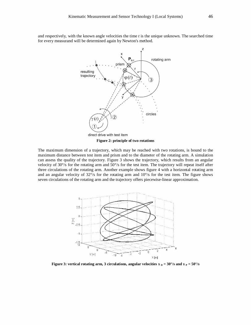
Kinematic Measurement and Sensor Technology I (Local Systems) 46
and respectively, with the known angle velocities the time t is the unique unknown. The searched time for every measurand will be determined again by Newton's method.
Figure 2: principle of two rotations
The maximum dimension of a trajectory, which may be reached with two rotations, is bound to the maximum distance between test item and prism and to the diameter of the rotating arm. A simulation can assess the quality of the trajectory. Figure 3 shows the trajectory, which results from an angular velocity of 30°/s for the rotating arm and 50°/s for the test item. The trajectory will repeat itself after three circulations of the rotating arm. Another example shows figure 4 with a horizontal rotating arm and an angular velocity of 32°/s for the rotating arm and 10°/s for the test item. The figure shows seven circulations of the rotating arm and the trajectory offers piecewise-linear approximation.
Figure 3: vertical rotating arm, 3 circulations, angular velocities ωD = 30°/s and ωP = 50°/s
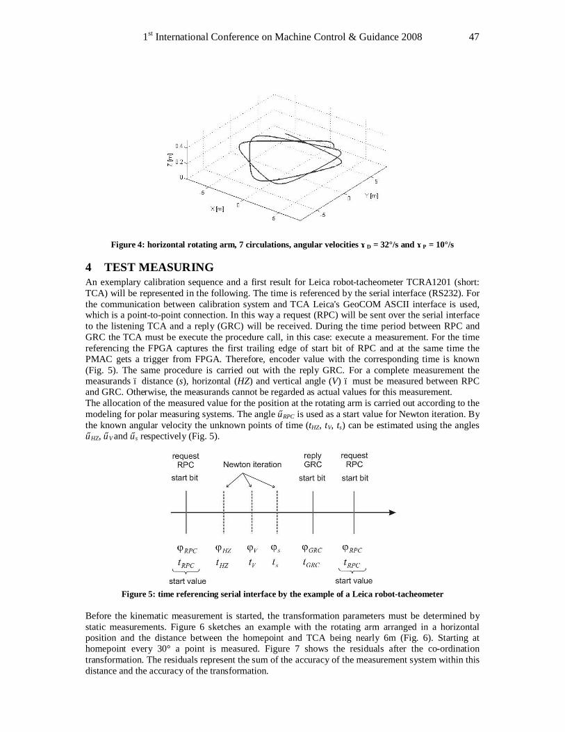
1st International Conference on Machine Control & Guidance 2008 47
Figure 4: horizontal rotating arm, 7 circulations, angular velocities ωD = 32°/s and ωP = 10°/s
4 TEST MEASURING An exemplary calibration sequence and a first result for Leica robot-tacheometer TCRA1201 (short: TCA) will be represented in the following. The time is referenced by the serial interface (RS232). For the communication between calibration system and TCA Leica's GeoCOM ASCII interface is used, which is a point-to-point connection. In this way a request (RPC) will be sent over the serial interface to the listening TCA and a reply (GRC) will be received. During the time period between RPC and GRC the TCA must be execute the procedure call, in this case: execute a measurement. For the time referencing the FPGA captures the first trailing edge of start bit of RPC and at the same time the PMAC gets a trigger from FPGA. Therefore, encoder value with the corresponding time is known (Fig. 5). The same procedure is carried out with the reply GRC. For a complete measurement the measurands – distance (s), horizontal (HZ) and vertical angle (V) – must be measured between RPC and GRC. Otherwise, the measurands cannot be regarded as actual values for this measurement. The allocation of the measured value for the position at the rotating arm is carried out according to the modeling for polar measuring systems. The angle φRPC is used as a start value for Newton iteration. By the known angular velocity the unknown points of time (tHZ, tV, ts) can be estimated using the angles φHZ, φV and φs respectively (Fig. 5).
Figure 5: time referencing serial interface by the example of a Leica robot-tacheometer
Before the kinematic measurement is started, the transformation parameters must be determined by static measurements. Figure 6 sketches an example with the rotating arm arranged in a horizontal position and the distance between the homepoint and TCA being nearly 6m (Fig. 6). Starting at homepoint every 30° a point is measured. Figure 7 shows the residuals after the co-ordination transformation. The residuals represent the sum of the accuracy of the measurement system within this distance and the accuracy of the transformation.
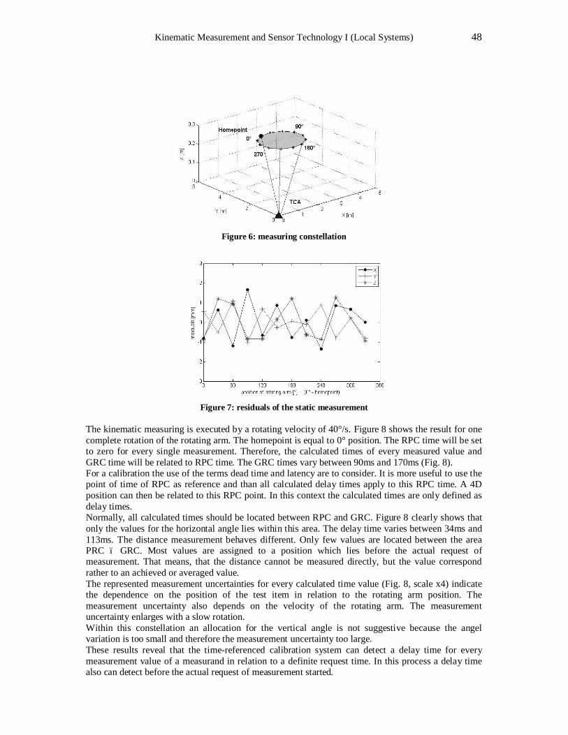
Kinematic Measurement and Sensor Technology I (Local Systems) 48
Figure 6: measuring constellation
Figure 7: residuals of the static measurement
The kinematic measuring is executed by a rotating velocity of 40°/s. Figure 8 shows the result for one complete rotation of the rotating arm. The homepoint is equal to 0° position. The RPC time will be set to zero for every single measurement. Therefore, the calculated times of every measured value and GRC time will be related to RPC time. The GRC times vary between 90ms and 170ms (Fig. 8). For a calibration the use of the terms dead time and latency are to consider. It is more useful to use the point of time of RPC as reference and than all calculated delay times apply to this RPC time. A 4D position can then be related to this RPC point. In this context the calculated times are only defined as delay times. Normally, all calculated times should be located between RPC and GRC. Figure 8 clearly shows that only the values for the horizontal angle lies within this area. The delay time varies between 34ms and 113ms. The distance measurement behaves different. Only few values are located between the area PRC – GRC. Most values are assigned to a position which lies before the actual request of measurement. That means, that the distance cannot be measured directly, but the value correspond rather to an achieved or averaged value. The represented measurement uncertainties for every calculated time value (Fig. 8, scale x4) indicate the dependence on the position of the test item in relation to the rotating arm position. The measurement uncertainty also depends on the velocity of the rotating arm. The measurement uncertainty enlarges with a slow rotation. Within this constellation an allocation for the vertical angle is not suggestive because the angel variation is too small and therefore the measurement uncertainty too large. These results reveal that the time-referenced calibration system can detect a delay time for every measurement value of a measurand in relation to a definite request time. In this process a delay time also can detect before the actual request of measurement started.
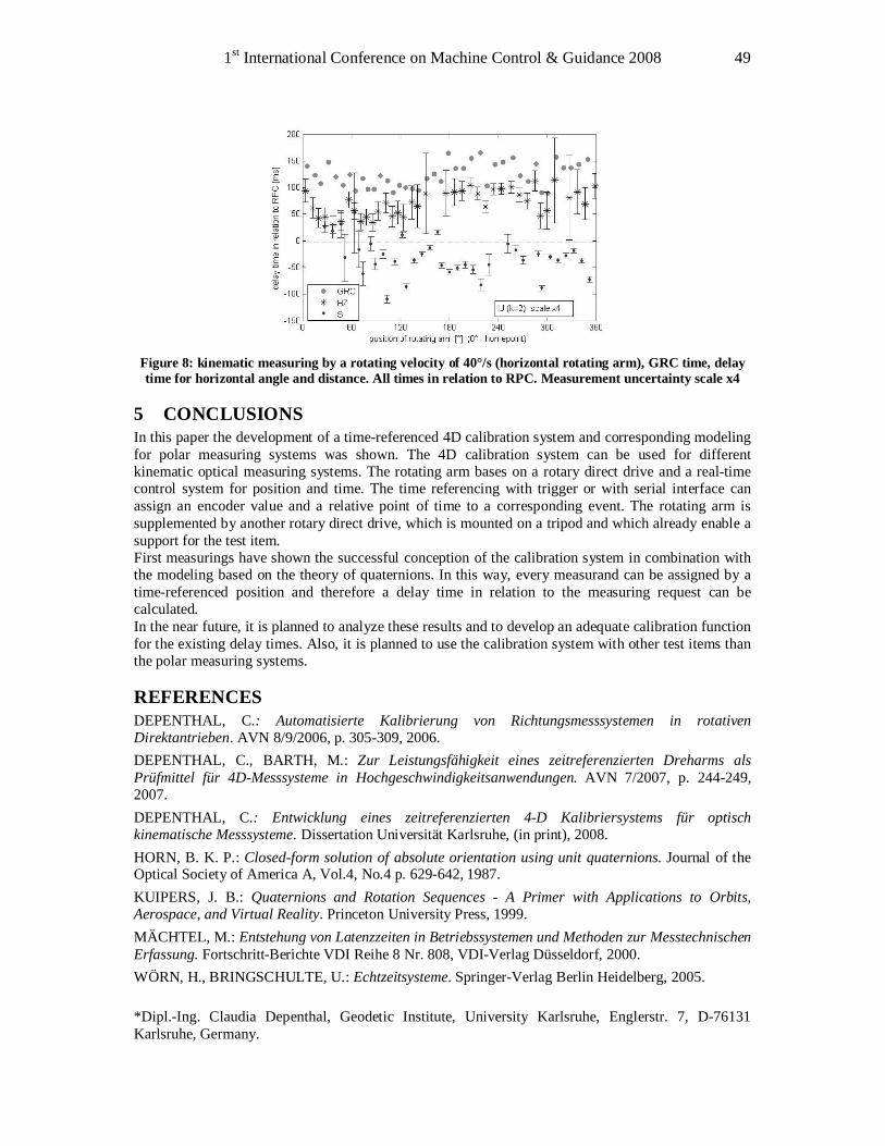
1st International Conference on Machine Control & Guidance 2008 49
Figure 8: kinematic measuring by a rotating velocity of 40°/s (horizontal rotating arm), GRC time, delay time for horizontal angle and distance. All times in relation to RPC. Measurement uncertainty scale x4
5 CONCLUSIONS In this paper the development of a time-referenced 4D calibration system and corresponding modeling for polar measuring systems was shown. The 4D calibration system can be used for different kinematic optical measuring systems. The rotating arm bases on a rotary direct drive and a real-time control system for position and time. The time referencing with trigger or with serial interface can assign an encoder value and a relative point of time to a corresponding event. The rotating arm is supplemented by another rotary direct drive, which is mounted on a tripod and which already enable a support for the test item. First measurings have shown the successful conception of the calibration system in combination with the modeling based on the theory of quaternions. In this way, every measurand can be assigned by a time-referenced position and therefore a delay time in relation to the measuring request can be calculated. In the near future, it is planned to analyze these results and to develop an adequate calibration function for the existing delay times. Also, it is planned to use the calibration system with other test items than the polar measuring systems.
REFERENCES DEPENTHAL, C.: Automatisierte Kalibrierung von Richtungsmesssystemen in rotativen Direktantrieben. AVN 8/9/2006, p. 305-309, 2006. DEPENTHAL, C., BARTH, M.: Zur Leistungsfähigkeit eines zeitreferenzierten Dreharms als Prüfmittel für 4D-Messsysteme in Hochgeschwindigkeitsanwendungen. AVN 7/2007, p. 244-249, 2007. DEPENTHAL, C.: Entwicklung eines zeitreferenzierten 4-D Kalibriersystems für optisch kinematische Messsysteme. Dissertation Universität Karlsruhe, (in print), 2008. HORN, B. K. P.: Closed-form solution of absolute orientation using unit quaternions. Journal of the Optical Society of America A, Vol.4, No.4 p. 629-642, 1987. KUIPERS, J. B.: Quaternions and Rotation Sequences - A Primer with Applications to Orbits, Aerospace, and Virtual Reality. Princeton University Press, 1999. MÄCHTEL, M.: Entstehung von Latenzzeiten in Betriebssystemen und Methoden zur Messtechnischen Erfassung. Fortschritt-Berichte VDI Reihe 8 Nr. 808, VDI-Verlag Düsseldorf, 2000. WÖRN, H., BRINGSCHULTE, U.: Echtzeitsysteme. Springer-Verlag Berlin Heidelberg, 2005. *Dipl.-Ing. Claudia Depenthal, Geodetic Institute, University Karlsruhe, Englerstr. 7, D-76131 Karlsruhe, Germany.

Kinematic Measurement and Sensor Technology I (Local Systems) 50
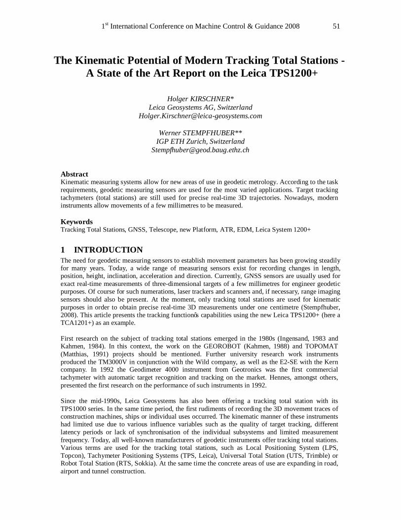
1st International Conference on Machine Control & Guidance 2008 51
The Kinematic Potential of Modern Tracking Total Stations - A State of the Art Report on the Leica TPS1200+
Holger KIRSCHNER*
Leica Geosystems AG, Switzerland [email protected]
Werner STEMPFHUBER**
IGP ETH Zurich, Switzerland [email protected]
Abstract Kinematic measuring systems allow for new areas of use in geodetic metrology. According to the task requirements, geodetic measuring sensors are used for the most varied applications. Target tracking tachymeters (total stations) are still used for precise real-time 3D trajectories. Nowadays, modern instruments allow movements of a few millimetres to be measured. Keywords Tracking Total Stations, GNSS, Telescope, new Platform, ATR, EDM, Leica System 1200+
1 INTRODUCTION The need for geodetic measuring sensors to establish movement parameters has been growing steadily for many years. Today, a wide range of measuring sensors exist for recording changes in length, position, height, inclination, acceleration and direction. Currently, GNSS sensors are usually used for exact real-time measurements of three-dimensional targets of a few millimetres for engineer geodetic purposes. Of course for such numerations, laser trackers and scanners and, if necessary, range imaging sensors should also be present. At the moment, only tracking total stations are used for kinematic purposes in order to obtain precise real-time 3D measurements under one centimetre (Stempfhuber, 2008). This article presents the tracking function’s capabilities using the new Leica TPS1200+ (here a TCA1201+) as an example. First research on the subject of tracking total stations emerged in the 1980s (Ingensand, 1983 and Kahmen, 1984). In this context, the work on the GEOROBOT (Kahmen, 1988) and TOPOMAT (Matthias, 1991) projects should be mentioned. Further university research work instruments produced the TM3000V in conjunction with the Wild company, as well as the E2-SE with the Kern company. In 1992 the Geodimeter 4000 instrument from Geotronics was the first commercial tachymeter with automatic target recognition and tracking on the market. Hennes, amongst others, presented the first research on the performance of such instruments in 1992. Since the mid-1990s, Leica Geosystems has also been offering a tracking total station with its TPS1000 series. In the same time period, the first rudiments of recording the 3D movement traces of construction machines, ships or individual uses occurred. The kinematic manner of these instruments had limited use due to various influence variables such as the quality of target tracking, different latency periods or lack of synchronisation of the individual subsystems and limited measurement frequency. Today, all well-known manufacturers of geodetic instruments offer tracking total stations. Various terms are used for the tracking total stations, such as Local Positioning System (LPS, Topcon), Tachymeter Positioning Systems (TPS, Leica), Universal Total Station (UTS, Trimble) or Robot Total Station (RTS, Sokkia). At the same time the concrete areas of use are expanding in road, airport and tunnel construction.

Kinematic Measurement and Sensor Technology I (Local Systems) 52
In the following article, the various components such as target tracking, motorisation, reflector and electronic distance measurement will be more closely examined and verified in respect to the kinematic requirements for reference tracks. The results of the TPS1200+ show that the deviations in position and height to a geometrically known reference lie within the scope of a few millimetres.
2 MOTIVATION AND INITIAL SITUATION Tachymeters are used for the most varied of tasks in the field of engineering geodesy. Geodesists know that there are currently hardly any alternatives to this optical measuring system, neither for static nor kinematic measuring tasks. Presently the main area of use for kinematic measuring systems is in road construction. Here fine grading, milling off existing layers, compaction and, above all, installation of road surfaces has to be carried out to a level of precision of a few millimetres. The definition of the required measure of quality often varies here. In tunnel and airport construction, comparable precision of surfaces is required. When considering such requirements in detail, certain questions quickly arise regarding the 3D trajectory with tracking total stations:
- the maximum tracking speed - the precision of 360° prism (influence of orientation and tilting) - the dynamic behaviour of the integrated two-axis tilt sensor - the synchronisation of the angle and distance measurements, as well as the latency and dead
times - the quality of the kinematic angle and distance measuring - the behaviour of the target tracking (generally in strong sunlight, rain, snow, darkness or fog) - the configuration or use of the measuring process (e.g. with Leica via onboard application,
GeoCom or a company internal binary protocol) - the maximum ranges and their impact on the measurement precision - the measuring frequency - the possibilities of retrieval after target loss - prism identification (target selection) - Multipath - the instrument calibration, particularly the calibration of the target tracking unit or internal
EDM calibration and data transmission The following aims to demonstrate the performance and absolute position precision that can be reached using one of today’s tracking total stations. This will be done using the new Leica TPS1200+ instrument as the example (release autumn 2007). Special attention should be paid here to the separation of the individual influence variables. The completely redesigned telescope in the TPS1200+ has created significant improvements. Furthermore, this article will specify measures for optimising kinematic measurement apparatus. Before presenting and evaluating the results, a comprehensive description will first be made of the individual subsystems of the target tracking TPS1200+.
3 TECHNICAL DESCRIPTION OF THE INDIVIDUAL SUBSYSTEMS A modern tachymeter establishes the spherical polar coordinates using the measurements of the various individual components, which are also known as subsystems. The essential processes arise from the distance, horizontal and vertical angle measurements, target tracking (known as ATR for Leica) as well as the complete servomotor control system, the two-axis tilt sensor, data calculation, storage and output. The Leica GeoCom Manual provides a good overview of the individual hard and software components. This lists all the relevant subsystems and their interactions using the example of the bidirectional communication between the TPS1200 and a computer. All results of the relevant subsystems are collected in a data pool. This allows all readings and reductions to be selected via a serial interface. The instrument firmware is entirely responsible for measurements with the GeoCom instruction set. In the new telescope, the EDM, ATR and PowerSearch hardware is condensed to one circuit board (see paragraph 3.1).
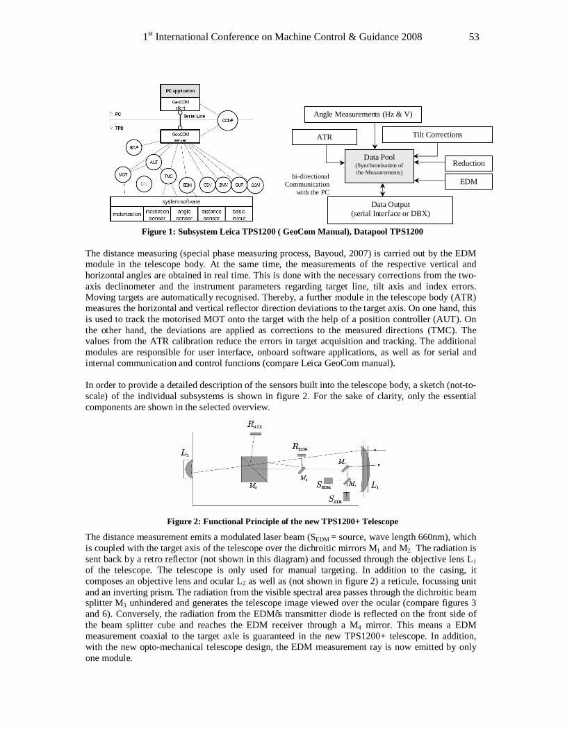
1st International Conference on Machine Control & Guidance 2008 53
Figure 1: Subsystem Leica TPS1200 ( GeoCom Manual), Datapool TPS1200
The distance measuring (special phase measuring process, Bayoud, 2007) is carried out by the EDM module in the telescope body. At the same time, the measurements of the respective vertical and horizontal angles are obtained in real time. This is done with the necessary corrections from the two-axis declinometer and the instrument parameters regarding target line, tilt axis and index errors. Moving targets are automatically recognised. Thereby, a further module in the telescope body (ATR) measures the horizontal and vertical reflector direction deviations to the target axis. On one hand, this is used to track the motorised MOT onto the target with the help of a position controller (AUT). On the other hand, the deviations are applied as corrections to the measured directions (TMC). The values from the ATR calibration reduce the errors in target acquisition and tracking. The additional modules are responsible for user interface, onboard software applications, as well as for serial and internal communication and control functions (compare Leica GeoCom manual). In order to provide a detailed description of the sensors built into the telescope body, a sketch (not-to-scale) of the individual subsystems is shown in figure 2. For the sake of clarity, only the essential components are shown in the selected overview.
Figure 2: Functional Principle of the new TPS1200+ Telescope
The distance measurement emits a modulated laser beam (SEDM = source, wave length 660nm), which is coupled with the target axis of the telescope over the dichroitic mirrors M1 and M2. The radiation is sent back by a retro reflector (not shown in this diagram) and focussed through the objective lens L1 of the telescope. The telescope is only used for manual targeting. In addition to the casing, it composes an objective lens and ocular L2 as well as (not shown in figure 2) a reticule, focussing unit and an inverting prism. The radiation from the visible spectral area passes through the dichroitic beam splitter M3 unhindered and generates the telescope image viewed over the ocular (compare figures 3 and 6). Conversely, the radiation from the EDM’s transmitter diode is reflected on the front side of the beam splitter cube and reaches the EDM receiver through a M4 mirror. This means a EDM measurement coaxial to the target axle is guaranteed in the new TPS1200+ telescope. In addition, with the new opto-mechanical telescope design, the EDM measurement ray is now emitted by only one module.
Data Pool (Synchronisation of the Measurements)
Angle Measurements (Hz & V)
Tilt Corrections ATR
EDM
Data Output (serial Interface or DBX)
bi-directional Communication
with the PC
Reductionen
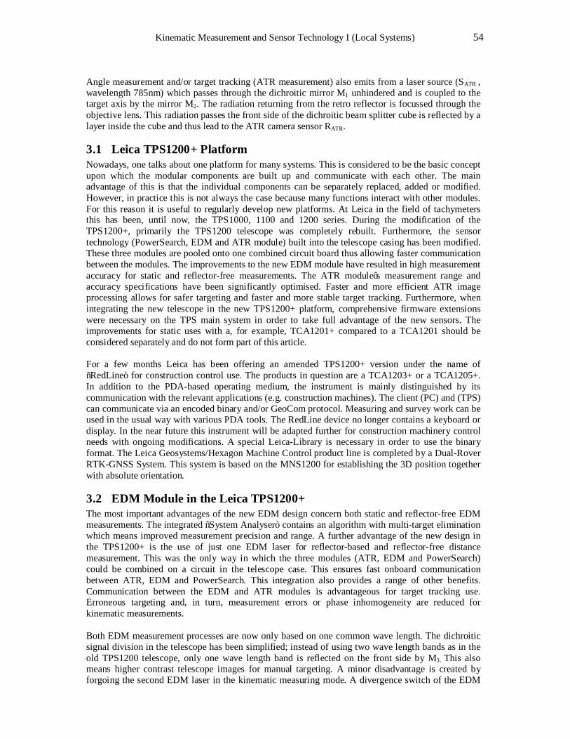
Kinematic Measurement and Sensor Technology I (Local Systems) 54
Angle measurement and/or target tracking (ATR measurement) also emits from a laser source (SATR , wavelength 785nm) which passes through the dichroitic mirror M1 unhindered and is coupled to the target axis by the mirror M2. The radiation returning from the retro reflector is focussed through the objective lens. This radiation passes the front side of the dichroitic beam splitter cube is reflected by a layer inside the cube and thus lead to the ATR camera sensor RATR.
3.1 Leica TPS1200+ Platform Nowadays, one talks about one platform for many systems. This is considered to be the basic concept upon which the modular components are built up and communicate with each other. The main advantage of this is that the individual components can be separately replaced, added or modified. However, in practice this is not always the case because many functions interact with other modules. For this reason it is useful to regularly develop new platforms. At Leica in the field of tachymeters this has been, until now, the TPS1000, 1100 and 1200 series. During the modification of the TPS1200+, primarily the TPS1200 telescope was completely rebuilt. Furthermore, the sensor technology (PowerSearch, EDM and ATR module) built into the telescope casing has been modified. These three modules are pooled onto one combined circuit board thus allowing faster communication between the modules. The improvements to the new EDM module have resulted in high measurement accuracy for static and reflector-free measurements. The ATR module’s measurement range and accuracy specifications have been significantly optimised. Faster and more efficient ATR image processing allows for safer targeting and faster and more stable target tracking. Furthermore, when integrating the new telescope in the new TPS1200+ platform, comprehensive firmware extensions were necessary on the TPS main system in order to take full advantage of the new sensors. The improvements for static uses with a, for example, TCA1201+ compared to a TCA1201 should be considered separately and do not form part of this article. For a few months Leica has been offering an amended TPS1200+ version under the name of “RedLine” for construction control use. The products in question are a TCA1203+ or a TCA1205+. In addition to the PDA-based operating medium, the instrument is mainly distinguished by its communication with the relevant applications (e.g. construction machines). The client (PC) and (TPS) can communicate via an encoded binary and/or GeoCom protocol. Measuring and survey work can be used in the usual way with various PDA tools. The RedLine device no longer contains a keyboard or display. In the near future this instrument will be adapted further for construction machinery control needs with ongoing modifications. A special Leica-Library is necessary in order to use the binary format. The Leica Geosystems/Hexagon Machine Control product line is completed by a Dual-Rover RTK-GNSS System. This system is based on the MNS1200 for establishing the 3D position together with absolute orientation.
3.2 EDM Module in the Leica TPS1200+ The most important advantages of the new EDM design concern both static and reflector-free EDM measurements. The integrated “System Analyser” contains an algorithm with multi-target elimination which means improved measurement precision and range. A further advantage of the new design in the TPS1200+ is the use of just one EDM laser for reflector-based and reflector-free distance measurement. This was the only way in which the three modules (ATR, EDM and PowerSearch) could be combined on a circuit in the telescope case. This ensures fast onboard communication between ATR, EDM and PowerSearch. This integration also provides a range of other benefits. Communication between the EDM and ATR modules is advantageous for target tracking use. Erroneous targeting and, in turn, measurement errors or phase inhomogeneity are reduced for kinematic measurements. Both EDM measurement processes are now only based on one common wave length. The dichroitic signal division in the telescope has been simplified; instead of using two wave length bands as in the old TPS1200 telescope, only one wave length band is reflected on the front side by M3. This also means higher contrast telescope images for manual targeting. A minor disadvantage is created by forgoing the second EDM laser in the kinematic measuring mode. A divergence switch of the EDM
1st International Conference on Machine Control & Guidance 2008 55
laser is necessary for both measurement modes. On the other hand, space constrictions meant that the divergence switch control had to be combined with the controls for the internal calibration of the reflector based EDM. This has created a slightly longer time period to switch to the internal calibration path. A new built-in revolver wheel switches between the reflector-free and reflector-based distance measurements (Bayoud, 2007). Here it can be seen that the internal calibration of the EDM creates a 700ms long measurement gap. With a standard instrument this is performed every 10 seconds. During the EDM calibration, no real-time data is available for the user. However, this is also the case with other manufacturers’ instruments (see Wagner, 2006). Otherwise, measurements of around 8-10Hz are possible with the built-in EDM module.
3.3 ATR Module in the Leica TPS1200+ The modules for horizontal and vertical angle measurement remain unchanged, as do the relevant slant correction to the conventional TPS1200 instrument. This paper will only consider the improved ATR module. Angle measurement happens on retro-reflective targets, which are generally triple prisms. As shown in figure 3 (left), the ATR laser radiation is emitted from a target device SATR which is reflected back to the measuring device by a retro-reflector and focussed on a camera sensor RATR by an objective L1. Figure 3 shows the measuring principle in a simplified model for short and long range. The SATR target device can therefore be replaced by its virtual image S´ATR caused by the reflection on M2.
Range > 100m Range << 100m
Figure 3: Measuring Principle of the new TPS1200+ ATR Module
The camera sensor RATR, together with the main objective L1, presents an “focus-infinity camera system”, although the camera centre CATR lies very close to the vertex V of the tilting and vertical axes. Again for demonstrative purposes, the distances in the diagram have been exaggerated. In good approximation, the laser target device can be construed as a point source, the location of the S´ATR virtual image is also near to V. The systematic error, which is generated by the distance
at the edge of the ATR field of view is 0.1mm (independent of the reflector distance) and is therefore negligible with other measurement errors. The measurement arrangement in ATR mode in figure 3 (left) correlates with a larger reflector distance, i.e. range to reflector> 100m. For this long range, the detected image of the point source S´ATR on the sensor, is a very small spot of only a few pixels in diameter. The position of this spot on the CCD sensor is calculated in the sensor coordination system by the ATR image processing system. Later, the values for the Hz and V deviations will be calculated from the position in the total station coordinate system. Divergences in establishing the spot position lead to errors in determining direction. In long range use (reflector distance > 100m), the camera sensor is the dominating source of error. The errors (noise) in the brightness value of the few pixels involved in the spot image and the variation in the electrical parameters of these pixels limit the measurement precision. On one hand, the improvements to measurement errors with the TPS1200+ for long range was the result of the higher resolution of the CMOS image sensor compared to the previous system. On the

Kinematic Measurement and Sensor Technology I (Local Systems) 56
other hand, the new CMOS sensor offers higher dynamic, which means less errors with the pixel brightness values. In close range measurement, i.e. for reflector distances << 100m (see fig. 3 right), a slightly different spot shape is produced. The virtual image of the point source which was created by the reflector has a shorter distance to the ATR camera system in close range. The image position through L1 (real image) moves behind the sensor RATR. A defocused image of the point source appears on the sensor. The defocus leads to a circular symmetric point spread function. This means the centre of brightness of the image does not move compared with the long range. A spot image appears, as shown in figure 3. The “hole” in the middle of the spot is created by the fastening of M2. This central aperture is centrosymmetric to the ATR camera centre and therefore does not lead to any further systematic errors. This is an advantage for static two-face measurements. Due to the size of the spot image in close range, the image sensor retreats as an error source. The influence of the pixel variation is negligible as the position averages across all the spot image pixels. The dominant error influence is the laser emitter. The point source has a slightly varying radiant intensity, i.e. it generates uneven target illumination. This is negligible for large target distances because only very small solid angles of the given radiation contribute to the image. On the other hand, in close range uneven target illumination causes greater total errors. The amount becomes less the more the distance increases. This distance dependence of measurement precision in the TPS1200 is shown in figure 4 (definition of measurement precision see Bockhorn, 2006).
0 20 40 60 80 100 120 140 160 180 2000
0.5
1
1.5
2
2.5
3
Measurement Error ATR-Deviation vs. Measurement Range
Range in [m]
ATR
-Ang
le E
rror [
arcs
ec]
SimulationMeasurement HzMeasurement V
Figure 4: ATR-Error versus Prim Range (Simulation)
The modified ATR wave length of 785nm in the TPS1200+ (in the old TPS1200 telescope 850nm) allows additional use of the new laser sources with improved features and, above all, increased performance with unchanged laser safety class (IEC 60825-1 Class 1: unrestricted eye-safe). This, in particular, increases precision for measurements with larger ranges. In close range, one additionally profits from more regular illumination of the ATR field of view with the new laser emitter. This means a significant increase in angle measurement for close range has been implemented in the new TPS1200+.
3.4 Angle Measurement from ATR, Telescope and Tilt Sensor The direction determination to the reflector, i.e. from the image of the point source and direction determination to the inversion centre of the prim are equivalent. This camera is permanently focussed at infinity. The point source is therefore focussed for larger distances. For close range measurements, a blurred image is created without losing measurement precision. Furthermore, a temperature calibration has been installed in the telescope to ensure stability. In addition, the new higher resolution CMOS sensor provides more precise determination of the spot centre, therefore offering increased precision for direction position determination. For static measurements, the TPS1201 reaches a measurement precision of one arc second according to ISO 17123-3, and for close range measurement errors of less than 1mm. A protected implementation for the user means that ATR precisions can also be established in lock mode with sub-pixel precision.

1st International Conference on Machine Control & Guidance 2008 57
The ATR module provides more than 200 image segmentations per second (compare: a PC manages around 50 XVGA image segmentations per second whilst using 100 times as much power). This high measurement frequency ensures stable target tracking, even with short reflector distances. For large ranges, sufficient measurement precision can only be achieved with retro-reflective tripe prisms of sufficient size. With too small reflector diameters << 20mm or cat’s eye reflector or reflector tape, the measurement is significantly less precise. This is primarily due to the fact that the aperture stop of the measurement bundle for small reflector diameters is at the reflector and, thus, the camera centre of the imaging system is moved. This creates distance dependent systematic errors in the conversion of the pixel deviations into angle deviations. If the reflector becomes dirty, this also has a negative effect on precision. For kinematic measurements the influence of the refraction of the glass when measuring with tilted triple prisms is also perturbing. This error is reduced by multi-spot analysis of the ATR algorithm.
3.5 Influence of the 360° Reflector on the ATR Automatic tracking of precision prisms is imperative for precise measurement with minimal sources of error. A simple and price effective implementation is surely not elaborate. All manufacturers’ tracking total stations use 360° prisms for kinematic measurements. Such all-round reflectors are generally built out of many triple prisms (e.g. Leica GRZ4, GRZ121 or the new GRZ122). The advantage of being able to use the reflector independent of its horizontal orientation is confronted by the disadvantage of larger measurement errors (Hennes, 2000). Prism-dependent errors in horizontal and vertical directions here are several millimetres. The reflector’s additional error contribution is caused by refraction of the EDM and ATR sensor radiation on the lens of the all-round reflector (Ingensand, 2001).
0 20 40 60 80 100 120 140 160 180-4
-3
-2
-1
0
1
2
3Variation of a rotation 36° Prism (horizontal View)
Rotation Leica GRZ4 360°-Prism in [deg]
Dev
atio
n in
[mm
]
ENH
Figure 5: Rotation 360° Prism (GRZ4) Figure 6: 360° Prism ATR Spot close-up range
Figure 5 shows the influence of continual rotation of a Leica GRZ4 all-round reflector on the reflector axis, in static horizontal measurements at 50m apart with the TPS1200+. Here the reflector rotates along its (vertical) longitudinal axis in 0.3° steps. This example shows relative examples in the height (H) of 2.4mm, in the EDM measurement (N) of 0.5mm and in the direction vertical to both (E) of approximately 1.5mm. With steep measurements an even greater height error is produced. It is simple to estimate the error from reflector geometry and refractive index for the EDM measurement. For ATR measurements, this measurement error, mostly of Hz direction, is corrected by analysing several prisms of different orientation. This is outlined in the following figure. For measurements on the direct prism area (fig. 6, left side bottom), the spot image (fig. 6 left side top) is similar to the precision single prism but the systematic errors are however high due to the vertical tilt of the prism (the prism orientation in fig. 6 left side equals to the rotation angle 90° in fig. 5). Conversely, an ATR measurement on an edge crossover (fig. 6 right side bottom) of the two participating prisms generates two diagonally displaced spot images in opposite directions (fig. 6 right side top). This is due to the strong tilting of the prisms. In this case, the mean of both spot centres is used for the ATR measurement. This means respective errors establishing deviations are
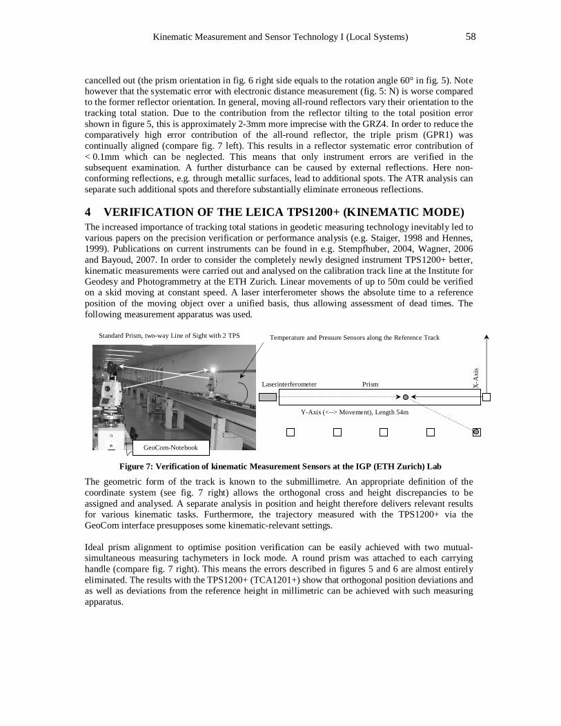
Kinematic Measurement and Sensor Technology I (Local Systems) 58
cancelled out (the prism orientation in fig. 6 right side equals to the rotation angle 60° in fig. 5). Note however that the systematic error with electronic distance measurement (fig. 5: N) is worse compared to the former reflector orientation. In general, moving all-round reflectors vary their orientation to the tracking total station. Due to the contribution from the reflector tilting to the total position error shown in figure 5, this is approximately 2-3mm more imprecise with the GRZ4. In order to reduce the comparatively high error contribution of the all-round reflector, the triple prism (GPR1) was continually aligned (compare fig. 7 left). This results in a reflector systematic error contribution of < 0.1mm which can be neglected. This means that only instrument errors are verified in the subsequent examination. A further disturbance can be caused by external reflections. Here non-conforming reflections, e.g. through metallic surfaces, lead to additional spots. The ATR analysis can separate such additional spots and therefore substantially eliminate erroneous reflections.
4 VERIFICATION OF THE LEICA TPS1200+ (KINEMATIC MODE) The increased importance of tracking total stations in geodetic measuring technology inevitably led to various papers on the precision verification or performance analysis (e.g. Staiger, 1998 and Hennes, 1999). Publications on current instruments can be found in e.g. Stempfhuber, 2004, Wagner, 2006 and Bayoud, 2007. In order to consider the completely newly designed instrument TPS1200+ better, kinematic measurements were carried out and analysed on the calibration track line at the Institute for Geodesy and Photogrammetry at the ETH Zurich. Linear movements of up to 50m could be verified on a skid moving at constant speed. A laser interferometer shows the absolute time to a reference position of the moving object over a unified basis, thus allowing assessment of dead times. The following measurement apparatus was used.
Figure 7: Verification of kinematic Measurement Sensors at the IGP (ETH Zurich) Lab
The geometric form of the track is known to the submillimetre. An appropriate definition of the coordinate system (see fig. 7 right) allows the orthogonal cross and height discrepancies to be assigned and analysed. A separate analysis in position and height therefore delivers relevant results for various kinematic tasks. Furthermore, the trajectory measured with the TPS1200+ via the GeoCom interface presupposes some kinematic-relevant settings. Ideal prism alignment to optimise position verification can be easily achieved with two mutual-simultaneous measuring tachymeters in lock mode. A round prism was attached to each carrying handle (compare fig. 7 right). This means the errors described in figures 5 and 6 are almost entirely eliminated. The results with the TPS1200+ (TCA1201+) show that orthogonal position deviations and as well as deviations from the reference height in millimetric can be achieved with such measuring apparatus.
Laserinterferometer Prism X-A
xis
Y-Axis (<--> Movement), Length 54m
Temperature and Pressure Sensors along the Reference Track Standard Prism, two-way Line of Sight with 2 TPS
GeoCom-Notebook
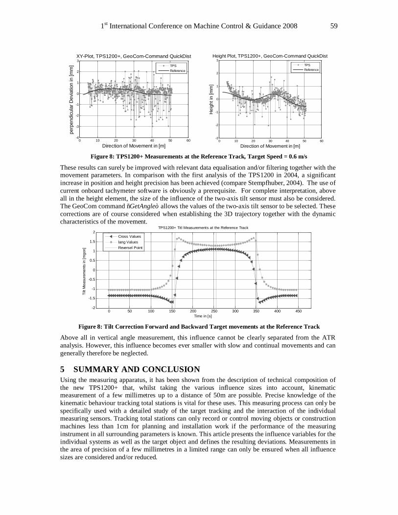
1st International Conference on Machine Control & Guidance 2008 59
0 10 20 30 40 50 60-4
-3
-2
-1
0
1
2
3
Direction of Movement in [m]
perp
endi
cula
r Dev
iatio
n in
[mm
]
XY-Plot, TPS1200+, GeoCom-Command QuickDist
TPSReference
0 10 20 30 40 50 60-3
-2
-1
0
1
2
3
Direction of Movement in [m]
Hei
ght i
n [m
m]
Height Plot, TPS1200+, GeoCom-Command QuickDist
TPSReference
Figure 8: TPS1200+ Measurements at the Reference Track, Target Speed = 0.6 m/s
These results can surely be improved with relevant data equalisation and/or filtering together with the movement parameters. In comparison with the first analysis of the TPS1200 in 2004, a significant increase in position and height precision has been achieved (compare Stempfhuber, 2004). The use of current onboard tachymeter software is obviously a prerequisite. For complete interpretation, above all in the height element, the size of the influence of the two-axis tilt sensor must also be considered. The GeoCom command “GetAngle” allows the values of the two-axis tilt sensor to be selected. These corrections are of course considered when establishing the 3D trajectory together with the dynamic characteristics of the movement.
0 50 100 150 200 250 300 350 400 450-2
-1.5
-1
-0.5
0
0.5
1
1.5
2
Time in [s]
Tilt
Mea
sure
men
ts in
[mgo
n]
TPS1200+ Titl Measurements at the Reference Track
Cross Valueslang ValuesReversel Point
Figure 8: Tilt Correction Forward and Backward Target movements at the Reference Track
Above all in vertical angle measurement, this influence cannot be clearly separated from the ATR analysis. However, this influence becomes ever smaller with slow and continual movements and can generally therefore be neglected.
5 SUMMARY AND CONCLUSION Using the measuring apparatus, it has been shown from the description of technical composition of the new TPS1200+ that, whilst taking the various influence sizes into account, kinematic measurement of a few millimetres up to a distance of 50m are possible. Precise knowledge of the kinematic behaviour tracking total stations is vital for these uses. This measuring process can only be specifically used with a detailed study of the target tracking and the interaction of the individual measuring sensors. Tracking total stations can only record or control moving objects or construction machines less than 1cm for planning and installation work if the performance of the measuring instrument in all surrounding parameters is known. This article presents the influence variables for the individual systems as well as the target object and defines the resulting deviations. Measurements in the area of precision of a few millimetres in a limited range can only be ensured when all influence sizes are considered and/or reduced.
Kinematic Measurement and Sensor Technology I (Local Systems) 60
REFERENCES BAYOUD, F.: Leica TPS1200+ A Telescope with Opto-Meachnical Design, White Paper, www.leica-geosystems.com, 2007.
BOCKHORN, M.: Richtungsbestimmung mit Leica ATR bei Zielweiten über 100m, Fachhochschule Bochum, Fachbereich Vermessungswesen und Geoinformatik, unveröffentlichte Masterarbeit, 2006.
HENNES, M.: Leistungsmerkmale des One-Man-Systems Geodimeter System 4000, VR 54. Vol. 5+6, Seite 287-295, 1992.
HENNES, M.: Grundlegende Aspekte zur Bestimmung der Leistungsfähigkeit von Robottachymetern, AVN 106, S. 374-385, 1999.
HENNES, M. and FAVRE, C.: Zum Einfluss der geometrischen Ausrichtung von 360°-Reflektoren bei Messungen mit automatischer Zielerfassung, VPK 2/2000, S. 72-78, 2000.
INGENSAND, H.: Die Weiterentwicklung der automatischen Zieleinstellung nach dem Intensitätsmaximumprinzip, BDVI-Forum, Vol. 4, Seite 212-223, 1983.
INGENSAND, H.: Systematische Einflusse auf praktische Messungen mit dem Tachymeter
und Digitalnivellier, DVW Schriftenreihe 42/2001, Qualitätsmanagement in der geodätischen Messtechnik, Wittwer Verlag Stuttgart, S. 120-137, 2001.
http://www.leica-geosystems.com, last accessed on April 22, 2008, Leica GeoCom Manual.
KAHMEN, H.: Selbsttätig zielende tachymetrische Vermessungssysteme für Aufgaben der Ingenieurgeodäsie, IX. Internationaler Kurs für Ingenieurvermessung, Dümmler Verlag, Bonn, Band 1, 1984.
KAHMEN, H. and STEUDEL, J.: Das automatisch zielende Messsystem GEOROBOT II, Ingenieurvermessung Dümmler Verlag, Bonn, 1988.
MATTHIAS, H.: Der Robotertheodolit TOPOMAT, Technik, Anwendungen und Auswirkungen auf dem Beruf, Vermessung Photogrammetrie und Kultur, Heft 8/91, S. 427-431, 1991.
STAIGER, R.: Verfahren der automatischen Zielpunktserfassung und -verfolgung, DVW Schriftenreihe 29/1998, Hybride Vermessungssysteme - Grundlagen und Anwendungen -, Wittwer Verlag Stuttgart, S. 13-27, 1998.
STEMPFHUBER, W. and WUNDERLICH, TH., Auf dem Weg zur Sensorsynchronisation von GPS und TPS für kinematische Messaufgaben, Allgemeine Vermessungs-Nachrichten (AVN), 05/2004.
STEMPFHUBER, W.: Baumaschinenführung und -steuerung, Von der statischen zur kinematischen Absteckung, ZfV Heft 1/2008, Seite 36-44, 2008.
WAGNER, M.: Trimble ATS-Totalstation: Moderne hochgenaue Tracking-Systeme für Anwendungen in der Baubranche. (www.trimble.com/ats_wp.asp), 2006.
* Dr. Holger Kirschner, Leica Geosystems AG, Heinrich-Wild-Strasse, CH-9435 Heerbrugg. ** Dr. Werner Stempfhuber, Institute of Geodesy, Wolfgang-Pauli-Str. 15, CH-8093 Zürich.
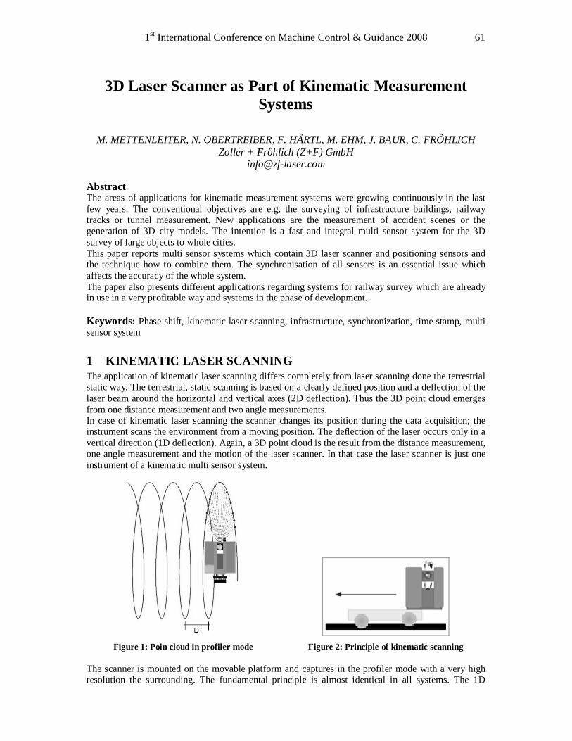
1st International Conference on Machine Control & Guidance 2008 61
3D Laser Scanner as Part of Kinematic Measurement Systems
M. METTENLEITER, N. OBERTREIBER, F. HÄRTL, M. EHM, J. BAUR, C. FRÖHLICH
Zoller + Fröhlich (Z+F) GmbH [email protected]
Abstract The areas of applications for kinematic measurement systems were growing continuously in the last few years. The conventional objectives are e.g. the surveying of infrastructure buildings, railway tracks or tunnel measurement. New applications are the measurement of accident scenes or the generation of 3D city models. The intention is a fast and integral multi sensor system for the 3D survey of large objects to whole cities. This paper reports multi sensor systems which contain 3D laser scanner and positioning sensors and the technique how to combine them. The synchronisation of all sensors is an essential issue which affects the accuracy of the whole system. The paper also presents different applications regarding systems for railway survey which are already in use in a very profitable way and systems in the phase of development. Keywords: Phase shift, kinematic laser scanning, infrastructure, synchronization, time-stamp, multi sensor system
1 KINEMATIC LASER SCANNING The application of kinematic laser scanning differs completely from laser scanning done the terrestrial static way. The terrestrial, static scanning is based on a clearly defined position and a deflection of the laser beam around the horizontal and vertical axes (2D deflection). Thus the 3D point cloud emerges from one distance measurement and two angle measurements. In case of kinematic laser scanning the scanner changes its position during the data acquisition; the instrument scans the environment from a moving position. The deflection of the laser occurs only in a vertical direction (1D deflection). Again, a 3D point cloud is the result from the distance measurement, one angle measurement and the motion of the laser scanner. In that case the laser scanner is just one instrument of a kinematic multi sensor system.
Figure 1: Poin cloud in profiler mode Figure 2: Principle of kinematic scanning
The scanner is mounted on the movable platform and captures in the profiler mode with a very high resolution the surrounding. The fundamental principle is almost identical in all systems. The 1D
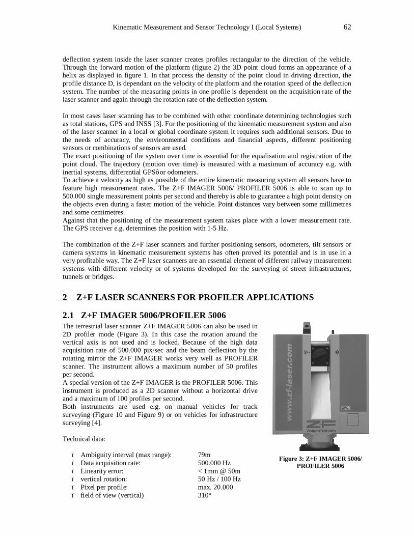
Kinematic Measurement and Sensor Technology I (Local Systems) 62
deflection system inside the laser scanner creates profiles rectangular to the direction of the vehicle. Through the forward motion of the platform (figure 2) the 3D point cloud forms an appearance of a helix as displayed in figure 1. In that process the density of the point cloud in driving direction, the profile distance D, is dependant on the velocity of the platform and the rotation speed of the deflection system. The number of the measuring points in one profile is dependent on the acquisition rate of the laser scanner and again through the rotation rate of the deflection system. In most cases laser scanning has to be combined with other coordinate determining technologies such as total stations, GPS and INSS [3]. For the positioning of the kinematic measurement system and also of the laser scanner in a local or global coordinate system it requires such additional sensors. Due to the needs of accuracy, the environmental conditions and financial aspects, different positioning sensors or combinations of sensors are used. The exact positioning of the system over time is essential for the equalisation and registration of the point cloud. The trajectory (motion over time) is measured with a maximum of accuracy e.g. with inertial systems, differential GPS’ or odometers. To achieve a velocity as high as possible of the entire kinematic measuring system all sensors have to feature high measurement rates. The Z+F IMAGER 5006/ PROFILER 5006 is able to scan up to 500.000 single measurement points per second and thereby is able to guarantee a high point density on the objects even during a faster motion of the vehicle. Point distances vary between some millimetres and some centimetres. Against that the positioning of the measurement system takes place with a lower measurement rate. The GPS receiver e.g. determines the position with 1-5 Hz. The combination of the Z+F laser scanners and further positioning sensors, odometers, tilt sensors or camera systems in kinematic measurement systems has often proved its potential and is in use in a very profitable way. The Z+F laser scanners are an essential element of different railway measurement systems with different velocity or of systems developed for the surveying of street infrastructures, tunnels or bridges.
2 Z+F LASER SCANNERS FOR PROFILER APPLICATIONS
2.1 Z+F IMAGER 5006/PROFILER 5006 The terrestrial laser scanner Z+F IMAGER 5006 can also be used in 2D profiler mode (Figure 3). In this case the rotation around the vertical axis is not used and is locked. Because of the high data acquisition rate of 500.000 pix/sec and the beam deflection by the rotating mirror the Z+F IMAGER works very well as PROFILER scanner. The instrument allows a maximum number of 50 profiles per second. A special version of the Z+F IMAGER is the PROFILER 5006. This instrument is produced as a 2D scanner without a horizontal drive and a maximum of 100 profiles per second. Both instruments are used e.g. on manual vehicles for track surveying (Figure 10 and Figure 9) or on vehicles for infrastructure surveying [4]. Technical data:
– Ambiguity interval (max range): 79m – Data acquisition rate: 500.000 Hz – Linearity error: < 1mm @ 50m – vertical rotation: 50 Hz / 100 Hz – Pixel per profile: max. 20.000 – field of view (vertical) 310°
Figure 3: Z+F IMAGER 5006/
PROFILER 5006
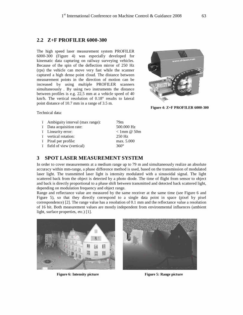
1st International Conference on Machine Control & Guidance 2008 63
2.2 Z+F PROFILER 6000-300 The high speed laser measurement system PROFILER 6000-300 (Figure 4) was especially developed for kinematic data capturing on railway surveying vehicles. Because of the spin of the deflection mirror of 250 Hz (rps) the vehicle can move very fast while the scanner captured a high dense point cloud. The distance between measurement points in the direction of motion can be increased by using multiple PROFILER scanners simultaneously . By using two instruments the distance between profiles is e.g. 22,5 mm at a vehicle speed of 40 km/h. The vertical resolution of 0.18° results to lateral point distance of 10.7 mm in a range of 3.5 m. Technical data:
– Ambiguity interval (max range): 79m – Data acquisition rate: 500.000 Hz – Linearity error: < 1mm @ 50m – vertical rotation: 250 Hz – Pixel per profile: max. 5.000 – field of view (vertical) 360°
3 SPOT LASER MEASUREMENT SYSTEM In order to cover measurements at a medium range up to 79 m and simultaneously realize an absolute accuracy within mm-range, a phase difference method is used, based on the transmission of modulated laser light. The transmitted laser light is intensity modulated with a sinusoidal signal. The light scattered back from the object is detected by a photo diode. The time of flight from sensor to object and back is directly proportional to a phase shift between transmitted and detected back scattered light, depending on modulation frequency and object range. Range and reflectance value are measured by the same receiver at the same time (see Figure 6 and Figure 5), so that they directly correspond to a single data point in space (pixel by pixel correspondence) [2]. The range value has a resolution of 0.1 mm and the reflectance value a resolution of 16 bit. Both measurement values are mostly independent from environmental influences (ambient light, surface properties, etc.) [1].
Figure 6: Intensity picture Figure 5: Range picture
Figure 4: Z+F PROFILER 6000-300
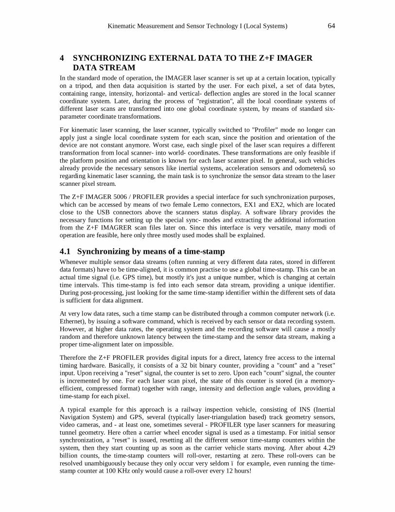
Kinematic Measurement and Sensor Technology I (Local Systems) 64
4 SYNCHRONIZING EXTERNAL DATA TO THE Z+F IMAGER DATA STREAM
In the standard mode of operation, the IMAGER laser scanner is set up at a certain location, typically on a tripod, and then data acquisition is started by the user. For each pixel, a set of data bytes, containing range, intensity, horizontal- and vertical- deflection angles are stored in the local scanner coordinate system. Later, during the process of "registration", all the local coordinate systems of different laser scans are transformed into one global coordinate system, by means of standard six-parameter coordinate transformations. For kinematic laser scanning, the laser scanner, typically switched to "Profiler" mode no longer can apply just a single local coordinate system for each scan, since the position and orientation of the device are not constant anymore. Worst case, each single pixel of the laser scan requires a different transformation from local scanner- into world- coordinates. These transformations are only feasible if the platform position and orientation is known for each laser scanner pixel. In general, such vehicles already provide the necessary sensors like inertial systems, acceleration sensors and odometers’, so regarding kinematic laser scanning, the main task is to synchronize the sensor data stream to the laser scanner pixel stream. The Z+F IMAGER 5006 / PROFILER provides a special interface for such synchronization purposes, which can be accessed by means of two female Lemo connectors, EX1 and EX2, which are located close to the USB connectors above the scanners status display. A software library provides the necessary functions for setting up the special sync- modes and extracting the additional information from the Z+F IMAGRER scan files later on. Since this interface is very versatile, many modi of operation are feasible, here only three mostly used modes shall be explained.
4.1 Synchronizing by means of a time-stamp Whenever multiple sensor data streams (often running at very different data rates, stored in different data formats) have to be time-aligned, it is common practise to use a global time-stamp. This can be an actual time signal (i.e. GPS time), but mostly it's just a unique number, which is changing at certain time intervals. This time-stamp is fed into each sensor data stream, providing a unique identifier. During post-processing, just looking for the same time-stamp identifier within the different sets of data is sufficient for data alignment. At very low data rates, such a time stamp can be distributed through a common computer network (i.e. Ethernet), by issuing a software command, which is received by each sensor or data recording system. However, at higher data rates, the operating system and the recording software will cause a mostly random and therefore unknown latency between the time-stamp and the sensor data stream, making a proper time-alignment later on impossible. Therefore the Z+F PROFILER provides digital inputs for a direct, latency free access to the internal timing hardware. Basically, it consists of a 32 bit binary counter, providing a "count" and a "reset" input. Upon receiving a "reset" signal, the counter is set to zero. Upon each "count" signal, the counter is incremented by one. For each laser scan pixel, the state of this counter is stored (in a memory-efficient, compressed format) together with range, intensity and deflection angle values, providing a time-stamp for each pixel. A typical example for this approach is a railway inspection vehicle, consisting of INS (Inertial Navigation System) and GPS, several (typically laser-triangulation based) track geometry sensors, video cameras, and - at least one, sometimes several - PROFILER type laser scanners for measuring tunnel geometry. Here often a carrier wheel encoder signal is used as a timestamp. For initial sensor synchronization, a "reset" is issued, resetting all the different sensor time-stamp counters within the system, then they start counting up as soon as the carrier vehicle starts moving. After about 4.29 billion counts, the time-stamp counters will roll-over, restarting at zero. These roll-overs can be resolved unambiguously because they only occur very seldom – for example, even running the time-stamp counter at 100 KHz only would cause a roll-over every 12 hours!
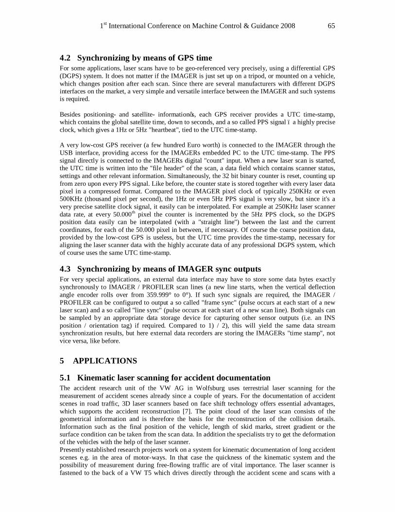
1st International Conference on Machine Control & Guidance 2008 65
4.2 Synchronizing by means of GPS time For some applications, laser scans have to be geo-referenced very precisely, using a differential GPS (DGPS) system. It does not matter if the IMAGER is just set up on a tripod, or mounted on a vehicle, which changes position after each scan. Since there are several manufacturers with different DGPS interfaces on the market, a very simple and versatile interface between the IMAGER and such systems is required. Besides positioning- and satellite- information’s, each GPS receiver provides a UTC time-stamp, which contains the global satellite time, down to seconds, and a so called PPS signal – a highly precise clock, which gives a 1Hz or 5Hz "heartbeat", tied to the UTC time-stamp. A very low-cost GPS receiver (a few hundred Euro worth) is connected to the IMAGER through the USB interface, providing access for the IMAGERs embedded PC to the UTC time-stamp. The PPS signal directly is connected to the IMAGERs digital "count" input. When a new laser scan is started, the UTC time is written into the "file header" of the scan, a data field which contains scanner status, settings and other relevant information. Simultaneously, the 32 bit binary counter is reset, counting up from zero upon every PPS signal. Like before, the counter state is stored together with every laser data pixel in a compressed format. Compared to the IMAGER pixel clock of typically 250KHz or even 500KHz (thousand pixel per second), the 1Hz or even 5Hz PPS signal is very slow, but since it's a very precise satellite clock signal, it easily can be interpolated. For example at 250KHz laser scanner data rate, at every 50.000th pixel the counter is incremented by the 5Hz PPS clock, so the DGPS position data easily can be interpolated (with a "straight line") between the last and the current coordinates, for each of the 50.000 pixel in between, if necessary. Of course the coarse position data, provided by the low-cost GPS is useless, but the UTC time provides the time-stamp, necessary for aligning the laser scanner data with the highly accurate data of any professional DGPS system, which of course uses the same UTC time-stamp.
4.3 Synchronizing by means of IMAGER sync outputs For very special applications, an external data interface may have to store some data bytes exactly synchronously to IMAGER / PROFILER scan lines (a new line starts, when the vertical deflection angle encoder rolls over from 359.999° to 0°). If such sync signals are required, the IMAGER / PROFILER can be configured to output a so called "frame sync" (pulse occurs at each start of a new laser scan) and a so called "line sync" (pulse occurs at each start of a new scan line). Both signals can be sampled by an appropriate data storage device for capturing other sensor outputs (i.e. an INS position / orientation tag) if required. Compared to 1) / 2), this will yield the same data stream synchronization results, but here external data recorders are storing the IMAGERs "time stamp", not vice versa, like before.
5 APPLICATIONS
5.1 Kinematic laser scanning for accident documentation The accident research unit of the VW AG in Wolfsburg uses terrestrial laser scanning for the measurement of accident scenes already since a couple of years. For the documentation of accident scenes in road traffic, 3D laser scanners based on face shift technology offers essential advantages, which supports the accident reconstruction [7]. The point cloud of the laser scan consists of the geometrical information and is therefore the basis for the reconstruction of the collision details. Information such as the final position of the vehicle, length of skid marks, street gradient or the surface condition can be taken from the scan data. In addition the specialists try to get the deformation of the vehicles with the help of the laser scanner. Presently established research projects work on a system for kinematic documentation of long accident scenes e.g. in the area of motor-ways. In that case the quickness of the kinematic system and the possibility of measurement during free-flowing traffic are of vital importance. The laser scanner is fastened to the back of a VW T5 which drives directly through the accident scene and scans with a
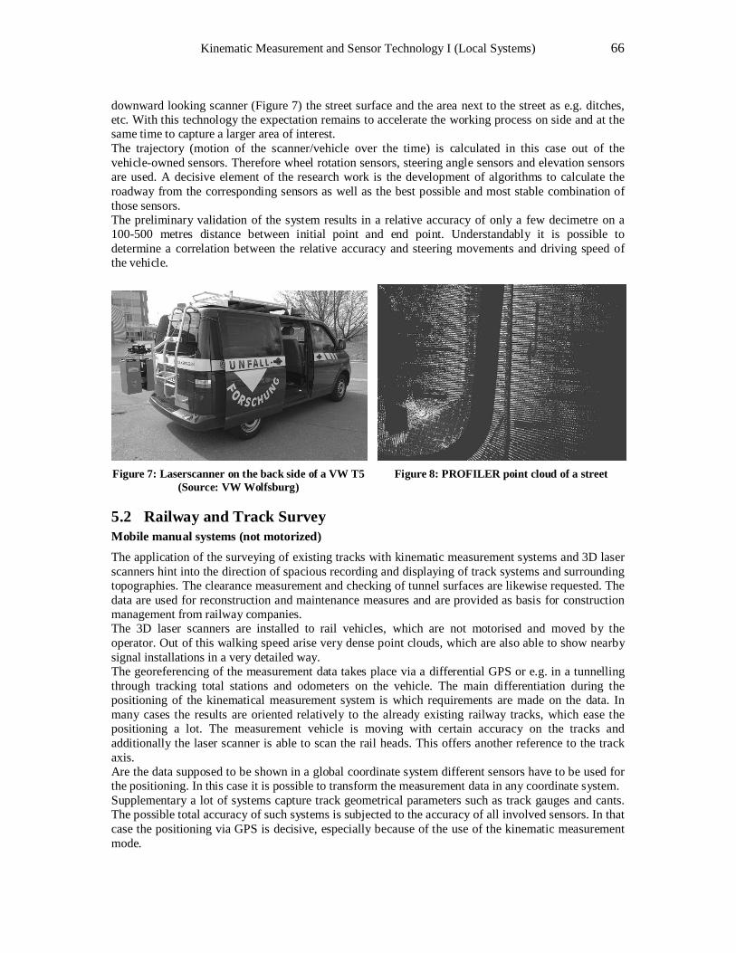
Kinematic Measurement and Sensor Technology I (Local Systems) 66
downward looking scanner (Figure 7) the street surface and the area next to the street as e.g. ditches, etc. With this technology the expectation remains to accelerate the working process on side and at the same time to capture a larger area of interest. The trajectory (motion of the scanner/vehicle over the time) is calculated in this case out of the vehicle-owned sensors. Therefore wheel rotation sensors, steering angle sensors and elevation sensors are used. A decisive element of the research work is the development of algorithms to calculate the roadway from the corresponding sensors as well as the best possible and most stable combination of those sensors. The preliminary validation of the system results in a relative accuracy of only a few decimetre on a 100-500 metres distance between initial point and end point. Understandably it is possible to determine a correlation between the relative accuracy and steering movements and driving speed of the vehicle.
Figure 7: Laserscanner on the back side of a VW T5
(Source: VW Wolfsburg) Figure 8: PROFILER point cloud of a street
5.2 Railway and Track Survey Mobile manual systems (not motorized) The application of the surveying of existing tracks with kinematic measurement systems and 3D laser scanners hint into the direction of spacious recording and displaying of track systems and surrounding topographies. The clearance measurement and checking of tunnel surfaces are likewise requested. The data are used for reconstruction and maintenance measures and are provided as basis for construction management from railway companies. The 3D laser scanners are installed to rail vehicles, which are not motorised and moved by the operator. Out of this walking speed arise very dense point clouds, which are also able to show nearby signal installations in a very detailed way. The georeferencing of the measurement data takes place via a differential GPS or e.g. in a tunnelling through tracking total stations and odometers on the vehicle. The main differentiation during the positioning of the kinematical measurement system is which requirements are made on the data. In many cases the results are oriented relatively to the already existing railway tracks, which ease the positioning a lot. The measurement vehicle is moving with certain accuracy on the tracks and additionally the laser scanner is able to scan the rail heads. This offers another reference to the track axis. Are the data supposed to be shown in a global coordinate system different sensors have to be used for the positioning. In this case it is possible to transform the measurement data in any coordinate system. Supplementary a lot of systems capture track geometrical parameters such as track gauges and cants. The possible total accuracy of such systems is subjected to the accuracy of all involved sensors. In that case the positioning via GPS is decisive, especially because of the use of the kinematic measurement mode.
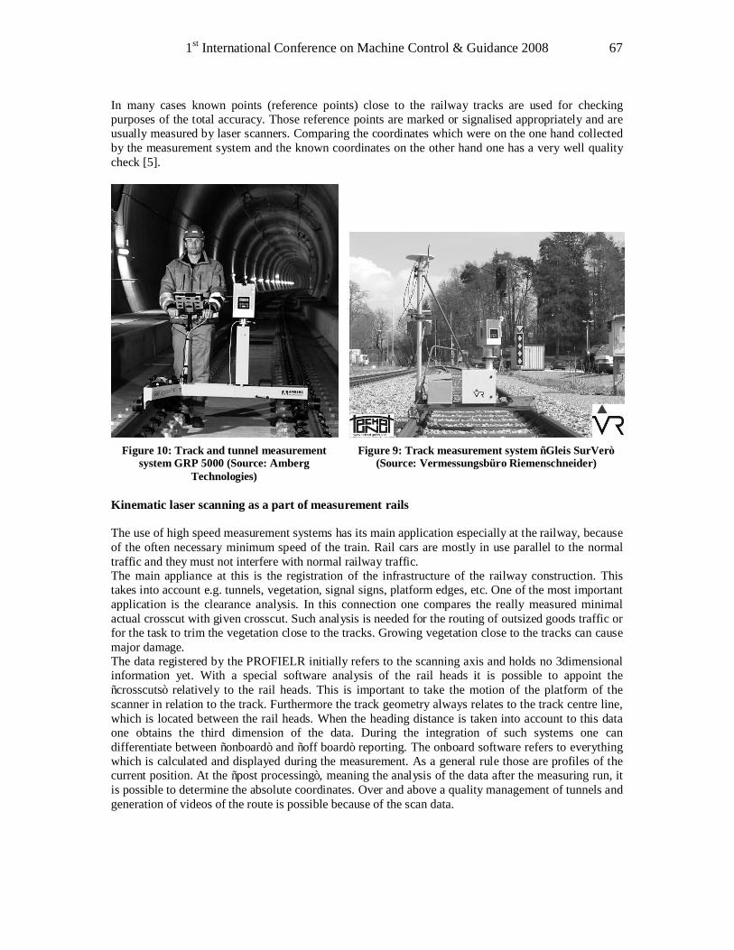
1st International Conference on Machine Control & Guidance 2008 67
In many cases known points (reference points) close to the railway tracks are used for checking purposes of the total accuracy. Those reference points are marked or signalised appropriately and are usually measured by laser scanners. Comparing the coordinates which were on the one hand collected by the measurement system and the known coordinates on the other hand one has a very well quality check [5].
Figure 10: Track and tunnel measurement
system GRP 5000 (Source: Amberg Technologies)
Figure 9: Track measurement system “Gleis SurVer” (Source: Vermessungsbüro Riemenschneider)
Kinematic laser scanning as a part of measurement rails The use of high speed measurement systems has its main application especially at the railway, because of the often necessary minimum speed of the train. Rail cars are mostly in use parallel to the normal traffic and they must not interfere with normal railway traffic. The main appliance at this is the registration of the infrastructure of the railway construction. This takes into account e.g. tunnels, vegetation, signal signs, platform edges, etc. One of the most important application is the clearance analysis. In this connection one compares the really measured minimal actual crosscut with given crosscut. Such analysis is needed for the routing of outsized goods traffic or for the task to trim the vegetation close to the tracks. Growing vegetation close to the tracks can cause major damage. The data registered by the PROFIELR initially refers to the scanning axis and holds no 3dimensional information yet. With a special software analysis of the rail heads it is possible to appoint the “crosscuts” relatively to the rail heads. This is important to take the motion of the platform of the scanner in relation to the track. Furthermore the track geometry always relates to the track centre line, which is located between the rail heads. When the heading distance is taken into account to this data one obtains the third dimension of the data. During the integration of such systems one can differentiate between “onboard” and “off board” reporting. The onboard software refers to everything which is calculated and displayed during the measurement. As a general rule those are profiles of the current position. At the “post processing”, meaning the analysis of the data after the measuring run, it is possible to determine the absolute coordinates. Over and above a quality management of tunnels and generation of videos of the route is possible because of the scan data.

Kinematic Measurement and Sensor Technology I (Local Systems) 68
Figure 12: 3 Profiler 6000 simultaneously Figure 11: Point cloud Profiler 6000
6 CONCLUSION The combination of kinematic measurement systems and 3D laser scanners to a multi sensor system is already reality in practise and is used successfully. Different systems for rail and street measurement have given prove to that. The advantage of multi sensor systems is an integral and fast registration which is highly important in the field of infrastructure. During motion collected 3D coordinates with a point density in the reach of millimetres and centimetres offer the possibility of a very detailed and at the same time efficient measurement. In a lot of areas the measurement has to take place without an interference of the free-flowing traffic by integrating the measurement vehicle in the “normal” traffic. A laser scanner with a high measurement rate based on phase shift technology as a part of a kinematic measurement system possesses the best requirements for this purpose.
ACKNOWLEDGEMENTS The authors would like to thank all involved institutes and persons. Especially the Accident Research Unit of VW AG, Wolfsburg, Herr Dipl.-Ing. Markus Jungmichel and Herr Dipl.-Ing. Andreas Riemenschneider, Vermessungsbüro Riemenschneider.
REFERENCES [1]Heinz, I., Mettenleiter, M., Härtl, F., Fröhlich, C.: “3-D Ladar for Inspection of Real World Environments“. 5th ISPRS Conf. on Optical 3-D Measurement Techniques, Wien, Oct 1-4 2001, pp.10 – 17
[2]Fröhlich, C.: „Aktive Erzeugung korrespondierender Tiefen- und Reflektivitätsbilder und ihre Nutzung zur Umgebungserfassung“; 1. Auflage; Pro Universitate Verlag, 1996
[3]Ingensand, H.: „Metrological Aspects In Terrestrial Laser-Scanning Technology“ 3rd IAG / 12th FIG Symposium, Baden, May 22-24, 2006

1st International Conference on Machine Control & Guidance 2008 69
[4]Zoller + Fröhlich GmbH: “Technical Data, Z+F IMAGER 5006”
[5]Riemenschneider, A.: “Das 3D-Multisensor-System auf der Basis des Messsystems Gleis SurVer in der Gleis- und Bauvermessung“ VDV - Schriftenreihe, Band 26
[6]Rolle, P.: „Untersuchung zur Verwendbarkeit fahrzeugspezifischer Sensoren für das kinematische Laserscanning“, Diplomarbeit, FH für Technik und Wirtschaft Dresden
[7]Ehm, M.; Saeger, H.; Fröhlich, C.: „Laser Scanning based on phase-shift or pulsed technology – which will be the future?”, 8th Conference on Optical 3-DMeasurement Techniques, Zürich, July 2007
*Zoller + Fröhlich (Z+F) GmbH, Simoniusstraße 22, D-88239 Wangen, Germany Phone: +49-7522-9308-0; www.zf-laser.com

Kinematic Measurement and Sensor Technology I (Local Systems) 70

1st International Conference on Machine Control & Guidance 2008 71
Local Positioning Systems in Construction Basics, Limitations and Examples of Application
Jochen WENDEBAUM, Johannes FLIEDNER, Bernhard MARX, Alfons HORN
MOBA, Mobile Automation AG, Limburg, Germany [email protected]
1 INTRODUCTION Many constructional applications are characterised by the use of mobile machines. In many cases the machine operator carries out machine control tasks which, on the one hand require high precision, on the other hand, however, involve frequent repetition or are highly monotone (for example when operating along a guide wire). Furthermore, often high investments referring the outline planning and the building measure itself are made without being able to implement the planning data with adequate accuracy when executing or to sufficiently document the constructional measures and a high remeasuring effort is necessary respectively. To abolish these weak points of conventional construction, the use of positioning systems that on the one hand support and relieve the operator respectively as well as on the other hand allow the documentation of the executed tasks is a precondition. In the following several positioning possibilities and applications are described in an overview.
2 THE NEED OF POSITIONING INFORMATION FOR MOBILE PROCESSING MACHINES
Mobile processing machines like construction machines, agricultural machines or mobile machines used within industrial logistics chains with few exceptions are manually controlled by positioning measurement systems without operator support. Different process chains as for example:
1. Bringing out the seed (storage – disposal/turnover – transport as well as spreading the seed), 2. Bringing in the harvest (harvesting – transport – storage – turnover), 3. Asphalt integration and compaction in road construction (storage – production of the fitting
material – transport – feeding – integration – compaction), 4. Mining and converting construction material in quarries (drilling/ramming – blasting –
excavator-lorry-operation – transport – conditioning – disposal/turnover) allow extensive rationalisation, enhanced quality and improved documentation of the executed tasks, provided that the processing machinery used is equipped with positioning measurement systems and supports the operator. However, the high investment costs, times for daily commissioning, often also during ongoing operation, as well as necessary trainings for the operating personnel among other aspects are reasons for caution regarding the acquisition and use of such systems. In addition, inbuilt weaknesses of the different versions of positioning measurement systems are to be considered: satellite-based (global) positioning measurement systems in many cases provide only insufficient accuracies in the vertical coordinate and in case of shadowing effects referring the receiver (for example due to buildings, bridges or the natural in-situ area) are unusable. Local positioning systems like tachymeters, depending on their application, require frequent moving of the measuring equipment. Therefore, to determine the positions of the different machines positioning systems have to be used which deliver the machine’s position with adequate accuracy at reasonable prices for the measuring equipment and acceptable operation effort.
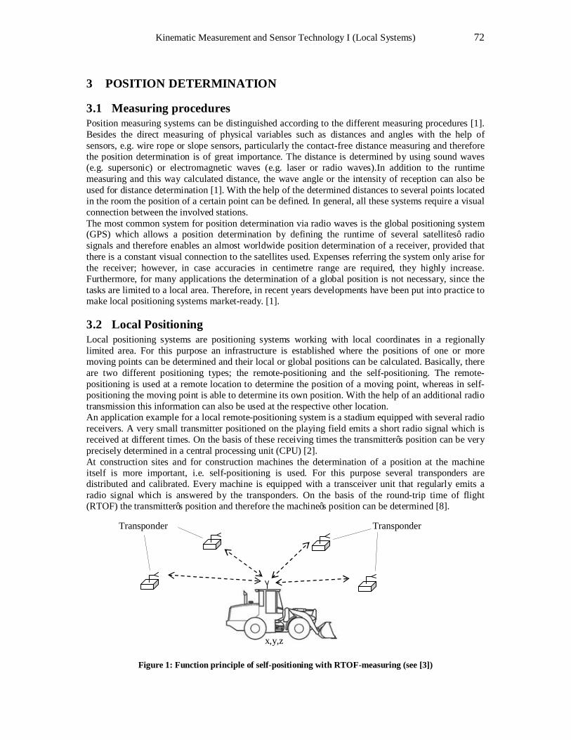
Kinematic Measurement and Sensor Technology I (Local Systems) 72
3 POSITION DETERMINATION
3.1 Measuring procedures Position measuring systems can be distinguished according to the different measuring procedures [1]. Besides the direct measuring of physical variables such as distances and angles with the help of sensors, e.g. wire rope or slope sensors, particularly the contact-free distance measuring and therefore the position determination is of great importance. The distance is determined by using sound waves (e.g. supersonic) or electromagnetic waves (e.g. laser or radio waves).In addition to the runtime measuring and this way calculated distance, the wave angle or the intensity of reception can also be used for distance determination [1]. With the help of the determined distances to several points located in the room the position of a certain point can be defined. In general, all these systems require a visual connection between the involved stations. The most common system for position determination via radio waves is the global positioning system (GPS) which allows a position determination by defining the runtime of several satellites’ radio signals and therefore enables an almost worldwide position determination of a receiver, provided that there is a constant visual connection to the satellites used. Expenses referring the system only arise for the receiver; however, in case accuracies in centimetre range are required, they highly increase. Furthermore, for many applications the determination of a global position is not necessary, since the tasks are limited to a local area. Therefore, in recent years developments have been put into practice to make local positioning systems market-ready. [1].
3.2 Local Positioning Local positioning systems are positioning systems working with local coordinates in a regionally limited area. For this purpose an infrastructure is established where the positions of one or more moving points can be determined and their local or global positions can be calculated. Basically, there are two different positioning types; the remote-positioning and the self-positioning. The remote-positioning is used at a remote location to determine the position of a moving point, whereas in self-positioning the moving point is able to determine its own position. With the help of an additional radio transmission this information can also be used at the respective other location. An application example for a local remote-positioning system is a stadium equipped with several radio receivers. A very small transmitter positioned on the playing field emits a short radio signal which is received at different times. On the basis of these receiving times the transmitter’s position can be very precisely determined in a central processing unit (CPU) [2]. At construction sites and for construction machines the determination of a position at the machine itself is more important, i.e. self-positioning is used. For this purpose several transponders are distributed and calibrated. Every machine is equipped with a transceiver unit that regularly emits a radio signal which is answered by the transponders. On the basis of the round-trip time of flight (RTOF) the transmitter’s position and therefore the machine’s position can be determined [8].
Figure 1: Function principle of self-positioning with RTOF-measuring (see [3])
Transponder Transponder
x,y,z
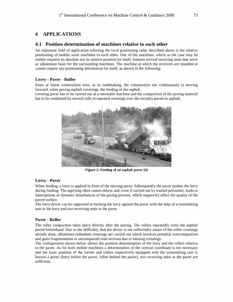
1st International Conference on Machine Control & Guidance 2008 73
4 APPLICATIONS
4.1 Position determination of machines relative to each other An important field of application referring the local positioning radar described above is the relative positioning of mobile work machines to each other. One of the machines, which as the case may be neither requires its absolute nor its relative position for itself, features several receiving units that serve as adjustment basis for the surrounding machines. The machine at which the receivers are installed at cannot require any positioning information for itself, as shown in the following: Lorry - Paver - Roller Since at linear construction sites, as in roadmaking, the construction site continuously is moving forward, when paving asphalt coverings, the feeding of the asphalt covering paver has to be carried out at a moveable machine and the compaction of the paving material has to be conducted by several rolls in repeated crossings over the recently paved-in asphalt.
Figure 2: Feeding of an asphalt paver [4]
Lorry - Paver When feeding, a lorry is applied in front of the moving paver. Subsequently the paver pushes the lorry during feeding. The applying often causes delays and, even if carried out by trained personnel, leads to interruptions or dynamic disturbances of the paving process, which negatively affect the quality of the paved surface. The lorry-driver can be supported at backing the lorry against the paver with the help of a transmitting unit at the lorry and two receiving units at the paver. Paver - Roller The roller compaction takes place directly after the paving. The rollers repeatedly cross the asphalt paved beforehand. Due to the difficulty, that the driver is not sufficiently aware of the roller crossings already done, oftentimes redundant crossings are carried out which involves potential overcompaction and grain fragmentation or uncompacted road sections due to missing crossings. The configuration shown below allows the position determination of the lorry and the rollers relative to the paver. As for both mobile machines a determination of the vertical coordinate is not necessary and the basic position of the lorries and rollers respectively equipped with the transmitting unit is known a priori (lorry before the paver, roller behind the paver), two receiving units at the paver are sufficient.
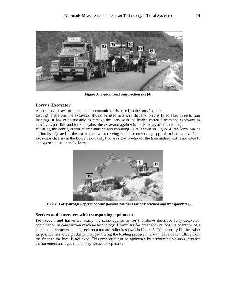
Kinematic Measurement and Sensor Technology I (Local Systems) 74
Figure 3: Typical road construction site [4]
Lorry – Excavator At the lorry-excavator-operation an economic use is based on the lorry’s quick loading. Therefore, the excavator should be used in a way that the lorry is filled after three to four loadings. It has to be possible to remove the lorry with the loaded material from the excavator as quickly as possible and back it against the excavator again when it is empty after unloading. By using the configuration of transmitting and receiving units, shown in Figure 4, the lorry can be optimally adjusted to the excavator: two receiving units are exemplary applied to both sides of the excavator chassis (in the figure below only two are shown) whereas the transmitting unit is mounted to an exposed position at the lorry.
Figure 4: Lorry-dredger-operation with possible positions for base stations and transponders [5]
Seeders and harvesters with transporting equipment For seeders and harvesters nearly the same applies as for the above described lorry-excavator-combination in construction machine technology. Exemplary for other applications the operation of a combine harvester reloading seed on a tractor trailer is shown in Figure 5. To optimally fill the trailer its position has to be gradually changed during the loading process in a way that an even filling from the front to the back is achieved. This procedure can be optimised by performing a simple distance measurement analogue to the lorry-excavator-operation.
BS1
T1 T2
BS
T1
T2
BS
BS
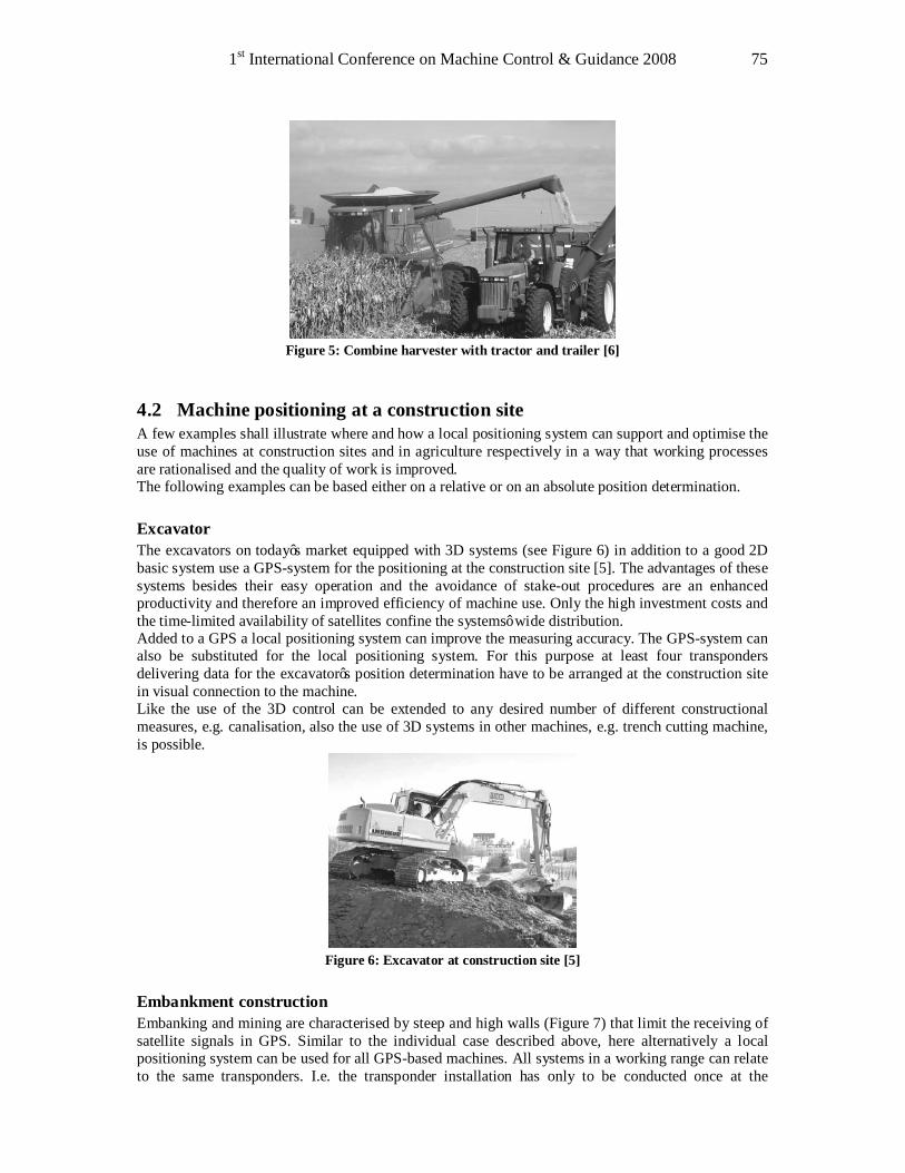
1st International Conference on Machine Control & Guidance 2008 75
Figure 5: Combine harvester with tractor and trailer [6]
4.2 Machine positioning at a construction site A few examples shall illustrate where and how a local positioning system can support and optimise the use of machines at construction sites and in agriculture respectively in a way that working processes are rationalised and the quality of work is improved. The following examples can be based either on a relative or on an absolute position determination. Excavator The excavators on today’s market equipped with 3D systems (see Figure 6) in addition to a good 2D basic system use a GPS-system for the positioning at the construction site [5]. The advantages of these systems besides their easy operation and the avoidance of stake-out procedures are an enhanced productivity and therefore an improved efficiency of machine use. Only the high investment costs and the time-limited availability of satellites confine the systems’ wide distribution. Added to a GPS a local positioning system can improve the measuring accuracy. The GPS-system can also be substituted for the local positioning system. For this purpose at least four transponders delivering data for the excavator’s position determination have to be arranged at the construction site in visual connection to the machine. Like the use of the 3D control can be extended to any desired number of different constructional measures, e.g. canalisation, also the use of 3D systems in other machines, e.g. trench cutting machine, is possible.
Figure 6: Excavator at construction site [5]
Embankment construction Embanking and mining are characterised by steep and high walls (Figure 7) that limit the receiving of satellite signals in GPS. Similar to the individual case described above, here alternatively a local positioning system can be used for all GPS-based machines. All systems in a working range can relate to the same transponders. I.e. the transponder installation has only to be conducted once at the
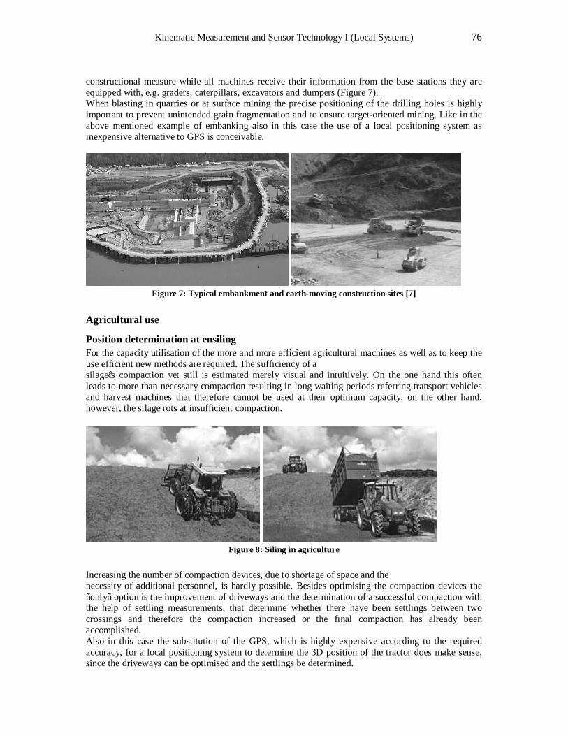
Kinematic Measurement and Sensor Technology I (Local Systems) 76
constructional measure while all machines receive their information from the base stations they are equipped with, e.g. graders, caterpillars, excavators and dumpers (Figure 7). When blasting in quarries or at surface mining the precise positioning of the drilling holes is highly important to prevent unintended grain fragmentation and to ensure target-oriented mining. Like in the above mentioned example of embanking also in this case the use of a local positioning system as inexpensive alternative to GPS is conceivable.
Figure 7: Typical embankment and earth-moving construction sites [7]
Agricultural use
Position determination at ensiling For the capacity utilisation of the more and more efficient agricultural machines as well as to keep the use efficient new methods are required. The sufficiency of a silage’s compaction yet still is estimated merely visual and intuitively. On the one hand this often leads to more than necessary compaction resulting in long waiting periods referring transport vehicles and harvest machines that therefore cannot be used at their optimum capacity, on the other hand, however, the silage rots at insufficient compaction.
Figure 8: Siling in agriculture
Increasing the number of compaction devices, due to shortage of space and the necessity of additional personnel, is hardly possible. Besides optimising the compaction devices the “only“ option is the improvement of driveways and the determination of a successful compaction with the help of settling measurements, that determine whether there have been settlings between two crossings and therefore the compaction increased or the final compaction has already been accomplished. Also in this case the substitution of the GPS, which is highly expensive according to the required accuracy, for a local positioning system to determine the 3D position of the tractor does make sense, since the driveways can be optimised and the settlings be determined.
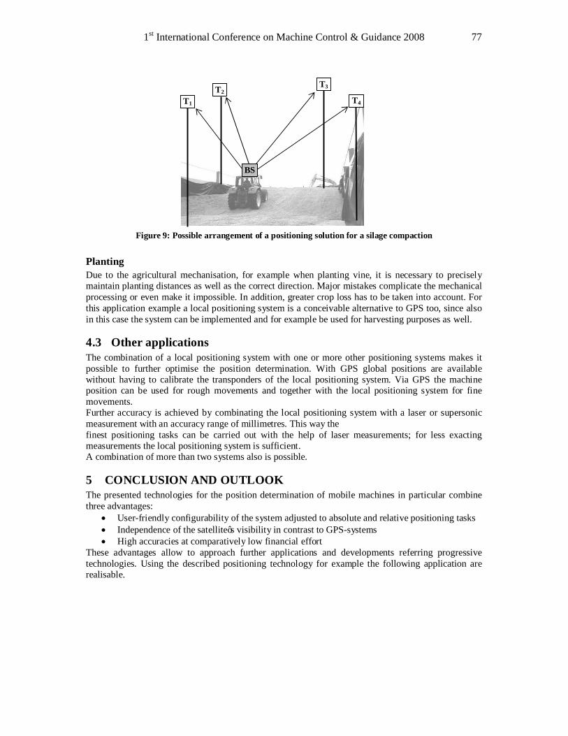
1st International Conference on Machine Control & Guidance 2008 77
Figure 9: Possible arrangement of a positioning solution for a silage compaction
Planting Due to the agricultural mechanisation, for example when planting vine, it is necessary to precisely maintain planting distances as well as the correct direction. Major mistakes complicate the mechanical processing or even make it impossible. In addition, greater crop loss has to be taken into account. For this application example a local positioning system is a conceivable alternative to GPS too, since also in this case the system can be implemented and for example be used for harvesting purposes as well.
4.3 Other applications The combination of a local positioning system with one or more other positioning systems makes it possible to further optimise the position determination. With GPS global positions are available without having to calibrate the transponders of the local positioning system. Via GPS the machine position can be used for rough movements and together with the local positioning system for fine movements. Further accuracy is achieved by combinating the local positioning system with a laser or supersonic measurement with an accuracy range of millimetres. This way the finest positioning tasks can be carried out with the help of laser measurements; for less exacting measurements the local positioning system is sufficient. A combination of more than two systems also is possible.
5 CONCLUSION AND OUTLOOK The presented technologies for the position determination of mobile machines in particular combine three advantages:
• User-friendly configurability of the system adjusted to absolute and relative positioning tasks • Independence of the satellite’s visibility in contrast to GPS-systems • High accuracies at comparatively low financial effort
These advantages allow to approach further applications and developments referring progressive technologies. Using the described positioning technology for example the following application are realisable.
BS
T1
T2
T3
T4

Kinematic Measurement and Sensor Technology I (Local Systems) 78
Positioning for automated guided vehicles The applications described in chapter 4.2 as well as many others like for example the control of sports field markings can also be realised without a machine operator. The same is valid for many other applications like the maintaining and clearing of circulation areas (driveways or runways), the cultivation of adjacent areas (e.g. mowing). It is also possible to use the system as a positioning help in stationary production lines or conveying systems where automated guided vehicles are intended to be freely area-moveable. Influence on traffic and vehicle control Receivers once calibrated when constructing a circulation area, a road in particular, can also be left and used for vehicle control and to prevent vehicle collisions. This is especially true for circulation areas where the same vehicles are consistently moving. In addition, the use for traffic control at busy motorway sections is conceivable and possible, provided the cars and lorries are equipped with transmitting units and vehicle distances are controlled to enhance the passage capacity. Literature 1. Vossiek et. al., "Wireless Local Positioning", IEEE microwave magazine, Dez. 2003, S. 77-86 2. Fischer et. al., "Local position measurement system for fast and accurate 3D monitoring",
Proceedings of the SPIE, Volume 5048, 2003, S. 128-135 3. Wiebking et. al, "Local Positioning Radar", Proceedings of the 1. Workshop on Positioning,
Navigation an Communication, Institute of Communications Engineering, Hannover, 2004 4. Jurasz, J., et.al: „OSYRIS Worksite Evaluation Report“, Universität Karlsruhe, 2003 5. Liebherr, www.liebherr.com 6. Wisconsin Farm Bureau Federation's online Media Center, www.wfbf.com 7. Wikimedia Commons, commons.wikimedia.org 8. Symeo AG, www.symeo.de
1st International Conference on Machine Control & Guidance 2008 79
Combination of Indoor and Outdoor Positioning
Rainer MAUTZ* ETH Zurich, Switzerland
[email protected] Abstract Indoor and outdoor environments create contradictory conditions for positioning and guidance of machines. While indoor environments are limited in size to rooms and buildings, outdoor positioning capabilities require regional or even global coverage. Secondly, the difficulty of receipting satellite signals indoors has triggered development of high sensitive and AGNSS receivers – with many issues remaining unsolved. Thirdly, the accuracy requirements are dissimilar between indoor and outdoor environments – typically there is a higher demand for relative accuracy indoors. This paper should be regarded as an overview of the current and near future positioning capabilities for indoor and outdoor environments. However, it does not lay claim to completeness. Focus is given on GNSS and various novel position systems that achieve cm-level accuracy or better which is a requirement for most applications in machine control and guidance of construction machines. Keywords Indoor positioning, GNSS, wireless networks, novel positioning systems, future positioning scenarios
1 INTRODUCTION In order to successfully control construction equipment or agricultural machinery, the ability to precisely position the machine in real-time is a curial component of any guidance system. Today, GNSS and tracking total stations play a dominant role for determining 3D real-time positions in machine control. However, to access increased availability, various weaknesses remain inherent in theses positioning systems such as signal attenuation, masking and requirement of direct line-of-sight. This paper addresses these weaknesses and looks forward to alternative positioning methods that may enable a 'Centimetres Everywhere' scenario in the near future. Unfortunately, locations inside buildings, basements and tunnels remain harsh environments for precise positioning. Typical indoor environments contain multiple walls and a large number of obstacles that are made of various materials. As a result, current indoor positioning systems cannot satisfy the challenging demands for most indoor applications. This insufficiency may explain the huge variety of approaches for indoor position systems. Some attempts exploit new sensors that measure inter-nodal ranges, signal strengths, acceleration or angles for localisation; as well as research, leading to higher sensitivity algorithms for signal acquisition and tracking in harsh environments and in particular the combined usage or integration of different sensor systems and data sources. The diversity of available sensors has lead to a variety of localisation schemes such as triangulation, trilateration, hyperbolic localisation, data matching and many more. The employed signal technologies include RF (radio frequency) technology, ultrasound, infrared, vision based systems and magnetic fields. The RF signal based technologies can be split into WLAN (2.4 GHz and 5 GHz band), Bluetooth (2.4 GHz band), Ultrawideband and RFID. In general, most techniques and algorithms can be applied for both outdoors and indoors. This paper focuses on innovative positioning hardware and techniques that are currently or in the near future available to determine positions of moving devices.

Kinematic Measurement and Sensor Technology I (Local Systems) 80
Software components such as Kalman filtering, outlier detection algorithms, software integration of hybrid positioning systems, integration of GIS and topographical data play a major role for the overall system performance.
2 GNSS (GPS, GLONASS, GALILEO, BEIDOU) As far as outdoor environments are concerned Global Navigation Satellite Systems (GNSS) such as GPS have been adopted in a wide range of applications including machine control, multi-modal transport navigation and guidance; synchronisation of telecommunications networks; geodetic survey; and asset management systems. Cm-level accuracy for real time positioning can be reached when DGPS (differential GPS) is used. The idea of DGPS is that a mobile dual frequency GNSS receiver (rover) relies on a reference station to broadcast the difference between the position measured by the satellite system and its known fixed position. If the reference station is in the proximity of the rover, its differential corrections (such as the ionospheric delays) are also valid for the rover position determination. Alternatively to a reference station, ground based DGPS networks such as SWIPOS in Switzerland or SAPOS in Germany offer an area-wide cm-level accuracy real-time service via GSM or GPRS (mobile internet). For more details, see Grünig and Wild (2005). GNSS however doesn’t perform well in urban canyons, close to walls, buildings, trees, indoors and in underground environments. Currently, the existing GNSS systems are improved and new systems are in development. If the four global systems advance as scheduled today, we can expect 120 navigation satellites in space in the year 2013 – see Table 1. Table 1: Current and future GNSS systems with the number of satellites in space. MEO stands for Mean Earth Orbit, GEO for geostationary orbit and IGSO is the inclined geosynchronous orbit
GPS (United States)
GLONASS (Russia)
Galileo (EU)
Beidou (Compass) (China)
Current number of satellites 31 MEO 16 MEO 1 MEO 1 MEO, 4 GEO Future number of satellites 30 MEO 24 MEO 30 MEO 27 MEO, 5 GEO, 3 IGSO Full Operational Capability 1995 2011 2013 ca. 2010 Today, with GPS alone there is an average availability of 10 satellites in the open sky. This might well increase up to 40 satellites. Clearly, this will improve the GDOP and consequently result in better positioning accuracies. But what are the implications on ‘difficult’ environments? According to Hein et al. (2007) the relative gain from an increased number of satellites will be marginal. Position fixes in difficult urban canyon environments will improve. But in particular for indoor environments, other improvements may revolutionize the coverage indoors: increased receiver sensitivity, an increase of the transmitted signal power of the satellites (e.g. with directional antennas), the usage of frequencies that better penetrate buildings. GNSS alone however will not be able to give a global coverage for all kind of environments.
3 AGNNS & HIGH SENSITIVITY RECEIVERS As mentioned above, radio signal attenuation from walls causes standard GNSS receivers to perform poorly in indoor environments. The weak signals from the satellites become nearly undetectable for the receivers. Depending on the electrical properties such as the dielectric coefficient of the building material, GNSS signals are attenuated indoors by 20-30 dB (a factor of 100-1000) compared to outdoors, see Table 2. As a consequence, the attenuation in buildings is 5 – 15 dB for residential houses, 20 – 30 dB for office buildings and >30 dB for underground car parks and tunnels, see Table 3.
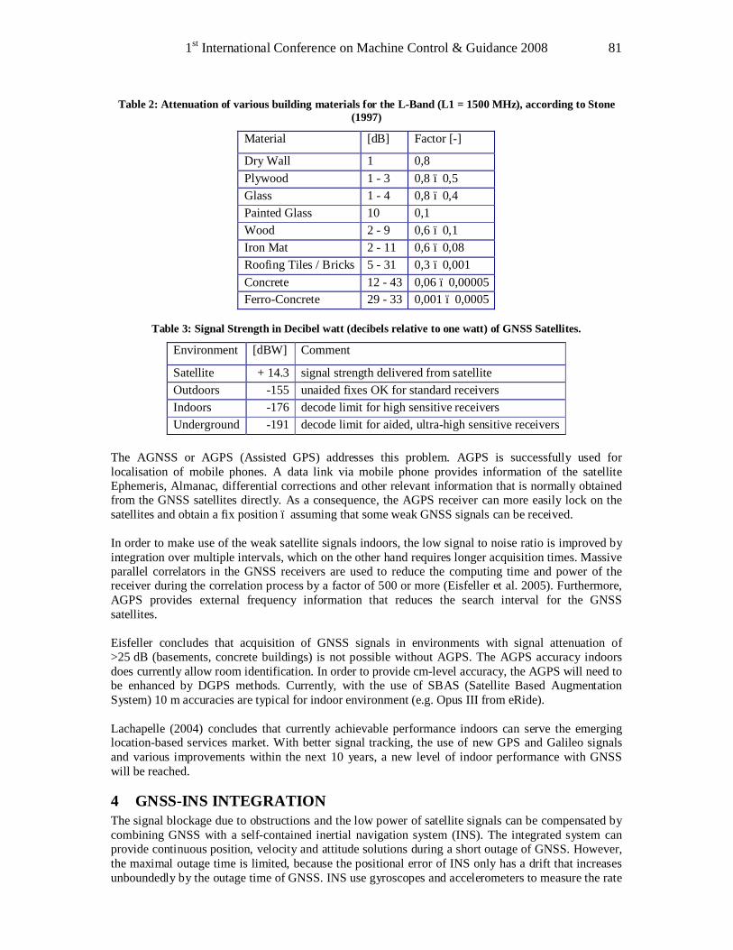
1st International Conference on Machine Control & Guidance 2008 81
Table 2: Attenuation of various building materials for the L-Band (L1 = 1500 MHz), according to Stone (1997)
Material [dB] Factor [-]
Dry Wall 1 0,8 Plywood 1 - 3 0,8 – 0,5 Glass 1 - 4 0,8 – 0,4 Painted Glass 10 0,1 Wood 2 - 9 0,6 – 0,1 Iron Mat 2 - 11 0,6 – 0,08 Roofing Tiles / Bricks 5 - 31 0,3 – 0,001 Concrete 12 - 43 0,06 – 0,00005 Ferro-Concrete 29 - 33 0,001 – 0,0005
Table 3: Signal Strength in Decibel watt (decibels relative to one watt) of GNSS Satellites.
Environment [dBW] Comment
Satellite + 14.3 signal strength delivered from satellite Outdoors -155 unaided fixes OK for standard receivers Indoors -176 decode limit for high sensitive receivers Underground -191 decode limit for aided, ultra-high sensitive receivers
The AGNSS or AGPS (Assisted GPS) addresses this problem. AGPS is successfully used for localisation of mobile phones. A data link via mobile phone provides information of the satellite Ephemeris, Almanac, differential corrections and other relevant information that is normally obtained from the GNSS satellites directly. As a consequence, the AGPS receiver can more easily lock on the satellites and obtain a fix position – assuming that some weak GNSS signals can be received. In order to make use of the weak satellite signals indoors, the low signal to noise ratio is improved by integration over multiple intervals, which on the other hand requires longer acquisition times. Massive parallel correlators in the GNSS receivers are used to reduce the computing time and power of the receiver during the correlation process by a factor of 500 or more (Eisfeller et al. 2005). Furthermore, AGPS provides external frequency information that reduces the search interval for the GNSS satellites. Eisfeller concludes that acquisition of GNSS signals in environments with signal attenuation of >25 dB (basements, concrete buildings) is not possible without AGPS. The AGPS accuracy indoors does currently allow room identification. In order to provide cm-level accuracy, the AGPS will need to be enhanced by DGPS methods. Currently, with the use of SBAS (Satellite Based Augmentation System) 10 m accuracies are typical for indoor environment (e.g. Opus III from eRide). Lachapelle (2004) concludes that currently achievable performance indoors can serve the emerging location-based services market. With better signal tracking, the use of new GPS and Galileo signals and various improvements within the next 10 years, a new level of indoor performance with GNSS will be reached.
4 GNSS-INS INTEGRATION The signal blockage due to obstructions and the low power of satellite signals can be compensated by combining GNSS with a self-contained inertial navigation system (INS). The integrated system can provide continuous position, velocity and attitude solutions during a short outage of GNSS. However, the maximal outage time is limited, because the positional error of INS only has a drift that increases unboundedly by the outage time of GNSS. INS use gyroscopes and accelerometers to measure the rate
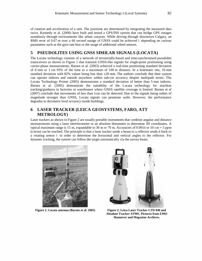
Kinematic Measurement and Sensor Technology I (Local Systems) 82
of rotation and acceleration of a unit. The positions are determined by integrating the measured data twice. Kennedy et al. (2006) have built and tested a GPS/INS system that can bridge GPS outages seamlessly through environments like urban canyons. While driving through downtown Calgary, an RMS error of 0.67 m over a 60 second outage of GNSS could be achieved – depending on various parameters such as the gyro rate bias or the usage of additional wheel sensors.
5 PSEUDOLITES USING GNSS SIMILAR SIGNALS (LOCATA) The Locata technology consists of a network of terrestrially-based and time-synchronised pseudolite transceivers as shown in Figure 1 that transmit GNSS-like signals for single-point positioning using carrier-phase measurements. Barnes et al. (2003) achieved a real-time positioning standard deviation of 6 mm or 1 cm 93% of the time to a maximum of 100 m distance. In a kinematic test, 16 mm standard deviation with 82% values being less than ±20 mm. The authors conclude that their system can operate indoors and outside anywhere within sub-cm accuracy despite multipath errors. The Locata Technology Primer (2005) demonstrates a standard deviation of better than 5 mm indoors. Barnes et al. (2005) demonstrate the suitability of the Locata technology for machine tracking/guidance in factories or warehouses where GNSS satellite coverage is limited. Barnes et al (2007) conclude that movements of less than 1cm can be detected. Due to the signals being orders of magnitude stronger than GNSS, Locata signals can penetrate walls. However, the performance degrades to decimetre level accuracy inside buildings.
6 LASER TRACKER (LEICA GEOSYSTEMS, FARO, ATT METROLOGY)
Laser trackers as shown in Figure 2 are usually portable instruments that combine angular and distance measurements using a laser interferometer or an absolute distometer to determine 3D coordinates. A typical maximum range is 15 m, expandable to 30 m or 70 m. Accuracies of 0.001” or 10 μm + 5 ppm (μm/m) can be reached. The principle is that a laser tracker sends a beam to a reflector sends it back to a rotating sensor – in order to determine the horizontal and vertical angles to the reflector. For dynamic tracking, the system can follow the target automatically via the survey beam.
Figure 1: Locata antenna (Barnes et al. 2005) Figure 2: Leica Laser Tracker LTD 840 and
Absolute Tracker AT901. Pictures from EMO Hannover and Magazine Archives.
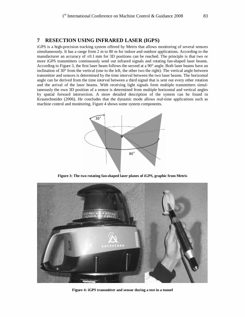
1st International Conference on Machine Control & Guidance 2008 83
7 RESECTION USING INFRARED LASER (IGPS) iGPS is a high-precision tracking system offered by Metris that allows monitoring of several sensors simultaneously. It has a range from 2 m to 80 m for indoor and outdoor applications. According to the manufacturer an accuracy of ±0.1 mm for 3D positions can be reached. The principle is that two or more iGPS transmitters continuously send out infrared signals and rotating fan-shaped laser beams. According to Figure 3, the first laser beam follows the second at a 90° angle. Both laser beams have an inclination of 30° from the vertical (one to the left, the other two the right). The vertical angle between transmitter and sensors is determined by the time interval between the two laser beams. The horizontal angle can be derived from the time interval between a third signal that is sent out every other rotation and the arrival of the laser beams. With receiving light signals form multiple transmitters simul-taneously the own 3D position of a sensor is determined from multiple horizontal and vertical angles by spatial forward intersection. A more detailed description of the system can be found in Krautschneider (2006). He concludes that the dynamic mode allows real-time applications such as machine control and monitoring. Figure 4 shows some system components.
Figure 3: The two rotating fan-shaped laser planes of iGPS, graphic from Metris
Figure 4: iGPS transmitter and sensor during a test in a tunnel
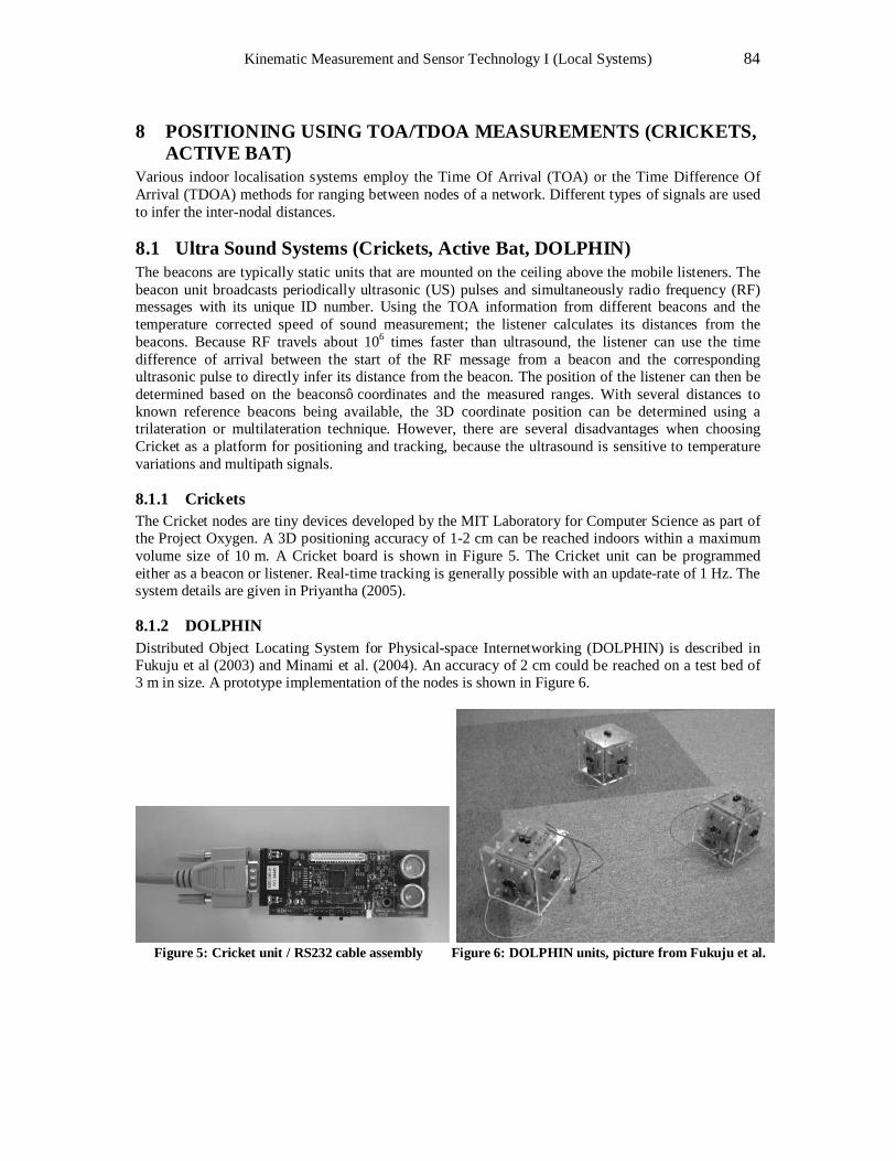
Kinematic Measurement and Sensor Technology I (Local Systems) 84
8 POSITIONING USING TOA/TDOA MEASUREMENTS (CRICKETS, ACTIVE BAT)
Various indoor localisation systems employ the Time Of Arrival (TOA) or the Time Difference Of Arrival (TDOA) methods for ranging between nodes of a network. Different types of signals are used to infer the inter-nodal distances.
8.1 Ultra Sound Systems (Crickets, Active Bat, DOLPHIN) The beacons are typically static units that are mounted on the ceiling above the mobile listeners. The beacon unit broadcasts periodically ultrasonic (US) pulses and simultaneously radio frequency (RF) messages with its unique ID number. Using the TOA information from different beacons and the temperature corrected speed of sound measurement; the listener calculates its distances from the beacons. Because RF travels about 106 times faster than ultrasound, the listener can use the time difference of arrival between the start of the RF message from a beacon and the corresponding ultrasonic pulse to directly infer its distance from the beacon. The position of the listener can then be determined based on the beacons’ coordinates and the measured ranges. With several distances to known reference beacons being available, the 3D coordinate position can be determined using a trilateration or multilateration technique. However, there are several disadvantages when choosing Cricket as a platform for positioning and tracking, because the ultrasound is sensitive to temperature variations and multipath signals.
8.1.1 Crickets The Cricket nodes are tiny devices developed by the MIT Laboratory for Computer Science as part of the Project Oxygen. A 3D positioning accuracy of 1-2 cm can be reached indoors within a maximum volume size of 10 m. A Cricket board is shown in Figure 5. The Cricket unit can be programmed either as a beacon or listener. Real-time tracking is generally possible with an update-rate of 1 Hz. The system details are given in Priyantha (2005).
8.1.2 DOLPHIN Distributed Object Locating System for Physical-space Internetworking (DOLPHIN) is described in Fukuju et al (2003) and Minami et al. (2004). An accuracy of 2 cm could be reached on a test bed of 3 m in size. A prototype implementation of the nodes is shown in Figure 6.
Figure 5: Cricket unit / RS232 cable assembly
Figure 6: DOLPHIN units, picture from Fukuju et al.
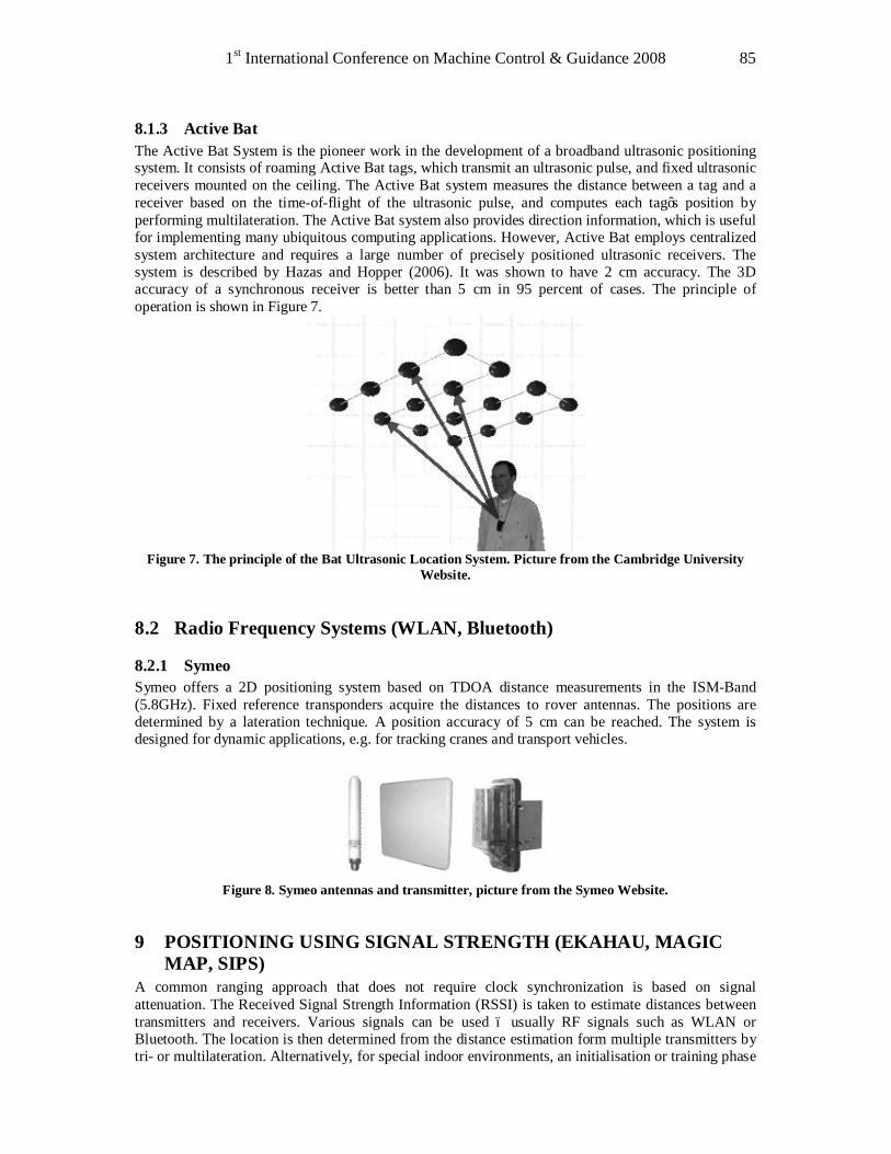
1st International Conference on Machine Control & Guidance 2008 85
8.1.3 Active Bat The Active Bat System is the pioneer work in the development of a broadband ultrasonic positioning system. It consists of roaming Active Bat tags, which transmit an ultrasonic pulse, and fixed ultrasonic receivers mounted on the ceiling. The Active Bat system measures the distance between a tag and a receiver based on the time-of-flight of the ultrasonic pulse, and computes each tag’s position by performing multilateration. The Active Bat system also provides direction information, which is useful for implementing many ubiquitous computing applications. However, Active Bat employs centralized system architecture and requires a large number of precisely positioned ultrasonic receivers. The system is described by Hazas and Hopper (2006). It was shown to have 2 cm accuracy. The 3D accuracy of a synchronous receiver is better than 5 cm in 95 percent of cases. The principle of operation is shown in Figure 7.
Figure 7. The principle of the Bat Ultrasonic Location System. Picture from the Cambridge University
Website.
8.2 Radio Frequency Systems (WLAN, Bluetooth)
8.2.1 Symeo Symeo offers a 2D positioning system based on TDOA distance measurements in the ISM-Band (5.8GHz). Fixed reference transponders acquire the distances to rover antennas. The positions are determined by a lateration technique. A position accuracy of 5 cm can be reached. The system is designed for dynamic applications, e.g. for tracking cranes and transport vehicles.
Figure 8. Symeo antennas and transmitter, picture from the Symeo Website.
9 POSITIONING USING SIGNAL STRENGTH (EKAHAU, MAGIC MAP, SIPS)
A common ranging approach that does not require clock synchronization is based on signal attenuation. The Received Signal Strength Information (RSSI) is taken to estimate distances between transmitters and receivers. Various signals can be used – usually RF signals such as WLAN or Bluetooth. The location is then determined from the distance estimation form multiple transmitters by tri- or multilateration. Alternatively, for special indoor environments, an initialisation or training phase
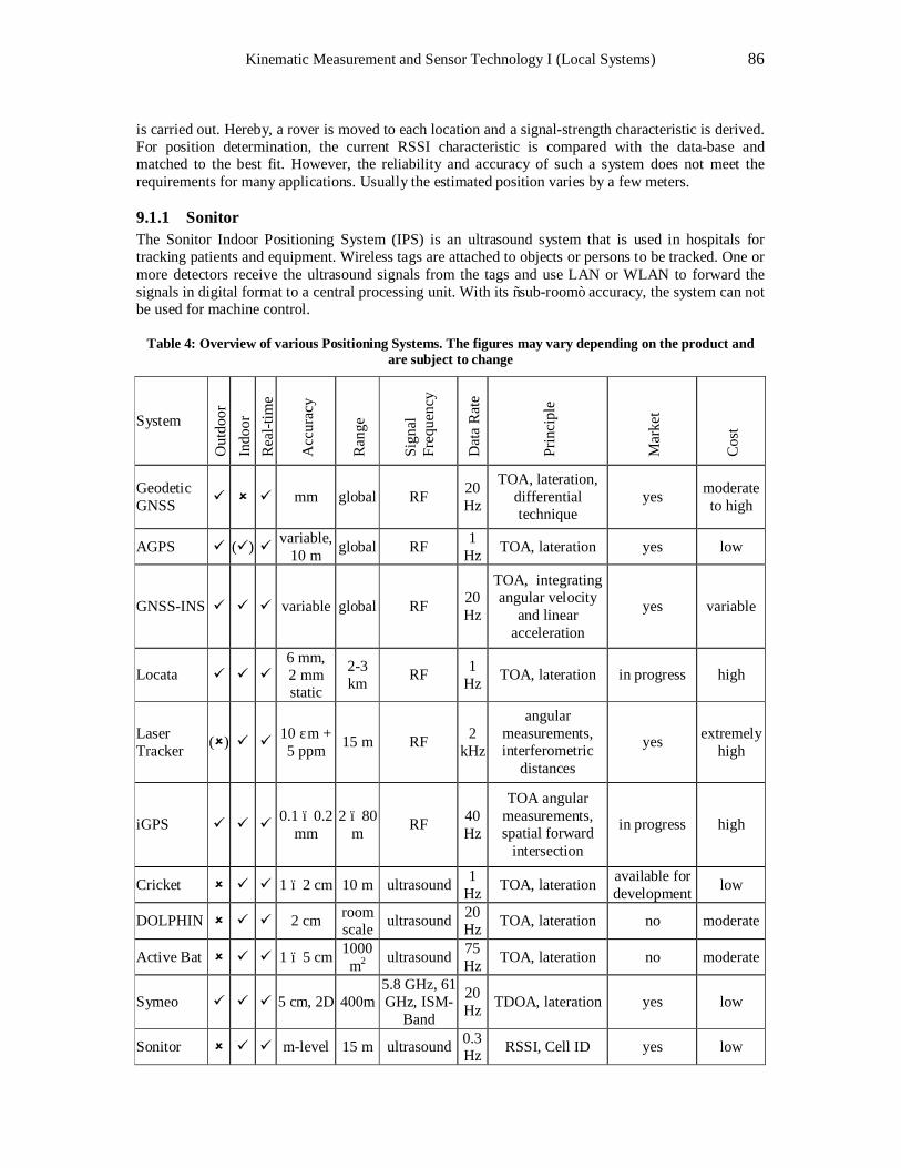
Kinematic Measurement and Sensor Technology I (Local Systems) 86
is carried out. Hereby, a rover is moved to each location and a signal-strength characteristic is derived. For position determination, the current RSSI characteristic is compared with the data-base and matched to the best fit. However, the reliability and accuracy of such a system does not meet the requirements for many applications. Usually the estimated position varies by a few meters.
9.1.1 Sonitor The Sonitor Indoor Positioning System (IPS) is an ultrasound system that is used in hospitals for tracking patients and equipment. Wireless tags are attached to objects or persons to be tracked. One or more detectors receive the ultrasound signals from the tags and use LAN or WLAN to forward the signals in digital format to a central processing unit. With its “sub-room” accuracy, the system can not be used for machine control.
Table 4: Overview of various Positioning Systems. The figures may vary depending on the product and are subject to change
System
Out
door
In
door
R
eal-t
ime
Acc
urac
y
Ran
ge
Sign
al
Freq
uenc
y
Dat
a R
ate
Prin
cipl
e
Mar
ket
Cos
t
Geodetic GNSS ü û ü mm global RF 20
Hz
TOA, lateration, differential technique
yes moderate to high
AGPS ü (ü) ü variable, 10 m global RF 1
Hz TOA, lateration yes low
GNSS-INS ü ü ü variable global RF 20 Hz
TOA, integrating angular velocity
and linear acceleration
yes variable
Locata ü ü ü 6 mm, 2 mm static
2-3 km RF 1
Hz TOA, lateration in progress high
Laser Tracker (û) ü ü 10 μm +
5 ppm 15 m RF 2 kHz
angular measurements, interferometric
distances
yes extremely high
iGPS ü ü ü 0.1 – 0.2 mm
2 – 80 m RF 40
Hz
TOA angular measurements, spatial forward
intersection
in progress high
Cricket û ü ü 1 – 2 cm 10 m ultrasound 1 Hz TOA, lateration available for
development low
DOLPHIN û ü ü 2 cm room scale ultrasound 20
Hz TOA, lateration no moderate
Active Bat û ü ü 1 – 5 cm 1000 m2 ultrasound 75
Hz TOA, lateration no moderate
Symeo ü ü ü 5 cm, 2D 400m 5.8 GHz, 61 GHz, ISM-
Band
20 Hz TDOA, lateration yes low
Sonitor û ü ü m-level 15 m ultrasound 0.3 Hz RSSI, Cell ID yes low
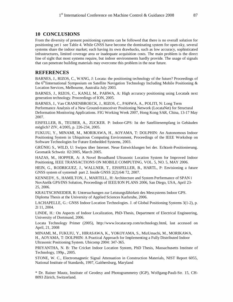
1st International Conference on Machine Control & Guidance 2008 87
10 CONCLUSIONS From the diversity of present positioning systems can be followed that there is no overall solution for positioning yet – see Table 4. While GNSS have become the dominating system for open-sky, several systems share the indoor market; each having its own drawbacks, such as low accuracy, sophisticated infrastructures, limited coverage area or inadequate acquisition costs. The main problem is the direct line of sight that most systems require, but indoor environments hardly provide. The usage of signals that can penetrate building materials may overcome this problem in the near future.
REFERENCES BARNES, J., RIZOS, C., WANG, J: Locata: the positioning technology of the future? Proceedings of the 6thIinternational Symposium on Satellite Navigation Technology Including Mobile Positioning & Location Services, Melbourne, Australia July 2003. BARNES, J., RIZOS, C., KANLI, M., PAHWA, A: High accuracy positioning using Locata’s next generation technology. Proceedings of ION, 2005. BARNES, J., Van CRANENBROECK, J., RIZOS, C., PAHWA, A., POLITI, N: Long Term Performance Analysis of a New Ground-transceiver Positioning Network (LocataNet) for Structural Deformation Monitoring Applications. FIG Working Week 2007, Hong Kong SAR, China, 13-17 May 2007. EISFELLER, B., TEUBER, A., ZUCKER. P: Indoor-GPS: Ist der Satellitenempfang in Gebäuden möglich? ZfV, 4/2005, p. 226-234, 2005. FUKUJU, Y., MINAMI, M., MORIKAWA, H., AOYAMA, T: DOLPHIN: An Autonomous Indoor Positioning System in Ubiquitous Computing Environment, Proceedings of the IEEE Workshop on Software Technologies for Future Embedded Systems, 2003. GRÜNIG S., WILD, U: Swipos über Internet. Neue Entwicklungen bei der. Echtzeit-Positionierung. Geomatik Schweiz 02/2005, March 2005. HAZAS, M., HOPPER, A: A Novel Broadband Ultrasonic Location System for Improved Indoor Positioning, IEEE TRANSACTIONS ON MOBILE COMPUTING, VOL. 5, NO. 5, MAY 2006. HEIN, G., RODRIGUEZ, J., WALLNER, T., EISSFELLER, B., HARTL, P: Envisioning a future GNSS system of systems—part 2. Inside GNSS 2(2):64–72, 2007. KENNEDY, S., HAMILTON, J., MARTELL, H: Architecture and System Performance of SPAN – NovAtel’s GPS/INS Solution, Proceedings of IEEE/ION PLANS 2006, San Diego, USA, April 23-25, 2006. KRAUTSCHNEIDER, R: Untersuchungen zur Leistungsfähirkeit des Messystems Indoor GPS. Diploma Thesis at the University of Applied Sciences Karlsruhe, 2006. LACHAPELLE, G.: GNSS Indoor Location Technologies. J. of Global Positioning Systems 3(1-2), p. 2–11, 2004. LINDE, H.: On Aspects of Indoor Localization, PhD-Thesis, Department of Electrical Engineering, University of Dortmund, 2006. Locata Technology Primer (2005), http://www.locatacorp.com/technology.html, last accessed on April, 21, 2008 MINAMI, M., FUKUJU, Y., HIRASAWA, K., YOKOYAMA, S., MizUmachi, M., MORIKAWA, H., AOYAMA, T: DOLPHIN: A Practical Approach for Implementing a Fully Distributed Indoor Ultrasonic Positioning System. Ubicomp 2004: 347-365. PRIYANTHA, N. B: The Cricket Indoor Location System, PhD Thesis, Massachusetts Institute of Technology, 199p., 2005. STONE, W. C., Electromagnetic Signal Attenuation in Construction Materials, NIST Report 6055, National Institute of Standards, 1997, Gaithersburg, Maryland * Dr. Rainer Mautz, Institute of Geodesy and Photogrammetry (IGP), Wolfgang-Pauli-Str. 15, CH-8093 Zürich, Switzerland.

Kinematic Measurement and Sensor Technology I (Local Systems) 88

Kinematic Measurement and Sensor Technology II (GNSS Systems)

1st International Conference on Machine Control & Guidance 2008 91
Advanced Concept in Multiple GNSS Network RTK Processing
Hans-Jürgen EULER
inPosition gmbh, Heerbrugg, Switzerland [email protected]
Joachim WIRTH
HSR Hochschule fuer Technik Rapperswil, Switzerland [email protected]
Abstract In the GNSS positioning community permanent reference stations applications, often called Network RTK, have been established. Even so this may still be considered as an emerging technology for some countries, there are already a lot of installations readily available and are offering their services to a broad community. However the efficient use of these services with GNSS receivers supporting multiple satellite systems is still quite limited. Obviously, a pure GPS reference station network can provide only the GPS portion of the required reference station information for positioning. Half of the available rover observation information cannot be utilized. Network RTK installations supporting multiple GNSS on all reference stations need significant investment on the service provider side for exchanging all receivers. Only new networks are more likely to be equipped completely with reference station receivers supporting all the same GNSS; at the time being GPS and GLONASS. For the future Galileo is on the horizon and again the service providers have to adapt their services. It is not very likely that a large portion of the services will be homogenously equipped with reference station receivers supporting the same GNSS. Summarizing the scenarios for users having invested in multiple-GNSS receiver equipment, one has to acknowledge, that either the user has to establish his own reference station for his work or the user can use only part of the capabilities of his new, expensive equipment. New concepts for processing multiple receiver observation information are desperately required. The paper is analysing the options for optimal use of a multi-GNSS receiver together with other GNSS receivers not supporting the complete set of GNSS. Furthermore the paper details on the processing of observation information from a receiver supporting two-GNSS together with single GNSS reference station receivers in a network application. The concept is specifically adapted for any combination of GNSS receivers. The only restriction is that a GNSS needs to be supported by at least two receivers in the network. Computational results are presented in various combinations for several single-GNSS receivers with multiple-GNSS receivers. The advantages of these combinations are high-lighted. The conclusion is that not necessarily all reference stations have to be equipped with receivers supporting all required GNSS for efficient use of the multiple-GNSS roving receivers. In the extreme a GPS-GLONASS or GPS-Galileo receiver can be used efficiently together with two reference stations supplying either of the GNSS independently. The study has been conducted as part of the Galileo project on Professional Receiver Development ARTUS.
1 INTRODUCTION Over the last years more and more permanent reference station systems have been established. For high precision positioning applications these installations are called Network RTK. Services are typically established based on reference stations equipped with GPS only receivers. The discussion and development of new GNSS, such as Galileo, Compass, QZSS and others, but also the revival of GLONASS will presumably require extension of these services. Combined
Kinematic Measurements and Sensor Technology II (GNSS Systems) 92
GPS/GLONASS Network RTK are being already established. However the efficient use of these services with GNSS receivers supporting multiple satellite systems is still quite limited. Mixing different hardware and services, today an exception will become some sort of commodity in the future. Even so sometimes considered as a solved issue some peculiarities require consideration. Brand-new receiver hardware supporting two GNSS for rover application faces such peculiarities. For example, a pure GPS reference station network can obviously provide only the GPS portion of the required reference station information for positioning. Half of the available rover observation information cannot be utilized. Existing Network RTK installations supporting multiple GNSS on all reference stations need significant investment on the service provider side for exchanging all receivers. Only new installations are more likely to be equipped completely with reference station receivers supporting all the same GNSS; at this time being GPS and GLONASS. For the future Galileo is on the horizon and again the service providers have to adapt their services. It is again not very likely that a large portion of the services will be homogenously equipped with reference station receivers supporting the same GNS systems. However, not only new satellite systems, but also the enhancements of existing system provide similar challenges. GPS has been extended already with an additional civil code L2C and a third civil code will be launched with a first satellite soon. For GLONASS the discussions on adding a CDMA navigation capability seem to finally materialize (GPS World 2008). With the increasing complexity of different observation types available new concepts for processing multiple-GNSS observation information are desperately required. Otherwise users having invested in state-of-the-art receiver equipment are forced to setup a reference station for the specific work or only part of the capabilities of the new, expensive equipment is utilized. The operation of new field equipment supporting additional GNSS or new satellite signals in conjunction with established, less sophisticated reference station infrastructures requires more flexible processing strategies than traditional rover applications. Rovers processing observations in the station-to-station baseline scheme are always restricted to have identical tracking capabilities on reference stations. The processing needs to be extended to support at least a small number of reference stations simultaneously. Future Network RTK applications face the identical situation. Either they are established with a homogenous set of reference stations or a mix of different capabilities in the station equipment has to be expected. Ultimately the concepts developed are the same for future field and network RTK processing. When starting a thorough list of all possibilities one will recognize quite soon the sheer amount of different combinations of different receivers ranging from pure single-system/single-frequency up to support of all different observation types for all GNSS. Direct implementation techniques will have to line out each of the combination and put into source code. The resulting source code will be inefficient and hard to maintain. The setup of processing algorithms has to concentrate on the differentiators instead. For development efficiency the actual design of the equation systems have to be done in more elaborate way. Subsequently we are lining out the observation properties and propose a concept for flexible processing. Our study is geared towards combination Galileo and GPS. However, our concept encompasses already the introduction and processing of more GNSS than just Galileo and GPS.
2 ANALYSIS OF OBSERVATION PROPERTIES The design of the European GNSS Galileo provides an over-whelming number of different combinations of all these observation types. Compared to this the traditional processing of GPS observations appears quite simple. GPS has by its original design only two different services, the civil Standard Positioning Service (SPS) and the military Precise Positioning Service (PPS). The general scientific community and all civil applications have been restricted to the civil branch of the system. All investigations, analysis and implementations were concentrating on the civil branch of the GPS. Thus initial GPS processing was limited by the amount of possibilities during the dawn of GPS applications. The European Galileo has five services and compared to GPS none of them seems to indicate to be initial off-limits for civil purposes as GPS’ military service. However most likely not of these services
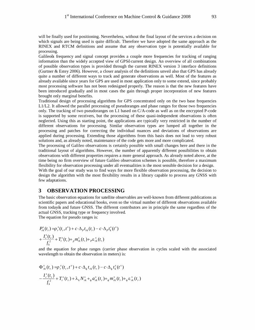
1st International Conference on Machine Control & Guidance 2008 93
will be finally used for positioning. Nevertheless, without the final layout of the services a decision on which signals are being used is quite difficult. Therefore we have adopted the same approach as the RINEX and RTCM definitions and assume that any observation type is potentially available for processing. Galileo’s frequency and signal concept provides a couple more frequencies for tracking of ranging information than the widely accepted view of GPS’ current design. An overview of all combinations of possible observation types is provided through the current RINEX version 3 interface definitions (Gurtner & Estey 2006). However, a closer analysis of the definitions unveil also that GPS has already quite a number of different ways to track and generate observations as well. Most of the features as already available since years for GPS are used in most application only to some extend, since probably most processing software has not been redesigned properly. The reason is that the new features have been introduced gradually and in most cases the gain through proper incorporation of new features brought only marginal benefits. Traditional design of processing algorithms for GPS concentrated only on the two base frequencies L1/L2. It allowed the parallel processing of pseudoranges and phase ranges for those two frequencies only. The tracking of two pseudoranges on L1 based on C/A-code as well as on the encrypted P-code is supported by some receivers, but the processing of these quasi-independent observations is often neglected. Using this as starting point, the applications are typically very restricted in the number of different observations for processing. Similar observation types are lumped all together in the processing and patches for correcting the individual nuances and deviations of observations are applied during processing. Extending those algorithms from this basis does not lead to very robust solutions and, as already noted, maintenance of the code gets more and more complicated. The processing of Galileo observations is certainly possible with small changes here and there in the traditional layout of algorithms. However, the number of apparently different possibilities to obtain observations with different properties requires a more general approach. As already noted above, at the time being no firm overview of future Galileo observation schemes is possible, therefore a maximum flexibility for observation processing under all eventualities is the most sensible decision for a design. With the goal of our study was to find ways for more flexible observation processing, the decision to design the algorithm with the most flexibility results in a library capable to process any GNSS with few adaptations.
3 OBSERVATION PROCESSING The basic observation equations for satellite observables are well-known from different publications as scientific papers and educational books, even so the virtual number of different observations available from today’s and future GNSS. The different contributors are in principle the same regardless of the actual GNSS, tracking type or frequency involved. The equation for pseudo ranges is:
)()()()(
)()(),()(
2 rsrkPr
srkpr
sr
k
rsr
sskPrrkP
sr
srr
srk
ttmtTftI
ttcttctttP
ε
ρ
++++
∆⋅−∆⋅+=
and the equation for phase ranges (carrier phase observation in cycles scaled with the associated wavelength to obtain the observation in meters) is:
)()()()()(
)()(),()(
2 rsrkr
srkr
srk
srkkr
sr
k
rsr
sskrrk
sr
srr
srk
ttmtaNtTf
tI
ttcttcttt
ελ
ρ
φφφ
φφ
+++++−
∆⋅−∆⋅+=Φ
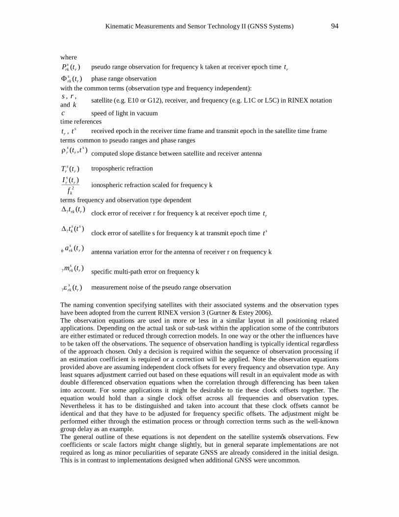
Kinematic Measurements and Sensor Technology II (GNSS Systems) 94
where )( r
srk tP pseudo range observation for frequency k taken at receiver epoch time rt
)( rsrk tΦ phase range observation
with the common terms (observation type and frequency independent): s , r , and k satellite (e.g. E10 or G12), receiver, and frequency (e.g. L1C or L5C) in RINEX notation
c speed of light in vacuum time references
rt , st received epoch in the receiver time frame and transmit epoch in the satellite time frame terms common to pseudo ranges and phase ranges
),( sr
sr ttρ
computed slope distance between satellite and receiver antenna
)( rs
r tT tropospheric refraction
2
)(
k
rsr
ftI
ionospheric refraction scaled for frequency k
terms frequency and observation type dependent )(? rrk tt∆
clock error of receiver r for frequency k at receiver epoch time rt
)(?ss
k tt∆
clock error of satellite s for frequency k at transmit epoch time st
)( rsrk taφ
antenna variation error for the antenna of receiver r on frequency k
)(? rsrk tm
specific multi-path error on frequency k
)(? rsrk tε measurement noise of the pseudo range observation
The naming convention specifying satellites with their associated systems and the observation types have been adopted from the current RINEX version 3 (Gurtner & Estey 2006). The observation equations are used in more or less in a similar layout in all positioning related applications. Depending on the actual task or sub-task within the application some of the contributors are either estimated or reduced through correction models. In one way or the other the influences have to be taken off the observations. The sequence of observation handling is typically identical regardless of the approach chosen. Only a decision is required within the sequence of observation processing if an estimation coefficient is required or a correction will be applied. Note the observation equations provided above are assuming independent clock offsets for every frequency and observation type. Any least squares adjustment carried out based on these equations will result in an equivalent mode as with double differenced observation equations when the correlation through differencing has been taken into account. For some applications it might be desirable to tie these clock offsets together. The equation would hold than a single clock offset across all frequencies and observation types. Nevertheless it has to be distinguished and taken into account that these clock offsets cannot be identical and that they have to be adjusted for frequency specific offsets. The adjustment might be performed either through the estimation process or through correction terms such as the well-known group delay as an example. The general outline of these equations is not dependent on the satellite system’s observations. Few coefficients or scale factors might change slightly, but in general separate implementations are not required as long as minor peculiarities of separate GNSS are already considered in the initial design. This is in contrast to implementations designed when additional GNSS were uncommon.
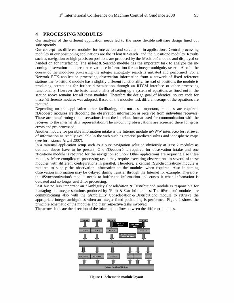
1st International Conference on Machine Control & Guidance 2008 95
4 PROCESSING MODULES Our analysis of the different application needs led to the more flexible software design lined out subsequently. Our concept has different modules for interaction and calculation in applications. Central processing modules in our positioning applications are the "Float & Search" and the “Position” modules. Results such as navigation or high precision positions are produced by the “Position” module and displayed or handed on for interfacing. The “Float & Search” module has the important task to analyze the in-coming observations and prepare covariance information for an integer ambiguity search. Also in the course of the module’s processing the integer ambiguity search is initiated and performed. For a Network RTK application processing observation information from a network of fixed reference stations the “Position” module has a slightly different functionality. Instead of positions the module is producing corrections for further dissemination through an RTCM interface or other processing functionality. However the basic functionality of setting up a system of equations as lined out in the section above remains for all these modules. Therefore the design goal of identical source code for these “different” modules was adopted. Based on the modules task different setups of the equations are required. Depending on the application other facilitating, but not less important, modules are required. “Decoder” modules are decoding the observation information as received from individual receivers. These are transforming the observations from the interface format used for communication with the receiver to the internal data representation. The in-coming observations are screened there for gross errors and pre-processed. Another module for possible information intake is the Internet module “WWW interface” for retrieval of information as readily available in the web such as precise predicted orbits and ionospheric maps (see for instance AIUB 2007). In a minimal application setup such as a pure navigation solution obviously at least 2 modules as outlined above have to be present. One “Decoder” is required for observation intake and one “Position” module is required for the navigation solution. Other applications are requiring also these modules. More complicated processing tasks may require executing observations in several of these modules with different configurations in parallel. Therefore, a central “Synchronization” module is required to supply the observation information to the modules when required. Also in-coming observation information may be delayed during transfer through the Internet for example. Therefore, the “Synchronization” module needs to buffer the information and erases it when information is outdated and no longer useful for processing. Last but no less important an “Ambiguity Consolidation & Distribution” module is responsible for managing the integer solutions produced by “Float & Search” modules. The “Position” modules are communicating also with the “Ambiguity Consolidation & Distribution” module to retrieve the appropriate integer ambiguities when an integer fixed positioning is performed. Figure 1 shows the principle schematic of the modules and their respective tasks involved. The arrows indicate the direction of the information flow between the different modules.
Figure 1: Schematic module layout
Kinematic Measurements and Sensor Technology II (GNSS Systems) 96
5 DIFFERENT PROPERTIES While our analysis led to the software layout described in the section before, it showed also that the different processing modules, especially the modules “Position” and “Float & Search”, need a principle “understanding” of the different observation properties for setup of their respective internal processing strategy. Some of these are basic properties while others generated through fusion of several other properties. The properties defined for our processing are summarized in Table 1. Each property defines a specific aspect required for processing. Some of the properties need also attributes to describe additional details. During the start-up of the application different properties are assigned to the processing modules. If a module is not aware of a property, the module will never process observations with that property. Similar the “Synchronization” module will not buffer and handle an observation whose property is not assigned in the whole application.
Table 1: Overview of properties
sys Satellite system (e.g. Galileo, GPS). The access structure defining the calculations will have as many instances of “sys” as satellite systems are involved.
sat Satellite assigned to specific system (sys). frq Transmitting frequency assigned to systems (sys) including the observation type. sta Station is a synonym of a location occupied by a hardware receiver. The calculation will
have as many instances of object sta as stations are involved. rcv Receiver boards assigned to specific station. One station will have one receiver instance for
each satellite system tracked at the station. chn Receivers are able to track a given number of satellites in parallel. One channel is for
tracking of one satellite. sln Slant denominates a satellite with a specific frequency observed by receiver. slt A placeholder for one satellite, tracked by a receiver in one channel. A slot is either empty
or contains one satellite. Fundamental properties are the system property “sys” and the station property “sta”. “sys” defines a satellite system accepted for processing. However just the definition of the property “sys” is not a sufficient description for performing any processing. So the property “sys” needs also a further detailing definition of its satellites described by properties “sat”. Any property “sys” will have the same count of properties “sat” as its number of satellites in the system’s constellation. Following the RINEX notation a satellite property together with its system property is described for instance for a Galileo satellite with ID 10 through the combined name “E10”. The combination of other properties of other satellite systems will be derived accordingly based on the RINEX version 3 definitions (Gurtner & Estey 2006). Also the addition of the satellite property does not allow a sufficient description of observations possible for a specific satellite. Since Galileo is planned to be launched to full constellation in a short period of time, most production satellites will have very likely the same signal capabilities. However, also Galileo will use initially its test satellites with probably slightly different functionality and furthermore the example of GPS draws another picture. Over the years different versions of satellites (Block I to Block IIF in the close future) have been launched. Each of these satellite versions has distinguished features. The newer satellites will have most dominantly the additional civil frequencies and codes L2C and L5. Therefore, the supported frequencies and observation types have to be detailed and distinguished for every satellite in addition. The “frq” property using again the notation of RINEX for description is defining possible observation types. A L1 carrier phase observation might have an “frq” property with the name “GALILEO L1C”. The combination of properties “sys”, “sat”, and “frq” allow the complete description of each individual satellite. So far only the origin of the signals used to take the observations, namely the space segment, is sufficiently defined. Another fundamental set of properties defines the receiving part in the application. It starts with the station property “sta” with the station name assigned. Additional attributes in property “sta” describe the coordinates and their dynamic behavior as static, fixed and kinematic. From the geodetic point of
1st International Conference on Machine Control & Guidance 2008 97
view the property is describing a marker or moving object. It should be noted that station might suggest to some a static monument, but our use of the term is more liberal. However, up to now the definition is not GNSS specific yet. The GNSS aspect is defined through a property “rcv”. The assumption is that at each station at least one receiver board is installed, which is represented by its “rcv” property. Each satellite system also described through “sys” and whose signals are being processed for the station needs a separate “rcv” property. The name for such a property is assembled from the associated station and system property names (e.g. 1000-GALILEO for the Galileo receiver board at station 1000). Initially our thought was that the receiver boards defined are equivalent to hardware boards installed. So an application based on one type of receiver (board) would have only one property “rcv”. However further elaboration of our concept showed that this requirement will restrict the flexibility. Therefore, the property “rcv” shall be considered more as a receiver board with an individual serial number. Each receiver board has a number of channel properties “chn” equivalent to the number of traceable satellites. Also for the receiver channels different observation properties might present dependent on the tracking modes of the hosting receiver. Therefore, each channel property has at least one frequency property “frq” defining the type of observation to be received. Also here “frq” defines complete property of each of the observation types used in processing. Finally the processing within the application requires certain unknowns to be estimated. The unknowns are setup based on the specified properties above. Additional supporting properties have been introduced to describe the allocation of unknowns. We called them slot properties “slt” and slant properties “sln”. A slot property “slt” is a placeholder for a satellite tracked somewhere for processing in the application. For the observation equation setup through the slot the associated satellite and its “frq” properties are defined. This is required to find for instance satellite clock unknowns and setup the required coefficient for estimation or determine and apply its corrector. The final slant property “sln” supports a similar functionality. The slants provide connections between receivers, satellites and their possible “frq” properties. The slant property might be considered as a synonym for channels, but has to have an observed satellite assigned. The slant properties are required for instance in a “Float & Search” module to setup the float ambiguity unknowns or, for a “Position” module to find the proper fixed integer ambiguity, but also coefficients for a stochastic modeling parameter as required for estimating the remainders of ionospheric refraction are setup based on this property. It is obvious that the properties of the space segment represented starting with “sys” and the properties of the ground segment starting with “sta” are correlated. Especially when through a property the setup of unknowns in the estimation process is foreseen a consolidation of these properties is recommendable. For instance the “slt” properties might need to define only those relations require for the actual set of “rcv” definitions. Such a consolidation can easily be conducted during start-up.
6 DESIGN & IMPLEMENTATION The properties described above have been mapped into an object-oriented design. An access structure instance will be initialized during start-up of each processing module. The inputs to the access structure instance are the hierarchical structures defining the computational task of the module. The initialization of the access instance defines the complete structure of the observation system for the Kalman filter used in processing. With the complexity of the targeted computations in the module the complexity of the access structure is increasing. The starting properties are always properties “sys” and “sta” as a minimum. For processing of a typical navigation solution the definition of the satellites is required through the properties “sat” with the signals supported observation types per satellite through property “frq”. An example of a single frequency navigation solution based on Galileo E1-L1-E2 frequency code observations will have an instance of property “sys” defined as “Galileo”. Furthermore a container holding instances with the individual satellite properties “sat”. Each of the satellite properties holds a container holding only one instance of “frq” defining “C1C”. For larger processing setups the properties “frq” of each satellite need to define the additional observation types somewhere tracked and required for processing in the setup. Since for navigation a solution compromise of only one station, properties “frq” may restrict the observations actually
Kinematic Measurements and Sensor Technology II (GNSS Systems) 98
processed. Property “sta” defines with its attributes the processing information for coordinates and dynamic behavior fixed or static. Through the property “rcv” the supported GNS Systems and their actual observation type properties “frq” are defined. As already stated above, the setup of all properties may require a consolidation. Only “frq” properties have to be included for “sys” which are also represented in properties “rcv”. The navigation processing of the Galileo single frequency navigation defined above will result in a Kalman filter setup of a receiver clock unknown based on property “frq” in “rcv”. Also three coordinate unknowns will be estimated based on the attributes of property “sta”. This example shows the required steps for initialization of a “Position” module for a single frequency navigation solution. For such a simple task the definition process implies somewhat an overhead. However, the access structure instance has been designed to support more complex processing. The single frequency navigation solution is also covered and allows, therefore, the use of identical source code for processing as a complete network of several receivers with various parameters for estimation. The schematic described has been implemented. The resulting software will be part of a Galileo/GPS prototype called ARTUS currently under development. More details on the prototype receiver can be found in Lück et al (2007). For verification of software’s functionality several tests have been performed and their results are detailed in the next section. Euler and Wirth (2007) was completely based on post-processing. The implementation was a single process showing the capabilities with the algorithmic concept. In the mean time the implementations have been extended to real-time. The communication per TCP/IP between the processes is established and runs in the first basic version. The decoding processes building the link to external GNSS receivers are set-up and communicate the observation information to the processing. Since due to external reasons the prototype receivers could not be connected, the implementation of the decoder modules allows reading the observations from a file and sends it with a pre-defined update rate. This intermediate step towards real-time allows also later on the reprocessing of collected observations. The observation information is received by the “Float & Search” module for processing. To the design also a display module has been added. This module receives also the information to display via TCP/IP. All modules are running on one platform. However as already noted, the design concept provides the opportunity to distribute the different processing task on different computers. This allows especially for larger application setups the distribution of the computational load.
7 TEST RESULTS Galileo observations are currently not available because the satellite system does not supply signals yet. Therefore we simulated raw observations using a Raw Data Generator (RDG) developed in the course of our working packages in the ARTUS project. The configuration simulated has been chosen to highlight the flexibility of our software design. The test configuration, we have chosen for illustration of the capabilities of our software design, is based on three-station configuration. One reference station (3002) features a Galileo only receiver tracking dual frequency pseudoranges and phaseranges on E1-L1-E2 and on E5a frequencies in the South. Another station (3001) is occupied by a GPS only receiver, which is tracking also in dual frequency mode. The pseudorange and phaserange information is collected based on L1 and on L2 frequencies. The third station (rover) is placed approximately in the middle between both stations. Figure 2 shows the geometry of the setup. While the reference stations are featuring single system receivers has the central rover station the capability to measure observations for both the Galileo system and the GPS. The observation types and frequencies are matching those tracked of the respective GNSS receivers at the reference stations.
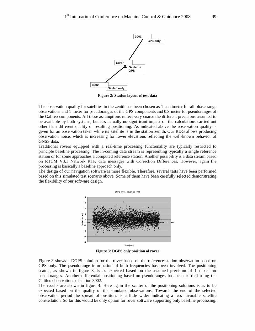
1st International Conference on Machine Control & Guidance 2008 99
Galileo only3002
GPS only3001
Galileo + GPS
rover
Galileo only3002
GPS only3001
Galileo + GPS
rover
Figure 2: Station layout of test data
The observation quality for satellites in the zenith has been chosen as 1 centimeter for all phase range observations and 1 meter for pseudoranges of the GPS components and 0.3 meter for pseudoranges of the Galileo components. All these assumptions reflect very coarse the different precisions assumed to be available by both systems, but has actually no significant impact on the calculations carried out other than different quality of resulting positioning. As indicated above the observation quality is given for an observation taken while its satellite is in the station zenith. Our RDG allows producing observation noise, which is increasing for lower elevations reflecting the well-known behavior of GNSS data. Traditional rovers equipped with a real-time processing functionality are typically restricted to principle baseline processing. The in-coming data stream is representing typically a single reference station or for some approaches a computed reference station. Another possibility is a data stream based on RTCM V3.1 Network RTK data messages with Correction Differences. However, again the processing is basically a baseline approach only. The design of our navigation software is more flexible. Therefore, several tests have been performed based on this simulated test scenario above. Some of them have been carefully selected demonstrating the flexibility of our software design.
DGPS (3001 - rover) C1 + C2
-4
-3
-2
-1
0
1
2
3
4
172500 173000 173500 174000 174500 175000 175500 176000 176500 177000
Time [sec]
Dev
iatio
ns [m
]
Figure 3: DGPS only position of rover
Figure 3 shows a DGPS solution for the rover based on the reference station observation based on GPS only. The pseudorange information of both frequencies has been involved. The positioning scatter, as shown in figure 3, is as expected based on the assumed precision of 1 meter for pseudoranges. Another differential positioning based on pseudoranges has been carried using the Galileo observations of station 3002. The results are shown in figure 4. Here again the scatter of the positioning solutions is as to be expected based on the quality of the simulated observations. Towards the end of the selected observation period the spread of positions is a little wider indicating a less favorable satellite constellation. So far this would be only option for rover software supporting only baseline processing.
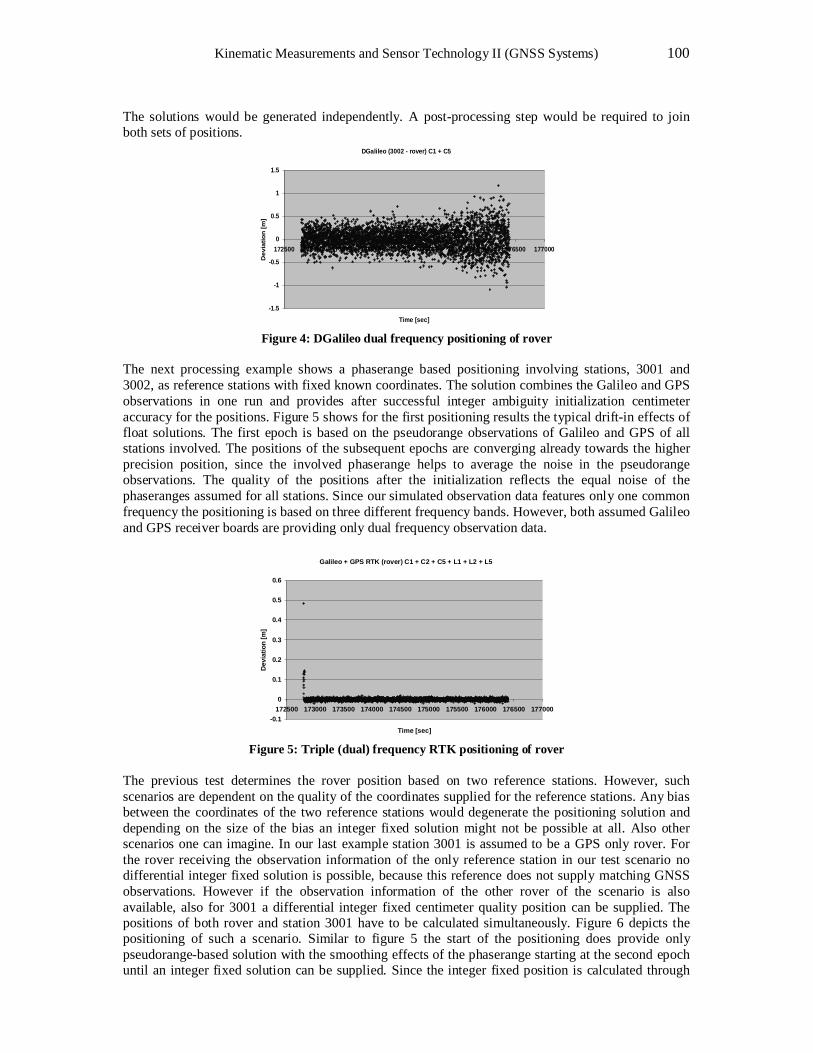
Kinematic Measurements and Sensor Technology II (GNSS Systems) 100
The solutions would be generated independently. A post-processing step would be required to join both sets of positions.
DGalileo (3002 - rover) C1 + C5
-1.5
-1
-0.5
0
0.5
1
1.5
172500 173000 173500 174000 174500 175000 175500 176000 176500 177000
Time [sec]
Dev
iatio
n [m
]
Figure 4: DGalileo dual frequency positioning of rover
The next processing example shows a phaserange based positioning involving stations, 3001 and 3002, as reference stations with fixed known coordinates. The solution combines the Galileo and GPS observations in one run and provides after successful integer ambiguity initialization centimeter accuracy for the positions. Figure 5 shows for the first positioning results the typical drift-in effects of float solutions. The first epoch is based on the pseudorange observations of Galileo and GPS of all stations involved. The positions of the subsequent epochs are converging already towards the higher precision position, since the involved phaserange helps to average the noise in the pseudorange observations. The quality of the positions after the initialization reflects the equal noise of the phaseranges assumed for all stations. Since our simulated observation data features only one common frequency the positioning is based on three different frequency bands. However, both assumed Galileo and GPS receiver boards are providing only dual frequency observation data.
Galileo + GPS RTK (rover) C1 + C2 + C5 + L1 + L2 + L5
-0.1
0
0.1
0.2
0.3
0.4
0.5
0.6
172500 173000 173500 174000 174500 175000 175500 176000 176500 177000
Time [sec]
Dev
iatio
n [m
]
Figure 5: Triple (dual) frequency RTK positioning of rover
The previous test determines the rover position based on two reference stations. However, such scenarios are dependent on the quality of the coordinates supplied for the reference stations. Any bias between the coordinates of the two reference stations would degenerate the positioning solution and depending on the size of the bias an integer fixed solution might not be possible at all. Also other scenarios one can imagine. In our last example station 3001 is assumed to be a GPS only rover. For the rover receiving the observation information of the only reference station in our test scenario no differential integer fixed solution is possible, because this reference does not supply matching GNSS observations. However if the observation information of the other rover of the scenario is also available, also for 3001 a differential integer fixed centimeter quality position can be supplied. The positions of both rover and station 3001 have to be calculated simultaneously. Figure 6 depicts the positioning of such a scenario. Similar to figure 5 the start of the positioning does provide only pseudorange-based solution with the smoothing effects of the phaserange starting at the second epoch until an integer fixed solution can be supplied. Since the integer fixed position is calculated through
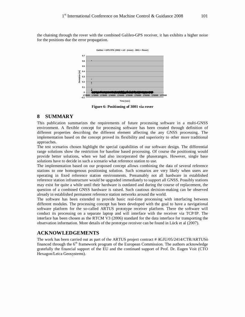
1st International Conference on Machine Control & Guidance 2008 101
the chaining through the rover with the combined Galileo-GPS receiver, it has exhibits a higher noise for the positions due the error propagation.
Galileo + GPS RTK (3002 = ref - (rover) - 3001 = Rover)
-0.1
0
0.1
0.2
0.3
0.4
0.5
0.6
0.7
172500 173000 173500 174000 174500 175000 175500 176000 176500 177000
Time [sec]
Dev
iatio
n [m
]
Figure 6: Positioning of 3001 via rover
8 SUMMARY This publication summarizes the requirements of future processing software in a multi-GNSS environment. A flexible concept for processing software has been created through definition of different properties describing the different element affecting the any GNSS processing. The implementation based on the concept proved its flexibility and superiority to other more traditional approaches. The test scenarios chosen highlight the special capabilities of our software design. The differential range solutions show the restriction for baseline based processing. Of course the positioning would provide better solutions, when we had also incorporated the phaseranges. However, single base solutions have to decide in such a scenario what reference station to use. The implementation based on our proposed concept allows combining the data of several reference stations to one homogenous positioning solution. Such scenarios are very likely when users are operating in fixed reference station environments. Presumably not all hardware in established reference station infrastructure would be upgraded immediately to support all GNSS. Possibly stations may exist for quite a while until their hardware is outdated and during the course of replacement, the question of a combined GNSS hardware is raised. Such cautious decision-making can be observed already in established permanent reference station networks around the world. The software has been extended to provide basic real-time processing with interfacing between different modules. The processing concept has been developed with the goal to have a navigational software platform for the so-called ARTUS prototype receiver platform. There the software will conduct its processing on a separate laptop and will interface with the receiver via TCP/IP. The interface has been chosen as the RTCM V3 (2006) standard for the data interface for transporting the observation information. More details of the prototype receiver can be found in Lück et al (2007).
ACKNOWLEDGEMENTS The work has been carried out as part of the ARTUS project contract # “GJU/05/2414/CTR/ARTUS” financed through the 6th framework program of the European Commission. The authors acknowledge gratefully the financial support of the EU and the continued support of Prof. Dr. Eugen Voit (CTO Hexagon/Leica Geosystems).

Kinematic Measurements and Sensor Technology II (GNSS Systems) 102
REFERENCES AUIB (2007): Web page of CODE activities at the Astronomical Institute of the University of Berne http://cmslive2.unibe.ch/unibe/philnat/aiub/content/e15/e59/e440/index_eng.html
Euler, H-J, Wirth, J. (2007): Novel Concept in Multiple GNSS Network RTK processing, Proceedings of ION GNSS 2007 September 25-28, 2007, Fort Worth, Tx
GPS World (2008): GLONASS to Begin CDMA Signal Broadcasting, GPS System Integration Design & Test Newsletter, February 26, 2008
Gurtner, W., Estey, L. (2006): RINEX - The Receiver Independent Exchange Format Version 3.0.
Lück, T., Winkel, J., Bodenbach, M., Gohler, E. Falk, N., Consoli, A., Piazza, F., Gerna, D., Granger, R., Reedman, P., Simpson, S., Euler, H-J (2007): ARTUS – A Second Generation Galileo/GPS receiver, Proceedings of ION GNSS 2007 September 25-28, 2007, Fort Worth, Tx
RTCM V3 (2006): RTCM Standard 10403.1 for Differential GNSS (Global Navigation Satellite Systems) Services – Version 3 developed by RTCM Special Committee NO. 104, October 27, 2006
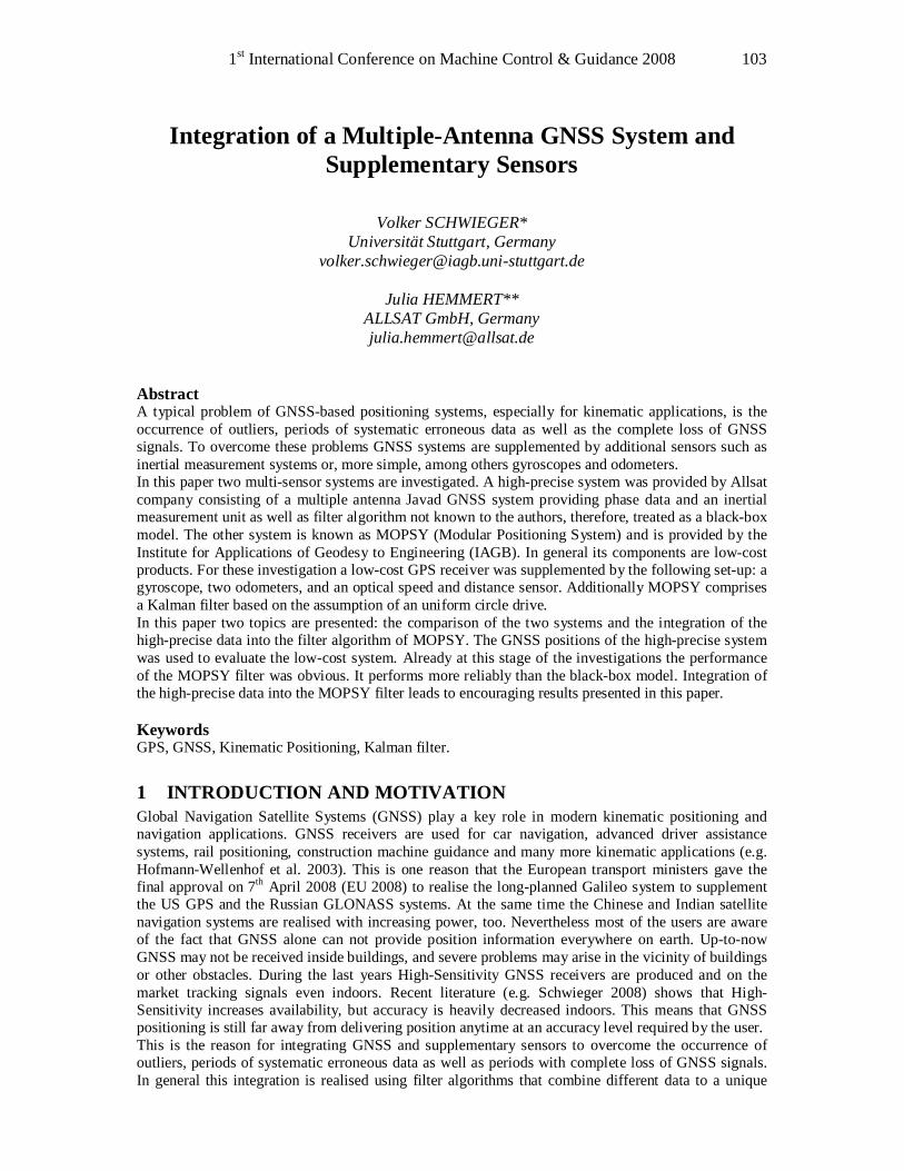
1st International Conference on Machine Control & Guidance 2008 103
Integration of a Multiple-Antenna GNSS System and Supplementary Sensors
Volker SCHWIEGER*
Universität Stuttgart, Germany [email protected]
Julia HEMMERT**
ALLSAT GmbH, Germany [email protected]
Abstract A typical problem of GNSS-based positioning systems, especially for kinematic applications, is the occurrence of outliers, periods of systematic erroneous data as well as the complete loss of GNSS signals. To overcome these problems GNSS systems are supplemented by additional sensors such as inertial measurement systems or, more simple, among others gyroscopes and odometers. In this paper two multi-sensor systems are investigated. A high-precise system was provided by Allsat company consisting of a multiple antenna Javad GNSS system providing phase data and an inertial measurement unit as well as filter algorithm not known to the authors, therefore, treated as a black-box model. The other system is known as MOPSY (Modular Positioning System) and is provided by the Institute for Applications of Geodesy to Engineering (IAGB). In general its components are low-cost products. For these investigation a low-cost GPS receiver was supplemented by the following set-up: a gyroscope, two odometers, and an optical speed and distance sensor. Additionally MOPSY comprises a Kalman filter based on the assumption of an uniform circle drive. In this paper two topics are presented: the comparison of the two systems and the integration of the high-precise data into the filter algorithm of MOPSY. The GNSS positions of the high-precise system was used to evaluate the low-cost system. Already at this stage of the investigations the performance of the MOPSY filter was obvious. It performs more reliably than the black-box model. Integration of the high-precise data into the MOPSY filter leads to encouraging results presented in this paper. Keywords GPS, GNSS, Kinematic Positioning, Kalman filter.
1 INTRODUCTION AND MOTIVATION Global Navigation Satellite Systems (GNSS) play a key role in modern kinematic positioning and navigation applications. GNSS receivers are used for car navigation, advanced driver assistance systems, rail positioning, construction machine guidance and many more kinematic applications (e.g. Hofmann-Wellenhof et al. 2003). This is one reason that the European transport ministers gave the final approval on 7th April 2008 (EU 2008) to realise the long-planned Galileo system to supplement the US GPS and the Russian GLONASS systems. At the same time the Chinese and Indian satellite navigation systems are realised with increasing power, too. Nevertheless most of the users are aware of the fact that GNSS alone can not provide position information everywhere on earth. Up-to-now GNSS may not be received inside buildings, and severe problems may arise in the vicinity of buildings or other obstacles. During the last years High-Sensitivity GNSS receivers are produced and on the market tracking signals even indoors. Recent literature (e.g. Schwieger 2008) shows that High-Sensitivity increases availability, but accuracy is heavily decreased indoors. This means that GNSS positioning is still far away from delivering position anytime at an accuracy level required by the user. This is the reason for integrating GNSS and supplementary sensors to overcome the occurrence of outliers, periods of systematic erroneous data as well as periods with complete loss of GNSS signals. In general this integration is realised using filter algorithms that combine different data to a unique
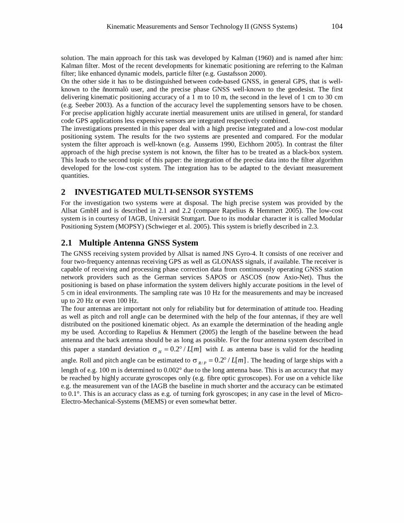
Kinematic Measurements and Sensor Technology II (GNSS Systems) 104
solution. The main approach for this task was developed by Kalman (1960) and is named after him: Kalman filter. Most of the recent developments for kinematic positioning are referring to the Kalman filter; like enhanced dynamic models, particle filter (e.g. Gustafsson 2000). On the other side it has to be distinguished between code-based GNSS, in general GPS, that is well-known to the “normal” user, and the precise phase GNSS well-known to the geodesist. The first delivering kinematic positioning accuracy of a 1 m to 10 m, the second in the level of 1 cm to 30 cm (e.g. Seeber 2003). As a function of the accuracy level the supplementing sensors have to be chosen. For precise application highly accurate inertial measurement units are utilised in general, for standard code GPS applications less expensive sensors are integrated respectively combined. The investigations presented in this paper deal with a high precise integrated and a low-cost modular positioning system. The results for the two systems are presented and compared. For the modular system the filter approach is well-known (e.g. Aussems 1990, Eichhorn 2005). In contrast the filter approach of the high precise system is not known, the filter has to be treated as a black-box system. This leads to the second topic of this paper: the integration of the precise data into the filter algorithm developed for the low-cost system. The integration has to be adapted to the deviant measurement quantities.
2 INVESTIGATED MULTI-SENSOR SYSTEMS For the investigation two systems were at disposal. The high precise system was provided by the Allsat GmbH and is described in 2.1 and 2.2 (compare Rapelius & Hemmert 2005). The low-cost system is in courtesy of IAGB, Universität Stuttgart. Due to its modular character it is called Modular Positioning System (MOPSY) (Schwieger et al. 2005). This system is briefly described in 2.3.
2.1 Multiple Antenna GNSS System The GNSS receiving system provided by Allsat is named JNS Gyro-4. It consists of one receiver and four two-frequency antennas receiving GPS as well as GLONASS signals, if available. The receiver is capable of receiving and processing phase correction data from continuously operating GNSS station network providers such as the German services SAPOS or ASCOS (now Axio-Net). Thus the positioning is based on phase information the system delivers highly accurate positions in the level of 5 cm in ideal environments. The sampling rate was 10 Hz for the measurements and may be increased up to 20 Hz or even 100 Hz. The four antennas are important not only for reliability but for determination of attitude too. Heading as well as pitch and roll angle can be determined with the help of the four antennas, if they are well distributed on the positioned kinematic object. As an example the determination of the heading angle my be used. According to Rapelius & Hemmert (2005) the length of the baseline between the head antenna and the back antenna should be as long as possible. For the four antenna system described in this paper a standard deviation 0.2 / [ ]H L mσ = ° with L as antenna base is valid for the heading angle. Roll and pitch angle can be estimated to / 0.2 / [ ]R P L mσ = ° . The heading of large ships with a length of e.g. 100 m is determined to 0.002° due to the long antenna base. This is an accuracy that may be reached by highly accurate gyroscopes only (e.g. fibre optic gyroscopes). For use on a vehicle like e.g. the measurement van of the IAGB the baseline in much shorter and the accuracy can be estimated to 0.1°. This is an accuracy class as e.g. of turning fork gyroscopes; in any case in the level of Micro-Electro-Mechanical-Systems (MEMS) or even somewhat better.

1st International Conference on Machine Control & Guidance 2008 105
Figure 1: JNS Gyro-4 four-antenna GNSS system mounted on IAGB measurement van
2.2 Supplementation by Inertial Measurement Unit If the accuracy is considered only the integration of any low-cost inertial measurement unit is without sense, since the accuracy is lower than the GNSS heading angle. The main problem regarding GNSS heading determination are multipath and shadowing effects especially within urban environments and in forests. In the case of disturbed or non-availablity of GNSS signals there is a need for supplementing sensors. The most easy way to have support in all three dimensions is an inertial measurement unit (IMU). In the case described here the four antenna system is completed by an Javad Navigation Systems (JNS) IMU. It consists of three vibration gyroscopes and three MEMS accelelerometers. According to the specifications (Javad 2006) the IMU provides an accuracy of 0.3° per second for the rotation rates and 0.025 m per square second for the accelerations in the respective three directions. We will not discuss the empirical accuracy reached within this paper, but focus is put on the integrated solution provided by the combination of the four antenna GNSS system JNS Gyro-4 and the JNS IMU. An essential part of any integrated system is the algorithm to combine the different sensor data. According to Mogilnitsky et al. (2004) a Kalman filter is used integrating the GNSSS positions, velocities and quarternions of rotation of the body frame with respect to the local horizon as well as the IMU accelerations and rotation rates in one central filter working at the sampling rate of the GNSS receiver. The state variables are estimated quarternions and positions. These are extrapolated and combined with the 100 or 200 Hz accelerations and rotation rates of the IMU to provide an output adapted to the high-rate IMU and not to the GPS sampling rate. More details regarding the mathematical background is presented in Mogilnitsky et al. (2004). For our test drives we have to treat the Kalman filter integration as a black-box model, since we did not know how the filter reacts in different environment, such as GNSS outages or multipath effects.
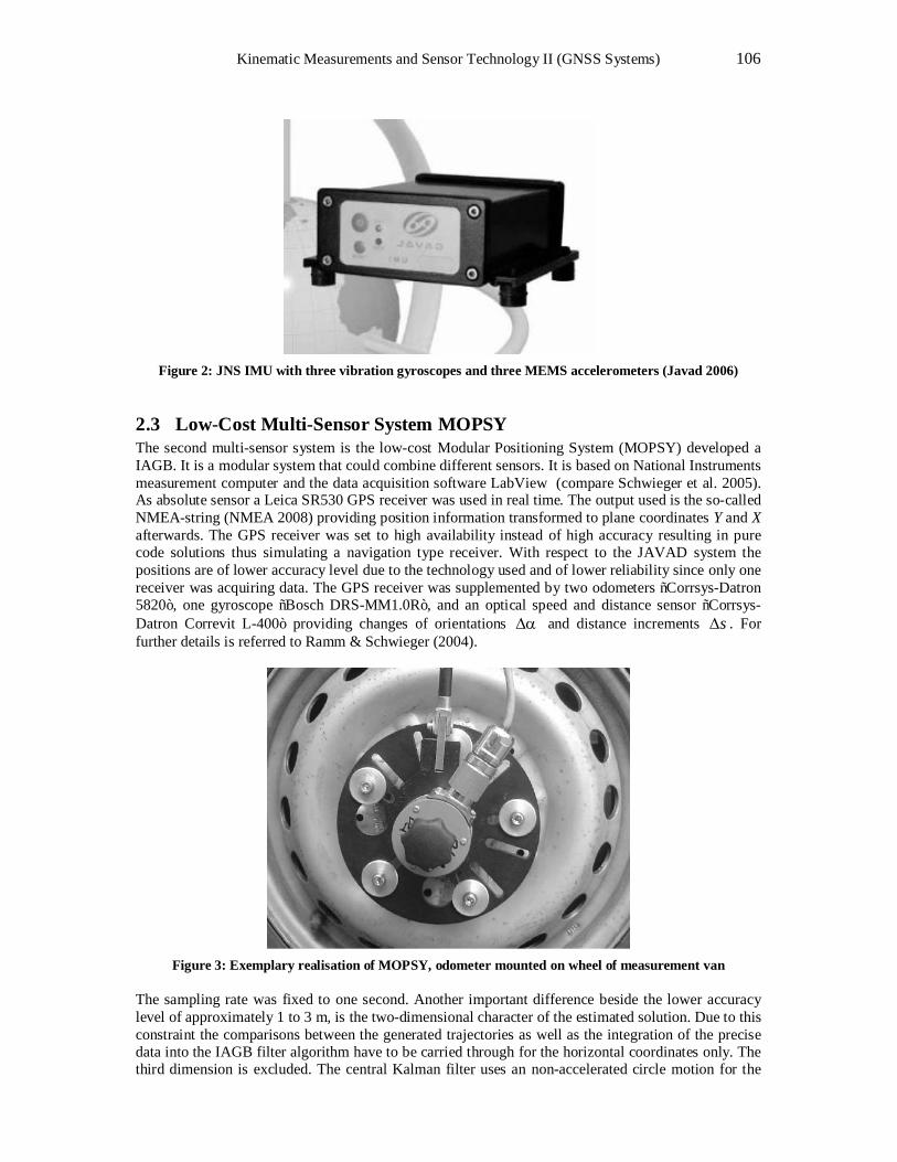
Kinematic Measurements and Sensor Technology II (GNSS Systems) 106
Figure 2: JNS IMU with three vibration gyroscopes and three MEMS accelerometers (Javad 2006)
2.3 Low-Cost Multi-Sensor System MOPSY The second multi-sensor system is the low-cost Modular Positioning System (MOPSY) developed a IAGB. It is a modular system that could combine different sensors. It is based on National Instruments measurement computer and the data acquisition software LabView (compare Schwieger et al. 2005). As absolute sensor a Leica SR530 GPS receiver was used in real time. The output used is the so-called NMEA-string (NMEA 2008) providing position information transformed to plane coordinates Y and X afterwards. The GPS receiver was set to high availability instead of high accuracy resulting in pure code solutions thus simulating a navigation type receiver. With respect to the JAVAD system the positions are of lower accuracy level due to the technology used and of lower reliability since only one receiver was acquiring data. The GPS receiver was supplemented by two odometers “Corrsys-Datron 5820”, one gyroscope “Bosch DRS-MM1.0R”, and an optical speed and distance sensor “Corrsys-Datron Correvit L-400” providing changes of orientations α∆ and distance increments s∆ . For further details is referred to Ramm & Schwieger (2004).
Figure 3: Exemplary realisation of MOPSY, odometer mounted on wheel of measurement van
The sampling rate was fixed to one second. Another important difference beside the lower accuracy level of approximately 1 to 3 m, is the two-dimensional character of the estimated solution. Due to this constraint the comparisons between the generated trajectories as well as the integration of the precise data into the IAGB filter algorithm have to be carried through for the horizontal coordinates only. The third dimension is excluded. The central Kalman filter uses an non-accelerated circle motion for the
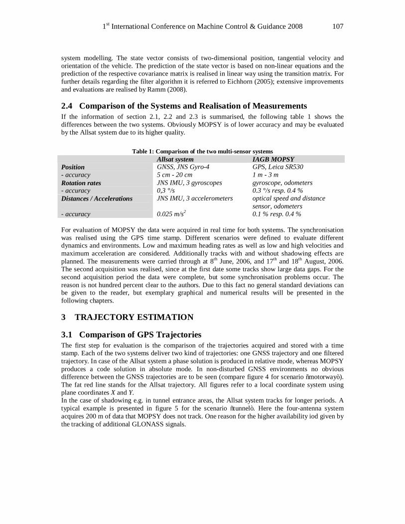
1st International Conference on Machine Control & Guidance 2008 107
system modelling. The state vector consists of two-dimensional position, tangential velocity and orientation of the vehicle. The prediction of the state vector is based on non-linear equations and the prediction of the respective covariance matrix is realised in linear way using the transition matrix. For further details regarding the filter algorithm it is referred to Eichhorn (2005); extensive improvements and evaluations are realised by Ramm (2008).
2.4 Comparison of the Systems and Realisation of Measurements If the information of section 2.1, 2.2 and 2.3 is summarised, the following table 1 shows the differences between the two systems. Obviously MOPSY is of lower accuracy and may be evaluated by the Allsat system due to its higher quality.
Table 1: Comparison of the two multi-sensor systems Allsat system IAGB MOPSY
GNSS, JNS Gyro-4 GPS, Leica SR530 Position - accuracy 5 cm - 20 cm 1 m - 3 m
JNS IMU, 3 gyroscopes gyroscope, odometers Rotation rates - accuracy 0,3 °/s 0.3 °/s resp. 0.4 %
JNS IMU, 3 accelerometers optical speed and distance sensor, odometers
Distances / Accelerations - accuracy 0.025 m/s2 0.1 % resp. 0.4 % For evaluation of MOPSY the data were acquired in real time for both systems. The synchronisation was realised using the GPS time stamp. Different scenarios were defined to evaluate different dynamics and environments. Low and maximum heading rates as well as low and high velocities and maximum acceleration are considered. Additionally tracks with and without shadowing effects are planned. The measurements were carried through at 8th June, 2006, and 17th and 18th August, 2006. The second acquisition was realised, since at the first date some tracks show large data gaps. For the second acquisition period the data were complete, but some synchronisation problems occur. The reason is not hundred percent clear to the authors. Due to this fact no general standard deviations can be given to the reader, but exemplary graphical and numerical results will be presented in the following chapters.
3 TRAJECTORY ESTIMATION
3.1 Comparison of GPS Trajectories The first step for evaluation is the comparison of the trajectories acquired and stored with a time stamp. Each of the two systems deliver two kind of trajectories: one GNSS trajectory and one filtered trajectory. In case of the Allsat system a phase solution is produced in relative mode, whereas MOPSY produces a code solution in absolute mode. In non-disturbed GNSS environments no obvious difference between the GNSS trajectories are to be seen (compare figure 4 for scenario “motorway”). The fat red line stands for the Allsat trajectory. All figures refer to a local coordinate system using plane coordinates X and Y. In the case of shadowing e.g. in tunnel entrance areas, the Allsat system tracks for longer periods. A typical example is presented in figure 5 for the scenario “tunnel”. Here the four-antenna system acquires 200 m of data that MOPSY does not track. One reason for the higher availability iod given by the tracking of additional GLONASS signals.
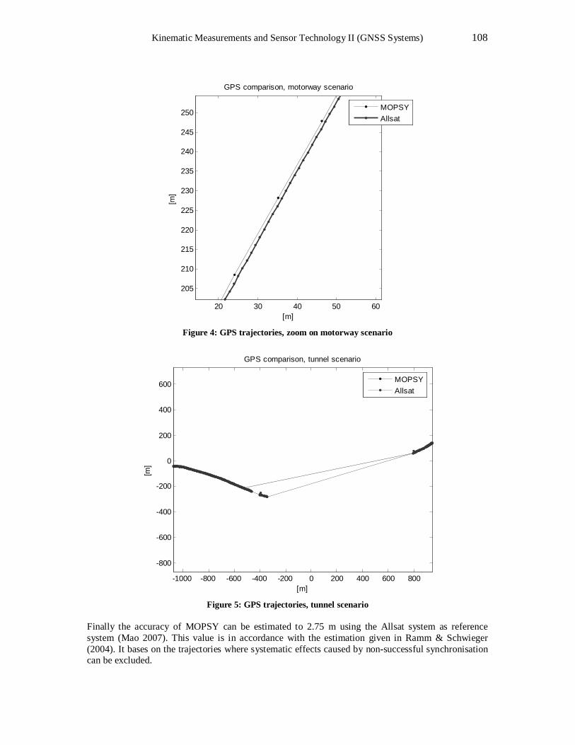
Kinematic Measurements and Sensor Technology II (GNSS Systems) 108
20 30 40 50 60
205
210
215
220
225
230
235
240
245
250
GPS comparison, motorway scenario
[m]
[m]
MOPSYAllsat
Figure 4: GPS trajectories, zoom on motorway scenario
-1000 -800 -600 -400 -200 0 200 400 600 800
-800
-600
-400
-200
0
200
400
600
GPS comparison, tunnel scenario
[m]
[m]
MOPSYAllsat
Figure 5: GPS trajectories, tunnel scenario
Finally the accuracy of MOPSY can be estimated to 2.75 m using the Allsat system as reference system (Mao 2007). This value is in accordance with the estimation given in Ramm & Schwieger (2004). It bases on the trajectories where systematic effects caused by non-successful synchronisation can be excluded.
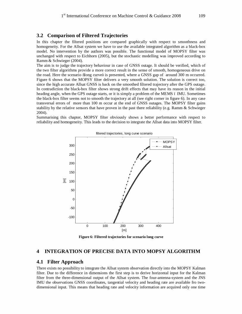
1st International Conference on Machine Control & Guidance 2008 109
3.2 Comparison of Filtered Trajectories In this chapter the filtered positions are compared graphically with respect to smoothness and homogeneity. For the Allsat system we have to use the available integrated algorithm as a black-box model. No intervention by the authors was possible. The functional model of MOPSY filter was unchanged with respect to Eichhorn (2005), but the stochastic modelling was improved according to Ramm & Schwieger (2004). The aim is to judge the trajectory behaviour in case of GNSS outage. It should be verified, which of the two filter algorithms provide a more correct result in the sense of smooth, homogeneous drive on the road. Here the scenario “long curve” is presented, where a GNSS gap of around 300 m occurred. Figure 6 shows that the MOPSY filter delivers a very smooth solution. The solution is correct too, since the high accurate Allsat GNSS is back on the smoothed filtered trajectory after the GPS outage. In contradiction the black-box filter shows strong drift effects that may have its reason in the initial heading angle, when the GPS outage starts, or it is simply a problem of the MEMS – IMU. Sometimes the black-box filter seems not to smooth the trajectory at all (see right corner in figure 6). In any case transversal errors of more than 100 m occur at the end of GNSS outages. The MOPSY filter gains stability by the relative sensors that have proven in the past there reliability (e.g. Ramm & Schwieger 2004). Summarising this chapter, MOPSY filter obviously shows a better performance with respect to reliability and homogeneity. This leads to the decision to integrate the Allsat data into MOPSY filter.
0 100 200 300 400
-100
-50
0
50
100
150
200
250
300
filtered trajectories, long curve scenario
[m]
[m]
MOPSYAllsat
Figure 6: Filtered trajectories for scenario long curve
4 INTEGRATION OF PRECISE DATA INTO MOPSY ALGORITHM
4.1 Filter Approach There exists no possibility to integrate the Allsat system observation directly into the MOPSY Kalman filter. Due to the difference in dimensions the first step is to derive horizontal input for the Kalman filter from the three-dimensional output of the Allsat system. The four-antenna-system and the JNS IMU the observations GNSS coordinates, tangential velocity and heading rate are available fro two-dimensional input. This means that heading rate and velocity information are acquired only one time
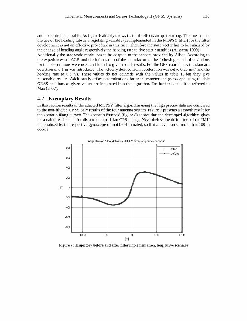
Kinematic Measurements and Sensor Technology II (GNSS Systems) 110
and no control is possible. As figure 6 already shows that drift effects are quite strong. This means that the use of the heading rate as a regulating variable (as implemented in the MOPSY filter) for the filter development is not an effective procedure in this case. Therefore the state vector has to be enlarged by the change of heading angle respectively the heading rate to five state quantities (Aussems 1999). Additionally the stochastic model has to be adapted to the sensors provided by Allsat. According to the experiences at IAGB and the information of the manufacturers the following standard deviations for the observations were used and found to give smooth results. For the GPS coordinates the standard deviation of 0.1 m was introduced. The velocity derived from acceleration was set to 0.25 m/s2 and the heading rate to 0.3 °/s. These values do not coincide with the values in table 1, but they give reasonable results. Additionally offset determinations for accelerometer and gyroscope using reliable GNSS positions as given values are integrated into the algorithm. For further details it is referred to Mao (2007).
4.2 Exemplary Results In this section results of the adapted MOPSY filter algorithm using the high precise data are compared to the non-filtered GNSS only results of the four antenna system. Figure 7 presents a smooth result for the scenario “long curve”. The scenario “tunnel” (figure 8) shows that the developed algorithm gives reasonable results also for distances up to 1 km GPS outage. Nevertheless the drift effect of the IMU materialised by the respective gyroscope cannot be eliminated, so that a deviation of more than 100 m occurs.
-1000 -500 0 500 1000
-800
-600
-400
-200
0
200
400
600
800
integration of Allsat data into MOPSY f ilter, long curve scenario
[m]
[m]
afterbefore
Figure 7: Trajectory before and after filter implementation, long curve scenario
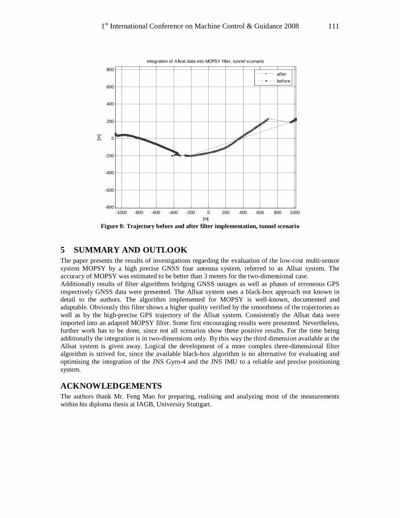
1st International Conference on Machine Control & Guidance 2008 111
-1000 -800 -600 -400 -200 0 200 400 600 800 1000-800
-600
-400
-200
0
200
400
600
800
integration of Allsat data into MOPSY filter, tunnel scenario
[m]
[m]
afterbefore
Figure 8: Trajectory before and after filter implementation, tunnel scenario
5 SUMMARY AND OUTLOOK The paper presents the results of investigations regarding the evaluation of the low-cost multi-sensor system MOPSY by a high precise GNSS four antenna system, referred to as Allsat system. The accuracy of MOPSY was estimated to be better than 3 meters for the two-dimensional case. Additionally results of filter algorithms bridging GNSS outages as well as phases of erroneous GPS respectively GNSS data were presented. The Allsat system uses a black-box approach not known in detail to the authors. The algorithm implemented for MOPSY is well-known, documented and adaptable. Obviously this filter shows a higher quality verified by the smoothness of the trajectories as well as by the high-precise GPS trajectory of the Allsat system. Consistently the Allsat data were imported into an adapted MOPSY filter. Some first encouraging results were presented. Nevertheless, further work has to be done, since not all scenarios show these positive results. For the time being additionally the integration is in two-dimensions only. By this way the third dimension available at the Allsat system is given away. Logical the development of a more complex three-dimensional filter algorithm is strived for, since the available black-box algorithm is no alternative for evaluating and optimising the integration of the JNS Gyro-4 and the JNS IMU to a reliable and precise positioning system.
ACKNOWLEDGEMENTS The authors thank Mr. Feng Mao for preparing, realising and analyzing most of the measurements within his diploma thesis at IAGB, University Stuttgart.

Kinematic Measurements and Sensor Technology II (GNSS Systems) 112
REFERENCES Books: AUSSEMS, T.: Positionsschätzung von Landfahrzeugen mittels Kalman-Filterung aus Satelliten- und Koppelnavigationsbeobachtungen. Veröffentlichung des Geodätischen Instituts der Rheinisch-Westfälischen Technischen Hochschule Aachen, Nr. 55, 1999.
EICHHORN, A.: Ein Beitrag zur parametrischen Identifikation von dynamischen Strukturmodellen mit Methoden der adaptiven Kalman Filterung. DGK, Reihe C, Heft 585, München, 2005.
GUSTAFSSON, F.: Adaptive Filtering and Change Detection. John Wiley & Sons, Chichester, UK, 2000.
HOFMANN-WELLENHOF, B., LEGAT, K., WIESER, M.: Navigation. Springer, Wien - New York, 2003.
MAO, F.: Evaluierung eines Low-Cost Multisensorsystems mittels Innertialmesstechnik und präzisem GPS. diploma thesis at IAGB, Universität Stuttgart, unpublished, 2007.
RAMM, K.: Evaluation von Filter-Ansätzen für die Positionsschätzung von Fahrzeugen mit den Werkzeugen der Sensitivitätsanalyse. DGK, Reihe C (in print), 2008.
SEEBER, G.: Satellite Geodesy - Foundations, Methods and Applications. De Gruyter, Berlin, 2003.
Journal and Symposium articles: KALMAN, R.E.: A New Approach to Linear Filtering and Prediction Problems. Transactions of the ASME –Journal of Basic Engineering, Volume 82, Series D, p. 35-45, 1960.
MOGILNITSKY, V.G., RAPOPORT, L.B., KHVALKOV, A.A., GRIBKOV, A.I., STANKEVICH, V.I.: Attitude / RTK / INS Integrated System: Experimental Results. Proceedings on ION GNSS 17th International Meeting of the Satellite Division, 21st – 24th September 2004, Long Beach, USA, 2004.
RAPELIUS, B., HEMMERT, J.: Navigationslösungen mit GNSS und Multisensorsystemen. Proceedings on Allsat Open, 16th June 2005, Hannover, Germany, 2005.
RAMM, K., SCHWIEGER, V.: Multisensorortung für Kraftfahrzeuge. Kinematische Messmethoden - Vermessung in Bewegung. Contributions on 58. DVW-Seminar, 17th and 18th february 2004, Stuttgart, Wißner Verlag, Augsburg, 2004.
SCHWIEGER, V.: High-Sensitivity GPS – an availability, reliability and accuracy test. Proceedings on FIG Working Week, 14th – 19th June 2008, Stockholm Sweden, 2008.
SCHWIEGER, V., SCHOLLMEYER, R., RAMM, K.: Integrated Positioning by MOPSY. Proceedings on 5th European Congress and Exhibition on Intelligent Transport Systems and Services, Hannover, 1st-3rd june 2005.
Links and data sheets: JAVAD: JNS IMU data sheet, version 2006.
NMEA: http://www.nmea.de/nmea0183datensaetze.html, last accessed on April, 21st, 2008.
EU: http://euobserver.com/9/25939, last accessed on April, 21st, 2008.
* PD Dr.-Ing. Volker Schwieger, Universität Stuttgart, Institute for Application of Geodesy to Engineering, Geschwister-Scholl-Str. 24D, D-70174 Stuttgart, Germany. ** Dipl.-Ing. Julia Hemmert, ALLSAT GmbH, Am Hohen Ufer 3A, D-30159 Hannover, Germany.
1st International Conference on Machine Control & Guidance 2008 113
Integrated Controls for Agricultural Applications – GNSS Enabling a New Level in Precision Farming
Patrick Ole NOACK*, Thomas MUHR
geo-konzept GmbH, Germany [email protected]
Abstract Naturally, most agricultural operations are undertaken in the space domain and are embedded in an environment that is subject to change and variability. Both, human actions such as cultivation and fertilization and natural factors such as weather and soil properties continuously influence and change the environment for plant and animal production. Hence, appropriate information on current and preceding states of this environment and the knowledge about actions taken in the past is important for decision making and planning future operations in order to maximize yield while minimising the ecological impact. The need to optimise food production also introduces the challenge to reduce the cost for labour and mineral fuels and thus to minimize the operation hour of machinery in the field to the minimum required. GNSS sensors have introduced the capability to record human actions and the variability of spatial structures in plant and animal production in the time and in the space domain. They also enhance the exact control of tractors and implements dependant on their position. Over the last 20 years GNSS technology has helped to establish tools which help to increase the productivity in agriculture substantially. Keywords GPS, GNSS, agriculture, automated steering, Precision Farming
1 INTRODUCTION Agriculture – as all other segments of the industry – is under continuous pressure to reduce costs and negative impacts of production on the environment. Furthermore, the demand for agricultural products for both consumption and energy production is rising with a growing world population. Today, GNSS sensors are widely used in agriculture serving different purposes, mainly with the aim to increase yield and cut down costs for labour and input material: they are a core component in manual guidance and automatic steering systems, position readings from GNSS sensors provide information to task controllers in order vary the application of fertilizer and herbicides according to soil heterogeneity and the expected level of yield on a sub-field level. Yet, more use cases for satellite based positioning devices in agriculture have been sketched and are being worked on.
2 FROM YIELD MAPPING TO AUTOMATIC STEERING SYSTEMS The concept of yield mapping has first been mentioned about 20 years ago (Bae e.a., 1987). The idea was to collect yield measurements on a combine harvester along with its position with the purpose of creating maps representing the spatial variability of yield. First trials in the field revealed that the mass flow sensors installed the grain auger were capable of measuring the grain flow with a satisfying accuracy. However, determining the position of the vehicle involved measuring the distance travelled on a tram line off the edge of the field which turned out to be awkward on large or irregularly shaped fields.
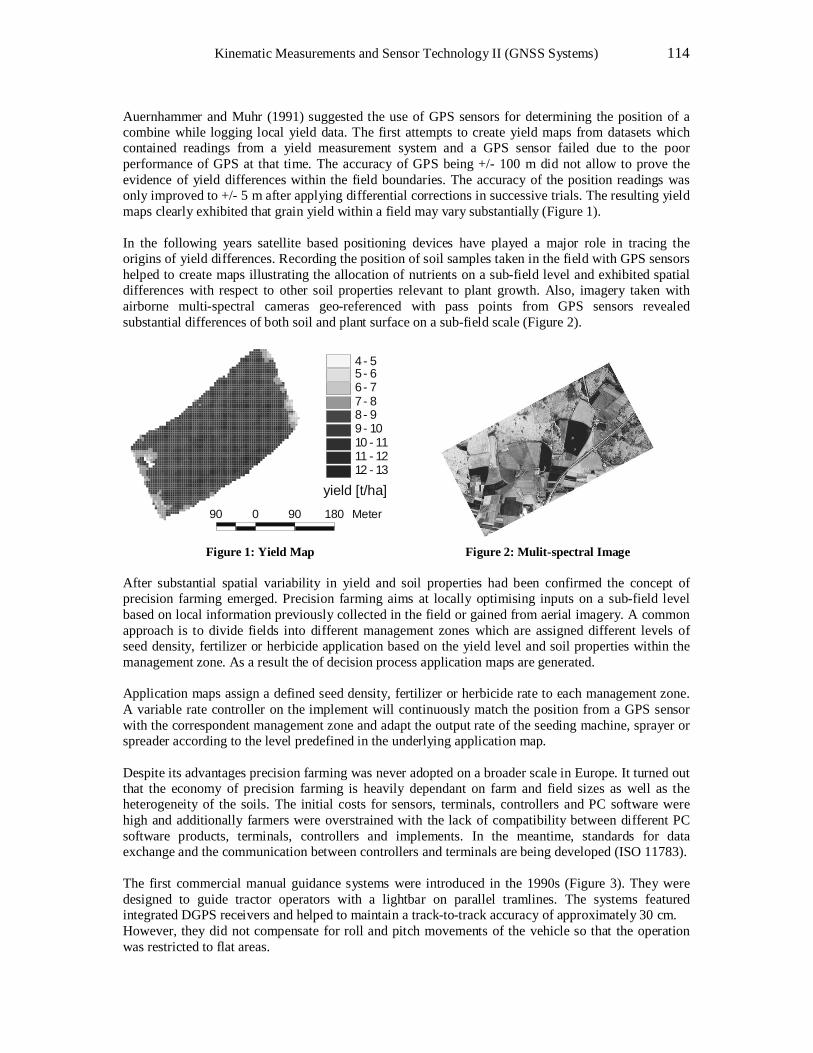
Kinematic Measurements and Sensor Technology II (GNSS Systems) 114
Auernhammer and Muhr (1991) suggested the use of GPS sensors for determining the position of a combine while logging local yield data. The first attempts to create yield maps from datasets which contained readings from a yield measurement system and a GPS sensor failed due to the poor performance of GPS at that time. The accuracy of GPS being +/- 100 m did not allow to prove the evidence of yield differences within the field boundaries. The accuracy of the position readings was only improved to +/- 5 m after applying differential corrections in successive trials. The resulting yield maps clearly exhibited that grain yield within a field may vary substantially (Figure 1). In the following years satellite based positioning devices have played a major role in tracing the origins of yield differences. Recording the position of soil samples taken in the field with GPS sensors helped to create maps illustrating the allocation of nutrients on a sub-field level and exhibited spatial differences with respect to other soil properties relevant to plant growth. Also, imagery taken with airborne multi-spectral cameras geo-referenced with pass points from GPS sensors revealed substantial differences of both soil and plant surface on a sub-field scale (Figure 2).
5 - 66 - 77 - 88 - 99 - 1010 - 1111 - 1212 - 13
4 - 5
yield [t/ha]90 0 90 180 Meter
Figure 1: Yield Map Figure 2: Mulit-spectral Image
After substantial spatial variability in yield and soil properties had been confirmed the concept of precision farming emerged. Precision farming aims at locally optimising inputs on a sub-field level based on local information previously collected in the field or gained from aerial imagery. A common approach is to divide fields into different management zones which are assigned different levels of seed density, fertilizer or herbicide application based on the yield level and soil properties within the management zone. As a result the of decision process application maps are generated. Application maps assign a defined seed density, fertilizer or herbicide rate to each management zone. A variable rate controller on the implement will continuously match the position from a GPS sensor with the correspondent management zone and adapt the output rate of the seeding machine, sprayer or spreader according to the level predefined in the underlying application map. Despite its advantages precision farming was never adopted on a broader scale in Europe. It turned out that the economy of precision farming is heavily dependant on farm and field sizes as well as the heterogeneity of the soils. The initial costs for sensors, terminals, controllers and PC software were high and additionally farmers were overstrained with the lack of compatibility between different PC software products, terminals, controllers and implements. In the meantime, standards for data exchange and the communication between controllers and terminals are being developed (ISO 11783). The first commercial manual guidance systems were introduced in the 1990s (Figure 3). They were designed to guide tractor operators with a lightbar on parallel tramlines. The systems featured integrated DGPS receivers and helped to maintain a track-to-track accuracy of approximately 30 cm. However, they did not compensate for roll and pitch movements of the vehicle so that the operation was restricted to flat areas.

1st International Conference on Machine Control & Guidance 2008 115
Figure 3: Trimble Ag GPS 21A
At the same GEOTEC, a company based in Germany, started developing a steering and control system for autonomous tractors (Ehrl, 2004). The system was designed to steer a tractor, control its speed and the implement without any human interaction. The concept involved planning the mission on a PC with the help of CAD software. During mission setup, all actions and the course of travel had to be defined. The system was never adopted in practice for several reasons. It turned out that mission planning was overburdening the average user. Also, the occurrence of unpredictable events and obstacles necessitated the presence of a supervisor while system was in action. Trimble Navigation Ltd. presented the first commercial automatic steering system for tractors in the year 2000. Initially, the AgGPS Autopilot system was only available with RTK GPS receivers and could only be fitted on a very limited number of vehicles. Integrated accelerometers and gyroscopes enable the AgGPS RTK Autopilot to account for pitch and roll of the vehicle and thus maintain a track-to-track accuracy in the range of 2.5 cm. In opposition to the approach GEOTEC had taken, the Autopilot system was only designed to automatically keep the vehicle on track on the tramline. It was not meant to supersede the operator but to release attention for monitoring the implement and the quality of the operation performed. Unlike precision farming, manual guidance and automatic steering systems have been easily adopted by farmers. Initially, the connotation of GPS and precision farming debased guidance and steering systems. Today, manual guidance and automatic steering are next to be accepted to such a level that they are regarded as tools alike tractors and implements.
3 GNSS IN AGRICULTURE TODAY Satellite based position sensors are serving farmers, contractors, consultants and officials involved in agriculture in many ways. Not all applications are necessarily related to machinery: all over Europe, officials use GPS based mapping systems to determine field sizes and compare them with the statements in the subsidy applications submitted by farmers. Already 15 years ago position readings from GPS sensors attached to sheep have been analysed to better understand their grazing behaviour (Roberts ea., 1993). This approach is still latently being followed (Braunreiter ea., 2007). Recording the position of soil samples and the subsequent creation of soil maps is a growing business in areas with large fields and heterogeneous soil conditions. When GPS receivers are installed on tractors or other agricultural machinery, they are not necessarily used for controlling or guiding the vehicle. Merely the information on where a machine is or has been and what state it is in is valuable: contractors use position data from GPS receivers transferred online with GSM technology to optimise the disposition of their tractors and combines. Also, low cost GPS sensors are adopted in systems for theft control. Position and time measurements from a GPS receiver collected along with other process data on a machine like speed, fuel consumption, traction force or yield can serve different purposes. Process data can be analysed to determine the usage of shared machinery and thus to share variable and fixed
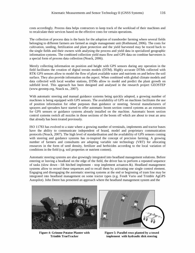
Kinematic Measurements and Sensor Technology II (GNSS Systems) 116
costs accordingly. Process data helps contractors to keep track of the workload of their machines and to recalculate their services based on the effective costs for certain operations. The collection of process data is the basis for the adoption of transborder farming where several fields belonging to different farmers are farmed as single management unit (Rothmund, 2006). The costs for cultivation, seeding, fertilization and plant protection and the yield harvested may be traced back to the single fields and their owners with analysing the process and yield data in specialized geographic information systems. The combined collection yield mass flow and GPS data on combine harvesters is a special form of process data collection (Noack, 2006). Merely collecting information on position and height with GPS sensors during any operation in the field facilitates the creation of digital terrain models (DTM). Highly accurate DTMs collected with RTK GPS sensors allow to model the flow of plant available water and nutrients on and below the soil surface. They also provide information on the aspect. When combined with global climate models and data collected with local weather stations, DTMs allow to model and predict the plant growth on subfield level. This approach has been designed and analysed in the research project GEOSTEP (www.geostep.org, Noack ea., 2007). With automatic steering and manual guidance systems being quickly adopted, a growing number of machines is being equipped with GPS sensors. The availability of GPS on machines facilitates the use of position information for other purposes than guidance or steering. Several manufacturers of sprayers and spreaders have started to offer automatic boom section control systems as an extension for GPS sensors or guidance systems already installed on the machine. Automatic boom section control systems switch all nozzles in those sections of the boom off which are about to treat an area that already has been treated previously. ISO 11783 has evolved to a state where a growing number of terminals, implements and tractor buses have the ability to communicate independent of brand, model and proprietary communication protocols (Noack, 2007). The high level of standardisation and the availability of GPS sensors coming with steering and guidance systems has re-inspired the concept of precision farming. A growing number of farmers and consultants are adopting variable rate technology (VRT) for allocating resources in the form of seed density, fertilizer and herbicides according to the local variation of conditions in the field (e.g. soil properties or nutrient content). Automatic steering systems are also growingly integrated into headland management solutions. Before entering or leaving a headland on the edge of the field, the driver has to perform a repeated sequence of tasks (slow down - lift hitched implement - stop implement actuators…). Headland management systems allow to record these sequences and to recall them by activating one single control element. Engaging and disengaging the automatic steering systems at the end or beginning of tram line may be integrated into headland management on some tractor types (e.g. Fendt Vario and Trimble AgGPS Autopilot). John Deere has presented an approach where the headland management system and the
Figure 4: Grimme Potatoe Planter with
Trimble TrueTracker
Figure 5: Parallel rows planted by a towed implement with hydraulic disk steering

1st International Conference on Machine Control & Guidance 2008 117
automatic steering system are so deeply integrated that the tractor even turns automatically at the end of a row (John Deere iTEC Pro™ , John Deere, 2008). Both Autofarm and Trimble, two manufacturers of automatic steering systems, also offer steering systems for towed and hitched implements (AF Tracker, TrueTracker). As automatic steering systems are only designed to keep vehicles on track implements tend to drift of the desired path whenever operated on side slopes or on fields with highly variable soil types. Implement steering systems are equipped with an additional GPS sensor and steer the implement with attached disks or wheels (Figure 4 and 5). Implement steering is especially adopted by farmers following the concepts of controlled traffic1 and strip tillage. Controlled traffic is an approach to minimise soil compaction to the tramlines. Once established, tramlines stored in the terminals of automatic steering systems are recalled for every operation. Consequently, the soil between the tramlines is never affected by compaction and thus provides a better environment for plant growth. Strip Tillage aims at reducing cultivation and tillage to that part of the soil where seeds are being placed (strip). It requires the ability to exactly place both fertilizer and seed and to accurately control all implements involved in cultivation. Parcel plot trials are a standard method in scientific and commercial research. A group of rectangular parcels are planted in a grid structure. Pathways divide the parcels in longitudinal direction. Comparing quantity and quality of yield from different parcels helps to determine how different breeds of plants perform under ceteris paribus conditions and standardized treatment. Parcel plot trials are also used for comparing the effect of different intensities of treatment with herbicides, insecticides and fertilizer on the growth of plants of the same breed. Creating parcel plots is labor and cost intensive. The adoption of automatic steering systems has helped to facilitate the creation of parcel plots without applying terrestrial surveying. The block design and the creation of the correspondent guidance elements may be carried out on a PC and uploaded to the guidance terminal (Noack, 2006). Besides keeping the tractor on the desired path while sowing advanced steering systems also feature output signals to trigger the seeding machine whenever it enters a new parcel. The adoption of PC based mission planning and GPS based automatic steering systems in parcel plot trials decreases the workload while sowing parcel plot trials and increases the quality of the trial results due to the increased accuracy of the parcel block geometry.
4 FUTURE OF GNSS IN AGRICULTURE Satellite based position sensors will play an increasingly important role in agriculture. They provide very basic information on time, heading, speed and position of a vehicle or implement. This information is valuable online for optimising processes (e.g. steering, implement control) and may also be recorded along with other data available for further analysis (e.g. process data). During the last two years Topcon and Trimble have started to introduce GNSS sensors into agricultural applications which are capable of tracking both GPS and GLONASS satellites. These sensors improve the reliability of position measurements especially in areas with many trees and regions with poor satellite coverage (Northern Europe). The price for RTK-GPS base stations has already been decreasing with the growing volume generated from demand by the agricultural market. Accessing RTK-GPS corrections will become even cheaper when machinery dealers start building RTK networks and commercial providers start offering correction services based on internet technology.
1 http://www.controlledtrafficfarming.net
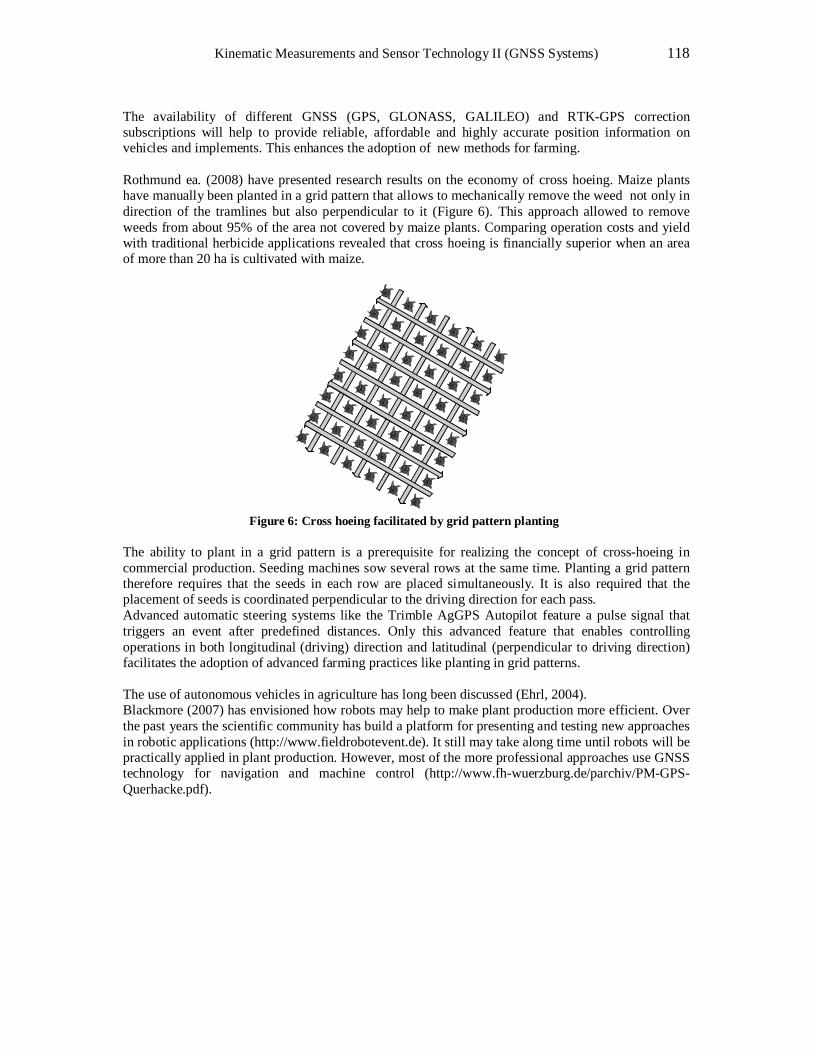
Kinematic Measurements and Sensor Technology II (GNSS Systems) 118
The availability of different GNSS (GPS, GLONASS, GALILEO) and RTK-GPS correction subscriptions will help to provide reliable, affordable and highly accurate position information on vehicles and implements. This enhances the adoption of new methods for farming. Rothmund ea. (2008) have presented research results on the economy of cross hoeing. Maize plants have manually been planted in a grid pattern that allows to mechanically remove the weed not only in direction of the tramlines but also perpendicular to it (Figure 6). This approach allowed to remove weeds from about 95% of the area not covered by maize plants. Comparing operation costs and yield with traditional herbicide applications revealed that cross hoeing is financially superior when an area of more than 20 ha is cultivated with maize.
Figure 6: Cross hoeing facilitated by grid pattern planting
The ability to plant in a grid pattern is a prerequisite for realizing the concept of cross-hoeing in commercial production. Seeding machines sow several rows at the same time. Planting a grid pattern therefore requires that the seeds in each row are placed simultaneously. It is also required that the placement of seeds is coordinated perpendicular to the driving direction for each pass. Advanced automatic steering systems like the Trimble AgGPS Autopilot feature a pulse signal that triggers an event after predefined distances. Only this advanced feature that enables controlling operations in both longitudinal (driving) direction and latitudinal (perpendicular to driving direction) facilitates the adoption of advanced farming practices like planting in grid patterns. The use of autonomous vehicles in agriculture has long been discussed (Ehrl, 2004). Blackmore (2007) has envisioned how robots may help to make plant production more efficient. Over the past years the scientific community has build a platform for presenting and testing new approaches in robotic applications (http://www.fieldrobotevent.de). It still may take along time until robots will be practically applied in plant production. However, most of the more professional approaches use GNSS technology for navigation and machine control (http://www.fh-wuerzburg.de/parchiv/PM-GPS-Querhacke.pdf).
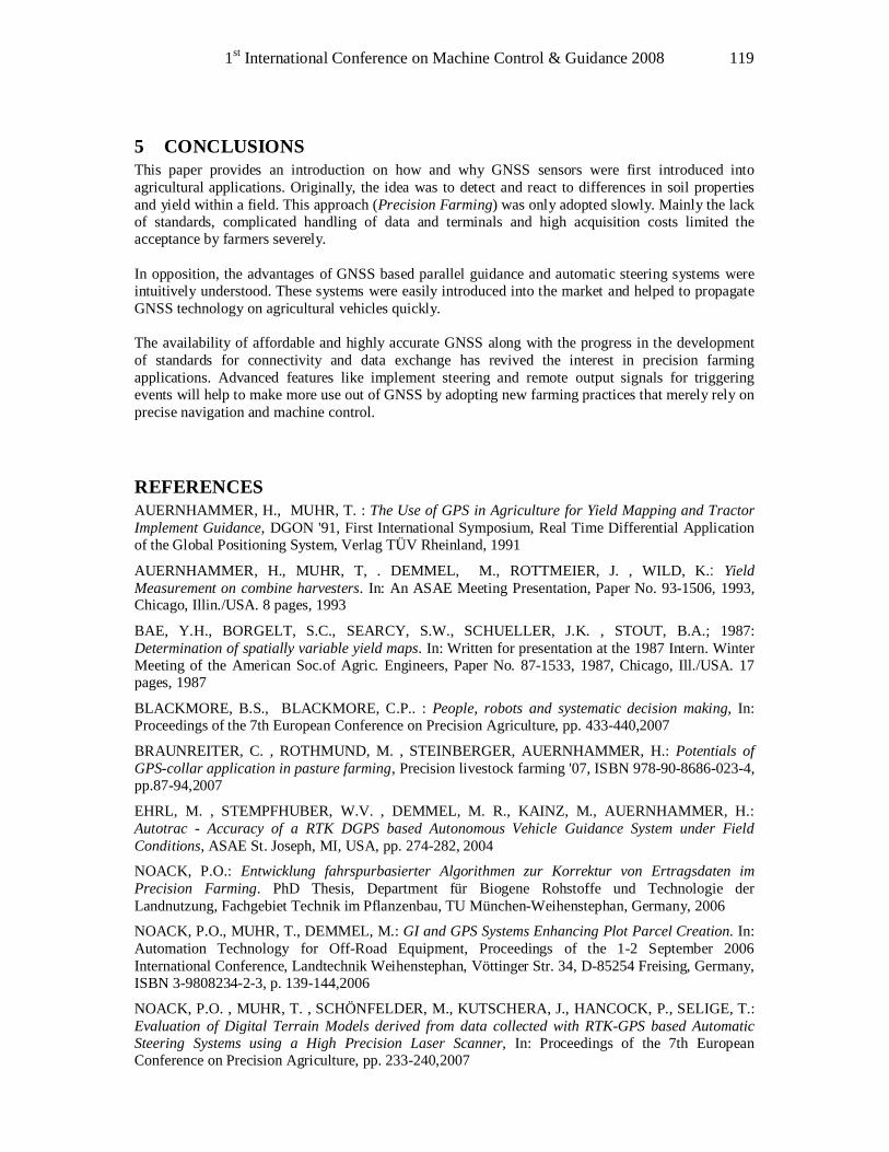
1st International Conference on Machine Control & Guidance 2008 119
5 CONCLUSIONS This paper provides an introduction on how and why GNSS sensors were first introduced into agricultural applications. Originally, the idea was to detect and react to differences in soil properties and yield within a field. This approach (Precision Farming) was only adopted slowly. Mainly the lack of standards, complicated handling of data and terminals and high acquisition costs limited the acceptance by farmers severely. In opposition, the advantages of GNSS based parallel guidance and automatic steering systems were intuitively understood. These systems were easily introduced into the market and helped to propagate GNSS technology on agricultural vehicles quickly. The availability of affordable and highly accurate GNSS along with the progress in the development of standards for connectivity and data exchange has revived the interest in precision farming applications. Advanced features like implement steering and remote output signals for triggering events will help to make more use out of GNSS by adopting new farming practices that merely rely on precise navigation and machine control.
REFERENCES AUERNHAMMER, H., MUHR, T. : The Use of GPS in Agriculture for Yield Mapping and Tractor Implement Guidance, DGON '91, First International Symposium, Real Time Differential Application of the Global Positioning System, Verlag TÜV Rheinland, 1991
AUERNHAMMER, H., MUHR, T, . DEMMEL, M., ROTTMEIER, J. , WILD, K.: Yield Measurement on combine harvesters. In: An ASAE Meeting Presentation, Paper No. 93-1506, 1993, Chicago, Illin./USA. 8 pages, 1993
BAE, Y.H., BORGELT, S.C., SEARCY, S.W., SCHUELLER, J.K. , STOUT, B.A.; 1987: Determination of spatially variable yield maps. In: Written for presentation at the 1987 Intern. Winter Meeting of the American Soc.of Agric. Engineers, Paper No. 87-1533, 1987, Chicago, Ill./USA. 17 pages, 1987
BLACKMORE, B.S., BLACKMORE, C.P.. : People, robots and systematic decision making, In: Proceedings of the 7th European Conference on Precision Agriculture, pp. 433-440,2007
BRAUNREITER, C. , ROTHMUND, M. , STEINBERGER, AUERNHAMMER, H.: Potentials of GPS-collar application in pasture farming, Precision livestock farming '07, ISBN 978-90-8686-023-4, pp.87-94,2007
EHRL, M. , STEMPFHUBER, W.V. , DEMMEL, M. R., KAINZ, M., AUERNHAMMER, H.: Autotrac - Accuracy of a RTK DGPS based Autonomous Vehicle Guidance System under Field Conditions, ASAE St. Joseph, MI, USA, pp. 274-282, 2004
NOACK, P.O.: Entwicklung fahrspurbasierter Algorithmen zur Korrektur von Ertragsdaten im Precision Farming. PhD Thesis, Department für Biogene Rohstoffe und Technologie der Landnutzung, Fachgebiet Technik im Pflanzenbau, TU München-Weihenstephan, Germany, 2006
NOACK, P.O., MUHR, T., DEMMEL, M.: GI and GPS Systems Enhancing Plot Parcel Creation. In: Automation Technology for Off-Road Equipment, Proceedings of the 1-2 September 2006 International Conference, Landtechnik Weihenstephan, Vöttinger Str. 34, D-85254 Freising, Germany, ISBN 3-9808234-2-3, p. 139-144,2006
NOACK, P.O. , MUHR, T. , SCHÖNFELDER, M., KUTSCHERA, J., HANCOCK, P., SELIGE, T.: Evaluation of Digital Terrain Models derived from data collected with RTK-GPS based Automatic Steering Systems using a High Precision Laser Scanner, In: Proceedings of the 7th European Conference on Precision Agriculture, pp. 233-240,2007
Kinematic Measurements and Sensor Technology II (GNSS Systems) 120
NOACK, P.O.: Standards für den Datenaustausch in der Landwirtschaft. In: Landtechnik, 62. Jahrgang, Sonderheft September 2007, Kuratorium für Technik und Bauwesen in der Landwirtschaft e.V., Darmstadt, Germany, pp. 283 –255, 2007.
ROBERTS, G., WILLIAMS, A., PENNING, P.D., RUTTER, S.M.: A Low-Power Portable Post-Processed DGPS Package for Precise Position-Logging of Sheep on Hill Pastures, ION GPS-93 Proceedings, Sixth International Technical Meeting of The Satellite Division of the Institute of Navigation, pp. 1141-1148, 1993
ROTHMUND, M.: Technische Umsetzung einer Gewannebewirtschaftung als „Virtuelle Flurbereinigung“ mit ihren ökonomischen und ökologischen Potenzialen, PhD Thesis, Department für Biogene Rohstoffe und Technologie der Landnutzung, Fachgebiet Technik im Pflanzenbau, TU München-Weihenstephan, Germany, 2006
ROTHMUND, M, STEINBERGER, G, AUERNHAMMER, H: Das Kreuzhackverfahren - Zweidimensionale mechanische Unkrautbekämpfung im Maisanbau durch Einzelkornsaat im spurübergreifenden übergreifenden quadratischen Verband , www.nas.boku.ac.at/fileadmin/_/H93/H931/AKAL-Seminar/Praesentationen/AKAL-Wien-ROTHMUND.pdf, last accessed on April 14,2008
JOHN DEERE: iTEC Pro™ , http://www.deere.com/en_US/ag/feature/2008/itecpro.html; last accessed on April 17,2008
* Dr. Patrick Ole Noack, geo-konzept GmbH, Gut Wittenfeld, D-85111 Adelschlag, Germany
1st International Conference on Machine Control & Guidance 2008 121
GNSS Orientation for kinematic applications David Eugen GRIMM*
ETH Zurich, Switzerland [email protected]
Abstract GNSS systems are a well established technique for guiding machines or the machine’s operator along predefined routes. Such GNSS applications have been successfully integrated into the design of construction machines and farming equipment. While a GNSS-equipped machine moves straight ahead conventional GNSS systems with only one antenna show good performance. However, the system reaches its limits when the machine turns on its own axis, such as an excavator does. This causes the GNSS receiver to be unable to determine its bearing, as a compass could do. A common single-antenna GNSS receiver can only estimate its moving direction (heading) using previous positions. Since a turn around its own axis does not change the coordinates, but changes the orientation of the machine, the orientation can not be calculated by this means. A common solution to this problem is the implementation of two GNSS antennas. Two antennas allow the bearing of the baseline between the antennas to be defined. A new approach with only one antenna required is under development at the ETH Zurich. This new system uses the satellite positions as a reference for orientation. For that purpose the direction of each satellite’s signal has to be known in relation to the antenna. In order to obtain orientation the signal strength of each satellite is measured. A well defined shading of the received signals allows estimating the required orientation. After full implementation of our approach, the second GNSS antenna found on most construction machines will not be required anymore. Keywords Antenna orientation, GPS compass, GNSS compass, azimuth, GNSS direction finding
1 INTRODUCTION The goal of this research work is to determine the orientation of a GNSS antenna. The opportunities of the GNSS system should be exploited instead of using additional sensors. The state of the art provides three options to achieve an orientation, or heading information in coherence with GNSS receivers.
• Using more antenna systems • Using the movement of the antenna • Using additional sensors
The application of GNSS systems for orientation was an object of research from the very beginning of the GPS technology. In a patent specification of 1989, Jablonski [1] described a method to “acquire accurate compass heading information without being affected by magnetic anomalies and without being dependent on the elapsed time since a previous position fix”. He uses two antennas with a specific distance between them. The receiver switches between the two antennas automatically thereby measuring their absolute positions. Based on the knowledge of these coordinates a compass heading is calculated. The accuracy of the calculated heading relies on satellite geometry, performance of receiver, baseline configuration and attitude, and in particular on the distance between the antennas. It is evident that an estimation of the heading is no longer possible when the baseline is vertical. Consequently it is advantageous to mount the baseline in a horizontal position for applications where heading determination is of interest. To obtain a more precise heading, a longer baseline has to be chosen. (Park et al.) [2]
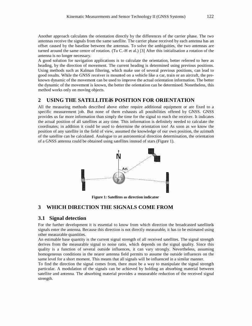
Kinematic Measurements and Sensor Technology II (GNSS Systems) 122
Another approach calculates the orientation directly by the differences of the carrier phase. The two antennas receive the signals from the same satellite. The carrier phase received by each antenna has an offset caused by the baseline between the antennas. To solve the ambiguities, the two antennas are turned around the same centre of rotation. (Tu C.-H et al.) [3] After this initialisation a rotation of the antenna is no longer necessary. A good solution for navigation applications is to calculate the orientation, better referred to here as heading, by the direction of movement. The current heading is determined using previous positions. Using methods such as Kalman filtering, which make use of several previous positions, can lead to good results. While the GNSS receiver is mounted on a vehicle like a car, train or an aircraft, the pre-known dynamic of the movement can be used to improve the actual orientation information. The better the dynamic of the movement is known, the better the orientation can be determined. Nonetheless, this method works only on moving objects.
2 USING THE SATELLITE’S POSITION FOR ORIENTATION All the measuring methods described above either require additional equipment or are fixed to a specific measurement job. But none of them exhausts all possibilities offered by GNSS. GNSS provides us far more information than simply the time for the signal to reach the receiver. It indicates the actual position of all satellites at any time. This information is definitely needed to calculate the coordinates; in addition it could be used to determine the orientation too! As soon as we know the position of any satellite in the field of view, assumed the knowledge of our own position, the azimuth of the satellite can be calculated. Analogue to an astronomical direction determination, the orientation of a GNSS antenna could be obtained using satellites instead of stars (Figure 1).
N
Azi.
N
Azi.
Figure 1: Satellites as direction indicator
3 WHICH DIRECTION THE SIGNALS COME FROM
3.1 Signal detection For the further development it is essential to know from which direction the broadcasted satellite’s signals enter the antenna. Because this direction is not directly measurable, it has to be estimated using other measurable quantities. An estimable base quantity is the current signal strength of all received satellites. The signal strength derives from the measurable signal to noise ratio, which depends on the signal quality. Since this quality is a function of several outside influences, it can vary strongly. Nevertheless, assuming homogeneous conditions in the nearer antenna field permits to assume the outside influences on the same level for a short moment. This means that all signals will be influenced in a similar manner. To find the direction the signal comes from, there must be a way to manipulate the signal strength particular. A modulation of the signals can be achieved by holding an absorbing material between satellite and antenna. The absorbing material provides a measurable reduction of the received signal strength.
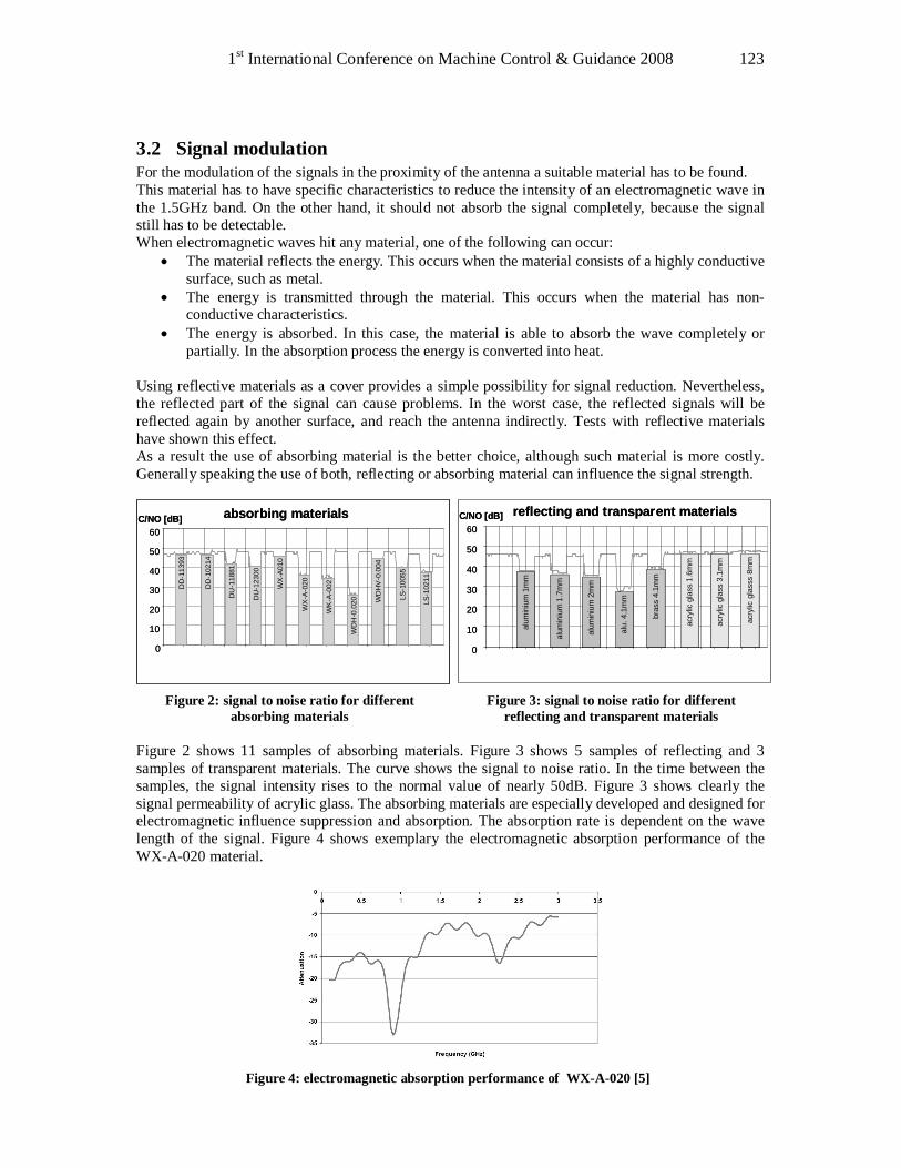
1st International Conference on Machine Control & Guidance 2008 123
3.2 Signal modulation For the modulation of the signals in the proximity of the antenna a suitable material has to be found. This material has to have specific characteristics to reduce the intensity of an electromagnetic wave in the 1.5GHz band. On the other hand, it should not absorb the signal completely, because the signal still has to be detectable. When electromagnetic waves hit any material, one of the following can occur:
• The material reflects the energy. This occurs when the material consists of a highly conductive surface, such as metal.
• The energy is transmitted through the material. This occurs when the material has non-conductive characteristics.
• The energy is absorbed. In this case, the material is able to absorb the wave completely or partially. In the absorption process the energy is converted into heat.
Using reflective materials as a cover provides a simple possibility for signal reduction. Nevertheless, the reflected part of the signal can cause problems. In the worst case, the reflected signals will be reflected again by another surface, and reach the antenna indirectly. Tests with reflective materials have shown this effect. As a result the use of absorbing material is the better choice, although such material is more costly. Generally speaking the use of both, reflecting or absorbing material can influence the signal strength.
absorbing materials
0
10
20
30
40
50
60C/NO [dB]
WD
H-0
.020 W
DH
V-0
.004
LS-1
0211
LS-1
0055
WK
-A-0
02
WX
-A-0
20WX
-A01
0
DU
-123
00
DU
-118
81
DD
-102
14
DD
-113
93
absorbing materials
0
10
20
30
40
50
60C/NO [dB]
WD
H-0
.020 W
DH
V-0
.004
LS-1
0211
LS-1
0055
WK
-A-0
02
WX
-A-0
20WX
-A01
0
DU
-123
00
DU
-118
81
DD
-102
14
DD
-113
93
reflecting and transparent materials
0
10
20
30
40
50
60C/NO [dB]
alum
iniu
m 1
mm
alum
iniu
m 1
.7m
m
alum
iniu
m 2
mm
alu.
4.1
mm
bras
s 4.
1mm
acry
lic g
lass
1.6
mm
acry
lic g
lass
3.1
mm
acry
lic g
lass
s8m
m
reflecting and transparent materials
0
10
20
30
40
50
60C/NO [dB]
alum
iniu
m 1
mm
alum
iniu
m 1
.7m
m
alum
iniu
m 2
mm
alu.
4.1
mm
bras
s 4.
1mm
acry
lic g
lass
1.6
mm
acry
lic g
lass
3.1
mm
acry
lic g
lass
s8m
m
Figure 2: signal to noise ratio for different
absorbing materials Figure 3: signal to noise ratio for different
reflecting and transparent materials Figure 2 shows 11 samples of absorbing materials. Figure 3 shows 5 samples of reflecting and 3 samples of transparent materials. The curve shows the signal to noise ratio. In the time between the samples, the signal intensity rises to the normal value of nearly 50dB. Figure 3 shows clearly the signal permeability of acrylic glass. The absorbing materials are especially developed and designed for electromagnetic influence suppression and absorption. The absorption rate is dependent on the wave length of the signal. Figure 4 shows exemplary the electromagnetic absorption performance of the WX-A-020 material.
Figure 4: electromagnetic absorption performance of WX-A-020 [5]
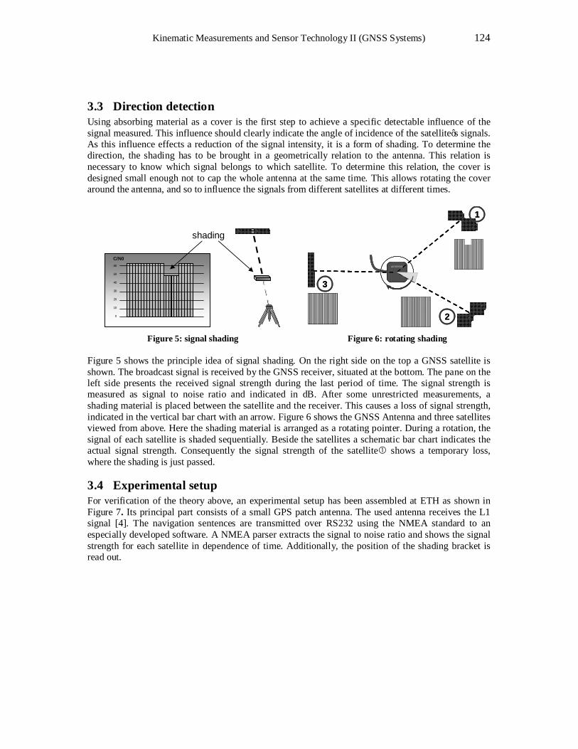
Kinematic Measurements and Sensor Technology II (GNSS Systems) 124
3.3 Direction detection Using absorbing material as a cover is the first step to achieve a specific detectable influence of the signal measured. This influence should clearly indicate the angle of incidence of the satellite’s signals. As this influence effects a reduction of the signal intensity, it is a form of shading. To determine the direction, the shading has to be brought in a geometrically relation to the antenna. This relation is necessary to know which signal belongs to which satellite. To determine this relation, the cover is designed small enough not to cap the whole antenna at the same time. This allows rotating the cover around the antenna, and so to influence the signals from different satellites at different times.
60
50
40
30
20
10
0
C/N0
shading
ANTENNE
ANTENNE
1
2
3
ANTENNE
ANTENNE
1
2
3
Figure 5: signal shading Figure 6: rotating shading
Figure 5 shows the principle idea of signal shading. On the right side on the top a GNSS satellite is shown. The broadcast signal is received by the GNSS receiver, situated at the bottom. The pane on the left side presents the received signal strength during the last period of time. The signal strength is measured as signal to noise ratio and indicated in dB. After some unrestricted measurements, a shading material is placed between the satellite and the receiver. This causes a loss of signal strength, indicated in the vertical bar chart with an arrow. Figure 6 shows the GNSS Antenna and three satellites viewed from above. Here the shading material is arranged as a rotating pointer. During a rotation, the signal of each satellite is shaded sequentially. Beside the satellites a schematic bar chart indicates the actual signal strength. Consequently the signal strength of the satellite shows a temporary loss, where the shading is just passed.
3.4 Experimental setup For verification of the theory above, an experimental setup has been assembled at ETH as shown in Figure 7. Its principal part consists of a small GPS patch antenna. The used antenna receives the L1 signal [4]. The navigation sentences are transmitted over RS232 using the NMEA standard to an especially developed software. A NMEA parser extracts the signal to noise ratio and shows the signal strength for each satellite in dependence of time. Additionally, the position of the shading bracket is read out.
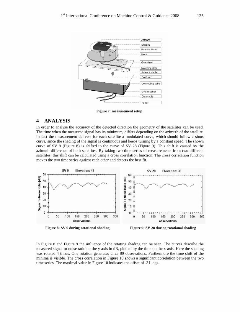
1st International Conference on Machine Control & Guidance 2008 125
Figure 7: measurement setup
4 ANALYSIS In order to analyse the accuracy of the detected direction the geometry of the satellites can be used. The time when the measured signal has its minimum, differs depending on the azimuth of the satellite. In fact the measurement delivers for each satellite a modulated curve, which should follow a sinus curve, since the shading of the signal is continuous and keeps turning by a constant speed. The shown curve of SV 9 (Figure 8) is shifted to the curve of SV 28 (Figure 9). This shift is caused by the azimuth difference of both satellites. By taking two time series of measurements from two different satellites, this shift can be calculated using a cross correlation function. The cross correlation function moves the two time series against each other and detects the best fit.
Figure 8: SV 9 during rotational shading
Figure 9: SV 28 during rotational shading
In Figure 8 and Figure 9 the influence of the rotating shading can be seen. The curves describe the measured signal to noise ratio on the y-axis in dB, plotted by the time on the x-axis. Here the shading was rotated 4 times. One rotation generates circa 80 observations. Furthermore the time shift of the minima is visible. The cross correlation in Figure 10 shows a significant correlation between the two time series. The maximal value in Figure 10 indicates the offset of -31 lags.
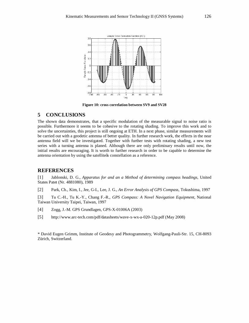
Kinematic Measurements and Sensor Technology II (GNSS Systems) 126
Figure 10: cross correlation between SV9 and SV28
5 CONCLUSIONS The shown data demonstrates, that a specific modulation of the measurable signal to noise ratio is possible. Furthermore it seems to be cohesive to the rotating shading. To improve this work and to solve the uncertainties, this project is still ongoing at ETH. In a next phase, similar measurements will be carried out with a geodetic antenna of better quality. In further research work, the effects in the near antenna field will we be investigated. Together with further tests with rotating shading, a new test series with a turning antenna is planed. Although there are only preliminary results until now, the initial results are encouraging. It is worth to further research in order to be capable to determine the antenna orientation by using the satellite’s constellation as a reference.
REFERENCES [1] Jablonski, D. G., Apparatus for and an a Method of determining compass headings, United States Patet (Nr. 4881080), 1989
[2] Park, Ch., Kim, I., Jee, G-I., Lee, J. G., An Error Analysis of GPS Compass, Tokushima, 1997
[3] Tu C.-H., Tu K.-Y., Chang F.-R., GPS Compass: A Novel Navigation Equipment, National Taiwan University Taipei, Taiwan, 1997
[4] Zogg, J.-M. GPS Grundlagen, GPS-X-01006A (2003)
[5] http://www.arc-tech.com/pdf/datasheets/wave-x-wx-a-020-12p.pdf (May 2008)
* David Eugen Grimm, Institute of Geodesy and Photogrammetry, Wolfgang-Pauli-Str. 15, CH-8093 Zürich, Switzerland.

Agriculture Applications

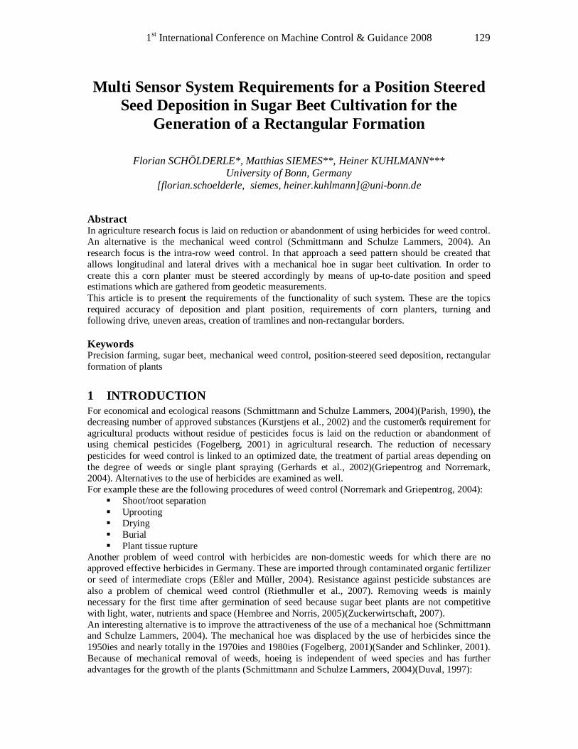
1st International Conference on Machine Control & Guidance 2008 129
Multi Sensor System Requirements for a Position Steered Seed Deposition in Sugar Beet Cultivation for the
Generation of a Rectangular Formation
Florian SCHÖLDERLE*, Matthias SIEMES**, Heiner KUHLMANN*** University of Bonn, Germany
[florian.schoelderle, siemes, heiner.kuhlmann]@uni-bonn.de Abstract In agriculture research focus is laid on reduction or abandonment of using herbicides for weed control. An alternative is the mechanical weed control (Schmittmann and Schulze Lammers, 2004). An research focus is the intra-row weed control. In that approach a seed pattern should be created that allows longitudinal and lateral drives with a mechanical hoe in sugar beet cultivation. In order to create this a corn planter must be steered accordingly by means of up-to-date position and speed estimations which are gathered from geodetic measurements. This article is to present the requirements of the functionality of such system. These are the topics required accuracy of deposition and plant position, requirements of corn planters, turning and following drive, uneven areas, creation of tramlines and non-rectangular borders. Keywords Precision farming, sugar beet, mechanical weed control, position-steered seed deposition, rectangular formation of plants
1 INTRODUCTION For economical and ecological reasons (Schmittmann and Schulze Lammers, 2004)(Parish, 1990), the decreasing number of approved substances (Kurstjens et al., 2002) and the customer’s requirement for agricultural products without residue of pesticides focus is laid on the reduction or abandonment of using chemical pesticides (Fogelberg, 2001) in agricultural research. The reduction of necessary pesticides for weed control is linked to an optimized date, the treatment of partial areas depending on the degree of weeds or single plant spraying (Gerhards et al., 2002)(Griepentrog and Norremark, 2004). Alternatives to the use of herbicides are examined as well. For example these are the following procedures of weed control (Norremark and Griepentrog, 2004): § Shoot/root separation § Uprooting § Drying § Burial § Plant tissue rupture
Another problem of weed control with herbicides are non-domestic weeds for which there are no approved effective herbicides in Germany. These are imported through contaminated organic fertilizer or seed of intermediate crops (Eßler and Müller, 2004). Resistance against pesticide substances are also a problem of chemical weed control (Riethmuller et al., 2007). Removing weeds is mainly necessary for the first time after germination of seed because sugar beet plants are not competitive with light, water, nutrients and space (Hembree and Norris, 2005)(Zuckerwirtschaft, 2007). An interesting alternative is to improve the attractiveness of the use of a mechanical hoe (Schmittmann and Schulze Lammers, 2004). The mechanical hoe was displaced by the use of herbicides since the 1950ies and nearly totally in the 1970ies and 1980ies (Fogelberg, 2001)(Sander and Schlinker, 2001). Because of mechanical removal of weeds, hoeing is independent of weed species and has further advantages for the growth of the plants (Schmittmann and Schulze Lammers, 2004)(Duval, 1997):
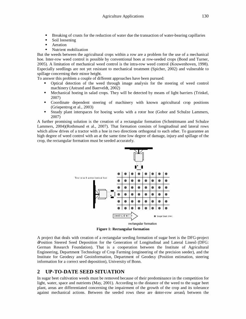
Agriculture Applications 130
§ Breaking of crusts for the reduction of water due the transaction of water-bearing capillaries § Soil loosening § Aeration § Nutrient mobilization
But the weeds between the agricultural crops within a row are a problem for the use of a mechanical hoe. Inter-row weed control is possible by conventional hoes at row-seeded crops (Bond and Turner, 2005). A limitation of mechanical weed control is the intra-row weed control (Kouwenhoven, 1998). Especially seedlings are not yet resistant to mechanical treatment (Spicher, 2002) and vulnerable to spillage concerning their minor height. To answer this problem a couple of different approaches have been pursued: § Optical detection of the weed through image analysis for the steering of weed control
machinery (Astrand and Baerveldt, 2002) § Mechanical hoeing in salad crops. They will be detected by means of light barriers (Trinkel,
2007) § Coordinate dependent steering of machinery with known agricultural crop positions
(Griepentrog et al., 2003) § Steady plant interspaces for hoeing works with a rotor hoe (Gobor and Schulze Lammers,
2007) A further promising solution is the creation of a rectangular formation (Schmittmann and Schulze Lammers, 2004)(Rothmund et al., 2007). That formation consists of longitudinal and lateral rows which allow drives of a tractor with a hoe in two directions orthogonal to each other. To guarantee an high degree of weed control with an at the same time low degree of damage, injury and spillage of the crop, the rectangular formation must be seeded accurately.
A project that deals with creation of a rectangular seeding formation of sugar beet is the DFG-project ‘Position Steered Seed Deposition for the Generation of Longitudinal and Lateral Lines’ (DFG: German Research Foundation). That is a cooperation between the Institute of Agricultural Engineering, Department Technology of Crop Farming (engineering of the precision seeder), and the Institute for Geodesy and Geoinformation, Department of Geodesy (Position estimation, steering information for a correct seed deposition), University of Bonn.
2 UP-TO-DATE SEED SITUATION In sugar beet cultivation weeds must be removed because of their predominance in the competition for light, water, space and nutrients (May, 2001). According to the distance of the weed to the sugar beet plant, areas are differentiated concerning the impairment of the growth of the crop and its tolerance against mechanical actions. Between the seeded rows these are ‘inter-row areas’, between the
Figure 1: Rectangular formation
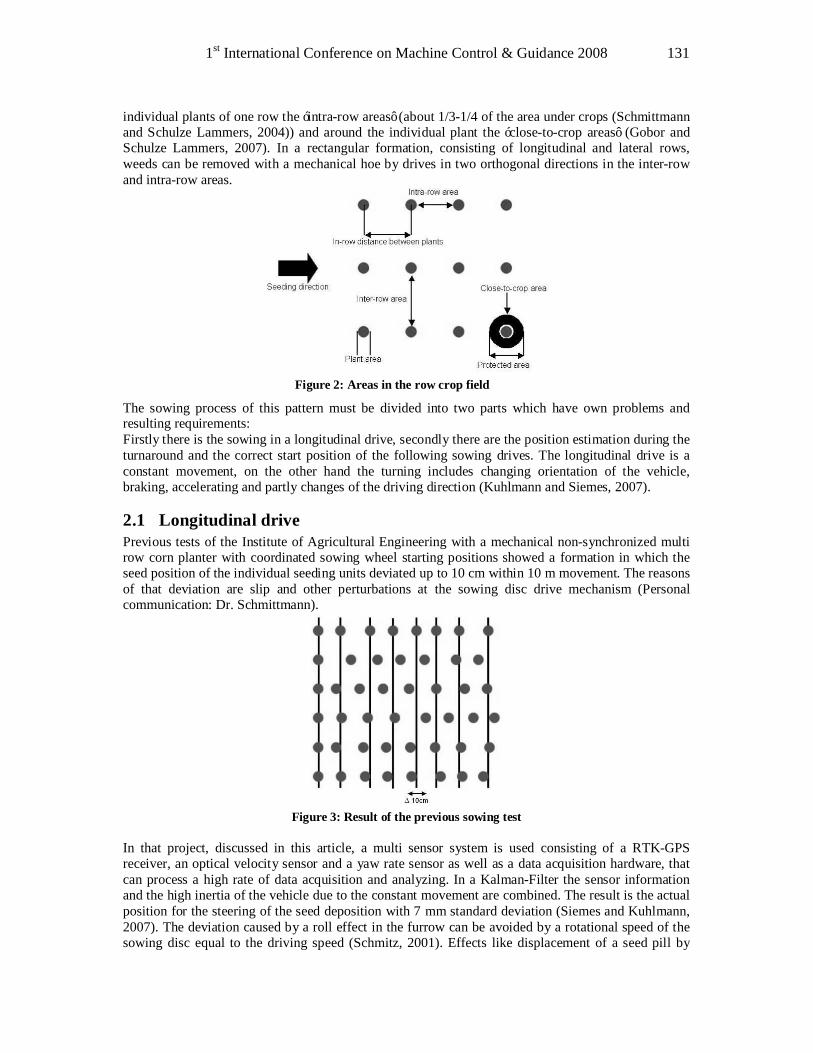
1st International Conference on Machine Control & Guidance 2008 131
individual plants of one row the ‘intra-row areas’ (about 1/3-1/4 of the area under crops (Schmittmann and Schulze Lammers, 2004)) and around the individual plant the ‘close-to-crop areas’ (Gobor and Schulze Lammers, 2007). In a rectangular formation, consisting of longitudinal and lateral rows, weeds can be removed with a mechanical hoe by drives in two orthogonal directions in the inter-row and intra-row areas.
The sowing process of this pattern must be divided into two parts which have own problems and resulting requirements: Firstly there is the sowing in a longitudinal drive, secondly there are the position estimation during the turnaround and the correct start position of the following sowing drives. The longitudinal drive is a constant movement, on the other hand the turning includes changing orientation of the vehicle, braking, accelerating and partly changes of the driving direction (Kuhlmann and Siemes, 2007).
2.1 Longitudinal drive Previous tests of the Institute of Agricultural Engineering with a mechanical non-synchronized multi row corn planter with coordinated sowing wheel starting positions showed a formation in which the seed position of the individual seeding units deviated up to 10 cm within 10 m movement. The reasons of that deviation are slip and other perturbations at the sowing disc drive mechanism (Personal communication: Dr. Schmittmann).
In that project, discussed in this article, a multi sensor system is used consisting of a RTK-GPS receiver, an optical velocity sensor and a yaw rate sensor as well as a data acquisition hardware, that can process a high rate of data acquisition and analyzing. In a Kalman-Filter the sensor information and the high inertia of the vehicle due to the constant movement are combined. The result is the actual position for the steering of the seed deposition with 7 mm standard deviation (Siemes and Kuhlmann, 2007). The deviation caused by a roll effect in the furrow can be avoided by a rotational speed of the sowing disc equal to the driving speed (Schmitz, 2001). Effects like displacement of a seed pill by
Figure 2: Areas in the row crop field
Figure 3: Result of the previous sowing test
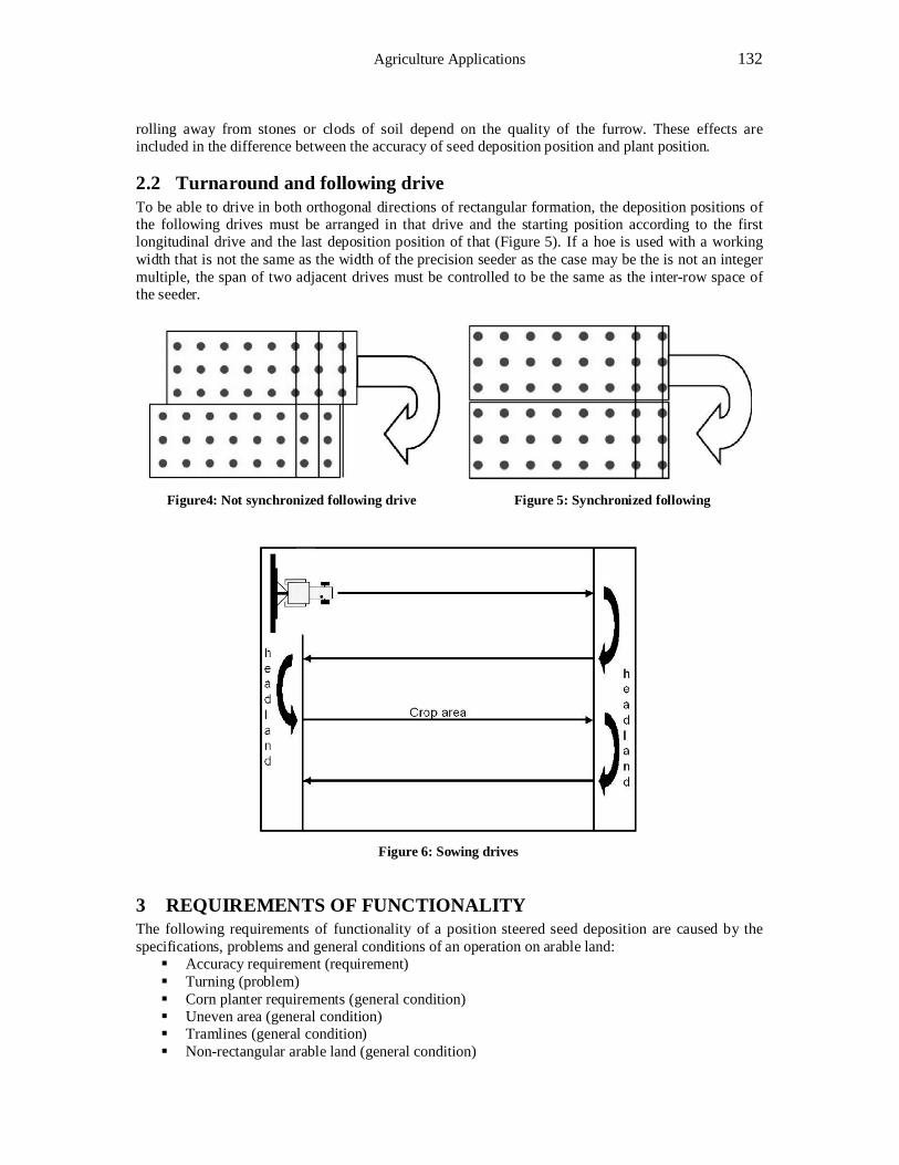
Agriculture Applications 132
rolling away from stones or clods of soil depend on the quality of the furrow. These effects are included in the difference between the accuracy of seed deposition position and plant position.
2.2 Turnaround and following drive To be able to drive in both orthogonal directions of rectangular formation, the deposition positions of the following drives must be arranged in that drive and the starting position according to the first longitudinal drive and the last deposition position of that (Figure 5). If a hoe is used with a working width that is not the same as the width of the precision seeder as the case may be the is not an integer multiple, the span of two adjacent drives must be controlled to be the same as the inter-row space of the seeder.
Figure4: Not synchronized following drive Figure 5: Synchronized following
Figure 6: Sowing drives
3 REQUIREMENTS OF FUNCTIONALITY The following requirements of functionality of a position steered seed deposition are caused by the specifications, problems and general conditions of an operation on arable land: § Accuracy requirement (requirement) § Turning (problem) § Corn planter requirements (general condition) § Uneven area (general condition) § Tramlines (general condition) § Non-rectangular arable land (general condition)
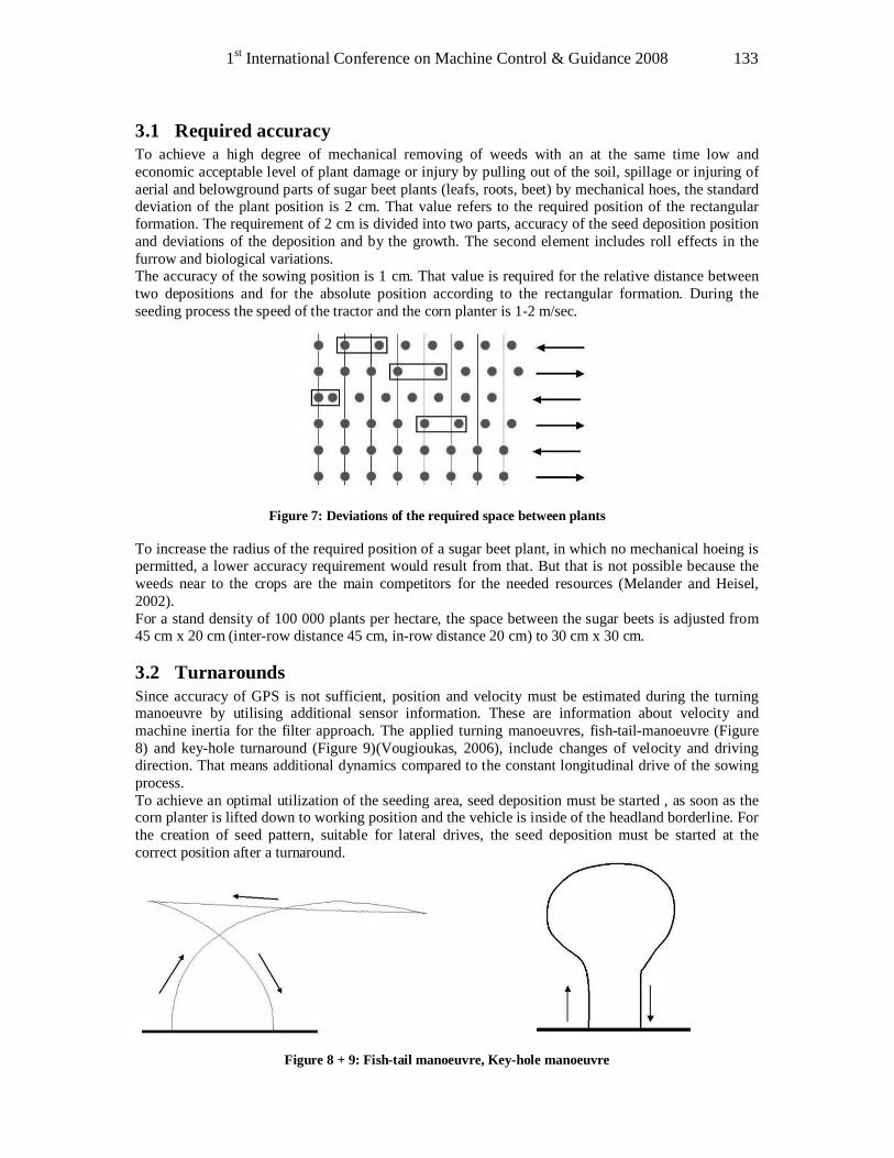
1st International Conference on Machine Control & Guidance 2008 133
3.1 Required accuracy To achieve a high degree of mechanical removing of weeds with an at the same time low and economic acceptable level of plant damage or injury by pulling out of the soil, spillage or injuring of aerial and belowground parts of sugar beet plants (leafs, roots, beet) by mechanical hoes, the standard deviation of the plant position is 2 cm. That value refers to the required position of the rectangular formation. The requirement of 2 cm is divided into two parts, accuracy of the seed deposition position and deviations of the deposition and by the growth. The second element includes roll effects in the furrow and biological variations. The accuracy of the sowing position is 1 cm. That value is required for the relative distance between two depositions and for the absolute position according to the rectangular formation. During the seeding process the speed of the tractor and the corn planter is 1-2 m/sec.
To increase the radius of the required position of a sugar beet plant, in which no mechanical hoeing is permitted, a lower accuracy requirement would result from that. But that is not possible because the weeds near to the crops are the main competitors for the needed resources (Melander and Heisel, 2002). For a stand density of 100 000 plants per hectare, the space between the sugar beets is adjusted from 45 cm x 20 cm (inter-row distance 45 cm, in-row distance 20 cm) to 30 cm x 30 cm.
3.2 Turnarounds Since accuracy of GPS is not sufficient, position and velocity must be estimated during the turning manoeuvre by utilising additional sensor information. These are information about velocity and machine inertia for the filter approach. The applied turning manoeuvres, fish-tail-manoeuvre (Figure 8) and key-hole turnaround (Figure 9)(Vougioukas, 2006), include changes of velocity and driving direction. That means additional dynamics compared to the constant longitudinal drive of the sowing process. To achieve an optimal utilization of the seeding area, seed deposition must be started , as soon as the corn planter is lifted down to working position and the vehicle is inside of the headland borderline. For the creation of seed pattern, suitable for lateral drives, the seed deposition must be started at the correct position after a turnaround.
Figure 8 + 9: Fish-tail manoeuvre, Key-hole manoeuvre
Figure 7: Deviations of the required space between plants
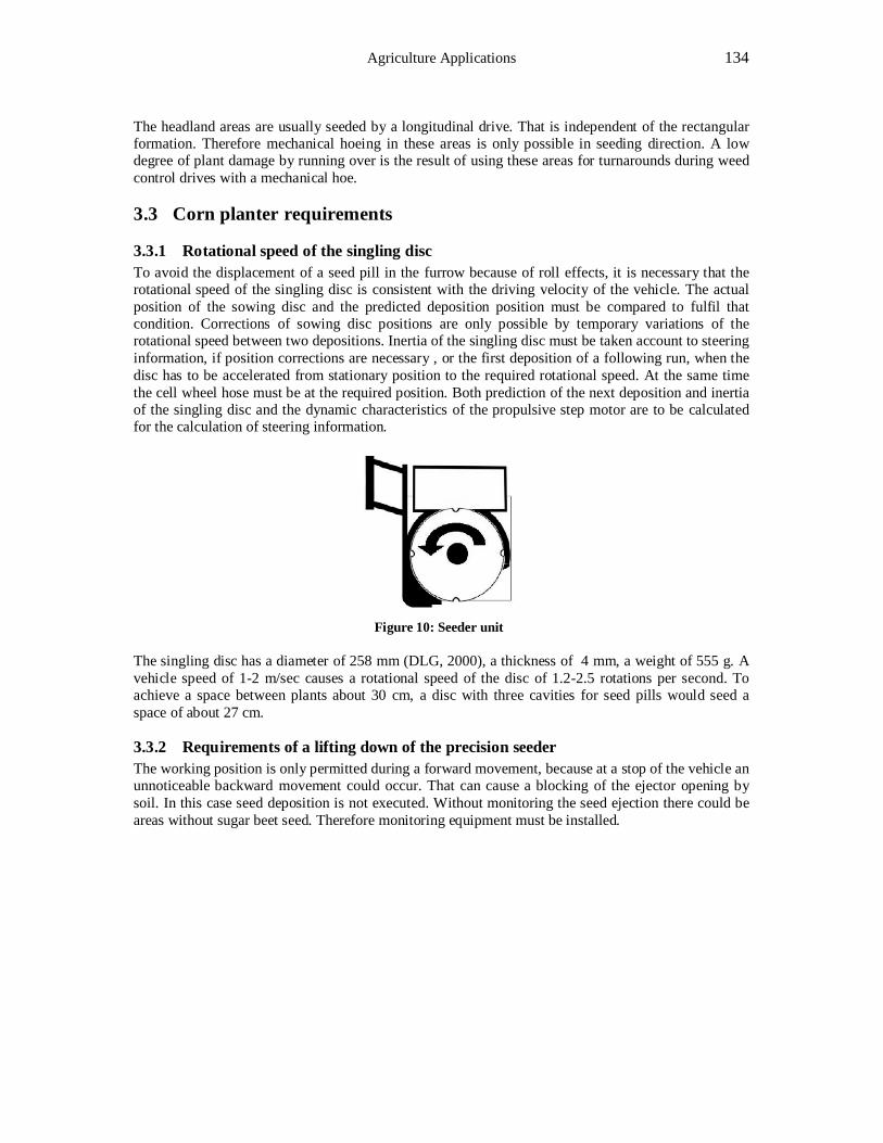
Agriculture Applications 134
The headland areas are usually seeded by a longitudinal drive. That is independent of the rectangular formation. Therefore mechanical hoeing in these areas is only possible in seeding direction. A low degree of plant damage by running over is the result of using these areas for turnarounds during weed control drives with a mechanical hoe.
3.3 Corn planter requirements
3.3.1 Rotational speed of the singling disc To avoid the displacement of a seed pill in the furrow because of roll effects, it is necessary that the rotational speed of the singling disc is consistent with the driving velocity of the vehicle. The actual position of the sowing disc and the predicted deposition position must be compared to fulfil that condition. Corrections of sowing disc positions are only possible by temporary variations of the rotational speed between two depositions. Inertia of the singling disc must be taken account to steering information, if position corrections are necessary , or the first deposition of a following run, when the disc has to be accelerated from stationary position to the required rotational speed. At the same time the cell wheel hose must be at the required position. Both prediction of the next deposition and inertia of the singling disc and the dynamic characteristics of the propulsive step motor are to be calculated for the calculation of steering information.
Figure 10: Seeder unit
The singling disc has a diameter of 258 mm (DLG, 2000), a thickness of 4 mm, a weight of 555 g. A vehicle speed of 1-2 m/sec causes a rotational speed of the disc of 1.2-2.5 rotations per second. To achieve a space between plants about 30 cm, a disc with three cavities for seed pills would seed a space of about 27 cm.
3.3.2 Requirements of a lifting down of the precision seeder The working position is only permitted during a forward movement, because at a stop of the vehicle an unnoticeable backward movement could occur. That can cause a blocking of the ejector opening by soil. In this case seed deposition is not executed. Without monitoring the seed ejection there could be areas without sugar beet seed. Therefore monitoring equipment must be installed.
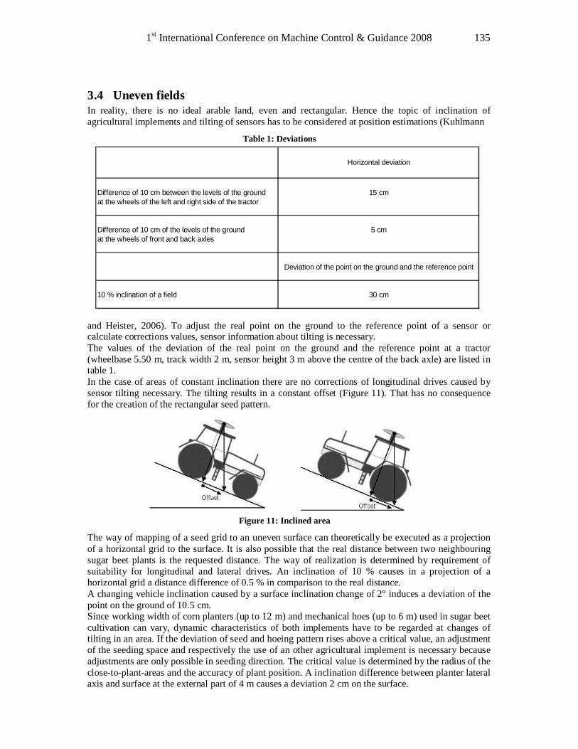
1st International Conference on Machine Control & Guidance 2008 135
3.4 Uneven fields In reality, there is no ideal arable land, even and rectangular. Hence the topic of inclination of agricultural implements and tilting of sensors has to be considered at position estimations (Kuhlmann
and Heister, 2006). To adjust the real point on the ground to the reference point of a sensor or calculate corrections values, sensor information about tilting is necessary. The values of the deviation of the real point on the ground and the reference point at a tractor (wheelbase 5.50 m, track width 2 m, sensor height 3 m above the centre of the back axle) are listed in table 1. In the case of areas of constant inclination there are no corrections of longitudinal drives caused by sensor tilting necessary. The tilting results in a constant offset (Figure 11). That has no consequence for the creation of the rectangular seed pattern.
The way of mapping of a seed grid to an uneven surface can theoretically be executed as a projection of a horizontal grid to the surface. It is also possible that the real distance between two neighbouring sugar beet plants is the requested distance. The way of realization is determined by requirement of suitability for longitudinal and lateral drives. An inclination of 10 % causes in a projection of a horizontal grid a distance difference of 0.5 % in comparison to the real distance. A changing vehicle inclination caused by a surface inclination change of 2° induces a deviation of the point on the ground of 10.5 cm. Since working width of corn planters (up to 12 m) and mechanical hoes (up to 6 m) used in sugar beet cultivation can vary, dynamic characteristics of both implements have to be regarded at changes of tilting in an area. If the deviation of seed and hoeing pattern rises above a critical value, an adjustment of the seeding space and respectively the use of an other agricultural implement is necessary because adjustments are only possible in seeding direction. The critical value is determined by the radius of the close-to-plant-areas and the accuracy of plant position. A inclination difference between planter lateral axis and surface at the external part of 4 m causes a deviation 2 cm on the surface.
Horizontal deviation
Difference of 10 cm between the levels of the ground 15 cmat the wheels of the left and right side of the tractor
Difference of 10 cm of the levels of the ground 5 cmat the wheels of front and back axles
Deviation of the point on the ground and the reference point
10 % inclination of a field 30 cm
Table 1: Deviations
Figure 11: Inclined area

Agriculture Applications 136
An adjustment of seeding space is only possible in one case, if the deviation rises above the critical value. That situation occurs, if the seeding direction is along the changing inclination or the part of inclination changing lateral to the seeding direction is a value below the critical value. To calculate correction values, dimensions and trails of planter and hoe must be known. Information about the inclinations of an area are necessary. These can be taken from maps or be mapped by geodetic measurements during former actions of soil tillage.
3.5 Tramlines As a result of increasing dimensions and therefore heavier agricultural machines (Wollenweber, 2004) counteractions are necessary to reduce floor loading and soil compaction (Brandhuber, 2006). An increasing contact area of tires reduces floor loading per area unit. To achieve that pressure is lowered or wider tires are mounted. If smaller and therefore lighter tractors are used for weed control, tramlines substitute the use of narrower cultivation tires. That means economically a second kit of tires and mounting time are not necessary (Südzucker, 2008). The width of cultivation tires is 260-358 mm depending on the tractor (CGS tyres, 2007). Because of a too small space between plants for tractor tires, tramline generation is essential (Schmittmann and Schulze Lammers, 2004). There can also conventional agricultural trailers used for removal of bolters (Lehnert, 2007). In seeding direction tramlines can be generated by actual corn planters, if these have an individual tramline switching tool (Schmitz, 2001). In a rectangular formation tramlines are also necessary in lateral direction (Figure 12). To create these, the position of every track must be determined by coordinates. If they are created during the first drive, every following theoretical deposition position
must be predicted at all following drives. The coordinates are checked, whether the position is in a tramline track or not. If that is true, the sowing disc must be braked and accelerated for the next real deposition position in the way described in previous chapters. Between 3.7 and 7.4 depositions per second are the result of 1 m/sec-2 m/sec speed of the agricultural implement. The time difference between two depositions is 0.135 sec to 0.27 sec. There is less than that space of time to decide whether the next position is in a tramline track or not.
3.6 Non-rectangular fields To achieve an efficient use of the agricultural area, every row must be seeded to the final position. That requirement means at non-rectangular areas and multi-row corn planters with a working width up to 12 m the final depositions are executed at different times. This is due to every individual seeder unit passing the headland borderline at another time. The governing system must check for every individual unit, may the next predicted deposition position inside of the seeding area or already in the headland area. In this case, the unit must be stopped. After a turnaround, the situation is more complex. When the corn planter is lifted down, for every individual unit must be calculated, if the next, at that time only mathematically predicted, deposition position is
Figure 12: Tramlines
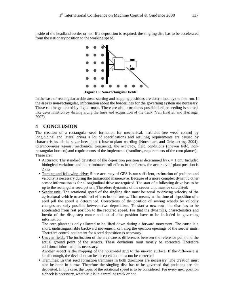
1st International Conference on Machine Control & Guidance 2008 137
inside of the headland border or not. If a deposition is required, the singling disc has to be accelerated from the stationary position to the working speed.
In the case of rectangular arable areas starting and stopping positions are determined by the first run. If the area is non-rectangular, information about the borderlines for the governing system are necessary. These can be generated by digital maps. There are also procedures possible before seeding is started, like determination by driving along the lines and acquisition of the track (Van Haaften and Harringa, 2007).
4 CONCLUSION The creation of a rectangular seed formation for mechanical, herbicide-free weed control by longitudinal and lateral drives a lot of specifications and resulting requirements are caused by characteristics of the sugar beet plant (close-to-plant weeding (Norremark and Griepentrog, 2004), tolerance-areas against mechanical treatment), the accuracy, field conditions (uneven field, non-rectangular borders) and requirements of the implements (tramlines, requirements of the corn planter). These are: § Accuracy: The standard deviation of the deposition position is determined by σ= 1 cm. Included
biological variations and not-eliminated roll effects in the furrow the accuracy of plant position is 2 cm. § Turning and following drive: Since accuracy of GPS is not sufficient, estimation of position and
velocity is necessary during the turnaround manoeuvre. Because of a more complex dynamic other sensor information as for a longitudinal drive are required. The start of a following drive has to be up to the rectangular seed pattern. Therefore dynamics of the seeder unit must be calculated. § Seeder unit: The rotational speed of the singling disc must be equal to driving velocity of the
agricultural vehicle to avoid roll effects in the furrow. That means, at the time of deposition of a seed pill the speed is determined. Corrections of the position of sowing wheels by velocity changes are only possible between two depositions. To start a new row, the disc has to be accelerated from rest position to the required speed. For that the dynamics, characteristics and inertia of the disc, step motor and actual disc position have to be included in governing information. The corn planter is only allowed to be lifted down during a forward movement. The cause is a short, undistinguishable backward movement, can clog the ejection openings of the seeder units. Therefore control equipment for a seed deposition is necessary. § Uneven fields: The inclination of the area causes differences between the reference point and the
actual ground point of the sensors. These deviations must mostly be corrected. Therefore additional information is necessary. Another aspect is the mapping of the horizontal grid to the uneven surface. If the difference is small enough, the deviation can be accepted and must not be corrected. § Tramlines: In that seed formation tramlines in both directions are necessary. The creation must
also be done in a row. Therefore the singling disc has to be governed that positions are not deposited. In this case, the topic of the rotational speed is to be considered. For every next position a check is necessary, whether it is in a tramline track or not.
Figure 13: Non-rectangular fields
Agriculture Applications 138
§ Non-rectangular areas: Non-rectangular areas in compliance with an efficient degree of use of an area mean that every seeder unit must be started and stopped at individual positions in relation of their actual position to the borderline. For every unit has to be checked individually, whether it is inside the borders or not. For a start of seeding the topic of singling disc position and accelerating from static position to the required speed must be considered. For all these topics not only the theoretical and mathematical solutions must be determined but also the dynamics and inertia of the tractor, corn planter and mechanical hoe must be determined and integrated into the governing information.
REFERENCES Astrand B., und Baerveldt A.-J.: An Agricultural Mobile Robot with Vision-Based Perception for Mechanical Weed Control, Autonomous Robots, volume 13, p.21-35, 2002. Bond, W., Turner R.J.: A review of mechanical weed control, June 2005, http://www.organicweeds.org.uk, last accessed March, 2008. Brandhuber R.: Bodenbelastung durch Landmaschinen-Wirkungsmechanismen und Risikobeurteilung, Bayerische Landesanstalt für Landwirtschaft: Ackerbau vor neuen Herausforderungen, Schriftenreihe 21/2006, p. 53-74. CGS tyres: Mobilität für die Landwirtschaft – Continental Landwirtschaftsreifen Radialreifenübersicht 2008/2009, CGS TYRES_35_11/07, p. 24-25, 2007. DLG: Prüfbericht 4875 Einzelkornsämaschine KVERNELAND-ACCORD Monopill SE 12r VH, 2000. Duval, J.: Mechanical weed control in cereals, EAP Publication-72, http://www.eap.mcgill.ca, last accessed on April 14, 2008. Eßler C. und Müller T., 2007: Exoten auf dem Rübenacker, Zuckerrübe, 3/2007, p. 138-139, 2007. Fogelberg, F.: Research on pest control and pesticide reduction in Sweden, Denmark and the Netherlands – ongoing work and new ideas for the future, Food 21 Report, 2001, http://www-mat21.slu.se, last accessed on April 14, 2008. Gerhards, R., Sökefeld, M., Timmermann, C., Kühbauch, W., Williams, M.M.: Site-specific weed control in maize, sugar beet, winter wheat, winter barley, Precision Agriculture, 3/2002, p. 25-35, 2002. Gobor, Z., Schulze Lammers, P.: Prototype of a rotary hoe for intra-row weeding, Proceedings of 12th World Congress in Mechanism and Machine Science IFToMM 2007, CD-ROM, 2007. Griepentrog, H.W., Norremark, M., Nielsen, H., Blackmore, S.: Individual plant care in cropping systems, Proceedings 4th European Conference on Precision Agriculture, p. 247-251, 2003. Griepentrog, H.W., Norremark, M.: Seed mapping of sugar beet to guide weeding robots, Proceedings 6th workshop of the EWRS working group ‘Physical and Cultural Weed Control, 2004. Hembree, K.J., Norris, R.F.: Integrated weed management, UC IPM Pest Management Guidelines: Sugarbeet, 10/2005, p. 44-48, http://www.ipm.ucdavis.edu, last accessed on April 14, 2008 Kouwenhoven, J.K.: Finger weeders for future intra-row weed control, Abstracts 3rd EWRS Workshop on Physical Weed Control, p. 9, 1998. Kuhlmann, H., Heister, H.: Steering problems and solutions during constructions of roads, Proceedings 3rd IAG Symposium on Geodesy for Geotechnical and Structural Engineering, 12th FIG Symposium on Deformation Measurement, CD-Rom, 2006. Kuhlmann, H., Siemes, M.: Nutzung eines Multi-Sensor-System mit Kalman-Filter für die Bestimmung von Längsbewegungen einer Landmaschine in der Präzisionslandwirtschaft, Ingenieurvermessung 07, Beiträge zum 15. Internationalen Ingenieurvermessungskurs Graz 2007, p. 369-382, 2007. Kurstjens, D.A.G., Bleeker, P.O., Kropff, M.J., Perdok, U.D.: Seven ways to improve the selective ability of mechanical intra-row weeders, Proceedings 12th Symposium European Weed Research Society, p. 238-239, 2002.

1st International Conference on Machine Control & Guidance 2008 139
Lehnert, J.: Heute Schosser, morgen Unkrautrübe, dzz – Die Zuckerrübenzeitung, Juni 2007, p. 10-11, 2007. May, M.: Sugar Beet - Crop Protection in sugar beet, Pesticide Outlook - 2001, Volume 12, Issue 5, p. 188-191, 2001. Melander, B., Heisel, T.: Prospects and limitations for agricultural engineering in the development of sustainable weed control methods – examples from European research, http://orgprints.org/00001548, last accessed on April 17, 2008, 2002. Norremark, M., Griepentrog, H.W.: Analysis and definition of the close-to –crop area in relation to robot weeding, Proceedings 6th EWRS Workshop on Physical and Cultural Weed Control, p. 127-140, 2004. Parish, S.: A Review of Non-Chemical Weed Control Techniques, Biological Agriculture and Horticulture, Volume 7, p. 117-137, 1990. Riethmuller, G.P., Hashem, A., Pathan, S.M.: Weed control in wide lupins in Western Australia, Proceedings 7th EWRS Workshop on Physical and Cultural Weed Control, p. 54-57, 2007. Rothmund, M., Steinberger, G., Auernhammer, H.: Zweidimensionale mechanische Unkrautbekämpfung im Maisanbau durch Einzelkornsaat im spurübergreifenden quadratischen Verband, Proceedings 15th Seminar of Work Science (VDI-MEG-Working Group Work Science in Agriculture), p. 138-144, 2007. Sander, G., Schlinker, G.: Pflanzenschutz in Zuckerrüben – gestern und heute, Zuckerrübe, 4/2001, p. 236-240, 2001. Schmittmann O., Schulze Lammers, P.: Mechanical Weed Control Measures, Landtechnik, 2/2004, p. 90-91, 2004. Schmitz, S.: Aktueller Stand der Einzelkornsätechnik, Zuckerrübe, 1/2001, p. 22-27, 2001. Siemes,M., Kuhlmann, H.: Calibration of a non-contact optical velocity sensor for a precision farming application, Proceedings The 5th International Symposium on Mobile Mapping Technology MMT’07, CD-Rom, 2007. Spicher, J.: Rüben mechanisch pflegen, Zuckerrübe, 3/2002, p. 138-139, 2002. Südzucker: http://www.bisz.suedzucker.de, last accessed on April 14, 2008. Trinkel: http://www.gemuesetechnik.de, last accessed on April 17, 288. Van Haaften, J., Harringa, E.: Gazing across the Field, GEOInformatics, January/February 2007, p. 40-42, 2007. Vougioukas, S.G.: Reactive path tracking for increasedsafety and robustness during automatic guidance, Proceedings of the 1-2 September 2006 Conference Automation Technology for Off-Road Equipment 2006, p.183-189, 2006. Wollenweber, D.: Fahrgassen für einen bodenschonenden Zuckerrübenanbau, Zuckerrübe, 1/2004, p. 24-26, 2004. Zuckerwirtschaft: Verantwortungsbewusster Pflanzenschutz, http://www.zuckerwirtschaft.de, last accessed on November 9, 2007. *Dipl-Ing. Florian Schölderle, Institute for Geodesy and Geoinformation, Department of Geodesy, University Bonn, Nussallee 17, Bonn, Germany. ** Dipl.-Ing. Matthias Siemes, Institute for Geodesy and Geoinformation, Department of Geodesy, University Bonn, Nussallee 17, Bonn, Germany. *** Univ.-Prof. Dr.-Ing. Heiner Kuhlmann, Institute for Geodesy and Geoinformation, Department of Geodesy, University Bonn, Nussallee 17, Bonn, Germany.

Agriculture Applications 140
1st International Conference on Machine Control & Guidance 2008 141
Generation and Analysis of Digital Terrain Models with Parallel Guidance Systems for Precision Agriculture
Görres GRENZDÖRFFER*
University Rostock, Germany [email protected]
Cornelius DONATH**
John Deere, AMS [email protected]
Abstract In Europe more than 10.000 dual frequency iTC Starfire GPS-receivers were sold in recent years. These GPS-receivers are mainly used for parallel tracking and autosteering of modern tractors and combine harvesters. The recorded GPS-data also includes precise height information which can be used for the generation of high accuracy digital terrain models at no or little additional cost. In the paper the achievable data accuracy under different conditions are investigated. The different steps for data preparation and digital terrain models DTM generation are described. Additionally several applications of high accuracy DTM’s in (precision) agriculture are highlighted. Keywords Parallel guidance systems, DEM, RTK-GPS, precision agriculture
1 INTRODUCTION Highly accurate parallel guiding and autosteering systems become more and more widely used in today’s agriculture. For instance in Europe more than 10.000 dual frequency iTC Starfire GPS-receivers were sold in recent years. More than 25 different companies for parallel guiding and auto steering systems are on the market, NIEMANN ET AL., 2007. While the immediate benefits of such systems are real reductions in labour and machine hours and fuel used, the secondary advantages lie in also saving sees fertilizers and pesticides. Autosteering systems also record data which may be used for documentation and planning. The core of a parallel guiding or an autosteering system is a GPS-receiver using a DGPS-reference signal either from a satellite or a nearby local reference station. The accuracy of such systems depends upon the quality of the GPS-receiver and the reference signal. For high accuracy purposes geodetic 2-frequency receivers are commonly used, providing an accuracy level of a few centimetres. Beside the guiding function the GPS-signal also provides information of the altitude which may be used to derive a highly accurate digital elevation model (DEM) of a given field. The high accuracy is important, because in order to prove connections between terrain and soil, a spatial resolution of 2 – 10 m (according to terrain type) and a vertical precision of the interpolated digital elevation model of ± 0,15 m is necessary Schmidt, 2003. Vehicle based surveying with Realtime-Kinematic (RTK)-GPS is the most efficient method to capture elevation under agricultural conditions. The processing of elevation data with the resulting stripe pattern of the GPS measurement points along the tram lines, however, requires special geostatistical interpolation methods to avoid artefacts.
Agriculture Applications 142
The focus of this contribution will cover the following topics: - The determination of the relative and the absolute height accuracy of parallel guidance systems
in relation to different correction signals. (geostationary reference signals (SF 2) and local reference station)
- From a DEM several terrain parameters, such as the topographic wetness index (TWI) or the sediment transport index (STI) may be derived, e.g. Schmidt, 2003. A joint analysis with maps of the soil conductivity, yields and other data will show the practical importance of the derived parameters and the DEM for precision agriculture in general.
- Describe several potential applications of high precision DEM’s in agriculture
2 DTM DATA ACQUISITION There are several different ways to obtain accurate digital terrain data, e.g.
- Digitizing of contour lines of existing maps (which is still done by several state surveying departments)
- Photogrammetrically, through automatic point matching methods of aerial stereo images. - Terrestrial with GPS or total stations - LIDAR
Due to the high accuracy of ± 0.15 m necessary for pedo-hydrologic modelling only RTK-GPS and laser scanning will be described in the following section in a little more detail.
2.1 RTK-GPS Elevation data for agricultural fields can be captured most efficiently using a parallel guidance system with a Real-Time-Kinematic GPS (RTK-GPS)as a terrestrial surveying method. The vehicle-based RTK-GPS consists of a rover (the GPS-receiver mounted on the tractor) and a second receiver that is transmitting differential correction in real-time to the rover. Thereby the second receiver may be located at field boundary or on top of a farm building within a radius of some 10 km. Another alternative is the use of a space borne reference signal such a s the starfire signal. Thus, coordinates can be immediately used in the field which is important for real-time parallel guidance. For completeness, highly accurate GPS-data may also acquired in a postprocessing mode using reference data e.g. from the SAPOS service in Germany. When certain topographical features make the radio link impossible, the base station has to be transferred to a more suited location. With vehicle-based RTK-GPS, an elevation accuracy better than 10 cm is usually reached. The terrain data is generally acquired in the tram lines during an overpass of the tractor e.g. for fertilizing or weed control. This, however, leads to an unfavourable geometry of sample points, since there are many points along the tramlines available, compared to the spacing between the tramlines. Sophisticated interpolation methods such as Kriging can handle this kind of data when generating the digital terrain model. The elevations given by GPS are based on the WGS84 ellipsoid and do not necessarily represent the heights above sea level. With a geoid model the undulations between the WGS84 ellipsoid and the local orthometric heights may be determined in an efficient manner. The DTM analysis generally requires grid coordinates, based on a plane coordinate system,. Generally the datum transformation in a national coordinate reference system or the wide-spread UTM is done using the well known EPSG-transformation parameters2. The transformation of the vertical datum is more difficult, because different countries have different definitions of the vertical height, a problem that will be fixed in the
2 http://www.epsg.org/
1st International Conference on Machine Control & Guidance 2008 143
future with a European Vertical Reference System (EVRS) 3. However the height differences due to the geoid are neglect able within an agricultural field, and for the DTM analysis the relative height accuracy is much more important than the absolute height.
2.2 Airborne Laser Scanning (ALS) An airborne laser scanning can provide data with height accuracy of approx. ± 0.10 – 0.15 m. In order to allow an extensive acquisition of the topography the laser beam scanning the landscape with typical point density of 1point/m² or denser. Based on the range measurement, the angle of deflection and the observations of a GPS/INS for direct geo-referencing, ALS allows the direct 3D determination of illuminated object points within one co-ordinate frame. Furthermore, if several objects at different ranges are illuminated by one laser beam, e.g. in the case of vegetation above the terrain, a complex interaction of the laser beam can be observed. Data are usually processed to a 1 m to 5 m grid. The most important advantages are that it produces a complete coverage of the landscape (not restricted to field boundaries or tram lines), thus allowing for regional DTM analysis on a watershed or landscape level. Currently, mapping agencies of many countries (e.g. The Netherlands, Swiss, Germany and Austria) utilize ALS for the determination of their countrywide terrain models.
3 DTM-GENERATION Grids (raster data) are most widely used because of their simplicity and ease of computer implementation. Hydrologic algorithms work straightforward with regular grids of equal spacing. Grids cannot handle abrupt changes (hard breaklines) in terrain. This, however, occurs rarely on agricultural plots. In order to get a continuous surface from unevenly distributed sample points it is necessary to interpolate between the recorded points. The interpolation method has a significant influence on the quality of the DTM. Several methods provided by common software have been tested, Schmidt, 2003. Best results were reached with Ordinary Kriging. Cross-validations (leaving out every second tram line of a vehicle-based RTK-GPS campaign) delivered RMS errors of 17-18 cm for Kriging Methods at the most unfavourable location (18 m away from the next captured data). Leaving out only 20% of the data, the RMSE is approx. 8 cm. Standard interpolation methods such as Inverse Distance Weighting (IDW) showed a RMSE worse than 30 cm, Schmidt, 2003. More important than the method itself is the quality of the raw data. Several quality measures such as the number of satellites available and the satellite geometry (GDOP, HDOP) are generally provided by the GPS-receivers. These quality information should be used to filter out bad points. The density of the GPS measurements and the characteristic features in the landscape (i.e. breaklines, saddle points, sinks), the better is the result of the interpolation – and the more similar are the results of different methods. Kriging simpler methods such as IDW or spline methods (minimum curvature) can be the better choice for lower quality requirements. There is a risk of a poor representation of the real surface by common interpolation methods available in standard GIS when there is an unfavourable sample point geometry, e.g. only along tram lines or contours. Derivatives from the DTM such as slope are very sensitive to anomalies and thus are a good indicator for a visual inspection of the DTM
4 HEIGHT ACCURACY ASSESSMENT OF RTK GPS RECEIVERS It is important to understand the accuracy and reliability of DTM derived from RTK-GPS data in order to adequately apply this information when modeling hydrologic parameters such as surface runoff, interflow and plant available water capacity. Also the accuracy is important for micro climate analysis, e.g. the influence of slope and aspect on global radiation, Noack et al., 2007. The accuracy of GPS-receivers itself as well as accuracy of auto guidance systems for agricultural purposes was examined in several studies, e.g. Adamchuk et al., 2007, DLG, 2002, DLG, 2007, Henault and Brouant, 2005. The focus of these examinations however was always on the horizontal accuracy and not on the vertical accuracy of GPS-receivers. Based on general literature on GPS it is known that the vertical accuracy
3 http://crs.bkg.bund.de/evrs/

Agriculture Applications 144
of GPS receivers is generally a factor of 2 – 3 lower than the horizontal accuracy. In order to determine the absolute height accuracy of by using different reference signals (local reference station, S1, S2) several practical tests were undertaken.
4.1 Determination of the static height accuracy Under static conditions the vertical accuracy of the GPS-receiver and the influence of the correction signal may be easily obtained through permanent observations, over e.g. 24 h. Figure 1 and Table 1,2 give a comparison between the satellite based reference Signal (Starfire SF 2) and a local reference station (RTK).
SF 2 RTK
8:5 7:17 12:57:17 16:57:17 20:57:17 0:57:17 4:57:17 8:57:17Time [s]
383618.10
383618.15
383618.20
383618.25
383618.30
383618.35
383618.40
383618.45
X-coordinate
11:04:09 15:04:09 19:04:09 23:04:09 3:04:09 7:04:09 11:04:09Time [s]
383618.25
383618.30
383618.35
383618.40
X-coordinate
8:57:17 12:57:17 16:57:17 20:57:17 0:57:17 4:57:17 8:57:17Time [s]
5453942.65
5453942.70
5453942.75
5453942.80
5453942.85
5453942.90
5453942.95
5453943.00
Y-coordiante
11:04:09 15:04:09 19:04:09 23:04:09 3:04:09 7:04:09 11:04:09Time [s]
5453942.70
5453942.75
5453942.80
5453942.85
Y-coordiante
8:57:17 12:57:17 16:57:17 20:57:17 0:57:17 4:57:17 8:57:17Time [s]
347.4
347.6
347.8
348
348.2
348.4
Elev
atio
n [m
]
Z-coordinate
11:04:09 15:04:09 19:04:09 23:04:09 3:04:09 7:04:09 11:04:09Time [s]
347.70
347.75
347.80
347.85
347.90
Z-coordinate
Figure 1: Comparison of static GPS-accuracy (24 h test) with SF 2 and RTK correction signals
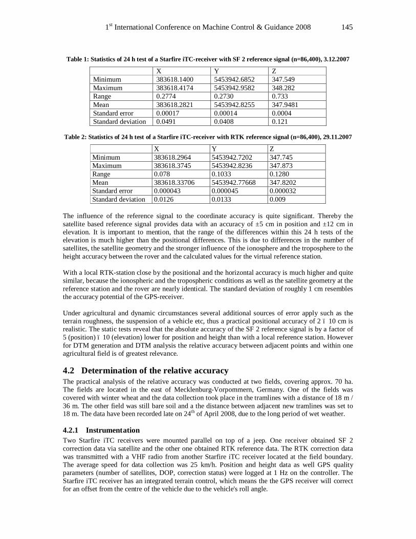
1st International Conference on Machine Control & Guidance 2008 145
Table 1: Statistics of 24 h test of a Starfire iTC-receiver with SF 2 reference signal (n=86,400), 3.12.2007
X Y Z Minimum 383618.1400 5453942.6852 347.549 Maximum 383618.4174 5453942.9582 348.282 Range 0.2774 0.2730 0.733 Mean 383618.2821 5453942.8255 347.9481 Standard error 0.00017 0.00014 0.0004 Standard deviation 0.0491 0.0408 0.121
Table 2: Statistics of 24 h test of a Starfire iTC-receiver with RTK reference signal (n=86,400), 29.11.2007
X Y Z Minimum 383618.2964 5453942.7202 347.745 Maximum 383618.3745 5453942.8236 347.873 Range 0.078 0.1033 0.1280 Mean 383618.33706 5453942.77668 347.8202 Standard error 0.000043 0.000045 0.000032 Standard deviation 0.0126 0.0133 0.009
The influence of the reference signal to the coordinate accuracy is quite significant. Thereby the satellite based reference signal provides data with an accuracy of ±5 cm in position and ±12 cm in elevation. It is important to mention, that the range of the differences within this 24 h tests of the elevation is much higher than the positional differences. This is due to differences in the number of satellites, the satellite geometry and the stronger influence of the ionosphere and the troposphere to the height accuracy between the rover and the calculated values for the virtual reference station. With a local RTK-station close by the positional and the horizontal accuracy is much higher and quite similar, because the ionospheric and the tropospheric conditions as well as the satellite geometry at the reference station and the rover are nearly identical. The standard deviation of roughly 1 cm resembles the accuracy potential of the GPS-receiver. Under agricultural and dynamic circumstances several additional sources of error apply such as the terrain roughness, the suspension of a vehicle etc, thus a practical positional accuracy of 2 – 10 cm is realistic. The static tests reveal that the absolute accuracy of the SF 2 reference signal is by a factor of 5 (position) – 10 (elevation) lower for position and height than with a local reference station. However for DTM generation and DTM analysis the relative accuracy between adjacent points and within one agricultural field is of greatest relevance.
4.2 Determination of the relative accuracy The practical analysis of the relative accuracy was conducted at two fields, covering approx. 70 ha. The fields are located in the east of Mecklenburg-Vorpommern, Germany. One of the fields was covered with winter wheat and the data collection took place in the tramlines with a distance of 18 m / 36 m. The other field was still bare soil and a the distance between adjacent new tramlines was set to 18 m. The data have been recorded late on 24th of April 2008, due to the long period of wet weather.
4.2.1 Instrumentation Two Starfire iTC receivers were mounted parallel on top of a jeep. One receiver obtained SF 2 correction data via satellite and the other one obtained RTK reference data. The RTK correction data was transmitted with a VHF radio from another Starfire iTC receiver located at the field boundary. The average speed for data collection was 25 km/h. Position and height data as well GPS quality parameters (number of satellites, DOP, correction status) were logged at 1 Hz on the controller. The Starfire iTC receiver has an integrated terrain control, which means the the GPS receiver will correct for an offset from the centre of the vehicle due to the vehicle's roll angle.
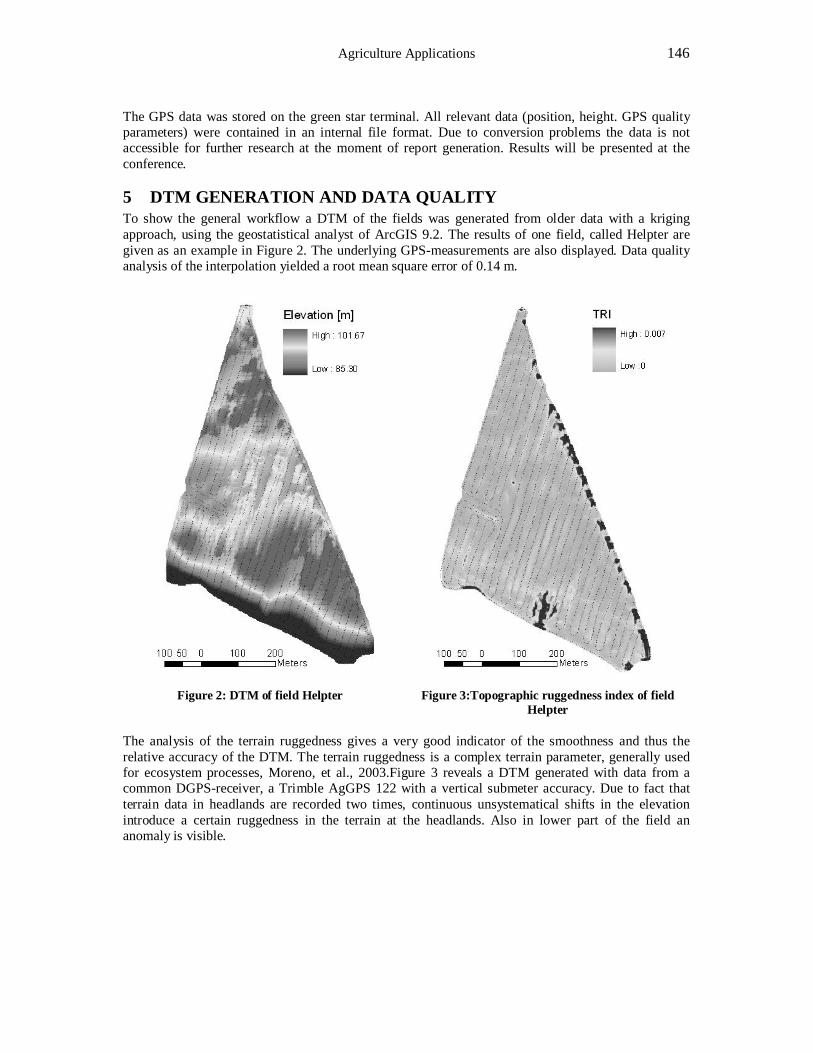
Agriculture Applications 146
The GPS data was stored on the green star terminal. All relevant data (position, height. GPS quality parameters) were contained in an internal file format. Due to conversion problems the data is not accessible for further research at the moment of report generation. Results will be presented at the conference.
5 DTM GENERATION AND DATA QUALITY To show the general workflow a DTM of the fields was generated from older data with a kriging approach, using the geostatistical analyst of ArcGIS 9.2. The results of one field, called Helpter are given as an example in Figure 2. The underlying GPS-measurements are also displayed. Data quality analysis of the interpolation yielded a root mean square error of 0.14 m.
Figure 2: DTM of field Helpter Figure 3:Topographic ruggedness index of field
Helpter The analysis of the terrain ruggedness gives a very good indicator of the smoothness and thus the relative accuracy of the DTM. The terrain ruggedness is a complex terrain parameter, generally used for ecosystem processes, Moreno, et al., 2003.Figure 3 reveals a DTM generated with data from a common DGPS-receiver, a Trimble AgGPS 122 with a vertical submeter accuracy. Due to fact that terrain data in headlands are recorded two times, continuous unsystematical shifts in the elevation introduce a certain ruggedness in the terrain at the headlands. Also in lower part of the field an anomaly is visible.

1st International Conference on Machine Control & Guidance 2008 147
5.1 Data Analysis The basic data analysis of the DTM itself consists of the derivation of several terrain parameters, which will be explained in the next section, Figure 4.
Primary terrain parameter Secondary terrain parameter
(a) Catchment areas with flow accumulation (b) Topographic wetness index
(c) Catchment areas with flow accumulation (d) Streampower Index
Figure 4: Primary and secondary terrain parameters for the field Helpter (26.54 ha)
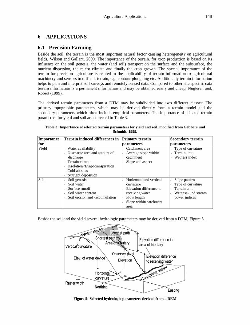
Agriculture Applications 148
6 APPLICATIONS
6.1 Precision Farming Beside the soil, the terrain is the most important natural factor causing heterogeneity on agricultural fields, Wilson and Gallant, 2000. The importance of the terrain, for crop production is based on its influence on the soil genesis, the water (and soil) transport on the surface and the subsurface, the nutrient dispersion, the micro climate and finally the crop growth. The special importance of the terrain for precision agriculture is related to the applicability of terrain information to agricultural machinery and sensors in difficult terrain, e.g. contour ploughing etc. Additionally terrain information helps to plan and interpret soil surveys and remotely sensed data. Compared to other site specific data terrain information is a permanent information and may be obtained easily and cheap, Nugteren and, Robert (1999). The derived terrain parameters from a DTM may be subdivided into two different classes: The primary topographic parameters, which may be derived directly from a terrain model and the secondary parameters which often include empirical parameters. The importance of selected terrain parameters for yield and soil are collected in Table 3.
Table 3: Importance of selected terrain parameters for yield and soil, modified from Gebbers und Schmidt, 1999.
Importance for
Terrain induced differences in Primary terrain parameters
Secondary terrain parameters
Yield - Water availability - Discharge area and amount of
discharge - Terrain climate - Insolation /Evapotranspiration - Cold air sites - Nutrient deposition
- Catchment area - Average slope within
catchment - Slope and aspect
- Type of curvature - Terrain unit - Wetness index
Soil - Soil genesis - Soil water - Surface runoff - Soil water content - Soil erosion and -accumulation
- Horizontal and vertical curvature
- Elevation difference to receiving water
- Flow length - Slope within catchment
area
- Slope pattern - Type of curvature - Terrain unit - Wetness- und stream
power indices
Beside the soil and the yield several hydrologic parameters may be derived from a DTM, Figure 5.
Elevation
NorthingEasting
Raster width
Observer point
Area of tributary
Longest pathShortest path
Elev. of water devide
Elevation difference in area of tributary
Elevation differenceto receiving water
Horizontalcurvature
Vertical curvature
Water devide
Receiving water
Elevation
NorthingEasting
Raster width
Observer point
Area of tributary
Longest pathShortest path
Elev. of water devide
Elevation difference in area of tributary
Elevation differenceto receiving water
Horizontalcurvature
Vertical curvature
Water devide
Receiving water
Figure 5: Selected hydrologic parameters derived from a DEM
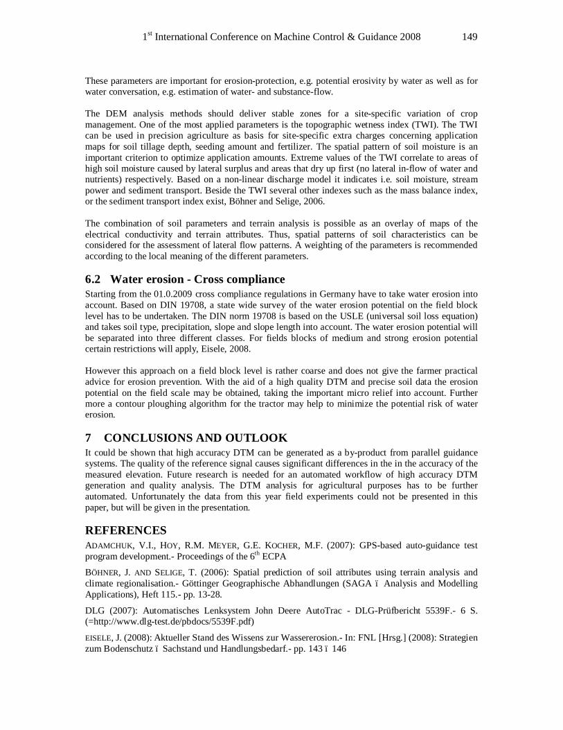
1st International Conference on Machine Control & Guidance 2008 149
These parameters are important for erosion-protection, e.g. potential erosivity by water as well as for water conversation, e.g. estimation of water- and substance-flow. The DEM analysis methods should deliver stable zones for a site-specific variation of crop management. One of the most applied parameters is the topographic wetness index (TWI). The TWI can be used in precision agriculture as basis for site-specific extra charges concerning application maps for soil tillage depth, seeding amount and fertilizer. The spatial pattern of soil moisture is an important criterion to optimize application amounts. Extreme values of the TWI correlate to areas of high soil moisture caused by lateral surplus and areas that dry up first (no lateral in-flow of water and nutrients) respectively. Based on a non-linear discharge model it indicates i.e. soil moisture, stream power and sediment transport. Beside the TWI several other indexes such as the mass balance index, or the sediment transport index exist, Böhner and Selige, 2006. The combination of soil parameters and terrain analysis is possible as an overlay of maps of the electrical conductivity and terrain attributes. Thus, spatial patterns of soil characteristics can be considered for the assessment of lateral flow patterns. A weighting of the parameters is recommended according to the local meaning of the different parameters.
6.2 Water erosion - Cross compliance Starting from the 01.0.2009 cross compliance regulations in Germany have to take water erosion into account. Based on DIN 19708, a state wide survey of the water erosion potential on the field block level has to be undertaken. The DIN norm 19708 is based on the USLE (universal soil loss equation) and takes soil type, precipitation, slope and slope length into account. The water erosion potential will be separated into three different classes. For fields blocks of medium and strong erosion potential certain restrictions will apply, Eisele, 2008. However this approach on a field block level is rather coarse and does not give the farmer practical advice for erosion prevention. With the aid of a high quality DTM and precise soil data the erosion potential on the field scale may be obtained, taking the important micro relief into account. Further more a contour ploughing algorithm for the tractor may help to minimize the potential risk of water erosion.
7 CONCLUSIONS AND OUTLOOK It could be shown that high accuracy DTM can be generated as a by-product from parallel guidance systems. The quality of the reference signal causes significant differences in the in the accuracy of the measured elevation. Future research is needed for an automated workflow of high accuracy DTM generation and quality analysis. The DTM analysis for agricultural purposes has to be further automated. Unfortunately the data from this year field experiments could not be presented in this paper, but will be given in the presentation.
REFERENCES ADAMCHUK, V.I., HOY, R.M. MEYER, G.E. KOCHER, M.F. (2007): GPS-based auto-guidance test program development.- Proceedings of the 6th ECPA
BÖHNER, J. AND SELIGE, T. (2006): Spatial prediction of soil attributes using terrain analysis and climate regionalisation.- Göttinger Geographische Abhandlungen (SAGA – Analysis and Modelling Applications), Heft 115.- pp. 13-28.
DLG (2007): Automatisches Lenksystem John Deere AutoTrac - DLG-Prüfbericht 5539F.- 6 S. (=http://www.dlg-test.de/pbdocs/5539F.pdf)
EISELE, J. (2008): Aktueller Stand des Wissens zur Wassererosion.- In: FNL [Hrsg.] (2008): Strategien zum Bodenschutz – Sachstand und Handlungsbedarf.- pp. 143 – 146
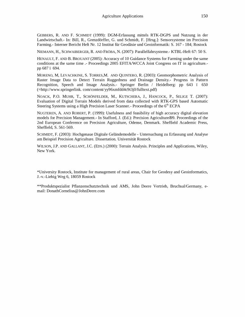
Agriculture Applications 150
GEBBERS, R. AND F. SCHMIDT (1999): DGM-Erfassung mittels RTK-DGPS und Nutzung in der Landwirtschaft.- In: Bill, R., Grenzdörffer, G. und Schmidt, F. [Hrsg.]: Sensorsysteme im Precision Farming.- Interner Bericht Heft Nr. 12 Institut für Geodäsie und Geoinformatik: S. 167 - 184; Rostock
NIEMANN, H., SCHWAIBERGER, R. AND FRÖBA, N. (2007): Parallelfahrsysteme.- KTBL-Heft 67: 50 S.
HENAULT, F. AND B. BROUANT (2005): Accuracy of 10 Guidance Systems for Farming under the same conditions at the same time .- Proceedings 2005 EFITA/WCCA Joint Congress on IT in agriculture.- pp 687 – 694.
MORENO, M, LEVACHKINE, S. TORRES,M. AND QUINTERO, R. (2003): Geomorphometric Analysis of Raster Image Data to Detect Terrain Ruggedness and Drainage Density.- Progress in Pattern Recognition, Speech and Image Analysis.- Springer Berlin / Heidelberg: pp 643 – 650 (=http://www.springerlink. com/content/yy96xmfdd4c9t3j0/fulltext.pdf)
NOACK, P.O. MUHR, T., SCHÖNFELDER, M., KUTSCHERA, J., HANCOCK, P., SELIGE T. (2007): Evaluation of Digital Terrain Models derived from data collected with RTK-GPS based Automatic Steering Systems using a High Precision Laser Scanner.- Proceedings of the 6th ECPA
NUGTEREN, A. AND ROBERT, P. (1999): Usefulness and feasibility of high accuracy digital elevation models for Precision Management.- In Stafford, J. (Ed.): Precision Agriculture’99. Proceedings of the 2nd European Conference on Precision Agriculture, Odense, Denmark. Sheffield Academic Press, Sheffield, S. 561-569.
SCHMIDT, F. (2003): Hochgenaue Digitale Geländemodelle - Untersuchung zu Erfassung und Analyse am Beispiel Precision Agriculture. Dissertation. Universität Rostock
WILSON, J.P. AND GALLANT, J.C. (EDS.) (2000): Terrain Analysis. Principles and Applications, Wiley, New York.
*University Rostock, Institute for management of rural areas, Chair for Geodesy and Geoinformatics, J.-v.-Liebig Weg 6, 18059 Rostock **Produktspezialist Pflanzenschutztechnik und AMS, John Deere Vertrieb, Bruchsal/Germany, e-mail: [email protected]
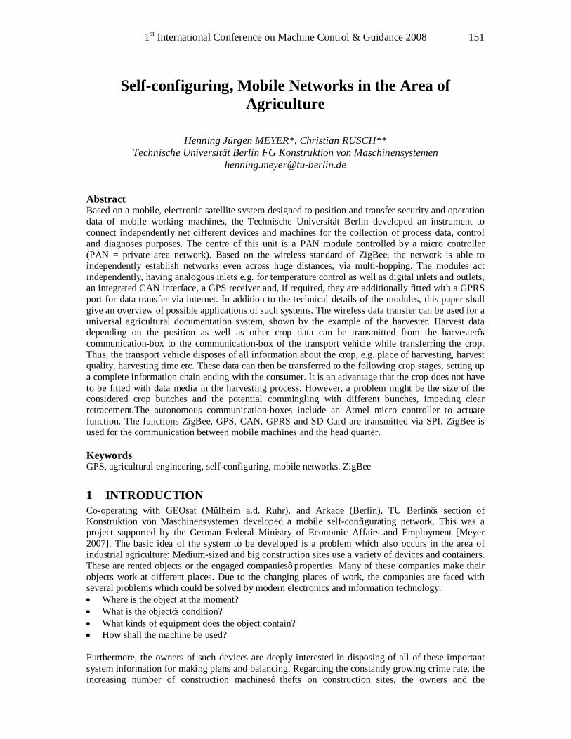
1st International Conference on Machine Control & Guidance 2008 151
Self-configuring, Mobile Networks in the Area of Agriculture
Henning Jürgen MEYER*, Christian RUSCH**
Technische Universität Berlin FG Konstruktion von Maschinensystemen [email protected]
Abstract Based on a mobile, electronic satellite system designed to position and transfer security and operation data of mobile working machines, the Technische Universität Berlin developed an instrument to connect independently net different devices and machines for the collection of process data, control and diagnoses purposes. The centre of this unit is a PAN module controlled by a micro controller (PAN = private area network). Based on the wireless standard of ZigBee, the network is able to independently establish networks even across huge distances, via multi-hopping. The modules act independently, having analogous inlets e.g. for temperature control as well as digital inlets and outlets, an integrated CAN interface, a GPS receiver and, if required, they are additionally fitted with a GPRS port for data transfer via internet. In addition to the technical details of the modules, this paper shall give an overview of possible applications of such systems. The wireless data transfer can be used for a universal agricultural documentation system, shown by the example of the harvester. Harvest data depending on the position as well as other crop data can be transmitted from the harvester’s communication-box to the communication-box of the transport vehicle while transferring the crop. Thus, the transport vehicle disposes of all information about the crop, e.g. place of harvesting, harvest quality, harvesting time etc. These data can then be transferred to the following crop stages, setting up a complete information chain ending with the consumer. It is an advantage that the crop does not have to be fitted with data media in the harvesting process. However, a problem might be the size of the considered crop bunches and the potential commingling with different bunches, impeding clear retracement.The autonomous communication-boxes include an Atmel micro controller to actuate function. The functions ZigBee, GPS, CAN, GPRS and SD Card are transmitted via SPI. ZigBee is used for the communication between mobile machines and the head quarter. Keywords GPS, agricultural engineering, self-configuring, mobile networks, ZigBee
1 INTRODUCTION Co-operating with GEOsat (Mülheim a.d. Ruhr), and Arkade (Berlin), TU Berlin’s section of Konstruktion von Maschinensystemen developed a mobile self-configurating network. This was a project supported by the German Federal Ministry of Economic Affairs and Employment [Meyer 2007]. The basic idea of the system to be developed is a problem which also occurs in the area of industrial agriculture: Medium-sized and big construction sites use a variety of devices and containers. These are rented objects or the engaged companies’ properties. Many of these companies make their objects work at different places. Due to the changing places of work, the companies are faced with several problems which could be solved by modern electronics and information technology: • Where is the object at the moment? • What is the object’s condition? • What kinds of equipment does the object contain? • How shall the machine be used? Furthermore, the owners of such devices are deeply interested in disposing of all of these important system information for making plans and balancing. Regarding the constantly growing crime rate, the increasing number of construction machines’ thefts on construction sites, the owners and the
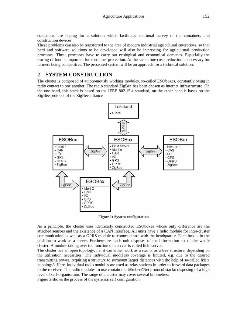
Agriculture Applications 152
companies are hoping for a solution which facilitates continual survey of the containers and construction devices. These problems can also be transferred to the area of modern industrial agricultural enterprises, so that hard and software solutions to be developed will also be interesting for agricultural production processes. These processes have to carry out ecological and economical demands. Especially the tracing of food is important for consumer protection. At the same time costs reduction is necessary for farmers being competitive. The presented system will be an approach for a technical solution.
2 SYSTEM CONSTRUCTION The cluster is composed of autonomously working modules, so-called ESOboxes, constantly being in radio contact to one another. The radio standard ZigBee has been chosen as internet infrastructure. On the one hand, this stack is based on the IEEE 802.15.4 standard, on the other hand it bases on the ZigBee protocol of the ZigBee alliance.
Figure 1: System configuration
As a principle, the cluster uses identically constructed ESOboxes whose only difference are the attached sensors and the existence of a CAN interface. All units have a radio module for intra-cluster communication as well as a GPRS module to communicate with the headquarter. Each box is in the position to work as a server. Furthermore, each unit disposes of the information set of the whole cluster. A module taking over the function of a server is called field server. The cluster has an open topology, i.e. it can either work as a star or as a tree structure, depending on the utilisation necessities. The individual modules’ coverage is limited, e.g. due to the desired transmitting power, requiring a structure to surmount larger distances with the help of so-called “data hoppings”. Here, individual radio modules are used as relay stations in order to forward data packages to the receiver. The radio modules in use contain the “EmberZNet protocol stack” disposing of a high level of self-organisation. The range of a cluster may cover several kilometres. Figure 2 shows the process of the system’s self configuration.
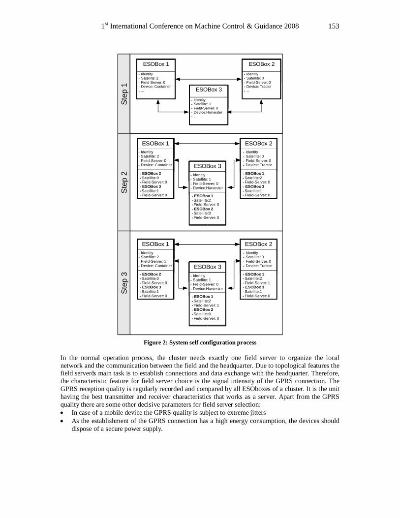
1st International Conference on Machine Control & Guidance 2008 153
ESOBoxFieldESOBoxMillESOBoxFieldESOBoxESOBox 3
Identity Satellite: 1 Field-Server: 0 Device:Harvester ...
ESOBoxFieldESOBoxMillESOBoxFieldESOBoxESOBox 1
Identity Satellite: 2 Field-Server: 0 Device: Container ...
ESOBoxFieldESOBoxMillESOBoxFieldESOBoxESOBox 2
Identity Satellite: 0 Field-Server: 0 Device: Tractor ...
ESOBoxFieldESOBoxMillESOBoxFieldESOBoxESOBox 3
ESOBox 1Satellite:2Field-Server: 0 ESOBox 2Satellite:0Field-Server: 0
ESOBoxFieldESOBoxMillESOBoxFieldESOBoxESOBox 1
ESOBox 2Satellite:0Field-Server: 0 ESOBox 3Satellite:1Field-Server: 0
ESOBoxFieldESOBoxMillESOBoxFieldESOBoxESOBox 2
ESOBox 1Satellite:2Field-Server: 0 ESOBox 3Satellite:1Field-Server: 0
Identity Satellite: 2 Field-Server: 0 Device: Container
Identity Satellite: 1 Field-Server: 0 Device:Harvester
Identity Satellite: 0 Field-Server: 0 Device: Tractor
ESOBoxFieldESOBoxMillESOBoxFieldESOBoxESOBox 3
ESOBox 1Satellite:2Field-Server: 1 ESOBox 2Satellite:0Field-Server: 0
ESOBoxFieldESOBoxMillESOBoxFieldESOBoxESOBox 1
ESOBox 2Satellite:0Field-Server: 0 ESOBox 3Satellite:1Field-Server: 0
ESOBoxFieldESOBoxMillESOBoxFieldESOBoxESOBox 2
ESOBox 1Satellite:2Field-Server: 1 ESOBox 3Satellite:1Field-Server: 0
Identity Satellite: 2 Field-Server: 1 Device: Container
Identity Satellite: 1 Field-Server: 0 Device:Harvester
Identity Satellite: 0 Field-Server: 0 Device: Tractor
Step
1St
ep 2
Step
3
Figure 2: System self configuration process
In the normal operation process, the cluster needs exactly one field server to organize the local network and the communication between the field and the headquarter. Due to topological features the field server’s main task is to establish connections and data exchange with the headquarter. Therefore, the characteristic feature for field server choice is the signal intensity of the GPRS connection. The GPRS reception quality is regularly recorded and compared by all ESOboxes of a cluster. It is the unit having the best transmitter and receiver characteristics that works as a server. Apart from the GPRS quality there are some other decisive parameters for field server selection: • In case of a mobile device the GPRS quality is subject to extreme jitters • As the establishment of the GPRS connection has a high energy consumption, the devices should
dispose of a secure power supply.
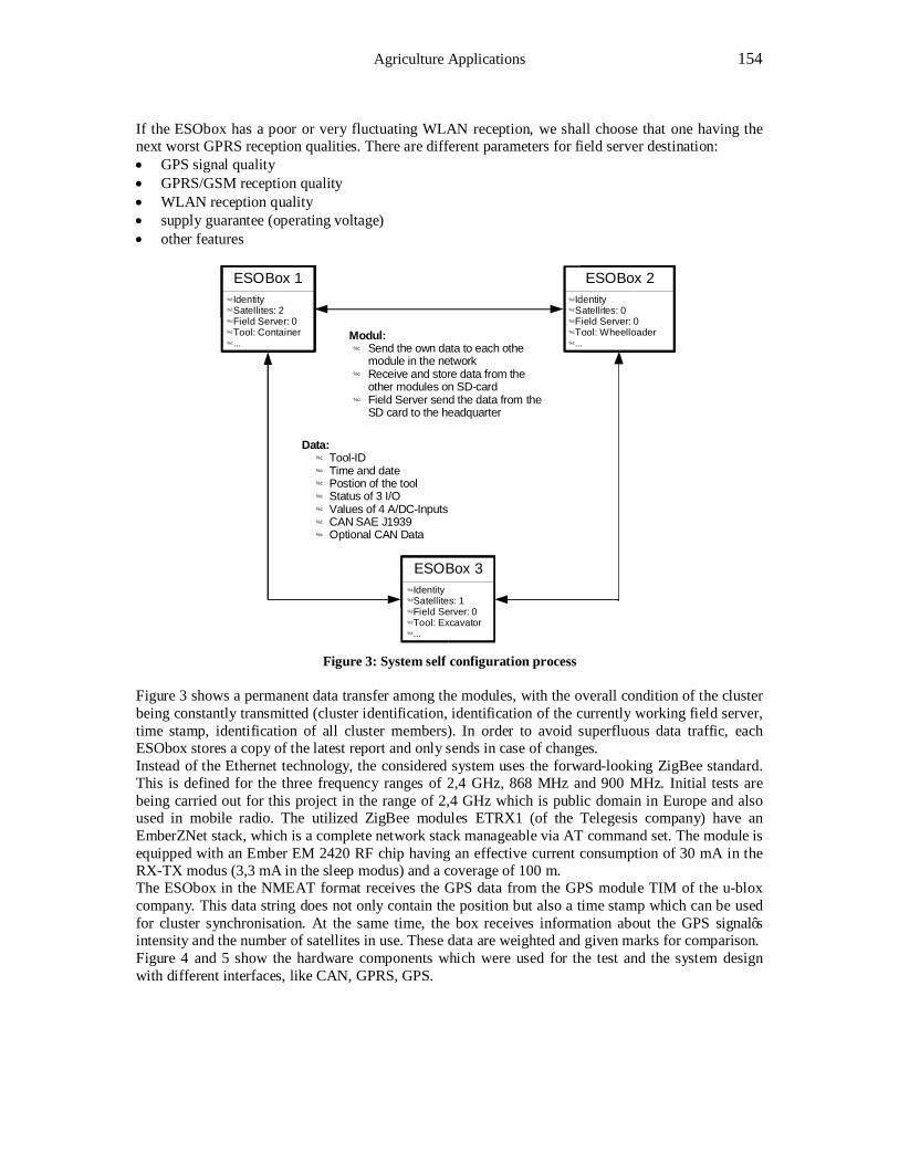
Agriculture Applications 154
If the ESObox has a poor or very fluctuating WLAN reception, we shall choose that one having the next worst GPRS reception qualities. There are different parameters for field server destination: • GPS signal quality • GPRS/GSM reception quality • WLAN reception quality • supply guarantee (operating voltage) • other features
ESOBoxFieldESOBoxMillESOBoxFieldESOBoxESOBox 3 Identity Satellites: 1 Field Server: 0 Tool: Excavator ...
ESOBoxFieldESOBoxMillESOBoxFieldESOBoxESOBox 1 Identity Satellites: 2 Field Server: 0 Tool: Container ...
ESOBoxFieldESOBoxMillESOBoxFieldESOBoxESOBox 2 Identity Satellites: 0 Field Server: 0 Tool: Wheelloader ...
Modul: Send the own data to each othe
module in the network Receive and store data from the
other modules on SD-card Field Server send the data from the
SD card to the headquarter
Data: Tool-ID Time and date Postion of the tool Status of 3 I/O Values of 4 A/DC-Inputs CAN SAE J1939 Optional CAN Data
Figure 3: System self configuration process
Figure 3 shows a permanent data transfer among the modules, with the overall condition of the cluster being constantly transmitted (cluster identification, identification of the currently working field server, time stamp, identification of all cluster members). In order to avoid superfluous data traffic, each ESObox stores a copy of the latest report and only sends in case of changes. Instead of the Ethernet technology, the considered system uses the forward-looking ZigBee standard. This is defined for the three frequency ranges of 2,4 GHz, 868 MHz and 900 MHz. Initial tests are being carried out for this project in the range of 2,4 GHz which is public domain in Europe and also used in mobile radio. The utilized ZigBee modules ETRX1 (of the Telegesis company) have an EmberZNet stack, which is a complete network stack manageable via AT command set. The module is equipped with an Ember EM 2420 RF chip having an effective current consumption of 30 mA in the RX-TX modus (3,3 mA in the sleep modus) and a coverage of 100 m. The ESObox in the NMEAT format receives the GPS data from the GPS module TIM of the u-blox company. This data string does not only contain the position but also a time stamp which can be used for cluster synchronisation. At the same time, the box receives information about the GPS signal’s intensity and the number of satellites in use. These data are weighted and given marks for comparison. Figure 4 and 5 show the hardware components which were used for the test and the system design with different interfaces, like CAN, GPRS, GPS.
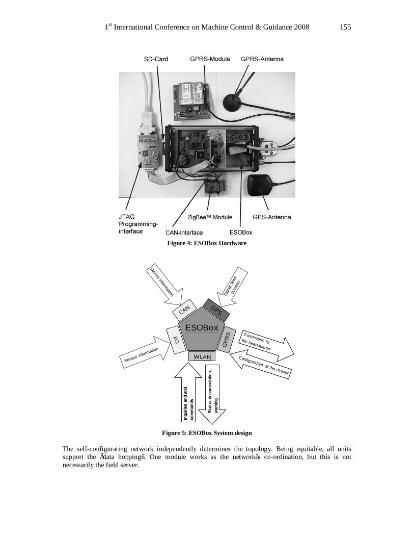
1st International Conference on Machine Control & Guidance 2008 155
Figure 4: ESOBox Hardware
Configuration of the cluster
Connection to the headquarter
Sign
al lev
elpo
sition
Device information
WLAN
GPS
GPR
S
CAN
ESOBoxI/O
WLAN
GPS
GPR
S
CAN
ESOBox
I/O
Sensor information
Stat
us d
ocum
enta
tion,
,w
arni
ng
Inqu
iries
and
and
co
mm
ands
Stat
us d
ocum
enta
tion,
,w
arni
ng
Inqu
iries
and
and
co
mm
ands
Figure 5: ESOBox System design
The self-configurating network independently determines the topology. Being equitable, all units support the „data hopping“. One module works as the network’s co-ordination, but this is not necessarily the field server.

Agriculture Applications 156
Relais stationsRelais stations
Figure 6: Principle of data hoping
The collected data are buffered in each box on a SD card. As all data packages have a time stamp, it is always possible to dispose of the latest data. The data are decoded and compared. In fixed intervals, the server then sends the data of the entire cluster to the headquarter. The common data format is XML.
3 AGRICULTURAL APPLICATION Agricultural engineering processes have to carry out ecological and economical demands. Especially the tracing of food is important for consumer protection. At the same time reducing costs is necesarry for farmers being competitive. This demand is independent of the way of farming – conventional or organic.
Figure 7: Agricultural production process and the harvest process

1st International Conference on Machine Control & Guidance 2008 157
Figure 7 shows the agricultural production process with different sub-processes like tillage, sowing and so on. Each sub-process consists of further sub-processes which can be very different. The self-configurating network described above using ESOboxes facilitates multiple application varieties in the field of agriculture:
3.1 Control of mobile agricultural machines With a machine being equipped with an ESObox and CAN interface, it is possible to realize communication between the machine and the headquarter. This helps to establish services like remote maintenance and diagnosis, remote operation and manipulation as well as process and machine modelling [MEYER 1998]. By using teleservice technologies, it is possible e.g. to cyclically store and send data regarding load, environment conditions and wear characteristics to a central databank within the operation process. Thanks to the increased number of measured data per machine type, manufacturers are in the position to set up highly reliable analyses even after a short period of time. Furthermore, they can more precisely develop utilisation and damage profiles for the individual machines and, thus, offer useful new services to the operators, such as individual adjustment hints and maintenance measures. The operator will gain from the following advantages: • low-priced guarantee of machine accessibility and reliability • optimum planning of maintenance measures • long-term increase of machine reliability • improved spare parts supply with operators • improved cost-value-ratio for tele-service systems • concentrated core competence The machine manufacturers may dispose of the following advantages: • better customer retention • machine information for design improvement • new services • better planning and organisation of spare parts supply Teleservice applications exist for a great number of products. In the field of mobile working machines there is only little use of teleservice systems. The reasons are high costs, the missing data infra structure, and the need for special customer services [LIESTMANN 2007, REICHENBACH 2006]. [GÖRES 2007] presented an actual telesesevice research project called DAMIT. They want to develop a data management system for a teleservice application on mobile working machines. The project is being executed at the Institute of Agricultural Machinery and Fluid Power (ILF), TU Braunschweig, in co-operation with the two agricultural machinery manufacturers Claas and Grimme and the LINEAS Project Services Company providing software services. They define four major objectives of their project:
1. New maintenance strategies for exemplary sub-assemblies 2. Methods to reduce the amount of data to transfer 3. Methods to optimise communication and data storage 4. Process modelling of a sugar beet harvesting chain and a service workshop.
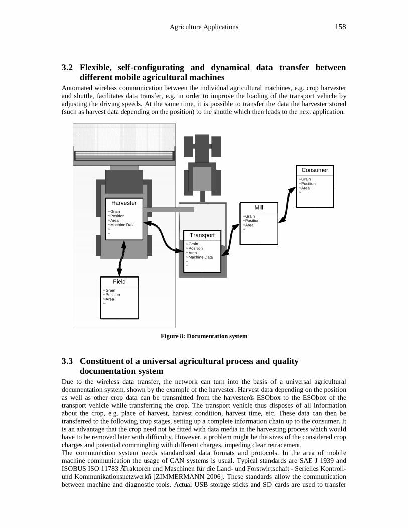
Agriculture Applications 158
3.2 Flexible, self-configurating and dynamical data transfer between different mobile agricultural machines
Automated wireless communication between the individual agricultural machines, e.g. crop harvester and shuttle, facilitates data transfer, e.g. in order to improve the loading of the transport vehicle by adjusting the driving speeds. At the same time, it is possible to transfer the data the harvester stored (such as harvest data depending on the position) to the shuttle which then leads to the next application.
ESOBoxIdent 1
Harvester Grain Position Area Machine Data ESOBox
Ident 1
Transport Grain Position Area Machine Data
ESOBoxIdent 1
Field Grain Position Area
ESOBoxIdent 1
Field Grain Position Area
ESOBoxIdent 1
Field Grain Position Area
ESOBoxIdent 1
Mill Grain Position Area
ESOBoxIdent 1
Field Grain Position Area
ESOBoxIdent 1
Mill Grain Position Area
ESOBoxIdent 1
Field Grain Position Area
ESOBoxIdent 1
Mill Grain Position Area
ESOBoxIdent 1
Field Grain Position Area
ESOBoxIdent 1
Consumer Grain Position Area
Figure 8: Documentation system
3.3 Constituent of a universal agricultural process and quality documentation system
Due to the wireless data transfer, the network can turn into the basis of a universal agricultural documentation system, shown by the example of the harvester. Harvest data depending on the position as well as other crop data can be transmitted from the harvester’s ESObox to the ESObox of the transport vehicle while transferring the crop. The transport vehicle thus disposes of all information about the crop, e.g. place of harvest, harvest condition, harvest time, etc. These data can then be transferred to the following crop stages, setting up a complete information chain up to the consumer. It is an advantage that the crop need not be fitted with data media in the harvesting process which would have to be removed later with difficulty. However, a problem might be the sizes of the considered crop charges and potential commingling with different charges, impeding clear retracement. The communiction system needs standardized data formats and protocols. In the area of mobile machine communication the usage of CAN systems is usual. Typical standards are SAE J 1939 and ISOBUS ISO 11783 „Traktoren und Maschinen für die Land- und Forstwirtschaft - Serielles Kontroll- und Kommunikationsnetzwerk“ [ZIMMERMANN 2006]. These standards allow the communication between machine and diagnostic tools. Actual USB storage sticks and SD cards are used to transfer
1st International Conference on Machine Control & Guidance 2008 159
data from the machine to the farm office’s personal computer and the farm management information system (FIMS) [Hieronymus 2007]. Hamacher uses GRPS and sends every 15 min data but breeds costs. This is a barrier for market penetration. Another barrier are non-open communication systems, i. e. systems which allow only the communication between machines of one manufacturer. Special sensor systems are necessary for the quality determination. Regarding grain quality determination in the combine, near infrared spectroscopy (NIRS) can be employed. [RISIUS 2007, RECKLEBEN 2004, RADEMACHER 2003]. The gathered machine data can be imported into FIMS. Farmers or farm service providers will thus have detailed information on which machines are used in what way on which field. Agricultural software companies provide software packages for appropriate uses. However, these programmes are not designed for simulating complex harvest and transport processes to improve the company’s organisation. In order to provide other partners with these FIMS information set up these, e. g. production and process chains, the agroXML standard is used [KUNISCH 2007]. This standard facilitates easy importing and exporting data into different software applications as all process data and variables are standardized. The area of lifestock farming aims at standardizing a data bus ISOagriNET designed to facilitate the communication between processing computers [PAULSEN 2008]. It will be reasonable here to implement an interface via agroXML as this will be the interface between lifestock farming and plant production in future.
4 CONCLUSIONS The usage of modern information and communication systems helps to optimize construction processes and agricultural engineering processes. The collected data can be used for machine control, diagnosis and documentation. Especially the documentation of harvesting processes is necessary for general quality documentation of food. The presented system using the ZigBee-Standard fulfills the demands on mobile communication systems for mobile working machines. Further investigations at the Technische Universität Berlin will improve the practical use in harvesting machines and the data security.
ACKNOWLEDGEMENTS The authors would like to thank the Arbeitsgemeinschaft innovativer Forschungsvereinigungen (AiF) for supporting and financing the project.
REFERENCES GÖRES, T.; GROTHAUS, H. P.; RUSTEMEYER, T.; MÖLLER, A.: Development of a data management system for teleservice application on mobile working machines – DAMIT. VDI-Berichte Band 2001, pp. 265-270, 2007
HIERONYMUS, P.: Development of an electronic concept for harvesting machinery and tractors. VDI-Berichte Nr. 2001, pp. 303 – 308, 2007
HAMACHER, H.: Telematics – Maximum combine capacity over the whole season. VDI-Berichte Nr. 2001, pp. 387 – 391, 2007
KUNISCH, M. ET AL. : agroXML – der Standard für den Datenaustausch in der Landwirtschaft. Landtechnik 62. Jhg. Nr. 1, pp. 46 - 47, 2007
LIESTMANN, V.; RÜHMANN, N.; SCHUH, G.; STICH, V.: Integration von TeleService in die Serviceorganisation. Teleservicegerechte Prozesse. Praxis-Edition Band 10, pp. 1-62, 2007

Agriculture Applications 160
MEYER, H. J.; KAUSCH, C.; DIEKHANS, N: Teleservicesysteme. Landtechnik 53. Jhg. 2, pp. 104- 105, 1998
MEYER, H. J.; RUSCH, C.: Entwicklung der technischen Lösung für die Kommunikation der Container bzw. Baumaschinen untereinander sowie innerhalb des Gesamtsystems. Abschlussbericht zum Förderkennzeichen KF 0088501SS4. TU Berlin FG Konstruktion von Maschinensystemen. 2007
PAULSEN, C.: Der intelligente Kuhstall – Perspektive oder Illusion, http://www.isoagrinet.org last accessed on April 18, 2008
RADEMACHER, J.: Kontinuierliche Messung der Getreidequalität während des Mähdrusches. Dissertation Christian-Albrechts-Universität, Kiel, 2003.
REICHENBACH, G.: Webbasiertes Auftrags- und Maschinendatenmanagement für mobile Arbeitsmaschinen. Fachtagung Baumaschinentechnik 2006, Dresden, 5.-6.10.2006, pp. 279-283, 2006
RISIUS, H.: Verfahrenstechnische Grundlagen der selektiven Getreideernte. Landtechnik 62. Jhg., 5, p. 354, 2007
RECKLEBEN, Y.: Innovative Echtzeitsensorik zur Bestimmung und Regelung der Produktqualität von Getreide während des Mähdruschs. Dissertation Christian-Albrechts-Universität, Kiel, 2004
ZigBee Specification v 1.0. ZigBee Document 053473r00, Version 1.00. 14 April 2005
* Prof. Dr.-Ing. Henning Jürgen Meyer, Technische Universität Berlin FG Konstruktion von Maschinensystemen, Sekr. W1, Straße des 17. Juni 144, D - 10623 Berlin, Germany ** Dipl.-Ing. Christian Rusch, Technische Universität Berlin FG Konstruktion von Maschinensystemen, Sekr. W1, Straße des 17. Juni 144, D - 10623 Berlin, Germany
1st International Conference on Machine Control & Guidance 2008 161
A Self Calibrating Attitude Determination System for Precision Farming using Multiple Low-Cost
Complementary Sensors
William KELLAR*, Peter ROBERTS, Oliver ZELZER Leica Geosystems, Brisbane, Australia [email protected]
Abstract A low cost three axis attitude determination system for moving platforms has been developed by Leica Geosystems that requires a minimal calibration procedure, and has the ability to self-calibrate for the various biases caused by temperature variation and mounting misalignment. Sensor fusion techniques are used to combine the data from a high quality survey grade GNSS receiver with additional cost effective high performance inertial sensors to produce a high rate of attitude data with low noise and low bias in the form of an attitude sensor module for machine control and guidance applications. The sensor module has been successfully integrated into a tractor steering system for precision farming. This paper demonstrates the minimal installation and calibration procedures for the system, and presents the results from benchmarking the system in real farm operating conditions. Keywords GPS, agriculture, precision farming, tractor, Leica, mojoRTK
1 INTRODUCTION The benefits of machine guidance systems are well known within the field of precision agriculture. These may include increased yield from crops, reduced input costs due to overlap, reduced driver fatigue and reduced fuel usage [Webb, 2004]. Modern GPS equipment is capable of producing high quality position measurements with standard deviations of less than one inch and update rates faster than ten times per second, however, this alone is not sufficient for accurate tractor guidance. The terrain on farms is rarely smooth and flat, and this means that a GPS antenna mounted in the roof of a tall vehicle such as a tractor will experience movement relative to the ground position as the vehicle pitches and rolls over uneven terrain. The use of two or three axis attitude solutions to compensate for lever arm effect of the GPS antenna [Korver, 1999] is frequently practiced within the field of precision agriculture. The literature refers to this as “terrain compensation” or “tilt compensation”. The benefits of this include increased on-line accuracy in rough terrain [Ag Leader, 2005] as well as a reducing skips and overlaps between passes on sloped and undulating country [Trimble, 2005]. Agricultural guidance systems typically calculate vehicle attitude using a combination of inertial sensors [Trimble, 2005], or multiple GPS antennas [O’Connor, 1996], and each approach has strengths and weaknesses. Inertial based attitude solutions are subject to errors caused by sensor biases, axis misalignment, scale factor biases and temperature drift. A purely GPS-based attitude solution does not have these sensor biases, but does experience the availability and signal outage problems associated with GPS positioning.

Agriculture Applications 162
The Leica mojoRTK system makes use of automotive grade MEMS inertial sensors and a dual frequency survey grade GPS/GLONASS receiver to provide position and attitude information that is suitable for agricultural guidance and machine control applications. This paper focuses specifically on the roll of the vehicle, since it is the quantity of most interest for a terrain compensation system.
1.1 System Overview The mojoRTK sensors consist of three rate gyros, a three axis accelerometer package and a digital compass. In addition to these sensors, the system includes two GPS receivers that produce a two axis attitude solution which is used for estimating the biases of the inertial sensors.
Position andAttitude Output
X Gyro (MEMS)
X,Y,Z Accelerometer (MEMS)
Dual Frequency GPS/GLONASS Single Frequency GPS
400MHz PowerPC CPU
2-Axis Digital Compass
Y Gyro (MEMS)
Z Gyro (MEMS)
Figure 1: System Sensor Architecture
1.1.1 Installation The installation of the mojoRTK system into a vehicle is relatively simple. First, the two GPS antennas are stuck to the roof of the vehicle. The antennas are mounted in such a way that a line through the centres of the antennas is parallel to the left-right axis of the vehicle. Antenna cables then are routed into the cab of the tractor. After the antennas are installed, the mojoRTK console is installed into the radio slot of the tractor. The mojoRTK console contains the inertial sensors and other electronics.
Figure 2: Installation Diagrams from the mojoRTK User Manual
1.1.2 Calibration The calibration of the mojoRTK system is conducted by performing two manoeuvres with the vehicle. The first manoeuvre involves sitting the vehicle in a stationary position for a short period of time, then rotating the vehicle 180 degrees in the same location. This allows the system to estimate the roll and pitch orientation of the mojoRTK console within the vehicle reference frame, and estimate the bias of
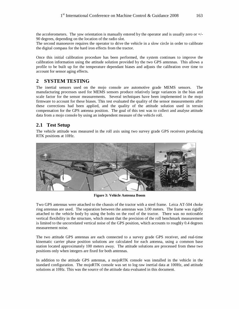
1st International Conference on Machine Control & Guidance 2008 163
the accelerometers. The yaw orientation is manually entered by the operator and is usually zero or +/- 90 degrees, depending on the location of the radio slot. The second manoeuvre requires the operator to drive the vehicle in a slow circle in order to calibrate the digital compass for the hard iron effects from the tractor. Once this initial calibration procedure has been performed, the system continues to improve the calibration information using the attitude solution provided by the two GPS antennas. This allows a profile to be built up for the temperature dependant biases and adjusts the calibration over time to account for sensor aging effects.
2 SYSTEM TESTING The inertial sensors used on the mojo console are automotive grade MEMS sensors. The manufacturing processes used for MEMS sensors produce relatively large variances in the bias and scale factor for the sensor measurements. Several techniques have been implemented in the mojo firmware to account for these biases. This test evaluated the quality of the sensor measurements after these corrections had been applied, and the quality of the attitude solution used in terrain compensation for the GPS antenna position. The goal of this test was to collect and analyse attitude data from a mojo console by using an independent measure of the vehicle roll.
2.1 Test Setup The vehicle attitude was measured in the roll axis using two survey grade GPS receivers producing RTK positions at 10Hz.
Figure 3: Vehicle Antenna Boom
Two GPS antennas were attached to the chassis of the tractor with a steel frame. Leica AT-504 choke ring antennas are used. The separation between the antennas was 3.00 meters. The frame was rigidly attached to the vehicle body by using the bolts on the roof of the tractor. There was no noticeable vertical flexibility in the structure, which meant that the precision of the roll benchmark measurement is limited to the uncorrelated vertical noise of the GPS position, which accounts to roughly 0.4 degrees measurement noise. The two attitude GPS antennas are each connected to a survey grade GPS receiver, and real-time kinematic carrier phase position solutions are calculated for each antenna, using a common base station located approximately 100 meters away. The attitude solutions are processed from these two positions only when integers are fixed for both antennas. In addition to the attitude GPS antennas, a mojoRTK console was installed in the vehicle in the standard configuration. The mojoRTK console was set to log raw inertial data at 100Hz, and attitude solutions at 10Hz. This was the source of the attitude data evaluated in this document.
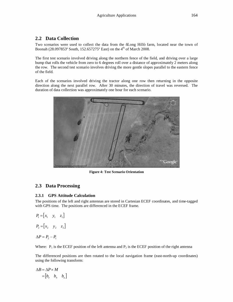
Agriculture Applications 164
2.2 Data Collection Two scenarios were used to collect the data from the “Long Hill” farm, located near the town of Boonah (28.097853º South, 152.657275º East) on the 4th of March 2008. The first test scenario involved driving along the northern fence of the field, and driving over a large bump that rolls the vehicle from zero to 6 degrees roll over a distance of approximately 2 meters along the row. The second test scenario involves driving the more gentle slopes parallel to the eastern fence of the field. Each of the scenarios involved driving the tractor along one row then returning in the opposite direction along the next parallel row. After 30 minutes, the direction of travel was reversed. The duration of data collection was approximately one hour for each scenario.
Figure 4: Test Scenario Orientation
2.3 Data Processing
2.3.1 GPS Attitude Calculation The positions of the left and right antennas are stored in Cartesian ECEF coordinates, and time-tagged with GPS time. The positions are differenced in the ECEF frame.
[ ]1111 zyxP =
[ ]2222 zyxP =
12 PPP −=∆ Where: P1 is the ECEF position of the left antenna and P2 is the ECEF position of the right antenna The differenced positions are then rotated to the local navigation frame (east-north-up coordinates) using the following transform:
[ ]une bbbMPB
=×∆=∆
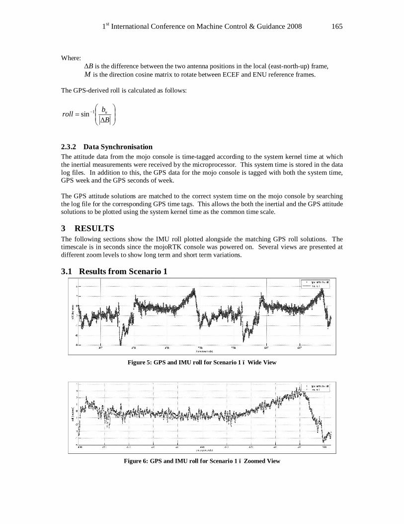
1st International Conference on Machine Control & Guidance 2008 165
Where: B∆ is the difference between the two antenna positions in the local (east-north-up) frame,
M is the direction cosine matrix to rotate between ECEF and ENU reference frames. The GPS-derived roll is calculated as follows:
∆= −
Bbroll u1sin
2.3.2 Data Synchronisation The attitude data from the mojo console is time-tagged according to the system kernel time at which the inertial measurements were received by the microprocessor. This system time is stored in the data log files. In addition to this, the GPS data for the mojo console is tagged with both the system time, GPS week and the GPS seconds of week. The GPS attitude solutions are matched to the correct system time on the mojo console by searching the log file for the corresponding GPS time tags. This allows the both the inertial and the GPS attitude solutions to be plotted using the system kernel time as the common time scale.
3 RESULTS The following sections show the IMU roll plotted alongside the matching GPS roll solutions. The timescale is in seconds since the mojoRTK console was powered on. Several views are presented at different zoom levels to show long term and short term variations.
3.1 Results from Scenario 1
Figure 5: GPS and IMU roll for Scenario 1 – Wide View
Figure 6: GPS and IMU roll for Scenario 1 – Zoomed View
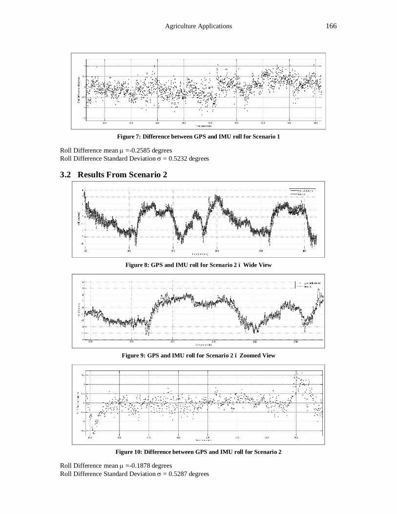
Agriculture Applications 166
Figure 7: Difference between GPS and IMU roll for Scenario 1
Roll Difference mean µ =-0.2585 degrees Roll Difference Standard Deviation σ = 0.5232 degrees
3.2 Results From Scenario 2
Figure 8: GPS and IMU roll for Scenario 2 – Wide View
Figure 9: GPS and IMU roll for Scenario 2 – Zoomed View
Figure 10: Difference between GPS and IMU roll for Scenario 2
Roll Difference mean µ =-0.1878 degrees Roll Difference Standard Deviation σ = 0.5287 degrees
1st International Conference on Machine Control & Guidance 2008 167
4 CONCLUSIONS The results in the previous section show that performance of the roll calculation from the mojoRTK inertial sensors is very close the measurable precision of the GPS attitude benchmarking system. This is achieved at a much lower cost to performance ratio because of the cost effective sensors that are used in the system. The mean error for the roll calculations is 0.2585 degrees in the worst case of scenario 2, which translates to a 13.5mm mean pass to pass position error (based on a 3 meter tall vehicle) due to roll error. The roll noise with standard deviation of 0.5287 degrees translates to a lateral roll compensation noise of 27.6mm. This is only slightly larger than the expected measurement noise of the GPS roll calculation. Overall, the accuracy of the roll calculation meant that the system performs successfully within the performance requirements of the mojoRTK product by satisfying the 50mm positioning accuracy of the terrain compensated position on the ground.
REFERENCES AG LEADER TECHNOLOGY: EZ-Steer Systems with T2 Terrain Compensation Technology, Ag Leader Technology, Iowa, USA, 2005
KORVER, K., HAWKINSON, W., and BOEDIGHEIMER, D.: Navigation/Guidance System for a Land-Based Vehicle, U.S. Patent 5928309, USA, 1999
O’CONNOR, M., BELL, T., ELKAIM, G. and PARKINSON, B.: Automatic Steering of Farm Vehicles Using GPS, Stanford University, Stanford, California, USA, 1996
TRIMBLE NAVIGATION LTD: Trimble T2 and T3 Technology Factsheet, Trimble Agricultural Division, Colorado, USA, 20056
WEBB, B., BLACKWELL, P., RIETHMULLER, G. and LEMON, J.: Tramline farming systems:
technical manual, Department of Agriculture Western Australia, Australia, 2004
* William Kellar, Leica Geosystems, 270 Gladstone Road, Dutton Park, QLD, 4102, Australia

Agriculture Applications 168
1st International Conference on Machine Control & Guidance 2008 169
3D-Object Recognition, Localization and Treatment of Rumex Obtusifolius in its Natural Environment
Dejan ŠEATOVIĆ*
ZHAW Winterthur, Switzerland [email protected]
Abstract Rumex obtusifolius is one of the most highly competitive and persistent sorts of weed in agriculture. An automatic recognition and plant-treatment system is currently under development as an alternative treatment technique. An infrared-laser triangulation sensor and a high-resolution smart camera are used to generate 3D images of the weeds and their natural environment. In a segmentation process, contiguous surface patches are separated from one other. These 3D surface patches are compared with different criteria of a plant database containing surface parameters such as shape, state of surface, etc. When individual objects are extracted and confirmed as possible leaves or parts of leaves, their texture is analyzed by comparing the information of simultaneously taken 2D images with database criteria. If an object is recognized as a dock leaf, its coordinates in the vehicle coordinate system are computed and the leaves are sprayed with herbicide. The surface analysis in space can boost segmentation performance under conditions where state-of-the-art 2D recognition systems are not successful, e.g. low contrast, green-on-green images, noisy images, or images taken from inappropriate positions. Initial results have been promising. System development focuses on a more robust imaging-sensor technique and refinement of the different algorithms. Looking to the future, the system design allows for the flexible integration of other plant species. Keywords plant recognition, plant localization, 3D image processing, segmentation, texture analysis
1 INTRODUCTION Sustainable land management is characterized by a systematic approach. Plant-production measures are in harmony with ecological, work-economics and business-management requirements. In practice, for example, this means that plant-protection products are only applied above a certain threshold of damage, or that individual plants are treated instead of broadcast spraying. At present, the mechanization and automation of tasks such as infestation recognition and plant recognition is seldom possible, given the lack of sensor technologies that work reliably in agricultural conditions with grime, dust, damp, vibrations, natural light, plants at different stages of growth, etc., and which are in addition affordable. With advances in the IT disciplines of image processing and localization, constantly improving tools for the development of applications for the agricultural and natural-space sectors are available. These tools can help us succeed – at least in part – in replacing the human capacity for observation and decisionmaking by technology. They free people from monotonous, physically and mentally taxing chores.The environment benefits e.g. from mechanical alternatives to chemical plant-protection means, the use of which is nowadays impracticable owing to time and ergonomic considerations. Precision farming as the specific treatment of plant cover on partial areas originally had the ability to differentiate with a resolution of several dozen square metres. With the new technologies for considering individual plants, precision farming is (from an agricultural point of view) making inroads into microspace dimensions.
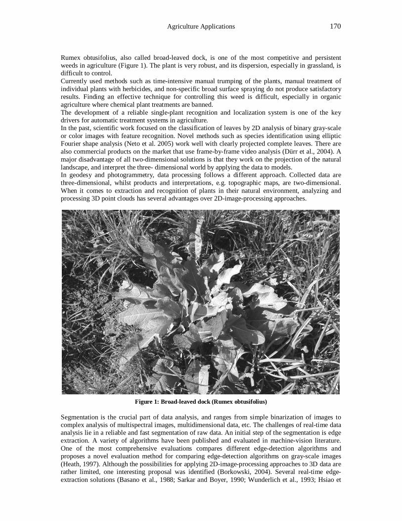
Agriculture Applications 170
Rumex obtusifolius, also called broad-leaved dock, is one of the most competitive and persistent weeds in agriculture (Figure 1). The plant is very robust, and its dispersion, especially in grassland, is difficult to control. Currently used methods such as time-intensive manual trumping of the plants, manual treatment of individual plants with herbicides, and non-specific broad surface spraying do not produce satisfactory results. Finding an effective technique for controlling this weed is difficult, especially in organic agriculture where chemical plant treatments are banned. The development of a reliable single-plant recognition and localization system is one of the key drivers for automatic treatment systems in agriculture. In the past, scientific work focused on the classification of leaves by 2D analysis of binary gray-scale or color images with feature recognition. Novel methods such as species identification using elliptic Fourier shape analysis (Neto et al. 2005) work well with clearly projected complete leaves. There are also commercial products on the market that use frame-by-frame video analysis (Dürr et al., 2004). A major disadvantage of all two-dimensional solutions is that they work on the projection of the natural landscape, and interpret the three- dimensional world by applying the data to models. In geodesy and photogrammetry, data processing follows a different approach. Collected data are three-dimensional, whilst products and interpretations, e.g. topographic maps, are two-dimensional. When it comes to extraction and recognition of plants in their natural environment, analyzing and processing 3D point clouds has several advantages over 2D-image-processing approaches.
Figure 1: Broad-leaved dock (Rumex obtusifolius)
Segmentation is the crucial part of data analysis, and ranges from simple binarization of images to complex analysis of multispectral images, multidimensional data, etc. The challenges of real-time data analysis lie in a reliable and fast segmentation of raw data. An initial step of the segmentation is edge extraction. A variety of algorithms have been published and evaluated in machine-vision literature. One of the most comprehensive evaluations compares different edge-detection algorithms and proposes a novel evaluation method for comparing edge-detection algorithms on gray-scale images (Heath, 1997). Although the possibilities for applying 2D-image-processing approaches to 3D data are rather limited, one interesting proposal was identified (Borkowski, 2004). Several real-time edge-extraction solutions (Basano et al., 1988; Sarkar and Boyer, 1990; Wunderlich et al., 1993; Hsiao et
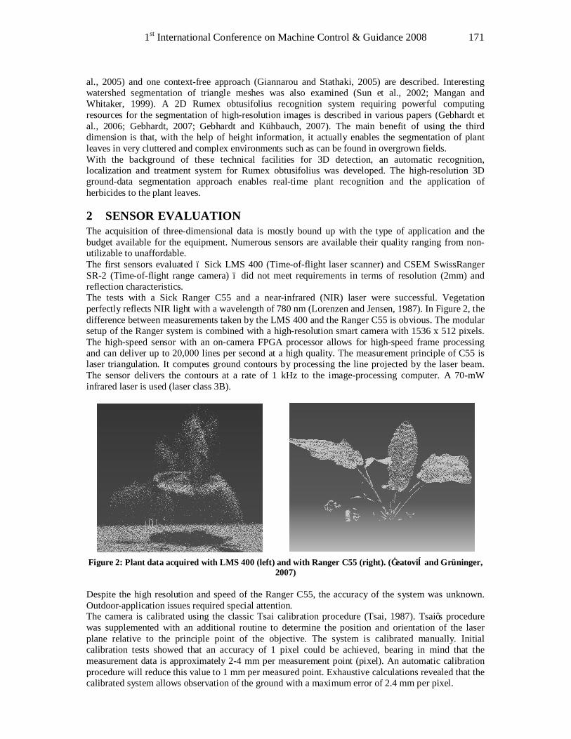
1st International Conference on Machine Control & Guidance 2008 171
al., 2005) and one context-free approach (Giannarou and Stathaki, 2005) are described. Interesting watershed segmentation of triangle meshes was also examined (Sun et al., 2002; Mangan and Whitaker, 1999). A 2D Rumex obtusifolius recognition system requiring powerful computing resources for the segmentation of high-resolution images is described in various papers (Gebhardt et al., 2006; Gebhardt, 2007; Gebhardt and Kühbauch, 2007). The main benefit of using the third dimension is that, with the help of height information, it actually enables the segmentation of plant leaves in very cluttered and complex environments such as can be found in overgrown fields. With the background of these technical facilities for 3D detection, an automatic recognition, localization and treatment system for Rumex obtusifolius was developed. The high-resolution 3D ground-data segmentation approach enables real-time plant recognition and the application of herbicides to the plant leaves.
2 SENSOR EVALUATION The acquisition of three-dimensional data is mostly bound up with the type of application and the budget available for the equipment. Numerous sensors are available their quality ranging from non-utilizable to unaffordable. The first sensors evaluated – Sick LMS 400 (Time-of-flight laser scanner) and CSEM SwissRanger SR-2 (Time-of-flight range camera) – did not meet requirements in terms of resolution (2mm) and reflection characteristics. The tests with a Sick Ranger C55 and a near-infrared (NIR) laser were successful. Vegetation perfectly reflects NIR light with a wavelength of 780 nm (Lorenzen and Jensen, 1987). In Figure 2, the difference between measurements taken by the LMS 400 and the Ranger C55 is obvious. The modular setup of the Ranger system is combined with a high-resolution smart camera with 1536 x 512 pixels. The high-speed sensor with an on-camera FPGA processor allows for high-speed frame processing and can deliver up to 20,000 lines per second at a high quality. The measurement principle of C55 is laser triangulation. It computes ground contours by processing the line projected by the laser beam. The sensor delivers the contours at a rate of 1 kHz to the image-processing computer. A 70-mW infrared laser is used (laser class 3B).
Figure 2: Plant data acquired with LMS 400 (left) and with Ranger C55 (right). (Šeatović and Grüninger,
2007) Despite the high resolution and speed of the Ranger C55, the accuracy of the system was unknown. Outdoor-application issues required special attention. The camera is calibrated using the classic Tsai calibration procedure (Tsai, 1987). Tsai’s procedure was supplemented with an additional routine to determine the position and orientation of the laser plane relative to the principle point of the objective. The system is calibrated manually. Initial calibration tests showed that an accuracy of 1 pixel could be achieved, bearing in mind that the measurement data is approximately 2-4 mm per measurement point (pixel). An automatic calibration procedure will reduce this value to 1 mm per measured point. Exhaustive calculations revealed that the calibrated system allows observation of the ground with a maximum error of 2.4 mm per pixel.
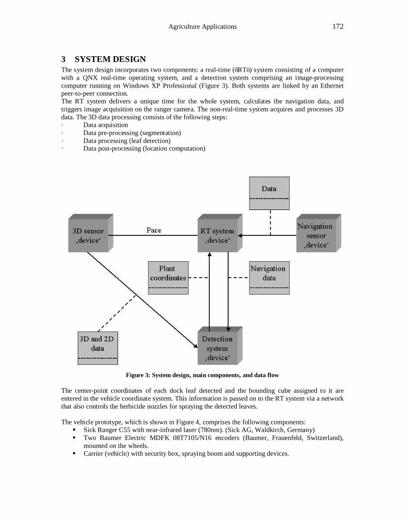
Agriculture Applications 172
3 SYSTEM DESIGN The system design incorporates two components: a real-time (“RT”) system consisting of a computer with a QNX real-time operating system, and a detection system comprising an image-processing computer running on Windows XP Professional (Figure 3). Both systems are linked by an Ethernet peer-to-peer connection. The RT system delivers a unique time for the whole system, calculates the navigation data, and triggers image acquisition on the ranger camera. The non-real-time system acquires and processes 3D data. The 3D data processing consists of the following steps: · Data acquisition · Data pre-processing (segmentation) · Data processing (leaf detection) · Data post-processing (location computation)
Figure 3: System design, main components, and data flow
The center-point coordinates of each dock leaf detected and the bounding cube assigned to it are entered in the vehicle coordinate system. This information is passed on to the RT system via a network that also controls the herbicide nozzles for spraying the detected leaves. The vehicle prototype, which is shown in Figure 4, comprises the following components: § Sick Ranger C55 with near-infrared laser (780nm). (Sick AG, Waldkirch, Germany) § Two Baumer Electric MDFK 08T7105/N16 encoders (Baumer, Frauenfeld, Switzerland),
mounted on the wheels. § Carrier (vehicle) with security box, spraying boom and supporting devices.

1st International Conference on Machine Control & Guidance 2008 173
Vehicle speed during recognition and treatment is 1 ms-1. Data collection is continuous, and the system extracts the plant leaves out of the collected data in real time. In a subsequent step, the coordinates of the leaves or leaf parts in question are computed and transferred to the treatment device that applies herbicide to the plants. The system has roughly 0.6 seconds to process 1 m2 of meadow. Some data facts are as follows: § On 1 m2 of meadow, the system measures 1536 x 1000 = 1 536 000 points. § Every measurement point has single-word (16-bit) precision. § High-res gray-scale row of C55 produces 3072 x 1000 = 3 072 000 8-bit pixels per 1 m2.
Figure 4: Left: Drawing of towed vehicle. Right: Test vehicle.
Thus, the processing unit must process 2.9 MBs-1 of 3D data and the same amount of gray-scale textures within one second. Under these conditions, fast and reliable segmentation algorithms – for raw data, ideally – are essential. A highly efficient segmentation procedure is therefore required.
4 OBJECT EXTRACTION Several plant-recognition and classification approaches have been published to date. The most recent and comprehensive of these is found in Gebhard, 2007. Nevertheless, vision systems, especially passive ones, can fail when environmental conditions change during the data-acquisition process. Failure can also result from insufficient contrast in a given input image, so that additional image-processing steps are necessary to extract the objects from the scene. Further recognition results depend strongly on the angle between the object and the optical axis of the camera. In extreme cases there is no way to distinguish between blades of grass and broad leaves. All these problems are partly resolved if the acquired data is three-dimensional. The other side of the coin is that the complexity of processing algorithms is is growing by increasing amounts of data. Although there is an additional dimension in 3D data, the algorithms are less complex than their 2D computer-vision counterparts. Edges exist in the data, and need not be derived from the shadows, texture or projection parameters (Šeatović, 2008). Edge detection is the first step in the segmentation procedure. An edge point can be described as a discontinuous place on the curve in the cutting plane π (Figure 5): the intersection of surfaces (red and blue) and plane p creates one intersection curve on each surface patch. Traveling along the curves from the beginning until the end, the ambiguous position will be hit at point P. The distance between these points and the direction of their connection vector determine whether or not there is an edge between these two surface patches.
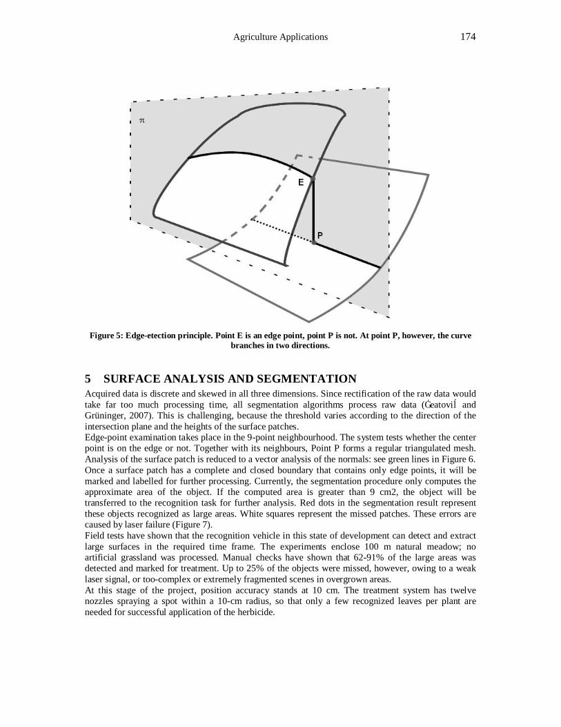
Agriculture Applications 174
Figure 5: Edge-etection principle. Point E is an edge point, point P is not. At point P, however, the curve
branches in two directions.
5 SURFACE ANALYSIS AND SEGMENTATION Acquired data is discrete and skewed in all three dimensions. Since rectification of the raw data would take far too much processing time, all segmentation algorithms process raw data (Šeatović and Grüninger, 2007). This is challenging, because the threshold varies according to the direction of the intersection plane and the heights of the surface patches. Edge-point examination takes place in the 9-point neighbourhood. The system tests whether the center point is on the edge or not. Together with its neighbours, Point P forms a regular triangulated mesh. Analysis of the surface patch is reduced to a vector analysis of the normals: see green lines in Figure 6. Once a surface patch has a complete and closed boundary that contains only edge points, it will be marked and labelled for further processing. Currently, the segmentation procedure only computes the approximate area of the object. If the computed area is greater than 9 cm2, the object will be transferred to the recognition task for further analysis. Red dots in the segmentation result represent these objects recognized as large areas. White squares represent the missed patches. These errors are caused by laser failure (Figure 7). Field tests have shown that the recognition vehicle in this state of development can detect and extract large surfaces in the required time frame. The experiments enclose 100 m natural meadow; no artificial grassland was processed. Manual checks have shown that 62-91% of the large areas was detected and marked for treatment. Up to 25% of the objects were missed, however, owing to a weak laser signal, or too-complex or extremely fragmented scenes in overgrown areas. At this stage of the project, position accuracy stands at 10 cm. The treatment system has twelve nozzles spraying a spot within a 10-cm radius, so that only a few recognized leaves per plant are needed for successful application of the herbicide.
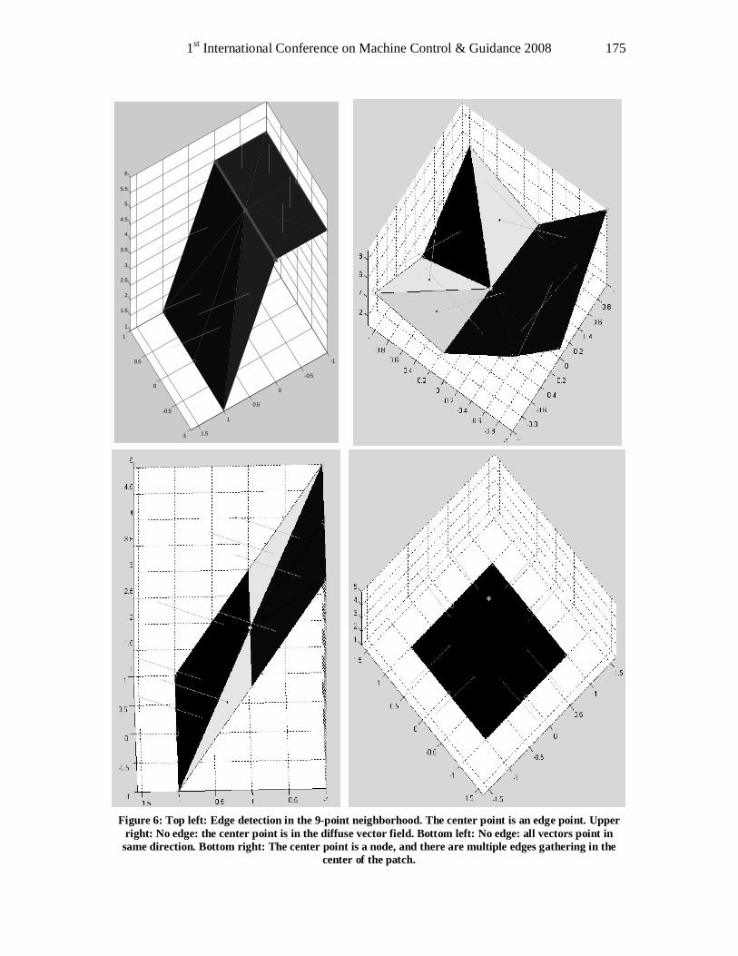
1st International Conference on Machine Control & Guidance 2008 175
-1
-0.5
0
0.5
1
-1
-0.5
0
0.5
1
1.5
1
1.5
2
2.5
3
3.5
4
4.5
5
5.5
6
Figure 6: Top left: Edge detection in the 9-point neighborhood. The center point is an edge point. Upper
right: No edge: the center point is in the diffuse vector field. Bottom left: No edge: all vectors point in same direction. Bottom right: The center point is a node, and there are multiple edges gathering in the
center of the patch.
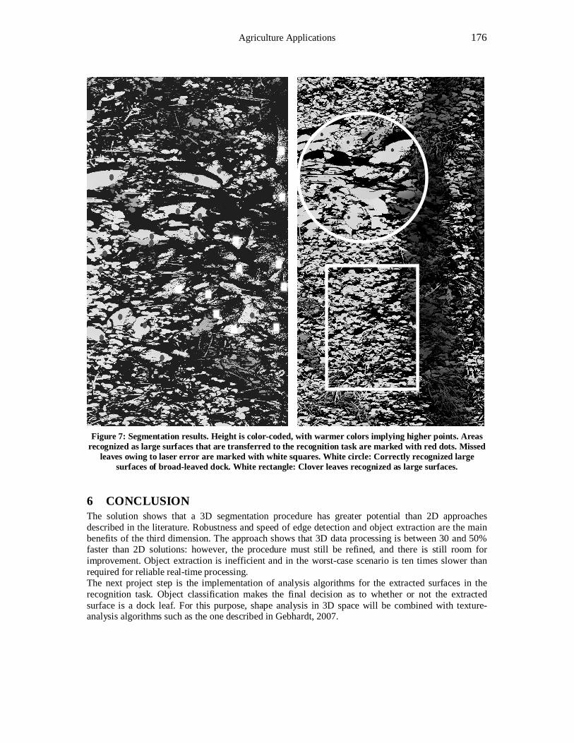
Agriculture Applications 176
Figure 7: Segmentation results. Height is color-coded, with warmer colors implying higher points. Areas
recognized as large surfaces that are transferred to the recognition task are marked with red dots. Missed leaves owing to laser error are marked with white squares. White circle: Correctly recognized large
surfaces of broad-leaved dock. White rectangle: Clover leaves recognized as large surfaces.
6 CONCLUSION The solution shows that a 3D segmentation procedure has greater potential than 2D approaches described in the literature. Robustness and speed of edge detection and object extraction are the main benefits of the third dimension. The approach shows that 3D data processing is between 30 and 50% faster than 2D solutions: however, the procedure must still be refined, and there is still room for improvement. Object extraction is inefficient and in the worst-case scenario is ten times slower than required for reliable real-time processing. The next project step is the implementation of analysis algorithms for the extracted surfaces in the recognition task. Object classification makes the final decision as to whether or not the extracted surface is a dock leaf. For this purpose, shape analysis in 3D space will be combined with texture-analysis algorithms such as the one described in Gebhardt, 2007.
1st International Conference on Machine Control & Guidance 2008 177
7 REFERENCES BASANO, L. et al.: Edge-detection schemes highly suitable for hardware implementation. J Opt Soc Am A 5(7), pp.1170-1175, 1988.
Borkowski, A.: Modellierung von Oberflächen mit Diskontinuitäten. PhD thesis, Fakultät für Forst-, Geo- und Hydrowissenschaften der Technischen Universität Dresden, Deutsche Geodätische Kommission, Marstallplatz 8, D-80539 Munich, 2004.
Dürr L. et al.: Machine vision detection and microwave based elimination of rumex obtusifolius L. on grassland. 5th European Conference on Precision Agriculture, Uppsala/Sweden. 5 pages, 2004.
Heath, M.D. et al.: A robust visual method for assessing the relative performance of edge-detection algorithms. In: IEEE Transactions. Number 12 in IEEE Transactions on Pattern Analysis and Machine Intelligence, IEEE, IEEE, pp. 1338-1359, 1997.
Hsiao, P.Y. et al.: An fpga architecture design of parameter-adaptive real-time image processing system for edge detection. In: Emerging Information Technology Conference, 3 pages, 2005.
Giannarou, S. and Stathaki, T.: Edge detection using quantitative combination of multiple operators. In: Signal Processing Systems Design and Implementation. IEEE Workshop, pp. 359-364, 2005.
Gebhardt, S. et al.: Identificat`ion of broad-leaved dock (rumex obtusifolius l.) on grassland by means of digital image processing. In: Precision Farming. Number 3 in Precision Agriculture, Institute of Crop Science and Resource Management - Crop Science and Plant Breeding, University of Bonn, Katzenburgweg 5, D-53115 Bonn. Springer Netherlands, pp. 165-178, 2006.
Gebhardt, S.: Automatic classification of grassland herbs in close-range sensed digital colour images. PhD thesis, Mathematisch-Naturwissenschaftliche Fakultät, University Bonn, 2007.
Gebhardt, S. and Kühbauch, W.: A new algorithm for automatic rumex obtusifolius detection in digital images using colour and texture features and the influence of image resolution. In: Precision Farming. Number 1-2 in Precision Agriculture, Institute of Crop Science and Resource Management - Crop Science and Plant Breeding, University of Bonn, Katzenburgweg 5, D-53115 Bonn, Springer Netherlands, pp. 1-13, 2007.
Lorenzen B. and Jensen A.,: Reflectance of blue, green, red and near infrared radiation from wetland vegetation used in a model discriminating live and dead above ground biomass, New Phytol, 1987.
Mangan, A.P. and Whitaker, R.T.: Partitioning 3d surface meshes using watershed segmentation. In: IEEE Transactions. Number 4 in IEEE Transactions on Visualization and Computer Graphics, IEEE, pp. 308-322, 1999.
Neto, J. C. et al.: Plant species identification using Elliptic Fourier leaf shape analysis. Elsevier, Computers and electronics in agriculture, no. 2, 121-134, 2006
Sarkar, S. and Boyer, K.: Optimal, efficient, recursive edge detection filters. In: Pattern Recognition. Proceedings, 10th International Conference on Pattern Recognition. Volume 1, pp. 931-936, 1990.
Šeatović, D. and Grüninger, R.: Smartweeder: Novel approach in 3d object recognition, localization and treatment of broad dock in its natural environment. In: RAAD 2007: Programme and Book of Abstracts, 2007.
Šeatović, D.: A Segmentation Approach in Novel Real Time 3D Plant Recognition System. In print: Proceedings of the 6th International Conference on Computer Vision Systems ICVS, Santorini, 2008.

Agriculture Applications 178
Sun, Y. et al.: Triangle mesh-based edge detection and its application to surface segmentation and adaptive surface smoothing. In: Image Processing. 2002. Proceedings. International Conference on.Image Processing, Volume 3, pp. 825-828, 2002.
Tsai, R.: A versatile camera calibration technique for high-accuracy 3d machine vision metrology using off-the-shelf tv cameras and lenses. In: IEEE Proceedings. Number 4 in Robotics and Automation, IEEE Journal of [legacy, pre - 1988], IBM T. J. Watson Research Center, Yorktown Heights, NY, USA, IEEE, IEEE, pp. 323-344, 1987.
Wunderlich, W. et al.: Optimizing edge detection in quantitative coronary arteriography: problems and proposals. In: Computers in Cardiology 1993. Proceedings, pp. 583-586, 1993.
* Dejan Šeatović, Institute of Mechatronic Systems IMS, Zurich University of Applied Sciences ZHAW, CH-8401 Winterthur, Switzerland

3D-Construction Applications II


1st International Conference on Machine Control & Guidance 2008 181
Trimble offers the Connected Construction Site
Connecting Office, People and Machines: The New Way to Increase Productivity on Earthmoving and Road Construction
Sites
Norbert MATTIVI*
Trimble [email protected]
Abstract Few will argue that construction is an industry of close tolerances, where precision and accuracy can make or break a contractor’s bottom line. At the same time, the pressures of a compressed schedule and tighter budget means jobs must be completed faster and cheaper, while improving profitability. To ensure a smooth completion, all parts of a job need to be integrated – from design to project completion to confirmation. To achieve this, contractors are increasingly relying on cutting-edge technology at each phase of the construction process. Trimble offers a broad range of solutions including conventional and 3D grade control systems, site positioning systems as well as construction fleet and equipment management solutions. As part of the Trimble Connected Site strategy, these solutions provide a high-level of process and workflow integration from the design phase through to the finished project—delivering significant improvements in productivity throughout the construction lifecycle. Grade control solutions extend from basic systems that rely on string lines and lasers to highly precise three-dimensional solutions. Most of the systems are added to construction equipment as an after-market add-on, although some manufacturers, like Caterpillar, are now offering integrated systems at the time of manufacture. Keywords Total Stations, GNSS, Connected Construction Site, Trimble Machine Control
1 LASER-BASED DISPLAY SYSTEMS There are three major categories of systems available. The first are laser-based display systems. These are generally easy-to-use modular systems that are flexible and configured to the machine and site requirements. Used for machine guidance, these laser-based systems are found in a range of earthmoving applications on machines, that include dozers, backhoes, scrapers, skid steers and excavators.
Figure 1: Skid Steer with Laser Receiver
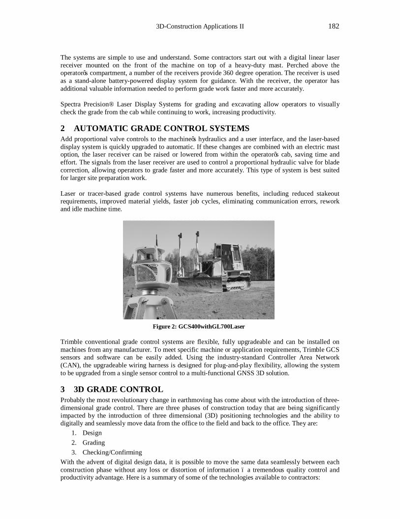
3D-Construction Applications II 182
The systems are simple to use and understand. Some contractors start out with a digital linear laser receiver mounted on the front of the machine on top of a heavy-duty mast. Perched above the operator’s compartment, a number of the receivers provide 360 degree operation. The receiver is used as a stand-alone battery-powered display system for guidance. With the receiver, the operator has additional valuable information needed to perform grade work faster and more accurately. Spectra Precision® Laser Display Systems for grading and excavating allow operators to visually check the grade from the cab while continuing to work, increasing productivity.
2 AUTOMATIC GRADE CONTROL SYSTEMS Add proportional valve controls to the machine’s hydraulics and a user interface, and the laser-based display system is quickly upgraded to automatic. If these changes are combined with an electric mast option, the laser receiver can be raised or lowered from within the operator’s cab, saving time and effort. The signals from the laser receiver are used to control a proportional hydraulic valve for blade correction, allowing operators to grade faster and more accurately. This type of system is best suited for larger site preparation work. Laser or tracer-based grade control systems have numerous benefits, including reduced stakeout requirements, improved material yields, faster job cycles, eliminating communication errors, rework and idle machine time.
Figure 2: GCS400withGL700Laser
Trimble conventional grade control systems are flexible, fully upgradeable and can be installed on machines from any manufacturer. To meet specific machine or application requirements, Trimble GCS sensors and software can be easily added. Using the industry-standard Controller Area Network (CAN), the upgradeable wiring harness is designed for plug-and-play flexibility, allowing the system to be upgraded from a single sensor control to a multi-functional GNSS 3D solution.
3 3D GRADE CONTROL Probably the most revolutionary change in earthmoving has come about with the introduction of three-dimensional grade control. There are three phases of construction today that are being significantly impacted by the introduction of three dimensional (3D) positioning technologies and the ability to digitally and seamlessly move data from the office to the field and back to the office. They are:
1. Design 2. Grading 3. Checking/Confirming
With the advent of digital design data, it is possible to move the same data seamlessly between each construction phase without any loss or distortion of information – a tremendous quality control and productivity advantage. Here is a summary of some of the technologies available to contractors:

1st International Conference on Machine Control & Guidance 2008 183
3.1 Design phase: survey data converted to a plan Before an earthmoving machine cuts the surface, there is considerable planning, surveying and design for creating the site design and project plan. Civil engineers and designers work with a wide range of powerful design and CAD packages, such as the Autodesk Land Desktop, Inroads, Geopak, MOSS, the Trimble Terramodel ® software or Trimble Business Center. Technological advances have shifted the design emphasis from the preparation of data for printed plans to the development of a 3D surface model. It is now possible to build a surface model of the entire project and interrogate it in multiple ways prior to grading, heading off potential design problems. As a result, any point observed in the field can be instantly compared to the surface model and grade can be established. Additionally, surface files can be transferred to automatic machine control systems, thereby reducing or even eliminating the need for construction staking. Today we are seeing an ever increasing use of digital data and the digital transfer of data to connect the design engineer, surveyor, and contractor into an integrated work flow. Gone are the days when it was acceptable that the only deliverable is a sheaf of paper plans. Instead, the same digital information created for the site design and project plan can be used for machine control to ensure accurate grading – and for site positioning during and after project completion.
Figure 3: Design
Trimble offers a suite of office software products that provide a wide range of capabilities facilitating job functions from planning and bidding to complete project productivity analysis which are designed to work together. Data changes made in the office or by a field crew are automatically recognized and used to populate the project data base and are routed to all other crews that need the data. Trimble Intelligent Data Tracking means that everyone has the latest and most up to date information at all times, reducing the possibility of making mistakes caused by having out of date models.
Here’s how it works: Design engineering and CAD software today typically allows the ability to import the original survey data. A 3D site design is generated. Once completed the design data is exported to a format suitable for loading onto the machine grade control system and onto the site controller system. Seamless data flow is critical from the design to construction stakeout or design to machine control without the need for additional data exchange or information reformatting which significantly reduces the potential for error and speeds the process.
3.2 Grading: turning the plan into reality During the construction phase, the earthworks contractor begins the process of converting the designer’s electronic designs into reality on the site. On the integrated construction site, design data is available to the machine operator and supervisors right at the site, in the cab of the machine or their vehicle. With the advent of 3D automatic grade control systems, contractors literally can put cutting-edge technology on their cutting edge – the blade of their earthmoving machine. This technology uses either the Global Navigation Satellite System (GNSS) or a robotic total station to control the actual position,
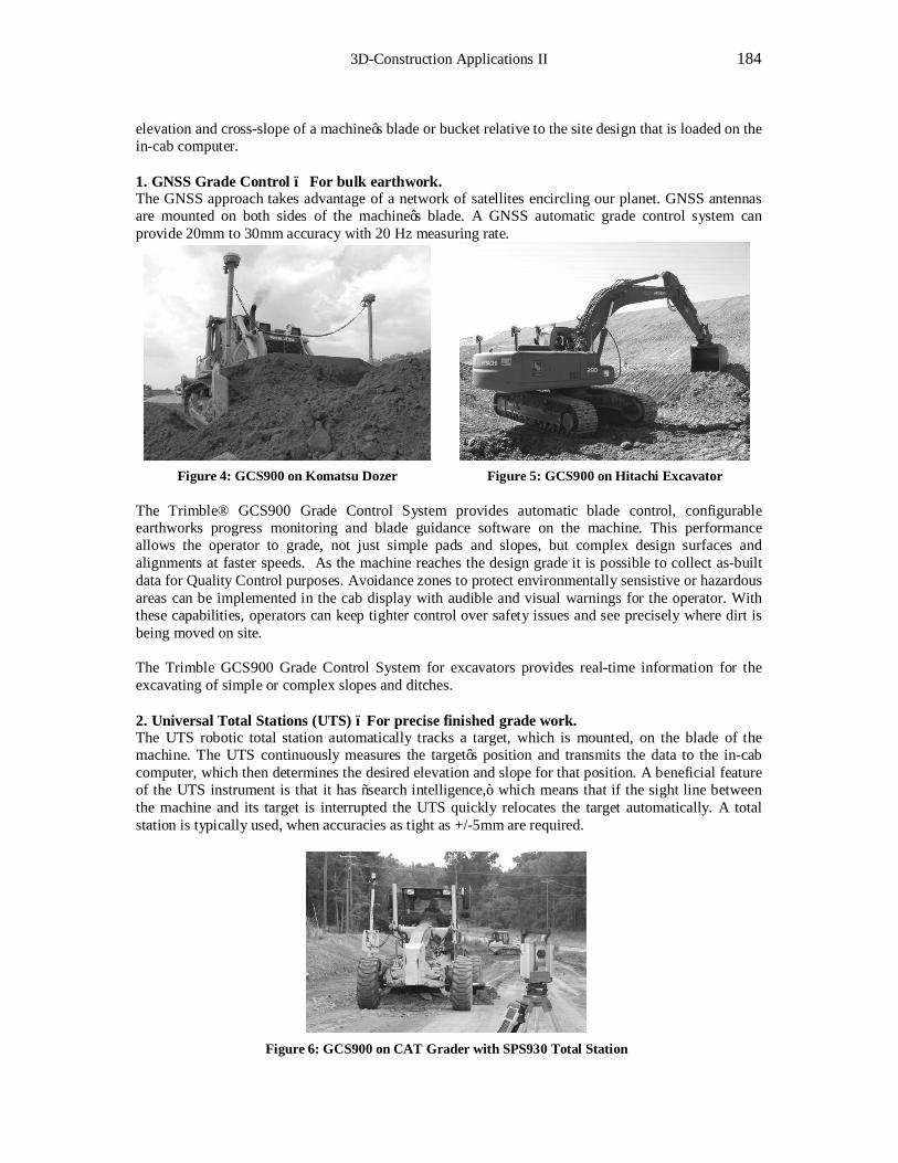
3D-Construction Applications II 184
elevation and cross-slope of a machine’s blade or bucket relative to the site design that is loaded on the in-cab computer. 1. GNSS Grade Control – For bulk earthwork. The GNSS approach takes advantage of a network of satellites encircling our planet. GNSS antennas are mounted on both sides of the machine’s blade. A GNSS automatic grade control system can provide 20mm to 30mm accuracy with 20 Hz measuring rate.
Figure 4: GCS900 on Komatsu Dozer Figure 5: GCS900 on Hitachi Excavator
The Trimble® GCS900 Grade Control System provides automatic blade control, configurable earthworks progress monitoring and blade guidance software on the machine. This performance allows the operator to grade, not just simple pads and slopes, but complex design surfaces and alignments at faster speeds. As the machine reaches the design grade it is possible to collect as-built data for Quality Control purposes. Avoidance zones to protect environmentally sensistive or hazardous areas can be implemented in the cab display with audible and visual warnings for the operator. With these capabilities, operators can keep tighter control over safety issues and see precisely where dirt is being moved on site. The Trimble GCS900 Grade Control System for excavators provides real-time information for the excavating of simple or complex slopes and ditches. 2. Universal Total Stations (UTS) – For precise finished grade work. The UTS robotic total station automatically tracks a target, which is mounted, on the blade of the machine. The UTS continuously measures the target’s position and transmits the data to the in-cab computer, which then determines the desired elevation and slope for that position. A beneficial feature of the UTS instrument is that it has “search intelligence,” which means that if the sight line between the machine and its target is interrupted the UTS quickly relocates the target automatically. A total station is typically used, when accuracies as tight as +/-5mm are required.
Figure 6: GCS900 on CAT Grader with SPS930 Total Station
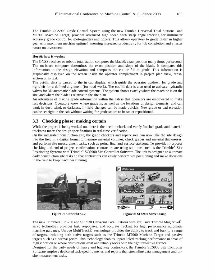
1st International Conference on Machine Control & Guidance 2008 185
The Trimble GCS900 Grade Control System using the new Trimble Universal Total Stations and MT900 Machine Target, provides advanced high speed with steep angle tracking for millimeter accuracy grade control for motorgraders and dozers. This allows operators to grade faster in higher gear with maximum machine uptime – meaning increased productivity for job completion and a faster return on investment.
Here’s how it works: The GNSS receiver or robotic total station computes the blade’s exact position many times per second. The on-board computer determines the exact position and slope of the blade. It compares this information to the design elevation and computes the cut or fill to grade. This information is graphically displayed on the screen inside the operator compartment in project plan view, cross-section or as text. The cut/fill data is passed to the in cab display, which guide the operator up/down for grade and right/left for a defined alignment (for road work). The cut/fill data is also used to activate hydraulic valves for 3D automatic blade control systems. The system shows exactly where the machine is on the site, and where the blade is relative to the site plan. An advantage of placing grade information within the cab is that operators are empowered to make fast decisions. Operators know where grade is, as well as the locations of design elements, and can work in dust, wind, or darkness. In-field changes can be made quickly. New grade or pad elevation can be set right in the cab without waiting for grade stakes to be set or repositioned.
3.3 Checking phase: making certain While the project is being worked on, there is the need to check and verify finished grade and material thickness meets the design specifications in real-time verification. On the integrated construction site, the grade checkers and supervisors can now take the site design into the field in a digital format to measure material volumes, check grades and material thicknesses, and perform site measurement tasks, such as point, line, and surface stakeout. To provide in-process checking and end of project confirmation, contractors are using solutions such as the Trimble® Site Positioning Systems with Trimble® SCS900 Site Controller Software. The unit is designed to automate daily construction site tasks so that contractors can easily perform site positioning and make decisions in the field to keep machines running.
Figure 7: SPSwithTSC2 Figure 8: SCS900 Screen Snap
The new Trimble® SPS730 and SPS930 Universal Total Stations with exclusive Trimble MagDrive™ servo technology provides fast, responsive, and accurate tracking for high performance automatic machine guidance. Unique MultiTrack™ technology provides the ability to track and lock to a range of targets, including both active targets such as the Trimble MT900 Machine Target and passive targets such as a normal prism. This technology enables unparalleled tracking performance in areas of high vibration or where obstructions exist and reliably locks onto the right reflective surface. Designed for the daily needs of heavy and highway contractors, the Trimble SCS900 Site Controller Software employs dedicated task-specific menus and reports that streamline data management and on-site measurement tasks.
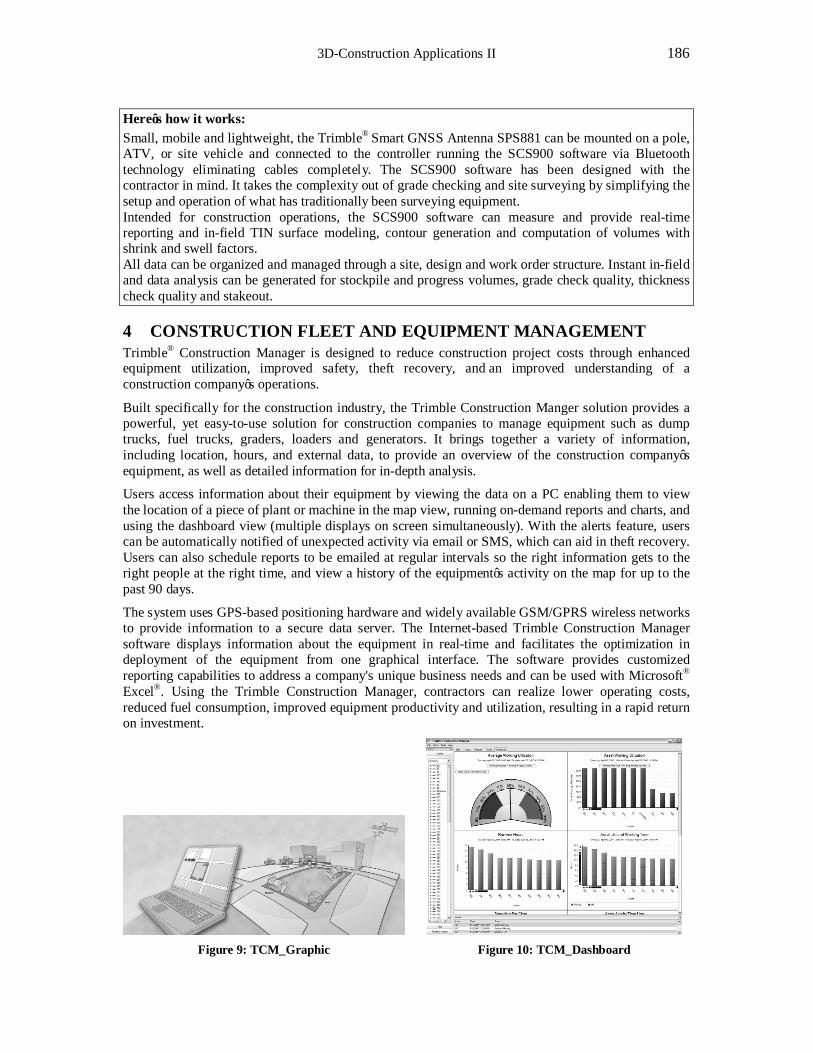
3D-Construction Applications II 186
Here’s how it works: Small, mobile and lightweight, the Trimble® Smart GNSS Antenna SPS881 can be mounted on a pole, ATV, or site vehicle and connected to the controller running the SCS900 software via Bluetooth technology eliminating cables completely. The SCS900 software has been designed with the contractor in mind. It takes the complexity out of grade checking and site surveying by simplifying the setup and operation of what has traditionally been surveying equipment. Intended for construction operations, the SCS900 software can measure and provide real-time reporting and in-field TIN surface modeling, contour generation and computation of volumes with shrink and swell factors. All data can be organized and managed through a site, design and work order structure. Instant in-field and data analysis can be generated for stockpile and progress volumes, grade check quality, thickness check quality and stakeout.
4 CONSTRUCTION FLEET AND EQUIPMENT MANAGEMENT Trimble® Construction Manager is designed to reduce construction project costs through enhanced equipment utilization, improved safety, theft recovery, and an improved understanding of a construction company’s operations.
Built specifically for the construction industry, the Trimble Construction Manger solution provides a powerful, yet easy-to-use solution for construction companies to manage equipment such as dump trucks, fuel trucks, graders, loaders and generators. It brings together a variety of information, including location, hours, and external data, to provide an overview of the construction company’s equipment, as well as detailed information for in-depth analysis.
Users access information about their equipment by viewing the data on a PC enabling them to view the location of a piece of plant or machine in the map view, running on-demand reports and charts, and using the dashboard view (multiple displays on screen simultaneously). With the alerts feature, users can be automatically notified of unexpected activity via email or SMS, which can aid in theft recovery. Users can also schedule reports to be emailed at regular intervals so the right information gets to the right people at the right time, and view a history of the equipment’s activity on the map for up to the past 90 days.
The system uses GPS-based positioning hardware and widely available GSM/GPRS wireless networks to provide information to a secure data server. The Internet-based Trimble Construction Manager software displays information about the equipment in real-time and facilitates the optimization in deployment of the equipment from one graphical interface. The software provides customized reporting capabilities to address a company's unique business needs and can be used with Microsoft® Excel®. Using the Trimble Construction Manager, contractors can realize lower operating costs, reduced fuel consumption, improved equipment productivity and utilization, resulting in a rapid return on investment.
Figure 9: TCM_Graphic Figure 10: TCM_Dashboard
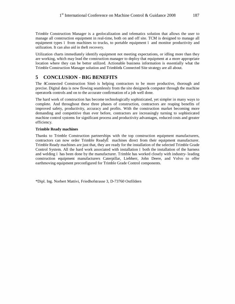
1st International Conference on Machine Control & Guidance 2008 187
Trimble Construction Manager is a geolocalization and telematics solution that allows the user to manage all construction equipment in real-time, both on and off site. TCM is designed to manage all equipment types – from machines to trucks, to portable equipment – and monitor productivity and utilization. It can also aid in theft recovery.
Utilization charts immediately identify equipment not meeting expectations, or idling more than they are working, which may lead the construction manager to deploy that equipment at a more appropriate location where they can be better utilized. Actionable business information is essentially what the Trimble Construction Manager solution and Trimble’s Connected Site strategy are all about.
5 CONCLUSION - BIG BENEFITS The “Connected Construction Site” is helping contractors to be more productive, thorough and precise. Digital data is now flowing seamlessly from the site designer’s computer through the machine operator’s controls and on to the accurate confirmation of a job well done.
The hard work of construction has become technologically sophisticated, yet simpler in many ways to complete. And throughout these three phases of construction, contractors are reaping benefits of improved safety, productivity, accuracy and profits. With the construction market becoming more demanding and competitive than ever before, contractors are increasingly turning to sophisticated machine control systems for significant process and productivity advantages, reduced costs and greater efficiency.
Trimble Ready machines Thanks to Trimble Construction partnerships with the top construction equipment manufacturers, contractors can now order Trimble Ready™ machines direct from their equipment manufacturer. Trimble Ready machines are just that, they are ready for the installation of the selected Trimble Grade Control System. All the hard work associated with installation – both the installation of the harness and welding – has been done by the manufacturer. Trimble has worked closely with industry- leading construction equipment manufacturers Caterpillar, Liebherr, John Deere, and Volvo to offer earthmoving equipment preconfigured for Trimble Grade Control components. *Dipl. Ing. Norbert Mattivi, Friedhofstrasse 3, D-73760 Ostfildern

3D-Construction Applications II 188
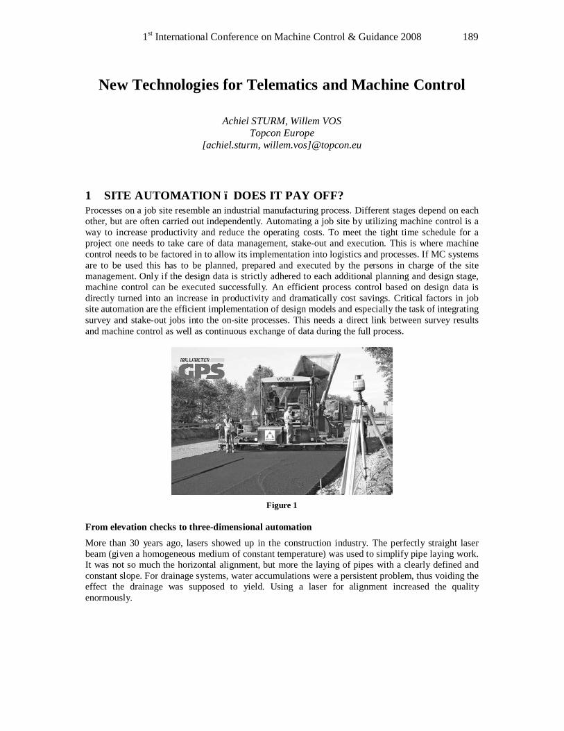
1st International Conference on Machine Control & Guidance 2008 189
New Technologies for Telematics and Machine Control
Achiel STURM, Willem VOS Topcon Europe
[achiel.sturm, willem.vos]@topcon.eu
1 SITE AUTOMATION – DOES IT PAY OFF? Processes on a job site resemble an industrial manufacturing process. Different stages depend on each other, but are often carried out independently. Automating a job site by utilizing machine control is a way to increase productivity and reduce the operating costs. To meet the tight time schedule for a project one needs to take care of data management, stake-out and execution. This is where machine control needs to be factored in to allow its implementation into logistics and processes. If MC systems are to be used this has to be planned, prepared and executed by the persons in charge of the site management. Only if the design data is strictly adhered to each additional planning and design stage, machine control can be executed successfully. An efficient process control based on design data is directly turned into an increase in productivity and dramatically cost savings. Critical factors in job site automation are the efficient implementation of design models and especially the task of integrating survey and stake-out jobs into the on-site processes. This needs a direct link between survey results and machine control as well as continuous exchange of data during the full process.
Figure 1 From elevation checks to three-dimensional automation
More than 30 years ago, lasers showed up in the construction industry. The perfectly straight laser beam (given a homogeneous medium of constant temperature) was used to simplify pipe laying work. It was not so much the horizontal alignment, but more the laying of pipes with a clearly defined and constant slope. For drainage systems, water accumulations were a persistent problem, thus voiding the effect the drainage was supposed to yield. Using a laser for alignment increased the quality enormously.
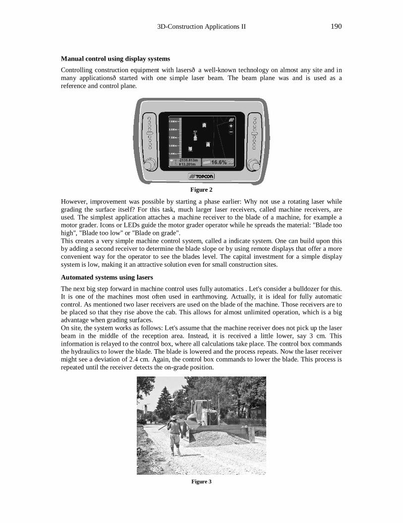
3D-Construction Applications II 190
Manual control using display systems Controlling construction equipment with lasers—a well-known technology on almost any site and in many applications—started with one simple laser beam. The beam plane was and is used as a reference and control plane.
Figure 2
However, improvement was possible by starting a phase earlier: Why not use a rotating laser while grading the surface itself? For this task, much larger laser receivers, called machine receivers, are used. The simplest application attaches a machine receiver to the blade of a machine, for example a motor grader. Icons or LEDs guide the motor grader operator while he spreads the material: "Blade too high", "Blade too low" or "Blade on grade". This creates a very simple machine control system, called a indicate system. One can build upon this by adding a second receiver to determine the blade slope or by using remote displays that offer a more convenient way for the operator to see the blades level. The capital investment for a simple display system is low, making it an attractive solution even for small construction sites.
Automated systems using lasers
The next big step forward in machine control uses fully automatics . Let's consider a bulldozer for this. It is one of the machines most often used in earthmoving. Actually, it is ideal for fully automatic control. As mentioned two laser receivers are used on the blade of the machine. Those receivers are to be placed so that they rise above the cab. This allows for almost unlimited operation, which is a big advantage when grading surfaces. On site, the system works as follows: Let's assume that the machine receiver does not pick up the laser beam in the middle of the reception area. Instead, it is received a little lower, say 3 cm. This information is relayed to the control box, where all calculations take place. The control box commands the hydraulics to lower the blade. The blade is lowered and the process repeats. Now the laser receiver might see a deviation of 2.4 cm. Again, the control box commands to lower the blade. This process is repeated until the receiver detects the on-grade position.
Figure 3
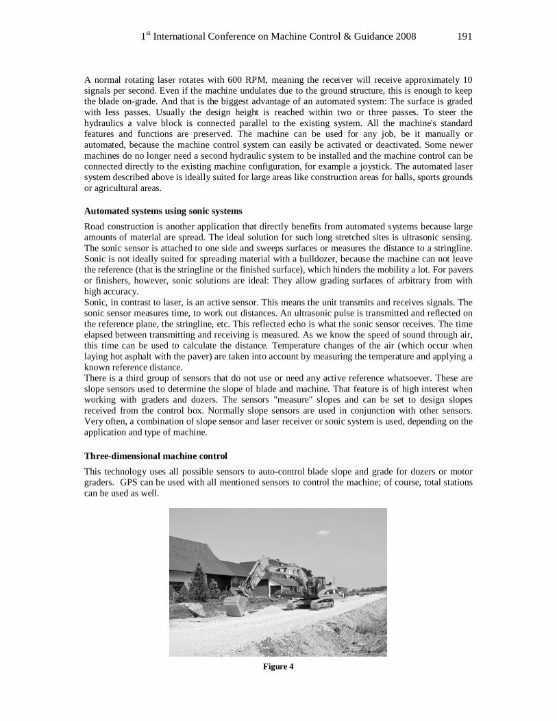
1st International Conference on Machine Control & Guidance 2008 191
A normal rotating laser rotates with 600 RPM, meaning the receiver will receive approximately 10 signals per second. Even if the machine undulates due to the ground structure, this is enough to keep the blade on-grade. And that is the biggest advantage of an automated system: The surface is graded with less passes. Usually the design height is reached within two or three passes. To steer the hydraulics a valve block is connected parallel to the existing system. All the machine's standard features and functions are preserved. The machine can be used for any job, be it manually or automated, because the machine control system can easily be activated or deactivated. Some newer machines do no longer need a second hydraulic system to be installed and the machine control can be connected directly to the existing machine configuration, for example a joystick. The automated laser system described above is ideally suited for large areas like construction areas for halls, sports grounds or agricultural areas. Automated systems using sonic systems Road construction is another application that directly benefits from automated systems because large amounts of material are spread. The ideal solution for such long stretched sites is ultrasonic sensing. The sonic sensor is attached to one side and sweeps surfaces or measures the distance to a stringline. Sonic is not ideally suited for spreading material with a bulldozer, because the machine can not leave the reference (that is the stringline or the finished surface), which hinders the mobility a lot. For pavers or finishers, however, sonic solutions are ideal: They allow grading surfaces of arbitrary from with high accuracy. Sonic, in contrast to laser, is an active sensor. This means the unit transmits and receives signals. The sonic sensor measures time, to work out distances. An ultrasonic pulse is transmitted and reflected on the reference plane, the stringline, etc. This reflected echo is what the sonic sensor receives. The time elapsed between transmitting and receiving is measured. As we know the speed of sound through air, this time can be used to calculate the distance. Temperature changes of the air (which occur when laying hot asphalt with the paver) are taken into account by measuring the temperature and applying a known reference distance. There is a third group of sensors that do not use or need any active reference whatsoever. These are slope sensors used to determine the slope of blade and machine. That feature is of high interest when working with graders and dozers. The sensors "measure" slopes and can be set to design slopes received from the control box. Normally slope sensors are used in conjunction with other sensors. Very often, a combination of slope sensor and laser receiver or sonic system is used, depending on the application and type of machine. Three-dimensional machine control This technology uses all possible sensors to auto-control blade slope and grade for dozers or motor graders. GPS can be used with all mentioned sensors to control the machine; of course, total stations can be used as well.
Figure 4
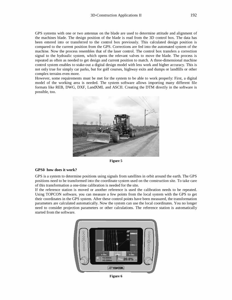
3D-Construction Applications II 192
GPS systems with one or two antennas on the blade are used to determine attitude and alignment of the machines blade. The design position of the blade is read from the 3D control box. The data has been entered into or transferred to the control box previously. This calculated design position is compared to the current position from the GPS. Corrections are fed into the automated system of the machine. Now the process resembles that of the laser control. The control box transfers a correction signal to the hydraulic system, which opens the relevant valves to move the blade. The process is repeated as often as needed to get design and current position to match. A three-dimensional machine control system enables to stake-out a digital design model with less work and higher accuracy. This is not only true for simply car parks, but for golf courses, highway exits and dumps or landfills or other complex terrains even more. However, some requirements must be met for the system to be able to work properly: First, a digital model of the working area is needed. The system software allows importing many different file formats like REB, DWG, DXF, LandXML and ASCII. Creating the DTM directly in the software is possible, too.
Figure 5
GPS—how does it work? GPS is a system to determine positions using signals from satellites in orbit around the earth. The GPS positions need to be transformed into the coordinate system used on the construction site. To take care of this transformation a one-time calibration is needed for the site. If the reference station is moved or another reference is used the calibration needs to be repeated. Using TOPCON software, you can measure a few points from the local system with the GPS to get their coordinates in the GPS system. After these control points have been measured, the transformation parameters are calculated automatically. Now the system can use the local coordinates. You no longer need to consider projection parameters or other calculations. The reference station is automatically started from the software.
Figure 6

1st International Conference on Machine Control & Guidance 2008 193
Site automation benefits Topcon offers comprehensive solutions to measure position and elevations for an optimized control of the complete production process on the construction site.
Topcon offers sophisticated and up-to-date solutions for any optical measuring devices, rotating lasers, machine control systems and GNSS survey products.
Topcon delivers modular solutions providing safety and efficiency. Without any interfacing hassle Topcon's automated machine control systems integrate survey and stake-out data, tailored to your requirements.
Cost reduction: Reduction of machinery time (hours, diesel, blade wear) Optimized use of materials by most accurate automatic control Reduction of stake-out cost (material, work time)
Increase in productivity: Up to four times faster execution of work Uninterrupted and continuous production Optimized use of materials – no remodeling
Increase in quality: Permanently utmost accuracy Constant quality during the whole process Elimination of miscellaneous sources of error
2 NEW TECHNOLOGIES FOR TELEMATICS AND MACHINE CONTROL
2.1 SiteLINK – a new communication and management system SiteLINK is a communication system that combines performance data for machines and construction activities, fleet management, theft prevention and reporting in a single application. It is a complete IT solution for global information management on construction site data.
Figure 7
The SiteLINK system supports different wireless communication options and processes data from the following areas: performance reports, data transfer, reporting and fleet management. One solution for all types and makes of construction equipment, regardless of manufacturer, age or technological issues. SiteLINK was developed by TOPCON and TSD, a joint-venture of TOPCON and Sauer Danfoss, the world's largest supplier of electro-hydraulic systems. Communication system
The new technology utilizes mesh radio networks in a standard WiFi environment. The communication system can track machines from all manufacturers on the site using GPS. By setting up no-go areas (geo-fencing), it can be used for theft prevention as well. SiteLINK is powered by a 5200 B micro processor, supports USB plus CAN, RS-232, and Ethernet. A simplified version, ADL-
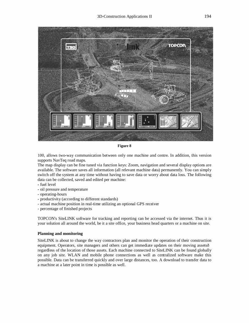
3D-Construction Applications II 194
Figure 8 100, allows two-way communication between only one machine and centre. In addition, this version supports NavTeq road maps. The map display can be fine tuned via function keys: Zoom, navigation and several display options are available. The software saves all information (all relevant machine data) permanently. You can simply switch off the system at any time without having to save data or worry about data loss. The following data can be collected, saved and edited per machine: - fuel level - oil pressure and temperature - operating-hours - productivity (according to different standards) - actual machine position in real-time utilizing an optional GPS receiver - percentage of finished projects TOPCON's SiteLINK software for tracking and reporting can be accessed via the internet. Thus it is your solution all around the world, be it a site office, your business head quarters or a machine on site. Planning and monitoring SiteLINK is about to change the way contractors plan and monitor the operation of their construction equipment. Operators, site managers and others can get immediate updates on their moving assets—regardless of the location of those assets. Each machine connected to SiteLINK can be found globally on any job site. WLAN and mobile phone connections as well as centralized software make this possible. Data can be transferred quickly and over large distances, too. A download to transfer data to a machine at a later point in time is possible as well.
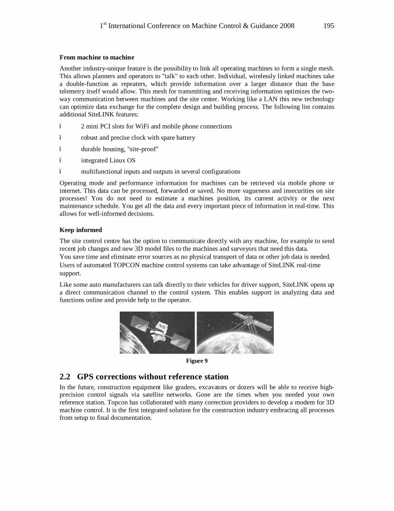
1st International Conference on Machine Control & Guidance 2008 195
From machine to machine Another industry-unique feature is the possibility to link all operating machines to form a single mesh. This allows planners and operators to "talk" to each other. Individual, wirelessly linked machines take a double-function as repeaters, which provide information over a larger distance than the base telemetry itself would allow. This mesh for transmitting and receiving information optimizes the two-way communication between machines and the site center. Working like a LAN this new technology can optimize data exchange for the complete design and building process. The following list contains additional SiteLINK features:
– 2 mini PCI slots for WiFi and mobile phone connections
– robust and precise clock with spare battery
– durable housing, "site-proof"
– integrated Linux OS
– multifunctional inputs and outputs in several configurations
Operating mode and performance information for machines can be retrieved via mobile phone or internet. This data can be processed, forwarded or saved. No more vagueness and insecurities on site processes! You do not need to estimate a machines position, its current activity or the next maintenance schedule. You get all the data and every important piece of information in real-time. This allows for well-informed decisions. Keep informed The site control centre has the option to communicate directly with any machine, for example to send recent job changes and new 3D model files to the machines and surveyors that need this data. You save time and eliminate error sources as no physical transport of data or other job data is needed. Users of automated TOPCON machine control systems can take advantage of SiteLINK real-time support.
Like some auto manufacturers can talk directly to their vehicles for driver support, SiteLINK opens up a direct communication channel to the control system. This enables support in analyzing data and functions online and provide help to the operator.
Figure 9
2.2 GPS corrections without reference station In the future, construction equipment like graders, excavators or dozers will be able to receive high-precision control signals via satellite networks. Gone are the times when you needed your own reference station. Topcon has collaborated with many correction providers to develop a modem for 3D machine control. It is the first integrated solution for the construction industry embracing all processes from setup to final documentation.
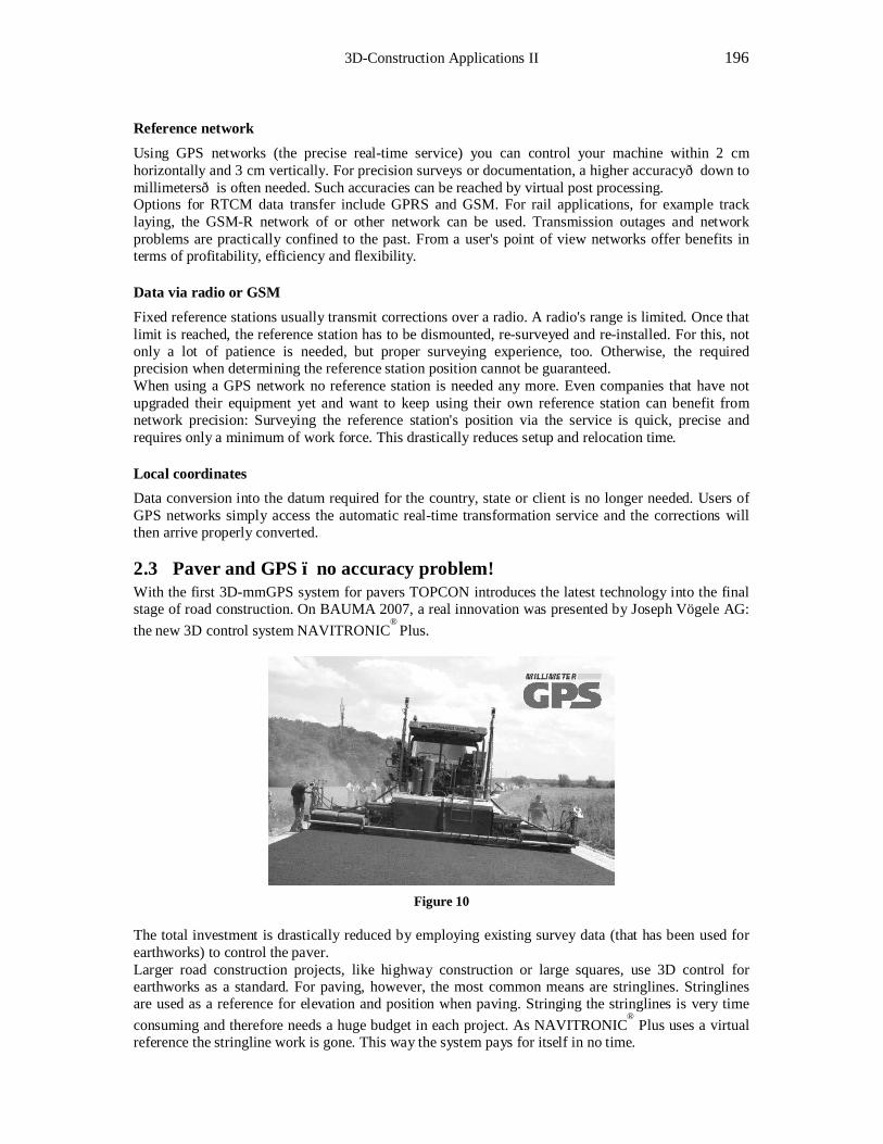
3D-Construction Applications II 196
Reference network Using GPS networks (the precise real-time service) you can control your machine within 2 cm horizontally and 3 cm vertically. For precision surveys or documentation, a higher accuracy—down to millimeters—is often needed. Such accuracies can be reached by virtual post processing. Options for RTCM data transfer include GPRS and GSM. For rail applications, for example track laying, the GSM-R network of or other network can be used. Transmission outages and network problems are practically confined to the past. From a user's point of view networks offer benefits in terms of profitability, efficiency and flexibility. Data via radio or GSM Fixed reference stations usually transmit corrections over a radio. A radio's range is limited. Once that limit is reached, the reference station has to be dismounted, re-surveyed and re-installed. For this, not only a lot of patience is needed, but proper surveying experience, too. Otherwise, the required precision when determining the reference station position cannot be guaranteed. When using a GPS network no reference station is needed any more. Even companies that have not upgraded their equipment yet and want to keep using their own reference station can benefit from network precision: Surveying the reference station's position via the service is quick, precise and requires only a minimum of work force. This drastically reduces setup and relocation time. Local coordinates Data conversion into the datum required for the country, state or client is no longer needed. Users of GPS networks simply access the automatic real-time transformation service and the corrections will then arrive properly converted.
2.3 Paver and GPS – no accuracy problem! With the first 3D-mmGPS system for pavers TOPCON introduces the latest technology into the final stage of road construction. On BAUMA 2007, a real innovation was presented by Joseph Vögele AG: the new 3D control system NAVITRONIC
® Plus.
Figure 10
The total investment is drastically reduced by employing existing survey data (that has been used for earthworks) to control the paver. Larger road construction projects, like highway construction or large squares, use 3D control for earthworks as a standard. For paving, however, the most common means are stringlines. Stringlines are used as a reference for elevation and position when paving. Stringing the stringlines is very time consuming and therefore needs a huge budget in each project. As NAVITRONIC
® Plus uses a virtual
reference the stringline work is gone. This way the system pays for itself in no time.
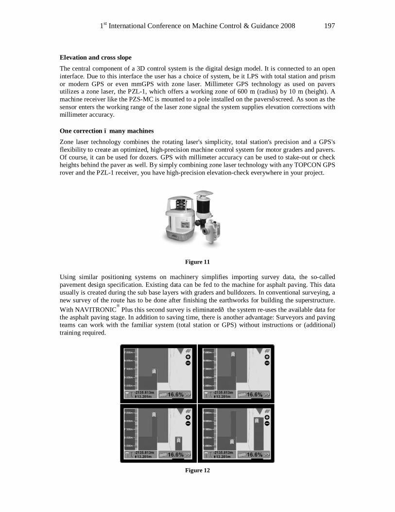
1st International Conference on Machine Control & Guidance 2008 197
Elevation and cross slope The central component of a 3D control system is the digital design model. It is connected to an open interface. Due to this interface the user has a choice of system, be it LPS with total station and prism or modern GPS or even mmGPS with zone laser. Millimeter GPS technology as used on pavers utilizes a zone laser, the PZL-1, which offers a working zone of 600 m (radius) by 10 m (height). A machine receiver like the PZS-MC is mounted to a pole installed on the pavers’ screed. As soon as the sensor enters the working range of the laser zone signal the system supplies elevation corrections with millimeter accuracy. One correction – many machines Zone laser technology combines the rotating laser's simplicity, total station's precision and a GPS's flexibility to create an optimized, high-precision machine control system for motor graders and pavers. Of course, it can be used for dozers. GPS with millimeter accuracy can be used to stake-out or check heights behind the paver as well. By simply combining zone laser technology with any TOPCON GPS rover and the PZL-1 receiver, you have high-precision elevation-check everywhere in your project.
Figure 11
Using similar positioning systems on machinery simplifies importing survey data, the so-called pavement design specification. Existing data can be fed to the machine for asphalt paving. This data usually is created during the sub base layers with graders and bulldozers. In conventional surveying, a new survey of the route has to be done after finishing the earthworks for building the superstructure. With NAVITRONIC
® Plus this second survey is eliminated—the system re-uses the available data for
the asphalt paving stage. In addition to saving time, there is another advantage: Surveyors and paving teams can work with the familiar system (total station or GPS) without instructions or (additional) training required.
Figure 12
3D-Construction Applications II 198
Automated control of direction
The new 3D control system steers the paver directly. This allows full automatic control along the alignment using the current mmGPS position. The 3D control box display shows the paver's position as well as any corrections to reach the design model.
Figure 13
For the best paving accuracy, the screed's extending parts are precisely controlled. Sensors on the extending parts determine the screed's actual width. The user has two options to setup the horizontal precision: The paving reference is set to either the extreme left or the extreme right end of the screed. This line is then used as the paving reference. Optionally, users can set a fixed paving width. This will be adhered to over the full length of the section. Even direction corrections of the paver the reference alignment can be easily compensated for by using precise control of the screed's extending parts. Of course, the width control for the screed can be used when steering the paver manually. This ensures perfect paving. Complete control of paving When using the system, the whole project is processed automatically. This is a crucial advantage if grade and slope are constantly changing. The system monitors the screed's grade, slope and position at all times and compares this data to the design data in the specification. Once the paver reaches a position where grade or slope need to be changed (for example in a bend), the screed is automatically adjusted to the new values. Using a combination of all measured data (paver position, paving direction, screed position and slope) NAVITRONIC
® Plus is capable of strictly controlling the paving process at any point of the planned
route. Combining mmGPS and NAVITRONIC
® Plus is your warranty for paving: no accuracy and
productivity problems.
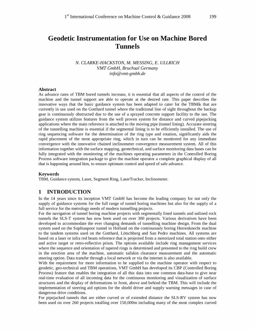
1st International Conference on Machine Control & Guidance 2008 199
Geodetic Instrumentation for Use on Machine Bored Tunnels
N. CLARKE-HACKSTON, M. MESSING, E. ULLRICH
VMT GmbH, Bruchsal Germany [email protected]
Abstract As advance rates of TBM bored tunnels increase, it is essential that all aspects of the control of the machine and the tunnel support are able to operate at the desired rate. This paper describes the innovative ways that the basic guidance system has been adapted to cater for the TBM’s that are currently in use used on the Gotthard tunnel where the traditional line of sight throughout the backup gear is continuously obstructed due to the use of a sprayed concrete support facility to the use. The guidance system utilizes features from the well proven system for distance and curved pipejacking applications where the main reference is attached to the moving pipe (tunnel lining). Accurate steering of the tunnelling machine is essential if the segmental lining is to be efficiently installed. The use of ring sequencing software for the determination of the ring type and rotation, significantly aids the rapid placement of the most appropriate ring, which in turn can be monitored for any immediate convergence with the innovative chained inclinometer convergence measurement system. All of this information together with the surface mapping, geotechnical, and surface monitoring data bases can be fully integrated with the monitoring of the machines operating parameters in the Controlled Boring Process software integration package to give the machine operator a complete graphical display of all that is happening around him, to ensure optimum control and speed of safe advance. Keywords TBM, Guidance system, Laser, Segment Ring, LaserTracker, Inclinometer.
1 INTRODUCTION In the 14 years since its inception VMT GmbH has become the leading company for not only the supply of guidance systems for the full range of tunnel boring machines but also for the supply of a full service for the metrology needs of modern tunnelling projects. For the navigation of tunnel boring machine projects with segmentally lined tunnels and unlined rock tunnels the SLS-T system has now been used on over 300 projects. Various derivatives have been developed to accommodate the ever changing demands of tunnelling machine design. From the dual system used on the Sophiaspoor tunnel in Holland on the continuously boring Herrenknecht machine to the tandem systems used on the Gotthard, Lötschberg and San Pedro machines. All systems are based on a laser or infra red beam reference that is projected from a motorized total station onto either and active target or retro-reflective prism. The options available include ring management services where the sequence and orientation of tapered rings is determined and presented to the ring build crew in the erection area of the machine, automatic tailskin clearance measurement and the automatic steering option. Data transfer through a local network or via the internet is also available. With the requirement for more information to be supplied to the machine operator with respect to geodetic, geo-technical and TBM operations, VMT GmbH has developed its CBP (Controlled Boring Process) feature that enables the integration of all this data into one common data-base to give near real-time evaluation of all incoming data for the continuous monitoring and visualization of surface structures and the display of deformations in front, above and behind the TBM. This will include the implementation of steering aid options for the shield driver and supply warning messages in case of dangerous drive conditions. For pipejacked tunnels that are either curved or of extended distance the SLS-RV system has now been used on over 260 projects totalling over 150,000m including many of the most complex curved
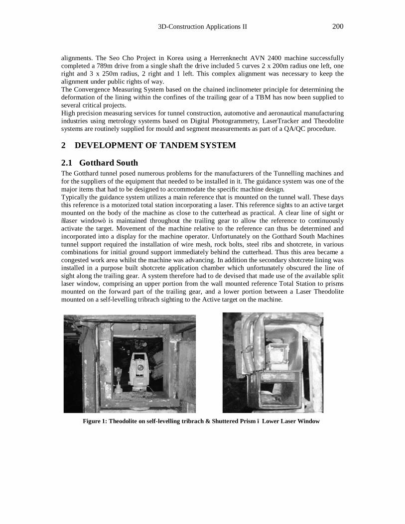
3D-Construction Applications II 200
alignments. The Seo Cho Project in Korea using a Herrenknecht AVN 2400 machine successfully completed a 789m drive from a single shaft the drive included 5 curves 2 x 200m radius one left, one right and 3 x 250m radius, 2 right and 1 left. This complex alignment was necessary to keep the alignment under public rights of way. The Convergence Measuring System based on the chained inclinometer principle for determining the deformation of the lining within the confines of the trailing gear of a TBM has now been supplied to several critical projects. High precision measuring services for tunnel construction, automotive and aeronautical manufacturing industries using metrology systems based on Digital Photogrammetry, LaserTracker and Theodolite systems are routinely supplied for mould and segment measurements as part of a QA/QC procedure.
2 DEVELOPMENT OF TANDEM SYSTEM
2.1 Gotthard South The Gotthard tunnel posed numerous problems for the manufacturers of the Tunnelling machines and for the suppliers of the equipment that needed to be installed in it. The guidance system was one of the major items that had to be designed to accommodate the specific machine design. Typically the guidance system utilizes a main reference that is mounted on the tunnel wall. These days this reference is a motorized total station incorporating a laser. This reference sights to an active target mounted on the body of the machine as close to the cutterhead as practical. A clear line of sight or “laser window” is maintained throughout the trailing gear to allow the reference to continuously activate the target. Movement of the machine relative to the reference can thus be determined and incorporated into a display for the machine operator. Unfortunately on the Gotthard South Machines tunnel support required the installation of wire mesh, rock bolts, steel ribs and shotcrete, in various combinations for initial ground support immediately behind the cutterhead. Thus this area became a congested work area whilst the machine was advancing. In addition the secondary shotcrete lining was installed in a purpose built shotcrete application chamber which unfortunately obscured the line of sight along the trailing gear. A system therefore had to de devised that made use of the available split laser window, comprising an upper portion from the wall mounted reference Total Station to prisms mounted on the forward part of the trailing gear, and a lower portion between a Laser Theodolite mounted on a self-levelling tribrach sighting to the Active target on the machine.
Figure 1: Theodolite on self-levelling tribrach & Shuttered Prism – Lower Laser Window
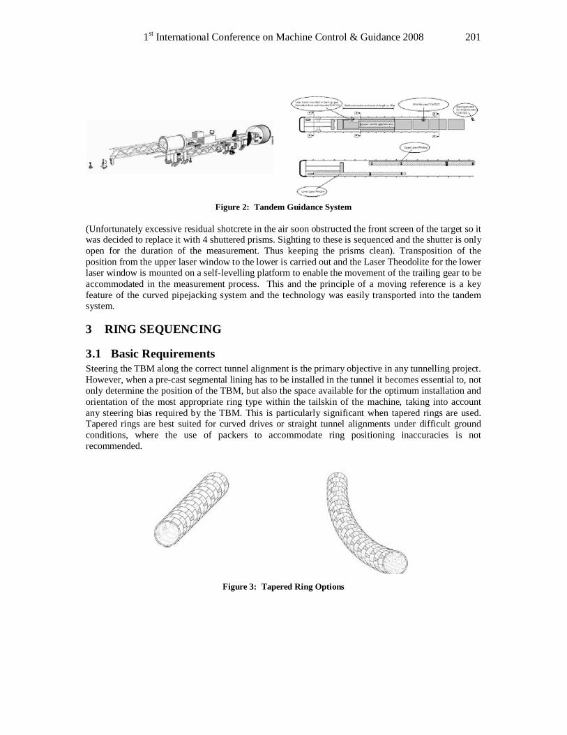
1st International Conference on Machine Control & Guidance 2008 201
Figure 2: Tandem Guidance System
(Unfortunately excessive residual shotcrete in the air soon obstructed the front screen of the target so it was decided to replace it with 4 shuttered prisms. Sighting to these is sequenced and the shutter is only open for the duration of the measurement. Thus keeping the prisms clean). Transposition of the position from the upper laser window to the lower is carried out and the Laser Theodolite for the lower laser window is mounted on a self-levelling platform to enable the movement of the trailing gear to be accommodated in the measurement process. This and the principle of a moving reference is a key feature of the curved pipejacking system and the technology was easily transported into the tandem system.
3 RING SEQUENCING
3.1 Basic Requirements Steering the TBM along the correct tunnel alignment is the primary objective in any tunnelling project. However, when a pre-cast segmental lining has to be installed in the tunnel it becomes essential to, not only determine the position of the TBM, but also the space available for the optimum installation and orientation of the most appropriate ring type within the tailskin of the machine, taking into account any steering bias required by the TBM. This is particularly significant when tapered rings are used. Tapered rings are best suited for curved drives or straight tunnel alignments under difficult ground conditions, where the use of packers to accommodate ring positioning inaccuracies is not recommended.
Figure 3: Tapered Ring Options
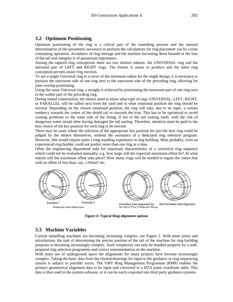
3D-Construction Applications II 202
3.2 Optimum Positioning Optimum positioning of the ring is a critical part of the tunnelling process and the manual determination of the parameters necessary to perform the calculations for ring placement can be a time consuming operation. Avoidance of ring damage and the machine becoming “iron bound” or the loss of the tail seal integrity is of paramount importance. Among the tapered ring conceptions there are two distinct subsets: the UNIVERSAL ring and the mirrored pair of LEFT and RIGHT rings. The former is easier to produce and the latter ring conception permits easier ring erection. To use a single Universal ring in a curve of the minimum radius for the ring’s design, it is necessary to position the narrowest side of one ring next to the narrowest side of the preceding ring, allowing for joint overlap positioning. Using the same Universal ring, a straight is achieved by positioning the narrowest part of one ring next to the widest part of the preceding ring. During tunnel construction, the miners need to know what type of ring: UNIVERSAL, LEFT, RIGHT, or PARALLEL will be called next from the yard and in what rotational position the ring should be erected. Depending on the chosen rotational position, the ring will take, due to its taper, a certain tendency towards the centre of the shield tail or towards the iron. This has to be optimized to avoid causing problems to the outer side of the lining, if not to the tail sealing itself, with the risk of dangerous water inrush after having damaged the tail sealing. Therefore, attention must be paid to the best choice of the key position for each ring to be erected. There may be cases where the selection of the appropriate key position for just the next ring could be judged by the miners themselves, without the assistance of a dedicated ring selection program. However, this would require quite a long standing experience in ring building. Most probably, even an experienced ring builder could not predict more than one ring at a time. Often the engineering department asks for important characteristics of a corrective ring sequence which could not be evaluated manually: e.g. how large will the expected maximum offset be? At what station will the maximum offset take place? How many rings will be needed to regain the centre line with an offset of less than, say, ±10mm? etc.
Figure 4: Typical Ring alignment options
3.3 Machine Variables Current tunnelling machines are becoming increasing complex, see Figure 5. With more joints and articulations, the task of determining the precise position of the tail of the machine for ring building purposes is becoming increasingly complex. Such complexity can only be handled properly by a well-prepared ring selection programme and correct instrumentation on the machine. With more use of underground space the alignments for many projects have become increasingly complex. Taking the basic data from the clients’ drawings for input to the guidance or ring sequencing system is subject to possible errors. The VMT Ring Management Programme (RMP) enables the primary geometrical alignment data to be input and converted to a DTA point coordinate table. This data is then used in the system software, or it can be easily exported into third party guidance systems.
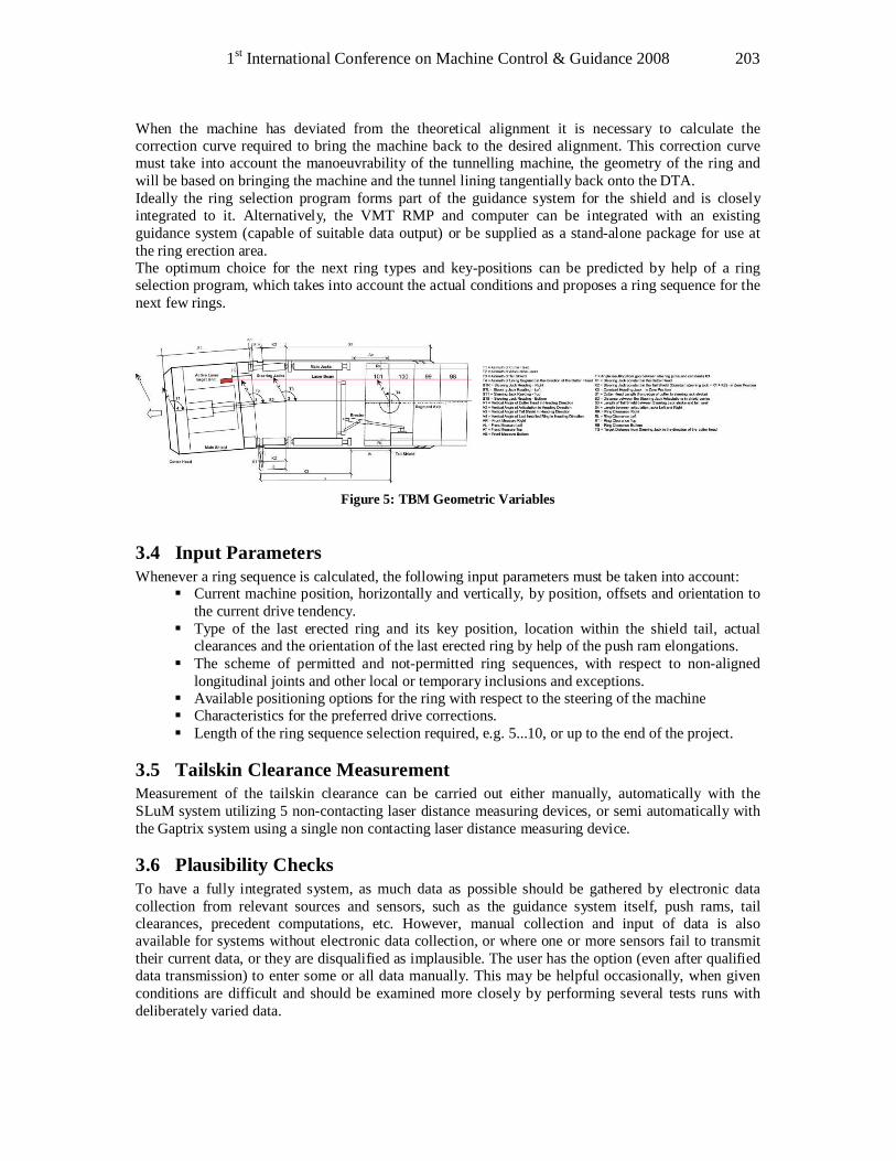
1st International Conference on Machine Control & Guidance 2008 203
When the machine has deviated from the theoretical alignment it is necessary to calculate the correction curve required to bring the machine back to the desired alignment. This correction curve must take into account the manoeuvrability of the tunnelling machine, the geometry of the ring and will be based on bringing the machine and the tunnel lining tangentially back onto the DTA. Ideally the ring selection program forms part of the guidance system for the shield and is closely integrated to it. Alternatively, the VMT RMP and computer can be integrated with an existing guidance system (capable of suitable data output) or be supplied as a stand-alone package for use at the ring erection area. The optimum choice for the next ring types and key-positions can be predicted by help of a ring selection program, which takes into account the actual conditions and proposes a ring sequence for the next few rings.
Figure 5: TBM Geometric Variables
3.4 Input Parameters Whenever a ring sequence is calculated, the following input parameters must be taken into account:
§ Current machine position, horizontally and vertically, by position, offsets and orientation to the current drive tendency.
§ Type of the last erected ring and its key position, location within the shield tail, actual clearances and the orientation of the last erected ring by help of the push ram elongations.
§ The scheme of permitted and not-permitted ring sequences, with respect to non-aligned longitudinal joints and other local or temporary inclusions and exceptions.
§ Available positioning options for the ring with respect to the steering of the machine § Characteristics for the preferred drive corrections. § Length of the ring sequence selection required, e.g. 5...10, or up to the end of the project.
3.5 Tailskin Clearance Measurement Measurement of the tailskin clearance can be carried out either manually, automatically with the SLuM system utilizing 5 non-contacting laser distance measuring devices, or semi automatically with the Gaptrix system using a single non contacting laser distance measuring device.
3.6 Plausibility Checks To have a fully integrated system, as much data as possible should be gathered by electronic data collection from relevant sources and sensors, such as the guidance system itself, push rams, tail clearances, precedent computations, etc. However, manual collection and input of data is also available for systems without electronic data collection, or where one or more sensors fail to transmit their current data, or they are disqualified as implausible. The user has the option (even after qualified data transmission) to enter some or all data manually. This may be helpful occasionally, when given conditions are difficult and should be examined more closely by performing several tests runs with deliberately varied data.
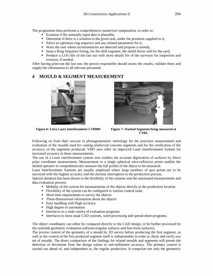
3D-Construction Applications II 204
The programme then performs a comprehensive numerical computation, in order to: § Examine if the manually input data is plausible, § Determine if there is a solution to the given task, under the premises supplied to it, § Select an optimum ring sequence and any related parameters for it, § Warn the user where inconsistencies are detected and propose a remedy, § Issue a Ring Sequence listing, for the shift engineer, the shield driver and for the yard, § Produce a LOG-file of the last run with more details for of the surveyor for inspection and
revision, if needed. After having print-out the last run, the person responsible should assess the results, validate them and supply the information to all relevant personnel.
4 MOULD & SEGMENT MEASUREMENT
Figure 6: Leica Laser Interferometer LTD800 Figure 7: Stacked Segments being measured at
CTRL Following on from their success in photogrammetric metrology for the precision measurement and evaluation of the moulds used for casting reinforced concrete segments and for the verification of the accuracy of the segments produced, VMT now offer its improved Laser Interferometer System for increased accuracy in these measurements. The use of a Laser interferometer system now enables the accurate digitization of surfaces by direct polar coordinate measurement. Measurement to a single spherical retro-reflective prism enables the skilled operator to comprehensively measure the full profile of the object to be measured. Laser Interferometer Systems are usually employed where large numbers of spot points are to be surveyed with the highest accuracy and the shortest interruption to the production process. Special attention has been drawn to the flexibility of the systems and the automated measurements and data evaluation process.
§ Mobility of the system for measurements of the objects directly at the production location § Flexibility of the system can be configured to various control tasks § Short time requirements to survey the objects § Three-dimensional information about the objects § Easy handling with High accuracy § High degree of automation § Interfaces to a wide variety of evaluation programs § Interfaces to most usual CAD systems, word processing and spread-sheet programs.
The object coordinates can either be compared directly to the CAD design, or be further processed by the system’s geometric evaluation software (regular surfaces and free-form surfaces). The precise control of the geometry of a mould by 3D survey before producing the first segment, as well as the control of the first produced segment itself is indispensable in order to check and verify any set of moulds. The direct comparison of the findings for related moulds and segments will permit the detection of deviations from the design values to sub-millimetre accuracy. The primary control is carried out ahead of, and independent to, the regular production. It comprises not only the geometric

1st International Conference on Machine Control & Guidance 2008 205
verification but the potential for verification of recesses for gaskets, bolts, identifiers, reference markers, etc. Attention should be drawn to the requirement, that all moulds and segments shall be exposed to the same environmental conditions and are undergoing the same stock conditions. As the most important result, the 3D-coordinates of the object points will be obtained in the format “point-name X, Y, Z, dx, dy, dz”. These records are the object’s coordinates in space along with an estimated accuracy of the internal quality criteria. The evaluation of the standard geometry and the comparison with design values and relevant tolerances will take place directly after the evaluation of spatial coordinates with help of the program “TUBGEO”.
Secondary Control is the term to denote the cyclic verification of complete sets of segments (i.e. rings) and related sets of moulds. Typical cycle times might be for example ‘one ring and one set of moulds per week’. The object (segment or mould) to be checked will be taken off the production process (storage or carousel) and placed at a convenient location somewhere in the production hall. For a cyclic Secondary Control the verification of the 6 outer surfaces and from them the derived distances and angles is essential. The data processing runs semi-automatically by help of only a few simple menu functions. The main result of the data evaluation will be displayed in a summary report, this includes the measurements and clear statements about the tolerances, whether they have been kept or exceeded. The process commences with the establishment of the frequency of measurement points to be taken. These may be at a time dependent interval, distance interval or by working to a grid matrix. For the actual use of the Laser Interferometer System in the measurement of segments and moulds VMT have included dialogue aided scripting for the operator to clearly explain the processes of each measurement operation. As the complete measurement of the mould or segment cannot be accomplished from a single standpoint it is necessary to relocate the LaserTracker to a second standpoint. To ensure that all the measurements taken can be reconciled within the same coordinate framework, index measurements are taken to the prism that is located in a “birds nest” cradle. Between 4 and 6 of these indexing locations are established and the dialogue control informs the operator when to locate the prism in the appropriate cradle. Upon commencement of a measurement cycle the operator places the retro-reflective prism in the reference point receptacle on the LaserTracker stand. The instrument is then able to carry out its own internal calibration and establish its zero reference point. The operator then removes the retro-reflective prism and making sure that the laser beam from the instrument is always in line of sight of the retro-reflective prism, he will commence the systematic tracing of the prism over the surface of the mould or segment; making sure to include all the significant surface points. If the line of sight between the LaserTracker instrument and the prism is broken then the prism must be replaced in the reference point receptacle on the Laser Tracker stand to re-zero the system. The measurement can then recommence at the point where line of sight was broken. The typical time taken to conduct the measurements for all six surfaces including the relocation of the LaserTracker as well as the analysis of the results is approximately 30 minutes. The Field proven TubGeo© software has already proven its functionality and enormous potential in numerous test measurements, and in several production plant operations, under tough industrial conditions. It has been developed employing modern software techniques in the programming language C++ with no restrictions in mind. With its help it is possible to calculate the external surfaces by “best-fit” and derive all relevant intersection measurements. The calculated output can be given numerically, graphically or in a combination of both. The resulting high-performance package including TubMes©, together with optional software such as (CAD Import/Export, Freeform surface calculation etc.) gives a tailor-made solution to suit individual needs.
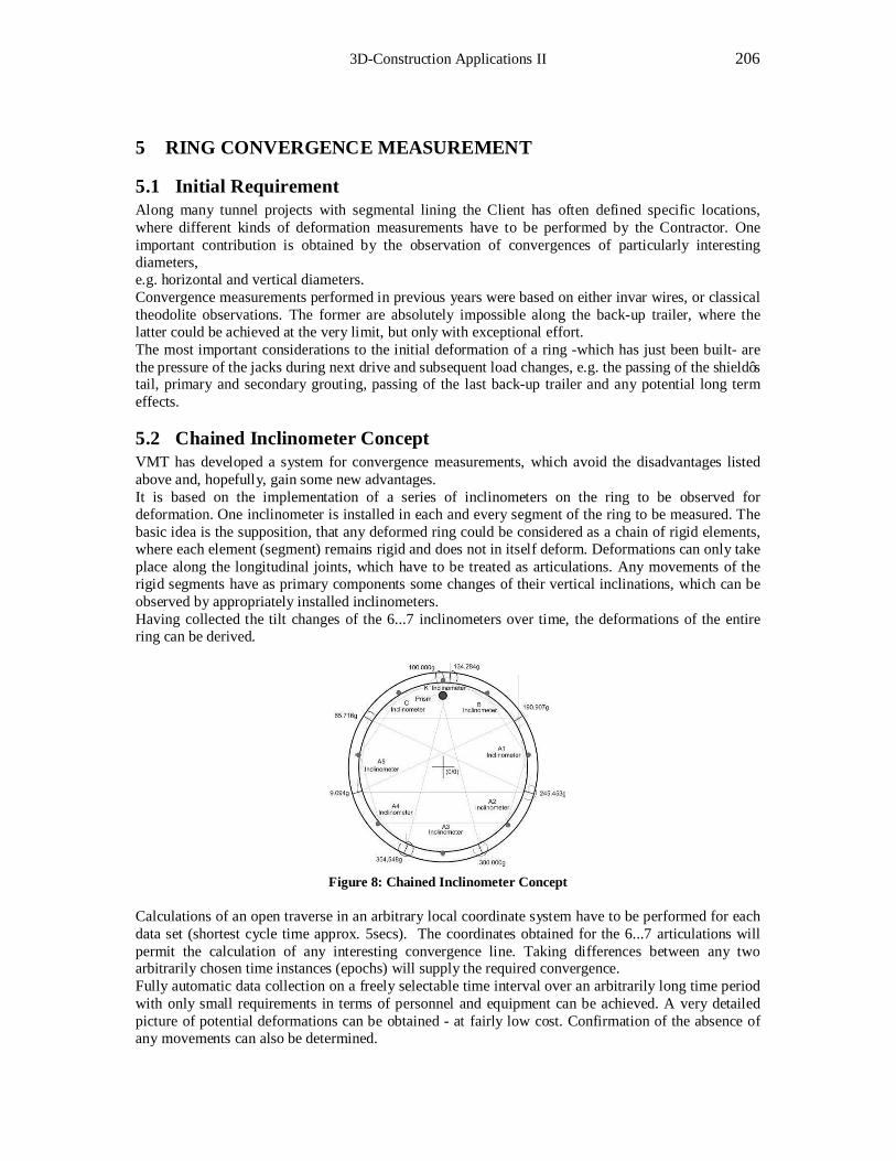
3D-Construction Applications II 206
5 RING CONVERGENCE MEASUREMENT
5.1 Initial Requirement Along many tunnel projects with segmental lining the Client has often defined specific locations, where different kinds of deformation measurements have to be performed by the Contractor. One important contribution is obtained by the observation of convergences of particularly interesting diameters, e.g. horizontal and vertical diameters. Convergence measurements performed in previous years were based on either invar wires, or classical theodolite observations. The former are absolutely impossible along the back-up trailer, where the latter could be achieved at the very limit, but only with exceptional effort. The most important considerations to the initial deformation of a ring -which has just been built- are the pressure of the jacks during next drive and subsequent load changes, e.g. the passing of the shield’s tail, primary and secondary grouting, passing of the last back-up trailer and any potential long term effects.
5.2 Chained Inclinometer Concept VMT has developed a system for convergence measurements, which avoid the disadvantages listed above and, hopefully, gain some new advantages. It is based on the implementation of a series of inclinometers on the ring to be observed for deformation. One inclinometer is installed in each and every segment of the ring to be measured. The basic idea is the supposition, that any deformed ring could be considered as a chain of rigid elements, where each element (segment) remains rigid and does not in itself deform. Deformations can only take place along the longitudinal joints, which have to be treated as articulations. Any movements of the rigid segments have as primary components some changes of their vertical inclinations, which can be observed by appropriately installed inclinometers. Having collected the tilt changes of the 6...7 inclinometers over time, the deformations of the entire ring can be derived.
Figure 8: Chained Inclinometer Concept
Calculations of an open traverse in an arbitrary local coordinate system have to be performed for each data set (shortest cycle time approx. 5secs). The coordinates obtained for the 6...7 articulations will permit the calculation of any interesting convergence line. Taking differences between any two arbitrarily chosen time instances (epochs) will supply the required convergence. Fully automatic data collection on a freely selectable time interval over an arbitrarily long time period with only small requirements in terms of personnel and equipment can be achieved. A very detailed picture of potential deformations can be obtained - at fairly low cost. Confirmation of the absence of any movements can also be determined.
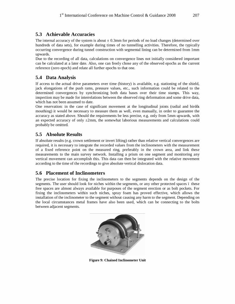
1st International Conference on Machine Control & Guidance 2008 207
5.3 Achievable Accuracies The internal accuracy of the system is about ± 0.3mm for periods of no load changes (determined over hundreds of data sets), for example during times of no tunnelling activities. Therefore, the typically occurring convergence during tunnel construction with segmental lining can be determined from 1mm upwards. Due to the recording of all data, calculations on convergence lines not initially considered important can be calculated at a later date. Also, one can freely chose any of the observed epochs as the current reference (zero epoch) and relate all further epochs to that one.
5.4 Data Analysis If access to the actual drive parameters over time (history) is available, e.g. stationing of the shield, jack elongations of the push rams, pressure values, etc., such information could be related to the determined convergences by synchronizing both data bases over their time stamps. This way, inspection may be made for interrelations between the observed ring deformation and some drive data, which has not been assumed to date. One reservation: in the case of significant movement at the longitudinal joints (radial and bird’s mouthing) it would be necessary to measure them as well, even manually, in order to guarantee the accuracy as stated above. Should the requirements be less precise, e.g. only from 5mm upwards, with an expected accuracy of only ±2mm, the somewhat laborious measurements and calculations could probably be omitted.
5.5 Absolute Results If absolute results (e.g. crown settlement or invert lifting) rather than relative vertical convergences are required, it is necessary to integrate the recorded values from the inclinometers with the measurement of a fixed reference point on the measured ring, preferably in the crown area, and link these measurements to the main survey network. Installing a prism on one segment and monitoring any vertical movement can accomplish this. This data can then be integrated with the relative movement according to the time of the recordings to give absolute vertical dislocation data.
5.6 Placement of Inclinometers The precise location for fixing the inclinometers to the segments depends on the design of the segments. The user should look for niches within the segments, or any other protected spaces – these free spaces are almost always available for purposes of the segment erection or as bolt pockets. For fixing the inclinometers within such niches, spray foam has proved effective, which allows the installation of the inclinometer to the segment without causing any harm to the segment. Depending on the local circumstances metal frames have also been used, which can be connecting to the bolts between adjacent segments.
Figure 9: Chained Inclinometer Unit

3D-Construction Applications II 208
6 TUNNEL CONSTRUCTION INFORMATION SYSTEM CBP Tunnel construction information systems create the infrastructure to supply data to experts, in as near real-time as possible, which they need for their decisions towards safer process control. Increasing complexity of construction sites and the data flow produced requires swift integration of all relevant data and information for advances. Also rapid analysis and its distribution to those who require the results by the various forms of modern communication that are available is required. The system is easy to use and has great flexibility to adapt to the individual circumstances of each construction site. CBP offers the following possibilities:
• Interdisciplinary management of one or several tunnel advances • Continuous monitoring of above ground deformations • Integration of geodetic, geo-technical and operation data of different TBM into one common
data-base • Unlimited number of users with the possibility of the assignment of defined user's rights • Self explanatory system of a user's spectrum from beginner to expert • Freely configurable analysis functions (visualization, mathematical analyses, etc.) with
concurrent default of standards • Visualization of surface structures and display of deformations in front, above and behind the
TBM • High security against failure, with demanding data protection • Replacement of labour-intensive activities by digital document management and automated
production of reports and protocols • Possibility for the automated monitoring of parameters • Generation and sending of warnings messages in case of dangerous drive conditions • Supply of adaptable interfaces to external data sources and to others, on the construction site
and company partners CBP as a tunnel information system can make a significant contribution to the minimization of risks and costs of tunnel construction.
Figure 10: CBP Data Integration

1st International Conference on Machine Control & Guidance 2008 209
7 CONCLUSIONS Rapid progress in the adaptation of Geodetic Instrumentation on machine bored tunnelling projects has been driven by the demand from an ever changing industry and supplied by dedicated teams of engineers from small companies that are flexible to reach to these demands.
REFERENCES Broomfield, J. Complex Pipejack Alignment in South Korea. No-Dig International Nov / Dec 2003 Clarke-Hackston, N. Guidance for Extended Distance & Curved Pipe Jacking Applications. Presented at the Microtunnelling Short-course. Feb 9-11 2000. Colorado School of Mines, Boulder, CO, USA Clarke-Hackston, N. Guiding the way Forwards. Tunnels & Tunnelling International, April 2003. Großkopf, J. & Fischer, A. Good cooperation leads to success. Gute Zusammenarbeit führt zum Erfolg April 2004 Frenzel, C. & Rehm, U. Controlled Boring Process (CBP) - a new approach to deformation-reduced tunneling in urban areas. Oslo 2002

3D-Construction Applications II 210
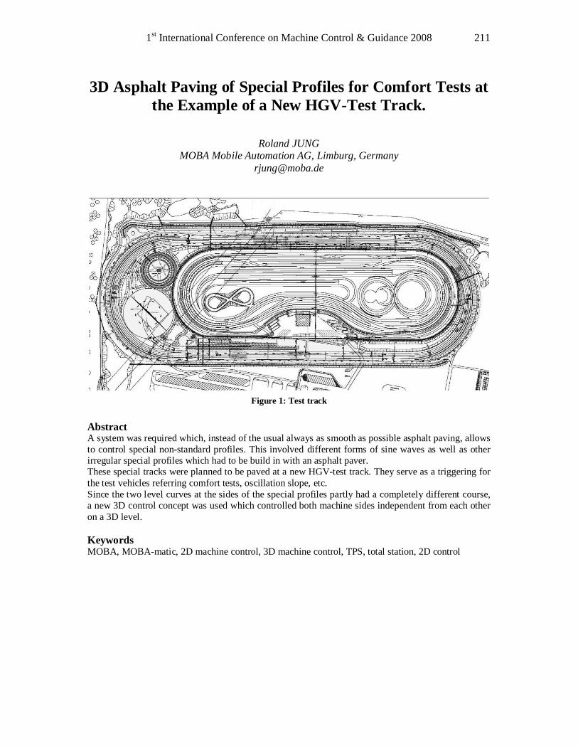
1st International Conference on Machine Control & Guidance 2008 211
3D Asphalt Paving of Special Profiles for Comfort Tests at the Example of a New HGV-Test Track.
Roland JUNG
MOBA Mobile Automation AG, Limburg, Germany [email protected]
Figure 1: Test track
Abstract A system was required which, instead of the usual always as smooth as possible asphalt paving, allows to control special non-standard profiles. This involved different forms of sine waves as well as other irregular special profiles which had to be build in with an asphalt paver. These special tracks were planned to be paved at a new HGV-test track. They serve as a triggering for the test vehicles referring comfort tests, oscillation slope, etc. Since the two level curves at the sides of the special profiles partly had a completely different course, a new 3D control concept was used which controlled both machine sides independent from each other on a 3D level. Keywords MOBA, MOBA-matic, 2D machine control, 3D machine control, TPS, total station, 2D control
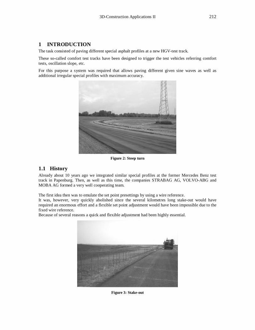
3D-Construction Applications II 212
1 INTRODUCTION The task consisted of paving different special asphalt profiles at a new HGV-test track.
These so-called comfort test tracks have been designed to trigger the test vehicles referring comfort tests, oscillation slope, etc.
For this purpose a system was required that allows paving different given sine waves as well as additional irregular special profiles with maximum accuracy.
Figure 2: Steep turn
1.1 History Already about 10 years ago we integrated similar special profiles at the former Mercedes Benz test track in Papenburg. Then, as well as this time, the companies STRABAG AG, VOLVO-ABG and MOBA AG formed a very well cooperating team. The first idea then was to emulate the set point presettings by using a wire reference. It was, however, very quickly abolished since the several kilometres long stake-out would have required an enormous effort and a flexible set point adjustment would have been impossible due to the fixed wire reference. Because of several reasons a quick and flexible adjustment had been highly essential.
Figure 3: Stake-out
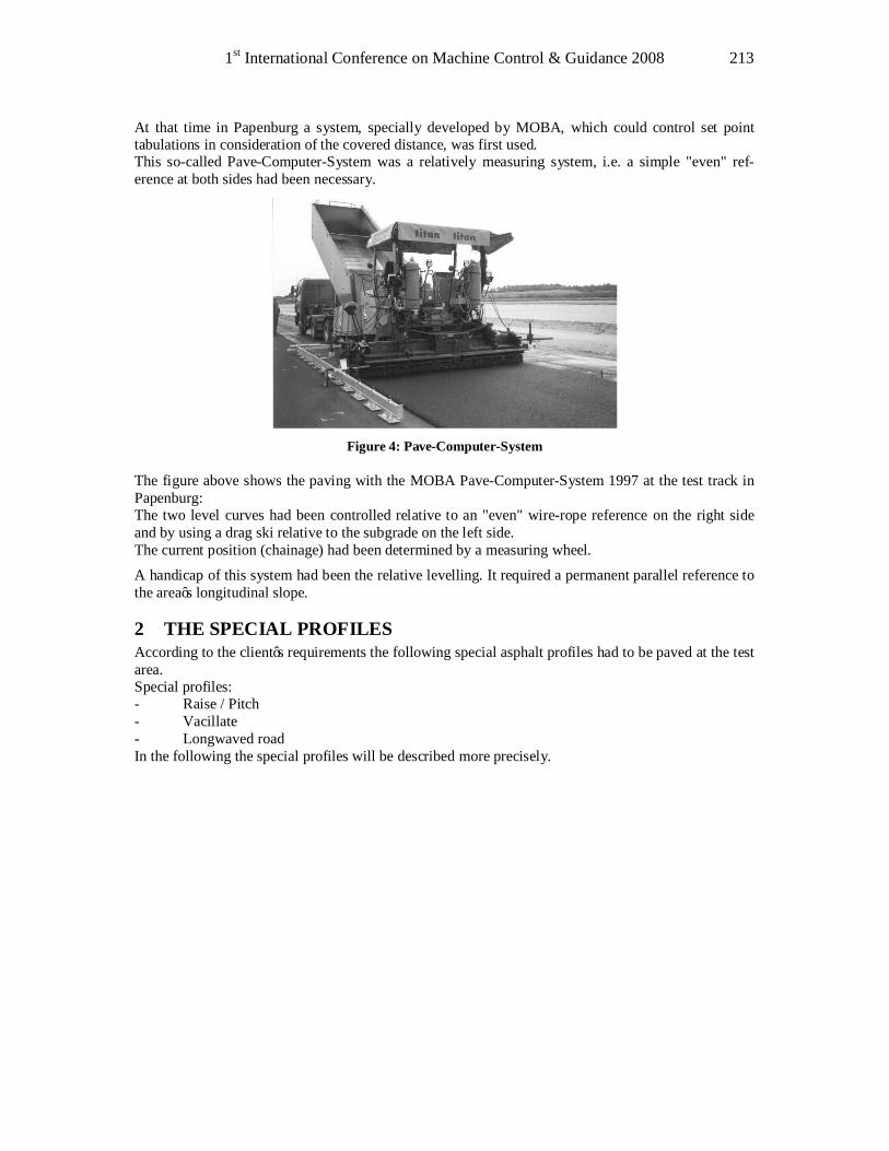
1st International Conference on Machine Control & Guidance 2008 213
At that time in Papenburg a system, specially developed by MOBA, which could control set point tabulations in consideration of the covered distance, was first used. This so-called Pave-Computer-System was a relatively measuring system, i.e. a simple "even" ref-erence at both sides had been necessary.
Figure 4: Pave-Computer-System
The figure above shows the paving with the MOBA Pave-Computer-System 1997 at the test track in Papenburg: The two level curves had been controlled relative to an "even" wire-rope reference on the right side and by using a drag ski relative to the subgrade on the left side. The current position (chainage) had been determined by a measuring wheel.
A handicap of this system had been the relative levelling. It required a permanent parallel reference to the area’s longitudinal slope.
2 THE SPECIAL PROFILES According to the client’s requirements the following special asphalt profiles had to be paved at the test area. Special profiles: - Raise / Pitch - Vacillate - Longwaved road In the following the special profiles will be described more precisely.
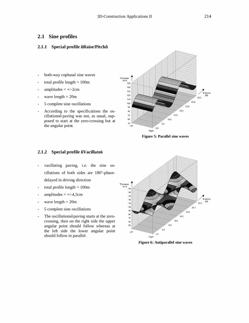
3D-Construction Applications II 214
2.1 Sine profiles
2.1.1 Special profile “Raise/Pitch“
- both-way cophasal sine waves
- total profile length = 100m
- amplitudes = +/-2cm
- wave length = 20m
- 5 complete sine oscillations
- According to the specifications the os-cillations’ paving was not, as usual, sup-posed to start at the zero-crossing but at the angular point.
Figure 5: Parallel sine waves
2.1.2 Special profile “Vacillate”
- vacillating paving, i.e. the sine os-
cillations of both sides are 180°-phase-
delayed in driving direction
- total profile length = 100m
- amplitudes = +/-4,5cm
- wave length = 20m
- 5 complete sine oscillations
- The oscillations’ paving starts at the zero-crossing, then on the right side the upper angular point should follow whereas at the left side the lower angular point should follow in parallel.
Figure 6: Antiparallel sine waves
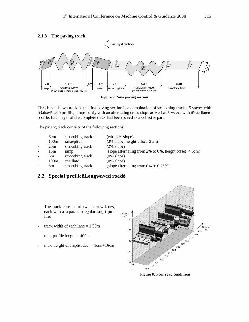
1st International Conference on Machine Control & Guidance 2008 215
2.1.3 The paving track
Figure 7: Sine paving section
The above shown track of the first paving section is a combination of smoothing tracks, 5 waves with “Raise/Pitch”-profile, ramps partly with an alternating cross-slope as well as 5 waves with “Vacillate”-profile. Each layer of the complete track had been paved as a cohesive part. The paving track consists of the following sections: - 60m smoothing track (with 2% slope) - 100m raise/pitch (2% slope, height offset -2cm) - 20m smoothing track (2% slope) - 15m ramp (slope alternating from 2% to 0%, height offset+4,5cm) - 5m smoothing track (0% slope) - 100m vacillate (0% slope) - 5m smoothing track (slope alternating from 0% to 0,75%)
2.2 Special profile“Longwaved road” - The track consists of two narrow lanes,
each with a separate irregular target pro-file.
- track width of each lane = 1,30m - total profile length = 400m - max. height of amplitudes = -1cm/+16cm
Figure 8: Poor road conditions
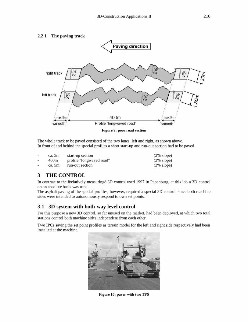
3D-Construction Applications II 216
2.2.1 The paving track
Figure 9: poor road section
The whole track to be paved consisted of the two lanes, left and right, as shown above. In front of and behind the special profiles a short start-up and run-out section had to be paved. - ca. 5m start-up section (2% slope) - 400m profile "longwaved road" (2% slope) - ca. 5m run-out section (2% slope)
3 THE CONTROL In contrast to the “relatively measuring” 3D control used 1997 in Papenburg, at this job a 3D control on an absolute basis was used. The asphalt paving of the special profiles, however, required a special 3D control, since both machine sides were intended to autonomously respond to own set points.
3.1 3D system with both-way level control For this purpose a new 3D control, so far unused on the market, had been deployed, at which two total stations control both machine sides independent from each other.
Two IPCs saving the set point profiles as terrain model for the left and right side respectively had been installed at the machine.
Figure 10: paver with two TPS
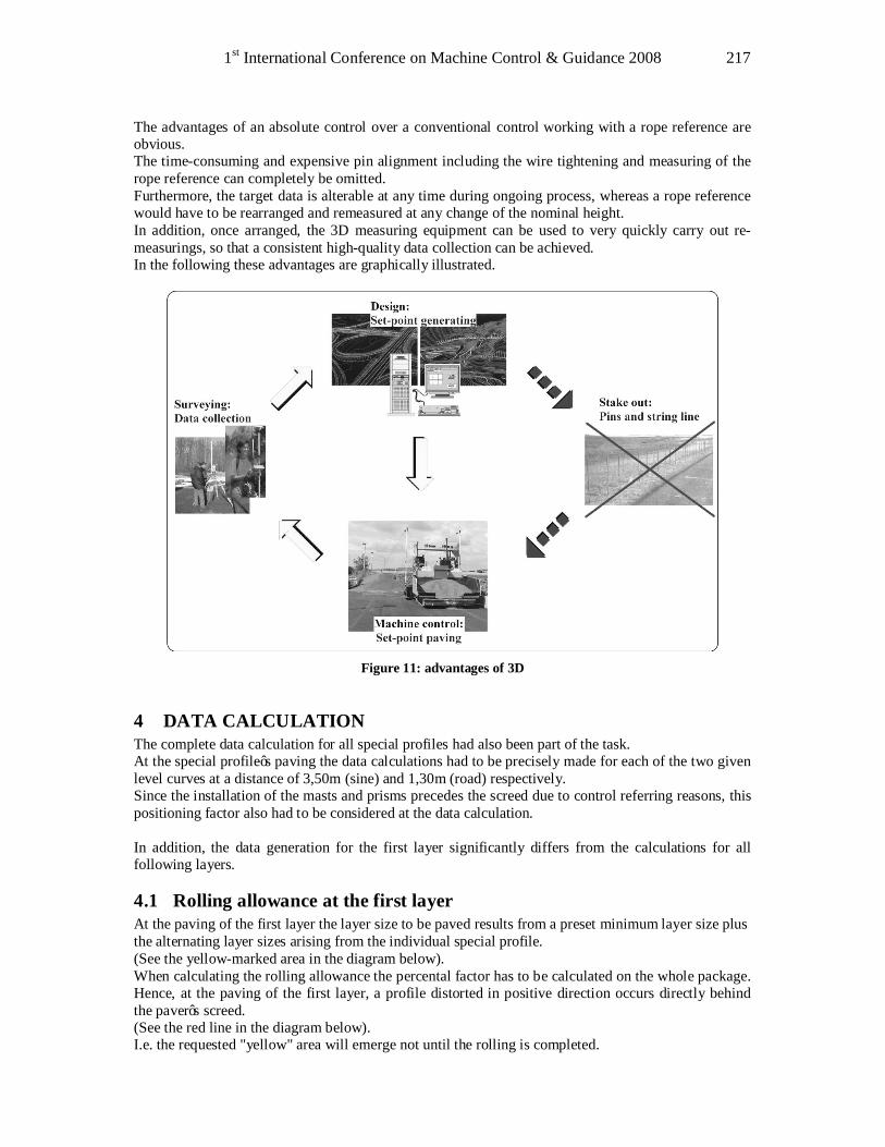
1st International Conference on Machine Control & Guidance 2008 217
The advantages of an absolute control over a conventional control working with a rope reference are obvious. The time-consuming and expensive pin alignment including the wire tightening and measuring of the rope reference can completely be omitted. Furthermore, the target data is alterable at any time during ongoing process, whereas a rope reference would have to be rearranged and remeasured at any change of the nominal height. In addition, once arranged, the 3D measuring equipment can be used to very quickly carry out re-measurings, so that a consistent high-quality data collection can be achieved. In the following these advantages are graphically illustrated.
Figure 11: advantages of 3D
4 DATA CALCULATION The complete data calculation for all special profiles had also been part of the task. At the special profile’s paving the data calculations had to be precisely made for each of the two given level curves at a distance of 3,50m (sine) and 1,30m (road) respectively. Since the installation of the masts and prisms precedes the screed due to control referring reasons, this positioning factor also had to be considered at the data calculation. In addition, the data generation for the first layer significantly differs from the calculations for all following layers.
4.1 Rolling allowance at the first layer At the paving of the first layer the layer size to be paved results from a preset minimum layer size plus the alternating layer sizes arising from the individual special profile. (See the yellow-marked area in the diagram below). When calculating the rolling allowance the percental factor has to be calculated on the whole package. Hence, at the paving of the first layer, a profile distorted in positive direction occurs directly behind the paver’s screed. (See the red line in the diagram below). I.e. the requested "yellow" area will emerge not until the rolling is completed.
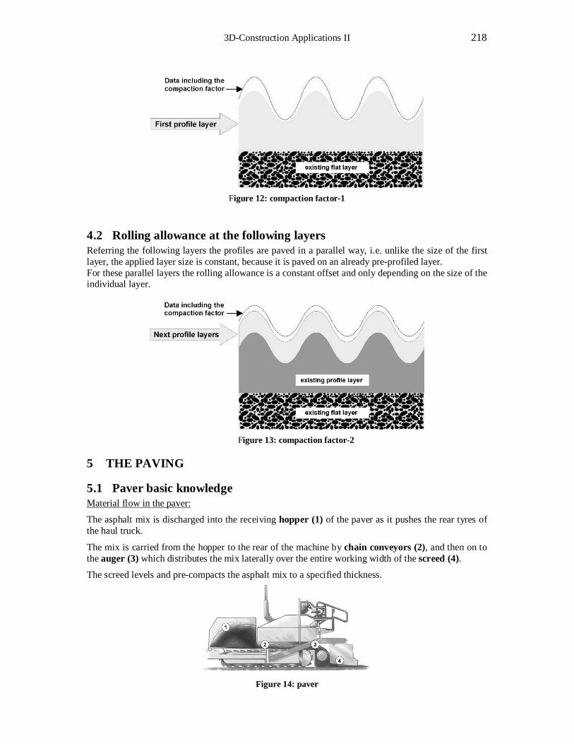
3D-Construction Applications II 218
Figure 12: compaction factor-1
4.2 Rolling allowance at the following layers Referring the following layers the profiles are paved in a parallel way, i.e. unlike the size of the first layer, the applied layer size is constant, because it is paved on an already pre-profiled layer. For these parallel layers the rolling allowance is a constant offset and only depending on the size of the individual layer.
Figure 13: compaction factor-2
5 THE PAVING
5.1 Paver basic knowledge Material flow in the paver:
The asphalt mix is discharged into the receiving hopper (1) of the paver as it pushes the rear tyres of the haul truck.
The mix is carried from the hopper to the rear of the machine by chain conveyors (2), and then on to the auger (3) which distributes the mix laterally over the entire working width of the screed (4).
The screed levels and pre-compacts the asphalt mix to a specified thickness.
Figure 14: paver
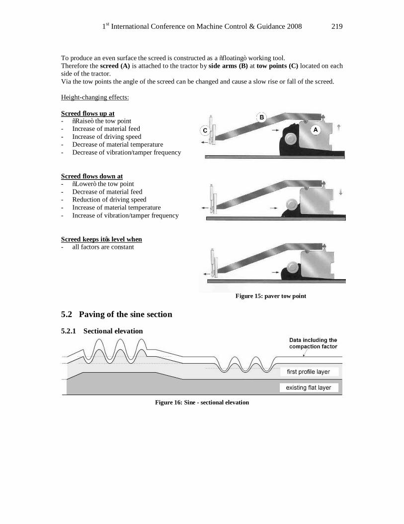
1st International Conference on Machine Control & Guidance 2008 219
To produce an even surface the screed is constructed as a “floating” working tool. Therefore the screed (A) is attached to the tractor by side arms (B) at tow points (C) located on each side of the tractor. Via the tow points the angle of the screed can be changed and cause a slow rise or fall of the screed. Height-changing effects: Screed flows up at - “Raise” the tow point - Increase of material feed - Increase of driving speed - Decrease of material temperature - Decrease of vibration/tamper frequency Screed flows down at - “Lower” the tow point - Decrease of material feed - Reduction of driving speed - Increase of material temperature - Increase of vibration/tamper frequency Screed keeps it’s level when - all factors are constant
Figure 15: paver tow point
5.2 Paving of the sine section
5.2.1 Sectional elevation
Figure 16: Sine - sectional elevation

3D-Construction Applications II 220
The paving started with a smoothing track and fluently went on with the profile “Raise/Pitch”. Special requirement: The sine wave did not have to begin at the oscillation’s zero-crossing, but at the upper angular point. Subsequently to this profile a smoothing track with a ramp and the profile “Vacillate” followed. Finally the profile „Vacillate” tapered off with an inclined ramp. Due to the rain water flow the cross-slope within the profile changed from 2% to 0% and back again.
Figure 17: Sine – layer
Altogether 5 profiled layers with different layer sizes and different rolling allowances had been paved one upon the other.
5.3 Paving of the “Longwaved road”
5.3.1 Sectional elevation
Figure 18: bad-road - sectional elevation
This section had been paved with a small footpath paver. The paving started with a short start-up phase and fluently went on with the "left" and "right" profile respectively. The different layers had been paved alternately left and right.
Altogether, for every lane 7 profiled layers with different layer sizes and different rolling allowances had been paved one upon the other. During the whole project the paved layers had been measured and recorded by the client’s surveyors. The measurements had been carried out in a 5m pattern and always delivered satisfying results. In case one or more variables responsible for the screed’s floating e.g. the material temperature, etc. should change during ongoing paving, this deviation could be directly detected and corrected by re-measuring. (Also see 5.1 Paver basic knowledge). For this purpose it had been possible to shift the current profile in a millimetre pattern either up or down during ongoing paving.

1st International Conference on Machine Control & Guidance 2008 221
6 CONCLUSIONS The newly designed 3D control system worked faultlessly at any time in practice. Altogether approx. 6.5km of special profiles had been paved on all layers. By measuring the asphalt layers directly behind the screed a very good paving quality could be proved. The calculated and paved-in rolling allowances had also been correct, so that the result after rolling also fitted very well.
Eventually all participating firms had been very content with the final result.
7 ACKNOWLEDGEMENTS The author would like to thank all the included companies: - STABAG AG - VOLVO-ABG Thank you very much for the always good and absolutely smooth cooperation!
REFERENCES Books: - "Compaction and paving", Theory and practice;
Copyright Svedala Industi AB, Schweden 2000;
Svedala Dynapac Publication no. IHCCCAPEN1; produced by Dowell/stubbs.
Printed by Kalmarsund Tryck AB, Schweden
- Technik und Technologie des Straßenbaus
3. Internationales Symposium Technologie des Straßenbaus, München 03. April 1998, bauma'98;
Computergesteuerter Einbau von Asphaltbahnen mit sinusförmigen und unregelmäßigen Wellen im Längsprofil; Dipl.-Ing. Ralf Jansen, Vorstand STRABAG AG Düsseldorf.

3D-Construction Applications II 222

Data Processing and Data Acquisition

No Driving in Circles - Improving the Research and Development of Mobile Machinery and Control Systems
by Using Advanced Simulation Technology
Jochen WENDEBAUM*, Mats KJELLBERG CC Systems AB, Sweden
[Jochen.Wendebaum, Mats.Kjellberg]@cc-systems.se Abstract The research and development of hardware, control and communication mechanisms for mobile machinery always requires a high amount of practical testing and debugging. In many cases, the developers need a machine or at least a test rack during a long time of a development project. By simulating the target hardware on the developers' PC, the development process, testing and debugging can already start at a very early phase of the project, before the target hardware is even available. This article presents and demonstrates an advanced simulation environment which can be used to simulate a complete as well as a mixed environment, and shows how testing and debugging can be performed in a much more controllable and repeatable manner. Also, the benefit for research of the behaviour of mobile machinery is shown, where the technology can be used to create and control a complete machine. Further, simulation is compared to the testing on real machines, and limitations and possible issues are discussed. Keywords Simulation, communication standards, control system development
1 INTRODUCTION Many engineers who develop control systems for mobile machinery or verify models of machinery behaviour have spent valuable time on construction sites, doing ad-hoc adaptations of hard- or software of their systems. Furthermore, if no dedicated test machine is available or testing has to be performed during the real work process, there are high restrictions concerning the access to the machine during work time, so this work has to be done in working breaks and before and after work, leading to an exhausting schedule. Such work is as ineffective as unsatisfactory and should be avoided as far as possible. To be able to solve most of the possible problems before moving to the machine or even real hardware, the target environment must be simulated as far as possible directly on the desk of the developer or researcher. Using test racks with sensors and controllers is a reasonable method but costly, especially if used in projects with several developers where more than one rack is needed. Minimization of the number of required hardware pieces during development and research can also be done by simulating the target environment in parts or as a whole. The simulation technology described
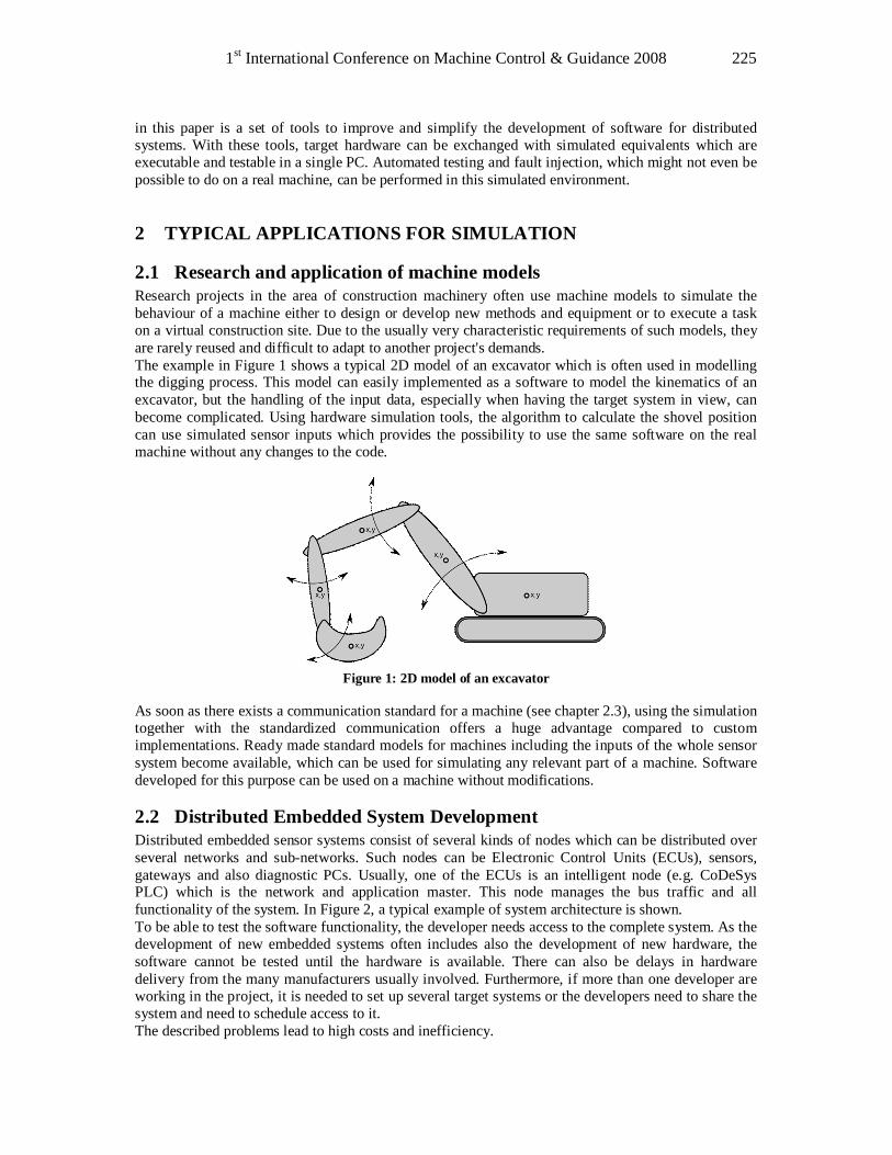
1st International Conference on Machine Control & Guidance 2008 225
in this paper is a set of tools to improve and simplify the development of software for distributed systems. With these tools, target hardware can be exchanged with simulated equivalents which are executable and testable in a single PC. Automated testing and fault injection, which might not even be possible to do on a real machine, can be performed in this simulated environment.
2 TYPICAL APPLICATIONS FOR SIMULATION
2.1 Research and application of machine models Research projects in the area of construction machinery often use machine models to simulate the behaviour of a machine either to design or develop new methods and equipment or to execute a task on a virtual construction site. Due to the usually very characteristic requirements of such models, they are rarely reused and difficult to adapt to another project's demands. The example in Figure 1 shows a typical 2D model of an excavator which is often used in modelling the digging process. This model can easily implemented as a software to model the kinematics of an excavator, but the handling of the input data, especially when having the target system in view, can become complicated. Using hardware simulation tools, the algorithm to calculate the shovel position can use simulated sensor inputs which provides the possibility to use the same software on the real machine without any changes to the code.
Figure 1: 2D model of an excavator
As soon as there exists a communication standard for a machine (see chapter 2.3), using the simulation together with the standardized communication offers a huge advantage compared to custom implementations. Ready made standard models for machines including the inputs of the whole sensor system become available, which can be used for simulating any relevant part of a machine. Software developed for this purpose can be used on a machine without modifications.
2.2 Distributed Embedded System Development Distributed embedded sensor systems consist of several kinds of nodes which can be distributed over several networks and sub-networks. Such nodes can be Electronic Control Units (ECUs), sensors, gateways and also diagnostic PCs. Usually, one of the ECUs is an intelligent node (e.g. CoDeSys PLC) which is the network and application master. This node manages the bus traffic and all functionality of the system. In Figure 2, a typical example of system architecture is shown. To be able to test the software functionality, the developer needs access to the complete system. As the development of new embedded systems often includes also the development of new hardware, the software cannot be tested until the hardware is available. There can also be delays in hardware delivery from the many manufacturers usually involved. Furthermore, if more than one developer are working in the project, it is needed to set up several target systems or the developers need to share the system and need to schedule access to it. The described problems lead to high costs and inefficiency.
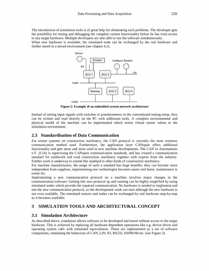
Data Processing and Data Acquisition 226
The introduction of simulation tools is of great help for eliminating such problems. The developer gets the possibility for testing and debugging the complete system functionality before he has even access to any target hardware. Multiple developers are also able to test the software simultaneously. When new hardware is available, the simulated node can be exchanged by the real hardware and further tested in a mixed environment (see chapter 4.2).
Figure 2: Example of an embedded system network architecture
Instead of setting input signals with switches or potentiometers in the conventional testing setup, they can be written and read directly on the PC with additional tools. A complete environmental and physical model of the machine can be implemented which writes virtual sensor values to the simulation environment.
2.3 Standardisation of Data Communication For sensor systems on construction machinery, the CAN protocol is currently the most common communication method used. Furthermore, the application layer CANopen offers additional functionality and gets more and more used in new machine developments. The CAN in Automations e.V. (CiA) is supervising the CANopen communication standards, and has created a communication standard for earthwork and road construction machinery together with experts from the industry. Further work is underway to extend this standard to other kinds of construction machinery. For machine manufacturers, the usage of such a standard has huge benefits: they can become more independent from suppliers, implementing new technologies becomes easier and faster, maintenance is easier etc. Implementing a new communication protocol on a machine involves major changes in the communication software. Getting this new protocol up and running can be highly simplified by using simulated nodes which provide the required communication. No hardware is needed to implement and test the new communication protocol, so the development work can start although the new hardware is not even available. The simulated sensors and nodes can be exchanged by real hardware step-by-step as it becomes available.
3 SIMULATION TOOLS AND ARCHITECTURAL CONCEPT
3.1 Simulation Architecture As described above, simulation allows software to be developed and tested without access to the target hardware. This is achieved by replacing all hardware dependent operations like e.g. device driver and operating system calls with simulated equivalences. These are implemented as a set of software components, simulating the behaviour of CAN, LIN, IO, RS232, EEPROM etc. (see Figure 3).
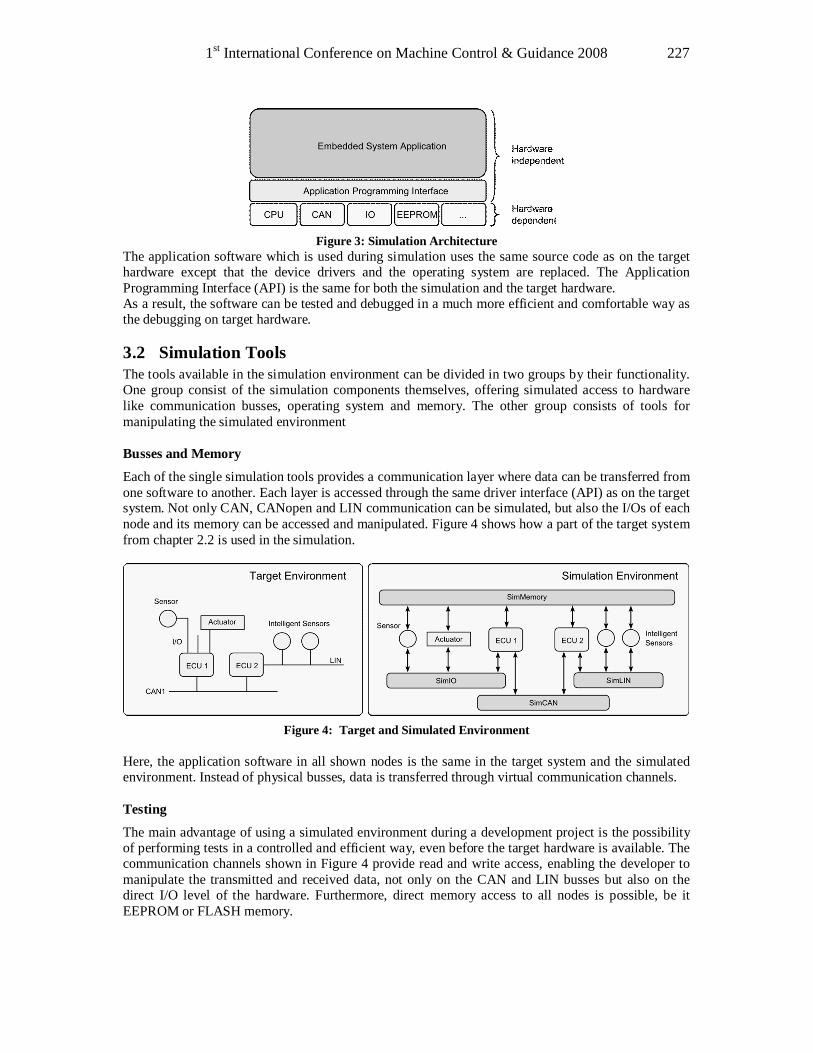
1st International Conference on Machine Control & Guidance 2008 227
Figure 3: Simulation Architecture
The application software which is used during simulation uses the same source code as on the target hardware except that the device drivers and the operating system are replaced. The Application Programming Interface (API) is the same for both the simulation and the target hardware. As a result, the software can be tested and debugged in a much more efficient and comfortable way as the debugging on target hardware.
3.2 Simulation Tools The tools available in the simulation environment can be divided in two groups by their functionality. One group consist of the simulation components themselves, offering simulated access to hardware like communication busses, operating system and memory. The other group consists of tools for manipulating the simulated environment Busses and Memory
Each of the single simulation tools provides a communication layer where data can be transferred from one software to another. Each layer is accessed through the same driver interface (API) as on the target system. Not only CAN, CANopen and LIN communication can be simulated, but also the I/Os of each node and its memory can be accessed and manipulated. Figure 4 shows how a part of the target system from chapter 2.2 is used in the simulation.
Figure 4: Target and Simulated Environment
Here, the application software in all shown nodes is the same in the target system and the simulated environment. Instead of physical busses, data is transferred through virtual communication channels. Testing
The main advantage of using a simulated environment during a development project is the possibility of performing tests in a controlled and efficient way, even before the target hardware is available. The communication channels shown in Figure 4 provide read and write access, enabling the developer to manipulate the transmitted and received data, not only on the CAN and LIN busses but also on the direct I/O level of the hardware. Furthermore, direct memory access to all nodes is possible, be it EEPROM or FLASH memory.
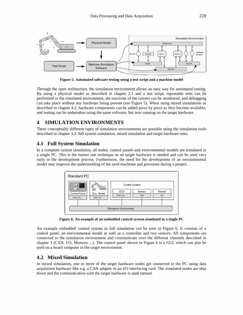
Data Processing and Data Acquisition 228
Figure 5: Automated software testing using a test script and a machine model
Through the open architecture, the simulation environment allows an easy way for automated testing. By using a physical model as described in chapter 2.1 and a test script, repeatable tests can be performed in the simulated environment, the reactions of the system can be monitored, and debugging can take place without any hardware being present (see Figure 5). When using mixed simulations as described in chapter 4.2, hardware components can be added piece by piece as they become available, and testing can be undertaken using the same software, but now running on the target hardware.
4 SIMULATION ENVIRONMENTS Three conceptually different types of simulation environments are possible using the simulation tools described in chapter 3.2: full system simulation, mixed simulation and target hardware tests.
4.1 Full System Simulation In a complete system simulation, all nodes, control panels and environmental models are simulated in a single PC. This is the easiest test technique as no target hardware is needed and can be used very early in the development process. Furthermore, the need for the development of an environmental model may improve the understanding of the used machines and processes during a project.
Figure 6: An example of an embedded control system simulated in a single PC
An example embedded control system in full simulation can be seen in Figure 6. It consists of a control panel, an environmental model as well as a controller and two sensors. All components are connected to the simulation environment and communicate over the different channels described in chapter 3 (CAN, I/O, Memory ...). The control panel shown in Figure 6 is a GUI, which can also be used on a board computer in the target environment.
4.2 Mixed Simulation In mixed simulation, one or more of the target hardware nodes get connected to the PC using data acquisition hardware like e.g. a CAN adapter or an I/O interfacing card. The simulated nodes are shut down and the communication with the target hardware is used instead.

1st International Conference on Machine Control & Guidance 2008 229
Figure 7: Overview of a mixed simulation setting
Regarding the above example of the full simulation, after e.g. the analogue sensor and the controller are available, the full simulation environment shown in the previous chapter can be moved to a mixed simulation. Here, the both target hardware nodes are connected to the PC using a CAN interface card. The software on the nodes is the same as in the full simulation, only the drivers have been exchanged to fit to the hardware. Mixed simulation has two main goals, one being the integration of target hardware and hardware related software in a controlled step-by-step procedure, and secondly the testing of the physical communication between the nodes. The same test scripts, models and also the control panel can be used also in the mixed simulation environment.
4.3 Target System Tests In the final phase of the development process, all target hardware nodes are used. The control panel component can still be simulated on the PC and connected to the external hardware through data acquisition hardware. To perform hardware-in-the-loop testing, the target system hardware communicates with the environmental model describing the peripheral components and behaviour in the system.
Figure 8: Setting for target hardware tests
5 LIMITATIONS AND BENEFITS
5.1 Limitations of the simulation The simulation environment will never fully simulate the target hardware. The simulation will not be usable when it comes to source code which is closely bound to the hardware (e.g. DSP, Assembler). Further, timing issues due to not fully simulatable clock frequencies can occur, although the
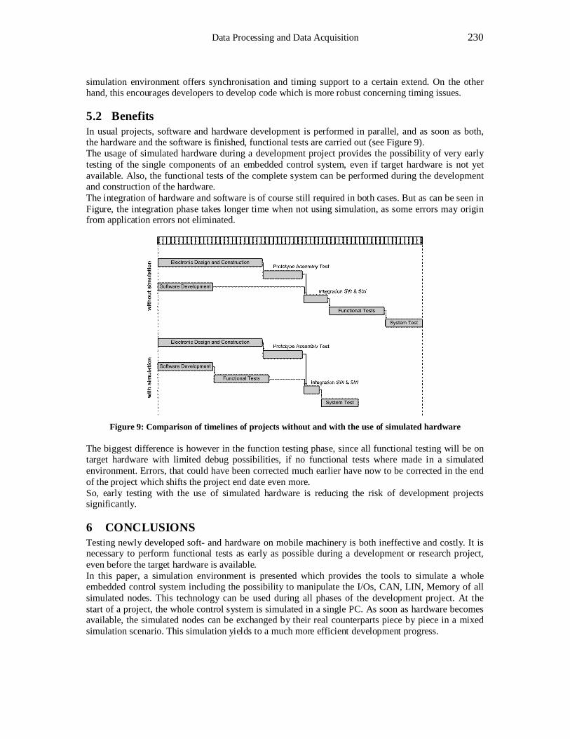
Data Processing and Data Acquisition 230
simulation environment offers synchronisation and timing support to a certain extend. On the other hand, this encourages developers to develop code which is more robust concerning timing issues.
5.2 Benefits In usual projects, software and hardware development is performed in parallel, and as soon as both, the hardware and the software is finished, functional tests are carried out (see Figure 9). The usage of simulated hardware during a development project provides the possibility of very early testing of the single components of an embedded control system, even if target hardware is not yet available. Also, the functional tests of the complete system can be performed during the development and construction of the hardware. The integration of hardware and software is of course still required in both cases. But as can be seen in Figure, the integration phase takes longer time when not using simulation, as some errors may origin from application errors not eliminated.
Figure 9: Comparison of timelines of projects without and with the use of simulated hardware
The biggest difference is however in the function testing phase, since all functional testing will be on target hardware with limited debug possibilities, if no functional tests where made in a simulated environment. Errors, that could have been corrected much earlier have now to be corrected in the end of the project which shifts the project end date even more. So, early testing with the use of simulated hardware is reducing the risk of development projects significantly.
6 CONCLUSIONS Testing newly developed soft- and hardware on mobile machinery is both ineffective and costly. It is necessary to perform functional tests as early as possible during a development or research project, even before the target hardware is available. In this paper, a simulation environment is presented which provides the tools to simulate a whole embedded control system including the possibility to manipulate the I/Os, CAN, LIN, Memory of all simulated nodes. This technology can be used during all phases of the development project. At the start of a project, the whole control system is simulated in a single PC. As soon as hardware becomes available, the simulated nodes can be exchanged by their real counterparts piece by piece in a mixed simulation scenario. This simulation yields to a much more efficient development progress.

1st International Conference on Machine Control & Guidance 2008 231
REFERENCES Journal articles: STRANDBERG, J. et. al.: Efficient engineering through simulation of CAN based control systems. Proceedings of the 51st National Conference on Fluid Power, 2008 Links: http://www.cc-systems.com/SYSTEMPLATFORMS/TESTSYSTEM/tabid/141/Default.aspx, last accessed on April 17, 2008 * Dr. Jochen Wendebaum, Mats Kjellberg, CC Systems AB, Kopparlundsvägen 14, SE 721 30 Västerås, Sweden.

Data Processing and Data Acquisition 232
1st International Conference on Machine Control & Guidance 2008 233
Autonomous Navigation Tool for Real & Virtual Field Robots
Ali ZOGHEIB*
Mid Sweden University, Sundsvall, Sweden [email protected]
Abstract Due to ecological and economical demands in agriculture as well as technological improvements, the development of autonomous field robots has gained importance within the last years. A common task for all field robots, whatever their main function is, is to Autonomously Navigate between row cultures. As a first step, toward a full featured Simulator tool dedicated to agriculture applications, an autonomous navigation tool based on sensor fusion and fuzzy logic, has been realised. The data of various sensors are transferred to control variables thereby opening the options for including further sensors without changing the model. Different aspects ranging from missing plants to path planning (such as skipping rows) and field mapping are included. A wireless connection with the physical robot is implemented, currently it is used for robot navigation control, data sending and receiving. The first experiments for the navigation between rows showed that simulation and real world were in phase. Keywords Field Robots, Simulator, Autonomous Navigation, Sensors Fusion, Agriculture Applications, Fuzzy Logic, Navigation Control.
1 INTRODUCTION The development of autonomous field robots has gained importance within the last years, due to ecological and economical demands in agriculture, as well as to technological improvements. Many experimental field robots were developed with a wide range of applications: Seeding (Trebinski G. et al., 2004), Weed Control (Van Evert. F.K. et al., 2006), Fruit Picking (Katupitiya J. et al., 2005), Data Collecting (Nagasaka Y., 2004), Harvesting (Edan Y., 2000), ...). In all these applications, the field robots are required to successfully achieve a common task: Autonomously Navigating between rows culture, making it one of the most important tasks, in this field, as can be observed in the place this task has in specialised field robots contests (i.e. Field Robot Event Contest). In this paper, we will present an Autonomous Navigation Tool, dedicated for real and virtual field robots’ in-between rows navigation. In this tool, data from different sensors types (i.e. distance sensors, mounted camera, remote sensing images, ...) can be fusioned into one coherent environment’s model. From this model a set of five control variables are derived, reducing the complexity of the navigation control to a constant one, whatever the number of fusioned sensors is. A Fuzzy Logic Controller (Zadeh L., 2002), taking the control variables as its inputs, is designed to derive the move commands (i.e. velocity and steering angle). A graphical user interface was developed allowing the design and adjustment of navigation strategies, by simple interactions with the tool. With this interface, the navigation designer is not required to know the underlying theory of the implemented fusion method nor of the navigation control’s one, allowing him/her to concentrate on the specialized tasks his/her field robot is required to do. In the next section, the tool’s overall architecture will be presented, as well as its major components’ descriptions. The tool’s features are detailed in section 3. Future works, and Conclusions are presented in section 4 and 5 respectively.
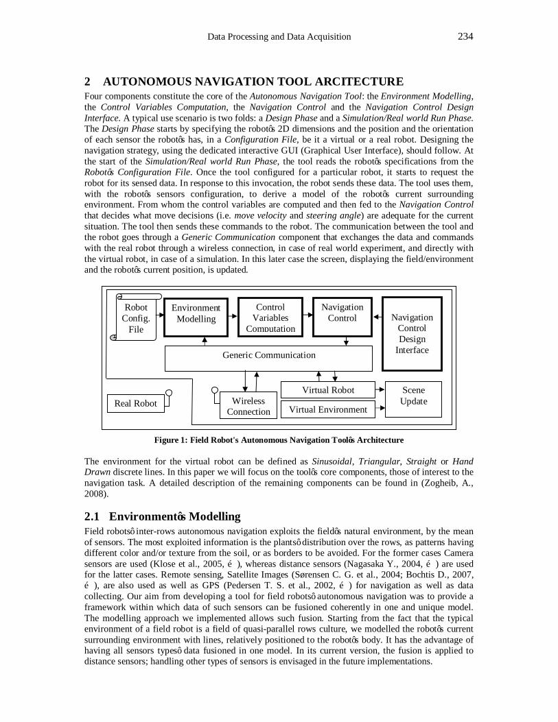
Data Processing and Data Acquisition 234
2 AUTONOMOUS NAVIGATION TOOL ARCITECTURE Four components constitute the core of the Autonomous Navigation Tool: the Environment Modelling, the Control Variables Computation, the Navigation Control and the Navigation Control Design Interface. A typical use scenario is two folds: a Design Phase and a Simulation/Real world Run Phase. The Design Phase starts by specifying the robot’s 2D dimensions and the position and the orientation of each sensor the robot’s has, in a Configuration File, be it a virtual or a real robot. Designing the navigation strategy, using the dedicated interactive GUI (Graphical User Interface), should follow. At the start of the Simulation/Real world Run Phase, the tool reads the robot’s specifications from the Robot’s Configuration File. Once the tool configured for a particular robot, it starts to request the robot for its sensed data. In response to this invocation, the robot sends these data. The tool uses them, with the robot’s sensors configuration, to derive a model of the robot’s current surrounding environment. From whom the control variables are computed and then fed to the Navigation Control that decides what move decisions (i.e. move velocity and steering angle) are adequate for the current situation. The tool then sends these commands to the robot. The communication between the tool and the robot goes through a Generic Communication component that exchanges the data and commands with the real robot through a wireless connection, in case of real world experiment, and directly with the virtual robot, in case of a simulation. In this later case the screen, displaying the field/environment and the robot’s current position, is updated.
Figure 1: Field Robot's Autonomous Navigation Tool’s Architecture
The environment for the virtual robot can be defined as Sinusoidal, Triangular, Straight or Hand Drawn discrete lines. In this paper we will focus on the tool’s core components, those of interest to the navigation task. A detailed description of the remaining components can be found in (Zogheib, A., 2008).
2.1 Environment’s Modelling Field robots’ inter-rows autonomous navigation exploits the field’s natural environment, by the mean of sensors. The most exploited information is the plants’ distribution over the rows, as patterns having different color and/or texture from the soil, or as borders to be avoided. For the former cases Camera sensors are used (Klose et al., 2005, …), whereas distance sensors (Nagasaka Y., 2004, …) are used for the latter cases. Remote sensing, Satellite Images (Sørensen C. G. et al., 2004; Bochtis D., 2007, …), are also used as well as GPS (Pedersen T. S. et al., 2002, …) for navigation as well as data collecting. Our aim from developing a tool for field robots’ autonomous navigation was to provide a framework within which data of such sensors can be fusioned coherently in one and unique model. The modelling approach we implemented allows such fusion. Starting from the fact that the typical environment of a field robot is a field of quasi-parallel rows culture, we modelled the robot’s current surrounding environment with lines, relatively positioned to the robot’s body. It has the advantage of having all sensors types’ data fusioned in one model. In its current version, the fusion is applied to distance sensors; handling other types of sensors is envisaged in the future implementations.
Scene Update
Virtual Robot Real Robot Wireless
Connection
Generic Communication
Environment Modelling
Control Variables
Computation
Navigation Control
Navigation
Control Design
Interface
Robot Config.
File
Virtual Environment
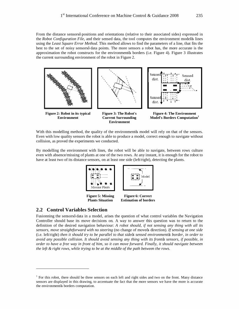
1st International Conference on Machine Control & Guidance 2008 235
From the distance sensors’ positions and orientations (relative to their associated sides) expressed in the Robot Configuration File, and their sensed data, the tool computes the environment model’s lines using the Least Square Error Method. This method allows to find the parameters of a line, that fits the best to the set of noisy sensors’ data points. The more sensors a robot has, the more accurate is the approximation the robot constructs for the environment’s borders (i.e. Figure 4). Figure 3 illustrates the current surrounding environment of the robot in Figure 2.
Figure 2: Robot in its typical
Environment Figure 3: The Robot's Current Surrounding
Environment
Figure 4: The Environment Model's Borders Computation1
With this modelling method, the quality of the environment’s model will rely on that of the sensors. Even with low quality sensors the robot is able to produce a model, correct enough to navigate without collision, as proved the experiments we conducted. By modelling the environment with lines, the robot will be able to navigate, between rows culture even with absence/missing of plants at one of the two rows. At any instant, it is enough for the robot to have at least two of its distance sensors, on at least one side (left/right), detecting the plants.
Figure 5: Missing Plants Situation
Figure 6: Correct Estimation of borders
2.2 Control Variables Selection Fusionning the sensors’ data in a model, arises the question of what control variables the Navigation Controller should base its move decisions on. A way to answer this question was to return to the definition of the desired navigation behaviour: A robot should, if not sensing any thing with all its sensors, move straightforward with no steering (no change of move’s direction). If sensing at one side (i.e. left/right) then it should try to be parallel to that side’s sensed environment’s border, in order to avoid any possible collision. It should avoid sensing any thing with its front’s sensors, if possible, in order to have a free way in front of him, so it can move forward. Finally, it should navigate between the left & right rows, while trying to be at the middle of the path between the rows.
1 For this robot, there should be three sensors on each left and right sides and two on the front. Many distance sensors are displayed in this drawing, to accentuate the fact that the more sensors we have the more is accurate the environment’s borders computation.
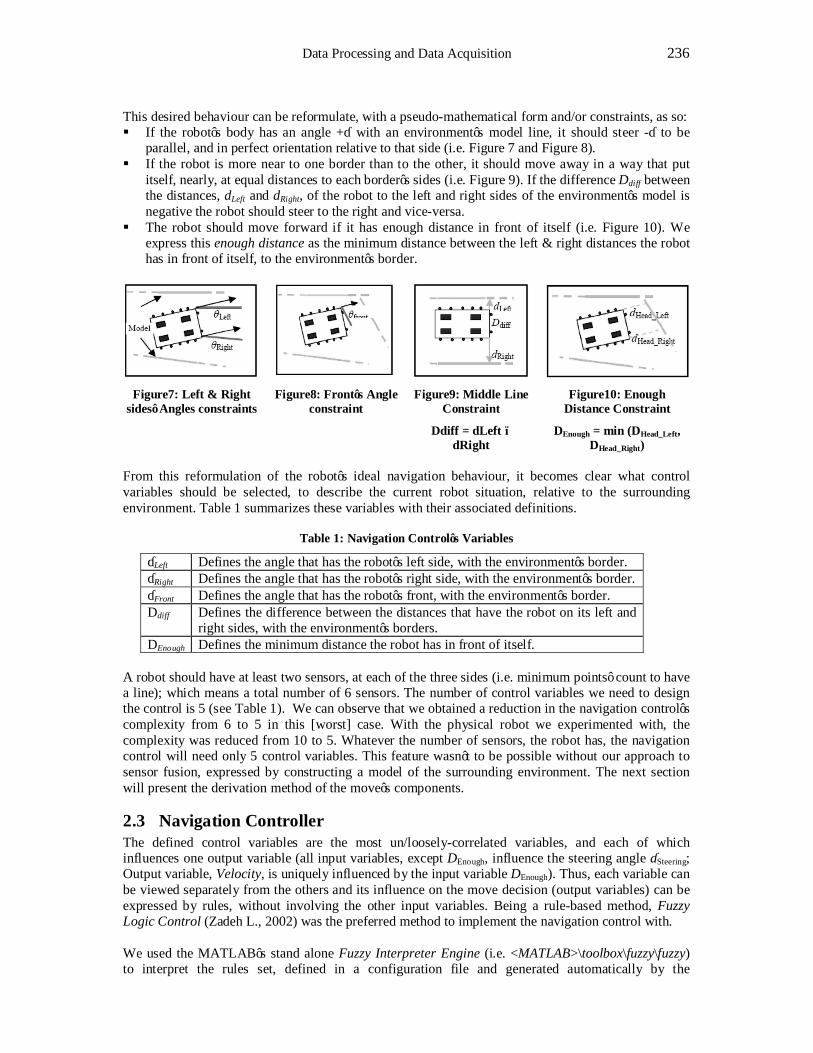
Data Processing and Data Acquisition 236
This desired behaviour can be reformulate, with a pseudo-mathematical form and/or constraints, as so: § If the robot’s body has an angle +θ with an environment’s model line, it should steer -θ to be
parallel, and in perfect orientation relative to that side (i.e. Figure 7 and Figure 8). § If the robot is more near to one border than to the other, it should move away in a way that put
itself, nearly, at equal distances to each border’s sides (i.e. Figure 9). If the difference Ddiff between the distances, dLeft and dRight, of the robot to the left and right sides of the environment’s model is negative the robot should steer to the right and vice-versa.
§ The robot should move forward if it has enough distance in front of itself (i.e. Figure 10). We express this enough distance as the minimum distance between the left & right distances the robot has in front of itself, to the environment’s border.
Figure7: Left & Right
sides’ Angles constraints Figure8: Front’s Angle
constraint Figure9: Middle Line
Constraint
Ddiff = dLeft – dRight
Figure10: Enough Distance Constraint
DEnough = min (DHead_Left, DHead_Right)
From this reformulation of the robot’s ideal navigation behaviour, it becomes clear what control variables should be selected, to describe the current robot situation, relative to the surrounding environment. Table 1 summarizes these variables with their associated definitions.
Table 1: Navigation Control’s Variables
θLeft Defines the angle that has the robot’s left side, with the environment’s border. θRight Defines the angle that has the robot’s right side, with the environment’s border. θFront Defines the angle that has the robot’s front, with the environment’s border. Ddiff Defines the difference between the distances that have the robot on its left and
right sides, with the environment’s borders. DEnough Defines the minimum distance the robot has in front of itself.
A robot should have at least two sensors, at each of the three sides (i.e. minimum points’ count to have a line); which means a total number of 6 sensors. The number of control variables we need to design the control is 5 (see Table 1). We can observe that we obtained a reduction in the navigation control’s complexity from 6 to 5 in this [worst] case. With the physical robot we experimented with, the complexity was reduced from 10 to 5. Whatever the number of sensors, the robot has, the navigation control will need only 5 control variables. This feature wasn’t to be possible without our approach to sensor fusion, expressed by constructing a model of the surrounding environment. The next section will present the derivation method of the move’s components.
2.3 Navigation Controller The defined control variables are the most un/loosely-correlated variables, and each of which influences one output variable (all input variables, except DEnough, influence the steering angle θSteering; Output variable, Velocity, is uniquely influenced by the input variable DEnough). Thus, each variable can be viewed separately from the others and its influence on the move decision (output variables) can be expressed by rules, without involving the other input variables. Being a rule-based method, Fuzzy Logic Control (Zadeh L., 2002) was the preferred method to implement the navigation control with. We used the MATLAB’s stand alone Fuzzy Interpreter Engine (i.e. <MATLAB>\toolbox\fuzzy\fuzzy) to interpret the rules set, defined in a configuration file and generated automatically by the
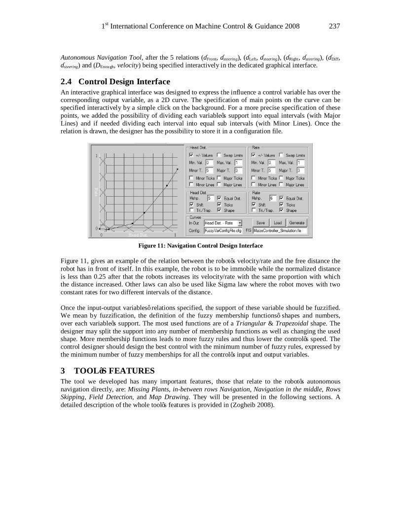
1st International Conference on Machine Control & Guidance 2008 237
Autonomous Navigation Tool, after the 5 relations (θFront, θsteering), (θLeft, θsteering), (θRight, θsteering), (θDiff, θsteering) and (DEnough, velocity) being specified interactively in the dedicated graphical interface.
2.4 Control Design Interface An interactive graphical interface was designed to express the influence a control variable has over the corresponding output variable, as a 2D curve. The specification of main points on the curve can be specified interactively by a simple click on the background. For a more precise specification of these points, we added the possibility of dividing each variable’s support into equal intervals (with Major Lines) and if needed dividing each interval into equal sub intervals (with Minor Lines). Once the relation is drawn, the designer has the possibility to store it in a configuration file.
Figure 11: Navigation Control Design Interface
Figure 11, gives an example of the relation between the robot’s velocity/rate and the free distance the robot has in front of itself. In this example, the robot is to be immobile while the normalized distance is less than 0.25 after that the robots increases its velocity/rate with the same proportion with which the distance increased. Other laws can also be used like Sigma law where the robot moves with two constant rates for two different intervals of the distance. Once the input-output variables’ relations specified, the support of these variable should be fuzzified. We mean by fuzzification, the definition of the fuzzy membership functions’ shapes and numbers, over each variable’s support. The most used functions are of a Triangular & Trapezoidal shape. The designer may split the support into any number of membership functions as well as changing the used shape. More membership functions leads to more fuzzy rules and thus lower the control’s speed. The control designer should design the best control with the minimum number of fuzzy rules, expressed by the minimum number of fuzzy memberships for all the control’s input and output variables.
3 TOOL’S FEATURES The tool we developed has many important features, those that relate to the robot’s autonomous navigation directly, are: Missing Plants, in-between rows Navigation, Navigation in the middle, Rows Skipping, Field Detection, and Map Drawing. They will be presented in the following sections. A detailed description of the whole tool’s features is provided in (Zogheib 2008).
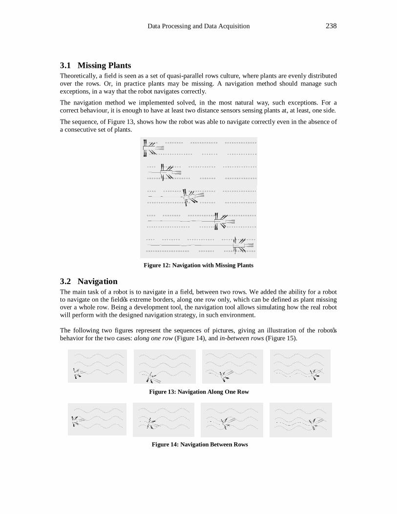
Data Processing and Data Acquisition 238
3.1 Missing Plants Theoretically, a field is seen as a set of quasi-parallel rows culture, where plants are evenly distributed over the rows. Or, in practice plants may be missing. A navigation method should manage such exceptions, in a way that the robot navigates correctly.
The navigation method we implemented solved, in the most natural way, such exceptions. For a correct behaviour, it is enough to have at least two distance sensors sensing plants at, at least, one side.
The sequence, of Figure 13, shows how the robot was able to navigate correctly even in the absence of a consecutive set of plants.
Figure 12: Navigation with Missing Plants
3.2 Navigation The main task of a robot is to navigate in a field, between two rows. We added the ability for a robot to navigate on the field’s extreme borders, along one row only, which can be defined as plant missing over a whole row. Being a development tool, the navigation tool allows simulating how the real robot will perform with the designed navigation strategy, in such environment. The following two figures represent the sequences of pictures, giving an illustration of the robot’s behavior for the two cases: along one row (Figure 14), and in-between rows (Figure 15).
Figure 13: Navigation Along One Row
Figure 14: Navigation Between Rows
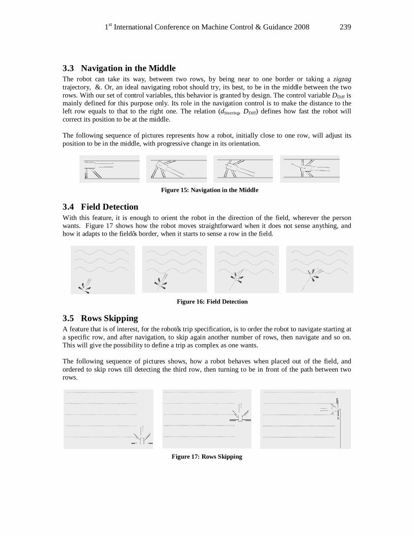
1st International Conference on Machine Control & Guidance 2008 239
3.3 Navigation in the Middle The robot can take its way, between two rows, by being near to one border or taking a zigzag trajectory, …. Or, an ideal navigating robot should try, its best, to be in the middle between the two rows. With our set of control variables, this behavior is granted by design. The control variable DDiff is mainly defined for this purpose only. Its role in the navigation control is to make the distance to the left row equals to that to the right one. The relation (θSteering, DDiff) defines how fast the robot will correct its position to be at the middle. The following sequence of pictures represents how a robot, initially close to one row, will adjust its position to be in the middle, with progressive change in its orientation.
Figure 15: Navigation in the Middle
3.4 Field Detection With this feature, it is enough to orient the robot in the direction of the field, wherever the person wants. Figure 17 shows how the robot moves straightforward when it does not sense anything, and how it adapts to the field’s border, when it starts to sense a row in the field.
Figure 16: Field Detection
3.5 Rows Skipping A feature that is of interest, for the robot’s trip specification, is to order the robot to navigate starting at a specific row, and after navigation, to skip again another number of rows, then navigate and so on. This will give the possibility to define a trip as complex as one wants. The following sequence of pictures shows, how a robot behaves when placed out of the field, and ordered to skip rows till detecting the third row, then turning to be in front of the path between two rows.
Figure 17: Rows Skipping
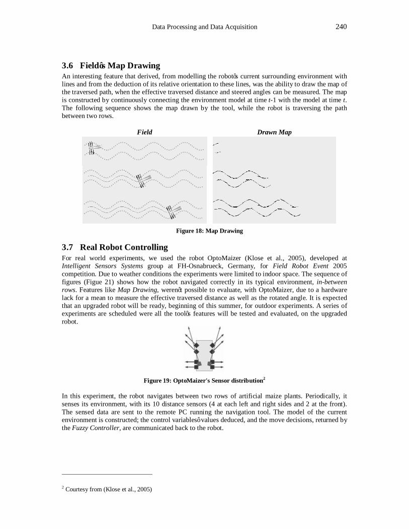
Data Processing and Data Acquisition 240
3.6 Field’s Map Drawing An interesting feature that derived, from modelling the robot’s current surrounding environment with lines and from the deduction of its relative orientation to these lines, was the ability to draw the map of the traversed path, when the effective traversed distance and steered angles can be measured. The map is constructed by continuously connecting the environment model at time t-1 with the model at time t. The following sequence shows the map drawn by the tool, while the robot is traversing the path between two rows.
Field Drawn Map
Figure 18: Map Drawing
3.7 Real Robot Controlling For real world experiments, we used the robot OptoMaizer (Klose et al., 2005), developed at Intelligent Sensors Systems group at FH-Osnabrueck, Germany, for Field Robot Event 2005 competition. Due to weather conditions the experiments were limited to indoor space. The sequence of figures (Figue 21) shows how the robot navigated correctly in its typical environment, in-between rows. Features like Map Drawing, weren’t possible to evaluate, with OptoMaizer, due to a hardware lack for a mean to measure the effective traversed distance as well as the rotated angle. It is expected that an upgraded robot will be ready, beginning of this summer, for outdoor experiments. A series of experiments are scheduled were all the tool’s features will be tested and evaluated, on the upgraded robot.
Figure 19: OptoMaizer's Sensor distribution2
In this experiment, the robot navigates between two rows of artificial maize plants. Periodically, it senses its environment, with its 10 distance sensors (4 at each left and right sides and 2 at the front). The sensed data are sent to the remote PC running the navigation tool. The model of the current environment is constructed; the control variables’ values deduced, and the move decisions, returned by the Fuzzy Controller, are communicated back to the robot.
2 Courtesy from (Klose et al., 2005)
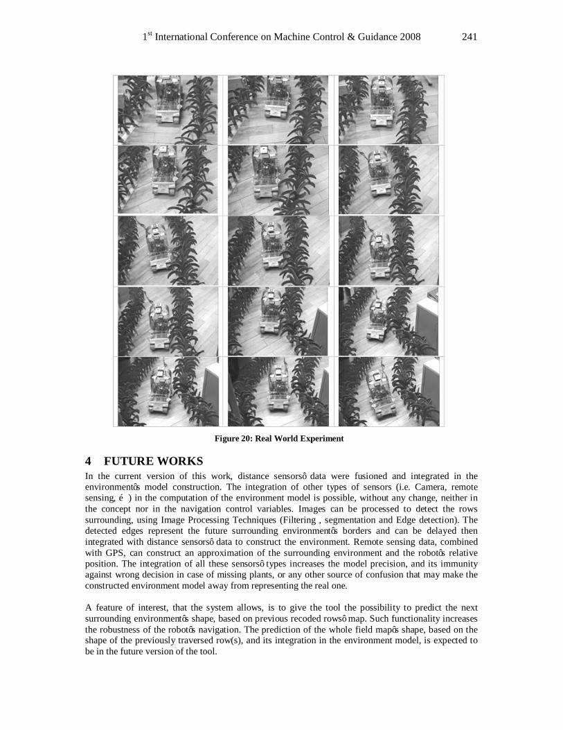
1st International Conference on Machine Control & Guidance 2008 241
Figure 20: Real World Experiment
4 FUTURE WORKS In the current version of this work, distance sensors’ data were fusioned and integrated in the environment’s model construction. The integration of other types of sensors (i.e. Camera, remote sensing, …) in the computation of the environment model is possible, without any change, neither in the concept nor in the navigation control variables. Images can be processed to detect the rows surrounding, using Image Processing Techniques (Filtering , segmentation and Edge detection). The detected edges represent the future surrounding environment’s borders and can be delayed then integrated with distance sensors’ data to construct the environment. Remote sensing data, combined with GPS, can construct an approximation of the surrounding environment and the robot’s relative position. The integration of all these sensors’ types increases the model precision, and its immunity against wrong decision in case of missing plants, or any other source of confusion that may make the constructed environment model away from representing the real one. A feature of interest, that the system allows, is to give the tool the possibility to predict the next surrounding environment’s shape, based on previous recoded rows’ map. Such functionality increases the robustness of the robot’s navigation. The prediction of the whole field map’s shape, based on the shape of the previously traversed row(s), and its integration in the environment model, is expected to be in the future version of the tool.

Data Processing and Data Acquisition 242
5 CONCLUSIONS In this paper, we presented an Autonomous Navigation tool, for virtual and real robots; with which the design of the robot’s navigation strategy is done interactively using a graphical interface. Five relations, between a defined set of control variables and the move commands, define the robot navigation’s behaviour. In its current version, the tool integrates distance sensors data; the integration of other types of sensors does not require changes in the modelling nor in the defined control variables. Many features of the tool were presented, like Field Map Drawing, Missing Plants, Rows Skipping, Navigation Strategies’ Design, …. Experiments conducted with a real robot, were in phase with the simulation results.
ACKNOWLEDGEMENTS The author would like to thank Pr. Bengt Oelmann and Pr. Arno Ruckelshausen for their encouragement during his research done in their respective groups Things That Think and Intelligent Sensors Systems at Mid Sweden University and the University of Applied Sciences (FH-Osnabrueck, Germany). Many thanks go too, to Eng. Ralph Klose for making available OptoMaizer for the experiments with a real robot.
REFERENCES Trebinski G., Bozsik B.: Autonomous unit for one row seeding. Conf. Proc. of 5th Int. Conference Microprocessor Systems in Agriculture. PW Plock, p: 225–234, 2004.
Van Evert F. K., Van Der Heijden G. W., Lotz L. A.P., Polder G., Lamaker A., De Jong A., Kuyper M. C., Groendijk E. J.K., Neeteson J. J., and Van Der Zalm T.: A Mobile Field Robot with Vision-Based Detection of Volunteer Potato Plants in a Corn Crop . Weed Science Society of America, Weed Technology Journal, Vol. 20, Issue 4, pp. 853–861, 2006.
Katupitiya J., Eaton R., Rodnay G., Cole A., Meyer C.: Automation of an Agricultural Tractor for Fruit Picking. IEEE Int. Conf. on Robotics and Automation, ICRA 2005, April 18-22, Barcelona, Spain, 2005.
Edan, Y.; Rogozin, D.; Flash, T.; Miles, G.E.: Robotic melon harvesting. IEEE Transactions on Robotics and Automation, Volume 16, Issue 6, p:831 – 835, Dec 2000.
Nagasaka Y., Zhang Q., Kanetani Y., Umeda N.: Design of an autonomous field watching-dog for information collection. 5th Int. Conf. Microprocessor Systems in Agriculture. PW Plock, p:120–130, 2004.
Pedersen T. S., Nielsen K. M., Andersen P., Bak T., Nielsen J. D.: Development of an Autonomous Vehicle for Weed and Crop Registration. Proceedings of the Int. Conf. on Agricultural Engineering, AgEng-2002, Budapest, Hungary 2002, 2002.
Sørensen C. G., Bak T., Jørgensen R.N. Mission Planner for Agricultural Robotics. Proc. AgEng 2004 Leuven, Belgium Int. Conf. on Agricultural Engineering. Abstract in Book of Abstracts, p.894-895, 2004.
Bochtis D., Vougioukas S., Tsatsarelis C. and Ampatzidis Y.: Field Operation Planning for Agricultural Vehicles: A Hierarchical Modeling Framework. Agricultural Engineering International: the CIGR Ejournal. Manuscript PM 06 021. Vol. IX. February, 2007.
Nagasaka Y., Grift T. E., Zhang Q., Knetani Y., Umeda N., Kokuryu T.: Development of AGBO, A Laser Scanner Guided Autonomous Crop Scouting Robot. Proc. of the 2nd Field Robot Event 2004, ISBN: 90-6754-818-9, p: 1-9, 2004.

1st International Conference on Machine Control & Guidance 2008 243
Zadeh L.: From computing with numbers to computing with words — from manipulation of measurements to manipulation of perceptions, Int. Journal of Applied Math and Computer Science, pp. 307-324, vol. 12, no. 3, 2002.
Zogheib A.: Field Robot Autonomous Navigation – Sensors Fusion-based. Mid Sweden University, Master thesis 2008.
Klose R. and Meier M.: Entwicklung eines autonomen Roboters auf Basis eines Multisensorkonzeptes diploma thesis University of Applied Sciences, 2005
Field Robot Event Contest: www.fieldrobot.de, last accessed 25/3/2008. * Ali ZOGHEIB, Mid Sweden University, Department of Information Technology and Media, Building S, SE-851 70 Sundsvall, Sweden.

Data Processing and Data Acquisition 244
1st International Conference on Machine Control & Guidance 2008 245
Kinematic 3D Laser Scanning for Road or Railway Construction Surveys
Gunnar GRÄFE*
3D Mapping Solutions GmbH, Germany [email protected]
Abstract Kinematic laser-scanning has been a key application for the Mobile Road Mapping System (MoSES) since a couple of years. The development of kinematic survey methods has reached a level, that allows the use of kinematic survey technology for high precision applications. Replacing static tachymetric surveys on the road itself, kinematic methods are more and more applied for construction projects. The technology is used for rapid airfield monitoring as well as an increasing number of highway construction projects or high-precision railway tunnel surveys. The resulting data is acquired and generated with static survey accuracy, but much faster and with much higher resolution - if needed. The results represent the basic survey information for planning tasks or high precision machine guidance. Within the last months, the next development steps have been taken with the aim to join static and kinematic scanner technology. High precision static 3D laser scanners, which are capable of performing profiling measurement modes, can now be used with the MoSES system. A special mounting and rapid-calibration procedure is required to enable the use of e.g. Zoller&Fröhlich or FARO 3D laser scanners for kinematic high precision applications. Pilot projects to demonstrate the capabilities of this new 3D laser scanner survey method have been high-speed surveys of automobile industry test sites or subway tunnel surveys. The new developments were completed by adding infrared photogrammetric camera technology to the MOSES system, which enables full night vision survey capacity, which is of high interest for tunnel or airfield monitoring applications. Keywords 3D Laser scanner, kinematic survey, digital road surface models, milling machine guidance
1 INTRODUCTION Road or rail construction tasks require reliable survey data. Due to highly increasing traffic load, combined with the age structure of the road or rail network, the responsible administrations are forced to put the main emphasis of maintenance activities into projects to ensure quality, safety and sufficient traffic capacity. The negative influences of maintenance tasks on the traffic flow, such as road blockings etc., have to be kept as short as possible. This is even more important for the necessary substantial engineering survey work, that is needed in advance to capture basic data for construction planning and preparation. For this task, kinematic survey methods offer new high-precision survey possibilities. Mobile technology minimizes the survey effort to capture the required data along existing roads and railways. Only a comparatively short driving time is needed for data collection, while the traffic flow is not significantly affected. This approach reduces both costs and safety risks. For these reasons, the capabilities of the Mobile-Road-Mapping-System (MoSES) have been expanded, so that high-precision engineering survey projects can be carried out with this kinematic survey system. 3D Mapping Solutions GmbH does service projects and develops and sells the necessary hardware and software to successfully operate mobile mapping systems. The latest developments enable the full kinematic usage of high performance 3D scanners, that are capable of profiling measurement modes. The kinematic survey with laser scanners plays a major role for new possibilities of construction machine control and guidance based on the kinematic survey results. This paper presents a new concept for road construction machine control based on digital road surface models.
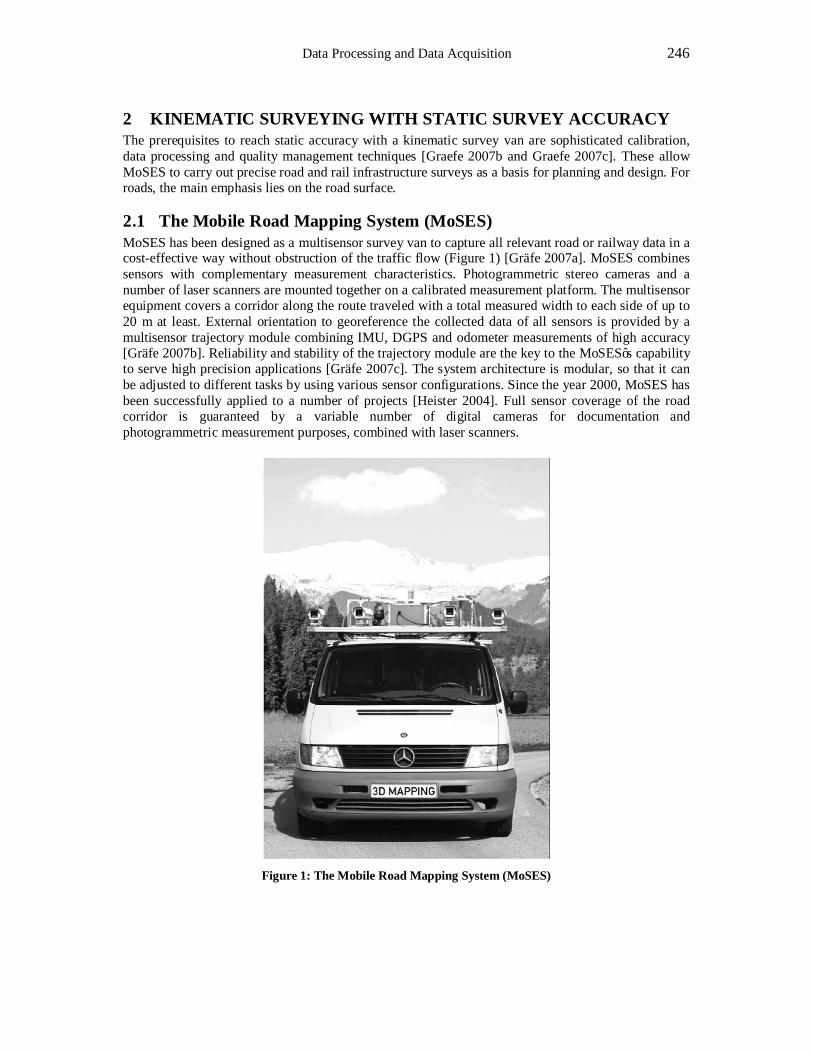
Data Processing and Data Acquisition 246
2 KINEMATIC SURVEYING WITH STATIC SURVEY ACCURACY The prerequisites to reach static accuracy with a kinematic survey van are sophisticated calibration, data processing and quality management techniques [Graefe 2007b and Graefe 2007c]. These allow MoSES to carry out precise road and rail infrastructure surveys as a basis for planning and design. For roads, the main emphasis lies on the road surface.
2.1 The Mobile Road Mapping System (MoSES) MoSES has been designed as a multisensor survey van to capture all relevant road or railway data in a cost-effective way without obstruction of the traffic flow (Figure 1) [Gräfe 2007a]. MoSES combines sensors with complementary measurement characteristics. Photogrammetric stereo cameras and a number of laser scanners are mounted together on a calibrated measurement platform. The multisensor equipment covers a corridor along the route traveled with a total measured width to each side of up to 20 m at least. External orientation to georeference the collected data of all sensors is provided by a multisensor trajectory module combining IMU, DGPS and odometer measurements of high accuracy [Gräfe 2007b]. Reliability and stability of the trajectory module are the key to the MoSES’s capability to serve high precision applications [Gräfe 2007c]. The system architecture is modular, so that it can be adjusted to different tasks by using various sensor configurations. Since the year 2000, MoSES has been successfully applied to a number of projects [Heister 2004]. Full sensor coverage of the road corridor is guaranteed by a variable number of digital cameras for documentation and photogrammetric measurement purposes, combined with laser scanners.
Figure 1: The Mobile Road Mapping System (MoSES)
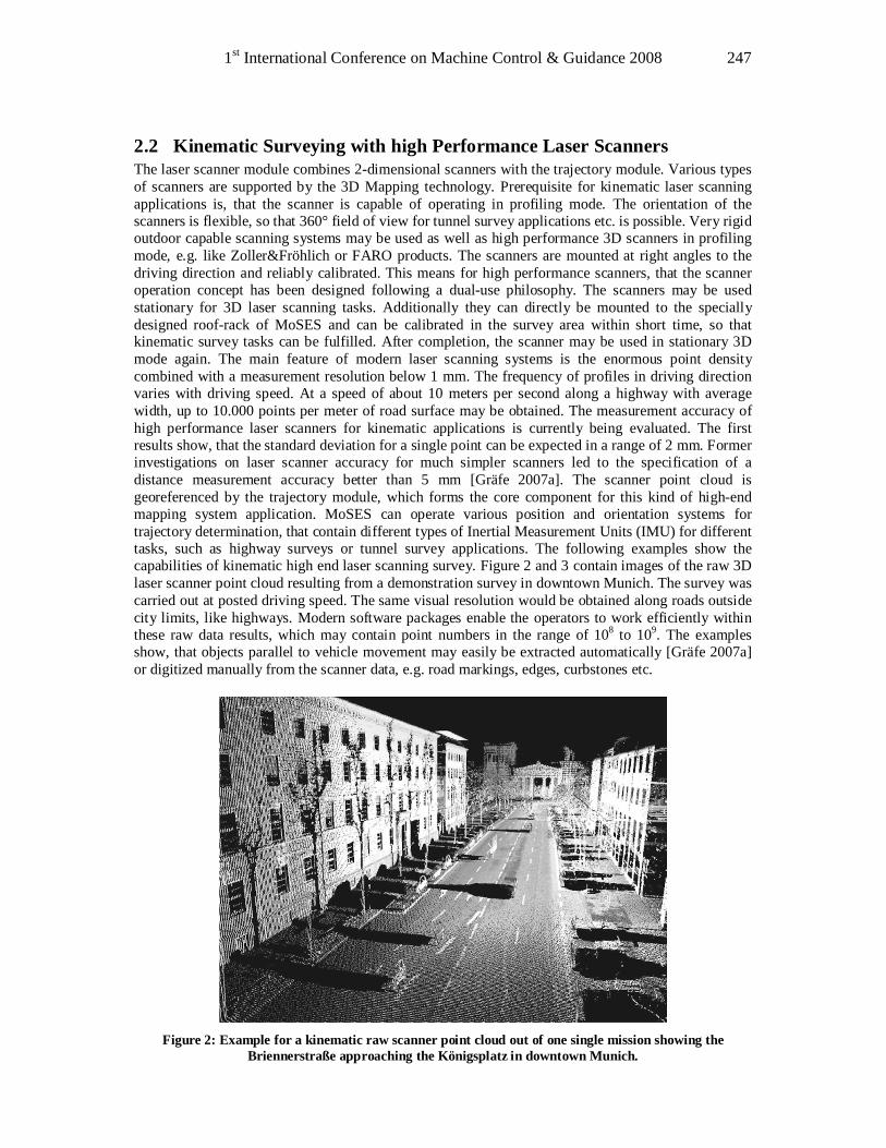
1st International Conference on Machine Control & Guidance 2008 247
2.2 Kinematic Surveying with high Performance Laser Scanners The laser scanner module combines 2-dimensional scanners with the trajectory module. Various types of scanners are supported by the 3D Mapping technology. Prerequisite for kinematic laser scanning applications is, that the scanner is capable of operating in profiling mode. The orientation of the scanners is flexible, so that 360° field of view for tunnel survey applications etc. is possible. Very rigid outdoor capable scanning systems may be used as well as high performance 3D scanners in profiling mode, e.g. like Zoller&Fröhlich or FARO products. The scanners are mounted at right angles to the driving direction and reliably calibrated. This means for high performance scanners, that the scanner operation concept has been designed following a dual-use philosophy. The scanners may be used stationary for 3D laser scanning tasks. Additionally they can directly be mounted to the specially designed roof-rack of MoSES and can be calibrated in the survey area within short time, so that kinematic survey tasks can be fulfilled. After completion, the scanner may be used in stationary 3D mode again. The main feature of modern laser scanning systems is the enormous point density combined with a measurement resolution below 1 mm. The frequency of profiles in driving direction varies with driving speed. At a speed of about 10 meters per second along a highway with average width, up to 10.000 points per meter of road surface may be obtained. The measurement accuracy of high performance laser scanners for kinematic applications is currently being evaluated. The first results show, that the standard deviation for a single point can be expected in a range of 2 mm. Former investigations on laser scanner accuracy for much simpler scanners led to the specification of a distance measurement accuracy better than 5 mm [Gräfe 2007a]. The scanner point cloud is georeferenced by the trajectory module, which forms the core component for this kind of high-end mapping system application. MoSES can operate various position and orientation systems for trajectory determination, that contain different types of Inertial Measurement Units (IMU) for different tasks, such as highway surveys or tunnel survey applications. The following examples show the capabilities of kinematic high end laser scanning survey. Figure 2 and 3 contain images of the raw 3D laser scanner point cloud resulting from a demonstration survey in downtown Munich. The survey was carried out at posted driving speed. The same visual resolution would be obtained along roads outside city limits, like highways. Modern software packages enable the operators to work efficiently within these raw data results, which may contain point numbers in the range of 108 to 109. The examples show, that objects parallel to vehicle movement may easily be extracted automatically [Gräfe 2007a] or digitized manually from the scanner data, e.g. road markings, edges, curbstones etc.
Figure 2: Example for a kinematic raw scanner point cloud out of one single mission showing the
Briennerstraße approaching the Königsplatz in downtown Munich.
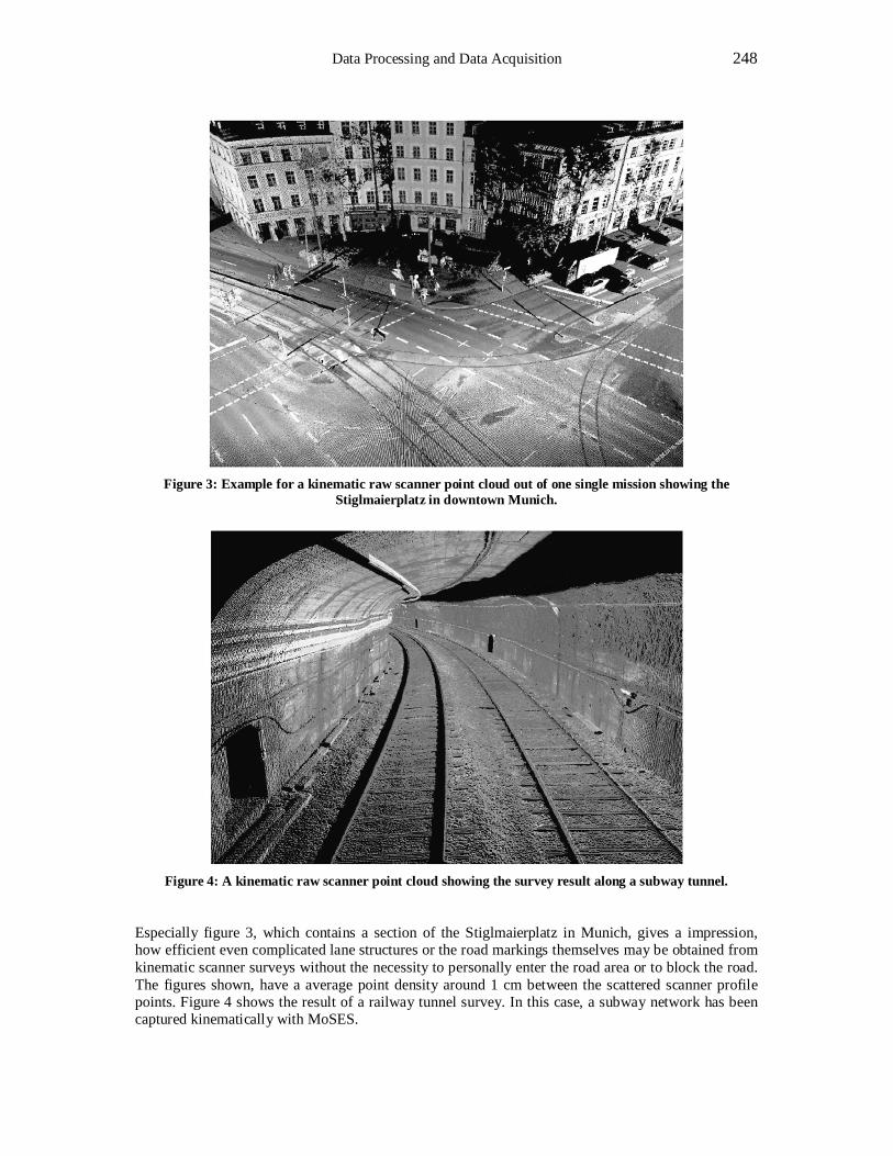
Data Processing and Data Acquisition 248
Figure 3: Example for a kinematic raw scanner point cloud out of one single mission showing the
Stiglmaierplatz in downtown Munich.
Figure 4: A kinematic raw scanner point cloud showing the survey result along a subway tunnel.
Especially figure 3, which contains a section of the Stiglmaierplatz in Munich, gives a impression, how efficient even complicated lane structures or the road markings themselves may be obtained from kinematic scanner surveys without the necessity to personally enter the road area or to block the road. The figures shown, have a average point density around 1 cm between the scattered scanner profile points. Figure 4 shows the result of a railway tunnel survey. In this case, a subway network has been captured kinematically with MoSES.
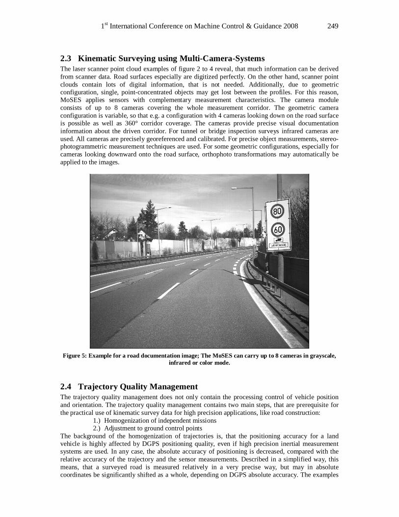
1st International Conference on Machine Control & Guidance 2008 249
2.3 Kinematic Surveying using Multi-Camera-Systems The laser scanner point cloud examples of figure 2 to 4 reveal, that much information can be derived from scanner data. Road surfaces especially are digitized perfectly. On the other hand, scanner point clouds contain lots of digital information, that is not needed. Additionally, due to geometric configuration, single, point-concentrated objects may get lost between the profiles. For this reason, MoSES applies sensors with complementary measurement characteristics. The camera module consists of up to 8 cameras covering the whole measurement corridor. The geometric camera configuration is variable, so that e.g. a configuration with 4 cameras looking down on the road surface is possible as well as 360° corridor coverage. The cameras provide precise visual documentation information about the driven corridor. For tunnel or bridge inspection surveys infrared cameras are used. All cameras are precisely georeferenced and calibrated. For precise object measurements, stereo-photogrammetric measurement techniques are used. For some geometric configurations, especially for cameras looking downward onto the road surface, orthophoto transformations may automatically be applied to the images.
Figure 5: Example for a road documentation image; The MoSES can carry up to 8 cameras in grayscale,
infrared or color mode.
2.4 Trajectory Quality Management The trajectory quality management does not only contain the processing control of vehicle position and orientation. The trajectory quality management contains two main steps, that are prerequisite for the practical use of kinematic survey data for high precision applications, like road construction:
1.) Homogenization of independent missions 2.) Adjustment to ground control points
The background of the homogenization of trajectories is, that the positioning accuracy for a land vehicle is highly affected by DGPS positioning quality, even if high precision inertial measurement systems are used. In any case, the absolute accuracy of positioning is decreased, compared with the relative accuracy of the trajectory and the sensor measurements. Described in a simplified way, this means, that a surveyed road is measured relatively in a very precise way, but may in absolute coordinates be significantly shifted as a whole, depending on DGPS absolute accuracy. The examples
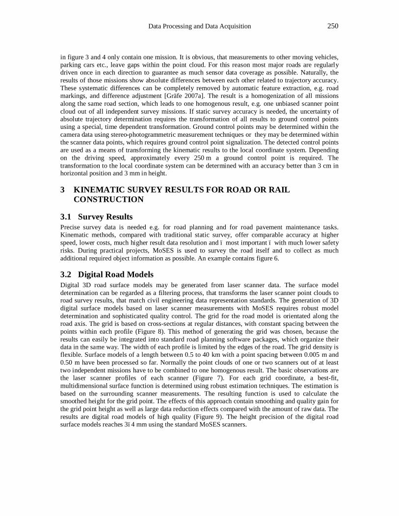
Data Processing and Data Acquisition 250
in figure 3 and 4 only contain one mission. It is obvious, that measurements to other moving vehicles, parking cars etc., leave gaps within the point cloud. For this reason most major roads are regularly driven once in each direction to guarantee as much sensor data coverage as possible. Naturally, the results of those missions show absolute differences between each other related to trajectory accuracy. These systematic differences can be completely removed by automatic feature extraction, e.g. road markings, and difference adjustment [Gräfe 2007a]. The result is a homogenization of all missions along the same road section, which leads to one homogenous result, e.g. one unbiased scanner point cloud out of all independent survey missions. If static survey accuracy is needed, the uncertainty of absolute trajectory determination requires the transformation of all results to ground control points using a special, time dependent transformation. Ground control points may be determined within the camera data using stereo-photogrammetric measurement techniques or they may be determined within the scanner data points, which requires ground control point signalization. The detected control points are used as a means of transforming the kinematic results to the local coordinate system. Depending on the driving speed, approximately every 250 m a ground control point is required. The transformation to the local coordinate system can be determined with an accuracy better than 3 cm in horizontal position and 3 mm in height.
3 KINEMATIC SURVEY RESULTS FOR ROAD OR RAIL CONSTRUCTION
3.1 Survey Results Precise survey data is needed e.g. for road planning and for road pavement maintenance tasks. Kinematic methods, compared with traditional static survey, offer comparable accuracy at higher speed, lower costs, much higher result data resolution and – most important – with much lower safety risks. During practical projects, MoSES is used to survey the road itself and to collect as much additional required object information as possible. An example contains figure 6.
3.2 Digital Road Models Digital 3D road surface models may be generated from laser scanner data. The surface model determination can be regarded as a filtering process, that transforms the laser scanner point clouds to road survey results, that match civil engineering data representation standards. The generation of 3D digital surface models based on laser scanner measurements with MoSES requires robust model determination and sophisticated quality control. The grid for the road model is orientated along the road axis. The grid is based on cross-sections at regular distances, with constant spacing between the points within each profile (Figure 8). This method of generating the grid was chosen, because the results can easily be integrated into standard road planning software packages, which organize their data in the same way. The width of each profile is limited by the edges of the road. The grid density is flexible. Surface models of a length between 0.5 to 40 km with a point spacing between 0.005 m and 0.50 m have been processed so far. Normally the point clouds of one or two scanners out of at least two independent missions have to be combined to one homogenous result. The basic observations are the laser scanner profiles of each scanner (Figure 7). For each grid coordinate, a best-fit, multidimensional surface function is determined using robust estimation techniques. The estimation is based on the surrounding scanner measurements. The resulting function is used to calculate the smoothed height for the grid point. The effects of this approach contain smoothing and quality gain for the grid point height as well as large data reduction effects compared with the amount of raw data. The results are digital road models of high quality (Figure 9). The height precision of the digital road surface models reaches 3–4 mm using the standard MoSES scanners.
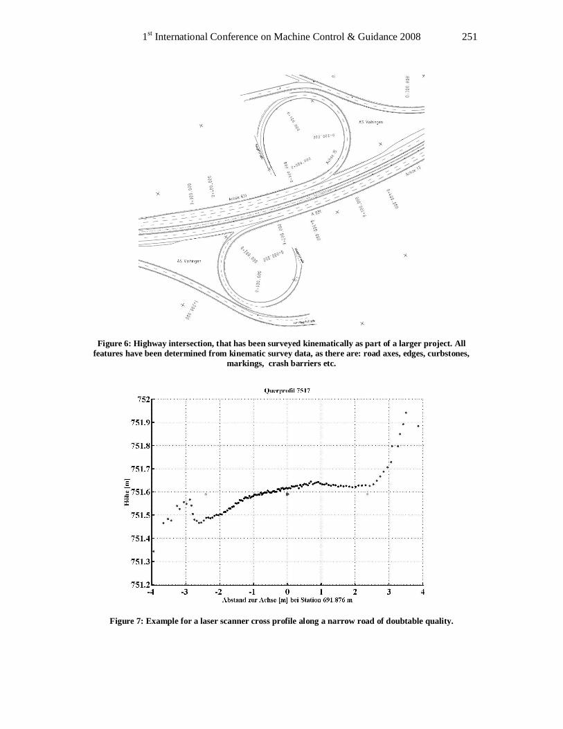
1st International Conference on Machine Control & Guidance 2008 251
Figure 6: Highway intersection, that has been surveyed kinematically as part of a larger project. All
features have been determined from kinematic survey data, as there are: road axes, edges, curbstones, markings, crash barriers etc.
Figure 7: Example for a laser scanner cross profile along a narrow road of doubtable quality.
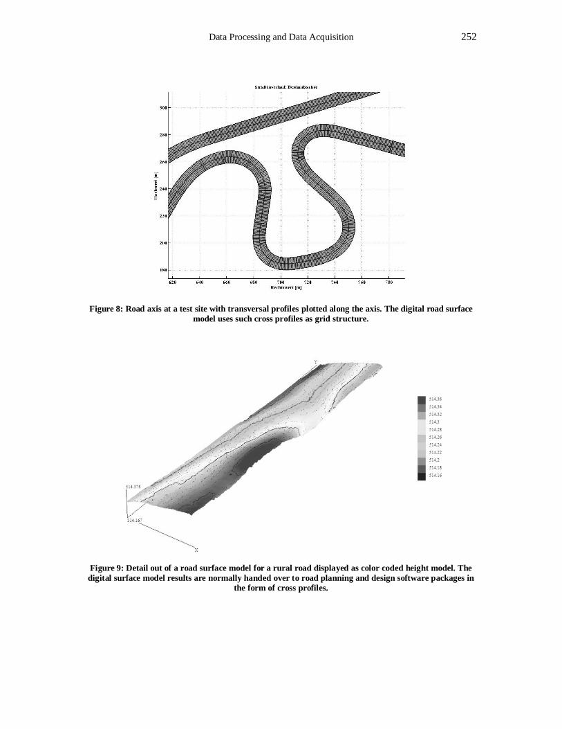
Data Processing and Data Acquisition 252
Figure 8: Road axis at a test site with transversal profiles plotted along the axis. The digital road surface
model uses such cross profiles as grid structure.
Figure 9: Detail out of a road surface model for a rural road displayed as color coded height model. The
digital surface model results are normally handed over to road planning and design software packages in the form of cross profiles.
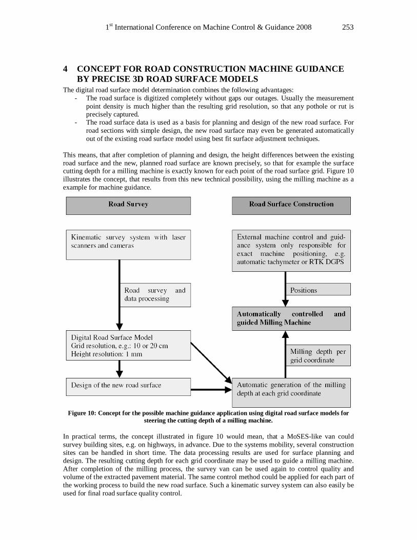
1st International Conference on Machine Control & Guidance 2008 253
4 CONCEPT FOR ROAD CONSTRUCTION MACHINE GUIDANCE BY PRECISE 3D ROAD SURFACE MODELS
The digital road surface model determination combines the following advantages: - The road surface is digitized completely without gaps our outages. Usually the measurement
point density is much higher than the resulting grid resolution, so that any pothole or rut is precisely captured.
- The road surface data is used as a basis for planning and design of the new road surface. For road sections with simple design, the new road surface may even be generated automatically out of the existing road surface model using best fit surface adjustment techniques.
This means, that after completion of planning and design, the height differences between the existing road surface and the new, planned road surface are known precisely, so that for example the surface cutting depth for a milling machine is exactly known for each point of the road surface grid. Figure 10 illustrates the concept, that results from this new technical possibility, using the milling machine as a example for machine guidance.
Figure 10: Concept for the possible machine guidance application using digital road surface models for steering the cutting depth of a milling machine.
In practical terms, the concept illustrated in figure 10 would mean, that a MoSES-like van could survey building sites, e.g. on highways, in advance. Due to the systems mobility, several construction sites can be handled in short time. The data processing results are used for surface planning and design. The resulting cutting depth for each grid coordinate may be used to guide a milling machine. After completion of the milling process, the survey van can be used again to control quality and volume of the extracted pavement material. The same control method could be applied for each part of the working process to build the new road surface. Such a kinematic survey system can also easily be used for final road surface quality control.
Data Processing and Data Acquisition 254
5 CONCLUSIONS Kinematic surveys with high precision laser scanners open a number of new survey application areas for road or rail construction tasks. In this paper some road construction examples have been presented. The result quality has been proved under practical survey conditions. A standard deviation for the scanner points of 0.004 m in height is obtained even with comparably simple scanners. High performance scanners are expected to reach 0.002 m height accuracy. The huge point resolution and precision of the scanner data on the road surface leads to ideas for new concepts for machine control and guidance, that have been illustrated using a milling machine as an example. Future developments will concentrate on this field. As far as scanner technology is concerned, calibration and scanner technology evaluation will also require some development effort in future.
REFERENCES Books: [Gräfe 2007a] GRÄFE, G.: Kinematische Anwendungen von Laserscannern im Straßenraum, PhD thesis, Universität der Bundeswehr München, Institut für Geodäsie, Neubiberg, 2007. Journal articles: [Gräfe 2007b] GRÄFE, G.: High precision kinematic surveying with laser scanners, Journal of Applied Geodesy, Editors in Chief: H.Kahmen / C. Rizos, Walter de Gruyter Verlag, 4/2007, p. 185-199, 2007.
[Gräfe 2007c] GRÄFE, G.: Quality Management in Kinematic Laser Scanning Applications, Proceedings 5th International Symposium on Mobile Mapping Technology (on CD), Padua, 2007.
[Heister 2004] HEISTER, H., GRÄFE, G.: Projekterfahrungen beim Einsatz der kinematischen Messsysteme KiSS und MoSES, 58. DVW-Seminar: kinematische Messmethoden – Vermessung in Bewegung, Volume 45 of DVW-Schriftenreihe, 95–111, Stuttgart, Wissner Verlag, 2004.
* Dr.-Ing. Gunnar Gräfe, 3D Mapping Solutions GmbH, Talanger 4a, 82041 Oberhaching, Germany.

Control Process and Control Algorithm

1st International Conference on Machine Control & Guidance 2008 257
Universal Developer Platform for Machine Control Applications
Hansjörg PETSCHKO*
MOBA GmbH, Switzerland [email protected]
Abstract Over the last two decades terrestrial and global 3D measurement sensors in the field of engineering geodesy have seen a significant upturn. With modern measurement techniques, a 3D trajectory of a moving object can be determined within a few centimetres of accuracy (GNSS). Under certain circumstances and with accuracies of within five to ten millimetres can be achieved (tracking total station). Additional sensors are rotation ring laser, orientation sensors, INS, or inclination sensors. New application areas have now been created in the fields of construction, mining and agriculture. The basic similarities between the applications in the above mentioned fields imply the development of a versatile and easily adaptable hardware and software platform. Furthermore 1D, 2D or 3D guidance or control of complex machinery generally includes heavy and diverse computational work and sophisticated user interaction. This suggests the use of embedded versions of general purpose computers and operating systems. The company MOBA is developing a Machine Control Platform which is intended to be the basis for solutions mainly in construction. Since many of the tasks in machine control are comparable to tasks in general robotics, this platform is based on a robotic framework which is available for several OS and which is publicly accessible. This framework, called The ViViVerse (the vivid universe), shall enable quick development of applications that read in sensor data, deduce actions based on built in rules and finally control actuators. Additionally communication between single units is one of the main goals. Information is given about common tasks in building machine control applications, like performance considerations and usability in a rough working environment. A second point will be the features and implementation of the ViViVerse framework. Keywords Machine automation, control software, extensible platform
1 INTRODUCTION The development of more and more sophisticated sensors and computer technology together with putting them into robust hardware during the last few years has enabled the use of techniques in rough environments such as industry, construction or agriculture, that seemed to be reserved only to hi-tech expert and high maintenance areas a few years ago. The higher complexity and performance increase of the modern equipment also require a complex and sophisticated control software, which can integrate all these abilities. From our experience there is a basic set of software components that is necessary to do machine guidance or control (consequently we’ll refer to both using the term ‘machine automation’).

Control Process and Control Algorithm 258
The basic workflow that has to be built is:
• collect data of the environment using any type of sensors • process the input data based on built in rules and a given data set (design) • display hints (for guidance) or control actuators (e.g. engines or valves)
2 MACHINE AUTOMATION REQUIREMENTS
2.1 Hardware requirements The hardware which is necessary to accomplish the basic workflow comprises:
• Sensors • Data transport devices (Cables or wireless transmitters) • Control device • Display • Actuators • Working tool
2.2 Basic Software requirements With these pieces of hardware given, the software has to be able to do the following:
2.2.1 Sensor handling Since many of the tasks in construction depend on the 3D position, position sensors like a GNSS or TPS and slope sensors will very likely be found on an automated construction machine. It might be necessary for the SW to configure them remotely. The control device might be an embedded controller or some PC derived computer hardware. The measurement data is transferred from the sensors to the control device using a bus system. Bus types widely used in automation are e.g. Serial or CAN, but could be Ethernet as well. The control device must be able to handle the protocol that is implied by the bus system and it must also interpret the protocol determined by the sensor, which usually is manufacturer specific. It is a good idea to strictly separate both protocols for testing and extensibility reasons.
2.2.2 Design handling Once the input data has been collected, it must be processed by the control device. In order to enable the device to do this processing, the desired data (design data set) must be supplied. In the simplest case this may only be one value e.g. for temperature control, but it might also be as complex as a spatial surface description (3D data), which is exactly what construction machine automation is using. In the past this design data was often supplied physically by one or more real stringlines, providing height and direction information (in simple cases a reference plane is sufficient), which was transferred to the control device by different types of sensors. During the last few years control applications have become more and more numerous, that are holding the design data in the controller memory as a mathematical representation. The type of representation depends on the control application, examples are:
• TIN (Triangulated Irregular network) The design surface is described by a set of triangles (as used in computer games). This type of representation is best used for area-like and irregular surfaces like a golf court or a waste disposal site. The resulting data set might be very large depending on how detailed the surface description must be.

1st International Conference on Machine Control & Guidance 2008 259
• Stringlines The design is represented by a smooth surface described by bounding lines, which consist of a set of well known mathematical curves like straight lines, arcs and clothoids. The bounding lines are the mathematical equivalence of the physical stringlines, hence the name. This type of representation is best used for line-like construction tasks like roads or ditches. The size of the data set is usually smaller than with TINs and independent from the demanded accuracy, because the description by mathematical functions is the natural format of a road design and thus no discretisation and approximation are necessary. The calculation of a 3D position however will need more computation power than with a TIN. It should be noted that the physical string lines too are no more than approximations by straight lines, except in very tight curves where flexible rods are used.
One possibility to create the design is on the fly within the control application, which is possible only for easy surfaces (e.g. ramp) and which needs more complex user interaction than a traditional panel might provide. The other possibility are dedicated external software tools which are not in the scope of this paper. The latter however poses the problem for the control application of reading the output data from the external tools. Since there are a lot of different formats in use (often only locally known), either deliberate self restriction to a common exchange format or the definition of a plug-in interface seem to be a viable way to deal with this problem.
2.2.3 Machine handling The next step in the workflow is the finding of the right machine action that corresponds to the current position. This action can either be derived directly from the position alone (e.g. open a valve for the output of colour or fertilizer) or it can be the result of a real time comparison between the measured is-values and the stored design-values (e.g. regarding to position and height). This is the crucial point of machine automation because it requires in-depth knowledge of the dynamic characteristics of the machine and of the best way to combine the measurement data from the (well) chosen set of sensors. And finally the control values which define the actions must be sent to the actuators or – translated for human perception - to a display. The values either go either directly to the actuators like electric motors, valves etc. or to other control devices that do their own computations before the motors or valves are accessed. As with the sensors the data is sent in a manufacturer specific format to the actuator/display hardware using one of the common bus systems whose protocol requires specific programming as well.
2.2.4 Coordinate systems Last but not least, and not linked to the workflow above: it is very important to precisely define the coordinate systems that will be used. General purpose computer hardware and basic software (‘libraries’) use different systems than surveyors, and this can lead to endless discussions and complete confusion in moments when they are least needed.
2.3 Additional software requirements As already said, the above describes only the most basic workflow for the automation of a machine. Commercial products will add more points to the software requirements list, some of which might be:
• Decoupling of control and display, by this enabling integration into existing Human Machine Interface (HMI) concepts: from ‘buttons & LEDs panel’ to a full fledged PC with graphics capability
• Logging of the system state (list of used modules, errors) • Support integration: identification of workflows instead of stand alone error messages • Production quality control and documentation • Internationalisation (multiple languages and measurement units) • Software update concept with special considerations regarding reliability and settings
persistence
Control Process and Control Algorithm 260
2.4 Special automation topics A major point that is usually underestimated, but that is crucial for the acceptance of an automation application is the HMI. In case a graphical user interface (GUI) is implemented, it must be clear that standard concepts of desktop and office GUIs do not work for machine automation. The success of the iPhone underlines the necessity of an interaction design that takes the application environment into special consideration. But usability and ergonomic aspects are not within the scope of this paper. A few words may also be said about computer performance. While the necessary performance of the control device will depend on the accuracy and (in construction and agriculture) on the speed with which the machine is moving, the fact must be stressed that the control device is only a link in a longer chain (see the workflow above). In our tests we found that the latency (a few hundred ms) caused by a) the filter algorithms built into the sensors (the time lag between the real movement and its visibility in the measurement values), b) the data transmission and c) the reaction times of hydraulics was more than ten times longer than the time span between the incoming of the measurement data and the output of the control values, even on slower computers. Thus spending lots of effort on performance increase of the control device may not lead to noticeable results. Anyhow the base algorithms (IO, design computations) should be as fast as possible in order to leave enough headroom for more complex applications and displays.
3 A SOFTWARE PLATFORM FOR MACHINE AUTOMATION When entering a new field of applications many parts of a software are written ad hoc: when they are needed and without strategic planning. But after many revisions and maybe lots of branches that make the software hard to maintain and hard to expand, the lessons learned tell you that carefully defining the points of flexibility and spending much effort on developing the maybe hard to identify cornerstones of the applications are crucial. The result is commonly called a ‘platform’, a framework on which new applications can be built trustfully and quickly. The conclusion drawn from the previous chapters must be: if you want to automate machines, there are many tasks when writing the required software that may not be within your core competency. Researchers and manufacturers in the field of machine automation often contribute only parts of a whole automation system and cannot dedicate time and development effort to areas beyond their expertise. Thus the goals of the suggested platform are:
• Provide an easy entry framework for researches who want to experiment with the automation of any kind of machines.
• Provide a set of interfaces for manufacturers of components of the overall machine automation setup so that they can easily access the market, can concentrate on their core competencies and can supply their components for a large set of solutions without having to expose their valuable know how.
4 THE VIVIVERSE PLATFORM
4.1 Explanation of the name The ViViVerse is the Universe of the Vivids. Following a very simplistic definition of ‘being alive’ (and excluding any aspects of reproduction), a Vivid is something that interacts with its environment by sensing, processing and acting. Being aware of, reacting on and changing the reality is the one key point of the ViViVerse (see the similarities between this and the basic workflow described initially?). Additionally the ability to communicate with other Vivids (including those in front of an HMI) is the second key point that goes somewhat beyond the basic tasks of machine automation, but will anyhow provide important features for commercial applications as can be seen in the next chapter.

1st International Conference on Machine Control & Guidance 2008 261
Though the above may sound somewhat philosophical and abstract, The ViViVerse’s first goal is to provide professional high performance solutions to most of the SW tasks mentioned earlier.
4.2 What The ViViVerse offers The ViViVerse offers a flexible framework with lots of ready-made implementations where manufacturers can add their solutions and branding without revealing their Intellectual Property and know how.
• Standardised Configuration • System state logging with Knowledge base support • Watchdog • Implementation of common bus protocols • Flexible handling of:
♦Channels (implementations of bus protocols) ♦Sensors (implementations of manufacturer specific protocols) ♦Designs (application tailored spatial and non spatial) ♦Actuators (implementations of manufacturer specific protocols) ♦Production quality control and documentation ♦HMI (Branding!) through plug-ins via defined interfaces
• Framework for Plug and Play support for sensors and actuators • Multi Language support • Framework for Communication between machines, display devices, remote controls and the
office • Development tools • Testing tools
4.3 What The ViViVerse does not offer (at least not initially) • Implementations for specific sensors (exception: NMEA GPS) • Special sensor know how (e.g. image recognition) • Implementations of specific machines (exception: a basic drawing robot sample) • HMI implementation
4.4 How to integrate your work or products into the platform The machine automation application that is built on top of the ViViVerse consists of a main body and extension modules. When the application starts it searches for installed channel/sensor/design/machine/other modules. These modules are then used according to the current configuration. Depending on your fields of interest, you have to do the following:
• Researcher: Exchange the module from the sample or any other existing application, that you do your research on
• Sensor manufacturer: Provide a module that implements the sensor specific protocol and passes the values to the defined sensor interfaces
• Machine manufacturer: Provide a module that combines all data, derives actions, computes and sends the control values to the control interfaces
• Machine control equipment manufacturer: Provide a module that implements the control equipment protocol and receives the values from the control interfaces
For all these tasks development wizards for the basic SW project setup are available.

Control Process and Control Algorithm 262
4.5 Technical details • Written in C++, managed wrappers will be available for use in .NET • Runs on Win32, Win64, WinCE (same code basis) • Visual Studio 2008 (most parts can be built with the Express (free) version) • Other OSs: no extra care has been taken to separate between OS layer and application layer
but other implementations of the framework and the interfaces are welcome and will be supported
5 CONCLUSIONS Since researchers and manufacturers in the field of machine automation often contribute only parts of the whole automation process without wanting to spend time and effort on building a complete system, it seems to be beneficial to provide a general purpose software platform that offers the following advantages:
• Developers can concentrate on their core tasks • Time to market is reduced significantly • Easy integration into existing solutions • A discussion forum is available
The ViViVerse platform is an approach to offer all this.
ACKNOWLEDGEMENTS The author would like to thank former colleagues at Leica Geosystems and current colleagues at MOBA, most notably Pedro Knecht, Andreas Bühlmann, Jürgen Maier, Bernd Möller, Miren Kauer, Karl Soar and Werner Stempfhuber.
REFERENCES Links: http://www.viviverse.net, first possible access end of April 2008 * DI Hansjörg Petschko, MOBA GmbH, Rietstrasse 7, CH-9443 Widnau, Switzerland.
1st International Conference on Machine Control & Guidance 2008 263
Integration of Controllers for Filter Algorithms for Construction Machine Guidance
Alexander BEETZ*, Volker SCHWIEGER**
Universität Stuttgart, Germany [alexander.beetz, volker.schwieger]@iagb.uni-stuttgart.de
Abstract In the past years the Institute for Applications of Geodesy to Engineering has developed a hardware-in-the-loop simulator for guiding and controlling of construction machines. This simulator consists of a tachymeter (Leica© TCRP 1201) for measurement of positions, a model truck (scale 1:14) as construction machine, a remote control connected to a PC over digital analogue converter and LabVIEW© as application development system. In the meantime it is possible to test different controllers in real time together with a Kalman Filter which is used to reduce noise of measurement data. The controllers can be changed any time during the drive. The same is valid for the activation of the Kalman filter. To compare quality of the controllers (P, PI, PID, 3-Point-Controller) the root mean square (RMS) was calculated using the lateral deviation. The RMS reached values between 2-3 mm. Keywords Construction Machine Guidance, Closed-loop circle. Kalman filter, Simulation
1 INTRODUCTION In the past years the machine guidance of construction machines gains importance at construction sites. Today it is impossible to work without those systems at big construction sites e.g. highways or tunnels, if the building companies want to work efficient and in time. The traditional guiding work with infrastructure like guiding wires will be exchanged by digital virtual guiding wires and 3D-Surface Models. Due to these facts the main parameters for construction machine guidance are geometric quantities. Therefore one speaks about geometric controlling as well (BAYER 2004). In this paper the focus is on lateral geometric control. For most applications using graders, caterpillars or diggers an accuracy of 1-3 cm in height and 2-5 cm for position at a velocity of 12-35 km/h is sufficient. These accuracies are reached by GNSS or tachymeter. Higher accuracy is required for applications with pavers. Here the requirements on accuracy in height and position are 5 mm for a velocity of 0.2 – 0.6 km/h (Stempfhuber/Ingensand (2008)). For static measurements a tachymeter reaches this accuracy without any problem. For kinematic measurements this accuracy is not always given. The biggest problem is the synchronization of distance and angle measurements. The latency between the measurements is up to 0.15 s. Newer developments reduce this error to 1 millisecond (e.g. Trimble SPS930). Especially at nearby targets and extreme changes of direction the accuracy of the tachymeter is worst than 5 mm. The height accuracy may reach between 5 mm and 3 cm in dependence of the distance to the tachymeter (Stempfhuber/Ingensand (2008)). To reach anyhow the required accuracy there is a special need to integrate measurement techniques as well as control and filter algorithms. In Schwieger/Beetz 2007 could be shown that an accuracy of 4 mm at a velocity between 8 cm/s and 16 cm/s is reachable, if a Kalman filter is integrated. The used controller was a 3-point-controller as an approximation to a PI-controller. This time it shall be shown that the combination of other controllers together with the Kalman filter obtain higher accuracies.
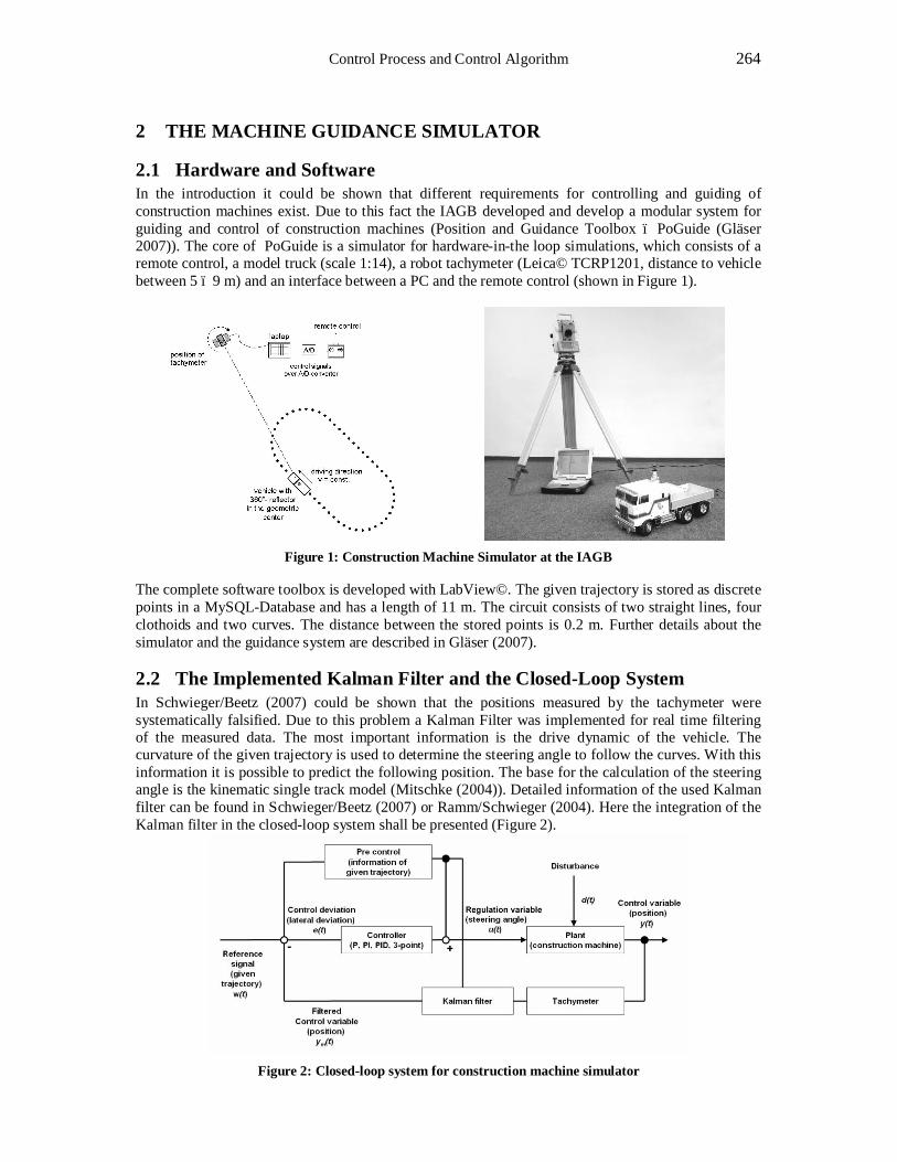
Control Process and Control Algorithm 264
2 THE MACHINE GUIDANCE SIMULATOR
2.1 Hardware and Software In the introduction it could be shown that different requirements for controlling and guiding of construction machines exist. Due to this fact the IAGB developed and develop a modular system for guiding and control of construction machines (Position and Guidance Toolbox – PoGuide (Gläser 2007)). The core of PoGuide is a simulator for hardware-in-the loop simulations, which consists of a remote control, a model truck (scale 1:14), a robot tachymeter (Leica© TCRP1201, distance to vehicle between 5 – 9 m) and an interface between a PC and the remote control (shown in Figure 1).
Figure 1: Construction Machine Simulator at the IAGB
The complete software toolbox is developed with LabView©. The given trajectory is stored as discrete points in a MySQL-Database and has a length of 11 m. The circuit consists of two straight lines, four clothoids and two curves. The distance between the stored points is 0.2 m. Further details about the simulator and the guidance system are described in Gläser (2007).
2.2 The Implemented Kalman Filter and the Closed-Loop System In Schwieger/Beetz (2007) could be shown that the positions measured by the tachymeter were systematically falsified. Due to this problem a Kalman Filter was implemented for real time filtering of the measured data. The most important information is the drive dynamic of the vehicle. The curvature of the given trajectory is used to determine the steering angle to follow the curves. With this information it is possible to predict the following position. The base for the calculation of the steering angle is the kinematic single track model (Mitschke (2004)). Detailed information of the used Kalman filter can be found in Schwieger/Beetz (2007) or Ramm/Schwieger (2004). Here the integration of the Kalman filter in the closed-loop system shall be presented (Figure 2).
Figure 2: Closed-loop system for construction machine simulator
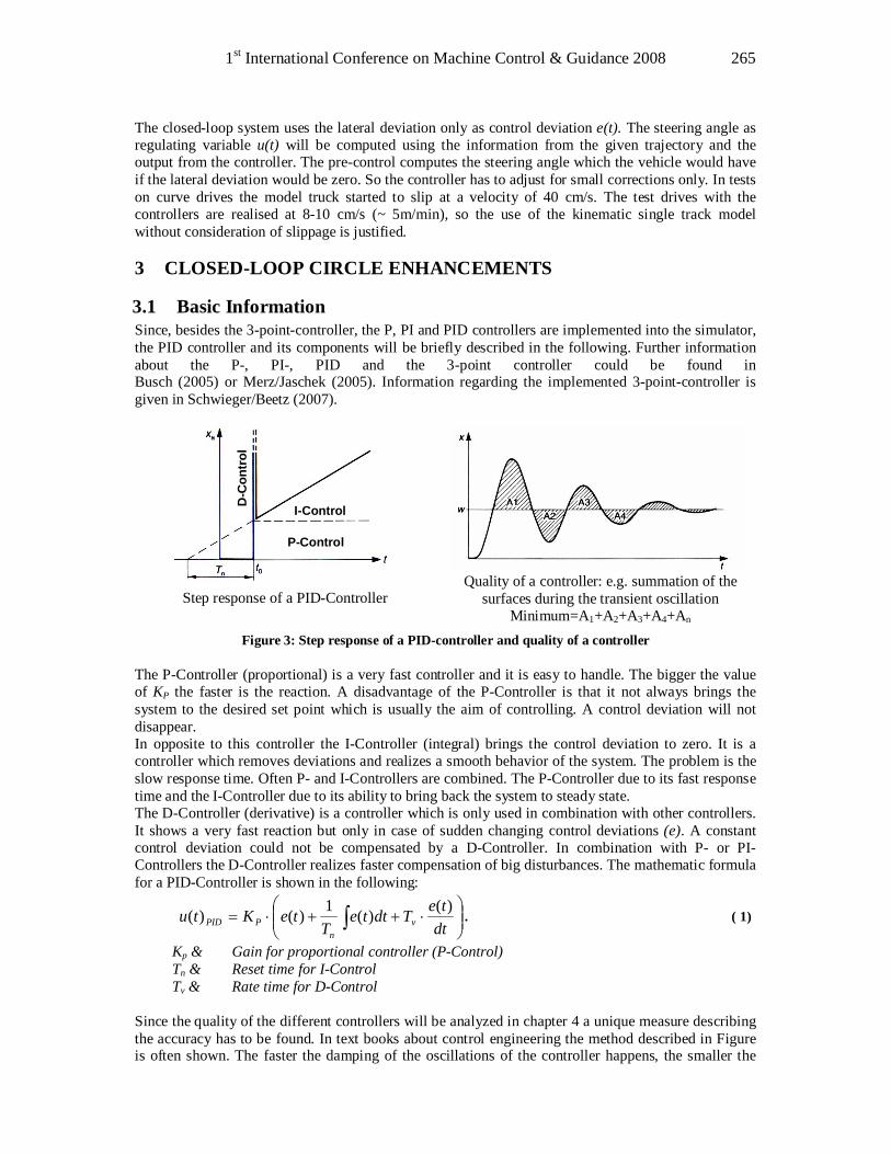
1st International Conference on Machine Control & Guidance 2008 265
The closed-loop system uses the lateral deviation only as control deviation e(t). The steering angle as regulating variable u(t) will be computed using the information from the given trajectory and the output from the controller. The pre-control computes the steering angle which the vehicle would have if the lateral deviation would be zero. So the controller has to adjust for small corrections only. In tests on curve drives the model truck started to slip at a velocity of 40 cm/s. The test drives with the controllers are realised at 8-10 cm/s (~ 5m/min), so the use of the kinematic single track model without consideration of slippage is justified.
3 CLOSED-LOOP CIRCLE ENHANCEMENTS
3.1 Basic Information Since, besides the 3-point-controller, the P, PI and PID controllers are implemented into the simulator, the PID controller and its components will be briefly described in the following. Further information about the P-, PI-, PID and the 3-point controller could be found in Busch (2005) or Merz/Jaschek (2005). Information regarding the implemented 3-point-controller is given in Schwieger/Beetz (2007).
I-Control
P-Control
D-C
ontr
ol
Step response of a PID-Controller
Quality of a controller: e.g. summation of the
surfaces during the transient oscillation Minimum=A1+A2+A3+A4+An
Figure 3: Step response of a PID-controller and quality of a controller The P-Controller (proportional) is a very fast controller and it is easy to handle. The bigger the value of KP the faster is the reaction. A disadvantage of the P-Controller is that it not always brings the system to the desired set point which is usually the aim of controlling. A control deviation will not disappear. In opposite to this controller the I-Controller (integral) brings the control deviation to zero. It is a controller which removes deviations and realizes a smooth behavior of the system. The problem is the slow response time. Often P- and I-Controllers are combined. The P-Controller due to its fast response time and the I-Controller due to its ability to bring back the system to steady state. The D-Controller (derivative) is a controller which is only used in combination with other controllers. It shows a very fast reaction but only in case of sudden changing control deviations (e). A constant control deviation could not be compensated by a D-Controller. In combination with P- or PI-Controllers the D-Controller realizes faster compensation of big disturbances. The mathematic formula for a PID-Controller is shown in the following:
⋅++⋅= ∫ dt
teTdtteT
teKtu vn
PPID)()(1)()( . ( 1)
Kp… Gain for proportional controller (P-Control) Tn… Reset time for I-Control Tv… Rate time for D-Control
Since the quality of the different controllers will be analyzed in chapter 4 a unique measure describing the accuracy has to be found. In text books about control engineering the method described in Figure is often shown. The faster the damping of the oscillations of the controller happens, the smaller the
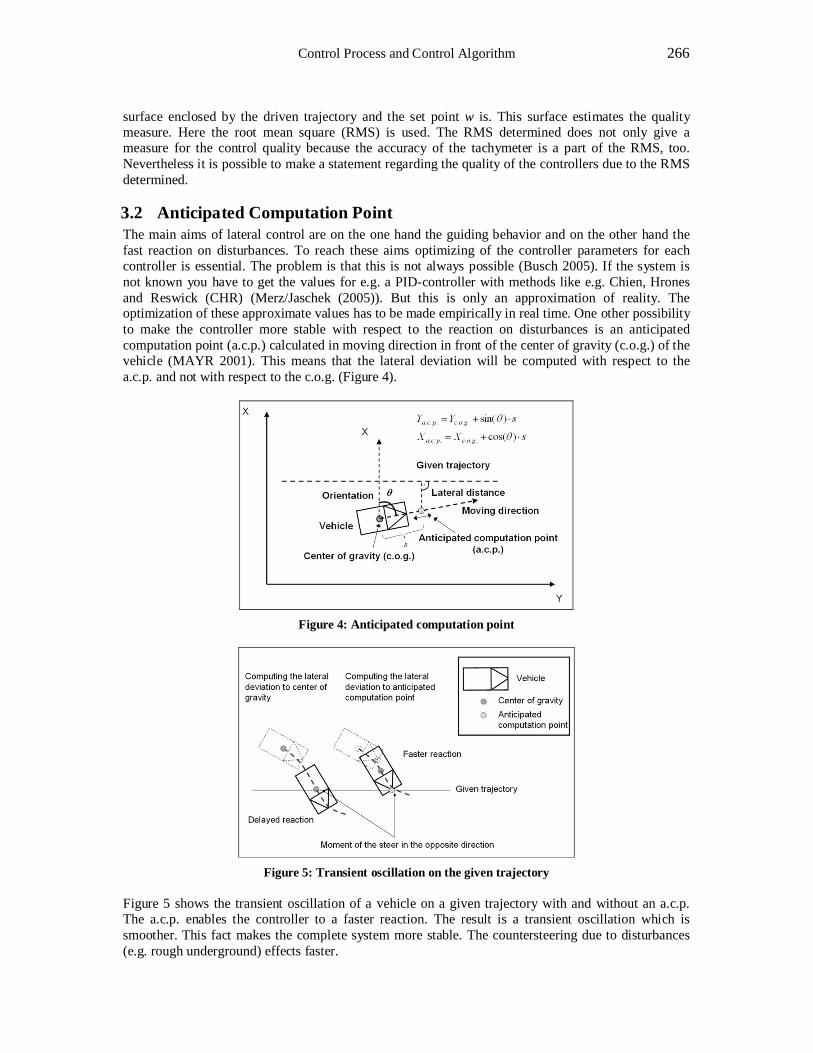
Control Process and Control Algorithm 266
surface enclosed by the driven trajectory and the set point w is. This surface estimates the quality measure. Here the root mean square (RMS) is used. The RMS determined does not only give a measure for the control quality because the accuracy of the tachymeter is a part of the RMS, too. Nevertheless it is possible to make a statement regarding the quality of the controllers due to the RMS determined.
3.2 Anticipated Computation Point The main aims of lateral control are on the one hand the guiding behavior and on the other hand the fast reaction on disturbances. To reach these aims optimizing of the controller parameters for each controller is essential. The problem is that this is not always possible (Busch 2005). If the system is not known you have to get the values for e.g. a PID-controller with methods like e.g. Chien, Hrones and Reswick (CHR) (Merz/Jaschek (2005)). But this is only an approximation of reality. The optimization of these approximate values has to be made empirically in real time. One other possibility to make the controller more stable with respect to the reaction on disturbances is an anticipated computation point (a.c.p.) calculated in moving direction in front of the center of gravity (c.o.g.) of the vehicle (MAYR 2001). This means that the lateral deviation will be computed with respect to the a.c.p. and not with respect to the c.o.g. (Figure 4).
Figure 4: Anticipated computation point
Figure 5: Transient oscillation on the given trajectory
Figure 5 shows the transient oscillation of a vehicle on a given trajectory with and without an a.c.p. The a.c.p. enables the controller to a faster reaction. The result is a transient oscillation which is smoother. This fact makes the complete system more stable. The countersteering due to disturbances (e.g. rough underground) effects faster.
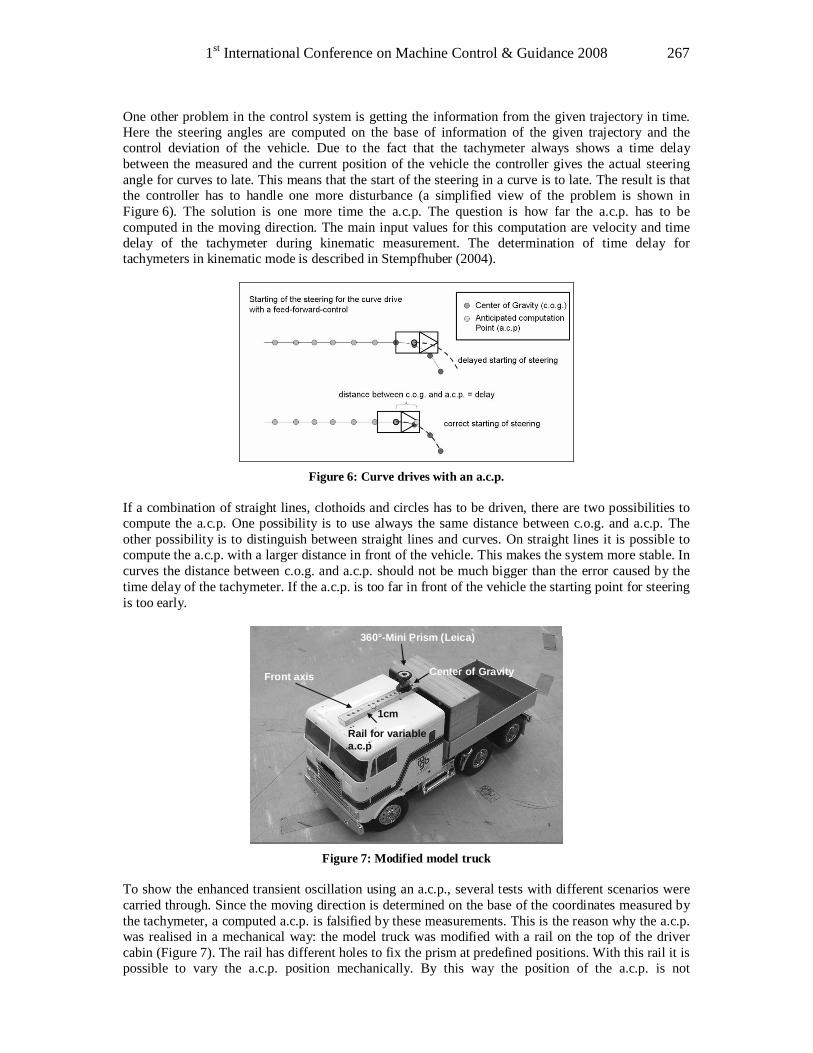
1st International Conference on Machine Control & Guidance 2008 267
One other problem in the control system is getting the information from the given trajectory in time. Here the steering angles are computed on the base of information of the given trajectory and the control deviation of the vehicle. Due to the fact that the tachymeter always shows a time delay between the measured and the current position of the vehicle the controller gives the actual steering angle for curves to late. This means that the start of the steering in a curve is to late. The result is that the controller has to handle one more disturbance (a simplified view of the problem is shown in Figure 6). The solution is one more time the a.c.p. The question is how far the a.c.p. has to be computed in the moving direction. The main input values for this computation are velocity and time delay of the tachymeter during kinematic measurement. The determination of time delay for tachymeters in kinematic mode is described in Stempfhuber (2004).
Figure 6: Curve drives with an a.c.p.
If a combination of straight lines, clothoids and circles has to be driven, there are two possibilities to compute the a.c.p. One possibility is to use always the same distance between c.o.g. and a.c.p. The other possibility is to distinguish between straight lines and curves. On straight lines it is possible to compute the a.c.p. with a larger distance in front of the vehicle. This makes the system more stable. In curves the distance between c.o.g. and a.c.p. should not be much bigger than the error caused by the time delay of the tachymeter. If the a.c.p. is too far in front of the vehicle the starting point for steering is too early.
Front axis
360°-Mini Prism (Leica)
Center of Gravity
1cm
Rail for variablea.c.p.
Figure 7: Modified model truck
To show the enhanced transient oscillation using an a.c.p., several tests with different scenarios were carried through. Since the moving direction is determined on the base of the coordinates measured by the tachymeter, a computed a.c.p. is falsified by these measurements. This is the reason why the a.c.p. was realised in a mechanical way: the model truck was modified with a rail on the top of the driver cabin (Figure 7). The rail has different holes to fix the prism at predefined positions. With this rail it is possible to vary the a.c.p. position mechanically. By this way the position of the a.c.p. is not
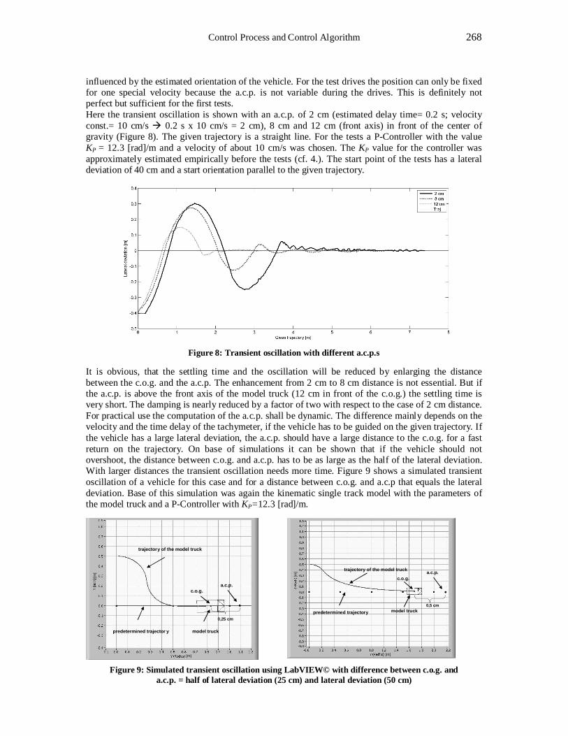
Control Process and Control Algorithm 268
influenced by the estimated orientation of the vehicle. For the test drives the position can only be fixed for one special velocity because the a.c.p. is not variable during the drives. This is definitely not perfect but sufficient for the first tests. Here the transient oscillation is shown with an a.c.p. of 2 cm (estimated delay time= 0.2 s; velocity const.= 10 cm/s à 0.2 s x 10 cm/s = 2 cm), 8 cm and 12 cm (front axis) in front of the center of gravity (Figure 8). The given trajectory is a straight line. For the tests a P-Controller with the value KP = 12.3 [rad]/m and a velocity of about 10 cm/s was chosen. The KP value for the controller was approximately estimated empirically before the tests (cf. 4.). The start point of the tests has a lateral deviation of 40 cm and a start orientation parallel to the given trajectory.
Figure 8: Transient oscillation with different a.c.p.s
It is obvious, that the settling time and the oscillation will be reduced by enlarging the distance between the c.o.g. and the a.c.p. The enhancement from 2 cm to 8 cm distance is not essential. But if the a.c.p. is above the front axis of the model truck (12 cm in front of the c.o.g.) the settling time is very short. The damping is nearly reduced by a factor of two with respect to the case of 2 cm distance. For practical use the computation of the a.c.p. shall be dynamic. The difference mainly depends on the velocity and the time delay of the tachymeter, if the vehicle has to be guided on the given trajectory. If the vehicle has a large lateral deviation, the a.c.p. should have a large distance to the c.o.g. for a fast return on the trajectory. On base of simulations it can be shown that if the vehicle should not overshoot, the distance between c.o.g. and a.c.p. has to be as large as the half of the lateral deviation. With larger distances the transient oscillation needs more time. Figure 9 shows a simulated transient oscillation of a vehicle for this case and for a distance between c.o.g. and a.c.p that equals the lateral deviation. Base of this simulation was again the kinematic single track model with the parameters of the model truck and a P-Controller with KP=12.3 [rad]/m.
predetermined trajector y
trajectory of the model truck
model truck
a.c.p.
[m]
[m]
c.o.g.
0,25 cm
predetermined trajectory
trajectory of the model truck
model truck
a.c.p.
[m]
[m]
c.o.g.
0,5 cm
Figure 9: Simulated transient oscillation using LabVIEW© with difference between c.o.g. and
a.c.p. = half of lateral deviation (25 cm) and lateral deviation (50 cm)
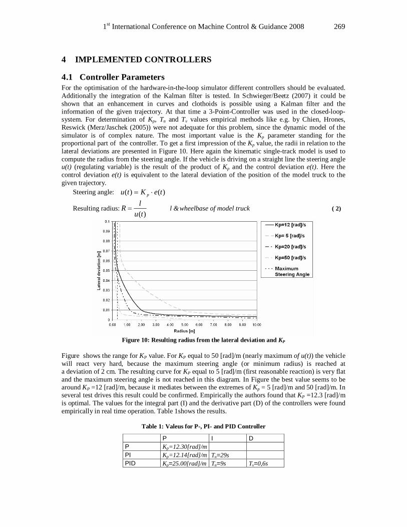
1st International Conference on Machine Control & Guidance 2008 269
4 IMPLEMENTED CONTROLLERS
4.1 Controller Parameters For the optimisation of the hardware-in-the-loop simulator different controllers should be evaluated. Additionally the integration of the Kalman filter is tested. In Schwieger/Beetz (2007) it could be shown that an enhancement in curves and clothoids is possible using a Kalman filter and the information of the given trajectory. At that time a 3-Point-Controller was used in the closed-loop-system. For determination of Kp, Tn and Tv values empirical methods like e.g. by Chien, Hrones, Reswick (Merz/Jaschek (2005)) were not adequate for this problem, since the dynamic model of the simulator is of complex nature. The most important value is the Kp parameter standing for the proportional part of the controller. To get a first impression of the Kp value, the radii in relation to the lateral deviations are presented in Figure 10. Here again the kinematic single-track model is used to compute the radius from the steering angle. If the vehicle is driving on a straight line the steering angle u(t) (regulating variable) is the result of the product of Kp and the control deviation e(t). Here the control deviation e(t) is equivalent to the lateral deviation of the position of the model truck to the given trajectory.
Steering angle: )()( teKtu p ⋅=
Resulting radius:)(tu
lR = l… wheelbase of model truck ( 2)
Figure 10: Resulting radius from the lateral deviation and KP
Figure shows the range for KP value. For KP equal to 50 [rad]/m (nearly maximum of u(t)) the vehicle will react very hard, because the maximum steering angle (or minimum radius) is reached at a deviation of 2 cm. The resulting curve for KP equal to 5 [rad]/m (first reasonable reaction) is very flat and the maximum steering angle is not reached in this diagram. In Figure the best value seems to be around KP =12 [rad]/m, because it mediates between the extremes of Kp = 5 [rad]/m and 50 [rad]/m. In several test drives this result could be confirmed. Empirically the authors found that KP =12.3 [rad]/m is optimal. The values for the integral part (I) and the derivative part (D) of the controllers were found empirically in real time operation. Table 1shows the results.
Table 1: Valeus for P-, PI- and PID Controller
P I D P Kp=12.30[rad]/m PI Kp=12.14[rad]/m Tn=29s PID Kp=25.00[rad]/m Tn=9s Tv=0,6s
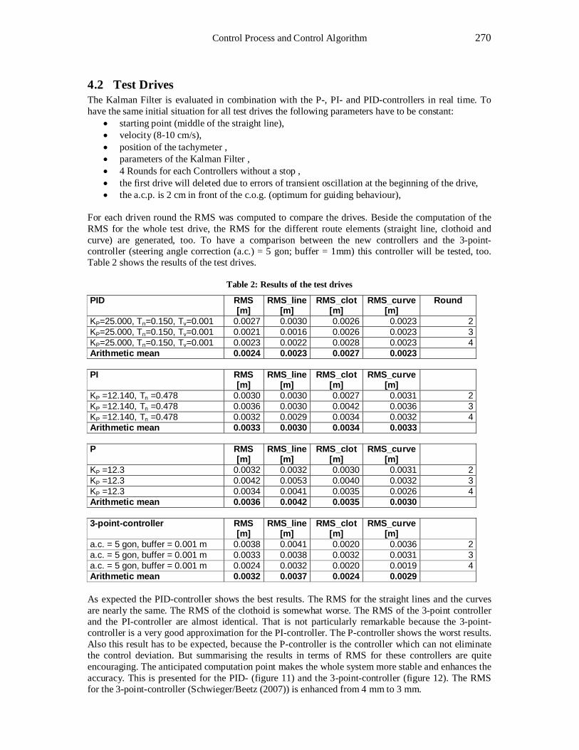
Control Process and Control Algorithm 270
4.2 Test Drives The Kalman Filter is evaluated in combination with the P-, PI- and PID-controllers in real time. To have the same initial situation for all test drives the following parameters have to be constant:
• starting point (middle of the straight line), • velocity (8-10 cm/s), • position of the tachymeter , • parameters of the Kalman Filter , • 4 Rounds for each Controllers without a stop , • the first drive will deleted due to errors of transient oscillation at the beginning of the drive, • the a.c.p. is 2 cm in front of the c.o.g. (optimum for guiding behaviour),
For each driven round the RMS was computed to compare the drives. Beside the computation of the RMS for the whole test drive, the RMS for the different route elements (straight line, clothoid and curve) are generated, too. To have a comparison between the new controllers and the 3-point-controller (steering angle correction (a.c.) = 5 gon; buffer = 1mm) this controller will be tested, too. Table 2 shows the results of the test drives.
Table 2: Results of the test drives
PID
RMS [m]
RMS_line [m]
RMS_clot [m]
RMS_curve [m]
Round
KP=25.000, Tn=0.150, Tv=0.001 0.0027 0.0030 0.0026 0.0023 2 KP=25.000, Tn=0.150, Tv=0.001 0.0021 0.0016 0.0026 0.0023 3 KP=25.000, Tn=0.150, Tv=0.001 0.0023 0.0022 0.0028 0.0023 4 Arithmetic mean 0.0024 0.0023 0.0027 0.0023 PI
RMS [m]
RMS_line [m]
RMS_clot [m]
RMS_curve [m]
KP =12.140, Tn =0.478 0.0030 0.0030 0.0027 0.0031 2 KP =12.140, Tn =0.478 0.0036 0.0030 0.0042 0.0036 3 KP =12.140, Tn =0.478 0.0032 0.0029 0.0034 0.0032 4 Arithmetic mean 0.0033 0.0030 0.0034 0.0033 P
RMS [m]
RMS_line [m]
RMS_clot [m]
RMS_curve [m]
KP =12.3 0.0032 0.0032 0.0030 0.0031 2 KP =12.3 0.0042 0.0053 0.0040 0.0032 3 KP =12.3 0.0034 0.0041 0.0035 0.0026 4 Arithmetic mean 0.0036 0.0042 0.0035 0.0030 3-point-controller
RMS [m]
RMS_line [m]
RMS_clot [m]
RMS_curve [m]
a.c. = 5 gon, buffer = 0.001 m 0.0038 0.0041 0.0020 0.0036 2 a.c. = 5 gon, buffer = 0.001 m 0.0033 0.0038 0.0032 0.0031 3 a.c. = 5 gon, buffer = 0.001 m 0.0024 0.0032 0.0020 0.0019 4 Arithmetic mean 0.0032 0.0037 0.0024 0.0029
As expected the PID-controller shows the best results. The RMS for the straight lines and the curves are nearly the same. The RMS of the clothoid is somewhat worse. The RMS of the 3-point controller and the PI-controller are almost identical. That is not particularly remarkable because the 3-point-controller is a very good approximation for the PI-controller. The P-controller shows the worst results. Also this result has to be expected, because the P-controller is the controller which can not eliminate the control deviation. But summarising the results in terms of RMS for these controllers are quite encouraging. The anticipated computation point makes the whole system more stable and enhances the accuracy. This is presented for the PID- (figure 11) and the 3-point-controller (figure 12). The RMS for the 3-point-controller (Schwieger/Beetz (2007)) is enhanced from 4 mm to 3 mm.
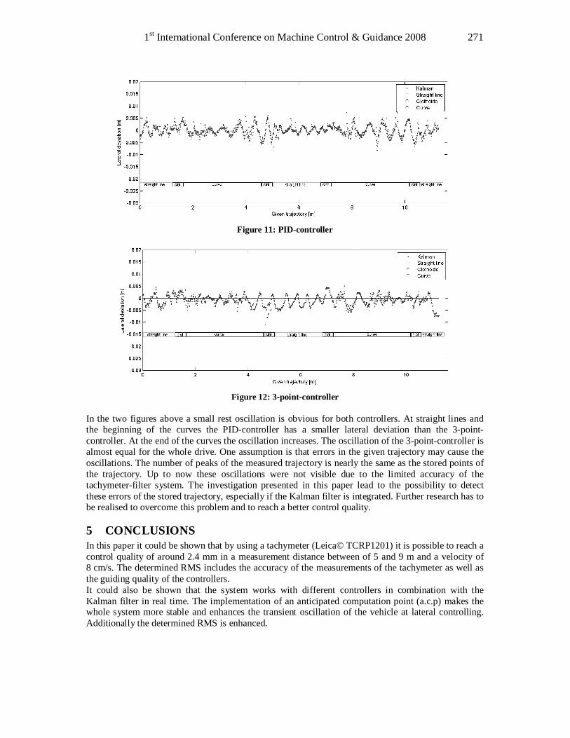
1st International Conference on Machine Control & Guidance 2008 271
Figure 11: PID-controller
Figure 12: 3-point-controller
In the two figures above a small rest oscillation is obvious for both controllers. At straight lines and the beginning of the curves the PID-controller has a smaller lateral deviation than the 3-point-controller. At the end of the curves the oscillation increases. The oscillation of the 3-point-controller is almost equal for the whole drive. One assumption is that errors in the given trajectory may cause the oscillations. The number of peaks of the measured trajectory is nearly the same as the stored points of the trajectory. Up to now these oscillations were not visible due to the limited accuracy of the tachymeter-filter system. The investigation presented in this paper lead to the possibility to detect these errors of the stored trajectory, especially if the Kalman filter is integrated. Further research has to be realised to overcome this problem and to reach a better control quality.
5 CONCLUSIONS In this paper it could be shown that by using a tachymeter (Leica© TCRP1201) it is possible to reach a control quality of around 2.4 mm in a measurement distance between of 5 and 9 m and a velocity of 8 cm/s. The determined RMS includes the accuracy of the measurements of the tachymeter as well as the guiding quality of the controllers. It could also be shown that the system works with different controllers in combination with the Kalman filter in real time. The implementation of an anticipated computation point (a.c.p) makes the whole system more stable and enhances the transient oscillation of the vehicle at lateral controlling. Additionally the determined RMS is enhanced.

Control Process and Control Algorithm 272
For further test drives the precision of the stored discrete points of the given trajectories has to be proved. The next steps should reduce the systematic oscillations for the driven trajectories. If this would be realised, the RMS would reach the sub-mm level (compare figures 11 and 12). Another future focus will be on test drives with different especially higher velocities. For this task it is necessary to implement a dynamic a.c.p. in dependence of velocity, lateral deviation and curvature of the road element. Later if height and longitudinal control are realised a real 3D-simulator will be established.
REFERENCES Books: BAYER, G.: Geometrische Führung von Baumaschinen, Kinematische Messmethoden - Vermessung in Bewegung. Beiträge zum 58.DVW Seminar, Wißner, Augsburg 2004.
BUSCH, P.: Elementare Regelungstechnik. Vogel, Würzburg 2005.
GLÄSER, A: Ein modulares System zur Automatisierung hochgenauer Positionierungs- und Führungsaufgaben im Bauwesen. Dissertation at IAGB, electronic publication, http://elib.uni-stuttgart.de/opus/volltexte/2007/3169/pdf/Diss_Glaeser.pdf, 2007.
MERZ,L., JASCHEK,H.: Grundkurs der Regelungstechnik, Oldenbourg, München, 2003.
MITSCHKE, M., WALLENTOWITZ H.: Dynamik der Kraftfahrzeuge, Springer, Berlin Heidelberg, 2004.
MAYR, R.: Regelungsstrategien für automatische Fahrzeugführung, Springer, Berlin Heidelberg, 2001.
RAMM, K., SCHWIEGER, V.: Multisensorortung für Kraftfahrzeuge, Kinematische Messmethoden - Vermessung in Bewegung. Beiträge zum 58.DVW Seminar, Wißner, Augsburg 2004.
SCHWIEGER, V., BEETZ, A.: Optimierung von Regelalgorithmen zur Baumaschinensteuerung am Beispiel eines Simulators, Ingenieurvermessung 07 - Beiträge zum 15. Internationalen Ingenieurvermessungskurs Graz, Wichmann, Heidelberg, 2007.
STEMPFHUBER, W.: Synchronisation von zielverfolgenden Servotachymetern für kinematische Anwendungen - Vermessung in Bewegung. Beiträge zum 58.DVW Seminar, Wißner, Augsburg 2004. ZIMMERMANN, D.: Ingenieurvermessung - Dreidimensional gesteuerte Baumaschinen, Ingensand,
ETH Zürich, 2004.
Journal articles: STEMPFHUBER,W., INGENSAND, H.: Baumaschinenführung und -steuerung - von der statischen zur kinematischen Absteckung, ZfV, 1/2008, p. 36-44, 2008. Links: http://www.uni-stuttgart.de/iagb http://control.engin.umich.edu *Dipl. Ing. Alexander Beetz, Institute for Applications of Geodesy to Engineering, Universität Stuttgart, Geschwister-Scholl Str. 24D, 70174 Stuttgart, Germany **PD Dr.Ing. Volker Schwieger, Institute for Applications of Geodesy to Engineering, Universität Stuttgart, Geschwister-Scholl Str. 24D, 70174 Stuttgart, Germany
1st International Conference on Machine Control & Guidance 2008 273
Comparison of Sequential Monte Carlo Filtering with Kalman Filtering for Nonlinear State Estimation
H. ALKHATIB*, I. NEUMANN, H. NEUNER, H. KUTTERER Geodetic Institute, Leibniz University of Hannover, Germany
[alkhatib,neumann,neuner,kutterer]@gih.uni-hannover.de Abstract In this paper different filtering techniques for nonlinear state estimation are explored and compared. We distinguish between approaches that approximate the nonlinear function (extended Kalman filter) and other approaches approximating the distribution of measurements and state (unscented Kalman filter and sequential Monte Carlo filter). The paper is showing both, the algorithms and simulated examples where a vehicle moves along a nonlinear trajectory such as a circle arc or a clothoid. It is shown, that the estimation of the system state can be improved if the nonlinearities were taken into account. Keywords Nonlinear state estimation, Kalman filter, Sequential Monte Carlo, importance sampling
1 INTRODUCTION A central point in machine guidance is how to drive an optimal guidance algorithm to fulfill a given purpose using all available sensors, together with targeting information. The guidance algorithm can be divided into two parts: estimation and control part. In both parts, the probability density function (PDF) has to be constructed. The estimator in the first part constructs the PDF of the target states, whereas the control element transforms this PDF into guidance requirements (Doucet et al. 2001, p. 517-532). The estimator element is provided usually by Kalman filtering. The Kalman filtering technique is used in engineering geodesy especially in applications such as engineering navigation and deformation analysis. Both kinds of application require a sequential estimation of the system state based on information coming from a (dynamic) model of the system and from external observations. Over the years refined models were introduced for the system description (i.e., the trajectory of a vehicle), and a great variety of sensors was used to observe the system state. This yielded often nonlinearities in the equations of the Kalman filter. In the field of engineering navigation for example, Aussems (1999) describes the vehicle’s trajectory by a refined model of consecutive arcs. In this model the vehicle coordinates are nonlinearly related to other state parameters like the angular velocity in the horizontal plane, the pitch angle or the tangential component of the linear velocity. Another approach that may lead to nonlinear state equations is the adaptive enhancement of the Kalman filter. For the estimation of the thermal diffusivity of an aluminum column Eichhorn (2008) introduces this physical parameter into the state vector. Thus, the initially linear state equations become nonlinear at the order of reciprocal exponentials. A majority of the performed observations of the system are nonlinearly related to its state parameters; refer to Sternberg (2000) for a disquisition on observation equations in engineering navigation. Non-linearities can occur directly due to the nature of the relation between measurements like distances or angles and point coordinates or due to the transformation of the observations in a different coordinate system as is often the case in navigation applications. Linear filtering theory according to Kalman and Bucy (1960) is optimal only if the system (which consists of measurement and transition equations) is linear and the error process is Gaussian. Unfortunately, the modelling of reality diverges from these optimal assumptions and nonlinear, non-Gaussian, and non-stationary state estimation should be taken into account. Thus over the years a multitude of approximate nonlinear filters has been proposed, see e.g. Bar-Shalom et al. (2001), Doucet et al. (2001), and Simon (2006).

Control Process and Control Algorithm 274
A well known analytical approximation to handle a nonlinear system is to linearize the measurement and the system equations using Taylor series expansions; see Gelb (1974). However, as pointed out in Doucet et al. (2001) this type of nonlinear filter which includes the first-order and the higher-order extended Kalman filter (EKF), is prone to diverge if the system equations are highly nonlinear. This gives us a motivation to use other filter techniques as Unscented Kalman filter (UKF) or sequential Monte Carlo (SMC) approach in order to take the nonlinearities into account. The UKF has been introduced in Julier and Uhlmann (1997) and approximates the first and the second moment of the posterior PDF rather than to approximate nonlinear functions. The approximation of the posterior PDF of the state proceeds by a set of deterministically chosen sample points which cover the true mean and covariance. These generated samples are all propagated through the nonlinear system, and the parameters of the first and the second moment is recomputed. However, the basis of the UKF approach is to approximate the posterior density of the state by a Gaussian. Unfortunately, the true PDF of the system is in some cases non-Gaussian, so a Gaussian can hardly approximate it. In such cases the SMC filter will be applied to improve the estimate of the system state. The SMC filter (also known as particle filter) is a suboptimal filter for implementing the recursive Bayesian filter by Monte Carlo (MC) techniques, see e.g. Doucet et al. (2001) and Ristic et. al (2003). The main idea behind the SMC filter is to approximate the posterior PDF by a set of random samples, which can be generated from a known PDF. These generated particles are propagated through the dynamic model. They are then weighted according to the likelihood of the observations. In a resampling step, the new weighted particles are drawn with a probability proportional to the likelihood of the observation. By means of the drawn particle the true mean and the covariance of the state vector are estimated. If we assume that the number of drawn particles is very large, the MC approximation becomes an equivalent representation to the functional description of the posterior PDF. The high computational cost due to the large required number of particles restricted the SMC in the past to post-processing applications. However, nowadays the computational burden does not prevent the use of SMC filter for real time applications. In this paper nonlinear filtering approaches are considered. We focus on two versions of the Kalman filter (EKF and UKF) and on the SMC filter. The results of the presented algorithms are demonstrated using two simulation studies: a vehicle moving along a nonlinear trajectory and a highly nonlinear scalar system. The paper is organised as follows. Section 2.1 describes the mathematical model of the system which includes both the system dynamics and the measurement model. Section 2.2 briefly introduces the EKF and the UKF. The SMC filter is presented in Section 2.3. Two numerical simulations are demonstrated in Section 3. A comparative analysis of the presented algorithms is presented in Section 4. Finally, Section 5 summarizes the results and gives an outlook for future work.
2 NONLINEAR STATE ESTIMATION
2.1 The Mathematical Model Before describing the different filter algorithms, we briefly introduce in this section the notation and the terminology used throughout the paper. To define the problem of nonlinear filtering, let us consider the state vector ∈kx ℝ xn , where xn is the dimension of the state vector, and k is the time index. The evolution of the state sequence kx of the target is given by the dynamic model:
( )1 , ,k k k k+ =x x u wf , (1) where f is a known, in general nonlinear function, ku is a vector of known (deterministic) input, and
kw is the process noise vector, which is caused by mismodelling effects and other disturbances in the motion model. The main aim of filtering is to estimate the optimal 1k +x from the observations
∈+1ky ℝ yn and ∈kx ℝ xn , where yn is the dimension of the measurement model:
( )1 1 1,k k k+ + +=y x vh , (2)
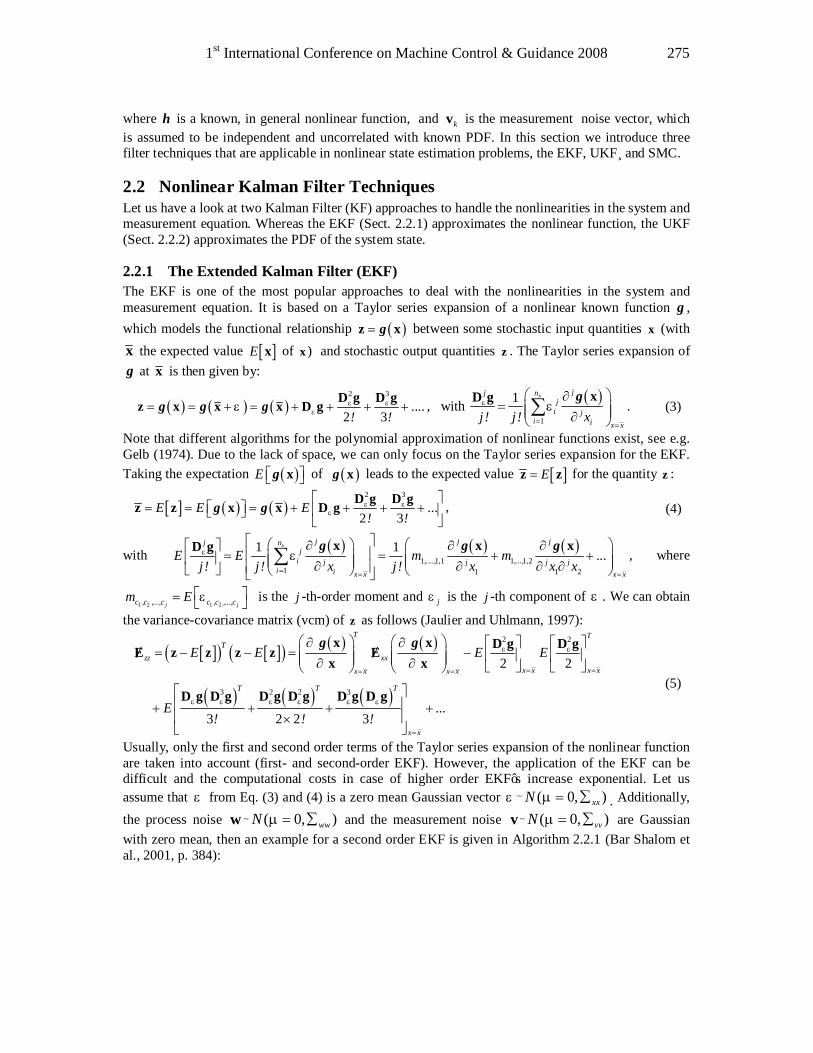
1st International Conference on Machine Control & Guidance 2008 275
where h is a known, in general nonlinear function, and kv is the measurement noise vector, which is assumed to be independent and uncorrelated with known PDF. In this section we introduce three filter techniques that are applicable in nonlinear state estimation problems, the EKF, UKF¸ and SMC.
2.2 Nonlinear Kalman Filter Techniques Let us have a look at two Kalman Filter (KF) approaches to handle the nonlinearities in the system and measurement equation. Whereas the EKF (Sect. 2.2.1) approximates the nonlinear function, the UKF (Sect. 2.2.2) approximates the PDF of the system state.
2.2.1 The Extended Kalman Filter (EKF) The EKF is one of the most popular approaches to deal with the nonlinearities in the system and measurement equation. It is based on a Taylor series expansion of a nonlinear known function g , which models the functional relationship ( )=z xg between some stochastic input quantities x (with x the expected value [ ]E x of x ) and stochastic output quantities z . The Taylor series expansion of g at x is then given by:
( ) ( ) ( )
2 3
2 3....
! != = + = + + + +
D g D gz x x x D g ε ε
εg g gε , with ( )1
1 x jj nj
i ji i x x
j ! j ! x= =
∂= ∂
∑xD gε ε
g. (3)
Note that different algorithms for the polynomial approximation of nonlinear functions exist, see e.g. Gelb (1974). Due to the lack of space, we can only focus on the Taylor series expansion for the EKF. Taking the expectation ( )E xg of ( )xg leads to the expected value [ ]E=z z for the quantity z :
[ ] ( ) ( )2 3
2 3E E E ...
! !
= = = + + + +
D g D gz z x x D g ε ε
εg g , (4)
with ( ) ( ) ( )1 1,1 1 1,2
1 1 1 2
1 1x j j jj nj
i ,...., ,...,j j j ji i x x x x
E E m m ...j ! j ! x j! x x x= = =
∂ ∂ ∂ = = + + ∂ ∂ ∂ ∂ ∑
x x xD gε εg g g
, where
1 2 1 2j jc ,c ,...,c c ,c ,...,cm E = ε is the j -th-order moment and jε is the j -th component of ε . We can obtain
the variance-covariance matrix (vcm) of z as follows (Jaulier and Uhlmann, 1997):
[ ]( ) [ ]( ) ( ) ( )
( ) ( ) ( )
2 2
3 2 2 3
2 2
3 2 2 3
T TT
zz xxx x x xx x x x
T T T
x x
E E E E
E ...! ! !
= == =
=
∂ ∂ = − − = − ∂ ∂
+ + + + ×
x x D g D gΣ z z z z Σx x
D g D g D g D g D g D g
ε ε
ε ε ε ε ε ε
g g
(5)
Usually, only the first and second order terms of the Taylor series expansion of the nonlinear function are taken into account (first- and second-order EKF). However, the application of the EKF can be difficult and the computational costs in case of higher order EKF’s increase exponential. Let us assume that ε from Eq. (3) and (4) is a zero mean Gaussian vector ε ~ ),0( xxN ∑=µ . Additionally, the process noise w ~ ),0( wwN ∑=µ and the measurement noise v ~ ),0( vvN ∑=µ are Gaussian with zero mean, then an example for a second order EKF is given in Algorithm 2.2.1 (Bar Shalom et al., 2001, p. 384):
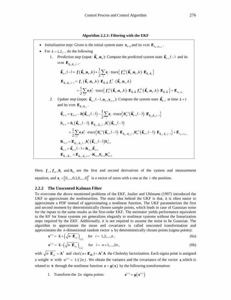
Control Process and Control Algorithm 276
Algorithm 2.2.1: Filtering with the EKF
• Initialization step: Given is the initial system state 0k=x and its vcm 0 0k k= =x xΣ .
• For 1,2,k = K do the following 1. Prediction step (input: k kˆ ,x u ): Compute the predicted system state ( )
1kˆ + −x and its vcm ( )1 1k kˆ ˆx x+ + −Σ .
( ) ( ) ( ) (i)1 xx x x
1 trace2 k kˆ ˆk k k i k k ,
i
ˆ ˆ ˆ, ,k , ,k+ − = + ⋅ ⋅∑x x u e x u Σf f
( ) ( ) ( )
( ) ( ) 1 1
(i) (i')xx
1 trace2
k kk k
k k k k k k
Tˆ ˆx k k x ,x x k kˆ ˆx x
Tˆ ˆ ˆ ˆi i' xx k k x ,x k k x ,x w ,w
i ,i'
ˆ ˆ, ,k , ,k
ˆ ˆ, ,k , ,k
+ + − = ⋅ ⋅
+ ⋅ ⋅ ⋅ +∑
Σ x u Σ x u
e e x u Σ x u Σ Σ
f f
f f
2. Update step (input: ( )1 1k k kˆ , ,+ +−x u y ): Compute the system state 1kˆ +x at time 1k +
and its vcm 1 1k kˆ ˆx x+ +
Σ .
( )( ) ( )( ) ( ) 1 11 1 1 112 k k
( i )k k k i xx k ˆ ˆx x
i
ˆ ˆ ˆtrace+ ++ + + + −= − − − ⋅ − ⋅∑v y x e x Σh h
( )( ) ( )( )( )
( )( ) ( )( )( ) ( )
1 1
1 11 1 1 1
1 1 1
1 112
k k
k kk k k k
Tk x k x kˆ ˆx ,x
T ( i ) ( i')i i' xx k xx k v ,vˆ ˆ ˆ ˆx ,x x ,x
i ,i'
ˆ ˆ
ˆ ˆtrace
+ +
+ ++ + + +
+ + +−
+ +− −
= − ⋅ −
+ ⋅ − ⋅ − ⋅ +∑
S x Σ x
e e x Σ x Σ Σ
h h
h h
( ) ( )( )1 1
11 1 1k k
T -k x k kˆ ˆx ,x ˆ
+ ++ + +−= −K Σ x Sh
( )1 1 1 1k k k kˆ ˆ ˆ+ + + += − +x x K v
( )1 1 1 1 1 1 1k k k k
Tˆ ˆx ,x k k kˆ ˆx ,x - -
+ + + + + + +=Σ Σ K S K
Here, x xx x xxand ,f , f h h are the first and second derivatives of the system and measurement
equation, and [ ]0 0 1 0 0 Ti ,..., , , ,...,=e is a vector of zeros with a one at the i -the position.
2.2.2 The Unscented Kalman Filter To overcome the above mentioned problems of the EKF, Jaulier and Uhlmann (1997) introduced the UKF to approximate the nonlinearities. The main idea behind the UKF is that, it is often easier to approximate a PDF instead of approximating a nonlinear function. The UKF parameterizes the first and second moment by deterministically chosen sample points, which leads in case of Gaussian noise for the inputs to the same results as the first-order EKF. The estimator yields performance equivalent to the KF for linear systems yet generalizes elegantly to nonlinear systems without the linearization steps required by the EKF. Additionally, it is not required to assume the noise to be Gaussian. The algorithm to approximate the mean and covariance is called unscented transformation and approximates the n-dimensional random vector x by deterministically chosen points (sigma points):
( )( ,i)
for 1 2 ( i )xxn i , ,...,n= + ⋅ =
:x x Σ , (6a)
( )( ,i)
for 1 2 ( i )xx- n i n ,..., n= ⋅ = +
:x x Σ , (6b)
with Txxn ⋅ =Σ A and chol T
ˆ ˆxx( n )× =Σ A A the Cholesky factorization. Each sigma point is assigned a weight w with 1 2( i )w /( n )= . We obtain the variance and the covariance of the vector ,z which is related to x through the nonlinear function ( )=z xg by the following transformation:
1. Transform the 2n sigma points: ( )( i ) ( i )=z xg

1st International Conference on Machine Control & Guidance 2008 277
2. Compute the estimated mean of z : 2
1
n( i ) ( i )
i
ˆ w=
= ∑z z
3. Compute the estimated variance of z : ( )( )2
1
n T( i ) ( i ) ( i )ˆˆzz
i
ˆ ˆw=
= − −∑Σ z z z z
4. Compute the covariance between x and z : ( )( )2
1
n T( i ) ( i ) ( i )ˆˆxz
i
ˆ ˆw=
= − −∑Σ x x z z
Let us approximate the process noise w with zero mean and covariance wwΣ and the measurement noise v with zero mean and covariance vvΣ . Then we can obtain the algorithm of the UKF with the above described unscented transformation as follows (Jaulier and Uhlmann, 1997) :
Algorithm 2.2.2: Filtering with the UKF
• Initialization step: Given is the initial system state 0k=x and its vcm 0 0k k= =x xΣ .
• For 1, 2,k = K do the following 1. Prediction step (input: k kˆ ,x u ): Generate the sigma points for kx with Eq. (6):
( ) ( ) ( )2 2
1 11 1
n n( i ) ( i ) ( i ) ( i )
k k k ki i
ˆ ˆ ˆw , ,k w+ += =
− = = −∑ ∑x x u xf
( )( ) ( )( ) ( ) ( )( )
1 1
2
1 1 1 11
k kk k
n T( i ) ( i ) ( i )k k k k w ,wˆ ˆx x
i
ˆ ˆ ˆ ˆw+ + + + + +−
=
= − − − − − − +∑Σ x x x x Σ
2. Update step (input: ( )1 1k k kˆ , ,+ +−x u y ): Generate the sigma points for ( )
1kˆ + −x with Eq. (6):
( ) ( )( ) ( )2 2
1 1 11 1
n n
( i ) ( i ) ( i ) ( i )k k k
i i
ˆ ˆ ˆw w+ + += =
− = − = −∑ ∑y x yh
( )( ) ( )( ) ( ) ( )( )
1 1
2
1 1 1 1 1
k k
n T( i ) ( i ) ( i )k k k kˆ ˆx , y
i
ˆ ˆ ˆ ˆw+ + + + + +−
=
= − − − − − −∑Σ x x y y
( )1 1 1k k kˆ ˆ+ + += − −v y y
( ) ( )( ) ( ) ( )( ) 1 1
2
1 1 1 1 11
k k
n T( i ) ( i ) ( i )k k k k k v ,v
i
ˆ ˆ ˆ ˆw+ ++ + + + +
=
= − − − − − − +∑S y y y y Σ
( )1 1
11 1k k
-k kˆ ˆx - , y+ ++ += K Σ S
( )1 1 1 1k k k kˆ ˆ ˆ+ + + += − +x x K v
( )1 1 1 1 1 1 1k k k k
Tˆ ˆx ,x k k kˆ ˆx ,x - -
+ + + + + + +=Σ Σ K S K
2.3 Generic Particle Filter Techniques Particle filtering (PF) is based on Monte Carlo (MC) simulation with sequential importance sampling (SIS), see e.g. Doucet et. al (2001) and Gentel (2003, p. 241). The goal is to approximate the optimal recursive Bayesian estimation. From a Bayesian perspective, the filtering problem is to estimate the state 1k +x recursively given the data 1: 1k+y up to to time 1k + . Thus it is required to evaluate the joint posterior PDF 1 1: 1( )k kp + +x y :
1 1 1 1:1 1: 1
1 1:
( ) ( )( )
( )k k k k
k kk k
p pp
p+ + +
+ ++
⋅=
y x x yx y
y y, (7)
where the posterior at time k , 1:( )k kp x y , is first projected forward in time in order to calculate the prior at time 1k + . This is done by using the probabilistic process model (cf. Simon, 2006, p. 464):
1 1: 1 1:( ) ( ) ( )k k k k k k kp p p d+ += ⋅∫x y x x x y x . (8)
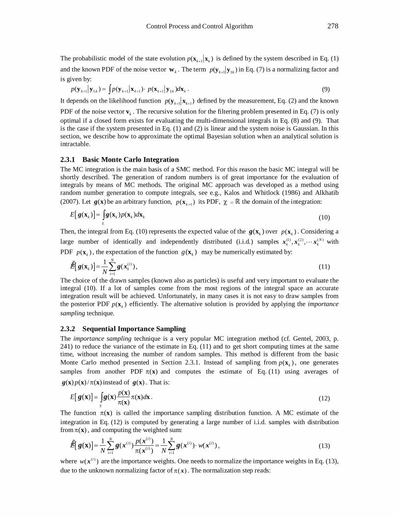
Control Process and Control Algorithm 278
The probabilistic model of the state evolution 1( )k kp +x x is defined by the system described in Eq. (1) and the known PDF of the noise vector kw . The term 1 1:( )k kp +y y in Eq. (7) is a normalizing factor and is given by:
1 1: 1 1 1 1:( ) ( ) ( )k k k k k k kp p p d+ + + += ⋅∫y y y x x y x . (9)
It depends on the likelihood function 1 1( )k kp + +y x defined by the measurement, Eq. (2) and the known PDF of the noise vector kv . The recursive solution for the filtering problem presented in Eq. (7) is only optimal if a closed form exists for evaluating the multi-dimensional integrals in Eq. (8) and (9). That is the case if the system presented in Eq. (1) and (2) is linear and the system noise is Gaussian. In this section, we describe how to approximate the optimal Bayesian solution when an analytical solution is intractable.
2.3.1 Basic Monte Carlo Integration The MC integration is the main basis of a SMC method. For this reason the basic MC integral will be shortly described. The generation of random numbers is of great importance for the evaluation of integrals by means of MC methods. The original MC approach was developed as a method using random number generation to compute integrals, see e.g., Kalos and Whitlock (1986) and Alkhatib (2007). Let ( )xg be an arbitrary function, 1( )kp +x its PDF, χ ⊂ ℝ the domain of the integration:
[ ]( ) ( ) ( )k k k kE p dχ
= ∫x x x xg g (10)
Then, the integral from Eq. (10) represents the expected value of the ( )kxg over ( )kp x . Considering a large number of identically and independently distributed (i.i.d.) samples (1) (2) ( ), , N
k k kLx x x with PDF ( )kp x , the expectation of the function ( )kg x may be numerically estimated by:
[ ] ( )
1
1ˆ ( ) ( )N
ik k
iE
N =
= ∑xg g x , (11)
The choice of the drawn samples (known also as particles) is useful and very important to evaluate the integral (10). If a lot of samples come from the most regions of the integral space an accurate integration result will be achieved. Unfortunately, in many cases it is not easy to draw samples from the posterior PDF ( )kp x efficiently. The alternative solution is provided by applying the importance sampling technique.
2.3.2 Sequential Importance Sampling The importance sampling technique is a very popular MC integration method (cf. Gentel, 2003, p. 241) to reduce the variance of the estimate in Eq. (11) and to get short computing times at the same time, without increasing the number of random samples. This method is different from the basic Monte Carlo method presented in Section 2.3.1. Instead of sampling from ( )kp x , one generates samples from another PDF ( )π x and computes the estimate of Eq. (11) using averages of
( ) ( ) / ( )p πx x xg instead of ( )xg . That is:
[ ] ( )) ) ( )( )
( ( pE dχ
= ππ∫
x x xx
x xg g . (12)
The function ( )π x is called the importance sampling distribution function. A MC estimate of the integration in Eq. (12) is computed by generating a large number of i.i.d. samples with distribution from ( )π x , and computing the weighted sum:
[ ]( )
( ) ( ) ( )( )
1 1
1 ( ) 1ˆ ) ( ) ( ) ( )( )
(iN N
i i ii
i i
pE wN N= =
= = ⋅π∑ ∑x xx x x
xg g g , (13)
where ( )( )iw x are the importance weights. One needs to normalize the importance weights in Eq. (13), due to the unknown normalizing factor of ( )π x . The normalization step reads:
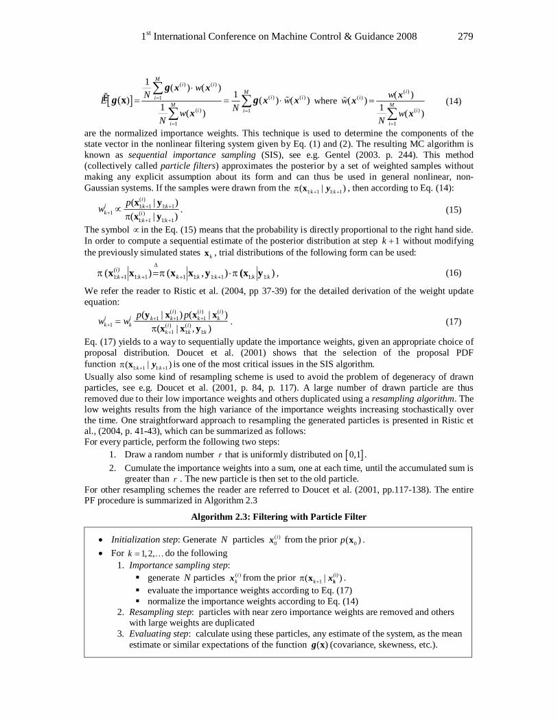
1st International Conference on Machine Control & Guidance 2008 279
[ ]( ) ( )
( ) ( )1
( ) 1
1
1 ( ) ( )1ˆ ) ( ) ( )
1 ( )(
Mi i
Mi ii
Mi i
i
wNE w
NwN
=
=
=
⋅= = ⋅
∑∑
∑x %
x xx x
x
gg g where
( )( )
( )
1
( )( )1 ( )
ii
Mi
i
www
N =
=
∑%
xxx
(14)
are the normalized importance weights. This technique is used to determine the components of the state vector in the nonlinear filtering system given by Eq. (1) and (2). The resulting MC algorithm is known as sequential importance sampling (SIS), see e.g. Gentel (2003. p. 244). This method (collectively called particle filters) approximates the posterior by a set of weighted samples without making any explicit assumption about its form and can thus be used in general nonlinear, non-Gaussian systems. If the samples were drawn from the 1: 1 1: 1( | )k k+ +π x y , then according to Eq. (14):
( )1: 1 1: 1
1 ( )1: 1 1: 1
( | )( | )
ii k kk i
k k
pw + ++
+ +
∝π
x yx y
. (15)
The symbol ∝ in the Eq. (15) means that the probability is directly proportional to the right hand side. In order to compute a sequential estimate of the posterior distribution at step 1k + without modifying the previously simulated states kx , trial distributions of the following form can be used:
)),()( :1:11:1:111:11:1 kkkkkk(i)
k y(xyxxxx πππ ⋅= ++
∆
++ , (16)
We refer the reader to Ristic et al. (2004, pp 37-39) for the detailed derivation of the weight update equation:
( ) ( ) ( )1 1 1
1 ( ) ( )1 1: 1:
( | ) ( | )( | , )
i i ii i k k k kk k i i
k k k
p pw w + + ++
+
=π
y x x xx x y
. (17)
Eq. (17) yields to a way to sequentially update the importance weights, given an appropriate choice of proposal distribution. Doucet et al. (2001) shows that the selection of the proposal PDF function 1: 1 1: 1( | )k k+ +π x y is one of the most critical issues in the SIS algorithm. Usually also some kind of resampling scheme is used to avoid the problem of degeneracy of drawn particles, see e.g. Doucet et al. (2001, p. 84, p. 117). A large number of drawn particle are thus removed due to their low importance weights and others duplicated using a resampling algorithm. The low weights results from the high variance of the importance weights increasing stochastically over the time. One straightforward approach to resampling the generated particles is presented in Ristic et al., (2004, p. 41-43), which can be summarized as follows: For every particle, perform the following two steps:
1. Draw a random number r that is uniformly distributed on [ ]0,1 . 2. Cumulate the importance weights into a sum, one at each time, until the accumulated sum is
greater than r . The new particle is then set to the old particle. For other resampling schemes the reader are referred to Doucet et al. (2001, pp.117-138). The entire PF procedure is summarized in Algorithm 2.3
Algorithm 2.3: Filtering with Particle Filter
• Initialization step: Generate N particles ( )0ix from the prior 0( )p x .
• For 1,2,k = K do the following 1. Importance sampling step: § generate N particles ( )i
kx from the prior 1( | )(i)k +π x kx .
§ evaluate the importance weights according to Eq. (17) § normalize the importance weights according to Eq. (14)
2. Resampling step: particles with near zero importance weights are removed and others with large weights are duplicated
3. Evaluating step: calculate using these particles, any estimate of the system, as the mean estimate or similar expectations of the function ( )xg (covariance, skewness, etc.).
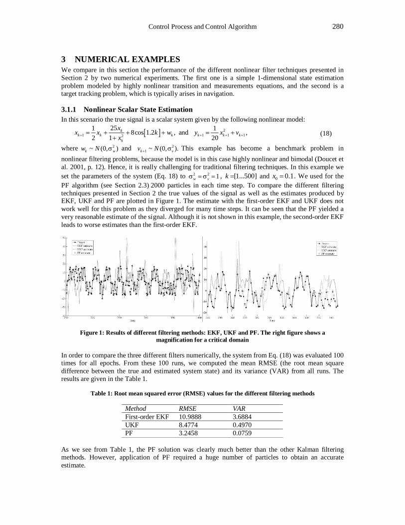
Control Process and Control Algorithm 280
3 NUMERICAL EXAMPLES We compare in this section the performance of the different nonlinear filter techniques presented in Section 2 by two numerical experiments. The first one is a simple 1-dimensional state estimation problem modeled by highly nonlinear transition and measurements equations, and the second is a target tracking problem, which is typically arises in navigation.
3.1.1 Nonlinear Scalar State Estimation In this scenario the true signal is a scalar system given by the following nonlinear model:
[ ] 21 1 1 12
251 18cos 1.2 , and2 1 20
kk k k k k k
k
xx x k w y x vx+ + + += + + + = +
+, (18)
where 2~ (0, )k ww N σ and 21 ~ (0, ).k vv N+ σ This example has become a benchmark problem in
nonlinear filtering problems, because the model is in this case highly nonlinear and bimodal (Doucet et al. 2001, p. 12). Hence, it is really challenging for traditional filtering techniques. In this example we set the parameters of the system (Eq. 18) to 2 2 1w vσ = σ = , [1...500]k = and 0 0.1x = . We used for the PF algorithm (see Section 2.3) 2000 particles in each time step. To compare the different filtering techniques presented in Section 2 the true values of the signal as well as the estimates produced by EKF, UKF and PF are plotted in Figure 1. The estimate with the first-order EKF and UKF does not work well for this problem as they diverged for many time steps. It can be seen that the PF yielded a very reasonable estimate of the signal. Although it is not shown in this example, the second-order EKF leads to worse estimates than the first-order EKF.
Figure 1: Results of different filtering methods: EKF, UKF and PF. The right figure shows a magnification for a critical domain
In order to compare the three different filters numerically, the system from Eq. (18) was evaluated 100 times for all epochs. From these 100 runs, we computed the mean RMSE (the root mean square difference between the true and estimated system state) and its variance (VAR) from all runs. The results are given in the Table 1.
Table 1: Root mean squared error (RMSE) values for the different filtering methods
Method RMSE VAR First-order EKF 10.9888 3.6884 UKF 8.4774 0.4970 PF 3.2458 0.0759
As we see from Table 1, the PF solution was clearly much better than the other Kalman filtering methods. However, application of PF required a huge number of particles to obtain an accurate estimate.
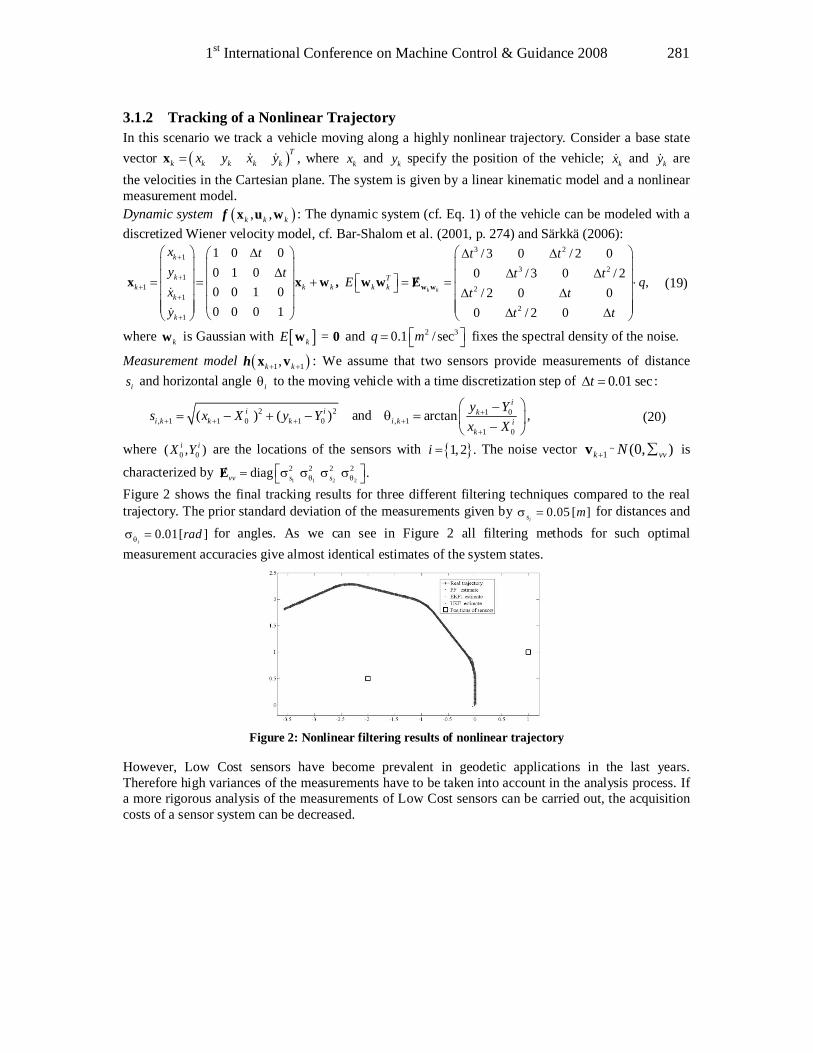
1st International Conference on Machine Control & Guidance 2008 281
3.1.2 Tracking of a Nonlinear Trajectory In this scenario we track a vehicle moving along a highly nonlinear trajectory. Consider a base state vector ( )T
k k k k kx y x y=x & & , where kx and ky specify the position of the vehicle; kx& and ky& are the velocities in the Cartesian plane. The system is given by a linear kinematic model and a nonlinear measurement model. Dynamic system ( ), ,k k kx u wf : The dynamic system (cf. Eq. 1) of the vehicle can be modeled with a discretized Wiener velocity model, cf. Bar-Shalom et al. (2001, p. 274) and Särkkä (2006):
3 21
3 21
1 21
21
1 0 0 / 3 0 / 2 00 1 0 0 / 3 0 / 2
,0 0 1 0 / 2 0 00 0 0 1 0 / 2 0
k k
k
k Tk k k k k
k
k
x t t ty t t t
E qx t ty t t
+
++
+
+
∆ ∆ ∆ ∆ ∆ ∆ = = + = = ⋅ ∆ ∆ ∆ ∆
w wx x w , w w Σ&
&
(19)
where kw is Gaussian with [ ] = kE w 0 and 2 30.1 / secq m = fixes the spectral density of the noise.
Measurement model ( )1 1,k k+ +x vh : We assume that two sensors provide measurements of distance
is and horizontal angle iθ to the moving vehicle with a time discretization step of 0.01 sect∆ = :
2 2, 1 1 0 1 0( ) ( )i i
i k k ks x X y Y+ + += − + − and 1 0, 1
1 0
arctani
ki k i
k
y Yx X
++
+
−θ = −
, (20)
where 0 0( , )i iX Y are the locations of the sensors with 1, 2 .i = The noise vector 1+kv ~ ),0( vvN ∑ is
characterized by 1 1 2 2
2 2 2 2diag .vv s sθ θ = σ σ σ σ Σ Figure 2 shows the final tracking results for three different filtering techniques compared to the real trajectory. The prior standard deviation of the measurements given by 0.05 [ ]
is mσ = for distances and
0.01[ ]i
radθσ = for angles. As we can see in Figure 2 all filtering methods for such optimal measurement accuracies give almost identical estimates of the system states.
Figure 2: Nonlinear filtering results of nonlinear trajectory However, Low Cost sensors have become prevalent in geodetic applications in the last years. Therefore high variances of the measurements have to be taken into account in the analysis process. If a more rigorous analysis of the measurements of Low Cost sensors can be carried out, the acquisition costs of a sensor system can be decreased.

Control Process and Control Algorithm 282
Figure 3: RMSE values for the nonlinear filtering results of the 500 runs From a theoretical point of view, the higher the variances the more important is a very good approximation of the nonlinear function (EKF) or of the PDF of the system (UKF, PF). One would expect that in cases of very high variances the PF produces significantly more accurate results of the estimated system states. For this reason, the variances in this simulation study are increased by a factor of four (see Table 2). The RMSE values for all 500 runs are shown in Figure 3. It is clearly noticeable that nearly all runs of the PF have a smaller RMSE in comparison to the EKF and UKF. Naturally, a more realistic dynamic model may reduce the mismodelling effects due to approximation errors of the function or the PDF, but this is not in the scope of the study. Table 2 provides the RMSE and the VAR of the estimated states based on 500 runs of the system given in Eq. (19) and (20). Each run consists of 500 epochs. Note that the location of the sensors changes randomly for every evaluated run. The results for the PF in Table 2 are obtained using 5000 particles for every time step. Although, the PF leads to a high quality of the estimated results, the computational costs are high.
Table 2: RMSE and variance values in 500 MC runs for different accuracy of the used sensors
First order EKF UKF PF Accuracy RMSE[m
] VAR[m2
] RMSE[m
] VAR[m2
] RMSE[m
] VAR[m2
] 0.05 [ ], 0.01 [ ]
i is m radθσ = σ = 0.0186 0.0001 0.0197 0.0001 0.0162 0.0000
0.5 [ ], 0.5 [ ]i is m radθσ = σ = 0.1446 0.0004 0.1303 0.0004 0.1246 0.0003
1.0 [ ], 0.5 [ ]i is m radθσ = σ = 0.2058 0.0010 0.2048 0.0012 0.1892 0.0009
2.0 [ ], 0.5 [ ]i is m radθσ = σ = 0.4001 0.0081 0.3902 0.0071 0.2516 0.0030
4 CONCLUSIONS AND OUTLOOK This paper gives a brief outline of some approaches to nonlinear filtering: EKF, UKF and PF. We focus on the comparison of the three algorithms from a theoretical point of view using two examples. Whereas the EKF approximates the nonlinear function, the UKF and the PF approximate the PDF. The higher the variances of the measurements or the system noise the more important becomes a good approximation of the nonlinearities in the measurement and system equation. The PF leads in the case of high variances to the best results. Further research has to deal with the relationship between the computational costs and the improvements of the estimates with the PF. In addition, the noticeable benefits of the PF shall be under consideration, especially when the PDF of the process and measurement noise are multi-modal. The algorithms presented here are written in Matlab. In case of real-time applications it should be useful to put the PF in a parallelized form in high-level language as C++.
1st International Conference on Machine Control & Guidance 2008 283
REFERENCES ALKHATIB, H.: On Monte Carlo methods with applications to the current satellite gravity missions. PhD thesis, Institute of Theoretical Geodesy, University of Bonn, 2007.
AUSSEMS, T.: Positionsschätzung von Landfahrzeugen mittels KALMAN-Filterung aus Satelliten- und Koppelnavigationsbeobachtungen. Veröffentlichungen des Geodätischen Instituts der Rheinisch-Westfälischen Technischen Hochschule Aachen, Nr. 55, Aachen, 1999.
BAR-SHALOM, Y., LI, X.R., KIRUBARAJAN T.: Estimation with Applications to Tracking and Navigation. Wiley, New York, 2001.
DOUCET, A., de FREITAS, N., GORDON, N.: Sequential Monte Carlo Methods in Practice. Springer, New York, Berlin, 2001.
EICHHORN, A.: Analysis of Dynamic Deformation Processes with Adaptive Kalman-Filtering. Journal of Applied Geodesy, Vol.1, No. 1, p. 9-15, 2008.
GENTEL, J.E.: Random Number Generation and Monte Carlo Methods. Springer, Berlin, 2003.
GELB, A.: Applied Optimal Estimation. MIT Press, Cambridge, MA, 1974
JULIER, S.J., UHLMANN, J.K.: A new extension of the Kalman filter to nonlinear systems, The 11th International Symposium on Aerospace/Defence Sensing, Simulation and Controls, Orlando, Florida, Vol. Multi Sensor Fusion, Tracking and Resource Management II, 1997.
KALOS, M., WHITLOCK, P.: Monte Carlo Methods. Vol. I. Wiley & Sons, New York, 1986.
KALMAN, R.E., BUCY, R.S.: New results in linear filtering and prediction theory. Journal of Basic Engineering Transactions ASME, D 83, pp. 95-108, 1960.
RISTIC, B., ARULAMPALAM, S., GORDON, N.: Beyond the Kalman Filter, Particle Filters for Tracking Applications. Artech House, Boston, 2004.
SÄRKKÄ. S.: Recursive Bayesian Inference on Stochastic Differential Equations. PhD thesis, Helsinki University of Technology, 2006.
SIMON, D.: Optimal State Estimation. Wiley, Hoboken, New Jersey, 2006.
STERNBERG, H.: Zur Bestimmung der Trajektorie von Landfahrzeugen mit einem hybriden Messsystem. Schriftenreihe des Studienganges Geodäsie und Geoinformation, Universität der Bundeswehr München, No. 67, Neubiberg, 2000.
* Dr.-Ing. Hamza Alkhatib, Geodetic Institute, Nienburger Straße 1, D-30167 Hannover, Germany.


3D-Construction Applications III

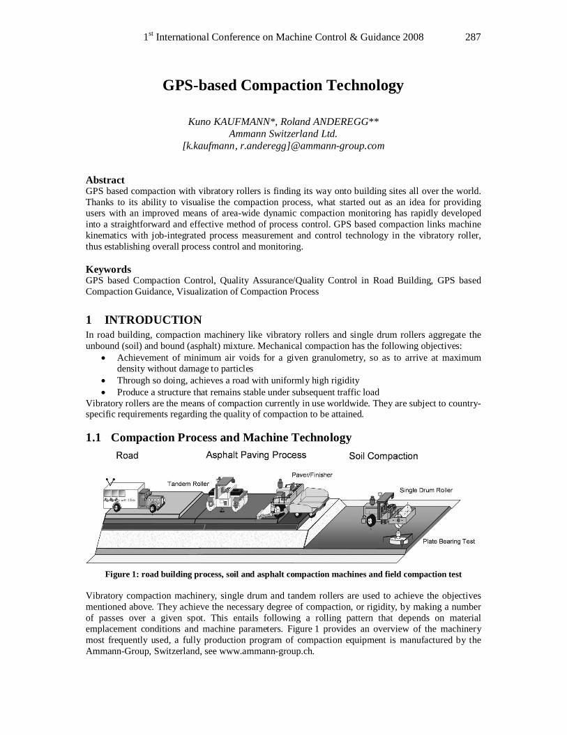
1st International Conference on Machine Control & Guidance 2008 287
GPS-based Compaction Technology
Kuno KAUFMANN*, Roland ANDEREGG** Ammann Switzerland Ltd.
[k.kaufmann, r.anderegg]@ammann-group.com Abstract GPS based compaction with vibratory rollers is finding its way onto building sites all over the world. Thanks to its ability to visualise the compaction process, what started out as an idea for providing users with an improved means of area-wide dynamic compaction monitoring has rapidly developed into a straightforward and effective method of process control. GPS based compaction links machine kinematics with job-integrated process measurement and control technology in the vibratory roller, thus establishing overall process control and monitoring. Keywords GPS based Compaction Control, Quality Assurance/Quality Control in Road Building, GPS based Compaction Guidance, Visualization of Compaction Process
1 INTRODUCTION In road building, compaction machinery like vibratory rollers and single drum rollers aggregate the unbound (soil) and bound (asphalt) mixture. Mechanical compaction has the following objectives:
• Achievement of minimum air voids for a given granulometry, so as to arrive at maximum density without damage to particles
• Through so doing, achieves a road with uniformly high rigidity • Produce a structure that remains stable under subsequent traffic load
Vibratory rollers are the means of compaction currently in use worldwide. They are subject to country-specific requirements regarding the quality of compaction to be attained.
1.1 Compaction Process and Machine Technology
Figure 1: road building process, soil and asphalt compaction machines and field compaction test
Vibratory compaction machinery, single drum and tandem rollers are used to achieve the objectives mentioned above. They achieve the necessary degree of compaction, or rigidity, by making a number of passes over a given spot. This entails following a rolling pattern that depends on material emplacement conditions and machine parameters. Figure 1 provides an overview of the machinery most frequently used, a fully production program of compaction equipment is manufactured by the Ammann-Group, Switzerland, see www.ammann-group.ch.

3D-Construction Applications III 288
1.2 GPS-Technology on the Job Site In addition to the automatic control of the compaction process by changing amplitude and frequency continuously and displaying the operator the optimum speed, the measurement of the soil stiffness kB and, additionally for asphalt layers, the measurement of the surface temperature T complete the “Intelligent Compaction“. These measurement values are calculated for at least each 360° revolution of the mechanical exciter, e. g. 25-50 times per second depending on type of roller. The automatic control of the roller parameters guarantees the optimal compaction result. The stiffness/rigidity measurement technology was developed during the last decade, see (ANDEREGG, R., 1998), (MOONEY, M. et al., 2007). Similarly important for the achievement of the optimum compaction result in practice are the following tasks: • Information about the achieved compaction value kB including the location coordinates (xi, yi, zi) • Information about the number of passes and the homogeneity of the achieved stiffness kB • Asphalt compaction data: asphalt temperature cooling rate, e. g. ∆T(xi,yi,tn)=T(xi,yi,tn)-T(xi,yi,tn-1) This information is available if the measurement data of the roller kB, T, etc. are combined with GPS-data xi, yi, (zi), Time t. (zi) is the vertical (out of plane) data with a lower accuracy compared to the in-plane data xi, yi (HOFMANN-WELLENHOFF, B, et. al., 1997). The process could be displayed to the roller operator in real time, the visualisation of the process allows him optimal application of the compaction equipment.
Figure 2: Differential Global Positioning System (DGPS) in application on single drum roller for soil
compaction The compaction process guidance system ACEplus enables the roller driver to gain an in-situ-overview of the job site. The operator maximises his productivity while adapting the machine-use to the displayed compaction data. The accuracy of the ACEplus-data is dependent on the type of GPS-receiver. On job sites, contractors very often use RTK-GPS-systems (RTK: Real Time Kinematics) consisting of a GPS-receiver on the roller, a GPS base station and a reference signal between base and roller receiver (KAUFMANN, K. et al., 2002). This technology leads to an accuracy of the roller position of about ±5 cm, see figure 2 for technical description. Comparing the roller passes (xi, yi, tn), the ACEplus-system shows the operator the overlap of the different roller passes. The overlap is displayed through markers (MANSFELD, W., 1998).
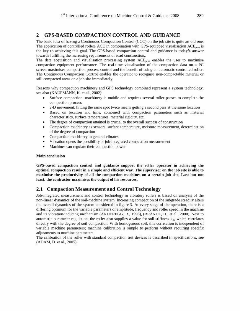
1st International Conference on Machine Control & Guidance 2008 289
2 GPS-BASED COMPACTION CONTROL AND GUIDANCE The basic idea of having a Continuous Compaction Control (CCC) on the job site is quite an old one. The application of controlled rollers ACE in combination with GPS-equipped visualisation ACEplus is the key to achieving this goal. The GPS-based compaction control and guidance is today’s answer towards fulfilling the increasing requirements of road construction,. The data acquisition and visualisation processing system ACEplus enables the user to maximise compaction equipment performance. The real-time visualisation of the compaction data on a PC screen maximises compaction process control and the benefit of using an automatic controlled roller. The Continuous Compaction Control enables the operator to recognise non-compactable material or still compacted areas on a job site immediately. Reasons why compaction machinery and GPS technology combined represent a system technology, see also (KAUFMANN, K. et al., 2002):
• Surface compaction: machinery is mobile and requires several roller passes to complete the compaction process
• 2-D movement: hitting the same spot twice means getting a second pass at the same location • Based on location and time, combined with compaction parameters such as material
characteristics, surface temperatures, material rigidity, etc. • The degree of compaction attained is crucial to the overall success of construction • Compaction machinery as sensors: surface temperature, moisture measurement, determination
of the degree of compaction • Compaction machinery in general vibrates • Vibration opens the possibility of job-integrated compaction measurement • Machines can regulate their compaction power
Main conclusion GPS-based compaction control and guidance support the roller operator in achieving the optimal compaction result in a simple and efficient way. The supervisor on the job site is able to maximise the productivity of all the compaction machines on a certain job site. Last but not least, the contractor maximises the output of his resources.
2.1 Compaction Measurement and Control Technology Job-integrated measurement and control technology in vibratory rollers is based on analysis of the non-linear dynamics of the soil-machine system. Increasing compaction of the subgrade steadily alters the overall dynamics of the system considered in figure 3. At every stage of the operation, there is a differing optimum for the variable parameters of amplitude, frequency and roller speed in the machine and its vibration-inducing mechanism (ANDEREGG, R., 1998), (BRANDL, H., et al., 2000). Next to automatic parameter regulation, the roller also supplies a value for soil stiffness kB, which correlates directly with the degree of soil compaction. With homogenous soil, this correlation is independent of variable machine parameters; machine calibration is simple to perform without requiring specific adjustments to machine parameters. The calibration of the roller with standard compaction test devices is described in specifications, see (ADAM, D. et al., 2005).
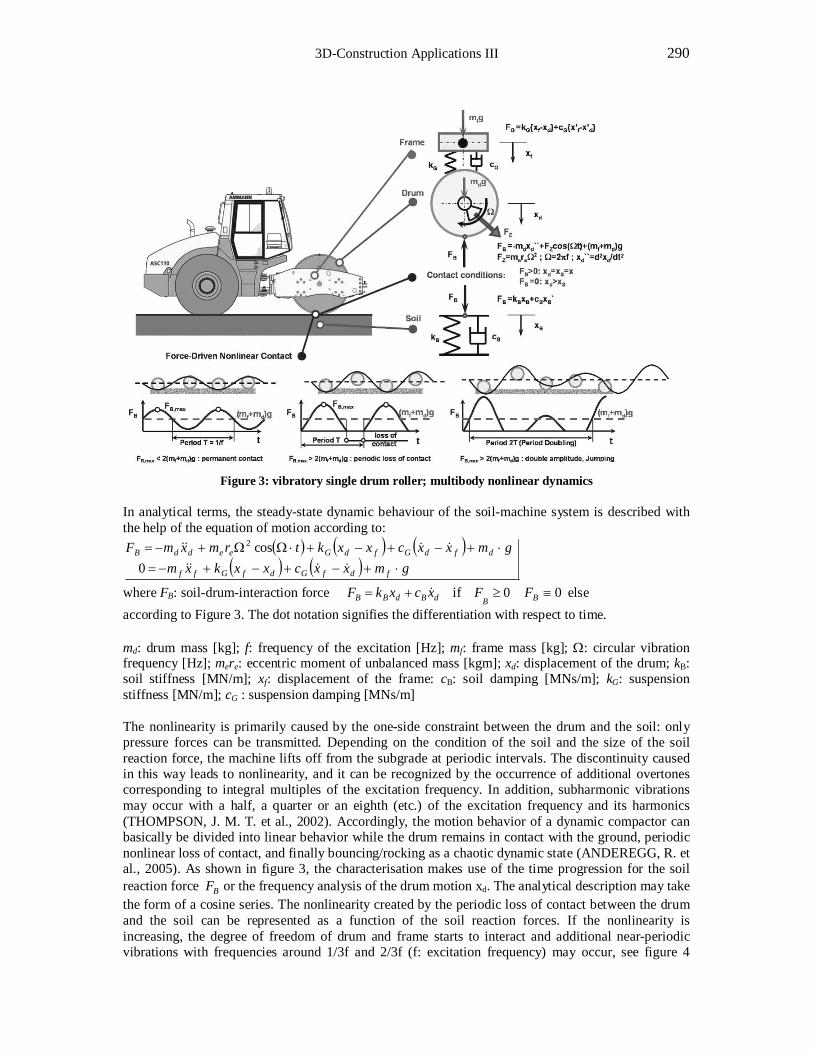
3D-Construction Applications III 290
Figure 3: vibratory single drum roller; multibody nonlinear dynamics
In analytical terms, the steady-state dynamic behaviour of the soil-machine system is described with the help of the equation of motion according to:
( ) ( ) ( )( ) ( ) 0
cos2
gmxxcxxkxmgmxxcxxktrmxmF
fdfGdfGff
dfdGfdGeeddB
⋅+−+−+−=⋅+−+−+⋅ΩΩ+−=
&&&&
&&&&
where FB: soil-drum-interaction force dBdBB xcxkF &+= if 0≥B
F 0≡BF else according to Figure 3. The dot notation signifies the differentiation with respect to time. md: drum mass [kg]; f: frequency of the excitation [Hz]; mf: frame mass [kg]; Ω: circular vibration frequency [Hz]; mere: eccentric moment of unbalanced mass [kgm]; xd: displacement of the drum; kB: soil stiffness [MN/m]; xf: displacement of the frame: cB: soil damping [MNs/m]; kG: suspension stiffness [MN/m]; cG : suspension damping [MNs/m] The nonlinearity is primarily caused by the one-side constraint between the drum and the soil: only pressure forces can be transmitted. Depending on the condition of the soil and the size of the soil reaction force, the machine lifts off from the subgrade at periodic intervals. The discontinuity caused in this way leads to nonlinearity, and it can be recognized by the occurrence of additional overtones corresponding to integral multiples of the excitation frequency. In addition, subharmonic vibrations may occur with a half, a quarter or an eighth (etc.) of the excitation frequency and its harmonics (THOMPSON, J. M. T. et al., 2002). Accordingly, the motion behavior of a dynamic compactor can basically be divided into linear behavior while the drum remains in contact with the ground, periodic nonlinear loss of contact, and finally bouncing/rocking as a chaotic dynamic state (ANDEREGG, R. et al., 2005). As shown in figure 3, the characterisation makes use of the time progression for the soil reaction force BF or the frequency analysis of the drum motion xd. The analytical description may take the form of a cosine series. The nonlinearity created by the periodic loss of contact between the drum and the soil can be represented as a function of the soil reaction forces. If the nonlinearity is increasing, the degree of freedom of drum and frame starts to interact and additional near-periodic vibrations with frequencies around 1/3f and 2/3f (f: excitation frequency) may occur, see figure 4
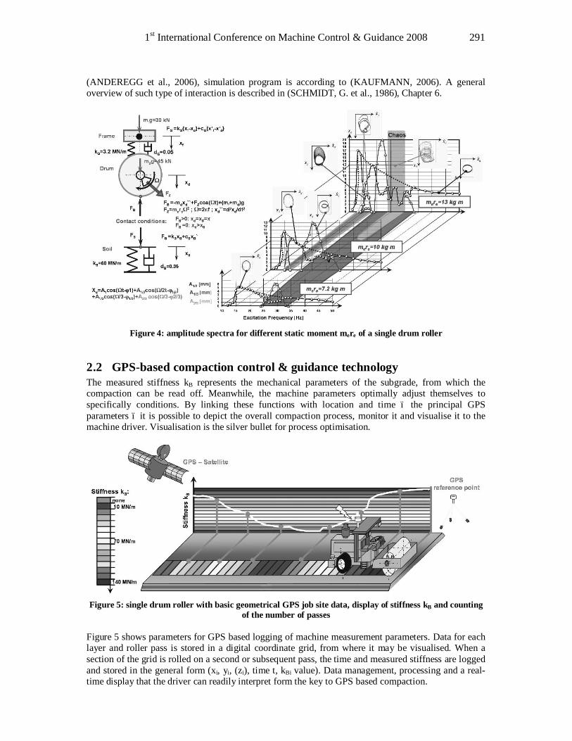
1st International Conference on Machine Control & Guidance 2008 291
(ANDEREGG et al., 2006), simulation program is according to (KAUFMANN, 2006). A general overview of such type of interaction is described in (SCHMIDT, G. et al., 1986), Chapter 6.
Figure 4: amplitude spectra for different static moment mere of a single drum roller
2.2 GPS-based compaction control & guidance technology The measured stiffness kB represents the mechanical parameters of the subgrade, from which the compaction can be read off. Meanwhile, the machine parameters optimally adjust themselves to specifically conditions. By linking these functions with location and time – the principal GPS parameters – it is possible to depict the overall compaction process, monitor it and visualise it to the machine driver. Visualisation is the silver bullet for process optimisation.
Figure 5: single drum roller with basic geometrical GPS job site data, display of stiffness kB and counting
of the number of passes Figure 5 shows parameters for GPS based logging of machine measurement parameters. Data for each layer and roller pass is stored in a digital coordinate grid, from where it may be visualised. When a section of the grid is rolled on a second or subsequent pass, the time and measured stiffness are logged and stored in the general form (xi, yi, (zi), time t, kBi value). Data management, processing and a real-time display that the driver can readily interpret form the key to GPS based compaction.
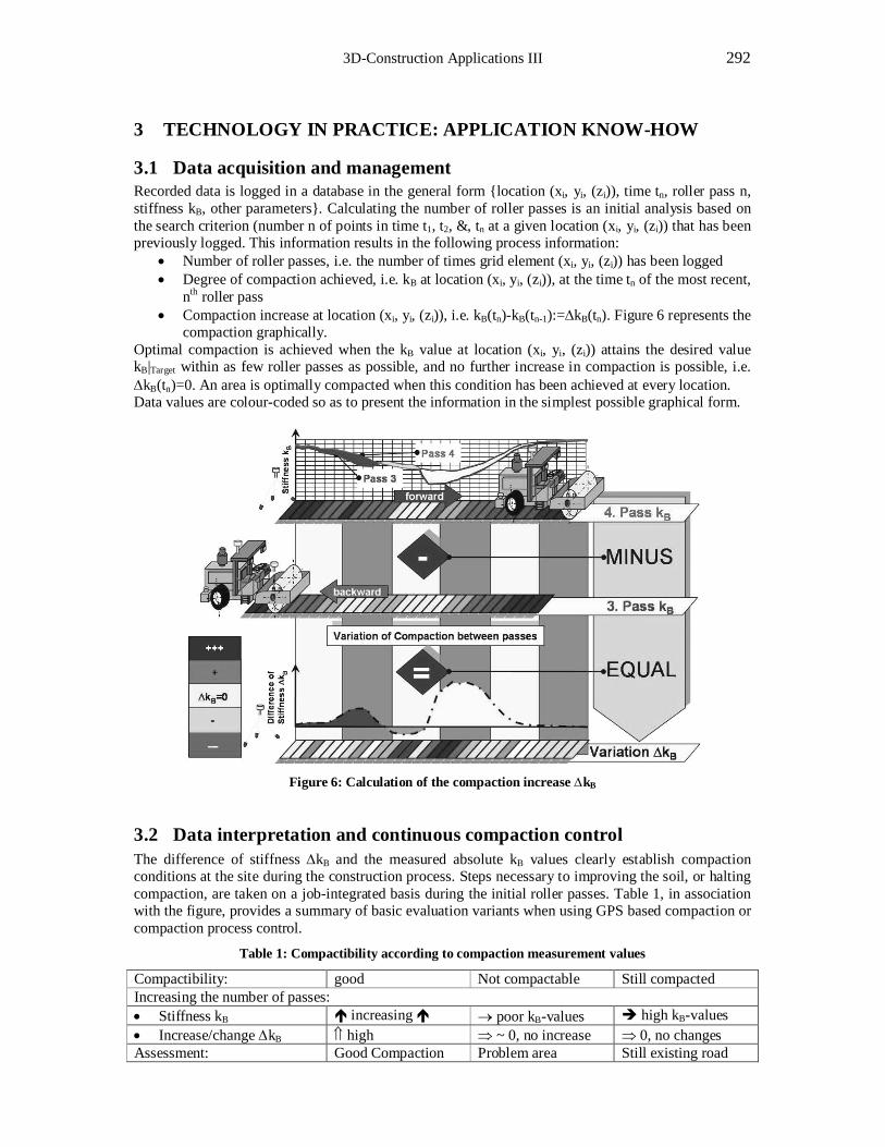
3D-Construction Applications III 292
3 TECHNOLOGY IN PRACTICE: APPLICATION KNOW-HOW
3.1 Data acquisition and management Recorded data is logged in a database in the general form location (xi, yi, (zi)), time tn, roller pass n, stiffness kB, other parameters. Calculating the number of roller passes is an initial analysis based on the search criterion (number n of points in time t1, t2,…, tn at a given location (xi, yi, (zi)) that has been previously logged. This information results in the following process information:
• Number of roller passes, i.e. the number of times grid element (xi, yi, (zi)) has been logged • Degree of compaction achieved, i.e. kB at location (xi, yi, (zi)), at the time tn of the most recent,
nth roller pass • Compaction increase at location (xi, yi, (zi)), i.e. kB(tn)-kB(tn-1):=∆kB(tn). Figure 6 represents the
compaction graphically. Optimal compaction is achieved when the kB value at location (xi, yi, (zi)) attains the desired value kB|Target within as few roller passes as possible, and no further increase in compaction is possible, i.e. ∆kB(tn)=0. An area is optimally compacted when this condition has been achieved at every location. Data values are colour-coded so as to present the information in the simplest possible graphical form.
Figure 6: Calculation of the compaction increase ∆kB
3.2 Data interpretation and continuous compaction control The difference of stiffness ∆kB and the measured absolute kB values clearly establish compaction conditions at the site during the construction process. Steps necessary to improving the soil, or halting compaction, are taken on a job-integrated basis during the initial roller passes. Table 1, in association with the figure, provides a summary of basic evaluation variants when using GPS based compaction or compaction process control.
Table 1: Compactibility according to compaction measurement values
Compactibility: good Not compactable Still compacted Increasing the number of passes: • Stiffness kB é increasing é → poor kB-values è high kB-values • Increase/change ∆kB ⇑ high ⇒ ~ 0, no increase ⇒ 0, no changes Assessment: Good Compaction Problem area Still existing road
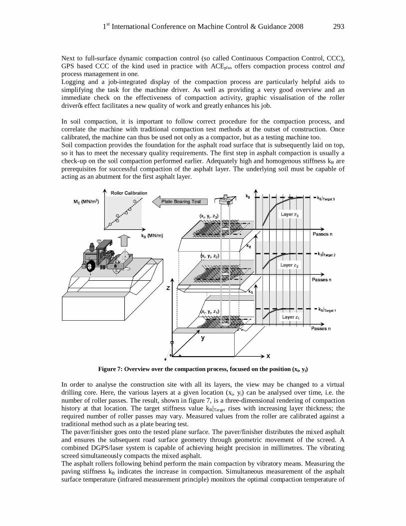
1st International Conference on Machine Control & Guidance 2008 293
Next to full-surface dynamic compaction control (so called Continuous Compaction Control, CCC), GPS based CCC of the kind used in practice with ACEplus offers compaction process control and process management in one. Logging and a job-integrated display of the compaction process are particularly helpful aids to simplifying the task for the machine driver. As well as providing a very good overview and an immediate check on the effectiveness of compaction activity, graphic visualisation of the roller driver’s effect facilitates a new quality of work and greatly enhances his job. In soil compaction, it is important to follow correct procedure for the compaction process, and correlate the machine with traditional compaction test methods at the outset of construction. Once calibrated, the machine can thus be used not only as a compactor, but as a testing machine too. Soil compaction provides the foundation for the asphalt road surface that is subsequently laid on top, so it has to meet the necessary quality requirements. The first step in asphalt compaction is usually a check-up on the soil compaction performed earlier. Adequately high and homogenous stiffness kB are prerequisites for successful compaction of the asphalt layer. The underlying soil must be capable of acting as an abutment for the first asphalt layer.
Figure 7: Overview over the compaction process, focused on the position (xi, yi)
In order to analyse the construction site with all its layers, the view may be changed to a virtual drilling core. Here, the various layers at a given location (xi, yi) can be analysed over time, i.e. the number of roller passes. The result, shown in figure 7, is a three-dimensional rendering of compaction history at that location. The target stiffness value kB|Target rises with increasing layer thickness; the required number of roller passes may vary. Measured values from the roller are calibrated against a traditional method such as a plate bearing test. The paver/finisher goes onto the tested plane surface. The paver/finisher distributes the mixed asphalt and ensures the subsequent road surface geometry through geometric movement of the screed. A combined DGPS/laser system is capable of achieving height precision in millimetres. The vibrating screed simultaneously compacts the mixed asphalt. The asphalt rollers following behind perform the main compaction by vibratory means. Measuring the paving stiffness kB indicates the increase in compaction. Simultaneous measurement of the asphalt surface temperature (infrared measurement principle) monitors the optimal compaction temperature of

3D-Construction Applications III 294
the paving and limits the zone where stiffness measurement is valid. kB measurements must be performed on paving within a temperature range of TO>T>TU, where the bitumen exhibits fluid-like behaviour and the measured stiffness is directly proportional to the density of contact points within the mineral mixture. Only under these conditions is increasing stiffness kB also a measure of increasing compaction. Other aspects of the compaction process are determined in a manner analogous to the soil compaction already described. Figure 8 shows an asphalt construction site including a paver with pre-compacting screed and a tandem asphalt roller to perform the main compaction. The paver screed width in turn determines the optimal rolling pattern for the roller driver. This rolling pattern may be specified in GPS terms, with job-integrated monitoring to verify that it is performed. Figure 8 shows a typical machine control response, along with anticipated kB stiffness and surface temperature T.
Figure 8: Asphalt compaction; compaction measurement & control and the rolling pattern
As figure 8 shows, compaction information is contained partly in the paver and partly in the roller, because the compaction process is distributed between both machines. The greater the pre-compaction at the paver, the less main compaction work there is for the roller to do, and vice versa. This, plus the fact that paver screed geometry and the paver speed dictate the rolling pattern and the rolling speed required, making a case for an online connection between the paver and the roller. This connection must be capable of exchanging machine data between all of the machines involved and displaying it fast and in real time to all concerned. This is essential to an optimal overall compaction process. With soil compaction, it should be possible to upload job site data wirelessly into the machine, and download process data from it. In contrast to asphalt compaction, this need not be a real-time process; it is possible for data exchange to occur only when the machines are not in operation, see for example the description in patent WO 2006/099772 A1 “System for Co-ordinated Soil-Cultivation”.
1st International Conference on Machine Control & Guidance 2008 295
4 CONCLUSIONS GPS based compaction technology with tandem and single drum rollers in asphalt and soil compaction make compaction machinery easier to use in practice, which brings user benefits as follows: • Automatic regulation of roller vibration parameters • Job-integrated measurement of kB stiffness as an adequate indicator of compaction in soil
compaction, supplemented by temperature measurement at the paving surface in asphalt compaction
• Straightforward calibration of measured values from the rollers using a traditional compaction measurement method, like a plate bearing test
• Graphic visualisation of the compaction process • A simple process display enables a driver to optimally deploy his machine (one picture says more
than a thousand words) • Automatic data logging (at second intervals). Logged data is retained in the event of a power
failure. The future development of GPS-based compaction technology might be driven by its application on the job. Especially the Internet working of machinery, online data exchange helps the operators on different rollers on one job site to optimise their tasks. The distinction between good and poor compaction will be supported by image recognition and image processing as the next step. In addition to today’s technologies, new possible technologies for image processing systems may take place: infrared thermal imaging camera, image recognition (contiguous unsatisfactory values = bad spot, distributed unsatisfactory values = variation, asphalt compaction algorithms, soil compaction algorithms, soil stabilisation specialities, …). Image processing is constrained for the purposes of GPS-based compaction control and guidance. Process control may provide the opportunity for modifying parameters via image processing technologies, on the basis of measured values.
REFERENCES Books: SCHMIDT, G., TONDL, A.: Non-Linear Vibrations. Cambridge University Press, Cambridge, 1986.
THOMPSON, J. M. T., STEWART, H. B.: Nonlinear Dynamics and Chaos. John Wiley & Sons, Ltd., Chichester, 2002
ANDEREGG, R.: Nichtlineare Schwingungen bei dynamischen Bodenverdichtern. Fortschritt-Berichte VDI, Reihe 4, VDI-Verlag GmbH, Düsseldorf, 1998.
BRANDL, H., ADAM, D.: Flächendeckende Dynamische Verdichtungskontrolle (FDVK) mit Vibrationswalzen. Bundesministerium für Verkehr, Innovation und Technologie, Strassenforschung Heft 506, Wien, 2000.
HOFMANN-WELLENHOFF, B., LICHTENEGGER, H., COLLINS, J.: GPS, Theory and Practice. 4., revised edition, Springer-Verlag, Wien, New York, 1997.
KAUFMANN, K.: Mehr Verdichtungsleistung mit bifrequenter Schwingungserzeugung. Diplomarbeit, Berner Fachhochschule HTI, Burgdorf, 2006.
MANSFELD, W.: Satellitenortung und Navigation, Grundlagen und Anwendung globaler Satellitennavigationssysteme. Vieweg Verlag, Braunschweig, 1998

3D-Construction Applications III 296
Journal articles: ADAM, D., KOPF, F.: Flächendeckende Dynamische Verdichtungskontrolle (FDVK), Kalibrierung und Anwendung gemäss RVS 8S.02.6. Österreichische Ingenieur- und Architekten-Zeitschrift (ÖIAZ), 150. Jg., Heft 4-5/2005, p. 162-173, 2005.
ANDEREGG, R., VON FELTEN, D.: Nonlinear Dynamic of Compaction Equipment – an Overview (in German). Österreichische Ingenieur- und Architekten-Zeitschrift (ÖIAZ), 150. Jg., Heft 4-5/2005, p. 145-149, 2005.
ANDEREGG, R., KAUFMANN, K., VON FELTEN, D.: Intelligent Compaction Monitoring Using Intelligent Soil Compactors. Proceedings of the GeoCongress 2006 “Sensing Methods and Devices”, American Society of Civil Engineers ASCE, Atlanta, 2006
KAUFMANN, K., ANDEREGG, R.: Geregelte Walzenzüge und die Flächendeckende Dynamische Verdichtungskontrolle (FDVK), Teil II. Strassen- und Tiefbau, 56. Jg. Heft 9/2002, p. 12-17, 2002.
MOONEY, M. A., RINEHART, R. V.: Field Monitoring of Roller Vibration during Compaction of Subgrade Soil. Journal of Geotechnical and Geoenvironmental Engineering, ASCE, p. 257-265, 2007.
Patents: WO 2006/099772 A1 System for Co-ordinated Soil-Cultivation Links: http://www.ammann-group.ch, last accessed on April 13, 2008 * Kuno Kaufmann, Ammann Switzerland Ltd, Research & Development, Eisenbahnstrasse 44, CH-4900 Langenthal, Switzerland. ** Dr. Roland Anderegg, Ammann Switzerland Ltd, Research & Development, Eisenbahnstrasse 44, CH-4900 Langenthal, Switzerland.
1st International Conference on Machine Control & Guidance 2008 297
Passage Simulation of Monorail Suspension Conveyors and Transport Goods for Collision Prevention
Thomas A. WUNDERLICH*, Thomas SCHÄFER*, Stefan AUER**
Technische Universität München, Germany [th.wunderlich, th.schaefer, stefan.auer]@bv.tum.de
Abstract Modern industrial production involves complex and time-critical process chains which demand a sophisticated supply chain management and logistics as well as safe and reliable transport systems. Inside a vast factory individual parts (e.g. engines) cover large distances by using specific transport lines, e.g. electric monorail suspension conveyors. In such an environment, the avoidance of any collision of units with the surrounding area or flexible tools becomes a must. Above all, it is an interruption of production that has to be prevented as this would result in very high financial losses for every minute break. On the other hand, last minute changes in product design are typical and call for a simulation tool to compute dynamic interference checks and to visualize detected risk zones where problems might occur. The paper gives an overview over common interference detection techniques of moving objects among solids and surfaces and finally introduces the prototype Software KoSimu (Kollisionsprüfungs-Simulator) developed at the Chair of Geodesy in course of a diploma thesis. It provides a collision check simulator that enables the designer to simulate the motion of a part prototype along a known trajectory through the facility and detect collision spots. To acquire the transport line’s surrounding, Terrestrial Laser Scanning is applied, creating representative point clouds. The complementing input for KoSimu consists of geometric models of the part prototype and the mounting device on the suspension conveyers. In a first step, these two models have to be linked using specific connection points. Subsequently, the new model is approximated by suitable cubes of selectable size and reduced to its characteristic envelope. Under the assumption of homogeneous mass distribution (centre of mass equals the geometric centre) physical effects (centrifugal and reset forces, oscillating movements) can be considered as well. The geometric and the physical model are jointly used to create a space of impact along the track which is tested against the point clouds of obstacles to reveal and successively prevent any possible collisions Keywords Collision prevention, Terrestrial Laserscanning, Simulation, Industrial Production
1 INTRODUCTION Collision avoidance has become a major issue in navigation and in industrial automation. It is the latter field on which we focus here. Starting with the broad employment of ever faster acting industrial robots in the late Seventies of the past century, the problem of preventing any collision of moving robot arms and effectors with infrastructure or treated objects arose. Parallel to sensor-based and visual control procedures, analytical approaches evolved. Their power increased with growing computational capacities and, obviously, simulations to detect possible collisions virtually in advance were preferred to in-situ collision avoidance attempts. Before 1980 collision tests were developed which made use of dilatation (a geometric method which reduces the size of an object by a constant amount and enlarges the environment to the same extent) to simplify intersections (Udupa 1977) or of contact proofs of corner points and edges with polyhedron surfaces (Boyse 1979). Then methods followed which aimed at substituting complex objects by simple
3D-Construction Applications III 298
solids like ashlars (Ozaki et al. 1984) or cubes (Uchiki et al. 1987) to keep the computation load in limits. A different approach tried to wrap the objects (Gilbert et al. 1988, 1989) by means of quadrics like cylinders or spheres to make mutual spacing control easier. At the turn of the century clear claims have been set up for analytical collision avoidance methods: simple, accurate and efficient (prompt). In the same treatise (Bao 2000) two simple but capable tools were suggested as to: wrap objects by cubes and test both three co-ordinate intervals for common content inscribe and circumscribe spheres to allow rotation-invariant distance calculations. Our investigations are based on these tools, increasing the level of detail by using an appropriate segmentation of complex objects into a large number of equal cubes. The quoted advances came from the robotics and CAD/CAM community as well as from computational geometry; engineering surveyors at that time rather dealt with robot calibration processes. It was the appearance of Terrestrial Laser Scanning that now involved geodesy in the field. Current interest focuses on simulations of transport missions in large, laser surveyed environments within vast production facilities. The challenge is represented by combining the geometrical model with a physical one to account for the resulting effects of centrifugal and gravitational forces along curved parts of the transport line. There, the trajectories have to be used for building up a space of impact, changing with the velocity of the transport platform. The space of impact can then serve for a static test of collision at suspected bottlenecks and obstacles.
2 TASK Complex and time-critical process chains in industrial production of premium automobiles demand a sophisticated supply chain management and logistics as well as safe and reliable transport systems. Inside a vast factory individual parts (e.g. engines) cover large distances by using electric monorail suspension conveyors. In such an environment, the avoidance of any collision of units with the surrounding area or flexible tools becomes a must. Last minute changes in the product’s design demand a simulation tool to compute dynamic interference checking and to visualize risk zones where problems might occur. In particular, financial losses have to be prevented which would occur either by the partial damage of a high-tech engine or, much more expensive, by provoking a standstill of transport line and whole production units.
3 SOLUTION The solution for the specific task splits up into four main parts:
• obtain a CAD-model of the transport object itself and of the bearing conveyor unit or scan them; get physical properties (weight, centre of mass, velocity, motions allowed)
• obtain a CAD-model of the guiding rail of the transport line or scan it • scan the present environment (and manipulator positions) along the transport line • develop a simulation program to virtually move conveyor with object along the rail through
the scanned environment and search for collision zones. This report will only deal with the fourth, most demanding item.
3.1 Simulation Strategy We start with preparing a point cloud of the transport object and a conveyor, either by precise scanning or by converting present VRML-models, which can be realized by a scene export from the software 3D Studio Max. Then the two point clouds are combined, using a defined matching point and defined orientations (specific bearing cone of the conveyor). Next, the couple is attached to the guiding rail by a transformation to the common system of rail and environment. Now the
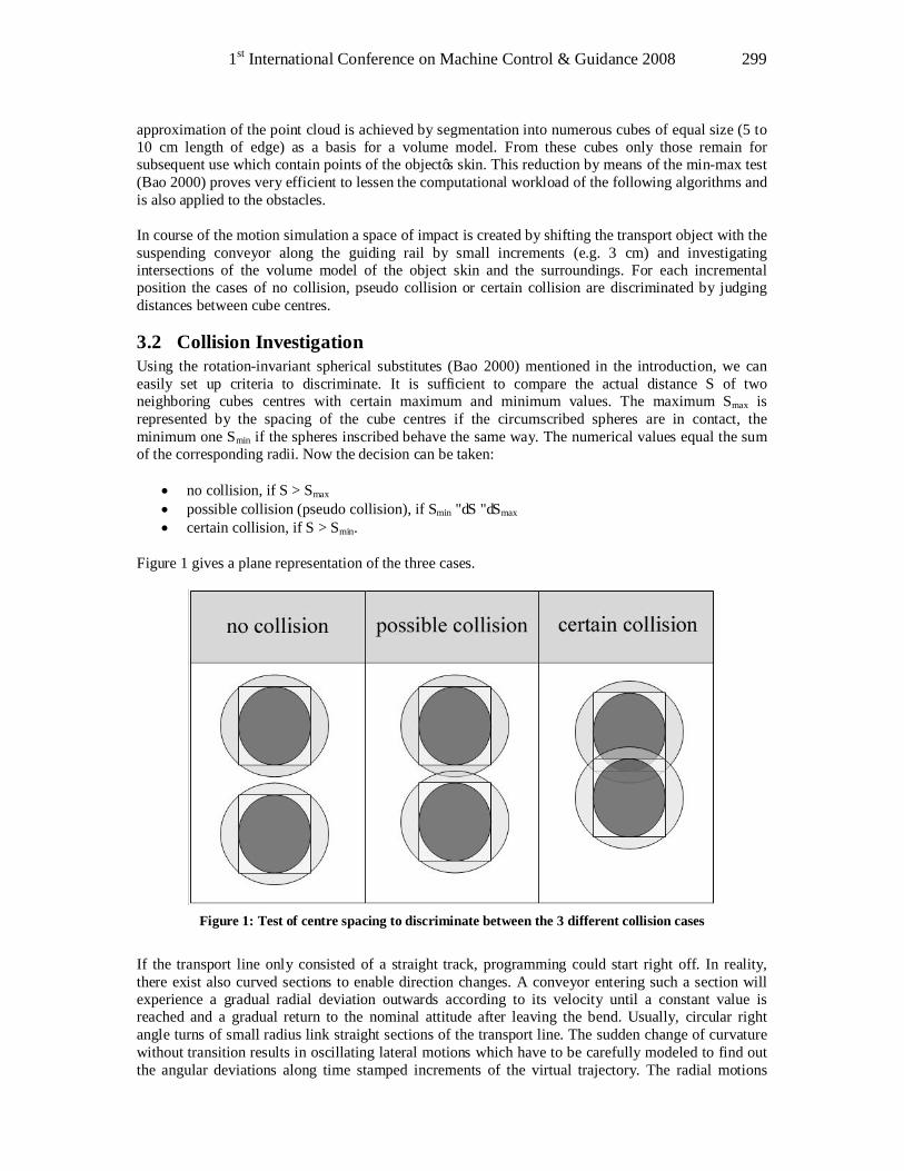
1st International Conference on Machine Control & Guidance 2008 299
approximation of the point cloud is achieved by segmentation into numerous cubes of equal size (5 to 10 cm length of edge) as a basis for a volume model. From these cubes only those remain for subsequent use which contain points of the object’s skin. This reduction by means of the min-max test (Bao 2000) proves very efficient to lessen the computational workload of the following algorithms and is also applied to the obstacles. In course of the motion simulation a space of impact is created by shifting the transport object with the suspending conveyor along the guiding rail by small increments (e.g. 3 cm) and investigating intersections of the volume model of the object skin and the surroundings. For each incremental position the cases of no collision, pseudo collision or certain collision are discriminated by judging distances between cube centres.
3.2 Collision Investigation Using the rotation-invariant spherical substitutes (Bao 2000) mentioned in the introduction, we can easily set up criteria to discriminate. It is sufficient to compare the actual distance S of two neighboring cubes centres with certain maximum and minimum values. The maximum Smax is represented by the spacing of the cube centres if the circumscribed spheres are in contact, the minimum one Smin if the spheres inscribed behave the same way. The numerical values equal the sum of the corresponding radii. Now the decision can be taken:
• no collision, if S > Smax • possible collision (pseudo collision), if Smin ≤ S ≤ Smax • certain collision, if S > Smin.
Figure 1 gives a plane representation of the three cases.
Figure 1: Test of centre spacing to discriminate between the 3 different collision cases
If the transport line only consisted of a straight track, programming could start right off. In reality, there exist also curved sections to enable direction changes. A conveyor entering such a section will experience a gradual radial deviation outwards according to its velocity until a constant value is reached and a gradual return to the nominal attitude after leaving the bend. Usually, circular right angle turns of small radius link straight sections of the transport line. The sudden change of curvature without transition results in oscillating lateral motions which have to be carefully modeled to find out the angular deviations along time stamped increments of the virtual trajectory. The radial motions
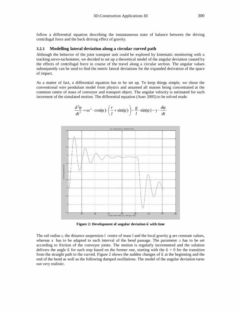
3D-Construction Applications III 300
follow a differential equation describing the instantaneous state of balance between the driving centrifugal force and the back driving effect of gravity.
3.2.1 Modelling lateral deviation along a circular curved path Although the behavior of the joint transport unit could be explored by kinematic monitoring with a tracking servo-tachometer, we decided to set up a theoretical model of the angular deviation caused by the effects of centrifugal force in course of the travel along a circular section. The angular values subsequently can be used to find the metric lateral deviations for the expanded derivation of the space of impact. As a matter of fact, a differential equation has to be set up. To keep things simple, we chose the conventional wire pendulum model from physics and assumed all masses being concentrated at the common centre of mass of conveyor and transport object. The angular velocity is estimated for each increment of the simulated motion. The differential equation (Auer 2005) to be solved reads:
dtd
lg
lr
dtd ϕ
γϕϕϕωϕ
⋅−⋅−
+⋅⋅= )sin()sin()cos(2
2
2
Figure 2: Development of angular deviation φ with time
The rail radius r, the distance suspension – centre of mass l and the local gravity g are constant values, whereas ω has to be adapted to each interval of the bend passage. The parameter γ has to be set according to friction of the conveyor joints. The motion is regularly incremented and the solution delivers the angle φ for each step based on the former one, starting with the φ = 0 for the transition from the straight path to the curved. Figure 2 shows the sudden changes of φ at the beginning and the end of the bend as well as the following damped oscillations. The model of the angular deviation turns out very realistic.
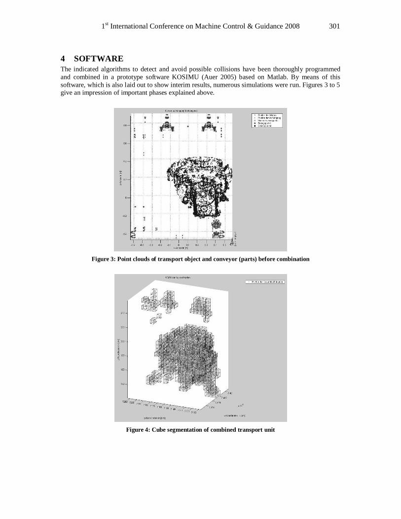
1st International Conference on Machine Control & Guidance 2008 301
4 SOFTWARE The indicated algorithms to detect and avoid possible collisions have been thoroughly programmed and combined in a prototype software KOSIMU (Auer 2005) based on Matlab. By means of this software, which is also laid out to show interim results, numerous simulations were run. Figures 3 to 5 give an impression of important phases explained above.
Figure 3: Point clouds of transport object and conveyor (parts) before combination
Figure 4: Cube segmentation of combined transport unit
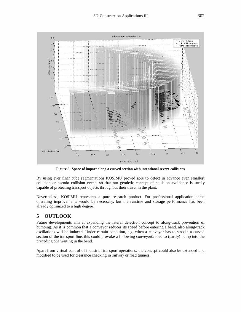
3D-Construction Applications III 302
Figure 5: Space of impact along a curved section with intentional severe collisions
By using ever finer cube segmentations KOSIMU proved able to detect in advance even smallest collision or pseudo collision events so that our geodetic concept of collision avoidance is surely capable of protecting transport objects throughout their travel in the plant. Nevertheless, KOSIMU represents a pure research product. For professional application some operating improvements would be necessary, but the runtime and storage performance has been already optimized to a high degree.
5 OUTLOOK Future developments aim at expanding the lateral detection concept to along-track prevention of bumping. As it is common that a conveyor reduces its speed before entering a bend, also along-track oscillations will be induced. Under certain condition, e.g. when a conveyor has to stop in a curved section of the transport line, this could provoke a following conveyor’s load to (partly) bump into the preceding one waiting in the bend. Apart from virtual control of industrial transport operations, the concept could also be extended and modified to be used for clearance checking in railway or road tunnels.
1st International Conference on Machine Control & Guidance 2008 303
REFERENCES AUER, S.: Geodätisches Konzept zur Kollisionsvermeidung entlang von Elektrohängebahnen in der Automobilproduktion. Diploma Thesis, TU München, 2005.
BAO, Z.: Rechnerunterstützte Kollisionsprüfung auf der Basis eines B-rep Polytree CSG-Hybidmodells in einem integrierten CAD/CAM System. VDI Nachrichten, Vol. 322, 2000.
BOYSE, J.W.: Interference Detection among Solids and Surfaces. Comm. of the ACM, Vol.22, No.1, 1979.
GILBERT, E.G., JOHNSON, D.W., KEERTHI, S.S.: A fast Procedure for Computing the Distance between complex Objects in three-dimensional Space. IEEE Transaction on Robotics and Automation, Vol.4, pp.193-203, 1988.
GILBERT, E.G., HONG, S.M.: A new Algorithm for Detetcing the Collision of Moving Objects. Proc. of the IEEE Int. Conf. on Robotics and Automation, Scottsdale, Arizona, 1989.
OZAKI, H., MOHRI, A., TAKATA, M: On the Collision-free Movement of a Manipulator. In: Advanced Software in Robotics, A. Danthine and M. Geradin (eds.), Elsevier, North-Holland, 1984.
SCHÄFER, Th.: Terrestrial Laser Scanning – Examples for Kinematic Applications. Lecture Notes, Workshop ’TLS - Prospects of the New Surveying Approach’, University of Ljubljana, Slovenia, 2006.
UCHIKI, T., OHASHI, T., TOKORO, M.: Collision Detection in Motion Simulation. Computer & Graphics, Vol. 11 supplement, 1987.
UDUPA, S.: On the Collision-free Movement of a Manipulator, PhD Thesis, California Institute of Technology, 1977.
WUNDERLICH, Th.: Kollisionsvermeidung entlang industrieller Elektrohängebahnen. Internal Report, Chair of Geodesy, TU München, 2004.
* Prof. Thomas A. Wunderlich and Dipl.-Ing. Thomas Schäfer, Chair of Geodesy, TU München,
Arcisstrasse 21, D-80290 Munich, Germany. ** Dipl.-Ing. Stefan Auer, Remote Sensing Technology, TU München, Arcisstrasse 21, D-80290
Munich, Germany.

3D-Construction Applications III 304

Poster Session

1st International Conference on Machine Control & Guidance 2008 307
Kinematic Surface Analysis by Terrestrial Laser Scanning
Hans-Martin ZOGG*, David GRIMM* ETH Zurich, Switzerland
[zogg, grimm]@geod.baug.ethz.ch Abstract This paper presents terrestrial laser scanning with emphasis on kinematic surface analysis. Besides an overview of terrestrial laser scanning in general, the 2D-laser scanner SICK LMS200-30106 is introduced as well as investigations on its distance measurement qualities. This 2D-laser scanner is often used for kinematic applications in the field of engineering geodesy due to its high scanning frequency, robustness, and reliability. The kinematic surface analysis at Hamburg Airport in conjunction with load tests is presented as an application for the 2D-laser scanner. In general, an application of terrestrial laser scanning into the field of machine control and guidance is conceivable. Keywords Terrestrial laser scanning, engineering geodesy, kinematic, surface detection,
1 INTRODUCTION In recent years, terrestrial laser scanning has become an additional acquisition method in engineering geodesy. Terrestrial laser scanners touchlessly measure distances and angles to an object or environment within short time. The result of a scan is a 3D-point cloud which contains thousands of 3D-points. Besides scanning from a stable scanner setup, the kinematic approach has been established as well by moving a terrestrial laser scanner in the environment. Hence, profile laser scanners with a high measurement frequency are often implemented in kinematic applications, e.g. for surface analysis. Additional sensors, e.g. tacheometry, GPS, odometers or levels, enable the detection of position and orientation of the profile scanner with reference to the environment. By combining the measurements of the different sensors, 3D-coordinates can be calculated, e.g. for volume detection. The kinematic approach and the high measurement frequency offer the application of terrestrial laser scanning in the field of machine control and guidance. In section 2 of this paper, an overview of terrestrial laser scanning in conjunction with engineering geodesy is given. Section 3 deals with the profile laser scanner SICK LMS200-30106 which is well known for applications in the field of industrial engineering and robotics. Moreover in recent years, its applications in the field of engineering geodesy are increasing, in particular for kinematic applications. Section 4 introduces an application of kinematic surface analysis at the Hamburg Airport. Finally, a conclusion and an outlook are given in section 5, and section 6 respectively.
2 TERRESTRIAL LASER SCANNING Terrestrial laser scanning is strongly influenced by the development of the LiDAR technique (Light Detection And Ranging), which started in the 1970s. This technique has been successfully used in airborne and remote sensing applications. The LiDAR technique was implemented in geodetic instruments since 1990 due to technical improvements as for micro-chip laser technology, optical elements, micro-electro-mechanical systems, and computer technology. Main elements of a LiDAR unit are an emitter, a receiver and a detector system. Hence, a laser is the emitter which contains the information for the detection of the travelling time from the transmitter to the objects. Depending on the measurement principle and the wavelength of the laser, the specifications and measurement feasibilities of a LiDAR system change. In addition to the laser, each LiDAR system has to deflect the laser beam for areal measurements. The deflection unit is responsible for the field-of-view of the laser scanning system. Terrestrial laser scanners for applications in the field of engineering geodesy are mainly classified in respect to their distance measurement principle and their field-of-view.
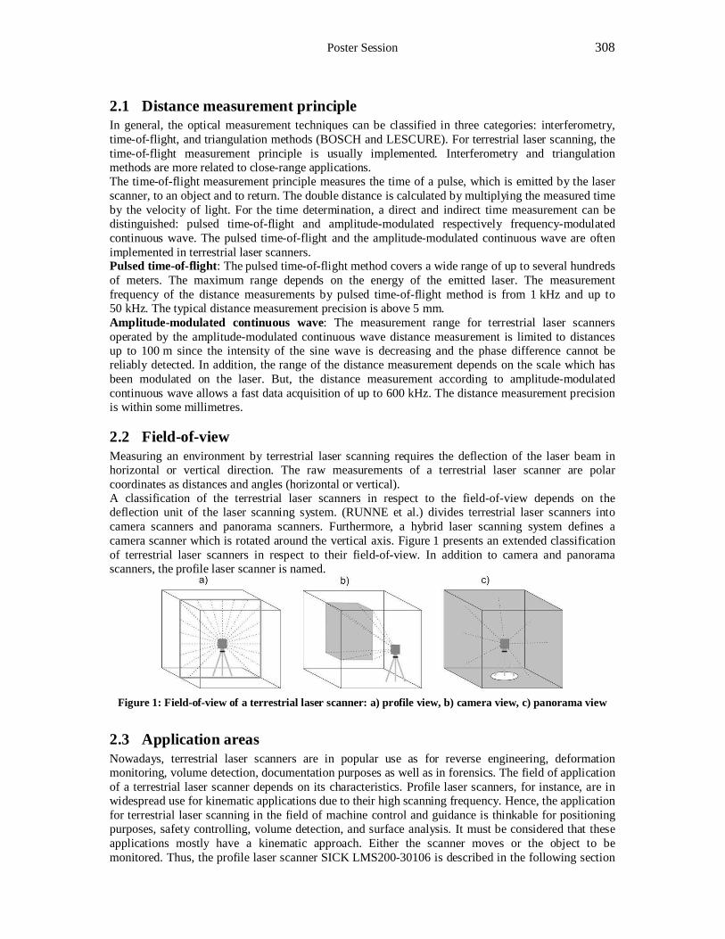
Poster Session 308
2.1 Distance measurement principle In general, the optical measurement techniques can be classified in three categories: interferometry, time-of-flight, and triangulation methods (BOSCH and LESCURE). For terrestrial laser scanning, the time-of-flight measurement principle is usually implemented. Interferometry and triangulation methods are more related to close-range applications. The time-of-flight measurement principle measures the time of a pulse, which is emitted by the laser scanner, to an object and to return. The double distance is calculated by multiplying the measured time by the velocity of light. For the time determination, a direct and indirect time measurement can be distinguished: pulsed time-of-flight and amplitude-modulated respectively frequency-modulated continuous wave. The pulsed time-of-flight and the amplitude-modulated continuous wave are often implemented in terrestrial laser scanners. Pulsed time-of-flight: The pulsed time-of-flight method covers a wide range of up to several hundreds of meters. The maximum range depends on the energy of the emitted laser. The measurement frequency of the distance measurements by pulsed time-of-flight method is from 1 kHz and up to 50 kHz. The typical distance measurement precision is above 5 mm. Amplitude-modulated continuous wave: The measurement range for terrestrial laser scanners operated by the amplitude-modulated continuous wave distance measurement is limited to distances up to 100 m since the intensity of the sine wave is decreasing and the phase difference cannot be reliably detected. In addition, the range of the distance measurement depends on the scale which has been modulated on the laser. But, the distance measurement according to amplitude-modulated continuous wave allows a fast data acquisition of up to 600 kHz. The distance measurement precision is within some millimetres.
2.2 Field-of-view Measuring an environment by terrestrial laser scanning requires the deflection of the laser beam in horizontal or vertical direction. The raw measurements of a terrestrial laser scanner are polar coordinates as distances and angles (horizontal or vertical). A classification of the terrestrial laser scanners in respect to the field-of-view depends on the deflection unit of the laser scanning system. (RUNNE et al.) divides terrestrial laser scanners into camera scanners and panorama scanners. Furthermore, a hybrid laser scanning system defines a camera scanner which is rotated around the vertical axis. Figure 1 presents an extended classification of terrestrial laser scanners in respect to their field-of-view. In addition to camera and panorama scanners, the profile laser scanner is named.
Figure 1: Field-of-view of a terrestrial laser scanner: a) profile view, b) camera view, c) panorama view
2.3 Application areas Nowadays, terrestrial laser scanners are in popular use as for reverse engineering, deformation monitoring, volume detection, documentation purposes as well as in forensics. The field of application of a terrestrial laser scanner depends on its characteristics. Profile laser scanners, for instance, are in widespread use for kinematic applications due to their high scanning frequency. Hence, the application for terrestrial laser scanning in the field of machine control and guidance is thinkable for positioning purposes, safety controlling, volume detection, and surface analysis. It must be considered that these applications mostly have a kinematic approach. Either the scanner moves or the object to be monitored. Thus, the profile laser scanner SICK LMS200-30106 is described in the following section
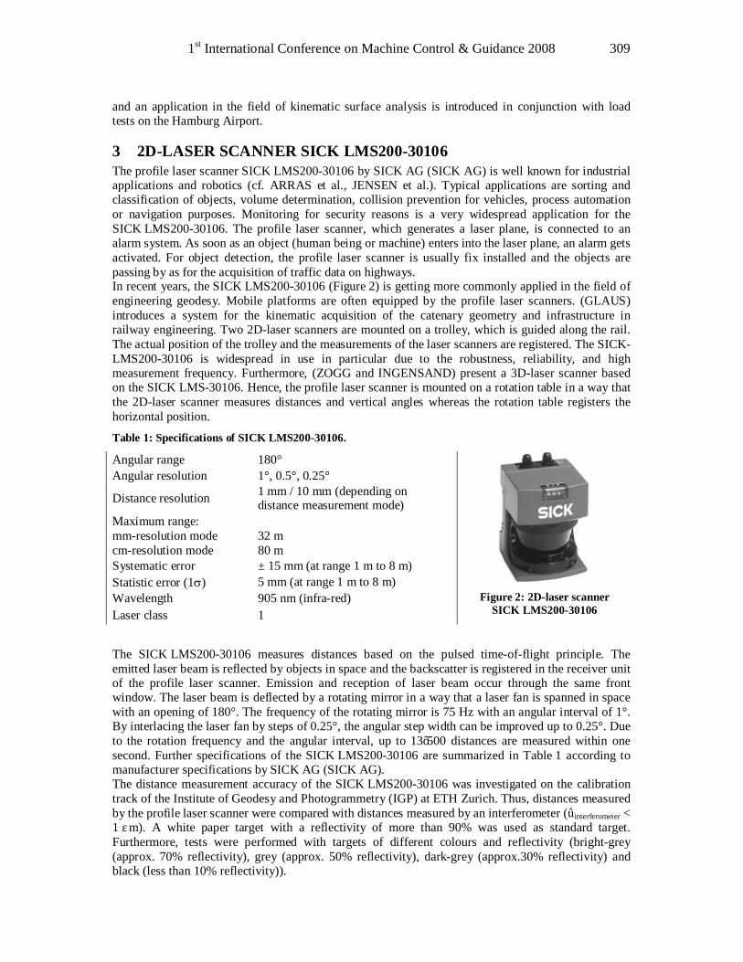
1st International Conference on Machine Control & Guidance 2008 309
and an application in the field of kinematic surface analysis is introduced in conjunction with load tests on the Hamburg Airport.
3 2D-LASER SCANNER SICK LMS200-30106 The profile laser scanner SICK LMS200-30106 by SICK AG (SICK AG) is well known for industrial applications and robotics (cf. ARRAS et al., JENSEN et al.). Typical applications are sorting and classification of objects, volume determination, collision prevention for vehicles, process automation or navigation purposes. Monitoring for security reasons is a very widespread application for the SICK LMS200-30106. The profile laser scanner, which generates a laser plane, is connected to an alarm system. As soon as an object (human being or machine) enters into the laser plane, an alarm gets activated. For object detection, the profile laser scanner is usually fix installed and the objects are passing by as for the acquisition of traffic data on highways. In recent years, the SICK LMS200-30106 (Figure 2) is getting more commonly applied in the field of engineering geodesy. Mobile platforms are often equipped by the profile laser scanners. (GLAUS) introduces a system for the kinematic acquisition of the catenary geometry and infrastructure in railway engineering. Two 2D-laser scanners are mounted on a trolley, which is guided along the rail. The actual position of the trolley and the measurements of the laser scanners are registered. The SICK-LMS200-30106 is widespread in use in particular due to the robustness, reliability, and high measurement frequency. Furthermore, (ZOGG and INGENSAND) present a 3D-laser scanner based on the SICK LMS-30106. Hence, the profile laser scanner is mounted on a rotation table in a way that the 2D-laser scanner measures distances and vertical angles whereas the rotation table registers the horizontal position.
Table 1: Specifications of SICK LMS200-30106.
Angular range 180° Angular resolution 1°, 0.5°, 0.25°
Distance resolution 1 mm / 10 mm (depending on distance measurement mode)
Maximum range: mm-resolution mode cm-resolution mode
32 m 80 m
Systematic error ± 15 mm (at range 1 m to 8 m) Statistic error (1σ) 5 mm (at range 1 m to 8 m) Wavelength 905 nm (infra-red) Laser class 1
Figure 2: 2D-laser scanner SICK LMS200-30106
The SICK LMS200-30106 measures distances based on the pulsed time-of-flight principle. The emitted laser beam is reflected by objects in space and the backscatter is registered in the receiver unit of the profile laser scanner. Emission and reception of laser beam occur through the same front window. The laser beam is deflected by a rotating mirror in a way that a laser fan is spanned in space with an opening of 180°. The frequency of the rotating mirror is 75 Hz with an angular interval of 1°. By interlacing the laser fan by steps of 0.25°, the angular step width can be improved up to 0.25°. Due to the rotation frequency and the angular interval, up to 13’500 distances are measured within one second. Further specifications of the SICK LMS200-30106 are summarized in Table 1 according to manufacturer specifications by SICK AG (SICK AG). The distance measurement accuracy of the SICK LMS200-30106 was investigated on the calibration track of the Institute of Geodesy and Photogrammetry (IGP) at ETH Zurich. Thus, distances measured by the profile laser scanner were compared with distances measured by an interferometer (σinterferometer < 1 μm). A white paper target with a reflectivity of more than 90% was used as standard target. Furthermore, tests were performed with targets of different colours and reflectivity (bright-grey (approx. 70% reflectivity), grey (approx. 50% reflectivity), dark-grey (approx.30% reflectivity) and black (less than 10% reflectivity)).
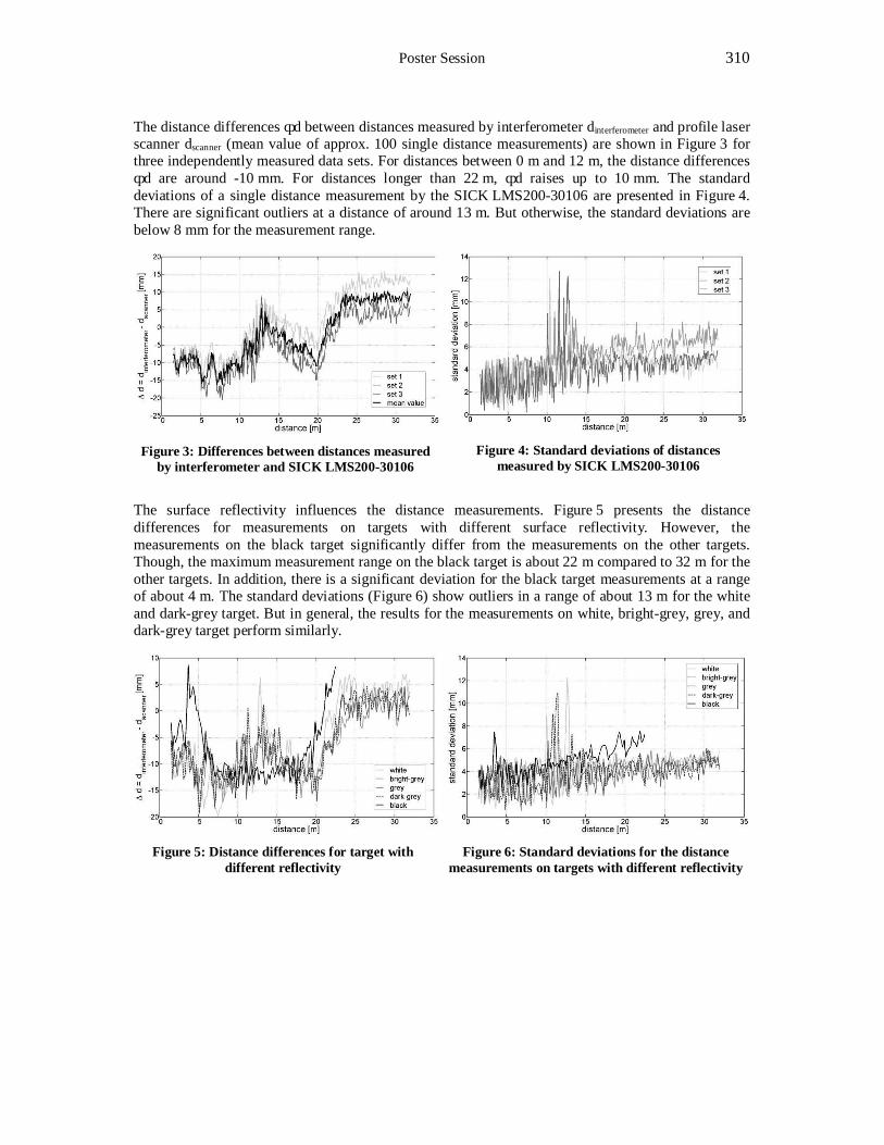
Poster Session 310
The distance differences Δd between distances measured by interferometer dinterferometer and profile laser scanner dscanner (mean value of approx. 100 single distance measurements) are shown in Figure 3 for three independently measured data sets. For distances between 0 m and 12 m, the distance differences Δd are around -10 mm. For distances longer than 22 m, Δd raises up to 10 mm. The standard deviations of a single distance measurement by the SICK LMS200-30106 are presented in Figure 4. There are significant outliers at a distance of around 13 m. But otherwise, the standard deviations are below 8 mm for the measurement range.
Figure 3: Differences between distances measured by interferometer and SICK LMS200-30106
Figure 4: Standard deviations of distances measured by SICK LMS200-30106
The surface reflectivity influences the distance measurements. Figure 5 presents the distance differences for measurements on targets with different surface reflectivity. However, the measurements on the black target significantly differ from the measurements on the other targets. Though, the maximum measurement range on the black target is about 22 m compared to 32 m for the other targets. In addition, there is a significant deviation for the black target measurements at a range of about 4 m. The standard deviations (Figure 6) show outliers in a range of about 13 m for the white and dark-grey target. But in general, the results for the measurements on white, bright-grey, grey, and dark-grey target perform similarly.
Figure 5: Distance differences for target with different reflectivity
Figure 6: Standard deviations for the distance measurements on targets with different reflectivity
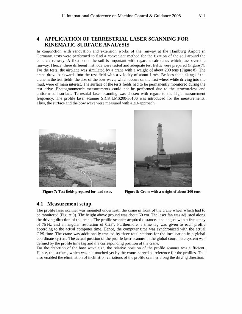
1st International Conference on Machine Control & Guidance 2008 311
4 APPLICATION OF TERRESTRIAL LASER SCANNING FOR KINEMATIC SURFACE ANALYSIS
In conjunction with renovation and extension works of the runway at the Hamburg Airport in Germany, tests were performed to find a convenient method for the fixation of the soil around the concrete runway. A fixation of the soil is important with regard to airplanes which pass over the runway. Hence, three different methods were tested and adequate test fields were prepared (Figure 7). For the tests, the airplane was simulated by a crane with a weight of about 200 tons (Figure 8). The crane drove backwards into the test field with a velocity of about 1 m/s. Besides the sinking of the crane in the test fields, the size of the bow wave, which occurs on the first wheel while driving into the mud, were of main interest. The surface of the tests fields had to be permanently monitored during the test drive. Photogrammetric measurements could not be performed due to the structureless and uniform soil surface. Terrestrial laser scanning was chosen with regard to the high measurement frequency. The profile laser scanner SICK LMS200-30106 was introduced for the measurements. Thus, the surface and the bow wave were measured with a 2D-approach.
Figure 7: Test fields prepared for load tests.
Figure 8: Crane with a weight of about 200 tons.
4.1 Measurement setup The profile laser scanner was mounted underneath the crane in front of the crane wheel which had to be monitored (Figure 9). The height above ground was about 60 cm. The laser fan was adjusted along the driving direction of the crane. The profile scanner acquired distances and angles with a frequency of 75 Hz and an angular resolution of 0.25°. Furthermore, a time tag was given to each profile according to the actual computer time. Hence, the computer time was synchronized with the actual GPS-time. The crane was additionally tracked by three total stations for the localisation in a global coordinate system. The actual position of the profile laser scanner in the global coordinate system was defined by the profile time tag and the corresponding position of the crane. For the detection of the bow wave size, the relative position of the profile scanner was sufficient. Hence, the surface, which was not touched yet by the crane, served as reference for the profiles. This also enabled the elimination of inclination variations of the profile scanner along the driving direction.
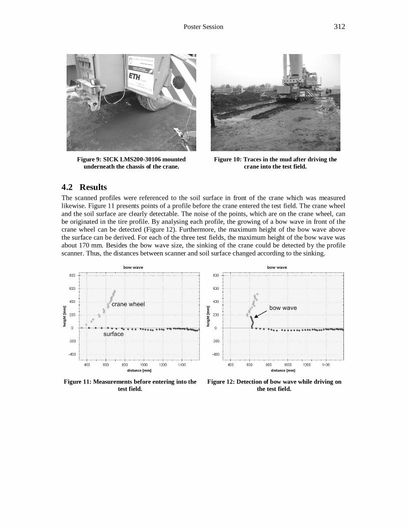
Poster Session 312
Figure 9: SICK LMS200-30106 mounted underneath the chassis of the crane.
Figure 10: Traces in the mud after driving the crane into the test field.
4.2 Results The scanned profiles were referenced to the soil surface in front of the crane which was measured likewise. Figure 11 presents points of a profile before the crane entered the test field. The crane wheel and the soil surface are clearly detectable. The noise of the points, which are on the crane wheel, can be originated in the tire profile. By analysing each profile, the growing of a bow wave in front of the crane wheel can be detected (Figure 12). Furthermore, the maximum height of the bow wave above the surface can be derived. For each of the three test fields, the maximum height of the bow wave was about 170 mm. Besides the bow wave size, the sinking of the crane could be detected by the profile scanner. Thus, the distances between scanner and soil surface changed according to the sinking.
Figure 11: Measurements before entering into the test field.
Figure 12: Detection of bow wave while driving on the test field.
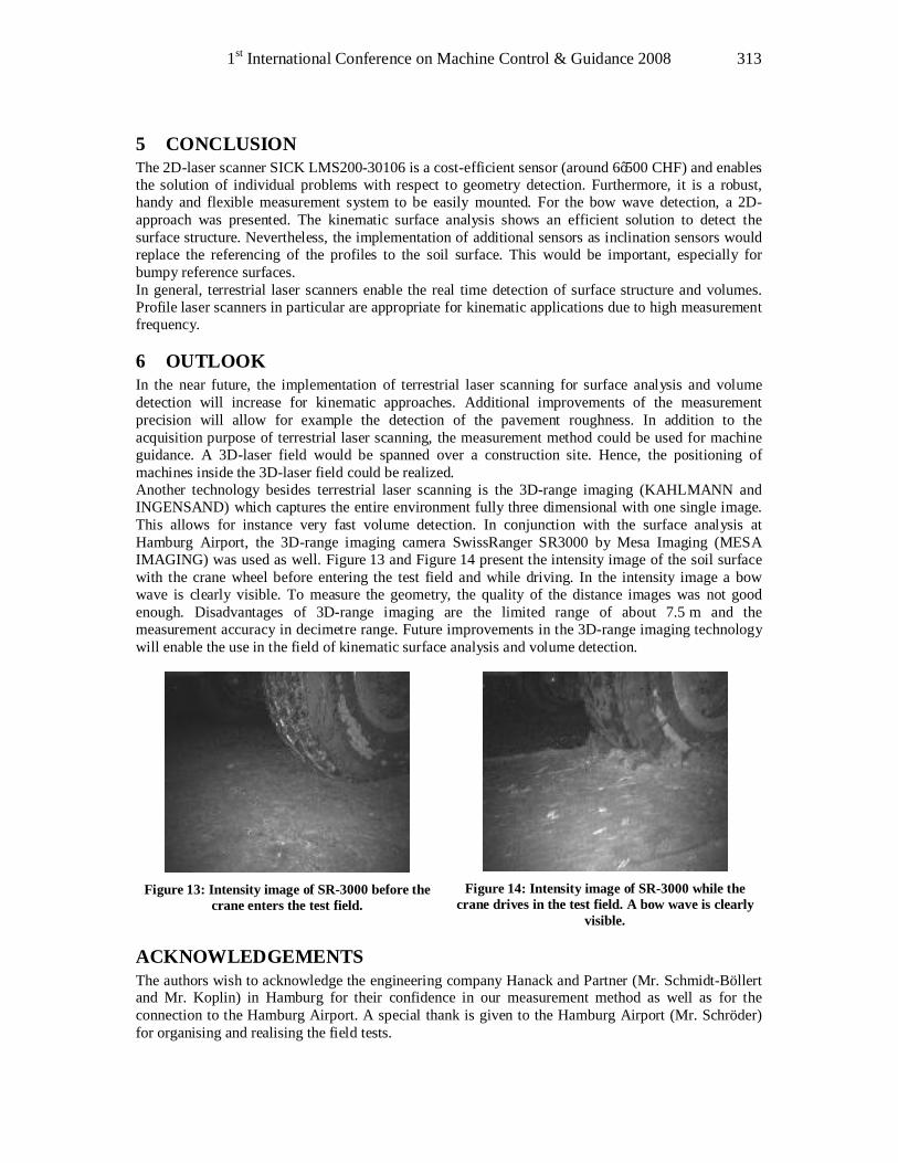
1st International Conference on Machine Control & Guidance 2008 313
5 CONCLUSION The 2D-laser scanner SICK LMS200-30106 is a cost-efficient sensor (around 6’500 CHF) and enables the solution of individual problems with respect to geometry detection. Furthermore, it is a robust, handy and flexible measurement system to be easily mounted. For the bow wave detection, a 2D-approach was presented. The kinematic surface analysis shows an efficient solution to detect the surface structure. Nevertheless, the implementation of additional sensors as inclination sensors would replace the referencing of the profiles to the soil surface. This would be important, especially for bumpy reference surfaces. In general, terrestrial laser scanners enable the real time detection of surface structure and volumes. Profile laser scanners in particular are appropriate for kinematic applications due to high measurement frequency.
6 OUTLOOK In the near future, the implementation of terrestrial laser scanning for surface analysis and volume detection will increase for kinematic approaches. Additional improvements of the measurement precision will allow for example the detection of the pavement roughness. In addition to the acquisition purpose of terrestrial laser scanning, the measurement method could be used for machine guidance. A 3D-laser field would be spanned over a construction site. Hence, the positioning of machines inside the 3D-laser field could be realized. Another technology besides terrestrial laser scanning is the 3D-range imaging (KAHLMANN and INGENSAND) which captures the entire environment fully three dimensional with one single image. This allows for instance very fast volume detection. In conjunction with the surface analysis at Hamburg Airport, the 3D-range imaging camera SwissRanger SR3000 by Mesa Imaging (MESA IMAGING) was used as well. Figure 13 and Figure 14 present the intensity image of the soil surface with the crane wheel before entering the test field and while driving. In the intensity image a bow wave is clearly visible. To measure the geometry, the quality of the distance images was not good enough. Disadvantages of 3D-range imaging are the limited range of about 7.5 m and the measurement accuracy in decimetre range. Future improvements in the 3D-range imaging technology will enable the use in the field of kinematic surface analysis and volume detection.
Figure 13: Intensity image of SR-3000 before the crane enters the test field.
Figure 14: Intensity image of SR-3000 while the crane drives in the test field. A bow wave is clearly
visible.
ACKNOWLEDGEMENTS The authors wish to acknowledge the engineering company Hanack and Partner (Mr. Schmidt-Böllert and Mr. Koplin) in Hamburg for their confidence in our measurement method as well as for the connection to the Hamburg Airport. A special thank is given to the Hamburg Airport (Mr. Schröder) for organising and realising the field tests.
Poster Session 314
REFERENCES ARRAS, O.K., PHILIPPSEN, R., TOMATIS, N., DE BATTISTA, M., SCHILT, M., SIEGWART, R.: A Navigation Framework for Multiple Mobile Robots and its Application at the Expo-02 Exhibition. In: Proceedings of the 2003 IEEE International Conference on Robotics and Automation, Taipei, 2003.
BOSCH, T., LESCURE, M.: Selected papers on laser distance measurements. SPIE Milestone Series, Vol. MS 115, SPIE Optical Engineering Press, Bellingham, 1995.
GLAUS, R.: Kinematic Track Surveying by Means of a Mulit-Sensor Platform. Dissertation. Institute of Geodesy and Photogrammetry, ETH Zurich, 2006.
KAHLMANN, T., INGENSAND, H.: Range Imaging Metrologie: Einführung, Untersuchungen und Weiterentwicklungen. In: Allgemeine Vermessungsnachrichten (AVN), Vol. 11-12/2007, pp. 384-388.
JENSEN, B., WEINGARTEN, J., KOLSKI, S., SIEGWART, R.: Laser Range Imaging using Mobile Rogots: From Pose Estimation to 3D-Models. In: Proceedings of 1st Range Imaging Research Day, Zurich, 2005.
MESA IMAGING: http://www.mesa-imaging.ch, last accessed on April 1, 2008.
RUNNE, H., NIEMEIER, W., KERN, F.: Application of Laser Scanners to Determine the Geometry of Buildings. In: Proceedings of Optical 3D-Measurement Techniques V, Vienna, 2001.
SICK AG: http://www.sick.com, last accessed on April 15, 2008.
ZOGG, H.-M., INGENSAND, H.: Terrestrial 3D-laser scanner ZLS07 developed at ETH Zurich: an overview of its configuration, performance and application. In: Proceedings of Optical 3D-Measurement Techniques VIII, Zurich, 2007. * Hans-Martin Zogg, David Grimm, Institute of Geodesy and Photogrammetry ETH Zurich, Wolfgang-Pauli-Str. 15, CH-8093 Zurich, Switzerland.
1st International Conference on Machine Control & Guidance 2008 315
Monitoring of the spatiotemporal movement of an industrial robot using a laser tracker
Manfred JURETZKO*, Maria HENNES* University of Karlsruhe, Germany
[juretzko, hennes]@gik.uni-karlsruhe.de
Abstract The project introduced here describes the geometric inspection of an innovative robot-based production process for spatially curved extruded profiles. The aim was to prove that the trajectories fulfil a given spatiotemporal tolerance level with respect to repeatability and absolute accuracy using an independent, i.e. geodetic, measurement method. In order to inspect this motion regarding spatiotemporal tolerance, it is necessary to synchronize a laser tracker with the control system of the robot with an order of magnitude of micro seconds. This resolution has been achieved by triggered measurements with a Leica LTD500. Very specific and for the production process decisive deviations of the robot trajectory have been detected as well as an extraordinarily high kinematic repeatability of the robot. Keywords Laser tracker, kinematic measurement, industrial robot, synchronization
1 INTRODUCTION With the development of new production methods robots play nowadays an ever more important role. By the advancements of robot controls in the last years, also sophisticated motions of the robot can be programmed in a relatively simple way. In doing so it is necessary to prove by an independent measuring method how precisely the predefined trajectories are converted and how the given spatial positions are tightened by the robot. The presented project describes the monitoring of an innovative, robot-supported procedure for the production of spatially curved extruded profiles developed by the Institute of Production Science at the University of Karlsruhe. In doing so, the special challenge for the measurement is the synchronization of the involved laser tracker with the robot in the range of microseconds.
2 MOVEMENT OF THE ROBOT Using the innovative process of rounding during extrusion, spatially curved extruded profiles can be flexibly manufactured. This facilitates the cost-effective production of lightweight structures with curved profiles even for small series. Due to the extrusion process a continuous flow of material is unavoidable. The profiles have to be separated reactionlessly during the extrusion following the complex trajectory of the cut-off point in space. Because of the high accelerations which occur during the spatial motion of the profile the trajectory is separated into the slow motion of an industrial robot guiding the cut-off device and a fast superposed movement generated by a specially designed clamping device with redundant axes. To synchronize the motions according to the real extrusion velocity a server-based central control unit is used [Fleischer et al.].
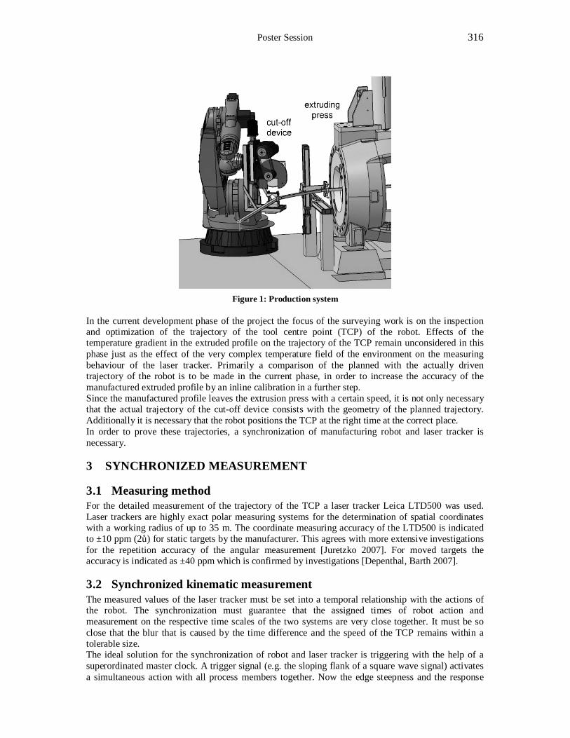
Poster Session 316
Figure 1: Production system
In the current development phase of the project the focus of the surveying work is on the inspection and optimization of the trajectory of the tool centre point (TCP) of the robot. Effects of the temperature gradient in the extruded profile on the trajectory of the TCP remain unconsidered in this phase just as the effect of the very complex temperature field of the environment on the measuring behaviour of the laser tracker. Primarily a comparison of the planned with the actually driven trajectory of the robot is to be made in the current phase, in order to increase the accuracy of the manufactured extruded profile by an inline calibration in a further step. Since the manufactured profile leaves the extrusion press with a certain speed, it is not only necessary that the actual trajectory of the cut-off device consists with the geometry of the planned trajectory. Additionally it is necessary that the robot positions the TCP at the right time at the correct place. In order to prove these trajectories, a synchronization of manufacturing robot and laser tracker is necessary.
3 SYNCHRONIZED MEASUREMENT
3.1 Measuring method For the detailed measurement of the trajectory of the TCP a laser tracker Leica LTD500 was used. Laser trackers are highly exact polar measuring systems for the determination of spatial coordinates with a working radius of up to 35 m. The coordinate measuring accuracy of the LTD500 is indicated to ±10 ppm (2σ) for static targets by the manufacturer. This agrees with more extensive investigations for the repetition accuracy of the angular measurement [Juretzko 2007]. For moved targets the accuracy is indicated as ±40 ppm which is confirmed by investigations [Depenthal, Barth 2007].
3.2 Synchronized kinematic measurement The measured values of the laser tracker must be set into a temporal relationship with the actions of the robot. The synchronization must guarantee that the assigned times of robot action and measurement on the respective time scales of the two systems are very close together. It must be so close that the blur that is caused by the time difference and the speed of the TCP remains within a tolerable size. The ideal solution for the synchronization of robot and laser tracker is triggering with the help of a superordinated master clock. A trigger signal (e.g. the sloping flank of a square wave signal) activates a simultaneous action with all process members together. Now the edge steepness and the response
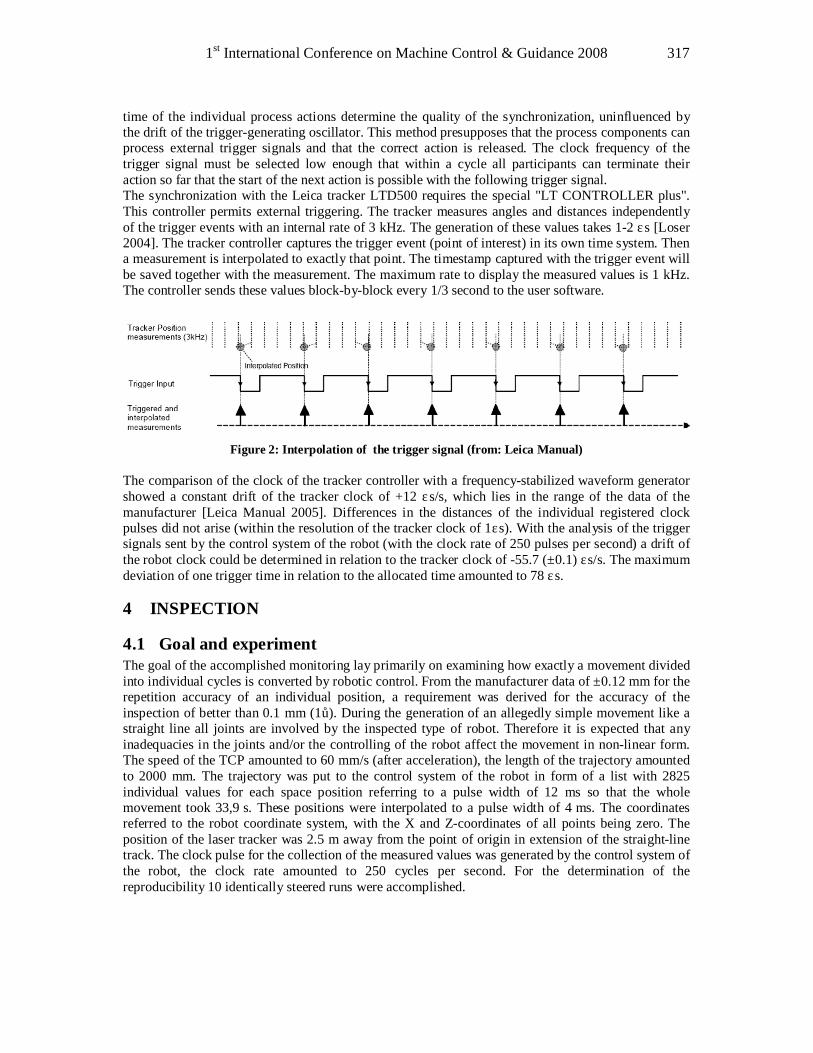
1st International Conference on Machine Control & Guidance 2008 317
time of the individual process actions determine the quality of the synchronization, uninfluenced by the drift of the trigger-generating oscillator. This method presupposes that the process components can process external trigger signals and that the correct action is released. The clock frequency of the trigger signal must be selected low enough that within a cycle all participants can terminate their action so far that the start of the next action is possible with the following trigger signal. The synchronization with the Leica tracker LTD500 requires the special "LT CONTROLLER plus". This controller permits external triggering. The tracker measures angles and distances independently of the trigger events with an internal rate of 3 kHz. The generation of these values takes 1-2 μs [Loser 2004]. The tracker controller captures the trigger event (point of interest) in its own time system. Then a measurement is interpolated to exactly that point. The timestamp captured with the trigger event will be saved together with the measurement. The maximum rate to display the measured values is 1 kHz. The controller sends these values block-by-block every 1/3 second to the user software.
Figure 2: Interpolation of the trigger signal (from: Leica Manual)
The comparison of the clock of the tracker controller with a frequency-stabilized waveform generator showed a constant drift of the tracker clock of +12 μs/s, which lies in the range of the data of the manufacturer [Leica Manual 2005]. Differences in the distances of the individual registered clock pulses did not arise (within the resolution of the tracker clock of 1μs). With the analysis of the trigger signals sent by the control system of the robot (with the clock rate of 250 pulses per second) a drift of the robot clock could be determined in relation to the tracker clock of -55.7 (±0.1) μs/s. The maximum deviation of one trigger time in relation to the allocated time amounted to 78 μs.
4 INSPECTION
4.1 Goal and experiment The goal of the accomplished monitoring lay primarily on examining how exactly a movement divided into individual cycles is converted by robotic control. From the manufacturer data of ±0.12 mm for the repetition accuracy of an individual position, a requirement was derived for the accuracy of the inspection of better than 0.1 mm (1σ). During the generation of an allegedly simple movement like a straight line all joints are involved by the inspected type of robot. Therefore it is expected that any inadequacies in the joints and/or the controlling of the robot affect the movement in non-linear form. The speed of the TCP amounted to 60 mm/s (after acceleration), the length of the trajectory amounted to 2000 mm. The trajectory was put to the control system of the robot in form of a list with 2825 individual values for each space position referring to a pulse width of 12 ms so that the whole movement took 33,9 s. These positions were interpolated to a pulse width of 4 ms. The coordinates referred to the robot coordinate system, with the X and Z-coordinates of all points being zero. The position of the laser tracker was 2.5 m away from the point of origin in extension of the straight-line track. The clock pulse for the collection of the measured values was generated by the control system of the robot, the clock rate amounted to 250 cycles per second. For the determination of the reproducibility 10 identically steered runs were accomplished.
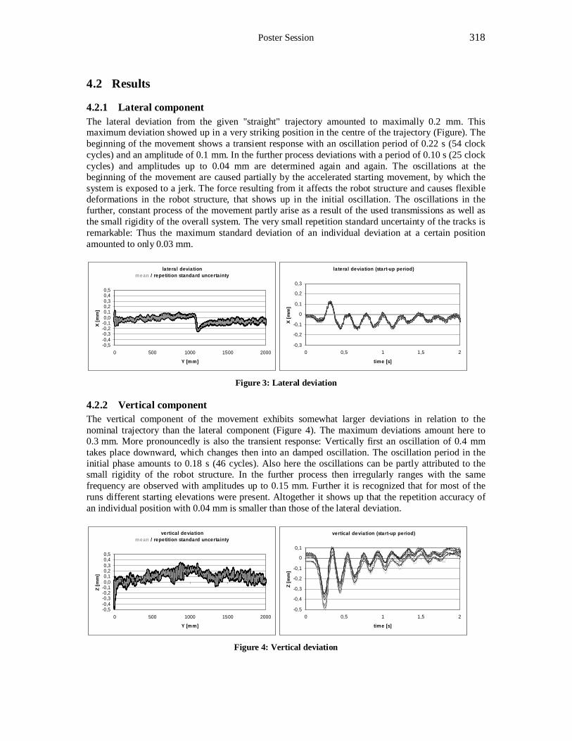
Poster Session 318
4.2 Results
4.2.1 Lateral component The lateral deviation from the given "straight" trajectory amounted to maximally 0.2 mm. This maximum deviation showed up in a very striking position in the centre of the trajectory (Figure). The beginning of the movement shows a transient response with an oscillation period of 0.22 s (54 clock cycles) and an amplitude of 0.1 mm. In the further process deviations with a period of 0.10 s (25 clock cycles) and amplitudes up to 0.04 mm are determined again and again. The oscillations at the beginning of the movement are caused partially by the accelerated starting movement, by which the system is exposed to a jerk. The force resulting from it affects the robot structure and causes flexible deformations in the robot structure, that shows up in the initial oscillation. The oscillations in the further, constant process of the movement partly arise as a result of the used transmissions as well as the small rigidity of the overall system. The very small repetition standard uncertainty of the tracks is remarkable: Thus the maximum standard deviation of an individual deviation at a certain position amounted to only 0.03 mm.
la te ra l devia tionmean / repetition standard uncerta inty
-0,5-0,4-0,3-0,2-0,10,00,10,20,30,40,5
0 500 1000 1500 2000
Y [m m]
X [m
m]
la te ra l deviation (start-up period)
-0,3
-0,2
-0,1
0
0,1
0,2
0,3
0 0,5 1 1,5 2
time [s]
X [m
m]
Figure 3: Lateral deviation
4.2.2 Vertical component The vertical component of the movement exhibits somewhat larger deviations in relation to the nominal trajectory than the lateral component (Figure 4). The maximum deviations amount here to 0.3 mm. More pronouncedly is also the transient response: Vertically first an oscillation of 0.4 mm takes place downward, which changes then into an damped oscillation. The oscillation period in the initial phase amounts to 0.18 s (46 cycles). Also here the oscillations can be partly attributed to the small rigidity of the robot structure. In the further process then irregularly ranges with the same frequency are observed with amplitudes up to 0.15 mm. Further it is recognized that for most of the runs different starting elevations were present. Altogether it shows up that the repetition accuracy of an individual position with 0.04 mm is smaller than those of the lateral deviation.
vertical devia tionmean / repetition standard uncerta inty
-0,5-0,4-0,3-0,2-0,10,00,10,20,30,40,5
0 500 1000 1500 2000
Y [m m]
Z [m
m]
ve rtical deviation (start-up period)
-0,5
-0,4
-0,3
-0,2
-0,1
0
0,1
0 0,5 1 1,5 2
time [s]
Z [m
m]
Figure 4: Vertical deviation
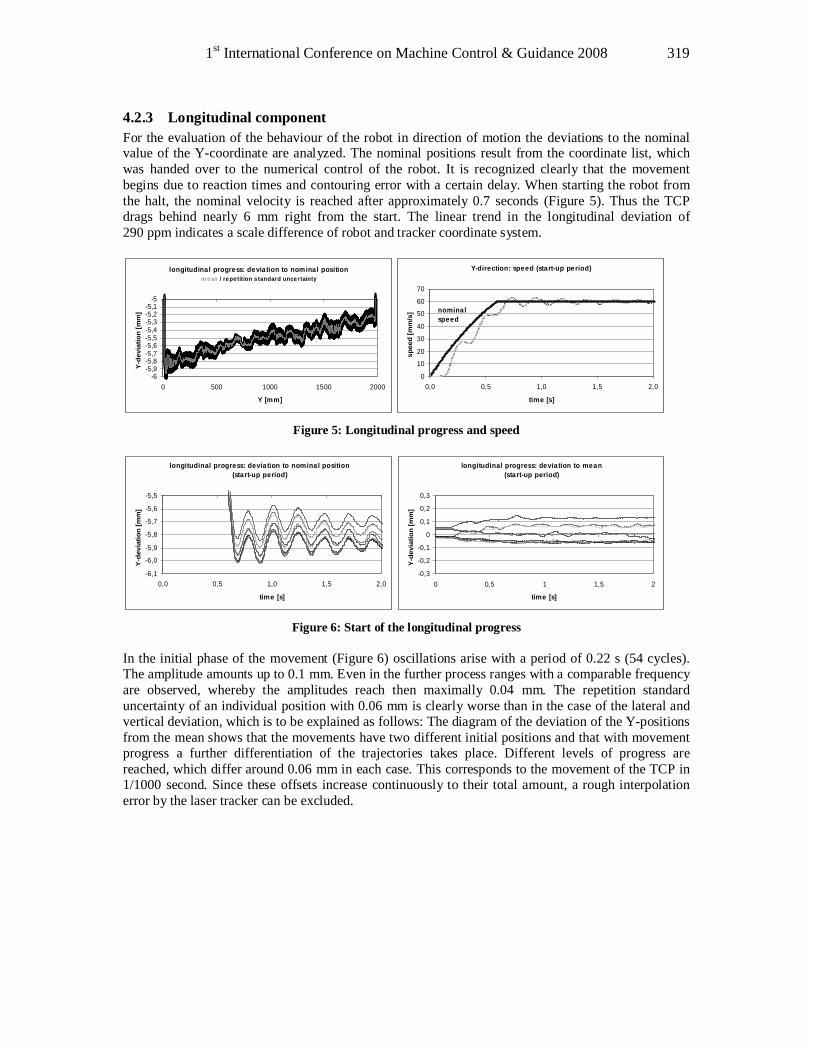
1st International Conference on Machine Control & Guidance 2008 319
4.2.3 Longitudinal component For the evaluation of the behaviour of the robot in direction of motion the deviations to the nominal value of the Y-coordinate are analyzed. The nominal positions result from the coordinate list, which was handed over to the numerical control of the robot. It is recognized clearly that the movement begins due to reaction times and contouring error with a certain delay. When starting the robot from the halt, the nominal velocity is reached after approximately 0.7 seconds (Figure 5). Thus the TCP drags behind nearly 6 mm right from the start. The linear trend in the longitudinal deviation of 290 ppm indicates a scale difference of robot and tracker coordinate system.
longitudina l progress: devia tion to nomina l positionm ean / repe tition s tandard uncer tainty
-6-5,9-5,8-5,7-5,6-5,5-5,4-5,3-5,2-5,1
-5
0 500 1000 1500 2000
Y [m m]
Y-d
evia
tion
[mm
]
Y-direction: speed (start-up pe riod)
0
10
20
30
40
50
60
70
0,0 0,5 1,0 1,5 2,0
time [s]sp
eed
[mm
/s] nominal
speed
Figure 5: Longitudinal progress and speed
longitudinal progress: deviation to nominal position
(start-up period)
-6,1
-6,0
-5,9
-5,8
-5,7
-5,6
-5,5
0,0 0,5 1,0 1,5 2,0
time [s]
Y-d
evia
tion
[mm
]
longitudinal progress: devia tion to mean(start-up period)
-0,3
-0,2
-0,1
0
0,1
0,2
0,3
0 0,5 1 1,5 2
time [s]
Y-d
evia
tion
[mm
]
Figure 6: Start of the longitudinal progress
In the initial phase of the movement (Figure 6) oscillations arise with a period of 0.22 s (54 cycles). The amplitude amounts up to 0.1 mm. Even in the further process ranges with a comparable frequency are observed, whereby the amplitudes reach then maximally 0.04 mm. The repetition standard uncertainty of an individual position with 0.06 mm is clearly worse than in the case of the lateral and vertical deviation, which is to be explained as follows: The diagram of the deviation of the Y-positions from the mean shows that the movements have two different initial positions and that with movement progress a further differentiation of the trajectories takes place. Different levels of progress are reached, which differ around 0.06 mm in each case. This corresponds to the movement of the TCP in 1/1000 second. Since these offsets increase continuously to their total amount, a rough interpolation error by the laser tracker can be excluded.
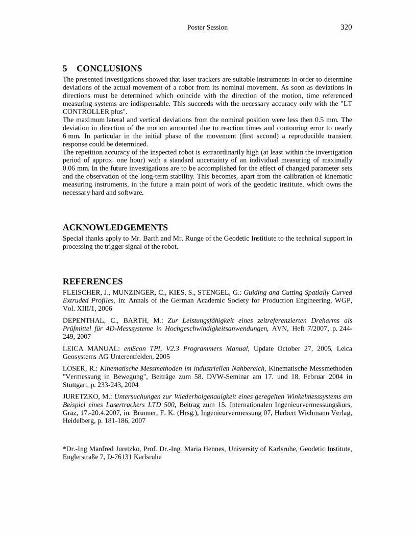
Poster Session 320
5 CONCLUSIONS The presented investigations showed that laser trackers are suitable instruments in order to determine deviations of the actual movement of a robot from its nominal movement. As soon as deviations in directions must be determined which coincide with the direction of the motion, time referenced measuring systems are indispensable. This succeeds with the necessary accuracy only with the "LT CONTROLLER plus". The maximum lateral and vertical deviations from the nominal position were less then 0.5 mm. The deviation in direction of the motion amounted due to reaction times and contouring error to nearly 6 mm. In particular in the initial phase of the movement (first second) a reproducible transient response could be determined. The repetition accuracy of the inspected robot is extraordinarily high (at least within the investigation period of approx. one hour) with a standard uncertainty of an individual measuring of maximally 0.06 mm. In the future investigations are to be accomplished for the effect of changed parameter sets and the observation of the long-term stability. This becomes, apart from the calibration of kinematic measuring instruments, in the future a main point of work of the geodetic institute, which owns the necessary hard and software.
ACKNOWLEDGEMENTS Special thanks apply to Mr. Barth and Mr. Runge of the Geodetic Institiute to the technical support in processing the trigger signal of the robot.
REFERENCES FLEISCHER, J., MUNZINGER, C., KIES, S., STENGEL, G.: Guiding and Cutting Spatially Curved Extruded Profiles, In: Annals of the German Academic Society for Production Engineering, WGP, Vol. XIII/1, 2006
DEPENTHAL, C., BARTH, M.: Zur Leistungsfähigkeit eines zeitreferenzierten Dreharms als Prüfmittel für 4D-Messsysteme in Hochgeschwindigkeitsanwendungen, AVN, Heft 7/2007, p. 244-249, 2007
LEICA MANUAL: emScon TPI, V2.3 Programmers Manual, Update October 27, 2005, Leica Geosystems AG Unterentfelden, 2005
LOSER, R.: Kinematische Messmethoden im industriellen Nahbereich, Kinematische Messmethoden "Vermessung in Bewegung", Beiträge zum 58. DVW-Seminar am 17. und 18. Februar 2004 in Stuttgart, p. 233-243, 2004
JURETZKO, M.: Untersuchungen zur Wiederholgenauigkeit eines geregelten Winkelmesssystems am Beispiel eines Lasertrackers LTD 500, Beitrag zum 15. Internationalen Ingenieurvermessungskurs, Graz, 17.-20.4.2007, in: Brunner, F. K. (Hrsg.), Ingenieurvermessung 07, Herbert Wichmann Verlag, Heidelberg, p. 181-186, 2007
*Dr.-Ing Manfred Juretzko, Prof. Dr.-Ing. Maria Hennes, University of Karlsruhe, Geodetic Institute, Englerstraße 7, D-76131 Karlsruhe
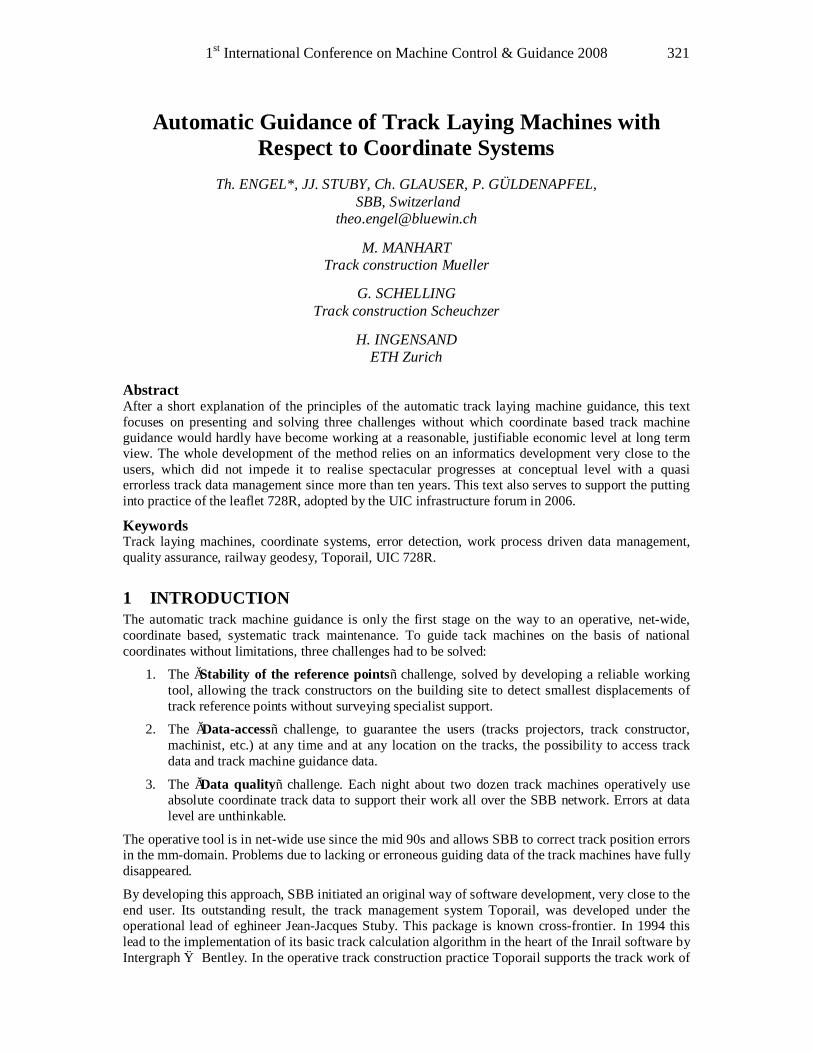
1st International Conference on Machine Control & Guidance 2008 321
Automatic Guidance of Track Laying Machines with Respect to Coordinate Systems
Th. ENGEL*, JJ. STUBY, Ch. GLAUSER, P. GÜLDENAPFEL, SBB, Switzerland
M. MANHART Track construction Mueller
G. SCHELLING
Track construction Scheuchzer
H. INGENSAND ETH Zurich
Abstract After a short explanation of the principles of the automatic track laying machine guidance, this text focuses on presenting and solving three challenges without which coordinate based track machine guidance would hardly have become working at a reasonable, justifiable economic level at long term view. The whole development of the method relies on an informatics development very close to the users, which did not impede it to realise spectacular progresses at conceptual level with a quasi errorless track data management since more than ten years. This text also serves to support the putting into practice of the leaflet 728R, adopted by the UIC infrastructure forum in 2006.
Keywords Track laying machines, coordinate systems, error detection, work process driven data management, quality assurance, railway geodesy, Toporail, UIC 728R.
1 INTRODUCTION The automatic track machine guidance is only the first stage on the way to an operative, net-wide, coordinate based, systematic track maintenance. To guide tack machines on the basis of national coordinates without limitations, three challenges had to be solved:
1. The „Stability of the reference points“ challenge, solved by developing a reliable working tool, allowing the track constructors on the building site to detect smallest displacements of track reference points without surveying specialist support.
2. The „Data-access“ challenge, to guarantee the users (tracks projectors, track constructor, machinist, etc.) at any time and at any location on the tracks, the possibility to access track data and track machine guidance data.
3. The „Data quality“ challenge. Each night about two dozen track machines operatively use absolute coordinate track data to support their work all over the SBB network. Errors at data level are unthinkable.
The operative tool is in net-wide use since the mid 90s and allows SBB to correct track position errors in the mm-domain. Problems due to lacking or erroneous guiding data of the track machines have fully disappeared.
By developing this approach, SBB initiated an original way of software development, very close to the end user. Its outstanding result, the track management system Toporail, was developed under the operational lead of eghineer Jean-Jacques Stuby. This package is known cross-frontier. In 1994 this lead to the implementation of its basic track calculation algorithm in the heart of the Inrail software by Intergraph → Bentley. In the operative track construction practice Toporail supports the track work of
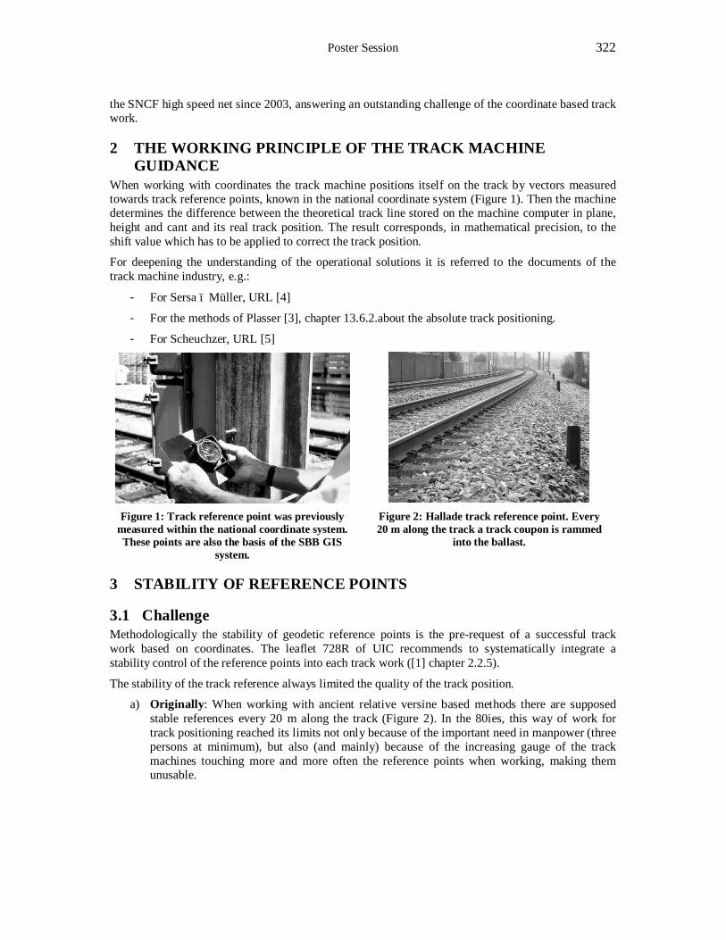
Poster Session 322
the SNCF high speed net since 2003, answering an outstanding challenge of the coordinate based track work.
2 THE WORKING PRINCIPLE OF THE TRACK MACHINE GUIDANCE
When working with coordinates the track machine positions itself on the track by vectors measured towards track reference points, known in the national coordinate system (Figure 1). Then the machine determines the difference between the theoretical track line stored on the machine computer in plane, height and cant and its real track position. The result corresponds, in mathematical precision, to the shift value which has to be applied to correct the track position.
For deepening the understanding of the operational solutions it is referred to the documents of the track machine industry, e.g.:
- For Sersa – Müller, URL [4]
- For the methods of Plasser [3], chapter 13.6.2.about the absolute track positioning.
- For Scheuchzer, URL [5]
Figure 1: Track reference point was previously
measured within the national coordinate system. These points are also the basis of the SBB GIS
system.
Figure 2: Hallade track reference point. Every 20 m along the track a track coupon is rammed
into the ballast.
3 STABILITY OF REFERENCE POINTS
3.1 Challenge Methodologically the stability of geodetic reference points is the pre-request of a successful track work based on coordinates. The leaflet 728R of UIC recommends to systematically integrate a stability control of the reference points into each track work ([1] chapter 2.2.5).
The stability of the track reference always limited the quality of the track position.
a) Originally: When working with ancient relative versine based methods there are supposed stable references every 20 m along the track (Figure 2). In the 80ies, this way of work for track positioning reached its limits not only because of the important need in manpower (three persons at minimum), but also (and mainly) because of the increasing gauge of the track machines touching more and more often the reference points when working, making them unusable.
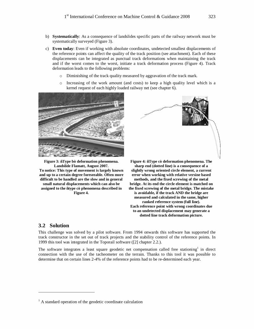
1st International Conference on Machine Control & Guidance 2008 323
b) Systematically: As a consequence of landslides specific parts of the railway network must be systematically surveyed (Figure 3).
c) Even today: Even if working with absolute coordinates, undetected smallest displacements of the reference points can affect the quality of the track position (see attachment). Each of these displacements can be integrated as punctual track deformations when maintaining the track and if the worst comes to the worst, initiate a track deformation process (Figure 4). Track deformation leads to the following problems:
o Diminishing of the track quality measured by aggravation of the track mark.
o Increasing of the work amount (and costs) to keep a high quality level which is a kernel request of each highly loaded railway net (see chapter 6).
Figure 3: “Type b” deformation phenomena. Landslide Flamatt, August 2007.
To notice: This type of movement is largely known and up to a certain degree foreseeable. Often more difficult to be handled are the slow and in general
small natural displacements which can also be assigned to the “type c” phenomena described in
Figure 4.
Figure 4: “Type c” deformation phenomena. The sharp end (dotted line) is a consequence of a
slightly wrong oriented circle element, a current error when working with relative versine based
methods, and the fixed screwing of the metal bridge. At its end the circle element is matched on
the fixed screwing of the metal bridge. The mistake is avoidable, if the track AND the bridge are measured and calculated in the same, higher
ranked reference system (full line). Each reference point with wrong coordinates due
to an undetected displacement may generate a dotted line track deformation picture.
3.2 Solution This challenge was solved by a pilot software. From 1994 onwards this software has supported the track constructor in the set out of track projects and the stability control of the reference points. In 1999 this tool was integrated in the Toporail software ([2] chapter 2.2.).
The software integrates a least square geodetic net compensation called free stationing1 in direct connection with the use of the tacheometer on the terrain. Thanks to this tool it was possible to determine that on certain lines 2-4% of the reference points had to be re-determined each year.
1 A standard operation of the geodetic coordinate calculation

Poster Session 324
4 DATA-ACCESS
4.1 Challenge Initially the handling of the data and the results of Toporail was file driven, with the classical risks bound to this type of data management. This meant that sometimes, because of bad steering data, the tamping took place “at zero” without correction of the track position.
4.2 Solution The topologic data storage of the results from the track calculation within a centralised database and a structured interface connecting the track system with the database and giving also access from the tamping machine to the track data on an Internet FTP server, allowed solving this challenge.
Two years of daily project work and several dozens of data transfers from the central database into the track calculation system and back again, have allowed testing this unique and original “topology-interface”. Nevertheless it is only now, that the ultimate development stage of this interface will be reached in a currently running revision project.
Given this big investment needed it makes sense to consider the actual development stage for a tool- and database independent handling of topologically structured data in such a way that the result can also be extended to other data domains of the infrastructure.
5 DATA-QUALITY
5.1 Challenge Forty track machines operate each night (and some during the day) on the SBB railway net. More than half of them use coordinate based track data for steering. Given this context it was hard to imagine another solution than “zero error” data quality.
5.2 Solution The solution rests on the outcome of the previous challenge (structured data and interface). It allowed achieving the “zero error data quality” required in practice. An important teamwork between the user, the user proximity informatics in charge of Toporail and the SBB central informatics responsible of the database has supported this achievement. The result is a new automatically driven data interchange and control concept between the track calculation system and the database, the whole driven by informatics.
The final outcome, a track project, delimited at its topological end points, replacing a corresponding part of the track to be demolished between this topology points. The track project passes through an “enriching process” where the specialised services add by stages their partial information to the data of the complete project. Each step ends with a data update in the database after a test of completeness, consistency and logical structure. It is only after having successfully passed the tests, that the following service can take over by adding its contribution to the data. So, at the end of this process, the project data replace the corresponding dismounted track part with absolute guarantee completely and correctly (Figure 5).
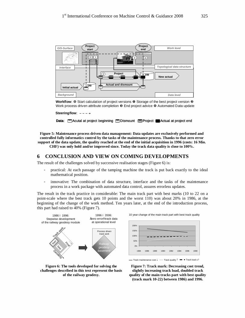
1st International Conference on Machine Control & Guidance 2008 325
Figure 5: Maintenance process driven data management: Data updates are exclusively performed and controlled fully informatics control by the tasks of the maintenance process. Thanks to that zero error
support of the data update, the quality reached at the end of the initial acquisition in 1996 (costs: 16 Mio. CHF) was only hold and/or improved since. Today the track data quality is close to 100%.
6 CONCLUSION AND VIEW ON COMING DEVELOPMENTS The result of the challenges solved by successive realisation stages (Figure 6) is:
- practical: At each passage of the tamping machine the track is put back exactly to the ideal mathematical position.
- innovative: The combination of data structure, interface and the tasks of the maintenance process in a work package with automated data control, assures errorless updates.
The result in the track practice in considerable: The main track part with best marks (10 to 22 on a point-scale where the best track gets 10 points and the worst 110) was about 20% in 1986, at the beginning of the change of the work method. Ten years later, at the end of the introduction process, this part had raised to 40% (Figure 7).
Figure 6: The tools developed for solving the challenges described in this text represent the basis
of the railway geodesy.
Figure 7: Track mark: Decreasing cost trend, slightly increasing track load, doubled track
quality of the main tracks part with best quality (track mark 10-22) between 1986) and 1996.
0%
50%
100%
150%
200%
1984 1986 1988 1990 1992 1994 1996 1998
10 year change of the main track part with best track quality
Track maintenance cost ↓ Track quality ↑ Track load ±?
GIS-Surface
0 1 4
Background
Work level
Data level
Actual and dismount
Project
Projectstart
New actualDB
Projectend
2
3
Workflow: Start calculation of project versions Storage of the best project version Work process driven attribute completion End project advice Automated Data update
DB
Data: Acutal at project beginning Dismount Project Actual at project endData: Acutal at project beginning Dismount Project Actual at project end
Steeringflow:
Interface Topological data structure
Initial actual
1986 – 1996:Stepwise development
of the railway geodesy module
1996 – 2006:„zero error“ track data
at operational level
Track w
ork
Geodesy
Railwaygeodesy
basement
Process driventrack work
Step
FinalStart

Poster Session 326
Of course there are still tasks to be solved. E.g. the question of improving the stability check of the reference points. Is it only a problem amongst others? Not so sure. Let’s look into detail.
In 2005, the introduction of “Rail 2000” had brought from one day to the other, a traffic load increase of 14% and higher velocities on certain lines. It is evident that the track quality increase mentioned, has contributed to the success of this important extension of the railway offer. Actually the quality of the track diminishes again. Is this phenomena bound to “Rail 2000”? A detailed exam positions the beginning of a slight degradation in 2000 onwards.
Therefore different explanations are possible to answer the asked question:
- No: The only reason is the undetected instability of the reference points.
- Yes: The reason is bound to the increase of “Rail 2000” and to the missing maintenance volume due to cost savings.
- Both explanations are partially correct.
The answer contains at least two components.
- The control of the stability of the reference points through the maintenance process driven data-management.
- A line specific, detailed systematic reporting of the variation of the track mark in time.
REFERENCES [1] UIC leaflet 728E. Absolute coordinates for track engineering work – A Railway Geodesy approach, 2006
[2] Müller u.a. Eisenbahnbau, 2., völlig neubearbeitete und erweiterte Auflage (Serie: Handbuch Ingenieurgeodäsie), Wichmann Verlag, 2000, ISBN 3-87907-297-3.
[3] Lichtberger Bernhard. Handbuch Gleis. Tezlaff Verlag, ISBN 3-87814-803-8
Links [4] http://www.sersa.ch.
[5] http://www.scheuchzer.ch/
*Théo Engel, Dr ès sc techn, CFF-I-ST-SF, Schanzenstrasse 5, 3000 Bern 5, Tél. +41 512 20 21 80 [email protected]
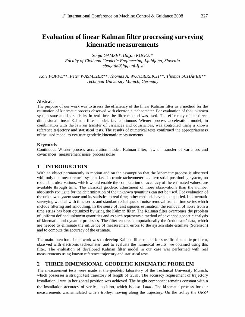
1st International Conference on Machine Control & Guidance 2008 327
Evaluation of linear Kalman filter processing surveying kinematic measurements
Sonja GAMSE*, Dušan KOGOJ* Faculty of Civil and Geodetic Engineering, Ljubljana, Slovenia
Karl FOPPE**, Peter WASMEIER**, Thomas A. WUNDERLICH**, Thomas SCHÄFER** Technical University Munich, Germany
Abstract The purpose of our work was to assess the efficiency of the linear Kalman filter as a method for the estimation of kinematic process observed with electronic tacheometer. For evaluation of the unknown system state and its statistics in real time the filter method was used. The efficiency of the three-dimensional linear Kalman filter model, i.e. continuous Wiener process acceleration model, in combination with the law on transfer of variances and covariances, was controlled using a known reference trajectory and statistical tests. The results of numerical tests confirmed the appropriateness of the used model to evaluate geodetic kinematic measurements. Keywords Continuous Wiener process acceleration model, Kalman filter, law on transfer of variances and covariances, measurement noise, process noise
1 INTRODUCTION With an object permanently in motion and on the assumption that the kinematic process is observed with only one measurement system, i.e. electronic tacheometer as a terrestrial positioning system, no redundant observations, which would enable the computation of accuracy of the estimated values, are available through time. The classical geodetic adjustment of more observations than the number absolutely requisite for the determination of the unknown quantities can not be used. For evaluation of the unknown system state and its statistics in real time, other methods have to be applied. In kinematic surveying we deal with time series and standard techniques of noise removal from a time series which include filtering and smoothing. In the sense of least squares estimation, the removal of noise from a time series has been optimized by using the Kalman filter. The Kalman filter overcomes the problem of uniform defined unknown quantities and as such represents a method of advanced geodetic analysis of kinematic and dynamic processes. The filter ensures computationally the ˝redundant˝ data, which are needed to eliminate the influence of measurement errors to the system state estimate (Sorenson) and to compute the accuracy of the estimate. The main intention of this work was to develop Kalman filter model for specific kinematic problem, observed with electronic tacheometer, and to evaluate the numerical results, we obtained using this filter. The evaluation of developed Kalman filter model in our case was performed with real measurements using known reference trajectory and statistical tests.
2 THREE DIMENSIONAL GEODETIC KINEMATIC PROBLEM The measurement tests were made at the geodetic laboratory of the Technical University Munich, which possesses a straight test trajectory of length of m25 . The accuracy requirement of trajectory installation mm1 in horizontal position was achieved. The height component remains constant within the installation accuracy of vertical position, which is also mm1 . The kinematic process for our measurements was simulated with a trolley, moving along the trajectory. On the trolley the GRZ4
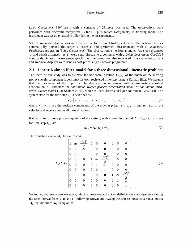
Poster Session 328
Leica Geosystems °360 -prism with a constant of mm1.23 was used. The observations were performed with electronic tachymeter TCRA1101plus (Leica Geosystems) in tracking mode. The instrument was set up on a stable pillar during the measurements. Sets of kinematic observations were carried out for different trolley velocities. The tacheometer has automatically pursued the target – prism – and performed measurements with a GeoBASIC FastRecord programm (Leica Geosystems). The observations – horizontal angles hz , slope distances d and zenith distances zr – were send directly to a computer with a Leica Geosystems GeoCOM commands. At each measurement epoch, the time stamp was also registered. The evaluation of data and graphical displays were done as post-processing by Matlab programme.
2.1 Linear Kalman filter model for a three dimensional kinematic problem The focus of our study was to estimate the horizontal position ),( yx of the prism on the moving trolley (height component is constant) for each registered time-step, using a Kalman filter. We assume that the movement of the object can be described as movement with approximately constant acceleration a . Therefore the continuous Wiener process acceleration model or continuous third-order Wiener model (Bar-Shalom et al.), which is three-dimensional per coordinate, was used. The system state for the time-step kt is described as:
[ ] Tkzzyyxxk avzavyavx=x , (1)
where x , y , z are the position components of the moving prism, xv , yv , zv and xa , ya , za are velocity and acceleration in all three directions. Kalman filter discrete process equation of the system, with a sampling period kk ttt −=∆ +1 , is given for time-step 1+kt as:
kkkk wxAx +⋅=+1 . (2) The transition matrix kA for our case is:
∆
∆∆
∆
∆∆
∆
∆∆
=∆
10000000010000000
2)(1000000
00010000000010000
0002
)(1000
00000010000000010
0000002
)(1
)(
2
2
2
t
tt
t
tt
t
tt
tkA . (3)
Vector kw represents process noise, which is unknown and not modelled in the state dynamics during the time interval from k to 1+k . Following Brown and Hwang the process noise covariance matrix
kQ that describes kw is equal to:
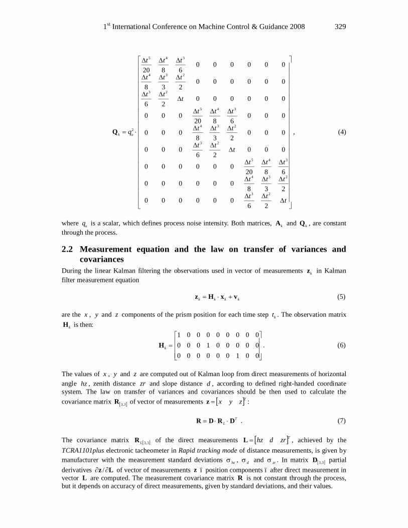
1st International Conference on Machine Control & Guidance 2008 329
∆∆∆
∆∆∆
∆∆∆
∆∆∆
∆∆∆
∆∆∆
∆∆∆
∆∆∆
∆∆∆
⋅=
ttt
ttt
ttt
ttt
ttt
ttt
ttt
ttt
ttt
quk
26000000
238000000
6820000000
00026
000
000238
000
0006820
000
00000026
000000238
0000006820
23
234
345
23
234
345
23
234
345
2Q , (4)
where uq is a scalar, which defines process noise intensity. Both matrices, kA and kQ , are constant through the process.
2.2 Measurement equation and the law on transfer of variances and covariances
During the linear Kalman filtering the observations used in vector of measurements kz in Kalman filter measurement equation
kkkk vxHz +⋅= (5) are the x , y and z components of the prism position for each time step kt . The observation matrix
kH is then:
=
001000000000001000000000001
kH . (6)
The values of x , y and z are computed out of Kalman loop from direct measurements of horizontal angle hz , zenith distance zr and slope distance d , according to defined right-handed coordinate system. The law on transfer of variances and covariances should be then used to calculate the covariance matrix [ ]3,3R of vector of measurements [ ]Tzyx=z :
TL DRDR ⋅⋅= . (7)
The covariance matrix [ ]3,3LR of the direct measurements [ ]Tzrdhz=L , achieved by the TCRA1101plus electronic tacheometer in Rapid tracking mode of distance measurements, is given by manufacturer with the measurement standard deviations hzσ , dσ and zrσ . In matrix [ ]3,3D partial derivatives Lz ∂∂ / of vector of measurements z – position components – after direct measurement in vector L are computed. The measurement covariance matrix R is not constant through the process, but it depends on accuracy of direct measurements, given by standard deviations, and their values.
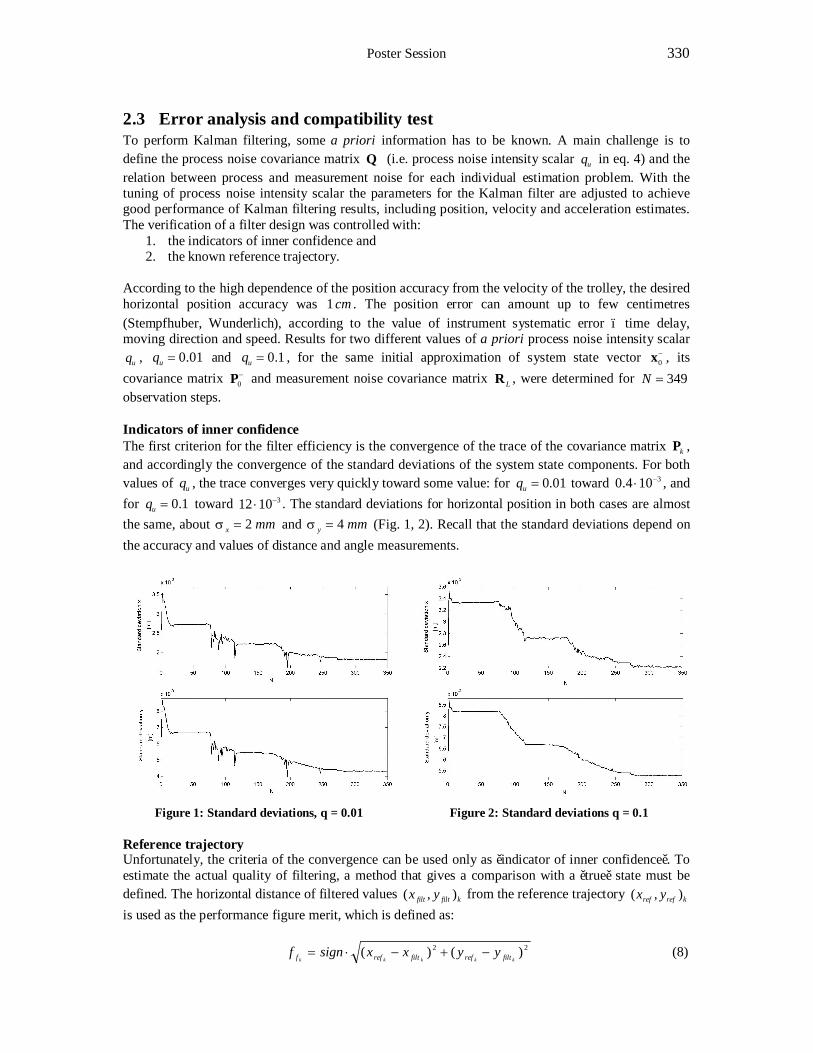
Poster Session 330
2.3 Error analysis and compatibility test To perform Kalman filtering, some a priori information has to be known. A main challenge is to define the process noise covariance matrix Q (i.e. process noise intensity scalar uq in eq. 4) and the relation between process and measurement noise for each individual estimation problem. With the tuning of process noise intensity scalar the parameters for the Kalman filter are adjusted to achieve good performance of Kalman filtering results, including position, velocity and acceleration estimates. The verification of a filter design was controlled with:
1. the indicators of inner confidence and 2. the known reference trajectory.
According to the high dependence of the position accuracy from the velocity of the trolley, the desired horizontal position accuracy was cm1 . The position error can amount up to few centimetres (Stempfhuber, Wunderlich), according to the value of instrument systematic error – time delay, moving direction and speed. Results for two different values of a priori process noise intensity scalar
uq , 01.0=uq and 1.0=uq , for the same initial approximation of system state vector −0x , its
covariance matrix −0P and measurement noise covariance matrix LR , were determined for 349=N
observation steps. Indicators of inner confidence The first criterion for the filter efficiency is the convergence of the trace of the covariance matrix kP , and accordingly the convergence of the standard deviations of the system state components. For both values of uq , the trace converges very quickly toward some value: for 01.0=uq toward 3104.0 −⋅ , and for 1.0=uq toward 31012 −⋅ . The standard deviations for horizontal position in both cases are almost the same, about mmx 2=σ and mmy 4=σ (Fig. 1, 2). Recall that the standard deviations depend on the accuracy and values of distance and angle measurements.
Figure 1: Standard deviations, q = 0.01 Figure 2: Standard deviations q = 0.1 Reference trajectory Unfortunately, the criteria of the convergence can be used only as ˝indicator of inner confidence˝. To estimate the actual quality of filtering, a method that gives a comparison with a ˝true˝ state must be defined. The horizontal distance of filtered values kfiltfilt yx ),( from the reference trajectory krefref yx ),( is used as the performance figure merit, which is defined as: 22 )()(
kkkkk filtreffiltreff yyxxsignf −+−⋅= (8)
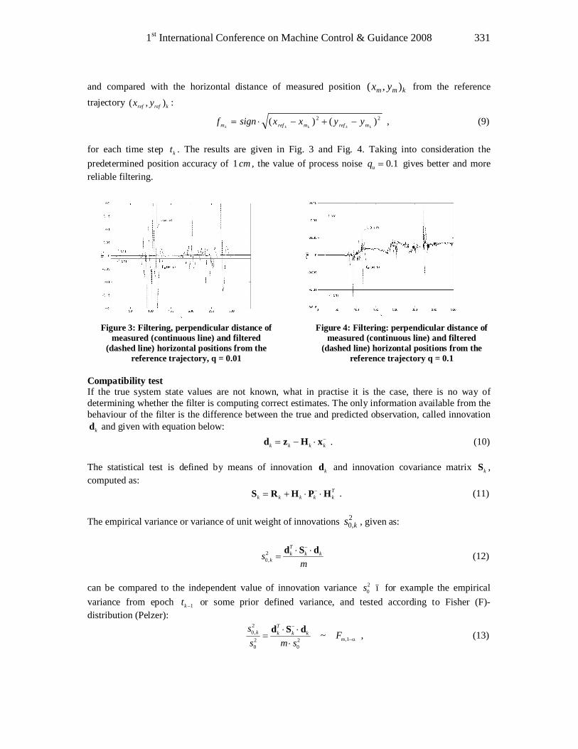
1st International Conference on Machine Control & Guidance 2008 331
and compared with the horizontal distance of measured position kmm yx ),( from the reference trajectory krefref yx ),( :
22 )()(kkkkk mrefmrefm yyxxsignf −+−⋅= , (9)
for each time step kt . The results are given in Fig. 3 and Fig. 4. Taking into consideration the predetermined position accuracy of cm1 , the value of process noise 1.0=uq gives better and more reliable filtering.
Figure 3: Filtering, perpendicular distance of
measured (continuous line) and filtered (dashed line) horizontal positions from the
reference trajectory, q = 0.01
Figure 4: Filtering: perpendicular distance of measured (continuous line) and filtered
(dashed line) horizontal positions from the reference trajectory q = 0.1
Compatibility test If the true system state values are not known, what in practise it is the case, there is no way of determining whether the filter is computing correct estimates. The only information available from the behaviour of the filter is the difference between the true and predicted observation, called innovation
kd and given with equation below: −⋅−= kkkk xHzd . (10)
The statistical test is defined by means of innovation kd and innovation covariance matrix kS , computed as:
Tkkkkk HPHRS ⋅⋅+= − . (11)
The empirical variance or variance of unit weight of innovations 2
,0 ks , given as:
m
s kkTk
kdSd ⋅⋅
=−
2,0 (12)
can be compared to the independent value of innovation variance 2
0s – for example the empirical variance from epoch 1−kt or some prior defined variance, and tested according to Fisher (F)-distribution (Pelzer):
α−
−
⋅⋅⋅
= 1,20
20
2,0 ~ m
kkTkk F
smss dSd , (13)
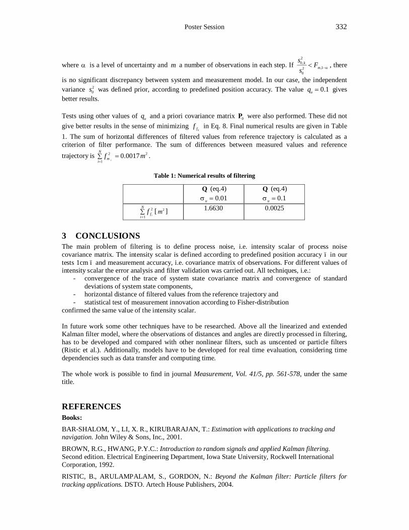
Poster Session 332
where α is a level of uncertainty and m a number of observations in each step. If α−< 1,20
2,0
mk F
ss
, there
is no significant discrepancy between system and measurement model. In our case, the independent variance 2
0s was defined prior, according to predefined position accuracy. The value 1.0=uq gives better results.
Tests using other values of uq and a priori covariance matrix 0P were also performed. These did not give better results in the sense of minimizing
kff in Eq. 8. Final numerical results are given in Table 1. The sum of horizontal differences of filtered values from reference trajectory is calculated as a criterion of filter performance. The sum of differences between measured values and reference trajectory is 2
1
2 0017.0 mfN
im i
=∑=
.
Table 1: Numerical results of filtering
3 CONCLUSIONS The main problem of filtering is to define process noise, i.e. intensity scalar of process noise covariance matrix. The intensity scalar is defined according to predefined position accuracy – in our tests 1cm – and measurement accuracy, i.e. covariance matrix of observations. For different values of intensity scalar the error analysis and filter validation was carried out. All techniques, i.e.:
- convergence of the trace of system state covariance matrix and convergence of standard deviations of system state components,
- horizontal distance of filtered values from the reference trajectory and - statistical test of measurement innovation according to Fisher-distribution
confirmed the same value of the intensity scalar. In future work some other techniques have to be researched. Above all the linearized and extended Kalman filter model, where the observations of distances and angles are directly processed in filtering, has to be developed and compared with other nonlinear filters, such as unscented or particle filters (Ristic et al.). Additionally, models have to be developed for real time evaluation, considering time dependencies such as data transfer and computing time. The whole work is possible to find in journal Measurement, Vol. 41/5, pp. 561-578, under the same title.
REFERENCES Books:
BAR-SHALOM, Y., LI, X. R., KIRUBARAJAN, T.: Estimation with applications to tracking and navigation. John Wiley & Sons, Inc., 2001.
BROWN, R.G., HWANG, P.Y.C.: Introduction to random signals and applied Kalman filtering. Second edition. Electrical Engineering Department, Iowa State University, Rockwell International Corporation, 1992.
RISTIC, B., ARULAMPALAM, S., GORDON, N.: Beyond the Kalman filter: Particle filters for tracking applications. DSTO. Artech House Publishers, 2004.
Q (eq.4) 01.0=uσ
Q (eq.4) 1.0=uσ
∑=
N
if i
f1
2 [ 2m ] 6630.1 0025.0

1st International Conference on Machine Control & Guidance 2008 333
Journal articles: PELZER, von H.: Deformationsuntersuchungen auf der Basis kinematischer Bewegungsmodelle. Allgemeine Vermessungs-Nachrichten. 94. Jg. Heft 2. Herbert Wichmann Verlag GmbH, Karlsruhe, 1987.
SORENSON, H.W.: Least-squares estimation: from Gauss to Kalman. Copyright (c) 2004 IEEE. Reprinted from IEEE Spectrum, vol.7, pp. 63-68, 1970.
STEMPFHUBER, W., WUNDERLICH, T.: Leica System 1200: Auf dem Weg zur Sensorsynchronisation von GPS und TPS für kinematische Messaufgaben. Allgemeine Vermessungs-Nachrichren. 5/2004, S. 175-184, Hüthig GmbH & Co. KG, Heidelberg, 2004.
*Faculty of Civil and Geodetic Engineering, Jamova 2, 1000 Ljubljana, Slovenia. **Technical University Munich, Arcisstraße 21, D-80290 Munich, Germany.