1st Latin American Summer School

Prof Jacob BedrossianUniversity of Maryland, College Park USA

June 20, 2019

Contents

1 Introduction 2

2 Mathematical modeling and ODEs 22.1 ODEs in dimension one for population dynamics . . . . . . . . . . . . . . . . . . . . 22.2 Method of linearization . . . . . . . . . . . . . . . . . . . . . . . . . . . . . . . . . . 52.3 2x2 systems for population dynamics . . . . . . . . . . . . . . . . . . . . . . . . . . . 72.4 Linearization method for 2x2 systems . . . . . . . . . . . . . . . . . . . . . . . . . . 9

3 General abstract theory for ODEs 12

4 Numerical methods for ODEs 134.1 Stiffness and implicit methods . . . . . . . . . . . . . . . . . . . . . . . . . . . . . . . 154.2 Higher order methods . . . . . . . . . . . . . . . . . . . . . . . . . . . . . . . . . . . 16

5 Diffusion: introduction to PDE 175.1 Linearization method for PDE . . . . . . . . . . . . . . . . . . . . . . . . . . . . . . 19

6 Numerical methods for diffusion and reaction-diffusion 206.1 Numerical stability for PDE methods . . . . . . . . . . . . . . . . . . . . . . . . . . . 20

7 Transport in fluid mechanics 227.1 Scalar transport in 1D . . . . . . . . . . . . . . . . . . . . . . . . . . . . . . . . . . . 227.2 Transport in higher dimensions . . . . . . . . . . . . . . . . . . . . . . . . . . . . . . 24

8 Numerical methods for transport equations 25

9 Advection-diffusion and reaction-advection-diffusion 279.1 1D advection-diffusion and advection-diffusion reaction . . . . . . . . . . . . . . . . . 279.2 Advection-Diffusion and Reaction-Advection-Diffusion in higher dimensions . . . . . 279.3 Reaction-advection-diffusion . . . . . . . . . . . . . . . . . . . . . . . . . . . . . . . . 27

10 Introduction to fluid mechanics 28

A Taylor’s theorem and finite differences 30

B Vector calculus review or crash-course 31

1

C Eigenvalues and eigenvectors 34

1 Introduction

These notes were devised for a week long intensive introduction to some topics in using partialdifferential equations for mathematical modeling. To fix examples which are accessible without alot of background in the specific application topic, the kind of mathematical models we are discussingmostly apply to biology and chemistry, i.e. population dynamics of organisms or a system of multiplechemical species undergoing chemical reactions. In the last section, we briefly discuss the extensionof some of the ideas to modeling the dynamics of fluids. These notes serve as a reference for thecourse – maybe not every topic and every example discussed in these notes will be covered in thecourse due to time constraints.

It is assumed the reader has some basic knowledge of vector calculus and linear algebra, butthere is an appendix briefly reviewing some of the concepts we are using (also sets the notationbeing used).

2 Mathematical modeling and ODEs

In this section I will introduce some of the basic ideas behind using ordinary differential equations(ODEs) to model things in the real world. For illustrative purposes, I will mostly use examples frombiology and chemistry, rather than physics, simply because there are some good examples that areaccessible and interesting without requiring a lot of technical background in the field of study.

2.1 ODEs in dimension one for population dynamics

2.1.1 Exponential growth model

Consider the population of bacteria in a petri dish represented by N(t), i.e. the number of bacteriaas a function of time. Suppose that there are lots of available resources so that λr of the bacteriadivides into two new bacteria every r hours. We then have the following relation:

N(t+ r) = N(t) + λrN(t). (2.1)

In order to figure out the population of bacteria, you would need also to know how many you hadat the beginning of the experiment – the so-called initial condition. This gives the mathematicalmodel for the number of bacteria in the dish

N(t+ r) = (1 + λr)N(t). (2.2)

N(0) = N0. (2.3)

We can solves this and we have for all J > 0,

N(Jr) = (1 + λr)JN0. (2.4)

There are so many bacteria, it seems silly to try to keep track of each individual one. Moreover, itdoesn’t really make sense to expect all the bacteria to be dividing on the same discrete set of times,this is of course not how bacteria divide. We should come up with a mathematical model for whicht and N are continuous variables. Re-writing

N(t+ r)−N(t)

r= λN(t). (2.5)

2

We want to think about sending r → 0, so taking this limit gives

d

dtN(t) = λN(t) (2.6a)

N(0) = N0. (2.6b)

Theorem 2.1. The solution to (2.6) is given by

N(t) = N0eλt. (2.7)

Proof. Write

1

N(t)

d

dtN(t) = λ, (2.8)

and then the backwards chain rule:

d

dtlogN(t) = 2λ, (2.9)

Then integrate ∫ T

0

d

dtlogN(t)dt = 2λT (2.10)

which gives

logN(T )− logN(0) = 2λT, (2.11)

and rearranging then gives (switching T back to t also),

N(t) = N0eλt. (2.12)

2.1.2 Logistic equation

Example 1. E. Coli replicate at a very fast rate. Given enough resources, they can replicate inunder around 30 minutes. Since we are measuring t in hours, this suggests that λ = 2 is a roughguess for how big we can take λ. Suppose that on the first day, you have a tiny culture of 100 E.Coli, i.e. N0 = 100. Our mathematical model predicts that in 2 days, we should have around

N(48) = 100e2∗48 ≈ 4.9× 1043 E. Coli. (2.13)

For comparison, an E. Coli cell has a mass of around 10−15 kg, and so our mathematical modelpredicts you have around 1028 kg worth of E. Coli. All of these rates and numbers were veryapproximate, but given that the Earth has a mass of around 6×1024 kg, we can be pretty confidentthat something went horribly wrong. Everything was pretty hand-wavy there, but we’re looking ata prediction that is astronomically inaccurate1.

1This calculation is really only very sensitive to λ and the length of time you run the experiment. For example, ifyou change λ = 2 to λ = 1, you get about 70× 106 kg of E. Coli by day 2. This is still ridiculous, but its nowhere thesize of planets.

3

Figure 1: A plot of the solution to (2.6) for various initial conditions.

The key point in the above example was “Given enough resources...”. The original model (2.6)should only work well when the resources and space available to the bacteria can be assumedunlimited. Once the bacteria are numerous enough, they will start running out of resources (orspace), which means that the original model (2.6) will no longer be a good approximation. Itmakes sense to replace the growth rate λ with something that decreases as the number of bacteriaincreases. Assuming this dependence is linear, we would get a growth rate λ(1 − 1

AN(t)), and themodel we have is the logistic model :

d

dtN(t) = λ

(1− 1

AN(t)

)N(t) (2.14a)

N(0) = N0. (2.14b)

Note that when 1AN(t) is very small, the growth rate is close to λ, so that the model is very similar

to (2.6). When N(t) > A the population is actually decreasing, i.e. the bacteria are dying due tolack of resources. When N(t) = A the population is not changing - we call this equilibrium. Thisis one of the few nonlinear ODEs that can be solved without the aid of a computer, if you know afew tricks.

Theorem 2.2. The solution to (2.14a) is given by

N(t) =eλtN0

1− N0A + 1

AeλtN0

. (2.15)

Notice that, if N0 = A, then N(t) = A and that if N0 = 0 then N(t) = 0. These are the twoequilibria of the model. If 0 < N0, note that limt→∞N(t) = A.

Proof. As before, re-write as:

1(1− 1

AN(t))N(t)

d

dtN(t) = λ. (2.16)

4

Then we use partial fractions

1(1− 1

AN(t))N(t)

=1

N(t)+

1

A(1− 1

AN(t)) (2.17)

So,

d

dtlogN(t)− d

dtlog

(1− N(t)

A

)= λ (2.18)

d

dtlog

N(t)(1− N(t)

A

) = λ. (2.19)

Integrating as above [] then gives

logN(t)(

1− N(t)A

) − logN0(

1− N0A

) = λt. (2.20)

Then,

N(t)(1− N(t)

A

) = eλtN0(

1− N0A

) , (2.21)

which re-arranges to

N(t) =

eλt N0(1−N0

A

)1 + 1

Aeλt N0(

1−N0A

) (2.22)

=eλtN0

1− N0A + 1

AeλtN0

. (2.23)

2.2 Method of linearization

Let’s go back and consider this model:

d

dtN(t) = λ

(1− 1

AN(t)

)N(t) (2.24)

N(0) = N0. (2.25)

We expect that for small population sizes, the exponential growth model is actually fine. Let’s seeif that’s true. Suppose that N(t) = εf(t) and N0 = εf0. This would give

d

dtf(t) = λf(t)− ε λ

Af2(t) (2.26)

f(0) = f0. (2.27)

5

Figure 2: A plot of the solution to (2.14a) for various initial conditions.

I haven’t actually changed the model, I just basically changed the units of N . However, supposethat ε� λ

A , i.e. much, much smaller. Then, as long as f wasn’t too large, we could safely drop thelast term and get left with

d

dtf(t) = λf(t) (2.28)

f(0) = f0. (2.29)

The exponential growth model! This shows that small population sizes will tend to grow exponen-tially.

Now, let’s see if we can find an approximate model near the other equilibrium, N(t) = A. Hence,suppose that N(t) = A+ εf(t). We then have

d

dtf(t) = −λf(t)− ελf2(t) ≈ −λf(t) (2.30)

N(0) = f0. (2.31)

This model is an exponential decay model

f(t) = f0e−λt. (2.32)

This shows that populations close to equilibrium N(t) = A will converge to this equilibrium expo-nentially fast.

What we’re seeing is the method of linearization, in which near equilibria at least, we approx-imate the nonlinear dynamics by linear dynamics. This is sort of analogous to when one locallyapproximates a nonlinear curve by its tangent line. Let’s see this method in action. Suppose that

6

we had a general model

d

dtN(t) = G(N(t)) (2.33)

N(0) = N0 (2.34)

and that you have an equilibrium point G(A) = 0. Doing the same procedure by consideringN(t) = A+ εf(t) and applying Taylor’s theorem gives:

εd

dtf(t) = G(A+ εf(t)) = G(A) + εG′(A)f(t) +

ε2

2G′′(A)f2(t) + ... (2.35)

Therefore, if we use G(A) = 0, divide by ε and then drop all the terms with at least one ε, we getthe linearized equation

d

dtf(t) = G′(A)f(t) (2.36)

f(0) = f0 (2.37)

which is then solved by

f(t) = f0eG′(A)t. (2.38)

Therefore, if G′(A) < 0, f(t), i.e. the small perturbation, converges exponentially back to A. Inthis case, we say the equilibrium is stable. If G′(A) > 0, then f(t) grows exponentially. In this case,we say the equilibrium is unstable. If G′(A) = 0, then the equilibrium is neutral and a higher orderexpansion is needed to make a good guess about stability.

2.3 2x2 systems for population dynamics

Many systems of interest in the real-world have more than one variable. In fact, many of themcan have hundreds, thousands, or even millions. Let’s start with the case of just two variables,which is already representative of some of the new aspects one sees when going from one unknownto many. A very simple and beautiful model for two species interacting in the same environmentis the Lotka-Volterra model. Suppose one has two populations: a population of rabbits u(t) anda population of foxes v(t) (prey and predator). The rabbits we assume have essentially unlimitedresources from the available plant food sources and grow naturally at a rate a, but are consumedat some rate by the foxes b. The Foxes on the other hand, will die in the absence of rabbits at arate of d and can only grow by consuming the rabbits at a rate c. This gives

d

dt

(u(t)v(t)

)=

((a− bv(t))u(t)(cu(t)− d)v(t)

). (2.39a)(

u(0)u(0)

)=

(u0u0

). (2.39b)

To look for equilibria states for this system, we look for where the time-derivative vanishes:(00

)=

((a− bv(t))u(t)(cu(t)− d)v(t)

). (2.40)

(2.41)

7

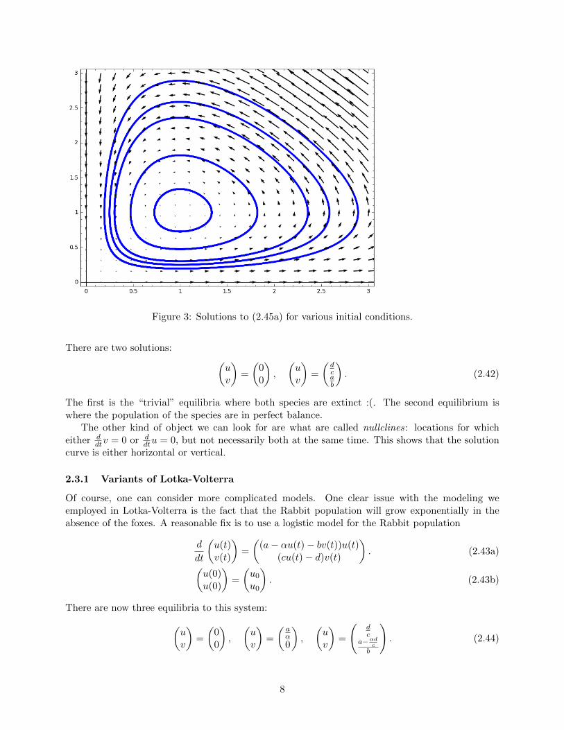
Figure 3: Solutions to (2.45a) for various initial conditions.

There are two solutions: (uv

)=

(00

),

(uv

)=

(dcab

). (2.42)

The first is the “trivial” equilibria where both species are extinct :(. The second equilibrium iswhere the population of the species are in perfect balance.

The other kind of object we can look for are what are called nullclines: locations for whicheither d

dtv = 0 or ddtu = 0, but not necessarily both at the same time. This shows that the solution

curve is either horizontal or vertical.

2.3.1 Variants of Lotka-Volterra

Of course, one can consider more complicated models. One clear issue with the modeling weemployed in Lotka-Volterra is the fact that the Rabbit population will grow exponentially in theabsence of the foxes. A reasonable fix is to use a logistic model for the Rabbit population

d

dt

(u(t)v(t)

)=

((a− αu(t)− bv(t))u(t)

(cu(t)− d)v(t)

). (2.43a)(

u(0)u(0)

)=

(u0u0

). (2.43b)

There are now three equilibria to this system:(uv

)=

(00

),

(uv

)=

(aα0

),

(uv

)=

(dc

a−αdc

b

). (2.44)

8

Note that if a < αdc , then the third equilibrium would only appear for negative values of the fox

population, which is obviously non-physical. A more detailed analysis shows that if a < αdc , the

foxes are doomed to go extinct no matter what the initial condition is. This is because the Rabbitsdo not have enough resources to support a population large enough to support a Fox population.

There are also models involving, for example, two herbivore species in competition for the samelimited resources:

d

dt

(u(t)v(t)

)=

((a− αu(t)− bv(t))u(t)(d− βv(t)− cu(t))v(t)

). (2.45a)(

u(0)u(0)

)=

(u0u0

). (2.45b)

2.4 Linearization method for 2x2 systems

For a general system of n variables, we consider an ODE for a vector-valued variables X(t) ∈ Rnevolving by a vector-field F

d

dtX(t) = F(X(t)) (2.46)

X(0) = X0. (2.47)

The equilibria states are those states which F(X∗) = 0. It again makes sense to use the linearizationmethod: hence writing X(t) = X∗ + εf(t), we have

d

dtf(t) =

1

εF(X∗ + εf(t)) (2.48)

f(0) = f0. (2.49)

To derive the linearized system, we want to send ε→ 0, which is the same as differentiation. Hence,(see Appendix B),

d

dtf(t) = DF(X∗)f(t) (2.50)

f(0) = f0. (2.51)

where DF is the Jacobian matrix with entries

(DF)ij = ∂xjFi. (2.52)

Hence, the linearization method leads us to studying linear systems.

2.4.1 2x2 linear systems

The general form of a 2× 2 linear ODE is the following:

d

dt

(x(t)y(t)

)=

(a bc d

)(x(t)y(t)

)(2.53a)(

x(0)y(0)

)=

(x0y0

). (2.53b)

9

Let’s first consider the case that c = b = 0:

d

dt

(x(t)y(t)

)=

(a 00 d

)(x(t)y(t)

)(2.54)(

x(0)y(0)

)=

(x0y0

). (2.55)

In this case, each of the variables can be solved independently, giving(x(t)y(t)

)=

(x0e

at

y0edt

). (2.56)

For solving (2.53) in general, one approach is to find a change of unknowns so that we get a newsystem that is diagonal. See Appendix C for a refresher on diagonalization. Suppose that A is realdiagonalizable, that is, we have real eigenvalues λ1, λ2 ∈ R and P ∈ R2×2 invertible such that

A = P

(λ1 00 λ2

)P−1. (2.57)

Then, applying P−1 to both sides of (2.53),

d

dtP−1

(x(t)y(t)

)=

(λ1 00 λ2

)P−1

(x(t)y(t)

). (2.58)

Our new variables are then (u(t)v(t)

)= P−1

(x(t)y(t)

). (2.59)

and we have

d

dt

(u(t)v(t)

)=

(λ1 00 λ2

)(u(t)v(t)

)(2.60)(

u(0)v(0)

)= P−1

(x0y0

). (2.61)

Solving this system gives (x(t)y(t)

)= P

(eλ1t 0

0 eλ2t

)P−1

(x0y0

). (2.62)

The following notation is sometimes used

eAt = P

(eλ1t 0

0 eλ2t

)P−1. (2.63)

Example 2 (Lotka-Volterra near extinction). Let’s consider the example of the Lotka-Volterrasystem (2.45a) linearized around (u, v) = (0, 0). In this case, the linear system is

d

dt

(u(t)v(t)

)=

(au(t)−dv(t)

). (2.64)(

u(0)u(0)

)=

(u0u0

). (2.65)

10

Figure 4: The linearized dynamics of Lotka-Volterra near the extinction state (u, v) = (0, 0).

The system is diagonal with one positive eigenvalue (λ1 = a) and one negative eigenvalue (λ2 = −d).The equilibria is unstable, because solutions to this system diverge from the origin. However, it ismore specific than this. The Rabbit population grows exponentially, whereas the population offoxes decreases exponentially, i.e. the foxes go extinct and the rabbits flourish. This is because thefoxes do not have enough food to survive on so few rabbits but the rabbits are just fine. Trajectoriesare hyperbolas (see the lab); such an equilibrium is called a hyperbolic point or a saddle point.

As we know from linear algebra, not all real-valued matrices are real diagonalizable. Supposethat the matrix A has complex eigenvalues

λ1 = λ+ iω (2.66)

λ2 = λ− iω. (2.67)

We will show the following:

Theorem 2.3. Let A have complex eigenvalues

λ1 = λ+ iω (2.68)

λ2 = λ− iω. (2.69)

Then there is a real matrix P such that(x(t)y(t)

)= P

(eλt cosωt eλt sinωt−eλt sinωt eλt cosωt

)P−1

(x0y0

). (2.70)

Proof. This follows from Theorem C.1. Indeed, set(u(t)v(t)

)= P−1

(x(t)y(t)

). (2.71)

11

Then,

d

dt

(u(t)v(t)

)=

(λ ω−ω λ

)(u(t)v(t)

). (2.72)

One can directly check (this can be derived more systematically, but this is one of the tricks it paysto just remember in differential equations)(

u(t)v(t)

)= eλt

(cosωtu0 + sinωtv0− sinωtu0 + cosωtv0

). (2.73)

The result follows after undoing the change of coordinates.

Example 3 (Lotka-Volterra at balanced equilibrium). Next, let us linearize (2.45a) around theequilibrium balanced equilibrium (

uv

)=

(dcab

). (2.74)

The linearized system is

d

dt

(u(t)v(t)

)=

(0 − bd

ccab 0

)(u(t)v(t)

)(2.75)

The eigenvalues are

λ± = ±i√ad. (2.76)

It follows from Theorem 2.3 that there is some invertible matrix P such that the following holdsfor ω =

√ad: (

u(t)v(t)

)= P

(cosωt sinωt− sinωt cosωt

)P−1. (2.77)

It follows that the equilibrium is stable. However, small disturbances of the equilibrium do notactually converge back to equilibrium. Instead, they circulate around the equilibrium, neithergetting closer nor getting further on average. Sometimes this is called neutrally stable.

3 General abstract theory for ODEs

Let F(t,x) : [0, T ]×D → Rd be a known vector field and consider the ODE

d

dtX(t) = F(t,X(t)) (3.1a)

X(0) = x0. (3.1b)

Any potential solution is a curve in Rd, X(t) : [0, T ] → Rd. In general, a solution may not exist.The theorem (which is not stated with optimal conditions) is the following. For simplicity I willjust state the theorem on Rd.

Theorem 3.1 (Cauchy-Lipschitz). Let F(t,x) : [0, T ] × Rd → Rd be continuously differentiable(i.e. the vector-field DF exists and is continuous). Then, there is a T∗ ≤ T such that there is aunique solution to the initial-value problem (3.1). Moreover, if T∗ < T then limt↗T∗ ‖X(t)‖ = ∞.If T =∞ and there exists a constant C > 0 such that ‖F(t,x)‖ ≤ C for all t,x, then T∗ =∞.

12

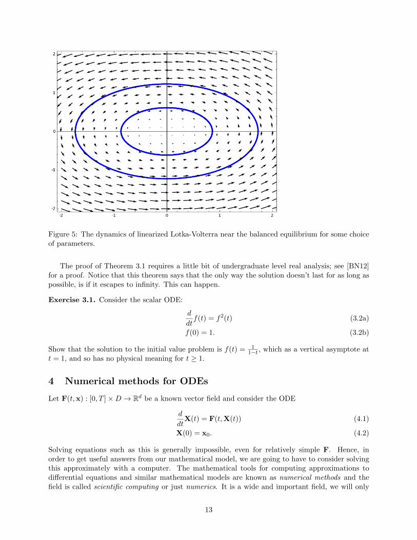
Figure 5: The dynamics of linearized Lotka-Volterra near the balanced equilibrium for some choiceof parameters.

The proof of Theorem 3.1 requires a little bit of undergraduate level real analysis; see [BN12]for a proof. Notice that this theorem says that the only way the solution doesn’t last for as long aspossible, is if it escapes to infinity. This can happen.

Exercise 3.1. Consider the scalar ODE:

d

dtf(t) = f2(t) (3.2a)

f(0) = 1. (3.2b)

Show that the solution to the initial value problem is f(t) = 11−t , which as a vertical asymptote at

t = 1, and so has no physical meaning for t ≥ 1.

4 Numerical methods for ODEs

Let F(t,x) : [0, T ]×D → Rd be a known vector field and consider the ODE

d

dtX(t) = F(t,X(t)) (4.1)

X(0) = x0. (4.2)

Solving equations such as this is generally impossible, even for relatively simple F. Hence, inorder to get useful answers from our mathematical model, we are going to have to consider solvingthis approximately with a computer. The mathematical tools for computing approximations todifferential equations and similar mathematical models are known as numerical methods and thefield is called scientific computing or just numerics. It is a wide and important field, we will only

13

discuss a few of the simplest numerical methods, some of them already in use for several hundredyears before the invention of computers2..

Divide the time interval [0, T ] into an evenly chosen set of times tn = nh, 0 ≤ n ≤ N , h = T/Nand t0 = 0, t1 = h, ... tN = T . We will build our numerical approximation {Xn}0≤n≤N withthe hope that Xn ≈ X(tn). A reasonable first approach is known as Euler’s method, which is toapproximate the time-derivative on the left-hand side of the ODE as a difference quotient:

Xn+1 −Xn

h= F(tn,Xn) (4.3)

X0 = x0. (4.4)

Re-arranging gives

Xn+1 = Xn + hF(tn,Xn) (4.5)

X0 = x0. (4.6)

It is the case that if one takes h smaller and smaller, the approximate solution approaches the exactsolution ‖Xn −X(tn)‖ → 0. This property is called convergence.

Theorem 4.1 (Euler’s method is convergent). Let F(t,x) : [0, T ]×Rd → Rd be twice differentiableand let Xn be the solution given by Euler’s method. Then for all x0 ∈ Rd, there exists a constantC such that

max0≤n≤N

‖Xn −X(tn)‖ ≤ Ch. (4.7)

The above theorem shows that one can use Euler’s method to solve the initial-value problem forODEs. Moreover, it even gives an estimate on, in general, approximately how accurate we can expectthe method to be. That is, how large you have to pick N in order to be sure that the computedsolution Xn is close to the exact solution (which in general is not known) X. The proof of Theorem4.1 also requires a little bit of undergraduate level real analysis, see [Ise09] (which in general is anexcellent resource for mathematically rigorous analysis of numerical methods). However, we canguess the accuracy of the method only using Taylor’s theorem. It will be convenient to introduce“Big-Oh” notation:

Definition 1 (Big-Oh). Given two functions f, g we say f = O(g) (pronounced f is Big-Oh of g)if there exists a constant such that

f(x) ≤ Cg(x). (4.8)

We will write f1 = f2 +O(g) (and similar expressions) if |f1 − f2| = O(g).

Let us estimate the error. the true solution X(t) satisfies

X(tn+1) = X(tn) +

∫ tn+1

tn

F(s,X(s))ds. (4.9)

2Before computers, people had to approximately calculate solutions by hand. This was a tedious and time-consuming task but sometimes there was no other option. In the 1940s and 1950s or so, entire teams of people wouldbe devoted to implementing numerical methods by hand in order to calculate the results required to do all sorts ofthings, for example, flight trajectories of space craft.

14

Hence,

Xn+1 −X(tn+1) = Xn −X(tn) + hF(tn,Xn)−∫ tn+1

tn

F(s,X(s))ds. (4.10)

Then, we use Taylor’s theorem to show that

F(s,X(s))ds = F(tn,X(tn)) + (s− tn)∂tF(tn,X(tn)) + (s− tn)DF(tn,X(tn))d

dtX(tn) +O

(|s− tn|2

).

(4.11)

Hence,

Xn+1 −X(tn+1) = Xn −X(tn) + h (F(tn,Xn)− F(tn,X(tn))) +O(h2). (4.12)

Then, because F is continuously differentiable,

F(tn,Xn)− F(tn,X(tn) = DF(tn,Xn)(Xn −X(tn)) +O(‖Xn −X(tn)‖2). (4.13)

Therefore, we can deduce that there exists a constants K1,K2 > 0 such that

‖Xn+1 −X(tn+1)‖ ≤ (1 +K1h) ‖Xn −X(tn)‖+K2h2. (4.14)

This is an estimate on how rapidly the error between the exact solution and our numerical calculationgrows. Notice that this has nothing to do with the round-off error of the computer, i.e. the fact thatcomputers do not do exact arithmetic. This error would be present even with perfect arithmetic.We see several things:

1. Each time-step loses at least K2h2 accuracy. Since there are N = T/h time steps, this suggests

an error at best like O(h).

2. The error in general is amplified exponentially a tiny bit every time-step. For many systemsthis is actually not true, and the estimate we have obtained is very sub-optimal. However,for some systems, there is exponential growth of error. For some systems (for example, theweather) we will never be able to accurately compute the solution very far in advance.

3. The error estimate (4.14) is the first step in the proof of Theorem 4.1.

4.1 Stiffness and implicit methods

There was something arbitrary in how we designed the Euler method. After all, we could havechosen

Xn+1 −Xn

h= F(tn+1,Xn+1) (4.15)

X0 = x0. (4.16)

This method is called backward Euler. One can show that Theorem 4.1 also applies to backwardEuler as well. It is not any more accurate than (forward) Euler. However, it is in general muchmore difficult to code, because it is not usually possible to easily solve for Xn+1. Methods of thistype are called implicit. Methods of the forward Euler type are called explicit. Usually one needsto numerically solve for Xn+1 using a numerical linear or nonlinear system solver (depending on

15

whether F is linear in Xn+1 or not). Given that it is not any more accurate, but is way harder toimplement, there must be another reason I brought up this method.

Consider the very simple scalar linear equation:

d

dty(t) = −100y(t) (4.17)

y(0) = 1. (4.18)

The exact solution is y(t) = e−100t. Consider now solving this with Euler’s method:

yn+1 = yn − 100hyn = (1− 100h)yn, (4.19)

and hence Euler’s method gives the solution

yn = (1− 100h)n. (4.20)

Hence, we see a fundamental problem: if 1 − 100h < −1, that is, if h > 1/50, then the numericalsolution is actually growing (and oscillating!). This looks absolutely nothing like the rather boringexact solution, which is, for intents and purposes, essentially zero for t > 1/50. This is an exampleof what is called a numerical instability : an “instability” observed numerically which is not actuallythere physically. Notice that there is nothing wrong with Euler’s method per se: the method reallyis convergent, so when you make h small enough, the issue goes away. The problem is appearingfor h which is small, but not quite small enough to “resolve” the real dynamics. This problem iscalled stiffness, and problems which have this kind of character are called stiff (see [Ise09] for amore detailed study). Stiffness is the fundamental reason why anyone cares about implicit methods.Indeed, consider now backward Euler:

yn+1 = yn − 100hyn+1, (4.21)

and hence

yn+1 =yn

1 + 100h. (4.22)

This solution decays exponentially regardless of h and so it does not suffer from the same problemas forward Euler. As a general rule, implicit methods handle stiffness better than explicit methods.In fact, no explicit method can handle stiffness very well. A problem may be so stiff that it isactually more efficient to use the slow and difficult to implement implicit methods, which allow alarger time-step, than it is to use a simpler explicit methods (which would require prohibitivelysmall time-steps).

4.2 Higher order methods

One can design methods which are more accurate than O(h). The first such an example is theimplicit trapezoidal method

Xn+1 = Xn +h

2F(tn+1,Xn+1) +

h

2F(tn,Xn). (4.23)

One can show that this method is O(h2) accurate.

Definition 2. We say that a method is p-th order accurate if Theorem 4.1 holds for the methodwith an error estimate of the form

max0≤n≤N

‖Xn −X(tn)‖ ≤ Chp. (4.24)

16

Hence, implicit trapezoidal is second-order accurate. That extra accuracy can go a long way.There is also an explicit analogue of the trapezoidal method, called explicit trapezoidal method

Xn+1 = Xn +h

2F (tn+1,Xn + hF(tn,Xn)) +

h

2F(tn,Xn). (4.25)

This is a very similar method but one which we have approximated the implicit part by an explicittime step. As it turns out, this method is still O(h2) accurate, despite this approximation. Aswith the Euler method, the implicit trapezoidal method performs better on “stiff” problems thanexplicit trapezoidal.

There are a number of higher order accurate schemes. The matlab routine ode45 is a combinationof 4-th order and 5-th order explicit methods. The answers are compared to one another to adjusth, the step-size, on the fly in order to automatically estimate whether or not h is small enough toget an accurate answer – adaptive refinement is very useful and is a much more advanced topicin numerical algorithms. The matlab routine ode23 is a similar combination of second and thirdorder implicit methods. The difference in accuracy is due to the fact that the computational costof implicit methods goes up rapidly as you go to higher order. For most applications the thirdorder accuracy of ode23 is good enough to get by and is still fast enough to execute in a reasonableamount of time. If your problem does not have stiffness problems, you should use ode45 and if thereare stiffness problems you should use ode23.

5 Diffusion: introduction to PDE

Suppose now we are interested in a density of chemical or a population of a species as a functionof both space and time, denoted ρ(t, x). Let us consider the case x ∈ R for now. Now, we areinterested in understanding the total amount of material in the the interval [a, b]:

d

dt

∫ b

aρ(t, x)dx =

∫ b

a∂tρ(t, x)dx. (5.1)

Let us suppose for now that the total amount of material is conserved, and so material can onlyenter and exit at the boundary of the interval. Hence, we can suppose there is a function F (t, x),called the flux, which specifies flow into and out of the interval. The flux tells how material ismoving in space and time, different mathematical models for the physics/biology/chemistry givedifferent F . By convention, the sign is take so that

d

dt

∫ b

aρ(t, x)dx = −F (t, b) + F (t, a) = −

∫ b

a∂xF (t, x)dx. (5.2)

The second equality was the fundamental theorem of calculus. Since this is supposed to hold for all[a, b] we get that in fact

∂tρ(t, x) + ∂xF (t, x) = 0. (5.3)

The first model we will consider is the case that density tends to move from high concentration tolow concentration. The simplest flux that does this is just that the flux is inversely proportional tothe slope: for some constant κ > 0,

F (t, x) = −κ∂xρ(t, x). (5.4)

17

Here κ > 0 is a positive constant called the diffusivity, and it depends on the exact physics/biology/chemistry.This leads to our first partial differential equation, a PDE known as the diffusion equation

∂tρ = κ∂xxρ (5.5)

ρ(0, x) = ρ0(x). (5.6)

As before, we need also an initial distribution. A thorough study of this elegant PDE would requiremore time and mathematical background than we have, but we can learn a little about the equationjust by observing two of its exact solutions and also through numerical studies in the lab.

Example 4. The following function

ρ(t, x) =1

(4πκt)1/2e−|x|24κt . (5.7)

solves ∂tρ = κ∂xxρ (the initial data is a little hard to make sense of). This function is concentratedon an interval of width ≈

√κt with height ≈ (κt)−1/2 (note that

∫∞−∞ ρ(t, x)dx = 1). Hence, the

solution is concentrated for short times and becomes increasingly more and more spread out (hencethe term “diffusion”).

Example 5. The following function solves

ρ(t, x) = e−κ4π2n2t sin 2πnx. (5.8)

solves ∂tρ = κ∂xxρ. This function keeps its shape of a sin curve of frequency 2πn but decaysexponentially. It is interesting to note that the decay is faster for n larger (and this rate of increaseis quite rapid). The diffusion equation tends to wipe out rapid oscillations whereas larger ripplestake longer to decay.

The diffusion equation is a universal model in that it is a decent model for a wide range ofphysical, biological, and chemical phenomena. It accurately models heat diffusing through a ho-mogeneous medium. It accurately models a chemical solvent as it diffuses through a liquid at rest.It accurately models a population of organisms that are executing a “random walk” that is, thevelocity at any given time can be considered a random variable that does not depend on the pastchoices and chosen with a bell-curve distribution (this turns out to be a reasonable approximationfor some organisms, but not others).

For bacteria, the diffusion equation is actually a pretty good approximation. If we then add inlogistic population dynamics, we get a type of equation called a reaction-diffusion equation

∂tρ = κ∂xxρ+ λ(1− 1

Aρ)ρ (5.9)

ρ(0, x) = ρ0(x). (5.10)

This population will diffuse while at each point, the population will try to tend to ρ = A. This is areasonable first model for the expansion of some bacteria populations in a petri dish. The bacteriawill randomly explore while dividing and using the resources. This model does not have a boundaryin it yet, so the bacteria population will continue expanding forever (but at each location at space,the population will settle to ρ(t, x) = A. If we want to study the model on an interval [a, b] thenwe need a boundary condition. If we want to impose that the population cannot enter or exit fromthe boundary (for example, the side of a petri dish), then we need to ensure that there is no fluxinto or out of the boundary, i.e.

∂xρ(t, a) = ∂xρ(t, b) = 0. (5.11)

18

The equations then become

∂tρ = κ∂xxρ+ λ(1− 1

Aρ)ρ x ∈ (a, b) (5.12)

ρ(0, x) = ρ0(x) x ∈ (a, b) (5.13)

∂xρ(t, a) = ∂xρ(t, b) = 0. (5.14)

Multiple interacting populations is also possible. For example, the following variant of Lotka-Volterra:

∂tu = κ1∂xxu+ (a− bv)u (5.15a)

∂tv = κ2∂xxv + (cu− d)v (5.15b)

u(0, x) = u0(x) (5.15c)

v(0, x) = v0(x). (5.15d)

This would model the tendency for foxes and rabbits to also tend to disperse from high populationdensities as they hunted or foraged (respectively).

5.1 Linearization method for PDE

The Lotka-Volterra-diffusion system (5.15) still has the balanced equilibrium solution u(t, x) = dc ,

v(t, x) = ab . Let us investigate the stability of the balanced equilibrium, which gives linearized

system

∂tu = κ1∂xxu−d

cv (5.16)

∂tv = κ2∂xxv +a

bu. (5.17)

This is still a PDE so we cannot immediately use the ODE linearization method. However, we canif we just ask about solutions of the specific form(

u(t, x)v(t, x)

)= eλt

(u0 sinnxv0B sinnx

), (5.18)

then we can reduce the PDE stability problem down to an ODE stability problem! Similar argumentsapply also for cosnx. Plugging this into the PDE gives

λ

(u0v0

)=

(−κ1n2 −d

cab −κ2n2

)(u0v0

). (5.19)

This is an eigenvalue problem! Hence, we ’re looking for λ such that

0 = (−λ− κ1n2)(−λ− κ2n2) +ad

cb(5.20)

0 = λ2 + λn2(κ1 + κ2) + κ1κ2n4 +

ad

cb. (5.21)

The eigenvalues of this are given by

2λ± = −n2(κ1 + κ2)±

√n4(κ1 + κ2)2 − 4

(κ1κ2n4 +

ad

cb

). (5.22)

19

These eigenvalues both have a negative real part, which means that solutions will spiral backto the balanced equilibrium. It is a deep fact that actually this calculation implies stability for allperturbations, not just those of sin and cosine type. Hence, the addition of spatial diffusion changedthe dynamics: we now see damped oscillations back to balanced equilibrium whereas before we sawpure oscillations. This is due to the tendency for diffusion to eliminate spatial oscillations.

6 Numerical methods for diffusion and reaction-diffusion

Let us consider trying to solve the diffusion equation numerically:

∂tρ = κ∂xxρ x ∈ [0, 1] (6.1)

ρ(0, x) = ρ0(x) (6.2)

∂xρ(t, 0) = ∂xρ(t, 1) = 0. (6.3)

I have changed the problem a little. I have decided to study over one interval and I imposedzero-flux boundary conditions at x = 0, 1. These conditions ensure that density cannot enter orleave the interval. As in the case of ODEs divide the time interval [0, T ] into an evenly chosen setof times tn = nh, 0 ≤ n ≤ Nh, h = T/N and t0 = 0, t1 = h, ... tN = T . Now we also haveto divide the space interval [0, 1] into an evenly chosen set of locations xn = nk, 0 ≤ n ≤ Nk,k = 1/Nk and x0 = 0, x1 = h, ... xNk = 1. Our numerical solution will now be a double indexedset ρn,j ≈ ρ(nh, jk) = ρ(tn, xj). For any three-times differentiable function, Taylor’s theorem gives(a good exercise!)

∂xxf(x) =f(x+ k)− 2f(x) + f(x− k)

k2+O(k2). (6.4)

Hence, it makes sense to replace the diffusion equation with the PDE equivalent of forward Euler:

ρn+1,j − ρn,jh

=κ

k2(ρn,j+1 − 2ρn,j + ρn,j+1) 0 ≤ j ≤ Nk. (6.5)

ρ(0, x) = ρ0(x) (6.6)

ρn,−1 = −ρn,1 (6.7)

ρn,Nk+1 = −ρn,Nk−1. (6.8)

Note the latter two strange conditions are approximations to the boundary conditions. They areused to resolve the problems at the boundaries in the first equation at j = 0, Nk.

6.1 Numerical stability for PDE methods

Let us ignore boundary conditions for a moment and consider just the pure numerical method

ρn+1,j − ρn,jh

=κ

k2(ρn,j+1 − 2ρn,j + ρn,j+1) . (6.9)

The method looks like it should work – but is there a stiffness issue? There is a convenient wayof investigating this, known as von Neumann analysis (at least if you ignore boundary conditions).Let us look for solutions of the form (a reasonable thing to do if we remember the exact solutionsabove!):

ρn,j = λn sinωj. (6.10)

20

Then note that by trig identities,

sinω(j + 1) = sinω cosωj + cosω sinωj (6.11)

sinω(j − 1) = − sinω cosωj + cosω sinωj. (6.12)

Hence,

λ− 1 =κh

k2(2 cosω − 2) (6.13)

Now you might point out that not every value of ω really makes sense – the grid is only so fine, sothe fastest kind of oscillation we can really represent is one which oscillates like +1, −1, +1, −1.This suggests an ω = π (or more accurately, we can choose ω ∈ [−π, π]). If we use ω = π, then

λ = 1− 4κh

k2. (6.14)

The numerical solution is going to decay if

−1 < 1− 4κh

k2< 1,

and hence we get the restriction

κh

k2<

1

2. (6.15)

This is sometimes called a CFL condition (for Courant-Friedrichs-Lewy). We can view this as atime-step restriction on h in terms of κ and k. One can prove the following theorem (see [Str04] forthe proof, and a general introduction to numerical methods PDEs).

Theorem 6.1. If (6.15) is satisfied, then the forward Euler-central difference numerical approxi-mation ρn,j satisfies

max0≤n≤Nh

max0≤j≤Nk

|ρn,j − ρ(tn, xj)| = O(h) +O(k2). (6.16)

In order to obtain both better accuracy and better stability, we can use the implicit trapezoidal(which for some reason in this context is called Crank-Nicolson (CR)):

ρn+1,j − ρn,jh

=κ

2k2(ρn+1,j+1 − 2ρn+1,j + ρn+1,j+1) +

κ

2k2(ρn,j+1 − 2ρn,j + ρn,j+1) . (6.17)

This method does not have a time-step restriction.

Theorem 6.2. The Crank-Nicolson scheme numerical approximation ρn,j satisfies

max0≤n≤Nh

max0≤j≤Nk

|ρn,j − ρ(tn, xj)| = O(h2) +O(k2). (6.18)

Note that CR requires solving a linear system each time-step. However, solving linear systemsis much easier than solving nonlinear ones, and moreover, this particular kind of linear system canbe solved especially efficiently. For this reason it is often much faster to use implicit methods suchas this for diffusion problems.

In order to extend the methods to reaction diffusion equations, consider a problem of the form

∂tρ = κ∂xxρ+ F (ρ). (6.19)

As it happens, it is usually the case that the reaction term F does not contain any stiffness problems.One method that is very reliable is a mixed backward-forward Euler:

ρn+1,j − ρn,jh

=κ

k2(ρn+1,j+1 − 2ρn+1,j + ρn+1,j+1) + F (ρn,j). (6.20)

Designing higher order accurate methods that both (A) have no time-step restriction and (B) don’trequire solving a nonlinear system is a little more complicated.

21

7 Transport in fluid mechanics

7.1 Scalar transport in 1D

In this section we are interested in understanding another fundamental physical phenomenon thatrequires a PDE to model: transport. Let us start as in Section 5 and consider a density ρ(t, x) afunction of time and space. Suppose that we are not yet modeling the creation or destruction ofthe density, and so for some flux function F (t, x) we have, as in (5.2):

d

dt

∫ b

aρ(t, x)dx = −F (t, b) + F (t, a) = −

∫ b

a∂xF (t, x)dx. (7.1)

Now, we suppose that, instead of diffusing, the material is just being carried along by a knownvelocity field v(t, x); convention has it that v > 0 means the density is being transported to theright, whereas v < 0 means the density is being transported to the left. Therefore, the flux at apoint is the rate at which material is being transported from the right to the left:

F (t, x) = v(t, x)ρ(t, x).

This leads to the PDE known as the transport equation

∂tρ+ ∂x(vρ) = 0 (7.2)

ρ(0, x) = ρ0(x). (7.3)

We are assuming right now that we already know the velocity field v, and we only need to solve forρ.

A mathematical study of this PDE is also pretty complicated, but in some ways a little lesscomplicated than the diffusion equation. One case we can begin with is when the velocity is just aconstant: v(t, x) = v ∈ R, i.e. the density is being transported at a constant velocity v. Here, theequation is

∂tρ+ v∂xρ = 0 (7.4a)

ρ(0, x) = ρ0(x). (7.4b)

If we think about a single particle X(t, α) moving with constant velocity v starting at location α,i.e.

d

dtX(t, α) = v (7.5)

X(0, α) = α, (7.6)

then we have

X(t, α) = α+ tv. (7.7)

This physical system describes the motion of a single particle in a constant velocity. If we imaginethe density is just being transported, then if you follow this same path, maybe we expect the densityto be constant. This is precisely right! By the chain rule:

d

dt(ρ(t, α+ tv)) = ∂tρ(t, α+ tv) + v∂xρ(t, α+ tv) = 0. (7.8)

22

Therefore, the density at the location α+ tv is the same as at t = 0,

ρ(t, α+ tv) = ρ0(α). (7.9)

If you want to know ρ(t, x) as a function of x, you then finally have to solve x = α+ tv for α. Thisgives

ρ(t, x) = ρ0(x− tv). (7.10)

This is the general solution of (7.4) – we have succeeded in solving our first PDE.

7.1.1 The method of characteristics

We have also learned a hint about how to solve transport equations in general – the method, whichis actually a more general method that can solve a whole class of different PDEs, is called the methodof characteristics. Consider now the general scalar case:

∂tρ(t, x) + v(t, x)∂xρ(t, x) = −∂xv(t, x)ρ(t, x) (7.11a)

ρ(0, x) = ρ0(x). (7.11b)

The particles are solving

d

dtX(t, α) = v(t,X(t, α)) (7.12)

X(0, α) = α. (7.13)

The solution can always be found (assuming the velocity field v isn’t messed up), but not by hand,you’d need a computer. We then have

d

dt(ρ(t,X(t, α))) = −∂xv(t,X(t, α))ρ(t,X(t, α)). (7.14)

Therefore, by integrating factors

ρ(t,X(t, α)) = ρ0(α) exp

(−∫ t

0∂xv(s,X(s, α))ds

). (7.15)

Then, we still have to solve X(t, α) = x for α. This can always been done, theoretically speaking,but you’d probably need a computer. Then the general solution is

ρ(t, x) = ρ0(α(t, x)) exp

(−∫ t

0∂xv(s,X(s, α(t, x)))ds

). (7.16)

This formula, while true, is also pretty useless, because in most cases, it is way too hard to solve.There are only a few cases which can be solved. Let’s just do one example:

v(t, x) = −x. (7.17)

In this case, the particle trajectory is

d

dtX(t, α) = −X(t, α) (7.18)

X(0, α) = α, (7.19)

23

which is solved as

X(t, α) = αe−t. (7.20)

Along these trajectories

d

dt(ρ(t,X(t, α))) = ρ(t,X(t, α)) (7.21)

ρ(0, X(0, α)) = ρ0(α), (7.22)

which solves to

ρ(t,X(t, α)) = ρ0(α)et. (7.23)

Then we can solve x = αe−t for α and we get α = xet. This gives the formula

ρ(t, x) = etρ0(xet). (7.24)

7.2 Transport in higher dimensions

Most environments we are concerned with in the real world need to be modeled as two or threedimensional. In this section we introduce some of the basic mathematical vocabulary for doing so.

A fluid here will be represented as a (generally time-dependent) velocity field u(t,x), whichwe suppose satisfies max ‖Du(t,x)‖ < ∞. Let ρ(t,x) be a scalar quantity, e.g. the density of apollutant or chemical in the fluid, the population density of a microbe species swimming in thefluid, or the temperature of the fluid itself. Let V ⊂ Rd be any volume. If nothing is creating ordestroying concentration then the amount of ρ in a given domain can only change by transportacross the boundary of the domain . Hence, as in the 1d case, there should be a flux F(t,x) suchthat

d

dt

∫Vρ(t,x)dx = −

∫∂V

F(t,x) · ndS(n), (7.25)

where n is the outward unit normal to D (the − sign is convention). The flux tells us how thematerial is being transported in the fluid, and different mathematical models for the physics leadto different choices of F. By the divergence theorem (B.26),

d

dt

∫Vρ(t,x)dx = −

∫V∇ · F(t,x)dx. (7.26)

Since this has to hold for all V , we obtain

∂tρ+∇ · F = 0. (7.27)

To model transport, the flux takes the form

F(t,x) = ρ(t,x)u(t,x), (7.28)

which leads to the transport equation in Rd:

∂tρ+∇ · (ρu) = 0. (7.29)

24

In many (but not all) applications, it is physically reasonable to assume the velocity satisfies thefollowing (called incompressibility):

∇ · u = 0. (7.30)

Under this assumption, the transport equation becomes

∂tρ+ u · ∇ρ = 0. (7.31)

Naturally, in order to compute ρ, we also need an initial condition:

ρ(0,x) = ρ0(x). (7.32)

If the domain in which the fluid is moving, D ⊂ Rd, has boundaries, then we also might needboundary conditions. For simplicity, we will assume that (denoting ∂D the boundary of D and nthe outward unit normal),

u · n|∂D = 0. (7.33)

This ensures that the flux (7.28) satisfies F·n|∂D = 0 which means that no concentration ρ is exitingor entering the domain. This also ensures that we do not need to add any additional boundaryconditions on ρ.

8 Numerical methods for transport equations

Consider first trying to use a computer to numerically approximate solutions to

∂tρ+ a∂xρ = 0. (8.1)

Following what we did in the case of the diffusion equation, it makes sense to try to use

∂tρn,j ≈ρn+1,j − ρn,j

h(8.2)

∂xρn,j ≈ρn,j+1 − ρn,j−1

2k. (8.3)

Resulting in the simple explicit scheme

ρn+1,j = ρn,j − ah

2k(ρn,j+1 − ρn,j−1) . (8.4)

Unfortunately, this scheme does not actually work! Indeed, let us follow the argument in Section6.1 with a slight twist and look for a solution of the form

ρn,j = λneiωj (8.5)

It is a little strange looking for complex-valued solutions, but it results in a much cleaner under-standing. Plugging this in,

λ = 1− ah

2k

(eiω − e−ω

)= 1− iah

ksinω. (8.6)

25

The complex modulus of is then

|λ| = 1 +a2h2

k2sin2 ω. (8.7)

For most values of ω this is strictly larger than one and hence solutions will grow exponentially, i.e.a non-physical instability.

In order to obtain a numerical method that is stable, we have to devise a numerical method thatrespects the PDE more. A transport equation such as this only sends information in one direction:to the right if a > 0 and to the left if a < 0. It makes sense to devise a numerical method thatrespects this fact. A scheme of this type is called an upwinding scheme. Let as assume a > 0. Thenthe scheme we should try to use is

ρn+1,j − ρn,jk

= −aρn,j − ρn,j−1h

. (8.8)

Giving the explicit “upwinding” scheme

ρn+1,j = ρn,j − ah

k(ρn,j − ρn,j−1) . (8.9)

Then,

λ =

(1− ah

k

)+ a

h

ke−iω (8.10)

= 1− ahk

(1− cosω) + iah

ksinω. (8.11)

Then, (note the argument is using a > 0),

|λ|2 = (1− ahk

)2 + ah

k(1− ah

k) cosω + a2

h2

k2(8.12)

≤ (1− ahk

)2 + ah

k(8.13)

≤ 1− ahk

+ a2h2

k2. (8.14)

We can view this as a polynomial in x = ahk and we get x2 − x + 1 ≤ 1 precisely when 0 ≤ x ≤ 0.That is, the requirement

ah

k≤ 1. (8.15)

This is the CFL requirement for the upwinding scheme. It has a physical meaning in this context:a particle moving in the velocity field cannot travel more than one grid cell in a single time step! Ifa < 0, then we hae to change the scheme:

ρn+1,j − ρn,jk

= −aρn,j+1 − ρn,jh

. (8.16)

If a depends on space and time, then the direction of the finite difference must be adapted on thefly to respect the direction that transport is occurring.

Upwinding is a convenient and physically motivated way to obtain very fast explicit schemes (italso works in higher dimensions). Obtaining robust higher order upwinding schemes is not so easy,but can be done.

26

9 Advection-diffusion and reaction-advection-diffusion

9.1 1D advection-diffusion and advection-diffusion reaction

By adjusting the 1D flux to contain both advection and diffusion,

F (t, x) = −κ∂xρ+ ρv, (9.1)

we get the advection-diffusion equation

∂tρ+ ∂x(vρ) = κ∂xxρ. (9.2)

Similarly, we can include population dynamics and chemical reactions, such as the Lotka-Volterrasystem:

∂tρ+ ∂x(vρ) = κ1∂xxρ+ (a− bq)ρ (9.3a)

∂tq + ∂x(vq) = κ2∂xxq + (cρ− dq)q (9.3b)

ρ(0, x) = ρ0(x) (9.3c)

q(0, x) = q0(x). (9.3d)

9.2 Advection-Diffusion and Reaction-Advection-Diffusion in higher dimensions

In higher dimensions, flux is updated to be

F(t,x) = ρ(t,x)u(t,x)− κ∇ρ(t,x),

where κ > 0 is a positive constant that depends on the exact physics being modeled. The extraterm −κ∇ρ is called the diffusive flux. This Flux Law says that, if the fluid is at rest, then theconcentration of ρ moves from high concentration to low concentration at a rate proportional to theconcentration gradient. It gives the PDE

∂tρ+∇ · (ρu) = κ∆ρ, (9.4)

which is usually called the advection-diffusion equation. We will always assume that u · n|∂D = 0along the boundary. Now however, due to the diffusion term κ∆ρ, this will not imply that the fluxis vanishing at the boundary. Hence, if we want to keep the density inside the domain, we have toimpose the additional boundary condition

∇ρ · n|∂D = 0, (9.5)

where n is the outward unit normal of the boundary ∂D.

9.3 Reaction-advection-diffusion

Many industrial and scientific applications of the above ideas involve one or more concentrationsof interacting species of chemicals in a fluid flow. The flow is sometimes occurring in nature (forexample, in the atmosphere or ocean) or the flow is engineered in a machine to, for example, attemptto maximize the rate at which chemicals react. For example, suppose there were two chemicals ρ1and ρ2, that react at rate λ and form a third species ρ3. Suppose that C1 + 2C2 7→ C3 and thateach diffused at their own rates κi. Then, the equations would be

∂tρ1 + u · ∇ρ1 = κ1∆ρ1 − λρ1ρ2 (9.6)

∂tρ2 + u · ∇ρ2 = κ2∆ρ2 − 2λρ1ρ2 (9.7)

∂tρ3 + u · ∇ρ3 = κ3∆ρ3 + λρ1ρ2. (9.8)

27

Exercise 9.1. Show that

d

dt

∫ρ1 +

1

2ρ2 + 2ρ3dx = 0. (9.9)

This expresses the conservation of total mass as the reactants are changing form.

It makes sense to measure

C3(t) =

∫Dρ3(t,x)dx (9.10)

as the total amount of final product produced. The faster C3 increases, the more efficient thereaction is. We will see in the numerical exercises that different choices of u can yield differentreaction rates. Hence, trying to make intelligent choices for u can change the effectiveness ofvarious manufacturing jobs, for example.

10 Introduction to fluid mechanics

In all of the above examples, the velocity field is assumed to be known already. However, in manyengineering examples (i.e. the design of cars, airplanes, ships, oil extraction and pipeline design)and scientific applications (i.e. weather/climate prediction) the velocity field of the fluid is one ofthe unknowns that must be solved for. To get a hint for what kind of differential equations appearin this context, consider the motion of a particle of fluid, which moves with the fluid velocity field:

d

dtX(t, α) = u(t,X(t, α)) (10.1)

X(0, α) = α. (10.2)

The motion of a particle of fluid will be subject to Newton’s equation ma = F : mass timesacceleration equals force. The acceleration is computed via the chain rule (Theorem B.1):

d2

dt2X(t, α) =

d

dtu(t,X(t, α)) = ∂tu(t,X(t, α)) +

d∑j=1

∂xju(t,X(t, α))dXj

dt(10.3)

= ∂tu(t,X(t, α)) +d∑j=1

∂xju(t,X(t, α))uj(t,X(t, α)). (10.4)

At every point in the fluid, this quantity (times the density of the fluid) will balance the forcesacting within the fluid. For reasons which are a little beyond the scope of the course, in the absenceof external forces acting on the material, the force inside a fluid (or a solid) is always in the form ofa matrix, ∇ · σ (called the Cauchy stress tensor). The divergence of a matrix is defined row-wise:for example, in 3D

∇ · σ =

∂x1σ11 + ∂x2σ12 + ∂x3σ12∂x1σ21 + ∂x2σ22 + ∂x3σ22∂x1σ31 + ∂x2σ32 + ∂x3σ32

. (10.5)

Therefore, the general equations of motion of a fluid (basically this is just an extension of ma = F )is

ρ

∂tu +

d∑j=1

∂xjuuj

= ∇ · σ, (10.6)

28

where ρ(t, x) is the density (this may or may not be constant). Pretty much every different typeof fluid (or fluid-like substance), has an equation basically this form – it is called a momentumbalance equation. What distinguishes one fluid from another is the choice of σ. At first, this matrixwas derived from experiments and basic physical principles. Now one can also attempt to deriveσ from underlying physical principles about molecular dynamics. The simplest type of fluid is a“Newtonian fluid”, in which σ is simply the sum of two contributions:

σ = p(t, x)Id+ µDu +DuT

2+ µ̃∇ · uId, (10.7)

the scalar function p(t, x) is the pressure, Id is the identity matrix, DuT denotes the transpose ofthe Jacobian matrix, and the parameters µ, µ̃ > 0 are known respectively as the shear viscosity andthe bulk viscosity. The case of incompressible fluid mechanics, that is, where we impose ∇ · u = 0is easier, and in this case the stress tensor is

σ = −p(t, x)Id+ µDu +DuT

2. (10.8)

Therefore, the governing equations are the infamous Navier-Stokes equations

ρ

∂tu +d∑j=1

∂xjuuj

= −∇p+ µ∆u (10.9)

∇ · u = 0. (10.10)

where we performed the following calculation and used the incompressibility again

[∇ ·(Du +DuT

)]j

=d∑

k=1

∂xk(∂xkuj + ∂xjuk

)(10.11)

= ∆uj + ∂xj∇ · u (10.12)

= ∆uj . (10.13)

Written component-wise the Navier-Stokes equations become

ρ

∂tuk +d∑j=1

uj∂xjuk

= −∂xkp+ µ∆uk (10.14)

∇ · u = 0. (10.15)

In incompressible fluid mechanics, it is usually reasonable to assume that ρ is a constant, i.e. doesnot depend on t, x. Hence, replacing q = 1

ρp and ν = µρ , we further reduce

∂tuk +d∑j=1

uj∂xjuk = −∂xkq + ν∆uk (10.16)

∇ · u = 0. (10.17)

There is one thing left: how does one determine the pressure? The pressure is actually determinedby the incompressibility condition ∇ · u = 0. Taking ∂xk of the first equation and summing themgives

d∑j=1

d∑k=1

∂xkuj∂xjuk = −∆q. (10.18)

29

Hence, the pressure is determined by solving yet another PDE – called Poisson’s equation. Theequations are hence

∂tuk +

d∑j=1

uj∂xjuk = −∂xkq + ν∆uk (10.19)

∇ · u = 0 (10.20)

d∑j=1

d∑k=1

∂xkuj∂xjuk = −∆q, (10.21)

though the last equation is usually left off because it is derived from the first two. These equationsform the basis of fluid mechanics, i.e. essentially all models in fluid and gas dynamics are somevariation of these equations, or include these equations a subset of the mathematical model (thoughmany models are not incompressible and so have different equations for the pressure!). In this way,these fundamental equations underlie the design of ships, airplanes, and cars. They underlie ourunderstanding of how blood moves in our veins, how air moves in our lungs. They underlie ourunderstanding of weather, climate, and the currents in the oceans. They are a pretty important setof equations!

A Taylor’s theorem and finite differences

It is convenient to introduce “Big-Oh” notation:

Definition 3 (Big-Oh). Given two functions f, g we say f = O(g) (pronounced f is Big-Oh of g)if there exists a constant such that

f(x) ≤ Cg(x). (A.1)

We will write f1 = f2 +O(g) (and similar expressions) if |f1 − f2| = O(g).

We recall Taylor’s theorem in one dimension, which is kind of an ultimate theorem about localapproximation of functions.

Theorem A.1 (Taylor’s theorem). Let f be k + 1-times differentiable. Then, (using the notationf (k) to denote k derivatives of f),

f(x+ h) = f(x) + hf ′(x) +h2

2f ′′(x) +

h3

6f ′′′(x) + ...+

hk

k!f (k)(x) +O(hk+1) (A.2)

=

k∑j=0

hj

j!f (j)(x) +O(hk+1). (A.3)

The following finite-difference approximations are good exercises in using Taylor’s theorem.

Theorem A.2. Let f be at least three times differentiable. Then

f(x+ h)− f(x)

h= f ′(x) +O(h) (A.4)

f(x)− f(x− h)

h= f ′(x) +O(h) (A.5)

f(x+ h)− f(x− h)

2h= f ′(x) +O(h2) (A.6)

f(x+ h)− 2f(x) + f(x− h)

h2= f ′′(x) +O(h2). (A.7)

30

Higher order approximations are possible, as are more general forms. However, these will besufficient for our purposes here.

There is a Taylor’s theorem that work in higher dimensions as well, but it starts to becomerather tedious to state. It will suffice for us here to just use the following.

Theorem A.3. Let f : Rn → R be twice differentiable. Then,

f(x + v) = f(x) +∇f(x) · v +O(‖v‖2). (A.8)

Let F : Rn → Rn be twice differentiable. Then,

F(x + v) = F(x) +DF(x)v +O(‖v‖2). (A.9)

B Vector calculus review or crash-course

We use bold-face v to denote a vector and plain text v to denote a real number. We denote the setof d-dimensional vectors Rd, that is the set of all vectors

v =

v1v2...vd

. (B.1)

Often, v can denote a position or velocity (in which case we usually have d = 1, 2 or 3) but vectorscan be used to store many kinds of information. For example, each vj could be the stock price ofa company in the S & P 500, in which case one would have d = 500. In the examples we considerhere, we will focus on examples with d = 1, 2, or 3. The length of a vector is denoted

‖v‖ =√v21 + v22 + ...+ v2d =

√√√√ d∑i=1

v2i . (B.2)

If v is a position in space, then ‖v‖ is the distance to the origin. If v, u are two positions, then‖v − u‖ the distance between these two points. We denote ej the “canonical unit vectors”, i.e. thevectors pointed in the cardinal directions:

e1 = (1, 0, 0, ..., 0) (B.3)

e2 = (0, 1, 0, ..., 0) (B.4)

... (B.5)

ed = (0, 0, ...1). (B.6)

We say any vector v is a “unit vector” if ‖v‖ = 1. The dot-product of two vectors is defined as

u · v = v1u1 + v2u2 + ...+ vdud =

d∑i=1

viui. (B.7)

Notice that

‖v‖ =√

v · v. (B.8)

31

Two vectors u,v are called orthogonal if u · v = 0. This is the same thing as being at right angles.Note ej · ei = 0 if i 6= j and so the collection {e1, ..., ed} is a set of orthogonal, unit vectors (calledorthonormal vectors).

We denote scalar functions f : Rd → R with plain text and vector-fields F : Rd → Rd withbold-face. A scalar function f(x) could measure, for example, the temperature in the room as afunction of x ∈ Rd. A vector-field F(x) could measure, for example, the velocity of the air in theroom a function of x ∈ Rd. Unless we mention otherwise, we use the notation

F(x) =

F1(x)F2(x)...Fd(x)

. (B.9)

Definition 4. A function f : Rd → R is differentiable, if there exists a vector-field, denoted ∇f(x),such that for all v ∈ Rd,

d

dhf(x + hv)|h=0 = lim

h→0

f(x + hv)− f(x)

h= ∇f(x) · v. (B.10)

The vector field ∇f is called the gradient.

The gradient ∇f(x) gives the direction of fastest increase of a scalar function, i.e. the steepestascent. The direction −∇f(x) is the direction of fastest decrease, that is, the steepest descent. Thecomponents of ∇f are called partial derivatives and are denoted via:

∇f(x) =

∂x1f(x)∂x2f(x)

...∂xdf(x)

. (B.11)

Notice that

∇f(x) · ej = ∂xjf(x) =d

dhf(x + he)|h=0 = lim

h→0

f(x + hej)− f(x)

h(B.12)

Definition 5. A vector-field F : Rd → Rd is called differentiable if for all x, there is a matrixDF ∈ Rd×d such that for al v,u ∈ Rd

d

dhF(x + hv)|h=0 = lim

h→0

F(x + hv)− F(x)

h= DF(x)v. (B.13)

the matrix DF is called the Jacobian (named after German mathematician Carl Gustav JacobJacobi).

By unwrapping the above annoying definition we see that the i, j-th entry in DF is given as

(DF)ij = ∂xjFi. (B.14)

For example, in two dimensions

DF =

(∂x1F1 ∂x2F1

∂x1F2 ∂x2F2

). (B.15)

For vector-fields F we define the divergence (a scalar function),

∇ · F = ∂x1F1 + ...+ ∂xdFd =d∑i=1

∂xiFi. (B.16)

32

Definition 6. A function f : Rd → R is twice differentiable f is differentiable and ∇f is differen-tiable (as a vector-field).

The second partial derivatives are defined in a similar way:

∂xj∂xif(x) = ∂xjxif(x) =d

dh∂xif(x + he)|h=0 = lim

h→0

∂xif(x + hej)− ∂xif(x)

h. (B.17)

If f is twice-differentiable then we can have equality of mixed partials:

∂xjxif = ∂xixjf. (B.18)

The last differential operator we will need is the Laplacian (named after French mathematicianPierre-Simon Laplace), for a scalar function f ,

∆f = ∇ · ∇f = ∂x1x1f + ∂x2x2f + ...+ ∂xdxdf =d∑i=1

∂xixif. (B.19)

We will also have examples where scalar functions and vector-fields depend on both time andspace, denoted f(t,x) and F(t,x). In this case ∇f(t,x) denotes only derivative with respect tospace

∇f(t,x) =

∂x1f(t,x)∂x2f(t,x)

...∂xdf(t,x)

. (B.20)

Similar conventions hold for the Jacobian, divergence, and Laplacian. We denote ∂tf to be thepartial derivative with respect to time:

∂tf(t,x) = limh→0

f(t+ h,x)− f(x)

h. (B.21)

Sometimes we will use the multi-dimensional chain rule.

Theorem B.1 (The chain rule). Let f(t,x) : Rd → R and G(t,x) : Rd → Rd both be differentiable.Then,

∂xj (f(t,G(t,x))) =

d∑i=1

∂xif(t,G(x))∂xjGi(t,x). (B.22)

and

∂t (f(t,G(t,x))) = ∂tf(t,G(t,x) +

d∑i=1

∂xif(t,G(x))∂tGi(t,x). (B.23)

When integrating scalar functions (or vector-fields) over rectangles and squares, we can definethe volume or area integral as a multiple integral of one-dimensional integrals. For example, wecan denote the domain D = [a, b] × [c, d] the rectangle in R2 with corners (a, c), (b, c), (b, d), (a, d)(labeled counter-clockwise) and then the area integral of a scalar function f(x) over D is defined as∫

Df(x)dx =

∫ d

c

∫ b

af(x1, x2)dx1dx2 =

∫ b

a

∫ d

cf(x1, x2)dx2dx1. (B.24)

33

Note that we can order the integrals in whatever order we want. Given any ‘nice’ domain D ⊂ Rd,we denote ∂D the boundary of the domain. For the above rectangle for example, it is the 4 linesconnecting the corners; by convention they are listed in counter-clockwise order. Most domains Dthat you encounter in real life all have perfectly reasonable notions of boundary that are evident.For example, if D is a polygon, the boundary consists of the edges, the set of vectors in R3 with‖x‖ ≤ 1, boundary is the sphere of radius 1. Basically any reasonable domain will have a reasonable∂D and we can define the multi-dimensional integral

∫D f(x)dx by taking the limit of smaller and

smaller boxes (similar to how the Riemann integral is defined in one dimension). We will only haveto deal with circles, spheres, and polygons here. For all such domains, for any x ∈ ∂D we cansimilarly define n(x) the outward unit normal, which is the unit vector that is orthogonal to theboundary and which points out of the boundary. For example, consider the disk of radius R > 0,DR =

{x ∈ R2 such that ‖x‖ ≤ R

}. Then, ∂DR =

{x ∈ R2 such that ‖x‖ = R

}. Notice that if

x ∈ ∂DR, then there is a θ ∈ [0, 2π) such that x = R

(cos θsin θ

). Conveniently, if x ∈ ∂DR then we

have n(x) = 1Rx. For nice domains we can also define a surface integral∫

∂Df(x)dS(x). (B.25)

If D is a two-dimensional area, then the surface integral is defined as an integral along the lines/curvemaking up the boundary of D. If D is a three-dimensional volume, then it is a multi-dimensionalintegral over the areas. For all but very simple examples, doing actual calculations of surfaceintegrals by hand is very painstaking and annoying. We won’t need to do anything of the sort.

For nice domains, we have the all-important divergence theorem that relates most of the aboveconcepts: If F is a differentiable vector field and D is a bounded domain in Rd, then∫

D∇ · Fdx =

∫∂D

F · n(x)dS(x). (B.26)

You should think of this as the multi-dimensional version of the fundamental theorem of calculus:∫ b

af(x)dx = f(b)− f(a). (B.27)

C Eigenvalues and eigenvectors

Let Rn×n denote n-by-n matrices with real entries. Recall matrix multiplication of vectors v ∈ Rn(or v ∈ Cn) is defined as

(Av)k =

n∑j=1

Akjvj . (C.1)

We denote I ∈ Rn×n the identity matrix

I =

1 0 . . . . . . 00 1 0 . . . 0

......

0 . . . . . . 0 1

. (C.2)

34

It is the unique matrix for which Iv = v for all v ∈ Rn. Matrix-matrix multiplication AB is definedby applying A successively to the columns of B:

(AB)ij =n∑k=1

AikBkj . (C.3)

Definition 7. Let A ∈ Rn×n be an n-by-n matrix with real entries. We call λ ∈ C and v ∈ Cn aneigenvalue/eigenvector pair if

Av = λv. (C.4)

Notice that an eigenvalue/eigenvector pair solves

(A− λI) v = 0. (C.5)

Hence, the set of all eigenvalues is given by det(A − λI) = 0. If one recalls the definition ofdeterminant, one sees that eigenvalues are the roots of an n-degree polynomial. By the fundamentaltheorem of algebra, this means there are exactly n eigenvalues, counting multiplicity. For example,for the identity matrix I, the polynomial is

(1− λ)n = 0, (C.6)

which has only the root λ = 1, but it has multiplicity n.We will only discuss the example of R2×2. If we have a matrix

A =

(a bc d

), (C.7)

then det(A− λI) = 0 is the polynomial equation

(a− λ)(d− λ)− bc = 0. (C.8)

Once one finds eigenvalues, one then would try to solve (C.5) to find corresponding eigenvectors.

Definition 8 (Real diagonalizability). A matrix A is called real diagonalizable if all of the eigenval-ues λ1, ..., λn (with some possible repetitions) are real and there is an invertible matrix P ∈ Rn×nsuch that

A = P

λ1 0 . . . . . . 00 λ2 0 . . . 0

......

0 . . . . . . 0 λn

P−1 (C.9)

Note that if one considers the formula

AP = P

λ1 0 . . . . . . 00 λ2 0 . . . 0

......

0 . . . . . . 0 λn

, (C.10)

35

we see that the j-th column of P is an eigenvector corresponding to λj . Not every matrix with realeigenvalues is real diagonalizable. Consider for example

A =

(0 10 0

). (C.11)

This matrix has two zero eigenvalues but is not zero; and so it cannot be real diagonalizable.Not every real matrix has real eigenvalues, for example the matrix

A =

(0 1−1 0

), (C.12)

as eigenvalues which solve

λ2 + 1 = 0, (C.13)

i.e. λ± = ±√−1. In this case, one can in general diagonalize the matrix, but P and the λj ’s will

be complex. There is a different kind of matrix decomposition that is more convenient, at least forR2×2 matrices.

Theorem C.1. Let A ∈ R2×2 with eigenvalues λ± = λr ± iλi where λr, λi ∈ R and λi 6= 0. Then,there is an invertible matrix P ∈ R2×2 such that

A = P

(λr λi−λi λr

)P−1. (C.14)

The above examples (real diagonalizable, non-diagonalizable, and complex diagonalizable) doessentially exhaust the possibilities however: all matrices can, up to a change of variables, be placedin essentially some combination of the three above cases.

References

[BN12] Fred Brauer and John A Nohel. The qualitative theory of ordinary differential equations:an introduction. Courier Corporation, 2012.

[Ise09] Arieh Iserles. A first course in the numerical analysis of differential equations. Number 44.Cambridge university press, 2009.

[Str04] John C Strikwerda. Finite difference schemes and partial differential equations, volume 88.Siam, 2004.

36