Meta-Heuristic Approach to Supply Chain Optimizationin an Integrated Hierarchical Production Planning System

A thesis submitted to the Department of Industrial and ProductionEngineering in partial fulfillment of the requirements for the degrec of

DOCTOR OF PHILOSOPHY

bySultana Parvccn

.- 0 -

DEPARTMENT 'OF INDUSTRIAL AND PRODUCTION ENGINEERINGBANGLADESH UNIVERSITY OF ENGINEERING AND TECHNOLOGY

:r- DHAKA.LOOO,_BANGLf..DESH.__", , ,

1IIIIIIIIIIIIIIIIIImllnii I. ,• , ,, III1081SSII

,•< - ' ,~- - ------ --- - -

March, 2009

This thesis titled "Mela-I-!euristk Approach to Supply Chain Optimization in an IntegratedHierarchical Production Planning System", submitted by Sultana Parveen, Roll No,:P04030801F, Se~sion: April 2003, to the Department of Industrial and ProductionEngineering. 13angladesh University of Engineering and Technology, Dhaka 1000,Bangladesh, has hcen accepted as satisfactory in partial fulfillment of the requirements forthe degree of Doc lOrorPhilo~ophy on 07 March 2009.

Board of Examiners

L_¥:_-Dr. M. Ah~an Akhtar HasinProfcssor and HeadOep\. orrndCl~trial & PmdClction Engg, BUET, Dhaka

Chairman(Supervisor & Ex-oflieio)

2. ~ :2:> £'-"'Dr. M, A. Rashid SarkarProfcssorDept. of Mechanical Engineering, BUET, Dhaka

3.~ .~Dr. M . Kamal UddmProfessorIn. 'tute of Approptiate Technology, HUET, Dhaka

Member

Member

4. Member

G.

Dr. /\. .. M. LatifuJ HoqueAssociate ProfessorDept. of Computer Science & Engg, BUET, Dhaka

5.Dr.l\~-hm-'-d---------

Assistant ProfessorDept. of Industrial & Production Engg, I.lliE 1, Dhaka

5-<' ~Dr, Md. Abdul GafurSemor Research EngineerBCSJR, Science Laboratory, Dhaka

7.Dr. Mokbul Ahmed KhanFormer Consultant of World Bank, andFonner Visiting Faculty Member. Business SchoolOtago University, New Lealand

Member

Member

Memher(E~temal)

Candidate's Declaration

It is hereby declared that this thesis or any part of it has nol been submitted elsewhere for

the award of allY degree or diploma.

~~ 0'163/63Sultana r"rvccn

Candidale

Bounl of Examiners,.

Candiobte's Declaration

List of Tables .

List of figures .

List of Abbreviations

Acknowledgement,

Contents

.m

. ..... , .VI

. ... , .. IX

, .. ,. ,Xl

,43

..... ,,52

....... 52

.. .. 13

.... 17

." .. 17

..... 19

.3S

.]6

Abstract 1

Chapter 1 Introdnctil}n •..••....•••..••••..•••..••••.....•.••••..•••..•••...••........•••.••••.•••..•••........••..•••.•••..•3

1,1 Background, _ ".. " ,3

1.2. Objectives orlhe Research Work , 7

13, Organiwlion oflhe Thesis .,.......... ...... "........ ,. ~

Chapter 2 Aggregate Planning 9

2.1 Introduction.. .., .... " ..... , , "... . ., 9

2.2 Disaggregating the Aggregate Plan ,... ,.11

2.2.1 Master Production Scheduling ."... ,.... ,.... , ,.. 11

2,2.2 Material Requirements Plmming System. 12

2.2.3 Lot-Sizing Problem ., ....

2.3 Literature Study ... ,... . , .

2.3.1 Lot-Sizing Techniques " .

2.3.2 Heuri,tie Techniques

2.4 Development of the Mode!... ...

2.4.1 Lot-Size Model with Setup Time." ...

2.4.2 Model with the Limited Lot-Size Per Setup

2.5 Computational Result> with Real Life Data ..".. ,.... ,.... ,

2.5.1 Results of a Multi-item Single Level Capacitated Lot-sizing Problem.

2,5.2 Results orMulti-ltcm Single Level Capacitated Lot-Sizing Problem

with Sdl.lp Time , ,.... . , " , , ,,,.. ,, ,, ,... .... , , , 59

2.5,3 Results with the Limited [,at-Size per Setup , , ,... , 62

2.6 Concll.l~ions, ,' ,' " , , , , , , , ,' ,,. 61\

Ch"pler 3 Scheduling 69

3.1 Introduction. . , "... ." , , , 69

3,2 Literature Sludy .. 70

3.3 Problem Description.... . ,83

3.4 Parelo-Optimal Algorithm .. 85

3.5 Computational Results with Bench Mark Data.. .. 88

3.6 Neighborhood Search Algorithm ,.... , .. 94

3.7 Computational Results with Real Life Data 98

3.8 Neighborhood Search Algorithm ".. ,.... ,..... . 1()7

3.9 Conclusion ... 123

Ch"ptcr 4 Distribution

4.1 Introduction ...

4.2 Mull; Criteria Decisiun Making .....

4.3 Basic Concepts of Analytic Hierarchy Process (AllP) .."

4.4 Problem Dcscription.... " .

4,5 Computational Results

4.6 The Transportation Cos!.

4.6.1 Integrated Logistics: Needs and Variables ..

4.6,2 Materials flow in Hicrarchical Planning System __.

4.6.3 Physical Distribution .." .... ".... .., .... " ...

4.6.4 Operating Arrangcments: Anticipatory versus Rcsponse-H"sed

4.7 Tran,;porration Economies .....

4.8 Problem Description ...

4.9 Computational Rcsults

4.10 Conclusions, .... ,' .... ,...

124

... 124125

127

132

.. 136

. 143

. .. 143

... 144

,.. 146

.. 146

...149

..... 158

... 160

... 163

Chapter 5 Conclusions and Rccommcndlltions 165

5.l Summary of Findings and Conclusions ., , ,' ." , , 165

5.2 Recommendations.. . " "... "... " I70

References ...

Appendix A.

.173

.. .. 183

List of Tables

Table 2,1 Relevant product data for the particular machine .. ,.... , ..

Table 2.2 Forecasted demand and capacity ufthe hypothetical machine.

Table 2.3 Equivalent demand with the usc of initial inventory, endinginvcntoryandsafetystock ,........ . " .

Table 2.4 Finallot-si7'<:s and forecasted m<lchinc time requirements forDixon-Silver heuristic ,.,.. , .

. 54

. 55

. .. 56

. .... 57

.., 60

Table 2.5 Inventories at the end of each period for all items.... . .. 57

Table 2.6 Relevant product data for the extended heuristic with setup time .... .. ,59

Table 2.7 finallot-si:ocs and forecasted machine time requirements for the

extended heuristic with setup time .

Table 2.8 Inventories lor the heuristic with setup time

Table 2.9 Time and cost after applying the heuristic algorithm with selUp time ....

.... 60

. .. 61

Table 2.10 Relevant Product data for the heuristic with the limited lot-size per setup 62

Table 2.11 Demand after considering limitation on the maximum allowable lot-size , 63

Table 2.12 Lot sizes for N' ~ 25 items , , , . .65

Table 2, 13 Final lot-sizes and forecasted machine time requirements for theheuristic with the limited lllt-size per setup ... .... . .. '" .... . 66

Table 2.14 Inventories for the heuristic with the limited lot-size per setup 66

Table 3.1 The proecssing timc and due dates (in hour) for 9-job problem. 88

Table 3.2 Pareto-optimal schedule, S(!;PII till!) .....

Tablc 3,3 Revised schedule S"", 1.1)1)) by inserting maintenance and idle times

Table 3.4 Second Pareto-optimal schedule, S( "DDISI'I ) •••••••••••••

T"hie 3,5 Revi,e schedule SII,'DDI.<PI) for second Pareto schedule .....

Table 3,6 Updated d, =dJ+7 (in EDDorder)., .

Table 3.7 Repetition or Steps 5 through 7..

Table 3.8 Third Pareto-optimal schedule, St.

899090.91

. ... 91

. 92

Table 3.9 Revised scheduleS,.

Table 3.10 AU the iterations ortho algorithm ..

Table 3.11 A Pareto-Optimal Set .

Table 3.10 All the iterations of the algorithm .

Table 3.11 A Pareto-Optimal Set .

Table 3.12 Solution with a given initial seed, S: < 1-2-3-4-5-6-7-8-9> ....

Table 3.13 The processing time and due dates (in minute) for 12-job problem.

Table 3.14 Pareto-optimal schedule, S(.,rT IliDD) •••.•.••••••

.92

.93

...93

.93

93

96

.'"..98

Table 3.15 Revised schedule S(SI'I'EDDi by inserting maintenance and idle times .... .. .99

Table 3.16 Second Pareto-optimal schedule, S(I DDIS/'J)"'"

Table 3.17 Revised ~chedule S(WIII.I'rT)for second Pareto schedule .

Table 3.18 Updated dJ= d I + I8 (in EDD order) ..

.... 99

100

100

Table 324 Repetition of Step~ 5 through 7 , .

Table 325 Revised schedule S) ......... ..........

Table 3.26 Repetition or Steps 5 through 7. .........

Table 327 Revised schedule 84.. ...........

Table 328 All the iterations of the algorithm .........

Table 3.29 A Pareto-Optimal Set ...... , ....... ................

105

.... lOG

................ 106

Table 3.19 Repetition of Steps 5 through 7....

Table 3.20 Third Pareto-optimal ~chcdule, .'II.,

Table 3.21 Revised scheduleS, , 102

Table 322 Repetition of Steps 5 through 7....

Table 3.23 Revi~ed schedule 8; , .

...........................

.•..........•............•.

.................... ., .

. I 0 1

.. 102

.103

103

..104

104

.105

Table 3.30 Solution with a givcn initial sced, S: < 1-2-3-4-5-6-7-8-9-10-1 1-12> 108

Table 3.31 Pareto vs Neighborhood: Costs from One Weight Combination(WI=0.5, Wz=0.4, w] =0,1) "" " " I10

Table 3.32 Pareto vs Neighborhood: Costs from all Weight combinations(wl=O.lto 0.8, w2=0.1 to 0.8, wJ=O.1 to 0.8, and WI+Wl +W]=1.0)... 113

vii

'] able 3.33 Summary ofperforrnanee measures for all different alternative

parameters ,., .. ,. ., , , . , , " .. , , ,. ., ... 121

Table 4, I Measurement scale. , ,. , , , .

Table 4.2 Business variables for MRP-DRP integration ...

Table 4.3 Paramder table for the transportation problem

Table 4.4 Parameter lable for the transportation problem

Table 4.5 Solution lable for the lransportation problem ..

Vlll

. .... , .... , .128

147

. ,159

.. 162

..,162

List of Figures

I"igure 1.1 Hicrarchicall'roduction Planning and Distribution System.

Figure 2.1 Twelve models of fixed chairs thaI have been considered assample product ,., ,

Figure 3.1 'Pareto Optimal: Costs from One Weighl Combination._

Figure 3.2 Neighborhood Search: Costs from One Weight Combination

Figure 3.3 Pareto vs Neighborhood: Costs from One Weigh! Combinatiun

Figure 3.4 Pardo vs Neighborhood: Costs from One Weight Combination.

Figure 3.5 Pareto vs Neighborhood: Costs from One Weight Combinalion

Figure 3.6 Pareto Optimal: Costs from All Weight Combinations,., .

Figure 3.7 Neighborhood Search: Cosl~ from All Weight Combinations,.

Figure 3.8 Pareto vs Neighborhood: Costs from ,,11Weight cornbimtions

Figure 3.9 Pareto vs Neighborhood: Costs from all Weight combinu(ions .

Figure 3.10 Pareto vs Neighborhood: Costs from "II Weight combinations

Figure 4.1 Model Selection llierarchy used [or Multi-allributc Evaluu(ion ..

Figure 4.2 I lierarchy used l"orMu1ti-"llributc Evaluation. ,. ... . ... , .... , ..

Figure 4.3 Transportation cost as a limclion of warehouse loc<\lions .... ,

. ... 7

..... ,53

.. 115

.. 115

,,116

116

.. 117

.117

. .... 118

. ,.. 118

. ..... 119

.119

137

.138

__151

AllP

CLSP

COP

DLSP

ORPEDD

EOQ

FGSP

GAGPPB

GSA

LTC

LUC

MCDM

MOE!\.

MOGA

MOP

MPCS

MPS

MRPNPGA

NPGA

NSGA

POQPPll

RORSPT

List of Abbreviations

Analytic Hierarchy Process

Capacitated Lot-Sizing Problem

Combinatorial l'wcedure

Dynamic Lot-Sizing Problem

Distribution Requirement Planning

Earliest Due Date

Ecunomic Order Quantity

Flexible Job-Shop Scheduling Problem

Gcnetic Algorithm

Generalized Part Period Balancing

Genetic Algorithm With Search Area

Least Total Cost

Least Unit Cost

Multi Criteria Decision Making

MnHi Objective Evolutionary Algorithm

Multi Objective Genetic Algorithm

Multi Objective Problem

Material Planning and Contwl System

Master Production SehcdnJing

Material Requirements Phlnning

Niched Pareto Genetic Algorithm

Nondcterministic Polynomial

Non Dominated Sorting Genetic Algorithm

Period Order Quantity

Part Period Balancing

Re-Order Point

Shortest Processing Time

Acknowledgments

Firs! of all, the author would like to cxpre~s her profound gratitude to Almighty Allah, the

mosl gracious and the most merciful, for giving her adequate physical and mental strength

for doing this research work.

The author is pleased to express her heart-felt and most ~inccre grutiludc to Dr. M. Ahs,m

Akhtar Hasin, Professor, Department of Industrial and Production Etlgine~ring, for

supervising the research work and subsequently for rcading numerous inferior drafts and

improving them, lor his constructive criticism, valuable ad".;cc and continual

encouragement.

The author would like to acknowledge gratefl.llncss to the members of doctoral committee,

Professor Dr. M. A. Rashid Sarkar, Professor Dr. Md. Kamal Uddin, Dr. A. S, M. Latiful

Hoque, Dr. Nafis Ahmad and Dr, Md. Abdul Gafur for thcir rigorous monitoring the

research progress and valuable suggestions. The author would like to express her utmost

gratitude to the external member of the board of examiners, Dr. Mokbul Ahmed Khan for

hi~ valuable ~uggestions.

The author gratefully acknowledges to the authorities of the furniture eompa.ny for

providing data. The author is very much thankful to the authority of I3UET for allowing

study leave to complete her research work.

Special thanks go to Professor Dr. Md, Abul Kashem Mia, Department of Computer

Science and Engineering, BUET and the beloved husband of the author, who has shared in

much of her postgraduate life and provided continual emotional support and understanding.

Finally, the a.uthor acknowledges with sincere thanb the all out co-operation and services

rendered by the faculty members and statTs of the department she belongs.

AbstractThe total supply chain of any enterprise is composed of three main scctions: backward

linkage, furv,rard linkage and im;idc value-chain. The backward link"gc is a function orinward supply management, with its inherent uncertainly. The internal value chain is

basically a hybrid function of several materials management functions. The two most

important of these functions arc complex issues of uncertain inventory control and NP-hard

type production scheduling problem. The forward side is composed of multi-variable

interactive system, where variables interact with each other to control market demand. An

internal material planning is one of the most complex tasks in an industry. Pre~ence of a

large number of variables, operating in uncertain environment, is Ihe main rea~on behind

~uch complexity. As a result, optimization in a materials planning system requires a great

deal of simplification, A material planning is thus suggested in several levC!s, starting from

long-range aggregate planning, going through disaggrcgated Master Production Scheduling,

individnal ~omponent planning and finally ending to shop !loor scheduling. Each individual

level ha~ its own form of complexity. The first level of complexi!y starts in converting an

aggregate production planning system into disaggrega!ed master production scheduling. The

master production scheduling is esscntially the output of aggregate planning where master

production scheduling process drives the material requirements planning (MRP) sy,tcm.

The determination of net requirements is the core of MRP proees~ing. Lot-~i7jng is a major

aspect of the MRP process, A lot-sizing problem involves decisions to determine the

quantity and timing of production for N different items over a horizon of T period,. In the

present work, it has been assumed that only one machine of each type i~ available with a

fixed capacity in each period, The objective is to minimize the sum of set-up and inventory

carrying cos!..'>for all items without incurring backlogs. In case of a single item production

only an optimal solution algorithm exists. l3ut for medium~size and multi-item problems,

optimal solution algorithms arc not available. It has been proved that even the two-item

problem with con~!ant capacity is NP-hard (Nondeterministic polynomial-hard). This has

increased the importance of searching for good heurj~lie solutions, In the presenl research

I

work, heuristic mc!hods have been developed and implemented to solve the multi-item,

single level, limited capacity lot-sizing problem, bypassing paramekrs to the next step of

planning,

Production scheduling is the most complex step in the hierarchical production planning

system. That is why the production scheduling problems have reccived ample attention from

both rescarchers and practitioners, because an efficient produdion schedule can achieve

reduction of production cost and inventory cost, increasc in prollt and incre<lsein 'on-time'

delivery to customcrs. A Pareto-optimal algorillun is developed in this research work for a

scheduling problem on a single machine with periodic mainlenance and non-preemptive

jobs. In literature, most of the scheduling problems address only one objectivc function;

while ill the real world, such problems are always associated with morc than one objective.

In this work, both multi-objeclive functions and multi-maintenance period~ arc considered

for a single machine scheduling problem. On the other hand, pcriodic maintenance

schedules are also considered in the model. The objective of the modd addres,ed in this

work is to minimize the weighted function of the total job now time, the maximum

tardiness, and the machine idle time in a single machine environment. Thc parametric

analysis of the trade-offs of all solutions with all possible weighted eombill<ltionof the

criteria has been carried oul. i\ neighborhood search heuristic has been developed abo. 'Ihe

computational results have shown that the modified Pareto-optimal algorithm provides a

better solution lhan the neighborhood search heuristic and this shows the efficiency of thc

modified Pareto-optim<llalgorithm.

For forward side optimization, distribution system parametcrs have becn identified that

affcct ~ubseqt1cntmarketing. The parameter of distribution for optimization has been

selceted with Multi Criteria Decision Making (MCDM) technique. Fin<lllya distribution

plan has been optimized lIsingoptimization-ba>cd'Transportation algorithm' .

2

Chapter 1Introduction

1.1 Background

The supply chain management is an integrated and coordinated process of planning,

implementing and controlling efficient and cost effective flow and ~(orage of goods,

services and related information from the point of origin 10 the point of consumption with

the ultimale objective of conforming to customer requirements. It begin~ with raw materials

acquisition, continues tluough internal value"chain operations and ends with di~lribl1tjon of

l1nishcd goods.

The lOla! supply chain is composed of three main stages: the backward linkage, internal

value-chain <II1d the forward linkage. The backward linkage is a function of supply

management, centered on multiplicity of basically operations research-based

'Transportation problem', The internal materials management is a lypleal exanlple of NP-

hard (NP ,tands for Non-deterministic Polynomial, i.e. the problem cannot be solved

optimally in polynomial time) type inventory control and production scheduling problem.

The forward linkage is composed of multi"variable interactive system, where variable>

interact wilh each other to control markel <lemand. In fact, the forward side again becomcs

an input to backward linkage, because the market demand again helps in creating aggregate

<lemand. As >uch, it forms a loop of integrated "Production Pbnning Syslem", However,

this loop, as a 'system' has never bcen studied, although discrcte studies on single c1emenls

have been reported.

Materials planning is one of the mosl complex trn;ks in an industry. Presence of a brge

number of variables, operating in uncertain environment, is the main reason behind such

complexity. As a result, optimi~)ltion in a matcrials planning system requires a great deal of

simplification. Materials planning is thus suggested in ~everal levels, starting from long-

range aggregate planning, going through disaggregated Master Production Scheduling,

3

individual component planning and finally ending to shop noor scheduling. Each individual

Icvel has its own form of complexity. A large majority of these complex plilllning issues fall

in the category of either 5ub-optimi.wlion or in totally infeasible solution space. Thus,

optimization in a hierarchical materials planning is of high level of attcntion to the

re~earchers, although results obtained so far is nol considerable fl, 2]' The noted

complexities in four individual lewIs of hierarchical planning system are explained below.

The first level of complexity starts in converting an aggregale production planning system

into di~aggrcgated master production scheduling. Linearity of co~t functions, non-lincarity

of demand functions and other operating variables create this complexity, When resource

(manpower, machine hours illld inventory) availabilily and conslraints are added to this,

complexily increases several fo!d~ [3, 4]' As a result, the prohlem becomcs a complex one,

having conflicting constraints and thus, difficult to <lchieveobjective. The m<lsterproduction

~cheduling i~ essenti<llly the output of aggregate plilllning where master prodLletion

scheduling process drives the material requirements planning (MRP) system. The

determination of net requirements is the core of MRP processing. Lot-si:cingis a significant

aspect of the MRP process. Lot-sizes generally meet products requiremenl~ ror one or morc

periods. Optimiy-ingroutines for lot-si~-ingproblem have been shown to be all demanding

from a eompuling stand point in holh practical as well <ISrcsearch environment The multi-

item capacitated lot-sizing problem is found to be NP-hard [4]. '1he problem is even harder

from pwctical poinl or view, since optimal solution methods have failed to solve all but

very fe", problem. It has been found that most methods require exlensive computational

power. Thus theit applicability is rather limited. So a heuristic method has been developed

to solve the 101-siLoingproblem, bypassing:parameters 10lhe next ,tep of planning:.

For the multi-item capaci1.<ltedlot-sizing problems, (he various heuristics, ,~hich have been

proposed over the years, are elas>llied into a number of c1a~~e~_He\ITistic~belonging to the

period-by-period hcuristic work from period 1 to period H. Consider a period I in the

proces~. One certainly has to produce max{O,du, Iu_d for all products i in order to avoid

stock outs in the current period, whcre d" is the demillld for item i in period I and I" is the

4

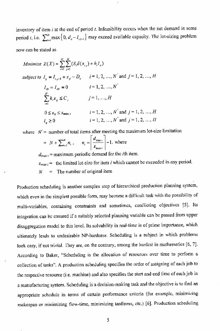
inventory of item i at the end of period I. Infeasibility occur~ when the net demand in some

period I, i.e. L::,max {0, d" -1",_,1 may exceed available capacity. The lot-sizing problem

now ean be stated a~

N' H

Mmimize L(X) '" L:IcS,o(x,,)+ hJ,),_1 ,_I

1,o = I,H =0,L:k,x" :s; C I

'"'

j= I, 2, ,N' and j= I, 2, ... ,H

j= 1,2, ,N'

j= 1, ... ,H

i= 1, 2, ... ,N' and j~ 1, 2, ,H

i= 1,2, .. "N' and j= 1, 2, , II

wherc N' = number of total items after meeting the maximum lot-size limitation

'" ,v+L::,n" n,=rdm'''1-Lwherexm,"

dm", = maximum periodic demand for the ith item,

Xm" i = the limited lot-size for item j which cannot be exceeded in any period.

N The nllmber of original item

Production scheduling is another complex step of hierarchical production planning systcm,

which even in thc simplest possible fonn, may become a diflicult task with the possibility of

multi-variables, containing constraints and somelimcs, conllieting objectives [5]. Its

integration Cilll be ensured if a suitably selected plmming variable can be passed from upper

disaggregation model 10 this level. Its solvability in real-timc is of prime importance, which

ultimately leads to undesirable NP-hardne;s. Sehcduling is a subject in which problems

look easy, ifnoltrivial. l"heyare, on the contrary, among the hardcst in mathematics [6, 7].

According to Baker, "Scheduling is the allocation of resources over time to perform a

collection of tasks". A production scheduling specifies the ordcr of assigning of each job to

the respective resource (i,e. machine) and also specilie, the start and end time of each job in

a manufacturing system. Scheduling is a decision-making task and the objcctive is to lind an

appropriate schedule in tenns of cerbin performance criteria (for example, minimi/-ing

makcspan or minimizing flo'W-lime,minimizing tardiness, etc.) [6]. Production scheduling

5

problem h,ISreceived ample allention from bolh rcscarchers ami practitioncrs, because an

efficient production schedule contributes to reduction of production cost and invenlory cost,

increase in profit and increase in 'on-time' delivery to customers. The theory of scheduling

includes a variety of techniques that arc useful in solving scheduling problems. Indeed, the

scheduling field has become a focal point for the development, application and evaluation

of combinatorial pr(leedures (COP), simulation techniques, network methods and heuristic

solutiun approaches. The selection of an appropriate technique depends on the complexity

of the problem, nature of the model and the choice of the eriteriun, as well as oilier factors

[8]. However, a local search optimization technique or a hcuristic can be used, in llrder to

trade-off belween time to solve a problem and aceL/raeyof results. This research shows that

Pareto optimal sulution method provides better ,olution than even a neighborhood search

technique. a local search teelUlique,This research aims at applying Pareto optimal technique

[9] to selcet the right schedule. Must sludies on production scheduling aim to minimize

makespan, that is, the tutal complelion time of all jub~. The objeclive (If this research, in

case of scheduling, is to nnd tradc-otIs among total completion time Lei' maximum

lateness Lm", and tolal machine idle time 1, where 1= L:_, I", Lmar = maxj("!j} and Tj =

max{O,LI} for jobsj.j = 1,2, .,., n, and batch i.

It must be acknowledged thaI optimization al an indi\'idual lcvel may end up m a highly

sub-optimized and even a non-oplimil.ed solution. \Vhile hcuristics have beell suggested by

many to solve an independent planning level, solution to an integrated flow ur hicrarehical

materials planning has never been reported so far [10, I I]. This necessitates an integrated

solution at several levels of production planning with appropnatc heuristics, where

production planning;s a part of total product planning loop.

A limitalion of CUTTentresearch 011 applylllg optimization technique is the selection of

llnjllstijied objective functwn. Traditionally, it is assumed iliat a parameter needs to be

optimized through right operations m,magemcnt technique [12-14]. However, there is no

basis as to why a particular parameter is selected as the objectIve fllnetion. This research

provides an idea that AHP can be used to justify selection of the right parameter as the

6

objective function of an optimization technique. The following Figure i. I shows the

summary of the research:

Thus, thi~ research aim~ at optimizing materials planning system in the total supply chain

which integrates different levels of planning system.

~Aggregate Plan ~•

Di~aggregation optimizationg.,0-•Disaggrcgation : MPS ~•,

Material~ phmning optimization,~,~

Material~ Planning,0-g.,

• l'rodudion scheduling optimization ••g.,Production Schcduling ~a

0

Distributioll optimization~,~nc

Di~tribufion I'lanniug ~

Figure 1.1 liiemrehieal Production Planning and Distributi(>fi System

1.2 Objectives of the Research WorkThe objectives orthe research work have been defined as follows:

1. To configure aggregation-disaggregation ofmateri<ll plarming system,

2. To develop m<lthematieai modcls and heuristics for the optimiLlltion of aggregate

plarming, master production scheduling, material requircment plarming through lot-

si"ing technique.

3. To implement. simulate and run (he heuristics 10minimize the total cost.

7

4. To identify the production scheduling parameters that affect subsequent planning

steps.

5. To select the balancing parameter i.e. total completion time, maximum lalene~s,

machine idle time with MeUM (multi criteria dccision making) technique.

6. To develop a Pareto optimal algorithm for minimizing total completion time,

maximum lateness, and machine idle lime of a production scheduling system.

7. To implement, simulate and [LInthe Parcto optimal algorithm.

8, To identify distribntion ~y~tem parameters that affect subsequent marketing,

9, To select the parameter of di~tribution for optimilalion with MCDM lechnique.

10. To design und optimize dovmslream distribution plan, with selected variubles.

1.3 Organization of the Thesis

This thesis is organized as follows. The second chapter deals basically with aggregate

planning and mastcr pl'Oduction sebcduling which have been optimized throLlgh lot sizing

optImization. This cbapler also illelude~ various lot ~izillg lechniques, background of lot

sizing problem, heuristic methods of solution of present real life lot sizing problem and

computational resull~ and eonelusion, The third chapler deals with production scheduling

optimization. This chapter presents a description of the multi-criterion scheduling concept,

literature survey of production scheduling problem, a modified Pareto-optimal algorithm to

~olve multi-criterion ~~beduling problem, an algorithm for neighborhood search technique,

problem seltings [Of a ~ingle machine ~cheduling problems, computational rcsnlts of lhe

modi lied algorithm and Ihe neighborhood search heurislic and finally the conclusion on the

multi-criterion pcrspective of this problem under consideration. The fourth chapter

concentrates on distribution planning optimization. Thi~ chaptcr include~ introduction of

di~lribution planning, il', background, application of transportation-based optimization

techniquc, analysis of computational results and conclusion. The 1,I)h chapter consist~ of

conclusiuns and recommendallOn~ for future.

8

Chapter 2Aggregate Planning

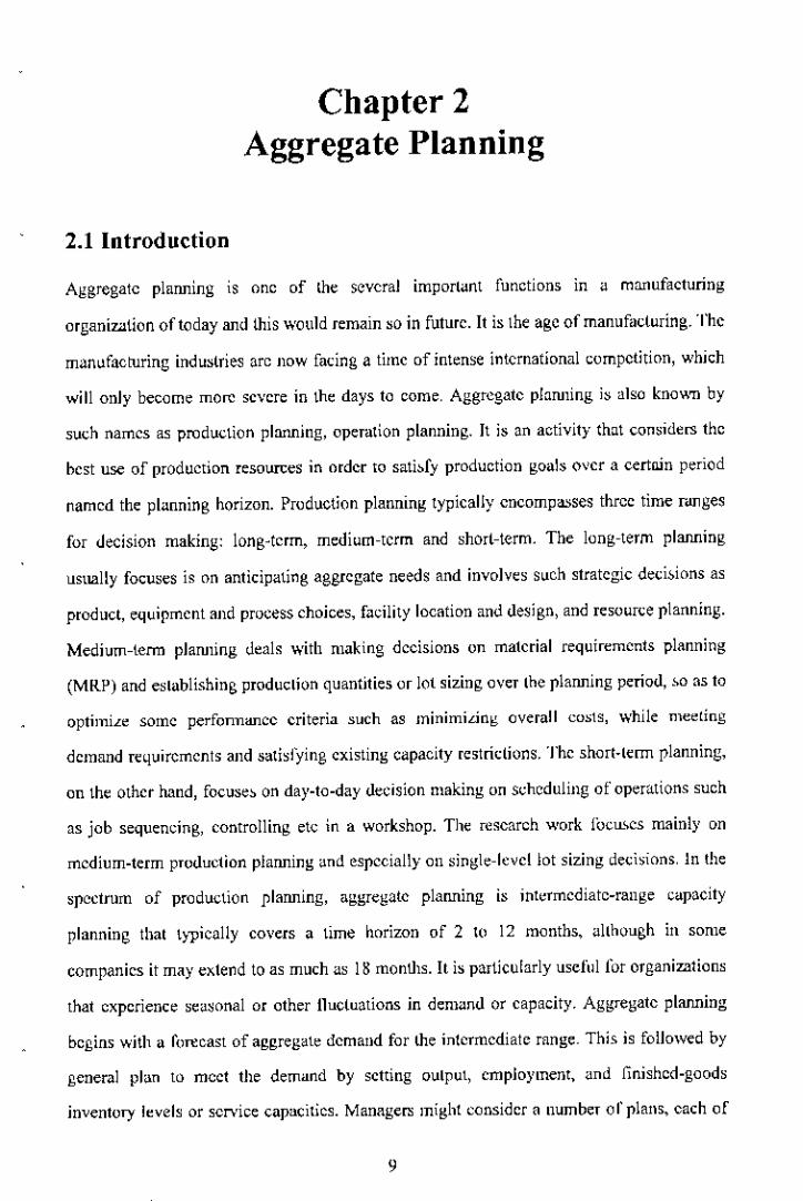
2.1 Introduction

Aggregate planning is one of the several important functions in <l manufacturing

organization oflociay and this would remain so in future. It is the age of manufacturing. The

mani.lfacturing industries arc now facing a time of intenge international competition, which

will only become more severe ill the days to come, Aggregate planning i~also known by

such names as production plarming, operation planning. It is un activity th~t considers the

best use of production resources in order to sati~fy production goals over a certain period

named the planning horizon. Production planning typically cncomp~ses three time nmges

for decision making: long"tcrm, medium-term and short-term. The long-term planning

usually focuses is on anticipating aggregate needs and involves sl.1Chstrategic deci~ions as

product, equipment and process choices, facility location and design, and resource planning.

Medium-term plalUling deals with making decisions on material requirements planning

(MRP) and establishing production quantities or lot sizing over the plalUling period, w as to

optimiLe some perfonnanee criteria such as minimiLing overall costs, while meeting

demand requirements and satisfying existing capacity restriclions. The short.term planning,

on the other hand, focuse~ on day.to.day decision making on scheduling of operations such

as job sequencing, controlling etc in a workshop. The research work loc\L<,esmainly on

medium.term production pJalUling and especially on single-level Jot sizing deci,ions. In the

spcctrnm of production plalUling, aggregate plmming is intermediate-range capacity

planning that typically covers a time horizon of 2 to 12 months, although III some

companies it may extend to as much as 18 months. It is particularly useful lor organizations

that experience seasonal or other l1uctuutions in demand or capacity. Aggregate platUling

begins with a rorecast of aggregate demand for the intermediate range. This is followed by

general plan to meet the demand by setting output, employment, ,md finished.goods

inventory levels or service capacities. Managers might consider a number or plans, each of

9

which must be examined in the light of fea5ibility and cost. If a plan i5 reasonably good but

hus morc weakness, it may be revised and improved. Conversely, a poor plan ~hould be

discarded and allemative plans be ~ought eonsidercd until an a~ceptable one is found oul.

Thc production pbn is essentially the output of aggregate planning.

Aggregate plmmer~are concerned with the quantity and the timing of expected demand. If

total expe~ted demand for the planning period is much different from avaibble capacity

over that same period, thc major approa~h of plarllers \\iill be 10try to achieve a balance by

allering capacity, demand or both. On the other hand, even if capacity and dcmand are

approximately cqual for the planning horizon as a whole, planners may still be faecd with

thc problem of dealing with unevell demand within the planning interval. III some periods,

expected demand may execed projected capacity, in others expected demand may be Jess

than projectcd capacity, and in somc periods the two may be equal. The task of aggregate

planners is to achicvc rough equalily of demand and capacity over the enlire planning

horizon. Moreover, planners arc usually ~onecrned with minimi/lng the cost of aggregate

plan, Effeclhe aggregatc planning requires good information. First, the available resollrccs

over the planning period mu~t be known, Theil, a foreea<;tof expected demand must be

available.

From forecasts and customer orders, production planning determines the requirement of

human and malerial resources to produce efficiently lhe oulputs demanded. The goal is to

efTectivelyallocate syslem capacity (plant, equipment, and manpower) over a designated

time horizon,

Production plan indicates the organization's strategic position in response to lhe expected

demand for ils outpl.lt.A good produ~tion plan with the optimal U5eof resources should

yield such results as (i) be ~onsi51ent with organi~utional policy, (ii) meet demand

requirements, (iii) be within capa~ily constraints, and (jv) minimize costs, However, for a

constant dcmand for a product, the planning activity becomes trivial. But with a stochastic

demand, the system must have a sound production planning; and the a~~(lciatedplamling

problem is said to be dynamic, Some major strategy variables associated wilh production

10

planning for stochastic demand arc the produclion rate, the invenlory kvcl, the work force

size, etc. These variablcs could be varied, modified or CH,nkept fixed, or be noncxistent in

a given organi/.3tion, depending on its pceuliarilie, and policies.

2.2 Disaggregating the Aggregate Plan

For the production plan 10be translated into meaningful terms for production, it is nece~sary

to di~aggrcgatc the aggregatc plan. The re5ult of disaggrcgating thc aggregate plan is a

master schedule showing the quantity and liming of spccific end itcms for a schedukd

horizon. A mastcr schedule shows the planned output for individu<llproducts rather than an

entire product group, along with the timing of production.

2.2.1 Master Production Scheduling

Production planning is an input to the Mw;ter Production S~hcduling (MPS), "hcre thc

master production schedule is a statement of what eml it~m, a comp~uy plans to produce by

quantity and time p~riod. MPS is a di~aggregation fild implementation of the production

plan. It translates the production plan into specific products or product moduks and

specille~ the time period for their eompletion.The master scheduk is the heart of production

planning :md control. The master schedule has lhrec inputs: the beginning inventory, which

is the actual quanlity on hand from the preceding period; forecasts for each period of the

~ehedule; and cuslomer orders, which <Irequantities already commilted to customers. The

master scheduling process uses this information on a period-by-period basis 10determine

the projected inventory, production requirements, and the resulting un~ommittcd inventol)'.

The master production scheduling process drives the material reqlliremcn!s planning

system.

11

2.2.2 Material Requirements Planning System

The intensc global competition in manufacturing has lhrown a strong challenge to the

management 10seek new and more effective ways of managing produclion to maintain or 10

achieve a competitive edge. Therefore, many companies have to implement computer-based

production and inventory control systems, rhe mosl widely adapted systems are called

material requirements planning (MRP) and manufacturing resouree planning.

MRP system is a eomputer-ba,ed information sy~tem lhat translates master schedule

requirements for end items into time-phased requirement~ for subassemblies, components,

and raw materials. Hence, requirements for end items generate requirements for lower-level

components, which are broken down by planning period~~o that ordering, fabrication, and

assembly can be scheduled for limely completion or end items while inventory levels are

kept reasonably low. Material requirements planning IS as much a phil()~()phyas it is a

technique, and as mueh an approach to scheduling a~ il is to inventory controL MRP begins

with a seheuule for finished good~ that is converted into a schedule of requirements for the

subassemblies, componcnts parts, and raw material~needed to prodnce the finished items in

the ~peeifiedtime frame.

The primary inputs ()fMRP arc a bill of materials, which tells lhe composition of a finished

producl; a master schedule, which tells how much finishcd product is desired and whcn; and

an inventory records file, which lells how much inventory is on hand or on order. The

planner processes this inlonnation to detennine the net requiremenls for eaeb period of the

planning horizon. The materials that a finn must aeli.mlly acquire to meet the demand

generated by the master schedule arc the net material requiremcnts. The detennination of

the nel requirements is the core ofMRP proccssing. So there are two major distinguishing

!Catmcs of MKP, (1) requirement tor items conlrolled by MRP are calculaled ba~~d on

schedules for higher-levels ilems as opposed to being rorecast, and (2) plans are time pha~ed

in the ronn of lot-sizing showing order releases and receipts by lime periods throughout

some planning horizon. So lot-sizing is a ~ignifieant aspect of the mat~rials requirement

planning pruce~~and acts as a major component of a balanced MRP opcration,

12

2.2.3 Lot-Sizing Problem

The determination of lot siLes in an MRP system is a complicated and difticult problem, Lot

sizes are the product quantities issued in the planned order receipt and planned order release

sections of an MRP schedule. For products prodl.lcedin-house, lot sizes are the production

quantities of batch sizes, For purchased products, these are the quantities ordered from the

supplier, Lot si7.-e~generally meet product requirements for \Jne or more periods. Lot sizing

decisions give rise to the pwblem of identifying when and how much of a product to

produce such that setup, production and holding costs arc minimilcd, Making thc right

decisions in lot sizing will affect directly the system performance and its productivity,

which arc important for a manufacturing firm's ability to compctc in the markct. Therefore,

developing and improving solution procedures for lot sizing problems is very important.

Most lot-SIzing techniques deal ""ith how to balance the setup or order costs and holding

costs associated with meeting the nel requirements generated by the MRP planning process.

]n the past few years there have been several activities in computer based production and

inventory control dealing with how to select lot-sizes in the face of an cssentially

dctcrministic but time-varying demand pattern. Presently, lot-si7ing problem has taken its

place as one of the most important functions in an industrial enterprise. However,

optimizing routines for lot-sizing problems have been shown to he all 100demanding from a

computing standpoint in both practical as well as research environment. The present work

would seck for an efficient means of obtaining an optimal multi-item lohizing solution to

resealch problems. This would facilitatc development of improved hcuristics appropriate for

practical settings. Research on the relevant fields has yielded several mathematical and

heuristic policies which produce optimal and near optimal results, The ever increa<;mg

importance of this issue therefore calls for further research in this field.

The complexity of lot sizing problems depends on thc features taken into account by the

model. The following characteristics affect classifying, modeling and the complexity of lot

siling decisions.[ 15J

13

Planning Horizon

The planning horiron is the time interval on which the master production schedule extends

into the future. The planning horizon may be Jinile or infinile. A finite-planning horizon is

uSU<lllyaccompanied by dynamic demand and an in finite planning horizon by slationary

demand. In addition, the system can be observed continuously or at discrete time points,

which then elassifies it as a continuous or discrete-type system, In terms of time period

terminology, lot sizing problems fall inlo the categories of cithcr big bucket or small bucket

problems. Big bucket problems, are tho~e where the time pcriod is long enough 10produce

multiple items (in multi-item problem cases), while for small bucket problems the time

pcriod is 50 short that onl} onc item can be produced in each time period. Another varianl of

the planning horilon is a rolling horizon usually considered when there is uncertainty in

data. Under this assumption, oplimal approaches for each horizon act as heuristics but

cannot guarantee the optimal solution.

Number of Levcl~

Production sy~lems may be single-level or multi-level. In single-level ~ystems, usually the

final producl is simple, Raw materials, aftcr proces,ing by a single operation such as

forging or casting, arc changed to final product. In other words, the end item is directly

produced from raw malerials or purchased material~ with no intermediate subassemblies.

Product demands are asses,ed directly from customer orders or market forecu:;ls.This kind

of demand, a> will be further discussed laler, is kno"",llas independent demand. In multi-

level system~, there i, a parent-component relationship among the items, Raw materials

after processing by several operations change to end products, fhe oulput of an operalion

(level) is inpul for another operation. Therefore, the demand al onc level depends on the

demand for its parents' level, This kind of dcmand is named dcpendent demand. MultI-level

problems are more difficult to solve than single-level problems. Mlllli-lcvel systems arc

further distinguishcd by the type of product struelllre, which ineludes senal, assembly,

disassembly und general or MRP systems.

14

Number of Products

The number of end items or final products in a produdion systcm is another important

characteristic that arkcts the modeling and complexity of prodllction planning problems.

There are two principal types of production system in terms of number of products, In

single-item produdion planning there is only one end item (final product) for which the

planning adivity has to be organized, while in multi-item produetion pbnning, there are

sevcral end items, The complexity of multi-item problems is much higher than that of

single-item problems. van Hoese! and Wage!mans [16] provide theoretical results for the

performance of algorithms for the single item capacitated lot sizing problem. (See also

Section 4 of this paper.) Resources or capacities in a production ,ystem include manpower,

equipment, machines, budget, etc. When there is no restriction on resources, the problem is

said to be IJneapacitaled, and when capacity constraints are explicitly stated, the problem is

named capacitated. Capacity restriction is important, and directly aired, problem

complexity. Problem solving will be more difficult when capacity constraints exist.

Deterioration of Items

In the case that deterioration of items IS possible, we encounter restrictions in the inventory

holding time. This in turn is anothcr eharaderistie which would affect problem complexity.

Demand

Demand type is considered as an input to the model of the problem. S\;ltic demand means

that ils value does not change over time, it is stationary or even constant, while dynamic

demand means that its value changes over time. If the value of demand is known in advance

(static or dynamic), it is termed detenninistie, but ifit is not known exactly and thc demand

values occurring are ba5ed on some probabilities, then it is termed probabili~tic. In

independent demand cases, an item's requirements do not depend on decisions regarding

another item's 101size, This kind of demand can be seen in single-level production systems.

15

In multi-level lot sizing, where there is a parent-component relationship among the item~,

because the demand at one level depends on the demand for their parents (pervious level), it

is called dependent. Problems with dynamic and dependent demands arc much more

complex than problems with static and/or independent demands. Also, problems with

probabilistic demand will bc more complex than problems with deterministic demand.

Setup Structure

Setup stmcture is anothcr important eharactenstic that directly affects problem complexity,

Setup costs and/or setup timcs, are usually modeled by introducing zero-{)ne variables in

the mathematical model of the problem and cause problem solving to be more di4cult.

Usually, production changeover between different products can incur setup time and setup

cost. There are two types of setup structl.lrc: simple ~etup stmcture and complex setup

stmcture. If the setup time and cost m a period are independent or the sequence and the

decisions in previous periods, it is termed a simple setup stmeture, but when it is dependent

on the sequence or previous periods, it is termed a complex setup. Three types of complex

setups will now be described. First, if it is possible to continue the production run trom the

previous period into the current period without the necd for <ill additional setup, thus

reducing the setup cost and time, thc structure is named setup carry-over. It can also be

define a sceond type of complex setup, family or major setup, caused by similarities in

manufacturing process and dcsign of a group of item(s). An item setup or minor setup also

occurs whcn changing production among itcms within the samc family. lf thcre is sequence-

dcpcndent setup, itcm setup cost and time depend on the production sequence; this is the

third type of complex sctup ~trueturc. It is obvious thaI the complex structures arc more

awkward in both modeling and solving the lot sizing problems.

16

Inventory Shortage

Inventory shortage is another characteristic afTeetingmodeling and complexity of problem

solving. If shortage is allowed it means that it is possible to satisfy the demand of the

current period in future periods (backlogging case), or it may be allowable fur demand not

to be satisfied at all (lost sales case). Thc combination of backlogging and lost sales is also

possible. Problems with shortage are more difficult to solve than without shortage.

2.3 Literature Study

The importance of lot-sizing in inventory management has been noteworthy over the years,

since it is one of the basic features of the MRI', 'Ihe MRP on the other hand, has the central

importance in manufacturing resource planning and comprehensive MRP system, 'I his has

been evident from e1Tortsby researchers from amongest the academics and inuu<;tries

yielding vast literatures containing abstract mathematical approach as well as highly

pragmatic tedmiques. The literalllrcs have been found places in a large numbers or journals.

Section 2.3.1. presents some or the lot-sizing techniques and Section 2.3.2 summarizes the

historical backgronnd study on the subject. Dixon-Silver heuristic used Silver"Meal

heuristic and Wagner and Whitin algorithm. Seclion 2.3 rigorou<;lydescribes these two

heuristics, since the present work i, fundamentally an extension ofDixon-Silver's work.

2.3.1 Lot-Sizing Techniques

The various approaches and techniques of lot-sizing as developed arc presented below.

2.3.1.1 Period Order Quantity

The period order quantity (POQ) uses the same type (If economic reasoning as th~ EOQ

(Economic Order Quantity which is for fixcd demand or order), bllt determine~ the number

of periods to be covered by each order rather than the number oj"units to order. This results

17

in a fixed on.kr eyele as opposed to a fixed quantity as in EOQ. Total cost per period as a

fllllction of I, the cycle tIme in periods i~given by

C(I) = kit + h(rt)/2.

POQ is an improvement over EOQ as it eliminates remnants, and it perfonns quite well if

demand is relatively stable, However, like EOQ, it does not take full advantage of

knowledge of future period-to-period variations in demand. Some other techniques

described subsequently outperform rOQ when variation in demand is significant [17].

2.3.1.1 Part-Period Algorithm

The part-period ulgoritlun cun determine order sizes under conditions of known, but

varying, demand rates. While the algorithm doe~ not ensure optimality, it does approach

optimal techniques, It equates the part-period value derived from order und holding costs to

the generated part-period value. The generated part-period lor an item is the number of parts

held in imentory multiplied by the number of time periods over which the parts are held. ]n

calculating the generated number of part-periods, it is assumed that no holding costs are

incurred for items eonsl.lme<.1in the period in which they arrive.

To express order cost and holding cost in part-periods, it i~ necessary to divide the order

cost by the holding cost per part per period, The order Co~land holding cost part-periods urc

relerrcd to as the derived part-period value. The derived part-period value is the number of

part-periods it takes to make order cost and holding cost equal. A generated part-period

value is obtained by accumulating part-periods over the demand time horizons for one or

more periods. When the generated part-period value is first greater than the derived part-

period valoe, an order should Ix:placed. The or<.1erquantity will be the accumulated <.1emand

up to the time period for the next order [17].

18

2.3.1.3 Lot-For-Lot

The simplcst lot-sizing technique is lot-for"lot. A lot is scheduled in each period in which a

demand occurs for a quantity equal to the net requirement

Lot-for-lot ordering results in a zero inventory balancc each period, but does involve many

orders. It is mo~t appropriate where the item has a large carrying cost and a small ordering

cost, such as large assembles \"ith expensive components. Another ~i!lmtionwhere lot-for-

101is appropriate is when demand is very sporadic and one or a few units are needed only

occasionally. Lot-ror-Iot also provides a steadier flow of work than other lol-siling

techniques which produce fewer and larger orders [17].

2.3,2 Heuristic Techniques

The next three techniques are heuristics. They aim at providing a good, although not

necessarily optimal solution wilh a ~asonable amount of computing. All the three

techniqucs usc stopping rules. ThaI is, they starl from the first period and lest prospective

ordcrs covering the first period, lhen the first and second periods, then the first, second, and

third periods, and so forth, until a stopping criterion is mel. An order is ~~hedulcdcovering

demands in all periods up through the stopping period. Then the process is repeated starting

at the next period after the la~tstopping period.

Least Unit Cost

The first of the~e rules is called least unit cost (LUC). The unit costs of orders covering

successively greater numbers ofpcriods arc calculated. The unit co~t for each prospeclive

order is obtained by dividing lhe sum of lhe ordering and carrying costs by the number of

units on the order. The first lime cost pcr unil goes up, the prior period becomes the

SlOppingperiod.

19

LUC b widcly used in industry, ~nd on the surface appears to be a reasonable approach to

lot-sizing_However, closer analysis has raised some serious questions concerning the basic

logic of the technique [17]'

Least Period Cost

The least period cost method [18] was developed by Silver and Meal and is generally

referred to as Silver"Meal. This procedure seeks to detennine the total costs of ordering and

carrying for lots covering successively greater numbers of periods into the future and to

select the lot with the least total cost per period covered [17J_

Least Total Cost

The idea for the Least Total Cost (LTC) method (also called part_period_balancing),was

developed by Matties and Mendoza. The concept stems from the fact that in the basic EOQ

model, the inventory carrying cost is equal to the ordering cost at the optimum point. In the

LTC procedure. lot-sizes covering successively greater number~ of periods into the future

are tested until the largest lllt is obtained for which the carrying cost is less than or equal to

the ordering cost. The Authors presented this method to determine the lot for which the

carrying cost was close to the ordering cost. This means that sometimes the carrying cost

wOlildbe greater than the ordering cost. However, [his is not the method presented by the

original authors, and moreover it did not perform well because it ha, a bias tow~rd orders

th;llarc too brge [t 71.

Look AheadlLook Back

Look ahead/look back is ~ technique used to adjust a schedule or order already obtained by

nsing some other technique. It "';IS originally proposed as a rdinement of LTC. !-lowevc>f,

20

look ahead/look back can be applied just as well to adjust schedules produced by other

heuristics.

Look ahead/look back ha~ the effect of moving orders scheduled I"orperiods of low demand

into nearly periods of higher dcmand, This redllces the number of part-periods and,

therefore, the carrying cost. Aueamp and Fogarty have substantially improved and extended

the lechniquc. For one thing, their algorithm also takes into account the fact that if an order

is moved forward or back to a period ill which another order is scheduled, all ordering cost

is saved. Their claim is that regardless of what schedule they ~tart with, the end result is

virtually optimal.

However, look aheadllook back is not widely used. The reasons arc that adding this

procedure makes lot-sizing more complex, adds to the amount of computation, and may

only improve results marginally if a good lohizing procedure has been selected to arrive at

the initial lot-sizes [171,

Dynamic Lot-Sizing Problem

The dynamic lot-sizing problem (DLSP) has received considerable attention Ii-om both

academics and mdustry during the past two decades. Specifically, the problem is (hat of

detennining lot-sizes for a single item when demand i~ deterministic and lime varying.

Time is diseretiled into periods (e,g. days, weeks and months) and production can be

initiated only at the start of a period. Each time that production is initiated, a set-up cost is

incurred, A holding co,! is incurred for each unit of inventory that is carried from ope

period to the next. The objective is to minimize the total of set-up and holding costs, while

ensuring thal all demand is ~atisl"icd on time. The dynamic demand, coordinated lot-size

problem delennincs the time-phased replenishment schedule (i.e., timing and order

quantity) thal minimizes the sum of inventory and ordering costs for a l"<lmilyof items. A

joint shared fixed setup cost is incurred each time one or more items of the product family

<lrereplenished, and <lminor setup cost is charged for each item replenished. tn addition, a

21

unit co,t is applied to ~aeh item ord~rct.l. Demand i~ assumed to be deterministic but

dymlmle over the planning horizon and must be met through current order~ or inventory.

Coordinated lot-sil~ problems are onen cncountered in production, procurement, and

transporlalion planning, The mathemalical complexity of lh~ coordinated lol-size problem

i~ NP.complele indicating that il i~ unlikely that a polynomial boond algorithm will be

discovered for its solution. For this reason, a significant lil~rature base detailing alternative

mathcmatieal f'ormulations and exact solution approaches for lhe problem i~ rapidly

~\'()Iving in an elTorl to solve large industry probl~ms.119 ] 'nlis p"per 120] consid~rs thc

determination of lot sizes I'ormultiple products that can b~ jointly replenished. A fixed sel-

up or onJer cost AO (onen refcrrcd to as a major set-up cost) is incurred whenever any

product is ordered or produecd, independently of the number or lype of producls; and an

extra cost Ai (usually referred to as a minor or line set-up cost) is added if product i is

included in the joint order. The dcmillld for each item is discrete, and varie~ in time, bul i~

kno\~11over a given time horiwn H, Linear holding costs are charged on the end-of-period

inventories and backlogging is not permitted. The variable unit pur~hase cost for each

product is constanl throughout lhe horizon, so lhat the purchase cost of any item for total

demand inlhe horif.on is invariant of the replenishment poli~y. The problem is to determine

a replenishment schedule for all items that minimizes the total set-up plus invcntory holding

cost o,'er the hori7(m. Many dynumi~ programming solutions exisl [or this problem, bul

they are eomputationully ~omplex. For example, when specialized to the multi-product

dynaml~ lot-size problem Zangv,'jJl's method' has a compulational complcxity that is

exponential m the number of products, while Veinott's soluti()n~ arc computalionaIIy

exponenlial III lhe number or time periods, Othcr solutions thal arc computationally

exponenlial in lhe number of products have also been proposed, However these solutions

are of no usc for practical problems, which usually involve many items and many lime

periods, so efi(nts have shifted tu the development or heuristic solulions. Unfoltunately,

though these heuristics arc relatively simple, when compared with the uplimum dynamic

programming solutions, they have two major disadvantages, First, they generally depend on

the \Vagner-Whitin dynamic programming solulion for thc single-item dynamic lol-size

22

problem. Second, it is not known how good these heuristics are, Because a typical practical

problem involves many itcms, and manager~ lind it difficult to understand dynamic

prognlmming solutions, these heuri~lics arc not dcsirable from a pruc!ical standpoint. A

heuristic which overcomes these two problems has been ghen, This relics on a lower bound

obtained from deeumposing thc problem inlo single-item problems, The decomposition

gives an easily computed lower bound. The aim of this paper b (wu-fold: first, it givcs two

simple heuristics and dctcrmines their theoretical worst-case performances, and second it

gives an improved version of the heuristic in Atkins and Iyogun. All these heuri~tics are

generalized versions of exbting single-item heuristics-the part period balancing (PPB 1)

heuristic and a v<uian( of PPH 1 denoted by PPB2, and the Silvcr- Meal (SM) heuristic. The

generali~.cd Silver-Meal heuristic was shown to perform very well on a wide set of

problems. The part-period balancing heuristic is known to perform well in practicc and it is

simple, but i( has a worst-easc perfomlance of 1/3.11 will be shown thut when this heuristic

is generali~ed to thc multi-product dynamic lot-size problem, the worst-case performance of

the generali~ed heuristic cannot be less than 1/3. The other heuristic, 1'1'B2, which i, a

simple variant of the part- period balancing heuristic, has a worst-case perform~nee of Y,. It

will be shown also that when this heuristic is gcneralized to the multiplc product problem

lhenthe worst-case performance is prcserved. The remainder of the paper i~ organized as

follows. The second section gives a brier description of the problem and thc lower bound.

"lhe following section describes the two heuristie~, the gencralized PPB! (GPPBI) and the

generali/cd PPB2 (G1'1'U2), and establishes thcir worst-c~se performances. Considerable

recent ~ltention has foeuscd on lhe "Bullwhip Effect," a term coined b} Proctor and

Gamble. Dynamic programming techniques applied to stock millimiz~tion have also becn

used to qu~n(iry the Bullwhip Effecl. The av~ilability of an exact solution to the continuous

differential inventory cquations seemsto have been o\'erlooked [11]. for example, when

discussing equations withtime delays, none of the text buob on differential cquations or

Laplaec transforms point out that such cquations can be solved exactly in terms of the

Lambcrt Wfunction (Corless et ai, 1996), This paper begins to addrcss this omission. The

aim is to solve exactly the equations lor a model th~t has been shown to be practically

23

valuable, and that has been stlldied in some dewi!. Only from analytlcal solutions can the

precise behavior of a model be carefully assessed over a wide range of condition:;, This

contributes valuable concepti.mlinformation to managers and expert system developers, who

depend on behavioral heuristics, Therefore, a goal of this paper [21J is to provide tools that

help guide the exploration of the parameter space "ith numerical technique~. Since

numcrical treatments of unstable solutions require more care, such approaches should

benel1t.

Many optimal and heuristic techniques have been developed for variations of this problem.

Single Item Uncapacitated Lot-Sizing Problem

Fir~t thc concept of single item comes and there i~no capacity restriction. Somc ofthc most

widely uscd heuristics for lot-sizing arc: Silver-Meal hcuristic [22], least unit cost heuristic

[23]. These hcuristics are not directly applicable to the present work on scheduling problem.

The reason is that these heuristics made the following assumptiuns:

(i) no capacity restrictions,

(ii) only une product to be produ~ed, and

(iii) quantity produced 10mect demand in only integcr number of periods.

'1he cffective use of the availablc capacity of plant could not be made in these hcuristics.

But when capacity constraint is realisti~ally imposed in the scheduling problem, the

availablc capacity use becomes necessary. This part of consideration is an important

contribution to the pr~scnt work.

Thc Silver-Mcal heuristic ealclllatcs the lot size as the total demand for an integ~r number

of pcriods that give the minimum total sct-up and hulding costs pcr unit time. The leas! m,it

cost heuri~tic calculatcs the lot-sizes in thc same way as the Sil~er-Meal heuristic. But thc

execption is that, it minimizes the total costs pcr unit number of products produced rather

than minimizing the tol.<llcosts pcr unit time ~ is donc in the Silver-Mcal hcuristic. For

24

multiple products to be produced with no capacity con~trainls, the above heuristlcs can be

applied to each of the products independently.

Multi Item Uncapacitated Lot-Sizing Problem

Frequently, muillplc items are produced on a single m;lehine. This machine has finite

capacity ;lnd it is usually loaded to or ncar c;lpacity. Most of the existing mdhods for the

multi-item dynamic Jot-sizing problem implicitly as~ume that capacity is unlimited and

hence their use will frequently result in excessive over or under loading in some period~.

Therefore, in practice. planned lot-size~ may be split into smaller lots with some demand

backlogged. lbis resulted to the orders are not being produced on time and the eeonomk~

of scale of butch production is losl.

Multi Item Capacitated Lot-Sizing Problem

. The multi-item capacitated lot-sizing problcm (CLSP) i~ found to be NP-hard when the

singlc-itcm capacitated dynamic lot-sizing problem is already pro"en to be NP-hard [24-

28]. The problem is even harder from practical point of view, since optimal solution

method, have failed to solve all but very small problems within reasonable computation

times_ Moreover, since very rew workable techniques have been reported, methods to obtam

optimum solutions could not be available easily. It ha, been found that most methods

require extensive computational power, thus, their applicability is rather limited. As a

consequence efforts arc now being given to develop heuristics for the multi-item capacitated

lot-si/.ing problems. The various heuristics, \vhich have been proposed over the years, arc

classified into a number of classe~_ The first group of heuristics falling in a clas~ could be

called "common sense" heuristics. The heuristics belonging to this cbs, can be found in

Eisenhut [29], Lambrecht and Vanderveken [30], Dixon-Silver [31] etc. Many different

variants have been proposed, for these common-sense heuristics, but they can basically be

classified into 1\\'0 categories, sueh as

25

-_.-'~- --'-(i) the pcriod-by-period heuristics, and

(ii) improvement heuristics,

(il Period by period heuristic; Heuristics belongmg (0 the period-by-pcriod heuristic work

Ii-urn period 1 to period H. Consider a period I in the proce~s. One certainly has 10 produce

roW({O, d", 1",_1}for all products i in order to avoid stock ol.lls in the currenl period, where d"

is the demand for item i ill period I and lit is the inventory of item iat the end of period I.

'j he remaining capacity (if any) can be used to produce demand for some future period, in

which case future sct-up costs may be saved at the expense of added inventory-holding

costs. To indicate the viability of producing demand for a fulure period in the period under

consideration, all heuristics usc a priority index. The priority indices used by the heuristics

arc more sophisticated in that they try to capture the potential savings per time period and

per unit demand. Although the exact I'riority index may differ from heLlristieto heuristic,

they all proceed in the same way. Priority indices are calculated for all products and for all

future periods. These priority indices arc used to include future demands into the current

produclion lot cither until no more vy'itha positive index or until the capacity limit is hit.

Besides the difference in using priorily index, the period-by"period heuri~tics also differ in

the way in which they ensure feasibilily.lnfeasibility occurs when the ncl demand in ~omeperiod I, i.e. L:~,max{O.d"-I,,,.,} may exceed available capacity. Two different

approaches ean be u.>edto overcome this problem. The lirst one is the feedback mechanism.

When an infeasible period is encounlered, demand with negative priority indices is shifted

from tbe period to an earlier period. A se~ond approach, look ahead mechanism, however,

calculales u priority the required cumulative production up (0 period I (for all t) sllch that no

infeasibility will arise in period (I + I). This pure ~inglc-pass heuristics require smaller

computation time.

(ii) Improvements heuristics; The second category of heuristics called improvements

heuristics start with a solution for the enlire horizon and then lry (0 improve this solUlionin

co~(erfeetive fashion by going through a sel or simplc local improvement steps.

The second group of heuristics is all based 011 optimum seeking mathematical

programming methods which are truncated in some way to reduce computational effort.

The Mathematical-programming based heuristics are (i) Relaxation heuristics (ii) Branch-

and-Bound procedure (iii) Linear programming based heuri,ties. Heuristic~belonging to the

elass can be found in Wagner-Whitin's algoritlun [28], Maes [32J Mixed-integer-

programming formulation etc. In Wagner-Whitin's algorithm capacity constraints are

relaxed i.e. the capacity may be infinite. So (he problem decomposes into ]\I number of

single-item uneapaeitaled dynamic lot siling problems lor which it provides an ellective

method of solution. The first approach of this type is attributed to Newson (33). Startirig

from the Wagner-Whitin ,olutions for each product, the heuristic proceeds as follows,

(i) Select a period in which capacity is violated. For products with a set-up in th<lt

period, caleulale the next best WW solution (i.e, the best solution Jor the

problem where production in the violated period is forced to zero).

(ii) Select the next best plan for (he product yielding the smallest extra cost per unit

capacity absorption, thereby releasing some capacity in the violated periud.

(iii) The method proceeds in this way until all infeasibilities arc removed.

The above approach has two drawbacks. Firsl1y, it may end lip with no feasible solution at

all, and secondly it restricts itself to WW schedules, whereas the optimal solution may not

satisfy the WW eonditiun x"I",_1= 0 at all.

Mathematical-programming based heuristics are nol considered bec<lusethese methods may

nol be very transp<lrentto thc casual user and these heuristics limil lh~ir rcgular use in

industry,

Wagner-Whitin Algorithm

l'he "square root formula" ior an economic lot-size under the assumption oj"a steady-state

demand m!e is well known. The calculation is based on halancing of the costs of holding

27

inventory against the costs of placmg an order. \Vl1en the assumption of a steady-state

demand rate is dropped, i.e., when the amounl~ demanded in each period arc knOVvTIbut arc

diffcrcnt and furthermore, when inv~nlory costs vary jrom period to period, the square root

formula (applied 10 the overall nvewge demand and costs) no longer assur~s a minimum

cost solution.

The mathematical model may be viewed as a "one-way temporal f~asibility" problem, in

thaI it is feasible to ord~r inventory in period I for demand in period I+k but not vice versa.

This suggests that lhe same model also permits an alternative illt~rpretation as the following

"one-way teclmological feasibility" problem.

Mathematical Model

As ill the standard lot ~ile formulalion, onc assumption is thaI th~ buying (or

manufacturing) costs and selling price of the item arc constant throughout all time periods,

and consequently only the costs of inventory manag~ment are of concern, In the I-lh period,

I"" I, 2, .. , ,H, we lct

d, = amount demanded,

hi ~ holding eosl p~r unit of inventory earricd forw<lrd to pcriod I + I,

S,= ordering (or set-up) cost,

x, = amount ordered (or manuf<lctured or size of lh~ lot), and

0', = unit vari<lble cost, which can vary from period 10 period.

Let all period demands and cosls are non-negative. The problem is to find a progr<lmme

x, ~O, 1=1,2, ... ,11, such that all demands <Iremet at a minimum total cost; any such

progwm, will be termed optimal.

Of course one method of solving the optimization problem is to enumerate 211-1

combinations of either ord~ring or not ordering in caeh period (it has been assumed that an

order is placed in the first period). A more effiei~nt algorithm evolves from a dynamic

programming eharacterizalion of an optimal policy.

28

Ld f denote the inventory entering a period and fo initi;II inventory; for period 1'.1 ,-I

J = J" + Z>J - :Ld, ;:.,O.j=1 H

(2.1)

The functional equation representing the minimal cost policy for periods I through H, given

incoming inventory 1, as

where

/,(1) = min [h'.ll + o (x,)s,+/'+1 (l + x,- d, )],

x, ;:.,0,

l+x, ;:.,d"

(2.2)

J(x,) = {~ijx,=Oif x, >0

(2.3)

In period Ii

J;PJ = min fh/i./ + D(xlI}~I!]'

l+xll;:.,d".

(2.4)

Thereby obtaining an optimal solution as 1 for period I is specified. Assumption 2 below

eslabli~hes that it is permissible to confine consideration to only H + 2 - I, I> I, values of J

"t period I.

By taking cogni7...ance of the special properties of the model, an altemative functional

equation has been formulated which h,,-, the advantage of potentially requiring less than Ii

periods' data to "btain an optim"l program; that is, il may be possible without any loss of

optimality to n<\ITOWthe program commitment to a shorter "plarming horiwn" than .11

period~ on the sole basis of data for this horizon. Just as one may prove lhat in a linear

programming model it suffices to investigate only ba~ic sets of variables in search of an

optimal solution, it is demon,trated that in the model an optimal solution exist~ among a

very simple cla~~of policies.

29

It is nece~saryto postulate that d, ;0:° is demand in period 1 net of starling inventory, Then

the fundamental proposition underlying the approach asscrts that it is sufJicient to consider

programs in which at periud lone docs not both place an order and bring in inventof)'.

Characteristics:

(l) There ex;sl, an optimal program sueh tbal! =Ofor all I (where I is"

inventory

entering period I),

(2) There exists an optimal program such that for all I, x, = 0 or x, = I:=, d, for some k,

l5,k5,N.

(3) There exists an optimal program such that if d" is satisfied by some x,'" IU < 1*,

then d" I = I"'.+ 1, .." 1*- I, is also satisfied by X,'"

For the particular C(lststructure assumed, it can be shown that an optimal policy has the

property that/'_lx, = 0, for I = I, 2, .. " H. That is, the requirements in a period are satisfied

either entirely from procurement in the period or entirely Irom procurement in a prior

period.

The property of an optimal solmion slaled above implies that we need consider only

procurement programs where x, = 0, or x, = d, + d ,_,+ -I- u" for some k = I, I + 1, ,. " H.

To etliciently investigate such programs, the following algorithm can be used.

Let FA be the minimum cost program for periods 1,2, .'" k, when I. = 0 is required, Let} be

the lmolperiod prior to k having an ending inventory of zero. Thus II = 0, I, = 0, und I, > 0,

for I =.1+1.}402, .. " k-1. Therefore, xJ+] = ~+] + dJ+2 + ... + d,. Define~! to be the cost

incurred in pcriodsj + 1 through k. It is,~,M J' =X1'1 + C,.,xj+, + Lh,f,-

,-J"

Since, ,

I, = x,., - Ld, = Ld" (or) < I < k, and1=,., 1_,,1

,_1 ,MJ• =X,+, +C,,,x,,, Lh, Ld,.

'=J+t '=j+'

30

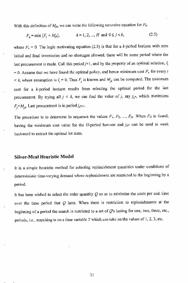
With this definition of ''0" we can \vrile lhe following recursive equalion for F".k= 1,2, "., Hand 0 $oj <k, (2.5)

where 1'0 = 0, The logic motivating equation (2.5) is that for a k-period horizon with zero

initial and Ilnal invcntories and no short~ges allowed. there will be some period where lhe

last procurement is made, Call this periodj+ 1, and by the propcrty of <Inoptimal solution, Ii

= 0, Assume lhat wc have found thc optimal policy, and hence minimum cost F,. for every I

< k, where assumption is I, = O. Thus ~ is known and ,~" can be compllted. The minimum

cost for a k-pcriod horizon results from selecting the optimal period for lhe last

procurement. By trying all 1 < k, we can find the value of}, say l,,', which minimize~

Fj+MJk, Last procurement is in periodlk'+I,

Thc procedure is to delerminc in sequence the value~ FL, 1'2, .. , FH_Whcn I'll is fllund,

having the minimum cost value for lhe II-period hOTlzon and ill' can be used III work

b<lckward to extract thc optim<lliot sizes.

Silver-Meal Heuristic Model

It is a simple heuristic method for ~electing repleni~hment qU<lntitics under conditions of

deterministic time-varying demand where repleni~hment arc restricted 10 the beginning by a

period.

It has been wishcd to select the order quantity Q so as to minimize lhe costs per unit time

over the time period that Q lasts. \Vhen there is restriction to repleni~hments al the

begilUling of a period the search is restricted tll a set of Q's 1<lslingfor one, two, three, cte.,

period~, i.e" searching is on a time variahle Twhich c~n lakc on the values of 1, 2, 3, etc.

31

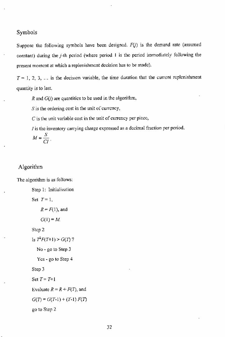
Symbols

Suppose the following symbols have been designed. F(j) is the demand rate (assumed

constant) during thej-lh period (where period I is lhe period immediately following the

presenl moment at which a replenishment decision has l() be made).

T = I, 2, 3, .,. is the decislOn variable, the lime dllration that the current replenishment

quantity is to last.

Rand G(;) are quantities to be used in the algorithm,

S is the ordering cost in the unit oj"currcney,

C is the unil variable cosl in the unit of currency per piece,

I is the inventory carrying charge expressed as a decimal fraclion per period.

M",~CI

Algorithm

The algorithm is as follows:

Slep 1: lnitialinltion

SetT=I,

R=F(I),and

G(I)=M

Step 2

Is ~F(T+I»G(1)?

No - go to Step 3

Yes - go to Step 4

Step 3

SetT=T+!

Evaluate R = R -I-F(T), and

G(T) = G(T-l) + Cr-I) F(T)

go to Step 2

]2

Step 4: Calculation ofreplenishmcnt quantity

Q = current value of R (because R is defined in such a wa>'thal it has accumulated

total demand through the end of period T).,= LF(j).,.,

Thc most complicated operation in the algorithm is seen to be straight multiplication of two

terms or thc squaring of a number.

Dixon-Silver Model

Onc class of "common sensc" hcuristics eonsidcrcd hcrc was initiated by Eisenhut [29] and

could be called pcriod-by-period heuristics. Eiscnhuts procedurc was luter extended by

Lambrccht and Vander Vakcn [30], Dixon and Silver [pI]. In Eisenhut heuristic there is no

guarantee one will find a feasible solution when only positive priotity indices arc

considered, the reason bcing, that net demand in some period I, i.e., L::,maxI0, d,,- 1",_,1may exceed available capacity.

Lambrecht and Vanderveken [28J, Dixon and Silver both are period-by-period hCllris(icand

bascd on Wagner"Whitin condition. Thcsc pcriod-by-pcriod hcuristics havc the advantagcs

that their computation time is low. Both heuristics use the priority index which is derived

from the well-known Silver-Meal heuristic for the single level llncapacitated dynamic lot-

sizing problem.

Lambrecht and Vanderveken use a feedback mechanism (Backtracking) when an infeasible

period is eneountcred, i,e. thcy Iry to shift excess demand to lellover capacity in previous

periods, taking into consideration setnp and holding costs, until the infeasibility in period t

i, removed.

Dixon and Silver, on the olher hand, perform a priority (look ahead) computation of the

cumulative production requirement~ up to period I (for allt) ~uch that no infeasibility will

arise in period (I+ 1).

33

From the comparison study of M"es and Van W"ssenhove [32], bClCktr"ckingprocedure

creates" lot of additional setups whereas in a look-ahead procedure demand to be shifted to

carlier periods is incorporated in planned production lots. Indeed, whcn capacity constr"ints

are tighl it may not be possible to shift demand backwards such that it can be addcd to an

already planned production lot. Instead demand may have to be split up and several extra

setups may be ncecssary to fit everything. This expbins why rather large differences

between Dixon and Silver and the other heuristics occur. On the basis of the results ofMaes

and Van Wassenhovc's [32] comparison study it can be concluded that a look ahead

procedure such as the onc used by Dixon-Silvcr[31] should be prefeITCdto a backtracking

procedure used by Lambrecht and Vandcrvaken. However, when a strong trend in demand

prevails, one should usc a look-ahead procedure to ensure feasibility rather tban relying on a

baektracking routine as in Lambrecht and Vandervaken, So a good heuristic shoi.lldhavc a

look ahead mechanism to ensurc fcasibility at the outset and period-by-period heuristic take

advantage when e"paeities are tight and difference in capacity absorption "cro~s produets

"re large.

Considering these points as discussed above the Dixon and Silver heuristic is considered for

further improvements in the present work.

Dixon-Silver model detcrmines lot-sizes for a group of products that are produced at a

single machine. II i, a~sumcd that the requirements lor each product are knovvnperiod by

period, out to thc end of some common time horizon. For cach product there is a fixed sctu::,

cost incurred cach time production takes place. Unit production and holding Co,lS arc

assumcd linear. The objective of the model is to determine lot-~il.es so that the total costs

arc minimized, with no back-logging and having capacity re~tridion.

The input to the model would include all the co~l'; and product data for each item, sucb as

inventory holding cost, setup co,t, Sellip time, production rate or c"pacily absorption rate,

safety stock, initial inventory and ending inventory. Foreca>teddemand would be given for

each item in each period. In addition, avaibbJe capacity would be used period by period as

input data. Th~mathematical model is pre~entedbelow:

34

Malhematieal model

" "Min;mi~e Z(X) = LL(S,5{x'J) + h,1'J),,1 ,H

Subj~ct to I" '" 1,,)_, +X, - D.

1,0=1,,,=0

":2),x, :::;C,,,'

1 ;0:0,

where N = the number or items,

i=I,2, ... ,A'and/=1,2, ,H

i=I,2, ... ,Nand/=1,2, ,H

j= I, 2, ... , H

i=I,2, ... ,Nandj=I,2" .,IJ

H = the time horizon,

Dij = the given demand for item i in periodj,

lij = the inventory of item i at the end of periodj (after period j production illld

demand satisfied),

Xlj = the lot-size of item j in periodj,

S, = the setup cost fOTitem i,

h, '" the unit holding eost for it~m i,

k, '" thc capacity absorption nlte for item i,

C1~ the capacity in periodj,

jl ijx'l>OJ(x,,)= 0 "r -0, x,) _

J(X,,) is a binary setup variable indicating ""heth~Ta ~dup cost must be incurred

for item i in periodj or not.

2.4 Development of the Model

Thi~ section deals with the modilkation of the Dixon-SilveTmodd with new parameters:

setup tIme and limited lot-size per setup. The modified models aT~more attractive than the

Dixon-Silver model ~inee the setup time and the limited lot-size per setup would be two

important parameters from management point of view. In this regard two models huve been

35

formulated. The model \\,ilh setup time, its heuristic method of solution has been presented

in section 2.4,1.The model with the limited lot-size per setup, its heuristic method of

solution, and sample omput have been presented in Section 2.4.2.

2.4.1 Lot-Size Model with Setup Time

The lot-size modcl \liith selup time included is presented below showing the mathematical

model, heuristic and sample calculations, The input to the model would include all the costs

and product data for each item, such as inventory holding cost, sctup cost, sdup time,

production rate or capacity absorption rate, safety stock, initial inventory and ending

inlientory, Forecasted dcmand \liould be given for each item in each period. In addition,

availahlc capacity would be used period by period a:;input data. 'j he mathematical model is

presented below.

Mathematical model, ,

Minimize Z(X)= II(S,J(x,,)+h),)i_I,,'

Subjectlo f" = f',I_' + X, - D"

f,o = f,JI =0,Ikrv + SI,,5(x,)j..,;c,,-,

where St, = setup time for ilem i.

Heuristic Method of Solution

i= 1,2, ... , lv' and j= 1, 2, ... , H

1=1,2, ... ,N

j=I,2, ... ,1f

j"O 1,2, .. ,N and) = 1, 2, _._,If

Several methods havc been proposed for a solution of the multi-item constrained dynamic

lot-sizing problem (DLSP). Most of these techniques have weakness or limitation that either

they can not guarantee thc generation of a fea,ible 501"tion or become computationally

prohibitive. It has been proved that cvcn the single-item problem with constant capacity is

36

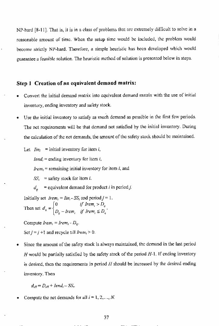
NP-hard [8-11], That is, il is in a class of probkm~ that are extremely diffieLlIt to solve in a

reasonable amount of time. When the selLlp lime would be included, the problem \\iould

become ~trietly NP-hard. Therej()re, a simple heuri~tic has heen developed which would

guarantee il feasible solution, The heuri~tic method of solution is presented bclow in steps,

Step 1 Creation oran equivalent demand matrix:

• Convert the initial demand matrix into equivalent demand matrix with the use of initiill

inventory, ending inventory and safety stock.

• Use Ihe initial inventor)' to siltisly as much demand as possible in the first few periods.

The net requirements v.ill be that demand not satisfied by the initial inventory. During

the cilkulation of the net demands, the amount of the safety stock should be maintained.

Lel lin; ~ initial inventory for ilem i,

fend, = ending inventory l'or item i,

!r~m,= remaining initial inventory for item i, and

SS, = safety stock for item i.

dy

~ equivalent demand l'or product i in pcriodj.

Initially set lrem, = lin, - SS, und periodj = 1.

.. 10 if lrem, > D'JIhensetd,,= _ .Dlj - !rem, if !r~m, ::;D"

Compute !rem, = !rem, - D~_

Setj = j +\ and recycle tlll Jr~m,> 0,

• Since the amounl orthe safety stock is always milinl<lined, the demand in the last period

H would be partially satisfied by the safety stock of the period H-l. If ending inventor>'

i8 desired, then the requirements in period 11 shonld be increa~ed by the desired ending

inventory. Then

d,H = D,/I + fend, - SS,.

• Compute the net demands rOT all i~I, 2, .. ,N

37

Step 2 Cheek the feasibility of the problem:

Feasibility Condition:

" "L CR, ~LC",=1 1=1

"where CRJ '" Lk,d",,=,

CRj ~ demand in terms of cap<lc;ty lmit for periodj,

k, = capacity absorption rate for product ;

If the feasibility condition i~ nol satisfied, the problem is infeasible i,e. all demands cannut

be met with the available capacity,

Step 3 Use the Dixon-Silver heuristic with inclusion of setup time [throughsteps 3.1 to 3.12)

Step 3.1

• Start at period 1, i,e. sel R~l [R = I, 2, ... , 11J. When lot-sizing of period 1 is complete,

then lot-sizing i" started for period 2 up to period H.

Step 3.2

• Initialize lot-size x" by equalizing 10dem~nd d", i,e.,

i= I, 2, ... , A' and j= I, 2, ... ,11.

Step 3.3

• Initially set the value of the time supply to one i,e., T,= 1, where i= 1, 2, .. ,N.

Time supply (T,) denotes the integer number of period requirements that this lot will

exactly,atisfy.

Step 3.4

• Produce J'R > 0, in the lot-sizing period R, where i= I, 2, ... , N.

• After producing rim calculale remaining capacity in period R, <.knoted by RCR, by

]8

"RCft = CR - I),d,,,.,.,

• Let l~be the amount of inventory at the end of period} for item i, resulting from only

the currently scheduled production in period R.lnitializc f~with zero, i,e.,

i=1,2, ... ,Nandj=1,2, .. ,11.

Step 3.5

• Let APj be the amount of inventory (in capacity units) resulted from the production of

period R that will be used in period). Then

"AI',=~),(I",J.,-I".J,o1

• Let eR) be the total demand (in capacity units) ill period}. Then,

CR,=Lk,d".'=1

• The prodl.lction plan for period 11 is feasible if and only if the following condition is

salisfiedforl=2, .. ,H."'I-I "+<_1

LAPJ~ I(CRj-C,+SI,).,/"iI" ,-.""

• Determine the earliest period I, at which the above feasibilily constraint is not satisfied,

l.e.,11+<_' 11+'_'L AP,< L>CR,-C,+SI,)}.1=11+' )=",.

To remove infeasibility upto Ie, extra amount 1S to be produced with lhe use of

remaining eapa~jty Reil of period R,

If there is no infeasibility, set Ie - H + t_

Step 3,6

• Consider only items i' which have

(1) T"<!,,

39

(2) RCR is sufficient to produce d"I<.!: ,and

(3) d",.",.> O.

To decide the best item (li:om a cost standpoint) to be produced in period R, calculate

the priority index U•.for all of these items, where

V,=ACCt;.)-AC{T,,+I) ,and, k"d"J,,+1

\,.,-, )

Ac{J:,)= S,.+h" !U-R)d,., IT,,,,-,

Among these find the one, denoted by i, that has the largest U,.

• V, is the marginal decrease in average costs per unit of capacity absorbcd.

(3, I)

• AC{T,) is average cost pcr unit time of a lot of itcm i which will ,atisfy '1', periods'

requirement~. This is from the Silver-M~ul model in which future setup cost may be

saved at the expen~e of added inventory holding c{)~l.

Step 3.7

• Ch~ek the value of U,.

(a) IfUi > 0, then it is economic to produce d,.IUI, in period R,

lncrea~~ the value of lot-size x,Nand inventory /~ by d"n.]: . i,e.,

x,. = X," + d"R>7,

j=R+l, ."R+T,.

Decrease the value of lot-size X',M,',' demand d',R'T, and remaining capacity RCa by

di•H"" i.e" set

RC~ = RCR - d',II.', .

• Set T, = T,+ 1 and continue from Step 3.5.

40

(b) If V, 5: 0, then it is not economic to inereaw T, of any item, becuuse of the increase of

the total cost.

• Check the value of Ie.

(i) If I, > H, then no infeasibilities left and lot-sizing of the current period is complete,

Go to Step 3.12.

(ii) If Ie < H, there are infeasibilities and production of one or more item is to be

increased and it is done through Steps 3.8 to 3.11.

Step 3.8

• Calculate the value of Q,where

• Q is the amount of production still needed in the current period to eliminate

inlCasibilities in the later period because the available capacity is not suffkient to meet

the demands of those periods.

Step 3.9

• Consider only items i' for which

I. T<I,and, '

]'- d".I1", > O.

To decide the best item (from a cost standpoint) to be produced in period R, calculate

the priority index A" for all of these items, where

AC(T, + l)-AC(T,,)• = '~,' .

k"d".T.,.]

• Find the one, denoted by i, that has the smallest 8"

41

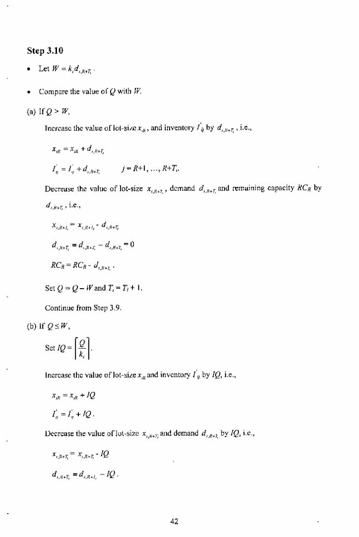
Step 3.10

• Let W = k,d,.I"T, ,

• ComparethevalueofQwithW

(a) IfQ> W,

Increase the value of lo(-si/£ X,I" and inventory r"ij by d"II+". ' i.e.,

j = R+I, ... , R+T,.

Decrea~~ the value of lot-size X,.II.',' demand d',H+". and remaining capacity RCR by

J',R+1; , i.e"

x =x -J• ,.1<'1, ',e,', "R+T,

SetQ =Q- Wand T,= T1+ I.

Continue from St~p 3,9.

(b)lfQs:W,

setIQ=r~lIncrease the value oflol-~ile x,,, and inventory io by IQ, i.e.,

x," = x,,, + IQ

I,;=/:,+IQ.

Decrease the value ofillt-size x'."+'; and demand d"ft.), by IQ, i.e.,

',,,'1'= x ".,.-IQ'., '.,

42

Step 3.lt

• Set R=R+ 1.

• Check the value of R.

(a) If R <H, then continuc from Step 3.3.

(b) If R > JI, lot-sizing is complete up to period 11.

Step 3.12

• Calculate the vali.lcsof

J. forecasted machine time required/period.

11.Total expccted setup cost.

iii. Total expected invenlory holding cost.

IV. Tolul expcctcd safety stock cost.

• Slop.

2.4.2 Model with the Limited Lot-Size Per Setup

The lot-size model with the limited lol-size per setup is presentcd bclow showing the

mathcmatical model, heuri~tic and samplc calculations. Like the previous model, the input

would include all the cost and product data for each item, such as invcntory holding cost,

setup cost, the limited lot-size per setup, prodi.lctionrate or capacity absorption rate, safety

stock, inilial inventory and ending inventory. Forecasted demand would be given lor eaeh

item in eaeh period. In addition, available capacity would be llsed period by period as input

data.1t is 10be noted that Dixon-Silver heuri,tic allows only one setup for each item in each

period. Bul lhe iimilution on lot-size may need more than one ~etup in a particular period.

So should Ihis limitation be incorporated into Dixon-Silver heuristic, each time an item

when processed in a new sctup is to be considered a new item, This may call for splitting an

43

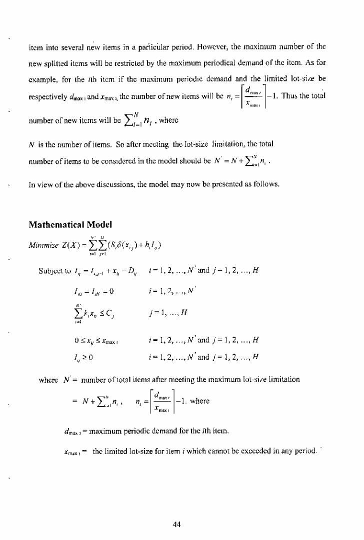
item into several new items in a particular period, However, the maximum llumber of the

new splitted items will be l'estricted by the maximum periodical demand of the item, As for

example, for the ith item if the maximum periodIc demand and the limited lot-~i/-e be

respectively dm" I and Xm" 1, the number of new items will be n, = r~"""1-1. Thu~ the tot~1"," ,

number ornew items will be I;~lni ' where

N is the number of items, So aftel' meeting the lot-size limitation, the total

number of items to be consIdered in the model should be !./ = 1'" +L::,n, .1n view of the above discussions, the model may nllW be presented as follows.

Mathematical Model," II

Mimmize Z(X) = LL(S,5(x,)+h,I,,).=1 r'

!,'=!,H=O

"Lk,x" ~Cl,=,

!" ~ 0

i= l, 2, ,.. ,N' and j= 1, 2, ... , H

i=I,2, .. ,N'

j=l, .."H

i= 1, 2,._ ,N' and./= l, 2, ... , H

i= 1,2, ... ,N' and./= 1, 2, .. " H

where N' = number of tot a! items after meeting the maximum Illt-si/e limitation

,<,'N + .Lt,., n, , rd"." 11 hn,= -- - ,were

x"""

dm"" = maximum periodic demand for the ith item.

Xm>x' = the limited lot-size for item iwhich cannot be exceeded in any perillO_ '

44

Heuristic Method of Solution

The original two-item problem with constant capacity i~NP-hard. In the present work a new

eonstraint on upper limit of the limiled lot-size is eonsidered. With this new eonstraint the

prllblem is also NP-hard. Therefore, a simple heuri~tie has been developed which

gLmrantees a feasible solution.

Step 1 Creation of an equivalent demand matrix:

• Using the same technique of Step I of Section 3.2. I, the given N x Ii demand matrix i~

converted into an equivalent N x H demand matrix with the use of initial inventory,

emlmg inventory and safety stock.

Step 2 Check the feasibility of the problem:

• The feasibility of the problem for N item, is checked using the same formulas of Step 1

of Section 3.1 ,2.

Step 3 Convert the multi-setup problem into single setup problem

Ithrough steps 3.1 aud 3.2]

Step 3.1

• Find the maximum demand dmax, for each item i by using the formula

dm", = max {d~Ij= I, 2, .,., H}.

• Find the number of new ilems fI, to be considered to satisfy demand dm" , by using the

formula

" .[d."'1-1, x""' .

Then the number of total item, aIler limiting the lot-size is

// = N + "'"," n .L.'_I •

hem i is splilled into n, + I items. Let the new items are io' I", ., 1",_

45

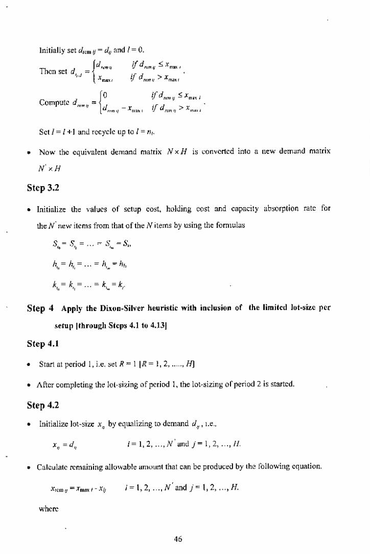
Initially set d"m if ~ d'J and 1=0.

ijd"'ffllj :-o;xm",if d",,,,'1 > xm,"

Set I = I'" I ami rceycle up to I = n,.

• Now the equivalenl demand matrix N x H is ~onverted into a new dem"nd matrix

N'xH

Step 3,2

• Initialize lhe values of setup cost, holding cost and capacity absorplion rate for

the N' neW items from that of the N items by using the formulas

s~~S,' = ... ~ S,_ ~S"

h,,,= h"=,,, = h,~=hl,

k,,,= k"=,,, = k,_=k"

Step 4 Appl)' the Dixon-Silver heuristic with inclusion of the limited lot-sizc PCf

setup Ithrough Steps 4.1 to 4.13J

Step 4,1

• Start at period I, i.e. ~el R = 1 IR = I, 2, .."., H]

• After completing the lol-sizing of period 1, the lot-~izing orperiod 2 is started.

Step 4,2

• Initialize lot-size x" by eq\41lizing to demand d'J' I.e"

x" =d" i= I, 2, ... ,N' and j= 1, 2, .. , II,

• Calculate remaining allov'iable amount that can be produced by (he following equation.

j= 1,2, ... ,N' and j= \,2, ... ,H.

where

46

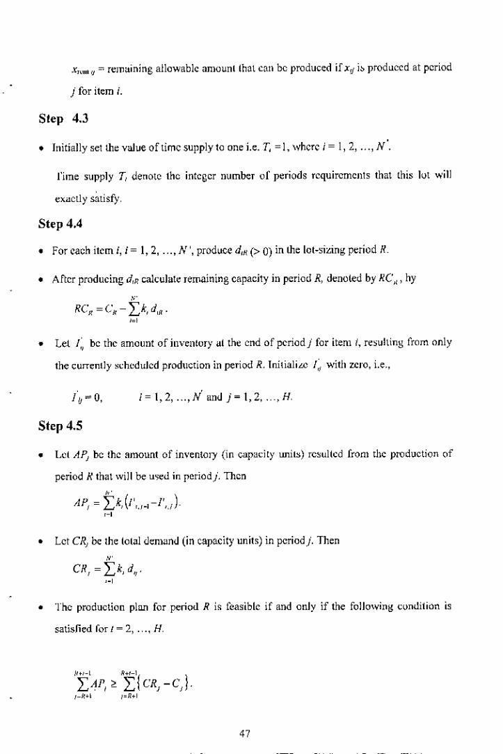
x,,'" 'i ~ rem<tining allowable amountthut eun be produced if xif i~ prodlleed ut period

j for item i.

Step 4.3

• Initially set the value of time supply to one i.e. T, ~I, where i~I, 2, .. ,N'.

J'ime supply T, denote the integer number of periods requirements that lhis lut will

exactly satisfy.

Step 4.4

• For each item i, i ~ 1,2, .. , N " prodl.lee d,H (> 0) in the lot-sizing period R.

• After producing d,R calculate remaining capacity in period R, denoted by RC", by

,,"'

RC" ~ ek - L), d,I"1=1

• Let I;, be tbe amount ofinvenlory al the end ofperiodj for item t, re,ulting from only

the currently s~hcdulcd production in period R. Inilialim 1;, with zcro, i.e.,

Iu""O,

Step 4.5

i~1,2, ... ,N' and1'-1,2, .. ,H.

• I.e! APi be the amount of inventory (in capa~ily units) rc~u)(ed from the production of

period R that will be u5ed in periodj. Then

"AP, ~ L),(i',.,_,-J',J.,-,• Let CRJ be the lolal demand (in capacity unit,) in periodj. Then

,CR,~ i),d".,-,

• The production plan for period R is feasiblc if and only if the following cundition is

satisfied for I ~ 2, ... , H.

47

• Determine the earliest period /, at \\'hi~h the above feasibility constraint is not s<llisfied,

I.e.,1<"_1 ,,+<-,L AP, < L(CR} -C)}.1_1<'] }=II+'

To r~move infeasibility upto I" extra amount is to be produced with the usc of

remaining ~apacity RCR of period R.

If there b no infeasibility, set I, - H + I.

Step 4.6

• Consider only items i' which have

(2) RCR is sufJicient to produce X,~,,,

(3) Xca" > 0,

By equation (1) find the ilem, denotcd by i, that has lhe Jarge~lVi.

Step 4.7

• Check the value of V,.

(a) IrUi > 0, thcn it is economi~ to producc xcan in period R.

lnerease the value of lot-sizeX,R' inventory /'1 and X"m ,.m 7,by XU'", i.c., set

X" _ X,II + x,,,,

)=R+l, .. ,R+1",

Decrease thc value of1ol-~ilc x, II, r' demand d, I/.e ' rem~ining capacity RCR and X,''" ,R, , . ,

by X'aI" Le" set

48

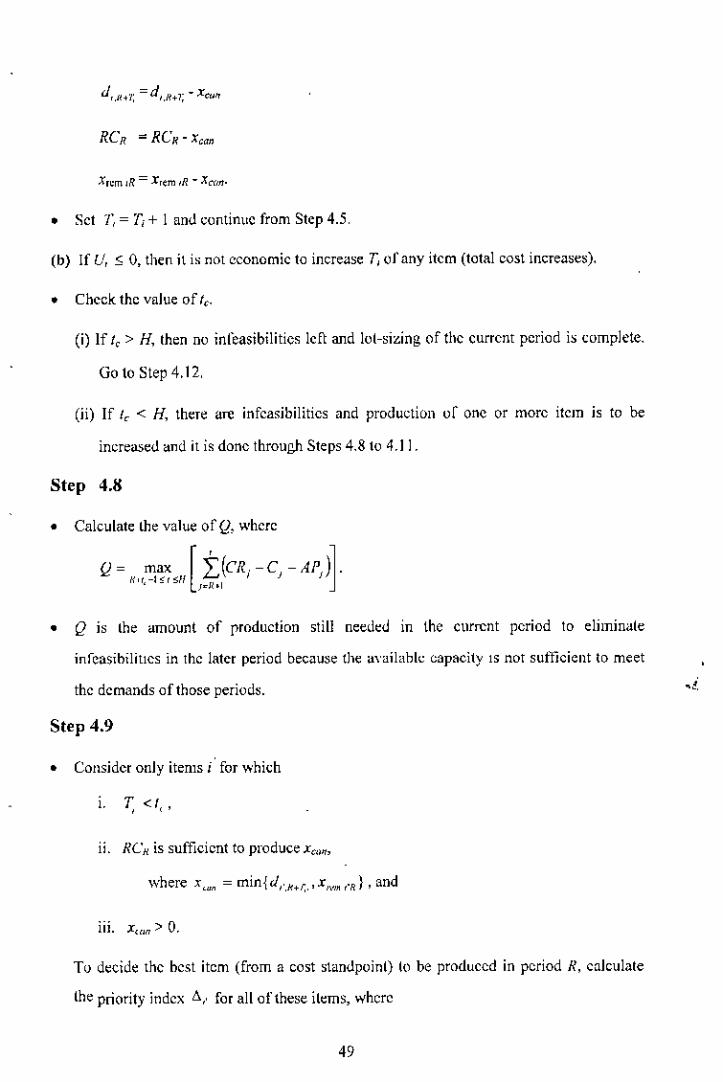
• Set T,= T,+ 1 and continue from Step 4.5.

(b) If U, ~ 0, then it i, not economic to increase T, orany item (total cost increase~).

• Check thc value of Ie.

(i) If I, > H, then no infeasibilities left and lot-sizing of the current period i~ complete.

Go to Step 4,12,

(ii) If Ie < H, there are infeasibilities and production of one or more item IS to be

increased and it is done through Steps 4.8 to 4.1 I.

Step 4.8

• Calculate the value of Q, where

Qo m" [*'ICR-C -APlJ.",,-10""" £...- , J J, ,.11"

• Q is the amount of production still needed in the current period to eliminate

infea5ibiliues in the latcr period because the <l\'ailabk capacity 15not sut!Jcient to meet

the dcmands of those periods.

Step 4.9

• Consider only items i for which

1. T, <I"

11. RC~ is suffieicnt to produce XC,,",

1IJ. x,,,n>O.

To decide the best item (from a cost standpoint) to be produced in period R, calculate

the priority index "' .. for all of these items, whcre

49

A,AC(1;. + 1) - ACCT,.)

k"do:'+1

• Among these find the onc, denoted by i, that has the smallest !:J,.

Steps 4.10

• Let fV = k,x,,,,,.

• Compare the value of Q with W.

(a) IrQ> w,Increase the value of lol-sizcx,H, inventory t'~and x"", ,',R+I, by XW", l.C., set

j=R+l, ... ,R+T,

Decrease the value of lot-size x, ",1" demand d !I.e, remaining capacity RCR and XIcm IR by. , " ,

XC"'" i.e., set

X.,R+1; = X"R+', • XC""

Set Q ~ Q- Wand T1~ T,+ 1, and continue from Step 4.9.

(b)IfQ~W,

SelfQ~ Ii.l-increa,e the value oflot -size x,"' inventory r'~amI x ~rn,',R+1; by lQ, i.e., set

j=R+l, ... ,R1-T;

50

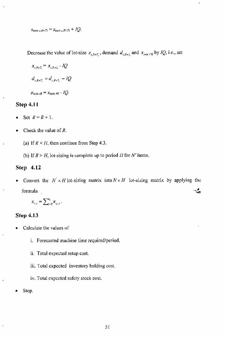
Decrea.>e the value oflot-size X.,R+',' demand d,_"", and x",,,, n, by IQ, i,e., set

X,_"+': = X'_"", - IQ

d'_R+7: = d'_H", -!Q

X""n ,R = X"miR - !Q,

Step 4.11

• Set R=R+L

• Check the value of R.

(a) If R < ll, thcn continue from Step 4_3.

(b) If R > H, lot-sizing is complete up to period II for N' items.

Step 4.12

• Convert the l{ x H lot-sizing matrix into N x H lot-siling matrix by applying the

formula

Step 4.13

• Calculate the values "j"

1. Forecasled machine time required/period.

n, Total expected selup cost.

iii. Total expected inventory holding cos!.

iv. Total expceted safety stock cost.

• Stop,

5 I

2.5 Computational Results with Real Life Data

The algorithm developed by Dixon and Silver [31] to generJ(e feasible solution for multi-

item single level ~apacitated lot-sizing problem was tested by a programming language in

PC versiull. Thus a ncar optimal solution was obtained, The results arc detailed in Section

2.5, I beluw. This algorithm has been extended in the pre~ent ,,,,rk. The setup time and the

upper limit on the lot-size have been ineluded in the original algurithm. Thus the Dixon-

Silver algorithm is separately extended with these two new parameters as described in

section 2.4. This section presents the results obtained from the mudiJ1ed models using a

programming language in PC version. Section 2.5.2 shows results with setup time

consideration, and Section 2.5.3 shows lhe results with upper bound on the limited lot-size.

2.5.1 Results of a Multi-item Single Level Capacitated Lot-sizing Problem

The Dixon-Silver algorithm has been used with real life data. Dala has been collected from

a renowned rumitlITecompany. The products arc fixed chairs. Twelve models of fixed

chairs have been considered here, and these models arc given in Figure 2.1. It is assumed

that lhe entire production to meet demands is done in lhe plant and no subcontracting is

permissible, Moreover, a further assumplion is made that plant capacity could not be

increased.

52

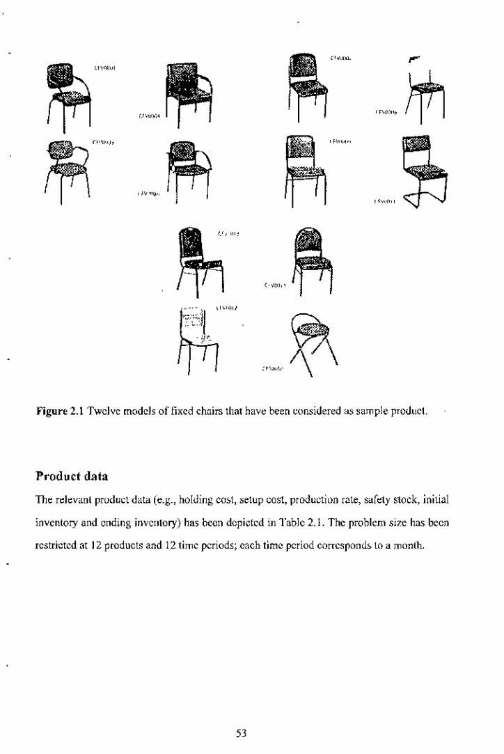
~~~~I"'I,- "--

- ''':

"''''''

Figure 2.1 Twelve models of fixed chairs that have been considered <ISsample product.

Product data

The rekvanl product data (e.g., holding co~t, setup cost, production rale, safdy stock, initial

inventory and ending inventory) has been depicted in Table 2, I. The problem size ha5 been

restricted at 12 products and 12 time periods; each time period corrcspond~ 10a month.

53

Table 2.1 Relevant product data for the particular machine,

Itom Holding Setup Production Safety Initial Ending

~~ ~:~t ~;.~t ~~:~~,~;~In~~j~,t,~ry In".ntnry

• l/.I, >S. f", fJ",,~:"

" 12.0 200.0 6 '" ISO 90

" 12.0 3000 5 60 100 120OJ 12.0 300 () 5 SO 150 12004 12.0 250,0 , 100 200 no05 12.0 300,0 10 130 250 22006 12.0 300,0 9 ISO 250 200

" 12.0 250,0 8 100 100 20008 12.0 200,0 8 '" 250 20009 12.0 200,0 , 100 '"0 50010 12.0 200,0 , 190 220 210

" 12.0 250.0 8 90 130 13012 12.0 200,0 12 70 200 100

2. Product demand plant capacity

Product demands arc quite sea>onal and the same seasonal indice~ UTeused for all the

product>. Foreca~ted demand and the capadty of the machine arc shown in Table 2.2. H has

been assumed that the capacity per month is the totul number of hours available per month.

In this problem, Period I corresponds to the month of January, Period 2 corresponds to the

month of February. Thus the machine capacity in Period I is the total production hours in

January. There is two shifts (8 hours in each shift) in the factory. There i~ one hour for rest,

tea etc in each shirt. There is six working days in a week. To be on Ihe safe side, it has been

assumed that there is some ovcrtime in some month for overproduction dliC to higher

demand. Also there is some holidays in some month for differetl! festival. As for example,

the machine capadty in Period 2 is 14 hr x 24 days = 330 houtS. Similarly the machine

capacity for the other periods has been calculated.

54

Table 2.2 Forecm.ted demand and capacity of the hypothetical machine.

''''' PeriodNo , 2 3 , 5 6 7 , , '" " "" 90 60 '" 80 90 80 70 75 60 60 50 '""' 80 " '" '" 75 90 90 '" '" 60 60 ;003 ,"0 60 60 50 80 "" 90 '"0 90 >20 80 ';0

"' 180 165 m >50 200 '"0 120 '50 145 240 220 22005 200 ,"0 280 260 200 210 200 DO 120 2" 240 21006 400 240 245 250 230 200 230 205 1" 380 255 '9007 450 350 350 380 340 360 400 '50 ';0 4110 "0 35008 200 250 250 200 150 160 '"0 '"0 250 100 250 '"009 500 500 450 '00 450 500 400 400 "0 ';0 700 110

'" 3>0 250 220 225 120 130 t3 Il '" 115 204 200 150

" 300 200 200 100 160 100 130 '"0 '0 '40 120 90

" 150 95 95 '"0 ,"0 90 75 75 60 t]O I" 90Forecasted Machine Requirements (hours)

370 330 370 3>0 3" 350 3" 370 350 300 350 300

3. Equivalent demand schedule

An equivalent demand schedule is generated such thaI ~tarting and ending inventory are

accommodated. In addition, demands are adju~ted such that in the heuristic solution, the

inventory at the end of any period never drops below the safety stock level. Table 2.3

depicts the equivalent demand alter considering initial inventory, ending inventory and

safety stock.

55

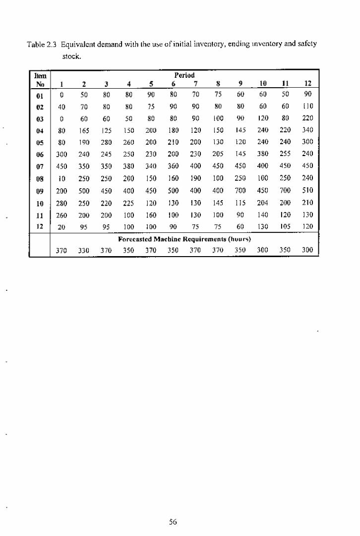
Table 2.3 Equivalent demand with lhe uw of initial invenlol)', ending mvenlory and safety

stock.

lrem PeriodNo 1 2 3 4 5 6 7 , 9 10 11 1201 0 50 80 80 90 '0 70 75 60 60 56 '0

" 40 70 80 80 J5 90 00 "" 80 60 60 11003 0 60 60 50 80 80 00 100 90 120 80 22004 80 165 '" 150 700 ISO 120 150 145 "0 220 34000 80 100 no 700 200 210 200 130 170 "0 240 30006 300 240 2" 750 230 200 230 205 '" '"0 255 240

07 450 350 350 380 340 360 400 450 450 400 450 "0US 10 250 250 200 150 "0 190 100 250 100 250 24009 200 500 456 400 456 500 400 400 700 456 700 51010 280 750 220 225 110 130 130 145 115 204 200 21011 260 200 200 100 "0 100 130 100 90 140 liD 13012 70 03 95 100 100 00 J5 J5 60 130 lOS 120

Forecasted Machine nequirements (huur~)

370 m m 356 370 356 370 no 350 300 356 300

50

4. Results

Tablc 2.4 shows the final lot-sizes and forecasted machine hour reqllirements for each

period, and Tablc 2.5 shows lhe inventories at the cnd of each period for all itcms.

Table 2.4 Finallol-si/.es and forecasted machine lime requiremcnts for l)ixon-Silverhetlristic.

"'" PeriodN. t 2 3 4 5 6 7 8 9 '0 II 1201 0 SO 80 80 90 90 70 1)5 60 50 90 001 90 '" 80 80 75 911 m 188 0 60 110 003 0 60 60 SO 80 '" on '95 115 80 no 0

" 80 165 125 150 '"0 180 120 295 240 no 0 HO

" 80 190 280 260 '"0 "" 200 130 020 240 240 )0006 )00 240 245 250 230 200 230 205 145 3ijO 255 24007 450 )50 350 380 340 360 400 450 450 400 450 450OS 10 250 250 200 ISO 160 190 100 )50 0 250 24009 200 500 450 400 450 500 400 400 M3 309 698 51016 280 250 220 225 120 1)0 130 260 204 200 145 65II 750 200 200 100 160 100 1)0 190 0 260 0 13012 20 95 95 100 100 90 75 75 60 130 105 120

Forecasted Machine Requirements (hours)221.0 3 18.G 318,0 297,2 291,1 29l.3 28U 371l 0 J50.0 JOO.O 350,0 300.0

Table 2.5 Invcntories at the end of each period for all ilems.

,- PeriodNo , 2 ) 4 5 6 7 8 9 16 II 1201 60 '" 50 50 50 50 50 110 110 100 140 on01 90 60 60 60 90 60 92 200 120 120 170 12003 50 '" 50 50 50 50 50 145 170 130 no 12004 160 100 100 100 100 100 100 245 340 no 100 noos no IJO 130 130 130 1)0 130 130 130 130 1)0 22006 ISO ISO ISO ISO ISO 150 ISO ISO ISO ISO ISO 20007 100 100 100 100 100 100 160 100 100 100 100 20008 60 60 60 60 60 60 60 60 160 60 60 200

"' '00 100 100 100 100 100 100 100 24) 102 100 '"0

" ISO ISO 150 ISO ISO ISO ISO 265 354 J50 295 200II 90 90 on 90 90 90 90 180 90 210 90 13012 70 70 70 '" '" '" '" '" 70 70 '" 100

57

Other results are tabulated below:

Total available machine time (I::, C, ) 4180.0 hour

Total setup time (L;:, n,SI,) (J.Ohour

where n, is the number of setup for item i.

TOlal forecasted machine time 3695,9 hour

Total inventor)' holduingcosl, C,n,= I.,N L:' (/" - SS,) Tk. 49,332.00-I _I,Total expected safety-stock cost, C, = L:=I SS, Tk.159,840.00

,Total expected setup COS!, C,,, = L=I n,S, Tk. 32,850.00

Total expected cost (en> + Coo+ C",) Tk.242,022.00

58

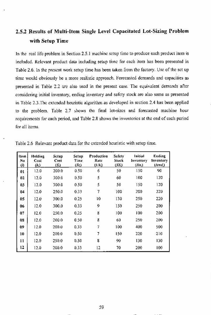
2.5.2 Results of Multi-Item Single Level Capacitated Lot-Sizing Problem

with Setup Time

In the real life problem in Section 2.5.1 machine setup time to produce each product item is

included. Relevant product data including setup time for each item has been presented in

Table 2.6. In the present work setup time has been taken from the factory. Usc of the sct up

time would obviously be a more realistic approach. Forecastcd dcmands and capacities as

presented in Table 2.2 are also used in the present case. The equivalent demands after

considering initial inventory, ending inventory and safety stock are also same as presented

in Table 2.3.The extended heuristic algorithm as developed in section 2.4 has been applied

to the problem. Table 2.7 ~hows the final lot-sizes and forecasted machine hour

requirements for caeh period, and Table 2.8 shows the inventories at the end of each period

ror all items,

Table 2.6 Relevant product data for the extended heuristic with setup time.

Item Holding Setup Setup Produclion Sarety Ini(ial ~:ndingN. Co>! Cost Tim. R.lo Slock III'CnIOr)' Im'clltory

1m ,",' "" (S,,) (lik,) (SS,) (1111,1 fiend,) .

" t2.0 200,0 0,50 6 50 '" 00

" t2.0 300,0 0,50 5 60 >00 >7003 t2.0 300,0 0,50 5 50 >50 >70

"' 12.0 250.0 0.33 7 >00 700 no05 12.0 300.0 0.25 >0 no 250 22006 12,0 300.0 0.33 9 >50 250 20007 12,0 250.0 0.25 " >00 >00 200os 12.0 200.0 0.50 8 00 2;0 20009 t2.0 200,0 0.33 7 >00 400 ;00>0 12.0 200.0 0.50 7 >50 220 2>0

" 12.0 250,0 0.50 8 90 >30 >30

" 12.0 200,0 0.33 >7 70 200 >00

59

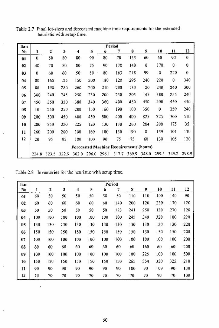
Table 2.7 Finallot-sizcs and forecasted machine time requirements for the extendedhellristie with setllp time.

I"" PcriodN. I 2 3 4 5 6 7 8 9 10 II 12OJ 0 50 80 80 90 80 00 IJ5 60 50 90 002 40 00 80 80 75 90 170 I" 0 170 0 003 0 <>0 60 50 80 80 16) m 99 0 220 0

" 80 165 125 ISO 200 180 120 295 240 220 0 34005 80 190 280 260 200 m 200 IJO 120 240 240 '"0SO 300 240 '" »0 2;0 200 230 205 14> '"0 '" 24007 4>0 350 350 380 340 360 400 450 450 400 450 450

"' 10 250 250 200 150 160 190 100 350 0 »0 24009 200 500 450 400 450 500 400 400 S25 325 700 51010 280 250 220 225 120 1)0 1)0 260 204 200 I75 35II 2<>0 200 200 100 160 100 130 190 0 IS' 101 13012 20 95 95 100 I00 90 75 75 60 130 105 no

Forccastcd Machin. Rcquirements (hnnn)

224.8 323.5 322.9 302,0 296.0 296.1 3 [7.7 369,9 348,0 299.5 349.2 298,9

Table 2.8 Inventories for the heuristic with setup time.

I~, l'criodNo I 2 3 4 5 6 7 , 9 10 II 12OJ 60 50 50 50 50 50 50 110 I10 100 140 9002 60 60 60 60 on on 140 200 120 2)0 100 12003 '" '" '" 50 50 50 123 241 250 130 270 12004 100 100 100 100 100 100 100 245 340 320 100 22005 no IJO 130 130 130 130 IJO 130 130 130 130 22006 ISO 150 150 150 150 150 150 150 150 150 ISO 20007 100 100 100 100 100 100 100 100 100 100 100 20008 60 60 60 60 60 60 60 60 160 60 60 20009 100 100 100 100 100 100 100 100 225 100 100 50010 150 150 150 150 150 ISO ];0 205 35< 350 325 210II 90 " 90 90 90 90 90 180 90 109 90 noI2 70 70 70 70 70 70 70 70 70 70 70 100

60

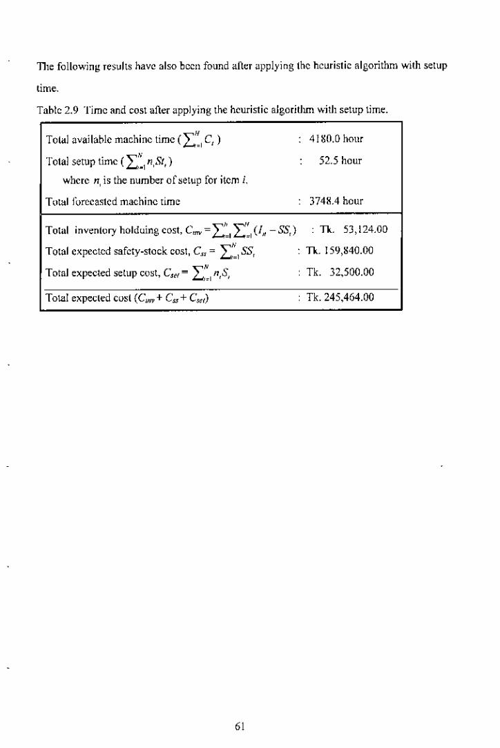
TIle following: results have also been found aller applying the hellristie algorithm with setup

time.

Table 2.9 Time and cost aller applying the heuristic algorithm with setup time.

Total available machine time (L::,C,) 41 gO.Ohour

Total setup time (I:~1n,SI,) 52.5 hour

where n, is the number of setup for item i.

Total forecasted machine time 3748.4 hour

Total invent(11)'holduing cost, c."" =I::, I:':,(/"- SS,) TIc. 53,124.00

"Total expected safety-stock cost, C, = I,=,SS, n.159,g40.00

Total expected setup cost, C,,' = IN n S TIc. 32,500.00'0' ' ,

Total expected cost (Cm" + C,",+ C,,,) Tk. 245,464.00

61

2.5.3 Results with the Limited Lot-Size per Setup

Relevant product data including the limited lot-size per setup for eaeh item has been

depicted in Table 2.10. The limited lot-size per setup for each item has been taken

arbitrarily. The demands und capacities are extracted hom Table 2.2. rhe equivalent

demands after considering in;ual inventory, ending inventory and safety stock arc extracted

Irom Table 2.3. To illustrate the algorithm a few samplc calculations for the period 8 have

been shown. Forecasted demand and capacity with limited lot size per setup are depicted in

l"ablc2.11.

Table 2.13 shows the final lot-sizes and forecasted machine hour requirements for each

period, and Table 2.14 show8 the inventories at the end of each period ror all items.

Tablc 2.10 Relevant Product datu for the heuristic with the limited lot-size per setup.

Item Hotding Sctup 1't1nimum Productiou Safety Initial Endin!!:No Cost Cost Lot-Size """ Stock Invcntorv Invcnto

01 12,0 200,0 ISO 6 50 150 9002 12,0 300.0 150 5 60 100 12003 12,0 300.0 150 5 50 1>0 12004 12,0 250.0 ISO 7 '"0 200 22005 12,0 300.0 200 '" 130 2>0 22006 12,0 300.0 200 9 ,>0 ,>0 200

"' 12.0 250.0 200 8 '00 ,"0 200

"' 12.0 200.0 200 • 60 250 200

" 12.0 200.0 200 7 '"0 400 50010 12.0 200,0 200 7 ISO 220 210II 12.0 250.0 200 • 90 110 'JO

12 12,0 200,0 200 12 70 200 '"0

The maximum periodic demand Jor item 9 is

dm"9 ~max{dIJlj~ t,2, ... ,H}

= max {200, 500, 450, 400, 450, 500, 400, 400, 700, 450, 700, SIO}

= 700

The limited Jot-size for item 9 is x"''' 9 = 200.

62

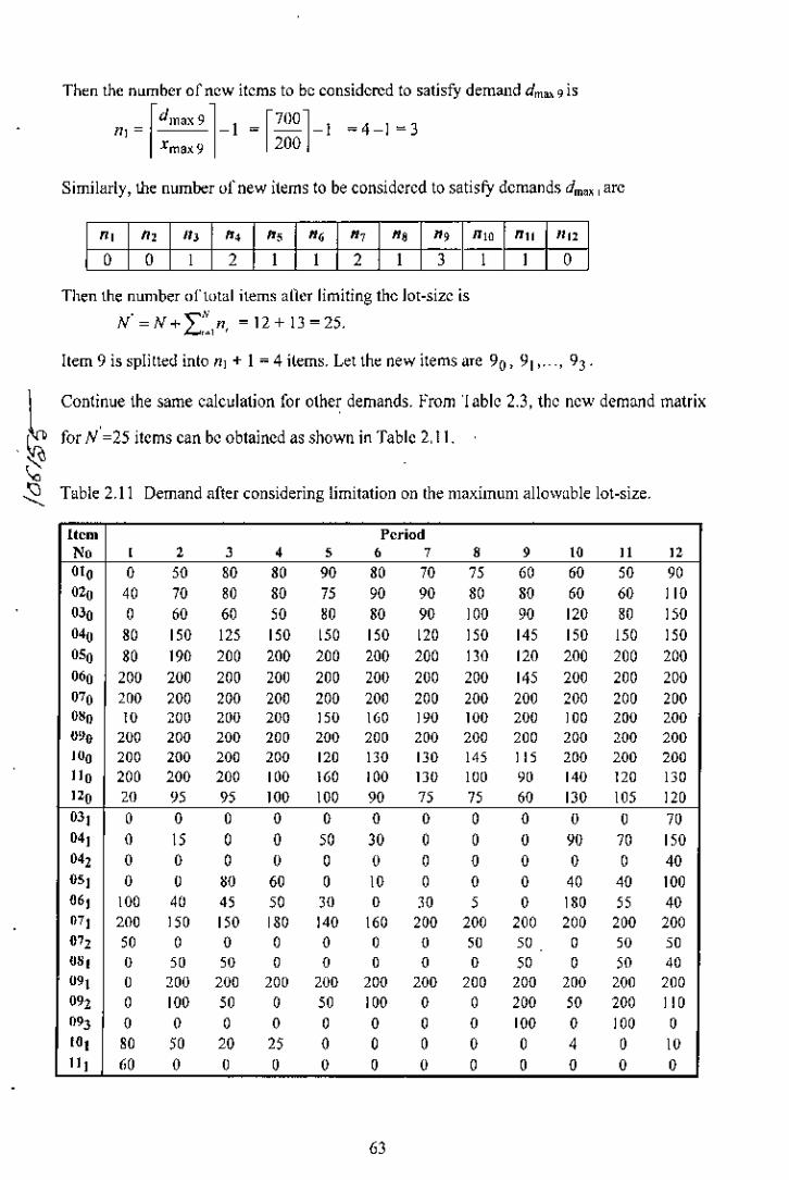
Then the flllmbcr of new items to be considered to satisfy demand dm", 9is

II] = rdmaX91-1 = [70°1-1 =4-1 =3xmax9 200

Similarly, the number of new items to be considered to satisfY demands dm" I arc

0, 0, 0, Q, Q, Q, Q, Q. Q, "" 0" 1112

0 0 I 2 I I 2 I 3 I I 0

Then the number "fl,,!al items ancr limiting the Jot-size isN'=N+'C"Nn =12+13=25.4..,., '

hem 9 is spIiltcd into II] + 1 = 4 items. Let the new items arc 90, 91" _, 93,

Continue the same calculation for other demands. From 'lablc 2.3, the new demand matrix

for 4=25 items can be obtained as shown in Table 2,11.

Table 2.11 Demand after considering limitation on the maximum allowable lot-size.

Item PeriodNo , , , • ; • , • , 10 H "'m. 0 50 80 80 90 80 70 75 60 60 50 90

"'" 40 70 80 80 75 90 90 80 80 60 60 HO

"" 0 60 60 50 80 80 90 100 90 "'0 80 15004" 80 150 125 150 150 150 120 150 145 150 150 150"'0 80 190 200 200 200 200 200 lJO 120 200 200 200000 200 200 200 200 200 200 200 200 145 200 200 200"'0 200 200 200 200 200 200 200 200 200 200 200 200""0 10 200 200 200 ISO 100 100 100 200 100 200 200ll~ll 200 200 200 '"0 '"0 200 200 200 200 200 200 20010. 200 200 200 200 120 uo uo 1'5 H5 200 200 200Ho 200 200 200 100 160 100 lJO 100 00 140 un 130"0 2<l 95 95 100 100 90 " 75 60 130 105 120031 0 0 0 0 0 0 0 0 0 0 0 70041 0 15 0 0 50 30 0 0 0 90 70 15004, 0 0 0 0 0 0 0 0 0 0 0 40"I 0 0 '" 60 0 10 0 0 0 40 40 100"I 100 40 45 50 30 0 30 5 0 180 55 40"'I 200 150 150 180 140 160 200 200 200 200 200 200"" 50 0 0 0 0 0 0 " 50 0 50 50"', 0 50 50 0 0 0 0 0 50 0 50 40"', 0 200 200 200 200 200 200 200 200 '"0 200 200

"" 0 100 50 0 50 100 0 0 200 50 200 1I0

"" 0 0 0 0 0 0 0 0 100 0 100 010, 80 50 20 25 0 0 0 0 0 4 0 10"l 60 0 0 0 0 0 0 0 0 0 0 0

63

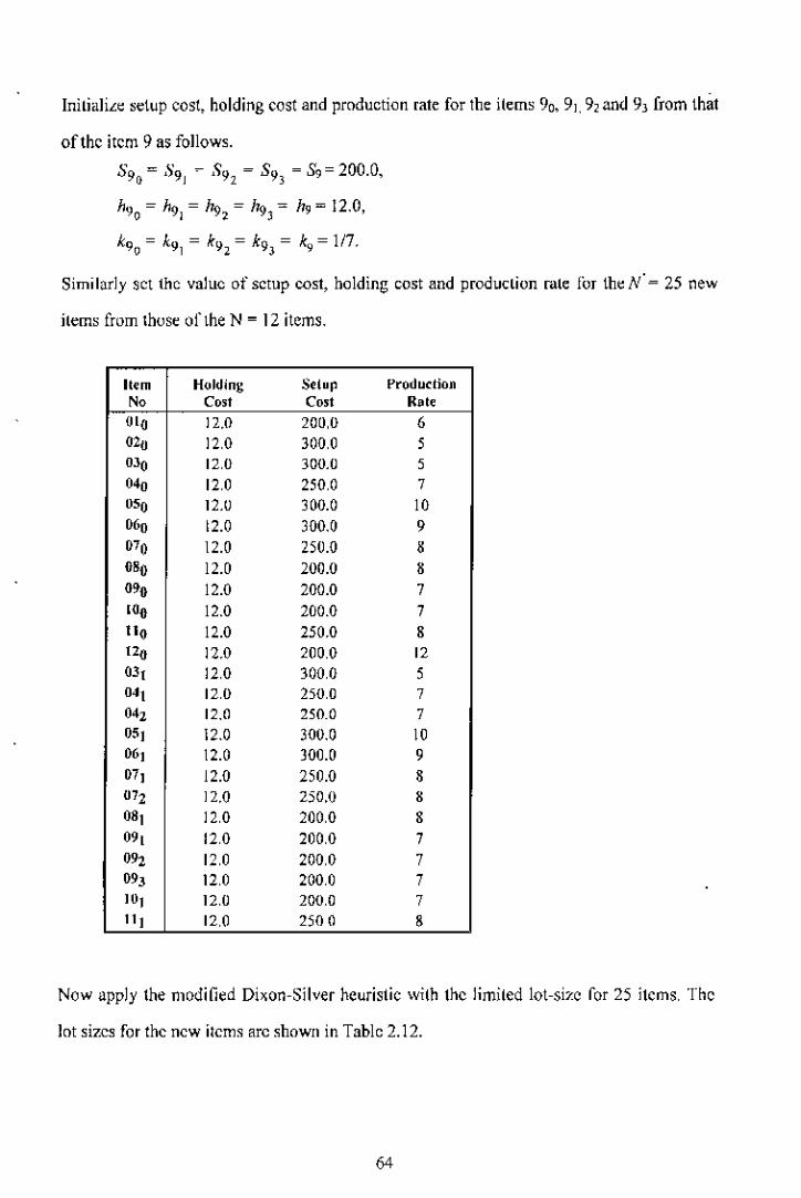
InilialiL~ setup cost, holding cost and production rate for the items 90, 91, 92 and 9] from that

ofthc itcm 9 as follows.

59G = 591 ~ S92 ~ S9) ~ S9= 200.0,

h9 =h9 =h9 =h9 = h9=12.0o I ~ J '

k9 = k9 = k9 = k9 = k = 117.o I ~ J 9

Similarly sct the value of setup cost, holding eost and produclion nile for thd{~ 25 new

ilems from thuse oi"lhe N = 12 items.

Item Holding Selup Produ<tion

'" Co,t Co,t Rate

"'. 12.0 200,0 6

"'" 12,0 300,0 5

"'. 12,0 300.0 5

"'" 12,0 250,0 ,0'0 12.0 300.0 10

""0 12.0 300.0 9

"'. 12.0 250.0 8

"". 12.0 200.0 8

"'. 12.0 200.0 ,'". 12.0 200.0 ,n. 12.0 250.0 8n. 11.0 200,0 """ 12,0 300.0 5", 11,0 250,0 ,"" 12.0 250.0 ,05t 12.0 300.0 10

"", 12.0 300.0 9

"" 12.0 250.0 8

"" 12.0 150,0 8

"', 12,0 200,0 8

"" 12,0 200,0 ,"" 12,0 200,0 ,"" 12,0 200,0 ,'"' 12,0 200,0 ,n, 11,0 2500 8

Now apply the modil1ed Dixon-Silver heuristic with the limited lot-size i"or25 items, The

lot sizes for the new items are shown in Table 2.12.

64

Table 2. 12 Lot sizes for N' = 25 items.

Hem PeriodNo , , , , , • , " , '" " ""'0 50 '50 150 0 150 0 '50 0 0 45 90 0"'0 "0 '50 '50 0 '50 0 '5 0 ISO 50 "0 0"'. no 0 50 0 ISO '50 50 0 ISO ISO 0 ,<0"'0 150 ISO 150 55 150 ISO 150 120 150 ISO 150 ''5050 200 200 200 70 200 200 200 130 200 '"0 '"0 "0"" '"0 200 200 200 200 200 200 200 200 200 200 145"'0 200 200 200 200 200 200 200 200 200 200 200 2000'0 '0 200 200 200 200 200 200 0 200 100 200 200"'0 200 200 200 200 200 200 200 200 200 200 200 ,"0100 200 200 200 200 200 200 200 200 <0 0 200 200"0 200 200 200 200 200 200 0 200 20 120 1)0 0'" 200 "0 0 200 0 200 0 0 200 35 120 200"" 0 0 0 0 0 0 0 0 0 0 70 0"', IS 0 0 80 0 0 0 0 150 10 150 '50"'2 0 0 0 0 0 0 0 0 0 0 <0 0"', 0 140 0 0 10 0 0 0 80 0 100 0"" 200 0 35 0 30 " 0 " 200 " 0 0"" 200 200 200 200 200 200 200 200 200 200 0 180"', 50 0 0 0 0 0 50 0 50 'DO 0 0"', 100 a 0 0 0 0 0 50 0 90 0 0"'I 0 200 200 200 200 200 200 200 200 200 200 200"'2 150 0 0 150 0 0 0 200 50 0 200 "0"" a 0 0 0 0 0 0 '00 0 100 0 010, 175 0 0 0 0 0 0 0 4 0 10 0"I 60 0 0 0 0 0 0 0 0 0 0 0

Convert the N' x H lot-sizing matrix intoN x H lot-sizing matrix by applying the l"onnula

I"4" 4I,j ~ '-<) ',,1'

As an example let us compute X9.8_

~",X9,S = LI~Ox91>8

= L}=oX91,8

=200+200+200+100

= 700.

65

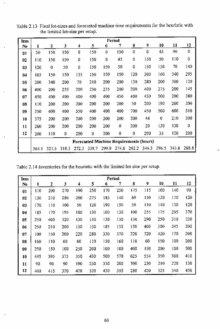
Table 2.13 Final lot-sizes and forecasted machine time requirements for the heuristic withthe limited lot-size per setup.

,- PeriodNo , , 3 4 5 6 7 8 9 " U D

"' SO 'SO ISO 0 'SO 0 'SO 0 0 45 90 002 no 'SO 'SO 0 'SO 0 45 0 ISO SO no 003 "0 0 so 0 ,so 'SO so 0 ISO ISO 70 "004 'OS ISO 'SO m ,so 'SO 'SO "" 300 '60 J40 29505 200 340 200 70 2" 200 200 "0 280 200 JOO 120

06 400 200 2JS 200 230 2JS 200 200 '"0 27> 200 '"07 450 400 400 400 400 400 450 400 450 500 200 28008 no 200 200 200 200 200 200 SO 200 '"0 200 20009 350 400 400 550 400 400 400 700 "0 500 600 "0

" J75 200 200 200 200 200 200 200 44 0 "" 200n 260 200 200 200 200 200 0 200 20 "" DO 0

" 200 no 0 200 0 200 0 0 200 35 DO 200Forecasted Machine Requirements (hours)

365.1 327.5 318.3 272.3 338.7 299.9 274.6 262,2 346.3 296.5 343.8 288,8

Table 2.14 Inventories for the heuristic with the limited lot-si7.e pcr setup,

,- PeriodNo , 2 3 4 5 6 7 , , " n ""' no 200 270 '90 250 "" 250 '" 115 '"0 '40 9002 DO "" 280 200 27> '"' '40 60 ISO "0 "0 """ no "0 '"0 so "0 '"0 ISO so "0 no DO ""04 '85 "0 '" ,SO DO '00 ISO '00 m '" 295 37005 250 400 "" DO "0 ISO 130 ISO 290 2SO "" 22006 250 "" 200 ISO ISO ,"5 '55 ISO 405 300 205 20007 '00 'SO 200 220 280 no no no no 420 no 20008 '60 ''" 60 60 no ISO '60 no 60 ISO '"0 20009 250 ISO '"0 250 200 ,"0 '"0 400 ISO 200 ,"0 SOO

'" 445 395 J75 350 430 500 570 625 554 350 360 4'"U 90 90 90 '"0 230 330 200 300 230 2," no DO

" 400 '" no 420 no 430 355 280 420 m 340 450

66

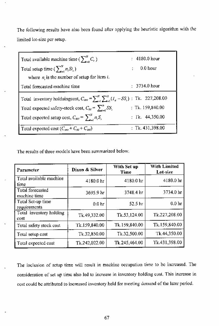
The following results have also been foum! after applying the heuristic algorithm with the

limited lot"size per setup.

Tornl available machine time (L' C,) 4!80.0 hour-,Tornl setup time (L:v niSI,) 0,0 hour.,

where n, is the number of setup for item i.

Total forecasted machine time 3734.0 hour

Tornl inventory hoJduingeost, c'm =L:,L:~,(1" -8S,) Tk. 227,208.00

Tornl expecteu ~arety-stoek cost, C"= :E" SS, Tk. 159,~40.00,.,,Total expected setup cost, C," = L.,n,S, rk. 44,350.00

Total expected cost (Cnv+ C,,+ CseI) Tk.431,398.00

The results of three models have been summarized bcJo\\!.

Parametcr Dixon & Silver With Set up With LimitedTime Lot siLc

Total available machine 41S0,Ohr 41S0,Ohr 41S0.0hrtimeTotal forecasted 3695.9 hr 374S.4 hr 3734.0 hrma~hine timeTotal Set-up time 0,0 hr 52.5 hr 0.0 hrrequirementsTotal inventory holding Tk.49,332.00 Tk.53,124.00 Tk.227,20S,00costTotal safety stock Co~l Tk.159,S40.00 Tic 159,840.00 Tk. I59,840.00

Tornl setup cost Tk.32,850.00 Tk.32,500.00 Tk.44,350.00

Tornl expected cosl Tk.242,022.00 Tk,245,464.00 Tk.43J,398.00

The inclusion of setup time \"ill re8uU in machine occupatiun lime to be increased. The

consideration of ~d up time also led to innease in inventory holding cllsL This increase in

cos! could be attributed to incre;l~ed inventory held for meeting ,knmnd of the later period,

67

Effect of the limitation on the lot-size is dependent on the extent of reduction of the lot-size,

]t is obvious that the smaller the allowable lot-sile, the greater will be the number of setup

which \~ill eventually lead to more splilled items. This in tum led to the increase number of

required setups.

Costs due to implementation of this restrictiun on lot-sile went up quite ~igni!icantly.

Further decrease in lot-size would obviously result in higher costs. But at the lower range of

allowable lot-size, there has been a trend ofsJight increase in setup costs.

2.6 Conclusions

Lot-sizing problem has been recognized to be one of most important functions in industrial

units. Thus efforts have been given to develop usable optimizing routines but within limited

boundary conditions. Various models have been developed with restricted applications in

real-life settings because of their demanding computatiunal enomlislty. Thus heuristic

models have been evolved. These heuristics have given feasible solutions, The Dixon-Silver

heuristic was used in the present work. The heuristic was extended to include two very

important parameters such as, (i) plant or machine set up time and (ii) maximum limit of

production lot-sizc from a machinc. From analysis amI results, the prescnt work has

demonstrated that J"easiblesolutions could be obtained with competitive computer usage.

The Te~ultsof the two heuristics developed in the present work, have been discussed lJl

Section 2.5.

68

Chapter 3Scheduling

3.1 Introduction

Operations schedules are shorHerm p!<lns designed to implement the lTIa>ter production

schedule. Operations scheduling focuses on how best to usc existing capacity, taking into

account technical production constraints. Often several jobs must be processed ul one or

more workstations, Typically, a variety of tasks can be performed at each workstation. If

schedules arc not carefully planned 10 avoid bottlenecks, waiting lines may develop. In

poorly scheduled job shops, it is not at all uncommon for jobs to wail for 95 percem of their

lotal production cycle. This rCSl.lltsin a long workllow cycle. A schedule is II timetable for

pcr/arming aClivilies, utilizing resources, or llllocaling facilities.

Most real-world scheduling problems arc naturally multi-criterion, However, due to the lack

of suitable solution techniques such problems are u~ually transfoillled into a single-

objective problem. A solution is called Panlo-oplimal if it is no! possible to decrease the

value of one objective without increasing the value of the other [34). The difficulty that

arises with this approach is the rise of a set of Pareto-optimal solutions, instead of a single

oplimum solution.

A Pareto-optimal solution is developed in this re,earch "ork for a scheduling problem on a

single machine with periodic maintenance and non-preemptive jobs. In literature, most of

the scheduling problems address only one objective function, while in the real world, such

problems are always associated wilh more than one objective. III this research work, both

multi-objective functions and mliiti-mainienance periods are considered for the machine

scheduling problem. To avoid the complexities involved in solving an explicit multi-

objective optimization problem, multiple objective Junctions arc consolidated and

transformed inlo a single objective function after they are weighted and assigned proper

weighting fadors. In addition, periodic maintenance schedules are also considered in the

model. The objective of the model addressed in this re,earch work is to minimize the

69

weighted function of lhe tolal job /low lime, lhe maximum tardiness, and the machine idle

time in a single machine problem with periodic maintenance and non-preemptive jobs. An

algorithm is dcveloped to solve this multiple criterion problem and to conslructlhe pareto-

sel. The parametric analysis of the trade-offs of all solutions with all possiblc weighted

combination of the eriterions is analyzed. The result of a neighborhood search heuristic is

also provided. Results are provided to explore thc best schedule among all the Pareto-

optimal sets and to compare the result of the modified Pareto-optimal algorithm with the

result of the neighborhood search heuristic.

3.2 Literature Study

Most real-world scheduling problems are naturally multi-criterion, However, due to the lack

of suitable solution techniques such problems are usually lransformed into a single-

objective problem, A solution is called Parelo-oplimal if il is not possible to decrease lhe

value of one objective without increasing the value of the other [34]. The difficulty that

arises with this approach is the risc of a set of Pareto-optimal solutions, instead of a single

optimum solution.

There are several approaches that deal with the multi-objective problem" Traditionally, the

most common way is to combine the multiple eriterions into a single scalar value by using

weighted aggregating functions according to the preferences sel by the scheduler (or

decision-makers) and then to find a compromise solution tbat rellects these preferences

135J. However, in many real scenarios involving multi-criterion scheduling problems, it isprefcrable to present a set of promising solutions to the decision-makers so that the most

adequate schedule can be chosen. This has increased the interest in investigating the

applicatiun of Parelo-optimization techniques to multi-criterion scheduling problems. The

aim in Pareto-oplimization is 10 find a set of compromised solutions that represent a good

upproximution to the Pareto-optimality [34]. In recent yeur:;, ~everal algorithms proposed

for Pareto-optimizalion have been published becuuse multi-objective optimization problems

70

exist in almost any domain [36, 37]. The job shop scheduling problem OSP) with a single

objective is a widely researched problem in the area of production scheduling. In ajob shop,

several jobs require scheduling, each with different processing times on different machines.

Man} appliclltions of JSPs in industry have been discussed in the literature. Operlltions

research practitioner.:;, production management experts, management scientists,

mathematicians and computer scientists have discussed the scheduling theory. The solution

procedure for solving the JSP differ.:;as the objective of the scheduling differs. Most of the

researchers concerning the job shop scheduling problem have focused on developing

scheduling algorithms for a single objective measure. Much work has been done to solve

lSI's by using single objective metu-heLiristic procedures like simulated annellling

lllgorithm, genetic algorithm and 1llbLisellrch lllgorithm. These algorithms arc generic

optimization algorithms, i.e. 1hey arc in1ended for use on II wide range of optimization

problems [38]. Thc real-world scheduling problems arc mnhi-objective in nature. In such

cases, sevewl objectives are considercd simultaneonsly when a schedule is generated.

Simuhancous consideration of several objectives during scheduling totally modifies the

scheduling approach. A scheduler who improves the schedule with re~pect to one objective

may want to know how the schedule performs with respect to the other objeetive~.Thus the

goal is 10generate a tCasiblc schcdLllclhal minimizes severlll objectives. This schedule is

called u Pareto optimal solution. A single feasible schedule lhat minimizes several

objectives may not exist. In other words, individual optimal solutions of each objective are

usually different. Under such situations, the scheduler may be interested in having a

schedule with weighted combinalion of several sehcduling objectives llS the performance

measure. It is possible thaI the weights of various objeelives llre known beforc scheduling.

This approach [38] permits computing of a unique strict Parcto optimal solution. It is also

possible that the decision maker wants to choose a Pareto optimal solLitionllccording to the

priorities existing at the time of decision making. In that case, II family of best trade-off

schedules called the Pareto optimal set is to be found. The sel of Pareto solutions is called

the Pareto jronl. Therefore solving a multi-objective scheduling problem is a Parcto

optimization problem. Generating the Pareto optimal sel for the scheduling problem can be

71

computationally expen~ive and is oftcn infeasible,' because of the complexity of the

scheduling problem [38]. Moreover, when meta-heuri~tics are used, thcrc is no guarantee

that the Pareto set for a givcn multi-objective optimization problem like multi-<Jbjectivc

scheduling can be gcnerated. However, a set of non-dominated solutions can be generated

elose to the Pareto optimal set [38J. Many real-world optimization problems involve

multiple (and often conflicting) objectives. These problems are relevant in a variety of

engineering disciplines, scientific fields, and various industrial applications. Unlike single

objective optimization problems, where one attempts to find the best solution (global

optimum), in multi objedive optimization problems, there may not exist one solution that

corresponds to the best with respect to all objectives. Solving a multi-objective optimization

problem consists of generating the Pareto fronticr, the set of non-dominated s<Jlutionsthat

represents the tmde-off among the objective function values. Different approaches are used

to approximate and generate such sets of Pareto optimal solutions. S<Jmeinteractive

approaches incorporate preferences into the optimization procedurc to explore a specillc

region of thc solution space, whilc other approaches focus on generating diverse sets of

Pareto optimal solutions. Sl.Ichsets of Pareto optimal solutions can be extremely large.

which motivates the need for post-optimality analysis for multi objective optimiwtion

problems. The area of post_optimality analysis addressed in this paper focu~e~on obtaining

a preferred subset of solutions from a very large set of solutions with acceptable objective

function value~.The goal in obtaining large sets ofP"reto optimal solutions is to provide the

decision-maker with a diver~e set of such solutions. Although obtaining diverse Pareto

optimal s<Jlutions is important, it is often impractical for a human decision-maker to

manually examine each such solution, and henee, efficiently identify a good subset of such

solutions. Previous research in this area has focused on generalizing the representation of

the full set of Pareto optimal solutions with a smaller subset [39J. Such procedures are not

post-optimality analysis procedures, but rather, extensions to multi-objective optimization

procedures, whieh are designed to genemte diverse set.sof Pareto optimal "olutions, Another

area of tesearch that incorporates preferences into the optimization pwceul.lres arc

interactive methods. These interactive methods provide a decision-maker WIthbetter control

72•

over the optimization process, allowing them to explllre specili~ regions of the search space.

However, solutions obtained are quite sensitive towards the preference~ of the deci~illn-

maker. These approaches also require the decision-maker to have a thorough knowledge of

thc problem. 111is paper [39] analyzes a discrete optimization problem fonnulation for

obtaining a preferred sl.lbset of Pareto optimal soIl.ltions from a larger set. This formulation

alleviates the 3en,itivity of value function approaches, while obtaining a de,ired ,ize subset of

Pareto optimal solutions [39]. In recent years, several variations of multi objective

evolutionary algorithms (MOEAs) [40] have been developed to handle MOPs [35]' Many of

the suggested MOEAs have been employed in a variety of real-world applications [40J.

These next generation algorithms have been improved in three dimensions compared to the

previous generation of MOEAs introduced inlhe 1990's, which inelude the first (original)

~e~ion of the nlln dllminaled sllrting genetic algorithm (NSGA) of Srinivas and Deb

(1994), the niched Pareto genetic algoritlun (NPGA) ofNafploitis et aJ. (1994) and the multi

objective genetic algorithm (MOGA) of Fonseca and Flemming (1993). First, the

computational complexity of Ihe existing MOEAs has been reduced from O(mN3) of the

first generation 10 O(mlv2) of the second generation so that solving larger-sized problems is

not as cllmputationaUy burdensome. [40]. The m and N arc the number of objectives and the

population size, respectively. Second, some degree of elitism is incorporated in most

MOEAs to ensure the propagation of good non dominated solutions for faster convergence.

In cxpensi~c MOPs, ra~l convergence lowards Pareto optimal solutions is a highly desired

fealllre of any promising algorithm. Third, new diversification strategies that are insensitive

to the selection of the sharing factor have been employed. Given the variations of MOEAs,

the idea of using dynamic population sizing has not been thoroughly investigated, and to

date only a few studies have explored thi~ idea. For example, Tan et al. (2001) introduced

an increment in MOEA lhat uses dynamic population sizing based on the online discovered

Pareto front and lis desired population distribution density [40]. 1n another study, Shen and

Daskin (2005) suggest a MOEA-based heuristic approach for finding tradcoffs between

customer service and cost in an integrated supply chain design using a dynamic population

si/jng scheme. However, they do not address how the growing population size is controlled.

73

The related work of Farina et al. (2004) addresses dynami~ MOPs, where the optimization

is time-dependent and the objective functions, the constraints and/or (he parameters of the

problem, nol the MOEA, vary with lime (Le., at each iteration oflhe optimi'l-ution process).

In this study [40J, considering slatic MOPs, where optimization using FPGA is performed

omine, and the chara~teristics of lhe MOP are not lime-dependent. The majority of

evolutionary multi objective optimization (EMO) sludies that propose new MOEAs lur

solving MOPs evaluate the performance of those algorithms over a large number oI

generations (or solution evaluations). However, there is now a growing need for designing

MOEAs capable of dealing wilh computationally- and/or Jinan~ial1y-expensiveMOPs. Lillie

work exists that considers expensive MOPs. Additionally, many real-world problems

involve ~omplicated, "bla~k-box" objective fun~tions that ~an make a large number of

solutions evaluations compulationally prohibiti"e [40J. Furthermore, repeatedly evaluating

such complicated objective functions can be demanding on resources. Specifically, the

motivation comes rrom simLilation-based optimization resear~h. Cumputer simulation of

real-world systems tends to involve the constmetion of complicated models that capture the

complex, nonlinear inlerre!ation~hips between independent and dependent variables and can

report the value of several system performance objectives simultaneously. These models

[40] are used to evaluale candidate system design solulions in ,carch oIthe best soluliun (or

set of solutions) according to several performance objectives.

A multi-objective optimization algorithm capable of rapidly finding a diverse set of Pareto

optimal solutions would be greatly bene/leial in such a situalion. The purpose of this

research is to propose a multi-objective optimization mdhodology that finds evenly-

distributed Pareto optimal solutions in a computationally-efficient manner. ln addition to

multiple objectives, periodic maintenance is also considered for this scheduling problem.

An unexpected breakdown will make the ~bop bebavior hard to predict, and thereby will

rcduce the efficiency ur the production system. Maintenance can reduce the breakdown rate

with minor sacrifices in production [411.

74

In literature, there are several approaches for handling multi-critcrion problems. Branch and

Bound teehniquc is one of those approaches that could obtain a better solution for such

problems. Branch and bound teehniquc explorcs all the possible enumeralions 10 lind the

best sequence wilh minimum v"lue in O(2")timc complexity [42]. Liao and Chen [41]

address minimizing the maximum (;jrdine~s of Jobs in a periodically maintained single

machine problem. A branch and bound algorithm is dcvelopcd to find the optimal solution,

and a heuristic solution is also devised for handling the large problem. The larger is the

neighborhood, the bettcr is the quality of the locally optimal solutions, and lhe greater i~the

accuracy of the final solution. At the same time, se"rching brger neighborhoods requires

more time "t each ~lage. Because of many runs of a neighborhood search algorithm, longer

execulion limes per run le"d to !ewer tlLllS wilhin a specified time. For this reason, a larger

neighborhood can produce a more effective heuristic algorithm only if the larger

neighborhood can be searched in a very efficient manner. A survey of large-scale

neighborhood search algorithms can be found in Ahuja [43J. For the single-machine

problem, Adiri [44] assumes two cases of a breakdown, that is, the resumable and non-

resumable cases "ssuming that machine idle time is unknown and 1;,l1owa probabilbtic

distribution pattern. Mosheiov [45] solves the minimizalion of total completion time for

two-p"r••l1el-machine-schedliling problem by assuming each machine is available in a

specified imcrval. Lee [46] also studies in this are" for olher m"chine configurations

including single and parallcl machines.

Problem of schcduling on a single machine to minimize total weighted tardiness of jobs can

be described as follows: thcrc arc n jobs to be processed, each job has an integer processing

time, " weight and" due d"le. The objeclive is to minimi7e lhe 101,,1\\cighted lardiness of

jobs. The problem belongs to the class of NP-hard problems. Some new propertie~ of the

problem associated with the blocks have been presenled and discu~sed. These properties

"How any to propose a new fast local search procedure based on a .1abu search approach

with a specific neighborhood which emplo)'s blocks of jobs and a compound moves

technique. A compound move consi~15in performing several moves 8;mullaneously in a

75

single iteration of algorithm and allows any to accelerate the convergence to good solutions.

In the algorithm [47], an idea has been used which decreases the complexity for the search

of neighborhood from O(n3) to O(n2). Additionally, the neighborhood is reduced by using

some elimination criteria. The method presentcd in this paper [47J i, deterministic one and

has not any random elemcnt, as distinct from other effective but non-determini,tic methods

proposed for thi, problem, such as Tabu scareh of Crauwels, H. A. J" Potts, C. N., & Van

Wassenhove, L. N. (1998) Computational e.~periments on thc benchmark im;tances from

OR-Library (http://pcoplc.brunel.ac.ukl mastjjb/jeb/info.html) are presented and compared

with the results yielded by the best algorithms discussed in the literature. The,e re,ults show

that the algorithm proposed allows us to obtain the best known results for the benchmarks in

a short time. The presented properties and ideas can be apphed in any local search

procedures [47]'

In many manufacturing systems, jobs that are completed early are held as Iinished-

goods inventory until their duc-dates, and hence one incurs earliness costs, Similarly, jobs

that arc completed aller their due-dates incur penalty. The objective in such situations

would, therefore, be to meet the due-dates of the respective johs as c1o,ely as possible, and

consequently minimize the sum of earliness and tardiness of jobs because earliness and

tardiness of jobs gre"tly influence the perfonnance of a schedule with respect to cost. In

addition, a job incun; holding cost from the time of its arrival unul its completion. Most

studies on scheduling in such manufacturing systems assume unit earliness cost, unit

tardiness cost and unit holding eo,t of a job. llowever, in reality such an a<;sumptionneed

not always hold und it is quite possible that there exist different costs of earliness, tardiness

and holding for different jobs. In addition, most studies onjob-shop scheduling ussume lhat

jobs are independcnt and that no assembly operations exist. The study [48] addres~es th~

problem of schcduling in dynamic ",,"semblyjob-shop, (i.e. shops that manuf"cture multi-

level jobs) ",ith the consideration of jobs having di[r~r~nt earliness, tardines, and holding

costs. An attempt is made in this paper to present dispatching rules by incorporating the

relatiVecosts of carliness, tardiness and holding of jobs in the form of scalar weights. In the

76•

first ph<lseof the study, relative costs (ur weights for) earliness and tardiness of jobs are

considered, and the dispatching rules are presented in order to minimize the sum of

weighted earliness and weighted tardiness of jobs. In the second phase of the study, the

objective considered is the minimization of the sum of weighted earliness, weighted

tardiness and weighted flow time of jobs, and the disp<ltching rules are presented by

incorporating the rdative costs of earliness, tardiness and flow lime of jobs. Simulation

studies have been conducted separately for both phases of the current sllldy, the

perfonnanee of the scheduling rules h<lvebeen observed independently, aml!he results of

the simulation study have been reported. The proposed rules are found to be elTective In

minimizing the mean and maximum values of the measures of performance [48J.

This paper [49] studies two models of two-stage processing with flow shop at the lirst stage

followed by open shop at the second st<lge.Thc first model involves multiple m<lchinesat

the first stage and two machines at the second stage, and the other involves multiple

machines at both stages. In both models, the objective is to minimize the makespan_This

problem is NP-complete, for which an efficient hellristie solution algorithm is eonstrneted

and its worst-case perfonnance guarantee is analyzed for both models. An integer

programming model and a branch and bound algorithm arc proposed for model I and a

lower bound is developed for model 2 as benchmarks for the heuristic ulgurithms.

Computational experiences show that the heuristic algorithms consistently generate good

schedule and the branch and bound algorithm is much efficient than the integer-

programming modeL

This rescarch [50] presents an interesting scheduling problem common to freight

consolidation tcnninals. This previously unstudied problem involves scheduling a set of

inbound trailers to a fixed number of unload docks. The objective is to schedule the trailers

to the unload docks to minimize the time span of the transfer operation. This study focuses

on freight consolidation tenninals in the parcel delivery industry. A simulation-bascd

scheduling algoritlun that uses a gcnetic algorithm to drive the search for new solutions is

proposed. In addition to the introduction and discussion of thc parcel hub "~hedu1ing

77

problem, the contribution of this rescarch is an approach that serves as the initial effort to

solve this pradical problem.

This work [51] presents the development and implementation of a production scheduling

system lor an electrical appliance manufacturer. Based on recent advances in optimization-

based scheduling approaches, two diiTerent software architedures based on two (.hiferent

scheduling formulation>, namely the RTN and the STN, are proposed to integrate

infonnation available in the different production units and stages with formal algorithmic

tools. Optimization re,ults indicate that sigmJicant eeonomie beneJib can be achieved (e.g.

minimization of total operating costs) while ensuring full customer satisfaction a.>opposed

to normal pradiees followed in the company relying on human expertise. The \~ork

indicates that it is possible to solve real-life manufacturing problems using oplimi/ation-

based approaches but the integration of information in a timely fashion seems to be a major

factor in successfully implementing the system and fully realizing its benefits,

The paper [52] deals with the problem of finding a job sequence that minimizes the

make,pan in m-maehine flow shops under the no-idle condition. This condition requires that

each machine must process jobs without any interruption from the start of processing the

IIrst job to the completion of processing the last jub. Since the problem is NP-hard, we

propose a constructive heuristic for solving it that significantly outperforms heuristics

knO\~11so far.

This paper [531considers the n-job, In-machinepennutalion tlow shop with the objective of

minimizing the mean flow time. Initial seqncnces that are slruclured to enhancc the

performanec of local search techniques arc construcled from jub rankings delivcred by a

trained nenral network. Thc network's training is done by using data collected from optimal

sequcnccs obtained from solved examples or l10w shop problcms. Once traincd, the nenral

network provides rankable measurcs that can be used to construct a sequence in which jobs

are located as elose as possible to the positions they would occupy in an optimal sequenec.

The contribution of these 'nenral' sequences in improving the perfonnanec of some

common local search tcehniqncs, such as adjaecnt pairwise interchange and Tabu search is

"

examined. Tests using initial sequences generated by different heuristics show that the

sequenecs suggested by the neural networks are more effective in directing neighborhood

search methods to lower local optima.

This paper [54] deals with the production and preventive maintenance control problem lor a

muhiple-machine manufacturing sy5tem, The objective of such a problem is to find the

production and preventive maintenance rates for the machines so as to minimize thc total

cost of invcntoryibaeklog, repair and preventive maintenance. A two-level hierarchical

control model is presented, and the structure of the control policy for both identical and

non-identical manufacturing syslem~is described using parameters, refen-ed to here as input

jaclOrs. By combining analytical formalism with simulation-based statistical tools stleh as

experimental design and respon~e surface methodology, an approximation of the optimal

control policies and values or inptlt factors are determined. The restllts obtained extend

those available in existing literature to cover non-identical machinc mallulilcturing systems.

A ntlmerical example and a sensitivity analysis are presented in order to illustratc the

robtlstness of the proposed approach. The extension of the propo~ed prodClction and

preventive maintenance policies to cover large systems (multiple machines, multiple

prodClct~)l~diseClssed..

This paper [55] deals "ith the problem of selecting and schcduling the orders to be

processed by a manufacttlring plant for immediate delivery to thc customer site. Among the

constraints to be con~idered are the limited production capacity, the available number of

vehicles and the time windows within which orders must be served, At first the problem has

been described as it ocetlC>;in practiee in some indtlstrial envirolillients, and then has been

presented an integer programming model that maximizes rhe profit dtle to the customer

orders to be processed. A Tabu ~earch-based solution proeedme to solve this problem is

developed and tested cmpirically with randomly generated problems. Comparisons with an

exact procedure show that the method finds very good-quality soltltions with small

comptltatioll re'ltlirements,

79

The genclie algorithm ''lth search area udaptalion (GSA) has a capacity for adapting to the

structure of solution space and controlling the tradeoff balanec between global and local

searches, even if one docs not adju>t the parameters of the genctic algorithm (0 A), such as

crossover and/or mutation rates [56]. But, GSA needs thc crossover operator that has ability

for characteristic inheritancc ratio control. In this paper, the modificd genetic algorithm has

bcen proposed with scarch area adaptation (mGSA) for solving the Job-shop schcduling

problem (JSP). Unlikc GSA, the proposed method does not need such a cro~~\lveroperator.

To show the effectiveness of the proposed method, numerical experiment~ have been

conducted by using two benchmark problems. It is shown that this method has belter

performance than existing Gas [56].

The effectiveness of the solution method based on simulated annealing (SA) mainly

depends on how 10 determine the SA-related parameters, A ~eheme as well as paramcler

vallies for defining all annealing schedule ShOlildbe appropriately determined, sillce various

schemes and their cOITe~pondingparameter values have a significanl impact on the

performance of SA algorithms, In this paper [57], based on robu~lJe5ign a new annealing

parameter design method has been proposed for the mixed-model sequencing problem

which is known to be NP-hard. To show the effectiveness of the proposed methud,

extensive eompul<ltiun~xperiments are conducted. lt was found that the robust designed

method uutperforms the SA algurithm.

One of the basic and significant problems [58], that a shup or a factory manager' is

encountered, is a suitable scheduling and sequencing of jubs on machines. One lype of

sehednJing problem is job shop schedliling. There arc different machines in a shop of which

ajob may reqnire some or all thcse machines in some specific sequence. For solving this

problem, the objective may be to minimize the makespan. After optimizing the makespan,

the Jobs sequencing mu~tbe carried om for each machine. The above problem can be solved

by a number of different method~ ~lLchas branch and bound, cutting plane, heuristic

methods, etc. In recent years, re5earehes have used genetic algorithms, simulated annealing,

and machine learning methods for solving sl.lchproblems. In this papcr, a simulatiull model

80

is presented to work out job shop scheduling problems with the objective of minimizing

makcspan. The model has been coded by Visual SLAM which is a special simulation

langtmge. The struc!ure of this language is based on the network modeling. After modeling

the scheduling problem, the model is verified and validated. Then the computational results

are presented and eomp"red with other result, reported in the literature. Finally, the model

outPllt is analyzed.

This paper [59J considers thc problem of scheduling part families and jobs withm each part

family in a flow shop manufacturing cell with sequence dependent family setups times

where it is desired to minimizc the makespan while processing parts (jobs) in each family

togdher. Two evolutionary algoritluns - a Genetic Algoritlun and a Mcmetie Algorithm

with local ,earch _ are proposed and empirically evalllated as to their effectiveness in

finding optimal permutation schedules. The proposed algorithms u~e a compact

representation for the solution and a hierarchically structured population where the number

of possible neighborhoods is limited by dividing the population into clusters. In comparison

to a Multi-Start procedure, solutions obtained by the propo~ed evolutionary algorithms were

vcry close to the lower bounds for all problem instances. Moreover, the comparison against

the previous best algorithm, a heuristic named CMD, indicated a considerable performance

improvement.

This paper [60) studies the single machine scheduling problem for the objective of

minimizing the expected number of tardy jobs. Jobs have normally distributed processing

times and a common detemlinistic due date. A llew approach has becn developed lor this

problem that generate ncar optimal solutions. lbe original stochastic problem is

transformed into a non-linear integer programming model and its relaxations.

Computational study 'validatestheir effectiveness by comparison with optimal sollltions.

This paper [61) considers the evaluation of the WOllit-caseperformance ratio between rhe

best solution of the flow shop problem and the permutation flow shop with time delays

considerations. It is observcd that, even in the restricted case of two machines and unit

execution time operations, the two models may generate different optimal values for the

81•

makespan. Morc spccifically, it is shown that, in the two-machine case, the !X'rfonnance

ratio between the bcst pcrmutation schedule and the best flow shop schedule is bounded by

2. When the operations of the n jobs arc restricted to be unit exceution time, this ratio is

reduced to (2 - (3//1 + 2) for the two-machine case, and is m for the nt-machine case.

In this paper [62], filtcrcd and recovering beam search algorithms for the single machine

earliness/tardiness scheduling problem with no idle time has been pre~ented and compared

them with existing neighborhood scarch and dispatch rule heuristics, Fillering procedures

using both priority evaluation functions and problem-specific properties have been

considered. The computational results show that the reeovcring beam scarch algorithms

out!X'rfonn their filtered counterparts, while thc priority-based filtering procedure proves

superior to the rules-based alternative. The best solutions are given by the neighborhood

search algorithm, but this procedure is computationally intensive and ean only be applied to

small or medium size instances. The rec<nering beam search heuristic provides results that

arc close in solution quality and is significantly faster, Sll it can be used to solve even large

problems.

Scheduling for the flexible job-shop [63J is very important in both fields of production

management and combinatorial optimization, However, it is quite difficult to achieve an

optimal solution to this problem with traditional optimization approaehcs owing to tbc high

compulalional complexity. Tbc combining of sevcral optimization criteria induces

additional complcxity and new problems. Particle swam] optimi7..ation is an evolulionary

computation technique mimicking the behavior of flying birds and their means of

information exchange. It combines local search (by sell' experience) and global scarch (by

neighboring expericnee), possessing high search efiiciency. Simulated annealing (SA) us a

local search algorithm employs ccrtain probability to avoid becoming trapped in a local

optimum and has been proved 10 be effective for a variety of situations, includiug

scheduling and sequencing. By reasonably hybridi>:ing the~c two methodologies, an easily

implemented hybrid approach for the multi-objective flexible job-shop scheduling problem

(FJSP) has been developed. The results oblained from the computational study have ~hOWTl

82

that the propo~ed algorithm is a viable and effective approach for the multi-objective FJSP,

especially for problems on a large scale.

In this study, a modified Pareto-optimal algorithm (determining the trade-offs between total

completion time and maximum lateness) is developed for the multi-criterion sehcduling

problem with periodic maintenance. The ~pecific problem eonsidercd in this paper is tIl

minimize flow time, maximum lateness and machine idle time. Thesc multiple objectives

arc transformed into a single objective function, cost function, by using an aggregate

weighted sum method, All possible weight combinations are calculated for each sequence of

Pareto-optimal set to present different level of importance of each objcctive. On the other

hand, to generate various sets of Pareto-optimal sequences from different maintenance

plans, dilferent values for both time interval between two maintenance periods and amount

of time to perrow maintenance are compl.ltedfor the same instance. Various maintenance

plans give more flexibility to the scheduler (or decision-makcr) to make a decision

according; to both his preferences and maintenance necessity/availability. A neighborhood

search heuristic is also applied to the same instance in order to compare it with the modified

algorithm.

3.3 Problem Description

There arc n independent non-preemptive jobs, that is, once a job is started it must be

completed to process them on a single machine without interruption, Each job j becomes

available for processing at ready time zero and has a due dated,. At every Tunit of time,

the machine is seized to hold for maintenancc, A numbcr of jobs that are grouped together

to fit in every T amount of time is a balch. Therc could be machine idle timc, I". before the

maintenance starts alter the last job in a batch ;5 completed. The maintenance period is AI

which is also a fixed time. The total machine idle time is ob1.<linedby adding the idle tim~ of

all the batches.

The algorithm presented here for the problem combines all the criterions togcther in one

schedule. The new approach starts with an initially obtained set of Pareto-optimal schedule

83

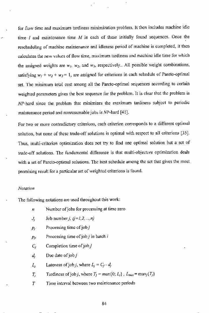
for !low timc and maximum tardiness minimization problem. It thcn includes machine idle

time I and maintcnance time ,11 in each of these initially found ~equenccs. Once the

rescheduling of machine maintenance and idleness period of machine is completed, it then

calculates the new values of flow time, maximum tardiness und maehinc idle time for which

the as~igned weights are WI, W}, and 11'3, respectively .. All possible weight combinations,

satisfying WI+ W)+ U'J= I, are assigned for eriterions in each schedule of Pareto-optimal

set. The minimum lolal cost among all the Pareto-optimal sequences according to certain

weighted parameters gives the bcst sequence for the problem. It is clear that thc problem is

NP-hard sincc the problem that minimize~ the maximum tardines~ subjcet to periodic

maintenance period and nonrcsumable job~ is lV"P-hard[41].

For two or more contradictory criterions, cach criterion corre~ponds to a different optimal

solution, but none of thcsc trade-off solutions is optimal \\'ith respect to all eriterions [35]'

Thus, multi-criterion optimization docs not try to find one optimal solution bl.lt a set of

trade-off solutions. The fundamental difference is that multi-objectIve optimization deals

with a ~el of Pareto-optimal solutions. Thc bcst schedole among thc sct that gives the most

promising result for a particular set of weighted eriteriol1s is found.

NOlalion

Thc following notations arc uscd throughout this work:

n Number of jobs for processing at timc zero

~ Job numberj. (j=1,2, ".,nj

P! Processing timc of job j

PjI Processing lime of job j in balch j

C~ Completion time ofjobj

4 Due date ofjobj

Ij Lateness of job j, where Ij = Cj - dj

T, T<lrdincss of job j, \'ihere "0 = max{O; I,} , Imax= m<lxj{ 7J}

T Time interval bctween two maintenance periods

84

M Amount of time to perform one maintenance

Ib, Machine idle time in batch i, (i= 1,2, .. , r)

I Total machine idle time ofa schedule

Tb, Total processing time for scheduled jobs in batch i, (i= I, 2, ... ,r)

m Heration number.

3.4 Pareto.Optimal Algorithm

When there are multiple objectives, the concept of Pareto-optimality plays a role in

scheduling. A schedule is Pareto-optimal if it is impossible to improve on one of the

objectives without making at least one other objective worse. The scheduler may want to

view a set of Pareto-optimal schedules before deciding which schedllie to select, when there

are multiple objectives. ln this paper, the algorithm of determining trade-oITsbetween total

completion time and maximum latenesg, initially proposed by Pinedo [34J, is modified and

extended, which includes periodic maintenance, In addition to the total completion time and

the maximum lateness, the machine idle time is also considered as the third objective. A set

of Pareto-optimal schedules represent the trade-offs between total completion time,

maximum latenes~and machine idle time.

There are many ~equeneing rules thnt can be apphcd to the jobs tluough the machines

in a job shop according to the preferences. Two of those basic seqllencing rules, shortest

processing time (SPI) und e"r1ie~1due date (EDD) "re adapted in th~ modified Parcto-

optimal algorithm. For explanatory convenience, we define two term~thaI arc needed in the

"lgorithm. The machine idle time of" batch, Ib" is defined as the time by subtnlcting the

total processing time for scheduled jobs in a batch, hi, from thc time interval between two

maintenance periods T (i.e., Ib, = T - Tbi). The toM machine idle time of a schedule, J, isdelined by summing all machine idle time of all batchcs (i.e., I = I:=, Ib, ).

Pareto-optimal algorithm determines the trade-offs between lolal completion time and

maximum latencss only a~inilially prescnted by Pinedo [34]. A third objective, machine

85

idle time, is added and the stated algorithm is modified and extended accordingly. T11estep,

of the modified Pareto-optimal algorithm are outlined as follows:

Algorithm 1: M()dified Pareto-Optimal AIg()rilhm

Step 1. Setm ~ I (number of iteralion)

a) Schedule the jobs by SPT rule and apply EDD rule to the jobs with same

processing time as schedule SSPTiJWD

b) Compute Lmax(SPTIEDD)

c) Go to Step ~ to find machine idle time in the schedule SSn'WD and the revised

SSPT/EDD is now called S'SNIEDD when maintenance time is included.

Step 2. Sci m = 2

a) First schedule the jobs by EDD rule, and apply SPT rule to the jobs with same

due date, as schedule SEDDISPT

b) Compute LmaJEDDISPlJ

c) Go to Step ~ to find machine idle time in the schedule SWDSPT and, on

inclusion of maintenance time the revised SWD'Srr is called S'£DDISN'

Step 3.lteration m = 3.

Set L<p,,,= L,o", (t;UD) and :I, = d I + Lrn,,'Step 4. Set k = n, J" '" {l,...,n}, r = 2::;=1 PJ and <:i = r.

Step 5.Find j'in J'such that- -d,. ::::r, andp,.:::: p, for alljubs fin J' such that d,:::: f,

Put job j' in position k of the sequence.

Step 6.lfthere is no job £ such that d, < rand p, > P", go to Step 7.

Otherwise lind j" such that r - dJ•• = min(r - d,)

For all e such that d, < rand p, > PI" Set 0" = r - d,._.

Ifo-' < 0, theno = (r.

Step7,Selk<- k-l,and r •... '_P)'. Update the set as J' =J' - /.

Ir k:::: I go to Step 5.

86

,Step 8. Generate a batch by grouping a sctofjobs such that LPj :::: T

1=1

Repeal grouping of the rcmainingjobs to form other batches.

Sel b, = number ofbalchcs in one schedule, wheT~ i = 1, 2, __.r.,

Find machine idle time for one batch I"~= T - LP I'

}= I

,['ind machine idle time for one schedule, J = L:I",

,,,,

Revise the sch~dule by adding the amount of time to perform maintenance, M,

10the end of each batch.

Compute ," C:, J:""" and t'.L..J-I '

Step 9. Set L,"", = Lm" + O.- -IrLm,,:S; Lm,,(SPT! EDD) , sctm = m + 1, dJ = d, +0, and go to Step 4,

Otherwise STOP,

In Step 1, the algorithm starts with sequencing the jobs in SI'T order. If two jobs have the

same prucessing time, the job with smaller due date is placed earlier. Then !"""x(SPTinDD)

is calculated for this generated SPT/EDD schedule. This L",,,,,(Sf'T/1'-DD) value indieates

when to stop the iterations in lhe algorithm. For the schedule of SPT/EDD (SIif)JWV),"

batches are generated by grouping sets of jobs according toLP, s: T .J~'

The first Pareto-optimal schedule (S'sn;wD) is obwined after adding lhc maintenance time

to the generated batches in SSf'T/EDD. The second Pareto-optimal schedule (S' wD'srr) is

obtained in Step 2 which is similar to Step I. The only difference is that instead of starting

with srT order, the procedure slarb with EDD order and follows the same idea as in Step 1.

In Step 3, dlle dales 01"the jobs arc increased by Lm",,(.tDDISl'1) for the next iteration. Step

4 caleulates the total processing time for n jobs and assigns that v~lue loS. Step 5 generates

a Pareto-optimal schedule that minimizes "" C, in which job k is scheduled last, if ~ndL..,_, ,only if

,(i)d,:?:LP),

r' ,(ii) p, ~ p, for all jobs fin J' such that d, ;::LP,.

,~I

87

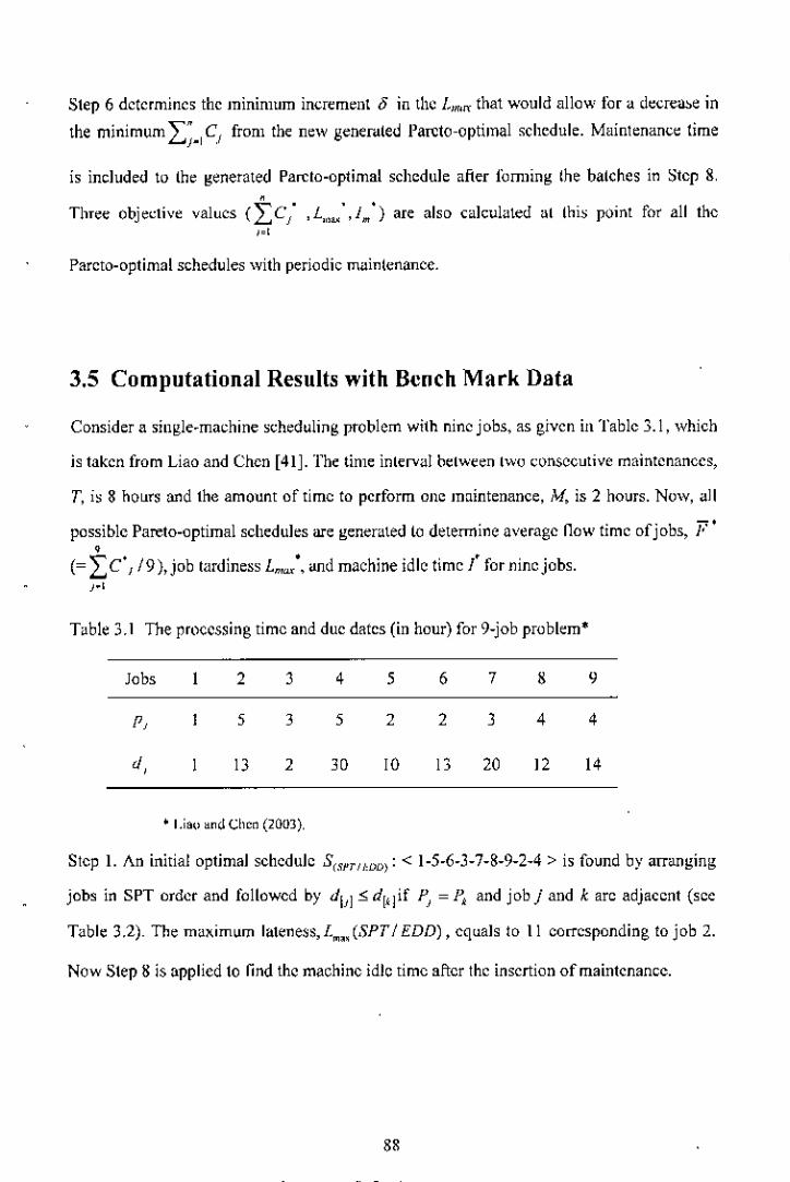
Step 6 determines the minimum increment J in the Lm'IT that would allow for a decrea.>e in

the minimum ," C, from the new genenlled Pareto-optimal schedule. Maintenance limeL..J-I .'

is included to (he generated Pardo-optimal schedule after fOffiling (he batches in Step 8,,

Three objedive values (L Cj" ,L,,,,..:, 1,,') are also ealcubted al (hi~ point for all the,~t

Parcto-optimalschedules with periodic maintenance.

3,5 Computational Results with Bench Mark Data

Consider a single.machine scheduling problem with nine jobs, as given in Table 3.1, which

is taken from Liao and Chen [41]' The time inlerval belween lwo consecutive maintenances,

T, i~8 hours ill1dthe amount of lime to perform one maintenance, M, is 2 hours. Now, all

possible Pareto-optimal schedules are generated to determine average flow time of jobs, F"•

(=L:c'J 19 ),job tardiness Lmax', and machine idlc timc l for ninc jobs.,.,Table 3.1 The processing time and due datcs (in hour) for 9-job problem*

Jobs

d,

1 2

5

13

3

3

2

4

5

30

5

2

10

6

2

13

7

3

20

8

4

12

9

4

14

• I.i,,, and Chon (2003),

Step 1. An initial optimal schedule S(SPrttDD): < 1-5-6-3-7-8-9-2-4 > is found by arranging

jobs in SPT order and followed by dill'" d1qif PJ= P, and job j and k arc adjacent (see

Table 3.2). The maximl.lrn lateness, L~" (8PT 1EDD) , eqllals to 11 corresponding to job 2.

Now Step 8 is applied to find the machine idle time aftcr thc insertion of rnaintena nee.

88

Table 3_2 Pareto-optimal schedule, S(SPTiWO)

Jobs 1 5 6 3 7 8 9 2 4

P, 1 2 2 3 3 4 4 5 5

d, 1 10 13 2 20 12 14 13 30

C, 3 5 8 11 15 19 24 29

L, 6 3 5 11

Step 8. A maintenance of 2 hours is inserted into the optimal schedule of Step I every 8

hours as shown in Table 3. Thus from the table, L,"",'(Sl'T! EDD) = 22, ICJ' = 1 + 3 + 5

+ 8 + 13 + 17 + 24 -+ 35 +45 = 151and ]*= 0 + 1 + 4 + 3 = 8 for the Iirst Pareto-optimal

s~hedule S'(.'PIIWI>I: < 1-5-6-3-7-~-9-2-4 >. Another possible Parelo-s~hedulc is now

sought in Step 2.

Table 3.3 Revised schedule S(:,."U-DIJ) by inserting mainlenan~e and idle limes

Jobs 5 6 3 I., M, 7 8 I" M, 9 I., M, 2 1M 1"1, 4

P, 2 2 3 Q 2 3 4 ! 2 4 4 2 5 , 2 5

d, I 10 13 2 20 12 14 13 30

C~

8 IO~ 18 20828 30 G 38 40 G,

I, 6 5 10 22 15

Step 2. Now instead of finding S'SI'I'I.'iJfJ)' another schedul~ ,S(EM \.1'1)' is obtained by Jlrst

applying EDD rule followed by SrT for the jobs with same due dates (not the ~ame

processing time a~ in S(.II'I ioN!}). These computational results using Table 3.1 arc reported in

Tablo 3.4.

89

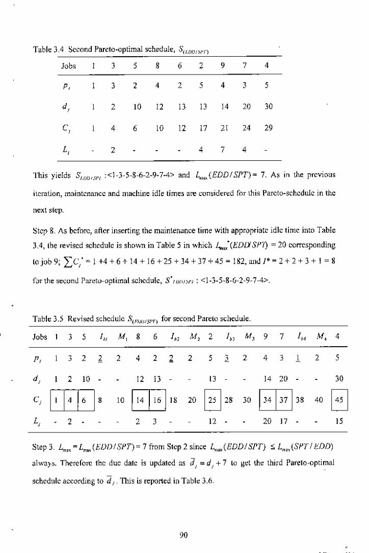
Table 3.4 Second Pareto-optimal schedule, SfWlJi,lI'l'l

Jobs 3 5 8 6 2 9 7 4

p, J 2 4 2 5 4 3 5

d, 2 10 12 I J IJ 14 20 30

C 4 6 10 12 17 21 24 29,L, 2 4 7 4

This yields SWI,,""'I :<1-3-5-8-6-2-9-7-4> and L",,,,(EDDISPT)~ 7. As in the previous

iteration, maintenance and machine idle times are considered l'or this Pareto-schedule in the

next slep.

Step 8. As before, after inserting the maintemmee time with appropriate idle time into Table

3.4, the revised schedule is shov,u in Table 5 in which L",,,,.(EDIY SPi) = 20 corresponding

tojob9; Ie,' = I +4 +6 + 14 + 16 +25 +34+37+45 ~ 182, and/*= 2+ 2+ 3 + 1 = 8

f"r the second Pareto-optimal schedule, S'II)I)I,'I'I : <1-3-5.8.6-2-9-7-4>.

Table 3.5 Revised schedule Sfl''''!I,,"r) for second Pareto schedule.

Jobs J 5

10 EG 18 20 B 28 30 EG 38 40 BP, 3 2 2 2

1 2 10

2

4 2 ~

12 13

2 3

2 5 1 2

13

12-

4 J I

14 20

20 17 -

2 5

30

I 5

Step 3, Lm" = Lm" (FDf)/ SPT) = 7 from Step 2 since L",,,,(EDDI SPT) ::;L",,(SPT Il:DD)

alwa}~, Thercrorc the due date is updated as dJ

= dJ+ 7 to gd the third Pareto-optimal

schedule according to d J' 111is is reported in Table 3.6.

Table 3.6 Updated dl '" dj + 7 (in EDD order)

Jobs 3 , 8 6 2 , 7 4

d, 2 " " D D 14 20 '"J, 8 9 17 19 " " " 27 37

Step 4. Here, .f' = {1,2,3,4,5,6,7,8,9}, the lotal number of jobs, k = IJ'I = 9, and total

processing time of the remaining jobs, r =LP, = 29 and set J= r =29 (allhe beginning).

Step 5, J-Isatisfies condition d,. ? t (= 29) and the correspondingl'4 is 5. So J4 is scheduled

as the last job in the sequence, 51:< 4>,

Step 6. None orthe remaining jobs satisfies the condition~ J, < randp, > Pj ••

Step 7. The ~et ~tatisties is updated as J' = {1,2,3,5,6,7,8,9}, k= IJ'I = 8, and t = 29 - 5 =

24,

Since the Sleps 5 to 7 are repeated likewise in order to gel the third Pareto-optimal schedule,

the results of this repeated search are ~ummariz.cd in Table 3.7, and the last search result~ in

S,: <;1,5,6,3,8,2,9,7,4>which, in lum, yields lhe third Pareto oplimalschedule JS in ']able 3.8. The

maximum lateness for the third Pareto-optimal schedule isL",••(5,) = 7.

Tahle 3.7 Repetition of Steps 5 through 7

Job (j) Processing Time (PI) Schedule (S) J

4 5 , 4> 29

7 3 , 7,4> 3

9 7 , 9,7,4>

2 , , 2,9,7,4>

8 4 , 8,2,9,7,4>

3 3 , 3,8,2,9,7,4>

6 2 ,." 6,3,8,2,9,7,4>

, 2 ,.,5,6,3,8,2,9,7,4><1,5,6,3,8,2,9,7,4>

""17

12

8

5

3

o

91

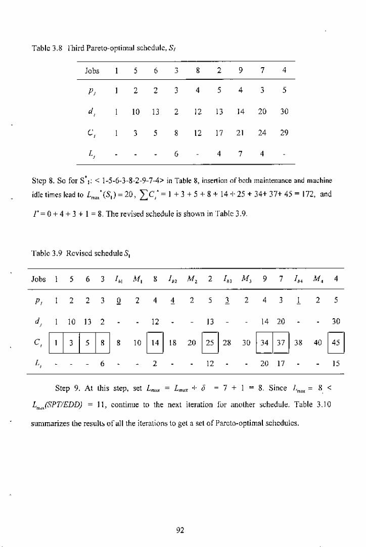
Tablc 3.8 l'hird Pareto-oplimal schedule, SI

Jobs 1 5 6 3 8 2 9 7 4

P, 2 2 3 4 5 4 3 5

d, 10 13 2 12 13 14 20 30

C 3 5 8 12 17 21 24 29,

L, G 4 7 4

Step 8. So for S'I: < 1-5-6.3-8-2-9-7-4> in Table 8, insertion of both maintenance and machine

idle times lead 10 Lm,:(S,) = 20, Ie,' = I + 3 + 5 + 8 + 14 -I-25 + 34+ 37+ 45 = 172, ood

r = 0 + 4 + 3 + I = 8, The revi~ed schedule is shown in Table 3.9,

Table 3.9 Revised schedule 5,

Jobs 5 6 3 I., Ai, 8 1" M, 2 1" M, 9 7 1" A1., 4

P, 2 2 3 Q 2 4 4 2 5 3 2 4 3 1 2 5

d, 10 13 2 12 13 14 20 30

C, [TEE] 8 10 G 18 20 B 28 30 IT] 38 40 BL, 6 2 12 20 17 15

Step 9. At !his step, set Lrow, = Lmax -I- i5 ~ 7 + 1 = 8. Since I, 0 8 ,m."

L".,lSPTIEDD) 0 11, continue to the next ileration lor another ,eheduk Table 3.10

summarizes lhe result.>of all the iterations to get a set of Pareto-optimal schedules.

92

rable3.10 Allihe iterations of the algorithm

Iteration PHreto-Oplimal,

Schedule Ie; ,L~',I" Currenl d I + ()"m Sequence H

SPT/EDD <1-5-6-3-7-8-9-2-4> 151,22,8 30,20,14,13,13,12,10,2, I

2 HlD/Sl'"f <1-3-5-8-6.2-9-7-4> t82, 20, 8 30,20,14,13,13,12,10,2,1 7

3 S, <1-5-6-3-8-2-9-7-4> t72,20,8 37,27,21,20,20,19,17,9,8

, 57 <1-5-6.3.8.9-2-7-4> tJ7, t2, 0 38,28,22,21,21,20,18,10,9 2

5 5 <1-5-6-3-7-8.2-9.4> 151,20,8 40, JO, 24, 23, 23, 22, 20,12,11,6 5, <1-5-6.3.7-8-9-2-4> 151,22,8 41,31,25,24,24,23,21,13,12 Stop

After generating all possible Pareto-optimal schedules with respect to job completion

time F' , job tardiness I.,,,,,;, and machine idle time t for nine jobs, the total weighled,funclion, c(F''!",.:,r' )=w/LC,' /9)+w,I;...,' +w/, where w, = 0.5, W.I= (lA, Wj = 0.1

j_1

(arbitrarily chosen) for 6 schedules is calculated [sec Table 3.11]. The minimum-weighled

schedule is S* = S2:<1-5-6-3-8.9-2-7-4> corresponding to c(F' ,L",~',I' ) = 12.411.

Tablc 3.11 A Parelo-Optimal Set

Iteration,m

Schedule Pareto-OptimalSequence

. .,L"",,l~

-, "c(F,Lm~,l )

1 SPTIEDD <1-5-6-3-7-8-9-2-4> 151,22,8 17.989

2 EDD/srT <1-3-5-8-6-2-9-7-4> 182,20,8 18.911

3 5, <1-5-6-3-8-2-9-7 -4> 172,20,8 18.356

4 5, <1-5-6-3-8-9-2-7-4> 137,12,0 12.41t"

5 57 < 1.5.6-3-7-8-2-9-4> 151,20,8 17.189

6 53 <1-5-(;-3-7.8-9-2-4> 151,22,8 17.989

• Ihebe'l schedulewiththemjlllm"m weightedfunCllon

93

3.6 Neighborhood Search Algorithm

As a second approach to the multi-criterion scheduling problem, a neighborhood search

technique is considered. Many discrete optimization problems of practical interest cannot be

solved optimally in tbe reasonable time. A practical approach to these problems is l(l usc

heuristics which do not guarantee the optimality of the solution, hut ncar-optimal solutions

. can be obtained in a tolerable time limit. Neighborhood search starts with a feasible

schedule and iteratively tries to improve the solution. At each stage, it searches the

"neighborhood" of the current solution to find an improved solution, The search terminates

when it finds a solution that is at least as good as any of its neighbors; such a solution is

called a locally optimal solution. Typically, multiple runs of the neighborhood search are

perlormed with different starting schedules called seeds. and the best locally optimal

solution is selected. A comprehensive discussion of neighborhood search can be found in

Ehrgott and Klamroth [64].

A method of taking one sequence as a seed and systematici.lllycreating a collcction of

relatcd sequcnccs is the generating mechanism. In this work, thc single adjacent pairwise

interchange operation scrves as a generating mechanism lor the example. The neighborhood

of the seed sequence is a list of (n-l) = 9-1 = 8, distinct sequences for this palticular

generating mechanism. The single adjacent pairwise interchange i~O(n') in size (Baker,

1998). The search is illustrated on the numerical example. The performance measure of all

the neighborhood sequences that is evaluated with respect to the initial seed is the weighted

function. The same weight combinations, as given earlier, arc used to evaluate the

objective~ (See Tahles 3.12, 3.13 and 3.14). The following steps of neighborhood search,

initially pre~entedby Baker [42J, arCapplied to the numerical example.

Algorithm 2: Nejghborhood Search

Step L Obtain a sequence to be an initial seed and evaluate it with respect to the

perfoml,mee measure,

Step 2.Generate and evall.mteall the sequences in the neighborhood of the seed, If none or

the sequences is better than the ~ecdwith respect to the perI"uTmaneemeasure, stop.

Olherwise proceed.

Step 3. Seleel one of the sequences in the neighborhood thaI improved lhe performance

mea,ure. Let this sequence be the new seed. Return (0 Step 2.

The single adjacent pairwise interchange mechanism is applied to the initial seeds, and the

performance mea,ure (weighted function) of each seed is compared with the perfOlmance

measure of i(~neighborhood. Instead of generating all the sequences in the neighborhood of

the seed, when a neighborhood gives an improved performance measure, the search stops,

and that sequence becomes the new seed for the next stage. When a search of the new

neighborhood produces no improvement, the search procedure terminates. The details of

three seeds with their neighborhood sequences and their performance measures are

presented in Tables 3.12, 3.13, and 3,14,

Table 3.12 Solution with a given initial seed, S: < 1"2-3-4-5-6-7-8-9>

,Schedule L:C I' I.",,, ,1" 0.5F' +OALm.: +0.1/",-,Stage I

Seed: 1"2-3-4-5-6-7-8-9 183,24,3 20.067

Neighborhood: 2-1-3-4"5-6-7-8-9 187,24,3 20.289

1-3-2-4-5-6-7-8-9 231,34, II 27.533

1-2-4-3-5-6-7-8-9 185,24,3 20,178

1-2-3-5-4-6-7-8-9 201,30,7 23.867

1-2-3-4-6-5-7-8-9 183,24,3 20,067

1-2-3+5-7-6-8-9 184,24,3 21.122

1-2-3-4-5-6-8-7-9 182,23,2 19,511*sc1cetion

Siage 2

New Seed: 1-2-3-4-H-8-7-9 182,23,2 19.511

Neighborhood: 2-1-3-4-5-6-8-7-9 186,23,2 19.733

1-3-2-4-5-6-8-7-9 230,33,10 26.978

1-2-4-3-5-6-8"7-9 184,23,2 19.622

1-2-3-5-4-6-8-7-9 202,30,7 23.922

1_2_3_4_6_5_8_7_9 182,23,2 19.511

1"2-3-4-5-8-6-7-9 184,23,2 19.622

1-2-3-4-5-6-7-8-9 183,24,3 20.067

1.2-3-4-5-6-8-9-7 183,20,2 18.367* selection

Stage 3

New Seed: 1"2-3-4-5-6-8-9-7 183,20,2 18.367* selection

Neighborhood: 2-1-3-4-5-6-8-9-7 187,20,2 18.589

1_3_2_4_5_6_8_9_7 240, 30, 10 26.333

1-2-4-3-5-6-8-9-7 185,20,2 18.478

1-2-3-5-4-6-8-9-7 202,24,6 2\.422

1-2-3-4-6-5-8-9-7 183,20,2 18.367* selection

1-2-3-4-5-8-6-9-7 185,20,2 18,478

1-2-3-4-5.6-9-8-7 183,22,2 19.167

1-2-3-4-5.6-8-7-9 182,23,2 19.511

Sean;h terminates with "eighted functional value = 18.367

96

To compare the modified Pareto-optimal algorithm with the neighborhood search heuristic

in ease of bench mark data, the same instance with parameter~ T = S, tv!= 2, WI = 0.5, W2 =

0.4 and Wj = 0.1 is used. The neighborhood search heuristic gives the best near-optimal

schedule us S: <1-5-6-3-7-2-8-9-4> with the minimum weighted fundion equals to 18.367.

On the other hand, the modified Pareto-optimal algorithm gives the best near-optimal

schedule as S: <1-5-6-3-8-9-2-7-4> with the minimum weighted function equals to 12.410.

It can be concluded that the modified Pareto-optimal algorithm provides a better re~ult than

the neighborhood seareh heuri,tic ror this instance.

97

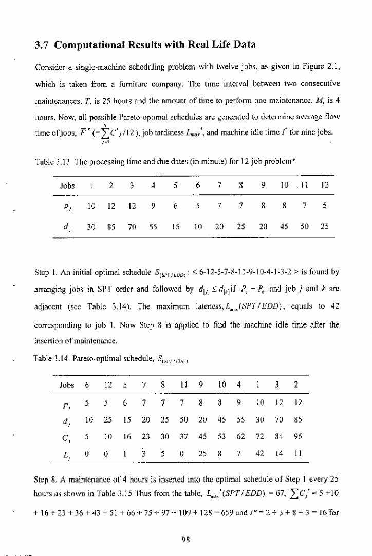
3.7 Computational Results with Real Life Data

Consider a single-machine scheduling problem with twelve jobs, as givcn in Figure 2.1,

which is taken from a furniture company. The time inlerval between two consecutive

maintenances, T, is 25 hours and the amount of lime to perlorm onc maintenance, M, is 4

hours. Now, all possible Parel(l-\'pllmal schedules arc generated to detennine average flow,time of jobs, F' (=LC'! /12), job tardiness Lma, " and machine idle timc l for nine jobs.

,-,

Table 3.13 The processing time and due dates (in minute) for 12-job problem*

Jobs 2 3 4 5 6 7 8 9 10,11 12

P,

d,

10 12 12 9

30 85 70 55

6

15

577

10 20 25

8 8 7 5

20 45 50 25

Step I. An initial optimal schedule 8(.I''''lwo): < 6-12-5-7-8-11-9-10-4-1-3-2 > is found by

arranging jobs in sl'r order and followed by dljl::S;dl,!if P, = Pk and job j and k arc

adjacent (sec Table 3.14). Th, maxImum lateness, Lm,,,(SYl' /i'-DD) , equals ,0 42

corresponding to job 1. Now Step 8 is applied to find the machine idle time after the

insertion ofmaintenallce.

Table 3.14 Pareto-optimal schedule, .'11.11"II'I!I»)

Jobs 6 " 5 7 8 11 9 10 4 3 2

P, 5 5 6 7 7 7 8 8 9 10 " 12

d, 10 25 15 20 25 50 20 45 55 )0 70 85

C, 5 10 16 23 30 37 45 53 62 72 84 96

L, 0 0 1 3 5 0 25 , 7 42 14 11

Step 8. A maintenance of 4 hours is inserted into the optimal schedule of Step I every 25

hours as shown in Table 3.15 Thus from the table, L",,: (SJ'T I EDD) = 67, L:C,' = 5 + 10

+ 16 + 23 +36 +43 + 51 +66+ 75 + 97+ 109 + 128 ~659 anol*= 2+ 3 + 8 +3 = 16Tor

98

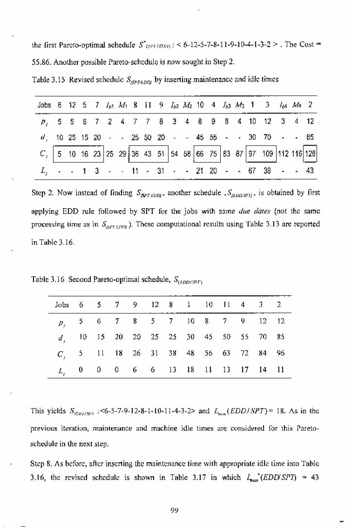
lhe IIrst Pareto-optimal schedule S'(,'1'III,'JIJ): < 6-12-5-7-8-11-9-10-4-1-3-2 >. The Co~l =

55.86. Another pos~ible Pareto"seheduJc is now sought in Step 2.

Table 3.15 Revised schedule Sm'N,On) by inserting maintenance and idle times

Jobs 6 12 5 7 1" M1 8 11 9 1" M, 10 4 h7 M7 I 3 I" M< 2

P, 5 5 6 7 2 4 7 7 8 3 4 8 9 8 4 10 12 3 4 12

d, ID 25 15 20 25 50 20 45 55 30 70 85

C 5 10 16 231

25 2g136 43 51 154 58~83 87~112 11611281,

", 1 3 , 11 31 , 21 20 67 39 , 43

Step 2. Now instead of finding S(SJ'J't'DD)' another schedule ,SIWD.I'I'I)' is obtained by first

applying EDD rule followed by SrT for the jobs with same due dales (not the same

proces,ing time as in 8,,,,,,UJIl))' These eomplllalional results using Table 3, 13 are reported

in Table 3.16.

Table 3.16 Second Pareto-optimal schedule, S{'!,,)!,1'Prj

Jobs 6 5 7 9 12 8 10 11 4 3 2

P, 5 6 7 8 5 7 10 8 7 9 12 12

d, 10 15 20 20 25 25 30 45 50 55 70 85

C, 5 11 18 26 Jl 3M 48 56 63 72 "' 96

I, 0 0 0 6 6 13 18 11 13 17 14 11

This yields S"'J'J'-"" :<6"5-7"9"12-8-1-10-11-4-3-2> and Lm,,,(EDD!SPT)= 18. As in the

previous iteration, mainlenanee and machine idle lime, ;Ire e{)n~idered lor lhis Parelo-

schedule ;n the next ~lep.

Step 8. As before, after inserting the maintenance time with appropriate idle lime into Table

3.16, the revised schedule is shown in Table 3.17 in which L",,,,"(EDrYSI'T; = 43

corresponding to job 2; Lei' '"5+11 +18 + 37 + 42 + 49 + 68 + 76 + 83 + 96 + 108 + 128

'" 721, and f* '" 7 + 5 + 0 + 4 '" 16 for the second Pareto-optimal schedule, S'I,lm""'T : <6-5-

7-9-12-8-1-10-11-4-3-2>, The Cost = 48.84

'lablc3.17 Revi~ed ~ehedule SIIDDlSJ'1') for se~ond Pareto schedule.

Jobs 6 5 7 I" M, 9 12 8 /0, M, 1 10 11 I" M, 4 ] I" M, 2

P, 5 6 7 7 4 8 5 7 5 4 10 8 7 0 4 9 12 4 4 12d, 10 15 20 20 25 25 - 30 45 50 55 70 65C

15 11 18

125 29

137 42 49 I 54 58

168 76 83 183 87 B112 11611281,

I - 17 17 24 - ]8 ]1 33 - 41 38 43,

Step ] L"""= Lrn,,(EDDI SPT) = 18 from Step 2 smee Lrn,,(mDISPT)

:'> L"",(SPTI EDD) always, Therefore the due date is updated as dj =d, +18 (0 get the

third Parcto-optimal schedule a~cording to d j. This is reported in Table 3.18.

Table 3,18 Updated d I = d I + 18 (in EDD order)

Jobs 6 5 7 9 12 8 10 II , 3 2

J, 10 15 20 20 25 25 ]0 45 50 55 70 85

d, 28 3] ]8 " 43 43 48 63 68 73 88 103

Step 4. Here, J' = {1.2,J.4,5,6,7,8,9,10,11,12}, the total number of jobs, k = 1;-1 = 12, and

total processing time or the remaining jobs. r= LPj = 96 and set 8= r =96 (at the

beginning).

Step 5. J2 sati,rie, condition dj• ~ r (= 96) and the correspondingpl is 5. So.l] is scheduled

as the las( job in the sequence, SI:< 2>,

Step 6, None of the remaining job, satisfies the conditions d, < rand p, > Pj.'

100

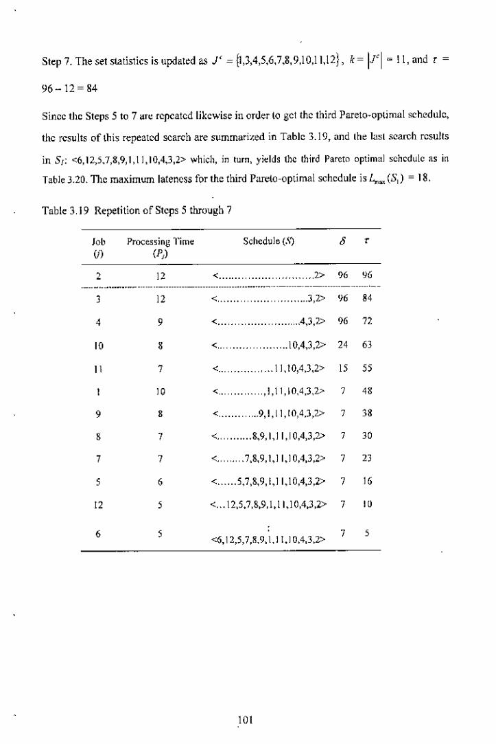
Step 7. The set statistics is updated as J' = {1,3,4,5,6,7,8,9,lO,11,12j, k= 1.1'1 = 11, and r =

96-12=84

Since the Steps 5 to 7 are repeated likewise ill order (0 get the third Pareto~optimal schedule,

the results of this repeated search are summari;-:ed in Table 3.19, and the b~t search results

in Sf: <6,12,5.7,8,9,1,11,10,4,3,2> which, in turn, yields the third Pareto optimal schedule as in

Table 3.20. TIle maximum lateness for the third Parelo~optimal schedule is L,.,,,(S,) = 18.

Table 3, I9 Repetition of Steps 5 through 7

JobU)

Processing Time(P)

Schedule (.\) J ,

2

]

4

10

11

9

8

7

5

12

6

12 <....... ,', ...... " ...... ".,2> '" %--------- --------------_ ...........- --------

12 , ....3,2> " 84

9 <... ."., ...... "..4,3,2> 96 72

8 < .... 10,4,3,2> 24 63

7 , .. 11,10,4,3,2> 15 5510 < .. ",,1,11,10,4,3,2> 3 "8 < " ...9, I, 11,10,4.3,2> 3 38

7 ,'" ....... 8,9, I,ll, I0,4,3,2> 3 30

3 ,", ..,' .7,8,9,1,11,10,4,3,2> 3 2)

6 ,..... 5,7,8,9,1,11,10,4,3,2> 3 16

5 ,.. 12,5,7,8,9,1,11,10,4,3,2> 3 19

5 <6,12,5,7,8,9,1, It, I0,4,3,2> 7 5

101

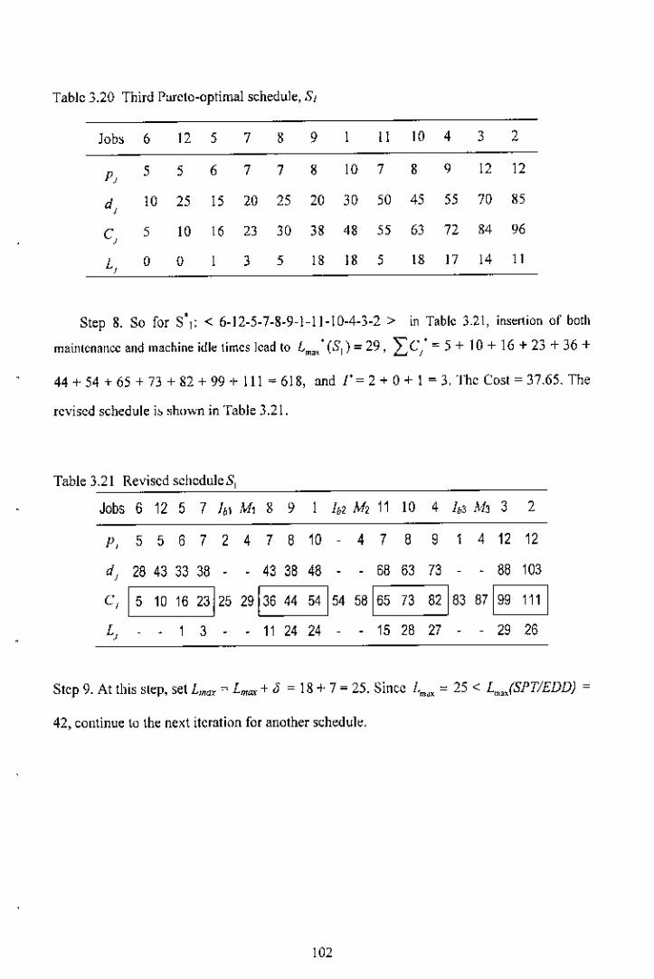
Table 3.20 Third Pareto-optimal schedule, 81

Job~ 6 12 5 7 8 9 II 10 , ] 2

P, 5 5 6 7 7 8 10 7 8 9 12 12

d, 10 25 15 20 25 20 ]0 50 45 55 70 85

C, 5 10 16 2] ]0 ]8 48 55 6] 72 8' 96

L, 0 0 ) 5 18 18 5 18 17 14 11

•Step 8. So for S I: < 6-12-5-7-8-9-1-11-10-4-3-2 > in Table 3.21, insertion of both

mailllenanCCand machine idle limes lead to L.m,: (8,) = 29, Lej' =- 5 + 10 + 16 + 23 + 36 +

44 + 54 + 65 + 73 + 82 + 99.f- 111 =- 618, and 1'= 2 + 0 + 1 =- 3, Thc Cost = 37.65. The

revised schedule i~shown in Table 3.21.

Table 3.21 Revised schcduleS,

Jobs 6 12 5 7 I" U, S 9 102 M2 11 10 , 103 All 3 2

P, 5 5 6 7 2 , 7 8 10 4 7 8 9 1 4 12 12

d, 28 43 33 38 43 38 48 - 68 63 73 - 88 103

C15 10 16231252913644 54

154 58

165 73 82

183 87~,

L, 1 3 - 11 24 24 - - 15 28 27 - - 29 26

Step 9. At this step, set Lmax ~ L",,,,,+ i5 = 18 + 7 =- 25. Sincc L••" = 25 < L",,(SPT/EDD) =

42, continue to the next iteration for another scheduk.

102

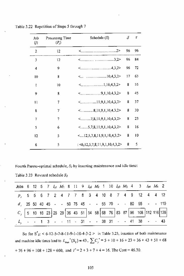
Table 3.22 R~pelition of Steps 5 lhruugh 7

leb Pro~CSSlngTime Schedule (S) J ,Ul (PJ

2 12 , ......... ...... 2> 96 96--------- --------- -_ ..------ ---------

J 12 , .... ,', ..... ,3,2> 96 "', 9 ,..... ,', ...... , , ... ,.._.4,3,2> 96 72

10 8 <... .... , , , ........ lO,4,3,2> " "10 , .. .... " I ,10,4,3,2> 8 "

9 8 , .. ," .. _9,1,10,4,3,2> 8 "11 7 <.... .,' ,.... II ,9,1,10,4,3,2> 8 J7

8 , ,, , ........ 8, II ,9, I , ltl,4,3,2> 8 30

7 , ,... " ... 7,8, II ,9, I , I0,4,3,2> 8 23; 6 , .. 5,7,8, II ,9, I , I0,4,3,2> 8 16

12 5 <... 12,5,7 ,8, 11,9, 1, I0,4,3,2> 8 10

6 5 : <6,12,5,7,8, t 1,9,1, I0,4,3,2> 8 ;

Fourth Pareto-optimal schedule, 81 by ins~rting maintenance and idle lime:

Table 3_23 ReVIsed schedule SJ

Jobs 6 " 5 7 I" M, 8 11 9 I" M, 1 10 J,l M, 4 3 1M M, 2

P, 5 5 6 7 2 4 7 7 8 3 4 10 8 7 4 9 " 4 4 12d, 35 50 40 45 50 75 45 - 55 70 80 95 110

C, 5 10 16 23125 29

136 43 51

1

54 58B83 87B112 11611281

, L, 1 3 11 31 - 38 31 - 41 38 43

So for S'2: < 6-12-5-7-8-11-9-1-10.4-3-2 > in Table 3.23, insertion of both maintenance

and machine idle times lead to !.m,,'(Sl)=43, :LCJ'=5 + 10+ 16+23 of- 36 +43 + 51 +68

+ 76 + 96 + 108 + 128 = 660, und l'~2 + 3 + 7 +4 = 16. The Cost = 46.30,

103

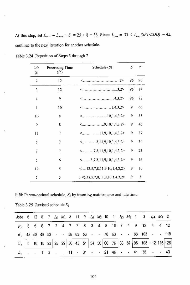
At this step, set Lmox = Lm"" + r5 = 25 + S = 33. Since Lm" = 33 < L",JSf'TIEDD) = 42,

continue to the next iteration for another ~chedulc.

rable 3.24 Repetition of Steps 5 through 7

3

4

9

""7

5

Proccssmg Time Schedule (S) 6 ,(P,)

" < " ,,2> 96 96---_ ...._ ....---- ----_.- -_ .......--- ------ -----_._-_ ..._---

" < ... " .... " ...3,2> 96 84

9 , ".4,3,2> 96 72

W < "".1,4,),2> 9 m8 <,,-- ,,10,1,4,3,2> 9 "8 < "'" .... 9,1 0, 1,4,),2> 9 "7 < , .. ,,11,9,10,1,4,),2> 9 37

7 <..-- , , ..8, 11,9, 10, I ,4,3,2> 9 30

7 < " ... 7,8, II ,9,1 0,1 ,4,3,2> 9 23

6 < .. 5,7,8, II ,9,1 0,1 ,4,),2> <I >6

5 < ___12,5,7 ,8, 11,9, I0, I ,4,3,2> 9 W

, : <6, I2,5,7,8, 11,9, j 0, 1,4,3,2> 9 ,

Fifth Pareto-optimal schedule, 83 by inserting maintenance and idle time:

Table 3.25 Revised schedule SJ

Jobs 6 12 5 7 I" M, S 11 9 1" M, 10 I" M, 4 3 I" M, 2

P, 5 5 6 7 2 4 7 7 8 3 4 8 10 7 4 9 12 4 4 12

d, 43 58 48 53 58 83 53 78 63 88 103 118

C 5 10 16 2312529

136 43 51

1

54 58~83 87~112 11611281,", 3 ~ 11 31 ~ 21 46 ~ 41 38 43

104

So for S": < 6_12.5.7_8_11_9_10_1_4_3_2 > in Table 3 25, insertion or both maLn!enance and

m.chinc idlc tilne~ lead to L",,,,'(S,) =43, Le,' = 5 + 10 -I. 16 + 23 + 36 + 43 + 51 + 66 +

76 + 96 -+- 108 + 128 = 658, and ]'= 2 + 3 + 7 +4 = 16. The Cost = 47.42.

Althis step, sci Lmax = Lmax + 13 = 33 + 9 = 42. Since Lm" = L""JSPTIEDD) '" 42, So,

STOPTable 3.26 Repetition of Steps 5 thl'Ough 7

',bvl2

3

4

W

3

II

8

7

5

12

6

Processing Time Schedule (S) 6 ,(1'1)

12 < ".,', ...... " .... ., ...... .2> 96 9612 <, ,,3,2> 96 84

10 < ... .4,3,2> 96 729 <..... .. 1,4,3,2> 9 63

8 <... .... ," ... 10,1,4,3,2> 9 536 < ...... 9,10, [,4,3,2> 9 "7 < ..... 11,9,10,1,4,3,2> 9 377 , ,.8,11 ,9, 10, 1,4,3,2> 9 307 <.... ,... 7,8,11,9,10,1,4,3,2> 9 236 <" ., .. 5,7,8,11 ,9, 10, 1,4,3,2> 9 165 < ... 12,5,7,8, II ,9, I0, I ,4,3,2> 9 105 : <6, I2,5,7,8, I [,9,10, I,4,3,2> 9 5

Sixth Parclo-opumal schedule, S, by inserting maintenance and idle time:

Table 3.27 Revised schedule S4

Jobs 6 12 5 7 I" U- S II 9 I" Me 10 4 '" M, 1 3 1" M, 2

P, 5 5 6 7 2 4 7 7 8 3 4 8 9 8 4 10 12 3 4 12

d, 52 67 57 62 67 92 62 87 97 72 112 127

C, 5 101623125 2913643 51154 58B83 87B112 11611281

", 1 3 . 11 31 . 21 20 . . 67 39 . 43

105

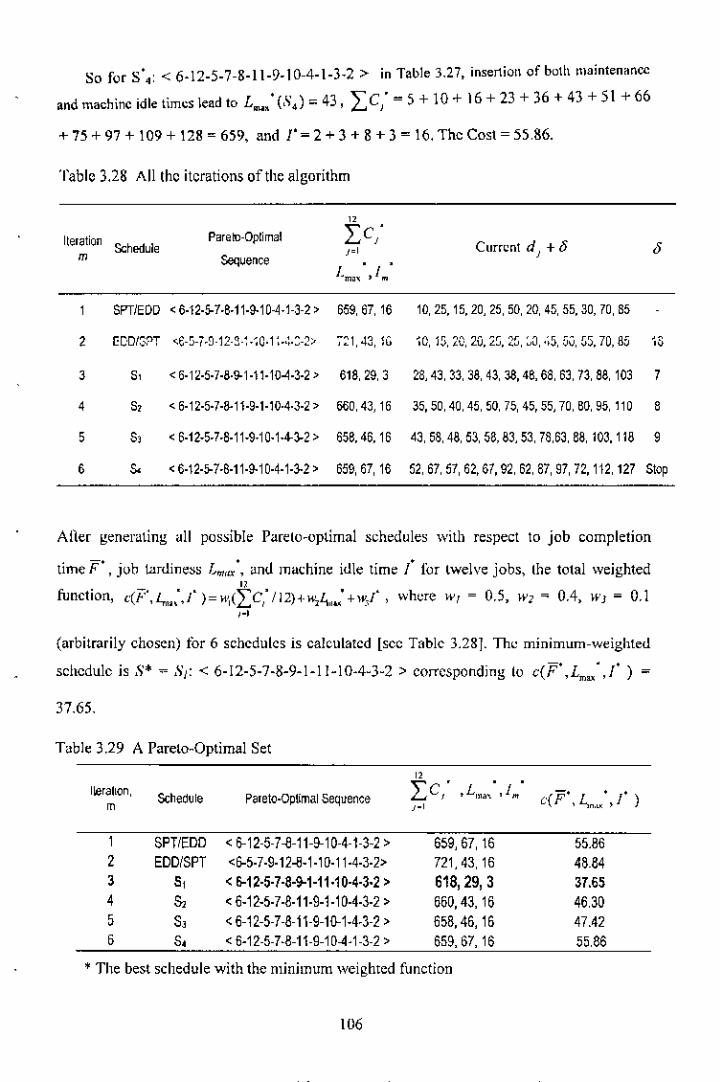
So for S'.: < 6_12_5_7_8_11_9_10-4_1_3_2> in Table 3.27, insertion of both maintenancc

and machine idle times lead to L•••: (S.l '" 43, IC; = 5 + 10 + 16 + 23 + 36 + 43 + 51 + 66

+75+97 + 109+ 128 ~ 659, and ]'=2+3 + 8 +3 ~ 16. The Cost = 55,86.

Table 3,28 All the iteratiOnS of the algorithm

"Iter"tionSchedule

Pareto-Oplimal LC}'Cur,ont d

J+ {; Jm Sequence

j~1. .!.m" .1.

SPTIEOO < 6.12.5-7.6.11.1}.104.1-3-2 > 659,67, 16 10,25.15.20,25,50,20,45,55.30,70,85

2 ~CDI3PT <€-"-; .9.12.~.~.;0.1 ; ..:.:-2, ~:'1,43, lG ,0, 15,20, 20. 2". 2~,~J,'-.5,50, 53. 70, 85 ',5

; e, < 6.12.5.7.8.1}.1.11.10-4.3.2> 618,29,3 28,43,33,38,43,38,46,68,63,73, 88, 103 7

, e, < 6.12.5.7.8-11.9.1.10-4-3.2> 660,43,16 35,50,40,45,50,75,45,55,70, BO,95, 110 ;

5 e, < 6.12-5.7.6.11-9.10.1.4-:}-2> 656.46.16 43,56,46,53,58,63,53,78,63,68, 103,118 9

6 & < 6.12.5-7.6.11.1}.10.4.1.3-2 > 659,67, 16 52,67,57,62,67,92,62,87,97,72,112,127 Stop

Aner gener~ting ~11 pos~ible P~reto-oplimal ~chedules with re~pect to job completion

time F', jllb w.n.line~sL",,,,:,and m~chine idle time l for twelve jobs, the total weighted

"function, c(F',4,.,:J )=w,(L:C/' /12)+"11,,,.: +w/, wh~n" WI ~ 0.5, w, = 0.4, W] = 0.1,-,(arbitrarily chosen) tor 6 schcdules is calculatcd [scc Table 3.28J. llw minimum-weighted

schedule is S* = S( < 6-12-5-7-8-9-1-11-10-4"3"2 > corresponding (0 c(F',Lm",",J') =

37.65.

T~ble 3.29 A Pareto"Optimal Set

"LC; ,L",:,1".

IteralLon, S<;hedule Pareto.OptimalSequence c(F' , L,",~',J' )" ,-,

1 SPTIEDD < 6-12-5-7-8-11-9-10-4-1-3-2 > 659,67,16 55.862 EDDISPT <6-5.7.9.12-8-1.10.11.4.3.2> 721,43,16 48.843 S, < 8-12.5.7.8-9+11.10.4.3.2 > 618,29,3 37,654 ~ < 6-12-5.7.8.11.9-1.10.4.3.2 > 660,43,16 46,305 S, < 6-12-5-7-8-11-9-10--1-4.3-2> 658,46,16 47.425 S. < 6-12-5-7.8-11-9-104.1-3-2 > 559,67,16 55,86

• The best schedule with the minimum weighted function

106

3.8 Neighborhood Search Algorithm

As a second approach to the multi-criterion scheduling problem, a neighborhood search

teclmique is considered. Many discrete optimization problems ofpraclical intcrcst cannot be

solved optimally in the reasonable timc. A practical approach to lhe~e problems is to use

heuristics which do not guarantee the optimality of the solution, but ncar-optimal sohI1ions

can be obtaincd in a tolerable timc limit. Neighborhood search starts with a feasible

schedulc and iteratively tries to improve the solution. At each stagc, it searches the

"neighborhood" of the current solution to find an improved solution. The ~eareh terminates

when it finds a solution that is at leasl as good as any of its neighbors; such a solution is

called a locally optimal solulion. A method of taking one sequence as a seed and

systematically creating a collection of related sequences is the generating mechanism. In

this work, the single adjacent pairwise interchange operation serves as a generating

mechanism for the example. The neighborhood of the seed sequence is a lbt of (n-l) = 12-1

= 11, distinct sequences for this particular generating mechanism. The single adjacent

pairwi~e interchange mechanism is applied to the initial seed, and the performance measure

(weighted fu.netion) of each seed is compared with the perfomlanee measure of its

neighborhood. Instead or generating all the sequences in the neighborhood of the ~eed.

when a neighborhoml gives an improved perfomlance measure, the search stops, and that

sequence becomes the new seed for the next stage. When a search of the lleWneighborhood

produces no improvement, the search procedurc terminates. The details of the seed with

their neighborhood sequences and their performance measures arc presented in Tables 3.30.

Search terminates with weighted functional value = 68.917

107

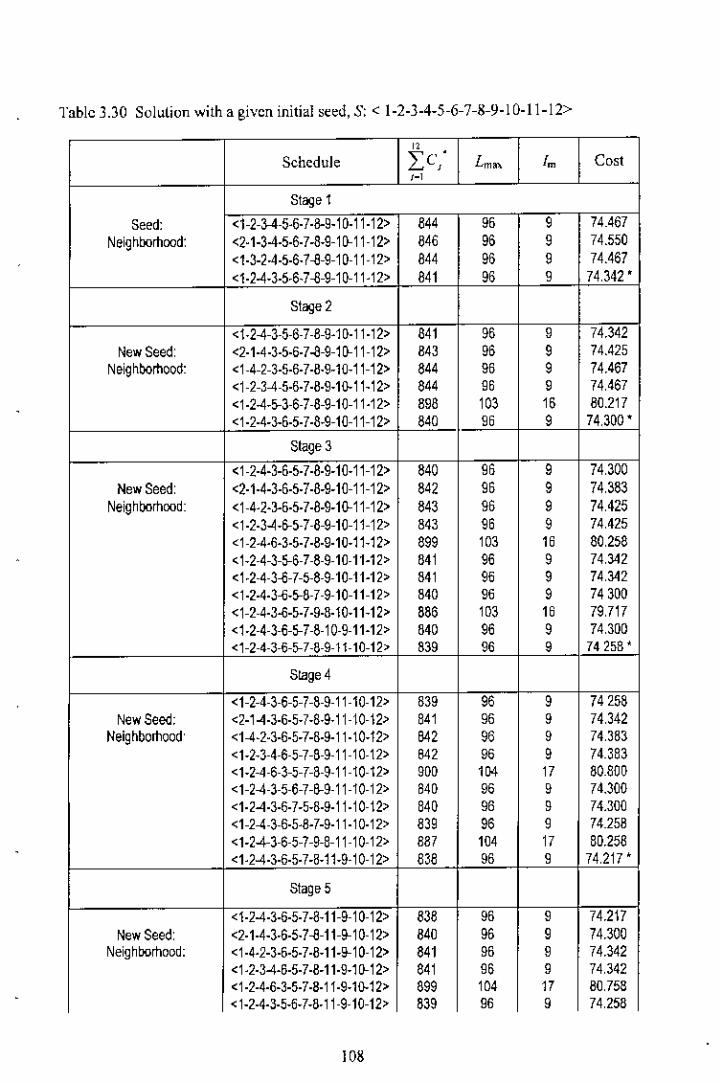
Table 3.30 Sol~lion with a given initial seed, S: < 1-2-3-4-5-6-7-8-9-10-11-12>

" .Schedule Le. L~. [~ Cost

H

Stage 1

Seed: <1-2-3-4-5.6.7.8-9-10.11.12> 844 95 9 74.467Neighoorhood: <2.1-)-4.5.6.7-8-9-1 (}.11-12> 846 95 9 74.550

<1.)-2-4.5.6.7-8-9-10-11-12> 844 96 9 74.467<1.2-4-).5.6.7-8-9-1 (}.11.12> 841 96 9 74,342 •

Stage 2

<1.2-4-3-5-6-7-8-9.10.11.12> 841 95 9 74.342New Seed: <2.1.4.3.5.6.7-8-9-1 (}.11-12> 843 96 9 74.425

Neighoorhood: <1-4-2-3.5.6.7.8.9.10.11-12> 844 95 9 74.467<1-2-3-4-5.6.7.8.9-10-11.12> 844 95 9 74.467<1.2-4-5-3-6-7-8-9-10-11.12> 898 103 15 80.217<1.2.4-3-6.5.7.8-9-10-11-12> 840 96 9 74,300'

Stage 3<1-2.4.)-6.5.7.8.9-10-11-12> 840 95 9 74,)00

New Seed: <2.1.4-).6.5.7.8-9-10-11-12> 842 95 9 74,383Neighoorhood: <1-4.2.3-6.5.7.8-9-1(}.11-12> 843 95 9 74,425

<1.2.3-4-5-5-7-8-9-10-11-12> 843 95 9 74,425<1-2-4.6.3.5.7.8.9.10-11.12> 899 103 16 80,258<1.2-4-3-5-6-7-8-9-10-11-12> 841 96 9 74.:>42<1.2-4-3-S-7-5-8-9-10-11-12> 841 95 9 74,342<1.2.4.3-6-5-8-7-9-10-11-12> 840 96 9 74300<1-2-4.3-S-5.7.9.8.10-11.12> 885 103 16 79,717<1.2-4-3-6-5-7-8-10-9-11.12> 840 96 9 74,300<1-2-4-3-6-5-7-8-9-11-10-12> 839 90 9 74258'

Stage 4

<1-2-4-3-6-5-7-8-9-11-10-12> 839 96 9 74258New Seed: <2-1-4.3.6.5-7-8.9.11-10-12> 841 90 9 74,342

Neighborhood' <1-4.2.3.6.5-7-8.9.11.10-12> 842 96 9 74,383<1-2.3-4-6-5-7-8-9-11-10-12> 842 95 9 74.383<1-2-4-6-3-5-7-8-9-11-10-12> 900 104 17 80.800<1-2-4-3-5-6-7-8-9-11-10-12> 840 95 9 74.300<1.2-4.3.6.7-5-8.9.11.10-12> 840 96 8 74.300<1-2-4-3-6.5.8-7-9.11.10.12> 838 95 9 74.258<1-2-4-3-6-5-7-9-8-11-10-12> B87 104 17 80.258<1.2-4.3.6.5.7-8-11-9-10-12> B3B 96 9 74,217 •

Stage 5

<1.2-4.3.6.5.7-8.11-9-10-12> 838 95 9 74.217New Seed: <2.1.4-3.6.5.7-8-11-9-10-12> 840 95 9 74.300

Neighoorhood: <1.4.2-3.6.5.7.8-11-9--10-12> 841 95 9 74.342<1.2.3-4.6.5.7.8-11.9-1 (}.12> 841 95 9 74,342<1.2.4.6.3-5.7.8.11.9-10-12> 899 104 17 80,758< 1-2.4.3.5-6-7-8.11-9-10-12> 839 90 9 74,258

108

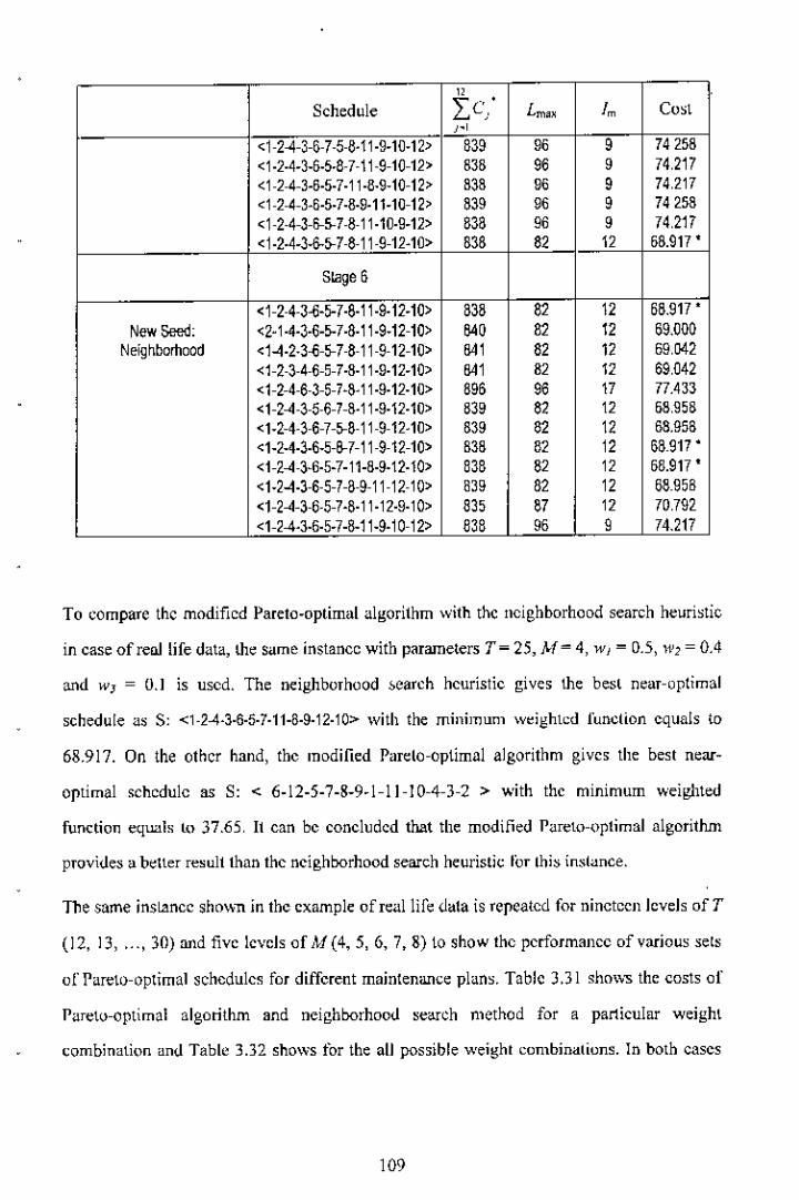
"Schedule Ie,' Lm" J. Co,l,.,~1-2-4-3-6-7 -5-8.11.9-10-12> 639 96 9 74258<1.2.4-3-5.5.8-7-11-9-10-12> 638 96 9 74,217<1-2-4-3-6.5.7.11.8.9.10-12> 838 96 9 74,217<1-2-4-3.5.5.7.8.9.11-10-12> 839 96 9 74258<1-2-4-3-6-~7 -8-11.10.9.12> B3B 96 9 74,217<1.2.4-3+~7 -8-11-9-12-10> 838 82 12 68.917 •

Stage 5

<1-2-4-3-{i-5-7.8.11.9.12-10> 838 82 12 68.917 •New$eed: <2-1.4.3.5-5-7.8.11.9.12-10> ~o 82 12 69.000

Neighborhood <1-4.2.3-M-7 -8-11-9-12-10> 841 82 12 69,042<1-2-3-4-6-5-7.8.11.9.12-10> ~I 82 12 69,042<1-2-4-6-3-5-7+11.9.12.10> 895 96 17 77.433<1-2-4-3-5-6-7-8.11.9.12.10> 839 82 12 68,958<1-2-4-3-6-7-5-8-11-9-12-10> 839 82 12 68.958<1-2-4.3.6.5-8-7-11-9-12-10> 838 82 12 68.917 •<1-2-4-H.5-7-11-8.9.12.10> 6BB 82 12 68.917 •<1.2-4.3-6-5-7-8-9-11-12-10> 639 82 12 68.958<1-2-4-3-6-5-7.8.11.12.9.10> 835 87 12 70.792<1-2-4.3.6.5.7.8-11.9.10-12> eBB 96 9 74.217

To compare the modified Pareto.optimal algorithm with the neighborhood search heuri~tie

in case of real life data, the same instance with parameters T= 25, M= 4, WJ = 0.5, W2 = 0.4

and W] = 0.1 is used. The neighborhood ~earch heuristic gives the best near-optimal

schedule a~ s: <1-2-4.3.6.5.7.11.6.9.12.10> with the minimum weighted function equals to

68.917. On the other hand, the modified Pareto-optimal algorithm gives the best near-

optimal schedule as S: < 6.12.5.7.8-9.1-11-10-4-3-2 > with the minimum weighted

function eqwls to 37.65. It can be concluded that the modified P<lreto-optimal algoritlun

pTovide~ a beller result than the neighborhood search heuristic fOTlhi~ insl<lnee.

The same instance shown in the example of real life data is repeated for nineteen levels of T

(12,13, ,.. , 30) and five levels of Af(4, 5, 6, 7, 8) to show the performance of various sets

of Pareto-optimal schedules for different maintenance plan~. Table 3.31 shows the costs of

P<lreto-optimal algorithm and neighborhood search method for a particular weight

combination and Table 3.32 shows for the all possible weighl combinalions. In both cases

109

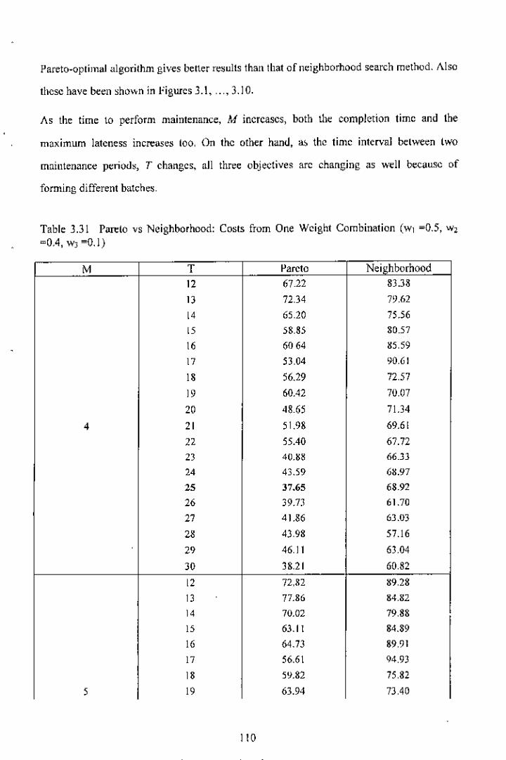
Pareto-optimal algorithm gives better results than that of neighborhood search method. Also

these have been sho"n in Figurcs 3.1, ,. " 3.10.

As the time to perform maintenance, M increases, both the completion time and the

maximum lateness increases too, On the other hand, a> the time interval between two

maintenance periods, T changcs, all three objectives arc changing as well because of

forming different batches.

Table 3.31 Pareto vs Neighborhood: Costs from One Weight Combination (WI=0.5, w~=OA, w] =0.1)

M T Pareto Nei 'hborhood12 67.22 83.3812 72.34 79.62

" 65,20 75.56

" 58,85 80.5716 6064 M5,5912 53,04 90,61

18 56.29 72.5719 60042 70.0720 48.65 71.34

4 21 51.98 69.61n 55.40 67.72

" 40.M8 66.3324 43.59 6M.97

" 37.65 68.9226 39.7J 61.7027 41.86 63.0328 4),98 57.16

" 46,11 63,04

20 38,21 60,82

12 72.82 M9,2812 77.86 M4,8214 70.02 79,88

I' 63.1 t 84.8916 64.73 89,9112 56.61 94,9318 5'1.82 75,82, 19 63.94 73.40

110

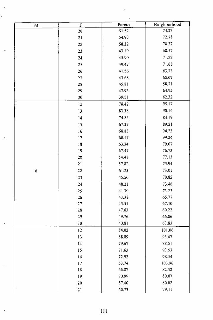
M T Pareto Nci hborhood

'" 51.57 74.23

" 54.90 72.78

22 58.32 70.37

23 43. t 9 68.57

24 45.90 71.22

25 39.47 71.0826 41.56 63.73

n 43.68 65.07

" 45.81 58.7J

" 47.93 64.95

30 39.51 62.32

" 78.42 95.1713 83.38 90.14

14 74,85 84.19

" 67,37 89,21

16 68,83 94,2]

17 60,17 99,24

18 63.34 79,0719 67.47 76.7320 54.48 77.1321 57.82 75.94

6 22 61.23 73.0 I23 45.50 70.8224 48.21 73.4625 41.30 73.2325 43.38 65.77n 45.51 67.10

" 47.63 60.22

" 49.76 66.86

JO 40.81 63.83

12 84.02 101.0613 88.89 95.4714 79,67 88,5115 71,63 93,53

16 72.92 98,54

17 63.74 103,96

18 66,87 82,32

19 70.99 80m

20 57.40 80.02

21 60.73 79.11

111

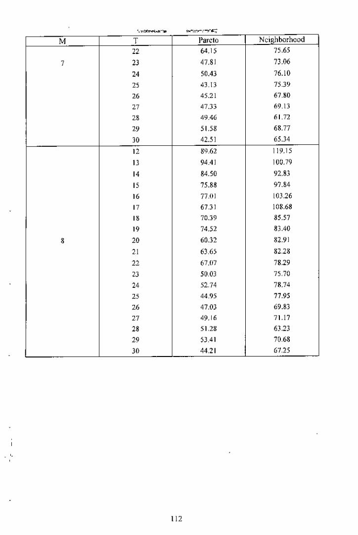
. - -M T Pareto Nd hborhood

22 64.15 75.65

7 23 47.81 73.0624 5Q.43 76.10

" 43.13 75.39

" 45.21 67.80

n 47.33 69.13

" 49.46 61.72

" 51.58 68.77

30 42.51 65.34

" 89.62 119.15

13 94.41 100.79

14 84.50 92.83IS 75.88 97.84

16 77.0] 103.26

" 67.31 108.68

" 70.39 85.57

19 74.52 83.40

8 20 60.32 82.91

21 63,65 82,28

22 67,07 78.29

2J 50,03 75,70

24 52,74 78.74

" 44.95 77.95

" 47.03 69.83

n 49.16 71.17

28 51.28 63.23

29 53.41 70,68

JO 44,21 67,25

'"

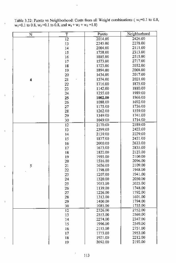
Table 3.31: Pareto vs Neighborhood: Costs from all Weight combinations (wI=O.l to 0.8,w2=0.1 to 0,8, WJ=0.1 to 0.8, and WI +W)+WJ=1.0)

N T Pareto Nci hborhood12 2014.00 2426.00IJ 2245.00 2278.0014 2004.00 2111.0015 1758.00 2313.0016 1885.00 2515.0017 1573.00 2717.00IS 1723.00 2032.0019 1894.00 200X.0020 1434.00 2017.00

4 21 1574.00 2021.0022 1716.00 1875.0023 1142.00 1880.0024 1255,00 1989,0025 1002.00 1966,0026 1088.00 1692,0027 1175.00 1736,002S 1262,00 1559.0029 1349,00 1741.0030 1049,00 1714.0012 2170,00 2589,0013 2399,00 2422,0014 2139,00 2229.0015 1877.00 2431,0016 2000.00 2633.0017 1673.00 2835.0018 1822.00 2122.0019 1993,00 2100.0020 1516.00 2096.00

5 21 1656.00 2109.0022 1798.00 1948.[)02] 1207.00 1941.0024 1320.00 2050.[)025 1053.00 2025.0026 1139.00 1748.0027 1226.00 1792.0028 1313.00 1601.0029 1400.00 1794.0030 1085.[)0 1755.0012 2326.00 2752.00I] 2553.00 2569.0014 2274,00 2347.0015 1996.00 2549.0016 2115.00 2751.[)017 1773.00 2953.0018 1921.00 2212.0019 1092,00 2192.00

II]

N T P<lwto Neighborhood6 20 1598,00 2175.00

21 1738.00 2197.0022 1880,00 2021.0023 1272.00 2002.0024 1385.00 2111.002S 1104,00 2084.0026 1190,00 1804.0027 1277.00 1848,0028 1364,00 1642.0029 1451.00 1847,00)0 1121.00 1796,00I2 2482,00 2915,0013 2707,00 2716.0014 2409.00 2465.00IS 2115.00 2667.0016 2230.00 2869.0017 1873.00 3083.00

I " 2020.00 2302,0019 2191.00 2284.00

7 20 1680.00 2254,0021 1820.00 2285,0022 1962.00 2094.0023 1337.00 2063.0024 1448.00 2184.002S 1155.00 2143.0026 1241.00 1860.0027 J 328.00 1904.0028 1415.00 1683.0029 1502.00 1900.0030 1169.00 1837.00I2 2638.00 3474.0013 2861.00 2863.0014 2544.00 2583.0015 2234.00 2785.0016 2345.00 2999.0017 1973.00 3213.0018 2119.00 2392.0019 2290,00 2376.0020 1762.00 2333.00

8 21 1902,00 2373.0022 2044.00 2167.0023 1400.00 2136.0024 1513,00 2257.0025 1206,00 2214.0026 1292.00 1916,0027 1379.00 1960,002. 1466.00 1724.0029 1553.00 1953.00]0 1217.00 J 890.00

114

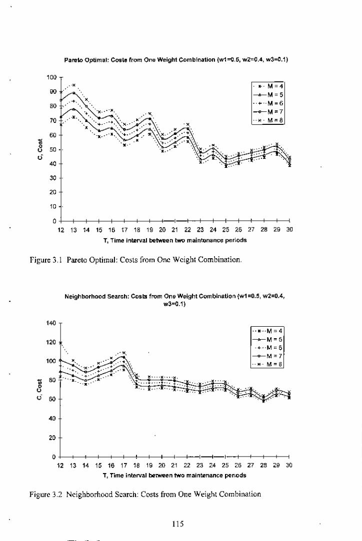
Pareto Op~m.l: C""tl5 from One Weight Combination (w1 "\l,5, wZ~O,4, w3"\l,1)

'" •" • •"' • • '-',"

_-x,'~.-.. '.-,-•

"' -X," • ,+ •• '

• •0 .~--U "' .." "

"""

o12 13 14 15 16 17 18 19 W 21

co.c. 0M"-'"__ M=5

.. •... M_6__ M~7

--*- M"8

I I I I I I I I

22 23 M 25 26 27 28 29 30T, Time interval between two mainwnance periods

Figure 3,1 Pareto Optimal: Costs from One Weight Combination,

Neighborhood Search: Costs from One Weight Combination (w1 =0.5, w2=0.4,w3~O,1)

'"'"'" • •

K'"-.,,-' •"" ,+.-• •• "' -'--. •

0 --.-UU '"

K •••

.".' "' ..-',- ."-- ....•

r.c.o,cM",."l__ M~5

-+ .. M = 6__ M ~ 7

--,,- M-S

o12 13 14 15 16 17 18 19 W 21

I l-l-"-~'-~-'~~-.'~ 23 M 25 26 27 28 29 30

T, Time interval between two maintenance pe"ods

Figure 3,2 Neighborhood Search: Costs from One Weight Combination

115

Pareto V$ Neighborhood: Costs from One Weight Combination(w1=O.5, w2=O.4, w3=O.1), and Maintenance Time M=4

hgure 3.3 Pareto vs Neighborhood: Costs from One W~ighl Combination

Pareto vs Neighborhood: Costs from One Weight Combination(w1=O.5, w2={1.4,w3=O.1), and Maintenance Time M=6

-0- Pa,el0 Oplimal-. - Neighborhood Search

'"

,"' .. , •

00

•00 00

0

00

•

~.' .•' .•..- ..• ..- .-.-

'.' .•..-' . .' - ...•

. ,,. " 1. " " " 1. ,. '0 21 " ,. ,. " m 2' ,. 0' "

T, Time interval betweentwo maintenanceperiods

Figure 3.4 Pareto vs Neighborhood: Costs from Onc Weight Combination

1!6

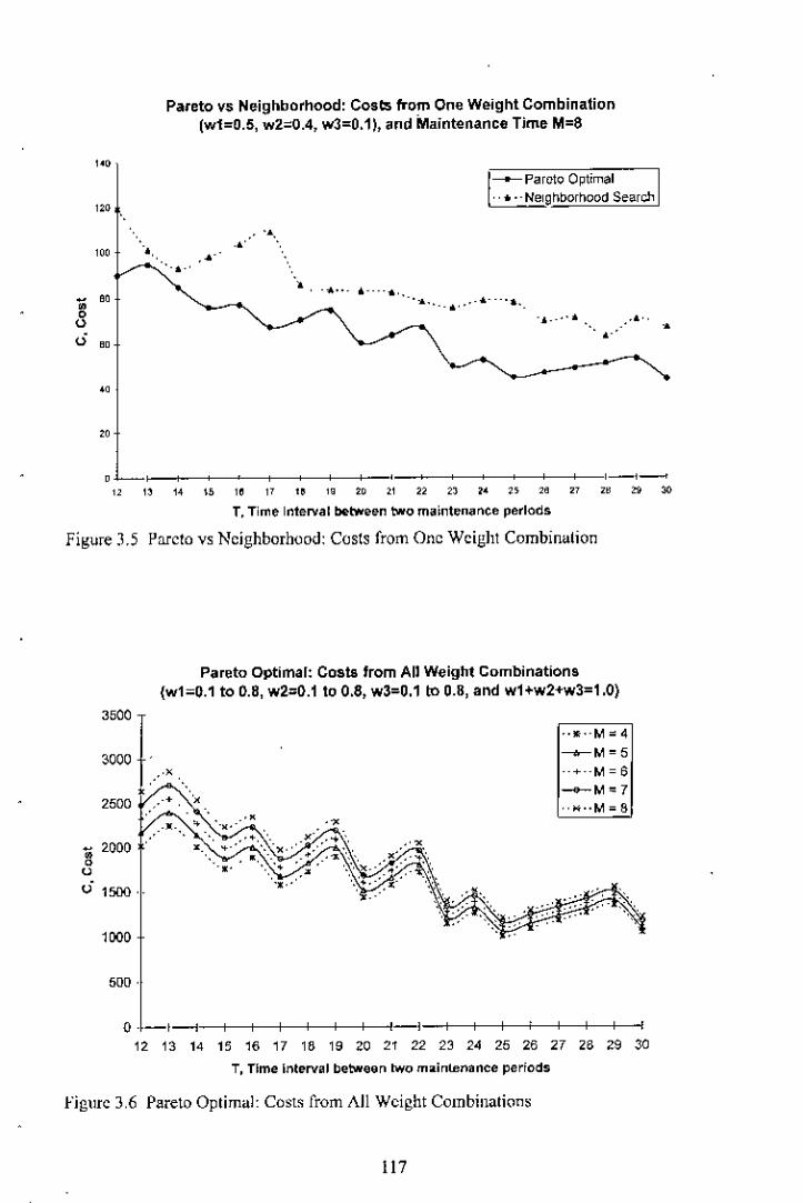
Pareto vs Neighborhood: Costs from One Weight Combination(w1=0.5, wZ=0.4, w3=0.1), and MaIntenance Time M=8

'"'"

I . Paroto Optimal, , •. -Neighborhood Search

'" • ."---'-'-'

•-.,.'

., - ..... ---. .- - ..•. -.-_.,. ..'" ..-.-' •

o ,--,-" " ,. " ,. " " " " ., " " ~ " " ,. " a _

T. Time Interval between two maintenance periods

Figure 3.5 Pareto vs Neighborhood: Costs from One Weight Combination

Pareto Optimal: Costs from All Weight Combinations{w1=0.1 to 0.8, wZ=0.110 0.8, w3=0.1 to 0.8, and w1+w2+w3=1.0}

..••.. M ~ 4----<r- M ~ 5--+--M ~ 6-<>--M ~ 7" ••..M~8

•• • • •• •2000 • • •• •

•

,"00I3000 :., x

•2500,uU 1500,

500 '

0-1--1 I I I I I I I I I I I I I I I

12 13 14 15 16 17 18 19 20 21 22 23 24 25 26 27 28 29 30T, Time Interval between two maintenance periods

Figure 3,6 Pareto Optimal: Costs from All Weight Combillation~

117

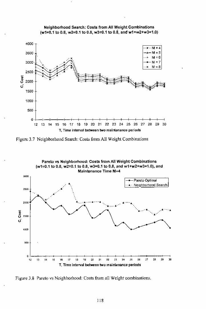
Neighborhood Search: Costs from AllWeight Combinations(w1=0.1 to 0.8, w2=0.1 to 0.8, w3=0.1 to 0.8, and w1+w2+w3=1.0)

4000I .. ~ ..M=43500 x --o-M_5

3000r , • M-6• •

__ M_7, • • ,~'':' • M~8

2500 "~. • • •• • • •" • • --',0 •u 2000 • • •u1500

'";,"'"0-'-' , , , , , , , , , , , , , ,

" " " " " " " " " " " " " '" '" " '" " "T,Timeintervalbetween twomaintenance periods

Figure 3,7 Neighborhood Search: Cos!.';[rom All Weight Combination,

Pareto vs Neighborhood: Costs from AllWeight Combinations(w1=0.1 to 0.8, w2=0.1to 0.8. w3=0.1 to 0.8, and w1+w2+w3=1.0), and

Maintenance Time M=4

__ Pareto Optimal

--. - Neighborhood Seeroh

~

•"" •

•"00

"0u ,-u

,=

". .....•,._' •.....- ..'.-.- "

'" ...' ." -- -.

o ,- __ ,_~_.

1. ,. " " ,. '7 ,. " '0 " " " ,. " " " " '" ~T,Timeintervalbetween two maintenance periods

Figure 3.8 P<tretovs Neighborhood: Costs from all Weight eombinalions.

I 18

Pareto vs Neighborhood: Costs from An Weight Combinations(w1=O.1 to 0.8, w2=O.1 to 0.8, w3=O.1 to 0.8, and w1+w2+w3=1.0), and

Maintenance Time M=6

,'-", •.",.,-•

r=;.=i".".;,,".Co',',"m'."--'- - •• - Neighborhood Search

•......

- ",,

,--,----"-----------" " ,. 1. m 21 ,. " • " " " u " ~T, Time interval between two maintenance periods

=

'"00

'"00,0000

uu .-.-

.00

• •• •• •• ••

Figure 3,9 Pareto vs Neighborhood: Costs from all Weigh! combinations.

Pareto va Neighborhood: Costs from All W",ight Combinations(w1=O.1 to 0.8, w2=O.1 to 0.8, w3={).1 to 0.8, and w1+w2+w3=1.0}, and

Maintenance Time M=8'000

__ Pareto Opllm"1

--.- Nel hborhood Search

•,"

'""U

'

0000

u

- ..•.,... ' •.

•....- •.

•00

," ,. ,. " " '7 " " ro " '2 " 2. ,. " ,. ,a " '0

T, Time Interval between two maintenance periods

Figure 3.10 Pareto vs Neighborhood: Costs from all Weight combinations.

119

Various maintenance plans give more flexibility to the >cheduler (or decision-maker) to

make a decision according to the preference and available maintcnance alternativcs.

Moreover, to tnmsform multiple obJectivcs into a single objective optimization problcm, a

weighted ~ombination is considered. Thc wcights may be timc or situation dependent and

sum of the weights must be equal to I. Typically, a scheduler may not know the exact

weights and may want to perform a parametric analysis to get a feeling lor the trade-offs. In

this work, all possible weight combinations of three objcctivcs are performed to calculate

the weighted function, rhcse possible combinations for each ~chcduleof Pareto-optimal set

arc also presented. The reason of presenting all the possible weighl-~ombinations is thaI the

importance level of each objective can be different according to the schcduler. These results

are summarized in Appendix A Appcndix A provides cost of Pareto-optImal schedules

which is dependent on total completion timc, maximum lateness, and machine idle time for

each combination of T and !vi for lhe all possible weight combinations. Table 3.29 only

provides Pareto-optimal schedules with one possible weight combinalion (i.e., WI = 0.5, w)=

0.4, 11') = 0.1), while Appendix A provides information on the all possible weight

combinations of three objeclives (F',Lm,,', f '). Also the sum of the costs of each Pareto-

optimal schedule for all the weight combinations is calculated in order to givc an overall

reslllt of certain Pllreto-optimal ~~hedule. A schedule with the minimum sum of the co,ts is

the best schcdule within the set of Pareto-optimal schedules for a certain maintenance plan.

Table 3.33 presents the sum of the cosls of each Pareto-optimal schcdule for all the weighl

combinations according to a certain maintenance plan. It also provides the Pareto-optimal

schcdule which gives the minimum cost for each maintenance pilln. A dccision maker can

decide which Pareto-optimal schedule and which combination or weights he/shc wants 10

use according to an available maintenance plan (i-e., rand M values), It can be concluded

that the objective c( F' ,Lm,,, ' , f ') is depended on T and /vl, and this shows thc importance

ofa good mmntcnancc plan, The minimum cost is 1002,00 for T=25 and lor M=4.

120

Table 3.33 Summary of performance measures for all different alternative parameters

T M SPTIEDD SPTIEDD S [I] S[2] S[3] Sr4]

12 4 2709.00 2014.00 2457.00 2457.00 2517.00 2709.005 2860.00 2170.00 2632.00 2632,00 2656.00 2860.006 3011.00 2326.00 2807.00 2807,00 2807.00 3011.007 3162.00 2482.00 2982.00 2982,00 2982.00 3 [62.008 3313.00 2638.00 3157.00 3157,00 3157.00 3313.00

II 4 2473.00 2264.00 2245.00 2245,00 2269.00 2473.005 2603.00 2419.00 2399.00 2399.00 2399.00 2603.006 2733.00 2574.00 2553.00 2553,00 2553.00 2733.007 2863.00 2729.00 2707.00 2707.00 2707.00 2863.008 2993.00 2884.00 286\.00 2861.00 2861.00 2993.00

14 4 2208.00 2527.00 2507.00 2004.00 2004.00 2208.005 2319.00 2682.00 266\.00 2139.00 2139.00 2319.006 2430.00 2837.00 2815.00 2274.00 2274.00 2430.007 2541.00 2992.00 2969.00 2409.00 2409.00 2541.008 2652.00 3147.00 3123.00 2544.00 2544.00 2652.00

IS 4 2415.00 1758.00 1758.00 2235.00 2235.00 2415.005 2526.00 1877.00 1877.00 2370.00 2370.00 2526.006 2637.00 1996.00 1996.00 2505.00 2505.00 2637.007 2748.00 2115.00 2115.00 2640.00 2640.00 2748.008 2859.00 2234.00 2234,00 2775.00 2775.00 2859.00

16 4 2041.00 1961.00 1925,00 1885.00 1885.00 204\.005 2132.00 2080.00 2042.00 2000.00 2000.00 2132.006 2223.00 2199.00 2159.00 2115.00 2115.00 2223.007 2314.00 2318.00 2276.00 2230.00 2230.00 2314.008 2405.00 2437.00 2393,00 2345.00 2345.00 2405.00

17 4 1684.00 2164.00 1597.00 J 573.00 2084.0n 1684.005 1759.00 2283.00 1698.00 J 673.00 2[99.00 1759.006 1834.00 2402.00 1799.00 1773.00 2314.00 1834.007 1909.00 2521.00 1900.00 J 873.00 2429.00 1909.008 1984.00 2640.00 2001,00 J 973.00 2544.00 1984.00

18 4 1831.00 1725.00 1723.00 J 725.00 1723.00 183[.005 1906.00 1824.00 1822.00 J 824.00 1822.00 1906.006 1981.00 1923.00 1921.00 J 923.00 1921.00 1981.007 2056.00 2022.00 2020,00 2022.00 2020.00 2056,008 2131.00 212\.00 2119.00 2121.00 2119.00 2131,00

19 4 1978.00 1896.00 1894,00 1896.00 1894.00 1978,005 2053.00 1995.00 1993.00 1995.00 1993.00 2053,006 2128.00 2094.00 2092.00 2094.00 2092.00 2128.007 2203.00 2193.00 2191.00 2193.00 2191,00 2203.008 2290.00 2292.00 2290,00 2292.00 2290.00 2290,00

20 4 2125.00 1434.00 2065,00 2067.00 2065.00 2125,005 2200.00 1516.00 2164.00 2166.00 2164.00 2200,006 2275.00 1598.00 2263,00 2265.00 2263.00 2275,007 2362.00 1680.00 2362.00 2364.00 2362.00 2362,00, 2461,00 1762.00 2461.00 2463.00 246[.00 2461,00

21 4 1719.00 1576.00 1667,00 J 574.00 1612.00 1719.005 1777.00 1658.00 1740.00 1656.00 [670.00 1777.006 1835.00 1740.00 [813.00 17J&,OO 1740.00 [835.00

121

T M SPT/UJD SPI/EOD S[I J S[21 5[3 J 5[4]

7 1893.00 1822,00 1898.00 1820.00 1822,00 1893.008 1951,00 1904,00 1983.00 1902.00 1904,00 1951.00

22 4 1837.00 1718,00 1718.00 1716,00 1730,00 1837.005 1895,00 1800.00 \800.00 1798,00 1800,00 1895.006 1953,00 1882,00 1882.00 1880.00 1882,00 1953.007 2011.00 1964.00 1964.00 1962.00 1964.00 2011.008 2069,00 2046,00 2046.00 2044,00 2046,00 2069.00

23 4 1453,00 1860.00 1835.00 1142.00 1224.00 1453.005 1506,00 1942,00 1916.00 1207,00 1265.00 1506.006 1559,00 2024.00 1997.00 1272.00 1306.00 1559.007 IG12,00 2106.00 2078.00 1337,00 1347.00 1612.008 1665,00 2188.00 2159.00 1402,00 1400.00 1665.00

24 4 1554.00 1686.00 1660,00 1255,00 1313.00 1554.005 1607.00 1755.00 1728.00 1320,00 1354.00 1607.006 1660.00 1824.00 1796.00 1385,00 1395.00 1660.007 1713.00 1893.00 1864,00 1450.00 1448.00 1713.008 1766.00 1962.00 1932.00 1515.00 1513.00 1766.00

25 4 1655.00 1429.00 1002.00 1368.00 1402.00 1655.005 1708.00 1496.00 1053.00 1433,00 1443.00 1708.006 1761.00 1563.00 1104.00 1498.00 1496.00 1761.007 1814.00 1630.00 1155.00 1563.00 1561.00 1814.008 1867.00 1697.00 1206.00 1628.00 1626.00 1867,00

26 4 1756.00 1088.00 1089,00 1481.00 1491.00 1756.005 1809.00 1139.00 1140,00 1546.00 1544.00 1809,006 1862.00 1190.00 1191.00 1611.00 1609.00 1862,007 1915.00 1241.00 1242,00 1676.00 1674.00 1915,008 1968.00 1292.00 1293,00 1741.00 1739.00 1968,00

27 4 1466.00 1175.00 1176.00 1265.00 1359.00 1466,005 1505.00 1226.00 1227.00 1304.00 1398.00 1505,006 1544.00 1277.00 1278.00 1343.00 1437.00 1544,007 1583.00 1328,00 1329.00 1382.00 1476.00 1583,008 1622.00 1379,00 1380.00 1421.00 1515.00 1622,00

28 4 1541,00 1262,00 1263.00 1340.00 1434,00 1541.005 1580.00 1313.00 1314.00 1379.00 1473,00 1580.006 1619.00 1364.00 1365.00 1418.00 1512.00 1619.007 1658.00 14[5.00 1416.00 1457.00 1551.00 1658.008 1697.00 1466.00 1467.00 1496,00 1590.00 1697.00

29 4 1616.00 1349.00 1350.00 1415.00 1509.00 1616.005 1655.00 1400.00 1401.00 1454,00 1548.00 1655.006 1694.00 1451.00 1452.00 1493,00 1587.00 1694.007 1733.00 1502.00 1503.00 1532.00 1626.00 1733.008 1772.00 1553.00 1554.00 1571.00 1665.00 1772.00

30 4 1535.00 1054.00 1053.00 1049,00 1428.00 1535.005 1572.00 1103.00 1089.00 1085.00 1465.00 1572.006 1609.00 1152.00 1125,00 1121.00 1502.00 1609.007 1646.00 1201.00 1173.00 1169,00 1539.00 1646.008 1683,00 1250,00 1221.00 1217.00 1576,00 1683.00

• Minimum sum of the cost for each m";n!en"ncc plan

122

3.9 ConclusionA multi-criterion non-preemptive scheduling that reduces thc total cost of the problem is

considered in thi~ study. Thrce eriterions are considered: reduction of flow time, maximum

tardiness, and machine idle time in a p~riodieally maintained single machine problem. The

trade-oIl':;between the flow time and maximum tardiness is comparatively simple, but the

trade-ofT between minimum flow time, maximum tardiness and machine idle time is a

complcx problem. In this study a new kind of approach that allows thc use of weight~d

aggregation of th~ eriterions is presented. Th~ new approach started with an initially

obtained set of Pareto-optimal schedule for flow time and maximum l<lrdm~ssminimization

problem. It then introduces machine idle time and maintcnance time in each of these

initially foond s~quenees. Onec the rescheduling of machine maintenance and idleness

period of machine is completed, it then ealeulates th~ new values of flow time, maximum

tardiness and machine idle time. All possible weight combinations fur the eriterions arc

computed. The search for thc minimum tol<llcost among all the Pareto-optimal schedules

with the assigned weights on cnterions is obtained. Finally, a promising s~quence is chosen

that gives the minimum total cost for a particular set ofwcights on the criterions.

A modified Pareto-optimal algorithm for such techniqu~ has been devised and several

properties associated with problem have also been inve~tigated. An algorithm for

neighborhood search technique has been proposed to provid~ the near-optimal solution for

the problem. The performance of the modified Pareto-optimal algorithm hilSbeen evaluated

by comparing its solution with the solutions derived by the neighborhood search heuristic.

Results have shown that the modified Pareto-optimal algorithm provides a better solution

than th~ neighborhood search heuristic, Jlld this show~ the efficiency of the modified

Pareto-optimal algorithm

123

Chapter 4Distribution

4.1 Introduction

Supply-chain management seeks (0 synchronize a firm's processes und (hose of its suppliers

to match the now of materials, services, and information with customer demand. Supply-

chain management has strategic implications because the supply system can be used to

achieve important competitive priorities. It also involves the coordination of key processes

in the finn such as order placement, order fulfillment, and purchasing, which are supported

by marketing, finance, engineering, infonnation systems, operations and logistics.

Successful supply-chain management requires a high degree of func(ional and

organizational integratiun, The interconnected set of linkages belween suppliers of materials

and services that spans the transformation of raw materials into products and serVICes and

delivers them to a firm's customers is known as the supply-chain. The value of supply-chain

management becomes apparent when the complexity of the supply-chain is recognized. The

performance of numerous suppliers determines the inward flow of materials. The

performance of the lim]'s marketing, production, and distribution processes determines the

outward flow of products. Traditionally, organih1tions have divided the responsibility for

managing the flow of materials and service~ among three departments: purchasing,

produellon, and distribution.

Distribution is the management of the flow of materials from m~nufacturers to customers

and from warehouses to retailers, involving the storage and transportation of products, 11

may also be responsible for finished goods inventories and the selection of transportation

service providers. Typically, firms me willing to undergo the rigors of developing integrated

supply-chain progress through a scries of phases. The starling point for most linus, external

suppliers and customers arc considered to be independent of the firm. Relations with this

124

entities are formal, and there is liuk ~haringof operating information and costs. Internally,

purchasing, production, and distribution act independently, ea~h "ptimi~ing its Own

activities without considering other entitics. Traditionally, it is assumed that a parameter

needs to be optimized through right opcrations managcmcnt technique. Howevcr, there is no

basis as to why a particular parametcr is selected as the objective function. This research

provides an idea that AHP which is a technique of MCDM (Multi Criteria Decision

Making) technique can be used to justify selection of the right parameter as the objective

function of an optimization technique.

After determining whcrc the demand for goods and scrvices is grcatcst, managcmcnt must

select a location for the facility that will supply that demand. For warehOLlsingand

distribution operations, transportation costs and proximity to markets are extremely

important. With a warehouse nearby, many firms can hold inventory closer to the cu~tomer,

thus reducing delivery time, transportation cost and promoting sales.

4.2 Multi Criteria Decision Making

In many real world situations, there are many, often conflicting, objectives. Fur instance, if

there arc multiple potential suppliers requiring evaluation with conllicting criteria, such as

quality of material, timely delivery, price, quickness of delivery, m,maging sudden ordering,

etc., then it requires a solution [65, 66]' Or, in selecting thc right communication system,

scveral conflicting criteria, ~ueh as speed of communication, cost, reliability of transaction,

maintainability, etc. becomes Important, which requires a combination of qualitative and

quantitative solution [67J. As another instance, a multi eritcria solution is required when a

selecting the right manufacturing system or material handling system olll of many available

ones [68]. In an advertising campaign, therc might be a numbcr of dilTcrent market

segments to reach. In lire station problem, there might be two types of objectives:

minimizing response time und minimizing service cost. The models discussed here,

125

however, only allow one objective, How can they be adapted to handle multiple objective~?

This requires Multi Criteria Decision making (MCDM) [69].

However, there are a numbcr of fundamental problems when there are multiple objectives.

For instanee, in case where there arc a number of decision makers. eaeh with a prcference

ordering over a number of alternatives. The goal is to choose the "fair" alternative that

aggregates the prererence~ of the Jeci~ion makers. This is an example of multiple criteria

decision making (each decision makers represents one criteria), and it is required to balance

those objectives in a fair \vay. The field of ~tudy that addres;es these problems is called

MCDM, and is filled with pessimistie results [65].

These issue~of aggregating views about alternatives arc difficult even with a single decision

maker (or a group trying to reach consensus). Imagine trying to locate an "obnoxious

facility", like a waste disposal plant. There are mally factors that go illto such a Jecision.

These might include distance from highly populated areas, transportation costs, land costs,

geological ~tability, and so on. Is there any organi/.ed way that one might think about

determining the relative importance of these factors and then go about comparing

alternative sites? One technique that is used is the Analytic Hierarchy Process (AHP),

whieh uscs very simplc calculations to try to put numerical values on factors and

alternatives [70, 71J.

Finally, a logical question follows as to how these models be used in more complicated

situations, where the ehoiec is not just a number of alternativcs, but rather an entire decision

set, say represented by a lincar program. Obviously, a lincar programming approach tQ~uch

situations will at least theoretically provide better solutions, But it has been proved ill many

situation~ that MCDM, more specifieally AJ-JP, ean offset the benefits of more fine-tuned

optimality over po~sibility of"gelling a solution in a realistic time period [72].

126

4.3 Basic Concepts of Analytic Hierarchy Process (AHP)

Devdoped by Thomas Saaty, AIlP provides a proven, effective means to deal ",ith complcx

decision making and can assist with identifying and weighting selection criteria, analyzing

the data collceted for the criteria and expediting the dceision-making pro~ess [70-72]. i\

large number of situations, with varieties of variables, havc been analyzed using AHI'

mcthod [73-74].

i\HP helps capture both subjectivc and objective evaluation mea~",rcs, providing a useful

mechanism for checking the eon,isteney of the evaluation measures and alternatives

suggested by the team thus reducing bias in decision making. Combined with meeting

autumation, organizations can minimize common pitllllls of team decision making process,

sueh as lack of foens. planning, participation or ownership, which ullimalely are eostly

distractions that can prevent teams from making the right choice.

The first slep IS lor the team to decompose the goal illto its constituent parts, progressing

from the general to (he specilic. In its simplest form, this structure comprises a goal, ~riteria

and alternative levels. Each set of alternatives would then be furlher divided into an

appropriate level of detail, re~ognizing that the more criteria included, the less important

each individual criterion may become.

Next, a relative weight is w;signed to each one. Each criterion has a local (immediate) and

global priority. I'he sum of all the criteria beneath a given parent criterion in each tier of the

model must equal olle. Its global priority shuws ils relative importance within the overall

model.

Finally, alter the criteria are weighted and the information is collected, put the information

into the model. Scoring is on a relalive basis, not an absollile basis, comparing one choice to

another. Relative seorcs for each choice are computed within each lcaf of thc hierarchy.

Scores are then synthesiL.Cu through the model, yielding a compu"ile ,cure for cach choice

at every tier, as well as an overall score.

127

Theoretical Details of AHP

Analytic hierarchy is a framework fol' solving a problem. 'Jhc analytic hierarchy process is a

systematic procedure for representing the elements of any problem. Jt organiles the basic

rationality by breaking down a problem into its smaller constituents and then calls for pair-

wise comparison judgments, to develop priorities in each level.

The analytic hierarchy process provides a comprehensive framework to cope with intuitive,

rational, and irrational fact(Jrs in making judgments at the same time. It is a method of

integrating perceptions and plllposes into an overall synthesis. The analytic hierarchy

process does not require that judgments be consistent or even tnmsitivc. 'lhe degree of

consistency (or inconsistency) of the jndgment is revealed at the end of the analytic

hierarchy process.

People making comparisons nse their feelings and judgment. Both vary in intensity. T(J

distinguish among different intensities, the scale of absolute numbers in the l<lbleis useful.

Table 4.1 Measurement scale

Intensity (Ifrclative imp(lrtanee Explanllti(ln

I (equal importance)Two activitie~ eontribllle equally to theobjective

3 (slight imporlance (Jrone over another)Experience andjudgmcnt slightly favorone activitv over another

5 (essential or ~trong importance)Experience andJudgment strongly favorone aetivitv over another

7 (demonstrated importance)An activity is strongly favored and itsdominance i~demonstrated in nraetiee'jhe evidence favoring one activity over

9 (ab~{)luteimportance) another is (Jrthe highest possible orderof affirmation

2,4,6,8 (inkrmediate values between the When ~ompromise is neededtwo adja~ent judgments)Recipro~als (Jfabove nonzero numbers (if anactivity h" '"' of <h, above numbersassigned to it when compared ""ith sccondactivity, ,h, second activity has thereeinroeal value when comnareu to the first)

128

The ~nalytie hierarchy process can be decomposed into the followmg steps. Particular steps

may be emphasized more in some situations than in others. Also a:. noted, interaction is

generally useful for stimulation and for representing different points of view.

\. Define the,problem and determine what knowledge is sought.

2. Structure the hierarchy from the top (the objective~ from a broad perspective)

through the intermediate leveb (criteria on whieh subsequent levels depend) to the

lowest level (which usually is a list of the alternatives),

3. Construct a set of pair-wise comparison matrices for each of the lower levels, one

matrix for eaeh element in the 1cvel immediately above, An element in the higher

level is said to be a governing element for those in the lower level since it

conlribule~ 10 it or affects it. In a complete simple hierarchy, every element in the

lower level affects every element in the upper level. The element~ in lhe lower level

are then compared 10 each other, ba:.ed on their effect on the governing clement

<lbove.This yields a square matrix of judgments. The pair-wise comparisons are

done in terms of which clement dominates the other, These judgmenls arc then

expressed as integers according to the judgment values in the table. If clement A

dominates element B, then the whole number integer is entered in row A, column 13,

and lhe reciprocal (fraction) i, entered in row B, column A.

4. There arc n(n - 1)12 judgmenls required to develop lhe sel of matrices in step 3,

where n is the number 01' elements in the lower level.

5, Having collected <Ill the paiH'iise comparison data and entered the reciprocals

together with n unil entries down the main diagonal, the eigenvalue problem Aw =

)'m""w is solved and con~i~teneyis tested, using the deparlllTeof Am" from n (see

below).

6. Steps 3, 4, and 5 are performed for al11cvelsand e1u~tersin the hierarchy.

7. Hierarchal composition is now used (0 weigh the cigenveclor~ by lhc weights of the

criteria, and the sum is taken over all weighted eigenvector enlries corresponding to

those in the lower level orthe hierarchy.

129

8, The consistency ratio of the entire hierarchy is fuund by multiplying eaeh

consistency index by the priority of the corresponding criterion and adding them

together. The resuh is then divided by the same type of expression, using the random

consistency index cOITe~pondingto the dimensions of each matrix weighted by the

priorities a~ berore. The consistency ratio ~hould be about 10% or less to be

acceptable, If not, the quality of the judgmenb ~hould be improved, perhaps by

revising the manner in which qucstions arc asked in making the pair-wise

compansons, If this should rail to improve consistency, it is likely that the problem

should be more accllTatelystructured; that is, similar elements should be grouped

lmder more meaningful criteria. A return to step 2 would be required, although only

the problematic parts orthe hierarehy may need revision.

The main advantage of this mcthod is its ability to handle a complcx problem to prcpare a

hierarchy of choice and reasons of choiccs through decomposition and ~ynthesis. It can

compare different alternatives and attribldcs using a sealc of relative importance.

The numerical results of auributcs arc prescnted to the decision maker to assign rclativ'e

importance according to a predefined scale. Now ajudgmcnt matrix is prepared.lt i~an (n x

n) matrix. From thc judgment matrix, nomlaliz.edweights arc calculated as follows.

"" " """ " "

G,,,m<lri,' m,an , Normalized we'Rhls ,"" " "1 " "

where, i and j are the altemative~ or attributcs to be compared. ail IS a value which

represents comparison between alternatives / attributes i andj.

The above judgmcnt matrix may be consistenl if II"' ajA = ail, for all values of i, j, k.

In the abovc matrix, sum of all c1cmentsin a column i<

130

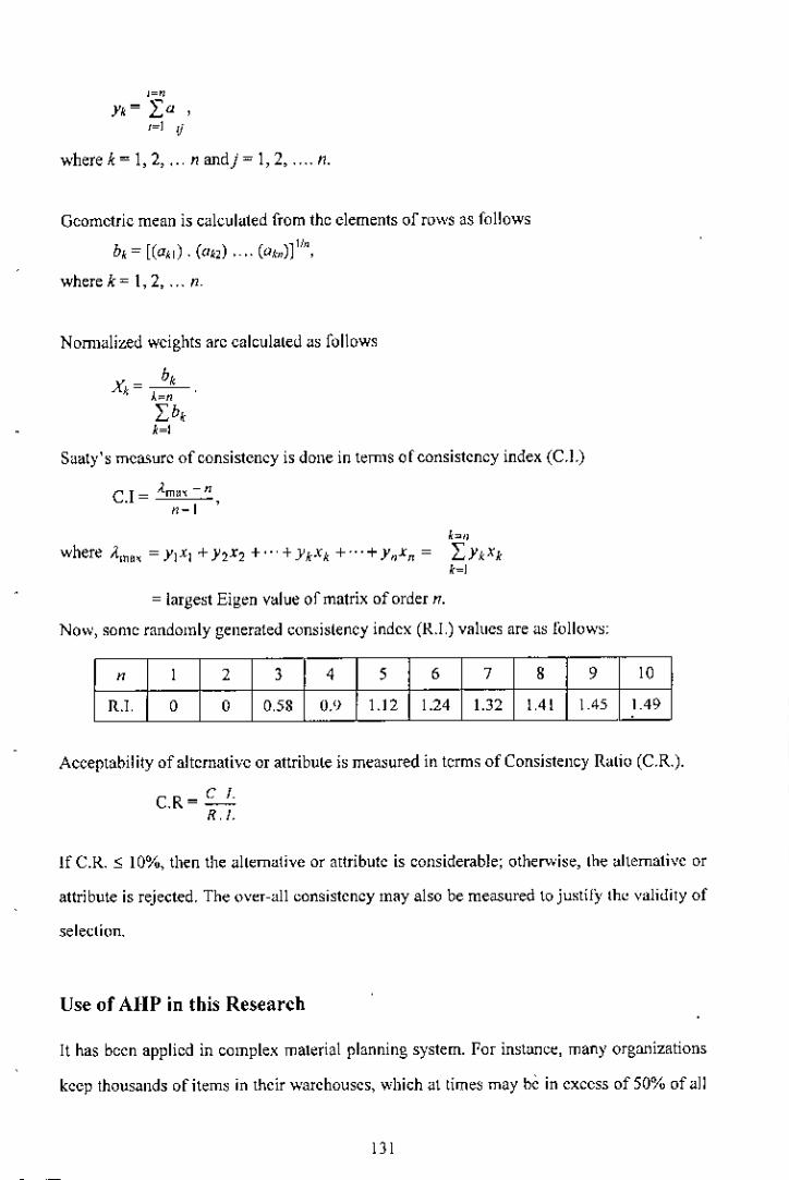
J="y, = La1=1 Ij

where k = 1, 2, , .. nand) = 1, 2, .... n.

Geometric mean is calculated from the clements ofrows as follows

b, = [(ail). (ad, ,.(atn)J1!",

wherek=I,2, ... n.

NOffilalized weights arc ealculaled as follows

b,Xk=--.1.="Lb,.=1

Suaty's measure of consistency is done in teffilS of eonsistcncy index (C.l.)

C.I =

b"where ,t,"" = y1x1+ Y2X2 +, ..+YkXk + ...+ y"x" = LYkXk

!=I

= largest Eigen value of matrix of order n.

Now, some randomly generated consislency index (R.I.) values are as follows:

" 1 2 3 4 5 6 7 8 9 10

R.I. 0 0 0.58 0.'> 1.l2 1.24 1.32 1.41 1.45 1.49

Acceptability of alternativc or attribule is measured in terms of Consistency Ralio (C.R.).

C.R=Cl.R. I.

If C.R. S; 10%, then the allernative or attributc is considerable; other.vise, lhe alternativc or

attribute is rejected. The over-all consistcncy may also be measured to justify th~ validity of

seleclion.

Use of AI-IP in this Research

It has becn applied in complex material planning system. For instmJce, many organizations

kcep thousands ofitem~ in thcir warchouscs, which at limes may be in cxcess of 50% of all

the company's expenses. Each item typically possesse, its own unique characteristic" since

these are typieall} sourced from different suppliers. Under these circumstances, it may not

be rational or economical to deal with each item via a gcnerie material control system

(either push or pull system). A mulli-eriteria approach that utilizes the Analytic Hierarchy

Process (ABP) has been reported in an occasion. The paper proposes a modified AIIP, such

that it is able to classi(y the materials and components for different Material Planning anci

Control Systems (MPCS), i.e. Kanban, MRP, hybrid, and Re-Order Point (ROP) Systcms.

This modified AI-IP is better at rising to the ehaJIenge of diversity of material characteristics

in deriving an optimal decision for MPCS system selection [75J. This research aims at

util izing this concept in evaluating a different situation of material planning, where the right

parameter needs to be selected through AHP. Traditionally, it is as~umed that a parameter

needs to be optimized through right operations management technique, However, there is no

basis as to why a particular parameter is selected as the objedive f,mction. 111is research

provides an idea that AlJP can be llsed to justify selcction of the right parameter as the

objective function of an optimization technique.

4,4 Problem Description

Manufactunng firms rarely seIl directly to the ultimatc cuSlOmer, Some buyers are

manufacturing firms that buy products and services and incorporate them into their own

omput. Othcr buyers are wholesalers, retailers und distriblltion firms who buy the products

and then distribute them further down the chain towards the ultimate customers.

What difference docs it make whether the firms acts as the bllyer from suppliers or a

suppliers to othcr buyers? Buyers talk about such thmgs as schedulcs, lot sizes, costs, lead

timcs, and just-in-timc delivery, Firms ollen take thi~ as a gi vcn whcn finding suppliers who

comply with their demands. Schedules sent to the firm by their customers may not fit their

sehcdules, The just-in-time deliveries that thc firms demand from their vendors may not bc

compatible with, for example, their job-shop production,

132

The principles of MRP ~an also be applied to distributlOn inventories, or sto~ks of items

held at retailers and distribution centeR<.Consider the distribution system of which the top

level represents retail stores at various locations through the country. The middle levels arc

regional distribution centers that replenish retail store inventories on reque~LThe bottom

level consists of one or more plants that ~upply the distribution centers.

The distribution planning is an inventory control and scheduling technique that applies

MRP principles to distribution inventories. An inventory record is maintained fur each item

at each location, Use of distribution planning requires an integrated information system. jf

the manufacturers operates its own distribution centers and retail stores, called fixed

quantity model or self distribution, gathering demand information and relaying it back to the

plants is easy. If the manufacturer does not own the distribution centers and retail store~

then ;t ;s called fixed time period model or contacted distribution. In this research work

three models are considered.

I) Fixed -quantity model or Self di~(ributionmodel (Mil,

2) Fixed- (ime period model or Contracted distribution model (M2l,

31 Partly self and partly contracted distribution or Mixed model (!vh),

The basic distinction is that fixed-order quantity models are "~v~nt trigg~red" and fixed-

time period models are "time triggered." That i~, a (i"ed-order quantity model initiates an

order when the event of reaching a specified reorder level occurs. This event may take plaee

at any time, depending on the demand for the items considered, i.e, it is under firm's

control. In contrast, the fixed.time period model is limited to placing orders at the end of a

predetemlined period; only the passage of time triggers the model. To use the fixed-order

quantity model which places an order when the remaining inventory drops to a

predetermined ordcr point, the inventory rcmaining must be continually monilored. Thus,

the Jixed-order quantity model is a perpetual system, which requires that every time a

withdrawal from inventory or an addition (0 inventory is made, records must be updated

133

to ensl.lrethat the reorder point has or has not been reached. In a fixed.time period model

counting takes place only at the review period.

In this research work it has been assumed that there arc four criteria that are being I.Isedto

evaluate distribution model. Four criteria are management effort, cost, integration,

reliability. Further, it has been assumed that there are three distribution models (MI, MJ•

Management effort: TIle idea is to apply a total system approach to managing the flow of

information, materials, and services from raw material suppliers through factories and

warehouses to the end cu~tomer. Recent trends such as outsourcing and mass customilation

are forcing companies to find l1exible way" to meet customer demand. The focus is on

optimizing those core activitie~ to maximize the speed of response to changes in customer

expectations.

For many years, few companies regarded the operating processes of a firm as a source of

competitive advantagc. The goals of the firm relating to operations were cost reduction and

improved labor utilization. Decisions were made on narrow, tactical grounds. This was the

domain of the technically oriented engineering specialists. Little attention was paid to how

the processes, which deliver the goods aDd ~erviees of the firm, fit with its strat;,gy. To

regain a competitive position, wcstcrn managers realized that major change wis required.,,1r~

Operations had to become an integral part of the corporate strategy. This corporate strategy

had to be responsive to the needs of the firm's customers. Companje~ learned how different

customers had different priorities. The old idea that cost minimization wu.:;always the goal

Wasshattered. A new fleld called operations strategy emerged.

Operations strategy offers a new per~pective about operations problems, as well as a new sel

of concepts and techniques. The new perspective relates to the context within which

decisions arc made. This context considers the needs or Cl.lstomertogether with the overall

strategy of the liml. A company that is considered to be world elass recognizes that its

ability to compete in the market place depends on developing an operatioll~ ~trategy that is

properly aligned with its mission of serving the customer.

134

Cost: Within every industry, thcrc is usually a segm~nt o[the market that buys strictly on

the basis of low cost. To successfully compete in this niche, a firm must be the low-cost

producer, but even doing thi~ does not always guarantee profitability and success,

Products sold strictly on the basis of cost are typically commodity like in nature. In other

worth, customers eallllot distinguish the product~ of one firm from those of other, as a

result, cuslorner~ use cost as the primary determinant for muking a purchasc,

However, this segment of the market is frequently very large, and many companies are

lured by the potential for significant profits, which they associate with lhe large unit

volumes of product. As u consequence, ~ompeti(ion in this segment is fierce and so is the

failure rate. After all, there can only be one low cost producer, which usually eslablishes the

selling price in the market.

Integration: Successful supply-chain maJIagement requires a high dcgrcc of functional and

organiLutional integration. Such integration docs not happen overnight. The firm initiates

internal integration by creating a materials management department. Muteriuls management

is concerned with decisions about purchasing materials and services, inventories, produclion

levels, staffing patterns, schedules, und ,hstribl.dion. The focus is on the integration of those

aspects of the supply-chain directly under the firm's control to create an internul supply-

chain. Firms in this phase utilize a seamless infOlmation and materials control syslem Irom .' '.'.

distribution to purchasing, inlegrating markeling, finance, accounting, and operations. The

inlernal supply-chain is extended to embrace suppliers and customers, thcrcby linking it to

the external supply-chain, which is not Clndcrthe dircct control of the firm. Thc firm must

change its focus from a product or service orientation to a customer orientalion.

Reliability: Another dimcnsion of quality related to product design is reliability, which

refers to the probability that thc product will bc functional whcn uscd. Products often

consist of a number of componcnts that all must be operativc for thc product to perform as

intended. Suppose that u producl has u.number "I' subsystems, each with its own reliability

135

measure, The reJiabliity of eaeh subsystem contrihute~ to the quality of the total system.

Di~lnbution reliability relales 10 the abihl} of the firm to supply the prOl.luetto the cuslomer

on or bel"ore a promised delivery due dale.

4.5 Computational Results

There arc four criteria lhat are being used to evaluate the models are management dTort,

co,>t, reliability, and integration. Furlher, "s,>ume that models MI, l\h, MJ are being

eongidered. rhe measurement scale and hierarchy for this applicalion are shown. For

analysis purpose, primary data "nd information have been eolleclcd from ~eveml n"lional

and international logi,ties companies operaling in B"ngl"de,>h.

rhe finn must now develop a set of pair-wise comparisons to define the imporlance of the

criteria. If the firnl believes thaI co,t is equally to moderately more important th"n

reliahility, a valuc 01'2 exprcsses thisjudgment.lfreliabihly i~ moderately more important

service, a value of J is appropriate.

However, as previously mentioned, judgments arc not always perfedly consislent. Suppose

that, for example, cost is judged moderately to slrongly more important than management

el1ort, so a value of 4 is appropriale. Continuing "ilh this process, the deciSIOn maker had

decided that cost is moderately more important than integration i.e. ~ value "f2. Thc~e six

judgments complete the pair-wise comp~risons lhat are needed at this stage; this

information is entered in a pair-wise comparison malrix shown in Exhibit. The other entrie's

in lhe m"trix are ~Iong lhe diagonal and reciprocals of the six judgments as previou~ly

discussed.

Measurement Scale

People making comparisons use lheir feelings and judgment. Both vary in intensity. To

di~tinguish among di lii;rent intensities, lhe scale of absolute numbers in Table 1.I is useful.

136

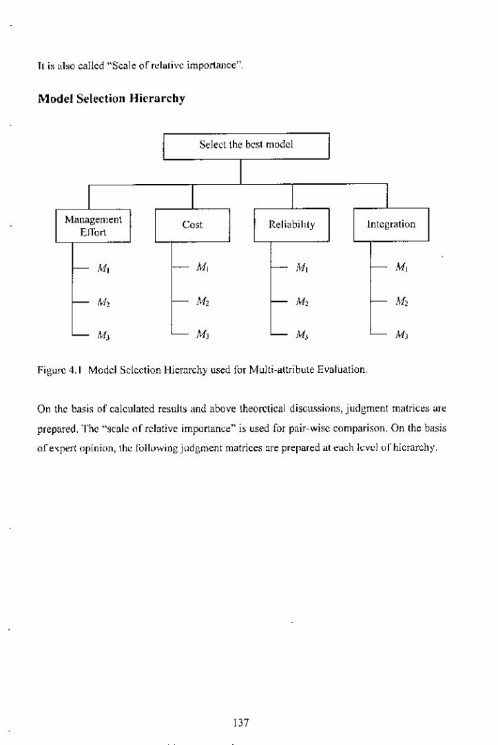
Il is also called "Seal ear rdalive importance".

Model Selection Hierarchy

.,

Select the best model

Manageme~t Cost Reliubihly IntegrationEJTort

f- MI f- M, - ;111 - Mj

f- kEl r-- M2 - Ml - Ai)

~M '---M -M -M

Figl1fC4.1 Model Selection Hierarchy l1sed for M l11li-allribllle Evaluation.

On the basis of calculated resnhs a~d above theoretical discussions, jndgment malrices ar~

prepared. The "scale of relative importance" is used for pair-wise comparison. On the basis

of e~perl "pinion, th~ Jollowing judgment matrices nre prepar~d al each level or hierarchy.

IJ7

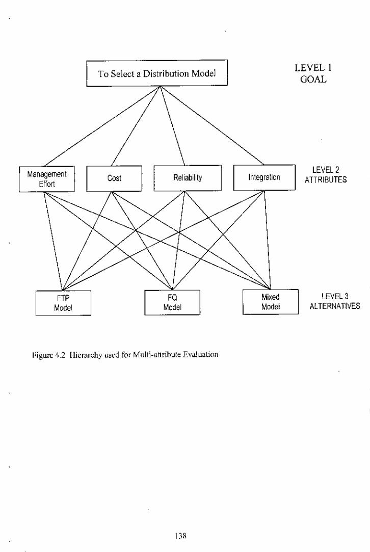
To Select a Distribution ModelLEVEL 1GOAL

LEVEL2ATTRIBUTES

Mixed LEVEL3Model ALTERNATIVES

IntegrationReliabililyCostManagementEffort

Figure 4,2 l-lierarchy u~ed for Multi-attribute Evall.lation

138

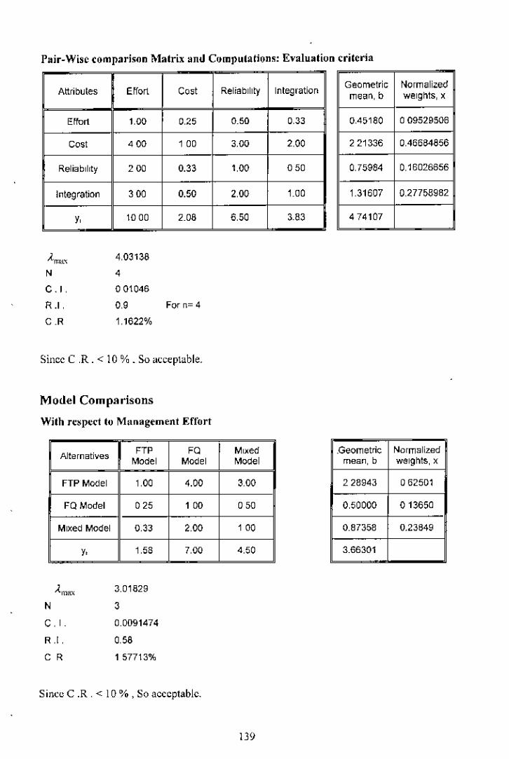
Pair-Wise comparison Matrix amI Computations: Evaluation criteria

Attribules Effort Cost Reliability Inlegration

cern" 1,00 0,25 0.50 0,33

Cost '00 '"0 3,00 2,00

Reliability '00 0.33 1.00 000

Integration 300 0.50 2,00 1.00

y, 10 00 2.08 6,50 3.83

An"" 4,03138, ,C.I, 001046

R.l, 09 For n= 4

C., 1,1622%

Since C ,R. < 10 %. So acceptable.

Model Comparisons

With respect to MlUlagement Effort

Alternatives '" eQ Mi~edModel Model Model

FTPModel 1,00 4.00 3,00

FQ Model 0'; '00 000

Mixed Model 0,33 2,00 '00

y, 1,58 7,00 4,50

Am"" 3.01829, 3

C. , 0.0091474

R ,I, 0,58

C< 157713%

Since C .R ,< 10% , So acceptable.

139

Geometric Normalizedmean, b weights, x

0,45180 009529506

221336 0,46684856

0,75984 0,16026656

1,31607 0,27758982

474107

.Geometric Normalizedmean, b weights, X

228943 062501

0,50000 013650

0.87358 0.23849

3.66301

\-Vith rcspcd to Cost

Alternativesew FO MixedModel Model Model

FTPModel '00 0.25 0,50

FQ Model 4,00 1.00 '00

Mixed Model 2,00 0.50 '00

y, ;00 no 3,50

Geometnc Normalizedmean, b wei his, x

0,50000 0,14286

2.00000 057143

1.00000 0.28571

3.50000

,C .1.

R.I,

ce

3.00000,o0.58

o

Since C .R , < 10 %, So acceplable.

With rcspcd to Reliability

Alternatives nF Mixed MixedModel Model Model

FTPModel 1,00 0.33 0;0

FQ Model '00 1.00 ;00

Mixed Model '00 0.50 1,00

y, 6.00 '" 3,50

Geometric NO;~~llizedmean, b wei hts, x

0,55032 0,16342

181712 0,53961

1.00000 0.29696

3.36744

"C,I,

H

C ,R.

300920,0,0046014

0,58

079334%

Sincc C .R , < 10 %, So acceptable.

140

With respect to Integration

Alternativesne eo MixedModel Model Model

FTPModel 1.00 "" 0,50

FQ Model 3.00 "0 2.00

Mixed Model 2.00 I 050 1.00

y, 6.00 1,83 '"Am,,, 3,00920, ,C. , 00046014

" 0,58

C.R. 079334%

Sin~e C ,R. < 10 %, So ac~eptuble.

Geometric No~~~llzedmean. b wei hts, x

0,55032 016342

181712 0,53961

1 00000 029696

3,36744

On lhe basis of the above matrices, an over-all evaluallon is perfornled u,ing the calculated

weights of the alternatives and four ~ri(eria. The eompo,ile weights of the three alternatives

arc ealeulaled, On (he basis of these composite weights, the alternative models are ranked.

These are given in the follO'ving wble.

Onrall ),;valuation; Com padson of model alternatives

Attributes and their weights

Alternatives Effort Cost ReliabilIty Integration Composite Overall

009530 0.46685 0,16027 027759 weights Ranking

FTPModel 062501 0, t4266 0.16342 0,16342 0.19781 ,(M2)

FQ Model 0,13650 0,57143 0.53961 0,53961 051605 ,(M1)

Mixed Model 0.23849 0,28571 0,29696 029896 0,28614 ,(M3)

'"

The data in the matrix can be used to generate a good cslimute of the criteri~ weight~, 'I he

weights provide a measure of the relutive importance of each criterion. The AHP allows

individuals to use lheir own personal psychometric ~cale for making the reqmred pair-wise

comparisons. Measuring the eonsi~teney of one's judgments allows a cross-check on how

well that scale is being followed. As long as the scale i:; applied cOllsigtently by eaeh

individual, the AHP can correctly proeegs their judgments, Computations of the consistency

mtio arc somewhat more invoh'ed, but they arc performed with a ,preadsheet package such

as Micro~oll Excel.

The three models must be comparcd pair-wise for each criterion. This process is virtually

identical to the proecdure that was nsed to develop the criteria comparison matnx, The only

difIerence is that lhere is a model compari,on matrix for each criterion, Therefore, the

decision maker eompares each pair of models with resped to the management effort

criterion, Thi~ is repeated for the three other criteria,

The final step of the AllP analysi~ is sllmmarized in overall evaluation table. This table

shows how the overall formulation ~cores are computed. This procedurc can be explained as

a simple weighled average lcchnique. For a given model, lour "eights are computcd. one

for cach of the four evaluation criteria. These Jour weights are multiplicd by the appropriate

critcria weights in meeting the goal of the hicrarchy and the re,uits of thc four

multiplications are added togethcr to compute the model ~c<J[e,Each model score represents

the estimated tolal benefits 10 be obtained from selecting this model. In this problem,

according to the result> obtained, thc FQ model (Ml) with a score 01'0.51605 is rankcd 1

i,e. judged to be best. Based on lhe ,olution, model Ml is selectcd. III lhi, problem cost

among all of the criteria is critic<l1.So cost i.e. transportation cost should be mmimi>:ed.

142

4.6 The Transportation Cost

The tr~nsportation problem, received thi, n~me because many of its applications involve

determining how to optimally transport goods. Transportation costs play an important role

in loc~tion decisions. These can stem from the movement of either raw materiab or linished

goods, If a facility \vill be the ~ole source or destination of ,hipmenl" Ihe company can

include the transportation costs in a 10cation~1 cost-volume analysis by incorpor~ting the

transportation cost per unit being shipped into Ihe variable co,t per unit.

When a problem involves shipment of goods trom multiple sending points to multiple

receiving points, and a new location (sending or receiving point) is to be added to the

system, the company should undertake a separate analysis of transportation. In Slleh

instances the transportation model of linear programming is very helpful. It is a special-

purpose algorithm used to determine the minimum transp0l1ation co,\'

4.6.1 Integrated Logistics: Nceds and Variables

The conceptu~li;r.atlOn of integrated logistics can be defined as a 'uni1', composed of various

major functions of a supply chain system, Logistic> is viewed as the competency that links

an enlcrprise wilh its customers and suppliers. !nformatirlll Irom and about customers flows

through the enterprise in the form of sales activity, li)re~a~b, and orders 176.1. The

information is refined into specJic manufacluring and purchasing plans. As products and

materials arc procured, a value-added inventory /low i, initiakd that \lltimately results in

ownership transfer of finished products to customer:; [77]. Thus, thc proccss is viewed in

terms of two intcrrdalcd efforts, inventory t10w and information /low. Prior (0 di,ms~ing

cach tlow in greater detail, two observations are important, Fir<:>tly,,m integrated opcration

is a must 111hicrarehical planning system, or value"chain system, or ~lmply a supply chain

syslCm. Secondly, optimization in distribution network is necessary for nO! only cost

miniml.wtion, bllt also other qualitative and quantitative variables 1781.

143

\l,.'hilesl.lchintegration is prerequisite to su~ee~s, it is not sufficient to guarantee that a linn

will achieve its perrollll~nce goals, Obviously, a related issue i~how to achieve the goal and

how to me~sure the performance. Possibly, operations research, especially in the IUllll '1f

lo~al ,;ear~halgorithm, is the only feasible solution, although it is true that global sear~h

~lgorilhms may theoretically provide a beller ~olution, however, at the expense of

infeasibility und NP-hardne,8[79-80J.

To be fully effective in today's competitive environment, firms must expand their integrated

behavior to incorporate eu~tomersand suppliers in the hierarchically integrated system. This

extensinn, through external integration, i~ referred to a5 value-added supply chain

management system [81].

Second, the basic process is not restricted tll for-profil business, nor is it unique to

manl.lracturing IInns. The need to integrate requirements and operations occur~ in all

businesse~ as well ,IS within pl.lblie sector organizations. For example, retailing or

wholesaling firms typically link physical distribution and purchasing, since traditional

manufacturing is not required. Nevertheless, retailers ~nd wholesaler, mu~t ellmplcte the

logistics value-added process. The same is true ror all public sector organizmions that

manufacture prodnct, or provide other services. In fact, that is the essence of hierarchical

materials planning system.

4.6.2 Materials Flow in Hierarchical Planning System

The operational management of hierarchical malCrials plunning system has many

components: materials itself, logistics to integrate materials flow, information flow and

many others. This research is concentrated on physical integration i,sues, concerning

materials and business logistics. It may be mentioned that bllsines, logi,tics is concerned

with movement and storage of materials, finished products and associated service.

Logi~tical operations start with the initial shipment oj"a muterial or component part from a

supplier and are lin~li7ed when a manufacturcJ or processed product is delivered to a

144

customer. Here, optimization would mean somc objective~: matcrials flow ut the shortest

pos~ible time and information passing from one stage of planning to the other, such thaI

certain degree of integration is achieved. This research aims both.

hom the initi"l purch"se of a material or component, the logistical proce~s add.,>value by

moving inventor)' when "nd where needed. Providing all goes well, a mmeriu!g"ins value al

ea~h ,tel' of its transformation into lini~hedinventory. In other words, ,m individual part has

greater value after it i, incorporated into a machine. Likewise, the machine has greater v,,]ue

once it is delivered to a buyer. l'his value addition should be maximum, if optimization is

achieved from several dimensions, leuding" multi-objective optimization, which is desired,

but most of the time, not achievable because of eomputation"l problems.. 1his researeh

solves the problem of multi-criteria optimization using linear progrumming and multi-

criteria technique in two steps.

To support manufacturing, work-in-process inventory mu~t be moved to support final

assembly. The cost of each component and its movement becomes part of the value-added

process. The final or meaningful value thut i~ added o~curs only with final owncrship

tr"nsl'er of products to customers when and where spe~ijied [82]. For a large manufacturer,

logistical operations may consist of thousand, of movemenls, which ultimately culminate in

the deli\'ery 01" product~ to an industrial user, retailer, wholesaler, dealer, or other cw.tomer,

which constitule the complex dislribution nc!work. For a large retailer. logistical operations

may commence with the prOC\lrcmcntof products for resale and may terrninute with

consumer pickup or delivery. For a service organilation, like a hospital, logistics start with

pa)curemcnt and end with full support of patient surgery and recovery. The significant point

is that rcgardlcs> or the size and typc of enterprise, integrated logistic~ is essentiul for

hlcrarchical materials planning system and requires continuous m"nagement allcntion. For

bettcr understanding it IS useful to dividc logistical operations into three "rea-.: physic,,]

distribution, manufacturing support, and procurement. These components constItute the

~entcr of the combined logistics operational units of an enterprise.

145

4.6.3 Physical Distribution

The area of physical distribution concerns the last step of di,tribution network operations,

which involves movement of a finished product to customers in shortest possible time and

minimum possible co,;\. In physical distribution, the customer is the final destination of a

markcting eharmc!, The availability of the product is a vital part of each channel

participant's marketing elTort, Even a manufacturer'~ agent, which typically does not own

invental)', must depend on imentory availability to perform expected marketing

responsibilities, Unless a proper assortment of products is efficiently deliv~red when and

wh~re needed, a great deal of the overall marketing effort can be jeopardi~ed. It is through

the physical di,tributi"n process that the time and ~pacc of customer service becam~ an

integral part of marketing. Thu,; physical distribution links a marketing channel with its

customers, To suppart the wide variety of marketing ~y~tems that exists in a highly

commercialized nation, many dilTerent physical distribution systems are utilizcd. All

physical distribution systems have one common featurc: they link manufacturers,

wholesalers, and retailer,; into marketing channels that provide product availability as an

intcgral aspect of the overall markding proeesslS3]'

4.6.4 Operating Arrangements: Anticipatory versus Respouse-Based

The fundamental diffcrcnce in anticipatory and response-bascd logistical arrangem~nt~ i~

timing. Anticipatory arrangements ur~ traditional and reflcet the best practice dev~lop~d

dunng a period prior to widespread availability of inromlution technology. In contrast,

rcsponse-bascd arrnngements reflect strategies to exploit thc potential of time-based

logi~ties. Timc-bascd logistics provide the basis ror optimi/.a(ion.

This qucstion again raises <mather dcrived qucstion regarding Anticipatory-drivcn value

chain against Responsc-driven value chain, Obviously, an anticipatory-driven value chain is

desired at any manLlfaet\Lrer's nct\.vork, However, this \voulJ requirc market drivcn forec~st,

originating from distri bution neLwork, Ir this is achieved. only then a tru~ materials planmng

integl'ation is ilchieved, H""evcr, this wonld require an integrated MRP (Material

t46•

Requirements Planning) and Distribution Requirements I'lanning (DRP). Currently, this

integration is absent. As >uch, total Manufacturing Re~ouree Planning (MRPIl) is not yet

realized, This research pruvides integration between MRP and ORP at the planning level.

The following table sho\~s the variables operating at different levels lor such integration.

Table 4.2 Business variables for MRP-DRP integration.

Anticipatury-driyen hierarchical materials Re~ponse-driven hierarchical materialsplanning chain planning chain

Manufacturing level

Slochaslic torceast Deterministic forecast

MIU':ORP planning MRP-DRP planning

Anticipatury inventory including stochastic Delinitive inventory with optional sal"etysalety stock stock

Multi-item dispatching with stochastic Multi-item dispatching with definitiveinventory at the dO\~llstream inventory at the downstream

Intermediate Distribution network pipeline

Slocha,tic furecast and inventory build-up Determini~tic reqllirement-based inventoryas per: An mtegration with '.Multi-item planning, as per MRP of t\IRPII systemdispatching from the upper manufacturinglever.,

Inventory speculatiun as per statistical Inventury pustpunement and flow throughdistribulion pattern lurn-over

Selectiun waves throngh fixed Selection waves based on requirementsreplenishment schedule from MRPII system,

Profit center philosophy ServIce center philosophy

Sales Point I Retailer

Model stock (ROP, Safety stock) Model stock (ROP)

Slocha.>tic demund based replenishment Scheduled replenishment

Table 4.2 illustrates contrasting priorities and practice~ thut managers can be expected to

employ with logislics"related activities at each stage of the supply chain. Even a casual

review of the detailed paradigm~ il111~tratesthe stark differences between the two operating

arrangements. especially during planning intcgralion.

147

Anticipatory practices "ere dcveloped during a time period when busine,s was primarily

conducted on a transaclional basis. l3eeause informalion was nol shamJ freely and

leelmology was nol <lvailablc to facilitate such sharing, firms tended 10 operate on the basis

of long.term foreea,ts, which is highly stochastic in nature. It ml.lst be noted and

remembered that the longer the (materials) planning period, the more stochastic the plao is.

Thus, the operational goal becomes 10 build and push inventory with higher degree of

uncerlainty to the next level in the channel. l3eeau,e of high Cosl ami risk a,soeiated with

anticipatory practices, the prevailing relationship between tradmg partners was typic<llly

advers<lri,,1,Each party to the transaction needed to look out and deal \\.ilh uncertainty for its

own selJ~interest.

Response-based arrangements slress cooperation and infOlmation shm-ing. Because of

chmmel-wide data concerning requirements, timely point-of-sale experience can be

substituted for total reliance on forecasts, When all members in a m<lrketing channel

synchronize their operations, opportunities exisl to reduce total supply chain inventory <lnd

eliminate duplicate practices that increase cost without generating customer value.

However, lhls would require optimization and integration in the overall material, planning

system. This research aims at that purpose.

The reality of tod<l}'~besl practice logistics is that it does not wllect the extreme of either an

,mlicipatory or <lresponse-bascd arrangcment. Many well-e,tablished bcliefs and practices

lend to pre~erve conformance to anticipatory paradigms. Perh<lps Ihe greatest barrier to

adopting response-based arrangements is the need for publicly held corporalions to

appropriately project sales volume to financial indices. Financial indices <lcl<II; the ba~e-Iine

economic accountability factor, which means that financial goals musl be reflected in

operating plans and forecasts. Such goals often encourage promotional slrategies to "load

the ~hannel" in order to creale timely sales volume. The financial burden to "deload" the

ch,mnel in order to create a response-based environment is never timely. This deloading

occurs, for example, every year in many remil stores right after ~elebr<ltion-ba,ed sales-

hike, (e.g. Christmas, Eid festival8, etc)_ Slore, promote heavily to sell lheir remaining

148

stock befure the end-of-the-year invcntory is countcd to help reduce the expense oi"tuking

inventory and to lower inventory cost. This overflow scenario is opposite to normally

prevailing backlog situation in many slores downstream.

A second barricr to implemenling re~ponse-based operations is the fad thai it is easier to

manage on an adversarial relation on power-dominated basis than to develop and leverage

cooperative relationships. Cooperative relationship requires strong synchronized ~upply

chain network, Most business managers simply do not hu~e training or experience for

instituting coopewtive urnmgements designed to share both benefit~ und risks. While

logistics managers report a high degree of belief in the long-term potential for response-

based alliances, they report considewble frustration in how to get the job done.

For the foreseeable future il appear~ that most firms will be simultaneously involved m

various combinations of anticipatory and response-based logistical arrangcments. The trend

toward increased involvement in response.based relalion~hip, with specific customers and

suppliers llppears to be \vell e~lablished and will continue to expand. Thi~ need for Jirms to

purlicipate in u vuriety or dilTerent delivery at'fangements hus pluced new perrormanee

demands on logistical strategy.

4.7 Transportation Economies

From the preceding di~cus,ion, it is clear that warehouses enter a logistical system only

when a differential advantage 111 servICe or co~t re~ults from their inclusion between

manufacturing and customers. from the viewpoinl of tran~porlation economie~_ eo~l

advantage i~ accomplished by using lhe warehouse to achieve maximum consolidation of

freight [84]. The next di~cus~ion illustrates the economics of transportation consolidation

that justify establi~hment of a warehouse, in comparison to direct shipmcnt without

intClTIledi"ry warehouse. Then the chapter focuses on transportation cost minimi"..ation

acro~s a network of warehou~e~"

149

Cost-Based Warehouse Justification

Thc basic economic principle justifying establishment of a warchouse is transportation

consolidation. A manufacturer typically sells products ovcr a broad geographical markct

arca. If customer orders tend to he small, then thc potential to consolidate may provide

economic justification for establ ishing a warehouse.

Transportation Cost Minimization

It is a matter of question whether adding a warehouse in the distriblltion channel helps

minimizing cost. As a general rule, warehouses would bc added to the logistical sy<;tem in

situations, where-p- + T-

L 't./-' +W-,+Ly S; LP.i'+7r,"

where

P, = Processing cost of volume shipment

T, =Transportation cost of volume shipment

W,=Warehousing cost of average shipment

L.i' = Local delivery of average shipment

N,= Number of average shipments per volume shipment

Pi = Processing cost of average shipment

Tl= Direct freight cost of average shipment

The only limitation to this generalization is that sunicicnt shipment volume must be

available to cover the lixed cost of each warehouse facility. As long as the combined cost of

warehousing and local delivery is equal to or less than the eOlnbined cost of shipping direcl

to customers, the establishment and operation of mJciitillnal warehouse facilities would be

economically jllstified.

The generalized relationship of transportation cost and consolidatIOn location is ililistrated

in Figure 4.1. Totallran~portation cost will decrease as consolidation locations are added to

ISO

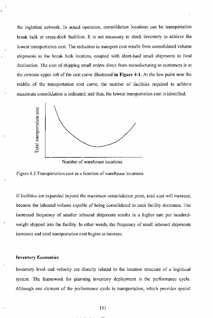
the logistical network. In actuul operation, consolidation locations c~n be transportation

breuk bull\. or cross-dock facilities. It is not nece~~ary (0 stock invcntory to achieve the

lowest transportation cost. The reduction ill tnmsport co~t results from consolidated volume

shipmenls 10 lhe break bulk location, coupled with short-h~ul sm~lI ~hipments to final

destination, The cost of shipping small orders direct Ii-ommanufacturing 10euSlOmersis at

lhe extreme upper left of the cost curve i1Juslrutedin Figure 4-1. At (he low point near the

middle of the transportalion cost curve, the number of [~cilities requir~d to achieve

maximum consolid~(ion is indicated; and thus, the lowest transportation cost i, identified.

Number of warehouse loc~tions

Figure 4.3 Tran~portation eo~las a function ofwarchOllse loealions.

If Elcilitie~are e"pand~d beyond the maximum consolidation point, (olal C<J~(will inerea~e,

because the inbound volume capable of being consolidated to each facility decreases. 'Ihe

increased frequency of smaller inbound shipments results in 'a higher ralc per hundred-

weight shipped into the facilily. In other word" the frequency of small inbound shipments

increases and total transportation cost begins to increase,

lnvcntury Economics

Inventory levcl and velocity are directly rel~ted to the loc~lion struclure of a 10gistlc~1

system, The framework for planning inventory dcploymcnt is the performance cycle.

Although one clement of the performance cycle is transportation, \'ihich provide, spatial

151

closure, lhe key l'udor in inventory economics is time. The forward deployment of

inventory in u logi~tic<d ~ystem improves service response lime. Su~h deployment also

increases the overall system inventory requirements, re~tLhing in greater costs and risk, In

the folJovv'ingdiscussion, Ihe impact of inventory on service response capability is inilially

presented, followed b} a review of the impact of increasing the number of warehouses on

total system inventory requiremenls.

Service-Based Warehouse Justification

The usc of warehouses can be a vital part of lhe logislic~ strulegy of a riml engaged in

national distribution, To achieve essential economy of scale, iinm are ofien required to sell

over broad geogruphical areas. Thc~e lllaniJfacturi ng economics of scale often compel firms

10locale planL>where low production cost~ can be realized.

The dynamics <)1'~palial competition enter an industry when products begin to gam

cu~lomer acceptance in olher Ihan prime markets or ncar manufacturing locations, The

cnterprise may find it desirable to deploy inventory to support marketing. In highly

compelitive industries, the policy may be 10 locale a warehou~e in a particular market area

even if operalion of lhe facility increases total cost. The availability of a local inventory

offers lhe p(ltcntial to provide high l~vcJs oj"euslomer service. For customers, lhis means

faster replenishment and an overall reduction of inventory. Thus, the enterprise that

eommils to establishing a \varchouse may be viewed as having a differential advantage.

The inventory rcquired l() ~upp{)[l a war~h{)u~e consi~ls oj" lran,it, ha,~, and ,akty .,>l()~k.

This research considers the yariou> inv~nlory componenl>, including MrS-lype finisheu

goods (base inventory), pipeline (transit) inventory, distribution inventory, etc. ami

describes how each rclates to average invcntory level.

Adding warehouses to a logislieal system increases the number of performance cycles. The

impael on transil invenlory and safety stock can he significant In contrast, the impact on

base stock by adding inventory is not significant The ba>e stock lev~1 within u logislicul

152

s}~tem is determined by nlJnufacturing and transportation lot sizes, which do not change as

a function of the number of warehouses [85], The combination of maintenance and ordering

~OM,adjusted to take into consideration volume transportation rates and p"rehase discounts,

determines the replenishment EOQ and the resultant base stock. In just-in- time

procurement situ~tions, base stock is determined by the discrete order quantity required to

support the planned manufacturing run or assembly. In either situation, the base stock

determination is independent of the number or warehouses included in the logistical system.

Transit inventory is important to logistical sy~lem design because it requires capil"l

commilment. As more performance cycles arc added to a 10gistic,,1 nelwork, the expected

resull is lhat exisling C}eles will experience a reduclion in transit inventory, This reduction

OCCI.ll1>becal.lse the total transit days inthe system are reduced. It shollid be noted lhm the

second warehouse does not creale additional performance cycles on the physical distribution

side of the logistics flow. However, on the inbound side, each product stocked in the new

warehouse requires II replenishmenl SOUTCe.ASSllming a fl.lllproduct line al each warehouse,

the number ofperlormance cycle, required to replenish the system will increase each lime a

new warehouse is added l86].

Despite the increased need for invenlory replenishmenl, lhe average in-lransit inventory for

the total ~ystcm drops as new warehouses arc added because of a reduclion in days required

10 service customers, Thus, even if multiple plant-to-warehouse replenishment cycles were

added to the logistical syslem. the average transit time reduces becau~e uf" the reduclion in

IOta! replenishment days.

ln summary, the addilion of facililics will generally have the net effecl of reducing lola! in-

transit days and, thus, inventory level. This result will vary in accordance with the

particulars of each situation. Each network of localions Il1U~tbe carerlll1} analyzed to

determine the exact impact on average transil inventory, The k<~}to lllldcrstanding the

impact of increasing warehouses on transit inventory is to remember that tolal lran~it day~

are reduced even though lhe number of rcquircd p~rrormanee cycles increases, A

qualification is thaI while ml increase in the number of performance cycles typically reduces

153

tnm,it days, it may also incr~aoc overall lead time uncertainty. As lhe number of

performance cycles i, increased, the possibility of breakdowns leading (0 potential service

failures also incr~ases .. rhis potential impact is treated under salely ~toek.

From the viewpoint of safety stock, the expe~t~d result of adding war~hou,es will bc an

increase in average system inventory. The impact 01" sales and performance-cycle

un~erlainty on inventory must b~ evaluated using two independ~nl jj-~quency distributions.

The purpose of Safely ~l()~k IS 10 protect again~l unplanned stock-oul during inventory

repl~nishment, Thus, if safely stock is predicted to incr~ase a, a funclion of adding

warehou,es, then the overall system uncertainty must also be increasing.

The addition of warehouses (0 the logistical syst~m impacts uncertainly in two w~y~. First,

since performance-cycle days arc reduced, lhe variability in sales during repkmshmcnt and

the variability io th~ cyclc arc both reduced. Therdore, redncing the length of the

performance cycle reli~v~~ to some degree the need for s~l(,ty stock to protect ag~in~l

variabilily .

.] he second impacl of adding locations has a direcl ami signiJleam effect on average

inventory, Each new pcrformanee cycle added to the gystem creates the need lor ~ddi(ional

safety stock. The introduction of 3n 3dditional warehouse to scrviec a specific market arca

reduc~s thc ~pplicablc size of the demand database used (0 delenninc safety stock

requirements, In effect; lh~ ,i/.c ofthc markct area serviced by a givcn radlity is reduced

without 3 corresponding reduction in uncertainty [87]. For example, wh~n th~ demand of

s~v~ral markets is aggregated to a single war~hoLlsC,the variability of demand is averagcd

across markets. This 3110\>,'speaks in dem~nd io onc market to be offsel by low demand in

another. In essence. the use of probability allows the idle slack of one market to bc nsed to

med ,a1Cty stock rcquirements or othcr markets,

The impact of adding "arehouses on system safety stock i~ really vital in complete supply

chaio management. The important point lo und~r,tand is th3t thc increase in s~rety ~lock

rcsult~ from an inability to aggregat~ the Llnecrtainty across a large market area. As a

conscqLlcnee, sep3mte safety s(och mu~t accommodate alilocaJ demand variation.

154

Inventory Cost MinimiLation

The overall impact on average inventory of increasing the number uf warehouses in a

logistical system is uf vital importance. A reduction in average transit inventory is obvious.

The assumption is that a linear rebtionship e:dsts between average transit inventory and (he

number of warehouses in the network.

The actual inventory increases at a decreasing rate since the net increase for each facility is

hmited (the added safety stock required to accommodate uncertainty is related only to

demand Msigned to that warehouse less the reduction 'in safety stock required for less lead

time uncertainty resulting from a shorter replenishment cycle), Thu~, the incremental

invcntory required to maintain customer ,en ice performance dimini,hes for each new

warehouse location added to the system. The average inventory represents the combmed

impact of safety stock and transit inventory, The signillcant obsen'ation is that the s<ll"ety

stock dominates the impact of transit inventory reduction. For the overall systcm, the

average inventory is the safety stock plus half of the onJcr quantity plus transit inventory.

Thus, given the S<lmedemand llIld customer service goals, total inventory increases at a

de<;leasing rate as the number ofwarehoLlscs used in a logistical system increases.

Least Total Cost Design

As noted earlier, the identiJicalion of the least-total-cost system design is the goal of

logistical integration. The basic lotal cost for the overall logistical system is composed or

minimllm holding llIld ordering cost, a~ well as transit llIld safety stock, As <lresult, average

inventory commitment increases \vith each additional warehouse. for the overall system,

the lowest total cost nctwork is a function of locations. In fact, a trade-on' relation exists

among number ofwarehou5es, amount of inventory and overall di~tribtLtion cost.

The identification of the leusHotal-eost design of warehouses in the network may be

illustrated by a trade-olTbetween cost-generating activities, The minimal total-cost point for

the system is not at the point of lea,t cost ror either transportution or inventory, This is the

155

hallmark of integrated logistical aJlaly~is. In actual practice, a great many problems mu~t be

overcome to effectively examin~ total cost. Foremost among them is that many assumptions

must be madc to operationalize the logistical system analysis. A second concern is the fact

that a two-dimensional analysis, ahhollgh may provide a le~~ trade-off, such system doe~

not encompass th~ comple"ity of total eo,t int~gr"tion. Each of the critical assumptions and

associated implemeniational problems are matter of concern.

Some Assumptions ami Limitations

Thi, research assumes an average projected level of sales volume acr\lS, a planning horizon.

Tr;m~por\.;ltion requirements are represented by one average-size shipment. In actual

operations. neither of these simplifying assumptions would bc valid. First, the nature of

logistical network design is not a ,hort-t~rm planning problem. Wh~n j~ciJity decisions are

involved, the planning hori.wn extends across several y~ars and must accommodate a range

or different annual sales projection~_ Second, actual shipment und order sizes will vary

substantially around an average. In fact, the a~~umption that shipments must be serviced

through a war~house must oc relaxed to uccommodate high-volume customer-dir~et

truckload or container di~tribution. A realistic approach to planning must incorporate a

range of shipment sizes supported by alt~rnative logistical methods to satisfy customer

service requirements l~9]. In actual operation, alternative modes of transport~tion <lI"e

employ~d, as necessary, to upgrade the speed of deli very

Significant cost trade-ofr~ eXl~t between inventory and transportation. lnventory cost as a

function of the number of war~houses is directly related to the desired level of inventory

availability. lfno safety stock i~maintained in the system, the total inventory requirement is

limited to base and transit stock. Under a no-safety- stock situation, (he total least cost for

the system would be itt or n~ar the point of lowest transportution C\lsL Thus, assumptions

made with respect to the desired inventory availability and till rate arc essential to trade-\llf

analysis and have a significant impJct 011the lea>t-t()tal-c()~!de!.ign solution.

156

The locational ,clection aspect of logistICal network planning is far more complex than

simply deciding how many facilities to choose from a single array of locations. A firm

engaged in nationwide logistics has wide latilode in choicc of \vhcre to locate warehouses.

In a largc market, there may be as high (l$ filly regions within which one or more

dimibution warehouses could be located. Assuming that the total allowable warehouses for

a logislieal system cannot exceed fifty and that locations are limIted to a maximum of one in

each region, there are 1.1259 x 1015 combinations ofwarchouses to be evaluated in lhe

selection of a least-lotal -cost network.

To over~ome some of the above noted simplifying assumptions. variatioll> in shipmenl size

and tran~portation alternalives need to be introduced. Extending the analysis 10 a more

complete treatment oi"variables lypically demands the usc of eompuler planning models and

lechni'llle~, Apphcalion "r!incar programming may provide an optimal point for a lrade-ofI

Such refinement requires linkage of a full range of variables [901. At least three crilical ones

to be considered are shipment size, lrampurtation mode, and localion alternatives. The

conslants are level of inventory availability, performancc- cycle duration, and the specific

warehouse lucations being evaluated.

In con,tructing a more comprehensive analysis, shipment size can be grouped in lelTI1Sof

frequency of occurrence and transporwtion mode economically JtLslitied handling eaeh

shipment size within the specified performance-cycle lime constrmnts. For each shipment

size. a luwl-cost relatlUn>hip can be identificd. The resLlItis a two-dinlcnsional analysis for

each shipment size and appropriale transportation mode. Nexl, the individual lwu-

dimensional pruliles can be linked by joining the pomts or least cost lo make a planning

curve. 1n a lechnical sense, lhis is an envelope curve lhal joins the low lotal-cusl poinb of

individual shipmenl si/e-transpurl nwde relationships.

A compromise is required to select lhe final warehouse network, Inilially. lhe lime duration

of lhe perfOlTIlanCec}ele and invenlory availability assumptions should be held constant.

The service availability and perfonnJnce-cycle duration ~erve as paramelers to help i~ulate

an inilial least-cost approximation, At a later point in strategy formulation, thesc parameters

157

can be relaxed and subjected to sellsitivily ;maly~is. The fit of the least-eosl planning curv~

requir~s margin<ll Co~lanalysis for eaeh shipment size transportalion mode combinalion for

the stipulated nelwork.

4.8 Problem Description

The transportation problem involv~s Emling the lowest-cost plan for distributing stocks of

goods or supplies from multiple origins to muhiple destinalions th"t demand (he goods. For

instance, a firm might hav~ some jllctorie~, all or which arc capable of producing identical

units of the same producls, and ~omewar~hou~e~ that ~toek or demand those products. The

transportation model can be used to delelmine how 10 allocat~ the ~upplies available from

the various factories to lhe \\'arehou~~s thaI slock the demund ortho~e goods, in such a way

th<ltlot<ll shipping COstlSminimizcJ (i.~. lhe optimal shipping plan).

The ,hipping (sllpply) points can he factories, warehouses, departments, or any other place

from which goods arc sent Destinations can be factories, warehouses, depm1ments, or any

olher points lhat receive goods. To d~scribe th~ general model for the transportation

problem, il b needed to use tenns that arc considerably less specific than those for the

components of the prototype examples. In particular, the general transportation problem i~

C(}nc~rned wilh distributing any commodily jj-om "ny group of supply ~~nters, eall~d

sources, to any group of rec~iving: c~nl~rs, call~d d~,tinati()ns, ;n su~h a way as to minimize

the 10taI distribution cost. The model for a transportation problem makes the following

assumption ahout supplies and demands.

I. Each source has a fixed supply of units, wh~r~ this ~nlire ~upply mu~t b~ di~lributed to

th~ de~tination~. Let s, d~note lhe number of unil, b~ing suppl;~d by s()urc~ i, lor i = I, 2,

.... , m. Similarly, each destination has a fixed demmld for units, where this entire demand

musl b~ r~celved Ij-om the S()urc~. Ld dj Jcnole the number of units being received by

destinationj, for j = 1,2. ., n.

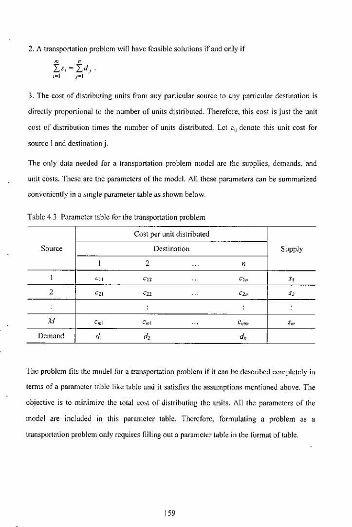
2. A transportation problem will have lCasible solutions if and only if

"' "Is, = Id! .1=1 )=1'

3. The cost of distributing units from any particular source to any particular destination is

dire~tly proportional to the nl.lmber of I.lllitsdistributed. Therefore, this cost is just the unit

~ost of distribulion times the number of units distributed. Let e'J denote this unit cost for

source Iand destinationj.

The only dala needed for a transportation problem model arc the supplies, demands, and

unit costs. These arc the parameters of the model. All these parllmekrs ean be summari7.ed

conveniently in a ~mgle parameler lable as sho'wn below,

Table 4.3 Parameter table for the trllnsportation problem

Cost per I.lnildistribl.lled

Source Destination Sl.lpply

I 2 ... "'I ell Cil ... "" "2 Cli CO, co" "M '., eml ... C'!lm Sm

Demand d, d, d"

'j he problem fits the model l,n <Itrunsport~tion problem if it can be dc~crjbed ~()mpletely if]

terms of a paranleter table like tuble ~nd it satisfies the assumptions mentioned <lbove. The

objective is to minimi7e the total ~o,t of dislributing the units. All the parameters or the

model are included in this paramcler table. Therefore, formulating a problem as a

transport;llion problem only requires filling om a parumeter table in the form<ltof l<lble,

159

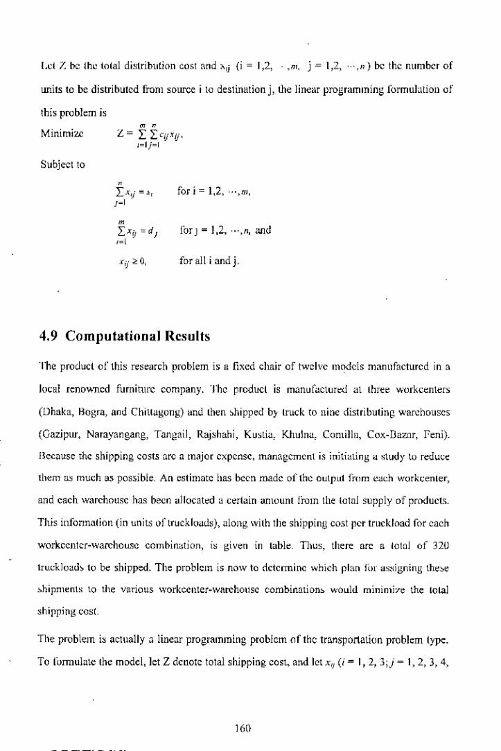
Ld 7..be the total distribution cost and ",j (i = 1,2, ',m, j = 1,2, "',n) be the number of

lUlits to be distributed Irom source i to destination j, tbe linear programming formulalion of

this problem is

Minimize

Subject to

" "Z= I Ie,pij',,=lj=1

"u ;;,0,

for i = 1,2, "',m,

lor] = 1,2, "',n, and

for all i andj.

4.9 Computational Results

The produd of this research problem is a fixed chair of twelvc models manufacturcd in a

local reno\','Jlcd furniturc company. Thc product is manufactured at three workcenters

(Dhaka, Hogra, and ChiUagong) and then ,hipped b} truck to nine distributing warchouscs

(Gazjpur, Narayangang, Tangail, Rajshahi, Kuslia, Khulna, Comilla, Cox-Bazar, Feni).

Because the shipping costs arc a major expense, management is initiating a study tll reduce

them as much as possible, An estimate has been made of the output from ea~h workcenter,

and each warchousc has becn allocated u certain anlOunt lrom the total supply of products.

This information (in units oftruekloaus), along with the shipping cost per truckload for each

workccnter-warchousc combin~tion, is given in table, Thus, there are a total of 320

lruckload, 10 be shipped. The problem is now 10 determine which plan I,", assigning the~e

~hipments to the various workeenter-warchollse eombination~ would minimi"e the total

~hipping cost.

The problem i~ actually a linear programming problem of Ihe transportation problem type.

To lomlulute the model, let Z denote tatal shipping cost, and let x'! (i = 1,2, 3;j ~ 1,2,3,4,

160

5, 6, 7, 8, 9) be the number of trucklDads tD be shipped irom work centers i tD warehouse j,

Thus the objective is tl.lchOD~ethe values of these decision variables (xu) so as tQ

Minimize Z = IOOOXll+ 800xl~ + 2000X1J + SOOOXt4+4000X15 + 7000x]{; + 3000XI7 +

8000xla + 4000XI9 + 4500Xli + 5500x~~+3000x'J + lOOOx24 + 3000X2\ +

SOOOX1'+ 6000X21 + 12000x2g '" 6500X~9+6000X31 + S()OOX.12+ 6S0()xJJ

10000x34 + 9000xJj + 12000xJ{; + 3000xJ7+ IOOOxJS+ 2000XJ9

Subject to constraint

X11+XII+XIJ+XI4+XI>+XI6+XI7+XI~ +XI~ 120

,>, ,X22+ ~2) +X24+ Xl, +X26+Xn + X 2S + X l~ ~ 125Xli + xJ~+ Xj] + X.1< + XJ~ + x),+x]) + X JS + X)9 75

XII +X21+XJI ~20

'" + X22+X.l2 40

"",X2)+X.lJ ~20

XI4 ,X14+X24 ~55XI, + Xl5+ Xl, ~50XI" + X26+XJ6 ~ 45XI7 + X~J+X,,7 20

XI.\ + X2S+XJ~ = 50

XI~ + X29+ XJ~ = 20

lG1

Table 4,4 Parameter table for the transportation problem

Destination

G"zipur Narayan Tangall Rojsilohi Kusti" Kilulno Comilla Cox. FeoiSource gang Bazar Supply

Unit cost Per Truck load(TL) in Tk,

Dhaka 1000 '00 2000 5000 4000 7000 3000 8000 4000 120

Bogra 4500 5500 3000 1000 3000 5000 6000 12000 6500 mChittagong 6000 5000 6500 10000 9000 12000 3000 1000 2000 '"Demand

" " " "' 00 " " 00 "(TL)

Table 4.5 Solution table for the transpoltation probkm

Destination

GoZipur Narayan Tongail Rajshahl Kustla Khulna Comillo Cox- Feni Totalgang Bazar

Source Shipment Quantities (Truck toads)

Dhaka " " " 0 25 0 " 0 0 '"Bogra 0 0 0 55 25 " 0 0 0 m

Chitta gong 0 0 0 0 0 0 5 00 " '"Tot"1 " " " 55 00 " 20 50 "• • - -

Demand 20 " 20 "' 00 " " 00 " Tk 697,000(TL) .

Supply

= 120

= 125

= 75

Applications of the transportation problems tend to require a very large number of

constraints and variables, so a straightfOf"'ard computer application o1"lh" simplex mclhod

may require an exorbitant computational effort. rhercforc, it is important to become

sufficiently familiar with this special type of pl'Oblems that one can recognize them when

they arise and apply the proper computational procedure.

A major pmt of the study revolved around IUilllUlating "nd solving transportation problems

for individu~l product categories. For each option r~garding (h" planl~ (0 k" ••p open, etc.,

solving the corresponding transportation problem for a product category shows what the

t62

distribution cost woulJ be for shipping the product category from those plants to the

distribution centers and customer O\oncs,

Any problem fits the model for a transportation problem if it can be described completely in

terms or u p"r"meler lable like table 4.3 and it satisfies botb tb~ reljuirements assumption

and the cost assumption. TIle objective is to minimil~ lhe tOlal cost of distributing the units.

All the p"rameters orlhe modcl arc ineluded in the parmn~t~r table 4.4,

To rormulate and solve a transportation problem using Excel Solver, two separate tables

need to be entered on a spreadsheet, The lirst one is the parameter table. All the parameters

01" the model arc included in the parameter table 4.4. The second is th~ solution table 4.5,

containing the quantitie, to d;stribut~ from eaeh source to each destination. Spr~adsh~et

~uftware, such as Excel Solver, is a popular tool for unuly/.ing and solving linear

programmmg probJem~. Th~ main feature of the linear programming model, induding all its

parameter, can be easily entered onto a spreadsheet. However, spreadsheet software can do

much more than just display data. In addition, the Excel Solver can quickly "pply the

simplex method to find an oplim"l wluti(lIl for the model. For transportation problems

where every s, and dJ have an integer value, all the basic variables ("lIoeations) in every

basic feasible solution (including an optimal olle) also h"ve integer values. 'lhe solution

procedure deals only "ith basic feasible solutions, so it automatically will obtain an integer

~lliulilln fur lhis case. The optimal total cost and distribution quantities have been shown in

the solution table 4.5.

4.10 Conclusions

DIstribution is the m<mugement of the flow of materials from manufacturers to customers

and from warehouses to retailers, involving lh~ stor~ge and transportation of products, It

may also be responsible for finished goods inv~ntorie~ and the ~eleetion of transportation

service providers, This research provide~ an ide~ that AHI' which is a technique ofMCDM

163

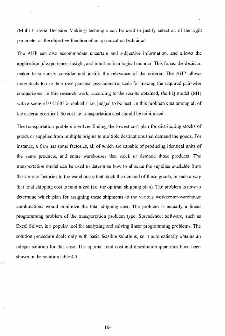
(Multi Criteria Decision Making) technique can be used 10 ju,ti I:" ~e1ection of lhe nght

parameter as the obj eelive funclion of an optimiwtion technique

The AI-!P can also accommodate uncertain and subjective information, and allows thc

application of experience, insight, and intuition in a logical manner, This forces the decision

maker to scriously considcr and justify the relevance of the crileria. The AHP allllw~

individuals 10 lLM~ their own personal psychometric scale for making the required pair-wise

compari~ons. ln this research ''1ork, according 10 the fCMtlts oblained, lhe FQ mode! (MI)

with a score of 0.51605 is ranked I i.e. judged to he best. In this problem cost among all of

the crileria is crilicaL So co~t i.e. transportation cosl ~houlJ be minimi~ed.

The transp0l1ation problem involves Iinding the lowe~t-cost plan lor di,tribuling stocks of

goods or supplies from multiple origins to multiple destinations that demand thc goods. For

instance, a finn has some factories, all of whieh arc capable of producing identical units of

Ihe same products, and some warehouses that stock or demand lho~e products. The

trall>porlalilln model can be used tll determine how to allllcate Ihe supplic~ available from

the various faelories to the warehouses that stock the demand of those goods, in such a way

that total shipping cost is minimized (i,e. lhe optimal shipping plan). The problem IS now tll

detemline which plan for assigning lhese shipments (0 lhe variou~ workcenter-"arehlluse

eombinJtions would minimize thc tolal shipping cos!. The problcm is actually a lineur

programming problem of the lran~porlation problem type. Sprca,hheC! soiiwarc, such as

Excel Solver. is a popular 1001for analyzing and solving lincar programming problems. The

solution procedure deals only with basic feasible solutions, so it automatically obtains an

integer solution for this case. The optimal total cost and distribution quantities have heen

sbo",n in the solulion t~ble 4,5.

164

Chapter 5Conclusions and Recommendations

5.1 Summary of Findings and Conclusions

It is the age. of coordinated manufacturing and distribution. The manufacturing industries

are now facing a time of inten~e international competition, which will only become morc

severe in the days to come. For manufacturing companies, the danger lies in lower co~t-

higher quality producers taking an increasing share of hoth dume~tic and foreign markets.

The opportunity lies in new technology that can enable a company to improve both

productivity and 4uality, and obtain a competitive edge.

The new ledmology can be divided inlo two cutegorie~; (I) the uCltomalion of production

activities using complllcr-aidcd design and manufacturing, robotics, or flexible

manufacturing systems and (2) computer-based production and inventory control.

Computer-ba,ed production and inventory control embudie, powerful tools for the usc of

new and better planning and control conccpts and tcchnique<

The research work focuses on production planning and distribution system of total supply

chain. In thlS research work the production pbnning and distrihution system of a produd

(chair) of a furniture company have been optimized.

Lot-Sizing

Intcrnal matcrials planning or Production planning is an activity that con.,iders the best u~e

of production resources in order to satisfy production goals (satisfying production

requiremcnts and anticipating sales opportunities) over a ccrtain period numed the plunning

horizon. Production plannillg typically encompasscs thrce time ranges for dccision making:

165

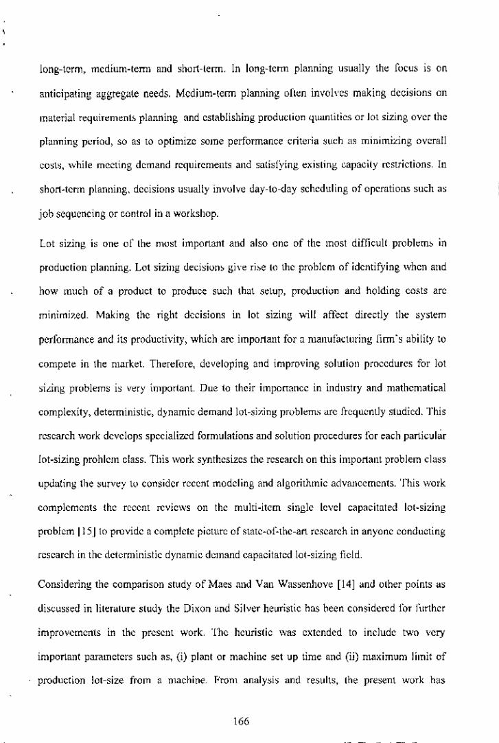
long-term, medium-term and short-term. In long"term planning usually the focus is on

anticipating aggregate needs. Mcdium-term planning often involvcs making decisions on

material requiremenb planning and establishing production q\Lantities or Jot sizing over the

planning p~riod, so as to optimize some performance criteria ~uch as minimizing overall

co~t~, while mccting demand rcquircments and satisfYing existing capacity restrictions, In

short.tcrm planning, decisions usually involve day-to-day scheduling of operations such a~

job sequencing or control in a workshop.

Lot sizing is one of the most important and also one of the most difJicuJ( prob1em~ in

production planning. Lot sizing decision, gi\'e ri.,>eto the problem of identifying when and

how much of a product to produce such thut setup, produ~tion and holding costs arc

minimi7,ed. Making the right dccisions in lot sizing will affect directly the system

perfonnance and its productivity, which are important for a manufacturing linn's ability to

compete in the market. Therefore, developing and improving solution procedures for lot

~idng problems is very important. Due to their importance in industry and mathematical

complexity, deterministic, dynamic demand l<Jhizing prublems arc frequently stlldied. This

research work develops specialized formulations and solution procedures for each particular

lot-sizing problem elass. This work synthesizes the research on this important problem class

updating the ~urvey to consider recent modeling and algorithmic advancements. Tilis \\(ol'k

complements the recent reviews on the multi-item single level capacitated lol-sizing

problem 115.1to provide a complete picture of state~ol:thc-art research in anyone conducting

research in the dctcrministic dynamic demand capacitated lot-sizing field,

Considering; the comparison study of Maes and Vall Was~enhove [14] and other points a~

discLls~ed in literature study the Dixon and Silver hellristic has been considered for further

improvements in the prcsent work. The heuristic was extended to inelude two very

important parameters such as, (i) plant or machine set up time and (ii) maximum limit of

production lot-size from a machine. From analy~i~ and results, the present work ha~

166

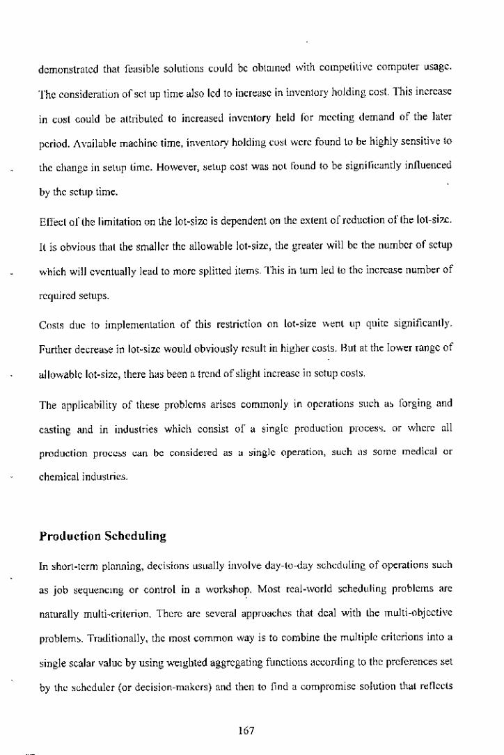
demonstrated that feasible solutions coold bc obtulll~d with compditivc computer usagc.

Thc consideration of sct up time also led to inc[~asc in inventory holding cost. This increase

in cosl could be allributed to increased inventory held for meeling d~mand of the lat~r

pcriod. Availabk machinc time, inventory holding cust were found to b~ highly sensitiv~ to

the change in s~t\LPtime. However, ~elup cost was nol l(lUnd to be signilicantly influellc~d

by the setup time.

Effect of the limitation on the lot-si7£ is dependent on the extent of reduction of lh~ lot-sizc.

II is obvious that the smaller the allowable lot-size, the gr~ater will be the number of setup

which will eventually lead to more splilled il~m" This in tum led to the increase number of

required setups.

Costs due to implementation of this restriction on lot-size '~~nl up quite significantly.

Further decrea,e in lot-,ize would obviously result in higher costs. But at the lower rangc of

allov'iable lot-size, there has been a trend of slight increase in sctup costs,

The applicability of these problems arises communly in operations such a, forging and

casting and in industries which eOllsist of a single productioll proces~. or where all

production procc~s can be considered as a single operation, such ns some medical or

chemical industries.

Production Scheduling

In short-term plnnning, decision, usually involve day-(o-d~y scheduling of operations such

as job sequencmg or control in a worbhop. Most real-world scheduling problems arc

naturally multi-criterion. There are several appru,,-ches that deal with the !nulti-objective

problem,. Tmditionally, the most common way is to combine the multiple eriterions into "-

single scalar value by using weIghted aggrcgatillg functions aceurding to the preferences set

by the s~hedlllcr (or decision-makers) and thell to find ~ compromise solution th,,-t r~lleds

167

these prereren~es However, in many real scenarios involving mLllli-eriterion sehedLiling

problems, it is preferable 10 present a set of promising ,0lLitions to the decision-makers so

that the most adequale ,ehedule can be chosen. This has increased the inlerest in

investigating the application of Parelo-optimization techniques 10mLllti-eriterion scheduling

problems. /I. Pareto-optimal algorithm is devcloped in this paper for a schedLlling problem

on a single machine wilh periodic maintenance and non-preemptive jobs. In litewture, most

or the sehedLiling problems address only one objective fLinetion, while in the real world,

such problem!. arc always associaled with more than nne objective. In this work, bolh multi-

objective fLinetion, and multi-maintenance periods are considered ror the machine

sehedLlling problem. /I. multi-criterion non-preemptive scheduling lhm reduces the total cosl

or the problem is considered in this study. Three criterion~ arc considered: reduction of flow

lime, maximum k!rdiness, and machine idle time in a periodically maintaincd single

machine problem. The twde-off between minimLim l10V'!lime, mu"imLlm tardiness and

m"chine Idle lime is a complex problem. The objective of lhe model uddrcssed in this work

is 10minimia: the \veighted funelion of the total job flow lime, the muximum turdiness, and

lhe machine idle lime in u single machine problem wilh periodic mainlenam;e und non"

preemptive jobs. An algorithm is devcloped to solve this mulliple criterion problem and to

construct the pareto-set. In this study a new kind of approach lhat allows lhe use ur

weighted aggreguliun orthc criterions is presented. All possible weight combinations fllr lhe

crilerions are computed. 11lc search for the minimum total co,t among all the Pareto-

optimal schedules with the assigned weighls lln crileriuns is oblained. Finally, a promising

sequence is chosen lhat gIves the minimLlm total eost for a particular set of weighls on the

crilerions. The paranlelri~ analysis of the tradc-offs of all solLilions with all po,sible

weighled combination of the eriterions is analyzed.

A nClghborhood scarch heuristic is also developed to provide the near-uplimal Mllution for

lhe problem. Resu](8 aTeprovided to explore the best schedule among all the Pareto-optimal

168

sets and to compare the result of the modified Pareto-optimal algorithm with the result of

the neighborhood search heuristic. The perfoml,mce of the modified Pareto-optimal

algorithm has been evaluated by comparing its solution with the solutions derived by the

neighborhood scarch heuristic. Results have shown that the modi lied Pareto-optimal

algorithm provides a beUer ~olution than thc neighborhood ~ear~h heuristic, and this show~

thc efficiency of the modified Pareto-optimal algoritlun. Direct application of this study

may be applied to the industries where performance of machine maintenance is a routine

work and worthwhile as well. Chemical processing equipments. boilers, furnaces,

mechanical machinerie~ ctc. arc the examples of such implications.

Distribution Planning

Distribution is the management or the flow of materials from manufacturers to customers

and from warehouses to retailers, involving the storage and transportation of products. It

may also be responsible for finished goods inventorie~ and the selection of transportation

service providers. Alter determining where the demand for goods and service~ is greatest,

management must select a location for the fad lily that will supply that demand. For

warehousing and di,tribution operation" transportation costs and proximity to markets arc

extremely important. With a warehouse nearby, many firms can hold invenlory d()~er to the

customer, thus reducing delivery time, transport;\tion cost amI promoting sales. The

transportation problem, receIved this name because many of its applications involve

determining: how to optimally transport goods. When a problem involves shipment of goods

from multiple scnding points to multiple receiving points, and a new location (sending or

receiving point) is \0 be added to the system, the company should undertake a separate

analysis of transportation. In this work lhe transportation model or linear programming has

been used. It is a special-purpose algorithm used 10 determine [he minimum transportation

co~l.

169

Applicalion~ of the transporlalion problems tend to require a very large number of

constraints and variables, so a straightforward computer application of the simplex method

requires an exorbitant computalional effort, For each option regarding the planb solving the

corresponding transportation problem for a prod"et category shows whal the distribulion

cosl would be for shipping the product category from lho~e plants to the di,tri):lI.llion centers

and customer zones. The oplimal total cost and di~trib"lion quantities have been shown in

the ~ol"tion table of distribution chapter.

5.2 Recommendations

Successful supply-cham managcment requir~~ a high degree of runclional and

organizational integralion. The interconnected sel or linkages betwcen suppliers of materials

and services that span~ the transformation of raw matetials into products and s~rviees and

delivers them to a firm's cuslomers is known as the supply-chi.lin. The value of supply-chain

management becom~s apparent when the complexity of the supply-ehain is recogniled. The

performance of num~rous suppliers determines th~ inward flow of materiab. The

pcrformanee of the fiml'S marketing, production, and di~lriblltion proces~e' detcmlines the

oulward /low of products. Traditionally, organizations have divided lbe responsibility for

managing the flow of materii.ll~ and services among three deparlments: purchasing,

production, and distribution, In this research work integration of int~mal production

planning and distribution has been consider~d. Purchasing can be ineluded ,ISa future work.

In case of aggregate planning and lot sizing though some practical and real-hk ~iluations

have been incorporated in the Dixon-Silver model, th~r~ arc plenly of scope of

improvement of the model. Following rceommendatiom; can be made for further

development

170

1. The Dixon-Silver model was rxtcndcd through inclusion of setup time and placing

limitation on the maximum allowable lot-size. In the present work these two conditions

were considered separately. Further work can be performcd combining thc two

situation~ lo develop a unilorm model.

2. A restriction of thc heuristic lies with number of production stages. Single production

stage has been considered in the present work. Development of a heuristic for multiple

production stagcs could bc a significant contribution.

3. Setup cosls and setup lime have been cousidered independently, Realistically larger

setup time would lead to increased setup costs. Linking of these two parameters in the

heuristic would bc clearly a morc realistic approach.

4. Back-logging was not considered in this model, Heuristic with back-logging could be

developed as further work

5. Other promising research areas arc available. While genetic algorilhm~, tabu search and

capa~itated network How models are successfully applied to solve other lot-size

problems, their potential to solve cr.sp is unknown, Re8ear~h examining sensitivity

analysis of dynamic lot-sizi ng heuristics within thc contcxt of CLSP is al,o worth while.

Finally, extending the CLSP problem representation to capturc thc impact of cquipmcnt

downtime on capacity during item changcover and multiple produd Illmilies me

important research areas.

In case of scheduling, although some practical and real-life situations have been

incorporatcd in the Parcto-Optimal algorithm and neighhorhood ~e"r~h method, there arc

plenty of wope of improvement in the modeL following rccommcndations can be made lor

further development:

I. The performance of the modified Pme!o-optimal algorithm has becn cvaluated by

comparing its Mllution with the ~ol\ltion~ derived by tbe neighborhood search heuristic.

171

The perlunmmce ol'the modified Pareto-optimal algorithm, can be compared with other

local search methods.

2. There are many sequencing rules that can be applied to the jobs through the machines in

ajob shop according to the preferences, Two of those bJsic sequencing rules, Shortest

Processing Time (SPT) and Earliest Due Dale (EDD) hJve been adopted in the modified

Pareto-optimal algorithm. Additional priority rule, such as Critical Ratio can also be

adopted in future.

3, In the modified Pareto-optimal algorithm single production stJge has been considered

Pareto-optimal algorithm can be developed for multiple production slage~.

In ease of distribution system bcside the l"ransportJtion method other linear programming

methods can be applied for optimization.

172

References

l. Anh, T and Mosih, F., "A hierarchical materials planning system: sl.Ib-oplimiL.ation

behavior". International Journal "I' SyslCms Engineering. Vol. 5, No, 2, pp 55-61,

2006.

2. Farrel, Y., "A heuristic-based optimization algorithm [or disaggrcgating demand",

Journal of Produel ion Science, Vol.~, No.2, pp 72-80, 2006.

3. Chowdhury, S. and Farrel, Y., "Non-linear co~t function for disaggregation", Journal

of Production Science, VuL 8, No.3, pp 151-162,2006.

4, Yu, H, and Liang, W., "Neural network and genelk algorithm-based hybrid approach

to expanded job-shop scheduling", Computers and Industrial Engineering, VoL 39. pp

337-356,2001.

5. Zhou, H., Feng, Y., Han, L., "The hybrid heurislic algorithm for job ,hop scheduling",

Computers and Industrial Engineering, VI'!. 40, pp 191-200, 2001.

6. Zhu, Z., ami Head}, R. B., "Minimizing the sum of earliness /tardiness in mulli-

machine scheduling: a mixed integer programming approach", Compu(er~ and

Industrial Engineering, Vo!. 38, pp 297-305, 2000.

7. Huang, M.. Chang, P. and Chou, Y., "Forward recur,ive ~chcmc with improved

marginal analy~is heurisli~ for machinc cxpansion scheduling in a ncw job shop",

Compulers and Industrial Engineering, Vol. 50, Issue 1-2, pp 148-160, 2006.

8. Moghadd3lll, R. T. and Mehr, M. D., "A computer simulation model for job shop

scheduhng problems minimi/.ing makespan", Computers :md Industrial Engineering,

Vol. 48, Issue 4, pp 811-823, 2005.

9. Sarkar, Bhaba, R., Yu, J., MI.mgan, D., Rahman, M. A. A. and P:lfVeen. S., "Pareto-

oplimal solution of a scheduling problem on a single machine with periodic

maintenance and non-prc"cmptivc jobs", ICME 2007, ME department, SUET, 2007,

173

10, Watun<lbe, M., ltla, K. and Gen, lvI., "A genetic algorithm with modi lied ~rllss"ver

operator and search area adaptatioll lor the job shop scheduling pwblem", Computers

and Industrial Engineering, Vol. 48, Issue 4, pp 743-752, 2005

11. Xia, W, and Wu, Zhiming, "An effective hybrid optimization approach for multi-

objective flexible job-shop scheduling problems", Computers and Industrial

Engineering, Vol. 48, ]ssue 2, pp 409-425, 2005.

12. Razmi, Jarar and Ahmed, P, K., "Use of a modiJied analytic hierarchy process in

selecting push, pull or hybrid systems for material ~ontrol", International Journal of

manufacturing Technology and Management, Vol. 5, NO.3, 2003, pr 262-278.

13. Hasin, M. A. A., Alam, Noor-E, and Lipi, Tahmina F" "Supplier evaluation program

with rtL/./.Yrevised AHP", Proceedings of the 4Lh International Me~hani~al Engineering

C()nreren~~, 29.31 December 2004, Dhaka, pp 362-%6,

14. Alam, Noor-E, Hasin, M. A. A. Sharifullah, A. M. M., "Supplier evaluation with GD-

ba,~J multi criteria decision making", International Journal of 1lJ(lu~tnillund Systems

Engineering, Vol, 3, NO.4. 2008 (waiting for publi~,ltion).

15. Karimi, 8., Fatcmi, S.M.T., Ghomi, J.M, Wilson, "Th~ capacitated lot sil.ing problcm:

a review of models and algorithms", The International Journal of Managcment

S{;i~nec,Omega 31,2003,365 - 378,

16. Van. I-loescJ C.P.M., Wagelmans A.P,M., "Fully polynllmial approximation schemes

for single-itcm capacitated economic lot-sizing pwblems", Mathematics of Op~rations

Research, 200 I , 26(2):339-57.

17. Smitb, S, 8., "Computer-based production and inventory control", Prentice Hull,

Englewood Cliffs, pp. 2, 19, 108, 258-265.

18. Vollmann, T. E" Berry, W. L., Whybark, D. C., "Manufacturing Planning and Control

Systems", Galgotia Publications Pvt. Ltd" pp, 35.

174

19, Po"el1 Robinwn, Arunachalam Nuruyanan, Funda Sahin, "Coordinated detemljnj~tic

dynamic demand lot-sizing problem: Areviewof models and algorithms",The

InternatIOnal Journal of Management Science, Omega 37 (2009), 3 - 15.

20. Parveen, Sultana and Haque, A.F.M. Anwarul, "A heuristic solution of"multi-item

single level capacitated dynamic lot-sizing Problem", Journal of" Mechanical

Engineering, \'01. ME38, Dec, 2007, 1 - 7, Transaction of thc Mech. Eng. Oiv., The

Institution of Enginecrs, Bangladesh.

21. Roger, D.H, Warburton, "An exact analytical solution to the production invcntory

control problem", lnt. J. Production Economics 92 (2004) 81-96.

22. Silver, E. A., and Meal, H., "A Hcuristic for sclecting lot-size quantities for the case of

a deterministic time varying demand rule and discrete opportunilie~ li'r replenish-

ments", Production and Inventory Management, Vol. 12, NO.2 (I 973), pp. 64-74,

23. Ditran, G.R" Magnanli. T.L., and Yanasse, H.H., "Approximation methods for the

uncapacitatcd dynamic lot-size problem", Management Science, vol. 31 (1984), pp.

1121-1140.

24, llakcr, K. R., Dixon, P.. Magazine, M. 1., and Silver, E. A, "An algorithm for the

d}nmnic lot-si~e probkl7l with lime varying produclion capacity eon,lrainl~",

Management Science, Vol. 24, No. I6. (December 1978), pp. 1710-1720,

25. Florian, M., and Klein, M., "Deterministic production planning with concave costs

and capacity constrainls", Mana"ement SClenee, Vol. 18, No, 1 (September 1971), pp.

12-20,

26. Flotian, M., and Robillard, P., "An implicit enumeration algorithm ror the COnCave

cost network How problcm", Mana,;emenl Sciena, Vol. 18 , NO.3 (November 1971).

27. Florian, M., Lenstru, J. k., and Rinnomy Kan, AH.G., "De(errnini~lic prlluuC\l()n

planning: Algorilhms and complexity", Management Scirnce, Vol. 26, NO.7 (July

lnO), pp, 669-679,

175

28, Wagner, n, M. and Whitin, T.M., "Dynamic version orthe economic lot-size moder',

Managemenl SCience, Vol. 5, No. 1 (Octohcr 1958), pp. 89-96.

29, Eisenhut, P.S., "A dynamic lot-sizing algllri(hm with capacity constraints", AIIE

Tranl'<lctiun.l',Vol. 7, No. 2, (June 1975), pp. 170-176,

30, Lambtrccht.l\.l. R. and Vanderveken, H., "Heuristic procedure for the single operation

multi-item loading problem", AIIE Transuctwm!, Vol. 11, No. 4 (December 1979), pp.

319-326.

31. Dixon, Paul S., and Silver, Edward A., "Heuristic solution procedure for the mulli-

item. single,lcvcl, Iimitcd capacity, Jot-sizing problem", Journal of OperatIOns

Management, Vol. 1, NO.1 (Odober 1981), pp. 23,38.

32, Maes, Johan, and Wassenhove, Luk Villl, " Multi-item ~inglc-kvcl capacitatcd

dynamic lot-sizing hcuristics: a general review", OperatIOnal Re:!ean.'h Society Lid.,

Vol. 39, No. 1I (1988), pp. 991- 1004.

33. Newson, E.I'-.P" "Multi-itcm lot-size scheduling by heuristic, Partl: with fixed

re~()",rces". "'4an(lg~menl Science, Vol. 21, No 10 (June 1975), pp. 1I86-1193.

34. Pinedo, M., Scheduling, Theory, Algorithms, and 0y:,'/fJlJ.\' (2nd edition), 2002,

Prcntice Hall, inc., Uppcr SaddJc Rivcr, New Jersey.

35. Kal}anmoy, K. Deb, Mulli-objn'liw Oplimizalion using l;'vo/ulionary A!gorilhms,

John Wiley, Inc" 2001, London, England.

36. Kaspr~~\k, E.M, and Lewis. K.E .. "Parelo unalysi, in mlliliohjeclive opllmW\tlOn using:

the ~olinearity thellrem aml waling: melhod", SlnKlural and ..ifullidi.l'ciplllJary

Oplimization, 22(3), 2001, pro 208-218.

37. (,upta, A. K. and Sivakumar, A. 1., "Simulation based multiobjective scheuule

optimization in semiconductor manufacturing". Proceeuings of the 2002 Winter

Simulation Conference, Singapore, 2002, 1862-1870.

176

38. R.K. Suresh , K.M. Mohanasundaram, "Pareto archi\'ed ~imuluted UJlneulingfor job

shop scheduling with multiple objectives", Int J Adv Manuf Technol (2006) 29: 184-

196.

39. Gio K. Kao, Sheldon H. Jacobson, "finding preferred subsets of Pareto optimal

solutions", Comput Optim Appl (2008) 40: 73-95.

40. Hamidreza Eskandari, Christopher D. Geiger, "A fast Pareto genetic algorithm

approach for solving expensive multiobjective optimization problems", J Heuristics

(2008) 14: 203-241

41. Liuo. C.J. and Chen, W.J. (2003), "Single-machine scheduling with periodic

maintenance and nonresumuble jobs", Compulers & Opemlions Research, 30, 2003,

pp,1335-]347.

42. Baker, K. R., Elcmcnls o/Sequencing and Scheduling, .IohnWiley, 1998, Inc" NY.

43. Ahuja, R.K., Ergun, 0., Orlin, J,ll., and Punnen, A,P. :'A survey of very large >~ale

neighborhood search techniques", Discrele Applied Mathematics, 123, 2002, pp. 75-

102,

44. Adiri, I., Frostig. E., and Rinno"y, A. H, G, K., "Scheduling on a single machine with

a single breakdown to minimize stochastically the number of mrdy jobs", Naval

Research L()gistic;>"38, 1991. pp, 261-71.

45. Mosheiov, G" "Minimizing the sum of job completion times on capacitated parallci

machines", Mathematical and Compuler Modeling, 20(6), 1994, pp, 91-99.

46. Lee, c.Y. "Two-machine flow shop scheduling with a\'ailabihly construints",

European Journal a/Operational Research, 114, 1999, pp. 420-429,

47. Wojeieeh Bo.i.ejko,JOLefGmbowski und Mieczyslaw Wodeeki, "llioek approach

Tab" scar~h algorithm for single machine total weighted tardiness problem".

48. Computers and Industrial Engineering .Io11mal'yolllme50. ls>lIes 1-2, May 2006,

Page 1"14.

177

49. S. Thiagarajan and Chandrasekharan Rlljemhan, "Scheduling in a Dynamic

Assembly Job Shup' 10 !VIinimizcthe Sum of W~ighted Earliness, Weighted

Tardiness and Weighted flow Tim~ uf Jobs", Computers and Induslrial

Engine~ring,Vol. 49, Issue 4, 2005, pp. 463-503.

50, Ling-l-Iuey Su, Fuh-Der Chou, and Wei-Ching Ting, "Minimizing Makespan in a

Two-stage Syslem with Fluw shop and Open Shop", Compulers and Industrial

Engineering,Volume 49, Issue 4, 2005, pp. 520-536.

51. Douglas L. McWilliams, Paul M. Stanfield and Christopher D. Geig~r, "The Parallel

Hub Scheduling Problem: A Simulation-based Solution Approach", Computers and

Industrial Engineering, Vol, 49, No.3, 2005, pp 393-412.

52. Michael C. Georgiadis, Aaron A. Levi~, Panagiotis Tsiakis, loannis Sanidiotis,

Conslantinos C. Pantelides and Lazaros G, Papageorgiou, Optimi,ation-hascd

Sehednling: A Discrete Manufaclllring Cu.,e Computers and !ndllstrial Eng, VoL 49,

Issue I, 2005, pp, 118-145,

53. Pawel Jan Kale7ynski and Jcrzy Kamburowski, "A Heuristic for Minimizing the

Makespan in No-Idle Permutation Flow Shops", Computers and Industrial Eng. Vol.

49, Is~ue!, 2005, pp. 146-154.

54. Ahmed EI-Floun, Suhramaniam Balakrislman and Neil Popplewell, ,. A Neural

Nelwork 10Enhance Lueal Search in the Permutation Flow Shop", Compulers und

Industrial Eng, Vol, 49, Is~ue \, 2005, pp. 182-\96.

55. Gharbi and J.-P. Kenne, .. Maintenance Scheduling and Production Control of

Muhiple-machine Manufacturing Systems",Computers and Industrial Eng, Vol. 48,

hsue 4, 2005, pp, 693-707.

56, J.M. Garcia and S, Lozano", Production and Delivery S~h~dulingProblem With Time

Windows", Computers and Industl'ialEng. Vol. 48, hsue 4, 2005, pp, 733-742.

178

57, M...,alOWatanabe, Keniehi Ida and Mitsuo Gen, "A Genetic Algorithm with Modili~d

Crossover Operator and Search Arca Adaptation for th~ Job Shop Scheduling

Problem. Computers and Ind"stri,,1Eng,Vo!. 48, Issue 4, 2005, pp, 743-752.

58. Hyung-Soo Cho, Chun-Hyun Paik, Hang-Mook Yoon and Ho-Gyun Kim, " A Robust

Design of Sirnulat~dAnnealing Approach for Mixed-Model Sequencing, "Computers

and Industrial Eng.Vol. 48, Issue 4, 2005, pp.

59. R. Tavakkoli-Moghaddam and M, Daneshmand-Mehr, " A Comp"tcr Simulation

Model for Job Shop Sched"ling Problems Minimizing Makesp,m", Cllmputcrs and

Ind. Eng,Vo!. 48, Issue 4, 2005, pp. 811-823.

60, Paulo M. Franl(a, Jatindcr N.D. Gupta, Alexandre S, Mendes. Pablo Moseato and

Klaas J. Vdtink, " Evolutionary Algorithms for Scheduling; a Flu,,' shop

Manufacturing Cdl With Sequence Dependent Family Setup,", Computers and

Industrial Eng.Vol. 48, Issue 3, 2005, pp. 491-506.

61. Dong K. S~o, C~rry M. Klein and Wooseung Jang, " Single Machin~ Stocha~ti~

Scheduling to Minimize the Expected Number llf Tardy Jobs Using Mathematical

Programming Models", Computers and Industrial Engineering,Ylll. 48, Is~ue2, 2005,

pp. 153-l61.D. R~bain~, "Flow Shop VS, Permutation Shop with Time Delays",

Computer and Industrial Engineering,Vol. 48, lss"e 2, 2005, pr. 357-362,

62. Jorgc M,S. Va1cnte and Rui Al'.S, Alves, •. Filtered and Recov~ring Ream Scar~h

Algorithms for the EarlylTardy Sehcduling Problem With No Idle Time",Comp"lcrs

and Industrial Engin~ering,VoL48, Issue 2, 2005, pp, 363-375.

63. WeijLlnXia and Zhiming Wu, " An Effective Hybrid Optimization Approach for

Mulli-Obj~dive Flexible Job-shop Scheduling Problems", Computers and Industnal

Engineering,Vol. 48, Is,uc 2, 2005, pp, 409.425,

64. Ehrgolt, M. and Klamroth, K., "Conneetednes, of efficient solutions in multiple

criteria combinatorial optimization", t;uropean Journal oj Operational Reseurch, 97,

1997, pp. 159-166,

179

65. Ilasin, M. A. A., Alum, Nom-E, and Lipi, Tahmina 1'., Supplier Evaluation Progwm

with Fuzzy Revised AHI'. Proceedings of the 4Lh International Mechanical

Engineering Conference, 29-31 December 2004, Dhaka, Pl'. 362-366.

66. Alam, Noor-E, lla,in. M. A. A. Sharifullah, A. M. M., Supplier Evaluation with GD-

b<l8cdMulli Criteria Decision Making, International Journal of Industrial and Systems

Engineering, Vol. 3, No, 4, 1008 (waiting for publication),

67. Shamcem, K. Basin, M, A. A. and Alum, Nom-E, Multi-criteria Evalu<ltion of

Networking Different Centers of Power Development Hoard, Proceedings of the

International Conference on ManufaclLlIing, ICM 2002, 9-11 August. 2001, Dhaka.

pp. 414-421 (Vol.l).

68. Basin, Id, A. A., Multi-attribute Evaluation of Flexible ManufaclLlring Systems (FMS)

Through Simulation, Prncecdings of the 1st Internation<ll Confcrencc

(WORKSIMS'94) on Simlilation. Uangkok, November 9-11, 1994, pp. 203-207.

69. Basin. M. A. A., An MCDM Approach to Manufacturing System Oplimi~ation,

Procecdings of the Intcrnational Confc::rence on ManLlracturing Systcms, 22-24

August, 2006, Ihailand, pp. 172-180.

70, Saaty, Thomas, L, The An<llyli~ Hierarchy Proccss, 19~0, McGraw.JJiIi Co., New

York, NY.

71. Somty, Thomas, L., "How to Make a Decision: TIle Analytic Hiewrchy Proce8~",

Europcan Journal of Oper<ltions Research, Vol. 4~, 1990, PI' 9-26,

72. Saaty, L. Thomas and Vargas, Luis Gonzalez" Models, Methods, Concept~ &.

Applications oj" the AnalytIc Hicrarchy Process, Springer, ISUN 0792372670, New

York, USA, 2001.

73. Duke, Joshu<I M. & Aull-Hydc, Rhonda, "Idcntifying public preferences for !<Ind

preservation using the analytic hierarchy proecss," Ecological Economics, Elsevier,

vol. 42, No. 1-2, August. 2002, PI', 131-145,

ISO

74, SinU<J,ny-Slem, Z. Israeli, Y., Bar-Eli, M" Application or the analytic hierarchy

process for the evaluation of basketball teams, International Journal of Sport

Management and Marketing, Vol. I, No.3, 2006, pp. 193-207,

75. Ruzmi, Jafar and Ahmed, P. K., Usc of a modified analytic hierarchy process in

selecting push, pull or hybrid systems for material control, International Journal of

manufacturing Teclmology and Management, VoL 5, No.3, 2003, pp. 262-278.

76. Wanke, P. and Zinn, W., Strategic logistics decision making, International JOl.lmal oj"

Physical Distribution & Logistics Management, Vol. 34, No.6, pp.466- 478, 2004.

77. fawcett, S.E, and Fawcett, S,A., The finn as a value-added system: integrating

logistics, operations and purchasing, International Jourml1 or Physical Distribution &

Logistics Management, Vol. 25, No.5, pp.24-42, 1995.

n. Jonathan, Ray, Distribution optimization in product marketing, Journal ufDistribution

System, Vol. 2, No.3, 2006.

79. Abrahamssun, M, and Aronsson, H" Measuring logistics structure, International

Journal of Logistics: Research and Application, VoL 2, No.3, pp.263-284, 1999.

80. Wu, Yen-Chun Jim and Chou, Ya Huci, A new look at logistics business performance:

intellectual capital perspective, The International Journal 01"Logistics Management,

Vol. 18. ls~ue 1, pp. 41 - 63, 2007.

81. Angulo, A., Nachtmann, H. and Waller, M.A., Supply chain infornliltion shilring in a

vendor managed inventory partnership, Journal of Business Logistics, Vol. 25, No, I,

pp.IOI-120, 2004.

82. Baker, P, An exploratory framework of the role 01"in\'entory and warehousing in

international supply chains, The International Journ~1 01"Logistics Management, VoL

18, JS~tLeI, pp, 64 - 80, 2007.

83. Cooper, l, Browne. M., and Peter:., M" European Logistics: Markets, Management

and Strategy, Blackwell, Oxford, UK, 1991.

84. Stank, T. and Gold,by, "1".,A framework for transportation decision making in an

integmted supply chain, Supply Chain Management: An Internmional JoulTIal,Vol. 5,

No,2, pp.71.77, 2000.

85. Flels~h, E. and Tellkamp, C., Inventory inaccuracy and supply ~hain performance: a

~imulation !,tudy or a relail supply chain, International Journal of Produ~lion

Economics, Vol. 95, No.3, pp.373-385, 2005.

86, Ha07.he,Chen, Daniel D., Maltioda, Patricia 1., Daugherty, J., Firm-wide integration

and linn perlurnlanee, International Journal of Logistics Management, Vol. 18, Issue

l,pp.5-21,2007.

87. Malls~on_Lar~-Gunnar and Juhanson, J., Discovering market networks, European

Journal of Marketing, Vol. 40, Issue 3/4, pp. 259-274, 2006.

88. Patrick K., Fung, 0., Ivy S,N. c., Leslie S., and Yip, c., Relationships and

performance of trade inlermediaries: an exploratory study, European Journal of

Marketing, Vo1.41, Issue 1/2, pp. 159-180,2007.

89. VatUliclI\venhuyse, 13., Gdders. L., and Pintelon, L., An online decision support

~y,tem fur (ran~porla(ionmode choice, Logistics Information Managemenl. Vol. 16,

No.2, 1'1'.125-133,2003.

90, Wmslon, W., Operations Research Applications und Algorithms. 4th ~d" Thomson

Leammg, 80,ton, MA, USA, 2004.

182

Appendix A

Table A.I Performance of schedules at different weight~ und maintenance alternatives., " ., w, W, SPTIEDD EDDISPT " " sl~J "" , ,, ., 00 47.775 33,B3 ",675 45,675 46175 4777,

"' " " 5497, 38263 5D775 50775 51,77~ $0 975

"' " ,. 62.17; 429B3 55875 55,575 07.375 62175,, .' " 69.375 47683 60,97, 60975 62.975 69375

"' " "' 7657, 52.Ja~ 66075 66 D75 68.575 76575

"' ., " 83775 57.083 71175 71175 74.175 BJ.775., " " 90975 61.783 76,275 76275 79.775 90975., 00 "' 9B 175 615483 81.375 81375 85375 9a175

" ., " 52350 38.467 50,250 50,250 50.750 52350

" " •• 595S0 43.'67 55350 M,J50 "'~59550

" " O. 66750 47.867 60450 60450 61 950 66750

" "' "' 73.950 52.567 65550 65,550 67,550 73 950

" ,.. " B1.150 ,7267 70650 706,0 73.'50 81.150

" '" ., S8,350 61 967 75750 75.7,0 78,750 88350

" " "' 9,,550 66 667 80850 BO85IJ M350 95,50

" "' •• 56925 43350 54825 :4.82, 5,325 56,926

" " 00 64126 4B 050 59,925 ,9,925 60925 64125

" .., " 71 325 52 750 65,025 66.025 66525 71 325

" " " 78,25 57450 70,126 70.125 72125 78,25

" 00 " 85.725 62, \50 75225 75.22, 77 725 85725

" " ., 92,925 66.850 80325 80325 83325 92925 '

" "' 00 61,000 48,233 59.~00 59 400 59900 61 ,00

" " " 6S,700 52,933 64.500 ~.oo 65500 68,700

" "' " 75,900 57,633 69.600 69 600 71 100 75900

" " " 83100 62333 74.700 74700 76700 83100

" 00 "' 903DO 67033 79.800 79,800 82,300 9030000 "' " 66,075 53 117 63.975 63975 64475 6607500 " " 73 275 57,817 69075 69075 70 D75 73.27500 " " 80475 62517 74175 74175 75675 8047500 " ,, B7.675 67,217 79,27, 79 275 81275 87675

" "' " 70650 58000 66,500 6S,550 69050 70650

" " " 77.B,O 62.700 7:l 650 7:l 650 746,0 77 850

" " "' 650;0 67 <00 7B 750 78750 802,0 85050

" ., ., 75225 62853 73125 73125 73 6,5 75,225., " "' 6242, 67583 7B 225 7a 225 79225 82,425•• ., "' 79 800 67767 77 700 77 700 78200 79800

'"" 2709 GO 2014,~O 2<57.00 2407 00 2517 DO 2709.00

183

, -,- w, w, W, SPTIEDD EDD/SPT " " " "" , " " M 49,033 ).4,883 47133 47.133 47333 49.033" , " "' 57033 40483 53 <33 5~n~ 53633 57033

" ,., 00 65033 46,053 ~9,333 59.333 59933 65033

" " " 7J.033 51 883 85433 65433 66 233 n 033

" " "' 81 D33 57283 71 533 71.5,3 7US3 81,033,, " " 89033 62883 77 633 77.6J3 78,833 89033

" " " 97033 88483 B3733 837J3 85.ISJ 97.033,, M " lOS 033 74083 B9.833 898.]3 91.433 105,033

" ,, " 54.067 40167 52.'67 52167 52367 54,067

" " " 62.087 45.767 58267 58267 58867 62.067

" " " 70087 51.367 64 367 64367 64967 70.067

" "' "' 78087 56967 70,461 70,467 71287 78 067

" " " 8S 067 62567 76567 76567 77 567 86,067

" ,. " 64 087 68167 82667 82667 83867 94,061

" " o , 102,067 73767 88767 88767 90.'67 102067,., " 00 ,9,100 45450 57,200 57200 57.400 59100

" " M 87.\00 51.050 63 JOO 63300 63 700 87100

" " "' 75 tOO 56650 69400 69.400 70000 75100

" "' " 83100 62250 75500 75500 76300 8~,100

" " " 91,100 67,800 81,600 e, 600 82 600 91100

" " ,, 99100 73 450 87700 87.700 88900 99100

" ,., " 64133 50 733 62.233 62233 62433 U4 133

" " " 72 133 56333 68.~J3 65 3~J 68,733 72.1JJ

" " " 80133 61,93J 744JJ 74.43J 75,0~3 e013J

" " " 88133 67533 50.5~J SO533 81 J~~ 6613J

" " ,., 96133 73 133 8t 6~J 86 63~ 87 6~~ 96.13J

" " ,< 69167 56017 67267 67267 67467 69167

" " " 77.167 61.617 73.367 73 ~67 73767 77.167

" " " 65167 67,217 79,467 79.467 80067 85167

" " 0.' 93.167 72817 8,567 85567 66367 9~ 167

" " " 74200 613DO 72 300 72 300 72 500 74200

" " " B2200 66 000 78400 78400 78800 82,200

" " " 90200 72.500 84500 84500 65100 90200

" " " 79233 66.583 77 333 77 333 77.533 79,23~

" " " 87,23~ 72.183 8~,4~:l 6~ 4~~ 6~ 8JJ 81,233

" ,, " 84,267 71.861 82,J67 62367 62567 84267

'" 286000 2170.0~ 263200 263200 26560D 286000

, " w, w, m SPTIEDD EDDlSPT Sl,~, Sl!l S ~I S~,12 6 " " " 50292 36183 48592 48592 48592 50292

" " " 59092 42683 55.692 55 692 55692 59092o , "' " 67,892 49,183 62-792 62792 62792 67.892

" " " 76692 55683 69892 69 892 69692 76692,, " " 86492 62,183 76992 76992 76992 85492

"' " " 94.292 68683 1I4092 84092 84,092 94,292

" " " 103092 75183 91 192 91192 91192 1Q~.092,, •• " 111.892 816B3 98292 98292 98292 111.892,

" ,, 0' ,5.7BJ 41.867 54,OBJ 54,083 54 08~ 55,78J,., " 0' U4583 48367 61183 6116~ 61.183 64583

" " " 7J 383 54.867 68283 68283 68283 73383

" " " 82183 61 367 70,Je~ 70,353 7O,:l83 82,133

" '" " 90983 67867 82483 82.483 B2483 90983

" " " 99.783 74367 89,33 69.583 89583 99783

" " " 108 583 80861 96 66~ 96 68~ 96,68J \08.563

" "' " 61275 H5W 59575 59.575 59,575 61.275

" " ,., 70075 54 050 66.675 65675 66675 70075

" " " 78.875 60550 73.775 7J 775 73.775 78875

" " " 87675 67,050 80875 80875 80675 67.815

" 0' " 96475 73 550 87,970 87,975 87,976 96,475

" " " 105275 80,050 95075 95,075 95075 105.275

" o , " 66.767 63233 65067 65067 66067 66.767

" " " 75561 59 7J~ n \67 72167 72167 75557,., " " 1I4367 662J3 79267 79267 79.267 1I4367

" " " 93167 72 7J3 86367 86 J67 B6~67 9J 167

" " " 10\.967 79233 9~ 467 93467 93.467 101 967

'" ,, " 72.258 58917 70,558 70568 705;6 72.258

" " " 81 058 65-417 77 658 77 658 77.656 81,058

'" " 0' 89,858 71.917 84,758 64.756 1I4.7,8 8~,e~a

'" " " 98658 78417 91858 91.85B 91 85B 98658

" ,, " 77 750 54 600 76050 76050 76050 77 750

" " " 86,50 71 \00 33.10D 83150 83150 8655000 " " 95350 71.600 90250 90,250 90,250 95,350

" "' " 83,242 70,283 81,542 81.542 81,542 63242

" " 0.' 92042 76783 86642 88,642 88.&42 92.042•• "' ,, 88733 75~lo 87033 a7033 87033 68.733

"" ,01100 2328.00 260700 :807,00 2807,00 JOll 00

184

, " w, w, W, SPTIEDD EDDISPT 5[!1 " =li! 't'" , 0' o , '" 51 550 37.483 50050 50050 50,050 51,550

"' " "' 61150 ~4883 58150 58150 58,150 61150

"' "' O. 707,0 52.283 66 250 60250 66250 707500' 0- 00 80350 59683 ,",300 74.350 74350 80,350

"' 00 0- 899,0 67083 82450 62.4,0 5:2.',0 89950

"' 00 0.' 995,0 74483 9{)550 905,0 90550 99 550

"' "' " 109.1>0 81 883 00 650 966,0 98650 109.150o , '" "' 118.750 89 2B~ 106,750 100.750 106 750 116.750

" "' "' 57.500 43567 55,000 56.0OD 56000 57,MO

" " '0 67.100 50967 64,100 &4.lOD 64100 67.100

" " 00 7£ 700 5'l 367 72.200 72 20D 72 200 76,700

" ,< 0- 86 300 65.767 80,300 80.300 BO 300 a6,~OO

" 00 '0 g,900 73167 88 400 66 4[1{) 884DO 9,900

" 00 0' 105500 ao 567 96500 %.00 96 5{)O 105500

" "' "' 115100 87,967 10~ Boa 104 600 104 600 1151[1{)

" "' 00 63450 49,650 61.950 61.950 £\.950 6J.450

"' " 00 73 050 57050 70,050 70050 70.050 73050

"' "' 0- 82 SSG 64450 78150 76,150 78.150 82 £50.00 " 0.0 92250 71 850 86250 86,250 86.200 9225000 00 "' 101 850 79250 94,~50 ~ 350 !l4.350 101 850,., 00 " 111 450 BG,050 102450 102450 102.450 111.4500.< " " 69,400 50 733 67900 67900 67,900 694000- " " 79000 63 133 76,000 76,000 76000 79000

" 00 00 88600 70,,33 60,100 84100 !l4 100 88600

" 0- " 9B 200 77.933 92200 92200 92200 9B,.00

" 00 " 107,800 85333 100 300 100300 100 300 107,80000 " " 75,3,0 61,817 73 850 7~ B50 73 850 75,36000 " " 84 950 69,217 81,950 81 950 81 950 8495000 " " 94,50 76517 90,060 90050 90 050 94550

" 0' ,, 104150 84017 98150 98150 9B,150 104,15000 " " 81.300 67,900 79800 79 BOO 79800 81,)00

" " " 90900 75300 87.900 87900 87900 9090000 " " 100500 82.700 96,000 96000 96000 100 500

" " " 87.250 73 983 65.750 85,750 85750 B7.250

" "' 0.' 968,0 61.383 938;0 93850 93850 96.850

" "' ,, 93 200 60067 91.700 91700 91 700 93200

'"" l162 00 •• 82.~O 2932.00 298200 2982,00 J16200

, " w, w, WO SPTIEDD EDDISPT S[l] Sl~l '. "12 8 " " ,. 52808 J8783 51 50B 5\.506 51,508 52,808

" " 0' 63208 4708J 60 60B 60.60B 60608 63.208

" 0; 00 n608 05,38J 6970B 69.70B 69708 73608

" " " 84 008 63683 78,808 78808 78808 84008o , ,.. " ~ 408 71 98~ 87908 87.908 67,906 94.408

" 00 0; 104 808 BO,28J ~7,OO8 97.008 97.008 104808

" " " 115208 88,583 106,108 106.100 106 108 115208

" '" "' 125,608 96,683 1",208 115200 115.208 125 608

" " " 59217 45,267 57,917 57917 57.917 59217

" " 00 69617 53567 67017 67017 67017 69617

" " " 80017 61867 76117 76117 76117 60017

"' 0- 0< 90417 70,167 65,217 88217 85217 90A170' " " 100817 78467 94317 94317 ~317 100.B17

"' 00 " 111217 86767 103417 lOJ417 10),417 111.2170' " o , 121,617 96007 112517 112517 112517 121.617

" " 00 65625 5U50 £4.325 64325 64325 65625

" " ,., 76.025 £0050 73.425 nA25 13.425 76.025

" " " B6420 68.~'0 62.525 82,525 82,525 86,4250; 0< 0; 95825 76 65!J 91.625 91625 91.625 96,825

" 00 " 107.225 1l4.950 100.725 100725 100725 107,2250; 00 " 117.625 93.250 109 B2, 109H25 109 625 117,625,< ,, " 72 03J 58nJ 7D7~J 70.733 70133 72 0330< " '" 82,43J 86 53J 7983J 79 S33 79833 824330< " 0' 92833 7483J 8893J B8.933 88933 92 83~0' 0< 0' 10323J 83133 sa 033 98.0J3 98033 1O~23~0- " " 1.363J 91 43J 107133 107.133 107133 113 63~

" " 0- 76442 6<\.717 77, 142 77.142 77 142 78442

" 0; 0' 88842 13 017 86242 86242 86242 88 6<\2

" ,., " 99242 81 317 95342 953 •• 95 l4~ 99.02

" ,., " 109 642 89617 104442 104,44. 104,44Z 109,642

'" 0.' " 84 850 71.200 83,>50 83550 83550 84850

" " " %260 79600 92650 92650 92.650 95250

" 0; " 10,650 87800 101 750 101,750 101.750 105.660

" ,, " 91 258 77.683 B9,95B B9,9,8 89958 91 268

" " " 101 658 H, 98~ 99058 99.0,6 99058 101.658

" ,, " 97667 !l4 167 96 367 96367 96367 97,057'

'"" ~313 00 2638.00 3157.00 315700 3157,00 331300

185

; " w, w. m SPTIEDD EDDISPT 51!] , " 8[4]n , "' "' ,.• 43708 41 967 41 B08 41,806 42 OOB 43708

"' ,. "' 50 lOB 46 667 4G 508 46,,08 46908 50308

"' "' " 56908 51 367 51,208 ~120a 51808 56908

"' 0- " 635DB 56 067 55,908 55908 567D8 53508o , ,. 0- 70 106 60 767 6QSOB 60608 61,608 70.1DB

"' " "' 767DB 6,467 6,,308 653DB 56506 76708

"' "' "' 33.3GB 70167 70,008 70 (Hl8 7l.4DB 63.306

"' " "' 69906 74 B67 74708 74.706 76.30e B9.90B

"' "' ,. 47.817 46,233 45917 45917 46,117 47.817

"' "' " 54417 50933 50617 50617 51,017 54.417

"' "' 0; 61,017 55633 55317 ,~ 317 55917 61.017

"' O. M 67.617 60 JJ3 00017 60017 60817 67617•• 0; "' 74217 65,033 64717 &4.717 65717 74,217

"' O. "' 50817 697:)3 69417 69417 7D,617 80817

"' "' "' 67,417 74433 74.'17 74,117 75517 87417

"' o , ,.. 51.925 SO 500 5002, 50025 50 225 51 925

•• O. 0; 5B.525 55 ZOO 54.725 54 725 55125 5B5.,

•• •• 0- 65.125 59900 59025 59425 6{)025 651.,., M "' 71 72, 64,500 64.125 64 12, 64 92, 71.725

0' "' "' 7B325 69,300 68.825 6B825 6982, 78,325., 0.' "' 84 925 74000 n,525 73525 74725 8',92;

" ., 0.' 56 033 54767 ;4.103 54 133 54333 56,033

" " " 61,633 59467 5B833 58833 59,233 62633

" " 0; 69233 64,167 63.533 63533 6' 133 69,233

" ., O• 75833 58 a67 68233 6a,233 69033 7,833

" ., ., 82433 73567 72 933 7<,933 73933 82433

"' ., " 60142 59033 58,242 58242 5a442 60142

"' " 0; 66 742 63733 629'2 62942 63342 66.74.0; 0; "' 73.342 68433 67642 67642 6~ 242 73.342

" " "' 79942 n 133 7<.34< 72 342 73142 79942

" "' 0; 64 250 53300 623,0 62350 6.550 64250

" "' " 70850 68 000 67050 67050 67.450 70,8,0

" 0; 0' 77.450 72.700 71.750 71 750 72.~50 774500; 0; 0' 66,~58 67.567 66 45a 6645~ 66,658 68358,. " 0; 7' 958 72-267 71 15a 71 158 71 558 701.968

" "' "' 72 467 71.833 70567 70567 70 757 72,'67,

'"" 2473 00 126400 224500 224500 226900 2473.00

, " w, w. ., SPTIEDD EDDISPT " '" SEll "13 5 "' "' "' 44,792 43258 43092 4J 092 ,~,on 44792o , "' 0; 52,092 48 e58 48692 4a 692 '6692 52092

"' "' " 59,~92 54458 54292 5' 292 ;4,292 59392

"' " 0; 66,692 60 058 59 a92 59892 59,892 86692

"' "' " 7,3,\'92 65658 85492 65492 55,492 7:)992o , •• " 81292 71.<58 71.0n 71 092 71 092 Bun

"' " " 88592 78,a58 76692 76692 76692 e8,5no , •• ,, 95892 82458 82292 82292 82,2S2 9~ 892

"' "' " 49,.5, 47,917 4'.56~ 47583 4758l 49.a30' •• " 56 56~ 53517 531a3 53183 53,lS3 56.58:)O. " ,. 63853 59117 58,78~ 58783 58783 63.8a3

" " " 71.1a3 64717 64,383 64,383 54 :)83 71.1aJ•• ,. " 784a3 70.317 69.983 69,983 69983 78Aa3

"' ,.• " 65.7aJ 75.S17 75.583 75,563 75,583 a5.7a3

" " .., g~oa~ 6\.517 e1.1aJ 811B3 81 183 93083•• ,, •• 53.775 52.575 52.075 52,075 52075 53.775., " " 61.075 58.175 57.675 57,675 57,675 61 075,.. " " 68.375 63.775 6327, 6~ 275 63275 6B375

" " "' 75675 69.375 6887, 68875 68,675 75675

" ,.. "' B2.975 74.97, 7.475 74.• 75 74475 82975

" •• 0; 90275 60575 ao 075 80075 80075 00,275., ,, " 5B.267 57.233 56 567 56567 56,567 58267

" " " 65,567 62.aJ3 62.167 62.167 62167 6,,567., " " 72.867 68.4J3 67767 67.767 677S7 72867

" " "' BO.167 74m3 73 361 7:).367 73387 80167

" •• ., B7,467 79.633 Ie 967 78967 78,907 87.467., ,, " 62.758 61 892 61 058 61.0,B 61,008 62758•• " " 70.0sa 67492 66,65~ 66656 66658 70058•• " " 77.35a 13092 7<.258 72.25~ 72 2,8 77 358•• " ,., 1l4.6sa 76692 77.85~ 77.856 77 858 84 6580.' " "' 67.2S0 60550 6,550 65550 65,,50 67250•• " " 74.550 72.150 71 150 71.1,0 71.150 7455000 ,.. ,, B1.850 77.7S0 76750 757,0 76,750 81 850., ,, " 71.7.2 71.20B 70042 70042 70,042 71 7420' 0.' ,, 79 042 7680B 75642 756012 75,642 79042

"" ., " 762J:) 751167 74533 74 5~~ 7',533 76.233

'"" 260J,00 241.00 2399,00 239~ 00 2~99 00 260300

186

, " ~ m "' SPTIEDD EDDI6PT " , '" S[4]

" 6 "' ,., 0' 45875 44 550 44 37, 44 J75 4',~70 45,87;

"' " "' 53875 51 050 ,087, 50~70 00,57, 53875,, " " 61 875 57550 57375 57.375 57375 61 87>,, M M 69,875 64 050 63875 63.875 63875 69,875o , M M 77.875 7D 550 70375 70.375 70375 77.6750.' M " 8;,875 77,050 76 a75 76875 76875 B53750.' "' " 93675 83.550 8U75 83375 60.375 93875.

"' " "' 101 B75 90050 89,875 89,875 ~9875 101675

" o , "' 50750 49600 49250 49250 49250 50,750

" " M 58,750 56100 55750 55750 55750 58.750

" " 0.' 66,750 62,600 62250 62250 62250 66.75D

" " " 74.750 69100 68750 68,750 68,750 74.750

" 00 " 82.75D 75600 75.250 75 Z50 7; 250 82.7>0

" M " 90750 82.10D B1.75D 81750 B1 750 90750

" " ,., 9875D 88.60D BB.250 88250 sa 250 96750

" "' 0.' 55625 54.650 64.'25 54125 54 125 ,56:1,

" " 00 636., 61.150 60 625 60625 60625 636250' " M 71.625 67650 67.125 67.125 67125 71 62500 0< " 79.625 74.150 73 625 73 6~5 7J,625 79,02500 " " 57.625 506S0 80,12, 60125 80125 a7625

" " ,, 95,625 87,150 86,625 66.625 86625 956250< 0< " 50 500 59,700 59,000 59000 59000 605000< " "' 66,500 66,200 6;,600 65500 65500 685000.' 00 00 76500 72 700 72 000 72000 72.000 76 ;00

" 0' " 84500 79200 78500 7B500 78.500 84500

"' M o , 92,600 S5,700 S5,000 85000 65.000 92500

" 0< "' 65375 64750 63675 6387> 63875 65,375

" " 00 n 375 71,250 70,375 70,37, 70315 73375

" " 00 81 375 77.750 76,875 76,87, 78,S75 61,375

" 0' o , 89,375 54,250 63,375 83,:)7!; 83375 89375

" " , 00 70250 69800 68750 68750 68.750 70250

" 0' " 78250 763DO 75250 75250 75250 78250

" 00 0< 86250 82500 81.750 81 750 a1 750 B6.250

" "' " 75125 74 a50 73625 n625 73.625 75,1.5

" "' 0.' 83125 6U50 60,125 80,125 80,120 8~.125

" "' 0< 60000 79900 78 SOO 78,;00 78,500 80000

'"" 2733 (H) 257400 2553.~~ 255300 255300 273300

, " "' "' "' SPTIEDD EDDISPT S[11 '" SIl] S[41

" , o , o , " 46.958 45842 45658 45658 45658 46958

" " "' ,56S8 ,3,242 53,058 530,6 53,058 5,,658

" " 00 64 358 60642 6045a 60456 60456 64 ~580.' "' " 73058 6ll 042 67858 67 B58 67.a,8 730580.' " "' 81 758 75442 75258 75258 75.25B 81.758

" 00 "' SOA5B B.,6.2 B265B 82558 8265B 90458

" " " 99158 90242 90058 9005a 90058 99158

" " "' 107,858 97,"'~ 97,45B S7AM 97408 107.858

" o , " 52217 51.283 50917 50917 50917 52.217

" " " 60917 58 66~ 58317 58317 08 317 60.917

" " " 69617 66.003 65.717 65717 65.717 69617

" 0' " 78:;17 73 453 73117 73.117 n 117 76317

" " " 87.017 80883 80.517 80517 80517 87017

" 00 " 95.717 88.28J 87.917 87917 87917 95717

" 0' " 1D4417 95683 95317 95317 953\7 104417

" 0.' 0' 57475 56 725 56 175 56175 56175 57475

"' " M 66 175 64 125 63575 (;3575 63575 66,175

"' "' "' 74,875 71 525 70975 70975 70975 74,875

"' "' "' 83,575 78925 78,~75 76,375 78375 83,5750.' " " 92275 a6325 a5775 85.775 85775 92275

"' "" " 100 975 9J 725 9J 175 9'.175 93175 100975

" ,, M 62.733 62,167 61.43J 61.4J3 01,4~~ 6V~30< " M 71 433 69567 68833 68.83~ 68 8~3 714330.' " " 8D133 76967 76233 76233 76233 80133

" " 0' 8~,83~ !14307 SJ,53J ~3 6J3 63633 as,e33

" M ,, 97,5~3 91,757 91,0~3 91,033 9'-O3~ 97 5~3

" " "' 67992 67608 66692 66 692 66.692 67992

" "' " 76592 75 ooa 74,092 74092 74.092 766920.' " " 85392 82408 81A92 81.492 81.492 65,3~~0.' " " 94092 89808 B8692 8BB92 68.892 940920.0 " " 73250 7J 050 71,950 71,950 71.950 ,3,2500.• " " 81 950 80450 79350 79350 79.~50 81 9500' " o , 90 650 878S0 86750 llQ.75~ B6750 90(;500' " " 78508 78492 77 208 77200 77.208 78508

" "' "' 87208 85892 84608 1I46oo M~e 87208

"" 0' o , 83767 83,933 82.467 82467 82,467 83767

"" 286300 272900 27~7.00 2707.00 2707,00 286300

187

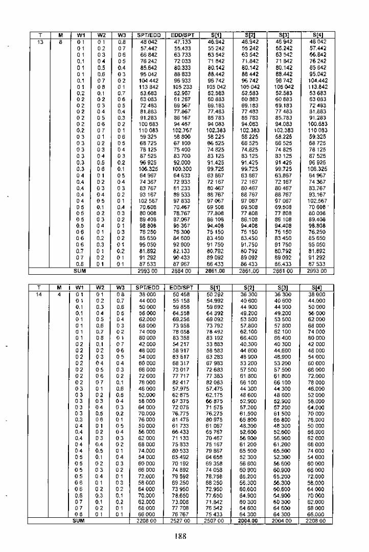
, " w, w, m SPTIEDD EDDfSPT " , " "B • "' "' ••• 48042 47.133 4(;,942 46,94~ 46942 48042

"' "' "' 57.442 55.4~l ,5242 55242 55,242 57,4'2

"' "' •• 66842 6Jn3 63542 63542 63542 %,842., 0< "' 76242 72 033 71 842 7l.a42 71 B42 76242

"' ., ., 85,642 80,333 80.142 80.142 80,142 a:; 64,"' ••• " 95042 88 633 88.442 86442 68,442 9,,042.., "' "' 104442 96933 96742 %742 96742 104.442

"' "" "' 113 842 10,233 105042 105042 1050.02 113,842., ., .' 53,663 52,967 52,563 52,5S3 52.583 53683

"' "' "" 63083 61267 60883 60883 60883 63083

"' " "' 72 '~3 69 >67 69,163 69,183 69,18J 72 453

"' "' ., BUB, 77.867 ?lAB3 77483 77 483 BU8]

"' "' .., 91.283 86167 65783 85783 a,.78J 91..8J

"' "" "' 100 683 94467 94083 94,063 94,083 100,683., "' "' 110083 102.767 102.383 102,363 102,~83 110083

" "' "' 5932, ,6800 56225 58225 58,225 59,325

" "' "' 6872, 67100 66 525 66 525 66025 68725

" "' "' 7B 125 7540Q 74825 74.a25 74825 78125

" "' " 87525 83700 8J 125 B3125 B3125 87525., ., ., 96 925 92,000 91.425 91.425 91425 96925., •• ., 106,325 100,300 99,725 99,725 99.725 106,325

"' "' 0; 64967 64633 6~ B67 6J 867 63.B67 64967

"' "' "' 74367 72 933 72167 72 167 72 167 74367.., "' "' 8~ 7£7 81233 80467 80467 80467 B3.767.., "' "' 93167 89533 88767 88767 aa 767 93.167

•• 0; "' 102007 97833 97067 97067 97067 102.5670; ., .' 70,608 70,467 ~9 ,06 6~"oa 69,~oa 70606 '0; "' "' 80006 78.767 71.80B 77 808 77 808 8000B0; "' "' 89408 87.067 B610a 86,108 86 loa 89,4000; •• "' 96 a06 9~ 367 ~,'06 94,406 9',40a 96.808•• " "' 76250 76300 75150 75150 75150 76,250

•• .., "' B5650 84 600 83450 B3.450 83450 85650

"" ., "' 95050 92 900 91 750 91.7,0 91750 95050., " ., 81.892 8l,13J 80,792 80792 60,792 81.692

" " " 91 292 00433 89092 89092 69092 91 292

••• "' " 87533 87967 86433 B6433 B6.4J3 87533

"" 299300 288400 2861.00 2861,00 266100 2993 DO

, " , w, w, m SPT/EDD EDDISPT " " " "" , " "' •• 38000 50458 50292 36300 .'00 38000

"' "' 0.' 44000 5515B 54.992 40600 4D 600 44.000., ., '.0 ~O000 ~9 8,8 59692 44900 44900 ,0000,, " " ,6000 64,0,6 64:392 49,200 49,200 "00

"' " " 62.000 69.25B 69092 53500 53500 62000

"' •• "' 6B000 73958 73792 57.800 57800 EHl000

"' .., " 74000 76 "08 784.2 62.100 62100 74000

" "" "' 80000 83358 aJ 192 66.400 56400 80000

"' .., " 42000 54 217 5J 883 40.300 40 JDO 42000

" "' "" 48000 58917 58 ~8:3 44 600 4'.600 48 DOO

" "' " 54000 6J 017 6~ 283 46900 46.900 54000

" "' "' 60000 6a 317 67933 5J 200 53200 600DO

"' " "' 66000 73017 72 683 57500 57500 65000

"' "" " 72 000 77717 77 3B3 61 BOO 61 800 72.000

"' " .., 78000 82417 82053 66100 66 tOO 78000

"' " •• 46000 57.975 57,475 44300 44300 46.000

" " " 52.000 62675 62.17, 48600 48600 52000

"' "' " 56000 6737, B6a7, ~2,900 5,,900 ,5,000

"' " "' 64 000 72 075 71 575 57.200 57200 54,000

"' " ., 70,000 76,77, 76,275 61.500 61 ,00 70 000.., "" "' 76000 81 475 ao 975 66 aoo 60800 76,000

" "' " 50000 61 733 61 067 48.300 48300 50 000•. < "' "' 56 000 B643J 6,767 ,2,600 ,2,600 56,000.., "' "' 62000 71133 70467 "00 56.900 62000

"' e, " 68000 75333 75167 61 200 6\.200 68000

" ., "' 74,000 80 ~33 79 B67 6,500 6~.500 74000

" " " 54000 65492 64 6~8 52300 52.300 540000; " "' 60 DOO 70192 69358 56600 "00 600000; "' "' 66 DOO 74 B92 740,6 60900 60,900 660000; " " 72,000 79692 78.758 6o,~00 6,,200 72,000., " "' 58000 69250 68260 56,300 56,300 56.000

"" "' " 64000 7J 950 72.960 60,600 60,600 64 000•• 0, ., 70,000 ?M50 77.600 54,900 84,900 70000

"' ,, ., 62,000 nooa 71,842 60300 60300 52,000

"' " "' 68000 77 706 76542 64600 ~.oo 68000

"" "' " 66000 76767 75433 64300 64 300 66.000

"" 220800 ~527 00 250700 2004,00 2004 00 220800

'88

, , ., m m SPT/EDD EDDISPT " " , "" , oo oo "' ~8,925 51.750 51575 37.425 37425 38925o , 0, 0' 45,25 57350 57175 42525 42525 45525o , " " 52125 62950 62.775 47,625 ~7,625 52,125o , " 0.' 58725 68.550 68375 52,725 52,725 56.7250.' 0; " 65.32, 74.150 70.975 57,825 57 B25 65325oo "0 " 71,925 79,750 7957, 62.925 62925 71 925oo oo "' 7B 525 as 350 85.175 68 025 6B 025 78525oo "' oo 85125 90 950 90,775 n.12, 73,1Z5 85125

"' ,, "' 4~250 55900 55550 .1 750 41.7,0 4:l,~5a

"' "' " 498,0 61,,00 61150 46850 ~o~ 49850

"' " 0; 56~50 67100 667,0 5U50 51 950 56450

"' " " S3050 72 700 72.350 57050 57,050 630,0

"' 0; " 69-6>0 78 :300 77.9,0 62150 62 150 69.650

"' " "' 7625<) 60.900 6M50 67,Z50 67250 7625D

"' "' oo 82850 89500 89150 72 350 72 ,50 82850

" oo 00 47575 60,050 59.525 40.075 46 D75 47575

" "' "' 5<,175 6,650 6,125 51.175 51175 54,175

" 0' " 60.775 71 250 70725 56 275 56275 60,7750' 0' 0' 67375 76 B50 76325 61.375 61.375 67375

" " "' 73975 82,460 81.925 66475 68 476 7J 975

" 0' o , 80,;75 68050 87526 71 675 71,575 60,5750.' o , 0' 51.000 64200 63500 50400 50,400 51.900

" " " 58.500 69.800 69.lOD 55500 5;,500 6B500

" " " 66,100 75400 74.700 60600 60600 6,,100

" " "' 71.700 81,000 ao 300 65700 65700 71 700

"' "' oo 7B 300 B6600 B5900 70 aoo 70 BOO 7B 300

" oo "' 56 225 6a,350 67475 54 726 64725 56,225

" " " 62625 73,950 73075 59825 69.825 62 B250' 0> "' 69425 79550 78,675 64,925 64.925 69425

" " " 76025 85150 84275 70,025 70026 7602500 " " 60550 72 500 71..60 59,050 59050 60.55000 " " 67.150 78.100 77.0;0 64,150 64150 67.15000 " " 73.750 6:J.7oo 82,6;0 69250 69250 73750

"' oo "' 64 875 76,650 75426 £3.375 63375 64,875

"' "' "' 71.475 82 250 a1 025 68475 68,475 71475oe " , " , 59 200 aDBOO 79400 67.700 67.700 69200

'"' 231900 26B200 2661 00 2139.00 :1139,00 231900

, " w, w, W, SPTIEDD EDDISPT " '. '" S[.]

" , o , " ,., 39850 53042 52,858 38,550 3a 550 398500.' "' " 47050 59.542 59 :J58 4.,450 44450 47.050

" "' 00 ,42,0 66 042 65858 50360 50,350 54 2,0" , "' "' 61.450 72542 72,358 56250 56250 61 450oo " 0' 63650 79042 78858 62.150 62160 66,650

" 00 " 758'0 85,42 65,),8 68050 68 050 75850

" " " 83050 92042 91.856 73 960 73 950 83050

" "' " 90,250 98542 98.356 79,850 79850 902500.' oo " 44600 57.583 57217 43,200 43200 445000.' "' 00 51700 £4.083 61717 49,100 49100 51.7DO

" "' "' 5800D 7058l 70,217 55000 55 DOO 680000> "' "' 66.100 77.083 76717 60900 60900 66,100

" "' "' 73300 83,583 83217 66 BOO 66800 73.3000' "' "' 8D500 90,083 89717 72 700 72.700 aO,5000' " " 87700 96583 ~6 217 78600 78600 87,7000.0 0.' 00 49150 62125 61.575 47,800 47850 49150

" " 0.' ,6350 08615 68075 53750 OU50 56350

" " " 63550 75,125 74575 59650 596,0 ~3 5500' "' "' 70750 81.625 81 075 66,>50 65550 70.750

"' 0; " 77.9,0 38.125 87575 71,450 71450 77.950

"' 00 oo 65160 94626 94075 77 350 77.3,0 85150

"' oo 0; 5MOO 66667 65933 52500 52500 ,3 sao

"' "' "' 61.000 7l '57 72.433 58400 5SAOO 61 000M " "' 6B 200 79667 78,n3 £4.300 64.300 6B 2000' M " 75400 S6167 85.33 70200 70200 754000' 0; " a2600 92667 91.933 7~ 100 76100 826000; " " sa 450 71208 70292 57,150 57150 58450

" " "' 65650 77.708 76792 63050 63 D50 65.6000; " "' 72850 84,20a S3,292 6S 950 68.950 72 850

"' " " aD 050 90,708 89792 74.850 74.85D aD050

" ,, " 61100 75750 74650 61.800 61 800 631000.' " " 70 lOO 82250 81 150 57,700 67.700 7030000 "' 0.' 77,,00 68,760 87650 73600 73,~00 77.500

" oo "' 67.750 80292 79008 66450 66450 67.750

"' " oo 74950 a6.79. 85508 72.350 72,3>0 74950

"" " o , 72.400 84 833 83367 71.100 71.100 72 400

'"' 243000 283700 2615 DO 2274,00 2274,00 2430.00

'89

; " w, w, W. SPTIEOD EDDISPT " " Si3 S[4]

" , " " " 40.775 >4 333 54.14'- 39615 ,9t15 ~O775

" ., " 48575 61.733 61.542 46375 .6 :)75 46575o , " ••• ,6375 t9,133 68942 53075 ,3075 56,J7~

" " ,., 64175 76,533 76342 59775 59.775 64,175

" 00 " 7' 975 83,93~ 83742 66475 66475 71,975,, 00 "' 79775 91.333 91,142 73175 73.175 79,775

" "' " 87,,75 98733 98542 79,675 7987, 87575

" ••• " 90,375 106133 105942 86575 86.575 95375

" ., "' '5,750 59,57 sa 883 .4650 44650 45750

" " " 53550 66,667 66283 51 350 51.350 53,550

" " 00 61.350 74,067 73 083 58 0&0 58050 61.350

" " " 69150 81.467 81 083 54 750 64750 69,150

" ., "' 76950 88,867 as 4a3 71.450 71450 76,950

" " " 84 750 96 267 95883 781&0 78150 54 750., "' ., 92550 103667 103,283 B48,0 84 B50 92 550

•• "' •• 5D.725 64 200 63,625 49625 49625 50725

•• " 00 53.525 71.600 71 025 56325 56325 58525

••• "' " 66.325 ,,~784" 63025 63025 66325

•• " "' 74.125 BB.400 6582, 69725 69725 74.12,

O' 0; "' 81.925 93.800 9~ 22, 76425 76425 81.92,

0.' 00 ., 89,72, 10L200 100 62, 83125 SJ 125 897250< ., 0; 55,700 69133 68367 54,600 54600 ,5700

0< ., 0< 63,,00 76533 75767 6DOO 61 300 63500

" 0; 0; 71 300 83 9~~ 83167 68000 66000 71 300

0' 0< 0' 79100 91,333 90567 74700 74.700 79 1000< 0; o , 86900 98733 97,957 81 400 8lAOO 86,90000 o , 0< 60675 74067 13.108 59575 59575 60,67500 " ., 68475 81467 80,508 66275 66275 68,475•., •• ., 76275 88,867 87,908 72.975 72975 76,275•., 0< " 84075 96,267 9,308 79.675 79675 84,075

"' ., "' 65,650 79000 77 850 64,550 04550 656500; "' "' 73450 00 400 85250 71.250 71 250 73450

"' "' " BI 250 9~ 800 92.650 77 950 77 950 81.200., " " 70.625 8~.933 82.592 59525 69,625 70625

"' " 0.' 78425 91.333 B9.992 78225 7622, 75.425M " "' 75600 88867 Bnn 74500 7',500 75600

"" 2041,00 299200 296900 2'09 DO 240900 25-11.00

; " w, w, W. SPTIEDD EDDlSPT " S ~I '" .-" " "' " •• 41700 55625 55,'25 40600 '0800 4',700

"' "., 50100 63925 63,725 48300 '8.30D 50,100., "' •• sa 500 72.225 72 025 55800 55800 5B500., "' ., 66900 80,525 80325 63300 63,300 66900

" 0; "' 75300 88,625 88625 70800 70.800 75300

"' 0; ., S3700 97125 96,925 78300 78,300 83700

"' "., 92 100 105425 105,225 B5.aoo 85800 92 100

"' 0' "' 100 500 113 725 113,525 93 ~OO 93300 100,500

"' ., " '7,000 60 950 60 550 46100 46100 47,000., ., 0; 55400 69,250 6B850 ,~ 500 53600 55400., •• 0; 63800 77.550 77 150 61100 61,100 63800., "' "' 72 200 85850 854,0 58600 68800 72200

" "' "' 80800 94 150 93.750 76,100 76100 80600

" "' " 89000 1024,0 102.050 83600 83,500 89000., " "' 97400 110.750 110J,O 91100 91 100 97400

•• "' "' 52 300 6627, 6567, 51400 51 400 52.300

"' " 0; 60.700 74.57, 73970 58900 ,6 900 60700

•• •• "' 69.100 6287, 82275 66'00 56,'00 691000.' "' 0.' 77 000 91175 90,,75 7~ 900 73 900 77 000

"' "' ., 85900 99 '75 98675 81 '00 81.400 85900

"' 0; ., 94300 107,775 107175 8B900 86900 943uO

"' "' ., 57600 71.600 70 BOO 56 700 56700 57600

"' ., "' 66000 79900 79100 ~,oo 64.200 66 DOO

"' ., •• 7'.400 a8200 87 '00 71 700 71700 74 '00

"' "' ., 82.800 96500 95700 79 200 79200 82 BOO

"' 00 "' 91 200 10.1,800 104 000 86.700 66700 91 2000; "' "' 62900 76,925 75925 62000 62,000 62900

"' ., ., 71 300 8,225 84 22, 69.500 69,,00 71 300

"' "'., 79700 93525 9;>,52, 77.000 77 000 79.700

"' "' "' 8B 100 101 825 100,825 B4.500 84500 B8,100., "' "' 56200 82,250 81 050 67.300 67300 68200

•• " ., 76600 90,550 89350 74800 74,800 766ao., "' ., 8,000 98850 97650 82300 82,300 a, 000

"' ., ., 73 500 8757, 86 175 72600 72 600 73.500

" " "' 81,900 9'.875 94.475 80100 80100 81.900

" "' "' 78 800 92.900 91.300 77.900 77 900 7680D

'"" 2652.00 J147,00 312300 2544 DO 250\400 265200

190

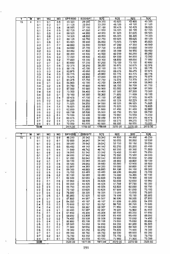
, " w, w, W, SPTlEDD EDDISPT " 8[2] --'" "" , "' ,, '" 45325 29350 29350 43 B25 43 &25 45325,, " " 51 125 33200 33250 48,1,0 48125 51125

" " ,.• ,6925 37150 ~7,'00 (;2.425 52425 56,92,,, " 00 62725 41,0,0 41050 56.725 ~6 725 62725,, 00 ,. 68525 ",950 44950 61 025 61,025 68525

"' •• " 74325 48,650 48850 65.325 65,325 74325,, " " SO 125 52,750 52,750 69625 69,625 80 \25

"' '" ,, 85925 56650 56,650 73.925 73 925 S5,925

" "' 0; 48,850 33 BOO 33600 '7350 47350 48850

" " •• 54,650 37.700 37700 ,1,650 51,650 54650

" " 00 60450 41600 4UOO 55950 55950 60.450

" " ,.• 66250 45500 45,500 60 250 60.250 66,250

" " " 72 050 49400 49.400 64 550 64.550 72,050

" •• " 77.650 53300 5~300 68,850 68.850 77 B50

" " ,, 83650 57200 57,ZOO 73,150 73.15D 83650

" ,, 00 52375 38 :150 3S,250 50875 50 B75 52,375

" " 00 58175 42,150 42150 55175 ,517, 58,175

" " ,. 63,975 46050 46050 59.47& 59.475 63975

" " " 69775 49,950 49,950 63775 63775 69,775

" " " 75575 53 a,o 53 a,o 6a 075 65,075 75575

"' '" " , 61.375 57.750 57.750 72.~75 72375 81.375

" " " 55,900 42700 42.700 50,400 54 400 55.900,.. ,., 0< 61.700 46 600 46 600 58.700 sa 700 6\.700

" " " 67,500 50 5{)0 50 5{)0 63,000 63000 67.5DO

" ,. " 73 300 54,400 54400 67300 67,300 73300,., " ,, 79100 58300 58,300 71,600 71 600 79100

" ,, 0< 59425 47.15D 47.150 57,925 57925 59425

" " " 65225 51.0,0 5\.050 62225 62,225 65225

" " ,., 7\.025 54.9,0 54 9>0 66525 66525 71.025

" " ,., 76825 58850 58.850 70 B25 70825 76,a25

" " " 62.950 51.600 51.600 61450 61 450 62,950

" " " 68750 55-500 55.500 65750 65.700 68.750

" " "' 74550 59400 59400 70050 70050 74.550

" "' " 6847, ,5 05{) 56 05{) 64975 64975 66475

" " " 72 27, ,9,9,0 59.95D 69275 69,275 72.275

" " ,, 70000 60.500 60500 68,,00 68500 70.000eo" 2415.00 175800 1758.00 2235 DO 223500 241500

; " W, W, W, SPTfEOD EDDISPT '" '" Sm ~" , ,, ,, " 46 250 30342 )0,342 44950 44950 46250

" " "' ;2650 14,942 :l4 942 50050 50,050 52650

" " 00 59050 39542 39,542 55150 55150 ,9050

" " 00 66,450 44142 44142 60 250 60,250 65450

" 00 " 71 850 48,742 ~9 742 65350 65350 71.850

" 00 " 7" 250 53342 53342 704,0 70450 7B250,, " " S4 650 57942 57,942 75550 75550 S4 650

" "" "' 91 050 62,542 62542 80650 80650 91,050

" " , " 50100 35083 ~, 08~ 48800 4S,aOO 50100

" "' 00 56500 ~9,68:3 :39683 53.900 53900 56500

" " "' 62,900 44283 44 28~ 59000 59,000 62900

" " " 69300 4a,86:l '8,863 64.100 64.100 69 :l00

" 0; " 75,700 53483 53483 69200 69,.00 70.700

" " " 82,100 58083 58063 74,:l00 74,JOO 82100

" " "' 88500 6268:l 62,683 79400 79400 88500

" " " 53950 39 B25 39,625 52,650 52.650 53950

" " 00 60350 44425 44425 57,750 57.750 60350

" " " 65750 49025 49025 62,850 62.850 86750

" " " 73150 53625 53625 67950 67.9,0 73.150

" " " 79,550 58225 5a 225 7J 050 13050 79,550

"' "" ,, 85,950 62625 62825 7B 150 76,1,0 85,950

". " , " 57,600 44567 44567 ~,oo 56,500 57,800

" " ".' 64,200 49167 49167 61 600 6\.600 6' 200

" " " 70600 53767 5J.707 66 700 66.700 70600

" " " 77 000 5~,Jo7 58 ~67 71 800 71800 77 000

" 0; " 8:3400 62967 62967 76900 70,900 SJ 400

" " " 01650 49,J08 49,J08 60 350 60.350 51650

" " " 6B,050 53,908 53908 65450 65.450 6B,050

"' " " 74,460 58508 58508 70550 70550 74460

" " " , 80 ~50 63,108 63108 75650 75650 80,550

"' " " 65500 54050 54050 64200 64.00 65,500

" " "' 71 900 5~ 650 5B,650 69,300 69300 71 900

" "' "' 7a 300 63250 63,250 74,400 74.400 78300

" " " 69350 5a 792 58.792 68050 68050 69350

" "',, 7,.750 6.l 392 63392 73.1,0 73,150 75.750

" " "' 73.200 63533 63533 71900 71,900 73200eo" 252600 1B77.oo 1~77.00 237000 237000 252500

'"

, " w, w, W, SPTIEDD EDDISPT 5[11 " " S[:!•....'" , ,, " oe 47175 31.333 31 333 45070 46075 47175

" " " 54 175 36,633 36 £33 51 97, 5\.975 54175o , " 00 61175 '1.9~3 41 933 5787, 57,875 61175

" "' 0; 6~,175 47233 47233 63,775 63775 6a 175

" 0; "' 7, 175 52533 52,533 69675 69.675 75175

" 00 " 82,175 57 B30 57,633 75575 75575 82175,, " " 89175 6J,133 631~3 81 475 61.475 S9,175

" oe " 96175 6a,'~3 68433 87375 67.375 96175

" " " 51 350 36367 36367 50250 50250 51.J50

"' "' 00 58350 416£7 41667 56, ',0 56.1,0 58350

"' " " 65350 46 %7 46967 62,050 62050 65350

"' "' "' 72 )50 52,267 52267 67950 67,950 72,50

"' " ,., 79350 57567 57,5{;7 73 BSO 73850 79350

" 00 " 36350 62 B67 62867 79.750 79750 86350,., " " 933,0 68,167 £8167 85650 85,650 93350

" ,, " 55525 4 \..00 4\.400 54425 54425 55,,25

" " " 62525 46700 46700 60325 6D 325 52525

" " "' 69525 52000 ,2.000 66225 66225 69,25

" "' " 7552, 57.300 ,7.30D 72125 72 125 76,25

" " " 53,2, 62600 62.500 78025 78025 e~ ,25

" " ,, 90525 67.900 67.900 83,n5 a3.920 90.025

" " " 59700 464Jl 46,433 58.600 58600 59700

" " " 66.700 51.733 51 733 64.500 64500 00'00

" " " 7J 700 57033 57033 70400 70400 73 700

"' "' " ao 700 6Z 33J 6.,~~3 76300 76300 80700

"' " " 87700 67,5~3 67,633 82200 82200 87700

" " " 6l,675 01.467 51467 62775 62775 6387,

" " " 70675 56,767 56,767 6667, 68675 70 B75

" "' " 77 B75 6.067 62,067 74575 74575 77 8750, " " 84 B75 67367 67367 80,475 60,~75 84,87500 o , " 68,050 56,00 56500 66 950 66950 68,050

" " " 75050 61.600 61.600 n850 72 8,0 75 D50

" " " B.050 67,100 67,100 78750 787,0 8. D50

" ,., " 72 225 61 ,33 61,,33 71.12, 71.125 72 225

" " " 79225 66833 06 833 77.025 77,025 79225

" " ,, 76400 66667 66 %7 75300 7,300 76400W" 2637.00 1996 00 1996,O~ 250500 .505 00 .637,00

, " w, w, '"' SPTIEDD EDDISPT S[.~l 'I. " ••" , " " " 4B 100 3232> J232> 47,<00 41',200 46100

" " " 55700 JB 325 )e,32, ,3900 53900 5,.700

" " "' 63300 44,325 44,~25 60600 60600 63300

" " " 70900 >0,325 50,32, 67.300 67,300 70900

" " " 78500 56 325 56 325 74,000 74,000 78,500

" 00 " 86 lOa 61325 61,325 eo 700 so 700 86100

" " " 93700 68,~25 68,328 e7.400 87400 93700

" " " 101 300 74325 74325 94.100 94,100 101 300

" " " 5.600 37650 37650 51.700 51.700 52,600

" " 00 60200 43650 4~ 650 53400 58400 60,200

" " " 67 BOO 49650 49650 65100 65 100 67,600

" ,.. " 75400 55650 55,650 71,800 71.800 75,400,., " " 83000 61,6,0 61,6~0 76,00 78-500 83000

" 00 " 90 600 676,0 676,0 85200 B5.'00 90600,., " " 9B .00 73,650 73.6~0 91,900 91.900 9S 200

" " 00 ~7,100 42975 42975 56200 ~,oo 57.100

" " " 54.700 4897, 4897, 6.900 62900 64 700

" " " 72 300 ~4,970 ,4.975 69600 69600 72,300

" " ,., 79.900 60,975 60975 76300 76300 79.900

" " " e7.000 66.915 66.97, 83000 83000 87.500

" 00 ,, 95100 72,975 72.97, 89700 89700 95.100

" " " 61.600 48.300 48300 60700 6070a 61.60D

"' "' "' 69200 54,300 54,300 67,400 67400 69200

" " " 76800 60,300 60300 74100 74100 76800

"' "' " 54400 60.300 66300 80,800 SO800 84.400

"' " " 92.000 72.300 72.300 87,500 S7.500 92000

" " " 65100 ,~ 62, 53625 65200 65200 00'00

" "' " 73700 59625 59625 71,900 71 900 73.700

" " " 61.300 65625 656<5 7a.600 78600 81.300

" "' " B8.900 71 62, 71.6.5 85300 a,300 86900

'" " " 70.6ao 58.950 53950 69700 69.700 70600'0 "' " 76200 64.950 64.95D 76400 76400 78.200

'" " ,, 85.800 70.950 70.950 83100 83100 65800

" ,, " 75100 64.75 6427, 74,200 74200 75.100

" " " evoo 70275 70275 80900 80900 82700

" " " 79600 696DO 69600 78700 78.700 79 6£,,90_W" 274800 211500 21'5,~0 264000 264000 2748,00

192

, " w, w, W, SPTIEDD EDDISPT S[l] , S[3] "" • " ,., '" 49025 33317 33317 48325 48325 49,025,, " " 57.225 40.017 40017 55825 55625 57,225,, " ,. 65A25 415717 46.717 63325 6U25 65425,, " ,. 73.6.5 50.417 53.417 70,825 70325 73 625,, " ,. 51.825 60.'17 60.117 78325 78325 S1,a.,,, '" " 90025 S6.an 66817 85825 85325 90.025,, 0; " 98225 73.517 73.517 93325 9~325 96225

" '" " 10(; 425 BO.217 50217 100 825 100 325 106 425

" " 0; 53850 JB_9~3 36 gJJ 53150 5~ 150 ;3850

" " '" 62050 45633 45633 60650 60650 62 000

" " " 70250 52.303 52.333 68150 68,150 70250

" " " 75450 59033 ,9033 75650 75,650 75450

" " " 56650 65733 65733 83150 a3,1~O oo.~" '" "' 94,850 72.433 72.433 90650 90£50 94 850

"' 0; " 103050 79133 79_1~J 98150 98150 103050

" " ., 53675 44,550 44 550 57.975 57,975 55615

" "' " 66 B75 51.250 51 250 65475 65,475 6£.875e, " " 7507, 57.950 57950 72 975 72 975 75075

" " " 63275 64 650 64 6,0 BO475 80475 5~ 275

" " " 91 47, 71.3,0 71.350 87.975 S7,970 91.475

"' 00 "' 99675 78050 780><) 90475 95475 99 G75

•• "' " 63500 ,0167 ,0,107 62800 62600 6MOO

•• "' •• 71 700 56 867 56 807 70300 70300 71,700

•• " " 79900 63567 63567 77.8DO 77 600 79900

•• •• " 88100 7D267 70267 85300 85300 S6100

•• " "' %300 76967 76967 92.800 92 BOO %'00

" "' •• 6532, 55783 557Bl 67.625 67625 6B 32,

" "' "' 76525 62,48) 62483 75125 75,125 76525

" " " 84 725 691Sl 69183 B2.625 82,625 84 725

" •• ,, 92925 758B3 75 SS3 90125 90125 92.92500 "' " 7:) 150 61.400 61,400 72.450 72 450 731><)00 " " B1.350 63100 66100 79950 79950 81.35000 " " B9550 74.BOO 74,800 87.450 87450 S9 5><)

"' ,, " 77.975 67.017 67,017 77.275 77 275 77.975

" "' "' 8617, 73717 73 717 B4775 84.775 86.175

'" "' "' 82 BOO 72,633 72 633 32100 82,100 82800-eo" 285900 2234 00 2~34.00 <77500 277500 2859.00

, " w, w, W, SPTIEDD EDDISPT S[1] " " S[4]

•• • "' "' 00 36,608 35 !l42 35642 35306 35308 56 60B

"' "' "' 41.80S 39,842 39542 39206 39208 41 80B

" ., ., 47008 43,742 43442 43.1OB 43 lOB 4700B

" " ., 52208 47842 47.042 47.00B 47.000 5220B

"' " " 57408 51 542 51.242 50.90B 50.900 57,40B

"' ., " 62608 55442 55142 54.808 54 80B 62,606

" " "' 67808 59,342 59.042 58.70B ,5.70B 6780Bo , " "' 73.008 63242 62.942 62606 6~,608 7300B

" " e, .0017 39983 39 J83 36717 3B 717 40017

" " "" 45217 43883 4~ 283 42617 42617 4, ;;17

"' " " 004'7 47.783 47.183 46517 46517 50417

" " •• 55617 ,1,683 O1,OS3 50417 50417 5,617

"' " " 60,6\7 55.083 54.983 54317 54,317 60817

" "" " 660\7 59.483 ,6 B~3 5S,217 58217 66017

" " " 71 217 63383 62,7~3 62,117 62117 71 217

" ,, "" 43425 44.025 4312, 4.1,t25 42125 43425

" " " 48625 47.925 47.02, <6025 46025 48625

" " " 53 B25 ,1 82, ,092, 49,925 49925 53825

" " " 59025 55.725 54 82, 5J.825 53,825 59 D250' " " 64225 59625 5B 72, 57,725 57725 64225

" "" ,, 69,425 63-525 62625 61.625 61,625 69425

" " " 46,6~3 48067 46867 45533 45,533 46 B33

" " " 52033 51 967 50767 49,4~3 49433 62 D33

" " " 57233 55867 54,567 53,333 53333 57233

" " " 62433 59767 58,567 57233 57233 62433

" " " 67,633 6~ 667 62467 61133 61,1~~ 67633

" " 0' 50 ~42 52108 50608 48,94;; 48 !l42 50242

" " " 55442 56008 54,5a~ 52642 52 842 55442

" " "' 60&42 ,9903 oB,408 58742 56742 60&42

" " " 65 842 63808 6.,308 60 &42 60 &42 65 842

"" " " 53650 56 150 54,350 52,350 52350 53650

"" " " 58850 60050 08250 56250 56250 58,660

"" " " 64050 63950 62,150 60150 60150 64050

" " " 57058 60192 58092 55,768 55758 570580.' " " 62258 &4092 61 992 59,658 59658 62258

'" " ,, 60467 &4233 61 B33 59167 59,167 60467

'"" 2041,00 1%1.00 192500 1885.00 18a,oo 2041.00

193

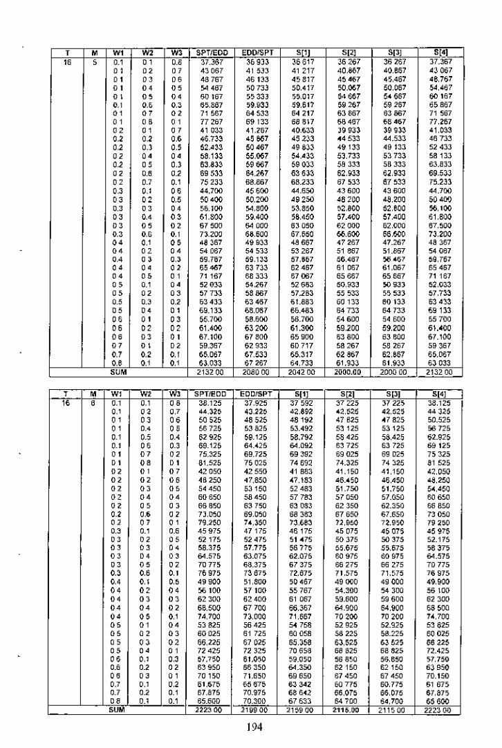
, "., w, W, SPTIEDO EDDISPT "' SP] S[J] S[4]

'" , ,, "' ,.. 37.367 36933 J6617 36267 ~6267 37.367

"' " " 43067 41 5.lJ 41 217 40,867 40,667 43067

"' " " 48767 461.l3 45817 45467 4,.467 46,757

"' "' "' 54 467 ,0733 50,417 50,067 50,067 54,467

"' "' "' 60167 ,533) ",017 54667 5< 667 60 167., ., ., 6,,867 ,9,933 ,,9,617 59267 59267 6,867

"' "' " 71 567 64533 64217 63 B67 63867 71 567., ., "' 77 267 69133 68817 6B 4G7 68467 77.267

" "' "' 41 033 41.<67 40,633 )9933 39 93~ 41.0~3

" ., •• 46,733 45667 45233 44533 44.533 46733., ., ., 52,'~3 50467 49833 49133 49133 52433

" "' "' M,133 55.067 54,'3~ 53.733 53733 58133., "' ., 63.83~ 59667 59033 S8333 5B 333 £3.S33

" " " 69533 64.267 63633 62,933 6:2,933 69.533

" ., ., 75 nJ 68.867 6B.233 67533 67533 75.233., ., •• 44.700 45600 44.65D 436DO 43600 44.700

" " "' 50400 50,200 49250 48200 48,200 50 40')0.' " "' 50.100 54,800 ,3,850 52,800 52,eOO 5(>.100

" "' "' 61.800 ,9,400 ,6.450 57.400 57.400 61.800

" ., " 67500 64 000 63050 62 000 52,000 67,500., ., ., 7J.200 65,500 67,550 66,600 66,600 73.200

" o , ., 48387 49933 48667 <7267 47.267 48367

" " " 54067 54533 53267 51 867 51.867 54 067

" " " 59.767 59,133 57,557 06,467 66 067 59.767

" •• " 65 <87 63 7:):) 62467 61 067 61.067 65467

"' ., "' 71167 68333 67067 65667 65667 71167., ,, •• 52033 54,267 52653 50,93~ 60 9~J 52,033., " " 57733 58867 57.253 55533 55 5~J 57,733

" " 0.' 534J3 63467 61.aa3 00 133 60133 63433., •• " 69.133 68.067 65.483 64733 64 73~ 69133

" " " 55.700 58.600 56.700 54600 54600 55700

" " " 61.400 63200 61.300 59,200 59,200 61.~00

"' " " 67.100 67800 65900 63800 63800 67.100

" " " 59.367 62933 6D717 58267 58267 593670' ., ., 66,067 67,533 55,317 62857 62,667 65,067O. o , ., 53.033 57267 6<,733 61.933 61,933 63033

'0" 213200 208000 204200 2000.00 2000 DO 213200

, " w, w, W, SPTIEOO EOOISPT S[lJ '" S[J] 5[4J

" , ,, ,, " 38,125 37,925 37092 37225 J7225 38,126., " " 44,325 43,n5 42,892 02.020 42,025 44325

" " " 50025 48525 48192 47 B25 ~7 825 50.525

" •. < " 5B725 53825 53,492 53125 53125 56 725., ., .< 62925 59.125 58.792 58425 58.425 62.925., " ., 69.125 64.• 25 64.092 63725 63725 69125

" "' " 75.325 69.725 69392 69026 69 D25 75325

" '" " 81,525 75025 74692 74.325 74325 81 525

" " " 42050 42550 41 883 41.100 41.150 42,050

" " " 4B250 47,850 ~7,183 46.050 46,.50 48,250

" " " 54450 53150 52483 51.750 5l.750 50.450

" " " 60650 58450 57783 57050 57.050 60650

" " " 66660 63750 63083 62350 62.350 66850

" " " 7J.050 69,050 68383 67650 67.650 73050

"' " " 79,260 70,350 73.563 7<.900 72.9,0 792500.' .., .." 45975 47175 46175 45075 <5075 45976

" " " 52175 52475 51 ~75 50375 60 375 52.175

'" "' " 68.315 67.715 66 71~ 00,570 5,,675 56375

'" " " 64.575 63.075 62.075 60975 60975 64.576

" "' " 70775 68.375 67375 66275 66275 70775., ., ., 7597> 73670 72.67> 71.575 71,575 76975

" o , " 49900 ,1,800 ,0467 49000 49000 49,900

" "' "' 56 100 57100 55767 54.300 64300 56100

" " " 62300 62400 61 067 59.600 59600 62300

" " " 66.500 67700 65,367 64.900 64,900 68500

" " ., 74,700 73.000 71,667 70200 70200 70,700

" " " 53825 56425 5~ 758 52925 52.925 53825

" " " 60025 61 725 60058 68 225 58.225 60026

" " " 66,225 67025 65,358 63,625 53525 58225

" " " 72 425 72 325 70658 68325 68825 72.425

" ., ., 57.750 51.0>0 59.0,0 66850 56,850 ,7.7500." .., " 63950 66350 64.360 62150 62150 53950

" " " 70150 71.6,0 69650 67450 67450 70.150., ,, " Ill,675 f5 675 63342 60776 60.775 61 67,.., .., 0.' 67.875 70.S75 586<2 66,075 66,075 67,8750' ,, ,, 65.60D 70.30D 67633 64700 64,700 55600W" 222300 21~900 215~00 2115,~~ 211500 2223 [H)

194

; " m "' "' SPTIEOD EDDISPT S[11 S~l " "'" , ,, " " 38 B8J ,6,917 38567 38.183 3S,163 38883

" "' " 455~J •• 917 44567 44.183 44,163 <5583,, " 00 52.283 5D917 50567 50.183 50183 5228J

" " " 56 gal %,917 56567 56.183 56163 !l6,9S3

" " M 6"eSJ 62917 62567 62.183 02.163 6,683

" 0' .0 72 ~83 68917 68567 66 '83 6alB3 72 383., ., "' 79083 74917 74,567 74 183 741BJ 7908~., •• o , 85783 SQ917 BO 567 8O,lS3 80163 85783

"' " ., 43,067 43633 43133 42367 42.367 43067

"' "' 00 49,767 49,633 49133 48367 48.367 49.767., "' ., 56467 55 B33 55,133 54,367 >4.367 564670; •• •• 63167 61 flJ3 61133 60367 60367 63,1670; ., ., 69,867 67,833 67.133 66367 136367 69,8670; 00 0.' 76 >67 73.833 73,133 72 J67 72 367 76.567.., ., " 83267 79an 79,133 78,67 78367 B3.267.., .., ., 47,2,0 48.750 47.700 46550 46550 47.2>0.., " ., 53.9>0 54.750 53.700 52550 52550 53.9,0., ., •• 606,0 60.750 59.700 58,50 58550 606,0.., .., .., 67.3,0 66750 65.700 60,050 64,650 67350.., .., " 74.0,0 72.75.(l 71.700 70,,0 70,50 7405.(l

" '" .., 50,75{l 78.7,,0 77.700 7,5,0 76,50 80750

•• •• ., ,1,'33 ,J 667 52267 50.733 50733 51,433M " " ,8133 59667 5B 267 56733 56733 58133

" ,., " 64 833 65667 64 267 62733 02733 64,833

" " " 71 533 71 667 70267 63733 08733 71.53J

" ., ,, 78,233 77.667 76267 74.733 74733 78233., ., ., 55,617 58,583 56833 54 917 54917 55tH., "' "' 62,317 64,683 62,633 60917 60.917 62317., "' "' 69017 70,563 68,633 66,917 66917 69017., " •• 75717 76,583 74,633 72.917 72.917 75717

'" " •• 59 BOO 6~ 500 61400 59,100 ,9,100 59600

'" ., "' 66500 69500 67400 6,,100 65100 6650000 •• " 73 100 75,,00 73.400 71.100 71.100 73 200

•• •• " 63 96~ 6a,417 65967 63283 632a3 63983

" "' •• 70 66~ 74417 71.967 69283 69283 70.683

'" .., .., 68167 73,~33 70533 67,4157 67,467 68167

'"" n14,00 n1800 227600 2230,00 223000 231400

, " "' "' "' SPTIEDD EDDfSPT 5['1 S[~ SjJl Sl:.!,.-;; , •• •• .0 39642 39.900 39542 39142 39142 ~9 642,, " " 46842 46608 46242 45642 45642 46842•• 00 •• 54,042 53,308 52,042 52.542 52542 54042•• •• •• 61 242 60 008 59642 ,9242 59242 61.242

" •• •• 68442 66 70B 66342 65.942 55942 68.442•• 00 00 75,642 7J.408 n04< 72 0.2 72.642 75642., ., •• 82842 80,108 79742 79342 79.342 82642

" •• " 90042 86808 86442 86 042 66042 90042., ., .' 44,083 40,117 40,383 '30a3 4:) ,a3 440B:)

" ., •• 51283 51817 51083 50283 502a3 51.263.., '.0 •• 58483 58,17 57,7B3 56,98~ 5<',9Bl ,8483., •• •• 65,6e~ 65217 6446:) 63883 6:) 683 65.683., ., .., 72 863 71917 71.163 70 383 70383 72.BB3.., '.0 .., 800B3 78617 77.8B3 77 083 77 08~ 80.0BJ

" .., .., 87.2B3 85 ~17 84,5<13 83.763 a3,7aJ a7,2a3.., •• •• 48525 50 ~2, 4922, 48,025 48,025 46.52,

" " •• 55.72, 57.02, ,5.92> 54725 54.725 ",72,

"' "' •• 62.92, 63.72, 6262, 61425 61425 6292500 •• ., 70.125 70.425 69.325 68125 6B125 7D 12,

" •• " 77,32, 77.12, 76025 74825 74825 77 32,

" •• ,, 64 52, 8:) 825 8272, 81525 81 ,25 64 525., ., M 02 967 55533 54 067 52 ~67 52467 52967., ., •• 60,167 62233 6D767 59.167 59167 60167•• 00 "' 67367 6B 93~ 67467 65 B67 65,B57 67,~67

•• •• •• 74567 75 63~ 74,167 72.,67 72.567 74567

•• •• ., 81.767 a2,~3J ao 867 79.267 79267 81 767•• " •• ,7408 60742 58,90a ,6905 56,906 o7,40a

•• •• ., 64,50B 67,442 6,608 6:) 606 63608 64,608•• " •• 71 808 74142 72308 70.300 70308 71 B08•• " " 79008 BO642 79008 77.008 77.008 79,00a00 " 00 6' 350 6,,950 6~.750 6',300 QU'O 61,65000 •• •• 69,050 72.650 70,450 66.050 68050 6905000 00 •• 76250 79,~50 77.100 74,750 74,700 76260

•• " •• 60292 7, 158 6a,592 65,792 66.792 66,202., •• " 73492 77 858 75292 72.492 72 492 73492". ., ., 70,733 76367 73 433 70233 70233 70733

'"" 240500 2437.00 2393.00 2J45,~~ 234500 2405.00

195

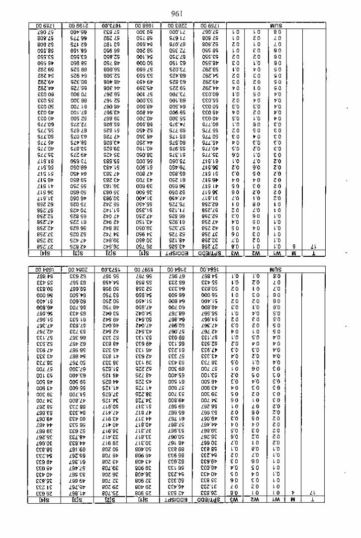
961006,lt 00S6~<: OD'U9~ 00H691 00fgZG 008<;LI ""L90L9 00'",9 ,.S L~ 00<6; 000'" L90'H; " " "gOS'L. HL99 ~6<:£; 0,£ g. ;L9 tL gO~£; " eo H9011Z9 9U <:9 Z6~Cg 099'.g ;lO'[9 SOg'Zg eo " HOWgg Ogl'99 0.69g OO~g, 0>( U O>~g. " CO "0.;-£9 099't9 099'<:9 O(W.g OH'L9 O~,'£. eo eo "0'>9g~ 0;6 ~; 09L 9t 00009 O~~~g O~g'gt CO

" ""ZOG8~ ;<:<;69 909"9. 01;9L~ ~W"<L l£Z"6, '" '" ;0<:6l t, 9G£t9 90,"Z, 0'>9<~ ~<:H9 ,£n', eo CO ;0~6<:'6' .It'09 gO~9t O;t 6~ ~Zg£9 ,£Z"6t CO eo ;0~6O'OO .u;. 90r tt O;£'.~ ~ZZ6. lent '" " ;0rm 09 0060L L9Z 9. 001L~ ooHL [£0"09 '" ;0 '"n:o ~, OO[99 L9~ Z. 000"[, 00~"69 [£O"g, eo '" '"n:o Q<; OOL19 Loo9t 006"gt oon9 [[0 O. '" '" '"tm~o oa~'" Lg6'£' OOgtt 0006. £[0 ;t '" eo '"n:o O~ 00, ~<; L9S 61: OOL'Ot om:,. [[OOt '" '" '"~LL"09 ga'U ;z6'g; 0~~'9g glt'.L gU09

";0 ",U".S ~L9 L9 9Z~~<; O,t zg .LL 69 gLL<;g eo ;0 CO

gLL"09 ~LO(9 9Zl L> Ogt9. 9l~9g 9a 09 CO '0 COgIL 9t >Ln~ ;zgT. OgZ'" 9lg'09 9US' 00 " ".UOt ",B'~, ;".'6£ 0"~'Ot .l6';; ;U'O' " 0' ".U.~ ",060 ;Gt ~8 0.0'9~ ;In. ;U';8 .,

"co

un9 C)g9~L tS9'gg 000'9; 090'SL LIng" " 0'H9'99 O~O"Sg t~n~ 006'~9 O;V'O[ LI.'W 0' ., 0'l!, ~. O~~t9 (~.lt 009l' 0;9'~9 L19I~ " 00 0'

L1.9. O,H6. (HZ(t OOL£> 09Z19 L1g9~ 00 00 "ll. I' O.l ,. (HI"6( 0096£ 0999'i L19I~ 00 co "l~. 9, 0.909 .~O91: oog9t 0,0 z~ H9ilt " 0' ".!~nt 0909' ~96'0~ oont ",no .!~nt '" " '"9><:19 gZO~L Ztl <;9 O~."<;g ~on.! W~"Z9 co " cogRlg ~"tO[ "N'~9 o~n~ ~n'll ~~n9 " '" co9~n. ~ZS~9 ZtO"' o.nt g;;~99 ijO""ZO '" " '"g~Z"lt ~ZO~9 Zt6 Zt O~~"~t ,,8"19 g~ZLt '0 ;0 '09~Z"ot ~Z99, Ztg g~ O,O"S( ,l£"L. g." Zt ;0 '" '0g,U( ~~Ol~ ~tl ~. Og£>I: glL Zg 99, L~ 00 CO cog9<:Z( ,e'"~ e.g'OS 099 O~ gU'S. 9gn~ " " "g,UZ 9i:9l~ e.9'9<; 09L 9Z 9zn. ggn<: ., co

", "[tIs !.ls • " .ld~IQ03 (103/idS 'M 'M 'M " •

00tg9l 00 'SOl OO'£L~, 00 l£91 00\>9~<: 00'\>99~ ""L99 ~; £(9 Zg L9~ <;S L9L 9> [96 L9 L99\>9"

,. .,££t~; L9~ £9 g~."\>9 g,g ,~ £<ZH9 ££. 99 '0 00 '"££9'0; L9n. 9ge 09 9;~ <:~ [r£"\>9 £rg"o" " co '"0009<; 009'09 09[ £g 0~6'\>9 00; 99 0009<; co co "oon~ 00H9 O~~0> o;n~ oo.~ oon. " " "009'90 00.('9. 0'" gt O;S"lt ooLOg oo9"9t 0" '" ."L9.'9<; r£t~9 G\>O£<; l~O"t><; L9L"99 19,"9g '" '" '"196"1<; •• g ~9 zt><;6t l~9"Og 19~"t09 .(9Fn~ " co "19no t~g'[g ZI'O'9. ll'O'lt 196"09 lilt"Lt 0' eo "19at • £l [; zt><;Zt It,"£t loo"L • 19l Zt 00 " "(H"Lg 19£ 99 <1:(eg (n"£g ~tO69 ~~~'"" " "(\SZg 19t 19 £~g~. ~t9 SV ~n';9 ~~g'o. " '" '"£(£ Lt L99 9~ .[(~.~I:I9t ~~n9 ~~6'L. CO " ••~(~ £t L99 t><; <£g~. [(9 Zt [tt [; ~~n." 0' ••££L9~ L9L O~ ,I:I:sr I:(~SI: I:(t .9 ££l g£ ,. ,. ••OOLL9 oon9 ,<:n~ .ll'~. OO(£9 DOl H; " " coOO~I:. OOH9 ~Z19~ 9U ~. 00t'~9 OO~'t; O' ;0 co009~. OQ<;69 ~~9t~ ;Zl ~. DO.~9 00.9. ,. ,. '0006•• 009;g g<:no ;u ~. 009 L, 006£~ 00 co co00\:61: 00n9 ge9'lt nn8 DOl [, 00££. " " coOOL~. OaH"Lt 9<:nt gon. ow£~ DOLM: ." " coL9l g9 ~(, gg .n6'0~ Hn; L9<;69 L9ZW co " "L9g'~; ~~t'.9 lWlt HSl~ [99,9 [99 (~ '" " '"[90'6~ 8~~09 l~8~t L~I: t~ L9L ~9 ,90'60 '" " co19t t~ .(,99 L~~Ot l~S'OO .!Wl~ L9ni> '" '" eoL996£ •• 9 e; l~G'9~ l~nt L96'£, 199"6( '" co '"L9Z"g£ ££,'g. LW8~ l~n( lSO"O. 19""9~ ., '" co199"Ot r~9'~~ LI£ 6Z ll£"O~ 19~ 9t L99 O~ '" co '"tt~"99 [91'69 BOlO; 90~"O, ~£~Sg ~t~ S. '" '" '"((e",g L90'~9 gOl9t gOO9t ((6 ;g ~tn. co '" '"~t9 6t .!9n9 gOl.t gat ~t ~tO'<:9 ~t9'6' CO " co((0 <;t L9n~ SO,'££ gO£6~ ((~99 ££0'9. " " co~~~Ot L9; (~ gOZ9£ 90~'9£ ~~n. ~(tO' 00 •• "~~g-g~ 1996t BOL"~ ga6 i:£ ~~t'og ~£g;s " co "~(<:I~ L9L'g. gOl £Z SOt6Z £~t'9. ~~nr " co "~(9 9Z LW~O SOl'~Z g06,Z 1:(9e' £~g-g<: •• " " , "[tIs '" \tlS [~Is .ldSIOO3 (lQ31!dS 'M OM 'M 0 ,

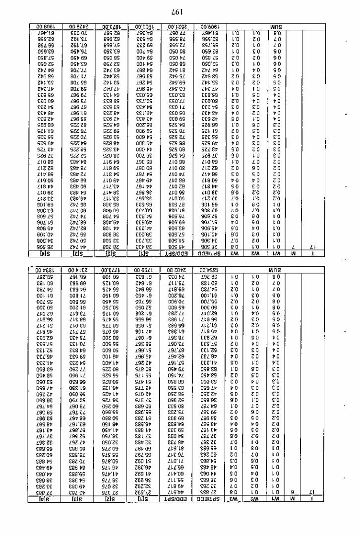
[61

aQ'S06~ 00 6l.~ OO.t£~ i-9r06~ On<:9~ OO'606~ ""'L9n9 n:60£ .991:9 .9\:-'9 ,(00 1.1. '(9'-'9 '" '" 0"9~n9 ~6''tt; B~6'~9 W;'\'9 9WBL 9Wi':9

" " "991: 99 Z6~',9 ~g9'1;!< ~~ng g,,~'U g.1'9; " " "099'£9 OO.'9L Og~'(9 OOL.9 0.0 OS 0.9,9 " " "O,g-L<; Q,v 69 0,0 g; 001> 6~ OgO ~L O~~L, " " "0,0 Z, O~H9 O<;Ll5 OO~'~g 090 R9 09O'i:~ " " "Z.l ~9 9QLLL loL £9 L9g P9 Zjog ~g "vL 1>"9 " " "ZI'6 R, gaL It ll'H<; L9. 6~ <:., .L <vB g~ " co "~.l'(; gOl,9 lv~£. L9ZK ,~,-69 ,~L"[. co " 0"~.n. BOl'6; "WLt> 196'SI' lo,"£9 l~Uj> " " ,'0t£g .9 L966L ££ ~ 1'9 [£0-<;9 [£0-£9 [£g-<;g

" " "n:o 09 L96H £[g B, [H-6, "O"LL ,ro'og '" " "(£~I"i 196 ,[9 .,9.9 '£'-1'9 t£O ,I. tee jo9 co " "tto a. L96'~9 C~l'~. ~t~'6v ~to;9 ~t.g. " " "IT9'Z. /96 ~, .,6 c' t~~,t ~~o6~ .~9~. " '" ",,~6'99 ~ZZ'le ;",,'.9 OOZ';9 .l,'.9 .l6'99" 0' ".;TI9 ~,z9L "~l£, 0066<; >os 9L <;a 19 " 0' "ga: <;g gelOL <;Z6," 009 jog 915 u. 9lt ~g " " '"919 6v g;Tt>9 ,l9 g~ oat 6v gog 99 gog 6v '" co ",lL .v gll-g9 9ll:H 000 ~v 9l<; 09 goL £v " " "916 L[ G;TZg 9lO Ill: OOL9£ 9l<; ~g 916 L£ " " "LlO 99 [9n9 L~6 t>9 L9[ ,9 LlO 99 L~Og9 '0 " '"Ling ~R~~l LI969 L9009 LlOOB LI;: 19 " "' "LlV'9, ~g.u LI~K L9l •• L10 .L Llv9, " " "L19'0. £9.99 ll06v L9v6~ L10R9 L190, '" " "LIS .~ £9v 09 l~nv L91v~ L10;:9 L1gv~ " co '"L106. .~~~,<~>9t L99gr L~O9S LlO'6t '0 '0 '0

Llln £90'~' .(II '£t L9g'tt LlO'O, Ll"'tt '0 '0 '0 ,ROI'69 ZvL gg gO£,9 £., <;9 gO, LR gOl69 co " "gO~(9 <;".( 09 200 Og tt1:'09 gong gOt t9 " '0 "RO, L9 ZvL ~L gaL "9 (£6-1'9 ~o~nu ao~-tg co 00 "oon9 (:'09 900'6. tt9'61' 90~'69 oon. " " "g06 •• Zvl'l9 sa~"v [£n" HO,-£9 ~06-,V 0" '" '"Rm-av lvL 9. SOHB£ [[Q-6[ 90,-L, 90~-OV 0" co '"90nt ~~LOg SO. ££ [[n, 9()<;-1, 90\:-v[ '" '" '"90li Sl ~~, 1'0 go;: g~ ---.£it go 90. 'v 909 go 00

" " , H

" " lfrs- [ils ldSIOO~ OO~lldS ~ '" '" " ,00 ~I:~I OOvl(~ OO"tlll 0066L1 00 W~O On~gl "CO£9l'69 .(91-99 00109 ££9 19 ££0 ~L L906, co " '"£9~09 t9669 91:1'09 1:~9'19 LII'>! £9109 " " ".SL ~, [119v9 9~~ 9S (:~6'99 £19'69 C9nii '0 " "00~~9 oo~ Il 09109 Ogl' ~9 OOZ'9£ 00n9 '0 '0 '000< 9, 00999 09' gO Ogl'9g 006'OL OOgg '0 " ""00£ 0, OO~19 09L-09 0,0 " 00999 001:()<; " " ""UO~9 H9£l 9'~ 09 ~gn9 reZ'lL LIO'Zg " .0 '0,t9'9!i £11:'99 "L~ ,. 9" 9!i C9S~L H99!i " co ""L~Z ~g HO.9 gLng g,S ~9 t~9 99 I;~(;'19 " '0 .0L~9g~ Hl., 910 9> g~~'.(0 nn9 L19.1' " " ;01:f:6-l9 ££.>! OOt09 '(90'~9 ,(98 91 [I:S-l9 " ;0 '"[[,-LS ££~'O' 00, g9 ,(9£ 99 ,(90-~L [f.-L" " '" '"1:£1-<. <£9~9 oaR 0, 199-\9 L9ng ttl"~9 " " "~fL"91' fS.6; 0019v 196-9v 19H9 tUg. " " "[(nl' t£ZK oon~ ,(91:<:1' .(91-,,, I:[nv 0' '0 .,O.~ £9 O.OU '0< 09 9H09 0" 6,( 09n9

" " "0•• ~. 0,6 IL '0' " 9l~9, 09~'~L Ogo'S9 " " "090'C9 Og9'99 ;~g'O, .ll' ~. O.R B9 0,0., " '" "099 L' 09C'19 Ii;:I'9~ ,LL 9v 0<;<;89 099 L~ '" " "09~ O' 0li0'g; ;"1' I~ ,LO lv 0,;: g, 0,;: ~~ ;0 " "Ogg'g~ (K;LQ. 9U9. 9LI:LI: 096 ~, 099'9£ .," "L9L'~9 L906L O,Z 09 .8909 .,9 os £9.('.9 '0 " '0

L9l:6, .9' t. O~g'~~ ~96',g ~£<';L L9[ 6, '" " "196'~g 19. 99 m;s (K; I:S<~, <£669 £96 f~ '" 00 '0L9, g~ L9~T9 ~,~£99'9~ ~~9'.9 L9"'9. .0 '" '"£9~'r. 1ge"L" (K;V'l1' 8S~ ~~ .<1:6, £9\ (> ;0 '" '01.9l'l8 L9'; o. agL-9[ .S~L. ~.a~ '9Ht 00 '0 '"'9n8 19~LV 090-0, £gv;:. ~£l 90 '9£'~t ,. co "tS9'99 ~~g OS ga-09 ~6v09 H9'lg t99.9 " "' cot~o'09 £99'!iL 91. " ~6L,9 L~£ 9,( tgo 09 " " "(9B \><; £2l0L 9.(g'09 l60 I~ L~O-Il I:gg-v9 " ., "tgH~ £~6 ~9 9l~9v 1:6C'9P '(1L'99 I:g~61' ., ., "[gO-VI' £99'6g 9.(n~ ;:69 II' lW09 tOO~" ;0 " "t~9 ~f .B[ t<; 9LL9t ~66 9l: 111-" [H9 gl: "" " "t~o [[ ,gO 6~ 9LOzt l6;:'<t 11gSv [H~ <I: " " "---.£f!a .9l n ,l( a ?wa Llnv [9RLe "' " " • "[p]s [l:ls , " ldSJom oo~adS '" '" '" " ,

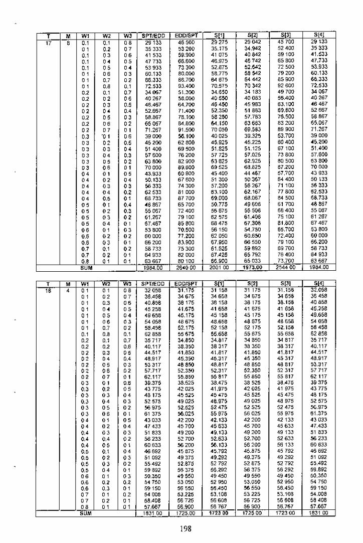
, , ., w, W> SPTIEDD EDDISPT " '" " ""U , ,, ,, "" 29133 4650D 29275 29 042 45700 29133

"' " 0' 35 JJ3 53200 35.175 34,942 52400 35333,, 00 "' 41533 59.900 41 07, 40842 59100 41.533,, 0< 00 47733 66.600 45.975 46742 65 BOO 47.733,, "' 0< 53933 73300 52.875 52.642 72 500 ,3.933

" "' 00 6a,1J~ 80.000 58.775 5S ;42 79200 60,13~

" ,., 0' 66,J3~ B6.700 !l4 67, 64442 85900 60.333

" ,., 0.' 72,,33 93.400 70.575 70 ).42 92 SOO 72.533,., e., " ,4067 5\.300 34,6;0 34183 49700 34 067e, "' "' 40267 58.000 '0550 400B3 56.400 '0267

"' "' " 46.467 64.700 46 45{) 459B3 63,100 ~6467

"' 0< " 52.667 71.400 ,2.35D 518B3 69,800 526670.' "' 00 58.a67 7B.1oo 58250 57.7B3 76,500 06867e, "' "' 65067 Il4.BOO 64.150 63663 83200 55,067

"' 0' "' 71.267 91.500 70050 69.5~3 89900 71.267

" " e' 39000 ;G,100 40025 39.325 53.700 3900000 "' M 45200 62 BOO 45,925 45.225 60400 ~5,200co "' 0< 51 400 69500 51.825 51.125 67100 51.400co 0< " 57600 76200 5772, 57.025 73800 57,600co "' co 63800 82900 6362, 62.925 80500 63800co 00 "' 70000 89,600 69525 68.825 87,200 70000

"' "' "' 43,9Jo 60900 45400 44467 57,700 43930

"' "' "' ,0,133 67600 51 300 ,0367 S4400 50133

"' co "' 56 333 74300 57,200 56267 71100 56333

"' "' " 62533 81 000 63,100 62.167 77 800 62,533

"' "' " 68733 87700 59,000 68.067 84500 68,733

"' "' "' ~6 867 65700 50,775 49606 61700 48867

"' "' " 55067 72 400 56675 56506 68400 55067

"' "' " 61.267 79100 62575 61,406 751DO 61 267

"' "' "' 67,467 85800 68475 67.306 81,800 6746700 "' "' 53800 70,600 56150 54.750 65,700 53800., "' "' 60000 77.200 62050 60.650 72,'00 6000000 "' "' 66200 83.900 67,950 66 550 79100 66,200

" ,, "' 58733 75300 61.625 59892 69700 58733

" "' "' 64 933 82000 61,425 65792 76400 64933

"' "' "' 63667 B0100 66,900 65033 73.700 63667

""' 1984,00 26<000 2001 00 l~TUO 254400 1984,00

, , ., we W> SPTIEOD EDDISPT " " SP] "'" , "' "' "" 32058 31.175 31 158 31 175 31.15~ 32,068

"' co "' 36,'66 04 675 34658 34575 54 6,6 36458

"' .., "' 40,856 38175 38158 38175 36.156 40858

"' 0< "' 45258 41.676 41658 41 675 41 658 45,:/58

"' "' "' 49658 45,176 45158 45175 45158 49,658

"' "' "' 54058 48675 48,658 4867, 4B 658 54058

"' ,., co 58,4,6 52,176 52158 52175 ,2,158 58468,, ,., ,., 62858 55675 55,658 55675 55658 62856,., e, e, 35717 34,850 04.817 34850 :M817 35717,., ,., eo 40.117 38.3,0 38317 3a 350 38 317 40.117co e, "' 44.517 41.a5D 41.a17 41,850 41.811 44.517co "' ,., 48.917 45.350 4~,:317 45360 45 317 48.917co "' "' 53317 '6 S50 48.817 48850 48817 53,:317

" "' co 57.717 52.350 52.:317 52,360 5:/317 57717

" 0' "' 62.117 ,5,8'50 ,5817 55850 55817 62117co "' •• 39.315 38.525 38.475 38525 :3~.47'5 39315

" " "' 43775 42025 41.975 42025 41 975 43775

" "' "' 4B 175 455., '5475 45525 45475 4~ 175., "' "' 52575 49025 '6,975 49025 4a 975 52575

"' " "' 56 975 >2,52, 52475 52525 52475 56,970

"' "' "' 61 375 56,025 55975 56025 55975 61.37>

"' "' " 430:33 42200 42,133 422DO 42133 430:33

"' "' "' 4743J '5700 '6633 45700 45633 47.43J., "' "' 51 833 49200 09,133 49200 49133 51 8~3

"' "' "' 56 233 52700 52,633 52.700 52633 56 233

"' 0; "' 6D633 56 200 56,133 56 :/00 56133 60 6~0M ., "' 0\6 692 45875 45,792 45.875 45792 46692M " "' 51 092 49375 49,292 49.375 49292 51 092., "' "' 55492 52,875 52792 52875 52792 5>.492M "' "' 59892 56375 56,29:/ 56 375 56292 59,692

"' "' "' 50,350 49650 49450 49550 49450 ~0,3~O,. " " M 750 53050 52950 53,0'50 6295D 54750

"' " "' 59150 56550 56,'~0 58 550 56,450 59150

"' "' "' 54008 50,225 53,108 5J 225 53.108 54,ooa

"' co "' M,408 56725 56608 56725 56606 58408

"" "' "' 57,667 56,900 56767 56900 56.767 57,667

""' 183100 1725,00 172300 172600 172300 1831 00

198

661oa~96~ OO"ZM 00 as! OO'~Z6~ 00 £l6 ~ OO'196~ ""'tOO 19 L9<; ~9 oong L9n9 OOU9 L90 ~9 " " ""g~~T9 ij91 ,9 ga'zg 9<;1;:9 51119 ~;,'~9 " co "9';6'l~ g<;,. H; ,LS-L, ~!i~L~ ,Lg'l~ g<;6 L5 co " ,.O.Z V9 0," <:9 O~BZ9 O<;L <:9 O<;g 19 ogn'9 " co ""o~a'M 0<;0 Q<; 05~-~g OgO'gg ma g, 0<;06, co " ""0<;9.<; 0<;£ .9 ~n, 0.£ .<; Ogl>"., 099'£. co " '"ZI'I: ,9 ~I'I:~g ~zn9 lK .9 .l~ £9 ZI>£';9 " '" co~t~'09 ~~9-9<; 5U \IS ~V9'g9 .<:LB, IN 09 co co co~r6'~g <pS"£, 5Z0 v, It'6 €g .lO .<; It>6 ~g co co co:l>l'S. lPZ"Sv 5ZI:6~ ~pl'Sj> ,l[ 61' lt~6. '" " co££1' 99 [£6-1:9 000'.9 ££6 <9 000~9 ~t.'99 " co '"£~~~9 [£Z"SS 00£'6; ~I:,6. oaf 69 ~£n9 co '" ,.££0 99 ~g-V;; 009 t<; ££n9 009.; [[09, co " '"£~g'O; t~B-61' 0066~ £~S'6. 006 Sj> [,R 0, '" co '"£r9 gr tEP;!- DOcS~ £H ;. oon;. £[9 <;1' co " '",lS [9 ~<:gV9 ,l.~9 glS~g 9L~'.9 <;l~ L9

" '" co9~t'(;9 ~Zg6~ ~lg6<; ,lS 69 gig'S. ,l£ <:9 co co cogU'l. SZI <;5 5£\ 5. g~~'gg .l ~.; gn L. co '" co<;;:G-I, gi:~as ';L.'Og ,<~ 0, <;l~ 0<; ,~6'1; " " ",U'9~ ~u<;~ ~LL ~. ;u;. ,lL',~ <;U9~ 0' co co<;<~I~ ~"O'~~ ;La'~. ,W Iv <;.0-1v ;znv " "

.,Lc9'e9 L~ I <;9 0,1 ~9 H~ ;9 a.~,9 L~ge9

" " "L~v.9 L~.a9 0,.09 L~v09 ago 09 l~H9 " 0' ".~~S9 l~"'~ O,L" .~.;9 a;.'gg LlI: g<; ,. " "HOSg lWI~ 0,0 I~ L 10' Ig D~Ot, LIO., " " "L\9£1> llf:-9v O,S 9' Lit 9. a<;t 9. L~Sl. " " "Lin. l19-1 v 0;9 ~. L 19 I. 0<;9 ~. .~9". ., " "LWl~ 1169~ 0,6 OC Ll6'9~ o,fj 9~ LlvLS " " "SOL'69 90L'<;9 gug9 BOH9 ,ll <;9 90.69 " " "909 '9 900'\9 ~ZO 19 900 ~9 g<0'19 go~ .9 " " "BOI:6, 9m:-g, g<:s 9> eon, ,ll: 9<; eOI: 6. " " "SOI'.g 909-1, ~i:9 Ig B09'l, ,l9 I, 90~'.g " " "906 S. 906 9v ~Z6 g. 906'9. ,~fj'9. gOfjg. " " "90L •• 90<:'<:. ~Z" ~~ 90" 2. gn'2. gOL£. " " "gOg g. 900"1t ~"' L. 90g L~ g<g'L~ gO~ g[ " " "901: S~ 90S Zt ~"g of: 90S i:~ ,<g'"£ gor £[ •• " " • "'1.IS !tJS _1._5 " J.d51003 003/1"S '" '" '" " "OO'9{lSI 00 z"g I oo-t<~t oo'nH~ 00 ~"91 00'9061 "'"L99 fj, .9~'6g 00£ fj~ L9~6, 00t'6g L996, co " ••.9.09 ~g£'6. 00, 6~ ~9t'sg OO~6, ~9L 09

" " ".96,; ~n'" 00. <;~ ~9l'S9 OOV,. £g6 ~; ,. " '"OOL19 009'69 00l'6~ 00S6; 001'6; OOL 19 ,. '0 ••0069. 005 9g 009 ~~ 00<;~, OOS',; 0069. co " ••001'<:<; oon. 00, I, 001"1, DO. I, 00 I '<:; " co ••LIS 1:9 LI~'69 006 6~ LlS'69 006'69 119i:9

" '" ••£I9L9 LIL'9g OOSV; ltL'" 009',; L\9[9 co co "llO £, LI9-\, OOL'I{; II 9 I, OOL~9 L\O'[; '" " "ll~'R. ll,-LI' 009' •• Lt~ LV 009l. LI~'~. '" " ••££. £9 [£0-09 001 '09 ££0 09 00~'09 ££. £9 co •• ,.££1 R, [£6-99 000 \)<; £[6 ~, OO0'9g ££1 g<; co ,. ,..[6 «; ttn9 006 I~ <£~~9 006'1, r£6 £<; co " '".\; ~ 6t ~£Ul' 009 •• £tl'LV 009 LV .1: ~'6. ,. " '"~~t' •• ££9-[1' OOLt. ££9£. OOL£. £~~' •• •• co ,.0<;1'.9 0%-09 00£ 09 0<;l09 00t'09 0<;1'~9 " •• co0<;96, 091'9g OO'~ 09~99 DOl 9. 0<;96, ,. •• coO,g ~, 090"<9 OOll, 090'<;; OO~Z, O<;g.; " '" co0<;00; 096"LI' 000 9~ Og6'£. 0009. 0900; ,. co coO<;l<;V Og~ ~I' 006 £~ 09nt 006 £. O<;l~. " " co0,1' O. 0~L-6~ OOgfj£ O<;L6~ 009'6£ 0<;1'O. co ,. co19£ ,9 L9~-09 OOg09 191'09 009'09 19[ ~9 " ,. coL9g'09 19£-9<; OO'M 19~g, 001' 99 19909 co '" ,.19L ,9 19~ l~ 00£ l~ 19<'C9 DO[ 1:<; 19.->; co •• coL960; 191'gl' ooz 9~ £91'~. OOl H. £96'0<; '" '" ,.1919. 190 .1' 0011'~ 190' •• 001 •• £9 ~'9' co co coL9[ I. 196'6~ 000 01' £96'6£ 000 O. £9~'1' '" " co199 9~ L9Il <;[ 006 .~ 199 ~£ 0069S 19<;9. '" "

co~9n9 £99-09 00L'09 £g909 00l'09 .ijl99 ,. "' "~91"19 [9,-99 009'\)<; [g,99 0099. • gv ~9 ,. " co£gg 9, ~S. ~~ 00<;Z~ ~9.'Zg 00<; i:, £S~'9<; co "" ,.rg9 ~, tSr'91' 00. 9~ ~9~'B. 001' S. £gn. '" ,. ,.£gO LV tsnl' 00£ I'~ ~9n. OO~'•• £gO l~ 00 ,. "£el Z. ~SI"OI' OOZO' £910. OOl'O. £gll~ '" ,. co£91' l[ tSO 91: 00~9S .go 9£ 00 I '9. £gI'Lf: ,. co co£99 Z[ n6'1£ 000 i:. ~g6 I. 000'<:£ rg9l£ "' ,. co 0 "'[tIs '"'

,,, [i S ldSIOO3 amnd5 '" '" '" " "

, " w, w, m SPTI~DD EDDISPT " , '" "•• , ,., 0.' M 33933 33,1l"0 33S3~ 33.65D 33633 339330.' "' " 39.533 36950 ~893) 38.950 ,a,no 39533,, ,., M 45133 44 250 44233 442,0 44233 4',133,, 0.' 0.' 50.733 49550 49533 495;0 49533 50,733,, " 0< 56,333 54.B50 548~3 54850 54833 56,333,, M 0.' 61.933 60.150 60,133 £01,0 60,13~ 61 933o , 0.' " 67.533 65,450 65433 654,0 65433 67533,, 0.' 0.' 7:J.13J 70 t5(j 70733 70750 70733 73.133

"' o , ,., 38,267 JB 000 37,967 38000 37,967 JB 267

"' "' M 43.B67 43300 43267 4,.300 43267 4J 867

"' "' M 49.467 46600 4B 567 48600 48567 49,4670.' 0< 0< 55.067 5~ 900 53867 53900 53 B6l 55,067

0.' "' "' 60.667 ,9200 59.'67 59200 59167 60,667

"' M "' 66267 &4.500 G4467 64,000 64467 66,267

"' "' "' 71,S67 69800 6V67 69800 66.757 71 867

"' " , M 42600 42,000 .2300 42_~,O 42300 426000' "' 0; 48200 47.650 47600 .7.650 47600 45,200

"' "' 0< 53800 52.950 52.900 52.950 02,900 53800

"' 0< "' 59 400 ,5250 56 200 58 2,0 58200 59 400

" " " 65 000 63550 63 500 63550 63500 5,,000

" '" " 70,600 6B850 66800 68850 68600 70600

" "' "' 46,933 <16700 46633 46700 46633 46,933

" " "' 52533 52,000 51 933 52.000 51933 52533

" "' "' 5~ 133 57,300 57233 57.300 67,233 58133

"' " " 63733 62600 62,533 62 600 62533 63.733

" "' "' 69,333 6790G 67833 67.900 67833 69,333

"' "' " 51.267 51 05G 50967 51.050 50967 51.267

"' " " 56 867 5(U50 56 267 56,3;0 56267 86 867'0 "' " 62,467 61 650 61 567 61.650 61867 62467

"' " "' 68.067 66 950 66 867 669;0 66667 6-B067

"" "' "' 55600 55400 85 300 55.400 55 JOO 5,,600

"' "' " 61 200 60.700 60 600 60.700 60 600 61,200

"" " "' 66 800 66,000 65900 ~,oo 65,900 66800

" "' " 5993J 59750 59633 59750 ,9633 59933

"' " " , 65533 65050 G4,93J 66050 64933 65533

"" " " , 64 267 64100 GJ,9157 ~,oo 63.967 64,2157

'"" 2056 00 2022,00 20:lD.00 2022.00 2020,00 2056 00

, , w, w, W, SPTIEDD EDDISPT 5[1] S~l ::;>l'k 8[4]

'" , " ,,"' 34558 340475 34,468 34 475 34 456 34,568

" "' "' 40558 40375 40,358 40375 40.356 40,558

" " "" 46,558 46275 46258 46275 46 25~ 4655B" , " " 52558 52,175 52158 52 175 521;6 52558o , 0' " 5a 558 58075 58058 58075 58.05B 58,568

" 00 "' 64558 6~,975 63958 63975 63,9;6 64058

" 0; 0; 70558 69,675 6~ 856 69875 69.85~ 70,,5S0; '" " 76,,8 75775 75758 75,71; 75.756 765580; o , 0; 39117 39050 39017 39050 39.017 391170; ,., 00 45117 40,9,0 44917 44950 44917 40 117

" " 0; 51117 50850 50817 00,800 50817 511170; " 0< 57117 56750 56,717 56750 56717 57 1170; 0; " 63117 62650 152,617 62650 62617 63 117

" 00 "' 69 117 68,550 68517 6855G 6~ 517 69,1170' 0; " 75117 74450 74,417 7~,450 74417 75117

" " 00 43675 43625 43575 43,625 43575 43.675

" 0' 0; 49675 49525 49475 49,525 ~9 475 49675

" " 0.' 55675 55425 55375 55,425 85,375 55.675

" " " 61,675 61325 61.275 61 320 61.275 6\.675

" 0; 0; 67,675 67225 67.175 67225 67,175 67.675

" 0; o , 73676 73 125 73 075 n125 73075 73675

" " 0; 48233 48200 48133 48,200 ~8 133 48.233

" 0; " 54233 54,100 54.033 54100 54 03~ 54.• 33

" " " 60,:133 600DO 599J3 60000 599:J3 60233

" " " 66233 65900 65833 65,900 65833 66.2J3

" 0; " 72 233 71,800 71,733 71 800 71D3 72.2330; " " 52,792 52775 52692 52770 ;2,692 52.7920; 0; 0' 58792 58675 58592 58,675 56592 58.7920; " 0' 64792 64575 64492 6',575 54 492 54.792

" " " 70792 70475 70392 70475 70.3S2 7079200 0; "' 57 J50 07350 57250 57,350 57.250 57350

"" "' " 63350 6J 250 63,150 63250 63150 6~ 35000 "' "' 69350 69 \50 69,000 69.150 69050 6S 350

"' "' " 61 908 61 920 61,608 61.925 61808 61 9080; "' "' 67.908 67 B2, 67,708 67.825 67708 67906

'" "' "' 66467 66.500 65.367 66500 66 J67 66,467

"" :113100 212100 2119,D~ 2121,00 211900 213100

200

, " ., ., ., SPTIEoD EPOIS?T S(lJ -'" "' 6[4J

" • "' "' '" ~7,483 36 800 36783 36,800 36783 37483

"' "' " 41 683 4D 300 40283 40 300 402B3 41683

"' "' '" 4588l 43,600 43783 ~J800 43,783 45,683

"' "' "' ,008) 4DOO 47283 47300 47.26~ 50083

"' "' "' >4283 5(1,600 50783 50800 50.78" 54,283

"' " "' 56,483 54,300 54283 ~'OO 5~283 58.483

"' 0; " 62,683 57,600 57783 57 sao ,7.783 62,683

" " " 66683 61.300 61,283 61 300 61.283 66863

" " 0; 40767 40,100 40067 40 lOG 40.067 40767

" " " 44967 4~600 43.567 ~J,600 43.567 44967

" "' 0; 49,167 47100 47067 47,100 47,067 49167

" "' "' 53.367 50,600 50567 50600 50 567 53367

" 0; "' 57567 54100 54,067 5~10a 54 067 57.567

" " " 61 767 57600 57,567 57,600 57567 61.767

" 0; " 65 %7 61100 61.067 61.100 61 067 65.967

" " " 44050 43400 43300 43,'00 ~3,50 44 050

"' " 0; 48250 46000 48,8,0 46900 46850 4B 250

"' " "' ~2,4,O ~o400 50.350 50400 50350 n,400

"' "' "' 56650 53 000 53.8,0 5~,900 53,650 56 650

" ,; ,., 608,0 57,400 ,7.~>O 57400 57350 60850

" " " 65050 60.900 60.850 60 000 60,650 6,,000

" " 0; 47.333 46700 46 633 46.700 46633 47,~~3

" " "' 51 533 50,200 5(1,133 50.20D 50133 51 533

" " "' ,5733 ,3,700 53,633 53.700 5363:) 55733

" " " 59 93~ 57200 57, t33 57,200 57.133 59933

" 0; " 64 t33 60700 60,6~3 60,700 60 63~ 64133

" ,, " 50617 50000 49917 "'00 49917 50,6170; " " 54,617 53500 53417 53500 53.417 54,6170; " " 59017 57000 56917 57000 56.917 59,Ot70; ,.• " 632\7 60500 604t7 60 500 60.417 63,217,.• " " 53900 53300 53200 53300 53.200 53,90000 " " 58100 56 BOO 56700 56 800 ,6700 5S100

'" " " 62300 60 300 60,200 60,~00 60,200 62,300

"' " " 57183 56600 56463 5MOO 56,4S3 57.1S3

"' " ,, 61,363 60,100 59,96~ 60100 59983 61.383

" o , " 60 _67 59900 59.767 59900 59767 60.467

""" 197B 00 tB9600 1594.0~ 1896 00 1894 00 1978 00

, " ., ., ., SPTIEDD EDDISPT -'J'J , " "'" , o, " 0; 38.108 37625 37608 ~7.625 ~7 608 3S,108

" " "' 42.7GB 4t 725 41 708 4\.725 41708 42,708,, ., ;; 47308 45825 ~5 808 45.825 45808 4730B

" •• 0; ,1.908 49,925 49,90S 49925 49,908 51 908

" ;; •• 56 508 54,025 54,008 54,025 "00' 56508

" " " 61, t os OS,125 5S10S 06125 58.10B Bl108

" 0; " 65708 62225 62208 62,22> 82208 55,706

" " " 70 ~oe 66325 66306 66 ~25 OO'M 70308

" " " 41 6 t7 41150 41,1 t7 41,150 41,117 41.617

" " M 46,217 452,0 45217 45250 ~5 217 46.217

" •• ;; 50,8t7 49,3,0 49317 49,350 _9317 ,0.817

" 0.' •• 55~17 53 ~50 53~17 53450 53417 55.417,., 0; ,., 60017 57550 57.517 57550 57517 60.017

" 0.' 0.' 64617 616,0 61.617 61650 61 617 64 6170.' 0.' ,., 69217 657,0 65717 65750 6,717 692170.' 0.' 0.' 45.125 44.675 44.625 44675 44625 45.12,

•• " 0; 49.725 48.77, 48.725 48775 48725 4972,

•• •• •• 54.325 52.875 52825 52875 52 B25 54 325

" ••• ., 56,925 56975 56,925 56,975 56,9<5 5~ 925•• ;; ., 63.52, 61.07; 61.025 61.075 61,025 63,525., ,. " 66125 6517> 6,12, 65,175 65,126 6S,125

•• ., ;; 46.633 46,200 46,133 _6200 4S1~~ 48633

•• " "' 53233 52300 52233 52.300 52233 53233

•• •• •• 57833 56 400 56333 •• 00 56333 57,633

•• " " 62,430 60,500 60.430 60500 60_n 62 4~3

•• ;; " 67033 64 600 64533 ~.oo 64,,33 67,033

" " •• ,)" t4 • 51.725 51.64. ,1.725 51.642 52,1420; " •• 56 742 55825 55742 55825 55.742 56742;; •• " 61 34. 59925 591142 599.5 59.842 61342;; •• ,, 6,,942 64,0~5 63,94:; 640<5 639_< 65942,.• ,, " 5,,650 55,250 55,160 55,250 55150 55650M " " 60250 59350 59250 59350 59250 60250M •• " 64,650 53450 63350 53450 633>0 6~,8~0., " " 59,158 5~ 775 58658 5B.775 58658 59 t58., ., ., 6~,758 6,,875 62758 62.875 62758 63758•• " " 52667 62,~00 62,167 62.300 62,167 62,667W" 205300 1995.00 1993.00 1995 OD 1993 00 2G5J 00

201

, " "' "' "' SPTIEDD EDD/SPT " " , S[~l "" • " " '" 38.733 38 450 38433 lB 450 38433 38,733

" "' "' 43,733 .3150 43133 431,0 43133 43733

" "' 00 46733 ~7850 47833 47.8>0 47833 48733,, "' 00 53 733 52,550 52533 52.500 52,533 53733

"' " " 56733 57250 57,233 57.250 57233 38,733

"' •• " 63733 61 950 61 933 61.950 51933 63733

" "' " 68733 6665G 66 63~ 65,6>0 66633 68733

" "" " 73.733 71 350 71 33~ 71.350 71.333 73733

"' ,, " .2467 42200 42,167 42,200 42.167 42467

" "' •• 47467 46,900 <S BS7 46900 46887 47,467

"' "' " 5•. 467 51600 51 567 51 600 ,1.557 52467

" "' " 57467 56,300 ~6,ZS7 56 300 56 267 57,467

" 0; "' 62467 61,000 60,967 61 000 &Il 967 62,467

" 0; "' 67467 65.700 65 &67 6570G 65667 67.467

"' "' " 72 467 70,400 70 J67 70400 70367 72 ~67

" " •• 46200 45,950 45900 45950 45.900 46200

" "' •• 51200 50,650 50,600 5065G 50600 51.200

" " "' 56200 55,350 55,300 55350 55300 56200

" 0' 0' £1200 60050 60000 60,050 00000 6l.2000; 0; " 66,200 64750 647DO 64750 ~,700 66.2000; "' " 71.200 69,~50 694DD 69450 69.400 71.2000< 0; "" 49933 49.700 49633 49700 49 63~ _9.93,0< " " 549JJ 54400 54.333 54400 54333 54 9.]30< " 0.' 59.933 59.100 59033 69,100 59033 599.l30' " 0' 64.9.lJ 63 BOO 63,133 63600 63733 64 9.ll0.' "" 0; 69933 68600 66433 68500 68433 69,933

" " " 63.067 53.450 53367 53,4,0 6~367 53667

"' " " 56667 56.150 ,6.067 58150 58067 56667

"" " " 6366, 62850 62767 628,0 62.767 63667

"" 0< " 68667 67.550 67467 67.,,0 67.467 68 66700 0; " 57.400 57200 ,7,100 67-200 57100 5740000 "' " 62400 61 900 61.800 6\.900 61 BOO 62400,; 0; 0; 67400 66 600 66 500 66600 66500 67400

" 0; " 61.133 60,950 6{)833 60.9,0 60633 61.133

" " " 66 133 65,650 65.533 6565D 65533 66133

" ,, " 64 867 64 700 64 567 64 700 64,567 64667

""" ;m600 2Q9400 209200 209400 209200 212600

, " "' "' "' SPTIEDD EDDISPT SIll "" S[~l S~~"'" , ,, ,, ,. 39,,58 39 275 39258 39275 392,6 39,358,, 0' "' 4~758 44575 44558 44575 44 5,6 .',758

"' 0; "' 50158 49675 49,558 '9,875 .9858 501580; 0< 0; 55558 55175 50.158 55175 55158 55558,, " 0< 60958 60 475 60458 60475 60458 60,956

"' •• 0; 66 l58 65775 65.758 6,.770 55758 66358o , " " 71,756 71 075 '11.058 71 075 71 058 71.7,60.' •• 0.' 7715B 76375 76,l56 75,375 7535B 77.15B0' "' ,., 43,317 43250 43217 43250 43217 43.3170.' " 00 48.717 48550 48517 48550 48517 48717

" 0.' " 54,117 53850 53.817 53 B50 5J 817 ,.1.1170.' " 0.' 59,517 59150 59.117 59150 59117 59.517

" " ,., S4,917 64.450 64417 64,450 64417 64.9170' 00 0' 70,317 69750 69.717 69750 69717 7D3170' " 0.' 75.717 7505(l 75017 75050 75D\7 757170.' "' 00 47275 47.22, '7.175 47.225 47175 47275

" " " 52,675 52,520 52,47, 52.525 52475 526750; 0; 0< 5B 075 57825 57775 57.825 57775 55,on;0; "' 0; 63475 6J 125 63075 63125 63075 8M?S

"' 0; " 6B 875 66.42, 65,370 6M2, 68375 68875

" ,; ,, 74275 73 726 73676 73.72, 73 675 74275•• " " 51 233 51 200 51 133 ,1.200 ~',1J3 61 233

•• " •• 06 63l 06,000 56,433 66 SOD 56433 56633

"' " " 6203J 61 800 61 733 6\.800 61.733 6,,03J•• "' "' 67433 67100 6703l 67.100 67.033 674J3

•• "' " 72 83l 7<.400 72033J 72.400 72 333 72 833

"' " •• ,5192 ,5175 55,092 56176 65092 55192

"' "' " 60 592 60.475 60,392 60476 60392 60 592

"' " " 6,992 6,,775 6,,692 66,775 65592 65,992

"' "' " 71 392 71 075 70 992 71 07, 70,992 71.392

"' " " 59150 59 loa 59050 ,9150 ,9050 69,160

"' " " 64 550 64 450 64,350 64,410 64,J50 64650

"" " " 69.950 69750 G9650 69 7,0 69,660 69,960

" " "' 63.106 63125 63,008 63'2, 63.008 6J,105

"' " " 66500 6M2, 68 308 68,426 68 J08 68608

"' ,, o , 67.067 67.100 66 967 67.100 66967 67067

"'" n0300 .1~300 2101.00 2193-00 2191.00 2203.00

202

, " "' "' "' SPTIEOO EOOISPT Sll] " Sll] "" , ,, 0.' " 40 (llll 40100 40083 40100 40.003 40083

" " ,., 45,983 46 000 4,,983 46.000 45,9~3 45983

" " ,., 51.883 51 900 51.683 ,1.900 51863 51 883

" " " 57.783 57,800 57 7B~ 57.aOO 577B3 57,7a3,, 0; 0.' 63683 63700 63,683 63.700 63,683 63 sa3,, '0 " 69583 69600 69583 69.600 69583 69,SS3

" " " 754Bl 75,500 754m 75.50(1 75433 7,48)

" " " 81 383 31.400 81 383 81.400 81 383 a1 3B3

" ,, "' 44 267 44,300 44267 44.300 44267 44267

" " " 50 167 50 200 50167 ,0200 50167 50,167

" " 0; 56 067 56100 56067 ",00 56067 ,S,067

" ,. " 61 967 62,000 61 967 62.000 61967 61 967

" 0; " 67,667 67900 67,667 67900 67867 67,e57

" " ., 7:1767 73800 73.767 73800 73.767 73767

" ., " 79667 79,700 79667 79.700 79667 79607

" ., " 48450 48,500 48450 46500 48450 48.450

" " 0; 54 350 54.400 54 350 ~.oo 54.350 54350

" " " 60 250 60300 60,250 6D300 60,:250 60250

" " " 66,150 66 200 65150 00'00 66150 66,150

" " " 72 050 72,100 n050 72100 72,050 72 050

"' •• " 77.950 78000 77.950 nooo 77 950 77.950

" " , " 52 63~ 52,700 52633 52.700 5253:) 52 63~

"' " "' 58 533 58600 58,533 5B 600 58,33 58533

"' "' ., 6<1433 6<1500 64.433 6<1.500 54433 6~.433

" "' "' 70,333 70400 70,333 70400 70.~33 70,333

"' " ., 76233 76300 76,233 76300 76,233 76233

" ., " 56 817 ,6,900 56817 00000 ~6,817 56 B17., "' " 62717 62600 62717 62.800 e2,717 62717

" " " 63,617 68700 68,~17 66700 e8617 68,617

" "' ., 74517 74600 74,517 74.600 74,,17 74517

" ., ., 61 000 61,100 61 000 6UOO 61,000 61 000•." "' "' 66900 67,000 66900 67.000 e6OO0 66900

•• " " 72 800 72.900 72 BOO 72.900 72 8DO 72 BOO., ,, "' 6,18J 65,300 65183 6~ 300 65163 65183., " " 71 08J 71.200 71 083 71.200 71 06:) 71 08~

'" " ., 69 :)67 69500 69367 69 500 69,367 69 :)67S'UM 2.9~.OO 2292,00 229000 2292 00 2290,00 2200 00

, " "' "' "' SPTIEDD EDDISPT SI1 " S[3] "" • " " '" 42,908 23150 42408 42.425 42408 42,908

" "' 0; 46,908 26250 4,,908 45.925 45908 46,908

" " •• 50908 29 :)50 49.408 49.425 49408 50908

" " 0; 54908 32450 52,90S 52.925 52,906 5490S., 0; "' 58908 ~, 550 56408 56 4., 56 '08 58908,, •• "' 62908 38650 59908 ,9926 59008 62,908

" 0; " 66,908 .1 750 63408 63425 ~:J406 6590S

" " o , 70,908 44 B50 66,90a 66 925 66908 7O,~C8

" " " 45B17 27200 4,,~17 .B.350 45317 45817

" " " 49 B17 30 :)00 48,B17 48.850 48817 49,B17

" 0; 0; 53817 3MOO 52317 52.350 52,117 53,617

" " " 57 B17 ~6,500 55617 55.B5O 55 H17 57,6\7

" " " 61817 39500 5Ul7 59.350 59317 61.B17

" " 0' 65817 42,700 62,617 62850 52 a17 65,617

" " o , 69817 45 BOO 66,~17 66 350 66.~17 69,B17

" " 0.' 48725 ~1,250 48225 46275 48225 48,7250; " " 52725 ~4.350 51 725 51 77, ,1.72, 52,725

" " " 56,72~ 37460 55225 5"Z7, ".225 56725

" ,. " 60725 40550 58725 ,8,77, 56.725 60725

" " " 64725 43650 62,225 62275 6222, 64725

" " " 68,725 46750 65725 6,,775 6,.720 68725

" " " 51 633 35300 51133 ,1,200 51.133 51 6:)30.' " " 55633 ,MOO 54 533 54 700 54 G13 655330.' " " 59633 41.500 5S 133 58 ZOO ,6.133 596:)3

" " " 6~ 53~ 4' 500 61 6:)3 61.700 61.63~ 636:)3

" " " 67,6~3 47700 65133 65,200 65.13:) 67533

" " " 54,542 3S 350 54042 54,125 54042 54542

" " " 58542 42450 57542 5762, 57.542 585420; " " 62542 45,550 61042 61 12, e1.042 62542

" " " 66 6<12 4B 650 64,542 64625 64.542 66,542

" 0.' 0; 57450 43400 56950 57050 56.9>0 57,460

" " " 6lA5D 46500 SO'50 60550 50450 61,450

" " ,, 65.45D 49600 5~ 9>0 64050 53950 e5,'50

" ,, " 60.358 474>0 ,9.8>8 5g 975 59858 60,358

" " " 64.358 50.550 63358 63475 63 ~5a e4.358

" "' " 63267 ,1.500 62757 62900 62.767 63257SUM 212500 143'.00 206,00 206700 2005 00 2125,00

203

, " ., ., ., SPTlEDD EDDISPT " sl~l " S(4J

"' "' "' 43533 23333 43 2:)3 43250 432JJ 43533

"' "'., 47933 27.433 47,333 47350 47.333 47933

"' ., .0 52333 31.033 51433 51 450 5'-433 52 ]JJ

"' "' ., 56 733 34 £33 55,533 55550 55.533 56,n,

"' "' "' 51 133 38233 59,533 59650 59.633 61133

"' '.0 •., 65533 41 633 SUJS 6J 750 63,733 65533., ., "' 69933 4,.433 67 ess 67850 67,833 69933

"' 0.' ., 74333 49033 71,933 71 950 71.933 7433J

" "' ., 46667 28067 46.367 46400 46.367 46,667

" 0' ••• 51 067 31667 50,467 50500 00.457 51,067

" "' "' 55.467 35267 54.567 54600 54.567 55,457

" "' "' 59,667 38567 58667 68,700 ,8667 59867

" "' "' 64257 42,457 62767 62,600 62767 642670' "' " 68657 45,067 66867 66900 66,867 68667

" " "' 73 067 49,667 70967 71 000 70,967 7:).[167., "' "' 49800 32,300 49500 49560 49,500 49.aOD

0' " "' 54200 35,900 53600 53650 ,3,600 54.200

"' "' "' 58600 39,500 57.7DO 57750 ,7,700 58.600

"' "' "' 63000 43100 61600 61.650 61 sao 63 000

" " "' 67,400 46700 65900 60,050 65900 67.400

"' "' " 71800 50 300 70000 70,050 700ao 71.800

"' " , " 52933 36533 52,G33 52700 52633 52933

•• "' •• 57333 40133 56733 56,600 56 733 57..l33

"' " " 617JJ 43.733 60an 60900 60833 61.733

"' "' " 66133 47.333 64.933 65,000 64 933 66.133

•• .., " , 70,,33 50 ~JJ 69.OJ3 69,100 69033 70.533

" " "' 56067 40.767 65.767 55650 55.767 56.067

" " 0.' 60467 44.367 59.867 59950 59867 60467

" " " 64.667 47.967 63967 64,050 63967 64 867

"' •• " 69.267 5l.567 66067 68150 as 067 69267'.0 .., 0.' 59200 45.000 56.900 59,000 58900 59200'.0 " " 63600 48.600 63.000 63,100 63,000 63.600".0 .., " 68000 52.200 67.100 67,200 6710a 66000

" " " 62.333 49.233 62,0']3 62150 62033 6233J

" " " 66.733 52833 66,133 66250 66133 66.7330.' " " 65467 ,3 <67 65167 65300 65,167 66467

'"" :,aoo 00 '510.00 2164 00 2166,00 216400 2200.00

, " ., ., ., SPTlEOD EDDISPT " '" SI~l ••" • ., " "' 44 158 24517 ~4,058 44.075 44058 44,158., ., 0; ~B958 28617 ~8,758 ~8.77, 48758 48958

"' " 00 53.758 32717 53458 5347, 53 ~,8 5J 758

"' " " ,6558 ]6,817 56158 58175 58158 58,558., ., " 6J 358 40917 62,858 62 a7, 62858 6J 35B

" "' •• 68,H;~ ~, 017 6755B 67.575 67 ,~a 6a 158

" 0; ., 72.95a ~9117 72 258 72.275 72,2,8 72 958

" •• ., 77 758 5J 217 76958 70 g7~ 76958 77 758

" " 0; 47 ~17 25,933 .7417 ~7 450 ~7417 47,~17

" " ., 02,317 33033 52117 52150 52,117 02,~17., " 00 57117 ~7,133 06,6'7 56 850 ,6.B17 57117., .' 0' 61 917 41 233 61 517 61,550 61.017 61 9,7

" " " 66717 45333 66,~17 66 ~,o 66.217 66717

" " " 71,517 '9,4~~ 70917 70950 70.917 71.,17., 0' ., 76317 53533 75617 75,650 75617 763170' " 00 50875 3~ 350 50.776 50825 50775 508750' 0.' " 55675 37,4,0 ~0,475 55525 55475 55675

" " "' 60,475 41.0,0 60175 60225 6017, 60,475

" " "' 65275 45650 64,675 6~ 925 64 875 652750' O. " 70075 49750 69,575 69,625 69575 700750' 00 o , 74875 53850 74275 74,~25 74,275 74875M o , M 5oU33 37767 54133 54 zoo >4,133 5423:)M " M 59,O~3 4U67 58833 58900 ,B 8.l3 69,033M " ., 63633 45007 63533 63600 63.533 6383JM M 0' 68,633 50067 68233 68300 66,233 68633., M ., 73 ~33 54167 72 933 7J.OOO 72.933 73.33M " M 57,92 42,1e~ 57,092 57,75 57492 57.592M " " 62,)92 46263 62.192 62275 62 192 5~,:JnM '0 "' 67.192 50383 66 an 66975 66892 67.192

" M " , 71.g92 54.483 71 592 71,675 71 592 71.992". o , 0' 60.95D ~6 600 60850 60,950 60,850 6095000 " 0' 65.75D 50.700 65550 65560 65,50 6575000 0' 0.' 7055D 54.800 70250 70350 70250 70.5500' o , 0.' £430B 51.017 054206 64,325 64208 64.3GB0' " o , 69.100 55.117 66.908 69,025 58,908 69.10BM M M 67.667 55 4~3 67567 67,700 67567 67.667

"" 227500 1598.00 2263 [H) 226500 2263.00 227500

204

, , " "' "' "' SPTIEDD EDDISPT 5[lJ " " 6[4]

" , "' "' "" 44,883 25,200 44 B83 44900 44.883 44 B83

"' " "' ,0, 'SJ 29800 50183 50 200 50,163 50183o , 0' "" 55483 34400 55.483 ,5500 554B3 5548~., •• "' 6D 783 ~9000 60,763 W.OO 60783 6078~

"' "' •• 66 083 43600 66,083 00'00 66.mB 66,08J

"' "' " 71,383 48200 71 383 71 400 71.383 71.383

"' "' ., 75,683 52.800 76683 76700 76.683 76,683

"' ••• ., 81.983 57.400 81 983 az 000 81.983 81.963

" "' ., 48,467 29600 48467 48500 46467 4S,467

" " 00 53.767 34,400 53767 53800 53767 53,767

" "' "' 59067 39,000 59,067 59100 59067 59.067

" •• •• 64367 43,600 64367 64400 64 367 64.367

" "' .., 69667 48200 69667 69.700 69667 69.667., 00 " 74967 52.00D 74967 75000 74,967 74.967.., ., ., 80267 57.40D BO.267 80 lOa ao 267 80267., .., •• 52.050 ~4.'OO 52.050 521DO 52050 52,050.., " .., 57.3,0 39000 57.350 57400 57350 57,350.., "' •• 62.650 43.600 62650 62700 62,850 6<.650

"' •• "' 67.950 48.200 67950 68000 67,950 67950

•• "' ., 73250 ,2800 73.200 73 300 73250 73250

•• 00 " 76000 57400 78550 78600 78,50 7~,050

•• " •• 05633 39000 55 6~3 55700 50.633 55633

" " " 60 9~3 4J 600 OO,9~l 61.000 60933 60933

" •• •• 66 233 46,200 66,233 66 300 66233 66233

" " " 71 533 >2,600 71.533 71.600 71533 71 53~

" •• "' 76633 57,400 76,833 76 900 768J3 76 B3~

•• " •• 59217 43.600 59,217 ,9,300 59217 59217

•• " •• 64 517 48200 64517 64,600 64,517 645170' " " 69817 52 BOO 69817 69900 69,817 69,617

•• " ., n,117 57.400 75117 75200 75.117 7511100 " •• 62 BOO 48,200 62,600 62,900 62.800 6280000 ., " 6a100 52 BOO 68100 66,200 68.100 68100•• •• " 73400 57400 73400 73 500 73400 734000' " " 66 J83 52 BOO 66 JB3 66500 65383 66,363

" " " 716B3 57400 71683 71 BOO 71,683 71663

" " " 69967 57400 69967 70,100 69967 69967

'"" 2362,00 1680,DO 236200 236400 236200 236200

, , "' "' "' SPTIEDD EDDISPT S[1] S[~ -'J' "" , 0.' .., 0.0 45.70B 25.883 45.706 45,725 45,70a 45700

" ., " 51.60B 30.983 ,1,600 51.625 51,608 51 608

" •• '.0 57.500 36.08J ,7.500 57,25 57,50S 57,508

" " 00 63.06 41.18J 63.400 63425 63408 63408

" "' " 69.300 46283 69,308 69,325 69 J08 69 J08o , 00 ., 75200 51.3a3 75200 75225 75208 75,208o , 0' ., 81 108 564a3 81 100 31.125 81,108 81.108o , " o , 87008 61 583 87008 B7025 87008 87,008., " "' 49517 30667 49517 49550 49,17 49,517., "' 00 55417 35767 5,417 55400 55.417 56,417

" ., ., GU17 40,667 61,317 61.350 61317 61 317., " •• 61217 45967 67217 67.250 67217 67,217., ., ., 73117 51 067 73.117 731>0 7, 117 73117., 00 ., 79017 56167 79017 79050 79.017 79017., ., " 84917 61,267 84,917 84900 64.~17 64917

"' " , 00 5J,325 3, '00 03325 53375 53325 53325., " ., 59225 40550 59225 59275 5922, 592250.' .., •• 65125 45650 65125 65175 60,1., 65,1200.' •• "' 71 0,5 50750 71.025 71.075 71.02, 71,025.., 0.' .., 76925 55850 76,925 76,975 76,925 76.925.., •• 0.' 82825 150950 62825 82675 82,825 62.826•• ., ., 571JJ 402J3 57.133 57200 57133 57.133

" 0' O' 630JJ 45333 63.QJ3 63100 6J 033 63.033•• ., ., 68,933 50 ~33 68.93J 69 DOO 68933 6B.93J

•• •• ., 74833 55533 74833 74,900 7~,633 7483J

•• 00 ., 60,733 80,633 60.733 80,800 80.733 ll{)n3.., .., •• 50,942 45017 60.942 61,025 60942 80 942., " ., 66-842 50.117 66842 66925 66642 66842., •• " 72.742 55217 72.742 72 825 72 742 72 742., •• ., 7864 • 60317 7B 642 78725 78642 7864200 "' 0.' 64.750 49.800 64 750 64 850 64,750 64.75000 ., ., 706>0 64.900 70650 70750 70650 7065000 ., ., 76,660 60000 76.550 76650 76,550 76550.., .., ., 68,5,6 04.633 68-556 68675 68558 6B 558., ., .., 7445B 59.683 74.458 74575 74458 74458•• ., o , 72 367 59367 72 367 72 500 72 367 72 367." 2461.00 1762.0D "461.00 2463,00 2461.00 2461.00

205

, " ., ., ., SPTIEDD EDDISPT 8m '" " "" • o , 0.' " 29.025 27,833 2~,592 27,817 28133 29025

0.' " 0' 3'.3., 3D 933 31 B92 30917 31 ,3~ 3~325

" 0' 00 ~7_625 J4,o:n 35192 34.017 34933 ~H;2S,, o' 0.' 4\.925 J7,133 ~8492 37.117 38333 41.925

0.' 0' " 4622, 40.233 41 792 40217 41.733 46225,., 00 0.' 50,525 43.333 45092 43.317 45133 5D 525

" 0; " 54825 46.433 48392 40417 48533 04 825o , " " 5912, 49533 51.692 49 :;17 51.933 59.125

" ,, 0; 32.750 31567 32 SS] 31.533 31 867 32.750

" " 00 370,0 34667 36,183 34633 35267 ~7.0,O

" " " 41350 37,767 39463 37733 38,667 41.350

" " ,.• 45650 40667 42753 40 B33 42,067 45 G,O

" " " 49950 43967 46063 43933 45,467 49.9,0

" 00 " 54250 47,007 49,J53 47033 <6,867 54,,0

" " " 58,50 501£7 52,683 50133 52267 58.5;0

" ,, 00 36,475 35 lOO 37175 3,,2~O 35600 36475

0' " " 40,775 38400 40475 :J8,~50 39000 40775

" " 0.' 45075 41 500 43,770 41450 '~,400 450750; ,.• 0; 49,375 44600 47,075 44550 45.800 49,375

0' 00 0; 53,675 47700 50 375 47,050 49.200 ,3675

" "" o , 57975 50,600 53675 50750 52.600 57975.0 " " 40,200 39033 41467 38,967 39.333 40,200

•• ., " 44,500 42 133 44.767 42067 42.733 44,500

" " " 48 BOO 45,23J 48067 45167 46133 48 BOO

•• •• 0; ,3,100 48333 51.067 46267 49.533 53,100

•• " " 57,400 51433 50,667 51 367 52.933 57.400

" " •• 43925 02767 45,758 426a3 43067 4392500 0; ., 4B225 45,867 49058 45.783 46467 4822500 0; 0; 52525 46967 52358 46-883 49867 5252500 " " 56 82, 52067 55658 51.983 53,267 56 825

"" " " 47,6'50 46 500 >0,050 46,400 46 BOO 47.6>0O. " " 51.950 49600 53350 49,500 50200 51.9500.' " " 5B250 52.700 56 650 52600 53600 56 250

" " " 51.J70 50.233 04,302 50117 50533 51.37,

" " " 55.675 53.3J3 57.642 53,217 53933 ",675

" " " 55100 53967 5B633 53.8~~ 54267 05,100

"" 171900 157600 1667.00 157400 161200 171900

, " ., ., ., SPTIEDD EDDISPT 8[1] , S[.~I "" • ,, " 00 29.50B 26517 29200 28,500 28617 ;19.508o , " " :>4.100 ~2.117 32.900 32,100 32317 :>4,108

" " ,. ~8 706 35.717 36600 35700 36017 36706

" 00 0.' 43 J06 ,9 317 40300 39 lOO 39,717 43.30B0; 0; " 47,906 42917 44,000 42900 43,417 47.90B

" 0.' " ~2 50B 46517 .7.700 46500 47\17 52.506

" 0; 0; 57106 ~o 117 51.400 ~0100 50817 57.108

" 0.' " 61,706 53717 55100 53700 54,17 6\.703

" " 0; 33417 ,;; 43~ 33700 ,2,.00 3~ 533 334170; " 00 3B,017 ~6 Ol3 37.400 36000 :J6 2,3 38.017

" " 00 42617 ,9.63~ .1100 ~9.000 39933 .2.617

" " " 47,217 43233 .4800 .320G 43633 .7.217

" 00 " 51,817 46833 4B ,00 46 BOO 47,333 5\.817

" 00 0; 56.17 50433 52200 50.00 51 033 56,417

" " " 61,017 54033 55,900 54000 04,733 61.0'7

" ,, 00 37,325 36 l50 38200 36300 .,. 37.3250; " 00 41,925 39950 41,900 39900 40.150 .1925

" " " 46525 4,550 45600 43500 .3 a,o .6525

" " " 51 125 47,150 49300 47 100 .7.550 51125

0' 00 0; 5,.725 50750 53,000 50 700 01.250 55725

" ,. " 60,~25 54350 56,700 5<l300 04,9,0 60325

" "' 0' 41 233 40,267 42700 40,200 .0.367 41,n3

" " " 4563, 43867 46.400 43 BOO 44,%7 45833

" 0; 0; 50433 47,467 50100 47.400 .7767 50,.~3

" " " 55033 ,1,061 53800 01.000 51457 55033

" " " 596,3 5<l667 57,500 04.600 ~5,167 59633

" "' " 4514. "'1183 47,200 "'1.100 44,<83 45 \42

"' 0; " 49742 47.783 >0 900 .7.700 47983 4974.

"' 0; 0; 04 34. 51.3a3 04 600 5\ 300 51633 5<l34:2

"' " ,, B8.9~2 54,983 58300 ,4900 55383 ,59'200 ,, " 49050 46100 51 700 48000 48200 4905000 " 0; 53.650 ,t.7oo 55400 ,1600 51 900 ,~ 650

00 " ,., 582,0 55300 59.100 55200 5560G 56250

" " " 52,956 52.017 56200 51900 52,117 52.9,6

" " ,, 57.556 55617 59,900 55500 5,,817 57.5,B

" 0.' ,, ,6.867 55933 60 700 55800 '56033 5B867

"" 1777.00 165800 17.000 1656,00 167000 1777 00

206

, • w, m m SPT/EOD EDD/SPT " " " "" 0 "' o , " 29992 29.200 29 SOB 29183 29200 29992

"' " " 34892 33,300 33.90B 33,,63 33300 34 892

"' " " 39792 ~7.400 38.00B 37,383 37400 39792

" " 0.' 44M2 41.500 42.10<1 41483 41500 44.692

" " " 49592 45 600 46.20B 45,583 4560G 49.5920.' " " 54492 49.700 50300 49663 ~9.700 54.4920.' 0' 0.' 59392 53 BOO 54,408 537B3 5J 600 59,392o , " 0.' 64.292 57.900 58508 57,86, 57900 64,292

" "' 0.' 34.083 3, 300 34.517 33,267 33 JOG 34.0830' 0' 0' 38983 37,400 38617 37 )(;7 37400 3B 983

" " " 43 aSJ 41,500 42717 41467 41.500 43 sal

" M M 4B 78J '5,600 4£.817 455{;7 45600 4B 78J

" " " ,36al 49700 50917 49667 49700 53683

" " " ,65Bl 53 sao 55017 53,767 53 BOO 5B 5BJ

" " "' 6~4a3 57900 59117 57.867 57900 63,4S3

" "' " 36175 37400 39,22, 37.350 37400 36, '75

" " " 43075 41 500 43,325 4\.450 41 500 '3,075

" " M 47975 .5,600 .7425 45550 45,600 ~7975

" M " 52875 '9,700 51 525 49.6,0 49700 52875

" "' " 57775 53,800 5,825 53.7,0 53.600 57775

"' "' " 6267> 57,900 59725 57.B,0 57,900 62675

" " " 42267 41.500 ~3 933 41.433 41.500 ~2 267

" ., " 47167 45 sao 48,033 45.533 45600 47,167

" " " ,2,087 ~9 700 52 133 49633 497DO 52067

" " " 56967 53,800 56233 53D3 53800 56967M " " 61 867 57900 60,333 57833 57000 61,867

" ,, " 4635a 4,600 48,642 45517 45600 06,358

" " " 51 258 49700 52,742 49617 497DO 51.268

" " "' 5615S 5J 600 56642 53717 53800 56158

" " " 61 058 57,~00 60942 57817 57,900 61 0580; " " 50.400 09,700 53350 4~ 600 49700 50450

"' " " 5,350 53 BOO 07.400 ,3.700 53.800 5,300

"' " ,, 00 250 57900 6U~0 57800 57900 60,200

" ,, " 54 542 53800 08,058 53.683 53800 04,~42

" " " 59442 57,900 62,158 57.783 57,900 59.442

'" ,, ,, 58633 57900 62.767 57.767 57900 58,633". la35 00 174000 181300 1738,O~ 174000 \8)5,00

, • w, m w, SPTIEDD EDDISPT Sill " s[J] Sl~l

" , o , " '" 30475 29683 30517 29867 29883 30475o , "' " 35675 30.483 351\7 J4 467 34.• e3 35 £75o , 0' " 40 e75 39,083 39717 39067 39083 40 e75

" 0.' " 46075 43663 44317 43667 43663 46,075o , " 00 51 275 48,263 48917 48267 48263 61 275

" " 0; 56475 52,663 53517 52 B67 ~2.863 56475

" " " 61675 57Ae, oS 117 57467 57.4B, 61,£70

" '" o , 66875 620B3 62717 62,067 62.083 66675

" 0.' " ,4750 ,4,167 35 4', J4 13) J4.167 ,4,750

" " " 39,950 38767 40033 387J3 38.767 39950

" 00 0; 45150 43367 44,£33 43 333 43.367 45150

" 00 00 50350 47%7 49,233 47933 47.967 50 350

" 0.' 0.' 55,50 52 >67 53,833 52533 52.567 555500, 0' 0.' 60750 57,167 58,433 57133 57.167 60,750

"' " o , 65950 £1.767 63033 61,733 61 767 65950

" " " 39,025 38450 40 350 38.400 38.450 390250; "' '" 44,2:2e 430,0 44950 43000 43.050 44225

" " 00 49.'26 476,0 49550 47600 47,650 49 ~25

" 00 0.0 54.625 52.250 541,0 52200 5~ 250 64,6:250.0 '" " 59825 568,0 58.750 56600 >6,8'50 59.8:25

" " o , 66-02(; 61.450 63350 61.400 61 450 65.02500 " " 43.300 42.7J3 4~ 267 42667 42733 43,:3000.' " 00 4B.5oo 47.33) 49867 47,207 .7333 48.50000 " 0.' 53,700 ~1.~a3 54.067 51 867 51,9,~ 5:),70000 00 " 58.900 56.533 5~ 067 56467 56533 58,90000 '" 0.' 64,100 6l.13l 63.667 61.007 61,\33 &1.100

'" " 00 47.575 47.017 50,183 46933 47017 47.575

'" " " 52.77, 51.617 54.783 51 533 51 617 52.775

'" 0; " 57.97, 56217 59.383 56133 >6,217 (;7.975co 00 " 63175 60 817 63.983 60733 60 817 63175

" 0.' " 5\ B,O 51.300 55100 51,200 >1.300 5l.B50

" " 0.' 57.050 66900 59700 55800 ,5900 57050

" 0; 0.' 62250 60500 64300 60400 60500 62,2500.' 0.' 0' 56,1:25 55583 60017 55.467 55.58J 56125

" " o , 61 3~5 6018J 54617 60067 60.183 61 3250.• 0.' " 60.00 59867 6493J 59733 69867 60400". 1B~:3DO 1822-00 1898 00 1820.00 1622,00 laa300

207

, " w, w, W, SPTIEOD EDDISPT 6[1] " 6[3] "" , ,, "' " 30 95B 30567 31 225 30,550 30567 30,958

"' " ,., 3645~ 35667 36325 35650 35,667 36458,, " " 4\.9,6 40.767 41.425 40750 4076"1 41 958

"' " " 47.4,6 45867 4552, 45850 45 B67 47,458

"' " " 52958 50967 51.62, 50,950 50967 52,958

"' " " 58458 56067 &6.725 56,050 56067 &6 458

"' 0; " 63958 61.167 61.825 51.150 61,167 6J 958

"' " "' 69.458 60,267 &6 925 56.,0 66267 69458

" "' 0; 35417 35033 J6 350 ~~ 000 35033 ~,.417

" " " 40,917 40133 41,4,0 40100 40133 40,917

" " " 46.417 452~J 46050 45200 45,<33 46417

" " " 51.917 50333 51 650 50300 50 lJ3 51 917

" "' "' ,7,417 55433 56.750 55.400 55433 57,.'7

" " " 62,917 60533 61 850 60.500 SO,33 62,917

" 0; "' 66417 65633 66,950 65.600 65633 68,417

"' "' " 39 a75 39 sao 41 475 ~9,~50 39500 39,675

"' " " 45.37, 44,600 46 575 44.550 44,600 45375

" "' " 50.875 49700 51.675 49650 49700 50,875

"' " "' 56375 "000 >6 776 54.750 54 BOO 55,~75

" " " 61.B75 59900 61.875 59850 59,900 61 875

" " " 67.375 65000 66 975 B4 950 65,000 67375

" " " 44.333 43.967 46 6W 43 000 43,967 ~4333

" 0< ,. 49833 49067 51.700 49.000 49067 09,833

" " " 55333 >4,167 56 sao 04.'00 54,16, 55333

" " " 608~3 59,267 61 900 59.200 59,267 60833,., " o , 66 333 64 367 67,000 64.300 64367 66,oJ)

" o , " 48792 4B 433 51.725 48.350 48433 46,792

" " " 54 292 53.533 56 825 53450 5:3,633 54 292

" " " 5~,792 58633 61 925 58,550 58633 59792

" " " 55292 63733 67,026 5~650 63733 65292

'" " " 53250 52900 56 850 52.800 52900 53250eo " " 58750 5B 000 61,950 57.9'00 58000 SB 750

" " 0.' 64250 63.100 67050 63,000 63100 64 250

" o , " 57.708 57361 61 975 57.250 57,367 5770a

" 0< ,, 63208 62467 57,075 62350 62467 63,208eo " " 62,167 61 833 67100 61.700 61833 62 167

"" 1951.00 1904.00 19B300 190200 1904 DO 1951 00

; " w, w, W, SPTlEDD EDD/SPT Sl!l " S[J] Sl~~;;-

" • " " "' J:) 50a 32517 ~2,517 32.500 32617 :)J,50a,, "' "' 37608 ~,,017 35617 J5 600 35 a17 37,608o , "' " 41 70a 36,717 3a 717 J3.700 :)9 017 41 708

"' "' "' 45,60a .1 817 41 817 41,800 42217 45 BOB

" " "' 49,90a 44917 44,917 4~ 900 ~5~17 4990a

" '0 0.' 54 ooa 4a 017 4a,017 48000 ~8617 54,Doa

" 0; " ,a 108 51117 ", 117 ,1.100 5'-817 58108,, 0.' " 62208 ,4217 54,217 54 200 55017 62"oa

"' " "' 36,917 J,933 35933 35.900 315033 369\7

" "' " 41 017 39,033 39 033 39000 39233 41 017

" " 0; 4,,117 '2,133 42133 42100 ~2,4:)3 45117

" "' " 49217 45,233 45233 45200 ~5,5:)3 49217

" ,. " 53317 48333 48,333 ~B300 ~8 a33 53,:)170' ,.• " 57~17 51,433 51,433 51 400 52.033 57,417

" 0; " 61 517 54533 54,533 "'00 55.233 51.5170' o , " 40325 39350 39,350 39300 39.450 40,325

"' "' "' 44 ~25 "1.450 42 ~50 42400 ~2MO 4. ~25

"' 0' 0.' '8525 45550 45550 40.000 45.850 485250' 0.' 0.' 52625 48650 4a.650 '6 BOO ~9.05D 52625

"' O. " 56725 51,750 51 750 51 700 52.250 56,725

"' " ,, 60,525 5' 850 54 B50 5~ 800 55.450 60825

" o , 0; 43733 42767 42.767 42700 ~2.867 43733M " M 47333 4,,607 45667 45800 ~6 067 47,633M "' "' 51 933 48,967 4a 967 48900 ~9 267 51 933M M " 56033 52,067 52 D67 52000 52.467 56,033

"' 0; "' 60 133 55167 55167 55100 55667 60133

"' "' M 47 142 46,183 46183 46100 ~5 263 471420; " "' 51 242 49,283 49283 49200 ~9 463 51.242

"' "' " 5,342 52,383 52383 52300 52.683 55,3420; "' "' 59442 ,MSJ 55~83 55400 55863 5~ 442eo "' " 50,550 ~9 600 49600 49.500 49700 50,550eo " " 54.6S0 52.700 52700 5ZGOO 52900 5~ 6500." 0.' "' 587,D 55.80D 55800 55.700 56100 5B.7500.' " " 53958 53017 53017 52900 53117 ,3.9,6

" " "' 68058 5G117 56117 56000 56317 58056eo "' "' 57367 56 ~33 56433 56300 ,6.533 57357

"" 183700 171BOO 1718,00 1716:00 173000 I 183700

208

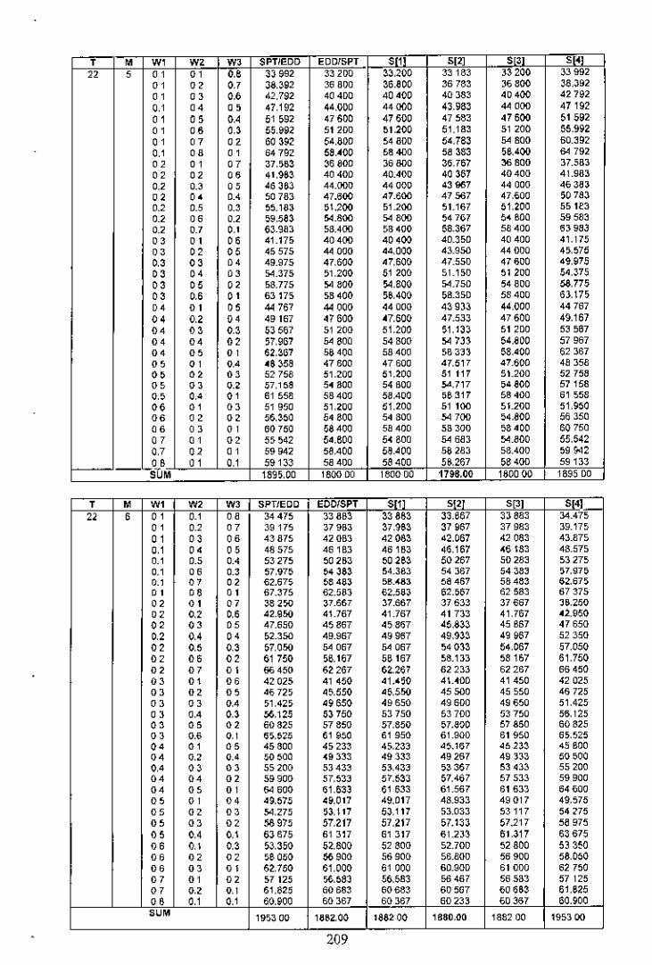
, • ., w, W, SPTIEDD EDDISPT " '" " "n • "' "' ••• 33992 33200 ~3,200 33183 33200 :)3992

"' " ., 38,392 36800 36,800 36783 ,"00 38,392

"' " ,. 42,792 404DO 40400 40383 40400 42792., •• 0; 47,192 44,000 44000 43,983 «.00 47192

"' 0; ••• 51 592 47600 47600 47583 47600 51592

"' ,. ., 55,992 512DO 51.200 51,183 51 200 55,992

"' " " 60392 54,800 54800 54,783 54 800 £O_~92., •• "' 64792 5a,~OO 58400 5B 383 ,6,400 64 792

" "' " 37,,53 36800 36 8DO 36.767 36 sao 37.583

" " •• 41,96~ 40400 40.400 40367 40400 41.983.., 0.' ., 46363 44.000 44000 43967 4400G 463~J

" •• .., 50783 47.600 '7.600 47567 47,600 5078J.., •• ., 55.183 5\.200 51.200 51.167 01.200 551t3.., 00 0.' 59,583 54.800 "'00 54767 54 Boa 595B30.' 0.' ., 60.983 58.400 03400 58.367 58400 639BJ

" "' ,. 41.175 40400 40400 40.350 40400 41,175

" " 0; 45575 44 000 44,000 43.950 44000 4,,575., 00 •• 49.975 47,600 '7,600 47.550 47600 49,97500 •• 00 54.375 51,200 51 200 51.150 51200 54,37500 00 " 53.775 54 800 54,800 54.750 54800 sa,775

" •., " 63175 ,3400 56,400 58.35D 58400 63.\75

" " 00 44 767 44 000 44000 439)3 44,000 447670< " 0< 49167 47600 ~7,600 47.53J 47600 49,1670< " ., 5J 567 51 200 51.200 51.13) 51200 5~ 5670< •• " 57,967 54 800 54800 54 733 54,800 579670< 00 " 62,367 sa 400 58400 ,B 3~3 58,400 6236700 " .' ~6 358 47600 47600 47,517 47.600 4835800 " " 52758 51,200 51,200 51117 51.200 5275B00 " ., ,7,1M 54800 54 BOO 54.717 ,4800 57158., •• " 61 558 58400 5BAOO ,8317 58400 61 558•• "' " 51 950 51,200 51.200 51 100 51.200 51.950

•• " " 56,350 54800 54 BOO ~,oo ,4,800 5G350

•• " " GO750 58400 58400 5B 300 ,8400 60750

" " " 5,542 54,600 5~ 800 54 6aJ 54.MO 55,5420' " " 59942 58.400 58,400 58 28~ 58.400 59942

L~!" o , 59 133 5a 400 58400 56,267 58400 59133SUM 189,,00 1800 DO 180000 1798.00 180000 1895 DO

, • w, w, W, SPTIEOO , EOOISPT " " "" '"" , " ., •• 34475 338B3 33863 33,867 338B3 34.475

" ., " 39175 379B3 37,963 37967 37983 39.175

" 0; 00 43875 42 GB3 42003 42,067 42083 43.875., 0< 00 48575 461B3 461B3 46,167 '6183 43.575.., •• .., 53275 502B3 50263 50267 50283 53275.., 00 .., 57,97~ 54 J83 54.383 54367 54 38~ 57,SlO.., "' " 62.675 ~5 483 '".'83 58467 58453 62,675

" 00 " 67.375 62.583 62.583 62,,67 62583 67375

" " " 38250 37.667 37.667 37633 37667 ~5,250

" ., 00 42.950 41.767 41.767 41733 41.767 ~2,9(i0

" 00 00 47.650 45867 45 B67 46,833 45867 47 650., 0< 0< 52.350 49.967 49967 49,933 49967 52350

" ., "' 57,050 54 067 54 067 54033 54,067 57,050

" 00 " 61 750 ,8,167 56167 58.133 58167 61.750

" " " 66 450 62267 62,267 62233 62267 6645000 " ., 42025 41 450 41.'50 4UOO 41450 4202500 " 00 4672, 45,550 46,550 45500 45550 4672500 00 •• ,1,42, 49650 49650 49600 49650 51.4250; ., ., 06,125 53750 5J 750 53700 53750 56,12500 00 0; 60825 57850 57,850 ~7.BOO 57850 6082500 •., ., 6,,5", 61 9,0 61 950 61.900 61950 6,,5"5•• " 00 45800 45233 45,23~ .5.167 .5233 458000< " .' ,0500 <9333 49333 49267 49133 50 ~OO0< 0; 00 55200 5J43~ 5l.43~ ,3367 63433 552000< 0< " 59 gOO 57,53~ 57,533 57,467 575J3 599000< 00 " 64 soo 61.633 61 633 61.567 61633 6460000 " 0< 49,57, 49,017 49,017 43.93J 49017 49,57500 " 0; 54,275 ,3,117 53,117 53.03J 53117 5427500 0; " 5-8975 57,217 57,217 57.133 57.217 5897500 0< ., 63675 61 017 61 317 61.213 61.317 6367500 o , ., 53,350 52,800 52800 52.700 52800 53 3~O00 " " ~6 0,0 06 SOO 56900 56.800 56900 58,05000 0; " 52,750 51.000 G1000 60.90D 61000 62750

" " " ,7125 06,583 56,583 56 467 565B3 57 125

" ., ., 61,82, 60683 60883 60567 60 663 61,82500 ., ., 60,900 60367 60367 60233 60367 60,900". 19,300 1852,00 188200 1880,00 1882 00 195300

209

; • w, w, W, SPTl~DO EDDISPT " , Sl;l "" , "' "' "" J.1,958 34567 34,%7 345S0 34 567 04.958

"' "' "' 39,958 39167 39167 39150 39.167 ~9 958

"' " 0; .4958 U707 43767 43 750 43.767 44958

"' M 00 49958 4~,~67 48367 48350 46367 49958,, 0; M 5495a 0<.967 52967 51,950 52.967 54958

"' "" "' 59,9~a 57567 57567 57,550 57.567 59958,, "' "' 64,958 62167 62157 62, \50 62.167 64958

"' "" "' 69,958 66767 66707 66,750 66.767 69958

"' "' "' 38,917 38533 38533 38,500 JB 533 38917

"' "' 00 43917 43,133 43133 43100 '3,133 43917

"' "' 00 48917 47733 47,703 47,700 47733 48917

" M M 53917 52 JJJ 52 n~ 52,300 52333 53917

"' 00 "' 58917 56 gJ] 56933 56,900 56933 5B.917

"' 00 " 63917 61-5:l, GUl] 61 ,00 61.533 63~17

"' ,., ,, OS917 66.133 66.133 66100 66,133 68.917

" ,, 00 42.875 42500 42.500 42,',0 '2,500 42 B75

"' "' 00 47.815 47.100 47.100 47,050 47100 47.87,

"' "' M 52.875 51.700 51.700 51650 51 700 02,875

"' M " 57.875 00.300 ,0.30D 562,0 56300 ,7,870

" " " 62.~" 60.900 60.900 60 ~50 60,~00 62875

" " " 67.875 6'.500 6,500 65400 65,,00 67875

" " " 46833 46467 ol£ 467 46400 46,467 46833

" " " 51.833 51 067 51 067 51.000 51067 51.833

" " " 56 833 55667 55667 55600 55 %7 56,833

" " " 61 83l 60,267 60267 60.200 60267 61 633

" " " 66 833 64,867 64,867 MOOO 64.867 66 B33

" " "' 50792 50 433 50.433 ,0350 ,0433 50 7~2M 0' " 55792 5,033 5,033 54,950 55033 55792

" " " 50 792 59633 59533 ,9,550 59633 60792M "' ,, 65,792 64233 64233 64 150 64.233 65,79200 "' " 54,750 54400 54400 54 300 54400 5<,750

" " " 59750 59000 59000 56,~00 ,9000 59750

" " " 64750 63600 63600 6J,500 63600 647,0

" "' "' 58708 58 J67 0~,J07 58250 ,8.367 58708

" " ,, 6UOS 62967 62967 62 S50 62.967 63.708

'" ,, " 62667 62333 62333 62200 62,333 62667

'0' 201100 1964,00 1964,00 1962.00 1964.00 2011 00

, , w, w, W, SPTIEDD EDDlSPT S[1] SJ~!".. Sl~l "" , " " '" 35,442 35250 35250 35233 ~5 250 35.442

" " " 40742 40350 40,350 40333 40350 40.742

"' " " 46,1>42 45450 45450 45433 45450 46042

" ,. " 51342 50550 50,550 50,33 50550 51.342,, " 0< 56642 506,0 55.G50 55633 55,650 56,642,, " " 61.942 60750 60.750 60733 60700 61 942,, " " 67.242 65850 65 a50 05 a:)3 65850 67242

" " " 72 542 70950 70.950 709:)3 70950 72 042

" " " 39583 :)9400 39.400 39367 09.400 39583

"' " " 4'1 88~ 4'1 500 M'OO 44,467 4' 600 44883

" " " 50183 49600 49600 49567 49,600 ,0 'aJ

" 0< 0< 554a3 54.700 ,... 700 54.667 54700 55 483

" '0 " 60783 59800 59800 59.767 59,600 60.78J

"' 00 " 66 08~ 64.900 64,900 64.S67 64900 66083

" " "' 71,38) 70,000 70000 69.967 70.000 71 383

"' "' " 43.725 '3550 .3550 43 500 43.550 43725

" " M 09,025 ~8 650 48650 48 600 48.650 49025

" " M 54,~25 53750 53750 53700 53.750 54325

" 0< "' 59625 58,650 58,850 5~,800 58850 59625

" 00 " 64925 61950 6J 950 6~,900 63.950 64925

" ,. ,, 70225 69050 69000 69000 69 050 70,225

" " " .7,667 .7,700 47700 47633 47.700 47.8070< " 0< 53167 52 ~OO 52 BOO 5Z 73) 52 BOO 531670< " " 58467 57900 57900 57,83J ,7.900 584670< 0< " 63767 63000 "~,OOO 52,933 6MOO 637670< " " 69,067 6a,100 68100 6B 033 68.lOD 69067

" ,, " ,2,00S 51 850 51 850 51 767 51.850 52,00a

" "' " 57308 56 %0 56950 56,aG7 ,0.950 57308

" " " 62,008 62,050 62,050 61,967 62050 626D800 0< " 67,90B 67150 67150 67067 67.150 67,908

" " "' 56150 56000 56000 55900 55000 56150

" " "' 614,0 61100 61100 61,000 61 '00 6"<00

" " " 66750 56,ZOO 66200 66,100 66200 66.750

" " " 60292 601,0 60.150 60.033 60,150 60292

" " ,., 65592 65.250 65250 65,133 65,250 6,,592

" " " 64.J3 M'OO 64,300 64167 64300 64 433W. Z069 00 2046.00 2046.00 Z~44,~~ 204600 206900

210

III

00 909 ~ 00 .9Z~ DO"LOn a09\6~ OQ'ZI'6~ 00 90g ~ '"'000 O. £.6 L~ £g~'Lj> £H 6<; L9H 09 000 09 " " "OW). <:669~ 90~9P 199"6'; [H~19 090',g " " "o~. ,I' <:sen SOO'£. 190-9. [\I5-L9 09. gp " '" "O[Wl~ 0,09~ 0,9 "" (l{lZ 09 Gong oo~'<:g " <0 "O{).9~ 0, •. Gl' 09n. 0099. 006-[, 0[1';9' <0 <0 '"006 a. O<;~ g£ 0';. B~ 000 £S oong 006 ot>" <0 " "001 ~,; eOI ;. Z61.t nL09 ling a~ 1-1:<; " '" '"~gg'!. eo. I. l6001' nn~ 11<:9. [J<;,-Lt " <0 "m;s I~ 9061:" ~66'9£ u:<; £~ .! 19-M; 0,5"'1> <0 " "o,,£~ SOO€ l6R ££ n:661>" !10"~ O~f:-9[ ., " "OOl M; LgI'.1' [£LIt ,gn9 U:I-09 ()On, " " .,009'R. L9S 01' £1:99~ L99'1~ [[;<;-9, 0099. " '" '"ooon L969£ £tg'n 1.90 p;; [[;6-1"] 000 ~. <0 <0 '"oot>L£ [9, .1: tt. ~~ L91'a~ n:. ,g OOo'lt '" " '"009 I. .9" 6~ £££ 6< L9ij 9~ tsn. OOg 1£ '" " .,0," ,<; gnu ,ao!' OOg 19 O~H9 0;" ,,~ " " <00<;9 £1' 919 6~ >1.I'l£ OD~gS O~9g, 0;96. " co <00,0~l' <;W 9£ 9<0 j>~ 009 v;; O<;~9~ OgO'I'O <0 '" <00.v9£ ,lv Z[ 9L6'O~ 000 I~ 0<;9 15 O~~9t ., co co0.9 U: .lH gl gL~a oo.-L~ m;o g~ 0~9lt " co coo.la ,ll,l gLnl oos [~ O,H"I' o;n~ 00 '" co00£ 9; .gl <:~ L~~'g£ [.£"l9 L9L"l9 00£% '" '" eoOOL05 £9H£ l~L.£ [.L g~ ,9'-69 {H)La9 eo 00 eo00' '90 rgo ,I: L~9 ll: ttl g~ L9; ,9 00' ,~ 0' " eo00,6, .gv'~£ L~~'6l n:n~ L96-~9 009'6t '" '" eo006 ~~ £9a'a L~~9l ~,6-l0 L9~-9p {H)6" '" 0' "00£ gi: £9no L~[rl n:. VI>' ,9£-~0 (H)£9l 00 eo eoOOlU eag'Do lIi: OC [[L 00 L9"I~ ooL"ll '" " eoo.n~ ZVI:~. 99t L~ L9B-l9 [gO-[9 O~£19 " '" '"O.l ~~ ~~LL. Qgt'~~ 19Z 6S [g. 6g O;l'I~ eo '" '"0<;190 <:.~'01; 99~1£ L99 g9 [g~., 05~-9~ co " '"0;. o~ ZI'5 o£ 9g0'Sl 19D'l~ [g~ 19 0<;9O. '" '" "O\6't>[ Z~6 9Z 996.2 .(9' 9~ [H9-g~ 0<;6-~t co '" '"o,~ 6<: <:Kel 9.9 '" 199-~0 [~O•• 0,<-6l 00 0' '"09£ [i: ~tL 6' 9"HI L9n~ t~no O,L £Z '" eo

"0<;1g ~ IN 9' 9,9.1 L99 L[ nS'lt m;~9~ 00 " " 0 "[']5 " EZIs " !dSlllm amlidS OM 'M ,M " 0

00 £.~~ 00 ~<:~I OQ;;~H 00 ,£g~ 00 09~~ OO'£;~~ ""'L9, ~. 009'9~ £[0 9~ «0.(9 0069. L9,-g~ " '" 0'9.>'60 009 <;t lI[ .~ lon~ ooS-g<; ~~. 60 '" eo "g", VI>' OOl<:. 1~9 ,. lKt>S ooe-99 S'~-pp '" '" "0.£ O~ 009'," 009 ". 059-Lg 006-99 0<;£-0. '" 00 "0.0 S. OOc~~ 006'S£ 05,-1'5 009 gg [}';o-,. " " 00O,L 6£ 009' L£ 00" L[ osn9 oon. 05l-6[ 00 '" 0'"'Z ~~ 009U £@o. R,9-L9 OOS-99 "~n<; " '" "~.6.~ OOt'O. £g ~91; ~'K 90S g. ,~s-,. " 00 00,.9 O~ OOR9£ £90 ;£ R,9-~S ooH9 ;;~9 0. <0 " 00<:.£'9£ 00. <I; ~ga~ gg; 9' 009-6' ~,£ g~ '" '" co[<I "~ oon. L9~-6[ L9099 00699 [<n9

"co '"[.99' 00~'6£ 19~-9[ L961'S OOg.9 [<9-9' " '" .,

H. ~. Oog~£ 19L £[ 1.99 ~g 00L"l~ [£9'1. 00 0' '"n:l9£ 00. ,~ 190-1£ L9Lg. 009'6~ [£" g[ '" 00 "££6'0£ 000 6~ <9£'9~ L99 <;. OOg90 t£6 a, 00 '" '";zo [. 009~' 090'l£ ~ag~ 00699 9~0 £9 '" 00 00~l<•• OOl'g£ O~LVI: H,'9~ 009 <;~ ~(:no " 00 '"n.'z. 009 >I; 090 ;;t ~LO;:~ 00£ c9 9Z.;:. 00 '" 0'."1 L. 00. ~~ O~£'6l ~L6g. 009'60 ~~'-L[ '" 0' 00,l9 ~< 000'9Z O~9-9l 9£9'90 00, 9~ ~(:9 ~t co 00 00,lS 91: 009'.;: O~S-[Z 9H'~. 00. £P 9(:9'9Z 00 '" coL\6 <, 0090' [[L'<;[ £e~'g9 006 9~ L16T. '" '" 00Ll9g. oon£ [[0-[[ te~'9> ODS9~ H9'90 00 0" 00L1[£' 009 £~ ,[£-0, ~gn. OOll~ H£tO 0' 00 00LIO9S 00. O~ t(9-a £B\ 6~ 009'60 L10 9[ ., '" 00£\H£ oooa t(6'.~ m09~ 009'90 L1ll[ 0' 0" 00L1.a 009 £<: [[~-U (S6'<:~ oo.n L1.1.~ 00 00 "LI 1 ,~ oo~ OZ ,[.-6~ t996C 00£ O~ HI'U '" '" 00BOg~, 009'6£ 1WVI: ~6g'9~ 006 9~ ~09'P<; '" 00 "eo, 6. 00t9~ l~n, ~69'''' oos 9~ ~09'60 00 '" "gOl •• 009'<:£ l~9-gl i:6H9 OOll~ 90no 00 00 "B06 g< 000'6Z L~S-<;Z ~6£'60 009 6~ ~06'~( '" co

"gOg££ 000 9;: l.~~,[ ZS" 9~ 00,9' e09 £[ '" ., '"son" 009 Zl 1.~9OZ Z61 [> DO~to gO£ g, 00 00 '"goa £z OOZ6~ L~9l~ <:60o~ 00£ Q~ ~OO~;; '" 00 '"SOLLl OOSg~ HI S~ ,"66'9~ OOlL< ~on~ 00 '" '" • "[.Is "" [;;15 -,I, .l.dSI(Ja3 amlldS OM 'M ,M " 0

, " "' "' "' SPTIEDD EDOISPT s1!l "" "' "" • ,, ., ,.. 18592 3B 567 38342 1620D 16,46, 18592,, " ., 24492 42.667 4~,442 19700 20263 24492,, " 00 30392 46767 _6542 23200 24083 :)0392., " ••• 36.292 50867 50642 26700 27,883 36,292

0.' 00 ., 42.192 54967 54.742 30200 31.683 42.192

"' •• 0.' 481)92 59067 58.M2 33700 35,483 4B.092., ., " 53,992 63157 62.942 37200 39,283 53.992., ,. o , 59892 67.257 £7.[1-12 40700 4J,083 59892

" ., .., 23253 42 OJ3 41$B3 20900 21 \67 2~_28J

" " 00 29,1B3 46133 45683 24,400 24967 29.183

" oo ., 35083 00,233 49763 27900 .5.761 35003

" ., ., 4096~ 54333 o3,ae3 31400 32567 40,9B3

" " oo 4G.663 58433 579B3 3',900 36 367 46 fiB3

" 00 " 52,783 62533 620B3 38,400 40167 527B3., " "' 58,683 66533 661B3 41.900 43967 586B3oo "' 00 27,975 45500 44825 25600 258,0 27975oo ., " 33.875 49600 48,925 29100 29.650 33,875oo ., ., 39,775 53700 53025 32,600 33.4,0 39775oo ., oo 45,675 57 BOO 57,125 36 100 37.250 45,675

"' "' "' 51 575 61 900 61.225 39600 4\.050 51.575

"' ••• " 57,475 66 000 55325 43.100 44850 57,475

" ., "' 32,667 4B 967 48,057 30.300 30533 32,567

" ., " 3B 567 53067 52,167 33.800 34,333 38,567

" .0 "' 44 467 57167 66 267 3nOO 33133 4',467

"., "' 50367 61 267 60,367 .0800 41933 50,367

" " " 55267 65367 ". 467 44,300 45733 66 267

" " " 37.358 5Z,433 51 308 35000 35217 37.35B0.' " '0 ',255 56.533 55.406 38500 39,017 ".256

" " " .9156 60 6~J 59505 '2,000 42 B17 '9158

"' " ,, 55 05~ "..7~J 63.60B 45500 46617 55058

•• " 0.' 42,0;0 55.900 54.550 39700 39900 42,050

•• " " 47,950 60 000 586,0 43200 43700 47,950

•• "' " 53850 64100 52.750 46700 47,500 53850

" " ., 46742 59.367 57792 44.400 44583 46742.,"' " 52 ".2 63467 61892 47,900 4B 383 52 ".2

"' " " 51.433 62833 61,033 49100 .9267 51 '33,.. 1559 DO 202400 1997 DO 1272.00 n0600 1559,00

, • "' m m SPTIEDD EDD/SPT " '" " S[4]

" , ., " "' 19D33 39250 39017 16742 16825 19,033

"' "., 25233 43,800 43617 20,842 20.B20 25233

" "' •• 31433 4M50 48217 2.542 24 B20 31433

" " '0 37633 53,050 52 BI7 28442 23.820 :)7633

" "0 " 43333 57,650 57417 :)2342 32.826 43833

" •• ., 50033 62,250 62017 36 242 36 BZ5 50,033.' " " 56,23:) 66850 G6,617 .0.142 40,825 56233

" "' ., 62.433 71 450 71 217 .4.0.2 44825 62.433

" "' ., 23867 4290G 42433 21.563 21650 23,667

" " •• 30067 47500 .7033 25463 25650 30067

"' "' ., 36 267 52100 51 633 29 J63 29650 36,267

" " " '2467 66 700 56 233 33263 33650 42467., 0; 0; '8667 61 300 60833 37183 37650 48667

" •• ., 54 867 60900 65433 41.083 41650 5' 867

" "' " 61 067 70500 70033 44963 45650 61 0670; ., •• 257GO 46.550 45 B>Q 26425 26,470 2B 700

"' " 0; 34 900 ,1.l"0 50450 30325 30475 34 900., "' " 41.1GO 55.750 55 G,D :)4225 :)4.470 .1 100

"' "' "' .7.300 60350 59.65D 3B125 38475 47,300

"' 00 " 5'.500 64.950 "'.250 .2025 42475 63 50000 ,. ,, 09,700 695,D 688,0 45925 46.47, ,9.7000< ,, 0; 33533 50200 49267 31,257 31 300 33,5J30< " 0< 39 D3 54,aoo 53867 3,,167 35300 39 n,0< "' ., 45933 59,'00 584£7 39,067 39300 45,933., 0< " 52,133 64000 63,067 42967 43300 521,3'0 0; "' 58,333 6B £00 67,667 46867 47.300 58333

" ., 0< 38367 53 e50 52683 36108 36125 383670; ., ., 44567 58.450 57283 .oooa 40.125 44667

" ., " 50767 63,050 61 68:J '3.908 44.125 50,767

" " ., 56 967 67,650 66483 '7,a08 48125 06,967

•• " "' '3200 57500 56, tOO 40.9,0 40900 432QOCO " " '9400 62.100 60700 44 B50 44950 49,4060.0 "'

,, 55600 66.700 65.300 .8750 48950 ,5600

" " " 48033 6l.1,0 59017 45792 4,775 4e 033

" " " 54233 60750 64117 49692 49775 04.233

•• " " 52,867 64800 02,93, 50633 ,0600 52867,.. 161200 2'06 DO 207800 llJl.00 134700 1612,00

m

m00K;~ OaHU 00 s;~~ 0O-O99~ 00 999~ 00 I'<;<;~ ""OOt'O, £££ BI' L90".' L909S 009 "~ 001' 0<; '" " 0'09ns; l6£-LI" ~Ogg. ££v~<; O~600 m;n~ '" " "0.2'91' l6~-tv gOg cO .£v i:, Og6'~; O,Z9' " '" "oo~Zg 0,' 9. 0,0S~ oo~'.g 00~9<; Don,

" " '"oon •. m;z'£. 0';( i:l' ao9'l. 00 ~ ., OOt'LV " " "ON-l!' 0<;0O~ 0.9 S£ aog gt OO~'O. ao ~~I' " " 0'O,g'£~ gO, 5' Z6~Tj> L9~-1"J Q,Z g<; O~,., " '" 0'0;1: ~~ 90£ 01' l6g ot> L9n; o,:.~, fr\;.-g •. " " 0'O~;)(v 8a~o£ ~Mg~ L91 ~~ 0;060 0,1"[1>" " " ;0096'L(: gOG ';[ ~6'g, 191S~ 0<;<:'91' 0<;6LI: '" '" ;0oong [9" .1' £H-~. [£, I:~ oon, 009 I"J '" 0' '"00•. 6. l'<l;t. I:tH~ (£. m; 001' ~s 00.6. " " '"DOl ~. L9~'g~ [H-9, ££9'!.' 001'H~ non'. " " "000 61: ,%'.1: [£0 V£ £~g'•• OOVS~ 000 6r '" " '"OOg £~ 19l"l£ n:. ~t ££. ~. DOt ,~ 009 U: 0' '" "099'gg .<:9-£ •. 5£9 O. 006 Z, 099 t9 0.9" '" '" "0".0<; ,cHI>" ~l6'1. 00661' O;9'og 0<;1>"0<; " 0' "0.<: , •. gent ~a". 0069. 0., LV 0," 'v " '" "O<;OOt ~toK 5L, ,. OOG e. 0" ~~ 0.0 O~ 00 00 00o~n~ ~Zg a~ ~L9 6<: 006 O. 0" ~~ O~g'.~ 00 co "O,9-6l ,"9'n: .un: 006 L~ o.~ g~ O,96l 00 '" 0000r-99 (gg l. L1l6. ,:gn. 00': Z, 00l'9g '" co "00n9 (g.6£ Ll99£ 19Z D' OOL6~ OW~g " 00 "aar g. £gl9£ Ll9U L9Z 9. 00l'9. 00£ 9~ 00 ;0 coOO~-\. £~O~~ L1\~r L9l £~ OOLr. oo~ ~~ " 00 "000 ';[ ~g9 6, H.6Z L9l0. oaL O. 006 <;£ 0' co 00OOLO[ ~~9 9Z L~L ,Z L9?'L€ oaL L€ oa~'o€ 00 " coGOg-,l £~~ ~, HO£Z L9;; ~€ oaL V£ OM 9l co " "0,0. Z~L ~, ~gL I.S [,9 19 09g'19 0,1. L9 '" 0' '"O,g-l, Z'" s. ggO',£ [(99. O~g'g. O,5l, " " '"a~n. i:~~'9C g<;[Z£ ~~9 9. a"s "" ogn~ 00 0' "0;1'l' Z~l Z£ s.g DO [£9-0' O~~O. 0, ~l. 00 ;0

"0;69£ z.6n s.a go [£9-6~ O>~6£ a~B 9£ 00 00"o;n( Z.L ~Z ggno [£9-9, O,~ 9£ a~n[ 00 " "O;g 9Z Zj>gol g.no [£9'£1: O,g ££ a~<;-9l co 00"0,. ~z oKH g,S gl tt9 a( Mg-O[ o,n? 0' " '" , "" [cIs , r~s !<JSI(](]3 (](]3I.L<JS 'M 'M 'M " ,

ao ggg~ OO':QG~~ OOW.~ 00'6.~Z oo9g~, 00'g99~ ""00£.'" S£O0' L9~og [£g 1'9 L9L'99 aGn, '" '" 0',09-gg ,(9£ ~g ~W19 ,.r-99 [~O-99 ~W-g. '" '" co'0.6. ,(90 LV [~~'H ,"0-19 [t6'~9 ~ZS'6. co

"co

o~n, OOl'OI; OagO. O,S"N 00.-69 o,n."

00 00O~gO. oo.9~ OO~9. MU9 000'1'9 og~ 09 " '" 00o~n'l' DO~"~ oon. 0,9-Lg 00~-6~ o,n.p- 00 " 0'gL999 ££a D, U~'Og s.£ 69 L9gW ~mg~ '" 00 ;0,Lng £1:1g. L~S91' Sgo 1'9 L9~ g9 ~Kl~ '" 00 ;0S.(S9. ££j>~. un. S.I 6~ L9£09 ~m,," 00 '" ;0grn~ £[~,(£ L~nt 9.0 j><; Lng~ ~l£ 6£ 00 '" ;000~'09 L9£ 6. tt~ 6. L9g Ol r£nL oo~ 09 " ;0 00D06£1; L90 g~ £(1";' r9L'g9 rU99 006'~~ " '" "00. LV ,9['0. a:g o. .99'09 .£9 ~9 OWL' " " "006'0~ L9~ 9[ t£~ 9t L9. ~<; ££g'gg 006 O. " '" '"oal"~£ L9~-ll: t[o l( L9.oo r£. ~> OO~l't ;0 " '0gl6 ~9 aOL91' ooL-g. gKU 001 [l go6'~9 " 00 '0'0' " 00••• M~ 1'. gaL9 OOO'~9 ~o. ,~ '" 0' ",l6 g. OO~O. 0,1-01' gn Z9 006'~9 g06 H~ 00 '.0 ",l. Z~ OO~gl: 0,9 gt gLOLg 009 Lg ;o.l~ 00 '0 ",l6,[ oonl: 0" ~~ gL6 ~g OOL',g g06 ~r ;0 '" ".,1' 60 oonz OgoU gL9'9~ DOgL~ gZj>'6~ 0' "

00Og.'C9 em-g. "90 ~. .99 ~l ,(9£ .L O.H9 '" co "Og6'9g I;£HI' L9n. [gL ~9 .(9<69 0.6'9g " 00 "OSI'09 ~(~ 61: 1.9. 6~ £gg r9 .(9~'.9 Og.o<; " ;0 '"0.6 [. ((t .£ L9\ g~ £9~ g, ,(90'6g 0,6 <V '0 00 co0"" <£ t[g o£ 1990£ £9. rg L96'£g 0"" l. 00 co '"0<;6O[ t[g 9, L99 90 £91;g. .(99'~~ 0.6 O. " '" "0<;1'~o ((O"U L90," £9l S. L9L £~ Og. ~l co '" '",L6 ~9 L9n. .9~'LV 06£ <;L £~9 gL 9L6 ~s

"00 "9L~ gg L90 [~ egan 06,'0': ££~ OL gl.'gg '" " '"9L6'19 L9'( H£ £gL 9£ l6~'g9 ££1' <;9 g16 t, '" ;0 '"91.. g. L9.1'~ £9. ~£ ~60 09 ~I:£ 09 <;1~,. 00 0' "91$9£ 19\ O~ £9~O£ ~60 .<; 1;(, gg ,1681; 0' '" '"91.~ll: L99 go £9H'0 ~6g 6. ~t~ Og .L~ l~ ;0 " "9L6-.l L9ni': £9~ 10 ,6,(-" (to g. ,L69l '0 " "gL.'6~ '(9l LI 1:9UI ,69 6~ ~~6 6€ <;LH~ " " "

, "'" [tIs ils " !<JSIOO3 (](]3Il.<1S I tM 'M 'M " ,

tIC

OOOWt 00 ~6£1 , OO';Q~~ 0096H 00 .~g~ 00 099~ "eoL9Z ~, OOO'~g ~~O'I" (:<.6, 001'19 L9~£g " " ""~£9v, ,L I 0<; <:600g L9~'6, 000 19 ££9 •.• " '" '"(1:9 a~ <;l,9v Z6, g~ L99',g OOl L~ H:~ 91' '" " '"000'99 O~( 61' m<l 6~ 00;: 6<; 00909 000 9<;

" "" ""OOlO<; o;n~ O;9'~. 001' ;; 0099, aOl G, '" '" .,oa~vt OfWlO 091'0' 009't. 000 •• OOvP~ '" " '"<9•• 9 ~"99. ~on. ££06. 00;: 09 L9£ L<; " '" '"L9ng Se6 v. Bon', ~t~gg oav'~g [9" I, '" '" ;,L9nt sen. Bon. ~£n. 009 Zg L9L ,1' '" '" '"l%6~ ~;;O( eOl L£ ££9tl>" OOH gt L966. '" " '"~USg OOL L~ L9l LV LW9g oo~6, I:,.ng " ;, "££6-Zg 001 V. 1.91. ~. NO gg 000'9. ££6 Z; '" '" '".n""v 00;'0. L9l'O. Lgo I, OOZ Z, .£ I LV co " "ccn •. 006 OC L9L 9. 19t'l.t ow~. ~~n.'" '" '"~,Sg~ OO£'~t L9~'t£ L99 £1' 009~l' .£<; 5. '" " '"001'09 ~mg. ,~£9. OOL g" 00 •. 6<; 00109 " '" "00, 1'. ~lZ £1' ,~9 <:l' 006 .<; 009 g<; oong '" ;, "oo~81> ~L96£ ,Z[ 6. 00I I, OOg I; oon~ " " "OOL of ~Wgt ,ZS ~£ DO, LI' 000 H~ OOLOV " co "0069£ 9LH£ 9i':£'lr 00. 'v DOl ~v 006 m: ;, " "co~r£ 9L~-9l 9i:~'n 00.('68 OOV'O~ 001 18 '" " "L9v ~9 0909t t~8 9. ~£g'g; 0006, L9. 19 " '" '"L995<; 09~ z. t~~ ~. C£L'''; OOl'~~ L99 ~~ " "' "£99 6~ 09H£ tg~ 9t .£6 m; 00. ~S 19ij 6~ " ;, "190'.0 09Z'g~ ~9g .£ £.1 .(~ 009 LI' ,(90 •• " " "19GH£ 0<;9 ~. [g£ I[ ( ..(. ODS ~. L9G at ;0 " "L9v zt ogo'eG £aa'Ll U:<; 6£ 000-0. L9v Z( "' " "L99'9Z Og•• z £9, VZ (H-'!( OO(;-gt L999l " '" "££9l9 <;zzS~ z•• ~. .(9£ a9 0099. £ml9 , 0 '" '0£.O'(S gen. 1:M'O. L9;-t><; OOg-t><; (£D-LO " " "££z IS ,ZO H. Z•• L£ L9£-09 000"1. £(z-l. e, '0 '0rev gv .ZV ~£ Z\>6[£ L96-9. OO<:"Lv ~r. gv " '" '0t£96, .Z90£ Z•• O£ L9~Tt 00' ~v ~t9 6~ " '0 "ttS ~t ;(;l'.(i': Z\>69Z L9.-6[ 0096£ £t~ £~ '" e, ",to-Sl ~1:9't<: i':.v £l L9, g£ O@<;[ [[0 ez " " "£"u ~i':O'O~ 0.6 61 L9LI£ oao Z£ £C, ~Z '" " "

, "lOIS lCJS li:l-,- [lIs IdS/GG3 GG311dS ~ -~ 'M " ,00'[091 OO_.~M OO"OZ.~ OOHUI 005,1l 00'.(09' ""££ng L59-6v 00<; 6~ 0091.9 009'£. ££9 1<; " " '"l\>C £g [Rnv 00\; g. 000'1.9 glG'9. Z.O [, " '" '"~t><;lj> [g.-.v 001:'~. 000 •• <;L<;S<; ov<;l> " " "09l ~9 aWLI' 00' Lv 000 L, 0<;£R~ 09Z ••

" '" "OgL'e. 00 •• 1' 000 •• 009.9 096' •• OgL'g. " " "Ogl •• 001-)1' 006 O. OO~'Og Ogg I. O<;Z,~ '" " "B<;v '" L~O-Lv 006 ~. OOg'9. .UL, g<;j>95 '" " ;,gg66v L~9[v ooSl. OOi':'t; ;l£ t><; B.66v '" " "g<;v ~v L~,Ov OOL'6t 009'6~ ,Z6 a~ g,,- •• '" " '"996'g£ LIH9£ aog g, 00.'9" ~"g'.(v g,S g[ " " "L9g'99 ~~ I 9. aOL-•• OOZ9> 00' 'L~ /999> '" " '0L9~~9 ££L'<:. 009-11' OOgl~ 00L't9 L9n~ " " "L99 ~~ [[[ 6£ OO~9£ OOj>'6~ 001:-0. L99-<;v " " "L910' 1:£6.[ oo~-", 000'9. 006-gv L91-0v " " ,.,1.99'.( 1:1:. ZI: om: Z[ oon. 009-1:1' L99-" '0 " "<;/.S'.(~ Ogl <;j> Oa51:v 009-99 ~LOg~ .H-L<; '0 " '"~L£'l~ 0<;9 I. 00.01' oo","~ ~LO-I:. SL. Z. " '" '"SL9 9. 0<;1'g. OOt'L~ aOO-6v 9L96v ~.(e 9. '" " '"5L£ ~. 090'~£ 00, vI: 009 <;1' 91091> ,In. " '" "~I;~ 9t Ogg I. 00 ~ ~I: 00<;-0. "L~ lv ,H <;[ '" " '"~L8 Ot Ogl H~ 000 gZ OOS98 .L~ 68 ,Lf: O£ " " '"t~O 6. L9£ v~ 00\: eV 00. gg 05R <;<; [~O 6<; " " "[H<; £S L96 O' OOZ'6£ 000 Z<; os~ ~9 ~9~'£9 " " "1;\l1l 91' L9<;If: 001'9£ 009 gv 0,06. £90 e. '" " "~9!i lv L91" 000 t£ OO~gv 0.9 <;j> £gg Zv " " "~gO.L8 L9L af 0066<: oon. 0., Z. £90 l£ ;, '" "[gS 1£ 19~'a 0099Z 001' g[ 099'S£ £9. 18 " " "~~O9l L96 [Z 00L't<: 000.1: 0<;1'~£ ~90'9(; " " "Z6~ 09 tW8v DOl ~~ 000-;9 gl< ,g Z6l09

" " '"Z6L V<; £gO 01> 000 m: 009 ~g 9<:9'19 Z6L 1'<; '" " "l6l S. ,R9-9£ 006'1>(: DOl gv 9Zt'~. ~6l6~ '" " "l6L (:. [RZ'££ 009'18 DOg~v 9Z0'SO i':6l £~ " '" "~6l g£ [Rg-Gl OOL'g<: 001' I. ,zno Z6l g£ '" " "~6l ZI: tgO 9l 009 ~~ 000 g£ 9ZZ'gr ~6L l£ " " "~ara tgO £C 00<; '" 009'.£ ;Z9 o. "6~a " '" "Z6L'll [g96~ OOv'G~ DOl 1£ <;znc ZBL 12 " " " ; "I [ols " ,r, [~Is ldSIOO3 GG3/ldS '" '" '" " ,

m~~~0,099l ~ OOU~~ OOg~;~ 00 <:£61 00 <:96 ~ 00'99,(1 ."£U 9, 196-~~ 00\ 1', 000 .9 000';9 £[ I 9<; '" '" COH9L. \lS~-£g gL9 n; 00£ [9 090'g9 Ll9L, '" <0 "Ling g,Z"6v 5L~'6' OOL g<; Ogj>09 Lin. " '" "OOg 69 0>~-I:j; o,,~£~ 009 £9 001,9 009'69 '" <0 "001£. ass-gv 0<;6 g~ oooe; 009'09 00 I ," <0 " '"OOL 91> rn;n7 Ogg l'~ OOV ~g 006'<;<; DOL91' '0 '" "1:9 1'19 l.L'l" 5~9[9 006.9 0<;I ,9 Sg I '19 '" " '0~9L'•• ;:PH •. gi':g'~. DO, £, 099'09 eSL P. <0 '0 "~~t'gj> eN-tv gol' •• OOl ~<; 096 g~ es£ 91' " <0 "£g6~v l.~6t ~Z6M: OOIM o.n. .96 I' " '" "L99'Z9 [£.-zg oo,'z, 00;:~9 OOl99 L99 <:9 '" " '0LSI> gg ttO a. 001 ~~ 009E9 00909 L9t9, " " ".90 Og [rn•. 009 •• 000';; 000% <90'0; " " "L99 £1' ,(Ht 00<; 6. OOtOg aon. L99 £1' " '0 "tSZ L£ tn'~~ OD~Sf: 009'9. 00991' LHl LS " '" "O,S jo9 >~6'1" 5L6 15 009'09 0<;;:59 Ogg>9 '0 " "0<; I 99 ~~9'lv ,L9 Lv 006'69 0<;909 Ogl~g <0 " coO,L 1<; 9t£ ~. ,Len oot gg 0.0 g<; OgLIg " " "09t 9, "Wct 9LO'6C OOL0, 09ng 09( go " " "096'S~ <;ZL"t>i: SLOC 00~9, 099 9~ 096 ~~ " " "a" Z~ 9Z. O( 9L,m: 009' '" O,Z Z, a9n~ " '" co[[Z 99 LW~9 0" ~<; 009'.g OO(99 £~;; gg " " "n:g69 L~o l, 0,0 L. aOZ'09 OOL09 ~~ng " " "1:,. ~9 L~6<, 0,6 i:. 009 g9 00~9, ~~.'~g " " "~to'L, L~9 g( Mnc 000 I, oo~19 £~0'Ll> '" " co£(90v l~CH: 0'<£~f: OOV9' 006'9v [[90v co " co~t<~~ L~OO( 0<;0DC 009~v OO( o~ ~~~ .£ " " co£[g-a HL-9, 09L ~Z OOlL< OOL'L, [(g £l co " coleD'L9 gO~ ~S "(On; 00 ~<;9 09( g9 l~£L9 '0 '0 "ling 908 g. 'oS 9. 00<;09 09L'09 L~~19 co " '".~~-gg gO, ,:~ ,lg ,v 00£ go Og~9' .~~ gg " " ".nL'9v gOl 9~ 9ll g£ oang 09>'19 .~L9v " '0 "L~C-lv g06 a: 9~6'CC oaL 9v OWgv L~£~v " '" "L~69( 909 £Z <;09'6~ ao~-~v a9C'O. l~69£ " co '"l~96l W,~O ,o[ 9Z oonl: aSUI: L~96~ " " '"----l.g -£l ~OO'~~ 9<:0~o 0(16'0£ 09~£[ L~~ £~ co

" " • "!OJs [£15 " [~ls !dSlOO3 0031.Ld5 'M 'M 'M " ,OO£~L~ OO'H\>V~ OO'09H 00 v99 ~ 00'£69~ OO<~L~ .e,00'" •• v;;g L9~ 0' L9n9 000 £9 OOLV9 '" "

.,Si:Z9<; '9l'~9 £gg ~, -~tn9 ,W'£9 9'" 99 " '0 ""T09 '99 LV £g£ ,~ (H"i, SW-gg 9~~ 0" " "

coO~O~ 00~ ~<; Oong 00V'l9 09n9 O~U,

"co "0;9-~~ 00<:,. 001:Lv 00<:-.9 0,99S 0~9-\9 co co 0'

099 SP oon. OOP£v 000 ~~ Q!;n,s M99~ co '" 00~a6, ££P'Og L~~0, ,9V'~9 ~l9-l9 9£069 " " "SlI t9 s~"9v L~99P L9<:l" ~LVg9 9H £. co " ",La L~ £~n. L~Lov 190 ~9 ~lZ V9 HO"lv " co .,.LS OP ££L'~£ L~~9[ L99 gO HOO, ,L6 O. " " "OOB09 L9l 5~ ~(~ 6v ~."-~9 OOg<:9 OD909 " " '"oon; L9g 'v £[6'9~ [££ l~ 00£ g9 OOL-V;; " " "009 g~ £96'~. ~[OoV (£I '£9 001 V9 009'g~ " co "00, l~ L!lO B~ [H-g, (C6'BO 006 6~ oon~ " ,e "OOV9. L9~'.~ ~[Z VI: ££L' •• OOLS~ 00~'9t " " ",Z£ 09 00~'6v 0~~-6v 00n9 ~Z£ <:9 9~~'l9 " ., ",lo 99 00<:9v a~<:-•• OOVL~ ,l~ g~ ~o<:9<; " " ",l ~'Og OQ[lv O9no 000 [~ ~"6 ~; ~ZI 09 " ,. co9~0 ~. OO.'L~ 0,. L£ OOO'Gv 9U £~ ~"O'OO " co "9<:6l. 009 ~£ 0',,-[£ 009'0. <;Zgg. n6L£ " " co9<:g~. 0096<: 0,96" 009'0. <;l~~. 909 ~£ 00

"co

0,9 £9 ~£v 9v L9. g. L99 ~9 09H9 099 £9"

co coO,L Lg £(9 VV L99 ~. L9v L" 096',~ O,L L, " 00 coO,g ~g ~~9 av L99 O. L9l £9 09L'(~ 099 ~<; " ., co0" g~ £(L'9[ L9£ 9£ L90 £. 099'6v 0" ~~ " '" coO,V6£ nB'~( L9g <:~ L99 ~. 09(';~ 09v6. ,. " co09( ££ (t6 gl L96 gi: L99'0. O,~~. 09~,(£ 00 " "09l'L(; [[0 g<: ,90,Z L9V9£ 096 m: 09n~ co " "9L£ gg 19Uv ~90v ££L ~9 9L6 ~9 ,L( Sg '" "" ,."LZ69 L9B~v £9g £~ £'" L9 gLng 9a £<; " co ",L~£g L9661: eg6 £~ ££1:£" 9L9'£9 9LI£, " 00 '"910 Lv 19O'9t ,gO 9~ ~£~SV 9Lt o. 9LOL~ " ., '",L£ OV 19~'l£ e9\ ,f: ££6.v 9L~'~v ,L6 O. " " '"9.(9'.~ 19Z 9<: ce~'6Z £[l O~ 916 O. 9.9'OC 00 co

"9il S<: .9£-1>/ .9£ ~Z ~£9'9£ 9ll 9£ 9U'HZ co " '"9L9ll ,9v QZ .8VO<: £[£ <:[ gK~£ "L9U " '" '" , "" '" " [~ls !dS/GG3 QQ31!dS 'M 'M 'M • ,,

,

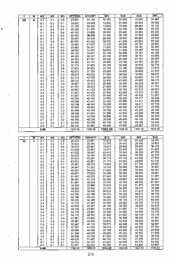
, " ., ., W, SPTIEDD EDDISPT " S[2] " sHl_

" , o , "' " 24,992 23108 10450 22 600 22.883 24,992,, " "' )0,092 2, Boa 13.050 25300 Z5 aBo 30092

"' "' 00 J,192 28508 1,,650 2B000 28,863 35 192

"' " 0; 4Q 292 31 208 18250 ,0 700 3186~ 40292

"' 0; " 45392 33.908 20 BSO 3~,400 348B3 4!U92

"' '0 " 50492 36,608 2J 450 36100 37 RB3 50.492

"' "' " ;5592 39308 26050 JB BOO 40,863 55592

"' "' " 60692 4200B 28650 41.500 438B3 60592

" " "' 2B 8B~ 27,5'7 15300 ,6000 26767 2~eS3

" " 00 33,98) 30217 17,900 29 200 29,767 33983

" "' 0; 39083 32917 20500 31.900 32.767 39083

" " "' 44 lB~ 3,,6'7 23100 :;4,600 35767 44,183

" " "' 4928) 3B317 25700 37.300 38767 49283

"' 0; "' 54 383 01 017 28300 '0000 41767 5',383

"' "' "' ,948J 43717 ~o900 42.700 44767 59483

"' "' 0; 32775 31.925 20150 30,400 30650 32,775

"' " 0; 37875 J4 62, 22,750 33.100 33,650 37 B75

" "' "' 42,97, 37325 25,350 J5.BOD 36650 429750.' 0' "' 48.075 40,025 27950 38-500 39650 48,0750.' " 0; 53.175 42725 30550 4\.200 42,650 5J1750.' 00 o , 58275 45425 J3150 43 goo 45650 582750' " " 36.667 36 3~J 26000 :,uoo 34,533 36667

" 0; " 41.767 J9 03~ 27,600 37.000 37,533 41 767

" " " 46867 41.73) 3D200 39700 40533 46867

" " " 51.967 44,433 32800 42.400 43533 51,967

" " " 57,067 47133 ~5 400 4~ 100 46533 ,7,0~70; " " 40.558 '0742 29850 38200 38417 405580; " " 456><1 .3442 J~ 450 '0 goo 41417 ',656

" " 0; ,0.758 46 142 J"O,O 43600 440417 50758c; " o , 55858 .6842 37650 46 ~OO 47.417 5585800 0.' " <14.450 45.150 34.700 42100 42,300 •• 450c.o 0.' 0; 49.550 47.850 37,3(H) 44800 45,~00 4955000 " 0.' 546,0 50.550 ~9.9(H) 475DO 48 ~OO >4650

" " c., 483.2 49.55-8 39.550 46000 46 18~ '8,342c., 0.' o , 53442 522;6 42.150 48700 49,18~ 53 4420' 0.' 0.' 52233 53.967 '4 4(H) 499DO 50,067 5~ 23J

'"" 1555 (H) 1.29 (H) 1002.00 136800 \40200 165500

, " ., ., ., SPTIEDD EDDISPT 'l' " 51~1 "" ; 0.' 0.' 00 254;13 ~3.667 10875 23142 2~ ~25 25 4~30.' 0; 0, 30.833 26.767 1~.775 26242 26,425 3D833

" , "' 0.0 36 2J~ 29867 16.675 29,3-12 29825 :l6 2~)

" , " 0; 41.6JJ ~2.967 19.57, ~2,.42 32825 '1,63J

"' "' " .7.0)~ 36.067 ,2470 35 5'12 ~6 025 .7 0~3c., " "' 52.4J3 ~9 167 25.~75 38 6<\2 3g 225 524330.' " "' 07.833 42.267 26275 41742 420425 57833c., "' o , 63.23J 45.~67 31.175 44842 4$,625 6~ 2330' "' " ~9 467 28.233 15.850 27,183 27250 294670; "' " 3-1.867 ~t.3;13 18.750 ~0,283 ~0450 34 8670; " "' 40.267 ~4.4;13 21.650 33 J6~ ~;1650 'Q 2670; "' " 45.667 ~7.5;13 24.550 ~6 .63 36,850 456670; " " 51.067 406)) 21.450 39583 40,050 51.0670.' 00 " 56467 43.7J3 ~0,3,0 42 6B3 43.250 08 467

"' 0' 0.' 6l.B67 45833 ~3.250 45763 46.450 61 8070' o , 0.0 33500 ~2 8(H) 20.825 31.<25 31 275 J3 sao0' 0; c; 38,900 ~5 90D 23.725 34,325 3.475 J8900c., " " 44.;10D 39 000 26625 37425 37,07, .4300

" " 0.' 49.7(H) 42.100 29.525 40525 40,875 497000.' c; 0; ,~ 100 45.200 ~2.420 43625 44075 5~ 100

"' 00 "' 60500 48 lOO ~5.;125 46725 47,275 60.500

"' "' 0; 37.5J3 ~U67 25800 35 ,07 35300 ~7 5lJ

" "' "' 429JJ 40 <67 28700 ~8 ~67 38,500 42.9~~0' "' "' 48 lJ~ 4~ 567 3\.600 41,467 41700 46,:313

" "' "' 53,7J~ 46567 34500 44,567 44900 ,3.n~

" 0' "' 59133 49,767 37.400 47,667 48100 59.113

"' o , " 41087 41,93~ ,0775 ~g 30S 39,25 41 5670; 0; 0' 40007 45 0~3 ~3 675 42 40S <2,525 46.9670; "' 0; 52,367 48133 ~6.575 4550S 45725 52,3670; 0.' "' ~7.767 5l.2J3 J9470 48608 48925 ;776700 c., 0.' 45 6(H) 46.5(H) 35750 43,350 43350 456000' " 0; ,1 O(H) 49.600 36,550 46.450 46550 51.00000 " " 56400 5~.7aO .1 550 49.550 49,7,0 56400

" ,, 0; 49633 51,067 .0725 47.392 47,375 49 63~

" 0; ,, " O:J~ "" 167 43625 ,04g2 50575 55 03~

"' "' ,, 5J 667 55633 45,700 ,1 433 51AOO 53667SUM 1706,00 1400 00 10~J.OO 143300 1443 00 1700 00

216

,

, " ., "' "' SPTIEDD EOOI$PT fill] , Sm "" , ,., " ,., 25.87> 24225 11 300 23.683 23,%7 25375

" " " 31.57, 27.725 14500 27.183 27,167 31 575

" " " 37275 31.225 17700 306B3 30,667 37275

" " 0; 42.97, :l4 725 20.900 34183 34167 .2975

" 0; " 48675 36225 24.1(1[) 37,663 ~7 1;67 46,675

" "' " ;4 375 41.725 27 31){) 41133 41.167 54.375

" "' " 60015 45225 30500 44683 44667 60075

" " " 65.775 46725 ,J.7QD 48163 48167 65.775

" " " 30.050 26950 16.400 27,667 27333 30.0,0

"' "' 0; 35.750 32.450 19.60D 31367 31 333 35.750

"' "' 0; 41 450 35,950 22.800 34567 34333 41 450

"' " " 47.150 39450 26000 ~8 067 38333 47,150

"' 0; "' ,2,8,0 42950 Z~200 4U67 41 B33 52850

"' " "' 58550 46 450 32 400 45367 45,n3 5B 550

"' " " 64 250 49950 35600 48867 48833 64 250

"' " " J4 22, 33675 21 500 ~2.050 32 DOO ~4225

"' "' 0; 39,~2, 37175 24700 ~55,0 35500 39,92,

" " " '5625 4D 675 27.900 39.050 39000 '5,625

" " " 51.325 44 175 31.100 42.550 42500 51.32,

" 0; " 5702, 47.67, 34,300 46.050 46000 57,02,

" 00 " 62.72, 51 17, 37500 49550 49500 6U25

" " 0; 36400 38400 26600 36233 36,167 3B400

" eo " 44.100 41.900 29800 39733 39667 44,100

" " " 49,800 45400 33 000 43233 43167 49,800

" ". "' 55500 4B,900 36 200 46733 46,667 55500

" M "' 61 200 ,2,400 39400 50.233 50,167 61 200M "' " 42575 4312, 31.700 40417 40 333 4~ 575

"' "' " 4B275 46,62, 34 900 43.917 4,,6~~ 48.275M " "' 53,97" 50 125 ~8 100 47.• 17 47 33~ 53975M "' " , 59675 53625 '1,~00 50.917 50,833 ,9675M "' " 46750 47,600 ~6 800 44 600 44,,00 46.750". "' "' 02,450 51 350 40000 48100 48000 5~ 450". " " , ,6150 54 850 43,200 516DO 51 500 ,6.'50

"' "' "' 50925 5~ 575 41,900 48763 48667 ,0925

"' eo "' 56 625 56 07, 45,100 52263 52157 56 625

"' "' "' ,5,100 57300 47 000 52967 52 B33 ,5100

'"" 1761.00 156300 11~.00 1408,00 1496 00 1761.00

, " "' "' "' SPTIEDD EDDISPT " '" Sl~ "'" , "' ,,"' 26317 24783 11.725 24.225 24208 26,317

"' " " 32317 28583 15,225 23.125 28108 J2.~17

" " ,. 38 :)17 32583 18725 :)2.025 :)2008 38317

" " " '4,:)1l 36483 22225 35925 35908 44317

" " "' 50 :)Il 40383 25725 39825 39808 50 :)17

" ,. "' 56317 44283 29225 4~ 725 43708 56 :)17

" " "' 6<,:)17 '818' 02725 47.625 '7 G08 62'17

" ,. "' 68317 52,OB, 36225 51.525 51 508 "8,~17

" " " 30 "'3 29667 16950 ~8 5,0 28,17 30633

" " ,. 36633 ~3 567 20,400 32.450 :)2 .17 36,033

"' " " 42,6~:) 37467 23950 36 350 ~6317 42633

" " " 48.6:)3 41 367 27450 .0,250 40217 48633

" 0; " 5.,633 45 ~67 30950 44,150 44,117 54633

" ,. " 60,6~3 49167 34450 4B,050 48.017 60633

" " " 66633 53,007 37950 51 950 51.917 66,6:)3

" " 00 34950 3.,550 22,175 32875 32.aZ5 34,950

" " " 40950 ,~,450 25,675 36 775 36.725 40,950

" " " 46950 42,350 29175 4D675 40.625 46,~50

" ,. ,., 52950 46,250 32675 44575 44.525 52,950

" ,.; " 5S 950 50150 36175 4847, 46.25 58950

" ,. " 64950 54050 39,670 '2375 52.325 64950,. ,, ,. 39,.67 39433 27400 37200 37.133 39267

" " " 45267 43,333 30900 41100 41 033 45,,07

" " " 51.267 47233 34400 45,000 44933 51267

" " " 57267 51133 37,900 '8000 48.833 57267

" " " 63257 55,0~3 41400 52800 52.733 632670; " " 4~ 583 44,317 32625 41525 41.442 43,583

" " " 49583 48,217 361~5 4542, 45342 49,583

" " " 55563 52,117 39 6~5 49325 49242 55,583

" " ,, 61 583 56017 43125 53,225 53 14~ 61 583,. " " 47900 49200 37650 45850 45750 47900,. " " 53900 53100 41 350 49750 49650 53900,. " ,, 59900 57000 44850 53,650 53550 59900

" " " 52217 54083 43075 50,175 60058 52 ~17

" " " 55217 57983 46,575 54 075 53958 58,217

" " " 56533 58,967 4a 300 M'OO 54357 56,533

'"" 181400 16JO 00 1155.00 15£300 156100 1B1400

217

,, , w, W< W, SPTIEDD EDDISPT 'I' S12] " "" " ,, "' "' 33058 29.&42 15 950 29067 29,050 33058,, "' "' 39,358 3,J,942 \9750 33367 33350 393,6,, 0< '0 .5658 ~~,242 23050 37667 37,650 45658

"' "' " 51 95B 42,[>42 27,350 41 967 '1.95D 51.958

"' "' " 5825B 46 842 31,150 46267 _6250 58,.58

"' " "' 64,55~ 51142 3' 950 50567 50.550 60,558., oe "' 70,658 55442 38750 54,867 54.850 70 B5S

"' "' ., 31 217 :lO,~a3 17 500 29233 29.• 00 31217

"' ., .0 37517 34683 21,~OO 335~J ~3 500 37517

"' " " 4J 817 38983 2,,100 37B~J ~7.80D 4~ B17

"' 0< 0< 5D117 '3283 28900 42.133 42.100 50117

"' 0; ., 56417 .7,583 32700 ~4~J 46000 56417., .0 "' 62717 51 883 36500 50.733 50700 62,717., ., "' 69,017 56 lB.l 00,300 550n 55000 69,0'7., "' "' 35,675 35425 22,850 33.700 33650 3,675., ., " '1,975 39725 26,650 38.000 ~7,950 41 975., "' 0< 46,275 44 025 30,450 42.300 42,250 48275

"' 0< ., 54 575 4632, 34 250 4" GOO 46550 5-1,~7S

" " " 60875 ,2625 36050 50000 50 6~0 50 875

" 00 " 67.17, ,6925 41.850 ,5200 ~5,1~0 67175

" " 00 40133 40467 2B200 38167 38100 40 1:33

" " " 46433 44.767 32.0ao 42467 42400 46,433

" " " ,2.733 49067 35600 46,767 46700 ,2,733

" " " 59.033 5~ 367 39600 51.067 51 DOO ;9,033

" " " 65.333 57,667 43400 5~.l67 55 JOO 65,~330.0 0.' 0< 44.592 45.50~ 3J.550 42 63~ 42550 44,592

" 0.' " 50 a92 49.806 37.350 46 93~ 46850 50.892

" 0.' " 57.192 54.105 41.150 51203 51.150 57.192

" " 0.' 63 '92 58.40B 44-9>0 55533 5,.450 63.492

" " " 49050 50.55D ~8 900 47100 47,000 49.05000 " " 55350 548,0 42.700 51,400 51 300 5530000 " " 61650 59,150 46.500 55,700 55600 6t.650

" "' " 535DB 55,592 44250 51 567 51 450 5~ 508

" " " 598D8 59Bn 48050 55667 55750 59806

'" "' " 57967 60633 49600 06,0~3 55900 57.967

'"' 1867 00 1697 00 120600 162800 162600 1867 00

, " w, w, W, SPTIEDD EDDISPT " SI~1 " S~!.---

" , " "' '" 28633 1,267 13 275 26,~42 26425 28 GJ~

" " " 33633 15,867 15875 29,042 29225 3~ 633

" " 00 3863, 18,467 16475 31.742 3202, 38633

" " " 43633 21007 21075 :34442 34 825 43633

" " " 48633 23,687 23675 37 \42 37625 486J3

"' " " 53633 26,267 26275 39,842 40425 5MJ:J

" " " 58,633 28 B57 28,675 42542 43225 56633

" " " 63633 ,1,407 31475 45,24. 46.025 63,6"

"' " " 32257 17,9~3 17 950 29983 30.050 32267

" " 00 37257 20 5~3 20550 J2683 32.850 37,,07

" 0; " 42,,67 23133 2~ 150 3538, 35.650 42,267

" " " 47267 25.7,3 25750 33083 ~M5D 47167

" " " 52,57 28,333 28350 40,783 41.250 52,267

" 00 " 57.57 309,3 30,9~0 43483 440,0 ~7 267

" " " 62267 33 5~3 33550 4618J 46850 62,267

" ,, 00 ,5,900 22600 22,625 J3625 3,675 ~5 900

" " " 40900 2,,200 25225 36.325 ~6,<7, 40900

'0 .., " 45900 27,600 27 825 3902; 39.275 45900.., ., " 50900 30400 30425 41.725 42.075 00,900

" ., " 55900 33.000 33025 44,425 44.875 55900

" 00 ,, 60900 30600 35625 47.125 47.675 60,900

" ,, " 39 53~ 27,267 2730G 37.267 37300 39533

" "' " 44533 29,667 29900 39.967 40,100 44 53~

" " ., 49 53~ ~2 467 32,500 42.667 42,900 49 53~

" " " ~ 53;1 35067 ~5,100 45.367 45,700 54533

" " "' 59,533 37667 37,700 48.067 46500 59533

" "' " 4~.167 31.9~3 31.975 40.908 40,925 43167

" " " 48.167 14,5,3 J4 575 4,608 43,725 48167

" " .., 5'.167 ~7.133 37.175 40 J08 46525 5J,167

" " o , 58.167 J9nJ 39775 49006 4g,~25 S816700 "' 0.' 46800 ~6 600 36650 44,000 44550 46,60000 " " 51.800 39.00 ~9.250 47,250 47300 51.80000 " " ~6 800 41800 41.~00 49950 50150 56.800

" o , 00 5043, 41,:167 41.325 4~,192 .B 175 5043,

" 0' " 55433 43,BB7 43925 50,692 50.975 55,4~~00 "' " 54,067 45933 46,000 51 833 51.800 54067

""' 175600 !O8600 108900 14B\.00 149100 1756 00

218

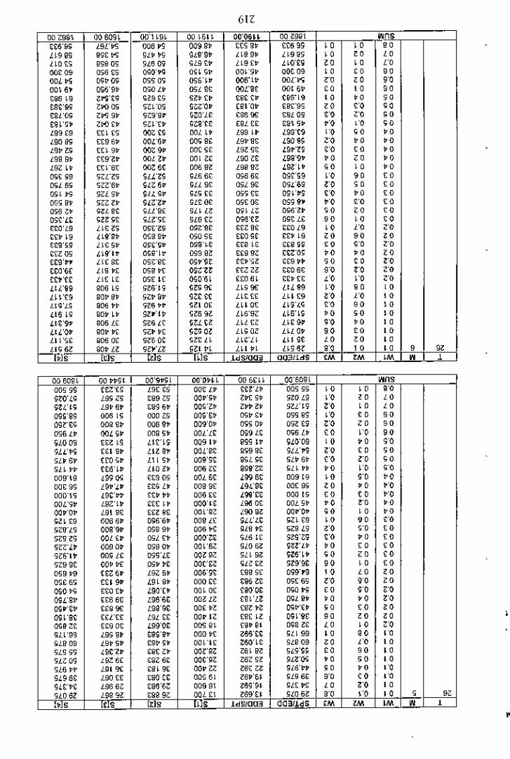
m00 "B91 00 609 ~ 00-\ ~B~ 00 ~61I oo.oon 00 <:9g\ ~ns~~6'9; LBl-P<; 006 P<; 009 g, ££S g, ££699 CO CO "'U999 R;£ P<; ;L, ~, gl.g'g, l ~Rg, L ~9g, CO " eol ~D£. g,S G, gm 09 .L9 £j> L~9£j> LW£9 " CO '"00£ 09 0<;6£, OgO'.; ma ';j> OO~-<;. ooc Og CO " ""OOLt>S 0;'0; 0,<; 0, 0~6'~. 006.~' OOl-P<; '" " "001 6~ 0\;6'9' 0.0 L. O,L g£ 00l"9£ OOt 6' " CO 00f:96 ~9 ~t>S'C; >19 £. <;Z.l:~ £ij£ £. tgG.19 CO '" ""£9n; oj>{)0, ,a-o, soo'o. (gl-O' £ij£-9S " '0 "89l'0; oP<;9. ,Z9-9. !i:0'l8 £g6 OC £ijL 0<; '0 '0 .,89 ~'!i. lo{) £. szn, !iZ9'tS £gL ££ .gl <;> '0 '0 .,L99 £9 [[ ~£, 00<;I':S DOL~. 199 I~ L99't9 '0 ., '"L9Qg; [[9 6. 00£-6. om; R£ L9.H£ '::90HS '0 '" '"L9. 0; l:n 9. 00<;9. 00£ ~£ 190 <;f: '::9r't!i '0 " '"L9H 9. [£9-~. OOL~~ 001 O. L90 ;;~ L99'9' '" " '"L9l ~. l:n-6, 00: 6t 006 9Z L9g m: '::9n. ., CO '"0.£ ;9 >ZH, ~La~ ;L6 ££ 0<;6£. 09£'S9 '0 "" "O.l S, ,,<:-6' ~a6. ;Ll 9£ O,L 9. 09L'69 '0 " "0, I j><; ,U,. ~'" g. ;L. £. 0" £. 091'.g " '" "or,. g. ''"0' ~a'z. ;L£ oe 0>£ Of: 099 S~ ., " "0,6 o. guSI': ~LL-9£ <;LIa 01'1 U. 0,,6'~~ " " 00o"nc ;~: ;£ .a-,£ <;L6ti: og6't: 0;£ L£ 0' " 008~0'L9 L 1£ ~, O<;c-l, ogz'se e~o R£ •• Ol9 " " ".1:. 19 .(~s'e, O~B9. 0<;0Sf: ££0 ~r 8r. ~9 00 0' "r~ng LI£<;> 0<;.-,. ognt erg If: •• g ~g 00 " '"<£00, lIS'I. O,g' I" 0<;9R~ •• 9 go C8~'og •• •• "££9' •• LI£g£ OSf:-gl: 09~'~C: e£.'~z <£9 .~ " " "C£0'6, Ll9.£ aSH .r Ogc'Z~ fel," •• 06£ "" " ,.~sne Lll: ~£ 0,£ 1£ O!iO'6~ ££O6~ ••• [£ ,.

",.

.::tn9 g06 ~<; '06' tg ~~; 9l: .(~<;OC HLg(!" "' ".(~n9 go. g. <;l.9. ~i:£ £t .(~£ £[ '(~1l:9 '0 " CO

Hg'L!i 90G •• 9l£ •• ~~I O£ L~IO[ H9'L~ '0 00 CO.::16~; go.~. 9Zo'l, ~oB 9<: L~6-9l H6.~~ •• " ".::,~'9' 90£ L£ ~l£ L£ ~UI:Z L~l l:i: LI£ 9. '0 •• CO.::tL '0' go•• £ ,l~ .1: ~:; O~ L~; Ol LIL O. " 00 COLlIW gOGO[ ,n 01': ~o£l~ L~UI H' 9t " " CO

...1:i'60 go.a ,,~.a ,ll .~ L~I.I [l96r •• CO CO " "jpJs [~Is '" ms _ld_S/C1C13 C1C1~lldS OM 'M 'M " ,00 6091 oo •• gt 00'9.;1 OO'D.U 006.11 00'6091 "eo00, 99 t8ng L9[ «; 00£ L. £~n, OOS" " " .,9Z0-,::g L9, l~ .89 <:<; 00.';, lOl: ,. 9Wl9 '0 " eo9zn; L9.6. .89 £~ OWO' l •• Z. 9Ut9 " " eo09.-sg 006 I~ 000 <:, ows, 0',. •• 0" g9 '0 " 0009n. OOgg~ 006 S. 009'0, 0<;>O. O,l £9 '0 " "00,6 L. OOL .~ 009 ~. OOL'L£ 0.9 LI: 0,£ L. " " ">,(009 £.z I~ un; 0091. 99~ t. 9LO'09 CO •• "9U,9 £.1 H~ L1l ~~ 001'8£ 9,9 g£ 9LL'~9 ,. " "SL~ 6. (SO •• l\ I" 00S'9£ 9.L ;£ ,L.6. ,. " ",l ~ •• t£6'~. LlO <:. 00£ o£ 9WO£ .L~ •• •• " "009-\9 '::99Q<; ££90<; OOL6£ L996~ 009 t9 CO " ••oa£ 9, .(9)' •• e£. Ll> OaR9£ L91.'9~ 00£ 9<; " " .,oaO-I, '::91':'•• ££••• 006 .1: L9n~ 000 " 00 " .,Oo.::-g. LgZ'~~ <£l: I. 000' II': LOOO£ 00,( ,. " " ••00.'0' L9\ R£ c,l g£ OO~'gl Loo 9l OO.'O~ " " ••;l~rg 0066. Og6'£. OaRL£ 9.n8 ;U £9 CO 00 ,.,lR-t, 008'9. 0,99. 00£ .£ glS .£ ,l~ £g '0 " "Sl5l9 OOL£. O<;L£. OOO':~ >,(£ L£ 90n9 '0 " 009li:'Lv 009 O~ 0,9 o. OO~'6l ,lO 6l 9Zl'H " 00 00nnv 00; 1£ 0,9',::£ OOZ9l ,L I 9l 9Z6'~. 00 " 00,Z99£ 00' .£ 0,. ~£ oon~ ,u.o 9Z9'9£ " " "0<;9.9 H:60 L9l B. 006'<;[ £9R <;[ 09n9 " " "O~£6, to 9. L9~9. 000 ££ ~96 o~ 0<;[£, '0 " "090 j><; £.0 l:. L90n OO~O£ £90'0£ 0.0 ~; 00 " '009.::'8' £.66£ L96'6~ 00<:Ll £91'[Z Ogl R. '" " ,.O~O'~' ££g OC L99'9~ 00£ '0 £9l.~ 0;0'£. 00 00 '"09 ~'91': ££H£ L9L ££ OO.ll £g£ Il 0; ~'se " '" "O~eZ£ £.9 O£ '::99'0~ 00;; g\ £~. ~I 0;8 Z. eo " '09L~'99 L9<;H~ S9n~ OGO.r l65U ;LI 99 CO 00 ,.•H09 L9. g. e9. ; • 001-" Z60'~£ <;Lg09 " " CO<;L<;<;g .9~'l. .gl: <:. OoO'gZ 061gZ ,Lg'9, 00 00 CO9U09 19Z 6£ .9l6. oon< 06Z ,Z 9a'Q<; '" 00 CO<;.(£., L919£ .gI9. OO.ol 06, <:l ;l6'~. 00 '"

,.9.96£ L90 l:£ .gO ~~ am; 61 06t'6t ;L9 ££ 0" " '09'::£"£ L966<: £S6'6: 0099\ l69'91 ;L£ M: eo ,. CO,LO 6Z L989<: .9g 9<: OOL£\ 069'0 ;LO £Z 0" ,. CO , "'[.JS ItlS '" " IdSJClCl3 aa3/ldS OM ~ 'M " , ,

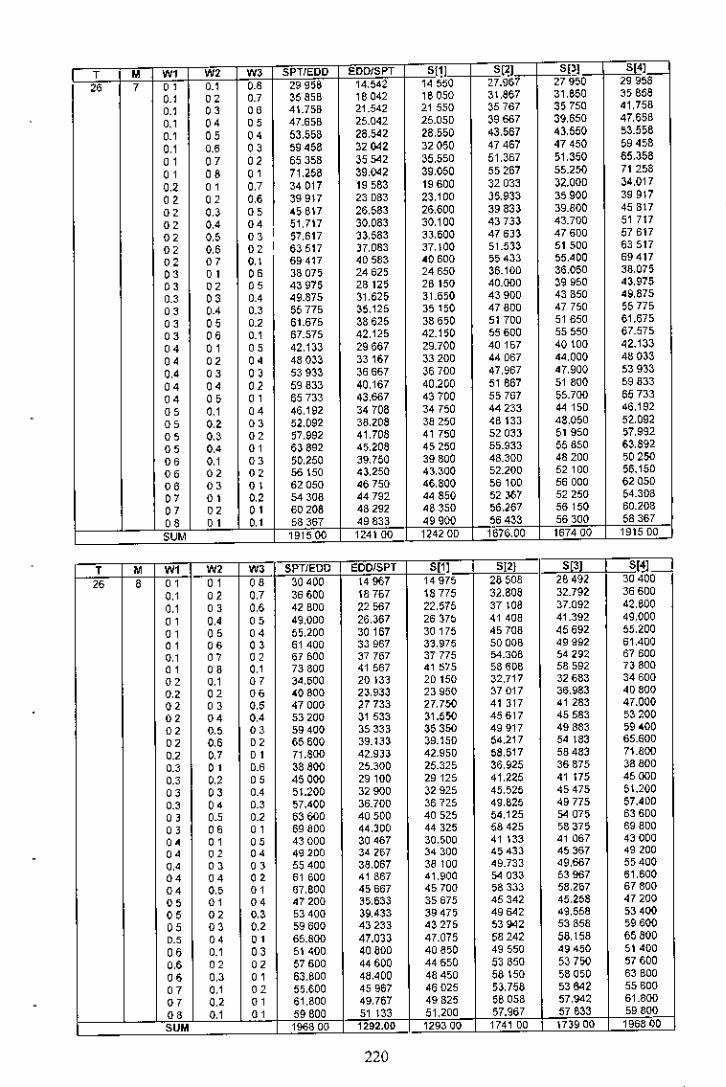
, " ., ., ., SPTIEDD EODISPT 5j11 s~J SP] 0<,

" , 0' ,, M 299,~ 14,542 14550 27.967 27950 29958,, " " ~5 8SB 16042 1e050 3\,857 31,650 ~, 658,, 0' " 4U5B 21.542 21 550 ~5767 3,750 41.758,, 0< " 47.65B 25.042 25.05D 39 &67 39,650 47,6SB,, " 0< 53,55~ 28,5<12 28.550 43,567 43.550 53.556,, '.0 " 59.58 321M2 32050 47467 47450 594580' " " 65 J5B 35542 35,550 51.067 51.350 05,358

0' " 0' 71.258 39,04, 39,050 5,267 55.25{) 71258

" 0' " 34017 19563 19600 3203~ 32.000 34,017

" "' M W917 23 DB3 23,100 35,933 35900 39917

"' " " .,e17 26,583 26,600 39833 39.800 45B\7

"' 0< 0< 51,717 30,083 30,100 43733 43.700 51 717

"' " ",

;7,617 J3,583 ~J,600 476)3 47600 57617

"' M "',

6:) 517 37,083 ~7,100 51.533 51500 63517

" " ,, 69417 4D 583 00 BOO ,,433 55,400 69417

" 0' 00 33 on 24625 24650 36.100 36,050 ~8,O];

" " " 43970 2312, 2B 150 40.000 ~9950 43,975

" " 0< 49.875 31,62, 31.650 43900 43 B50 49,875

" 0< " 55775 35,125 35150 47800 47750 55775

"' 0; " 51.675 38625 386,0 51700 51 £50 61.675

"' 00 ,, 67.575 42,125 42.1,0 55600 55550 67.575

"' " 0; 42,133 29667 29.700 40157 40 \00 42.133

"' "' "' 4B 033 33167 :)3200 44067 44,000 48033,.• "' " 53933 :)6667 36700 47,967 47,900 53933

"' "' " 598:):) 40,167 40,200 51 667 51 800 598:):)

"' 0; " 657:):) 43,0>(;7 43700 55767 ,5.700 65 7030; ,, O. 46,192 34708 34750 44233 4415D 46,1920, " 0' 52,092 38,20S 3S 250 ~B 13J 48,050 52,092

" " " 57,992 41.70S 41 750 52033 51950 ,7,992

" ,.• " 63892 4,,20S 45250 55.93:) 55850 6M92

00 ,, " ,0,250 39,750 39800 43.300 48200 ,0250

00 "' "' 56 \50 '3,25Q 43,300 52.200 52100 56.15000 "' " 52050 46750 46,800 56100 56000 62 G50

" " " 54 308 44792 44850 52367 52250 54.308

" " " 60203 48292 48 ~50 56,267 56150 60.20800 " ,, 58367 49833 49900 56433 56300 58367

'"" 191500 124100 12420D 1676,00 1674 00 191500

, " ., ., ., SPT/EDD EOD/SPT 5[1] , 512) SQI I 51'!] I

'" ; "' "' 0; 30400 \4967 14975 2S 508 26492 30400,, " " 36600 IS 707 18775 32,80S :)2.792 36600,, "' M 42 BOO 22567 22,575 37 \08 37.092 42,600

"' ,.• "' 49,000 26,367 26 37~ 41 40B 41.~92 49,000

"' 00 "' 5',200 30167 30175 457aB 45692 55,200

"' "' 0; 61400 3~ 967 3~,975 5000B 49992 61.400o , " " 6' BOO ~7 767 37775 54.30B 54.9< 67600

" 0; ,, 73800 41 567 .1 5,5 58606 58592 73800

" ,, " ~4,OOO 20131 2D 150 ,2,717 32683 34600

0' " "' '0800 23.93J 2:) 950 37017 :J6,98~ 40800

" " M 47000 n7~3 27.7W 41 J 17 41 28~ 47.000

"' "' "' 5:) 200 ~1 5~3 31.650 45617 45583 53200

"' 0' " 59400 35 ~33 36350 49917 49883 ,9000

" M " 66600 :)9.1.]3 39.150 54,217 54 \83 65.600

" " " 71.SOO 42.9)3 42.950 ~a,517 55483 71.800

" " ,.; 38800 25.300 25.325 36,925 36875 38 SOO

" " M 45000 29100 29125 41.225 41 175 4500D

" " "' 5\.200 :)2900 32925 45,525 45475 6\.200

" "' " 57.400 :)6.700 36725 49,~25 49775 57.4DO

" " " 63600 40500 40525 54,125 54 070 B~6DO

" 00 "' 69 BDO 44.300 44325 58425 08,75 69800

"' " " 4~ 000 30467 30,,00 41 1~3 41 067 4~ 000

"' " "' 4~200 34257 34300 4, 4~3 45 ~67 49200

0.' " "' 55 400 38,067 38 100 49.733 49,667 5,400

"' "' " 61 600 41 B67 41,900 54 033 5~ 967 61,600

"' M "' G7,eOO 45 667 45700 ,8 ~J3 58,207 6780000 "' "' 47200 J,,63~ 35675 45342 45,2~S 47200M " " 5J 400 39,4~3 3947, 49642 49,558 50 400

" " "' 59600 4:) 233 43275 53942 53358 ,9600

" "' " 65.800 47m3 47.075 58242 58,158 65 sao00 ,, 0; 51.00 40800 40 ~,O 49550 494,0 51400

M " " 57600 44600 44650 5,850 537>0 5760000 " "' 6~,eDO 4~,400 48450 58 \50 580,0 6~ BOO

" ,, " 55,600 45967 46025 ;3.75S 53642 55600

" " "' 61,BOO 49.767 49 B25 5e 058 57,942 61.8000; ,, "' 59600 51 \33 51,200 57.967 57633 59800

eo" 196800 1292.00 129300 174100 173900 1968 QO

220

, , ., m "' SPT/EDD EDDISPT S[l] " S[JJ ~" , " o , " 18517 16,092 16100 16842 17 625 185\7,., " " 23.517 16692 1B700 20142 21725 23 517

0.' " " 28517 21.292 21,:l00 23.442 25,52, 2B517,, " " ~~o17 23892 <,900 26742 29,925 3J 517

" " " 38517 26492 26 sao 30 042 34 D25 ~8 517,., '" " 43517 29.092 29.100 33342 38,125 43517

" " " 48.517 31.692 31 100 36642 42225 ~B517

" " ,, 53517 34 292 "'00 39~2 46325 ;3517

" " " 23033 20.583 20,600 21~B3 22,150 23O~J

" "' " 28O~J n 183 23200 24.683 26250 2B 033

" " " :)J 033 25783 25 BOO 27 963 30350 330.lJ

" " M 38033 26383 28400 31283 34450 36033

" " " 4:) 033 30 gal 31 000 34,63 38,550 43033

"' " " '8033 JJ 58J 33600 378B3 42,850 4B 033

"' " ,, 5J 033 35183 ~'OO 41.163 46750 5J O.lJ

" " '0 27550 ,o,07; 25100 25925 26675 27550

" "' " 32550 27,675 27700 ~9225 30775 32 550

" " M 37,050 3D 275 30300 32525 34675 37,550

" " " .2550 3287, 32,900 35825 38975 .2550

" " " '7,550 35475 35,500 39125 43075 .7550

" 00 "' 52550 lB 075 38100 42425 47175 52550

" "' " 32,067 29567 29,600 30.467 31200 32.067

"' "' "' 37067 32 167 32200 33767 35300 37067

"' "' "' .2067 34.767 34 800 37.067 39.400 .2067

"' "' " 47067 37367 37,400 40.367 43500 47067

" "' "' 5~,067 39967 '0,000 43.667 47600 52,067

"' "' "' :16583 34 05S 34 100 ,5008 35725 :1658,

"' "' "' 41 583 :16,658 :16700 ,8308 39 B~5 41.5a3

"' "' "' offi 5al 39,258 39300 4\.608 43925 46.583

" "' "' 51 583 '1.858 41 900 44.908 48025 51.58300 "' "' .1 100 36,550 38600 395>0 40250 41.100

" "' " '6100 41 150 41,200 42.850 44350 '6.10000 " "' 51 100 'J 750 03800 46.150 48 '50 ,1 100

" "' "' 45617 '3,042 43 lOa 44092 44 775 45617

"' "' "' 50,617 45642 45700 '7.392 48875 50517

" "' "' 50,133 47533 47500 .8633 49300 5013J

'" 1466 00 1175.00 117600 126500 135900 1'65 00

, , "' "' "' SPTIEDD EDDISPT " , , S(3] "" , "' "' "' 18,642 16 517 16525 17,167 17.950 18842

"' "' "' 24042 19.417 19425 20,667 ~2.2,0 24042

"' " "' 29242 22,317 22,325 24167 26550 29,242

"' "' " 34442 25217 25225 27667 30.a50 34 '42

"' "' "' 39642 28117 28125 31.l67 35.150 39642

"' "' "' 44 1142 :l1 017 3',0~5 ~4 667 39.• 50 44M2

"' "' 0.' 50,042 33917 33925 36,167 437,0 5" 042

"' "' ,, 55242 36,817 ,6525 .1 667 48050 55,.42

"' " "' 23 'B3 21133 21150 .1,S~J 22600 23.83

"' " ,., 2a 6BJ 24,0" 24060 25333 26.900 2M53

"' "' "' 33 aB3 26933 26950 2a B33 31 200 33863

" " " 39 OlD 29 S33 ~9 850 32333 35500 39063

" " " 44.283 32.733 32.7,0 35 B33 39800 44,.63

" " " 49 '83 36633 35650 39333 '4100 49 '63

"' "' ,, 54683 38,533 38550 42 B33 4B400 54,683

"' "' "' ~a.125 257,0 25775 26500 27250 28125

" " " J3 32, 28.650 28675 30,000 31 550 33325

"' "' "' 38525 3\.550 3\.575 33500 35,850 38525

" "' " 43725 :>4450 34.475 37000 40,150 43725

"' "' " 4B925 37.350 37.375 40500 4'.450 48.925

" 00 "' 54,1., 40250 40.275 44000 4a.750 114.125

" "' " 32.767 30.367 30.400 31,167 31 900 32.767

" " " 37967 " 267 33300 34667 36200 37.~67

" "' " 43,167 36.167 36200 3a,157 40,500 43.167

" " "' .3367 39067 39100 41667 4.800 48367

" " "' 53567 .'.967 42.00D 45167 49,100 53567

" "' " 37.406 :>4.983 35025 35,5" 36550 37.408

" "' " 42.60ll 37 aal 37.925 39333 40850 42.606

" " "' 47.808 407a3 '0825 42 B33 45150 '7.80e

"' "' "' ,3,008 43683 43725 46,333 49450 53 008

"' "' " '2,050 39600 J9650 40,,00 41 200 42.05000 "' " 47250 42,500 42550 44.000 45,500 47250,.• "' "' 52450 45.400 4,.450 47.500 49 BOO ,2,450

"',, " 46692 44217 4' 275 45.167 45850 46692

"' " ,, 51,692 47 117 47175 .8667 50150 51 892

"" "' "' 51.333 48633 48900 '9 BJ3 50500 ,1.333'0' 150,00 122600 1227,00 1304.00 139800 1505.00

'"

zzzOQTS<;~ 00"9<0' 00 ZSU 006'" no-SlH 00 <g~, ."[H~~ 006 <:<; ~t~"'

009 ~g ££v ~<; £~l't; " " "'~••.K OOL 0' l~Z"I. <;Z ~'Og L900<; (OW.; " '0 "<:.9H~ 000 SV L~.L" '0991' .g~'~. lliJ gl' '0 " "o~a5<; om; "" OOlM O,L gt aon. Og~~g " co ""0,<;6. DOnI' OO£'9V os" <;1' ooz ,I' 09S e. '" '" ""0,6 £1' ao~-£v DOH' O,L II' aon. 096'8. co '0 "0S,g ,~ aon. rS1'6. <;LI:Lr ~\;( LI' ~9g'!<g " >0 '"S9~'O; DOg-Lv £ge S~ giS'S" £I:S£. 9.l0g '" '0 '"999'" a06-Z~ m£ ~l' 9,('0. £t£ Or 9.91'1' '0 '" '0gsa 6£ ooz-gr £Bj>' 1£ 9Lg'9~ £[R 9£ 9>0 S[ >0 '0 '"L\I'; 99 OOI-;:~ L9 ~'g. 000 91" l%,V L%'9. '0 '0 '"L'16 0, OOP l~ L9l'," 005 ZV ,(9'-01>" L%'O. '0 '" '0t9\: ,I" Don. .91: O' 000"6, ,(969£ L9~g. '0 co '"L9L-6, 000 m: .9.'9£ ao"-,, L9. <;, ,9L"6~ " '" "L9t K 00\; ,~ Lg<; ~[ Q{lO'lt L96 ~( L91 t>i: '" " "~Ll.S 006 ~; 09~L. ~Z9VI>" D09'VI' sal, " "" '",l9'~, OOl £1' a,z £v sen. 001 ~~ gL9'~, '" '0 '",La 91' OQ~OV o,.-Gt ;09 Lf; 009''-£ ,LO 9~ '" " cos£. O. DOHL£ a, •• £ ,ZI ~S 001 ~f: ~L~'O. " " '0~L9'.£ 00 I S\; m;ni: ~Z9'0£ Dosm: gLg .£ " '0 ";Ll6Z 00. 8~ OS9-Ll nl'u 001 a .LlSZ '" co '0£86 Lg OO{\, n:1 s~ Og~£. ££~'S. £96 Lg co '" '"S9n. OOO-L. S£Z l~ 09l 6~ £[l 6~ ~g[ Zg '" "0 '0~9l 9. OO~~. (££ \l\: Og~'g~ [[l9~ ~gl 91' " '0 '"S8~'~I' 009-L£ (£1' 1'. og,a~ £I:L Z~ ~g~ II' '" '" '"~9,';~ 006-Zt (£. Q( OSlo" ~[G SZ ~g~ >£ '0 " '0~96 6" 00" 9~ ££99" O,L ." ££L'9~ [W6" '0 " '"~9t'." OO,-tl (£lU o,n" [("a tHOl " co '"~69 ~. oong L115. ,1911' "WI. l69-g9 '0 '0 cozeo c. ooe 9~ LIZ I' <;L.-g, 19C'9£ l60-~9 " '0 "l6Ht 001 ,~ ll~ .::~ SH-I'\: "De t~ ?snl' '" '" "lSnl' 001'Lf: £W~~ SH:'I£ L9£ II: WS'l1' '" ;0 "ltc 9~ DOL<:. L~, 6G gLS'Ll L9SLl lOGg[ '" '" co,69 at 000 go L~9<;l H£'I'Z L9. I'Z Z69O£ '0 '" co~OO';C OO~~o LILIG ,LS 0<: .990Z Z60g, '0 '" '0<:61'61 OOHI LI~D 5£UI .9~1~ e6H~ '0 '0 co , "Il'ls li:ls " Ills l~SIOO3 oaalldS ,. ,. ,. • ,001'1',1 OO'L£I'~ 00 £tH 00 Hal OO"Hn OO'O~;I ."££9'1-; Oong [£0 I; OOlO. ££~'0; .~n; co '0 '"L91£~ S,~ 1<; ,.G-6~ OSH. Z6SR. £91 f, '0 '" '0£9i L. gn 91' ,~Z 9_ 0<;1'5. l61: ,. L9n. " co '"009'(; Og~"lg m;g H~ 00~ LV 090'LV OO~£9 " " '"OOt'S. OS9-91' 0.1 S. 006'81' OSgS' 001'g. 0' " '"ooon 05~ l. 0<;1'I. OOL01' 099 O. 000 •• " " '0£~~'•• 9Lg 0, g<;LL. a's <;I' 90>'gl' £I:~ ~9 " '" '"£~a 61' ,.~ 9. g<;o~. 0.£ G' 90£'GI' £1:06' '" " "8[9.t .£g I~ gg~'OI' OSI6~ 90~ 61: ~t9 81' '0 '" '"",~~ S£8 L8 Sg998 09£'g~ gOG<;1: ~f<:gl: '" " '"Loo'g" 009 o~ L9991' 000-1'1' L96 ~~ L90 <;g '0 '" '"19,961' 001'9' L96lt OOB01' ,9£ 01' L99-6~ '0 '" '019~ 1'1' oon. L9<:o~ 009 Li: ,9.-L[ /9: 1'1' co " "19~ 91: 00~',8 LlI5~~ oo,~ ,98 M: 19~ 9, " '" "i9.-££ 009 <:£ L9S II: OOG~, L9n, L9. ~t '" co "OOl'<;S 9:£'0. ~L, 91' O,.l~ ~ZI' l~ OOl'<;" '0 '" '"00£-0, ~l9'<;. <;Ln~ OgG6C ~ZZ6f OO~as '" '" '"006 1'1' .l( ~I' >L~-9[ 0909, ~00'9( 006' •• '" '0 '"0096f: 92S 9~ gL."M: o,n8 'Gg ,£ 00<;6[; '0 '" '"DOl'.£ <;,,'o~ SLl O~ 0<;96<: gG96<: 001 P. '0 '" "oonG SZ~-a SLOa 0<;1'9Z 'GI' 9Z OOlHZ '" co "8£1:99 OSO-Og ml' I'~ 00601' £9901' ~~~'9. " " ".1:60; OS,-g. (gL Ot OOLL8 ~99£~ ~~6 O. " '" "~~, <;I' OSO'I. .80.S OOS.1: ~gp t£ ~£. ';V " '" '"~t ~01' O~g9( .9n~ OOCI~ [~<:I~ £H Ot '" " "[[Dr 0,0 Z< £996G ao~ Sl ~gO'g;: ,tn~ '" '" "[f.-6l 0,<; a £96,G OOlrl'l ~RgI'l ~t8 6l '" '0 '"[£6-~~ 0<;0fc £9l <:Z oonl £H9-ll ~tB £l co '0 '"H69. ,US. G6f £. as.-6~ l~.-6t L9S-9, co '" coL9n~ ~ln. G696~ O,~ 9t Z~~-9C L9ng '" '" "L91'9. <;LLO. G6S9~ 0,6-" G'S-l£ L9~ 91' '" '0 "L9l'0. 9Lt'9£ l6G l£ 0,£6~ <.£6~ L9£ OP " '0 "L9£5. .LLI[ 2Sg-9Z 09.9Z 0.99<: .9£ .;; '0 '" co£966Z ga'Ll lSB I'~ 09nz e.no L96'6~ '" '" co£99"2 gLa2 ZSIV 091'00 <1'1'02 L99 .~ '" " co

~~~ 61 .L<-91 lSI' LI 0<;691 ZI'691 £91 6~ '0 co co , aIpls I£ls lils [lIs ldSl003 003/ldS ,. ,. ,. • ,

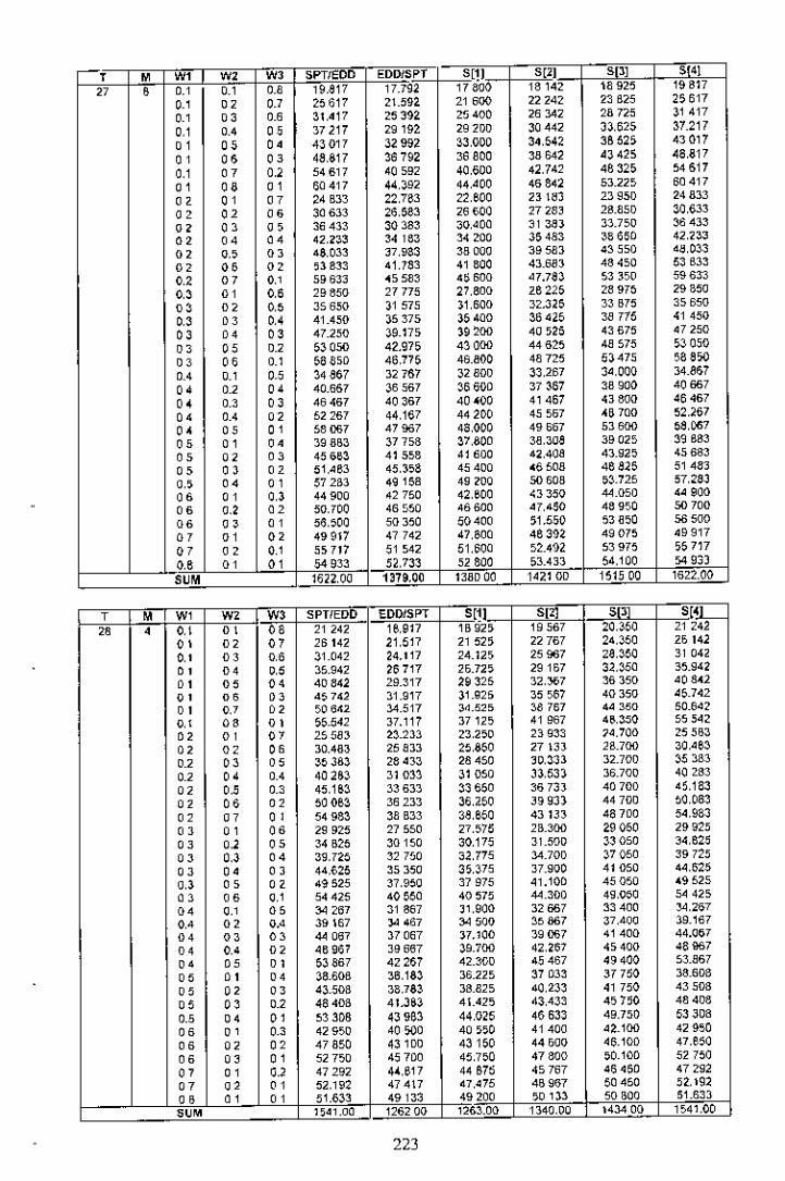
, " w, w, W, SPTIEOD EDDISPT 6[11 S[.) '" '"" ; ,., ,., " 19,817 17.792 17 800 18142 18925 19817,, " " 25617 2l.59l 21 600 22242 23 B25 25617,, " ,.; 31,417 25392 25400 26 342 28725 31417,, 0< " 37217 29192 29200 30442 33,625 37.217

" " 0< 43017 32992 ~3,OOO 34,542 3B 525 43017

" " " 4a,817 36792 36800 ~8642 43425 48,817,, " " 54617 40592 40,600 42,742 46325 54617

" " " 60417 44,392 44,400 46842 53.225 60417

" " "' 24 BJ3 22,783 22,800 2l1~J 23950 24833

" " " 30 633 26,583 26600 272BJ 28.850 ~O,633

" " " 36433 30383 00,400 313~J 33.750 36433

" 0< 0< 42,~33 34 183 34200 35483 386,0 42,0'3,

" " " 48,033 ~7,983 38000 39583 43550 4~,O:)3

" 0; " ,3833 41.783 41 800 43.683 48450 53 B33

" "' ,, 59633 455B3 ., SOG 47.783 53350 59533

" " 0; 29850 27775 27,800 26225 2B 975 29850

" " " 35650 31 575 31.600 32.3,5 33 B75 3565G

" " " 41.450 35375 35400 36425 38775 41 450

" 0< " 47.250 39.175 39200 40,25 43 £75 47250

" " " 53050 42.975 43000 44625 48575 53050

" 0; ,, 5885D 46,775 48.MO 48725 53475 58 a50

" ,., " 34 a67 32767 32800 33,287 34,000 34.867

" " " 40.667 36567 36600 37367 38900 40667

" " 0; 46467 40367 40 '00 41467 43 800 46467

" " 0; 52267 44,167 44200 45557 .~ 700 52,267

" 0; " 58007 47967 48,000 49667 5J 600 5S,007

" "' " 398B3 37758 37,SOO 38,30S 39025 39 B83

" " " 45663 41558 41600 4.AOS 43.925 45683

" " "' 51,4B3 45,358 45400 '6508 46 S26 51 48,

" " " 572B3 49158 49 ~OO 50 608 53.725 57,2SJ0; " " 44900 42750 42,600 43350 44.050 449000; " " 50.700 46550 46£00 '7,450 48950 50 7000; "' "' 56,500 50350 50400 51.550 53850 5-6500

"' " " 49917 47742 47,800 .6392 49075 49917

"' "' o , 5,717 51 542 51,600 52.492 53975 ,5717,. "' "' 54 933 51,733 52800 ,3.433 54,100 54 933-SUM 1612.00 1379.00 138D00 14210D 151500 1622.00

, " W, w, W, SPTlEDD EDDISPT S[!l '" " ~E1h-" , ,, " " 21 242 18,917 lB92, 19567 20,350 21 242

"' "' 0; 26142 21.517 21 525 22767 24.050 Z,142,, "' "' 31.042 24.117 24.12, 25967 2S,350 31 04,

" " " 35.942 l6717 2'.725 29157 32,350 35.942

" " " 40842 29.317 29325 32,367 36350 408.2

" "' " 45742 31.917 31.925 35567 40350 45.742

" 0' " 5064< 34.517 3'.525 38767 44350 50.6.2o , oe "' 55.542 37.117 37125 41 967 45,3,0 55542

" "' " 25583 2~.2J~ 23,250 23933 ,4,700 25563

" " " 30.483 25 S33 25,S50 27133 28.700 30,48~

" " " 35 3S~ 28 '33 28450 ~0,~3l 32.700 ~5 3B3

0.' " " 40 26~ ~1033 31 050 33.533 36.700 40283

" " '0 45,163 ~3 633 ~3 650 ~6 733 40700 45,183

" "' " 50083 36233 36,;(50 ,]9933 44700 50,083

"' " " 54983 38 B33 3S,850 .3 1,]3 48700 5',983

"' " "' 29925 27550 27,,75 2B.3oo 29050 29925

" " "' 34 B25 30150 30,175 31.500 ~3 050 3',625

" " " 39.725 32750 :32,775 34.700 ~7 050 ~9 725

" " " 44,625 35350 3,,~75 37.900 41050 44,620

" "' " 49525 37,950 37975 41.100 45050 '9525

" "' ,, 54425 40550 40575 44.300 49,050 54 425

" ,, 00 34 267 31 867 )1,900 32667 33400 34,267

" " " 39167 34 467 34 500 35007 37,400 39.167

" "' " 44 067 37067 J7.100 39007 41400 44.067

" " " 48967 39667 39.700 42,267 45400 48967

" " " 53867 42267 42.300 45467 49400 53.867

" " " 38.60B 36,lS~ 36.225 37033 ,]7750 38.608

" " " 43.508 38,7S~ 38.825 40,233 41 750 43508

" " " 4840B 41.363 41"Z5 43.433 .,750 48.08

" " "' 53306 43963 44,015 46633 49.750 53308

" " " 42950 40 5-IJO 40,50 41400 4l.100 42950

" " " 47850 431DO 43150 4' 500 46.100 47,85000 " " 52750 45700 45,750 47800 50.100 527500; " 0' 47292 44,B17 44 B76 45767 '6450 47292

" "' " 52,192 47417 47,'75 4B 967 50450 52,192oe " "' 51,633 49133 49200 ,013~ 50300 51.633

'"" 15'1.00 126200 126~.00 1340,00 1434 00 1541,00

223

mOO'6~9~ QO"I~~ 0091~1 0099~~ OO'~9t~ 006\91 ""££0 •• ()Qn, £~9'". Olm I\; tU"19 U:O'.., '" '" COlve 1'<; 000 ,~ Lin. ~Zl'OS L%09 ~.n,., '" co '"ltHv 009'9. LiG-Lv ~i:n~ LRI-Lv "~H~ '0 '" '"09.'9~ 009'Z9 005 A, O~O'6. 000 61' 0<;1'99 '0 co "0(m-o~ DO!' ~. 006 91>" 099 ~. 009-S~ 09\ 0; co co com;g v. 000'1' aot ~. 099 <:l' 009 c' 09S'". co '" co~919; 00919 t90"6. <;L9Ll' S~g',. B, I 9<; '" '0 '0egg 0<; 00<:91' teg ". ,Lv., £~•.•• 9<;90<; co co cog,g 9' 009'£1> £g~l. 9<~ I' ££l II' 9" ~l' co co '0B9~'O. 00.6£ t~9gr 9iG g£ £[0 S. 9gl'O. '" ,0 coL999<; O'Wlg LW~. 00,91' .9~9' t9999 '" co '0L99 I~ OOO'Sl' iR9 v~ 00 I'£V L90 £1' i99 19 '0 '" '"L9l91' 009 ~v L9Z I~ 006'6~ 199'B£ t9Z 91' co co '"L9601' 00i: 6~ iR9 L. DOL 9~ 199'9£ tOO 01' '" co '"[99~£ OO~-j>1: L90 tc 009U L9l' ££ L9'9 ~~ co '" '",LS LC; OOi:'~9 0" Ll' 9l6.t 006',1> <;15L, '" '" co.1, Z. OOgLv 0<;9'(. ,U It oon. .1, 0" '0 co co916 gj> 00. [t Og~'o. 9l. ~£ OM9~ 9,691> '0 '" co9<9' It, 000 6, 0~9'9C ;l[ ;£ 00£ ';[ 9.(9"1v '0 " ";.«( 9£ oo,~ O~OTS ;l~Z£ OO~ZI: 9.«( 9~ " " "".(0 ~[ OOZO( OW6Z ""69Z 006'S~ "'(O"l[ " " "£~Z 9, OOO'Z~ f:£vBI' 095 CV ~(~'£v [gZ gg " " "1:960g 009 .(V .,g ZI' O~('O. £££ OV l:~6 Zg " " co£99 Lv 00;:;(. t£~'6f: 0, ~LI: ~(~'L~ £B9 Lv C, " "£~~ 01> OOg9( e.9 S. 096'££ ££6<£ \;~~ ;:;1> " " co£gOL£ 00'" ,CO'zt O"LO£ 1:,10. ~~O'L£ " " ",gL ~~ 0000£ n:. ~Z own: ££, n: I:~I.~. " " "~~.'g" 009"<;l ~.8",," 0<;('." ££1:I'Z ~91>'go " '" "~66 B; aong LW~. ;L ~Z. L9 ~<:~ "66 B<; " '0 "Z69 f:, oon" L~S~" <;l6 g. 19S'B£ "69 «; " " '"Z6('BI' OOOU LlZ'SC ;li. ;\: L9L ';[ ZGt g~ '0 " ""60 \:. 009 9~ H9v£ <;L90£ Ls!; Z\: zeo C~ " " '"061. L£ aon'~ LW~£ <;L£6Z Lst'6" "61 L\: " " '"Z6v'i:£ oo~ 62 H.LG 9<~9" L9~ 9Z ~6. o\: " " ""6llZ 001' 9Z H9[Z ,L6'i:Z t96 ZO ze~'n: " " "f----l~;g lZ 000 ~l H"OZ <;li. 6\ L9/61 "6R ~Z '0 " " , "',,, " [zls ,,, Lds/aa3 003/ldS 'M ~ 'M " ,OO'0~9\ 00 UV~ OO"6.(£< OO.l£1 oonn OOOg;\ ""££9'Z; OOlng (££'l, oos0, ~~U'O; £[9 i:<; " " "0L9v.<; g,n9 ZI'" 0<; 0,6 SI' ~69 g. L9v.9 '0 co '"19[ HI' 9znv ol'g 9~ 090'91' l66 <;j> L9nl' co " "oo~.g o~n. O<;~6~ OO.'L> OgE"LV OOl'.; '" " '0000'6. O"Z'LV O,L 9. OO~'joj> O<;Vl'l' 000'61' co " '0006't. O.O"£V o~n. 009 l. 099'~~ 006 f:l' co '0 "e.L .g ,Ll"'" g,O S. O.S ,. g09 ~I' ~~11'; '" " "• £961' 9L6'9. 9<;9v~ 096'<:1' ga6 Z• £~9'61' " " '0.£" 1>1' 9Ln. g," ~I' 090'01' 80001' £~nl' co co '0£€v'6£ ,L,"9~ ~g9'L\: 0<;~ l£ 90l'L€ \:[v 6. '0 '" "19~ ~g 006"0. L96'9~ OO[j>j> LgZ'I'~ L91:" " " "L9l0; oonv L9, ~I' OOVl. L91: ~I' L9~ 0; co '0 '"L9 ~<;j> oon. L9 ~01' 009'S~ L9t>g\: L9 l ',1' " " "LOO0. OO€9t 19L 9. 0099€ L9> <;[ LOO0. '" co '"L96 .£ oo~ '0( L9£ n: 001.'i':€ L99 Z\: <;)G'.\: co " "0009, ~o9 o~ ,L9 SI' 09l'l. gUlP 0009; " " co006'0; 501' 9~ gL.'Z. O,S 61: g~9'6£ 0060<; '0 co "ooe ;v soz lu ;LO'6\: 096 9~ ;Z69£ 009 g~ co " "oaL OV SWgt ;L9,£ 090 ~~ "WI'\: OO{O~ '" " "009 <;[ ~(;9'~( <;a <:. 09l'l£ <;u ~. 009 ;£ " co "00>"0£ Si:96<: ,L9 gZ 09,'S" "U9Z oo~ O£ " '0 "~~9 g. O,\: a. £91'.1' OO<:~V ~9l ~. ~~9'99 '" " "~~S'l9 0,19t> C9nl' oar 9~ €ij, g£ ~~ng co " '0£[1> 9v 0>6 l~ .96 L£ oav <;£ £gt'9€ £[1>9. '0 co co~I:nv O>L'lt £g" •• OO~o€ [HI>o~ ~I:£ l. " " co€I:o 9[ o~gn £g~~. 0096<: [gS 6Z ~I:o 6£ " " co£~l'l~ O,\: 6<: £gt a oaL 90 ~g9 9l ~~l'~~ " " co[~O 9Z o,~ ,<: £90" OaR.0 ~ijL £" £~o 9~ " " "L9n9 "La as <:69'£1' 0,96£ ~U96£ L9n9 " "0 "L9~"Z9 HS.~ 06~'01' O"L B[ oul.'9~ L9~ Zg " " "L,KrLv H9'lu Z6~ 9£ O.R ££ ZI>R'£€ LooL> " '" "L9il'! I> H.L£ i:61>U 0>6 O£ ~ue'o~ Loo ~. " " "L9g g~ ~Ll ££ Z60'O~ 0,0 go ~uon L9~ 9~ " " "19n~ SLa 6<: (;69'9l 09 ~ '0 lv~ <;l .(9[' ~£ " " "<99 gl ,Lg ui: l6, £l O~l'"l "I>i:ZZ t99 9l " co "L99'li: ,L90;; "6S6~ 0<;£6l "~~"6l 19, ~l " " " , "" ,,, Ills " IdSIOO3 003/ldS 'M 'M 'M " ,

, M W, W, W, SPTIEOO EODISPT '" " " 'I'" , ,, 01 '" 22217 20,192 20200 20542 21 325 22217

01 " "' 27,717 23.692 23700 24342 25925 27.717

01 " 0; 33217 27,192 27200 2a 142 3D52, 33217

01 0< "' 3a717 ~O692 30,700 31 942 3512, ~8717,, 0; " 44217 34192 3' lOa ~,,742 39.7<, 4421701 " " 49,717 37692 37700 39542 44.325 49717

01 " "' M 2\7 41,192 41 200 43342 48.925 55,217

01 '" 01 607\7 ",692 44.700 4714. 53.525 60717

" 01 0' 26933 2~883 24,900 25,:83 260,0 26933

0' " 0.' 32433 28383 28.400 29,083 30650 32433

" " " 37933 31 883 31.900 32.883 35250 37933

0' 0< 0< 4343~ 35383 35.400 36683 39850 43433

"' 00 "' ~~ 933 )5,883 ~a900 40.483 44450 ~89~3

"' 00 "' 54,433 42383 42400 44.283 49,050 54,433

"' ., 01 59,933 45 SSJ 45900 48 aB3 53,650 59933

" 01 00 31 650 29575 29 sao ~o025 30,775 31 650

" "' 00 37.150 JJ 075 33.100 33,825 35375 37.150

" " 0< 42650 J6 57, " .00 ~7,625 39975 42.650

"' M " 46150 40 07, 40.100 41,425 44,575 48.150

" 0; " 5~ 650 4357, 43.600 45225 49,175 53.6500; " 0.' 59.150 47.075 47.100 49025 53 775 59,150

" ,, " 36.367 ~4.267 34.300 34767 35500 ~6,3G7

" " " 4\.867 ~7.767 37800 3B 567 4010G 41.867,., " " 4n67 4\.267 4'-300 42367 44700 47.367

" " " 52,~67 44767 44800 46,167 49300 52867

" " " 68,367 48267 48 ~oo 49967 53,900 58367

" " " 41,083 38.906 39000 39508 40225 41033

" " "' 46,563 42456 42500 43,308 44 825 46533

"' " " 52,063 45958 46,000 47,108 49.425 520S3

" " " 57 56~ 49458 49,500 5090a >4.025 57,58300 " " 45 BDO 43,650 43700 44250 44.950 45600

0.' " " 51,300 47,150 47200 '6050 49550 51 300

" 0' " 56,600 50650 50700 51 850 54150 56800

" o , " 50,617 4a 342 .a 400 46,992 49675 50,517

"' 0' " 56,017 51 642 51 900 52.792 54275 56 017

" " " '55233 53,033 53100 ,~.73~ 54400 55233

'"' 165~ 00 1415.00 ,.1600 145700 155100 16,6-00

, M W, W, W, SPTIEOD EDDISPT " S[~ S[J] "" , " o , oe 22,542 20617 20625 20867 21650 22,542

" 0' " 28,242 24417 24425 24867 26450 28242

" "' ,. ~3 942 n217 26,225 28867 31 250 3394,., " " 39642 32017 32025 32,007 36050 39642

" " oe 45,342 35817 3582, ~6,~67 40850 45.3'2

" M " 51 042 39617 39625 40867 45650 51.0~~., " •. < '0.7<2 40417 43.'2, 44367 50 450 56.742., '" " 62.4~2 47.217 47.225 48,867 55250 62 <42

" " ., 27.3a~ 2'5433 25450 25,733 26500 27,3~3

" ., M ~3.aa3 29,233 29250 29,733 3UOO ~3 083

" " " 387a3 ~~ 033 330,0 33733 36,100 38733., " " 44 48~ 36 a33 ~6 850 3773J 40.900 44,463

" " " ,0.18~ 40 ~33 40650 41.73J 45.700 50,16~,., " ,., 55 a~3 44 '~3 444,0 45733 ,0.000 55833., ,., ,., 61,5~~ 48233 4$ 250 49 73~ ;;.300 61,56~

" ,., M ~2 225 30,2,0 ~o 275 30,;00 31.350 ~2 225

" " " 37,925 ~4 050 34,075 34600 3;.150 37925

" " " 43625 37850 ~7 675 38,600 40.950 4J 625

" ,., " 49325 41650 41675 42,600 45.750 49,~25

" " ., 55 0~5 45450 45475 46,600 50.550 55,025

" ,.• " 60,725 49250 49 ~75 50600 55350 60,725

" ,, " 37067 35067 35,100 35.467 36,200 37067

" ., " 42767 38,867 38900 39.467 41,000 42767

" "' 0' 48467 42,667 42700 4:) 467 45800 4B467

0' " " 54 \67 '6,467 46500 47.467 50,600 >4.167

" "' o , 59867 >0,267 50 300 51.467 55400 59867

" " " 41 90a 39833 39,92, 40333 41.050 41 90~

" " "' 47,008 436B3 .~ 725 44333 45850 47,GO~

" " " 53308 47.483 47,52, 48333 50,GoG 53.30~., "' " 59008 5ua3 ;1.325 52,~~3 55450 ,s 008M " " 46.750 44.700 44 700 45200 '5900 46750M ,., 0.' ,2450 48500 48550 49,~00 50.700 '52,45000 " ,, 58150 52,300 52350 '5,200 55500 58150

" " " 51 592 49517 49,575 50067 50,750 51 592

" " " 57,,92 533\7 '53,~75 >4.067 55550 ,7.292

"',, " 56,433 5433:J 54400 54,93~ 55600 ,6 '3~

OCM 169700 1.66.00 146700 1496,00 159000 1697 00

225

9"00 ;~m 00 SKI 00 ~<;v~ 00-~o.~ oo-oo.~ 00S~9~ """[a: 1', 009~9 ~t~';:g 00\ <; .£0,,, .££ ~g '9 " eoc~O-gg oong lWI. ,ZL G5 L990, <:1'09; '9 " "<~o-a~ ooc 61' L~g9. ;c9,~ 19L Lv <:.00; '9 '9 "OS! >; 00 ~ <> Oog-Qg 09~'6' OO~'6. O<;L ,<; " " 99O~<'O~ oao's. aO;-Lp 0,1>"91' OOt9~ 0;,( 0; " " '"O;L g~ 006'.1' oon'l' D<;gcl' 009U a.g. " " '"g<;t% 006'0. £9L 61' <;L6 LV .1:6 ,~ ~gv9; " •• '"~gn> OOR'gj> [gl' 9l' ,La ,1' £~o;. g.ng " " ••~gj>'9. OOL1'1>" [gl [~ <;L~ <;. ~~,',.ggj>9. " " 99g,. ~~ 0090t ~~s6t gLl 6£ ££;: B. 9<;1",I' " " ••[9\ LS 001;~g 19L'9. 0099. L9S 91' £9,'£; ,. •• .9'91 '~; 009 g•. L91"g•. 00,( r> L99n 191 'Z<; " •• ••L91 L~ 00, •• £9' 'Z. OOSOl' L9L 01' £9'1;" " " ••• 9\ '~. 00.'0. 199 g[ 006 Lf: £99,8 L91'<:. •• " ••L91'if: 00£ 9£ L9,-gr 000 >8 196'0£ 191 L£ 99 " "5[9 L, 00<; ;:9 0,':'.(. ;""~.00l5. "L~ L<; " 9. '9<;Lg z<; oo~ 91" 0;",,'. ;"£ z. DO, <:1' <;L~ ," " •• ".L9 L~ 00, vt o;n. ;;:1>'6S 001>6S ,Lg LV 99 '" "~ml~ 00, 01> OSS.Lt go,'9S 00<;9S ,L9ol> 99 '" 99~Lg 1£ 00~9£ a~n'l: ;1:9't€ 009 £€ ,L9 if: 99 99 ,9HS'lt 000 oS o~n, ,UO~ OOl'O€ gL9 IT 99 " "tS9'~~ 001: 0' ,£L"91> O;g'n €Sg'tl> Sg, R, co " 99£8, tS 00t'S1> ~t. ~I> m;6 O~ .[6 O~ ssng '9 '" 99rg, 91> 00 ~ ~I> SH O. OgOg£ f:£0 m: S99'SO '9 99 99£g, co 000'0, £~g 9~ o~a .£ ££1 •• ~sno '9 99 99£g, et 006',S ~£>££ 0<;;:<:£ tsnt Sg, e£ " " 99,gg-" 009 ~£ £1:<:O. MC6Z te~u £g; i:r 99 99 99,g<;-ij~ OOL'a ~S6 90 0,1> 9, tsl>'9~ m,g;: 99 co 99~o;:G, DOl co LllOO ~Ln. L91>ll> <:6;: GS " 99 ,.Ui;:K 000 HI> L~t;:1> Hg6t L9; 6£ e6;:K " 99 "ZB;: 6t 006 £1> "'~6~ ~l9 9£ L999£ <:6(:6' '" 0" co,6;: j>j>- OWSS L~9g~ ~Ll,£ L9L ,t ,61: 1>. 99 99 co'D;: 61: OOL~S L~~o~ ~mo£ L99 at ni':'6t 99 99 co,6;:-1>£ 009 ~. L ,('6i': H6-a L9sa ,61:'j>£ 99 " "l61:'6i': 00' Lo Ll6 <;0 g[Q gl .(90,l l6;:-6l " " "l6i: I>l OOHi': Lin;: SHOll .(9'-<:l <6nl " ,. ,. 9 "[tIs '" "" [~ls IdSfOO3 aa31J.dS '" '" '" "

,oa919~ 00-60~, W~'"\ ooo;u OO'6tH OO'9'9~ ""'[U S9 OO~," <£9 ~" aM09 ~UO; ,U £, " ,. '"Lgn~ ";:O-l~ ;:1><;0<; 091"6r ~6 ~ SI> ,(9,( ., " ,. "£9G'~. ,U 9. 01>1>LI> 0999' l6~ 91> ,(96 91> 99 '" "001>~; o,ng 09r'G' OOLLI> OS9 LI> 00' .g '" " "00961> 0,9.(> ognl> 00 ~ ,I> ago <;1> 009'61> " 99 "OO~~I> Og6 ~. O,l fj> OO~;:1> 09' ;:. OOg1>1> <9 ,, "s~ng "Ln~ g<;[ gl> 09,'91> 90 ~ 91> ,1:0 ';g ,. ," 99~~l'D; SLnt g,;: s. O,~'~I> eo, ~I> 1:,,09 '" " 99£SI>,1> 9'(9Tt ~gJ '~. 0;601> g0601> ~~.';I> <9 99 99<£901> sa-6t S;O 6. 0" gl: gOt ~£ ~£901> " co 9.L99~, OQi:-\g [9<:l' DOg~I> L9g 1>1> L9g';. " 99 '9L99'Og OOUI> L91 t~ 000'<:1> L96 ~I> Lge09 ,. " ••L90'9~ 00. ~I> L90 ~~ 00.'6£ L91:6£ L909~ " " "L9l ~~ oas 6t <96'l( 0099. L9l'9S L9< ~~ " " .9[9j>'9S 009" ,(99 t>t oons L9~~. L9v'9S 99 co .,DO, 9<; 9lS'O, ~llg. 090'£. ,"0 £1> 00£ 9; '9 '" 99OOg~<; g~O'.(1) ,La ,t 0,1>O~ g;:I>'O. OOS~<; '9 99 9900.(9' ,U ~I> <;L6-6£ 0;9'L£ ,09 L. 00<'9' " " 99006'~. ;iT6, 9.9 OC Ogl,e "u~. 006'~. •• " '900 ~ LI: 9<:.-g, HH£ 0;9 ". nne OO~L£ 99 '9 '900, ;:£ glo"l£ ~L9O£ OgO'O£ ;000£ OO~'~C 99 co <9S~6'9g 0.90<; ,gO 9' om; ~I> .SI> ~I> £~6 9g co '" '9S~~'~g OSL91> t~6'~. 006 R£ .ge SS £~I" 99 '9 '9eS, Lt> a9~ ;:t ~Rg 9[ 00£ 9. Sg~ 9. <£, .(~ ,9 99 99e~; ;:1> OSS9~ tag£ DOLr~ SS9W <£g l~ •• .9 99S€l'.(S OSO<;[ tS9'i':£ 00\ ~f: S90'~( ££L .(£ 9. '9 99C€6';:~ O.~I£ tSg-6l 00; m: ~gt'S;: .£6 a: "' '" 99tn'gi': 0";: Ll £SI>9< 006 ~;: .ge go S£l H;: '" " '"L9<;L, 9.(£'09 ,6S-,1> 0~6'SS ;:1>66£ L9n~ co "' '"L9l ;:, ,.(~ 91> <6g 00 D';[ .(~ <:.~If: L9L ;:S ,. '" "L96'[. .1~ 01> lEUt OgL t. <:I>L"S 1961. " '9 coL9 ~£1> 919 B~ l69-1>£ Qg\ ',c ;:1>1,£ L91 '~~ " 99 ,.L9, gS gli.'.~ l6nr 099'6~ ;:1>,61: L9~9£ 99 " '"19S c£ 9lS O~ lBI>9Z 096'9;: ;:1>691: £9nt "' <9 '"L9L 90 ,.(6 9~ <:SS.G 09~'.;: ;:1>,ti: .9L'9;: '" 99 coL%~o 9W ~<: ;:sou 09n;: ;:I>L~" '::96W ., " " • e,, ,,, 99 ,,, "" ~~IdSloa3 am/IdS '" '" '" " ,

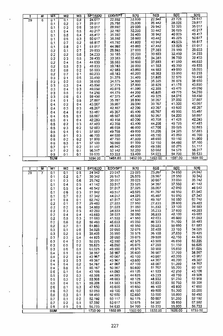
, " w, m w, SPTIEDD EDDJSPT " S[~l " "" 0 o , ,., 0.' 24.017 22.592 22.600 n942 23725 24617,, 0.' " 29 a17 25,792 25.Boo 26442 28,025 29.8170.' " '" 35017 28.992 29000 29942 32325 35 017,, "' ,., 40217 32.192 ~2.200 33442 36625 40217

0.' " "' 45,417 35392 ~o400 36942 40925 45417

" " ,., 50617 38.592 ~8 600 40.442 45225 50,617,., " " 55817 41.792 4UOO 43942 ~9,525 55817,, "" " 61017 44,992 45000 47,442 53825 61017

"' ,., " 29 OJ] 26,9~o 27 GOO 27,383 2B 150 29,033

"' " ,., ~4,23J 30183 30200 30683 32.450 34233

"' " " 39433 33383 33.00 34.383 36750 39 4'):)

0.' "' "' 44633 ~6,5eJ 36600 37,683 41 050 44.633

" " " 49 SJJ 39.783 39 aDD 41 383 4,350 49833

" '0 "' 55 OJ] 42 gS3 43.000 44 B83 49650 55.0J3

" " " 60.233 46,183 46.200 48,363 53950 60233

" " '" 33.450 ,1.375 3\.400 31,S25 32575 33.,0

" " " 386,0 :>4.575 34.600 ,5325 36875 36650

" " "' 4~_85D 37.77, 37.800 3B 825 41.170 4J.850

" "' " 49.050 _0.975 41.000 42,no 45475 490>0

" " " 54.>0 44.175 44200 45,825 49775 :4.250

" "" ,, 59450 4737, 47.400 49325 54,075 59.450

" "' " 37.867 35767 35800 36267 37,000 37.867

"' "' "' 43.067 JB.967 39,000 39767 41,300 43.067

" "' "' 46,257 42.167 42200 43267 45600 48267

"' "' "' 53467 45367 45400 46,767 49900 53.467

"' " " 5M67 4B567 46,600 50267 54,200 ,B.66700 "' "' 42,283 4D 158 40200 40,708 41425 42.283

" "' "' 47.48, 43358 43.400 44,208 45725 47.483

" "' "' ,268, 46558 46 600 47.708 50025 52.683

" "' "' 578B3 '9758 49800 51.208 54 J25 57.883

"" "' "' 46 700 .4550 44600 45,150 45850 46700

"" "' 0' ,1 900 47750 47,800 48650 50150 5\.000

"" 0; "' 57 \00 >0,950 51 000 521,0 54.450 57.100

" "' "' 51117 '6942 49000 49"n 50 275 5\.1170; 0; 0' >6,317 52142 ,2,200 53092 54575 56.3170; 0; ,, 5,533 53 33~ 53,400 54 OJ3 54700 55533

"" 1694 00 1.51.00 1.,200 149~ 00 , 1587,00 16940D

, " w, w, W, SPTIEDD EDDISPT Sl1l sm " '"" , o , ,, 0' 24942 23017 23025 23.267 24050 24,9420; " " 30342 26517 26,525 26.967 28,50 303420; 0; '" 3,,742 30017 30025 30667 330,0 35742,, "' 00 41142 33,5\7 33525 J4 367 37,,50 41142o , " ,. 46542 37,0\7 37,025 3B.067 42050 <6542,, "" 00 51 942 40,5\7 40,525 41.767 46550 51.942,, " "' 57342 44,0\7 4',025 45.467 51050 57,~42

"' "" "' 62.742 47,517 47525 49.167 55,50 62742

" "' "' 29483 27,533 27550 27."33 28600 29.483

"' "' "" 34,883 31,033 31 050 3Uj3~ ~3100 34 88~00 00 00 40283 34,533 04550 35.233 37600 40,2S3

"' ,. "' 4,,68~ 38033 3a 050 36.9J:l 42.100 45683

" 00 00 51083 41,533 41 550 .2633 46600 51.08~

"' '0 0.' 56453 45.033 45 D50 46333 51.100 564830.' " ,, 61,863 48533 48,50 ,O,03J 55600 61 B83

" ,, 00 34,025 320,0 32075 32.400 33150 34 D25

" " 00 ~9,425 35550 35,75 ~6 100 37.6,0 39425

" " ,. 44825 39050 39075 ~9 800 42.1,0 4462500 "' " 50225 42,550 42,75 43 500 4,6,0 50,22500 00 "' 55.625 46,050 46075 47200 51.150 55,625

" "" ,, 51.025 49,560 49575 50900 ,5.650 61.020

" " " 38567 36067 36600 36967 37.700 ~8,567

"' " ,. 43967 40067 40100 40,667 42.200 43967,. 00 " 49367 43 >67 43,600 4' 367 46.700 49,367,. ,. " 54,767 47 (167 47100 48067 51.200 5' 767,. 00 ,, 60.167 50567 50,600 51 767 ,5.700 6016700 ,, ,. 43 lOB 41,06~ 41125 41533 42250 43,108

" "' " 48,506 44.563 44625 4, 23~ 467,0 4850800 " " 53,908 480B3 48125 48,933 51.2,0 53 9~8

" ,. 0.' 59,306 515B3 51625 52,633 55750 59308

"" ,, 0.' 47650 45600 45650 46100 48800 47650

"" " " 53050 49100 49,150 49800 5UOO 53,050,., " ,, 58450 52600 52,650 53500 55.aoo 58450

" ,, "' 52,192 50117 50175 50667 51.3,0 52192

" "' ,, 57.592 53617 53675 54367 55 a50 57,592

'" "' "' 56.733 54 63~ 547QO 55233 55.900 56,733

"" 173300 1502,00 1503 00 15~2,00 1626,00 173300

227

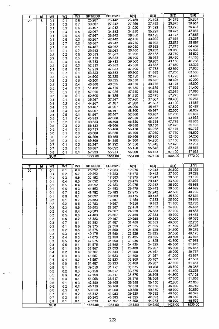
, , w, w, W, SPTIEDD EDDISPT " S[~l SP] 51']

" 0 ,, " '0 25.267 23442 23,450 23.592 24375 25,267,, " " 30.B57 27242 27.250 27.492 29,075 ,0867

" " 00 36.467 31.0~2 31.050 31392 33,775 36457

" " " 42.007 34.842 >4.850 ~5,Z92 38475 42067

" " "' 47.667 38.&12 38650 39,192 43175 47,667

" 00 ,., 53,267 42.442 42.4,0 4~,O92 47675 53,267,, " " 58867 46.242 46,250 46992 52,575 5B a67

" 00 " 04457 50042 ,0050 SO B92 57,275 64 467

" " " 29.933 28,003 28.100 2~,2e3 29050 .~93~

" " '0 35SJJ ~L88J Jl.9QO 32183 33750 35533

" " " 4\.133 35683 35700 36 D83 38,450 41.133

" "' "' 467JJ 39 '83 39500 39,~e3 43150 45 7J~

" " " 52.lJJ 43.283 43300 43883 47850 ,2.333

" 00 " 57.933 47.083 47.100 47783 52550 57.933

" " " 63.533 50.B83 50.900 51633 57,250 63533., ,, 00 34.600 32.725 ~2-7,O 32975 33,725 34.600

"' " " 40200 30.525 36.550 :)6875 38425 40 200

"' "' " 45800 40.325 40.3,0 40,775 4~'25 05,800

" o. "' 51.400 44,125 44.150 44,575 47 B25 ,1.400

'0 " "' 5700D 47.925 47.950 48,75 52,525 57.0000.' '" "' 62.600 51.725 51.750 52075 57.225 62600., ,, " ~9.257 37.~67 ~7.<00 37667 38.400 39.267o. " o. 44.857 41.167 01.200 41567 4,] '00 44 867o. " "' 50.457 44.967 05000 45467 47,eOO 50467o. o. " 50.067 48.767 46800 49367 52,500 56.067o. " ,, 61.667 52557 52600 53,267 57200 61.6G7

" ,, o. O~933 42000 02,0,0 42.358 43075 O~933

" " "' 49.533 4580a 05850 46258 47.775 49533

" " " 55 1.]3 49600 09650 50,156 52475 55133

" o. " 50733 53408 ,3,450 54058 57175 60.733

'" " " 46,600 46 650 46 700 47.0,0 47750 06,600

'" " "' 64.200 50450 ,0500 50950 52450 64,200

'" " " 59800 64 250 64 300 64,850 57150 ,9800

" " , " 53.267 ,1 292 51 350 51.702 52425 53267

" " " 58 B67 55,092 S,150 55642 57,125 5B 867

" "' ,, ,7.9~3 55933 •• 00 56033 57100 ,7 9~3

'"' 1772 00 1553.00 15,400 1,71 DO 166500 1772 00

, " w, w, W, 5PTlEDD EDDISPT '" 5[2] " S[4]

"' , " "' " 25392 12,983 12975 12.902 24,500 25392

"' "' "' 29292 1,28~ 1,475 15 •• 2 27500 2929.

"' " " 33192 17 583 17,975 17.9H 30500 33,192

"' ., 0; 37092 19883 20,475 20442 33500 37,092

"' 0; "' 4099. 22183 22975 22.942 ~6 000 40992

"' ", "' 40,692 2448~ 25475 25402 39500 44 B92

"' "' "' 08,792 26 78~ 27975 27.902 42000 48792

"' '" ", ,2,692 29 08~ 30475 30442 45500 52 L92

"' ., "' 28 88~ 17,557 17,450 17.333 28000 28683

"' ., 00 32 78~ 19967 19,950 16883 31000 32,783., ., ., 36683 22267 22,450 22.383 34000 36,683

"' " " 40583 24587 20950 24883 37000 40583

"' " ., 40 48~ 26887 27450 27,383 40000 44483

" M ., 48 38~ 29167 .9,950 29883 43.000 48383., " "' 52283 31.467 32.450 32383 46.000 5.,263

" "' 00 32375 22,~50 21 925 21 825 J 1.500 ~2,375

" " " 36275 24650 24425 ",32, 34.500 36275'0 ., "' 40175 26950 .6,925 26825 37.500 40,175

" "' " 44075 .~,250 29425 29325 40500 44075

" " " 47975 ~, ,50 31,925 31,825 43500 47975., M "' 51 B75 33,550 3< 425 34325 ~,oo 51.875., "' " 35 B67 27,033 26400 26267 35000 36867

"' "' " 39,767 29 33~ 28900 28,767 38000 39767

"' " " 4),667 31633 31400 31,267 41.000 43667

"' "' " <7,567 33 93~ 33900 33,767 44.000 47567

"' " "' 51.467 ~6 233 36400 )5,267 47.00D 51457., "' "' 39 ~5a 31.7\7 W875 3070a 38500 39358

" ., ., 43258 340\7 33.075 33 20B 41.500 43,258

" " ., 47158 363\7 3,,675 35.70B 44.500 47,1580; "' ., 51,058 ~8 617 38375 36206 47500 51.058M "' "' 02850 36400 ~5 350 ~5150 42,000 0285000 "' "' 46750 38700 17,8,0 ~7.650 45000 46.7,000 ., ., 50 650 4' 000 '0,350 40.150 48000 50,650

" "' "' 46342 41,08:J 39825 19592 45500 <6342

" "' " 50,242 43 38~ 42325 02,092 485DO 50242

'0 " "' 49833 4,767 4< 300 44 033 49000 <9 8~3

"" 1535.00 105400 10,3,00 1049.00 142800 1535,00

228

-, • w, m w, SPTIEOO EODISPT $[1] 6[2] " ";0 , " " "' 25700 13.392 13 275 13.242 24808 25.700

" 0.' "' 29 aoo 15.991 15,97, 15942 28008 2S 600

" "' "" 33.900 16592 18,675 18642 3120B 33900

" "' 0; 38000 21 192 21 375 21.342 34,408 ~8 Doa,, "' "' 42100 2379. 24075 24.042 37608 42,100o , 00 "' 46 200 26,~92 26775 26742 40808 4$,200,, "' "' 5Q300 28992 29475 29442 44.[1{)6 50 :)00

" "' e, " 400 31 592 32175 lZ,14. .7.20B 54400

"' " "' 29,300 1~,183 17 B50 17783 18417 29,300

"' "' 00 :)3,.00 20783 20550 204B3 31.617 ~3.00

"' "' 0; 37500 23 JB3 23250 2J. 1~J 34,817 37500

"' "' "' 41600 25963 25,950 25883 38017 41600

"' "" "' 45,700 28,63 28650 28583 ., 217 45,700

"' "' "' 49,800 311B3 31.350 31 283 '4,417 49800

"' " " 539DO 337BJ 34050 3,] 983 47,617 53900

"' ,, "" 32 000 22975 22415 2U25 32025 32.9000; "' " 37000 25575 25115 25,025 35,225 37.0000; 0; "' 4\.10D 28.175 27.825 27,725 38,425 41.1000; "' 0; 4520D 30.775 30.525 30425 41.G25 45200

" "' " 49300 3337, 33225 33125 44825 49.300

"' 00 ,, 53400 3597, 3,.925 35825 4a 025 53400

"' "' "' 36.500 27.767 27,000 26867 35,633 :16500

"' "' "' 40600 30367 29700 29567 38,633 40600

"' "' "' 4'1700 32967 J2400 ~~.267 42,033 .4700

"' "' "' 4B800 J,567 J,100 34,967 4S233 .B 800

"' "' " ,2,900 3a1D7 37800 37667 48433 52900

" "' "' 40100 32558 31 575 31 408 39,242 40,100

"' "' "' 44200 3\,158 34,U5 J4 'OB 42.«2 4.200

"' "' " 48300 37758 36975 3680B 45642 48300

" "' ,, 52400 40358 39675 3950B 48842 52.400

"' "' "' 43700 37350 36150 35950 42850 4J 700

"' "' " 47 BOO 39950 3B 850 38550 46 050 47,600

"" "' "' 51900 42550 41550 41 350 49250 51900

"' "' "' 47,300 42,142 40725 40492 46458 47300

"' "' "' 51,400 44,742 43 ~25 43192 49658 5L400CO "' 0.' 50900 46,9J3 45300 45,033 50 067 50900

-SUM 1572,00 110300 1089,00 108500 146500 157200

I ; --M---wr -W2 I W, SPTIEDD EDDISPT S[11 '" l-----J!JI-,-- S[~I

'" " "' "' CO 26008 13 800 13 575 13 542 25 117 26 OoB

"' "' "' 30308 16700 1647, 16 442 28517 30,308

"' "' ,. J4608 19600 19,37\ 19J42 31917 34 S08

"' "' " ']8,908 2<.500 ;;<,270 22242 35317 3890a

"' "' "' 4320a 25400 25175 25.1.2 38717 43208

"' "" "' 47508 28300 28075 280.2 42 117 47508

"' e, "' 51 808 31 200 30,975 309., 45,17 01,60S,, CO "' 56,108 34100 33 B75 33842 48917 56108

"' " "' 29717 IS 700 18250 1B.183 28833 29717

"' "' "" 34 017 21600 21150 21 083 32233 34017

"' "' "' 38317 24500 24050 23983 35633 38317

"' "' "' 42617 27.400 26%0 26 B83 39033 42.617

"' "' "' 46,917 30300 298,0 2U83 42,433 .6917

"' 00 "' 51,217 J3 200 32.75(1 32683 45833 51 217

"' "' " 55517 36100 35650 35563 49233 05517

"' "' CO Jl425 23600 22 925 22.825 32550 JJ 425

"' "' "' 37725 2650a 25825 25725 359S0 J7725

"' "' ,. 42,0;;0 n'oo 28,720 26025 3S l50 4.,020

"' "' "' 46325 32300 31 S25 31 525 42750 46325

"' "' "' 50625 35200 34525 34,420 461,0 50525

"' "' "' 54,925 38,100 37,425 37,320 '9 ",0 5'.925

"' "' "' 37133 28500 27600 27467 :l6 267 37133

"' "' "' 41433 31400 30500 30367 39667 41.33

"' 0.' "' 45733 343DO 33.00 33267 .3067 45733

"' "' "' 50033 37200 36 JDO 36167 46467 50033

"' "' "' 54 JJ3 40,100 39200 ;m,OG7 49,867 0.1.3J3

"' "' "' 40842 33 '00 32275 32,108 39,981 408420.5 "' 0.' 45142 36 JOQ 35175 35008 4J 383 451'2

"' " "' 49442 39200 38075 37,908 45,78J 4~,44<

"' "' "' 537'2 42.100 40975 40,B08 ,0,183 53,7'20; "' " 44000 38300 3B950 36750 43700 M55D

" " " 48850 41 200 39850 39650 47 100 4BB50

'" "' "' 53150 .4100 .2750 42550 50500 ,} 150

"' "' e, 48,258 43200 41,5;;, 41.09'1 47,417 46,2oB

"' "' "' 52558 46100 4.525 4'1292 50817 52558

"' "' "' 51 %7 48 100 46300 460.l3 51133 51~k-". 160900 115200 112500 1121.00 1502~60 160900

229

on:

00 .99~ DO9L,1 OO'lIU oo-Ill~ ooo<;a 00 £gg ~ wns_00~~<; 19l t5 •• l g~ Ol>!i-ij~ rno<; 00~~<; " " "'glS ~g nl tS ;;S99~ 9i:~L~ L~H9~ <;LH~<; " " "gH'O; ttS 6. i:6n. 9~9S~ L~n~ 9UM " " "Og9'~g 000S9 Og;'90 09L'~~ OO~'", Og9<;9 " " ""096'og 00;;6~ ogo<:0 09l ;;~ OOL.~ 096og " " '"on'90 OOO';~ as; 9t O;l'9~ OO~'O. og;;9. '" '" ""~;;~99 LSH;;<; 90n" SL£'~. .e<;'~o ~Z~'99 ," ." ."~~n~ ':90'6~ 90': Ot ~LijO. t~o l~ <;;;n~ " " '0<;lO-L~ L9l~~ gone H.l£ £9; g£ ~ZO'L~ '" '" "~~'~o ':9.~' 90l S. 9,9" ,90-'" ~;;n~ '" '" 0"ODZ'L. .£l'Z<; L9S'Z~ 000'•• loo .1> oon~ '" " '"OOS-l, •• 6 g. L9l:6. 00,-6, 19.-0~ O()';Z. '" ." "OIlSLI' tn'9. L9S9S O(ll)'9[ lOO-9[ OIlSlv ," '" .,OO~'£V t££ ~~ 19r ;;" O()';l[ L!II' .[ oa~.v " " .,OO~'g. tS9'lt [99'Si: 000SZ LOO6l OOVB[ 00

".,

9L6I<; 009-l<; <;Z<;~~ ,l9~v 0.£ ZV .l6 '" " "" ",Ll ~<; OOlrgv ~~O9l: 5iU'~€ 09H£ 9ln9 " " '"H<;H~ 000<;v ~~911: ~~n€ 09t'9£ 9lH' " " 00Hg'~o oonl' 9W'~t 9~ns 099 ~~ gl9n " " "HI '6t OOo'l€ 9i:g".(~ 9~9'a 09£n <;1I6. 00 " ".IHi: 009.£ <;lOv~ ~Zl'v~ O;g'~~ H.'11: '" '" '"a~H, lBv;;, £9~'OV m;zo. t.l'O. 0~l9~ '" '" "090-1") ,99 H~ .g99. (),;l-9, [~n[ (}<;o-v<; " "' "a~t'o' ':9\1'O~ £g~~£ 09;;-\;, ,£H[ 05.-ov ," ," "0.9 VV I90 ~~ .gS6;; 0,[ 6l ~tZ'O£ OW •• '" '" co096S£ ,9llr £919l 0<;l9l [[l9l 0566~ " '" "O.l,~ 19. £( £B9'U o~n:< ~.n< 09Zg£ " co co0" O. 199-6l [BI 6~ O.l'SI ££l'61 O,,"'OC '" " co;Z~'6g ttS-Z~ zos St 9lHC £U6£ .l<; 6, '" ," '"~l9 t, [[<;-gv l~ •• £ <;L~',e lI9'9. nS'Hi '" co '"<;ZIO<; ~u.v ~tn~ 5iLnS In'~s S;;IOS '" "" '"~~H~ €f6'O. ~~£-Sl S,£ H;; II9 g;; ~;;..~ '" " '"9UOV £r~l£ Z\>inl <;l9v;; L~I-" ~nov 00 '" ",W-S[ ~~I:ee <:~'i'I~ Hn~ lW~~ 9;:O'9r " '" "9~nr ££9'6~ lVllll ,HD l~~-g~ .;;HI: " '" "9~99~ ~£LS;; ll'\: ~I --1fAvl l~9-H >~99<: " " "

, oc" !I;]s , 0 "' .LdSm03 M311dS 'M 'M ,M W ,

00 !ll'91 00 6£';~ 00'69~~ OO't':~1 OO'~O;;I 009\>i1l we,S€0't9 00;;-l9 [n-l~ OOVL~ 19l6V .~O'£~ '" '" '"L1L't~ 9l6'19 l6.-9~ 5lg 5~ B,v l~ /lL[5 '" co coL~Z6~ <;It'g. ~6."<v nn. ~nV. Hl6. co '" co00'" O<;l~<; o~o'.v o<;~'vo 099'90 OO~-I") '" '" ""006-6v 0.1 B. o<;g'Ov O;o'~t og~'~o 006-6~ '" co '"OOt-,v 0" ~. 0.9l~ (}<;g-l[ ognt OO~9. " '" "~90'" ~zn~ gO~'~v ,l9'<:. ~.~ €. t90 99 " " "€9~'O; ~<6'l~ gOt'6€ ,l.6f ~1'901' r9,09 " '" "eg0'9' ~~€.~ gO~'9€ 9ll9£ ~~V££ £909~ '" " 00tgn~ 9;:l"0. g06'~S glO££ l~l ~£ £9, ~~ " '" "19l'9; 00n9 L960V OO~~~ <£0 ;;~ L9L<;<; '" " '"L9n~ OOL'L~ 1.9l'lf 006L£ ££9S~ ,9l ~~ co '" '"19L9~ OO~~V 19,-1'\: OOL~. ..9 ~. L9L91- co co '"190'~. 009O~ L9nt 00, ~( •• v l. I9Z It '" co '"1.9ut 0069£ 19~-ijl 00. H;; £.l6;; L9U[ " '" '"00.- ;lO'~9 9Z.-S£ 9;;96£ 5;;l O~ (}<;.-g, '" "" '0(}<;S-I<; ,Lv'l> <;~Z9f ~Z€'9t 'cO'lt 0>6"" " " '"05n~ ,la .~ ,W <£ ~ll-[[ <;lB[[ (}<;~-Lv '" '" "096-~t 9Ll'0~ <;lSSl ,cEi6l ,;;g-O[ 056lv '" ," '"O~~g~ ~l9'9. <;l9'9< ~ll'9l ~~o"a o~.'~." " '"056<£ ~W[( ,Zv£l .l~-~l .ll'l'l 0,6.£ " " "<£~l. (}<;B0<; .9g Le 0,6 L~ L~I>B~ £[~l, " " co<£9l, (}<;u~ £99t. O<;l~< L~l,. <£9;;, co " co.[~g. 0<;9-[v [Bv ~~ 0" ~~ LIOl~ ~[~g~ " " co.€9'(~ O~O-OV (~<'n o;nz ani: €€9'(~ '" '" '"(€I'6S O,O'9~ t~O'9~ 09~'~Z l19'90 £€1'6. '" '" '"t~9 11: O,S l£ [Hnl 0,6 ~l /Iv;;;; •• 9 I'\: " co co~o(II: 0.l6l [99-9~ O<;lg~ /ll6~ .£\ O. co '" coLlg n; .l9 o. lKOC ,L[ 9. 9099. lie L. " "" "/I~'£<; <;lO-Lv l~ll:~ <;L~(~ 90v .~ lI[ £, co co '"lI9 g. <;It-~v ;;.66l ,l6 SZ 90l0. L\9 H. " "' '"lIl:" ,W-6[ ;;.L 9l ,U9Z gOO,l U[ ~. " " "ll96£ ,;;l-9[ ;;~,[;; 9L, ~l 90S~l L~S'6£ " " "ll£ <;£ ,;;9-l[ ;;'" Ol ,l[ Ol g090l l~t'9£ " " "llH O[ <;W-6l ;;~ILI 9l~'L\ son \ l~R'O~ " '" '"ll[Sl ,l.-.;; ;;v6n 9lH~ gon~ l~t'9~ "" ," ," , oc

" " 0 " IdSIOO3 OC31ldS ~ 'M 'M W ,