1D-model of the interaction between a stack of wood and

an imposed electromagnetic wave

Linus Hagg, Daniel Noreland,Eddie Wadbro, and Martin Berggren

Abstract

We have developed and investigated a 1D-model for the interaction between a stackof wood and an impinging electromagnetic field. Maxwell’s equations are used to modelthe electromagnetic interaction and each layer in a stack of boards has been modeled as ahomogenous lossy dielectric slab.

The main reason for developing this model has been to investigate the possibility ofmeasuring the moisture content of wood inside a drying kiln using electromagnetic waves.

Our investigations show that it is in principle possible to measure the moisture content,since the electromagnetic field is sensitive to changes in the moisture content of the wood.We also show that it might be possible to measure the average moisture content, withoutdetailed knowledge of the distribution of moisture content between different boards.

Contents

1 Introduction 1

2 Preliminary electrodynamics 2

3 Scattering by one linear slab 3

4 Scattering by N linear slabs 64.1 Analytic solution . . . . . . . . . . . . . . . . . . . . . . . . . . . . . . . . . . . . 8

5 Simulation results 8

6 Conclusion 11

A Powers of a 2× 2 matrix 13

1 Introduction

The moisture content of a piece of wood is defined as the ratio between the mass of the waterit contains and its dry mass. Today, industrially sawn wood is dried in large chambers calledkilns in order to lower the wood’s moisture content to a pre-specified value. Kiln drying hasmany beneficial effects; for instance, both the resistance to biodegradation and the strength ofthe wood increase.

1

The drying process uses vast amounts of energy, mainly in terms of biofuel for heating of thekiln, but also in the form of electricity for the fans. A badly controlled drying process mightlead to substantial quality and value loss.

For operating purposes, accurate measurements of the average moisture content of woodinside a drying kiln would be very valuable. The idea to use electromagnetic properties of thewood to determine the moisture content originates from the late 1920s [1], and hand held resistivemoisture meters are widely used in industry today. To obtain satisfactory estimates of theaverage moisture content of a larger batch of wood by resistive meters is however cumbersome,since they only provide very localized measurements. Neither are the resistive meters suitablefor continuously measuring the moisture content since they rely on adequate contact betweenthe wood and the electrodes.

To investigate the possibility of in kiln moisture content measurements, we have developeda simplified model of the interaction between an imposed electromagnetic field and a stack ofwood. This report is however mainly devoted to describe the aforementioned 1D-model and noton how to extract the moisture content based on electromagnetic measurements. We will beginby presenting some preliminary electrodynamics1, which will be used in consequent chapters todevelop and exploit the model.

2 Preliminary electrodynamics

Maxwell’s equations govern the electromagnetic field and its interaction with matter, and in thecase of a linear homogenous and isotropic Ohmic conductor they are given by

∇ · E = 0, (1)

∇ ·B = 0, (2)

∇× E = −∂B

∂t, (3)

∇×B = µε∂E

∂t+ µσE, (4)

where µ = µrµ0 is the permeability, ε = εrε0 is the permittivity, and σ is the conductivity of themedium. These equations admit plane wave solutions, and by aligning the coordinate system,these can be taken to be proportional to ei(kz−ωt), where ±z are coordinates in the propagationdirection, k is the (complex) wave number, and ω is the (real) angular frequency. We will henceuse the ansatz

E = E0ei(kz−ωt)x, (5)

B = B0ei(kz−ωt)y, (6)

where E0 and B0 are complex amplitudes of the electric and magnetic fields respectively, and xand y are unit vectors along the x and y axis respectively. It is easily verified that this ansatzsatisfies the first two of Maxwell’s equations, equation (1) and equation (2), while the third,equation (3) yields the following relation between the field amplitudes

B0 =k

ωE0. (7)

Insertion of the ansatz and equation (7) into the fourth Maxwell equation (4) yields the dispersionrelation

k2 = µεω2 (1 + i tan δ) , (8)

1A more comprehensive account on electrodynamics can be found in, for instance, [2].

2

where we have introduced the loss tangent

tan δ =σ

εω. (9)

The expression

±√w =

√a

[√1 + b2 + 1

2

]1/2+ i

√a

[√1 + b2 − 1

2

]1/2(10)

for the square root of a complex number w = a (1 + ib) with a, b ≥ 0 applied on equation (8)gives

k = ±k0 (a+ + ia−) , (11)

a± =√εrµr

[√1 + tan2 δ ± 1

2

]1/2≥ 0, (12)

were k0 = ω√ε0µ0 is the wave number in vacuum; the positive sign in expression (11) corre-

sponds to a wave propagating along the positive z axis, while the negative sign corresponds topropagation along the negative z axis. Since Maxwell’s equations are linear, a general monochro-matic plane wave solution representing waves propagating along both the positive and negativez axis is given by

E =[E+eikz + E−e−ikz

]e−iωtx, (13)

B =k

ω

[E+eikz − E−e−ikz

]e−iωty, (14)

where E± are the complex amplitudes of the electric field and where we have used expression(7) to eliminate the corresponding amplitudes of the magnetic field.

The Poynting vector Y determines the energy flux density, and its time average can in thecase of expressions (13) and (14) be calculated as

〈Y 〉 = 1

2Re

(E∗ × B

µ

)(15)

=

[Re(k)

2µω

(|E+|2 − |E−|2

)+

Im(k)

µωIm(E−E+∗

)]z, (16)

where ∗ denotes complex conjugation.

3 Scattering by one linear slab

In this section, we study how a linear, homogenous, lossy dielectric slab scatters a monochromaticplane electromagnetic wave at normal incidence. The setup is illustrated in figure 1 where wealso show the definitions of the complex amplitudes E±

l of the electric field in the differentregions l ∈ {L,M,R}; E±

L is defined in region L at the interface between regions L and M ; E±M

is defined in region M at the interface between regions L and M ; E±R is defined in region R at

the interface between regions M and R. We will use a transfer matrix method2 to relate theamplitudes in the different regions [3]. In our application, the material in regions L and R willbe the same and it will also be assumed that the material in these regions is lossless; that is,tan δL = tan δR = 0.

2Transfer matrix methods are also used for analyzing acoustical and quantum mechanical wave scattering.

3

E−L E−

M E−R

E+L E+

M E+R

L M R

dMz

Figure 1: Definitions of the notation used for the six complex amplitudes related to the dielectricslab.

At the interface between two regions with different material properties, the electric andmagnetic field must satisfy so-called interface conditions; in this particular case that the electricfield and the H-field H = 1

µB should be continuous at the interface. The interface conditionsfor the fields at the LM -interface can be summarized as

CL

(E+

L

E−L

)= CM

(E+

M

E−M

), (17)

where the first component corresponds to the electric field and the second to the H-field. At theMR-interface the corresponding interface conditions are given by

CMPM

(E+

M

E−M

)= CR

(E+

R

E−R

)(18)

In equations (17) and (18) the connection matrices Cl, l ∈ {L,M,R} are defined as

Cl =

(1 1al −al

), (19)

where al ≡ kl/µl, and the propagation matrix Pl is defined as

Pl =

(eikldl 00 e−ikldl

)≡(ϕl 00 ϕ−1

l

). (20)

Note that since kl ∈ C we have, in general, that ϕ−1l 6= ϕ∗

l .Solving for E±

R in terms of E±L gives(

E+R

E−R

)= T

(E+

L

E−L

), (21)

where we have defined the transfer matrix T = C−1R CMPMC−1

M CL. Since CL = CR, T is relatedto PM via a similarity transformation and hence

det(T ) = det(PM ) = 1, (22)

4

where the last equality follows from expression (20).By definition (19) it follows that

C−1L CM =

1

1− q

(1 −q−q 1

), (23)

where q ≡ ∆a/∑

a,∑

a ≡ aL + aM , and ∆a ≡ aM − aL. The matrix C−1M CL is found from

expression (23) by interchanging L and M noticing that∑

a →∑

a, and ∆a → −∆a, andhence q → −q. Using these observations the entries of T can be computed as

T =ϕ−1M

1− q2

(ϕ2M − q2 −q(1− ϕ2

M )q(1− ϕ2

M ) 1− q2ϕ2M

). (24)

We note that if Im(kM )dM � 1, that is, if the losses in M are large or the slab is thick, theentries of T will be very large. Hence T is not suitable for computations using finite precisionarithmetic, and it is preferable to work with the scattering matrix S instead, defined via(

E−L

E+R

)= S

(E+

L

E−R

). (25)

By rearranging the terms of equation (21) in accordance with equation (25) we find that

S11 = −T21

T22, (26)

S12 =1

T22, (27)

S21 =det(T )

T22

(22)=

1

T22, (28)

S22 =T12

T22. (29)

We see that S12 = S21 and by equation (24) that S11 = S22 since T12 = −T21. These symmetriesof the scattering matrix are anticipated due to the symmetry of the problem. By rearrangingthe terms in definition (25) we find that(

E+R

E−L

)= PSP

(E−

R

E+L

), (30)

where P = P−1 = ( 0 11 0 ), but since the problem is symmetric the relation between ingoing and

outgoing waves must be invariant, meaning that S = PSP . Hence we must have S11 = S22 andS12 = S21 which according to expression (26) to (29) means that we must have det(T ) = 1 andT12 = −T21. We remark that systems with the property S12 = S21 are called reciprocal, see forinstance [4].

From equation (24) and equations (26) to (29) we finally get

S11 = S22 = −(

1− ϕ2M

1− q2ϕ2M

)q, (31)

S12 = S21 =

(1− q2

1− q2ϕ2M

)ϕM . (32)

We note that the entries of S remain finite even when Im(kM )dM � 1

5

n = 1 n = 2 n = 3 n = 4 n = 5

Figure 2: An array of five consecutive slabs.

4 Scattering by N linear slabs

In this section we extend the results from the previous section to an array of N consecutive slabsat normal incidence, see figure 2. Parenthesized superscripts will be used to indicate which slabthe corresponding quantity is related. We note that(

E+L,n+1

E−L,n+1

)= P

(n)R

(E+

R,n

E−R,n

), (33)

that is, the field to the left of slab n + 1 can be obtained by propagating the field to the rightof slab n. By equation (21), we furthermore get that the global transfer matrix TG is found bymultiplying the elemental transmission matrices:

(E+

R,N

E−R,N

)= P

(N)R

−1

N∏j=1

P(j)R T (j)

(E+L,1

E−L,1

)≡ TG

(E+

L,1

E−L,1

)(34)

Despite being easy to compute the global transfer matrix in (34) suffers from the same behavioras its elemental counterpart when there are losses present, that is, the elements of TG can bevery large. As pointed out before, elemental scattering matrices do not suffer from that behaviorand can be related to the global scattering matrix SG defined via(

E−L,1

E+R,N

)= SG

(E+

L,1

E−R,N

). (35)

We remark that SG is related to TG in the same way as S is related to T , see expression (26)to (29), and that we still have det(TG) = 1. However, in general, TG12 6= −TG21 which meansthat SG12 = SG21 but SG11 6= SG22. If the array is symmetric with respect to the center planewe will however still have PSGP = SG as for the elemental scattering matrix S.

Defining E(n) ∈ C4 as

E(n) =(E+

L,n E−R,n E−

L,n E+R,n

)T, (36)

6

G(n) ∈ C4×8 as

G(n) =

(G

(n)11 G

(n)12

G(n)21 G

(n)22

)(37)

where

G(n)11 =

(S(n) −I

)∈ C2×4 (38)

G(n)12 =

(0 0 0 00 0 0 0

)(39)

G(n)21 =

(0 0 0 ϕ

(n)R

0 1/ϕ(n)R 0 0

)(40)

G(n)22 =

(−1 0 0 00 0 −1 0

)(41)

the problem of finding the complex amplitudes of the electric field boils down to solving Ax = bfor x = (E(1)T , . . . , E(N)T )T where

A =

G(1) 0

. . .

0 G(N)11

BC

, b =

0...0bc

. (42)

The parts BC and bc are used to enforce boundary conditions at the first and last slab. Theboundary conditions we have used are

E+L,1 = EI (43)

E−R,N = ξE+

R,N , (44)

where EI is the amplitude of an incoming wave and ξ ∈ C, |ξ| ≤ 1 is a constant that can beadjusted to generate different boundary conditions. For instance ξ = 0 corresponds to the casewhen nothing is reflected at the far end while ξ = −1 corresponds to ending the array with aperfect electric conductor. Note that the condition |ξ| ≤ 1 guarantees that no energy is gainedat the boundary.

The reflection coefficient rξ is defined as the quotient of the amplitude of the reflected waveand that of the incident wave:

rξ =E−

L,1

E+L,1

(45)

Similarly the transmission coefficient tξ is defined as the quotient of the amplitude of the trans-mitted wave and that of the incident wave:

tξ =E+

R,N

E+L,1

(46)

Using the boundary conditions (43) and (44) in expression (35) the reflection and transmissioncoefficients can be computed as

rξ = r0 + t′0ξtξ, (47)

tξ = t0 + r′0ξtξ ⇔ tξ =t0

1− ξr′0, (48)

7

where r0 = SG11 and t0 = SG21 are the reflection and transmission coefficients respectively whenξ = 0, and r′0 = SG22 and t′0 = SG12 are the reflection and transmission coefficients respectivelyfor the same array, but with the boundary conditions:

E+L,1 = 0 (49)

E−R,N = EI , (50)

Note that ξr′0 = 1 if and only if |ξ| = |r′0| = 1, which implies that t′0 = 0 since energy balancedemands that |r′0|2+ |t′0|2 ≤ 1. A remarkable property for any type of system with det(TG) = 1,as for instance the type of arrays studied here, is that t′0 = t0 since SG12 = SG21.

The input impedance Z is defined as the quotient of the electric and magnetic field and isgiven by

Z = η1 + rξ1− rξ

, (51)

where η = µ0c is the impedance of vacuum. Z can be used to quantify the response of a systemto an imposed electromagnetic wave.

4.1 Analytic solution

Assuming all unit cells to be equal (hence the array is symmetric with respect to the centerplane) we get from equation (34) that the global transfer matrix is given by

TG = P−1R (PRT )

N. (52)

Using the results in Appendix A on page 13 we get (note that det(PRT ) = 1)

(PRT )n =

sinnθ

sin θPRT − sin(n− 1)θ

sin θI ⇒ (53)

TG =sinnθ

sin θT − sin(n− 1)θ

sin θP−1R , (54)

where cos θ = tr(PRT )/2. Using equation (24) we get

cos θ =1

1− q2[cos(kRdR + kMdM )− q2 cos(kRdR − kMdM )

](55)

Hence we get the following explicit expressions for the entries of SG

SG11 = SG22 = S11gn(θ)

gn(θ)− S12gn−1(θ)ϕReiθ(56)

SG12 = SG21 = S12g1(θ)e

i(n−1)θ

gn(θ)− S12gn−1(θ)ϕReiθ, (57)

where gn(θ) ≡ 2ieinθ sinnθ = ei2nθ − 1.The analysis in this section show that the response of the array to an imposed electromagnetic

field in general depends in a complex way on the material properties and geometry.

5 Simulation results

To verify the model in the lossless case we tested energy conservation by computing

δ = |R+ T − 1|, (58)

8

0 1 2 3 4 5 60

0.2

0.4

0.6

0.8

z[m]

|E||E

I|−

1

(a) u = 30%

0 1 2 3 4 5 60

0.2

0.4

0.6

0.8

1

z[m]

|E||E

I|−

1

(b) u = 20%

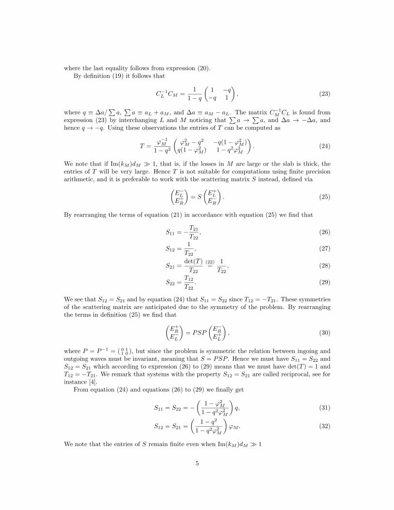
Figure 3: Electric field in a pile of wood consisting of four packages containing 21 boards withthickness 50mm and moisture content u when hit by a wave with frequency 100MHz.

where R = |r0|2 is the reflectance and T = |t0|2 is the transmittance. We found that maxν δ ∼10−12. In the lossy case we used equation (15) to test that the energy flux out of each slabwas less than the corresponding influx. We have also compared the numerical solution with theanalytic expressions in section 4.1.

The model has been tested on a stack of wood consisting of 84 boards distributed in fourpackages with 21 boards each. Each board was 50mm thick and the air gaps between boardsin a package was 20mm and the air gap between two consecutive packages was 100mm. Thismeans that the stack will be about 6m high in total. At the far end of the stack we used aboundary condition that tries to mimic the effect of a 100mm air gap followed by reinforcedconcrete by choosing ξ in equation (43).

For the properties of wood at different moisture contents and frequencies we used the valuestabulated in [5]. For intermediate frequencies not found in the table we interpolated linearlybetween the entries in the table.

Figure 3a shows the magnitude of the electric field inside a stack of wood with moisturecontent 30% at 100MHz. It can be seen that the behavior is dominated by the damping eventhough some interference is also present. Figure 3b shows the corresponding figure for u = 20%.The damping is still dominating the behavior but now the interference is more pronounced. Forhigher moisture contents the field is practically damped out already in the first package. Dueto the low penetration at high moisture contents we will henceforth assume that the pile hasbeen partitioned after the first package using a metallic mesh. This means that the responsecomputed only depends on the properties of the first package.

Figure 4 shows the input impedance as a function of frequency for a package with averagemoisture content 100%. The thicker line shows the response when there is no variation inmoisture content between different boards in the package while the four thinner shows theresponse when there is 50% variation. We see that all five curves shows a high degree ofagreement up to around 30MHz. This means that the response for low frequencies is mainlydue to the average properties of the package and not the variation. This is expected since thelow frequency limit corresponds to the long wavelength limit. When the wavelength is muchlarger than the thickness of the boards in the package, the package can be approximated witha homogenous block with some effective electromagnetic properties.

9

100

101

102

103

−20

−15

−10

−5

0

5

10

15

ν [MHz]

|Z|η

−1[dB]

Figure 4: Input impedance for a package of wood ended by a perfect electric conductor. Thethicker line shows the response when all slabs have moisture content 100%. The four thinnerones correspond to cases where the moisture content varies between different slabs but theaverage moisture content of the package is still 100%.

The figures 5a, 5b, 5c and 5d shows to figure 4 corresponding figures when the moisturecontent is 60, 30, 20% and 10% respectively. These figures show the same general tendencyas figure 4, that is for low frequencies the response is mainly due to the average properties ofthe package. However what is regarded as a low frequency changes with the average moisturecontent.

6 Conclusion

Our investigations show that the electromagnetic field is sensitive to changes in moisture contentof a pile of wood. At high moisture contents the penetration is quite poor and the behaviorof the electromagnetic field inside the pile is mainly characterized by exponential damping.For lower moisture contents, when there is less damping, interference effects are also present.The response for low frequencies is mainly related to the average electromagnetic properties ofthe pile. This indicates that it should be possible to measure the average moisture content ofthe wood without detailed knowledge of the distribution of moisture content between differentboards.

The model presented in this report neglects all 3D-effects, as for instance the finite size ofthe packages and non normal propagation of the electromagnetic waves. Within this projectthese effects have not been studied.

10

100

101

102

103

−20

−15

−10

−5

0

5

10

15

ν [MHz]

|Z|η

−1[dB]

(a) u = 60%

100

101

102

103

−20

−15

−10

−5

0

5

10

15

ν [MHz]

|Z|η

−1[dB]

(b) u = 30%

100

101

102

103

−20

−15

−10

−5

0

5

10

15

ν [MHz]

|Z|η

−1[dB]

(c) u = 20%

100

101

102

103

−20

−15

−10

−5

0

5

10

15

ν [MHz]

|Z|η

−1[dB]

(d) u = 10%

Figure 5: Input impedance for a package of wood ended by a perfect electric conductor. Thethicker line shows the response when all slabs have moisture content u. The four thinner onescorrespond to cases where the moisture content varies between different slabs but the averagemoisture content of the package is still u.

11

A Powers of a 2× 2 matrix

Let M ∈ R2×2 then

M0 = I (59)

M1 = M (60)

M2 = tr(M)M − det(M)I ≡ αM + βI (61)

where equation (61) follows by brute force or the Cayley-Hamilton theorem. The sequence ofpowers shows that Mn = anM + bnI for some an and bn. Using this as an ansatz we get

an+1M − bn+1I = Mn+1 (62)

= M(anM + bnI) (63)

= anM2 + bnM (64)

= an(αM + βI) + bnM (65)

= (αan + bn)M + βanI (66)

ie. an+1 = αan + bn and bn+1 = βan which together with equation (59) and (60) yields thefollowing recurrence relation:

a0 = 0

a1 = 1 (67)

an = αan−1 + βan−2

Define the operator S by San = an+1 then the recurrence can be written as

(S2 − αS − β)an = 0 (68)

which factors into (S− λ1)(S− λ2)an = 0 where λi is the i:th eigenvalue of M . We will assumethat λ1 6= λ2. Hence an = A1λ

n1 + A2λ

n2 is a solution to the recurrence (67) for any pair of

constants Ai. Further since the recurrence is homogenous this is also the only solution. Usingthat a0 = 0 and a1 = 1 we get finally that A1 = −A2 = 1/(λ1 − λ2) and hence:

an =λn1 − λn

2

λ1 − λ2(69)

For a matrix with det(M) = 1 we get that λ1 = 1/λ2 ≡ eiθ, tr(M) = λ1 + λ2 = eiθ + e−iθ =2 cos θ and that an = sinnθ/ sin θ, note that θ ∈ C. Hence the nth power of M is given by:

Mn = anM − detMan−1I =sinnθ

sin θM − sin (n− 1)θ

sin θI (70)

References

[1] A. J. Stamm (1927). The electrical resistance of wood as a measure of its moisture content,Industrial and Engineering Chemistry 19(9): 1021-1025.

[2] D. J. Griffiths (2004). Introduction to electrodynamics, 3rd ed, Pearson Education.

[3] S. J. Orfanidis (2014). Electromagnetic waves and antennas, online athttp://www.ece.rutgers.edu/~orfanidi/ewa/

12

[4] D. M. Pozar (2011). Microwave Engineering, 4th ed, Ch. 4, John Wiley & Sons

[5] G. I. Torgovnikov (1993). Dielectric properties of wood and wood-based materials, SpringerSeries in Wood Science, Springer-Verlag, Berlin.

13