1930: First Modern Crisis

NBER WORKING PAPER SERIES

1930: FIRST MODERN CRISIS

Gary GortonToomas Laarits

Tyler Muir

Working Paper 25452http://www.nber.org/papers/w25452

NATIONAL BUREAU OF ECONOMIC RESEARCH1050 Massachusetts Avenue

Cambridge, MA 02138January 2019

We thank Andy Law, Chase Ross, Alex Yang, and Arwin Zeissler for research assistance. We thank Joshua Rosenbloom and William Sundstrom for sharing their Census of Manufacturing data with us; see Rosenbloom and Sundstrom (1999). Also, thanks to Mrdjan Mladjan for sharing his data on the instruments used in Mladjan (2016). The views expressed herein are those of the authors and do not necessarily reflect the views of the National Bureau of Economic Research.

At least one co-author has disclosed a financial relationship of potential relevance for this research. Further information is available online at http://www.nber.org/papers/w25452.ack

NBER working papers are circulated for discussion and comment purposes. They have not been peer-reviewed or been subject to the review by the NBER Board of Directors that accompanies official NBER publications.

© 2019 by Gary Gorton, Toomas Laarits, and Tyler Muir. All rights reserved. Short sections of text, not to exceed two paragraphs, may be quoted without explicit permission provided that full credit, including © notice, is given to the source.

1930: First Modern CrisisGary Gorton, Toomas Laarits, and Tyler MuirNBER Working Paper No. 25452January 2019JEL No. E02,E3,G01

ABSTRACT

Modern financial crises are difficult to explain because they do not always involve bank runs, or the bank runs occur late. For this reason, the first year of the Great Depression, 1930, has remained a puzzle. Industrial production dropped by 20.8 percent despite no nationwide bank run. Using cross-sectional variation in external finance dependence, we demonstrate that banks' decision to not use the discount window and instead cut back lending and invest in safe assets can account for the majority of this decline. In effect, the banks ran on themselves before the crisis became evident.

Gary GortonYale School of Management135 Prospect StreetP.O. Box 208200New Haven, CT 06520-8200and [email protected]

Toomas LaaritsYale School of Management135 Prospect StreetP.O. Box 208200New Haven, CT [email protected]

Tyler MuirUniversity of California at Los AngelesAnderson School of Management110 Westwood PlazaLos Angeles, CA 90024and [email protected]

1 Introduction

One reason it has been hard to understand modern financial crises is that they all appear different.

If financial crises are always due to the vulnerability of short-term debt to runs, shouldn’t we

always see bank runs? Indeed, before the existence of central banks, crises were clearly triggered

by bank runs. However, the presence of a central bank complicates matters rendering a modern

crisis timeline different and varied. Bank runs, if they occur at all, may happen late in the crisis.

Or there could be no runs at all if, for example, a credible guarantee is issued.1

Nowhere is this dynamic more evident than 1930, the first year of the Great Depression. At the start

of the Great Depression there were no nationwide bank runs and banks did not avail themselves of

the discount window. Yet, output dropped substantially: industrial production fell over 20%. As a

consequence, 1930 is viewed as a puzzle. For example, Romer (1988) writes: ”The primary mystery

surrounding the Great Depression is why output fell so drastically in late 1929 and all of 1930”

(p. 5).2 And Bernanke (1983) does not include 1930 in his study of the effects of bank failures on

output: ”it should be stated at the outset that my theory does not offer a complete explanation of

the Great Depression (for example, nothing is said about 1929-1930)” (p. 258).

In this paper show that a large part of the output drop in 1930 can be explained by bank actions:

the reduction in loans and purchase of safe assets. We argue that banks realized the severity of

economic conditions and, in effect, ran on themselves.

We further argue that this exemplifies a common feature of modern crises where a central bank is

present. Banks reduce loans prior to the crisis while depositors stand pat to see what the central

bank does, even if they already recognize crisis conditions. The true start of the crisis, then, can be

before any obvious indications of stress, such as bank failures. Indeed, Boyd et al. (2009) examine

the dating of crisis in four crisis databases and find that large reductions in loan growth predict

crisis start dates. Absent means to observe these responses by the banking sector, modern crises

may appear to be idiosyncratic events without a common core element.

Our empirical strategy to ascertain the role of banks in output declines in 1929-31 combines state-

industry level data on output with state-level data on the banking sector. We use data from

the Federal Reserve to construct state-level measures of banking sector behavior in 1929-31; we

employ data from the Biennial Census of Manufacturers to construct measures of state-industry

level performance.

In order to identify the effect stemming from the banking sector’s decision to cut back—and not from

demand side effects—we use an approach along the lines of Rajan and Zingales (1998). We hand-

1The Laevan and Valencia (2008) crisis database covers the period 1970-2007, during which there were 124 systemicbanking crises globally. They find that 62 percent of the crises in their data experienced bank runs, defined as asharp reduction in total deposits.

2Also, Romer (1990): ”. . . 1930 is . . . the most puzzling year of the Great Depression” (p. 599).

1

collect firm balance sheet data reported in Moody’s Manuals from the period of 1922 to 1928 and

calculate a measure of external finance dependence. We include this measure of external dependence

as a treatment intensity in a cross-sectional regression of industry output on contemporaneous

changes in the state-level aggregate bank balance sheet.

We find that industries which were more dependent on external finance were affected more severely

by reductions in loans, reductions in total assets, reductions in deposits, and increases in holdings

of safe assets by their home state banks. Further, we demonstrate that this conclusion is robust to

controlling for contemporaneous bank suspensions.

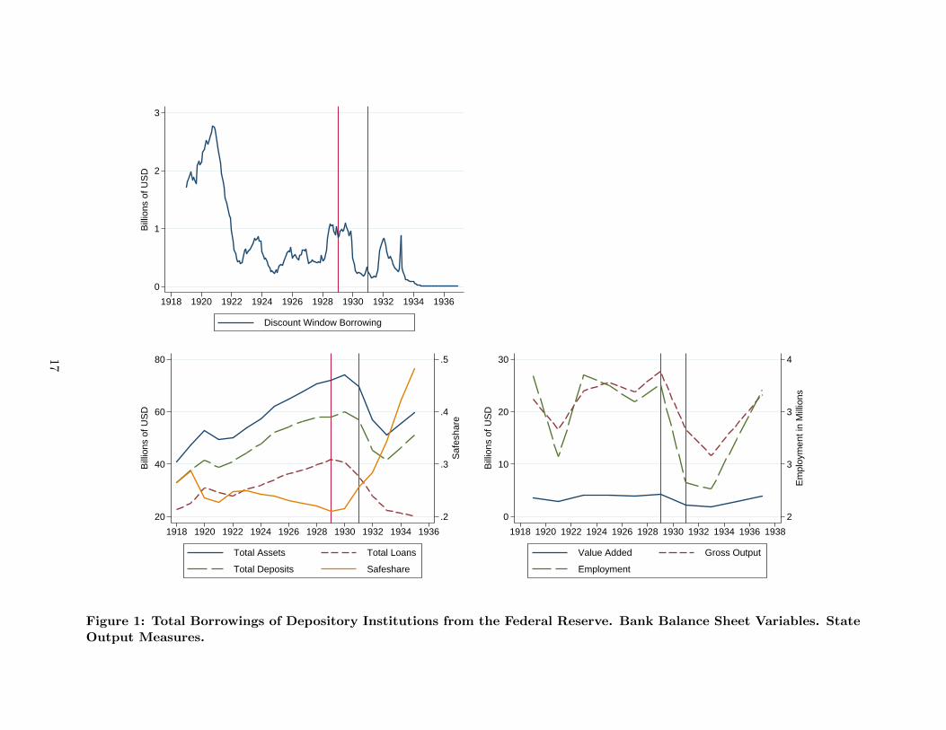
The behavior of banks during this early stage of the Great Depression is evident from the aggregate

balance sheet of the banking sector, shown in Table 1. From 1929 to 1931 banks cut back on loans

by over 15%, and increased the share of total assets invested in safe assets by 6 percentage points.

At the same time, there was little action stemming from the household side: total deposits fell by

just 1.9 %. This contrasts with a drop in deposits of 27.4% in the subsequent two years.

Our estimates suggest that the reduction in loans accounted for a substantial share of the output

decline in 1929-31. Extrapolating from the cross-sectional estimates and nationwide totals in total

bank loans, we estimate a roughly 30% drop in the three output measures.

Our empirical approach is close to Mladjan (2016) and Lee and Mezzanotti (2017). In both of

these papers, the authors look at interactions of measures of firm dependence on external finance

interacted with bank failures to show effects on measures of economic performance. Mladjan (2016)

studies the effects of bank failures on output in a panel of state-industry observations over the years

1929-1933. Lee and Mezzanotti (2017) look at a sample of 29 cities over the period 1929-1933.

They also find that where bank failures were high, the more financially dependent industries show

reductions in the same three outcome variables we use: total output, employment, and value added.

In other related work, Benmelech et al. (2017) show that credit frictions played a large role in the

employment drop from 1928 to 1933.

In contrast to these studies, we focus solely on the seemingly anomalous year of 1930. We demon-

strate that the early part of the Great Depression, where bank failures were not substantial, can

also be explained by the impact of the banking sector on the real economy. There is a large causal

impact of the contraction of bank lending on macroeconomic activity before the major bank runs

of the Depression.

Finally, we place the crisis dynamics of the Great Depression in a broader context. We find that the

unfolding of the Great Depression is typical of modern crises. At the start there is no widespread

bank run, but output falls. In contrast, panics during the National Banking Era, 1863-1914,

occurred near business cycle peaks. With the establishment of the Federal Reserve in 1914, banks

had the opportunity to borrow from the discount window. During one of the first recessions to occur

under the watch of the newly-established Fed, the recession of 1920-1921, banks made extensive

2

use of the Fed discount window, which was giving out loans at an attractive rate. The broad use

of the Fed’s discount window to avoid a panic was hailed at the time as having precluded a panic

(see Gorton (1988)). As we describe in Section 4 of this paper, the discount window subsequently

became stigmatized as the Fed tried to ensure that it was not used as a permanent source of funding.

Indeed, as demonstrated in Anbil (2018), the discount window stigma was a major consideration

of depositors during the Great Depression. We hypothesize that because the use of the discount

window had become stigmatized banks mostly avoided borrowing from the Fed in 1930 and instead

opted to cut back on lending, and tilted towards a safer portfolio.

To provide evidence to this point we compare the early stage of the Depression with the prior

recession in 1920-21. Repeating our analysis, we show that in contrast to the early part of the

Depression, bank balance sheet changes cannot account for the drop in output during the 1920-21

recession.

Our findings regarding the unfolding of the Great Depression suggest a reason for the common

thread underlying all modern financial crises. As shown in Boyd et al. (2009), modern crises are

typically preceded by banks reducing loans. These authors examine the dating of crisis starts in the

four main modern crisis databases: (1) Demirguc-Kunt and Detragiache (2002) and Demirguc-Kunt

and Detragiache (2005); (2) Caprio et al. (2005); (3) Reinhart and Rogoff (2008); (4) Laevan and

Valencia (2008). These databases pin down the starting dates using an event methodology, usually

noting some form of government intervention. Boyd et al. (2009) find that large reductions in loan

growth predict the crisis start dates in the four databases, roughly a year before the traditional start

date. In contrast, similar magnitude deposit changes do not predict the start dates. Depositors

appear to wait, perhaps due to explicit or implicit deposit insurance. Loans are reduced significantly

but deposit reductions—meaning runs—only come later, if at all. In other words, banks realize the

crisis conditions before any public signs of stress.

The paper proceeds as follows. In the remainder of this section we provide a brief literature review.

In Section 2 we describe the data sources and the data construction process. Section 3 contains

our main empirical results on impact of bank decisions on manufacturing output. In Section 4 we

compare crises during the National Banking Era and under the Federal Reserve. We also provide

a history of the development of the discount window stigma. We conclude in Section 5.

1.1 Related Literature

There is an enormous literature on various aspects of the Great Depression. Calomiris (1993) and

Romer (1993) provide reviews of the literature. Perhaps closest to our work is Calomiris and Wilson

(2004). They do not focus on the year 1930, but like us they find evidence of banks shedding risk.

Their focus is on New York City banks where they show that in the early 1930’s banks shed risk,

reducing dividends and increasing their holdings of safe assets. They argue that they provide ”an

3

explanation for the decline in bank capital and the increase in bank cash” (p. 422).

Also related are papers by Romer (1990) and Olney (1999). These authors focus on consumer

demand behavior. Romer (1990) argues that the Great Depression was a singular event. The

1929 stock market crash created “uncertainty” which caused a reduction in household purchases

of durable and semi-durable goods. Olney (1999) also focuses on consumers, pointing out that

consumers were highly indebted and there were large costs to defaulting. Olney (1999) argues that

for consumers to avoid default they cut consumption. These authors focus on the demand side,

while we focus on the supply side. These authors argue that consumers’ purchases of durables

declined. Our explanation is not mutually exclusive with the demand-side explanation, especially

as banks did not make significant amounts of loans to consumers until later. Consumer credit at

the time came mainly from installment buying, see, for instance, Clark (1931).

Finally, closely related are papers on the effects of bank failures and suspensions on output during

the Great Depression, e.g., Bernanke (1983), Calomiris and Mason (2003), and as already discussed,

Lee and Mezzanotti (2017), Mladjan (2016), and Benmelech et al. (2017). These authors do not

examine 1930 separately.

2 Results

Our empirical results establish the importance of banking sector in capturing the heretofore under-

studied first year of the Great Depression.

2.1 Identification

We use the cross-section of state-industry level data to establish the effects of bank behavior on

macroeconomic outcomes. We measure variation in the aggregate banking sector balance sheet

by state in the period from 1929 to 1931 and link this to output declines in different industries

in the corresponding state. To separate out the shock caused by a contraction in lending from

a demand side story (e.g., the particular state faced low productivity shocks which drove down

macroeconomic quantities as well as the demand for bank financing) we employ industry external

finance dependence as a measure of treatment intensity, following Rajan and Zingales (1998).

2.2 Data

We use data from three main sources: the Biennial Census of Manufacturers, Moody’s Manuals,

and statistics published by the Board of Governors of the Federal Reserve.

4

The Biennial Census of Manufacturers provides biannual data disaggregated by manufacturing

sector (industry) and state. This data is described in detail in Rosenbloom and Sundstrom (1999)

and available online on the author’s website.3 We use three measures of output: total wages (value

added), value of production (gross output), and employment. The data covers 15 industries for a

total of 387 industry-state observations. Because this data is collected only every two years, our

regression evidence uses the change in the output measure in 1929 to 1931.

We hand collect firm-level data from the Moody’s Manuals over the period 1922-1928 to construct

the measure of dependence on external finance. Firms are assigned to industries based on Ken

French’s industry classifications.4 The firms that are in the industries that are captured by the

Census of Manufacturers form the basis of an industry-level measure of external finance dependence,

constructed after Rajan and Zingales (1998). The industry level measure is based on 1224 firm-

years.

Bank data is from All-Bank Statistics: United States, 1896-1955 published by the Federal Reserve

Board of Governors. With this data we measure changes in state-level total assets, and total loans,

and total deposits. We also construct a measure of share of safe assets, defined as the sum of

Treasuries, Munis, currency and coin, and banker’s balances, normalized by total assets.

Finally, data on deposits in suspended banks is from the Federal Reserve Bulletin, September 1937,

available online at the St. Louis Federal Reserve Bank FRASER database.5

2.3 Measuring Firm External Finance Dependence

For each firm-year we calculate dependence on external funding as capital expenditures (Capex)

minus lagged cash flow from operations (CFO), divided by Capex:

CXt =Capext − CFOt−1

Capext

We lag CFO because the time t variable is not known when capital expenditure decisions are made.

We then sort the firm-year measures into ten buckets, and assign integer values to each bucket. We

do this to allow for potential nonlinearities in the relationship between CX and the bank measures.

The industry-level measure is the firm asset weighted sum of CX bucket values in industry i:

Depi ≡∑k∈I

CXbucketk

(TAk∑k∈I TAk

)

where i indexes industries; k indexes firms; and I represents the set of all firms in industry i. The

3http://joshua-rosenbloom.squarespace.com/data-sets/4http://mba.tuck.dartmouth.edu/pages/faculty/ken.french/data_library.html.5https://fraser.stlouisfed.org/files/docs/publications/FRB/1930s/frb_091937.pdf

5

industries and the corresponding dependence measures are reported in Table 1 of the Appendix.

The CX measure constructed in this section is not specific to bank finance, but instead captures

dependence on all sources of external finance. However, we find that bank lending constituted a

substantial share of external finance at the time. As shown in Table 1, total bank loans in 1929

were nearly 42 billion USD. For reference, the total market cap of the 856 companies listed on the

NYSE was 89.7 billion USD in August 1929, as reported in McGrattan and Prescott (2004).

3 Results

3.1 Aggregate Balance Sheet

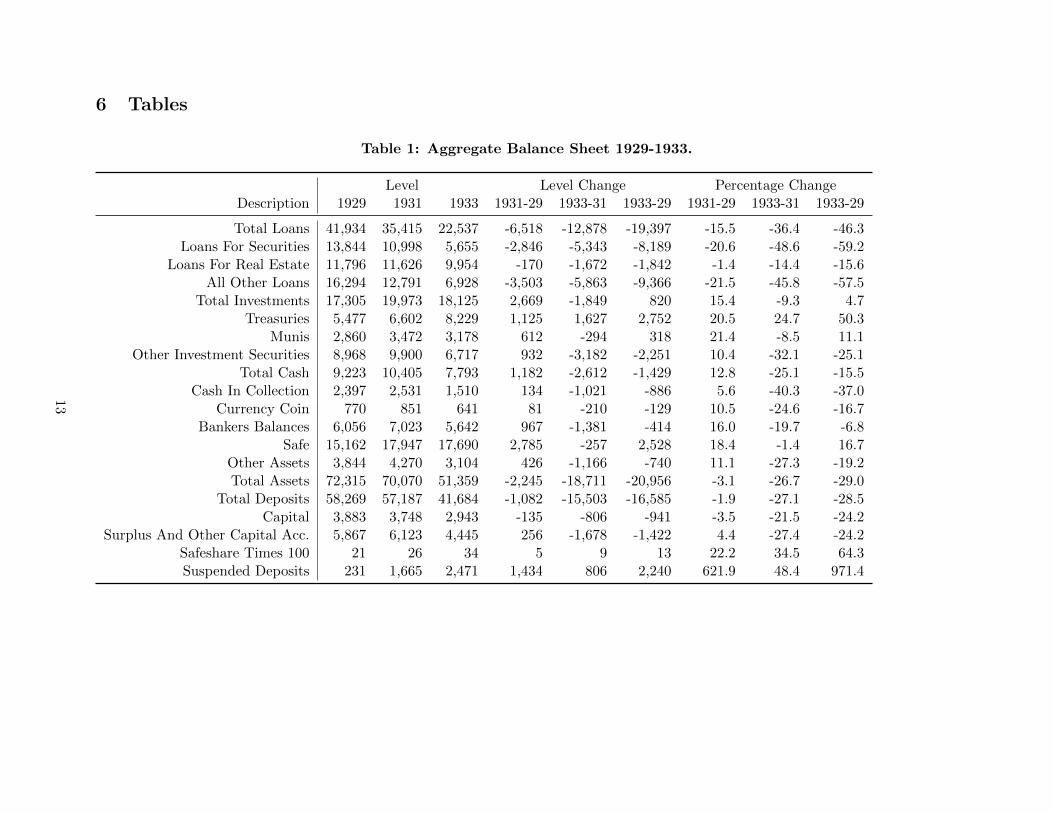
The dynamics we describe are evident in the aggregate balance sheet of the banking sector. Table

1 shows the levels, the change in the levels, and percentage changes in the aggregate balance sheet

items of all U.S. banks during the Great Depression (based on All-Bank Statistics: United States,

1896-1955 ). Corresponding to our output measures, the data is shown are for the years 1929, 1931,

and 1933.

Most interesting in the table are the categories that show large increases and large declines from

1929-1931. Total loans, loans for securities, and all other loans show large declines. Safe assets

including Treasuries, Munis, cash, and banker’s balances show substantial increases. These changes

are consistent with the findings of Calomiris and Wilson (2004) who focus on New York City, the

most important banking center in the U.S. They show that during the year 1930 total loans divided

by cash plus Treasuries declined 81 percent. This was primarily due to loans declining and safe

assets increasing. Note that total deposits only declined by 1.9 percent in 1929-1931—the big

declines in deposits occurred starting in 1932. The time-series behavior of these aggregates is

shown in Figure 1.

3.2 Regression Evidence

The goal of our empirical analysis is to measure the impact of changes in the various bank balance

sheet items on contemporaneous output measures. Specifically, our regressions take the form

∆Outcomei,s = αi + βs + γCXi x ∆Banks + εi,s,

where the outcome variable is defined as

∆Outcomei,s = log(Measurei,s,1931) − log(Measurei,s,1929)

6

for value added, gross output, and total employment of industry i in state s.

Similarly, the right-hand-side banking measures Banks are defined as

∆Banks = log(Banks,1931) − log(Banks,1929),

with the exception of Safeshare which is measured as a percentage point change. We show the

aggregate time-series behavior of the output measures in Figure 1.

The variable CXi is an industry level measure of external finance dependence, constructed in Section

2.3. The terms αi are industry level fixed effects, and the terms βs are state level fixed effects. The

specification does not include time fixed effects because the regression is a pure cross-section.

By studying the interaction term of the state-level bank measure with industry-level external fi-

nance dependence index, we are able alleviate concerns about reverse causality. The underlying

assumption is that in a given state, the output in industries with different exposures to exter-

nal finance would have shrinked at the same rate—relative to the corresponding industry-wide

averages—without the shock from the banking sector. Because the states differ in the magnitude of

the banking sector shocks, we are able to identify the effect on output stemming from the shock to

external finance availability—and not the effect from the demand side. Note we cannot include the

CXi and Banks terms separately because of the full slate of state- and industry-level fixed effects.

The regression results are shown in Table 2. Panel A examines value added as measured by wages

during from 1929 to 1931. Table 2 Panel B repeats the analysis with gross output as the dependent

variable. Panel C repeats the same analysis with employment. In all three panels, reduction in

total loans, total assets, are associated with decreases in the output measures, and this relationship

is in all cases statistically significant. In the specifications with value added and employment as

the dependent variable, an increase in average Safeshare in the state is a statistically significant

covariate of output changes.

In order to put the estimated magnitudes in context, we calculate the output drop implied by the

estimated coefficients of an industry with median exposure to external finance (meaning CX=5)

facing a banking sector whose balance sheet mirrors the national aggregate change. This calculation

is provided in Table 4. In the table, ”Implied Aggregate” refers to the aggregate change in the

right-hand side variable from 1 under these assumptions. While all four measures of bank balance

sheet are estimated to have a strong impact on output, the cutback in loans was the deepest, and

as such imply the largest output loss with estimates ranging from 27% to 44%.

These results are robust to including a measure of bank suspensions. In Table 2 of the Online

Appendix, we re-estimate the regressions reported in Table 2, controlling for the total amount

of deposits in suspended banks by each state. Existing work in Mladjan (2016) has shown that

suspended deposits are a strong determinant of output contraction over the entire Depression era.

7

We find that it is the decision of banks to cut back on lending and switch to safe assets that accounts

for the drop in output in the early part of the Depression, even when accounting for suspended

deposits.

Now, because of the availability of the Census of Manufacturing data we are only able to carry

out the analysis for the 1929 to 1931 period. In Table 3 of the Appendix we show that our results

hold when measuring the right-hand-side bank balance sheet measures from 1929-1930. With the

exception of Safeshare, we find that the drop in bank total assets, bank loans, and bank deposits

in 1929-1930 are significant determinants of the drop in 1929-1931 output measures.

In Appendix Table 4 we re-estimate the regressions in an OLS setting. We find a smaller implied

response to the bank balance sheet variables, suggesting that the effect stems mostly from large

states. In Appendix Table 5 we re-estimate the regressions using two instruments constructed by

Mladjan (2016). The results are consistent with the WLS estimates presented in Table 2, with the

exception of specifications with Safeshare that are no longer statistically significant.

3.3 Importance Discount Window Stigma: 1920-21 Recession

Like we show in Figure 1, banks made little use of the discount window in 1929-1931. Instead, they

opted to cut back on lending. The regression evidence suggests that the decision to cut back on

lending had a strong impact on economic output.

In order to illustrate the importance of the decision not to go to the discount window, we repeat

the analysis presented in Table 4 for the 1920-1921 recession. This recession started in January

1920; the trough, according to the NBER, was July 1921. Unlike during the Great Depression, the

discount rate offered by the Fed was below market rates. As a result, and in direct contrast to the

Great Depression, banks made extensive use of the Fed’s discount window during the Recession

of 1920-1921. Correspondingly, as we report in Table 3, the four measures of bank balance sheets

have little explanatory power over industry level outcomes. We interpret this as evidence of the

importance of discount window stigma during the Great Recession. We take up the the development

of Federal reserve discount window stigma in the next section.

4 Bank Panics in the National Banking Era and in the Great

Depression

As discussed, the lack of discount window borrowing in the early part of the Great Depression

stands in contrast to the recession of 1920-1921. In this section we summarize the history of earlier

banking panics in the U.S. Then we provide a brief history of the Federal Reserve’s discount window

8

policy and the development of stigma.

4.1 The National Banking Era

The National Banking Era began with legislation in 1863 that introduced a system of ”national

banks” that could issue their own currency, but that required backing by U.S. Treasuries. The

legislation was aimed at developing a demand for U.S. Treasuries so as to finance the North in

the Civil War. But, in addition, it was thought that with Treasury backing, creating a uniform

currency (i.e., one without discounts from face value as had occurred with private bank money

prior to the Civil War), there would no longer be banking panics—which did not turn out to be

the case. In the National Banking Era panics depositors sought to withdraw their cash in National

Bank notes.

Gorton (1988) analyzes seven panics that occurred during this period: 1873, 1884, 1890, 1893, 1896,

1907, and 1914. These panics occurred at or just after business cycle peaks; see Gorton (1988) and

Calomiris and Gorton (1991).6 Gorton (1988) showed that banking panics during the National

Banking Era, 1863-1914, were information events. The panics occurred when depositors observed

an innovation in a leading indicator of recessions, namely the liabilities of failed businesses.7 If this

measure exceeded a threshold it indicated that a large recession was coming and, upon observing

this information, there would be a panic. There was never a panic without this threshold being

exceeded and there was no case where the threshold was exceeded without a panic. Subsequent

to the Federal Reserve System coming into being this threshold can be used to determine the

counterfactual of when panics could have occurred.

4.2 Federal Reserve System and the Discount Window

The purpose of the Federal Reserve System was to prevent banking panics by having a permanent

discount window which banks could always access.8

According to the measure of innovation in the liabilities of failed businesses, estimated over the

period 1873-1934, there were two shocks exceed the threshold: June 1920 and December 1929.9

6This timing is generally true. For example, Dimsdale and Hotson (2004) summarize the U.K. experience since1825: ”The general pattern is one in which financial crises occur close to business cycle peaks, and are followed bya downturn in the wider economy” (p. 26). And in the modern era it also tends to be true. See, for example,Demirguc-Kunt and Detragiache (1998) who study a large sample of developed and developing countries over theperiod 1980-1994 and find that ”crises tend to erupt when the macroeconomic environment is weak” (p. 81).

7Burns and Mitchell (1946) identified this variable as a leading indicator of recession.8Prior to the Federal Reserve, private bank clearinghouses opened discount windows only during crises. See Gorton

and Mullineaux (1987).9Gorton (1988) lined up the data with the Office of the Comptroller of the Currency Call Report dates. October

1929 was not a bank Call Report date, so the shock is essentially coincident with the stock market crash in October1929.

9

These two dates just follow business cycle peaks, just as in the pre-Fed period. However, there was

no panic at the start of the recession of January 1920-July 1921. Banks heavily used the discount

window during the 1920-21 recession. Figure 1 shows the dramatic use of the window during the

1920 recession. The successful avoidance of a panic in 1920 was was widely remarked upon at the

time. For example, Herbert Hoover, then the Commerce Secretary, said that ”we know now that

we have cured [bank panics] through the Federal Reserve System.”10 And Wesley Mitchell wrote

in 1922 that: ”We have learned how to prevent crises from degenerating into panics” (see Mitchell

(1922)).

At that time of the 1920-21 recession, the discount rate was below market rates because the Federal

Reserve wanted to support the sale of U.S. Treasuries to pay off the debt from World War I.

Background on the Fed-Treasury relations during this period can be found in Beckhart (1924),

Parker and Steiner (1926), Whittlesey (1959), Wicker (1966), Wicker (2015), and Meltzer (2003),

among others. In any case, banks did avail themselves of the discount window to a significant extent,

as seen in Figure 1. But, the Fed became concerned that banks were using the discount window as

a permanent source of funding and also that banks were using the discount window borrowings to

lend to speculative stock market investors. To solve these perceived problems, the Fed introduced

the discount window stigma. To control discount window borrowing without raising the discount

rate (to accommodate the Treasury), the Fed introduced non-pecuniary penalties. The methods

used to control credit are listed by Parker and Steiner (1926): the issuance of warnings; the use

of moral suasion; advising banks to reduce their outstanding lines of credit and to discriminate

against speculative and non-essential loans; the rationing of credit; the attempt to drive war paper

from the portfolios of reserve member banks; controlling the issue of Federal Reserve notes; closer

scrutiny of paper offered for discount.

Parker and Steiner (1926) write that: ”moral pressure was exercised by means of conferences

with groups of banks and with individual banks to ascertain the reason for heavy borrowing and

if necessary to request them to reduce their aggregate borrowings” (p. 530). In the beginning

of the 1920s there was less stigma. E.g., Carlson and Burcu (2016): ”There was notably less

stigma associated with borrowing from the discount window in the 1920s and borrowing was fairly

widespread with about one-third of all member banks borrowing in any given month (roughly 3,000

borrowers out of 9,000 member banks)” (no page). But, this changed. Armantier et al. (2015)

”From the late 1920s, the DW [discount window] gradually fell into disuse as the Fed began to take

a dim view of DW borrowing and adopted a stance against this practice” (no page). Whittlesey

(1959): ”. . . administration of the discount window, in the admonitory, moral suasion sense, has a

tendency to strengthen the attitude of mind among bankers, the instinct against borrowing, which

is the basis of the tradition [against borrowing]. To be admonished is likely to seem embarrassing

and even humiliating” (p. 213-214.).

10Quoted in Ginzberg (2004), p. 33.

10

4.3 The Great Depression

The introduction of non-pecuniary penalties worked. Discount window borrowing declined, but

with unintended consequences. Banks did not borrow from the discount window in 1929 and 1930,

as they had in 1920-21.

Wicker (1996), speaking of the localized panic in late 1930, wrote: ”We can look in vain in the

pages of the financial press for an event clearly designated as a panic; it was certainly not the

name given to the accelerated bank suspensions in the final two months of 1930. The public had

no difficulty in identifying the banking crises in 1873, 1884, 1893, and 1907. The passage of time

should not have dulled the recognition of a banking crisis in 1930, especially if the events in those

months bore a close resemblance to what had happened earlier” (p. 24). Our interpretation is that

banks realized they were in crisis conditions but did not go to the discount window because of the

stigma.

By the end of 1930 there were bank failures as there had been in the 1920s, but the consensus view

is that these were not significant in turning a recession into a depression. The significant runs came

later. White (1984): ”. . . the [1930] banking crisis did not mark the change from a recession to

a depression. These results corroborate other recent studies that . . . find that the crisis [in 1930]

was primarily regional in nature and had little impact on the national economy” (p. 120); and

”The importance of the banking crisis in 1930 in the history of the Great Depression appears to

be somewhat inflated. The increased number of bank failures did not represent a radical departure

from the 1920s. The characteristics of the banks that failed in 1930 were very similar to those

failed in earlier years” (p. 138). Also, Calomiris (1993): ” . . .the first banking crisis of 1930, may

have been primarily of local importance and seems to have had little effect on national economic

activity” (p. 65).

While the bank failures in late 1930 were limited, banks did start to fail later during all out panics

in 1931 and 1933, as described by Friedman and Schwartz (1971), for example.

5 Conclusion

The first year of the Great Depression appears to be an anomaly. Industrial output dropped by

over 20% but there were no immediate signs of banking troubles evident during prior crises. In

this paper we show that the banks’ decision to significantly cut back on lending and invest instead

in safe assets contributed to the drop in output. Consistent with the results of Boyd et al. (2009),

we find large declines in loan growth preceding the start of the crisis. As these authors show, loan

growth predicts the start dates of modern financial crises that are based on the date when the

government or central bank responds.

11

This observation establishes a common thread through seemingly idiosyncratic modern financial

crises. At the start of the Great Depression, depositors did not run to banks, perhaps having faith

in the discount window which was used to great effect in the recession of 1920-21. In modern crises

more generally, depositors wait, perhaps due to explicit or implicit deposit insurance. Therefore,

the economy can be in crisis conditions without any apparent signals of distress.

Our results are complementary to Romer (1990) and Olney (1999). Romer (1990) argue that the

stock market crash of 1929 created “uncertainty” which caused a reduction in household purchases.

Similarly, the explanation in Olney (1999) centers on households cutting expenditures. These cuts

were primarily not due to banks reducing consumer loans as banks did not make significant amounts

of consumer loans until later (see Clark (1931).) With respect to Romer (1990), we offer a possible

interpretation of this “uncertainty.” Households observed the leading indicator shock and knew

that they would have panicked prior to the Fed—but there was still uncertainty about whether

the discount window would work. Banks, however, responded to the leading indicator by cutting

lending and investing in safe assets.

12

6 Tables

Table 1: Aggregate Balance Sheet 1929-1933.

Level Level Change Percentage ChangeDescription 1929 1931 1933 1931-29 1933-31 1933-29 1931-29 1933-31 1933-29

Total Loans 41,934 35,415 22,537 -6,518 -12,878 -19,397 -15.5 -36.4 -46.3Loans For Securities 13,844 10,998 5,655 -2,846 -5,343 -8,189 -20.6 -48.6 -59.2

Loans For Real Estate 11,796 11,626 9,954 -170 -1,672 -1,842 -1.4 -14.4 -15.6All Other Loans 16,294 12,791 6,928 -3,503 -5,863 -9,366 -21.5 -45.8 -57.5

Total Investments 17,305 19,973 18,125 2,669 -1,849 820 15.4 -9.3 4.7Treasuries 5,477 6,602 8,229 1,125 1,627 2,752 20.5 24.7 50.3

Munis 2,860 3,472 3,178 612 -294 318 21.4 -8.5 11.1Other Investment Securities 8,968 9,900 6,717 932 -3,182 -2,251 10.4 -32.1 -25.1

Total Cash 9,223 10,405 7,793 1,182 -2,612 -1,429 12.8 -25.1 -15.5Cash In Collection 2,397 2,531 1,510 134 -1,021 -886 5.6 -40.3 -37.0

Currency Coin 770 851 641 81 -210 -129 10.5 -24.6 -16.7Bankers Balances 6,056 7,023 5,642 967 -1,381 -414 16.0 -19.7 -6.8

Safe 15,162 17,947 17,690 2,785 -257 2,528 18.4 -1.4 16.7Other Assets 3,844 4,270 3,104 426 -1,166 -740 11.1 -27.3 -19.2Total Assets 72,315 70,070 51,359 -2,245 -18,711 -20,956 -3.1 -26.7 -29.0

Total Deposits 58,269 57,187 41,684 -1,082 -15,503 -16,585 -1.9 -27.1 -28.5Capital 3,883 3,748 2,943 -135 -806 -941 -3.5 -21.5 -24.2

Surplus And Other Capital Acc. 5,867 6,123 4,445 256 -1,678 -1,422 4.4 -27.4 -24.2Safeshare Times 100 21 26 34 5 9 13 22.2 34.5 64.3Suspended Deposits 231 1,665 2,471 1,434 806 2,240 621.9 48.4 971.4

13

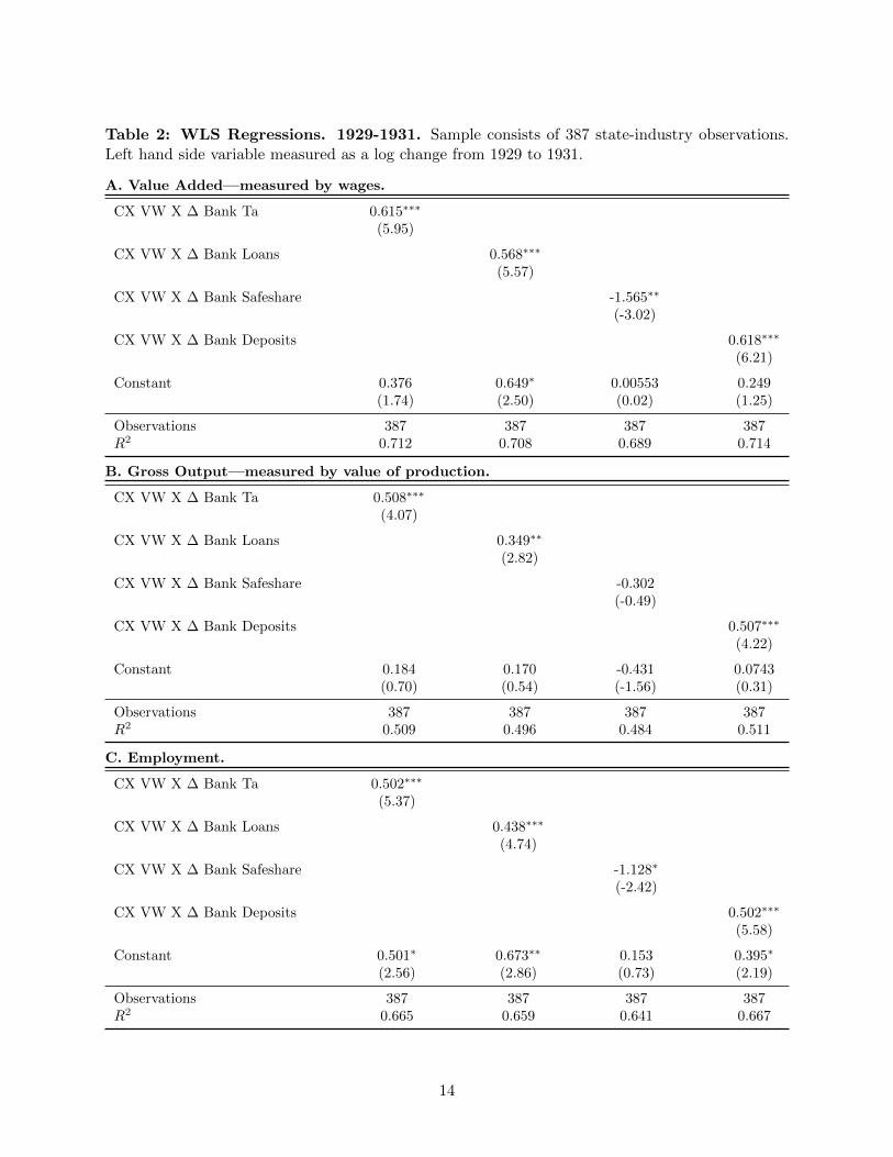
Table 2: WLS Regressions. 1929-1931. Sample consists of 387 state-industry observations.Left hand side variable measured as a log change from 1929 to 1931.

A. Value Added—measured by wages.

CX VW X ∆ Bank Ta 0.615∗∗∗

(5.95)

CX VW X ∆ Bank Loans 0.568∗∗∗

(5.57)

CX VW X ∆ Bank Safeshare -1.565∗∗

(-3.02)

CX VW X ∆ Bank Deposits 0.618∗∗∗

(6.21)

Constant 0.376 0.649∗ 0.00553 0.249(1.74) (2.50) (0.02) (1.25)

Observations 387 387 387 387R2 0.712 0.708 0.689 0.714

B. Gross Output—measured by value of production.


(4.07)

CX VW X ∆ Bank Loans 0.349∗∗

(2.82)

CX VW X ∆ Bank Safeshare -0.302(-0.49)


(4.22)

Constant 0.184 0.170 -0.431 0.0743(0.70) (0.54) (-1.56) (0.31)

Observations 387 387 387 387R2 0.509 0.496 0.484 0.511

C. Employment.


(5.37)


(4.74)

CX VW X ∆ Bank Safeshare -1.128∗

(-2.42)


(5.58)

Constant 0.501∗ 0.673∗∗ 0.153 0.395∗

(2.56) (2.86) (0.73) (2.19)

Observations 387 387 387 387R2 0.665 0.659 0.641 0.667

14

Table 3: WLS Regressions. 1919-1921. Sample consists of 387 state-industry observations.Left hand side variable measured as a log change from 1929 to 1931.


CX VW X ∆ Bank Ta 0.143(0.94)

CX VW X ∆ Bank Loans 0.0338(0.31)

CX VW X ∆ Bank Safeshare 0.292(0.95)

CX VW X ∆ Bank Deposits 0.138(1.05)

Constant -0.222 -0.220 -0.0274 -0.151(-1.27) (-1.03) (-0.12) (-0.88)

Observations 395 395 395 395R2 0.588 0.587 0.588 0.589


CX VW X ∆ Bank Ta -0.0751(-0.52)

CX VW X ∆ Bank Loans -0.157(-1.55)

CX VW X ∆ Bank Safeshare 0.597∗

(2.05)

CX VW X ∆ Bank Deposits -0.0135(-0.11)

Constant -0.430∗ -0.263 -0.142 -0.456∗∗

(-2.59) (-1.31) (-0.65) (-2.80)

Observations 394 394 394 394R2 0.597 0.599 0.601 0.596

C. Employment.

CX VW X ∆ Bank Ta 0.0174(0.13)



CX VW X ∆ Bank Deposits -0.0750(-0.66)

Constant -0.273 -0.298 -0.333 -0.284(-1.80) (-1.62) (-1.65) (-1.91)

Observations 395 395 395 395R2 0.458 0.458 0.458 0.459

15

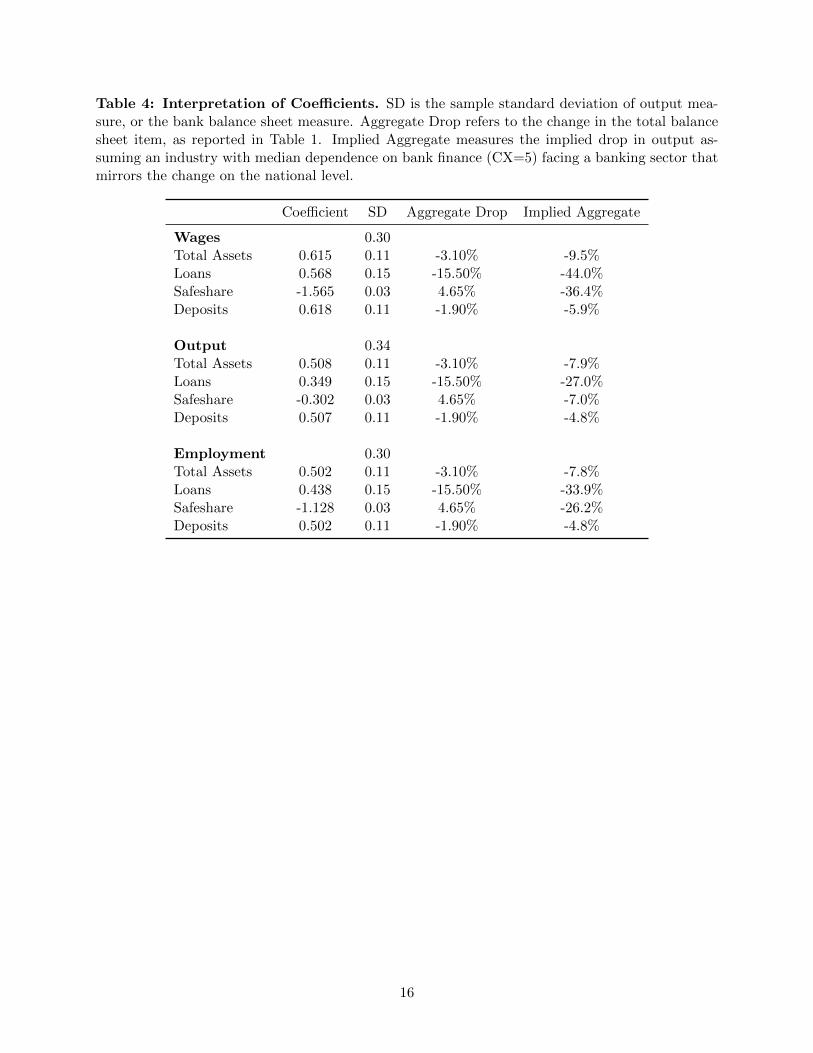
Table 4: Interpretation of Coefficients. SD is the sample standard deviation of output mea-sure, or the bank balance sheet measure. Aggregate Drop refers to the change in the total balancesheet item, as reported in Table 1. Implied Aggregate measures the implied drop in output as-suming an industry with median dependence on bank finance (CX=5) facing a banking sector thatmirrors the change on the national level.

Coefficient SD Aggregate Drop Implied Aggregate

Wages 0.30Total Assets 0.615 0.11 -3.10% -9.5%Loans 0.568 0.15 -15.50% -44.0%Safeshare -1.565 0.03 4.65% -36.4%Deposits 0.618 0.11 -1.90% -5.9%

Output 0.34Total Assets 0.508 0.11 -3.10% -7.9%Loans 0.349 0.15 -15.50% -27.0%Safeshare -0.302 0.03 4.65% -7.0%Deposits 0.507 0.11 -1.90% -4.8%

Employment 0.30Total Assets 0.502 0.11 -3.10% -7.8%Loans 0.438 0.15 -15.50% -33.9%Safeshare -1.128 0.03 4.65% -26.2%Deposits 0.502 0.11 -1.90% -4.8%

16

0

1

2

3

Bill

ions

of U

SD

1918 1920 1922 1924 1926 1928 1930 1932 1934 1936

Discount Window Borrowing

.2

.3

.4

.5

Saf

esha

re

20

40

60

80

Bill

ions

of U

SD

1918 1920 1922 1924 1926 1928 1930 1932 1934 1936

Total Assets Total Loans

Total Deposits Safeshare

2

3

3

4

Em

ploy

men

t in

Mill

ions

0

10

20

30

Bill

ions

of U

SD

1918 1920 1922 1924 1926 1928 1930 1932 1934 1936 1938

Value Added Gross Output

Employment

Figure 1: Total Borrowings of Depository Institutions from the Federal Reserve. Bank Balance Sheet Variables. StateOutput Measures.

17

References

Anbil, Sriya, “Managing stigma during a financial crisis,” Journal of Financial Economics, 2018,

130 (1), 166–181.

Armantier, Olivier, Helene Lee, and Asani Sarkar, “History of Discount Window Stigma,”

Liberty Street Economics, 2015, August 10, 2015.

Beckhart, Benjamin, The Discount Policy of the Federal Reserve System, H. Holt and Co., 1924.

Benmelech, Efraim, Carola Frydman, and Dimitris Papanikolaou, “Financial frictions

and employment during the great depression,” Technical Report, National Bureau of Economic

Research 2017.

Bernanke, Ben S, “Nonmonetary Effects of the Financial Crisis in Propagation of the Great

Depression,” American Economic Review, June 1983, 73 (3), 257–76.

Boyd, John, Gianni De Nicolo, and Elena Loukoianova, “Banking Crises and Crisis Dating:

Theory and Evidence,” IMF Working Pape WP/09/141, 2009.

Burns, Arthur and Wesley Mitchell, Measuring Business Cycles, National Burean of Economic

Research, 1946.

Calomiris, Charles, “Financial Factors in the Great Depression,” Journal of Economic Perspec-

tives, 1993, 7 (2), 61–85.

and Gary Gorton, “The Origins of Banking Panics: Models, Facts, and Bank Regulation,”

in “Financial Markets and Financial Crises,” National Bureau of Economic Research, Inc, 1991,

pp. 109–174.

Calomiris, Charles W. and Berry Wilson, “Bank Capital and Portfolio Management: The

1930s and the Scramble to Shed Risk,” The Journal of Business, July 2004, 77 (3), 421–456.

and Joseph R. Mason, “Consequences of Bank Distress During the Great Depression,” Amer-

ican Economic Review, June 2003, 93 (3), 937–947.

Caprio, Gerard, Daniela Klingebiel, Luc Laevan, and Guillermo Noguera, “Banking

Crises Database,” in “Systemic Financial Crises,” Cambridge University Press, 2005.

Carlson, Mark and Duygan-Bump Burcu, “The Tools and Transmission of Federal Reserve

Monetary Policy in the 1920s,” Fed Notes, 2016, November 22, 2016.

Clark, Evans, Financing the Consumer, Harper & Brothers, 1931.

Demirguc-Kunt, Asli and Enrica Detragiache, “The Determinants of Banking Crises: Evi-

dence from Developing and Developed Countries,” IMF Staff Papers, 1998, 45, 81–109.

18

and , “Does Deposit Insurnace Increase Banking System Stability? An Empirical Investiga-

tion,” Journal of Monetary Economics, 2002, 49, 1373–1406.

and , “Cross-Country Empirical Studies of Systemic Bank Distress: A Survey,” National

Institute of Economic Review, 2005, 192.

Dimsdale, Nicholas and Anthony Hotson, Financial Crises and Economic Activity in the

U.K. since 1825, Oxford University Press, 2004.

Friedman, Milton and Anna Schwartz, Monetary History of the United States, 1867-1960,

Princeton University Press, 1971.

Ginzberg, Eli, The Illusion of Economic Stability , Transaction, 2004.

Gorton, Gary, “Banking Panics and Business Cycles,” Oxford Economic Papers, 1988, 40 (4),

751–81.

and Don Mullineaux, “The Joint Production of Confidence: Endogenous Regulation and

Nineteenth Century Commercial Bank Clearinghouses,” Journal of Money, Credit and Banking,

1987, 19 (4), 458–68.

Laevan, Luc and Fabian Valencia, “Systemic Banking Crises: A New Database,” Working

Paper 08/224, IMF 2008.

Lee, James and Filippo Mezzanotti, “Bank Distress and Manufacturing: Evidence from the

Great Depression,” Working Paper, Northwestern, Kellogg School 2017.

McGrattan, Ellen R and Edward C Prescott, “The 1929 stock market: Irving Fisher was

right,” International Economic Review, 2004, 45 (4), 991–1009.

Meltzer, Alan, A History of the Federal Reserve, Volume 1: 1913-1951, University of Chicago

Press, 2003.

Mitchell, Wesley, “The Crisis of 1920 and the Problem of Controlling Business Cycles,” American

Economic Review, 1922, 12, 20–32.

Mladjan, Mrdjan, “Accelerating into the Abyss: Financial Dependence and the Great Depres-

sion,” Working Paper, EBS Business School 2016.

Olney, Martha L, “Avoiding Default: The Role of Credit in the Consumption Collapse of 1930,”

Quarterly Journal of Economics, 1999, 114 (1), 319–335.

Parker, H. Willis and William Steiner, Federal Reserve Banking Practice, D. Appleton and

Company, 1926.

Rajan, Raghuram and Luigi Zingales, “Financial Dependence and Growth,” American Eco-

nomic Review, 1998, 88 (3), 559–86.

19

Reinhart, Carmen and Kenneth Rogoff, “This Time is Different: A Panoramic View of Eight

Centuries of Financial Crises,” Working Paper No. 13882, NBER 2008.

Romer, Christina, “The Great Crash and the Onset of the Great Depression,” NBER Working

Papers 2639, National Bureau of Economic Research, Inc 1988.

, “The Great Crash and the Onset of the Great Depression,” The Quarterly Journal of Economics,

1990, 105 (3), 597–624.

, “The Nation in Depression,” Journal of Economic Perspectives, 1993, 7 (2), 19–39.

Rosenbloom, Joshua and William A. Sundstrom, “The Sources of Regional Variation in the

Severity of the Great Depression: Evidence from U.S. Manufacturing, 19191937,” The Journal

of Economic History, 1999, 59 (03), 714–747.

White, Eugene, “A Reinterpretation of the Banking Crisis of 1930,” Journal of Economic History,

1984, 44 (1), 119–138.

Whittlesey, C.R., “Credit Policy at the Discount Window,” Quarterly Journal of Economics,

1959, 73 (2), 207–216.

Wicker, Elmus, Federal Reserve Policy, 1917-1933, Random House, 1966.

, The Banking Panics of the Great Depression, Cambridge University Press, 1996.

, Wall Street, the Federal Reserve and Stock Market Speculation: A Retrospective, Center for

Financial Stability, 2015.

20

1930: First Modern Crisis. Online Appendix

Gary Gorton∗ Toomas Laarits† Tyler Muir‡

November 25, 2018

∗Yale University. Email: [email protected]†Yale University. Email: [email protected]‡UCLA Anderson School of Management. Email: [email protected]

1

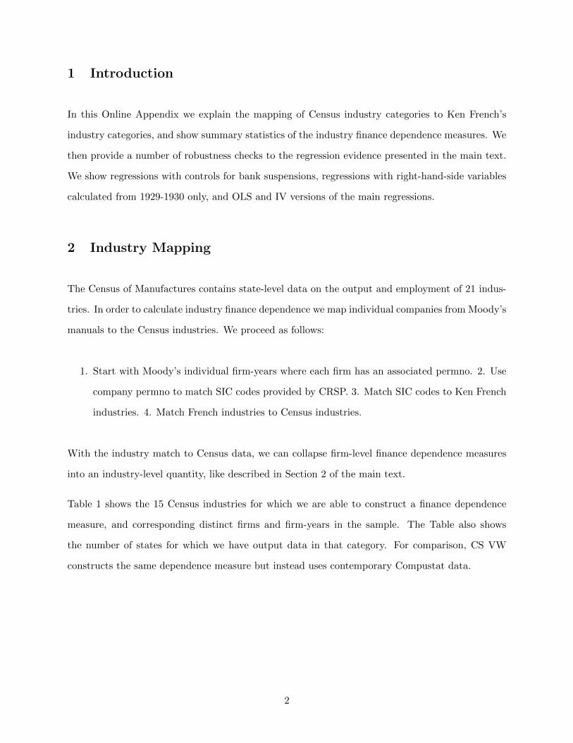
1 Introduction

In this Online Appendix we explain the mapping of Census industry categories to Ken French’s

industry categories, and show summary statistics of the industry finance dependence measures. We

then provide a number of robustness checks to the regression evidence presented in the main text.

We show regressions with controls for bank suspensions, regressions with right-hand-side variables

calculated from 1929-1930 only, and OLS and IV versions of the main regressions.

2 Industry Mapping

The Census of Manufactures contains state-level data on the output and employment of 21 indus-

tries. In order to calculate industry finance dependence we map individual companies from Moody’s

manuals to the Census industries. We proceed as follows:

1. Start with Moody’s individual firm-years where each firm has an associated permno. 2. Use

company permno to match SIC codes provided by CRSP. 3. Match SIC codes to Ken French

industries. 4. Match French industries to Census industries.

With the industry match to Census data, we can collapse firm-level finance dependence measures

into an industry-level quantity, like described in Section 2 of the main text.

Table 1 shows the 15 Census industries for which we are able to construct a finance dependence

measure, and corresponding distinct firms and firm-years in the sample. The Table also shows

the number of states for which we have output data in that category. For comparison, CS VW

constructs the same dependence measure but instead uses contemporary Compustat data.

2

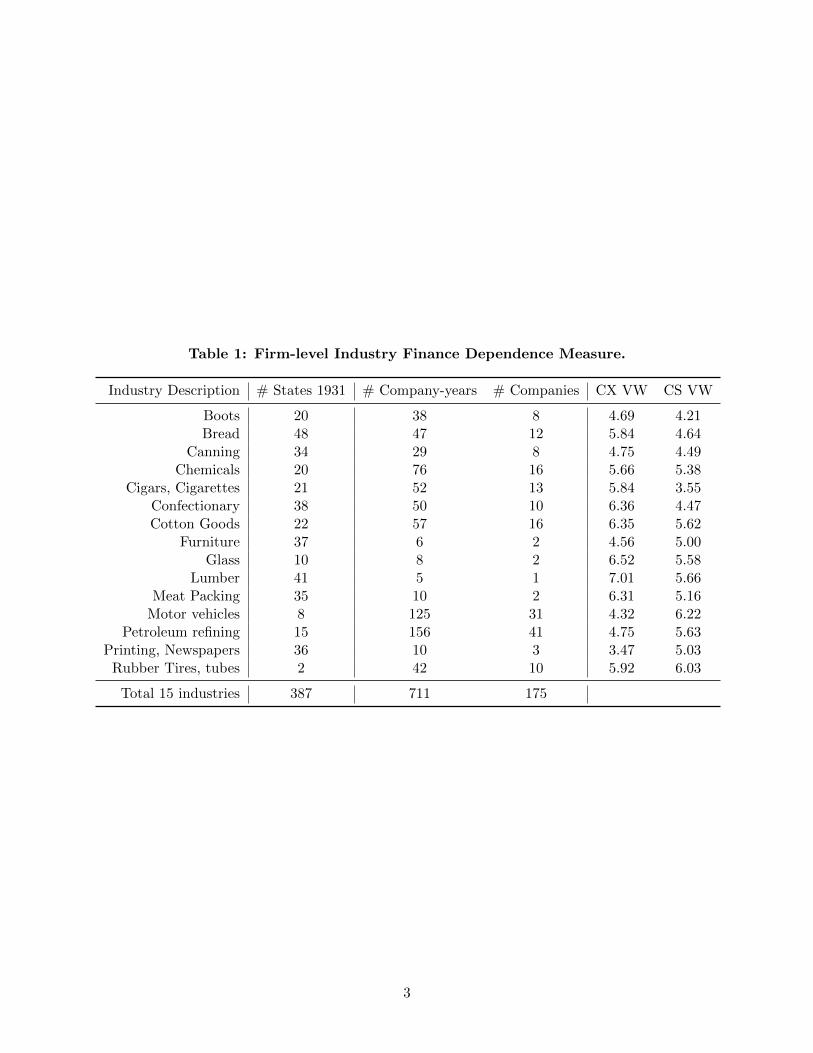
Table 1: Firm-level Industry Finance Dependence Measure.

Industry Description # States 1931 # Company-years # Companies CX VW CS VW

Boots 20 38 8 4.69 4.21Bread 48 47 12 5.84 4.64

Canning 34 29 8 4.75 4.49Chemicals 20 76 16 5.66 5.38

Cigars, Cigarettes 21 52 13 5.84 3.55Confectionary 38 50 10 6.36 4.47Cotton Goods 22 57 16 6.35 5.62

Furniture 37 6 2 4.56 5.00Glass 10 8 2 6.52 5.58

Lumber 41 5 1 7.01 5.66Meat Packing 35 10 2 6.31 5.16

Motor vehicles 8 125 31 4.32 6.22Petroleum refining 15 156 41 4.75 5.63

Printing, Newspapers 36 10 3 3.47 5.03Rubber Tires, tubes 2 42 10 5.92 6.03

Total 15 industries 387 711 175

3

3 Robustness Checks

4

Table 2: WLS Regressions 1929-1931. Controlling for amount of deposits in suspended banks.



(4.19)


(3.73)

CX VW X ∆ Bank Safeshare -1.524∗∗

(-3.01)


(4.54)

CX VW X ∆ Bank Suspended 0.191 -0.282 -1.087∗∗∗ 0.177(0.47) (-0.82) (-4.12) (0.46)

Constant 0.405 0.586∗ 0.291 0.259(1.80) (2.16) (1.23) (1.29)

Observations 387 387 387 387R2 0.712 0.709 0.705 0.715


CX VW X ∆ Bank Ta 0.621∗∗

(3.21)




(3.37)

CX VW X ∆ Bank Suspended 0.373 -0.418 -0.818∗ 0.327(0.77) (-1.01) (-2.57) (0.71)

Constant 0.240 0.0755 -0.216 0.0939(0.88) (0.23) (-0.75) (0.39)

Observations 387 387 387 387R2 0.510 0.498 0.495 0.512

C. Employment.


(4.09)


(3.21)

CX VW X ∆ Bank Safeshare -1.097∗

(-2.39)


(4.35)

CX VW X ∆ Bank Suspended 0.300 -0.199 -0.828∗∗∗ 0.268(0.82) (-0.64) (-3.47) (0.77)

Constant 0.546∗∗ 0.629∗ 0.370 0.411∗

(2.69) (2.56) (1.72) (2.27)

Observations 387 387 387 387R2 0.665 0.659 0.654 0.668

5

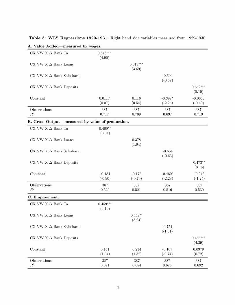
Table 3: WLS Regressions 1929-1931. Right hand side variables measured from 1929-1930.



(4.90)


(3.69)



(5.10)

Constant 0.0117 0.116 -0.397∗ -0.0663(0.07) (0.54) (-2.25) (-0.40)

Observations 387 387 387 387R2 0.717 0.709 0.697 0.719



(3.04)



CX VW X ∆ Bank Deposits 0.473∗∗

(3.15)

Constant -0.184 -0.175 -0.460∗ -0.242(-0.90) (-0.70) (-2.28) (-1.25)

Observations 387 387 387 387R2 0.529 0.521 0.516 0.530

C. Employment.


(4.19)


(3.24)



(4.39)

Constant 0.151 0.234 -0.107 0.0979(1.04) (1.32) (-0.74) (0.72)

Observations 387 387 387 387R2 0.691 0.684 0.675 0.692

6

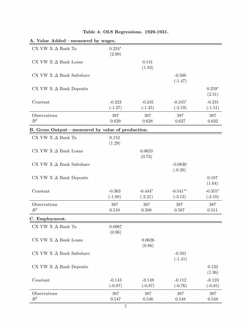
Table 4: OLS Regressions. 1929-1931.


CX VW X ∆ Bank Ta 0.224∗

(2.09)



CX VW X ∆ Bank Deposits 0.259∗

(2.51)

Constant -0.223 -0.245 -0.345∗ -0.231(-1.27) (-1.35) (-2.19) (-1.51)

Observations 387 387 387 387R2 0.629 0.628 0.627 0.632


CX VW X ∆ Bank Ta 0.152(1.29)




Constant -0.363 -0.444∗ -0.541∗∗ -0.355∗

(-1.88) (-2.21) (-3.12) (-2.10)

Observations 387 387 387 387R2 0.510 0.508 0.507 0.511

C. Employment.

CX VW X ∆ Bank Ta 0.0967(0.96)




Constant -0.143 -0.149 -0.112 -0.123(-0.87) (-0.87) (-0.76) (-0.85)

Observations 387 387 387 387R2 0.547 0.546 0.548 0.548

7

3.1 IV Regressions

In the IV specifications DEPi x Banks is instrumented by two variables:

1. Percentage of state’s bank offices that belong to branch banks in 1920 x DEPi.

2. Growth of farm land value in 1910s x DEPi.

Note that interaction terms are instrumented with the corresponding interactions. More informa-

tion on the construction of these instruments is available in Mladjan (2016).

8

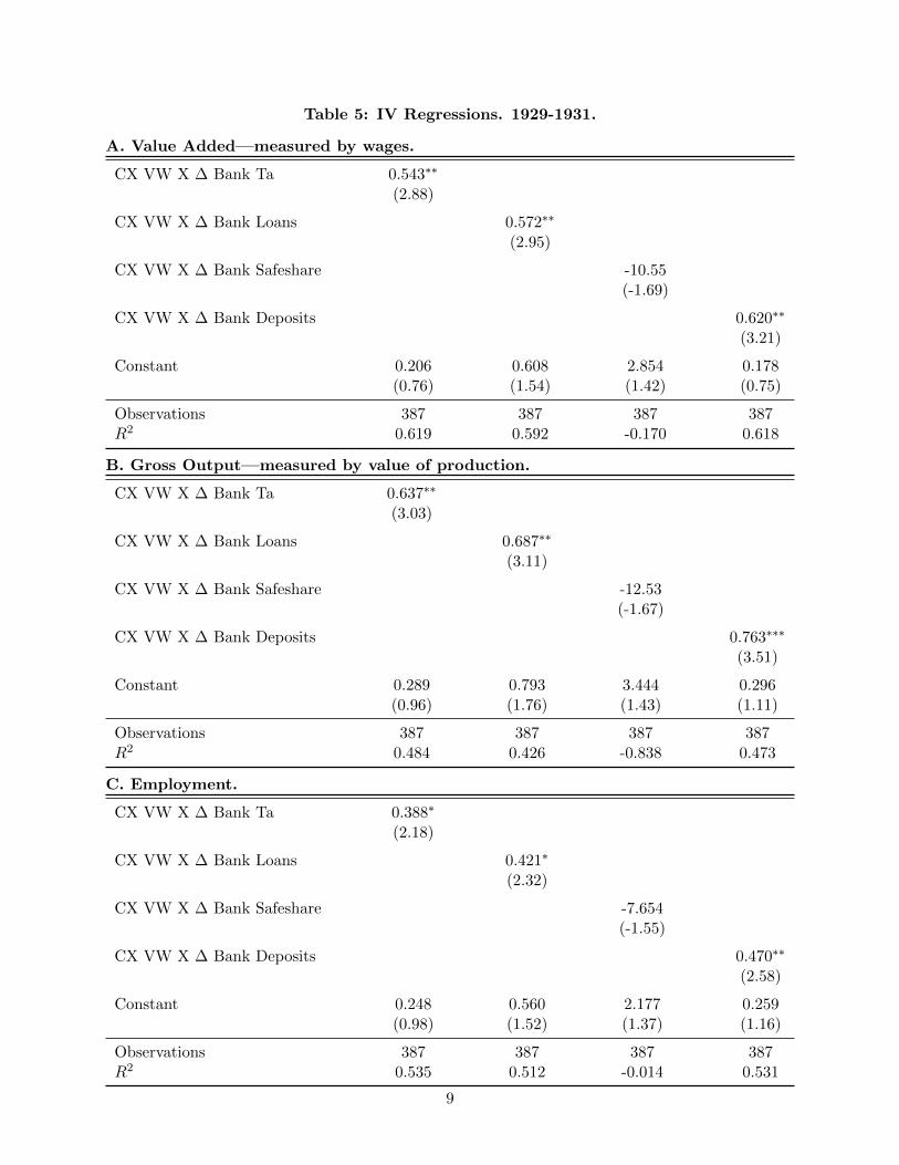
Table 5: IV Regressions. 1929-1931.



(2.88)


(2.95)



(3.21)

Constant 0.206 0.608 2.854 0.178(0.76) (1.54) (1.42) (0.75)

Observations 387 387 387 387R2 0.619 0.592 -0.170 0.618



(3.03)


(3.11)



(3.51)

Constant 0.289 0.793 3.444 0.296(0.96) (1.76) (1.43) (1.11)

Observations 387 387 387 387R2 0.484 0.426 -0.838 0.473

C. Employment.

CX VW X ∆ Bank Ta 0.388∗

(2.18)

CX VW X ∆ Bank Loans 0.421∗

(2.32)



(2.58)

Constant 0.248 0.560 2.177 0.259(0.98) (1.52) (1.37) (1.16)

Observations 387 387 387 387R2 0.535 0.512 -0.014 0.531

9

References

Mladjan, Mrdjan, “Accelerating into the Abyss: Financial Dependence and the Great Depres-

sion,” Working Paper, EBS Business School 2016.

10

1930: First Modern Crisis

Documents

Transcript of 1930: First Modern Crisis