


Image pre-processing for optimizing automated photogrammetry performances
Upload
uomustansiriyahCategory
view
1download
0
IEEE Catalog Number: ISBN:
CFP0910G-PRT 978-1-4244-3603-3
2009 International Conference on Multimedia, Signal Processing and Communication Technologies (IMPACT)
Aligarh, India 14 – 16 March 2009

VIA S. FELICE A EMA, 20
50125 FIRENZE
http://ronchi.isti.cnr.it
ATTIDELLA
FONDAZIONE
GIORGIO RONCHIFONDATA DA VASCO RONCHI
ISSN: 0391 2051
ANNO LXVII LUGLIO-AGOSTO 2012 N. 4

ANNO LXVII LUGLIO-AGOSTO 2012 N. 4
A T T I
DELLA «FONDAZIONE GIORGIO RONCHI»
EDITORIAL BOARD
Pubblicazione bimestrale - Prof. LAURA RONCHI ABBOZZO Direttore Responsabile
La responsabilità per il contenuto degli articoli è unicamente degli Autori
Iscriz. nel Reg. stampa del Trib. di Firenze N. 681 - Decreto del Giudice Delegato in data 2-1-1953
Tip. L’Arcobaleno - Via Bolognese, 54 - Firenze - Agosto 2012
Prof. Roberto BuonannoOsservatorio Astronomico di RomaMonteporzio Catorne, Roma, Italy
Prof. Ercole M. GloriaVia Giunta Pisano 2, Pisa, Italy
Prof. Franco GoriDip. di Fisica, Università Roma IIIRoma, Italy
Prof. Vishal GoyalDepartment of Computer SciencePunjabi University, Patiala, Punjab, India
Prof. Enrique Hita VillaverdeDepartamento de OpticaUniversidad de Granada, Spain
Prof. Irving KaufmanDepartment of Electrical EngineeringArizona State University, TucsonArizona, U.S.A.
Prof. Franco LottiI.F.A.C. del CNR, Via Panciatichi 64Firenze, Italy
Prof. Tommaso MaccacaroDirettore Osservatorio Astronomico di Brera,Via Brera 28, Milano
Prof. Manuel MelgosaDepartamento de OpticaUniversidad de Granada, Spain
Prof. Alberto MeschiariScuola Normale Superiore, Pisa, Italy
Prof. Riccardo PratesiDipartimento di FisicaUniversità di Firenze, Sesto Fiorentino, Italy
Prof. Adolfo PazzagliClinical PsychologyProf. Emerito Università di Firenze
Prof. Edoardo ProverbioIstituto di Astronomia e Fisica SuperioreCagliari, Italy
Prof. Andrea RomoliGalileo Avionica, Campi BisenzioFirenze, Italy
Prof. Ovidio SalvettiI.ST.I. del CNRArea della Ricerca CNR di Pisa, Pisa, Italy.
Prof. Mahipal SinghDeputy Director, CFSL, Sector 36 AChandigarh, India
Prof. Marija StrojnikCentro de Investigaciones en OpticaLeon, Gto Mexico
Prof. Jean-Luc TissotULIS, Veurey Voroize, France
Prof. Paolo VanniProfessore Emerito di Chimica Medicadell’Università di Firenze
Prof. Sergio VillaniLatvia State University, Riga, Lettonia

Camera Zoom-Dependent to estimate Object’s Range
ALI ABID D. AL- ZUKY (*), MARWAH M. ABDULSTTAR (*)
SUMMARY. – In present paper a mathematical model to estimate the real distance for a certain
object has been found based on camera Zoom where the fi tting curves for the practical data of the
object’s length in pixels (Lp) in the image plane which decreased with increasing distance (dr)
for each Zoom number of the used camera were achieved. Then fi nd the mathematical modeling
equation that relates object’s length in pixels (Lp), real distance (dr) and Zoom (Z) to estimate object
distance. A graph between object’s length in pixels and distance for 3 and 8 zoom to the theoretical
and practical results have been plotted and there was a very good similarity between them, as well
as the estimated distances were very close to the real measurements.
Key words: Optical zoom, mathematical model, object’s length in pixels, estimated dis-
tance.
1. Introduction The most important subgroup of the indirect distance measurement is the
non-contact distance measurement, as many technical applications require dis-tance measurement without any physical contact with the object. Therefore, up from the beginning of the 20th century measurement procedures using sound waves and electromagnetic waves to transfer the distance information to the measuring instrument have been developed, as in Sonar and Radar systems the distance be-tween the device and an object are derived via time of fl ight (TOF) measurement (1). The utilization of image information to contact distance measurement is com-mon practice in photogrammertry and robot vision. On other hand robot vision is capable obtaining measurement of real time basis (2). One of the most common uses for a vision system is to provide information to a robot about its environ-ment. The use of a color camera provides a low cost solution compared to devices
(*) Physics Department, College of Science, Al-Mustansiriya University, Iraq, e-mails: [email protected]; [email protected]
ATTI DELLA “FONDAZIONE GIORGIO RONCHI” ANNO LXVII, 2012 - N. 4
INSTRUMENTATION

A.A.D. Al- Zuky - M.M. Abdulsttar464
such as infrared lasers or electromagnetic sensors. However, image analysis re-quires high computational power, valuable in mobile robots, as in RoboCup (3). So signifi cant research efforts were devoted to the building of autonomous vision systems, capable of providing location and direction competencies to robots. The procedures of obstacle avoidance or object manipulation can be accomplished by integrating vital visual information derived from pose estimation techniques. Algorithms that were recently proposed utilize either visual sensor (4, 5).
Many Researchers have studied the possibility of determining object’s range and used the techniques of a variety physical foundations. Here are some of these studies addressed this issue
Lourdes de Agapito et al. (1999) (6). A linear self-calibration method is given for computing the calibration of a stationary but rotating camera where the inter-nal parameters of the camera are allowed to vary from image to image, allowing for zooming (change of focal length) and possible variation of the principal point of the camera. In order for calibration to be possible some constraints must be placed on the calibration of each image, they focus on the image of the absolute conic rather than it’s dual. This leads to a linear algorithm for the constrained calibration problem, rather than the iterative algorithms. The linear algorithm is extremely simple to implement and performs very well compared with iterative algorithms. But the method fails in the case where the computed image of the absolute conic is not positive-defi nite. However, this did not occur in their experi-ments, except in the case of critical rotation sequences for which the calibration problem is inherently unstable. So this serves as a warning that the data used does not support a useful estimate of the cameras’ calibration parameters.
Hyongsuk Kim et al. (2005) (7).They presents a new distances measurement method with the use of a single camera and a rotating mirror. The camera was placed in front of a rotating mirror acquires a sequence of refl ected images, from which distance information is extracted.
Cyrus Minwalla et al. (2009) (8) described a correlation method whereby the high precision of a commercial translator, which can be10-5 or smaller in fractional error, is transferred to the image plane of a camera system through the determination of magnifi cation and scale factor (effective focal length).
Ming-Chih Lu et al. (2010) (9) presents an image-based system for measur-ing target objects on an oblique plane based on pixel variation of CCD images for digital cameras by referencing to two arbitrarily designated points in image frames. Based on an established relationship between the displacement of the camera movement along the photographing direction and the difference in pixel counts between reference points in the images.
R. Kouskouridas et al. (2012) (10) proposed a novel algorithm for objects’ depth estimation. Moreover, they comparatively study two common two-part ap-proaches, namely the scale invariant feature transform SIFT and the speeded-up robust features algorithm, in the particular application of location assignment of an object in a scene relatively to the camera, based on the proposed algorithm.
Camera Zoom-Dependent to estimate Object’s Range 465
In the present work a digital Sony camera with zoom lens has been used to determine a mathematical model depending on Zoom process to object distance estimation.
2. Digital zoom and optical zoom
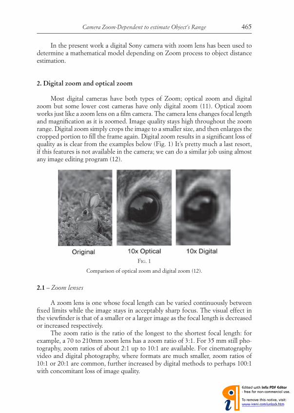
Most digital cameras have both types of Zoom; optical zoom and digital zoom but some lower cost cameras have only digital zoom (11). Optical zoom works just like a zoom lens on a fi lm camera. The camera lens changes focal length and magnifi cation as it is zoomed. Image quality stays high throughout the zoom range. Digital zoom simply crops the image to a smaller size, and then enlarges the cropped portion to fi ll the frame again. Digital zoom results in a signifi cant loss of quality as is clear from the examples below (Fig. 1) It’s pretty much a last resort, if this features is not available in the camera; we can do a similar job using almost any image editing program (12).
FIG. 1
Comparison of optical zoom and digital zoom (12).
2.1 – Zoom lenses
A zoom lens is one whose focal length can be varied continuously between fi xed limits while the image stays in acceptably sharp focus. The visual effect in the viewfi nder is that of a smaller or a larger image as the focal length is decreased or increased respectively.
The zoom ratio is the ratio of the longest to the shortest focal length: for example, a 70 to 210mm zoom lens has a zoom ratio of 3:1. For 35 mm still pho-tography, zoom ratios of about 2:1 up to 10:1 are available. For cinematography video and digital photography, where formats are much smaller, zoom ratios of 10:1 or 20:1 are common, further increased by digital methods to perhaps 100:1 with concomitant loss of image quality.
A.A.D. Al- Zuky - M.M. Abdulsttar466
The optical theory of a zoom lens is simple (though the practical designs tend to be complex): the equivalent focal length of a multi-element lens depends on the focal lengths of individual elements and their axial separations. An axial movement of one element will therefore change the focal length of the combina-tion. Such a movement coupled to a hand control would give a primitive zoom lens or strictly a varifocal lens, as is used for a slide projector (13).
For camera used in this work The Cyber-shot H70 offers a 10x, wide-angle zoom lens, a Sony G Lens composed of 10 elements in seven groups with four aspheric elements (14).
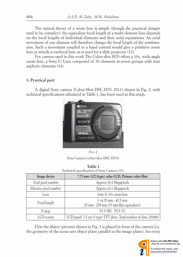
3. Practical part A digital Sony camera (Cyber-Shot DSC-H70, 2011) shown in Fig. 2, with
technical specifi cations tabulated in Table 1, has been used in this study.
FIG. 2
Sony Camera (cyber-shot DSC-H70).
Table 1Technical specifi cation of Sony Camera (15).
Image device 7.75 mm (1/2.3type) color CCD, Primary color fi lter
Total pixel number Approx.16.4 Megapixels
Effective pixel number Approx.16.1 Megapixels
Lens Sony G 10× zoom lens
Focal lengthf =4.25 mm - 42.5 mm
25 mm - 250 mm (35 mm fi lm equivalent))
F-stop F3.5 (W) - F5.5 (T)
LCD screen LCD panel: 7.5 cm (3 type) TFT drive, Total number of dots: 230400
First the object (picture) shown in Fig. 3 is placed in front of the camera (i.e. the geometry of the scene sets object plane parallel to the image plane), for every
Camera Zoom-Dependent to estimate Object’s Range 467
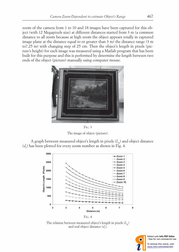
zoom of the camera from 1 to 10 and 18 images have been captured for this ob-ject (with 12 Megapixels size) at different distances started from 3 m (a common distance to all zoom because at high zoom the object appears totally in captured image plane at the distance equal to or greater than 3 m) the distance range (3 m to7.25 m) with changing step of 25 cm. Then the object’s length in pixels (pic-ture’s height) for each image was measured using a Matlab program that has been built for this purpose and this is performed by determine the length between two ends of the object (picture) manually using computer mouse.
FIG. 3
The image of object (picture).
FIG. 4
The relation between measured object’s length in pixels (Lp) and real object distance (dr).
A graph between measured object’s length in pixels (Lp) and object distance (dr) has been plotted for every zoom number as shown in Fig. 4.
A.A.D. Al- Zuky - M.M. Abdulsttar468
4. Results and discussion
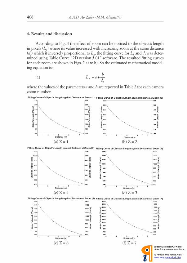
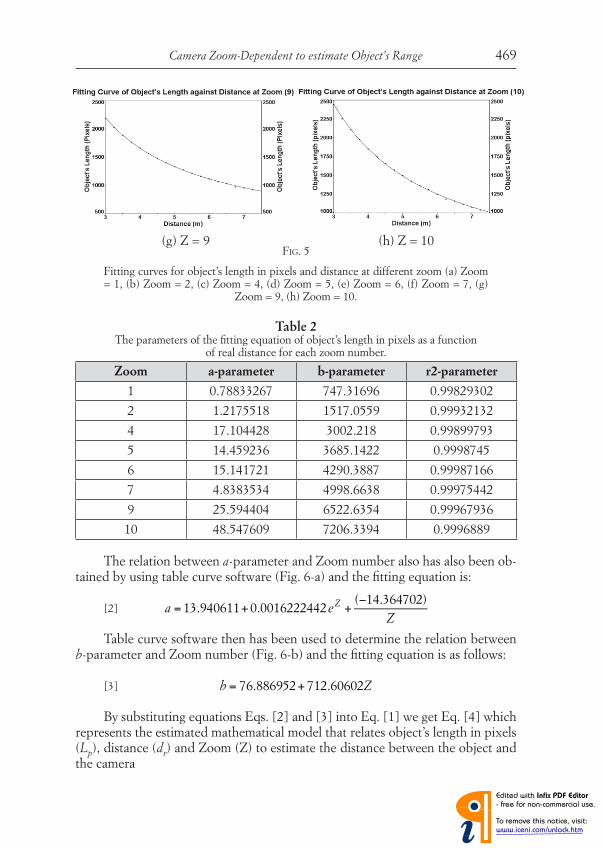
According to Fig. 4 the effect of zoom can be noticed to the object’s length in pixels (Lp) where its value increased with increasing zoom at the same distance (dr) which it inversely proportional to Lp, the fi tting curve for Lp and dr was deter-mined using Table Curve “2D version 5.01” software. The resulted fi tting curves for each zoom are shown in Figs. 5 a) to h). So the estimated mathematical model-ing equation is:
[1]
where the values of the parameters a and b are reported in Table 2 for each camera zoom number.
L p = a +
b
dr
(a) Z = 1 (b) Z = 2
(c) Z = 4 (d) Z = 5
(e) Z = 6 (f) Z = 7
Camera Zoom-Dependent to estimate Object’s Range 469
Table 2The parameters of the fi tting equation of object’s length in pixels as a function
of real distance for each zoom number.
Zoom a-parameter b-parameter r2-parameter
1 0.78833267 747.31696 0.99829302
2 1.2175518 1517.0559 0.99932132
4 17.104428 3002.218 0.99899793
5 14.459236 3685.1422 0.9998745
6 15.141721 4290.3887 0.99987166
7 4.8383534 4998.6638 0.99975442
9 25.594404 6522.6354 0.99967936
10 48.547609 7206.3394 0.9996889
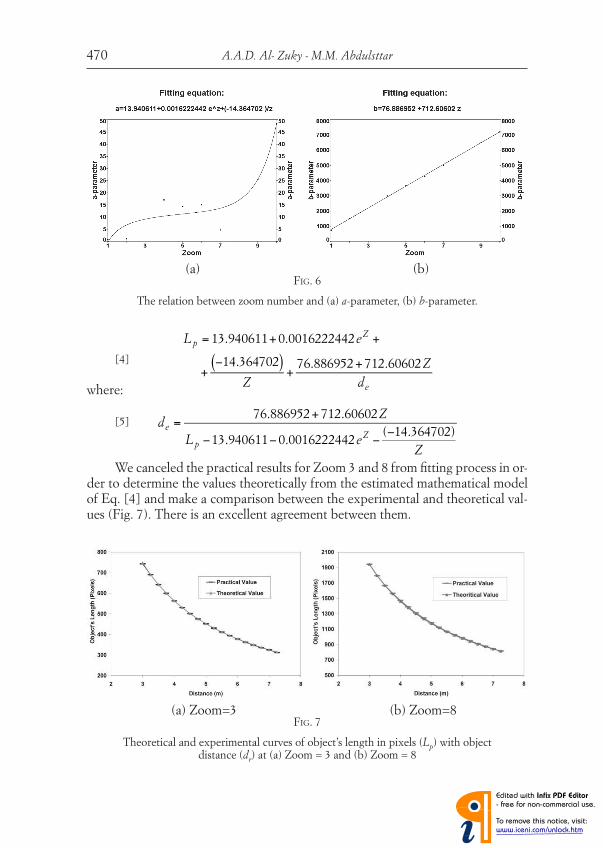
The relation between a-parameter and Zoom number also has also been ob-tained by using table curve software (Fig. 6-a) and the fi tting equation is:
[2]
Table curve software then has been used to determine the relation between b-parameter and Zoom number (Fig. 6-b) and the fi tting equation is as follows:
[3]
By substituting equations Eqs. [2] and [3] into Eq. [1] we get Eq. [4] which represents the estimated mathematical model that relates object’s length in pixels (Lp), distance (dr) and Zoom (Z) to estimate the distance between the object and the camera
FIG. 5
Fitting curves for object’s length in pixels and distance at different zoom (a) Zoom = 1, (b) Zoom = 2, (c) Zoom = 4, (d) Zoom = 5, (e) Zoom = 6, (f) Zoom = 7, (g) Zoom = 9, (h) Zoom = 10.
(g) Z = 9 (h) Z = 10
a = 13.940611+0.0016222442eZ +
(−14.364702)
Z
b = 76.886952+ 712.60602Z
A.A.D. Al- Zuky - M.M. Abdulsttar470
[4]
where:
[5]
We canceled the practical results for Zoom 3 and 8 from fi tting process in or-der to determine the values theoretically from the estimated mathematical model of Eq. [4] and make a comparison between the experimental and theoretical val-ues (Fig. 7). There is an excellent agreement between them.
(a) (b)FIG. 6
The relation between zoom number and (a) a-parameter, (b) b-parameter.
L p = 13.940611+0.0016222442eZ +
+−14.364702( )
Z+
76.886952+ 712.60602Z
de
de =76.886952+ 712.60602Z
L p −13.940611−0.0016222442eZ −(−14.364702)
Z
(a) Zoom=3 (b) Zoom=8FIG. 7
Theoretical and experimental curves of object’s length in pixels (Lp) with object distance (dr) at (a) Zoom = 3 and (b) Zoom = 8
Camera Zoom-Dependent to estimate Object’s Range 471
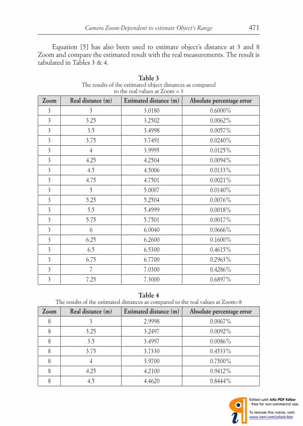
Equation [5] has also been used to estimate object’s distance at 3 and 8 Zoom and compare the estimated result with the real measurements. The result is tabulated in Tables 3 & 4.
Table 3The results of the estimated object distances as compared
to the real values at Zoom = 3
Zoom Real distance (m) Estimated distance (m) Absolute percentage error
3 3 3.0180 0.6000%
3 3.25 3.2502 0.0062%
3 3.5 3.4998 0.0057%
3 3.75 3.7491 0.0240%
3 4 3.9995 0.0125%
3 4.25 4.2504 0.0094%
3 4.5 4.5006 0.0133%
3 4.75 4.7501 0.0021%
3 5 5.0007 0.0140%
3 5.25 5.2504 0.0076%
3 5.5 5.4999 0.0018%
3 5.75 5.7501 0.0017%
3 6 6.0040 0.0666%
3 6.25 6.2600 0.1600%
3 6.5 6.5300 0.4615%
3 6.75 6.7700 0.2963%
3 7 7.0300 0.4286%
3 7.25 7.3000 0.6897%
Table 4The results of the estimated distances as compared to the real values at Zoom=8
Zoom Real distance (m) Estimated distance (m) Absolute percentage error
8 3 2.9998 0.0067%
8 3.25 3.2497 0.0092%
8 3.5 3.4997 0.0086%
8 3.75 3.7330 0.4533%
8 4 3.9700 0.7500%
8 4.25 4.2100 0.9412%
8 4.5 4.4620 0.8444%
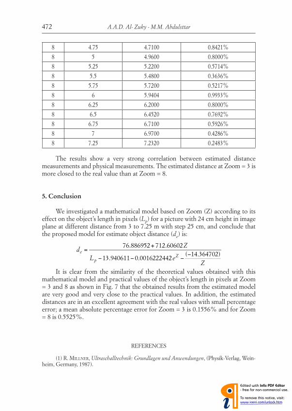
A.A.D. Al- Zuky - M.M. Abdulsttar472
8 4.75 4.7100 0.8421%
8 5 4.9600 0.8000%
8 5.25 5.2200 0.5714%
8 5.5 5.4800 0.3636%
8 5.75 5.7200 0.5217%
8 6 5.9404 0.9933%
8 6.25 6.2000 0.8000%
8 6.5 6.4520 0.7692%
8 6.75 6.7100 0.5926%
8 7 6.9700 0.4286%
8 7.25 7.2320 0.2483%
The results show a very strong correlation between estimated distance measurements and physical measurements. The estimated distance at Zoom = 3 is more closed to the real value than at Zoom = 8.
5. Conclusion
We investigated a mathematical model based on Zoom (Z) according to its effect on the object’s length in pixels (Lp) for a picture with 24 cm height in image plane at different distance from 3 to 7.25 m with step 25 cm, and conclude that the proposed model for estimate object distance (de) is:
It is clear from the similarity of the theoretical values obtained with this mathematical model and practical values of the object’s length in pixels at Zoom = 3 and 8 as shown in Fig. 7 that the obtained results from the estimated model are very good and very close to the practical values. In addition, the estimated distances are in an excellent agreement with the real values with small percentage error; a mean absolute percentage error for Zoom = 3 is 0.1556% and for Zoom = 8 is 0.5525%.
REFERENCES
(1) R. MILLNER, Ultraschalltechnik: Grundlagen und Anwendungen, (Physik-Verlag, Wein-heim, Germany, 1987).
de =76.886952+ 712.60602Z
L p −13.940611−0.0016222442eZ −(−14.364702)
Z

Camera Zoom-Dependent to estimate Object’s Range 473
(2) T. WANG, M. CHIHLU, W. WANG, C. TSAI, Distance Measurement Using Single Non-metric CCD Camera, Proc. of the 7th WSEAS Int. Conf. on Signal Processing, Computational Geometry & Artifi cial Vision, (Athens, Greece, August 24-26, 2007).
(3) A. ACEVES, M. JUNCO, J. RAMIREZ-URESTI, R. SWAIN-OROPEZA, Borregos salvajes 2003. team description, in: RoboCup: 7th Intl. Symp. & Competition. (2003).
(4) G. SCHWEIGHOFER, Robust pose estimation from a planar target, IEEE Trans. Pattern Anal. Mach. Intell., 28 (12), 2024-2030, 2006.
(5) M.K. CHANDRAKER, C. STOCK, A. PINZ, Real-time camera pose in a room, Lect. Notes Comput. Sci., 2626, 98-110, 2003.
(6) L. DE AGAPITO, R.I. HARTLEY, E. HAYMAN, Linear calibration of a rotating and zooming camera. This work was sponsored by DARPA contract F33615-94-C-1549, Dept. of Engine-ering, Oxford University, and G.E. Corporate Research and Development, 1ResearchCircle, Niskayuna, NY 12309, 1999.
(7) H. KIM, C. SHIN LIN, J. SONG, H. CHAE, Distance Measurement Using a Single Camera with a Rotating Mirror, Intern. J. of Control, Automation, and Systems, 3 (4), 542-551, Decem-ber 2005.
(8) C. MINWALLA, E. SHEN, P. THOMAS, R. HORNSEY, Correlation-Based Measurements of Camera Magnifi cation and Scale Factor, IEEE Sensor J., 9 (6), 699-706, June 2009.
(9) M. CHIH LU, C. CHIEN HSU, Y. YU LU, Distance and angle measurement of distant objects on an oblique plane based on pixel variation on CCD image, IEEE Instrumentation and Measurement Technology Conf. (12 MTC 2010), pp. 318-322.
(10) R. KOUSKOURIDAS, A. GASTERATOS, E. BADEKAS, Evaluation of two-part algorithms for object’s depth estimation, The Institution of Engineering and Technology, IET, Computer Vision, 6 (1), 70-78, 2012.
(11) Digital camera basics http://www.rrlc.org [visited: December 2011].(12) Digital Cameras - A beginner’s guide by Bob Atkins, 2003, homepage, http://www.
photo.net [visited: May 2012].(13) R.E. JACOBSON, S.F. RAY, G.G. ATTRIDGE, N.R. AXFORD, The Manual of Photography:
photographic and Digital Imaging, 9th Ed. (Focal Press, 2000), p. 95.(14) http://www.imaging-resource.com [visited: April 2012].(15) Training guide, Cyber-shot® Digital Still Cameras 2011.

ATTI DELLA “FONDAZIONE GIORGIO RONCHI” ANNO LXVII, 2012 - N. 4
INDEX
Instrumentation A.A.D. AL-ZUKY, M.M. ABDULSTTAR, Camera Zoom-Dependent to estimate Object’s Range
History of Mathematics A. DRAGO Antonino, La geometria non euclidea come la più importante crisi nei fondamenti della matematica moderna
History of ScienceM.T. MAZZUCATO, Ignazio Porro: un geniale ma poco conosciuto ottico
LaserM.F.H. AL-KADHEMY, E.M. ABWAAN, M.A.M. HASSAN, Microstructure Be-havior of Laser Dye Fluorescein Doped PMMA Thin FilmsS.M. ARIF, B.R. MAHDI, A. ABADI, A. JABAR, S.M. ALI S.M., A Compact Syn-chronous UV-IR Laser System with Unifi ed Electronic Circuit of Blumlein Type.
MaterialsA. HASHIM, Preparation and Study of Electrical Properties of (PS- AlCl3.6H2O) CompositesA. HASHIM, Effect of Silver Carbonate on electrical properties of PS-AgCO3 com-posites
Nuclear PhysicsM.H. JASIM, Z.A. DAKHIL, R.S. AHMED, The internal transition rates of pre-equilibrium nuclear reactions in 232Th
OphthalmologyM.F. ABBAS, The effect of hyperthyroidism on visual acuity and refractive errors
Solar PanelsN.K. KASIM, A.J. AL-WATTAE, K.K. ABBAS, A.F. ATWAN, Evaluating the per-formance of fi xed solar panels relative to the tracking Solar Panels under natural de-position of dust
Strip LinesA.A. AZEEZ BARZINJY, Theoretical analysis of normal and superconducting strip-line parameters
Thin Films N.F. HABUBI, S.S. CHIAD, F.H. AHMED, A.S. MAHDI, Gamma-Radiation Ef-fects on Some Optical Constants of CuS Thin Films
VarietyC.M. ROSITANI, L’uomo Vasco Ronchi
Pag. 463
» 475
» 499
» 517
» 525
» 529
» 535
» 539
» 553
» 561
» 577
» 593
» 601

1 23
Journal of Optics ISSN 0972-8821Volume 41Number 1 J Opt (2012) 41:54-59DOI 10.1007/s12596-012-0062-4
Scattering effects upon test image inside adesigning system facing the equator
Ali A. D. Al-Zuky, Amal M. Al-Hillou &Fatin E. M. Al-Obaidi

1 23
Your article is protected by copyright and all
rights are held exclusively by Optical Society
of India. This e-offprint is for personal use only
and shall not be self-archived in electronic
repositories. If you wish to self-archive your
work, please use the accepted author’s
version for posting to your own website or
your institution’s repository. You may further
deposit the accepted author’s version on
a funder’s repository at a funder’s request,
provided it is not made publicly available until
12 months after publication.
RESEARCH ARTICLE
Scattering effects upon test image inside a designingsystem facing the equator
Ali A. D. Al-Zuky & Amal M. Al-Hillou &
Fatin E. M. Al-Obaidi
Received: 21 June 2010 /Accepted: 20 January 2012 /Published online: 15 February 2012# Optical Society of India 2012
Abstract This paper describes an experiment to
investigate the influence of scattering effects upon
test image. The image is located inside an optical
built system facing the equator. Scattering effects
have been distinguished and tested by analyzing
the whole images that captured at regular intervals.
The analyses process is performed by measuring the
average intensity values of the RGB-bands for a certain
selected line of the captured images. These measure-
ments are executed in Baghdad city at a clear day. At
certain intervals, Rayleigh and Mie scattering are the
dominant effects which works individually while at other
periods, the previous scattering types work together.
Keywords Rayleigh scattering .Mie scattering .
RGB bands . Intensity measurement
Introduction
Color of the atmosphere is much influenced by the
spectrum of the sunlight, scattering/absorption effects
due to particles in the atmosphere, reflected light from
the earth’s surface and the relationship between the
sun’s position and the viewpoint (and direction). The
sunlight entering the atmosphere is scattered/absorbed
by air molecules, aerosol and ozone layers. The
characteristics of scattering depend on the size of
particles in the atmosphere. Scattering by small
particles such as air molecules is called Rayleigh
scattering and scattering by aerosols such as dust
is called Mie scattering. Light is attenuated by both
scattering and absorption [1].
Physical processes in the scene have not been a
strong point of interest in the traditional line of
computer vision research. Recently, work in image
understanding has started to use intrinsic models
of physical processes in the scene to analyze intensity or
color variation in the image[2].
This paper presents an approach to image under-
standing that uses intensity measurements and
shows how the intensity varies in the image during
the natural diurnal variation of sunlight in the case
of a clear day.
Scattering regimes
When the solar radiation in the form of electromagnetic
wave hits a particle, a part of the incident energy is
scattered in all directions as diffused radiation. All small
or large particles in nature scatter radiation [3]. The
scattering of the incident electromagnetic wave by a
gas-phase molecule or by a particle mainly depends on
J Opt (January–March 2012) 41(1):54–59
DOI 10.1007/s12596-012-0062-4
A. A. D. Al-Zuky :A. M. Al-Hillou :
F. E. M. Al-Obaidi (*)
Department of Physics, College of Science,
Al-Mustansiriyah University,
P.O. Box no.(46092), Baghdad, Iraq
e-mail: [email protected]
A. A. D. Al-Zuky
e-mail: [email protected]
A. M. Al-Hillou
e-mail: [email protected]
Author's personal copy
the comparison between the wavelength (l) and the
characteristic size (d). We recall that, d ffi 0:1 nm for a
gas-phase molecule, d∈[10nm, 10μm] for an aerosol
and d∈[10, 100] μm for a liquid water drop. The wide
range covered by the body size will induce different
behaviors. Three scattering regimes are usually distin-
guished; Rayleigh scattering (typically for gases), scat-
tering represented by the optical geometry’s laws
(typically for liquid water drops) and the so-called
Mie-scattering (for aerosols) [4].
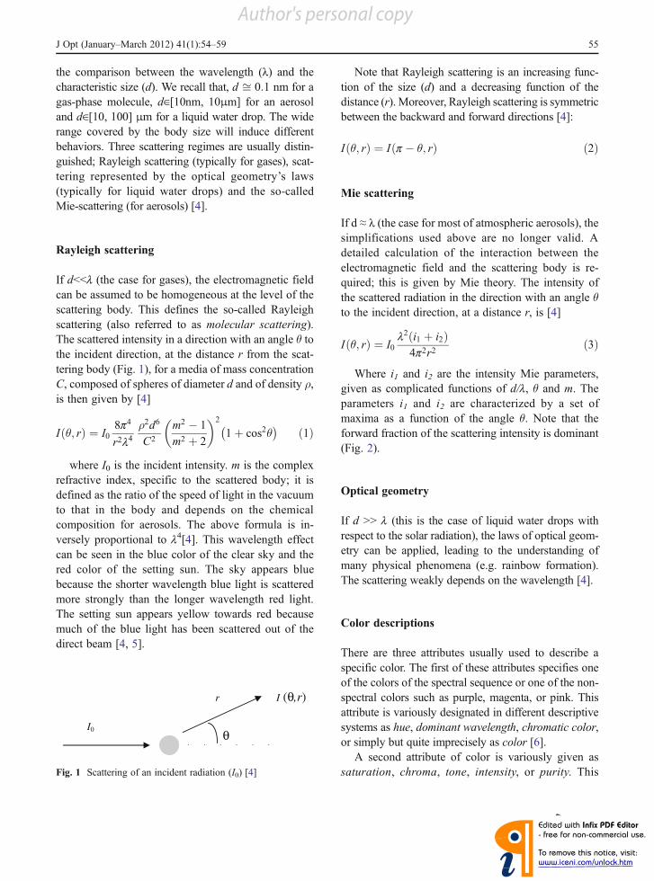
Rayleigh scattering
If d<<l (the case for gases), the electromagnetic field
can be assumed to be homogeneous at the level of the
scattering body. This defines the so-called Rayleigh
scattering (also referred to as molecular scattering).
The scattered intensity in a direction with an angle θ to
the incident direction, at the distance r from the scat-
tering body (Fig. 1), for a media of mass concentration
C, composed of spheres of diameter d and of density ρ,
is then given by [4]
I θ; rð Þ ¼ I08p4
r2l4ρ2d6
C2
m2 � 1
m2 þ 2
� �2
1þ cos2θ� �
ð1Þ
where I0 is the incident intensity. m is the complex
refractive index, specific to the scattered body; it is
defined as the ratio of the speed of light in the vacuum
to that in the body and depends on the chemical
composition for aerosols. The above formula is in-
versely proportional to l4[4]. This wavelength effect
can be seen in the blue color of the clear sky and the
red color of the setting sun. The sky appears blue
because the shorter wavelength blue light is scattered
more strongly than the longer wavelength red light.
The setting sun appears yellow towards red because
much of the blue light has been scattered out of the
direct beam [4, 5].
Note that Rayleigh scattering is an increasing func-
tion of the size (d) and a decreasing function of the
distance (r). Moreover, Rayleigh scattering is symmetric
between the backward and forward directions [4]:
I θ; rð Þ ¼ I p � θ; rð Þ ð2Þ
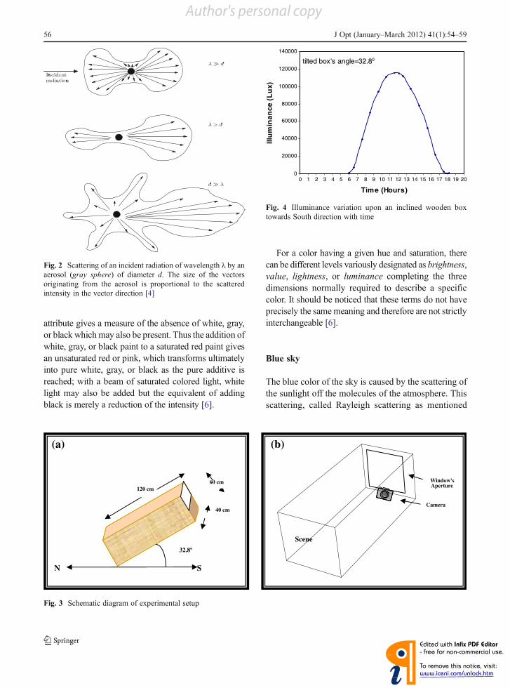
Mie scattering
If d ≈ l (the case for most of atmospheric aerosols), the
simplifications used above are no longer valid. A
detailed calculation of the interaction between the
electromagnetic field and the scattering body is re-
quired; this is given by Mie theory. The intensity of
the scattered radiation in the direction with an angle θ
to the incident direction, at a distance r, is [4]
I θ; rð Þ ¼ I0l2 i1 þ i2ð Þ
4p2r2ð3Þ
Where i1 and i2 are the intensity Mie parameters,
given as complicated functions of d/l, θ and m. The
parameters i1 and i2 are characterized by a set of
maxima as a function of the angle θ. Note that the
forward fraction of the scattering intensity is dominant
(Fig. 2).
Optical geometry
If d >> l (this is the case of liquid water drops with
respect to the solar radiation), the laws of optical geom-
etry can be applied, leading to the understanding of
many physical phenomena (e.g. rainbow formation).
The scattering weakly depends on the wavelength [4].
Color descriptions
There are three attributes usually used to describe a
specific color. The first of these attributes specifies one
of the colors of the spectral sequence or one of the non-
spectral colors such as purple, magenta, or pink. This
attribute is variously designated in different descriptive
systems as hue, dominant wavelength, chromatic color,
or simply but quite imprecisely as color [6].
A second attribute of color is variously given as
saturation, chroma, tone, intensity, or purity. This
I0
r
θ
I (θ,r)
Fig. 1 Scattering of an incident radiation (I0) [4]
J Opt (January–March 2012) 41(1):54–59 55
Author's personal copy
attribute gives a measure of the absence of white, gray,
or black whichmay also be present. Thus the addition of
white, gray, or black paint to a saturated red paint gives
an unsaturated red or pink, which transforms ultimately
into pure white, gray, or black as the pure additive is
reached; with a beam of saturated colored light, white
light may also be added but the equivalent of adding
black is merely a reduction of the intensity [6].
For a color having a given hue and saturation, there
can be different levels variously designated as brightness,
value, lightness, or luminance completing the three
dimensions normally required to describe a specific
color. It should be noticed that these terms do not have
precisely the same meaning and therefore are not strictly
interchangeable [6].
Blue sky
The blue color of the sky is caused by the scattering of
the sunlight off the molecules of the atmosphere. This
scattering, called Rayleigh scattering as mentioned
Fig. 2 Scattering of an incident radiation of wavelength l by an
aerosol (gray sphere) of diameter d. The size of the vectors
originating from the aerosol is proportional to the scattered
intensity in the vector direction [4]
Scene
Window's Aperture
Camera
32.8º
SN
120 cm
40 cm
60 cm
(a) (b)
Fig. 3 Schematic diagram of experimental setup
tilted box's angle=32.80
0
20000
40000
60000
80000
100000
120000
140000
0 1 2 3 4 5 6 7 8 9 10 11 12 13 14 15 16 17 18 19 20
Time (Hours)
Illu
min
an
ce
(L
ux
)
Fig. 4 Illuminance variation upon an inclined wooden box
towards South direction with time
56 J Opt (January–March 2012) 41(1):54–59
Author's personal copy
before is more effective at short wavelengths. There-
fore the light scattered down to the earth at a large
angle with respect to the direction of the sun’s light is
predominantly in the blue end of the spectrum. Noting
that the blue of the sky is more saturated when you
look further from the sun. The almost white scattering
near the sun can be attributed to Mie scattering, which
is not very wavelength dependent. The mixture of
white light with the blue gives a less saturated blue [7].
Intensity image measurement
An image is an array of measured light intensities and
it is a function of the amount of light reflected from the
objects in the scene [8]. The color of the a pixel is
defined by the intensities of the red (R), green (G) and
blue (B) primaries. These intensity values are called
the display tristimulus values R, G and B [6].
In order to measure the intensity, we have been
used the following equation [9–11].
I i; jð Þ ¼ 0:3Rþ 0:59Gþ 0:11B ð4Þ
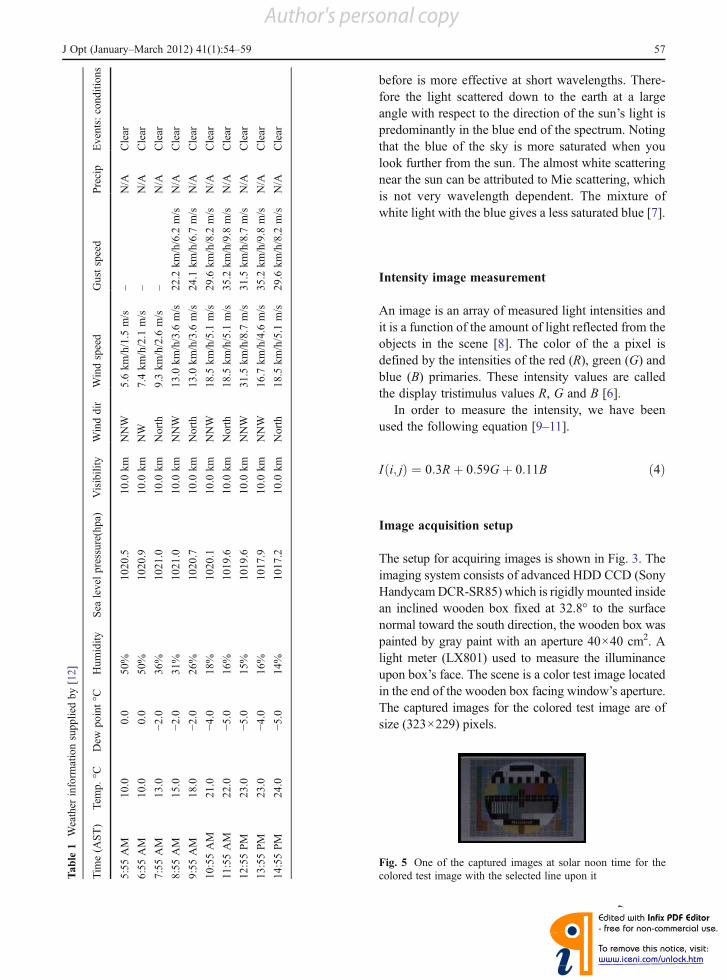
Image acquisition setup
The setup for acquiring images is shown in Fig. 3. The
imaging system consists of advanced HDD CCD (Sony
HandycamDCR-SR85) which is rigidly mounted inside
an inclined wooden box fixed at 32.8° to the surface
normal toward the south direction, the wooden box was
painted by gray paint with an aperture 40×40 cm2. A
light meter (LX801) used to measure the illuminance
upon box’s face. The scene is a color test image located
in the end of the wooden box facing window’s aperture.
The captured images for the colored test image are of
size (323×229) pixels.
Fig. 5 One of the captured images at solar noon time for the
colored test image with the selected line upon itTable
1Weather
inform
ationsupplied
by[12]
Tim
e(A
ST)
Tem
p.°C
Dew
point°C
Humidity
Sea
level
pressure(hpa)
Visibility
Winddir
Windspeed
Gustspeed
Precip
Events:conditions
5:55AM
10.0
0.0
50%
1020.5
10.0
km
NNW
5.6
km/h/1.5
m/s
–N/A
Clear
6:55AM
10.0
0.0
50%
1020.9
10.0
km
NW
7.4
km/h/2.1
m/s
–N/A
Clear
7:55AM
13.0
−2.0
36%
1021.0
10.0
km
North
9.3
km/h/2.6
m/s
–N/A
Clear
8:55AM
15.0
−2.0
31%
1021.0
10.0
km
NNW
13.0
km/h/3.6
m/s
22.2
km/h/6.2
m/s
N/A
Clear
9:55AM
18.0
−2.0
26%
1020.7
10.0
km
North
13.0
km/h/3.6
m/s
24.1
km/h/6.7
m/s
N/A
Clear
10:55AM
21.0
−4.0
18%
1020.1
10.0
km
NNW
18.5
km/h/5.1
m/s
29.6
km/h/8.2
m/s
N/A
Clear
11:55AM
22.0
−5.0
16%
1019.6
10.0
km
North
18.5
km/h/5.1
m/s
35.2
km/h/9.8
m/s
N/A
Clear
12:55PM
23.0
−5.0
15%
1019.6
10.0
km
NNW
31.5
km/h/8.7
m/s
31.5
km/h/8.7
m/s
N/A
Clear
13:55PM
23.0
−4.0
16%
1017.9
10.0
km
NNW
16.7
km/h/4.6
m/s
35.2
km/h/9.8
m/s
N/A
Clear
14:55PM
24.0
−5.0
14%
1017.2
10.0
km
North
18.5
km/h/5.1
m/s
29.6
km/h/8.2
m/s
N/A
Clear
J Opt (January–March 2012) 41(1):54–59 57
Author's personal copy
1PM1(5)
0
50
100
150
200
250
0 100 200 300 400
x
I(x,y
1)
R-Band G-Band
B-Band
2PM1(5)
0
50
100
150
200
250
0 100 200 300 400
x
I(x,y
1)
R-Band G-Band
B-Band
3PM1(5)
0
50
100
150
200
250
0 100 200 300 400
x
I(x,y
1)
R-Band
G-Band
B-Band
4PM1(5)
0
50
100
150
200
250
0 100 200 300 400
x
I(x,y
1)
R-Band G-Band
B-Band
5PM1(5)
0
50
100
150
200
250
0 100 200 300 400
x
I(x,y
1)
R-Band G-Band
B-Band
6PM1(5)
0
50
100
150
200
250
0 100 200 300 400
x
I(x,y
1)
R-Band G-Band
B-Band
BRIS1(5)
0
50
100
150
200
250
0 100 200 300 400
x
I(x,y
1)
R-Band G-Band
B-Band
7AM1(5)
0
50
100
150
200
250
0 100 200 300 400
x
I(x,y
1)
R-Band G-Band
B-Band
8AM1(5)
0
50
100
150
200
250
0 100 200 300 400
x
I(x,y
1)
R-Band G-Band
B-Band
9AM1(5)
0
50
100
150
200
250
0 100 200 300 400
x
I(x,y
1)
R-Band G-Band
B-Band
10AM1(5)
0
50
100
150
200
250
0 100 200 300 400
x
I(x,y
1)
R-Band G-Band
B-Band
11AM1(5)
0
50
100
150
200
250
0 100 200 300 400
x
I(x,y
1)
R-Band G-Band
B-Band
12PM1(5)
0
50
100
150
200
250
0 100 200 300 400
x
I(x,y
1)
R-Band G-Band
B-Band
BNOON1(5)
0
50
100
150
200
250
0 100 200 300 400
x
I(x,y
1)
R-Band G-Band
B-Band
BSET1(5)
0
50
100
150
200
250
0 100 200 300 400
x
I(x,y
1)
R-Band G-Band
B-Band
(a) (b)
(i)
(l)
(h)
(f)(d) (e)
(c)
(g)
(j) (k)
(m) (n) (o)
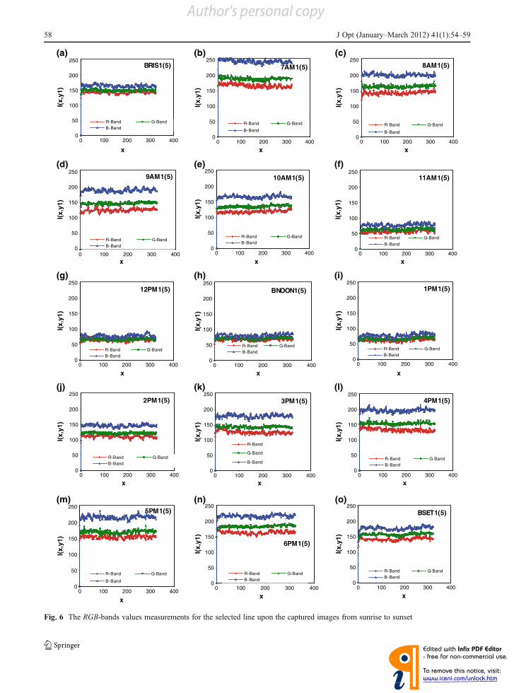
Fig. 6 The RGB-bands values measurements for the selected line upon the captured images from sunrise to sunset
58 J Opt (January–March 2012) 41(1):54–59
Author's personal copy
Acquisition data
At Monday, March 22, 2010, images were captured at
regular intervals (from sunrise to sunset) in Baghdad
city (Latitude 33.2°N, Longitude 44.2°E). The illumi-
nance measurements upon box’s face is shown in
Fig. 4, weather information obtained from [12] and
is shown in Table 1.
Experimental results
Figure 5 shows one of the captured images with the
selected line location upon it. The line was selected in
a white region to analyze the illuminance distribution
for a homogeneous region upon the image. Figure 6
shows the corresponding intensities to the previous
selected line from sunrise to sunset. The x in intensity
figures denotes line’s position upon the color test
image while I(x,y1) is line’s corresponding intensity.
Conclusions
Due to the scattering effects, it is clear to the eye that the
progression in daytime leads to give us different sunlight
colors. Measurements of the color were made at each
time based on the presence of amounts of red, green and
blue. Figure 6a & o are the measured intensities at
sunrise/sunset times with enough dark exposure, i.e.,
the light from the sun does not saturate the CCD detector
(Rayleigh scattering). The green was significantly
brighter than the red and the blue is the brightest one.
This is consistent with Rayleigh scattering which
emphasizes the shorter wavelengths. The highest satu-
ration occurred at early morning hour due to Rayleigh
scattering intensity value for B-band ≈ 250 as shown in
Fig. 6b. The color after that becoming less saturated.
This can be interpreted as blue mixed with an increasing
fraction of white light, which is consistent with the light
being a combination of Rayleigh and Mie scattering in
intermediate times to the solar noon shown in Fig. 6c, d,
e, j, k, l, m, n. As we approach the normality state of the
sun’s direction to the acqusition system (at solar noon
explained in Fig. 6g & h), Mie scattering accounts for a
larger fraction of the total light and the Mie scattered
light is essentially white (intensity value ≈ 50 for all
bands at solar noon).
Thus, our measurement for intensity gives us an
essential tool to explain the physical phenomena
around us (i.e. scattering effects).
References
1. T. Nishita, T. Sirai, K. Tadamura, E. Nakamae, “Display of
the earth taking into account atmospheric scattering”, Inter-
national Conference on Computer Graphics and Interactive
Techniques Proceedings of the 20th Annual Conference on
Computer Graphics and Interactive Techniques, (1993)
2. G.J. Klinker, S.A. Shafer, T. Kanade, A physical approach
to color image understanding. Int. J. Comput. Vis. 4, 7–38
(1990)
3. Z. Şen, “Solar energy in progress and future research
trends” (Elsevier Ltd., 2004)
4. B. Sportisse, “Fundamentals in air pollution from process
to modelling” (Springer Science + Business Media B. V.,
2010)
5. R. H. B. Exell, “The intensity of solar radiation” (King
Mongkut’s University of Technology Thonburi, 2000)
6. K. Nassau, “Color for science, art and technology” (Elsevier
Science B. V., 1998)
7. R. Nave, “Characterizing color” (HyperPhysics, Depart-
ment of Physics and Astronomy, Georgia State University,
2001)
8. J. R. Parker, “Algorithms for image processing and computer
vision” (John Wiley & Sons, Inc., 1997)
9. C. B. Neal, “Television colorimetry for receiver engineers”
(IEEE Trans. Broadcast Tele. Receiver, 1973)
10. F. E. M. Al-Obaidi, “A study of diurnal variation of solar
radiation over Baghdad City” (Ph.D thesis, Department of
Physics, College of Science, Al-Mustansiriyah University,
2011)
11. H.Maruyama,M. Ito, F. Arai, T. Fukuda, “On-chip fabrication
of optical multiple microsensor using functional gel-
microbead”. IEEE. (2007)
12. Weather Underground home page. (web site: http://www.
wunderground.com)
J Opt (January–March 2012) 41(1):54–59 59
Author's personal copy

ANNO LXVII MARZO-APRILE 2012 N. 2
A T T I
DELLA «FONDAZIONE GIORGIO RONCHI»
EDITORIAL BOARD
Pubblicazione bimestrale - Prof. LAURA RONCHI ABBOZZO Direttore Responsabile
La responsabilità per il contenuto degli articoli è unicamente degli Autori
Iscriz. nel Reg. stampa del Trib. di Firenze N. 681 - Decreto del Giudice Delegato in data 2-1-1953
Tip. L’Arcobaleno - Via Bolognese, 54 - Firenze - Aprile 2012
Prof. Roberto BuonannoOsservatorio Astronomico di RomaMonteporzio Catorne, Roma, Italy
Prof. Ercole M. GloriaVia Giunta Pisano 2, Pisa, Italy
Prof. Franco GoriDip. di Fisica, Università Roma IIIRoma, Italy
Prof. Vishal GoyalDepartment of Computer SciencePunjabi University, Patiala, Punjab, India
Prof. Enrique Hita VillaverdeDepartamento de OpticaUniversidad de Granada, Spain
Prof. Franco LottiI.F.A.C. del CNR, Via Panciatichi 64Firenze, Italy
Prof. Tommaso MaccacaroDirettore Osservatorio Astronomico di Brera,Via Brera 28, Milano
Prof. Manuel MelgosaDepartamento de OpticaUniversidad de Granada, Spain
Prof. Alberto MeschiariScuola Normale Superiore, Pisa, Italy
Prof. Riccardo PratesiDipartimento di FisicaUniversità di Firenze, Sesto Fiorentino, Italy
Prof. Adolfo PazzagliClinical PsychologyProf. Emerito Università di Firenze
Prof. Edoardo ProverbioIstituto di Astronomia e Fisica SuperioreCagliari, Italy
Prof. Andrea RomoliGalileo Avionica, Campi BisenzioFirenze, Italy
Prof. Ovidio SalvettiI.ST.I. del CNRArea della Ricerca CNR di Pisa, Pisa, Italy
Prof. Mahipal SinghDeputy Director, CFSL, Sector 36 AChandigarh, India
Prof. Shyam SinghPhysical DepartmentUniversity of Namibia
Prof. Marija StrojnikCentro de Investigaciones en OpticaLeon, Gto Mexico
Prof. Jean-Luc TissotULIS, Veurey Voroize, France
Prof. Paolo VanniProfessore Emerito di Chimica Medicadell’Università di Firenze
Prof. Sergio VillaniLatvia State University, Riga, Lettonia
Diurnal daylight illuminance measurements for a tilted optical system
FATIN E.M. AL-OBAIDI (*), ALI A.D. AL-ZUKY (*), AMAL M. AL-HILLOU (*)
SUMMARY. – The variation in sky luminance caused by weather, season and time of the day are
diffi cult to codify. To meet this, a tilted system with window’s aperture of size 40×40 and 10×10 cm2,
facing the south direction have been optically designed for studying sky illuminance with weather,
season and time parameters. An exterior and interior illuminance have been measured by using two
sensors, LX801 and Silicon NPN Phototransistors. Results show that tilt angle plays the main role
in illuminance values, reaching its maximum exterior value on 21 March using an angle near site’s
latitude, while a maximum interior one is recorded on November 27 by adopting another angle.
1. Introduction
The sun releases a power fl ux of 63 MW, equivalent to six thousand million lumens, for every square meter of its surface area. Of this around 134 kilo lux reaches the earth’s outer atmosphere. The atmosphere absorbs about 20% of this light and refl ects 25% back into outer space. A fraction of the remaining 55% reaches the ground directly, as sunlight, the rest is fi rst diffused by the atmosphere (skylight) - these two together make up daylight (1).
The amount of daylight received on the ground varies with location. Lati-tude, coastal or inland situation, climate and air quality affect the intensity and duration of daylight. In addition, the quantity and quality of daylight in any one place varies with the hour of the day, time of year and meteorological conditions (1). The actual daylight illuminance of a room is found to be related to the lumi-nance pattern of the sky in the direction of window’s view (2).
(*) Dept. of Physics, College of Science, Al-Mustansiriyah University, Baghdad, Iraq; P.O. Box no.46092; e-mails: [email protected]; [email protected]; [email protected]
ATTI DELLA “FONDAZIONE GIORGIO RONCHI” ANNO LXVII, 2012 - N. 2
ENVIRONMENT
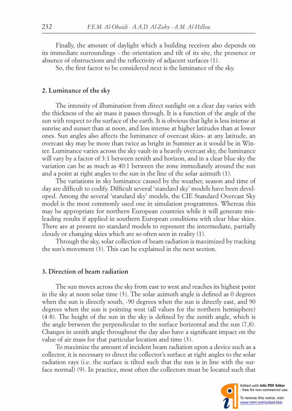
F.E.M. Al-Obaidi - A.A.D. Al-Zuky - A.M. Al-Hillou232
Finally, the amount of daylight which a building receives also depends on its immediate surroundings - the orientation and tilt of its site, the presence or absence of obstructions and the refl ectivity of adjacent surfaces (1).
So, the fi rst factor to be considered next is the luminance of the sky.
2. Luminance of the sky
The intensity of illumination from direct sunlight on a clear day varies with the thickness of the air mass it passes through. It is a function of the angle of the sun with respect to the surface of the earth. It is obvious that light is less intense at sunrise and sunset than at noon, and less intense at higher latitudes than at lower ones. Sun angles also affects the luminance of overcast skies- at any latitude, an overcast sky may be more than twice as bright in Summer as it would be in Win-ter. Luminance varies across the sky vault-in a heavily overcast sky, the luminance will vary by a factor of 3:1 between zenith and horizon, and in a clear blue sky the variation can be as much as 40:1 between the zone immediately around the sun and a point at right angles to the sun in the line of the solar azimuth (1).
The variations in sky luminance caused by the weather, season and time of day are diffi cult to codify. Diffi cult several ‘standard sky’ models have been devel-oped. Among the several ‘standard sky’ models, the CIE Standard Overcast Sky model is the most commonly used one in simulation programmes. Whereas this may be appropriate for northern European countries while it will generate mis-leading results if applied in southern European conditions with clear blue skies. There are at present no standard models to represent the intermediate, partially cloudy or changing skies which are so often seen in reality (1).
Through the sky, solar collection of beam radiation is maximized by tracking the sun’s movement (3). This can be explained in the next section.
3. Direction of beam radiation
The sun moves across the sky from east to west and reaches its highest point in the sky at noon solar time (3). The solar azimuth angle is defi ned as 0 degrees when the sun is directly south, -90 degrees when the sun is directly east, and 90 degrees when the sun is pointing west (all values for the northern hemisphere) (4-8). The height of the sun in the sky is defi ned by the zenith angle, which is the angle between the perpendicular to the surface horizontal and the sun (7,8). Changes in zenith angle throughout the day also have a signifi cant impact on the value of air mass for that particular location and time (3).
To maximize the amount of incident beam radiation upon a device such as a collector, it is necessary to direct the collector’s surface at right angles to the solar radiation rays (i.e. the surface is tilted such that the sun is in line with the sur-face normal) (9). In practice, most often the collectors must be located such that
Diurnal daylight illuminance measurements … 233
during one day the maximum of the solar radiation can be converted into solar energy. South-facing surface in the northern hemisphere has a zero azimuth angle (i.e. facing the equator) (10,11).
Hence, for a given latitude there is a certain angle, which yields the maxi-mum solar energy over the year. So, it is necessary to have tilted surfaces for the maximum solar energy collection (12,13). The tilt angle is dependent on both the latitude and the day of the year. Maximum yearly solar radiation can be achieved using a tilt angle approximately equal to the site’s latitude, then the sun’s rays will be perpendicular to the system surface at midday in March and September. To optimize performance in the winter, the surface can be tilted 15° greater than the latitude (i.e. the surface is tilted more to the vertical). For the maximization of solar collection in the summer, it is convenient to tilt the surface 15° less than the latitude (i.e. a little more towards the horizontal) (12-14).
4. Solar radiation striking a surface
The total solar radiation received by a tilted surface is composed of three components; the direct solar radiation from the sun, the scattered solar radiation from the sky, and the refl ected solar radiation from the ground. So, the hourly to-tal solar radiation incident upon the tilted surface, IIT, can be obtained by Eq.[1] in which the hourly direct solar radiation on a normal, ID, the hourly scattered solar radiation, IS, and the hourly total solar radiation on a horizontal, IHT, are contained (8,15).
[1]
where θ is the solar incident angle on a tilted surface, β is the surface tilted angle, φ is site’s latitude and ρ is the albedo of the ground.
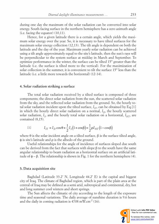
Useful relationships for the angle of incidence of surfaces sloped due south can be derived from the fact that surfaces with slope β to the south have the same angular relationship to beam radiation as a horizontal surface on an artifi cial lati-tude of φ – β. The relationship is shown in Fig. 1 for the northern hemisphere (4).
5. Data acquisition site
Baghdad (Latitude 33.2˚ N, Longitude 44.2˚ E) is the capital and biggest city of Iraq. The climate of Baghdad region, which is part of the plain area at the central of Iraq may be defi ned as a semi arid, subtropical and continental, dry, hot and long summer cool winters and short springs.
The Sun affects the climatic of city according to the length of the exposure time and seasonal variations. The daily average of sunshine duration is 9.6 hours and the daily in coming radiation is 4708 mW.cm-2 (16).
I IT = ID cosθ+
1
2IS 1+ cosβ( )+
1
2ρIHT 1− cosβ( )
F.E.M. Al-Obaidi - A.A.D. Al-Zuky - A.M. Al-Hillou234
6. The optical built system
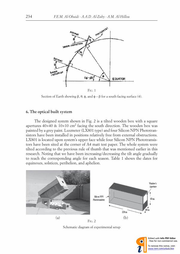
The designed system shown in Fig. 2 is a tilted wooden box with a square apertures 40×40 & 10×10 cm2 facing the south direction. The wooden box was painted by a grey paint. Luxmeter (LX801 type) and four Silicon NPN Phototran-sistors have been installed in positions relatively free from external obstructions. LX801 is located upon system’s upper face while four Silicon NPN Phototransis-tors have been sited at the corner of A4 matt test paper. The whole system were tilted according to the previous rule of thumb that was mentioned earlier in this research. Noting that we have been increasing/decreasing the tilt angle gradually to reach the corresponding angle for each season. Table 1 shows the dates for equinoxes, solstices, perihelion, and aphelion.
FIG. 1
Section of Earth showing β, θ, φ, and φ – β for a south-facing surface (4).
FIG. 2
Schematic diagram of experimental setup
(a) (b)
Diurnal daylight illuminance measurements … 235
Table 1Dates and times of Universal Time for northern hemisphere equinoxes and solstices
for the current year. From the US Naval Observatoryhttp://aa.usno.navy.mil/data/docs/EarthSeasons.html (17)
YearSpring Equinox
(March)Summer Solstice
(June)Fall Equinox(September)
Winter Solstice(December)
Perihelion Aphelion
2010 20 17.32 21 11.28 23 03.09 21 23.38 3 00 6 12
7. Sensor calibration
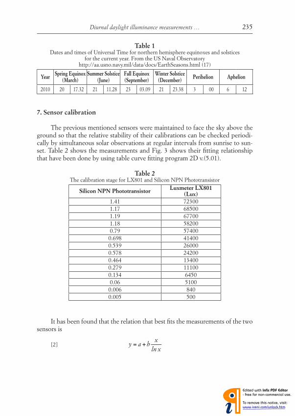
The previous mentioned sensors were maintained to face the sky above the ground so that the relative stability of their calibrations can be checked periodi-cally by simultaneous solar observations at regular intervals from sunrise to sun-set. Table 2 shows the measurements and Fig. 3 shows their fi tting relationship that have been done by using table curve fi tting program 2D v.(5.01).
Table 2The calibration stage for LX801 and Silicon NPN Phototransistor
Silicon NPN PhototransistorLuxmeter LX801
(Lux)
1.41 72300
1.17 68500
1.19 67700
1.18 58200
0.79 57400
0.698 41400
0.539 26000
0.578 24200
0.464 13400
0.279 11100
0.134 6450
0.06 5100
0.006 840
0.005 500
It has been found that the relation that best fi ts the measurements of the two sensors is
[2]
y = a +b
x
ln x
F.E.M. Al-Obaidi - A.A.D. Al-Zuky - A.M. Al-Hillou236
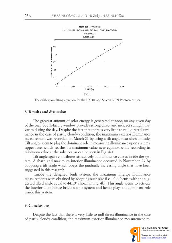
8. Results and discussion
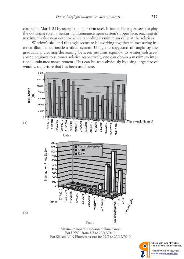
The greatest amount of solar energy is generated at noon on any given day of the year. South-facing window provides strong direct and indirect sunlight that varies during the day. Despite the fact that there is very little to null direct illumi-nance in the case of partly cloudy condition, the maximum exterior illuminance measurement was recorded on March 21 by using a tilt angle near site’s latitude.
Tilt angles seem to play the dominant role in measuring illuminance upon system’s upper face, which reaches its maximum value near equinox while recording its minimum value at the solstices, as can be seen in Fig. 4a).
Tilt angle again contributes attractively in illuminance curves inside the sys-tem. A sharp and maximum interior illuminance occurred in November, 27 by adopting a tilt angle which obeys the gradually increasing angle that have been suggested in this research.
Inside the designed built system, the maximum interior illuminance measurements were obtained by adopting such size (i.e. 40×40 cm2) with the sug-gested tilted angle equal to 44.19° shown in Fig. 4b). This angle seems to activate the interior illuminance inside such a system and hence plays the dominant role inside this system.
9. Conclusions
Despite the fact that there is very little to null direct illuminance in the case of partly cloudy condition, the maximum exterior illuminance measurement re-
FIG. 3
The calibration fi tting equation for the LX801 and Silicon NPN Phototransistor.
Diurnal daylight illuminance measurements … 237
corded on March 21 by using a tilt angle near site’s latitude. Tilt angles seem to play the dominant role in measuring illuminance upon system’s upper face, reaching its maximum value near equinox while recording its minimum value at the solstices.
Window’s size and tilt angle seems to be working together in measuring in-terior illuminance inside a tilted system. Using the suggested tilt angle by the gradually increasing/decreasing between autumn equinox to winter solstices/spring equinox to summer solstice respectively, one can obtain a maximum inte-rior illuminance measurement. This can be seen obviously by using large size of window’s aperture that has been used here.
FIG. 4
Maximum monthly measured illuminanceFor LX801 from 5/3 to 22/12/2010
For Silicon NPN Phototransistor fro 27/5 to 22/12/2010
(a)
(b)

F.E.M. Al-Obaidi - A.A.D. Al-Zuky - A.M. Al-Hillou238
REFERENCES
(1) The European Commission Directorate-General for Energy (DGXVll), Daylighting in buildings (1994).
(2) D.H.W. LI, C.C.S. LAU, J.C. LAM, Overcast sky conditions and luminance distribution in Hong Kong, Building and Environment, (Elsevier Ltd.), 39,.101-108, 2004
(3) G. SCHLEGEL, A trnsys model of a hybrid lighting system, M.Sc., Mechanical Enginee-ring, Univ. of Wisconsin (Madison, 2003).
(4) J.A. DUFFIE, W.A. BECKMAN, Solar engineering of thermal processes (John Wiley & Sons, Inc., 1991).
(5) A.M. AL-HILLOU, A.A.D. AL-ZUKY, F.E.M. AL-OBAIDI, Digital image testing and analy-sis of solar radiation variation with time in Baghdad city, Atti Fond. G. Ronchi, 65 (2), 223, 2010.
(6) L. KUMAR, A.K. SKIDMORE, E. KNOWLES, Modelling topographic variation in solar ra-diation in a GIS environment, Int. J. Geogr. Info. Sci., 11 (5), 475-497 (1997).
(7) M.J. BRANDEMUEHL, Solar radiation and sun position, in http://civil.colorado.edu/∼brandem/Buildingenergysystems/docs/solar_4.pdf.
(8) Solar radiation, Appendix D, http://www.me.umn.edu/courses/me4131/LabManual/AppDSolar Radiation.Pdf.
(9) R.C. LOVE, Surface refl ection model estimation from naturally illuminated image sequen-ces, Ph.D thesis, School of Computer studies (Univ. of Leeds, 1997).
(10) Solar geometry. A look into the path of the sun, in: www.teachengineering.com/…/cub_housing_lesson03_activity1_Solargeometryreading.pdf.
(11) NASA surface meterology and solar energy-available tables, in: http://eosweb.larc.nasa.gov/cgi-bin/sse/grid.cgi.
(12) Z. ŞEN, Solar energy fundamentals and modeling techniques: atmosphere, environment, climate change and renewable energy (Springer-Verlag London Limited, 2008).
(13) Z. ŞEN, Solar energy in progress and future research trends, (Elsevier Ltd., 2004).(14) http://www.nrel.gov/rredc,”Solar radiation data manual for fl at-plate and concen-
trating collectors(15) H. BABA, K. KANAYAMA, Estimation of solar radiation on a tilted surface with any incli-
nation and direction angle, Memoirs of the Kitami Inst. of Techn., 18 (2), 1987.(16) S.A.H. SALEH, Remote sensing technique for land use and surface temperature analysis
for Baghdad, Iraq, Proc. 15th Intern. Symp. and Exhibition on Remote Sensing and Assisting Systems (2006), in www.gors-sy.org.
(17) UNITED STATES NAVAL OBSERVATORY, Earth’s seasons: Equinoxes, Solstices, Perihelion, and Aphelion, 2000-2020, http://www.usno.navy.mil/USNO/astronomical-applications/ata-services/earth-seasons.
�������������� ���������������������������������������������� ���!"�#$�%��&��$�����%���'%�($�$��$%���)���$�'%*�+���,-'%**+������%�.$�/�%�%,�$���!"�0/����11�$$$2��%�$��$$$�%�,12��1������$3$������4��5���+*6$�7�"�89 :;
Spatial and Spectral Quality Evaluation Based On Edges Regions of Satellite Image Fusion
Firouz Abdullah Al-Wassai1 N.V. Kalyankar2 Research Student, Computer Science Dept. Principal, Yeshwant Mahavidyala College
(SRTMU), Nanded, India Nanded, India [email protected] [email protected]
Ali A. Al-Zaky3
Assistant Professor, Dept. of Physics, College of Science, Mustansiriyah Un. Baghdad – Iraq.
[email protected] Abstract: The Quality of image fusion is an essential
determinant of the value of processing images fusion for
many applications. Spatial and spectral qualities are the
two important indexes that used to evaluate the quality
of any fused image. However, the jury is still out of
fused image’s benefits if it compared with its original
images. In addition, there is a lack of measures for
assessing the objective quality of the spatial resolution
for the fusion methods. Therefore, an objective quality
of the spatial resolution assessment for fusion images is
required. Most important details of the image are in
edges regions, but most standards of image estimation
do not depend upon specifying the edges in the image
and measuring their edges. However, they depend upon
the general estimation or estimating the uniform region,
so this study deals with new method proposed to
estimate the spatial resolution by Contrast Statistical
Analysis (CSA) depending upon calculating the contrast
of the edge, non edge regions and the rate for the edges
regions. Specifying the edges in the image is made by
using Soble operator with different threshold values. In
addition, estimating the color distortion added by image
fusion based on Histogram Analysis of the edge
brightness values of all RGB-color bands and L-
component.
Keywords: Spatial Evaluation; Spectral Evaluation;
contrast; Signal to Noise Ratio; Measure of image
quality; Image Fusion
I. INTRODUCTION
Many fusion methods have proposed for fusing high spectral and spatial resolution of satellite images to produce multispectral images having the highest spatial resolution available within the data set. The theoretical spatial resolution of fused images � is supposed to be equal to resolution of high spatial resolution panchromatic image���; but in reality, it reduced. Quality is an essential determinant of the value of surrogate digital images. Quantitative measures of image quality to yield reliable image quality metrics can be used to assess the degree of degradation. Image quality measurement has become crucial for most image processing applications [1].
With the growth of digital imaging technology over the past years, there were many attempts to develop models or metrics for image quality that incorporate elements of human visual sensitivity [2]. However, there is no current standard and objective definition of spectral and spatial image quality. Image quality must be inferred from measurements of spatial resolution, calibration accuracy, and signal to noise, contrast, bit error rate, sensor stability, and other factors [3]. Most important details of the spatial resolution image are included in edges regions, but most of its standards assessment does not depend upon specifying edges in the image and measuring their edges, but they depend upon the general estimation or estimating the uniform region [4-6]. Therefore, in this study, a new scheme for evaluation, spatial quality of the fused images based on Contrast Statistical Analysis (CSA), and it depends upon the edge and non-edge regions of the image. The edges of the image are made by using Soble operator with different thresholds, and in comparing its results with traditional method of MTF depending upon the uniform region of the image as well as on completely image as the metric evaluation of the spatial resolution. In addition, this study testifies the metric evaluation of the spectral quality of the fused images based on Signal to Noise Ratio SNR of image upon
separately uniform regions and comparing its results with other method depends on whole MS & fused images.
The paper is planned in five sections that are as follows: Section I, which is considered the introduction of the study, brings framework and background of the study, Section II illustrates the quality evaluation of fused images i.e., a new proposed scheme of spatial evaluation quality of fused images defined as Contrast Statistical Analysis Technique CSA. Section III brings experimenting and analyzing results of the study based on pixel and feature level fusion including: High –Frequency-
Addition Method (HFA)[20], High Frequency Modulation Method (HFM) [7], Regression variable substitution (RVS) [8], Intensity Hue Saturation (IHS) [9], Segment Fusion (SF), Principal Component Analysis based Feature Fusion (PCA) and Edge Fusion (EF) [10]. All these methods will mention in section IV. Section V will be the conclusion of the study. II. QUALITY EVALUATION OF THE FUSED
IMAGES
The quality Evaluation of the fused images clarified through describing of various spatial and spectral quality metrics that used to evaluate them. With respect to the original multispectral images MS, the spectral fidelity of the fused images is described. The spectral quality of the fused images analyzed by compare them with spectral characteristics of resampled original multispectral imagesM�. Since the goal is to preserve the radiometry of the original MS images, any metric used must measure the amount of change in digital number values of the pan-sharpened or fused image F� and compared to the original imageM� for each of band k. In order to evaluate the spatial properties of the fused images, a panchromatic image PAN and intensity image of the fused image have to be compared since the goal is to retain the high spatial resolution of the PAN image.
A. The MTF Analysis
This technique defined as Modulation transfer function (MTF)[3] and referred to Michelson Contrast � . In order to calculate the spatial resolution by this method, it is common to measure the contrast of the targets and their background [11]. In this study, I used this technique in equation (1) to calculating the contrast rating based on uniform regions as well as overall images. The homogenous regions selected (see Fig. 11) have the size as the following: 1. 30 × 30 Block size for two different
homogenous regions named b1 b2 respectively. 2. 10 × 10 Block size for seven different
homogenous regions at same time named b3. Contrast performance over a spatial frequency range is characterized by the � [3]: � = ������������������ (1)
Where ���� ���� are the maximum and minimum radiance values recorded over the region of the homogenous image. For a nearly homogeneous
image, � would have a value close to zero while the maximum value of � is 1.0. B. Signal-to Noise Ratio (���)
The signal-to-noise ratio SNR is a measure of the purity of a signal [11]. Other means measuring the ratio between information and noise of the fused image [12]. Therefore, estimation of noise contained within image is essential which leads to a value indicative of image quality of the spectral resolution. Here, this study proposes to estimate the SNR based on regions for evaluation of the spectral quality. Also, results of the SNR based on regions that was compared with other results of the SNR based on whole MS and Fused images employed in our previous studies [13]. The two methods as the following: 1. SNRa Based On Regions
The SNR evaluation is Similar to contrast analysis technique, the final SNR rating is based on a 30 × 30 block size for two different regions of the homogenous as well as seven different regions at same time a 10x10 block size (see fig.3) image calculation of all RGB-color bands ". Which reflects the SNR across the whole image, the SRN in this implementation defined as follows [14]: ����# = %& '& (2)
Where: ����# Signal-to Noise Ratio, ( standard deviation and ) the mean of brightness values of RGB band " in the image region. The mean value μ� is defined as [15]: )# = +�� ∑ ∑ -#(/, 1)�34+��4+ (3)
The standard deviation σ is the square root of the variance. The variance of image reflects the dispersion degree between the brightness values and the brightness mean value. The larger σ is more disperse than the gray level. The definition of σ is [15]:
(# = 6 +�� ∑ ∑ (-#(/, 1) − )#)8�34+��4+ (4)
2. ���9 Based On Whole :� With Fused Images
In this method, the signal is the information content of original MS imageM�, while the merging �# can cause the noise, as error that is added to the image fusion. The signal-to-noise ratio���#, given by [16]:
���9# = ; ∑ ∑ (<&(�,3))=�>��∑ ∑ (<&(�,3)�&(�,3))=�>�� (5)
The SNR therefore is a relative value that reflects the percentage of significant values representing borders of objects. Thus, the SNR can be used to generate an indication of image quality of spectral resolution in dependence on the results of analyzing the image data. In the first method the result of ���� should has highly dissimilar to the results of MS as possible. In the second method, the maximum value of ���9 is the best image to preservation of the spectral quality for the original MS image. C. The Histogram Analysis The histograms of the multispectral original MS and the fused bands must be evaluated [17]. If the spectral information preserved in the fused image, its histogram will closely resemble the histogram of the MS image. The analysis of histogram deals with the brightness value histograms of all RGB-color bands, and L-component of the resample MS image and the fused image that computed the edges of image’s points regions only by using the next technique to estimated the edge regions. A greater difference of the shape of the corresponding histograms represents a greater spectral change [18]. III. CSA a New Scheme Of Spatial Evaluation
Quality of The Fused Images
To explain the new proposed technique of Contrast Statistical Analysis CSA for evaluation the quality of the spatial resolution specifying the edges in the image by using Soble operator. In this technique the metric starts by applying Soble edge detector for the whole image [19, 20], but the new proposed method based on contrast calculation of each of the edge and homogenous regions. The steps for evaluation of the spatial resolution as follows: 1- Apply Soble edge detector for the whole image
with different thresholds of its operator i.e. 20, 40, 60, 80 and 100.
2- The pixel value of the image is labeled into edge regions or homogenous regions in corresponding with applied Soble thresholds. If the pixel number value is greater than a certain predefined threshold, it (the pixel) is labeled as an edge point, otherwise, it is considered smooth or homogenous region and further processing is disabled.
3- Calculated the rate of the strong edges pixels for all RGB bands " with different thresholds of Soble operators and drawing the histograms for them as well.
4- Estimate the mean µ and standard deviation ( for all RGB bands " of all edges points and homogenous regions.
5- Finally, CSA was calculated by the statistical characteristics of the edges points and homogenous regions for all RGB color bands " in image were adopted according to equation (1). Here, the ���� & ���� are calculated by adopting the mean µ (eq.3)and standard deviation ( (eq.4) of edges regions at (n, m) for the intensity -#(/, 1) of image components relating to points and homogenous regions according to the two following relations: �#��� = �# – σ# & �#��� = �# + σ# (6)
∴∴∴∴ ���# = '&%& (7)
Where: CSA contrast of band k, μ mean, σ# standard deviation. For a nearly homogeneous image, ���# would have a value close to zero while the maximum value of ���# is 1.0. The maximum contrast value for the image means that it has the high spatial resolution.
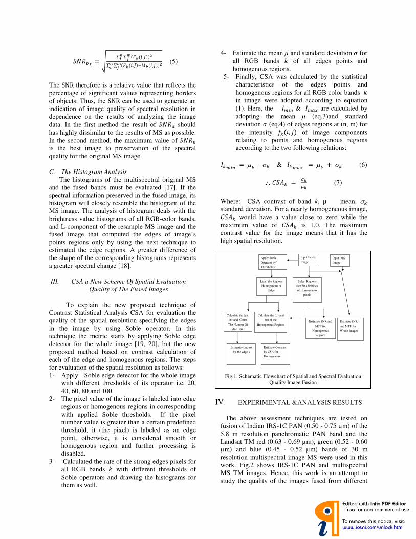
IV. EXPERIMENTAL &ANALYSIS RESULTS The above assessment techniques are tested on fusion of Indian IRS-1C PAN (0.50 - 0.75 µm) of the 5.8 m resolution panchromatic PAN band and the Landsat TM red (0.63 - 0.69 µm), green (0.52 - 0.60 µm) and blue (0.45 - 0.52 µm) bands of 30 m resolution multispectral image MS were used in this work. Fig.2 shows IRS-1C PAN and multispectral MS TM images. Hence, this work is an attempt to study the quality of the images fused from different
Fig.1: Schematic Flowchart of Spatial and Spectral Evaluation Quality Image Fusion
Input Fused Image
Apply Soble Operator by” Thresholds”
Select Regions size 30 x30 block of Homogenous
pixels
Calculate the (µ) and (σ) of the
Homogenous Regions
Calculate the (µ) , (σ) and Count
The Number Of Edge Pixels
Estimate contrast for the edge s
Estimate Contrast by CSA for Homogenous
Label the Regions Homogenous or
Edge
Estimate SNR and MTF for
Homogenous Regions
Input MS Image
Estimate SNR and MTF for Whole Images

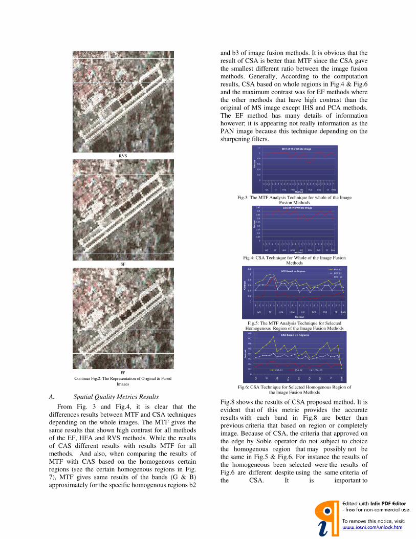
sensors with various characteristics. The size of the PAN is 600 * 525 pixels at 6 bits per pixel and the size of the original multispectral is 120 * 105 pixels at 8 bits per pixel, but this is upsampled by nearest neighbor. The pairs of images were geometrically registered to each other. Fig. 2 shows the fused images of the HFA, HFM, HIS, RVS, PCA, EF, and SF methods are employed to fuse IRS-C PAN and TM multi-spectral images. To simplify the comparison of the different fusion methods, the results of the fused images are provided as charts from Fig. 3 to Fig.12 for quantify the behavior of HFA, HFM, IHS, RVS, PCA, EF, and SF methods.
Original PAN Image
Original MS Image
HFA
Fig.1: The Representation of Original & Fused Images
HFM
IHS
PCA
Continue Fig.2: The Representation of Original & Fused Images
A. Spatial Quality Metrics Results
From Fig. 3 and Fig.4, it is clear that the differences results between MTF and CSA techniques depending on the whole images. The MTF gives the same results that shown high contrast for all methods of the EF, HFA and RVS methods. While the results of CAS different results with results MTF for all methods. And also, when comparing the results of MTF with CAS based on the homogenous certain regions (see the certain homogenous regions in Fig. 7), MTF gives same results of the bands (G & B) approximately for the specific homogenous regions b2
and b3 of image fusion methods. It is obvious that the result of CSA is better than MTF since the CSA gave the smallest different ratio between the image fusion methods. Generally, According to the computation results, CSA based on whole regions in Fig.4 & Fig.6 and the maximum contrast was for EF methods where the other methods that have high contrast than the original of MS image except IHS and PCA methods. The EF method has many details of information however; it is appearing not really information as the PAN image because this technique depending on the sharpening filters.
Fig.8 shows the results of CSA proposed method. It is evident that of this metric provides the accurate results with each band in Fig.8 are better than previous criteria that based on region or completely image. Because of CSA, the criteria that approved on the edge by Soble operator do not subject to choice the homogenous region that may possibly not be the same in Fig.5 & Fig.6. For instance the results of the homogeneous been selected were the results of Fig.6 are different despite using the same criteria of the CSA. It is important to
RVS
SF
EF
Continue Fig.2: The Representation of Original & Fused Images
Fig.3: The MTF Analysis Technique for whole of the Image
Fusion Methods
Fig.4: CSA Technique for Whole of the Image Fusion
Methods
Fig.5: The MTF Analysis Technique for Selected
Homogenous Region of the Image Fusion Methods
Fig.6: CSA Technique for Selected Homogenous Region of
the Image Fusion Methods
0
0.2
0.4
0.6
0.8
1
1.2
1 2 3 1 2 3 1 2 3 1 2 3 1 2 3 1 2 3 1 2 3 1 2 3 I
MS EF HFA HFM IHS PCA RVS SF PAN
Co
ntr
ast
Method
MTF of The Whole Image
0
0.05
0.1
0.15
0.2
0.25
0.3
0.35
0.4
0.45
1 2 3 1 2 3 1 2 3 1 2 3 1 2 3 1 2 3 1 2 3 1 2 3 I
MS EF HFA HFM IHS PCA RVS SF PAN
Co
ntr
ast
Method
CSA of The Whole Image
0
0.2
0.4
0.6
0.8
1
1.2
1 2 3 1 2 3 1 2 3 1 2 3 1 2 3 1 2 3 1 2 3 1 2 3 I
MS EF HFA HFM IHS PCA RVS SF PAN
Co
ntr
ast
Method
MTF Based on RegionsMTF b1
MTF b2
MTF b3
0
0.1
0.2
0.3
0.4
0.5
0.6
0.7
0.8
MS EF
HFA
HF
M
IHS
PC
A
RV
S SF
PA
N
Co
ntr
ast
CAS Based on Regions
CSA-b1 CSA-b2 CSA -b3
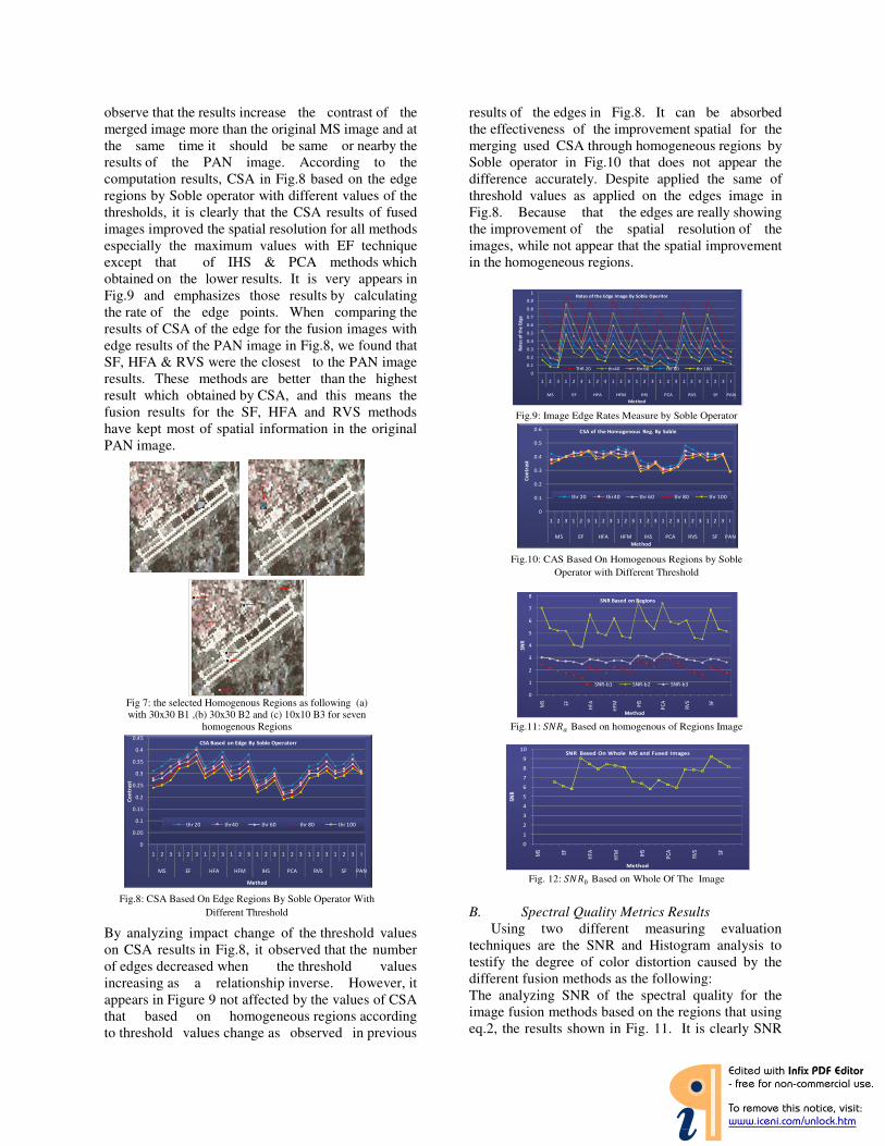
observe that the results increase the contrast of the merged image more than the original MS image and at the same time it should be same or nearby the results of the PAN image. According to the computation results, CSA in Fig.8 based on the edge regions by Soble operator with different values of the thresholds, it is clearly that the CSA results of fused images improved the spatial resolution for all methods especially the maximum values with EF technique except that of IHS & PCA methods which obtained on the lower results. It is very appears in Fig.9 and emphasizes those results by calculating the rate of the edge points. When comparing the results of CSA of the edge for the fusion images with edge results of the PAN image in Fig.8, we found that SF, HFA & RVS were the closest to the PAN image results. These methods are better than the highest result which obtained by CSA, and this means the fusion results for the SF, HFA and RVS methods have kept most of spatial information in the original PAN image.
By analyzing impact change of the threshold values on CSA results in Fig.8, it observed that the number of edges decreased when the threshold values increasing as a relationship inverse. However, it appears in Figure 9 not affected by the values of CSA that based on homogeneous regions according to threshold values change as observed in previous
results of the edges in Fig.8. It can be absorbed the effectiveness of the improvement spatial for the merging used CSA through homogeneous regions by Soble operator in Fig.10 that does not appear the difference accurately. Despite applied the same of threshold values as applied on the edges image in Fig.8. Because that the edges are really showing the improvement of the spatial resolution of the images, while not appear that the spatial improvement in the homogeneous regions.
B. Spectral Quality Metrics Results Using two different measuring evaluation techniques are the SNR and Histogram analysis to testify the degree of color distortion caused by the different fusion methods as the following: The analyzing SNR of the spectral quality for the image fusion methods based on the regions that using eq.2, the results shown in Fig. 11. It is clearly SNR
Fig 7: the selected Homogenous Regions as following (a) with 30x30 B1 ,(b) 30x30 B2 and (c) 10x10 B3 for seven
homogenous Regions
Fig.8: CSA Based On Edge Regions By Soble Operator With
Different Threshold
0
0.05
0.1
0.15
0.2
0.25
0.3
0.35
0.4
0.45
1 2 3 1 2 3 1 2 3 1 2 3 1 2 3 1 2 3 1 2 3 1 2 3 I
MS EF HFA HFM IHS PCA RVS SF PAN
Co
ntr
ast
Method
CSA Based on Edge By Soble Operatorr
thr 20 thr40 thr 60 thr 80 thr 100
Fig.9: Image Edge Rates Measure by Soble Operator
Fig.10: CAS Based On Homogenous Regions by Soble
Operator with Different Threshold
Fig.11: ���A Based on homogenous of Regions Image
Fig. 12: ���B Based on Whole Of The Image
0
0.1
0.2
0.3
0.4
0.5
0.6
0.7
0.8
0.9
1
1 2 3 1 2 3 1 2 3 1 2 3 1 2 3 1 2 3 1 2 3 1 2 3 I
MS EF HFA HFM IHS PCA RVS SF PAN
Ra
tes
of
the
Ed
ge
Method
Rates of the Edge Image By Soble Operitor
THR 20 thr40 thr 60 thr 80 thr 100
0
0.1
0.2
0.3
0.4
0.5
0.6
1 2 3 1 2 3 1 2 3 1 2 3 1 2 3 1 2 3 1 2 3 1 2 3 I
MS EF HFA HFM IHS PCA RVS SF PAN
Co
ntr
ast
Method
CSA of the Homogenous Reg. By Soble
thr 20 thr40 thr 60 thr 80 thr 100
0
1
2
3
4
5
6
7
8
MS
EF
HF
A
HF
M
IHS
PC
A
RV
S SF
SN
R
Method
SNR Based on Regions
SNR-b1 SNR-b2 SNR-b3
0
1
2
3
4
5
6
7
8
9
10
MS EF
HFA
HFM IH
S
PC
A
RV
S SF
SNR
Method
SNR Based On Whole MS and Fused Images
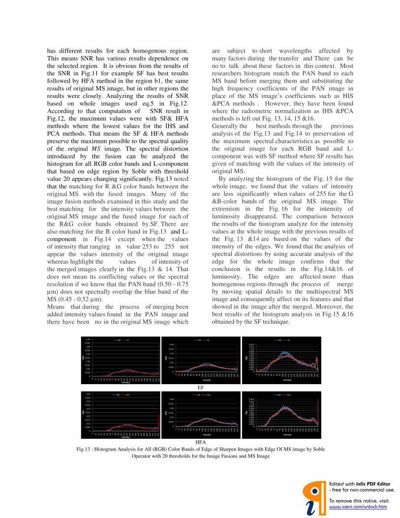
has different results for each homogenous region. This means SNR has various results dependence on the selected region. It is obvious from the results of the SNR in Fig.11 for example SF has best results followed by HFA method in the region b1, the same results of original MS image, but in other regions the results were closely. Analyzing the results of SNR based on whole images used eq.5 in Fig.12. According to that computation of SNR result in Fig.12, the maximum values were with SF& HFA methods where the lowest values for the IHS and PCA methods. That means the SF & HFA methods preserve the maximum possible to the spectral quality of the original :� image. The spectral distortion introduced by the fusion can be analyzed the histogram for all RGB color bands and L-component that based on edge region by Soble with threshold value 20 appears changing significantly. Fig.13 noted that the matching for R &G color bands between the original MS with the fused images. Many of the image fusion methods examined in this study and the best matching for the intensity values between the original MS image and the fused image for each of the R&G color bands obtained by SF. There are also matching for the B color band in Fig.13 and L-component in Fig.14 except when the values of intensity that ranging in value 253 to 255 not appear the values intensity of the original image whereas highlight the values of intensity of the merged images clearly in the Fig.13 & 14. That does not mean its conflicting values or the spectral resolution if we know that the PAN band (0.50 - 0.75 µm) does not spectrally overlap the blue band of the MS (0.45 - 0.52 µm). Means that during the process of merging been added intensity values found in the PAN image and there have been no in the original MS image which
are subject to short wavelengths affected by many factors during the transfer and There can be no to talk about these factors in this context. Most researchers histogram match the PAN band to each MS band before merging them and substituting the high frequency coefficients of the PAN image in place of the MS image’s coefficients such as HIS &PCA methods . However, they have been found where the radiometric normalization as IHS &PCA methods is left out Fig. 13, 14, 15 &16. Generally the best methods through the previous analysis of the Fig.13 and Fig.14 to preservation of the maximum spectral characteristics as possible to the original image for each RGB band and L-component was with SF method where SF results has given of matching with the values of the intensity of original MS. By analyzing the histogram of the Fig. 15 for the whole image, we found that the values of intensity are less significantly when values of 255 for the G &B-color bands of the original MS image. The extremism in the Fig. 16 for the intensity of luminosity disappeared. The comparison between the results of the histogram analyze for the intensity values at the whole image with the previous results of the Fig. 13 &14 are based on the values of the intensity of the edges. We found that the analysis of spectral distortions by using accurate analysis of the edge for the whole image confirms that the conclusion is the results in the Fig.14&16 of luminosity. The edges are affected more than homogenous regions through the process of merge by moving spatial details to the multispectral MS image and consequently affect on its features and that showed in the image after the merged. Moreover, the best results of the histogram analysis in Fig.15 &16 obtained by the SF technique.
EF
HFA
Fig.13 : Histogram Analysis for All (RGB) Color Bands of Edge of Sharpen Images with Edge Of MS image by Soble Operator with 20 thresholds for the Image Fusions and MS Image
0
0.005
0.01
0.015
0.02
0.025
0.03
0.035
0.04
0.045
0.05
0
11
22
33
44
55
66
77
88
99
11
0
12
1
13
2
14
3
15
4
16
5
17
6
18
7
19
8
20
9
22
0
23
1
24
2
25
3
P(R
)
Intensity
MS EF
0
0.005
0.01
0.015
0.02
0.025
0.03
0
12
24
36
48
60
72
84
96
10
8
12
0
13
2
14
4
15
6
16
8
18
0
19
2
20
4
21
6
22
8
24
0
25
2
P(G
)
Intensity
MS EF
00.0010.0020.0030.0040.0050.0060.0070.0080.009
0.010.0110.012
0
12
24
36
48
60
72
84
96
10
8
12
0
13
2
14
4
15
6
16
8
18
0
19
2
20
4
21
6
22
8
24
0
25
2
P(B
)
Intensity
MS EF
0
0.005
0.01
0.015
0.02
0.025
0.03
0.035
0.04
0.045
0.05
0
11
22
33
44
55
66
77
88
99
11
0
12
1
13
2
14
3
15
4
16
5
17
6
18
7
19
8
20
9
22
0
23
1
24
2
25
3
P(R
)
Intensity
MS HFA
0
0.005
0.01
0.015
0.02
0.025
0.03
0
12
24
36
48
60
72
84
96
10
8
12
0
13
2
14
4
15
6
16
8
18
0
19
2
20
4
21
6
22
8
24
0
25
2
P(G
)
Intensity
MS HFA
00.0010.0020.0030.0040.0050.0060.0070.0080.009
0.010.0110.012
0
12
24
36
48
60
72
84
96
10
8
12
0
13
2
14
4
15
6
16
8
18
0
19
2
20
4
21
6
22
8
24
0
25
2
P(B
)
Intensity
MS HFA
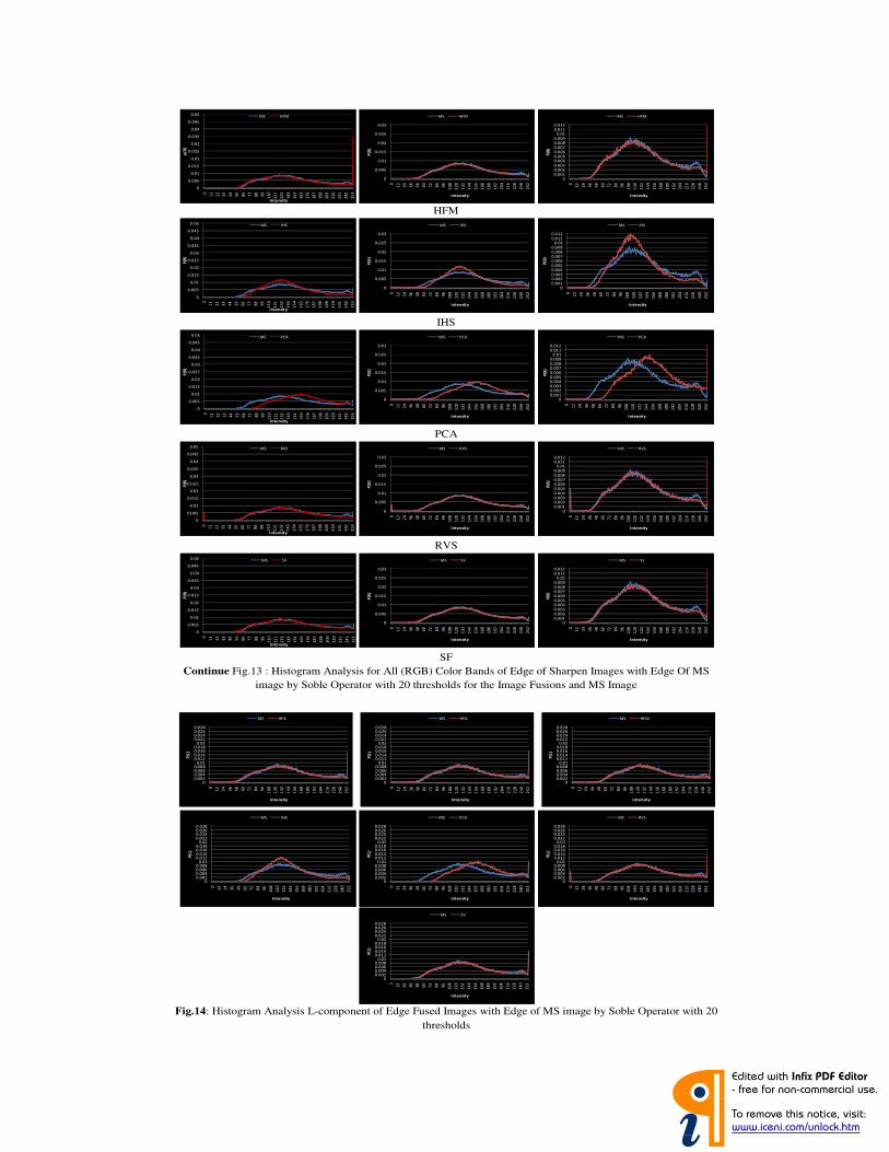
HFM
IHS
PCA
RVS
SF
Continue Fig.13 : Histogram Analysis for All (RGB) Color Bands of Edge of Sharpen Images with Edge Of MS image by Soble Operator with 20 thresholds for the Image Fusions and MS Image
0
0.005
0.01
0.015
0.02
0.025
0.03
0.035
0.04
0.045
0.05
0
11
22
33
44
55
66
77
88
99
11
0
12
1
13
2
14
3
15
4
16
5
17
6
18
7
19
8
20
9
22
0
23
1
24
2
25
3
p(R
)
Intensity
MS HFM
0
0.005
0.01
0.015
0.02
0.025
0.03
0
12
24
36
48
60
72
84
96
10
8
12
0
13
2
14
4
15
6
16
8
18
0
19
2
20
4
21
6
22
8
24
0
25
2
P(G
)
Intensity
MS HFM
00.0010.0020.0030.0040.0050.0060.0070.0080.009
0.010.0110.012
0
12
24
36
48
60
72
84
96
10
8
12
0
13
2
14
4
15
6
16
8
18
0
19
2
20
4
21
6
22
8
24
0
25
2
P(B
)
Intensity
MS HFM
0
0.005
0.01
0.015
0.02
0.025
0.03
0.035
0.04
0.045
0.05
0
11
22
33
44
55
66
77
88
99
11
0
12
1
13
2
14
3
15
4
16
5
17
6
18
7
19
8
20
9
22
0
23
1
24
2
25
3
P(R
)
Intensity
MS IHS
0
0.005
0.01
0.015
0.02
0.025
0.03
0
12
24
36
48
60
72
84
96
10
8
12
0
13
2
14
4
15
6
16
8
18
0
19
2
20
4
21
6
22
8
24
0
25
2
P(G
)
Intensity
MS IHS
00.0010.0020.0030.0040.0050.0060.0070.0080.009
0.010.0110.012
0
12
24
36
48
60
72
84
96
10
8
12
0
13
2
14
4
15
6
16
8
18
0
19
2
20
4
21
6
22
8
24
0
25
2
P(B
)
Intensity
MS IHS
0
0.005
0.01
0.015
0.02
0.025
0.03
0.035
0.04
0.045
0.05
0
11
22
33
44
55
66
77
88
99
11
0
12
1
13
2
14
3
15
4
16
5
17
6
18
7
19
8
20
9
22
0
23
1
24
2
25
3
P(R
)
Intensity
MS PCA
0
0.005
0.01
0.015
0.02
0.025
0.03
0
12
24
36
48
60
72
84
96
10
8
12
0
13
2
14
4
15
6
16
8
18
0
19
2
20
4
21
6
22
8
24
0
25
2
P(G
)
Intensity
MS PCA
00.0010.0020.0030.0040.0050.0060.0070.0080.009
0.010.0110.012
0
12
24
36
48
60
72
84
96
10
8
12
0
13
2
14
4
15
6
16
8
18
0
19
2
20
4
21
6
22
8
24
0
25
2
P(B
)
Intensity
MS PCA
0
0.005
0.01
0.015
0.02
0.025
0.03
0.035
0.04
0.045
0.05
0
11
22
33
44
55
66
77
88
99
11
0
12
1
13
2
14
3
15
4
16
5
17
6
18
7
19
8
20
9
22
0
23
1
24
2
25
3
P(R
)
Intensity
MS RVS
0
0.005
0.01
0.015
0.02
0.025
0.03
0
12
24
36
48
60
72
84
96
10
8
12
0
13
2
14
4
15
6
16
8
18
0
19
2
20
4
21
6
22
8
24
0
25
2
P(G
)
Intensity
MS RVS
00.0010.0020.0030.0040.0050.0060.0070.0080.009
0.010.0110.012
0
12
24
36
48
60
72
84
96
10
8
12
0
13
2
14
4
15
6
16
8
18
0
19
2
20
4
21
6
22
8
24
0
25
2
P(B
)
Intensity
MS RVS
0
0.005
0.01
0.015
0.02
0.025
0.03
0.035
0.04
0.045
0.05
0
11
22
33
44
55
66
77
88
99
11
0
12
1
13
2
14
3
15
4
16
5
17
6
18
7
19
8
20
9
22
0
23
1
24
2
25
3
P(R
)
Intensity
MS SV
0
0.005
0.01
0.015
0.02
0.025
0.03
0
12
24
36
48
60
72
84
96
10
8
12
0
13
2
14
4
15
6
16
8
18
0
19
2
20
4
21
6
22
8
24
0
25
2
P(G
)
Intensity
MS SV
00.0010.0020.0030.0040.0050.0060.0070.0080.009
0.010.0110.012
0
12
24
36
48
60
72
84
96
10
8
12
0
13
2
14
4
15
6
16
8
18
0
19
2
20
4
21
6
22
8
24
0
25
2
P(B
)
Intensity
MS SV
Fig.14: Histogram Analysis L-component of Edge Fused Images with Edge of MS image by Soble Operator with 20
thresholds
00.0020.0040.0060.008
0.010.0120.0140.0160.018
0.020.0220.0240.0260.028
0
12
24
36
48
60
72
84
96
10
8
12
0
13
2
14
4
15
6
16
8
18
0
19
2
20
4
21
6
22
8
24
0
25
2
P(L
)
Intensity
MS HFA
00.0020.0040.0060.008
0.010.0120.0140.0160.018
0.020.0220.0240.0260.028
0
12
24
36
48
60
72
84
96
10
8
12
0
13
2
14
4
15
6
16
8
18
0
19
2
20
4
21
6
22
8
24
0
25
2
P(L
)
Intensity
MS HFA
00.0020.0040.0060.008
0.010.0120.0140.0160.018
0.020.0220.0240.0260.028
0
12
24
36
48
60
72
84
96
10
8
12
0
13
2
14
4
15
6
16
8
18
0
19
2
20
4
21
6
22
8
24
0
25
2
P(L
)
Intensity
MS HFM
00.0020.0040.0060.008
0.010.0120.0140.0160.018
0.020.0220.0240.0260.028
0
12
24
36
48
60
72
84
96
10
8
12
0
13
2
14
4
15
6
16
8
18
0
19
2
20
4
21
6
22
8
24
0
25
2
P(L
)
Intensity
MS IHS
00.0020.0040.0060.008
0.010.0120.0140.0160.018
0.020.0220.0240.0260.028
0
12
24
36
48
60
72
84
96
10
8
12
0
13
2
14
4
15
6
16
8
18
0
19
2
20
4
21
6
22
8
24
0
25
2
P(L
)
Intensity
MS PCA
00.0020.0040.0060.008
0.010.0120.0140.0160.018
0.020.0220.0240.0260.028
0
12
24
36
48
60
72
84
96
10
8
12
0
13
2
14
4
15
6
16
8
18
0
19
2
20
4
21
6
22
8
24
0
25
2
P(L
)
Intensity
MS RVS
00.0020.0040.0060.008
0.010.0120.0140.0160.018
0.020.0220.0240.0260.028
0
12
24
36
48
60
72
84
96
10
8
12
0
13
2
14
4
15
6
16
8
18
0
19
2
20
4
21
6
22
8
24
0
25
2
P(L
)
Intensity
MS SV
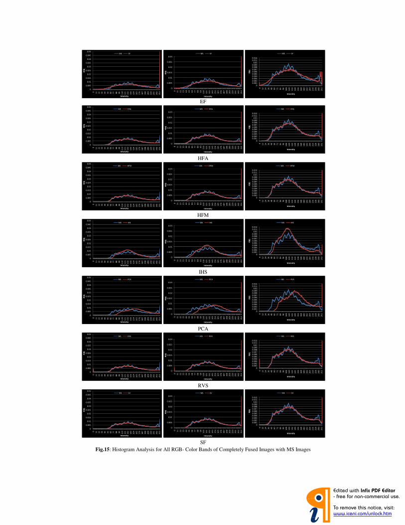
EF
HFA
HFM
IHS
PCA
RVS
SF
Fig.15: Histogram Analysis for All RGB- Color Bands of Completely Fused Images with MS Images
0
0.005
0.01
0.015
0.02
0.025
0.03
0.035
0.04
0.045
0.05
0
11
22
33
44
55
66
77
88
99
11
0
12
1
13
2
14
3
15
4
16
5
17
6
18
7
19
8
20
9
22
0
23
1
24
2
25
3
P(R
)
Intensity
MS EF
0
0.005
0.01
0.015
0.02
0.025
0.03
0
11
22
33
44
55
66
77
88
99
11
0
12
1
13
2
14
3
15
4
16
5
17
6
18
7
19
8
20
9
22
0
23
1
24
2
25
3
P(G
)
Intensity
MS EF
00.0010.0020.0030.0040.0050.0060.0070.0080.009
0.010.0110.012
0
12
24
36
48
60
72
84
96
10
8
12
0
13
2
14
4
15
6
16
8
18
0
19
2
20
4
21
6
22
8
24
0
25
2
P(B
)
Intensity
MS EF
0
0.005
0.01
0.015
0.02
0.025
0.03
0.035
0.04
0.045
0.05
0
11
22
33
44
55
66
77
88
99
11
0
12
1
13
2
14
3
15
4
16
5
17
6
18
7
19
8
20
9
22
0
23
1
24
2
25
3
P(R
)
Intensity
MS HFA
0
0.005
0.01
0.015
0.02
0.025
0.03
0
11
22
33
44
55
66
77
88
99
11
0
12
1
13
2
14
3
15
4
16
5
17
6
18
7
19
8
20
9
22
0
23
1
24
2
25
3
P(G
)
Intensity
MS HFA
00.0010.0020.0030.0040.0050.0060.0070.0080.009
0.010.0110.012
0
12
24
36
48
60
72
84
96
10
8
12
0
13
2
14
4
15
6
16
8
18
0
19
2
20
4
21
6
22
8
24
0
25
2
P(B
)
Intensity
MS HFA
0
0.005
0.01
0.015
0.02
0.025
0.03
0.035
0.04
0.045
0.05
0
11
22
33
44
55
66
77
88
99
11
0
12
1
13
2
14
3
15
4
16
5
17
6
18
7
19
8
20
9
22
0
23
1
24
2
25
3
P(R
)
Intensity
MS HFM
0
0.005
0.01
0.015
0.02
0.025
0.03
0
11
22
33
44
55
66
77
88
99
11
0
12
1
13
2
14
3
15
4
16
5
17
6
18
7
19
8
20
9
22
0
23
1
24
2
25
3
P(G
)
Intensity
MS HFM
00.0010.0020.0030.0040.0050.0060.0070.0080.009
0.010.0110.012
0
12
24
36
48
60
72
84
96
10
8
12
0
13
2
14
4
15
6
16
8
18
0
19
2
20
4
21
6
22
8
24
0
25
2
P(B
)
Intensity
MS HFM
0
0.005
0.01
0.015
0.02
0.025
0.03
0.035
0.04
0.045
0.05
0
11
22
33
44
55
66
77
88
99
11
0
12
1
13
2
14
3
15
4
16
5
17
6
18
7
19
8
20
9
22
0
23
1
24
2
25
3
P(R
)
Intensity
MS IHS
0
0.005
0.01
0.015
0.02
0.025
0.03
0
11
22
33
44
55
66
77
88
99
11
0
12
1
13
2
14
3
15
4
16
5
17
6
18
7
19
8
20
9
22
0
23
1
24
2
25
3
P(G
)
Intensity
MS IHS
00.0010.0020.0030.0040.0050.0060.0070.0080.009
0.010.0110.012
0
12
24
36
48
60
72
84
96
10
8
12
0
13
2
14
4
15
6
16
8
18
0
19
2
20
4
21
6
22
8
24
0
25
2
P(B
)
Intensity
MS IHS
0
0.005
0.01
0.015
0.02
0.025
0.03
0.035
0.04
0.045
0.05
0
11
22
33
44
55
66
77
88
99
11
0
12
1
13
2
14
3
15
4
16
5
17
6
18
7
19
8
20
9
22
0
23
1
24
2
25
3
P(R
)
Intensity
MS PCA
0
0.005
0.01
0.015
0.02
0.025
0.03
0
11
22
33
44
55
66
77
88
99
11
0
12
1
13
2
14
3
15
4
16
5
17
6
18
7
19
8
20
9
22
0
23
1
24
2
25
3
P(G
)
Intensity
MS PCA
00.0010.0020.0030.0040.0050.0060.0070.0080.009
0.010.0110.012
0
12
24
36
48
60
72
84
96
10
8
12
0
13
2
14
4
15
6
16
8
18
0
19
2
20
4
21
6
22
8
24
0
25
2
P(B
)
Intensity
MS PCA
0
0.005
0.01
0.015
0.02
0.025
0.03
0.035
0.04
0.045
0.05
0
11
22
33
44
55
66
77
88
99
11
0
12
1
13
2
14
3
15
4
16
5
17
6
18
7
19
8
20
9
22
0
23
1
24
2
25
3
P(R
)
Intensity
MS RVS
0
0.005
0.01
0.015
0.02
0.025
0.03
0
11
22
33
44
55
66
77
88
99
11
0
12
1
13
2
14
3
15
4
16
5
17
6
18
7
19
8
20
9
22
0
23
1
24
2
25
3
P(G
)
Intensity
MS RVS
00.0010.0020.0030.0040.0050.0060.0070.0080.009
0.010.0110.012
0
12
24
36
48
60
72
84
96
10
8
12
0
13
2
14
4
15
6
16
8
18
0
19
2
20
4
21
6
22
8
24
0
25
2
P(B
)
Intensity
MS RVS
0
0.005
0.01
0.015
0.02
0.025
0.03
0.035
0.04
0.045
0.05
0
11
22
33
44
55
66
77
88
99
11
0
12
1
13
2
14
3
15
4
16
5
17
6
18
7
19
8
20
9
22
0
23
1
24
2
25
3
P(R
)
Intensity
MS SV
0
0.005
0.01
0.015
0.02
0.025
0.03
0
11
22
33
44
55
66
77
88
99
11
0
12
1
13
2
14
3
15
4
16
5
17
6
18
7
19
8
20
9
22
0
23
1
24
2
25
3
P(G
)
Intensity
MS SV
00.0010.0020.0030.0040.0050.0060.0070.0080.009
0.010.0110.012
0
12
24
36
48
60
72
84
96
10
8
12
0
13
2
14
4
15
6
16
8
18
0
19
2
20
4
21
6
22
8
24
0
25
2
P(B
)
Intensity
MS SV

V. CONCLUSION
This study proposed a new measure to test the efficiency of spatial and spectral resolution of the fusion images applied to a number of methods of merge images. These methods have obtained the best results in our previous studies and some of them depend on the pixel level fusion including HFA, HFM, IHS and RVS methods while the other methods based on features level fusion as fallows PCA, EF and SF method. Results of the study show the importance to proposed new CSA as a criterion to measure the quality evaluation for the spatial resolution of the fused images, in which the results showed the effectiveness of high efficiency when compared with the other criterion methods for measurement such as the MTF. The study proved the importance of analysis using the edge, which is more accurate and objective than different one that depending on the selection regions or even the whole image to test the spatial improvement for the fused images. This is because the edges are really showing the improvement of the spatial resolution of the images, whereas there is no apparent spatial improvement in the homogeneous regions. In addition, the edges are more affected than the homogenous regions in the image through the processing of the merge by moving the spatial details to the multispectral MS image and consequently affect on the spectral features and that showed in the image after the merged. Therefore, it is recommended to use the spectral analysis for the whole image to determine the spectral distortions in the
images, whereas the use of edge’s analysis image has shown crucial difference. According to CSA, SNR and Histogram results of the analysis, SF is the best method applied in this study to determine the best method of merging in conservation spectral characteristics for original MS image and adding the maximum possible of spatial details of PAN image to the fused image.
REFERENCES
[1] Wang, Z., Sheikh, H.R. And Bovik, A.C., 2002, “No-reference perceptual quality assessment of JPEG compressed images”. In IEEE International Conference on Image Processing, 22–25 September 2002, Rochester, New York, pp. 477–480. Watson, A.B., Borthwick, R. And Taylor, M., 1997. “Image quality and entropy masking”.Proceedings of SPIE, 3016, pp. 2–12.
[2] G. Y. LUO,2006. “Objective image quality measurement by local spatial-frequency wavelet analysis”.International Journal of Remote Sensing, Vol. 27, No. 22, 20 November 2006, pp. 5003–5025.
[3] Zhou J., D. L. Civico, and J. A. Silander. A wavelet transform method to merge landsat TM and SPOT panchromatic data. International Journal of Remote Sensing, 19(4), 1998.
[4] Ryan. R., B. Baldridge, R.A. Schowengerdt, T. Choi, D.L. Helder and B. Slawomir, 2003. “IKONOS Spatial Resolution And Image Interpretability Characterization”, Remote Sensing of Environment, Vol. 88, No. 1, pp. 37–52.
[5] Pradham P., Younan N. H. and King R. L., 2008. “Concepts of image fusion in remote sensing applications”. Edited by: Stathaki T. “Image Fusion: Algorithms and Applications”. 2008 Elsevier Ltd.
[6] Firouz A. Al-Wassai , N.V. Kalyankar , A.A. Al-Zuky, 2011a. “Arithmetic and Frequency Filtering Methods of Pixel-Based Image Fusion Techniques “.IJCSI International Journal of Computer Science Issues, Vol. 8, Issue 3, No. 1, May 2011, pp. 113- 122.
Fig. 16: Histogram Analysis L-component for Whole of the Fused Images with MS Image
00.0020.0040.0060.008
0.010.0120.0140.0160.018
0.020.0220.0240.0260.028
0
12
24
36
48
60
72
84
96
10
8
12
0
13
2
14
4
15
6
16
8
18
0
19
2
20
4
21
6
22
8
24
0
25
2
P(L
)
Intensity
MS EF
00.0020.0040.0060.008
0.010.0120.0140.0160.018
0.020.0220.0240.0260.028
0
12
24
36
48
60
72
84
96
10
8
12
0
13
2
14
4
15
6
16
8
18
0
19
2
20
4
21
6
22
8
24
0
25
2
P(L
)
Intensity
MS HFA
00.0020.0040.0060.008
0.010.0120.0140.0160.018
0.020.0220.0240.0260.028
0
12
24
36
48
60
72
84
96
10
8
12
0
13
2
14
4
15
6
16
8
18
0
19
2
20
4
21
6
22
8
24
0
25
2
P(L
)
Intensity
MS HFM
00.0020.0040.0060.008
0.010.0120.0140.0160.018
0.020.0220.0240.0260.028
0
12
24
36
48
60
72
84
96
10
8
12
0
13
2
14
4
15
6
16
8
18
0
19
2
20
4
21
6
22
8
24
0
25
2
P(L
)
Intensity
MS IHS
00.0020.0040.0060.008
0.010.0120.0140.0160.018
0.020.0220.0240.0260.028
0
12
24
36
48
60
72
84
96
10
8
12
0
13
2
14
4
15
6
16
8
18
0
19
2
20
4
21
6
22
8
24
0
25
2
P(L
)
Intensity
MS PCA
00.0020.0040.0060.008
0.010.0120.0140.0160.018
0.020.0220.0240.0260.028
0
12
24
36
48
60
72
84
96
10
8
12
0
13
2
14
4
15
6
16
8
18
0
19
2
20
4
21
6
22
8
24
0
25
2
P(L
)
Intensity
MS RVS
00.0020.0040.0060.008
0.010.0120.0140.0160.018
0.020.0220.0240.0260.028
0
12
24
36
48
60
72
84
96
10
8
12
0
13
2
14
4
15
6
16
8
18
0
19
2
20
4
21
6
22
8
24
0
25
2
P(L
)
Intensity
MS SV

[7] Firouz A. Al-Wassai, N.V. Kalyankar , A.A. The Statistical methods of Pixel-Based Techniques”. International Journal of ArtificiaKnowledge Discovery Vol.1, Issue 3, July, 201
[8] Firouz A. Al-Wassai, N.V. Kalyankar, A. A. AThe IHS Transformations Based Image FusGlobal Research in Computer Science, Volum2011, pp. 70 – 77.
[9] Firouz A. Al-Wassai, N.V. Kalyankar, A. A. Multisensor Images Fusion Based on International Journal of Advanced ResearScience, Volume 2, No. 4, July-August 2011, p
[10] Mather P. M., 2004. “Computer processing of Images”. 3rd Edition, John Wiley & Sons Ltd.
[11] Damera-Venkata, N., et al., 2000. Image qbased on a degradation model”.IEEE TransaProcessing, 9 (4), 636–635.
[12] Firouz A. Al-Wassai, N.V. Kalyankar, A. A.“Studying Satellite Image Quality Based Techniques”. International Journal of AdvanComputer Science, Volume 2, No. 5, Sept-Oc362.
[13] Erdas, 1998. Erdas Field Guide, Fourth EditiERDAS Inc.)
[14] Hui Y. X.And Cheng J. L., 2008. “FusioRemote Sensing Images Based On NonsubsaTransform”. ACTA AUTOMATICA SINIC3.pp. 274- 281
[15] Gonzales R. C, and R. Woods, 1992. Processing”. A ddison-Wesley Publishing Com
[16] Vijayaraj V., O’Hara C. G. And Younan N. Analysis Of Pansharpened Images”. 0-7803-87IEEE,pp.85-88
[17] ŠVab A.and Oštir K., 2006. “High-ResolutioMethods To Preserve Spectral And SpaPhotogrammetric Engineering & Remote Sens5, May 2006, pp. 565–572.
[18] Richards J. A. · X. Jia, 2006. “Remote SensiAnalysis An Introduction”.4th Edition, SprinHeidelberg 2006.
[19] Li S. and B. Yang , 2008. “Region-based mfusion”. in Image Fusion: Algorithms and Appby: Stathaki T. “Image Fusion: Algorithms a2008 Elsevier Ltd.
AUTHOR
Firouz Abdullah Al-Wassai. Received the BPhysics from University of Sana’a, Yemen, SanM.Sc.degree in, Physics from Bagdad UniversityResearch student.Ph.D in the department of (S.R.T.M.U), India, Nanded.
Dr. N.V. Kalyankar, Principal,Yeshwant Nanded(India) completed M.Sc.(Physics) fromAurangabad. In 1980 he joined as a leturer physics at Yeshwant Mahavidyalaya, Nandecompleted his DHE. He completed his Ph.D. fAurangabad in 1995. From 2003 he is working asdate in Yeshwant Mahavidyalaya, Nanded. Heguide for Physics and Computer Science in S.R
. Al-Zuky, 2011c.” ed Image Fusion cial Intelligence and 011 5, pp. 5- 14. . Al-zuky ,2011b. “ usion”. Journal of
ume 2, No. 5, May
. Al-zuky ,2011. “ n Feature-Level”. arch in Computer , pp. 354 – 362.
of Remotely Sensed
quality assessment nsactions on Image
A. Al-zuky ,2011e. d on the Fusion anced Research in
Oct 2011, pp. 354 –
ition (Atlanta, GA:
ion Algorithm For sampled Contourlet
ICA, Vol. 34, No.
2. “Digital Image mpany.
. H., 2004.“Quality 8742-2/04/(C) 2004
tion Image Fusion: patial Resolution”. nsing, Vol. 72, No.
nsing Digital Image inger-Verlag Berlin
multi-focus image pplications “.Edited and Applications”.
B.Sc. degree in, ana’a, in 1993. The ity , Iraqe, in 2003, f computer science
nt Mahvidyalaya, om Dr. B.A.M.U, r in department of ded. In 1984 he
. from Dr.B.A.M.U. as a Principal to till He is also research .R.T.M.U, Nanded.
03 research students are successfully awScience under his guidance. 12 research awarded M.Phil in Computer Science ualso worked on various boides in S.R.T.Mworked on various bodies is S.R.T.Mpublished 34 research papers in variojournals. He is peer team member of NAAand Accreditation Council, India ). He p“DBMS concepts and programming invarious educational wards in which “BesS.R.T.M.U, Nanded in 2009 and “BesGovt. of Maharashtra, India in 2010. He “Fellowship of Linnean Society of LondonCongress, Kolkata (India). He is also h2009.
Dr. Ali A. Al-Zuky. B.Sc Physics MBaghdad , Iraq, 1990. M Sc. In1993 aUniversity of Baghdad, Iraq. He wpostgraduate students (MSc. & Ph.D.) incomputers and Computer Engineering anhas More than 60 scientific papers publisin several scientific conferences.
warded Ph.D in Computer h students are successfully under his guidance He is T.M.U, Nanded. He is also .M.U, Nanded. He also
rious international/national AAC (National Assessment published a book entilteld in Foxpro”. He also get est Principal” award from est Teacher” award from e is life member of Indian on(F.L.S.)” on 11 National honored with November
Mustansiriyah University, and Ph. D. in1998 from was supervision for 40 in different fields (physics, and Medical Physics). He lished in scientific journals
International Journal of Computer Applications (0975 – 8887) Volume 73– No.9, July 2013
31
Study the Quality of Image Enhancement by using Retinex Technique which Capture by different Lighting
(Sun and Tungsten)
Ali A. Al-Zuky Professor, College of sciences, Al-
Mustansiryha Un. Baghdad-Iraq
Salema S.Salman College of pharmacy, Baghdad
Un. Baghdad-Iraq
Anwar H. Al-Saleh College of sciences, Al-
Mustansiryha Un. Baghdad-Iraq
ABSTRACT In this paper, the quality of the still image which is captured with difference sources of lighting (light of sun, light of tungsten) under different conditions was studying, thereby improving the resulting image of the imaging system using Retinex technique. Results were analyzed and estimated the quality improvement of capturing by using criterion of contrast depending of the point edge and by various statistical criteria based on the expense of mean, absolute of center moment and global contrast.
Keywords Image enhancement, Retinex technique, Lighting.
1. INTRODUCTION The visible portion of the electromagnetic spectrum extends from about 380 to about 780 nanometers is called light. The Illuminating Engineering Society of North America defines light as radiant energy that is capable of exciting the retina and producing a visual sensation. Light therefore, cannot be separately described in terms of radiant energy or of visual sensation but is a combination of them [1]. Radiometry is the study of optical radiation light, ultraviolet radiation, and infrared radiation. Photometry on the other hand is concerned with humans visual response to light Radiometry is concerned with the total energy content of the radiation, while photometry examines only the radiation that humans can see. Thus the most common unit in radiometry is the watt (W), which measures radiant flux (power), while the most common unit in photometry is the lumen (lm), which measures luminous flux. For light at other wavelengths, the conversion between watts and lumens is slightly different, because the human eye responds differently to different wavelengths, radiant intensity is measured in watts/steroidal (W/sr), while luminous intensity is measured in candelas (cd, or lm/sr) [2,3]. The human eye is more sensitive to some wavelengths than to others. This sensitivity depends on whether the eye is adapted for brightness or darkness because the human eye contains two types of photoreceptors cones and rods. When the eye is adapted for bright light, called photopic vision (luminance levels generally greater than about 3.0 cd/m2), the cones dominate. At luminance levels below approximately 0.001 cd/m2, the rods dominate in what is called scotopic vision. Between these two luminance levels, mesopic vision uses both rods and cones. Figure (1) shows the relative sensitivity to various wavelengths for cones (photopic) and rods (scotopic).
Fig 1: Relative Sensitivity function versus wavelength [4, 5]
The curves represent the spectral luminous efficacy for human vision. The lumen is defined such that the peak of the photopic vision curve has a luminous efficacy of 683 lumens/watt. This value for the scotopic peak makes the efficacy the same as the photopic value at 555 nm. The scotopic vision is primarily rod vision, and the photopic vision includes the cones. The previous work in color image processing techniques enhancement, will be given below: The researchers Zhixi Bian and Yan Zhang in 2002 study
Retinex Image Enhancement Techniques Algorithm, Application and Advantages They will implement Single scale retinex(SSR), multiscale retinex(MSR), and color restoration method for MSR(MSRCR )with gain/offset. Where they adjust the gain/offset parameters to adjust most of the pixels values to display domain and clap small part of the values to improve the contrast. Comparisons with other image enhancement techniques will be made [6] . Yaoyu cheng, Yu wang and Yan hu study in 2009 introduce image enhancement algorithm based on Retinex for Small-bore steel tube butt weld’s X-ray imaging then determine the characteristics of X-ray images and the inadequacy of conventional enhancement methods then propose variable framework model of Retinex algorithm for the X-ray image enhancement, improve the detection efficiency and quality [7].
2. RETINEX THEORY Color is important information source to describe, distinguish and identify an object for human and other biological visual system. In the image, the object can be displayed in different color saturation and has nothing to do with the change of the light. The human’s visual perception is more sensitive to the reflection light of the object's surface [6, 7]. Retinex theory is introduced by Land to explain human’s visual model, and establish illumination invariance model of
International Journal of Computer Applications (0975 – 8887) Volume 73– No.9, July 2013
32
which the color has nothing to do with. The basic objective of retinex model is carring out image reconstruction, making the image after reconstruction the same as the observer saw the images at the scene. Retinex balance three aspects in compress the dynamic range of gray-scale, edge enhancement and color constancy, which can be use with different types of images and self-adaptive enhance. Retinex basic principles are to be divided into an brightness image and reflect|}ion image, then enhance images to achieve the purpose by reducing the impact of image brightness on reflection image .According to Land's retinex model, an image can be defined as S (x, y), is shown as fig (2) . 傘(姉,姿) = 三(姉,姿) ∙ 鯖(姉,姿) (層)
Fig 2: diagram of Retinex [7] Where L expresses the brightness of the surrounding environment, and R is the reflectivity of objects, which includes details of the characteristics of objects. The algorithm is process of Retinex was shown in figure (3).
Fig 3: The algorithm Process of Retinex [7] The Retinex Image Enhancement Algorithm is an automatic image enhancement method that enhances a digital image in terms of dynamic range compression, color independence from the spectral distribution of the scene illuminant, and color/lightness rendition. The digital image enhanced by the Retinex Image Enhancement Algorithm is much closer to the scene perceived by the human visual system, under all kinds and levels of lighting variations, than the digital image enhanced by any other method .The multiscale retinex (MSR) is explained from single-scale retinex (SSR) [7, 8 ] : 三�(姉,姿, )
= 鯖伺� �� 姉,姿 鯖伺� � 姉,姿, �� 姉,姿 (想)
Where ),,( cyxRi the output of channel i ( i R,G,B)
at position x ,y , and c is the Gaussian shaped surrounding
space constant, ),( yxI i is the image value for channel i and
symbol denoted to the convolution and ),,( cyxF is the
Gaussian surrounds function that is defined as [9,10 ] : �(姉,姿, ) = � ∙ (姉 姿 ) (捜)
k is the normalization constant that can be determined as follows : �(捲 ,検 ,潔) 穴捲穴検 = 1 (6)
The MSR output is then simply a weighted sum of the outputs of several different SSR output where [9, 10]:
三捌傘三� 姉, 姿, 始, = 始仔錆仔=層 三�(姉, 姿, 仔) (7)
Where N is the number of scales, Ri(x, y, cn) the i'th component of the n’th scale, the i'th RMSRi x, y, w, c spectral component of the MSR output and the wnweight associated with the n’th scale, in which wn
Nn=1 = 1.
The result of the above processing will have both negative and positive RGB values, and the histogram will typically have large tails. Thus a final gain-offset is discussed in more detail below. This processing can cause image colors to go towards gray, and thus an additional processing step proposed in [9]:
三 = 三捌傘三 �� (姉, 姿, ) (8)
Where Ii is given by the following formula [9] �� 姉, 姿, 珊, 産
= 産鯖伺� 層+ 珊 �� 姉,姿 �� 姉,姿 惣�=層 (�)
Where the liberty to use log (1+x) was toke in place of log(x) to ensure a positive result. In a value of 125 is suggested for (a); for empirically settled on a value of (b= 100) for a specific test image. The difference between using these two values is small. In formula (9) a second constant is used which is simply a multiplier of the result, and the final step is gain-offset by 0.35 and 0.56 respectively. The present research uses: (w1=w2=w3=1/3) and (c1=250, c2=120, c3=80) [9].
3. GAMMA CHARACTERISTICS CAMERA The output signal level characteristics with respect to the light received by the TV camera imaging element is called the camera’s gamma characteristic. The output signal level that corresponds to the brightness (optical power) of the incident light, P, is approximated by the following relation [11]:
International Journal of Computer Applications (0975 – 8887) Volume 73– No.9, July 2013
33
� = 皐�� (層宋)
The gamma () value indicates the degree of nonlinearity, =1 means that the output signal level is proportional to the incident light. When the TV camera is used for surveillance or other such purposes, value of about 0.7 is suitable [11, 12].
Fig 4: Show gamma less than one and gamma greater than one
In Figure (4), the pixel values range from 0.0 representing pure black, to 1.0, which represents pure white. As the figure shows gamma values of less than 1.0 darken an image. Gamma values greater than 1.0 lighten an image and a gamma equal to 1.0 produces no effect on an image. Some cameras allow switching of the value. Most cameras that allow the value to be selected give you the two choices of = 1 or = 0.45.
4. ABSOLUTE CENTRAL MOMENTUM (ACM) The absolute central momentum represents the statistical criteria to determine the image quality. The ACM calculates depending on the probability distribution of gray intensity as in the following relationship [13].
)(1
0
gPgACML
g (11)
where P(g):- Probability distribution of intensity in image .
g:-The intensity values of image elements. L: - Number of levels of intensity in image.
5. THE IMAGE CONTRAST (ct) In this research the statistical properties of the image edge points is adopted to compute the variance by contrast equation [11], where first Imin and Imax depending on the mean of edge points (μe) and the standard deviation of the edge points (σe) were calculated by following two relationships:
Imin = �結 – �結 , Imax = �結 + �結 (12)
minmax
minmax
II
IICt
(13)
6. EXPERIMENTAL DESIGN Figure 5 shows lighting system, which consists of a dark box painted inside with black color. The distance between test image desired for imaging and the light source is 120 cm. The dark box includes light source (tungsten bulb) in one of its corners. The same corner at the bottom of light source has an opening for imaging to put the camera on it. On the other side the object is placed to be captured at different lighting conditions whereas lighting intensity is controlled using electronic circuit. All images in this study are captured by Sony Digital Camera with different lighting intensities by the voltage applied on the light source. 12 images were captured, using a homogeneous lighting with different cases lighting, figure 6 shows the resulting images for different cases of lighting before applying enhancement method.
Fig 5: The Lighting System (Tungsten Light Source)
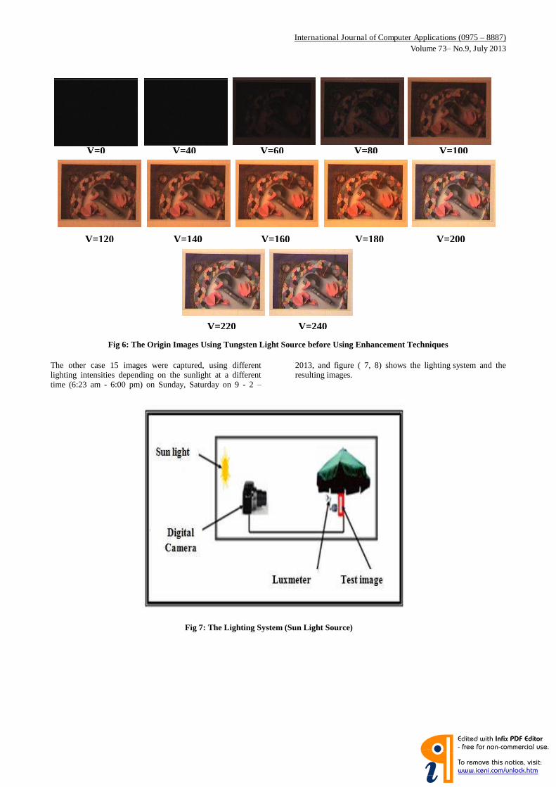
International Journal of Computer Applications (0975 – 8887) Volume 73– No.9, July 2013
34
Fig 6: The Origin Images Using Tungsten Light Source before Using Enhancement Techniques
The other case 15 images were captured, using different lighting intensities depending on the sunlight at a different time (6:23 am - 6:00 pm) on Sunday, Saturday on 9 - 2 –
2013, and figure ( 7, 8) shows the lighting system and the resulting images.
V=0 V=40 V=60 V=80 V=100
V=120 V=140 V=160 V=180 V=200
V=220 V=240
Fig 7: The Lighting System (Sun Light Source)
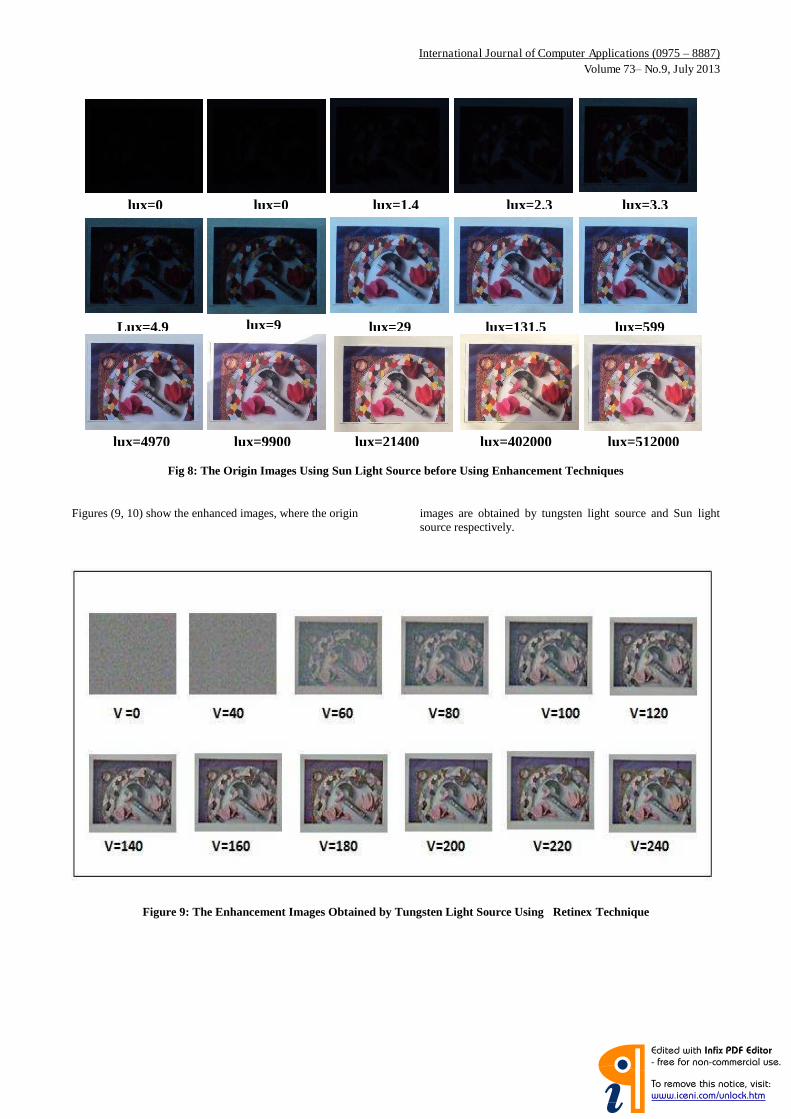
International Journal of Computer Applications (0975 – 8887) Volume 73– No.9, July 2013
35
Fig 8: The Origin Images Using Sun Light Source before Using Enhancement Techniques
Figures (9, 10) show the enhanced images, where the origin images are obtained by tungsten light source and Sun light source respectively.
Fig 9: The Enhancement Images Obtained by Tungsten Light Source Using Retinex Technique
Figure 9: The Enhancement Images Obtained by Tungsten Light Source Using Retinex Technique
lux=0 lux=0 lux=1.4 lux=2.3 lux=3.3
Lux=4.9 lux=9 lux=29 lux=131.5 lux=599
lux=4970 lux=9900 lux=21400 lux=402000 lux=512000
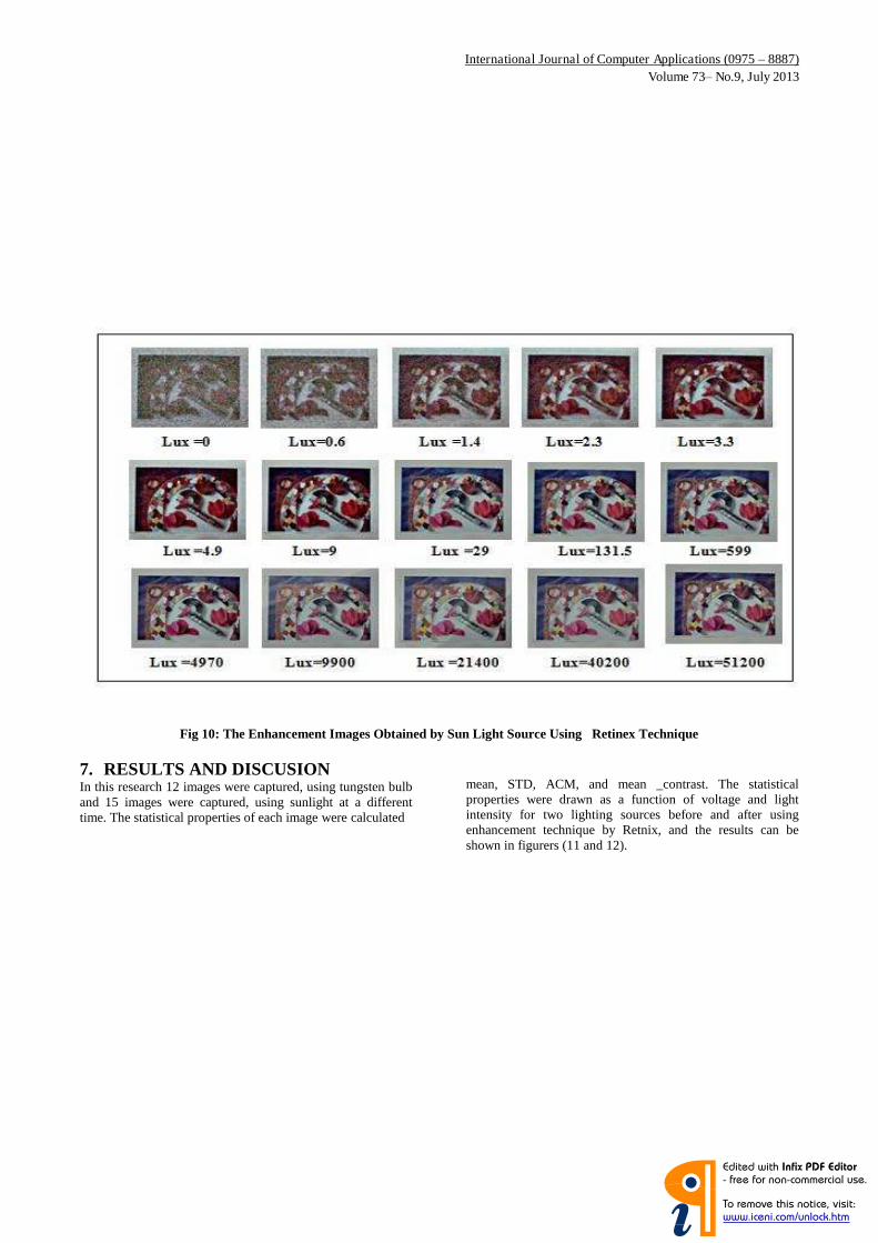
International Journal of Computer Applications (0975 – 8887) Volume 73– No.9, July 2013
36
Fig 10: The Enhancement Images Obtained by Sun Light Source Using Retinex Technique
7. RESULTS AND DISCUSION In this research 12 images were captured, using tungsten bulb and 15 images were captured, using sunlight at a different time. The statistical properties of each image were calculated
mean, STD, ACM, and mean _contrast. The statistical properties were drawn as a function of voltage and light intensity for two lighting sources before and after using enhancement technique by Retnix, and the results can be shown in figurers (11 and 12).
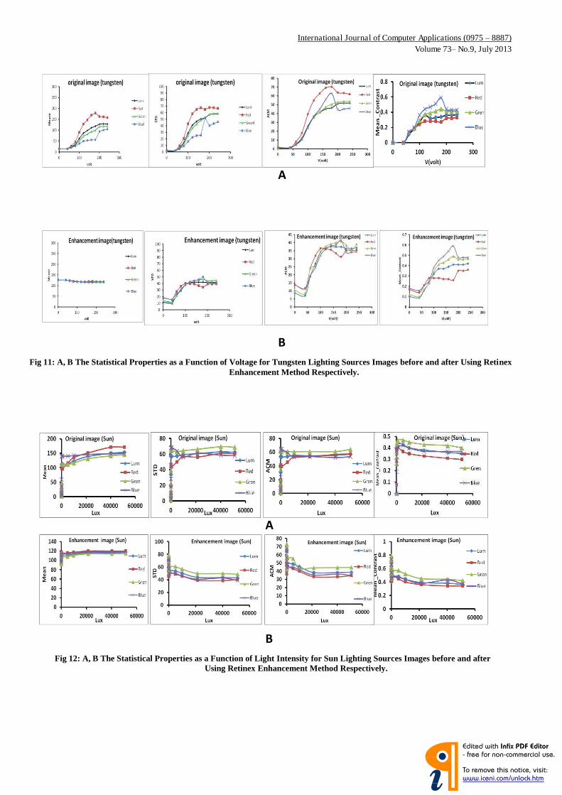
International Journal of Computer Applications (0975 – 8887) Volume 73– No.9, July 2013
37
Fig 12: A, B The Statistical Properties as a Function of Light Intensity for Sun Lighting Sources Images before and after Using Retinex Enhancement Method Respectively.
Fig 11: A, B The Statistical Properties as a Function of Voltage for Tungsten Lighting Sources Images before and after Using Retinex Enhancement Method Respectively.
B
B
A
A
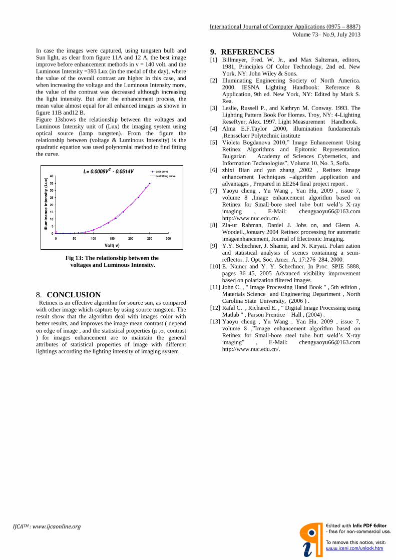
International Journal of Computer Applications (0975 – 8887) Volume 73– No.9, July 2013
38
In case the images were captured, using tungsten bulb and Sun light, as clear from figure 11A and 12 A, the best image improve before enhancement methods in v = 140 volt, and the Luminous Intensity =393 Lux (in the medal of the day), where the value of the overall contrast are higher in this case, and when increasing the voltage and the Luminous Intensity more, the value of the contrast was decreased although increasing the light intensity. But after the enhancement process, the mean value almost equal for all enhanced images as shown in figure 11B and12 B. Figure 13shows the relationship between the voltages and Luminous Intensity unit of (Lux) the imaging system using optical source (lamp tungsten). From the figure the relationship between (voltage & Luminous Intensity) is the quadratic equation was used polynomial method to find fitting the curve.
8. CONCLUSION Retinex is an effective algorithm for source sun, as compared with other image which capture by using source tungsten. The result show that the algorithm deal with images color with better results, and improves the image mean contrast ( depend on edge of image , and the statistical properties ( ,, contrast ) for images enhancement are to maintain the general attributes of statistical properties of image with different lightings according the lighting intensity of imaging system .
9. REFERENCES [1] Billmeyer, Fred. W. Jr., and Max Saltzman, editors,
1981, Principles Of Color Technology, 2nd ed. New York, NY: John Wiley & Sons.
[2] Illuminating Engineering Society of North America. 2000. IESNA Lighting Handbook: Reference & Application, 9th ed. New York, NY: Edited by Mark S. Rea.
[3] Leslie, Russell P., and Kathryn M. Conway. 1993. The Lighting Pattern Book For Homes. Troy, NY: 4-Lighting ReseRyer, Alex. 1997. Light Measurement Handbook.
[4] Alma E.F.Taylor ,2000, illumination fundamentals ,Rensselaer Polytechnic institute
[5] Violeta Bogdanova 2010,” Image Enhancement Using Retinex Algorithms and Epitomic Representation. Bulgarian Academy of Sciences Cybernetics, and Information Technologies”, Volume 10, No. 3, Sofia.
[6] zhixi Bian and yan zhang ,2002 , Retinex Image enhancement Techniques –algorithm ,application and advantages , Prepared in EE264 final project report .
[7] Yaoyu cheng , Yu Wang , Yan Hu, 2009 , issue 7, volume 8 ,Image enhancement algorithm based on Retinex for Small-bore steel tube butt weld’s X-ray imaging , E-Mail: [email protected] http://www.nuc.edu.cn/.
[8] Zia-ur Rahman, Daniel J. Jobs on, and Glenn A. Woodell.,Jonuary 2004 Retinex processing for automatic imageenhancement, Journal of Electronic Imaging.
[9] Y.Y. Schechner, J. Shamir, and N. Kiryati. Polari zation and statistical analysis of scenes containing a semi-reflector. J. Opt. Soc. Amer. A, 17:276–284, 2000.
[10] E. Namer and Y. Y. Schechner. In Proc. SPIE 5888, pages 36–45, 2005 Advanced visibility improvement based on polarization filtered images.
[11] John C. , " Image Processing Hand Book " , 5th edition , Materials Science and Engineering Department , North Carolina State University, (2006 ) .
[12] Rafal C. , Richared E. , " Digital Image Processing using Matlab " , Parson Prentice – Hall , (2004) .
[13] Yaoyu cheng , Yu Wang , Yan Hu, 2009 , issue 7, volume 8 ,”Image enhancement algorithm based on Retinex for Small-bore steel tube butt weld’s X-ray imaging” , E-Mail: [email protected] http://www.nuc.edu.cn/.
L= 0.0008V2 - 0.0514V
0
5
10
15
20
25
30
35
40
0 50 100 150 200 250 300
Volt( v)
illu
min
an
ce i
nte
nsit
y (
Lu
x)
data curve
best fitting curve
Fig 13: The relationship between the voltages and Luminous Intensity.
IJCATM : www.ijcaonline.org
International Journal of Computer Applications (0975 – 8887) Volume 85 – No 3, January 2014
17
Estimation of the Deposited Aerosol Particles in Baghdad City, using Image Processing Technique
Huda Al-Ameer Abood College of Science,
Al-Mustansiriya University Baghdad-Iraq
Ali A. Al-Zuky College of Science,
Al-Mustansiriya University Baghdad-Iraq
Anwar H. M. Al-Saleh College of Science,
Al-Mustansiriya University Baghdad-Iraq
ABSTRACT In this study, an algorithm was developed to measure the volume and the covered area by the dust particles, and the radius of dust particle deposited for different time hours of the day. Slices transparent glass has been used to collect samples of dust particle deposited for different time of the day in Rusafa area of Baghdad city, were taken digital image of the samples through an optical microscope (EYEPIECE 10X). What have been noticeable are the difference in radii and areas of dust particles deposited as well as the difference in the density of dust particles for each slice according to time that put the slice to deposition.
Keywords Dust particle, Atmospheric Aerosols.
1. INTRODUCTION Air pollution is one of the important problems in latest decades, with increasing use of fuels from oil and natural gas in various fields of life, spread in the environment many air pollutants such as gases resulting from industrial activities or different modes of transport [1].Air pollutants are classified according to the nature of its presence into two main groups: gaseous pollutants and aerosols. An example of gaseous pollutants and hydrocarbons that exist in the form of organic compounds may be gaseous, liquid or solid, such as sulfur oxides, nitrogen oxides and carbon [2]. The aerosol pollutants other are divided into solid and liquid non-permanent, such as the normal dust and pollen. Aerosol sooner or later precipitates out of the air but gases, containing space which launches it and act like the air and will not precipitate [3]. Aerosol light-absorption measurements are important for health, climate, and visibility applications [4].
Michael D. King et al. (1999) [5] Studied the advantages and disadvantages systems of Remote sensing for aerosol application, Where no one sensor system is capable of providing totally unambiguous information. Also a careful intercomparison of derived products from different sensors, to gather with comprehensive network of ground-based sun photometer and sky radiometer systems. W.Partrick Arnottet. al.(2005)[4] exploited the aerosol optics use in experiment develop a model-based calibration scheme for the 7-wavelength aethalometer, and the photo acoustic instrument operating at 532nm is used to evaluate the filter loading effect caused by aerosol light absorption and multiple scattering theory is used to analytically obtain a filter-loading correction function. G. J. Wong et al. (2007) [6] Studied the temporal development for air quality, was develop the image processing technique for enhancing the capability of an internet video surveillance (IVS) camera for real time air quality monitoring, in this technique could to detect particulate mater with diameter less than 10 micrometers(PM10).Xiaolei Yu et. al. (2011) [7] introduced a relationship between aerosol anthropogenic component and
air quality in the city of Wuhan, by used satellite remote sensing. A. Bagatet. al. (2013) [8] exploit the aerosol optical depth, Angstrom exponent, single scattering albedo, and polarized phase function have been retrieved from polarized sun-photometer measurements for atmosphere. Where the Angstrom exponent has a meaningful variations respect to the changes in the complex refractive index of the aerosol, and the polarized phase function shows a moderate negative correlation respect to aerosol optical depth and single scattering albedo, so polarized phase function became regarded as a key parameter to characterize the aerosol. In this paper, measuring system will be introduced for determine radius, covered area by deposited aerosol particle and deposited aerosol particle volume as a function of day time, will be calculated by using image analysis and computer algorithms.
2. ATMOSPHERIC AEROSOLS Aerosols are minute particles suspended in the atmosphere. When these particles are sufficiently large can be observed their presence as they scatter and absorb sunlight. Was the scattering of sunlight can reduce visibility (haze) and redden sunrises and sunsets [9]. Measured the size in unit micrometer, particle largest of 50 micrometers can be seen by the naked eye but smaller of (0.005) micrometers can be observing it only in electronic microscope. where that extreme importance of particles in the study of air pollution which their ranging size from (0.01 -100) micrometers and particles younger than 10 micrometers tend not to quickly sedimentation, so remain in the atmosphere for a long time either the fumes, smoke, metal dust, cement, fly ash, carbon black and spray sulfuric acid all located within the range (10 -100) micrometers which are larger and heavier than the outstanding and deposited of near their sources. The deposition process of these particles is the most important natural process to self-cleaning of remove the particle from the air [10]. Particles are typically classified as total suspended particulate (TSP: comprising all particle sizes), medium to fine particulate (PM10: particles less than 10 mm in diameter), fine particulate (PM2.5: particles less than 2.5 mm in diameter), and ultra-fine particulate (PM1.0 and smaller). Fine particles, or PM2.5, are the most significant contaminant influencing visibility conditions because their specific size allows them to scatter or absorb visible light. It also allows them to remain airborne for long periods of time, and under favorable climatic conditions they may be transported over long distances. This is one reason why locations distant from the main pollution sources.Secondary reactions are influenced by a wide range of factors, such as temperature, sunlight, the mixture of gases present, and time. Secondary formation of particles from gaseous pollutants can take some time to occur and will be exacerbated under conditions of low wind speed and poor dispersion [11]. The major component comes in the form of sulfate aerosols created by the burning of coal and oil. The concentration of
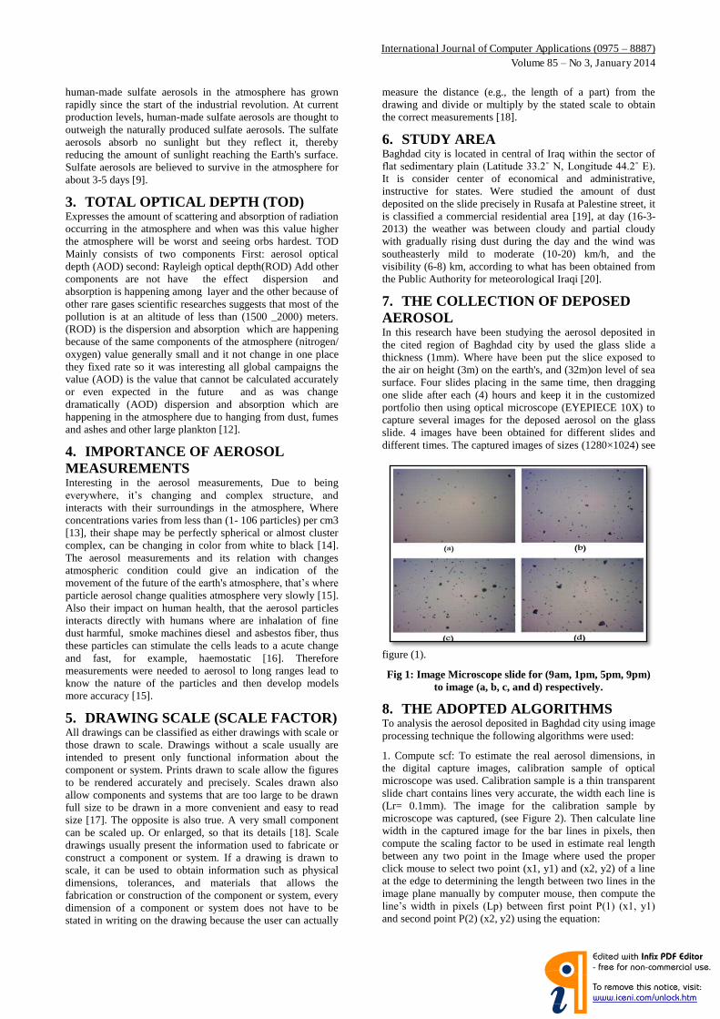
International Journal of Computer Applications (0975 – 8887) Volume 85 – No 3, January 2014
18
human-made sulfate aerosols in the atmosphere has grown rapidly since the start of the industrial revolution. At current production levels, human-made sulfate aerosols are thought to outweigh the naturally produced sulfate aerosols. The sulfate aerosols absorb no sunlight but they reflect it, thereby reducing the amount of sunlight reaching the Earth's surface. Sulfate aerosols are believed to survive in the atmosphere for about 3-5 days [9].
3. TOTAL OPTICAL DEPTH (TOD) Expresses the amount of scattering and absorption of radiation occurring in the atmosphere and when was this value higher the atmosphere will be worst and seeing orbs hardest. TOD Mainly consists of two components First: aerosol optical depth (AOD) second: Rayleigh optical depth(ROD) Add other components are not have the effect dispersion and absorption is happening among layer and the other because of other rare gases scientific researches suggests that most of the pollution is at an altitude of less than (1500 _2000) meters. (ROD) is the dispersion and absorption which are happening because of the same components of the atmosphere (nitrogen/ oxygen) value generally small and it not change in one place they fixed rate so it was interesting all global campaigns the value (AOD) is the value that cannot be calculated accurately or even expected in the future and as was change dramatically (AOD) dispersion and absorption which are happening in the atmosphere due to hanging from dust, fumes and ashes and other large plankton [12].
4. IMPORTANCE OF AEROSOL MEASUREMENTS Interesting in the aerosol measurements, Due to being everywhere, it’s changing and complex structure, and interacts with their surroundings in the atmosphere, Where concentrations varies from less than (1- 106 particles) per cm3 [13], their shape may be perfectly spherical or almost cluster complex, can be changing in color from white to black [14]. The aerosol measurements and its relation with changes atmospheric condition could give an indication of the movement of the future of the earth's atmosphere, that’s where particle aerosol change qualities atmosphere very slowly [15]. Also their impact on human health, that the aerosol particles interacts directly with humans where are inhalation of fine dust harmful, smoke machines diesel and asbestos fiber, thus these particles can stimulate the cells leads to a acute change and fast, for example, haemostatic [16]. Therefore measurements were needed to aerosol to long ranges lead to know the nature of the particles and then develop models more accuracy [15].
5. DRAWING SCALE (SCALE FACTOR) All drawings can be classified as either drawings with scale or those drawn to scale. Drawings without a scale usually are intended to present only functional information about the component or system. Prints drawn to scale allow the figures to be rendered accurately and precisely. Scales drawn also allow components and systems that are too large to be drawn full size to be drawn in a more convenient and easy to read size [17]. The opposite is also true. A very small component can be scaled up. Or enlarged, so that its details [18]. Scale drawings usually present the information used to fabricate or construct a component or system. If a drawing is drawn to scale, it can be used to obtain information such as physical dimensions, tolerances, and materials that allows the fabrication or construction of the component or system, every dimension of a component or system does not have to be stated in writing on the drawing because the user can actually
measure the distance (e.g., the length of a part) from the drawing and divide or multiply by the stated scale to obtain the correct measurements [18].
6. STUDY AREA Baghdad city is located in central of Iraq within the sector of flat sedimentary plain (Latitude 33.2˚ N, Longitude 44.2˚ E). It is consider center of economical and administrative, instructive for states. Were studied the amount of dust deposited on the slide precisely in Rusafa at Palestine street, it is classified a commercial residential area [19], at day (16-3-2013) the weather was between cloudy and partial cloudy with gradually rising dust during the day and the wind was southeasterly mild to moderate (10-20) km/h, and the visibility (6-8) km, according to what has been obtained from the Public Authority for meteorological Iraqi [20].
7. THE COLLECTION OF DEPOSED AEROSOL In this research have been studying the aerosol deposited in the cited region of Baghdad city by used the glass slide a thickness (1mm). Where have been put the slice exposed to the air on height (3m) on the earth's, and (32m)on level of sea surface. Four slides placing in the same time, then dragging one slide after each (4) hours and keep it in the customized portfolio then using optical microscope (EYEPIECE 10X) to capture several images for the deposed aerosol on the glass slide. 4 images have been obtained for different slides and different times. The captured images of sizes (1280×1024) see
figure (1).
Fig 1: Image Microscope slide for (9am, 1pm, 5pm, 9pm) to image (a, b, c, and d) respectively.
8. THE ADOPTED ALGORITHMS To analysis the aerosol deposited in Baghdad city using image processing technique the following algorithms were used:
1. Compute scf: To estimate the real aerosol dimensions, in the digital capture images, calibration sample of optical microscope was used. Calibration sample is a thin transparent slide chart contains lines very accurate, the width each line is (Lr= 0.1mm). The image for the calibration sample by microscope was captured, (see Figure 2). Then calculate line width in the captured image for the bar lines in pixels, then compute the scaling factor to be used in estimate real length between any two point in the Image where used the proper click mouse to select two point (x1, y1) and (x2, y2) of a line at the edge to determining the length between two lines in the image plane manually by computer mouse, then compute the line’s width in pixels (Lp) between first point P(1) (x1, y1) and second point P(2) (x2, y2) using the equation:
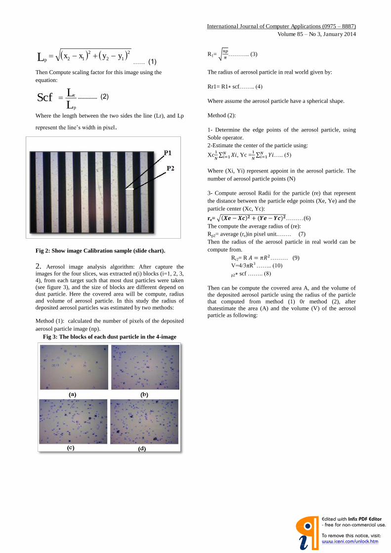
International Journal of Computer Applications (0975 – 8887) Volume 85 – No 3, January 2014
19
…… (1)
Then Compute scaling factor for this image using the equation:
LLScf
p
r …………… (2)
Where the length between the two sides the line (Lr), and Lp
represent the line’s width in pixel.
Fig 2: Show image Calibration sample (slide chart).
2. Aerosol image analysis algorithm: After capture the images for the four slices, was extracted n(i) blocks (i=1, 2, 3, 4), from each target such that most dust particles were taken (see figure 3), and the size of blocks are different depend on dust particle. Here the covered area will be compute, radius and volume of aerosol particle. In this study the radius of deposited aerosol particles was estimated by two methods:
Method (1): calculated the number of pixels of the deposited aerosol particle image (np).
Fig 3: The blocks of each dust particle in the 4-image
R1= ……….. (3)
The radius of aerosol particle in real world given by:
Rr1= R1 scf…….. (4)
Where assume the aerosol particle have a spherical shape.
Method (2):
1- Determine the edge points of the aerosol particle, using Soble operator. 2-Estimate the center of the particle using:
Xc , Yc =
….. (5)
Where (Xi, Yi) represent appoint in the aerosol particle. The number of aerosol particle points (N)
3- Compute aerosol Radii for the particle (re) that represent the distance between the particle edge points (Xe, Ye) and the particle center (Xc, Yc):
re= ………(6) The compute the average radius of (re): Rp2= average (re)in pixel unit.……. (7) Then the radius of the aerosol particle in real world can be compute from.
Rr2= R ……… (9) V=4/3πR3 …….. (10) p2 scf …….. (8)
Then can be compute the covered area A, and the volume of the deposited aerosol particle using the radius of the particle that computed from method (1) 0r method (2), after thatestimate the area (A) and the volume (V) of the aerosol particle as following:
2122
12 yyxxLp
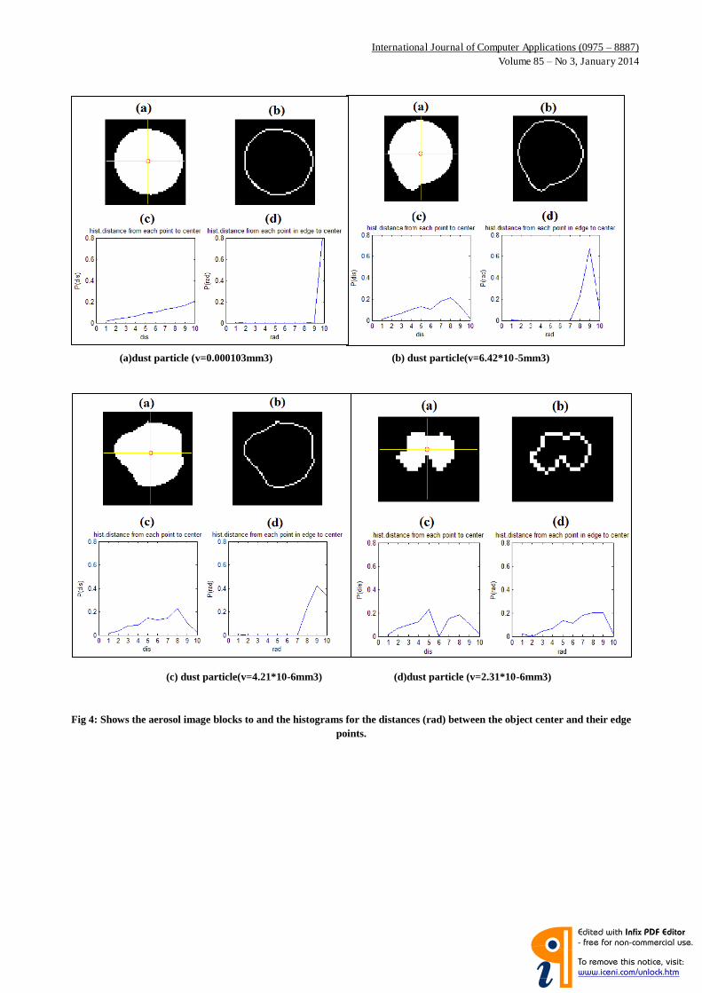
International Journal of Computer Applications (0975 – 8887) Volume 85 – No 3, January 2014
20
Fig 4: Shows the aerosol image blocks to and the histograms for the distances (rad) between the object center and their edge points.
(a)dust particle (v=0.000103mm3) (b) dust particle(v=6.42*10-5mm3)
(c) dust particle(v=4.21*10-6mm3) (d)dust particle (v=2.31*10-6mm3)
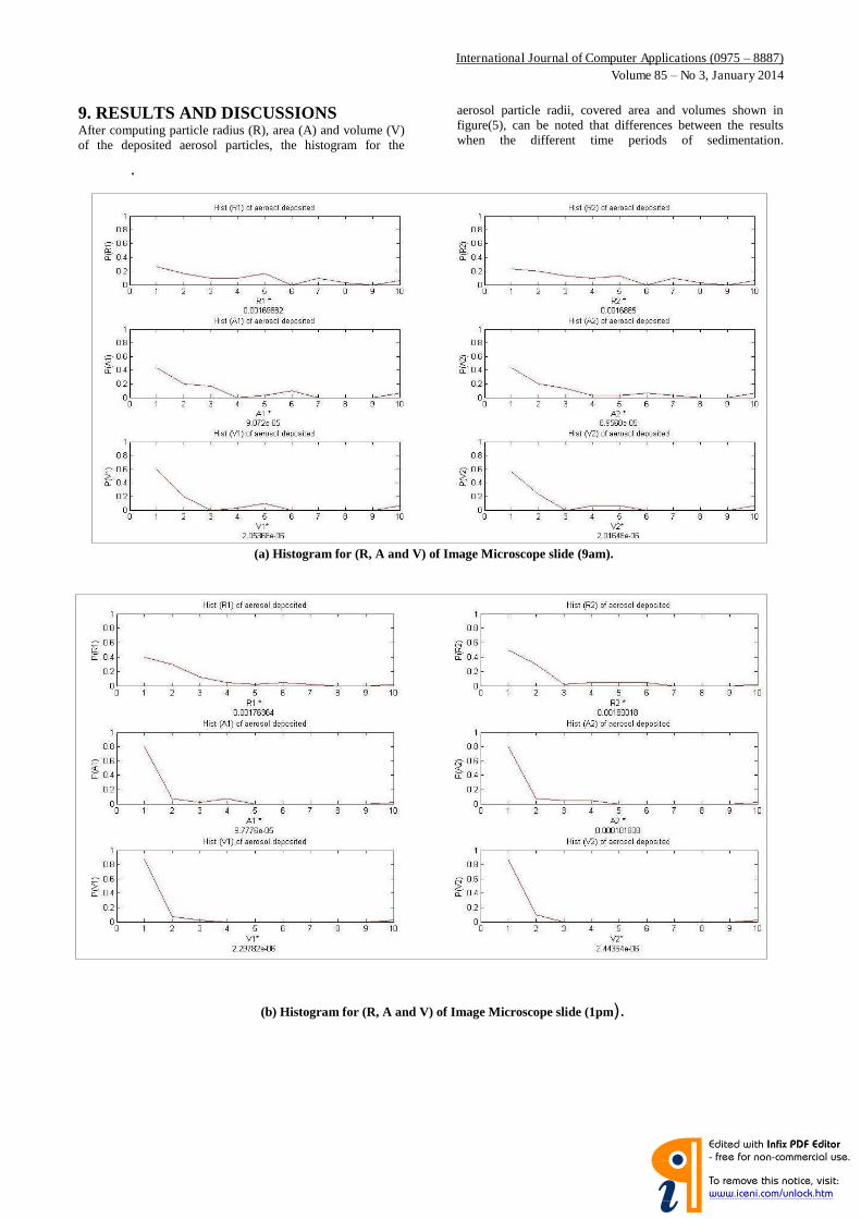
International Journal of Computer Applications (0975 – 8887) Volume 85 – No 3, January 2014
21
9. RESULTS AND DISCUSSIONS After computing particle radius (R), area (A) and volume (V) of the deposited aerosol particles, the histogram for the
aerosol particle radii, covered area and volumes shown in figure(5), can be noted that differences between the results when the different time periods of sedimentation.
.
(a) Histogram for (R, A and V) of Image Microscope slide (9am).
(b) Histogram for (R, A and V) of Image Microscope slide (1pm).
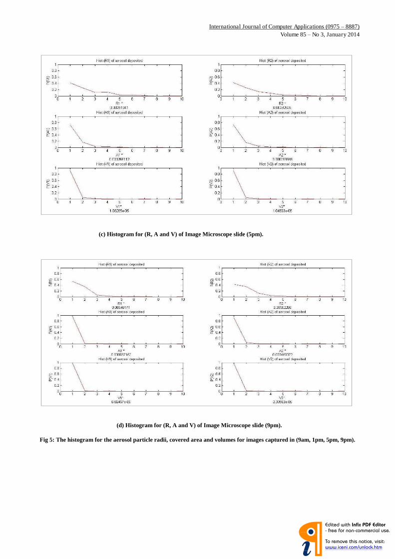
International Journal of Computer Applications (0975 – 8887) Volume 85 – No 3, January 2014
22
(c) Histogram for (R, A and V) of Image Microscope slide (5pm).
(d) Histogram for (R, A and V) of Image Microscope slide (9pm).
Fig 5: The histogram for the aerosol particle radii, covered area and volumes for images captured in (9am, 1pm, 5pm, 9pm).
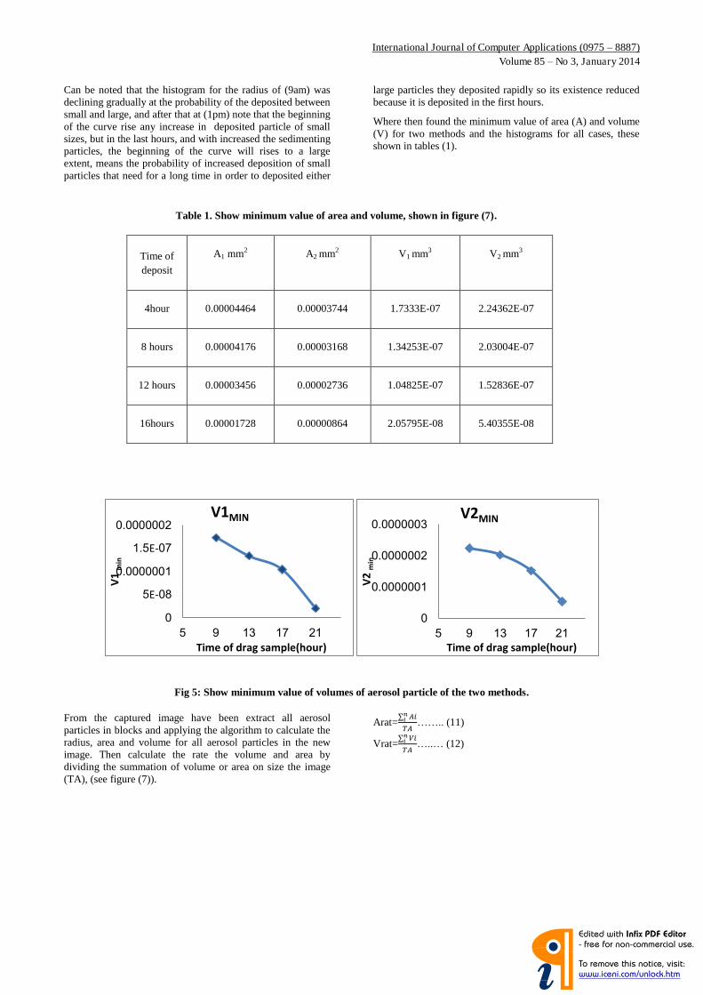
International Journal of Computer Applications (0975 – 8887) Volume 85 – No 3, January 2014
23
Can be noted that the histogram for the radius of (9am) was declining gradually at the probability of the deposited between small and large, and after that at (1pm) note that the beginning of the curve rise any increase in deposited particle of small sizes, but in the last hours, and with increased the sedimenting particles, the beginning of the curve will rises to a large extent, means the probability of increased deposition of small particles that need for a long time in order to deposited either
large particles they deposited rapidly so its existence reduced because it is deposited in the first hours.
Where then found the minimum value of area (A) and volume (V) for two methods and the histograms for all cases, these shown in tables (1).
Table 1. Show minimum value of area and volume, shown in figure (7).
Time of deposit
A1 mm2 A2 mm2 V1 mm3 V2 mm3
4hour 0.00004464 0.00003744 1.7333E-07 2.24362E-07
8 hours 0.00004176 0.00003168 1.34253E-07 2.03004E-07
12 hours 0.00003456 0.00002736 1.04825E-07 1.52836E-07
16hours 0.00001728 0.00000864 2.05795E-08 5.40355E-08
Fig 5: Show minimum value of volumes of aerosol particle of the two methods.
From the captured image have been extract all aerosol particles in blocks and applying the algorithm to calculate the radius, area and volume for all aerosol particles in the new image. Then calculate the rate the volume and area by dividing the summation of volume or area on size the image (TA), (see figure (7)).
Arat= …….. (11)
Vrat= …..… (12)
0
5E-08
0.0000001
1.5E-07
0.0000002
5 9 13 17 21
V1
min
Time of drag sample(hour)
V1MIN
0
0.0000001
0.0000002
0.0000003
5 9 13 17 21
V2
min
Time of drag sample(hour)
V2MIN

International Journal of Computer Applications (0975 – 8887) Volume 85 – No 3, January 2014
24
10. CONCLUSION
From the result can be concluded:
1-The density of dust particle deposited on the first slide (9am) very low aerosols comparing with the other, and the covered area to each dust particle is medium measurement.
2- There is significantly increased density of dust particle on the second slice and different kinds of shapes and sizes of dust particle, that can be observed from the histogram of the second slice the peaks is reduced for curve to areas (A1, A2) that means increased in Measurements the covered area of dust particle gradually from very small to large.
3-On the third slide (5pm) there was increased density but difference less the first cases (9am).
4-In the last (9pm) case was observed that the small particle of the dust is the most increased, this is due to small particle nature of slow deposition, and that clear in histogram, the Curved rise because the dust proportion increased due to increased hours of the deposition, and the start of the curve is rise at the low values of covered area to dust particle, and the peaks non-existent Almost at the high values. Was obtaining the results different of shapes and areas, there symmetric, semi-symmetric and asymmetric and asymmetric is majority.
5-at calculate the smaller covered area and the volume of the aerosols particles deposited, notice that the curve is exponential decreasing that was sedimenting particles small-scale take more time to fall, and whenever the time of the deposition increasing then the small particles can be deposited where that small volume of the aerosol particles are depositing at the final hours because number of effects such as the wind speed in night.
11. REFERENCES [1] Bassim M. Hashim*, Dr.Maitham A. Sultan," Using
remote sensing data and GIS to evaluate air pollution and their relationship with land cover and land use to Baghdad city" International Applied Geological Congress, Department of Geology, Islamic Azad University - Mashad Branch, Iran, 26-28 April , 2010.
[2] White, H., 1986: On the theoretical and empirical basis for apportion extinction by aerosols: A critical Review. Atmos. Envir., 20, 1659-1672.
[3] Ahmed F. Hussun" Properties of Urban boundary layer and their effects on variation of atmospheric aerosols concentration Particles over Baghdad city" AL-Mustansiriyah University (2010).
[4] W. Patrick Arnott et al."Towards Aerosol Light-Absorption Measurements with a 7-Wavelength Aethalometer: Evaluation with a Photoacoustic Instrument and 3-Wavelength Nephelometer" (2005).Aerosol Science and Technology, 39:17–29, 2005 Copyright _c American Association for Aerosol Research.
[5] Michael D. King, Yoram J. K, Didier T., and Teruyuki N.," Remote Sensing of Troposphere Aerosols from Space: Past, Present, and Future" American Meteorological Society, Vol. 80, No. 11, November 1999.
[6] C.J. Wong et al."Using Image Processing Technique for the Studies on Temporal Development of Air
Fig 5: Show the rate for total (A1, A2, V1 and V2) in the image.
0
0.0002
0.0004
0.0006
0.0008
0.001
5 9 13 17 21
V2
rat
Time of drag sample(hour)
V2rat
0
0.0002
0.0004
0.0006
0.0008
0.001
5 9 13 17 21
V1
rat
Time of drag sample(hour)
V1rat
0
0.01
0.02
0.03
0.04
5 9 13 17 21
A2
rat
Time of drag sample(hour)
A2rat
0
0.01
0.02
0.03
0.04
5 9 13 17 21
A1
rat
Time of drag sample(hour)
A1rat

International Journal of Computer Applications (0975 – 8887) Volume 85 – No 3, January 2014
25
Quality"(2007) School of Physics, UniversitiSains Malaysia, 11800 USM, Penang, Malaysia.
[7] Xiaolei Yu, Zhaocong Wu," Study on the Relationship Between Aerosol Anthropogenic Component and Air Quality in the City of Wuhan" IEEE978-1-4244-9171,2001.
[8] A. Bayat, H. R. Khalesifard, and A. Masoumi," Retrieval of aerosol single scattering albedo and polarized phase function from polarized sun-photometer measurements for Zanjan atmosphere" Atmos. Meas. Tech. Discuss., 6, 3317–3338, 2013.
[9] Internet(http://www.nasa.gov/centers/langley/news/factsheets/Aerosols.html)
[10] Faiza Ali et al."Evaluation and statistical analysis of the measurements of the total outstanding minutes and bullets in the air of the city of Baghdad for the year (2008)"Iraqi Ministry of the Environment (http://www.moen.gov.iq/lastest-stadies.html).
[11] Hon Marian L Hobbs"Good practice guide for monitoring and management of visibility in New Zealand"ISBN 0-478-24035-X, 406, pp.10-11, Ministry for the Environment, August 2001
[12] Internet (http://blog.icoproject.org).
[13] Stern, A.C."Air Pollution"Acadamic press Inc., 1976.
[14] Korhonen, P., M. Kulmala, A. Laksonen, Y. Viisanen, R. Mc. Grew, and J. H. Seinfeld "Ternary nucleation of H2So4, NH3 and H2O in the atmosphere" J. Geoph. Res., 104, 1999.
[15] Seaton, A., W. Macuee, K., Donaldson, and D. Godden"Particulate air pollution and acute health effects"The Lancent, 345, 176-178, 1995.
[16] Peter K. Kaiser "Comparison of static visual acuity between snellen and early treatment diabetic retina patly study charts", Kalpana, Karlhick J., Jayrajinis. 24 February 2013.
[17] Daniel Herrington,”Easy image processing camera interfacing for robotics”, www.atmel.com.2003.
[18] R.C.Gonzalez, “Digital image processing”, second edition University of Tennessee, (2001).
[19] Internet (http://ar.wikipedia.org/wiki/Baghdad).
[20] Internet (http://www.meteoseism.gov.iq) 16/3/2013.
IJCATM : www.ijcaonline.org

FONDAZIONE GIORGIO RONCHIhttp://ronchi.isti.cnr.it
Estratto da: Atti della Fondazione Giorgio RonchiAnno LXVIII, n. 2 - Marzo-Aprile 2013
Tip. L’Arcobaleno s.n.c. - Via Bolognese, 54 - Firenze2013
ALI ABID D. AL-ZUKY, MARWAH M. ABDULSTTAR
Tilting Angle-Dependent to Estimate Object’s Range

ANNO LXVIII MARZO-APRILE 2013 N. 2
A T T I
DELLA «FONDAZIONE GIORGIO RONCHI»
EDITORIAL BOARD
Pubblicazione bimestrale - Prof. LAURA RONCHI ABBOZZO Direttore Responsabile
La responsabilità per il contenuto degli articoli è unicamente degli Autori
Iscriz. nel Reg. stampa del Trib. di Firenze N. 681 - Decreto del Giudice Delegato in data 2-1-1953
Tip. L’Arcobaleno - Via Bolognese, 54 - Firenze - Aprile 2013
Prof. Roberto BuonannoOsservatorio Astronomico di RomaMonteporzio Catorne, Roma, Italy
Prof. Ercole M. GloriaVia Giunta Pisano 2, Pisa, Italy
Prof. Franco GoriDip. di Fisica, Università Roma IIIRoma, Italy
Prof. Vishal GoyalDepartment of Computer SciencePunjabi University, Patiala, Punjab, India
Prof. Enrique Hita VillaverdeDepartamento de OpticaUniversidad de Granada, Spain
Prof. Irving KaufmanDepartment of Electrical EngineeringArizona State University, TucsonArizona, U.S.A.
Prof. Franco LottiI.F.A.C. del CNR, Via Panciatichi 64Firenze, Italy
Prof. Tommaso MaccacaroDirettore Osservatorio Astronomico di Brera,Via Brera 28, Milano
Prof. Manuel MelgosaDepartamento de OpticaUniversidad de Granada, Spain
Prof. Alberto MeschiariScuola Normale Superiore, Pisa, Italy
Prof. Riccardo PratesiDipartimento di FisicaUniversità di Firenze, Sesto Fiorentino, Italy
Prof. Adolfo PazzagliClinical PsychologyProf. Emerito Università di Firenze
Prof. Edoardo ProverbioIstituto di Astronomia e Fisica SuperioreCagliari, Italy
Prof. Andrea RomoliGalileo Avionica, Campi BisenzioFirenze, Italy
Prof. Ovidio SalvettiI.ST.I. del CNRArea della Ricerca CNR di Pisa, Pisa, Italy.
Prof. Mahipal SinghDeputy Director, CFSL, Sector 36 AChandigarh, India
Prof. Marija StrojnikCentro de Investigaciones en OpticaLeon, Gto Mexico
Prof. Jean-Luc TissotULIS, Veurey Voroize, France
Prof. Paolo VanniProfessore Emerito di Chimica Medicadell’Università di Firenze
Prof. Sergio VillaniLatvia State University, Riga, Lettonia
Tilting Angle-Dependent to Estimate Object’s Range
ALI ABID D. AL-ZUKY (*), MARWAH M. ABDULSTTAR (*)
SUMMARY. – In present paper a mathematical model to estimate the real distance of a certain
circular object has been found based on tilting angle where the fi tting curves of the experimental
data of the object’s area in square pixels (Ap) in the image plane for each tilting angle were achieved.
Then the mathematical modeling equation was found that relates object’s area Ap, real distance dr
and tilting angle θ to estimate object distance. A graph of the theoretical and experimental results
of Ap vs distance for angles from 35° to 75° has been plotted and there was a very good similarity
between them, as well as the estimated distances were very close to the real measurements.
Key words: Tilting angle, mathematical model, object’s area in square pixels (Ap), esti-
mated distance.
1. Introduction
Measurement of the range of objects in many industrial fi elds is very impor-tant. Popular sensor types for non-contact length measurements include Moire, laser, and camera sensors, but measurement systems that utilize a camera are fre-quently used because they are inexpensive, easy to install, fast, and suffi ciently accurate.
CLARK et al. (1998) (1) used the digital imaging to measure distances in horti-cultural, i.e. involved images that are not perpendicular to the object being photo-graphed; for example, many photographs of trees taken from ground level require the camera to be tilted up to capture the whole canopy. When the camera is tilted in the vertical plane, vertical distance measurements will be affected by the verti-cal tilt angle. That can be used to collect multiple height and diameter measure-ments from a stem in a relatively short period of time without felling the tree.
(*) Physics Department, College of Science, Al-Mustansiriya University, Iraq; e-mails: [email protected]; [email protected]
ATTI DELLA “FONDAZIONE GIORGIO RONCHI” ANNO LXVIII, 2013 - N. 2
OPTICAL INSTRUMENTATION
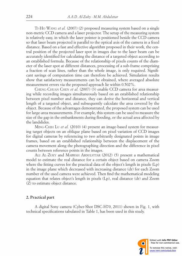
A.A.D. Al-Zuky - M.M. Abdulsttar224
TI-HO WANG et al. (2007) (2) proposed measuring system based on a single non-metric CCD camera and a laser projector. The setup of the measuring system is relatively easy, in which the laser pointer is positioned beside the CCD camera so that laser beam projected is parallel to the optical axis of the camera in a fi xed distance. Based on a fast and effective algorithm proposed in their work, the cen-tral position of the projected laser spot in images due to the laser beam can be accurately identifi ed for calculating the distance of a targeted object according to an established formula. Because of the relationship of pixels counts of the diam-eter of the laser spot at different distances, processing of a sub-frame comprising a fraction of scan lines, rather than the whole image, is only required. Signifi -cant savings of computation time can therefore be achieved. Simulation results show that satisfactory measurements can be obtained, where averaged absolute measurement errors via the proposed approach lie within 0.502%.
CHENG-CHUAN CHEN et al. (2007) (3) enable CCD camera for area measur-ing while recording images simultaneously based on an established relationship between pixel number and distance, they can derive the horizontal and vertical length of a targeted object, and subsequently calculate the area covered by the object. Because of the advantages demonstrated, the proposed system can be used for large-area measurements. For example, this system can be used to measure the size of the gap in the embankments during fl ooding, or the actual area affected by the landslides.
MING-CHIH LU et al. (2010) (4) present an image-based system for measur-ing target objects on an oblique plane based on pixel variation of CCD images for digital cameras by referencing to two arbitrarily designated points in image frames, based on an established relationship between the displacement of the camera movement along the photographing direction and the difference in pixel counts between reference points in the images.
ALI AL-ZUKY and MARWAH ABDULSTTAR (2012) (5) present a mathematical model to estimate the real distance for a certain object based on camera Zoom where the fi tting curves for the practical data of the object’s length in pixels (Lp) in the image plane which decreased with increasing distance (dr) for each Zoom number of the used camera were achieved. Then fi nd the mathematical modeling equation that relates object’s length in pixels (Lp), real distance (dr) and Zoom (Z) to estimate object distance.
2. Practical part
A digital Sony camera (Cyber-Shot DSC-H70, 2011) shown in Fig. 1, with technical specifi cations tabulated in Table 1, has been used in this study.
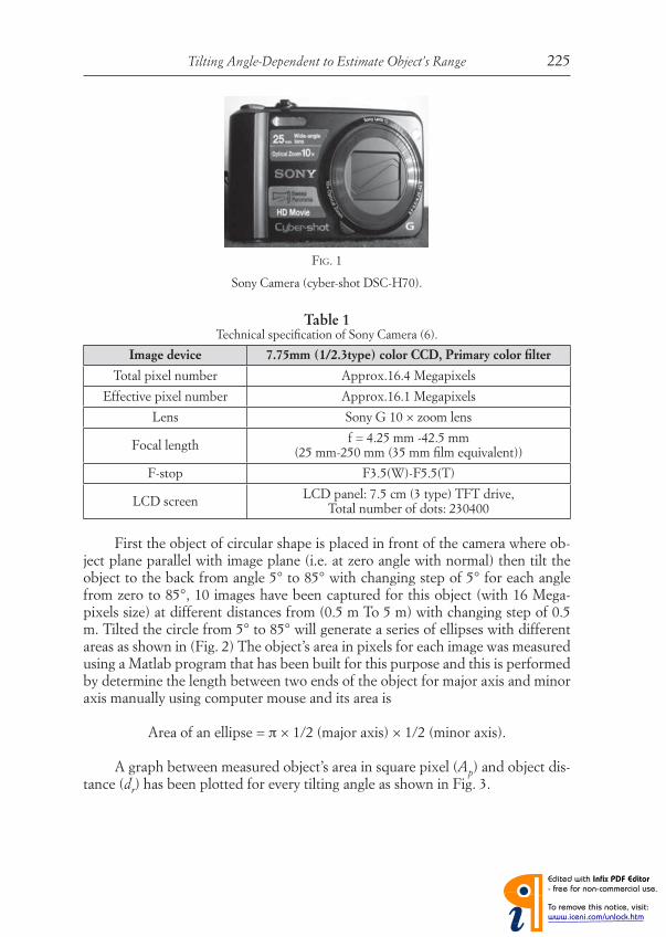
Tilting Angle-Dependent to Estimate Object’s Range 225
Table 1Technical specifi cation of Sony Camera (6).
Image device 7.75mm (1/2.3type) color CCD, Primary color fi lter
Total pixel number Approx.16.4 Megapixels
Effective pixel number Approx.16.1 Megapixels
Lens Sony G 10 × zoom lens
Focal lengthf = 4.25 mm -42.5 mm
(25 mm-250 mm (35 mm fi lm equivalent))
F-stop F3.5(W)-F5.5(T)
LCD screenLCD panel: 7.5 cm (3 type) TFT drive,
Total number of dots: 230400
First the object of circular shape is placed in front of the camera where ob-ject plane parallel with image plane (i.e. at zero angle with normal) then tilt the object to the back from angle 5° to 85° with changing step of 5° for each angle from zero to 85°, 10 images have been captured for this object (with 16 Mega-pixels size) at different distances from (0.5 m To 5 m) with changing step of 0.5 m. Tilted the circle from 5° to 85° will generate a series of ellipses with different areas as shown in (Fig. 2) The object’s area in pixels for each image was measured using a Matlab program that has been built for this purpose and this is performed by determine the length between two ends of the object for major axis and minor axis manually using computer mouse and its area is
Area of an ellipse = π × 1/2 (major axis) × 1/2 (minor axis).
A graph between measured object’s area in square pixel (Ap) and object dis-tance (dr) has been plotted for every tilting angle as shown in Fig. 3.
FIG. 1
Sony Camera (cyber-shot DSC-H70).
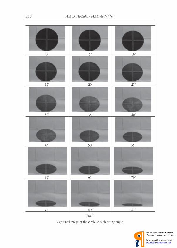
A.A.D. Al-Zuky - M.M. Abdulsttar226
0˚ 5˚ 10˚
15˚ 20˚ 25˚
30˚ 35˚ 40˚
45˚ 50˚ 55˚
60˚ 65˚ 70˚
75˚ 80˚ 85˚
FIG. 2
Captured image of the circle at each tilting angle.
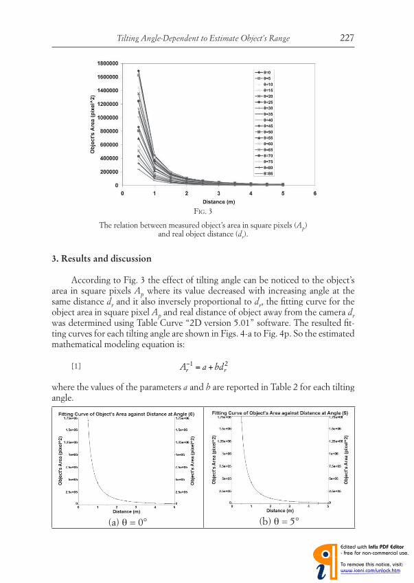
Tilting Angle-Dependent to Estimate Object’s Range 227
3. Results and discussion
According to Fig. 3 the effect of tilting angle can be noticed to the object’s area in square pixels Ap where its value decreased with increasing angle at the same distance dr and it also inversely proportional to dr, the fi tting curve for the object area in square pixel Ap and real distance of object away from the camera dr was determined using Table Curve “2D version 5.01” software. The resulted fi t-ting curves for each tilting angle are shown in Figs. 4-a to Fig. 4p. So the estimated mathematical modeling equation is:
[1]
where the values of the parameters a and b are reported in Table 2 for each tilting angle.
FIG. 3
The relation between measured object’s area in square pixels (Ap) and real object distance (dr).
(a) θ = 0° (b) θ = 5°
Ar−1 = a +bdr
2
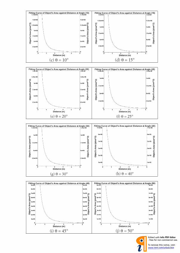
(c) θ = 10° (d) θ = 15°
(e) θ = 20° (f) θ = 25°
(g) θ = 30° (h) θ = 40°
(i) θ = 45° (j) θ = 50°
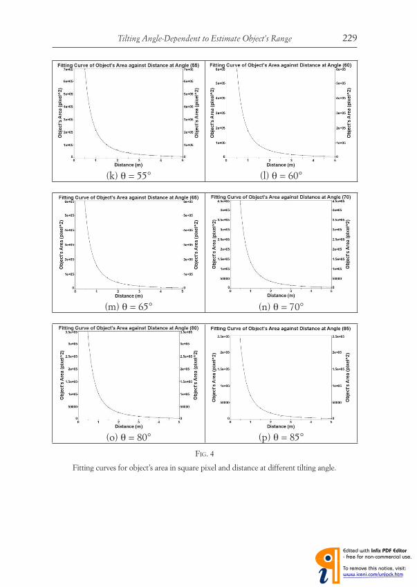
Tilting Angle-Dependent to Estimate Object’s Range 229
(k) θ = 55° (l) θ = 60°
(m) θ = 65° (n) θ = 70°
(o) θ = 80° (p) θ = 85°
FIG. 4
Fitting curves for object’s area in square pixel and distance at different tilting angle.
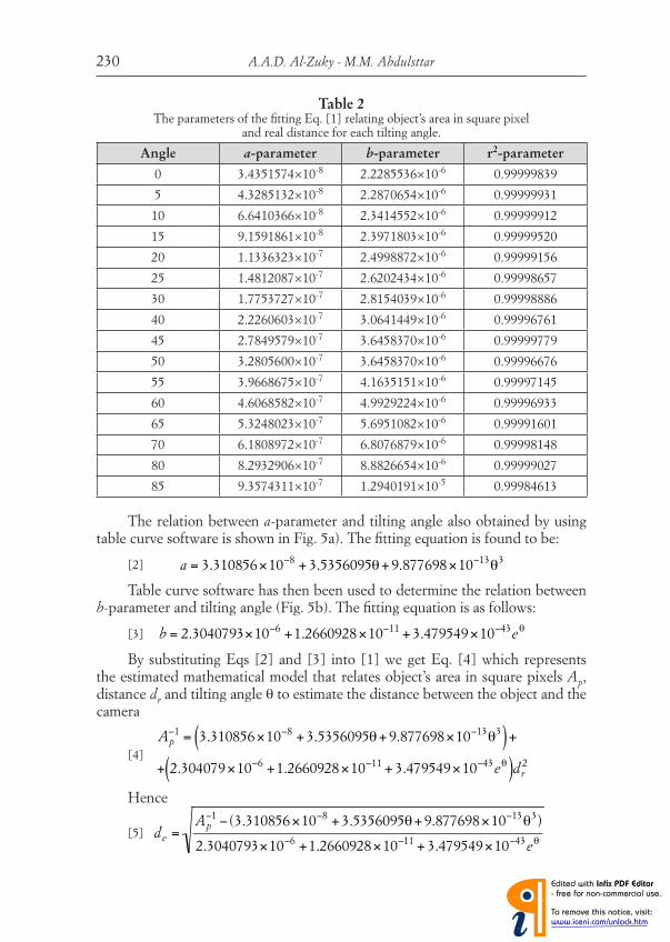
A.A.D. Al-Zuky - M.M. Abdulsttar230
Table 2The parameters of the fi tting Eq. [1] relating object’s area in square pixel
and real distance for each tilting angle.
Angle a-parameter b-parameter r2-parameter
0 3.4351574×10⁻⁸ 2.2285536×10⁻⁶ 0.99999839
5 4.3285132×10⁻⁸ 2.2870654×10⁻⁶ 0.99999931
10 6.6410366×10⁻⁸ 2.3414552×10⁻⁶ 0.99999912
15 9.1591861×10⁻⁸ 2.3971803×10⁻⁶ 0.99999520
20 1.1336323×10⁻⁷ 2.4998872×10⁻⁶ 0.99999156
25 1.4812087×10⁻⁷ 2.6202434×10⁻⁶ 0.99998657
30 1.7753727×10⁻⁷ 2.8154039×10⁻⁶ 0.99998886
40 2.2260603×10⁻⁷ 3.0641449×10⁻⁶ 0.99996761
45 2.7849579×10⁻⁷ 3.6458370×10⁻⁶ 0.99999779
50 3.2805600×10⁻⁷ 3.6458370×10⁻⁶ 0.99996676
55 3.9668675×10⁻⁷ 4.1635151×10⁻⁶ 0.99997145
60 4.6068582×10⁻⁷ 4.9929224×10⁻⁶ 0.99996933
65 5.3248023×10⁻⁷ 5.6951082×10⁻⁶ 0.99991601
70 6.1808972×10⁻⁷ 6.8076879×10⁻⁶ 0.99998148
80 8.2932906×10⁻⁷ 8.8826654×10⁻⁶ 0.99999027
85 9.3574311×10⁻⁷ 1.2940191×10⁻⁵ 0.99984613
The relation between a-parameter and tilting angle also obtained by using table curve software is shown in Fig. 5a). The fi tting equation is found to be:
[2]
Table curve software has then been used to determine the relation between b-parameter and tilting angle (Fig. 5b). The fi tting equation is as follows:
[3]
By substituting Eqs [2] and [3] into [1] we get Eq. [4] which represents the estimated mathematical model that relates object’s area in square pixels Ap, distance dr and tilting angle θ to estimate the distance between the object and the camera
[4]
Hence
[5]
b = 2.3040793×10⁻⁶ +1.2660928×10⁻¹¹ + 3.479549×10−43eθ
Ap−1 = 3.310856×10⁻⁸ + 3.5356095θ+9.877698×10⁻¹³θ3( )+
+ 2.304079×10⁻⁶ +1.2660928×10⁻¹¹ + 3.479549×10−43eθ( )dr2
de =
Ap−1 − (3.310856×10⁻⁸ + 3.5356095θ+9.877698×10⁻¹³θ3)
2.3040793×10⁻⁶ +1.2660928×10⁻¹¹ + 3.479549×10−43eθ
a = 3.310856×10⁻⁸ + 3.5356095θ+9.877698×10⁻¹³θ3

Tilting Angle-Dependent to Estimate Object’s Range 231
FIG. 6
Theoretical and experimental curves of object’s area in square pixel Ap with object distance dr at (a) θ = 35° and (b) θ = 75°.
(a) θ = 35° (b) θ = 75°
We canceled the practical results for angle 35° and 75° from fi tting process in order to determine their values theoretically from the estimated mathematical model of Eq. [4] and make a comparison between the experimental and theoreti-cal values (see Fig. 6). There is an excellent agreement between them.
Equation [5] has also been used to estimate object’s distance at 35° and 75° angle in order to compare the estimated result with the real measurements. The result is tabulated in Tables 3 & 4.
FIG. 5
The relation between tilting angle and (a) a-parameter, (b) b-parameter.
(a) (b)
4. Conclusion
We investigated a mathematical model based on tilting angle θ according to its effect on the object’s area in square pixels Ap for a circular shape with 30 cm diameter in image plane at different distance from 0.5 to 5 m with step 0.5 m, and conclude that the proposed model for estimate object distance (de) is:
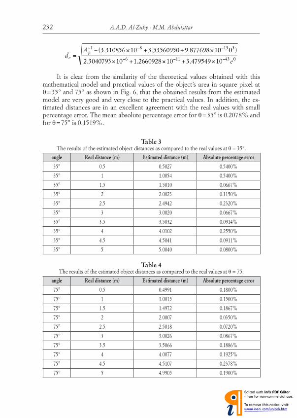
A.A.D. Al-Zuky - M.M. Abdulsttar232
Table 3The results of the estimated object distances as compared to the real values at θ = 35°.
angle Real distance (m) Estimated distance (m) Absolute percentage error
35° 0.5 0.5027 0.5400%
35° 1 1.0054 0.5400%
35° 1.5 1.5010 0.0667%
35° 2 2.0023 0.1150%
35° 2.5 2.4942 0.2320%
35° 3 3.0020 0.0667%
35° 3.5 3.5032 0.0914%
35° 4 4.0102 0.2550%
35° 4.5 4.5041 0.0911%
35° 5 5.0040 0.0800%
Table 4The results of the estimated object distances as compared to the real values at θ = 75.
angle Real distance (m) Estimated distance (m) Absolute percentage error
75° 0.5 0.4991 0.1800%
75° 1 1.0015 0.1500%
75° 1.5 1.4972 0.1867%
75° 2 2.0007 0.0350%
75° 2.5 2.5018 0.0720%
75° 3 3.0026 0.0867%
75° 3.5 3.5066 0.1886%
75° 4 4.0077 0.1925%
75° 4.5 4.5107 0.2378%
75° 5 4.9905 0.1900%
It is clear from the similarity of the theoretical values obtained with this mathematical model and practical values of the object’s area in square pixel at θ = 35° and 75° as shown in Fig. 6, that the obtained results from the estimated model are very good and very close to the practical values. In addition, the es-timated distances are in an excellent agreement with the real values with small percentage error. The mean absolute percentage error for θ = 35° is 0.2078% and for θ = 75° is 0.1519%.
de =
Ap−1 − (3.310856×10⁻⁸ + 3.5356095θ+9.877698×10⁻¹³θ3)
2.3040793×10⁻⁶ +1.2660928×10⁻¹¹ + 3.479549×10−43eθ

Tilting Angle-Dependent to Estimate Object’s Range 233
REFERENCES
(1) N. CLARK, R.H. WYNNE, D.L. SCHMOLDT , P.A. ARAMAN, M. WINN, Use of a non-metric digital camera for tree stem evaluation, Am. Soc. for Photogrammetry & Remote Sensing ASPRS/RTI Annual Conference, 1998.
(2) T. WANG, M. CHIHLU, W. WANG, C. TSAI, Distance Measurement Using Single Non-metric CCD Camera, Proc. of 7th WSEAS Intern. Conf. on Signal Processing, Computational Geometry & Artifi cial Vision, (Athens, Greece, August 24-26, 2007).
(3) C. CHEN, M. LU, C. CHUANG, C. TSAI, Vision-Based Distance and Area Measurement System, Intern. J. of Circuits, System and Signal Processing, 1 (1), 28-33, 2007.
(4) M. CHIH LU, C. CHIEN HSU, Y. YU LU, Distance and angle measurement of distant ob-jects on an oblique plane based on pixel variation on CCD image, IEEE Instrum. Measur. Techn. Conf., MTC-12, 318-322, 2010.
(5) A. AL-ZUKY, M. ABDULSTTAR, Camera Zoom-Dependent to Estimate Object’s Range, Fond. G. Ronchi, 67 (4), 463-473, 2012.
(6) Training guide, Cyber-shot® Digital Still Cameras 2011.

ATTI DELLA “FONDAZIONE GIORGIO RONCHI” ANNO LXVIII, 2013 - N. 2
INDEX
FluidodynamicsD. SREENIVASU, B. SHANKAR, Finite element method solution for oscillatory motion of dusty visco elastic fl uid through porous media with horizontal force
History of ScienceA. DRAGO, The inadequacy of Planck’s calculations on black body theory
LasersAl-D.H. AL-SAIDI I, A.H. KAREEM, Nonlinear dynamics of optically injected semiconductor lasers
MaterialsA. HASHIM Ahmed, Characterization of Addition Cobalt nitrite on Polyvinyl al-coholF.M. AHMED, T.S. UDAY, F.H. ITAB, Study of shielding properties for different materials
Nano FilmsK.N. CHOPRA, A Short Note on Magneto Optic Kerr Effect (MOKE) and the Hys-teresis Loops obtained for Fe/Si and CoFeB/Glass Nano Films
Optical InstrumentsA.A.D. AL-ZUKY, M.M. ABDULSTTAR, Tilting Angle-Dependent to Estimate Object’s Range
Pattern RecognitionC. SUNIL KUMAR, Face recognition and detection system of human faces
Philosophy of ScienceM.A. FORASTIERE, A. GIULIANI, G. MASIERO, On the falsifi ability or cor-roborability of Darwinism
PlasmasK.N. CHOPRA, A Technical Review on the Dusty Plasmas, their Concept, Dynam-ics, Shocks and Production Processes
SpintronicsK.N. CHOPRA, A Technical Note on Important Experimental Revelations and the Current Research in SpintronicsK.N. CHOPRA, A Technical Note on Spintronics (An Off -shoot of Electronics) - its Concept, Growth and Applications
Pag. 155
» 165
» 183
» 193
» 197
» 207
» 223
» 235
» 249
» 263
» 279
» 293

FONDAZIONE GIORGIO RONCHIhttp://ronchi.isti.cnr.it
Estratto da: Atti della Fondazione Giorgio RonchiAnno LXVIII, n. 5 - Settembre-Ottobre 2013
Tip. L’Arcobaleno s.n.c. - Via Bolognese, 54 - Firenze2013
ALI ABID D. AL- ZUKY, MARWAH M. ABDULSTTAR
Using Tilting Angle to Estimate Square Range

ANNO LXVIII SETTEMBRE-OTTOBRE 2013 N. 5
EDITORIAL BOARD
Pubblicazione bimestrale - Prof. LAURA RONCHI ABBOZZO Direttore ResponsabileLa responsabilità per il contenuto degli articoli è unicamente degli Autori
Iscriz. nel Reg. stampa del Trib. di Firenze N. 681 - Decreto del Giudice Delegato in data 2-1-1953Tip. L’Arcobaleno - Via Bolognese, 54 - Firenze - Ottobre 2013
Prof. Roberto BuonannoOsservatorio Astronomico di RomaMonteporzio Catorne, Roma, Italy
Prof. Ercole M. GloriaVia Giunta Pisano 2, Pisa, Italy
Prof. Franco GoriDip. di Fisica, Università Roma IIIRoma, Italy
Prof. Vishal GoyalDepartment of Computer SciencePunjabi University, Patiala, Punjab, India
Prof. Enrique Hita VillaverdeDepartamento de OpticaUniversidad de Granada, Spain
Prof. Irving KaufmanDepartment of Electrical EngineeringArizona State University, TucsonArizona, U.S.A.
Prof. Franco LottiI.F.A.C. del CNR, Via Panciatichi 64Firenze, Italy
Prof. Tommaso MaccacaroDirettore Osservatorio Astronomico di Brera,Via Brera 28, Milano
Prof. Manuel MelgosaDepartamento de OpticaUniversidad de Granada, Spain
Prof. Alberto MeschiariScuola Normale Superiore, Pisa, Italy
Prof. Riccardo PratesiDipartimento di FisicaUniversità di Firenze, Sesto Fiorentino, Italy
Prof. Adolfo PazzagliClinical PsychologyProf. Emerito Università di Firenze
Prof. Edoardo ProverbioIstituto di Astronomia e Fisica SuperioreCagliari, Italy
Prof. Andrea RomoliGalileo Avionica, Campi BisenzioFirenze, Italy
Prof. Ovidio SalvettiI.ST.I. del CNRArea della Ricerca CNR di Pisa, Pisa, Italy.
Prof. Mahipal SinghDeputy Director, CFSL, Sector 36 AChandigarh, India
Prof. Marija StrojnikCentro de Investigaciones en OpticaLeon, Gto Mexico
Prof. Jean-Luc TissotULIS, Veurey Voroize, France
Prof. Paolo VanniProfessore Emerito di Chimica Medicadell’Università di Firenze
Prof. Sergio VillaniLatvia State University, Riga, Lettonia
A T T I
DELLA «FONDAZIONE GIORGIO RONCHI»
Using Tilting Angle to Estimate Square Range
ALI ABID D. AL- ZUKY (*), MARWAH M. ABDULSTTAR (*)
SUMMARY. – In present paper a mathematical model to estimate the real distance of a certain
square object has been found based on tilting angle where the fi tting curves for the experimen-
tal data of the object’s area in square pixels (Ap) in the image plane for each tilting angle were
achieved. Then the mathematical modeling equation was found that relates object’s area in
square pixels (Ap), real distance (dr) and tilting angle (θ) to estimate object distance. A graph
between object’s area in square pixels (Ap) and distance for angles 25° and 55° to the theoreti-
cal and experimental results have been plotted and there was a very good similarity between
them, as well as the estimated distances were very close to the real measurements.
Key words: Tilting angle, mathematical model, object’s area in square pixels, estimated
distance.
1. Introduction
The measurement of object distance is essential for many technical applica-tions. The classical direct distance measurement, which means the direct compari-son of the distance with a calibrated ruler, is the oldest and most obvious method, but not applicable in many cases. Therefore various indirect distance measure-ment procedures were developed throughout the centuries; here the distance is derived of any distance depending measure which is easier to access than the dis-tance itself (1). The determination of an object’s distance relative to an observer (sensor) is a common fi eld of research in computer vision and image analysis.
Clark et al. (1998) (2) used the digital imaging to measure distances in horti-cultural i.e. involved images that are not perpendicular to the object being photo-graphed; for example, many photographs of trees taken from ground level require the camera to be tilted up to capture the whole canopy. When the camera is tilted
(*) Physics Dept., College of Science, Al-Mustansiriya University, Iraq; e-mails: [email protected]; [email protected]
ATTI DELLA “FONDAZIONE GIORGIO RONCHI” ANNO LXVIII, 2013 - N. 5
OPTICAL INSTRUMENTATION
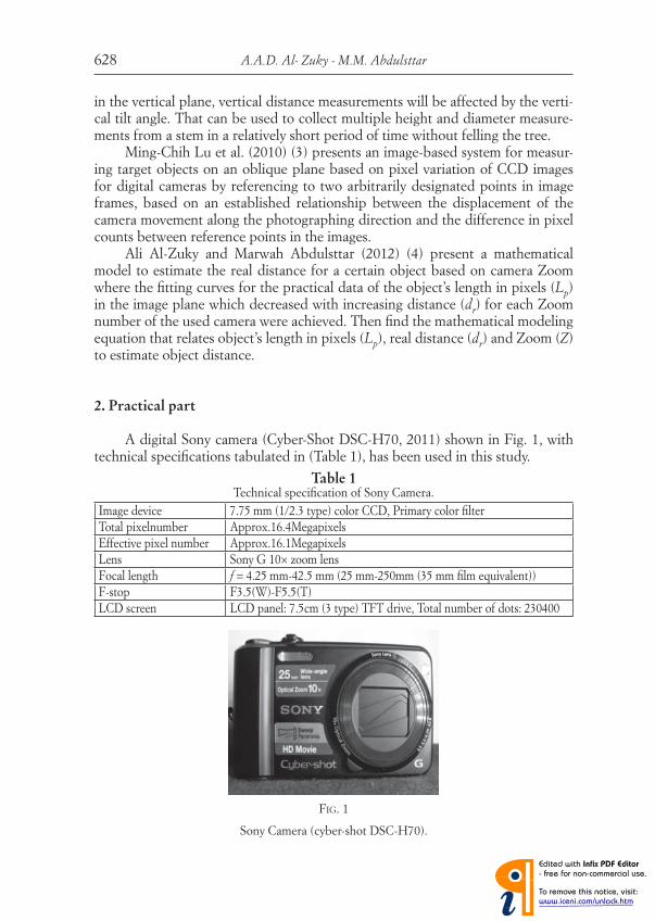
A.A.D. Al- Zuky - M.M. Abdulsttar628
in the vertical plane, vertical distance measurements will be affected by the verti-cal tilt angle. That can be used to collect multiple height and diameter measure-ments from a stem in a relatively short period of time without felling the tree.
Ming-Chih Lu et al. (2010) (3) presents an image-based system for measur-ing target objects on an oblique plane based on pixel variation of CCD images for digital cameras by referencing to two arbitrarily designated points in image frames, based on an established relationship between the displacement of the camera movement along the photographing direction and the difference in pixel counts between reference points in the images.
Ali Al-Zuky and Marwah Abdulsttar (2012) (4) present a mathematical model to estimate the real distance for a certain object based on camera Zoom where the fi tting curves for the practical data of the object’s length in pixels (Lp) in the image plane which decreased with increasing distance (dr) for each Zoom number of the used camera were achieved. Then fi nd the mathematical modeling equation that relates object’s length in pixels (Lp), real distance (dr) and Zoom (Z) to estimate object distance.
2. Practical part
A digital Sony camera (Cyber-Shot DSC-H70, 2011) shown in Fig. 1, with technical specifi cations tabulated in (Table 1), has been used in this study.
Table 1Technical specifi cation of Sony Camera.
Image device 7.75 mm (1/2.3 type) color CCD, Primary color fi lter
Total pixelnumber Approx.16.4Megapixels
Effective pixel number Approx.16.1Megapixels
Lens Sony G 10× zoom lens
Focal length f = 4.25 mm-42.5 mm (25 mm-250mm (35 mm fi lm equivalent))
F-stop F3.5(W)-F5.5(T)
LCD screen LCD panel: 7.5cm (3 type) TFT drive, Total number of dots: 230400
FIG. 1
Sony Camera (cyber-shot DSC-H70).

Using Tilting Angle to Estimate Square Range 629
First the object of square shape is placed in front of the camera with object plane parallel with image plane (i.e. at zero angle with normal), then tilt the object to the back from angle 5° to 85° with changing step of 5° for each angle from zero
FIG. 2
Captured image of the square at each tilting angle.
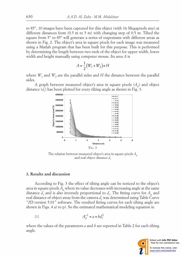
A.A.D. Al- Zuky - M.M. Abdulsttar630
to 85°, 10 images have been captured for this object (with 16 Megapixels size) at different distances from (0.5 m to 5 m) with changing step of 0.5 m. Tilted the square from 5° to 85º will generate a series of trapeziums with different areas as shown in Fig. 2. The object’s area in square pixels for each image was measured using a Matlab program that has been built for this purpose. This is performed by determining the length between two ends of the object for upper width, lower width and height manually using computer mouse. Its area A is
where W1 and W2 are the parallel sides and H the distance between the parallel sides.
A graph between measured object’s area in square pixels (Ap) and object distance (dr) has been plotted for every tilting angle as shown in Fig. 3.
FIG. 3
The relation between measured object’s area in square pixels Ap and real object distance dr
3. Results and discussion
According to Fig. 3 the effect of tilting angle can be noticed to the object’s area in square pixels Ap where its value decreases with increasing angle at the same distance dr and is also inversely proportional to dr. The fi tting curve for Ap and real distance of object away from the camera dr was determined using Table Curve “2D version 5.01” software. The resulted fi tting curves for each tilting angle are shown in Figs. 4 a) to p). So the estimated mathematical modeling equation is:
[1]
where the values of the parameters a and b are reported in Table 2 for each tilting angle.
Ap−1 = a + bdr
2
A =
1
2W1 +W2( )× H
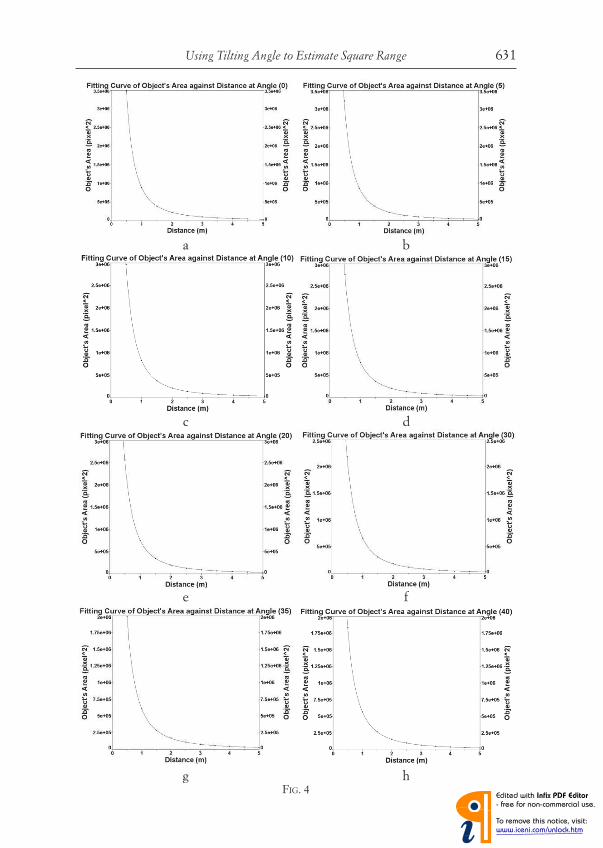
Using Tilting Angle to Estimate Square Range 631
FIG. 4
a
c
e
g
b
d
f
h
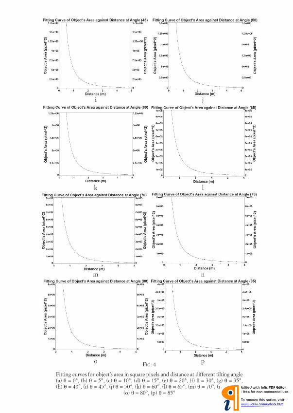
FIG. 4
Fitting curves for object’s area in square pixels and distance at different tilting angle(a) θ = 0°, (b) θ = 5°, (c) θ = 10°, (d) θ = 15°, (e) θ = 20°, (f) θ = 30°, (g) θ = 35°, (h) θ = 40°, (i) θ = 45°, (j) θ = 50°, (k) θ = 60°, (l) θ = 65°, (m) θ = 70°, (n) θ = 75°, (o) θ = 80°, (p) θ = 85°
i
k
m
o
j
l
n
p
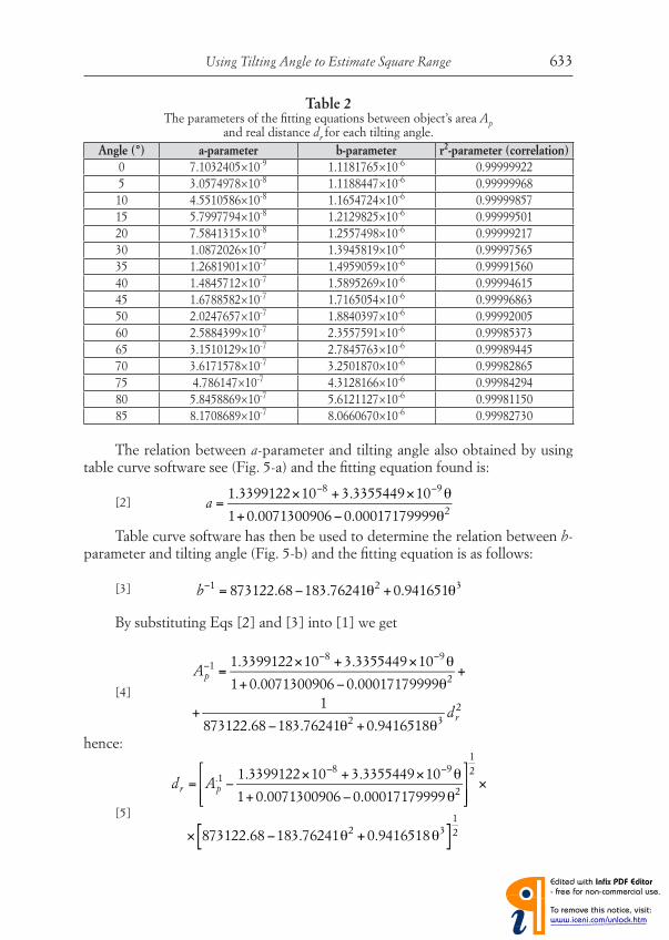
Using Tilting Angle to Estimate Square Range 633
The relation between a-parameter and tilting angle also obtained by using table curve software see (Fig. 5-a) and the fi tting equation found is:
[2]
Table curve software has then be used to determine the relation between b-parameter and tilting angle (Fig. 5-b) and the fi tting equation is as follows:
[3]
By substituting Eqs [2] and [3] into [1] we get
[4]
hence:
[5]
Table 2The parameters of the fi tting equations between object’s area Ap
and real distance dr for each tilting angle.
Angle (°) a-parameter b-parameter r2-parameter (correlation)
0 7.1032405×10⁻⁹ 1.1181765×10⁻⁶ 0.99999922
5 3.0574978×10⁻⁸ 1.1188447×10⁻⁶ 0.99999968
10 4.5510586×10⁻⁸ 1.1654724×10⁻⁶ 0.99999857
15 5.7997794×10⁻⁸ 1.2129825×10⁻⁶ 0.99999501
20 7.5841315×10⁻⁸ 1.2557498×10⁻⁶ 0.99999217
30 1.0872026×10⁻⁷ 1.3945819×10⁻⁶ 0.99997565
35 1.2681901×10⁻⁷ 1.4959059×10⁻⁶ 0.99991560
40 1.4845712×10⁻⁷ 1.5895269×10⁻⁶ 0.99994615
45 1.6788582×10⁻⁷ 1.7165054×10⁻⁶ 0.99996863
50 2.0247657×10⁻⁷ 1.8840397×10⁻⁶ 0.99992005
60 2.5884399×10⁻⁷ 2.3557591×10⁻⁶ 0.99985373
65 3.1510129×10⁻⁷ 2.7845763×10⁻⁶ 0.99989445
70 3.6171578×10⁻⁷ 3.2501870×10⁻⁶ 0.99982865
75 4.786147×10⁻⁷ 4.3128166×10⁻⁶ 0.99984294
80 5.8458869×10⁻⁷ 5.6121127×10⁻⁶ 0.99981150
85 8.1708689×10⁻⁷ 8.0660670×10⁻⁶ 0.99982730
a =
1.3399122×10⁻⁸ + 3.3355449×10⁻⁹θ
1+ 0.0071300906−0.00017179999θ2
b−1 = 873122.68−183.76241θ2 + 0.941651θ3
Ap−1 =
1.3399122×10⁻⁸ + 3.3355449×10⁻⁹θ
1+ 0.0071300906−0.00017179999θ2+
+1
873122.68−183.76241θ2 + 0.9416518θ3dr
2
dr = Ap.1 −
1.3399122×10⁻⁸ + 3.3355449×10⁻⁹θ
1+ 0.0071300906−0.00017179999θ2
⎡
⎣ ⎢ ⎢
⎤
⎦ ⎥ ⎥
1
2
×
× 873122.68−183.76241θ2 + 0.9416518θ3[ ]1
2

A.A.D. Al- Zuky - M.M. Abdulsttar634
which represents the estimated mathematical model that relates object’s area in square pixels Ap, distance and tilting angle θ to estimate the distance between the object and the camera.
FIG. 5
The relation between tilting angle and (a) a-parameter, (b) b-parameter.
(a) (b)
We canceled the practical results for angles 25° and 55° from fi tting process in order to determine their values theoretically from the estimated mathematical model Eq. [4] and to make a comparison between the experimental and theoreti-cal values (Fig. 6). There is an excellent agreement between them.
FIG. 6
Theoretical and experimental curves of object’s area in square pixels Ap with object distance dr at (a) θ = 25° and (b) θ = 55°
(a) θ = 25° (b) θ = 55°
Equation [5] has also been used to estimate object’s distances at 25° and 55° angles and compare the estimated results with the real measurements. The results are tabulated in Tables 3 & 4
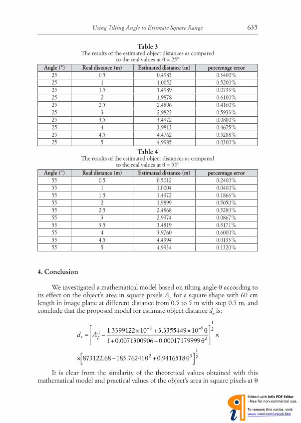
Using Tilting Angle to Estimate Square Range 635
4. Conclusion
We investigated a mathematical model based on tilting angle θ according to its effect on the object’s area in square pixels Ap for a square shape with 60 cm length in image plane at different distance from 0.5 to 5 m with step 0.5 m, and conclude that the proposed model for estimate object distance de is:
It is clear from the similarity of the theoretical values obtained with this mathematical model and practical values of the object’s area in square pixels at θ
Table 3The results of the estimated object distances as compared
to the real values at θ = 25°
Angle (°) Real distance (m) Estimated distance (m) percentage error
25 0.5 0.4983 0.3400%
25 1 1.0052 0.5200%
25 1.5 1.4989 0.0733%
25 2 1.9878 0.6100%
25 2.5 2.4896 0.4160%
25 3 2.9822 0.5933%
25 3.5 3.4972 0.0800%
25 4 3.9813 0.4675%
25 4.5 4.4762 0.5288%
25 5 4.9985 0.0300%
Table 4The results of the estimated object distances as compared
to the real values at θ = 55°
Angle (°) Real distance (m) Estimated distance (m) percentage error
55 0.5 0.5012 0.2400%
55 1 1.0004 0.0400%
55 1.5 1.4972 0.1866%
55 2 1.9899 0.5050%
55 2.5 2.4868 0.5280%
55 3 2.9974 0.0867%
55 3.5 3.4819 0.5171%
55 4 3.9760 0.6000%
55 4.5 4.4994 0.0133%
55 5 4.9934 0.1320%
dr = Ap.1 −
1.3399122×10⁻⁸ + 3.3355449×10⁻⁹θ
1+ 0.0071300906−0.00017179999θ2
⎡
⎣ ⎢ ⎢
⎤
⎦ ⎥ ⎥
1
2
×
× 873122.68−183.76241θ2 + 0.9416518θ3[ ]1
2

A.A.D. Al- Zuky - M.M. Abdulsttar636
= 25° and θ = 55° as shown in Fig. 6 that the obtained results from the estimated model are very good and very close to the practical values. In addition, the es-timated distances are in an excellent agreement with the real values with small percentage error. The results for large angles are better than for small angles, we found that a mean percentage error for distance at θ = 25° was 0.36589% and at θ = 55° was 0.28487%.
REFERENCES
(1) R. MILLNER, Ultraschalltechnik: Grundlagen und Anwendungen, (Physik-Verlag, Wein-heim, Germany, 1987).
(2) N. CLARK, R.H. WYNNE, D.L. SCHMOLDT , P A. ARAMAN, M. WINN, Use of a non-metric digital camera for tree stem evaluation, Proc. Annual Conf. of Am. Soc. for Photogrammetry & Remote Sensing ASPRS/RTI, 1998.
(3) M. CHIH LU, C. CHIEN HSU, Y. YU LU, Distance and angle measurement of distant ob-jects on an oblique plane based on pixel variation on CCD image, IEEE Conf. on Instrumentation and Measurement Technology (12MTC), 318-322, 2010.
(4) A. AL-ZUKY, M. ABDULSTTAR, Camera Zoom-Dependent to Estimate Object’s Range, Atti Fond. G. Ronchi, 67 (4), 463-473, 2012.

ATTI DELLA “FONDAZIONE GIORGIO RONCHI” ANNO LXVIII, 2013 - N. 5
INDEX
Adaptive opticsK.N. CHOPRA, A short review on modeling and compensation of the aberrations and turbulence effects by adaptive optics technology
BiologyF.H. KAMEL, C.H. SAEED, S.S. QADER, Biological effect of magnetic ield on the ultra structure of Staphylococcus aureus
ElectromagnetismD. SCHIAVULLI, A. SORRENTINO, M. MIGLIACCIO, A discussion on the use of X-band SAR images in marine applications
MaterialsZ. AL-RAMADH, H. GHAZI, A. HASHIM, Effect of Carbon NanoFiber on the Transmittance of Poly-Vinyl-Alcohol Edge FiltersM. HADI, S. HADI, A. HASHIM, Study of mechanical properties of UPE-AgNO3 and AlNO3 composites
OphthalmologyA.J. DEL ÁGUILA-CARRASCO, V. SANCHIS-JURADO, A. DOMÍNGUEZVI-CENT, D. MONSÁLVEZ-ROMÍN, P. BERNAL-MOLINA, Importance of pupil size measurement in refractive surgery
Optical instrumentationA.A.D. Al-ZUKY, M. ABDULSTTAR, Using Tilting Angle to Estimate Square Range
Physics of the matterD.H. AL-AMIEDY, Z.A. SALEH, R.K. AL-YASARI, Lambda doubling calculation for Cu63F19
PlasmasK.N. CHOPRA, A short note on the technical investigations of the plasma treatment for biomedical applications
Science of visionL. HSIN HSIN, Visual Cognition: From the Abstract to the Figurative Outline-Con-tinuation-In-Anticipation (OCIA) Phenomena
SpintronicsK.N. CHOPRA, New Materials and their Selection for Designing and Fabricating the Spintronic Devices. A Technical Note
Thin filmsH. SALEH SABIA, N.Z. SHAREEF, The effect of thermal annealing on the electri-cal properties of Ge-Se-Te thin ilmsS.S. CHIAD, S.F. OBOUDI, Z.A. TOMA, N.F. HABUBI, Optical dispersion char-acterization of sprayed mixed SnO2-CuO thin ilmsB.E. GASGOUS, M.M. ISMAIL, N.I. HASSAN, Effect of laser irradiation on the optical properties of CdO thin ilmsG.H. MOHAMED, S.S. CHIAD, S.F. OBOUDI, N.F. HABUBI, Fabrication and characterization of nanoparticles ZnO-NiO thin ilms prepared by thermal evapora-tion techniqueS.F. OBOUDI, S.S. CHIAD, S.H. JUMAAH, N.F. HABUBI, Effect of Mn doping concentration on the electronic transitions of ZnO thin ilms
VarietyP. STEFANINI, Il coleottero Lucciola che non vola
Pag. 579
» 595
» 601
» 611
» 615
» 619
» 627
» 637
» 645
» 661
» 673
» 681
» 689
» 699
» 707
» 717
» 725
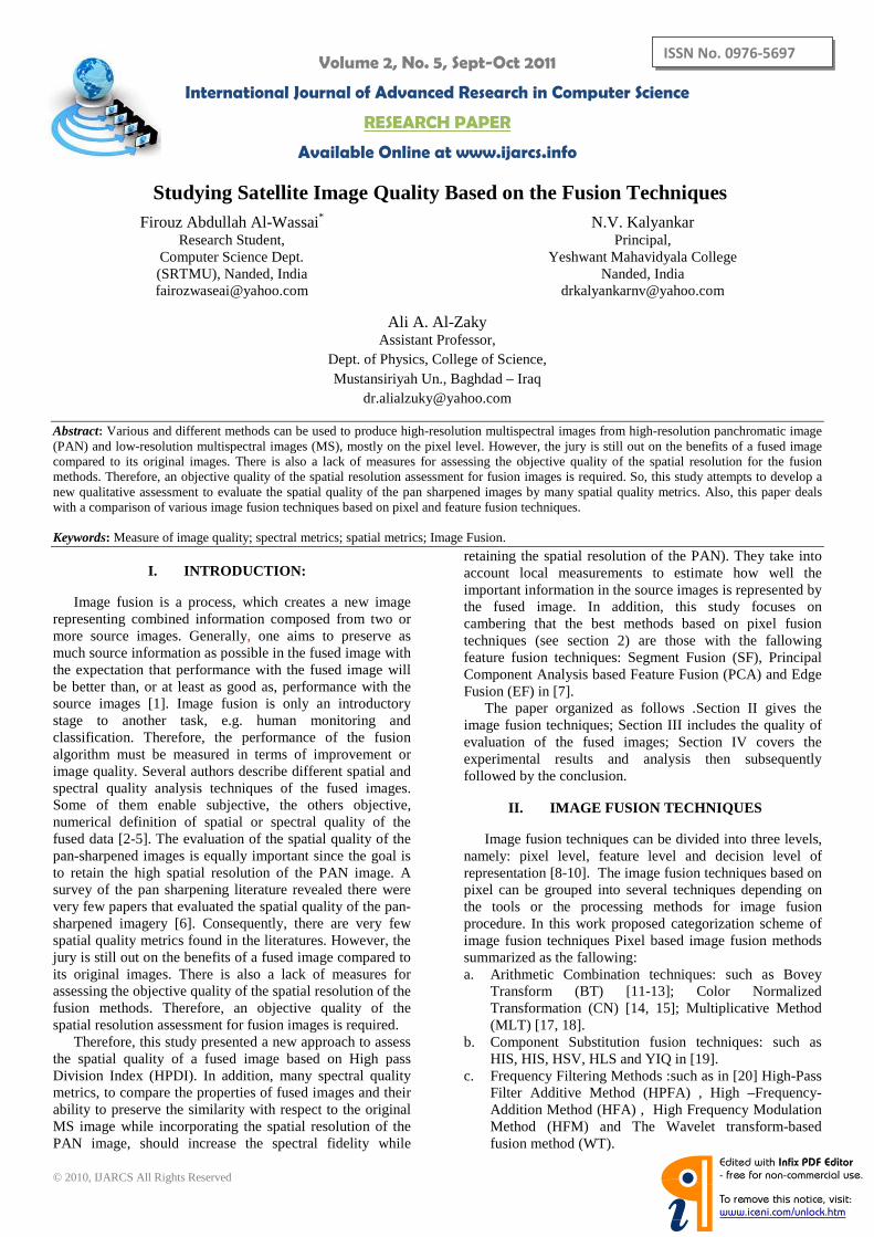
Volume 2, No. 5, Sept-Oct 2011
International Journal of Advanced Research in Computer Science
RESEARCH PAPER
Available Online at www.ijarcs.info
© 2010, IJARCS All Rights Reserved 516
ISSN No. 0976-5697
Studying Satellite Image Quality Based on the Fusion Techniques Firouz Abdullah Al-Wassai N.V. Kalyankar *
Research Student, Computer Science Dept. (SRTMU), Nanded, India [email protected]
Principal, Yeshwant Mahavidyala College
Nanded, India [email protected]
Ali A. Al-Zaky Assistant Professor,
Dept. of Physics, College of Science, Mustansiriyah Un., Baghdad – Iraq
Abstract: Various and different methods can be used to produce high-resolution multispectral images from high-resolution panchromatic image (PAN) and low-resolution multispectral images (MS), mostly on the pixel level. However, the jury is still out on the benefits of a fused image compared to its original images. There is also a lack of measures for assessing the objective quality of the spatial resolution for the fusion methods. Therefore, an objective quality of the spatial resolution assessment for fusion images is required. So, this study attempts to develop a new qualitative assessment to evaluate the spatial quality of the pan sharpened images by many spatial quality metrics. Also, this paper deals with a comparison of various image fusion techniques based on pixel and feature fusion techniques. Keywords: Measure of image quality; spectral metrics; spatial metrics; Image Fusion.
I. INTRODUCTION:
Image fusion is a process, which creates a new image representing combined information composed from two or more source images. Generally, one aims to preserve as much source information as possible in the fused image with the expectation that performance with the fused image will be better than, or at least as good as, performance with the source images [1]. Image fusion is only an introductory stage to another task, e.g. human monitoring and classification. Therefore, the performance of the fusion algorithm must be measured in terms of improvement or image quality. Several authors describe different spatial and spectral quality analysis techniques of the fused images. Some of them enable subjective, the others objective, numerical definition of spatial or spectral quality of the fused data [2-5]. The evaluation of the spatial quality of the pan-sharpened images is equally important since the goal is to retain the high spatial resolution of the PAN image. A survey of the pan sharpening literature revealed there were very few papers that evaluated the spatial quality of the pan-sharpened imagery [6]. Consequently, there are very few spatial quality metrics found in the literatures. However, the jury is still out on the benefits of a fused image compared to its original images. There is also a lack of measures for assessing the objective quality of the spatial resolution of the fusion methods. Therefore, an objective quality of the spatial resolution assessment for fusion images is required.
Therefore, this study presented a new approach to assess the spatial quality of a fused image based on High pass Division Index (HPDI). In addition, many spectral quality metrics, to compare the properties of fused images and their ability to preserve the similarity with respect to the original MS image while incorporating the spatial resolution of the PAN image, should increase the spectral fidelity while
retaining the spatial resolution of the PAN). They take into account local measurements to estimate how well the important information in the source images is represented by the fused image. In addition, this study focuses on cambering that the best methods based on pixel fusion techniques (see section 2) are those with the fallowing feature fusion techniques: Segment Fusion (SF), Principal Component Analysis based Feature Fusion (PCA) and Edge Fusion (EF) in [7].
The paper organized as follows .Section II gives the image fusion techniques; Section III includes the quality of evaluation of the fused images; Section IV covers the experimental results and analysis then subsequently followed by the conclusion.
II. IMAGE FUSION TECHNIQUES
Image fusion techniques can be divided into three levels, namely: pixel level, feature level and decision level of representation [8-10]. The image fusion techniques based on pixel can be grouped into several techniques depending on the tools or the processing methods for image fusion procedure. In this work proposed categorization scheme of image fusion techniques Pixel based image fusion methods summarized as the fallowing: a. Arithmetic Combination techniques: such as Bovey
Transform (BT) [11-13]; Color Normalized Transformation (CN) [14, 15]; Multiplicative Method (MLT) [17, 18].
b. Component Substitution fusion techniques: such as HIS, HIS, HSV, HLS and YIQ in [19].
c. Frequency Filtering Methods :such as in [20] High-Pass Filter Additive Method (HPFA) , High –Frequency- Addition Method (HFA) , High Frequency Modulation Method (HFM) and The Wavelet transform-based fusion method (WT).

Firouz Abdullah Al-Wassai et al, International Journal of Advanced Research in Computer Science, 2 (5), Sept –Oct, 2011,516-524
© 2010, IJARCS All Rights Reserved 517
d. Statistical Methods: such as in [21] Local Mean Matching (LMM), Local Mean and Variance Matching (LMVM), Regression variable substitution (RVS), and Local Correlation Modeling (LCM).
All the above techniques employed in our previous studies [19-21]. Therefore, the best method for each group selected in this study as the fallowing: a. Arithmetic and Frequency Filtering techniques are High
–Frequency- Addition Method (HFA) and High Frequency Modulation Method (HFM) [20].
b. The Statistical Methods it was with Regression variable substitution (RVS) [21].
c. In the Component Substitution fusion techniques the IHS method by [22] it was much better than the others methods [19].
To explain the algorithms through this study, Pixels should have the same spatial resolution from two different sources that are manipulated to obtain the resultant image. Here, The PAN images have a different spatial resolution from that of the original multispectral MS images. Therefore, resampling of MS images to the spatial resolution of PAN is an essential step in some fusion methods to bring the MS images to the same size of PAN, thus the resampled MS images will be noted by that represents the set of
of band in the resampled MS image .
III. QUALITY EVALUATION OF THE FUSED IMAGES
This section describes the various spatial and spectral quality metrics used to evaluate them. The spectral fidelity of the fused images with respect to the original multispectral images is described. When analyzing the spectral quality of the fused images we compare spectral characteristics of images obtained from the different methods, with the spectral characteristics of resampled original multispectral images. Since the goal is to preserve the radiometry of the original MS images, any metric used must measure the amount of change in DN values in the pan-sharpened image
compared to the original image. Also, In order to evaluate the spatial properties of the fused images, a panchromatic image and intensity image of the fused image have to be compared since the goal is to retain the high spatial resolution of the PAN image. In the following
are the measurements of each the brightness values pixels of the result image and the original MS image of band , and are the mean brightness values of both images and are of size . is the brightness value of image data and .
A. Spectral Quality Metrics:
a. Standard Deviation ( ): The standard deviation (SD), which is the square root of variance, reflects the spread in the data. Thus, a high contrast image will have a larger variance, and a low contrast image will have a low variance. It indicates the closeness of the fused image to the original MS image at a pixel level. The ideal value is zero.
(1)
b. Entropy ): The entropy of an image is a measure of information content but has not been used to assess the effects of information change in fused images. En reflects the capacity of the information carried by images. The larger En mean high information in the image [6]. By applying Shannon’s entropy in evaluation the information content of an image, the formula is modified as [23]:
(2) Where P(i) is the ratio of the number of the pixels with
gray value equal to over the total number of the pixels. c. Signal-to Noise Ratio ( ): The signal is the
information content of the data of original MS image , while the merging can cause the noise, as error that is added to the signal. The of the signal-to-noise ratio can be used to calculate the signal-to-noise ratio , given by [24]:
(3)
d. Deviation Index ( ): In order to assess the quality of the merged product in regard of spectral information content. The deviation index is useful parameter as defined by [25,26], measuring the normalized global absolute difference of the fused image with the original MS image as follows :
(4)
e. Correlation Coefficient ( ): The correlation
coefficient measures the closeness or similarity between two images. It can vary between –1 to +1. A value close to +1 indicates that the two images are very similar, while a value close to –1 indicates that they are highly dissimilar. The formula to compute the correlation between :
(5)
Since the pan-sharpened image larger (more pixels) than the original MS image it is not possible to compute the correlation or apply any other mathematical operation between them. Thus, the upsampled MS image is used for this comparison.
f. Normalization Root Mean Square Error (NRMSE): the NRMSE used in order to assess the effects of information changing for the fused image. When level of information loss can be expressed as a function of the original MS pixel and the fused pixel , by using the NRMSE between and
images in band . The Normalized Root- Mean-Square Error between and is a point analysis in multispectral space representing the amount of change the original MS pixel and the corresponding output pixels using the following equation [27]:

Firouz Abdullah Al-Wassai et al, International Journal of Advanced Research in Computer Science, 2 (5), Sept –Oct, 2011,516-524
© 2010, IJARCS All Rights Reserved 518
B. Spatial Quality Metrics: a. Mean Grades (MG): MG has been used as a measure
of image sharpness by [27, 28]. The gradient at any pixel is the derivative of the DN values of neighboring pixels. Generally, sharper images have higher gradient values. Thus, any image fusion method should result in increased gradient values because this process makes the images sharper compared to the low-resolution image. The gradient defines the contrast between the details variation of pattern on the image and the clarity of the image [5]. MG is the index to reflect the expression ability of the little detail contrast and texture variation, and the definition of the image. The calculation formula is [6]:
(7)
Where
(8)
Where and are the horizontal and vertical gradients per pixel of the image fused generally, the larger , the more the hierarchy, and the more definite the fused image.
b. Soble Grades (SG): this approach developed in this study by used the Soble operator is A better edge estimator than the mean gradient. That by computes discrete gradient in the horizontal and vertical directions at the pixel location of an image The Soble operator was the most popular edge detection operator until the development of edge detection techniques with a theoretical basis. It proved popular because it gave a better performance contemporaneous edge detection operator than other such as the Prewitt operator [30]. For this, which is clearly more costly to evaluate, the orthogonal components of gradient as the following [31]:
And
(9)
It can be seen that the Soble operator is equivalent to simultaneous application of the templates as the following [32]:
(10)
Then the discrete gradient of an image is given by
(11)
Where and are the horizontal and vertical gradients
per pixel. Generally, the larger values for, the more the hierarchy and the more definite the fused image.
C. Filtered Correlation Coefficients (FCC):
This approach was introduced [33]. In the Zhou’s approach, the correlation coefficients between the high-pass filtered fused PAN and TM images and the high-pass filtered PAN image are taken as an index of the spatial quality. The high-pass filter is known as a Laplacian filter as illustrated in eq. (12):
(12)
However, the magnitude of the edges does not
necessarily have to coincide, which is the reason why Zhou et al proposed to look at their correlation coefficients [33]. So, in this method the average correlation coefficient of the faltered PAN image and all faltered bands is calculated to obtain FCC. An FCC value close to one indicates high spatial quality.
D. High Pass Deviation Index (HPDI) This approach proposed by [25, 26] as the measuring of
the normalized global absolute difference for spectral quantity for the fused image with the original MS image . This study developed that is quality metric to measure the amount of edge information from the PAN image is transferred into the fused images by used the high-pass filter (eq. 12). which that the high-pass filtered PAN image are taken as an index of the spatial quality. The HPDI wants to extract the high frequency components of the PAN image and each band. The deviation index between the high pass filtered and the fused images would indicate how much spatial information from the PAN image has been incorporated into the image to obtain HPDI as follows:
(13)
The smaller value HPDI the better image quality.
Indicates that the fusion result it has a high spatial resolution quality of the image.
IV. EXPERIMENTAL RESULTS
The above assessment techniques are tested on fusion of Indian IRS-1C PAN of the 5.8- m resolution panchromatic band and the Landsat TM the red (0.63 - 0.69 µm), green (0.52 - 0.60 µm) and blue (0.45 - 0.52 µm) bands of the 30 m resolution multispectral image were used in this work. Fig.1 shows the IRS-1C PAN and multispectral TM images. Hence, this work is an attempt to study the quality of the images fused from different sensors with various characteristics. The size of the PAN is 600 * 525 pixels at 6 bits per pixel and the size of the original multispectral is 120 * 105 pixels at 8 bits per pixel, but this is upsampled by nearest neighbor to same size the PAN image. The pairs of images were geometrically registered to each other. The HFA, HFM, HIS, RVS, PCA, EF, and SF methods are employed to fuse IRS-C PAN and TM multi-spectral images. The original MS and PAN are shown in (Fig. 1).
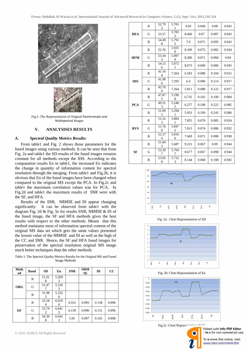
Firouz Abdullah Al-Wassai et al, International Journal of Advanced Research in Computer Science, 2 (5), Sept –Oct, 2011,516-524
© 2010, IJARCS All Rights Reserved 519
Fig.1: The Representation of Original Panchromatic and
Multispectral Images
V. ANALYSISES RESULTS
A. Spectral Quality Metrics Results:
From table1 and Fig. 2 shows those parameters for the fused images using various methods. It can be seen that from Fig. 2a and table1 the SD results of the fused images remains constant for all methods except the IHS. According to the computation results En in table1, the increased En indicates the change in quantity of information content for spectral resolution through the merging. From table1 and Fig.2b, it is obvious that En of the fused images have been changed when compared to the original MS except the PCA. In Fig.2c and table1 the maximum correlation values was for PCA. In Fig.2d and table1 the maximum results of were with the SF, and HFA.
Results of the , and appear changing significantly. It can be observed from table1 with the diagram Fig. 2d & Fig. 5e for results SNR, & of the fused image, the SF and HFA methods gives the best results with respect to the other methods. Means that this method maintains most of information spectral content of the original MS data set which gets the same values presented the lowest value of the and as well as the high of the CC and . Hence, the SF and HFA fused images for preservation of the spectral resolution original MS image much better techniques than the other methods.
Table 1: The Spectral Quality Metrics Results for the Original MS and Fused Image Methods
Meth
od Band SD En SNR NRMSE DI CC
ORG
R 51.01
8 5.209
3
G 51.47
7 5.226
3
B 51.98
3 5.232
6
EF
R 55.18
4 6.019
6 6.531 0.095 0.138 0.896
G 55.79
2 6.041
5 6.139 0.096 0.151 0.896
B 56.30
8 6.042
3 5.81 0.097 0.165 0.898
HFA
R 52.79
3 5.765
1 9.05 0.068 0.08 0.943
G 53.57 5.783
3 8.466 0.07 0.087 0.943
B 54.49
8 5.791
5 7.9 0.071 0.095 0.943
HFM
R 52.76 5.925
9 8.399 0.073 0.082 0.934
G 53.34
3 5.897
9 8.286 0.071 0.084 0.94
B 54.13
6 5.872
1 8.073 0.069 0.086 0.945
HIS
R 41.16
4 7.264 6.583 0.088 0.104 0.915
G 41.98
6 7.293 6.4 0.086 0.114 0.917
B 42.70
9 7.264 5.811 0.088 0.122 0.917
PCA
R 47.87
5 5.196
8 6.735 0.105 0.199 0.984
G 49.31
3 5.248
5 6.277 0.108 0.222 0.985
B 51.09
2 5.294
1 5.953 0.109 0.245 0.986
RVS
R 51.32
3 5.884
1 7.855 0.078 0.085 0.924
G 51.76
9 5.847
5 7.813 0.074 0.086 0.932
B 52.37
4 5.816
6 7.669 0.071 0.088 0.938
SF
R 51.60
3 5.687 9.221 0.067 0.09 0.944
G 52.20
7 5.704
7 8.677 0.067 0.098 0.944
B 53.02
8 5.712
3 8.144 0.068 0.108 0.945
Fig. 2a: Chart Representation of SD
Fig. 2b: Chart Representation of En
Fig.2c: Chart Representation of CC
0
10
20
30
40
50
60
OR
G
EF
HF
A
HF
M
IHS
PC
A
RV
S
SF
SD
0
1
2
3
4
5
6
7
8
OR
G EF
HF
A
HF
M
IHS
PC
A
RV
S
SF
En
0.84
0.86
0.88
0.9
0.92
0.94
0.96
0.98
1
EF
HF
A
HF
M
IHS
PC
A
RV
S SF
CC
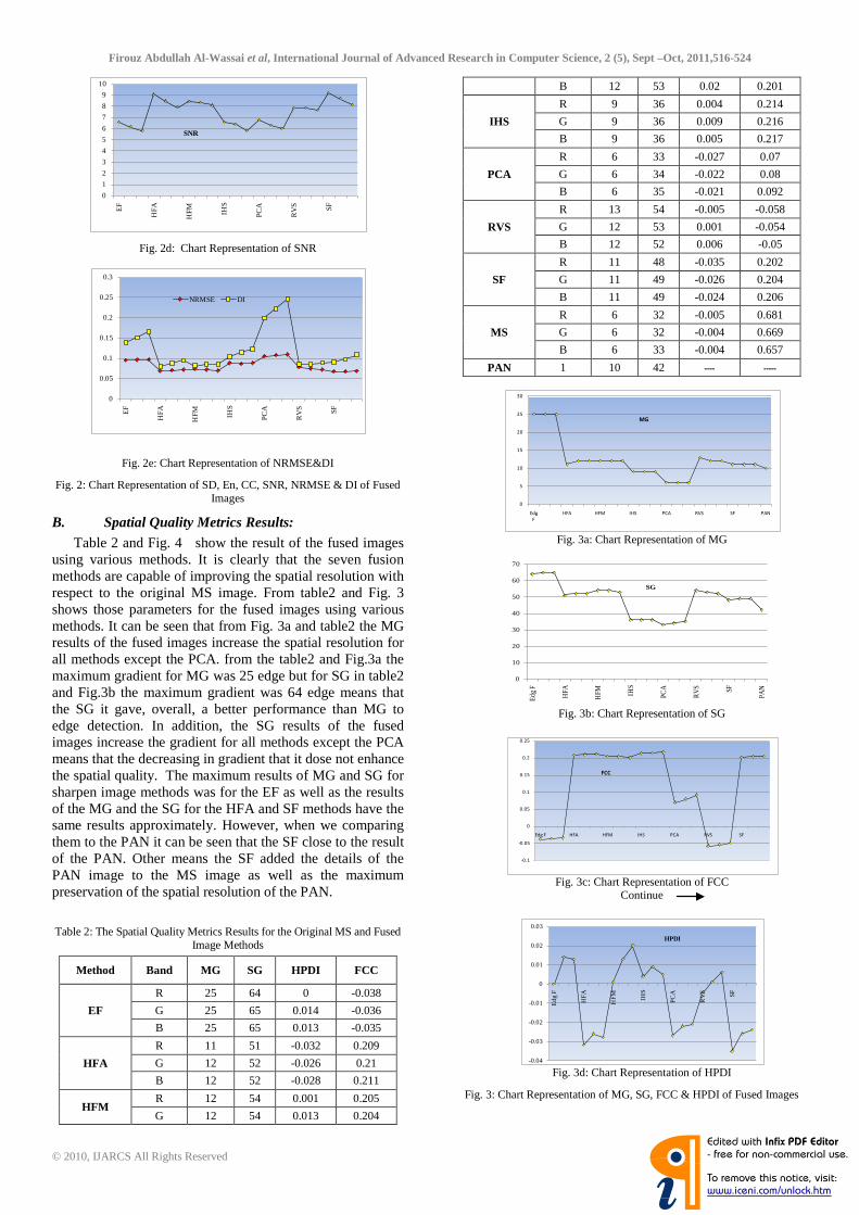
Firouz Abdullah Al-Wassai et al, International Journal of Advanced Research in Computer Science, 2 (5), Sept –Oct, 2011,516-524
© 2010, IJARCS All Rights Reserved 520
Fig. 2d: Chart Representation of SNR
Fig. 2e: Chart Representation of NRMSE&DI
Fig. 2: Chart Representation of SD, En, CC, SNR, NRMSE & DI of Fused Images
B. Spatial Quality Metrics Results: Table 2 and Fig. 4 show the result of the fused images using various methods. It is clearly that the seven fusion methods are capable of improving the spatial resolution with respect to the original MS image. From table2 and Fig. 3 shows those parameters for the fused images using various methods. It can be seen that from Fig. 3a and table2 the MG results of the fused images increase the spatial resolution for all methods except the PCA. from the table2 and Fig.3a the maximum gradient for MG was 25 edge but for SG in table2 and Fig.3b the maximum gradient was 64 edge means that the SG it gave, overall, a better performance than MG to edge detection. In addition, the SG results of the fused images increase the gradient for all methods except the PCA means that the decreasing in gradient that it dose not enhance the spatial quality. The maximum results of MG and SG for sharpen image methods was for the EF as well as the results of the MG and the SG for the HFA and SF methods have the same results approximately. However, when we comparing them to the PAN it can be seen that the SF close to the result of the PAN. Other means the SF added the details of the PAN image to the MS image as well as the maximum preservation of the spatial resolution of the PAN.
Table 2: The Spatial Quality Metrics Results for the Original MS and Fused Image Methods
Method Band MG SG HPDI FCC
EF
R 25 64 0 -0.038
G 25 65 0.014 -0.036
B 25 65 0.013 -0.035
HFA
R 11 51 -0.032 0.209
G 12 52 -0.026 0.21
B 12 52 -0.028 0.211
HFM R 12 54 0.001 0.205
G 12 54 0.013 0.204
B 12 53 0.02 0.201
IHS
R 9 36 0.004 0.214
G 9 36 0.009 0.216
B 9 36 0.005 0.217
PCA
R 6 33 -0.027 0.07
G 6 34 -0.022 0.08
B 6 35 -0.021 0.092
RVS
R 13 54 -0.005 -0.058
G 12 53 0.001 -0.054
B 12 52 0.006 -0.05
SF
R 11 48 -0.035 0.202
G 11 49 -0.026 0.204
B 11 49 -0.024 0.206
MS
R 6 32 -0.005 0.681
G 6 32 -0.004 0.669
B 6 33 -0.004 0.657
PAN 1 10 42
Fig. 3a: Chart Representation of MG
Fig. 3b: Chart Representation of SG
Fig. 3c: Chart Representation of FCC
Continue
Fig. 3d: Chart Representation of HPDI
Fig. 3: Chart Representation of MG, SG, FCC & HPDI of Fused Images
0
1
2
3
4
5
6
7
8
9
10
EF
HF
A
HF
M
IHS
PC
A
RV
S SF
SNR
0
0.05
0.1
0.15
0.2
0.25
0.3
EF
HF
A
HF
M
IHS
PC
A
RV
S SF
NRMSE DI
0
5
10
15
20
25
30
Edg
F
HFA HFM IHS PCA RVS SF PAN
MG
0
10
20
30
40
50
60
70
Edg
F
HFA
HFM IH
S
PC
A
RVS S
F
PAN
SG
-0.1
-0.05
0
0.05
0.1
0.15
0.2
0.25
Edg F HFA HFM IHS PCA RVS SF
FCC
-0.04
-0.03
-0.02
-0.01
0
0.01
0.02
0.03
Ed
g F
HF
A
HF
M
IHS
PC
A
RV
S SF
HPDI

Firouz Abdullah Al-Wassai et al, International Journal of Advanced Research in Computer Science, 2 (5), Sept –Oct, 2011,516-524
© 2010, IJARCS All Rights Reserved 521
According to the computation results, FCC in table and Fig.2c the increase FCC indicates the amount of edge information from the PAN image transferred into the fused images in quantity of spatial resolution through the merging. The maximum results of FCC From table2 and Fig.2c were for the SF, HFA and HFM. The results of better than FCC it is appear changing significantly. It can be observed that from Fig.2d and table2 the maximum results of the purpose approach it was with the SF and HFA methods. The purposed approach of HPDI as the spatial quality metric is more important than the other spatial quality matrices to distinguish the best spatial enhancement through the merging.
Fig..4a: HFA
Fig..4b: HFM
Fig..4c: HIS
Fig.4d: PCA
Contenue Fig. 4
Fig..4e: RVS
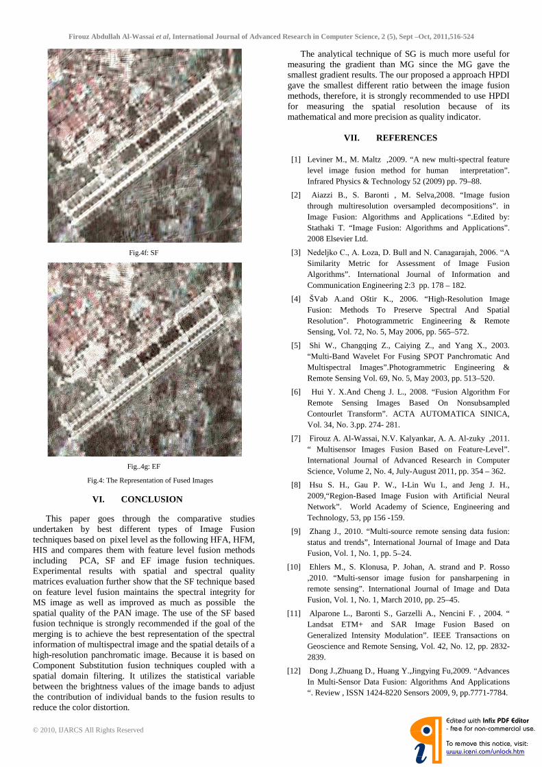
Firouz Abdullah Al-Wassai et al, International Journal of Advanced Research in Computer Science, 2 (5), Sept –Oct, 2011,516-524
© 2010, IJARCS All Rights Reserved 522
Fig.4f: SF
Fig..4g: EF
Fig.4: The Representation of Fused Images
VI. CONCLUSION
This paper goes through the comparative studies undertaken by best different types of Image Fusion techniques based on pixel level as the following HFA, HFM, HIS and compares them with feature level fusion methods including PCA, SF and EF image fusion techniques. Experimental results with spatial and spectral quality matrices evaluation further show that the SF technique based on feature level fusion maintains the spectral integrity for MS image as well as improved as much as possible the spatial quality of the PAN image. The use of the SF based fusion technique is strongly recommended if the goal of the merging is to achieve the best representation of the spectral information of multispectral image and the spatial details of a high-resolution panchromatic image. Because it is based on Component Substitution fusion techniques coupled with a spatial domain filtering. It utilizes the statistical variable between the brightness values of the image bands to adjust the contribution of individual bands to the fusion results to reduce the color distortion.
The analytical technique of SG is much more useful for measuring the gradient than MG since the MG gave the smallest gradient results. The our proposed a approach HPDI gave the smallest different ratio between the image fusion methods, therefore, it is strongly recommended to use HPDI for measuring the spatial resolution because of its mathematical and more precision as quality indicator.
VII. REFERENCES
[1] Leviner M., M. Maltz ,2009. “A new multi-spectral feature
level image fusion method for human interpretation”. Infrared Physics & Technology 52 (2009) pp. 79–88.
[2] Aiazzi B., S. Baronti , M. Selva,2008. “Image fusion through multiresolution oversampled decompositions”. in Image Fusion: Algorithms and Applications “.Edited by: Stathaki T. “Image Fusion: Algorithms and Applications”. 2008 Elsevier Ltd.
[3] Nedeljko C., A. Łoza, D. Bull and N. Canagarajah, 2006. “A Similarity Metric for Assessment of Image Fusion Algorithms”. International Journal of Information and Communication Engineering 2:3 pp. 178 – 182.
[4] ŠVab A.and Oštir K., 2006. “High-Resolution Image Fusion: Methods To Preserve Spectral And Spatial Resolution”. Photogrammetric Engineering & Remote Sensing, Vol. 72, No. 5, May 2006, pp. 565–572.
[5] Shi W., Changqing Z., Caiying Z., and Yang X., 2003. “Multi-Band Wavelet For Fusing SPOT Panchromatic And Multispectral Images”.Photogrammetric Engineering & Remote Sensing Vol. 69, No. 5, May 2003, pp. 513–520.
[6] Hui Y. X.And Cheng J. L., 2008. “Fusion Algorithm For Remote Sensing Images Based On Nonsubsampled Contourlet Transform”. ACTA AUTOMATICA SINICA, Vol. 34, No. 3.pp. 274- 281.
[7] Firouz A. Al-Wassai, N.V. Kalyankar, A. A. Al-zuky ,2011. “ Multisensor Images Fusion Based on Feature-Level”. International Journal of Advanced Research in Computer Science, Volume 2, No. 4, July-August 2011, pp. 354 – 362.
[8] Hsu S. H., Gau P. W., I-Lin Wu I., and Jeng J. H., 2009,“Region-Based Image Fusion with Artificial Neural Network”. World Academy of Science, Engineering and Technology, 53, pp 156 -159.
[9] Zhang J., 2010. “Multi-source remote sensing data fusion: status and trends”, International Journal of Image and Data Fusion, Vol. 1, No. 1, pp. 5–24.
[10] Ehlers M., S. Klonusa, P. Johan, A. strand and P. Rosso ,2010. “Multi-sensor image fusion for pansharpening in remote sensing”. International Journal of Image and Data Fusion, Vol. 1, No. 1, March 2010, pp. 25–45.
[11] Alparone L., Baronti S., Garzelli A., Nencini F. , 2004. “ Landsat ETM+ and SAR Image Fusion Based on Generalized Intensity Modulation”. IEEE Transactions on Geoscience and Remote Sensing, Vol. 42, No. 12, pp. 2832-2839.
[12] Dong J.,Zhuang D., Huang Y.,Jingying Fu,2009. “Advances In Multi-Sensor Data Fusion: Algorithms And Applications “. Review , ISSN 1424-8220 Sensors 2009, 9, pp.7771-7784.
Firouz Abdullah Al-Wassai et al, International Journal of Advanced Research in Computer Science, 2 (5), Sept –Oct, 2011,516-524
© 2010, IJARCS All Rights Reserved 523
[13] Amarsaikhan D., H.H. Blotevogel, J.L. van Genderen, M. Ganzorig, R. Gantuya and B. Nergui, 2010. “Fusing high-resolution SAR and optical imagery for improved urban land cover study and classification”. International Journal of Image and Data Fusion, Vol. 1, No. 1, March 2010, pp. 83–97.
[14] Vrabel J., 1996. “Multispectral imagery band sharpening study”. Photogrammetric Engineering and Remote Sensing, Vol. 62, No. 9, pp. 1075-1083.
[15] Vrabel J., 2000. “Multispectral imagery Advanced band sharpening study”. Photogrammetric Engineering and Remote Sensing, Vol. 66, No. 1, pp. 73-79.
[16] Wenbo W.,Y.Jing, K. Tingjun ,2008. “Study Of Remote Sensing Image Fusion And Its Application In Image Classification” The International Archives of the Photogrammetry, Remote Sensing and Spatial Information Sciences. Vol. XXXVII. Part B7. Beijing 2008, pp.1141-1146.
[17] Parcharidis I. and L. M. K. Tani, 2000. “Landsat TM and ERS Data Fusion: A Statistical Approach Evaluation for Four Different Methods”. 0-7803-6359- 0/00/ 2000 IEEE, pp.2120-2122.
[18] Pohl C. and Van Genderen J. L., 1998. “Multisensor Image Fusion In Remote Sensing: Concepts, Methods And Applications”.(Review Article), International Journal Of Remote Sensing, Vol. 19, No.5, pp. 823-854.
[19] Firouz A. Al-Wassai, N.V. Kalyankar, A. A. Al-zuky ,2011b. “ The IHS Transformations Based Image Fusion”. Journal of Global Research in Computer Science, Volume 2, No. 5, May 2011, pp. 70 – 77.
[20] Firouz A. Al-Wassai , N.V. Kalyankar , A.A. Al-Zuky, 2011a. “Arithmetic and Frequency Filtering Methods of Pixel-Based Image Fusion Techniques “.IJCSI International Journal of Computer Science Issues, Vol. 8, Issue 3, No. 1, May 2011, pp. 113- 122.
[21] Firouz A. Al-Wassai, N.V. Kalyankar , A.A. Al-Zuky, 2011c.” The Statistical methods of Pixel-Based Image Fusion Techniques”. International Journal of Artificial Intelligence and Knowledge Discovery Vol.1, Issue 3, July, 2011 5, pp. 5- 14.
[22] Li S., Kwok J. T., Wang Y.., 2002. “Using the Discrete Wavelet Frame Transform To Merge Landsat TM And SPOT Panchromatic Images”. Information Fusion 3 (2002), pp.17–23.
[23] Liao. Y. C., T.Y. Wang, and W. T. Zheng, 1998. “Quality Analysis of Synthesized High Resolution Multispectral Imagery”. URL: http://www.gisdevelopment.net/AARS/ACRS 1998/Digital Image Processing (Last date accessed:28 Oct. 2008)
[24] Gonzales R. C, and R. Woods, 1992. Digital Image Procesing. A ddison-Wesley Publishing Company.
.
[25] De Béthume S., F. Muller, and J. P. Donnay, 1998. “Fusion of multi-spectral and panchromatic images by local mean and variance matching filtering techniques”. In: Proceedings of The Second International Conference: Fusion of Earth Data: Merging Point Measurements, Raster Maps and Remotely Sensed Images, Sophia-Antipolis, France, 1998, pp. 31–36.
[26] De Bèthune. S and F. Muller, 2002. “Multisource Data Fusion Applied research”. URL:http://www.Fabricmuller.be/realisations/fusion.html.
[27] Sangwine S. J., and R.E.N. Horne, 1989. The Colour Image Processing Handbook. Chapman & Hall.
(Last date accessed:28 Oct. 2002).
[28] Ryan. R., B. Baldridge, R.A. Schowengerdt, T. Choi, D.L. Helder and B. Slawomir, 2003. “IKONOS Spatial Resolution And Image Interpretability Characterization”, Remote Sensing of Environment, Vol. 88, No. 1, pp. 37–52.
[29] Pradham P., Younan N. H. and King R. L., 2008. “Concepts of image fusion in remote sensing applications”. Edited by: Stathaki T. “Image Fusion: Algorithms and Applications”. 2008 Elsevier Ltd.
[30] Mark S. Nand A. S. A.,2008 “Feature Extraction and Image Processing”. Second edition, 2008 Elsevier Ltd.
[31] Richards J. A. · X. Jia, 2006. “Remote Sensing Digital Image Analysis An Introduction”.4th Edition, Springer-Verlag Berlin Heidelberg 2006.
[32] Li S. and B. Yang , 2008. “Region-based multi-focus image fusion”. in Image Fusion: Algorithms and Applications “.Edited by: Stathaki T. “Image Fusion: Algorithms and Applications”. 2008 Elsevier Ltd.
[33] Zhou J., D. L. Civico, and J. A. Silander. “A wavelet transform method to merge landsat TM and SPOT panchromatic data”. International Journal of Remote Sensing, 19(4), 1998.
Short Biodata of the Author
Firouz Abdullah Al-Wassai. Received the B.Sc. degree in, Physics from University of Sana’a, Yemen, Sana’a, in 1993. The M.Sc.degree in, Physics from Bagdad University , Iraqe, in 2003, Research student.Ph.D in the department of computer science (S.R.T.M.U), Nanded, India.
Dr. N.V. Kalyankar, Principal,Yeshwant Mahvidyalaya, Nanded(India) completed M.Sc.(Physics) from Dr. B.A.M.U, Aurangabad. In 1980 he joined as a leturer in department of physics at Yeshwant Mahavidyalaya, Nanded. In 1984 he completed his DHE. He completed his Ph.D. from Dr.B.A.M.U. Aurangabad in 1995. From 2003 he is working as a Principal to till date in Yeshwant Mahavidyalaya, Nanded. He is also research guide for Physics and Computer Science in S.R.T.M.U, Nanded. 03 research students are successfully awarded Ph.D in Computer Science under his guidance. 12 research students are successfully awarded M.Phil in Computer Science under his guidance He is also worked on various boides in S.R.T.M.U, Nanded. He is also worked on various bodies is S.R.T.M.U, Nanded. He also published 34 research papers in various international/national journals. He is peer team member of NAAC (National Assessment and Accreditation Council, India ). He published a book entilteld “DBMS concepts and programming in Foxpro”. He also get various educational wards in which “Best Principal” award from S.R.T.M.U, Nanded in 2009 and “Best Teacher” award from Govt. of Maharashtra, India in 2010. He is life member of Indian

Firouz Abdullah Al-Wassai et al, International Journal of Advanced Research in Computer Science, 2 (5), Sept –Oct, 2011,516-524
© 2010, IJARCS All Rights Reserved 524
“Fellowship of Linnean Society of London(F.L.S.)” on 11 National Congress, Kolkata (India). He is also honored with November 2009.
Dr. Ali A. Al-Zuky. B.Sc Physics Mustansiriyah University, Baghdad , Iraq, 1990. M Sc. In1993 and Ph. D. in1998
from University of Baghdad, Iraq. He was supervision for 40 postgraduate students (MSc. & Ph.D.) in different fields (physics, computers and Computer Engineering and Medical Physics). He has More than 60 scientific papers published in scientific journals in several scientific conferences.

Volume 2, No. 5, May 2011
Journal of Global Research in Computer Science
RESEARCH PAPER
Available Online at www.jgrcs.info
© JGRCS 2010, All Rights Reserved 70
THE IHS TRANSFORMATIONS BASED IMAGE FUSION
Mrs. Firouz Abdullah Al-Wassai*1, Dr. N.V. Kalyankar2, Dr. Ali A. Al-Zuky3 * 1 Research Student, Computer Science Dept., Yeshwant College, (SRTMU), Nanded, India
[email protected] 2 Principal, Yeshwant Mahavidyala College, Nanded, India
3 Assistant Professor, Dept.of Physics, College of Science, Mustansiriyah Un. , Baghdad – Iraq. [email protected]
Abstract: The IHS sharpening technique is one of the most commonly used techniques for sharpening. Different transformations have been developed to transfer a color image from the RGB space to the IHS space. Through literature, it appears that, various scientists proposed alternative IHS transformations and many papers have reported good results whereas others show bad ones as will as not those obtained which the formula of IHS transformation were used. In addition to that, many papers show different formulas of transformation matrix such as IHS transformation. This leads to confusion what is the exact formula of the IHS transformation?. Therefore, the main purpose of this work is to explore different IHS transformation techniques and experiment it as IHS based image fusion. The image fusion performance was evaluated, in this study, using various methods to estimate the quality and degree of information improvement of a fused image quantitatively. Keywords: Image Fusion, Color Models, IHS, HSV, HSL, YIQ, transformations
INTRODUCTION
Remote sensing offers a wide variety of image data with different characteristics in terms of temporal, spatial, radiometric and Spectral resolutions. For optical sensor systems, imaging systems somehow offer a tradeoff between high spatial and high spectral resolution, and no single system offers both. Hence, in the remote sensing community, an image with „greater quality‟ often means higher spatial or higher spectral resolution, which can only be obtained by more advanced sensors [1]. It is, therefore, necessary and very useful to be able to merge images with higher spectral information and higher spatial information [2]. Image fusion techniques can be classified into three categories depending on the stage at which fusion takes place; it is often divided into three levels, namely: pixel level, feature level and decision level of representation [3; 4]. The pixel image fusion techniques can be grouped into several techniques depending on the tools or the processing methods for image fusion procedure. By [5; 6] it is grouped into three classes: Color related techniques, statistical, arithmetic/numerical, and combined approaches. The acronym IHS is sometimes permutated to HSI in the literature. IHS fusion methods are selected for comparison because they are the most widely used in commercial image processing systems. However, lots of papers reporting results of IHS sharpening technique and not those in which the formula of IHS transformation were used [7-19]. Many other papers describe different formula of IHS transformations, which have some important differences in the values of the matrix, are used such as IHS transformation [20-27]. The objectives of this study are to explain the different IHS transformations sharpening algorithms and experiment it as based image fusion techniques for remote sensing applications to fuse multispectral (MS) and Panchromatic (PAN) images.
To remove that confusion, i. e IHS technique, this paper presents the most different formula of transformation matrix IHS it appears as well as effectiveness based image fusion and the performance of these methods. These are based on a comprehensive study that evaluates various PAN sharpening based on IHS techniques and programming in VB6 to achieve the fusion algorithm. IHS FUSION TECHNIQUE
The IHS technique is one of the most commonly used fusion techniques for sharpening. It has become a standard procedure in image analysis for color enhancement, feature enhancement, improvement of spatial resolution and the fusion of disparate data sets [29]. In the IHS space, spectral information is mostly reflected on the hue and the saturation. From the visual system, one can conclude that the intensity change has little effect on the spectral information and is easy to deal with. For the fusion of the high-resolution and multispectral remote sensing images, the goal is ensuring the spectral information and adding the detail information of high spatial resolution, therefore, the fusion is even more adequate for treatment in IHS space [26]. Literature proposes many IHS transformation algorithms have been developed for converting the RGB values. Some are also named HSV (hue, saturation, value) or HLS (hue, luminance, saturation). (Fig.1) illustrates the geometric interpretation. While the complexity of the models varies, they produce similar values for hue and saturation. However, the algorithms differ in the method used in calculating the intensity component of the transformation. The most common intensity definitions are [30]:
(1)
The first system (based on V), also known as the Smith‟s hexcone and the second system (based on L), known as Smith‟s
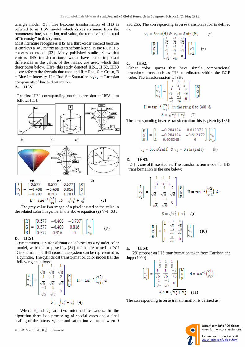
Firouz Abdullah Al-Wassai et al, Journal of Global Research in Computer Science,2 (5), May 2011,
© JGRCS 2010, All Rights Reserved 71
triangle model [31]. The hexcone transformation of IHS is referred to as HSV model which drives its name from the parameters, hue, saturation, and value, the term “value” instead of “intensity” in this system. Most literature recognizes IHS as a third-order method because it employs a 3×3 matrix as its transform kernel in the RGB IHS conversion model [32]. Many published studies show that various IHS transformations, which have some important differences in the values of the matrix, are used, which that description below. Here, this study denoted IHS1, IHS2, IHS3 …etc refer to the formula that used and R = Red, G = Green, B = Blue I = Intensity, H = Hue, S = Saturation, = Cartesian components of hue and saturation. A. HSV
The first IHS1 corresponding matrix expression of HSV is as follows [33]:
The gray value Pan image of a pixel is used as the value in the related color image, i.e. in the above equation (2) V=I [33]:
(3)
B. IHS1: One common IHS transformation is based on a cylinder color model, which is proposed by [34] and implemented in PCI Geomatica. The IHS coordinate system can be represented as a cylinder. The cylindrical transformation color model has the following equations:
Where and are two intermediate values. In the algorithm there is a processing of special cases and a final scaling of the intensity, hue and saturation values between 0
and 255. The corresponding inverse transformation is defined as:
(5)
(6)
C. IHS2: Other color spaces that have simple computational transformations such as IHS coordinates within the RGB cube. The transformation is [35]:
(7) The corresponding inverse transformation this is given by [35]:
(8)
D. IHS3: [24] is one of these studies. The transformation model for IHS transformation is the one below:
(9)
(10)
E. IHS4: [29] propose an IHS transformation taken from Harrison and Jupp (1990).
(11)
The corresponding inverse transformation is defined as:
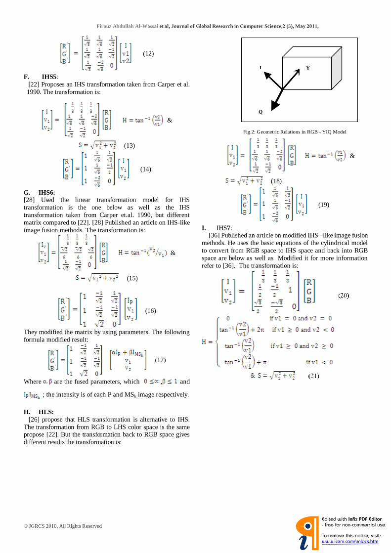
Firouz Abdullah Al-Wassai et al, Journal of Global Research in Computer Science,2 (5), May 2011,
© JGRCS 2010, All Rights Reserved 72
(12)
F. IHS5: [22] Proposes an IHS transformation taken from Carper et al. 1990. The transformation is:
&
(13)
(14)
G. IHS6: [28] Used the linear transformation model for IHS transformation is the one below as well as the IHS transformation taken from Carper et.al. 1990, but different matrix compared to [22]. [28] Published an article on IHS-like image fusion methods. The transformation is:
&
(15)
(16)
They modified the matrix by using parameters. The following formula modified result:
(17)
Where are the fused parameters, which , and
; the intensity is of each P and MSk imagerespectively.
H. HLS: [26] propose that HLS transformation is alternative to IHS. The transformation from RGB to LHS color space is the same propose [22]. But the transformation back to RGB space gives different results the transformation is:
&
(18)
(19)
I. IHS7: [36] Published an article on modified IHS –like image fusion methods. He uses the basic equations of the cylindrical model to convert from RGB space to IHS space and back into RGB space are below as well as Modified it for more information refer to [36]. The transformation is:
Fig.2: Geometric Relations in RGB - YIQ Model
I
Q
Y

Firouz Abdullah Al-Wassai et al, Journal of Global Research in Computer Science,2 (5), May 2011,
© JGRCS 2010, All Rights Reserved 73
(22)
J. YIQ: Another color encoding system called YIQ (Fig.2) has a straightforward transformation from RGB with no loss of information. The YIQ model was designed to take advantage of the human system‟s greater sensitivity to changes in luminance than to changes in hue or saturation [37]. In the case of the YIQ transformations, the component Y represents the luminance of a color, while its chrominance is denoted by I and Q signals [38].Y is just the brightness of a panchromatic monochrome image. It combines the red, green, and blue signals in proportion to the human eye‟s sensitivity to them .The I signal is essentially red minus cyan, while Q is magenta minus green [39] express jointly hue and saturation . The relationship between and is given as follows: [30; 37]:
(23)
The YIQ is transformed inversely to RGB space is given by
[30; 37]:
(24)
THE IHS-BASED PAN SHARPENING
The IHS pan sharpening technique is the oldest known data fusion method and one of the simplest. Fig.3 illustrates this technique for convenience. In this technique the following steps are performed:
1. The low resolution MS imagery is co-registered to the
same area as the high resolution PAN imagery and resampled to the same resolution as the PAN imagery.
2. The three resampled bands of the MS imagery, which represent the RGB space, are transformed into IHS components.
3. The PAN imagery is histogram matched to the „I‟ component. This is done in order to compensate for the spectral differences between the two images, which occurred due to different sensors or different acquisition dates and angles.
4. The intensity component of MS imagery is replaced by the histogram matched PAN imagery. The RGB of the new merged MS imagery is obtained by computing a reverse IHS to RGB transform.
To evaluate the ability of enhancing spatial details and preserving spectral information, some Indices including Standard Deviation ( ), Entropy ), Correlation Coefficient ( ), Signal-to Noise Ratio ( ), Normalization Root Mean Square Error (NRMSE) and Deviation Index () of the image these measures given in (Table 1), and the results are shown in Table 2. In the following sections, are the measurements of each the brightness values of homogenous pixels of the result image and the original multispectral image of band k, and are the mean brightness values of both images and are of size . is the brightness value of image data and .
Table 1: Indices Used to Assess Fusion Images. Item Equation
SD
CC
En )(2
log)(1
0iPiP
IEn
DI
SNR
PAN Image
Input Images
Multispectral Image
R G B
Feature
H S
I
Inverse Transformation
R new G new B new
Image Fusion
Matching PAN with I
Replace I by PAN
Fig. 3: IHS Image Fusion Process

Firouz Abdullah Al-Wassai et al, Journal of Global Research in Computer Science,2 (5), May 2011,
© JGRCS 2010, All Rights Reserved 74
NRMSE
RESULTS AND DISCUSSION
In order to validate the theoretical analysis, the performance of the methods discussed above was further evaluated by experimentation. Data sets used for this study were collected by the Indian IRS-1C PAN (0.50 - 0.75 µm) of the (5.8 ) resolution panchromatic band. Where the American Landsat (TM) the red (0.63 - 0.69 µm), green (0.52 - 0.60 µm) and blue (0.45 - 0.52 µm) bands of the 30 m resolution multispectral image were used in this experiment. Fig. 2 shows the IRS-1C PAN and multispectral TM images. The scenes covered the same area of the Mausoleums of the Chinese Tang – Dynasty in the PR China [40] was selected as test sit in this study. Since this study is involved in evaluation of the effect of the various spatial, radiometric and spectral resolution for image fusion, an area contains both manmade and natural features is essential to study these effects. Hence, this work is an attempt to study the quality of the images fused from different sensors with various characteristics. The size of the PAN is 600 * 525 pixels at 6 bits per pixel and the size of the original multispectral is 120 * 105 pixels at 8 bits per pixel, but this is upsampled to by Nearest neighbor was used to avoid spectral
contamination caused by interpolation. The pairs of images were geometrically registered to each other. The Fig. 5 shows quantitative measures for the fused images for the various fusion methods. It can be seen that the standard deviation of the fused images remain constant for all methods except HSV, IHS6 and IHS7. Correlation values also remain practically constant, very near the maximum possible value except IHS6 and IHS7. The differences between the reference image and the fused images during & values are so small that they do not bear any real significance. This is due to the fact that, the Matching processing of the intensity of MS and PAN images by mean and standard division was done before the merging processing. But with the results of ,
and appear changing significantly. It can be observed that from the diagram of Fig. 5. That the fused image the results of & show that the IHS5 and methods give best results with respect to the other methods followed by the HLS and IHS4who get the same values presented the lowest value of the & as well as the higher of the . Hence, the spectral qualities of fused images by the IHS5 and YIQ methods are much better than the others. In contrast, It can also be noted that the IHS7, HS6, IHS2, IHS1 images produce highly & values indicate that these methods deteriorate spectral information content for the reference image.
Fig 4: Original and Fused Images
Fig. 5: Chart Representation of En, CC, SNR, NRMSE & DI of Fused Image
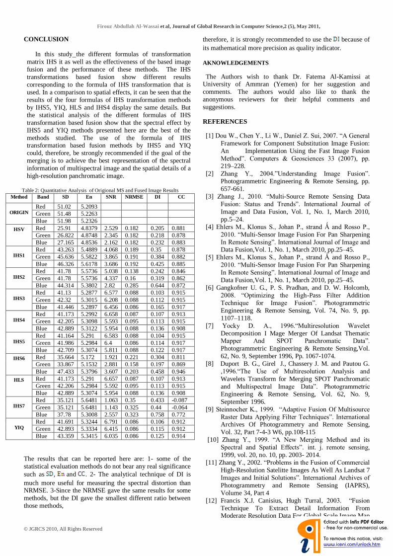
Firouz Abdullah Al-Wassai et al, Journal of Global Research in Computer Science,2 (5), May 2011,
© JGRCS 2010, All Rights Reserved 75
CONCLUSION In this study the different formulas of transformation matrix IHS it as well as the effectiveness of the based image fusion and the performance of these methods. The IHS transformations based fusion show different results corresponding to the formula of IHS transformation that is used. In a comparison to spatial effects, it can be seen that the results of the four formulas of IHS transformation methods by IHS5, YIQ, HLS and IHS4 display the same details. But the statistical analysis of the different formulas of IHS transformation based fusion show that the spectral effect by IHS5 and YIQ methods presented here are the best of the methods studied. The use of the formula of IHS transformation based fusion methods by IHS5 and YIQ could, therefore, be strongly recommended if the goal of the merging is to achieve the best representation of the spectral information of multispectral image and the spatial details of a high-resolution panchromatic image.
Table 2: Quantitative Analysis of Origional MS and Fused Image Results Method Band SD En SNR NRMSE DI CC
ORIGIN Red 51.02 5.2093 Green 51.48 5.2263
Blue 51.98 5.2326
HSV
Red 25.91 4.8379 2.529 0.182 0.205 0.881 Green 26.822 4.8748 2.345 0.182 0.218 0.878 Blue 27.165 4.8536 2.162 0.182 0.232 0.883
IHS1 Red 43.263 5.4889 4.068 0.189 0.35 0.878 Green 45.636 5.5822 3.865 0.191 0.384 0.882 Blue 46.326 5.6178 3.686 0.192 0.425 0.885
IHS2 Red 41.78 5.5736 5.038 0.138 0.242 0.846 Green 41.78 5.5736 4.337 0.16 0.319 0.862 Blue 44.314 5.3802 2.82 0.285 0.644 0.872
IHS3 Red 41.13 5.2877 6.577 0.088 0.103 0.915 Green 42.32 5.3015 6.208 0.088 0.112 0.915 Blue 41.446 5.2897 6.456 0.086 0.165 0.917
IHS4 Red 41.173 5.2992 6.658 0.087 0.107 0.913 Green 42.205 5.3098 5.593 0.095 0.113 0.915 Blue 42.889 5.3122 5.954 0.088 0.136 0.908
IHS5 Red 41.164 5.291 6.583 0.088 0.104 0.915 Green 41.986 5.2984 6.4 0.086 0.114 0.917 Blue 42.709 5.3074 5.811 0.088 0.122 0.917
IHS6
Red 35.664 5.172 1.921 0.221 0.304 0.811 Green 33.867 5.1532 2.881 0.158 0.197 0.869 Blue 47.433 5.3796 3.607 0.203 0.458 0.946
HLS
Red 41.173 5.291 6.657 0.087 0.107 0.913 Green 42.206 5.2984 5.592 0.095 0.113 0.915 Blue 42.889 5.3074 5.954 0.088 0.136 0.908
IHS7 Red 35.121 5.6481 1.063 0.35 0.433 -0.087 Green 35.121 5.6481 1.143 0.325 0.44 -0.064 Blue 37.78 5.3008 2.557 0.323 0.758 0.772
YIQ Red 41.691 5.3244 6.791 0.086 0.106 0.912 Green 42.893 5.3334 6.415 0.086 0.115 0.912 Blue 43.359 5.3415 6.035 0.086 0.125 0.914
The results that can be reported here are: 1- some of the statistical evaluation methods do not bear any real significance such as , and . 2- The analytical technique of DI is much more useful for measuring the spectral distortion than NRMSE. 3-Since the NRMSE gave the same results for some methods, but the DI gave the smallest different ratio between those methods,
therefore, it is strongly recommended to use the because of its mathematical more precision as quality indicator. AKNOWLEDGEMENTS
The Authors wish to thank Dr. Fatema Al-Kamissi at University of Ammran (Yemen) for her suggestion and comments. The authors would also like to thank the anonymous reviewers for their helpful comments and suggestions. REFERENCES
[1] Dou W., Chen Y., Li W., Daniel Z. Sui, 2007. “A General Framework for Component Substitution Image Fusion: An Implementation Using the Fast Image Fusion Method”. Computers & Geosciences 33 (2007), pp. 219–228.
[2] Zhang Y., 2004.”Understanding Image Fusion”. Photogrammetric Engineering & Remote Sensing, pp. 657-661.
[3] Zhang J., 2010. “Multi-Source Remote Sensing Data Fusion: Status and Trends”. International Journal of Image and Data Fusion, Vol. 1, No. 1, March 2010, pp.5–24.
[4] Ehlers M., Klonus S., Johan P., strand Ǻ and Rosso P., 2010. “Multi-Sensor Image Fusion For Pan Sharpening In Remote Sensing”. International Journal of Image and Data Fusion,Vol. 1, No. 1, March 2010, pp.25–45.
[5] Ehlers M., Klonus S., Johan P., strand Ǻ and Rosso P., 2010. “Multi-Sensor Image Fusion For Pan Sharpening In Remote Sensing”. International Journal of Image and Data Fusion,Vol. 1, No. 1, March 2010, pp.25–45.
[6] Gangkofner U. G., P. S. Pradhan, and D. W. Holcomb, 2008. “Optimizing the High-Pass Filter Addition Technique for Image Fusion”. Photogrammetric Engineering & Remote Sensing, Vol. 74, No. 9, pp. 1107–1118.
[7] Yocky D. A., 1996.“Multiresolution Wavelet Decomposition I Mage Merger Of Landsat Thematic Mapper And SPOT Panchromatic Data”. Photogrammetric Engineering & Remote Sensing,Vol. 62, No. 9, September 1996, Pp. 1067-1074.
[8] Duport B. G., Girel J., Chassery J. M. and Pautou G. ,1996.“The Use of Multiresolution Analysis and Wavelets Transform for Merging SPOT Panchromatic and Multispectral Image Data”. Photogrammetric Engineering & Remote Sensing, Vol. 62, No. 9, September 1996.
[9] Steinnocher K., 1999. “Adaptive Fusion Of Multisource Raster Data Applying Filter Techniques”. International Archives Of Photogrammetry and Remote Sensing, Vol. 32, Part 7-4-3 W6, pp.108-115
[10] Zhang Y., 1999. “A New Merging Method and its Spectral and Spatial Effects”. int. j. remote sensing, 1999, vol. 20, no. 10, pp. 2003- 2014.
[11] Zhang Y., 2002. “Problems in the Fusion of Commercial High-Resolution Satelitte Images As Well As Landsat 7 Images and Initial Solutions”. International Archives of Photogrammetry and Remote Sensing (IAPRS), Volume 34, Part 4
[12] Francis X.J. Canisius, Hugh Turral, 2003. “Fusion Technique To Extract Detail Information From Moderate Resolution Data For Global Scale Image Map

Firouz Abdullah Al-Wassai et al, Journal of Global Research in Computer Science,2 (5), May 2011,
© JGRCS 2010, All Rights Reserved 76
Production”. Proceedings Of The 30th International Symposium On Remote Sensing Of Environment – Information For Risk Management Andsustainable Development – November 10-14, 2003 Honolulu, Hawaii.
[13] Shi W., Changqing Z., Caiying Z., and Yang X., 2003. “Multi-Band Wavelet for Fusing SPOT Panchromatic and Multispectral Images”. Photogrammetric Engineering & Remote Sensing Vol. 69, No. 5, May 2003, pp. 513–520.
[14] Park J. H. and Kang M. G., 2004. “Spatially Adaptive Multi-Resolution Multispectral Image Fusion”. INT. J. Remote Sensing, 10 December, 2004, Vol. 25, No. 23, pp. 5491–5508.
[15] Vijayaraj V., O‟Hara C. G. And Younan N. H., 2004. “Quality Analysis of Pansharpened Images”. 0-7803-8742-2/04/ (C) 2004 IEEE, pp.85-88
[16] ŠVab A.and Oštir K., 2006. “High-Resolution Image Fusion: Methods to Preserve Spectral and Spatial Resolution”. Photogrammetric Engineering & Remote Sensing, Vol. 72, No. 5, May 2006, pp. 565–572.
[17] Moeller M. S. And Blaschke T., 2006. “Urban Change Extraction from High Resolution Satellite Image”. ISPRS Technical Commission Symposium, Vienna, 12 – 14 July pp. 151-156.
[18] Das A. and Revathy K., 2007. “A Comparative Analysis of Image Fusion Techniques for Remote Sensed Images”. Proceedings of the World Congress on Engineering 2007 Vol I, WCE 2007, July 2 – 4, London, U.K..
[19] CHEN S., SU H., ZHANG R., TIAN J. AND YANG L., 2008.”THE TRADEOFF ANALYSIS FOR REMOTE
SENSING IMAGE FUSION USING EXPANDED
SPECTRAL ANGLE M APPER”. FULL RESEARCH
PAPER, SENSORS 2008, 8, PP.520-528. [20] Schetselaar E. M., 1998. “Fusion By The IHS
Transform: Should We Use Cylindrical or Spherical Coordinates?,” Int. J. Remote Sens., Vol. 19, No. 4, pp.759–765,
[21] Schetselaar E. M. B, 2001. “On Preserving Spectral Balance in Image Fusion and Its Advantages For Geological Image Interpretation”. Photogrammetric Engineering & Remote Sensing Vol. 67, NO. 8, August 2001, pp. 925-934.
[22] Li S., Kwok J. T., Wang Y.., 2002. “Using the Discrete Wavelet Frame Transform To Merge Landsat TM And SPOT Panchromatic Images”. Information Fusion 3 (2002), pp.17–23.
[23] Chibani Y. and A. Houacine, 2002. “The Joint Use of IHS Transform and Redundant Wavelet Decomposition for Fusing Multispectral and Panchromatic Images”. int. j. remote sensing, 2002, vol. 23, no. 18, pp. 3821–3833.
[24] Wang Z., Ziou D., Armenakis C., Li D., and Li Q.2005. “A Comparative Analysis of Image Fusion Methods”. IEEE Transactions on Geoscience and Remote Sensing, Vol. 43, No. 6, June 2005 pp.1391-1402.
[25] Lu J., Zhang B., Gong Z., Li Z., Liu H., 2008. “The Remote-Sensing Image Fusion Based On GPU”. The International Archives of the Photogrammetry, Remote Sensing and Spatial Information Sciences. Vol. XXXVII. Part B7. Beijing pp. 1233-1238.
[26] Hui Y. X. and Cheng J. L., 2008. “Fusion Algorithm for Remote Sensing Images Based on Nonsubsampled
Contourlet Transform”. ACTA AUTOMATICA SINICA, Vol. 34, No. 3.pp. 274- 281.
[27] Hui Y. X. and Cheng J. L., 2008. “Fusion Algorithm for Remote Sensing Images Based on Nonsubsampled Contourlet Transform”. ACTA AUTOMATICA SINICA, Vol. 34, No. 3.pp. 274- 281.
[28] Hsu S. L., Gau P.W., Wu I L., and Jeng J.H., 2009. “Region-Based Image Fusion with Artificial Neural Network”. World Academy of Science, Engineering and Technology, 53, pp 156 -159.
[29] Pohl C. and Van Genderen J. L. (1998), Multisensor Image Fusion In Remote Sensing: Concepts, Methods And Applications (Review Article), International Journal Of Remote Sensing, Vol. 19, No.5, pp. 823-854
[30] Sangwine S. J., and R.E.N. Horne, 1989. “The Colour Image Processing Handbook”. Chapman & Hall.
[31] Nùñez J., Otazu X., Fors O., Prades A., Pal`a V., and Arbiol R., 1999. “Multiresolution -Based Image Fusion with Additive Wavelet Decomposition”. IEEE Transactions On Geoscience and Remote Sensing, VOL. 37, NO. 3, pp. 1204- 1211
[32] Garzelli A., Capobianco L. and Nencini F., 2008. “Fusion of multispectral and panchromatic images as an optimisation problem”. Edited by: Stathaki T. “Image Fusion: Algorithms and Applications”. Elsevier Ltd
[33] Liao Y. C., Wang T. Y. and Zheng W. T., 1998. “Quality Analysis Of Synthesized High Resolution Multispectral Imagery”.(URL:http://www.Gisdevelopment.Net/AARS/ACRS 1998/Digital Image Processing (Last date accessed: 8 Feb 2008).
[34] Kruse F.A., Raines G.L, 1984. “A Technique for Enhancing Digital Colour Images By Contrast Stretching In Munsell Colour Space”. Proceedings Of The International Symposium On Remote Sensing Of Environment, 3RD Thematic Conference, Environmental Research Institute Of Michigan, Colorado Springs, Colorado, pp. 755-773
[35] Niblack W, 1986.”An Introduction to Digital Image Processing”. Prentice Hall International.
[36] Siddiqui Y., 2003. “The Modified IHS Method for Fusing Satellite Imagery”. ASPRS Annual Conference Proceedings May 2003, ANCHORAGE, Alaska.
[37] Gonzalez, R.C. And Woods, R.E., 2001. “Digital Image Processing “. Prentice Hall.
[38] Kumar A. S., B. Kartikeyan and K. L. Majumdar, 2000. “Band Sharpening of IRS- Multispectral Imagery By Cubic Spline Wavelets”. int. j. remote sensing, 2000, vol. 21, no. 3, pp.581–594.
[39] Russ J. C., 1998. “The Image Processing Handbook”, Third Edition, CRC Press, CRC Press LLC.
[40] Böhler W. and G. Heinz, 1998. “Integration of high Resolution Satellite Images into Archaeological Docmentation”. Proceeding International Archives of Photogrammetry and Remote Sensing, Commission V, Working Group V/5, CIPA International Symposium, Published by the Swedish Society for Photogrammetry and Remote Sensing, Goteborg. (URL: HTTP://WWW.I3MAINZ .FHMAINZ.DE/PUBLICAT/CIP
A-98/SAT-IM.HTML (LAST DATE ACCESSED: 28 OCT. 2000).

Firouz Abdullah Al-Wassai et al, Journal of Global Research in Computer Science,2 (5), May 2011,
© JGRCS 2010, All Rights Reserved 77
AUTHORS Mrs. Firouz Abdullah Al-Wassai1.Received the B.Sc. degree in, Physics from University of Sana‟a, Yemen, Sana‟a, in 1993. The M.Sc.degree in, Physics from Bagdad University , Iraqe, in 2003, Research student.Ph.D in thedepartment of computer science (S.R.T.M.U), India, Nanded. Dr. N.V. Kalyankar .B.Sc.Maths, Physics, Chemistry, Marathwada University, Aurangabad, India, 1978. M Sc.Nuclear Physics, Marathwada University, Aurangabad, India, 1980.Diploma in Higher Education, Shivaji University, Kolhapur, India, 1984.Ph.D. in Physics, Dr.B.A.M.University, Aurangabad, India, 1995.Principal Yeshwant Mahavidyalaya College, Membership of Academic Bodies,Chairman,
Information Technology Society State Level Organization, Life Member of Indian Laser Association, Member Indian Institute of Public Administration, New Delhi, Member Chinmay Education Society, Nanded.He has one publication book, seven journals papers, two seminars Papers and three conferences papers. Dr. Ali A. Al-Zuky. B.Sc Physics Mustansiriyah University, Baghdad , Iraq, 1990. M Sc. In1993 and Ph. D. in1998 from University of Baghdad, Iraq. He was supervision for 40 post-graduate students (MSc. & Ph.D.) in different fields (physics, computers and Computer Engineering and Medical Physics). He has More than 60 scientific papers published in scientific journals in several scientific conferences.
International Journal of Artificial Intelligence and Knowledge Discovery Vol.1, Issue 3, July, 2011
5
The Statistical methods of Pixel-Based Image Fusion Techniques
Firouz Abdullah Al-Wassai1 N.V. Kalyankar2 Research Student, Computer Science Dept. Principal, Yeshwant Mahavidyala College (SRTMU), Nanded, India Nanded, India [email protected] [email protected]
Ali A. Al-Zaky 3 Assistant Professor, Dept.of Physics, College of Science, Mustansiriyah Un.
Baghdad – Iraq. [email protected]
Abstract: There are many image fusion methods that can be used to produce high-resolution mutlispectral images from a high-resolution panchromatic (PAN) image and low-resolution multispectral (MS) of remote sensed images. This paper attempts to undertake the study of image fusion techniques with different Statistical techniques for image fusion as Local Mean Matching (LMM), Local Mean and Variance Matching (LMVM), Regression variable substitution (RVS), Local Correlation Modeling (LCM) and they are compared with one another so as to choose the best technique, that can be applied on multi-resolution satellite images. This paper also devotes to concentrate on the analytical techniques for evaluating the quality of image fusion (F) by using various methods including Standard Deviation ( ), Entropy ), Correlation Coefficient ( ), Signal-to Noise Ratio ( ), Normalization Root Mean Square Error (NRMSE) and Deviation Index ( ) to estimate the quality and degree of information improvement of a fused image quantitatively.
Keywords: Data Fusion, Resolution Enhancement, Statistical fusion, Correlation Modeling, Matching, pixel based fusion.
I. INTRODUCTION Satellite remote sensing offers a wide variety of image data with different characteristics in terms of temporal, spatial, radiometric and Spectral resolutions. Although the information content of these images might be partially overlapping [1], imaging systems somehow offer a tradeoff between high spatial and high spectral resolution, whereas no single system offers both. Hence, in the remote sensing community, an image with „greater quality‟ often means higher spatial or higher spectral resolution, which can only be obtained by more advanced sensors [2]. However, many applications of satellite images require both spectral and spatial resolution to be high. In order to automate the processing of these satellite images new concepts for sensor fusion are needed. It is, therefore, necessary and very useful to be able to merge images with higher spectral information and higher spatial information [3]. Image fusion is a sub area of the more general topic of data fusion [4].So, Satellites remote sensing image
fusion has been a hot research topic of remote sensing image processing [5]. This is obvious from the amount of conferences and workshops focusing on data fusion, as well as the special issues of scientific journals dedicated to the topic [6]. Previously, data fusion, and in particular image fusion belonged to the world of research and development. In the meantime, it has become a valuable technique for data enhancement in many applications. The term “fusion” gets several words to appear, such as merging, combination, synergy, integration … and several others that express more or less the same concept have since appeared in literature [7]. A general definition of data fusion can be adopted as fallows “Data fusion is a formal framework which expresses means and tools for the alliance of data originating from different sources. It aims at obtaining information of greater quality; the exact definition of „greater quality‟ will depend upon the application” [8-10]. Many image fusion or pansharpening techniques have been developed to produce high-resolution mutlispectral images. Most of these methods seem to work well with images that were acquired at the same time by one sensor (single-sensor, single-date fusion) [11-13]. It becomes, therefore increasingly important to fuse image data from different sensors which are usually recorded at different dates. Thus, there is a need to investigate techniques that allow multi-sensor, multi-date image fusion [14]. Generally, Image fusion techniques can divided into three levels, namely: pixel level, feature level and decision level of representation [15-17]. The pixel image fusion techniques can be grouped into several techniques depending on the tools or the processing methods for image fusion procedure. This paper focuses on using statistical methods of pixel-based image fusion techniques. This study attempts to comparing four Statistical Image fusion techniques including Local Mean Matching (LMM), Local Mean and Variance Matching (LMVM), Regression variable substitution (RVS), Local Correlation Modeling (LCM). so, This study introduces
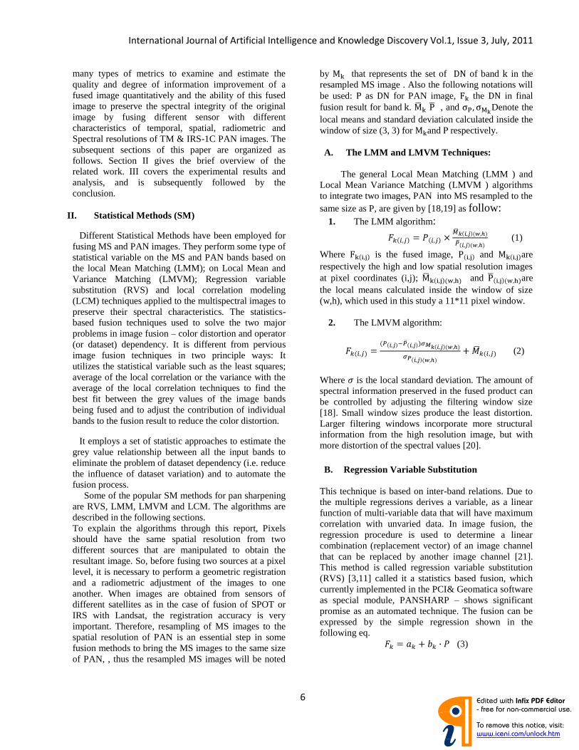
International Journal of Artificial Intelligence and Knowledge Discovery Vol.1, Issue 3, July, 2011
6
many types of metrics to examine and estimate the quality and degree of information improvement of a fused image quantitatively and the ability of this fused image to preserve the spectral integrity of the original image by fusing different sensor with different characteristics of temporal, spatial, radiometric and Spectral resolutions of TM & IRS-1C PAN images. The subsequent sections of this paper are organized as follows. Section II gives the brief overview of the related work. III covers the experimental results and analysis, and is subsequently followed by the conclusion.
II. Statistical Methods (SM)
Different Statistical Methods have been employed for fusing MS and PAN images. They perform some type of statistical variable on the MS and PAN bands based on the local Mean Matching (LMM); on Local Mean and Variance Matching (LMVM); Regression variable substitution (RVS) and local correlation modeling (LCM) techniques applied to the multispectral images to preserve their spectral characteristics. The statistics-based fusion techniques used to solve the two major problems in image fusion – color distortion and operator (or dataset) dependency. It is different from pervious image fusion techniques in two principle ways: It utilizes the statistical variable such as the least squares; average of the local correlation or the variance with the average of the local correlation techniques to find the best fit between the grey values of the image bands being fused and to adjust the contribution of individual bands to the fusion result to reduce the color distortion.
It employs a set of statistic approaches to estimate the grey value relationship between all the input bands to eliminate the problem of dataset dependency (i.e. reduce the influence of dataset variation) and to automate the fusion process. Some of the popular SM methods for pan sharpening are RVS, LMM, LMVM and LCM. The algorithms are described in the following sections. To explain the algorithms through this report, Pixels should have the same spatial resolution from two different sources that are manipulated to obtain the resultant image. So, before fusing two sources at a pixel level, it is necessary to perform a geometric registration and a radiometric adjustment of the images to one another. When images are obtained from sensors of different satellites as in the case of fusion of SPOT or IRS with Landsat, the registration accuracy is very important. Therefore, resampling of MS images to the spatial resolution of PAN is an essential step in some fusion methods to bring the MS images to the same size of PAN, , thus the resampled MS images will be noted
by that represents the set of of band in the resampled MS image . Also the following notations will be used: as for PAN image, the in final fusion result for band. , and Denote the local means and standard deviation calculated inside the window of size (3, 3) for and respectively. A. The LMM and LMVM Techniques:
The general Local Mean Matching (LMM ) and Local Mean Variance Matching (LMVM ) algorithms to integrate two images, PAN into MS resampled to the same size as P, are given by [18,19] as follow:
1. The LMM algorithm:
(1)
Where is the fused image, and are respectively the high and low spatial resolution images at pixel coordinates (i,j); and are the local means calculated inside the window of size (w,h), which used in this study a 11*11 pixel window.
2. The LMVM algorithm:
(2)
Where is the local standard deviation. The amount of spectral information preserved in the fused product can be controlled by adjusting the filtering window size [18]. Small window sizes produce the least distortion. Larger filtering windows incorporate more structural information from the high resolution image, but with more distortion of the spectral values [20]. B. Regression Variable Substitution
This technique is based on inter-band relations. Due to the multiple regressions derives a variable, as a linear function of multi-variable data that will have maximum correlation with unvaried data. In image fusion, the regression procedure is used to determine a linear combination (replacement vector) of an image channel that can be replaced by another image channel [21]. This method is called regression variable substitution (RVS) [3,11] called it a statistics based fusion, which currently implemented in the PCI& Geomatica software as special module, PANSHARP – shows significant promise as an automated technique. The fusion can be expressed by the simple regression shown in the following eq.
(3)
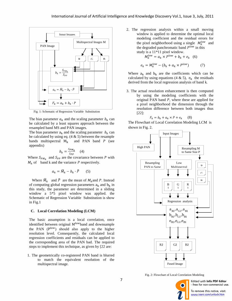
International Journal of Artificial Intelligence and Knowledge Discovery Vol.1, Issue 3, July, 2011
7
The bias parameter and the scaling parameter can be calculated by a least squares approach between the resampled band MS and PAN images. The bias parameter and the scaling parameter can be calculated by using eq. (4 & 5) between the resample bands multispectral and PAN band (see appendix)
(4)
Where and are the covariance between with of band k and the variance respectively.
(5)
Where and are the mean of and . Instead of computing global regression parameters and in this study, the parameter are determined in a sliding window a 5*5 pixel window was applied. the Schematic of Regression Variable Substitution is show in Fig.1 C. Local Correlation Modeling (LCM)
The basic assumption is a local correlation, once identified between original band and downsample the PAN ( ) should also apply to the higher resolution level. Consequently, the calculated local regression coefficients and residuals can be applied to the corresponding area of the PAN bad. The required steps to implement this technique, as given by [22 are:
1. The geometrically co-registered PAN band is blurred to match the equivalent resolution of the multispectral image.
2. The regression analysis within a small moving window is applied to determine the optimal local modeling coefficient and the residual errors for the pixel neighborhood using a single and the degraded panchromatic band in this study is a 11*11 pixel window.
(6)
(7)
Where and are the coefficients which can be calculated by using equations (4 & 5), the residuals derived from the local regression analysis of band k.
3. The actual resolution enhancement is then computed by using the modeling coefficients with the original PAN band , where these are applied for a pixel neighborhood the dimension through the resolution difference between both images thus [22]:
(8) The Flowchart of Local Correlation Modeling LCM is shown in Fig. 2.
Input Images
Resampling M to Same Size P
High PAN
B
G
RLow
Multispectral Resampling
PAN to Same
R1
G1
B1
Regression analysis
111
111
111
,,
,,
,,
BGR
BGR
BGR
eee
bbb
aaa
B2
N
G2
N
R2
N
Fused Image
Fig. 1: Schematic of Regression Variable Substitution
Input Images
Multispectral Images M
PAN Image
P
R G B
Fig. 2: Flowchart of Local Correlation Modeling
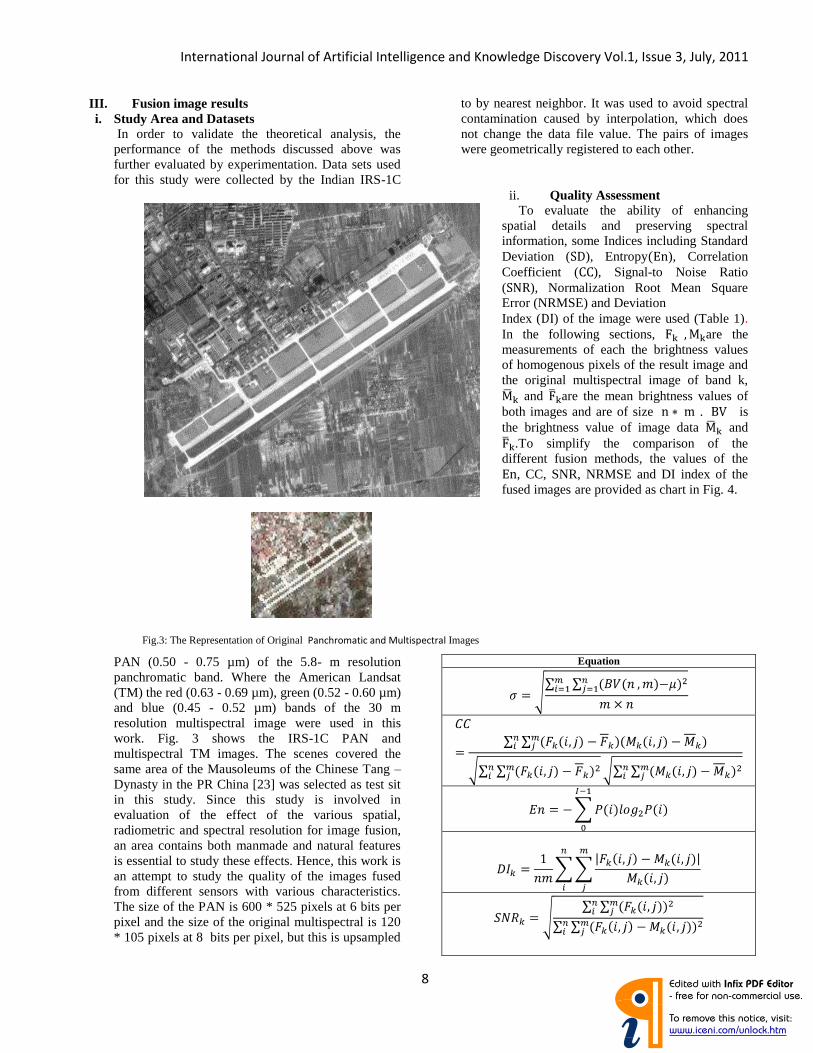
International Journal of Artificial Intelligence and Knowledge Discovery Vol.1, Issue 3, July, 2011
8
III. Fusion image results i. Study Area and Datasets
In order to validate the theoretical analysis, the performance of the methods discussed above was further evaluated by experimentation. Data sets used for this study were collected by the Indian IRS-1C
PAN (0.50 - 0.75 µm) of the 5.8- m resolution panchromatic band. Where the American Landsat (TM) the red (0.63 - 0.69 µm), green (0.52 - 0.60 µm) and blue (0.45 - 0.52 µm) bands of the 30 m resolution multispectral image were used in this work. Fig. 3 shows the IRS-1C PAN and multispectral TM images. The scenes covered the same area of the Mausoleums of the Chinese Tang – Dynasty in the PR China [23] was selected as test sit in this study. Since this study is involved in evaluation of the effect of the various spatial, radiometric and spectral resolution for image fusion, an area contains both manmade and natural features is essential to study these effects. Hence, this work is an attempt to study the quality of the images fused from different sensors with various characteristics. The size of the PAN is 600 * 525 pixels at 6 bits per pixel and the size of the original multispectral is 120 * 105 pixels at 8 bits per pixel, but this is upsampled
to by nearest neighbor. It was used to avoid spectral contamination caused by interpolation, which does not change the data file value. The pairs of images were geometrically registered to each other.
ii. Quality Assessment To evaluate the ability of enhancing spatial details and preserving spectral information, some Indices including Standard Deviation ( ), Entropy ), Correlation Coefficient ( ), Signal-to Noise Ratio ( ), Normalization Root Mean Square Error (NRMSE) and Deviation Index ( ) of the image were used (Table 1). In the following sections, are the measurements of each the brightness values of homogenous pixels of the result image and the original multispectral image of band k,
and are the mean brightness values of both images and are of size . is the brightness value of image data and
.To simplify the comparison of the different fusion methods, the values of the
, CC, SNR, NRMSE and DI index of the fused images are provided as chart in Fig. 4.
Equation
Fig.3: The Representation of Original Panchromatic and Multispectral Images
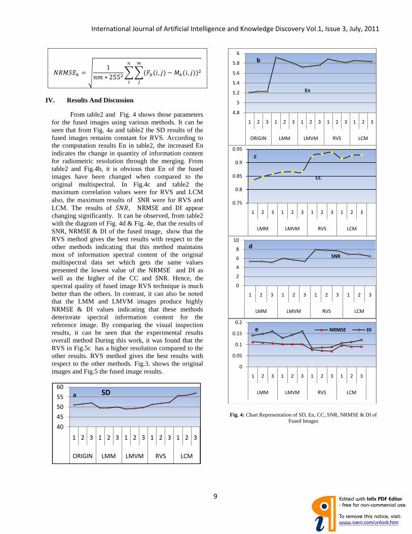
International Journal of Artificial Intelligence and Knowledge Discovery Vol.1, Issue 3, July, 2011
9
IV. Results And Discussion
From table2 and Fig. 4 shows those parameters for the fused images using various methods. It can be seen that from Fig. 4a and table2 the SD results of the fused images remains constant for RVS. According to the computation results En in table2, the increased En indicates the change in quantity of information content for radiometric resolution through the merging. From table2 and Fig.4b, it is obvious that En of the fused images have been changed when compared to the original multispectral. In Fig.4c and table2 the maximum correlation values were for RVS and LCM also, the maximum results of were for RVS and LCM. The results of , and appear changing significantly. It can be observed, from table2 with the diagram of Fig. 4d & Fig. 4e, that the results of SNR, & of the fused image, show that the RVS method gives the best results with respect to the other methods indicating that this method maintains most of information spectral content of the original multispectral data set which gets the same values presented the lowest value of the and as well as the higher of the CC and . Hence, the spectral quality of fused image RVS technique is much better than the others. In contrast, it can also be noted that the LMM and LMVM images produce highly
& values indicating that these methods deteriorate spectral information content for the reference image. By comparing the visual inspection results, it can be seen that the experimental results overall method During this work, it was found that the RVS in Fig.5c has a higher resolution compared to the other results. RVS method gives the best results with respect to the other methods. Fig.3. shows the original images and Fig.5 the fused image results.
Fig. 4: Chart Representation of SD, En, CC, SNR, NRMSE & DI of
Fused Images 40
45
50
55
60
1 2 3 1 2 3 1 2 3 1 2 3 1 2 3
ORIGIN LMM LMVM RVS LCM
SDa
4.8
5
5.2
5.4
5.6
5.8
6
1 2 3 1 2 3 1 2 3 1 2 3 1 2 3
ORIGIN LMM LMVM RVS LCM
En
b
0.75
0.8
0.85
0.9
0.95
1 2 3 1 2 3 1 2 3 1 2 3
LMM LMVM RVS LCM
CC
c
0
2
4
6
8
10
1 2 3 1 2 3 1 2 3 1 2 3
LMM LMVM RVS LCM
SNR
d
0
0.05
0.1
0.15
0.2
1 2 3 1 2 3 1 2 3 1 2 3
LMM LMVM RVS LCM
NRMSE DIe
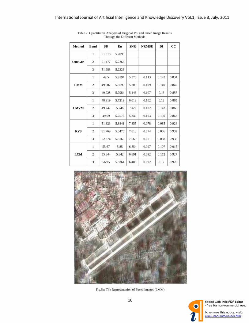
International Journal of Artificial Intelligence and Knowledge Discovery Vol.1, Issue 3, July, 2011
10
Fig.5a: The Representation of Fused Images (LMM)
Table 2: Quantitative Analysis of Original MS and Fused Image Results Through the Different Methods
Method Band SD En SNR NRMSE DI CC
ORIGIN
1 51.018 5.2093
2 51.477 5.2263
3 51.983 5.2326
LMM
1 49.5 5.9194 5.375 0.113 0.142 0.834
2 49.582 5.8599 5.305 0.109 0.149 0.847
3 49.928 5.7984 5.146 0.107 0.16 0.857
LMVM
1 48.919 5.7219 6.013 0.102 0.13 0.865
2 49.242 5.746 5.69 0.102 0.143 0.866
3 49.69 5.7578 5.349 0.103 0.159 0.867
RVS
1 51.323 5.8841 7.855 0.078 0.085 0.924
2 51.769 5.8475 7.813 0.074 0.086 0.932
3 52.374 5.8166 7.669 0.071 0.088 0.938
LCM
1 55.67 5.85 6.854 0.097 0.107 0.915
2 55.844 5.842 6.891 0.092 0.112 0.927
3 56.95 5.8364 6.485 0.092 0.12 0.928
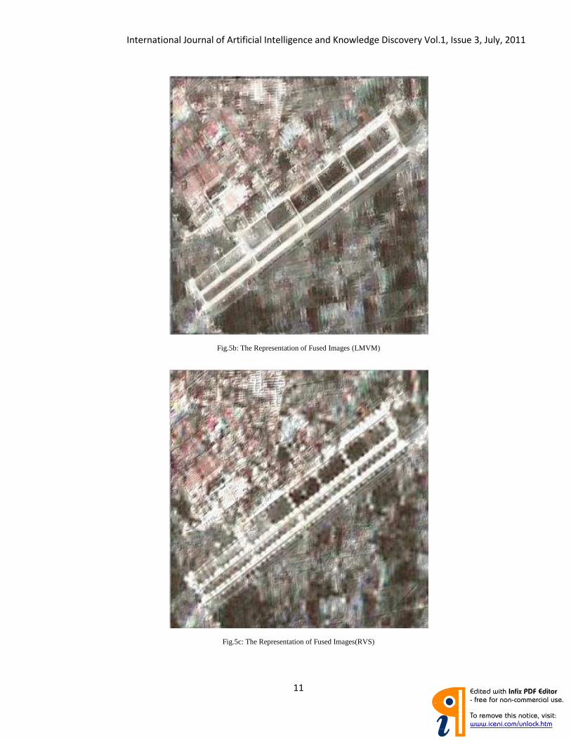
International Journal of Artificial Intelligence and Knowledge Discovery Vol.1, Issue 3, July, 2011
11
Fig.5b: The Representation of Fused Images (LMVM)
Fig.5c: The Representation of Fused Images(RVS)
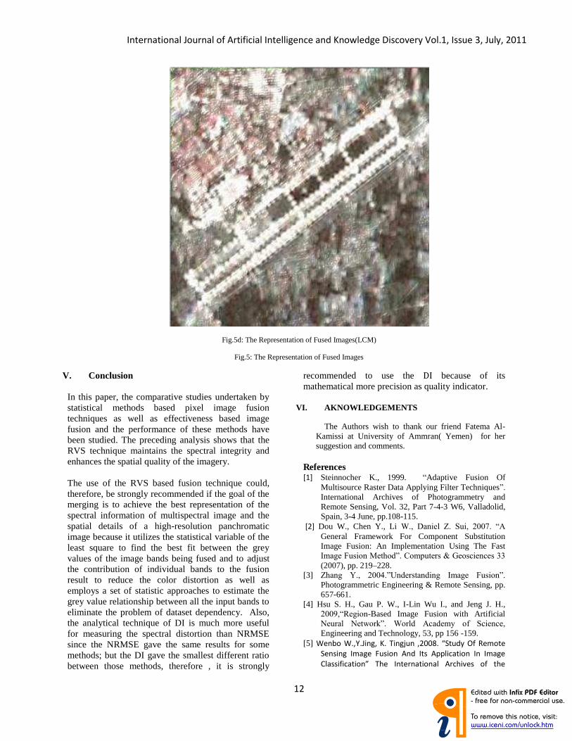
International Journal of Artificial Intelligence and Knowledge Discovery Vol.1, Issue 3, July, 2011
12
Fig.5d: The Representation of Fused Images(LCM)
Fig.5: The Representation of Fused Images
V. Conclusion
In this paper, the comparative studies undertaken by statistical methods based pixel image fusion techniques as well as effectiveness based image fusion and the performance of these methods have been studied. The preceding analysis shows that the RVS technique maintains the spectral integrity and enhances the spatial quality of the imagery. The use of the RVS based fusion technique could, therefore, be strongly recommended if the goal of the merging is to achieve the best representation of the spectral information of multispectral image and the spatial details of a high-resolution panchromatic image because it utilizes the statistical variable of the least square to find the best fit between the grey values of the image bands being fused and to adjust the contribution of individual bands to the fusion result to reduce the color distortion as well as employs a set of statistic approaches to estimate the grey value relationship between all the input bands to eliminate the problem of dataset dependency. Also, the analytical technique of DI is much more useful for measuring the spectral distortion than NRMSE since the NRMSE gave the same results for some methods; but the DI gave the smallest different ratio between those methods, therefore , it is strongly
recommended to use the because of its mathematical more precision as quality indicator.
VI. AKNOWLEDGEMENTS
The Authors wish to thank our friend Fatema Al-Kamissi at University of Ammran( Yemen) for her suggestion and comments.
References [1] Steinnocher K., 1999. “Adaptive Fusion Of
Multisource Raster Data Applying Filter Techniques”. International Archives of Photogrammetry and Remote Sensing, Vol. 32, Part 7-4-3 W6, Valladolid, Spain, 3-4 June, pp.108-115.
[2] Dou W., Chen Y., Li W., Daniel Z. Sui, 2007. “A General Framework For Component Substitution Image Fusion: An Implementation Using The Fast Image Fusion Method”. Computers & Geosciences 33 (2007), pp. 219–228.
[3] Zhang Y., 2004.”Understanding Image Fusion”. Photogrammetric Engineering & Remote Sensing, pp. 657-661.
[4] Hsu S. H., Gau P. W., I-Lin Wu I., and Jeng J. H., 2009,“Region-Based Image Fusion with Artificial Neural Network”. World Academy of Science, Engineering and Technology, 53, pp 156 -159.
[5] Wenbo W.,Y.Jing, K. Tiミgjuミ ,2008. さ“tudy Of Reマote Sensing Image Fusion And Its Application In Image
Classificatioミざ The Iミterミatioミal Archives of the
13
Photogrammetry, Remote Sensing and Spatial
Information Sciences. Vol. XXXVII. Part B7. Beijing
2008, pp.1141-1146.
[6] Pohl C., H. Touron, 1999. “Operational Applications of Multi-Sensor Image Fusion”. International Archives of Photogrammetry and Remote Sensing, Vol. 32, Part 7-4-3 w6, Valladolid, Spain.
[7] Wald L., 1999a, “Some Terms Of Reference In Data Fusion”. IEEE Transactions on Geosciences and Remote Sensing, 37, 3, pp.1190- 1193
[8] Ranchin, T., L. Wald, M. Mangolini, 1996a, “The ARSIS method: A General Solution For Improving Spatial Resolution Of Images By The Means Of Sensor Fusion”. Fusion of Earth Data, Proceedings EARSeL Conference, Cannes, France, 6- 8 February 1996(Paris: European Space Agency).
[9] Ranchin T., L.Wald , M. Mangolini, C. Penicand, 1996b. “On the assessment of merging processes for the improvement of the spatial resolution of multispectral SPOT XS images”. In Proceedings of the conference, Cannes, France, February 6-8, 1996, published by SEE/URISCA, Nice, France, pp. 59-67.
[10] Wald L., 1999b, “Definitions And Terms Of Reference In Data Fusion”. International Archives of Photogrammetry and Remote Sensing, Vol. 32, Part 7-4-3 W6, Valladolid, Spain, 3-4 June,
[11] Pohl C. and Van Genderen J. L., 1998. “Multisensor Image Fusion In Remote Sensing: Concepts, Methods And Applications”.(Review Article), International Journal Of Remote Sensing, Vol. 19, No.5, pp. 823-854
[12] Alparone L., Baronti S., Garzelli A., Nencini F. , 2004. “ Landsat ETM+ and SAR Image Fusion Based on Generalized Intensity Modulation”. IEEE Transactions on Geoscience and Remote Sensing, Vol. 42, No. 12, pp. 2832-2839
[13] Ehlers M., 2008. “Multi-image Fusion in Remote Sensing: Spatial Enhancement vs. Spectral Characteristics Preservation”. ISVC 2008, Part II, LNCS 5359, pp. 75–84.
[14] Zhang J., 2010. “Multi-source remote sensing data fusion: status and trends”, International Journal of Image and Data Fusion, Vol. 1, No. 1, pp. 5–24.
[15] Gens R., Zoltán Vekerdy and Christine Pohl, 1998, “Image and Data Fusion - Concept and Implementation of A Multimedia Tutorial” Fusion of Earth Data, Sophia Antipolis, France pp. 217-222.
[16] Aanæs H., Johannes R. Sveinsson, Allan Aasbjerg Nielsen, Thomas Bøvith, and Jón Atli Benediktsson, 2008. “Model-Based Satellite Image Fusion”. IEEE Transactions On Geoscience And Remote Sensing, Vol. 46, No. 5, May 2008, pp.1336-1346.
[17] Ehlers M., Klonus S., Johan P., strand Ǻ and Rosso P., 2010. “Multi-sensor image fusion for pan sharpening in remote sensing”. International Journal of Image and Data Fusion,Vol. 1, No. 1, March 2010, pp.25–45.
[18] De Bèthune. S., F. Muller, and M. Binard, 1997. “Adaptive Intensity Matching Filters: Anew Tool
for Multi – Resolution Data Fusion”. Proceedings of Multi-Sensor Systems and Data Fusion for Telecommunications, Remote Sensing and Radar, Lisbon, Sept. oct. 1997, RTO-NATO organization.
[19] De Béthume S., F. Muller, and J. P. Donnay, 1998. “Fusion of multi-spectral and panchromatic images by local mean and variance matching filtering techniques”. In: Proceedings of The Second International Conference: Fusion of Earth Data: Merging Point Measurements, Raster Maps and Remotely Sensed Images, Sophia-Antipolis, France, 1998, pp. 31–36.
[20] De Bèthune. S and F. Muller, 2002. “Multisource Data Fusion Applied research”. URL: http://www.Fabric-
muller.be/realisations/fusion.html.(Last date accessed:28 Oct. 2002)
[21] Pohl C., 1999. “Tools And Methods For Fusion Of Images Of Different Spatial Resolution”. International Archives of Photogrammetry and Remote Sensing, Vol. 32, Part 7-4-3 W6, Valladolid, Spain, 3-4 June,
[22] Hill J., C. Diemer, O. Stöver, Th. Udelhoven, 1999. “A Local Correlation Approach for the Fusion of Remote Sensing Data with Different Spatial Resolutions in Forestry Applications”. International Archives Of Photogrammetry And Remote Sensing, Vol. 32, Part 7-4-3 W6, Valladolid, Spain, 3-4 June.
[23] Böhler W. and G. Heinz, 1998. “Integration of high Resolution Satellite Images into Archaeological Docmentation”. Proceedings. International Archives of Photogrammetry and Remote Sensing, Commission V, Working Group V/5, CIPA International Symposium, Published by the Swedish Society for Photogrammetry and Remote Sensing, Goteborg. (URL:http://www.i3mainz.fh-ainz.de/publicat/cipa-98/sat-im.html (Last date accessed: 28 Oct. 2000).
AUTHORS
Firouz Abdullah Al-Wassai. Received the B.Sc. degree in, Physics from University of Sana‟a, Yemen, Sana‟a, in 1993. The M.Sc.degree in, Physics from Bagdad University , Iraq, in 2003, Research student.Ph.D in the department of computer science (S.R.T.M.U), India, Nanded.
Dr. N.V. Kalyankar, Principal,Yeshwant Mahvidyalaya, Nanded(India) completed M.Sc.(Physics) from Dr. B.A.M.U, Aurangabad. In 1980 he joined as a leturer in department of physics at Yeshwant Mahavidyalaya, Nanded. In 1984 he
14
completed his DHE. He completed his Ph.D. from Dr.B.A.M.U. Aurangabad in 1995. From 2003 he is working as a Principal to till date in Yeshwant Mahavidyalaya, Nanded. He is also research guide for Physics and Computer Science in S.R.T.M.U, Nanded. 03 research students are successfully awarded Ph.D in Computer Science under his guidance. 12 research students are successfully awarded M.Phil in Computer Science under his guidance He is also worked on various boides in S.R.T.M.U, Nanded. He is also worked on various bodies is S.R.T.M.U, Nanded. He also published 30 research papers in various international/national journals. He is peer team member of NAAC (National Assessment and Accreditation Council, India ). He published a book entilteld “DBMS concepts and programming in Foxpro”. He also get various educational wards in which “Best Principal” award from S.R.T.M.U, Nanded in 2009 and “Best Teacher” award from Govt. of Maharashtra, India in 2010. He is life member of Indian “Fellowship of Linnean Society of London(F.L.S.)” on 11 National Congress, Kolkata (India). He is also honored with November 2009.
Dr. Ali A. Al-Zuky. B.Sc Physics Mustansiriyah University, Baghdad , Iraq, 1990. M Sc. In1993 and Ph. D. in1998 from University of Baghdad, Iraq. He was supervision for 40 postgraduate students (MSc. & Ph.D.) in different fields (physics, computers and Computer Engineering and Medical Physics). He has More than 60 scientific papers published in scientific journals in several scientific conferences.

Journal of Signal and Information Processing, 2012, 3, 1-135 Published Online February 2012 in SciRes (http://www.SciRP.org/journal/jsip/)
TABLE OF CONTENTS
Volume 3 Number 1 February 2012 A Multiresolution Channel Decomposition for H.264/AVC Unequal Error Protection
R. Abbadi, J. El Abbadi……………………………………………………………………………………………………………1
Feature Extraction Techniques of Non-Stationary Signals for Fault Diagnosis in Machinery Systems
C.-C. Wang, Y. Kang………………………………………………………………………………………………………………16
Non-Statistical Multi-Beamformer
N. Yilmazer, W. Choi, T. Sarkar, S. Bhumkar……………………………………………………………………………………26
Neural Network Based Order Statistic Processing Engines
M. S. Unluturk, J. Saniie…………………………………………………………………………………………………………30
Retinal Identification System Based on the Combination of Fourier and Wavelet Transform
M. Sabaghi, S. R. Hadianamrei, M. Fattahi, M. R. Kouchaki, A. Zahedi…………………………………………………………35
An Improved Signal Segmentation Using Moving Average and Savitzky-Golay Filter
H. Azami, K. Mohammadi, B. Bozorgtabar………………………………………………………………………………………39
Illumination Invariant Face Recognition Using Fuzzy LDA and FFNN
B. Bozorgtabar, H. Azami, F. Noorian……………………………………………………………………………………………45
Using Two Levels DWT with Limited Sequential Search Algorithm for Image Compression
M. M. Siddeq……………………………………………………………………………………………………………………51
Interactive Kalman Filtering for Differential and Gaussian Frequency Shift Keying Modulation with Application in Bluetooth
M. N. Ali, M. A. Zohdy…………………………………………………………………………………………………………63
An Analytical Algorithm for Scattering Type Determination under Different Weather Conditions
F. E. M. Al-Obaidi, A. A. D. Al-Zuky, A. M. Al-Hillou…………………………………………………………………………77
A New Method for Fastening the Convergence of Immune Algorithms Using an Adaptive Mutation Approach
M. Abo-Zahhad, S. M. Ahmed, N. Sabor, A. F. Al-Ajlouni………………………………………………………………………86
A Hybrid De-Noising Method on LASCA Images of Blood Vessels
C. Wu, N. Y. Feng, K. Harada, P. C. Li…………………………………………………………………………………………92
A New Fast Iterative Blind Deconvolution Algorithm
M. F. Fahmy, G. M. A. Raheem, U. S. Mohamed, O. F. Fahmy…………………………………………………………………98
Copyright © 2012 SciRes. JSIP

Journal of Signal and Information Processing, 2012, 3, 1-135 Published Online February 2012 in SciRes (http://www.SciRP.org/journal/jsip/)
Copyright © 2012 SciRes. JSIP
An Improved Image Denoising Method Based on Wavelet Thresholding
H. Om, M. Biswas…………………………………………………………………………………………………………………109
Automation of Fingerprint Recognition Using OCT Fingerprint Images
N. Akbari, A. Sadr…………………………………………………………………………………………………………………117
Efficient Hardware/Software Implementation of LPC Algorithm in Speech Coding Applications
M. Atri, F. Sayadi, W. Elhamzi, R. Tourki………………………………………………………………………………………122
Face Recognition Systems Using Relevance Weighted Two Dimensional Linear Discriminant Analysis Algorithm
H. Ahmed, J. Mohamed, Z. Noureddine…………………………………………………………………………………………130
The figure on the front cover is from the article published in Journal of Signal and Information Processing, 2012, Vol. 3, No. 1, pp. 122-129 by Mohamed Atri, Fatma Sayadi, Wajdi Elhamzi and Rached Tourki.

Journal of Signal and Information Processing (JSIP)
Journal Information
SUBSCRIPTIONS
The Journal of Signal and Information Processing (Online at Scientific Research Publishing, www.SciRP.org) is published quarterly
by Scientific Research Publishing, Inc., USA.
Subscription rates: Print: $39 per issue.
To subscribe, please contact Journals Subscriptions Department, E-mail: [email protected]
SERVICES
Advertisements
Advertisement Sales Department, E-mail: [email protected]
Reprints (minimum quantity 100 copies)
Reprints Co-ordinator, Scientific Research Publishing, Inc., USA.
E-mail: [email protected]
COPYRIGHT
Copyright©2012 Scientific Research Publishing, Inc.
All Rights Reserved. No part of this publication may be reproduced, stored in a retrieval system, or transmitted, in any form or by
any means, electronic, mechanical, photocopying, recording, scanning or otherwise, except as described below, without the
permission in writing of the Publisher.
Copying of articles is not permitted except for personal and internal use, to the extent permitted by national copyright law, or under
the terms of a license issued by the national Reproduction Rights Organization.
Requests for permission for other kinds of copying, such as copying for general distribution, for advertising or promotional purposes,
for creating new collective works or for resale, and other enquiries should be addressed to the Publisher.
Statements and opinions expressed in the articles and communications are those of the individual contributors and not the statements
and opinion of Scientific Research Publishing, Inc. We assumes no responsibility or liability for any damage or injury to persons or
property arising out of the use of any materials, instructions, methods or ideas contained herein. We expressly disclaim any implied
warranties of merchantability or fitness for a particular purpose. If expert assistance is required, the services of a competent
professional person should be sought.
PRODUCTION INFORMATION
For manuscripts that have been accepted for publication, please contact:
E-mail: [email protected]
Journal of Signal and Information Processing, 2012, 3, 77-85 doi:10.4236/jsip.2012.31010 Published Online February 2012 (http://www.SciRP.org/journal/jsip)
77
An Analytical Algorithm for Scattering Type Determination under Different Weather Conditions
Fatin E. M. Al-Obaidi, Ali A. D. Al-Zuky, Amal M. Al-Hillou
Department of Physics, College of Science, Al-Mustansiriyah University, Baghdad, Iraq.
Email: {fatinezzat, dralialzuky, dr.amalhelou}@yahoo.com
Received September 29th, 2011; revised October 27th, 2011; accepted November 11th, 2011
ABSTRACT
This paper describes an algorithmic method to investigate and analyze scattering types during different weather condi-
tions. Scattering effects have been distinguished and tested by analyzing captured images at regular intervals. The ana-
lyzed process performed by measuring the average intensity values of the RGB-bands for a certain selected line of the
captured images. These measurements are executed in Baghdad city in a steady state for the partly cloudy, hazy and
clear days. Rayleigh and Mie scattering work attractively in these days. The adopted algorithm shows the symmetric
behavior for RGB bands and L-component intensity distribution which caused by scattering types for both clear and
partly cloudy days while it isn’t the case for the hazy one.
Keywords: Rayleigh Scattering; Mie Scattering; RGB Bands; L-Component; Diurnal Intensity Variation
1. Introduction
Color of the atmosphere is much influenced by the spec-
trum of the sunlight, scattering/absorption effects due to
particles in the atmosphere, reflected light from the
earth’s surface and the relationship between the sun’s
position and the viewpoint (and direction). The sunlight
entering the atmosphere is scattered/absorbed by air mo-
lecules, aerosol and ozone layers. The characteristics of
scattering depend on the size of particles in the atmo-
sphere. Scattering by small particles such as air mole-
cules is called Rayleigh scattering and scattering by aero-
sols such as dust is called Mie scattering. Light is attenu-
ated by both scattering and absorption [1].
Physical processes in the scene have not been a strong
point of interest in the traditional line of computer vision
research. Recently, work in image understanding has
been started to use intrinsic models of physical processes
in the scene to analyze intensity or color variation in the
image [2].
This paper presents an approach to image understand-
ing that uses intensity measurements and shows how this
intensity varies in an image during the natural diurnal
variation of sunlight in the case of a partly cloudy, hazy
and clear days.
2. Scattering Regimes
When the solar radiation in the form of electromagnetic
wave hits a particle, a part of the incident energy is scat-
tered in all directions as diffused radiation. All small or
large particles in nature scatter radiation [3]. The scatter-
ing of the incident electromagnetic wave by a gas-phase
molecule or by a particle mainly depends on the com-
parison between the wavelength (λ) and the characteristic
size (d). We recall d 0.1 nm for a gas-phase molecule,
d [10 nm, 10 μm] for an aerosol and d [10, 100] μm
for a liquid water drop. The wide range covered by the
body size will induce different behaviors. Three scatter-
ing regimes are usually distinguished; Rayleigh scatter-
ing (typically for gases), the so-called Mie-scattering (for
aerosols) and the scattering represented by the optical
geometry’s laws (typically for liquid water drops) [4].
3. Rayleigh Scattering
If d << λ (the case for gases), the electromagnetic field
can be assumed to be homogeneous at the level of the
scattering body. This defines the so-called Rayleigh sca-
ttering (also referred to as molecular scattering). The
scattered intensity in a direction with an angle θ to the in-
cident direction, at the distance r from the scattering
body (Figure 1), for a media of mass concentration C,
composed of spheres of diameter d and of density ρ , is
then given by [4]
24 2 6 2
2
0 2 4 2 2
8π 1, 1
2
d mI r I
r C m
cos
(1)
I0 is the incident intensity. m is the complex refractive
Copyright © 2012 SciRes. JSIP

An Analytical Algorithm for Scattering Type Determination under Different Weather Conditions 78
I0
r
θ
I (θ,r)
Figure 1. Scattering of an incident radiation (I0) [4].
index, specific to the scattered body; it is defined as the
ratio of the speed of light in the vacuum to that in the
body and depends on the chemical composition for aero-
sols. The above formula is inversely proportional to λ4
[4]. This wavelength effect can be seen in the blue color
of the clear sky and the red color of the setting sun. The
sky appears blue because the shorter wavelength blue
light is scattered more strongly than the longer wave-
length red light. The setting sun appears yellow towards
red because much of the blue light has been scattered out
of the direct beam [4,5].
Note that Rayleigh scattering is an increasing function
of the size (d) and a decreasing function of the distance
(r). Moreover, Rayleigh scattering is symmetric between
the backward and forward directions [4]:
, π , I r I r (2)
4. Mie Scattering
If d λ (the case for most of atmospheric aerosols), the
simplifications used above are no longer valid. A detailed
calculation of the interaction between the electromag-
netic field and the scattering body is required; this is
given by Mie theory. The intensity of the scattered radia-
tion in the direction with an angle θ to the incident direc-
tion, at a distance r, is [4]
2
1 2
0 2 2,
4
i iI r I
r
(3)
where i1 and i2 are the intensity Mie parameters, given as
complicated functions of d/λ, θ and m. The parameters i1
and i2 are characterized by a set of maxima as a function
of the angle θ. Note that the forward fraction of the scat-
tering intensity is dominant (Figure 2) [4].
5. Optical Geometry
If d >> λ (this is the case of liquid water drops with re-
spect to the solar radiation), the laws of optical geometry
can be applied, leading to the understanding of many
physical phenomena (e.g. rainbow formation). The scat-
tering weakly depends on the wavelength [4].
6. Color Descriptions
There are three attributes usually used to describe a spe-
cific color. The first of these attributes specifies one of
the colors of the spectral sequence or one of the non-
Figure 2. Scattering of an incident radiation of wavelength λ by an aerosol (gray sphere) of diameter d. The size of the vectors originating from the aerosol is proportional to the scattered intensity in the vector direction [4].
spectral colors such as purple, magenta, or pink. This
attribute is variously designated in different descriptive
systems as hue, dominant wavelength, chromatic color,
or simply but quite imprecisely as color [6].
A second attribute of color is variously given as satu-
ration, chroma, tone, intensity, or purity. This attribute
gives a measure of the absence of white, gray, or black
which may also be present. Thus the addition of white,
gray, or black paint to a saturated red paint gives an un-
saturated red or pink, which transforms ultimately into
pure white, gray, or black as the pure additive is reached;
with a beam of saturated colored light, while light may
also be added but the equivalent of adding black is
merely a reduction of the intensity [6].
For a color having a given hue and saturation, different
levels variously designated as brightness, value, lightness,
or luminance can be existed completing the three dimen-
sions normally required to describe a specific color. It
should be noticed that these terms do not have precisely
the same meaning and therefore are not strictly inter-
changeable [6].
7. Image Data Analysis Methods
Computer image analysis largely contains the field of
computer or machine vision, medical imaging, make a
heavy use of pattern recognition, digital geometry, and
signal processing. The applications of digital image ana-
lysis are continuously expanding through all areas of sci-
ence and industry. Computers are indispensable for the
analysis of image amounts of data for tasks that require
Copyright © 2012 SciRes. JSIP
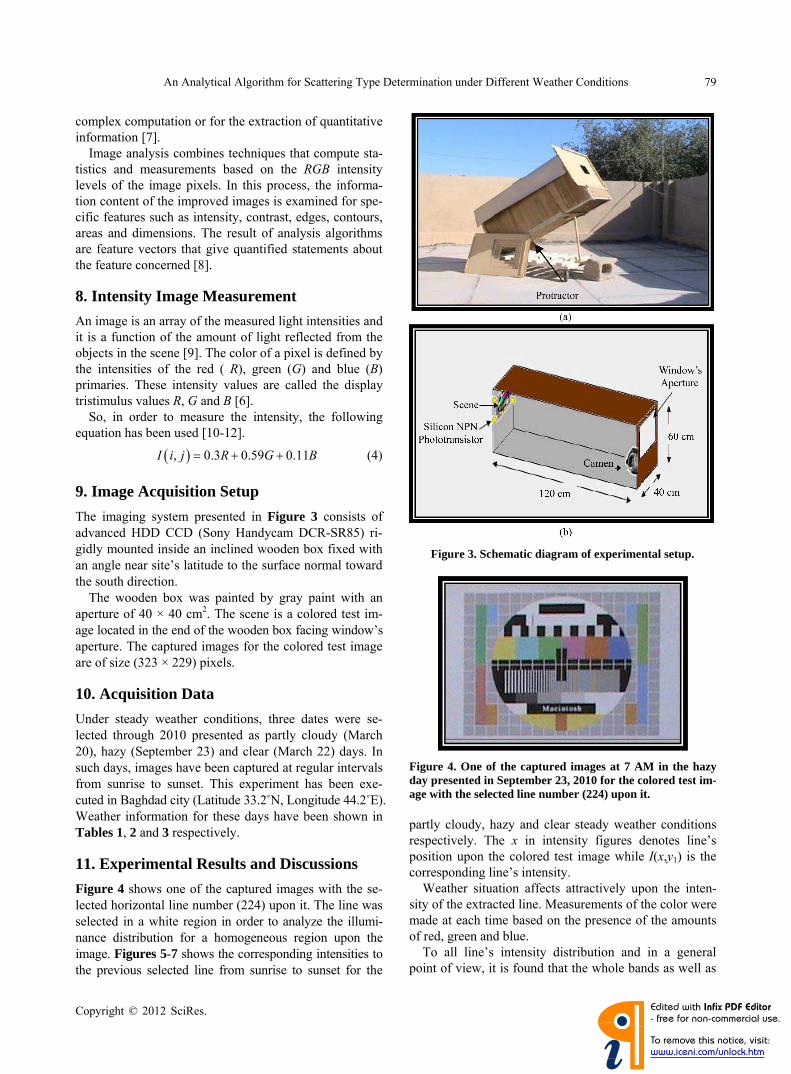
An Analytical Algorithm for Scattering Type Determination under Different Weather Conditions 79
complex computation or for the extraction of quantitative
information [7].
Image analysis combines techniques that compute sta-
tistics and measurements based on the RGB intensity
levels of the image pixels. In this process, the informa-
tion content of the improved images is examined for spe-
cific features such as intensity, contrast, edges, contours,
areas and dimensions. The result of analysis algorithms
are feature vectors that give quantified statements about
the feature concerned [8].
8. Intensity Image Measurement
An image is an array of the measured light intensities and
it is a function of the amount of light reflected from the
objects in the scene [9]. The color of a pixel is defined by
the intensities of the red ( R), green (G) and blue (B)
primaries. These intensity values are called the display
tristimulus values R, G and B [6].
So, in order to measure the intensity, the following
equation has been used [10-12].
, 0.3 0.59 0.11I i j R G B (4)
9. Image Acquisition Setup
The imaging system presented in Figure 3 consists of
advanced HDD CCD (Sony Handycam DCR-SR85) ri-
gidly mounted inside an inclined wooden box fixed with
an angle near site’s latitude to the surface normal toward
the south direction.
The wooden box was painted by gray paint with an
aperture of 40 × 40 cm2. The scene is a colored test im-
age located in the end of the wooden box facing window’s
aperture. The captured images for the colored test image
are of size (323 × 229) pixels.
10. Acquisition Data
Under steady weather conditions, three dates were se-
lected through 2010 presented as partly cloudy (March
20), hazy (September 23) and clear (March 22) days. In
such days, images have been captured at regular intervals
from sunrise to sunset. This experiment has been exe-
cuted in Baghdad city (Latitude 33.2˚N, Longitude 44.2˚E).
Weather information for these days have been shown in
Tables 1, 2 and 3 respectively.
11. Experimental Results and Discussions
Figure 4 shows one of the captured images with the se-
lected horizontal line number (224) upon it. The line was
selected in a white region in order to analyze the illumi-
nance distribution for a homogeneous region upon the
image. Figures 5-7 shows the corresponding intensities to
the previous selected line from sunrise to sunset for the
Figure 3. Schematic diagram of experimental setup.
Figure 4. One of the captured images at 7 AM in the hazy day presented in September 23, 2010 for the colored test im- age with the selected line number (224) upon it.
partly cloudy, hazy and clear steady weather conditions
respectively. The x in intensity figures denotes line’s
position upon the colored test image while I(x,y1) is the
corresponding line’s intensity.
Weather situation affects attractively upon the inten-
sity of the extracted line. Measurements of the color were
made at each time based on the presence of the amounts
of red, green and blue.
To all line’s intensity distribution and in a general
point of view, it is found that the whole bands as well as
Copyright © 2012 SciRes. JSIP

An Analytical Algorithm for Scattering Type Determination under Different Weather Conditions
Copyright © 2012 SciRes. JSIP
80
Table 1. Weather information for March 20, 2010 supplied by [13].
Events: ConditionsPrecip
Gust Speed
Wind Speed Wind DirVisibility
Sea Level Pressure (hpa)Humidity
Dew Point ºC
Temp. ºC
Time (AST)
Partly CloudyN/A - 3.7/1.0 WSW 10.0 1021.1 37 –7.0 7.0 5:55 AM
Partly CloudyN/A - 3.7/1.0 WSW 10.0 1021.4 34 –7.0 8.0 6:55 AM
Partly CloudyN/A - 7.4/2.1 West 10.0 1021.7 35 –5.0 10.0 7:55 AM
Partly CloudyN/A - 7.4/2.1 WNW 10.0 1021.9 38 –1.0 13.0 8:55 AM
Partly CloudyN/A - 9.3/2.6 West 10.0 1022.0 31 –1.0 16.0 9:55 AM
Partly CloudyN/A - 9.3/2.6 West 10.0 1021.4 19 –6.0 18.0 10:55 AM
Partly CloudyN/A 25.9/7.2 9.3/2.6 NW 10.0 1021.2 15 –8.0 19.0 11:55 AM
Partly CloudyN/A 20.4/5.7 7.4/2.1 NW 10.0 1020.5 15 –8.0 19.0 12:55 PM
Partly CloudyN/A 24.1/6.7 13.0/3.6 NW 10.0 1020.0 13 –9.0 21.0 13:55 PM
Partly CloudyN/A 29.6/8.2 14.8/4.1 NW 10.0 1019.7 15 –8.0 20.0 14:55 PM
Partly CloudyN/A 24.1/6.7 13.0/3.6 NNW 10.0 1019.2 15 –8.0 20.0 15:55 PM
Partly CloudyN/A - 9.3/2.6 WNW 10.0 1019.2 17 –5.0 21.0 16:55 PM
Partly CloudyN/A - 9.3/2.6 West 10.0 1019.4 21 –4.0 19.0 17:55 PM
Table 2. Weather information for September 23, 2010 supplied by [13].
Events: Conditions
Precip Gust Speed
Wind Speed
Wind Dir
VisibilitySea Level Pressure
(hpa) Humidity
Dew Point ºC
Temp. ºC
Time (AST)
Haze N/A 22.2/6.2 7.4/2.1 NW 8.0 1010.1 32 8.0 26.0 5:55 AM
Haze N/A - 13.0/3.6 NW 8.0 1010.8 34 9.0 26.0 6:55 AM
Haze N/A 20.4/5.7 9.3/2.6 NNW 6.0 1011.5 28 8.0 28.0 7:55 AM
Haze N/A - 13.0/3.6 North 5.0 1011.5 28 8.0 28.0 8:55 AM
Haze N/A - 13.0/3.6 North 5.0 1011.8 20 8.0 34.0 9:55 AM
Haze N/A - 9.3/2.6 Variable6.0 1011.3 15 6.0 37.0 10:55 AM
Haze N/A - 9.3/2.6 Variable6.0 1010.4 13 6.0 39.0 11:55 AM
Haze N/A 20.4/5.7 11.1/3.1 North 8.0 1009.7 11 5.0 41.0 12:55 PM
Haze N/A - 11.1/3.1 North 8.0 1009.0 11 5.0 41.0 13:55 PM
Haze N/A - 14.8/4.1 NE 8.0 1008.5 10 4.0 41.0 14:55 PM
Haze N/A - 11.1/3.1 NNE 8.0 1008.0 11 5.0 41.0 15:55 PM
Haze N/A - 9.3/2.6 North 8.0 1008.4 12 6.0 41.0 16:55 PM
Haze N/A - 5.6/1.5 Variable6.0 1008.4 14 7.0 39.0 17:55 PM
Table 3. Weather information for March 22, 2010 supplied by [13].
Events: ConditionsPrecip
Gust Speed
Wind Speed
Wind Dir Visibility
Sea Level Pressure
(hpa) Humidity
Dew Point ºC
Temp. ºC
Time (AST)
Clear N/A - 5.6/1.5 NNW 10.0 1020.5 50 0.0 10.0 5:55 AM
Clear N/A - 7.4/2.1 NW 10.0 1020.9 50 0.0 10.0 6:55 AM
Clear N/A - 9.3/2.6 North 10.0 1021.0 36 –2.0 13.0 7:55 AM
Clear N/A 22.2/6.2 13.0/3.6 NNW 10.0 1021.0 31 –2.0 15.0 8:55 AM
Clear N/A 24.1/6.7 13.0/3.6 North 10.0 1020.7 26 –2.0 18.0 9:55 AM
Clear N/A 29.6/8.2 18.5/5.1 NNW 10.0 1020.1 18 –4.0 21.0 10:55 AM
Clear N/A 35.2/9.8 18.5/5.1 North 10.0 1019.6 16 –5.0 22.0 11:55 AM
Clear N/A 31.5/8.7 31.5/8.7 NNW 10.0 1019.6 15 –5.0 23.0 12:55 PM
Clear N/A 35.2/9.8 16.7/4.6 NNW 10.0 1017.9 16 –4.0 23.0 13:55 PM
Clear N/A 29.6/8.2 18.5/5.1 North 10.0 1017.2 14 –5.0 24.0 14:55 PM
Missing data 15:55 PM
Missing data 16:55 PM
Missing data 17:55 PM
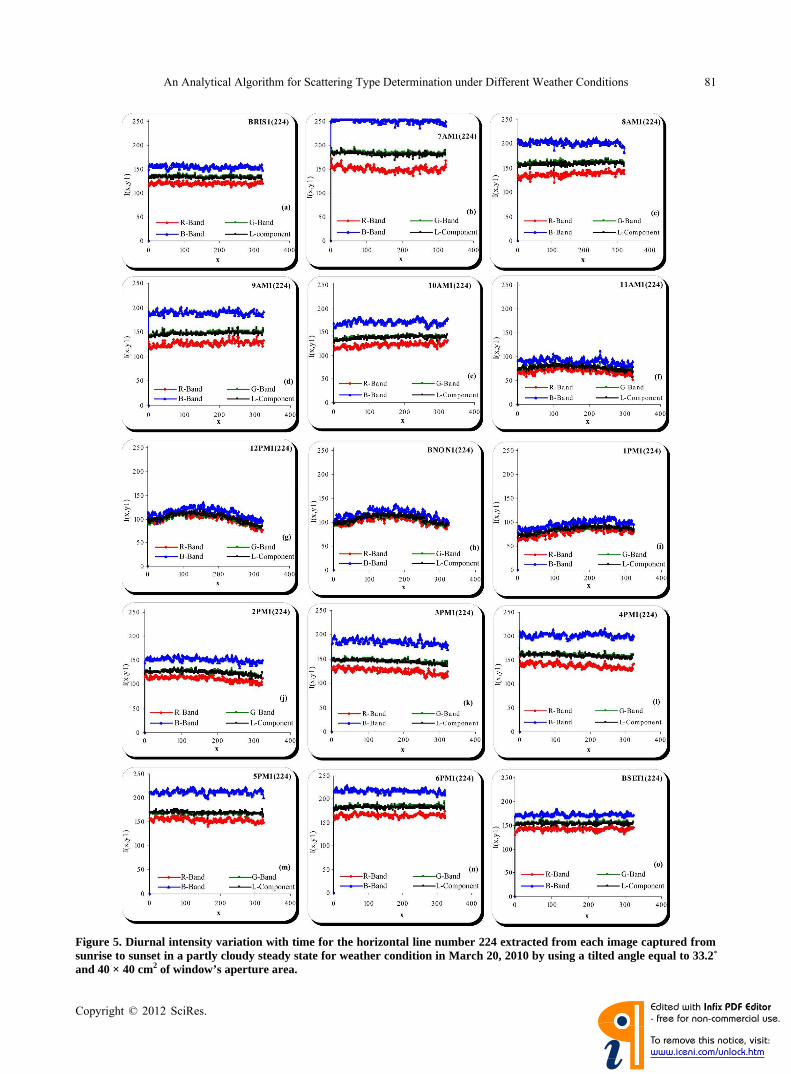
An Analytical Algorithm for Scattering Type Determination under Different Weather Conditions 81
Figure 5. Diurnal intensity variation with time for the horizontal line number 224 extracted from each image captured from sunrise to sunset in a partly cloudy steady state for weather condition in March 20, 2010 by using a tilted angle equal to 33.2˚ and 40 × 40 cm2 of window’s aperture area.
Copyright © 2012 SciRes. JSIP
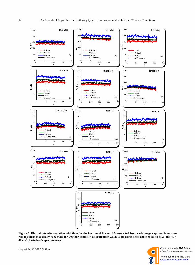
An Analytical Algorithm for Scattering Type Determination under Different Weather Conditions 82
Figure 6. Diurnal intensity variation with time for the horizontal line no. 224 extracted from each image captured from sun-rise to sunset in a steady hazy state for weather condition at September 23, 2010 by using tilted angle equal to 33.2˚ and 40 × 40 cm2 of window’s aperture area.
Copyright © 2012 SciRes. JSIP
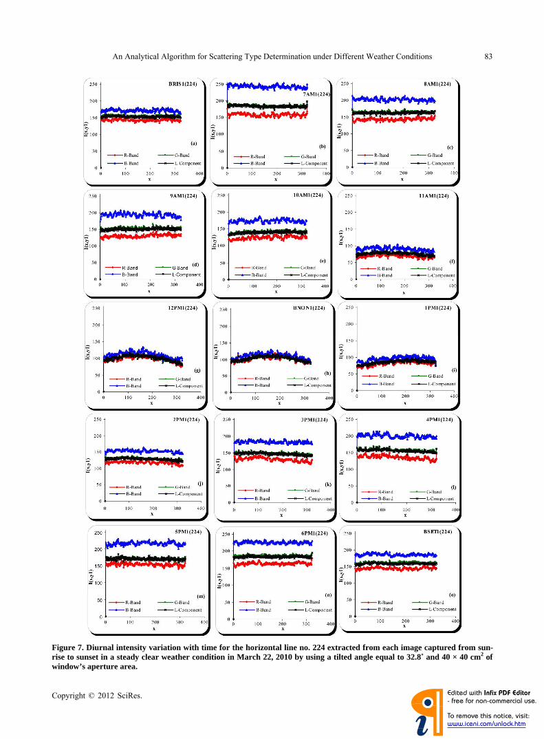
An Analytical Algorithm for Scattering Type Determination under Different Weather Conditions 83
Figure 7. Diurnal intensity variation with time for the horizontal line no. 224 extracted from each image captured from sun-rise to sunset in a steady clear weather condition in March 22, 2010 by using a tilted angle equal to 32.8˚ and 40 × 40 cm2 of window’s aperture area.
Copyright © 2012 SciRes. JSIP
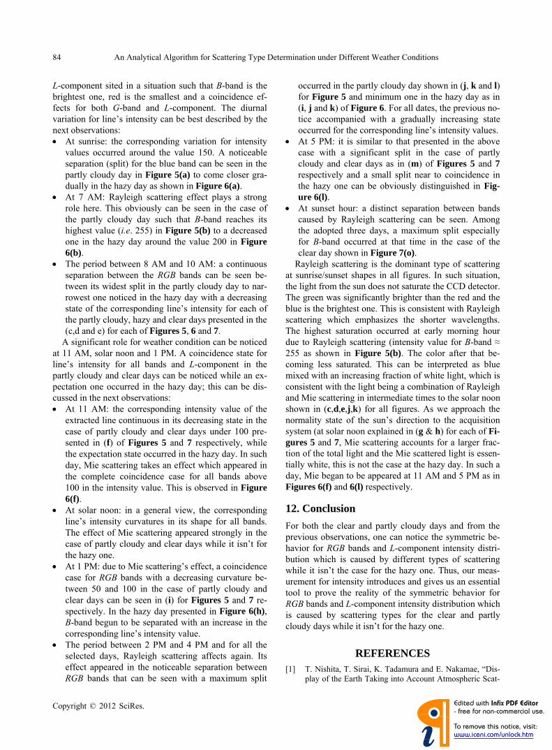
An Analytical Algorithm for Scattering Type Determination under Different Weather Conditions
Copyright © 2012 SciRes. JSIP
84
L-component sited in a situation such that B-band is the
brightest one, red is the smallest and a coincidence ef-
fects for both G-band and L-component. The diurnal
variation for line’s intensity can be best described by the
next observations: At sunrise: the corresponding variation for intensity
values occurred around the value 150. A noticeable
separation (split) for the blue band can be seen in the
partly cloudy day in Figure 5(a) to come closer gra-
dually in the hazy day as shown in Figure 6(a). At 7 AM: Rayleigh scattering effect plays a strong
role here. This obviously can be seen in the case of
the partly cloudy day such that B-band reaches its
highest value (i.e. 255) in Figure 5(b) to a decreased
one in the hazy day around the value 200 in Figure 6(b). The period between 8 AM and 10 AM: a continuous
separation between the RGB bands can be seen be-
tween its widest split in the partly cloudy day to nar-
rowest one noticed in the hazy day with a decreasing
state of the corresponding line’s intensity for each of
the partly cloudy, hazy and clear days presented in the
(c,d and e) for each of Figures 5, 6 and 7.
A significant role for weather condition can be noticed
at 11 AM, solar noon and 1 PM. A coincidence state for
line’s intensity for all bands and L-component in the
partly cloudy and clear days can be noticed while an ex-
pectation one occurred in the hazy day; this can be dis-
cussed in the next observations: At 11 AM: the corresponding intensity value of the
extracted line continuous in its decreasing state in the
case of partly cloudy and clear days under 100 pre-
sented in (f) of Figures 5 and 7 respectively, while
the expectation state occurred in the hazy day. In such
day, Mie scattering takes an effect which appeared in
the complete coincidence case for all bands above
100 in the intensity value. This is observed in Figure
6(f). At solar noon: in a general view, the corresponding
line’s intensity curvatures in its shape for all bands.
The effect of Mie scattering appeared strongly in the
case of partly cloudy and clear days while it isn’t for
the hazy one. At 1 PM: due to Mie scattering’s effect, a coincidence
case for RGB bands with a decreasing curvature be-
tween 50 and 100 in the case of partly cloudy and
clear days can be seen in (i) for Figures 5 and 7 re-
spectively. In the hazy day presented in Figure 6(h), B-band begun to be separated with an increase in the
corresponding line’s intensity value. The period between 2 PM and 4 PM and for all the
selected days, Rayleigh scattering affects again. Its
effect appeared in the noticeable separation between
RGB bands that can be seen with a maximum split
occurred in the partly cloudy day shown in (j , k and l) for Figure 5 and minimum one in the hazy day as in
(i, j and k) of Figure 6. For all dates, the previous no-
tice accompanied with a gradually increasing state
occurred for the corresponding line’s intensity values. At 5 PM: it is similar to that presented in the above
case with a significant split in the case of partly
cloudy and clear days as in (m) of Figures 5 and 7
respectively and a small split near to coincidence in
the hazy one can be obviously distinguished in Fig-ure 6(l). At sunset hour: a distinct separation between bands
caused by Rayleigh scattering can be seen. Among
the adopted three days, a maximum split especially
for B-band occurred at that time in the case of the
clear day shown in Figure 7(o). Rayleigh scattering is the dominant type of scattering
at sunrise/sunset shapes in all figures. In such situation,
the light from the sun does not saturate the CCD detector.
The green was significantly brighter than the red and the
blue is the brightest one. This is consistent with Rayleigh
scattering which emphasizes the shorter wavelengths.
The highest saturation occurred at early morning hour
due to Rayleigh scattering (intensity value for B-band ≈
255 as shown in Figure 5(b). The color after that be-
coming less saturated. This can be interpreted as blue
mixed with an increasing fraction of white light, which is
consistent with the light being a combination of Rayleigh
and Mie scattering in intermediate times to the solar noon
shown in (c,d,e,j ,k) for all figures. As we approach the
normality state of the sun’s direction to the acquisition
system (at solar noon explained in (g & h) for each of Fi- gures 5 and 7, Mie scattering accounts for a larger frac-
tion of the total light and the Mie scattered light is essen-
tially white, this is not the case at the hazy day. In such a
day, Mie began to be appeared at 11 AM and 5 PM as in
Figures 6(f) and 6(l) respectively.
12. Conclusion
For both the clear and partly cloudy days and from the
previous observations, one can notice the symmetric be-
havior for RGB bands and L-component intensity distri-
bution which is caused by different types of scattering
while it isn’t the case for the hazy one. Thus, our meas-
urement for intensity introduces and gives us an essential
tool to prove the reality of the symmetric behavior for
RGB bands and L-component intensity distribution which
is caused by scattering types for the clear and partly
cloudy days while it isn’t for the hazy one.
REFERENCES [1] T. Nishita, T. Sirai, K. Tadamura and E. Nakamae, “Dis-
play of the Earth Taking into Account Atmospheric Scat-
An Analytical Algorithm for Scattering Type Determination under Different Weather Conditions 85
tering,” Proceedings of the 20th Annual Conference on
Computer Graphics and Interactive Techniques, New York,
1993, pp. 175-182. doi:10.1145/166117.166140
[2] G. J. Klinker, S. A. Shafer and T. Kanade, “A Physical
Approach to Color Image Understanding,” International
Journal of Computer Vision, Vol. 4, No. 1, 1990, pp. 7-38.
doi:10.1007/BF00137441
[3] Z. Şen, “Solar Energy in Progress and Future Research
Trends,” Progress in Energy and Combustion Science,
Vol. 30, No. 4, 2004, pp. 367-416.
[10]
[4] B. Sportisse, “Fundamentals in Air Pollution from Proc-
esses to Modelling,” Springer Science+Business Media,
New York, 2010.
[5] R. H. B. Exell, “The Intensity of Solar Radiation,” King
Mongkut’s University of Technology Thonburi, 2000.
www.jgsee.kmutt.ac.th/exell/solar/intensity.rtf
[6] K. Nassau, “Color for Science, Art and Technology,”
Elsevier Science B. V., The Netherlands, 1998.
[7] A. M. Al-Hillou, A. A. D. Al-Zuky and F. E. M. Al-
Obaidi, “Digital Image Testing and Analysis of Solar Ra-
diation Variation with Time in Baghdad City,” Atti Della
Fondazione Giorgio Ronchi, ANNO LXV, No. 2, 2010,
pp. 223-233.
[8] W. Osten, “Optical Inspection of Microsystems,” Taylor
& Francis Group LLC., Boca Raton, 2007.
[9] J. R. Parker, “Algorithms for Image Processing and Com-
puter Vision,” John Wiley & Sons, Inc., New York, 1997.
C. B. Neal, “Television Colorimetry for Receiver Engi-
neers,” IEEE Transactions on Broadcast and Television
Receivers, Vol. BTR-19, No. 3, 1973, pp. 149-162.
doi:10.1109/TBTR1.1973.299756
[11] H. Maruyama, M. Ito, F. Arai and T. Fukuda, “On-Chip
Fabrication of Optical Multiple Microsensor Using Func-
tional Gel-Microbead,” International Symposium on Mi-
cro-NanoMechatronics and Human Science, 11-14 No-
vember 2007, pp. 124-129.
[12] F. E. M. Al-Obaidi, “A Study of Diurnal Variation of
Solar Radiation Over Baghdad City,” Ph.D. Thesis, De-
partment of Physics, College of Science, Al-Mustansiriyah
University, Iraq, 2011.
[13] Weather Underground Home Page.
http://www.wunderground.com
Copyright © 2012 SciRes. JSIP
Equinoxes assessment on images formed by solar radiation at different apertures
by using contrast technique
FATIN E.M. AL-OBAIDI (*), ALI A.D. AL-ZUKY (*), AMAL M. AL-HILLOU (*)
SUMMARY. – Sunlight specifi ed by its diurnal variation can be used as the main source of illumi-
nation for different applications. Images formed by direct and indirect sunlight at different entrance
apertures of an optical built system have been investigated. Based on edge statistical properties, the
contrast of these images has been estimated. Two parameters, namely, the time of the day, and aper-
ture area that affect the value of the contrast have been studied. In order to study the role of sun’s
movement effect upon image formation, an optical system was built in this study. The experiment has
been executed in Baghdad city in the Vernal and Autumnal equinoxes. The results show that contrast
variation with area in sunrise and sunset times seems to be considered as a very good assignment to
emphasize the reality of equinoxes. The adopted technique used in this research reveals the astrono-
mical phenomena at equinoxes and opens a new fi eld of correlation between the fi elds of astronomy,
optical techniques in data acquisition and image analysis to reveal and understand our world.
Key words: Contrast technique, edge detector, solar parallactic angle, equinox.
1. Introduction
Beyond its social and historical importance, the investigation of the Sun’s movement in our terrestrial world has many benefi ts. Our connection to the movement of celestial bodies, including the Sun, has been somewhat diminished by modern life, in contrast to the practical interest, fascination or even awe of earlier civilizations (1).
The earth revolves around the sun as well as around its axis. It makes one revolution about its axis every 24 hours giving diurnal variation in solar intensity.
(*) Dept. of Physics, College of Science, Al-Mustansiriyah Univ., Baghdad, Iraq, P.O. Box No.46092. e-mails: [email protected], [email protected]; [email protected]
ATTI DELLA “FONDAZIONE GIORGIO RONCHI” ANNO LXVII, 2012 - N. ?
IMAGE PROCESSING
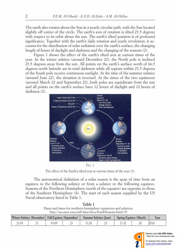
F.E.M. Al-Obaidi - A.A.D. Al-Zuky - A.M. Al-Hillou2
The earth also rotates about the Sun in a nearly circular path, with the Sun located slightly off center of the circle. The earth’s axis of rotation is tilted 23.5 degrees with respect to its orbit about the sun. The earth’s tilted position is of profound signifi cance. Together with the earth’s daily rotation and yearly revolution, it ac-counts for the distribution of solar radiation over the earth’s surface, the changing length of hours of daylight and darkness and the changing of the seasons (2).
Figure 1 shows the effect of the earth’s tilted axis at various times of the year. At the winter solstice (around December 22), the North pole is inclined 23.5 degrees away from the sun. All points on the earth’s surface north of 66.5 degrees north latitude are in total darkness while all regions within 23.5 degrees of the South pole receive continuous sunlight. At the time of the summer solstice (around June 22), the situation is reversed. At the times of the two equinoxes (around March 22 and September 22), both poles are equidistant from the sun and all points on the earth’s surface have 12 hours of daylight and 12 hours of darkness (2).
Table 1Dates and times for northern hemisphere equinoxes and solstices.
http://aa.usno.navy.mil/data/docs/EarthSeasons.html (5)
Winter Solstice (December) Fall Equinox (September) Summer Solstice (June) Spring Equinox (March) Year
23:38 21 03:09 23 11:28 21 17:32 20 2010
FIG. 1
The effect of the Earth’s tilted axis at various times of the year (3).
The astronomical defi nition of a solar season is the span of time from an equinox to the following solstice or from a solstice to the following equinox. Seasons of the Northern Hemisphere (north of the equator) are opposite to those of the Southern Hemisphere (4). The start of each season supplied by the US Naval observatory listed in Table 1.

Equinoxes assessment on images … 3
According to the International Astronomical Union (IAU), each season can be defi ned by the ecliptic solar longitude relative to the mean equinox of date (the ecliptic position of the mean northward equinox, taken as the 0° origin of ecliptic longitude). This can be summarized in table 2 (4).
Table 2Seasons of the Northern Hemisphere(4).
Sunset Direction Sunrise Direction Solar DeclinationEcliptic Solar
LongitudeMarked by
Northern Hemisphere Season
True West True EastCross 0° from south
to north0°
Northward Equinox (in March)
Spring
Furthest to North-West
Furthest to North-East
+obliquity 90°North Solstice
(in June)Summer
True West True EastCross 0° from north
to south180°
Southward Equinox (in September)
Autumn
Furthest to South-West
Furthest to South-East
-obliquity 270°South Solstice (in December)
Winter
2. Solar Parallactic Angle
Sunrise and Sunset are obviously a part of our everyday life(1). The direction or azimuth of sunrise or sunset must be distinguished from the angle made by the path of the rising or setting Sun with respect to the horizon, known as the solar parallactic angle (SPA). Although Sun rises at the true east direction and sets at the true west direction on the day of an equinox, on that day the parallactic angle would be 90° only at the equator. The variation of the direction of sunrise and sunset with latitude at the equinoxes can be shown in Fig. 2 (4).
FIG. 2
Charts of variation of the direction of sunrise and sunset with latitude at the equinoxes (4).
F.E.M. Al-Obaidi - A.A.D. Al-Zuky - A.M. Al-Hillou4
At sunrise or sunset only, the solar parallactic angle is given by:
[1]
where L is the geographic latitude and δS is solar declination. All angles are in degrees.
At both equinoxes, the daytime length is slightly longer than the length of night, due to atmospheric refraction making Sun appear higher at sunrise and sunset and due to the approximately 1/2° diameter of the solar disk (4).
Since astronomy is considered to be one branch of computer science, one can adopt machine vision to understand the astronomical phenomena.
3. Image Data Analysis Methods
Computer image analysis largely contains the fi eld of computer or machine vision, medical imaging, makes a heavy use of pattern recognition, digital geom-etry and signal processing. The applications of digital image analysis are contin-uously expanding through all areas of science and industry. Computers are indis-pensable for the analysis of image amounts of data, for tasks that require complex computation, or for the extraction of quantitative information (6,7).
Image analysis combines techniques that compute statistics and measure-ments based on the RGB intensity levels of the image pixels. In this process, the information content of the improved images is examined for specifi c features such as intensity, contrast, edges, contours, areas and dimensions. The result of analysis algorithms are feature vectors that give quantifi ed statements about the feature concerned (8).
The most important analysis methods of both spectral features of image seg-ments and operations related to spatial image structures utilized in measurements and testing technology are described in the following sections (8).
3.1 – Mean Value for RGB-Color Image
The simplest image analysis method of all is calculating the mean for the RGB color image (i.e M). The calculation rule for the mean for each RGB-band by using:
[2]
where n is the number of pixels and gi is the RGB-intensity value of the pixels in the image segment (9,10).
SPA at sunrise or sunset = cos−1 sin(L)
cos(δS )
⎛
⎝ ⎜
⎞
⎠ ⎟
M = g =1
n. gi
i=1
n
∑
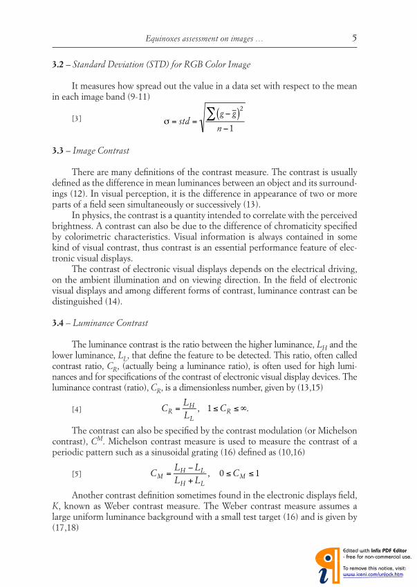
Equinoxes assessment on images … 5
3.2 – Standard Deviation (STD) for RGB Color Image
It measures how spread out the value in a data set with respect to the mean in each image band (9-11)
[3]
3.3 – Image Contrast
There are many defi nitions of the contrast measure. The contrast is usually defi ned as the difference in mean luminances between an object and its surround-ings (12). In visual perception, it is the difference in appearance of two or more parts of a fi eld seen simultaneously or successively (13).
In physics, the contrast is a quantity intended to correlate with the perceived brightness. A contrast can also be due to the difference of chromaticity specifi ed by colorimetric characteristics. Visual information is always contained in some kind of visual contrast, thus contrast is an essential performance feature of elec-tronic visual displays.
The contrast of electronic visual displays depends on the electrical driving, on the ambient illumination and on viewing direction. In the fi eld of electronic visual displays and among different forms of contrast, luminance contrast can be distinguished (14).
3.4 – Luminance Contrast
The luminance contrast is the ratio between the higher luminance, LH and the lower luminance, LL, that defi ne the feature to be detected. This ratio, often called contrast ratio, CR, (actually being a luminance ratio), is often used for high lumi-nances and for specifi cations of the contrast of electronic visual display devices. The luminance contrast (ratio), CR, is a dimensionless number, given by (13,15)
[4]
The contrast can also be specifi ed by the contrast modulation (or Michelson contrast), CM. Michelson contrast measure is used to measure the contrast of a periodic pattern such as a sinusoidal grating (16) defi ned as (10,16)
[5]
Another contrast defi nition sometimes found in the electronic displays fi eld, K, known as Weber contrast measure. The Weber contrast measure assumes a large uniform luminance background with a small test target (16) and is given by (17,18)
σ = std =
g − g ( )2∑
n−1
CR =
LH
LL
, 1≤ CR ≤∞.
CM =
LH −LL
LH + LL
, 0 ≤ CM ≤ 1
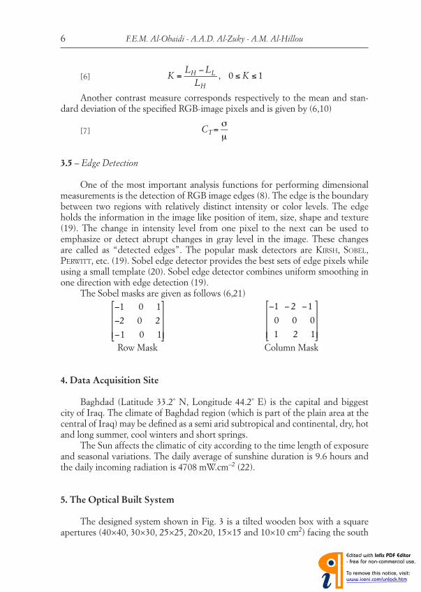
F.E.M. Al-Obaidi - A.A.D. Al-Zuky - A.M. Al-Hillou6
[6]
Another contrast measure corresponds respectively to the mean and stan-dard deviation of the specifi ed RGB-image pixels and is given by (6,10)
[7]
3.5 – Edge Detection
One of the most important analysis functions for performing dimensional measurements is the detection of RGB image edges (8). The edge is the boundary between two regions with relatively distinct intensity or color levels. The edge holds the information in the image like position of item, size, shape and texture (19). The change in intensity level from one pixel to the next can be used to emphasize or detect abrupt changes in gray level in the image. These changes are called as “detected edges”. The popular mask detectors are KIRSH, SOBEL, PERWITT, etc. (19). Sobel edge detector provides the best sets of edge pixels while using a small template (20). Sobel edge detector combines uniform smoothing in one direction with edge detection (19).
The Sobel masks are given as follows (6,21)
Row Mask Column Mask
4. Data Acquisition Site
Baghdad (Latitude 33.2˚ N, Longitude 44.2˚ E) is the capital and biggest city of Iraq. The climate of Baghdad region (which is part of the plain area at the central of Iraq) may be defi ned as a semi arid subtropical and continental, dry, hot and long summer, cool winters and short springs.
The Sun affects the climatic of city according to the time length of exposure and seasonal variations. The daily average of sunshine duration is 9.6 hours and the daily incoming radiation is 4708 mW.cm–2 (22).
5. The Optical Built System
The designed system shown in Fig. 3 is a tilted wooden box with a square apertures (40×40, 30×30, 25×25, 20×20, 15×15 and 10×10 cm2) facing the south
K =
LH −LL
LH
, 0 ≤ K ≤ 1
CT =
σ
μ
−1 0 1
−2 0 2
−1 0 1
⎡
⎣
⎢ ⎢ ⎢
⎤
⎦
⎥ ⎥ ⎥
−1 − 2 −1
0 0 0
1 2 1
⎡
⎣
⎢ ⎢ ⎢
⎤
⎦
⎥ ⎥ ⎥

Equinoxes assessment on images … 7
direction for reason mentioned in (6). The wooden box was painted by a grey paint. To maximize solar energy collection, the system has been tilted at an angle equal to site’s latitude, then Sun’s rays will be normal to the system surface at mid-day in March and September.
The scene is located at the end of the wooden box facing window’s aperture such that the center of aperture window is optically in line with that of the scene.
By using the optical built system shown in Fig. 3, images of the scene size 323×229 pixels have been selected. The capturing operation have been done at regular intervals from sunrise to sunset at the equinoxes (March 22 and Septem-ber 23).
Table 3Astronomical Parameters at Spring and Autumnal Equinoxes (23).
Date Rise Solar Noon SetTime AST Sun Declination Time AST Sun Declination Tme AST Sun Declination
March 20, 2010 6:07 am -0.24° 12:10 pm -0.14° 6:14 pm -0.04°September 23, 2010 5:51 am 0.01° 11:55 am -0.09° 5:58 pm -0.19°
FIG. 3
Image Acquisition Setup.
(a) (b)
6. Digital Image Analysis Step
This can be done by developing certain techniques using Visual Basic lan-guage, version 6. We have used the several algorithms to determine the statistical image properties based on the equations previously mentioned.
7. Contrast Measure based on RGB Image
Based on a local analysis of image edges, a contrast measure is derived from the defi nition of contrast in Eq. [7].

Table 5 Autumn equinox weather information supplied by (23).
Events: Conditions
Precip Gust Speed Wind Speed Wind Dir VisibilitySea Level Pressure
(hpa)Humidity
Dew Point ºC
Temp. ºCTime
(AST)
Haze N/A22.2km/h/
6.2m/s7.4km/h/
2.1m/sNW 8.0km 1010.1 32% 8.0 26.0 5:55am
Haze N/A -13.0km/h/3.6m/s
NW 8.0km 1010.8 34% 9.0 26.0 6:55am
Haze N/A20.4km/h/
5.7m/s9.3km/h/
2.6m/sNNW 6.0km 1011.5 28% 8.0 28.0 7:55am
Haze N/A -13.0km/h/3.6m/s
North 5.0km 1011.5 28% 8.0 28.0 8:55am
Haze N/A -13.0km/h/3.6m/s
North 5.0km 1011.8 20% 8.0 34.0 9:55am
Haze N/A -9.3km/h/
2.6m/sVariable 6.0km 1011.3 15% 6.0 37.0 10:55am
Haze N/A -9.3km/h/
2.6m/sVariable 6.0km 1010.4 13% 6.0 39.0 11:55am
Haze N/A20.4km/h/
5.7m/s11.1km/h/3.1m/s
North 8.0km 1009.7 11% 5.0 41.0 12:55pm
Haze N/A -11.1km/h/3.1m/s
North 8.0km 1009.0 11% 5.0 41.0 1:55pm
Haze N/A -14.8km/h/4.1m/s
NE 8.0km 1008.5 10% 4.0 41.0 2.55pm
Haze N/A -11.1km/h/3.1m/s
NNE 8.0km 1008.0 11% 5.0 41.0 3.55pm
Haze N/A -9.3km/h/
2.6m/sNorth 8.0km 1008.4 12% 6.0 41.0 4.55pm
Haze N/A -5.6km/h/
1.5m/sVariable 6.0km 1008.4 14% 7.0 39.0 5.55pm
Table 4Spring equinox weather information supplied by (23).
Events: Conditions
Precip Gust Speed Wind Speed Wind Dir VisibilitySea Level Pressure
(hpa)Humidity
Dew Point ºC
Temp. ºCTime
(AST)
Partly Cloudy
N/A -3.7km/h/
1.0m/sWSW 10.0km 1021.1 37% -7.0 7.0 5:55am
Partly Cloudy
N/A -3.7km/h/
1.0m/sWSW 10.0km 1021.4 34% -7.0 8.0 6:55am
Partly Cloudy
N/A -7.4km/h/
2.1m/sWest 10.0km 1021.7 35% -5.0 10.0 7:55am
Partly Cloudy
N/A -7.4km/h/
2.1m/sWNW 10.0km 1021.9 38% -1.0 13.0 8:55am
Partly Cloudy
N/A -9.3km/h/
2.6m/sWest 10.0km 1022.0 31% -1.0 16.0 9:55am
Partly Cloudy
N/A -9.3km/h/
2.6m/sWest 10.0km 1021.4 19% -6.0 18.0 10:55am
Partly Cloudy
N/A25.9km/h/
7.2m/s9.3km/h/
2.6m/sNW 10.0km 1021.2 15% -8.0 19.0 11:55am
Partly Cloudy
N/A20.4km/h/
5.7m/s7.4km/h/
2.1m/sNW 10.0km 1020.5 15% -8.0 19.0 12:55pm
Partly Cloudy
N/A24.1km/h/
6.7m/s13.0km/h/
3.6m/sNW 10.0km 1020.0 13% -9.0 21.0 1:55pm
Partly Cloudy
N/A29.6km/h/
8.2m/s14.8km/h/
4.1m/sNW 10.0km 1019.7 15% -8.0 20.0 2:55pm
Partly Cloudy
N/A24.1km/h/
6.7m/s13.0km/h/
3.6m/sNNW 10.0km 1019.2 15% -8.0 20.0 3.55pm
Partly Cloudy
N/A -9.3km/h/
2.6m/sWNW 10.0km 1019.2 17% -5.0 21.0 4.55pm
Partly Cloudy
N/A -9.3km/h/
2.6m/sWest 10.0km 1019.4 21% -4.0 19.0 5.55pm

Equinoxes assessment on images … 9
The detection of edges is based on comparing the edge gradient with a threshold value. This can been achieved by using one of the edge detection opera-tors (i.e. Sobel edge detector).
In the fi rst stage of the present work, loading the image, then applying Sobel edge detector to determine the edges using threshold value 60. Each of Sobel masks, convolved at the same time with images tristimulus (Red, Green and Blue bands and L-Component) separately. The pixel gh then is assigned to be an edge point, if and only if, the biggest convolution value for the coloumn and row masks has a value greater than the specifi ed threshold value (th) (6), i.e.
[8]
8. Experimental Results and Discussions
According to the tilted built system which has been set at a fi xed angle and during nearly same weather conditions for the two selected dates, the following results are obtained.
Figures 4 & 5 represent contrast variation and its component with time. For the two working days, contrast variation seems to look alike. The role of using dif-ferent window’s aperture areas take place all of the time (i.e. an increase/decrease state occurs only at sunrise and sunset times respectively, while a signifi cant sepa-ration occurs in times between sunrise and sunset).
For RGB bands and L-Component Figs.6 & 7 show contrast variation and its corresponding components with window’s aperture area. A signifi cant behav-ior for contrast variation with area is strongly noticed here. Window’s aperture area plays a dominant role in this situation. In spring equinox, sunrise and sunset curves separate in the case of larger areas and coincide in the smaller one. This separation (split) is by a distance such that sunset progress fi rst. This emphasizes the sun declination at that equinox shown previously in table 3, where it is shown in this table that sunset declination progress that of sunrise. The difference be-tween them is noticed by using large aperture areas.
In Autumn, the previous noticeable is reversed. Sunrise curve progresses that of sunset and this proves the astronomical reality explained also in the pre-vious table (i.e. 0.01 > - 0.19) and separated in the case of small areas.
The adopted technique used in this research proves the astronomical phe-nomena at equinoxes and opens a new fi eld of cooperation between astronomy science, data acquisition, optical technique and image analysis to understand our world.
gh =255 (an edge po int) biggest convolution sum > th
0 (non edge po int else
⎧ ⎨ ⎪
⎩ ⎪

F.E.M. Al-Obaidi - A.A.D. Al-Zuky - A.M. Al-Hillou10
FIG. 4
Contrast and its components variation with time in the Spring equinox (a), (d), (g), (j) variation of mean RGB bands and L-component respectively (b), (e), (h), (k) variation of standard deviation RGB bands and L-component respectively (c), (f), (i), (l) variation of contrast RGB bands and L-component respectively.
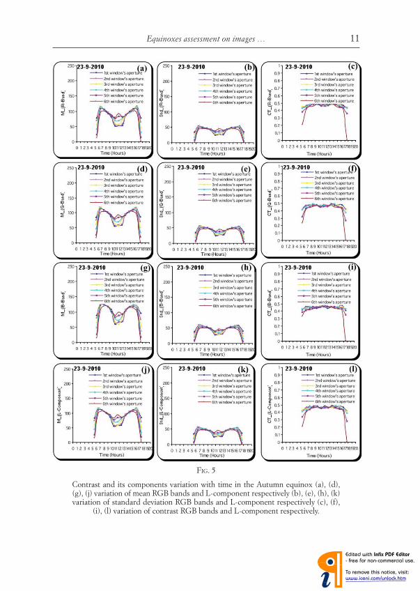
Equinoxes assessment on images … 11
FIG. 5
Contrast and its components variation with time in the Autumn equinox (a), (d), (g), (j) variation of mean RGB bands and L-component respectively (b), (e), (h), (k) variation of standard deviation RGB bands and L-component respectively (c), (f), (i), (l) variation of contrast RGB bands and L-component respectively.

F.E.M. Al-Obaidi - A.A.D. Al-Zuky - A.M. Al-Hillou12
FIG. 6
Contrast and its components variation with window’s aperture area in the Spring equinox (a), (d), (g), (j) variation of mean RGB bands and L-Component respectively (b), (e), (h), (k) variation of standard deviation RGB bands and L-Component respectively (c), (f), (i), (l) variation of contrast RGB bands and L-Component respectively.
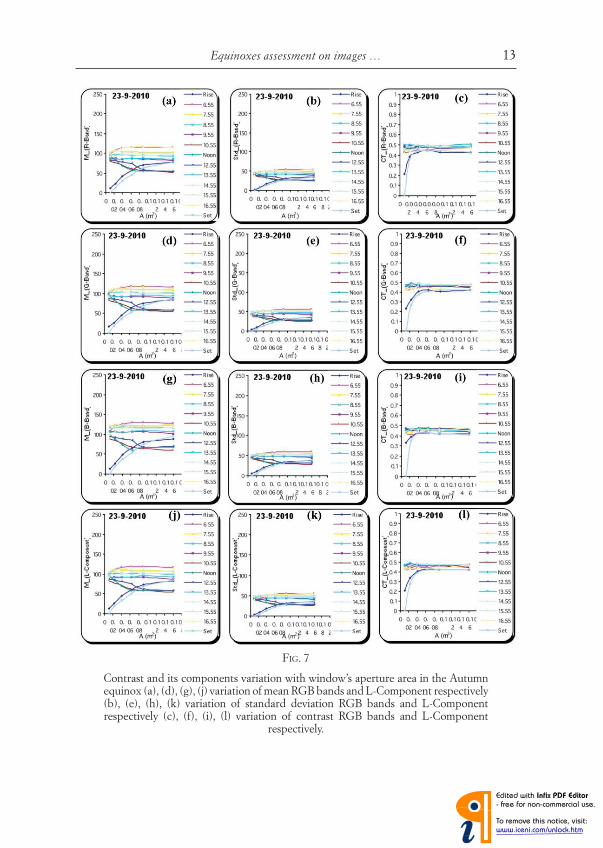
Equinoxes assessment on images … 13
FIG. 7
Contrast and its components variation with window’s aperture area in the Autumn equinox (a), (d), (g), (j) variation of mean RGB bands and L-Component respectively (b), (e), (h), (k) variation of standard deviation RGB bands and L-Component respectively (c), (f), (i), (l) variation of contrast RGB bands and L-Component respectively.
F.E.M. Al-Obaidi - A.A.D. Al-Zuky - A.M. Al-Hillou14
9. Conclusions
From the previous results and for all RGB bands and L-Component, the variation of contrast with time and area seems to be the same. In order to notice the equinoxes, one can adopt contrast variation with area as a very good tool to represent and notice the case. This can be seen clearly by adopting the relation between mean and window’s aperture area. A reversed role for sunrise and sunset curves can be noticed in the two equinoxes. This proves the nature of solar paral-lactic angle at sunrise and sunset at the equinoxes which can be used in future as a data set to distinguish other situations through the year.
REFERENCES
(1) A. FRIEDLANDER, T. RESNICK, Sunrise…Sunset…, in: The Montana Mathematics Enthu-siast, ISSN 1551-3440, 3 (2), 249-255, 2006.
(2) Appendix D: Solar radiation, in: http://www.me.umn.edu/courses/ me4131/LabMa-nual/ AppDSolorRadiation.Pdf
(3) N.M. SHORT, Meteorology-weather and climate: a condensed primer, in: http://rst. gsfc. nasa. gov/Sec14/ Sec14_1a.html (2005).
(4) I. BROMBERG, The lengths of the seasons (on Earth), in: http://www.sym454. org/seasons (2009).
(5) United States Naval Observatory, Earth’s seasons: equinoxes, solstices, perihelion and aphelion, 2000-2020, in: http://www.usno.navy.mil/USNO/astronomical-applications/data -ser-vices/earth-season (2010).
(6) A.M. AL-HILLOU, A.A.D. AL-ZUKY, F.E.M. AL-OBAIDI, Digital image testing and analy-sis of solar radiation variation with time in Baghdad city, Atti Fond. G. Ronchi, 65 (2), 223, 2010
(7) Image analysis, in: www.wikipedia,the free encyclopedia.htm (2010). (8) W. OSTEN, Optical inspection of microsystems, (Taylor & Francis Group, LLC., 2007). (9) M.A. YACOUB, A.S. MOHAMED, Y.M. KADAH, A cad system for the detection of malignant
tumors in digitized mammogram fi lms, in: Proceedings Cario Intern. Biomedical Engineering Conf. (2006).
(10) E. MILES, A. ROBERTS, Non-destructive speckle imaging of subsurface detail in paper-based cultural materials, Optics Express, 17 (15), 2009.
(11) S. RAMLI, M.M. MUSTAFA, A. HUSSAIN, D. ABDDUL WAHAB, Histogram of intensity feature extraction for automatic plastic bottle recycling system using machine vision, Am. J. Env. Sci., 4 (6), 583-588, 2008.
(12) J.K. KIM, J.M. PARK, K.S. SONG, H.W. PARK, Adaptive mammographic image enhan-cement using fi rst derivative and local statistics, IEEE Trans. on Medical Imaging, 16 (5), 1997.
(13) M.E. BECKER, Specsmanship: the artistry of sugarcoating performance specifi cations, (LCD TV Matters, 2008), Vol. 1.
(14) Display contrast, in: www.wikipedia, the free encyclopedia.htm (2009). (15) S.T. LAU, P.H. DICKINSON, Contrast formulae for use with contrast measuring devices,
provided by Spectrum Technologies PLC (1999). (16) J. TANG, E. PELI, S. ACTON, Image enhancement using a contrast measure in the com-
pressed domain, in: IEEE Signal Processing Lett., 10 (10) (IEEE, 2003)(17) J. BEISH, Observing the planets with color fi lters, in: Association of Lunar and Plane-
tary Observers web page The Mars Section, http://www.lpl.arizona.edu/∼rhill/alpo /marstuff/articles/FILTERS1.HTM.

Equinoxes assessment on images … 15
(18) R. SHAPLEY, R.C. REID, Contrast and assimilation in the perception of brightness, Proc. Natl. Acad. Sci., 82, 5983-5986, (1985)
(19) A.V. DESHPANDE, S.P. NAROTE, V.R. UDUPI, H.P. INAMDAR, A region growing segmen-tation for detection of microcalcifi cation in digitized mammograms, in Proc. Intern. Conf. on Co-gnition and Recognition (2005).
(20) J.R. PARKER, Algorithms for image processing and computer vision (John Wiley & Sons, Inc., 1997)
(21) F.E.M. AL-OBAIDI, Segmentation of coherent objects, M.Sc. thesis, College of Science, Al- Mustansiriyah University, Baghdad, Iraq (2001).
(22) S.A.H. SALEH, Remote sensing technique for land use and surface temperature analysis for Baghdad, Iraq, in Proc. 15th Intern. Symp.and Exhib. on Remote Sensing and Assisting Sy-stems, www.gors-sy.org.(2006)
(23)Weather Underground home page, in web site: http://www.wunderground.com.

Copyright © 2009 by the Institute of Electrical and Electronic Engineers, Inc All Rights Reserved Copyright and Reprint Permissions: Abstracting is permitted with credit to the source. Libraries are permitted to photocopy beyond the limit of U.S. copyright law for private use of patrons those articles in this volume that carry a code at the bottom of the first page, provided the per-copy fee indicated in the code is paid through Copyright Clearance Center, 222 Rosewood Drive, Danvers, MA 01923. For other copying, reprint or republication permission, write to IEEE Copyrights Manager, IEEE Service Center, 445 Hoes Lane, Piscataway, NJ 08854. All rights reserved. ***This publication is a representation of what appears in the IEEE Digital Libraries. Some format issues inherent in the e-media version may also appear in this print version. IEEE Catalog Number: CFP0910G-PRT ISBN 13: 978-1-4244-3603-3 Library of Congress No.: 2008911556 Additional Copies of This Publication Are Available From: Curran Associates, Inc 57 Morehouse Lane Red Hook, NY 12571 USA Phone: (845) 758-0400 Fax: (845) 758-2633 E-mail: [email protected] Web: www.proceedings.com

TABLE OF CONTENTS
Analysis of Some CFAR Detectors in Nonhomogenous Environments Based on Switching Algorithm .............................................................................................................................................................1
Saeed Erfanian, Vahid T. Vakili
Seismic Signal Enhancement Through Statistical (wiener) Approach...........................................................5R. Thandan Babu Naik, D. Srinagesh , R. V. Raghavan , H. V. S. Satyanarayana, D. Shashidhar
Robot Arm Controller Using FPGA..................................................................................................................8Urmila Meshram, Pankaj Bande, P. A. Dwaramwar, R. R. Harkare
Quality Controlled ECG Compression using Discrete Cosine Transform (DCT) and Laplacian Pyramid (LP) ...................................................................................................................................12
Vibha Aggarwal, Manjeet Singh Patterh
A Novel Voltage-Controlled Grounded Resistor Using FGMOS Technique...............................................16Rishikesh Pandey, Maneesha Gupta
Genetic Algorithm for Traveling Salesman Problem: Using Modified Partially-Mapped Crossover Operator..........................................................................................................................................20
Vijendra Singh, Simran Choudhary
An Optimal Transform Architecture for H.264/AVC ...................................................................................24A. K. Prasoon, K. Rajan
An Acoustic Signature Based Neural Network Model for Type Recognition of Two-Wheelers............................................................................................................................................................28
Basavaraj S. Anami, Veerappa B. Pagi
Wavelet Based Partial Image Encryption.......................................................................................................32Nahla A. Flayh, Rafat Parveen, Syed I. Ahson
Bit Reduction Based Matching Criterion for Motion Compensation in Video Coding..............................36Anchal Jain
Adaptive Vector Quantization Based Video Compression Scheme..............................................................40S. Esakkirajan, T. Veerakumar, P. Navaneethan
A New Method for Estimating Signal Matched Dual Tree Complex Wavelet System...............................44Shanti Swamy
Energy Efficient High Speed CNFET Based Interconnect Drivers for FPGAS..........................................48Kureshi Abdul Kadir, M. Hasan
A 2DAnalytical Model of the Channel Potential and Threshold Voltage of Double-Gate (DG) MOSFETs With Vertical Gaussian Doping Profile..............................................................................52
Pramod Kumar Tiwari, Surendra Kumar, Samarth Mittal, Vaibhav Srivastava, Utkarsh Pandey, S. Jit
Programmable Multi Channel Monitoring and Control Linux Based Data Acquisition System................................................................................................................................................................56
Rita Nagar, S. Sadistap, K. S. N. Rao
Objective Quality Assessment of Conversion & Reconstruction of Image from DCT to Integer Transform & Vice-Versa ....................................................................................................................60
Muhammed Yusuf Khan, Ekram Khan, M. Salim Beg
Reproducible Research in Various Facets of Signal Processing...................................................................64Dilshad Hussain, Siddiqui Mohd, Shabab Ather
A method for Authentication of the GPS Transmitter..................................................................................69Prarthan D. Mehta
Categorization, Clustering and Association Rule Mining on WWW...........................................................73S. S. Bedi, Hemant Yadav, Pooja Yadav
Low Component Voltage Mode Universal Biquadratic Filt er using Low Voltage DOCCII......................78T. Parveen, M. T. Ahmed, I. A. Khan
OFC Based Versatile Circuit for Realization of Impedance Converter, Grounded Inductance, FDNR and Component Multipliers............................................................................................81
T. Parveen, M. T. Ahmed
Recent Advances in Transport Level Error Control Techniques for Wireless Video Transmission.....................................................................................................................................................85
Yoong Choon Chang, Sze Wei Lee, Ryoichi Komiya
Comparison of JPEG and SPIHT Image Compression Algorithms using Objective Quality Measures............................................................................................................................................................90
Bhawna Rani, R. K. Bansal, Savina Bansal
An Ultra Broadband Stacked Circular Patch Antenna.................................................................................94Pramendra Tilanthe, P. C. Sharma
Performance of Blackman Window Family in M-channel Cosine Modulated Filter Bank for ECG Signals.......................................................................................................................................................98
Ashutosh Datar, Alok Jain, P. C. Sharma
Iterative and Distributed Range-free Localization Algorithm for Wireless Sensor Networks................102Madhulika, Alok Kumar, Shirshu Varma
Wideband Digital Integrator ..........................................................................................................................106Maneesha Gupta, Madhu Jain, B. Kumar
Analysis of Power Saving Multicasting Routing Applications for Mica2 Motes-An event based MATLAB Implementation ..................................................................................................................109
Pradeep Kumar Gaur, B. S. Dhaliwal, Ameeta Seehra
Experimental Use of Electronic Nose for Analysis of Volatile Organic Compound (VOC).....................113Syed Hasan Saeed, Zia Abbas, Bal Gopal
Fast Multiplierless Recursive Transforms Using Ramanujan Numbers...................................................116K. S. Geetha, V. K. Ananthashayana
A Non-Linear Neural Circuit for Solving System of Simultaneous Linear Equations.............................120Mohd Samar Ansari, Syed Atiqur Rahman
Analysis of Carbon Nanotube Interconnects and their Comparison with Cu Interconnects...................124Naushad Alam, A. K. Kureshi, Mohd Hasan, T. Arslan
A Feed-Forward Neural Circuit for Ranking N Numbers Using O (N) Neurons.....................................128Mohd Samar Ansari, Syed Javed Arif
Smoothing Cephalographs Using Modified Anisotropic Diffusion Filter ..................................................131Amandeep Kaur
A Simple Modified Fixed Step Size Power Control Algorithm for CDMA Cellular Systems..................134M. A. Rahim Khan, P. C. Jain
Load Balancing Issues in Automotives..........................................................................................................138Rajeshwari Hegde, K. S. Gurumurthy
Separation Performance of ICA Algorithmsin Communication Systems..................................................142S. D. Parmar, Bhuvan Unhelkar

Development of CMOS based Gas Sensors..................................................................................................146Rajesh Kumar, S. A. Imam, M. R. Khan
Effect of Wavelength Conversion Factor on Blocking Probability and Link Utilization in Wavelength Routed Optical Network...........................................................................................................151
Aditya Goel, Vitthal J. Gond
Tunable Four Phase Voltage Mode Quadrature Oscillator using Two CMOS MOCCIIs .......................155Parveen Beg, Iqbal A. Khan, Muslim T. Ahmed
Electronically Tunable MOSFET-C Mixed-Mode Quadrature Oscillator................................................158Mohd Samar Ansari, Sudhanshu Maheshwari
A High-Speed, Hierarchical 16×16 Array of Array Multiplier Design ......................................................161Abhijit Asati, Chandrashekhar
Shot Boundary Detection Using Texture Feature Based On Co-Occurrence Matrices............................165Brojeshwar Bhowmick, Debaleena Chattopadhyay
Performance Comparison and Variability Analysis of CNT Bundle and Cu Interconnects....................169Naushad Alam, A. K. Kureshi, Mohd Hasan, T. Arslan
Evaluate the Quality of Satellite Image Depending on the Correlation.....................................................173Ali A. Al – Zuky, Firas Sabeeh Mohammed, Haidar Jawad M. A. Al-Taa’y
A New Watermarking Attack Based on Content-Aware Image Resizing..................................................177A. H. Taherinia, M. Jamzad
Real Time Streaming Video over Bluetooth Network.................................................................................181M. Siddique Khan, Rehan Ahmad, Tauseef Ahmad, Mohammed A. Qadeer
High Input Impedance SIMO Versatile Biquad Filter ................................................................................185Jitendra Mohan, Sudhanshu Maheshwari, Sajai Vir Singh, Durg Singh Chauhan
Development and Modelling of High-Efficiency Computing Structure for Digital Signal Processing........................................................................................................................................................189
Annapurna Sharma, Hakimjon Zaynidinov, Hoon Jae Lee
Interhemispheric Interaction and Cause of Hindrance During Handedness Activity: An Electro-Physiological Evidence......................................................................................................................193
B. Ghosh, P. Swami, T. Gandhi, J. Santhosh, S. Anand
MUHIS : A Middleware approach Using LiveGraph..................................................................................197Mangal Sain, HoonJae Lee, Wan-Young Chung
IP-based Ubiquitous Sensor Network for In-Home Healthcare Monitoring .............................................201Dhananjay Singh, Sanjay Singh, Madhusudan Singh, Hsein-Ping Kew, Do-Un Jeoung, U. S. Tiwary, Hoon-Jae Lee
A High Performance VLSI Architecture for Fast Two-Step Search Algorithm for Sub-Pixel Motion Estimation ..........................................................................................................................................205
Sumit K. Chatterjee, Indrajit Chakrabarti
Versatile Quadrature Oscillator with Grounded Components...................................................................209Sudhanshu Maheshwari, Bhartendu Chaturvedi
VHDL Modelling and Simulation of Parallel-Beam Filtered Backprojection for CT Image Reconstruction................................................................................................................................................213
Pranamita Basu, M. Manjunatha
Asterisk VoIP Private Branch Exchange......................................................................................................217Ale Imran, Mohammed A. Qadeer, M. J. R. Khan
Object Detection and Features Extraction in Video Frames using Direct Thresholding.........................221Asaad A. M. Al-Salih, Syed I. Ahson

Effect of Topological and Traffic Variations on Quality of Service Using RSVP/ns................................225Navneet, Trilok Chand Aseri, Ash Mohammad Abbas
Multi-Scroll Chaos Generator Using Current Conveyors...........................................................................229Shahnaz Hasan, Iqbal A. Khan
Significance of Tree Structures for Zerotree-Based Wavelet Video Codecs..............................................233Athar Ali Moinuddin, Ekram Khan, Mohammed Ghanbari
Error Resilient Technique for SPIHT coded Color Images........................................................................237Mohd Ayyub Khan, Ekram Khan
On the Realization and Design of Chaotic Spread Spectrum Modulation Technique for Secure Data Transmission..............................................................................................................................241
G. M. Bhat, Javaid Ahmad, Shabir Ahmad
Indoor Environment Gas Monitoring System Based on the Digital Signal Processor..............................245Anuj Kumar, I. P. Singh, S. K. Sud
Bluetooth Based Implementations for Realising New Consumer Systems................................................250M. Salim Beg, Binish Fatimah, Shashank Jain, Rehan Muzammil
Design and Simulation of a Modified Block Transmission System with Pre-Coding...............................254Mutamed Khatib, Farid Ghani, Mohd Fadzil Ain
Multi-Carrier Frequency Hopping Spread Spectrum System with Girth-Six Low-Density Parity-Check Codes........................................................................................................................................258
Farid Ghani, Abid Yahya
Performance Evaluation of Enhanced FIR Filter based Module for clock Synchronization in MPEG2 Transport Stream .......................................................................................................................261
Monika Jain, Ankit Jain, P. C. Jain, Sharad Jain
Enhanced A5/1 Cipher with Improved Linear Complexity........................................................................265Musheer Ahmad, Izharuddin
LFSR and PLA based Complex Code Generator for Stream Cipher........................................................268Farah Maqsood, Omar Farooq, Wasim Ahmad
Shape Based Classification of Breast Tumors Using Fractal Analysis.......................................................272M. Syed Abdaheer, Ekram Khan
A Method for FinFET Intermodulation Analysis from TCAD Simulations using a Time-domain Waveform Approach ........................................................................................................................276
F. Ahmad, M. S. Alam, G. A. Armstrong
Embedding and Non-Blind Extraction of Watermark Data in Images in FRFT domain.......................280Farooq Hussain, Ekram Khan, Omar Farooq
A Novel Current-mode Non-Linear Feedback Neural Circuit for Solving Linear Equations .................284Mohd Samar Ansari, Syed Atiqur Rahman
SPICE Model for Optoelectronic XOR Gate Based on Light Amplifying Optical Switch (LAOS) .............................................................................................................................................................288
Hamad Alhokail
Digital Image Encryption Based on Chaotic Map for Secure Transmission.............................................292Musheer Ahmad, Chanki Gupta, Ankit Varshney
NML Detection Processes for Some Outdoor Vehicular Environments ....................................................296Mohd Israil, M. Salim Beg
An Overview of Advanced FPGA Architectures for Optimized Hardware Realization of Computation Intensive Algorithms ...............................................................................................................300
Syed Manzoor Qasim, Shuja Ahmad Abbasi, Bandar Almashary

Modernization of Soild Density Standards Setup to Make it a Fully Computer Controlled Unattended System.........................................................................................................................................304
Nisha, Nitu Dhyani, Vijay Sharma, Sanjeev Sinha, T. K. Saxena
Tuning of PID Parameters Using Artificial Neural Network ......................................................................309Nisha, Avneesh Mittal, O. P. Sharma, Nitu Dhyani, Vijay Sharma, Avinashi Kapoor, T. K. Saxena
A Review of FPGA-Based Design Methodology and Optimization Techniques for Efficient Hardware Realization of Computation Intensive Algorithms....................................................................313
Syed Manzoor Qasim, Shuja Ahmad Abbasi, Bandar Almashary
Modeling and Simulation of Wideband Low Jitter Frequency Synthesizer..............................................317Ahmed A. Telba
A New Adaptive Watermarking Attack in Wavelet Domain......................................................................320A. H. Taherinia, M. Jamzad
Author Index
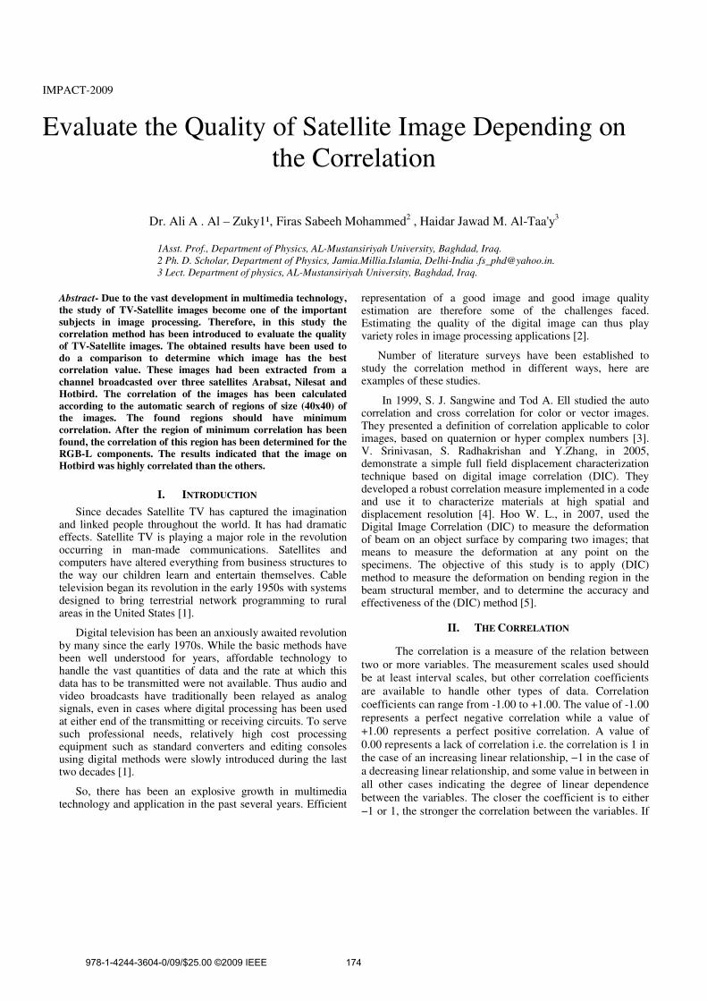
IMPACT-2009
Evaluate the Quality of Satellite Image Depending on
the Correlation
Dr. Ali A . Al – Zuky1¹, Firas Sabeeh Mohammed2 , Haidar Jawad M. Al-Taa'y
3
1Asst. Prof., Department of Physics, AL-Mustansiriyah University, Baghdad, Iraq.
2 Ph. D. Scholar, Department of Physics, Jamia.Millia.Islamia, Delhi-India [email protected].
3 Lect. Department of physics, AL-Mustansiriyah University, Baghdad, Iraq.
Abstract- Due to the vast development in multimedia technology,
the study of TV-Satellite images become one of the important
subjects in image processing. Therefore, in this study the
correlation method has been introduced to evaluate the quality
of TV-Satellite images. The obtained results have been used to
do a comparison to determine which image has the best
correlation value. These images had been extracted from a
channel broadcasted over three satellites Arabsat, Nilesat and
Hotbird. The correlation of the images has been calculated
according to the automatic search of regions of size (40x40) of
the images. The found regions should have minimum
correlation. After the region of minimum correlation has been
found, the correlation of this region has been determined for the
RGB-L components. The results indicated that the image on
Hotbird was highly correlated than the others.
I. INTRODUCTION
Since decades Satellite TV has captured the imagination and linked people throughout the world. It has had dramatic effects. Satellite TV is playing a major role in the revolution occurring in man-made communications. Satellites and computers have altered everything from business structures to the way our children learn and entertain themselves. Cable television began its revolution in the early 1950s with systems designed to bring terrestrial network programming to rural areas in the United States [1].
Digital television has been an anxiously awaited revolution by many since the early 1970s. While the basic methods have been well understood for years, affordable technology to handle the vast quantities of data and the rate at which this data has to be transmitted were not available. Thus audio and video broadcasts have traditionally been relayed as analog signals, even in cases where digital processing has been used at either end of the transmitting or receiving circuits. To serve such professional needs, relatively high cost processing equipment such as standard converters and editing consoles using digital methods were slowly introduced during the last two decades [1].
So, there has been an explosive growth in multimedia technology and application in the past several years. Efficient
representation of a good image and good image quality estimation are therefore some of the challenges faced. Estimating the quality of the digital image can thus play variety roles in image processing applications [2].
Number of literature surveys have been established to study the correlation method in different ways, here are examples of these studies.
In 1999, S. J. Sangwine and Tod A. Ell studied the auto correlation and cross correlation for color or vector images. They presented a definition of correlation applicable to color images, based on quaternion or hyper complex numbers [3]. V. Srinivasan, S. Radhakrishan and Y.Zhang, in 2005, demonstrate a simple full field displacement characterization technique based on digital image correlation (DIC). They developed a robust correlation measure implemented in a code and use it to characterize materials at high spatial and displacement resolution [4]. Hoo W. L., in 2007, used the Digital Image Correlation (DIC) to measure the deformation of beam on an object surface by comparing two images; that means to measure the deformation at any point on the specimens. The objective of this study is to apply (DIC) method to measure the deformation on bending region in the beam structural member, and to determine the accuracy and effectiveness of the (DIC) method [5].
II. THE CORRELATION
The correlation is a measure of the relation between
two or more variables. The measurement scales used should
be at least interval scales, but other correlation coefficients
are available to handle other types of data. Correlation
coefficients can range from -1.00 to +1.00. The value of -1.00
represents a perfect negative correlation while a value of
+1.00 represents a perfect positive correlation. A value of
0.00 represents a lack of correlation i.e. the correlation is 1 in
the case of an increasing linear relationship, −1 in the case of
a decreasing linear relationship, and some value in between in
all other cases indicating the degree of linear dependence
between the variables. The closer the coefficient is to either
−1 or 1, the stronger the correlation between the variables. If
978-1-4244-3604-0/09/$25.00 ©2009 IEEE 174
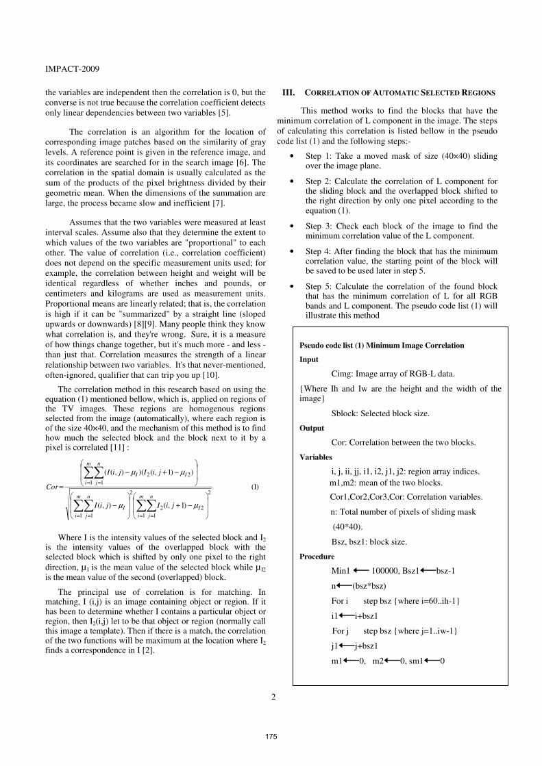
IMPACT-2009
2
the variables are independent then the correlation is 0, but the
converse is not true because the correlation coefficient detects
only linear dependencies between two variables [5].
The correlation is an algorithm for the location of
corresponding image patches based on the similarity of gray
levels. A reference point is given in the reference image, and
its coordinates are searched for in the search image [6]. The
correlation in the spatial domain is usually calculated as the
sum of the products of the pixel brightness divided by their
geometric mean. When the dimensions of the summation are
large, the process became slow and inefficient [7].
Assumes that the two variables were measured at least
interval scales. Assume also that they determine the extent to
which values of the two variables are "proportional" to each
other. The value of correlation (i.e., correlation coefficient)
does not depend on the specific measurement units used; for
example, the correlation between height and weight will be
identical regardless of whether inches and pounds, or
centimeters and kilograms are used as measurement units.
Proportional means are linearly related; that is, the correlation
is high if it can be "summarized" by a straight line (sloped
upwards or downwards) [8][9]. Many people think they know
what correlation is, and they're wrong. Sure, it is a measure
of how things change together, but it's much more - and less -
than just that. Correlation measures the strength of a linear
relationship between two variables. It's that never-mentioned,
often-ignored, qualifier that can trip you up [10].
The correlation method in this research based on using the equation (1) mentioned bellow, which is, applied on regions of the TV images. These regions are homogenous regions selected from the image (automatically), where each region is of the size 40×40, and the mechanism of this method is to find how much the selected block and the block next to it by a pixel is correlated [11] :
Where I is the intensity values of the selected block and I2 is the intensity values of the overlapped block with the selected block which is shifted by only one pixel to the right
direction, µ I is the mean value of the selected block while µ I2 is the mean value of the second (overlapped) block.
The principal use of correlation is for matching. In matching, I (i,j) is an image containing object or region. If it has been to determine whether I contains a particular object or region, then I2(i,j) let to be that object or region (normally call this image a template). Then if there is a match, the correlation of the two functions will be maximum at the location where I2 finds a correspondence in I [2].
III. CORRELATION OF AUTOMATIC SELECTED REGIONS
This method works to find the blocks that have the
minimum correlation of L component in the image. The steps
of calculating this correlation is listed bellow in the pseudo
code list (1) and the following steps:-
• Step 1: Take a moved mask of size (40×40) sliding over the image plane.
• Step 2: Calculate the correlation of L component for the sliding block and the overlapped block shifted to the right direction by only one pixel according to the equation (1).
• Step 3: Check each block of the image to find the minimum correlation value of the L component.
• Step 4: After finding the block that has the minimum correlation value, the starting point of the block will be saved to be used later in step 5.
• Step 5: Calculate the correlation of the found block that has the minimum correlation of L for all RGB bands and L component. The pseudo code list (1) will illustrate this method
)1(
)1,(),(
))1,()(),((
2
1 1
22
2
1 1
1 1
22
��
�
�
��
�
�−+
��
�
�
��
�
�−
��
�
�
��
�
�−+−
=
����
��
= == =
= =
m
i
n
j
I
m
i
n
j
I
m
i
n
j
II
jiIjiI
jiIjiI
Cor
µµ
µµ
Pseudo code list (1) Minimum Image Correlation
Input
Cimg: Image array of RGB-L data.
{Where Ih and Iw are the height and the width of the image}
Sblock: Selected block size.
Output
Cor: Correlation between the two blocks.
Variables
i, j, ii, jj, i1, i2, j1, j2: region array indices.
m1,m2: mean of the two blocks.
Cor1,Cor2,Cor3,Cor: Correlation variables.
n: Total number of pixels of sliding mask
(40*40).
Bsz, bsz1: block size.
Procedure
Min1 100000, Bsz1 bsz-1
n (bsz*bsz)
For i step bsz {where i=60..ih-1}
i1 i+bsz1
For j step bsz {where j=1..iw-1}
j1 j+bsz1
m1 0, m2 0, sm1 0
175

IMPACT-2009
Continued
For ii, jj {where ii=i..i1, jj=j..j1}
m1 m1+cimg(i,j)
m2 m2+cimg(i,j+1)
sm1 sm1+cimg(i,j) ^ 2
End For
m1 m1/n
m2 m2/n
std ( (sm1/n) – (m1 ^ 2) ) ^ 0.5
Cor1 0, Cor2 0, Cor3 0
For i,j {where i=(y1+1)..y2, j=(x1+1)..x2}
{Calculate the correlation for just L value for comparison}
If std>=0 and std <=2 then Cor 1
Else
Cor1 cor1+(cimg(i,j)-m1)*(cimg(i,j+1)-m2)
Cor2 cor2+(cimg(i,j)-m1)^2
Cor3 cor3+(cimg(i,j+1)-m2)^2
End if
End For
If Cor=1 then goto the step of determining the min. correlation
ElseIf Cor1=0 and Cor2=0 and Cor3=0 then Cor 1
Else if Cor2=0 or Cor3=0 then Cor 1
Else Cor Abs ( )32
1
* corcor
cor
End If
If Cor <= min1 then {Checking to find the min block}
min1 Cor
x ii – bsz
y jj – bsz
End if
End For
End For {End of searching min correlation algorithm}
{Then calculate the correlation for all RGB-L for the found block }
m1 0, m2 0
n (Sblock*Sblock)
For i, j {where i=(y1+1)..y2, j=(x1+1)..x2}
{Calculate the Mean and STD for all RGB bands and L component}
Continued
m1 m1+cimg(i,j)
m2 m2+cimg(i,j+1)
sm sm+(cimg(i,j)) ^ 2
End For
m1 m1/n
m2 m2/n
std ( (sm/n)-(m1)^2 ) ^ 0.5
cor1 0, cor2 0, cor3 0
For i,j {where i=(y1+1)..y2, j=(x1+1)..x2}
{Calculate the correlation for each RGB bands and L component}
If std>=0 and std<=2 then Cor 1
Else
Cor1 cor1+(cimg(i,j)-m1)*(cimg(i,j+1)-m2)
Cor2 cor2+(cimg(i,j)-m1)^2
Cor3 cor3+(cimg(i,j+1)-m2)^2
End if
End For
If Cor=1 then Print Cor
Else If cor1=0 and cor2=0 and cor3=0 then Cor 1
Else if cor2=0 or cor3=0 then Cor 0
Else
Cor Abs ( ))*( 32
1
CorCor
Cor
End If
End Procedure
Table (1): shows the image Searched Min. correlation results of
the satellites��
Block Size = 40x40 For all Regions
R1 = (321,340) R2 = (281,180)
Color Bands
Satellite Operation Red Green Blue
Lumina
nce
µ 31 22 1 22
� 6.77 9.04 4.27 7.45
Arabsat Cor(R1) 0.79 0.88 0.82 0.85
µ 25 9 5 13
� 21.29 26.09 24.87 23.93
Hotbird Cor(R2) 0.84 0.89 0.88 0.87
µ 32 23 1 23
� 6.88 9.51 3.97 7.65
Nilesat Cor(R1) 0.77 0.87 0.86 0.85
176
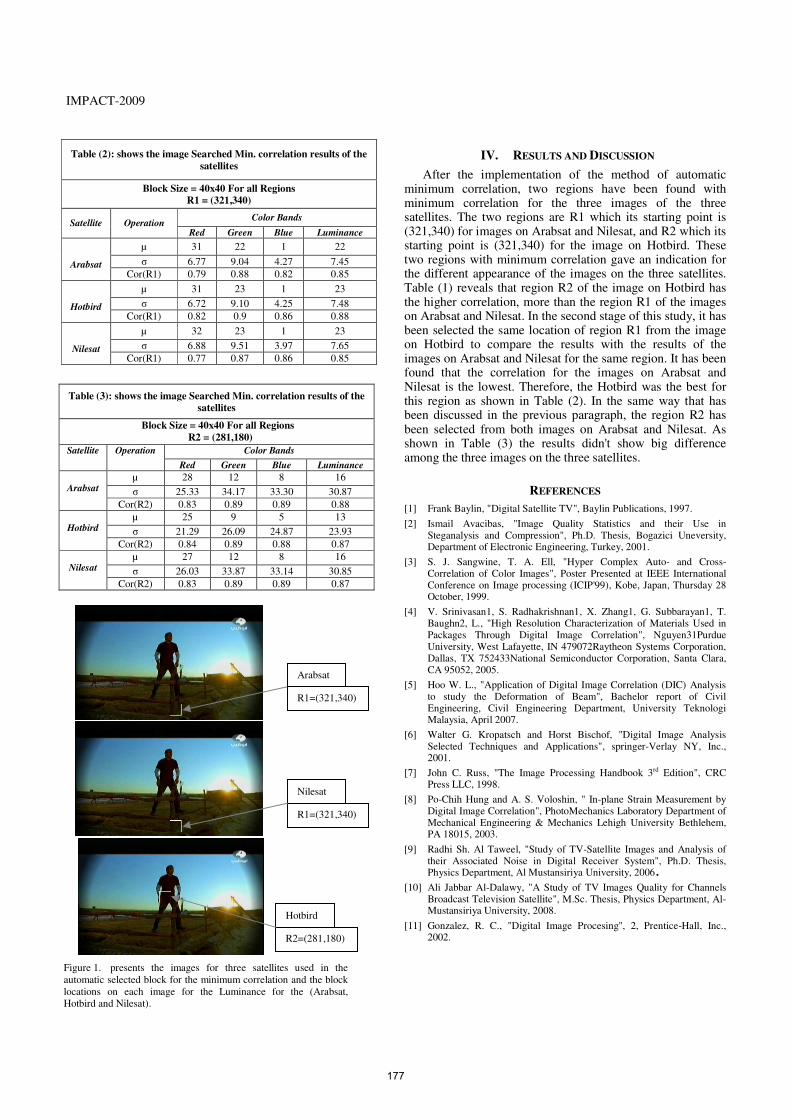
IMPACT-2009
Figure 1. presents the images for three satellites used in the
automatic selected block for the minimum correlation and the block
locations on each image for the Luminance for the (Arabsat,
Hotbird and Nilesat).
IV. RESULTS AND DISCUSSION
After the implementation of the method of automatic minimum correlation, two regions have been found with minimum correlation for the three images of the three satellites. The two regions are R1 which its starting point is (321,340) for images on Arabsat and Nilesat, and R2 which its starting point is (321,340) for the image on Hotbird. These two regions with minimum correlation gave an indication for the different appearance of the images on the three satellites. Table (1) reveals that region R2 of the image on Hotbird has the higher correlation, more than the region R1 of the images on Arabsat and Nilesat. In the second stage of this study, it has been selected the same location of region R1 from the image on Hotbird to compare the results with the results of the images on Arabsat and Nilesat for the same region. It has been found that the correlation for the images on Arabsat and Nilesat is the lowest. Therefore, the Hotbird was the best for this region as shown in Table (2). In the same way that has been discussed in the previous paragraph, the region R2 has been selected from both images on Arabsat and Nilesat. As shown in Table (3) the results didn't show big difference among the three images on the three satellites.
REFERENCES
[1] Frank Baylin, "Digital Satellite TV", Baylin Publications, 1997.
[2] Ismail Avacibas, "Image Quality Statistics and their Use in Steganalysis and Compression", Ph.D. Thesis, Bogazici Uneversity, Department of Electronic Engineering, Turkey, 2001.
[3] S. J. Sangwine, T. A. Ell, "Hyper Complex Auto- and Cross-Correlation of Color Images", Poster Presented at IEEE International Conference on Image processing (ICIP'99), Kobe, Japan, Thursday 28 October, 1999.
[4] V. Srinivasan1, S. Radhakrishnan1, X. Zhang1, G. Subbarayan1, T. Baughn2, L., "High Resolution Characterization of Materials Used in Packages Through Digital Image Correlation", Nguyen31Purdue University, West Lafayette, IN 479072Raytheon Systems Corporation, Dallas, TX 752433National Semiconductor Corporation, Santa Clara, CA 95052, 2005.
[5] Hoo W. L., "Application of Digital Image Correlation (DIC) Analysis to study the Deformation of Beam", Bachelor report of Civil Engineering, Civil Engineering Department, University Teknologi Malaysia, April 2007.
[6] Walter G. Kropatsch and Horst Bischof, "Digital Image Analysis Selected Techniques and Applications", springer-Verlay NY, Inc., 2001.
[7] John C. Russ, "The Image Processing Handbook 3rd Edition", CRC Press LLC, 1998.
[8] Po-Chih Hung and A. S. Voloshin, " In-plane Strain Measurement by Digital Image Correlation", PhotoMechanics Laboratory Department of Mechanical Engineering & Mechanics Lehigh University Bethlehem, PA 18015, 2003.
[9] Radhi Sh. Al Taweel, "Study of TV-Satellite Images and Analysis of their Associated Noise in Digital Receiver System", Ph.D. Thesis, Physics Department, Al Mustansiriya University, 2006.
[10] Ali Jabbar Al-Dalawy, "A Study of TV Images Quality for Channels Broadcast Television Satellite", M.Sc. Thesis, Physics Department, Al-Mustansiriya University, 2008.
[11] Gonzalez, R. C., "Digital Image Procesing", 2, Prentice-Hall, Inc., 2002.
Table (2): shows the image Searched Min. correlation results of the
satellites
Block Size = 40x40 For all Regions��
R1 = (321,340)
Color Bands Satellite Operation
Red Green Blue Luminance
µ 31 22 1 22
� 6.77 9.04 4.27 7.45
Arabsat Cor(R1) 0.79 0.88 0.82 0.85
µ 31 23 1 23
� 6.72 9.10 4.25 7.48
Hotbird Cor(R1) 0.82 0.9 0.86 0.88
µ 32 23 1 23
� 6.88 9.51 3.97 7.65
Nilesat��
Cor(R1) 0.77 0.87 0.86 0.85
Table (3): shows the image Searched Min. correlation results of the
satellites
Block Size = 40x40 For all Regions
R2 = (281,180) Color Bands Satellite Operation
Red Green Blue Luminance
µ 28 12 8 16
� 25.33 34.17 33.30 30.87
Arabsat
Cor(R2) 0.83 0.89 0.89 0.88
µ 25 9 5 13
� 21.29 26.09 24.87 23.93
Hotbird
Cor(R2) 0.84 0.89 0.88 0.87
µ 27 12 8 16
� 26.03 33.87 33.14 30.85
Nilesat��
Cor(R2) 0.83 0.89 0.89 0.87
R1=(321,340)
Hotbird
R2=(281,180)
Nilesat
R1=(321,340)
Arabsat
177

International Journal of Software Engineering Research & Practices Vol.1, Issue 4, Oct, 2011
Print-ISSN: 2231-2048 e-ISSN: 2231-0320
© RG Education Society (INDIA)
Feature-Level Based Image Fusion Of Multisensory Images
Firouz Abdullah Al-Wassai
1 Dr. N.V. Kalyankar
2
Research Student, Computer Science Dept. Principal, Yeshwant Mahavidyala College
(SRTMU), Nanded, India Nanded, India
[email protected] [email protected]
Dr. Ali A. Al-Zaky3
Assistant Professor, Dept.of Physics, College of Science, Mustansiriyah Un.
Baghdad – Iraq.
Abstract- Until now, of highest relevance for remote sensing
data processing and analysis have been techniques for pixel
level image fusion. So, This paper attempts to undertake the
study of Feature-Level based image fusion. For this purpose,
feature based fusion techniques, which are usually based on
empirical or heuristic rules, are employed. Hence, in this
paper we consider feature extraction (FE) for fusion. It aims at
finding a transformation of the original space that would
produce such new features, which preserve or improve as
much as possible. This study introduces three different types of
Image fusion techniques including Principal Component
Analysis based Feature Fusion (PCA), Segment Fusion (SF)
and Edge fusion (EF). This paper also devotes to concentrate
on the analytical techniques for evaluating the quality of image
fusion (F) by using various methods including ( ), ), ( ),
( ), (NRMSE) and ( ) to estimate the quality and degree of
information improvement of a fused image quantitatively.
Keywords: Image fusion , Feature, Edge Fusion, Segment
Fusion, IHS, PCA
INTRODUCTION
Over the last years, image fusion techniques have interest within the remote sensing community. The reason of this is that in most cases the new generation of remote sensors with very high spatial resolution acquires image datasets in two separate modes: the highest spatial resolution is obtained for panchromatic images (PAN) whereas multispectral information (MS) is associated with lower spatial resolution [1].
Usually, the term „fusion‟ gets several words to appear, such as merging, combination, synergy, integration … and several others that express more or less the same meaning the concept have since it appeared in literature [Wald L., 1999a]. Different definitions of data fusion can be found in literature, each author interprets this term differently depending on his research interests, such as [2, 3] . A general definition of data fusion can be adopted as fallowing: “Data fusion is a formal framework which expresses means and tools for the alliance of data originating from different sources. It aims at
obtaining information of greater quality; the exact definition of „greater quality‟ will depend upon the application” [4-6].
Image fusion techniques can be classified into three
categories depending on the stage at which fusion takes place; it is often divided into three levels, namely: pixel level, feature level and decision level of representation [7,8]. Until now, of highest relevance for remote sensing data processing and analysis have been techniques for pixel level image fusion for which many different methods have been developed and a rich theory exists [1]. Researchers have shown that fusion techniques that operate on such features in the transform domain yield subjectively better fused images than pixel based techniques [9].
For this purpose, feature based fusion techniques that is usually based on empirical or heuristic rules is employed. Because a general theory is lacking fusion, algorithms are usually developed for certain applications and datasets. [10]. In this paper we consider feature extraction (FE) for fusion.It is aimed at finding a transformation of the original space that would produce such new features, which are preserved or improved as much as possible. This study introduces three different types of Image fusion techniques including Principal Component Analysis based Feature Fusion (PCA), Segment Fusion (SF) and Edge fusion (EF). It will examine and estimate the quality and degree of information improvement of a fused image quantitatively and the ability of this fused image to preserve the spectral integrity of the original image by fusing different sensor with different characteristics of temporal, spatial, radiometric and Spectral resolutions of TM & IRS-1C PAN images. The subsequent sections of this paper are organized as follows: section II gives the brief overview of the related work. III covers the experimental results and analysis, and is subsequently followed by the conclusion.
FEATURE LEVEL METHODS

International Journal of Software Engineering Research & Practices Vol.1, Issue 4, Oct, 2011
9
Feature level methods are the next stage of processing where
image fusion may take place. Fusion at the feature level
requires extraction of features from the input images.
Features can be pixel intensities or edge and texture features
[11]. The Various kinds of features are considered depending
on the nature of images and the application of the fused
image. The features involve the extraction of feature
primitives like edges, regions, shape, size, length or image
segments, and features with similar intensity in the images to
be fused from different types of images of the same
geographic area. These features are then combined with the
similar features present in the other input images through a
pre-determined selection process to form the final fused
image . The feature level fusion should be easy. However,
feature level fusion is difficult to achieve when the feature
sets are derived from different algorithms and data sources
[12].
To explain the algorithms through this study, Pixel should
have the same spatial resolution from two different sources
that are manipulated to obtain the resultant image. So, before
fusing two sources at a pixel level, it is necessary to perform
a geometric registration and a radiometric adjustment of the
images to one another. When images are obtained from
sensors of different satellites as in the case of fusion of SPOT
or IRS with Landsat, the registration accuracy is very
important. But registration is not much of a problem with
simultaneously acquired images as in the case of
Ikonos/Quickbird PAN and MS images. The PAN images
have a different spatial resolution from that of MS images.
Therefore, resampling of MS images to the spatial resolution
of PAN is an essential step in some fusion methods to bring
the MS images to the same size of PAN, thus the resampled
MS images will be noted by that represents the set of
of band k in the resampled MS image . Also the
following notations will be used: Ρ as DN for PAN image,
Fk the DN in final fusion result for band k. ,
Denotes the local means and standard deviation
calculated inside the window of size (3, 3) for and Ρ respectively.
A. Segment Based Image Fusion(SF):
The segment based fusion was developed specifically
for a spectral characteristics preserving image merge . It is
based on an transform [13] coupled with a spatial
domain filtering. The principal idea behind a spectral
characteristics preserving image fusion is that the high
resolution of PAN image has to sharpen the MS image
without adding new gray level information to its spectral
components. An ideal fusion algorithm would enhance high
frequency changes such as edges and high frequency gray
level changes in an image without altering the MS
components in homogeneous regions. To facilitate these
demands, two prerequisites have to be addressed. First, color
and spatial information have to be separated. Second, the
spatial information content has to be manipulated in a way
that allows adaptive enhancement of the images. The
intensity of MS image is filtered with a low pass filter
( ) [14-16] whereas the PAN image is filtered with an
opposite high pass filter ( ) [17-18].
basically consists of an addition of spatial details, taken
from a high-resolution Pan observation, into the low
resolution MS image [19]. In this study, to extract the PAN
channel high frequencies; a degraded or low-pass-
filtered version of the PAN channel has to be created by
applying the following set of filter weights (in a 3 x 3
convolution filter example) [14]:
(1)
A , which corresponds to computing a local average
around each pixel in the image, is achieved. Since the goal of
contrast enhancement is to increase the visibility of small
detail in an image, subsequently, the ( ) extracts the high
frequencies using a subtraction procedure .This approach is
known as Unsharp masking (USM) [20]:
(2)
When this technique is applied, it really leads to the
enhancement of all high spatial frequency detail in an image
including edges, line and points of high gradient [21].
(3)
The low pass filtered intensity ( ) of MS and the high pass
filtered PAN band ( ) are added and matched to the
original intensity histogram. This study uses mean and
standard deviation adjustment, which is also called adaptive
contrast enhancement, as the following: [5]:
(4)
and Mean adaptation are, in addition, a useful means of
obtaining images of the same bit format (e.g., 8-bit) as the
original MS image [22]. After filtering, the images are
transformed back into the spatial domain with an inverse
薩∗
� 殺�擦
Fig. 1. segment Based Image Fusion
PAN
Image
三
G
B
薩 殺 傘
傘
H
S
殺 傘
薩∗
三 ∗ 札 ∗ � ∗
�LP
Matching 薩∗ with I
Replace
IHS Transform Reverse IHS
International Journal of Software Engineering Research & Practices Vol.1, Issue 4, Oct, 2011
10
and added together( ) to form a fused intensity component
with the low frequency information from the low resolution
MS image and the high-frequency information from the high
resolution PAN image. This new intensity component and
the original hue and saturation components of the MS image
form a new image. As the last step, an inverse
transformation produces a fused image that contains the
spatial resolution of the panchromatic image and the spectral
characteristics of the MS image. An overview flowchart of
the segment Fusion is presented in Fig. 1.
B. PCA-based Feature Fusion
The PCA is used extensively in remote sensing
applications by many such as [23 -30]. It is used for
dimensionality reduction, feature enhancement, and image
fusion. The PCA is a statistical approach [27] that
transforms a multivariate inter-correlated data set into a new
un-correlated data set [31]. The PCA technique can also be
found under the expression Karhunen Loeve approach [3].
PCA transforms or projects the features from the original
domain to a new domain (known as PCA domain) where the
features are arranged in the order of their variance. The
features in the transformed domain are formed by the linear
combination of the original features and are uncorrelated.
Fusion process is achieved in the PCA domain by retaining
only those features that contain a significant amount of
information. The main idea behind PCA is to determine the
features that explain as much of the total variation in the data
as possible with as few of these features as possible. The
PCA computation done on an N-by-N of MS image having 3
contiguous spectral bands is explained below. The
computation of the PCA transformation matrix is based on
the eigenvalue decomposition of the covariance matrix is
defined as[33]:
(5)
where is the spectral signature , denotes the mean
spectral signature and is the total number of spectral
signatures. the total number of spectral signatures. In order to
find the new orthogonal axes of the PCA space, Eigen
decomposition of the covariance matrix is performed. The
eigen decomposition of the covariance matrix is given by
(6)
where denotes the eigenvalue, denotes the
corresponding eigenvector and varies from 1 to 3. The
eigenvalues denote the amount of variance present in the
corresponding eigenvectors. The eigenvectors form the axes
of the PCA space, and they are orthogonal to each other. The
eigenvalues are arranged in decreasing order of the variance.
The PCA transformation matrix, A, is formed by choosing
the eigenvectors corresponding to the largest eigenvalues.
The PCA transformation matrix A is given by
(7)
where are the eigenvectors associated with the J
largest eigenvalues obtained from the eigen decomposition of
the covariance matrix . The data projected onto the
corresponding eigenvectors form the reduced uncorrelated
features that are used for further fusion processes.
Computation of the principal components can be presented
with the following algorithm by [34]:
1) Calculate the covariance matrix from the input
data.
2) Compute the eigenvalues and eigenvectors of and
sort them in a descending order with respect to the
eigenvalues.
3) Form the actual transition matrix by taking the
predefined number of components (eigenvectors).
4) Finally, multiply the original feature space with the
obtained transition matrix, which yields a lower-
dimensional representation.
The PCA based feature fusion is shown in Fig. 2. The input
MS are, first, transformed into the same number of
uncorrelated principal components. Its most important steps
are:
a. perform a principal component transformation to
convert a set of MS bands (three or more bands)
into a set of principal components.
b. Substitute the first principal component PC1 by
the PAN band whose histogram has previously
been matched with that of the first principal
component. In this study the mean and standard
deviation are matched by :
(8)
Perform a reverse principal component
transformation to convert the replaced components
back to the original image space. A set of fused MS
bands is produced after the reverse transform [35-
37].
The mathematical models of the forward and backward
transformation of this method are described by [37], whose
processes are represented by eq. (9) and (10). The
transformation matrix contains the eigenvectors, ordered
with respect to their Eigen values. It is orthogonal and
determined either from the covariance matrix or the
correlation matrix of the input MS. PCA performed using the
covariance matrix is referred to as nun standardized PCA,
while PCA performed using the correlation matrix is referred
to as standardized PCA [37]:

International Journal of Software Engineering Research & Practices Vol.1, Issue 4, Oct, 2011
11
(9)
Where the transformation matrix
(10)
(9) and (10) can be merged as follows:
(11)
Here and are the values of the pixels
of different bands of and PAN images
respectively and the superscripts and denote high and low
resolution. Also and is
stretched to have same mean and variance as . The PCA
based fusion is sensitive to the area to be sharpened because
the variance of the pixel values and the correlation among the
various bands differ depending on the land cover. So, the
performance of PCA can vary with images having different
correlation between the MS bands.
C. Edge Fusion (EF):
Edge detection is a fundamental tool in image processing
and computer vision, particularly in the areas of feature
detection and feature extraction, which aim at identifying
points in a digital image at which the image brightness
changes sharply or, more formally, has discontinuities [38].
The term „edge‟ in this context refers to all changes in image signal value, also known as the image gradient [38].There
are many methods for edge detection, but most of them can
be grouped into two categories, search-based and zero-
crossing based.
i. Edge detection based on First order difference –derivatives:
usually a first-order derivative expression such as the
gradient magnitude, and then searching for local
directional maxima of the gradient magnitude using a
computed estimate of the local orientation of the edge,
usually the gradient direction, so the edge detection
operator Roberts, Prewitt, Sobel returns a value for the
first derivative in the horizontal direction ( ) and the
vertical direction ( ). When applied to the PAN image
the action of the horizontal edge-detector forms the
difference between two horizontally adjacent points, as
such detecting the vertical edges, Ex, as:
(12)
To detect horizontal edges we need a vertical edge-
detector which differences vertically adjacent points. This
will determine horizontal intensity changes, but not vertical
ones, so the vertical edge-detector detects the horizontal
edges, Ey, according to:
(13)
Combining the two gives an operator E that can detect
vertical and horizontal edges together.
That is,
(14)
This is equivalent to computing the first order difference
delivered by Equation 14 at two adjacent points, as a new
horizontal difference Exx, where
– (15)
In this case the masks are extended to a
neighbourhood, . The and masks given below are first
convolved with the image to compute the values of and .
Then the magnitude and angle of the edges are computed
from these values and stored (usually) as two separate image
frames. the edge magnitude, M, is the length of the vector
and the edge direction, is the angle of the vector:
(16)
Fig. 2. : Schematic flowchart of PCA image fusion
PAN Image
Input
MS
Image 3
or More
Bands
PC1
PC2
PC3
……
PC1
PC2
PC3
……
PC1*
PC2
PC3
……
PAN
sharpend
image 3 or
more bands
PC1
Matching Replace
Principal Component
Transform
Reverse Principal
Component Transform

International Journal of Software Engineering Research & Practices Vol.1, Issue 4, Oct, 2011
12
(17)
ii. Edge detection based on second-order derivatives:
In 2-D setup, a commonly used operator based on
second-order derivatives is the following Laplacian
operator[39]:
(18)
For the image intensity function f(x, y), if a given pixel
( is on an edge segment, then has the zero-
crossing properties around ( it would be positive on
one side of the edge segment, negative on the other side, and
zero at ( at someplace(s) between ( and its
neighboring pixels [39].
The Laplace operator is a second order differential operator
in the n-dimensional Euclidean space, There are many
discrete versions of the Laplacian operator. The Laplacian
mask used in this study as shown in Eq.20., by which only
the given pixel and its four closest neighboring pixels in the
z- and y-axis directions are involved in computation.
Discrete Laplace operator is often used in image
processing e.g. in edge detection and motion estimation
applications. Their extraction for the purposes of the
proposed fusion can proceed according to two basic
approaches: i) through direct edge fusion which may not
result in complete segment boundaries and ii) through the
full image segmentation process which divides the image
into a finite number of distinct regions with discretely
defined boundaries. In this instance. This study used first-
order by using Sobel edge detection operator and second –
order by discrete Laplacian edge detection operator as the
following:
The Sobel operator was the most popular edge
detection operator until the development of edge
detection techniques with a theoretical basis. It
proved popular because it gave, overall, a better
performance than other contemporaneous edge
detection operators ,such as the Prewitt operator
[40]. The templates for the Sobel operator as the
following[41]:
(19)
The discrete Laplacian edge detection operator
(20)
The proposed process of Edge Fusion is depicted in (Fig. 3)
and consists of three steps:
1- edge detection of PAN image by soble and discrete
Laplacian 2- then subtraction the PAN from them. 3- Low Pas Filter the intensity of MS and add the edge
of the pan. 4- After that, the images are transformed back into the
spatial domain with an inverse and added
together( ) to form a fused intensity component with
the low frequency information from the low
resolution MS image and the edge of PAN image.
This new intensity component and the original hue
and saturation components of the MS image form a
new image. 5- As the last step, an inverse transformation
produces a fused image that contains the spatial
resolution of the panchromatic image and the spectral
characteristics of the MS image. An overview
flowchart of the segment Fusion is presented in Fig. 3.
EXPERIMENTS
In order to validate the theoretical analysis, the
performance of the methods discussed above was further
evaluated by experimentation. Data sets used for this study
were collected by the Indian IRS-1C PAN (0.50 - 0.75 µm)
Fig. 3. Edge Based Image Fusion
Fusion
Image A
Reverse IHS
Image B
Edge Detection By Soble And
Discrete Laplacian
Feature Identification
Low
Pass I
H
S
I
Fig.4. Original Panchromatic and Original Multispectral
International Journal of Software Engineering Research & Practices Vol.1, Issue 4, Oct, 2011
13
of the 5.8- m resolution panchromatic band. Where the
American Landsat (TM) the red (0.63 - 0.69 µm), green
(0.52 - 0.60 µm) and blue (0.45 - 0.52 µm) bands of the 30
m resolution multispectral image were used in this work.
Fig.4 shows the IRS-1C PAN and multispectral TM
images. The scenes covered the same area of the
Mausoleums of the Chinese Tang – Dynasty in the PR
China [42] was selected as test sit in this study. Since this
study is involved in evaluation of the effect of the various
spatial, radiometric and spectral resolution for image
fusion, an area contains both manmade and natural features
is essential to study these effects. Hence, this work is an
attempt to study the quality of the images fused from
different sensors with various characteristics. The size of
the PAN is 600 * 525 pixels at 6 bits per pixel and the size
of the original multispectral is 120 * 105 pixels at 8 bits
per pixel, but this is upsampled to by nearest neighbor. It
was used to avoid spectral contamination caused by
interpolation, which does not change the data file value.
The pairs of images were geometrically registered to each
other.
To evaluate the ability of enhancing spatial details and
preserving spectral information, some Indices including :
Standard Deviation ( ),
Entropy ) :
Signal-to Noise Ratio ( )
Deviation Index ( )
Correlation Coefficient ( )
Normalization Root Mean Square
Error (NRMSE)
where the are the measurements of each the
brightness values of homogenous pixels of the result
image and the original MS image of band , and
are the mean brightness values of both images and
are of size . is the brightness value of
image data and .To simplify the comparison of
the different fusion methods, the values of the , ,
, and index of the fused images are
provided as chart in Fig. 5
DISCUSSION OF RESULTS
From table1 and Fig. 5 shows those parameters for the
fused images using various methods. It can be seen that from
Fig. 5a and table1 the SD results of the fused images remains
constant for SF. According to the computation results En in
table1, the increased En indicates the change in quantity of
information content for radiometric resolution through the
merging. From table1 and Fig.3b, it is obvious that En of the
fused images have been changed when compared to the
original multispectral excepted the PCA. In Fig.3c and
table1 the maximum correlation values was for PCA , the
maximum results of was for SF. The results of ,
and appear changing significantly. It can be
observed, from table1 with the diagram of Fig. 5d & Fig. 5e,
that the results of SNR, & of the fused image,
show that the SF method gives the best results with respect
to the other methods indicating that this method maintains
most of information spectral content of the original MS data
set which gets the same values presented the lowest value of
the and as well as the high of the CC and .
Hence, the spectral quality of fused image SF technique is
much better than the others. In contrast, it can also be noted
that the PCA image produce highly & values
indicating that these methods deteriorate spectral information
content for the reference image. By combining the visual
Table 1: Quantitative Analysis of Original MS and Fused Image Results Through the
Different Methods
Method Band SD En SNR NRMSE DI CC
ORIGIN
1 51.018 5.2093 / / / /
2 51.477 5.2263 / / / /
3 51.983 5.2326 / / / /
EF
1 55.184 6.0196 6.531 0.095 0.138 0.896
2 55.792 6.0415 6.139 0.096 0.151 0.896
3 56.308 6.0423 5.81 0.097 0.165 0.898
PCA
1 47.875 5.1968 6.735 0.105 0.199 0.984
2 49.313 5.2485 6.277 0.108 0.222 0.985
3 47.875 5.1968 6.735 0.105 0.199 0.984
SF
1 51.603 5.687 9.221 0.067 0.09 0.944
2 52.207 5.7047 8.677 0.067 0.098 0.944
3 53.028 5.7123 8.144 0.068 0.108 0.945

International Journal of Software Engineering Research & Practices Vol.1, Issue 4, Oct, 2011
14
inspection results, it can be seen that the experimental results
overall method are SF result which are the best results. Fig.6.
shows the fused image results.
Fig. 5: Chart Representation of SD, En, CC, SNR, NRMSE & DI of Fused
Images
Edge Fusion
PCA
Segment Fusion
Fig.6: The Representation of Fused Images
40
45
50
55
60
1 2 3 1 2 3 1 2 3 1 2 3
ORIGIN E F PCA S F
SD
4.5
5
5.5
6
6.5
1 2 3 1 2 3 1 2 3 1 2 3
ORIGIN E F PCA S F
En
0.7
0.8
0.9
1
1 2 3 1 2 3 1 2 3
EF PCA S F
CC
0
2
4
6
8
10
1 2 3 1 2 3 1 2 3
EF PCA S F
SNR
0
0.05
0.1
0.15
0.2
0.25
0.3
1 2 3 1 2 3 1 2 3
EF PCA S F
NRMSE
DI
International Journal of Software Engineering Research & Practices Vol.1, Issue 4, Oct, 2011
15
CONCLUSION
Image Fusion aims at the integration of disparate and
complementary data to enhance the information apparent in
the images as well as to increase the reliability of the
interpretation. This leads to more accurate data and increased
utility in application fields like segmentation and
classification. In this paper, we proposed three different types
of Image fusion techniques including PCA, SF and EF image
fusion. Experimental results and statistical evaluation further
show that the proposed SF technique maintains the spectral
integrity and enhances the spatial quality of the imagery. The
proposed SF technique yields best performance among all the
fusion algorithms.
The use of the SF based fusion technique could, therefore, be
strongly recommended if the goal of the merging is to
achieve the best representation of the spectral information of
MS image and the spatial details of a high-resolution PAN
image. Also, the analytical technique of DI is much more
useful for measuring the spectral distortion than NRMSE
since the NRMSE gave the same results for some methods;
but the DI gave the smallest different ratio between those
methods, therefore , it is strongly recommended to use the
because of its mathematical more precision as quality
indicator.
REFERENCES
[1] Ehlers M. ,2007 . “Segment Based Image Analysis And Image Fusion”. ASPRS 2007 Annual Conference,Tampa, Florida , May 7-
11, 2007 [2] Hall D. L. and Llinas J., 1997. "An introduction to multisensor data
fusion,” (invited paper) in Proceedings of the IEEE, Vol. 85, No 1, pp. 6-23.
[3] Pohl C. and Van Genderen J. L., 1998. “Multisensor Image Fusion In Remote Sensing: Concepts, Methods And Applications”.(Review Article), International Journal Of Remote Sensing, Vol. 19, No.5, pp. 823-854.
[4] Ranchin T., L. Wald, M. Mangolini, 1996a, “The ARSIS method: A General Solution For Improving Spatial Resolution Of Images By The Means Of Sensor Fusion”. Fusion of Earth Data, Proceedings
EARSeL Conference, Cannes, France, 6- 8 February 1996(Paris:
European Space Agency). [5] Ranchin T., L.Wald , M. Mangolini, C. Penicand, 1996b. “On the
assessment of merging processes for the improvement of the spatial
resolution of multispectral SPOT XS images”. In Proceedings of the conference, Cannes, France, February 6-8, 1996, published by
SEE/URISCA, Nice, France, pp. 59-67.
[6] Wald L., 1999b, “Definitions And Terms Of Reference In Data Fusion”. International Archives of Assessing the quality of resulting
images‟, Photogrammetric Engineering and Remote Sensing, Vol. 63, No. 6, pp. 691–699.
[7] Zhang J., 2010. “Multi-source remote sensing data fusion: status and
trends”, International Journal of Image and Data Fusion, Vol. 1, No. 1, pp. 5–24.
[8] Ehlers M., S. Klonusa, P. Johan A ˚ strand and P. Rosso ,2010. “Multi-sensor image fusion for pansharpening in remote sensing”. International Journal of Image and Data Fusion, Vol. 1, No. 1, March 2010, pp. 25–45
[9] Farhad Samadzadegan, “Data Integration Related To Sensors, Data
And Models”. Commission VI, WG VI/4. [10] Tomowski D., Ehlers M., U. Michel, G. Bohmann , 2006.“Decision
Based Data Fusion Techniques For Settlement Area Detection From
Multisensor Remote Sensing Data”. 1st EARSeL Workshop of the
SIG Urban Remote Sensing Humboldt-Universität zu Berlin, 2-3
March 2006, pp. 1- 8. [11] Kor S. and Tiwary U.,2004.‟‟ Feature Level Fusion Of Multimodal
Medical Images In Lifting Wavelet Transform Domain”.Proceedings of the 26th Annual International Conference of the IEEE EMBS San Francisco, CA, USA 0-7803-8439-3/04/©2004 IEEE , pp. 1479-
1482
[12] Chitroub S., 2010. “Classifier combination and score level fusion: concepts and practical aspects”. International Journal of Image and Data Fusion, Vol. 1, No. 2, June 2010, pp. 113–135.
[13] Firouz A. Al-Wassai, Dr. N.V. Kalyankar2, Dr. A. A. Al-zuky ,2011a. “ The IHS Transformations Based Image Fusion”. Journal of Global Research in Computer Science, Volume 2, No. 5, May
2011, pp. 70 – 77. [14] Green W. B., 1989. Digital Image processing A system
Approach”.2nd Edition. Van Nostrand Reinholld, New York. [15] Hill J., C. Diemer, O. Stöver, Th. Udelhoven, 1999. “A Local
Correlation Approach for the Fusion of Remote Sensing Data with
Different Spatial Resolutions in Forestry Applications”. International Archives Of Photogrammetry And Remote Sensing, Vol. 32, Part 7-
4-3 W6, Valladolid, Spain, 3-4 June.
[16] Firouz Abdullah Al-Wassai1 , Dr. N.V. Kalyankar2 , A.A. Al-Zuky,
2011b. “Arithmetic and Frequency Filtering Methods of Pixel-Based Image Fusion Techniques “.IJCSI International Journal of Computer Science Issues, Vol. 8, Issue 3, No. 1, May 2011, pp. 113- 122.
[17] Schowengerdt R. A.,2007. “Remote Sensing: Models and Methods for Image Processing”.3rd Edition, Elsevier Inc.
[18] Wenbo W.,Y.Jing, K. Tingjun ,2008. “Study Of Remote Sensing Image Fusion And Its Application In Image Classification” The International Archives of the Photogrammetry, Remote Sensing and
Spatial Information Sciences. Vol. XXXVII. Part B7. Beijing 2008, pp.1141-1146.
[19] Aiazzi B., S. Baronti , M. Selva,2008. “Image fusion through multiresolution oversampled decompositions”. in Image Fusion: Algorithms and Applications “.Edited by: Stathaki T. “Image Fusion: Algorithms and Applications”. 2008 Elsevier Ltd.
[20] Sangwine S. J., and R.E.N. Horne, 1989. “The Colour Image Processing Handbook”. Chapman & Hall.
[21] Richards J. A., and Jia X., 1999. “Remote Sensing Digital Image Analysis”. 3rd Edition. Springer - verlag Berlin Heidelberg New York.
[22] Gangkofner U. G., P. S. Pradhan, and D. W. Holcomb, 2008.
“Optimizing the High-Pass Filter Addition Technique for Image Fusion”. Photogrammetric Engineering & Remote Sensing, Vol. 74, No. 9, pp. 1107–1118.
[23] Ranchin T., Wald L., 2000. “Fusion of high spatial and spectral resolution images: the ARSIS concept and its implementation”. Photogrammetric Engineering and Remote Sensing, Vol.66, No.1,
pp.49-61. [24] Parcharidis I. and L. M. K. Tani, 2000. “Landsat TM and ERS Data
Fusion: A Statistical Approach Evaluation for Four Different
Methods”. 0-7803-6359-0/00/ 2000 IEEE, pp.2120-2122. [25] Kumaran T. V ,R. Shyamala , L..Marino, P. Howarth and D. Wood,
2001. “Land Cover Mapping Performance Analysis Of Image-
Fusion Methods”. URL:http://www.gisdevelopment.net/application/ environment/
overview/ envo0011pf.htm (last date accessed 18-05-2009).
[26] Colditz R. R., T. Wehrmann , M. Bachmann , K. Steinnocher , M. Schmidt , G. Strunz , S. Dech, 2006. “Influence Of Image Fusion Approaches On Classification Accuracy A Case Study”. International Journal of Remote Sensing, Vol. 27, No. 15, 10, pp. 3311–3335.
[27] Amarsaikhan D. and Douglas T., 2004. “Data Fusion And Multisource Image Classification”. INT. J. Remote Sensing, Vol. 25, No. 17, pp. 3529–3539.
[28] Sahoo T. and Patnaik S., 2008. “Cloud Removal From Satellite Images Using Auto Associative Neural Network And Stationary Wavelet Transform”. First International Conference on Emerging Trends in Engineering and Technology, 978-0-7695-3267-7/08 ©
2008 IEEE [29] Wang J., J.X. Zhang, Z.J.Liu, 2004. “Distinct Image Fusion Methods
For Landslide Information Enhancement”. URL:
International Journal of Software Engineering Research & Practices Vol.1, Issue 4, Oct, 2011
16
http://www.isprs.org/.../DISTINCT%20IMAGE%20FUSION%20M
ETHODS%20FOR%20LANDS(last date accessed: 8 Feb 2010). [30] Amarsaikhan D., H.H. Blotevogel, J.L. van Genderen, M. Ganzorig,
R. Gantuya and B. Nergui, 2010. “Fusing high-resolution SAR and
optical imagery for improved urban land cover study and classification”. International Journal of Image and Data Fusion, Vol. 1, No. 1, March 2010, pp. 83–97.
[31] Zhang Y., 2002. “PERFORMANCE ANALYSIS OF IMAGE FUSION TECHNIQUES BY IMAGE”. International Archives of Photogrammetry and Remote Sensing (IAPRS), Vol. 34, Part 4.
Working Group IV/7. [32] Li S., Kwok J. T., Wang Y.., 2002. “Using The Discrete Wavelet
Frame Transform To Merge Landsat TM And SPOT Panchromatic
Images”. Information Fusion 3 (2002), pp.17–23. [33] Cheriyadat A., 2003. “Limitations Of Principal Component Analysis
For Dimensionality-Reduction For Classification Of Hyperpsectral
Data”. Thesis, Mississippi State University, Mississippi, December 2003
[34] Pechenizkiy M. , S. Puuronen, A. Tsymbal , 2006. “The Impact of Sample Reduction on PCA-based Feature Extraction for Supervised
Learning” .SAC‟06, April 23–27, 2006, Dijon, France.
[35] Dong J.,Zhuang D., Huang Y.,Jingying Fu,2009. “Advances In Multi-Sensor Data Fusion: Algorithms And Applications “. Review , ISSN 1424-8220 Sensors 2009, 9, pp.7771-7784.
[36] Francis X.J. Canisius, Hugh Turral, 2003. “Fusion Technique To Extract Detail Information From Moderate Resolution Data For Global Scale Image Map Production”. Proceedings Of The 30th International Symposium On Remote Sensing Of Environment – Information For Risk Management Andsustainable Development –
November 10-14, 2003 Honolulu, Hawaii
[37] Wang Z., Djemel Ziou, Costas Armenakis, Deren Li, and Qingquan Li,2005..A Comparative Analysis of Image Fusion Methods. IEEE
Transactions On Geoscience And Remote Sensing, Vol. 43, No. 6,
JUNE 2005, pp. 1391-1402. [38] Xydeasa C. and V. Petrovi´c “Pixel-level image fusion metrics”. ”.
in Image Fusion: Algorithms and Applications “.Edited by: Stathaki T. “Image Fusion: Algorithms and Applications”. 2008 Elsevier Ltd.
[39] Peihua Q., 2005. “Image Processing and Jump Regression Analysis”. John Wiley & Sons, Inc.
[40] Mark S. Nand A. S. A.,2008 “Feature Extraction and Image Processing”. Second edition, 2008 Elsevier Ltd.
[41] Li S. and B. Yang , 2008. “Region-based multi-focus image fusion”. in Image Fusion: Algorithms and Applications “.Edited by: Stathaki T. “Image Fusion: Algorithms and Applications”. 2008 Elsevier Ltd.
[42] Böhler W. and G. Heinz, 1998. “Integration of high Resolution Satellite Images into Archaeological Docmentation”. Proceeding International Archives of Photogrammetry and Remote Sensing,
Commission V, Working Group V/5, CIPA International
Symposium, Published by the Swedish Society for Photogrammetry and Remote Sensing, Goteborg. (URL: http://www.i3mainz.fh-
mainz.de/publicat/cipa-98/sat-im.html (Last date accessed: 28 Oct.
2000).
AUTHORS
Firouz Abdullah Al-Wassai. Received the B.Sc. degree in, Physics from University of Sana‟a, Yemen, Sana‟a, in 1993. The M.Sc.degree in, Physics from Bagdad University , Iraq, in 2003, Research student.Ph.D in the department of computer science (S.R.T.M.U), India, Nanded.
Dr. N.V. Kalyankar, Principal,Yeshwant Mahvidyalaya, Nanded(India) completed M.Sc.(Physics) from Dr. B.A.M.U, Aurangabad. In 1980 he
joined as a leturer in department of physics at Yeshwant Mahavidyalaya,
Nanded. In 1984 he completed his DHE. He completed his Ph.D. from
Dr.B.A.M.U. Aurangabad in 1995. From 2003 he is working as a Principal
to till date in Yeshwant Mahavidyalaya, Nanded. He is also research guide for Physics and Computer Science in S.R.T.M.U, Nanded. 03 research
students are successfully awarded Ph.D in Computer Science under his
guidance. 12 research students are successfully awarded M.Phil in Computer Science under his guidance He is also worked on various boides
in S.R.T.M.U, Nanded. He is also worked on various bodies is S.R.T.M.U,
Nanded. He also published 30 research papers in various international/national journals. He is peer team member of NAAC
(National Assessment and Accreditation Council, India ). He published a
book entilteld “DBMS concepts and programming in Foxpro”. He also get various educational wards in which “Best Principal” award from S.R.T.M.U, Nanded in 2009 and “Best Teacher” award from Govt. of Maharashtra, India in 2010. He is life member of Indian “Fellowship of Linnean Society of London(F.L.S.)” on 11 National Congress, Kolkata
(India). He is also honored with November 2009.
Dr. Ali A. Al-Zuky. B.Sc Physics Mustansiriyah University, Baghdad , Iraq,
1990. M Sc. In1993 and Ph. D. in1998 from University of Baghdad, Iraq.
He was supervision for 40 postgraduate students (MSc. & Ph.D.) in different fields (physics, computers and Computer Engineering and
Medical Physics). He has More than 60 scientific papers published in
scientific journals in several scientific conferences.
IJCSI International Journal of Computer Science Issues, Vol. 8, Issue 3, No. 1, May 2011 ISSN (Online): 1694‐0814 www.IJCSI.org 113
Arithmetic and Frequency Filtering Methods of Pixel-Based
Image Fusion Techniques
Mrs. Firouz Abdullah Al-Wassai1 , Dr. N.V. Kalyankar 2 , Dr. Ali A. Al-Zuky 3
1 Research Student, Computer Science Dept., Yeshwant College, (SRTMU), Nanded, India
2Principal, Yeshwant Mahavidyala Colleg,Nanded, India
3Assistant Professor, Dept.of Physics, College of Science, Mustansiriyah Un. Baghdad – Iraq.
Abstract
In remote sensing, image fusion technique is a useful tool used to fuse high spatial resolution panchromatic images (PAN) with lower spatial resolution multispectral images (MS) to create a high spatial resolution multispectral of image fusion (F) while preserving the spectral information in the multispectral image (MS).There are many PAN sharpening techniques or Pixel-Based image fusion techniques that have been developed to try to enhance the spatial resolution and the spectral property preservation of the MS. This paper attempts to undertake the study of image fusion, by using two types of pixel –based image fusion techniques i.e. Arithmetic Combination and Frequency Filtering Methods of Pixel-Based Image Fusion Techniques. The first type includes Brovey Transform (BT), Color Normalized Transformation (CN) and Multiplicative Method (MLT). The second type include High-Pass Filter Additive Method (HPFA), High –Frequency- Addition Method (HFA) High Frequency Modulation Method (HFM) and The Wavelet transform-based fusion method (WT). This paper also devotes to concentrate on the analytical techniques for evaluating the quality of image fusion (F) by using various methods including Standard Deviation (SD), Entropy岫En), Correlation Coefficient (CC), Signal-to Noise Ratio (SNR), Normalization Root Mean Square Error (NRMSE) and Deviation Index (DI) to estimate the quality and degree of information improvement of a fused image quantitatively.
Keywords: Image Fusion; Pixel-Based Fusion; Brovey Transform; Color Normalized; High-Pass Filter ;
Modulation, Wavelet transform.
1. INTRODUCTION
Although Satellites remote sensing image fusion has been a hot research topic of remote sensing image processing [1]. This is obvious from the amount of conferences and workshops focusing on data fusion, as well as the special issues of scientific journals dedicated to the topic. Previously, data fusion, and in
particular image fusion belonged to the world of research and development. In the meantime, it has become a valuable technique for data enhancement in many applications. More and more data providers envisage the marketing of fused products. Software vendors started to offer pre-defined fusion methods within their generic image processing packages [2].
Remote sensing offers a wide variety of image data with different characteristics in terms of temporal, spatial, radiometric and Spectral resolutions. Although the information content of these images might be partially overlapping [3], imaging systems somehow offer a tradeoff between high spatial and high spectral resolution, whereas no single system offers both. Hence, in the remote sensing community, an image with ‘greater quality’ often means higher spatial or higher spectral resolution, which can only be obtained by more advanced sensors [4]. However, many applications of satellite images require both spectral and spatial resolution to be high. In order to automate the processing of these satellite images new concepts for sensor fusion are needed. It is, therefore, necessary and very useful to be able to merge images with higher spectral information and higher spatial information [5].
The term “fusion” gets several words to appear, such as merging, combination, synergy, integration … and several others that express more or less the same concept have since appeared in literature [6]. Different definitions of data fusion can be found in literature, each author interprets this term differently depending his research interests, such as [7-8] . A general definition of data fusion can be adopted as fallowing “Data fusion is a formal framework which expresses means and tools for the alliance of data originating from different sources. It aims at obtaining information of greater quality; the exact definition of ‘greater quality’ will depend upon the
IJCSI International Journal of Computer Science Issues, Vol. 8, Issue 3, No. 1, May 2011 ISSN (Online): 1694‐0814 www.IJCSI.org 114
application” [11-13]. Image fusion forms a subgroup within this definition and aims at the generation of a single image from multiple image data for the extraction of information of higher quality. Having that in mind, the achievement of high spatial resolution, while maintaining the provided spectral resolution, falls exactly into this framework [14].
2. Pixel-Based Image Fusion Techniques
Image fusion is a sub area of the more general topic of data fusion [15]. Generally, Image fusion techniques can be classified into three categories depending on the stage at which fusion takes place; it is often divided into three levels, namely: pixel level, feature level and decision level of representation [16, 17] . This paper will focus on pixel level image fusion. The pixel image fusion techniques can be grouped into several techniques depending on the tools or the processing methods for image fusion procedure. It is grouped into four classes: 1) Arithmetic Combination techniques (AC) 2) Component Substitution fusion techniques (CS) 3) Frequency Filtering Methods (FFM) 4) Statistical Methods (SM). This paper focuses on using tow types of pixel –based image fusion techniques Arithmetic Combination and Frequency Filtering Methods of Pixel-Based Image Fusion Techniques. The first type is included BT; CN; MLT and the last type includes HPFA; HFA HFM and WT. In this work to achieve the fusion algorithm and estimate the quality and degree of information improvement of a fused image quantitatively used programming in VB.
To explain the algorithms through this report, Pixels should have the same spatial resolution from two different sources that are manipulated to obtain the resultant image. So, before fusing two sources at a pixel level, it is necessary to perform a geometric registration and a radiometric adjustment of the images to one another. When images are obtained from sensors of different satellites as in the case of fusion of SPOT or IRS with Landsat, the registration accuracy is very important. But registration is not much of a problem with simultaneously acquired images as in the case of Ikonos/Quickbird PAN and MS images. The PAN images have a different spatial resolution from that of MS images. Therefore, resampling of MS images to the spatial resolution of PAN is an essential step in some fusion methods to bring the MS images to the same size of PAN, , thus the resampled MS images will be noted by Μ谷 that represents the set of DN of band k in the resampled MS image . Also the following notations will be used:
Ρ as DN for PAN image, F谷 the DN in final fusion result for band k. M拍 谷 P拍 , σP, σ托島Denotes the local means and standard deviation calculated inside the window of size (3, 3) for M谷and Ρ respectively.
3. The AC Methods
This category includes simple arithmetic techniques. Different arithmetic combinations have been employed for fusing MS and PAN images. They directly perform some type of arithmetic operation on the MS and PAN bands such as addition, multiplication, normalized division, ratios and subtraction which have been combined in different ways to achieve a better fusion effect. These models assume that there is high correlation between the PAN and each of the MS bands [24]. Some of the popular AC methods for pan sharpening are the BT, CN and MLM. The algorithms are described in the following sections.
3.1 Brovey Transform (BT)
The BT, named after its author, uses ratios to sharpen the MS image in this method [18]. It was created to produce RGB images, and therefore only three bands at a time can be merged [19]. Many researchers used the BT to fuse a RGB image with a high resolution image [20-25].The basic procedure of the BT first multiplies each MS band by the high resolution PAN band, and then divides each product by the sum of the MS bands. The following equation, given by [18], gives the mathematical formula for the BT: 擦暫岫餐,斬岻 噺 捌暫岫餐,斬岻抜皿岫餐,斬岻∑ 捌暫岫餐,斬岻暫 (1)
The BT may cause color distortion if the spectral range of the intensity image is different from the spectral range covered by the MS bands.
3.2 Color Normalized Transformation (CN)
CN is an extension of the BT [17]. CN transform also referred to as an energy subdivision transform [26]. The CN transform separates the spectral space into hue and brightness components. The transform multiplies each of the MS bands by the p imagery, and these resulting values are each normalized by being divided by the sum of the MS bands. The CN transform is defined by the following equation [26, 27]: 擦暫岫餐,斬岻 噺 盤捌暫岫餐,斬岻袋層.宋匪盤皿岫餐,斬岻袋層.宋匪抜惣.宋∑ 捌暫岫餐,斬岻暫 袋惣.宋 伐 な.ど (2)
IJCSI International Journal of Computer Science Issues, Vol. 8, Issue 3, No. 1, May 2011 ISSN (Online): 1694‐0814 www.IJCSI.org 115
(Note: The small additive constants in the equation are included to avoid division by zero.)
3.3 Multiplicative Method (MLT)
The Multiplicative model or the product fusion method combines two data sets by multiplying each pixel in each band k of MS data by the corresponding pixel of the PAN data. To compensate for the increased brightness, the square root of the mixed data set is taken. The square root of the Multiplicative data set, reduce the data to combination reflecting the mixed spectral properties of both sets. The fusion algorithm formula is as follows [1; 19 ; 20]: 擦暫岫餐,斬岻 噺 紐捌暫岫餐,斬岻 抜 皿岫餐,斬岻 (3)
4. Frequency Filtering Methods (FFM)
Many authors have found fusion methods in the spatial domain (high frequency inserting procedures) superior over the other approaches, which are known to deliver fusion results that are spectrally distorted to some degree [28] Examples of those authors are [29-31].
Fusion techniques in this group use high pass filters, Fourier transform or wavelet transform to model the frequency components between the PAN and MS images by injecting spatial details in the PAN and introducing them into the MS image. Therefore, the original spectral information of the MS channels is not or only minimally affected [32]. Such algorithms make use of classical filter techniques in the spatial domain. Some of the popular FFM for pan sharpening are the HPF, HFA, HFM and the WT based methods.
4.1 High-Pass Filter Additive Method (HPFA)
The High-Pass Filter Additive (HPFA) technique [28] was first introduced by Schowengerdt (1980) as a method to reduce data quantity and increase spatial resolution for Landsat MSS data [33]. HPF basically consists of an addition of spatial details, taken from a high-resolution Pan observation, into the low resolution MS image [34]. The high frequencies information is computed by filtering the PAN with a high-pass filter through a simple local pixel averaging, i.e. box filters. It is performed by emphasize the detailed high frequency components of an image and deemphasize the more general low frequency information [35]. The HPF method uses standard
square box HP filters. For example, a 3*3 pixel kernel given by [36], which is used in this study: 鶏張牒庁 噺 怠苔 煩伐な 伐な 伐な伐な 8 伐な伐な 伐な 伐な晩 (4)
In its simplest form, The HP filter matrix is occupied by “-1” at all but at the center location. The center value is derived by算 噺 仔 茅 仔 伐 層, where 算 is the center value and 仔 茅 仔 is the size of the filter box [28]. The HP are filters that comput a local average around each pixel in the PAN image. The extracted high frequency components of 皿殺皿擦 superimposed on the MS image [1] by simple addition and the result divided by two to offset the increase in brightness values [33]. This technique can improve spatial resolution for either colour composites or an individual band [16]. This is given by [33]: 擦暫 噺 岫捌暫袋皿殺皿擦岻匝 (5)
The high frequency is introduced equally without taking into account the relationship between the MS and PAN images. So the HPF alone will accentuate edges in the result but loses a large portion of the information by filtering out the low spatial frequency components [37].
4.2 High –Frequency- Addition Method (HFA)
High-frequency-addition method [32] is a technique of filter techniques in spatial domain similar the previous technique, but the difference between them is the way how to extract the high frequencies. In this method, to extract the PAN channel high frequencies; a degraded or low-pass-filtered version of the panchromatic channel has to be created by applying the following set of filter weights (in a 3 x 3 convolution filter example) [38]: 鶏挑牒庁 噺 怠苔 煩な な なな な なな な な晩 (6)
A low pass or smoothing filter, which corresponds to computing a local average around each pixel in the image, is achieved. Since the goal of contrast enhancement is to increase the visibility of small detail in an image, subsequently, the high frequency addition method (HFA) extracts the high frequencies using a subtraction procedure .This approach is known as Unsharp masking USM [39]: 鶏腸聴暢 噺 鶏 伐 鶏挑牒庁 (7) Some authors, for example [40]; defined USM as HPF; while [36, 41] multiply the original image by an implication factor, denoted by a, and hence define it as a High Boost Filter (HBF) or high-frequency-emphasis filter: in the original, that is:
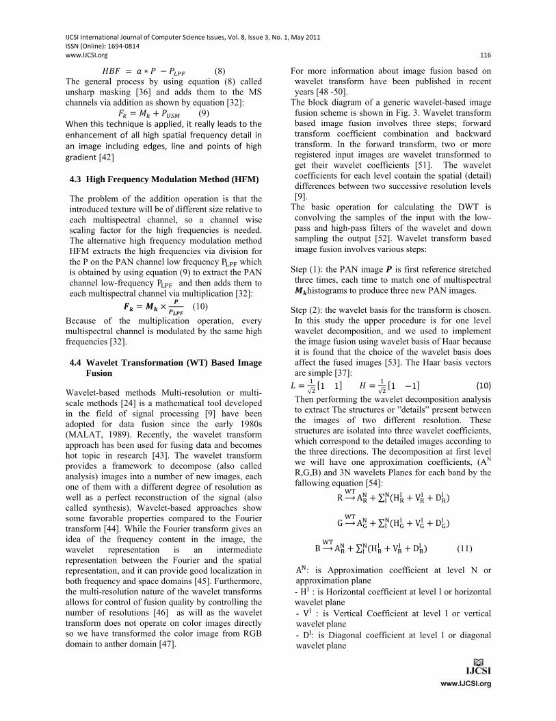
IJCSI International Journal of Computer Science Issues, Vol. 8, Issue 3, No. 1, May 2011 ISSN (Online): 1694‐0814 www.IJCSI.org 116
茎稽繋 噺 欠 茅 鶏 伐 鶏挑牒庁 (8) The general process by using equation (8) called unsharp masking [36] and adds them to the MS channels via addition as shown by equation [32]: 繋賃 噺 警賃 髪 鶏腸聴暢 (9) When this technique is applied, it really leads to the enhancement of all high spatial frequency detail in an image including edges, line and points of high gradient [42] 4.3 High Frequency Modulation Method (HFM)
The problem of the addition operation is that the introduced texture will be of different size relative to each multispectral channel, so a channel wise scaling factor for the high frequencies is needed. The alternative high frequency modulation method HFM extracts the high frequencies via division for the P on the PAN channel low frequency P宅P題 which is obtained by using equation (9) to extract the PAN channel low-frequency P宅P題 and then adds them to each multispectral channel via multiplication [32]: 擦暫 噺 捌暫 抜 皿皿鯖皿擦 (10)
Because of the multiplication operation, every multispectral channel is modulated by the same high frequencies [32]. 4.4 Wavelet Transformation (WT) Based Image
Fusion
Wavelet-based methods Multi-resolution or multi-scale methods [24] is a mathematical tool developed in the field of signal processing [9] have been adopted for data fusion since the early 1980s (MALAT, 1989). Recently, the wavelet transform approach has been used for fusing data and becomes hot topic in research [43]. The wavelet transform provides a framework to decompose (also called analysis) images into a number of new images, each one of them with a different degree of resolution as well as a perfect reconstruction of the signal (also called synthesis). Wavelet-based approaches show some favorable properties compared to the Fourier transform [44]. While the Fourier transform gives an idea of the frequency content in the image, the wavelet representation is an intermediate representation between the Fourier and the spatial representation, and it can provide good localization in both frequency and space domains [45]. Furthermore, the multi-resolution nature of the wavelet transforms allows for control of fusion quality by controlling the number of resolutions [46] as will as the wavelet transform does not operate on color images directly so we have transformed the color image from RGB domain to anther domain [47].
For more information about image fusion based on wavelet transform have been published in recent years [48 -50].
The block diagram of a generic wavelet-based image fusion scheme is shown in Fig. 3. Wavelet transform based image fusion involves three steps; forward transform coefficient combination and backward transform. In the forward transform, two or more registered input images are wavelet transformed to get their wavelet coefficients [51]. The wavelet coefficients for each level contain the spatial (detail) differences between two successive resolution levels [9].
The basic operation for calculating the DWT is convolving the samples of the input with the low-pass and high-pass filters of the wavelet and down sampling the output [52]. Wavelet transform based image fusion involves various steps:
Step (1): the PAN image 皿 is first reference stretched three times, each time to match one of multispectral 捌暫histograms to produce three new PAN images.
Step (2): the wavelet basis for the transform is chosen. In this study the upper procedure is for one level wavelet decomposition, and we used to implement the image fusion using wavelet basis of Haar because it is found that the choice of the wavelet basis does affect the fused images [53]. The Haar basis vectors are simple [37]: 詣 噺 怠√態 岷な な峅 茎 噺 怠√態 岷な 伐な峅 (10) Then performing the wavelet decomposition analysis to extract The structures or ”details” present between the images of two different resolution. These structures are isolated into three wavelet coefficients, which correspond to the detailed images according to the three directions. The decomposition at first level we will have one approximation coefficients, (AN R,G,B) and 3N wavelets Planes for each band by the fallowing equation [54]: R WT屬屐 AR択 髪 ∑ 岫HR狸択狸 髪 VR狸 髪 DR狸 岻
G WT屬屐 A鷹択 髪 ∑ 岫H鷹狸択狸 髪 V鷹狸 髪 D鷹狸 岻 B WT屬屐 AB択 髪 ∑ 岫HB狸択狸 髪 VB狸 髪 DB狸 岻 (11) A択: is Approximation coefficient at level N or
approximation plane - H狸 : is Horizontal coefficient at level l or horizontal wavelet plane - V狸 : is Vertical Coefficient at level l or vertical wavelet plane - D狸: is Diagonal coefficient at level l or diagonal wavelet plane
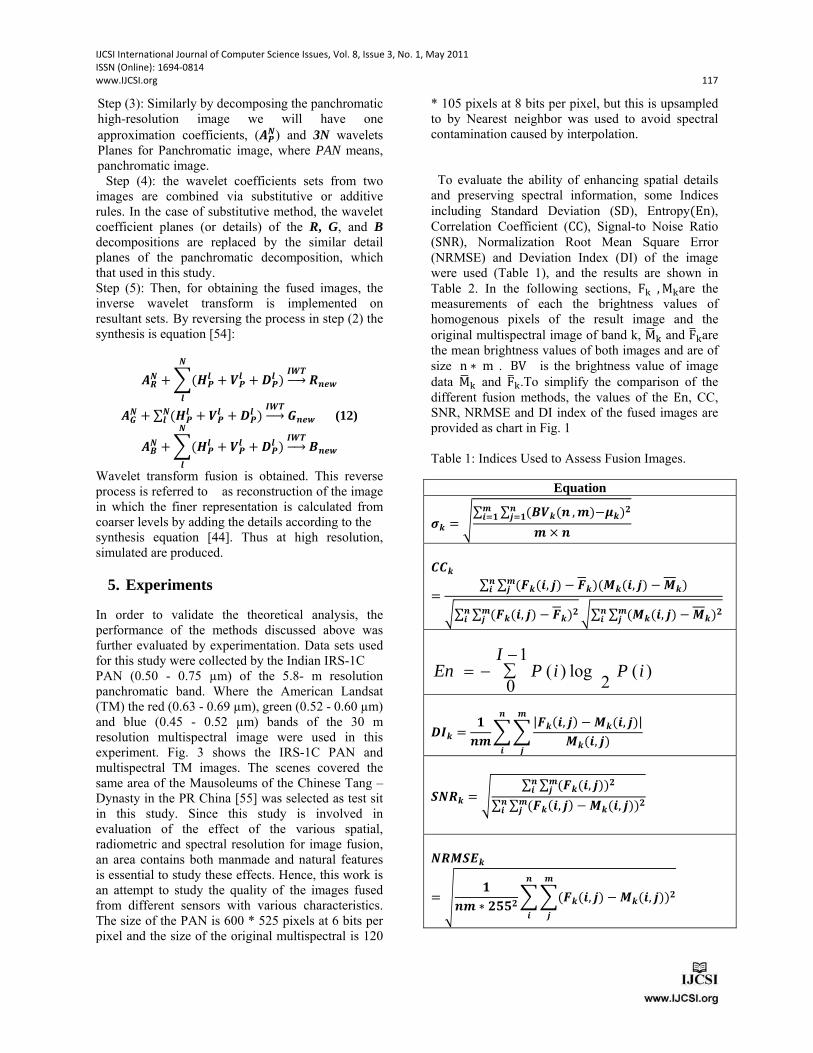
IJCSI International Journal of Computer Science Issues, Vol. 8, Issue 3, No. 1, May 2011 ISSN (Online): 1694‐0814 www.IJCSI.org 117
Step (3): Similarly by decomposing the panchromatic high-resolution image we will have one approximation coefficients, (冊皿錆) and 3N wavelets Planes for Panchromatic image, where PAN means, panchromatic image. Step (4): the wavelet coefficients sets from two images are combined via substitutive or additive rules. In the case of substitutive method, the wavelet coefficient planes (or details) of the R, G, and B decompositions are replaced by the similar detail planes of the panchromatic decomposition, which that used in this study. Step (5): Then, for obtaining the fused images, the inverse wavelet transform is implemented on resultant sets. By reversing the process in step (2) the synthesis is equation [54]: 冊三錆 髪 布岫殺皿残錆
残 髪 惨皿残 髪 拶皿残 岻 薩撒参屬吟屐 三仔蚕始 冊札錆 髪 ∑ 岫殺皿残錆残 髪 惨皿残 髪 拶皿残 岻 薩撒参屬吟屐 札仔蚕始 (12) 冊刷錆 髪 布岫殺皿残錆残 髪 惨皿残 髪 拶皿残 岻 薩撒参屬吟屐 刷仔蚕始
Wavelet transform fusion is obtained. This reverse process is referred to as reconstruction of the image in which the finer representation is calculated from coarser levels by adding the details according to the synthesis equation [44]. Thus at high resolution, simulated are produced.
5. Experiments
In order to validate the theoretical analysis, the performance of the methods discussed above was further evaluated by experimentation. Data sets used for this study were collected by the Indian IRS-1C PAN (0.50 - 0.75 µm) of the 5.8- m resolution panchromatic band. Where the American Landsat (TM) the red (0.63 - 0.69 µm), green (0.52 - 0.60 µm) and blue (0.45 - 0.52 µm) bands of the 30 m resolution multispectral image were used in this experiment. Fig. 3 shows the IRS-1C PAN and multispectral TM images. The scenes covered the same area of the Mausoleums of the Chinese Tang – Dynasty in the PR China [55] was selected as test sit in this study. Since this study is involved in evaluation of the effect of the various spatial, radiometric and spectral resolution for image fusion, an area contains both manmade and natural features is essential to study these effects. Hence, this work is an attempt to study the quality of the images fused from different sensors with various characteristics. The size of the PAN is 600 * 525 pixels at 6 bits per pixel and the size of the original multispectral is 120
* 105 pixels at 8 bits per pixel, but this is upsampled to by Nearest neighbor was used to avoid spectral contamination caused by interpolation. To evaluate the ability of enhancing spatial details and preserving spectral information, some Indices including Standard Deviation (SD), Entropy岫En), Correlation Coefficient (CC), Signal-to Noise Ratio (SNR), Normalization Root Mean Square Error (NRMSE) and Deviation Index (DI) of the image were used (Table 1), and the results are shown in Table 2. In the following sections, F谷 , M谷are the measurements of each the brightness values of homogenous pixels of the result image and the original multispectral image of band k, M拍 谷 and F博谷are the mean brightness values of both images and are of size n 茅 m . BV is the brightness value of image data M拍 谷 and F博谷.To simplify the comparison of the different fusion methods, the values of the En, CC, SNR, NRMSE and DI index of the fused images are provided as chart in Fig. 1 Table 1: Indices Used to Assess Fusion Images.
Equation 時暫 噺 俵∑ ∑ 岫刷惨暫岫仔仔斬退層 , 仕岻伐侍暫岻匝仕餐退層 仕 抜 仔
察察暫噺 ∑ ∑ 岫擦暫岫餐, 斬岻 伐 擦暫岻岫捌暫岫餐, 斬岻 伐 捌暫岻仕斬仔餐謬∑ ∑ 岫擦暫岫餐, 斬岻 伐 擦暫岻匝仕斬仔餐 謬∑ ∑ 岫捌暫岫餐, 斬岻 伐 捌暫岻匝仕斬仔餐
)(2
log)(1
0iPiP
IEn
拶薩暫 噺 層仔仕 布 布 |擦暫岫餐, 斬岻 伐 捌暫岫餐, 斬岻|捌暫岫餐, 斬岻仕斬
仔餐
傘錆三暫 噺 俵 ∑ ∑ 岫擦暫岫餐, 斬岻岻匝仕斬仔餐∑ ∑ 岫擦暫岫餐, 斬岻 伐 捌暫岫餐, 斬岻岻匝仕斬仔餐
錆三捌傘撮暫噺 彪 層仔仕 茅 匝捜捜匝 布 布岫擦暫岫餐, 斬岻 伐 捌暫岫餐, 斬岻岻匝仕
斬仔餐
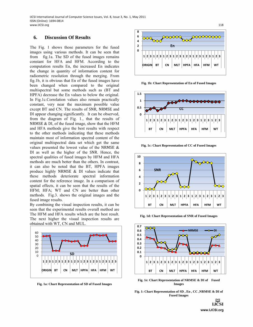
IJCSI International Journal of Computer Science Issues, Vol. 8, Issue 3, No. 1, May 2011 ISSN (Online): 1694‐0814 www.IJCSI.org 118
6. Discussion Of Results
The Fig. 1 shows those parameters for the fused images using various methods. It can be seen that from fig.1a. The SD of the fused images remains constant for HFA and HFM. According to the computation results En, the increased En indicates the change in quantity of information content for radiometric resolution through the merging. From fig.1b, it is obvious that En of the fused images have been changed when compared to the original multispectral but some methods such as (BT and HPFA) decrease the En values to below the original. In Fig.1c.Correlation values also remain practically constant, very near the maximum possible value except BT and CN. The results of SNR, NRMSE and DI appear changing significantly. It can be observed, from the diagram of Fig. 1., that the results of NRMSE & DI, of the fused image, show that the HFM and HFA methods give the best results with respect to the other methods indicating that these methods maintain most of information spectral content of the original multispectral data set which get the same values presented the lowest value of the NRMSE & DI as well as the higher of the SNR. Hence, the spectral qualities of fused images by HFM and HFA methods are much better than the others. In contrast, it can also be noted that the BT, HPFA images produce highly NRMSE & DI values indicate that these methods deteriorate spectral information content for the reference image. In a comparison of spatial effects, it can be seen that the results of the HFM; HFA; WT and CN are better than other methods. Fig.3. shows the original images and the fused image results. By combining the visual inspection results, it can be seen that the experimental results overall method are The HFM and HFA results which are the best result. The next higher the visual inspection results are obtained with WT, CN and MUL.
Fig. 1a: Chart Representation of SD of Fused Images
Fig. 1b: Chart Representation of En of Fused Images
Fig. 1c: Chart Representation of CC of Fused Images
Fig. 1d: Chart Representation of SNR of Fused Images
Fig. 1e: Chart Representation of NRMSE & DI of Fused Images
Fig. 1: Chart Representation of SD , En , CC ,NRMSE & DI of
Fused Images
0
10
20
30
40
50
60
1 2 3 1 2 3 1 2 3 1 2 3 1 2 3 1 2 3 1 2 3 1 2 3
ORIGIN BT CN MLT HPFA HFA HFM WT
SD
0
2
4
6
8
1 2 3 1 2 3 1 2 3 1 2 3 1 2 3 1 2 3 1 2 3 1 2 3
ORIGIN BT CN MLT HPFA HFA HFM WT
En
0
0.5
1
1.5
1 2 3 1 2 3 1 2 3 1 2 3 1 2 3 1 2 3 1 2 3
BT CN MLT HPFA HFA HFM WT
CC
0
2
4
6
8
10
1 2 3 1 2 3 1 2 3 1 2 3 1 2 3 1 2 3 1 2 3
BT CN MLT HPFA HFA HFM WT
SNR
0
0.1
0.2
0.3
0.4
0.5
0.6
0.7
1 2 3 1 2 3 1 2 3 1 2 3 1 2 3 1 2 3 1 2 3
BT CN MLT HPFA HFA HFM WT
NRMSE DI
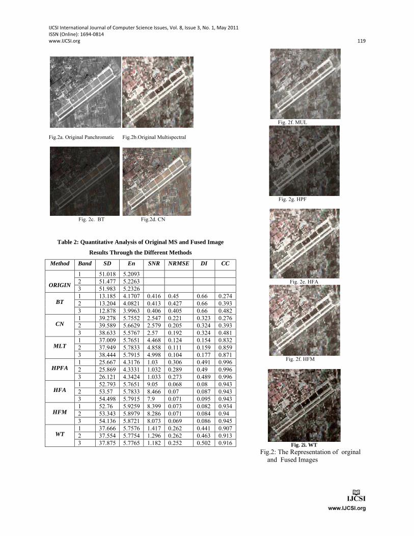
IJCSI International Journal of Computer Science Issues, Vol. 8, Issue 3, No. 1, May 2011 ISSN (Online): 1694‐0814 www.IJCSI.org 119
Fig.2a. Original Panchromatic Fig.2b.Original Multispectral
Fig. 2c. BT Fig.2d. CN
Fig. 2f. MUL
Fig. 2g. HPF
Fig. 2e. HFA
Fig. 2f. HFM
Fig. 2i. WT
Fig.2: The Representation of orginal and Fused Images
Table 2: Quantitative Analysis of Original MS and Fused Image
Results Through the Different Methods
Method Band SD En SNR NRMSE DI CC
ORIGIN
1 51.018 5.2093 2 51.477 5.2263 3 51.983 5.2326
BT 1 13.185 4.1707 0.416 0.45 0.66 0.274 2 13.204 4.0821 0.413 0.427 0.66 0.393 3 12.878 3.9963 0.406 0.405 0.66 0.482
CN 1 39.278 5.7552 2.547 0.221 0.323 0.276 2 39.589 5.6629 2.579 0.205 0.324 0.393 3 38.633 5.5767 2.57 0.192 0.324 0.481
MLT 1 37.009 5.7651 4.468 0.124 0.154 0.832 2 37.949 5.7833 4.858 0.111 0.159 0.859 3 38.444 5.7915 4.998 0.104 0.177 0.871
HPFA 1 25.667 4.3176 1.03 0.306 0.491 0.996 2 25.869 4.3331 1.032 0.289 0.49 0.996 3 26.121 4.3424 1.033 0.273 0.489 0.996
HFA 1 52.793 5.7651 9.05 0.068 0.08 0.943 2 53.57 5.7833 8.466 0.07 0.087 0.943 3 54.498 5.7915 7.9 0.071 0.095 0.943
HFM 1 52.76 5.9259 8.399 0.073 0.082 0.934 2 53.343 5.8979 8.286 0.071 0.084 0.94 3 54.136 5.8721 8.073 0.069 0.086 0.945
WT 1 37.666 5.7576 1.417 0.262 0.441 0.907 2 37.554 5.7754 1.296 0.262 0.463 0.913 3 37.875 5.7765 1.182 0.252 0.502 0.916
IJCSI International Journal of Computer Science Issues, Vol. 8, Issue 3, No. 1, May 2011 ISSN (Online): 1694‐0814 www.IJCSI.org 120
6. Conclusion Image Fusion aims at the integration of disparate and complementary data to enhance the information apparent in the images as well as to increase the reliability of the interpretation. This leads to more accurate data and increased utility in application fields like segmentation and classification. In this paper, the comparative studies undertaken by using two types of pixel –based image fusion techniques Arithmetic Combination and Frequency Filtering Methods of Pixel-Based Image Fusion Techniques as well as effectiveness based image fusion and the performance of these methods. The fusion procedures of the first type, which includes (BT; CN; MLT ) by using all PAN band, produce more distortion of spectral characteristics because such methods depend on the degree of global correlation between the PAN and multispectral bands to be enhanced. Therefore, these fusion techniques are not adequate to preserve the spectral characteristics of original multispectral. But those methods enhance the spatial quality of the imagery except BT. The fusion procedures of the second type includes HPFA; HFA; HFM and the WT based fusion method by using selected (or Filtering) PAN band frequencies including HPF, HFA, HFM and WT algorithms. The preceding analysis shows that the HFA and HFM methods maintain the spectral integrity and enhance the spatial quality of the imagery. The HPF method does not maintain the spectral integrity and does not enhance the spatial quality of the imagery. The WTF method has been shown in many published papers as an efficient image fusion. In the present work, the WTF method has shown low results. In general types of the data fusion techniques, the use of the HFM &HFA could, therefore, be strongly recommended if the goal of the merging is to achieve the best representation of the spectral information of multispectral image and the spatial details of a high-resolution panchromatic image.
References
[1] Wenbo W.,Y.Jing, K. Tingjun ,2008. “Study Of Remote Sensing Image Fusion And Its Application In Image Classification” The International Archives of the Photogrammetry, Remote Sensing and Spatial Information Sciences. Vol. XXXVII. Part B7. Beijing 2008, pp.1141-1146.
[2] Pohl C., H. Touron, 1999. “Operational Applications of Multi-Sensor Image Fusion”. International Archives of Photogrammetry and Remote Sensing, Vol. 32, Part 7-4-3 w6, Valladolid, Spain.
[3] Steinnocher K., 1999. “ Adaptive Fusion Of Multisource Raster Data Applying Filter Techniques”.
International Archives of Photogrammetry and Remote Sensing, Vol. 32, Part 7-4-3 W6, Valladolid, Spain, 3-4 June, pp.108-115.
[4] Dou W., Chen Y., Li W., Daniel Z. Sui, 2007. “A General Framework for Component Substitution Image Fusion: An Implementation Using the Fast Image Fusion Method”. Computers & Geosciences 33 (2007), pp. 219–228.
[5] Zhang Y., 2004.”Understanding Image Fusion”. Photogrammetric Engineering & Remote Sensing, pp. 657-661.
[6] Wald L., 1999a, “Some Terms Of Reference In Data Fusion”. IEEE Transactions on Geosciences and Remote Sensing, 37, 3, pp.1190- 1193.
[7] Hall D. L. and Llinas J., 1997. "An introduction to multisensor data fusion,” (invited paper) in Proceedings of the IEEE, Vol. 85, No 1, pp. 6-23.
[8] Pohl C. and Van Genderen J. L., 1998. “Multisensor Image Fusion In Remote Sensing: Concepts, Methods And Applications”.(Review Article), International Journal Of Remote Sensing, Vol. 19, No.5, pp. 823-854.
[9] Zhang Y., 2002. “PERFORMANCE ANALYSIS OF IMAGE FUSION TECHNIQUES BY IMAGE”. International Archives of Photogrammetry and Remote Sensing (IAPRS), Vol. 34, Part 4. Working Group IV/7.
[11] Ranchin, T., L. Wald, M. Mangolini, 1996a, “The ARSIS method: A General Solution For Improving Spatial Resolution Of Images By The Means Of Sensor Fusion”. Fusion of Earth Data, Proceedings EARSeL Conference, Cannes, France, 6- 8 February 1996(Paris: European Space Agency).
[12] Ranchin T., L.Wald , M. Mangolini, C. Penicand, 1996b. “On the assessment of merging processes for the improvement of the spatial resolution of multispectral SPOT XS images”. In Proceedings of the conference, Cannes, France, February 6-8, 1996, published by SEE/URISCA, Nice, France, pp. 59-67
[13] Wald L., 1999b, “Definitions And Terms Of Reference In Data Fusion”. International Archives of Photogrammetry and Remote Sensing, Vol. 32, Part 7-4-3 W6, Valladolid, Spain, 3-4 June.
[14] Pohl C., 1999.” Tools And Methods For Fusion Of Images Of Different Spatial Resolution”. International Archives of Photogrammetry and Remote Sensing, Vol. 32, Part 7-4-3 W6, Valladolid, Spain, 3-4 June.
[15] Hsu S. H., Gau P. W., I-Lin Wu I., and Jeng J. H., 2009,“Region-Based Image Fusion with Artificial Neural Network”. World Academy of Science, Engineering and Technology, 53, pp 156 -159.
[16] Zhang J., 2010. “Multi-source remote sensing data fusion: status and trends”, International Journal of Image and Data Fusion, Vol. 1, No. 1, pp. 5–24.
[17] Ehlers M., S. Klonusa, P. Johan A ˚ strand and P. Rosso ,2010. “Multi-sensor image fusion for pansharpening in remote sensing”. International Journal of Image and Data Fusion, Vol. 1, No. 1, March 2010, pp. 25–45
[18] Vijayaraj V., O’Hara C. G. And Younan N. H., 2004.“Quality Analysis Of Pansharpened Images”. 0-7803-8742-2/04/(C) 2004 IEEE,pp.85-88
IJCSI International Journal of Computer Science Issues, Vol. 8, Issue 3, No. 1, May 2011 ISSN (Online): 1694‐0814 www.IJCSI.org 121
[19] ŠVab A.and Oštir K., 2006. “High-Resolution Image Fusion: Methods To Preserve Spectral And Spatial Resolution”. Photogrammetric Engineering & Remote Sensing, Vol. 72, No. 5, May 2006, pp. 565–572.
[20] Parcharidis I. and L. M. K. Tani, 2000. “Landsat TM and ERS Data Fusion: A Statistical Approach Evaluation for Four Different Methods”. 0-7803-6359-0/00/ 2000 IEEE, pp.2120-2122.
[21] Ranchin T., Wald L., 2000. “Fusion of high spatial and spectral resolution images: the ARSIS concept and its implementation”. Photogrammetric Engineering and Remote Sensing, Vol.66, No.1, pp.49-61.
[22] Prasad N., S. Saran, S. P. S. Kushwaha and P. S. Roy, 2001. “Evaluation Of Various Image Fusion Techniques And Imaging Scales For Forest Features Interpretation”. Current Science, Vol. 81, No. 9, pp.1218
[23] Alparone L., Baronti S., Garzelli A., Nencini F. , 2004. “ Landsat ETM+ and SAR Image Fusion Based on Generalized Intensity Modulation”. IEEE Transactions on Geoscience and Remote Sensing, Vol. 42, No. 12, pp. 2832-2839
[24] Dong J.,Zhuang D., Huang Y.,Jingying Fu,2009. “Advances In Multi-Sensor Data Fusion: Algorithms And Applications “. Review , ISSN 1424-8220 Sensors 2009, 9, pp.7771-7784.
[25] Amarsaikhan D., H.H. Blotevogel, J.L. van Genderen, M. Ganzorig, R. Gantuya and B. Nergui, 2010. “Fusing high-resolution SAR and optical imagery for improved urban land cover study and classification”. International Journal of Image and Data Fusion, Vol. 1, No. 1, March 2010, pp. 83–97.
[26] Vrabel J., 1996. “Multispectral imagery band sharpening study”. Photogrammetric Engineering and Remote Sensing, Vol. 62, No. 9, pp. 1075-1083.
[27] Vrabel J., 2000. “Multispectral imagery Advanced band sharpening study”. Photogrammetric Engineering and Remote Sensing, Vol. 66, No. 1, pp. 73-79.
[28] Gangkofner U. G., P. S. Pradhan, and D. W. Holcomb, 2008. “Optimizing the High-Pass Filter Addition Technique for Image Fusion”. Photogrammetric Engineering & Remote Sensing, Vol. 74, No. 9, pp. 1107–1118.
[29] Wald L., T. Ranchin and M. Mangolini, 1997. ‘Fusion of satellite images of different spatial resolutions: Assessing the quality of resulting images’, Photogrammetric Engineering and Remote Sensing, Vol. 63, No. 6, pp. 691–699.
[30] Li J., 2001. “Spatial Quality Evaluation Of Fusion Of Different Resolution Images”. International Archives of Photogrammetry and Remote Sensing. Vol. XXXIII, Part B2, Amsterdam 2000, pp.339-346.
[31] Aiazzi, B., L. Alparone, S. Baronti, I. Pippi, and M. Selva, 2003. “Generalised Laplacian pyramid-based fusion of MS + P image data with spectral distortion minimization”.URL:http://www.isprs.org/ commission3/ proceedings02/papers/paper083.pdf (Last date accessed: 8 Feb 2010).
[32] Hill J., C. Diemer, O. Stöver, Th. Udelhoven, 1999. “A Local Correlation Approach for the Fusion of Remote Sensing Data with Different Spatial Resolutions in
Forestry Applications”. International Archives Of Photogrammetry And Remote Sensing, Vol. 32, Part 7-4-3 W6, Valladolid, Spain, 3-4 June.
[33] Carter, D.B., 1998. “Analysis of Multiresolution Data Fusion Techniques”. Master Thesis Virginia Polytechnic Institute and State University, URL: http://scholar.lib.vt.edu/theses/available /etd-32198–21323/unrestricted/Etd.pdf (last date accessed: 10 May 2008).
[34] Aiazzi B., S. Baronti , M. Selva,2008. “Image fusion through multiresolution oversampled decompositions”. in Image Fusion: Algorithms and Applications “.Edited by: Stathaki T. “Image Fusion: Algorithms and Applications”. 2008 Elsevier Ltd.
[35] Lillesand T., and Kiefer R.1994. “Remote Sensing And Image Interpretation”. 3rd Edition, John Wiley And Sons Inc.,
[36] Gonzales R. C, and R. Woods, 1992. “Digital Image Processing”. A ddison-Wesley Publishing Company.
[37] Umbaugh S. E., 1998. “Computer Vision and Image Processing: Apractical Approach Using CVIP tools”. Prentic Hall.
[38] Green W. B., 1989. Digital Image processing A system Approach”.2nd Edition. Van Nostrand Reinholld, New York.
[39] Sangwine S. J., and R.E.N. Horne, 1989. “The Colour Image Processing Handbook”. Chapman & Hall.
[40] Gross K. and C. Moulds, 1996. Digital Image Processing. (http://www.net/Digital Image Processing.htm). (last date accessed: 10 Jun 2008).
[41] Jensen J.R., 1986. “Introductory Digital Image Processing A Remote Sensing Perspective”. Englewood Cliffs, New Jersey: Prentice-Hall.
[42] Richards J. A., and Jia X., 1999. “Remote Sensing Digital Image Analysis”. 3rd Edition. Springer - verlag Berlin Heidelberg New York.
[43] Cao D., Q. Yin, and P. Guo,2006. “Mallat Fusion for Multi-Source Remote Sensing Classification”. Proceedings of the Sixth International Conference on Intelligent Systems Design and Applications (ISDA'06)
[44] Hahn M. and F. Samadzadegan, 1999. “ Integration of DTMS Using Wavelets”. International Archives Of Photogrammetry And Remote Sensing, Vol. 32, Part 7-4-3 W6, Valladolid, Spain, 3-4 June. 1999.
[45] King R. L. and Wang J., 2001. “A Wavelet Based Algorithm for Pan Sharpening Landsat 7 Imagery”. 0-7803-7031-7/01/ 02001 IEEE, pp. 849- 851
[46] Kumar Y. K.,. “Comparison Of Fusion Techniques Applied To Preclinical Images: Fast Discrete Curvelet Transform Using Wrapping Technique & Wavelet Transform”. Journal Of Theoretical And Applied Information Technology.© 2005 - 2009 Jatit, pp. 668- 673
[47] Malik N. H., S. Asif M. Gilani, Anwaar-ul-Haq, 2008. “Wavelet Based Exposure Fusion”. Proceedings of the World Congress on Engineering 2008 Vol I WCE 2008, July 2 - 4, 2008, London, U.K
[48] Li S., Kwok J. T., Wang Y.., 2002. “Using The Discrete Wavelet Frame Transform To Merge Landsat TM And SPOT Panchromatic Images”. Information Fusion 3 (2002), pp.17–23.
IJCSI International Journal of Computer Science Issues, Vol. 8, Issue 3, No. 1, May 2011 ISSN (Online): 1694‐0814 www.IJCSI.org 122
[49] Garzelli, A. and Nencini, F., 2006. “Fusion of panchromatic and multispectral images by genetic Algorithms”. IEEE Transactions on Geoscience and Remote Sensing, 40, 3810–3813.
[50] Aiazzi, B., Baronti, S., and Selva, M., 2007. “Improving component substitution pan-sharpening through multivariate regression of MS+Pan data”. IEEE Transactions on Geoscience and Remote Sensing, Vol.45, No.10, pp. 3230–3239.
[51] Das A. and Revathy K., 2007. “A Comparative Analysis of Image Fusion Techniques for Remote Sensed Images”. Proceedings of the World Congress on Engineering 2007, Vol. I, WCE 2007, July 2 – 4,London, U.K.
[52] Pradhan P.S., King R.L., 2006. “Estimation of the Number of Decomposition Levels for a Wavelet-Based Multi-resolution Multi-sensor Image Fusion”. IEEE Transaction of Geosciences and Remote Sensing, Vol. 44, No. 12, pp. 3674-3686.
[53] Hu Deyong H. L., 1998. “A fusion Approach of Multi-Sensor Remote Sensing Data Based on Wavelet Transform”. URL: http://www.gisdevelopment.net/AARS/ACRS1998/Digital Image Processing (last date accessed: 15 Feb 2009).
[54] Li S.,Li Z.,Gong J.,2010.“Multivariate statistical analysis of measures for assessing the quality of image fusion”. International Journal of Image and Data Fusion Vol. 1, No. 1, March 2010, pp. 47–66.
[55] Böhler W. and G. Heinz, 1998. “Integration of high Resolution Satellite Images into Archaeological Docmentation”. Proceeding International Archives of Photogrammetry and Remote Sensing, Commission V, Working Group V/5, CIPA International Symposium, Published by the Swedish Society for Photogrammetry and Remote Sensing, Goteborg. (URL: http://www.i3mainz.fh-mainz.de/publicat/cipa-98/sat-im.html (Last date accessed: 28 Oct. 2000).
AUTHORS Mrs . Firouz Abdullah Al-Wassai1.Received the B.Sc. degree in, Physics from University of Sana’a, Yemen, Sana’a, in 1993. The M.Sc.degree in, Physics from Bagdad University , Iraqe, in 2003, Research student.Ph.D in thedepartment of computer science (S.R.T.M.U), India, Nanded. Dr. N.V. Kalyankar .B.Sc.Maths, Physics, Chemistry, Marathwada University, Aurangabad, India, 1978. M Sc.Nuclear Physics, Marathwada University, Aurangabad, India, 1980.Diploma in Higher Education, Shivaji University, Kolhapur, India, 1984.Ph.D. in Physics, Dr.B.A.M.University, Aurangabad, India, 1995.Principal Yeshwant Mahavidyalaya College, Membership of Academic Bodies,Chairman, Information Technology Society State Level Organization, Life Member of Indian Laser Association, Member Indian Institute of Public Administration, New Delhi, Member Chinmay Education Society, Nanded.He has one publication book, seven journals papers, two seminars Papers and three conferences papers. Dr. Ali A. Al-Zuky. B.Sc Physics Mustansiriyah University, Baghdad , Iraq, 1990. M Sc. In1993 and Ph. D. in1998 from University of Baghdad, Iraq. He was supervision for 40 post-graduate students (MSc. & Ph.D.) in different fields (physics, computers and Computer Engineering and Medical Physics). He
has More than 60 scientific papers published in scientific journals in several scientific conferences.
International Journal of Software Engineering Research & Practices Vol.1, Issue 4, Oct, 2011
Print-ISSN: 2231-2048 e-ISSN: 2231-0320
© RG Education Society (INDIA)
Feature-Level Based Image Fusion Of Multisensory Images
Firouz Abdullah Al-Wassai
1 Dr. N.V. Kalyankar
2
Research Student, Computer Science Dept. Principal, Yeshwant Mahavidyala College
(SRTMU), Nanded, India Nanded, India
[email protected] [email protected]
Dr. Ali A. Al-Zaky3
Assistant Professor, Dept.of Physics, College of Science, Mustansiriyah Un.
Baghdad – Iraq.
Abstract- Until now, of highest relevance for remote sensing
data processing and analysis have been techniques for pixel
level image fusion. So, This paper attempts to undertake the
study of Feature-Level based image fusion. For this purpose,
feature based fusion techniques, which are usually based on
empirical or heuristic rules, are employed. Hence, in this
paper we consider feature extraction (FE) for fusion. It aims at
finding a transformation of the original space that would
produce such new features, which preserve or improve as
much as possible. This study introduces three different types of
Image fusion techniques including Principal Component
Analysis based Feature Fusion (PCA), Segment Fusion (SF)
and Edge fusion (EF). This paper also devotes to concentrate
on the analytical techniques for evaluating the quality of image
fusion (F) by using various methods including ( ), ), ( ),
( ), (NRMSE) and ( ) to estimate the quality and degree of
information improvement of a fused image quantitatively.
Keywords: Image fusion , Feature, Edge Fusion, Segment
Fusion, IHS, PCA
INTRODUCTION
Over the last years, image fusion techniques have interest within the remote sensing community. The reason of this is that in most cases the new generation of remote sensors with very high spatial resolution acquires image datasets in two separate modes: the highest spatial resolution is obtained for panchromatic images (PAN) whereas multispectral information (MS) is associated with lower spatial resolution [1].
Usually, the term „fusion‟ gets several words to appear, such as merging, combination, synergy, integration … and several others that express more or less the same meaning the concept have since it appeared in literature [Wald L., 1999a]. Different definitions of data fusion can be found in literature, each author interprets this term differently depending on his research interests, such as [2, 3] . A general definition of data fusion can be adopted as fallowing: “Data fusion is a formal framework which expresses means and tools for the alliance of data originating from different sources. It aims at
obtaining information of greater quality; the exact definition of „greater quality‟ will depend upon the application” [4-6].
Image fusion techniques can be classified into three
categories depending on the stage at which fusion takes place; it is often divided into three levels, namely: pixel level, feature level and decision level of representation [7,8]. Until now, of highest relevance for remote sensing data processing and analysis have been techniques for pixel level image fusion for which many different methods have been developed and a rich theory exists [1]. Researchers have shown that fusion techniques that operate on such features in the transform domain yield subjectively better fused images than pixel based techniques [9].
For this purpose, feature based fusion techniques that is usually based on empirical or heuristic rules is employed. Because a general theory is lacking fusion, algorithms are usually developed for certain applications and datasets. [10]. In this paper we consider feature extraction (FE) for fusion.It is aimed at finding a transformation of the original space that would produce such new features, which are preserved or improved as much as possible. This study introduces three different types of Image fusion techniques including Principal Component Analysis based Feature Fusion (PCA), Segment Fusion (SF) and Edge fusion (EF). It will examine and estimate the quality and degree of information improvement of a fused image quantitatively and the ability of this fused image to preserve the spectral integrity of the original image by fusing different sensor with different characteristics of temporal, spatial, radiometric and Spectral resolutions of TM & IRS-1C PAN images. The subsequent sections of this paper are organized as follows: section II gives the brief overview of the related work. III covers the experimental results and analysis, and is subsequently followed by the conclusion.
FEATURE LEVEL METHODS
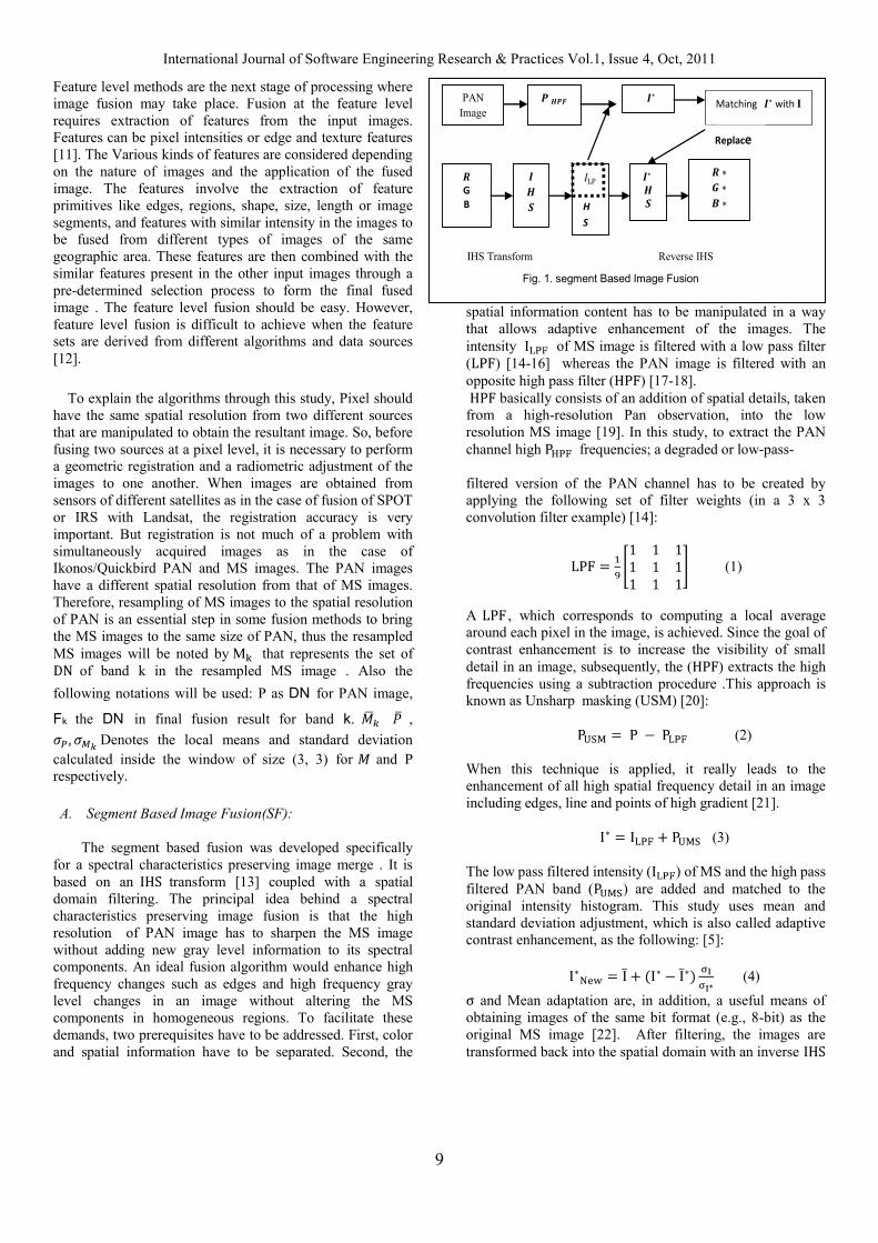
International Journal of Software Engineering Research & Practices Vol.1, Issue 4, Oct, 2011
9
Feature level methods are the next stage of processing where
image fusion may take place. Fusion at the feature level
requires extraction of features from the input images.
Features can be pixel intensities or edge and texture features
[11]. The Various kinds of features are considered depending
on the nature of images and the application of the fused
image. The features involve the extraction of feature
primitives like edges, regions, shape, size, length or image
segments, and features with similar intensity in the images to
be fused from different types of images of the same
geographic area. These features are then combined with the
similar features present in the other input images through a
pre-determined selection process to form the final fused
image . The feature level fusion should be easy. However,
feature level fusion is difficult to achieve when the feature
sets are derived from different algorithms and data sources
[12].
To explain the algorithms through this study, Pixel should
have the same spatial resolution from two different sources
that are manipulated to obtain the resultant image. So, before
fusing two sources at a pixel level, it is necessary to perform
a geometric registration and a radiometric adjustment of the
images to one another. When images are obtained from
sensors of different satellites as in the case of fusion of SPOT
or IRS with Landsat, the registration accuracy is very
important. But registration is not much of a problem with
simultaneously acquired images as in the case of
Ikonos/Quickbird PAN and MS images. The PAN images
have a different spatial resolution from that of MS images.
Therefore, resampling of MS images to the spatial resolution
of PAN is an essential step in some fusion methods to bring
the MS images to the same size of PAN, thus the resampled
MS images will be noted by that represents the set of
of band k in the resampled MS image . Also the
following notations will be used: Ρ as DN for PAN image,
Fk the DN in final fusion result for band k. ,
Denotes the local means and standard deviation
calculated inside the window of size (3, 3) for and Ρ respectively.
A. Segment Based Image Fusion(SF):
The segment based fusion was developed specifically
for a spectral characteristics preserving image merge . It is
based on an transform [13] coupled with a spatial
domain filtering. The principal idea behind a spectral
characteristics preserving image fusion is that the high
resolution of PAN image has to sharpen the MS image
without adding new gray level information to its spectral
components. An ideal fusion algorithm would enhance high
frequency changes such as edges and high frequency gray
level changes in an image without altering the MS
components in homogeneous regions. To facilitate these
demands, two prerequisites have to be addressed. First, color
and spatial information have to be separated. Second, the
spatial information content has to be manipulated in a way
that allows adaptive enhancement of the images. The
intensity of MS image is filtered with a low pass filter
( ) [14-16] whereas the PAN image is filtered with an
opposite high pass filter ( ) [17-18].
basically consists of an addition of spatial details, taken
from a high-resolution Pan observation, into the low
resolution MS image [19]. In this study, to extract the PAN
channel high frequencies; a degraded or low-pass-
filtered version of the PAN channel has to be created by
applying the following set of filter weights (in a 3 x 3
convolution filter example) [14]:
(1)
A , which corresponds to computing a local average
around each pixel in the image, is achieved. Since the goal of
contrast enhancement is to increase the visibility of small
detail in an image, subsequently, the ( ) extracts the high
frequencies using a subtraction procedure .This approach is
known as Unsharp masking (USM) [20]:
(2)
When this technique is applied, it really leads to the
enhancement of all high spatial frequency detail in an image
including edges, line and points of high gradient [21].
(3)
The low pass filtered intensity ( ) of MS and the high pass
filtered PAN band ( ) are added and matched to the
original intensity histogram. This study uses mean and
standard deviation adjustment, which is also called adaptive
contrast enhancement, as the following: [5]:
(4)
and Mean adaptation are, in addition, a useful means of
obtaining images of the same bit format (e.g., 8-bit) as the
original MS image [22]. After filtering, the images are
transformed back into the spatial domain with an inverse
薩∗
� 殺�擦
Fig. 1. segment Based Image Fusion
PAN
Image
三
G
B
薩 殺 傘
傘
H
S
殺 傘
薩∗
三 ∗ 札 ∗ � ∗
�LP
Matching 薩∗ with I
Replace
IHS Transform Reverse IHS

International Journal of Software Engineering Research & Practices Vol.1, Issue 4, Oct, 2011
10
and added together( ) to form a fused intensity component
with the low frequency information from the low resolution
MS image and the high-frequency information from the high
resolution PAN image. This new intensity component and
the original hue and saturation components of the MS image
form a new image. As the last step, an inverse
transformation produces a fused image that contains the
spatial resolution of the panchromatic image and the spectral
characteristics of the MS image. An overview flowchart of
the segment Fusion is presented in Fig. 1.
B. PCA-based Feature Fusion
The PCA is used extensively in remote sensing
applications by many such as [23 -30]. It is used for
dimensionality reduction, feature enhancement, and image
fusion. The PCA is a statistical approach [27] that
transforms a multivariate inter-correlated data set into a new
un-correlated data set [31]. The PCA technique can also be
found under the expression Karhunen Loeve approach [3].
PCA transforms or projects the features from the original
domain to a new domain (known as PCA domain) where the
features are arranged in the order of their variance. The
features in the transformed domain are formed by the linear
combination of the original features and are uncorrelated.
Fusion process is achieved in the PCA domain by retaining
only those features that contain a significant amount of
information. The main idea behind PCA is to determine the
features that explain as much of the total variation in the data
as possible with as few of these features as possible. The
PCA computation done on an N-by-N of MS image having 3
contiguous spectral bands is explained below. The
computation of the PCA transformation matrix is based on
the eigenvalue decomposition of the covariance matrix is
defined as[33]:
(5)
where is the spectral signature , denotes the mean
spectral signature and is the total number of spectral
signatures. the total number of spectral signatures. In order to
find the new orthogonal axes of the PCA space, Eigen
decomposition of the covariance matrix is performed. The
eigen decomposition of the covariance matrix is given by
(6)
where denotes the eigenvalue, denotes the
corresponding eigenvector and varies from 1 to 3. The
eigenvalues denote the amount of variance present in the
corresponding eigenvectors. The eigenvectors form the axes
of the PCA space, and they are orthogonal to each other. The
eigenvalues are arranged in decreasing order of the variance.
The PCA transformation matrix, A, is formed by choosing
the eigenvectors corresponding to the largest eigenvalues.
The PCA transformation matrix A is given by
(7)
where are the eigenvectors associated with the J
largest eigenvalues obtained from the eigen decomposition of
the covariance matrix . The data projected onto the
corresponding eigenvectors form the reduced uncorrelated
features that are used for further fusion processes.
Computation of the principal components can be presented
with the following algorithm by [34]:
1) Calculate the covariance matrix from the input
data.
2) Compute the eigenvalues and eigenvectors of and
sort them in a descending order with respect to the
eigenvalues.
3) Form the actual transition matrix by taking the
predefined number of components (eigenvectors).
4) Finally, multiply the original feature space with the
obtained transition matrix, which yields a lower-
dimensional representation.
The PCA based feature fusion is shown in Fig. 2. The input
MS are, first, transformed into the same number of
uncorrelated principal components. Its most important steps
are:
a. perform a principal component transformation to
convert a set of MS bands (three or more bands)
into a set of principal components.
b. Substitute the first principal component PC1 by
the PAN band whose histogram has previously
been matched with that of the first principal
component. In this study the mean and standard
deviation are matched by :
(8)
Perform a reverse principal component
transformation to convert the replaced components
back to the original image space. A set of fused MS
bands is produced after the reverse transform [35-
37].
The mathematical models of the forward and backward
transformation of this method are described by [37], whose
processes are represented by eq. (9) and (10). The
transformation matrix contains the eigenvectors, ordered
with respect to their Eigen values. It is orthogonal and
determined either from the covariance matrix or the
correlation matrix of the input MS. PCA performed using the
covariance matrix is referred to as nun standardized PCA,
while PCA performed using the correlation matrix is referred
to as standardized PCA [37]:
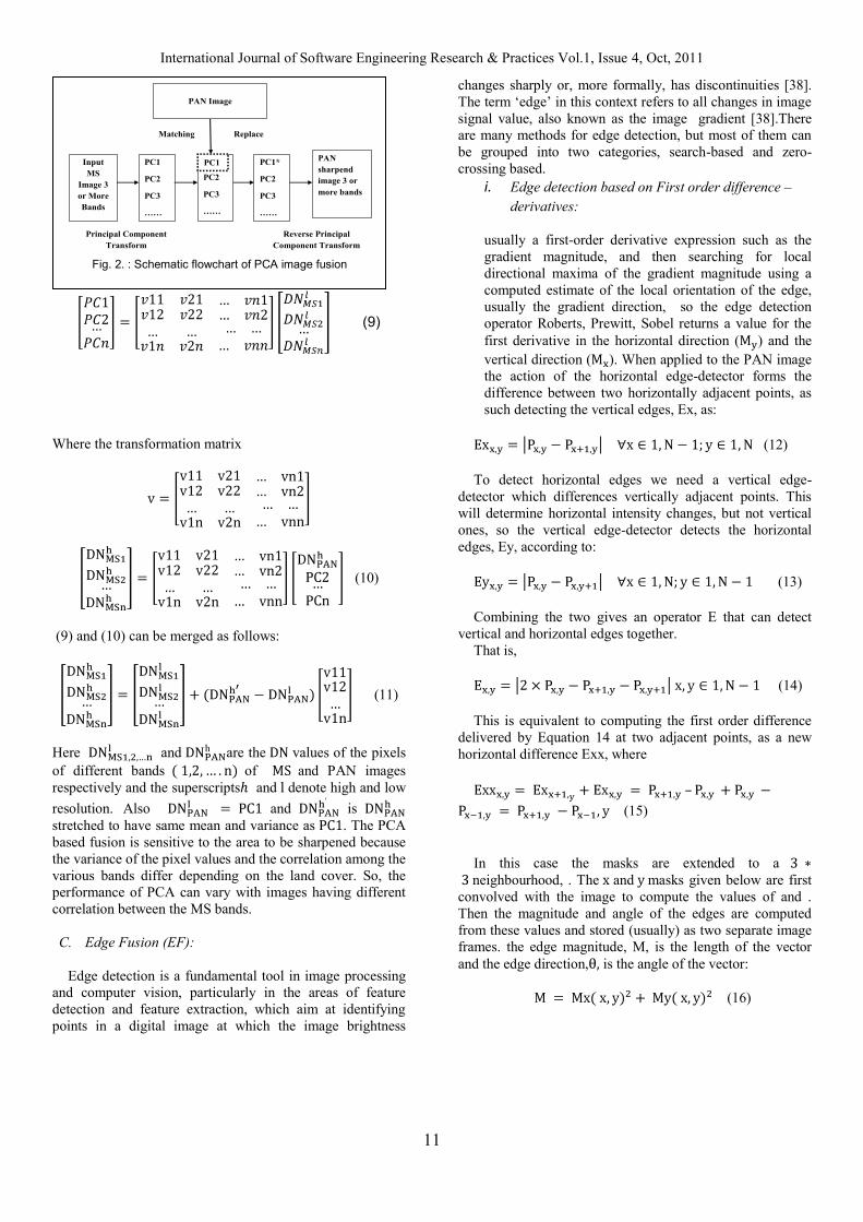
International Journal of Software Engineering Research & Practices Vol.1, Issue 4, Oct, 2011
11
(9)
Where the transformation matrix
(10)
(9) and (10) can be merged as follows:
(11)
Here and are the values of the pixels
of different bands of and PAN images
respectively and the superscripts and denote high and low
resolution. Also and is
stretched to have same mean and variance as . The PCA
based fusion is sensitive to the area to be sharpened because
the variance of the pixel values and the correlation among the
various bands differ depending on the land cover. So, the
performance of PCA can vary with images having different
correlation between the MS bands.
C. Edge Fusion (EF):
Edge detection is a fundamental tool in image processing
and computer vision, particularly in the areas of feature
detection and feature extraction, which aim at identifying
points in a digital image at which the image brightness
changes sharply or, more formally, has discontinuities [38].
The term „edge‟ in this context refers to all changes in image signal value, also known as the image gradient [38].There
are many methods for edge detection, but most of them can
be grouped into two categories, search-based and zero-
crossing based.
i. Edge detection based on First order difference –derivatives:
usually a first-order derivative expression such as the
gradient magnitude, and then searching for local
directional maxima of the gradient magnitude using a
computed estimate of the local orientation of the edge,
usually the gradient direction, so the edge detection
operator Roberts, Prewitt, Sobel returns a value for the
first derivative in the horizontal direction ( ) and the
vertical direction ( ). When applied to the PAN image
the action of the horizontal edge-detector forms the
difference between two horizontally adjacent points, as
such detecting the vertical edges, Ex, as:
(12)
To detect horizontal edges we need a vertical edge-
detector which differences vertically adjacent points. This
will determine horizontal intensity changes, but not vertical
ones, so the vertical edge-detector detects the horizontal
edges, Ey, according to:
(13)
Combining the two gives an operator E that can detect
vertical and horizontal edges together.
That is,
(14)
This is equivalent to computing the first order difference
delivered by Equation 14 at two adjacent points, as a new
horizontal difference Exx, where
– (15)
In this case the masks are extended to a
neighbourhood, . The and masks given below are first
convolved with the image to compute the values of and .
Then the magnitude and angle of the edges are computed
from these values and stored (usually) as two separate image
frames. the edge magnitude, M, is the length of the vector
and the edge direction, is the angle of the vector:
(16)
Fig. 2. : Schematic flowchart of PCA image fusion
PAN Image
Input
MS
Image 3
or More
Bands
PC1
PC2
PC3
……
PC1
PC2
PC3
……
PC1*
PC2
PC3
……
PAN
sharpend
image 3 or
more bands
PC1
Matching Replace
Principal Component
Transform
Reverse Principal
Component Transform
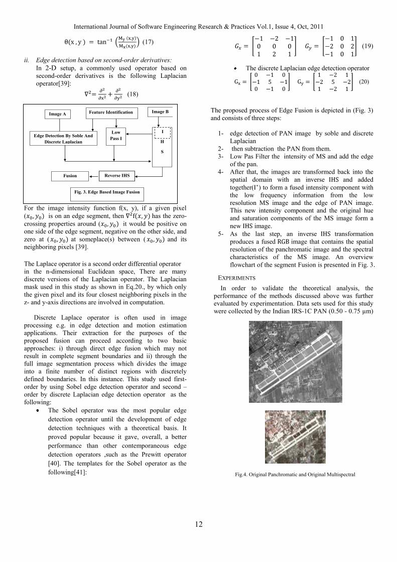
International Journal of Software Engineering Research & Practices Vol.1, Issue 4, Oct, 2011
12
(17)
ii. Edge detection based on second-order derivatives:
In 2-D setup, a commonly used operator based on
second-order derivatives is the following Laplacian
operator[39]:
(18)
For the image intensity function f(x, y), if a given pixel
( is on an edge segment, then has the zero-
crossing properties around ( it would be positive on
one side of the edge segment, negative on the other side, and
zero at ( at someplace(s) between ( and its
neighboring pixels [39].
The Laplace operator is a second order differential operator
in the n-dimensional Euclidean space, There are many
discrete versions of the Laplacian operator. The Laplacian
mask used in this study as shown in Eq.20., by which only
the given pixel and its four closest neighboring pixels in the
z- and y-axis directions are involved in computation.
Discrete Laplace operator is often used in image
processing e.g. in edge detection and motion estimation
applications. Their extraction for the purposes of the
proposed fusion can proceed according to two basic
approaches: i) through direct edge fusion which may not
result in complete segment boundaries and ii) through the
full image segmentation process which divides the image
into a finite number of distinct regions with discretely
defined boundaries. In this instance. This study used first-
order by using Sobel edge detection operator and second –
order by discrete Laplacian edge detection operator as the
following:
The Sobel operator was the most popular edge
detection operator until the development of edge
detection techniques with a theoretical basis. It
proved popular because it gave, overall, a better
performance than other contemporaneous edge
detection operators ,such as the Prewitt operator
[40]. The templates for the Sobel operator as the
following[41]:
(19)
The discrete Laplacian edge detection operator
(20)
The proposed process of Edge Fusion is depicted in (Fig. 3)
and consists of three steps:
1- edge detection of PAN image by soble and discrete
Laplacian 2- then subtraction the PAN from them. 3- Low Pas Filter the intensity of MS and add the edge
of the pan. 4- After that, the images are transformed back into the
spatial domain with an inverse and added
together( ) to form a fused intensity component with
the low frequency information from the low
resolution MS image and the edge of PAN image.
This new intensity component and the original hue
and saturation components of the MS image form a
new image. 5- As the last step, an inverse transformation
produces a fused image that contains the spatial
resolution of the panchromatic image and the spectral
characteristics of the MS image. An overview
flowchart of the segment Fusion is presented in Fig. 3.
EXPERIMENTS
In order to validate the theoretical analysis, the
performance of the methods discussed above was further
evaluated by experimentation. Data sets used for this study
were collected by the Indian IRS-1C PAN (0.50 - 0.75 µm)
Fig. 3. Edge Based Image Fusion
Fusion
Image A
Reverse IHS
Image B
Edge Detection By Soble And
Discrete Laplacian
Feature Identification
Low
Pass I
H
S
I
Fig.4. Original Panchromatic and Original Multispectral

International Journal of Software Engineering Research & Practices Vol.1, Issue 4, Oct, 2011
13
of the 5.8- m resolution panchromatic band. Where the
American Landsat (TM) the red (0.63 - 0.69 µm), green
(0.52 - 0.60 µm) and blue (0.45 - 0.52 µm) bands of the 30
m resolution multispectral image were used in this work.
Fig.4 shows the IRS-1C PAN and multispectral TM
images. The scenes covered the same area of the
Mausoleums of the Chinese Tang – Dynasty in the PR
China [42] was selected as test sit in this study. Since this
study is involved in evaluation of the effect of the various
spatial, radiometric and spectral resolution for image
fusion, an area contains both manmade and natural features
is essential to study these effects. Hence, this work is an
attempt to study the quality of the images fused from
different sensors with various characteristics. The size of
the PAN is 600 * 525 pixels at 6 bits per pixel and the size
of the original multispectral is 120 * 105 pixels at 8 bits
per pixel, but this is upsampled to by nearest neighbor. It
was used to avoid spectral contamination caused by
interpolation, which does not change the data file value.
The pairs of images were geometrically registered to each
other.
To evaluate the ability of enhancing spatial details and
preserving spectral information, some Indices including :
Standard Deviation ( ),
Entropy ) :
Signal-to Noise Ratio ( )
Deviation Index ( )
Correlation Coefficient ( )
Normalization Root Mean Square
Error (NRMSE)
where the are the measurements of each the
brightness values of homogenous pixels of the result
image and the original MS image of band , and
are the mean brightness values of both images and
are of size . is the brightness value of
image data and .To simplify the comparison of
the different fusion methods, the values of the , ,
, and index of the fused images are
provided as chart in Fig. 5
DISCUSSION OF RESULTS
From table1 and Fig. 5 shows those parameters for the
fused images using various methods. It can be seen that from
Fig. 5a and table1 the SD results of the fused images remains
constant for SF. According to the computation results En in
table1, the increased En indicates the change in quantity of
information content for radiometric resolution through the
merging. From table1 and Fig.3b, it is obvious that En of the
fused images have been changed when compared to the
original multispectral excepted the PCA. In Fig.3c and
table1 the maximum correlation values was for PCA , the
maximum results of was for SF. The results of ,
and appear changing significantly. It can be
observed, from table1 with the diagram of Fig. 5d & Fig. 5e,
that the results of SNR, & of the fused image,
show that the SF method gives the best results with respect
to the other methods indicating that this method maintains
most of information spectral content of the original MS data
set which gets the same values presented the lowest value of
the and as well as the high of the CC and .
Hence, the spectral quality of fused image SF technique is
much better than the others. In contrast, it can also be noted
that the PCA image produce highly & values
indicating that these methods deteriorate spectral information
content for the reference image. By combining the visual
Table 1: Quantitative Analysis of Original MS and Fused Image Results Through the
Different Methods
Method Band SD En SNR NRMSE DI CC
ORIGIN
1 51.018 5.2093 / / / /
2 51.477 5.2263 / / / /
3 51.983 5.2326 / / / /
EF
1 55.184 6.0196 6.531 0.095 0.138 0.896
2 55.792 6.0415 6.139 0.096 0.151 0.896
3 56.308 6.0423 5.81 0.097 0.165 0.898
PCA
1 47.875 5.1968 6.735 0.105 0.199 0.984
2 49.313 5.2485 6.277 0.108 0.222 0.985
3 47.875 5.1968 6.735 0.105 0.199 0.984
SF
1 51.603 5.687 9.221 0.067 0.09 0.944
2 52.207 5.7047 8.677 0.067 0.098 0.944
3 53.028 5.7123 8.144 0.068 0.108 0.945
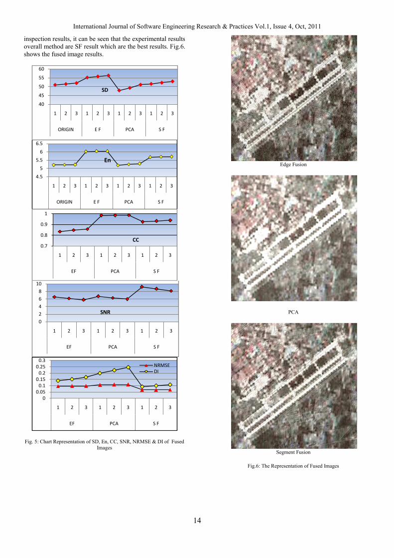
International Journal of Software Engineering Research & Practices Vol.1, Issue 4, Oct, 2011
14
inspection results, it can be seen that the experimental results
overall method are SF result which are the best results. Fig.6.
shows the fused image results.
Fig. 5: Chart Representation of SD, En, CC, SNR, NRMSE & DI of Fused
Images
Edge Fusion
PCA
Segment Fusion
Fig.6: The Representation of Fused Images
40
45
50
55
60
1 2 3 1 2 3 1 2 3 1 2 3
ORIGIN E F PCA S F
SD
4.5
5
5.5
6
6.5
1 2 3 1 2 3 1 2 3 1 2 3
ORIGIN E F PCA S F
En
0.7
0.8
0.9
1
1 2 3 1 2 3 1 2 3
EF PCA S F
CC
0
2
4
6
8
10
1 2 3 1 2 3 1 2 3
EF PCA S F
SNR
0
0.05
0.1
0.15
0.2
0.25
0.3
1 2 3 1 2 3 1 2 3
EF PCA S F
NRMSE
DI

International Journal of Software Engineering Research & Practices Vol.1, Issue 4, Oct, 2011
15
CONCLUSION
Image Fusion aims at the integration of disparate and
complementary data to enhance the information apparent in
the images as well as to increase the reliability of the
interpretation. This leads to more accurate data and increased
utility in application fields like segmentation and
classification. In this paper, we proposed three different types
of Image fusion techniques including PCA, SF and EF image
fusion. Experimental results and statistical evaluation further
show that the proposed SF technique maintains the spectral
integrity and enhances the spatial quality of the imagery. The
proposed SF technique yields best performance among all the
fusion algorithms.
The use of the SF based fusion technique could, therefore, be
strongly recommended if the goal of the merging is to
achieve the best representation of the spectral information of
MS image and the spatial details of a high-resolution PAN
image. Also, the analytical technique of DI is much more
useful for measuring the spectral distortion than NRMSE
since the NRMSE gave the same results for some methods;
but the DI gave the smallest different ratio between those
methods, therefore , it is strongly recommended to use the
because of its mathematical more precision as quality
indicator.
REFERENCES
[1] Ehlers M. ,2007 . “Segment Based Image Analysis And Image Fusion”. ASPRS 2007 Annual Conference,Tampa, Florida , May 7-
11, 2007 [2] Hall D. L. and Llinas J., 1997. "An introduction to multisensor data
fusion,” (invited paper) in Proceedings of the IEEE, Vol. 85, No 1, pp. 6-23.
[3] Pohl C. and Van Genderen J. L., 1998. “Multisensor Image Fusion In Remote Sensing: Concepts, Methods And Applications”.(Review Article), International Journal Of Remote Sensing, Vol. 19, No.5, pp. 823-854.
[4] Ranchin T., L. Wald, M. Mangolini, 1996a, “The ARSIS method: A General Solution For Improving Spatial Resolution Of Images By The Means Of Sensor Fusion”. Fusion of Earth Data, Proceedings
EARSeL Conference, Cannes, France, 6- 8 February 1996(Paris:
European Space Agency). [5] Ranchin T., L.Wald , M. Mangolini, C. Penicand, 1996b. “On the
assessment of merging processes for the improvement of the spatial
resolution of multispectral SPOT XS images”. In Proceedings of the conference, Cannes, France, February 6-8, 1996, published by
SEE/URISCA, Nice, France, pp. 59-67.
[6] Wald L., 1999b, “Definitions And Terms Of Reference In Data Fusion”. International Archives of Assessing the quality of resulting
images‟, Photogrammetric Engineering and Remote Sensing, Vol. 63, No. 6, pp. 691–699.
[7] Zhang J., 2010. “Multi-source remote sensing data fusion: status and
trends”, International Journal of Image and Data Fusion, Vol. 1, No. 1, pp. 5–24.
[8] Ehlers M., S. Klonusa, P. Johan A ˚ strand and P. Rosso ,2010. “Multi-sensor image fusion for pansharpening in remote sensing”. International Journal of Image and Data Fusion, Vol. 1, No. 1, March 2010, pp. 25–45
[9] Farhad Samadzadegan, “Data Integration Related To Sensors, Data
And Models”. Commission VI, WG VI/4. [10] Tomowski D., Ehlers M., U. Michel, G. Bohmann , 2006.“Decision
Based Data Fusion Techniques For Settlement Area Detection From
Multisensor Remote Sensing Data”. 1st EARSeL Workshop of the
SIG Urban Remote Sensing Humboldt-Universität zu Berlin, 2-3
March 2006, pp. 1- 8. [11] Kor S. and Tiwary U.,2004.‟‟ Feature Level Fusion Of Multimodal
Medical Images In Lifting Wavelet Transform Domain”.Proceedings of the 26th Annual International Conference of the IEEE EMBS San Francisco, CA, USA 0-7803-8439-3/04/©2004 IEEE , pp. 1479-
1482
[12] Chitroub S., 2010. “Classifier combination and score level fusion: concepts and practical aspects”. International Journal of Image and Data Fusion, Vol. 1, No. 2, June 2010, pp. 113–135.
[13] Firouz A. Al-Wassai, Dr. N.V. Kalyankar2, Dr. A. A. Al-zuky ,2011a. “ The IHS Transformations Based Image Fusion”. Journal of Global Research in Computer Science, Volume 2, No. 5, May
2011, pp. 70 – 77. [14] Green W. B., 1989. Digital Image processing A system
Approach”.2nd Edition. Van Nostrand Reinholld, New York. [15] Hill J., C. Diemer, O. Stöver, Th. Udelhoven, 1999. “A Local
Correlation Approach for the Fusion of Remote Sensing Data with
Different Spatial Resolutions in Forestry Applications”. International Archives Of Photogrammetry And Remote Sensing, Vol. 32, Part 7-
4-3 W6, Valladolid, Spain, 3-4 June.
[16] Firouz Abdullah Al-Wassai1 , Dr. N.V. Kalyankar2 , A.A. Al-Zuky,
2011b. “Arithmetic and Frequency Filtering Methods of Pixel-Based Image Fusion Techniques “.IJCSI International Journal of Computer Science Issues, Vol. 8, Issue 3, No. 1, May 2011, pp. 113- 122.
[17] Schowengerdt R. A.,2007. “Remote Sensing: Models and Methods for Image Processing”.3rd Edition, Elsevier Inc.
[18] Wenbo W.,Y.Jing, K. Tingjun ,2008. “Study Of Remote Sensing Image Fusion And Its Application In Image Classification” The International Archives of the Photogrammetry, Remote Sensing and
Spatial Information Sciences. Vol. XXXVII. Part B7. Beijing 2008, pp.1141-1146.
[19] Aiazzi B., S. Baronti , M. Selva,2008. “Image fusion through multiresolution oversampled decompositions”. in Image Fusion: Algorithms and Applications “.Edited by: Stathaki T. “Image Fusion: Algorithms and Applications”. 2008 Elsevier Ltd.
[20] Sangwine S. J., and R.E.N. Horne, 1989. “The Colour Image Processing Handbook”. Chapman & Hall.
[21] Richards J. A., and Jia X., 1999. “Remote Sensing Digital Image Analysis”. 3rd Edition. Springer - verlag Berlin Heidelberg New York.
[22] Gangkofner U. G., P. S. Pradhan, and D. W. Holcomb, 2008.
“Optimizing the High-Pass Filter Addition Technique for Image Fusion”. Photogrammetric Engineering & Remote Sensing, Vol. 74, No. 9, pp. 1107–1118.
[23] Ranchin T., Wald L., 2000. “Fusion of high spatial and spectral resolution images: the ARSIS concept and its implementation”. Photogrammetric Engineering and Remote Sensing, Vol.66, No.1,
pp.49-61. [24] Parcharidis I. and L. M. K. Tani, 2000. “Landsat TM and ERS Data
Fusion: A Statistical Approach Evaluation for Four Different
Methods”. 0-7803-6359-0/00/ 2000 IEEE, pp.2120-2122. [25] Kumaran T. V ,R. Shyamala , L..Marino, P. Howarth and D. Wood,
2001. “Land Cover Mapping Performance Analysis Of Image-
Fusion Methods”. URL:http://www.gisdevelopment.net/application/ environment/
overview/ envo0011pf.htm (last date accessed 18-05-2009).
[26] Colditz R. R., T. Wehrmann , M. Bachmann , K. Steinnocher , M. Schmidt , G. Strunz , S. Dech, 2006. “Influence Of Image Fusion Approaches On Classification Accuracy A Case Study”. International Journal of Remote Sensing, Vol. 27, No. 15, 10, pp. 3311–3335.
[27] Amarsaikhan D. and Douglas T., 2004. “Data Fusion And Multisource Image Classification”. INT. J. Remote Sensing, Vol. 25, No. 17, pp. 3529–3539.
[28] Sahoo T. and Patnaik S., 2008. “Cloud Removal From Satellite Images Using Auto Associative Neural Network And Stationary Wavelet Transform”. First International Conference on Emerging Trends in Engineering and Technology, 978-0-7695-3267-7/08 ©
2008 IEEE [29] Wang J., J.X. Zhang, Z.J.Liu, 2004. “Distinct Image Fusion Methods
For Landslide Information Enhancement”. URL:

International Journal of Software Engineering Research & Practices Vol.1, Issue 4, Oct, 2011
16
http://www.isprs.org/.../DISTINCT%20IMAGE%20FUSION%20M
ETHODS%20FOR%20LANDS(last date accessed: 8 Feb 2010). [30] Amarsaikhan D., H.H. Blotevogel, J.L. van Genderen, M. Ganzorig,
R. Gantuya and B. Nergui, 2010. “Fusing high-resolution SAR and
optical imagery for improved urban land cover study and classification”. International Journal of Image and Data Fusion, Vol. 1, No. 1, March 2010, pp. 83–97.
[31] Zhang Y., 2002. “PERFORMANCE ANALYSIS OF IMAGE FUSION TECHNIQUES BY IMAGE”. International Archives of Photogrammetry and Remote Sensing (IAPRS), Vol. 34, Part 4.
Working Group IV/7. [32] Li S., Kwok J. T., Wang Y.., 2002. “Using The Discrete Wavelet
Frame Transform To Merge Landsat TM And SPOT Panchromatic
Images”. Information Fusion 3 (2002), pp.17–23. [33] Cheriyadat A., 2003. “Limitations Of Principal Component Analysis
For Dimensionality-Reduction For Classification Of Hyperpsectral
Data”. Thesis, Mississippi State University, Mississippi, December 2003
[34] Pechenizkiy M. , S. Puuronen, A. Tsymbal , 2006. “The Impact of Sample Reduction on PCA-based Feature Extraction for Supervised
Learning” .SAC‟06, April 23–27, 2006, Dijon, France.
[35] Dong J.,Zhuang D., Huang Y.,Jingying Fu,2009. “Advances In Multi-Sensor Data Fusion: Algorithms And Applications “. Review , ISSN 1424-8220 Sensors 2009, 9, pp.7771-7784.
[36] Francis X.J. Canisius, Hugh Turral, 2003. “Fusion Technique To Extract Detail Information From Moderate Resolution Data For Global Scale Image Map Production”. Proceedings Of The 30th International Symposium On Remote Sensing Of Environment – Information For Risk Management Andsustainable Development –
November 10-14, 2003 Honolulu, Hawaii
[37] Wang Z., Djemel Ziou, Costas Armenakis, Deren Li, and Qingquan Li,2005..A Comparative Analysis of Image Fusion Methods. IEEE
Transactions On Geoscience And Remote Sensing, Vol. 43, No. 6,
JUNE 2005, pp. 1391-1402. [38] Xydeasa C. and V. Petrovi´c “Pixel-level image fusion metrics”. ”.
in Image Fusion: Algorithms and Applications “.Edited by: Stathaki T. “Image Fusion: Algorithms and Applications”. 2008 Elsevier Ltd.
[39] Peihua Q., 2005. “Image Processing and Jump Regression Analysis”. John Wiley & Sons, Inc.
[40] Mark S. Nand A. S. A.,2008 “Feature Extraction and Image Processing”. Second edition, 2008 Elsevier Ltd.
[41] Li S. and B. Yang , 2008. “Region-based multi-focus image fusion”. in Image Fusion: Algorithms and Applications “.Edited by: Stathaki T. “Image Fusion: Algorithms and Applications”. 2008 Elsevier Ltd.
[42] Böhler W. and G. Heinz, 1998. “Integration of high Resolution Satellite Images into Archaeological Docmentation”. Proceeding International Archives of Photogrammetry and Remote Sensing,
Commission V, Working Group V/5, CIPA International
Symposium, Published by the Swedish Society for Photogrammetry and Remote Sensing, Goteborg. (URL: http://www.i3mainz.fh-
mainz.de/publicat/cipa-98/sat-im.html (Last date accessed: 28 Oct.
2000).
AUTHORS
Firouz Abdullah Al-Wassai. Received the B.Sc. degree in, Physics from University of Sana‟a, Yemen, Sana‟a, in 1993. The M.Sc.degree in, Physics from Bagdad University , Iraq, in 2003, Research student.Ph.D in the department of computer science (S.R.T.M.U), India, Nanded.
Dr. N.V. Kalyankar, Principal,Yeshwant Mahvidyalaya, Nanded(India) completed M.Sc.(Physics) from Dr. B.A.M.U, Aurangabad. In 1980 he
joined as a leturer in department of physics at Yeshwant Mahavidyalaya,
Nanded. In 1984 he completed his DHE. He completed his Ph.D. from
Dr.B.A.M.U. Aurangabad in 1995. From 2003 he is working as a Principal
to till date in Yeshwant Mahavidyalaya, Nanded. He is also research guide for Physics and Computer Science in S.R.T.M.U, Nanded. 03 research
students are successfully awarded Ph.D in Computer Science under his
guidance. 12 research students are successfully awarded M.Phil in Computer Science under his guidance He is also worked on various boides
in S.R.T.M.U, Nanded. He is also worked on various bodies is S.R.T.M.U,
Nanded. He also published 30 research papers in various international/national journals. He is peer team member of NAAC
(National Assessment and Accreditation Council, India ). He published a
book entilteld “DBMS concepts and programming in Foxpro”. He also get various educational wards in which “Best Principal” award from S.R.T.M.U, Nanded in 2009 and “Best Teacher” award from Govt. of Maharashtra, India in 2010. He is life member of Indian “Fellowship of Linnean Society of London(F.L.S.)” on 11 National Congress, Kolkata
(India). He is also honored with November 2009.
Dr. Ali A. Al-Zuky. B.Sc Physics Mustansiriyah University, Baghdad , Iraq,
1990. M Sc. In1993 and Ph. D. in1998 from University of Baghdad, Iraq.
He was supervision for 40 postgraduate students (MSc. & Ph.D.) in different fields (physics, computers and Computer Engineering and
Medical Physics). He has More than 60 scientific papers published in
scientific journals in several scientific conferences.
Volume 2, No. 4, July-August 2011
International Journal of Advanced Research in Computer Science
RESEARCH PAPER
Available Online at www.ijarcs.info
© 2010, IJARCS All Rights Reserved 354
Multisensor Images Fusion Based on Feature-Level
Firouz Abdullah Al-Wassai* Research Student,
Computer Science Dept. (SRTMU), Nanded, India [email protected]
N.V. Kalyankar Principal,
Yeshwant Mahavidyala College Nanded, India
Ali A. Al -Zaky Assistant Professor,
Dept. of Physics, College of Science, Mustansiriyah Un.
Baghdad – Iraq. [email protected]
Abstract : Until now, of highest relevance for remote sensing data processing and analysis have been techniques for pixel level image fusion. So, This paper attempts to undertake the study of Feature-Level based image fusion. For this purpose, feature based fusion techniques, which are usually based on empirical or heuristic rules, are employed. Hence, in this paper we consider feature extraction (FE) for fusion. It aims at finding a transformation of the original space that would produce such new features, which preserve or improve as much as possible. This study introduces three different types of Image fusion techniques including Principal Component Analysis based Feature Fusion (PCA), Segment Fusion (SF) and Edge fusion (EF). This paper also devotes to concentrate on the analytical techniques for evaluating the quality of image fusion (F) by using various methods including (), ), ( ), ( ), (NRMSE) and ( ) to estimate the quality and degree of information improvement of a fused image quantitatively. Keywords: Image fusion , Feature, Edge Fusion, Segment Fusion, IHS, PCA
I. INTRODUCTION
Over the last years, image fusion techniques have interest within the remote sensing community. The reason of this is that in most cases the new generation of remote sensors with very high spatial resolution acquires image datasets in two separate modes: the highest spatial resolution is obtained for panchromatic images (PAN) whereas multispectral information (MS) is associated with lower spatial resolution [1].
Usually, the term ‘fusion’ gets several words to appear, such as merging, combination, synergy, integration … and several others that express more or less the same meaning the concept have since it appeared in literature [Wald L., 1999a]. Different definitions of data fusion can be found in literature, each author interprets this term differently depending on his research interests, such as [2, 3] . A general definition of data fusion can be adopted as fallowing: “Data fusion is a formal framework which expresses means and tools for the alliance of data originating from different sources. It aims at obtaining information of greater quality; the exact definition of ‘greater quality’ will depend upon the application” [4-6].
Image fusion techniques can be classified into three categories depending on the stage at which fusion takes place; it is often divided into three levels, namely: pixel level, feature level and decision level of representation [7,8]. Until now, of highest relevance for remote sensing data processing and analysis have been techniques for pixel level image fusion for which many different methods have been developed and a rich theory exists [1]. Researchers have shown that fusion techniques that operate on such features in
the transform domain yield subjectively better fused images than pixel based techniques [9].
For this purpose, feature based fusion techniques that is
usually based on empirical or heuristic rules is employed. Because a general theory is lacking fusion, algorithms are usually developed for certain applications and datasets. [10]. In this paper we consider feature extraction (FE) for fusion.It is aimed at finding a transformation of the original space that would produce such new features, which are preserved or improved as much as possible. This study introduces three different types of Image fusion techniques including Principal Component Analysis based Feature Fusion (PCA), Segment Fusion (SF) and Edge fusion (EF). It will examine and estimate the quality and degree of information improvement of a fused image quantitatively and the ability of this fused image to preserve the spectral integrity of the original image by fusing different sensor with different characteristics of temporal, spatial, radiometric and Spectral resolutions of TM & IRS-1C PAN images. The subsequent sections of this paper are organized as follows: section II gives the brief overview of the related work. III covers the experimental results and analysis, and is subsequently followed by the conclusion.
II. FEATURE LEVEL METHODS
Feature level methods are the next stage of processing where image fusion may take place. Fusion at the feature level requires extraction of features from the input images. Features can be pixel intensities or edge and texture features [11]. The Various kinds of features are considered depending on the nature of images and the application of the fused
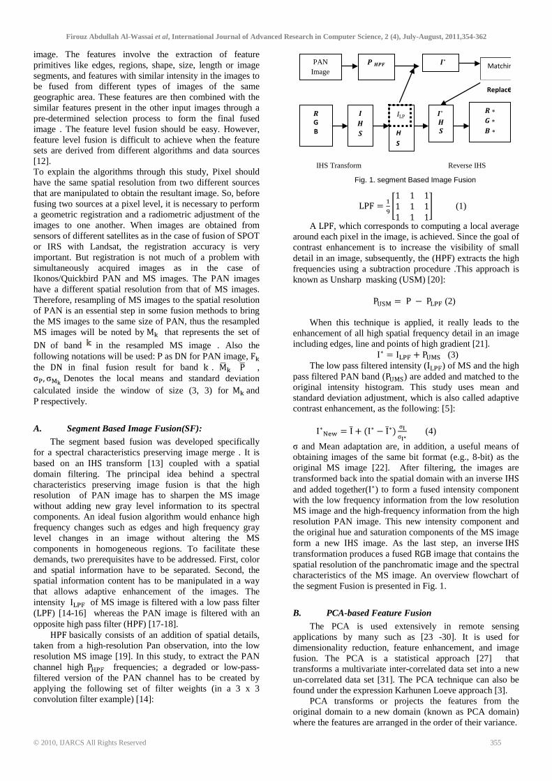
Firouz Abdullah Al -Wassai et al, International Journal of Advanced Research in Computer Science, 2 (4), July-August, 2011,354-362
© 2010, IJARCS All Rights Reserved 355
image. The features involve the extraction of feature primitives like edges, regions, shape, size, length or image segments, and features with similar intensity in the images to be fused from different types of images of the same geographic area.These features are then combined with the similar features present in the other input images through a pre-determined selection process to form the final fused image . The feature level fusion should be easy. However, feature level fusion is difficult to achieve when the feature sets are derived from different algorithms and data sources [12]. To explain the algorithms through this study, Pixel should have the same spatial resolution from two different sources that are manipulated to obtain the resultant image. So, before fusing two sources at a pixel level, it is necessary to perform a geometric registration and a radiometric adjustment of the images to one another. When images are obtained from sensors of different satellites as in the case of fusion of SPOT or IRS with Landsat, the registration accuracy is very important. But registration is not much of a problem with simultaneously acquired images as in the case of Ikonos/Quickbird PAN and MS images. The PAN images have a different spatial resolution from that of MS images. Therefore, resampling of MS images to the spatial resolution of PAN is an essential step in some fusion methods to bring the MS images to the same size of PAN, thus the resampled MS images will be noted by that represents the set of
of band in the resampled MS image . Also the following notations will be used: as for PAN image, the in final fusion result for band . ,
Denotes the local means and standard deviation calculated inside the window of size (3, 3) for and
respectively.
A. Segment Based Image Fusion(SF): The segment based fusion was developed specifically
for a spectral characteristics preserving image merge . It is based on an transform [13] coupled with a spatial domain filtering. The principal idea behind a spectral characteristics preserving image fusion is that the high resolution of PAN image has to sharpen the MS image without adding new gray level information to its spectral components. An ideal fusion algorithm would enhance high frequency changes such as edges and high frequency gray level changes in an image without altering the MS components in homogeneous regions. To facilitate these demands, two prerequisites have to be addressed. First, color and spatial information have to be separated. Second, the spatial information content has to be manipulated in a way that allows adaptive enhancement of the images. The intensity of MS image is filtered with a low pass filter ( ) [14-16] whereas the PAN image is filtered with an opposite high pass filter ( ) [17-18].
basically consists of an addition of spatial details, taken from a high-resolution Pan observation, into the low resolution MS image [19]. In this study, to extract the PAN channel high frequencies; a degraded or low-pass-filtered version of the PAN channel has to be created by applying the following set of filter weights (in a 3 x 3 convolution filter example) [14]:
(1)
A , which corresponds to computing a local average around each pixel in the image, is achieved. Since the goal of contrast enhancement is to increase the visibility of small detail in an image, subsequently, the ( ) extracts the high frequencies using a subtraction procedure .This approach is known as Unsharp masking (USM) [20]:
(2)
When this technique is applied, it really leads to the enhancement of all high spatial frequency detail in an image including edges, line and points of high gradient [21].
(3) The low pass filtered intensity ( ) of MS and the high
pass filtered PAN band ( ) are added and matched to the original intensity histogram. This study uses mean and standard deviation adjustment, which is also called adaptive contrast enhancement, as the following: [5]:
(4)
and Mean adaptation are, in addition, a useful means of obtaining images of the same bit format (e.g., 8-bit) as the original MS image [22]. After filtering, the images are transformed back into the spatial domain with an inverse and added together( ) to form a fused intensity component with the low frequency information from the low resolution MS image and the high-frequency information from the high resolution PAN image. This new intensity component and the original hue and saturation components of the MS image form a new image. As the last step, an inverse transformation produces a fused image that contains the spatial resolution of the panchromatic image and the spectral characteristics of the MS image. An overview flowchart of the segment Fusion is presented in Fig. 1.
B. PCA-based Feature Fusion
The PCA is used extensively in remote sensing applications by many such as [23 -30]. It is used for dimensionality reduction, feature enhancement, and image fusion. The PCA is a statistical approach [27] that transforms a multivariate inter-correlated data set into a new un-correlated data set [31]. The PCA technique can also be found under the expression Karhunen Loeve approach [3].
PCA transforms or projects the features from the original domain to a new domain (known as PCA domain) where the features are arranged in the order of their variance.
�∗
� ���
Fig. 1. segment Based Image Fusion
PAN Image
�
G
B
� � �
�
H
S
� �
�∗
� ∗ � ∗ � ∗
�LP
Matchin
Replace
IHS Transform Reverse IHS

Firouz Abdullah Al -Wassai et al, International Journal of Advanced Research in Computer Science, 2 (4), July-August, 2011,354-362
© 2010, IJARCS All Rights Reserved 356
The features in the transformed domain are formed by the linear combination of the original features and are uncorrelated. Fusion process is achieved in the PCA domain by retaining only those features that contain a significant amount of information. The main idea behind PCA is to determine the features that explain as much of the total variation in the data as possible with as few of these features as possible. The PCA computation done on an N-by-N of MS image having 3 contiguous spectral bands is explained below. The computation of the PCA transformation matrix is based on the eigenvalue decomposition of the covariance matrix is defined as[33]:
(5)
where is the spectral signature , denotes the mean spectral signature and is the total number of spectral signatures. the total number of spectral signatures. In order to find the new orthogonal axes of the PCA space,
Eigen decomposition of the covariance matrix is performed. The eigen decomposition of the covariance matrix is given by
(6)
where denotes the eigenvalue, denotes the corresponding eigenvector and varies from 1 to 3. The eigenvalues denote the amount of variance present in the corresponding eigenvectors. The eigenvectors form the axes of the PCA space, and they are orthogonal to each other. The eigenvalues are arranged in decreasing order of the variance. The PCA transformation matrix, A, is formed by choosing the eigenvectors corresponding to the largest eigenvalues. The PCA transformation matrix A is given by
(7)
where are the eigenvectors associated with
the J largest eigenvalues obtained from the eigen decomposition of the covariance matrix . The data projected onto the corresponding eigenvectors form the reduced uncorrelated features that are used for further fusion processes.
Computation of the principal components can be presented with the following algorithm by [34]: a. Calculate the covariance matrix from the input data. b. Compute the eigenvalues and eigenvectors of and sort
them in a descending order with respect to the eigenvalues.
c. Form the actual transition matrix by taking the predefined number of components (eigenvectors).
d. Finally, multiply the original feature space with the obtained transition matrix, which yields a lower- dimensional representation. The PCA based feature fusion is shown in Fig. 2. The
input MS are, first, transformed into the same number of uncorrelated principal components. Its most important steps are:
i. perform a principal component transformation to convert a set of MS bands (three or more bands) into a set of principal components.
ii. Substitute the first principal component PC1 by the PAN band whose histogram has previously been matched with that of the first principal component. In
this study the mean and standard deviation are matched by :
(8)
Perform a reverse principal component transformation to convert the replaced components back to the original image space. A set of fused MS bands is produced after the reverse transform [35-37].
The mathematical models of the forward and backward transformation of this method are described by [37], whose processes are represented by eq. (9) and (10). The transformation matrix contains the eigenvectors, ordered with respect to their Eigen values. It is orthogonal and determined either from the covariance matrix or the correlation matrix of the input MS. PCA performed using the covariance matrix is referred to as nun standardized PCA, while PCA performed using the correlation matrix is referred to as standardized PCA [37]:
Figure: 2 Schematic flowchart of PCA image fusion
(9)
Where the transformation matrix
(10)
(9) and (10) can be merged as follows:
(11)
Here and are the values of the pixels of different bands of and PAN images respectively and the superscripts and denote high and low
resolution. Also and is stretched to have same mean and variance as . The PCA
Fig. 2. : Schematic flowchart of PCA image fusion
PAN Image
Input MS
Image 3 or More Bands
PC1
PC2
PC3
……
PC1
PC2
PC3
……
PC1*
PC2
PC3
……
PAN sharpend image 3 or more bands
PC1
Matching Replace
Principal Component Transform
Reverse Principal Component Transform
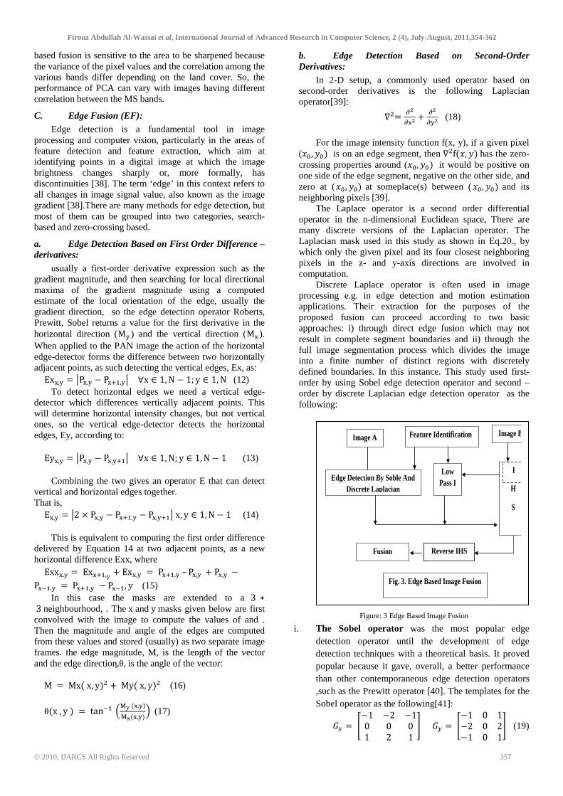
Firouz Abdullah Al -Wassai et al, International Journal of Advanced Research in Computer Science, 2 (4), July-August, 2011,354-362
© 2010, IJARCS All Rights Reserved 357
based fusion is sensitive to the area to be sharpened because the variance of the pixel values and the correlation among the various bands differ depending on the land cover. So, the performance of PCA can vary with images having different correlation between the MS bands.
C. Edge Fusion (EF):
Edge detection is a fundamental tool in image processing and computer vision, particularly in the areas of feature detection and feature extraction, which aim at identifying points in a digital image at which the image brightness changes sharply or, more formally, has discontinuities [38]. The term ‘edge’ in this context refers to all changes in image signal value, also known as the image gradient [38].There are many methods for edge detection, but most of them can be grouped into two categories, search-based and zero-crossing based.
a. Edge Detection Based on First Order Difference –derivatives:
usually a first-order derivative expression such as the gradient magnitude, and then searching for local directional maxima of the gradient magnitude using a computed estimate of the local orientation of the edge, usually the gradient direction, so the edge detection operator Roberts, Prewitt, Sobel returns a value for the first derivative in the horizontal direction ( ) and the vertical direction ( ). When applied to the PAN image the action of the horizontal edge-detector forms the difference between two horizontally adjacent points, as such detecting the vertical edges, Ex, as:
(12) To detect horizontal edges we need a vertical edge-
detector which differences vertically adjacent points. This will determine horizontal intensity changes, but not vertical ones, so the vertical edge-detector detects the horizontal edges, Ey, according to:
(13)
Combining the two gives an operator E that can detect
vertical and horizontal edges together. That is,
(14)
This is equivalent to computing the first order difference delivered by Equation 14 at two adjacent points, as a new horizontal difference Exx, where
–
(15) In this case the masks are extended to a
neighbourhood, . The and masks given below are first convolved with the image to compute the values of and . Then the magnitude and angle of the edges are computed from these values and stored (usually) as two separate image frames. the edge magnitude, M, is the length of the vector and the edge direction, is the angle of the vector:
(16)
(17)
b. Edge Detection Based on Second-Order Derivatives:
In 2-D setup, a commonly used operator based on second-order derivatives is the following Laplacian operator[39]:
(18)
For the image intensity function f(x, y), if a given pixel
( is on an edge segment, then has the zero-crossing properties around ( it would be positive on one side of the edge segment, negative on the other side, and zero at ( at someplace(s) between ( and its neighboring pixels [39].
The Laplace operator is a second order differential operator in the n-dimensional Euclidean space, There are many discrete versions of the Laplacian operator. The Laplacian mask used in this study as shown in Eq.20., by which only the given pixel and its four closest neighboring pixels in the z- and y-axis directions are involved in computation.
Discrete Laplace operator is often used in image processing e.g. in edge detection and motion estimation applications. Their extraction for the purposes of the proposed fusion can proceed according to two basic approaches: i) through direct edge fusion which may not result in complete segment boundaries and ii) through the full image segmentation process which divides the image into a finite number of distinct regions with discretely defined boundaries. In this instance. This study used first-order by using Sobel edge detection operator and second – order by discrete Laplacian edge detection operator as the following:
Figure: 3 Edge Based Image Fusion
i. The Sobel operator was the most popular edge detection operator until the development of edge detection techniques with a theoretical basis. It proved popular because it gave, overall, a better performance than other contemporaneous edge detection operators ,such as the Prewitt operator [40]. The templates for the Sobel operator as the following[41]:
(19)
Fig. 3. Edge Based Image Fusion
Fusion
Image A
Reverse IHS
Image B
Edge Detection By Soble And Discrete Laplacian
Feature Identification
Low Pass I
H
S
I

Firouz Abdullah Al -Wassai et al, International Journal of Advanced Research in Computer Science, 2 (4), July-August, 2011,354-362
© 2010, IJARCS All Rights Reserved 358
ii. The discrete Laplacian edge detection operator
(20) The proposed process of Edge Fusion is depicted in (Fig.
3) and consists of three steps:
a) edge detection of PAN image by soble and discrete Laplacian then subtraction the PAN from them.
b) Low Pas Filter the intensity of MS and add the edge of the pan.
c) After that, the images are transformed back into the spatial domain with an inverse and added together( ) to form a fused intensity component with the low frequency information from the low resolution MS image and the edge of PAN image. This new intensity component and the original hue and saturation components of the MS image form a new image.
d) As the last step, an inverse transformation produces a fused image that contains the spatial resolution of the panchromatic image and the spectral characteristics of the MS image. An overview flowchart of the segment Fusion is presented in Fig. 3.
III. EXPERIMENTS
In order to validate the theoretical analysis, the performance of the methods discussed above was further evaluated by experimentation. Data sets used for this study were collected by the Indian IRS-1C PAN (0.50 - 0.75 µm) of the 5.8 m resolution panchromatic band. Where the
Figure.4. Original Panchromatic and Multispectral Images
American Landsat (TM) the red (0.63 - 0.69 µm), green (0.52 - 0.60 µm) and blue (0.45 - 0.52 µm) bands of the 30 m resolution multispectral image were used in this work . Fig.4 shows the IRS-1C PAN and multispectral TM images. The scenes covered the same area of the Mausoleums of the Chinese Tang – Dynasty in the PR China [42] was selected
as test sit in this study. Since this study is involved in evaluation of the effect of the various spatial, radiometric and spectral resolution for image fusion, an area contains both manmade and natural features is essential to study these effects. Hence, this work is an attempt to study the quality of the images fused from different sensors with various characteristics. The size of the PAN is 600 * 525 pixels at 6 bits per pixel and the size of the original multispectral is 120 * 105 pixels at 8 bits per pixel, but this is upsampled to by nearest neighbor. It was used to avoid spectral contamination caused by interpolation, which does not change the data file value. The pairs of images were geometrically registered to each other.
To evaluate the ability of enhancing spatial details and
preserving spectral information, some Indices including : A. Standard Deviation ( ),
B. Entropy ) :in this study the measure of entropy values based on the first differences best than use the measure it based on the levels themselves.
C. Signal-to Noise Ratio ( )
D. Deviation Index ( )
E. Correlation Coefficient ( )
F. Normalization Root Mean Square Error (NRMSE)
where the are the measurements of each the brightness values of homogenous pixels of the result image and the original MS image of band , and are the mean brightness values of both images and are of size . is the brightness value of image data and .To simplify the comparison of the different fusion methods, the values of the , , , and index of the fused images are provided as chart in Fig. 5
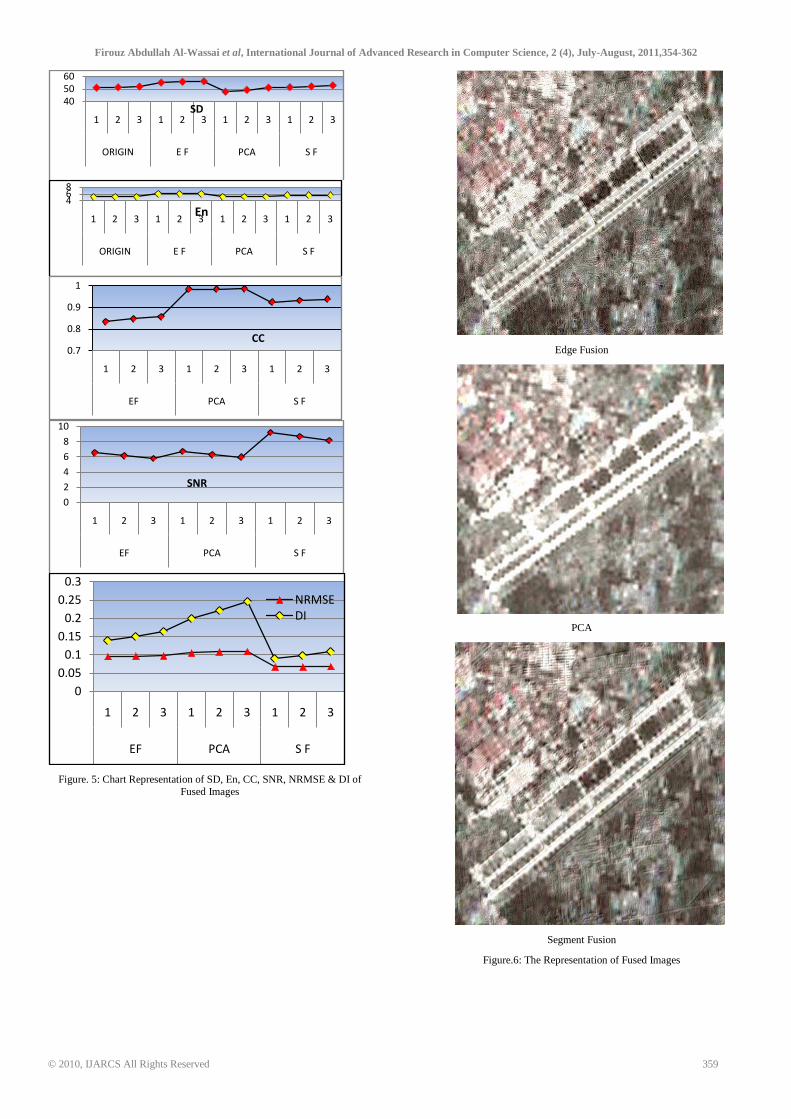
Firouz Abdullah Al -Wassai et al, International Journal of Advanced Research in Computer Science, 2 (4), July-August, 2011,354-362
© 2010, IJARCS All Rights Reserved 359
Figure. 5: Chart Representation of SD, En, CC, SNR, NRMSE & DI of
Fused Images
Edge Fusion
PCA
Segment Fusion
Figure.6: The Representation of Fused Images
40
50
60
1 2 3 1 2 3 1 2 3 1 2 3
ORIGIN E F PCA S F
SD
468
1 2 3 1 2 3 1 2 3 1 2 3
ORIGIN E F PCA S F
En
0.7
0.8
0.9
1
1 2 3 1 2 3 1 2 3
EF PCA S F
CC
0
2
4
6
8
10
1 2 3 1 2 3 1 2 3
EF PCA S F
SNR
0
0.05
0.1
0.15
0.2
0.25
0.3
1 2 3 1 2 3 1 2 3
EF PCA S F
NRMSE
DI
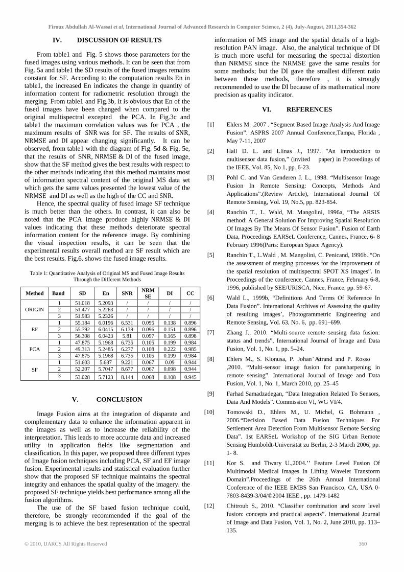
Firouz Abdullah Al -Wassai et al, International Journal of Advanced Research in Computer Science, 2 (4), July-August, 2011,354-362
© 2010, IJARCS All Rights Reserved 360
IV. DISCUSSION OF RESULTS
From table1 and Fig. 5 shows those parameters for the fused images using various methods. It can be seen that from Fig. 5a and table1 the SD results of the fused images remains constant for SF. According to the computation results En in table1, the increased En indicates the change in quantity of information content for radiometric resolution through the merging. From table1 and Fig.3b, it is obvious that En of the fused images have been changed when compared to the original multispectral excepted the PCA. In Fig.3c and table1 the maximum correlation values was for PCA , the maximum results of was for SF. The results of ,
and appear changing significantly. It can be observed, from table1 with the diagram of Fig. 5d & Fig. 5e, that the results of SNR, & of the fused image, show that the SF method gives the best results with respect to the other methods indicating that this method maintains most of information spectral content of the original MS data set which gets the same values presented the lowest value of the
and as well as the high of the CC and . Hence, the spectral quality of fused image SF technique
is much better than the others. In contrast, it can also be noted that the PCA image produce highly & values indicating that these methods deteriorate spectral information content for the reference image. By combining the visual inspection results, it can be seen that the experimental results overall method are SF result which are the best results. Fig.6. shows the fused image results.
Table 1: Quantitative Analysis of Original MS and Fused Image Results
Through the Different Methods
Method Band SD En SNR NRMSE
DI CC
ORIGIN 1 51.018 5.2093 / / / / 2 51.477 5.2263 / / / / 3 51.983 5.2326 / / / /
EF 1 55.184 6.0196 6.531 0.095 0.138 0.896 2 55.792 6.0415 6.139 0.096 0.151 0.896 3 56.308 6.0423 5.81 0.097 0.165 0.898
PCA 1 47.875 5.1968 6.735 0.105 0.199 0.984 2 49.313 5.2485 6.277 0.108 0.222 0.985 3 47.875 5.1968 6.735 0.105 0.199 0.984
SF 1 51.603 5.687 9.221 0.067 0.09 0.944 2 52.207 5.7047 8.677 0.067 0.098 0.944 3 53.028 5.7123 8.144 0.068 0.108 0.945
V. CONCLUSION
Image Fusion aims at the integration of disparate and complementary data to enhance the information apparent in the images as well as to increase the reliability of the interpretation. This leads to more accurate data and increased utility in application fields like segmentation and classification. In this paper, we proposed three different types of Image fusion techniques including PCA, SF and EF image fusion. Experimental results and statistical evaluation further show that the proposed SF technique maintains the spectral integrity and enhances the spatial quality of the imagery. the proposed SF technique yields best performance among all the fusion algorithms.
The use of the SF based fusion technique could, therefore, be strongly recommended if the goal of the merging is to achieve the best representation of the spectral
information of MS image and the spatial details of a high-resolution PAN image. Also, the analytical technique of DI is much more useful for measuring the spectral distortion than NRMSE since the NRMSE gave the same results for some methods; but the DI gave the smallest different ratio between those methods, therefore , it is strongly recommended to use the because of its mathematical more precision as quality indicator.
VI. REFERENCES
[1] Ehlers M. ,2007 . “Segment Based Image Analysis And Image Fusion”. ASPRS 2007 Annual Conference,Tampa, Florida , May 7-11, 2007
[2] Hall D. L. and Llinas J., 1997. "An introduction to multisensor data fusion,” (invited paper) in Proceedings of the IEEE, Vol. 85, No 1, pp. 6-23.
[3] Pohl C. and Van Genderen J. L., 1998. “Multisensor Image Fusion In Remote Sensing: Concepts, Methods And Applications”.(Review Article), International Journal Of Remote Sensing, Vol. 19, No.5, pp. 823-854.
[4] Ranchin T., L. Wald, M. Mangolini, 1996a, “The ARSIS method: A General Solution For Improving Spatial Resolution Of Images By The Means Of Sensor Fusion”. Fusion of Earth Data, Proceedings EARSeL Conference, Cannes, France, 6- 8 February 1996(Paris: European Space Agency).
[5] Ranchin T., L.Wald , M. Mangolini, C. Penicand, 1996b. “On the assessment of merging processes for the improvement of the spatial resolution of multispectral SPOT XS images”. In Proceedings of the conference, Cannes, France, February 6-8, 1996, published by SEE/URISCA, Nice, France, pp. 59-67.
[6] Wald L., 1999b, “Definitions And Terms Of Reference In Data Fusion”. International Archives of Assessing the quality of resulting images’, Photogrammetric Engineering and Remote Sensing, Vol. 63, No. 6, pp. 691–699.
[7] Zhang J., 2010. “Multi-source remote sensing data fusion: status and trends”, International Journal of Image and Data Fusion, Vol. 1, No. 1, pp. 5–24.
[8] Ehlers M., S. Klonusa, P. Johan A ˚ strand and P. Rosso ,2010. “Multi-sensor image fusion for pansharpening in remote sensing”. International Journal of Image and Data Fusion, Vol. 1, No. 1, March 2010, pp. 25–45
[9] Farhad Samadzadegan, “Data Integration Related To Sensors, Data And Models”. Commission VI, WG VI/4.
[10] Tomowski D., Ehlers M., U. Michel, G. Bohmann , 2006.“Decision Based Data Fusion Techniques For Settlement Area Detection From Multisensor Remote Sensing Data”. 1st EARSeL Workshop of the SIG Urban Remote Sensing Humboldt-Universität zu Berlin, 2-3 March 2006, pp. 1- 8.
[11] Kor S. and Tiwary U.,2004.’’ Feature Level Fusion Of Multimodal Medical Images In Lifting Wavelet Transform Domain”.Proceedings of the 26th Annual International Conference of the IEEE EMBS San Francisco, CA, USA 0-7803-8439-3/04/©2004 IEEE , pp. 1479-1482
[12] Chitroub S., 2010. “Classifier combination and score level fusion: concepts and practical aspects”. International Journal of Image and Data Fusion, Vol. 1, No. 2, June 2010, pp. 113–135.

Firouz Abdullah Al -Wassai et al, International Journal of Advanced Research in Computer Science, 2 (4), July-August, 2011,354-362
© 2010, IJARCS All Rights Reserved 361
[13] Firouz A. Al-Wassai, Dr. N.V. Kalyankar2, Dr. A. A. Al-zuky ,2011a. “ The IHS Transformations Based Image Fusion”. Journal of Global Research in Computer Science, Volume 2, No. 5, May 2011, pp. 70 – 77.
[14] Green W. B., 1989. Digital Image processing A system Approach”.2nd Edition. Van Nostrand Reinholld, New York.
[15] Hill J., C. Diemer, O. Stöver, Th. Udelhoven, 1999. “A Local Correlation Approach for the Fusion of Remote Sensing Data with Different Spatial Resolutions in Forestry Applications”. International Archives Of Photogrammetry And Remote Sensing, Vol. 32, Part 7-4-3 W6, Valladolid, Spain, 3-4 June.
[16] Firouz Abdullah Al-Wassai1 , Dr. N.V. Kalyankar2 , A.A. Al-Zuky, 2011b. “Arithmetic and Frequency Filtering Methods of Pixel-Based Image Fusion Techniques “.IJCSI International Journal of Computer Science Issues, Vol. 8, Issue 3, No. 1, May 2011, pp. 113- 122.
[17] Schowengerdt R. A.,2007. “Remote Sensing: Models and Methods for Image Processing”.3rd Edition, Elsevier Inc.
[18] Wenbo W.,Y.Jing, K. Tingjun ,2008. “Study Of Remote Sensing Image Fusion And Its Application In Image Classification” The International Archives of the Photogrammetry, Remote Sensing and Spatial Information Sciences. Vol. XXXVII. Part B7. Beijing 2008, pp.1141-1146.
[19] Aiazzi B., S. Baronti , M. Selva,2008. “Image fusion through multiresolution oversampled decompositions”. in Image Fusion: Algorithms and Applications “.Edited by: Stathaki T. “Image Fusion: Algorithms and Applications”. 2008 Elsevier Ltd.
[20] Sangwine S. J., and R.E.N. Horne, 1989. “The Colour Image Processing Handbook”. Chapman & Hall.
[21] Richards J. A., and Jia X., 1999. “Remote Sensing Digital Image Analysis”. 3rd Edition. Springer - verlag Berlin Heidelberg New York.
[22] Gangkofner U. G., P. S. Pradhan, and D. W. Holcomb, 2008. “Optimizing the High-Pass Filter Addition Technique for Image Fusion”. Photogrammetric Engineering & Remote Sensing, Vol. 74, No. 9, pp. 1107–1118.
[23] Ranchin T., Wald L., 2000. “Fusion of high spatial and spectral resolution images: the ARSIS concept and its implementation”. Photogrammetric Engineering and Remote Sensing, Vol.66, No.1, pp.49-61.
[24] Parcharidis I. and L. M. K. Tani, 2000. “Landsat TM and ERS Data Fusion: A Statistical Approach Evaluation for Four Different Methods”. 0-7803-6359-0/00/ 2000 IEEE, pp.2120-2122.
[25] Kumaran T. V ,R. Shyamala , L..Marino, P. Howarth and D. Wood, 2001. “Land Cover Mapping Performance Analysis Of Image-Fusion Methods”. URL:http://www.gisdevelopment.net/application/ environment/ overview/ envo0011pf.htm (last date accessed 18-05-2009).
[26] Colditz R. R., T. Wehrmann , M. Bachmann , K. Steinnocher , M. Schmidt , G. Strunz , S. Dech, 2006. “Influence Of Image Fusion Approaches On Classification Accuracy A Case Study”. International Journal of Remote Sensing, Vol. 27, No. 15, 10, pp. 3311–3335.
[27] Amarsaikhan D. and Douglas T., 2004. “Data Fusion And Multisource Image Classification”. INT. J. Remote Sensing, Vol. 25, No. 17, pp. 3529–3539.
[28] Sahoo T. and Patnaik S., 2008. “Cloud Removal From Satellite Images Using Auto Associative Neural Network And Stationary Wavelet Transform”. First International Conference on Emerging Trends in Engineering and Technology, 978-0-7695-3267-7/08 © 2008 IEEE
[29] Wang J., J.X. Zhang, Z.J.Liu, 2004. “Distinct Image Fusion Methods For Landslide Information Enhancement”. URL: http://www.isprs.org/.../DISTINCT%20IMAGE%20FUSION%20METHODS%20FOR%20LANDS(last date accessed: 8 Feb 2010).
[30] Amarsaikhan D., H.H. Blotevogel, J.L. van Genderen, M. Ganzorig, R. Gantuya and B. Nergui, 2010. “Fusing high-resolution SAR and optical imagery for improved urban land cover study and classification”. International Journal of Image and Data Fusion, Vol. 1, No. 1, March 2010, pp. 83–97.
[31] Zhang Y., 2002. “PERFORMANCE ANALYSIS OF IMAGE FUSION TECHNIQUES BY IMAGE”. International Archives of Photogrammetry and Remote Sensing (IAPRS), Vol. 34, Part 4. Working Group IV/7.
[32] Li S., Kwok J. T., Wang Y.., 2002. “Using The Discrete Wavelet Frame Transform To Merge Landsat TM And SPOT Panchromatic Images”. Information Fusion 3 (2002), pp.17–23.
[33] Cheriyadat A., 2003. “Limitations Of Principal Component Analysis For Dimensionality-Reduction For Classification Of Hyperpsectral Data”. Thesis, Mississippi State University, Mississippi, December 2003
[34] Pechenizkiy M. , S. Puuronen, A. Tsymbal , 2006. “The Impact of Sample Reduction on PCA-based Feature Extraction for Supervised Learning” .SAC’06, April 23–27, 2006, Dijon, France.
[35] Dong J.,Zhuang D., Huang Y.,Jingying Fu,2009. “Advances In Multi-Sensor Data Fusion: Algorithms And Applications “. Review , ISSN 1424-8220 Sensors 2009, 9, pp.7771-7784.
[36] Francis X.J. Canisius, Hugh Turral, 2003. “Fusion Technique To Extract Detail Information From Moderate Resolution Data For Global Scale Image Map Production”. Proceedings Of The 30th International Symposium On Remote Sensing Of Environment – Information For Risk Management Andsustainable Development – November 10-14, 2003 Honolulu, Hawaii
[37] Wang Z., Djemel Ziou, Costas Armenakis, Deren Li, and Qingquan Li,2005..A Comparative Analysis of Image Fusion Methods. IEEE Transactions On Geoscience And Remote Sensing, Vol. 43, No. 6, JUNE 2005, pp. 1391-1402.
[38] Xydeasa C. and V. Petrovi´c “Pixel-level image fusion metrics”. ”. in Image Fusion: Algorithms and Applications “.Edited by: Stathaki T. “Image Fusion: Algorithms and Applications”. 2008 Elsevier Ltd.
[39] Peihua Q., 2005. “Image Processing and Jump Regression Analysis”. John Wiley & Sons, Inc.
[40] Mark S. Nand A. S. A.,2008 “Feature Extraction and Image Processing”. Second edition, 2008 Elsevier Ltd.

Firouz Abdullah Al -Wassai et al, International Journal of Advanced Research in Computer Science, 2 (4), July-August, 2011,354-362
© 2010, IJARCS All Rights Reserved 362
[41] Li S. and B. Yang , 2008. “Region-based multi-focus image fusion”. in Image Fusion: Algorithms and Applications “.Edited by: Stathaki T. “Image Fusion: Algorithms and Applications”. 2008 Elsevier Ltd.
[42] Böhler W. and G. Heinz, 1998. “Integration of high Resolution Satellite Images into Archaeological Docmentation”. Proceeding International Archives of Photogrammetry and Remote Sensing, Commission V, Working Group V/5, CIPA International Symposium, Published by the Swedish Society for Photogrammetry and Remote Sensing, Goteborg. (URL: http://www.i3mainz.fh-mainz.de/publicat/cipa-98/sat-im.html (Last date accessed: 28 Oct. 2000).
AUTHORS
Firouz Abdullah Al-Wassai. Received the B.Sc. degree in, Physics from University of Sana’a, Yemen, Sana’a, in 1993. The M.Sc.degree in, Physics from Bagdad University , Iraqe, in 2003, Research student.Ph.D in the department of computer science (S.R.T.M.U), India, Nanded.
Dr. N.V. Kalyankar, Principal,Yeshwant Mahvidyalaya, Nanded(India) completed M.Sc.(Physics) from Dr. B.A.M.U,
Aurangabad. In 1980 he joined as a leturer in department of physics at Yeshwant Mahavidyalaya, Nanded. In 1984 he completed his DHE. He completed his Ph.D. from Dr.B.A.M.U. Aurangabad in 1995. From 2003 he is working as a Principal to till date in Yeshwant Mahavidyalaya, Nanded. He is also research guide for Physics and Computer Science in S.R.T.M.U, Nanded. 03 research students are successfully awarded Ph.D in Computer Science under his guidance. 12 research students are successfully awarded M.Phil in Computer Science under his guidance He is also worked on various boides in S.R.T.M.U, Nanded. He is also worked on various bodies is S.R.T.M.U, Nanded. He also published 30 research papers in various international/national journals. He is peer team member of NAAC (National Assessment and Accreditation Council, India ). He published a book entilteld “DBMS concepts and programming in Foxpro”. He also get various educational wards in which “Best Principal” award from S.R.T.M.U, Nanded in 2009 and “Best Teacher” award from Govt. of Maharashtra, India in 2010. He is life member of Indian “Fellowship of Linnean Society of London(F.L.S.)” on 11 National Congress, Kolkata (India). He is also honored with November 2009.
Dr. Ali A. Al-Zuky. B.Sc Physics Mustansiriyah University, Baghdad , Iraq, 1990. M Sc. In1993 and Ph. D. in1998 from University of Baghdad, Iraq. He was supervision for 40 postgraduate students (MSc. & Ph.D.) in different fields (physics, computers and Computer Engineering and Medical Physics). He has More than 60 scientific papers published in scientific journals in several scientific conferences.
www.ccsenet.org/apr Applied Physics Research Vol. 3, No. 1; May 2011
Published by Canadian Center of Science and Education 29
Study of Experimental Simple Pendulum Approximation Based on
Image Processing Algorithms
Mohammed Y. Kamil
Department of Physics, College of Sciences, AL–Mustansiriyah University, Iraq
Tel: 964-770-257-5673 E-mail: [email protected]
Ali Abid D. Al-Zuky
Department of Physics, College of Sciences, AL–Mustansiriyah University, Iraq
Tel: 964-770-273-2705 E-mail: [email protected]
Radhi Sh. Al-Tawil
Department of Physics, College of Education, AL–Mustansiriyah University, Iraq
Tel: 964-780-213-4935 E-mail: [email protected]
Received: December 6, 2010 Accepted: December 22, 2010 doi:10.5539/apr.v3n1p29
Abstract
In this study we used image processing algorithms to determine pendulum ball motion and present an approach
for solving the nonlinear differential equation that governs its movement. This formulae show an excellent
agreement with the exact period calculated with the use of elliptical integrals, and they are valid for both small
and large amplitudes of oscillation.
Also, we reveal some interesting aspects of the study simple pendulum or procedures for determining analytical
approximations to the periodic solutions of nonlinear differential equations.
Keywords: Simple pendulum, Large amplitude, Exact period, Image processing, Nonlinear equation
1. Introduction
The simple pendulum is one of the most popular examples analyzed in the textbooks and undergraduate courses
in physics and it is perhaps the most investigated oscillatory motion in physics [Baker G, 2005]. Many nonlinear
phenomena in the real world are governed by pendulum-like differential equations, which arise in many fields of
science and technology (e.g., analysis of acoustic vibrations, oscillations in small molecules, optically torqued
nanorods, Josephson junctions, electronic filters, gravitational lensing in general relativity, advanced models in
field theory, oscillations of buildings during earthquakes, and others) [Lima F.M.S., 2008].
The nonlinear differential equation for the simple pendulum can be exactly solved and the period and periodic
solution expressions involve the complete elliptic integral of the first kind and the Jacobi elliptic functions,
respectively. Due to this, several approximation schemes have been developed to investigate the situation for
large amplitude oscillations of a simple pendulum, and several approximations for its large-angle period have
been suggested (a summary of most of them can be found in [Beléndez A., 2009]).
In 1997 M. I. Molina appears expression to pendulum equation from using interpolatory-like linearizations is
shown for the simple pendulum which can be used for any initial amplitude [Molina M. I., 1997]. In 2002 Kidd
and Fogg found that it is feasible to extend the theory to the case of larger amplitudes and to employ it in a fairly
involved laboratory experiment [Kidd R. B., 2002]. In 2003 Millet proposed a mathematical justification for the
Kidd and Fogg formula by considering trigonometric relation and small-angle approximations for sine and
cosine functions, as well as the comparison between the sine function and various of its linear approximations
[Millet L. E., 2003]. In 2005 Hite three approximations are discussed for the frequency of a simple pendulum.
The first, proposed earlier by Kidd and Fogg, is simple in form but is the least accurate. The third, also based on
the analogy to the simple harmonic oscillator, is also simple and about twice as accurate as the first. The second
one is obtained using very little physics but is by far the most accurate [Hite G. E., 2005]. In 2006 Lima and
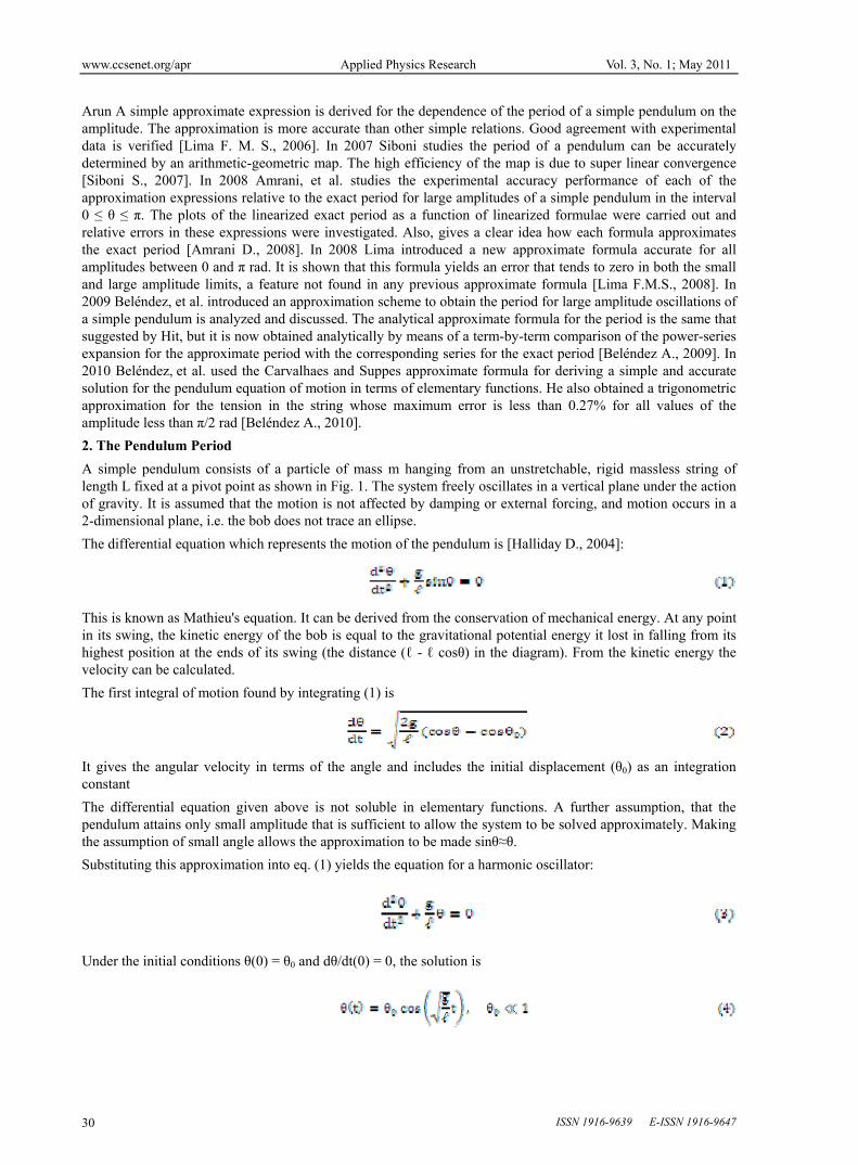
www.ccsenet.org/apr Applied Physics Research Vol. 3, No. 1; May 2011
ISSN 1916-9639 E-ISSN 1916-9647 30
Arun A simple approximate expression is derived for the dependence of the period of a simple pendulum on the
amplitude. The approximation is more accurate than other simple relations. Good agreement with experimental
data is verified [Lima F. M. S., 2006]. In 2007 Siboni studies the period of a pendulum can be accurately
determined by an arithmetic-geometric map. The high efficiency of the map is due to super linear convergence
[Siboni S., 2007]. In 2008 Amrani, et al. studies the experimental accuracy performance of each of the
approximation expressions relative to the exact period for large amplitudes of a simple pendulum in the interval
0 ≤ し ≤ π. The plots of the linearized exact period as a function of linearized formulae were carried out and
relative errors in these expressions were investigated. Also, gives a clear idea how each formula approximates
the exact period [Amrani D., 2008]. In 2008 Lima introduced a new approximate formula accurate for all
amplitudes between 0 and π rad. It is shown that this formula yields an error that tends to zero in both the small
and large amplitude limits, a feature not found in any previous approximate formula [Lima F.M.S., 2008]. In
2009 Beléndez, et al. introduced an approximation scheme to obtain the period for large amplitude oscillations of
a simple pendulum is analyzed and discussed. The analytical approximate formula for the period is the same that
suggested by Hit, but it is now obtained analytically by means of a term-by-term comparison of the power-series
expansion for the approximate period with the corresponding series for the exact period [Beléndez A., 2009]. In
2010 Beléndez, et al. used the Carvalhaes and Suppes approximate formula for deriving a simple and accurate
solution for the pendulum equation of motion in terms of elementary functions. He also obtained a trigonometric
approximation for the tension in the string whose maximum error is less than 0.27% for all values of the
amplitude less than π/2 rad [Beléndez A., 2010].
2. The Pendulum Period
A simple pendulum consists of a particle of mass m hanging from an unstretchable, rigid massless string of
length L fixed at a pivot point as shown in Fig. 1. The system freely oscillates in a vertical plane under the action
of gravity. It is assumed that the motion is not affected by damping or external forcing, and motion occurs in a
2-dimensional plane, i.e. the bob does not trace an ellipse.
The differential equation which represents the motion of the pendulum is [Halliday D., 2004]:
This is known as Mathieu's equation. It can be derived from the conservation of mechanical energy. At any point
in its swing, the kinetic energy of the bob is equal to the gravitational potential energy it lost in falling from its
highest position at the ends of its swing (the distance (ℓ - ℓ cosし) in the diagram). From the kinetic energy the
velocity can be calculated.
The first integral of motion found by integrating (1) is
It gives the angular velocity in terms of the angle and includes the initial displacement (し0) as an integration
constant
The differential equation given above is not soluble in elementary functions. A further assumption, that the
pendulum attains only small amplitude that is sufficient to allow the system to be solved approximately. Making
the assumption of small angle allows the approximation to be made sinし≈し. Substituting this approximation into eq. (1) yields the equation for a harmonic oscillator:
Under the initial conditions し(0) = し0 and dし/dt(0) = 0, the solution is
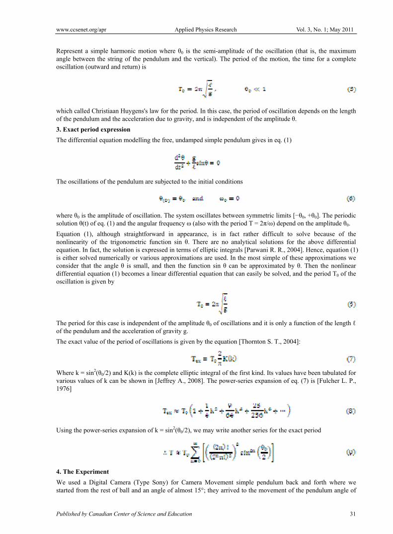
www.ccsenet.org/apr Applied Physics Research Vol. 3, No. 1; May 2011
Published by Canadian Center of Science and Education 31
Represent a simple harmonic motion where し0 is the semi-amplitude of the oscillation (that is, the maximum
angle between the string of the pendulum and the vertical). The period of the motion, the time for a complete
oscillation (outward and return) is
which called Christiaan Huygens's law for the period. In this case, the period of oscillation depends on the length
of the pendulum and the acceleration due to gravity, and is independent of the amplitude し. 3. Exact period expression
The differential equation modelling the free, undamped simple pendulum gives in eq. (1)
The oscillations of the pendulum are subjected to the initial conditions
where し0 is the amplitude of oscillation. The system oscillates between symmetric limits [−し0, +し0]. The periodic
solution し(t) of eq. (1) and the angular frequency ω (also with the period T = 2π/ω) depend on the amplitude し0.
Equation (1), although straightforward in appearance, is in fact rather difficult to solve because of the
nonlinearity of the trigonometric function sin し. There are no analytical solutions for the above differential
equation. In fact, the solution is expressed in terms of elliptic integrals [Parwani R. R., 2004]. Hence, equation (1)
is either solved numerically or various approximations are used. In the most simple of these approximations we
consider that the angle し is small, and then the function sin し can be approximated by し. Then the nonlinear
differential equation (1) becomes a linear differential equation that can easily be solved, and the period T0 of the
oscillation is given by
The period for this case is independent of the amplitude し0 of oscillations and it is only a function of the length ℓ of the pendulum and the acceleration of gravity g.
The exact value of the period of oscillations is given by the equation [Thornton S. T., 2004]:
Where k = sin2(し0/2) and K(k) is the complete elliptic integral of the first kind. Its values have been tabulated for
various values of k can be shown in [Jeffrey A., 2008]. The power-series expansion of eq. (7) is [Fulcher L. P.,
1976]
Using the power-series expansion of k = sin2(し0/2), we may write another series for the exact period
4. The Experiment
We used a Digital Camera (Type Sony) for Camera Movement simple pendulum back and forth where we
started from the rest of ball and an angle of almost 15°; they arrived to the movement of the pendulum angle of

www.ccsenet.org/apr Applied Physics Research Vol. 3, No. 1; May 2011
ISSN 1916-9639 E-ISSN 1916-9647 32
less than 5°. After that, we converted the video clip in to still images (frame), and cut to 25 frames per second.
Then we used the Segmentation technique to highlight the moving ball only then we easy find the angle at which
you make with the vertical axis of the pendulum.
We measured the length of a pendulum from the center of the bob to the edge of a pendulum clamp and adjusted
it to be as close to 0.20 m. Figure (2) shows captured images of the pendulum Motion of in the laboratory.
Then we have found the angle of pendulum from compute the averages of X-values and Y-values for the indices
of object image point. After that using the trigonometric functions to estimate the angle between vertical line and
pendulum string in each image. By using Table Curve 2D software, we found at the period time through the
relationship between the angular displacements with time and found the wavelength of the oscillating, which is
the time of period. See Figure (3), which illustrates the period time in experiment of the multiple angles, where
the time for the period represented by (c/30).
5. Comparison between exact and approximate expression
We compare the accuracy of the approximation for the pendulum period in Eq. (9) to that of exact solution for
amplitudes less than or equal to (15°).
Figure (4) illustrate the ratio between the actual period of a pendulum and the approximate value obtained for
small angles, as a function of the amplitude.
Appears from (Fig. 4) the difference between a power series period time for the power 1 to power 5, also we see
that the difference is increasing with increase the value of angle, it seems clear in the angles which more than
(20°), while the values of the angle that is smaller than (15°) - The scope of work in this research - the difference
does not appear clear from the values of the time, where the maximum difference in (し=15°) reach (0.037 mSec),
therefore, we will compare between the power series of power 5 with exact period time, which we got from the
test.
The measurement of the time interval for several successive periods is a good strategy for oscillations in the
small angle regime, where the amplitude does not change significantly from one swing to the next, but not for
large angle oscillations, because the period decreases considerably due to air friction.
This behavior is confirmed in Figure (5), where the period T is plotted as a function of し. In Figure (5),
Experimental data taken from Figure (3) also theoretical data taken from equation (9). The experimental data for
amplitudes small than (15°) clearly reveal a systematic over estimation for the period due to air damping.
6. Conclusion
We found that it is feasible to extend the theory to the case of larger amplitudes and to employ it in a fairly
involved laboratory experiment. As has been noted, the simple pendulum is particularly rich in physics
implications, and an understanding of its behavior over a more realistic range of phenomena is a worthwhile
goal.
It seems that the reported errors in approximating the exact period of the approximation formulae for large
amplitudes of a simple pendulum in the range 0° ≤ し ≤ 15° are not very accurate for physics students who
perform the simple pendulum experiment.
A simple approximate expression is derived for the dependence of the period of a simple pendulum on the
amplitude. The approximation is more accurate than other simple relations. Good agreement with experimental
data is verified.
References
Amrani D., Paradis P. and Beaudin M. (2008). Approximation expressions for the large-angle period of a simple
pendulum revisited. Rev. Mex. Fis. E, 54, 59-64.
Baker G. L.and Blackburn J. A. (2005). The Pendulum: A Case Study in Physics (Oxford: Oxford University
Press, 2005).
Beléndez A., Francés J., Ortuño M., Gallego S. and Bernabeu J.G. (2010). Higher accurate approximate
solutions for the simple pendulum in terms of elementary functions, Eur. J. Phys., 31, 65–70.
Beléndez A., Rodes J.J., Beléndez T. and Hernández A. (2009). Approximation for the large-angle simple
pendulum period, Eur. J. Phys., 30, 25–28.
Beléndez A., Rodes J.J., Beléndez T. and Hernández A. (2009). Approximation for the large-angle simple
pendulum period, Eur. J. Phys, 30, 25–28.
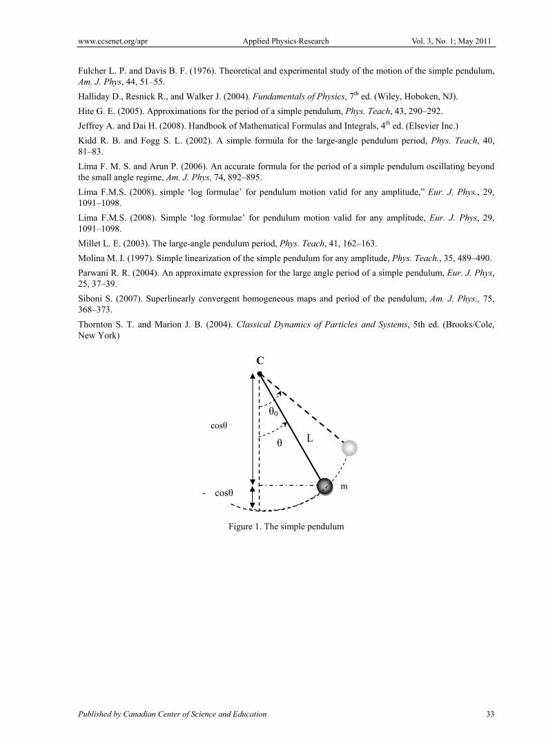
www.ccsenet.org/apr Applied Physics Research Vol. 3, No. 1; May 2011
Published by Canadian Center of Science and Education 33
Fulcher L. P. and Davis B. F. (1976). Theoretical and experimental study of the motion of the simple pendulum,
Am. J. Phys, 44, 51–55.
Halliday D., Resnick R., and Walker J. (2004). Fundamentals of Physics, 7th ed. (Wiley, Hoboken, NJ).
Hite G. E. (2005). Approximations for the period of a simple pendulum, Phys. Teach, 43, 290–292.
Jeffrey A. and Dai H. (2008). Handbook of Mathematical Formulas and Integrals, 4th ed. (Elsevier Inc.)
Kidd R. B. and Fogg S. L. (2002). A simple formula for the large-angle pendulum period, Phys. Teach, 40,
81–83.
Lima F. M. S. and Arun P. (2006). An accurate formula for the period of a simple pendulum oscillating beyond
the small angle regime, Am. J. Phys, 74, 892–895.
Lima F.M.S. (2008). simple ‘log formulae’ for pendulum motion valid for any amplitude,” Eur. J. Phys., 29,
1091–1098.
Lima F.M.S. (2008). Simple ‘log formulae’ for pendulum motion valid for any amplitude, Eur. J. Phys, 29,
1091–1098.
Millet L. E. (2003). The large-angle pendulum period, Phys. Teach, 41, 162–163.
Molina M. I. (1997). Simple linearization of the simple pendulum for any amplitude, Phys. Teach., 35, 489–490.
Parwani R. R. (2004). An approximate expression for the large angle period of a simple pendulum, Eur. J. Phys,
25, 37–39.
Siboni S. (2007). Superlinearly convergent homogeneous maps and period of the pendulum, Am. J. Phys., 75,
368–373.
Thornton S. T. and Marion J. B. (2004). Classical Dynamics of Particles and Systems, 5th ed. (Brooks/Cole,
New York)
Figure 1. The simple pendulum
C
し
し0
L
m
� cosし
� - � cosし
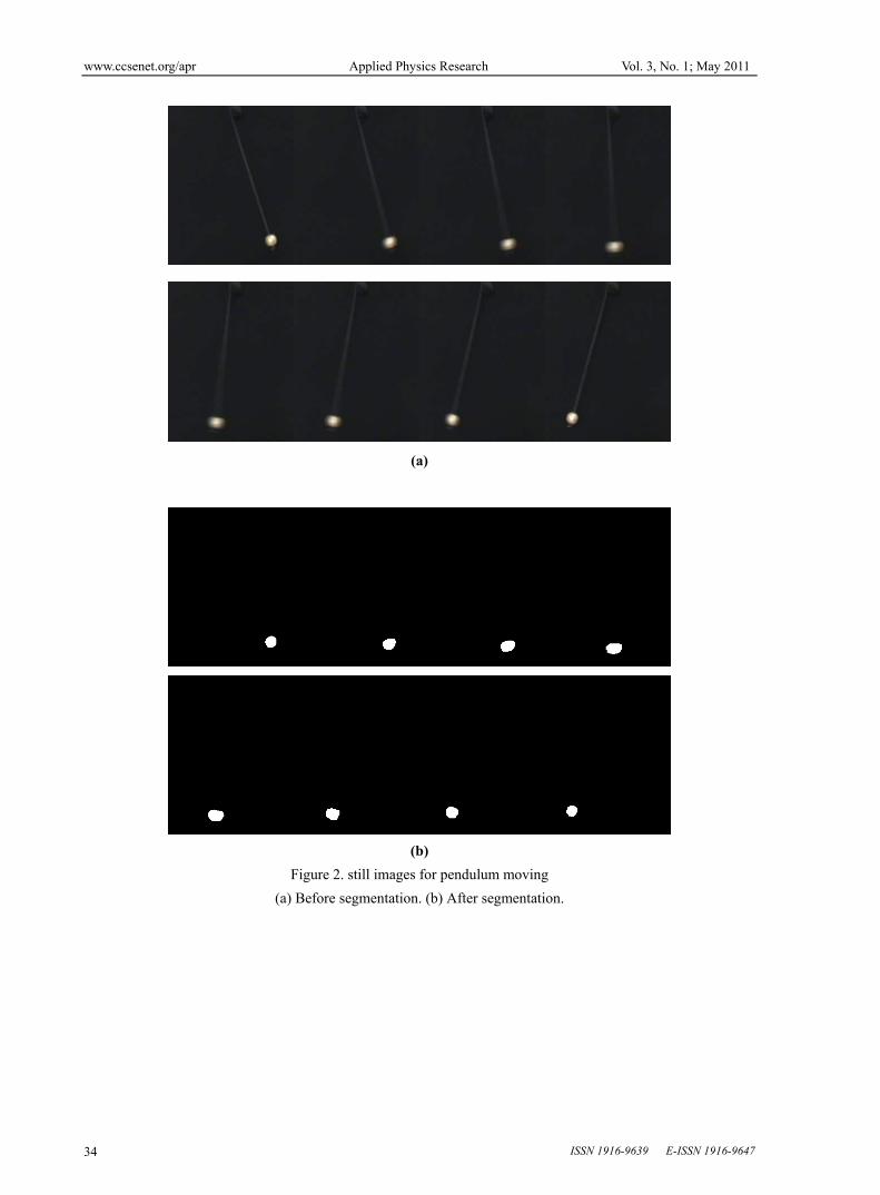
www.ccsenet.org/apr Applied Physics Research Vol. 3, No. 1; May 2011
ISSN 1916-9639 E-ISSN 1916-9647 34
(a)
(b)
Figure 2. still images for pendulum moving
(a) Before segmentation. (b) After segmentation.
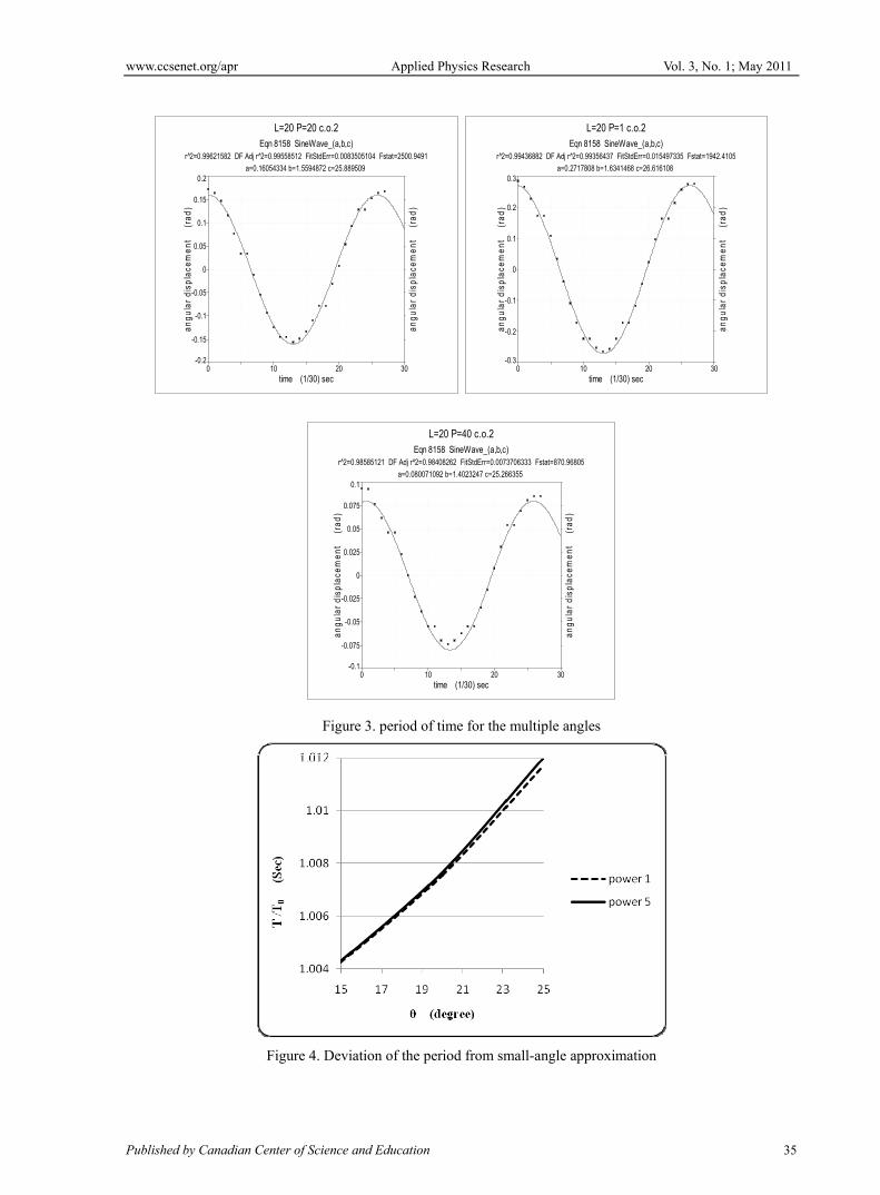
www.ccsenet.org/apr Applied Physics Research Vol. 3, No. 1; May 2011
Published by Canadian Center of Science and Education 35
L=20 P=20 c.o.2
Eqn 8158 SineWave_(a,b,c)
r^2=0.99621582 DF Adj r^2=0.99558512 FitStdErr=0.0083505104 Fstat=2500.9491
a=0.16054334 b=1.5594872 c=25.889509
0 10 20 30
time (1/30) sec
-0.2
-0.15
-0.1
-0.05
0
0.05
0.1
0.15
0.2a
ng
ula
r d
isp
lac
em
en
t
(r
ad
)
an
gu
lar
dis
pla
ce
me
nt
(ra
d)
L=20 P=1 c.o.2
Eqn 8158 SineWave_(a,b,c)
r^2=0.99436882 DF Adj r^2=0.99356437 FitStdErr=0.015497335 Fstat=1942.4105
a=0.2717808 b=1.6341468 c=26.616108
0 10 20 30
time (1/30) sec
-0.3
-0.2
-0.1
0
0.1
0.2
0.3
an
gu
lar
dis
pla
ce
me
nt
(ra
d)
an
gu
lar
dis
pla
ce
me
nt
(ra
d)
L=20 P=40 c.o.2
Eqn 8158 SineWave_(a,b,c)
r^2=0.98585121 DF Adj r^2=0.98408262 FitStdErr=0.0073706333 Fstat=870.96805
a=0.080071092 b=1.4023247 c=25.266355
0 10 20 30
time (1/30) sec
-0.1
-0.075
-0.05
-0.025
0
0.025
0.05
0.075
0.1
an
gu
lar
dis
pla
ce
me
nt
(ra
d)
an
gu
lar
dis
pla
ce
me
nt
(ra
d)
Figure 3. period of time for the multiple angles
Figure 4. Deviation of the period from small-angle approximation

www.ccsenet.org/apr Applied Physics Research Vol. 3, No. 1; May 2011
ISSN 1916-9639 E-ISSN 1916-9647 36
Figure 5. Experimental and theoretical period time
Copyright © 2022 FDOKUMEN