19-01 - Greater Atlantic Region Policy Series
235
Greater Atlantic Region Policy Series [19-01] Greater Atlantic Region Policy Series | NOAA Fisheries | Greater Atlantic Regional Fisheries Office 55 Great Republic Drive | Gloucester, MA 01930 Guidance for Integrating Climate Change Information in Greater Atlantic Region Habitat Conservation Division Consultation Processes Michael R. Johnson, Christopher Boelke, Louis A. Chiarella, and Karen Greene
-
Upload
khangminh22 -
Category
Documents
-
view
2 -
download
0
Transcript of 19-01 - Greater Atlantic Region Policy Series

Greater Atlantic Region Policy Series [19-01]
Greater Atlantic Region Policy Series | NOAA Fisheries | Greater Atlantic Regional Fisheries Office 55 Great Republic Drive | Gloucester, MA 01930
Guidance for Integrating Climate Change Information in Greater Atlantic Region Habitat Conservation Division Consultation Processes
Michael R. Johnson, Christopher Boelke, Louis A. Chiarella, and Karen Greene

ii
ABSTRACT
There is a growing body of knowledge that climate change has already affected, and will increasingly affect, the nation’s ability to maintain productive and resilient ecosystems. Climate change is having global and regional effects on marine, estuarine, and riverine habitats and prey that are critical to sustaining fisheries. Some of these effects include warming waters, changes to coastal wetland productivity and resilience from rising sea levels, increased stratification and hypoxia, acidification of ocean water, and changes in primary productivity.
While impacts to and degradation of coastal habitats are historically associated with coastal development activities, such as land-use and land-cover change, point and non-point pollution, extraction of natural resources, dredging and filling of wetlands, and the loss of and physical obstructions to freshwater habitats for migratory fish, it is also becoming evident that climate change will exacerbate the vulnerability of habitats that are already affected by natural and other anthropogenic stressors.
This guidance was developed to assist the Greater Atlantic Region Habitat Conservation Division (HCD) increase effectiveness, efficiency, and consistency when evaluating the effects of climate change on NOAA trust resources and develop advice to avoid and minimize adverse effects to those resources. Part 1 of this guidance includes a strategy and process for integrating climate change information into the HCD consultation processes. Part 2 provides a synthesis of global and regional information on climate change science and the effects of climate change on coastal and marine ecosystems. In addition, a summary of existing climate change resources and tools (e.g., website links to reports, studies, and climate projection models) has been included to assist HCD staff in assessing and communicating climate-related impacts on NOAA trust resources.

iii
The Greater Atlantic Region Policy Series is a secondary publication series based in the NOAA Fisheries Greater Atlantic Regional Fisheries Office in Gloucester, MA. Publications in this series include works in
the areas of marine policy and marine policy analysis.
Please visit www.greateratlantic.fisheries.noaa.gov/policyseries/ for more information.
This document may be cited as:
Johnson, M.R., Boelke, C., Chiarella, L.A., and Greene, K. 2019. Guidance for Integrating Climate Change Information in Greater Atlantic Region Habitat Conservation Division Consultation Processes. Greater Atlantic Region Policy Series 19-01. NOAA Fisheries Greater Atlantic Regional Fisheries Office - www.greateratlantic.fisheries.noaa.gov/policyseries/. 235p.
Cover Image Credit: Michael Johnson Cover Figure Credit: Sea level rise projection data from https://tidesandcurrents.noaa.gov/publications/techrpt083.csv
KEYWORDS
Climate change; Greater Atlantic Region; Habitat consultation; Coastal and marine ecoystems; NOAA trust resources

Johnson et al. 2019 Greater Atlantic Region Policy Series
1
Table of Contents List of Figures ................................................................................................................................. 4
List of Tables .................................................................................................................................. 7
Abbreviations and Acronyms ......................................................................................................... 8
Part 1. Strategies for Integrating Climate Change Information into the HCD Consultation Processes ....................................................................................................................................... 10
Introduction ............................................................................................................................... 10
Section 1. Fisheries Habitat and Climate Change ..................................................................... 11
Section 2. Regulatory Authorities ............................................................................................. 12
Section 3. Prior Guidance on Climate Change ......................................................................... 14
Section 4. Integrating Climate Information into the HCD Consultation Processes .................. 16
Assessment Criterion 1: Could species or habitats be adversely affected by the proposed action due to projected changes in the climate? ................................................................ 17
Assessment Criterion 2: Is the expected lifespan of the action greater than 10 years? .... 19
Assessment Criterion 3: Is climate change currently affecting vulnerable species or habitats, and would the effects of a proposed action be amplified by climate change? ... 20
Assessment Criteria 4: Do the results of the assessment indicate the effects of the action on habitats and species will be amplified by climate change? .......................................... 21
Assessment Criterion 5: Can adaptive management strategies (AMS) be integrated into the action to avoid or minimize adverse effects of the proposed action as a result of climate change? ................................................................................................................. 22
Part 2. Climate Science Information and Tools ............................................................................ 25
Section I. The Physical Science of Climate Change ................................................................. 25
Introduction ........................................................................................................................... 25
Chapter 1. Global Climate Change ....................................................................................... 26
A. Climate Predictions and Projections ......................................................................... 26
B. Climate Models and Uncertainty .............................................................................. 27
C. Observed and Projected Atmospheric Greenhouse Gases Concentrations ............... 30
D. Observed and Projected Radiative Forcing ............................................................... 31
E. Observed and Projected Atmospheric Temperature ................................................. 32
F. Observed and Projected Ocean Temperature ............................................................ 33
G. Observed and Projected Sea Level ........................................................................... 36
H. Observed and Projected Meridional Overturning Circulation .................................. 40
I. Observed and Projected Ocean Salinity .................................................................... 41
J. Observed and Projected Ocean pH ........................................................................... 41
K. Observed and Projected Ocean Dissolved Oxygen .................................................. 45

Johnson et al. 2019 Greater Atlantic Region Policy Series
2
L. Observed and Projected Precipitation ....................................................................... 45
M. Observed and Projected Cryosphere ......................................................................... 46
Chapter 2. Northeast Region Climate Change..................................................................... 52
A. Observed and Projected Atmospheric Temperature ................................................. 53
B. Observed and Projected Ocean Temperature ............................................................ 54
C. Observed and Projected Tropical and Extratropical Storms ..................................... 59
D. Observed and Projected Sea Level ........................................................................... 60
E. Observed and Projected Ocean and Coastal Salinity ................................................ 63
F. Observed and Projected Ocean and Coastal pH ....................................................... 65
G. Observed and Projected Ocean Dissolved Oxygen .................................................. 66
H. Observed and Projected River and Stream Temperature .......................................... 67
I. Observed and Projected Precipitation and Inland Hydrology ................................... 68
Section II. Climate Change Effects on Marine and Coastal Resources .................................... 74
Introduction ........................................................................................................................... 74
Chapter 1. Temperature-related Effects ............................................................................... 76
A. Observed and Projected Effects for Fish and Invertebrates ...................................... 76
B. Observed and Projected Effects for Coastal Wetlands and Seagrasses .................... 97
C. Observed and Projected Effects from Marine Invasive Species and Disease ......... 100
Chapter 2. Salinity-related Effects..................................................................................... 102
A. Observed and Projected Effects for Fish and Invertebrates .................................... 102
B. Observed and Projected Effects for Coastal Wetlands and Seagrasses .................. 103
C. Observed and Projected Effects from Marine Invasive Species and Disease ......... 104
Chapter 3. Sea-Level Rise Effects ..................................................................................... 104
A. Observed Effects for Coastal Wetlands, Seagrasses, and Non-vegetated Shorelines... ................................................................................................................................. 104
B. Projected Effects for Coastal Wetlands, Seagrasses, and Non-vegetated Shorelines ... ................................................................................................................................. 108
C. Observed and Projected Effects from Marine Invasive Species ............................. 114
Chapter 4. Water Quality Effects ...................................................................................... 114
A. Observed and Projected Effects of Hypoxia ........................................................... 114
B. Observed and Projected Effects of Streamflow ...................................................... 115
C. Observed and Projected Effects of Eutrophication ................................................. 116
Chapter 5. Ocean Acidification and CO2-related Effects .................................................. 117
A. Ocean Acidification Effects on Calcifying Organisms ........................................... 118
B. Ocean Acidification and CO2-related Effects on Non-calcifying Organisms ........ 128

Johnson et al. 2019 Greater Atlantic Region Policy Series
3
Chapter 6. Synergistic Effects from Climate Change........................................................ 134
Chapter 7. Summary and Recommendations .................................................................... 138
Acknowledgements ................................................................................................................. 142
Literature Cited ....................................................................................................................... 143
Appendices .............................................................................................................................. 194
Appendix A. Potential climate exposure factors and habitat effects for various activity types. Activity types from Johnson et al. (2008). H (high), M (medium), and L (low) values indicate the potential risk to habitats from a climate exposure factor for each activity type ... ............................................................................................................................................. 195
Appendix B. Federal guidance documents on climate change for natural resource agencies .. ............................................................................................................................................. 200
Appendix C. Coastal Blue Carbon ...................................................................................... 202
Appendix D. Living Shorelines .......................................................................................... 206
Appendix E. Additional Climate Change Resources and Tools ......................................... 210
a. Global Climate Change Assessment Reports ......................................................... 210
b. National Climate Change Assessment Reports ....................................................... 210
c. Northeast Region Climate Change Assessment Reports ........................................ 211
d. State and Watershed-level Regional Climate Change Assessments ....................... 213
e. Physical, Chemical and Biological Climate Change Resources ............................. 216
f. Climate Change Adaptation .................................................................................... 218
g. Vulnerability Assessment Methodologies .............................................................. 222
h. Living Shorelines/Nature-based Shoreline Protection ............................................ 224
i. Coastal Blue Carbon ............................................................................................... 224
Literature Cited ....................................................................................................................... 226

Johnson et al. 2019 Greater Atlantic Region Policy Series
4
List of Figures Figure 1. Decision tree for evaluating the potential climate change effects of a proposed action........................................................................................................................................................ 24 Figure 2. Atmospheric CO2, CH4, and N2O concentrations from year 0 to the year 1750 (left) and over the industrial era (right), determined from air enclosed in ice cores and firn air (color symbols) and from direct atmospheric measurements (blue lines, measurements from the Cape Grim observatory) (Ciais et al. 2013). .......................................................................................... 26 Figure 3. Global mean land-surface temperature anomalies, 1880-2017 (NOAA National Centers for Environmental Information; http://www.ncdc.noaa.gov/cag/time-series). ............................. 32 Figure 4. CMIP5 multi-model simulated time series from 1950 to 2100 for change in global annual mean surface temperature relative to 1986–2005. Time series of projections and a measure of uncertainty (shading) are for scenarios RCP2.6 (blue) and RCP8.5 (red). Black (grey shading) is the modelled historical evolution using historical reconstructed forcings. The mean and associated uncertainties averaged over 2081−2100 for all RCP scenarios as colored vertical bars. The numbers of CMIP5 models used to calculate the multi-model mean is indicated (modified from IPCC 2013). ......................................................................................................... 33 Figure 5. Energy accumulation within the Earth’s climate system. Estimates are in 1021 J and are relative to 1971 and from 1971 to 2010, unless otherwise indicated. Components included are upper ocean (above 700 m), deep ocean (below 700 m; including below 2000 m estimates starting from 1992), ice melt (for glaciers and ice caps, Greenland and Antarctic ice sheet estimates starting from 1992, and Arctic sea ice estimate from 1979 to 2008), continental (land) warming, and atmospheric warming (estimate starting from 1979). Uncertainty is estimated as error from all five components at 90 percent confidence intervals (IPCC 2014b). ...................... 34 Figure 6. Change in global sea level (mm) from 1993-2018 estimated from the TOPEX and Jason satellite radar altimeters and monitored against a network of tide gauges (Nerem et al. 2018; http://sealevel.colorado.edu/). ............................................................................................. 37 Figure 7. Observed and projected global mean sea level rise (m) scenarios to 2100 (Parris et al. 2012). ............................................................................................................................................ 39 Figure 8. Based on IPCC A2 scenario, (top) the CC SM-modeled decrease in surface Ωar between the decades centered around the years 1875 and 2095 (ΔΩar = Ωar, 1875 – Ωar, 2095), and (bottom) the CCSM modeled percent decrease in surface Ωar between the decades centered around 1875 and 2095 (100 x ΔΩar, 2095/Ωar, 1875). Deep coral reefs are indicated by darker gray dots; shallow-water coral reefs are indicated with lighter gray dots. White areas indicate regions with no data (Feely et al. 2009; https://doi.org/10.5670/oceanog.2009.95). ................................ 44 Figure 9. Monthly change in the total mass of the Greenland ice sheet between April 2002 and September 2016, estimated from Gravity Recovery and Climate Experiment (GRACE) measurements. Gray dots are the GRACE data, the black line is the interpolated values between two successive GRACE points, and the dashed line is the best linear fit over the entire time period (Blunden and Arndt 2017; ©American Meteorological Society. Used with permission). 48 Figure 10. Arctic sea ice extent as of September 17, 2017, along with daily ice extent data for five previous years. The 1981 to 2010 median is in dark gray. The gray areas around the median line show the interquartile and interdecile ranges of the data (National Snow and Ice Data Center 2017; http://nsidc.org/arcticseaicenews/files/2017/09/Figure2a-1.png). ...................................... 50 Figure 11. Monthly March Arctic sea ice extent from 1979 to 2017. The linear rate of decline is 42,700 km2 per year, or 2.74 percent per decade (National Snow and Ice Data Center 2017; http://nsidc.org/arcticseaicenews/2017/04/).................................................................................. 51

Johnson et al. 2019 Greater Atlantic Region Policy Series
5
Figure 12. Observed changes in annual, winter, and summer temperature (°F). Changes are the difference between the average for present-day (1986–2016) and the average for the first half of the last century (1901–1960) for the contiguous United States, 1925–1960 for Alaska and Hawai‘i) (Vose et al. 2017). .......................................................................................................... 53 Figure 13. Changes in Atlantic Ocean mean sea surface temperature [°C per decade] between 1982-2017 (from Taboada and Anadón 2012 and updated by primary author. Reprinted with authors' permission). ..................................................................................................................... 55 Figure 14. Annual sea surface temperature for the Northeast U.S. Shelf Ecosystem based on the Extended Reconstructed Sea Surface Temperature Analysis (NOAA/OAR/ESRL PSD; http://www.esrl.noaa.gov/psd/data/gridded/data.noaa.ersst.html). ............................................... 55 Figure 15. Sea surface temperature (SST) trends from the Gulf of Maine and the global ocean. A. Daily (blue, 15d smoothed) and annual (black dots) SST anomalies from 1982-2013 with the long-term trend (black dashed line) and trend over the last decade (2004-2013) (red solid line). C. Histogram of global 2004-2013 SST trends with the trend from the Gulf of Maine indicated at the right extreme of distribution (Pershing et al. 2015). Reprinted with permission from AAAS........................................................................................................................................................ 57 Figure 16. Projected sea surface temperature anomaly for the North Atlantic Ocean under IPCC RCP8.5 emission scenario for the time-period 2050-2099 (NOAA/OAR/ESRL PSD; https://www.esrl.noaa.gov/psd/ipcc/ocn/ccwp.html). ................................................................... 58 Figure 17. Projected Northwest Atlantic versus global upper-ocean (0–300 m) temperature change. Ocean temperature change is smoothed by a 10-year moving average and is based on monthly differences between the doubling CO2 run and the preindustrial control run (Saba et al. 2016. Reprinted with authors' permission). .................................................................................. 59 Figure 18. Mean relative sea level trends for 26 northeast U.S. tide gauge stations over the 20th century to 2017. The mean global rate of sea level rise for the 20th century is shown in the red line. The beginning of record for tide gauge data varies by station and range between 1900 and 1970 (NOAA Tides and Currents; https://tidesandcurrents.noaa.gov/sltrends/sltrends.html). .... 61 Figure 19. Projected sea level rise for Boston, MA, based upon six global sea level scenarios for the year 2100: Low (0.3 m), Intermediate-Low (0.5 m), Intermediate (1.0 m), Intermediate-High (1.5 m), High (2.0 m), and Extreme (2.5 m) (Sweet et al. 2017; https://tidesandcurrents.noaa.gov/publications/techrpt083.csv). .................................................. 63 Figure 20. Spatial distribution in flood magnitude for streams in the northeast region, represented as percent change over the period of record for each gauge. Dark blue and red symbols are for Mid-Atlantic gauges and lighter symbols are for New England gauges (Armstrong et al. 2014).69 Figure 21. Spatial distribution of trends in flood frequency in the northeast region, represented as exceedances of “peak over threshold” discharge occurring in a “water year” (POT/WY). Dark blue and red symbols are for Mid-Atlantic gauges and lighter symbols are for New England gauges (Armstrong et al. 2014). .................................................................................................... 70 Figure 22. Projected change (percent) in total seasonal precipitation from CMIP5 simulations for 2070–2099 for the RCP8.5 scenario. The values are weighted multimodel means and expressed as the percent change relative to the 1976–2005 average. Stippling indicates that changes are assessed to be large compared to natural variations. Hatching indicates that changes are assessed to be small compared to natural variations. Blank regions are where projections are assessed to be inconclusive. Data source: World Climate Research Program’s Coupled Model Intercomparison Project. (Easterling 2017; Figure source: NOAA NCEI). ................................. 73

Johnson et al. 2019 Greater Atlantic Region Policy Series
6
Figure 23. Changing spatial distribution of red hake (northern and southern stocks combined) in 5-year time blocks from 1968 to 2007 using inverse distance weighting. Units of biomass are in kg per tow (Nye et al. 2009. Used with permission). ................................................................... 80 Figure 24a) Change in mean latitude of catch, and 24b) Change in mean depth of catch. Species per year of each survey (weighted by biomass) for all fish and invertebrate species in the U.S. NES Ecosystem from NOAA Fisheries fall bottom trawl survey data, 1967-2016 (data from OceanAdapt, http://oceanadapt.rutgers.edu/regional_data; Pinsky et al. 2013. Reprinted with authors' permission). ..................................................................................................................... 81 Figure 25. Comparison of spring modeled historical and future distribution of suitable thermal habitat (red: more suitable, blue: less suitable) for species with more northern distributions (Atlantic cod and red hake) versus more southern distributions (Atlantic croaker and smooth dogfish) (Kleisner et al. 2017. Reprinted with authors' permission). ........................................... 86 Figure 26. Time series of Gulf of Maine cod spawning stock biomass (blue), and age-1 recruitment (green) from the 2014 assessment. Cod age-1 recruitment modeled using adult biomass and summer temperatures (dashed line). Gray squares are recruitment estimates using a model without a temperature effect fit to data prior to 2004. Yellow diamonds are a temperature-dependent model fit to this earlier period (Pershing et al. 2015). Reprinted with permission from AAAS. ........................................................................................................................................... 88 Figure 27. Climate vulnerability scores, based on individual species climate exposure and biological and ecological sensitivity attributes, for 82 species of fish and invertebrates in the U.S. NES. Certainty in score is denoted by text font and text color: very high certainty (>95 percent, black, bold font), high certainty (90–95 percent, black, italic font), moderate certainty (66–90 percent, white or gray, bold font), low certainty (<66 percent, white or gray, italic font) (Hare et al. 2016b). ..................................................................................................................................... 93 Figure 28. Depiction of the potential consequences of sea level rise and shoreline armoring on tidal wetlands (Drawing used with permission; © H. Burrell/Virginia Institute of Marine Science). ...................................................................................................................................... 112 Figure 29. Scanning electron microscope images of bivalve larvae grown under different levels of CO2, ∼250, 390, 750, and 1,500 ppm. A. 52-day-old bay scallop individual larvae under each CO2 level and, B. Magnification of the outermost shell of bay scallop under each CO2 level. C. 36-day-old hard clam larvae under each CO2 level (adapted from Talmage and Gobler 2010. Reprinted with authors' permission). .......................................................................................... 124 Figure 30. Hard clams exposed to two levels of pH and dissolved oxygen. A. Percent survival of 2-month-old individuals, B. Growth of 2-month-old individuals, C. Growth of 4-month-old individuals. Bars are means ±SD. Shared lowercase letters indicate treatments that are not significantly different (p >0.05) (Gobler et al. 2014. Reprinted with authors' permission). ...... 137 Figure 31. Mean long-term rates of C sequestration (g C per m2 per yr) in soils in terrestrial forests and sediments in vegetated coastal ecosystems. Error bars indicate maximum rates of accumulation. Note the logarithmic scale of the y-axis (Mcleod et al 2011. Reprinted with authors' permission). ................................................................................................................... 203 Figure 32. A continuum of green (soft) to gray (hard) shoreline stabilization techniques based on the more detailed continuum in the Systems Approach to Geomorphic Engineering SAGE Natural and Structural Measures for Shoreline Stabilization brochure (NOAA 2015c). ........... 206

Johnson et al. 2019 Greater Atlantic Region Policy Series
7
List of Tables Table 1. Regional glacier mass change rates for the period 2003–2009 (Vaughan et al. 2013, from Gardner et al. 2013) .............................................................................................................. 47 Table 2. Observed poleward shifts in range of marine species ..................................................... 77 Table 3. Projected changes to Northwest Atlantic cod stocks under various ocean temperature projections (NR=not reported; msy=maximum sustainable yield) ............................................... 94 Table 4. Projected global and regional coastal wetland losses due to sea level rise. Other climatic and non-climatic factors of wetland losses are not included ...................................................... 109

Johnson et al. 2019 Greater Atlantic Region Policy Series
8
Abbreviations and Acronyms AMOC Atlantic Meridional Overturning Circulation AMS adaptive management strategies AO Arctic Oscillation AR IPCC Assessment Report BES Baltimore Ecosystem Study CaCO3 calcium carbonate
CAKE Climate Adaptation Knowledge Exchange CCRUN Consortium for Climate Risk in the Urban Northeast CCVATCH Climate Change Vulnerability Assessment Tool for Coastal Habitats CH4 methane CINAR Cooperative Institute for the North Atlantic Region cm centimeters CMIP Coupled Model Intercomparison Project CPO Climate Program Office CO2 carbon dioxide CO3
2– carbonate ion CZM Coastal Zone Management DO dissolved oxygen DoD U.S. Department of Defense EFH Essential Fish Habitat ENSO El Niño Southern Oscillation EPA U.S. Environmental Protection Agency ERSST Extended Reconstructed Sea Surface Temperature FEMA Federal Emergency Management Agency FERC Federal Energy Regulatory Commission FWCA Fish and Wildlife Coordination Act FPA Federal Power Act GAR Greater Atlantic Region GCM Global Climate Model GOM Gulf of Maine GT gigatons GWP global warming potential HCO3
– bicarbonate ion H2CO3 carbonic acid HCD Habitat Conservation Division Hz Hertz IPCC Intergovernmental Panel on Climate Change km kilometers kHz kilohertz LCC Landscape Conservation Cooperative LiDAR Light Detection and Ranging LME large marine ecosystem LTER Long Term Ecological Research Network m meter mm millimeter

Johnson et al. 2019 Greater Atlantic Region Policy Series
9
MAB Middle Atlantic Bight MAFMC Mid-Atlantic Fishery Management Council MSA Magnuson-Stevens Fishery Conservation and Management Act MSX Eastern oyster disease MTC mean temperature of the catch N2 nitrogen N2O nitrous oxide NAO North Atlantic Oscillation NARCCAP North American Regional Climate Change Assessment Program NCEI National Centers for Environmental Information NECIA Northeast Climate Impacts Assessment NEPA National Environmental Policy Act NES U.S. Northeast Shelf NMFS National Marine Fisheries Service NOAA National Oceanic and Atmospheric Administration NSF National Science Foundation NYSERDA New York State Energy Research and Development Authority O2 oxygen OA ocean acidification OHC ocean heat content pCO2 CO2 partial pressure PDO Pacific Decadal Oscillation PIE Plum Island Ecosystem Pg petagrams ppm parts per million ppmv parts per million by volume RCP Representative Concentration Pathway RES relative environmental suitability RF radiative forcing RISA Regional Integrated Sciences and Assessments SLAMM Sea Level Affecting Marshes Model SLR sea level rise SRES Special Report on Emissions Scenarios SST sea surface temperature Tg teragram TNC The Nature Conservancy USACE U.S. Army Corps of Engineers USFWS U.S. Fish and Wildlife Service USGS U.S. Geological Survey VCR Virginia Coast Reserve W watts Ωar and Ωca aragonite and calcite saturation state μatm micro atmospheres

Johnson et al. 2019 Greater Atlantic Region Policy Series
10
Part 1. Strategies for Integrating Climate Change Information into the HCD Consultation Processes
Introduction The National Oceanic and Atmospheric Administration’s National Marine Fisheries
Service (NOAA Fisheries) is responsible for the stewardship of the nation’s ocean resources and their habitat. As discussed throughout this guidance, climate change impacts marine, coastal, and riverine ecosystems through the direct effects of increased water temperature and ocean acidification (OA) (Bindoff et al. 2007; Doney et al. 2009; Doney et al. 2012; Pershing et al. 2018). In addition, numerous indirect effects impacts these resources, including sea level rise (SLR), ocean stratification, reduced sea-ice extent, changing ocean circulation, changes in precipitation and freshwater input, and increased deoxygenation (Doney et al. 2012; Hoegh-Guldberg and Bruno 2010; Pershing et al. 2018; Scavia et al. 2002; Walther et al. 2002).
NOAA Fisheries Greater Atlantic Region (GAR) Habitat Conservation Division (HCD)
works to conserve and manage marine, coastal, and riverine resources through consultation and coordination with other federal, state, and local agencies, and the public. This guidance will increase the effectiveness, efficiency, and consistency of HCD staff when evaluating the effects of climate change on NOAA trust resources and developing advice to avoid, minimize, and compensate adverse effects to those resources through our various consultation authorities.
The objective of this guidance is to assist in integrating the consideration of climate
change in the protection and restoration of marine, coastal and riverine habitats needed to maintain productive fisheries and rebuild depleted stocks in the Northeast United States. Coastal communities in particular depend on productive commercial and recreational fisheries as an economic driver. Including climate change considerations into our habitat consultation processes can minimize the negative effects on fishery habitats and maintain the sustainability of these valuable fisheries. The HCD program in GAR encompasses the coastal area, including many tidally-connected inland rivers, streams and estuaries, from Virginia through Maine and the U.S. Northeast Continental Shelf out to the Exclusive Economic Zone.
There are two primary components to this guidance: Part 1 A strategy for integrating climate change information into the HCD consultation processes
Part 2 A synthesis of global and regional information on climate change science Information on the effects of climate change on coastal and marine ecosystems, with a focus
on fisheries and fish habitats A summary of existing climate change resources and tools (e.g., website links to reports,
studies, and climate projection models) intended to assist HCD staff in assessing and communicating climate-related impacts on NOAA trust resources

Johnson et al. 2019 Greater Atlantic Region Policy Series
11
Section 1. Fisheries Habitat and Climate Change Ecosystems, the species and habitats contained within them, and the biodiversity and
services they support, are intrinsically dependent on climate (Staudinger et al. 2012). Climate plays an important role in shaping fish habitat, as changes to water temperature, pH, and other water column properties are affected by larger climate conditions (Gaichas et al. 2016). Wide-ranging climate change effects have been observed on all continents, oceans, and coastal regions around the world, and are projected to increase in frequency and severity as climate change continues and possibly accelerates through the 21st century and beyond (Grimm et al. 2013b). In particular, climate change is having global and regional effects on the marine, estuarine, and riverine habitats that are critical to sustaining fisheries.
Climate change is one of the most critical problems in human history because its effects
are global and irreversible on ecological timescales (IPCC 2014a; NRC 2010). The rate of physical and chemical changes in marine ecosystems have been most rapid in recent decades and will most certainly accelerate over the next several decades without immediate and dramatic efforts in climate mitigation (Doney et al. 2012; NRC 2011; Pershing et al. 2018; Pörtner et al. 2014; Wong et al. 2014). The survival of marine biological systems under a changing climate depend on their ability to adapt to change, but also to what degree other human activities may impair their natural adaptive capacity (Scavia et al. 2002).
There is a growing understanding that the consequences of climate change have already
affected, and will increasingly affect, the nation’s ability to maintain productive and resilient ecosystems (Howard et al. 2013; IPCC 2014b; Nelson et al. 2013; Pershing et al. 2018). Impacts and degradation of coastal habitats are historically associated with coastal development activities, including land-use and land-cover change, point and non-point pollution (e.g., intensive use of fertilizers, industrial and sewage effluent), dredging and filling, extraction of natural resources (e.g., overexploitation of fish stocks, sand and gravel mining), and the loss of and physical obstructions to freshwater habitats for migratory fish (e.g., dams and culverts) (Johnson et al. 2008; Lotze et al. 2006; Nightingale and Simenstad 2001). The effects of climate change will exacerbate the vulnerability of ecosystems that are already under stress from natural and other anthropogenic stressors (Bierbaum et al. 2013; Brander 2008; Pershing et al. 2018; Staudt et al. 2013).
This guidance document describes the observed and projected effects of climate change
to the physical, chemical, and biological attributes of the benthic and water column habitats. The term “climate change” throughout this document includes acidification due to the increased uptake of anthropogenic-origin atmospheric CO2 into the ocean. The use of the term “habitat” in this document is broadly defined as the environment in which fish and invertebrate species and their prey are supported. As defined in the NOAA National Habitat Policy, “habitat” is the “coastal rivers and watersheds, estuaries, the Great Lakes, and marine waters; bottom zones through the water column; and an area’s physical, geological, chemical, and biological components” (NOAA 2015a). In essence, habitat is the physical space used by the life stages of marine, estuarine, and riverine species. As such, changing physical and chemical attributes of the water column impacts the habitats of the organisms living in that space.

Johnson et al. 2019 Greater Atlantic Region Policy Series
12
This guidance provides a reasonably in-depth review of the state of scientific knowledge on climate change and the responses by living marine resources to a changing climate, including changes projected to occur over the 21st century. However, climate change involves complex interactions, sometimes resulting in unexpected responses by living marine resources. In addition, there remains some uncertainty regarding the rate and degree to which some of these changes will take place in the future, and in the responses by living marine resources to these projected changes.
In recognition of the rapidly growing field of climate and other scientific disciplines that
serve to increase our knowledge on this issue, this document is intended to be a starting point for HCD staff to integrate climate science into our work to protect and enhance living marine resources. Because of the rapid advancements of the discipline, we expect new climate science information to become available which will provide our program with greater understanding of climate change effects to our trust resources. In addition, we expect to identify case studies from HCD consultations, as well as data needs and gaps, as we gain experience in assessing potential climate-related impacts to NOAA trust resources. This new information may warrant future revisions of this guidance document.
While our knowledge and understanding of the effects of climate change to living marine
resources is far from complete, the rapidly growing field of climate science has matured to a degree that allows integration of climate adaptation strategies in conservation and resource management decisions (Grimm et al. 2013a; Grimm et al. 2013b; Staudinger et al. 2012). Knowledge gaps remain in the application of climate science for natural resource management and conservation tools and resources to address climate change vary in scope and scale. Although the resolution of climate models is improving, they typically provide projections at coarse global or regional scales that may lack the resolution needed to make decisions at local, site-specific scales (Stock et al. 2011). In addition, gaps remain in the scientific understanding of climate change effects at the species, community, and ecosystem level. Nonetheless, efforts are underway to close these knowledge gaps, as demonstrated by the development of the NOAA Fisheries Climate Science Strategy (Link et al. 2015) and regional climate science action plans (Hare et al. 2016a).
Section 2. Regulatory Authorities The HCD, through federal mandates including the Magnuson-Stevens Fishery
Conservation and Management Act (MSA), the Fish and Wildlife Coordination Act (FWCA), the Federal Power Act (FPA), and the National Environmental Policy Act (NEPA), provides advice to federal and state action agencies on activities that may adversely affect NOAA trust resources. The consultation responsibilities include assessing the direct, indirect, and cumulative adverse effects to fishery habitats and providing recommendations to avoid, minimize, and compensate for those effects. By combining HCD’s knowledge and expertise in assessing traditional anthropogenic activities that may impact fishery habitats with current scientific information on climate change, we can provide important advice to federal action agencies regarding the nation’s ability to maintain resilient coastal habitats and ecosystems.

Johnson et al. 2019 Greater Atlantic Region Policy Series
13
MSA: In the MSA, Congress determined that one of the greatest long-term threats to the
viability of commercial and recreational fisheries is the continuing loss of marine, estuarine, and other aquatic habitats. As a result, one of the purposes of the MSA is to promote the protection of essential fish habitat (EFH) in the review of projects conducted under federal permits, licenses, or other authorities that affect or have the potential to affect such habitat. To accomplish this, each federal agency is required to consult with NOAA Fisheries with respect to any action authorized, funded, or undertaken, or proposed to be authorized, funded, or undertaken, by such agency that may adversely affect any EFH (50 CFR 600.905; 16 U.S.C. 1855(b)(2-4)) as defined in the MSA and designated by NOAA Fisheries and the eight regional fishery management councils. The EFH regulations broadly define an adverse effect to mean any impact that “reduces the quality and/or quantity of EFH, and may include direct or indirect physical, chemical, or biological alterations of the waters or substrate”. An adverse effect may include the loss of, or injury to, benthic organisms, prey species and their habitat, and other ecosystem components, if such modifications reduce the quality and/or quantity of EFH. Furthermore, the adverse effects to EFH may “result from actions occurring within EFH or outside of EFH and may include site specific or habitat-wide impacts, including individual, cumulative, or synergistic consequences of actions” (50 CFR 600.810). The “individual, cumulative, and synergistic consequences of an action” should be considered in the context of other known effects in the project vicinity, which may include climate change.
FWCA:
The FWCA represents one of the earliest indications of the intent of Congress that fish and wildlife considerations should be a major component of the analysis of projects affecting bodies of water and were to receive equal consideration with other traditional project purposes such as navigation and flood damage reduction (Smalley 2004). The FWCA requires consultation between federal agencies whenever the waters of any stream or other body of water are proposed or authorized to be impounded, diverted, channelized, controlled, or modified for any purpose with a view to the conservation and development of fish and wildlife resources. Subsection 2(a) of the FWCA states that consultations are accomplished “with a view to the conservation of wildlife resources by preventing loss of and damage to such resources as well as providing for the development and improvement thereof”.
The FWCA consultation process may be used to assess impacts to habitats that are not
identified as EFH, including shellfish, certain SAV, and riverine habitats for diadromous fish. Unlike EFH, the FWCA consultation process also applies to the species themselves. Some of the species identified in FWCA consultations include alewife (Alosa pseudoharengus), rainbow smelt (Osmerus mordax), American shad (A. sapidissima), striped bass (Morone saxatilis), and American lobster (Homarus americanus).
FPA:
Under the FPA, when a new hydropower project is proposed, or when an existing license expires, the Federal Energy Regulatory Commission (FERC) can issue a new license for a period of 30 to 50 years. Federal actions occurring over these timeframes can involve substantial climate risks to both fish and wildlife resources and the hydropower operations (Viers 2011). Section 10(j) of the FPA requires the FERC, pursuant to the FWCA, to consider NOAA

Johnson et al. 2019 Greater Atlantic Region Policy Series
14
Fisheries’ recommendations to protect, mitigate damages to, and enhance fish and wildlife resources (including related spawning grounds and habitat) affected by the development, operation, and management of a licensed hydropower project (16 U.S.C. 803(j)(1)). The FERC is required to include NOAA Fisheries’ recommendations unless it finds that they are inconsistent with Part I of the FPA or other applicable law, and that alternative conditions will adequately address fish and wildlife issues.
In addition, under Section 18 of the FPA, NOAA Fisheries may prescribe fish passage
(e.g., fish ladder or a downstream route of passage that avoids the turbines in the powerhouse) and any other conditions necessary to ensure effective passage (16 U.S.C. 811). A Section 18 prescription applies to upstream or downstream passage and diadromous or riverine fish and aquatic species. As with Section 10(j) of the FPA, FERC must incorporate a Section 18 prescription that either NOAA Fisheries or the U.S. Fish and Wildlife Service submits unless it finds that the condition exceeds the permissible scope of the FPA. The FERC can issue hydropower licenses under one of several license processes, each with its own statutory timeline and requirements. Regardless of the FPA licensing process used, HCD has several points of engagement with the license applicant during the 5-year relicensing process. Although the licensing process under the FPA is distinct from the MSA consultation process, similar rationale exists for assessing the long-term effects of a hydropower project on NOAA-trust resources in relation to climate change.
NEPA:
The NEPA process is “forward-looking”, in that it focuses on the potential impacts of the proposed action on the “reasonably foreseeable affected” environment. Thus, a review of past actions may be appropriate to the extent that they are relevant and useful in analyzing whether the reasonably foreseeable effects of the agency proposal for action and its alternatives may have a continuing, additive, and significant relationship to those effects. Therefore, NEPA requires the consideration of “cumulative impacts”, which the Council on Environmental Quality defines as the "impact on the environment that results from the incremental impact of the action when added to other past, present, and reasonably foreseeable future actions" (40 CFR 1508.7). Considerations for the effects of climate change on NOAA trust resources may be appropriate in the context of cumulative impacts under NEPA.
Section 3. Prior Guidance on Climate Change This guidance addresses many of the strategies, goals, and recommendations identified in
a number of federal climate change documents and reports (see Appendix B of this document for a more detailed listing of relevant reports). In addition, NOAA and NOAA Fisheries have convened workshops and conferences, and issued guidance and strategy documents to address climate in resource management decisions.
NOAA Fisheries issued a strategy report in 2008 for incorporating climate change into its
stewardship responsibilities for living marine resources and coastal ecosystems (Griffis et al. 2008). Some of the findings from this report that are relevant to this guidance include:

Johnson et al. 2019 Greater Atlantic Region Policy Series
15
1. There is an urgent need and high demand from internal and external customers/partners for NOAA to provide climate information and decision-support tools that can be used to assess risks and adaptation strategies for living marine resources, coastal resources, and coastal communities.
2. NOAA is unique in its mandates and abilities to provide observations for climate predictions and to help address impacts of climate change on living marine resources, coastal ecosystems, and communities.
3. NOAA should expand development and delivery of state-of-the-art information and decision support tools on climate change and marine and coastal ecosystems.
4. NOAA should develop consistent procedures for evaluating climate impacts for its statutory mandates to protect living resources and habitats.
5. The impacts of climate should be viewed in the context of multiple stressors, such as extreme events, pollution, land and resource use, and invasive species, which can have synergistic effects. In 2011, the NOAA Fisheries’ Office of Habitat Conservation developed internal
guidance for including climate information in the regional HCD program’s authorities and mandates under the MSA, anadromous fish habitat under the FPA, and fish habitat under the FWCA. The guidance indicates the regional HCD programs should consider climate implications when implementing conservation authorities and mandates, which fulfills NOAA’s commitment to use the best available scientific information. Furthermore, the guidance clarified that HCD programs should not disregard relevant climate change data merely because it may contain uncertainties or is otherwise inconclusive. In the context of using the best available information to protect NOAA trust resources, HCD should meaningfully discuss and consider the extent and nature of the uncertainties and limitations of the available information so it is clear how such information was weighted and evaluated.
NOAA National Habitat Policy (NOAA 2015a) identified the importance of adapting to
long-term climate change. The policy recommends applying natural and nature-based infrastructure (e.g., living shorelines) and using best available science to improve the resiliency of ecosystems. Furthermore, landscape-scale approaches should be applied to address a range of stressors including SLR, land-based sources of pollution, water shortages affecting river flows, and habitat loss, each of which can be exacerbated by climate change.
The NOAA Fisheries Habitat Enterprise identified habitat management priorities for
fiscal years 2016 to 2020 (NOAA 2016). This plan identified the need for developing best practices and guidance for incorporating climate and extreme weather adaptation considerations into habitat conservation actions related to restoration, EFH consultations, Federal Energy Regulatory Commission licensing/relicensing agreements, and fishery management actions. In addition, the plan recommends implementing climate adaptation in each region directly or through conservation recommendations, including natural and nature-based infrastructure projects, upland buffers, and removing or modifying stream and tidal barriers.

Johnson et al. 2019 Greater Atlantic Region Policy Series
16
Section 4. Integrating Climate Information into the HCD Consultation Processes
The potential adverse effects of climate change on living marine resources can be assessed as part of the cumulative and synergistic effects of an action, including changes in the current and future states of the environment. For simplicity, we have focused on the EFH consultation process in this guidance, although as described previous HCD conducts consultations on activities under a variety of authorities including the FWCA, FPA, and NEPA.
The MSA requires federal agencies and NOAA Fisheries to take measures that avoid
irreversible or long-term adverse effects on fishery resources and the marine environment (16 U.S.C. 1801). The EFH Final Rule defines an adverse effect to mean any impact that “reduces the quality and/or quantity of EFH, and may include direct or indirect physical, chemical, or biological alterations of the waters or substrate.” An adverse effect may include the loss of, or injury to, benthic organisms, prey species and their habitat, and other ecosystem components, if such modifications reduce the quality and/or quantity of EFH. Furthermore, the adverse effects to EFH may “result from actions occurring within EFH or outside of EFH and may include site specific or habitat-wide impacts, including individual, cumulative, or synergistic consequences of actions” (50 CFR 600.810). The “individual, cumulative and synergistic consequences of an action” should be considered in the context of other known effects in the project vicinity, which may include climate change if the assessment is based on the best available information and can reasonably project the directionality of climate change and overall extent of effects to the species and/or the habitats. Climate impacts to fishery habitats are best analyzed as part of the EFH assessment or NEPA document if it has the potential to cause additive, cumulative, or synergistic effects to fishery habitats relative to the proposed action.
Climate-related effects to NOAA Fisheries trust resources should be included in the EFH
assessment if the best available information indicates climate change may cause the action to have an adverse effect, or exacerbate the adverse effect of the action. Additional information should accompany an assessment, including climate projections and assessments of effects to habitats and species in the project area from climate change. For example, site-specific effects of the project may include projections of SLR for the site, including an analysis of the interactions of SLR and habitats due to a proposed action (e.g., bulkhead, seawall). The assessment may include alternatives that avoid or minimize adverse effects on EFH (50 CFR 600.920(e)(4)). Alternatives that could avoid or minimize adverse effects on EFH may include adaptation measures that modify the design of a project upon construction or at some future period (i.e., adaptive management), or it may involve eliminating an alternative if there are significant adverse impacts and adaptation is not possible.
Climate change is only one of many factors affecting the function and condition of
species and their habitats. While challenges will arise in our ability to identify and isolate impacts due to climate change from other anthropogenic and natural changes that affect living marine resources, a robust body of scientific knowledge supports evidence that species and habitats are currently affected by climate change at multiple scales and through various physical, chemical, and biological mechanisms, and many of those changes are expected to accelerate in the future.

Johnson et al. 2019 Greater Atlantic Region Policy Series
17
Integrating climate science into the consultation process is consistent with HCD’s strategic planning, but it is also a matter of recognizing that decision-making under changing climate conditions means managing scientific uncertainty. A range of uncertainty exists in the rate and magnitude of climate-related change, including future energy pathways chosen by society. Furthermore, our understanding of response of various organisms to those changes, including the degree to which organisms can acclimate to changing conditions and the ability of species and populations to adapt genetically to climate-related change remains limited. However, the EFH regulations stipulate that federal agencies and NOAA Fisheries must use the best scientific information available regarding the effects of the action on EFH, and measures that can be taken to avoid, minimize, or offset such effects (50 CFR 600.920(d)). Where scientific uncertainty exists, a well-reasoned explanation that is based on consideration of all relevant information, including scientifically-defensible climate projections and an assessment of adverse effects to species and habitats from climate change, does not require that information be free from uncertainty. Nor does it require a higher degree of specificity, or fineness of scale in projections, than existing climate studies allow (NMFS 2016a).
To provide a general indication of activities the HCD program reviews under its
consultation responsibilities that may have climate-related effects, a matrix of five general categories of climate factors (i.e., temperature, salinity, SLR, water quality, and OA) was developed (Appendix A). This matrix was adapted from the list of development activities evaluated in Impacts to Marine Fisheries Habitat from Nonfishing Activities in the Northeastern United States (Johnson et al. 2008). Although the description of climate-related effects for each activity in the matrix is generalized and abbreviated and may not apply to all projects for which HCD consults, the intent is to provide context for initial considerations that may be relevant for climate change impacts. In addition, proposed actions often contain multiple activities that could each have their own distinct climate-related effects, which may result in additive, synergistic, and cumulative impacts at different time horizons over the life of the project.
We have developed the criteria for a five-step, sequential assessment process for determining the potential climate change effect of an action and for developing conservation recommendations. A decision tree, modified from the NOAA Fisheries West Coast Region white paper for treating climate change in Endangered Species Act biological opinions (NMFS 2016b), is used to illustrate the process HCD staff should follow to evaluate potential climate change effects from an action (Figure 1). The climate effects of an action can be evaluated using the following iterative steps:
Assessment Criterion 1: Could species or habitats be adversely affected by the proposed action due to projected changes in the climate?
The first criterion involves assessing exposures and sensitivities of species and habitats to changes in climate and an action. In most cases, this will require at least a modest level of climate change analyses to make a determination. Climate vulnerability can be interpreted as a combination of exposure to climate variables that have potential effects on the species and habitats (e.g., changes in temperature or pH), the sensitivity of the species and habitats to the climate variables (e.g., intrinsic resilience to changes in temperature or pH), and the adaptive capacity to accommodate or cope with the change with minimal disruption (Glick et al. 2011).

Johnson et al. 2019 Greater Atlantic Region Policy Series
18
This criterion not only evaluates the climate exposure and sensitivity of species and habitats, but also the capacity and capability of species and habitats to adapt to the effects of changes in the climate with respect to the project. At this stage, a qualitative assessment of potential direct and indirect climate change effects for vulnerable species and habitats, including potential amplification of effects from the project due to changes in the climate, is necessary. Site specific, quantitative analyses (e.g., downscaled climate modeling of future temperature or sea levels for the project area) is not appropriate for this level of assessment. The use of existing global climate change assessments and, if available state or regional climate change assessments, will suffice for this analysis.
If the assessment of potential climate exposures and sensitivities of species or habitats to
changes in the climate and by an action indicate an adverse effect is unlikely, a more detailed, quantitative climate assessment is not needed. However, if a qualitative assessment indicates species or habitats could be adversely affected by the action due to climate change, or is uncertain without further analysis, then Assessment Criterion 2 should be considered.
Examples of Criterion 1
Climate change can affect habitats and aquatic organisms in a variety of ways. For example, the rate of SLR can exceed the capacity of salt marsh wetlands to accrete and maintain optimal elevation (Cahoon and Guntenspergen 2010; Crosby et al. 2016; Donnelly and Bertness 2001; Kennedy et al. 2002; Kirwan et al. 2010; Nicholls et al. 1999). Increased flooding of the salt marsh due to SLR and subsidence has been shown to stress marsh vegetation (Donnelly and Bertness 2001; Kearney et al. 2002; Kirwan and Guntenspergen 2012). If a salt marsh builds vertically at a rate slower than the sea rises, it cannot maintain its elevation relative to sea level, will become submerged for progressively longer periods during tide cycles, and may die due to waterlogging. Some salt marsh wetlands have demonstrated a response to moderate rates of SLR that suggests increased rates of vertical accretion and inland migration is possible (Kirwan et al. 2010; Kirwan et al. 2009; Kirwan et al. 2016; Kolker et al. 2010; Morris et al. 2002). However, coastal flooding structures (e.g., seawalls) interfere with inland migration of salt marsh wetlands (Kennedy et al. 2002; Nicholls et al. 1999; Scavia et al. 2002) and can interfere with the ability of the habitat to adapt and persist over time. Another example is a new or proposed replacement bridge over a tidal stream, which can be inundated with seawater if the design of the bridge does not account for SLR. A bridge that is inundated during storm or high tides events can impede the flow of water in a tidal stream and erode and impact adjacent stream banks and salt marsh wetlands. Some species and habitats may have a greater degree of exposure and sensitivity to changes in climate than others. Those populations and habitats occurring near the northern extent of their range may benefit from warming ocean temperatures by expanding their range and/or increasing abundance, while those occuring near the southern extent of their range may be highly vulnerable to the warming. Published climate projections for SLR and temperature can help determine the future state of the environment, and species or habitat climate risk assessments (Hare et al. 2016b) can be used when available to identify vulnerable habitats that may be affected by an action.

Johnson et al. 2019 Greater Atlantic Region Policy Series
19
Assessment Criterion 2: Is the expected lifespan of the action greater than 10 years? The second criterion is the lifespan of the expected effects that a proposed action may
have on species and habitats in the project area. The expected lifespan of an action is important in the context of climate change because the effects of an action must be relevant within a period of time that future climate change signals can be identified.
In order to assess the potential for future direct or indirect climate change effects to
habitats, one needs to compare the “climate normal” for the geographic area of a proposed action with the projected climate during the expected life of the action. NOAA and the World Meteorological Organization define “climate normals” as the previous 30 years of observations, including temperature and precipitation (NOAA 2010). All climate projection models contain inherent uncertainties because of factors affecting future climate forcing (e.g., greenhouse gas emissions, solar input, volcanic eruptions), climate model error, and natural variability (Snover et al. 2013). Climate models tend to be dominated by uncertainties in natural climate variability early in the projection period, while the other sources of uncertainty (e.g., emissions pathways) become more important later in the projection period (NMFS 2016b).
Actions that are proposed to occur over a period of less than a decade will be affected by
both long-term climate change and annual- to decadal-scale climate variability, such as the North Atlantic Oscillation (NAO) and the Arctic Oscillation (AO). Distinguishing long-term climate change from climate variability will generally be difficult for actions having short life spans (e.g., small, timber-pile docks or boat moorings). For general purposes, we recommend using a 10-year lifespan of an action to assess the effects of future climate change. However, considerations for identifying potential climate change effects for shorter-term actions may be appropriate on a case-by-case basis.
If the duration of potential effects of a proposed action is less than 10 years, Assessment
Criteria 3 should be used to determine the vulnerability of species and habitats due to historic or current climate change trends, and if the proposed action would exacerbate those effects.
If the lifespan of potential effects of a proposed action is greater than 10 years and there
is evidence that species or habitats may be vulnerable to climate change impacts due to the action, a more detailed and quantitative climate change assessment is likely necessary and Criterion 4 should be used to determine if the effects of the action will be amplified due to climate change.

Johnson et al. 2019 Greater Atlantic Region Policy Series
20
Example of Criterion 2 Some projects or activity types may have long-term climate impacts that are not apparent immediately or in the short-term. For example, bulkheads constructed landward of the mean high water line may not have an immediate adverse effect on salt marsh vegetation in the adjacent intertidal zone. However, given the range of global SLR projections over the expected life of the project (e.g., 20–30 years), without a pathway for salt marsh migration the marsh vegetation could become inundated with progressively higher tides and the salt marsh would be lost over time. Another example is a cooling-water system for a new proposed or relicensed power plant that would increase the water temperature surrounding the outfall structure. Under existing conditions, the elevated water temperature from the cooling-water system may not exceed the upper temperature threshold for species and habitats in the area. However, using the range of modeled projected water temperature within the life of the power plant (and its operating license), the upper temperature threshold of species and habitats may be exceeded and cause an adverse effect to the species and habitats in the project area. In most cases, determining the expected lifespan of a structure, such as a bulkhead or a structure built within the floodplain, can be based on historical experience. However, the duration of a permit or license granted for a proposed project may be considered, as well. For example, a bulkhead or structure may have an expected life of 20 years, but because the permit or license granted for the construction of the structure often allows for repair and replacement of the structure, the potential lifespan of a structure may last many decades longer than the initial action. In most cases, a hardened structure proposed within the coastal floodplain may have a lifespan of multiple decades, and the time horizon relevant for climate change projections. For large-scale projects with extended lifespans, such as power plants or hydropower dams, the operating license granted by the regulatory agency can be valid for 30 years or more. Furthermore, federal regulations permit license holders to initiate the relicensing process several decades prior to the expiration of an existing license. For these time scales, past and current climate variability is unlikely to adequately describe the environmental baseline conditions of an action. Assessing the effects of an action with lifespans of multiple decades will require the use of more detailed climate change analyses, including model projections for temperature, sea level rise, and other climate variables that may be appropriate. Climate change analyses for these time scales may require modeling of both project operations and climate change (e.g., precipitation-runoff hydrologic modeling for hydropower dams).
Assessment Criterion 3: Is climate change currently affecting vulnerable species or habitats, and would the effects of a proposed action be amplified by climate change?
Although future changes in the climate is an important consideration in assessing climate change effects on living marine resources, short-term actions (i.e., < 10 years) may also result in adverse effects to species or habitats if historic changes in the climate (i.e., those observed during the past 50 years) are not considered in the context of the proposed action. Recent extreme events, such as flooding, precipitation, tropical and temperate storms, anomalous tidal events (e.g., “king tides”) and anomalous warming events (e.g., Gulf of Maine 2012 temperature

Johnson et al. 2019 Greater Atlantic Region Policy Series
21
record), should be included in the range of climate conditions expected in the near future. For example, the mean rate of global sea level rise since 1990 has been shown to be more than twice the rate observed during the first half of the 20th century (Church et al. 2013; Hay et al. 2015). In the northeast U.S. precipitation falling in very heavy events has increased by over 70 percent from 1958 to 2012 (Karl et al. 2009) coinciding with increased river and coastal flooding (Collins et al. 2014; Walsh et al. 2014).
Historical climate information is useful in assessing climate-related effects for short-term
proposed actions, where climate model projections may not be appropriate. To the extent possible, the assessment should consider recent historical climate information for the action area. For example, recent tide data for the site, if available, should be reviewed in context with the proposed project to assess the effect structures may have on adjacent habitats. Data on extreme astronomical tides (e.g., “king tides”) and nuisance or “sunny day” flooding may be of particular interest. Proposed actions that have failed to account for recent climate information may fail to function as designed and cause adverse effects to species and habitats.
If an assessment of the historical climate information indicates the proposed action would
not adversely affect species or habitats, further analysis is not necessary. However, if the assessment concludes that species or habitats may be adversely affected by the action, then a more site specific climate assessment may be needed and modeled quantitative projections may be necessary. If so, Assessment Criterion 4 should be used to determine if the effects of the action will be amplified due to climate change.
Assessment Criteria 4: Do the results of the assessment indicate the effects of the action on habitats and species will be amplified by climate change?
For the purposes of quantitative climate change assessment of future impacts to habitats for HCD consultations, it is recommended that at least two possible future climate scenarios be used, including the IPCC “business as usual” scenario Representative Concentration Pathway RCP8.5 (see Climate Models and Uncertainty in Part 2 for more detail).
The use of RCP8.5 is consistent with other NOAA Fisheries climate guidance
recommendations, including the NOAA Fisheries Endangered Species Act national guidance for climate change (NMFS 2016a) and the NOAA Fisheries Endangered Species Act Listing determination for corals (NOAA 2014). A second, lower emissions scenario used for the projections may be either the RCP4.5 or RCP6.0.
All climate projection models contain inherent uncertainties because of factors affecting
future climate forcing (e.g., greenhouse gas emissions, solar input, volcanic eruptions, cloud dynamics), climate model error, and natural variability (Snover et al. 2013). Climate models tend to be dominated by uncertainties in natural climate variability early in the projection period, while the other sources of uncertainty (e.g., emissions pathways, cloud dynamics) become more important later in the projection period (NMFS 2016b).
If results of a more detailed climate assessment for either short- or long-term actions
indicate the adverse effects of an action on habitats will be amplified by climate change, HCD

Johnson et al. 2019 Greater Atlantic Region Policy Series
22
should evaluate potential adaptive management strategies that may avoid or minimize adverse effects using Assessment Criterion 5. If the analyses suggest the adverse effects of a proposed action would unlikely be greater as a result of projected climate change (for long-term actions) or historic climate change (for short-term actions), no further climate change analysis is necessary and conservation recommendations for climate-related effects are not needed.
Assessment Criterion 5: Can adaptive management strategies (AMS) be integrated into the action to avoid or minimize adverse effects of the proposed action as a result of climate change?
This criterion evaluates whether or not an action can be modified during the life of the project or constructed in a manner that provides resiliency to the effects of climate change. AMS are alternatives to avoid or minimize the potential additive/cumulative effects of climate change and the action. The potential for integrating AMS is an important exercise that allows HCD to explore project designs or operational measures that we can recommend to federal action agencies to avoid or minimize adverse effects from a project caused by climate change. This may include adaptation measures in the design of a project that increase the resiliency of the project to projected changes in the climate. In addition, adaptive management may be recommended for a license or permit that allows for specific changes in the operations or the structure at some point in the future if a predetermined threshold is exceeded. In situations where substantial uncertainty exists regarding the adverse effects of climate change on living marine resources and/or exacerbation of effects caused by climate change, an adaptive management approach may be appropriate. These recommendations can be provided as conservation recommendations in an EFH consultation or as part of a more general review of a NEPA document.
Examples of Adaptive Management Recommendations
• Recommending hydropower licenses include fish passage requirements that condition base flow rates and generation to future changes in water levels due to temperature or precipitation patterns.
• Recommending nature-based shoreline protection designs (e.g., living shorelines) that may reduce adverse effects to habitats compared to hardened shorelines such as vertical seawalls. These designs may allow vegetated habitats to migrate inland with SLR (See Appendix D on living shorelines).
• Recommending the design of bridge structures account for projected SLR and flood water heights that provide appropriate flow rates for fish and minimize erosion of river and stream banks and bottom.
• Recommending the design of culverts account for projected changes in water volume due to higher rainfall events and SLR.
• Recommending the permit conditions for tide gates anticipate SLR, including gate closure criteria that ensure appropriate tidal flow regime to salt marsh wetlands, tidal creeks, and mudflats.
It is important to acknowledge that it may not be possible for AMS to avoid climate
impacts to habitats permanently but may simply delay the impact to a future time. For example, designing larger culverts to accommodate a higher volume of water or raising bridge elevations to account for future SLR may provide temporary avoidance of the impacts until the elevation or

Johnson et al. 2019 Greater Atlantic Region Policy Series
23
hydraulic capacity of the structures is exceeded, rather than permanently avoiding the climate change impact. The need for identifying alternative analyses is relevant in the context of the scientific uncertainty pertaining to climate change scenarios and projections, the significance of the adverse effects of climate change and the action on habitats, and the efficacy of adaptive management strategies in avoiding or minimizing the adverse effects.
Lastly, HCD may have to recommend a “no-build” alternative in situations where AMS
is not possible or feasible and the project cannot be modified to minimize significant adverse impacts to habitat and species. While a “no-build” recommendation may be applicable on a case-by-case basis, HCD should do so only after working with an action agency to investigate and evaluate alternatives. We may find that after climate change analysis is conducted the projected impacts to a structure or project will help persuade the agency to seek alternative solutions.

Johnson et al. 2019 Greater Atlantic Region Policy Series
24
Figure 1. Decision tree for evaluating the potential climate change effects of a proposed action.

Johnson et al. 2019 Greater Atlantic Region Policy Series
25
Part 2. Climate Science Information and Tools
Section I. The Physical Science of Climate Change
Introduction Much of the information contained within this report on the state of the physical science
of climate change, particularly the global effects chapter of this report, came from various chapters the Fourth and Fifth Assessment reports (AR4 and AR5) by the Intergovernmental Panel on Climate Change (IPCC). The IPCC was established by the United Nations Environment Programme and the World Meteorological Organization in 1988 and is the leading international body for the assessment of climate change. The purpose of the IPCC is to provide the world with a clear scientific view on the current state of knowledge in climate change and its potential environmental and socio-economic impacts.
The Third and Fourth National Climate Assessment (NCA) reports, including the
technical reports associated with the NCA reports, were used to describe climate-related effects in the Northeast region. The National Climate Assessment is produced by the U.S. Global Change Research Program and is the most comprehensive review of climate and climate change affecting the United States. In addition to regional chapters, the NCA reports include chapters for coastal and oceans, ecosystems, and ancillary reports with additional details for some regions and subject areas.
The IPCC AR5 has established the highest degree of certainty on the state of the science
on climate change by stating, “Warming of the climate system is unequivocal, and since the 1950s, many of the observed changes are unprecedented over decades to millennia. The atmosphere and ocean have warmed, the amounts of snow and ice have diminished, and sea level has risen” (IPCC 2013). Multiple lines of independent evidence have confirmed that human activities are the primary driver of climate change over the past 50 years.
Since the pre-industrial era, anthropogenic greenhouse gas (GHG) emissions have
resulted in growing concentrations of these gases, primarily CO2, CH4 and N2O, in the atmosphere (Figure 2). The evidence of increased concentration of GHGs and its effects on the climate system has been observed globally at all levels of the atmosphere to the depths of the oceans, in the cryosphere, the water cycle, in sea levels, and in ocean chemistry (IPCC 2013). Empirical evidence of climate change is also visible in the observed and measured changes in the geographic ranges, seasonal activities, migration patterns, abundances, and species interactions in terrestrial, freshwater, and marine species (IPCC 2014a).

Johnson et al. 2019 Greater Atlantic Region Policy Series
26
Figure 2. Atmospheric CO2, CH4, and N2O concentrations from year 0 to the year 1750 (left) and over the industrial era (right), determined from air enclosed in ice cores and firn air (color symbols) and from direct atmospheric measurements (blue lines, measurements from the Cape Grim observatory) (Ciais et al. 2013).
Chapter 1. Global Climate Change
A. Climate Predictions and Projections To understand the effects of increased concentrations of GHGs on the climate system, as
well as the concurrent effects on ecosystems and society, climate scientists use climate projections based on various likely emission pathways that may be taken. These projections provide a range of possible future climate trajectories. Confusion sometimes exists over the correct meaning, interpretation, and application of the terms “projections” and “predictions or forecasts”.

Johnson et al. 2019 Greater Atlantic Region Policy Series
27
A prediction is a statement that something will happen in the future based on what is known today, and generally assumes that future changes in related conditions will not have a significant influence. In this sense, a prediction is most influenced by "initial conditions". For example, a one-day lead-time weather forecast is a prediction for tomorrow’s weather based on the state of the atmosphere today and not on unpredictable changes in "boundary conditions", such as how ocean temperatures or even society may change between today and tomorrow (MacCracken 2001).
Because the rate of GHG emissions are mainly driven by population size, economic
activity, lifestyle, energy use, land-use patterns, technology and climate policy, the rate of emissions in the future depends upon socioeconomic and technological developments that may or may not be realized (IPCC 2014a). Consequently, predictions of the rate of GHG emissions in the future are subject to a high degree of uncertainty, hence the necessity of producing a number of projections using a variety of emissions pathway scenarios (e.g., business as usual, 20 percent reduction, etc.).
In contrast to a prediction, a projection specifically allows for changes in the set of
"boundary conditions" that might influence the future state of the climate system, creating "if this, then that" types of statements. Thus, a projection is a probabilistic statement that it is possible that something will happen in the future if certain conditions develop. The set of boundary conditions that is used in conjunction with making a projection is often called a scenario, and each scenario is based on assumptions about how the future will develop (MacCracken 2001). While scenarios do not predict future changes, they do provide potential conditions that support decision-making under conditions of uncertainty. Such an approach strengthens our ability to recognize, adapt to, and take advantage of changes (Parris et al. 2012).
B. Climate Models and Uncertainty Climate models are critical tools for studying the human impact on the climate as well as
the effects of a changing climate on society and the environment. These models can run simulations on the physical, chemical, and biological processes in the atmosphere, ocean, cryosphere, and land surface for future simulations out to 2100 and beyond, as well as simulations of past climate conditions, or “hindcasts”. Climate models are the most advanced tools currently available for simulating the response of the global climate system to increasing GHG concentrations.
State of the art global climate models (GCMs) consist of complex mathematical
representations of the major climate system components and their interactions. GCMs depict the climate using a three-dimensional grid over the globe, typically having a horizontal resolution of between 100 and 600 km, 10 to 20 vertical layers in the atmosphere, and sometimes as many as 30 layers in the oceans (IPCC 2014c). Most GCMs simulate the climate based upon four main components: 1) the atmospheric component simulates clouds and aerosols and plays a large role in transport of heat and water around the globe; 2) the land surface component simulates surface characteristics such as vegetation, snow cover, soil water, rivers, and carbon storage; 3) the ocean component is the dominant reservoir of heat and carbon in the climate system and simulates observed movement and mixing, and biogeochemistry and; 4) the sea ice component

Johnson et al. 2019 Greater Atlantic Region Policy Series
28
modulates solar radiation absorption and air-sea heat and water exchanges (GFDL 2014). Simulating the general behavior of the climate system over long periods requires models to represent the important properties of the atmosphere, cryosphere, land surface, and the oceans in four dimensions. At the interfaces, the modeled atmosphere is coupled to the land, ice and oceans through exchanges of heat, moisture, and momentum.
The resolutions of GCMs are very coarse (often 1-2°) relative to the scale of exposure
needed for most regional impact assessments. Downscaling is used to resolve the mismatch in scale between the coarse spatial resolution of GCM output and the need for weather and climate information at a higher resolution. Two techniques for downscaling GCMs are statistical downscaling and dynamical downscaling. Dynamical downscaling refers to the use of high-resolution regional simulations to dynamically extrapolate the effects of large-scale climate processes to regional or local scales of interest. Regional climate models receive initial and boundary conditions from the coupled GCM and use more detailed physical parameterizations and regional topography to project the GCM information onto a higher resolution grid (e.g., 1, 10, 25 km) and/or time interval.
Unlike dynamical downscaling, which relies on physically-based numerical equations
that govern atmospheric behavior, statistical downscaling is an approach that involves establishing statistical relationships between large-scale climate conditions and those at a local scale (e.g., regression, weather classification), then applying those relationships to coupled GCM output to produce predicted conditions at a finer spatial or temporal resolution (Hoar and Nychka 2008). Dynamical and statistical downscaling techniques each have strengths and weaknesses and are normally selected based on available information and the specific application need.
Many physical processes (e.g., clouds and air turbulence) occur at smaller scales and
cannot be properly modeled by GCMs. Therefore, their known properties must be averaged over the larger scale in a technique known as parameterization. This is one source of uncertainty in GCM-based simulations of future climate. Other uncertainties relate to the simulation of various climate feedback mechanisms, such as water vapor and warming, clouds and radiation, ocean circulation, and ice and snow albedo.
Other uncertainties in climate modeling include gaps in knowledge of the climate system
and processes. Climate projection uncertainty can be broken down into three major contributors: 1) imperfect knowledge of the drivers of change (i.e., the sources and sinks of anthropogenic GHGs and aerosols); 2) the response of the climate system to those drivers (e.g., ice sheet contribution to SLR) and; 3) how unforced variability [e.g., NAO, El Niño Southern Oscillation (ENSO)] may mask the forced response to drivers (Mote et al. 2011).
Climate change projections are made using a hierarchy of climate models ranging from
simple climate models, to models of intermediate complexity, to comprehensive climate models, and Earth System Models (IPCC 2013). These models simulate changes to the climate based on a set of scenarios for anthropogenic forcings (e.g., changes in the atmospheric concentration of greenhouse gases). Natural forcings (e.g., volcanic eruptions, changes in the energy output of the sun) are employed in the GCM calculations and output, but they are kept constant in the set of

Johnson et al. 2019 Greater Atlantic Region Policy Series
29
future climate scenarios for the 21st century. For example, the 1985–2005 solar cycle is repeated for solar forcing in each of the climate scenarios (Collins et al. 2013).
Since the IPCC’s first report in 1990, GCM calculations have used various GHG
emission scenarios or futures. These provide a quantitative basis for estimating likelihoods for many aspects of future climate change, and climate model simulations cover a range of possible futures that present alternative development pathways covering a wide range of demographic, economic, and technological driving forces and resulting GHG emissions.
The global climate model simulations used in the IPCC’s 2007 Assessment Report 4
(AR4) projections were based on the scenarios described in the Special Report on Emissions Scenarios (SRES) (IPCC 2000) and carried out using the simulations of the third phase of the Coupled Model Intercomparison Project (CMIP). The SRES scenarios are grouped into four scenario families (A1, A2, B1, and B2) that represent different demographic, economic, and technology forces and GHG emissions for the 21st century. The A1 family assumes a world of very rapid economic growth, a global population that peaks in mid-century, and rapid introduction of new and more efficient technologies. A1 is subdivided into three groups that describe alternative directions of technological change: fossil intensive, high-emissions rate (A1FI); non-fossil energy resources, lower-emissions rate (A1T); and a balanced emissions rate across all sources (A1B). The A2 scenario family describes a very heterogeneous world with high population growth, slow economic development, and slow technological change. The A2 scenario may also be referred to as the “business as usual” or “high-emissions” scenario. The B1 storyline describes a convergent world, with the same global population as A1, but with more rapid changes in economic structures toward a service and information economy. The B1 storyline may be referred to as the “low emissions” scenario. The B2 storyline describes a world with intermediate population and economic growth and may be referred to as an “intermediate” emissions scenario.
For the IPCC AR5, Representative Concentration Pathways (RCPs) are used for the new
global climate model simulations carried out under the framework of the CMIP Phase 5 (CMIP5) of the World Climate Research Programme. The RCPs were modeled as four possible 21st century pathways for GHG emissions and atmospheric concentrations. The RCPs include a stringent mitigation scenario (RCP2.6), two intermediate scenarios (RCP4.5 and RCP6.0), and one scenario with high GHG emissions (RCP8.5) (sometimes referred to as the “business as usual” scenario). The RCP2.6 requires net-negative global emissions in the last quarter of the 21st century, through a combination of intensive GHG mitigation and at least modest active CO2 removal, while RCP4.5 involves moderate GHG mitigation policies. The RCP6.0 and RCP8.5 scenarios are pathways without additional efforts to constrain “baseline emissions” (IPCC 2014a).
In most cases for the purposes of assessing future impacts to species and habitats for
HCD consultations, the default GHG emissions scenario should be RCP8.5. This is consistent with other NOAA Fisheries climate guidance recommendations, including the NOAA Fisheries Endangered Species Act national guidance for climate change (NMFS 2016a) and the NOAA Fisheries Endangered Species Act Listing determination for corals (NOAA 2014). As with any resource management decision, uncertainties exist in the projections of future climate conditions.

Johnson et al. 2019 Greater Atlantic Region Policy Series
30
However, in cases of uncertainty, it is appropriate to assume conditions similar to the status quo until new information suggests a change is appropriate. Recent trends in GHG emissions are within the high end of emissions scenarios in AR5 (about 407 ppm reported in August 2018, https://www.esrl.noaa.gov/gmd/ccgg/trends/index.html). At least two possible future scenarios are recommended to determine the “reasonably foreseeable affected” environment. The second emissions scenario used for the projections may be either the RCP4.5 or RCP6.0. The RCP2.6 involves net-negative emissions for the end of the 21st century and, based on the current rate of GHG emissions, is an increasingly unlikely scenario based on current global energy use and sources.
While CMIP Phase 3 (CMIP3) and CMIP5 are both climate model ensembles, and a
number of the models used in CMIP3 form the basis of CMIP5 models, the climate projections produced by the two ensemble projects are not directly comparable owing to differences in the various scenario assumptions. From an operational standpoint, the primary differences between CMIP3 and CMIP5 are the increased number of numerical models used by CMIP5 and the advanced state of those models compared to their CMIP3 predecessors. While AR5 relies heavily on CMIP5 RCPs, it also integrates results of the CMIP3 modeling. The IPCC has noted that there exists overall consistency between both CMIP3 and CMIP5 projections, with variations in temperature and precipitation patterns attributed largely to changes in the scenario assumptions (IPCC 2013).
C. Observed and Projected Atmospheric Greenhouse Gases Concentrations CO2 emissions from fossil fuel combustion and industrial processes contributed about 76
percent of the total GHG emission increase between 1970 and 2010 and it is the main anthropogenic GHG contributor. Of the remaining GHGs, 16 percent comes from methane (CH4), 6.2 percent from nitrous oxide (N2O), and 2.0 percent from fluorinated gases (IPCC 2014a).
The current concentration of anthropogenic GHGs in the atmosphere is unprecedented in
at least the last 800,000 years based on ice core data (IPCC 2013; 2014a). The rising concentration of greenhouse gases in the atmosphere, together with other anthropogenic drivers (e.g., deforestation), has been detected throughout the climate system and is extremely likely to have been the dominant cause of the observed warming since the mid-20th century (IPCC 2014a). The atmospheric concentration of CO2 has increased globally from a mean of 278 ppm in 1750 to about 407 ppm in August 2018 (https://www.esrl.noaa.gov/gmd/ccgg/trends/index.html). About one-half of all anthropogenic GHG emissions between 1750 and 2011 occurred in the last 40 years of that period (IPCC 2014a), while the rate of increase in atmospheric CO2 concentration has tripled between 1959 and 2016, from 0.96 ppm per year to 2.89 ppm per year, respectively.
Between 1750 and 2011, the cumulative anthropogenic CO2 emissions to the atmosphere
were about 2,040 gigatons of CO2. About 40 percent of these emissions have remained in the atmosphere and the ocean has absorbed about 30 percent of the emitted anthropogenic CO2; the remainder (~30 percent) was removed from the atmosphere and stored on land (in plants and soils) (IPCC 2014a).

Johnson et al. 2019 Greater Atlantic Region Policy Series
31
Future emissions pathways for atmospheric CO2 mean concentrations simulated by the
CMIP5 Earth Systems Models for 2100 are 421 ppm for the stringent mitigation scenario (RPC2.6); 538 and 670 ppm for the two intermediate scenarios (RCP4.5 and RCP6.0); and 936 ppm for the very high emissions scenario (RCP8.5) (Meinshausen et al. 2011).
Cumulative CO2 mean emission scenarios simulated by the CMIP5 Earth Systems
Models for the 2012 to 2100 period are 990 gigatons of CO2 for RCP2.6; 2,860 gigatons of CO2 and 3,885 gigatons of CO2 for RCP4.5 and RCP6.0, respectively; and 6,180 gigatons of CO2 for RCP8.5 (IPCC 2013).
D. Observed and Projected Radiative Forcing Natural and anthropogenic substances and processes that alter the Earth’s energy budget
are drivers of climate change. Measures of the energy budget can be expressed as radiative forcing (RF) which quantifies the change in energy fluxes caused by changes in the drivers. A positive RF leads to surface warming, whereas a negative RF leads to surface cooling. Emissions of CO2 alone have caused an RF of 1.68 watts (W) per m2 in 2011 relative to pre-industrial conditions in 1750, whereas the RF from CH4 emissions was 0.97 W per m2 (IPCC 2013).
Solar irradiance and volcanic aerosols are natural sources of changes to RF but have
made small contributions to the net RF throughout the last century. The RF from stratospheric volcanic aerosols can have a large cooling effect some years after major eruptions. However, global annually averaged emissions of CO2 from volcanic eruptions since 1750 have been at least 100 times smaller than anthropogenic emissions, and sulphate aerosols from eruptions have lifetimes from several months to about one year and are inconsequential for climate on millennial and shorter time scales (Myhre et al. 2013). The RF for stratospheric volcanic aerosols from 2008 to 2011 was -0.11 W per m2 (IPCC 2013). The RF due to changes in solar irradiance was 0.05 W per m2, which is estimated to have contributed only around 2 percent of the total RF in 2011, relative to 1750 (IPCC 2014a).
Another measure of the energy absorbed by individual gases is Global Warming Potential
(GWP), which is a measure of the total energy that a gas absorbs over a particular period of time (usually 100 years), compared to CO2 (Forster et al. 2007). The larger the GWP, the more warming the gas causes. For example, the 100-year GWP for CH4 is 21, which means that the gas will cause 21 times as much warming as an equivalent mass of CO2. However, CO2 persists in the atmosphere for thousands of years, whereas a molecule of CH4 has an average residence time in the atmosphere of around a decade (NRC 2010).
Application of the four IPCC future emissions pathways for projected total RFs in year
2100 (relative to 1750) are 2.6 W per m2 for the stringent mitigation scenario (RCP2.6); 4.5 W per m2 and 6.0 W per m2 for the two intermediate scenarios (RCP4.5 and RCP6.0), respectively; and 8.5 W per m2 for the very high emissions scenario (RCP8.5) (IPCC 2013).

Johnson et al. 2019 Greater Atlantic Region Policy Series
32
E. Observed and Projected Atmospheric Temperature The globally averaged land surface temperature data show a warming of 0.10 °C per
decade from 1880 to 2017 (Figure 3), and at an average rate of 0.29 °C per decade since 1970 (NOAA 2018a). Globally, the warmest year on record was 2016, and nine of the top ten warmest years in the 137-year period of record have occurred in the 21st century (NOAA 2018b). The average global surface temperature has been higher every year between 1977 and 2016 compared to the long-term average since 1880 (NOAA 2018b). In the Northern Hemisphere, 1983–2012 was likely the warmest 30-year period of the last 1,400 years (IPCC 2013).
Figure 3. Global mean land-surface temperature anomalies, 1880-2017 (NOAA National Centers for Environmental Information; http://www.ncdc.noaa.gov/cag/time-series).
Despite a robust multi-decadal warming trend over the past century, global mean surface temperature has exhibited substantial decadal and interannual variability. Natural climate variability influences short-term temperature trends that do not in general reflect long-term climate trends. For example, according to the IPCC the rate of global warming in the period between 1998 and 2012 (which began with a strong El Niño) was 0.05 °C per decade and is smaller than the rate of 0.12 °C per decade calculated between 1951 and 2012 (IPCC 2013). The reduced rate of rising global mean surface temperature between 1998 and 2012, despite a sustained rate of anthropogenic greenhouse gases, is paradoxical and the center of much debate. Various explanations for a “hiatus” in the rate of global surface warming during this period have been proposed, including an increase in ocean heat uptake below the superficial ocean layer (Balmaseda et al. 2013; Guemas et al. 2013; Yan et al. 2016), prolonged solar minimum, changes in stratospheric water vapor and stratospheric and tropospheric aerosols, incomplete global data coverage resulting in bias of global temperature reconstructions in unsampled regions (e.g., Arctic) (Cowtan and Way 2014; Karl et al. 2015), and biases in sea surface temperature data (Karl et al. 2015). However, an assessment of newly corrected and updated global surface

Johnson et al. 2019 Greater Atlantic Region Policy Series
33
temperature data by Karl et al. (2015) refutes the occurrence of a warming “hiatus” between 1998 and 2012. Their analysis shows the temperature trends from 1950–1999 were virtually indistinguishable from 2000–2014, at 0.113 °C per decade and 0.116 °C per decade, respectively. Even starting the trend calculation with 1998, the extremely warm El Niño year, the newly corrected data show warming of 0.106 °C per decade from 1998–2014. Other publications have similarly concluded that there have been no statistically significant differences in trends, no stalling of the global mean temperature, and no change in year-to-year temperature increases (Lewandowsky et al. 2016; Rajaratnam et al. 2015).
Mid-21st century (2046-2065) global projections for mean surface temperature relative to
1986-2005 suggest a 1.0 °C increase for the stringent mitigation scenario (RCP2.6); 1.4 °C and 1.3 °C increases for the two intermediate scenarios (RCP4.5 and RCP6.0), respectively; and a 2.0 °C increase for the very high emissions scenario (RCP8.5). The projected global mean surface temperature by the end of the 21st century (2081-2100) relative to 1986-2005 is likely to increase by 1.0 °C under RCP2.6; 1.8 °C under RCP4.5; 2.2 °C under RCP6.0; and 3.7 °C under RCP8.5 (IPCC 2013) (Figure 4). Figure 4. CMIP5 multi-model simulated time series from 1950 to 2100 for change in global annual mean surface temperature relative to 1986–2005. Time series of projections and a measure of uncertainty (shading) are for scenarios RCP2.6 (blue) and RCP8.5 (red). Black (grey shading) is the modelled historical evolution using historical reconstructed forcings. The mean and associated uncertainties averaged over 2081−2100 for all RCP scenarios as colored vertical bars. The numbers of CMIP5 models used to calculate the multi-model mean is indicated (modified from IPCC 2013).
F. Observed and Projected Ocean Temperature Warming of the ocean accounts for about 93 percent of the energy accumulated between
1971 and 2010, with only about 1 percent stored in the atmosphere (Figure 5). On a global scale, the greatest warming occurred near the surface– the temperature of the upper 75 m increased by 0.11 °C per decade over the period 1971 to 2010 (IPCC 2014a). Global sea surface temperature (SST) composite reconstructions from NOAA’s Extended Reconstructed Sea Surface

Johnson et al. 2019 Greater Atlantic Region Policy Series
34
Temperature version 4 indicate a warming rate of 0.12 °C per decade from 1998 to 2016 (Hausfather et al. 2017). Ocean temperature trends from 0 to 700 m depth between 1971 and 2010 are positive in each major basin and nearly all latitudes (Levitus et al. 2012), with more prominent warming in the Northern Hemisphere, especially the North Atlantic (Rhein et al. 2013). The warming of the upper (0 to 700 m) ocean accounts for about 64 percent of the total, but the oceans below 700 m were much more strongly involved in the heat uptake after 1998 and subsequently accounted for about 30 percent of the ocean warming (Balmaseda et al. 2013; Rhein et al. 2013). Similar trends were reported by Gleckler (2016) using a model-based analysis of global ocean heat content (OHC), who reported nearly half of the increase in OHC occurred since 1997 and 35 percent of this increased from depths below 700 m.
Figure 5. Energy accumulation within the Earth’s climate system. Estimates are in 1021 J and are relative to 1971 and from 1971 to 2010, unless otherwise indicated. Components included are upper ocean (above 700 m), deep ocean (below 700 m; including below 2000 m estimates starting from 1992), ice melt (for glaciers and ice caps, Greenland and Antarctic ice sheet estimates starting from 1992, and Arctic sea ice estimate from 1979 to 2008), continental (land) warming, and atmospheric warming (estimate starting from 1979). Uncertainty is estimated as error from all five components at 90 percent confidence intervals (IPCC 2014b).

Johnson et al. 2019 Greater Atlantic Region Policy Series
35
Ocean warming trends, ranging from 0.08 °C to 1.35 °C, were observed for the period 1980-2006 in 61 of the 63 large marine ecosystems (LME) evaluated by Sherman et al. (2009). For those LME where warming exceeded 0.6 °C, almost all were exclusively the middle and high latitudes (Belkin 2009; Sherman et al. 2009).
Global OHC estimates from 0 to 700 m depth appeared to increase more slowly from
2003 to 2010 than over the previous decade (Rhein et al. 2013). This apparent change in the upper ocean warming rate was concurrent with a slowing of global land temperature. Global OHC from 0 to 2000 m showed less slowing after 2003 than did 0 to 700 m (Levitus et al. 2012). Using reconstructed temperature data, Cheng et al. (2017) reported a nine-fold increase in OHC for 700 to 2000 m for 1992–2015, compared to 1960–1991. Various explanations for this differential in OHC include changes in the state of the ENSO and/or Pacific Decadal Oscillation (PDO), volcanic eruptions, and a weakening of the meridional overturning circulation (Balmaseda et al. 2013). In addition, this change coincided with the transition to a new ocean observing system which could have introduced spurious signals (Rhein et al. 2013). However, based on reconstructed temperature data, Cheng et al. (2017) found no slowdown in global OHC since 1998 compared with the previous decade. Their analysis showed a four-fold increase in OHC for 0– to 700 m depth for 1992-2015, compared to 1960–1991.
The largest warming projected during the 21st century is in the top few hundred meters of
the subtropical gyres, similar to the observed warming pattern during the 20th century and early 21st century (Collins et al. 2013; Levitus et al. 2012). Surface waters in the tropical and Northern Hemisphere subtropical regions are projected to experience the strongest ocean warming but varies considerably between emission scenarios and ranges from about 1 °C in RCP2.6 to more than 3 °C in RCP8.5. Mixing and advection processes gradually transfer the additional surface heat to deeper levels of about 2000 m at the end of the 21st century. Collins et al. (2013) projected ocean warming by the end of the 21st century in the top one hundred meters will be about 0.6 °C for the RCP2.6 and 2.0 °C for the RCP8.5 scenario; at a depth of about 1000 m, projections are 0.3 °C for RCP2.6 and 0.6 °C for RCP8.5 scenario. By the end of the 21st century in the RCP4.5 scenario, 50 percent of the energy taken up by the ocean will be stored in the uppermost 700 m and 85 percent in the uppermost 2000 m (Collins et al. 2013).
Under IPCC emissions scenario RCP8.5 (“business as usual”), Henson et al. (2017)
projected the global median SST will exceed the bounds of natural seasonal variability in much of the world oceans by 2034. Indeed, their analysis indicates the climate change signal in SST has also already exceeded the bounds of natural variability in the subtropics and the Arctic. SSTs in LMEs adjacent to North America, Europe, and the Arctic Ocean were summarized by Alexander et al. (2018) under RCP8.5 using 26 models in the CMIP5 archive and 30 simulations from the National Center for Atmospheric Research Large Ensemble Community Project. They reported the annual SST trends from 1976–2099 in the 18 LMEs examined ranged from approximately 0.25° to 0.5°C per decade, with the strongest warming in the Bering Sea, along ~45°N in the western North Atlantic, and in the Norwegian and Barents seas. The projected warming trends are generally larger in summer than in winter. They found the change in the mean SST is so large that in many regions the period from 2070–2099 will always be warmer than the warmest year during 1976–2005 (Alexander et al. 2018).

Johnson et al. 2019 Greater Atlantic Region Policy Series
36
G. Observed and Projected Sea Level Two major processes are responsible for altering the volume of water in the global oceans
and raising global sea levels. Steric forces involve changes in the density of seawater, and include thermosteric, or thermal expansion, which is the result of increased warming of the oceans, and halosteric, or the freshening of ocean waters. Eustatic forces are contributions from the melting of glaciers, ice caps, ice sheets, and other land water reservoirs, including changes in land hydrology and the atmosphere. In addition, regional sea level can be affected by dynamic changes associated with changing ocean currents and the redistribution of mass in the ocean and by isostatic forces, or vertical land movements resulting from postglacial rebound, plate tectonics, subsidence, and sedimentation (Church et al. 2013; Church et al. 2008).
The maximum global mean sea level during the last interglacial period (129,000–116,000
years ago) was at least 5 m higher than present sea levels and occurred in the context of different orbital forcing and with high-latitude surface temperature (IPCC 2014a). Recent reconstructions of global temperature during the last interglacial period indicated peak mean SSTs were 0.5 °C warmer than the climatological mean from 1870-1889, and indistinguishable from the 1995-2014 mean (Hoffman et al. 2017).
Since the mid-19th century, the rate of global SLR has been larger than the mean rate
during the previous 2,000 years (IPCC 2014a; Kemp et al. 2011). Using statistical meta-analysis of proxy relative sea-level reconstructions and tide-gauge data, Kopp et al. (2016) reported a significant acceleration of global SLR beginning in the 19th century and yielded a 20th century rise that is extremely likely to be greater than during any of the previous 2,800 years.
The major contributions to global SLR in the 20th century were ocean thermal expansion
and the melting of glaciers and ice caps (Bindoff et al. 2007). Since the early 1970s, the combined glacier mass loss and ocean thermal expansion from warming are attributed to about 75 percent of the observed mean global SLR (IPCC 2014a). Continental glaciers (excluding Greenland and Antarctica ice sheets) are believed to be the second largest contributor to 20th century global SLR after thermal expansion (Cazenave and Nerem 2004). However, Marcos et al. (2011) suggested ocean mass contributions from the melting of glaciers and ice sheets has been the main contributor to regional SLR during the second half of the 20th century. Although melting of ice sheets may have played a secondary role in global SLR over the past century, this is expected to be the largest contributor to global SLR in the future (Bindoff et al. 2007; Church et al. 2008).
Tide-gauge records indicated global SLR was 0.19 m between 1901 and 2010, a rate of
1.7 mm per year, compared to satellite-derived data of about 3.2 mm per year between 1993 and 2010 (Church et al. 2013). Efforts to account for the observed rate from tide-gauge records before 1990 by summing estimates of individual contributions to global SLR have fallen short of observed rates of SLR. Probabilistic reanalysis of tide gauge records by Hay et al. (2015) suggests the 1901-1990 rate of global SLR was 1.2 mm per year, lower than previous estimates by Jevrejeva et al. (2008) and Church and White (2011), but matches the global SLR estimates from individual contributions. This reanalysis suggests that, compared to 1901-1990, rates for global SLR since 1993 have been larger than previously believed (Hay et al. 2015). Using a semi-empirical relation for global SLR to global mean surface temperature, Rahmstorf (2007)

Johnson et al. 2019 Greater Atlantic Region Policy Series
37
reported a global SLR rate of 3.4 mm per year per °C during the over the 20th century. This matches closely altimeter measured SLR since 1993 as reported by the National Aeronautics and Space Administration and the University of Colorado Sea Level Research Group (Figure 6). Figure 6. Change in global sea level (mm) from 1993-2018 estimated from the TOPEX and Jason satellite radar altimeters and monitored against a network of tide gauges (Nerem et al. 2018; http://sealevel.colorado.edu/).
Several researchers reported an approximate 30 percent slow-down in the rate of global SLR in the 2000s, compared to the 1990s (Cazenave et al. 2014; Leuliette and Miller 2009; Willis et al. 2008). However, recent corrections of satellite altimetry-based global SLR due to interannual variability, such as the ENSO (Cazenave et al. 2014), and vertical land movement effects to global positioning systems (Watson et al. 2015), indicate there has been no slow-down of the rate of global SLR in the 2000s.
The rate of SLR is not uniform spatially, and in some regions the rates can be several
times higher than the global mean, while in other regions sea level is falling (Bindoff et al. 2007). For example, rates of SLR between 1993 and 2009 in the Western Pacific are up to three times larger than the global mean, while those for much of the Eastern Pacific are near zero or are negative (Beckley et al. 2010; IPCC 2014a). In addition, there is considerable inter-annual to multi-decadal variation in the rates of SLR in different ocean basins due to intensification of Pacific trade winds (Merrifield and Maltrud 2011), differential heating, and salinity changes of various ocean layers and associated physical processes (Han et al. 2014; Yin et al. 2010). Dynamic sea level changes associated with changing ocean currents, including the Atlantic Meridional Overturning Circulation (AMOC), have been attributed to an accelerating rate of SLR (3–4 times higher than the global average) north of Cape Hatteras, North Carolina (Levermann et al. 2005; Sallenger et al. 2012; Yin et al. 2009). An extreme SLR event occurring

Johnson et al. 2019 Greater Atlantic Region Policy Series
38
along the northeast coast of North America in 2009–2010 was attributed to a 30 percent downturn of the AMOC and a significant negative NAO Index (Goddard et al. 2015).
The confidence in the range of global SLR projections for the IPCC AR5 has increased
since the AR4 because of the improved physical understanding of the components of sea level, the improved agreement of process-based models with observations, and the inclusion of ice-sheet dynamical changes (IPCC 2013). Although significant uncertainties remain, including those related to the magnitude and rate of the ice-sheet contribution and the regional distribution of SLR, global mean sea level will continue to rise during the 21st century under all AR5 RCP scenarios. Furthermore, future SLR will very likely exceed the rate observed between 1971 and 2010 due to increased ocean warming and increased loss of mass from glaciers and ice sheets (IPCC 2013).
According to the IPCC, the global mean SLR for the period 2081–2100 (relative to 1986–
2005) will likely be in the ranges of 0.26–0.55 m for RCP2.6; 0.32–0.63 m for RCP4.5; 0.33–0.63 m for RCP6.0; and 0.45–0.82 m for RCP8.5. Thermal expansion accounts for 30–55 percent of 21st century global mean SLR, and glaciers for 15–35 percent. For RCP8.5, the rate of SLR for the period 2081 to 2100 is projected to be 8–16 mm per year (IPCC 2013).
The IPCC SLR projections use process-based models, which deliver projections for the
main components of climate-driven SLR (i.e., thermal expansion, glaciers and ice caps, the Greenland ice sheet, and the Antarctic ice sheet). An alternative method of semi-empirical modeling uses statistic relations between global mean temperature or radiative forcing and sea level from past observations. The full physics of sea level components are not captured in semi-empirical models, but instead assume past statistical relations in SLR holds true in the future (Mengel et al. 2016). Some semi-empirical model projections of global mean SLR are higher than process-based model projections (up to about twice as large), but there is no consensus in the scientific community about their reliability and thus were not included in the AR5 RCP projections.
Recent research in ice sheet mass balance suggests ice sheets may currently be melting at
a faster rate than previously reported in IPCC reports (Bamber et al. 2009; Ivins 2009; Vaughan 2008; Velicogna 2009). Although complete loss of the ice sheets in the 21st century is unlikely, even a partial loss of large ice masses would have a significant effect on global sea levels. The Antarctic and Greenland ice sheets contain about 99 percent of the freshwater available on Earth, and they would raise global sea level by 70 m if totally melted (Cazenave and Nerem 2004). Bamber et al. (2009) estimated global eustatic SLR of about 3.3 m from the complete collapse of the West Antarctic Ice Sheet alone, with important regional variations. Complete loss of the Greenland Ice Sheet would raise sea levels approximately 7 m (Gregory et al. 2004).
Observed acceleration in the Greenland and Antarctica ice sheet mass suggest a shift in
global SLR currently dominated by ocean thermal expansion to one dominated by the melting of polar ice sheets (Overpeck and Weiss 2009). Combining climate modeling and paleoclimatic data, global SLR of about 2.0 m by 2100 has been estimated as the maximum that could occur under physically possible glaciological conditions, with a best estimate of about 0.8 m (Pfeffer et al. 2008). Using semi-empirical approaches to projecting future global SLR based upon a

Johnson et al. 2019 Greater Atlantic Region Policy Series
39
correlation between the magnitude of warming and SLR between 1880 and 2000, Rahmstorf (2007) projected global SLR in 2100 at 0.5 to 1.4 m above 1990 levels, while Vermeer and Rahmstorf (2009) reported a range of 0.75 to 1.9 m. Using a global network of tide gauges, Kopp et al. (2014) projected a 90 percent probability of global SLR of 0.5–1.2 m under RCP8.5, 0.4–0.9 m under RCP4.5, and 0.3–0.8 m under RCP2.6. Similarly, using the maximum plausible loss rate from Greenland established by Pfeffer et al. (2008), Parris et al. (2012) reported a 90 percent confidence in projected global mean SLR between 0.2 but no more than 2.0 m by 2100 (Figure 7).
Figure 7. Observed and projected global mean sea level rise (m) scenarios to 2100 (Parris et al. 2012).
Mengel et al. (2016) combined long-term sensitivity and individual observations to
constrain estimates of SLR using semi-empirical relations for each sea level contributor. Their projections for global sea levels for 2100 were 0.28–0.56 m for RCP2.6, 0.57–0.77 m for RCP4.5, and 0.57–1.31 m for RCP8.5, which are consistent with the IPCC AR5 range of projections. Kopp et al. (2016) used a semi-empirical model based on statistical meta-analysis of proxy relative sea-level reconstructions and tide-gauge data to project global SLR for 2100, and reported similar ranges for RCP2.6, RCP4.5, and RCP8.5 of 0.24–0.61 m, 0.33–0.85 m, and 0.52–1.31 m, respectively. These newer semi-empirical models reconcile differences with process-based models of 21st century SLR projections and strengthen confidence in both sets of projections (Kopp et al. 2016).
Using a coupled ice-sheet/ice-shelf model, Golledge et al. (2015) projected the collapse
of the major Antarctic ice shelves over century to millennial time-scales, with long-term commitments and unstoppable contributions to global sea level. Under RPC8.5, they projected Antarctic SLR contributions to global SLR to be 0.1–0.39 m by 2100, 1.6–2.96 m by 2300, and 5.2–9.31 m by 5000.
Reconstruction of global mean sea level during the late Pleistocene (130,000 to 115,000
years ago) and the Pliocene (about 3 million years ago) interglacial periods indicate sea levels

Johnson et al. 2019 Greater Atlantic Region Policy Series
40
were 10–30 m (Miller et al. 2012) and 6–9 m higher than today (Dutton et al. 2015; Kopp et al. 2009; O'Leary et al. 2013), respectively, while global mean temperatures were only slightly higher than today (McKay et al. 2011). These findings suggest the Antarctic ice sheet has considerable sensitivity to warming and may have contributed to higher sea levels to a greater degree in the past than the Greenland ice sheet (DeConto and Pollard 2016). Using a coupled ice-sheet and climate dynamics model calibrated against Pliocene and Last Interglacial sea level estimates, DeConto and Pollard (2016) projected sea levels using future emissions scenarios. They concluded under a high emissions scenario (RCP8.5), Antarctica alone has the potential to contribute >1 m of global mean SLR by 2100 and >15 m in the next 500 years. In addition, in the RCP8.5 the projected onset of major ice sheet retreat begins around 2050 and at a rate faster than projected in previous studies.
Based upon the most recent observational data and modeling related to rapid ice melt and
ice sheet instability in Greenland and Antarctica discussed above, Sweet et al. (2017) presented revised projections for global and U.S. regional SLR. Observational data and modeling led them to develop a revised “extreme” upper-bound scenario of global SLR of 2.5 m by the year 2100, which is 0.5 m higher than the upper bound reported by Parris et al. (2012) used for the Third National Climate Assessment. Sweet et al. (2017) reported six global SLR scenarios for 2100: Low (0.3 m), Intermediate-Low (0.5 m), Intermediate (1.0 m), Intermediate-High (1.5 m), High (2.0 m), and Extreme (2.5 m). Based upon analyses conducted by Kopp et al. (2014), the probabilities of exceeding the global mean SLR for the Low and Intermediate-Low scenarios under RCP8.5 emissions scenario are 100 percent and 96 percent, respectively (Sweet et al. 2017).
H. Observed and Projected Meridional Overturning Circulation Global Meridional Overturning Circulation, sometimes referred to as the global ocean
conveyor belt, is responsible for much of the ocean’s capacity to carry excess heat from the tropics to middle latitudes, and important in the ocean’s sequestration of carbon. The AMOC is responsible for most of the meridional transport of heat and carbon in the mid-latitude Northern Hemisphere and associated with the production of about half of the global ocean’s deep waters in the northern North Atlantic Ocean (Rhein et al. 2013). The AMOC consists of an upper limb from the surface to approximately 1200 m depth with net northward transport, and a lower limb between 1200 m and 5000 m of denser, colder, fresher waters returning southward (Rhein et al. 2013). There is no observational evidence of a trend in the AMOC, based on the short, decade-long record of the complete AMOC (IPCC 2013). However, using Atlantic SST anomalies as an indirect indicator of the evolution of the AMOC, Rahmstorf et al. (2015) demonstrated a correlation in a persistent subpolar North Atlantic cooling south of Greenland and a weakening of the AMOC from 1975 and 1995. They attributed this to freshening of the Arctic Ocean due to increasing river discharges and from increasing meltwater and iceberg discharge from the Greenland Ice Sheet. Although major uncertainties remain about the evolution of the AMOC, indirect evidence suggests linkages between surface temperature, ocean circulation, and Greenland ice mass balance (Rahmstorf et al. 2015). More recently, Caesar et al. (2018) found that the enhanced warming of the Northwest Atlantic (including the NES) and the cooling of the North Atlantic subpolar gyre were linked to a weakening AMOC in both a high-resolution climate model published by Saba et al. (2016) and in long-term observations. Caesar et al. (2018)

Johnson et al. 2019 Greater Atlantic Region Policy Series
41
suggest an AMOC weakening of about 15 percent since the mid-twentieth century and that this weakening is caused by anthropogenic GHG emissions.
Coupled climate models find that a slowdown of the AMOC in the next decades is very
likely, though with uncertain magnitude (IPCC 2014a). Estimates are for the AMOC to weaken over the 21st century, with model ranges for a reduction of 1-24 percent for the RCP2.6 scenario and 12-54 percent for the RCP8.5. Rahmstorf et al. (2015) suggested accelerated melting of the Greenland Ice Sheet, which reached an extreme in 2012, could lead to weakening of the AMOC over the next few decades. However, an abrupt transition or collapse of the AMOC in the 21st century is not expected (IPCC 2014a).
I. Observed and Projected Ocean Salinity Regional differences in ocean salinity have been observed since the 1950s, such that
saline surface waters in the evaporation-dominated mid-latitudes have become more saline, while relatively fresh surface waters in rainfall-dominated tropical and polar regions have become fresher (Rhein et al. 2013). Curry et al. (2003) found systematic freshening at both poleward ends of the world’s oceans, contrasted with large increases of salinity pervading the upper water column at low latitudes between the 1950s and the 1990s. These regional trends in ocean salinity provide indirect evidence that evaporation and precipitation over the oceans have changed.
The CMIP5 climate model projections suggest these trends in global surface salinity will
continue as the century progresses, indicating the Atlantic subtropical surface waters will become more saline and the Pacific (particularly the Northern Pacific) will become less saline (Collins et al. 2013). Using a higher resolution model and a doubling of atmospheric CO2 concentration, Saba et al. (2016) projected warming of the Northwest Atlantic Ocean at nearly three times the global average would result in an increase in salinity due to changes in water mass distribution related to a retreat of the Labrador Current and a northerly shift in the Gulf Stream.
J. Observed and Projected Ocean pH The carbonate chemistry of the oceans, including pH, has been constant for hundreds of
thousands of years, with typical surface ocean variations of no more than 0.2 pH units (Rhein et al. 2013). However, since the beginning of the industrial revolution, the oceans have taken up approximately 30 percent of the CO2 produced from fossil fuel burning, cement manufacturing, and land use changes (Sabine et al. 2004). The oceans have absorbed approximately 155 ± 30 Pg of carbon from the atmosphere since the beginning of the industrial revolution (Rhein et al. 2013). Although ocean absorption has significantly reduced the GHG levels in the atmosphere and minimized some of the impacts of global warming, the uptake of CO2 in the ocean is having a significant impact on the chemistry of seawater. It is very likely that the oceanic anthropogenic carbon dioxide inventory increased between 1.0 and 3.2 Pg of carbon/year from 1994 to 2010 (Rhein et al. 2013).
Ocean uptake of CO2 results in gradual acidification of seawater; this process is termed
ocean acidification (OA). Dissolved CO2 forms a weak acid (carbonic acid, H2CO3) and, as CO2

Johnson et al. 2019 Greater Atlantic Region Policy Series
42
in seawater increases, the pH, carbonate ions (CO32–), and calcium carbonate (CaCO3) saturation
state of seawater decrease while bicarbonate ions (HCO3–) and free hydrogen ions increase
(Rhein et al. 2013). Most surface waters in the global ocean are currently supersaturated with respect to CaCO3. The current global mean sea surface saturation state values for aragonite and calcite (notated as Ωar and Ωca) is 2.98 ± 0.9 and 4.58 ± 1.3, respectively, where Ω = 1 expresses saturation (Feely et al. 2009). When seawater is supersaturated with respect to aragonite and calcite (i.e., Ω > 1), calcification is favored more than dissolution.
OA can also be caused by other chemical processes in the oceans that are natural (e.g.,
increased volcanic activity, methane hydrate releases, long-term changes in net respiration) or human-induced (e.g., release of nitrogen and sulfur compounds into the atmosphere) (Rhein et al. 2013). In addition to global changes in oceanic carbon conditions, regional factors such as eutrophication, upwelling of CO2-enriched waters, and river discharges temporarily increase OA in coastal waters (Ekstrom et al. 2015).
The normal mean pH of surface waters ranges between 7.8 and 8.4 in the open ocean, so
the ocean remains mildly basic (pH >7) at present (Feely et al. 2009). The average pH of global ocean surface waters has fallen by about 0.1 units, from about 8.2 to 8.1 since the beginning of the Industrial Revolution, corresponding to a 26 percent increase in the hydrogen ion concentration of seawater (Feely et al. 2009; Rhein et al. 2013; Zeebe 2012). The pH scale is logarithmic, so a change of 1 unit corresponds to a 10-fold change in hydrogen ion concentration. This rate of change in ocean pH is likely unprecedented in Earth’s history (Zeebe 2012), and the fastest in the past 300 million years (Caldeira and Wickett 2003; Hönisch et al. 2012). The largest reduction of ocean surface water pH (-0.10) has been recorded in the northern North Atlantic and the smallest reduction (-0.05) in the subtropical South Pacific (Rhein et al. 2013).
OA reduces the CO3
2– concentrations and the saturation states (Ω) of CaCO3 minerals such as calcite (Ωca) and aragonite (Ωar), and can substantially effect the physiology of shell-forming marine organisms (Cooley et al. 2009; Doney et al. 2009; Fabry et al. 2008; Kroeker et al. 2013; Kroeker et al. 2010). Planktonic foraminifera, coccolithophores, and some bivalves (e.g., oysters) secrete tests or shells made of calcite, the stable form of CaCO3 (Orr et al. 2005), whereas euthecosome pteropods (high-latitude zooplankton taxa), stony corals, and some bivalves (e.g., mussels) form shells made of aragonite, a metastable form of CaCO3, which is 50 percent more soluble in seawater than calcite (Mucci 1983). See Chapter 5. Ocean Acidification and CO2-related Effects for a detailed review.
Projections of future OA from rising atmospheric CO2 do not suffer from the
uncertainties associated with other climate change forecasts (Doney et al. 2009). The Earth System Models project an increase in global OA for all RCP scenarios by the end of the 21st century, with a slow recovery after mid-century under the RCP2.6 scenario. The projected change in surface ocean pH by the end of this century is 0.06–0.07 (i.e., 15–17 percent increase in acidity) for RCP2.6; 0.14–0.15 (38–41 percent increase in acidity) for RCP4.5; 0.20–0.21 (58–62 percent increase in acidity) for RCP6.0; and 0.30–0.32 (100–109 percent increase in acidity) for RCP8.5 scenario (IPCC 2014a).

Johnson et al. 2019 Greater Atlantic Region Policy Series
43
Water in the high latitudes and in upwelling regions are projected to be the first areas of the globe to become undersaturated with respect to aragonite. In the Arctic Ocean, reductions in pH and CaCO3 saturation states are projected to be exacerbated by increased freshwater influx due to melting of sea ice, increased precipitation, and greater air-sea CO2 fluxes due to less sea ice cover (Steinacher et al. 2009; Yamamoto et al. 2012). For example, 10 percent of Arctic surface waters are projected to become undersaturated by 2025 when atmospheric CO2 concentration reaches 428 ppm (under all IPCC emission scenarios) (Steinacher et al. 2009), and by 2050 all of the Arctic will become undersaturated with respect to aragonite (Ωar) under the A2 (“business as usual”) scenario (Feely et al. 2009) (Figure 8). Henson et al. (2017), using the IPCC emissions scenario RCP8.5 (“business as usual”) and a combination of historical runs (1860–2005) and future scenarios (2006–2100), reported the climate change signal in pH already exceeds the bounds of natural variability in 99 percent (±0.5 percent) of the open oceans.

Johnson et al. 2019 Greater Atlantic Region Policy Series
44
Figure 8. Based on IPCC A2 scenario, (top) the CC SM-modeled decrease in surface Ωar between the decades centered around the years 1875 and 2095 (ΔΩar = Ωar, 1875 – Ωar, 2095), and (bottom) the CCSM modeled percent decrease in surface Ωar between the decades centered around 1875 and 2095 (100 x ΔΩar, 2095/Ωar, 1875). Deep coral reefs are indicated by darker gray dots; shallow-water coral reefs are indicated with lighter gray dots. White areas indicate regions with no data (Feely et al. 2009; https://doi.org/10.5670/oceanog.2009.95).

Johnson et al. 2019 Greater Atlantic Region Policy Series
45
K. Observed and Projected Ocean Dissolved Oxygen The long-term reduction in dissolved oxygen (DO) concentration in the open ocean is
consistent with the expectation that warmer waters can hold less dissolved oxygen (solubility effect), and that warming-induced stratification leads to a decrease in the transport of oxygen from surface to subsurface waters (stratification effect) (Rhein et al. 2013). About 15 percent of the observed oxygen decline that occurred between 1970 and 1990 can be explained by warming and the solubility effect. The remainder of the decline is attributed to increased ocean stratification, which is generally strengthened by warming surface waters, but can also be affected by changes in wind and ocean circulation patterns and by freshening due to an enhanced hydrological cycle (Helm et al. 2011; Keeling et al. 2010). From 1970 to 1990, the global ocean DO concentration between 100 and 1,000 m in depth decreased by 0.55 ± 0.13 × 10¹⁴ mol yr–1 (Helm et al. 2011). While the dominant global pattern is a decrease in oxygen concentration, there are substantial region variations.
Hypoxic zones, often referred to as “dead zones”, in coastal oceans have spread
exponentially since the 1960s, and have been reported from more than 400 systems around the world (Diaz and Rosenberg 2008). Hypoxic zones may be exacerbated by climate change through increased stratification, ocean warming, and precipitation patterns (Pörtner et al. 2014). In addition, coastal hypoxia is exacerbated by increased deposition of organic matter and microbial growth, which increases respiration and biological oxygen demand. If organic matter and nutrients continue to accumulate in the sediments, and DO concentrations continue to fall, anoxia is established and microbially-generated hydrogen sulfide is released which is toxic to most organisms (Diaz and Rosenberg 2008).
The DO content of the global oceans is projected to decrease by a few percent during the
21st century in response to surface warming, predominantly in the subsurface mid-latitude oceans (IPCC 2014a). Under IPCC emissions scenario RCP8.5 (“business as usual”), Henson et al. (2017) projected the global median DO will exceed the bounds of natural seasonal variability in much of the world oceans by 2052. Keeling et al. (2010) reviewed various modeled projections of ocean average DO concentrations, which ranged from a 1–7 percent decline by 2100.
L. Observed and Projected Precipitation The amount of precipitation over the mid-latitude land areas of the Northern Hemisphere
has likely increased since 1901, with high confidence of increased precipitation after 1951 (IPCC 2014a). The observed changes in ocean surface salinity have also provided indirect evidence for changes in evaporation and in the global water cycle. Specifically, parts of the global oceans where evaporation dominates have become more saline, while areas where precipitation dominates have become fresher since the 1950s. The frequency and intensity of heavy precipitation events has likely increased in North America and Europe, and this pattern appears to hold true in land regions where observational coverage is sufficient for assessment (IPCC 2014a).
Although recent detection of increasing trends in extreme precipitation and discharges in
some catchments implies greater risks of flooding on a regional scale, a lack of long-term records for many catchments, and the prevalence of widespread human activities affecting flooding,

Johnson et al. 2019 Greater Atlantic Region Policy Series
46
make detection of changes in the frequency and magnitude of fluvial floods on a global scale difficult (IPCC 2014a).
Although global precipitation is projected to increase with rising global mean surface
temperature, projected changes will not be uniform. High latitude areas and the equatorial Pacific is projected to experience an increase in annual mean precipitation by the end of the 21st century under the RCP8.5 scenario, while for many dry, mid-latitude and subtropical regions mean precipitation will likely decrease (IPCC 2014a). For all scenarios except RCP2.6, global precipitation is projected to increase 1–3 percent per °C by 2100 (Collins et al. 2013). Extreme precipitation events over most mid-latitude land masses and wet tropical regions will very likely become more intense and more frequent as global mean surface temperature increases (IPCC 2014a).
M. Observed and Projected Cryosphere The Earth’s cryosphere is defined generally as places subject to temperatures at or below
0 °C for at least part of the year and refers collectively to the portions of the earth where water is in solid form (NSIDC 2017). Ice and snow on land are one component of the cryosphere, including the continental ice sheets, ice caps, glaciers, and areas of snow and permafrost. The other part of the cryosphere is ice that is found in water, including frozen parts of the ocean (sea ice) such as waters surrounding Antarctica and the Arctic, and frozen rivers and lakes, which mainly occur in polar areas.
Currently, about 10 percent of the Earth’s surface (over 15 million km2) is covered with
glacial ice, including glaciers, ice caps, ice shelves, and the ice sheets of Greenland and Antarctica (NSIDC 2017). Ice sheets are glacial land ice that extends at least 50,000 km2, while glaciers are areas of land ice less than 50,000 km2. Ice sheets contain more than 99 percent of the freshwater ice on Earth. Glaciers form when snow remains in one location long enough to transform into ice. Due to sheer mass, glaciers flow like very slow rivers. Ice shelves are platforms of ice that form where ice sheets and glaciers move out into the oceans. Ice shelves exist mostly in Antarctica and Greenland, as well as in the Arctic near Canada and Alaska (NSIDC 2017).
All components of the cryosphere are inherently sensitive to changes in air temperature
and precipitation, and hence to a changing climate. The largest increases in global temperature are occurring closer to the poles, especially in the Arctic (Walsh et al. 2014). Since the mid-1990s, the Greenland and Antarctic ice sheets have been losing mass, glaciers have continued to shrink almost worldwide, and Arctic sea ice and Northern Hemisphere spring snow cover have continued to decrease in extent (IPCC 2013). The total Antarctic sea ice extent very likely increased over the last decade, although strong regional differences exist (IPCC 2014a).
The components of the cryosphere play an important role in regional and global climate,
as well as global ocean circulation and marine ecosystem productivity (Vaughan et al. 2013). Snow and ice reflect heat back into space, which has a cooling (albedo) effect and is important in regulating the planet’s temperature. Sea ice also affects the movement of ocean waters. When sea ice forms, most of the salt is transferred into the ocean water below the ice. Water below sea ice

Johnson et al. 2019 Greater Atlantic Region Policy Series
47
therefore has a higher concentration of salt and is denser than surrounding ocean water, causing it to sink. Sea ice contributes to the ocean's global "conveyor-belt" circulation (e.g., AMOC). Cold, dense, polar water sinks and moves along the ocean bottom toward the equator, while warm water from mid-depth to the surface travels from the equator toward the poles.
a. Glaciers, Ice Sheets, and Ice Shelves Almost all glaciers worldwide have declined according to the time series of measured
changes in glacier length, area, volume, and mass (Vaughan et al. 2013). The greatest ice loss between 2003 and 2009 was from glaciers in Alaska, the Canadian Arctic, the periphery of the Greenland ice sheet, the Southern Andes, and the Asian Mountains, accounting for more than 80 percent of the total global ice loss (Table 1) (Vaughan et al. 2013).
Table 1. Regional glacier mass change rates for the period 2003–2009 (Vaughan et al. 2013, from Gardner et al. 2013)
Region No. Region Name (kg m–2 yr–1) (Gt yr–1) 1 Alaska –570 ± 200 –50 ± 17 2 Western Canada and USA –930 ± 230 –14 ± 3 3 Arctic Canada North –310 ± 40 –33 ± 4 4 Arctic Canada South –660 ± 110 –27 ± 4 5 Greenland periphery –420 ± 70 –38 ± 7 6 Iceland –910 ± 150 –10 ± 2 7 Svalbard –130 ± 60 –5 ± 2 8 Scandinavia –610 ± 140 –2 ± 0 9 Russian Arctic –210 ± 80 –11 ± 4
10 North Asia –630 ± 310 –2 ± 1 11 Central Europe –1060 ± 170 –2 ± 0 12 Caucasus and Middle East –900 ± 160 –1 ± 0
13–15 High Mountain Asia –220 ± 100 –26 ± 12 16 Low Latitudes –1080 ± 360 –4 ± 1 17 Southern Andes –990 ± 360 –29 ± 10 18 New Zealand –320 ± 780 0 ± 1 19 Antarctic and Sub-Antarctic –50 ± 70 –6 ± 10
Total –350 ± 40 –259 ± 28
The rate of ice mass loss from the Greenland ice sheet has accelerated since 1992, resulting in a greater mass loss from 2002–2011 compared to 1992–2011 (Figure 9) (Vaughan et al. 2013). Over the past 20 years, a significant portion of mass loss of the Greenland ice sheet has occurred from glaciers in southeast, west, and northwest Greenland (Khan et al. 2014). However, glaciers located in the northeast Greenland ice stream, extending more than 600 km into the interior of the ice sheet and covering about 16 percent of the Greenland ice sheet, is now also undergoing sustained dynamic thinning and is expected to continue as regional temperatures continue to increase (Khan et al. 2014). During the summer of 2012, nearly 97 percent of the ice sheet’s surface had melted, representing the most extreme extent of melting scientists had seen in three decades of satellite records.

Johnson et al. 2019 Greater Atlantic Region Policy Series
48
Figure 9. Monthly change in the total mass of the Greenland ice sheet between April 2002 and September 2016, estimated from Gravity Recovery and Climate Experiment (GRACE) measurements. Gray dots are the GRACE data, the black line is the interpolated values between two successive GRACE points, and the dashed line is the best linear fit over the entire time period (Blunden and Arndt 2017; ©American Meteorological Society. Used with permission).
The Canadian Arctic Archipelago, which contains about one-third of the global volume
of land ice excluding Greenland and Antarctica, has undergone a recent accelerated rate of mass loss. Using radiocarbon dated rooted plants, Miller et al. (2013) demonstrated unprecedented recent warming in the eastern Canadian Arctic, with average summer temperatures for approximately the last 100 years being higher than any century in more than 44,000 years. In four Canadian Arctic Archipelago glaciers monitored since 1963, between 30–48 percent of the total mass lost has occurred since 2005 (Sharp et al. 2011). The mean rate of mass loss from these glaciers from 2005–2009 was nearly five times greater than the 1963–2004 average. In another study from the region comparing the years 2004–2006 and 2007–2009, the rate of mass loss increased from 31 ± 8 Gt per year to 92 ± 12 Gt per year (Gardner et al. 2011). The authors attribute the increased rate of melting to warmer summer air temperatures in the Arctic. Although the duration of this study was too short to establish a long-term trend, this rate in mass loss makes the Canadian Arctic Archipelago the single largest contributor to eustatic SLR outside Greenland and Antarctica during the years of the study (Gardner et al. 2011).
The rate of ice mass loss from the Antarctic ice sheet, mainly from the northern Antarctic
Peninsula and the Amundsen Sea sector of West Antarctica, has likely increased from 2002-2011 compared to 1992-2011 and most of this is a result of an acceleration of loss of outlet glaciers (Vaughan et al. 2013). DeConto and Pollard (2016) suggested the Antarctic ice sheet has considerable sensitivity to warming and may have contributed to higher sea levels to a greater

Johnson et al. 2019 Greater Atlantic Region Policy Series
49
degree in the past than the Greenland ice sheet, indicating considerable instability of the Antarctic ice sheet as warming continues. The ice shelves of the Antarctic Peninsula have undergone progressive decline over the past five decades, including the catastrophic collapses of Larsen A and Larsen B ice shelves in 1995 and 2002, respectively (Cook and Vaughan 2010). Recent research by Holland et al. (2015) indicates the surface of Larsen C Ice Shelf, the largest ice shelf on the peninsula, has been lowering due to both ice loss and firn-air loss. On the Amundsen Sea sector of the West Antarctic Ice Sheet, recent studies (Joughin et al. 2014; Rignot et al. 2014) have measured rapid and accelerated retreat of several glaciers, mostly likely a response to the increased presence of warm modified Circumpolar Deep Water on the adjacent continental shelf. These authors found no major obstacles preventing further retreat, suggesting early-stage collapse has already begun and will significantly contribute to SLR in the decades to centuries to come. Recent research has also found high mass loss and basal melt rates of the East Antarctica glaciers (Greenbaum et al. 2015), indicating potential ice sheet instability in both Antarctic regions.
By the end of the 21st century, the global glacier volume (excluding glaciers on the
periphery of Antarctica) is projected to decrease by 15-55 percent for RCP2.6 and by 35-85 percent for RCP8.5 (IPCC 2013). Using the IPCC AR5 RCP4.5 (moderate-warming scenario) and GCM model ensemble for the 21st century, Lenaerts et al. (2013) projected mass loss of the Canadian Arctic Archipelago glaciers by the end of the 21st century to be 12,400 ± 8,500 Gt. This is an 18 percent total surface mass loss for this region compared to current volume, and equivalent to a eustatic global SLR of 0.35 ± 0.24 mm per year (Lenaerts et al. 2013).
Using a state-of-the-art continental ice sheet model, Feldman and Levermann (2015)
demonstrated currently observed sea ice retreat could cause a complete disintegration of the marine ice in the Amundsen Sea sector after approximately 60 years, after which further marine ice-sheet instability fully unfolds and is not halted by topographic features. Their model suggests currently observed sea ice melt rates may mark the beginning of self-sustaining ice discharge from West Antarctica that will irrevocably contribute at least 3 m to global SLR over centuries to millennia.
Using an ice-sheet/ice-shelf model, Golledge et al. (2015) projected the collapse of the
major Antarctic ice shelves triggered by atmospheric warming of 1.5 to 2 °C over centuries to millennial time scales. Although the projected time scales for the complete collapse of West Antarctic Ice Sheet are uncertain at this time, present observations and ice-sheet models suggest it may occur in the range of a few centuries to a millennium (Golledge et al. 2015; Joughin et al. 2014; Rignot et al. 2014).
b. Sea Ice Since satellite observations began in 1979, the annual mean Arctic sea ice extent has
decreased at a rate of between 3.5–4.1 percent per decade (0.45 to 0.51 million km2 per decade). This reduction in Arctic sea ice extent has occurred in every season and in every successive decade since 1979 (Vaughan et al. 2013). Lindsay and Schweiger (2015) reported evidence of substantial reduction in sea ice thickness in the Arctic Basin. Using direct measurements from various observational sources, they found a decrease in annual Arctic Basin sea ice thickness from 3.59 m in 1975 to 1.25 m in 2012, a 65 percent reduction. The reduction in Arctic ice began

Johnson et al. 2019 Greater Atlantic Region Policy Series
50
in the late 19th century, becoming most pronounced over the last three decades–conditions not documented in at least the last few thousand years (Polyak et al. 2010).
Arctic sea ice minimum extent is typically reached in mid-September, sea ice extent
increases through autumn and winter, and the maximum occurs between February and April. Between 1979 and 2012, the Arctic summer sea ice minimum (i.e., summertime minimum) decreased at a rate of 9.4–13.6 percent per decade (IPCC 2014a). The September Arctic minimum extent reached record lows in 2012 (49 percent below the 1979 to 2000 average), after previously breaking records in 2005 and 2007 (Figure 10) (NSIDC 2017). The Arctic sea ice maximum (i.e., winter maximum) generally occurs in February or March each year. In March 2017, the Arctic Ocean maximum sea ice extent reached 14.42 million km2, reported to be a record low maximum extent for the third straight year and the lowest in the 38-year satellite record. The 2017 Arctic sea ice maximum extent was below the 2015 maximum of 14.517 million km2 and the 2016 maximum of 14.52 million km2 (NSIDC 2017). The linear rate of decline is 42,700 km2 per year, or of 2.74 percent per decade (Figure 11). Figure 10. Arctic sea ice extent as of September 17, 2017, along with daily ice extent data for five previous years. The 1981 to 2010 median is in dark gray. The gray areas around the median line show the interquartile and interdecile ranges of the data (National Snow and Ice Data Center 2017; http://nsidc.org/arcticseaicenews/files/2017/09/Figure2a-1.png).

Johnson et al. 2019 Greater Atlantic Region Policy Series
51
Figure 11. Monthly March Arctic sea ice extent from 1979 to 2017. The linear rate of decline is 42,700 km2 per year, or 2.74 percent per decade (National Snow and Ice Data Center 2017; http://nsidc.org/arcticseaicenews/2017/04/).
In the Antarctic, the annual mean sea ice extent increased from 1.2–1.8 percent per
decade since 1979. However, strong regional differences exist in annual sea ice extent, increasing in some regions and decreasing in others (Vaughan et al. 2013). The 2017 Antarctic winter maximum sea ice contracted to 2.287 million km2, smaller than the previous low of 2.290 million km2 measured in February 1997 (NSIDC 2017).
Reductions in Arctic sea ice extent are projected year-round by the end of the 21st century
based on multi-model averages. These reductions range from 43 percent (RCP2.6) to 94 percent (RCP8.5) for sea ice minimum in September and from 8 percent (RCP2.6) to 34 percent (RCP8.5) for sea ice maximum in February–April (IPCC 2013).
Based on an assessment of the subset of models that most closely reproduce the
climatological mean state and 1979 to 2012 trend of the Arctic sea ice extent, a nearly ice-free Arctic Ocean in September is likely before mid-century for scenario RCP8.5. For the other scenarios, projections for when the Arctic might become nearly ice free in the 21st century could not be made with confidence (IPCC 2013).
For the Antarctic, the climate models show wide ranges of sea ice responses. For
comparisons between 1986–2005 and 2081–2100, the CMIP5 models project sea ice declines

Johnson et al. 2019 Greater Atlantic Region Policy Series
52
from 16 percent for RCP2.6 to 67 percent for RCP8.5 in February, and from 8 percent to 30 percent in September (Collins et al. 2013). About 75 percent of the CMIP5 models project a nearly ice-free Antarctic in February under RCP8.5 by 2100 (about 60 percent under RCP4.5). For RCP8.5, only small portions of the Weddell and Ross Seas stay ice-covered in February during 2081–2100 in those models that do not project a seasonally ice-free Southern Ocean (Collins et al. 2013).
c. Snow Cover Between 1967 and 2012, the extent of Northern Hemisphere snow cover has decreased
since the mid-20th century by 1.6 percent per decade for March and April, compared to a rate of 11.7 percent per decade for June (IPCC 2014a). In response to increased surface temperature and changing snow cover, permafrost temperatures have increased in most regions of the Northern Hemisphere since the early 1980s, with reductions in thickness and areal extent in some regions (IPCC 2014a). The area of Northern Hemisphere spring snow cover is projected to decrease by 7 percent for RCP2.6 and by 25 percent in RCP8.5 by the end of the 21st century for the model average (IPCC 2013).
Chapter 2. Northeast Region Climate Change The climate of the northeast United States region, which for the purposes of this guidance
includes the coastal region from Virginia through Maine, is highly diverse with large spatial variations. The moderating effect of the Atlantic Ocean affects coastal-area climates, while the prevailing westerly flow of air masses from the interior of the continent bring bitter cold to the region during the winter. The polar jet stream is often located near or over the region during the winter, bringing with it frequent storm systems. In the southern portions of the region, the Appalachian Mountains act to partially shield coastal regions from these interior air masses, while also shielding the western part of the region from the warm, humid air masses characteristic of the western Atlantic Ocean. The mountain range also influences the position, track, and movement of synoptic pressure events that affect the region (e.g., high- and low-pressure centers, “back door cold fronts”). However, the western part of the region can be affected by humid air masses from the Gulf of Mexico (Kunkel et al. 2013).
A semi-permanent high-pressure system over the subtropical Atlantic Ocean draws
warm, humid maritime air into the southern parts of the region during the summers, while in the north the summers are considerably more moderate due to their latitude and the frequent intrusions of cooler air masses from Canada. The northeast region is subject to a strong seasonal cycle and is often affected by extreme events such as ice storms, floods, droughts, heat waves, hurricanes, and nor’easters (Kunkel et al. 2013).
Several dominant synoptic storm tracks converge over the northern Atlantic states,
bringing frequent adverse weather conditions such as low temperatures, heavy rainfall, high winds, and blizzard conditions. These tracks include Alberta Clippers, Gulf and Hatteras Lows, and Colorado Lows. In addition, the region is part of the area that is affected by tropical cyclone systems that originate in the Atlantic and Caribbean basins.

Johnson et al. 2019 Greater Atlantic Region Policy Series
53
A. Observed and Projected Atmospheric Temperature Between 1895 and 2011, mean annual land surface temperatures in the northeast
increased by almost 1.1 °C, or 0.09 °C per decade (Horton et al. 2014). In comparison, over this period the entire U.S. mean annual temperature increased by approximately 0.89 °C, or 0.07 °C per decade (Walsh et al. 2014). As with the global rate of atmospheric warming, the most rapid rate has occurred in the last half of the 20th century. Between 1970 and the early 2000s, the rate of warming in the northeast was substantially higher at 0.25°C per decade (Frumhoff et al. 2007; Hayhoe et al. 2007). Mean annual temperatures across the northeast have generally remained above the 1901–1960 average for the last 30 years, especially during the winter and spring seasons (Kunkel et al. 2013; Vose et al. 2017) (Figure 12). For example, winter temperatures rose at a rate of 0.72°C per decade between 1970 and 2000 (Frumhoff et al. 2007), and fifteen of the twenty winters from 1992–2011 had surface temperatures that were above average (Kunkel et al. 2013).
Figure 12. Observed changes in annual, winter, and summer temperature (°F). Changes are the difference between the average for present-day (1986–2016) and the average for the first half of the last century (1901–1960) for the contiguous United States, 1925–1960 for Alaska and Hawai‘i) (Vose et al. 2017).
The Fourth National Climate Assessment (NCA 4) temperature projections for the
northeast region are based on global model results and associated downscaled products from IPCC AR5 CMIP5 climate models and the RCP4.5 (lower) and RCP8.5 (higher) emission scenarios (Horton et al. 2014; Vose et al. 2017). If global emissions continue to increase (RCP8.5 scenario), mid-century (2036–2065) and late-century (2071–2100) warming of 2.8 ºC

Johnson et al. 2019 Greater Atlantic Region Policy Series
54
and 5.1 ºC, respectively, is projected; if global emissions were reduced substantially (RCP4.5), projected warming for mid-century and late-century is 2.2 ºC and 2.9 ºC, respectively (Horton et al. 2014; Vose et al. 2017).
Karmalkar and Bradley (2017) analyzed the United States regional and national
implications for projected changes in temperature when the global mean air temperature reaches the 1.5 °C and 2.0 °C thresholds using the CMIP5 models. Although the rates of warming differ across the regions, the authors reported all regions in the United States are expected to reach the +2 ºC mark about 10 to 20 years before the global mean. Furthermore, the northeast showed the highest rate of warming and is expected to warm by 3 ºC when the global mean anomaly reaches +2 ºC. The northeast also stands out as the only region that is projected to have greater warming during winter months than in summer (Karmalkar and Bradley 2017).
Temperature extremes for the northeast region are projected to increase under both
emissions scenarios. Under the RCP8.5 scenario, the coldest and warmest days of the year for mid-century (2036–2065) are projected to increase by 5.3 °C and 3.6 °C, respectively, compared to the mean for near-present (1976–2005) (Vose et al. 2017).
B. Observed and Projected Ocean Temperature The U.S. Northeast Shelf (NES) is characterized by the southward flowing, cold and
relatively fresh water from the Labrador Sea and the Gulf of St. Lawrence, and from the northward flowing, warm and saltier Gulf Stream (Fogarty et al. 2007). The NES is influenced by cross-shelf exchanges of these two sources of slope water, which in turn is influenced by remote forcing (Greene and Pershing 2003). Some of this forcing is linked to shifts in atmospheric pressure gradients over the North Atlantic, including the NAO and the related AO, which are the principal modes of annual- to decadal-scale climate variability in the North Atlantic (Hurrell et al. 2003). The NAO can influence ocean temperature, salinity, vertical mixing, circulation patterns, and ice formation of the North Atlantic Ocean, which in turn can influence marine ecosystems and fish stocks through both direct and indirect pathways (Fogarty et al. 2007; Hurrell et al. 2003).
The ocean thermal conditions in the Northwest Atlantic Ocean, and in the NES
ecosystem specifically, have experienced some of the largest rates of change in the world on centennial and decadal time scales and in both the mean value and range (Hobday and Pecl 2013; Wu et al. 2012). The annual mean SST in the NES ecosystem has increased more than 1.0 °C since 1854, and ≥ 0.5 °C in recent decades (Friedland et al. 2013; Taboada and Anadón 2012) (Figure 13 and 14).

Johnson et al. 2019 Greater Atlantic Region Policy Series
55
Figure 13. Changes in Atlantic Ocean mean sea surface temperature [°C per decade] between 1982-2017 (from Taboada and Anadón 2012 and updated by primary author. Reprinted with authors' permission).
Figure 14. Annual sea surface temperature for the Northeast U.S. Shelf Ecosystem based on the Extended Reconstructed Sea Surface Temperature Analysis (NOAA/OAR/ESRL PSD; http://www.esrl.noaa.gov/psd/data/gridded/data.noaa.ersst.html).

Johnson et al. 2019 Greater Atlantic Region Policy Series
56
A general latitudinal gradient of SST warming has been observed along the NES
ecosystem, with reported warming rates of 0.2 ºC/decade in the Middle Atlantic Bight (MAB), 0.3 ºC/decade in Southern New England, and 0.4 ºC/decade in the Gulf of Maine (GOM) (F. Taboada, personal communication). Shearman and Lentz (2010) reported long-term SST warming for the GOM and MAB, whereas they reported no warming in the South Atlantic Bight and off Florida. They found temperatures on the NES had risen at a rate 1.8–2.5 times higher than the regional atmospheric temperature trend but are comparable to warming rates for the Arctic and Labrador, the source of ocean waters north of Cape Hatteras, North Carolina. Mountain (2003) reported an approximate 1°C warming in the waters of the MAB in the 1990s, compared to the 1977–1987 period, with large interannual variability. Similarly, Forsyth et al. (2015) found water temperature of the continental shelf off New Jersey increased by 0.11°C per year between 2002 and 2013. The authors also reported increased intensity of warm-water anomalies, while the cold-water anomalies remained relatively uniform throughout the record.
While the spatial extent of warmer, surface water thermal habitats (16–27 °C) for the
NES ecosystem has increased, cooler water habitats (5–15 °C) have declined (Friedland et al. 2013). However, the extent of the coldest thermal habitats (1–4 °C) has increased slightly, or remained constant, reflecting a discontinuity in the progression of warming along a latitudinal gradient. Friedland et al. (2013) suggests this discontinuity could be the result of recent changes in the circulation of water masses in the northern GOM, potentially associated with the Labrador Current.
Recent warming of the NES indicates a bifurcation in trends of minima and maxima SST
and increased temperature range, suggesting that this is being driven by warming summer conditions while winter conditions have remained cool (Friedland and Hare 2007; Friedland et al. 2013). Ocean temperatures in the Northwest Atlantic also show signals of the AMO with high SST temperatures in the late 1940s and early 2010s, suggesting that oceanic conditions are a combination of anthropogenic climate change and natural climate variability (Alexander et al. 2014; Nye et al. 2014).
The recent warming trend in the GOM is particularly dramatic. From 2004–2013 the
GOM waters warmed at a rate faster than the overall NES ecosystem, and 99 percent of the global ocean (Figure 15) (Pershing et al. 2015). From 1982–2013, the satellite-derived mean SST in the GOM rose at a rate of 0.03 °C per year, increasing to almost 0.30 °C per year from 2004 to 2013 (Mills et al. 2013a; Pershing et al. 2015). A large and intense ocean warming event occurred in the Northwest Atlantic in 2012. From Cape Hatteras, North Carolina to the Labrador Sea, SST in 2012 was 1–3 °C warmer than the 1982–2011 average (Mills et al. 2013a). The GOM warming event in 2012 was particularly pronounced. The SST anomaly for that year was 2 °C above the 1982–2011 climatology and 3.5 standard deviations from the mean (Mills et al. 2013a).

Johnson et al. 2019 Greater Atlantic Region Policy Series
57
Figure 15. Sea surface temperature (SST) trends from the Gulf of Maine and the global ocean. A. Daily (blue, 15d smoothed) and annual (black dots) SST anomalies from 1982-2013 with the long-term trend (black dashed line) and trend over the last decade (2004-2013) (red solid line). C. Histogram of global 2004-2013 SST trends with the trend from the Gulf of Maine indicated at the right extreme of distribution (Pershing et al. 2015). Reprinted with permission from AAAS.
Khan et al. (2013) analyzed projections of SST for six LME in the Northwest Atlantic
during the period 2071–2100 using global climate models and earth system models and under the IPCC AR5 RCP8.5 (“business as usual” emissions scenario) and RCP4.5 (“low” emissions scenario). The projected increase in the NES summer SST under RCP8.5 was 4.12 ± 0.32 °C, and 2.65 ± 0.21 °C under RCP4.5; increases in the NES winter SST is projected to be 3.15 ± 0.50 °C under RCP8.5 and 2.62 ± 0.33 °C under RCP4.5 for 2100. The projected increase in SST for the Scotian Shelf, an important source of cold water to the GOM, was the highest of all six LME. By 2100, under RCP8.5, increases in the summer Scotian Shelf SST are projected to be 4.76 ± 0.31 °C, and 3.72 ± 0.34 °C for the winter (Khan et al. 2013).
Using CMIP5 climate models, NOAA’s Earth Systems Research Laboratory website
provides maps depicting SST changes for the world’s oceans under high (RCP8.5) and low (RCP4.5) for the mid- and late-21st century (https://www.esrl.noaa.gov/psd/ipcc/ocn/ccwp.html). The SST changes for the North Atlantic Ocean under RCP8.5 for the period 2050–2099 are shown in Figure 16. Henson et al. (2017) projected median SST in the NES will exceed the bounds of natural seasonal variability by 2034.

Johnson et al. 2019 Greater Atlantic Region Policy Series
58
Figure 16. Projected sea surface temperature anomaly for the North Atlantic Ocean under IPCC RCP8.5 emission scenario for the time-period 2050-2099 (NOAA/OAR/ESRL PSD; https://www.esrl.noaa.gov/psd/ipcc/ocn/ccwp.html).
However, the SSTs simulated in the CMIP5 climate models have been shown to contain a
cold bias for the North Atlantic Ocean, such that the projected SSTs generally show too low values (Wang et al. 2014). This bias has been attributed to CMIP5 models not adequately resolving regionally-complex processes, including ocean eddies, coastal upwelling, and interactions with topographic features, and where western boundary currents separate from the coast (Wang et al. 2014). Using a high-resolution global climate model (CM2.6) with ocean resolution of 0.1° (~10 km horizontal), Saba et al. (2016) was able to resolve Northwest Atlantic circulation and water mass distribution more accurately than previous models. Using the higher resolution model, the projected doubling of atmospheric CO2 concentration would result in a warming of the NES in the upper 300 m depth by about 3 °C, a rate twice that of the coarser models and nearly three times the global average (Figure 17). The CM2.6 model projects a northwestern shift of the Gulf Stream and a poleward retreat of the Labrador Current, increasing the proportion of warmer and saltier Atlantic Temperate Slope Water entering the Gulf of Maine

Johnson et al. 2019 Greater Atlantic Region Policy Series
59
(Saba et al. 2016). This enhanced warming of the Northwest Atlantic Shelf is also linked to a weakening of the AMOC in both the model and in observations (Caesar et al. 2018). Figure 17. Projected Northwest Atlantic versus global upper-ocean (0–300 m) temperature change. Ocean temperature change is smoothed by a 10-year moving average and is based on monthly differences between the doubling CO2 run and the preindustrial control run (Saba et al. 2016. Reprinted with authors' permission).
C. Observed and Projected Tropical and Extratropical Storms The IPCC AR5 reported no significant observed trends in frequency of global tropical or
extratropical cyclones over the past century (Hartmann et al. 2013). However, historical data indicate that between the 1950s and 2010s, mid-latitude synoptic storm systems (i.e., extratropical cyclones) which include blizzards and nor'easters in the northeast region, increased in intensity and their tracks shifted northward (Vose et al. 2014; Wang et al. 2012). Lehmann et al. (2014) examined the results of CMIP5 RCP8.5 and concluded that up to the year 2100 the northeast region would likely experience an increase in the frequency and intensity of winter extratropical cyclone events, but a slight decrease in summer events. (Colle et al. 2013) projected extratropical cyclones may become more intense (10-40 percent) along the northeast coast, especially during the mid-twenty-first century as a result of an increase in latent heat release due to a moister atmosphere.
The northeast region is also affected by tropical cyclone systems that originate in the
Atlantic and Caribbean basins. Various researchers have hypothesized that an increase in SST will increase the maximum potential intensity of tropical cyclones and should be reflected by an increase in the frequency of the strongest hurricanes (Knutson et al. 2010; Kossin et al. 2007;

Johnson et al. 2019 Greater Atlantic Region Policy Series
60
Trenberth 2005). In fact, over the satellite era the intensity of the strongest hurricanes in the Atlantic increased, although there is little evidence for this trend in other regions and the globe (Hartmann et al. 2013; Kossin et al. 2007). The intensification of Atlantic tropical cyclones is borne out in the historical record. Between the 1970s and early 2000s, the number of major hurricanes (Category 4 and 5) in an average year approximately doubled (Emanuel 2005; Webster et al. 2005).
D. Observed and Projected Sea Level Over the past thousand years, sea levels along the northeast coast have been rising at a
rate of 8.6 to 10.9 mm per decade (Kunkel et al. 2013). This change was primarily the result of geological processes (i.e., glacio-isostatic adjustments) following the retreat of the Laurentide Ice Sheet tens of thousands of years ago. Land areas near the southern periphery of the ice sheet forced upward by the weight of ice to the north have slowly subsided in response to the melting of the ice sheet (DeJong et al. 2015).
The mean rate of SLR along the northeast coast has accelerated during the 20th century to
approximately 3.1 mm per year (Kunkel et al. 2013), which exceeds the global average of approximately 1.7 mm per year (Church et al. 2013). The increased rate of SLR over the past 100 years or so reflects increased ocean water volume as the oceans warm, the melting of glaciers and ice sheets, changes to the Atlantic Ocean circulation, and geological processes (e.g., subsidence and postglacial rebound). Yin et al. (2009) found that changes in ocean circulation in the North Atlantic – specifically, a weakening of the Gulf Stream – is playing a role in increasing SLR. Sallenger et al. (2012) reported a recent acceleration in SLR on 1,000 km of the east coast of North America north of Cape Hatteras, which may be attributed to high-latitude North Atlantic warming and rising surface water buoyancy. This hotspot of SLR is consistent with a slowdown of the AMOC. Long-term tide gauge records identified an extreme SLR event north of New York City in the 2009–2010 period (i.e., an increase of 128 mm), which was considered unprecedented (a 1-in-850-year event) during the entire history of the tide gauge records (Goddard et al. 2015). This extreme SLR event was attributed to a combined effect of a 30 percent downturn of the AMOC and a significant negative NAO. Ezer (2015) also reported significant weakening in AMOC between 2009 and 2010 occurred during a period of faster than normal SLR along the northeastern U.S. coast.
Figure 18 depicts the mean annual rates of relative SLR during the 20th century and the
first two decades of the 21st century for twenty-six northeast region cities. The mean annual rate of SLR for nearly all northeast stations is higher than the global average and, in general, the rate for the Mid-Atlantic region are higher than the New England region. For example, the mean rate of SLR for Virginia locations is more than twice the rate in Maine. Comparing the rates between 1950–1979 and 1980–2009, Sallenger et al. (2012) found an area along a 1,000-km-long area between Cape Hatteras, North Carolina and Boston, Massachusetts experienced relative SLR about 3–4 times higher than the global average rate. The relative SLR in the Chesapeake Bay region between 1927 and 2006 was 3.5–4.4 mm per year, faster than any other location on the Atlantic coast and twice the global average eustatic rate (DeJong et al. 2015; Eggleston and Pope 2013). Post-glacial adjustment has been reported to be the primary cause of the deviation from global SLR trends in the Chesapeake Bay region (DeJong et al. 2015), although compaction due

Johnson et al. 2019 Greater Atlantic Region Policy Series
61
to extensive groundwater pumping has been attributed to more than half of the observed land subsidence in this region (Eggleston and Pope 2013). Figure 18. Mean relative sea level trends for 26 northeast U.S. tide gauge stations over the 20th century to 2017. The mean global rate of sea level rise for the 20th century is shown in the red line. The beginning of record for tide gauge data varies by station and range between 1900 and 1970 (NOAA Tides and Currents; https://tidesandcurrents.noaa.gov/sltrends/sltrends.html).
Yin et al. (2009) and Yin et al. (2010) projected higher and more rapid SLR along the
northeast coast of the United States compared to the global mean induced by a weakening of the AMOC, leading to a larger distribution of water towards the shelf. Yin et al. (2009) projected combined dynamic and steric SLR for Boston, Massachusetts by 2100 to be 0.52, 0.48, and 0.37 meters above 1990 levels for the high, medium, and low emission scenarios using the AR4 model ensemble. However, these projections did not include meltwater from the Greenland ice sheet, which may further weaken the AMOC and increase the SLR directly (Yin et al. 2009).
Bamber et al. (2009) projected eustatic SLR on the Atlantic seaboard of the United States
to be about 25 percent greater than the global mean, even for the case of a partial collapse of the Greenland ice sheet. Climate models project an increase in magnitude and frequency of extreme interannual SLR events along the northeast coast during the 21st century (Goddard et al. 2015; Sallenger et al. 2012). DeJong et al. (2015) projected SLR of 0.16 m by 2100 from subsidence alone in the Chesapeake Bay region due to on-going glacio-isostatic adjustments. Superimposed on this the likely range of global SLR of 0.33–0.82 m based on the RCP6.0 and RCP8.5 scenarios (IPCC 2013), yields a projected 0.49–0.98 m SLR for this region by 2100 (DeJong et al. 2015).
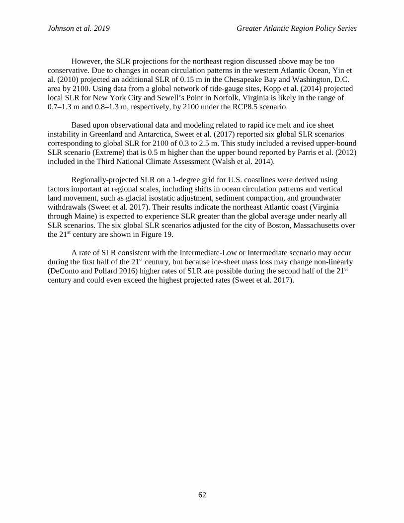
Johnson et al. 2019 Greater Atlantic Region Policy Series
62
However, the SLR projections for the northeast region discussed above may be too
conservative. Due to changes in ocean circulation patterns in the western Atlantic Ocean, Yin et al. (2010) projected an additional SLR of 0.15 m in the Chesapeake Bay and Washington, D.C. area by 2100. Using data from a global network of tide-gauge sites, Kopp et al. (2014) projected local SLR for New York City and Sewell’s Point in Norfolk, Virginia is likely in the range of 0.7–1.3 m and 0.8–1.3 m, respectively, by 2100 under the RCP8.5 scenario.
Based upon observational data and modeling related to rapid ice melt and ice sheet
instability in Greenland and Antarctica, Sweet et al. (2017) reported six global SLR scenarios corresponding to global SLR for 2100 of 0.3 to 2.5 m. This study included a revised upper-bound SLR scenario (Extreme) that is 0.5 m higher than the upper bound reported by Parris et al. (2012) included in the Third National Climate Assessment (Walsh et al. 2014).
Regionally-projected SLR on a 1-degree grid for U.S. coastlines were derived using
factors important at regional scales, including shifts in ocean circulation patterns and vertical land movement, such as glacial isostatic adjustment, sediment compaction, and groundwater withdrawals (Sweet et al. 2017). Their results indicate the northeast Atlantic coast (Virginia through Maine) is expected to experience SLR greater than the global average under nearly all SLR scenarios. The six global SLR scenarios adjusted for the city of Boston, Massachusetts over the 21st century are shown in Figure 19.
A rate of SLR consistent with the Intermediate-Low or Intermediate scenario may occur
during the first half of the 21st century, but because ice-sheet mass loss may change non-linearly (DeConto and Pollard 2016) higher rates of SLR are possible during the second half of the 21st century and could even exceed the highest projected rates (Sweet et al. 2017).

Johnson et al. 2019 Greater Atlantic Region Policy Series
63
Figure 19. Projected sea level rise for Boston, MA, based upon six global sea level scenarios for the year 2100: Low (0.3 m), Intermediate-Low (0.5 m), Intermediate (1.0 m), Intermediate-High (1.5 m), High (2.0 m), and Extreme (2.5 m) (Sweet et al. 2017; https://tidesandcurrents.noaa.gov/publications/techrpt083.csv).
E. Observed and Projected Ocean and Coastal Salinity As discussed above, the NAO and the related AO are the principal modes of annual- to
decadal-scale climate variability in the North Atlantic and effect atmospheric and oceanic thermohaline circulation patterns in the region. Curry et al. (2003) found systematic freshening of the North Atlantic Ocean between the 1950s and the 1990s.
Changes to the Arctic climate between the late 1980s and early 2000s are associated with
a strong cyclonic atmospheric circulation pattern that is characteristic of highly positive AO condition (Greene et al. 2008). Highly-positive AO conditions favor the melting of permafrost, snow, ice, and river discharge (as a result of increased precipitation) into the Arctic Ocean (Greene and Pershing 2007; Greene et al. 2008). This, in turn, led to an increase in low-salinity waters entering the Canadian Archipelago and a general freshening of shelf waters of the Labrador Sea, GOM, Georges Bank, and the MAB (Häkkinen 2002; Mountain 2003; Smith et al. 2001). Mountain (2003) reported freshening of MAB waters by about 0.25 ppt in the 1990s, compared to the 1977–1987 period, with large interannual variability attributed to reduced salinity from greater Scotian Shelf Water inflow into the GOM and Georges Bank (an important source of MAB water).

Johnson et al. 2019 Greater Atlantic Region Policy Series
64
Using satellite-derived coastal ocean and estuarine modeling, Geiger et al. (2013) reported decreasing trends in salinity for the Mid-Atlantic region, with the largest areas of salinity change off the coast of Long Island and New Jersey. They found correlations for positive intervals of the NAO and a tendency for high discharge and low salinity in the Long Island Sound and suggested the trends of coastal salinity freshening are linked to a larger natural climate cycle. The annual streamflow in the Hudson and Connecticut Rivers, which provide fresh water to the Long Island Sound estuary, have been increasing due to higher flow rates in the low-flow months (June-December) and the spring freshet is arriving 8-days earlier than a century ago (EPA 2016).
Balch et al. (2012) reported reductions in the salinity and density of surface waters of the
western GOM between 2005 and 2010, coinciding with extremes in precipitation and river discharge. They attributed these changes to changes in the North American hydrological cycle, as well as warming and melting of the polar ice cap that reduces salinities in the southward flowing Labrador Current. Furthermore, Balch et al. (2012) reported decreases in carbon fixation by phytoplankton during this time series and suggested the observed physical and chemical changes attributed to precipation and river discharge are playing a critical role in controlling the long-term productivity in the GOM.
Four similar salinity anomaly events attributed to Arctic Ocean freshwater pulses have
occurred since the 1970s, affecting the North Atlantic Ocean circulation patterns and climate in adjacent landmasses (Belkin 2004; Greene et al. 2008). In 1997 and 1998, the strongly positive AO conditions that prevailed in the 1990s shifted to a negative phase with a corresponding reduction in freshwater export from the Arctic Ocean and elevated salinities throughout the Northwest Atlantic shelf waters (Greene et al. 2012).
The changes observed in the Arctic climate in the 1990s, including increased
precipitation and freshwater river discharges into the Arctic Ocean, and increased melting of permafrost, snow, and ice, may be an indicator of future conditions in a warming climate (Greene et al. 2008). These changes, in turn, resulted in enhanced freshwater export from the Canadian Archipelago and freshening of shelf waters from the Labrador Sea to the MAB. In addition, since the 1970s, the AO has predominantly been in a positive phase, and some studies have suggested this may be a response to anthropogenic climate change (McBean et al. 2004). Although the AO has exhibited variable phase patterns in the past decade, the great salinity anomaly events observed in previous decades have not repeated and the Arctic Ocean has been in an extended period of freshwater storage (Greene et al. 2012). Consequently, future salinity trends for the NES waters are difficult to project.
Using a high-resolution global climate model, Saba et al. (2016) found a projected
doubling of atmospheric CO2 concentration would result in an increase in salinity in the NES due to changes in water mass distribution related to a retreat of the Labrador Current and a northerly shift in the Gulf Stream.

Johnson et al. 2019 Greater Atlantic Region Policy Series
65
F. Observed and Projected Ocean and Coastal pH The average pH of global ocean surface waters has declined about 0.1 units, from about
8.2 to 8.1 since the beginning of the Industrial Revolution, corresponding to a 26 percent increase in the hydrogen ion concentration of seawater (Feely et al. 2009; Rhein et al. 2013; Zeebe 2012). The largest reduction of ocean surface water pH (–0.10) has been recorded in the northern North Atlantic (Rhein et al. 2013).
Coastal waters are generally more susceptible to acidification than oceanic waters
because they are subject to more acid sources and are generally less buffered than oceanic waters (i.e., differences in the amount of dissolved inorganic carbon, dissolved and particulate organic carbon, total alkalinity and nutrients from riverine and estuarine sources) (Ekstrom et al. 2015; Gledhill et al. 2015; Waldbusser et al. 2011). Feely et al. (2010) reported substantially lower pH and aragonite saturation state values in parts of Puget Sound than would be expected from atmospheric CO2 alone. They estimated approximately 51–76 percent of the reduced pH in Puget Sound is attributed to decomposition of organic matter within the estuary. A long-term monitoring program in the Chesapeake Bay found statistically significant declines in daytime average pH from 1985 to 2008 within polyhaline waters, but not in mesohaline waters of the Bay (Waldbusser et al. 2011). Coastal acidification generally exhibits higher spatial and temporal variability relative to OA.
The cold waters of the Arctic Ocean also have naturally low CaCO3 saturation states. The
lower saturation state with respect to aragonite and calcite in the Arctic is also related to a decrease in total alkalinity in surface waters due to higher rates of freshwater inflow from river water and ice melt (Chierici and Fransson 2009; Mathis et al. 2015; Yamamoto-Kawai et al. 2011; Yamamoto-Kawai et al. 2009). These studies reported surface waters in the Canadian Basin of the Arctic Ocean in the 2000s to be undersaturated with respect to aragonite, attributed to recent increased rate of melting sea ice. In addition, Yamamoto-Kawai et al. (2009) concluded the recent retreat of the ice edge in the Canadian Basin past the shelf-break has produced conditions favoring enhanced upwelling of subsurface, aragonite-undersaturated water into the Arctic continental shelf. Additionally, the indirect effect of decreasing sea ice coverage is providing a positive feedback, in which more open water increases the uptake of atmospheric CO2 (Mathis et al. 2015).
Most surface waters in the global ocean are currently supersaturated with respect to
CaCO3. The current global mean sea surface saturation state values is 2.98 ± 0.9 for aragonite (Ωar) and 4.58 ± 1.3 for calcite ( Ωca), where Ω = 1 expresses saturation (Feely et al. 2009). When seawater is supersaturated with respect to aragonite and calcite (i.e., Ω > 1), calcification is favored more than dissolution.
The current North Atlantic mean sea surface saturation state is approximately Ωar = 3.47
± 0.3, and Ωca = 5.31 ± 0.8 (Feely et al. 2009). However, on the continental shelf between the MAB and Georges Bank, mean sea surface saturation state of aragonite declines to the north, and generally with depth. Wang et al. (2013) reported mean Ωar = 3 east of North Carolina, 2.5 southeast of Massachusetts, and 1.9 east of New Hampshire; the lowest values were found in the deep waters in the GOM (Ωar = 1.3).

Johnson et al. 2019 Greater Atlantic Region Policy Series
66
According to Gledhill et al. (2015), New England and Scotian Shelf waters may be particularly susceptible to OA because of lower temperatures and changes in the concentration of total alkalinity and dissolved inorganic carbon from river discharge, both of which reduces the buffering capacity of those waters. Rivers in New England that have a combination of cool temperatures, low alkalinity, and runoff typically consisting of soils containing carbonic acid, a by-product of organic decomposition, have particularly low Ωar values (Salisbury et al. 2008). For example, in the Casco Bay during times of high discharges from the Kennebec River and down-welling (northerly) winds, acidic river waters with Ωar <1.5 have been recorded (Salisbury et al. 2008).
G. Observed and Projected Ocean Dissolved Oxygen Coastal waters and estuaries in the northeastern U.S. frequently experience both hypoxic
(low oxygen) and anoxic (zero oxygen) conditions. Natural, periodic high rates of photosynthesis can induce high rates of oxygen consumption in subsurface waters and sediments, and eutrophication by agricultural runoff and sewage inputs pose serious problems in many coastal and estuarine systems (Diaz and Rosenberg 2008; Keeling et al. 2010).
Coastal hypoxia follows four general patterns: 1. Increased deposition of organic matter promotes microbial growth and respiration and increases biological oxygen demand, resulting in hypoxia. 2. It occurs transiently, often followed by mass mortalities of benthic and sessile organisms. 3. It occurs seasonally or periodically, characterized by boom-and-bust cycles of populations. 4. If organic matter and nutrients continue to accumulate in the sediments, and the DO concentrations continue to fall, anoxia is established and microbially-generated hydrogen sulfide is released which is toxic to most organisms (Diaz and Rosenberg 2008). These patterns of hypoxia and anoxia are exemplified in the Chesapeake Bay.
Anthropogenic nutrient loading into the Chesapeake Bay since the mid-20th century has reduced the system’s ability to assimilate nitrogen inputs without developing hypoxia and have led to reductions or losses of key ecological processes sensitive to eutrophication (Kemp et al. 2005).
Climate change will likely further complicate the causative factors of natural and
anthropogenic hypoxia (Rabalais et al. 2010). Because a continued warming trend is projected for the Western Atlantic, including the northeastern U.S. coastal waters (Hayhoe et al. 2007; Khan et al. 2013; Saba et al. 2016), strengthened stratification alone will worsen hypoxia where it currently occurs and expand its formation in additional areas (Rabalais et al. 2010). Furthermore, most models project increases in winter and spring precipitation and in precipitation intensity in the northeast region (Hayhoe et al. 2007; Horton et al. 2014; Meehl et al. 2007), suggesting that greater freshwater discharges into bays and estuaries may increase nutrient inputs and exacerbate eutrophic and hypoxic conditions (Rabalais et al. 2010).

Johnson et al. 2019 Greater Atlantic Region Policy Series
67
H. Observed and Projected River and Stream Temperature Water temperatures are increasing in many streams and rivers throughout the United
States, although some of this change can be attributed to urbanization and deforestation. Kaushal et al. (2010) found significant increases in annual mean water temperatures in 20 of the 40 assessed U.S. rivers and streams. The authors reported increased water temperatures between 0.009 and 0.077 °C per year that were typically correlated with increases in air temperatures and urbanization. Although there were significant increases observed for nearly all streams and rivers in the southeastern, midwestern, and western regions of the United States, the observed rates of increase were the highest for more urbanized areas of the mid-Atlantic United States. The highest rates of increased river and stream temperatures were on the Delaware River and Brandywine Creek in Pennsylvania, the Gunpowder River in Maryland, and the Potomac River in Washington, D.C. (Kaushal et al. 2010). Rice and Jastram (2015) reported statistically significant increases in water and air temperature anomalies (0.54 and 0.39 °C, respectively) between the periods 1961–1985 and 1986–2010 in the Chesapeake Bay watershed. They found increasing water temperature trends despite increasing trends in streamflow in the northern part of the study area. The authors concluded that continued warming in the Chesapeake Bay will likely result in shifts in distributions of aquatic biota and worsening eutrophic conditions in the bay and estuary (Rice and Jastram 2015). In a New England study on alewife migration timing, four streams with both historic and recent temperature data had warmed to 13 °C about 12 days earlier in the spring than they did in the 1970s (Ellis and Vokoun 2009).
Other measures of river and stream temperature conditions in the northeast are changing,
including ice thickness, dates of spring ice-out, and seasonal stream runoff volume. Huntington et al. (2003) reported average ice thickness decreased by about 46 percent, and both ice-out and seasonal center-of-volume date occurred earlier during the 20th century for the Piscataquis River, Maine. All of these systemic temporal trends were correlated with winter air temperature, suggesting sensitivity to regional climate forcing (Huntington et al. 2003). Similarly, Hodgkins et al. (2005) found 12 of the 16 studied unregulated New England rivers demonstrated a significant decrease in the number of days of ice-affected flow and earlier last dates of ice-affected flow in the spring.
Correlations between air temperatures and lake, river, and stream water temperatures
have been reported in several studies (IPCC 2001; Kaushal et al. 2010; Livingstone 1997; Vaughan et al. 2013). This includes water temperature-related conditions such as ice-affected flow and ice-out dates (Hodgkins and Dudley 2006; Hodgkins et al. 2003; Hodgkins et al. 2005; Hodgkins et al. 2002; Huntington et al. 2003), and ice thickness (Huntington et al. 2003). Climate models for atmospheric warming in the northeast U.S. region by the 2080s under the A2 and BI emission scenarios are projected to be 2.50–5.56 ºC and 1.67–3.33 ºC, respectively (Horton et al. 2014), and so it is reasonable to assume river and stream temperatures will warm accordingly.

Johnson et al. 2019 Greater Atlantic Region Policy Series
68
I. Observed and Projected Precipitation and Inland Hydrology High inter-annual variability for precipitation makes distinguishing long-term trends from
natural fluctuations difficult. Nonetheless, analyses of historical records over the last century show a consistent long-term positive trend in annual precipitation in the northeast region (Easterling et al. 2017; Guilbert et al. 2015; Hayhoe et al. 2007; Horton et al. 2014; Karl and Knight 1998; Thibeault and Seth 2014; Walsh et al. 2014). Between 1895 and 2011, mean annual precipitation increased by approximately 10 mm per decade (Kunkel et al. 2013). Similar increases in decadal trends (9.5 mm per decade) for New England over the last century were reported by Hayhoe et al (2007). Kunkel et al. (2013) reported only fall precipitation trends were statistically significant (+6.1 mm per decade), but not winter, spring, or summer precipitation trends. Easterling et al. (2017) reported fall precipitation increased by more than 15 percent across most of the northeast region between 1986 and 2015 compared to the first half of the last century (1901–1960).
Guilbert et al. (2015) reported an increased persistence of precipitation events (i.e.,
probability of precipitation in one day and given precipitation in the proceeding day) in the northeast United States. More than two-thirds of the 222 stations analyzed in the northeast region showed positive trends (+0.5 mm per day per decade) for the 95th percentile of daily precipitation in the months of October through May (Guilbert et al. 2015). However, these trends are not spatially uniform. Connecticut exhibited the largest increases with a trend of +1.1 mm per day per decade in the 95th percentile of daily precipitation, while no trends were observed for West Virginia. Similarly, Thibeault and Seth (2014) attributed observed increases in total annual rainfall in the northeast U.S. region and adjacent Canada to increasing trends in observed wet precipitation extremes rather than an increase in the number of wet days.
Annual precipitation has shown a shift towards greater variability and higher totals across
the entire United States since 1970, although extreme precipitation events have been higher on the east coast than on the west coast and midwest regions (Karl and Knight 1998; Sun and Lall 2015; Walsh et al. 2014). Between 1958 and 2016, the northeast region saw a 55 percent increase in the amount of precipitation falling as very heavy events (defined as the total precipitation falling in the top 1 percent of all days with precipitation) (Easterling et al. 2017). Furthermore, the number of 2-day events with a precipitation total exceeding the largest 2-day amount that is expected to occur, on average, only once every 5 years increased by 92 percent in the northeast region (Easterling et al. 2017). Douglas and Fairbanks (2011) reported strong increases in the magnitude of extreme precipitation events between 1970 and 2008 in New England, and especially in eastern Massachusetts and southern New Hampshire. They also found increases in the frequency of extreme rainfall events in New England, which was highest during August through November, but the increased frequency was not as great as the increase in the magnitude of extreme events.
In general, stream discharges in New England and the mid-Atlantic have increased over
the past century. A number of investigators have reported increases in minimum and medial flow quantiles (Douglas et al. 2000; Hodgkins and Dudley 2005; Lins and Slack 1999; McCabe and Wolock 2002). McCabe and Wolock (2002) also found step increases in annual minimum and median daily streamflow in the northeast United States beginning around 1970. Collins (2009) reported 25 of the 28 examined New England stream gages with minimal human influence had

Johnson et al. 2019 Greater Atlantic Region Policy Series
69
upward trends in the highest annual instantaneous discharges. This study also demonstrated evidence for a step increase in flood magnitudes at about 1970. The results of similar studies for both New England (Armstrong et al. 2012) and mid-Atlantic streams (Armstrong et al. 2014) have shown evidence of widespread hydroclimatic increases in flood magnitude (Figure 20) and frequency (Figure 21), as well as evidence of a step increase around 1970 reported by McCabe and Wolock (2002) and Collins (2009). These studies suggest these hydroclimatic changes in regional flood response are related to a combination of factors, including cyclic atmospheric variability and secular trends related to climate warming.
Balch et al. (2012) observed extremes in precipitation and river discharge between 2005
and 2010 from the major watersheds in Maine that appear to have resulted in changes in the physical, chemical, and biological characteristics of the GOM. The physical and chemical changes included reductions in salinity and density of surface waters and increases in dissolved organic matter concentrations and nitrate and phosphate in the western GOM, which likely decreased primary production via light limitations. Figure 20. Spatial distribution in flood magnitude for streams in the northeast region, represented as percent change over the period of record for each gauge. Dark blue and red symbols are for Mid-Atlantic gauges and lighter symbols are for New England gauges (Armstrong et al. 2014).

Johnson et al. 2019 Greater Atlantic Region Policy Series
70
Figure 21. Spatial distribution of trends in flood frequency in the northeast region, represented as exceedances of “peak over threshold” discharge occurring in a “water year” (POT/WY). Dark blue and red symbols are for Mid-Atlantic gauges and lighter symbols are for New England gauges (Armstrong et al. 2014).
Collins et al. (2014) reported over half the annual peak floods in the northeast United States and Atlantic Canada occur in the late winter-early spring period. The floods are dominantly generated by Great Lakes-sourced storms and coastal lows (also known as “nor’easters”). They found the dominant mechanism for producing annual floods is rainfall. Although less dominant than Great Lakes-based storms in terms of the total number of annual floods they cause, coastal lows generally produce the larger annual floods across the region each year and account for a substantial proportion of the most extreme events.
Changes in the timing of winter-spring streamflows in the northeast have been reported
(Hodgkins and Dudley 2005; Hodgkins and Dudley 2006; Hodgkins et al. 2003). Hodgkins et al. (2003) found the timing of high-river flows in New England was positively correlated with late-winter and early-spring air temperatures. Most of the change has occurred since 1970, with the date of peak streamflow occurring 1-2 weeks earlier. For gaging stations north of 44° N latitude, approximately 32 percent have significantly earlier flows over 50, 60, 70, and 90-year periods, while 64 percent have significantly earlier flows over an 80-year period. Earlier winter-spring streamflows were attributed to earlier snowmelt runoff, mostly likely due to warmer air temperatures and/or increased ratios of winter rain to snow (Hodgkins and Dudley 2006).

Johnson et al. 2019 Greater Atlantic Region Policy Series
71
Hodgkins and Dudley (2005) reported mean March streamflows increased significantly at 14 unregulated rivers in northern New England, while mean streamflows in May significantly decreased at 10 stations, primarily in northern or mountainous sections of Maine, New Hampshire, and Vermont. The authors attributed earlier snowmelt to increased March and April air temperatures and thus increased streamflows in March and decreased streamflows in May.
Huntington et al. (2003) conducted an assessment of river ice patterns on the Piscataquis
River in central Maine because it is free of any significant confounding influences such as consumptive use, impoundment and release, or changes to land use. The authors reported average ice thickness decreased by about 46 percent, and both ice-out and seasonal center-of-volume date occurred earlier during the second half of the 20th century compared to the first half. All of these systemic temporal trends were correlated with air temperature, suggesting sensitivity to regional climate forcing (Huntington et al. 2003). A study of ice-affected flows of rural, unregulated New England rivers was conducted by Hodgkins et al. (2005), who found 12 of the 16 rivers demonstrated a significant decrease in the number of days of ice-affected flow and earlier last dates of ice-affected flow in the spring. The total annual days of ice-affected flow decreased on average by 20 days from 1936 to 2000 with most of the decrease occurring since the 1960s.
Hayhoe et al. (2007) projected precipitation in the northeast U.S. region using IPCC AR4
atmosphere-ocean general circulation models and reported that almost all model simulations show consistent increases in winter precipitation and a small decrease in summer rainfall. Specifically, by 2100 winter precipitation in the northeast region is projected to increase by 11 percent under the B1 (lower) and 14 percent under the A2 (mid-high) emission scenarios (Hayhoe et al. 2007). For the mid-Atlantic region, projections of annual precipitation are confounded by a wide spread among climate models, likely owing to the region’s position at the boundary between subtropical precipitation decreases and subpolar precipitation increases (Najjar et al. 2010).
The CMIP3 models used in the Third NCA (NCA 3) exhibited large uncertainties in
precipitation for the region, particularly in the first half of the 21st century (Kunkel et al. 2013). However, the models are mostly in agreement that precipitation is projected to increase across the entire region. The CMIP3 model projections indicate that under both the A2 and lower emission (B1) scenarios, the northernmost portions of the northeast region show the largest simulated increases in mean annual precipitation while the southern and coastal areas show less of an increase (Kunkel et al. 2013). The geographic gradient is largest in the latter half of the 21st century, especially in the A2 emissions scenario. For example, by 2085 the increase in precipitation for the southern West Virginia area is projected to be 0–3 percent, while the northern New England and New York areas area projected to experience a 6–9 percent increase.
Using CMIP5 models and the high-emissions RCP8.5, Thibeault and Seth (2014)
projected increases in total annual precipitation for the northeast region during the latter half of the 21st century, and largely attributed this to increases in winter wet extremes. They also projected the largest increases in heavy precipitation extremes will occur in the northern, coastal, and mountainous areas of the region.

Johnson et al. 2019 Greater Atlantic Region Policy Series
72
Karmalkar and Bradley (2017) analyzed the U.S. regional and national implications for projected changes in precipitation when the global mean air temperature exceeds the 1.5 °C and 2.0 °C thresholds (above pre-industrial levels) using the CMIP5 models for two future periods (2020-2039 and 2036-2055). They found a high degree of uncertainty among the models in regional precipitation projections for every region except the northeast United States. Winter precipitation is projected to increase in the eastern United States (including the northeast), and 75 percent of the models also indicate wetter summers in the northeast during both 20-year periods leading to an overall increase in annual mean precipitation.
Important progress was made in the multimodel ensembles used in the NCA 4, such as
CMIP5 and the North American Regional Climate Change Assessment Program (NARCCAP), to characterize projection uncertainty arising from model differences due to internal climate variability as reported in the NCA 3 (Easterling et al. 2017). The NCA 4 model projections for the northeast region indicate significant increases in precipitation in all seasons except for summer, with the largest increases in winter and spring. This is consistent with the simulated trends in the recent period (1971–2000) but at odds with the observed trends, which show increases only in fall (Lynch et al. 2016). The winter and spring precipitation is projected to increase between 10 and 20 percent for most areas of the northeast (Easterling et al. 2017). In the early to middle parts of this century, precipitation will likely be manifested as increases in snowfall, but in the latter half of the century precipitation will mostly be rainfall as it will be too warm to snow in many current snow-producing situations (Easterling et al. 2017).The NCA 4 reported monthly precipitation in the northeast region is projected to be about 2.5 cm greater for December through April by end of century (2070–2100) under the higher scenario (RCP8.5) (Easterling et al. 2017) (Figure 22).

Johnson et al. 2019 Greater Atlantic Region Policy Series
73
Figure 22. Projected change (percent) in total seasonal precipitation from CMIP5 simulations for 2070–2099 for the RCP8.5 scenario. The values are weighted multimodel means and expressed as the percent change relative to the 1976–2005 average. Stippling indicates that changes are assessed to be large compared to natural variations. Hatching indicates that changes are assessed to be small compared to natural variations. Blank regions are where projections are assessed to be inconclusive. Data source: World Climate Research Program’s Coupled Model Intercomparison Project. (Easterling 2017; Figure source: NOAA NCEI).
For extreme precipitation, the NCA 3 used NARCCAP regional climate and downscaled CMIP3 model simulations. These results indicated all areas of the northeast region are expected to see increases in the average annual number of days with precipitation exceeding 1 inch, with both model approaches showing a 21 percent increase for the 2041–2070 time-period under the A2 emissions scenario (Kunkel et al. 2013). The increases are higher for the more extreme thresholds (e.g., +79 percent for #days >4 inches) in the downscaled CMIP3 model. The greatest increases will be in parts of New York (30 percent in the 2041–2070 time-period) and the smallest increases are expected for the coastal region (9–12 percent). The NCA 4 reported similar projections for extreme precipitation in the northeast region, indicating the 20–year return period amount for daily precipitation (a daily precipitation quantity that has only a 5 percent chance of being exceeded in any year) will increase by 14 percent and 22 percent under the RCP4.5 and RCP8.5 scenarios, respectively (Easterling et al. 2017). For the mid-Atlantic region,

Johnson et al. 2019 Greater Atlantic Region Policy Series
74
most IPCC AR4 models have been in agreement that precipitation intensity is projected to increase. For example, under the high-emissions scenario (A1B), precipitation intensity is projected to increase by one standard deviation by 2100 (Meehl et al. 2007).
Neff et al. (2000) used general circulation model scenarios to project the effects of
climate change on mid-Atlantic region stream flows. Although both model scenarios indicate changes in the seasonality of peak flows (earlier autumn and winter-spring peaks), one model (Hadley Center HADCM2) projects an increase in annual streamflow while the other (Canadian Climate Center CGCMI) projects a modest decrease in annual streamflow. The authors point out that the Canadian model projects an increasingly warmer and drier climate than does the Hadley model, which effects the model outputs for streamflow. However, both models project an increase in stream flows during winter months due to warming-induced decreases in snow pack (Neff et al. 2000).
Similar results were reported in eastern Massachusetts by Tu (2009), who found climate
change will mainly affect the timing of streamflow, rather than the annual average. Using the outputs of the Third Generation Coupled Global Climate Model with the A1B (high) emissions scenario for the early 21st century (i.e., 2015-2024), stream flows in late fall and winter months were projected to increase while other months, especially in the summer and early fall, would decrease in most watersheds. The author attributed the increased streamflow during late fall and winter months to earlier snowmelt caused by increases in temperature (Tu 2009).
Hodgkins and Dudley (2013) modeled future peak stream flows in the basins of four
coastal Maine rivers (i.e., Pleasant, Narragaugus, Sheepscot, and Royal) which have minimal or no regulation of stream flows and continuous stream gage data for 19 to 70 years. The projected annual daily maximum peak flows increased or decreased, depending on the adjusted values of temperature and precipitation. Specifically, peak flows decreased as air temperature increased (with no change in precipitation), whereas increases in precipitation (with no change in temperature) lead to increased peak flows. They found peak flows decreased by larger amounts as the magnitude of air temperatures increased. As discussed previously, climate model projections for the northeast region under the high (A2) emissions scenario show warming of 2.50–5.56 ºC by the 2080s and annual and winter precipitation increasing as much as 9 percent and 29 percent, respectively (Kunkel et al. 2013). Assuming an increase in temperature of 4 ºC and a 15 percent increase in precipitation, the annual daily maximum peak flows increased between 4.5–13.7 percent for the four New England rivers studied; however, under the same warming scenario, the maximum peak flows for the four rivers increased between 34.2–54.3 percent if precipitation increased by 30 percent (Hodgkins and Dudley 2013).
Section II. Climate Change Effects on Marine and Coastal Resources
Introduction The effects of climate change on marine ecosystems have been documented in numerous
scientific publications and in major national and international reports (Doney et al. 2012; IPCC 2014b; Pershing et al. 2018; Pörtner et al. 2014; Staudinger et al. 2012). Climate change effects

Johnson et al. 2019 Greater Atlantic Region Policy Series
75
may manifest at the organismal level through physiological responses to changing environmental variables, individual-level behavioral changes, and at the population level through changes in the balance between mortality, growth, and reproduction (Portner and Peck 2010). In addition, changes in large ocean currents and wind-driven gyres that could occur as a result of climate change (Rhein et al. 2013) can influence the retention and dispersion of early life stages of marine organisms (Portner and Peck 2010). Poloczanska et al. (2013) found approximately 83 percent of all observations for marine species’ distribution, phenology, community composition, abundance, demography, and calcification across taxa and ocean basins were consistent with the expected impacts of climate change.
Climate-related impacts on living marine resources often involve multiple stressors that
can affect species individually, synergistically, and cumulatively. The vulnerability of marine species and habitats to climate change can be thought of as a combination of the exposure to climate variables (e.g., temperature, pH), the sensitivity of the variables that predict the species and population’s intrinsic resilience to change, and the adaptive capacity to accommodate or cope with the change with minimal disruption (Glick et al. 2011). The effects can be complex and interacting because climate change affects biodiversity and ecosystems through a variety of direct and indirect pathways. Many ecosystems have already been stressed by natural and other anthropogenic impacts, and human adaptation and mitigation responses are varied across multiple sectors (Staudt et al. 2013). By projecting the rate of changes for drivers of ocean ecosystem stress (i.e., SST, pH, DO, and primary production) using IPCC emission scenarios, Mora et al. (2013) projected biochemical changes (i.e., temperature, oxygen, pH, and primary food supply) would affect all global habitats and biodiversity hotspots under both RCP4.5 and RCP8.5. The smallest absolute changes in biogeochemical parameters are expected in deep-sea habitats, while the largest changes will likely occur in shallow-water habitats, such as coral and rocky reefs, seagrass beds, and shallow soft-bottom benthos (Mora et al. 2013). Henson et al. (2017) reported multiple drivers would exceed the background of natural variability in 55 percent and 86 percent of the world’s oceans by the 2030s and 2050s, respectively, under the RCP8.5 (“business as usual”) scenario.
While the effects of climate change may benefit some habitats and the populations of
species through increased availability of food or nutrients, reduced physiological costs for maintenance, or reduced competition and predation, a shift in environmental conditions outside the normal range of variability can result in suboptimal physiological performance for those habitats and species unable to adapt. This, in turn, may lead to higher mortality, reduced growth, smaller size, and reduced reproduction or populations (Doney et al. 2012). Thus, climate change will result in “winners” and “losers”.
For clarity, we have classified climate-related impacts on living marine resources into
five broad effects chapters: 1) temperature-related; 2) salinity-related; 3) sea level rise; 4) water-quality; and 5) OA and CO2-related effects. Chapter 6 of the guidance includes information related to the synergistic effects attributed to climate change.

Johnson et al. 2019 Greater Atlantic Region Policy Series
76
Chapter 1. Temperature-related Effects Temperature is an important factor in determining the metabolic rate and numerous life
history traits for species including growth, reproduction, the timing of migration (i.e., phenology), and defining the range and distribution of individuals within an ecosystem (Murawski 1993; O'Connor et al. 2007). Generally, the metabolic rate of ectothermic organisms increases exponentially with temperature (within the range of temperatures that an organism can tolerate), resulting in higher rates of most physiological processes, such as photosynthesis and respiration (Doney et al. 2012). However, regardless of metabolic rate, other physiological requirements must be met, including nutrition, thermal tolerance, oxygen availability, and environmental and organismal chemistry (Doney et al. 2012).
Ocean warming can affect the availability and distribution of suitable habitat (Bell et al.
2015; Hare et al. 2012a) and the abundance and activity rates of predator and prey species (Beaugrand et al. 2003; Beaugrand et al. 2009). Changes in the temperature regime of species and habitats as a result of climate change can result in direct and indirect, cumulative, and synergistic effects when combined with other natural and anthropogenic environmental impacts. Changes to the phenology (the annually-recurring life-cycle events such as the timing of migrations, spring phytoplankton blooms, and flowering, and the peak in the abundance of prey populations), is one of the key indicators of the impacts of climate change on biological populations. The different level of response to warming across functional groups and multiple trophic levels can lead to mismatches between successive trophic levels, which can then lead to altered food-web structures and ecosystem-level changes (Edwards and Richardson 2004).
A. Observed and Projected Effects for Fish and Invertebrates
a. Observed Changes in Spatial Distribution One of the primary responses of fish and invertebrate populations to warming oceans is a
shift in their spatial distribution, generally to higher latitudes (i.e., poleward) and to deeper waters as species seek cooler waters within their normal temperature preferences (Beaugrand et al. 2009; Cheung et al. 2009; Cheung et al. 2013; Dulvy et al. 2008; Hare et al. 2016b; Kleisner et al. 2016; Lucey and Nye 2010; Murawski 1993; Nye et al. 2009; Perry et al. 2005; Pinsky et al. 2013; Weinberg 2005). In general, the latitudinal changes observed in the ranges of marine species have exceeded those of terrestrial species, despite slower rates of warming in the oceans (Burrows et al. 2011). Sorte et al. (2010b) found the range shifts of marine species throughout the 20th century to be an order of magnitude faster than terrestrial species, and 75 percent of all range shifts in marine species were poleward. Pinsky et al. (2013) found that “climate velocity” (i.e., the rate and direction that climate shifts across the landscape) explained the magnitude and direction of shifts in latitude and depth of occurrence more effectively than did species life history characteristics. Although marine species are capable of more rapid shifts in distribution than terrestrial species because they face fewer barriers to dispersal and more completely fill their thermal niches, the observed rapid range shifts will fundamentally reorganize marine communities (Pinsky et al. 2013). Although the establishment and rates of colonization for marine species through human introductions (e.g., shipping ballast) are likely greater than range shifts due to warming waters, the community-level effects of climate change has the potential to seriously affect the structure and function of ecosystems (Sorte et al. 2010b).

Johnson et al. 2019 Greater Atlantic Region Policy Series
77
Although the distributions of marine species over recent decades have generally trended
poleward, there is a high degree of variability within the published literature in the rate of change in the distributions (Table 2). The global poleward shift in marine species ranges from 4 to 190 km per decade (Przeslawski et al. 2012; Sorte et al. 2010b). Some of the variability in estimates may be an artifact of methods used to define the range shifts or the study selection criteria used in the meta-analyses. Poloczanska et al. (2013) found the fastest rates of leading-edge expansions were found in highly mobile or dispersive pelagic organisms, including phytoplankton (470 km per decade), bony fishes (278 km per decade), and invertebrate zooplankton (142 km per decade). These rates are substantially greater than the average range shifts for terrestrial plants and animals, estimated to be about 6 km per decade (Parmesan and Yohe 2003).
Table 2. Observed poleward shifts in range of marine species
Study Taxa (# of species/stocks)
Poleward Shift (km per decade)
Geography Comments
Sorte et al. (2010a) Marine spp. (129)
190 Global Includes introduced species; meta-analysis
Poloczanska et al. (2013)
Marine spp. (360)
72 Global Measured leading edge of range; meta-analysis
Prezeslawski et al. (2012)
Marine spp. (311)
3.9–9.1 Global Meta-analysis
Perry et al. (2005) Marine fish (36) 71.7 North Sea Measured mean center of distribution
Overholtz et al. (2011)
Atlantic mackerel (1)
62.5 NES Measured mean center of distribution
Bell et al. (2015) Black sea bass, scup (2)
37.5–50 NES Measured spring center of biomass
Pinsky and Fogarty (2012)
Marine spp. (4) 27–78 NES Measured biomass-weighted mean range
Nye et al. (2009) Marine spp. (36) 10–80 NES Measured mean center of biomass
Pinsky and Fogarty (2012) compared the shifts in fishery landings and the geographic
distributions of four commercially-important species [i.e., American lobster, yellowtail flounder (Limanda ferruginea), summer flounder (Paralichthys dentatus), and red hake (Urophycis chuss)] in the northeast U.S. from the 1970s to 2010. The landings and landed value showed much weaker shifts than the species geographic distributions, suggesting that economic and regulatory constraints played important roles in creating lags. Their analysis showed a poleward shift in geographic distribution for these four species at rates of 27–78 km per decade, substantially faster than the shifts in the landings of 3–9 km per decade (Pinsky and Fogarty 2012).
Cheung et al. (2013) reported a statistically-significant positive relationship between
changes in SST and the mean temperature of the catch (MTC) index (i.e., based on the average inferred temperature preference of exploited species weighted by the annual catch) in 52 large marine ecosystems covering the majority of the world’s coastal and shelf areas. The analysis shows an increase in the MTC at a rate of 0.23 °C per decade between 1970 and 2006 in temperate and subtropical areas. In the northeast Atlantic Ocean, the MTC index increased 0.49 °C per decade (Cheung et al. 2013). Even after accounting for the effects of fishing and large-

Johnson et al. 2019 Greater Atlantic Region Policy Series
78
scale oceanographic variability, this study suggests the composition of marine fisheries catch is significantly related to temperature changes, such that warmer-water species are increasingly dominant in higher latitudes.
In the northeastern Atlantic Ocean, Perry et al. (2005) found the centers of distribution
(as measured by mean latitude) for North Sea fishes shifted in response to warming waters for 15 of 36 species investigated, and 21 of these species showed a shift in mean latitude or depth, or both. The mean centers of distribution changed by 172 km for all species assessed between 1977 and 2001, and most (13 of 15 species) of these shifts were northward (Perry et al. 2005). Dulvey et al. (2008) demonstrated a deepening of the North Sea demersal fish assemblage by 3.6 m per decade in response to increased winter bottom temperatures over a 25-year period.
In the northwestern Atlantic Ocean, similar poleward changes in the latitudinal
distribution have been observed in response to rising ocean temperatures for large numbers of U.S. northeast marine species (Bell et al. 2015; Kleisner et al. 2016; Lucey and Nye 2010; Murawski 1993; Nye et al. 2009; Pinsky and Fogarty 2012). In an analysis of 36 fish and squid species using over 20 years of fisheries-independent trawl data from the northwest Atlantic, Murawski (1993) found the variations in water temperature were significant in explaining changes in mean latitude of occurrence in 12 of the 36 species. Pelagic species, such as Atlantic mackerel (Scomber scombrus) and Atlantic herring (Clupea harengus), demonstrated the greatest latitudinal responses to interannual differences in water temperature (Murawski 1993). For example, with each one-degree C increase in average water temperature, the Atlantic mackerel stock moved 0.5–0.8 degrees of latitude (about 56-89 km) to the north. Overholtz et al. (2011) reported changes in the distribution of the Atlantic mackerel stock in the NES waters between 1968 and 2008, indicating the stock moved about 250 km to the north and east, and into shallower shelf waters in response to long-term warming. They attributed these trends to the AMO and anthropogenic global warming, as well as interannual temperature variability related to bottom temperatures and the NAO.
Bell et al. (2015) reported significant poleward shifts in distributions of black sea bass
(Centropristis striata), scup (Stenotomus chrysops), and summer flounder for at least one season, while the Southern New England/Mid-Atlantic Bight (SNE/MAB) stock of winter flounder (Pseudopleuronectes americanus) did not shift. The results of their generalized additive model indicated the changes in the centers of biomass for black sea bass and scup in spring were related to increased water temperatures on the shelf, while the change in the distribution of summer flounder was primarily attributed to reduced fishing pressure and an expansion of the length–age structure. Their analysis indicated black sea bass and scup have shifted their spring center of biomass by 150–200 km in the four decades since the 1970s (Bell et al. 2015). Their results indicating the range of the SNE/MAB winter flounder stock has not shifted northward may be due to their life history. Winter flounder is a cold-water species that tend to spawn each winter in their natal estuary (Collette and Klein-MacPhee 2002). Because they show spawning site fidelity, it appears individuals are not shifting north with their suitable thermal habitat but return to their natal estuary where conditions are suboptimal. While the abundance of the stock has declined since the 1980s and has remained low (NOAA 2015b), their range has not shifted or contracted, suggesting that winter flounder continue to occupy the same area, but their total density within that area is greatly reduced. Bell et al. (2014) reported a decline in productivity and low

Johnson et al. 2019 Greater Atlantic Region Policy Series
79
recruitment of the stock with warming conditions, suggesting a reduction in total fitness has led to a further decline in abundance despite a stable range (Bell et al. 2015).
In an assessment of fish stock distributions in the northeast U.S. continental shelf from
1968–2007, Nye et al. (2009) reported statistically significant poleward shifts in the mean center of biomass for 17 of the 36 stocks reviewed over a broad range of taxa and life histories. The observed shifts in the mean center of biomass for these 36 fish stocks ranged from 1–8 km per year. In addition, 17 stocks showed statistically significant increases in the mean depth of occurrence, and eight exhibited poleward shifts in distribution. They found long-term changes in distributions across many families, life histories, habitat preference, and historical fishing pressure, and these changes have been correlated to large-scale warming and climatic conditions over the NES ecosystem. Species that are comprised of northern (i.e., GOM) and southern (i.e., southern New England and MAB) stocks, such as red hake, showed larger distributional responses for the southern stocks (Figure 23). Their study suggested the bathymetry and geography of the GOM constrains the poleward shift in distribution for many of the species found in the GOM. If fish shifted directly poleward or in a northwesterly direction from their historical GOM habitat, the shallow waters of the Bay of Fundy and Scotian shelf would be suboptimal for many of the cold deep-water fishes of the GOM. Although stocks restricted to the GOM, such as cusk (Brosme brosme) and pollock (Pollachius virens), generally did not demonstrate poleward shifts in their centers of biomass, they did exhibit increases in mean depth of occurrence and temperature of occurrence. In addition, some of the deep-water sedentary species in the GOM demonstrated range contractions, such as pollock, cusk, American plaice (Hippoglossoides platessoides), and Acadian redfish (Sebastes spp.), even though temperatures in the deep waters did not experience fluctuations as great as shallower parts of the NES ecosystem. This suggests some deep-water sedentary fishes may not be able to adjust their spatial distribution in response to warming and may experience sublethal effects including greater changes in growth, reproduction, and recruitment compared to species that have shifted their distribution (Nye et al. 2009).

Johnson et al. 2019 Greater Atlantic Region Policy Series
80
Figure 23. Changing spatial distribution of red hake (northern and southern stocks combined) in 5-year time blocks from 1968 to 2007 using inverse distance weighting. Units of biomass are in kg per tow (Nye et al. 2009. Used with permission).
Although Nye et al. (2009) did not directly assess the role of fishing in distributional
shifts, there is evidence that fishing may exacerbate the effects of climate change (Brander 2010; Lucey and Nye 2010; Perry et al. 2010; Pershing et al. 2015; Planque et al. 2010; Rose 2004). A number of historically heavily-exploited species in the NES ecosystem (e.g., Atlantic cod) are at record low levels, particularly at the southern limit of their range, which can shift the distribution to higher latitudes. Despite reduced fishing mortality through stricter management, the southern stocks of many of these species have not recovered to historic population sizes (Nye et al. 2009). Thus, already stressed populations are expected to be less resilient and more vulnerable to climate impacts (Staudinger et al. 2012; Staudt et al. 2013).
Data collected from the NOAA Fisheries bottom trawl fall survey data for the U.S. NES
indicate the mean rate of shift in distribution for all species reported in the survey between 1967 and 2016 is approximately 0.11 °N (12.7 km) per decade in latitude and 2.3 m per decade in depth (Figures 24a and 24b).

Johnson et al. 2019 Greater Atlantic Region Policy Series
81
Figure 24a) Change in mean latitude of catch, and 24b) Change in mean depth of catch. Species per year of each survey (weighted by biomass) for all fish and invertebrate species in the U.S. NES Ecosystem from NOAA Fisheries fall bottom trawl survey data, 1967-2016 (data from OceanAdapt, http://oceanadapt.rutgers.edu/regional_data; Pinsky et al. 2013. Reprinted with authors' permission).
Nye et al. (2011) and Davis et al. (2017) reported a correlation between the position of the Gulf Stream and the spatial distribution of silver hake (Merluccius bilinearis) on the U.S. NES, with the Gulf Stream leading the silver hake biomass by about 6 months. As reported by Nye et al. (2009), the center of of biomass for the southern population of silver hake has shifted

Johnson et al. 2019 Greater Atlantic Region Policy Series
82
poleward in response to warmer bottom temperatures, which has been in part attributed to large-scale circulation change affecting the Gulf Stream path, namely changes in the AMOC (Nye et al. 2011). Davis et al. (2017) found a large spring biomass of silver hake was concentrated in the Gulf of Maine and northern Mid-Atlantic Bight when the Gulf Stream was in its northerly position, while a large spring biomass was mainly along the outer shelf of southern Mid-Atlantic Bight when the Gulf Stream was in its southerly position. Using linear autoregressive modeling, they predicted the Gulf Stream would shift towards its northerly position after 2010, which is in agreement with recent observations, although the most recent silver hake distribution data were not available at the time of their publication (Davis et al. 2017). These studies suggest predictions of Gulf Stream position produces better prediction skills of silver hake center of biomass than the linear autoregressive modeling projection solely based on the observed silver hake time series. Furthermore, if the recently observed weakening of the AMOC and the Gulf Stream continues (Ezer et al. 2013; Sallenger et al. 2012), silver hake distribution will likely remain in a more northerly position on the U.S. NES.
A recent analysis of observed shifts in marine fish distributions in the U.S. NES
ecosystem with respect to regional climate velocity (i.e., the rate and direction of change of temperature isotherms) from 1968–2012 found consistent climate-related changes between groups of species that share similar depth and thermal characteristics (Kleisner et al. 2016). Species assemblages associated with warmer and shallower waters of the Mid-Atlantic Bight to Georges Bank have shifted along northerly latitudinal gradients with little change in depth. In contrast, they reported assemblages associated with the semi-enclosed GOM have exhibited two different trends: the shallower, warmer water species have tended to shift west-southwest and to shallower waters, while species associated with relatively cooler and deeper waters have shifted deeper, with little latitudinal change. In the absence of strong physiographic constraints in the Mid-Atlantic Bight/Georges Bank region, the shift in distribution for most species has largely followed the prevailing shift in temperature isotherms toward the northeast. In the GOM, where physiographic constraints are strong, shallow water assemblages have shifted west-southwest to where cooler bottom temperatures due to mixing of cooler surface water in the winter have been observed. In addition, they suggest competition from species entering the GOM from the southern NES, or species shifting from other parts of the GOM, may also be influencing this trend (Kleisner et al. 2016).
As NES waters have warmed the Atlantic cod observed range and core habitat areas have
contracted to approximately one-half its maximum extent between 1968 and 2014 (Selden et al. 2018). Cod primarily occupied the coldest bottom temperature areas of the inner shelf of the Mid-Atlantic Bight, Georges Bank, and coastal regions of the Gulf of Maine in the beginning of this time series but by 2010, its range extent had contracted to a subset of these cold regions. In contrast, spiny dogfish (Squalus acanthias), with its warmer sea bottom temperature affinity, has increased its core habitat area over the time series. Furthermore, Selden et al. (2018) found the fraction of the range for two prey species (sandlance and Atlantic herring) occupied by cod declined to 50 percent of the historic maximum by the end of the time series, while the overlap of core habitat declined for cod and four of its prey (sand lance, Atlantic herring, longfin squid, and Atlantic mackerel).

Johnson et al. 2019 Greater Atlantic Region Policy Series
83
There is evidence that warming ocean conditions may be influencing the distribution of diadromous fish. The center of biomass on the NES ecosystem for populations of alewife and American shad has shifted poleward by 5.47 and 6.86 km per year, respectively, from 1968 to 2007 (Nye et al. 2009). The rate of poleward shift of these two species was the fourth and second highest, respectively, in the 36 species examined in the study. Nye et al. (2009) hypothesized that widespread warming of the waters in the southern extent of the range for these species was a contributing factor in the recovery failure of the southern stocks despite reduced fishing pressure.
Changes in the spatial and temporal distributions of larval fish have been reported in the
NES ecosystem between 1977–1987 and 1999–2008 (Walsh et al. 2015). The spatial distribution of larvae was found to have changed in 43 percent of taxa (predominantly northward), while the timing of occurrence changed in 49 percent of larval taxa, with shifts evenly split between occurring earlier and later in the season. Observed changes in the timing of larval occurrence in this study suggest potential changes in spawning times and locations for some species. In species where both larvae and adults were analyzed, 48 percent exhibited different shifts between the larval and adult stages. Many of the changes in larval fish distributions reported in this study are consistent with warming water temperatures, indicating impacts on the productivity and distribution of fish stocks in the NES ecosystem are occurring (Walsh et al. 2015).
A shift in the distribution of Atlantic surf clams (Spisula solidissima solidissima) was
reported by Weinberg (2005) near the Delmarva Peninsula in the mid-Atlantic region of the United States. The area is close to the southern limit of the species range and the population typically experiences thermal stress during the fall season when nearshore water temperatures reach their maxima. Unusually warm water was prevalent from 1999–2002 in the Delmarva region, concurrent with a reduction in the probability of capture of surf clams in shallow waters based on fishery independent monitoring surveys. The combined effect of poor physiological condition and thermal stress was attributed to higher mortality of surf clams in shallow water, resulting in a shift in distribution to deeper water (Weinberg 2005). Jones et al. (2010) determined the southern range edge of blue mussel (Mytilus edulis) moved poleward by approximately 350 km since 1960 and provided evidence the shift was directly attributed to adult mortality related to high summer sea surface temperature.
Temperature-related effects have also been detected in the distribution and abundance of
zooplankton in the northeastern Atlantic Ocean. Beaugrand et al. (2009) observed changes in the biodiversity of calanoid copepods in response to rising SST over the period 1960–1999, with shifts from colder-water species to warm-water species in the North Sea. Smyth et al. (2004) reported satellite imagery from 1989 to 2003 showed the coccolithophorid phytoplankton Emiliana huxleyi may be advancing northward into the Barents Sea during periods of higher temperature and less saline conditions. Although coccolithophorid blooms in the Barents Sea are not a new phenomenon, the authors suggest the frequency of the blooms may be increasing with concurrent warming and freshening as a result of increased input of melt water and precipitation in the Arctic and the Barents Sea.
b. Projected Changes in Spatial Distribution The expected rates of change in the spatial distributions of fish and invertebrates under
projected warming scenarios are generally similar to or exceeding trends observed in recent

Johnson et al. 2019 Greater Atlantic Region Policy Series
84
decades. Cheung et al. (2009) projected the global median rate of poleward range shift for marine fish and invertebrates to be 45–59 km per decade across multiple IPCC emissions scenarios in the period 2040–2060 compared to 2001–2005. They reported the projected range-shift for demersal fish under the high emissions scenario (A1B) would be two times greater than the observed rate of range shift reported by Perry et al. (2005) from 1977 to 2001.
Cheung et al. (2010) projected large-scale changes in distribution of global fisheries catch
potential between 2005 and 2055. Under the IPCC high emissions scenario (A1B), catch potential in the Arctic and offshore region of the North Atlantic is projected to increase by more than 50 percent from the 2005 level. However, the catch potential on the east coast continental shelf is projected to decline approximate 13 percent due to shifts in species distribution and by changes in total primary production (Cheung et al. 2010).
Using species distribution modeling, Jones and Cheung (2015) predicted global shifts in
the distributions for 802 marine fish and invertebrate species under the low (RCP 2.6) and high (RCP 8.5) IPCC emission scenarios. The study predicted poleward shifts in the centers of distribution of 93 percent of marine species from 2000 to 2059 under the low emissions scenario, and 97 percent under the high emissions scenario in the same period. The median rate of poleward shift under the low and high emissions scenarios was predicted to be 15.5 km per decade and 25.6 km per decade, respectively. In addition, the modeling results indicated the highest rate of novel species immigration is projected to occur in higher latitude regions. For example, under the high emissions scenario the rate of immigration intensity is predicted to increase by 26 percent in the Arctic Ocean, with an average immigration rate of two species per 0.5° latitude change (Jones and Cheung 2015).
The geographic ranges of some marine species are projected to expand and may
experience increases is abundances due to warming ocean temperatures. Using a coupled climate-population model, Hare et al. (2010) projected a northward shift in the center of the population for Atlantic croaker (Micropogonias undulatus) of 50–100 km by 2100 under two emissions scenarios. Hare et al. (2012b) projected a northward expansion of gray snapper (Lutjanus griseus), a reef-associated, tropical species. Although young-of-the-year gray snapper have been reported as far north as Massachusetts, adults are rarely found north of Florida. Based on the hypothesis that the northern range of gray snapper is determined by distribution of overwinter mortality of young-of-the-year, they projected a rate of northward shift of 1.0–1.3 km per year using the IPCC AR4 low emissions (B1) scenario and 1.7–1.8 km per year under the high (A1B) scenario (Hare et al. 2012b).
Morley et al. (2018) modeled thermal habitats of 686 marine species in the Atlantic and
Pacific oceans of the North American continental shelves, which were coupled with GCMs run under high (RCP8.5) and low (RCP2.6) future GHG emission scenarios over the 21st century to project the magnitude and direction of future shifts in preferred thermal habitat. The West Coast U.S. and the Gulf of Alaska regions had the highest mean shifts under both emission scenarios, with 1,162 km and 954 km, respectively, for the RCP8.5 scenario. The NES also had a relatively high magnitude mean projected shift of 637 km under RCP8.5. In addition, many of the species on both coasts were projected to experience increases in thermal habitat availability. One exception noted for the NES was spiny dogfish which, although projected to shift distribution by

Johnson et al. 2019 Greater Atlantic Region Policy Series
85
483 km into the Newfoundland shelf and the Gulf of St. Lawrence region, was predicted to have a 32 percent net loss of thermal habitat due to declines in habitat availability in the southern portion of its range (Morley et al. 2018).
Selden et al. (2018) investigated the effect of future ocean warming on four important
piscivores (Atlantic cod, spiny dogfish, silver hake, and white hake) and four prey species (Atlantic herring, Atlantic mackerel, longfin squid, and sand lance) in the U.S. NES. With a projected doubling of CO2 over an 80-year period (approximate emissions under the IPCC RCP8.5 scenario), Atlantic cod is projected to lose 3.5 percent of total habitat area per degree of warming on average, and its range and core habitat increasingly restricted to cold-water habitat on Georges Bank and the Gulf of Maine. In contrast, spiny dogfish and silver hake are projected to gain 6 percent and 3 percent of habitat area per degree of warming on average, respectively, and simultaneously increase their core habitat area. In addition, the authors found projected ocean warming reduces the overlap in the range of Atlantic cod and the majority of its prey and limits cod to cold-water habitats in the northern part of the study region. Lower proportions of Atlantic cod prey range is projected to be occupied by cod as the ocean warms, and cod’s historically strong top-down control in the NES ecosystem is expected to diminish. Conversely, the projected range expansion of dogfish and silver hake resulted in enhanced overlap with prey, likely increasing their relative importance as piscivores in this ecosystem (Selden et al. 2018). This study demonstrates how a changing climate may benefit some species in the U.S. NES, while adversely affecting others (i.e., resulting in “winners and losers”). Furthermore, the ability of other piscivores in the marine ecosystem to functionally replace previously dominant species may contribute to greater resilience to climate change.
Shackell et al. (2014) proposed a “realized thermal habitat” index (i.e., habitat/niche
constrained by physiology and species interactions such as competition and predation) for marine fish and invertebrates in the Northwest Atlantic (U.S. and Canadian waters) under two warming scenarios (i.e., year 2030 = +0.7 °C for ≤ 100 m depth and +0.35 °C for >100 m, and year 2060 = +3 °C for ≤100 m depth and +1.5 °C for >100 m). On a regional scale, the realized thermal habitat of most species was projected to withstand warming projected for 2030, but not for 2060. For MAB, Southern New England, Georges Bank, and GOM waters, under the year 2030 scenario only 8 percent of all species will lose realized thermal habitat, while 10 percent will gain, and 83 percent will stay neutral. However, under the year 2060 scenario, 65 percent of all species assessed will lose realized thermal habitat, while 20 percent will gain, and 15 percent will stay neutral. The loss of realized thermal habitat is most pronounced in the GOM and Georges Bank, where many temperate/boreal species are already at their southern range limit. For example, the populations of Atlantic cod are projected to lose approximately 60 percent, 50 percent, and 45 percent of realized thermal habitat in the GOM, Southern New England, and Georges Bank, respectively (Shackell et al. 2014).
Using a high-resolution global climate model (CM2.6) and historical observations of
species distributions from trawl survey, Kleisner et al. (2017) projected changes in future distribution of suitable thermal habitat for various demersal and pelagic species on the U.S. NES. Projected warming, roughly corresponding to RCP8.5 emission scenario for 60-80 years in the future, for the Mid-Atlantic Bight and Georges Bank (4.1 °C at the surface and 5.0 °C at the bottom) resulted in a northward shift of thermal habitat for the majority of the species. For

Johnson et al. 2019 Greater Atlantic Region Policy Series
86
example, species associated with the southern portion of the NES, including summer flounder, striped bass, smooth dogfish (Mustelus canis), and Atlantic croaker, are expected to have significant increases in suitable thermal habitat. The Gulf of Maine subregion is projected to warm by 3.7 °C (surface) and 3.9 °C (bottom), resulting in substantial reductions in suitable thermal habitat such that some species currently inhabiting this area may not remain under continued warming. Kleisner et al. (2017) projected a loss in suitable thermal habitat for species such as Acadian redfish, American plaice, Atlantic cod, red hake, haddock, and thorny skate, but potential gains for some species such as spiny dogfish and American lobster. Figure 25 depicts the projected changes in spring modeled historical and future distribution of suitable thermal habitat of northern (top two) and southern (bottom two) associated species. Figure 25. Comparison of spring modeled historical and future distribution of suitable thermal habitat (red: more suitable, blue: less suitable) for species with more northern distributions (Atlantic cod and red hake) versus more southern distributions (Atlantic croaker and smooth dogfish) (Kleisner et al. 2017. Reprinted with authors' permission).
Projections in the distributions of 28 diadromous fish species over 196 basins across
Europe, North Africa, and the Middle East by 2100 under IPCC high-emissions scenario A2 resulted in range contraction for 14 species, the expansion in three species (mainly northward), and little or no change in the distribution of five species (Lassalle and Rochard 2009).
c. Observed Changes in Population Dynamics Water temperature can have a profound impact on the survival of fish, from enzyme
reactions, feeding rates, and seasonal distribution (Pörtner and Farrell 2008), and is especially

Johnson et al. 2019 Greater Atlantic Region Policy Series
87
relevant in early life history stages, recruitment, and biomass. The temperature-dependent survival mechanism may be due to physiological limits of fish, but also from effects of predation risk and food availability (Bell et al. 2014; Hare and Able 2007; Manderson 2008). Winter water temperature has been positively correlated with the spring juvenile and adult abundance of Atlantic croaker and may be important in explaining large year classes of the species and latitudinal range expansions during sequential warm winters in Chesapeake Bay (Hare and Able 2007). The authors correlated strong recruitment pattern in Atlantic croaker with warm winters that result in high juvenile survival in mid-Atlantic estuaries. This study demonstrated the variability of commercial catches of Atlantic croaker catch is strongly correlated with the NAO index, which is related to winter water temperatures on the east coast of the United States.
Beaugrand et al. (2003) found evidence that warming North Sea waters since the 1980s
have produced unfavorable conditions of the prey (i.e., calanoid copepods) for juvenile Atlantic cod. They concluded that increasing temperature may have resulted in doubly negative impact on cod survival by increasing cod metabolism and energetic cost as the availability and size of prey for juvenile cod was declining.
Collie et al. (2008) reported long-term changes in species composition inside
Narragansett Bay and in Rhode Island Sound from 1959 to 2005. Using weekly trawl data, they found estuarine communities shifted from vertebrates to invertebrates and since 1980, from benthic to pelagic species. The abrupt shift from benthic to pelagic species in 1980 and 1981 suggests a regime shift in community composition. Changes in species composition correlated strongly with spring-summer SST, which increased by 1.6 °C, as well as the winter NAO index. Demersal species such as winter flounder, silver hake, and red hake declined, while warm-water fishes, including butterfish (Peprilus triacanthus) and scup, and invertebrates such as American lobster and longfin squid (Loligo pealeii), increased with time. These changes in the species composition support the hypothesis that southern species are replacing northern ones in Narragansett Bay and Rhode Island Sound. A shift towards smaller body size was also correlated with changes in community structure, which may be a response to fishing pressure but is also a predicted response to warming waters (Collie et al. 2008). Wood et al. (2009) found the incidence of warm-water fish species (those generally associated with tropical and subtropical climates) has generally increased since the 1980s in Narragansett Bay and Long Island Sound, and warmer years were correlated with greater abundance of warm-water fish. Although they reported significant correlation with abundance of warm-water species and warmer years, they suggested non-temperature related factors could also be contributing to the observed trend, such as shifts in the transport mechanisms responsible for supplying warm-water fishes to northern habitats.
Fogarty et al. (2008) found Atlantic cod distribution, recruitment, and growth was highly
correlated with bottom temperature on the NES, such that the catch probability, recruitment success, and weight at age decreased with increasing water temperatures. In a meta-analysis of Atlantic cod stocks throughout the North Atlantic, Planque and Fredou (1999) demonstrated that recruitment-temperature relationship was generally positive in cold waters and negative in warm waters.

Johnson et al. 2019 Greater Atlantic Region Policy Series
88
Pershing et al. (2015) found strong associations with the survival and fitness of larval, juvenile and adult Atlantic cod and ocean temperatures, suggesting the substantial warming occurring in the GOM has led to reduced recruitment and increased mortality in the stock. They reported a reduction in recruitment of age-1 fish with higher summer temperatures, and an increase in mortality of age-4 fish with higher fall temperatures in the GOM, although the exact mechanism of these relationships was unknown. Unprecedented warming in the GOM between 2005 and 2015 was correlated with reduced recruitment and increased mortality of Atlantic cod. They suggested neglecting to include the influence of temperature in stock-recruitment models produced recruitment estimates that are on average 100 percent higher than if temperature were included and has therefore contributed to overfishing (Figure 26). By incorporating temperature in a population dynamics model, the authors demonstrated the spawning stock biomass of the stock had declined steadily rather than remaining constant, as assumed (Pershing et al. 2015). Figure 26. Time series of Gulf of Maine cod spawning stock biomass (blue), and age-1 recruitment (green) from the 2014 assessment. Cod age-1 recruitment modeled using adult biomass and summer temperatures (dashed line). Gray squares are recruitment estimates using a model without a temperature effect fit to data prior to 2004. Yellow diamonds are a temperature-dependent model fit to this earlier period (Pershing et al. 2015). Reprinted with permission from AAAS.
Manderson (2008) reported phase synchrony in nursery production for winter flounder
among 19 southern New England estuaries in the 1990s that were correlated with increased frequency of warmer spring temperatures. Winter flounder development, growth, and survival of egg, larvae, and early juvenile stages are generally negatively affected by high spring temperatures. A number of factors can influence phase synchrony in species, including population density and phenology in predator-prey populations. Increasing water temperatures in estuaries may increase the spatial scale of synchrony in nursery production and result in boom or bust cycles for winter flounder populations in the region (Manderson 2008).

Johnson et al. 2019 Greater Atlantic Region Policy Series
89
Bell et al. (2014) found the abundance of winter flounder was negatively correlated with winter water temperature but did not find this relationship in summer flounder. Conversely, the authors reported summer flounder abundance was negatively correlated with fishing mortality, while no such relationship with evident in winter flounder abundance. A reduction in fishing pressure in the mid-Atlantic and southern New England regions on both species since the mid-1990s has led to a rebuilding of the southern flounder stock, but winter flounder stocks have remained very low. The authors suggest that warmer winter temperatures and earlier spring warming may be reducing the thermally-available habitat and refuge from predation for winter flounder (Bell et al. 2014).
The decline in abundance of North American and European diadromous fish populations
are well documented and primarily attributed to the fracturing of coastal watersheds by man-made obstructions (e.g., hydropower dams, culverts) (Hall et al. 2011; 2012; Mattocks et al. 2017). Other anthropogenic factors have been attributed, including habitat loss, pollution, aquaculture, introduction of non-native species, water withdrawals, overfishing, and climate change (ASMFC 2012; Fay et al. 2006; Hall et al. 2012; Helfman 2007; Köster et al. 2007; Limburg and Waldman 2009; Mattocks et al. 2017). Relative abundances have dropped to less than 98 percent of historic levels in populations of some diadromous species (Limburg and Waldman 2009). Many populations persist at sharply reduced levels, but all species have suffered population extirpations, and many species have been classified as threatened or endangered. The life history strategies of diadromous fish subject individuals and populations to greater osmoregulatory and energetic demands, and to the uncertainties inherent in adapting to changing conditions in marine, estuarine, and freshwater environments. There is evidence that rising river and stream temperatures may be a contributing factor in the population declines of some North American diadromous fish. In a review of the diadromous fish fauna in the Hudson River, Waldman (2006) suggested a link between declines in populations of Atlantic tomcod (Microgadus tomcod) and rainbow smelt, both occurring at the southern margin of their ranges in the Hudson River, and thermal stress related to climate change. Historic records and publications indicate rainbow smelt were relatively abundant in the Hudson River prior to the 1980s, but the species has since declined considerably in both the Hudson River and Delaware River systems (Waldman 2006). Kaushal et al. (2010) reported the Delaware River exhibited one of the highest rates of increased river temperature in the United States.
The decline of diadromous fish abundances represents significant loss of the forage base
and trophic dynamics, and several studies have found correlations in the reduced population abundance of alewife and groundfish (e.g., Atlantic cod, haddock, pollock) in the western GOM (Ames 2004; Ames and Lichter 2013; Hall et al. 2012). Jordaan et al. (2008) hypothesized low abundance levels of alewife is a contributing factor in depressed productivity in Atlantic cod and may by an impediment in the recovery of the species.
Atlantic salmon abundance has declined since the 1970s in all Atlantic populations,
which Jonsson and Jonsson (2004) attributed to reduced marine growth rate, survival-rate, and production during the marine life stages. Chaput et al. (2005) reported a phase shift in the productivity of Northwest Atlantic salmon stocks in the 1990s, and low marine survival was identified as a contributing factor. Mills et al. (2013b) found coherence in the decline in abundance and productivity of salmon across major regions of North America, suggesting

Johnson et al. 2019 Greater Atlantic Region Policy Series
90
marine survivorship, rather than local, river-specific factors are responsible. Friedland et al. (2014) also reported strong coherence in juvenile salmon survival during post-smolt period in North American and European stock complexes and attributed the response to trends in SST and the AMO index. Beaugrand and Reid (2012) attributed marine mortality and low return rates to spawning rivers since the late 1980s to declines in North American salmon stocks. They reported parallel declines in zooplankton populations, considered the prey base for salmon, and salmon catches associated with increasing ocean temperatures.
Friedland et al. (2003a; 2003b) reported negative correlations in North American salmon
stock abundance with winter and spring SST in the inshore areas of the Gulf of Maine and Gulf of St. Lawrence. Friedland et al. (2003b) found air temperature and rainfall do not appear to be significant environmental variables in post-smolt salmon survival and concluded that climate impacts on freshwater habitats must be a secondary factor. However, they did find the timing of smolt runs appears to be out of synchronization with ocean conditions, with ocean conditions favorable to post-smolts. Friedland et al. (2003a) reported the highest negative correlations with stock abundance were for June SST, the time frame associated with the first weeks at sea for post-smolts for many stocks.
Friedland and Todd (2012) reported a strong positive relationship between growth
(weight and length at age) of post-smolt salmon and warmer waters in the southern portion of the Labrador Sea from about 1993 to 2009, but not with primary production and other metrics related to the forage base of salmon (i.e., plankton biomass and bloom timing). Winter-spring SST records for the Northwest Atlantic confirm spatial increases in 4-8 °C water, considered to be the preferred temperature for post-smolt salmon. Although higher ocean temperature appears to be associated with greater growth in post-smolt salmon, which would be expected to increase the reproductive output and recruitment of adults, the salmon abundance for North American stocks has nonetheless experienced multi-decadal decline (Friedland et al. 2009a; Friedland et al. 2009b; Hogan and Friedland 2010).
Friedland et al. (2014) reported the large-scale ocean surface climate shifts observed in
the western North Atlantic underlie the historical changes in salmon abundance, although they suggest this is unlikely directly associated with physiological effect of temperature alone on post-smolts, but rather probably manifested in temperature-driven changes in the ecosystem, including changes in the availability of plankton and nekton prey. Similarly, Mills et al. (2013b) found changes in climate-driven environmental factors, including warmer ocean temperatures, are associated with changes in plankton communities and prey availability that directly and indirectly affects the abundance and productivity of North American salmon stocks. They found ecosystem responses to warming Northwest Atlantic waters, including changes in the populations of phytoplankton, zooplankton, and forage fish [e.g., capelin (Mallotus villosus)] may be more important in the abundance and productivity of salmon than the direct influence of temperature (Mills et al. 2013b).
Warmer waters in overwintering young-of-the-year and juvenile habitats in estuaries and
rivers in the Northwest Atlantic caused by climate change may facilitate the expansion of populations of temperate species and facilitate northerly shifts in their distribution. For example, Hurst and Conover (1998) found evidence of size-dependent mortality with winter water

Johnson et al. 2019 Greater Atlantic Region Policy Series
91
temperatures in age-1 striped bass in the Hudson River, and suggested the severity of winters plays a fundamental role in regulating juvenile recruitment. Likewise, blue crabs (Callinectes sapidus) suffered higher mortality rates in the Chesapeake Bay when February water temperatures were below the 8-year average (Rome et al. 2005).
Although American lobster stock abundance in the GOM and Georges Bank is at an all-
time high and recruitment has remained high between 2008 and 2013, the southern New England population experienced steep declines beginning in the late 1990s to record low abundance in 2013 (ASMFC 2017). The declining southern New England stock has been attributed to changing environmental conditions, including warming waters and increased predation, but also high fishing mortality (ASMFC 2017). The stock has been particularly affected in the inshore portion of the distribution where environmental conditions have remained unfavorable to lobsters since the late 1990s (ASMFC 2017). Prolonged elevated water temperatures above 20 °C throughout southern New England waters, particularly in inshore waters where declines in population abundance are most pronounced since the late 1990s, is the most likely cause of the decline in the southern New England lobster stock abundance (ASMFC 2010). In addition, the loss of optimal shallow water habitat has caused the stock to contract spatially into deeper waters. Prolonged exposures to water temperature above 20 °C are associated with a variety of physiological stresses in American lobster, including respiratory and immune stress, and increased incidence of shell disease and other pathogen infections (Glenn and Pugh 2006; Robohm et al. 2005), and hemolymph acidosis (Dove et al. 2005).
Sorte et al. (2017) found evidence of long-term declines since the 1970s in blue mussel
populations, a foundation species known to influence diversity and productivity of intertidal habitats in the Gulf of Maine. At four sites with historical community data, they demonstrated blue mussel changed from a dominant to a minor contributor to the compositional patterns of intertidal communities in the Gulf of Maine. During the same period, sessile communities became increasingly dominated by algal species followed by a reduction in species richness. Although the authors attributed the loss of blue mussel populations to a multitude of direct and indirect effects of human activities (e.g., commercial harvesting, invasive species), they suggested that warming waters likely exacerbated these impacts (Sorte et al. 2017).
Warming of the upper layers of the ocean can increase stratification of the water column,
which reduces vertical mixing and nutrient availability for primary production (Gregg et al. 2003; Polovina et al. 2008). Global satellite observations of ocean chlorophyll are a standard method used to estimate global ocean primary production. Although global ocean chlorophyll concentrations increased by about 4 percent from 1998 to 2003, most of the increase occurred in coastal regions in less than 200 m depth (Gregg et al. 2005). However, major declines in chlorophyll concentrations were observed in the North and South Pacific and in the North and South Atlantic. Gregg et al. (2003) reported a 6 percent decline in global ocean primary productivity between 1997 and 2002, with nearly 70 percent of the decadal decline occurring in the high latitudes. Furthermore, the reductions in primary productivity corresponded with increased SST in northern high latitudes. Similarly, Polovina et al. (2008) showed an expansion of low chlorophyll waters in the North Atlantic Ocean over a 9-year period from 1998–2007. They found mean SST increased concurrently with the expansion of low chlorophyll waters. Although the area of low chlorophyll waters has expanded in both northern and southern

Johnson et al. 2019 Greater Atlantic Region Policy Series
92
hemispheres of the Atlantic and Pacific oceans, the rate of expansion in the North Atlantic was greater than other oceans measured in the study. High latitude oceans typically represent net sink of atmospheric carbon (i.e., carbon absorption exceeds release), primarily due to dominance of diatoms which grow and sink faster than other phytoplankton groups (Gregg et al. 2003). Therefore, a reduction in primary production in the North Atlantic could imply a reduced sink of atmospheric carbon via the photosynthetic pathway. However, longer time series and more focused analyses are necessary to characterize long-term trends in primary productivity with anthropogenic climate change and natural decadal oscillatory behavior, such as the NAO and PDO (Gregg et al. 2005).
Fulweiler and Nixon (2009) reported a climate-induced decline in sediment oxygen
consumption and biogeochemical exchanges between sediment and the water as a result of a 1.7 °C warming in the Narragansett Bay over a 30-year period. They attributed this change to a reduction in the standing crop of water-column chlorophyll due to shifts from a dominant winter-spring diatom bloom to ephemeral, less intense summer-autumn blooms, resulting in oligotrophication of the bay.
d. Projected Changes in Population Dynamics An assessment of the effects of projected climate change on 82 fish and invertebrate
species in the NES ecosystem by Hare et al. (2016b) found high to very high climate vulnerabilities for more than half the species based on the RCP 8.5 “business as usual” climate model projection for 2055 (Figure 27). Out of the seven climate exposure factors examined, changes in mean ocean surface temperature and mean surface pH were scored as the highest for all species because of the magnitude of change projected for the NES. The study concluded approximately half the assessed species would be negatively affected by climate change (e.g., decreased productivity and distribution shifts out of the NES ecosystem), including many of the iconic species such as Atlantic sea scallop (Placopecten magellanicus), Atlantic cod, Atlantic mackerel, Atlantic cod, and winter flounder. Diadromous fish and benthic invertebrates were estimated to have the highest climate vulnerabilities of all functional groups, whereas pelagic fish and cephalopods had no species that scored very highly or highly vulnerable and elasmobranchs and groundfish had no species that scored very highly vulnerable. This suggests that species with sessile life stages (e.g., adult shellfish) or species with specialized life histories or dependence on specific habitats (e.g., diadromous fish) are more vulnerable to climate change. Conversely, pelagic species and generalist species capable of shifting their distributions may be more resilient to a changing climate. About 17 percent of the species analyzed in this assessment, including longfin squid, butterfish, and Atlantic croaker, were estimated to have positive climate change effects (Hare et al. 2016b). Another study by Hare et al. (2010), using a coupled climate-population model, projected higher abundances for Atlantic croaker in northeastern U.S. coastal waters by the end of the century under two CO2 emission projections. At current levels of fishing, the average spawning biomass of Atlantic croaker is projected to increase by 60–100 percent (Hare et al. 2010).

Johnson et al. 2019 Greater Atlantic Region Policy Series
93
Figure 27. Climate vulnerability scores, based on individual species climate exposure and biological and ecological sensitivity attributes, for 82 species of fish and invertebrates in the U.S. NES. Certainty in score is denoted by text font and text color: very high certainty (>95 percent, black, bold font), high certainty (90–95 percent, black, italic font), moderate certainty (66–90 percent, white or gray, bold font), low certainty (<66 percent, white or gray, italic font) (Hare et al. 2016b).
Fogarty et al. (2008) projected the distribution and production of Atlantic cod for the end
of the 21st century using coupled atmosphere-ocean general circulation models and found substantial loss in thermal habitat in the MAB and some reduction in fishery yields for the entire NES fishing area, primarily a result of negative impacts on cod recruitment. Under the high-emissions (A1) scenario, the 12 °C mean annual bottom temperature threshold for cod will be exceeded in the MAB and approach the threshold level on Georges Bank by 2100. An increase in mean bottom temperature of 2 °C relative to the baseline in the GOM under the high-emissions scenario would result in a 43 percent decline in maximum yields. At the 2 °C temperature level, the GOM stock is projected to go extinct at fishing mortality rates in excess of F=1.6 (Fogarty et al. 2008). Using three temperature scenarios for the GOM, Pershing et al. (2015) projected the spawning stock biomass of Atlantic cod producing a maximum sustainable yield could be achieved by 2025 under the low and medium scenario, and by 2026 under the high scenario, but only if fishing mortality was completely eliminated (i.e., fishing moratorium).
Using air temperature projections from the IPCC AR3 as a surrogate for ocean bottom
temperature, Drinkwater (2005) estimated Georges Bank Atlantic cod recruitment would be

Johnson et al. 2019 Greater Atlantic Region Policy Series
94
reduced and the stock would begin to decline with a 1 °C increase above baseline. The Georges Bank cod stock would continue to decline with an increase of 2–3 °C, and the stock would likely disappear with a 4 °C increase. However, cold-water cod stocks, such as most of those off eastern Canada, off Greenland, in the Barents Sea, and the Kara Sea would benefit from increased recruitment with warmer waters. However, the authors caution the responses of cod to warming projections are highly uncertain, as the populations will also depend on changes to climate and oceanographic variables besides temperature, such as plankton production, the prey and predator fields, and industrial fishing.
A summary of projected impacts to Northwest Atlantic cod stocks under various ocean
temperature scenarios for the 21st century is shown in Table 3. Table 3. Projected changes to Northwest Atlantic cod stocks under various ocean temperature projections (NR=not reported; msy=maximum sustainable yield) Study IPCC Emissions
Scenario Temp. Anomaly (°C)
GOM Stock Change
Georges Bank Stock Change
Projected Time Frame
Comments
Drinkwater (2005)
N/R +1 +2 +3 +4
No change No change Decline Decline
Decline Decline Decline Collapse
2100 Relative to 1961 to 1990 baseline
Fogarty et al. (2008)
B1 (Low) A2 (High)
+1 +2
-21 percent msy -43 percent msy
NR 2080-2084 Relative to 1982-2003 baseline; evaluated ocean temperature
Shackell et al. (2014)
Historic SST Mid-range SST
+0.7 +3.0
-12 percent -60 percent
-6 percent -45 percent
2030 2060
Projected loss of thermal habitat ≤ 100 m water depths
Clark et al. (2003) used the output from a global climate model and fisheries population
model to simulate recruitment and spawning stock biomass for Atlantic cod populations in the North Sea between 2000 and 2050. The results suggest that even under a relatively low level of temperature increase (i.e., B1 emissions scenario), cod stocks are likely to decline more rapidly at current levels of fishing mortality compared to present-day SST. The model results indicate that temperature will affect Atlantic cod populations through reductions in recruitment rather than its influence on adult growth. Under a high level of temperature projection (i.e., A1F scenario), the model simulations indicate that North Sea cod may be extirpated by 2040 if the current level of fishing mortality continues unabated (Clark et al. 2003).
The effects of projected increases in water temperature under various climate change
scenarios on the distribution of Northwest Atlantic cusk was evaluated by Hare et al. (2012a), concluding that its habitat in the GOM, Georges Bank, and the Scotian Shelf will shrink and fragment as a result of spatial mismatch between high complexity bottom habitat and suitable temperature. Under two high-emissions scenarios (A1B and A2), the habitat distribution of cusk will be reduced by about 80 percent in 2100, while the lower-emission scenario (B1) resulted in reductions of about 50 percent. Although the study cited natural climate variability (i.e., NAO, AMO) could impose biases in these projections of habitat losses, they concluded that climate change poses a significant threat to cusk in the 50 to 100-year time period and at temperature increases greater than 1.5 °C (Hare et al. 2012a).

Johnson et al. 2019 Greater Atlantic Region Policy Series
95
Bell et al. (2017) integrated estuarine winter water temperature into a population model for southern New England/Mid-Atlantic winter flounder to estimate the stock-recruitment parameters and projected the stock under different environmental and fishing scenarios to 2050. Warmer winter estuarine conditions have been shown to increase predation on the early life stages of winter flounder, lowering the stock recruitment potential. Although the climate model projected winter estuarine temperature will increase, they found the impacts of temperature did not become the dominant driver of recruitment until the late 2020s. However, once the temperature threshold was crossed, recruitment declined, causing spawning stock biomass to decrease, even in the absence of fishing. The authors concluded that the projected reduction in recruitment due to changes in productivity (e.g., from increased temperature or other factors), will likely make it challenging for the southern New England/Mid-Atlantic winter flounder stock to achieve and sustain its biomass above the rebuilding target set by the New England Fishery Management Council (Bell et al. 2017).
Anadromous and catadromous fish may be particularly sensitive to climate change and
variability because they rely on specific spawning habitat conditions in both freshwater and marine environments. Using an environmentally explicit stock-recruitment model for alewife and blueback herring (Alosa aestivalis) populations in five river systems in the northeast United States, Tommasi et al. (2015) demonstrated water temperature and river flow explained a substantial portion of the observed variability in river herring recruitment. As temperatures across the range of river herring are projected to rise with climate change, the abundance of juveniles in the southernmost part of their range may decline. However, this study highlights the large variation in stressors and system-specific environmental dependencies that act on river herring recruitment, making predictions of responses to climate variability and change difficult.
Lynch et al. (2015) used species distribution models and the temperature projections from
atmosphere-ocean GCMs to demonstrate the preferred habitat of alewife and blueback herring, will likely contract in the NES ecosystem due to rising ocean temperatures. Despite recent increasing trends in the two species’ abundance in some spawning runs in the northern parts of the distribution, they estimated ocean warming will cause declines in the density and probability of occurrence for both species during the fall for nearly all combinations of initial abundance and emission scenario by the period 2060-2100. The largest declines for the probability of occurrence and density for alewife were in the fall, which may experience up to 80 percent reductions. However, they projected the spring densities for both species to increase, particularly in the northern areas of the distribution, which may buffer the net impacts to alewife and blueback herring from ocean warming in the future. Nonetheless, they indicate warmer fall temperatures would more likely exceed the thermal tolerance threshold of river herring and be more constraining to the populations than spring temperatures (Lynch et al. 2015). Furthermore, low abundance scenarios for alewife and blueback herring populations were shown to increase their sensitivity to warming waters, suggesting that effective conservation efforts that promote high-population abundance in the near term can reduce their sensitivity to climate change.
Using a coupled atmosphere-ocean GCM and a finer-scale, circulation model for the Gulf
of Maine, Fogarty et al. (2007) projected the critical threshold temperature of 20 °C for American lobster would be consistently exceeded in the Long Island Sound and possibly near shore waters of the northern MAB by mid-century. However, more moderate temperature

Johnson et al. 2019 Greater Atlantic Region Policy Series
96
increases in the Gulf of Maine were projected to remain below the critical threshold temperature for lobster and may result in a potential increase in productivity for this area. This could result from possible increases in the amount of thermally-suitable habitat for settlement, prolonged growing season, enhanced growth rates, an earlier hatching season, faster planktonic development, and smaller size at sexual maturity (Fogarty et al. 2007).
Grieve et al. (2017) used a generalized additive model to examine how projected changes
in ocean temperature and salinity would affect the distribution and density of the copepod, Calanus finmarchicus, one of the most abundant and widespread zooplankton species in the NES. This copepod species is an important lipid-rich food source for commercial species such as larval Atlantic cod, haddock, and Atlantic herring, as well as the critically-endangered North Atlantic right whale (Eubalaena glacialis). Using the CMIP5 climate models under RCP4.5 and RCP8.5 emission scenarios, their study projected large declines in copepod densities especially in the GOM and Georges Bank. While the rate of decreased copepod density under both scenarios are similar in the 2041-2060 period, the two scenarios diverge during the 2081-2100 time-period (32 percent fewer copepod under RCP4.5 than present, compared to 50 percent fewer under RCP8.5). These changes could have profound impacts on the population of North Atlantic right whale and a number of commercially important species dependent upon copepods (Grieve et al. 2017).
e. Observed and Projected Changes in Phenology Similar to the rapid poleward range shifts in marine species discussed above, changes
have been observed in the phenology of marine species. Poloczanska et al. (2013) reported spring phenology advancement rates were highest in invertebrate zooplankton (about 12 days per decade) and larval bony fishes (about 11 days per decade) between 1960 and 2009, while the average advancement of spring events on land has been estimated to be about 2 days per decade (Parmesan and Yohe 2003). Dufour et al. (2010) found tuna arrive earlier to feeding grounds in the Bay of Biscay in the northeastern Atlantic, with albacore tuna (Thunnus alalunga) arriving about eight days earlier than 40 years ago and bluefin tuna (Thunnus thynnus) arriving 14 days earlier than 25 years ago. In addition, the mean catch latitude for albacore tuna has increased over the time set. They suggested these observations in tuna migrations and catch latitude are related to a regime shift in the northeast Atlantic marine ecosystem due to increasing SST (Dufour et al. 2010).
Anadromous and catadromous fish may be particularly sensitive to phenology-related
climate change impacts because they rely on specific spawning habitat conditions in both freshwater and marine environments. For example, temperature can affect the timing of alewife and blueback herring spawning and juvenile emigration and create mismatches between young-of-the-year and optimal conditions in freshwater or estuarine habitats (Tommasi et al. 2015). Peer and Miller (2014) analyzed a time series of gill-net catch data to identify the environmental cues driving variation in the migration timing of striped bass on two primary spawning grounds in the Chesapeake Bay, and found females migrated approximately 3 days earlier for every 1 °C of increase in spring water temperature. Based upon climate model projections for the Chesapeake Bay region, they suggested female striped bass spawning could occur 1-2 weeks earlier by the end of the 21st century and the potential for negative influences on reproduction and recruitment (Peer and Miller 2014).

Johnson et al. 2019 Greater Atlantic Region Policy Series
97
Since spawning migrations and downstream movements of anadromous salmonids have
been shown to coincide with increased flows and changes in water temperature, genetically-determined migration cues can be decoupled due to altered hydroclimatology (Helfman 2007; McCormick et al. 1998). Juanes et al. (2004) reported the dates of first capture and median capture dates for spawning Atlantic salmon adults in the Connecticut River drainage has shifted about 0.5 days per year, or 9 to 21 days earlier over the 23-year time series. They also found similar shifts in the migration timing of Maine and Canada stocks, including Atlantic salmon on the Penobscot River. They reported these shifts in migration timing were correlated with long-term changes in temperature and river discharge rate, and possibly attributed to climate change (Juanes et al. 2004). Huntington et al. (2003) reported the median capture date for returning adult Atlantic salmon at the Veazie Fishway Trap on the Penobscot River, Maine, has advanced by 1.3 days per year between 1986 and 2001.
Downstream migration of Atlantic salmon smolts is believed to be dependent upon a
physiological “smolt window”– a limited time for successful migration of smolts, which is controlled by environmental and biotic factors (McCormick et al. 1998). McCormick et al. (1999) observed reduced physiological salinity tolerance in smolts at the end of the migratory period in warmer, southern rivers (Connecticut River and Penobscot River), but not in northern rivers in New Brunswick and Newfoundland. Loss of physiological smolt characteristics was not found in smolts during the start of migration in early May. They suggested late migrants in southern rivers lose physiological smolt characteristics as a result of high temperatures during spring migration, and delays in migration due to obstructions (e.g., dams) may have negative impacts on smolt survival in warmer rivers (McCormick et al. 1999).
Ellis and Vokoun (2009) reported stream temperature of 13 °C is a consistent predictor of
historic and recent spawning run timing for alewife in southern New England streams. Because streams are reaching this temperature about 12 days earlier in recent years compared to the 1970s, they suggested alewife spawning migration phenology has advanced as a result of climate warming and recommended water supply management at fish passage facilities may need to be reevaluated.
B. Observed and Projected Effects for Coastal Wetlands and Seagrasses Temperature can have important direct effects on salt marsh wetlands, including
photosynthetic rates and plant biomass, and other plant physiological processes (Charles and Dukes 2009; Gedan and Bertness 2010; Kirwan and Mudd 2012). Temperature can also have indirect effects on salt marsh wetlands, such as on production of soil organic matter, rates of evaporation and decomposition, and salt marsh community composition (Carey et al. 2017; Charles and Dukes 2009; Gedan and Bertness 2009; Gedan and Bertness 2010; Najjar et al. 2000). Understanding the responses of salt marsh plants to rising air and water temperatures are complicated by other factors, including increased atmospheric CO2 concentrations, SLR, sediment supply, and changes in nutrient levels (Deegan et al. 2012) and salinity (Charles and Dukes 2009; Cherry et al. 2009; Kirwan and Guntenspergen 2012; Kirwan et al. 2013; Langley et al. 2009; Mudd et al. 2009).

Johnson et al. 2019 Greater Atlantic Region Policy Series
98
Because salt marshes found in the northeast United States typically develop with relatively low sediment supply, they are typically considered “organic-rich” marshes and rely heavily on organic matter to maintain their elevation (Charles and Dukes 2009). By comparing historic accretion rates of salt marshes in Narragansett Bay, Rhode Island, Carey et al. (2017) correlated lower accretion rates of the past 30 years with a decline in soil organic matter, which they attributed to higher decomposition rates fueled by higher water temperature. However, other factors may be acting synergistically to affect salt marshes, including coastal eutrophication (Deegan et al. 2012) and SLR (Mariotti et al. 2010).
The precise responses of coastal wetlands to increased warming is difficult to predict,
given the complexity of interactions among biological and environmental factors and the coarse level of resolution of landscape-scale models (Cahoon et al. 2009). In a temperature manipulation experiment on tidal salt marsh communities in Massachusetts, Charles and Dukes (2009) found modest warming increased the above-ground biomass of the cordgrass (Spartina alterniflora) dominant community, but not the marsh hay-spike grass community (Spartina patens-Distichlis spicata). Warming also increased the maximum stem heights of cordgrass, marsh hay, and spike grass. The results of this study suggest salt marsh communities in southern New England may be resilient to modest warming. Kirwan et al. (2009) reported an increase in productivity of cordgrass throughout its range in North America by about 50-100 g per m2 per year under a projected warming of 2-4 °C. For the mid-Atlantic and New England region, this would represent a 10-40 percent increase in productivity for cordgrass, which approximates the projected marsh losses due to SLR. Similarly, in a salt marsh manipulative experiment in Narragansett Bay, Rhode Island, Gedan and Bertness (2010) reported warming (1-3 °C) resulted in a 38 percent increase in marsh hay biomass production, leading the authors to suggest warming may not have as large an adverse effect as other climate-related disturbances. Furthermore, a number of studies indicate warming temperatures, combined with elevated CO2 in some cases, could increase organic matter productivity and the ability of some salt marshes to keep pace with SLR (Cherry et al. 2009; Kirwan et al. 2014; Langley et al. 2009).
However, Kirwan and Blum (2011) suggested warmer temperatures, in concert with
enhanced CO2, could make coastal marshes less resilient to SLR by increasing the rates of organic decomposition. Their projections suggested elevated temperatures could increase SLR greater than organic matter accumulation rates, and that a positive feedback may exist in which warming reduces carbon accumulation rates resulting in additional warming and accelerated SLR. Kirwan and Mudd (2012) reported projected rates of SLR and warmer temperatures (i.e., +4 °C and 3 mm per year SLR) the first half of the 21st century would increase the productivity and accretion rate of cordgrass, allowing a hypothetical salt marsh to keep up with the rate of SLR. However, by mid-century, the combined effects of a growing carbon pool and increased organic decomposition reduces the rate of marsh accretion, and by about year 2085 the salt marsh loses elevation relative to sea level and drowns.
The effects of rising temperatures may have differential effects on plant species within
salt marsh communities, resulting in changes in species diversity. For example, forb pannes, which occur in anoxic and waterlogged soils, are mid-elevation salt marshes that provide refuge from clonal perennial grasses and allow increased species diversity in New England salt marshes (Gedan et al. 2011). An experimental warming study conducted at three New England salt

Johnson et al. 2019 Greater Atlantic Region Policy Series
99
marshes (one in Narragansett Bay, Rhode Island and two in Wells, Maine) indicated an increase of 4 °C allowed marsh hay to rapidly outcompete the forb panne species and resulted in a loss of plant diversity at all three locations (Gedan and Bertness 2009). The loss of cover by forb panne species also occurred in control plots in the Narragansett Bay marsh, close to the southern limit of forb panne distribution, suggesting that climate change warming may be currently reducing panne habitat area in southern New England marshes.
The effects of increasing water temperature on seagrasses depend upon the individual
species’ thermal tolerance and optimal temperatures for photosynthesis, respiration, reproduction and growth, nutrient uptake, flowering, and seed germination (Short and Neckles 1999). In addition, the effect of temperature on seagrasses may be complicated by interactions with changes in salinity, nutrients, pH, suspended sediments, increased atmospheric CO2 concentrations, and other stressors such as herbivory and algal competition (Björk et al. 2008; Neckles et al. 1993; Short and Neckles 1999).
In the western Mediterranean, increased mortality for the seagrass species Neptune grass
(Posidonia oceanica) caused by ocean heat wave events were reported by Dıáz-Almela et al. (2009) and by Marbà and Duarte (2010). Dıáz-Almela et al. (2009) found shoot mortality increased during summer months coinciding with higher summer seawater temperatures. Similarly, Marbà and Duarte (2010) reported the long-term mean water temperature was exceeded in four of the five years of their study between 2002 and 2006, with a 5 percent per year decline in the seagrass meadows that exceeded the previous decade by five-fold. The rate of decline was especially prominent after ocean heat wave events, and the authors suggested the meadows in this area could be decimated within two decades if warming events continue.
However, not all studies have found negative effects to seagrasses from warming.
Garthwin et al. (2014) reported beds of the seagrass Zostera muelleri exposed to warm water effluent from a power station in Lake Macquarie, Australia, for 30 years had similar levels of growth and herbivory compared to nearby control meadows. Furthermore, simulated herbivory experiments showed warmed beds were equally able to recover from the impacts of herbivory as control beds.
The projected effect of future increases in water temperature on seagrasses will depend
upon the individual species’ thermal tolerances and their optimum temperature for photosynthesis, respiration, and growth (Short and Neckles 1999). Increased temperatures may have the most effect on seagrasses at the edges of species thermal tolerances, particularly in the extreme tropics and at temperate-tropical and temperate-polar interfaces (Björk et al. 2008; Short et al. 2016; Short and Neckles 1999). For eelgrass (Zostera marina) populations in the U.S. east coast around the southern extent of distribution (i.e., North Carolina, Virginia, and Maryland) are at risk from declining productivity and distribution due to water temperature increases, primarily during summer months (Moore et al. 1996; Short and Neckles 1999; Thayer et al. 1984). Temperatures above 25 °C have been shown to result in reduction in plant growth for eelgrass (Kaldy 2014; Thom et al. 2014) and temperatures above 23 °C have resulted in a reduction in net primary production (Moore et al. 2014). Carr et al. (2012) determined that while extant eelgrass meadows within the shallow bay of the Virginia Coast Reserve are likely to tolerate increased SLR, an increase in the frequency of days when summer water temperature exceeds 30 °C will

Johnson et al. 2019 Greater Atlantic Region Policy Series
100
cause more frequent summer die-offs. Their model indicated that the eelgrass in these shallow coastal bays has limited resilience to increases in water temperatures projected by current climate change models.
In an eelgrass microcosm study investigating the effects of nutrient enrichment, water
temperature, and the presence/absence of epiphyte grazers, Neckles et al. (1993) reported plant production decreased under high nutrient levels as epiphyte growth increased due to reduced or eliminated epiphyte grazers. However, in all experimental treatments the effect of epiphyte grazers on reduced plant production was greatest at the higher (summer) temperature regimes. The rate of leaf respiration in eelgrass has been shown to increase more rapidly with rising temperature than that of leaf photosynthesis and can lead to negative daily carbon balances and increased mortality or reduced growth rates (Marsh et al. 1986). However, reductions in light reaching seagrass beds, such as reductions in water clarity from higher suspended sediment loads or plankton blooms, may exacerbate the thermal effects on seagrass metabolism. Thus, the effects on seagrasses through changes in temperature and light regimes can be linked.
Based on projected water temperatures under the A1B emissions scenario, Jordà et al.
(2012) concluded warming could lead to the functional extinction of Neptune grass in the Mediterranean Sea by the middle of the 21st century. In a 3-month-long mesocosm experiment, Olsen et al. (2012) reported reduced growth rates, leaf formation rates, and leaf biomass per shoot in Neptune grass seedlings after exposure to temperatures encompassing the range of maximum summer seawater temperatures projected for the Mediterranean Sea during the 21st century (i.e., 25–32 °C). However, temperature responses by little Neptune grass (Cymodocea nodosa) were variable: rhizome growth increased with warming, and above ground/below ground biomass, leaf biomass and population growth increased with rising temperature but declined with temperatures above about 30 °C. Although both species are expected to be negatively affected by temperatures projected during the 21st century, early life stages of Neptune grass appear to be especially sensitive (Olsen et al. 2012).
In addition, seagrasses are impacted during strong coastal storms through scouring and
uprooting (Duarte 2002; Fourqurean and Rutten 2004; Short and Wyllie-Echeverria 1996). These impacts could increase if the frequency of strong coastal storms increases with climate change. Global and U.S. east coast projections for SST, sea levels, and storm activity indicate an increase in frequency and intensity of flooding and storm events (Kirtman et al. 2013; Little et al. 2015), suggesting that seagrasses may be more vulnerable to warming-related effects during the 21st century.
C. Observed and Projected Effects from Marine Invasive Species and Disease In North America, the common reed, Phragmites australis, consists of two conspecific
lineages: the native lineage, P. australis americanus, present in North America for thousands of years (Saltonstall et al. 2004) and a non-native Eurasian lineage, P. australis australis, which was likely introduced in the 1800s (Saltonstall 2002). The introduced lineage has been identified as an invasive, nuisance species (EPA 2008), is prevalent on the Atlantic Coast, and has rapidly spread west and north, including the Great Lakes. Wilcox et al. (2003) reported the non-native

Johnson et al. 2019 Greater Atlantic Region Policy Series
101
common reed populations in Lake Erie wetlands were positively correlated with higher-than-average ambient air temperatures.
Climatic cycles, such as the ENSO and the NAO, are known to affect marine infectious
diseases by altering local and regional temperature and rainfall (salinity) conditions (Burge et al. 2014; Harvell et al. 2004). More recently, rising global ocean temperatures have been shown to facilitate the establishment and persistence of invasive marine species from warmer temperate or subtropic climates in northern temperate climates, including non-native, colonial ascidians (Sorte et al. 2010c; Stachowicz et al. 2002; Valentine 2009), bivalves (Ford and Smolowitz 2006; Schneider and Helmuth 2007), and bryozoans (Sorte et al. 2010c). Establishment of invasive species may have been influenced by increases in maximum and minimum temperatures, rather than increases in mean temperature (Sorte et al. 2010a; Stachowicz et al. 2002), as well as extreme climatic events such heat waves (Diez et al. 2012).
Several studies implicate prolonged exposure to warmer waters as a factor making
American lobsters more susceptible to epizootic shell disease in Massachusetts and Long Island Sound (Dove et al. 2005; Glenn and Pugh 2006). However, other contributing factors, including hypoxia, sulfides, ammonia, pesticides, and malnutrition have been hypothesized (Gomez-Chiarri and Cobb 2012). Tlusty et al. (2007) and others (Bell et al. 2012; Homerding et al. 2012) reported a “host susceptibility” hypothesis that involves one or multiple opportunistic bacterial pathogens that take advantage of a host’s stress and immunosuppression. Robohm et al. (2005) suggests synergistic effects of elevated temperature, hypoxia, and sulfides may increase death rates in lobsters infected with the pathogenic bacterium, Aerococcus veridans.
The MSX disease affects the eastern oyster (Crassostrea virginica), caused by the
introduced protozoan Haplosporidium nelson, and now occurs from the mid-Atlantic coast to Maine (Burge et al. 2014; Burreson et al. 2000). Temperature and salinity are known drivers for both MSX and a second eastern oyster disease, Dermo, caused by the marine parasite Perkinsus marinus. Between 1990 and 1992, a dramatic range extension of Dermo disease was reported over a 500 km area in the northeastern United States from Delaware Bay, New Jersey to Cape Cod Bay, Massachusetts (Ford and Smolowitz 2006). By 1995, Dermo was reported as far north as Maine (Burge et al. 2014). Coincident with this abrupt range shift in Dermo was a pronounced warming period, especially for the winter months, marked by consistently positive NAO anomalies (Forsyth et al. 2015; Mountain 2003; Shearman and Lentz 2010). Dermo disease was previously restricted to the southern U.S. coast and the Gulf of Mexico and had not been recorded or known to cause mortality in oysters in the northeastern United States. The high infection levels of Dermo in eastern oysters has persisted in the northeastern region since the early 1990s, likely due to increased winter temperatures and the expansion of oyster-growing sites in shallow, warmer waters that promote high parasite burdens and transmission rates (Ford and Smolowitz 2006). The persistently high infection levels of Dermo in eastern oysters since the early 1990s can be at least partially attributed to increased winter temperatures, and projected warmer conditions through the 21st century suggests a long-term presence and likely range expansion of the disease.
An in vitro study by La Peyre et al. (2010) reported temperature and salinity effects on
the viability of P. marinus cells, but much lower effects with either sub-optimal temperature or

Johnson et al. 2019 Greater Atlantic Region Policy Series
102
salinity alone. The study suggests that extended and simultaneous exposure to both low temperature and salinity are necessary to have a negative effect on Dermo outbreaks in eastern oysters (La Peyre et al. 2010).
In a modeling study on the effect of climate variability of MSX disease in the upper
Chesapeake Bay from 1986–1995, Hofmann et al. (2001) reported oysters exposed to one year of cold water temperatures (<3 °C), followed by a year of low salinity waters (<15 ppt), exhibited greatly reduced prevalence and intensity of MSX disease. However, the disease returns when average environmental conditions returns. Their model simulations supported the hypothesis that climate change is a contributing factor in the northward spread of MSX disease. Furthermore, continued winter warming trends suggests MSX disease will remain in areas where it is already established and facilitate its northward range expansion (Hofmann et al. 2001).
The frequency and abundance of Vibrio bacteria, transmitted to humans thorough
contaminated seafood and water, has been shown to be positively correlated with coastal water temperature (Jacobs et al. 2010; Louis et al. 2003). Muhling et al. (2017) used a statistical downscaling modeling framework for estuarine habitats to project spatial distribution and season length for three Vibrio species in the Chesapeake Bay, using GCMs run under a high-emission (RCP8.5) climate change scenario. Using high-resolution GCMs that resolved temperature and precipitation (as a proxy for salinity) at a fine scale within the Chesapeake Bay, their results indicate that climate change is likely to increase the probability of occurrence and concentration of V. vulnificus and V. parahaemolyticus, respectively. The probability of occurrence for the third species (V. cholerae) is projected to increase only in the wetter GCMs and remain restricted to the lower salinity zones of the bay (Muhling et al. 2017).
Chapter 2. Salinity-related Effects
A. Observed and Projected Effects for Fish and Invertebrates Observed changes to the Arctic climate beginning in the 1970s have increased
precipitation, river discharge, and glacial and sea-ice melting (Greene and Pershing 2007; Greene et al. 2008). Beginning in the late 1980s, strong cyclonic atmospheric circulation patterns characteristic of highly positive AO conditions altered the Arctic Ocean circulation patterns and enhanced the export of fresh water into the North Atlantic (Steele et al. 2004). This in turn led to a general freshening and stratification of shelf waters of the Labrador Sea, GOM, Georges Bank, and the MAB (Häkkinen 2002; Mountain 2003; Smith et al. 2001). These changes have been associated with a southward expansion of boreal plankton, including trans-Arctic exchanges of Pacific plankton species with the Atlantic, an increase in phytoplankton production, and a general reorganization of Northwest Atlantic zooplankton assemblage (Frank et al. 2005; Greene and Pershing 2007; Greene et al. 2008). Changes in ocean salinity caused by increased Arctic glacial melting, enhanced precipitation, and river runoff can also enhance the vertical stratification of continental shelf waters and alter circulation patterns in ways that affect the timing of phytoplankton blooms and ecosystem productivity (Ji et al. 2007). Earlier spring phytoplankton blooms and increases in plankton net primary productivity were reported in the Nova Scotian Shelf and the GOM as a result of sea surface freshening from 1998–2006 (Ji et al. 2007).

Johnson et al. 2019 Greater Atlantic Region Policy Series
103
Coincidental with the observed physical and biological changes in the Arctic ecosystem
were changes in the abundances and seasonal cycles of phytoplankton, zooplankton, and fish populations, including the populations of a number of commercially-important fish and crustacean species in the NES during the 1990s (Frank et al. 2005; Greene and Pershing 2007; Greene et al. 2008; Pershing et al. 2005). The collapse of the Atlantic cod stocks in the early 1990s was perhaps the most striking change affecting the NES fisheries. Although overfishing has been attributed as the primary cause of the collapse of Atlantic cod stocks, the export of cold, low-salinity waters from the Arctic into the northern part of their range may have hampered their recovery despite significant reductions in commercial harvests (Greene and Pershing 2007).
The changes observed in the Arctic climate in the 1990s, including increased
precipitation and freshwater river discharges into the Arctic Ocean, and increased melting of permafrost, snow, and ice, may be an indicator of future conditions in a warming climate (Greene et al. 2008). In addition, since the 1970s, a positive phase of the AO has dominated the climatology in the region, and some studies have suggested this may be a response to anthropogenic climate change (McBean et al. 2004).
Although the AO has exhibited variable phase patterns in the past decade, the great
salinity anomaly events observed in previous decades have not repeated and the Arctic Ocean has been in an extended period of freshwater storage (Greene et al. 2012). Saba et al. (2016) was able to resolve Northwest Atlantic circulation and water mass distribution using a high-resolution global climate model, which projected an increase in salinity caused by changes in water mass distribution related to retreat of the Labrador Current and a northerly shift in the Gulf Stream. Reduced freshening of the GOM waters may mediate some impacts to marine species, such as Atlantic cod, although future effects to marine ecosystems in NES due to changes in salinity are difficult to project at this time.
B. Observed and Projected Effects for Coastal Wetlands and Seagrasses Between 1895 and 2011, mean annual precipitation increased in the northeast by more
than 10 percent (Kunkel et al. 2013), with similar trends for New England over the last century reported by Hayhoe et al. (2007). Geiger et al. (2013) reported decreasing trends in salinity for the mid-Atlantic region, with the largest areas of salinity change off the coast of Long Island and New Jersey. Increased freshwater runoff from land can reduce the salinity in the bays and estuaries where coastal wetlands and seagrasses grow. The effect of changes in salinities for coastal wetlands and SAV are difficult to predict. Eelgrass grows optimally between about 12 and 30 ppt (Salo et al. 2014; Short et al. 2016), and optimum salinity for seedling establishment and colonization appears to be above 20 ppt in natural beds (Salo et al. 2014; Xu et al. 2016), which suggests low salinity due to increased freshwater runoff may have adverse effects to some eelgrass beds. However, the eelgrass wasting disease has been reported to thrive in salinities of 12–25 ppt (Burdick et al. 1993), indicating lower salinities in bays and estuaries may protect beds from the disease. Conversely, increases in frequency and intensity of coastal storms, combined with higher sea levels and storm surges, may increase salinities in coastal areas and negating the effect of increased precipitation on the salinity regime (Scavia et al. 2002).

Johnson et al. 2019 Greater Atlantic Region Policy Series
104
C. Observed and Projected Effects from Marine Invasive Species and Disease Synergistic effects involving low temperature and salinity have been shown to reduce
infections in eastern oysters by Dermo disease (Chu et al. 1993; La Peyre et al. 2010) and MSX disease (Burreson et al. 2000; Hofmann et al. 2001). However, for Dermo disease, neither sub-optimal temperatures nor salinities alone were shown to have a large effect on outbreaks of the disease in eastern oysters (La Peyre et al. 2010). Furthermore, La Peyre et al. (2010) reported the lower range tolerance of Dermo disease appears to exceed the salinity and temperature range where most eastern oyster production occurs. Rising sea levels are expected to move the saline-freshwater interface zone in estuaries further inland (Scavia et al. 2002), raising salinities and potentially making conditions more favorable for Dermo infections in eastern oysters.
In a modeling study on the effect of temperature and salinity on the prevalence and
intensity of MSX disease in the upper Chesapeake Bay from 1986–1995, Hofmann et al. (2001) reported oysters exposed to low temperatures, followed by a year of low salinity, exhibited greatly reduced prevalence and intensity of MSX disease. However, the disease returns when average environmental conditions returns. Their model simulations suggest warming waters is a contributing factor in the northward spread of MSX disease in northeast U.S. coastal waters (Hofmann et al. 2001).
Chapter 3. Sea-Level Rise Effects
A. Observed Effects for Coastal Wetlands, Seagrasses, and Non-vegetated Shorelines
a. Coastal Wetlands Coastal wetlands provide a number of important functions including flood protection,
resource conservation and biodiversity, waste assimilation, and spawning, nursery, and shelter habitats for fish and shellfish (Nicholls 2004; NRC 1997; Shellenbarger Jones et al. 2009; Valiela et al. 2004). In addition, coastal wetlands are some of the most efficient natural carbon sinks in the world, estimated to contribute to one-half of the carbon burial in the coastal and global ocean (Duarte et al. 2005) (see Appendix C for more information on coastal blue carbon).
Impacts to coastal wetlands due to SLR will result in a loss of shelter, forage, and nursery
habitats for fisheries and other wildlife, as well as nutrient cycling functions (Nicholls et al. 1999). Coastal wetlands serve important functions for juvenile finfish, including provision of productive forage habitat that allows for rapid growth for both resident and temporary inhabitants, and shelter from larger predators (Boesch and Turner 1984). Much of the productivity generated from coastal wetlands, such as tidal salt marshes, is exported to food webs supporting marine transient fish production in open waters. Many marine transient species recruited into coastal embayments during early life history stages are spawned on the continental shelf (Deegan et al. 2000). At least 50 percent of all commercially-valuable fish and shellfish in the United States depend upon estuaries and nearby coastal waters during one or more life history stage (Lellis-Dibble et al. 2008); other reports estimate this proportion at approximately 85 percent (NRC 1997). The loss of tidal wetlands from SLR will reduce the populations of wetland-dependent species of fish and invertebrates (Shellenbarger Jones et al. 2009).

Johnson et al. 2019 Greater Atlantic Region Policy Series
105
Wetlands are subject to multiple stressors and are declining worldwide. The loss rate of
global coastal wetlands was about 1 percent per year in the late 20th century, primarily through direct human destruction, although a number of direct and indirect mechanisms are responsible (Nicholls 2004). Without any consideration of SLR effects, assuming a linear rate of global coastal wetland losses continues, Nicholls (2004) projected 62 percent of existing wetland stock would be lost worldwide by the 2080s. According to Dahl and Stedman (2013), about 7,360 acres of estuarine salt marsh (-0.4 percent) was lost in the coastal area of the U.S. Atlantic between 2004 and 2009, predominantly along the Delaware Bay shorelines and primarily attributed to erosion and inundation related to increases in sea levels. Although there was a small net gain in the total area of intertidal wetlands on the U.S. Atlantic coast (about 330 acres, <1 percent increase), this gain was attributed to saltwater inundation of freshwater wetlands and some uplands, primarily near Delaware Bay, South Carolina, and Georgia (Dahl and Stedman 2013).
Climate change poses a significant risk to coastal wetlands through its effects on sea
level. In a review of studies assessing the effects of SLR on salt marsh resilience (globally, but with a geographic bias towards north Atlantic studies), Crosby et al. (2016) reported many salt marshes have failed to keep pace with SLR in the past century and kept pace even less well over the past two decades. The impact that SLR has on coastal ecosystems is determined by a combination of global mean sea levels, regional variations in sea-level change, and geological uplift and subsidence (Church et al. 2008). The immediate impacts of SLR are submergence of low-lying areas, increased flooding of coastal land, and saltwater intrusion of surface waters (Kennedy et al. 2002; Scavia et al. 2002). Longer-term impacts include coastal erosion and loss of some coastal wetlands unless sediment supply can keep pace with SLR (Nicholls and Cazenave 2010). However, coastal areas hardened by shoreline structures will restrict the capacity of coastal wetlands to migrate inland with increasing SLR. Although coastal erosion is observed on many of the world’s shorelines, it remains difficult to attribute individual contributions of relative sea-level rise, subsidence, and changes in land use to coastal wetland losses. Nonetheless, SLR is expected to exacerbate existing natural and anthropogenic causes of coastal erosion.
Coastal wetlands can maintain vertical accretion rates through increased sediment and
organic matter input if accretion equals or exceeds local rates of SLR (Andersen et al. 2011; Cahoon et al. 2009; Carey et al. 2017; Donnelly and Bertness 2001; Morris et al. 2002; Nicholls et al. 1999). However, if a salt marsh builds vertically at a slower rate than the sea rises it cannot maintain its elevation relative to sea level and will become submerged for progressively longer periods during tide cycles, and may die due to waterlogging (Cahoon and Guntenspergen 2010; Donnelly and Bertness 2001; Kennedy et al. 2002; Nicholls et al. 1999). Salt marsh elevation can change in response to SLR, but the processes contributing to the capacity of these tidal wetlands to maintain a stable relationship with changing sea levels are complex and often nonlinear. Many factors contribute to wetland vertical accretion, including tidal range, vegetation type, SLR rate, flooding, river flows, sediment supply, soil organic matter accretion, salinity, soil oxidative state, erosion, land subsidence, and land use changes (Cahoon and Guntenspergen 2010; Cahoon et al. 2009; Carey et al. 2017; Cherry et al. 2009; Kirwan et al. 2010; Mattheus et al. 2010; Morris et al. 2002).

Johnson et al. 2019 Greater Atlantic Region Policy Series
106
Sediment supply is an important factor in accretion rates in salt marsh wetlands, and
expansive coastal wetlands in regions with low tidal ranges or sediment concentrations are vulnerable to submergence under even conservative projections of SLR (Kirwan et al. 2010). The stability and resilience of coastal wetlands relative to SLR is related to the elevation capital, or the accumulation of material reserves (e.g., mineral and organic material) that contribute to the elevation of a wetland within the tidal zone (Cahoon and Guntenspergen 2010). Consequently, elevation capital will be greater for a wetland that receives large accumulations of material reserves and is located high in the tidal growth range, compared to a wetland with smaller accumulations of material reserves located near the bottom of the tidal growth range. The presence of dams, agricultural sediment control practices, and reforestation tend to lower sediment yields to the coast, while deforestation, urbanization, and mining increase sediment yields to the coasts (Syvitski et al. 2005). Salt marshes in the northeast United States typically develop with relatively low sediment supply and are typically considered “organic-rich” marshes, relying heavily on organic matter to maintain their elevation (Charles and Dukes 2009).
Using a hydrodynamic model to estimate the effect of SLR on erosion rates in tidal flats
and salt marshes in coastal Virginia under different wind and storm surge conditions, Mariotti et al. (2010) found the wave energy on marsh boundaries and bottom shear stresses on tidal flats increased with sea level elevation. For each increase in sea level elevation, wave energy on marsh boundaries was nearly ten times more than that of bottom shear stresses on tidal flats. Kearney et al. (2002) evaluated trends of marsh deterioration between 1984 and 1993 in the Chesapeake and Delaware Bays using satellite imagery to generate a “marsh surface condition index” that emulates changes in surface conditions that occur as marsh substrates lose vertical elevation (referred to by authors as “degradation”) when SLR outpaces rates of vertical accretion. They reported substantial increases in the extent of severely to completely degraded marshes in both estuaries. The greatest proportion of degraded marshes in both bays occurred in the middle and lower reaches, which they attributed to diminishing riverine sediment influx. The extent of degradation was highest in the Delaware Bay, where areal coverage of degraded marshes increased from 25 percent in 1984 to 54 percent in 1993. The degradation was highest along the New Jersey (eastern) shore of the Delaware Bay, as reduced mineral sediment influx was exacerbated by impoundments in those systems. In the Chesapeake Bay, marsh degradation was most pronounced on Maryland’s eastern shore and in the marsh islands in the Middle Bay, where waves during storms erode highly degraded shorelines. While increases in the extent of degraded marshes were attributed to modifications in hydrography and land use, large coastal storms and short-term acceleration in relative SLR were probable drivers in the Chesapeake and Delaware Bays (Kearney et al. 2002).
Kolker et al. (2010) provided evidence of a close linkage between rates of SLR and the
response of wetland accretion and mineral deposition in New York salt marshes, such that coastal wetlands may be responding to climate change. Based on data for Long Island salt marshes, they reported an increased wetland accretion rate of 3.0 mm per year per °C of global temperature, which closely matches reported rates of global SLR of 3.4 mm per year per °C of global temperature (Rahmstorf 2007). Large areas of salt marsh in Jamaica Bay, New York City have been lost since the mid-20th century. A number of potentially synergistic factors may be contributing to the losses, including a reduction in sediment input, dredging and filling,

Johnson et al. 2019 Greater Atlantic Region Policy Series
107
construction of seawalls and bulkheads, nutrient loading, bioturbation by ribbed mussels (Geukensia demissus) and herbivory by waterfowl, and encroachment by sea lettuce (Ulva lactuca) (Hartig et al. 2002).
In a multi-decadal analysis of Rhode Island salt marshes using historic and recent aerial
imagery and maps, Watson et al. (2017b) reported widespread and accelerating salt marsh vegetation loss. With the exception of one site, all marshes analyzed experienced declines in extent of wetland vegetation with an average loss rate of 17.3 percent over the four-decade study. Although the loss of vegetation was attributed to multiple mechanisms (e.g., shoreline erosion, widening and headward erosion of tidal channels), inundation due to SLR was strongly suggested as the primary driver. The processes involved in marsh deterioration and loss observed in Rhode Island is likely part of a larger regional pattern that extends to all of Long Island and southern New England (Watson et al. 2017a; Watson et al. 2017b).
In comparing historic accretion rates of salt marshes in Narragansett Bay, Rhode Island,
Carey et al. (2017) found no consistent change in salt marsh accretion rates over the past 30 years. However, the accretion rates in organic-rich marshes were predominantly lower than mineral-rich marshes in the Bay, highlighting the importance of sediment supply in marsh accretion. The overall accretion rates for the Narragansett Bay ranged between 2.7–6.9 mm per year in the study, and were similar to the historic rate. Given the 30-year average rate of relative SLR for the Bay is 4.1 ± 0.7 mm per year, the long-term survivability of these marshes may be in jeopardy (Carey et al. 2017). Donnelly and Bertness (2001) demonstrated low-marsh cordgrass rapidly migrated landward at the expense of higher marsh species in Narragansett Bay, Rhode Island between 1995 and 1998. The changes observed in these salt marsh wetlands coincided with accelerated rates of SLR, suggesting increased flooding has stressed high-marsh communities and promoted landward migration of cordgrass. However, the authors note that SLR projections of ≥ 6 mm per year may exceed the accretion rates of cordgrass over the 21st century. Smith (2014) reported similar shifts in salt marsh communities within the Cape Cod National Seashore. Between 1984 and 2013, high marsh species (e.g., marsh hay, spike grass) have been replaced with low marsh species cordgrass, as SLR outpaced vertical accretion.
Smith (2009) reported multi-decadal changes to salt marsh wetlands on Cape Cod,
Massachusetts, including tidal creek widening and a declining or complete loss of vegetation along the edges of tidal creeks and mosquito ditches in the low marsh and the landward retreat and replacement of high marsh with unvegetated mudflats and low marsh vegetation. Although several stressors were attributed to the loss of Cape Cod salt marsh wetlands, including widespread grazing by the herbivorous purple marsh crab (Sesarma reticulatum), inundation due to SLR was identified as a contributing factor (Smith 2009).
b. Seagrasses Long-term monitoring programs in the Mediterranean Sea have implicated sea level rise
as a likely cause of regression of the deep edge of Neptune grass (Pergent et al. 2015). Marbà and Duarte (1997) reported a significant negative correlation between vertical growth in Neptune grass and increasing sea levels in the Spanish Mediterranean Sea. The authors suggested widespread erosion observed in their region may be linked to SLR, although sediment retention in reservoirs may be exacerbating the problem. Similar to emergent wetlands, shoreline armoring

Johnson et al. 2019 Greater Atlantic Region Policy Series
108
can impede landward movement of seagrass beds as sea levels rise (Orth et al. 2017; Short and Neckles 1999). These structures can deflect wave energy, leading to increased turbulence and scouring of sediment and vegetation along their waterward edge, and increase suspended sediment and turbidity (Williams and Thom 2001).
c. Non-vegetated Shorelines Non-vegetated shorelines, including intertidal areas such as sheltered sand flats, sand in
estuaries and sheltered lagoons, and ocean beaches that are exposed to high-energy wave action, are susceptible to erosion (Brown and McLachlan 2002). Most of the world’s sandy shorelines have retreated during the past century (Leatherman et al. 2000). Beach erosion on sandy coastlines can degrade or eliminate sand dunes and coastal vegetation, which typically occurs at tens to hundreds of times the rate of SLR (Church et al. 2008; Leatherman et al. 2000).
Gravel beaches also may be threatened by rising sea levels and, like sandy beaches, the
rates of erosion on them are determined by the rate of SLR but are also influenced by the intensity and frequency of storms, tectonic events, and other factors (Nicholls et al. 2007). Cliffed coasts are also vulnerable to coastal erosion and SLR, although hard rock cliffs are more resistant to erosion than softer lithologies (Ashton et al. 2011; Nicholls et al. 2007). In addition, intertidal sand and mudflats may be inundated if bulkheads and shoreline stabilization structures prevent their landward migration (Peterson et al. 2008).
B. Projected Effects for Coastal Wetlands, Seagrasses, and Non-vegetated Shorelines
a. Coastal Wetlands Wetlands are declining worldwide with a loss rate of about 1 percent per year for coastal
wetlands in the late 20th century. Most of the losses of coastal wetlands have occurred through direct human destruction, such as shoreline protection, blocking of sediment sources for wetlands, and development activities, although a number of direct and indirect mechanisms are responsible (Hoozemans et al. 1993; Nicholls et al. 1999).
Nearly all studies conclude accelerated SLR will exacerbate existing wetland loss rates.
Several estimates for U.S. and global coastal wetland losses caused by projected SLR are shown in Table 4. Hoozemans et al. (1993) estimated a 1-meter SLR over the next century would result in the loss of one-half of the world's coastal wetlands, although in some areas they could be virtually eliminated because their ability to migrate inland would be limited over such short timescales. McFadden et al. (2007) estimated 32 percent and 44 percent global wetland losses in 2100 under the 0.5- and 1.0-meter SLR scenarios, respectively. Based on a 0.38 m global SLR projection, Nicholls et al. (1999) estimated between 6 percent and 22 percent of the global coastal wetlands could be lost. However, when combined with the direct loss of coastal wetlands due to direct human destruction, in the worst case, 36 percent to 70 percent of the world's wetlands (up to 210,000 km2) could be lost by the 2080s (Nicholls et al. 1999). Using the HadCM3 global climate models, Nicholls (2004) reported a SLR of 0.34 m under the A1F1 emissions scenario (e.g., business-as-usual emissions, increasing globalization, rapid economic growth, high coastal population growth, high consumerism and low environmental priorities) would result in up to 20 percent global losses of coastal wetlands caused by SLR only (Nicholls

Johnson et al. 2019 Greater Atlantic Region Policy Series
109
2004). Combining SLR with other direct and indirect anthropogenic wetland impacts, the global losses to coastal wetlands rises to as high as 70 percent. However, under the B2 emissions scenario (i.e., lower emissions, high environmental priorities, clean/efficient technologies, low coastal population growth) the estimated global wetland losses were reduced to 16 percent for SLR-only impacts, and 42 percent for combined SLR and other direct and indirect anthropogenic wetland impacts. While losses of coastal wetlands under all SLR projections are expected, the greatest factor influencing future states of coastal wetlands is the degree of direct and indirect anthropogenic impacts (Nicholls 2004). Table 4. Projected global and regional coastal wetland losses due to sea level rise. Other climatic and non-climatic factors of wetland losses are not included
Study IPCC Emissions Scenario
Sea Level Rise (m)
Time Frame
Coastal Wetlands Loss (%)
Geographic Area
Comments
Nicholls (2004)
A1F1 (High) BI (Low)
+0.34 +0.22
2080 20 16
Global Relative to 1990
Nicholls et al. (1999)
AR4 (High) +0.38 2080 22 Global Relative to 1961-1990 mean
Hoozemans et al. (1993)
“Business as usual” (High)
+1.0 2100 51-60 Global Relative to 1990
McFadden et al. (2007)
NR +0.5 +1.0
2100 32 44
Global Relative to 2000
Park et al. (1989)
NR +0.50 +1.0 +2.0 +3.0
2100 32 49 56 68
All U.S. coasts
Relative to 1986
Craft et al. (2009)
A1B (High) +0.52 +0.82
2100 20 45
Georgia coast
Relative to 1999
Glick et al. (2008)
A1B (High) +0.69 +1.0
2100 83 88
Chesapeake Bay
Losses for irregularly flooded (brackish) marsh
Najjar et al. (2000)
“Business as usual” (High)
+0.66 2095 21 Delaware Relative to 1990
Wetland responses to accelerated SLR are highly variable, both within and among
subregions, and for a variety of wetland geomorphic settings (Cahoon et al. 2009). Given the complexity of interactions among biological and environmental factors and the coarse level of resolution of landscape-scale models, it is difficult to predict how all coastal wetlands will respond to SLR (Cahoon et al. 2009). Using an estimate of 34,045 km2 of existing coastal vegetated wetlands for all U.S. coasts in 1986, Park et al. (1989) projected a 1.0-, 2.0-, and 3.0- m SLR would result in a loss of 49 percent, 56 percent, and 68 percent, respectively, of the total U.S. coastal wetland stock (assuming standard protection of residential and commercial development). Due to low elevation and tidal range, the U.S. Atlantic coast may be particularly susceptible to wetland losses due to SLR (Nicholls et al. 1999).
A climate modeling study by Craft et al. (2009) estimated a 20 percent reduction in salt
marsh habitats for the Georgia coastline based on a mean SLR projection of 52 cm by 2100 in the IPCC A1B (high) emissions scenario. They also projected an increase in tidal freshwater marsh and brackish marsh of 1 percent and 10 percent, respectively. However, for the maximum SLR scenario of 82 cm by 2100, salt marsh, tidal freshwater marsh, and brackish marsh habitats

Johnson et al. 2019 Greater Atlantic Region Policy Series
110
would all decline by 45 percent, 39 percent, and 1 percent, respectively. The authors reasoned that tidal freshwater habitats decline under accelerated SLR as saltwater intrudes and brackish marshes migrate inland to replace them. Salt marshes disappear as they convert to open water because of their low rates of vertical accretion. However, they caution their projections using the Sea Level Affects Marshes Model (SLAMM) do not incorporate the effects of increasing CO2 or temperature on plant productivity or soil chemistry (Craft et al. 2009).
For the mid-Atlantic region, an opinion-based assessment of wetland response to SLR
concluded with a moderate level of confidence that wetlands keeping pace with 20th century rates of SLR would survive a 2 mm per year acceleration (under optimal hydrology and sediment supply conditions) but would not survive a 7 mm per year acceleration of SLR (Cahoon et al. 2009). In a SLR case study in Delaware, Najjar et al. (2000) reported 21 percent of all marshlands in the state would be lost under a 0.66-meter SLR inundation scenario. Assuming 0.69 meter of SLR by 2100, Glick et al. (2008), projected all brackish marshes throughout the Chesapeake Bay would decline by 83 percent, and tidal marshes (including tidal freshwater marsh, irregularly flooded marsh, transitional salt marsh, and saltmarsh) in the entire Chesapeake Bay would decline by 36 percent. For a 1.5-meter SLR scenario the impacts are more dramatic; virtually all the region’s ocean beaches and irregularly flooded marshes (>1,790 km2) would disappear by 2100. Although the area of salt marsh wetlands is only 0.4 percent of the total Chesapeake Bay study area, the modeling results project an increase in this wetland type for both SLR scenarios as brackish and irregularly flooded marshes are converted to salt marsh (Glick et al. 2008).
A number of mesocosm studies have studied the effects of SLR on salt marsh wetlands
for the northeast U.S. coast. Kirwan et al. (2016) found that a number of modeling studies projecting coastal wetland losses due to SLR may be underestimating vertical accretion rates of coastal marshes because most landscape models fail to capture non-linear, ecogeomorphic feedbacks that are known to allow marshes to adapt to changes in sea level. In fact, catastrophic wetland loss predictions based on landscape models often do not agree with observations of historical wetland stability, migrating marshland in some portions of the mid-Atlantic region, and unchanging total acreage of salt marshes on the Atlantic Coast (Kirwan et al. 2016). The slightly higher rates of vertical accretion observed in the wetland accretion record suggest that non‐linear factors may indicate a response to accelerated SLR (Kirwan et al. 2009; Kirwan et al. 2016; Kolker et al. 2010). These authors suggest increased tidal inundation promotes more frequent and longer episodes of mineral sediment settling on the marsh platform, enhanced vegetation growth, and faster rates of organic matter accumulation.
Furthermore, Morris et al. (2002) and Kirwan et al. (2010) have reported enhanced plant
production and accretion in salt marshes exposed to moderate rates of SLR. However, at higher rates of SLR (≥5 mm per year) the marsh platform deepens, accretion rates decline, and vegetation begins to die, causing a conversion to unvegetated, subtidal surfaces (Kirwan et al. 2010). Using numerical models designed to explore feedbacks between inundation and sediment deposition, and interactions between physical and biological processes on long-term salt marsh evolution under future SLR, they predicted a threshold rate of about 5 mm per year for salt marshes in the Plum Island Estuary, Massachusetts and Albemarle-Pamlico Sound, North Carolina. These marshes have been stable under historic rates of relative SLR of about 2–3 mm

Johnson et al. 2019 Greater Atlantic Region Policy Series
111
per year, but projected SLR rates of about 5 mm per year would exceed their threshold rate and would be lead to replacement by unvegetated, subtidal habitats about 30–40 years after the threshold rate is exceeded (Kirwan et al. 2010). This has significant implications in the long-term survival of salt marshes in the U.S. northeast coast. The estimated rate of SLR after year 2020 exceeds 5 mm per year under all likely SLR scenarios (Sweet et al. 2017).
Kirwan and Guntenspergen (2012) reported the effects of inundation on marsh hay and
chairmaker's bulrush (Schoenoplectus americanus) for the eastern shore of the Chesapeake Bay, and found plants at or above optimum elevations within the intertidal zone respond to increasing inundation with enhanced root growth and rates of organic accretion. However, for plants below optimum elevations, increased inundation led to decreased root production and organic accretion. Surveyed areas in the Chesapeake Bay found more than 80 percent of marsh areas are below the optimum elevation for chairmaker’s bulrush and more than 99 percent are below optimum elevation for marsh hay, indicating that these marshes are losing elevation relative to sea level and runaway feedback may already be occurring (Kirwan and Guntenspergen 2012). To further investigate the importance of soil organic matter accumulation rates in influencing marsh elevation and resistance to SLR, Kirwan et al. (2013) manipulated the duration of tidal inundation in three mesohaline tributaries of the Chesapeake Bay. They found SLR will not increase the rate of peat accumulation by slowing the rate of soil organic matter decay. Consequently, they conclude salt marshes will require enhanced organic matter productivity or mineral sediment deposition to withstand rising sea levels (Kirwan et al. 2013).
Kirwan et al. (2009) estimated an increase in productivity of cordgrass throughout its
range in North America by 10-40 percent under a projected warming of 2-4 °C, approximating the projected marsh losses due to SLR over the 21st century. The authors suggest this expected increase in productivity for cordgrass could enhance vertical accretion and increase total salt marsh productivity and ecosystem services.
Expansive coastal wetlands in regions with low tidal ranges or sediment concentrations,
such as the Chesapeake Bay, are vulnerable to submergence under even conservative projections of SLR (Kirwan et al. 2010). The numerous small marsh islands in the Chesapeake Bay are rapidly eroding due to a lack of sediment source and accelerated SLR, with most projected to disappear in the 21st century (Wray et al. 1995). Najjar et al. (2000) suggests that increased streamflow due to increased precipitation projected for the mid-Atlantic region may provide additional sources of sediment to coastal marshes and result in increased accretion rates.
Kirwan et al. (2008) demonstrated using numerical modeling and field experiments that
temporary disturbance to vegetation facilitates rapid and widespread degradation or loss of salt marsh wetlands under various future SLR projections. The study found vegetation disturbance from snow geese herbivory led to slowing of vertical accretion, allowing localized submergence of the marsh platform, enlargement of the tidal prism, and permanent expansion of channel network. While channel dissection facilitates increased sediment delivery to other portions of the marsh and enhances the stability of the marsh platform in those areas, marshes with low sediment availability or those dominated by organic accretion could undergo greater channel dissection and loss with even moderate rates of SLR (Kirwan et al. 2008).

Johnson et al. 2019 Greater Atlantic Region Policy Series
112
Future losses of coastal wetlands due to SLR may be offset by inland wetland migration (i.e., upland conversion to wetlands) if steep shoreline gradients, hard rock cliffs, or coastal flooding structures (e.g., seawalls) are not present (Kennedy et al. 2002; Nicholls et al. 1999; Scavia et al. 2002). Shore protection structures in particular prevent inland migration of wetlands via “coastal squeeze” as the rates of SLR accelerate in the coming decades (Figure 28). Titus et al. (Titus et al. 2009) estimated that almost 60 percent of land within 1 m above the high tide line on the U.S. Atlantic coast (Florida to Massachusetts) is developed or expected to be developed and will be unavailable for inland migration of wetlands. However, the potential for inland migration varies considerably between northeast states. For example, approximately 26 percent of land within 1 m above high water in Massachusetts is already developed, and 23 percent is under some form of conservation. For land in Connecticut, 80 percent is developed and only 5 percent is in conservation (Titus et al. 2009). Kelley and Dickson (2000) reported 20 percent of the shoreline in Casco Bay, Maine has been armored, and SLR threatens the existence of intertidal habitats in those areas. Using a spatially-explicit model to evaluate the effect of coastal squeeze and accelerated sea level rise on selected salt marshes in Wells, Maine, Torio and Chmura (2013) found degradation of the marsh spatial structure, subhabitat composition, configuration, and connectivity. Under a projected SLR rate of 5 mm per year and the current marsh accretion rate, the marshes will expand at a rate of 1.14 percent annually, but at more than 10 mm per year increase in sea level, the marshes will deteriorate at an annual rate of 0.5 percent.
Figure 28. Depiction of the potential consequences of sea level rise and shoreline armoring on tidal wetlands (Drawing used with permission; © H. Burrell/Virginia Institute of Marine Science).

Johnson et al. 2019 Greater Atlantic Region Policy Series
113
b. Seagrasses Projecting future impacts to seagrasses from SLR are uncertain due to the relative short
time scales of seagrass growth dynamics compared to the rates of SLR and will vary depending on the coastal configurations. Short and Neckles (1999) estimated a 0.5 m increase in water depth from SLR could reduce light penetration by 50 percent, and lead to a 30 to 40 percent reduction in existing seagrass bed growth due to decreased photosynthesis. Increased erosion, leading to elevated levels of sedimentation turbidity can reduce light transmittance, and alter tidal range (Duarte 2002; Shellenbarger Jones et al. 2009; Short and Neckles 1999). SLR will cause an increase in the inland and upstream penetration of salt water in tidal systems, thus may contribute to a replacement of upper estuarine species of submerged macrophytes by seagrasses as sea level rises (Short and Neckles 1999). In addition, areas having extensive shallow mudflats may provide an opportunity for seagrass meadow expansion (Short et al. 2016).
Davis et al. (2016) used relative environmental suitability (RES) modeling for two
species of seagrass in Port Stevens estuary in New South Wales, Australia to examine relationships between light availability, wave exposure, and current flow in the context of projected SLR (0.25 m and 0.74 m for 2050 and 2100, respectively) and turbidity caused by increased storm activity and floods. They found that under predictions of RES models, SLR and increased turbidity are predicted to cause substantial seagrass losses in deeper estuarine areas. Although the RES model predicted net shoreward colonization of seagrasses under both SLR scenarios, they cautioned the capacity for seagrasses to migrate landward would be reduced where shoreline defenses are installed and in locations where climate change and other anthropogenic activities increases average turbidity (Davis et al. 2016). Furthermore, not all natural shorelines are conducive to progressive landward migration of seagrasses. For example, rocky shorelines or those consisting of steep bluffs, such as those found on the Maine coast, may serve as natural barriers to seagrass migration as sea levels increase.
As with coastal emergent wetlands, future states of seagrasses will be strongly dependent
upon the degree of direct and indirect anthropogenic impacts, rather than climatic changes. Duarte (2002) concluded future threats to seagrass ecosystems on a large scale will continue to be related to human activity, through disruption of the coastal zone from changes in land use and inputs of silt, and the increased input of nutrients and sewage.
c. Non-vegetated Shorelines Although the causes of sandy shoreline erosion are complex and not all are related to
climate change, the acceleration in SLR is expected to exacerbate beach erosion around the globe (Brown and McLachlan 2002; Chust et al. 2010; Nicholls et al. 2007). The effects of SLR will be exacerbated by extreme sea level events produced by local storm surges, even if storm intensities do not increase in response to the warming of the oceans and may accelerate the recession of sandy beaches (Brown and McLachlan 2002; Church et al. 2008; Kennedy et al. 2002; Scavia et al. 2002).
As the rate of SLR increases, natural and anthropogenic processes in estuaries and
lagoons interact to act as a sand sink and raise bed elevations, potentially increasing erosion along the coast and drive major coastal instability in the vicinity of tidal inlets (FitzGerald et al. 2008; Nicholls et al. 2007). Gutierrez et al. (2007) predicted an increased likelihood of erosion

Johnson et al. 2019 Greater Atlantic Region Policy Series
114
and shoreline retreat for all types of mid-Atlantic coastal shorelines, including an increased likelihood for overwash and inlet breaching and the possibility of segmentation or disintegration of some barrier islands as the rate of SLR increases.
C. Observed and Projected Effects from Marine Invasive Species A study by Smith (2013) found SLR differentially favored the expansion of the non-
native genotype of the common reed (P. australis australis) on the Delaware Bay coast of New Jersey as transgression into uplands proceeds. Over a 76-year period, upland coastal forests in the study area lost more than three times the amount salt marsh has gained via inland migration. The author reported the lag in habitat change at the salt marsh-forest interface was due to the ability of the non-native common reed to resist change by tolerating varying salinity and moisture regimes, accrete sediment, and seek less saline water via clonal expansion inland (Smith 2013). However, because the species can tolerate brackish but not saline water, sea level rise may help control the spread of this species in coastal habitats (EPA 2008).
Rooth and Stevenson (2000) compared salt marsh communities in Chesapeake Bay
dominated by the invasive common reed with native Spartina spp. and found greater rates of mineral and organic sediment trapping and depositional patterns in the common reed communities. Their work indicated the substrate elevation increased substantially by the common reed communities over relatively short time periods and suggests that in severely eroding marsh areas efforts of controlling invasive common reed may actually exacerbate erosion. They suggest the invasive common reed may provide resource managers with a strategy of addressing SLR impacts in salt marsh communities (Rooth and Stevenson 2000).
Chapter 4. Water Quality Effects
A. Observed and Projected Effects of Hypoxia Hypoxic zones (often referred to as “dead zones” in shallow coastal waters and “oxygen
minimum zones” in global oceans) have spread exponentially since the 1960s and have been reported from more than 400 systems around the world (Diaz and Rosenberg 2008). Warmer water is associated with lower oxygen solubility and can contribute to reductions to oxygen concentrations, particularly in vertically stratified waters and embayments with limited tidal exchange. With each °C of warming, oxygen solubility decreases about 2 percent (Najjar et al. 2000). Climate warming may lead to reduced DO concentrations and expanded hypoxic zones in select areas through increased stratification, ocean warming, and precipitation patterns (Helly and Levin 2004; Pörtner et al. 2014).
Coastal hypoxia follows a pattern of increased deposition of organic matter, microbial
growth, respiration, and increased biological oxygen demand. As hypoxia progresses, the first organisms to be affected are benthic and sessile organisms which are unable, or slower, to respond. Hypoxia can have important effects on the physiology and activity levels of marine species, initiating compensatory respiratory changes including reduced activity and/or cellular function and anaerobic metabolism, and can therefore reduce feeding, growth, reproduction, and

Johnson et al. 2019 Greater Atlantic Region Policy Series
115
survival of marine species populations (Doney et al. 2012). Mass mortalities can occur, leading to seasonal or periodic boom-and-bust cycles in populations of benthic and sessile organisms. If organic matter and nutrients continue to accumulate in the sediments, and DO concentrations continue to fall, anoxia is established and microbially-generated hydrogen sulfide is released which is toxic to most organisms (Diaz and Rosenberg 2008). Hypoxia and increased hydrogen sulfide concentrations can have negative impacts on vegetated wetlands, especially seagrasses. Holmer and Bondgaard (2001) reported hypoxic conditions and elevated sulfides negatively affected growth and above-ground biomass, photosynthesis, and survival of eelgrass beds in a laboratory experiment. Although both parameters likely play roles during eelgrass die-back events, their study found the reduction in biomass was most severe in the sulfide treatment.
On an ecosystem level, hypoxia can lead to habitat compression (such as the seasonal
loss of a pelagic species’ depth range), the loss of fauna, and the diversion of energy from higher trophic levels to microbial pathways (Diaz and Rosenberg 2008). Since the mid-20th century, these patterns of hypoxia and anoxia have reduced the Chesapeake Bay’s ability to assimilate nitrogen inputs and have led to alteration of key ecological processes sensitive to eutrophication (Kemp et al. 2005).
Secor and Gunderson (1998) found Atlantic sturgeon (Acipenser oxyrinchus) young-of-
year to be more susceptible than other estuarine fish to high temperature and low DO. Higher temperatures combined with hypoxic conditions reduced survival and growth rates in laboratory reared sturgeon, and the authors suggested increased hypoxia in the Chesapeake Bay may have contributed to the species decline. However, other estuarine species appear to be relatively tolerant of hypoxia. Shimps et al. (2005) reported spot (Leiostomus xanthurus) and Atlantic menhaden (Brevoortia tyrannus) tolerated DO to 1.2 ppm at 25 °C for 24 hours, but both species experienced 100 percent mortality in 2–6 hours at 0.6 ppm.
Most climate models project a 1–7 percent reduction in DO in 2100 compared to present-
day concentrations, especially in temperate to sub-polar regions (Pörtner et al. 2014). The combined effects of ocean warming and consequent loss of DO are projected to reduce the metabolic index (ratio of O2 supply to resting metabolic O2 demand) of marine ectotherms by about 20 percent globally and 50 percent in northern high-latitude regions by 2100 under IPCC emissions scenario RCP 8.5 (Deutsch et al. 2015). Reductions in metabolic index are expected to force poleward and vertical contraction of metabolically viable habitats and species ranges, although some losses may be partially offset by habitat expansions where species are limited by cold tolerance (Deutsch et al. 2015).
B. Observed and Projected Effects of Streamflow For estuarine ecosystems, streamflow is an important environmental driver influencing
water quality. Historical records for the northeast region indicate a consistent long-term positive trend in annual precipitation (Guilbert et al. 2015; Hayhoe et al. 2007; Horton et al. 2014; Karl and Knight 1998; Thibeault and Seth 2014; Walsh et al. 2014) and in stream discharges (Douglas et al. 2000; Hodgkins and Dudley 2005; Lins and Slack 1999; McCabe and Wolock 2002). Studies for both New England (Armstrong et al. 2012) and mid-Atlantic streams (Armstrong et al. 2014) have shown evidence of widespread hydroclimatic increases in flood magnitude and

Johnson et al. 2019 Greater Atlantic Region Policy Series
116
frequency, as well as evidence of step increases around 1970. These studies suggest the changes are related to a combination of factors, including cyclic atmospheric variability and long-term trends related to climate warming.
Streamflow volume and timing can affect productivity and growth in diadromous fish
species (Crecco and Savoy 1985; Walsh et al. 2005). Increases in streamflow volume can alter the hydrodynamic conditions in rivers and stream, which may have various effects on water quality in the future, and can affect normal food web interactions by altering predator and prey detection. Najjar et al. (2000) identified four potential effects to estuarine water quality due to increases in streamflow volume:
1. Increased vertical stratification of the water column as fresher water overrides denser
saltier water, reducing vertical mixing and replenishment of oxygen to deeper waters by winds and tides.
2. Increased nutrient inputs from watersheds can lead to increased plankton production and organic debris to deeper waters, thereby increasing biological oxygen demand as bacteria and other fauna consume the debris.
3. Increased particle loads in shallow waters can lead to reduced water clarity and photosynthesis, which affects submerged aquatic vegetation.
4. Increased nutrient loading can stimulate growth in epiphytic algae that can smother submerged aquatic vegetation and reduce light availability.
C. Observed and Projected Effects of Eutrophication Deegan et al. (2012) reported nutrient enrichment in coastal ecosystems can be a
significant driver in salt marsh loss. They demonstrated nutrient levels associated with coastal eutrophication increased above-ground leaf biomass but decreased below-ground biomass of bank-stabilizing roots and increased microbial decomposition of organic matter. Further, these alterations reduced geomorphic stability, causing creek-bank collapse and conversion to unvegetated mud. They suggested projected increases in the use of fertilizers and nitrogen fluxes to the coasts may result in larger rates of salt marsh deterioration and loss (Deegan et al. 2012).
Along the northeast U.S. coast, water quality in estuarine systems is impacted by nitrogen
loading from surface and groundwater flows from land but is also driven by changes in temperature and precipitation. An increased rate in intense storms could exacerbate stormwater runoff from urbanized watersheds to deliver more episodic nutrient and turbidity pulses that could reduce light available for seagrasses (Orth et al. 2017). A 22-year record of summer water-quality data within 17 embayments of Buzzards Bay, Massachusetts found an approximate 2 °C increase in temperature and a 4 percent increase in chlorophyll a in 15 embayments, while only seven exhibited an increase in total nitrogen concentrations (Rheuban et al. 2016). The relationships between nutrients and phytoplankton blooms and the effects on estuarine water quality are complex; however, climate-related stressors need to be considered because increased temperature and precipitation may impact water quality and partially offset the benefits achieved by reducing nitrogen loading in coastal bays and estuaries (Rheuban et al. 2016).

Johnson et al. 2019 Greater Atlantic Region Policy Series
117
Chapter 5. Ocean Acidification and CO2-related Effects Introduction
Since the beginning of the industrial revolution, the oceans have taken up approximately 30 percent of the anthropogenically-released CO2 (Sabine et al. 2004), which is having a significant impact on the chemistry of seawater. The average pH of global ocean surface waters has declined about 0.1 units, from about 8.2 to 8.1 since the beginning of the Industrial Revolution, corresponding to a 26 percent increase in the hydrogen ion concentration of seawater (Feely et al. 2009; Orr et al. 2005; Rhein et al. 2013). The largest reduction of ocean surface water pH (-0.10) has been recorded in the northern North Atlantic (Rhein et al. 2013).
OA may have an effect on biographic regions around the world, including open-ocean
planktonic systems, deep seas, coastal estuaries, coral reefs, and benthic habitats (Doney et al. 2009; Feely et al. 2009; Orr et al. 2005). Indeed, according to Henson et al. (2017) the pH over 99 percent of the world’s oceans already exceeds the bounds of natural variability.
The consequences of OA (i.e., changes in pH, carbonate ion concentration, and the
saturation state of CaCO3 minerals such as calcite and aragonite) alters the carbonate equilibrium of seawater and substantially effects the physiology of shell-forming marine organisms (Cooley et al. 2009; Doney et al. 2009; Kroeker et al. 2013; Kroeker et al. 2010). Evidence suggests that some species have the ability to compensate for reduced pH and CaCO3 saturation state levels by upregulating calcification rates, but this may increase metabolic costs and involve borrowing energy allocated to other functions like reproduction and immunity unless acclimation across life-history stages or evolutionary adaptation occurs (Fabry et al. 2008; Gazeau et al. 2013; Pörtner 2008). More active mobile organisms, such as crustaceans, cephalopods, and fish, may be less sensitive to OA because they are capable of controlling extracellular pH through active ion transport, although there are limited studies addressing this area of research (Kroeker et al. 2010; Melzner et al. 2009; Pörtner 2008). An increase in the partial pressure of CO2 (pCO2) could release inorganic carbon limitations in photosynthetic organisms and increase their photosynthetic and growth rates (Koch et al. 2013).
Decreased calcification rates could have wide-ranging and worldwide negative impacts
on many important marine organisms, including phytoplankton, shellfish species, and corals, and could therefore adversely affect marine ecosystems and marine food resources (Cooley et al. 2009; Doney et al. 2009; Fabry et al. 2008). Increased pCO2 and/or the decrease in pH can also affect the acid-base regulation, metabolic rate, immune response, organ development, and olfactory discrimination of marine organisms (Gledhill et al. 2015), which in turn can result in decreased survival, reproduction, growth, development, and abundance. However, the magnitude of responses will vary among taxonomic groups and by latitude and region (Kroeker et al. 2013; Kroeker et al. 2010). For example, high-latitude surface waters are already naturally low in carbonate ion (CO3
2–) concentration because of the presence of cold polar water and higher CO2 concentration associated with upwelled water in some high-latitude regions (Fabry et al. 2008; Orr et al. 2005). Surface waters in the Arctic Ocean have already been reported to be under-saturated with respect to aragonite due to extensive sea ice melting and elevated sea surface temperature (Yamamoto-Kawai et al. 2011; Yamamoto-Kawai et al. 2009) and freshening due to river runoff (Chierici and Fransson 2009).

Johnson et al. 2019 Greater Atlantic Region Policy Series
118
The sensitivity to carbonate chemistry by marine organisms is affected by changes in physical factors such as temperature, light, nutrient availability, stratification (Rost et al. 2008) and salinity (Waldbusser et al. 2011). Because other environmental conditions are likely to change with climate change, synergistic effects must be considered. Coastal waters may be more susceptible to acidification than oceanic waters because they are subjected to greater sources of acid and they are generally less buffered than oceanic waters. For example, coastal waters exhibit differences in the amounts of carbonate ion concentration, dissolved inorganic carbon, dissolved and particulate organic carbon, total alkalinity, and nutrients than oceanic waters (Armstrong et al. 2014; Gledhill et al. 2015; Salisbury et al. 2008; Waldbusser et al. 2011). Increased nutrient loading in coastal estuaries can cause the accumulation of algal biomass, which in turn can lead to low dissolved oxygen levels due to decomposition of organic matter. Some Gulf of Maine coastal waters (e.g., Casco Bay) have been known to have low aragonite saturation state associated with seasonal snowmelt and river flow that is low in carbonate ion concentration (Salisbury et al. 2008).
Several studies have reported close relationships between low oxygen and acidification in
coastal and open ocean systems (Feely et al. 2010; Wallace et al. 2014). Wallace et al. (2014) found low aragonite saturation state (i.e., Ω <1.0) and pH conditions (<7.4) in four urbanized, semi-enclosed estuaries in the northeastern United States (i.e., Narragansett Bay, Rhode Island, Long Island Sound, New York/Connecticut, Jamaica Bay and Hempstead Bay, New York) in summer and fall months during low oxygen conditions. The estuaries in this study had pCO2 during the summer months between 1,000 and 3,000 μatm, conditions not expected to occur in open oceans within a few hundred years (IPCC 2014a). Coastal acidification resulting from nutrient loading will likely be exacerbated by rising atmospheric CO2 concentrations.
There is evidence that the effects of OA could also result in physical impacts to marine
organisms through the reduction of low-frequency sound absorption due to a pH-dependent decline in dissolved borate and carbonate ions (Brewer and Hester 2009). Although there are uncertainties on the effects of pH on sound absorption in the oceans, altered sound fields are known to affect the fitness of marine organisms, predator-prey dynamics, and foraging behavior and efficiency (Purser and Radford 2011; Simpson et al. 2016; Wale et al. 2013).
A. Ocean Acidification Effects on Calcifying Organisms Shell-forming marine organisms, including plankton and benthic mollusks, echinoderms
(e.g., sea stars, sea urchins, sand dollars, and sea cucumbers), and corals, are particularly sensitive to changes in pH, CO3
2– concentration, and the saturation state of CaCO3 minerals such as calcite and aragonite (Cooley et al. 2009; Doney et al. 2009; Orr et al. 2005). Organisms such as coralline algae, crustaceans, echinoderms, and bryozoans have calcareous structures composed of variable proportions of magnesium ions (i.e., MgCO3), which tend to be more soluble than aragonite and calcite (Andersson et al. 2008). OA reduces the availability of carbonate ions in seawater, which is necessary for calcifying organisms to produce their CaCO3 shells and skeletons (Fabry et al. 2008). Multiple studies published thus far conclude calcifying organisms exhibit larger negative responses to OA than non-calcifying organisms across multiple response variables, although crustaceans may not be as sensitive as other calcifying organisms such as stony corals, some mollusks, and phytoplankton (Kroeker et al. 2010). Impacts from OA

Johnson et al. 2019 Greater Atlantic Region Policy Series
119
have been reported for all life stages of marine organisms, although the sensitivities vary among taxonomic groups and are probably dependent upon differing life histories (Kroeker et al. 2010; Kurihara 2008). Corals, coccolithophores, and mollusks appear to be most affected by OA from a reduction in seawater pH of 0.5, but less so for echinoderms and crustaceans (Kroeker et al. 2013). Calcifying algae and corals show high sensitivities to higher pCO2, and it also appears to reduce the development of the early life stages of mollusks and sea urchins (Kroeker et al. 2013).
a. Observed and Projected Effects on Plankton Marine plankton include two broad taxa that form CaCO3 shells and skeletons:
phytoplankton (mainly coccolithophores and foraminifera) and zooplankton (mainly euthecosomatous pteropods and copepods). The phytoplankton group also includes silicifiers (mainly diatoms), and diazotrophs (N2-fixing cyanobacteria), which do not form CaCO3 shells and skeletons, but nonetheless play major roles in determining vertical fluxes of organic carbon and in providing the availability of reactive nitrogen, respectively. Several studies have found that key species from these groups are also sensitive to changes in carbonate chemistry (Rost et al. 2008).
Coccolithophores, foraminifera, and euthecosomatous pteropods are responsible for
nearly all of the global export flux of CaCO3 from the upper ocean to the deep sea (Fabry et al. 2008). Globally, coccolithophores and foraminifera are the largest producers of CaCO3 among planktonic organisms (Balch and Fabry 2008; Schiebel 2002). Planktonic foraminifera and coccolithophores secrete tests or shells made of calcite, the stable form of CaCO3 (Orr et al. 2005), whereas pteropods form shells made of aragonite, a metastable form of CaCO3, which is 50 percent more soluble in seawater than calcite (Mucci 1983).
i. Phytoplankton Marine phytoplankton are responsible for about one-half the global primary production
and form the basis of the marine food web, and will be affected by OA in various ways over the coming decades. Important biogeochemical cycles are driven by marine phytoplankton, and they influence ocean-atmosphere gas exchange and export large amounts of carbon to deep oceans and sediments (Rost et al. 2008).
Kroeker et al. (2010) reported significant negative effects on calcification in
coccolithophores, and negative but non-significant effects on growth, from a 0.5-unit reduction in mean seawater pH projected for the year 2100. This meta-analysis study found no effects from OA on photosynthesis. For two of the most commonly studied coccolithophores (Emiliania huxleyi and Gephyrocapsa oceanica), a number of laboratory and mesocosm studies have reported enhanced photosynthesis in higher pCO2 conditions, but reduced calcification (-25 to -66 percent at pCO2 = 560–840 μatm, 2–3 times preindustrial concentrations) (Delille et al. 2005; Riebesell et al. 2000; Sciandra et al. 2003; Zondervan et al. 2002). Riebesell et al. (2000) and Langer et al. (2006) reported an increased proportion of malformed coccoliths and incomplete cocospheres exposed to higher pCO2. Bach et al. (2013) demonstrated a significant negative impact in growth rate and organic carbon production in E. huxleyi exposed to seawater pH below 7.7. However, the responses by coccolithophores to rising pCO2 are complex and strongly influenced by light and nutrient conditions and not all species respond similarly (Zondervan et al. 2002; Zondervan et al. 2001). Furthermore, species-specific differences in the sensitivities to

Johnson et al. 2019 Greater Atlantic Region Policy Series
120
carbonate chemistry have been reported, with the responses in laboratory experiments ranging from net dissolution to increased rates of net calcification some species exposed to high pCO2 (Langer et al. 2006; Riebesell et al. 2007; Riebesell et al. 2000; Sciandra et al. 2003). Langer et al. (2006) provided evidence that the coccolithophore Calcidiscus leptoporus may have the ability to adapt to pCO2 levels lower and higher than present day values. In addition, increased ocean stratification and reduced surface nutrient levels are expected with rising ocean temperatures, which may have beneficial effects to some coccolithophore species (Rost et al. 2008).
There were similar responses to high pCO2 and carbonate ion concentration on the shell
mass in planktonic foraminiferans, Orbulina universa, Globigerina bulloides, and G. sacculifer (Bijma et al. 2002; Bijma et al. 1999; Spero et al. 1997). Although not all studies indicate reduced calcification in marine phytoplankton under elevated pCO2, a number of CaCO3-secreting species have been shown to exhibit reduced calcification with decreasing pH and CO3
2- raising concerns of substantial alteration of the structure and functioning of marine systems and food webs (Zondervan et al. 2001).
ii. Zooplankton Planktonic copepods are one of the dominant members of the zooplankton and, as a
major prey item for small fish, whales, seabirds, and small crustaceans, are important to global ecology and the carbon cycle. Copepods appear to be relatively resilient to pCO2 concentrations up to about 3,500 ppm and aragonite saturation states Ω <1.0 (Gledhill et al. 2015). Pederson et al. (2013) reported survival of fertilized eggs and early development stages of the North Atlantic Ocean Subarctic copepod, C. finmarchicus, were unaffected by laboratory exposures as high as 3,300 ppm CO2. Runge et al. (2016) found no significant effect of elevated pCO2 (as high as 1,900 ppm) on the vital rates of all life stages of the copepod, including development times, lipid accumulation, feeding rate, and metabolic rate. A similar laboratory study of the early life stages of the Arctic copepod, C. glacialis, found no effects on the developmental rate, growth, or metabolic rate for pCO2 concentrations as high as 1,700 ppm (Bailey et al. 2016).
Euthecosome pteropods are high-latitude zooplankton taxa, major producers of aragonite
(Orr et al. 2005), and an important component of the ocean ecosystem. For example, the pteropod Limacina helicina is an abundant and important prey item for carnivorous zooplankton, finfishes, and whales in the Antarctic Ocean, sometimes replaces krill as the dominant zooplankton and is an overall indicator of ecosystem function (Seibel and Dierssen 2003).
Due to the greater solubility of the aragonite form of CaCO3, euthecosome pteropods are
expected to be more sensitive to OA than calcite-forming coccolithophores and foraminifera. All species of pteropods tested so far have been negatively affected by OA (Gazeau et al. 2013). Orr et al. (2005) and Fabry et al. (2008) have reported shell dissolution in live pteropod (Clio pyramidata) after 48-hour exposure to aragonite undersaturation levels projected for the Southern Ocean surface waters by year 2100 (i.e., Ω <1.0). Bednaršek et al. (2012) found severe levels of shell dissolution in live specimens of the pteropod L. helicina antarctica collected from the Scotia Sea in the Southern Ocean, which was undersaturated with respect to aragonite. Strong positive correlations between pteropod individuals with severe shell dissolution and undersaturated water in the top 100 m with respect to aragonite were reported off the coast of

Johnson et al. 2019 Greater Atlantic Region Policy Series
121
California (Bednaršek et al. 2012). Their study suggested the incidence of severe shell dissolution has already doubled relative to pre-industrial conditions and could increase as high as 70 percent by 2050 along the northern and central onshore California Current Ecosystem.
Feely et al. (2004) reported cold surface water of the Southern Ocean, Arctic Ocean, and
subarctic Pacific Ocean could become undersaturated with respect to aragonite when atmospheric CO2 concentration reaches 1,200 ppm (or four times pre-industrial levels), possibly after year 2100. However, Orr et al. (2005) provided evidence that average surface waters in the Southern Ocean will become undersaturated with respect to aragonite at approximately two times the pre-industrial levels, as soon as mid-century. There are already reports of surface waters being undersaturated with respect to aragonite in the Arctic Ocean after extensive sea ice melting, upwelling of subsurface aragonite-undersaturated water, and elevated sea surface temperature (Yamamoto-Kawai et al. 2011; Yamamoto-Kawai et al. 2009) and freshening due to river runoff (Chierici and Fransson 2009).
b. Observed and Projected Effects on Deep-Sea Corals Corals were one of the first groups of marine organisms studied and recognized as
vulnerable to OA (Gattuso et al. 1998; Langdon et al. 2000). As discussed elsewhere in this report, OA alters the concentrations of CO2, CO3
2–, and HCO3–, and reduces calcification in
corals either directly or indirectly (Kleypas and Yates 2009). Aragonite is the principal crystalline form of calcium carbonate deposited in stony corals, and its formation is inhibited in seawater with low carbonate ion concentration. The calcification rate in corals is correlated with the aragonite saturation state (Langdon et al. 2000).
Deep-sea corals are generally defined as occurring >200 m on continental shelves, slopes,
canyons, and seamounts (Doney et al. 2009). There is an incomplete understanding of the distribution, abundance, taxonomy, natural history, quantity, and quality of deep-sea corals in the northeastern U.S. region (Packer and Dorfman 2012). However, the North Atlantic waters are reported to support exceptionally large areas of deep-sea scleractinian corals, possibly related to the very deep aragonite saturation horizon (i.e., the limit between saturation and undersaturation) reported at depths greater than 2,000 m (Guinotte et al. 2006). Unlike most tropical and subtropical corals, the deep-sea scleractinian corals do not require sunlight and do not have symbiotic algae (zooxanthellae) to meet their energy needs (Packer and Dorfman 2012). Sixteen species of deep-sea scleractinian corals from three major taxonomic groups have been identified in the northeastern United States:
• Hard or stony corals (scleractinia). • Ceriantipatharians, which includes the black and thorny corals. • Octocorals, which include the true soft corals (alcyonacea), gorgonians (sea fans
and sea whips), and sea pens (Packer and Dorfman 2012). Although the effects of decreasing aragonite saturation state on deep-sea corals are not
well known, a large body of scientific literature exists for tropical reef building corals indicating calcification rates decline between 7 and 40 percent under reduced carbonate ion concentration (Gattuso et al. 1999; Langdon et al. 2003; Langdon et al. 2000; Marubini et al. 2003). In a meta-analysis study of the biological response of marine organisms to a 0.5-unit reduction in mean seawater pH projected for the year 2100, Kroeker et al. (2013) found a 35 percent reduction in

Johnson et al. 2019 Greater Atlantic Region Policy Series
122
mean calcification rate and a 47 percent reduction in mean abundance in corals. Using the IPCC “business as usual” scenario, the calcification rate of scleractinian-dominated coral reef communities is projected to decline by 21 percent (with a doubling in the pCO2 concentration) in year 2065 compared to the pre-industrial period of 1880 (Leclercq et al. 2000). Langdon et al. (2000) projected 40 percent reductions in coral reef calcification during the same time period, although Kleypas et al. (1999) indicated the response of corals to low aragonite saturation state could be species-specific.
Guinotte et al. (2006) used distribution maps of deep-sea scleractinian corals documented
by Freiwald et al. (2004), combined with the aragonite saturation horizon projections by Orr et al. (2005), to evaluate the effects of decreasing carbonate ion concentration on deep-sea corals under future climate change scenarios. Guinotte et al. (2006) estimated greater than 95 percent of the 410 records of deep-sea coral locations were supersaturated with respect to aragonite in the pre-industrial period (year 1765). Using the IPCC “business as usual” scenario of 788 ppm by volume of CO2 concentration for year 2099, they projected only 30 percent of deep-sea coral locations worldwide would remain in supersaturated waters. Unlike tropical coral reefs, which are likely to experience equatorial contraction, deep-sea coral communities are likely to experience depth contraction as the aragonite saturation horizon moves shallower over time as pCO2 increases (Guinotte et al. 2006).
c. Observed and Projected Effects on Calcifying Macroalgae Calcifying macroalgae are important components of marine benthic habitats. The most
common groups are coralline red algae (Rhodophyta) and calcifying green algae (Chlorophyta) (Kleypas and Yates 2009). Coralline red algae occur from tropical to polar oceans, and at all depths within the photic zone (Foster 2001; Littler et al. 1985; Nelson 2009). Kuffner et al. (2008) reported the recruitment rate and growth of a tropical crustose coralline algae species were severely inhibited in high-CO2 mesocosms (i.e., “business as usual” scenario, approximately 765 ppm atmospheric CO2 concentration). Gao et al. (1993) reported reduced calcification rate in a red coralline alga in a high CO2 mesocosm experiment. Using a meta-analysis of OA studies examining biological responses to a 0.5-unit reduction in mean seawater pH projected for the year 2100, Kroeker et al. (2013) reported calcifying algae showed high sensitivities to acidified treatments for photosynthesis (mean reduction of 28 percent), a decline in mean abundance by 80 percent, and a small, but non-significant reduction in calcification.
d. Observed and Projected Effects on Bivalves, Gastropods, and Cephalopods In a major review of OA effects on marine shelled mollusks, Gazeau et al. (2013)
concluded serious consequences for these taxa, including reduced shell size, thickness, calcification rates and growth, and especially the survival of embryo and larval bivalves and gastropods. There are conflicting results in studies investigating fertilization responses in shelled mollusks exposed to elevated pCO2. While some studies examined have reported reduced fertilization due to OA, most found no effects to these taxa and some indicated variable effects within members of the same species (Gazeau et al. 2013).
In a meta-analysis of studies investigating OA effects to marine organisms to a 0.5 unit
reduction in mean seawater pH projected for the year 2100, Kroeker et al. (2013) reported significant negative effects on calcification, survival, and growth in marine mollusks, including

Johnson et al. 2019 Greater Atlantic Region Policy Series
123
larger negative effects on survival for larvae than adults. OA is expected to reduce the shell size, thickness, calcification rates and growth, and survival of embryo and larval bivalves and gastropods (Gazeau et al. 2013). In a climate vulnerability study, Hare et al. (2016b) reported benthic invertebrates are projected to have the greatest proportion of species with negative effects and the highest vulnerabilities. Using the IPCC RCP 8.5 “business as usual” climate model projection for 2055, they attributed high or very high biological sensitivity in ocean quahog (Arctica islandica), northern quahog (Mercenaria mercenaria), bay scallop (Argopecten irradians), eastern oyster, blue mussel, softshell clam (Mya arenaria), channeled whelk (Busycotypus canaliculatus), knobbed whelk (Busycon carica), horseshoe crab (Limulus polyphemus), and blue crab (Callinectes sapidus) as indicators that the species are highly vulnerable to climate change. However, the authors cautioned that the effects of OA and warmer waters at the species-level are not well understood, particularly how spatial and temporal variability in climate factors may influence physiology and fitness (Hare et al. 2016b).
Talmage and Gobler (2010) exposed the larvae of hard clams (M. mercenaria) and bay
scallops to CO2 concentrations representative of pre-industrial (250 ppm), present-day (390 ppm), and future (1,500 ppm) ocean conditions. They found larvae grown under pre-industrial conditions had significantly faster growth and metamorphosis, and higher survival and lipid accumulation compared to both present-day and future ocean conditions. In addition, they found larvae grown under pre-industrial conditions had thicker and more robust shells than individuals grown under present-day conditions, and individuals exposed to future ocean conditions were malformed and eroded (Figure 29).

Johnson et al. 2019 Greater Atlantic Region Policy Series
124
Figure 29. Scanning electron microscope images of bivalve larvae grown under different levels of CO2, ∼250, 390, 750, and 1,500 ppm. A. 52-day-old bay scallop individual larvae under each CO2 level and, B. Magnification of the outermost shell of bay scallop under each CO2 level. C. 36-day-old hard clam larvae under each CO2 level (adapted from Talmage and Gobler 2010. Reprinted with authors' permission).
Kurihara et al. (2007) investigated the development of larvae of the Pacific oyster
(Crassostrea gigas) from eggs fertilized and incubated in seawater acidified to pH 7.4 and reported significant negative impacts. For the low-pH group, only 5 percent developed into normal veliger larvae and only 30 percent had fully-mineralized shells, compared to 68 percent and 72 percent, respectively, in the control group. In addition, between 24 and 48 hours after fertilization, the veliger larvae from the control group exhibited increased shell length and height, while the low-pH group showed no shell growth (Kurihara et al. 2007).
Miller et al. (2009) found the larvae of eastern oyster had a 16 percent decrease in shell
area and a 42 percent reduction in calcium content after exposure to pCO2 conditions projected for 2100 (800 μatm) compared to pre-industrial conditions (280 μatm). The closely related, but non-native Suminoe oyster (C. ariakensis), showed no change in growth or calcification when exposed to the same pCO2 regime. However, both species demonstrated net calcification and growth, despite being exposed to waters under-saturated with respect to aragonite, suggesting that these estuarine bivalves are able to tolerate elevated pCO2 for at least short durations. The authors suggest this tolerance to higher pCO2 may be an evolutionary adaptation to more variable

Johnson et al. 2019 Greater Atlantic Region Policy Series
125
environmental conditions in estuaries and could provide some calcifying species greater physiological capacity to respond to CO2-induced acidification than taxa adapted to narrow environmental conditions (Miller et al. 2009). In a laboratory experiment with California mussel (Mytilus californicus) embryos and larvae, Waldbusser et al. (2015) reported early shell development and growth were affected by aragonite saturation state, but not by pH or pCO2. The authors suggested that OA may be a multi-stressor, where saturation state affects early shell development and pH or pCO2 effects will carry-over to later development stages.
When juvenile and adult Mediterranean bivalve (Mytilus galloprovincialis) were
exposed to seawater with pH value of 7.3 caused by elevated pCO2, it resulted in shell dissolution (Michaelidis et al. 2005). Individuals in the study experienced hypercapnia (elevated CO2 cellular concentration), leading to a permanent reduction in haemolymph pH. To limit the degree of acidosis, mussels increased levels of haemolymph bicarbonate, which is derived mainly from the dissolution of shell CaCO3. Individuals with shell dissolution under modest hypercapnia were able to compensate for temporary acid-base disturbances. However, chronic exposure to elevated pCO2 lowered the metabolic rate and growth of this species, which was expected to lead to increased mortality and reduced fitness (Michaelidis et al. 2005). Ries et al. (2009) reported decreased calcification with increasing pCO2 in seven mollusk species, hard clam, Florida fighting conch (Strombus alatus), common periwinkle (Littorina littorea), bay scallop, eastern oyster, Atlantic oyster drill (Urosalpinx cinerea), and soft clam. In addition, all species except bay scallop and eastern oyster exhibited net dissolution of the shell for which the seawater was under-saturated with respect to aragonite and high-Mg calcite, but only at the highest pCO2 treatment (2,856 ppm). Only one species studied, blue mussel, exhibited no response to elevated pCO2 (Ries et al. 2009). Newly settled juvenile hard clam grown in benthic sediments under-saturated with respect to aragonite showed signs of shell corrosion and were susceptible to dissolution-induced mortality (Green et al. 2004).
Gazeau et al. (2007) reported the calcification rates in juvenile and adult blue mussel and
Pacific oyster declined by 25 percent and 10 percent, respectively, when exposed to pCO2 levels of ~740 ppmv. The authors suggested higher sensitivity to low pCO2 in blue mussel may partially be caused by a higher composition of aragonite in its shells, a form of CaCO3 mineral with greater solubility than calcite that is found in higher proportions in Pacific oysters. Thomsen and Melzner (2010) reported a significant reduction in shell growth in blue mussel exposed to elevated pCO2 for two months. Using an integrated assessment model that incorporated population and market dynamics and seawater carbonate chemistry (e.g., temperature, pH, and CaCO3 saturation state), Cooley et al. (2015) concluded the northeastern U.S. fishery Atlantic sea scallop populations and harvests would begin to decline after year 2030 under the IPCC RCP8.5 climate model projection. Prior to 2030, the model projected increased growth rates for scallops caused by ocean warming in the region, but reductions in the growth rate from OA overtakes the benefits of warmer oceans beyond this period. However, since studies assessing the effects of OA have not been conducted for Atlantic sea scallop, the authors parameterized growth rate and saturation state for post-settlement adults using relationships based on other adult bivalve species, which could bias their model results (Cooley et al. 2015). As noted by Gazeau et al. (2013), the majority of studies reporting reductions in shell growth or dissolution of shells in juvenile and adult bivalves have been conducted using pH (<7.8) and pCO2 (>1,000 μatm) values exceeding those projected for the 21st century.

Johnson et al. 2019 Greater Atlantic Region Policy Series
126
Cephalopods exhibit high metabolic rates and naturally-high pCO2 in their blood during
muscular exercise and are capable of controlling extracellular pH through active ion transport, which may provide these taxa a certain level of pre-adaptation to OA (Gutowska et al. 2008; Kroeker et al. 2013; Kroeker et al. 2010; Melzner et al. 2009). Gutowska et al. (2008) found juvenile cuttlefish (Sepia officinalis), exposed to pCO2 of 4,000 and 6,000 ppm over six weeks, were able to maintain rates of calcification and growth efficiencies as control animals. However, several studies (Fabry et al. 2008; Pecl and Jackson 2008; Rosa and Seibel 2008) have indicated that metabolically-active species, such as cephalopods, may be adversely affected by OA because oxygen binding in their blood is more pH sensitive, making them sensitive to future environmental changes that influence oxygen supply and demand. Kaplan et al. (2013) detected differences in the early life stages of Atlantic longfin squid (Doryteuthis pealeii) reared from eggs to hatchlings under ambient and elevated CO2 concentrations (2,200 μatm). Animals raised under elevated pCO2 demonstrated small increases in time to hatching and shorter mantle lengths, as well as aragonite statoliths (used for balance and detecting movement) that were significantly reduced in surface area, were abnormally shaped, and had altered crystalline structure.
Although it appears some mollusk species studied have the ability to upregulate
calcification rates under reduced pH and CaCO3 saturation state levels, this compensation may involve metabolic costs and trade-offs in species’ energy budgets unless acclimation across life-history stages or evolutionary adaptation occurs (Fabry et al. 2008; Gazeau et al. 2013; Melzner et al. 2011; Pörtner 2008). OA is expected to pose serious consequences for many marine, shelled mollusks, especially for the embryonic and larval life history stage.
e. Observed and Projected Effects on Benthic Crustaceans and Echinoderms In a meta-analysis of studies investigating OA effects on marine organisms to a 0.5-unit
reduction in mean seawater pH projected for the year 2100, Kroeker et al. (2013) found no effect on calcification, growth, survival, or abundance in crustaceans, and a negative but not statistically-significant effect for growth, survival, and abundance. For echinoderms, they found a statistically-significant negative effect on growth, a negative but not statistically significant effect on survival, and no effect on calcification. The authors of this analysis found a larger negative effect on growth for larval than juvenile and adult echinoderms, but no differences between life stages in crustaceans (Kroeker et al. 2013). This study did not suggest an explanation for a lack of effects from OA on calcification in crustaceans. However, Kroeker et al. (2010) noted that crustaceans utilize high-Mg calcite for their calcified structures, which would suggest this group would be highly sensitive to low pH seawater because Mg calcite is believed to be a highly soluble form of CaCO3 (Andersson et al. 2008).
The possible resistance to OA effects in calcification for crustaceans could be attributed
to their ability to control extracellular pH through active ion transport (Melzner et al. 2009), the presence of biogenic covering of their CaCO3 exoskeleton which may provide a buffer to low pH seawater (Ries et al. 2009), and that they regularly molt their shells and have fewer CaCO3 structures compared with other marine calcifiers (Kroeker et al. 2010). In a review of effects from OA on crustaceans, Whiteley (2011) found marine crustaceans are broadly tolerant of seawater pCO2 levels expected between years 2100 and 2300. The possible resistance to OA in

Johnson et al. 2019 Greater Atlantic Region Policy Series
127
some crustaceans may be limited to juvenile stages, and not embryonic and larval development. Kurihara et al. (2008) investigated the effect of elevated pCO2 on survival, growth, feeding and moulting of the marine shrimp (Palaemon pacificus) and reported reduced survival, moulting, and egg production at 1,000 and 1,900 ppm pCO2, while growth was affected only in the 1,900-ppm treatment. In a similar experiment investigating the early development of the sea urchins (Hemicentrotus pulcherrimus and Echinometra mathaei), Kurihara and Shirayama (2004) reported reductions in fertilization rate, cleavage rate, developmental speed, and pluteus larval size after 2-hour long exposure to pCO2 of 500 to 10,000 ppm. Dupont et al. (2008) reported 100 percent mortality in the larvae of brittlestar (Ophiothrix fragilis) exposed to low pH water (7.9 and 7.7) for 8 days. In addition, the authors found reductions in larvae size and abnormal development and skeletogenesis.
Ries et al. (2009) reported that net calcification increased in three crustaceans, the blue
crab, king prawn (Penaeus plebejus), and American lobster exposed to seawater with pCO2 levels two, three, and ten times higher than pre-industrial levels for 60 days. In contrast, Glandon and Miller (2017) exposed juvenile blue crab to future levels of temperature and pCO2 projected for the Chesapeake Bay and found no effect of increased pCO2 on growth and food consumption. Glandon et al. (2018) examined interactive effects of CO2 and temperature on juvenile blue crab carapace development, using current (26 °C and 800 μatm CO2) and predicted conditions for 2100 (32 °C and 8000 μatm CO2) in Chesapeake Bay. Ca and Mg in the carapace were assumed to be present in the form of high-magnesium calcite (HMC). They found that increased temperature decreased the carapace thickness by 8.5 percent and significantly reduced weight percent HMC. Increased pCO2 significantly increased HMC by 2.0 percent but a significant increase in Mg content was also found. Declines in carapace thickness and weight percent HMC have the potential to affect not only the ability of the carapace to protect the crab against predation, but also the process of carapace formation in this species (Glandon et al. 2018).
Keppel et al. (2012) reported the larvae of American lobster raised in acidified seawater
projected for the year 2100 had significantly shorter carapace length than those in control seawater after every molt, and also took significantly more time to reach each molt than control larvae. Waller et al. (2016) reported finding no direct effect on the survival, developmental rate, or oxygen consumption rate of lobster larvae and post-larvae exposed to elevated pCO2 level of 750 ppm. This study also investigated the effects of larval and postlarval lobster exposed to high temperature treatment (19 °C) and found warming had negative effects on survival and increased development and oxygen consumption rates. In the high pCO2 treatment they detected increases in larval length and mass, which they attributed to elevated calcification rates associated with high pCO2 reported by Ries et al. (2009). Waller et al. (2016) note that this and many OA studies investigated acute, short-term experimental treatments and may not reflect the response of species to environmental change over many generations.
Long et al. (2013a) tested the effects of acidified seawater on embryos and larvae of red
king crab (Paralithodes camtschaticus). They found hatch duration was longer and embryos had lower survival. Long et al. (2013b) also examined growth, condition, calcification, and survival of juvenile red king crab and Tanner crab (Chionoecetes bairdi). Survival decreased with pH in both species, with 100 percent mortality of red king crabs occurring after 95 days in pH 7.5 water, and both species grew slower in acidified water. Swiney et al. (2015) examined survival

Johnson et al. 2019 Greater Atlantic Region Policy Series
128
and development of Tanner crab embryos from female crabs held in acidic conditions for two years. Oocyte and embryonic development, hatching success, and carapace calcium content were negatively impacted with longer exposure to acidic conditions. Additionally, Long et al. (2016) observed a greater impact on Tanner crab larvae raised from adults that were in acidic conditions than from larvae exposed only during the larval period, indicating significant carryover effects in this species.
In general, marine organisms that tend to inhabit shallow coastal environments and
experience natural variations in pCO2, salinity, and temperature may be more tolerant of OA because of natural compensatory mechanisms to respond to acid-base disruptions (Whiteley 2011). Jakubowski et al. (2013) exposed the isopod Saduria entomon from the Baltic Sea to seawater as low as pH 7.0 for two weeks and found no significant effect to activity, resting metabolic rate, or survival. They suggested that because the isopod encounters large fluctuations in pCO2 in the environment, the species exhibits adaptive mechanisms to cope with hypercapnic exposure.
B. Ocean Acidification and CO2-related Effects on Non-calcifying Organisms Less is known about the effects of OA on non-calcifying organisms compared to
calcifying organisms. Higher pCO2 levels could potentially benefit some, but not all, non-calcifying, photosynthetic organisms (Doney et al. 2009; Koch et al. 2013; Palacios and Zimmerman 2007; Young and Gobler 2016). Plant species are categorized as either C3 and C4 plants based on the processes used to fix carbon during photosynthesis: C3 plants use a different carboxylating enzyme for photosynthesis than C4 plants, and the different pathway may provide benefits to C3 plants under elevated pCO2 levels.
a. Observed and Projected Effects on Macroalgae The response by macroalgae to changes in carbonate chemistry is complex and not fully
understood but is at least partially dependent upon the photosynthetic pathways used by this taxon (Young and Gobler 2016). Most marine macroalgae species use the C3 photosynthetic pathway, which results in lower rates of photosynthesis under current pCO2 levels compared to C4 plants. However, marine macroalgae species may benefit from elevated pCO2 conditions through higher photosynthetic and growth rates, while P4 plants may not (Young and Gobler 2016). Gledhill et al. (2015) found 10 of the 14 macroalgae species examined from the Gulf of Maine region showed increased growth rates and biomass under elevated pCO2.
b. Observed and Projected Effects on Coastal Wetlands and Seagrasses Some experimental evidence exists that suggests higher atmospheric CO2 levels can
increase the productivity rate of vegetated coastal wetlands via the CO2 fertilization effect, thus increasing terrestrial carbon sequestration (Ciais et al. 2013). Combined with warming, increased atmospheric CO2 concentration is expected to increase carbon burial rates in salt marshes during the first half of the 21st century, provided there is a sufficient sediment supply; carbon-climate feedbacks are expected to diminish after about 2050 (Kirwan and Mudd 2012). However, predicting benefits to wetland communities is complicated because of various feedback loops that exist in wetland plant biology. For example, Kirwan and Blum (2011) suggested that enhanced CO2 and warmer temperatures could make marshes less resilient to rising sea levels by

Johnson et al. 2019 Greater Atlantic Region Policy Series
129
increasing rates of organic decomposition and promote a release of soil carbon to the atmosphere. In addition, other coincidental abiotic drivers are changing that differentially affect plant growth (e.g., nitrogen loading, temperature). Nitrogen eutrophication, primarily from fertilizer use in agriculture and fossil fuel emissions, has increased globally and has modified the food-web structure and community diversity, led to more intense and long-lasting hypoxia, and led to more frequent occurrence of harmful algal blooms (Wong et al. 2014). Elevated CO2 may ameliorate some of the negative effects of nitrogen eutrophication in coastal wetlands by enhancing plant productivity, although not all species respond evenly.
Salt marsh plants such as cordgrass, marsh hay, and spike grass are C4 plants, while
species such as chairmaker's bulrush is a C3 plant. In a mesocosm experiment with salt-tolerant wetland plants, Cherry et al. (2009) found elevated CO2 enhanced plant production of chairmaker's bulrush but not marsh hay. The authors suggested elevated CO2 ameliorated the negative effects of salinity stress from tidal inundation of the upper-marsh species, chairmaker’s bulrush, indicating elevated CO2 may provide some competitive advantage in some salt marsh species but not others. Similarly, Langley et al. (2009) reported soil elevation gain in salt marshes comprised of chairmaker's bulrush, marsh hay, and spike grass in an elevated CO2 mesocosm experiment, an effect mediated by stimulation of subsurface plant productivity. However, in a multi-year, elevated-CO2 mesocosm experiment Langley and Megonigal (2010) reported the addition of nitrogen enhanced plant productivity in the first year of the experiment but found the nitrogen addition promoted the productivity of C4 plant species (i.e., marsh hay and spike grass) greater than C3 plant, chairmaker’s bulrush. The shift in the plant community composition suppressed the CO2-stimulation of plant productivity for the community as a whole by the third and fourth years of the study.
A microcosm experiment by Mozdzer and Megonigal (2012) comparing ecophysiological
traits in the native and introduced genotypes of common reed found both responded with increased growth to elevated CO2 concentrations but the introduced lineage had a greater overall growth response and plasticity to elevated nitrogen. They suggested future increases in CO2 and nitrogen eutrophication will favor the introduced lineage in areas where it competes with the native lineage. As a C3 plant, the common reed productivity may be enhanced by ongoing increases in the concentration of atmospheric CO2 more so than native C4 grasses, which respond weakly to elevated CO2 (Ainsworth and Long 2005). Mozdzer and Megonigal (2012) conclude rising atmospheric CO2, in combination with ongoing elevated nitrogen concentrations, will further promote introduced common reed invasion in North American wetlands.
Investigations of natural CO2 seeps (e.g., volcanic origins) have provided some insights
for how seagrasses may respond to future CO2 levels caused by climate change. Russell et al. (2013) found elevated rates of photosynthesis in a seagrass community in areas of naturally-high CO2 conditions, with rates of net primary production nearly twice as high as those under normal CO2 conditions. However, this study noted species-specific responses to seagrass density and biomass from higher CO2 conditions, such that species demonstrating the greatest increase in biomass were those forming dense beds and that have large mats of below-ground biomass. Another study also reported higher photosynthetic activity near a volcanic CO2 seep, but seagrass density and above-ground and below-ground biomass were lower at the high-CO2 stations compared to the control (Apostolaki et al. 2014).

Johnson et al. 2019 Greater Atlantic Region Policy Series
130
Seagrass productivity may benefit from increased CO2 in the ocean because the
photosynthetic rates of these plants appear to be limited by availability of inorganic carbon at the current ocean CO2 concentrations (Alexandre et al. 2012; Thom 1996). In an elevated-CO2 mesocosm experiment with eelgrass and bull kelp (Nerocystis luetkeana), Thom (1996) reported an approximate doubling of net apparent productivity in both species after exposure to a two-fold increase in CO2 concentrations but reduced productivity at a five-fold increase in CO2 concentrations. Zimmerman et al. (1997) measured a three-fold increase in the photosynthesis rate of eelgrass exposed to enriched CO2 seawater and light saturated conditions during a 45-day laboratory experiment. A longer-term (one year) mesocosm experiment with eelgrass under elevated CO2 seawater condition resulted in significantly higher reproductive output, below-ground biomass, and vegetative shoot proliferation under natural light conditions, but not under light-limited conditions (Palacios and Zimmerman 2007).
In a mesocosm experiment using Zostera noltii, a seagrass species found in coastal
lagoons of South Portugal in the Mediterranean Sea, Alexandre et al. (2012) reported higher photosynthetic rates and efficiencies compared to plants exposed to current levels of ocean CO2 concentrations. However, they reported no significant effects of CO2 enrichment on leaf growth rates, which they attributed to nitrogen limitations. Furthermore, they suggested the global effects of higher CO2 concentration on seagrass production may be spatially heterogeneous and dependent on the nitrogen availability of each system (Alexandre et al. 2012). Invers et al. (2001) reported similar findings for eelgrass, as well as three other seagrass species. This study also found higher photosynthetic rates at lower pH (i.e., 6-7) and high CO2 concentrations compared to “normal” pH (i.e., 8.2) and CO2 concentrations in all four species, suggesting that seagrasses may be able to adapt to acidifying waters and higher CO2 concentrations caused by climate change. However, neither of these studies investigated synergetic effects of CO2 enhancement with other factors such as warming waters, eutrophication, or reduction in light conditions.
c. Observed and Projected Effects on Fish Less research has been conducted on the effects of OA to fish compared to calcifying
invertebrates (Ishimatsu et al. 2008). Earlier studies investigating the effects of increased pCO2 on fish were conducted using freshwater species, under pCO2 conditions significantly higher than the levels expected over the next 50 to 100 years, and the duration of laboratory experiments was too short to assess the effect of chronic exposure to high pCO2 conditions on behavior, mortality, and growth (Ishimatsu et al. 2008).
Most fish species exhibiting high metabolic rates, high levels of mobility/activity, and
naturally-high pCO2 in their blood during exercise are capable of controlling extracellular pH through active ion transport and may provide a certain level of pre-adaptation to OA (Fabry et al. 2008; Gutowska et al. 2008; Kroeker et al. 2013; Kroeker et al. 2010; Melzner et al. 2009). In a meta-analysis of studies investigating OA effects on marine organisms of a 0.5 unit reduction in mean seawater pH projected for the year 2100, Kroeker et al. (2013) found no effect on growth in fish, but insufficient information was available to determine the effect on survival and abundance. Nonetheless, prolonged exposure to elevated pCO2 conditions may require fish to expend more energy for physiological adaptation, including acid-base regulation and cardiorespiratory control (Ishimatsu et al. 2008).

Johnson et al. 2019 Greater Atlantic Region Policy Series
131
Although some studies suggest juvenile and adult fish are somewhat tolerant of higher
pCO2 concentrations (Hurst et al. 2013; Hurst et al. 2017), the effect on egg and larval life stages may be more pronounced (Baumann et al. 2012; Frommel et al. 2013; Stiasny et al. 2016). Early life-history stages of fish lack gills and may be less competent at regulating acid-base balances compared to juveniles and adults (Baumann et al. 2012; Frommel et al. 2013), and their eventual inability to adapt may constitute a bottleneck for species exposed to increasing pCO2 conditions (Frommel et al. 2012).
Chambers et al. (2014) found alterations in the survival, growth, and development of
embryo and larval summer flounder exposed to intermediate (1,808 μatm) and high (4,714 μatm) pCO2 conditions up to 28 days post-hatching. They reported relative survival of embryos decreased by approximately one-half at the intermediate treatment compared to the local ambient pCO2 conditions (775 μatm). Conversely, they reported higher larval growth rates and lengths in fish reared at intermediate and high pCO2 conditions during the first half of larval development but had less energy reserves (smaller yolk and oil globules) remaining compared to fish reared at low pCO2 conditions. Larval Atlantic cod from the Norwegian coast showed severe lethal tissue damage after exposing fertilized eggs and larvae to elevated pCO2 for up to 7-weeks post hatching (Frommel et al. 2012). They found 12 percent of the larvae in the medium pCO2 treatment (1,800 μatm) and 75 percent of the larvae in the high pCO2 treatment (4,200 μatm) had severe tissue damage in multiple organs compared to the control group (380 μatm). However, it is important to note the CO2 treatments used in this study and others, such as Maneja et al. (2013) and Munday et al. (2011), are higher than levels projected for the end of the 21st century. This deficiency was addressed in a study by Stiasny et al. (2016), which evaluated survival in eggs and larvae of two Atlantic cod stocks (Western Baltic and Barents Sea) exposed to pCO2 concentrations projected for the end of the 21st century (1,100 μatm). They reported a doubling of mortality rates compared to present-day CO2 concentrations during the first 25 days post-hatch, even when higher feeding regimes allowed for adequate energy availability for potential acid-based regulation adjustment. In addition, the study included the mortality data into stock-recruitment models for the Western Baltic and Barents Sea stocks, and found an 8 percent and 24 percent reduction in recruitment, respectively, under elevated pCO2 ocean conditions (Stiasny et al. 2016). Similarly, in a controlled CO2 exposure experiment with embryos of inland silverside (Menidia beryllina), Baumann et al. (2012) reported reduced average survival and length by 74 percent and 18 percent, respectively, in embryos of the high CO2 treatment (1,000 ppm) compared to the control group (400 ppm). In addition, the authors found the egg stage embryos significantly more vulnerable to high CO2-induced mortality than the post-hatch larval stage.
Maneja et al. (2013) reported increased otolith growth in larval Atlantic cod exposed to
medium (1,800 μatm) and high (4,200 μatm) pCO2 conditions. The greatest difference in mean otolith surface area in the medium and high pCO2 conditions was 46 percent and 43 percent larger than the control group (370 μatm), respectively. Munday et al. (2011) reported similar findings in the larvae of a tropical orange clownfish (Amphiprion percula), but only at the more extreme treatment (1,721 μatm CO2) and not in the intermediate treatment (1,050 μatm pCO2). Similarly, Bignami et al. (2013) reported a significant increase in otolith mass, volume, and density in larval cobia (Rachycentron canadum) exposed to 2,100 μatm pCO2 for 20 days. Larvae exposed to 800 μatm pCO2 conditions, projected for the end of the 21st century, exhibited

Johnson et al. 2019 Greater Atlantic Region Policy Series
132
a trend of increased volume and surface area, although the trends were not statistically significant.
A study investigating the effects of high pCO2 (1,600 μatm) exposure on recently hatched
larvae of the dolphinfish (Coryphaena hippurus) reported reductions in oxygen consumption rate of up to 17 percent and decreased swimming duration and orientation frequency by 50 percent and 62.5 percent, respectively (Pimentel et al. 2014b). Ou et al. (2015) conducted a CO2-induced acidification experiment to investigate freshwater development and seawater entry for Pacific pink salmon (Onchorynchus gorbuscha). Fertilized embryos were exposed to freshwater CO2 treatments with 450 μatm (control), constant 1,000 μatm and 2,000 μatm, and diurnal fluctuating 450–2,000 μatm (to simulate naturally occurring CO2 fluctuations in freshwater and coastal ecosystems) for ten weeks. For both freshwater and seawater treatments, they reported significant, dose-dependent negative effects of CO2 on length and weight, yolk-to-tissue conversion efficiencies, maximal oxygen-uptake capacity, and alterations of olfactory responses for anti-predator behavior. In addition, they found the maximum metabolic rate was reduced for fish transferred to seawater, but not during freshwater development. This study suggests that pink salmon fry may be particularly sensitive to OA during exercise, which may have implications for success during seaward migration and early ocean survival (Ou et al. 2015). Shifts in the metabolic pathways of tissues in the Mediterranean fish gilt-head (sea) bream (Sparus aurata) were reported, including a shift from aerobic to anaerobic metabolism, when exposed to elevated CO2 levels and pH value of 7.3 (Michaelidis et al. 2007).
Not all studies investigating the effects of high pCO2 on early life stages of marine fishes
have found negative consequences. Munday et al. (2009) found no detectable effect in orange clownfish on embryonic duration, egg survival, and size at hatching after exposing eggs and larvae to between 550 and 1,030 ppm atmospheric CO2. However, they noted an increase in the growth rates of some larvae exposed to elevated CO2. Frommel et al. (2013) found no effect on the hatching, survival, development, or otolith size at any stage of embryo and larval development in Atlantic cod from the Baltic Sea. Eggs and larvae were exposed to various elevated pCO2 conditions between 560 to 4,000 μatm, and at low and high temperature regimes, without negative consequences. However, the eggs and larvae used in the study were obtained from adults captured at a spawning site in the Baltic Sea with situ levels of pCO2 already at levels of 1,100 μatm, mainly due to high eutrophication and microbial activities and permanent stratification, suggesting that this population of cod may have developed an adaptation response to elevated CO2. Franke and Clemmsen (2011) reported no significant effect of elevated pCO2 (1,260 to 4,635 μatm) on the occurrence of embryonic malformations, egg mortality, embryonic duration, hatch rate, or morphology (i.e., length, weight, yolk sac area, otolith area) in Atlantic herring. However, they found a significant negative relationship in the RNA concentration at elevated pCO2 conditions, which they suggest could lead to decreased protein biosynthesis and metabolism in early life stages of Atlantic herring. Similar to the study by Frommel et al. (2013) with Atlantic cod, the Atlantic herring adults obtained in the Franke and Clemmsen study were captured in areas of the Baltic Sea where surface water pCO2 seasonally fluctuates between 385 and 2,300 μatm, suggesting an adaptation to high pCO2 concentrations.
One study did compare closely related species that differed in early life history traits.
Hamilton et al. (2017) found that the congeners express different sensitivities to elevated CO2

Johnson et al. 2019 Greater Atlantic Region Policy Series
133
levels. Copper rockfish (Sebastes caurinus) exhibited changes in behavioral lateralization, reduced crititcal swimming speed, depressed aerobic scope, and changes in metabolic enzyme activity and increases in the epression of transcription factors and regulatory genes at high pCO2 exposure. In contrast, congener blue rockfish (S. mystinus) showed no significant changes except in the expression of muscle structural genes as a function of pCO2, indicating acclimatization potential in blue rockfish. These results indicate species–specific physiological tolerances.
Regarding the effects of OA on the olfactory senses of fish, Munday et al. (2009)
reported the larvae of orange clownfish became strongly attracted to olfactory stimuli they normally avoided when reared at 1,000 μatm pCO2 and failed to respond to any olfactory cues when reared at 1,700 μatm. In a similar study using orange clownfish, settlement stage larvae that were previously exposed 1,000 pCO2 during the egg and pre-settlement larval stage became strongly attracted to the smell of predators and lost the ability to discriminate between predators and non-predators (Dixson et al. 2010). Munday et al. (2010) conducted a similar laboratory experiment but with wild-caught, larval damselfish (Pomacentrus wardi). They found wild-caught larval damselfish exposed to high pCO2 conditions (850 μatm) in the laboratory developed a strong attraction to the smell of predators. In a separate experiment, they exposed settlement-stage damselfish larvae to intermediate (700 μatm pCO2) and high pCO2 conditions in the laboratory before transplanting them to a natural reef, where they observed riskier behaviors (e.g., swimming greater distances and for longer periods away from the reef) than in control larvae. Furthermore, intermediate and high pCO2 larvae had five-fold and nine-fold higher mortality rates, respectively, than control larvae, suggesting that loss of the olfactory ability to detect predators resulted in riskier behavior that led to higher mortality (Munday et al. 2010). Elevated pCO2 conditions were found to impair odor tracking in adult smooth dogfish after five-day exposure in high pCO2 (1,064 μatm) conditions projected by the end of the 21st century, while adults exposed to control (405 μatm) and mid-century (741 μatm) treatments maintained normal odor tracking behavior (Dixson et al. 2015). Jutfelt et al. (2013) observed several behavioral disturbances including effects on boldness, exploratory behavior, lateralization, and learning in the adult three-spined stickleback (Gasterosteus aculeatus), but Jutfelt and Hedgarde (2015) found no effect of elevated CO2 on behavior of Atlantic cod.
Although studies investigating the impairment on the olfactory system in fish from OA
are limited to a few (and mostly tropical) species, concerns for potential impacts to a critical life-history transition and the effects on the sustainability of fish populations are warranted. Simpson et al. (2011) found juvenile orange clownfish exposed to elevated pCO2 levels (600–900 μatm) as larvae showed no avoidance behavior towards predator-rich reef noises, while juveniles reared in ambient pCO2 water (390 μatm) exhibited significant avoidance behavior. The study did not investigate the physiological mechanism for the loss of auditory perception, but the authors speculated the effect could be attributed to deterioration of neural transmission as a result of acid-base imbalances or physiological stress due to acidification (Simpson et al. 2011). Using a modeling approach, Bignami et al. (2013) indicated increased otolith size and density could affect auditory sensitivity, which may alter the perception of auditory information by larval cobia in a high-CO2 ocean.
The relationship between pH and low-frequency sound absorption suggests OA could
have physical effects on the sound field of marine organism. As the ocean becomes more acidic,

Johnson et al. 2019 Greater Atlantic Region Policy Series
134
low-frequency sound within the 100 Hz-10 kHz range travels much farther because of the changes in the amounts of pH-dependent seawater constituents, such as magnesium sulphate, boric acid, and carbonate, which absorb acoustic waves (Brewer and Hester 2009; Ilyina et al. 2010). For example, a decline in pH of 0.3 has been experimentally shown to decrease sound absorption by approximately 40 percent, and underwater sound at frequencies important to marine animals will travel about 70 percent farther from a doubling of CO2 that is expected by mid-21st century (Brewer and Hester 2009).
Although there are uncertainties of how reduced sound absorption in the oceans from OA
will impact the fitness of marine organisms, the direct impact of anthropogenic noise on marine species has been demonstrated to effect predator-prey dynamics and foraging behavior and efficiency in fish and invertebrates (Purser and Radford 2011; Simpson et al. 2016; Wale et al. 2013). Rossi et al. (2016) investigated two potential physical pathways in which larval fish may be affected by elevated CO2: altered behavioral preferences towards useful auditory cues and indirect effects on larvae via altered quality of biological auditory cues. The first experiment exposed eggs and larvae of a temperate fish (Argyrosomus japonicas) to 1,369 μatm pCO2 and reported a significant avoidance towards auditory cues associated with preferred reef settlement habitats (i.e., recordings of snapping shrimp) compared to fish in the control group (607 μatm). In a second experiment, both control (539 μatm) and CO2-treated (930 μatm) larvae were released near a naturally-occurring CO2 vent where pH and pCO2 are representative of values projected for the end of the 21st century, business as usual scenario. In both the control and high-pCO2 treatment groups, larvae lost their responsiveness towards the auditory cues of snapping shrimp. Acoustic spectra analysis conducted on the auditory cue recordings in the CO2 vents indicated a marked decline in sound intensity compared to control reefs in the frequencies corresponding to snapping shrimp sound (Rossi et al. 2016).
Chapter 6. Synergistic Effects from Climate Change Warming waters in rivers, estuaries, and the ocean, ocean acidification, and
deoxygenation can interact with one another and with other stressors to cause complex and often unanticipated synergistic climate effects to species and habitats in the NES ecosystems (Pershing et al. 2018).
A number of studies have indicated elevated CO2 and warming could increase organic
matter productivity and the ability of some salt marshes to keep pace with SLR (Cherry et al. 2009; Kirwan et al. 2014; Langley et al. 2009). Kirwan and Mudd (2012) demonstrated using numerical modeling that during the first half of the 21st century the projected rate of SLR and warmer temperatures (i.e., +4 °C and 3 mm per year SLR) would increase productivity and accretion rates of cordgrass, allowing a hypothetical salt marsh to keep up with the rate of SLR. However, by about year 2050, the combined effects of a growing carbon pool and increased rate of organic decomposition reduced the rate of marsh accretion, and by about year 2085 the salt marsh lost elevation relative to sea level and drowned. Cherry et al. (2009) demonstrated in a mesocosm experiment that elevated CO2 concentrations ameliorated negative effects of SLR and salinity stress from tidal inundation and may provide some competitive advantage in some salt marsh species. Similarly, Langley et al. (2009) reported soil elevation gain in an elevated CO2

Johnson et al. 2019 Greater Atlantic Region Policy Series
135
mesocosm experiment for chairmaker’s bulrush, marsh hay, and spike grass, an effect mediated by stimulation of subsurface plant productivity.
However, increasing air and water temperatures, in concert with enhanced CO2, could
make salt marshes less resilient to SLR by increasing the rates of organic decomposition (Kirwan and Blum 2011). According to their projections, elevated temperatures could increase the rate of SLR greater than organic matter accumulation rates, resulting in a positive feedback in which warming reduces carbon accumulation rates which in turn leads to additional warming and accelerated SLR. Similarly, future responses by seagrasses to elevated CO2 concentrations will depend on concomitant acclimation to light harvesting components, respiration, enzyme activities, carbohydrate metabolism (Zimmerman et al. 1997), nutrients (Alexandre et al. 2012), and water temperature (Jordà et al. 2012). The response of seagrasses to higher-CO2 conditions may be highly species-specific, and dependent upon geochemical characteristics of the environment (Apostolaki et al. 2014).
Seagrasses are known to be impacted by strong coastal storms through scouring and
uprooting (Duarte 2002; Fourqurean and Rutten 2004; Short and Wyllie-Echeverria 1996), which could increase if the frequency of these events increases with climate change. Global and U.S. east coast projections for SST, sea levels, and storm activity indicates an increase in frequency and intensity of flooding and storm events (Kirtman et al. 2013; Little et al. 2015), suggesting that seagrasses may be more vulnerable from warming-related effects during the 21st century. Reduced abundance in SAV will in turn negatively affect fish and invertebrate species that rely on SAV habitat for food and protection from predators. Furthermore, the loss of SAV will reduce the carbon sequestration functions these ecosystems provide to mitigate the effects of climate change (Duarte et al. 2005; Mcleod et al. 2011).
Potential synergistic effects may occur in deep-sea corals as the aragonite saturation
horizon becomes shallower with increasing pCO2 and warming ocean waters affect deeper portions of the ocean. The rate of warming in GOM waters has been higher than that of the overall NES ecosystem, and over 99 percent faster than the global ocean (Pershing et al. 2015), suggesting warmer waters at greater ocean depths will probably affect deep-sea coral calcification rates, physiology, and biochemistry (Guinotte et al. 2006) in the GOM.
The synergistic effects of temperature, salinity, and pH on metabolism in marine
mollusks may be greater than reduced pH alone. Pörtner (2008) described how the synergistic effects of elevated temperature and OA may narrow the thermal tolerance window of marine ectotherms, such as marine mollusks. For example, Lannig et al. (2010) reported the metabolic rates of the Pacific oyster exposed to elevated temperature (5 °C above control) and reduced seawater pH conditions (0.5 below control) were significantly higher than oysters exposed to elevated temperature alone. They observed no change in the metabolic rates of oysters exposed only to elevated pCO2 conditions compared to the control.
Although several studies implicate prolonged exposure to warmer waters as a
contributing factor in epizootic shell disease in American lobsters in Massachusetts and Long Island Sound (Dove et al. 2005; Glenn and Pugh 2006), other contributing factors have been hypothesized, including hypoxia, sulfides, ammonia, pesticides, and malnutrition (Gomez-

Johnson et al. 2019 Greater Atlantic Region Policy Series
136
Chiarri and Cobb 2012). Robohm et al. (2005) suggested the synergistic effects of elevated temperature, hypoxia, and sulfides may accelerate mortality in lobsters infected with the pathogenic bacterium Aerococcus veridans.
An in vitro study by La Peyre et al. (2010) examining the effects of temperature and
salinity on the viability of the eastern oyster disease Dermo (P. marinus), reported synergistic effects of low salinity and temperature negatively affected P. marinus cells, but much less than by either low temperature or salinity alone. The authors suggested simultaneous exposure to both low temperature and salinity are necessary to have a significant impact on slowing or ending Dermo outbreaks in eastern oysters. In a modeling study on the effect of climate variability of MSX disease in the upper Chesapeake Bay from 1986–1995, Hofmann et al. (2001) reported oysters exposed to one year of cold water temperatures (<3 °C), followed by a year of low salinity (<15 ppt.), exhibited greatly reduced prevalence and intensity of MSX disease. Keppel et al. (2015) looked at the effect of co-varying diel-cycling hypoxia and pH on Dermo disesase and hemocyte activity. They found the diel-cycling DO had significant effects on disease acquisition and progression while diel-cycling pH did not affect infection either on its own in combination with diel-cycling DO.
Waldbusser et al. (2011) reported significant independent interactions with salinity and
temperature on pH (but not concurrently with salinity and temperature) in calcification rates of juvenile eastern oysters in the Chesapeake Bay. They found at higher temperatures (30 °C) and salinity (32 ppt), calcification rates did not significantly change as pH declined from high to mid-pH; however, at lower temperature (20 °C) and salinity (16 ppt), calcification rates declined as pH dropped. The authors suggested that estuarine conditions of higher temperature (within the range of tolerance) and salinity, expected as a consequence of climate change, may provide some resilience to juvenile oysters (Waldbusser et al. 2011). However, their analyses of pH data suggest that polyhaline portions of the Chesapeake Bay will become increasingly corrosive to oyster shell, and that current conditions in many oyster grounds are already unsuitable for shell preservation. A study by Dickinson et al. (2012) found shell growth was unaffected in juvenile eastern oysters exposed to salinities of either 15 or 30 ppt and elevated pCO2 conditions (-0.3 pH below the control group), although the researchers observed a significant increase in mortality and reduced tissue energy stores and soft tissue growth in the oysters. In addition, the combined exposure to low pH and salinity negatively affected mechanical properties of the shells of juveniles, resulting in reduced hardness and fracture resistance (Dickinson et al. 2012).
Melzner et al. (2011) reported synergistic effects of low food and high pCO2
concentrations causing lower shell growth of adult blue mussels. In addition, the authors observed internal shell corrosion in the two highest pCO2 treatments in the high food group and in all pCO2 treatments in the low food group.
Gobler et al. (2014) reported additive and synergistic negative effects from low oxygen
and acidification on the growth, survival, and metamorphosis in larval bay scallop and hard clam. Low oxygen conditions alone severely delayed the metamorphosis and reduced growth of larval bay scallop, but survival was compromised only when they were concurrently exposed to acidified conditions. In hard clam larvae, mortality rates increased only under low dissolved oxygen, and growth rates were depressed only by acidification. Growth rates of juvenile hard

Johnson et al. 2019 Greater Atlantic Region Policy Series
137
clam exhibited synergistic negative effect of concurrent acidification and hypoxia treatments (Figure 30). The authors stressed the importance of evaluating the combined effects of low oxygen and acidification when assessing how marine organisms may respond to future climate change scenarios (Gobler et al. 2014). In a subsequent publication, Gobler and Baumann (2016) further called for multi-stressor experiments in experimental, field, and modelling studies with multiple levels of stressors and, in the case of shallow water animals, conducting trials under diurnal changes. Figure 30. Hard clams exposed to two levels of pH and dissolved oxygen. A. Percent survival of 2-month-old individuals, B. Growth of 2-month-old individuals, C. Growth of 4-month-old individuals. Bars are means ±SD. Shared lowercase letters indicate treatments that are not significantly different (p >0.05) (Gobler et al. 2014. Reprinted with authors' permission).
In a microcosm experiment, Flynn et al. (2015) investigated the interactive effects of elevated temperature and high pCO2 on the embryonic physiology of an Antarctic dragonfish (Gymnodraco acuticeps). They reported elevated temperature (+3 °C above ambient) increased mortality, rate of development, whole-organism respiration rate, and cellular aerobic capacity of larvae. The lowest mortality rate was observed in embryos exposed to the low temperature and high pCO2, while the highest mortality was experienced by embryos held at high temperature

Johnson et al. 2019 Greater Atlantic Region Policy Series
138
and high pCO2. Importantly, exposure to increased pCO2 at 650 and 1,000 μatm (projected between mid and late 21st century under the “business as usual” scenario) and increased temperature resulted in a synergistic increase in mortality. In addition, dragonfish embryos exposed to warmer and more acidic waters developed faster than control embryos, which could potentially shorten the embryonic duration and have profound phenological impacts to the species. However, this relationship did not hold up for late-stage embryos exposed to the highest temperature and high pCO2, which experienced slower development possibly as a result of differences in the pCO2 sensitivity of stage-specific processes. Because some Antarctica fish undergo metabolic hibernation in the winter months, early hatching by dragonfish could have negative consequences for successful larval development if no food resources are available (Flynn et al. 2015).
Davidson et al. (2016) evaluated the effects of diel-cycling hypoxia and pH on growth
and survival of juvenile summer flounder and Lifavi et al. (2017) examined effects on juvenile weakfish (Cynoscion regalis). Summer flounder growth was significantly reduced in fish exposed to the most extreme DO across all pH conditions. Cycling treatments with mean daily low pH (~6.87) and high pCO2 (~1000 μatm) had neither an independent, nor interactive, effect with hypoxia on growth (Davidson et al. 2016). Weakfish showed negative effects only at the highest level of variability in water chemistry (100 percent mortality within 10 days). Weakfish appeared to be robust when faced with current-day and projected future CO2 conditions in nursery habitats (Lifavi et al. 2017). Lonthair et al. (2017) also hypothesized tolerance to elevated pCO2 in red drum (Sciaenops ocellatus) because they are routinely exposed to variable conditions. Yolk depletion rate, standard length, and scototaxis were unaffected by pCO2. Survival was significantly decreased when exposed to high pCO2 (1300 and 3000 μatm), although heart rate only increased at 3000 μatm. These effects were less pronounced than that reported for non-estuarine marine fishes supporting the hypothesis.
In another microcosm experiment, Pimentel et al. (2014a) exposed eggs and larvae of the
flatfish (Solea senegalensis) to combinations of elevated temperature (22 °C) and pCO2 (1,600 μatm) for up to 30-days post-hatch and found negative effects from both warming and acidification on hatching success and larval survival. In addition, the authors reported nearly a 32 percent increase in skeletal deformities compared to the control group and an increase in occurrence of oversized otoliths in the larvae from combined warming and elevated pCO2, which could have negative implications for this species’ ecological performance, behavior, and individual fitness.
Chapter 7. Summary and Recommendations Wide-ranging observed and projected climate change effects to living marine resources
are discussed in this report, including changes in water temperature and salinity, DO, sea level rise, water quality, and OA, as well as synergistic effects caused by these and other variables. There is overwhelming scientific evidence that climate change is already affecting marine ecosystems. The rate of change for some climate factors, such as ocean pH, is likely unprecedented in Earth’s recent history (Zeebe 2012), and potentially greater than any time in the past 300 million years (Caldeira and Wickett 2003; Hönisch et al. 2012). Future projections of anthropogenic climate change are likely unprecedented in evolutionary history, and geological

Johnson et al. 2019 Greater Atlantic Region Policy Series
139
records may not be applicable in predicting how changes occurring within a few generations will affect marine species and ecosystems (Pörtner et al. 2014). The affects from climate change, combined with other anthropogenic stressors on living marine resources, may lead to novel or altered species interactions, range shifts, changes in abundance, and extinctions (Staudinger et al. 2012). Specialists, or species with very specific or restricted ecological niches, may be particularly vulnerable to rapid environmental and climatic change (Blois et al. 2013; Pörtner et al. 2014).
There are a number of data and information gaps about how species and habitats are
currently responding to climate change, and how they will respond over the next few decades. For example, the synergistic effects to species and habitats for changes in temperature, pH, salinity, and DO are not well known. In addition, both climatic (e.g., temperature, pH) and non-climatic (urban nutrient enrichment and pollution, engineered-shore structures) stressors affect living marine resources at varying degrees, yet little is known about how the stressors may exert additive or synergistic pressures on species and habitats. The effects of OA on species biology and ecology is another climate change impact not well understood (Kroeker et al. 2013). In many cases, the impacts identified in experimental studies are difficult to apply within the context of the magnitude of projected climate change. Many of the experimental studies use treatments equivalent to ocean conditions expected after 2100 or 2200, and often use constant OA levels rather than those observed at temporal and spatial scales coastal species typically experience (Gazeau et al. 2013). Research is needed to test the impacts of OA at the levels expected over the next 20–40 years to support shorter-term projections that can be used in management (Hare et al. 2016b).
The capacity for species and habitats to adapt to a changing climate is another gap in our
scientific understanding (Pershing et al. 2018). It is clear that some marine organisms are shifting their distribution in response to warming waters, and some species have shown a capacity to acclimate to changes in conditions (plasticity) such as through migration and reproductive timing and adapting to different predators or prey (Glick et al. 2011), which is evidence of climate adaptation. Plasticity increases the probability that species will adapt to climate change. However, little is known about the ability of species to genetically adapt under conditions of rapidly changing climate compared to recent geological times (Hoffmann and Sgro 2011; Moritz and Agudo 2013).
Vulnerability assessments, which measure the risks under specified scenarios, are an
important tool for evaluating climate vulnerabilities of ecosystem services, including marine fisheries (Gaichas et al. 2016). The National Fish, Wildlife and Plants Climate Adaptation Strategy (2012) recommended the use of vulnerability and risk assessments to design and implement management actions at species to ecosystem scales. A climate vulnerability assessment was conducted for 82 fish and invertebrate species in the NES ecosystem (Hare et al. 2016b) and found high to very high climate vulnerabilities for more than half the species based on the RCP 8.5 “business as usual” climate model projection for 2055. The results of their study suggest that changes in the distribution and productivity of fisheries in the NES ecosystem are occurring now and likely to continue in the future, possibly becoming widespread among species in the ecosystem.

Johnson et al. 2019 Greater Atlantic Region Policy Series
140
Climate vulnerability assessments for fishery habitats are needed for HCD to prioritize the most vulnerable habitats to climate change in consultations for federal action agencies. Marine, estuarine, and riverine ecosystems are already at risk from habitat loss and alteration, overfishing, and pollution (Lotze et al. 2006). The loss of habitat quantity and quality may reduce the ability of marine ecosystems to support productive and resilient fish populations, increasing their vulnerability to extinction (Walther et al. 2002). These losses creates stresses on a population, and populations that are stressed by one or more factors can be more susceptible to stresses caused by other factors (Robinson and Pederson 2005), resulting in cumulative effects.
Lotze et al. (2006) estimated 67 percent of wetlands and 65 percent of seagrasses have
been lost throughout the world since the expansion of human development due to land reclamation, eutrophication, disease, destruction, and direct exploitation. Over the past 50 years, 25–50 percent of the global coastal vegetated habitat stocks have been lost (Duarte et al. 2013), and in the United States over 450 km2 of salt marsh wetlands were lost between 2004 and 2009, a rate of loss three times greater than the previous five-year period (Dahl 2011). The loss of coastal wetlands has significant implications to mitigating GHG emissions because in some cases the carbon stored in them have been buried in the soils for centuries to thousands of years (Duarte et al. 2005; Howard et al. 2017). The carbon stored in coastal wetlands soils can be released to the atmosphere when they are converted to a different habitat type (Chmura et al. 2003; Duarte and Cebrián 1996; Pendleton et al. 2012) (see Appendix C for more information on coastal blue carbon).
The direction and magnitude of direct and indirect climate change effects in recent
wetland trends are not always clear. However, given the important role of estuarine and nearshore coastal habitats as nursery areas for juvenile life stages of commercially-valuable fish and shellfish (Lellis-Dibble et al. 2008; NRC 1997), future marine ecosystem impact modeling and climate vulnerability assessments should incorporate other anthropogenic disturbances to address these questions (Glick et al. 2011; Moritz and Agudo 2013).
Anthropogenic stressors, including habitat fragmentation and loss, pollution,
eutrophication, overfishing, and invasive species, can limit the adaptive capacity of marine organisms and make them more vulnerable to climate change impacts. Therefore, reducing other anthropogenic stressors and perturbations will provide species and habitats more climate resiliency and allow greater adaptation to climate change (Brander 2008; Jackson 2010; Pörtner et al. 2014; Staudinger et al. 2012; Staudt et al. 2013). For example, shore protection structures can prevent inland migration of wetlands, causing “coastal squeeze” as the rates of SLR accelerate in the coming decades. The use of living shorelines as alternatives to traditional shoreline hardening is an important component of NOAA’s strategy for adapting to long-term climate change. In addition to providing erosion control and habitats for marine resources, living shorelines can provide carbon sequestration functions similar to natural coastal wetlands (Davis et al. 2015) (see Appendix D for more information on living shorelines). Nicholls (2004) suggests addressing climate change in the context of sustainable development, such that a future world is both less dependent on carbon energy and encourages climate resiliency and adaptation to reduce the extent of losses in coastal wetland habitats from climate change.

Johnson et al. 2019 Greater Atlantic Region Policy Series
141
In the context of EFH consultations conducted by the HCD, avoiding and minimizing the adverse effects of an action on living marine resources generally provides dual benefits in terms of sustainable fisheries. Projects that are designed and sited to avoid and minimize immediate impacts on existing habitats and associated species will protect and conserve fish stocks in the short term. In the long term, habitats and marine ecosystems that are less stressed, relatively intact, and appropriately functioning are generally more resilient and capable of adapting to a changing climate.

Johnson et al. 2019 Greater Atlantic Region Policy Series
142
Acknowledgements We would like to thank the following reviewers for their valuable comments and
suggestions on the draft manuscript: Kristy Beard, Mathias Collins, Dori Dick, Dan Kircheis, Michelle Lennox, Nathan Mantua, William McDavitt, Janelle Mueller, Jenna Pirotta, Beth Phelan, Vincent Saba, Rory Saunders, and Karsten Shein (NOAA); David Burdick (University of New Hampshire); Phil Colarusso (U.S. Environmental Protection Agency); Emily Powell (U.S. Fish and Wildlife Service); and Michelle Staudinger (USGS, DOI Northeast Climate Adaptation Science Center). In addition, we want to thank Jill Ortiz (NOAA) for assisting in acquiring much of the literature used in the preparation of the guidance.

Johnson et al. 2019 Greater Atlantic Region Policy Series
143
Literature Cited Ainsworth EA, Long SP. 2005. What have we learned from 15 years of free-air CO2 enrichment
(FACE)? A meta-analytic review of the responses of photosynthesis, canopy properties and plant production to rising CO2. New Phytologist 165(2):351-71.
Alexander MA, Kilbourne KH, Nye JA. 2014. Climate variability during warm and cold phases of the Atlantic Multidecadal Oscillation (AMO) 1871–2008. Journal of Marine Systems 133:14-26.
Alexander MA, Scott JD, Friedland KD, Mills KE, Nye JA, Pershing AJ, Thomas AC. 2018. Projected sea surface temperatures over the 21st century: changes in the mean, variability and extremes for large marine ecosystem regions of Northern Oceans. Elementa Science of the Anthropocene 6(1):9.
Alexandre A, Silva J, Buapet P, Björk M, Santos R. 2012. Effects of CO2 enrichment on photosynthesis, growth, and nitrogen metabolism of the seagrass Zostera noltii. Ecology and Evolution 2(10):2625-35.
Ames EP. 2004. Atlantic cod stock structure in the Gulf of Maine. Fisheries 29(1):10-28.
Ames EP, Lichter J. 2013. Gadids and alewives: structure within complexity in the Gulf of Maine. Fisheries Research 141:70-8.
Andersen TJ, Svinth S, Pejrup M. 2011. Temporal variation of accumulation rates on a natural salt marsh in the 20th century — The impact of sea level rise and increased inundation frequency. Marine Geology 279(1-4):178-87.
Andersson AJ, Mackenzie FT, Bates NR. 2008. Life on the margin: implications of ocean acidification on Mg-calcite, high latitude and cold-water marine calcifiers. Marine Ecology Progress Series 373:265-73.
Apostolaki ET, Vizzini S, Hendriks IE, Olsen YS. 2014. Seagrass ecosystem response to long-term high CO2 in a Mediterranean volcanic vent. Marine Environmental Research 99:9-15.
Armstrong WH, Collins MJ, Snyder NP. 2012. Increased frequency of low-magnitude floods in New England. JAWRA Journal of the American Water Resources Association 48(2):306-20.
Armstrong WH, Collins MJ, Snyder NP. 2014. Hydroclimatic flood trends in the northeastern United States and linkages with large-scale atmospheric circulation patterns. Hydrological Sciences Journal 59(9):1636-55.
Ashton AD, Walkden MJA, Dickson ME. 2011. Equilibrium responses of cliffed coasts to changes in the rate of sea level rise. Marine Geology 284(1):217-29.

Johnson et al. 2019 Greater Atlantic Region Policy Series
144
ASMFC, Atlantic States Marine Fisheries Commission. 2010. Recruitment failure in the Southern New England lobster stock. [Committee ALT (eds)]. Atlantic States Marine Fisheries Commission. p. 1-57.
ASMFC, Atlantic States Marine Fisheries Commission. 2012. River herring benchmark stock assessment. Atlantic States Marine Fisheries Commission. Report No. 12-02.
ASMFC, Atlantic States Marine Fisheries Commission. 2017. American lobster. Atlantic States Marine Fisheries Commission. [accessed 2019 Mar. 1]. http://www.asmfc.org/species/american-lobster.
Bach LT, Mackinder LCM, Schulz KG, Wheeler G, Schroeder DC, Brownlee C, Riebesell U. 2013. Dissecting the impact of CO2 and pH on the mechanisms of photosynthesis and calcification in the coccolithophore Emiliania huxleyi. New Phytologist 199(1):121-34.
Bailey A, Thor P, Browman HI, Fields DM, Runge J, Vermont A, Bjelland R, Thompson C, Shema S, Durif CMF, Hop H. 2016. Early life stages of the Arctic copepod Calanus glacialis are unaffected by increased seawater pCO2. ICES Journal of Marine Science: Journal du Conseil.
Balch WM, Drapeau DT, Bowler BC, Huntington TG. 2012. Step-changes in the physical, chemical and biological characteristics of the Gulf of Maine, as documented by the GNATS time series. Marine Ecology Progress Series 450:11-35.
Balch WM, Fabry VJ. 2008. Ocean acidification: documenting its impact on calcifying phytoplankton at basin scales. Marine Ecology Progress Series 373:239-47.
Balmaseda MA, Trenberth KE, Källén E. 2013. Distinctive climate signals in reanalysis of global ocean heat content. Geophysical Research Letters 40(9):1754-9.
Bamber JL, Riva REM, Vermeersen BLA, LeBrocq AM. 2009. Reassessment of the potential sea-level rise from a collapse of the West Antarctic Ice Sheet. Science 324(5929):901-3.
Baumann H, Talmage SC, Gobler CJ. 2012. Reduced early life growth and survival in a fish in direct response to increased carbon dioxide. Nature Climate Change 2(1):38-41.
Beaugrand G, Brander KM, Alistair Lindley J, Souissi S, Reid PC. 2003. Plankton effect on cod recruitment in the North Sea. Nature 426:661.
Beaugrand G, Luczak C, Edwards M. 2009. Rapid biogeographical plankton shifts in the North Atlantic Ocean. Global Change Biology 15(7):1790-803.
Beaugrand G, Reid PC. 2012. Relationships between North Atlantic salmon, plankton, and hydroclimatic change in the Northeast Atlantic. ICES Journal of Marine Science 69(9):1549-62.
Beckley BD, Zelensky NP, Holmes SA, Lemoine FG, Ray RD, Mitchum GT, Desai SD, Brown ST. 2010. Assessment of the Jason-2 extension to the TOPEX/Poseidon, Jason-1 sea-

Johnson et al. 2019 Greater Atlantic Region Policy Series
145
surface height time series for global mean sea level monitoring. Marine Geodesy 33(sup1):447-71.
Bednaršek N, Tarling GA, Bakker DCE, Fielding S, Jones EM, Venables HJ, Ward P, Kuzirian A, Lézé B, Feely RA, Murphy EJ. 2012. Extensive dissolution of live pteropods in the Southern Ocean. Nature Geoscience 5(12):881-5.
Belkin IM. 2004. Propagation of the “Great Salinity Anomaly” of the 1990s around the northern North Atlantic. Geophysical Research Letters 31(8).
Belkin IM. 2009. Rapid warming of Large Marine Ecosystems. Progress in Oceanography 81(1-4):207-13.
Bell RJ, Hare JA, Manderson JP, Richardson DE. 2014. Externally driven changes in the abundance of summer and winter flounder. ICES Journal of Marine Science 71(9):2416-28.
Bell RJ, Richardson DE, Hare JA, Lynch PD, Fratantoni PS. 2015. Disentangling the effects of climate, abundance, and size on the distribution of marine fish: an example based on four stocks from the Northeast US shelf. ICES Journal of Marine Science 72(5):1311-22.
Bell RJ, Wood A, Hare JA, Richardson DE, Manderson JP, Miller TJ. 2017. Rebuilding in the face of climate change. Canadian Journal of Fisheries and Aquatic Sciences 75:1405-14.
Bell SL, Allam B, McElroy A, Dove A, Taylor GT. 2012. Investigation of epizootic shell disease in American lobsters (Homarus americanus) from Long Island Sound: I. Characterization of associated microbial communities. Journal of Shellfish Research 31(2):473-84.
Bierbaum R, Smith JB, Lee A, Blair M, Carter L, Chapin FS, Fleming P, Ruffo S, Stults M, McNeeley S, Wasley E, Verduzco L. 2013. A comprehensive review of climate adaptation in the United States: more than before, but less than needed. Mitigation and Adaptation Strategies for Global Change 18(3):361-406.
Bignami S, Enochs IC, Manzello DP, Sponaugle S, Cowen RK. 2013. Ocean acidification alters the otoliths of a pantropical fish species with implications for sensory function. Proceedings of the National Academy of Sciences of the United States of America 110(18):7366-70.
Bijma J, Hönisch B, Zeebe RE. 2002. Impact of the ocean carbonate chemistry on living foraminiferal shell weight: comment on “Carbonate ion concentration in glacial-age deep waters of the Caribbean Sea” by W. S. Broecker and E. Clark. Geochemistry, Geophysics, Geosystems 3(11):1-7.
Bijma J, Spero H, Lea DW. 1999. Reassessing foraminiferal stable isotope geochemistry: impact of the oceanic carbonate system (experimental results). [Fischer G, Wefer G (eds)]. p. 489–512. New York: Springer-Verlag.

Johnson et al. 2019 Greater Atlantic Region Policy Series
146
Bindoff N, Willebrand J, Artale V, Cazenave A, M. Gregory J, Gulev S, Hanawa K, Le Quéré C, Levitus S, Nojiri Y, Shum CK, Talley L, Alakkat U. 2007. Observations: oceanic climate change and sea level. Climate change 2007. The physical science basis. Contribution of Working Group I to the Fourth Assessment Report of the Intergovernmental Panel on Climate Change. [Solomon S, Qin D, Manning M, Chen Z, Marquis M, Averyt KB, Tignor M, Miller HL (eds)]. Intergovernmental Panel on Climate Change. p. 386-432.
Björk M, Short F, Mcleod E, Beer S. 2008. Managing seagrasses for resilience to climate change. The International Union for the Conservation of Nature and Natural Resources (IUCN)/The Nature Conservancy. p. 1-56.
Blois JL, Zarnetske PL, Fitzpatrick MC, Finnegan S. 2013. Climate change and the past, present, and future of biotic interactions. Science 341(6145):499-504.
Boesch DF, Turner RE. 1984. Dependence of fishery species on salt marshes: The role of food and refuge. Estuaries 7(4):460-8.
Brander K. 2008. Tackling the old familiar problems of pollution, habitat alteration and overfishing will help with adapting to climate change. Marine Pollution Bulletin 56(12):1957-8.
Brander K. 2010. Impacts of climate change on fisheries. Journal of Marine Systems 79(3-4):389-402.
Brewer PG, Hester K. 2009. Ocean acidification and the increasing transparency of the ocean to low-frequency sound. Oceanography 22(4):93.
Brown AC, McLachlan A. 2002. Sandy shore ecosystems and the threats facing them: some predictions for the year 2025. Environmental Conservation 29(1):62-77.
Burdick DM, Short FT, Wolf J. 1993. An index to assess and monitor the progression of wasting disease in eelgrass Zostera marina. Marine Ecology Progress Series 94:83-90.
Burge CA, Eakin CM, Friedman CS, Froelich B, Hershberger PK, Hofmann EE, Petes LE, Prager KC, Weil E, Willis BL, Ford SE, Harvell CD. 2014. Climate change influences on marine infectious diseases: implications for management and society. Annual Review of Marine Science 6:249-77.
Burreson EM, Stokes NA, Friedman CS. 2000. Increased virulence in an introduced pathogen: Haplosporidium nelsoni (MSX) in the eastern oyster Crassostrea virginica. Journal of Aquatic Animal Health 12(1):1-8.
Burrows MT, Schoeman DS, Buckley LB, Moore P, Poloczanska ES, Brander KM, Brown C, Bruno JF, Duarte CM, Halpern BS, Holding J, Kappel CV, Kiessling W, O’Connor MI, Pandolfi JM, Parmesan C, Schwing FB, Sydeman WJ, Richardson AJ. 2011. The pace of shifting climate in marine and terrestrial ecosystems. Science 334(6056):652-5.

Johnson et al. 2019 Greater Atlantic Region Policy Series
147
Caesar L, Rahmstorf S, Robinson A, Feulner G, Saba V. 2018. Observed fingerprint of a weakening Atlantic Ocean overturning circulation. Nature 556(7700):191-6.
Cahoon DR, Guntenspergen GR. 2010. Climate change, sea-level rise, and coastal wetlands. National Wetlands Newsletter 32(1):8.
Cahoon DR, Reed DJ, Kolker AS, Brinson MM, Stevenson JC, Riggs S, Christian R, Reyes E, Voss C, Kunz D. 2009. Coastal wetland sustainability. Coastal Sensitivity to Sea-Level Rise: A Focus on the Mid-Atlantic Region. [Titus JG, Anderson KE, Cahoon DR, Gesch DB, Gill SK, Gutierrez BT, Thieler ER, Williams SJ (eds)]. Report by the U.S. Climate Change Science Program and the Subcommittee on Global Change Research. Synthesis and Assessment Product 4.1. p. 57-72.
Caldeira K, Wickett ME. 2003. Anthropogenic carbon and ocean pH. Nature 425:365.
Carey JC, Moran SB, Kelly RP, Kolker AS, Fulweiler RW. 2017. The declining role of organic matter in New England salt marshes. Estuaries and Coasts 40(3):626-39.
Carr JA, D’Odorico P, McGlathery KJ, Wiberg PL. 2012. Modeling the effects of climate change on eelgrass stability and resilience: future scenarios and leading indicators of collapse. Marine Ecology Progress Series 448:289-301.
Cazenave A, Dieng H-B, Meyssignac B, von Schuckmann K, Decharme B, Berthier E. 2014. The rate of sea-level rise. Nature Climate Change 4(5):358-61.
Cazenave A, Nerem RS. 2004. Present-day sea level change: observations and causes. Reviews of Geophysics 42(3).
Chambers RC, Candelmo AC, Habeck EA, Poach ME, Wieczorek D, Cooper KR, Greenfield CE, Phelan BA. 2014. Effects of elevated CO2 in the early life stages of summer flounder, Paralichthys dentatus, and potential consequences of ocean acidification. Biogeosciences 11(6):1613-26.
Chaput G, Legault C, Reddin D, Caron F, Amiro P. 2005. Provision of catch advice taking account of non-stationarity in productivity of Atlantic salmon (Salmo salar L.) in the Northwest Atlantic. ICES Journal of Marine Science 62(1):131-43.
Charles H, Dukes JS. 2009. Effects of warming and altered precipitation on plant and nutrient dynamics of a New England salt marsh. Ecological Applications 19(7):1758-73.
Cheng L, Trenberth KE, Fasullo J, Boyer T, Abraham J, Zhu J. 2017. Improved estimates of ocean heat content from 1960 to 2015. Science Advances 3(3):e1601545.
Cherry JA, McKee KL, Grace JB. 2009. Elevated CO2 enhances biological contributions to elevation change in coastal wetlands by offsetting stressors associated with sea-level rise. Journal of Ecology 97(1):67-77.

Johnson et al. 2019 Greater Atlantic Region Policy Series
148
Cheung WWL, Lam VWY, Sarmiento JL, Kearney K, Watson R, Pauly D. 2009. Projecting global marine biodiversity impacts under climate change scenarios. Fish and Fisheries 10(3):235-51.
Cheung WWL, Lam VWY, Sarmiento JL, Kearney K, Watson REG, Zeller D, Pauly D. 2010. Large-scale redistribution of maximum fisheries catch potential in the global ocean under climate change. Global Change Biology 16(1):24-35.
Cheung WWL, Watson R, Pauly D. 2013. Signature of ocean warming in global fisheries catch. Nature 497(7449):365-8.
Chierici M, Fransson A. 2009. Calcium carbonate saturation in the surface water of the Arctic Ocean: undersaturation in freshwater influenced shelves. Biogeosciences 6(11):2421-31.
Chmura GL, Anisfeld SC, Cahoon DR, Lynch JC. 2003. Global carbon sequestration in tidal, saline wetland soils. Global Biogeochemical Cycles 17(4):1-12.
Chu F-LE, La Peyre JF, Burreson CS. 1993. Perkinsus marinus infection and potential defense-related activities in eastern oysters, Crassostrea virginica: salinity effects. Journal of Invertebrate Pathology 62(3):226-32.
Church JA, Clark PU, Cazenave A, Gregory JM, Jevrejeva S, Levermann A, Merrifield MA, Milne GA, Nerem RS, Nunn PD, Payne AJ, Pfeffer WT, Stammer D, Unnikrishnan AS. 2013. Sea level change. Climate change 2013. The physical science basis. Working Group I Contribution to the Fifth Assessment Report of the Intergovernmental Panel on Climate Change. [Stocker TF, Qin D, Plattner G-K, Tignor M, Allen SK, Boschung J, Nauels A, Xia Y, Bex V, Midgle PM (eds)]. Intergovernmental Panel on Climate Change. p. 1137-216.
Church JA, White NJ. 2011. Sea-level rise from the late 19th to the early 21st century. Surveys in Geophysics 32(4-5):585-602.
Church JA, White NJ, Aarup T, Wilson WS, Woodworth PL, Domingues CM, Hunter JR, Lambeck K. 2008. Understanding global sea levels: past, present and future. Sustainability Science 3(1):9-22.
Chust G, Caballero A, Marcos M, Liria P, Hernández C, Borja Á. 2010. Regional scenarios of sea level rise and impacts on Basque (Bay of Biscay) coastal habitats, throughout the 21st century. Estuarine, Coastal and Shelf Science 87(1):113-24.
Ciais P, Sabine C, Bala G, Bopp L, Victor B, Canadell J, Chhabra A, Ruth D, Galloway J, Heimann M, Jones C, Le Quéré C, Myneni RB, Piao S, Thornton P. 2013. Carbon and other biogeochemical cycles. Climate change 2013. The physical science basis. Contribution of Working Group I to the Fifth Assessment Report of the Intergovernmental Panel on Climate Change. [Stocker TF, Qin D, Plattner G-K, Tignor M, Allen SK, Boschung J, Nauels A, Xia Y, Bex V, Midgley PM (eds)]. Intergovernmental Panel on Climate Change. p. 465-570.
Johnson et al. 2019 Greater Atlantic Region Policy Series
149
Clark RA, Fox CJ, Viner D, Livermore M. 2003. North Sea cod and climate change – modelling the effects of temperature on population dynamics. Global Change Biology 9(11):1669-80.
Colle BA, Zhang Z, Lombardo KA, Chang E, Liu P, Zhang M. 2013. Historical evaluation and future prediction of eastern North American and western Atlantic extratropical cyclones in the CMIP5 models during the cool season. Journal of Climate 26(18):6882-903.
Collette BB, Klein-MacPhee G. 2002. Bigelow and Schroeder's fishes of the Gulf of Maine. [Collette B, Klein-MacPhee G (eds)]. p. 1-748. Washington, D.C.: Smithsonian Institution Press.
Collie JS, Wood AD, Jeffries HP. 2008. Long-term shifts in the species composition of a coastal fish community. Canadian Journal of Fisheries and Aquatic Sciences 65(7):1352-65.
Collins M, Knutti R, Arblaster J, Dufresne J-L, Fichefet T, Friedlingstein P, Gao X, Gutowski WJ, Johns T, Krinner G, Shongwe M, Tebaldi C, Weaver AJ, Wehner MF. 2013. Long-term climate change: projections, commitments and irreversibility. Climate change 2013. The physical science basis. Contribution of Working Group I to the Fifth Assessment Report of the Intergovernmental Panel on Climate Change. [Stocker T, Qin D, Plattner G, Tignor M, Allen S, Boschung J, Nauels A, Xia Y, Bex V, Midgley P (eds)]. Intergovernmental Panel on Climate Change. p. 1029-136.
Collins MJ. 2009. Evidence for changing flood risk in New England since the late 20th century. JAWRA Journal of the American Water Resources Association 45(2):279-90.
Collins MJ, Kirk JP, Pettit J, DeGaetano AT, McCown MS, Peterson TC, Means TN, Zhang X. 2014. Annual floods in New England (USA) and Atlantic Canada: synoptic climatology and generating mechanisms. Physical Geography 35(3):195-219.
Cook AJ, Vaughan DG. 2010. Overview of areal changes of the ice shelves on the Antarctic Peninsula over the past 50 years. The Cryosphere 4(1):77-98.
Cooley SR, Kite-Powell HL, Doney SC. 2009. Ocean acidification’s potential to alter global marine ecosystem services. Oceanography 22(4):172-81.
Cooley SR, Rheuban JE, Hart DR, Luu V, Glover DM, Hare JA, Doney SC. 2015. An integrated assessment model for helping the United States sea scallop (Placopecten magellanicus) fishery plan ahead for ocean acidification and warming. PLoS One 10(5):e0124145.
Cowtan K, Way RG. 2014. Coverage bias in the HadCRUT4 temperature series and its impact on recent temperature trends. Quarterly Journal of the Royal Meteorological Society 140(683):1935-44.
Craft C, Clough J, Ehman J, Joye S, Park R, Pennings S, Guo H, Machmuller M. 2009. Forecasting the effects of accelerated sea-level rise on tidal marsh ecosystem services. Frontiers in Ecology and the Environment 7(2):73-8.

Johnson et al. 2019 Greater Atlantic Region Policy Series
150
Crecco VA, Savoy TF. 1985. Effects of biotic and abiotic factors on growth and relative survival of young American shad, Alosa sapidissima, in the Connecticut River. Canadian Journal of Fisheries and Aquatic Sciences 42(10):1640-8.
Crosby SC, Sax DF, Palmer ME, Booth HS, Deegan LA, Bertness MD, Leslie HM. 2016. Salt marsh persistence is threatened by predicted sea-level rise. Estuarine, Coastal and Shelf Science 181:93-9.
Curry R, Dickson B, Yashayaev I. 2003. A change in the freshwater balance of the Atlantic Ocean over the past four decades. Nature 426:826.
Dahl TE. 2011. Status and trends of wetlands in the conterminous United States 2004 to 2009. U.S. Department of the Interior; Fish and Wildlife Service. p. 1-108.
Dahl TE, Stedman S-M. 2013. Status and trends of wetlands in the coastal watersheds of the conterminous United States 2004 to 2009. U.S. Department of the Interior, Fish and Wildlife Service and National Oceanic and Atmospheric Administration, National Marine Fisheries Service. p. 1-46.
Davidson MI, Targett TE, Grecay PA. 2016. Evaluating the effects of diel-cycling hypoxia and pH on growth and survival of juvenile summer flounder Paralichthys dentatus. Marine Ecology Progress Series 556:223-35.
Davis JL, Currin CA, O’Brien C, Raffenburg C, Davis A. 2015. Living shorelines: coastal resilience with a blue carbon benefit. PLoS One 10(11):e0142595.
Davis TR, Harasti D, Smith SDA, Kelaher BP. 2016. Using modelling to predict impacts of sea level rise and increased turbidity on seagrass distributions in estuarine embayments. Estuarine, Coastal and Shelf Science 181:294-301.
Davis XJ, Joyce TM, Kwon Y-O. 2017. Prediction of silver hake distribution on the Northeast U.S. shelf based on the Gulf Stream path index. Continental Shelf Research 138:51-64.
DeConto RM, Pollard D. 2016. Contribution of Antarctica to past and future sea-level rise. Nature 531(7596):591-7.
Deegan LA, Hughes JE, Roundtree RA. 2000. Salt marsh ecosystem support of marine transient species. In: Weinstein MP, Kreeger DA, editors. Concepts and controversies in tidal marsh ecology. p. 333-68. Dordrecht, The Netherlands: Kluwer Academic.
Deegan LA, Johnson DS, Warren RS, Peterson BJ, Fleeger JW, Fagherazzi S, Wollheim WM. 2012. Coastal eutrophication as a driver of salt marsh loss. Nature 490(7420):388-92.
DeJong BD, Bierman PR, Newell WL, Rittenour TM, Mahan SA, Balco G, Rood DH. 2015. Pleistocene relative sea levels in the Chesapeake Bay region and their implications for the next century. GSA Today:4-10.

Johnson et al. 2019 Greater Atlantic Region Policy Series
151
Delille B, Harlay J, Zondervan I, Jacquet S, Chou L, Wollast R, Bellerby RGJ, Frankignoulle M, Borges AV, Riebesell U, Gattuso J-P. 2005. Response of primary production and calcification to changes of pCO2 during experimental blooms of the coccolithophorid Emiliania huxleyi. Global Biogeochemical Cycles 19(2):14.
Deutsch C, Ferrel A, Seibel B, Pörtner H-O, Huey RB. 2015. Climate change tightens a metabolic constraint on marine habitats. Science 348(6239):1132.
Díaz-Almela E, Marbà N, Martínez R, Santiago R, Duarte CM. 2009. Seasonal dynamics of Posidonia oceanica in Magalluf Bay (Mallorca, Spain): temperature effects on seagrass mortality. Limnology and Oceanography 54(6):2170-82.
Diaz RJ, Rosenberg R. 2008. Spreading dead zones and consequences for marine ecosystems. Science 321(5891):926.
Dickinson GH, Ivanina AV, Matoo OB, Pörtner HO, Lannig G, Bock C, Beniash E, Sokolova IM. 2012. Interactive effects of salinity and elevated CO2 levels on juvenile eastern oysters, Crassostrea virginica. Journal of Experimental Biology 215(Pt 1):29-43.
Diez JM, D'Antonio CM, Dukes JS, Grosholz ED, Olden JD, Sorte CJB, Blumenthal DM, Bradley BA, Early R, Ibáñez I, Jones SJ, Lawler JJ, Miller LP. 2012. Will extreme climatic events facilitate biological invasions? Frontiers in Ecology and the Environment 10(5):249-57.
Dixson DL, Jennings AR, Atema J, Munday PL. 2015. Odor tracking in sharks is reduced under future ocean acidification conditions. Global Change Biology 21(4):1454-62.
Dixson DL, Munday PL, Jones GP. 2010. Ocean acidification disrupts the innate ability of fish to detect predator olfactory cues. Ecology Letters 13(1):68-75.
Doney SC, Fabry VJ, Feely RA, Kleypas JA. 2009. Ocean acidification: the other CO2 problem. Annual Review of Marine Science 1:169-92.
Doney SC, Ruckelshaus M, Duffy JE, Barry JP, Chan F, English CA, Galindo HM, Grebmeier JM, Hollowed AB, Knowlton N, Polovina J, Rabalais NN, Sydeman WJ, Talley LD. 2012. Climate change impacts on marine ecosystems. Annual Review of Marine Science 4:11-37.
Donnelly JP, Bertness MD. 2001. Rapid shoreward encroachment of salt marsh cordgrass in response to accelerated sea-level rise. Proceedings of the National Academy of Sciences 98(25):14218.
Douglas EM, Fairbank CA. 2011. Is precipitation in northern New England becoming more extreme? Statistical analysis of extreme rainfall in Massachusetts, New Hampshire, and Maine and updated estimates of the 100-year storm. Journal of Hydrologic Engineering 16(3):203-17.

Johnson et al. 2019 Greater Atlantic Region Policy Series
152
Douglas EM, Vogel RM, Kroll CN. 2000. Trends in floods and low flows in the United States: impact of spatial correlation. Journal of Hydrology 240(1):90-105.
Dove ADM, Allam B, Powers JJ, Sokolowski MS. 2005. A prolonged thermal stress experiment on the American lobster, Homarus americanus. Journal of Shellfish Research 24(3):761-5.
Drinkwater KF. 2005. The response of Atlantic cod (Gadus morhua) to future climate change. ICES Journal of Marine Science 62(7):1327-37.
Duarte CM. 2002. The future of seagrass meadows. Environmental Conservation 29(02):192-206.
Duarte CM, Cebrián J. 1996. The fate of marine autotrophic production. Limnology and Oceanography 41(8):1758-66.
Duarte CM, Losada IJ, Hendriks IE, Mazarrasa I, Marbà N. 2013. The role of coastal plant communities for climate change mitigation and adaptation. Nature Climate Change 3(11):961-8.
Duarte CM, Middelburg JJ, Caraco N. 2005. Major role of marine vegetation on the oceanic carbon cycle. Biogeosciences 2(1):1-8.
Dufour F, Arrizabalaga H, Irigoien X, Santiago J. 2010. Climate impacts on albacore and bluefin tunas migrations phenology and spatial distribution. Progress in Oceanography 86(1-2):283-90.
Dulvy NK, Rogers SI, Jennings S, Stelzenmller V, Dye SR, Skjoldal HR. 2008. Climate change and deepening of the North Sea fish assemblage: a biotic indicator of warming seas. Journal of Applied Ecology 45(4):1029-39.
Dupont S, Havenhand J, Thorndyke W, Peck L, Thorndyke M. 2008. Near-future level of CO2-driven ocean acidification radically affects larval survival and development in the brittlestar Ophiothrix fragilis. Marine Ecology Progress Series 373:285-94.
Dutton A, Carlson AE, Long AJ, Milne GA, Clark PU, DeConto R, Horton BP, Rahmstorf S, Raymo ME. 2015. Sea-level rise due to polar ice-sheet mass loss during past warm periods. Science 349(6244):1-9.
Easterling DR, Kunkel KE, Arnold JR, Knutson T, LeGrande AN, Leung LR, Vose RS, Waliser DE, F. WM. 2017. Precipitation change in the United States. Climate Science Special Report: Fourth National Climate Assessment. [Wuebbles DJ, Fahey DW, Hibbard KA, Dokken DJ, Stewart BC, Maycock TK (eds)]. U.S. Global Change Research Program. p. 207-30.
Edwards M, Richardson AJ. 2004. Impact of climate change on marine pelagic phenology and trophic mismatch. Nature 430:881-4.

Johnson et al. 2019 Greater Atlantic Region Policy Series
153
Eggleston J, Pope J. 2013. Land subsidence and relative sea-level rise in the southern Chesapeake Bay region. Reston, Virginia:: U.S. Department of the Interior, U.S. Geological Survey. p. 1-30.
Ekstrom JA, Suatoni L, Cooley SR, Pendleton LH, Waldbusser GG, Cinner JE, Ritter J, Langdon C, van Hooidonk R, Gledhill D, Wellman K, Beck MW, Brander LM, Rittschof D, Doherty C, Edwards PET, Portela R. 2015. Vulnerability and adaptation of US shellfisheries to ocean acidification. Nature Climate Change 5(3):207-14.
Ellis D, Vokoun JC. 2009. Earlier spring warming of coastal streams and implications for alewife migration timing. North American Journal of Fisheries Management 29(6):1584-9.
Emanuel K. 2005. Increasing destructiveness of tropical cyclones over the past 30 years. Nature 436(7051):686-8.
EPA, U.S. Environmental Protection Agency. 2008. Effects of climate change for aquatic invasive species and implications for management and research. U.S. Environmental Protection Agency, National Center for Environmental Assessment. EPA/600/R-08/014. p. 1-337.
EPA, U.S. Environmental Protection Agency. 2016. Detecting climate change impacts in Long Island Sound. Long Island Sound Study. U.S. Environmental Protection Agency, Long Island Sound Office EPA Grant Number LI96144501, NEI Job Code: 0302-005, Project Code: 2013-007. p. 1-134.
Ezer T. 2015. Detecting changes in the transport of the Gulf Stream and the Atlantic overturning circulation from coastal sea level data: The extreme decline in 2009–2010 and estimated variations for 1935–2012. Global and Planetary Change 129:23-36.
Ezer T, Atkinson LP, Corlett WB, Blanco JL. 2013. Gulf Stream's induced sea level rise and variability along the U.S. mid-Atlantic coast. Journal of Geophysical Research: Oceans 118(2):685-97.
Fabry VJ, Seibel BA, Feely RA, Orr JC. 2008. Impacts of ocean acidification on marine fauna and ecosystem processes. ICES Journal of Marine Science 65(3):414-32.
Fay C, Bartron M, Craig S, Hecht A, Pruden J, Saunders R, Sheehan T, Trial J. 2006. Status review for anadromous Atlantic salmon (Salmo salar) in the United States. p. 1-294.
Feely RA, Alin SR, Newton J, Sabine CL, Warner M, Devol A, Krembs C, Maloy C. 2010. The combined effects of ocean acidification, mixing, and respiration on pH and carbonate saturation in an urbanized estuary. Estuarine, Coastal and Shelf Science 88(4):442-9.
Feely RA, Doney SC, Cooley SR. 2009. Ocean acidification: present conditions and future changes in a high-CO2 world. Oceanography 22(4):36-47.

Johnson et al. 2019 Greater Atlantic Region Policy Series
154
Feely RA, Sabine CL, Lee K, Berelson W, Kleypas J, Fabry VJ, Millero FJ. 2004. Impact of anthropogenic CO2 on the CaCO3 system in the oceans. Science 305(5682):362-6.
Feldmann J, Levermann A. 2015. Collapse of the West Antarctic Ice Sheet after local destabilization of the Amundsen Basin. Proceedings of the National Academy of Sciences of the United States of America 112(46):14191-6.
FitzGerald DM, Fenster MS, Argow BA, Buynevich IV. 2008. Coastal impacts due to sea-level rise. Annual Review of Earth and Planetary Sciences 36(1):601-47.
Flynn EE, Bjelde BE, Miller NA, Todgham AE. 2015. Ocean acidification exerts negative effects during warming conditions in a developing Antarctic fish. Conservation Physiology 3(1):1-16.
Fogarty M, Incze L, Hayhoe K, Mountain D, Manning J. 2008. Potential climate change impacts on Atlantic cod (Gadus morhua) off the northeastern USA. Mitigation and Adaptation Strategies for Global Change 13(5-6):453-66.
Fogarty M, Incze L, Wahle R, Mountain D, Robinson A, Pershing A, Hayhoe K, Richards A, Manning J. 2007. Potential climate change impacts on marine resources of the northeastern United States. Confronting climate change in the U.S. Northeast: science, impacts, and solutions. [Frumhoff PC, McCarthy JJ, Melillo JM, Moser SC, DJ W (eds)]. Union of Concerned Scientists. p. 33-45.
Ford SE, Smolowitz R. 2006. Infection dynamics of an oyster parasite in its newly expanded range. Marine Biology 151(1):119-33.
Forster P, Ramaswamy V, Artaxo P, Berntsen T, Betts R, Fahey DW, Haywood J, Lean J, Lowe DC, Myhre G, Nganga J, Prinn R, Raga G, Schulz M, Van Dorland R. 2007. Changes in atmospheric constituents and in radiative forcing. Climate change 2007. The physical science basis. Contribution of Working Group I to the Fourth Assessment Report of the Intergovernmental Panel on Climate Change. [Solomon S, Qin D, Manning M, Chen Z, Marquis M, Averyt KB, Tignor M, H.L. M (eds)]. Intergovernmental Panel on Climate Change. p. 130-234.
Forsyth JST, Andres M, Gawarkiewicz GG. 2015. Recent accelerated warming of the continental shelf off New Jersey: observations from the CMV Oleander expendable bathythermograph line. Journal of Geophysical Research: Oceans 120(3):2370-84.
Foster MS. 2001. Rhodoliths: between rocks and soft places. Journal of Phycology 37(5):659-67.
Fourqurean JW, Rutten LM. 2004. The impact of Hurricane Georges on soft-bottom, back reef communities: site- and species-specific effects in south Florida seagrass beds. Bulletin of Marine Science 75(2):239-57.
Frank KT, Petrie B, Choi JS, Leggett WC. 2005. Trophic cascades in a formerly cod-dominated ecosystem. Science 308(5728):1621.

Johnson et al. 2019 Greater Atlantic Region Policy Series
155
Franke A, Clemmesen C. 2011. Effect of ocean acidification on early life stages of Atlantic herring (Clupea harengus L.). Biogeosciences 8(12):3697-707.
Freiwald A, Fosså JH, Grehan A, Koslow T, Roberts JM. 2004. Cold-water coral reefs: Out of sight – no longer out of mind. UNEP-WCMC Biodiversity Series. [Hain S, Corcoran E (eds)]. UNEP World Conservation Monitoring Centre. p. 1-84.
Friedland KD, Hare JA. 2007. Long-term trends and regime shifts in sea surface temperature on the continental shelf of the northeast United States. Continental Shelf Research 27(18):2313-28.
Friedland KD, Jonsson B, Moore D, Hogan F. 2009a. Retrospective growth analysis of Atlantic salmon (Salmo salar) from the Miramichi River, Canada. Canadian Journal of Fisheries and Aquatic Sciences 66(8):1294-308.
Friedland KD, Kane J, Hare JA, Lough RG, Fratantoni PS, Fogarty MJ, Nye JA. 2013. Thermal habitat constraints on zooplankton species associated with Atlantic cod (Gadus morhua) on the US Northeast Continental Shelf. Progress in Oceanography 116:1-13.
Friedland KD, MacLean JC, Hansen LP, Peyronnet AJ, Karlsson L, Reddin DG, Ó Maoiléidigh N, McCarthy JL. 2009b. The recruitment of Atlantic salmon in Europe. ICES Journal of Marine Science 66(2):289-304.
Friedland KD, Reddin DG, Martin C. 2003a. Ocean thermal conditions in the post-smolt nursery of North American Atlantic salmon. ICES Journal of Marine Science 60(2):343-55.
Friedland KD, Reddin DG, McMenemy JR, Drinkwater KF. 2003b. Multidecadal trends in North American Atlantic salmon (Salmo salar) stocks and climate trends relevant to juvenile survival. Canadian Journal of Fisheries and Aquatic Sciences 60(5):563-83.
Friedland KD, Shank BV, Todd CD, McGinnity P, Nye JA. 2014. Differential response of continental stock complexes of Atlantic salmon (Salmo salar) to the Atlantic Multidecadal Oscillation. Journal of Marine Systems 133:77-87.
Friedland KD, Todd CD. 2012. Changes in Northwest Atlantic Arctic and Subarctic conditions and the growth response of Atlantic salmon. Polar Biology 35(4):593-609.
Frommel AY, Maneja R, Lowe D, Malzahn AM, Geffen AJ, Folkvord A, Piatkowski U, Reusch TBH, Clemmesen C. 2012. Severe tissue damage in Atlantic cod larvae under increasing ocean acidification. Nature Climate Change 2(1):42-6.
Frommel AY, Schubert A, Piatkowski U, Clemmesen C. 2013. Egg and early larval stages of Baltic cod, Gadus morhua, are robust to high levels of ocean acidification. Marine Biology 160(8):1825-34.
Frumhoff PC, McCarthy JJ, Melillo JM, Moser SC, Wuebbles DJ. 2007. Climate change in the Northeast: science, impacts, and solutions. Synthesis report of the Northeast Climate Impacts Assessment. Union of Concerned Scientists.

Johnson et al. 2019 Greater Atlantic Region Policy Series
156
Fulweiler RW, Nixon SW. 2009. Responses of benthic–pelagic coupling to climate change in a temperate estuary. Hydrobiologia 629(1):147-56.
Gaichas SK, Seagraves RJ, Coakley JM, DePiper GS, Guida VG, Hare JA, Rago PJ, Wilberg MJ. 2016. A framework for incorporating species, fleet, habitat, and climate interactions into fishery management. Frontiers in Marine Science 3:17.
Gao K, Aruga Y, Asada K, Ishihara T, Akano T, Kiyohara M. 1993. Calcification in the articulated coralline alga Corallina pilulifera, with special reference to the effect of elevated CO2 concentration. Marine Biology 117(1):129-32.
Gardner AS, Moholdt G, Cogley JG, Wouters B, Arendt AA, Wahr J, Berthier E, Hock R, Pfeffer WT, Kaser G, Ligtenberg SRM, Bolch T, Sharp MJ, Hagen JO, van den Broeke MR, Paul F. 2013. A reconciled estimate of glacier contributions to sea level rise: 2003 to 2009. Science 340(6134):852-7.
Gardner AS, Moholdt G, Wouters B, Wolken GJ, Burgess DO, Sharp MJ, Cogley JG, Braun C, Labine C. 2011. Sharply increased mass loss from glaciers and ice caps in the Canadian Arctic Archipelago. Nature 473(7347):357-60.
Garthwin RG, Poore AGB, Vergés A. 2014. Seagrass tolerance to herbivory under increased ocean temperatures. Marine Pollution Bulletin 83(2):475-82.
Gattuso J-P, Allemand D, Frankignoulle M. 1999. Photosynthesis and calcification at cellular, organismal and community levels in coral reefs: a review on interactions and control by carbonate chemistry. American Zoologist 39(1):160-83.
Gattuso JP, Frankignoulle M, Bourge I, Romaine S, Buddemeier RW. 1998. Effect of calcium carbonate saturation of seawater on coral calcification. Global and Planetary Change 18(1):37-46.
Gazeau F, Parker LM, Comeau S, Gattuso J-P, O’Connor WA, Martin S, Pörtner H-O, Ross PM. 2013. Impacts of ocean acidification on marine shelled molluscs. Marine Biology 160(8):2207-45.
Gazeau F, Quiblier C, Jansen JM, Gattuso J-P, Middelburg JJ, Heip CHR. 2007. Impact of elevated CO2 on shellfish calcification. Geophysical Research Letters 34(7).
Gedan KB, Altieri AH, Bertness MD. 2011. Uncertain future of New England salt marshes. Marine Ecology Progress Series 434:229-37.
Gedan KB, Bertness MD. 2009. Experimental warming causes rapid loss of plant diversity in New England salt marshes. Ecology Letters 12(8):842-8.
Gedan KB, Bertness MD. 2010. How will warming affect the salt marsh foundation species Spartina patens and its ecological role? Oecologia 164(2):479-87.

Johnson et al. 2019 Greater Atlantic Region Policy Series
157
Geiger EF, Grossi MD, Trembanis AC, Kohut JT, Oliver MJ. 2013. Satellite-derived coastal ocean and estuarine salinity in the Mid-Atlantic. Continental Shelf Research 63:S235-S42.
GFDL, Geophysical Fluid Dynamics Laboratory. 2014. Climate modeling. Geophysical Fluid Dynamics Laboratory, National Oceanic and Atmospheric Administration. [accessed 2019 Mar. 1]. https://www.gfdl.noaa.gov/wp-content/uploads/files/model_development/climate_modeling.pdf.
Glandon HL, Kilbourne KH, Schijf J, Miller TJ. 2018. Counteractive effects of increased temperature and pCO2 on the thickness and chemistry of the carapace of juvenile blue crab, Callinectes sapidus , from the Patuxent River, Chesapeake Bay. Journal of Experimental Marine Biology and Ecology 498:39-45.
Glandon HL, Miller TJ. 2017. No effect of high pCO2 on juvenile blue crab, Callinectes sapidus, growth and consumption despite positive responses to concurrent warming. In: Handling editor W, C. Brock, editor. ICES Journal of Marine Science. p. 1201-9.
Gleckler PJ, Durack PJ, Stouffer RJ, Johnson GC, Forest CE. 2016. Industrial-era global ocean heat uptake doubles in recent decades. Nature Climate Change 6(4):394-8.
Gledhill D, White M, Salisbury J, Thomas H, Misna I, Liebman M, Mook B, Grear J, Candelmo A, Chambers RC, Gobler C, Hunt C, King A, Price N, Signorini S, Stancioff E, Stymiest C, Wahle R, Waller J, Rebuck N, Wang Z, Capson T, Morrison JR, Cooley S, Doney S. 2015. Ocean and coastal acidification off New England and Nova Scotia. Oceanography 25(2):182-97.
Glenn RP, Pugh TL. 2006. Epizootic shell disease in American lobster (Homarus americanus) in Massachusetts coastal waters: interactions of temperature, maturity, and intermolt duration. Journal of Crustacean Biology 26(4):639-45.
Glick P, Clough J, Nunley B. 2008. Sea-level rise and coastal habitats in the Chesapeake Bay region. Technical Report. National Wildlife Federation. p. 1-121.
Glick P, Stein BA, Edelson NA. 2011. Scanning the conservation horizon: a guide to climate change vulnerability assessement. [Glick P, Stein BA, Edelson NA (eds)]. National Wildlife Federation. p. 1-168.
Gobler CJ, Baumann H. 2016. Hypoxia and acidification in ocean ecosystems: coupled dynamics and effects on marine life. Biology Letters 12(5):20150976.
Gobler CJ, DePasquale EL, Griffith AW, Baumann H. 2014. Hypoxia and acidification have additive and synergistic negative effects on the growth, survival, and metamorphosis of early life stage bivalves. PLoS One 9(1):e83648.
Goddard PB, Yin J, Griffies SM, Zhang S. 2015. An extreme event of sea-level rise along the Northeast Coast of North America in 2009-2010. Nature Communications 6:6346.

Johnson et al. 2019 Greater Atlantic Region Policy Series
158
Golledge NR, Kowalewski DE, Naish TR, Levy RH, Fogwill CJ, Gasson EG. 2015. The multi-millennial Antarctic commitment to future sea-level rise. Nature 526(7573):421-5.
Gomez-Chiarri M, Cobb JS. 2012. Shell disease in the American lobster, Homarus americanus: a synthesis of research from the New England Lobster Research Initiative: Lobster Shell Disease. Journal of Shellfish Research 31(2):583-90.
Green MA, Jones ME, Boudreau CL, Moore RL, Westman BA. 2004. Dissolution mortality of juvenile bivalves in coastal marine deposits. Limnology and Oceanography 49(3):727-34.
Greenbaum JS, Blankenship DD, Young DA, Richter TG, Roberts JL, Aitken ARA, Legresy B, Schroeder DM, Warner RC, van Ommen TD, Siegert MJ. 2015. Ocean access to a cavity beneath Totten Glacier in East Antarctica. Nature Geoscience 8(4):294-8.
Greene CH, Monger BC, McGarry LP, Connelly MD, Schnepf NR, Pershing AJ, Belkin IM, Fratantoni PS, Mountain DG, Pickart RS, Ji R, Bisagni JJ, Chen C, Hakkinen SMA, Haidvogel DB, Wang J, Head E, Smith P, Conversi A. 2012. Recent Arctic climate change and its remote forcing of Northwest Atlantic Shelf ecosystems. Oceanography 25(3):208-13.
Greene CH, Pershing AJ. 2003. The flip-side of the North Atlantic Oscillation and modal shifts in slope-water circulation patterns. Limnology and Oceanography 48(1):319-22.
Greene CH, Pershing AJ. 2007. Climate drives sea change. Science 315(5815):1084-5.
Greene CH, Pershing AJ, Cronin TM, Ceci N. 2008. Arctic climate change and its impacts on the ecology of the North Atlantic. Ecology 89(11):S24-S38.
Gregg WW, Casey NW, McClain CR. 2005. Recent trends in global ocean chlorophyll. Geophysical Research Letters 32(3).
Gregg WW, Conkright ME, Ginoux P, O'Reilly JE, Casey NW. 2003. Ocean primary production and climate: global decadal changes. Geophysical Research Letters 30(15).
Gregory JM, Huybrechts P, Raper SCB. 2004. Threatened loss of the Greenland Ice Sheet. Nature 428:616.
Grieve BD, Hare JA, Saba VS. 2017. Projecting the effects of climate change on Calanus finmarchicus distribution within the U.S. Northeast Continental Shelf. Scientific Reports 7(1):6264.
Griffis RB, Feldman RL, Beller-Simms NK, Osgood KE, Cyr N. 2008. Incorporating climate change into NOAA's stewardship responsibilities for living marine resources and coastal ecosystems: a strategy for progress. NOAA Technical Memorandum. [Griffis RB, Feldman RL, Beller-Simms NK, Osgood KE, Cyr N (eds)]. U.S. Department of Commerce, NOAA, NMFS. NMFS-F/SPO-95. p. 1-89.

Johnson et al. 2019 Greater Atlantic Region Policy Series
159
Grimm NB, Chapin FS, Bierwagen B, Gonzalez P, Groffman PM, Luo Y, Melton F, Nadelhoffer K, Pairis A, Raymond PA, Schimel J, Williamson CE. 2013a. The impacts of climate change on ecosystem structure and function. Frontiers in Ecology and the Environment 11(9):474-82.
Grimm NB, Staudinger MD, Staudt A, Carter SL, Chapin FS, Kareiva P, Ruckelshaus M, Stein BA. 2013b. Climate-change impacts on ecological systems: introduction to a US assessment. Frontiers in Ecology and the Environment 11(9):456-64.
Guemas V, Doblas-Reyes FJ, Andreu-Burillo I, Asif M. 2013. Retrospective prediction of the global warming slowdown in the past decade. Nature Climate Change 3(7):649-53.
Guilbert J, Betts AK, Rizzo DM, Beckage B, Bomblies A. 2015. Characterization of increased persistence and intensity of precipitation in the northeastern United States. Geophysical Research Letters 42(6):1888-93.
Guinotte JM, Orr J, Cairns S, Freiwald A, Morgan L, George R. 2006. Will human-induced changes in seawater chemistry alter the distribution of deep-sea scleractinian corals? Frontiers in Ecology and the Environment 4(3):141-6.
Gutierrez BT, Williams SJ, Thieler ER. 2007. Potential for shoreline changes due to sea-level rise along the U.S. Mid-Atlantic region. U.S. Geological Survey. Open-File Report 2007-1278. p. 1-25.
Gutowska MA, Portner H, Melzner F. 2008. Growth and calcification in the cephalopod Sepia officinalis under elevated seawater pCO2. Marine Ecology Progress Series 373:303-9.
Häkkinen S. 2002. Surface salinity variability in the northern North Atlantic during recent decades. Journal of Geophysical Research: Oceans 107(C12):1-12.
Hall CJ, Jordaan A, Frisk MG. 2011. The historic influence of dams on diadromous fish habitat with a focus on river herring and hydrologic longitudinal connectivity. Landscape Ecology 26(1):95-107.
Hall CJ, Jordaan A, Frisk MG. 2012. Centuries of anadromous forage fish loss: consequences for ecosystem connectivity and productivity. BioScience 62(8):723-31.
Hamilton SL, Logan CA, Fennie HW, Sogard SM, Barry JP, Makukhov AD, Tobosa LR, Boyer K, Lovera CF, Bernardi G. 2017. Species-specific responses of juvenile rockfish to elevated pCO2: from behavior to genomics. PLoS One 12(1):e0169670.
Han W, Meehl GA, Hu A, Alexander MA, Yamagata T, Yuan D, Ishii M, Pegion P, Zheng J, Hamlington BD, Quan X-W, Leben RR. 2014. Intensification of decadal and multi-decadal sea level variability in the western tropical Pacific during recent decades. Climate Dynamics 43(5):1357-79.

Johnson et al. 2019 Greater Atlantic Region Policy Series
160
Hare JA, Able KW. 2007. Mechanistic links between climate and fisheries along the east coast of the United States: explaining population outbursts of Atlantic croaker (Micropogonias undulatus). Fisheries Oceanography 16(1):31-45.
Hare JA, Alexander MA, Fogarty MJ, Williams EH, Scott JD. 2010. Forecasting the dynamics of a coastal fishery species using a coupled climate–population model. Ecological Applications 20(2):452-64.
Hare JA, Borggaard DL, Friedland KD, Anderson J, Burns P, Chu K, Clay PM, Collins MJ, Cooper P, Fratantoni PS, Johnson MR, Manderson JP, Milke L, Miller TJ, Orphanides CD, Saba VS. 2016a. Northeast Regional Action Plan – NOAA Fisheries Climate Science Strategy. NOAA Technical Memorandum. U.S. Department of Commerce, NOAA, NMFS. NMFS-NE-239. p. 1-94.
Hare JA, Manderson JP, Nye JA, Alexander MA, Auster PJ, Borggaard DL, Capotondi AM, Damon-Randall KB, Heupel E, Mateo I, O’Brien L, Richardson DE, Stock CA, Biegel ST. 2012a. Cusk (Brosme brosme) and climate change: assessing the threat to a candidate marine fish species under the US Endangered Species Act. ICES Journal of Marine Science 69(10):1753-68.
Hare JA, Morrison WE, Nelson MW, Stachura MM, Teeters EJ, Griffis RB, Alexander MA, Scott JD, Alade L, Bell RJ, Chute AS, Curti KL, Curtis TH, Kircheis D, Kocik JF, Lucey SM, McCandless CT, Milke LM, Richardson DE, Robillard E, Walsh HJ, McManus MC, Marancik KE, Griswold CA. 2016b. A vulnerability assessment of fish and invertebrates to climate change on the Northeast U.S. Continental Shelf. PLoS One 11(2):e0146756.
Hare JA, Wuenschel MJ, Kimball ME. 2012b. Projecting range limits with coupled thermal tolerance - climate change models: an example based on gray snapper (Lutjanus griseus) along the U.S. east coast. PLoS One 7(12):e52294.
Hartig EK, Gornitz V, Kolker A, Mushacke F, Fallon D. 2002. Anthropogenic and climate-change impacts on salt marshes of Jamaica Bay, New York City. 22(1):71-89.
Hartmann DL, Klein Tank AMG, Rusticucci M, Alexander LV, Brönnimann S, Charabi YA-R, Dentener FJ, Dlugokencky EJ, Easterling DR, Kaplan A, Soden BJ, Thorne PW, Wild M, Zhai P. 2013. Observations: atmosphere and surface. Climate change 2013. The physical science basis. Contribution of Working Group I to the Fifth Assessment Report of the Intergovernmental Panel on Climate Change. [Stocker T, Qin D, Plattner G-K, Tignor M, Allen S, Boschung J, Nauels A, Xia Y, Bex V, Midgley P (eds)]. Intergovernmental Panel on Climate Change. p. 159-254.
Harvell D, Aronson R, Baron N, Connell J, Dobson A, Ellner S, Gerber L, Kim K, Kuris A, McCallum H, Lafferty K, McKay B, Porter J, Pascual M, Smith G, Sutherland K, Ward J. 2004. The rising tide of ocean diseases: unsolved problems and research priorities. Frontiers in Ecology and the Environment 2(7):375-82.

Johnson et al. 2019 Greater Atlantic Region Policy Series
161
Hausfather Z, Cowtan K, Clarke DC, Jacobs P, Richardson M, Rohde R. 2017. Assessing recent warming using instrumentally homogeneous sea surface temperature records. Science Advances 3(1):1-13.
Hay CC, Morrow E, Kopp RE, Mitrovica JX. 2015. Probabilistic reanalysis of twentieth-century sea-level rise. Nature 517(7535):481-4.
Hayhoe K, Wake CP, Huntington TG, Luo L, Schwartz MD, Sheffield J, Wood E, Anderson B, Bradbury J, DeGaetano A, Troy TJ, Wolfe D. 2007. Past and future changes in climate and hydrological indicators in the US Northeast. Climate Dynamics 28(4):381-407.
Helfman GF. 2007. Fish conservation: a guide to understanding and restoring global aquatic biodiversity and fishery resources. Washington, DC: Island Press.
Helly JJ, Levin LA. 2004. Global distribution of naturally occurring marine hypoxia on continental margins. Deep Sea Research Part I: Oceanographic Research Papers 51(9):1159-68.
Helm KP, Bindoff NL, Church JA. 2011. Observed decreases in oxygen content of the global ocean. Geophysical Research Letters 38(23):6.
Henson SA, Beaulieu C, Ilyina T, John JG, Long M, Séférian R, Tjiputra J, Sarmiento JL. 2017. Rapid emergence of climate change in environmental drivers of marine ecosystems. Nature Communications 8:1-9.
Hoar T, Nychka D. 2008. Statistical downscaling of the community climate system model (CCSM) monthly temperature and precipitation projections. White paper. [accessed 2019 Mar. 1]. https://gisclimatechange.ucar.edu/sites/default/files/users/Downscaling.pdf.
Hobday AJ, Pecl GT. 2013. Identification of global marine hotspots: sentinels for change and vanguards for adaptation action. Reviews in Fish Biology and Fisheries 24(2):415-25.
Hodgkins GA, Dudley RW. 2005. Changes in the magnitude of annual and monthly streamflows in New England, 1902-2002. U.S. Department of the Interior, U.S. Geological Survey. Scientific Investigations Report 2005-5135. p. 1-37.
Hodgkins GA, Dudley RW. 2006. Changes in the timing of winter–spring streamflows in eastern North America, 1913–2002. Geophysical Research Letters 33(6):1-5.
Hodgkins GA, Dudley RW. 2013. Modeled future peak streamflows in four coastal Maine rivers. U.S. Department of the Interior, U.S. Geological Survey. U.S. Geological Survey Scientific Investigations Report 2013-5080. p. 1-18.
Hodgkins GA, Dudley RW, Huntington TG. 2003. Changes in the timing of high river flows in New England over the 20th Century. Journal of Hydrology 278(1-4):244-52.

Johnson et al. 2019 Greater Atlantic Region Policy Series
162
Hodgkins GA, Dudley RW, Huntington TG. 2005. Changes in the number and timing of days of ice-affected flow on northern New England rivers, 1930–2000. Climatic Change 71(3):319-40.
Hodgkins GA, James IC, Huntington TG. 2002. Historical changes in lake ice-out dates as indicators of climate change in New England, 1850-2000. International Journal of Climatology 22(15):1819-27.
Hoegh-Guldberg O, Bruno JF. 2010. The impact of climate change on the world's marine ecosystems. Science 328(5985):1523-8.
Hoffman JS, Clark PU, Parnell AC, He F. 2017. Regional and global sea-surface temperatures during the last interglaciation. Science 355(6322):276-9.
Hoffmann AA, Sgro CM. 2011. Climate change and evolutionary adaptation. Nature 470(7335):479-85.
Hofmann E, Ford S, Powell E, Klinck J. 2001. Modeling studies of the effect of climate variability on MSX disease in eastern oyster (Crassostrea virginica) populations. Hydrobiologia 460:195-212.
Hogan F, Friedland KD. 2010. Retrospective growth analysis of Atlantic salmon Salmo salar and implications for abundance trends. Journal of Fish Biology 76(10):2502-20.
Holland PR, Brisbourne A, Corr HFJ, McGrath D, Purdon K, Paden J, Fricker HA, Paolo FS, Fleming AH. 2015. Oceanic and atmospheric forcing of Larsen C Ice-Shelf thinning. The Cryosphere 9(3):1005-24.
Holmer M, Bondgaard EJ. 2001. Photosynthetic and growth response of eelgrass to low oxygen and high sulfide concentrations during hypoxic events. Aquatic Botany 70(1):29-38.
Homerding M, McElroy A, Taylor G, Dove A, Allam B. 2012. Investigation of epizootic shell disease in American lobsters (Homarus americanus) from Long Island Sound: II. Immune parameters in lobsters and relationships to the disease. Journal of Shellfish Research 31(2):495-504.
Hönisch B, Ridgwell A, Schmidt DN, Thomas E, Gibbs SJ, Sluijs A, Zeebe R, Kump L, Martindale RC, Greene SE, Kiessling W, Ries J, Zachos JC, Royer DL, Barker S, Marchitto TMJ, Moyer R, Pelejero C, Ziveri P, Foster GL, Williams B. 2012. The geological record of ocean acidification. Science 335(6072):1058-63.
Hoozemans FMJ, Stive MJF, Bijlsma L. 1993. A global vulnerability analysis: vulnerability assessment for population, coastal wetlands and rice production on a global scale. Paper presented at: Eighth Symposium on Coastal and Ocean Management, July 19-23, 1993. American Society of Civil Engineers; New Orleans, Louisiana, United States.
Horton R, Yohe G, Easterling W, Kates R, Ruth M, Sussman E, Whelchel A, Wolfe D, Lipschultz F. 2014. Chapter 16: Northeast. Climate change impacts in the United States.

Johnson et al. 2019 Greater Atlantic Region Policy Series
163
The Third National Climate Assessment. [Melillo JM, Richmond TC, Yohe GW (eds)]. U.S. Global Change Research Program. p. 371-95.
Howard J, Babij E, Griffis R, Helmuth B, Himes-Cornell A, Niemier P, Orbach M, Petes L. 2013. Ocean and marine resources in a changing climate. Oceanography and Marine Biology: An Annual Review. [Hughes RN, Hughes D, Smith IP (eds)]. CRC Press. p. 71-192.
Howard J, Sutton-Grier A, Herr D, Kleypas J, Landis E, McLeod E, Pidgeon E, Simpson S. 2017. Clarifying the role of coastal and marine systems in climate mitigation. Frontiers in Ecology and the Environment 15(1):42-50.
Huntington TG, Hodgkins GA, Dudley RW. 2003. Historical trend in river ice thickness and coherence in hydroclimatological trends in Maine. Climatic Change 61(1):217-36.
Hurrell JW, Kushnir Y, Ottersen G, Visbeck M. 2003. An overview of the North Atlantic Oscillation. In: Hurrell JW, Kushnir Y, Ottersen G, Visbeck M, editors. The North Atlantic Oscillation: climatic significance and environmental impact. p. 1-35. Geophysical Monograph Series.
Hurst TP, Conover DO. 1998. Winter mortality of young-of-the-year Hudson River striped bass (Morone saxatilis): size-dependent patterns and effects on recruitment. Canadian Journal of Fisheries and Aquatic Sciences 55(5):1122-30.
Hurst TP, Fernandez ER, Mathis JT. 2013. Effects of ocean acidification on hatch size and larval growth of walleye pollock (Theragra chalcogramma). ICES Journal of Marine Science 70(4):812-22.
Hurst TP, Laurel BJ, Hanneman E, Haines SA, Ottmar ML. 2017. Elevated CO2 does not exacerbate nutritional stress in larvae of a Pacific flatfish. Fisheries Oceanography 26(3):336-49.
Ilyina T, Zeebe RE, Brewer PG. 2010. Future ocean increasingly transparent to low-frequency sound owing to carbon dioxide emissions. Nature Geoscience 3(1):18-22.
Invers O, Zimmerman RC, Alberte RS, Pérez M, Romero J. 2001. Inorganic carbon sources for seagrass photosynthesis: an experimental evaluation of bicarbonate use in species inhabiting temperate waters. Journal of Experimental Marine Biology and Ecology 265(2):203-17.
IPCC, Intergovernmental Panel on Climate Change. 2000. Emissions scenarios. Summary for policymakers. A Special Report of Working Group III of the Intergovernmental Panel on Climate Change. [Nakicenovic N, Swart R (eds)]. Intergovernmental Panel on Climate Change. p. 1-20.
IPCC, Intergovernmental Panel on Climate Change. 2001. Climate change 2001. The scientific basis. Contribution of Working Group I to the Third Assessment Report of the Intergovernmental Panel on Climate Change. [Houghton J, Ding Y, Griggs D, Noguer M,

Johnson et al. 2019 Greater Atlantic Region Policy Series
164
van der Linden P, Dai X, Maskell K, Johnson C (eds)]. Intergovernmental Panel on Climate Change. p. 1-881.
IPCC, Intergovernmental Panel on Climate Change. 2013. Summary for policymakers. Climate change 2013. The physical science basis. Contribution of Working Group I to the Fifth Assessment Report of the Intergovernmental Panel on Climate Change. [Stocker T, Qin D, Plattner G-K, Tignor M, Allen S, Boschung J, Nauels A, Xia Y, Bex V, Midgley P (eds)]. Intergovernmental Panel on Climate Change. p. 1-29.
IPCC, Intergovernmental Panel on Climate Change. 2014a. Climate change 2014. Synthesis report. Contribution of Working Groups I, II and III to the Fifth Assessment Report of the Intergovernmental Panel on Climate Change. [Core WT, Pachauri R, Meyer L (eds)]. Intergovernmental Panel on Climate Change. p. 1-151.
IPCC, Intergovernmental Panel on Climate Change. 2014b. Summary for policymakers. Climate change 2014. Impacts, adaptation, and vulnerability. Part A: global and sectoral aspects. Contribution of Working Group II to the Fifth Assessment Report of the Intergovernmental Panel on Climate Change. [Field C, Barros V, Dokken D, Mach K, Mastrandrea M, Bilir T, Chatterjee M, Ebi K, Estrada Y, Genova R, Girma B, Kissel E, Levy A, MacCracken S, Mastrandrea P, White L (eds)]. Intergovernmental Panel on Climate Change. p. 1-32.
IPCC, Intergovernmental Panel on Climate Change. 2014c. What is a GCM? Intergovernmental Panel on Climate Change. [accessed 2019 Mar. 1]. http://www.ipcc-data.org/guidelines/pages/gcm_guide.html.
Ishimatsu A, Hayashi M, Kikkawa T. 2008. Fishes in high-CO2, acidified oceans. Marine Ecology Progress Series 373:295-302.
Ivins ER. 2009. Ice sheet stability and sea level. Science 324(5929):888.
Jackson JBC. 2010. The future of the oceans past. Philosophical Transactions of the Royal Society B Biological Sciences 365(1558):3765-78.
Jacobs JM, Rhodes M, Brown CW, Hood RR, Leight A, Long W, Wood R. 2010. Predicting the distribution of Vibrio vulnificus in Chesapeake Bay. NOAA Technical Memorandum NOS NCCOS 112. NOAA National Centers for Coastal Ocean Science, Center for Coastal Environmental Health and Biomolecular Research, Cooperative Oxford Laboratory. NOS NCCOS 112. p. 1-12.
Jakubowska M, Jerzak M, Normant M, Burska D, Drzazgowski J. 2013. Effect of carbon dioxide-induced water acidification on the physiological processes of the Baltic isopod Saduria entomon. Journal of Shellfish Research 32(3):825-34.
Jevrejeva S, Moore JC, Grinsted A, Woodworth PL. 2008. Recent global sea level acceleration started over 200 years ago? Geophysical Research Letters 35(8):1-4.

Johnson et al. 2019 Greater Atlantic Region Policy Series
165
Ji R, Davis CS, Chen C, Townsend DW, Mountain DG, Beardsley RC. 2007. Influence of ocean freshening on shelf phytoplankton dynamics. Geophysical Research Letters 34(24):1-5.
Johnson MR, Boelke C, Chiarella LA, Colosi PD, Greene K, Lellis-Dibble K, Ludemann H, Ludwig M, McDermott S, Ortiz J, Rusanowsky D, Scott M, Smith J. 2008. Impacts to marine fisheries habitat from nonfishing activities in the northeastern United States. NOAA Technical Memorandum. National Oceanic and Atmospheric Administration, National Marine Fisheries Service. NMFS-NE-2O9. p. 1-328.
Jones MC, Cheung WWL. 2015. Multi-model ensemble projections of climate change effects on global marine biodiversity. ICES Journal of Marine Science 72(3):741-52.
Jones SJ, Lima FP, Wethey DS. 2010. Rising environmental temperatures and biogeography: poleward range contraction of the blue mussel, Mytilus edulis L., in the western Atlantic. Journal of Biogeography 37(12):2243-59.
Jonsson B, Jonsson N. 2004. Factors affecting marine production of Atlantic salmon (Salmo salar). Canadian Journal of Fisheries and Aquatic Sciences 61(12):2369-83.
Jordà G, Marbà N, Duarte CM. 2012. Mediterranean seagrass vulnerable to regional climate warming. Nature Climate Change 2(11):821-4.
Jordaan A, Hall C, Frisk M. 2008. Is the recovery of cod (Gadus morhua) along the Maine coast limited by reduced anadromous river herring populations? Final Report to Marine Conservation Biology Institute’s Mia J. Tegner Memorial Research Grants Program.
Joughin I, Smith BE, Medley B. 2014. Marine ice sheet collapse potentially under way for the Thwaites Glacier Basin, West Antarctica. Science 344(6185):735-8.
Juanes F, Gephard S, Beland KF. 2004. Long-term changes in migration timing of adult Atlantic salmon (Salmo salar) at the southern edge of the species distribution. Canadian Journal of Fisheries and Aquatic Sciences 61(12):2392-400.
Jutfelt F, Bresolin de Souza K, Vuylsteke A, Sturve J. 2013. Behavioural disturbances in a temperate fish exposed to sustained high-CO2 levels. PLoS One 8(6):e65825.
Jutfelt F, Hedgärde M. 2015. Juvenile Atlantic cod behavior appears robust to near-future CO2 levels. Frontiers in Zoology 12:11.
Kaldy JE. 2014. Effect of temperature and nutrient manipulations on eelgrass Zostera marina L. from the Pacific Northwest, USA. Journal of Experimental Marine Biology and Ecology 453:108-15.
Kaplan MB, Mooney TA, McCorkle DC, Cohen AL. 2013. Adverse effects of ocean acidification on early development of squid (Doryteuthis pealeii). PLoS One 8(5):e63714.

Johnson et al. 2019 Greater Atlantic Region Policy Series
166
Karl TR, Arguez A, Huang B, Lawrimore JH, McMahon JR, Menne MJ, Peterson TC, Vose RS, Zhang H-M. 2015. Possible artifacts of data biases in the recent global surface warming hiatus. Science 348(6242):1-7.
Karl TR, Knight RW. 1998. Secular Trends of Precipitation Amount, Frequency, and Intensity in the United States. Bulletin of the American Meteorological Society 79(2):231-42.
Karl TR, Melillo JM, Peterson TC. 2009. Global climate change impacts in the United States. A state of knowledge report from the U.S. Global Change Research Program. [Karl TR, Melillo JM, Peterson TC (eds)]. U.S. Global Change Research Program. p. 1-188.
Karmalkar AV, Bradley RS. 2017. Consequences of global warming of 1.5 degrees C and 2 degrees C for regional temperature and precipitation changes in the contiguous United States. PLoS One 12(1):e0168697.
Kaushal SS, Likens GE, Jaworski NA, Pace ML, Sides AM, Seekell D, Belt KT, Secor DH, Wingate RL. 2010. Rising stream and river temperatures in the United States. Frontiers in Ecology and the Environment 8(9):461-6.
Kearney MS, Rogers AS, Townshend JRG, Rizzo E, Stutzer D, Stevenson JC, Sundborg K. 2002. Landsat imagery shows decline of coastal marshes in Chesapeake and Delaware Bays. Eos, Transactions American Geophysical Union 83(16):173-8.
Keeling RF, Körtzinger A, Gruber N. 2010. Ocean deoxygenation in a warming world. Annual Review of Marine Science 2:199-229.
Kelley JT, Dickson SM. 2000. Low-cost bluff-stability mapping in coastal Maine: providing geological hazard information without alarming the public. Environmental Geosciences 7(1):46-56.
Kemp AC, Horton BP, Donnelly JP, Mann ME, Vermeere M, Rahmstorff S. 2011. Climate related sea-level variations over the past two millennia. Proceedings of the National Academy of Sciences of the United States of America 108(27):11017-22.
Kemp WM, Boynton WR, Adolf JE, Boesch DF, Boicourt WC, Brush G, Cornwell JC, Fisher TR, Glibert PM, Hagy JD, Harding LW, Houde ED, Kimmel DG, Miller WD, Newell RIE, Roman MR, Smith EM, Stevenson JC. 2005. Eutrophication of Chesapeake Bay: historical trends and ecological interactions. Marine Ecology Progress Series 303:1-29.
Kennedy VS, Twilley RR, Kleypas JA, Cowan JHJ, Hare SR. 2002. Coastal and marine ecosystems and global climate change: potential effects on U.S. resources. Pew Center on Global Climate Change. p. 1-51.
Keppel AG, Breitburg DL, Wikfors GH, Burrell RB, Clark VM. 2015. Effects of co-varying diel-cycling hypoxia and pH on disease susceptibility in the eastern oyster Crassostrea virginica. Marine Ecology Progress Series 538:169-83.

Johnson et al. 2019 Greater Atlantic Region Policy Series
167
Keppel EA, Scrosati RA, Courtenay SC. 2012. Ocean acidification decreases growth and development in American lobster (Homarus americanus) larvae. Journal of Northwest Atlantic Fishery Science 44:61-6.
Khan AH, Levac E, Chmura GL. 2013. Future sea surface temperatures in Large Marine Ecosystems of the Northwest Atlantic. ICES Journal of Marine Science 70(5):915-21.
Khan SA, Kjær KH, Bevis M, Bamber JL, Wahr J, Kjeldsen KK, Bjørk AA, Korsgaard NJ, Stearns LA, van den Broeke MR, Liu L, Larsen NK, Muresan IS. 2014. Sustained mass loss of the northeast Greenland ice sheet triggered by regional warming. Nature Climate Change 4(4):292-9.
Kirtman B, Power SB, Adedoyin AJ, Boer GJ, Bojariu R, Camilloni I, Doblas-Reyes F, Fiore AM, Kimoto M, Meehl G, Prather M, Sarr A, Schär C, Sutton R, van Oldenborgh GJ, Vecchi G, Wang H-J. 2013. Near-term climate change: projections and predictability. Climate change 2013: the physical science basis. Contribution of Working Group I to the Fifth Assessment Report of the Intergovernmental Panel on Climate Change. [Stocker TF, Qin D, Plattner G-K, Tignor M, Allen SK, Boschung J, Nauels A, Xia Y, Bex V, Midgley PM (eds)]. Intergovernmental Panel on Climate Change. p. 953-1028.
Kirwan ML, Blum LK. 2011. Enhanced decomposition offsets enhanced productivity and soil carbon accumulation in coastal wetlands responding to climate change. Biogeosciences 8(4):987-93.
Kirwan ML, Guntenspergen GR. 2012. Feedbacks between inundation, root production, and shoot growth in a rapidly submerging brackish marsh. Journal of Ecology 100(3):764-70.
Kirwan ML, Guntenspergen GR, D'Alpaos A, Morris JT, Mudd SM, Temmerman S. 2010. Limits on the adaptability of coastal marshes to rising sea level. Geophysical Research Letters 37(23):1-5.
Kirwan ML, Guntenspergen GR, Langley JA. 2014. Temperature sensitivity of organic-matter decay in tidal marshes. Biogeosciences 11(17):4801-8.
Kirwan ML, Guntenspergen GR, Morris JT. 2009. Latitudinal trends in Spartina alterniflora productivity and the response of coastal marshes to global change. Global Change Biology 15(8):1982-9.
Kirwan ML, Langley JA, Guntenspergen GR, Megonigal JP. 2013. The impact of sea-level rise on organic matter decay rates in Chesapeake Bay brackish tidal marshes. Biogeosciences 10(3):1869-76.
Kirwan ML, Mudd SM. 2012. Response of salt-marsh carbon accumulation to climate change. Nature 489(7417):550-3.
Kirwan ML, Murray AB, Boyd WS. 2008. Temporary vegetation disturbance as an explanation for permanent loss of tidal wetlands. Geophysical Research Letters 35(5):1-5.

Johnson et al. 2019 Greater Atlantic Region Policy Series
168
Kirwan ML, Temmerman S, Skeehan EE, Guntenspergen GR, Fagherazzi S. 2016. Overestimation of marsh vulnerability to sea level rise. Nature Climate Change 6(3):253-60.
Kleisner KM, Fogarty MJ, McGee S, Barnett A, Fratantoni P, Greene J, Hare JA, Lucey SM, McGuire C, Odell J, Saba VS, Smith L, Weaver KJ, Pinsky ML. 2016. The effects of sub-regional climate velocity on the distribution and spatial extent of marine species assemblages. PLoS One 11(2):e0149220.
Kleisner KM, Fogarty MJ, McGee S, Hare JA, Moret S, Perretti CT, Saba VS. 2017. Marine species distribution shifts on the U.S. Northeast Continental Shelf under continued ocean warming. Progress in Oceanography 153:24-36.
Kleypas JA, Buddemeier RW, Archer D, Gattuso J-P, Langdon C, Opdyke BN. 1999. Geochemical consequences of increased atmospheric carbon dioxide on coral reefs. Science 284(5411):118-20.
Kleypas JA, Yates KK. 2009. Coral reefs and ocean acidification. Oceanography 22(4):108-17.
Knutson TR, McBride JL, Chan J, Emanuel K, Holland G, Landsea C, Held I, Kossin JP, Srivastava AK, Sugi M. 2010. Tropical cyclones and climate change. Nature Geoscience 3(3):157-63.
Koch M, Bowes G, Ross C, Zhang X-H. 2013. Climate change and ocean acidification effects on seagrasses and marine macroalgae. Global Change Biology 19(1):103-32.
Kolker AS, Kirwan ML, Goodbred SL, Cochran JK. 2010. Global climate changes recorded in coastal wetland sediments: Empirical observations linked to theoretical predictions. Geophysical Research Letters 37(14):5.
Kopp RE, Horton RM, Little CM, Mitrovica JX, Oppenheimer M, Rasmussen DJ, Strauss BH, Tebaldi C. 2014. Probabilistic 21st and 22nd century sea-level projections at a global network of tide-gauge sites. Earth's Future 2(8):383-406.
Kopp RE, Kemp AC, Bittermann K, Horton BP, Donnelly JP, Gehrels WR, Hay CC, Mitrovicak JX, Morrowa ED, Rahmstorf S. 2016. Temperature-driven global sea-level variability in the Common Era. Proceedings of the National Academy of Sciences of the United States of America 113(11):E1434-41.
Kopp RE, Simons FJ, Mitrovica JX, Maloof AC, Oppenheimer M. 2009. Probabilistic assessment of sea level during the last interglacial stage. Nature 462(7275):863-7.
Kossin JP, Knapp KR, Vimont DJ, Murnane RJ, Harper BA. 2007. A globally consistent reanalysis of hurricane variability and trends. Geophysical Research Letters 34(4):1-6.
Köster D, Lichter J, Lea PD, Nurse A. 2007. Historical eutrophication in a river-estuary complex in mid-coast Maine. Ecological Applications 17(3):765-78.

Johnson et al. 2019 Greater Atlantic Region Policy Series
169
Kroeker KJ, Kordas RL, Crim R, Hendriks IE, Ramajo L, Singh GS, Duarte CM, Gattuso J-P. 2013. Impacts of ocean acidification on marine organisms: quantifying sensitivities and interaction with warming. Global Change Biology 19(6):1884-96.
Kroeker KJ, Kordas RL, Crim RN, Singh GG. 2010. Meta-analysis reveals negative yet variable effects of ocean acidification on marine organisms. Ecology Letters 13(11):1419-34.
Kuffner IB, Andersson AJ, Jokiel PL, Rodgers KuS, Mackenzie FT. 2008. Decreased abundance of crustose coralline algae due to ocean acidification. Nature Geoscience 1(2):114-7.
Kunkel KE, Stevens LE, Stevens SE, Sun L, Janssen E, Wuebbles D, Rennells J, DeGaetano A, Dobson JG. 2013. Regional climate trends and scenarios for the U.S. National Climate Assessment: Part 1. Climate of the Northeast U.S. National Oceanic and Atmospheric Administration, National Environmental Satellite, Data, and Information Service. NOAA Technical Report NESDIS 142-1. p. 1-87.
Kurihara H. 2008. Effects of CO2-driven ocean acidification on the early developmental stages of invertebrates. Marine Ecology Progress Series 373:275-84.
Kurihara H, Kato S, Ishimatsu A. 2007. Effects of increased seawater pCO2 on early development of the oyster Crassostrea gigas. Aquatic Biology 1:91-8.
Kurihara H, Matsui M, Furukawa H, Hayashi M, Ishimatsu A. 2008. Long-term effects of predicted future seawater CO2 conditions on the survival and growth of the marine shrimp Palaemon pacificus. Journal of Experimental Marine Biology and Ecology 367(1):41-6.
Kurihara H, Shirayama Y. 2004. Effects of increased atmospheric CO2 on sea urchin early development. Marine Ecology Progress Series 274:161-9.
La Peyre MK, Casas SM, Gayle W, La Peyre JF. 2010. The combined influence of sub-optimal temperature and salinity on the in vitro viability of Perkinsus marinus, a protistan parasite of the eastern oyster Crassostrea virginica. Journal of Invertebrate Pathology 105(2):176-81.
Langdon C, Broecker WS, Hammond DE, Glenn E, Fitzsimmons K, Nelson SG, Peng T-H, Hajdas I, Bonani G. 2003. Effect of elevated CO2 on the community metabolism of an experimental coral reef. Global Biogeochemical Cycles 17(1):1-14.
Langdon C, Takahashi T, Sweeney C, Chipman D, Goddard J, Marubini F, Aceves H, Barnett H, Atkinson MJ. 2000. Effect of calcium carbonate saturation state on the calcification rate of an experimental coral reef. Global Biogeochemical Cycles 14(2):639-54.
Langer G, Geisen M, Baumann K-H, Kläs J, Riebesell U, Thoms S, Young JR. 2006. Species-specific responses of calcifying algae to changing seawater carbonate chemistry. Geochemistry, Geophysics, Geosystems 7(9):1-12.

Johnson et al. 2019 Greater Atlantic Region Policy Series
170
Langley JA, McKee KL, Cahoon DR, Cherry JA, Megonigal JP. 2009. Elevated CO2 stimulates marsh elevation gain, counterbalancing sea-level rise. Proceedings of the National Academy of Sciences of the United States of America 106(15):6182-6.
Langley JA, Megonigal JP. 2010. Ecosystem response to elevated CO2 levels limited by nitrogen-induced plant species shift. Nature 466(7302):96-9.
Lannig G, Eilers S, Pörtner HO, Sokolova IM, Bock C. 2010. Impact of ocean acidification on energy metabolism of oyster, Crassostrea gigas–changes in metabolic pathways and thermal response. Marine Drugs 8(8):2318-39.
Lassalle G, Rochard E. 2009. Impact of twenty-first century climate change on diadromous fish spread over Europe, North Africa and the Middle East. Global Change Biology 15(5):1072-89.
Leatherman SP, Zhang K, Douglas BC. 2000. Sea level rise shown to drive coastal erosion. Eos, Transactions American Geophysical Union 81(6):55-7.
Leclercq N, Gattuso J-P, Jaubert J. 2000. CO2 partial pressure controls the calcification rate of a coral community. Global Change Biology 6(3):329-34.
Lehmann J, Coumou D, Frieler K, Eliseev AV, Levermann A. 2014. Future changes in extratropical storm tracks and baroclinicity under climate change. Environmental Research Letters 9:8.
Lellis-Dibble KA, McGlynn KE, Bigford TE. 2008. Estuarine fish and shellfish species in U.S. commercial and recreational fisheries: economic value as an incentive to protect and restore estuarine habitat. NOAA Technical Memorandum. U.S. Department of Commerce. NMFSF/SPO-90. p. 1-94.
Lenaerts JTM, van Angelen JH, van den Broeke MR, Gardner AS, Wouters B, van Meijgaard E. 2013. Irreversible mass loss of Canadian Arctic Archipelago glaciers. Geophysical Research Letters 40(5):870-4.
Leuliette EW, Miller L. 2009. Closing the sea level rise budget with altimetry, Argo, and GRACE. Geophysical Research Letters 36(4):5.
Levermann A, Griesel A, Hofmann M, Montoya M, Rahmstorf S. 2005. Dynamic sea level changes following changes in the thermohaline circulation. Climate Dynamics 24(4):347-54.
Levitus S, Antonov JI, Boyer TP, Baranova OK, Garcia HE, Locarnini RA, Mishonov AV, Reagan JR, Seidov D, Yarosh ES, Zweng MM. 2012. World ocean heat content and thermosteric sea level change (0-2000 m), 1955-2010. Geophysical Research Letters 39(10):1-5.

Johnson et al. 2019 Greater Atlantic Region Policy Series
171
Lewandowsky S, Risbey JS, Oreskes N. 2016. The “pause” in global warming: turning a routine fluctuation into a problem for science. Bulletin of the American Meteorological Society 97(5):723-33.
Lifavi DM, Targett TE, Grecay PA. 2017. Effects of diel-cycling hypoxia and acidification on juvenile weakfish Cynoscion regalis growth, survival, and activity. Marine Ecology Progress Series 564:163-74.
Limburg KE, Waldman JR. 2009. Dramatic declines in North Atlantic diadromous fishes. BioScience 59(11):955-65.
Lindsay R, Schweiger A. 2015. Arctic sea ice thickness loss determined using subsurface, aircraft, and satellite observations. The Cryosphere 9(1):269-83.
Link JS, Griffis R, Busch S. 2015. NOAA Fisheries Climate Science Strategy. [Link JS, Griffis R, Busch S (eds)]. U.S. Department of Commerce, National Oceanic and Atmospheric Administration, National Marine Fisheries Service. NOAA Technical Memorandum NMFS-F/SPO-155. p. 1-70.
Lins HF, Slack JR. 1999. Streamflow trends in the United States. Geophysical Research Letters 26(2):227-30.
Little CM, Horton RM, Kopp RE, Oppenheimer M, Vecchi GA, Villarini G. 2015. Joint projections of US East Coast sea level and storm surge. Nature Climate Change 5(12):1114-20.
Littler MM, Littler DS, Blair SM, Norris JN. 1985. Deepest known plant life discovered on an uncharted seamount. Science 227(4682):57-9.
Livingstone DM. 1997. Break-up dates of alpine lakes as proxy data for local and regional mean surface air temperatures. Climatic Change 37(2):407-39.
Long WC, Swiney KM, Foy RJ. 2013a. Effects of ocean acidification on the embryos and larvae of red king crab, Paralithodes camtschaticus. Marine Pollution Bulletin 69(1-2):38-47.
Long WC, Swiney KM, Foy RJ. 2016. Effects of high pCO2 on Tanner crab reproduction and early life history, Part II: carryover effects on larvae from oogenesis and embryogenesis are stronger than direct effects. ICES Journal of Marine Science: Journal du Conseil 73(3):836-48.
Long WC, Swiney KM, Harris C, Page HN, Foy RJ. 2013b. Effects of ocean acidification on juvenile red king crab (Paralithodes camtschaticus) and Tanner crab (Chionoecetes bairdi) growth, condition, calcification, and survival. PLoS One 8(4):e60959.
Lonthair J, Ern R, Esbaugh AJ. 2017. The early life stages of an estuarine fish, the red drum (Sciaenops ocellatus), are tolerant to high pCO2. ICES Journal of Marine Science: Journal du Conseil 74(4):1042–50.

Johnson et al. 2019 Greater Atlantic Region Policy Series
172
Lotze HK, Lenihan HS, Bourque BJ, Bradbury RH, Cooke RG, Kay MC, Kidwell SM, Kirby MX, Peterson CH, Jackson JBC. 2006. Depletion, degradation, and recovery potential of estuaries and coastal seas. Science 312(5781):1806-9.
Louis VR, Russek-Cohen E, Choopun N, Rivera ING, Gangle B, Jiang SC, Rubin A, Patz JA, Huq A, Colwell RR. 2003. Predictability of Vibrio cholerae in Chesapeake Bay. Applied and Environmental Microbiology 69(5):2773-85.
Lucey SM, Nye JA. 2010. Shifting species assemblages in the Northeast US Continental Shelf Large Marine Ecosystem. Marine Ecology Progress Series 415:23-33.
Lynch C, Seth A, Thibeault J. 2016. Recent and Projected Annual Cycles of Temperature and precipitation in the Northeast United States from CMIP5. Journal of Climate 29(1):347-65.
Lynch PD, Nye JA, Hare JA, Stock CA, Alexander MA, Scott JD, Curti KL, Drew K. 2015. Projected ocean warming creates a conservation challenge for river herring populations. ICES Journal of Marine Science 72(2):374-87.
MacCracken M. 2001. Prediction versus projection– forecast versus possibility. Edition Number 26. Weather Zine. [accessed 2019 Mar. 1]. http://sciencepolicy.colorado.edu/zine/archives/1-29/26/guest.html.
Manderson JP. 2008. The spatial scale of phase synchrony in winter flounder (Pseudopleuronectes americanus) production increased among southern New England nurseries in the 1990s. Canadian Journal of Fisheries and Aquatic Sciences 65(3):340-51.
Maneja RH, Frommel AY, Geffen AJ, Folkvord A, Piatkowski U, Chang MY, Clemmesen C. 2013. Effects of ocean acidification on the calcification of otoliths of larval Atlantic cod Gadus morhua. Marine Ecology Progress Series 477:251-8.
Marbà N, Duarte CM. 1997. Interannual changes in seagrass (Posidonia oceanica) growth and environmental change in the Spanish Mediterranean littoral zone. Limnology and Oceanography 42(5):800-10.
Marbà N, Duarte CM. 2010. Mediterranean warming triggers seagrass (Posidonia oceanica) shoot mortality. Global Change Biology 16(8):2366-75.
Marcos M, Calafat FM, Llovel W, Gomis D, Meyssignac B. 2011. Regional distribution of steric and mass contributions to sea level changes. Global and Planetary Change 76(3-4):206-18.
Mariotti G, Fagherazzi S, Wiberg PL, McGlathery KJ, Carniello L, Defina A. 2010. Influence of storm surges and sea level on shallow tidal basin erosive processes. Journal of Geophysical Research 115(C11).

Johnson et al. 2019 Greater Atlantic Region Policy Series
173
Marsh JA, Dennison WC, Alberte RS. 1986. Effects of temperature on photosynthesis and respiration in eelgrass (Zostera marina L.). Journal of Experimental Marine Biology and Ecology 101(3):257-67.
Marubini F, Ferrier-Pages C, Cuif J-P. 2003. Suppression of skeletal growth in scleractinian corals by decreasing ambient carbonate-ion concentration: a cross-family comparison. Proc Biol Sci 270(1511):179-84.
Mathis J, Cross J, Evans W, Doney S. 2015. Ocean acidification in the surface waters of the Pacific-Arctic boundary regions. Oceanography 25(2):122-35.
Mattheus CR, Rodriguez AB, McKee BA, Currin CA. 2010. Impact of land-use change and hard structures on the evolution of fringing marsh shorelines. Estuarine, Coastal and Shelf Science 88(3):365-76.
Mattocks S, Hall CJ, Jordaan A. 2017. Damming, lost connectivity, and the historical role of anadromous fish in freshwater ecosystem dynamics. BioScience 67(8):713-28.
McBean G, Alekseev G, Chen D, Førland E, Fyfe J, Groisman PY, King R, Melling H, Vose R, Whitfield PH. 2004. Chapter 2. The Arctic climate: past and present. International Symposium on Climate Change in the Arctic. p. 1-60.
McCabe GJ, Wolock DM. 2002. A step increase in streamflow in the conterminous United States. Geophysical Research Letters 29(24):1-4.
McCormick SD, Cunjak RA, Dempson B, O’Dea MF, Carey JB. 1999. Temperature-related loss of smolt characteristics in Atlantic salmon (Salmo salar) in the wild. Canadian Journal of Fisheries and Aquatic Sciences 56(9):1649-58.
McCormick SD, Hansen LP, Quinn TP, Saunders RL. 1998. Movement, migration, and smolting of Atlantic salmon (Salmo salar). Canadian Journal of Fisheries and Aquatic Sciences 55:77-92.
McFadden L, Spencer T, Nicholls RJ. 2007. Broad-scale modelling of coastal wetlands: what is required? Hydrobiologia 577(1):5-15.
McKay NP, Overpeck JT, Otto-Bliesner BL. 2011. The role of ocean thermal expansion in Last Interglacial sea level rise. Geophysical Research Letters 38(14).
Mcleod E, Chmura GL, Bouillon S, Salm R, Björk M, Duarte CM, Lovelock CE, Schlesinger WH, Silliman BR. 2011. A blueprint for blue carbon: toward an improved understanding of the role of vegetated coastal habitats in sequestering CO2. Frontiers in Ecology and the Environment 9(10):552-60.
Meehl GA, Stocker TF, Collins WD, Friedlingstein P, Gaye AT, Gregory JM, Kitoh A, Knutti R, Murphy JM, Noda A, Raper SCB, Watterson IG, Weaver AJ, Zhao Z-C. 2007. Global climate projections. Climate change 2007. The physical science basis. Contribution of Working Group I to the Fourth Assessment Report of the Intergovernmental Panel on

Johnson et al. 2019 Greater Atlantic Region Policy Series
174
Climate Change. [Solomon S, Qin D, Manning M, Chen Z, Marquis M, Averyt KB, Tignor M, Miller HL (eds)]. Intergovernmental Panel on Climate Change. p. 748-845.
Meinshausen M, Smith SJ, Calvin K, Daniel JS, Kainuma MLT, Lamarque JF, Matsumoto K, Montzka SA, Raper SCB, Riahi K, Thomson A, Velders GJM, van Vuuren DPP. 2011. The RCP greenhouse gas concentrations and their extensions from 1765 to 2300. Climatic Change 109(1-2):213-41.
Melzner F, Gutowska MA, Langenbuch M, Dupont S, Lucassen M, Thorndyke MC, Bleich M, Portner HO. 2009. Physiological basis for high CO2 tolerance in marine ectothermic animals: pre-adaptation through lifestyle and ontogeny? Biogeosciences 6(10):2313-31.
Melzner F, Stange P, Trübenbach K, Thomsen J, Casties I, Panknin U, Gorb SN, Gutowska MA. 2011. Food supply and seawater pCO2 impact calcification and internal shell dissolution in the blue mussel Mytilus edulis. PLoS One 6(9):e24223.
Mengel M, Levermann A, Frieler K, Robinson A, Marzeion B, Winkelmann R. 2016. Future sea level rise constrained by observations and long-term commitment. Proceedings of the National Academy of Sciences of the United States of America 113(10):2597-602.
Merrifield MA, Maltrud ME. 2011. Regional sea level trends due to a Pacific trade wind intensification. Geophysical Research Letters 38(21):1-5.
Michaelidis B, Ouzounis C, Paleras A, Pörtner HO. 2005. Effects of long-term moderate hypercapnia on acid-base balance and growth rate in marine mussels Mytilus galloprovincialis. Marine Ecology Progress Series 293:109-18.
Michaelidis B, Spring A, Pörtner HO. 2007. Effects of long-term acclimation to environmental hypercapnia on extracellular acid–base status and metabolic capacity in Mediterranean fish Sparus aurata. Marine Biology 150(6):1417-29.
Miller AW, Reynolds AC, Sobrino C, Riedel GF. 2009. Shellfish face uncertain future in high CO2 world: influence of acidification on oyster larvae calcification and growth in estuaries. PLoS One 4(5):e5661.
Miller GH, Lehman SJ, Refsnider KA, Southon JR, Zhong Y. 2013. Unprecedented recent summer warmth in Arctic Canada. Geophysical Research Letters 40(21):5745-51.
Miller KG, Wright JD, Browning JV, Kulpecz A, Kominz M, Naish TR, Cramer BS, Rosenthal Y, Peltier WR, Sosdian S. 2012. High tide of the warm Pliocene: implications of global sea level for Antarctic deglaciation. Geology 40(5):407-10.
Mills K, Pershing A, Brown C, Chen Y, Chiang F-S, Holland D, Lehuta S, Nye J, Sun J, Thomas A, Wahle R. 2013a. Fisheries management in a changing climate: lessons from the 2012 ocean heat wave in the Northwest Atlantic. Oceanography 26(2):191-5.

Johnson et al. 2019 Greater Atlantic Region Policy Series
175
Mills KE, Pershing AJ, Sheehan TF, Mountain D. 2013b. Climate and ecosystem linkages explain widespread declines in North American Atlantic salmon populations. Global Change Biology 19(10):3046-61.
Moore KA, Neckles HA, Orth RJ. 1996. Zostera marina (eelgrass) growth and survival along a gradient of nutrients and turbidity in the lower Chesapeake Bay. Marine Ecology Progress Series 142(1-3):247-59.
Moore KA, Shields EC, Parrish DB. 2014. Impacts of varying estuarine temperature and light conditions on Zostera marina (eelgrass) and its interactions with Ruppia maritima (widgeongrass). Estuaries and Coasts 37(1):20-30.
Mora C, Wei C-L, Rollo A, Amaro T, Baco AR, Billett D, Bopp L, Chen Q, Collier M, Danovaro R, Gooday AJ, Grupe BM, Halloran PR, Ingels J, Jones DOB, Levin LA, Nakano H, Norling K, Ramirez-Llodra E, Rex M, Ruhl HA, Smith CR, Sweetman AK, Thurber AR, Tjiputra JF, Usseglio P, Watling L, Wu T, Yasuhara M. 2013. Biotic and human vulnerability to projected changes in ocean biogeochemistry over the 21st century. PLoS Biology 11(10):e1001682.
Moritz C, Agudo R. 2013. The future of species under climate change: resilience or decline? Science 341(6145):504-8.
Morley JW, Selden RL, Latour RJ, Frölicher TL, Seagraves RJ, Pinsky ML. 2018. Projecting shifts in thermal habitat for 686 species on the North American continental shelf. PLoS One 13(5):e0196127.
Morris JT, Sundareshwar PV, Nietch CT, Kjerfve B, Cahoon DR. 2002. Responses of coastal wetlands to rising sea level. Ecology 83(10):2869-77.
Mote P, Brekke L, Duffy PB, Maurer E. 2011. Guidelines for constructing climate scenarios. Eos, Transactions American Geophysical Union 92(31):257-8.
Mountain DG. 2003. Variability in the properties of Shelf Water in the Middle Atlantic Bight, 1977–1999. Journal of Geophysical Research 108(C1).
Mozdzer TJ, Megonigal JP. 2012. Jack-and-master trait responses to elevated CO2 and N: a comparison of native and introduced Phragmites australis. PLoS One 7(10):e42794.
Mucci A. 1983. The solubility of calcite and aragonite in seawater at various salinities, temperatures, and one atmosphere total pressure. American Journal of Science 283(7):780-99.
Mudd SM, Howell SM, Morris JT. 2009. Impact of dynamic feedbacks between sedimentation, sea-level rise, and biomass production on near-surface marsh stratigraphy and carbon accumulation. Estuarine, Coastal and Shelf Science 82(3):377-89.

Johnson et al. 2019 Greater Atlantic Region Policy Series
176
Muhling BA, Jacobs J, Stock CA, Gaitan CF, Saba VS. 2017. Projections of the future occurrence, distribution, and seasonality of three Vibrio species in the Chesapeake Bay under a high-emission climate change scenario. GeoHealth 1(7):278-96.
Munday PL, Dixson DL, Donelson JM, Jones GP, Pratchett MS, Devitsina GV, Døving KB. 2009. Ocean acidification impairs olfactory discrimination and homing ability of a marine fish. Proceedings of the National Academy of Sciences 106(6):1848.
Munday PL, Dixson DL, McCormick MI, Meekan M, Ferrari MCO, Chivers DP. 2010. Replenishment of fish populations is threatened by ocean acidification. Proceedings of the National Academy of Sciences of the United States of America 107(29):12930-4.
Munday PL, Hernaman V, Dixson DL, Thorrold SR. 2011. Effect of ocean acidification on otolith development in larvae of a tropical marine fish. Biogeosciences 8(6):1631-41.
Murawski SA. 1993. Climate change and marine fish distributions: forecasting from historical analogy. Transactions of the American Fisheries Society 122(5):647-58.
Myhre G, Shindell D, Bréon F-M, Collins W, Fuglestvedt J, Huang J, Koch D, Lamarque J-F, Lee D, Mendoza B, Nakajima T, Robock A, Stephens G, Takemura T, Zhang H. 2013. Anthropogenic and natural radiative forcing. Climate change 2013. The physical science basis. Contribution of Working Group I to the Fifth Assessment Report of the Intergovernmental Panel on Climate Change. [Stocker TF, Qin D, Plattner G-K, Tignor M, Allen SK, Boschung J, Nauels A, Xia Y, Bex V, Midgley P (eds)]. Intergovernmental Panel on Climate Change. p. 659-740.
Najjar RG, Pyke CR, Adams MB, Breitburg D, Hershner C, Kemp M, Howarth R, Mulholland MR, Paolisso M, Secor D, Sellner K, Wardrop D, Wood R. 2010. Potential climate-change impacts on the Chesapeake Bay. Estuarine, Coastal and Shelf Science 86(1):1-20.
Najjar RG, Walker HA, Anderson PJ, Barron EJ, Bord RJ, Gibson JR, Kennedy VS, Knight CG, Megonigal JP, O'Connor RE, Polsky CD, Psuty NP, Richards BA, Sorenson LG, Steele EM, Swanson RS. 2000. The potential impacts of climate change on the mid-Atlantic coastal region. Climate Research 14(3):219-33.
National Fish, Wildlife, and Plants Climate Adaptation Partnership. 2012. National Fish, Wildlife and Plants Climate Adaptation Strategy. Association of Fish and Wildlife Agencies, Council on Environmental Quality, Great Lakes Indian Fish and Wildlife Commission, National Oceanic and Atmospheric Administration, and U.S. Fish and Wildlife Service. p. 1-112.
Neckles HA, Wetzel RL, Orth RJ. 1993. Relative effects of nutrient enrichment and grazing on epiphyte-macrophyte (Zostera marina L.) dynamics. Oecologia 93(2):285-95.
Neff R, Chang H, Knight CG, Najjar RG, Yarnal B, Walker HA. 2000. Impact of climate variation and change on Mid-Atlantic Region hydrology and water resources. Climate Research 14(3):207-18.

Johnson et al. 2019 Greater Atlantic Region Policy Series
177
Nelson EJ, Kareiva P, Ruckelshaus M, Arkema K, Geller G, Girvetz E, Goodrich D, Matzek V, Pinsky M, Reid W, Saunders M, Semmens D, Tallis H. 2013. Climate change's impact on key ecosystem services and the human well-being they support in the US. Frontiers in Ecology and the Environment 11(9):483-893.
Nelson WA. 2009. Calcified macroalgae - critical to coastal ecosystems and vulnerable to change: a review. Marine and Freshwater Research 60(8):787-801.
Nicholls RJ. 2004. Coastal flooding and wetland loss in the 21st century: changes under the SRES climate and socio-economic scenarios. Global Environmental Change 14(1):69-86.
Nicholls RJ, Cazenave A. 2010. Sea-level rise and its impact on coastal zones. Science 328(5985):1517-20.
Nicholls RJ, Hoozemans FMJ, Marchand M. 1999. Increasing flood risk and wetland losses due to global sea-level rise: regional and global analyses. Global Environmental Change 9:S69-S87.
Nicholls RJ, Wong PP, Burkett V, Codignotto J, Hay J, McLean R, Ragoonaden S, Woodroffe CD. 2007. Coastal systems and low-lying areas. Climate change 2007: impacts, adaptation and vulnerability. Contribution of Working Group II to the Fourth Assessment Report of the Intergovernmental Panel on Climate Change. [Parry ML, Canziani OF, Palutikof JP, van der Linden PJ, Hanson CE (eds)]. Intergovernmental Panel on Climate Change. p. 315-56.
Nightingale B, Simenstad C. 2001. White paper on dredging activities: marine issues. Washington Department of Fish and Wildlife, Washington Department of Ecology, Washington Department of Transportation. p. 1-119.
NMFS, National Marine Fisheries Service. 2016a. Revised guidance for treatment of climate change in NMFS Endangered Species Act decisions. Department of Commerce, National Oceanic and Atmospheric Administration, National Marine Fisheries Service. Memorandum from Eileen Sobeck to NMFS Leadership Council, June 17, 2016.
NMFS, National Marine Fisheries Service. 2016b. White Paper: methods and technical considerations for treating climate change in West Coast Region biological opinions. Department of Commerce, National Oceanic and Atmospheric Administration, National Marine Fisheries Service. 1-39 p.
NOAA, National Oceanic and Atmospheric Administration. 2010. 1981-2010 U.S. Climate Normals. Asheville, North Carolina: NOAA, National Centers for Environmental Information. [accessed 2019 Mar. 1]. https://www.ncdc.noaa.gov/data-access/land-based-station-data/land-based-datasets/climate-normals/1981-2010-normals-data.
NOAA, National Oceanic and Atmospheric Administration. 2014. Endangered and threatened wildlife and plants: final listing determinations on proposal to list 66 reef-building coral species and to reclassify elkhorn and staghorn corals. Department of Commerce, National

Johnson et al. 2019 Greater Atlantic Region Policy Series
178
Oceanic and Atmospheric Administration. Federal Register 50 CFR Part 223. Volume 79. Number 175. September 10, 2014. 53852-4123 p.
NOAA, National Oceanic and Atmospheric Administration. 2015a. NOAA National Habitat Policy. Department of Commerce, National Oceanic and Atmospheric Administration. NOAA Administrative Order 216-117. Effective Date: June 30, 2015. 1-7 p.
NOAA, National Oceanic and Atmospheric Administration. 2015b. Southern New England Mid-Atlantic winter flounder 2015 assessment update report. U.S. Department of Commerce, National Oceanic and Atmospheric Administration, National Marine Fisheries Service Northeast Fisheries Science Center. p. 1-8.
NOAA, National Oceanic and Atmospheric Administration. 2016. NOAA Fisheries Habitat Enterprise Strategic Plan, 2016-2020. Department of Commerce, National Oceanic and Atmospheric Administration. 1-28 p.
NOAA, National Oceanic and Atmospheric Administration. 2018a. Climate at a glance: global time series. Department of Commerce, National Oceanic and Atmospheric Administration, National Centers for Environmental Information. [accessed 2019 Mar. 1]. https://www.ncdc.noaa.gov/cag/global/time-series.
NOAA, National Oceanic and Atmospheric Administration. 2018b. State of the climate: global climate report for annual 2017. NOAA, National Oceanic and Atmospheric Administration, National Centers for Environmental Information. [accessed 2019 Mar. 1]. https://www.ncdc.noaa.gov/sotc/global/201713.
NRC, National Research Council. 1997. Striking a balance: improving stewardship of marine areas. National Research Council. p. 1-177.
NRC, National Research Council. 2010. Advancing the science of climate change. p. 1-503. Washington, DC, USA: The National Academies Press.
NRC, National Research Council. 2011. Climate stabilization targets: emissions, concentrations, and impacts over decades to millennia. p. 1-10. Washington, DC: The National Academies Press.
NSIDC, National Snow and Ice Data Center. 2017. National Snow and Ice Data Center. [accessed 2019 Mar. 1]. https://nsidc.org/.
Nye JA, Baker MR, Bell R, Kenny A, Kilbourne KH, Friedland KD, Martino E, Stachura MM, Van Houtan KS, Wood R. 2014. Ecosystem effects of the Atlantic Multidecadal Oscillation. Journal of Marine Systems 133:103-16.
Nye JA, Joyce TM, Kwon Y-O, Link JS. 2011. Silver hake tracks changes in Northwest Atlantic circulation. Nature Communications 2:6.

Johnson et al. 2019 Greater Atlantic Region Policy Series
179
Nye JA, Link JS, Hare JA, Overholtz WJ. 2009. Changing spatial distribution of fish stocks in relation to climate and population size on the Northeast United States continental shelf. Marine Ecology Progress Series 393:111-29.
O'Connor MI, Bruno JF, Gaines SD, Halpern BS, Lester SE, Kinlan BP, Weiss JM. 2007. Temperature control of larval dispersal and the implications for marine ecology, evolution, and conservation. Proceedings of the National Academy of Sciences 104(4):1266–71.
O'Leary MJ, Hearty PJ, Thompson WG, Raymo ME, Mitrovica JX, Webster JM. 2013. Ice sheet collapse following a prolonged period of stable sea level during the last interglacial. Nature Geoscience 6(9):796-800.
Olsen YS, Sánchez-Camacho M, Marbà N, Duarte CM. 2012. Mediterranean seagrass growth and demography responses to experimental warming. Estuaries and Coasts 35(5):1205-13.
Orr JC, Fabry VJ, Aumont O, Bopp L, Doney SC, Feely RA, Gnanadesikan A, Gruber N, Ishida A, Joos F, Key RM, Lindsay K, Maier-Reimer E, Matear R, Monfray P, Mouchet A, Najjar RG, Plattner G-K, Rodgers KB, Sabine CL, Sarmiento JL, Schlitzer R, Slater RD, Totterdell IJ, Weirig M-F, Yamanaka Y, Yool A. 2005. Anthropogenic ocean acidification over the twenty-first century and its impact on calcifying organisms. Nature 437(7059):681-6.
Orth RJ, Dennison WC, Lefcheck JS, Gurbisz C, Hannam M, Keisman J, Landry JB, Moore KA, Murphy RR, Patrick CJ, Testa J, Weller DE, Wilcox DJ. 2017. Submersed aquatic vegetation in Chesapeake Bay: sentinel species in a changing world. BioScience 67(8):698-712.
Ou M, Hamilton TJ, Eom J, Lyall EM, Gallup J, Jiang A, Lee J, Close DA, Yun S-S, Brauner CJ. 2015. Responses of pink salmon to CO2-induced aquatic acidification. Nature Climate Change 5(10):950-5.
Overholtz WJ, Hare JA, Keith CM. 2011. Impacts of interannual environmental forcing and climate change on the distribution of Atlantic mackerel on the U.S. Northeast Continental Shelf. Marine and Coastal Fisheries 3(1):219-32.
Overpeck JT, Weiss JL. 2009. Projections of future sea level becoming more dire. Proceedings of the National Academy of Sciences of the United States of America 106(51):21461-2.
Packer D, Dorfman D. 2012. Chapter 5. Deep sea corals. A biogeographic assessment of seabirds, deep sea corals and ocean habitats of the New York Bight: science to support offshore spatial planning. [Menza C, Kinlan BP, Dorfman DS, Poti M, Caldow C (eds)]. National Oceanic and Atmospheric Administration. NOAA Technical Memorandum NOS NCCOS 141. p. 69-84.

Johnson et al. 2019 Greater Atlantic Region Policy Series
180
Palacios SL, Zimmerman RC. 2007. Response of eelgrass Zostera marina to CO2 enrichment: possible impacts of climate change and potential for remediation of coastal habitats. Marine Ecology Progress Series 344:1-13.
Park RA, Trehan MS, Mausel PW, Howe RC. 1989. The effects of sea level rise on U.S. coastal wetlands and lowlands. The potential effects of global climate change on the United States. U.S. Environmental Protection Agency. p. 1-56.
Parmesan C, Yohe G. 2003. A globally coherent fingerprint of climate change impacts across natural systems. Nature 421:37.
Parris A, Bromirski P, Burkett V, Cayan D, Culver M, Hall J, Horton R, Knuuti K, Moss R, Obeysekera J, Sallenger A, Weiss J. 2012. Global sea level rise scenarios for the U.S. National Climate Assessment. Department of Commerce, National Oceanic and Atmospheric Administration. p. 1-37.
Pecl GT, Jackson GD. 2008. The potential impacts of climate change on inshore squid: biology, ecology and fisheries. Reviews in Fish Biology and Fisheries 18(4):373-85.
Pedersen SA, Hansen BH, Altin D, Olsen AJ. 2013. Medium-term exposure of the North Atlantic copepod Calanus finmarchicus (Gunnerus, 1770) to CO2-acidified seawater: effects on survival and development. Biogeosciences 10(11):7481-91.
Peer AC, Miller TJ. 2014. Climate change, migration phenology, and fisheries management interact with unanticipated consequences. North American Journal of Fisheries Management 34(1):94-110.
Pendleton L, Donato DC, Murray BC, Crooks S, Jenkins WA, Sifleet S, Craft C, Fourqurean JW, Kauffman JB, Marbà N, Megonigal P, Pidgeon E, Herr D, Gordon D, Baldera A. 2012. Estimating global "blue carbon" emissions from conversion and degradation of vegetated coastal ecosystems. PLoS One 7(9):e43542.
Pergent G, Pergent-Martini C, Bein A, Dedeken M, Oberti P, Orsini A, Santucci J-F, Short F. 2015. Dynamic of Posidonia oceanica seagrass meadows in the northwestern Mediterranean: could climate change be to blame? Comptes Rendus Biologies 338(7):484-93.
Perry AL, Low PJ, Ellis JR, Reynolds JD. 2005. Climate change and distribution shifts in marine fishes. Science 308(5730):1912-5.
Perry RI, Cury P, Brander K, Jennings S, Möllmann C, Planque B. 2010. Sensitivity of marine systems to climate and fishing: concepts, issues and management responses. Journal of Marine Systems 79(3-4):427-35.
Pershing AJ, Alexander MA, Hernandez CM, Kerr LA, Le Bris A, Mills KE, Nye JA, Record NR, Scannell HA, Scott JD, Sherwood GD, Thomas AC. 2015. Slow adaptation in the face of rapid warming leads to collapse of the Gulf of Maine cod fishery. Science 350(6262):1-8.

Johnson et al. 2019 Greater Atlantic Region Policy Series
181
Pershing AJ, Greene CH, Jossi JW, O’Brien L, Brodziak JKT, Bailey BA. 2005. Interdecadal variability in the Gulf of Maine zooplankton community, with potential impacts on fish recruitment. ICES Journal of Marine Science 62(7):1511-23.
Pershing AJ, Griffis RB, Jewett EB, Armstrong CT, Bruno JF, Busch DS, Haynie AC, Siedlecki SA, Tommasi D. 2018. Oceans and Marine Resources. Impacts, Risks, and Adaptation in the United States: Fourth National Climate Assessment. [Reidmiller DR, Avery CW, Easterling DR, Kunkel KE, Lewis KLM, Maycock TK, Stewart BC (eds)]. U.S. Global Change Research Program. p. 353-90.
Peterson CH, Barber RT, Christian RR, Cottingham KL, Lotze HK, Simenstad CA, Piehler MF, Wilson J. 2008. National estuaries. Preliminary review of adaptation options for climate-sensitive ecosystems and resources. A Report by the U.S. Climate Change Science Program and the Subcommittee on Global Change Research. Final Report, Synthesis and Assessment Product 4.4. [Julius SH, West JM, Baron JS, Joyce LA, Griffith B, Kareiva P, Keller BD, Palmer M, Peterson C, Scott JM (eds)]. U.S. Environmental Protection Agency. p. 1-59.
Pfeffer WT, Harper JT, O'Neel S. 2008. Kinematic constraints on glacier contributions to 21st-century sea-level rise. Science 321(5894):1340-3.
Pimentel MS, Faleiro F, Dionísio G, Repolho T, Pousão-Ferreira P, Machado J, Rosa R. 2014a. Defective skeletogenesis and oversized otoliths in fish early stages in a changing ocean. The Journal of Experimental Biology 217(Pt 12):2062-70.
Pimentel MS, Pegado M, Repolho T, Rosa R. 2014b. Impact of ocean acidification in the metabolism and swimming behavior of the dolphinfish (Coryphaena hippurus) early larvae. Marine Biology 161(3):725-9.
Pinsky ML, Fogarty M. 2012. Lagged social-ecological responses to climate and range shifts in fisheries. Climatic Change 115(3-4):883-91.
Pinsky ML, Worm B, Fogarty MJ, Sarmiento JL, Levin SA. 2013. Marine taxa track local climate velocities. Science 341(6151):1239-42.
Planque B, Fredou T. 1999. Temperature and the recruitment of Atlantic cod (Gadus morhua). Canadian Journal of Fisheries and Aquatic Sciences 56(11):2069-77.
Planque B, Fromentin J-M, Cury P, Drinkwater KF, Jennings S, Perry RI, Kifani S. 2010. How does fishing alter marine populations and ecosystems sensitivity to climate? Journal of Marine Systems 79(3-4):403-17.
Poloczanska ES, Brown CJ, Sydeman WJ, Kiessling W, Schoeman DS, Moore PJ, Brander K, Bruno JF, Buckley LB, Burrows MT, Duarte CM, Halpern BS, Holding J, Kappel CV, O’Connor MI, Pandolfi JM, Parmesan C, Schwing F, Thompson SA, Richardson AJ. 2013. Global imprint of climate change on marine life. Nature Climate Change 3(10):919-25.

Johnson et al. 2019 Greater Atlantic Region Policy Series
182
Polovina JJ, Howell EA, Abecassis M. 2008. Ocean's least productive waters are expanding. Geophysical Research Letters 35(3):1-5.
Polyak L, Alley RB, Andrews JT, Brigham-Grette J, Cronin TM, Darby DA, Dyke AS, Fitzpatrick JJ, Funder S, Holland M, Jennings AE, Miller GH, O'Regan M, Savelle J, Serreze M, St. John K, White JWC, Wolff E. 2010. History of sea ice in the Arctic. Quaternary Science Reviews 29(15-16):1757-78.
Pörtner H-O. 2008. Ecosystem effects of ocean acidification in times of ocean warming: a physiologist’s view. Marine Ecology Progress Series 373:203-17.
Pörtner H-O, Karl DM, Boyd PW, Cheung WWL, Lluch-Cota SE, Nojiri Y, Schmidt DN, Zavialov PO. 2014. Ocean systems. Climate change 2014. Impacts, adaptation, and vulnerability. Part A: global and sectoral aspects. Contribution of Working Group II to the Fifth Assessment Report of the Intergovernmental Panel on Climate Change. [Field CB, Barros VR, Dokken DJ, Mach KJ, Mastrandrea MD, Bilir TE, Chatterjee M, Ebi KL, Estrada YO, Genova RC, Girma B, Kissel ES, Levy AN, MacCracken S, Mastrandrea PR, White LL (eds)]. Intergovernmental Panel on Climate Change. p. 411-84.
Pörtner HO, Farrell AP. 2008. Physiology and climate change. Science 322(5902):690-2.
Portner HO, Peck MA. 2010. Climate change effects on fishes and fisheries: towards a cause-and-effect understanding. Journal of Fish Biology 77(8):1745-79.
Przeslawski R, Falkner I, Ashcroft MB, Hutchings P. 2012. Using rigorous selection criteria to investigate marine range shifts. Estuarine Coastal and Shelf Science 113:205-12.
Purser J, Radford AN. 2011. Acoustic noise induces attention shifts and reduces foraging performance in three-spined sticklebacks (Gasterosteus aculeatus). PLoS One 6(2):e17478.
Rabalais NN, Diaz RJ, Levin LA, Turner RE, Gilbert D, Zhang J. 2010. Dynamics and distribution of natural and human-caused hypoxia. Biogeosciences 7(2):585-619.
Rahmstorf S. 2007. A semi-empirical approach to projecting future sea-level rise. Science 315(5810):368-70.
Rahmstorf S, Box JE, Feulner G, Mann ME, Robinson A, Rutherford S, Schaffernicht EJ. 2015. Exceptional twentieth-century slowdown in Atlantic Ocean overturning circulation. Nature Climate Change 5(5):475-80.
Rajaratnam B, Romano J, Tsiang M, Diffenbaugh NS. 2015. Debunking the climate hiatus. Climatic Change 133(2):129-40.
Rhein M, Rintoul SR, Aoki S, Campos E, Chambers D, Feely RA, Gulev S, Johnson GC, Josey SA, Kostianoy A, Mauritzen C, Roemmich D, Talley LD, Wang F. 2013. Observations: ocean. Climate change 2013. The physical science basis. Contribution of Working Group I to the Fifth Assessment Report of the Intergovernmental Panel on Climate Change.

Johnson et al. 2019 Greater Atlantic Region Policy Series
183
[Stocker TF, Qin D, Plattner G-K, Tignor M, Allen SK, Boschung J, Nauels A, Xia Y, Bex V, Midgley PM (eds)]. Intergovernmental Panel on Climate Change. p. 255-315.
Rheuban JE, Williamson S, Costa JE, Glover DM, Jakuba RW, McCorkle DC, Neill C, Williams T, Doney SC. 2016. Spatial and temporal trends in summertime climate and water quality indicators in the coastal embayments of Buzzards Bay, Massachusetts. Biogeosciences 13(1):253-65.
Rice KC, Jastram JD. 2015. Rising air and stream-water temperatures in Chesapeake Bay region, USA. Climatic Change 128(1-2):127-38.
Riebesell U, Schulz KG, Bellerby RG, Botros M, Fritsche P, Meyerhofer M, Neill C, Nondal G, Oschlies A, Wohlers J, Zollner E. 2007. Enhanced biological carbon consumption in a high CO2 ocean. Nature 450(7169):545-8.
Riebesell U, Zondervan I, Rost B, Tortell PD, Zeebe RE, Morel FMM. 2000. Reduced calcification of marine plankton in response to increased atmospheric CO2. Nature 407(6802):364-7.
Ries JB, Cohen AL, McCorkle DC. 2009. Marine calcifiers exhibit mixed responses to CO2-induced ocean acidification. Geology 37(12):1131-4.
Rignot E, Mouginot J, Morlighem M, Seroussi H, Scheuchl B. 2014. Widespread, rapid grounding line retreat of Pine Island, Thwaites, Smith, and Kohler glaciers, West Antarctica, from 1992 to 2011. Geophysical Research Letters 41(10):3502-9.
Robinson WE, Pederson J. 2005. Contamination, habitat degradation, overfishing – an "either-or" debate? The decline of fisheries resources in New England: evaluating the impact of overfishing, contamination, and habitat degradation. [Buchsbaum R, Pederson J, Robinson WE (eds)]. MIT Sea Grant College Program. Publication No. MITSG 05-5. p. 1-10.
Robohm RA, Draxler AFJ, Wieczorek D, Kapareiko D, Pitchford S. 2005. Effects of environmental stressors on disease susceptibility in American lobsters: a controlled laboratory study. Journal of Shellfish Research 24(3):773-9.
Rome MS, Young-Williams AC, Davis GR, Hines AH. 2005. Linking temperature and salinity tolerance to winter mortality of Chesapeake Bay blue crabs (Callinectes sapidus). Journal of Experimental Marine Biology and Ecology 319(1-2):129-45.
Rooth JE, Stevenson JC. 2000. Sediment deposition patterns in Phragmites australis communities: implications for coastal areas threatened by rising sea-level. Wetlands Ecology and Management 8(2):173-83.
Rosa R, Seibel BA. 2008. Synergistic effects of climate-related variables suggest future physiological impairment in a top oceanic predator. Proceedings of the National Academy of Sciences of the United States of America 105(52):20776-80.

Johnson et al. 2019 Greater Atlantic Region Policy Series
184
Rose GA. 2004. Reconciling overfishing and climate change with stock dynamics of Atlantic cod (Gadus morhua) over 500 years. Canadian Journal of Fisheries and Aquatic Sciences 61(9):1553-7.
Rossi T, Nagelkerken I, Pistevos JCA, Connell SD. 2016. Lost at sea: ocean acidification undermines larval fish orientation via altered hearing and marine soundscape modification. Biology Letters 12(1):20150937.
Rost B, Zondervan I, Wolf-Gladrow D. 2008. Sensitivity of phytoplankton to future changes in ocean carbonate chemistry: current knowledge, contradictions and research directions. Marine Ecology Progress Series 373:227-37.
Runge JA, Fields DM, Thompson CRS, Shema SD, Bjelland RM, Durif CMF, Skiftesvik AB, Browman HI. 2016. End of the century CO2 concentrations do not have a negative effect on vital rates of Calanus finmarchicus, an ecologically critical planktonic species in North Atlantic ecosystems. ICES Journal of Marine Science 73(3):937-50.
Russell BD, Connell SD, Uthicke S, Muehllehner N, Fabricius KE, Hall-Spencer JM. 2013. Future seagrass beds: can increased productivity lead to increased carbon storage? Marine Pollution Bulletin 73(2):463-9.
Saba VS, Griffies SM, Anderson WG, Winton M, Alexander MA, Delworth TL, Hare JA, Harrison MJ, Rosati A, Vecchi GA, Zhang R. 2016. Enhanced warming of the Northwest Atlantic Ocean under climate change. Journal of Geophysical Research: Oceans 121(1):118-32.
Sabine CL, Feely RA, Gruber N, Key RM, Lee K, Bullister JL, Wanninkhof R, Wong CS, Wallace DWR, Tilbrook B, Millero FJ, Peng T-H, Kozyr A, Ono T, Rios AF. 2004. The oceanic sink for anthropogenic CO2. Science 305(5682):367-71.
Salisbury J, Green M, Hunt C, Campbell J. 2008. Coastal acidification by rivers: a threat to shellfish? Eos, Transactions American Geophysical Union 89(50):513-28.
Sallenger AH, Doran KS, Howd PA. 2012. Hotspot of accelerated sea-level rise on the Atlantic coast of North America. Nature Climate Change 2(12):884-8.
Salo T, Pedersen MF, Boström C. 2014. Population specific salinity tolerance in eelgrass (Zostera marina). Journal of Experimental Marine Biology and Ecology 461:425-9.
Saltonstall K. 2002. Cryptic invasion by a non-native genotype of the common reed, Phragmites australis, into North America. Proceedings of the National Academy of Sciences 99(4):2445–9.
Saltonstall K, Peterson PM, Soreng RJ. 2004. Recognition of Phragmites australis subsp. americanus (Poaceae: Arundinoideae) in North America: evidence of morphological and genetic analyses. SIDA, Contributions to Botany 21(2):683-92.

Johnson et al. 2019 Greater Atlantic Region Policy Series
185
Scavia D, Field JC, Boesch DF, Buddemeier RW, Burkett V, Cayan DR, Fogarty M, Harwell MA, Howarth RW, Mason C, Reed DJ, Royer TC, Sallenger AH, Titus JG. 2002. Climate change impacts on US coastal and marine ecosystems. Estuaries 25(2):149-64.
Schiebel R. 2002. Planktic foraminiferal sedimentation and the marine calcite budget. Global Biogeochemical Cycles 16(4):1-21.
Schneider KR, Helmuth B. 2007. Spatial variability in habitat temperature may drive patterns of selection between an invasive and native mussel species. Marine Ecology Progress Series 339:157-67.
Sciandra A, Harlay J, Lefèvre D, Lemée R, Rimmelin P, Denis M, Gattuso J-P. 2003. Response of coccolithophorid Emiliania huxleyi to elevated partial pressure of CO2 under nitrogen limitation. Marine Ecology Progress Series 261:111-22.
Secor DH, Gunderson TE. 1998. Effects of hypoxia and temperature on survival, growth, and respiration of juvenile Atlantic sturgeon, Acipenser oxyrinchus. Fishery Bulletin 96(3):603-13.
Seibel BA, Dierssen HM. 2003. Cascading trophic impacts of reduced biomass in the Ross Sea, Antarctica: just the tip of the iceberg? The Biological Bulletin 205(2):93-7.
Selden RL, Batt RD, Saba VS, Pinsky ML. 2018. Diversity in thermal affinity among key piscivores buffers impacts of ocean warming on predator-prey interactions. Global Change Biology 24(1):117-31.
Shackell NL, Ricard D, Stortini C. 2014. Thermal habitat index of many northwest Atlantic temperate species stays neutral under warming projected for 2030 but changes radically by 2060. PLoS One 9(3):e90662.
Sharp M, Burgess DO, Cogley JG, Ecclestone M, Labine C, Wolken GJ. 2011. Extreme melt on Canada's Arctic ice caps in the 21st century. Geophysical Research Letters 38(11):1-5.
Shearman RK, Lentz SJ. 2010. Long-term sea surface temperature variability along the U.S. east coast. Journal of Physical Oceanography 40(5):1004-17.
Shellenbarger Jones A, Bosch C, Strange E. 2009. Vulnerable species: the effects of sea-level rise on coastal habitats. Coastal sensitivity to sea-level rise: a focus on the Mid-Atlantic Region. A report by the U.S. Climate Change Science Program and the Subcommittee on Global Change Research. [Titus JG, Anderson KE, Cahoon DR, Gesch DB, Gill SK, Gutierrez BT, Thieler ER, Williams SJ (eds)]. U.S. Environmental Protection Agency. p. 73-84.
Sherman K, Belkin IM, Friedland KD, O'Reilly J, Hyde K. 2009. Accelerated warming and emergent trends in fisheries biomass yields of the world's large marine ecosystems. Ambio 38(4):215-24.

Johnson et al. 2019 Greater Atlantic Region Policy Series
186
Shimps EL, Rice JA, Osborne JA. 2005. Hypoxia tolerance in two juvenile estuary-dependent fishes. Journal of Experimental Marine Biology and Ecology 325(2):146-62.
Short FT, Kosten S, Morgan PA, Malone S, Moore GE. 2016. Impacts of climate change on submerged and emergent wetland plants. Aquatic Botany 135:3-17.
Short FT, Neckles HA. 1999. The effects of global climate change on seagrasses. Aquatic Botany 63(3):169-96.
Short FT, Wyllie-Echeverria S. 1996. Natural and human-induced disturbance of seagrasses. Environmental Conservation 23(1):17-27.
Simpson SD, Munday PL, Wittenrich ML, Manassa R, Dixson DL, Gagliano M, Yan HY. 2011. Ocean acidification erodes crucial auditory behaviour in a marine fish. Biology Letters 7(6):917-20.
Simpson SD, Radford AN, Nedelec SL, Ferrari MCO, Chivers DP, McCormick MI, Meekan MG. 2016. Anthropogenic noise increases fish mortality by predation. Nature Communications 7:10544.
Smalley DH. 2004. Water resources development under the Fish and Wildlife Coordination Act. U.S. Fish and Wildlife Service.
Smith JAM. 2013. The role of Phragmites australis in mediating inland salt marsh migration in a Mid-Atlantic estuary. PLoS One 8(5):e65091.
Smith PC, Houghton RW, Fairbanks RG, Mountain DG. 2001. Interannual variability of boundary fluxes and water mass properties in the Gulf of Maine and on Georges Bank: 1993–1997. Deep Sea Research Part II: Topical Studies in Oceanography 48(1):37-70.
Smith SM. 2009. Multi-decadal changes in salt marshes of Cape Cod, MA: photographic analyses of vegetation loss, species shifts, and geomorphic change. Northeastern Naturalist 16(2):183-208.
Smith SM. 2014. Vegetation change in salt marshes of Cape Cod National Seashore (Massachusetts, USA) between 1984 and 2013. Wetlands 35(1):127-36.
Smyth TJ, Tyrrell T, Tarrant B. 2004. Time series of coccolithophore activity in the Barents Sea, from twenty years of satellite imagery. Geophysical Research Letters 31(11).
Snover AK, Mantua NJ, Littell JS, Alexander MA, McClure MM, Nye J. 2013. Choosing and using climate-change scenarios for ecological-impact assessments and conservation decisions. Conservation Biology 27(6):1147-57.
Sorte CJB, Davidson VE, Franklin MC, Benes KM, Doellman MM, Etters RJ, Hannigan RE, Lubchenco J, Menge BA. 2017. Long-term declines in an intertidal foundation species parallel shifts in community composition. Global Change Biology 23(1):341-52.

Johnson et al. 2019 Greater Atlantic Region Policy Series
187
Sorte CJB, Fuller A, Bracken MES. 2010a. Impacts of a simulated heat wave on composition of a marine community. Oikos 119(12):1909-18.
Sorte CJB, Williams SL, Carlton JT. 2010b. Marine range shifts and species introductions: comparative spread rates and community impacts. Global Ecology and Biogeography 19(3):303-16.
Sorte CJB, Williams SL, Zerebecki RA. 2010c. Ocean warming increases threat of invasive species in a marine fouling community. Ecology 91(8):2198-204.
Spero HJ, Bijma J, Lea DW, Bemis BE. 1997. Effect of seawater carbonate concentration on foraminiferal carbon and oxygen isotopes. Nature 390:497.
Stachowicz JJ, Terwin JR, Whitlatch RB, Osman RW. 2002. Linking climate change and biological invasions: ocean warming facilitates nonindigenous species invasions. Proceedings of the National Academy of Sciences 99(24):15497-500.
Staudinger MD, Grimm NB, Staudt A, Carter SL, Chapin III FS, Kareiva P, Ruckelshaus M, Stein BA. 2012. Impacts of climate change on biodiversity, ecosystems, and ecosystem services: technical input to the 2013 National Climate Assessment. Cooperative Report to the 2013 National Climate Assessment. p. 1-296.
Staudt A, Leidner AK, Howard J, Brauman KA, Dukes JS, Hansen LJ, Paukert C, Sabo J, Solórzano LA. 2013. The added complications of climate change: understanding and managing biodiversity and ecosystems. Frontiers in Ecology and the Environment 11(9):494-501.
Steele M, Morison J, Ermold W, Rigor I, Ortmeyer M. 2004. Circulation of summer Pacific halocline water in the Arctic Ocean. Journal of Geophysical Research 109(C2).
Steinacher M, Joos F, Frölicher TL, Plattner GK, Doney SC. 2009. Imminent ocean acidification in the Arctic projected with the NCAR global coupled carbon cycle-climate model. Biogeosciences 6(4):515-33.
Stiasny MH, Mittermayer FH, Sswat M, Voss R, Jutfelt F, Chierici M, Puvanendran V, Mortensen A, Reusch TBH, Clemmesen C. 2016. Ocean acidification effects on Atlantic cod larval survival and recruitment to the fished population. PLoS One 11(8):e0155448.
Stock CA, Alexander MA, Bond NA, Brander KM, Cheung WWL, Curchitser EN, Delworth TL, Dunne JP, Griffies SM, Haltuch MA, Hare JA, Hollowed AB, Lehodey P, Levin SA, Link JS, Rose KA, Rykaczewski RR, Sarmiento JL, Stouffer RJ, Schwing FB, Vecchi GA, Werner FE. 2011. On the use of IPCC-class models to assess the impact of climate on living marine resources. Progress in Oceanography 88(1-4):1-27.
Sun X, Lall U. 2015. Spatially coherent trends of annual maximum daily precipitation in the United States. Geophysical Research Letters 42(22):9781-9.

Johnson et al. 2019 Greater Atlantic Region Policy Series
188
Sweet WV, Kopp RE, Weaver CP, Obeysekera J, Horton RM, Thieler ER, Zervas C. 2017. Global and regional sea level rise scenarios for the United States. National Oceanic and Atmospheric Administration, National Ocean Service. NOAA Technical Report NOS CO-OPS 083. p. 1-56.
Swiney KM, Long WC, Foy RJ. 2015. Effects of high pCO2 on Tanner crab reproduction and early life history—Part I: long-term exposure reduces hatching success and female calcification, and alters embryonic development. ICES Journal of Marine Science: Journal du Conseil 73(3):825-35.
Syvitski JPM, Vörösmarty CJ, Kettner AJ, Green P. 2005. Impact of humans on the flux of terrestrial sediment to the global coastal ocean. Science 308(5720):376-80.
Taboada FG, Anadón R. 2012. Patterns of change in sea surface temperature in the North Atlantic during the last three decades: beyond mean trends. Climatic Change 115(2):419-31.
Talmage SC, Gobler CJ. 2010. Effects of past, present, and future ocean carbon dioxide concentrations on the growth and survival of larval shellfish. Proceedings of the National Academy of Sciences of the United States of America 107(40):17246-51.
Thayer GW, Kenworthy WJ, Fonseca MS. 1984. Ecology of eelgrass meadows of the Atlantic coast: a community profile. U.S. Fish and Wildlife Service. FWS/OBS-84/02. p. 1-147.
Thibeault JM, Seth A. 2014. Changing climate extremes in the Northeast United States: observations and projections from CMIP5. Climatic Change 127(2):273-87.
Thom R, Southard S, Borde A. 2014. Climate-linked mechanisms driving spatial and temporal variation in eelgrass (Zostera marina L.) growth and assemblage structure in Pacific Northwest estuaries, U.S.A. Journal of Coastal Research Special Issue (68):1-11.
Thom RM. 1996. CO2-Enrichment effects on eelgrass (Zostera marina L.) and bull kelp (Nereocystis luetkeana (Mert.) (P. & R.). Water, Air, and Soil Pollution 88(3):383-91.
Thomsen J, Melzner F. 2010. Moderate seawater acidification does not elicit long-term metabolic depression in the blue mussel Mytilus edulis. Marine Biology 157(12):2667-76.
Titus JG, Hudgens DE, Trescott DL, Craghan M, Nuckols WH, Hershner CH, Kassakian JM, Linn CJ, Merritt PG, McCue TM, O’Connell JF, Tanski J, Wang J. 2009. State and local governments plan for development of most land vulnerable to rising sea level along the US Atlantic coast. Environmental Research Letters 4(4):1-7.
Tlusty MF, Smolowitz RM, Halvorson HO, DeVito SE. 2007. Host susceptibility hypothesis for shell disease in American lobsters. Journal of Aquatic Animal Health 19(4):215-25.
Tommasi D, Nye J, Stock C, Hare JA, Alexander M, Drew K, Tierney K. 2015. Effect of environmental conditions on juvenile recruitment of alewife (Alosa pseudoharengus) and

Johnson et al. 2019 Greater Atlantic Region Policy Series
189
blueback herring (Alosa aestivalis) in fresh water: a coastwide perspective. Canadian Journal of Fisheries and Aquatic Sciences 72(7):1037-47.
Torio DD, Chmura GL. 2013. Impacts of sea level rise on marsh as fish habitat. Estuaries and Coasts 38(4):1288-303.
Trenberth K. 2005. Uncertainty in hurricanes and global warming. Science 308(5729):1753-4.
Tu J. 2009. Combined impact of climate and land use changes on streamflow and water quality in eastern Massachusetts, USA. Journal of Hydrology 379(3-4):268-83.
Valentine P. 2009. Larval recruitment of the invasive colonial ascidian Didemnum vexillum, seasonal water temperatures in New England coastal and offshore waters, and implications for spread of the species. Aquatic Invasions 4(1):153-68.
Valiela I, Rutecki D, Fox S. 2004. Salt marshes: biological controls of food webs in a diminishing environment. Journal of Experimental Marine Biology and Ecology 300(1-2):131-59.
Vaughan DG. 2008. West Antarctic Ice Sheet collapse – the fall and rise of a paradigm. Climatic Change 91(1-2):65-79.
Vaughan DG, Comiso JC, Allison I, Carrasco J, Kaser G, Kwok R, Mote P, Murray T, Paul F, Ren J, Rignot E, Solomina O, Steffen K, Zhang T. 2013. Observations: cryosphere. Climate change 2013. The physical science basis. Contribution of Working Group I to the Fifth Assessment Report of the Intergovernmental Panel on Climate Change. [Stocker TF, D. Q, Plattner G-K, Tignor M, Allen SK, Boschung J, Nauels A, Xia Y, Bex V, Midgley PM (eds)]. Intergovernmental Panel on Climate Change. p. 317-82.
Velicogna I. 2009. Increasing rates of ice mass loss from the Greenland and Antarctic ice sheets revealed by GRACE. Geophysical Research Letters 36(19).
Vermeer M, Rahmstorf S. 2009. Global sea level linked to global temperature. Proceedings of the National Academy of Sciences 106(51):21527-32.
Viers JH. 2011. Hydropower telicensing and climate change. Journal of the American Water Resources Association 47(4):655-61.
Vose RS, Applequist S, Bourassa MA, Pryor SC, Barthelmie RJ, Blanton B, Bromirski PD, Brooks HE, DeGaetano AT, Dole RM, Easterling DR, Jensen RE, Karl TR, Katz RW, Klink K, Kruk MC, Kunkel KE, MacCracken MC, Peterson TC, Shein K, Thomas BR, Walsh JE, Wang XL, Wehner MF, Wuebbles DJ, Young RS. 2014. Monitoring and understanding changes in extremes: extratropical storms, winds, and waves. Bulletin of the American Meteorological Society 95(3):377-86.
Vose RS, Easterling DR, Kunkel KE, LeGrande AN, Wehner MF. 2017. Temperature changes in the United States. Climate Science Special Report: Fourth National Climate Assessment.

Johnson et al. 2019 Greater Atlantic Region Policy Series
190
[Wuebbles DJ, Fahey DW, Hibbard KA, Dokken DJ, Stewart BC, Maycock TK (eds)]. U.S. Global Change Research Program. p. 185-206.
Waldbusser GG, Hales B, Langdon CJ, Haley BA, Schrader P, Brunner EL, Gray MW, Miller CA, Gimenez I, Hutchinson G. 2015. Ocean acidification has multiple modes of action on bivalve larvae. PLoS One 10(6):e0128376.
Waldbusser GG, Voigt EP, Bergschneider H, Green MA, Newell RIE. 2011. Biocalcification in the eastern oyster (Crassostrea virginica) in relation to long-term trends in Chesapeake Bay pH. Estuaries and Coasts 34(2):221-31.
Waldman JR. 2006. The diadromous fish fauna of the Hudson River: life histories, conservation concerns, and research avenues. [J.S. L, J.R. W (eds)]. p. 171-188. New York: Cambridge University Press.
Wale MA, Simpson SD, Radford AN. 2013. Noise negatively affects foraging and antipredator behaviour in shore crabs. Animal Behaviour 86(1):111-8.
Wallace RB, Baumann H, Grear JS, Aller RC, Gobler CJ. 2014. Coastal ocean acidification: the other eutrophication problem. Estuarine, Coastal and Shelf Science 148:1-13.
Waller JD, Wahle RA, McVeigh H, Fields DM. 2016. Linking rising pCO2 and temperature to the larval development and physiology of the American lobster (Homarus americanus). ICES Journal of Marine Science 74(4):1210-9.
Walsh HJ, Richardson DE, Marancik KE, Hare JA. 2015. Long-term changes in the distributions of larval and adult fish in the Northeast U.S. Shelf Ecosystem. PLoS One 10(9):e0137382.
Walsh HJ, Settle LR, Peters DS. 2005. Early life history of blueback herring and alewife in the lower Roanoke River, North Carolina. Transactions of the American Fisheries Society 134(4):910-26.
Walsh J, Wuebbles D, Hayhoe K, Kossin J, Kunkel K, Stephens G, Thorne P, Vose R, Wehner M, Willis J. 2014. Chapter 2: our changing climate. Climate change impacts in the United States. The Third National Climate Assessment. [Melillo JM, Richmond TC, Yohe GW (eds)]. U.S. Global Change Research Program. p. 19-67.
Walther G-R, Post E, Convey P, Menzel A, Parmesan C, Beebee TJC, Fromentin J-M, Hoegh-Guldberg O, Bairlein F. 2002. Ecological responses to recent climate change. Nature 416:389.
Wang C, Zhang L, Lee S-K, Wu L, Mechoso CR. 2014. A global perspective on CMIP5 climate model biases. Nature Climate Change 4(3):201-5.
Wang XL, Feng Y, Compo GP, Swail VR, Zwiers FW, Allan RJ, Sardeshmukh PD. 2012. Trends and low frequency variability of extra-tropical cyclone activity in the ensemble of twentieth century reanalysis. Climate Dynamics 40(11-12):2775-800.

Johnson et al. 2019 Greater Atlantic Region Policy Series
191
Wang ZA, Wanninkhof R, Cai W-J, Byrne RH, Hu X, Peng T-H, Huang W-J. 2013. The marine inorganic carbon system along the Gulf of Mexico and Atlantic coasts of the United States: insights from a transregional coastal carbon study. Limnology and Oceanography 58(1):325-42.
Watson CS, White NJ, Church JA, King MA, Burgette RJ, Legresy B. 2015. Unabated global mean sea-level rise over the satellite altimeter era. Nature Climate Change 5(6):565-8.
Watson EB, Raposa KB, Carey JC, Wigand C, Warren RS. 2017a. Anthropocene survival of southern New England’s salt marshes. Estuaries and Coasts 40(3):617-25.
Watson EB, Wigand C, Davey EW, Andrews HM, Bishop J, Raposa KB. 2017b. Wetland loss patterns and inundation-productivity relationships prognosticate widespread salt marsh loss for southern New England. Estuaries and Coasts 40(3):662-81.
Webster PJ, Holland GJ, Curry JA, Chang H-R. 2005. Changes in tropical cyclone number, duration, and intensity in a warming environment. Science 309(5742):1844-6.
Weinberg JR. 2005. Bathymetric shift in the distribution of Atlantic surfclams: response to warmer ocean temperature. ICES Journal of Marine Science 62(7):1444-53.
Whiteley NM. 2011. Physiological and ecological responses of crustaceans to ocean acidification. Marine Ecology Progress Series 430:257-71.
Wilcox KL, Petrie SA, Maynard LA, Meyer SW. 2003. Historical distribution and abundance of Phragmites australis at Long Point, Lake Erie, Ontario. Journal of Great Lakes Research 29(4):664-80.
Williams GD, Thom RM. 2001. Marine and estuarine shoreline modification issues. White paper submitted to Washington Department of Fish and Wildlife. Washington Department of Ecology and Washington Department of Transportation. p. 1-99.
Willis JK, Chambers DP, Nerem RS. 2008. Assessing the globally averaged sea level budget on seasonal to interannual timescales. Journal of Geophysical Research 113(C6):1-9.
Wong PP, Losada IJ, Gattuso J-P, Hinkel J, Khattabi A, McInnes KL, Saito Y, Sallenger A. 2014. Coastal systems and low-lying areas. Climate change 2014. Impacts, adaptation, and vulnerability. Part A: global and sectoral aspects. Contribution of Working Group II to the Fifth Assessment Report of the Intergovernmental Panel on Climate Change. [Field CB, Barros VR, Dokken DJ, Mach KJ, Mastrandrea MD, Bilir TE, Chatterjee M, Ebi KL, Estrada YO, Genova RC, Girma B, Kissel ES, Levy AN, MacCracken S, Mastrandrea PR, White LL (eds)]. Intergovernmental Panel on Climate Change. p. 361-409.
Wood AJM, Collie JS, Hare JA. 2009. A comparison between warm-water fish assemblages of Narragansett Bay and those of Long Island Sound waters. Fishery Bulletin 107(1):89-100.

Johnson et al. 2019 Greater Atlantic Region Policy Series
192
Wray RD, Leatherman SP, Nicholls RJ. 1995. Historic and future land loss for upland and marsh islands in the Chesapeake Bay, Maryland, USA. Journal of Coastal Research 11(4):1195-203.
Wu L, Cai W, Zhang L, Nakamura H, Timmermann A, Joyce T, McPhaden MJ, Alexander M, Qiu B, Visbeck M, Chang P, Giese B. 2012. Enhanced warming over the global subtropical western boundary currents. Nature Climate Change 2(3):161-6.
Xu S, Zhou Y, Wang P, Wang F, Zhang X, Gu R. 2016. Salinity and temperature significantly influence seed germination, seedling establishment, and seedling growth of eelgrass Zostera marina L. PeerJ 4:e2697.
Yamamoto-Kawai M, McLaughlin FA, Carmack EC. 2011. Effects of ocean acidification, warming and melting of sea ice on aragonite saturation of the Canada Basin surface water. Geophysical Research Letters 38(3):5.
Yamamoto-Kawai M, McLaughlin FA, Carmack EC, Nishino S, Shimada K. 2009. Aragonite undersaturation in the Arctic Ocean: effects of ocean acidification and sea ice melt. Science 326(5956):1098-100.
Yamamoto A, Kawamiya M, Ishida A, Yamanaka Y, Watanabe S. 2012. Impact of rapid sea-ice reduction in the Arctic Ocean on the rate of ocean acidification. Biogeosciences 9(6):2365-75.
Yan X-H, Boyer T, Trenberth K, Karl TR, Xie S-P, Nieves V, Tung K-K, Roemmich D. 2016. The global warming hiatus: slowdown or redistribution? Earth's Future 4(11):472-82.
Yin J, Griffies SM, Stouffer RJ. 2010. Spatial variability of sea level rise in twenty-first century projections. Journal of Climate 23(17):4585-607.
Yin J, Schlesinger ME, Stouffer RJ. 2009. Model projections of rapid sea-level rise on the northeast coast of the United States. Nature Geoscience 2(4):262-6.
Young CS, Gobler CJ. 2016. Ocean acidification accelerates the growth of two bloom-forming macroalgae. PLoS One 11(5):e0155152.
Zeebe RE. 2012. History of seawater carbonate chemistry, atmospheric CO2, and ocean acidification. Annual Review of Earth and Planetary Sciences 40(1):141-65.
Zimmerman RC, Kohrs DC, Steller DL, Alberte RS. 1997. Impacts of CO2 enrichment on productivity and light requirements of eelgrass. Plant Physiology 115(2):599-607.
Zondervan I, Rost B, Riebesell U. 2002. Effect of CO2 concentration on the PIC/POC ratio in the coccolithophore Emiliania huxleyi grown under light-limiting conditions and different daylengths. Journal of Experimental Marine Biology and Ecology 272(1):55-70.

Johnson et al. 2019 Greater Atlantic Region Policy Series
193
Zondervan I, Zeebe RE, Rost B, Riebesell U. 2001. Decreasing marine biogenic calcification: a negative feedback on rising atmospheric pCO2. Global Biogeochemical Cycles 15(2):507-16.

Johnson et al. 2019 Greater Atlantic Region Policy Series
194
Appendices

Johnson et al. 2019 Greater Atlantic Region Policy Series
195
Appendix A. Potential climate exposure factors and habitat effects for various activity types. Activity types from Johnson et al. (2008). H (high), M (medium), and L (low) values indicate the potential risk to habitats from a climate exposure factor for each activity type
Activity Type
Climate Factor
General Climate Change Issues for Consideration Temp Salinity
Sea-Level Rise
Water Quality
OA/ CO2
effects
Precip/ Storm Surge
Agriculture and Silviculture
Cropland, rangelands, livestock
M L L M M H
Runoff/discharge from agricultural operations can exacerbate climate change effects by increasing water temperature, sediment, nutrient runoff in adjacent rivers and estuaries, and water column stratification and reducing water quality; nutrient releases worsen eutrophic conditions, exacerbating ocean acidification in estuaries
Silviculture/ timber harvest
M L L M L H Deforestation can increase water temperatures and sediment erosion in adjacent rivers and estuaries, exacerbating water column stratification and reducing water quality related to climate change
Timber/ paper mill processing
M L L M L M
Runoff/discharges from timber and paper mill operations can increase water temperature, chemical pollutants, wood debris, and sediment in rivers and estuaries, exacerbating water column stratification and reducing water quality related to climate change
Freshwater Riverine Systems Dam construction/ operations
M L L M L H Dams alter hydrologic and temperature regimes, exacerbating the effects from climate change including rising water temperatures and changes in precipitation patterns and flooding
Dam removal L L L M L H
Dam removal can release contaminated sediments and turbidity onto downstream habitats, exacerbating water quality impacts related to climate change; in general, dam removal restores hydrologic and temperature regimes and has a net benefit and provides climate resiliency
Stream crossing structures
L L L M L H
Stream crossing structures can cause bank and vegetation scouring if they are not designed to accommodate changes in hydrology and precipitation caused by climate change; structures can impede migration of diadromous fish and may impact water quality due to loss of vegetation and erosion
Water withdrawal/ diversion
M L L M L H
Water withdrawal/diversion reduces volume and lowers water levels in streams and rivers, and can raise water temperatures and exacerbate climate effects of warming; increases biological oxygen demand and reduces DO and impacts water quality in streams and rivers

Johnson et al. 2019 Greater Atlantic Region Policy Series
196
Activity Type
Climate Factor
General Climate Change Issues for Consideration Temp Salinity
Sea-Level Rise
Water Quality
OA/ CO2
effects
Precip/ Storm Surge
Dredging, filling, and mining
L L L M L M
Dredging, filling and mining can adversely affect water quality by elevating suspended sediment and release of contaminants, exacerbating water quality impacts from climate change including increased water temperature and reduced DO, flooding events, and stormwater discharges
Chemical Effects: Water Discharge Facilities
Sewage discharge facilities
M L M H M M
Sewage discharges increase nutrient levels and cause eutrophication and adversely affect water quality, which can exacerbate climate change effects (e.g., warming waters, ocean acidification); SLR can inundate and threaten facilities and increase shoreline erosion around outfall pipes
Industrial discharge facilities
M L M M L M Industrial discharges can release contaminants and impact water quality, which can exacerbate climate change effects and reduce resiliency; SLR can inundate and threaten facilities and increase shoreline erosion around outfall pipes
Combined sewer overflows (CSO)
M M M H M H
CSOs can release untreated sewage and cause eutrophication affecting water quality, which may exacerbate climate change effects including warming waters and ocean acidification; SLR can inundate and threaten facilities and increase shoreline erosion around outfall pipes
Physical Effects: Water Intake and Discharge Facilities
Discharge facilities H H M H M M
Discharge facilities can increase water temperatures and alter salinity regime, exacerbating water quality impacts related to climate change; SLR can threaten discharge facilities through inundation and erosion
Intake facilities L L L L L L Intake facilities impinge and entrain fish and invertebrates, although climate-
related effects are unclear Coastal Development Nonpoint source pollution/ urban runoff
M M H H M H
Non-point source pollution increases water temperature, nutrients, and contaminants, which can exacerbate climate change effects including warming waters, water column stratification, and ocean acidification in coastal waters; SLR increases urban flooding events that can convey contaminated water into estuaries
Road construction and operation
M M H H L H
Road construction and operations can increase stormwater runoff of contaminants and sediments, reduce DO, raise water temperature, and alter streamflow and salinity regimes, which can exacerbate climate change effects; SLR will increase flood frequency and roads can create barriers to salt marsh inland migration

Johnson et al. 2019 Greater Atlantic Region Policy Series
197
Activity Type
Climate Factor
General Climate Change Issues for Consideration Temp Salinity
Sea-Level Rise
Water Quality
OA/ CO2
effects
Precip/ Storm Surge
Stream crossings L L H M L H
Stream crossings can degrade water quality and fragment or eliminate passage for resident and migratory species, which can exacerbate climate change effects related to changes in hydrology and warming; SLR will exacerbate these effects by increasing water levels and overwhelm the capacity of stream crossing structures
Flood control/tide gates/ shoreline protection
M M H M L H
Flood control and shoreline protection structures alter sediment transport processes and hydrologic, temperature, and salinity regimes, which can exacerbate climate related effects; in particular, hardened shorelines and flood control structures can exacerbate the problems associated with SLR by increasing erosion and preventing salt marsh inland migration
Beach nourishment L L M M L M
Beach nourishment projects can alter sediment transport, especially in combination with shoreline protection structures, and alter hydrology and increase turbidity at the nourished and sediment borrow sites; climate change may exacerbate these effects; SLR will increase the demand for and the impacts from beach nourishment
Wetland dredging and filling
M M H M M M
Wetland dredge and fill activities result in the physical loss/conversion of habitat, loss/impairment of wetland functions, changes in hydrologic patterns, and general water quality impacts, which can exacerbate climate-related impacts; the loss of wetlands due to dredging and filling removes vegetated buffers that can attenuate storm surge and increases the impacts from SLR
Overwater structures L L H L L M
Overwater structures can alter light transmission, wave energy, substrate type, and depth and impact benthic habitats, changes which can be exacerbated by climate-related affects including SLR; structures will be vulnerable to storm surge and wave action, and can impact adjacent habitats if they are not designed to account for SLR
Aquaculture activities M M L M H M
Aquaculture activities may be adversely affected by climate change, including warming waters, reduced water quality, and water column stratification; shellfish mariculture is expected to be adversely affected by OA; fish pens have been shown to impact local water quality, which may be exacerbated by climate change
Introduced/ nuisance species
H M L L L M Warming coastal waters are expected to increase introduction of marine invasive species; some invasive species (e.g., Phragmites australis) are expected to benefit from increased precipitation and freshwater runoff

Johnson et al. 2019 Greater Atlantic Region Policy Series
198
Activity Type
Climate Factor
General Climate Change Issues for Consideration Temp Salinity
Sea-Level Rise
Water Quality
OA/ CO2
effects
Precip/ Storm Surge
Energy-Related Activities Petroleum exploration, extraction, production, transport
M L M M M H
Petroleum-related activities can increase underwater noise and suspended sediments, release contaminants, generally impact water quality, which may be exacerbated by climate change; SLR and storm surge may inundate and threaten facilities and infrastructure, and exacerbate existing impacts from these activities
Liquified natural gas (LNG) facilities
M L M M L H
Facilities can increase underwater noise and suspended sediments, release contaminants during spills, and generally impact water quality, which may be exacerbated by climate change; LNG regassification facilities release warm water effluent, which exacerbates warming waters due to climate change; SLR and storm surge may inundate and threaten facilities and infrastructure, and exacerbate existing impacts from these facilities
Offshore wind energy facilities
L L M L L H Pile-supported wind turbines and electric service platforms may be vulnerable to SLR and higher storm surges, unless structures are designed to account for these changes
Wave/ tidal energy facilities
M M M M L H
Wave/tidal energy facilities, particularly tidal barrage structures, can alter sediment transport and hydrology, entrain/impinge marine organisms, and interfere with fish migration, which may be exacerbated by climate change; the structures can increase water temperatures and water column stratification, and reduce water quality which may be exacerbated by climate change; SLR and higher storm surge may threaten tidal energy structures
Cables and Pipelines L L M L L M
Submarine cables and pipelines may be resilient to most climate change impacts, although SLR and increased storm surge could increase erosion at the landing site if they are not designed, accordingly

Johnson et al. 2019 Greater Atlantic Region Policy Series
199
Activity Type
Climate Factor
General Climate Change Issues for Consideration Temp Salinity
Sea-Level Rise
Water Quality
OA/ CO2
effects
Precip/ Storm Surge
Marine Transportation Activities
Construction/ expansion of ports and marinas
M M H M M H
Construction of ports and marinas can result in the loss/conversion of coastal habitats and alter temperature, light, water quality, and hydrological regimes, which can be exacerbated by climate change; SLR will increase flooding and storm surge of marina facilities if they are not designed accordingly, which will increase storm water pollution and erosion
Operations and maintenance of ports and marinas
M M H M M H
Operations of ports and marinas can increase turbidity and erosion due to wave energy reflection and increase pollution and contaminant releases, which may be exacerbated by climate change; SLR will increase flooding and storm surge impacts at marina facilities, increasing erosion of adjacent habitats and pollutant releases into nearby waters; industrial shipping and recreational vessels increase proliferation of non-native, invasive marine species, which may worsen as warmer waters provide favorable conditions for expansion
Navigation dredging M L L M M H
Impacts from navigation dredging include direct impacts to shallow-water habitats, including SAV and mudflats, and can increase turbidity and release of contaminated sediments, which may be exacerbated by climate change; warming coastal waters and water quality impacts due to increased stormwater runoff and flooding can impact SAV and other shallow-water habitats
Offshore Dredging and Disposal Offshore mineral mining
M L L M M L Offshore mineral mining can increase suspended sediment and turbidity and reduce local water quality conditions, which may be exacerbated by climate change caused by warming ocean waters and water column stratification
Offshore dredge material disposal
M L L M M L Offshore dredge material disposal can increase local suspended sediments and turbidity and reduce water quality, which may be exacerbated by warming ocean waters and water column stratification
Fish waste disposal M L L M M L
Fish waste disposal can introduce pathogens, release nutrients, and degrade local water quality, which may be exacerbated by warming ocean waters and water column stratification; OA may be exacerbated by eutrophication
Vessel disposal M L L M L L
Vessel disposal activities can release contaminants and impact water quality at the disposal site if appropriate vessal preparation isn't conducted, which may be exacerbated by warming ocean waters and water column stratification

Johnson et al. 2019 Greater Atlantic Region Policy Series
200
Appendix B. Federal guidance documents on climate change for natural resource agencies Title of Report/Order Agency/Authors Date Issued Policy Guidance/Recommendations Agencies should develop guidance for addressing the effects on federal land and water resources
United States Government Accountability Office
August 2007 Secretaries of Agriculture, Commerce, and Interior should develop guidance for how managers can address the effects of climate change, identify where they can obtain relevant, site-specific information, and reflect on best practices that can be shared among the relevant agencies
National fish, wildlife and plants climate adaptation strategy
National Fish, Wildlife, and Plants Climate Adaptation Partnership
2012 Review and revise species and habitat impact avoidance, minimization, mitigation, and compensation standards that incorporates climate change considerations (Strategy 2.1.5); Increase climate change awareness and capacity of natural resource managers and other decision makers (Strategy 3.1); Identify, develop, and employ decision support tools for managing resources under uncertainty (Strategy 4.2); Assess physical barriers or structures that impede movement and dispersal within and among habitats to increase natural ecosystem resilience to climate change, and where necessary, consider the redesign or mitigation of these structures (Strategy 1.4.5)
Departmental Administrative Order 216-18: Addressing climate change impacts at the Department of Commerce in Operations and Programs
U.S. Department of Commerce
August 2011 1) Ensure Departmental policies, plans, and decisions anticipate and respond to current and projected climate impacts on our society, economies, and ecosystems; 2) Strengthen scientific understanding of climate variability and change and develop advanced measurements, tools, and standards for environmental monitoring and decision support
Climate change adaptation strategy U.S. Department of Commerce
June 2014 1) Enhance tools and services for governmental and nongovernmental entities that will help them integrate climate information and resiliency into their near- and long-term strategies and actions; 2) Ensure the Department’s resource management programs and policies incorporate climate change information and take action to reduce vulnerabilities and increase resilience of marine and coastal natural resources; 3) Ensure the Department’s policies, plans, and decisions anticipate and respond to current and projected climate impacts on our society, economies, and ecosystems
NOAA National Habitat Policy, Administrative Order 216-117
National Oceanic and Atmospheric Administration
June 2015 Recommends applying natural/nature-based infrastructure (e.g., living shorelines) and using best available science to improve the resiliency of ecosystems; landscape-scale approaches should be applied to address a range of stressors including sea level rise, land-based sources of pollution, water shortages affecting river flows, and habitat loss, each of which can be exacerbated by climate change
NOAA Fisheries Habitat Enterprise, 2016-2020
NOAA Fisheries 2016 Strategy 2: Develop best practices and guidance for incorporating climate and extreme weather adaptation into habitat conservation actions related to restoration, EFH consultations, FERC licensing/relicensing agreements, and fishery management actions; Strategy 3: Implement climate adaptation in each region directly or through conservation recommendations, including natural and nature-based infrastructure projects, upland buffers, and removing or modifying stream and tidal barriers.

Johnson et al. 2019 Greater Atlantic Region Policy Series
201
Title of Report/Directive Agency/Authors Date Issued Policy Guidance/Recommendations Incorporating climate change into NOAA's stewardship responsibilities for living marine resources and coastal ecosystems: a strategy for progress
Griffis et al. (2008)
December 2008
1) There is an urgent need and high demand from internal and external customers/partners for NOAA to provide climate information and decision-support tools; 2) NOAA should expand development and delivery of state-of-the-art information and decision support tools on climate change and marine and coastal ecosystems; 3) NOAA should develop consistent procedures for evaluating climate impacts for statutory mandates to protect living resources and habitats; 4) NOAA is unique in its mandates and abilities to provide observations for climate predictions, and to help address impacts of climate change on living marine resources, coastal ecosystems and communities; 5) The impacts of climate should be viewed in the context of multiple stressors, such as extreme events, pollution, land and resource use, and invasive species, which can have synergistic effects
NOAA Fisheries Climate Science Strategy
Link et al. (2015)
August 2015 The goals of the “Strategy” are to increase the production, delivery, and use of the climate-related information by addressing seven common objectives to meet the science information requirements needed to fulfill NOAA Fisheries stewardship mandates in a changing climate
Guidance for treatment of climate change in NMFS Endangered Species Act decisions: Procedural Instructions 02-110-18
NOAA Fisheries September 2016
Guidance includes seven key climate change issues that should be considered in ESA decisions to reduce confusion and duplication of effort, support greater consistency, efficiency, and effectiveness, and to make better and more defensible ESA management decisions

Johnson et al. 2019 Greater Atlantic Region Policy Series
202
Appendix C. Coastal Blue Carbon Coastal blue carbon refers to the carbon sequestered and stored by coastal ecosystems–
specifically mangroves, salt marshes, and seagrasses. Historically, our focus and rationale for protecting and conserving coastal wetlands has been because of the importance of their ecosystem functions and for providing fishery habitat, which is mandated through the consultation responsibilities in the Magnuson-Stevens Fishery Conservation and Management Act and the Fish and Wildlife Coordination Act. However, because of the ability of coastal wetlands to provide substantial long-term carbon storage capabilities and the relative low-cost of protecting and managing those resources, coastal wetlands are becoming recognized for their value in mitigating GHG emissions. There is growing national and international interest in leveraging the co-benefits of coastal blue carbon for climate mitigation and adaptation, coastal community resiliency, habitat protection, and habitat restoration (NOAA 2011; 2016a).
Coastal wetlands are some of the most efficient natural carbon sinks in the world,
estimated to contribute to one-half of the carbon burial in the coastal and global ocean (Duarte et al. 2005). Because net primary production in coastal habitats through absorption of CO2 generally exceeds respiration, vegetated coastal wetlands represent carbon sinks (Barbier et al. 2011; Chmura et al. 2003; Mcleod et al. 2011). In addition, an important component of the functions of vegetated coastal habitats for sequestering organic carbon is their efficiency in trapping sediments and associated carbon from outside their ecosystem boundaries (Duarte et al. 2005; Mcleod et al. 2011). Coastal wetlands are able to sequester carbon within underlying sediments, living biomass aboveground (e.g., leaves and branches) and belowground (roots), and non-living biomass (e.g., litter and dead wood) (Mcleod et al. 2011). Estimates indicate that salt marsh habitats alone sequester millions of tons of carbon annually (Mitsch and Gosselink 1993). Although the global area of coastal wetlands is less than 2 percent of the ocean surface and one to two orders of magnitude less than that of terrestrial forests, their contribution to long-term carbon sequestration per unit area is much greater (Duarte et al. 2005; Mcleod et al. 2011) (Figure 31). The burial rate of organic carbon in salt marsh, mangrove, and seagrass ecosystems collectively exceed that of terrestrial forests by 30–50 fold (Duarte et al. 2005; Mcleod et al. 2011).

Johnson et al. 2019 Greater Atlantic Region Policy Series
203
Figure 31. Mean long-term rates of C sequestration (g C per m2 per yr) in soils in terrestrial forests and sediments in vegetated coastal ecosystems. Error bars indicate maximum rates of accumulation. Note the logarithmic scale of the y-axis (Mcleod et al 2011. Reprinted with authors' permission).
Seagrasses, which occupy less than 0.2 percent of the area in the world’s oceans,
sequester approximately 10 percent of the annual organic carbon burial in the oceans (Duarte et al. 2005). Salt marsh, mangrove, and seagrass ecosystems are reported to each store about 10 petagrams (Pg) of carbon (10 billion metric tons) in their top 1 m soil layer on a global basis. Although this is an order of magnitude lower than the soil carbon stock under terrestrial forests, it is still large enough to play a role in the global carbon cycle (Duarte et al. 2013).
Although the total global carbon sequestration capacity of coastal vegetated habitats is
significant, there is considerable uncertainty in estimates of the rates. In a meta-analysis of carbon sequestration studies, Mcleod et al. (2011) reported estimates of global mean organic carbon burial rates for salt marsh and seagrasses to be 4.8–87.2 and 48–112 teragrams (Tg) C per year, respectively (1 Tg = 1 million metric tons). On a local scale, the burial rates for salt marsh and seagrass habitats was estimated at 18–1,713 and 45–190 g C per meter per year, respectively. The large range of estimates for carbon burial rates may be a reflection of variability in hydroperiod, salinity, nutrient availability, sediment supply, temperature, and biological factors (e.g., plant species) (Mcleod et al. 2011).
In addition, by trapping particles and accumulating organic carbon, coastal vegetated
habitats can accrete sediments and keep pace with SLR up to a point, providing additional climate adaptation and resiliency benefits (Temmerman et al. 2013). Coastal wetlands can migrate inland over terrestrial soils that have a lower carbon storage capacity (Chmura et al.

Johnson et al. 2019 Greater Atlantic Region Policy Series
204
2003). However, there is evidence that some coastal wetlands may not be able to keep pace with SLR. For example, between 2004–2009, about 30 km2 of estuarine salt marsh was lost (0.4 percent reduction) in the coastal area of the U.S. Atlantic, predominantly along the Delaware Bay shorelines, and attributed to erosion and inundation related to increases in relative sea levels (Dahl and Stedman 2013). In a review of studies assessing the effects of SLR on salt marsh resilience, Crosby et al. (2016) reported many salt marshes have failed to keep pace with SLR in the past century and kept pace even less well over the past two decades.
Coastal wetlands are one of the most threatened ecosystems on the planet, with up to
10,000 km2 lost each year–an annual loss rate of up to 7 percent of the global coverage (Mcleod et al. 2011). Seagrasses are among the most threatened coastal ecosystems in the world, disappearing at a rate of 110 km2 per year since 1980, and 29 percent of the known areal extent has been lost since seagrass areas were initially recorded in 1879. Most disturbing, the loss rates have accelerated from a median of 0.9 percent per year before 1940 to 7 percent per year since 1990 (Waycott et al. 2009). Globally 25-50 percent of vegetated coastal habitats have been lost in just the past 50 years (Duarte et al. 2013). In the United States, 111,500 acres of salt marsh was lost between 2004 and 2009–this rate of loss was three times greater than the losses from 1998–2004 (Dahl 2011). In addition, less than 1 percent of all estuarine emergent vegetation losses were attributed to discrete actions that fill or otherwise convert salt marsh areas to uplands, suggesting other non-point source impacts or potential climatic influences were at work during this most recent period (Dahl 2011). In the northeast United States, over 100,000 acres of palustrine, freshwater forested, and estuarine wetlands were lost from 1992–2010 (Sucik and Marks 2013).
Wetland loss is expected to be greatest in areas where coastal development limits
landward migration. Titus et al. (2009) estimated that in the United States, 60 percent of dry land within 1 m of the current high tide line is either already developed or expected to be developed, suggesting that large areas of the coast will be protected using bulkheads and seawalls and may not be available for wetland migration. Less than 10 percent of the land within 1 m of the high tide line has been set aside for conservation along the U.S. coastline (Titus et al. 2009). For example, 20 percent of the shoreline in Casco Bay, Maine, has been developed with shoreline stabilization structures (Kelley and Dickson 2000).
The loss of coastal wetlands worldwide has significant implications to GHG emissions
because in some cases the carbon stored in them have been buried in the organic-rich wetland soils for centuries to thousands of years (Duarte et al. 2005; Howard et al. 2017). Most of the carbon stored in coastal wetlands reside in their sediments and can be released to the atmosphere when the ecosystems are converted to a different habitat type (Chmura et al. 2003; Duarte and Cebrián 1996; Pendleton et al. 2012). Estimates using observed loss rates of coastal wetlands suggest the stored carbon released into the atmosphere is equivalent to 3–19 percent of those from deforestation globally, resulting in economic damages of 6–42 billion U.S. dollars annually (Pendleton et al. 2012).
Based on estimates for carbon sequestration rates, significant reductions in atmospheric
GHG concentrations from coastal wetland protection is achievable through effective land use management and stricter adherence to existing wetland protection regulations and laws.

Johnson et al. 2019 Greater Atlantic Region Policy Series
205
Identifying the inherent value of coastal blue carbon for mitigating climate change is an important policy rationale for reducing the loss and conversion of coastal wetland resources. Coastal blue carbon can help achieve climate mitigation needs, and simultaneously contribute to ecosystem benefits, conserve and protect habitat for fishery species and other living marine resources, and provide recreational opportunities and water quality benefits.
NOAA has been actively involved in blue carbon science, policy, and management,
including participation in the interagency Coastal Wetland Carbon Working Group that is conducting a baseline assessment of GHG emissions and removals associated with coastal wetlands. NOAA was heavily involved in an effort to include coastal wetlands into the U.S. Mid-Century Strategy for Achieving Deep Decarbonization by 2050 (U.S. White House 2016), submitted under the United Nations Framework Convention on Climate Change for the Paris Agreement in 2016 (UNFCCC 2016). The NOAA Fisheries Climate Science Strategy highlights the importance of ecosystem-based management as a national priority, and references carbon sequestration and storage by coastal wetlands as a strategy for mitigating climate change effects (Link et al. 2015). The NOAA Fisheries Office of Habitat Conservation has been involved in advancing regionally specific blue carbon assessments and market feasibility studies through demonstration projects, including one on the Herring River estuary in Massachusetts (NOAA 2016a).
Highlighting the benefits of coastal blue carbon can be a useful tool in demonstrating
additional value for protecting coastal wetlands and aligning with the NOAA Fisheries Habitat Enterprise Strategic Plan goals for restoring tidal wetlands and strengthening wetland protection measures (NOAA 2016b). Evaluating the functions of coastal vegetated wetlands in terms of coastal blue carbon benefits may include additional justification for protecting fishery habitats associated with proposed coastal development projects, coastal wetland restoration projects used as compensatory mitigation (e.g., mitigation banks, in-lieu fee programs), and climate mitigation for project-related GHG emissions (e.g., fossil fuel power plant, large navigational dredging projects).

Johnson et al. 2019 Greater Atlantic Region Policy Series
206
Appendix D. Living Shorelines Living shoreline is a broad term that encompasses a range of shoreline stabilization
techniques along estuarine coasts, bays, sheltered coastlines, and tributaries. A living shoreline is a shoreline management system designed to protect or restore natural shoreline ecosystems through the use of natural elements and, if appropriate, manmade elements which do not interrupt the natural water/land continuum to the detriment of natural shoreline ecosystems (NOAA 2015a). Living shorelines can serve as an alternative approach to traditional “gray” coastal infrastructure for risk reduction, and may provide additional socio-ecological benefits (Arkema et al. 2013; Powell et al. 2018; Reguero et al. 2018).
Living shorelines may incorporate vegetation or other living, natural “soft” elements
alone or in combination with some type of hardened shoreline structure (e.g. oyster reefs or rock sills) for added stability (Figure 32). Living shorelines maintain continuity of the natural land–water interface and reduce erosion while providing habitat value and enhancing coastal resilience (NOAA 2015a).
Figure 32. A continuum of green (soft) to gray (hard) shoreline stabilization techniques based on the more detailed continuum in the Systems Approach to Geomorphic Engineering SAGE Natural and Structural Measures for Shoreline Stabilization brochure (NOAA 2015c).
The use of living shorelines as alternatives to traditional shoreline hardening has been
identified as an important component of NOAA’s strategy for adapting to long-term climate change. The NOAA National Habitat Policy (NOAA 2015b) recommended applying natural and nature-based infrastructure. In addition, the NOAA Fisheries Habitat Enterprise included in the habitat management priorities for fiscal years 2016 to 2020 the use of natural and nature-based infrastructure projects (NOAA 2016b).
In addition to providing erosion control and habitats for living marine resources, living
shorelines can provide carbon sequestration functions similar to natural coastal wetlands (Davis et al. 2015). An investigation of S. alterniflora marshes planted as living shorelines in the

Johnson et al. 2019 Greater Atlantic Region Policy Series
207
Newport River Estuary, North Carolina (Davis et al. 2015) found the rates of carbon sequestration per unit area comparable to natural salt marshes. Although most individual living shorelines are narrow (<30 m wide) and small in linear extent, they represent significant potential benefits in sequestration of carbon dioxide if they become employed as a more standard practice and alternative for coastal shoreline protection.
Traditional shoreline hardening, predominantly engineered-shore structures to stabilize
sediment and prevent erosion and/or to provide flood protection, is a common practice worldwide, consisting of over 22,800 km of shoreline (about 14 percent of the total) hardened in the United States alone (Gittman et al. 2015). Nearly 13,000 km of the U.S. Atlantic coast was reported to be hardened–approximately 13 percent of the total shoreline. Artificial coastal protection structures were designed for historic coastal conditions and elevations, and generally do not account for future sea levels and climatic conditions projected for the 21st century–in some cases not even current sea levels and climate extremes (Day et al. 2007; Duarte et al. 2013; Jones et al. 2012). These structures will need to be repeatedly rebuilt or over-built in the coming decades, incurring huge capital investments.
Engineered-shore structures may be maladapted for their intended purpose. For example,
during Hurricane Katrina the levees in New Orleans actually restricted the ability of flood waters to recede, exacerbating the impacts to communities (Day et al. 2007; Jones et al. 2012). In addition, most engineered-shore structures are cement-based structures that generate their own CO2 emissions during manufacturing. To adapt to climate change, the UN Framework Convention on Climate Change estimates $11 billion will be needed globally for beach nourishment and dykes alone (UNFCCC 2007). This level of investment will likely not be met for all needs and for all communities, and alternative methods need to be considered.
Unlike artificial structures, vegetated coastal shorelines can naturally adapt to changes in
sea levels through vertical accretion, regrow and self-repair after storms if they are not affected by human impacts, and maintain their capacity for coastal protection at a negligible cost (Duarte et al. 2013; Gedan et al. 2011). Vegetated wetlands have been demonstrated to reduce wave heights, property damage, and human deaths (Gedan et al. 2011). There is evidence that shorelines having intact natural coastal habitats experience less damage from severe storms and are more resilient than hardened shorelines (Arkema et al. 2013; Gittman et al. 2014; Narayan et al. 2016; Seitz and Lawless 2008; Shepard et al. 2011; Temmerman et al. 2013). Using storm-surge numerical modeling, Loder et al. (2009) concluded coastal wetlands have the potential to reduce hurricane storm surge by increasing bottom friction and when marsh elevation and marsh segmentation was low. Large-scale flume experiments have shown the presence of marsh vegetation contributes to considerable wave attenuation, even when water levels and wave heights are high (Möller et al. 2014). Compared to unvegetated bottom, they estimated as much as 60 percent of wave reduction is attributed to marsh vegetation. The study also found that although waves progressively flatten and break vegetation stems, the marsh substrate remained stable and resistant to surface erosion under the highest wave heights examined (Möller et al. 2014).
As an example of coastal wetlands mitigating storm damage, the majority of the flood
losses from Hurricane Sandy (~$46 billion) were along the heavily urbanized coastlines of New

Johnson et al. 2019 Greater Atlantic Region Policy Series
208
York and New Jersey in areas with few remaining wetlands (Narayan et al. 2017). Coastal wetlands were estimated to have saved more than $625 million in avoided flood damages from Hurricane Sandy across the northeastern United States. Shorelines that supported wetlands within the affected area experienced on an average a 10 percent reduction in property damage across the region, and as high as 29 percent reduction in damage in Maryland (Narayan et al. 2017).
During Hurricane Irene in 2011, along the central Outer Banks, North Carolina, where
the strongest sustained winds blew across the longest fetch, 76 percent of the bulkheads surveyed were damaged, while minimal damage was detected for other types of shoreline protection, including living shorelines (Gittman et al. 2014). Across marsh sites within 25 km of its landfall, Hurricane Irene had no effect on marsh surface elevations behind living shoreline sills or along marsh shorelines without sills. Although Irene temporarily reduced marsh vegetation density at sites with and without sills, vegetation recovered to pre-hurricane levels within a year. This study suggested storm responses in marshes are more durable and may protect shorelines from erosion better than the bulkheads in a Category 1 storm (Gittman et al. 2014).
Engineered-shore structures generally do not provide benefits beyond the purpose for
which they are built and are associated with lower biodiversity compared to natural coastal shorelines. In a meta-analysis of studies comparing engineered-shore structures with natural shorelines, Gittman et al. (2016b) found shorelines with seawalls to be 23 percent and 45 percent lower than natural shorelines for biodiversity and species abundance, respectively. Although biodiversity and abundance associated with riprap and breakwater shorelines were not different than natural shorelines, the effect was highly heterogeneous across habitat type and species and studies. Similarly, Gittman et al. (2016a) compared the fish and crustacean communities of natural salt marshes with living shorelines (i.e., sills comprised of piled granite boulders with landward salt marsh) and unvegetated habitat adjacent to bulkheads. They found the sills supported higher abundances and species diversity of fish and higher abundances of crustaceans than unvegetated habitats adjacent to bulkheads and control marshes. In addition, the added structure provided by the sills enhanced biodiversity and food resources for fish and invertebrates and may provide better refuge for juveniles from predation. The ecosystem service enhancement of these living shorelines was detected in sills three or more years after construction (Gittman et al. 2016a). In a meta-analysis evaluating the effects of shoreline armoring in soft-sediment environments, Dugan et al. (2017) found the majority of studies reported significantly negative effects on habitat loss, shifts in species assemblages and trophic structure, changes in nutrient cycling, reduced productivity, and the loss of connectivity.
A study by Peterson et al. (2000) comparing the fish and invertebrate assemblages
adjacent to natural, Juncus/Spartina marsh with shorelines altered with bulkheads and rubble, found the native taxa were most abundant in shorelines fringed with Juncus/Spartina grasses and least abundant in the altered shorelines. Bozek and Burdick (2005) reported seawalls in the Great Bay, New Hampshire eliminated the high diversity vegetative transition zone between the upland and marsh. This effect was attributed to greater sediment movement and winnowing of finer-grain sediments, most likely the result of wave reflection. Scyphers et al. (2011) reported breakwater reefs constructed on oyster shell reduced shoreline retreat and supported higher

Johnson et al. 2019 Greater Atlantic Region Policy Series
209
abundances of fish and invertebrates compared to control sites without breakwater reefs. Similar results for living shorelines were reported by Swann (2008).
Other studies have reported the nearshore areas adjacent to riprap and bulkhead
shorelines have reduced habitat availability for fish spawning, and egg and embryo development (Balouskus and Targett 2012; Rice 2006) and lower abundance, biomass, and diversity of benthic prey and predators (Morley et al. 2012; Seitz et al. 2006). Other effects of engineered-shore structures include loss of sediment and reductions in beach volume and dimension (Kraus and McDougal 1996), loss of intertidal habitat and habitat fragmentation (Bozek and Burdick 2005; Bulleri and Chapman 2010; NRC 2007), and prevention of landward migration in response to SLR (Kennedy et al. 2002; Nicholls et al. 1999; Scavia et al. 2002; Titus et al. 2009). In addition, some studies suggest a higher incidence of marine exotic/invasive species associated with artificial structures compared to native material (Geraldi et al. 2013; Pappal 2010; Tyrrell and Byers 2007).
Patrick et al. (2014) used spatial-statistical models to identify estuarine shoreline
characteristics to explain variations in SAV abundance within the Chesapeake Bay and mid-Atlantic coastal bays and found sub-estuaries with less than 5.4 percent riprap followed a pattern of increased abundance of SAV since 1984 while those with more riprap showed no change in abundance. In a follow-up study by the same researchers in the same watershed, they reported natural shorelines had significantly more SAV habitat than both bulkhead and riprap shorelines (Patrick et al. 2016). In this study, they found larger watershed effects had substantial effects on SAV habitat and amplified the effects of shoreline type. Specifically, in polyhaline sub-estuaries with forested watersheds, hardened shorelines had a greater impact on SAV habitat than watersheds dominated by agriculture and development. The authors suggested this effect was likely a consequence of water quality insufficient to support SAV regardless of the shoreline type (Patrick et al. 2016).
For centuries, hardened coastal structures have provided protection from waves and storm
surges and the permitting regulations have evolved to manage their construction (O'Donnell 2016). Although the use of traditional hardened shorelines is necessary in some coastal conditions (e.g., high energy shorelines, the highest category storms, and critical infrastructure), perceptions remain that they provide complete and maintenance-free protection in locations where less environmentally damaging approaches, such as living shorelines, would be more appropriate (O'Donnell 2016). A lack of public awareness of the long-term benefits and payoffs of nature-based solutions and the current regulatory regime may be two of the primary constraints to expanding the use of living shorelines. Living shoreline projects often take longer and have higher costs because of the permitting process, creating disincentives for engineers and property owners from choosing them as alternatives to traditional hardened shorelines. However, in response to the need to facilitate the permitting process, the USACE developed a nationwide permit for living shorelines in 2017 (DOD 2017). Permitting and resources agencies should ensure that proposed shoreline protection projects include cost-benefit analyses to account for the long-term cumulative biological and economic effects. Improved coordination between regulators, resource agency, engineers, and property owners, combined with improved public education is needed to increase the application of living shorelines as a more environmentally-beneficial alternative to traditional hardened shoreline protection.

Johnson et al. 2019 Greater Atlantic Region Policy Series
210
Appendix E. Additional Climate Change Resources and Tools
a. Global Climate Change Assessment Reports The Fifth Assessment Report (AR5) of the Intergovernmental Panel on Climate Change
(IPCC) is the most current as of the writing of this report (http://www.ipcc.ch/report/ar5/). The IPCC is the leading international body for the assessment of climate change and was established by the United Nations Environment Programme and the World Meteorological Organization in 1988. The IPCC is currently in its Sixth Assessment Report (AR6) cycle and the AR6 Synthesis Report is expected to be finalized in 2022.
The State of the Climate in 2015 report is an international, peer-reviewed publication
published annually by the Bulletin of the American Meteorological Society as a summary of the global and regional climate. The report, compiled by NOAA’s Center for Weather and Climate at the National Centers for Environmental Information, is based on contributions from scientists from around the world. It provides a detailed update on global climate indicators, notable weather events, and other data collected by environmental monitoring stations and instruments located on land, water, ice, and in space (http://www.ametsoc.net/sotc/StateoftheClimate2015_lowres.pdf).
NOAA’s National Centers for Environmental Information website provides the most
recent State of the Climate reports, a collection of monthly and annual summaries of climate-related occurrences on both a global and national scale (https://www.ncdc.noaa.gov/sotc/).
b. National Climate Change Assessment Reports NOAA Fisheries Office of Science and Technology’s climate webpage contains
numerous climate change resources, including NOAA Fisheries Climate Science Strategy and Regional Climate Science Action Plans, information on the vulnerability of fish and invertebrates to climate change, and coastal community and ecosystem climate resiliency (http://www.st.nmfs.noaa.gov/ecosystems/climate/index).
NOAA’s Climate Services website hosts information and links to a wide range of
climate-related topics, including climate news and feature stories, data downloads and maps, and climate information for educators. The site also contains the “climate dashboard”, interactive graphs for various global historical and projected climate variables (https://www.climate.gov/).
The National Climate Assessment is produced by the U.S. Global Change Research
Program and is the most comprehensive review of climate and climate change affecting the United States. It includes regional chapters, as well chapters for coastal and oceans, ecosystems, and ancillary reports with additional details for some regions and subject areas. The Third National Climate Assessment was completed in 2014 (http://nca2014.globalchange.gov/report). The Climate Science Special Report, Volume I of the Fourth National Climate Assessment, is available for download at: https://science2017.globalchange.gov/downloads/. The full report of the Fourth National Climate Assessment was released in November 2018 and can be found at: https://nca2018.globalchange.gov/.

Johnson et al. 2019 Greater Atlantic Region Policy Series
211
U.S. Environmental Protection Agency’s 2006 Climate Indicators in the United States is
the fourth edition of the interagency report and presents 37 indicators observed from long-term records related to the causes and effects of climate change, the significance of these changes, and their possible consequences for people, the environment, and society (https://www.epa.gov/climate-indicators).
The Government Accountability Office (GAO 2016) report Federal Fisheries
Management: Additional Actions Could Advance Efforts to Incorporate Climate Information into Management Decisions, reviewed information from NOAA Fisheries and the U.S. fishery management councils about existing and anticipated effects of climate change on federally-managed fish stocks. In addition, the report evaluated the challenges fishery managers face in understanding these effects, and efforts NOAA Fisheries has taken to help it and the Councils incorporate climate information into fisheries management (http://www.gao.gov/assets/690/680088.pdf).
The National Fish, Wildlife and Plants Climate Adaptation Strategy report (2012) is
intended to help U.S. natural resource administrators, elected officials, and other decision makers assess impacts to natural ecosystems and identify steps to adapt and make them more resilient to a changing climate. The report contains chapters on marine and coastal ecosystem impacts and adaptation (https://www.wildlifeadaptationstrategy.gov/pdf/NFWPCAS-Final.pdf).
c. Northeast Region Climate Change Assessment Reports As a component of the Third National Climate Assessment under the U.S. Global Change
Program, the northeast region impacts chapter contains climate observations and projections, as well as general discussions on climate impacts to various sectors, including ecosystems.
Horton R, Yohe G, Easterling W, Kates R, Ruth M, Sussman E, Whelchel A, Wolfe D,
Lipschultz F. 2014. Ch. 16: Northeast. Climate change impacts in the United States: The Third National Climate Assessment. Melillo JM, Richmond TC, Yohe GW, Eds. U.S. Global Change Research Program (http://nca2014.globalchange.gov/report/regions/northeast).
Kunkel et al. (2013) provides supporting technical information used in Horton et al.
(2014), and contains more detailed and technical information for climate change in the Northeast region.
Kunkel KE, Stevens LE, Stevens SE, Sun L, Janssen E, Wuebbles D, Rennells J,
DeGaetano A, Dobson JG. 2013. Regional Climate Trends and Scenarios for the U.S. National Climate Assessment: Part 1. Climate of the Northeast U.S. NOAA Technical Report NESDIS 142-1. 87 pp. National Oceanic and Atmospheric Administration, National Environmental Satellite, Data, and Information Service, Washington, D.C. (http://www.nesdis.noaa.gov/technical_reports/NOAA_NESDIS_Tech_Report_142-1-Climate_of_the_Northeast_U.S.pdf).

Johnson et al. 2019 Greater Atlantic Region Policy Series
212
The northeast region impacts chapter for the Fourth National Climate Assessment contains updated information for the region, with new information on socio-economic and human health climate effects.
Dupigny-Giroux LA, Mecray EL, Lemcke-Stampone MD, Hodgkins GA, Lentz EE,
Mills KE, Lane ED, Miller R, Hollinger DY, Solecki WD, Wellenius GA, Sheffield PE, MacDonald AB, Caldwell C. 2018. Northeast. In: Impacts, risks, and adaptation in the United States: Fourth National Climate Assessment, Volume II [Reidmiller DR, Avery CW, Easterling DR, Kunkel KE, Lewis KLM, Maycock TK, Stewart BC (eds.)]. U.S. Global Change Research Program, Washington, DC, USA, pp. 669–742. doi: 10.7930/NCA4.2018.CH18 (https://nca2018.globalchange.gov/chapter/northeast)
The Northeast Climate Impacts Assessment (NECIA) report (Frumhoff et al. 2007) is a
collaboration between the Union of Concerned Scientists and over 50 independent experts providing an assessment of climate change, impacts on climate-sensitive sectors, and solutions in the northeastern United States. The NECIA report developed downscaled climate projections for the northeast region used as the basis for an assessment of projected climate change impacts on key climate-sensitive sectors.
Frumhoff PC, McCarthy JJ, Melillo JM, Moser SC, Wuebbles DJ. 2007. Confronting
climate change in the U.S. Northeast: science, impacts, and solutions. Synthesis report of the Northeast Climate Impacts Assessment (NECIA). Cambridge, MA: Union of Concerned Scientists (UCS) (http://www.ucsusa.org/sites/default/files/legacy/assets/documents/global_warming/pdf/confronting-climate-change-in-the-u-s-northeast.pdf).
The NOAA Fisheries Northeast Region Fishery Science Center, Ecosystems Dynamics &
Assessment Program climate change website includes a comprehensive review of climate change effects on the NES ecosystem (http://nefsc.noaa.gov/ecosys/climate-change/). The site includes information on drivers of climate change and variability, historical and projected changes, observed and projected impacts to fisheries and protected species, in addition to fishing, and the pressures and stressors affecting the status of the system. Included here are maps of projected changes in the thermal habitat for a number of NES species under the high emissions scenario (https://www.nefsc.noaa.gov/ecosys/climate-change/projected-thermal-habitat/). The site also contains links to the 2012 Ecosystem Status Report (http://www.nefsc.noaa.gov/publications/crd/crd1207/crd1207.pdf).
Rutgers School of Environmental and Biological Sciences hosts the OceanAdapt website,
developed in conjunction with NOAA and Cooperative Institute for the North Atlantic Region (CINAR). The site provides average changes in distribution by latitude and depth for marine fish and invertebrates based on NOAA Fisheries trawl data. Data can be viewed as site-generated plots or downloaded in Excel format (http://oceanadapt.rutgers.edu/).
The Mid-Atlantic Fishery Management Council (MAFMC) released a white paper
Climate change and variability, to inform the MAFMC on the impacts of climate change and variability on the marine resources under the management purview of the Council, including the

Johnson et al. 2019 Greater Atlantic Region Policy Series
213
implications for marine ecosystems, fish stocks, fishery management, and the communities and economies that depend on them. The white paper is intended to inform the development of future Council management actions that seek to incorporate ecosystem considerations into its existing management programs.
The Long Term Ecological Research (LTER) Network was created by the National
Science Foundation (NSF) in 1980 to conduct research on ecological issues that can last decades and span huge geographical areas. Three LTER sites are located in the northeast region, including the Plum Island Ecosystems (PIE), the Baltimore Ecosystem Study (BES), and the Virginia Coast Reserve LTER (VCR). The website provides links to each of the northeast LTER sites (https://lternet.edu/).
d. State and Watershed-level Regional Climate Change Assessments Maine:
Fernandez IJ, Schmitt CV, Birkel SD, Stancioff E, Pershing AJ, Kelley JT, Runge JA, Jacobson GL, Mayewski PA. 2015. Maine’s Climate Future: 2015 Update. Orono, ME: University of Maine. 24pp (http://cci.siteturbine.com/uploaded_files/climatechange.umaine.edu/files/Maines_Climate_Future_2015_UpdateFinal-1.pdf).
Monitoring, Mapping, Modeling, Mitigating and Messaging: Maine Prepares for Climate
Change. 2014. Summary and recommendations from the Environmental and Energy Resources Working Group. Department of Environmental Protection (http://www.maine.gov/dep/sustainability/climate/maine_prepares.pdf).
Maine Department of Environmental Protection, Sustainability Division created a climate
adaptation toolkit website to assist decision makers on climate change. The website includes links with information targeted to businesses, consultants, homeowners, and public officials. The “consultant” link provides climate information on various marine and coastal resources (http://www.maine.gov/dep/sustainability/climate/adaptation-toolkit/consultant.html).
New Hampshire:
Preparing New Hampshire for Projected Storm Surge, Sea-Level Rise, and Extreme Precipitation. Draft Report and Recommendations for Public Comment. 2016. New Hampshire Coastal Risk and Hazards Commission (http://nhcrhc.stormsmart.org/draft-for-comment/).
Sea-level Rise, Storm Surges, and Extreme Precipitation in Coastal New Hampshire:
Analysis of Past and Projected Future Trends. 2014. Science and Technical Advisory Panel New Hampshire Coastal Risks and Hazards Commission (http://nhcrhc.stormsmart.org/files/2013/11/CRHC_SAP_FinalDraft_09-24-14.pdf).
Massachusetts:
Massachusetts Climate Change Adaptation Report. 2011. Executive Office of Energy and Environmental Affairs and the Adaptation Advisory Committee (http://www.mass.gov/eea/docs/eea/energy/cca/eea-climate-adaptation-report.pdf).

Johnson et al. 2019 Greater Atlantic Region Policy Series
214
Climate Ready Boston Final Report. 2016. The City of Boston’s climate change
vulnerability, resiliency, and adaptation report (https://www.boston.gov/sites/default/files/20161207_climate_ready_boston_digital2.pdf).
Rhode Island:
Adapting to Climate Change in the Ocean State: A Starting Point. 2012. Rhode Island Climate Change Commission Progress Report (http://www.rilin.state.ri.us/Reports/Climate Change Commission Prog Report Final 11 15 12 final 2.pdf).
Heffner L, Williams R. 2012. Climate Change and Rhode Island’s Coasts. Past, Present,
and Future. URI Coastal Resources Center / Rhode Island Sea Grant (http://seagrant.gso.uri.edu/wp-content/uploads/2014/05/climate_summary.pdf).
Connecticut
Connecticut Department of Environmental Protection has its own climate change webpage (http://www.ct.gov/deep/cwp/view.asp?a=4423&q=521742&deepNav_GID=2121).
Climate Change in Long Island Sound: A Long Island Sound Study Resource Guide
(http://lissclimatechange.net/).
New York: Technical Report: Rosenzweig C, Solecki W, DeGaetano A, O'Grady M, Hassol S,
Grabhorn P. (Eds.). 2011. Responding to Climate Change in New York State: The ClimAID Integrated Assessment for Effective Climate Change Adaptation. Technical Report. New York State Energy Research and Development Authority (NYSERDA), Albany, New York (http://nyserda.ny.gov/~/media/Files/Publications/Research/Environmental/EMEP/climaid/ClimAID-report.pdf).
ClimAID Integrated Assessment for Effective Climate Change Adaptation. Synthesis
Report (http://nyserda.ny.gov/~/media/Files/Publications/Research/Environmental/EMEP/climaid/ClimAID-synthesis-report.pdf).
ClimAID Integrated Assessment for Effective Climate Change Adaptation. Coastal Zones
(http://nyserda.ny.gov/~/media/Files/Publications/Research/Environmental/EMEP/climaid/ClimAID-Coastal-Zones.pdf).
The New York State Sea Level Rise Task Force assessed sea-level rise impacts and
identified threats to coastal communities and natural resources. Final Report. Issued in 2011 (http://www.dec.ny.gov/docs/administration_pdf/slrtffinalrep.pdf).
New York State Climate Change Science Clearinghouse provides New York State-related
climate change data and information to inform decision making related to climate resiliency and adaptation (https://www.nyclimatescience.org/).

Johnson et al. 2019 Greater Atlantic Region Policy Series
215
New Jersey: Climate Change in New Jersey: Temperature, Precipitation, Extreme Events and Sea
Level (http://www.nj.gov/dep/dsr/trends/pdfs/climate-change.pdf). New Jersey Department of Environmental Protection’s Air Quality, Energy, and
Sustainability hosts the website, Adapting to a Changing Environment (http://www.nj.gov/dep/aqes/adapting.html).
New Jersey Climate Change Trends and Projections Summary. Sustainable Jersey
Climate Change Adaptation Task Force (CATF) (http://www.sustainablejersey.com/fileadmin/media/Media___Publications/Publications/2011-09-26_SJ_CATF_CC_Impacts_Summary_final.pdf).
A Summary of Climate Change Impacts and Preparedness Opportunities for the Coastal
Communities in New Jersey. 2014. NJ Climate Adaptation Alliance. Rutgers University (http://njadapt.rutgers.edu/docman-lister/working-briefs/108-njcaa-coastal-communities/file).
Delaware:
Delaware Climate Change Impact Assessment. 2014. Division of Energy and Climate. Delaware Department of Natural Resources and Environmental Control (http://www.dnrec.delaware.gov/energy/Documents/Climate Change 2013-2014/DCCIA interior_full_dated.pdf).
The Delaware Climate Change Projections Portal provides data visualization, data
downloads, and general information resulting from climate model runs conducted for the Delaware Climate Change Impact Assessment (http://climate.udel.edu/declimateprojections/).
Pennsylvania:
The Pennsylvania Climate Impacts Assessment, updated in 2015. The Pennsylvania Climate Change Act (Act 70 of 2008) requires the Department of Environmental Protection to conduct updates every three years on the anticipated impacts of climate change to Pennsylvania (http://www.elibrary.dep.state.pa.us/dsweb/Get/Document-108470/2700-BK-DEP4494.pdf).
The Pennsylvania Department of Environmental Protection hosts a climate change
webpage (http://www.elibrary.dep.state.pa.us/dsweb/Get/Document-108470/2700-BK-DEP4494.pdf).
Maryland:
Akerlof K, Maibach EW. 2014. Adapting to climate change & sea level rise: A Maryland statewide survey. Fairfax, VA: Center for Climate Change Communication, George Mason University.
The Comprehensive Strategy for Reducing Maryland’s Vulnerability to Climate Change.
Phase I: Sea-level rise and coastal storms. 2008. Report of the Maryland Commission on Climate Change Adaptation and Response Working Group (http://climatechange.maryland.gov/wp-content/uploads/sites/16/2014/12/ian_report_1971.pdf).

Johnson et al. 2019 Greater Atlantic Region Policy Series
216
Climate Change and Coast Smart Construction: Infrastructure Siting and Design
Guidelines. Johnson ZP (editor). 2013. Special Report of the Adaptation Response Working Group of the Maryland Commission on Climate Change. Maryland Department of Natural Resources, Annapolis, MD (http://climatechange.maryland.gov/wp-content/uploads/sites/16/2014/12/sea_level_rise_and_adaptation_20141.pdf).
Chapter 2: Comprehensive Assessment of Climate Change Impacts in Maryland. In:
Maryland Climate Action Plan. 2008. Maryland Commission on Climate Change (http://www.mde.state.md.us/programs/Air/ClimateChange/Documents/FINAL-Chapt 2 Impacts_web.pdf).
Pyke CR, Najjar RG, Adams MB, Breitburg D, Kemp M, Hershner C, Howarth R,
Mulholland M, Paolisso M, Secor D, Sellner K, Wardrop D, Wood R. 2008. Climate Change and the Chesapeake Bay: State-of-the-Science Review and Recommendations. A Report from the Chesapeake Bay Program Science and Technical Advisory Committee (STAC), Annapolis, MD. 59 pp (http://www.chesapeake.org/stac/Pubs/climchangereport.pdf).
Virginia:
Virginia’s Coastal Zone Management Program climate change adaptation website (http://www.deq.virginia.gov/Programs/CoastalZoneManagement/CZMIssuesInitiatives/ClimateChange.aspx).
Virginia Institute of Marine Science’s Initiative for Coastal Climate Change Research
(http://www.vims.edu/research/centers/programs/icccr/why_vims/index.php).
e. Physical, Chemical and Biological Climate Change Resources
(i) Sea Level Rise Projections The most recent report on sea level rise scenarios for the U.S., Sweet et al. (2017), is an
update of the Parris et al. (2012) report. Sweet WV, Kopp RE, Weaver CP, Obeysekera J, Horton RM, Theiler ER, Zervas C.
2017. Global and regional sea level rise scenarios for the United States. NOAA Technical Report NOS CO-OPS 083. 56 pp (https://tidesandcurrents.noaa.gov/publications/techrpt83_Global_and_Regional_SLR_Scenarios_for_the_US_final.pdf).
In addition to updating scenarios of global mean sea level rise, the new report integrates
the global scenarios with regional factors contributing to sea level change for the entire U.S. coastline. Regional SLR projection data by U.S. tide gauge is available at: https://tidesandcurrents.noaa.gov/publications/techrpt083.csv.
NOAA’s Office for Coastal Management, Digital Coast website hosts a SLR mapping
tool. The mapping tool allows the user to visualize community-level impacts from coastal

Johnson et al. 2019 Greater Atlantic Region Policy Series
217
flooding or sea level rise (up to 6 feet above average high tides), photo simulations of how future flooding might impact local landmarks are also provided, as well as data related to water depth, connectivity, flood frequency, socio-economic vulnerability, wetland loss and migration, and mapping confidence. The data is also available for download as inundation layers and digital elevation models for custom GIS applications (https://coast.noaa.gov/digitalcoast/tools/slr).
The University of Colorado Sea Level Research Group website provides comprehensive
global and regional sea level information using satellite radar altimeters and tide gauge data (http://sealevel.colorado.edu/).
The U.S. Army Corps of Engineers (USACE) developed a Sea-Level Change Curve
Calculator in 2015 that generates projected sea level change for specific years and NOAA tide gauge (http://corpsclimate.us/ccaceslcurves.cfm).
The Sea Level Affecting Marshes Model (SLAMM) simulates the dominant processes
involved in wetland conversions and shoreline modifications during long-term sea level rise. Future distributions of wetlands are predicted under conditions of accelerated sea level rise, and results are summarized in tabular and graphical form (http://www.warrenpinnacle.com/prof/SLAMM/).
A detailed description of SLAMM is provided by the U.S. Fish and Wildlife Service in
this technical document: https://www.fws.gov/slamm/SLAMM1.pdf
The Maine Geological Survey hosts a Sea Level Rise and Storm Surge projection viewer that approximates the inland extent of 1-, 2-, 3.3- and 6-feet sea level rise or storm surge scenarios along the Maine coastline on top of the 2015 Highest Annual Tide. The data were developed using a static (“bathtub”) inundation model that uses Light Detection and Ranging (LiDAR) topographic data as a base digital elevation model, first adjusting tidal predictions to take into account variability in the water surface elevations along the Maine coastline, and then adds scenarios of 1, 2, 3.3, and 6 feet of either storm surge or sea level rise to that initial starting elevation. The primary purpose of these data is to help inform storm surge and sea level rise vulnerability assessments (http://www.maine.gov/dacf/mgs/hazards/slr_ss/index.shtml).
(ii) Physical, Chemical, Biological Coastal and Ocean Changes NOAA’s Earth Science Research Laboratory, Physical Sciences Division houses the
Climate Change Portal, a web interface that users can access and display climate and earth system model output used in IPCC reports. The Oceans and Marine Ecosystems data displays a number of atmosphere and ocean physical, and ocean biogeochemical variables for mid- and late-century climate projections. Global and regional data can be plotted as maps or downloaded (https://www.esrl.noaa.gov/psd/ipcc/ocn/).
The Ocean Climate Laboratory Team within the National Centers for Environmental
Information provides support for the Northwest Atlantic Regional Climatology webpage, providing high-resolution ocean climatology as part of the NOAA-wide Sustained Marine Ecosystem in Changing Climate Project (https://www.nodc.noaa.gov/OC5/regional_climate/nwa-climate/).

Johnson et al. 2019 Greater Atlantic Region Policy Series
218
NOAA’s Office for Coastal Management, in collaboration with The Nature Conservancy
and ESRI, developed the Climate Wizard, a web-based interactive mapping platform which provides access to U.S. and global climate change information including historical and projected temperature and precipitation using different greenhouse gas emission scenarios for two future time periods (http://climatewizard.org/).
The Northeast Regional Climate Center, hosted by Cornell University, supports climate
services support from Northeast State Climate Offices, NOAA’s Regional Climate Centers the National Centers for Environmental Information. The site provides climate and weather-related information on drought, precipitation, and temperature in the northeast U.S., including monthly maps and quarterly outlooks (http://www.nrcc.cornell.edu/climate/resources/resources.html).
NASA’s global climate change homepage contains links to climate science information
including climate science basics, articles, mitigation, and adaptation options (http://climate.nasa.gov/).
The National Sea Ice Data Center, jointly funded by NOAA, NASA, National Science
Foundation, and the University of Colorado Boulder, conducts scientific research on the cryosphere. Their website provides information to manage and distribute scientific data, provide tools for data access, support data users, and educate the public about the cryosphere (http://nsidc.org/).
Arctic Regional Climatology Data provided by NOAA's National Centers for
Environmental Information (NCEI) (https://www.nodc.noaa.gov/OC5/regional_climate/arctic/).
f. Climate Change Adaptation
(i) Sea Level Rise The Sea Level Rise and Coastal Land Use Adaptation Tool Kit website, developed by the
Georgetown Climate Center, provides an introduction to some of the policy options that may be available to state and local governments looking to adapt to SLR. Although not a comprehensive listing of the options available, the tool kit provides a start for communities looking to plan and implement adaptive measures. It explains the available tools and provides a framework by which governments can begin to weigh the trade-off between tools to help governments develop a comprehensive strategy to address SLR (http://www.georgetownclimate.org/adaptation/toolkits/adaptation-tool-kit-sea-level-rise-and-coastal-land-use/introduction.html).
The Surging Seas website was developed by Climate Central, a climate change advocacy
group comprised of scientists and journalists researching and reporting on changing climate and its impact on the public. The website contains interactive mapping tools to visualize different amounts of sea level rise and flooding matched with area timelines of risk. The tool also provides statistics of population, homes and land affected by city, county and state (http://sealevel.climatecentral.org/maps).

Johnson et al. 2019 Greater Atlantic Region Policy Series
219
The U.S. Geological Survey (USGS) Coastal and Marine Geology Program's National
Assessment website includes tools and reports on the relative risks due to future SLR for the U.S. Atlantic, Pacific, and Gulf of Mexico coasts. Some of the products in the National Assessment site include:
Sea Level Rise Hazards and Decision Support (https://woodshole.er.usgs.gov/project-pages/sea-level-rise_hazards/).
National Assessment of Coastal Vulnerability to Sea Level Rise (https://woodshole.er.usgs.gov/project-pages/cvi/).
Coastal Vulnerability to Sea-Level Rise: A Preliminary Database for the U.S. Atlantic, Pacific and Gulf of Mexico Coasts (https://pubs.usgs.gov/dds/dds68/).
Coastal Landscape Response to Sea-Level Rise Assessment for the Northeastern United States (https://woodshole.er.usgs.gov/project-pages/coastal_response/).
Digital Shoreline Analysis System is an ArcGIS-based software package jointly
developed by NOAA’s Office for Coastal Management and the U.S. Geological Survey. The software computes the rate of shoreline change using historical shoreline positions represented in a GIS (https://coast.noaa.gov/digitalcoast/tools/dsas.html).
(ii) General Climate Adaptation and Resiliency The NOAA Fisheries Office of Habitat Conservation contains a Climate Smart Habitat
Conservation webpage on climate change information with links for Coastal Blue Carbon, addressing sea level rise in salt marsh restoration projects, and other climate-related topics (http://www.habitat.noaa.gov/ourwork/climate.html).
The U.S. Climate Resilience Toolkit is supported through NOAA’s Climate Program
Office and is hosted by NOAA’s National Centers for Environmental Information. The site contains tools, information, and subject matter on climate resilience. The Climate Resilience Toolkit is designed to help improve understanding and managing climate-related risks and opportunities, and to help make communities and businesses more resilient to extreme climate and weather events (https://toolkit.climate.gov/).
Information specific to marine ecosystem resiliency can be found at: https://toolkit.climate.gov/topics/marine-ecosystems.
The U.S. Climate Resilience Toolkit includes training materials and guidance documents
to assist coastal resource managers in incorporating climate change information into new or existing conservation plans. The guide draws from existing strategic conservation planning frameworks but focuses on climate considerations and key resources specifically relevant to the coastal environment, including coastal watersheds (https://coast.noaa.gov/digitalcoast/training/considering-climate-change).
The Guide for Considering Climate Change in Coastal Conservation can be downloaded
at: https://coast.noaa.gov/data/digitalcoast/pdf/considering-climate-change.pdf. The Climate Resilience Toolkit includes the Aquatic Connectivity Assessment and
Prioritization Tool, hosted at the North Atlantic Aquatic Connectivity Collaborative (NAACC).

Johnson et al. 2019 Greater Atlantic Region Policy Series
220
The NAACC is a network of individuals from universities, conservation organizations, and state and federal natural resource and transportation departments focused on improving aquatic connectivity across a thirteen-state region, from Maine to West Virginia. The Aquatic Connectivity Assessment and Prioritization Tool has been developed to assess road-stream crossings (culverts and bridges) and identify high priority bridges and culverts for upgrade and replacement (https://streamcontinuity.org/index.htm).
The NOAA Climate Program Office’s (CPO) Regional Integrated Sciences and
Assessments (RISA) program supports research teams that help expand and build the nation’s capacity to prepare for and adapt to climate variability and change. CPO funds a network of RISA teams across the United States and Pacific Islands, which are a model for interdisciplinary science and assessment (https://cpo.noaa.gov/Meet-the-Divisions/Climate-and-Societal-Interactions/RISA).
Consortium for Climate Risk in the Urban Northeast (CCRUN) is part of the NOAA
RISA program and includes Pennsylvania, New Jersey, New York, Connecticut, Rhode Island, and Massachusetts. CCRUN is the only RISA team with a principal focus on climate change adaptation in urban settings and as such, CCRUN is designed to address the complex challenges that are associated with densely populated, highly interconnected urban areas, such as urban heat island effects; poor air quality; intense coastal development, and multifunctional settlement along inland waterways; complex overlapping institutional jurisdictions; integrated infrastructure systems; and highly diverse, and in some cases, fragile socio-economic communities (http://www.ccrun.org/).
The Cooperative Institute for the North Atlantic Region (CINAR) is a NOAA-supported
Cooperative Institute that focuses on the U.S. NES from Cape Hatteras to Nova Scotia. CINAR sponsors research that meets the needs of NOAA managers and that provides important information and tools for decision-making within the NES ecosystem. Activities fall under six research themes: Ecosystem Forecasting, Ecosystem Monitoring, Ecosystem Management, Protection and Restoration of Resources, Sustained Ocean Observations and Climate Research and Education and Outreach (http://cinar.org/home).
The Northeast Ocean Data Portal provides a wide-range of spatial data information,
resources and decision support tools used for ocean planning, management, and decision making from Long Island Sound to the Gulf of Maine. The Portal is a collaborative effort involving federal agencies, New England states, ocean stakeholders, and many others. The priorities and products are developed in close association with the Northeast Regional Planning Body, the Northeast Regional Ocean Council, and stakeholders with expertise in the topics. Although the Northeast Ocean Data Portal does not host climate-related data and information, it does provide user-friendly access to maps, data, tools, and information that may be useful in developing climate change assessments (http://www.northeastoceandata.org/).
The complementary Mid-Atlantic Ocean Data Portal serves as host platform for
available spatial data from the five-state mid-Atlantic region on ocean resources and human use information such as fishing grounds, recreational areas, shipping lanes, habitat areas, and energy sites (www.portal.midatlanticocean.org).

Johnson et al. 2019 Greater Atlantic Region Policy Series
221
The Department of Interior’s North Atlantic Landscape Conservation Cooperative (LCC)
provides a partnership for private, state, tribal and federal conservation communities to work together to address increasing land use pressures and widespread resource threats and uncertainties amplified by a rapidly changing climate. The North Atlantic LCC website contains links to various related sites, including the Coastal Resiliency Team, Coastal and Marine Technical Team, and the Chesapeake Bay Team. The Coastal Resiliency Team site includes information on Hurricane Sandy marsh resiliency (http://northatlanticlcc.org/).
The Fish Habitat Decision Support Tool is supported by the North Atlantic LCC and the
Atlantic Coastal Fish Habitat, among others. The tool is intended to provide resource managers and the general public with access to the extensive spatial data and results produced from multiple fish habitat assessments. Three main analytical tools (visualization, ranking, and futuring) are combined with intuitive basemaps and mapping features to allow users to explore the details of the assessments and perform subsequent analyses. http://www.fishhabitattool.org/.
The Fish Habitat Decision Tool has been used for several projects in the northeast,
including predictive models for estuarine areas supporting winter flounder habitat (e.g., Narragansett Bay and Long Island Sound). The data and modeling results from these assessments are expected to be included in a web-based decision support tool that will enable users to visualize and download data and model outputs, establish conservation priorities based on user-defined ranking criteria, and allow resource managers to implement scientifically-defensible conservation actions. A report for the winter flounder predictive model project can be found at: http://www.downstreamstrategies.com/documents/reports_publication/winter-flounder-report_final.pdf.
The Department of Interior’s Northeast Climate Science Center, housed at the University
of Massachusetts Amherst, provides scientific information, tools, and techniques that natural and cultural resource managers and others interested in land, water, wildlife and cultural resources can use to anticipate, monitor, and adapt to climate change in the northeast region. https://necsc.umass.edu/.
The USACE maintains a climate change homepage with links to various policy, guidance
and technical documents. The USACE’s stated policy is to integrate climate change preparedness and resilience planning and actions in all activities for the purpose of enhancing the resilience of the built and natural water-resource infrastructure and the effectiveness of its military support mission, and to reduce the potential vulnerabilities of that infrastructure and those missions to the effects of climate change and variability. http://corpsclimate.us/.
The site include links to the USACE Climate Adaptation Plan:
http://corpsclimate.us/docs/USACE_Adaptation_Plan_12-NOV-2015_hires.pdf. USACE Procedures to Evaluate Sea Level Change, Impacts, Responses, and Adaptation:
http://www.publications.usace.army.mil/Portals/76/Publications/EngineerTechnicalLetters/ETL_1100-2-1.pdf.

Johnson et al. 2019 Greater Atlantic Region Policy Series
222
The Nature Conservancy (TNC) developed the Coastal Resilience mapping portal, which includes spatial planning tools to identify coastal hazard risk, resilience and adaptation issues. The U.S. Coastal Resilience tools provide support for decision-makers working in the continental U.S. identify solutions for risk reduction and conservation. They build from critical resources provided by many groups and agencies including NOAA, USGS, FEMA, U.S. Fish and Wildlife Service, TNC and the Natural Capital Project. The site contains mapping tools and resiliency information specific for New Jersey, New York, and Connecticut, including sea level rise, nature-based coastal protection, and marsh migration corridors. http://maps.coastalresilience.org/network/.
The U.S. Department of Defense (DoD) issued its directive on Climate Change
Adaptation and Resilience in 2016. The directive establishes a new policy to assess and manage risks associated with the impacts of climate change, and ensures that climate change is incorporated into all aspects of military planning. The policy states that DoD must be able to adapt current and future operations to address the impacts of climate change in order to maintain an effective and efficient U.S. military. http://www.adaptationclearinghouse.org/resources/u-s-department-of-defense-directive-4715-21-climate-change-adaptation-and-resilience.html.
The summary report of the 4th EU–U.S. Transportation Research Symposium,
Transportation Resilience: Adaptation to Climate Change and Extreme Weather Events, was sponsored by the European Commission and the U.S. Department of Transportation and organized by the Transportation Research Board (TRB) of the National Academies of Sciences, Engineering, and Medicine. The symposium brought together high-level experts to share their views on disruptions to the transportation system resulting from climate change and extreme weather events. https://www.nap.edu/catalog/24648/transportation-resilience-adaptation-to-climate-change.
The Massachusetts Office of Coastal Zone Management (CZM) StormSmart Coasts
program provides information, strategies, and tools to help communities and people working and living on the coast to address the challenges of erosion, flooding, storms, sea level rise, and other climate change impacts. http://www.mass.gov/eea/agencies/czm/program-areas/stormsmart-coasts/.
The StormSmart Coasts program includes the Shoreline Change Project, which is
intended to develop and distribute scientific data on shoreline trends, including erosion and accretion rates, to coastal managers, shorefront landowners, and potential property buyers in order to help make informed decisions. http://www.mass.gov/eea/agencies/czm/program-areas/stormsmart-coasts/shoreline-change/.
g. Vulnerability Assessment Methodologies The Methodology for assessing the vulnerability of marine fish and shellfish species to a
changing climate provides details for methods used in A vulnerability assessment of fish and invertebrates to climate change on the Northeast U.S. Continental Shelf (Hare et al. 2016) (https://www.st.nmfs.noaa.gov/Assets/ecosystems/climate/documents/TM%20OSF3.pdf).

Johnson et al. 2019 Greater Atlantic Region Policy Series
223
Nature Serve has developed the Climate change vulnerability index for ecosystems and habitats, a framework to assess the vulnerability of a given natural community or habitat type to climate change. The framework uses available data and expert knowledge to evaluate the climate change exposure (ecological stress caused by of climate change), and resilience (the ability to cope with ecological stress and avoid collapse) (http://www.natureserve.org/conservation-tools/climate-change-vulnerability-index-ecosystems-and-habitats). This framework and method serves as a habitat-based companion to the NatureServe Climate Change Vulnerability Index for species (http://www.natureserve.org/conservation-tools/climate-change-vulnerability-index).
The National Estuarine Research Reserve System supported the development of the Climate Change Vulnerability Assessment Tool for Coastal Habitats (CCVATCH) that could be applied to current management and conservation decisions. The CCVATCH uses a facilitated expert elicitation process to assign numerical scores for the potential impact of climate change (e.g. change in CO2, temperature, precipitation, sea level, and extreme climate events) and environmental stressors (e.g. invasive and pest species, nutrients, sedimentation/erosion, and environmental contaminants) on the habitat and adaptive capacity potential into a spreadsheet-based decision support tool.
Plunket J, Stanzel K, Weber R, Lerberg S. 2015. Climate change vulnerability assessment
tool for coastal habitats: guidance documentation (http://www.ccvatch.com). The Vulnerabilities to climate change of Northeast fish and wildlife habitats, Phase II
involved three assessments of the vulnerability of terrestrial, aquatic, and coastal habitats to climate change, including sea level rise. A database of coastal climate change projects and tools was also developed (http://northatlanticlcc.org/projects/vulnerabilities-climate-change-northeast-fish-wildlife-habitats).
The Vulnerabilities of northeastern fish and wildlife habitats to sea level rise evaluated
tide gauge data along the northeastern coastline from Virginia to Maine to assessed the vulnerabilities of fish and wildlife habitats from SLR. The assessment included Sea Level Affecting Marshes Model (SLAMM) to analyze 28 coastal National Wildlife Refuges in the Northeast Region (http://northatlanticlcc.org/projects/vulnerabilities-climate-change-northeast-fish-wildlife-habitats/the-vulnerabilities-of-northeastern-fish-and-wildlife-habitats-to-sea-level-rise/index_html).
The Climate Adaptation Knowledge Exchange (CAKE), a joint project of Island Press
and EcoAdapt, is intended to build a shared knowledge base for managing natural systems, including oceans (http://www.cakex.org/). This project developed the North American Marine Protected Area Rapid Vulnerability Assessment Tool to help marine protected area managers evaluate the implications of climate change for the habitats of their sites. This tool has three parts (a user guide, a set of blank worksheets, and a booklet containing completed sample worksheets) (http://www.cakex.org/sites/default/files/documents/11733-north-american-marine-protected-area-rapid-vulnerability-assessment-tool-en.pdf).
http://northatlanticlcc.org/projects/vulnerabilities-climate-change-northeast-fish-wildlife-habitats

Johnson et al. 2019 Greater Atlantic Region Policy Series
224
h. Living Shorelines/Nature-based Shoreline Protection NOAA’s living shorelines webpage contains background and technical information on, as
well as examples of, living shorelines (https://www.habitatblueprint.noaa.gov/living-shorelines/). NOAA Fisheries Office of Habitat Conservation’s Restoration Center website contains
information related to living shorelines (http://www.habitat.noaa.gov/restoration/techniques/livingshorelines.html).
NOAA guidance on living shorelines can be downloaded at:
http://www.habitat.noaa.gov/pdf/noaa_guidance_for_considering_the_use_of_living_shorelines_2015.pdf.
The Virginia Institute of Marine Science’s Center for Coastal Resources Management
webpage contains scientific, technical, and policy information on living shorelines (http://ccrm.vims.edu/livingshorelines/index.html).
The Systems Approach to Geomorphic Engineering (SAGE) addresses ongoing and
future coastal dynamic landscape change and threats, and supports coastal transformation by integrating green and gray solutions to contribute to the resiliency of natural communities, ecosystems and shorelines. The SAGE website contains various tools and references related to living shorelines and nature-based shoreline protection (http://www.sagecoast.org/info/information.html). The SAGE website includes a living shorelines brochure different types of shoreline solutions (http://www.sagecoast.org/docs/SAGE_LivingShorelineBrochure_Print.pdf).
i. Coastal Blue Carbon The Office of Habitat Conservation website provides general information on coastal blue
carbon, with a number of links for further reading on this subject (http://www.habitat.noaa.gov/coastalbluecarbon.html).
BlueCarbonPortal.org supports a clearinghouse for the international blue carbon
community, and serves as a platform to share information and connect and coordinate blue carbon activities and initiatives (http://bluecarbonportal.org/).
The International Blue Carbon Initiative produced a manual on methods for the
measurement, remote sensing, and climate policy for coastal blue carbon stocks and fluxes: Howard J, Hoyt S, Isensee K, Pidgeon E, Telszewski M (editors). 2014. Coastal Blue
Carbon: Methods for assessing carbon stocks and emissions factors in mangroves, tidal salt marshes, and seagrass meadows. Conservation International, Intergovernmental Oceanographic Commission of UNESCO, International Union for Conservation of Nature. Arlington, Virginia, USA (http://thebluecarboninitiative.org/new-manual-for-measuring-assessing-and-analyzing-coastal-blue-carbon/).
Sifleet S, Pendleton L, Murray BC. 2011. State of the Science on Coastal Blue Carbon: A
Summary for Policy Makers. Nicholas Institute

Johnson et al. 2019 Greater Atlantic Region Policy Series
225
(https://nicholasinstitute.duke.edu/ocean/publications/naturalresources/state-of-science-coastal-blue-carbon).
REDD+ Methodology Framework (REDD+MF) methodology provides tools for
quantifying the emission reductions achieved by avoiding the degradation or conversion of various ecosystems, including activities that conserve and restore tidal wetlands (http://database.v-c-s.org/methodologies/redd-methodology-framework-reddmf-v16).
A report describing a study to quantify carbon storage potential in eelgrass (Zostera
marina) beds in Massachusetts coastal waters by a team of researchers from U.S. EPA, MIT Sea Grant College Program, Massachusetts Bays National Estuary Program, Boston University, McGill University, and Massachusetts Division of Marine Fisheries with funding from the U.S. EPA Climate Ready Estuaries Program (http://www.mass.gov/eea/docs/mbp/publications/bluecarbon-greeneelgrass-2015-final.pdf).

Johnson et al. 2019 Greater Atlantic Region Policy Series
226
Literature Cited Arkema KK, Guannel G, Verutes G, Wood SA, Guerry A, Ruckelshaus M, Kareiva P, Lacayo
M, Silver JM. 2013. Coastal habitats shield people and property from sea-level rise and storms. Nature Climate Change 3(10):913-8.
Balouskus RG, Targett TE. 2012. Egg deposition by Atlantic silverside, Menidia menidia: substrate utilization and comparison of natural and altered shoreline type. Estuaries and Coasts 35(4):1100-9.
Barbier EB, Hacker SD, Kennedy C, Koch EW, Stier AC, Silliman BR. 2011. The value of estuarine and coastal ecosystem services. Ecological Monographs 81(2):169-93.
Bozek CM, Burdick DM. 2005. Impacts of seawalls on saltmarsh plant communities in the Great Bay Estuary, New Hampshire USA. Wetlands Ecology and Management 13(5):553-68.
Bulleri F, Chapman MG. 2010. The introduction of coastal infrastructure as a driver of change in marine environments. Journal of Applied Ecology 47(1):26-35.
Chmura GL, Anisfeld SC, Cahoon DR, Lynch JC. 2003. Global carbon sequestration in tidal, saline wetland soils. Global Biogeochemical Cycles 17(4):1-12.
Crosby SC, Sax DF, Palmer ME, Booth HS, Deegan LA, Bertness MD, Leslie HM. 2016. Salt marsh persistence is threatened by predicted sea-level rise. Estuarine, Coastal and Shelf Science 181:93-9.
Dahl TE. 2011. Status and trends of wetlands in the conterminous United States 2004 to 2009. U.S. Department of the Interior; Fish and Wildlife Service. p. 1-108.
Dahl TE, Stedman S-M. 2013. Status and trends of wetlands in the coastal watersheds of the conterminous United States 2004 to 2009. U.S. Department of the Interior, Fish and Wildlife Service and National Oceanic and Atmospheric Administration, National Marine Fisheries Service. p. 1-46.
Davis JL, Currin CA, O’Brien C, Raffenburg C, Davis A. 2015. Living shorelines: coastal resilience with a blue carbon benefit. PLoS One 10(11):e0142595.
Day JW, Boesch DF, Clairain EJ, Kemp GP, Laska SB, Mitsch WJ, Orth K, Mashriqui H, Reed DJ, Shabman L, Simenstad CA, Streever BJ, Twilley RR, Watson CC, Wells JT, Whigham DF. 2007. Restoration of the Mississippi Delta: lessons from Hurricanes Katrina and Rita. Science 315(5819):1679-84.
DOD, Department of Defense, Army Corps of Engineers. 2017. Issuance and Reissuance of Nationwide Permits, Final Rule. 33 CFR Chapter II [COE–2015–0017]. U.S. Department of Defense ACoE. Federal Register, Rules and Regulations. 82. 4. 1860-2008 p.
Duarte CM, Cebrián J. 1996. The fate of marine autotrophic production. Limnology and Oceanography 41(8):1758-66.

Johnson et al. 2019 Greater Atlantic Region Policy Series
227
Duarte CM, Losada IJ, Hendriks IE, Mazarrasa I, Marbà N. 2013. The role of coastal plant communities for climate change mitigation and adaptation. Nature Climate Change 3(11):961-8.
Duarte CM, Middelburg JJ, Caraco N. 2005. Major role of marine vegetation on the oceanic carbon cycle. Biogeosciences 2(1):1-8.
Dugan JE, Emery KA, Alber M, Alexander CR, Byers JE, Gehman AM, McLenaghan N, Sojka SE. 2017. Generalizing ecological effects of shoreline armoring across soft sediment environments. Estuaries and Coasts:1-17.
Frumhoff PC, McCarthy JJ, Melillo JM, Moser SC, Wuebbles DJ. 2007. Climate change in the Northeast: science, impacts, and solutions. Synthesis report of the Northeast Climate Impacts Assessment. Union of Concerned Scientists.
GAO, United States Government Accountability Office. 2016. Federal Fisheries Management: additional actions could advance efforts to incorporate climate information into management decisions. Report to Congressional Requesters. United States Government Accountability Office. GAO-16-827. p. 1-41.
Gedan KB, Kirwan ML, Wolanski E, Barbier EB, Silliman BR. 2011. The present and future role of coastal wetland vegetation in protecting shorelines: answering recent challenges to the paradigm. Climatic Change 106(1):7-29.
Geraldi NR, Smyth AR, Piehler MF, Peterson CH. 2013. Artificial substrates enhance non-native macroalga and N2 production. Biological Invasions 16(9):1819-31.
Gittman RK, Fodrie FJ, Popowich AM, Keller DA, Bruno JF, Currin CA, Peterson CH, Piehler MF. 2015. Engineering away our natural defenses: an analysis of shoreline hardening in the US. Frontiers in Ecology and the Environment 13(6):301-7.
Gittman RK, Peterson CH, Currin CA, Joel Fodrie F, Piehler MF, Bruno John F. 2016a. Living shorelines can enhance the nursery role of threatened estuarine habitats. Ecological Applications 26(1):249-63.
Gittman RK, Popowich AM, Bruno JF, Peterson CH. 2014. Marshes with and without sills protect estuarine shorelines from erosion better than bulkheads during a Category 1 hurricane. Ocean & Coastal Management 102:94-102.
Gittman RK, Scyphers SB, Smith CS, Neylan IP, Grabowski JH. 2016b. Ecological consequences of shoreline hardening: a meta-analysis. Bioscience 66(9):763-73.
Hare JA, Morrison WE, Nelson MW, Stachura MM, Teeters EJ, Griffis RB, Alexander MA, Scott JD, Alade L, Bell RJ, Chute AS, Curti KL, Curtis TH, Kircheis D, Kocik JF, Lucey SM, McCandless CT, Milke LM, Richardson DE, Robillard E, Walsh HJ, McManus MC, Marancik KE, Griswold CA. 2016. A vulnerability assessment of fish and invertebrates to climate change on the Northeast U.S. Continental Shelf. PLoS One 11(2):e0146756.

Johnson et al. 2019 Greater Atlantic Region Policy Series
228
Horton R, Yohe G, Easterling W, Kates R, Ruth M, Sussman E, Whelchel A, Wolfe D, Lipschultz F. 2014. Chapter 16: Northeast. Climate change impacts in the United States. The Third National Climate Assessment. [Melillo JM, Richmond TC, Yohe GW (eds)]. U.S. Global Change Research Program. p. 371-95.
Howard J, Sutton-Grier A, Herr D, Kleypas J, Landis E, McLeod E, Pidgeon E, Simpson S. 2017. Clarifying the role of coastal and marine systems in climate mitigation. Frontiers in Ecology and the Environment 15(1):42-50.
Jones HP, Hole DG, Zavaleta ES. 2012. Harnessing nature to help people adapt to climate change. Nature Climate Change 2(7):504-9.
Kelley JT, Dickson SM. 2000. Low-cost bluff-stability mapping in coastal Maine: providing geological hazard information without alarming the public. Environmental Geosciences 7(1):46-56.
Kennedy VS, Twilley RR, Kleypas JA, Cowan JHJ, Hare SR. 2002. Coastal and marine ecosystems and global climate change: potential effects on U.S. resources. Pew Center on Global Climate Change. p. 1-51.
Kraus NC, McDougal WG. 1996. The effects of seawalls on the beach: Part 1, an updated literature review. Journal of Coastal Research 12(3):691-701.
Kunkel KE, Stevens LE, Stevens SE, Sun L, Janssen E, Wuebbles D, Rennells J, DeGaetano A, Dobson JG. 2013. Regional climate trends and scenarios for the U.S. National Climate Assessment: Part 1. Climate of the Northeast U.S. National Oceanic and Atmospheric Administration, National Environmental Satellite, Data, and Information Service. NOAA Technical Report NESDIS 142-1. p. 1-87.
Link JS, Griffis R, Busch S. 2015. NOAA Fisheries Climate Science Strategy. [Link JS, Griffis R, Busch S (eds)]. U.S. Department of Commerce, National Oceanic and Atmospheric Administration, National Marine Fisheries Service. NOAA Technical Memorandum NMFS-F/SPO-155. p. 1-70.
Loder NM, Irish JL, Cialone MA, Wamsley TV. 2009. Sensitivity of hurricane surge to morphological parameters of coastal wetlands. Estuarine, Coastal and Shelf Science 84(4):625-36.
Mcleod E, Chmura GL, Bouillon S, Salm R, Björk M, Duarte CM, Lovelock CE, Schlesinger WH, Silliman BR. 2011. A blueprint for blue carbon: toward an improved understanding of the role of vegetated coastal habitats in sequestering CO2. Frontiers in Ecology and the Environment 9(10):552-60.
Mitsch WJ, Gosselink JG. 1993. Wetlands. p. 1-722. New York, NY: Van Nostrand Reinhold.
Möller I, Kudella M, Rupprecht F, Spencer T, Paul M, van Wesenbeeck BK, Wolters G, Jensen K, Bouma TJ, Miranda-Lange M, Schimmels S. 2014. Wave attenuation over coastal salt marshes under storm surge conditions. Nature Geoscience 7(10):727-31.

Johnson et al. 2019 Greater Atlantic Region Policy Series
229
Morley SA, Toft JD, Hanson KM. 2012. Ecological effects of shoreline armoring on intertidal habitats of a Puget Sound urban estuary. Estuaries and Coasts 35(3):774-84.
Narayan S, Beck MW, Reguero BG, Losada IJ, van Wesenbeeck B, Pontee N, Sanchirico JN, Ingram JC, Lange G-M, Burks-Copes KA. 2016. The effectiveness, costs and coastal protection benefits of natural and nature-based defences. PLoS One 11(5):e0154735.
Narayan S, Beck MW, Wilson P, Thomas CJ, Guerrero A, Shepard CC, Reguero BG, Franco G, Ingram JC, Trespalacios D. 2017. The value of coastal wetlands for flood damage reduction in the Northeastern USA. Scientific Reports 7(1):1-12.
National Fish, Wildlife, and Plants Climate Adaptation Partnership. 2012. National Fish, Wildlife and Plants Climate Adaptation Strategy. Association of Fish and Wildlife Agencies, Council on Environmental Quality, Great Lakes Indian Fish and Wildlife Commission, National Oceanic and Atmospheric Administration, and U.S. Fish and Wildlife Service. p. 1-112.
Nicholls RJ, Hoozemans FMJ, Marchand M. 1999. Increasing flood risk and wetland losses due to global sea-level rise: regional and global analyses. Global Environmental Change 9:S69-S87.
NOAA, National Oceanic and Atmospheric Administration. 2011. Opportunities to use carbon services to advance coastal habitat conservation. Department of Commerce, National Oceanic and Atmospheric Administration. p. 1-46.
NOAA, National Oceanic and Atmospheric Administration. 2015a. Guidance for considering the use of living shorelines. Department of Commerce, National Oceanic and Atmospheric Administration. p. 1-35.
NOAA, National Oceanic and Atmospheric Administration. 2015b. NOAA National Habitat Policy. Department of Commerce, National Oceanic and Atmospheric Administration. NOAA Administrative Order 216-117. Effective Date: June 30, 2015. 1-7 p.
NOAA, National Oceanic and Atmospheric Administration. 2016a. Coastal blue carbon: opportunities for enhanced NOAA engagement and integration. Department of Commerce, National Oceanic and Atmospheric Administration. 1-37 p.
NOAA, National Oceanic and Atmospheric Administration. 2016b. NOAA Fisheries Habitat Enterprise Strategic Plan, 2016-2020. Department of Commerce, National Oceanic and Atmospheric Administration. 1-28 p.
NRC, National Research Council. 2007. Mitigating eroding sheltered shorelines: a trade-off in ecosystem services. Mitigating shore erosion along sheltered coasts. p. 78-97. Washington, DC: National Research Council.
O'Donnell JED. 2016. Regulatory issues for implementing living shorelines. National Wetlands Newsletter 38(2):19-24.

Johnson et al. 2019 Greater Atlantic Region Policy Series
230
Pappal A. 2010. Marine invasive species. State of the Gulf of Maine Report. [Currier P, Gould D, Hertz L, Huston J, Tremblay ML (eds)]. The Gulf of Maine Council on the Marine Environment. p. 1-21.
Parris A, Bromirski P, Burkett V, Cayan D, Culver M, Hall J, Horton R, Knuuti K, Moss R, Obeysekera J, Sallenger A, Weiss J. 2012. Global sea level rise scenarios for the U.S. National Climate Assessment. Department of Commerce, National Oceanic and Atmospheric Administration. p. 1-37.
Patrick CJ, Weller DE, Li X, Ryder M. 2014. Effects of shoreline alteration and other stressors on submerged aquatic vegetation in subestuaries of Chesapeake Bay and the Mid-Atlantic coastal bays. Estuaries and Coasts 37(6):1516-31.
Patrick CJ, Weller DE, Ryder M. 2016. The relationship between shoreline armoring and adjacent submerged aquatic vegetation in Chesapeake Bay and nearby Atlantic coastal bays. Estuaries and Coasts 39(1):158-70.
Pendleton L, Donato DC, Murray BC, Crooks S, Jenkins WA, Sifleet S, Craft C, Fourqurean JW, Kauffman JB, Marbà N, Megonigal P, Pidgeon E, Herr D, Gordon D, Baldera A. 2012. Estimating global "blue carbon" emissions from conversion and degradation of vegetated coastal ecosystems. PLoS One 7(9):e43542.
Peterson MS, Comyns BH, Hendon JR, Bond PJ, Duff GA. 2000. Habitat use by early life-history stages of fishes and crustaceans along a changing estuarine landscape: differences between natural and altered shoreline sites. Wetlands Ecology and Management 8(2):209-19.
Powell EJ, Tyrrell MC, Milliken A, Tirpak JM, Staudinger MD. 2018. A review of coastal management approaches to support the integration of ecological and human community planning for climate change. Journal of Coastal Conservation.
Reguero BG, Beck MW, Bresch DN, Calil J, Meliane I. 2018. Comparing the cost effectiveness of nature-based and coastal adaptation: a case study from the Gulf Coast of the United States. PLoS One 13(4):e0192132.
Rice CA. 2006. Effects of shoreline modification on a northern Puget Sound beach: microclimate and embryo mortality in surf smelt (Hypomesus pretiosus). Estuaries and Coasts 29(1):63-71.
Scavia D, Field JC, Boesch DF, Buddemeier RW, Burkett V, Cayan DR, Fogarty M, Harwell MA, Howarth RW, Mason C, Reed DJ, Royer TC, Sallenger AH, Titus JG. 2002. Climate change impacts on US coastal and marine ecosystems. Estuaries 25(2):149-64.
Scyphers SB, Powers SP, Heck KLJ, Byron D. 2011. Oyster reefs as natural breakwaters mitigate shoreline loss and facilitate fisheries. PLoS One 6(8):e22396.
Seitz RD, Lawless AS. 2008. Landscape-level impacts of shoreline development on Chesapeake Bay benthos and their predators. Paper presented at: Management, Policy, Science and

Johnson et al. 2019 Greater Atlantic Region Policy Series
231
Engineering of Nonstructural Erosion Control in the Chesapeake Bay: Proceedings of the 2006 Living Shoreline Summit. CRC Press; Williamsburg, Virginia.
Seitz RD, Lipcius RN, Olmstead NH, Seebo MS, Lambert DM. 2006. Influence of shallow-water habitats and shoreline development on abundance, biomass, and diversity of benthic prey and predators in Chesapeake Bay. Marine Ecology Progress Series 326:11-27.
Shepard CC, Crain CM, Beck MW. 2011. The protective role of coastal marshes: a systematic review and meta-analysis. PLoS One 6(11):e27374.
Sucik MT, Marks E. 2013. The status and recent trends of wetlands in the United States. National Resource Inventory. Natural Resources Conservation Service.
Swann L. 2008. The use of living shorelines to mitigate the effects of storm events on Dauphin Island, Alabama, USA. Paper presented at: American Fisheries Society Symposium. American Fisheries Society.
Sweet WV, Kopp RE, Weaver CP, Obeysekera J, Horton RM, Thieler ER, Zervas C. 2017. Global and regional sea level rise scenarios for the United States. National Oceanic and Atmospheric Administration, National Ocean Service. NOAA Technical Report NOS CO-OPS 083. p. 1-56.
Temmerman S, Meire P, Bouma TJ, Herman PMJ, Ysebaert T, De Vriend HJ. 2013. Ecosystem-based coastal defence in the face of global change. Nature 504(7478):79-83.
Titus JG, Hudgens DE, Trescott DL, Craghan M, Nuckols WH, Hershner CH, Kassakian JM, Linn CJ, Merritt PG, McCue TM, O’Connell JF, Tanski J, Wang J. 2009. State and local governments plan for development of most land vulnerable to rising sea level along the US Atlantic coast. Environmental Research Letters 4(4):1-7.
Tyrrell MC, Byers JE. 2007. Do artificial substrates favor nonindigenous fouling species over native species? Journal of Experimental Marine Biology and Ecology 342(1):54-60.
U.S. White House. 2016. United States mid-century strategy for deep decarbonization. Washington, DC: U.S. Whitehouse. [accessed 2019 Mar. 1]. https://www.hsdl.org/?abstract&did=796819.
UNFCCC, United Nations Framework Convention on Climate Change. 2007. Investment and financial flows to address climate change. p. 1-271.
UNFCCC, United Nations Framework Convention on Climate Change 2016. Communication of long-term strategies. United Nations Framework Convention on Climate Change. [accessed 2019 Mar. 1]. http://unfccc.int/focus/long-term_strategies/items/9971.php.
Waycott M, Duarte CM, Carruthers TJB, Orth RJ, Dennison WC, Olyarnik S, Calladine A, Fourqurean JW, Heck KL, Hughes AR, Kendrick GA, Kenworthy WJ, Short FT, Williams SL. 2009. Accelerating loss of seagrasses across the globe threatens coastal ecosystems. Proceedings of the National Academy of Sciences 106(30):12377-81.

Johnson et al. 2019 Greater Atlantic Region Policy Series
232