
18/2011 December 2011 Miller's (2009) WACC model
20
SEF Working paper: 18/2011 December 2011 Miller’s (2009) WACC model: An extension Stephen P Keef, Mohammed S Khaled and Melvin L Roush
-
Upload
khangminh22 -
Category
Documents
-
view
0 -
download
0
Transcript of 18/2011 December 2011 Miller's (2009) WACC model
SEF Working paper: 18/2011
December 2011
Miller’s (2009) WACC model: An extension
Stephen P Keef, Mohammed S Khaled and
Melvin L Roush
The Working Paper series is published by the School of Economics and Finance to provide staff and research students the opportunity to expose their research to a wider audience. The opinions and views expressed in these papers are not necessarily reflective of views held by the school. Comments and feedback from readers would be welcomed by the author(s).
Further enquiries to:
The Administrator School of Economics and Finance
Victoria University of Wellington P O Box 600 Wellington 6140 New Zealand Phone: +64 4 463 5353 Email: [email protected]
Working Paper 18/2011
ISSN 2230-259X (Print)
ISSN 2230-2603 (Online)
Page 1
Miller’s (2009) WACC Model: An Extension
STEPHEN P. KEEF and MOHAMMED S. KHALED,
School of Economics and Finance,
Victoria University of Wellington,
PO Box 600,
Wellington,
New Zealand.
MELVIN L. ROUSH*,
Department of Accounting and Computer Information Science,
Pittsburg State University,
1701 S. Broadway,
Pittsburg, KS 66762
____________
* Corresponding author. Tel.: 620-235-4561; fax 620-235-4558; e-mail:
Page 2
Miller’s (2009) WACC Model: An Extension
Abstract
Miller (2009a) presents an analysis of the weighted average cost of capital WACC model.
The paper attracts debate which uses a variety of repayment schedules to support the
arguments raised. We present an extension of Miller‟s (2009a) WACC model in a world
where interest is tax deductible and debt principal is paid at maturity. We also present the
corresponding model for the required rate of return on levered equity which is a vital input to
the WACC model. Since these models are unwieldy, we explore an alternative definition of
the WACC. These models provide insights into the debate on Miller‟s (2009a) paper.
Keywords: WACC, finite life, discount rate, tax shield, APV
JEL: G31, G32
Miller’s (2009) WACC Model: An Extension
1. Introduction
Miller (2009a, p. 128) advances the thesis that the textbook weighted average cost of capital
“is not quite right”. He examines a number of repayment schedules to illustrate his argument.
Bade (2009) and Pierru (2009a) take issue with Miller (2009a) and offer alternative insights
and repayment schedules. Finally, Miller (2009b) offers a reply to Pierru (2009a) which is
further debated by Pierru (2009b). This issue of repayment schedules is important to our
understanding of the weighted average cost of capital model. However, a valuable insight by
Miller (2009a) has not received the attention it deserves. Miller (2009a, equation (23), p.
135) derives what can be called the „finite life weighted average cost of capital‟ model for the
case where there is not tax relief on interest paid. His model differs from the corresponding
textbook model.
Page 3
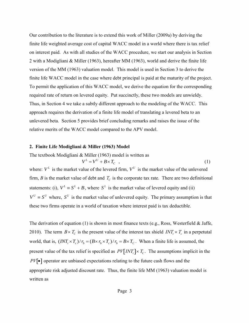
Our contribution to the literature is to extend this work of Miller (2009a) by deriving the
finite life weighted average cost of capital WACC model in a world where there is tax relief
on interest paid. As with all studies of the WACC procedure, we start our analysis in Section
2 with a Modigliani & Miller (1963), hereafter MM (1963), world and derive the finite life
version of the MM (1963) valuation model. This model is used in Section 3 to derive the
finite life WACC model in the case where debt principal is paid at the maturity of the project.
To permit the application of this WACC model, we derive the equation for the corresponding
required rate of return on levered equity. Put succinctly, these two models are unwieldy.
Thus, in Section 4 we take a subtly different approach to the modeling of the WACC. This
approach requires the derivation of a finite life model of translating a levered beta to an
unlevered beta. Section 5 provides brief concluding remarks and raises the issue of the
relative merits of the WACC model compared to the APV model.
2. Finite Life Modigliani & Miller (1963) Model
The textbook Modigliani & Miller (1963) model is written as
C
UL TBVV , (1)
where: LV is the market value of the levered firm, UV is the market value of the unlevered
firm, B is the market value of debt and
TC is the corporate tax rate. There are two definitional
statements: (i), BSV LL , where LS is the market value of levered equity and (ii)
UU SV where, US is the market value of unlevered equity. The primary assumption is that
these two firms operate in a world of taxation where interest paid is tax deductible.
The derivation of equation (1) is shown in most finance texts (e.g., Ross, Westerfield & Jaffe,
2010). The term
BTC is the present value of the interest tax shield
INTt Tc in a perpetutal
world, that is, Cbcbbct TBrTrBrTINT /)(/)( . When a finite life is assumed, the
present value of the tax relief is specified as
PV INTt TC . The assumptions implicit in the
PV operator are unbiased expectations relating to the future cash flows and the
appropriate risk adjusted discount rate. Thus, the finite life MM (1963) valuation model is
written as
Page 4
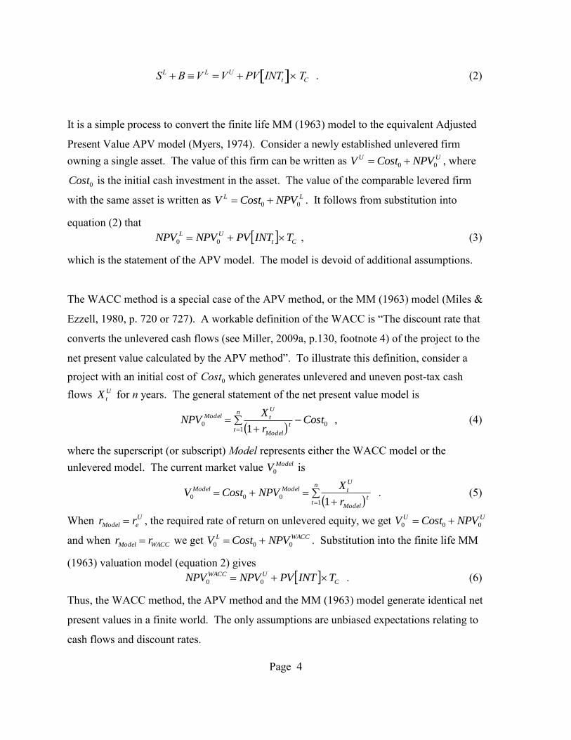
SL B V L VU PV INTt TC . (2)
It is a simple process to convert the finite life MM (1963) model to the equivalent Adjusted
Present Value APV model (Myers, 1974). Consider a newly established unlevered firm
owning a single asset. The value of this firm can be written as UU NPVCostV 00 , where
0Cost is the initial cash investment in the asset. The value of the comparable levered firm
with the same asset is written as LL NPVCostV 00 . It follows from substitution into
equation (2) that
Ct
UL TINTPVNPVNPV 00 , (3)
which is the statement of the APV model. The model is devoid of additional assumptions.
The WACC method is a special case of the APV method, or the MM (1963) model (Miles &
Ezzell, 1980, p. 720 or 727). A workable definition of the WACC is “The discount rate that
converts the unlevered cash flows (see Miller, 2009a, p.130, footnote 4) of the project to the
net present value calculated by the APV method”. To illustrate this definition, consider a
project with an initial cost of
Cost0 which generates unlevered and uneven post-tax cash
flows U
tX for n years. The general statement of the net present value model is
0
1 0
1Cost
r
XNPV
n
tt
Model
U
tModel
, (4)
where the superscript (or subscript) Model represents either the WACC model or the
unlevered model. The current market value ModelV0 is
n
tt
Model
U
tModelModel
r
XNPVCostV
1 000
1 . (5)
When U
eModel rr , the required rate of return on unlevered equity, we get UU NPVCostV 000
and when WACCModel rr we get WACCL NPVCostV 000 . Substitution into the finite life MM
(1963) valuation model (equation 2) gives
C
UWACC TINTPVNPVNPV 00 . (6)
Thus, the WACC method, the APV method and the MM (1963) model generate identical net
present values in a finite world. The only assumptions are unbiased expectations relating to
cash flows and discount rates.
Page 5
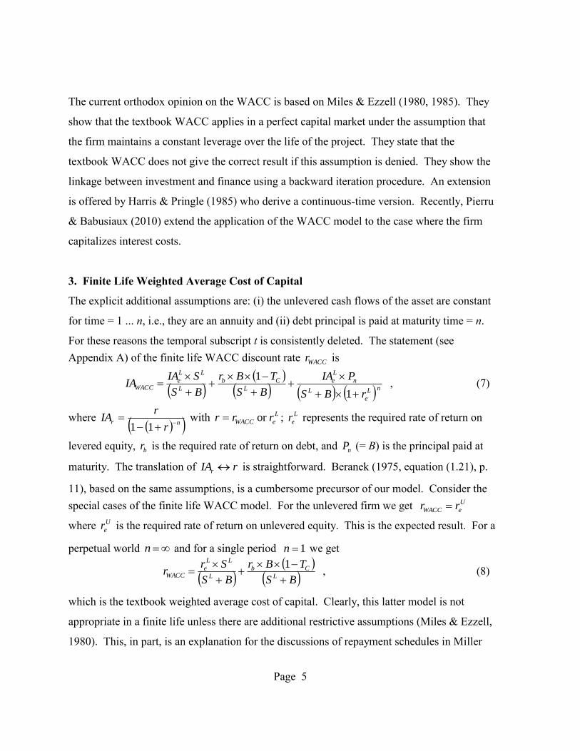
The current orthodox opinion on the WACC is based on Miles & Ezzell (1980, 1985). They
show that the textbook WACC applies in a perfect capital market under the assumption that
the firm maintains a constant leverage over the life of the project. They state that the
textbook WACC does not give the correct result if this assumption is denied. They show the
linkage between investment and finance using a backward iteration procedure. An extension
is offered by Harris & Pringle (1985) who derive a continuous-time version. Recently, Pierru
& Babusiaux (2010) extend the application of the WACC model to the case where the firm
capitalizes interest costs.
3. Finite Life Weighted Average Cost of Capital
The explicit additional assumptions are: (i) the unlevered cash flows of the asset are constant
for time = 1 ... n, i.e., they are an annuity and (ii) debt principal is paid at maturity time = n.
For these reasons the temporal subscript t is consistently deleted. The statement (see
Appendix A) of the finite life WACC discount rate WACCr is
nL
e
L
n
L
e
L
Cb
L
LL
eWACC
rBS
PIA
BS
TBr
BS
SIAIA
1
1
, (7)
where nr
r
rIA
11
with L
eWACC rrr or ; L
er represents the required rate of return on
levered equity, br is the required rate of return on debt, and nP (= B) is the principal paid at
maturity. The translation of rIAr is straightforward. Beranek (1975, equation (1.21), p.
11), based on the same assumptions, is a cumbersome precursor of our model. Consider the
special cases of the finite life WACC model. For the unlevered firm we get U
eWACC rr
where U
er is the required rate of return on unlevered equity. This is the expected result. For a
perpetual world n and for a single period 1n we get
BS
TBr
BS
Srr
L
Cb
L
LL
eWACC
1 , (8)
which is the textbook weighted average cost of capital. Clearly, this latter model is not
appropriate in a finite life unless there are additional restrictive assumptions (Miles & Ezzell,
1980). This, in part, is an explanation for the discussions of repayment schedules in Miller

Page 6
(2009a, 2009b), Bade (2009) and Pierru (2009a, 2009b).
In a practical context, the application of this finite life WACC formula requires an
appropriate required rate of return on levered equity L
er . The textbook version is
CLb
U
e
U
e
L
e TS
Brrrr 1 , (9)
see also MM (1963, equation (12.c), p. 439). This model clearly applies to a perpetual world,
but as we show later, it does not apply in a single period world. The corresponding model in
Miles & Ezzell (1980, equation (22), p. 727) appears to be of limited utility in a practical
sense since it is a function of the WACC. Using the assumptions adopted in the finite life
WACC model, the corresponding finite life required rate of return on levered equity (see
Appendix B) is determined via the non-linear equation
CbC
U
e
n
bnL
e
nL
n
C
nL
e
nL
b
U
e
nL
e
nL
LU
e
L
e
TIATIA
rr
PS
P
T
r
PS
BIAIA
r
PS
SIAIA
1
11
1
11
, (10)
which appears to be unwieldy. Notwithstanding, it is easy to programme into a spreadsheet,
and then solve for L
er using an iterative procedure. When n , we get the textbook model
(equation 9). When 1n , we get
C
b
b
Lb
U
e
U
e
L
e Tr
r
S
Brrrr
11 , (11)
which is popular in the literature. It is associated with the case when the leverage ratio is a
constant (Fernandez, 2004, Table 2, p. 156; Arzac & Glosten. 2005, equation (31), p. 458). It
is the specification of the required rate of return on levered equity for use in the textbook
WACC under the Miles & Ezzell (1980) assumption of constant leverage.
Miller‟s (2009a, equation (23), p. 135) finite life WACC model, using our notation, is
IAWACC IAeL
SL
SL B IAb
B
SL B . (12)
Page 7
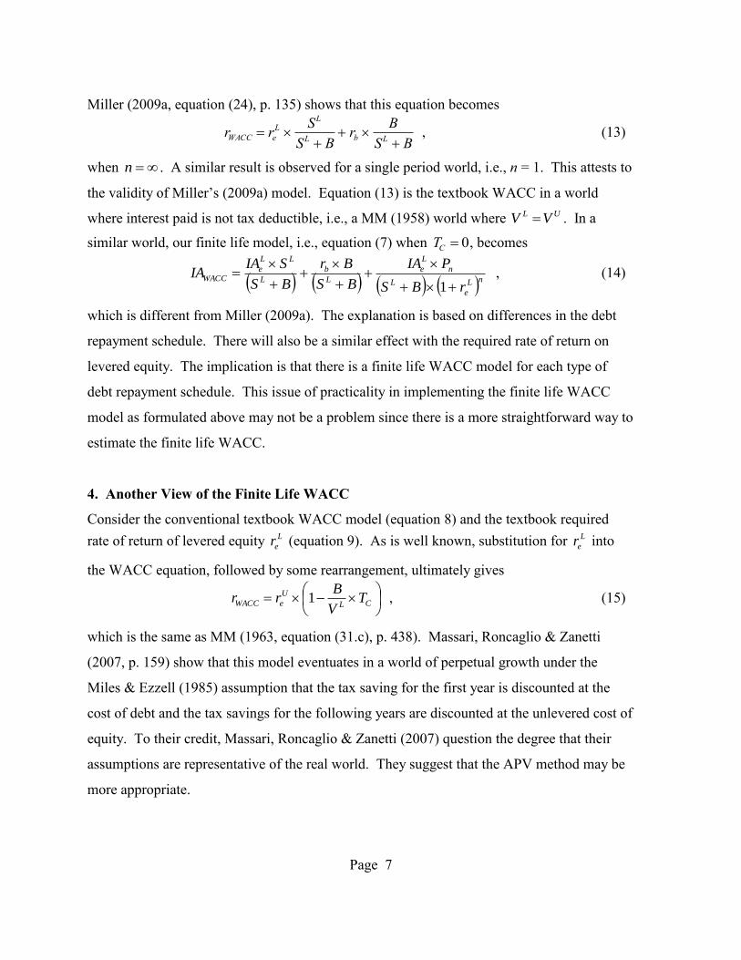
Miller (2009a, equation (24), p. 135) shows that this equation becomes
rWACC reL
SL
SL B rb
B
SL B , (13)
when n . A similar result is observed for a single period world, i.e., n = 1. This attests to
the validity of Miller‟s (2009a) model. Equation (13) is the textbook WACC in a world
where interest paid is not tax deductible, i.e., a MM (1958) world where UL VV . In a
similar world, our finite life model, i.e., equation (7) when
TC 0, becomes
nL
e
L
n
L
e
L
b
L
LL
eWACC
rBS
PIA
BS
Br
BS
SIAIA
1 , (14)
which is different from Miller (2009a). The explanation is based on differences in the debt
repayment schedule. There will also be a similar effect with the required rate of return on
levered equity. The implication is that there is a finite life WACC model for each type of
debt repayment schedule. This issue of practicality in implementing the finite life WACC
model as formulated above may not be a problem since there is a more straightforward way to
estimate the finite life WACC.
4. Another View of the Finite Life WACC
Consider the conventional textbook WACC model (equation 8) and the textbook required
rate of return of levered equity L
er (equation 9). As is well known, substitution for L
er into
the WACC equation, followed by some rearrangement, ultimately gives
CL
U
eWACC TV
Brr 1 , (15)
which is the same as MM (1963, equation (31.c), p. 438). Massari, Roncaglio & Zanetti
(2007, p. 159) show that this model eventuates in a world of perpetual growth under the
Miles & Ezzell (1985) assumption that the tax saving for the first year is discounted at the
cost of debt and the tax savings for the following years are discounted at the unlevered cost of
equity. To their credit, Massari, Roncaglio & Zanetti (2007) question the degree that their
assumptions are representative of the real world. They suggest that the APV method may be
more appropriate.
Page 8
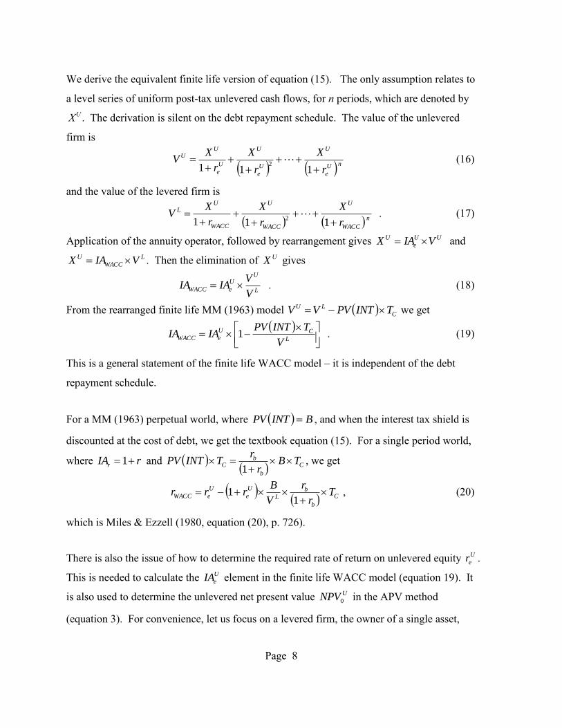
We derive the equivalent finite life version of equation (15). The only assumption relates to
a level series of uniform post-tax unlevered cash flows, for n periods, which are denoted by
XU . The derivation is silent on the debt repayment schedule. The value of the unlevered
firm is
nU
e
U
U
e
U
U
e
UU
r
X
r
X
r
XV
2111
(16)
and the value of the levered firm is
n
WACC
U
WACC
U
WACC
UL
r
X
r
X
r
XV
2111
. (17)
Application of the annuity operator, followed by rearrangement gives UU
e
U VIAX and
L
WACC
U VIAX . Then the elimination of UX gives
L
UU
eWACCV
VIAIA . (18)
From the rearranged finite life MM (1963) model C
LU TINTPVVV we get
L
CU
eWACCV
TINTPVIAIA 1 . (19)
This is a general statement of the finite life WACC model – it is independent of the debt
repayment schedule.
For a MM (1963) perpetual world, where BINTPV , and when the interest tax shield is
discounted at the cost of debt, we get the textbook equation (15). For a single period world,
where rIAr 1 and C
b
bC TB
r
rTINTPV
1, we get
C
b
b
L
U
e
U
eWACC Tr
r
V
Brrr
11 , (20)
which is Miles & Ezzell (1980, equation (20), p. 726).
There is also the issue of how to determine the required rate of return on unlevered equity U
er .
This is needed to calculate the U
eIA element in the finite life WACC model (equation 19). It
is also used to determine the unlevered net present value UNPV0 in the APV method
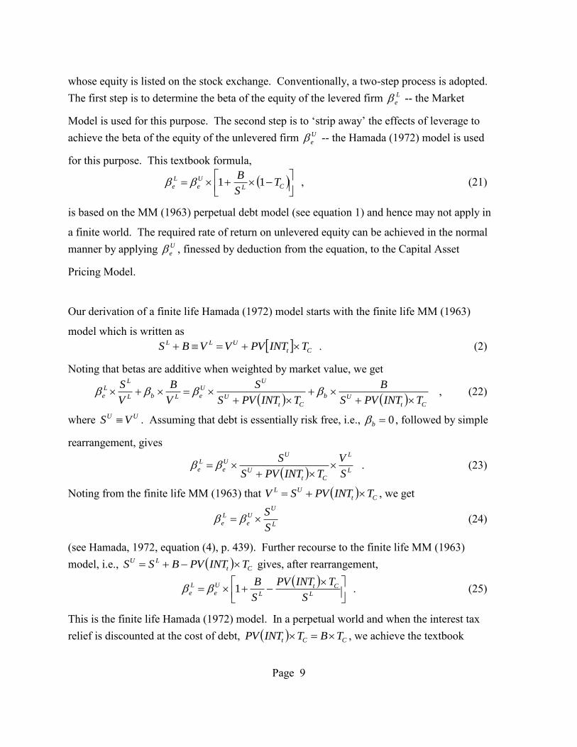
(equation 3). For convenience, let us focus on a levered firm, the owner of a single asset,
Page 9
whose equity is listed on the stock exchange. Conventionally, a two-step process is adopted.
The first step is to determine the beta of the equity of the levered firm L
e -- the Market
Model is used for this purpose. The second step is to „strip away‟ the effects of leverage to
achieve the beta of the equity of the unlevered firm U
e -- the Hamada (1972) model is used
for this purpose. This textbook formula,
CL
U
e
L
e TS
B11 , (21)
is based on the MM (1963) perpetual debt model (see equation 1) and hence may not apply in
a finite world. The required rate of return on unlevered equity can be achieved in the normal
manner by applying U
e , finessed by deduction from the equation, to the Capital Asset
Pricing Model.
Our derivation of a finite life Hamada (1972) model starts with the finite life MM (1963)
model which is written as
Ct
ULL TINTPVVVBS . (2)
Noting that betas are additive when weighted by market value, we get
Ct
Ub
Ct
U
UU
eLbL
LL
eTINTPVS
B
TINTPVS
S
V
B
V
S
, (22)
where UU VS . Assuming that debt is essentially risk free, i.e., 0b , followed by simple
rearrangement, gives
L
L
Ct
U
UU
e
L
eS
V
TINTPVS
S
. (23)
Noting from the finite life MM (1963) that Ct
UL TINTPVSV , we get
L
UU
e
L
eS
S (24)
(see Hamada, 1972, equation (4), p. 439). Further recourse to the finite life MM (1963)
model, i.e., Ct
LU TINTPVBSS gives, after rearrangement,
L
Ct
L
U
e
L
eS
TINTPV
S
B1 . (25)
This is the finite life Hamada (1972) model. In a perpetual world and when the interest tax
relief is discounted at the cost of debt, CCt TBTINTPV , we achieve the textbook
Page 10
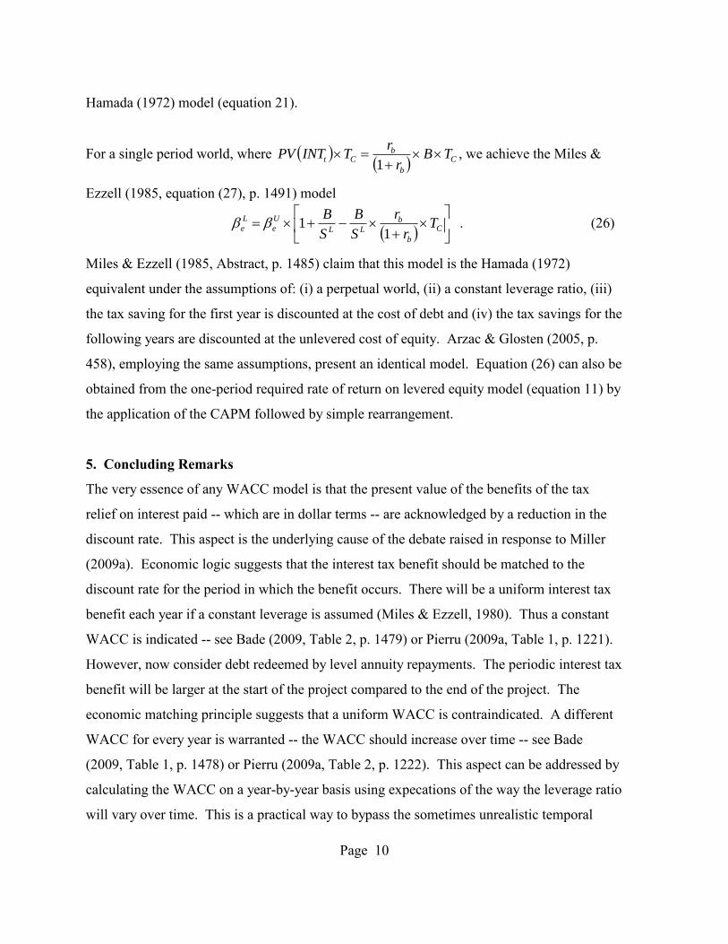
Hamada (1972) model (equation 21).
For a single period world, where C
b
bCt TB
r
rTINTPV
1, we achieve the Miles &
Ezzell (1985, equation (27), p. 1491) model
C
b
b
LL
U
e
L
e Tr
r
S
B
S
B
11 . (26)
Miles & Ezzell (1985, Abstract, p. 1485) claim that this model is the Hamada (1972)
equivalent under the assumptions of: (i) a perpetual world, (ii) a constant leverage ratio, (iii)
the tax saving for the first year is discounted at the cost of debt and (iv) the tax savings for the
following years are discounted at the unlevered cost of equity. Arzac & Glosten (2005, p.
458), employing the same assumptions, present an identical model. Equation (26) can also be
obtained from the one-period required rate of return on levered equity model (equation 11) by
the application of the CAPM followed by simple rearrangement.
5. Concluding Remarks
The very essence of any WACC model is that the present value of the benefits of the tax
relief on interest paid -- which are in dollar terms -- are acknowledged by a reduction in the
discount rate. This aspect is the underlying cause of the debate raised in response to Miller
(2009a). Economic logic suggests that the interest tax benefit should be matched to the
discount rate for the period in which the benefit occurs. There will be a uniform interest tax
benefit each year if a constant leverage is assumed (Miles & Ezzell, 1980). Thus a constant
WACC is indicated -- see Bade (2009, Table 2, p. 1479) or Pierru (2009a, Table 1, p. 1221).
However, now consider debt redeemed by level annuity repayments. The periodic interest tax
benefit will be larger at the start of the project compared to the end of the project. The
economic matching principle suggests that a uniform WACC is contraindicated. A different
WACC for every year is warranted -- the WACC should increase over time -- see Bade
(2009, Table 1, p. 1478) or Pierru (2009a, Table 2, p. 1222). This aspect can be addressed by
calculating the WACC on a year-by-year basis using expecations of the way the leverage ratio
will vary over time. This is a practical way to bypass the sometimes unrealistic temporal
Page 11
assumption of constant leverage required to make the WACC a constant.
Our analysis, as does the analysis of others, raises the issue of whether it is better, in a
conceptual sense, to account for the interest tax benefit as a dollar value or to account for it as
an adjustment to the discount rate. Is the Adjusted Present Value Model superior to the
WACC model? The APV model is straightforward. The potential problems in the
determination of: (i) the required rate of return on unlevered equity U
er (ii) the present value
of the tax shield Ct TINTPV (see Fernandez (2004, Table 1, p. 156) for a survey of the
literature) are common to the finite life WACC method and the APV method. The
application of Occam‟s Razor (Ennis, 2009) infers that the APV method is preferred to the
WACC method. The WACC is a special case of the APV (Miles & Ezzell, 1980) and
therefore it is based on additional assumptions. However, although is possible that the
textbook “weighted average cost of capital is not quite right” (Miller, 2009a), can one be
confident that the APV model is “quite right”?
Page 12
References
Arzac, E. and Glosten, L. (2005). A reconsideration of tax shield valuation. European
Financial Management, 11, 453-461.
Bade, B. (2009). Comment on “The weighted average cost of capital is not quite right”.
Quarterly Review of Economics and Finance, 49, 1476–1480.
Beranek, W. (1975). The cost of capital, capital budgeting, and the maximization of
shareholder wealth. Journal of Financial and Quantitative Analysis, 10, 1-20.
Ennis, R. M. (2009). Parsimonious asset allocation. Financial Analysts Journal, 65, 6-10.
Fernandez, P. (2004). The value of tax shields is NOT equal to the present value of tax
shields. Journal of Financial Economics, 73, 145-165.
Hamada, R. S. (1972). The effect of the firm's capital structure on the systematic risk of
common stocks. Journal of Finance, 27, 435-452.
Harris, R. S. and Pringle, J. J. (1985). Risk-adjusted Discount Rates – Extensions from the
Average-risk Case. The Journal of Financial Research, 8, 237-244.
Massari, M., Roncaglio, F. and Zanetti, L. (2007). On the equivalence between the APV and
the wacc approach in a growing leveraged firm. European Financial Management, 14, 152-
162.
Miles, J. and Ezzell, J. (1980). The weighted average cost of capital, perfect capital markets,
and project life: A clarification. Journal of Financial and Quantitative Analysis, 15, 719-730.
Miles, J. and Ezzell, J. (1985). Reformulating tax shield valuation: A note. Journal of
Finance, 40, 1485-1492.
Miller, R. A. (2009a). The weighted average cost of capital is not quite right. Quarterly
Review of Economics and Finance, 49, 128–138.
Miller, R. A. (2009b). The weighted average cost of capital is not quite right: Reply to M.
Pierru. Quarterly Review of Economics and Finance, 49, 1213-1218.
Page 13
Modigliani, F. and Miller, M. (1958). The cost of capital, corporate finance and the theory of
investment. American Economic Review, 48, 261-297.
Modigliani, F. and Miller, M. (1963). Corporate income taxes and the cost of capital: A
correction. American Economic Review, 53, 433-443.
Myers, S. (1974). Interactions of corporate financing and investment decision implications for
capital budgeting. Journal of Finance, 29, 1-25.
Pierru, A. (2009a). The weighted average cost of capital is not quite right: A comment.
Quarterly Review of Economics and Finance, 49, 1219–1223.
Pierru, A. (2009b). The weighted average cost of capital is not quite right: A rejoinder.
Quarterly Review of Economics and Finance, 49, 1481–1484.
Pierru, A. and Babusiaux, D. (2010). WACC and free cash flows: A simple adjustment for
capitalized interest costs. Quarterly Review of Economics and Finance, 50, 240–243.
Ross, S. A., Westerfield, R. W. and Jaffe, J. (2010). Corporate Finance, Ninth edition,
McGraw-Hill/Irwin.
Page 14
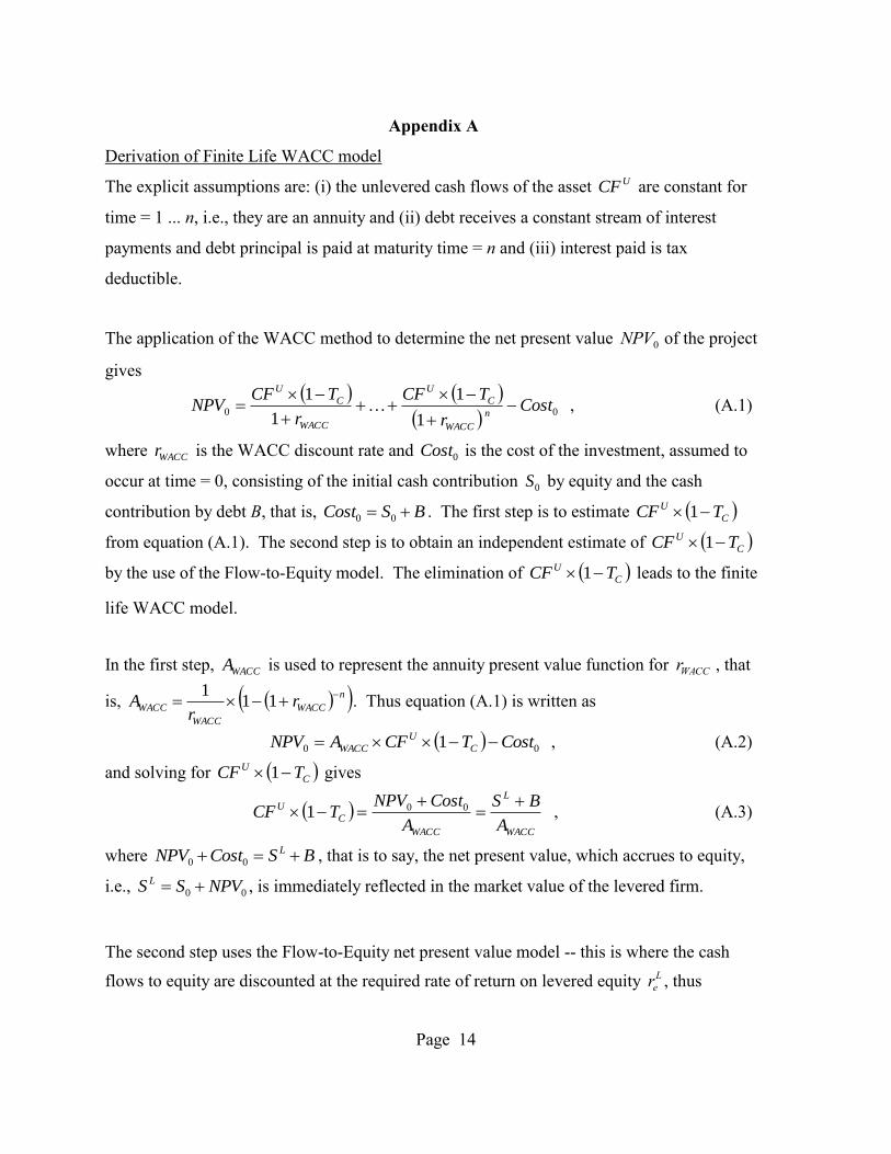
Appendix A
Derivation of Finite Life WACC model
The explicit assumptions are: (i) the unlevered cash flows of the asset UCF are constant for
time = 1 ... n, i.e., they are an annuity and (ii) debt receives a constant stream of interest
payments and debt principal is paid at maturity time = n and (iii) interest paid is tax
deductible.
The application of the WACC method to determine the net present value
NPV0 of the project
gives
0 01
1
1
1Cost
r
TCF
r
TCFNPV
n
WACC
C
U
WACC
C
U
, (A.1)
where WACCr is the WACC discount rate and 0Cost is the cost of the investment, assumed to
occur at time = 0, consisting of the initial cash contribution 0S by equity and the cash
contribution by debt B, that is, BSCost 00 . The first step is to estimate C
U TCF 1
from equation (A.1). The second step is to obtain an independent estimate of C
U TCF 1
by the use of the Flow-to-Equity model. The elimination of C
U TCF 1 leads to the finite
life WACC model.
In the first step, WACCA is used to represent the annuity present value function for
rWACC , that
is, n
WACC
WACC
WACC rr
A
111
. Thus equation (A.1) is written as
00 1 CostTCFANPV C
U
WACC , (A.2)
and solving for C
U TCF 1 gives
WACC
L
WACC
C
U
A
BS
A
CostNPVTCF
001 , (A.3)
where BSCostNPV L 00 , that is to say, the net present value, which accrues to equity,
i.e., 00 NPVSS L , is immediately reflected in the market value of the levered firm.
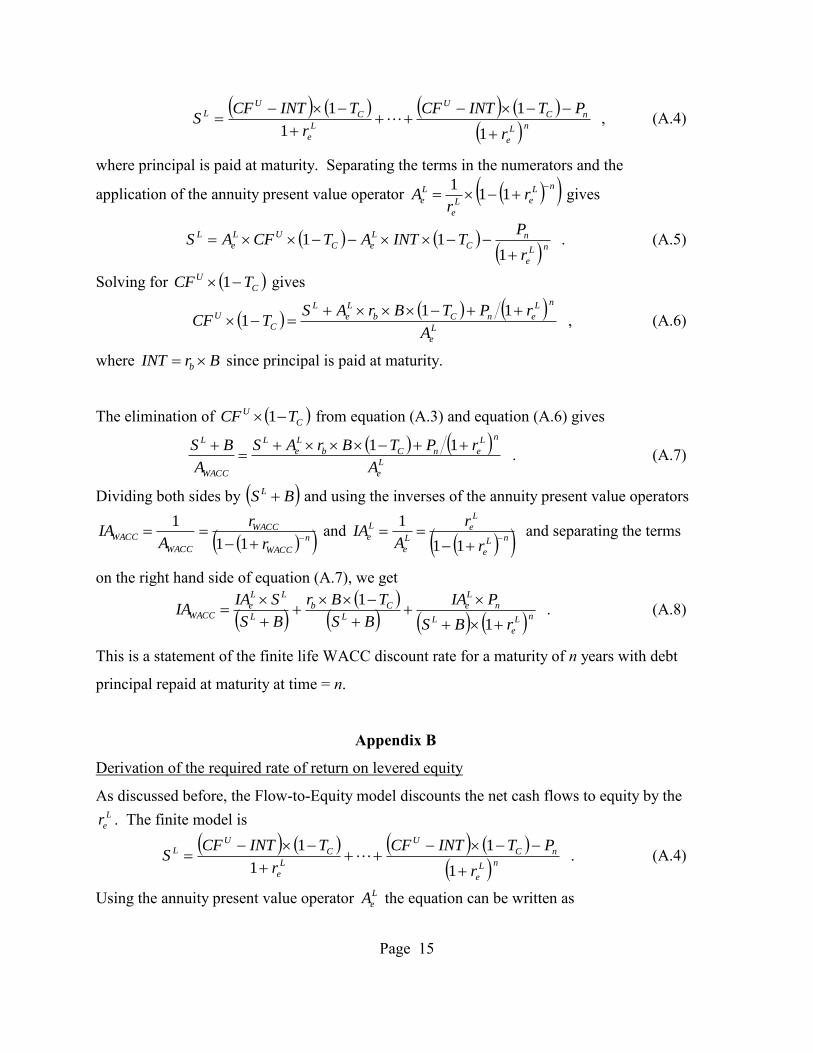
The second step uses the Flow-to-Equity net present value model -- this is where the cash
flows to equity are discounted at the required rate of return on levered equity
reL , thus
Page 15
nL
e
nC
U
L
e
C
UL
r
PTINTCF
r
TINTCFS
1
1
1
1
, (A.4)
where principal is paid at maturity. Separating the terms in the numerators and the
application of the annuity present value operator nL
eL
e
L
e rr
A
111
gives
nL
e
nC
L
eC
UL
e
L
r
PTINTATCFAS
1
11
. (A.5)
Solving for C
U TCF 1 gives
L
e
nL
enCb
L
e
L
C
U
A
rPTBrASTCF
11
1
, (A.6)
where BrINT b since principal is paid at maturity.
The elimination of C
U TCF 1 from equation (A.3) and equation (A.6) gives
L
e
nL
enCb
L
e
L
WACC
L
A
rPTBrAS
A
BS
11
. (A.7)
Dividing both sides by BS L and using the inverses of the annuity present value operators
n
WACC
WACC
WACC
WACCr
r
AIA
11
1 and
nL
e
L
e
L
e
L
e
r
r
AIA
11
1 and separating the terms
on the right hand side of equation (A.7), we get
nL
e
L
n
L
e
L
Cb
L
LL
eWACC
rBS
PIA
BS
TBr
BS
SIAIA
1
1
. (A.8)
This is a statement of the finite life WACC discount rate for a maturity of n years with debt
principal repaid at maturity at time = n.
Appendix B
Derivation of the required rate of return on levered equity
As discussed before, the Flow-to-Equity model discounts the net cash flows to equity by the L
er . The finite model is
nL
e
nC
U
L
e
C
UL
r
PTINTCF
r
TINTCFS
1
1
1
1
. (A.4)
Using the annuity present value operator L
eA the equation can be written as
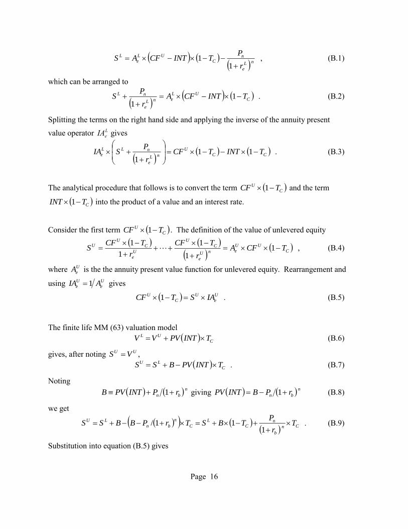
Page 16
nL
e
nC
UL
e
L
r
PTINTCFAS
1
1
, (B.1)
which can be arranged to
C
UL
enL
e
nL TINTCFAr
PS
1
1
. (B.2)
Splitting the terms on the right hand side and applying the inverse of the annuity present
value operator
IAeL gives
CC
U
nL
e
nLL
e TINTTCFr
PSIA
11
1
. (B.3)
The analytical procedure that follows is to convert the term C
U TCF 1 and the term
CTINT 1 into the product of a value and an interest rate.
Consider the first term C
U TCF 1 . The definition of the value of unlevered equity
C
UU
enU
e
C
U
U
e
C
UU TCFA
r
TCF
r
TCFS
1
1
1
1
1
, (B.4)
where U
eA is the the annuity present value function for unlevered equity. Rearrangement and
using U
e
U
e AIA 1 gives
U
e
U
C
U IASTCF 1 . (B.5)
The finite life MM (63) valuation model
C
UL TINTPVVV (B.6)
gives, after noting UU VS ,
C
LU TINTPVBSS . (B.7)
Noting
n
bn rPINTPVB
1 giving n
bn rPBINTPV
1 (B.8)
we get
Cn
b
nC
L
C
n
bn
LU Tr
PTBSTrPBBSS
1
11/ . (B.9)
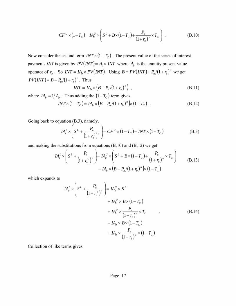
Substitution into equation (B.5) gives
Page 17
Cn
b
nC
LU
eC
U Tr
PTBSIATCF
1
11 . (B.10)
Now consider the second term CTINT 1 . The present value of the series of interest
payments INT is given by INTAINTPV b where bA is the annuity present value
operator of br . So INTPVIAINT b . Using n
bn rPINTPVB
1 we get
n
bn rPBINTPV
1 . Thus
n
bnb rPBIAINT
1 , (B.11)
where bb AIA 1 . Thus adding the CT1 term gives
C
n
bnbC TrPBIATINT 111
. (B.12)
Going back to equation (B.3), namely,
CC
U
nL
e
nLL
e TINTTCFr
PSIA
11
1
(B.3)
and making the substitutions from equations (B.10) and (B.12) we get
C
n
bnb
Cn
b
nC
LU
enL
e
nLL
e
TrPBIA
Tr
PTBSIA
r
PSIA
11
11
1
(B.13)
which expands to
Cn
b
nb
Cb
Cn
b
nU
e
C
U
e
LU
enL
e
nLL
e
Tr
PIA
TBIA
Tr
PIA
TBIA
SIAr
PSIA
11
1
1
1
1
. (B.14)
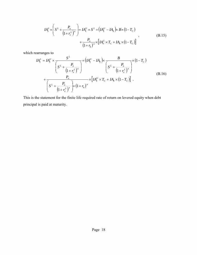
Collection of like terms gives
Page 18
CbC
U
en
b
n
Cb
U
e
LU
enL
e
nLL
e
TIATIAr
P
TBIAIASIAr
PSIA
11
11
, (B.15)
which rearranges to
. 1
11
1
11
CbC
U
e
n
bnL
e
nL
n
C
nL
e
nL
b
U
e
nL
e
nL
LU
e
L
e
TIATIA
rr
PS
P
T
r
PS
BIAIA
r
PS
SIAIA
(B.16)
This is the statement for the finite life required rate of return on levered equity when debt
principal is paid at maturity.