1

In-store One-to-one Marketing Diego Klabjan (d-klabjan@northwestern.edu) Jinxiang Pei (peipauj@u.northwestern.edu)

Department of Industrial Engineering and Management Sciences Northwestern University, Evanston, IL

With the proliferation of electronic media, one-to-one marketing has become more accessible and it is moving toward widespread adoption. It is particularly important for retailers, where several forms of one-to-one marketing are performed either before or after a shopping experience. One-to-one marketing during the shopping experience is still elusive, however, with recent technological advances it could soon become reality. We show how it can be carried out by using either personal digital assistance devices and wireless communication, or radio frequency identification. The main concept is based on providing coupons during a shopping experience and then routing the customer within the facility to possibly redeem them. The novel approach of selecting the coupons based on the already purchased goods enables one-to-one marketing during the actual shopping trip. Several models are presented based on the underlying technology and the option of a loyalty card. The concepts are computationally evaluated based on data obtained from a grocery store. They allude to substantially increased revenue by the store.

1. Introduction In one-to-one marketing, marketing material is targeted and customized for a particular customer

and it therefore takes into account his or her particular individual needs. As such it focuses on

economies of scope rather than scale. While selected forms, e.g. mail-in catalogs, of one-to-one

marketing date back many years, it is in the past few years that it gained much traction due to

modern information technology. Customer tailored email marketing, see e.g., Byron (2005), and

cross selling through customized web sites, (Amazon.com is considered a pioneer in this area)

are now established marketing practices.

In its infancy are one-to-one marketing opportunities exploring the near field communication

(NFC) protocol, which enables secure short range communication among devices such as cellu-

lar phones and terminals. So-called contactless smart cards (e.g., payments are made by simply

waiving the card) are slowly penetrating the market. In particular, cellular phones are well suited

for performing one-to-one marketing tasks. Consider, for example, a payment made by using an

NFC enabled cellular phone. During the payment transaction, the vendor's NFC enabled terminal

can easily pass along a web site link with promotional material. Trials have also been performed

2

on establishing communication between a billboard and a passing of a customer carrying a smart

phone. Other applications are listed in O'Connor (2006).

Another, well established and more traditional form of one-to-one marketing, used by high-

low pricing retailers, are the coupons. We are not referring to manufacturer coupons (e.g., peel-

off or in-box coupons, or coupons distributed by newspapers or magazines), but coupons distri-

buted by the retailers. Using scan or point-of-sale data, retailers can target coupons to individual

customers. A big limitation of such a strategy is the fact that the coupons are distributed to a cus-

tomer either before the actual shopping experience (mail-in coupons), or after during the check-

out process. So far, one-to-one marketing during the actual shopping experience is elusive. The

potential revenue increase can be substantial since approximately 60% of the purchasing deci-

sions by customers in grocery stores are made in the store, Kahn and McAlister (1997).

The main purpose of this research is to provide the modeling and algorithmic framework for

coupon distribution during a shopping trip. By using real world data from a grocery store we also

quantify potential revenue implications. Our framework is based on a deployment of two nascent

technologies: wireless personal mobile devices (e.g., smart phones or personal digital assistants)

and radio frequency identification (RFID). The former technology allows the exchange of infor-

mation between the device and a store server. We have explicitly in mind a potential shopping

list. The latter technology enables real time tracking of every individual item by affixing a small

tag or transponder to every item. In particular, interrogators mounted on shelves (called also

smart shelves) can query the items already purchased by a customer that are in the shopping cart.

Basic facts on RFID are given later in this section.

Under the first scenario, we assume that shoppers enter a retail store with a personal mobile

device preloaded with the shopping list. The list is next beamed to a central store server, which

then computes a shopping path or route and communicates it back to the customer. The novel

idea is to build into the route locations with promoted items. These locations are computed based

on the shopping list and/or based on the historical purchasing habits of the customer (e.g., if a

loyalty card program is in effect). The basic model finds a route that maximizes the store’s ex-

pected revenue based on the likelihood of the customer purchasing items on promotion subject to

the customer’s aggregated utility over the route above a given threshold. The expected revenue is

modeled based on discrete choice models. In the second scenario, which requires item level tag-

ging and smart shelves, it is assumed that an interrogator, which is part of smart shelves, reads

3

the already purchased items of the customer by interrogating the tags attached to these items in

the shopping cart. Based on current basket information, a different device can then issue coupons

to the customer and shows him or her a good route in order to redeem the coupons. As in the

previous scenario, we use discrete choice modeling and we maximize the store’s expected reve-

nue. The new component here is the addition of a market basket analysis at modeling the ex-

pected revenue. Clearly, in a potential implementation of this strategy, only selected locations in

the store should have the coupon issuing capability.

Given the store’s expected revenue of an impulse purchase via coupon redemption, the un-

derlying model for computing the route is the selective traveling salesman problem with time

windows. The objective is to find a tour maximizing the store’s expected revenue subject to the

customer’s aggregated utility on the route above a predefined value. Time windows model, for

example, the fact that frozen food should not be present early in the route.

In addition to the novel concept and modeling, we also conduct a computational study by us-

ing a major grocery store. The store layout and customer historical purchases were obtained from

the store, while promotions were simulated. The computational study shows large potential im-

provements in revenue.

To summarize, the main contributions of this study are as follows.

• By using two technologies, we develop concepts for in-store one-to-one marketing. The

most important fact here is that marketing is performed during the shopping trip, and not

before or after as is currently the case.

• Based on these concepts, we use both the standard logit model and a market basket model

to show how to apply discrete choice modeling in computing the expected value of cou-

pon redemption. When discussing the various scenarios, we consider two possible alter-

natives: the presence of a loyalty card program, and the ability to track shopping carts in

the store.

• We show how to use the selective traveling salesman problem in order to compute a fa-

vorable shopping route of a customer.

• The computational study based on real world data reveals substantial potential revenue

improvements.

The importance and relevance of our work has also recently been addressed in the Business

Week (December 2007), where importance for in-store one-to-one marketing during a shopping

4

experience is stressed. On the online portal www.shopbloom.com of Food Lion LLC, customers

can create personalized shopping lists and obtain a printout of the aisles they need to visit. While

this is convenient for the shopper, it decreases the revenue to the store since knowing where to

go, shoppers would buy less on impulse. By using our approach this is circumvented since shop-

pers are deliberately routed to certain locations and thus impulse buying is encouraged.

The document is structured as follows. In Section 2 we provide the general framework, in-

cluding all studied scenarios. All models are described in Section 3. This section also gives the

underlying solution methodologies and algorithms. Section 4 is devoted to the computational ex-

periments. We conclude the introduction with a quick tutorial on RFID and a literature overview.

1.1. Literature Review The discrete choice models have been of interest to researchers and practitioners for a long time

due to their applications. They are used in our work to compute the probabilities of buying prod-

ucts. An important approach to model customer's discrete choices is the multinomial logit

(MNL) model, Boztug and Hildebrandt (2007) and Li (2007). In multinomial logit models, ran-

dom utility maximization is applied to pick the best alternative among all available alternatives.

Multinomial logit models are a generalization of the binary logit model, in which customers have

only two alternatives, Cox (1972). On the other hand, if the utility follows the normal distribu-

tion, multinomial probit models are used. While the normal distribution is attractive in practice,

it does not provide a closed form solution, McCulloch and Rossi (1994). An alternative modeling

approach to MNL is the nested logit model, which allows correlations among alternatives in the

process within a group or nest, Guadagni and Little (1998). Customers make multi-category

choices during each shopping trip. We study the multi-category decision-making process, in

which alternatives in different categories are correlated. Multi-category choice models are the

extension of traditional single category models, Chiang (1991), Chintaguta (1993), Chong et al.

(2001). Among multi-category models, Mehta (2007) treats purchase incidence and brand

choice as distinct decision stages. A detailed state-of-the-art overview of multi-category models

is provided in Seetharaman et al. (2005).

The concept of promotions is the driving force behind our work. There are many reasons that

retailers run promotions, such as rewarding brand loyal customers and meeting short-term sales

targets, Cutler (2000). As expected, a retail promotion with respect to a specific brand according-

5

ly increases sales either through store substitutions across available stores and/or a brand substi-

tution within a store, Kumar and Leone (1988). Issuing coupons is an important approach for

price promotion. Traditional coupons such as those distributed by newspapers and magazines are

appealing to manufacturers while in-store “surprise” coupons catch retailer attention because of

many benefits, such as a subsequently increased basket size by unplanned purchases and better

prediction of the frequency and type of impulse buying, Heilman et al. (2002). The impacts of

coupons on customer's behavior in services such as repeated purchases and purchase timing are

studied in Taylor (2001). From the standpoint of a retail store, there are at least three levels that

need to be considered in a promotion decomposition model when evaluating a promotion: cross-

brand, cross-period, and category expansion effects, Van Heerde et al. (2004). The common

thread of all these works is that promotions in terms of coupons are effectively and frequently

used in retailing. Customers' motivations for impulse buying are studied in Hausman (2000).

Some impulse buying is unnecessary, but often such buying is rewarding to the customer. Rela-

tionship between store price promotions and customer purchases is investigated in Mulhern et al.

(1995). Increasing customers' exposure to categories by extending shopping times and thus dwell

time in the store also increases the probability of making impulse buying, Hui et. al (2007). As

shown by our work, the effect of impulse buying can be even more pronounced in one-to-one

marketing.

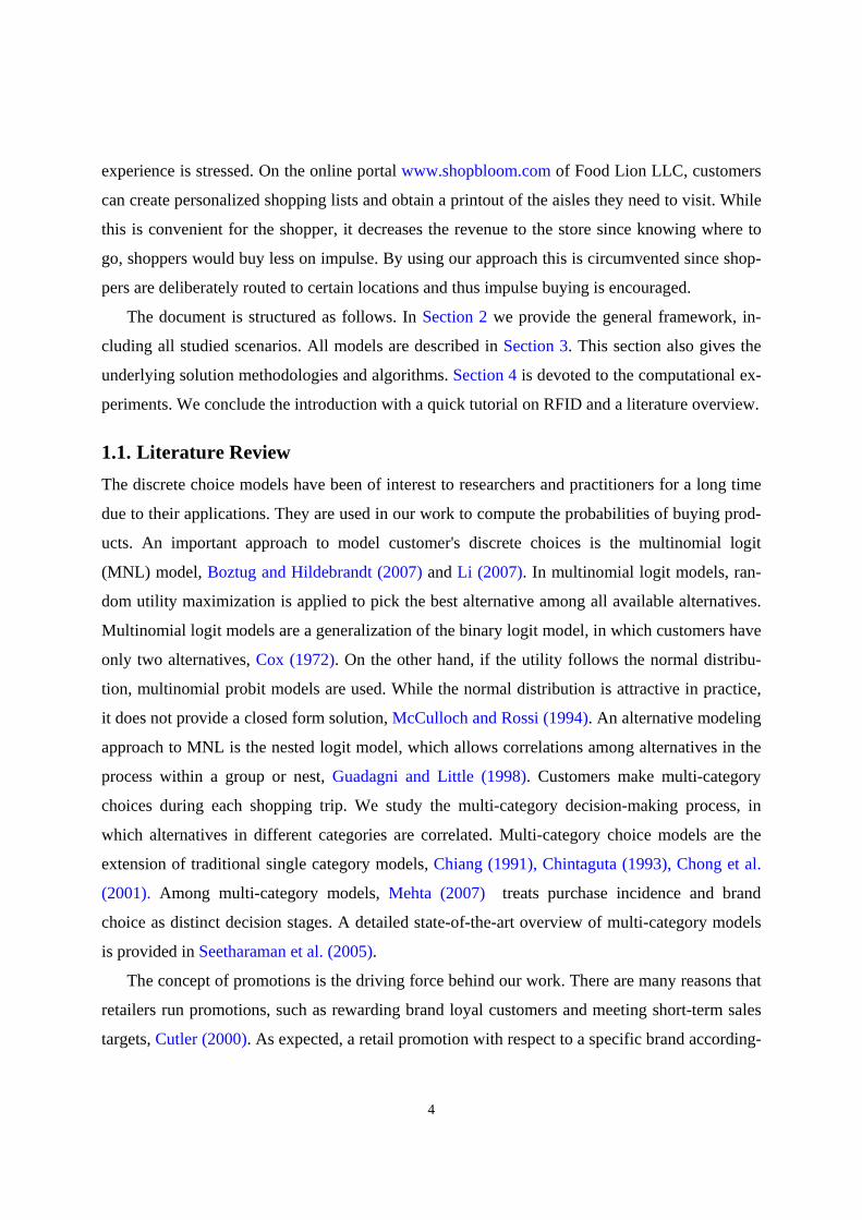
2. Framework We consider two main scenarios: (1) the store does not have an RFID deployment, or (2) the

store has an RFID deployment at item level as shown in Figure 1. If RFID is not deployed, then

in order to perform one-to-one marketing a different technological setting is assumed. With a

personal digital assistant or any similar device having a wireless capability and text editing fea-

tures, the customer in the first scenario preloads her shopping list and is willing to share it with

information systems in the store. The main idea is to improve the shopping experience by guid-

ing the shopper through the store. The loyalty card is an additional possible distinctive compo-

nent in this scenario. The store can better predict shopper's needs and habits, subsequently better

serve the shopper by using her past purchases recorded through the loyalty program. In the

second scenario, the store is RFID deployed with smart shelves and item level tagging is used.

We also assume that certain locations in the store have coupon issuing capabilities. The concept

6

here is that with the help of RFID, the on-shelf interrogator would detect the already purchased

items in the shopping cart and then coupons would be distributed to the customer on the spot

through the coupon issuing device. The on-shelf system can also recommend a route pass the lo-

cations with recommended coupons. Besides the functionality of smart shelves, which enables us

to recommend promotional products and display the route, the ability of tracking shopping carts

is beneficial in this scenario for preventing from frequently issuing coupons to the same shopper

during the same trip. Similarly, the loyalty card program is a plus here. The goal in both scena-

rios is to entice impulse buying. We next discuss in greater details these options.

2.1. Shopping Lists There are different types of shopping lists, Newcomb et al. (2003). The shopping list can be

created by the store based on shopper's past purchases. If a shopper frequents the store, the

store’s information system could be able to predict her needs. On the other hand, a shopper can

create the shopping list by herself. It can also be possible to combine the two strategies. We fo-

cus here on the case where the customer creates the personal shopping list by herself. The other

case does not require major changes to our models and concepts. Upon entering the store with a

preloaded shopping list on a personal digital assistant that has wireless capabilities, the list is

beamed to the store's information system. The information system receives the shopping list and

Figure 1: Scenarios based on various technologies

based on it computes a favorable route through the store. Furthermore, stores run promotions on

a regular basis and thus the customer can deliberately be routed to pass selected locations with

products on promotion (or, e.g., tasting booths). The ultimate goal is to induce impulsive buying.

shopping list

no loyalty card loyalty card

RFID (no shopping list)

ability to track shopping carts

no ability to track shopping carts

no loyalty card loyalty card

7

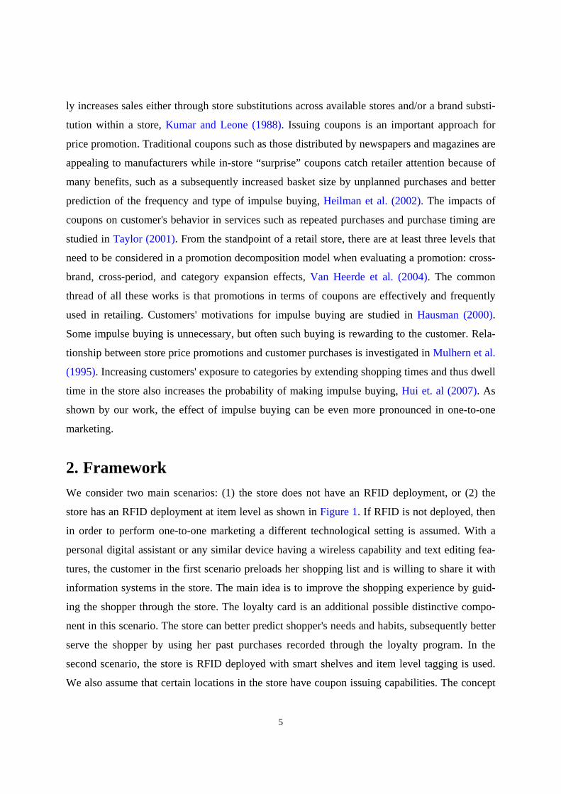
The objective of the proposed route is to maximize the store's expected revenue, which is defined

as the probability of buying promotional items multiplied by the price of the products. Clearly,

the generated route would potentially create a negative impact on the customer if her anticipated

shopping time is substantially increased. It is for this reason that we impose the maximum travel

time on the proposed route. In addition, it is desirable that selected items are towards the end of

the shopping experience, e.g., frozen food. At the end, the recommended computed route is sent

back to the shopper's device and appropriately displayed. The entire concept is shown in Figure

2.

Figure 2: Store entrance with a shopping list

2.2. Smart Shelves and Radio Frequency Identification In a smart shelf system, products are tagged by RFID transponders to give them a unique identi-

fication. Selected shelves are equipped with an antenna system and interrogator unit, which are

connected to an information system. Every interrogator has the ability to detect transponders

within a certain range and read their identifications. Through the signal strength, an interrogator

can also conclude if the items are on a shelf or in a shopping cart. Besides smart shelves, we also

assume that selected locations within the store are mounted with coupon issuing devices and user

friendly displays. Let us consider a customer with a shopping cart located near a point with such

devices. The customer has already purchased selected items and these can be identified by smart

shelves. This information can then be communicated to an information system. In the next step,

by considering the already purchased items and current promotions, a path can be computed that

routes the customer towards selected promotional items. In the final step, the selected coupons

Shopping list•Eggs •Beer •Milk

Shopping list•Eggs • Milk •Beer

8

would be issued by the device and the recommended route displayed. Similar to the previous

concept, the goal is to maximize the expected revenue. In this case, the probability of the cus-

tomer buying a promotional item is based on the market basket analysis, i.e., it takes into account

already purchased items. The recommended route travel time is bounded above by a number.

2.3. Presence of Loyalty Cards A loyalty program is commonly used in retailing to enhance the overall value-proposition and to

improve customer loyalty. It is supposed to motivate buyers to make next purchases through dis-

counts and potential faster service. A loyalty program also allows the store to track shopping pat-

terns and habits of individual customers.

In our context, loyalty cards play a role in probability estimations. In presence of a loyalty

program and the participation of the customer in such a program, discrete choice models pre-

sented in Section 3.1 are applicable. As a result, accurate probabilities can be derived. In absence

of a loyalty program, on the other hand, a customer has to be considered as “generic” and thus

indistinguishable. Discrete choice can still be used but its accuracy decreases.

2.4. Ability to Track Shopping Carts Besides smart shelves, RFID has other potential benefits in retailing. We are interested in so-

called smart shopping carts. A smart shopping cart resembles the normal one except that it is

equipped with a tracking device. Such carts can be tracked throughout the store and thus routes

of individual shoppers can be identified. This device can either be transparent to the shopper or it

can offer a display. Additionally, each shopping cart is tagged with a unique identifier.

There are two alternatives for tracking shopping carts. The first one is the installation of a

fixed number of interrogators into the floor, Larson et al. (2005). Shopping carts equipped with

transponders and moving within the store can then be detected and the relevant information is

communicated to an information system, which can then reconstruct the entire route for a cus-

tomer at any point in time. The second alternative is the establishment of a real-time locator sys-

tem. These systems use tagged objects (shopping carts in our case) and the well-known triangu-

lation technique to establish the location of objects. Real-time locator systems have been recently

installed in several industries, e.g., hospitals, Sokol (2005), and ports, Cho (2006).

In our context, shopping cart tracking would be beneficial in conjunction to the smart shelf

setting. Consider two locations equipped with coupon issuing devices as shown in Figure 3.

9

Without the ability to track shopping carts, duplicate coupons could be issued to the same cus-

tomer. This can clearly be annoying to the customer. On the other hand, with the shopping cart

tracking ability, at the second location the information system can account for only the items

purchased between the first and the second location and thus coupons can be issued only based

on these items.

Figure 3: Coupon issuing under shopping cart tracking

3. Models In this section, we provide the models. We give the framework and then point out the differences

between various scenarios discussed in Section 2. An important component of our models is the

discrete choice model. We need to model the probability of a potential customer buying a given

product in a category. More importantly, we study the interdependency among product choice

decisions. We also incorporate the current given basket of categories of a customer into the mod-

el.

3.1. Models Prior models address either single-category brand choice or joint-category purchase incidence.

On the one hand, single-category models ignore cross-category interdependence by independent-

ly maximizing utilities over individual categories. On the other hand, the standard multi-category

choice models, e.g., Chib et al. (2002), address joint-category purchase incidence within a shop-

ping trip at the level of categories. The brand selection decisions are omitted in basket analyses.

Depending on a specific context of a choice problem, the multiple category decision problem can

be perceived as either a collective choice or a sequence of choices (categories) in some order.

Harlam and Lodish (1995) is of particular interest since it is a sequential model and it includes

coupons coupons; only newly acquired items

shop

10

variables to reflect the dependencies among choices of items within the same shopping trip. We

normally observe the final outcome of consumer’s choices and not the partial steps. As a result a

full holistic model would be very hard to calibrate. Instead, we apply the idea of sequential

choice decisions and model the customer’s overall choice process by two separate stages that are

connected by conditional probabilities. In each stage, we apply the multinomial logit model and

derive the conditional probabilities.

We consider a customer’s decision process as a tree-structure where the brand choice is

nested in category purchase, Figure 4. First, customer k determines if she makes a purchase from

a category given she currently has a basket of categories kbc . This is followed by the decision of

selecting products1 corresponding to the chosen category. We denote by i a category and by |j i

a brand j in category i. We denote by C(i,k,t) the event of customer k considering a purchase

from category i at time t. Notation C(i,k,t)=1 encodes that such a purchase is made.

Figure 4: Hierarchical Decision Process

Given product j from category i, the choice probability is written as

( , | ) ( , | ( , , ) 1) { ( , , ) 1| ( ', , ) 1, ' , ' }.k kprob k j bc P k j C i k t P C i k t C i k t i bc i i= = ⋅ = = ∈ ≠ (1)

In (1) , ( , | )kprob k j bc represents the conditional probability of customer k buying brand j given

current basket kbc . In addition, { ( , , ) 1| ( ', , ) 1, ' , ' }kP C i k t C i k t i bc i i= = ∈ ≠ is the conditional

probability of selecting category i given basket kbc and ( , | ( , , ) 1)P k j C i k t = is the conditional

probability of picking product j from category i. We next study these conditional probabilities.

1We use products, brands and items interchangeably.

Categories

Brands

i

|j i

Customer k with basket kbc

11

Market Basket Selection Russell and Peterson (2000) propose a multivariate logistic distribution model for the market

basket selection problem. The market basket selection problem is modeled as a joint distribution

of stochastic variables where each of the variables represent the selection of a single category.

We borrow the conditional utility concepts to model the category selections. The error terms are

assumed to be i.i.d Gumbel with parameter μ . Assuming the symmetric property of the choice

variables, the probability of selecting category i by customer k at time t, given known purchases

from other categories 'i in the basket is formulated as

'

exp( ( , , )){ ( , , ) 1| ( ', , ) 1 for ' , ' }exp( ( ', , ))

k

k

i bc

V i k tP C i k t C i k t i bc i iV i k t

μμ

∉

= = ∈ ≠ =∑

, (2)

where V is the deterministic part of the utility function of customer k with respect to category i at

time t. The deterministic utility ( , , )V i k t in (2) is defined as

'' , '

( , , ) ( ', , )k

i ikt ikt ii ki bc i i

V i k t HH MIX C i k tβ θ∈ ≠

= + + + ∑ , (3)

where iβ represents the utility level term with respect to category i. Quantity iktHH in (3) cap-

tures household characteristics, and it is expressed as

1 2( 1)ikt ikt ikHH Ln Time Loyalδ δ= + + ,

where iktTime is the time since the last purchase of customer k and ikLoyal is the loyalty variable

characterizing customer k’s long-term propensity to buy from category i. Both 1δ and 2δ are ex-

pected to be positive. Quantity iktMIX in (3) captures variables defining the marketing mix, and

it is defined as

( ),ikt i iktMIX Ln Priceν=

where iktPrice is the average of products in category i at time t as encountered by customer k.

Weight iν is expected to be negative. Quantity 'ii kθ in (3) captures the correlation between two

categories. The symmetric assumption implies that ' 'ii k i ikθ θ= . These effects are modeled as

' 'ii k ii kSizeθ δ ε= + ⋅ .

Quantity kSize is the average number of categories per trip by customer k. It is expected ε to be

positive and 'iiδ symmetric with respect to i and 'i .

12

The Brand Choice Model Chong et al. (2001) introduce a hierarchy modeling framework to study customer’s shopping be-

haviors. It captures both the probability of making a purchase from a category and the probability

of brand selection during a trip. However, it investigates the purchase incidence in a single-

category context. We focus on the brand selection in a multi-category context. We assume that

the error terms of random utilities given selected category i are i.i.d Gumbel with parameter iμ .

The conditional probability ( , | ( , , ) 1)P k j C i k t = that customer k selects product j in category i to

maximize his/her utility is

' ( )

exp( ( , , ))( , | ( , , ) 1)exp( ( , ', ))

i

ij J t

V k j tP k j C i k tV k j t

μμ

∈

= =∑

(4)

In (4), ( )J t denotes the set of all products in the category and ( , , )V k j t represents the determi-

nistic part of the utility function. Furthermore, this deterministic portion of the utility function is

modeled as

( , , ) ( ) ( )j L kj p jV k j t L t P tα β β= + + ,

where jα is the level term of the utility function with respect to product j, which is assumed to

be stable over time and constant across all customers. Quantity ( )kjL t represents customer k’s

purchase experience with respect to product j before trip t and Lβ is the corresponding weight.

This purchase experience corresponds to brand loyalty and can be expressed as

1 if product was purchased during trip -1,

( ) ( 1)0 otherwise.kj kj

j tL t L t

νν

−⎧= ⋅ − + ⎨

⎩

Quantity ( 1)kjL t − is customer k’s loyalty to product j in time (trip) t-1 and ν is a smoothing

constant between 0 and 1. Next, ( )jP t represents price with respect to product j at trip t and pβ

are the corresponding weights.

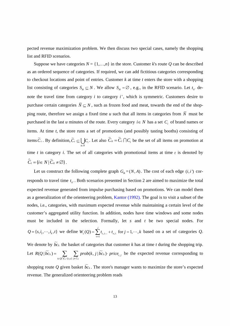
3.2. Modeling Framework We assume that the store layout and planogram are provided. Customers travel from a category

to a category. Based on a typical walking speed, the planogram, and layout, the anticipated walk-

ing time to go from one category to another can be computed. We first describe a general ex-

13

pected revenue maximization problem. We then discuss two special cases, namely the shopping

list and RFID scenarios.

Suppose we have categories N = {1,…,n} in the store. Customer k's route Q can be described

as an ordered sequence of categories. If required, we can add fictitious categories corresponding

to checkout locations and point of entries. Customer k at time t enters the store with a shopping

list consisting of categories tkS N⊆ . We allow tkS = ∅ , e.g., in the RFID scenario. Let 'iit de-

note the travel time from category i to category 'i , which is symmetric. Customers desire to

purchase certain categories N N⊆ , such as frozen food and meat, towards the end of the shop-

ping route, therefore we assign a fixed time u such that all items in categories from N must be

purchased in the last u minutes of the route. Every category i N∈ has a set iC of brand names or

items. At time t, the store runs a set of promotions (and possibly tasting booths) consisting of

items tC . By definition, t ii N

C C∈

⊆∪ . Let also ti t iC C C= ∩ be the set of all items on promotion at

time t in category i. The set of all categories with promotional items at time t is denoted by

{ | }t tiC i N C= ∈ ≠∅ .

Let us construct the following complete graph tkG = ( , )N A . The cost of each edge ( , ')i i cor-

responds to travel time 'iit . Both scenarios presented in Section 2 are aimed to maximize the total

expected revenue generated from impulse purchasing based on promotions. We can model them

as a generalization of the orienteering problem, Kantor (1992). The goal is to visit a subset of the

nodes, i.e., categories, with maximum expected revenue while maintaining a certain level of the

customer’s aggregated utility function. In addition, nodes have time windows and some nodes

must be included in the selection. Formally, let s and t be two special nodes. For

1{ , , , , }kQ s i i t= we define 1 1, ,

1

( ) for 1, ,j v v

j

i i i s iv

W Q t t j k+

=

= + =∑ based on a set of categories Q.

We denote by kbc the basket of categories that customer k has at time t during the shopping trip.

Let ,\{ , }

( | ) ( , | )tit

k k t jj Ci Q C s t

R Q bc prob k j bc price∈∈

= ⋅∑ ∑∩

be the expected revenue corresponding to

shopping route Q given basket kbc . The store's manager wants to maximize the store’s expected

revenue. The generalized orienteering problem reads

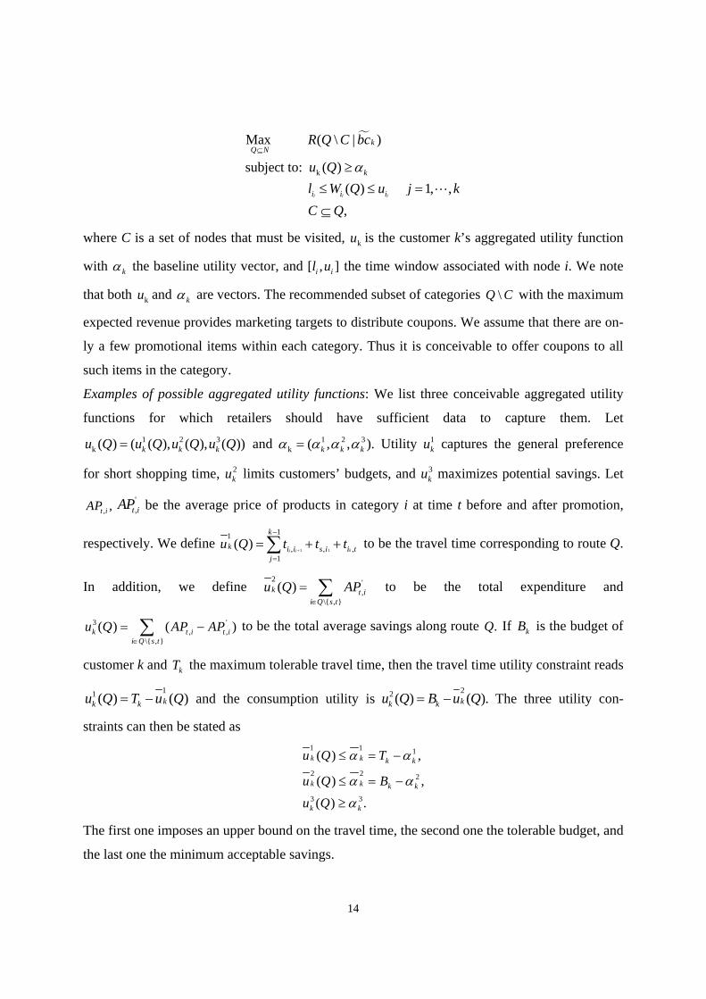
14

k

Max ( \ | )

subject to: ( ) ( ) 1, , ,

j j j

kQ N

k

i i i

R Q C bc

u Ql W Q u j kC Q

α⊆

≥

≤ ≤ =

⊆

where C is a set of nodes that must be visited, ku is the customer k’s aggregated utility function

with kα the baseline utility vector, and [ , ]i il u the time window associated with node i. We note

that both ku and kα are vectors. The recommended subset of categories \Q C with the maximum

expected revenue provides marketing targets to distribute coupons. We assume that there are on-

ly a few promotional items within each category. Thus it is conceivable to offer coupons to all

such items in the category.

Examples of possible aggregated utility functions: We list three conceivable aggregated utility

functions for which retailers should have sufficient data to capture them. Let 1 2 3

k ( ) ( ( ), ( ), ( ))k k ku Q u Q u Q u Q= and 1 2 3k ( , , ).k k kα α α α= Utility 1

ku captures the general preference

for short shopping time, 2ku limits customers’ budgets, and 3

ku maximizes potential savings. Let

, ,t iAP ',t iAP be the average price of products in category i at time t before and after promotion,

respectively. We define 1 1

11

, , ,1

( )j j k

k

k i i s i i tj

u Q t t t+

−

=

= + +∑ to be the travel time corresponding to route Q.

In addition, we define 2 '

,\{ , }

( )k t ii Q s t

u Q AP∈

= ∑ to be the total expenditure and

3 ', ,

\{ , }( ) ( )k t i t i

i Q s tu Q AP AP

∈

= −∑ to be the total average savings along route .Q If kB is the budget of

customer k and kT the maximum tolerable travel time, then the travel time utility constraint reads

11 ( ) ( )kk ku Q T u Q= − and the consumption utility is

22 ( ) ( ).kk ku Q B u Q= − The three utility con-

straints can then be stated as 1 1 1

2 2 2

3 3

( ) ,

( ) ,

( ) .

k k k k

k k k k

k k

u Q T

u Q B

u Q

α α

α α

α

≤ = −

≤ = −

≥

The first one imposes an upper bound on the travel time, the second one the tolerable budget, and

the last one the minimum acceptable savings.

15

We next elaborate on these aspects, including setting 1 2 3, and k k kα α α , and provide details on

the two scenarios considered.

Model with Shopping Lists

In this section we specify all data pertaining to this scenario with respect to the generalized

orienteering problem. We define s to be the location corresponding to the checkout counters and

t corresponding to the store entrance. For the initial basket we assume kbc = ∅ since there is no

way to identify and track customers' baskets in this scenario. The route is conceptually con-

structed backwards. Frozen food and other highly perishable categories in N that should be

purchased at the end of the trip have a time window[ 0 , ]u , which means that these categories

should be in the shopping cart in the last u time units of the trip. Other categories have a time

window of [0, ],∞ or no time window, because they could be purchased at any time during the

trip. For example, suppose a customer needs to purchase milk, crackers, chips, fruit, and meat.

Milk and meat have a time window of [ 0 , ] ,u while crackers, chips and fruit have no time win-

dow because they can be purchased anytime during the trip.

Next, we discuss 1kα . Assume customer k enters the store at time t with the shopping list

including items from categories in .tkS To determine 1kα , we first solve the traveling salesman

problem (TSP) with time windows on the sub-graph of tkG defined by tkS . The travel time tkv is

the time the shopper would spend in the store under an optimal route. We set 1

(1 )k tk tkvα α= + ,

where tkα is the travel time tolerance with respect to customer k at time t. To determine tkα ,

every time the customer visits the store, we record her shopping list. At checkout we link the

point-of-sale data with the specific shopping list. Let

the number of promoted items purchased that are not on the shopping listthe total number of items purchased tkλ = .

We take the average of tkλ over all previous visits of the customer. If the loyalty card is not

available, then we suggest to set tk tλ λ= , where

optimal route time with respect to the shopping listmax(1 ,0)optimal route time with respect to point-of-saletλ = −

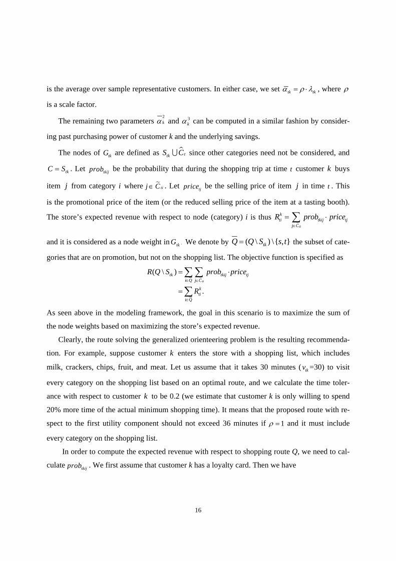
16

is the average over sample representative customers. In either case, we set tk tkα ρ λ= ⋅ , where ρ

is a scale factor.

The remaining two parameters 2kα and 3

kα can be computed in a similar fashion by consider-

ing past purchasing power of customer k and the underlying savings.

The nodes of tkG are defined as ttkS C∪ since other categories need not be considered, and

tkC S= . Let tkijprob be the probability that during the shopping trip at time t customer k buys

item j from category i where tij C∈ . Let tjprice be the selling price of item j in time t . This

is the promotional price of the item (or the reduced selling price of the item at a tasting booth).

The store’s expected revenue with respect to node (category) i is thus ti

kti tkij tj

j C

R prob price∈

= ⋅∑

and it is considered as a node weight in .tkG We denote by ( \ ) \{ , }tkQ Q S s t= the subset of cate-

gories that are on promotion, but not on the shopping list. The objective function is specified as

( \ )

.ti

tk tkij tji Q j C

kti

i Q

R Q S prob price

R∈ ∈

∈

= ⋅

=

∑ ∑

∑

As seen above in the modeling framework, the goal in this scenario is to maximize the sum of

the node weights based on maximizing the store’s expected revenue.

Clearly, the route solving the generalized orienteering problem is the resulting recommenda-

tion. For example, suppose customer k enters the store with a shopping list, which includes

milk, crackers, chips, fruit, and meat. Let us assume that it takes 30 minutes ( tkv =30) to visit

every category on the shopping list based on an optimal route, and we calculate the time toler-

ance with respect to customer k to be 0.2 (we estimate that customer k is only willing to spend

20% more time of the actual minimum shopping time). It means that the proposed route with re-

spect to the first utility component should not exceed 36 minutes if 1ρ = and it must include

every category on the shopping list.

In order to compute the expected revenue with respect to shopping route Q, we need to cal-

culate tkijprob . We first assume that customer k has a loyalty card. Then we have

17

' ( )'

exp( ( , , ))exp[ ( , , )] .exp[ ( ', , )] exp( ( , ', ))

t

itkij

ij J ti C

V k j tV i k tprobV i k t V k j t

μμμ μ

∈∈

=∑ ∑

(5)

based on (1). The first term in (5) denotes the purchase incidence probability of category i. The

second term in (5) follows the standard multinomial logit probability for selecting products with-

in category i. All parameters can be obtained by the maximum likelihood method, Ben-Akiva

and Lerman (1985).

If the loyalty card is not available, we follow the same concepts except that index k is neg-

lected. In this case, we take the average over sample representative customers when computing

the probabilities by using the utility expression.

Model with Radio Frequency Identification

In this scenario, the shopping list is not available. The store is, however, deployed with RFID.

Namely, smart shelves enable identifying items which are in the shopping carts and close enough

to an interrogator. Hence, the store's information system can identify the current purchases of a

customer up to a certain point and recommend promotional items with the goal to maximize the

store's total expected revenue. Notice that without tracking shopping carts we can only record the

sequence of purchases up to a certain point. The sequence is updated and recorded several times

during the shopping trip; every time the customer passes a coupon issuing device. Consider a

customer in front of a smart shelf equipped with a coupon issuing device. Let kbc be the set or

basket of categories that are already in customer k's shopping cart at time ,t which is the time

when the customer is in front of the smart shelf, and let 'kbc be the set of categories that were in

the shopping cart the last time customer k was in front of such a smart shelf. We denote by '\k k kbc bc bc= the added categories to the shopping cart after customer k was in front of such a

smart shelf the last time. Note that during a shopping trip the customer may pass by such shelves

several times (assuming there are many of such shelves in the store).

The graph nodes in this case correspond to the subgraph of tkG defined by tC . The set C is

empty and there are no time windows. The source node s equals to the node corresponding to the

category of the current shelf. The sink node t is a new fictitious node and 0itt = for every catego-

ry ti C∈ . We compute ( , | )kprob k j bc the probability of customer k purchasing product j given

18

categories kbc in the shopping cart in time t. We first assume that customer k has a loyalty card.

We obtain

' ( )' \

exp( ( , , ))exp[ ( , , )]( , | ) .exp[ ( ', , )] exp( ( , ', ))

t k

ik

ij J ti C bc

V k j tV i k tprob k j bcV i k t V k j t

μμμ μ

∈∈

=∑ ∑

(6)

The difference between (6) and (5) is in the fact that in the denominator we sum over categories

in \t kC bc .

Without the loyalty card it is the same concept except that index k is neglected and we take

the average over sample representative customers.

Similar to the shopping list scenario, the proposed route of categories with items on promo-

tion should be less than or equal to 1

(1 )k tk tkvα α= + , where tkv is the optimal travel time to visit

categories in kbc . The total travel time limit is based on the point-of-sale data, instead of the

shopping list. Additional inaccuracy here comes from the fact that a customer might have bought

a promoted item that she intended to buy anyway. Under the loyalty program, we propose

the number of promoted items purchased based on POSthe number of total purchased items based on POS tkλ = .

We take the average of tkλ over all previous visits of the customer. If the customer is not

enrolled in the loyalty program, then we average tkλ over sample representative customers. We

set tk tkα ρ λ= ⋅ , where ρ is a scale factor.

The remaining two parameters 2kα and 3

kα can be computed based on the same principles.

In addition, we can distinguish between the store being able to track the shopping carts or

not. Suppose first that shopping cart tracking is not available. An issue in this case is that we do

not want to hand out identical coupons to the same customer or issue coupons too frequently. We

offer a solution as follows. We recommend to pick a small subset of categories that are in high

traffic areas and are located far from the entry point. The latter implies that customers arrive at

the location supposedly with some items in the carts and the former reflects the fact that many

customers should pass by such a smart shelf. The coupon issuing devices are installed within the

area of a subset of categories recommended above.

In the other case, the shopping carts can be tracked (see Section 2.4 for a discussion). We can

now better control not giving the same coupons to a customer and when to deliver coupons. In

19

case they can be delivered at several store locations, it would be annoying for the customer to

receive them too frequently. To circumvent this, we propose the following strategy. We replace

kbc by kbc and thus use ( , | )kprob k j bc in ( | ).kR Q bc Consider \

max ( , | )t k

ktkj C bc

M prob k j bc∈

= ,

which is the maximum conditional probability customer k would buy a promotional item based

on added items to the shopping cart after the coupons were offered last time. If tktkM M≥ for a

threshold tkM , then consider giving the coupons. We can estimate tkM as follows. Let tS C⊆

be the set of promotional categories that have already been bought. Let S be the set of categories

that have already been bought, but are not on promotion. We offer two alternatives to compute

.tkM Let ( , | )kjq prob k j S= be based on S for every .j S∈ We also define

mink kjj Sqε

∈= or

| |

kjj S

k

q

Sε ∈=

∑.

We set tk kM ρ ε= ⋅ , where ρ is a scale factor.

3.3. Algorithms In the shopping list scenario, we need to solve the TSP problem to compute the baseline travel

time. On the other hand, in the second scenario, we also need to compute the baseline travel time

to acquire all items in the current shopping cart kbc with respect to customer k. Since the TSP

needs to be solved in real-time, a fast heuristic is required. The Lin-Kernighan heuristic is a very

efficient and quick heuristic for solving TSPs, Helsgaun (2000). Other heuristics can be em-

ployed, Gutin and Punnen (2002). The shopping list and current basket kbc are respectively the

input and the baseline travel time is the output.

The ultimate route in either scenario is obtained by solving the generalized orienteering prob-

lem. The standard orienteering problem does not include time windows and the predefined set of

nodes C. This problem also needs to be solved by fast heuristics. Efficient heuristics for the

orienteering problem exist, Chao et al. (1996), Ramesh and Kathleen (1991). These heuristics

can easily be extended to accommodate all of our requirements. We point out that in our setting

these are not large-scale problems (the number of nodes equals to the number of categories,

20

which is within hundreds). Due to the limited size, branch-and-cut algorithms could also be used,

Fischetti et al. (1998).

4. Numerical Experiments In this section, we apply the model with shopping list, i.e., the first scenario to a real-world case

of a major grocery store. Only the travel time utility component is considered. The store layout

and the complete planogram were given and therefore, the distances between any two categories

can accordingly be computed. The store holds from 200 to 250 categories and 35,000 to 50,000

different products.

Our information system was developed in VBA within Microsoft Excel. Parameters in the

utility functions were computed by the maximum likelihood method with What's Best from Lin-

do Systems as the optimization solver. All TSP instances were solved by using the Lin-

Kernighan routine of the branch-and-cut solver Concorde. The generalized orienteering problem

was solved with the branch-and-cut solver from Fischetti et al. (1998).

The unit selling price for each product during a period of time is available. The only data not

available were the current (future) promotions. For this reason we randomly generated them in

the following way. First, we randomly generated a subset of brand names (these were selected

from UPCs). In the second step, for each selected brand name we randomly generated a subset of

items running a promotion. We considered several levels of promotion: less than 1%, 3% and 6%

products on promotion. We stress that even the most aggressive level of 6% is below a typical

level of 10% employed by this store (the number conveyed to us by the store manager). The

price of a promotional item is reduced in a range of 20% to 30% (randomly in this range).

The store keeps point-of-sale data of each customer enrolled in the loyalty program. We fo-

cus our study on five representative customers. Each of these customers purchases on average 30

to 50 items during each shopping trip. Within the scope of our study, a customer on average vi-

sited the store 7 times during the time period. As a result, all data points in this section are the

accumulated sum over 7 shopping trips. Additional point-of-sale data from the source customers

were used to derive all of the parameters related to the discrete choice models.

Given a shopping list, we compute four different baseline cases. Baseline up-and-down

(“BUD”) represents the case where a customer travels along each aisle one by one from one end

of the aisle to the other end and never turns around in the same aisle. She only visits the aisles

21

where she has something to buy from. Adjusted baseline (“AB”) represents a similar case, but

when the customer reaches the last required category in one aisle she takes the shortest route to

the next aisle she must visit. Larson et al. (2005) show that the “AB” strategy is commonly used

by shoppers. On the other hand, the same authors argue that the ‘BUD’ strategy is not. We use

‘BUD’ as an additional benchmarking strategy. They are depicted in Figure 5, where the bigger

dot represents the store entrance and checkout location, and small dots represent products from

the shopping list. The solid line with arrows represents BUD and the dotted line with arrows

represents AB. In the remaining two cases, we compute the baseline route by the Lin-Kernighan

algorithm (“LK”) or an optimal TSP solution (“OPT”). In Table 1, we summarize the baseline

characteristics with respect to the travel time. We report the total travel time reduction over all

shopping trips.

The baseline travel times are compared among the baseline cases of interest, where we com-

pute the relative reduction of travel times between the two cases. For example, the travel time in

the LK case is reduced by 8.74% compared to the adjusted baseline case. In most of the cases the

TSP strategies yield significant time reduction (with the exception of customer 2) in the range

form 5% to 11%. This clearly indicates that with respect to the shopping time the current wisdom

can be substantially improved by using information systems (see also further discussion in Sec-

tion 5). We also observe that the LK strategy almost always yields an optimal solution with the

exception of customer 5.

We have already discussed random promotion generation. We apply three promotional le-

vels: low, medium, and high. In the low promotional level, 0.7% of products are on promotion.

There are 2.5% products on promotion in the medium promotional level, and 6.0% products in

the high promotional level. We compare the differences of expected revenues among all four

baseline cases and optimized cases. The time tolerance factor is fixed at 5%, i.e.,1

(1 0.05)k tkvα = + .

22

Figure 5: The BUD and AB strategies

Table 1: Baseline travel times

AB/LK

(%) AB/OPT

(%) BUD/LK

(%) BUD/OPT

(%) customer 1 8.74 8.74 10.42 10.42 customer 2 0.79 0.79 1.53 1.53 customer 3 5.29 5.29 9.11 9.11 customer 4 7.74 7.74 8.27 8.27 customer 5 8.25 8.62 10.14 10.50

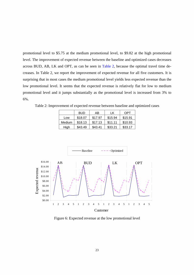
Figure 6, Figure 7, and Figure 8 show the expected revenue for all five customers and for all

three promotional levels, respectively. The baseline case shows the revenue based on the under-

lying baseline route. As the customer follows the baseline route, she passes by promotions and

the expected revenue is calculated accordingly based on ktiR . The optimal solutions vary since the

travel time of the corresponding baseline route is different. For example, in Figure 7, customer 1,

the adjusted baseline case shows revenue $5.75, which means that if this customer follows the

adjusted baseline strategy in the store, she is expected to purchase $5.75 of promotional products

that are not on her shopping list. On the other hand, if each time she follows the recommended

optimized route, under identical promotions, she is expected to buy $11.99 of promotional items

not on her shopping list. As the promotional level increases, more expected revenue is created,

e.g., under the AB case with respect to customer 1, the revenue increases from $2.27 at the low

BUD AB

23

promotional level to $5.75 at the medium promotional level, to $9.82 at the high promotional

level. The improvement of expected revenue between the baseline and optimized cases decreases

across BUD, AB, LK and OPT, as can be seen in Table 2, because the optimal travel time de-

creases. In Table 2, we report the improvement of expected revenue for all five customers. It is

surprising that in most cases the medium promotional level yields less expected revenue than the

low promotional level. It seems that the expected revenue is relatively flat for low to medium

promotional level and it jumps substantially as the promotional level is increased from 3% to

6%.

Table 2: Improvement of expected revenue between baseline and optimized cases

BUD AB LK OPT Low $18.07 $17.97 $15.94 $15.91

Medium $18.13 $17.13 $11.11 $10.93 High $43.49 $43.41 $33.21 $33.17

Figure 6: Expected revenue at the low promotional level

$0.00

$2.00

$4.00

$6.00

$8.00

$10.00

$12.00

$14.00

$16.00

1 2 3 4 5 1 2 3 4 5 1 2 3 4 5 1 2 3 4 5

Customer

Expe

cted

reve

nue

Baseline Optimized

AB BUD LK OPT

24

Figure 7: Expected revenue at the medium promotional level

Figure 8: Expected revenue at the high promotional level

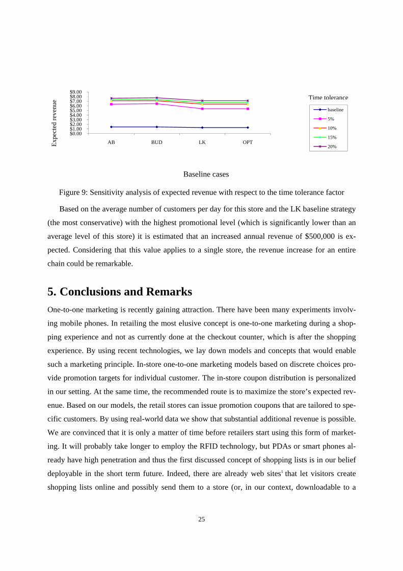
The expected revenue also varies with respect to the time tolerance factor. In Figure 9, we

compute the expected revenue across all customers as the time tolerance factor is set to 5%, 10%,

15%, and 20%. Clearly, as expected, the revenue increases. The most notable increase is from

5% to 10%.

$0.00

$2.00

$4.00

$6.00

$8.00

$10.00

$12.00

$14.00

$16.00

$18.00

1 2 3 4 5 1 2 3 4 5 1 2 3 4 5 1 2 3 4 5

Expe

cted

reve

nue

Customer

Baseline Optimized

$0.00

$5.00

$10.00

$15.00

$20.00

$25.00

$30.00

1 2 3 4 5 1 2 3 4 5 1 2 3 4 5 1 2 3 4 5Customer

Expe

cted

reve

nue

Baseline Optimized

LKAB BUD OPT

AB BUD LK OPT

25

Figure 9: Sensitivity analysis of expected revenue with respect to the time tolerance factor

Based on the average number of customers per day for this store and the LK baseline strategy

(the most conservative) with the highest promotional level (which is significantly lower than an

average level of this store) it is estimated that an increased annual revenue of $500,000 is ex-

pected. Considering that this value applies to a single store, the revenue increase for an entire

chain could be remarkable.

5. Conclusions and Remarks One-to-one marketing is recently gaining attraction. There have been many experiments involv-

ing mobile phones. In retailing the most elusive concept is one-to-one marketing during a shop-

ping experience and not as currently done at the checkout counter, which is after the shopping

experience. By using recent technologies, we lay down models and concepts that would enable

such a marketing principle. In-store one-to-one marketing models based on discrete choices pro-

vide promotion targets for individual customer. The in-store coupon distribution is personalized

in our setting. At the same time, the recommended route is to maximize the store’s expected rev-

enue. Based on our models, the retail stores can issue promotion coupons that are tailored to spe-

cific customers. By using real-world data we show that substantial additional revenue is possible.

We are convinced that it is only a matter of time before retailers start using this form of market-

ing. It will probably take longer to employ the RFID technology, but PDAs or smart phones al-

ready have high penetration and thus the first discussed concept of shopping lists is in our belief

deployable in the short term future. Indeed, there are already web sites1 that let visitors create

shopping lists online and possibly send them to a store (or, in our context, downloadable to a

$0.00 $1.00 $2.00 $3.00 $4.00 $5.00 $6.00 $7.00 $8.00 $9.00

AB BUD LK OPTExpe

cted

reve

nue

Baseline cases

baseline

5%

10%

15%

20%

Time tolerance

26

PDA). A system called Easi-Order, Electronics Times (1999), is a home-based shopping service

through which customers generate their shopping lists at home and communicate them back to

the grocery stores for picking up at a predetermined time. HighPoint Systems has deployed a

similar concept for the online grocer2 Peapod, LLC.

Regarding RFID, a few years ago a prototype future store has been built by Metro AG in

Rheinberg, Germany3. The store uses RFID at the item level and it also features displays at

shelves. These displays can be easily adopted to serve the purpose of our work. Nevertheless,

this is only a prototype store and at present the cost of an RFID deployment at this scale is still

prohibitive. There are also early implementations of smart shopping carts with mounted displays,

Embedded star (2004), Gizmag (2005), USA Today (2003). The Klever-Kart system, Embedded

star (2004), is different from previous intelligent carts since a Fujitsu mobile computer is perma-

nently attached to a standard cart. The devices can be used to demonstrate electronic ads and

promotions. On the other hand, the displays can also be used to track the current total charge by

scanning each item before putting it in the cart and also to recommend promotions. In our work,

we provide analytical models for such recommendations. We push this a step further, by also

providing a store route leading past promoted items. Such technology combined with tracking of

shopping carts can also serve our purpose (instead of presumably more costly RFID implementa-

tions).

Finally, we would like to comment on an important observation from our numerical study. In

Table 1 we report the deviation in terms of the travel time of the estimated shopping path to an

optimal shopping route. A similar study has recently been conducted by Hui et al. (2007). Their

conclusion is that this deviation is around 20%, which is substantially higher than our observa-

tions. By replicating our approach, their value would be even larger (we find an optimal TSP tour

while they use simulated annealing, which can yield suboptimal tours). Based on these facts it

follows that this deviation is not standard across the stores but it can vary significantly.

Based on the discussion in Section 4, an important managerial insight is derived. The compu-

tational experiments show that the added revenue of our personalized coupon distribution is rela-

tively flat up to a certain promotional level. Beyond this threshold, it increases substantially. As a

1http://www.commissaries.com/log_in/html/list_fr.cfm, http://www.shopbloom.com/ 2http://www.peapod.com/ 3http://www.future-store.org/servlet/PB/menu/1007054/index.html

27

result, the store manager should find out this threshold and then promote slightly above it, if

possible.

Acknowledgments We are obliged to Emily Io for her assistance in data gathering and mining. We also acknowl-

edge Intel Corporation for financially supporting Mrs. Io during her undergraduate study at the

University of Illinois at Urbana-Champaign. We are indebted to Professor Juan-José Salazar-

González from the University of La Laguna, Tenerife, Spain, for gratefully sharing his branch-

and-cut implementation of the orienteering problem. Without it this research would have been

prolonged for a significant time. We are also thankful to anonymous referees. Their comments

have enhanced the contributions and merits of the presented work.

References Anthes, G. (2000). Easi-Order. Computerworld. March, 20. Available from

http://www.computerworld.com/action/article.do?command=viewArticleBasic&articleId=41911&pageNumber=1

Bell, D. and J. Lattin. (1998). Shopping Behavior and Consumer Preference for Store Price Format: Why “Large Basket” Shoppers Prefer EDLP. Marketing Science 17(1): 66-68.

Ben-Akiva, M. and S. Lerman. (1985). Discrete Choice Analysis: Theory and Application to Travel Demand. The MIT Press, Cambridge, MA.

Boztug, Y. and L. Hildebrandt. (2007). A Market Basket Analysis Based on the Multivariate MNL Model. Available from http://edoc.hu-berlin.de/series/sfb-373-papers/2003-21/PDF/21.pdf

Bucklin, R. E. and J. M. Lattin.(1991). A Two-State Model of Purchase Incidence and Brand Choice. Marketing Science 10(1): 24-39.

Byron, E. (2005). Subject: Email Ads Grow Up. The Wall Street Journal, November 23. Byrnes, N. (2007). More Clicks at the Bricks. Business Week, December 17. Chao, I-Ming, B. Golden, and E. Wasil. (1996). A Fast and Effective Heuristic for Orienteer-

ing Problem. European Journal of Operational Research 88(3):475-489. Chiang, J. (1991). A Simultaneous Approach to the Whether, What and How Much to Buy

Questions. Marketing Science 10(4): 297-315. Chib, S., P. B. Seetharaman and A. Strijnev. (2002). Analysis of multicategory purchase inci-

dence decisions using IRI market basket data. Advances in Econometrics 16: 57–92 Chintagunta, P. K. (1993). Investigating Purchase Incidence, Brand Choice and Purchase

Quantity Decisions of Households. Marketing Science 12(2): 184-208.

28

Cho, H., H. Choi, W. Lee, Y. Jung, and Y. Baek. (2006). LITeTag: Design and Implementa-tion of an RFID System for IT-based Port Logistics. Journal of Communications 1(4): 48-57.

Chong, J., T. Ho, and C. Tang. (2001). A Modeling Framework for Category Assortment Planning. Manufacturing & Service Operations Management 3(3):191-210.

Concorde TSP Solver. (2005). http://www.tsp.gatech.edu/concorde/index.html Cox, D. (1972). The Analysis of Multivariate Binary Data. Applied Statistics 21(2): 113-120. Cutler, G. (2000). Why Promote? The Professional Assignments Group Pty. Ltd. Available

from http://www.pag.com.au/pdf/8_WhyPromoteArticle.pdf Dhar, S., D. Morrison, and J. Raju. (1996). The Effect of Package Coupons on Brand Choice:

An Epilogue on Profits. Marketing Science 15(2): 192-203. Embedded Star. (2004). Fujitsu, Klever Marketing Personalize Shopping with Intelligent Cart.

Available from http://www.embeddedstar.com/press/content/2004/2/embedded12742.html

Electronics Times. (1999). A Super Market-Easi-Order Service from Safeway-Company Business and Marketing. Available from http://findarticles.com/p/articles/mi_m0WVI/is_1999_June_14/ai_54935610

Fischetti, M., J. González, and P. Toth. (1998). Solving the Orienteering Problem through Branch-and-cut. INFORMS Journal on Computing 10(2): 133-148.

Gaukler G., R. Seifert and W. Hausman. 2007. Item-Level RFID in the Retail Supply Chain. Production and Operations Management (16)1: 65-76.

Gaukler G., Özalp Özer and W. Hausman. 2008. Order Progress Information: Improved Dy-namic Emergency Ordering Policies. Production and Operations Management 17(6): 599-613.

Gizmag. (2005). Klever Shopping Cart Begins Roll-out. Available from http://www.gizmag.com/go/3751/

Guadagni, P. and J. C. Little. (1998). When and What to Buy: A Nested Logit Model of Cof-fee Purchase. Journal of Forecasting 17(4): 303-326.

Gutin, G. and A. Punnen. (2002). The Traveling Salesman Problem and Its Variations. Kluw-er Academic publishers, Norwell, MA.

Harlam, Bari A., and Leonard M. Lodish. (1995). Modeling Consumers’ Choices of Multiple Items. Journal of Marketing Research 32 (4): 404-418

Hausman A. (2000). A Multi-method Investigation of Consumer Motivations in Impulse Buy-ing Behavior. Journal of Consumer Marketing 17(5): 403-419.

Heilman, C., K. Nakamoto, and A. Rao. (2002). Pleasant Surprises: Consumer Response to Unexpected In-Store Coupons. Journal of Marketing Research 39(2): 242-252.

Helsgaun, K. (2000). An Effective Implementation of the Lin–Kernighan Traveling Salesman Heuristic. European Journal of Operational Research 126(1): 106-130.

Hui, S., P. Fader, and E. Bradlow. (2007). The Traveling Salesman Goes Shopping: The Sys-tematic Deviations of Grocery Paths from TSP-Optimality. Technical Report, Wharton School of Business, University of Pennsylvania. Available from http://ssrn.com/abstract=942570

29

Kahn, E. and L. McAlister. (1997). Grocery Revolution: The New Focus on the Customer. Prentice Hall, Upper Saddle River, NJ.

Kantor, M. and M. Rosenwein. (1992). The Orienteering Problem with Time Windows. The Journal of the Operational Research Society 43(6): 629-635.

Kumar, V. and R. Leone. (1988). Measuring the Effect of Retail Store Promotions on Brand and Store Substitution. Journal of Marketing Research 25(2): 178-185.

Larson, J., E. Bradlow, and P. Fader. (2005). An Exploratory Look at Supermarket Shopping Paths. International Journal of Research in Marketing 22(4): 395-414.

Li Z. 2007. A Single-Period Assortment Optimization Model. Production and Operations Management. 16(3): 369-380.

McCulloch, R. and P. Rossi. (1994). An Exact Likelihood Analysis of the Multinomial Probit Model. Journal of Econometrics 64(1-2): 207-240.

Mehta, N. (2007). Investigating Consumers’ Purchase Incidence and Brand Choice Decisions Across Multiple Product Category: A Theoretical and Empirical Analysis. Marketing Science 26(2): 196-217.

Mulhern, F.J., and D.T. Padgett (1995). The Relationship Between Retail Price Promotions and Regular Price Purchases. Journal of Marketing 59(4):83-90.

Newcomb, E., T. Pashley, and J. Stasko. (2003). Mobile Computing in the Retail Arena. Pro-ceedings of the SIGCHI Conference on Human Factors in Computing Systems 5(1): 337-344.

O’Connor, M. (2006). RFID Gets Personal. RFID Journal. Available from http://www.rfidjournal.com/article/view/2233/1/3/

RFID Journal (2003). Part 8: Turbo-Charged Marketing. RFID Journal, February, 2003. Available from http://www.rfidjournal.com/article/articleprint/315/-1/5/

Ramesh, R. and M. Kathleen. (1991). An Efficient Four-phase Heuristic for the Generalized Orienteering Problem. Computers and Operations Research 18(2):151-165.

Russell, G. and A. Petersen. (2000). Analysis of Cross Category Dependence in Market Basket Selection. Journal of Retailing 76(3): 367-392.

Seetharaman, P.B., S. Chib, A. Ainslie, P. Boatwright, T. Chan, S. Gupta, N. Mehta, V. Rao and A. Strijnev. (2005). Models of Multi-Category Choice Behavior. Marketing Letters 16(3/4): 239-254.

Sokol, B. (2005). RFID & Emerging Technologies Market Guide to Healthcare. Fast Track Technologies Ltd. Available from http://www.rfidjournal.com/article/articleview/1511/1/1/

Taylor, G. (2001). Coupon Response in Services. Journal of Retailing 77(1): 139-151. USA Today. (2003). Smart Carts, Veggie Vision in Grocery Stores to Come. Available from

http://www.usatoday.com/tech/news/techinnovations/2003-09-26-future-grocery-shop_x.htm

Van Heerde, H., P. Leeflang, and D. Wittink. (2004). Decomposing the Sales Promotion Bump with Store Data. Marketing Science 23(3): 317-334.

Wolfe, E., and P. Alling. (2003). Track(ing) to the Future: The Impending RFID-Based Inven-tory Revolution. Bear Stearns Equity Research Report. Available from http://www.bearstearns.com/bscportal/html/research/supplychain_technology.htm

30

What’s Best, LINDO Systems. (2007). http://www.lindo.com/products/wb/wbm.html Zaino, J. (2008). Tag Sale. RFID Journal, January. Available from

www.rfidjournal.com/magazine/article/3542