QUANTIFYING THE INFLUENCE OF AIR ON THE

CAPACITY OF LARGE DIAMETER WATER

PIPELINES AND DEVELOPING PROVISIONAL

GUIDELINES FOR EFFECTIVE DE-AERATION

Volume 2

Provisional guidelines for the effective de-aeration of large diameter

water pipelines

S J van Vuuren, M van Dijk and J N Steenkamp

WRC Report No. 1177/2/03

Water Research Commission

QUANTIFYING THE INFLUENCE OF AIR ON THE CAPACITY OF

LARGE DIAMETER WATER PIPELINES AND DEVELOPING

PROVISIONAL GUIDELINES FOR EFFECTIVE DE-AERATION

Volume 2

Provisional guidelines for the effective de-aeration of large diameter water

pipelines

By

S J van Vuuren, M van Dijk and J N Steenkamp

NINHAM SHAND (Pty) Ltd

Private Bag X136

Centurion

0046

Report to the WATER RESEARCH COMMISSION on the project:

QUANTIFYING THE INFLUENCE OF AIR ON THE CAPACITY OF LARGE

DIAMETER WATER PIPELINES AND DEVELOPING PROVISIONAL GUIDELINES

FOR EFFECTIVE DE-AERATION

K5/1177

Project Leader: S J van Vuuren

WRC Report no: K5/1177/2/03

ISBN no: ……………………

i

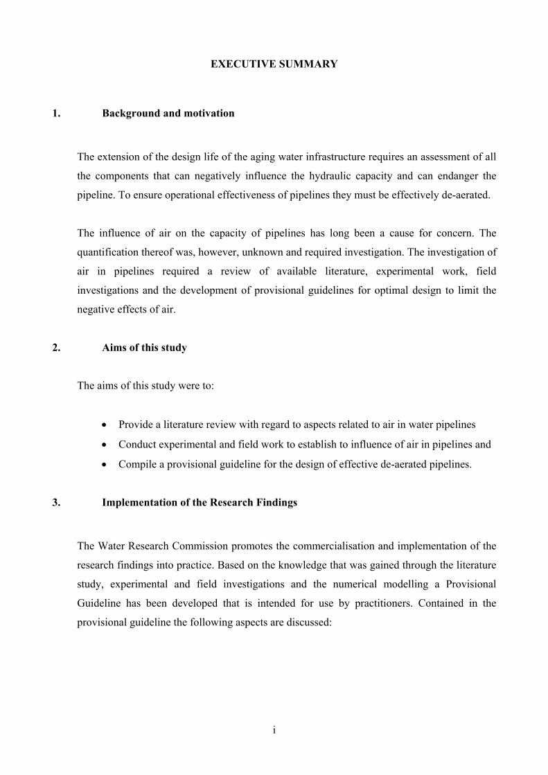
EXECUTIVE SUMMARY

1. Background and motivation

The extension of the design life of the aging water infrastructure requires an assessment of all

the components that can negatively influence the hydraulic capacity and can endanger the

pipeline. To ensure operational effectiveness of pipelines they must be effectively de-aerated.

The influence of air on the capacity of pipelines has long been a cause for concern. The

quantification thereof was, however, unknown and required investigation. The investigation of

air in pipelines required a review of available literature, experimental work, field

investigations and the development of provisional guidelines for optimal design to limit the

negative effects of air.

2. Aims of this study

The aims of this study were to:

• Provide a literature review with regard to aspects related to air in water pipelines

• Conduct experimental and field work to establish to influence of air in pipelines and

• Compile a provisional guideline for the design of effective de-aerated pipelines.

3. Implementation of the Research Findings

The Water Research Commission promotes the commercialisation and implementation of the

research findings into practice. Based on the knowledge that was gained through the literature

study, experimental and field investigations and the numerical modelling a Provisional

Guideline has been developed that is intended for use by practitioners. Contained in the

provisional guideline the following aspects are discussed:

ii

• Intrusion of air into pipelines

• The consequences of air in pipelines

• Hydraulic transport of air

• Air valves

• Implementation of a new pipeline

• Sizing and positioning of air valves

• Typical installation details of air valves

These aspects will provide the designer assistance in the review of existing, and the design of

new pipelines. The inclusion of utility software is a great advantage with regard to the

analyses of pipe systems with regard to the locations and sizing of air valves.

4. User comments

It is envisaged that it might be possible that the use of the guidelines will highlight

shortcomings and could lead to the implementation of other aspects to improve the provisional

guidelines.

The incorporations of procedures to determine the location of air pockets, the practical

experience of using the guidelines and the development of new products will create the

opportunity for the upgrading and extension of the guideline. All users are requested to

provide comments and feedback on the use of this guideline.

iii

PROVISIONAL GUIDELINES FOR THE EFFECTIVE DE-AERATION

OF LARGE DIAMETER WATER PIPELINES

TABLE OF CONTENTS Page

1.

2.

3.

Executive Summary

Table of Contents

List of Figures

List of Tables

Glossary of Terms

Definitions

INTRODUCTION

1.1 Aim of the study

1.2 Methodology

1.3 Layout of the reports

INTRUSION OF AIR INTO PIPELINES

2.1 Introduction

2.2 Category A – Implementation of a new pipeline or the refilling of an existing

pipeline

2.3 Category B – Operational conditions

THE CONSEQUENCE OF AIR IN PIPELINES

3.1 Introduction

3.2 Reduction of capacity

3.3 Blow-back and associated pressure fluctuations

3.4 White water

3.5 Water hammer and surge

3.6 Effect of uncontrolled air release from pipelines

3.7 Effect of free air on induced pressure surges

3.8 Other consequences of free air in pipelines

i

iii

vi

vii

viii

x

1-1

1-1

1-1

1-2

2-1

2-1

2-1

2-2

3-1

3-1

3-1

3-3

3-3

3-4

3-4

3-5

3-6

iv

4.

5.

6.

7.

HYDRAULIC TRANSPORT OF AIR

4.1 Introduction

4.2 Formula used for prediction of transportability of air

4.3 Proposed formula to use for the hydraulic transportability of air

AIR VALVES

5.1 Valve types

5.1.1 Large orifice air valves

5.1.2 Small orifice air valves

5.1.3 Combination air valves

5.1.4 Special types

5.2 Operational limitations

5.3 Maintenance of air valves

5.4 Procedures for testing air valves

5.4.1 Introduction

5.4.2 Release of air from pipes

5.4.3 Testing procedure for the intake capacity of air valves (large orifice

function)

5.4.4 Conclusion

IMPLEMENTATION OF A NEW PIPELINE

6.1 Filling of a pipeline

6.2 Hydrostatic testing

6.2.1 Purpose of hydrostatic testing

6.2.2 Selection of test sections

6.2.3 Specifications for hydrostatic pressure testing

6.2.4 Practical aspects related to hydrostatic pressures

SIZING AND POSITIONING OF AIR VALVES

7.1 Historical approach of air valve sizing and positioning

7.2 Air valve sizing and positioning procedure (ASAP)

7.2.1 ASAP input requirements

7.2.2 ASAP calculations

7.2.2.1 Burst analysis (uncontrolled flow release from the pipeline)

7.2.2.2 Drain analysis (controlled air release)

4-1

4-1

4-1

4-2

5-1

5-1

5-1

5-4

5-5

5-6

5-9

5-10

5-11

5-11

5-12

5-13

5-15

6-1

6-1

6-2

6-2

6-3

6-4

6-6

7-1

7-1

7-2

7-5

7-6

7-7

7-10

v

8.

9.

10.

7.2.2.3 Filling analysis

7.2.2.4 Small orifice air release analysis

7.2.2.5 Special consideration

7.2.2.6 Conclusion

7.2.3 ASAP results

7.3 Hand calculation

7.3.1 Introduction

7.3.2 Input data

7.3.3 Calculations

7.3.4 Results

7.4 Air valve sizing and positioning software

7.5 Economic value of effective de-aeration

TYPICAL INSTALLATION DETAILS OF AIR VALVES

8.1. Discontinuity

8.2 Size of accumulator

8.3 Installation and valve chamber design

USER COMMENTS

REFERENCES

7-12

7-14

7-16

7-16

7-16

7-18

7-18

7-18

7-19

7-28

7-29

7-30

8-1

8-1

8-2

8-3

9-1

10-1

vi

LIST OF FIGURES

Figure 2.1: Schematic definition of the concept of an air lock

Figure 3.1: Head loss in a gravity system

Figure 3.2: Head loss in a pumping system

Figure 3.3: Change in duty point resulting from additional secondary losses at air bubbles

Figure 3.4: Air bubble travelling back causing pressure fluctuations

Figure 3.5: A photo of white water in surge tower (Buffalo River abstraction, East London,

South Africa)

Figure 3.6: Effect of free air on a system’s wave celerity

Figure 4.1: Required flow velocity to remove air

Figure 4.2: Bubble size comparison of Kalinske & Bliss and Wisner et al. equations

Figure 5.1: Large orifice air valve (Val-Matic, 1993)

Figure 5.2: Differential pressure - discharge relationship for a two stage large orifice air

valve

Figure 5.3: Small orifice air valve (Val-Matic, 1993)

Figure 5.4: Combination air valve (Val-Matic, 1993)

Figure 5.5: Combination air valve (ARI, 1998)

Figure 5.6: Slow closing valve (APCO, 2003)

Figure 5.7: Hydraulically controlled air valve (APCO, 2003)

Figure 5.8a: Venting of a filling pipeline (Sub-critical water approach velocity)

(Vent-O-Mat, 1996)

Figure 5.8b: Venting of a filling pipeline (Excessive water approach velocity)(Vent-O-Mat,

1996)

Figure 5.8c: Pressurised air release from a full pipeline (Vent-O-Mat, 1996)

Figure 5.9: Intake capacity calculations

Figure 5.10: Comparative intake capacities

Figure 6.1: Unstable flow scenario during the filling of the pipeline

Figure 6.2: Pressure change due to temperature change

Figure 7.1: Flow diagram of the ASAP procedure

Figure 7.2: Pipeline profile

Figure 7.3: Bursting (example pipe section)

Figure 7.4: Illustrating the value of looking at a pipeline as a whole (Example)

Figure 7.5: Drainage (example)

Figure 7.6: Filling (example)

vii

Figure 7.7: Typical ASAP results (Pipeline profile)

Figure 7.8: Pumping system pipeline profile

Figure 7.9: Pipeline profile with air valves (Vent-O-Mat Utility Programs, 2003)

Figure 8.1: Graphical presentation of installation details (small orifice function)

Figure 8.2: Graphical presentation of installation details (large orifice function)

Figure 8.3: Well-designed air valve chamber (Umgeni Water)

Figure 8.4: Two air valves on a manifold (above ground installation)

Figure 8.5: Four air valves on a manifold (above ground installation)

Figure 8.6: Schematic layout of larger type installation above ground

LIST OF TABLES

Table 4.1: Comparison of the critical velocity to transport air

Table 5.1: Operating condition characteristic during the release of air from a pipeline

Table 5.2: Typical intake values for air valves

Table 6.1: Pro-forma data sheet for the hydrostatic pressure test

Table 7.1: Typical air valve sizing and positioning guideline (historical approach)

Table 7.2: Typical ASAP input requirements

Table 7.3: Rupture size as a percentage of pipe diameter (suggested default values that

should be checked by conducting a sensitivity analysis)

Table 7.4: Possible drainage scenarios

Table 7.5: Possible filling scenarios for the sections that can be isolated

Table 7.6: Typical ASAP result (valve requirements)

Table 7.7: Pipeline profile and details

Table 7.8: Intake requirements for every pipe section in case of a burst

Table 7.9: Intake requirements for every node (US and DS) due to burst analysis

Table 7.10: Possible draining scenarios

Table 7.11: Activation sequence for every drainage scenarios

Table 7.12: Intake requirements on the upstream and downstream of every node due to

controlled drainage

Table 7.13: Possible filling scenarios

Table 7.14: Sub-scenarios of Scenario 1

Table 7.15: Vmin for pipe sections with negative slopes

Table 7.16: Air valve requirements (Vent-O-Mat Utility Programs, 2003)

viii

GLOSSARY OF TERMS

a = Constant (for medium sized bubble: a = 0,2178)

e = Coefficient of volume thermal expansion of pipe wall material (/°C)

A = Area of the pipe (m²)

Ai = Flow area for intake orifice (m²)

A0 = Flow area for outflow orifice (m²)

Ao = Orifice area of the air valve (m²)

Arupture = Area of pipe rupture (m²)

B = Coefficient of volume thermal expansion of liquid (/°C)

b = Constant (for medium sized bubble: b = 0,4007)

c = Celerity with no air (m/s)

c' = Celerity with free air (m/s)

CD = Discharge coefficient for an orifice

Cdi = Discharge coefficient for the inflow orifice

Cd0 = Discharge coefficient for the outflow orifice

Co = Discharge coefficient

D = Inside diameter of pipe (m)

Doutlet = Inside diameter of outlet pipe (m)

E = Elasticity of the pipe material (MPa)

g = Gravitational acceleration (m/s²)

H = Henry’s Law constant

∆h = Available energy between peak and drainage point (m)

K = Bulk modulus of liquid (MPa)

k = Isentropic constant (ratio of specific heats = 1,4 for air)

ks = Absolute roughness of pipe (m)

L = Length of pipe (m)

m& = Mass flow rate (kg/s)

m = Mass of free gas per unit mix (kg/m³)

Pa = Partial pressure of gas

P = Pressure (MPa)

p = Absolute pressure of air in the valve (Pa)

pa = Atmospheric pressure (Pa)

∆P = Pressure differential across the air valve (kPa)

Qc = Flow rate at which removal starts (m³/s)

ix

Qdischarge = Discharge through air valve (m³/s)

Qdrain = Flow rate due to controlled drainage (m³/s)

Qburst = Flow rate due to burst (m³/s)

R = Gas constant (J/kg K)

S0 = Slope of pipe (m/m)

t = Wall thickness (m)

T = Temperature (° Kelvin)

∆T = Change in temperature (°C)

Vc = Clearing velocity, also called critical velocity (m/s)

Vmin = Flow velocity at which point removal will start (m/s)

VolL = Permissible leakage (l)

V2 = Velocity in steep section (m/s)

V1 = Velocity in less steep section (m/s)

Xa = Mole fraction of the gas in the liquid phase

λ = Friction factor

µ = Poisson's ratio

ρa = Density of air at atmospheric pressure (kg/m³)

ρv = Density of air in the air valve under line head conditions (kg/m³)

ρv = Fluid density (kg/m³)

θ = Slope of pipeline (°)

x

DEFINITIONS

Air valve

Air release valve

Atmospheric pressure

Automatic air release valve

Clearing velocity

Class

Column separation

Combination air valve

Differential pressure

-

-

-

-

-

-

-

-

-

A mechanical device with which air can be removed or

introduced from or into a pipeline system.

Valves which are designed to discharge air during the filling of a

pipeline with fluid, for ventilating a pipeline while emptying, or

for releasing air that may have accumulated in sections of a

pipeline under normal working conditions (Myles K, 1994).

Atmospheric pressure is defined as the force per unit area exerted

against a surface by the weight of the air above that surface.

This is a valve that releases entrapped air in pressurized

water/sewerage systems. It is also referred to a small orifice

valve since the outlet orifice is relatively small (typically 1mm²).

The minimum velocity to clear an air pocket from a line. No

distinction is made whether the air pocket is removed as a whole

or by means of generation and entrainment (Wisner, Mohsen &

Kouwen, 1975).

This refers to the pressure rating usually expressed as a

dimension less number.

This is a phenomenon that occurs when water separates creating a

vacuum.

This is a valve that combines the function of an air release

valve and a vacuum break valve.

The difference in pressure between two points.

xi

Discount rate

Energy head

Escalation rate

Flow rate

Friction head

Friction loss

Friction slope

Full bore

Gate valve

Head

Head loss

High point

-

-

-

-

-

-

-

-

-

-

-

-

The interest rate used to discount future cash flow to their present

values. This represents the rate of return that could have been

obtained by investing in a project with risks comparable to the

project being considered.

The difference in height between the hydraulic gradeline and the

centre line of the pipeline plus the velocity head of the fluid.

The rate at which prices/costs increase (inflation).

The rate at which a volume of fluid is transported usually

expressed as volume per time unit.

The head lost by the fluid due to the intermolecular friction and

the friction between the fluid and the pipeline wall.

See friction head.

The friction head per unit length of the pipeline.

A valve, which has a cross sectional seat area equal to that of the

inlet and outlet. In other words a valve that doesn’t reduce its

flow area.

A valve that closes with a gate or wedge, which is perpendicular

to the flow of the fluid.

The height of the free surface of fluid above any point in a

system.

The decrease in energy between two points due to friction and

other obstructions (secondary losses)

A point on the pipeline where the slope changes from positive to

negative.

xii

Hydraulic gradeline

Hydraulic gradient

Isolation valve

Kinetic air vacuum valve

Laminar flow

Large orifice valve

Negative pressure

Net Present Value (NPV)

Non-return valve

Operating pressure

Pipe collapsing pressure

-

-

-

-

-

-

-

-

-

-

-

A hydraulic profile of the piezometric level of water at all points

along a pipeline.

The hydraulic gradeline slope or the rate of change in pressure

head.

A shut-off valve used to isolate a section of pipeline. Can be a

gate valve, butterfly valve etc.

This is a valve used to discharge or admit a large volume of air at

a high rate. This is required when a pipeline is filled or emptied.

Also referred to a vacuum breaker or large orifice valve.

The region in which the relative roughness has no influence on

the friction factor (Chadwick & Morfett, 1994).

See kinetic air vacuum valve.

A pressure which is less than the atmospheric pressure at a given

point (also referred to as vacuum pressure)

The present value of the future net revenues of an investment less

the investment’s current and future cost. An investment is

profitable if the NPV of the net revenues it generates in the future

exceeds its costs, in other words if the NPV is positive.

A valve that is used in a pipeline to prevent a fluid from flowing

back i.e. only allows flow in one direction. Also called a check

valve or a reflux valve.

The pressure under which the pipeline and components normally

operate.

The maximum internal negative pressure a pipe can withstand

before it will collapse on itself.

xiii

Pipeline profile

Pressure

Pumping head

Secondary losses

Slope

Small orifice valve

Surge

Vacuum breaker

Vacuum pressure

Vacuum valve

Valve

-

-

-

-

-

-

-

-

-

-

-

A longitudinal view of a pipeline indicating elevation and length.

The force exerted by a fluid on the surfaces containing it (Val-

Matic.1996)

The total head delivered by a pump at a given flow rate (usually

static head and friction head).

The energy loss at a specific point due to obstructions in the fluid

path such as bends, valves, reducers etc. Losses are due to eddy

formation generated in the fluid at the obstruction.

The angle of the pipeline expressed as change in elevation

divided by length. A positive slope is where the change in

elevation is positive.

See Automatic air release valve.

Unsteady conditions due to the change in operating conditions i.e.

closure of isolating valve or pump trip (Chadwick & Morfett,

1994).

See kinetic air vacuum valve.

It is a space in which the pressure is far below the atmospheric

pressure. The definition of vacuum is used to describe any

pressure below one standard atmosphere. See also negative

pressure.

This is a valve used to admit a large volume of air at a high rate

to prevent a vacuum from forming. This is required when a

pipeline is emptied. See also kinetic air vacuum valve.

A device, which controls fluid flow.

xiv

Water column

Water hammer

Working pressure.

-

-

-

This term is used as a measure of head or pressure in a closed

pipe.

The phenomenon of oscillations in the pressure of water about its

normal pressure in a closed conduit, flowing full, which results

from a too-rapid acceleration or retardation of flow (Val-Matic,

1996)

See operating pressure.

1-1

QUANTIFYING THE INFLUENCE OF AIR ON THE CAPACITY OF LARGE

DIAMETER WATER PIPELINES AND DEVELOPING PROVISIONAL GUIDELINES

FOR EFFECTIVE DE-AERATION

1. INTRODUCTION

1.1 Aim of the study

The Water Research Commission (WRC) has funded the research on the quantification of

air on large diameter pipelines and the development of provisional guidelines for the

effective de-aeration of such systems

The aim of the study was:

• To quantify the influence of air on the capacity of large diameter water pipelines,

and

• To develop provisional guidelines for effective de-aeration.

The research findings are contained in two Volumes, Volume 1 contains details of the

literature study, experimental work, field work and numerical modeling while Volume 2

consists of a number of chapters that comprises the provisional guideline for the effective

de-aeration of pipelines.

1.2 Methodology

The approach that was used for the compilation of the provisional guidelines was based on the

knowledge gained during the experimental and field investigations and the addition of current

pipeline design and installation practice. The layout of the Volume 2 has been structured in

such a way to assist the designer to be able to evaluate a pipeline and to provide results with

regard to the de-aeration of pipelines.

Results from the experimental work and field measurements were used to develop provisional

guidelines with regard to the effective de-aeration of pipelines. The provisional guidelines also

include utility design software for the sizing and location of air valves. This software is freely

available from air valve manufacturers.

1-2

1.3 Layout of the reports

This Research report was divided into two volumes, each consisting of a number of chapters

and where applicable, supporting Appendices containing data captured during the research.

The Provisional Guideline for effective de-aeration of pipelines (Volume 2) was compiled in

such a way that it can be read as a stand-alone document. The following two volumes, reflect

the findings of this research:

Volume 1: Quantifying the influence of air on the capacity of large diameter water pipelines Volume 2: Provisional guidelines for the effective de-aeration of large diameter water

pipelines

The contents of Volume 1 comprises:

• Introduction

• Influence of air on pipelines

• Field investigations

• Experimental work

• Numerical modeling of air release from pipelines (CFD)

• Effective de-aeration of pipelines

• Further developments.

Volume 2, titled “Provisional guidelines for the effective de-aeration of large diameter water

pipelines” (This report – Provisional Guidelines) includes the following sections:

• Introduction

• Intrusion of air into pipelines

• The consequences of air in pipelines

• Hydraulic transport of air

• Air valves

• Implementation of a new pipeline

• Sizing and positioning of air valves

• Typical installation details of air valves

• User comments

2-1

2. INTRUSION OF AIR INTO PIPELINES

2.1 Introduction

Air in pipelines is nearly unavoidable. The manner in which air gets into a pipeline, which is,

supposed to transport water, can be divided into two categories.

Category A – Implementation: Initial air in pipeline that was not completely removed during

the filling process.

Category B – Operational: Air that enters into the system at intakes, vents etc. and air that is

freed from solution during normal operation.

These two categories are now discussed in more detail.

2.2 Category A – Implementation of a new pipeline or the refilling of an existing

pipeline

• Filling of pipelines

During the initial filling of a pipeline, or at any other stage when the pipeline is emptied

for regular maintenance or to fix a pipe burst and needs to be refilled, large quantities of

air can be trapped if sufficient air release mechanisms are not incorporated in the design.

Figure 2.1 reflects this condition, which is referred to as an air lock, which represents

the inability to transport water through the pipe due to the limited energy head, Hshuttoff,

which is less than the summation of the heads reflected in Figure 2.1 as A, B and C.

Figure 2.1: Schematic definition of the concept of an air lock

2-2

2.3 Category B – Operational conditions

• Air production at low pressure along rising main (Air from solution)

Water contains dissolved air, which comes out of solution in the form of very small

bubbles when the water pressure is sufficiently reduced. In a pipeline, this usually

occurs in sections, which are topographically close to the hydraulic grade line or at

siphons. The quantity of air, which comes out of solution at these lower pressure zones,

is given by Henry’s Law - “The weight of gas dissolved in a given mass of liquid, at

constant temperature is directly proportional to the partial pressure exerted upon the

gas.” (Wisner, 1982a), Equation 2.1.

a

a

XP

H = …………………………………………………………………………(2.1)

Where:

H = Henry’s Law constant

Pa = Partial pressure of gas

Xa = Mole fraction of the gas in the liquid phase

Low pressures can also be caused, by changing operational conditions such as when

negative surge pressures are generated by power failure, air can be released from

solution if sufficient vacuum break facilities have not been provided.

• Air separation at restrictions

Air may also be released when there is a drop in pressure due to an increase in velocity

at a restriction such as a partially closed valve (Stephenson, 1981). Water at

atmospheric conditions contains approximately 2% per volume of dissolved air, which

can be released from solution if the pressure drops, or if there is a rise in temperature

(Van Vuuren, 1991). Once air is released from solution, it does not easily dissolve and

free air thus remains in the pipeline.

• Pumps and pump sumps

Low pressure at pump intakes may be the source of air introduction (Wisner, 1982a),

especially when the suction pressure is negative. If at any point from the water source to

the pump the suction pipe is not air tight, air will intrude. Air may also be drawn in at

pump glands where pressure is sub-atmospheric.

2-3

On start-up, well pumps can add into the supply pipe a considerable quantity of air that

was trapped in the riser pipe, if no provision has been made to release the air before the

check valve opens.

Inlet sumps are a major source of air in pumping lines (Stephenson, 1981). In a sump

the water has a free surface that will absorb air depending on the temperature, pressure

and degree of saturation of the water. The correct design of pump sumps to prevent air

being drawn into the system was investigated by Denny and Young (1957) as well as

Prosser (1977). Favourable design conditions/criteria such as sufficient submergence,

bell mouthed entrance-floating grids or cover plates are some options that will limit free

air vortex formation and air intrusion.

• Intakes

Free surface vortices might result from characteristics such as unfavourable flow

conditions, inlet geometry and insufficient submergence.

• Vents

Vents, such as standpipes, are placed at apex points, in order to prevent the system

against high pressures and to prevent the formation of vacuums under which conditions

air will flow into the pipeline. Excessive air can be detrimental to the system if it cannot

be released in a controlled manner.

3-1

3. THE CONSEQUENCE OF AIR IN PIPELINES

3.1 Introduction

“It has been said that if a pipeline is properly de-aerated, you can’t guarantee against a

line break. However if you don’t properly de-aerate a pipeline, you should be prepared

for one.”(Val-Matic, 1993)

The free air in pipelines should be removed for two important reasons: Firstly to maintain the

efficiency of the pipeline system and secondly to protect the pipeline against high induced

pressures. These reasons are discussed in more detail below.

3.2 Reduction of capacity

Pipelines, which are not effectively de-aerated, can experience a substantial loss of hydraulic

capacity. When an air pocket is present in a pipeline the flow is restricted and an additional

head loss occurs. This head loss is directly proportional to the size of the air pocket

(Wisner, 1982a) and can be so high that the capacity reduces with up to 16%.

Figure 3.1: Head loss in a gravity system

Figure 3.1 illustrates the loss in capacity due to the restrictions resulting from air bubbles.

Pipelines with steep gradients and numerous peaks are prone to experience these additional

head losses. Correctly sized and placed air valves can, however, prevent these losses. In a

pumping system, the trapped air pockets have a similar effect, see Figure 3.2. Trapped air

cause additional head losses, requiring additional pumping head. The pump(s) has to operate

at a different duty point on the pump curve (H2, Q2), (Figure 3.3).

3-2

Figure 3.2: Head loss in a pumping system

Air pockets increase energy consumption resulting in a higher pump head, lower flow rate and

longer pumping hours. In extreme cases, the air pockets can completely stop the flow, the so-

called air lock condition (Figure 2.1).

Figure 3.3: Change in duty point resulting from additional secondary losses at air

bubbles

3-3

To be able to overcome the additional head loss due to the air pockets present in a pipeline,

the pump will operate at a lower flow rate, as can be seen in Figure 3.3. This also implies

that the pump will operate at a different efficiency. Pumping lines are usually designed to

operate at the optimum pump efficiency, a change in duty point will more often than not result

in a less efficient operating point.

3.3 Blowback and associated pressure fluctuations

Free air in pipelines also sometimes gives rise to surges and blowbacks. A pipeline, where

free air could be released from solution, is typically a pipeline that would be at risk. These

small air bubbles will be transported down a pipeline until they accumulate and grow into a

large bubble, which will periodically travel back, causing pressure fluctuations (Figure 3.4).

Figure 3.4: Air bubble travelling back causing pressure fluctuations

3.4 White water

White water has a milky white appearance due to large number of minute bubbles

(Figure 3.5). Because this “water is aesthetically repulsive and chemically corrosive”

provision must be made to determine the origin of the air intrusion into the system

(Wisner, 1982a).

3-4

Figure 3.5: A photo of white water in surge tower (Buffalo River abstraction, East

London, South Africa)

3.5 Water hammer and surge

When air is released from a pipeline in an uncontrolled manner (too high discharge rates),

pressure surges are induced, which could lead to pipe failure (Van Vuuren, 1991). The

difference between the characteristics of air and water will result in an almost instantaneous

stoppage of the approaching water column at the point when all the air has been released. This

is especially true for incorrectly sized (too large) vents/air valves.

3.6 Effect of uncontrolled air release from pipelines

When venting air through an air valve, a phenomenon referred to as blow-shut occurs when

air is released too quickly. As highlighted (Van Vuuren, 1991), a serious problem of some

large orifice air valves, is the inclusion of a dynamic shied to maintain large flow rates. When

air is discharged at high rates, the float will be closed either as a result of the blow-shut

phenomenon or at the point when all the air has been released. This will result in a dynamic

pressure spike.

The development of three-stage air valves addresses this problem. The basic concept of these

valves is to switch to the intermediate orifice through which the air can be released at high

differential pressures, but due to the size of the intermediate orifice, the generated pressure

surge is reduced.

3-5

3.7 Effect of free air on induced pressure surges

Free air in pipelines reduces the pressure surges due to the reduction of the wave celerity

(Van Vuuren 1994). The influence of air on the celerity can be determined by comparing the

celerity, based on the application of Equations 3.1 and 3.2.

Wave celerity in a pipeline with no air:

+=

tD

EK

Kc1

1ρ

………………………………………………………………….. (3.1)

Wave celerity in a pipeline with free air:

+

+

=

211

1'

ρtD

EKRTKm

cc …………………………………………………………(3.2)

Where:

c = Celerity with no air (m/s)

c' = Celerity with free air (m/s)

K = Bulk modulus of water (MPa) (2 140 MPa)

E = Elasticity of the pipe material (MPa)

D = Pipe diameter (m)

t = Wall thickness (m)

m = Mass of free gas per unit mix (kg/m³)

ρ = Fluid density (kg/m³)

R = Gas constant (J/kg K) (287)

T = Temperature in ° Kelvin

An example of the effect that free air has on a system’s celerity is shown in Figure 3.6, a

400 mm uPVC pipe with different percentages of free air.

3-6

Figure 3.6: Effect of free air on a system’s wave celerity

3.8 Other consequences of free air in pipelines

Reduction of pump efficiency

Deny and Young (1957) in Wisner (1982b) found that 1% of air is capable of reducing pump

efficiency by 15 %.

Biological effects

If air is constantly present in a pipeline, growth of certain aerobic organisms may be

promoted.

0

200

400

600

800 C

eler

ity (m

/s)

20 40 60 80 100 Internal pressure (m)

0.001 % 0.01 % 0.1 % 1.0 %

Wave celerity400 mm class 16 uPVC pipe

Percentage free air per volume

4-1

4. HYDRAULIC TRANSPORT OF AIR

4.1 Introduction

In the removal of air from pipelines, a distinction is made between hydraulic removal of air

and mechanical removal of air. Hydraulic removal is associated with the transportation of air

by means of fluid inertia. The free air may either be transported along the line until it reaches

the end reservoir, or until it reaches an air valve where it will be removed mechanically.

Mechanical removal of air therefore is associated with a device that contains a trap and a

release feature.

Air may be present in pipelines in different sizes, from small bubbles to large air pockets. Air

pockets can be stable or unstable depending on the flow rate, air pocket size and pipe diameter

(Wisner, 1982b). Once an air pocket has reached a certain size, it can travel back up the

pipeline due to buoyancy (blowback). The size of the air pocket is normally dynamic, due to

bubbles generated at the tail of the air pocket and swept downstream thus reducing the size of

the pocket. Bubbles developed upstream can however join the air pocket thus enlarging it

again. Conditions required to hold an air pocket stable on an inclined slope (Wisner, 1982b)

are the following:

a) The size remains constant, i.e. the volume of air received by the air pocket is equal to

the volume of air swept downstream at the tail of the pocket.

b) The flow rate is such that the buoyancy force is equal to the shear force, which the

water exerts on the air bubble.

4.2 Formula used for prediction of transportability of air

Numerous investigators have made recommendations regarding the so-called clearing velocity

(the minimum velocity to clear an air pocket from a line). The most commonly used

equations by practising engineers to determine the clearing velocity to transport the air are

Equation 4.1 (Kalinske & Bliss, 1943) and Equation 4.2 (Wisner, Mohsen & Kouwen, 1975).

i) Kalinske and Bliss (1943) provided a relationship for the clearing velocity for different

slopes.

θtan707,05

2

=gDQc …………………………………………………………. (4.1)

4-2

Where:

Qc = Flow rate at which removal starts (m³/s)

g = Gravitational acceleration (m/s²)

D = Diameter of pipeline (m)

θ = Slope of pipeline (°)

This relationship was based on experimental work that was conducted on air bubbles with a

dimension ratio (Y/D) between 1 and 0,65. Y refers to the dimension of the water depth

relative to the pipe diameter.

ii) Wisner, Mohsen & Kouwen (1975) concluded that there is great diversity in the

results of previous investigators and used a conservative approach in determining the

clearing velocity by plotting all the available experimental results from previous

investigators to obtain a lower bound for the clearing velocity (Equation 4.2).

825,0sin25,0 += θgD

Vc ………………………………………………….(4.2)

Where:

Vc = Clearing velocity, also called critical velocity (m/s)

g = Gravitational acceleration (m/s²)

D = Diameter of pipeline (m)

θ = Slope of pipeline (°)

Van Vuuren (1995b), commented that these two equations provided contradictory results.

The main reason for the difference in results obtained was the different size bubbles that were

being tested. Wisner et al. investigated large air pockets whilst Kalinske and Bliss looked at

small bubbles.

4.3 Proposed formula to use for the hydraulic transportability of air

From the experimental work that was conducted and described in the main report (Volume 1)

a new equation has been proposed (Equation 4.3). Various sized bubbles (small, medium and

large) were tested in the laboratory, and it was proposed that the relationship for the medium

sized air bubble (Y/D of about 0,25) should be used for design calculations. Where Y is the

vertical dimension of the air bubble and D is the diameter of the pipe.

4-3

bgDaV θ=min …………………………………………………………….. (4.3)

Where:

Vmin = Flow velocity at which point removal will start (m/s)

g = Gravitational acceleration (m/s²)

D = Diameter of pipeline (m)

θ = Slope of pipeline (°)

a = Constant (for medium sized bubble: a = 0,2178)

b = Constant (for medium sized bubble: b = 0,4007)

Experimental results were obtained for slopes of up to 15 °. A comparison of Equations 4.1 to

4.3 yielded Figure 4.1 for a 200 mm diameter pipe with a slope between 0° and 20°.

Figure 4.1: Required flow velocity to remove air

In Table 4.1, a comparison is reflected of the critical velocity to transport air, using the

Equations 4.1 to 4.3 for different pipe diameters and slopes. In Figure 4.2 a comparison is

made between the bubble sizes of Kalinske & Bliss and Wisner et al.

0.2

0.4

0.6

0.8

1

1.2

1.4

1.6

1.8

Req

uire

d ve

loci

ty (m

/s)

0 2 4 6 8 10 12 14 16 18 20 Angle (°)

Kalinske & Bliss Wisner WRC (2003)

Required velocity to transport air

4-4

Table 4.1: Comparison of the critical velocity to transport air

Investigator Equation Slope

(°)

Pipe diameter

(m)

Critical

velocity (m/s)

Kalinske & Bliss 4.1 0,496

WRC (2003) 4.3 0,650

Wisner et al. 4.2

250

1,408

Kalinske & Bliss 4.1 0,587

WRC (2003) 4.3 0,769

Wisner et al. 4.2

350

1,665

Kalinske & Bliss 4.1 0,701

WRC (2003) 4.3 0,919

Wisner et al. 4.2

5

500

1,991

Kalinske & Bliss 4.1 0,704

WRC (2003) 4.3 0,858

Wisner et al. 4.2

250

1,455

Kalinske & Bliss 4.1 0,833

WRC (2003) 4.3 1,015

Wisner et al. 4.2

350

1,722

Kalinske & Bliss 4.1 0,995

WRC (2003) 4.3 1,214

Wisner et al. 4.2

10

500

2,058

Kalinske & Bliss 4.1 0,868

WRC (2003) 4.3 1,010

Wisner et al. 4.2

250

1,491

Kalinske & Bliss 4.1 1,026

WRC (2003) 4.3 1,195

Wisner et al. 4.2

350

1,764

Kalinske & Bliss 4.1 1,227

WRC (2003) 4.3 1,428

Wisner et al. 4.2

15

500

2,109

4-5

Figure 4.2: Bubble size comparison of Kalinske & Bliss and Wisner et al. equations

Clearing Velocity

0

0.2

0.4

0.6

0.8

1

1.2

0 0.1 0.2 0.3 0.4 0.5 0.6 0.7

Kalinske WisnergDV

θsin

5-1

5. AIR VALVES

Air valves functions to release air from pipelines and to prevent vacuum conditions inside a

pipeline. The reason why air valves do not feature in a distribution networks is because

sufficient outlets are available to release the free air. On main supply lines, it is important to

provide features to remove the air from the system.

Mechanical removal of air is achieved through the use of air valves, which are available in

different shapes and sizes.

5.1 Valve types

There are basically two types of air release valves, the so-called large orifice air valve and the

small orifice air valve. The difference between the two types is the manner in which they

function. The large orifice valve releases or admits air during the charging or emptying of

water mains, while the small orifice valve automatically releases air whilst under normal

operating conditions/pressures. The two valves therefore each has a distinct function in

keeping the system operational. There are, however, numerous variations of the design of

these valves, which are not discussed in this document. To highlight the differences, the

function of the air valve is discussed by referring to the operational conditions:

• Discharging the air during the filling of the line.

• Releasing air during normal operation of the pipeline.

• Preventing pipe collapse by allowing air to enter the pipe.

5.1.1 Large orifice air valves

Large orifice valves are designed to release or admit air during the charging or filling of the

pipeline. Large orifice air valves are also referred to as vacuum breaker valves when used to

prevent low pressures. The large orifice air valve will only function to release air when the

line is under very low pressure. The function of the valve can be divided into two design

considerations, namely releasing air during the filling and admitting air during draining.

Since the air valve has a large orifice, only a low internal pressure is required to keep the float

closed (see Figure 5.1). Only when the pressure within the valve reaches atmospheric

pressure, will the float drop.

5-2

Figure 5.1: Large orifice air valve (Val-Matic, 1993)

a) Filling of pipelines

A pipeline can be filled from either the upstream side or the downstream side depending on

the location of the supply. In a pumping line the pumping station might be used to fill the line,

by throttling the flow with an isolating valve downstream of the pump. The filling rate of

pipelines is usually set to between 5 and 15% of the design discharge (Wisner, 1982b).

Filling a pipeline at a high rate can lead to devastating consequences. The ideal orifice in

terms of the filling of the line will be the orifice that remains open until all the air has been

discharged. A serious shortcoming in the functioning of the large orifice is the tendency to

blow shut at a small differential pressure. The reason why this occurs is because the float

should be lightweight (hollow steel ball) in order to be buoyant.

The blow-shut phenomenon is utilized by some valve manufacturers to step down the area of

the large orifice, thus limiting the induced pressures to acceptable levels (Van

Vuuren, 1995b).

The three-stage air valve (see Vent-O-Mat, 1996) was developed with a staged closure of the

large orifice, to limit the discharge to such an extent that the induction of high pressures is

limited. Figure 5.2 below is a typical relationship between the differential pressure and the

discharge for a two-stage large orifice air valve (Van Vuuren, 1995b).

5-3

Figure 5.2: Differential pressure - discharge relationship for a two-stage large orifice air

valve

b) Draining of pipelines

The draining of a pipeline can be either a controlled release through a scour valve, or an

uncontrolled drainage resulting from a pipe failure.

i) Controlled draining

During a controlled release, the large orifice air valve has to admit air into the pipeline to

prevent a vacuum from forming. The pipeline is usually drained at a scour valve with an

outlet diameter smaller than the pipe diameter. On a 300 mm diameter pipe, the outlet

diameter will typically be 80 mm. The sizing of the air valve to prevent the formation of a

vacuum is discussed in Section 7.

5-4

ii) Uncontrolled draining

During an uncontrolled release, the large orifice air valve has to admit air into the pipeline to

prevent a vacuum from forming. The pipe can fail at any point along the line. The failure can

be as a result of poor construction, faulty pipe, or due to a design error. The pipe failure will

result in the large orifice valve opening and admitting air into the pipeline. The break size

(water release opening) is not known beforehand and should be selected to reflect a realistic

condition.

5.1.2 Small orifice air valves

Under normal operating conditions, the small orifice air valve will release small quantities of

air when they accumulate in the valve. Small orifice air valves are also called automatic air

release valves since air is regularly released during normal operation of the pipeline system.

The basic concept of a small orifice air valve is that a float (ball or disc) is used to close the

orifice (Figure 5.3). The float is held in position by the buoyancy forces exerted on it by the

water. Air accumulates in the valve and at a certain stage the mass of the float and

atmospheric pressure exerted from the outside is greater than the buoyancy force, keeping it

pressed against the opening. At this point, the float drops and the accumulated air is released.

The water level rises again and lifts the float to close the opening again. Some developers

have employed a slit opening as the small orifice, which results in the float peeling the seal

from the opening when the float drops (Van Vuuren, 1995b). Small orifice air valves

generally have an opening diameter of between 2 and 4 mm. The float system must be

carefully designed for the specific pressure range in which the valve will operate. If the

orifice is too large, the air pressure in the air valve could cause the valve to stay closed.

Figure 5.3: Small orifice air valve (Val-Matic, 1993)

5-5

5.1.3 Combination air valves

A combination air valve is exactly what its name suggests, a combination of the small and

large orifice function in one air valve or together on a manifold. Combination air valves (dual

air valves) are installed where both functions (small and large) are required (Figure 5.4 and

Figure 5.5).

Figure 5.4: Combination air valve (Val-Matic, 1993)

Figure 5.5: Combination air valve (ARI, 1998)

5-6

5.1.4 Special types

Valve manufacturers have developed various types of valves to meet the requirements of the

designer. It has been indicated that fast closing of the large orifice of an air valve results in

high-pressure spikes. Some valve manufacturers have developed so called slow-closing air

valves or anti-slam air valves. Below are some of these generic valve types.

a) Slow-closing air valve (APCO design)

The slow closing air valve (APCO, 2003), is a standard air and vacuum valve mounted on a

surge check unit (Figure 5.6). The air and vacuum valve operates in the normal fashion

allowing air to escape freely at any velocity (maximum discharge velocity is approximately

91 m/s at 0,46 bar). The surge check unit operates on the interphases between the kinetic

energy in the relative velocity flows of air and water.

The surge check is a normally open valve, spring loaded, so that air passes through

unrestricted, but when water rushes into the surge check unit, the disc commences to close

against the spring and reduces the rate of flow of water into the air valve by means of

throttling holes in the disc. This normally ensures gentle closing of the air and vacuum valve.

As soon as the air and vacuum valve is closed, the pressure on both sides of the surge valve

disc equalizes and the disc automatically returns to its open position. As soon as the pressure

in the pipeline nears atmospheric pressure the air/vacuum valve opens, preventing a vacuum

from forming in the pipeline

Figure 5.6: Slow closing valve (APCO, 2003)

5-7

A disadvantage of this valve is that unwanted surge pressures can still be generated if the

throttling in flow rate is too rapid or the air/vacuum float closes to rapidly.

b) Hydraulically controlled air valve

The operating principle of this valve is the same as the conventional air and vacuum valve,

with one exception. Hydraulically controlled air and vacuum valves (see Figure 5.7) are

normally open (because the heavy cast float is not buoyant), and slowly close, only after

spilling a regulated volume of water, to prevent a pressure surge. According to APCO (2003),

this valve provides excellent pipeline protection against primary and secondary surge

pressures, which usually occur when filling or draining a pipeline. The closing time of this

valve is variable and adjustable by means of a hydraulic control system.

Figure 5.7: Hydraulically controlled air valve (APCO, 2003)

c) 3-stage air valve (Vent-O-Mat design)

The Vent-O-Mat design of a 3-stage air valve acts similar to a conventional air valve with one

alteration. It controls the rate of discharge, i.e. dissipating the energy of the surge whilst the

approaching water column is decelerated. Air would leave the air valve initially at sub-critical

velocities when the large orifice is operating. If the approaching water column excessively

increases the flow velocity through the air valve, the large orifice will close and the air will be

forced through the intermediate orifice (anti-shock orifice). The approaching water will

therefore decelerate due to the decrease in flow rate through the air valve. Once the pipeline

is filled the liquid will enter the valve and close the intermediate orifice and will allow the

valve to function as a small orifice during normal operating conditions (see Figures 5.8a – c).

5-8

Figure 5.8a: Venting of a filling pipeline

(Sub-critical water approach velocity)

(Vent-O-Mat, 1996)

Figure 5.8b: Venting of a filling pipeline

(Excessive water approach velocity)

(Vent-O-Mat, 1996)

Figure 5.8c: Pressurised air release from a

full pipeline (Vent-O-Mat, 1996)

5-9

5.2 Operational limitations

Air valves have some operational limitations, which should be taken note of.

• The pressure class of the air valve should be selected to cater for dynamic pressures or

the static condition, which ever is the highest. There are a number of standard pressure

classes: 10 bar, 16 bar, 25 bar, 40 bar and 64 bar.

• Air valves should be sized for burst, drain and filling at an acceptable differential

pressure across the valve, typically of about 0,35 bar. Standard size air valves are:

25 mm, 50 mm, 80 mm, 100 mm, 150 mm, and 200 mm. When a higher intake capacity

is required more than one valve can be installed on a manifold (see Section 8)

• There are different valve manufacturers and subsequently different valve types available

on the market. Air valves are distinguished by their operational characteristics and are

sometimes referred to as:

- Vacuum valves – operate to allow air intake

- Large orifice air valves – to release air at high flow rate and a low differential head

- Small orifice air valves – valves used to de-aerate air under operating conditions

- Combination air valves – combine the inlet and outlet functions referred to above.

Different features have been added to some of the air valve products of which the

following has a major benefit for pipeline operation:

- Bios mechanism that restrains the valve from leaking under low internal pressure.

- Anti-shock feature that controls the release rate and prevent the creation of high

induced pressures during filling.

Some problems, which might cause the air, valve to malfunction:

• If the air valve chamber is flooded and the air valve is submerged, the air valve’s inlet

characteristics will change. Contaminated water will intrude trough the air valve when

low operating pressures occur.

• Air valves sizes are not always what their nominal size reflect. Some products quoted as

a 100 mm air valve has in- and outlet diameters, which are smaller than 100 mm

diameter.

• Varies air valves uses a ball type float. The ball is prone to blow shut during high air

outlet velocities leading to ball deformation. The premature closure of these types of

floats forces operational and maintenance staff to restrict the ball from closing by

inserting an object.

5-10

• Impurities can get stuck between the float and the seal, causing the air valve to leak.

• If the drop test is not requested from the manufacturer, the valve might not function at

all.

5.3 Maintenance of air valves

It is extremely important to ensure that air valves are functioning properly to fulfill their

intended function. The air valve requires a clean operating environment with sufficient

ventilation and should not be submerged in water. Typical problems experienced are:

• Leaking at gaskets (filling up the valve chamber)

• Leaking at seal between float and valve body, due to debris and sediment

• Leaking at seal between float and valve body, due to deformed float

• Isolating valve underneath air valve not working (closed valve thus isolating the air

valve)

How to check whether or not the air valve is in a working condition:

• If air is released, the small orifice is working

• If there is any air in the accumulator underneath the air valve, it indicates the air valve is

not releasing the air. Tappings should be provided on the disc to check the working of

the valve. A small ball valve on the tapping can be opened to determine if the air has

been released effectively.

• Ensure that the isolating valve is fully open. This should not in any way restrict the flow

of air during drainage of the pipeline.

• Check to see if the float of the large orifice can be pushed down. If this is possible the

system is not under pressure, because the isolating valve is probably closed or the

operating pressure is low. This might lead to leakage.

• If the valve is leaking at the large orifice and there is no debris or sediment entrapped,

the line pressure might be insufficient to keep it properly sealed. An option might be to

install a bias mechanism.

Regular inspection (bi-annually) of the air valve chambers is required to monitor any changes

that could hamper the working of the valve. The important aspects to monitor are:

• Leaks

• Operating status

5-11

• Isolating valve’s operating status

• External aspects, high water table and ventilation ports on the valve chamber.

5.4 Procedures for testing air valves

5.4.1 Introduction

Air valves are used to de-aerate pipelines and prevent the formation of vacuum zones in

pipelines. The release of air from a pipeline is normally associated with either the filling of the

line or during operation where air is released from the system while it is operating at high

pressures. For a low differential pressure across the air valve (less that about 10 to 15 kPa) the

air will be released through the large orifice while the small orifice is used to expel air at

system pressures. Physical laws govern the maximum size of the small orifice. In the

application of these laws it can be shown that the maximum size of the small orifice is

governed by the operating pressure of the system, atmospheric pressure and the gravitational

force that works on the float arrangement of the specific valve. Based on the balance of forces

it can be shown that the size of the small orifice normally needs to be less than 4 mm in

diameter. Different operating conditions barely create opportunities to change this parameter

of the air valve and by increasing the potential generation of high dynamic pressures, the

initiative to increase the small orifice is reduced.

It is extremely important, however, to accurately size the intake of the air valve, since an

undersized vacuum break function will result in the failure of the seals that will be displaced

in the couplings and in the possible collapse of the pipe itself under low internal pressure. It is

therefore accepted that air valves should be sized for intake, because at any stage, the

atmospheric pressure is the available energy to prevent the formation of a vacuum in a

pipeline by forcing air into the pipeline through the inlet orifice of the air valve.

This is a critical aspect of pipeline design and hence it is included in this document. In the

following paragraph, the procedures for the testing of the release and intake capacity of air

valves are reviewed.

5-12

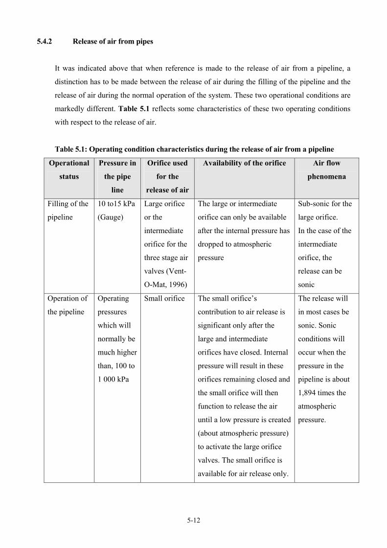
5.4.2 Release of air from pipes

It was indicated above that when reference is made to the release of air from a pipeline, a

distinction has to be made between the release of air during the filling of the pipeline and the

release of air during the normal operation of the system. These two operational conditions are

markedly different. Table 5.1 reflects some characteristics of these two operating conditions

with respect to the release of air.

Table 5.1: Operating condition characteristics during the release of air from a pipeline

Operational

status

Pressure in

the pipe

line

Orifice used

for the

release of air

Availability of the orifice Air flow

phenomena

Filling of the

pipeline

10 to15 kPa

(Gauge)

Large orifice

or the

intermediate

orifice for the

three stage air

valves (Vent-

O-Mat, 1996)

The large or intermediate

orifice can only be available

after the internal pressure has

dropped to atmospheric

pressure

Sub-sonic for the

large orifice.

In the case of the

intermediate

orifice, the

release can be

sonic

Operation of

the pipeline

Operating

pressures

which will

normally be

much higher

than, 100 to

1 000 kPa

Small orifice The small orifice’s

contribution to air release is

significant only after the

large and intermediate

orifices have closed. Internal

pressure will result in these

orifices remaining closed and

the small orifice will then

function to release the air

until a low pressure is created

(about atmospheric pressure)

to activate the large orifice

valves. The small orifice is

available for air release only.

The release will

in most cases be

sonic. Sonic

conditions will

occur when the

pressure in the

pipeline is about

1,894 times the

atmospheric

pressure.

5-13

As the internal pressure in a pipeline increases, the shear force of the expelling air will tend to

blow shut the large orifice. One of the tests for the air valve therefore focuses on the dynamic

closure of the large orifice. High-induced pressures can be created by the closure of the large

orifice, which pioneered the approach that it is appropriate for the protection of the pipeline,

that the large orifice close at a low differential pressure rather than a high pressure. This

reflects that the value of dynamic shields to prevent dynamic closure of the large orifice

creates the possibility of high-induced pressures and should therefore be discarded.

The functionality of the small orifice should be evaluated by employing the “drop tests”. The

drop test is conducted by pressurizing the system, with the valve that has to be tested installed

onto the system, to the operational pressure (or pressure class of the valve) and then

introducing air into the system. When this is done, the small orifice float should drop and the

air should be released through the small orifice.

Since the release through the small orifice will be sonic and because the physical forces and

the objective to minimize induced pressures govern the size of the small orifice, the release

rate is not important at all.

5.4.3 Testing procedure for the intake capacity of air valves (large orifice function)

During low pressures in the pipeline, the floats will drop and air can then enter the pipeline

through the large orifice. The entry of air at a sufficient rate will limit the negative pressure/

vacuum inside the pipeline. Vacuum break valves are sized for intake and the accepted criteria

is to limit the differential pressure across the valve to 40 kPa.

The determination of the intake capacity through the large orifice is one of the problems in the

quantification of the characteristics of air valves. International standards for the determination

of the capacity of air intake of air valves suggest that the outlet should be pressurised

(European Standard, 2000). This concept is incorrect, due to the compressibility of air and the

results from these tests can at best be used to compare valves, but surely not to determine the

intake capacity of the valves.

5-14

If the procedure contained in the European Standard document prEN 1074-4 is evaluated and

compared to the application of physical laws, the discrepancy can be identified. Figures 5.9

and 5.10 reflect the differences between the criteria used in prEN 1074-4 and the utilization of

physical laws. Procedure 1 refers to the prEN 1074-4 standard, while Procedure 2 refers to

the calculation of the intake capacity using physical laws. Determining the intake capacity of

air valves should be based on the following relationships as reflected in Figure 5.9:

Figure 5.9: Intake capacity calculations

5-15

Figure 5.10: Comparative intake capacities

5.4.4 Conclusion

From the above, it is apparent that the European Standard method of testing air valve intake

capacities is incorrect. When selecting an air valve, the intake rates supplied by the air valve

manufacturer should be checked, to ensure that it has been determined with the correct

procedure. It is proposed that the intake capacities of air valves be checked, by applying

Equation 5.1 and 5.2. As a guideline, the intake values in Table 5.2 below can be used. These

intake values were calculated using a discharge coefficient of 0,5 and typical inlet diameters.

Table 5.2: Typical intake values for air valves

Air valve

diameter (mm)

Differential

pressure (bar)

Intake capacity

(nm³/h)

25 0,35 169

50 0,35 677

80 0,35 1 733

100 0,35 2 707

150 0,35 6 019

200 0,35 10 829

0

200

400

600

800

1000

1200

1400

1600 In

take

rat

e (n

orm

al li

tres

/sec

ond)

0 0.1 0.2 0.3 0.4 0.5 0.6 0.7 0.8 0.9 1 Differential pressure (Bar)

Procedure 1 Procedure 2

Comparitive Intake Capacities

5-16

Choked conditions (pa/p < 1,894) [Intake]

( ) 5,012

12

−

−=

+ kk

a

k

aaaii p

ppp

kkpACdm ρ& …………………………….. (5.1)

Unchoked conditions (pa/p ≥ 1,894) [Intake]

( ) ( ) 5,0)11

12

+=

−+ kk

aaii kkpACdm ρ& ………………………………………………. (5.2)

Where:

Ai = Flow area for intake orifice (m²)

Cdi = Discharge coefficient for the inflow orifice (0,5 to 0,6)

k = Isentropic constant (ratio of specific heats = 1,4 for air)

m& = Mass flow rate (kg/s)

ρa = Density of air at atmospheric pressure (1,04 kg/m³)

p = Absolute pressure of air in the valve (Pa)

pa = Atmospheric pressure (Pa)

By applying these formulae, the intake capacities for air valves can be determined. Similar

equations can be used for calculating the discharge capacities of air valves. In this case, the

inside of the air valve is pressurized exhausting air to atmospheric pressure on the outside. It

must, however, be remembered that at a certain stage the system will become sonic and will

blow the float shut against the seat.

Choked conditions (p/pa ≤ 1,894) [Release]

( ) 5,012

00 12

−

−=

+ kka

ka

v pp

pp

kkpACdm ρ& ………...……………………(5.3)

Unchoked conditions (p/pa > 1,894) [Release]

( ) ( ) 5,0)11

00 12

+=

−+ kk

v kkpACdm ρ& and

k

v

aa

pp

=

ρρ

……………………………(5.4)

Where:

A0 = Flow area for outflow orifice (m²)

Cd0 = Discharge coefficient for the outflow orifice (0,5 to 0,6)

k = Isentropic constant (ratio of specific heats = 1,4 for air)

m& = Mass flow rate (kg/s)

5-17

ρv = Density of air in the air valve under line head conditions (kg/m³)

p = Absolute pressure of air in the valve (Pa)

pa = Atmospheric pressure (Pa)

6-1

6. IMPLEMENTATION OF A NEW PIPELINE

6.1 Filling of a pipeline

The velocity through the air valve is limited to ± 30 m/s according to Wisner (1982b). It must

be remembered that specifying a maximum filling velocity of say 0,5 m/s for a 300 mm

pipeline will result in a discharge velocity of 18 m/s through a 50 mm air valve. Using the

same filling velocity for a 400 mm pipeline will, however, result in a flow velocity of 32 m/s

through the same air valve. To prescribe a specific flow rate or velocity is difficult since the

filling of a pipeline is determined by:

- The pipeline profile (topography);

- Positions from where the pipeline is filled;

- Characteristics of the air valves; and

- Air valve closing sequence.

If air valves are oversized this could lead to unwanted surges when these valves suddenly

close when all the air has been expelled. Even if these valves have the anti-shock function,

over sizing will result in the air valve not switching to the intermediate orifice.

Since no general prescribed fill rate for pipelines can be defined, the selection of the required

air valve size for filling the line should be based on analysing various filling scenarios and

identifying the requirement to capture and release at each air valve node (see Section 7).

The designer should also be aware of possible unsteady flow with associated pressure

fluctuations, which might occur. Filling at a “safe filling rate” of say 35 l/s for the 300 mm

diameter pipeline, as shown in Figure 6.1 at first seems to be conservative. The topographic

profile, however, could result in an unstable situation where an air pocket is trapped leading to

a sudden increase in flow rate for which the air valves were not designed which might result

in blow-shut and associated high-induced pressures. The operator of the pipeline should also

be cautious of increasing the filling rate when it seems as if there is a decrease, which in fact

may only be a large air pocket, which is trapped.

The valid suggestion remains “The slower a pipeline can be filled the better”.

6-2

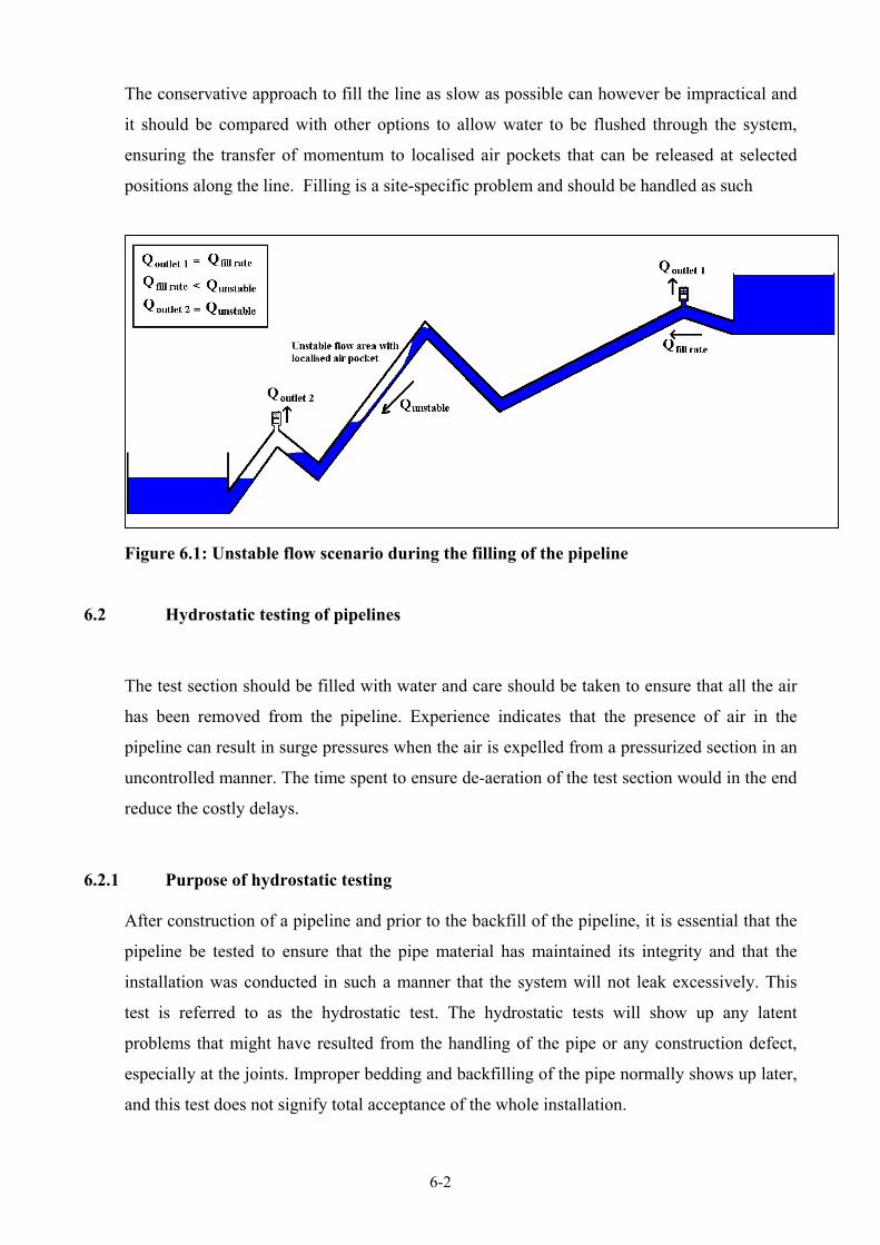
The conservative approach to fill the line as slow as possible can however be impractical and

it should be compared with other options to allow water to be flushed through the system,

ensuring the transfer of momentum to localised air pockets that can be released at selected

positions along the line. Filling is a site-specific problem and should be handled as such

Figure 6.1: Unstable flow scenario during the filling of the pipeline

6.2 Hydrostatic testing of pipelines

The test section should be filled with water and care should be taken to ensure that all the air

has been removed from the pipeline. Experience indicates that the presence of air in the

pipeline can result in surge pressures when the air is expelled from a pressurized section in an

uncontrolled manner. The time spent to ensure de-aeration of the test section would in the end

reduce the costly delays.

6.2.1 Purpose of hydrostatic testing

After construction of a pipeline and prior to the backfill of the pipeline, it is essential that the

pipeline be tested to ensure that the pipe material has maintained its integrity and that the

installation was conducted in such a manner that the system will not leak excessively. This

test is referred to as the hydrostatic test. The hydrostatic tests will show up any latent

problems that might have resulted from the handling of the pipe or any construction defect,

especially at the joints. Improper bedding and backfilling of the pipe normally shows up later,

and this test does not signify total acceptance of the whole installation.

6-3

6.2.2 Selection of test sections

In undulating terrain and steep long gradients in pipeline profile, the selection of sections to

be hydrostatically tested is influenced by the profile. If the test section has been arbitrary

selected it can happen that it will be impossible to pressurize the higher-lying sections to the

desired pressure while the lower elevated sections might be over-pressurized.

Hydrostatic testing of pipelines is a major operation and if it is not planned accurately, it can

be costly.

Small leaks are difficult to detect and temperature changes can appear as a leak. Furthermore,

with large volumes of air in the test section, it is extremely difficult to increase the pressure in

the line with a hand pump.

If the temperature does vary during the testing, it should be taken into account. The following

relationship can be used to determine the change in pressure due to a change in temperature

(normally a drop in temperature). Distinction is made between a restrained (not allowing

expansion) and an unrestrained pipe (Kenneth K Kienow).

Restrained pipes

( )[ ]( )

∆T1

EtDK1

Kµ12eBD2

P

−

+

+−=µ

………………………………………… (6.1)

Unrestrained pipes

( )( )

∆T25,1

EtDK1

K3DP

−

+

−=µ

eB ……………………………………………. (6.2)

Where:

B = Coefficient of volume thermal expansion of liquid (dV/Vdt, /°C (2,10E-04))

e = Coefficient of volume thermal expansion of pipe wall material (dL/Ldt, /°C)

µ = Poisson's ratio

K = Bulk Modulus of liquid (dP/(dV/V), MPa (2.07E+09))

E = Modulus of Elasticity of pipe wall (MPa)

D = Inside diameter (mm)

6-4

t = Wall thickness (mm)

∆T = Change in temperature (°C)

Figure 6.2: Pressure change due to temperature change

6.2.3 Specifications for hydrostatic pressure testing

Different specifications apply to different fluids transported and pipe materials used. In this

document, focus is on the conveyance of water and the criteria associated with water mains.

Manufacturers normally define the maximum working pressure in terms of a percentage of the

yield strength of the material. A norm is to set the maximum operating pressure equivalent to

between 50 and 75 % (and sometimes lower) of the yield stress of the pipe material. For

different pipe materials the pressure class rating of the pipe, is related to the maximum

operating pressure.

Depending on the setting of the maximum operating pressure with respect to the yield strength

of the material, the hydrostatic pressure in the pipeline is defined. The hydrostatic pressure is

normally set at 1,25 the maximum operating pressure and restricted to less than 1,5 times the

maximum operating pressure.

Pressure change due to Temperature changeD = 600 mm, t = 9 mm, Steel pipe

0.00

50.00

100.00

150.00

200.00

250.00

300.00

0.0 1.0 2.0 3.0 4.0 5.0 6.0 7.0 8.0 9.0 10.0

Temperature change, °C

Pres

sure

cha

nge,

(m)

Restrained Unrestrained

6-5

According to SABS 1200 L (7.3.2.1), the test pressure should be applied for 3 hours or such

time as is required for inspection of the pipeline. Provision is made to reduce the time for a

pipe with a diameter less than 400 mm.

The reduction in the time is proportional to the diameter with the assumption that the test

needs to be conducted for 3 hours on a 400 mm diameter pipeline. However, the minimum

time for which the test section should be pressurized is 1 hour.

During the hydrostatic pressure tests, the damaged pipes might rupture or leak and the joints,

thrust blocks and specials will reflect the installation shortcomings. The permissible leakage is

dependent on the type of installation. For jointed pipes in steel, cast iron, ductile iron and all

the thermoplastic materials, the following relationship is proposed to define the permissible

leakage volume for the prescribed test period.

PLD0,01VolL = ……………………………………………………………... (6.3)

Where:

Vol L = Permissible leakage (litres)

D = Inside diameter (m)

L = Length of pipe (m)

P = Pressure (MPa)

In the case where different sections of the test section are at different pressures, Equation 6.3

can be extended to be able to calculate the permissible leakage:

( )∑= iiL PLD0,01Vol ………………………………………………………….. (6.4)

Where:

“i” refers to the different pipe sections and pressures for these sections.

In the case where the diameter changes as well the equation can be changed to:

( )∑= iiiL PLD0,01Vol …………………………………………………………. (6.5)

6-6

6.2.4 Practical aspects related to hydrostatic pressures

The major problem with hydrostatic pressure tests can be related to insufficient planning,

defect testing equipment, lack of water for the test, and insufficient documentation of the tests.

Table 6.1 reflects a pro-forma data sheet that can be used for the documentation of the

hydrostatic pressure test.

Table 6.1: Pro-forma data sheet for the hydrostatic pressure test

Hydrostatic pressure test (Water) Test reference number: …………… Project: Pipeline: Pipe Test section From:…………(km) To: ………….(km) Date: …… Length of section, L ……………….(m) Diameter of section, D …….…(m) Pipe classes: Max working pressure, (m) Hydrostatic test pressure, P (MPa) Allowable leakage, Vol L = 0,01*L*D*(P)0.5 = …………………. Date when pipe was filled: …………………….. Pipe filled from chainage: ………….… Isolation of the test section Upstream Down stream De-aeration of the pipeline Yes No

End cap Air valves Installed Isolating valve Air valves Operational

Other Other Pipeline installation (Tick the box) Pipeline uncovered Pipeline covered up to blanket fill Pipeline covered with joints open Pipeline completely backfilled Source for test pressure: ……………………... Gauging of pressure: …………………. Location Location Pump ID Gauge description Hand pump ID Date of calibration Has this pipeline been tested before? Units of measurement

Burst Yes No When Test Reference ………………..

Failure recorded Leaks

Test sequence Time Pressure (units) Temperature °C

Start of test End of test

Remarks:

Time sequence of events during the testing Time Pressure (m) Temperature (°C) Time Pressure (m) Temperature (°C)

Consultants representative Contractors Signed: Signed: Date: Date: Failure report Reference Test Accepted Yes No

Planned actions for further tests:

7-1

7. SIZING AND POSITIONING OF AIR VALVES

7.1 Historical approach of air valve sizing and positioning

In the past air valve sizing and positioning was based on a few set guidelines. These

guidelines as described in Stephenson (1981) and Marcus (1998), are listed below (mainly

focussed on each individual node at a time) see Table 7.1.

Table 7.1: Typical air valve sizing and positioning guideline (historical approach)

Sections of pipeline which run parallel to

the hydraulic gradient

Section of pipeline which forms a peak

Section of pipeline which changes from a

negative slope to a larger negative slope

Section of pipeline which changes from a

positive slope to a less positive slope

Long descending or ascending sections

7-2

7.2 Air valve sizing and positioning procedure (ASAP)

In this section the proposed procedure for air valve sizing and positioning will be described.

The pipeline will be analysed as a whole and not as individual isolated sections. The basic

sizing for the large orifice air valves is based on drainage (burst and scouring) and filling,

while the small orifice valves are designed to release air during operating conditions. A step-

by-step worked example is provided in Section 7.3 of this document, to demonstrate this

proposed procedure. The procedures, with some modifications were also used in the

development of computer software for modelling the correct sizing and positioning of air

valves (Section 7.4).

The procedure is referred to ASAP, acronym for Air valve Sizing and Positioning Procedure,

and is described in the paragraphs below. The basic methodology used in the sizing, selection

and positioning of air valves is summarised below:

Objectives of the ASAP procedure

The main objective of the ASAP procedure is:

To determine the size and the position of the air valves in order to

• prevent excessive vacuum conditions in the pipeline during draining of the line;

• provide sufficient discharge capacity during filling; and to

• enable effective release of air under operating pressures.

In order to meet these objectives, certain input data is required in the procedure and several

calculations need to be performed.

Input data requirements for the ASAP procedure

Flow characteristics, pipe characteristics, longitudinal profile of the pipeline and other

relevant information such as the allowable maximum negative pressure and the pipe rupture

size.

Calculations performed in the ASAP procedure

The ASAP procedure firstly evaluates the intake requirements for the pipeline under draining

and burst conditions. The following steps are followed:

• The positions and type of all valves (i.e. isolating-, drainage- and non-return valves) are

determined that will be used to control the filling and draining of the pipeline or

7-3

isolation of sections thereof. Positions along the pipeline where water will be abstracted

are also defined.

• The burst analysis is based on the principle that the potential flow rate in all the sections

can be determined by utilising the continuity of energy. Using the Darcy Weisbach

relationship (or something similar) the potential flow is calculated for each pipe section

and assuming the rupture size of the burst (percentage of pipe diameter) the potential

flow is reduced linearly with the ratio of the burst area and the pipe area. The required

intake capacity of the air valve should be able to handle this flow rate.

• In the draining analyses, the potential maximum flow rate at which a section can be

drained/scoured is calculated and subsequently the required intake capacity of the air

valve is determined.

• The required intake capacities for the burst and drain analysis, for all the apex points and

other points where slope changes require an air valve, are combined for the final

determination of the required air valves.

Secondly the required discharge capacity of the air valves is evaluated for the filling of the

pipe. The procedure entails the following steps:

• Identifying all possible sections that can be isolated and the possible ways how these

sections can be filled.

• Determining the maximum discharge rates through the air valve to safely fill the

pipeline.

Next, the position of the air valves to release air under operating conditions need to be

determined. Apex points are the most appropriate positions to accumulate air and to release it

during operation. The positions for the small orifice air valves are then determined by:

• Determining the ability of the fluid to transport the air hydraulically, using the newly

developed transportability relationship as described in Section 4 (Equation 4.3).

• If the air cannot be transported an air release valve will be positioned at the said node.

• The designer’s preference for the spacing between air release valves is accommodated in

the analysis of the different analyses.

The last step is to combine the results and to determine the correct air valve (type and size) to

be installed, by comparing the calculated intake and discharge capacities with that of the air

valve manufacturer’s values and then to select a suitable valve.

7-4

Typical results from the ASAP procedure

A profile plot, as well as a table with all the results indicating the required valves along the

pipeline (pressure class, size, type and position), is provided.

Figure 7.1 reflects a flow diagram of the proposed ASAP procedure.

Figure 7.1: Flow diagram of the ASAP procedure

phaseInput requirement

Inta

ke r

equi

rem

ents

Dis

char

ge r

equi

rem

ents

Calculations phase

Oth

er

Results phase

System characteristicsPipeline profile, diameters, reservoir water levels, valves, offtakesMaximum safe negative pressure for couplingsFlow rates, filling velocity

SI unit conversion

Burst Analysis-Calculate slopes-Calculate maximum flow rate for each pipe section-Determine where column separation is possible-Determine position of air valves for various bursting scenarios-Calculate intake requirements for these points

Drain Analysis-Identify draining scenarios-Determine activation sequence for each scenario-Calculate intake requirements for all the peak points

Filling analysis-Identify filling scenarios-Calculate maximum filling rate or maximum discharge rate

Small orifice analysis-Calculate the transportability of air for every downward (negative) slope-Identify critical sections-Determine operating pressures-Use engineering judgement on the placing (always at peak points)

Miscellaneous-Hydraulic gradline-Surge analysis-Identification of special cases-Economic analysis

Pipeline profile with position of air valvesPipeline profile with required air valve size andtype for every nodeDetails of air calculations in order to use engineering judgement

7-5

7.2.1 ASAP input requirements

As indicated in the ASAP procedure flow diagram (Figure 7.1), the first step in determining

the air valve requirements for a pipeline is to obtain the system characteristics shown in

Figure 7.2 and listed in Table 7.2.

Figure 7.2: Pipeline profile

Table 7.2: Typical ASAP input requirements

Type Information

Pipeline profile Elevation, pipe segment lengths

Pipe details Diameters, roughness, pipe type, allowable

negative pressure

Valves, off-takes and connections Positions of isolating-, scour- and non-return

valves, off-takes or supply connections on the

pipeline.

Flow characteristics Operating flow rate.

Boundary controls Pump station and reservoir water levels,

Optional data for the economic

analysis

Discount rates, inflation rate and labour -,

mechanical -, and electricity escalation. Analysis

period, future demand and unit tariff of the water

7-6

The allowable negative pressure that the pipe can withstand must be obtained from the pipe

manufacturer and is used as the maximum differential pressure over the air valve for intake

conditions. The maximum differential pressure is the maximum safe sub-atmospheric

pressure that the pipe can withstand before collapsing, or before the seal is displaced in the

coupling. It must be emphasised that this pressure might be limited not necessary by the pipe

strength, but also by the joint seals, which can be damaged or displaced when, the internal

pressure is negative. The objective under intake conditions is to maintain subsonic flow

conditions and to prevent the float from blowing shut.

External forces on the pipeline and the construction/installation conditions of the pipe also

influence the maximum allowable negative pressure. High water tables and excessive negative

pressures can also result in intrusion of contaminated water into the pipeline.

7.2.2 ASAP calculations

The pipeline is taken as a whole to ensure that the air valve system of the pipeline performs

adequately. Each pipeline node is split into an upstream and a downstream node for

calculation identification. The evaluation for burst, drain, filling and air release under

operating conditions is then executed and the air intake and discharge requirements for the

upstream (US) and downstream (DS) sides of each node determined. Either the drain or the

burst requirements will define the required intake capacity of the air valves.

Calculating each node’s upstream and downstream requirements allows the design engineer to

make informed engineering decisions about the correct air valve size and its exact position.

Should the results indicate extremely large air intake requirements at a node, consideration

should be given to reduce the outlet size of the scour/draining valves.

In the ASAP procedure the operation of the system is visualized for all possible flow

scenarios. The importance of analysing the pipeline as a whole will be reflected in the sample

problem, which was set-up in SI units although other units are also accommodated in the

procedure.

7-7

7.2.2.1 Burst analysis (uncontrolled flow release from the pipeline)

When a pipe burst occurs, water flows from the pipe. To prevent the pipe from collapsing due

to the development of sub-atmospheric pressures, air should be allowed to enter the pipe at

such a rate as to prevent extreme low pressures that might displace the seals or lead to pipe

failures.

The factors, which will influence the outflow rate at the burst or fracture, are the effective size

of the rupture, available energy, installation conditions (above ground or below ground) and

the friction loss in the pipe. Since it is impossible to predict where a pipe fracture will occur,

all low lying positions should be investigated. The steps that should be followed to determine

the intake capacities for rupture along a pipeline, require:

o Calculation of pipe slopes (This will be the maximum hydraulic gradeline for each pipe

section and hence the maximum flow rate, i.e. S0 = Sf or pipe slope = friction slope)

o Calculate the maximum flow rate in each pipe section due to burst on that pipe section

based on Equation 7.1 (Modified Darcy-Weisbach equation) which incorporates a

reduction factor Arupture/A.

A

ASDgQ ruptureburst λ

π8

052

= ………………………………………….…… (7.1)

Where:

Qburst = Flow rate due to burst (m³/s)

g = gravitational acceleration (m/s²)

D = Inside diameter of pipe (m)

S0 = Slope of pipe (m/m)

λ = Friction factor

Arupture = Area of the rupture (m²) (See Table 7.3 reflects typical default rupture sizes

which can be used in the analysis). The standard Darcy-Weisbach equation

has been modified by adding this outlet coefficient to the equation. This

factor represents the influence of the layout of the system and the time

dependence of the outflow (the hole develops with time), which is complex

to define and hence it is suggested that a sensitivity analysis should be

conducted on this factor.

A = Area of the pipe (m²)

7-8

The friction factor can be calculated with the Karman Prandtl equation for rough turbulent

flow conditions (Equation 7.2), or some similar equation: 2

7,3log2

1

=

skD

λ ………………………………………………………………… (7.2)

Where:

λ = Friction factor

D = Inside diameter of pipe (m)

ks = Absolute roughness of pipe (m)

Table 7.3: Rupture size as a percentage of pipe diameter (suggested default values that

should be checked by conducting a sensitivity analysis)

Pipe type Rupture size (percentage

of pipe diameter)

Below ground installation

Rupture size (percentage

of pipe diameter)

Above ground installation

Cast / ductile iron 15% 50%

Corroded steel 15% 50%

Fibre cement 40% 50%

HDPE 15% 50%

GRP 20% 50%

LDPE 15% 50%

New-, Medium- steel 15% 50%

uPVC, mPVC 15% 50%

o For the various bursting possibilities the required intake capacities required along the

pipeline are determined. Figure 7.3 below is an example of a section of pipeline where

the maximum flow rate in each pipe section (A to D) due to burst was calculated.

Figure 7.3: Bursting (example pipe section)

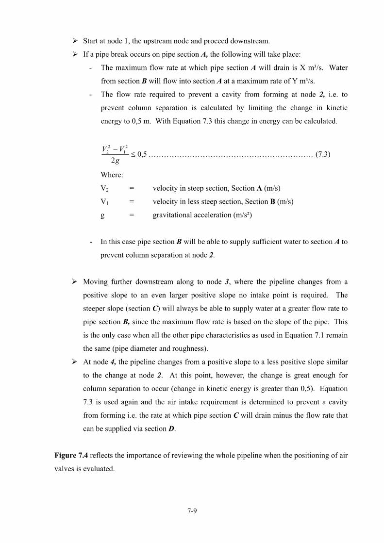
7-9

Start at node 1, the upstream node and proceed downstream.

If a pipe break occurs on pipe section A, the following will take place:

- The maximum flow rate at which pipe section A will drain is X m³/s. Water

from section B will flow into section A at a maximum rate of Y m³/s.

- The flow rate required to prevent a cavity from forming at node 2, i.e. to

prevent column separation is calculated by limiting the change in kinetic

energy to 0,5 m. With Equation 7.3 this change in energy can be calculated.

5,02

21

22 ≤

−gVV ………………………………………………………. (7.3)

Where:

V2 = velocity in steep section, Section A (m/s)

V1 = velocity in less steep section, Section B (m/s)

g = gravitational acceleration (m/s²)

- In this case pipe section B will be able to supply sufficient water to section A to

prevent column separation at node 2.

Moving further downstream along to node 3, where the pipeline changes from a

positive slope to an even larger positive slope no intake point is required. The

steeper slope (section C) will always be able to supply water at a greater flow rate to

pipe section B, since the maximum flow rate is based on the slope of the pipe. This

is the only case when all the other pipe characteristics as used in Equation 7.1 remain

the same (pipe diameter and roughness).

At node 4, the pipeline changes from a positive slope to a less positive slope similar

to the change at node 2. At this point, however, the change is great enough for

column separation to occur (change in kinetic energy is greater than 0,5). Equation

7.3 is used again and the air intake requirement is determined to prevent a cavity

from forming i.e. the rate at which pipe section C will drain minus the flow rate that

can be supplied via section D.

Figure 7.4 reflects the importance of reviewing the whole pipeline when the positioning of air

valves is evaluated.

7-10

Figure 7.4: Illustrating the value of looking at a pipeline as a whole (Example)

When a pipe burst occurs on section A the change in slope at node 2 will not result in column

separation. The change in slope at node 3 will also not result in column separation. The

accumulated change in energy will however result in a cavity forming at node 3, since it can

not supply sufficient flow for the steeper slope of section A. If only one node at a time was

analysed, this intake requirement would not have been anticipated and subsequently would not

have been designed for.

7.2.2.2 Drain analysis (controlled air release)

In the controlled drainage analysis the following procedure is followed.

o Identify possible drainage scenarios that result from isolating different sections and

opening various scour valves. The example in Figure 7.5 has four possible draining

scenarios, which are reflected in Table 7.4.

Figure 7.5: Drainage (example)

7-11

Table 7.4: Possible drainage scenarios

Scenario Drainage point Upstream control point Downstream control

point

1 Node 4 Node 1 (Reservoir) Node 11 (Reservoir)

2 Node 8 Node 1 (Reservoir) Node 11 (Reservoir)

3 Node 4 Node 1 (Reservoir) Node 6 (Isolating valve)

4 Node 8 Node 6 (Isolating valve) Node 11 (Reservoir)

o For each of the drainage scenarios, the sequence in which the air valves will start to

function should be determined. Using the pipeline illustrated in Figure 7.5 and drainage

scenario 1, the following air valve activation sequence can be determined. The first

node that will be activated is node 1, then node 10, and the last node to be activated is

node 7. The sequence is obtained by visualizing a horizontal line that represents the

available energy moving down as the water drains. This peak in the controlled drainage

section, will first be activated.

o The initial outlet (scour valve) at the drainage point is assumed to function as an orifice.

The maximum discharge rate is calculated utilizing the available head for the various

drainage scenarios by using Equation 7.4.

∆=

42

2outlet

DdrainD

hgCQπ

………………………………………………….. (7.4)

Where:

Qdrain = Flow rate due to controlled drainage (m³/s)

CD = Discharge coefficient for an orifice (0.6)

g = Gravitational acceleration (m/s²)

∆h = Available energy between peak and drainage point (m)

Doutlet = Inside diameter of outlet pipe (m)

o The intake requirement at each peak in this drainage scenario can now be calculated.

This is repeated for every possible drainage scenario identified. The activation sequence

is very important since a valve that is activated first on a specific side of the drainage

point (upstream or downstream) will be required to supply the total out flow rate. If a

peak on the other side is activated next, the drainage flow rate is halved for this air valve

for the available energy, since air can now be supplied from both sides of the drainage

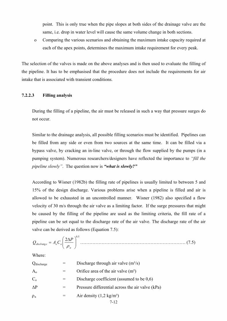
7-12

point. This is only true when the pipe slopes at both sides of the drainage valve are the

same, i.e. drop in water level will cause the same volume change in both sections.

o Comparing the various scenarios and obtaining the maximum intake capacity required at

each of the apex points, determines the maximum intake requirement for every peak.

The selection of the valves is made on the above analyses and is then used to evaluate the filling of

the pipeline. It has to be emphasised that the procedure does not include the requirements for air

intake that is associated with transient conditions.

7.2.2.3 Filling analysis

During the filling of a pipeline, the air must be released in such a way that pressure surges do

not occur.

Similar to the drainage analysis, all possible filling scenarios must be identified. Pipelines can

be filled from any side or even from two sources at the same time. It can be filled via a

bypass valve, by cracking an in-line valve, or through the flow supplied by the pumps (in a

pumping system). Numerous researchers/designers have reflected the importance to “fill the

pipeline slowly”. The question now is “what is slowly?”

According to Wisner (1982b) the filling rate of pipelines is usually limited to between 5 and

15% of the design discharge. Various problems arise when a pipeline is filled and air is

allowed to be exhausted in an uncontrolled manner. Wisner (1982) also specified a flow

velocity of 30 m/s through the air valve as a limiting factor. If the surge pressures that might

be caused by the filling of the pipeline are used as the limiting criteria, the fill rate of a

pipeline can be set equal to the discharge rate of the air valve. The discharge rate of the air

valve can be derived as follows (Equation 7.5): 5.0

arg2

∆=

aooedisch

PCAQρ

…………………………………………………………… (7.5)

Where:

Qdischarge = Discharge through air valve (m³/s)

Ao = Orifice area of the air valve (m²)

Co = Discharge coefficient (assumed to be 0,6)

∆P = Pressure differential across the air valve (kPa)

ρa = Air density (1,2 kg/m³)

7-13

It is suggested that the maximum pressure differential across the valve should be limited to

0,5 m (5 kPa). This limitation is to prevent blow-shut and high-induced pressure spikes due to

a rapid closing of the large orifice at high velocities.

It is important to visualize the filling process. Some topographic characteristics of the

pipeline may limit the filling velocity creating for instance a siphon. The filling analysis

procedure is as follows:

o Identify all possible filling scenarios for the sections that can be isolated. The pipeline

example in Figure 7.6, has five possible filling scenarios, see Table 7.5.

Figure 7.6: Filling (example)

Table 7.5: Possible filling scenarios for the sections that can be isolated

Scenario Isolated

section to be

filled

Upstream filling point Downstream filling point

1 Node 1 –6 Node 1 (Pump) Node 6 (Isolating valve)

2 Node 6 -11 Node 6 (Isolating valve) Node 11 (Reservoir must be

empty)

3 Node 6 - 9 Node 6 (Isolating valve) Node 9 (Bypass around

Non-return valve)

4 Node 9 - 11 Node 9 (Bypass around non-

return valve)

Node 11 (Reservoir)

5 Node 1 -11 Node 1 (Pump) Node 11 (Reservoir)

7-14

o Distinction should be made between first-time filling of the pipeline and subsequent

fillings where sections of the line can cause a water lock. In cases where water locks

can occur every air valve should be selected to ensure that the filling rate could be

expelled.

o For each of the filling scenarios the sequential filling of the pipeline sections should be

identified, to determine where air would be discharged. Using the pipeline illustrated in

Figure 7.6 and filling scenario 1, the following filling of the pipeline sections can be

identified. This is obtained by visualizing the water filling the pipe and determining

which peak in the controlled section will release air.

- The pipe section from node 1 to node 6 can be filled from the downstream side

through backflow through node 6 or from the flow that is supplied from the

pump.

- When the pipeline is filled from the pump station, the air valve at node 2 will

be the last to close. Initially, all the air valves in this pipeline section will

release air but the valve closing last will be required to release air at the same

rate as the filling rate. If this cannot be achieved the filling time will increase.

- If the pipeline is filled from the end of the section, node 6, the last valve to

close will again be the valve at node 2.

o Calculating the hydraulic gradeline and subtracting the pipeline elevation will provide

the pressure whereby the valve will be exhausting air.

o The maximum discharge rate before blow-shut will occur, is based on a calculation with

a maximum differential pressure of 0,5 m (Equation 7.5). The maximum outflow rate

for the selected valve at that node is then used as the limit for the filling rate. From the

valve supplier’s outlet characteristic curve a suitable valve(s) can be selected to prevent

this phenomenon.

7.2.2.4 Small orifice air release analysis

During operation, air can be released through the small orifice air valve only. For this to

occur, the air should be "stationary" at the valve, although the pipeline simultaneously

continues to handle the design flow. This emphasizes the need to provide a collection

chamber underneath the valve, where the air can be captured temporarily and then released

through the air valve. Although under normal conditions water can contain 2-3% per

volume free air, it is unrealistic to install small orifice air valves to provide such a

discharge rate!

7-15

The requirement of small orifice air valves is governed by the principle that air should be

released mechanically if it could be transported hydraulically to the air valve. The following

approach should be used to determine the position of small orifice air-release valves:

• Determine if free air in the pipeline can be hydraulically transported through the pipeline

along the downward sloping-sections. Equation 7.6 has been derived from experimental

work and should be used to determine whether the air can be hydraulically removed.

All the negative slopes should be evaluated to ensure that provision be made to release

the air mechanically at a position prior to the steep sloped sections where it will be

impossible to transport the air hydraulically.

bgDaV θ=min

Where:

Vmin = Flow velocity at the point where removal will start (m/s)

g = Gravitational acceleration (m/s²)

D = Diameter of pipeline (mm)

θ = Slope of pipeline (°)

a = Constant (for medium sized bubble: a = 0,2178)

b = Constant (for medium sized bubble: b = 0,4007)

• The nodes identified in the step above at which free air cannot be transported, constitutes

a position where a small orifice air valve is required.

• If the calculated distance between small orifice air valves is short (say 250 m), it is not

necessary to provide a small orifice air valve at all the identified points, provided that

the line is effectively filled and that the upstream small orifice air valve effectively

captures and releases all the air that reaches it.

• Small orifice air valves are nearly always required at apex points along the pipeline,

because these are the points where air is most likely to accumulate, especially for low

flow velocities. The apex points are also used to prevent vacuum formation, by allowing

air into the pipeline and hence the positioning of a combination air valve is provided at

these points.

7-16

7.2.2.5 Special consideration

A large orifice air valve, when used as an alternative for a one-way surge tank (or discharge

tank) to prevent negative pressures resulting from a power failure in a pump station, should be

placed just downstream from the pump check valve.

The results of surge analyses reflect where sub-atmospheric pressures might occur and it is

suggested that large orifice air valves should be provided wherever the pressure drops are in

excess of 4,0 m.

7.2.2.6 Conclusion

It is believed that if a pipeline is analysed as a whole, using the ASAP procedure the pipeline

system will meet all the requirements in terms of air release and intake requirements to

adequately protect the system and provide an effective de-aerated system.

7.2.3 ASAP results

Typical ASAP results will be a pipeline profile indicating the exact position/location of the air

valves (Figure 7.7) as well as valve class, valve type, valve size, accumulator

details/requirements etc. (Table 7.6). The operating & maintenance manual should describe

the drainage and filling procedures for the pipeline system.

Figure 7.7: Typical ASAP result (Pipeline profile)

7-17

Table 7.6: Typical ASAP result (valve requirements) Nr Point description Accumulated

length (m)

Elevation

(m)

Air valve Size

(mm)

Valve

class

Model

number

1 Pump station 0 1400,00 RBX Double acting 100 25 bar 100RBX2501

2 500 1420,00 RBX Double acting 100 16 bar 100RBX1601

3 1250 1410,00 RBX Double acting 80 25 bar 080RBX2501

4 Drainage (150mm) 1700 1370,00 No air valve - -

5 1800 1380,00 RBX Double acting 100 25 bar 100RBX2501

6 Isolating valve 2100 1375,00 RBX Double acting 100 25 bar 100RBX2501

2625 1341,25 RBX Double acting 80 40 bar 080RBX4001

7 2800 1330,00 No air valve - -

3150 1324,17 RBX Double acting 80 40 bar 080RBX4001

8 Drainage (150mm) 3400 1320,00 No air valve - - -

3675 1337,20 RBX Double acting 80 40 bar 080RBX4001

9 Non return valve 4200 1370,00 RBX Double acting 80 25 bar 080RBX2501

10 4400 1275,00 No air valve - - -

4900 1425,00 RBX Double acting 80 16 bar 080RBX1601

11 End reservoir 5600 1495,00 2 x RBX Double acting 150 16 bar 150RBX1601

7-18

7.3 Hand calculation

7.3.1 Introduction

The aim of this section is to provide the design engineer with an example of the proposed air

valve sizing and positioning procedure. The pumping system as shown in Figure 7.8 is an

example of the application of the proposed procedure for air valve sizing and positioning as

described in Section 7.2, performed by hand calculation. The calculations are performed

step-by-step, highlighting the required location of the air valves and rationale of the air valve

sizing and positioning (ASAP) procedure.

7.3.2 Input data

Figure 7.8: Pumping system pipeline profile

The pumping system reflected in Figure 7.8 consists of a pumpstation that supplies water to a

reservoir approximately 6 km away, through a 250 mm uPVC pipeline.

The system flow characteristics are as follows:

Operating flow rate: 0,1 m³/s

Operating flow velocity 2,04 m/s

Fluid type: water

7-19

Filling velocity: 0,3 m/s (15 % of flow rate)

The pipe characteristics are:

Pipe type: uPVC

Anticipated rupture size: 15% of pipe diameter

Pipe roughness: 0,03 mm

Along the 6 km of pipeline are a number of isolating valves (2) as well as scour valves (3) and

one non-return valve, indicated in Table 7.7.

Table 7.7: Pipeline profile and details

The static height difference between the reservoir at the pumpstation and the end reservoir is

135 m.

7.3.3 Calculations

The required input data, as defined in the ASAP flow diagram, Figure 7.1, is obtained from

Table 7.7. The information is used to analyse the pipeline for the various operating

conditions, i.e. burst, drainage, filling and small orifice air release analyses.

DiameterElevationAccumulatedDescriptionNodelengthNr

(mm)(m)(m)2501 4200Pumpstation (TWL 1420 m)12501 42530022501 43549032501 431780Scour valve (100 mm)42501 4391 105Isolating valve52501 4361 42062501 4291 830Scour valve (100 mm)72501 4452 05082501 4502 15092501 4602 750102501 4823 070112501 4763 240Scour valve (100 mm)122501 4793 3701325014903 690142501 5064 080Non-return valve152501 5064 290Isolating valve162501 5174 980172501 5225 110182501 5305 500192501 5425 720202501 5495 8702125015506 000Reservoir (TWL 1555 m)22

7-20

Burst Analysis:

• Calculate all the pipeline slopes for pipe sections 1 – 21. If a section is horizontal, it is

assumed that it has a slight positive slope. Such a slope will result in the air being

transported downstream to the end of the horizontal sloped section.

• Calculate the maximum discharge rate using the modified Darcy-Weisbach equation

(Equation 7.1) and the Karman Prandtl equation (Equation 7.2), assuming thus that the

hydraulic gradelines and pipe slopes for each specific section are equal for the

maximum discharge rate in these pipe sections

A

ASDgQ ruptureburst λ

π8

052

= and

2

7.3log2

1

=

skD

λ

The results of these calculations are reflected in Table 7.8.

Table 7.8: Intake requirements for every pipe section in case of a burst

VelocityBurstBurstSlopeElevationLengthEndStartPiperateratedifferencenodenodeNo

(m/s)(m³/h)(m³/s)(m/m)(m)(m)nono0.38568.040.01890.016666753002110.684120.920.03360.0526316101903220.35061.900.0172-0.0137931-42904330.46882.690.02300.024615483255440.29151.440.0143-0.0095238-33156550.39068.870.0191-0.0170732-74107660.804142.140.03950.0727273162208770.667117.860.03270.050000051009880.38568.040.01890.01666671060010990.782138.200.03840.0687500223201110100.56099.020.0275-0.0352941-61701211110.45380.070.02220.023076931301312120.55397.720.02710.0343750113201413130.604106.760.02970.0410256163901514140.0010.170.00000.00000010210161515*0.37766.550.01850.0159420116901716160.585103.370.02870.038461551301817170.42775.490.02100.020512883901918180.697123.100.03420.0545455122202019190.644113.860.03160.046666771502120200.26246.230.01280.00769231130222121

* If it has a zero slope the slope is made slightly positive6000Total

7-21

0.000120.9170.000

0.0000.0000.0000.0000.000

142.1390.0000.0000.000

0.0000.0000.0000.0000.000

Requirements for burst analysisResult of column separationChange in DescriptionSlopeNodeDSUSAccumulatedIndividualenergychangeNr

(m³/h)(m³/h)(m)0.00000.0000Starting point1

< 0.5 (OK)< 0.5 thus OK0.0163+ to + +2Peak point+ to -3Low point- to +4

68.868782.693Peak point+ to -5< 0.5 (OK)< 0.5 thus OK0.0034- to - -6

Low point- to +7< 0.5 (OK)< 0.5 thus OK0.0103+ + to +80.0254 < 0.5 (OK)< 0.5 thus OK0.0151+ + to +90.0490 < 0.5 (OK)< 0.5 thus OK0.0236+ to + +10

Peak point+ to -11Low point- to +12

< 0.5 (OK)< 0.5 thus OK0.0051+ to + +130.0081 < 0.5 (OK)< 0.5 thus OK0.0030+ to + +14

0.0000106.7560.0267 < 0.5 (OK)< 0.5 thus OK0.0186+ + to +150.00000.0530.0072 < 0.5 (OK)< 0.5 thus OK0.0072+ to + +16

0.0102 < 0.5 (OK)< 0.5 thus OK0.0102+ to + +170.0183 < 0.5 (OK)< 0.5 thus OK0.0081+ + to +180.0338 < 0.5 (OK)< 0.5 thus OK0.0154+ to + +190.0374 < 0.5 (OK)< 0.5 thus OK0.0036+ + to +200.0550 < 0.5 (OK)< 0.5 thus OK0.0177+ + to +21

123.0960.0000End point22

Although the slope is positive, a burst in the section can occur at the beginning of the section

resulting in the requirement to introduce air downstream from the burst. Assess the intake

requirement at all nodes along the pipeline, starting at node 1, moving downstream. Air

valves are usually placed at peaks and where the change in kinetic energy is more than 0,5 m

(assumed value) to prevent column separation. If the change in kinetic energy is less than 0,5

m it is used in the analysis of the next point, to determine if an intake is needed there. The

way in which this is done is to accumulate the kinetic energy differences until a node is

reached where an air intake is incorporated. For instance, if in two adjacent nodes

accumulated change in energy exceeds 0,5 m, a large orifice function is required at the higher

node. With Equation 7.3 this change in energy can be calculated.

5,02

21

22 ≤

−gVV

Each pipe section is checked to see whether or not it can supply sufficient flow to its adjacent

pipe sections. At a peak, this cannot be achieved, and therefore at peaks a large orifice

function is usually required. If, however, the elevation difference is such that the maximum

allowable negative pressure in the pipe section is not exceeded, a large orifice function might

not be required. Table 7.9 illustrates the intake requirements on the upstream and downstream

of every node due to burst.

Table 7.9: Intake requirements for every node (US and DS) due to burst analysis

7-22

Comments on Table 7.9:

• Only peaks require large orifice functions in this example, since at no change in pipe

gradient will cavities occur when there is a pipe break anywhere on the line.

• At node 5 there is an isolating valve. Node 5 is also at a peak and will therefore require

a large orifice function on both sides (i.e. both up- and downstream) unless the

downstream section can provide the flow and the elevation difference between node 5

and node 7 is less than the allowable negative pressure.

• The peak at chainage 3 070 m (Node 11) is sized for the maximum flow rate on its

upstream side (the slope of pipe section 7 between node 7 and 8). This is steeper than

the slope on its downstream side (pipe section 11 between node 11 and 12). No large

orifice functions were required at any of the slope changes between node 7 and 11

(upstream side of node 11). For this reason, node 11 is sized to supply the maximum

intake requirement on that side. If there was a valve at, for instance, node 9, node 11

would have been sized for pipe section 10 which is steeper than section 9 and 11. The

valve at node 9 would have provided sufficient intake capacity for sections 7 and 8.

• The non-return valve at node 15 only requires intake capacity on its upstream side. As

soon as the downstream side reaches a lower pressure than the upstream side the non-

return valve will open again. When a non-return valve is placed on a pipe section that

has a negative slope, no air valve is required on either side.

• From node 16 (isolating valve) to node 22 (end reservoir) there are a number of slope

changes. The cumulative change in kinetic energy (nodes 17 to 21) due to these slope

changes are, however, not sufficient to cause column separation (0,055m < 0,5 m set

criteria). The end reservoir intake requirement is, however, determined by the steepest

slope of these pipe sections (pipe section 19, i.e.123,1 m³/h).

• On the upstream side of the last node, node 22, at the end reservoir, an intake capacity of

123,1 m³/h is required. If the reservoir has an uncontrolled outlet with either top or

bottom entrance into the reservoir, no air valve is required. The required intake capacity

will in this case be supplied via the top inlet, which is open to the atmosphere or water

will be supplied in the case of an outlet below the water (bottom outlet). If the outlet is

controlled in any way, however, this intake requirement must be provided for.

7-23

Drain Analysis:

• Identify possible drainage scenarios. The pipeline example in Figure 7.8 initially seems

as if it has nine possible draining scenarios (see Table 7.10). The first three scenarios

are not possible, however, due to the non-return valve at node 15 preventing any

backflow from pipe sections 15 to 21 when draining upstream of node 15.

Table 7.10: Possible draining scenarios

Scenario Drainage point Upstream control point Downstream control point

1 Node 4 (100 mm) Node 1 (Reservoir) Node 22 (Reservoir)

2 Node 7 (100 mm) Node 1 (Reservoir) Node 22 (Reservoir)

3 Node 12 (100 mm) Node 1 (Reservoir) Node 22 (Reservoir)

4 Node 4 (100 mm) Node 1 (Reservoir) Node 5 (Isolating valve)

5 Node 4 (100 mm) Node 1 (Reservoir) Node 15 (Non-return valve)

6 Node 7 (100 mm) Node 1 (Reservoir) Node 15 (Non return valve)

7 Node 12 (100 mm) Node 1 (Reservoir) Node 15 (Non return valve)

8 Node 7 (100 mm) Node 5 (Isolating valve) Node 15 (Non return valve)

9 Node 12 (100 mm) Node 5 (Isolating valve) Node 15 (Non return valve)

For each of the drainage scenarios, the activation sequence is determined. Table 7.11

indicates the activation sequence for each drainage scenario.

Table 7.11: Activation sequence for every drainage scenarios

Scenario Drainage point Upstream peaks

(activation sequence)

Downstream peaks

(activation sequence)

1 Node 4 3 (4th) 22 (1st), 11 (2nd) & 5 (3rd)

2 Node 7 5 (3rd) 22 (1st) & 11 (2nd)

3 Node 12 11 (2nd) 22 (1st)

4 Node 4 5 (1st) 3 (2nd)

5 Node 4 3 (3rd) 15 (1st) & 11 (2nd)

6 Node 7 3 (3rd) 15 (1st) & 11 (2nd)

7 Node 12 11 (2nd) 15 (1st)

8 Node 7 5 (3rd) 15 (1st) & 11 (2nd)

9 Node 12 11 (2nd) 15 (1st)

7-24

• For draining scenario 5, the first node that will be activated is the upstream side of

node 15, and then node 11, and the last node to be activated is the node on the upstream

side of the drainage point node 3. This is obtained be visualizing a horizontal line as the

level of the water, this line is then moved down, as the water is released, determining

which peak in the controlled drainage section will first be activated for this controlled

section which has been isolated.

• The outlet (scour valve) at the drainage point is assumed to be an orifice (a realistic

value for the discharge coefficient (CD) is 0,6). The maximum discharge rate is

calculated utilizing the available head for various drainage scenarios with Equation 7.4.

∆=

42

2outlet

DdrainD

hgCQπ

• The intake requirement for each peak in this control section (scenario) can now be

calculated. This is repeated for every possible drainage scenario identified. The

activation sequence is very important, since a valve that is activated first on a specific

side of the drainage point (either upstream or downstream) will be required to supply the

total flow rate. If a peak on the other side is activated next, the drainage flow rate is

halved (if drained slopes are equal) for this air valve since air can now be supplied from

both sides (up- and downstream) of the drainage point. Table 7.12 is a summary of all

these calculations.

• The maximum intake requirement for every peak is now determined by comparing the

various scenarios and obtaining the intake rate.

7-25

Table 7.12: Intake requirements on the upstream and downstream of every node due to controlled drainage

Node987654nr

DSUSdH DSUSdH DSUSdH DSUSdH DSUSdH DSUSdH (m³/h)(m³/h)(m)(m³/h)(m³/h)(m)(m³/h)(m³/h)(m)(m³/h)(m³/h)(m)(m³/h)(m³/h)(m)(m³/h)(m³/h)(m)

12

75.14.075.14.034

118.810.0118.810.0212.58.05678910

92.06.0547.153.092.06.0547.153.0536.651.011121314

411.630.0659.477.0411.630.0659.477.0650.875.01516171819202122

7-26

From the burst and drain analysis the pipeline’s intake requirements were now calculated.

The next step is to determine the discharge requirements.

Filling Analysis:

The first step in the filling analyses is to identify all the possible filling scenarios. The

possible filling scenarios are shown in Table 7.13.

Table 7.13: Possible filling scenarios

Scenario Empty section Upstream filling point Downstream filling point

1 Node 1 - 5 Node 1 (Pump) Node 5 (Isolating valve)

2 Node 5 -16 Node 5 (Isolating valve) Node 16 (Isolating valve)

3 Node 16 - 22 Node 16 (Isolating valve) Node 22 (Reservoir)

4 Node 1 - 22 Node 1 (Pump) Node 22 (Reservoir)

5 Node 5 - 22 Node 5 (Isolating valve) Node 22 (Reservoir)

6 Node 15 - 16 Node 15 (Non-return valve) Node 16 (Isolating valve)

7 Node 15 - 22 Node 15 (Non-return valve) Node 22 (Reservoir)

8 Node 5 - 15 Node 5 (Isolating valve) Node 15 (Non-return valve)

9 Node 1 - 15 Node 1 (Pump) Node 15 (Non-return valve)

Looking at the first scenario the following filling sub-scenarios of this section can be

identified (Table 7.14):

Table 7.14: Sub-scenarios of Scenario 1

Filling from Last activated

air valve

Description of

filling

1 US 5 First time filling

1 3 Water lock 3-5

5 US 5 First time filling

5 US 5 Water lock 3-5

5 US 5 Water lock 1-3

The point on the pipeline where the entire fill rate should be exhausted should be identified,

such as node 3 and node 5 in this filling scenario. Subsequent filling of the pipeline will, in

most cases, be the design criterion since a water lock will force one air valve to provide the

total outlet capacity of 14,7 l/s.

7-27

Small orifice air release analysis:

o Determine whether free air in the pipeline can be hydraulically transported through the

pipeline along the downward sloping-sections by using Equations 4.3. All the negative

slopes should be evaluated to ensure that provision is made for releasing the air

mechanically at a position prior to the steep sloped sections where it will be impossible

to transport the air hydraulically.

bgDaV θ=min

Where:

Vmin = Flow velocity at the point where removal will start (m/s)

g = Gravitational acceleration (m/s²)

D = Diameter of pipeline (m)

θ = Slope of pipeline (°)

a = Constant (for medium sized bubble: a = 0,2178)

b = Constant (for medium sized bubble: b = 0,4007)

Therefore for this example the pipe diameter remains constant and the operating velocity

is 2,037 m/s.

Table 7.15: Vmin for pipe sections with negative slopes

Pipe no Slope (m/m) Vmin (m/s) Status

3 -0,01379 0,310 OK

5 -0,00952 0,267 OK

6 -0,01707 0,338 OK

11 -0,03529 0,452 OK

o The pipes identified in the step above are all capable of transporting air, in other words

does not require a small orifice air valve.

o Small orifice air valves, however, are nearly always required at apex points along the

pipeline since these points are where air is most likely to accumulate, especially for low

flow velocities. The apex points are also used to prevent vacuum formation by allowing

air into the pipeline and therefore the positioning of a combination air valve is provided

at these points.

o Free air reduces the capacity of the system and therefore the placing of small orifice air

valves at intervals of 600 m is a good design practice.

7-28

7.3.4 Results

Summarise the valve requirements at each node and at intermediate points along the pipeline,

by graphical (Figure 7.9) and table format (Table 7.16).

Figure 7.9: Pipeline profile with air valves (Vent-O-Mat Utility Programs, 2003)

Table 7.16: Air valve requirements (Vent-O-Mat Utility Programs, 2003)

7-29

7.4 Air valve sizing and positioning software

Software, which incorporates the ASAP procedure, was developed and is freely available

from two leading valve manufacturers, Vent-O-Mat (local manufacturer) and ARI Flow

Control Accessories (Israel based). The ASAP procedure is not bound to any valve

manufacturer, since the valve selection of the required valves are only performed once all the

intake and discharge capacities have been determined. The ASAP procedure, as described in

the previous sections, has been used in the software programs but has, however, been adapted

to meet the valve manufacturers’ requirements. An example is the exclusion of the filling

analysis for the Vent-O-Mat CATT program due to the ability of the 3-stage anti-shock

function to control the outflow rate.

For more information on air valve sizing and positioning software programs visit the

following web sites:

http://www.up.ac.za/academic/civil/divisions/water/airvalves.html

7-30

7.5 Economic value of effective de-aeration

It is a known fact that general maintenance and preventative maintenance on pipelines is poor

and sometimes non-existent. The yearly allocated budget is simply used to maintain a running

system. Time and money is hardly spent on monitoring the pipeline regularly.

It has been found during some fieldwork carried out under this project, that maintenance crew

often closed air valves because they were leaking. If the air cannot be transported

hydraulically down the pipeline in such a case, the air will be trapped resulting in additional

head loss and loss in capacity. Previous older installations of typical air valve layouts were

not effectively capturing the free air leading to hydraulic under performance and to higher

additional head loss.

Experimental studies performed at the Department of Water Affairs Hydraulic Laboratories,

see Section 4.5, indicated that the secondary loss k-value was in excess of 6,0 for a localised

air bubble situated at an apex point in the line and a low flow rate. It is not only the air bubble

volume that governs the secondary loss, but to a large extent the form of the air bubble. If the

flow velocity is increased the bubble lengthens and the calculated secondary loss coefficient

k, reduces. The results, however, indicate that if a system is not effectively de-aerated,

additional head loss will occur resulting in additional pumping head and/or a loss in hydraulic

capacity.

It is however extremely difficult to predict the exact additional loss associated with

insufficient de-aeration. The following procedure could, however, be followed to address this

uncertainty:

• Compare the design capacity with the existing capacity obtained from the pipeline system.

If the existing capacity is less than the design capacity the reason for the decrease in

capacity must be found.

• Identify a section of pipeline where there are no abstractions and no possibility for air

accumulation (only positive slope) i.e. a clean section. The section should preferably also

contain no isolating valves or other control points.

• Utilizing pressure transducers or other accurate pressure gauges to measure the pressure

drop across the selected pipe section.

• Perform a back calculation of the friction value.

7-31

• Use the calculated friction value and recalculate the capacity for the entire pipeline. If the

calculated capacity corresponds with the current capacity, then the loss in capacity is

solely due to the increased roughness of the pipe. If not, then air might be a problem or

some other localised obstruction in the pipeline such as a half closed isolating valve or

even leakage might be responsible for the under performance.

• If it is suspected that air is the reason then follow the following steps:

- Check the size and location of the air valves based on the procedures as described in

Section 7.2 (especially the hydraulic transportability of the air).

- During a site visit verify that every air valve on the pipeline is operational. Check the

small orifice’s function and that the large orifice will release air during filling and that

the float will drop during emptying of the line.

- Check to see that the discontinuity and accumulator is adequate to capture the

transported air.

- Isolate the sections where leaks or air could still have an influence on the capacity.

Use methods such as inverse transients or calculate the pressure drop across short

sections along the pipeline until a section is found where the obtained pressure drop

results in a steeper hydraulic gradient than the rest of the pipeline.

8-1

8. TYPICAL INSTALLATION DETAILS OF AIR VALVES

After the air valve size and location has been determined the following aspects should be

considered:

• Discontinuity requirement

• Size of the accumulator

• Air valve installation and valve chamber design

It is assumed that the procedures discussed before has been used to determine the size and

location of the air valve.

8.1 Discontinuity

From the experimental work conducted under this project as well as Computerized Fluid

Dynamic (CFD) numerical modelling of various discontinuities the proposed discontinuity to

capture the air should be at least 35 % of the pipeline diameter.

The reasons why a discontinuity/entrapment area is required is:

• To allow time for the air to enter the accumulator. As the bubble reaches the

discontinuity it has to change flow direction and due to buoyancy be forced out of the

pipe

• The air that enters through the discontinuity has to displace the water through the same

discontinuity back into the pipe.

• From the experimental work it was evident that due to turbulent conditions, the air

bubbles do not travel at the crown of the pipe and does not flow in a straight line. For

this reason a large enough discontinuity is required.

There are a number of factors that will influence this required size of the discontinuity:

• Flow velocity

• Turbulence in the approach towards the discontinuity

• Slope of the pipeline

The minimum discontinuity required for smaller pipes (D < 300 mm diameter) should be an

equal T, because when a smaller discontinuity is used the air will not be capable of displacing

the water in the riser pipe.

8-2

The required discontinuity is larger for higher flow velocities since the “time available” to

force the air into the discontinuity is less while it is also true that the bubble size reduces as

the velocity increases. The complex nature of air movement thus forces the requirement of

discontinuity to be selected conservatively. It is proposed that for diameters between

300 mm and 1 500 mm the discontinuity should be equal to 60% while for pipes in excess of

1 500 mm the discontinuity should at least be 35% of the pipe diameter.

8.2 Size of accumulator

During normal operation, air can be released only through the small orifice air valve. For this

to occur, the air should be "stationary" at the valve, although the pipeline simultaneously

continues to handle the design flow. This emphasises the need to provide a collection

chamber underneath the valve where the air can be captured temporarily and then released

through the air valve. Although water can contain 2-3% per volume free air, it is not

necessary to install small orifice air valves to provide such a discharge rate! It is assumed

that the approach discussed in Section 7 was used to determine the position of small orifice

air-release valves.

Ensuring the effective operation of the small orifice air valve necessitates the provision of a

collector chamber to capture all the air. Figure 8.1 and 8.2 provides a graphical presentation

of the suggested installation layout for air valves.

Figure 8.1: Graphical presentation of installation details (small orifice function)

VARIABLE SMALL ORIFICE FUNCTION

Location As topography requires. Determined by the procedure described in

Section 7

h h ≥ 1,0D h ≥ 150 mm

d d = D for D ≤ 300 mm

d = 0,6D for 300 < D ≤ 1500 mm d ≥ 0,35D for D > 1500 mm

8-3

Figure 8.2: Graphical presentation of installation details (large orifice function)

Special installation considerations might have to be considered for systems where intermittent

operation might lead to dynamic induced pressures. In these cases, where negative pressures

are created during the down surge, consideration should be given to incorporate an additional

volume to maintain some air. The captured air will reduce the induced positive pressure. The

layout in Figures 8.4 and 8.6 can be used for the application by extending the vertical riser

above the branch off to the air valves by 3-5 times the diameter.

8.3 Installation and valve chamber design

It is extremely important to properly design the air valve chamber. The chamber should fulfill

the following functions:

• Protect the installed valve against the elements as well as vandalism and theft.

• Create an effective operating environment for the air valve.

• Create a working area for pipeline maintenance to be carried out with ease.

LARGE ORIFICE FUNCTION VARIABLE

VACUUM BREAK

AIR RELEASE

Differential pressure for the calculation of

the outlet orifice

Pa – Pi ≤ 40 kPa Pi – Pa ≤ 5 kPa *

Location

Between shut-off valves or to

allow free draining

High points on an isolated

pipeline

h h ≥ 1,0D h ≥ 150 mm

h ≥ 1,0D h ≥ 150 mm

d 44

22add ππ

≥ See requirement for small orifice

function

Note: * To prevent dynamic closure of the large orifice. Refer to manufacturers details

8-4

Some features which are crucial (see Figure 8.3):

• Proper drainage of the chamber (layer of stone or other impervious material as a floor)

• Allowance for a pump sump for drainage purposes

• Entrance manhole with step ladder if more than 0,5 m deep

• Vents for in and out flow to create a flow through the chamber. These vents should be

larger than the nominal air valve area, or the combination of nominal air valve areas. This is

done to ensure that the vents do not restrict the capacity of the air valve system.

• Vent openings should be covered with a mesh to prevent insects or birds from entering the

valve chamber.

Figure 8.3: Well-designed air valve chamber (Umgeni Water)

Figures 8.4 and 8.5 are some alternative designs.

8-5

Figures 8.4: Two air valves on a manifold (above ground installation)

Figure 8.5: Four air valves on a manifold (above ground installation)

For even larger type installations, the air valve chamber can also be used as access points see

Figure 8.6. The air valves were also placed on different levels on the accumulator, which will

prevent all the air valves closing simultaneously when the water reaches them during filling of

the pipeline. This installation is above ground in other words, preventing flooding of the

chamber.

8-6

Figure 8.6: Schematic layout of larger type installation above ground

9-1

9. USER COMMENTS

This is still a provisional guideline for air valve sizing, selection and positioning. The project

team would like to receive your comments in order to improve the document. Please

complete this form below and fax/post to:

Prof SJ van Vuuren (Project leader)

University of Pretoria

Department of Civil & Biosystems Engineering

Pretoria

0001

Tel: 012 420 2438

Fax: 012 362 5218

E-mail: fvuuren@eng.up.ac.za

Name: …………………………………………

Postal address: ………………………………………………………………………………..

………………………………………………………………………………..

Tel nr: …………………………………………

E-mail: …………………………………………

Comment: ………………………………………………………………………………..

………………………………………………………………………………..

………………………………………………………………………………..

………………………………………………………………………………..

………………………………………………………………………………..

………………………………………………………………………………..

………………………………………………………………………………..

………………………………………………………………………………..

………………………………………………………………………………..

………………………………………………………………………………..

………………………………………………………………………………..

………………………………………………………………………………..

………………………………………………………………………………..

………………………………………………………………………………..

………………………………………………………………………………..

………………………………………………………………………………..

10-1

10. REFERENCES

Basson M.S., Van Niekerk P.H. & Van Rooyen J. (1997). An Overview of the Water Resources

availability and utilisation in South Africa.

Chadwick A. & Morfett J. (1994). Hydraulics in Civil and Environmental Engineering. (Second

Edition). London: E & FN Spon.

Denny D.F. & Young, G.A.J. (1957). The prevention of vortices in intakes. Proceedings 7th

Congress of the International Association of Hydraulic Research.

Kalinske A.A. & Bliss P.H. (1943). Removal of air from pipelines by flowing water. ASCE, 13.

p.480

Kalinske A.A. & Robertson J.M. (1943). Closed Conduit Flow. ASCE Transactions V108.

Kienow, K.K., (Editor). (1990). Pipeline design and installation. International Conference on

Pipeline Design and Installation, Las Vegas, Nevada, 1990.

Marcus, N. (1998). Air and Air Valves in Pipe Lines. Israel Water Commission.

Myles K.(Ed.). (1994). Valves - Principles & Practice. K. Myles and Associates. Northcliff.

Prosser M.J., (1977). The Hydraulic Design of Pump Sumps and Intakes. BHRA and CIRIA.

London.

Richards R.T. (1957). Air Binding in Large Pipe Lines Flowing under Vacuum. Journal of the

Gydraulic Division. ASCE.

Stephenson, D. (1981). Pipeline Design for Water Engineers. (Second Edition). Amsterdam:

Elsevier Scientific Publishing Company.

Val-Matic. (1993). Air in Pipelines - Sources, System Impact and Removal. Available from

Valmatic Valve and Manufacturing Corporation.

10-2

Val-Matic. (1996). Val-Matic Glossary of Valve Related Terms. Available with “airValve - Air

valve Sizing program Version 5.0".

Val-Matic. (1997). Theory, Application and Sizing of Air Valves. Available from Valmatic Valve

and Manufacturing Corporation.

Van Vuuren, S.J. (1989). Induced pressures in pipelines resulting from the fast release or air.

Original document was published in Afrikaans. PhD Thesis. University of Pretoria.

Van Vuuren, S.J. (1990). The effect of air in water pipes. South African Institution of Civil

Engineers (SAICE) and Fibre-Cement Association (FCA). One-day course on pipeline Engineering.

Van Vuuren, S.J. (1991). The Purpose and Location of Air Valves in Pipelines. SAICE - Lecture

notes. University of the Witwatersrand.

Van Vuuren, S.J. (1994). Control of Air in Pipeline Design. Unpublished notes.

Van Vuuren, S.J. (1995a). Air in Pipeline Design - Part 1. AC Pipes brochure - AC Underground.

Volume 8.

Van Vuuren, S.J. (1995b). Air in Pipeline Design - Part 2. AC Pipes brochure - AC Underground.

Volume 9.

Vent-O-Mat. (1995). Points to Consider when Sizing & Positioning Air Release & Vacuum Break

Valves for Water Pipelines. Available from Vent-O-Mat Mulric Hydro Projects (Pty) Ltd.

Vent-O-Mat. (1996). Air Valve Technology Reviewed. Available from Vent-O-Mat Mulric Hydro

Projects (Pty) Ltd.

Veronese, A. (1937). Sul motto delle bolle d’aria nelle condotte d’acqua (in Italian). Estrato dal

fasciacolo X. Vol. XIV, p.XV.

Wisner, P.E. (1982a). Causes, Consequences and Studies on Air Entrainment. Department of Civil

Engineering - University of Ottawa - Lecture notes Chapter 11.

10-3

Wisner, P.E. (1982b). Removal of Air from Pipelines (Air Pockets and Air Vents). Department of

Civil Engineering - University of Ottawa - Lecture notes Chapter 12.

Wisner, P.E.; Mohsen, F.N. & Kouwen, N. (1975). Removal of Air from Water Line by Hydraulic

Means. Journal of the Hydraulic Division. Proceedings, ASCE, Volume 101, February 1975,

pp 243-257