1

Optimal Loan Portfolio

(Case Study: Prudential Bank Ltd And Asante Akyem Rural Bank)

By

Augusina Adu (B. Ed Mathematics)

PG3006509

A Thesis submitted to the Department of Mathematics

Institute of Distance Learning

Kwame Nkrumah University of Science and Technology

In partial fulfillment of the requirements for the degree

of

MASTER OF SCIENCE

Industrial Mathematics

JUNE 2011

2

DECLARATION

I Augustina Adu hereby declare that except for reference to other people’s work, which have

duly been cited. This submission is my own work towards the Master of Science degree and

that, it contains no material previously published by another person nor presented elsewhere.

Augustina Adu, PG3006509 …………. ………..

Student’s Name & ID Signature Date

Certified By ………………… ……….

Dr. S. K. Amponsah Signature Date

Supervisor

Certified By ………………… ……….

Dr. S. K. Amponsah Signature Date

(Head of Department)

3

ACKNOWLEDGEMENT

I am most grateful to the Almighty God for his guidance, protection and presence throughout

the study of this course.

I wish to express my sincere thanks to my supervisor Dr. S K Amponsah who was always

ready to assist me in writing this thesis.

I further express my sincere gratitude to all my lectures in the Department mathematics

department for their dedication and effective teaching which has help me to write this project.

Finally, I am most grateful to all friends who helped me in one way or the other to the success

of this work.

4

DEDICATION

This research work is dedicated to my husband Mike Osei-Owusu and Children

Ama Serwaa Owusu-Achiaw and Yaw Osei-Owusu. For their love, support and

understanding through the study of this course.

5

ABSTRACT

The Banking Industry in Ghana is now characterized by increasing competition and

innovation. This phenomena has led to most banks adopting cutting edge technology to

improve the quality of their Loan structure . The decline of relevant portfolio planning

models especially in Ghana is attributed mainly to the evolving dynamics of the Ghanaian

banking industry where the regulatory controls have changed with a high frequency. A lot of

banks had suffered substantial losses from a number of bad loans in their portfolio due to the

models used in allocating funds to loans. As a result, most banks are not able to maximize

their profit margin due to poor allocation of funds. The purpose of this Study is to develop a

linear programming model using the Simplex algorithm to help Prudential Bank Limited and

Asante Akyem Rural Bank to maximize their profit margin. The results from the model

showed that, Prudential Bank and Asante Akyem Rural Bank would be making annual profit

of GH¢8003572.5 and GH¢176750 respectively if they are to stick to the model. From the

study, it was realized that the scientific method used to develop the propose model can have a

dramatic increase in the two banks profit margin if put into practice.

6

TABLE OF CONTENTS

Declaration ……………………………………………………………….. I

Acknowledgement ……………………………………………………………….. I

Dedication ……………………………………………………………….. Iii

Abstract ……………………………………………………………….. Iv

Chapter One Introduction ……………………………………………………………….. 1

1.1 Background to the Study ……………………………………………………………….. 3

1.2 Statement of the problem ……………………………………………………………….. 5

1.3 Objective of the study ……………………………………………………………….. 7

1.4 Significance of the Study ……………………………………………………………….. 7

1.5 Methodology ……………………………………………………………….. 7

1.6 Scope of the Study ……………………………………………………………….. 9

1.7 Limitation of the Study ……………………………………………………………….. 9

1.8 Organization of the Study ……………………………………………………………….. 9

Chapter Two: Literature Review ……………………………………………………………….. 11

2.0 The Basic Portfolio Theory By Markowitz ……………………………………………………………….. 11

2.1 The Efficient Frontier ……………………………………………………………….. 12

2.2 Linear Programming Financial Management ……………………………………………………………….. 12

2.3 Linear Programming for Bank Portfolio Management ……………………………………………………………….. 13

2.4 Risk Measure in Loan Portfolio Management ……………………………………………………………….. 14

2.4.1 Conditional Value At Risk ……………………………………………………………….. 14

2.5 Probability Of Loss on Loan Portfolio ……………………………………………………………….. 16

7

2.6 Credit Risk and Asset Price ……………………………………………………………….. 17

2.6.1 Boom and Bust Cycles ……………………………………………………………….. 17

2.7 Data on Asset Prices and Default ……………………………………………………………….. 18

2.8 Stochastic Programming ……………………………………………………………….. 19

2.8.1 Expected Utility Theory ……………………………………………………………….. 19

2.9 Models of Loan Portfolio Management ……………………………………………………………….. 21

2.9.1 Multiple Discriminate Models ……………………………………………………………….. 21

2.9.2 Portfolio Management By Moody's KMV ……………………………………………………………….. 22

2.9.3 Loan Volume- Based Models ……………………………………………………………….. 25

2.9.4 loan Loss Ratio- Based Models ……………………………………………………………….. 27

Chapter Three : Methodology ……………………………………………………………….. 28

3.0 Introduction ……………………………………………………………….. 28

3.1 Linear Programming ……………………………………………………………….. 28

3.2 Forms Of Linear Programming Problems ……………………………………………………………….. 30

3.2.1 A Linear Programming in The Matrix Form ……………………………………………………………….. 30

3.2.2 A Linear Programming in The General Form ……………………………………………………………….. 31

3.2.3 A linear Programming in the Standard Form ……………………………………………………………….. 31

3.3 Simplex Algorithm ……………………………………………………………….. 32

3.3.1 Basic Solution ……………………………………………………………….. 33

3.3.2 Non-standard Constraints ……………………………………………………………….. 34

3.4 Types of Simplex Method Solutions ……………………………………………………………….. 36

3.4.1 Alernatve Optmal Solutions ……………………………………………………………….. 36

3.4.2 Unbouded Solutions ……………………………………………………………….. 37

8

3.4.3 Infesasble Solution ……………………………………………………………….. 37

3.5 DUALITY ……………………………………………………………….. 38

3.6 Summary ……………………………………………………………….. 39

Chapter Four:

Data Collection and Modeling ……………………………………………………………….. 40

4.0 Introduction ……………………………………………………………….. 40

4.1 Proposed Model For Prudential Bank Limited ……………………………………………………………….. 41

4.2

Proposed Model For Asante Akyem Rural

Bank ……………………………………………………………….. 45

4.3 Optimal Solution For Prudential Bank Limited ……………………………………………………………….. 48

……………………………………………………………….. 50

4.4

Optimal Solution For Asante Akyem Rural

Bank ……………………………………………………………….. 51

4.5 Summary ……………………………………………………………….. 53

Chapter Five:

Conclusion And Recommendations ……………………………………………………………….. 54

5.0 Introduction ……………………………………………………………….. 54

5.1 Conclusions ……………………………………………………………….. 54

5.2 Recommendations ……………………………………………………………….. 54

5.3 Summary ……………………………………………………………….. 53

References ……………………………………………………………….. 57

Appendix A ……………………………………………………………….. 61

Appendix B ……………………………………………………………….. 63

9

Appendix C ……………………………………………………………….. 64

Appendix D ……………………………………………………………….. 65

Appendix E ……………………………………………………………….. 66

Appendix F ……………………………………………………………….. 67

Appendix G ……………………………………………………………….. 72

Appendix H ……………………………………………………………….. 73

Appendix I ……………………………………………………………….. 75

Appendix J ……………………………………………………………….. 76

Appendix K ……………………………………………………………….. 79

10

CHAPTER ONE

INTRODUCTION

The banking sector of Ghana in the past could be divided into two groups- the elite foreign

banks which concentrated on the rich of the society and the local banks mainly owned by the

state.The latter served the interest of most working class people. The elite banks were

Barclays Bank (formerly called the Colonial Bank) and Standard Chartered Bank

(formerly,Bank of British West Africa). The second group of banks with state ownership

include Ghana Commercial bank (GCB), Social Security Bank (now SG-SSB), Agricultural

Development Bank (ADB), and the National Investment Bank (NIB).

The clients of the localy owned banks found business transations very frustration espercally

during salary payments, for example, it was not uncommon observing long winding queus

extending serveral meters outside the banking hall. The few foreign banks on the other hand,

apply high charges and the initial deposit to open accounts was very high. The average

Ghanaian could therefore not open accounts with these banks. Choices were very few and

competition was virtually absent in the sector.

The Bank of Ghana (BOG) with the support of government undertook a process of financial

sector restructuring which transformed the financial sector. Some of the initiatives that led

this transformation is the movement to universal banking, the adoption of an open licensing

system and the modernization of the payments systems. According to Acquah (2006) the

governor of the BOG,´universal banking involves the removal of restrictions on banking

activities which allow banks to choose the type of banking services that they would like to

offer in line with their capital, risk appetite and their business orientation’(2006).

11

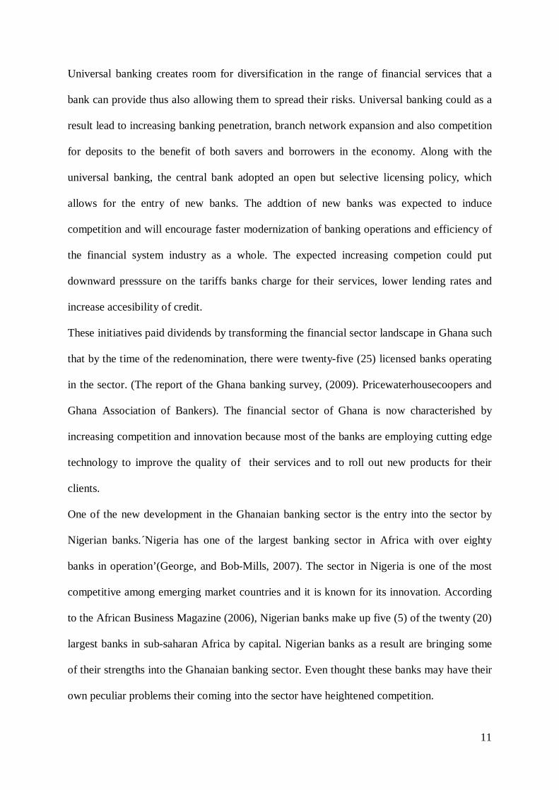
Universal banking creates room for diversification in the range of financial services that a

bank can provide thus also allowing them to spread their risks. Universal banking could as a

result lead to increasing banking penetration, branch network expansion and also competition

for deposits to the benefit of both savers and borrowers in the economy. Along with the

universal banking, the central bank adopted an open but selective licensing policy, which

allows for the entry of new banks. The addtion of new banks was expected to induce

competition and will encourage faster modernization of banking operations and efficiency of

the financial system industry as a whole. The expected increasing competion could put

downward presssure on the tariffs banks charge for their services, lower lending rates and

increase accesibility of credit.

These initiatives paid dividends by transforming the financial sector landscape in Ghana such

that by the time of the redenomination, there were twenty-five (25) licensed banks operating

in the sector. (The report of the Ghana banking survey, (2009). Pricewaterhousecoopers and

Ghana Association of Bankers). The financial sector of Ghana is now characterished by

increasing competition and innovation because most of the banks are employing cutting edge

technology to improve the quality of their services and to roll out new products for their

clients.

One of the new development in the Ghanaian banking sector is the entry into the sector by

Nigerian banks.´Nigeria has one of the largest banking sector in Africa with over eighty

banks in operation’(George, and Bob-Mills, 2007). The sector in Nigeria is one of the most

competitive among emerging market countries and it is known for its innovation. According

to the African Business Magazine (2006), Nigerian banks make up five (5) of the twenty (20)

largest banks in sub-saharan Africa by capital. Nigerian banks as a result are bringing some

of their strengths into the Ghanaian banking sector. Even thought these banks may have their

own peculiar problems their coming into the sector have heightened competition.

12

Another development in the Ghanaian banking sector, which cannot be overlooked is the

expansion in branch network of most of the banks. According to the past deputy governor of

the Bank of Ghana, (Bawumia, 2006) bank branches in Ghana increased by 1.3 percent from

three hundred and nine to three hundred and fourty four from 2002 to 2004 and eighty-one

(81) new branches sprang up between 2004 and 2006. One interesting development in the

sector is that there are no more ’elite banks in operation’ as the banks that formerly had this

status are also chasing the average Ghanaian income eaner for his or her business together

with the other banks.The economic lanscape in Ghana at the time of the redenomination was

favourable for financial intermediation by the banks. The country has moved from an

economic environment of generally high inflation and large exchange rate swings. Heavy

domestic borrowing by government in the past had crowded out private sector finance. Faced

with relatively low-risk, high return government debts in the form of treasury bills, the banks

had little incentive to lend to the private sector which was riskier. The consequence was very

limited access by small and medium-sized enterprise and individuals to credit. Thus the banks

had relatively low capacity to lend to the private sector and manage its associated risks.

However, the economic and financial sector reforms that was adopted had reversed this trend

years before the redenomination was implemmented. Government reduced its borrowing in

the domestic market reducing the return on government securities and thus banks were forced

to lend more to the private sector.

1.1 BACKGROUND

TO THE STUDY

There are a number of reasons why banks may suddenly stop or slow lending activity. This

may be due to an anticipated decline in the value of the collateral used by the banks to secure

the loans; an exogenous change in monetary conditions (for example, where the central bank

13

suddenly and unexpectedly raises reserve requirements or imposes new regulatory constraints

on lending); the central government imposing direct credit controls on the banking system; or

even an increased perception of risk regarding the solvency of other banks within the banking

system.The result of inefficences in the management of a banks loan portfolio may result in a

credit crunch. A credit crunch is often caused by a sustained period of careless and

inappropriate lending, which results in losses for lending institutions and investors in debt

when the loans turn sour and the full extent of bad debts becomes known. These institutions

may then reduce the availability of credit, and increase the cost of accessing credit by raising

interest rates. In some cases lenders may be unable to lend further, even if they wish, as a

result of earlier losses.The crunch is generally caused by a reduction in the market prices of

previously "overinflated" assets and refers to the financial crisis that results from the price

collapse. This can result in widespread foreclosure or bankruptcy for those investors and

entrepeneurs who came in late to the market, as the prices of previously inflated assets

generally drop precipitously. In contrast, a liquidity crisis is triggered when an otherwise

sound business finds itself temporarily incapable of accessing the bridge finance it needs to

expand its business or smooth its cash flow payments. In this case, accessing additional credit

lines and "trading through" the crisis can allow the business to navigate its way through the

problem and ensure its continued solvency and viability. It is often difficult to know, in the

midst of a crisis, whether distressed businesses are experiencing a crisis of solvency or a

temporary liquidity crisis.

Ghana has a well-developed banking system that was used extensively by previous

governments to finance and develop the local economy in the areas of lending. By the late

1980s, the banks had suffered substantial losses from a number of bad loans in their

portfolios. In addition, cedi depreciation had raised the banks' external liabilities. In order to

strengthen the banking sector, the government in 1988 initiated comprehensive reforms. In

14

particular, the amended banking law of August 1989 required banks to maintain a minimum

capital base equivalent to six (6) percent of net assets adjusted for risk and to establish

uniform accounting and auditing standards. The law also introduced limits on risk exposure

to single borrowers and sectors. These measures strengthened central bank supervision,

improved the regulatory framework, and gradually improved resource mobilization and credit

allocation. In 1989 the Bank of Ghana issued temporary promissory notes to replace non-

performing loans and other government-guaranteed obligations to state-owned enterprises as

of the end of 1988 and on private-sector loans in 1989. The latter were then replaced by

interest-bearing bonds from the Bank of Ghana or were offset against debts to the bank.

Effectively, the government stepped in and repaid the loans. By late 1989, some ¢62 billion

worth of non-performing assets had been offset or replaced by central bank bonds totaling

about ¢47 billionAs part of the regulatory framework,the cental bank prescribed minimum

capital requirements for three types of banks:

Banks with at least

60% Ghanaian ownership (i.e. Ghanaian banking business) the minimum paid-up

capital not less than twenty thousand Ghana cedis (GH¢20,000).

Banks with

Ghanaian ownership less than 60% (i.e.foreign bbanking buisness) the minimum paid-

up capital not less than fifty thousand Ghana cedis (GH¢50,000).

In the case of

development banking business,the minimum paid-up capital was hundred thousand

ghana cedis (Gh¢100,000).

The much higher minimum paid-up requirement for development banks is presumaably based

on the concept that as these banks undertake medium and long-term lending,they are exposed

to greater loan-loss risk.

15

1.2 STATEMENT OF THE PROBLEM

The decline of relevant portfolio planning models especially in Ghana is attributed mainly to

the evolving dynamics of the Ghanaian banking industry where the regulatory controls have

changed with a high frequency. Other contributory factors include the emergence of some

unconventional assets as well as an increase in treasury and foreign exchange activities.

The changing face of the Ghanaian banking industry coupled with the need to sustain and

improve Bank performance (especially at this critical period when many of them are

financially distressed) necessitates that the suitability and continued relevance of existing

models be evaluated.

According to Cohen and Hammer (1967), what makes the task of allocation/selection

difficult is the need to find an appropriate balance between three desirable objectives in loan

portfolio management-These objectives are; profitability, liquidity and safety. Generally, four

major factors influence the asset portfolio management behavior of banks. These factors are

government regulations, safety of deposits, credit demand as well as income aspirations of

shareholders.

However, some finance experts - Melnik (1968), Anderson and Burger (1969), Bradley and

Crane (1976), Sealey (1977), Reed et al., (1984) and Lambo (1986) have argued that the

demand for the safety of deposits and the and the income expectations of shareholders are, to

a large extent, incompatible. This incompatibility, they further contended, is reflected in the

unavoidable trade-off between desired profitability, necessary liquidity and acceptable safety

that is present in virtually every financial transaction of a bank.

Consequently, this trade-off between profitability, liquidity and safety could be regarded as

the central issue in the management of banks’ loan portfolio.

16

It is from the above observations that this research work is skewed at developing a linear

model with the specific purpose of providing an optimal solution of allocating funds to the

various types of loan of bank with a case study on Prudential Bank and Asante Akyem Rural

Bank.

1.3 OBJECTIVES OF THE STUDY

It is an indisputable fact that most banks operating in Ghana today are faced with the

complex problem of how to manage their loan portfolios in such a manner that the goals

of the bank are best achieved. For this purpose, the general objective of the study is to:

(i) select optimum loan portfolio adhering to the regulations governing the activities of

Prudential Bank and Asante Akyem Rural bank.

(ii) design a linear programming model to optimize the loan given out using the financial

loan records of Prudential Bank and Asante Akyem Rural Bank

(iii) explore ways of disbursing funds allocated for loans effectively and efficiently in

order to optimize profit margin of the two banks.

(iv) determine the sectors that records higher loan portfolio for the two banks.

(v) make recommendations that can address the issue of loan portfolio in the industry of

banking in Ghana.

1.4 SIGNIFICANCE OF THE STUDY

This project seeks to access the performance of the loan portfolio of Prudential Bank and

Asante Akyem Rural Bank on the community especially its customers. It is hoped that the

model designed in the course of this study based on empirical evidence, would go a long way

in providing useful planning tool to Banks operating in Ghana.

17

Suggestions and recommendations would be given to strengthen any weakness of the loan

portfolios of the two bank in that it would be exposed in the course of the study.

1.5 METHODOLOGY

The model to be used by this study seeks to find an optimal way of allocating funds to the

various loans types at Prudential Bank and Asante Akyem Rural Bank so as to maximised

profit. The linear programming optimization process was used to setup the allocation of

loans.

Linear programming models deals with optimization problems that can be modelled with a

linear objective function subject to a set of linear constraints. The model has three basic

components, that is the objective function which is to optimized (maximised or minimized),

the constraints or limitation and the negativity constraint. Linear programming is most used

among all the mathematical optimization techniques. It is best understood by both the elite

and the ordinary business man.

A set of questionnaires were developed and administered to Prudential Bank and Asante

Akyem Rural bank to obtain information on the various types of loan policies of they operate.

The data obtained was first tabulated and used to develop a linear programming model which

was then solved by the simplex method.

The simplex method passes from vertex to vertex on the boundary of the feasible polyhedron,

repeatedly increasing the objective function until either an optimal solution is found or, it is

established that no solution exists.

The simplex method was considered an appropriate method for solving the linear

programming problem developed as a result of its practical superiority and advantages over

the other methods.

18

Again, the simplex method was considered the most appropriate method for the study in view

of the fact that many computer software application programs for solving linear programming

problems involving simplex method are available.

The computerized software application program called Quantitative Methods (QM) model for

windows based on the simplex algorithm was used to facilitate the solution of the linear

programming model developed.

The Quantitative Methods (QM) model was considered the best option for the project

because the spreadsheet offers a very convenient data entry and editing features which allows

for a greater understanding of how to construct linear programs.

Again, the Quantitative Methods (QM) model for windows software application programme

was selected and used among the numerous computer programmes in view of the fact that it

is a popular programme used by the operational researchers.

1.6 SCOPE OF THE STUDY

The will cover the loan portfolio management policies Prudential Bank and Asante Akyem

Rural Bank for the 2010 financial year.

1.7 LIMITATION OF THE STUDY

The constrains encountered include finance considerations, inaccessibility of data, limited

time and unpreparedness and unreadiness of personnel to give out information necessary for

the study.

1.8 ORGANISATION OF THE STUDY

The research is organized into five chapters. Chapter one which is the introduction, gives the

background information of the study, statement of the problem, objectives of the study,

19

research questions, and significance of the study, scope of the study, methodology description

and organisation of the study.

Chapter two looks at review of related literature, which covers application of linear

programming to portfolio selection, types of loan portfolio and risk associated with loans.

Chapter three describes the methodology used for the study. It looks at the method of data

collection, organizational profiles of the selected banks for the research.

Chapter four discusses and analyses the data collected. Chapter five summarizes the various

findings, conclusions and recommendations.

20

CHAPTER TWO

LITERATURE REVIEW

In every field of study, it is possible to look back and identify a person or event that caused a

major change in the direction or development of the field. In the field of "investments" in

general and "portfolio management" in particular, it is an indisputable fact that the work by

Markowitz on Portfolio Theory changed the field more than any other single event

The doctoral thesis written by Markowitz (1952) at the University of Chicago dealt with

portfolio selection and in it he developed the basic portfolio model.

Because of this work, Markowitz is often referred to as the "father of modern portfolio

theory", and much subsequent research had been based on this effort (Sharpe, 1963, Fama,

1965 and Melnik, 1970).

The basic model, developed by Markowitz, derived the expected rate of return for a portfolio

of assets and an expected risk measure. Markowitz showed that the variance of the rate of

return was a meaningful measure of risk under a reasonable set of assumptions and derived

the formula for computing the variance of the portfolio.

This portfolio variance formulation indicated the importance of diversification for reducing

risk, and showed how to properly diversify. The Markowitz model is based on certain

assumptions. Under these assumptions, a single asset or portfolio of assets is considered to be

21

efficient if no other asset or portfolio of assets offers higher expected return with the same (or

lower) risk, or lower risk with the same (or higher) expected return (Markowitz, 1952 and

1959)

2.1 THE EFFICIENT FRONTIER

The Full Variance Model developed by Markowitz is based on the assumption that the

purpose of portfolio management is to minimize variance for every possible combination of

the expected yield (Best and Grauer, 1991:980). It has been argued by Blume (1970) and

Hodges and Brealey (1972) that the concept of the efficient frontier is basic to the

understanding of portfolio theory. Assume that in the market place, there are a fixed number

of common stocks in which a businessman can invest. Each of the securities has its own

expected yield and standard deviation; others have the same standard deviation but vary in

expected yield.

The investor will select the security that offers the highest yield for a chosen level of risk

exposure as presented by the standard deviation. It is assumed that investors try to minimize

risk by minimizing the deviation from the expected yield, and this is done by means of

portfolio diversification.

2.2 LINEAR PROGRAMMING IN FINANCIAL MANAGEMENT

The use of linear and other types of mathematical programming techniques has received

extensive coverage in the banking literature. Chambers and Chames (1961), as well as Cohen

and Hammer (1967, 1972), developed a series of sophisticated linear programming models

for managing the balance sheet of larger banks, while Waterman and Gee (1963) and Fortson

22

and Dince (1977) proposed less elegant formulations which were better suited for the small-

to medium-sized bank. Several programming models have also been proposed for managing a

bank's investment security portfolio, including those by Booth (1972).

Baldirer et al., (1981) used linear programming model to solve fundamental issues facing

senior bank management of Central Carolina Bank and Trust Company in structuring the

bank's balance sheet of approximately $360 million.

2.3 LINEAR PROGRAMMING FOR BANK PORTFOLIO MANAGEMENT

Various portfolio theories have been propounded for the management of bank funds. Ronald I

Robinson secondary reserves (1961) proposed four priorities of the use of banks funds. These

include primary reserves, (or protective investment), loans and advances (customer credit

demand) and investment account(open market investment for income) in descending order of

priority. His assessment has been fully supported in other works by Sheng-Yi and

Yong(1988).

A bank has to place primary reserves at the top of the priority in order to comply with the

minimum legal requirement, to meet any immediate withdrawal demand by depositors and to

provide a means of clearing cheques and credit obligations among banks.

Secondary reserves include cash items from banks, treasury bills and other short-term

securities. Bank should have to satisfy customers’ loan demand before allocating the balance

of the funds in the investment market.

Loans and investment are in fact complementary. According to Robinson, (1961) investment

should be tailored to the strength, seasonality and character of loan demand. He reiterated that

banks that experience sharp seasonal fluctuations in loan demand need to maintain more

liquidity in their investment programmme. Moreover, during a boom when loan demand is

high and credit-worthy customers are available, banks should allocate more funds to loans

and less funds to investment, and vice versa during recession when loan demand is low.

23

According to Robinson, (1961) the crucial banking problem is to resolve the conflict between

safety and profitability in the employment of bank funds. The conflict is essentially the

problem between liquidity and the size of the earning assets. Robinson suggested that where

there is a conflict between safety and profitability, it is better to err on the side of safety.

The best practice is identifying procedures that can bring out the optimal mixture of

management of banks funds. According to Tobin (1965) portfolio theory can be applied to

bank portfolio management in that a bank would maximize the rates of return of its portfolio

of assets, subject to the expected degree of risk and liquidity. Chambers and Charnes (1961)

applied linear programming analysis on the consolidated balance sheets of commercial banks

in Singapore for the period 1978-1983. The results show that that by a large banks do not try

to maximize the returns of their portfolios, subject to legal, policy, bounding and total assets

constraints, which denote riskiness and liquidity of the portfolio of assets. In a direct way,

banks conform to the portfolio choice theory; they have to balance yield and liquidity against

security. The pointed out that although the computer cannot replace a manager, linear

programming can serve as a useful guide.

2.4 RISK MEASURES IN LOAN PORTFOLIO MANAGEMENT

Given that a bank wants to find the optimal way of funding its Loan portfolio without taking

on too much risk, a good risk measure is essential. The risk measure must be easy for

management to interpret and suitable to act as a part of an optimization problem.

2.4.1 Conditional Value at Risk

A popular and widely used risk measure is Value at Risk (VaR). VaR is a measure that is

defined as the lowest amount ζ such that with probability α the loss will not exceed ζ during

a specified time period. For example, if you choose the probability level α to be 0.95 and the

24

time period to be one week, VaR states the maximum loss that you can expect over a one-

week period with 95% certainty.

Value at Risk (VaR) has a role in the approach , but the emphasis is on Conditional Value at

Risk (CVaR) which is known also as Mean Excess Loss, Mean Shortfall, or Tail VaR.

Conditional Value at Risk (CVaR) is defined as the conditional expected loss above VaR. by

definition with respect to a specific probability β, the loss will not exceed α, whereas the β-

CVaR is the conditional expectations of losses above the amount α. Three values of β are

commonly considered: 0.90, 0.95, and 0.99. The definitions ensure that the β-CVaR is never

more than the β-CVaR , so portfolios with low CVaR must have low VaR as well.

Rockafellar and Uryasev (1999) and Uryasev (2000) showed that VaR has undesirable

mathematical features. For instance, VaR has a lack of subadditivity, resulting in the fact that

the sum of the VaR of two different portfolios can be greater than the VaR of the

combination of the two portfolios. Under most circumstances, the portfolios are not perfectly

correlated and therefore the VaR of the combination of the two portfolios should not be

greater than the sum of the individual portfolios’ risk measures. In addition, Rockafellar and

Uryasev (1999) clarify that it is problematic to optimize a problem where VaR is used as a

risk measure. Difficulties arise, for example, from the fact that VaR then will be non-convex.

Convexity is a key property in optimization since it assures that a local optimum is also a

global optimum. The major drawback of using VaR as a risk measure is the fact that tail

events are not considered. In other words, great losses that might be devastating for a

company are not taken into account by using VaR as the risk measure of choice. For more

information on the difficulties regarding VaR as a risk measure in an optimization problem,

we refer to Rockafellar and Uryasev (1999).

According to Uryasev (2000), VaR can be restricted by constraining CVaR because of the

fact that CVaR always will be greater than VaR. This means that portfolios with low CVaR

25

also will have low VaR. Uryasev (2000) also shows how to optimize a problem with the

CVaR risk measure as a constraint while calculating VaR at the same time. Since the

Division has expressed that they want to know the VaR of the Combined portfolio, this is a

very useful feature of the CVaR approach presented by Rockafellar and Uryasev (1999) and

Uryasev (2000).

2.5 PROBABILITY OF LOSS ON LOAN PORTFOLIO

According to Klaus Rheinberger and Martin Summer in their credit risk portfolio models,

three parameters drives loan losses: The probability of default by individual obligors (PD),

the loss given default (LGD) and the exposure at default (EAD). While the standard credit

risk models focus on modelling the PD for a given LGD, a growing recent literature has

looked closer into the issue of explaining LGD and of exploring the consequences of

dependencies between PD and LGD. This literature is surveyed in Altman et al; (2003). Most

of the papers on the issue of dependency between PD and LGD have been written for US data

and usually find strong correlations between these two variables. The first papers

investigating the consequences of these dependencies for credit portfolio risk analysis were

Frye (2000a) and Frye (2000b) using a credit risk model suggested by Finger [1999] and

Gordy (2000). The authors used a different credit risk model in the tradition of actuarial

portfolio loss models and focus directly on two risk factors: an aggregate PD and an

aggregate API as well as their dependence. The authors used this approach because their

interest was to investigate the implications of some stylized facts on asset prices and credit

risk that have frequently been found in the macro economic literature for the risk of

collateralized loan portfolios. The authors also believe that the credit risk model we use gives

us maximal flexibility with assumptions about the distribution of systematic risk factors.

26

There are a variety of models that try to capture the dependence between PD and LGD. These

models are developed in the papers of Jarrow (2001), Jokivuolle and Peura (2003), Carey and

Gordy (2003), Hu and Perraudin (2002), Bakshi et al. (2001), G¨urtler and Heithecker (2005)

and Altman et al., (2004). Most of these papers look at bond data but some also cover loans.

There is a literature that looks in some detail into the determinants of LGD. Acharya et al.,

(2003) investigated defaulted bonds, Duellmann and Trapp (2004) look into recoveries of US

corporate credit exposures, Grunert and Weber (2005) investigated recoveries of German

bank loans and Schuermann (2004) summarizes existing knowledge about recoveries. While

these papers show a nuanced picture of the determinants of recoveries that consists of many

microeconomic and legal features such as the industry sector in which exposures are held or

the seniority of a claim all papers find that macroeconomic conditions play a key role.

2.6 CREDIT RISK AND ASSET PRICES

2.6.1 Boom and Bust Cycles

The close relationship between macroeconomic cycles and boom and bust cycles in bank

lending and asset prices has been described as a stylized fact by several authors dealing with

financial stability. Two recent examples are Borio (2002) and Goodhart et al.,

(2004). Borio (2002) provided evidence about the cyclical co-movements between credit,

asset prices and the macro-economy. Goodhart et al., (2004) analyze this dependency in the

context of banking system liberalization and banking regulation during the last two decades.

While these authors focus mainly on the past two decades, Bordo et al., (2001) point out that

financial accelerator mechanisms and boom and bust cycles in a long term perspective were

the rule rather than the exception.

27

When banking systems were liberalized after the break down of the Bretton Woods System in

the early 1970s banks were suddenly confronted with volatile exchange rates and interest

rates, tighter margins and increased competition from financial markets.

Due to this disintermediation process, banks often lost their biggest and safest borrowers in

industry to the capital market. As a consequence banks began to increase lending to smaller

and also riskier borrowers such as small and medium sized enterprises and persons. Banks

also increasingly engaged in mortgage lending to households. Since such a larger and more

dispersed pool of borrowers makes information acquisitions and monitoring more costly

(compared to a small pool of large industry customers), the weight of collateralized lending

increased. Goodhart et al., (2004) pointed out that this increasing weight of collateral as basis

for bank lending automatically accentuates financial accelerator mechanisms described in the

literature by Bernanke and Gilchrist (1999) or Kyotaki and Moore (1997).

Borio (2002) has described a stylized pattern of such an accelerator mechanism or a financial

cycle as we have observed it repeatedly in the past. The buildup of imbalances that trigger a

crisis usually starts with booming economic conditions. This boom is accompanied by a

climate of overly optimistic risk assessment, the gradual weakening of financing and credit

constraints and hiking asset prices (in particular property and real estate prices). In this

climate financial and real imbalances are building up. At some point an essentially

unpredictable trigger like an asset price drop or the interruption of an investment boom

causes a sudden run down of financial buffers and once these buffers are exhausted and the

contraction exceeds a certain threshold a full scale financial crisis occurs.

2.7 Data on Asset Prices and Default

Since loan quality and asset prices both depend on the general macroeconomic conditions,

these variables tend to be highly correlated. For instance, in the terminology of quantitative

28

risk management, probabilities of default (credit risk) of individual borrowers are high at the

same time when asset prices (market risk) are depressed. The distinction between market and

credit risk, which has been common standard in the regulatory and supervisory community,

has frequently been criticized by economists in the past (see for instance Hellwig (1995).

Academic research on quantitative risk management as well as risk management practitioners

are currently undertaking substantial efforts to include these dependencies into their risk

models and the integration of credit and market risk is an active field of research.

Following the work of Borio et al., (1994) the Bank for International Settlements (BIS) has

constructed an aggregate API for several of the major industrial countries (Arthur (2004). The

aggregate application programming interface (API) of the BIS is a geometric weighted

average of equity, commercial and residential real estate, the most important asset classes

used in collateralized bank lending. The weights represent estimates of the shares of those

assets in the total private sector wealth. While the aggregate API provides only a broad brush

perspective on the risk of collateral values – and therefore LGD in a collateralized loan

portfolio – we think that these data provide an excellent starting point to explore the order of

magnitude by which credit risk measures are underestimated when collateral values (an thus

recovery rates) are taken to be fixed or independent from credit risk. According to Crouhy et

al., (2000), this assumption is currently used in most of the standard portfolio credit risk

models used in the banking industry.

2.8 STOCHASTIC PROGRAMMING

Stochastic programming is an approach intended for finding optimal solutions to problems

including random variables such as interest and exchange rates. It is an approach that can be

used for practical decision making under uncertainty. The solution should be derived with

respect to the problem’s objective function (the Division’s preference functional), which will

29

encompass a utility function, and given constraints regarding for example the amount of risk

that the Division deems acceptable.

2.8.1 Expected Utility Theory

Gollier (2001) states that “Before addressing any decision problem under uncertainty, it is

necessary to build a preference functional that evaluates the level of satisfaction of the

decision maker who bears risk. If such a functional is obtained, decision problems can be

solved by looking for the decision that maximizes the decision maker’s level of satisfaction.”

The maximization of a decision maker’s satisfaction is one of the fundamental tenets of

expected utility theory (EUT). According to Mongin (1997), EUT “states that the decision

maker chooses between risky or uncertain prospects by comparing the expected utility values,

i.e., the weighted sums obtained by adding the utility values of outcomes multiplied by their

respective probabilities.” By choosing the prospect with the greatest expected utility value,

the decision maker maximizes his level of satisfaction.

Utility values are calculated with a utility function. Gustafsson and Salo (2004) explained the

distinction between a preference functional and a utility function. They assert that a

preference functional is U[X ] = E[u(X )] where u is the investor’s utility function and X is an

act that can result in many different outcomes. To each outcome, we can apply u and

calculate the decision maker’s utility associated with the outcome.

Kall and Wallace (1994) explained that attitudes towards risk can be characterized by utility

functions. A utility function can be regarded as a function that describes one’s happiness or

utility from a certain wealth. The function is used in order to determine if one outcome is

better or more preferable than another. We could e.g. choose to participate in a game where

we can win or lose a certain amount of money with given probabilities and level of initial

wealth. Given that we participate in the game, with a utility function we can quantify our

30

satisfaction (utility) with each of the possible outcomes. With a preference functional, we can

quantify our expected satisfaction from participating in the game. We can also choose not to

participate in the game. A preference functional can then determine which of the two

alternatives, to participate or not, is preferable.

From the perspective of an investor, the distinction between a preference functional and a

utility function can be explained as follows. The preference functional lets the investor

compare risky portfolios and rank them according to the degree of his satisfaction with the

portfolios. In essence, the investor can compare portfolios head-to-head and decide which one

is best. The utility function lets the investor compare different outcomes, given that he has

already selected a portfolio. By changing the utility function, the investor can adapt it so that

it mirrors his tolerance for losses.

Kall and Wallace (1994) show an example of a game where we can win or lose δw with

equal probabilities (50%). The initial wealth is w0 and it costs nothing to participate in the

game. After the outcome of the game is known, we will have a wealth of (w0 + δw or w0 –

δw) depending on whether we win or lose. If we choose to maximize the expected value of

the total wealth, we would consider the decision maker to be risk-neutral, meaning that the

decision maker would accept to participate in a fair game. A fair game is one where the

expected payoff is zero, as the case is for the game mentioned above.

2.9 MODELS OF LOAN PORTFOLIO MANAGEMENT

2.9.2 Multiple Discriminant Models

This model is statistical technique used to evaluate financial decisions that proposes a set of

alternatives, such as different shares of stock in a portfolio. An analyst takes multiple factors

into account, such as different financial ratios, when choosing between stocks in order to

31

design an efficient portfolio. This model was proposed by Altman (1968). Banks and the

corporate world nowadays use this model in predicting bankruptcy Halim (2008).

Previous bankruptcy research had identified many ratios that were important in predicting

bankruptcy. However, there was no conclusive agreement of which ratios were most useful to

assess the likelihood of failure. Altman (1993) noted that ratios measuring profitability, liquidity,

solvency and cash flow were the most significant indicators of bankruptcy.

The development of bankruptcy prediction model started with the use of univariate analysis by

Beaver (1966), followed by multivariate discriminant analysis (MDA) by Altman in 1968.

Beaver’s (1966) univariate analysis used individual financial ratios to predict distress. By using

79 failed and non-failed companies that were matched by industry and assets size in 1954 to

1964, his results from the prediction error tests suggested that cash flow to total debt, net income

to total asset and total debt to total assets have the strongest ability to predict failure. These ratios

differed from the MDA model proposed by Altman (1968). By utilizing 33 bankrupt companies

and 33 nonbankrupt companies over the period 1946 to 1964, five variables were selected on the

basis that they did the best overall job in predicting bankruptcy. These were working capital to

total assets, retained earnings to total assets, earnings before interest and taxes to total assets,

market value of equity to book value of total debt and sales to total assets. Z-Score was

determined and those companies with a score greater than 2.99 fall into the non-bankrupt group,

while those companies having a Z-Score below 1.81 were in the bankrupt group. The area

between 1.81 and 2.99 is defined as the zone of ignorance or the gray area. The cut-off index that

made the most accurate prediction of bankruptcy one year before filing for bankruptcy was 2.675.

The MDA model was able to provide a high predictive accuracy of 95 % one year prior to failure.

2.9.3 Portfolio Manager by Moody’s KMV

Portfolio Manager, which was the first portfolio credit risk model, was developed by KMV in

1993. It implements the Merton model in its commercial credit risk model for loan portfolios.

32

Based on the option price model, KMV estimates expected asset value and asset volatility as

a function of the existing capital structure of the firm, equity value (or stock price), and its

volatility. It measures the number of standard deviations between the mean of the future

distribution of the asset and a critical threshold, the default point, which is called distance-to-

default (DD). The probability of default (or expected default frequency, EDF) for each

individual loan is directly calculated by the predetermined relationship between the distance-

to-default and historical default or bankruptcy frequencies. The relationship15 is developed

from the database managed by KMV, which contains the firm’s stock price and balance

sheet.

To estimate credit risk at the portfolio level, Portfolio Manager uses asset return correlations

between all pairs of obligors as a proxy of asset correlation, which takes the effect of

portfolio diversification into account. It is derived from a multi-factor structural model16 to

avoid computational problems expected from a huge correlation matrix in a large loan

portfolio. In the multi-factor model, asset return is assumed to be generated by systematic

factors and idiosyncratic factors, and its correlations between two borrowers are only

explained by the common systematic factors to all firms.

In the banking environment, KMV seeks to estimate an efficient frontier for loans and thus

the optimal or best proportions (Xi) in which to hold loans made to different borrowers needs

to determine and measure three things:

the expected return on a loan to borrower i (Ri),

the risk of a loan to borrower i (i), and

the correlation of default risks between loans made to borrowers i and j (ij).

KMV measures each of these as follows:

Ri = AISi - E(Li) = AISi - [EDFi * LGDi]

i = ULi = Di* LGDi = [EDFi (1 - EDFi)]1/2 * LGDi

33

where

AIS = All-in-spread = Annual fees earned on the loan plus The annual spread between the

loan rate paid by the borrower and the FI's cost of funds - The expected loss on the loan

[E(Li)].

[E(Li)] = The Expected Loss = (The expected probability of the borrower defaulting over the

next year or its expected default frequency (EDFi)) * (The amount lost by the FI if the

borrower defaults [the loss given default or LGDi]).

Return on the Loan (Ri):

Measured by the so-called annual all-in-spread (AIS), which measures annual fees earned on

the loan by the FI plus the annual spread between the loan rate paid by the borrower and the

FI's cost of funds. Deducted from this is the expected loss on the loan [E(Li)].

This expected loss [E(Li)] is equal to the product of the expected probability of the borrower

defaulting over the next year, or its expected default frequency (EDFi) times the amount lost

by the FI if the borrower defaults [the loss given default or LGDi].

Risk of the Loan (i):

The risk of the loan reflects the volatility of the loan's default rate (Di) around its expected

value times the amount lost given default (LGDi).

The product of the volatility of the default rate and the LGD is called the unexpected loss on

the loan (ULi) and is a measure of the loan's risk or i.

To measure the volatility of the default rate, assume that loans can either default or repay (no

default); then defaults are "binomially" distributed, and the standard deviation of the default

rate for the ith borrower (Di) is equal to the square root of the probability of default times 1

minus the probability of default [( EDF) * (1-EDF)]1/2.

Correlation of Loan Defaults (ij):

34

To measure the unobservable default risk correlation between any two borrowers, the KMV

Portfolio Manager model uses the systematic return components of the stock or equity returns

of the two borrowers and calculates a correlation that is based on the historical co movement

between those returns.

According to KMV, default correlations tend to be low and lie between .002 and .15. This

makes intuitive sense. For example, what is the probability that both IBM and General

Motors will go bankrupt at the same time? For both firms, their asset values would have to

fall below their debt values at the same time over the next year!

A number of large banks are using the KMV model (and other similar models) to actively

manage their loan portfolios. Nevertheless, some banks are reluctant to use such models if it

involves selling or trading loans made to their long-term customers. In the view of some

bankers, active portfolio management harms the long-term relationships bankers have built

up with their customers. As a result, gains from diversification have to be offset against loss

of reputation.

2.9.4 Loan Volume-Based Models

This model was designed by Saunders and Marcia Cornett and in their work they explained

how this model work with the use of two(2) banks and a National Bank as benchmark as

illustrated in Table 2.1

Table 2.1: Allocation of the Loan Portfolio to Different Sector

National Bank A Bank B

________________________________________

Real estate 10% 15% 10%

35

C&I 60 75 25

Individuals 15 5 55

Others 15 5 10

To calculate the extent to which each bank deviates from the national benchmark, Saunders

and Cornett used the standard deviation of bank A's and bank B's loan allocations from the

National benchmark. They calculated the relative measure of loan allocation deviation as

[ (Xij - Xi)2]1/2

j = -----------------------

N

TABLE 2.2: Measures of Loan Allocation Deviation from the National Benchmark

Portfolio

________________________________________________________

Bank A Bank B

________________________________________________________

(X1j - X1)2 (.05)2 = .0025 (0)2 = 0

(X2j - X2)2 (.15)2 = .0225 (.05)2 = .0025

(X3j - X3)2 (-.10)2 = .01 (.4)2 = .16

(X4j - X4)2 (-.10)2 = .01 (-.05)2 = .0025

___________ ______________ ______________

(Xjj - Xi)2 = .045 = .285

36

A = 10.61% B = 26.69%

________________________________________________________

The results from the analysis after calculating the standard deviations of the two banks

showed that;

Bank B deviates significantly from the national benchmark due to its heavy

concentration in individual loans.

The standard deviation simply provides a manager with a measure of the degree to

which a bank’s loan portfolio composition deviates from the national average or

benchmark.

This partial use of modem portfolio theory provides an FI manager with a feel for the

relative degree of loan concentration carried in the asset portfolio.

2.9.5 Loan Loss Ratio-Based Models

This model involves estimating the systematic loan loss risk of a particular sector relative to

the loan loss risk of a bank's total loan portfolio. This systematic loan loss can be estimated

by running a time series regression of quarterly losses of the ith sector's loss rate on the

quarterly loss rate of a bank's total loans:

(Sectoral losses in the ith sector/Loans to the ith sector) = + (Total Loan Losses/Total

Loans)

Where measures the systematic loss sensitivity of the ith sector loans.

The implication of this model is that sectors with lower s could have higher concentration

limits than high sectors--since low loan sector risks (loan losses) are less systematic, that

is, are more diversifiable in a portfolio

37

CHAPTER 3

METHODOLOGY

3.0 INTRODUCTION

This chapter takes a critical look at the methodology adopted for the study.We shall discuss

Linear programming with particular emphases on the Simplex method.

3.1 LINEAR PROGRAMING

Linear programming, sometimes known as linear optimization, is the problem of maximizing

or minimizing a linear function over a convex polyhedron specified by linear and non-

negativity constraints. Simplistically, linear programming is the optimization of an outcome

based on some set of constraints using a linear mathematical model.

A linear programming model helps the business community to maximize the profit by using

the available resources or to minimize the cost of expenses. The linear programming model is

designed as a model in the following ways:

An objective function of linear function is created which is to be maximized or to be

minimized.

The objective function depends on certain constraints which will be represented in the

form of inequalities. The constraints equations will be represented in “≤” for

maximization model and for the minimization model it will have “≥”.

38

A linear programming problem is one in which one finds the maximum or minimum value of

a linear expression

ax + by + cz + . . .

(called the objective function), subject to a number of linear constraints of the form

Ax + By + Cz + . . .≤ N for maximization problems.

or

Ax + By + Cz + . . .≥ N for minimization problems.

The largest or smallest value of the objective function is called the optimal value, and a

collection of values of x, y, z, . . . that gives the optimal value constitutes an optimal solution.

The variables x, y, z, . . . are called the decision variables.

The Objective Function is a linear function of variables which is to be optimized i.e.,

maximised or minimize. The objective function may be expressed as a linear expression. In

other words, it represents the goal of the decision maker and should be related to the decision

variables and constrains are expressions that combains variables to express limits on the

possible solution.

Generally, there are there are four main steps that need to be followed in formulating a linear

programming model.

STEP 1: Identify the decision variables and assign symbols x and y to them. These decision

variables are those quantities whose values we wish to determine.

STEP 2: Identify the set of constraints and express them as linear equations/inequations in

terms of the decision variables. These constraints are the given conditions.

39

STEP 3: Identify the objective function and express it as a linear function of decision

variables. It might take the form of maximizing profit or production or minimizing cost.

STEP 4: Add the non-negativity restrictions on the decision variables, as in the physical

problems, negative values of decision variables have no valid interpretation.

3.2 FORMS OF LINEAR PROGRAMMING PROBLEMS

A linear programing may take one of the following forms:

(i) Matrix form

(ii) General form and

(iii) Standard form

3.2.1 A Linear Programming in the Matrix Form

Linear programs are problems that can be expressed in canonical form as:

Maximize

Subject to

Where x represents the vector of variables (to be determined), c and b are vectors of (known)

coefficients and A is a (known) matrix of coefficients. The expression to be maximized or

minimized is called the objective function ( in this case).

The inequalities are the constraints which specify a convex poly-tope over which the

objective function is to be optimized.

A Linear programming model may simply be presented in the matrix vector form as;

40

Maximize (Minimize) xcT

Subject to: 0, xbAx

3.2.2 A Linear Program in the General Form

A linear programming in the general form may be presented as;

Maximize (Minimize) I

a

jI XC

1

Subject to: ,1

bXn

iI

pi 1

,

1i

n

jij ba

kip 1

,

1bxa i

n

jij

mik 1

3.2.3 Linear Program in the Standard Form

Standard form is the usual and most intuitive form of describing a linear programming

problem. It consists of the following four parts:

A linear function to be maximized

e.g., Maximize:

Problem constraints of the following form

e.g.,

41

Non-negative variables

e.g.,

Non-negative right hand side constant

Other forms, such as minimization problems, problems with constraints on alternative forms,

as well as problems involving negative variables can always be rewritten into an equivalent

problem in standard form.

3.3 SIMPLEX ALGORITHM

The simplex algorithm, developed by George Dantzig in 1947, solves LP problems by

constructing a feasible solution at a vertex of the polytope and then walking along a path on

the edges of the polytope to vertices with non-decreasing values of the objective function

until an optimum is reached. Many pivots are made with no increase in the objective

function.

The simplex algorithm is quite efficient and has been proved to solve "random" problems

efficiently.

To solve a standard maximization problem using the simplex method, take the following

steps:

STEP 1: Convert to a system of equations by introducing slack variables to turn the

constraints into equations, and rewriting the objective function in standard form.

42

STEP 2: Write down the initial tableau.

STEP 3: Select the pivot column: Choose the negative number with the largest magnitude in

the bottom row (excluding the rightmost entry). Its column is the pivot column. (If there are

two candidates, choose either one.) If all the numbers in the bottom row are zero or positive

(excluding the rightmost entry), then you are done: the basic solution maximizes the objective

function (see below for the basic solution).

STEP 4: Select the pivot in the pivot column: The pivot must always be a positive number.

For each positive entry b in the pivot column, compute the ratio a/b, where a is the number in

the Answer column in that row. Of these test ratios, choose the smallest one. The

corresponding number b is the pivot.

STEP 5: Use the pivot to clear the column by using Gauss Elimination, and then relabel the

pivot row with the label from the pivot column. The variable originally labeling the pivot row

is the departing or exiting variable and the variable labeling the column is the entering

variable.

STEP 6: Go to Step 3.

3.3.1 Basic Solution

To get the basic solution corresponding to any tableau in the simplex method, set to zero all

variables that do not appear as row labels (these are the inactive variables).

The value of a variable that does appear as a row label (an active variable) is the number in

the rightmost column in that row divided by the number in that row in the column labeled by

the same variable.

3.3.2 Non-standard Constraints

43

To solve a linear programming problem with constraints of the form Ax + By + . . .≥ N with

N positive, subtract a surplus variable from the left-hand side. The basic solution

corresponding to the initial tableau will not be feasible since some of the active variables will

be negative

To solve a minimization problem using the simplex method, convert it into a maximization

problem. If you need to minimize c, instead maximize p = -c.

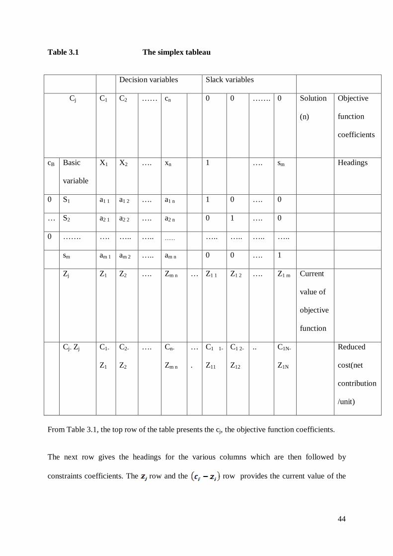
The terms used in the tableau are defined as follows:

= Objective function coefficients for variable j

= Right-hand side coefficients (value) for constraint i

= coefficients of variable j in constraint i

= Objective function coefficients of the basic variables.

From Table 3.1, the top row of the table presents the , the objective function coefficients.

The next row gives the headings for the various columns which are then followed by

constraints coefficients. The row and the ( row which provides the current value of

the objective function and the net contribution per unit of the jth variable respectively are

presented.

The leftmost column in the tableau indicates the values of the objective function coefficients

associated with the basic variable, with a set of constraints.

44

Table 3.1 The simplex tableau

Decision variables Slack variables

Cj C1 C2 …… cn 0 0 ……. 0 Solution

(n)

Objective

function

coefficients

cB Basic

variable

X1 X2 …. xn 1 …. sm Headings

0 S1 a1 1 a1 2 …. a1 n 1 0 …. 0

… S2 a2 1 a2 2 …. a2 n 0 1 …. 0

0 ……. …. ….. ….. …… ….. ….. ….. …..

sm am 1 am 2 ….. am n 0 0 …. 1

Zj Z1 Z2 …. Zm n … Z1 1 Z1 2 …. Z1 m Current

value of

objective

function

Cj- Zj C1-

Z1

C2-

Z2

…. Cn-

Zm n

…

.

C1 1-

Z11

C1 2-

Z12

.. C1N-

Z1N

Reduced

cost(net

contribution

/unit)

From Table 3.1, the top row of the table presents the cj, the objective function coefficients.

The next row gives the headings for the various columns which are then followed by

constraints coefficients. The row and the row provides the current value of the

45

objective function and the net contribution per unit of the jth variable respectively are

presented.

The leftmost column in the tableau indicates the values of the objective function coefficients

associated with the basic variable, with a set of constraints.

3.4 TYPES OF SIMPLEX METHOD SOLUTIONS

The simplex method will always terminate in a finite number of steps with an indication that

a unique optimal solution has been obtained or that one of three special cases has occurred.

These special cases are:

(i) Alternative optimal solutions

(ii) Unbounded solutions

(iii)Infeasible solutions

3.4.1 Alernatve Optmal Solutions

The simplex method provides a clear indication of the presence of alternative or multiple,

optimal solutions upon its termination. These alternative optimal solutions can be recognized

by considering the row. Assume that we are maximizing and remember that when

all

values are all negative, we know that an optimal solution has been obtained. Now,

the presence of an alternative optimal solution will be indicated by the fact that for some

variable not in the basis, the corresponding value will equal zero.

Thus, this variable can be entered into the basis, the appropriate variable can be removed

from the basis, and the value of the objective function will not change. In this manner, the

various alternative optimal solutions can be determined.

46

3.4.2 Unbouded Solutions

In the case of an unbounded solution, the simplex method will terminate with the indication

that the entering basic variable can do so only if it is allowed to assume a value of infinity.

Specifically, for a maximization problem we will encounter a simplex tableau having a non

basic variable whose row value is strictly greater than zero.And for this same

variable all of the a. elements in its column will be zero or negative value (i.e. every

coefficient in the pivot column will be either negative or zero). Thus, in performing the ratio

test for the variable removal criterion, it will be possible only to form ratios having negative

numbers or zeros as denominators. Negative numbers in the denominators cannot be

considered since this will result in the introduction of a basic variable at a negative level

Zeros in the denominator will produce a ratio having an undefined value and would indicate

that the entering basic variable should be increased indefinitely (i.e. infinitely) without any of

the current basic variables being driven from the basis.

Therefore, if we have an unbounded solution, none of the current basic variables can be

driven from solution by the introduction of a new basic variable, even if that new basic

variable assumes an infinitely large value.

Generally, arriving at an unbounded solution indicates that the problem was originally

misformulated within the constraint set and needs reformulation.

3.4.3 Infesasble Solution

An indication that no feasible solution is possible will be given by the fact that at least one of

the artificial variables, which should be driven to zero by the simplex method will be present

as a positive basic variable in the solution that appears to be optimal. For example, assuming

one wish to solve a maximization problem in which artificial variables are required. Then, at

some iteration one achieve a solution in which all the (cj – zj) values are zero or negative, but

which has one or more artificial variables as positive basic variables.

47

When an infeasible solution is indicated the management science analyst should carefully

reconsider the construction of the model, because the model is either improperly formulated

or two or more of the constraints are incompatible.

Reformulation of the model is mandatory for cases in which the no feasible solution

condition is indicated. consider the following linear programming problem as an example of

simplex algorithm.

The slack variables form the initial solution mix. The initial solution assumes that all

available hours are unused i.e. the slack variables take the largest possible values. Variables

in the solution mix are called basic variables. Each basic variable has a column consisting of

all 0’s except for a single 1. All variables not in the solution mix take the value 0.

The simplex method uses a four step process (based on the Gauss Jordan method for solving

a system of linear equations) to go from one tableau or vertex to the next. In this process, a

basic variable in the solution mix is replaced by another variable previously not in the

solution mix. The value of the replaced variable is set to 0.

3.5 DUALITY

Every linear programming problem, referred to as a primal problem, can be converted into a

dual problem, which provides an upper bound to the optimal value of the primal problem. In

matrix form, we can express the primal problem as:

Maximize cTx subject to Ax ≤ b, x ≥ 0;

There are two ideas fundamental to duality theory.

The dual of a dual linear program is the original primal linear program.

Every feasible solution for a linear program gives a bound on the optimal value of the

objective function of its dual. The duality theorem states that if the primal has an

48

optimal solution, x*, then the dual also has an optimal solution, y*, such that

cTx*=bTy*.

Duality theory states that if the primal is unbounded then the dual is infeasible. Likewise, if

the dual is unbounded, then the primal must be infeasible. However, it is possible for both the

dual and the primal to be infeasible .

3.6 SUMMARY

This chapter discussed the Simplex method and its variants. In the next chapter, we shall put

forward the data collected and its Analysis.

49

CHAPTER 4

DATA COLLECTION AND ANALYSIS

4.0 INTRODUCTION

In this chapter we shall analyze the data taken from Prudential Bank Limited and Asante

Akyem Rural Bank. A model is proposed and solved to help these two banks maximise its

profit.

Prudential Bank Limited (PBL) was incorporated in May 1993. The bank was opened to the

public for business on August 15, 1996. PBL is a commercial/development bank with a

strategic focus on the development and financing of industry and export. The bank currently

has 10 branches in Ghana with 4 correspondent banks outside Ghana. The products and

services of PBL include: Domestic Banking Services, International Banking Services, Project

Financing, Export Development, Funds management and Cash Collection Services.

Prudential Bank Limited is in the process of formulating a loan policy involving GH¢

406,491,393 for the year 2011. Being a full-service facility .The bank is obligated to grant

loans to different clientele.

Table 4.1 provides the type of loans, the interest rate charged by the bank and the probability

of bad debt as estimated from past experience.

50

Table 4.1: Loans available to the Prudential Bank Limited.

Type of loan Interest rate Probability of bad debt

Export 0.28 0.02

Industry or manufactory 0.30 0.12

Agriculture 0.31 0.2

Commence 0.31 0.1

Construction 0.32 0.1

Consumer 0.32 0.2

Fuel dealers 0.28 0.1

Bad debts are assumed unrecoverable and hence produce no interest revenue. For policy

reasons, there are limits on how the bank allocates its funds. Competition with other financial

institutions in the city requires that the bank

Allocate at least 40% of the total funds to consumer loans and Industry loans.

To assist agriculture production i n the region, agriculture loans must at least be

greater than 50% of Export, Industry and fuel dealers loans

The sum of consumer loans and construction loans must be at least greater than 40%

of Export, commence and fuel dealers loans

The sum of consumer loans and agriculture loans must be at least 25% of the total

funds

The bank also stated that the total ratio for bad debt on all loans must not exceed 0.08.

51

4.1 PROPOSED MODEL PRUDENTIAL BANK LIMITED

The variables of the model can be defined as follows:

= Export loans (in thousands of cedis)

=Industry or Manufactory loans

=Agriculture loans

= commence

= consumer loans

= Construction loans

= Fuel Dealers Loans

The objective of the Prudential Bank is to maximize its net returns comprised of the

difference between the revenue from interest and lost funds due to bad debts.

Objective function:

52

Maximize Z = 0.28(0.98 ) + 0.30(0.88 ) + 0.31(0.80 ) + 0.31(0.90 ) +

0.32(0.90 ) + 0.32(0.80 ) + 0.28(0.90 ) – 0.02 0.12 −0.2 − 0.1 –

0.1 − 0.2 − 0.1

This function simplifies to

Maximize Z = 0.2544 + 0.144 + 0.048 + 0.179 +0.188 +0.056 +0.152

The problem has seven constrains:

o Limits on total funds available

+ + + + + + ≤ 406,491,393

o Limits on industry, commence and consumer loans

o Limits on Agriculture loan compared to Export, industry and fuel dealers loan

≥ 0.5( + )

0.5 0.5 ≥ 0

o Limits on consumer loans and construction loans compared to Export,

commence and loan fuel dealer loans

53

+ ≥ 0.4( + )

o Limits on consumer and commence loans

+ ≥ 0.25(406491393)

o Limits on fuel dealers and industry or Manufactory loans

Limits on bad debts

Or

-0.06

8. Non-negativity

54

The Asante-Akyem Rural Bank . Juansa in the Asnate Akyem District give loans to the

active-rural poor to help reduce poverty and improve living standards of the rural folks.

Asante Akyem Rural Bank is in the process of formulating a loan policy involving GH¢

700,000 the year 2011.Being a full-service facility the bank is obligated to grant loans to

different clientele.

Table 4.2 depicts the type of loans, the interest rate charged by the bank and the probability

of bad debt as estimated from past experience.

Table 4.2: Loans available to the Asante Akyem Rural bank

Type of loan Interest rate Probability of bad debt

Salary Loan 0.28 0.01

Trading and Transport Loans 0.30 0.1

Agriculture 0.30 0.15

Micro Finance Loans 0.32 0.15

Susu Loans 0.30 0.1

55

Adwuma Nkosoo 0.30 0.5

Trading Overdrafts Loans 0.30 0.1

Salary Overdraft 0.31 0.01

Bad debts are assumed unrecoverable and hence produce no interest revenue. For policy

reasons, there are limits on how the bank allocates its funds. Competition with other financial

institutions in the city requires that the bank

Allocate at least 50% of the total funds to Salary loans and Micro Finance loans.

To assist agriculture production in the region, agriculture loans must at least be 5% of

The total fund.

The sum of Susu loans and Adwuma Nkosoo loans must be at least 25% of Micro

Finance loans and Salary Overdraft loans

The sum of Trading and Transport loans and agriculture loans must be at least 25% of

the total funds

The bank also stated that the total ratio for bad debt on all loans must not exceed 0.05.

4.2 PROPOSED MODEL FOR ASANTE AKYEM RURAL BANK

The variables of the model can be defined as follows:

= Salary loans (in thousands of cedis)

=Trading and Transport loans

56

=Agriculture loans

= Micro Finance Loans

= Micro Finance Loans

= Susu loans

= Adwuma Nkosoo loans

= Trading Overdraft Loans

= Salary Overdraft Loans

The objective of the Asante Akyem Rural Bank is to maximize its net returns

comprised of the difference between the revenue from interest and lost funds due to

bad debts.

Objective function:

Maximize Z = 0.28(0.99 ) + 0.30(0.90 ) + 0.30(0.85 ) + 0.32(0.85 ) +

0.30(0.90 ) + 0.30(0.80 ) + 0.30(0.90 ) +0.31(0.99 ) – 0.01 0.1

− 0.15 − 0.15 – 0.1 − 0.2 − 0.1 – 0.01

57

This function simplifies to

Maximize Z=0.2672 + 0.17 + 0.105 + 0.122 +0.17 +0.04

+0.17 +0.3

The problem has seven constrains:

1. Limits on total funds available

+ + + + + + ≤ 700,000

2. Limits on Salary and micro finance loans

+ ≥ 0.5×700,000

+ ≥ 350000

3. Limits on Agriculture

≥ 0.05(700,000)

4. Limits on Susu loans and Adwuma Nkosoo loans compared to Micro Finance

Loan and Salary Overdraft loans

+ ≥ 0.25( + )

58

5. Limits on Trading and Overdrafts Loans and Susu Loans

≥ 0.25(700000)

+ 00

6.Limits on bad debts

Or

-0.04

7. Non-negativity

The allocation of funds to the various clientele as formulated above was transferred onto the

Quantitative Methods (QM) for windows model by first selecting the linear programming

option from the module, create data set was used to select the number of variables involve in

each case and the number of constraints.

59

Solve problem icon was used to display the problem results including linear programming

results, ranging, solution list, as well as the iterations.The results given by the (QM) is

surmrised below.

4.3 OPTIMAL SULUTION FOR PRUDENTIAL BANK LIMITED

Optimal Value (Z)=80035725.5

Variable Status Value

Basic 146337000

Basic 117882500

NONBasic 0

Basic 101622800

Basic 40649120

NONBasic 0

NONBasic 0

slack 1 NONBasic 0

surplus 2 Basic 1625960

surplus 3 Basic 87395740

surplus 4 NONBasic 0

60

surplus 5 NONBasic 0

surplus 6 NONBasic 0

slack 7 Basic 1219481

Variable Value Reduced Cost

146337000. 0

117882500. 0

0. 0.206

101622800. 0

40649120. 0

0. 0.03

0. 0.0184

Constraint Dual Value Slack/Surplus

Constraint 1 .2544 0

Constraint 2 0 16259600

Constraint 3 0 87395740

Constraint 4 -0.0664 0

Constraint 5 -.10196 0

Constraint 6 -.1104 0

Constraint 7 0 1219481

4.5 OPTIMAL SULUTION FOR ASANTE AKYEM RURAL BANK

61

Optimal Value (Z) = 176750

Variable Status Value

Basic 350000

NONBasic 0

NONBasic 0

NONBasic 0

Basic 43750

NONBasic 0

Basic 131250

Basic 175000

slack 1 NONBasic 0

surplus 2 NONBasic 0

surplus 3 Basic 284375

surplus 4 NONBasic 0

surplus 5 NONBasic 0

slack 6 Basic 12250

Variable Value Reduced Cost

350000. 0

0. 0.13

0. 0.19

0. 0.15

43750. 0

0. 0.26

62

131250. 0

175000. 0

Constraint Dual Value Slack/Surplus

Constraint 1 .3 0

Constraint 2 -.03 0

Constraint 3 0 284375

Constraint 4 0 0.0011

Constraint 5 -.13 0

Constraint 6 0 12250

4.5 SUMMARY

In this chapter data collected from Prudential Bank and Asante Akyem Rural Bank were used

to formulate the proposed model. The next chapter presents the summary, conclusion and

recommendation for the study.

63

CHAPTER FIVE

SUMMARY,CONCLUSIONS AND RECOMMENDATIONS

5.0 INTRODUCTION

This chapter presents the summary, conclusions drawn from the study and make

recommendations to help Prudential Bank and Asante Akyem Rural Bank to optimize their

profit margin.

5.1 SUMMARY OF RESULTS (PRUDENTIAL BANK LIMITED ALLOCATION )

The problem went through ten iterations before an optimal solution was found.The reduced

cost for are zero. Since are at basic at the

optimum, The reduced cost for 0.206,0.03 and 0.0184 respectively are

non-basic at the optimum.the dual prices for constraints (1), (4), (5) and (6) are nonzero at the

optmum because they correspond to the four constraints at optmum,hence their slack

64

variables are nonbasic.the Optimal solution gives the optimal Value (Z)=GH¢80035725.5

which occures at =GH¢146337000, =GH¢ 117882500, 101622800 and

GH¢40649120. From the results, the value of zero at optimum because

theprobability of debt (see Table 4.1 ) of these these three variables are high and hence they

do not make any returns.

Refer to appendix B, C, D, Eand F for tables showing the solution list, ranging values, linear

programming results and the iterations as displayed by the QM for windows model

5.2 SUMMARY OF RESULTS (ASANTE AKYEM RURAL BANK LOAN

ALLOCATION)

The problem went through nine iteration before an optimal solution was reached. The

variables were in basic at optimum and had their reduced cost to be zeros.

The variables were nonbasic variables and had their reduced cost to be

nonzero. The optimal value (Z) = GH¢176750 occurs at =GH¢350000, =

GH¢43750, = GH¢131250, and = GH¢175000.With the values of being

zero. Since these variables high probability of bad debt (as shown in table 4.2)

Refer to appendix G,H,I,J and K for tables showing the solution list, ranging values, linear

programming results and the iterations as displayed by the QM for windows model.

From the results given by the (QM) on the allocation of funds to the various loan types by

Prudential Bank and Asante Akyem Rural Bank , it could be seen in general that loan types

that has high probability of bad debt do not yield any returns.

5.3 CONCLUSIONS

The results from the study has shown that most banks in the country do not have any

scientific method to give out loans. As a result of this most banks are unable to optimize their

65

profit margins. The model propose for Prudential bank and Asante Akyem Rural Bank would

help these two banks to disburse their available funds for loans more effectively and

profitably. The results from the model showed that, Prudential Bank and Asante Akyem

Rural would be making annual profit of GH¢176750 and GH¢80035725.5 respectively if

they are to stick to the model. Hence we conclude that the scientific method we used to

developed the propose model can have a dramatic increase in the two banks profit margin if

put into practise.

5.4 RECOMMENDATIONS

It was realised from the conclusion that the use of scientific methods to give out loans help

banks to avoid giving out loans that do not yield profit there by allocating funds to areas they

are sure to get returns. We therefore recommend Prudential Bank and Asante Akyem Rural

Bank to adapt this model in their allocation of funds for loans.

We also recommend that Banks and other financial institutions be educated to employ

scientific methods such as the use of mathematical models to help them disburse funds of the

bank more effectively and profitably.

We again recommend the use of other Mathematical tools to do further research into this wor

66

REFERENCES

1. Abd. Halim (2008). Predicting Corporate Failure of Malaysia's Listed

Companies: Comparing Multiple ... International Research Journal of Finance &

Economics; (2008). Issue 15, p201- 217.

2. Acharya, U., (2005). Does industry-wide distress affect defaulted firms – evidence

from creditor recoveries, London School of Business Working Paper.

3. Altman, E I. (1993). Corporate financial distress and bankruptcy, 2nd. Ed., Wiley,

New York.

4. Altmann E. A. Resti, A. Sironi (2005). Recovery Risk, Risk Books

5. Altman, E I. (1993). Corporate financial distress and bankruptcy, 2nd. Ed., Wiley,

New York.

67

6. Bakshi G. D., D. Madan, F. Zhang (2001). Understanding the Role of Recovery in

Default Risk Models: Empirical Comparisons and Implied Recovery Rates, Finance

and Economics Discussion Series 2001-37, Federal Reserve Board of Governors.

7. Beaver, W. (1966), Financial ratios as predictors of failure, Journal of Accounting

Research

8. (Supplement), 4, pp. 71-102.

9. Best M.J. and R.R. Grauer., (1991). Sensitivity Analysis for Mean- Variance Portfolio

Problems . Management Science. Vol. 37, No. 8, (Aug) pp. 980 - 989.

10. Blume M.E. (1970). Portfolio Theory - A Step Towards its Plactical Application.

Journal of Business. Vol. 43 (April) pp. 152-173.

11. Booth, G. G., (1972). Programming Bank Portfolios under Uncertainty, "Journal of

Bank Research Vol. 3, No. 4 (Winter), pp. 28-40.

12. Bordo, M.D. and A.P. Murshid ( 2001). Are Financial Crises Becoming More

Contagious?

13. chapter 14 in International Financial Contagion( eds) Stijn Claessens and Kristin I.

Forbes.Boston: Kluwer Academic Publishers pp 367-403.

14. Borio, C, N Kennedy and S Prowse (1994). Exploring aggregate asset price

fluctuations acrosscountries: measurement, determinants and monetary policy

implications, BIS Economic Papers,No 40, Basel, April.

15. Brealey, R. A. and Hodges, S. D (1972). Playing with Portfolios. The Journal of

Finance, Vol. 30, No. 1 (Mar., 1975), pp. 125-134

16. C. Finger, C. (1999). Conditional approaches for creditmetrics portfolio distributions

creditmetrics monitor.

17. Carey M., M. Gordy (2003). Systematic risk in recoveries on defaulted debt,

Unpublished

68

18. Working Paper presented at the 2001 Financial Management Association Meetings,

Toronto, 20 October. Cited in Altmann et al. [3].

19. Chambers.,Chames. (1961). Intertemporal Analysis and optimization of bank

portfolios, Management Science II,July 1961.

20. Cohen and Hamer, (1967:1972). Linear programming and optimal Bank Asset

Management Decision.Journal of Finance vol 22, No.2 (May pp.147-165).

21. Crouhy, M., Galai, D., Mark, R. (1994). A comparative analysis of current credit risk

models. Journal of Banking and ) 59±117.

22. Dince, R. R., and Fortson, J. C, (1977). An Application of Goal Programming to the

Management of a Country Bank, Journal of Bank Research. Vol. 7, No. 4 (Winter),

pp. 311-319.

23. Evans J. and R. Steuer (1973), A Revised Simplex Method for Linear Multiple

Objective Programmes. Mathematical Programming. Vol. 5, pp. 54-56.

24. Ferrier G.D., S. Grosskopf, K.J. Hayes and Yaisawarng (1993). Economics Of

Diversification in the Banking Industry - A Frontier Approach. Journal Of Monetary

Economics. Vol. 31, No 2, (April) pp 229 - 249.

25. Finger C. (2000). A Comparison of Stochastic Default Rate Models, Working Paper

00-022.

26. Frye . (2000a). Collateral damage, Risk, April, 91-94.

27. Frye. (2000b). Collateral Damage Detected, Federal reserve Bank of Chicago,

Emerging Issues Series, October, 1-14.

28. Gollier C. (2001). The Economics of Risk and Time. Cambridge, MA; London,

England: The MIT Press. ISBN 0-262-07215-7.

69

29. Goodhart, C. A. E. (2004). The Bank of England, 1970–2000, ch. 17 in R. Michie

(ed.), The British Government and the City of London in the Twentieth Century,

Cambridge, Cambridge University Press, 340–71.

30. Gordy, M. (2000). A comparative anatomy of credit risk models. Journal of Banking

and Finance 24, 119-149

31. Grunert, J., Norden, L., Weber, M. (2005). The Role of Non-Financial Factors in

Internal

32. Credit Ratings. Journal of Banking and Finance 29, 509-531.

33. Gurtler M., D. Heithecker (2005). Systematic credit cycle risk of financial collaterals:

34. Modelling and evidence, Working Paper, TU Braunschweig.

35. Gustafsson, J., A. Salo.( 2003). Valuing Risky Projects with Contingent Portfolio

Programming. Helsinki University of Technology.

36. Haspeslagh P. (1982), Portfolio Planning - Uses and Limits. Harvard pp. 58 -

73

37. Hodges S. and Brealey R. (1972). Portfolio Selection in a Dynamic and Uncertain

World. Financial Analyst Journal. (NovJDec.) pp 58-69.

38. Hu Y. T., W. Perraudin (2002). The dependence of recovery rates and defaults, .

Birkbeck College.

39. Jarrow R. A., S. Turnbull (2000). The Intersection of Market and Credit Risk, Journal

of Banking and Finance 24, 271–299.

40. Jokivuolle, E. And Peura, S. (2001). Regulatory Capital Volatility. Risk, May.

41. K. Duellmann and M. Trapp. Systematic risk in recovery rates–an empirical analysis

ofUS corporate credit exposures. Deutsche Bundesbank Discussion Paper 02/04,

2004.

70

42. Kall, P. and Wallace, S.W. (1994). Stochastic Programming. New York: John Wiley

& Sons. ISBN 0- 471-95108-0.

43. Lubatkin, M., Chatterjee, S. (1994). Extending modern diversification: does it apply?,

Academy of Management Journal, Vol. 33 pp.756-79.

44. Markowitz H.M. (1952). ,Portfolio Selection. Journal of Finance.Vol 7, pp. 77-91.

45. Martin.(1995). Systemic Aspects of Risk Management in Banking and Finance, Swiss

Journal of Economics and Statistics (SJES), vol. 131(IV), pages 723-737, December.

46. Melnik A. (1 970). Short-run Determinants of Commercial Bank Investment

Portfolios - An Empirical Analysis. Journal of Finance. Vol. 25, No. 3, (June) pp. 639

- 649.

47. Melnik A. (1970). Short-Run Determinants of Commercial Bank Investment

Portfolios, Journal of. Finance (June 1970), 639-649. 8.

48. Mongin, P. (1988). Expected Utility Theory, Handbook o f Economic Methodology

(J.Davis, W.Hands, and U.Maki, eds. London

49. Rheinberger, K.and Summer, M. (2009). Does Adding Up of Economic Capital for

Market- and Credit Risk amount to Conservative Risk Assessment? Journal of Risk,

1(4):33–53.

50. Rockafellar, R.T. and Uryasev, S. (1999). Optimization of Conditional Value-at-Risk.

URL:

51. http://www.ise.ufl.edu/uryasev/cvar.pdf (7/23/04).

52. Rockafellar, R. T., and Uryasev, S. (2002). Conditional Value-at-Risk for General

Loss Distributions. Journal of Banking and Finance, 26(7), 1443-1471.

53. Robinson,R.I., (1961). The Management of Bank funds, N Y,Mc Graw-Hill 1991.

54. Stephen Arthur, S. (2004). Experience with constructing composite asset price

indices. BIS.

71

55. Tobin.,(1965). The Theory of portfolio Selection.Macmillan Press.

56. Uryasev, S., and Rockafellar, R. T. (2000). Optimisation of Conditional Value-at-

Risk. Journal of Risk, 2(3), 21-41.

57. Waterman, R. H. and Gee, R. E.,(1981). An Application of Linear Programming to

Bank Financial. The Institute of Management Sciences. Vol. 11, No. 5, pp. 77-83.

58. Yong,W.Y. and Sheng-Yi, L. (1988). Asia Pacific Journal of Management vol 5 No.2

January 1988.

59. www.theghanaianjournal.com/.../address-the-energy-crisis-please-dr-paul-acquah/

60. www.pwc.com/gh/en/.../ghana-banking-survey-2008.jhtm

61. www.facebook.com/.../African-Business-Magazine/114117578656259

APPENDIX A

QUESTIONNAIRES

The questionnaire used to gather information on allocation of funds to loan types from

Prudential Bank Limited and Asante Akyem Rural Bank.

You are kindly requested to complete this questionnaire as frankly as possible; your response

will be kept confidential and shall be used only for this thesis.

1) What is the name of your bank?

………………………………………………………………………………………………

2) What are the various types of loans your bank give to its customers?

..........................................................................................................................................

..........................................................................................................................................

..........................................................................................................................................

72

..........................................................................................................................................

..........................................................................................................................................

3) What percentage do you bank charge on each loan above as interest?

…………………………………………………………………………………………

…………………………………………………………………………………………

…………………………………………………………………………………………

……………....................................................................................................................

…………………………………………………………………………………………

4) What is the probability of bad debt on each of the loans stated above?

…………………………………………………………………………………………

…………………………………………………………………………………………

…………………………………………………………………………………………

…………………………………………………………………………………………

……………………

5) State the total amount of money given out as loans.

…………………………………………………………………………………………

……...............................................................................................................................

6) Is there any condition under which loan is given out to customers?

…………………………………………………………………………………………

….................................................................................................................................

…………………………………………………………………………………………

73

APPENDIX B

PRUDENTIAL BANK LOAN ALLOCATION PROBLEM

X1 X2 X3 X4 X5 X6 X7 RHS

Maximize 0.2544 0.144 0.048 0.179 0.188 0.056 0.152 Constraint 1 1. 1. 1. 1. 1. 1. 1. <= 406,491,400

Constraint 2 0. 1. 0. 1. 0. 1. 0. >= 203,245,700

Constraint 3 1. -0.5 0. 0. 0. 0. -0.5 >= 0

Constraint 4 0. 0. 0. -0.4 1. 1. -0.4 >= 0

Constraint 5 0. 0. 0. 1. 0. 1. 0. >= 101,622,800

Constraint 6 0. 1. 0. 0. 0. 0. 1. >= 117,882,500

Constraint 7 -0.06 0.04 0.12 0.02 0.02 0.12 0.02 <= 0

Created by QM for Windows

74

APPENDIX C SOLUTION TO PRUDENTIAL BANK LOAN ALLOCATION

Variable Status Value

X1 Basic 146,337,000.

X2 Basic 117,882,500.

X3 NONBasic 0.

X4 Basic 101,622,800.

X5 Basic 40,649,120.

X6 NONBasic 0.

X7 NONBasic 0.

slack 1 NONBasic 0.

surplus 2 Basic 16,259,600.

surplus 3 Basic 87,395,740.

surplus 4 NONBasic 0.

surplus 5 NONBasic 0.

surplus 6 NONBasic 0.

slack 7 Basic 1,219,481.

Optimal Value (Z) 80,035,730.

75

Created by QM for Windows

APPENDIX D

SOLUTION TO PRUDENTIA BANK LOAN ALLOCATION

Variable Value Reduced Cost Original Val Lower Bound Upper Bound

X1 146,337,000. 0. 0.25 0.21 0.28

X2 117,882,500. 0. 0.14 0.13 0.25

X3 0. 0.2064 0.05 -Infinity 0.25

X4 101,622,800. 0. 0.18 0.15 0.28

X5 40,649,120. 0. 0.19 0.17 0.23

X6 0. 0.03 0.06 -Infinity 0.09

X7 0. 0.0186 0.15 -Infinity 0.17

Constraint Dual Value Slack/Surplus Original Val Lower Bound Upper Bound

Constraint 1 0.2544 0. 406,491,400. 386,166,700. Infinity

Constraint 2 0. 16,259,600. 203,245,700. -Infinity Infinity

Constraint 3 0. 87,395,740. 0. -Infinity Infinity

Constraint 4 -0.0664 0. 0. -Infinity Infinity

Constraint 5 -0.102 0. 101,622,800. 85,363,200. Infinity

Constraint 6 -0.1104 0. 117,882,500. 101,622,900. Infinity

Constraint 7 0. 1,219,481. 0. -Infinity Infinity

Created by QM for Windows

76

APPENDIX E

LINEAR PROGRAMMING RESULTS

SOLUTION TO PRUDENTIAL BANK LOAN ALLOCATION PROBLEM

X1 X2 X3 X4 X5 X6 X7 RHS Dual

Maximize 0.2544 0.144 0.04

8 0.179 0.188 0.056

0.152

Constraint 1 1. 1. 1. 1. 1. 1. 1. <

= 406,491,40

0. 0.254

4

Constraint 2 0. 1. 0. 1. 0. 1. 0. >

= 203,245,70

0. 0.

Constraint 3 1. -0.5 0. 0. 0. 0. -0.5 >

= 0. 0.

Constraint 4 0. 0. 0. -0.4 1. 1. -0.4 >

= 0. -

0.0664

Constraint 5 0. 0. 0. 1. 0. 1. 0. >

= 101,622,80

0. -

0.102

Constraint 6 0. 1. 0. 0. 0. 0. 1. >

= 117,882,50

0.

-0.110

4

Constraint 7 -0.06 0.04 0.12 0.02 0.02 0.12 0.02 <

= 0. 0.

Solution->

146,337,000.

117,882,500. 0. 101,622,80

0. 40,649,12

0. 0. 0. 80,035,725.59

77

Created by QM for Windows

APPENDIX F

ITERATIONS OF PRUDENTIAL BANK LOAN ALLOCATION

Cj Basi

c Variables

.2544 X1

.144

X2 .04

8 X3

.179

X4 .18

8 X5

.056

X6 .15

2 X7

0 slack 1

0 artfcl 2

0 sur

plus 2

0 artfcl 3

0 sur

plus 3

0 artfcl 4

0 sur

plus 4

0 artfcl 5

0 sur

plus 5

0 artfcl 6

0 sur

plus 6

0 slack 7

Quantity

Iteration 1

0 slack 1 1. 1. 1. 1. 1. 1. 1. 1. 0. 0. 0. 0. 0. 0. 0. 0. 0. 0. 0. 406,491,3

92. 0 artfcl

2 0. 1. 0. 1. 0. 1. 0. 0. 1. -1. 0. 0. 0. 0. 0. 0. 0. 0. 0. 203,245,696.

0 artfcl 3 1. -0.5 0. 0. 0. 0. -0.5 0. 0. 0. 1. -1. 0. 0. 0. 0. 0. 0. 0. 0.

0 artfcl 4 0. 0. 0. -

0.4 1. 1. -0.4 0. 0. 0. 0. 0. 1. -1. 0. 0. 0. 0. 0. 0.

0 artfcl 5 0. 0. 0. 1. 0. 1. 0. 0. 0. 0. 0. 0. 0. 0. 1. -1. 0. 0. 0. 101,622,8

00. 0 artfcl

6 0. 1. 0. 0. 0. 0. 1. 0. 0. 0. 0. 0. 0. 0. 0. 0. 1. -1. 0. 117,882,496.

0 slack 7

-0.0

6 0.0

4 0.1

2 0.0

2 0.0

2 0.1

2 0.0

2 0. 0. 0. 0. 0. 0. 0. 0. 0. 0. 0. 1. 0.

zj -

0.7456

-1.356

0.048

-1.421

-0.812

-2.944

0.052 0. 0. 1. 0. 1. 0. 1. 0. 1. 0. 1. 0. 422,750,9

92. cj-zj 1. 1.5 0. 1.6 1. 3. 0.1 0. 0. -1. 0. -1. 0. -1. 0. -1. 0. -1. 0. Iteration 2

78

0 slack 1 0. 1.5 1. 1. 1. 1. 1.5 1. 0. 0. -1. 1. 0. 0. 0. 0. 0. 0. 0. 406,491,3

92. 0 artfcl

2 0. 1. 0. 1. 0. 1. 0. 0. 1. -1. 0. 0. 0. 0. 0. 0. 0. 0. 0. 203,245,696.

0.2544 X1 1. -0.5 0. 0. 0. 0. -0.5 0. 0. 0. 1. -1. 0. 0. 0. 0. 0. 0. 0. 0.

0 artfcl 4 0. 0. 0. -

0.4 1. 1. -0.4 0. 0. 0. 0. 0. 1. -1. 0. 0. 0. 0. 0. 0.

0 artfcl 5 0. 0. 0. 1. 0. 1. 0. 0. 0. 0. 0. 0. 0. 0. 1. -1. 0. 0. 0. 101,622,8

00. 0 artfcl

6 0. 1. 0. 0. 0. 0. 1. 0. 0. 0. 0. 0. 0. 0. 0. 0. 1. -1. 0. 117,882,496.

0 slack 7 0. 0.0

1 0.1

2 0.0

2 0.0

2 0.1

2 -

0.01

0. 0. 0. 0.06

-0.0

6 0. 0. 0. 0. 0. 0. 1. 0.

zj 0.2544

-1.856

0.048

-1.421

-0.812

-2.944

-0.448

0. 0. 1. 1. 0. 0. 1. 0. 1. 0. 1. 0. 422,750,992.

cj-zj 0. 2. 0. 1.6 1. 3. 0.6 0. 0. -1. -1. 0. 0. -1. 0. -1. 0. -1. 0. Iteration 3

0 slack 1 0. 1.5 1. 0. 3.5 3.5 0.5 1. 0. 0. -1. 1. 2.5 -2.5 0. 0. 0. 0. 0. 406,491,3

92. 0 artfcl

2 0. 1. 0. 0. 2.5 3.5 -1. 0. 1. -1. 0. 0. 2.5 -2.5 0. 0. 0. 0. 0. 203,245,696.

0.2544 X1 1. -0.5 0. 0. 0. 0. -0.5 0. 0. 0. 1. -1. 0. 0. 0. 0. 0. 0. 0. 0. 0.179 X4 0. 0. 0. 1. -2.5 -

2.5 1. 0. 0. 0. 0. 0. -2.5 2.5 0. 0. 0. 0. 0. 0.

0 artfcl 5 0. 0. 0. 0. 2.5 3.5 -1. 0. 0. 0. 0. 0. 2.5 -2.5 1. -1. 0. 0. 0. 101,622,8

00. 0 artfcl

6 0. 1. 0. 0. 0. 0. 1. 0. 0. 0. 0. 0. 0. 0. 0. 0. 1. -1. 0. 117,882,496.

0 slack 7 0. 0.0

1 0.1

2 0. 0.07

0.17

-0.0

3 0. 0. 0. 0.0

6 -

0.06

0.05

-0.0

5 0. 0. 0. 0. 1. 0.

zj 0.2544

-1.856

0.048

0.179

-4.812

-6.944

1.152 0. 0. 1. 1. 0. -4. 5. 0. 1. 0. 1. 0. 422,750,9

92. cj-zj 0. 2. 0. 0. 5. 7. -1. 0. 0. -1. -1. 0. 4. -5. 0. -1. 0. -1. 0. Iteration 4

0 slack 1 0. 1.2

941 -

1.4706

0. 2.0588 0. 1.1

176 1. 0. 0. -

2.2353

2.2353

1.4706

-1.4

706 0. 0. 0. 0.

-20.5882

406,491,392.

0 artfcl 2 0. 0.7

941 -

2.4706

0. 1.0588 0.

-0.3

824 0. 1. -1.

-1.2

353 1.2

353 1.4

706 -

1.4706

0. 0. 0. 0. -

20.5882

203,245,696.

0.2544 X1 1. -0.5 0. 0. 0. 0. -0.5 0. 0. 0. 1. -1. 0. 0. 0. 0. 0. 0. 0. 0.

0.179 X4 0. 0.1

471 1.7

647 1. -

1.4706

0. 0.5588 0. 0. 0. 0.8

824 -

0.8824

-1.7

647 1.7

647 0. 0. 0. 0. 14.7059 0.

0 artfcl 5 0.

-0.2

059 -

2.4706

0. 1.0588 0.

-0.3

824 0. 0. 0.

-1.2

353 1.2

353 1.4

706 -

1.4706

1. -1. 0. 0. -

20.5882

101,622,800.

0 artfcl 6 0. 1. 0. 0. 0. 0. 1. 0. 0. 0. 0. 0. 0. 0. 0. 0. 1. -1. 0. 117,882,4

96. 0.05 X6 0. 0.0 0.7 0. 0.4 1. - 0. 0. 0. 0.3 - 0.2 - 0. 0. 0. 0. 5.88 0.

79

6 588 059 118 0.1765

529 0.3529

941 0.2941

24

zj 0.2544

-1.4

442 4.9

892 0.179

-1.9

296 0.056

-0.0

833 0. 0. 1. 3.4

706 -

2.4706

-1.9

412 2.9

412 0. 1. 0. 1. 41.1765

422,750,992.

cj-zj 0. 1.5882

-4.9

412 0. 2.1

176 0. 0.2353 0. 0. -1.

-3.4

706 2.4

706 1.9

412 -

2.9412

0. -1. 0. -1. -

41.1765

Iteration 5

0 slack 1 0. 1.6

667 3. 0. 0.1429 0. 1.8

095 1. 0. 0. 0. 0. -

1.1905

1.1905

-1.8

095 1.8

095 0. 0. 16.6667

222,602,517.7692

0 artfcl 2 0. 1. 0. 0. 0. 0. 0. 0. 1. -1. 0. 0. 0. 0. -1. 1. 0. 0. 0. 101,622,8

97.5991 0.2544 X1 1.

-0.6

667 -2. 0. 0.8

571 0. -

0.8095

0. 0. 0. 0. 0. 1.1905

-1.1

905 0.8

095 -

0.8095

0. 0. -

16.6667

82,266,075.8299

0.179 X4 0. 0. 0. 1.

-0.7

143 0. 0.2

857 0. 0. 0. 0. 0. -

0.7143

0.7143

0.7143

-0.7

143 0. 0. 0. 72,587,71

4.5445

0 surplus 3 0.

-0.1

667 -2. 0. 0.8

571 0. -

0.3095

0. 0. 0. -1. 1. 1.1905

-1.1

905 0.8

095 -

0.8095

0. 0. -

16.6667

82,266,075.8299

0 artfcl 6 0. 1. 0. 0. 0. 0. 1. 0. 0. 0. 0. 0. 0. 0. 0. 0. 1. -1. 0. 117,882,4

96. 0.056 X6 0. 0. 0. 0. 0.7

143 1. -

0.2857

0. 0. 0. 0. 0. 0.7143

-0.7

143 0.2

857 -

0.2857

0. 0. 0. 29,035,086.3081

zj 0.2544

-1.856

0.048

0.179

0.188

0.056

-0.848

0. 0. 1. 1. 0. 1. 0. 2. -1. 0. 1. 0. 219,505,395.1983

cj-zj 0. 2. 0. 0. 0. 0. 1. 0. 0. -1. -1. 0. -1. 0. -2. 1. 0. -1. 0. Iteration 6

0 slack 1 0. 0. 3. 0. 0.1

429 0. 1.8095 1.

-1.6

667 1.6

667 0. 0. -

1.1905

1.1905

-0.1

429 0.1

429 0. 0. 16.6667

53,231,025.2601

0.144 X2 0. 1. 0. 0. 0. 0. 0. 0. 1. -1. 0. 0. 0. 0. -1. 1. 0. 0. 0. 101,622,8

97.9284 0.2544 X1 1. 0. -2. 0. 0.8

571 0. -

0.8095

0. 0.6667

-0.6

667 0. 0. 1.1

905 -

1.1905

0.1429

-0.1

429 0. 0.

-16.6667

150,014,676.4679

0.179 X4 0. 0. 0. 1.

-0.7

143 0. 0.2

857 0. 0. 0. 0. 0. -

0.7143

0.7143

0.7143

-0.7

143 0. 0. 0. 72,587,71

4.5445

0 surplus 3 0. 0. -2. 0. 0.8

571 0. -

0.3095

0. 0.1667

-0.1

667 -1. 1. 1.1

905 -

1.1905

0.6429

-0.6

429 0. 0.

-16.6667

99,203,225.9894

0 artfcl 6 0. 0. 0. 0. 0. 0. 1. 0. -1. 1. 0. 0. 0. 0. 1. -1. 1. -1. 0. 16,259,59

8.0716 0.056 X6 0. 0. 0. 0. 0.7

143 1. -

0.2857

0. 0. 0. 0. 0. 0.7143

-0.7

143 0.2

857 -

0.2857

0. 0. 0. 29,035,086.3081

zj 0.2544

0.144

0.048

0.179

0.188

0.056

-0.848

0. 2. -1. 1. 0. 1. 0. 0. 1. 0. 1. 0. 16,259,599.3415

cj-zj 0. 0. 0. 0. 0. 0. 1. 0. -2. 1. -1. 0. -1. 0. 0. -1. 0. -1. 0. Iteration 7

80

0 slack 1 0. 0. 3. 0. 0.1

429 0. 0.1429 1. 0. 0. 0. 0.

-1.1

905 1.1

905 -

1.8095

1.8095

-1.6

667 1.6

667 16.6667

26,131,695.8746

0.144 X2 0. 1. 0. 0. 0. 0. 1. 0. 0. 0. 0. 0. 0. 0. 0. 0. 1. -1. 0. 117,882,4

95.9473 0.2544 X1 1. 0. -2. 0. 0.8

571 0. -

0.1429

0. 0. 0. 0. 0. 1.1905

-1.1

905 0.8

095 -

0.8095

0.6667

-0.6

667 -

16.6667

160,854,408.8036

0.179 X4 0. 0. 0. 1.

-0.7

143 0. 0.2

857 0. 0. 0. 0. 0. -

0.7143

0.7143

0.7143

-0.7

143 0. 0. 0. 72,587,71

4.5445

0 surplus 3 0. 0. -2. 0. 0.8

571 0. -

0.1429

0. 0. 0. -1. 1. 1.1905

-1.1

905 0.8

095 -

0.8095

0.1667

-0.1

667 -

16.6667

101,913,159.0733

0 surplus 2 0. 0. 0. 0. 0. 0. 1. 0. -1. 1. 0. 0. 0. 0. 1. -1. 1. -1. 0. 16,259,59

8.019 0.056 X6 0. 0. 0. 0. 0.7

143 1. -

0.2857

0. 0. 0. 0. 0. 0.7143

-0.7

143 0.2

857 -

0.2857

0. 0. 0. 29,035,086.3081

zj 0.2544

0.144

0.048

0.179

0.188

0.056

0.152 0. 1. 0. 1. 0. 1. 0. 1. 0. 1. 0. 0. 1.3226

cj-zj 0. 0. 0. 0. 0. 0. 0. 0. -1. 0. -1. 0. -1. 0. -1. 0. -1. 0. 0. Iteration 8

0 slack 1 0. 0. 3. 0. 0.1

429 0. 0.1429 1. 0. 0. 0. 0.

-1.1

905 1.1

905 -

1.8095

1.8095

-1.6

667 1.6

667 16.6667

26,131,695.8746

0.144 X2 0. 1. 0. 0. 0. 0. 1. 0. 0. 0. 0. 0. 0. 0. 0. 0. 1. -1. 0. 117,882,4

95.9473 0.2544 X1 1. 0. -2. 0. 0.8

571 0. -

0.1429

0. 0. 0. 0. 0. 1.1905

-1.1

905 0.8

095 -

0.8095

0.6667

-0.6

667 -

16.6667

160,854,408.8036

0.179 X4 0. 0. 0. 1.

-0.7

143 0. 0.2

857 0. 0. 0. 0. 0. -

0.7143

0.7143

0.7143

-0.7

143 0. 0. 0. 72,587,71

4.5445

0 surplus 3 0. 0. -2. 0. 0.8

571 0. -

0.1429

0. 0. 0. -1. 1. 1.1905

-1.1

905 0.8

095 -

0.8095

0.1667

-0.1

667 -

16.6667

101,913,159.0733

0 surplus 2 0. 0. 0. 0. 0. 0. 1. 0. -1. 1. 0. 0. 0. 0. 1. -1. 1. -1. 0. 16,259,59

8.019 0.056 X6 0. 0. 0. 0. 0.7

143 1. -

0.2857

0. 0. 0. 0. 0. 0.7143

-0.7

143 0.2

857 -

0.2857

0. 0. 0. 29,035,086.3081

zj 0.2544

0.144

-0.5

088 0.179

0.1302

0.056

0.1428 0. 0. 0. 0. 0. 0.2

15 -

0.215

0.3498

-0.3

498 0.3

136 -

0.3136

-4.24

72,515,608.8374

cj-zj 0. 0. 0.5568 0. 0.0

578 0. 0.0092 0. 0. 0. 0. 0.

-0.215

0.215

-0.3

498 0.3

498 -

0.3136

0.3136 4.24

Iteration 9

0 slack 7 0. 0. 0.1

8 0. 0.0086 0. 0.0

086 0.0

6 0. 0. 0. 0. -

0.0714

0.0714

-0.1

086 0.1

086 -0.1 0.1 1. 1,567,901.7479

0.144 X2 0. 1. 0. 0. 0. 0. 1. 0. 0. 0. 0. 0. 0. 0. 0. 0. 1. -1. 0. 117,882,4

95.9473 0.2544 X1 1. 0. 1. 0. 1. 0. 0. 1. 0. 0. 0. 0. 0. 0. -1. 1. -1. 1. 0. 186,986,1

06.5957 0.179 X4 0. 0. 0. 1.

-0.7

143 0. 0.2

857 0. 0. 0. 0. 0. -

0.7143

0.7143

0.7143

-0.7

143 0. 0. 0. 72,587,71

4.5445

81

0 surplus 3 0. 0. 1. 0. 1. 0. 0. 1. 0. 0. -1. 1. 0. 0. -1. 1. -1.5 1.5 0. 128,044,8

56.8655 0 surpl

us 2 0. 0. 0. 0. 0. 0. 1. 0. -1. 1. 0. 0. 0. 0. 1. -1. 1. -1. 0. 16,259,598.019

0.056 X6 0. 0. 0. 0. 0.7

143 1. -

0.2857

0. 0. 0. 0. 0. 0.7143

-0.7

143 0.2

857 -

0.2857

0. 0. 0. 29,035,086.3081

zj 0.2544

0.144

0.2544

0.179

0.1665

0.056

0.1791

0.2544 0. 0. 0. 0.

-0.0

879 0.0

879 -

0.1105

0.1105

-0.1

104 0.1

104 0. 79,163,512.6373

cj-zj 0. 0. -

0.2064

0. 0.0215 0.

-0.0

271 -

0.2544

0. 0. 0. 0. 0.0879

-0.0

879 0.1

105 -

0.1105

0.1104

-0.1

104 0.

Iteration 10

0 slack 7 0. 0. 0.1

8 0. 0. -

0.012

0.012

0.06 0. 0. 0. 0.

-0.0

8 0.0

8 -

0.112

0.112 -0.1 0.1 1. 1,219,480

.6097 0.144 X2 0. 1. 0. 0. 0. 0. 1. 0. 0. 0. 0. 0. 0. 0. 0. 0. 1. -1. 0. 117,882,4

95.9473 0.2544 X1 1. 0. 1. 0. 0. -

1.4 0.4 1. 0. 0. 0. 0. -1. 1. -1.4 1.4 -1. 1. 0. 146,336,985.5107

0.179 X4 0. 0. 0. 1. 0. 1. 0. 0. 0. 0. 0. 0. 0. 0. 1. -1. 0. 0. 0. 101,622,7

99.3031 0 surpl

us 3 0. 0. 1. 0. 0. -1.4 0.4 1. 0. 0. -1. 1. -1. 1. -1.4 1.4 -1.5 1.5 0. 87,395,73

5.7805 0 surpl

us 2 0. 0. 0. 0. 0. 0. 1. 0. -1. 1. 0. 0. 0. 0. 1. -1. 1. -1. 0. 16,259,598.019

0.188 X5 0. 0. 0. 0. 1. 1.4 -0.4 0. 0. 0. 0. 0. 1. -1. 0.4 -0.4 0. 0. 0. 40,649,12

1.085

zj 0.2544

0.144

0.2544

0.179

0.188

0.086

0.1706

0.2544 0. 0. 0. 0.

-0.0

664 0.0

664 -

0.102

0.102

-0.1

104 0.1

104 0. 80,035,725.5864

cj-zj 0. 0. -

0.2064

0. 0. -

0.03

-0.0

186 -

0.2544

0. 0. 0. 0. 0.0664

-0.0

664 0.102

-0.102

0.1104

-0.1

104 0.

Created by QM for Windows

82

APPENDIX G

ASANTE AKYEM RURAL BANK ALLOCATION OF LOAN PROBLEM

X1 X2 X3 X4 X5 X6 X7 X8 RHS

Maximize 0.27 0.17 0.11 0.12 0.17 0.04 0.17 0.3 Constraint 1 1. 1. 1. 1. 1. 1. 1. 1. <= 700,000

Constraint 2 1. 0. 0. 1. 0. 0. 0. 0. >= 350,000

Constraint 3 1. -0.5 0. 0. 0. 0. -0.5 0. >= 0

Constraint 4 0. 0. 0. -0.25 1. 1. 0. -0.25 >= 0

Constraint 5 0. 0. 0. 0. 1. 0. 1. 0. >= 175,000

Constraint 6 -0.04 0.05 0.1 0.1 0.05 0.15 0.05 -0.04 <= 0

Created by QM for Windows

83

APPENDIX H

Solution To Asante Akyem Rural Bank loan Allocation

Variable Value Reduced Cost Original Val Lower Bound Upper Bound

X1 350,000. 0. 0.27 0.12 0.3

X2 0. 0.13 0.17 -Infinity 0.3

X3 0. 0.19 0.11 -Infinity 0.3

X4 0. 0.15 0.12 -Infinity 0.27

X5 43,750. 0. 0.17 0.05 0.17

X6 0. 0.26 0.04 -Infinity 0.3

X7 131,250. 0. 0.17 0.17 0.27

X8 175,000. 0. 0.3 0.27 Infinity

Constraint Dual Value Slack/Surplus Original Val Lower Bound Upper Bound

Constraint 1 0.3 0. 700,000. 525,000. 1,225,000.

Constraint 2 -0.03 0. 350,000. 25,000. 525,000.

Constraint 3 0. 284,375. 0. -Infinity 284,375.

Constraint 4 0. 0.0011 0. -43,750. 131,250.

Constraint 5 -0.13 0. 175,000. 70,000. 311,111.1

Constraint 6 0. 12,250. 0. -12,250. Infinity

84

Created by QM for Windows

APPENDIX I

SOLUTION TO ASANTE AKYEM RURAL BANK LOAN ALLOCATION

Variable Status Value

X1 Basic 350,000.

X2 NONBasic 0.

X3 NONBasic 0.

X4 NONBasic 0.

X5 Basic 43,750.

X6 NONBasic 0.

X7 Basic 131,250.

X8 Basic 175,000.

slack 1 NONBasic 0.

surplus 2 NONBasic 0.

surplus 3 Basic 284,375.

surplus 4 NONBasic 0.

surplus 5 NONBasic 0.

slack 6 Basic 12,250.

Optimal Value (Z) 176,750.

Created by QM for Windows

85

APPENDIX J

LINEAR PROGRAMMING RESULTS

d) Solution

X1 X2 X3 X4 X5 X6 X7 X8 RHS Dual

Maximize 0.27 0.17 0.11 0.12 0.17 0.04 0.17 0.3

Constraint 1 1. 1. 1. 1. 1. 1. 1. 1. <= 700,000. 0.3

Constraint 2 1. 0. 0. 1. 0. 0. 0. 0. >= 350,000. -0.03

Constraint 3 1. -0.5 0. 0. 0. 0. -0.5 0. >= 0. 0.

Constraint 4 0. 0. 0. -

0.25 1. 1. 0. -0.25 >= 0. 0.

Constraint 5 0. 0. 0. 0. 1. 0. 1. 0. >= 175,000. -0.13

Constraint 6 -0.04 0.05 0.1 0.1 0.05 0.15 0.05 -0.04 <= 0. 0.

Solution-> 350,000. 0. 0. 0. 43,750. 0. 131,250. 175,000. 176,750.01

Created by QM for Windows

86

APPENDIX

ITERATIONS OF ASANTE AKYEM RURAL BANK LOAN ALLOCATION

Solution

Cj Basic Variables

.27

X1 .17 X2

.11 X3

.12 X4

.17

X5 .04 X6

.17 X7

.3 X8

0 slack 1

0 artfc

l 2 0

surplus 2

0 artfc

l 3 0

surplus 3

0 artfc

l 4 0

surplus 4

0 artfc

l 5 0

surplus 5

0 slack

6 Quantity

Iteration 1

0 slack 1 1. 1. 1. 1. 1. 1. 1. 1. 1. 0. 0. 0. 0. 0. 0. 0. 0. 0. 700,000.

0 artfcl 2 1. 0. 0. 1. 0. 0. 0. 0. 0. 1. -1. 0. 0. 0. 0. 0. 0. 0. 350,000.

0 artfcl 3 1. -0.5 0. 0. 0. 0. -0.5 0. 0. 0. 0. 1. -1. 0. 0. 0. 0. 0. 0.

0 artfcl 4 0. 0. 0.

-0.2

5 1. 1. 0. -

0.25 0. 0. 0. 0. 0. 1. -1. 0. 0. 0. 0.

0 artfcl 5 0. 0. 0. 0. 1. 0. 1. 0. 0. 0. 0. 0. 0. 0. 0. 1. -1. 0. 175,000.

0 slack 6

-0.

04 0.05 0.1 0.1 0.

05 0.15 0.05 -0.04 0. 0. 0. 0. 0. 0. 0. 0. 0. 1. 0.

zj -

1.73

0.67 0.11 -

0.63

-1.

83 -

0.96 -

0.33 0.55 0. 0. 1. 0. 1. 0. 1. 0. 1. 0. 525,000.

cj-zj 2. -0.5 0. 0.75 2. 1. 0.5 -

0.25 0. 0. -1. 0. -1. 0. -1. 0. -1. 0. Iteration 2

87

0 slack 1 0. 1.5 1. 1. 1. 1. 1.5 1. 1. 0. 0. -1. 1. 0. 0. 0. 0. 0. 700,000.

0 artfcl 2 0. 0.5 0. 1. 0. 0. 0.5 0. 0. 1. -1. -1. 1. 0. 0. 0. 0. 0. 350,000.

0.27 X1 1. -0.5 0. 0. 0. 0. -0.5 0. 0. 0. 0. 1. -1. 0. 0. 0. 0. 0. 0.

0 artfcl 4 0. 0. 0.

-0.2

5 1. 1. 0. -

0.25 0. 0. 0. 0. 0. 1. -1. 0. 0. 0. 0.

0 artfcl 5 0. 0. 0. 0. 1. 0. 1. 0. 0. 0. 0. 0. 0. 0. 0. 1. -1. 0. 175,000.

0 slack 6 0. 0.03 0.1 0.1 0.

05 0.15 0.03 -0.04 0. 0. 0. 0.04 -

0.04 0. 0. 0. 0. 1. 0.

zj 0.27

-0.33 0.11

-0.6

3 -

1.83

-0.96

-1.33 0.55 0. 0. 1. 2. -1. 0. 1. 0. 1. 0. 525,000.

cj-zj 0. 0.5 0. 0.75 2. 1. 1.5 -

0.25 0. 0. -1. -2. 1. 0. -1. 0. -1. 0. Iteration 3

0 slack 1 0. 1.5 1. 0. 5. 5. 1.5 0. 1. 0. 0. -1. 1. 4. -4. 0. 0. 0. 700,000.

0 artfcl 2 0. 0.5 0. 0. 4. 4. 0.5 -1. 0. 1. -1. -1. 1. 4. -4. 0. 0. 0. 350,000.

0.27 X1 1. -0.5 0. 0. 0. 0. -0.5 0. 0. 0. 0. 1. -1. 0. 0. 0. 0. 0. 0. 0.12 X4 0. 0. 0. 1. -4. -4. 0. 1. 0. 0. 0. 0. 0. -4. 4. 0. 0. 0. 0. 0 artfcl

5 0. 0. 0. 0. 1. 0. 1. 0. 0. 0. 0. 0. 0. 0. 0. 1. -1. 0. 175,000.

0 slack 6 0. 0.03 0.1 0. 0.

45 0.55 0.03 -0.14 0. 0. 0. 0.04 -

0.04 0.4 -0.4 0. 0. 1. 0.

zj 0.27

-0.33 0.11 0.1

2 -

4.83

-3.96

-1.33 1.3 0. 0. 1. 2. -1. -3. 4. 0. 1. 0. 525,000.

cj-zj 0. 0.5 0. 0. 5. 4. 1.5 -1. 0. 0. -1. -2. 1. 3. -4. 0. -1. 0. Iteration 4

0 slack 1 0. 1.16

67 -

0.1111

0. 0. -

1.1111

1.1667

1.5556 1. 0. 0.

-1.44

44 1.44

44 -

0.4444

0.4444 0. 0.

-11.1111

700,000.

0 artfcl 2 0. 0.23

33 -

0.8889

0. 0. -

0.8889

0.2333

0.2444 0. 1. -1.

-1.35

56 1.35

56 0.44

44 -

0.4444

0. 0. -

8.8889

350,000.

0.27 X1 1. -0.5 0. 0. 0. 0. -0.5 0. 0. 0. 0. 1. -1. 0. 0. 0. 0. 0. 0.

0.12 X4 0. 0.2667

0.8889 1. 0. 0.88

89 0.26

67 -

0.2444

0. 0. 0. 0.3556

-0.35

56 -

0.4444

0.4444 0. 0. 8.88

89 0.

0 artfcl 5 0.

-0.06

67 -

0.2222

0. 0. -

1.2222

0.9333

0.3111 0. 0. 0.

-0.08

89 0.08

89 -

0.8889

0.8889 1. -1.

-2.22

22 175,000.

0.17 X5 0. 0.0667

0.2222 0. 1. 1.22

22 0.06

67 -

0.3111

0. 0. 0. 0.0889

-0.08

89 0.88

89 -

0.8889

0. 0. 2.2222 0.

zj 0.27

0.0033

1.2211

0.12

0.17

2.1511

-0.99

67 -

0.2556

0. 0. 1. 2.4444

-1.44

44 1.44

44 -

0.4444

0. 1. 11.1111 525,000.

cj-zj 0. 0.1667

-1.11

11 0. 0.

-2.11

11 1.16

67 0.55

56 0. 0. -1. -

2.4444

1.4444

-1.44

44 0.44

44 0. -1. -

11.1111

Iteration 5 0 slack 0. 0.91 0.83 0. 0. - 0.91 1.29 1. - 1.06 0. 0. - 0.91 0. 0. - 327,049.

88

1 8 61 0.1639

8 51 1.0656

56 0.918

8 1.6393

1835

0 surplus 3 0. 0.17

21 -

0.6557

0. 0. -

0.6557

0.1721

0.1803 0. 0.73

77 -

0.7377

-1. 1. 0.3279

-0.32

79 0. 0.

-6.55

74 258,196.

7238

0.27 X1 1. -

0.3279

-0.65

57 0. 0.

-0.65

57 -

0.3279

0.1803 0. 0.73

77 -

0.7377

0. 0. 0.3279

-0.32

79 0. 0.

-6.55

74 258,196.

7238

0.12 X4 0. 0.3279

0.6557 1. 0. 0.65

57 0.32

79 -

0.1803

0. 0.2623

-0.26

23 0. 0.

-0.32

79 0.32

79 0. 0. 6.5574

91,803.2741

0 artfcl 5 0.

-0.08

2 -

0.1639

0. 0. -

1.1639

0.918

0.2951 0.

-0.06

56 0.06

56 0. 0. -

0.918

0.918 1. -1.

-1.63

93 152,049.

1815

0.17 X5 0. 0.082

0.1639 0. 1. 1.16

39 0.08

2 -

0.2951

0. 0.0656

-0.06

56 0. 0. 0.91

8 -

0.918

0. 0. 1.6393

22,950.8185

zj 0.27

0.252

0.2739

0.12

0.17

1.2039

-0.74

8 0.00

49 0. 1.0656

-0.06

56 1. 0. 1.91

8 -

0.918

0. 1. 1.6393

152,049.1835

cj-zj 0. -

0.082

-0.16

39 0. 0.

-1.16

39 0.91

8 0.29

51 0. -

1.0656

0.0656 -1. 0.

-1.91

8 0.91

8 0. -1. -

1.6393

Iteration 6

0 slack 1 0. 1. 1. 0. 0. 1. 0. 1. 1. -1. 1. 0. 0. 0. 0. -1. 1. 0. 175,000.

0055

0 surplus 3 0. 0.18

75 -

0.625

0. 0. -

0.4375

0. 0.125 0. 0.75 -

0.75 -1. 1. 0.5 -0.5 -

0.1875

0.1875 -6.25 229,687.

5017

0.27 X1 1. -

0.3571

-0.71

43 0. 0.

-1.07

14 0. 0.28

57 0. 0.7143

-0.71

43 0. 0. 0. 0. 0.35

71 -

0.3571

-7.14

29 312,500.

0024

0.12 X4 0. 0.3571

0.7143 1. 0. 1.07

14 0. -

0.2857

0. 0.2857

-0.28

57 0. 0. 0. 0.

-0.35

71 0.35

71 7.14

29 37,499.9

956

0.17 X7 0. -

0.0893

-0.17

86 0. 0.

-1.26

79 1. 0.32

14 0. -

0.0714

0.0714 0. 0. -1. 1. 1.08

93 -

1.0893

-1.78

57 165,625.

0013

0.17 X5 0. 0.0893

0.1786 0. 1. 1.26

79 0. -

0.3214

0. 0.0714

-0.07

14 0. 0. 1. -1.

-0.08

93 0.08

93 1.78

57 9,374.99

89

zj 0.27 0.17 0.11 0.1

2 0.

17 0.04 0.17 0.3 0. 1. 0. 1. 0. 1. 0. 1. 0. 0. 0.0055 cj-zj 0. 0. 0. 0. 0. 0. 0. 0. 0. -1. 0. -1. 0. -1. 0. -1. 0. 0. Iteration 7

0 slack 1 0. 1. 1. 0. 0. 1. 0. 1. 1. -1. 1. 0. 0. 0. 0. -1. 1. 0. 175,000.

0055

0 surplus 3 0. 0.18

75 -

0.625

0. 0. -

0.4375

0. 0.125 0. 0.75 -

0.75 -1. 1. 0.5 -0.5 -

0.1875

0.1875 -6.25 229,687.

5017

0.27 X1 1. -

0.3571

-0.71

43 0. 0.

-1.07

14 0. 0.28

57 0. 0.7143

-0.71

43 0. 0. 0. 0. 0.35

71 -

0.3571

-7.14

29 312,500.

0024

0.12 X4 0. 0.3571

0.7143 1. 0. 1.07

14 0. -

0.2857

0. 0.2857

-0.28

57 0. 0. 0. 0.

-0.35

71 0.35

71 7.14

29 37,499.9

956

0.17 X7 0. -

0.0893

-0.17

86 0. 0.

-1.26

79 1. 0.32

14 0. -

0.0714

0.0714 0. 0. -1. 1. 1.08

93 -

1.0893

-1.78

57 165,625.

0013

0.17 X5 0. 0.0893

0.1786 0. 1. 1.26

79 0. -0.32 0. 0.07

14 -

0.07 0. 0. 1. -1. -0.08

0.0893

1.7857

9,374.9989

89

14 14 93

zj 0.27

-0.05

36 -

0.1071

0.12

0.17

-0.16

07 0.17 0.04

29 0. 0.2271

-0.22

71 0. 0. 0. 0. 0.22

36 -

0.2236

-1.07

14 118,625.

0037

cj-zj 0. 0.2236

0.2171 0. 0. 0.20

07 0. 0.2571 0.

-0.22

71 0.22

71 0. 0. 0. 0. -

0.2236

0.2236

1.0714

Iteration 8

0 slack 1 0. 1. 1. 0. 0. 1. 0. 1. 1. -1. 1. 0. 0. 0. 0. -1. 1. 0. 175,000.

0055

0 surplus 3 0. 0.5 0. 0.8

75 0. 0.5 0. -

0.125

0. 1. -1. -1. 1. 0.5 -0.5 -0.5 0.5 0. 262,499.9978

0.27 X1 1. 0. 0. 1. 0. 0. 0. 0. 0. 1. -1. 0. 0. 0. 0. 0. 0. 0. 349,999.9975

0 slack 6 0. 0.05 0.1 0.1

4 0. 0.15 0. -0.04 0. 0.04 -

0.04 0. 0. 0. 0. -0.05 0.05 1. 5,249.99

94 0.17 X7 0. 0. 0. 0.2

5 0. -1. 1. 0.25 0. 0. 0. 0. 0. -1. 1. 1. -1. 0. 175,000.0001

0.17 X5 0. 0. 0. -

0.25

1. 1. 0. -0.25 0. 0. 0. 0. 0. 1. -1. 0. 0. 0. 0.0001

zj 0.27 0. 0. 0.2

7 0.

17 0. 0.17 0. 0. 0.27 -0.27 0. 0. 0. 0. 0.17 -

0.17 0. 124,250.0035

cj-zj 0. 0.17 0.11 -

0.15

0. 0.04 0. 0.3 0. -0.27 0.27 0. 0. 0. 0. -

0.17 0.17 0.

Iteration 9

0.3 X8 0. 1. 1. 0. 0. 1. 0. 1. 1. -1. 1. 0. 0. 0. 0. -1. 1. 0. 175,000.0041

0 surplus 3 0. 0.62

5 0.12

5 0.875 0. 0.62

5 0. 0. 0.125

0.875

-0.87

5 -1. 1. 0.5 -0.5

-0.62

5 0.62

5 0. 284,374.9983

0.27 X1 1. 0. 0. 1. 0. 0. 0. 0. 0. 1. -1. 0. 0. 0. 0. 0. 0. 0. 349,999.9975

0 slack 6 0. 0.09 0.14 0.1

4 0. 0.19 0. 0. 0.04 0. 0. 0. 0. 0. 0. -

0.09 0.09 1. 12,249.9994

0.17 X7 0. -0.25

-0.25

0.25 0. -

1.25 1. 0. -

0.25

0.25 -0.25 0. 0. -1. 1. 1.25 -

1.25 0. 131,249.9991

0.17 X5 0. 0.25 0.25 -

0.25

1. 1.25 0. 0. 0.25

-0.25 0.25 0. 0. 1. -1. -

0.25 0.25 0. 43,750.0011

zj 0.27 0.3 0.3 0.2

7 0.

17 0.3 0.17 0.3 0.3 -0.03 0.03 0. 0. 0. 0. -

0.13 0.13 0. 176,750.0068

cj-zj 0. -0.13

-0.19

-0.1

5 0. -

0.26 0. 0. -0.3 0.03 -

0.03 0. 0. 0. 0. 0.13 -0.13 0.

Created by QM for Windows