0 Paper Nino 1311

El Nino and Mexican children:

medium-term effects of early-life weather shocks

on cognitive and health outcomes

Arturo Aguilar∗ Marta Vicarelli†

February 22, 2013

JOB MARKET PAPER

Abstract

El Nino Southern Oscillation (ENSO) is a recurrent climatic event that causes

severe weather shocks. This paper employs ENSO-related floods at the end of the

agricultural season to identify medium-term effects of negative conditions in early child

development. The analysis shows that, four to five years after the shock, children

exposed to it during their early stages of life have test scores in language development,

working-memory, and visual-spatial thinking abilities that are 11 to 21 percent lower

than same aged children not exposed to the shock. Negative effects are also found on

anthropometric characteristics: children affected during their early life stages exhibit

lower height (0.42 to 0.71 inches), higher likelihood of stunting (11 to 14 percentage

points), and lower weight (0.84 pounds) than same aged children not affected by the

shock. Negative effects of weather shocks on income, food consumption, and diet

composition during early childhood appear to be key mechanisms behind the impacts

on children’s outcomes. Finally, no mitigation effects were found from the provision

of the Mexican conditional cash transfer program Progresa on poor rural households

with children affected by ENSO-related shocks.

∗ITAM. Contact e-mail: [email protected]†Yale University. Contact e-mail: [email protected]. This research project was developed with

the support of the Yale Climate and Energy Institute and the Sustainability Science Program of the Center

for International Development at the Harvard Kennedy School of Government.

1

1 Introduction

In rural, rain-fed agricultural settings, rainfall shocks are often cited as the most important

risk factor faced by households (Progresa-Mexico 1998-99; Fafchamps et al. 1998; Gine,

Townsend and Vickery 2008). Young children and pregnant women represent particularly

sensitive populations to events of this nature. The idea that stimuli or stressful condi-

tions during critical periods in early life can have lifetime consequences is well established

in developmental biology (Barker 1998). Previous work in the economics literature has

also shown how pervasive conditions (e.g. malnutrition, sickness, pollution, etc.) in-utero

and during the first years of life have considerable long-term consequences. Some of these

studies identify effects of early life conditions on outcomes at adulthood, such as income,

health, educational attainment, and physical and mental disabilities (Alderman et. al.

2003; Almond 2006; Almond and Mazumder 2011; Maccini and Yang 2009).

This paper investigates medium-term consequences of negative conditions experienced

during early stages of life on children’s physical and cognitive development. Test scores for

language development, working and long-term memory, and visual-spatial thinking provide

information about specific dimensions of cognitive development. This information, added

to objective anthropometric measures (like height and weight) and gross motor skills, has

been proven as a strong predictor of success later in adulthood (Case and Paxson 2006;

Grantham-McGregor et al. 2007). Therefore, identifying medium-term impacts of early-

life conditions on these indicators provides valuable information about the channels that

might be driving previously identified long-term impacts.

Weather events have been widely used in the economics literature as instruments. Some

examples include hurricanes, droughts, and rainfall events. To identify negative early-life

conditions, this paper employs extreme precipitation shocks1 that occurred during the

1998-1999 maize harvest seasons and were related to the “El Nino Southern Oscillation”

(ENSO) climatic event. The occurrence of these shocks severely compromised crop out-

puts (SAGARPA 2008). Using geographical variation in precipitation, we compare health,

1The terms “extreme precipitation shocks” and “floods” are used interchangeably throughout the paper.

Further details of the shocks identification are provided in Section 3.

2

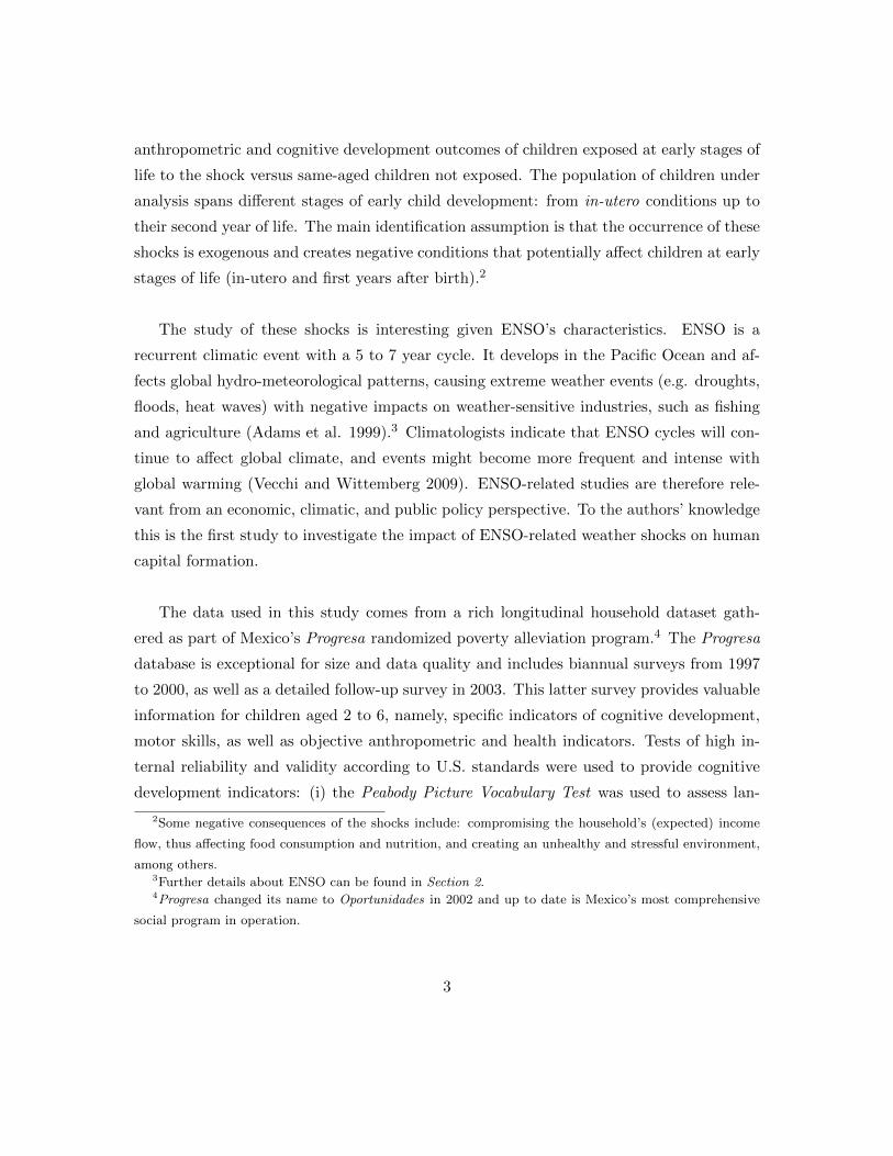
anthropometric and cognitive development outcomes of children exposed at early stages of

life to the shock versus same-aged children not exposed. The population of children under

analysis spans different stages of early child development: from in-utero conditions up to

their second year of life. The main identification assumption is that the occurrence of these

shocks is exogenous and creates negative conditions that potentially affect children at early

stages of life (in-utero and first years after birth).2

The study of these shocks is interesting given ENSO’s characteristics. ENSO is a

recurrent climatic event with a 5 to 7 year cycle. It develops in the Pacific Ocean and af-

fects global hydro-meteorological patterns, causing extreme weather events (e.g. droughts,

floods, heat waves) with negative impacts on weather-sensitive industries, such as fishing

and agriculture (Adams et al. 1999).3 Climatologists indicate that ENSO cycles will con-

tinue to affect global climate, and events might become more frequent and intense with

global warming (Vecchi and Wittemberg 2009). ENSO-related studies are therefore rele-

vant from an economic, climatic, and public policy perspective. To the authors’ knowledge

this is the first study to investigate the impact of ENSO-related weather shocks on human

capital formation.

The data used in this study comes from a rich longitudinal household dataset gath-

ered as part of Mexico’s Progresa randomized poverty alleviation program.4 The Progresa

database is exceptional for size and data quality and includes biannual surveys from 1997

to 2000, as well as a detailed follow-up survey in 2003. This latter survey provides valuable

information for children aged 2 to 6, namely, specific indicators of cognitive development,

motor skills, as well as objective anthropometric and health indicators. Tests of high in-

ternal reliability and validity according to U.S. standards were used to provide cognitive

development indicators: (i) the Peabody Picture Vocabulary Test was used to assess lan-

2Some negative consequences of the shocks include: compromising the household’s (expected) income

flow, thus affecting food consumption and nutrition, and creating an unhealthy and stressful environment,

among others.3Further details about ENSO can be found in Section 2.4Progresa changed its name to Oportunidades in 2002 and up to date is Mexico’s most comprehensive

social program in operation.

3

guage development; and (ii) three sub-tests of the Woodcock-Munoz Test5 provided working

and long-term memory, and visual-spatial thinking indicators (Schrank et al. 2005). An-

thropometric and health variables include height, weight, hemoglobin, and self-reported

health. Gross motor skill measures were obtained by administering the McCarthy Scale of

Children’s Abilities Test, and include balance and physical coordination.

To identify children exposed to ENSO-related weather shocks during their early stages

of life, the Progresa database was spatially merged with a monthly precipitation gridded

dataset using the child’s household geographical location. The climatic data used is publicly

available from the University of East Anglia Climate Research Unit, (UEA CRU-TS2p1)

and includes interpolated monthly time-series from 1961 to 1999, with a spatial resolution

of 0.5 x 0.5 degrees (Mitchell 2005). The magnitude of the deviation from the historical av-

erage monthly rainfall level in a given grid is used to identify extreme precipitation events.6

The main findings in this paper indicate medium-term negative effects of excessive rain

shocks on cognitive and anthropometric indicators. Children exposed to the shock during

the first two years of their life suffered the most severe consequences. Language develop-

ment, working memory, and visual-spatial thinking test scores of these children are 21, 19,

and 13 percent lower than same-aged children not exposed, respectively. Also, they exhibit

lower weight (0.84 lb.), height (0.71 in.), and higher likelihood of stunting (13 percentage

points). Similarly, children born the same year and up to one year after the shock obtain

lower cognitive results (that range from 11 to 16 percent), lower height (0.49 in.), and

higher likelihood of stunting (14 percentage points). No strong evidence of negative effects

is found for gross motor skills.

Furthermore, the longitudinal structure of the dataset allows investigating which house-

hold’s characteristics were most affected by the shock after its occurrence, and thus con-

tributed to the negative medium-term consequences found in children. Our estimates show

that the extreme rainfall events at the end of the harvest season represented an important

negative income shock. Total household income, reported two months after the shock oc-

5Spanish version of the Woodcock-Johnson Tests of Cognitive Abilities.6This is a standard practice recommended by climatologists (Heim 2002; Keyantash and Dracup 2004).

4

curred, was 39 percent lower for households living in regions exposed. This negative income

effect persisted up to two years after the shock occurrence. The value of food consumption

(per adult equivalents) was 10 to 15 percent lower when comparing households in exposed

versus non-exposed regions. Diet composition also had significant effects: up to two years

after the shock, households in affected regions significantly reduced their animal-origin pro-

tein consumption, as well as fruits and vegetables. Finally, mother’s self-reported measures

about their children’s sickness did not show any short nor medium-term effect from the

shocks.

The final part of this paper tests whether Progresa, a conditional cash transfer pro-

gram targeting poor rural households, helped mitigating the negative effects of ENSO-

related rainfall shocks. Progresa’s randomized evaluation phase took place between 1997

and 2000, which coincides with the ENSO event analyzed in this paper. This regional

and temporal coincidence provides a great opportunity to assess the possible benefits of

Progresa as an insurance mechanism against rainfall shocks.

Two empirical strategies were used for the Progresa analysis. First, the randomization

at the village level is employed.7 Given that the outcomes analyzed come from the 2003

follow-up survey, the comparison should be interpreted as an early versus late random al-

location (rather than treatment versus control). Second, a regression discontinuity design

is estimated using the administrative rule to select beneficiaries. This analysis is able to

identify effects of being a program beneficiary from its start (1998) with respect to early

2002.

No evidence of direct nor mitigating effects of Progresa on anthropometric and cognitive

outcomes is found. Despite providing cash transfers that household’s could choose how to

spend, Progresa does not offset the negative effects on consumption and diet composition

in the periods that follow the negative shock. Similarly, Paxson and Schady (2008) and

Fernald and Gertler (2004) find slightly positive to no direct effects on anthropometric and

7Villages that were selected for treatment began receiving the benefits in May 1998 while control villages

were added between February and May 2000.

5

cognitive development indicators from randomized poverty alleviation programs in Ecuador

(Bono de Desarrollo Humano) and Mexico (Progresa), respectively.

The remainder of the paper is organized as follows. Section 2 gives some background

on ENSO and maize agriculture. Section 3 describes the socioeconomic, child development

and climatic datasets used. Section 4 explains the identification strategy followed. Section

5 details the results of the anthropometric, cognitive, and motor skills outcomes. Section

6 analyzes the possible mechanisms that might be driving these medium-term outcomes.

Section 7 provides evidence from the Progresa analysis. Finally, section 8 concludes.

2 Background on ENSO and its effects

2.1 El Nino Southern Oscillation (ENSO)

ENSO is a recurrent quasi-periodic climatic event with a 5 to 7 year cycle and global mete-

orological impacts. It develops across the Pacific Ocean and combines two phenomena: (i)

a positive sea-surface temperature anomaly in the eastern tropical Pacific called El Nino8

(or La Nina in case of a negative temperature anomaly); and (ii) an atmospheric pressure

anomaly in the western tropical Pacific Ocean (i.e the Southern Oscillation). ENSO os-

cillates between its two extremes: El Nino (warm event) and La Nina (cold event). Each

phase typically lasts one year, with a peak in December, and then tapers down towards a

neutral state.

ENSO affects hydro-meteorological patterns around the world, causing extreme weather

events such as droughts, floods, and heat waves (Ropelewski and Halpert 1987; Philander

1990; Neelin et al. 1998; Larkin et al. 2005). Its strongest impacts are observed in coun-

tries bordering the Pacific Ocean, from Latin America to Southeast-Asia; however, ENSO’s

consequences reach regions as far as India and Africa (Cane et al. 1994).

8The term El Nino is the Spanish expression for The Child. It is a religious allegory that refers to the

arrival of Child Jesus (or the Nativity) because the periodic warming of eastern Pacific, along the coasts of

Peru and Ecuador was originally noticed after mid-December, around Christmas.

6

ENSO-related changes in weather patterns influence the frequency and intensity of

tropical storms, including a decrease (increase) in Atlantic hurricane activity (Gray 1984)

and an eastward (westward) shift of western Pacific cyclone activity during El Nino (La

Nina) (Revell and Goulter 1986; Chan 2000). Changes in climatic patterns and oceanic

circulation during ENSO events strongly influence terrestrial and marine ecosystems, and

societies around the globe. El Nino and La Nina events tend to differ for onset, mag-

nitude, spatial extent, duration and cessation (Ropelewski and Halpert 1987; Philander

1990; Allan 2000). Figure A.1 in the Appendix shows the spatial distribution of regional

precipitation anomalies, associated to different La Nina events occurred in late summer

(September-October). This study will focus on the late-summer rainfall shocks related to

the 1998-1999 La Nina event.

There is evidence suggesting that ENSO cycles have occurred for more than 6,000 years

(Markgraf and Diaz 2000), and will continue to occur and influence global climate in the

future. Moreover, ENSO events might become more frequent and more intense; ENSO

activity and characteristics appear to be strongly related to the tropical Pacific climate

system, which is expected to change during the 21st century in response to climate change

(Vecchi and Wittemberg 2009). It is, therefore, of great interest to understand the nature

and magnitude of ENSO impacts on society.

2.2 ENSO, weather and agriculture

ENSO periodically causes severe socioeconomic consequences in both developed and de-

veloping countries. The estimated costs of the two largest El Nino events of the twentieth

century were: 8 to 18 billion U.S. dollars (USD) for the 1982-83 event (UCAR 1994;

Sponberg 1999), and 35 to 45 billion USD for the 1997-98 event (Sponberg 1999). In devel-

oping countries, weak or absent insurance and credit markets make households employed

in weather-sensitive industries (e.g. agriculture and fishing) particularly vulnerable to cli-

matic events of this nature.

For this study, data was collected from Mexican poor rural areas where most of the

households depend directly or indirectly on agriculture. Most of the farmers surveyed

7

report growing maize under a rain-fed system (around 90% of the households). Maize

represents the most important crop in Mexico. Between 1996-2006, maize production

amounted for 51% of the surface planted, generated 7.4% of the total agricultural volume

produced, and represented 30% of the value of total production. Maize has two main agri-

cultural seasons: Spring-Summer (78.5% of total production) and Autumn-Winter (21.5%)

(SAGARPA 2008).

This study will focus on the Spring-Summer agricultural season, the most important

in terms of production. The agricultural season includes three main stages: (i) planting

(April-June), (ii) growing (July-August), and (iii) maturation and harvesting (September-

November). Conde et. al. (2004) indicate that April’s rain is fundamental for a successful

maize crop. If rain doesn’t arrive by May, farmers usually switch their crop to other vari-

eties that develop faster and have shorter cycles, mainly oat, which can be planted up to

June.9 Later, the growing season is vulnerable to lack of rain (FAO 1991). Finally, the

harvest season, which is the one we focus on in this study, is sensitive to hurricanes and

flooding events (SAGARPA 2008).

Figure 1 shows the rainfall distribution10 in the area under study for the Spring-Summer

agricultural seasons related to the 1997-1998 El Nino and 1998-1999 La Nina events. We

choose to analyze the extreme rainfall events at the end of the 1999 agricultural season

because of the high degree of spatial rainfall variability at the harvest season. As seen

in Figure 1, the 1997-1998 El Nino was also characterized by droughts at the beginning

of the agricultural season. The low variability of rainfall meant that most of the region

under study was similarly affected by this shock. Households could react to droughts at

the beginning of the agricultural season by shifting resources to other income generating

activities, for example, migrating seasonally or permanently (Munshi 2003). On the other

end, extreme rainfall shocks at the end of the agricultural season were closer to negative

9A popular Mexican farmer’s rhyme describes this behavior: “What Saint John doesn’t see born (June

24th), Saint Peter considers lost (June 29th)” (authors’ translation to the original: “Lo que San Juan no

ve nacido, San Pedro lo da por perdido”).10The region under study is divided by 0.5 degree x 0.5 degree grids. The graph illustrates the distribution

of rainfall standardized deviations from the 1961-1999 historic averages for the different grids.

8

income shocks given that all the investment of labor and resources had already been spent

on the crop. Evidence from the households in the database used suggests that these rainfall

shocks were unexpected.11

3 Data

3.1 Progresa Data

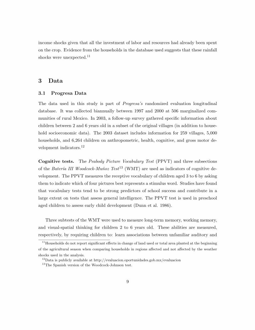
The data used in this study is part of Progresa’s randomized evaluation longitudinal

database. It was collected biannually between 1997 and 2000 at 506 marginalized com-

munities of rural Mexico. In 2003, a follow-up survey gathered specific information about

children between 2 and 6 years old in a subset of the original villages (in addition to house-

hold socioeconomic data). The 2003 dataset includes information for 259 villages, 5,000

households, and 6,264 children on anthropometric, health, cognitive, and gross motor de-

velopment indicators.12

Cognitive tests. The Peabody Picture Vocabulary Test (PPVT) and three subsections

of the Baterıa III Woodcock-Munoz Test13 (WMT) are used as indicators of cognitive de-

velopment. The PPVT measures the receptive vocabulary of children aged 3 to 6 by asking

them to indicate which of four pictures best represents a stimulus word. Studies have found

that vocabulary tests tend to be strong predictors of school success and contribute in a

large extent on tests that assess general intelligence. The PPVT test is used in preschool

aged children to assess early child development (Dunn et al. 1986).

Three subtests of the WMT were used to measure long-term memory, working memory,

and visual-spatial thinking for children 2 to 6 years old. These abilities are measured,

respectively, by requiring children to: learn associations between unfamiliar auditory and

11Households do not report significant effects in change of land used or total area planted at the beginning

of the agricultural season when comparing households in regions affected and not affected by the weather

shocks used in the analysis.12Data is publicly available at http://evaluacion.oportunidades.gob.mx/evaluacion13The Spanish version of the Woodcock-Johnson test.

9

visual stimuli; remember and repeat single words, phrases, and sentences; and identify an

object’s picture from a partial drawing or representation. Schrank et al. (2005) describe

these abilities as follows: (i) long-term memory is the ability to store information and

fluently retrieve it later; (ii) working memory (also referred to as short-term memory) is the

capacity to hold information in immediate awareness while performing a mental operation

on the information; and (iii) and visual-spatial thinking is the ability to perceive, analyze,

synthesize, and think with visual patterns, including the ability to store and retrieve visual

associations. Because of their high internal reliability and validity,14 the WMT and the

PPVT are regularly selected to evaluate early childhood abilities and have been found to

be good predictors of later school achievement (Duncan et al. 2007).

Anthropometric variables. The 2003 Progresa follow-up survey also includes objec-

tive measures of height and weight collected by a qualified nurse for all the children in the

sample. The binary variable stunting is constructed based on the WHO definition: equal to

one if the child’s height is two or more standard deviations below the age-sex standardized

height of a healthy reference population (World Health Organization 1979). Stunting, or

low weight for age, usually reflects insufficient nutrient intake during early stages of devel-

opment. It generally occurs before age two and once established, it is usually permanent

(most children never gain the height lost nor achieve a normal body weight). Consequences

may be extremely severe: a stunted growth may lead to premature death later in life due to

incomplete development of vital organs during childhood. Less extreme effects also include

delayed development, impaired cognitive function, and poor school performance (UNICEF

2007).

Health indicators. Blood samples were also gathered for all children as part of the 2003

data collection. By using hemoglobin levels, adjusted for village altitude, an indicator for

anemia is generated based on the World Health Organization standards (Ruiz-Arguelles

and Llorente-Peters 1981). Anemia is usually an indicator of poor nutrition (mainly iron

14In educational testing, internal reliability indicates the degree to which test scores for a group of test

takers are consistent over repeated applications of the measurement procedure (AERA 1999, pp. 180).

Validity refers to the degree to which accumulated evidence and theory support specific interpretations of

the test scores (AERA 1999, pp. 184.).

10

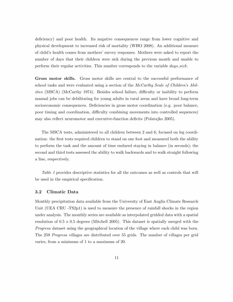
deficiency) and poor health. Its negative consequences range from lower cognitive and

physical development to increased risk of mortality (WHO 2008). An additional measure

of child’s health comes from mothers’ survey responses. Mothers were asked to report the

number of days that their children were sick during the previous month and unable to

perform their regular activities. This number corresponds to the variable days sick.

Gross motor skills. Gross motor skills are central to the successful performance of

school tasks and were evaluated using a section of the McCarthy Scale of Children’s Abil-

ities (MSCA) (McCarthy 1974). Besides school failure, difficulty or inability to perform

manual jobs can be debilitating for young adults in rural areas and have broad long-term

socioeconomic consequences. Deficiencies in gross motor coordination (e.g. poor balance,

poor timing and coordination, difficulty combining movements into controlled sequences)

may also reflect neuromotor and executive-function deficits (Polatajko 2005).

The MSCA tests, administered to all children between 2 and 6, focused on leg coordi-

nation: the first tests required children to stand on one foot and measured both the ability

to perform the task and the amount of time endured staying in balance (in seconds); the

second and third tests assessed the ability to walk backwards and to walk straight following

a line, respectively.

Table 1 provides descriptive statistics for all the outcomes as well as controls that will

be used in the empirical specification.

3.2 Climatic Data

Monthly precipitation data available from the University of East Anglia Climate Research

Unit (UEA CRU -TS2p1) is used to measure the presence of rainfall shocks in the region

under analysis. The monthly series are available as interpolated gridded data with a spatial

resolution of 0.5 x 0.5 degrees (Mitchell 2005). This dataset is spatially merged with the

Progresa dataset using the geographical location of the village where each child was born.

The 259 Progresa villages are distributed over 55 grids. The number of villages per grid

varies, from a minimum of 1 to a maximum of 20.

11

In the estimations, a binary variable for the ENSO-related rainfall shock (rain shock)

is used to analyze the impact of negative conditions during early stages of life on chil-

dren’s outcomes. The variable was constructed using each grid’s standardized precipitation

anomaly. The standardized precipitation anomaly indicates the number of standard devi-

ations from the long-term mean (1961-1999) for each grid-month pair. A rainfall shock

is identified (rain shock = 1) whenever the standardized precipitation anomaly is above

0.7 standard deviations in September or October of 1999 (harvest months). The threshold

to identify the weather shocks comes from conversation with climatologists who indicated

that this level is already dangerous (destructive) for the crop during the harvest season.

Nonetheless, in section 5, a sensitivity analysis will consider changing the 0.7 standard

deviations cutoff to 0.5 and 1 to assess the relevance of the cutoff point used to define the

shock. Figure 1 shows the monthly distribution of the standardized precipitation anoma-

lies used to define the rainfall shocks.

The use of the standard precipitation anomalies to identify the shocks is supported by

extensive applications in the climatology literature (Heim 2002; Keyantash and Dracup

2002). The decision to use a binary variable for the rain shocks was motivated by two

main reasons: (i) the qualitative evidence found on weather reports indicates substantive

loss of crops as a result of floods, therefore, the relation between crop output and rainfall

would not be easily fitted with a parametric functional form; and (ii) the use of the binary

variable aids the ease of interpretation of the results. Furthermore, the use of different

thresholds in the robustness checks informs about the pattern of the results with respect

to the standardized precipitation anomalies.

4 Empirical Specification

The following specification seeks to identify the medium-term effect of excessive rainfall

shocks occurring at early stages of children’s development on anthropometric, health, cog-

nitive development and gross motor skill outcomes. The analysis considers children born

between 1997 and 2001.

12

Yij =

( 2001∑k=1997

γkcoh kij + ηkrain shockj ∗ coh kij)

+ βXij + νj + εij (1)

where Yij is the outcome for individual i in pixel j , coh kij is an indicator for individ-

ual i in pixel j of being born on year (cohort) k, rainj is an indicator for a weather shock

occurrence in pixel j, Xij are controls for individual i in pixel j, and νj gives pixel-clustered

standard errors.

Yij refers to the set of outputs under analysis that include: (i) anthropometric vari-

ables, such as weight, height, and stunting; (ii) the logarithm of cognitive test results,

which include the Peabody test and three subsections of the Woodcock-Munoz test; (iii)

health indicators, such as anemia and self-reported health; and (iv) motor skills coordina-

tion results, which include variables from the McCarthy test.

On each estimation, the main parameter of interest will be ηk. Given that the rain

shock used for the estimations took place in a specific year (1999), the ηk parameter will

indicate the effect of the shock for children in a given development stage with respect to

same-aged children that were not affected by the shock. For example, η1997 will give the

effect of the shock on children that were one to two years old at the time of the shock with

respect to same-aged children not affected.

Exogeneity Test. The main identification assumption is that the occurrence of the

shocks is exogenous and generated negative conditions that affected children at early stages

of life. To test the exogeneity assumption of the shocks, the longitudinal feature of the

dataset is employed. Using the baseline data from 1997, which corresponds to household’s

information before the rainfall shock took place, a group of indicators is aggregated at the

village level. Table 2 shows the results from testing the difference of means for several

observable indicators extracted from the household’s survey.15 The statistics show that for

15The tests were also done using individual level data, and comparing individuals living in localities

exposed to the shock with those living in localities not exposed. The same results are derived whether the

test uses individual or grid level data.

13

most observable characteristics there is no difference between villages affected and those

not affected by the rainfall shocks at the baseline.

Spatially-correlated standard errors. The estimation of equation 1 adjusts for clus-

tered standard errors by grid. This assumption allows for correlation between observations

geographically located in the same grid-cell (i.e. pixel). However, it also assumes that errors

of observations located in adjacent grids are independent from each other. In the economic

literature, a growing number of studies that use geographical data have adopted an alter-

native solution that allows for correlation between observations closely located (Dell et al.

2009; Deschenes and Greenstone 2006). The strategy is based on Timothy Conley (1999)

work, who proposed a methodology to correct for spatial correlation when estimating the

standard errors. Conley’s correction consists in allowing the variance-covariance matrix

to have correlated standard errors if the observations are located within a pre-specified

distance threshold (the threshold has to be assumed).16 The main estimates in this paper

include clustered and spatially correlated standard errors (with 1 decimal degree cutoff

assumed). A sensitivity analysis for the standard errors is included in the supplementary

material.

5 Results

5.1 Effects on anthropometric and health indicators

Table 3 presents the estimated effects of excessive rainfall shocks during the 1999 harvest

season on children’s anthropometric indicators (height, weight, and a binary indicator for

stunting), and health outcomes (a binary indicator for anemia, and self-reported number

of sick days during the previous month, days sick).17

16See Conley (1999) for further details about this methodology. Statistical codes to correct for spatial

correlation are also available on Timothy Conley’s website.17Similar results were found using as main independent variable the indicator for excessive rainfall shocks

occurred in 1998 and can be made available upon request.

14

Results show significant lower weight and height for children that were exposed during

the first two years of life to the shock (0.84 lb. lower weight and 0.71 in. lower height

for those born in 1998, and 0.47 in. lower height for those born in 1997) with respect to

same-aged children not exposed. Similarly, children born the same year and one year after

the shock occurred, exhibit negative effects on height with respect to same-aged children

not affected (0.56 in. and 0.43 in., respectively).

The negative impacts on height are substantive enough to significantly increase the

probability of stunting. Children born between 1998 and 2001 are significantly more likely

to be stunted if they were exposed to the 1999 rainfall shock. The probability of stunting

is 14 percentage points higher for children born in 1999 and 2000, and 12 percentage points

higher for children born in 1998 and 2001 compared to same-aged children not affected by

the shock).

There is no evidence to suggest that anemia and children’s number of sick days (reported

by their mothers) are significantly affected by the weather shocks.

5.2 Effects on cognitive development

As described on Section 3, the 2003 Progresa survey includes several specific cognitive tests:

language skills (Peabody Test), long-term memory, short-term memory, and visual-spatial

thinking (Woodcock-Munoz Test). For the estimations, we use as outcomes the logarithm

of the test scores.

Table 4 reports the estimated effects of excessive rainfall shocks during the 1999 harvest

season on the test scores that measure specific cognitive abilities . The estimates suggest

negative and significant effects of the rainfall shocks on language development, long-term

memory, and visual-spatial thinking abilities. The larger negative effects are mostly found

on children who were affected by the shock during their first or second year of life (i.e.

children born in 1997 and 1998). This group of children exhibits 21, 19, and 13 percent

lower test scores on the language, long-term, and visual-spatial thinking tests, respectively,

with respect to same aged-children not affected by the shock. Lower (in absolute terms),

15

but still significant negative effects are found for children born the year of the shock (1999)

or the following year (2000); these negative outcomes range, in absolute value, from 11 to

14 percent. No significant effects were found in short-term memory test scores.

5.3 Effects on gross motor skills

Table 5 shows the effects on gross motor skills measured with outcomes from the McCarthy

Scale of Children’s Abilities Tests. No strong and consistent evidence of negative effects

of the shocks is found for these outcomes. Balance is the only outcome for which minor

negative effects from the rainfall shocks are found, being the effect on the 1997 cohort the

only statistically significant (decrease in 0.7 seconds in the ability to hold balance with one

foot).

5.4 Correction for spatially-correlated standard errors

Tables 3, 4, and 5 show the main estimation results calculated with clustered SEs by

grid (shown in brackets) and, alternatively, using Conley’s proposed corrections for spatial

correlation with a 1 decimal degree cutoff (shown in parentheses). As evidenced in the

tables, some of the standard errors increase as a result of allowing for spatial correlation, but

this increase tends to be small and does not affect the statistical significance of the results.

Table A.1 summarizes three alternatives for the calculation of the standard errors: clustered

by pixels, and two estimates of Conley SEs using 1 and 2 decimal degrees thresholds,

respectively. The standard errors for the anthropometric estimations are the most sensitive

to spatial correlation correction, but overall, the significance of the results remains.

5.5 Persistent effects of the shock

Exposure to weather shocks can have not only immediate impacts on children’s life con-

ditions, but also persistent effects over multiple years, such as an extended reduction of

income and consumption. Section 6 will investigate some of the mechanisms that might be

contributing to the negative effects on children’s cognitive and anthropometric indicators.

That section will provide further evidence of the prolonged effects that the shocks had on

these mechanisms.

16

Results for both anthropometric and cognitive outcomes indicate that children in their

first or second year of life at the time of the shock were more severely affected. However,

this does not necessarily mean that the shock had stronger effects if exposure occurred in

early childhood rather than in-utero. Given the persistent effects of the shocks on some of

the mechanisms, this could also mean that these chidlren were exposed to the shock for a

longer period of time. Similarly, estimates in tables 3 and 4, suggesting that children born

one year after the shock (in 2000) are negatively affected, could also result from negative

conditions in-utero and shortly after birth.

5.6 Robustness checks

Adding controls from the exogeneity test. As discussed in Section 4, the empirical

specification of this study is based on the assumption that the rain shock is exogenous.

The evidence presented in Table 2 supports this hypothesis. As a robustness test, the

few variables that presented significant differences in means in Table 218 are added to the

estimation. If the initial estimates presented are capturing regional effects, it is likely that

these additional control variables will pick up some of that effect, thus altering the main

coefficients. Tables A.2, A.3, and A.4 show that the main estimates do not change signifi-

cantly when these additional controls are added.

Sensitivity analysis for different weather shock cutoffs. A second robustness test

consisted on varying the threshold value used to define the rain shock variable (rain shock).

For this sensitivity test we adopted two additional cutoff points: 0.5 and 1 standard devi-

ation. Tables A.5, A.6 and A.7 suggest that both thresholds – using 0.5 and 1 standard

deviations to define the shock – yield similar results to the original estimates. Adopt-

ing the lower 0.5 threshold, produces larger significant coefficients; the reverse is observed

when the more stringent cutoff of 1 standard deviation is employed. These results sug-

gest that lower precipitation anomalies are enough to negatively affect children. When the

18The household characteristics presenting significantly different means are: (i) TV, (ii) vehicle, and (iii)

poultry ownership, (iv) household with permanent migrants at the U.S., (v) an indicator for household

head speaking an indigenous language, and (vi) an indicator for household head speaking both Spanish and

an indigenous language.

17

1 standard deviation cutoff is adopted, some children that were actually exposed to the

shock, are erroneously included in the control group, yielding a lower estimate for the shock.

6 Mechanisms Driving the Results

This section explores some of the mechanisms that might be driving the medium-term

effects of the rain shock on children’s cognitive development and anthropometric outcomes.

To do this, we exploit the longitudinal design of the database, spanning three years from

1998 to 2000, to analyze immediate and persistent effects of the weather shock on household

dimensions that may affect the child’s growing environment. We adopt the model described

in equation 1 to estimate the effect of the rainfall shock on these possible intermediate

mechanisms. As in the previous analysis, the underlying assumption for the identification

is the exogeneity of the shock. Tables 6 and 7 show the main results of the mechanisms

analysis.

Income. In response to shocks, households may experience income reductions with pos-

sible consequent contractions in consumption. We estimate the effect of rainfall shocks on

total household income and income from agricultural activities measured in the year of the

shock (period t) and up to two years after the shock (at periods t+ 1 and t+ 2).

The estimates indicate that households exposed to the shock have lower total income

than those not affected, being the effect persistent over three periods t, t+ 1, t+ 2: from

about 40% decline in period t to 26% in period t+ 2. Results for income from agricultural

activities are comparable: from about 28% decline in period t to 18% in period t+ 2.

Government aid. Post-shock governmental food and non-food aid might help smooth

consumption, particularly food consumption. The Progresa dataset allows us to assess if

villages exposed to shocks are more likely to have benefited from government transfers.

We find that the probability of receiving government food aid increases by 5% immediately

after the shock for households living in affected villages. Nevertheless, the government

18

aid did not seem to have neutralized the negative effect of the shocks on medium-term

children’s outcomes.

Informal transfers. In rural villages, informal insurance strategies aimed at smoothing

post-shock consumption include food and non-food transfers from relatives or neighbors.

From the data available it is possible to see if there was a response to the shocks in

terms of family or neighbor related transfers. The results show no significant changes in

the probability of receiving informal transfers from family members immediately after the

shock. However, we do observe a significant decrease of 3% in the probability of receiving

transfers from neighbors. Weakening of intra-village transfers may be explained by the fact

that neighbors were also exposed to the rain shock.

Consumption and diet composition. The negative effect on income, paired with ab-

sence of formal insurance and credit markets, and the weakening of informal safety nets (e.g.

intra-village transfers), may lead to consumption contractions. Non-food consumption is

usually the first portion of household consumption to be reduced. When these reductions

are insufficient to protect food consumption and savings are not available, households must

inevitably reduce the value of their food consumption, often by adopting changes in their

diet composition or even by reducing their food intake.

We estimate the effect of excessive rainfall shocks on food consumption and in diet

composition at periods t, t+ 1 and t+ 2. Results in Table 7 show contractions in the value

of food consumption over the three periods (10% on t, 11% on t+ 1, and 15% on t+ 2) for

households exposed to rainfall shocks with respect to those not exposed. These estimates

confirm the results found by Vicarelli (2011) using data for all the Progresa villages (506)

included in the pilot phase.

A reduction in the monetary value of food consumption is likely to lead to a dietary

shift towards cheaper foods. As expected, three main changes in diet composition are also

found in households exposed to the shock, compared to households not exposed. First,

consumption of tortillas19 increased immediately after the shock (13%), but later decreased

19Maize tortillas are the main food staple in Mexico

19

in period t+ 2 (22%). Second, consumption of animal-origin products decreased in periods

t+ 1 and t+ 2 by 14% and 17%, respectively. Lastly, consumption of fruit and vegetables

decreased by 20% in period t and 14% in period t + 2. This shift towards cheaper foods,

by privileging tortillas over the consumption of nutritious foods rich in animal proteins

(e.g. meat, fish, eggs, milk), might have negative consequences on the health conditions

and development of young children.

Health of household members and medicine expenditures. Worse health condi-

tions for children in household exposed to weather shocks immediately after the shock

might point to health as a possible channel for the medium-term results. Table 7 presents

estimates of the impact of the rainfall shock on two health-related measures: the propor-

tion of children reported sick by the mother within each household (children sick) and

medicine expenditures (medicine expenditure) immediately after the weather shock (pe-

riod t) and up to two years after its occurrence. The results seem to suggest that: health

conditions reported by the mother were not affected; and medicine expenditures decreased

for households exposed to shocks by 36% in period t and 30% in period t+ 1. Nonetheless,

results for medicine expenditure are very likely to be driven by liquidity constraints rather

than changes in health status.

7 The Role of Progresa

In 1997, villages in the region under analysis were selected to be included in a governmen-

tal conditional cash transfer (CCT) program, called Progresa. This section describes the

program and investigates its potential mitigating effects against the negative consequences

of exposure to the rainfall shock for households eligible to receive the program.

7.1 Brief Progresa’s Background

Progresa, now called Oportunidades, is a conditional cash transfer program initiated in 1997

by the Mexican government. Nowadays, it is Mexico’s most comprehensive and extensive

poverty alleviation program with a 5.6 million households’ coverage (SEDESOL 2011). Its

purpose is to break the intergenerational cycle of poverty through a combination of health

20

and education interventions. The delivery of the cash transfers is conditional on children’s

school attendance, as well as periodic health check-ups of all family members. The amounts

of the transfers vary mainly by the number, age, and gender of the children at school age.

Up to date, households receive on average US$588 per year, which corresponds to 0.6 times

the amount an individual would earn working for a minimum salary and 0.36 times what

the fifth decile household earns.

By design, the intervention included a randomized program evaluation that took place

between 1997 and 2000, with follow-up surveys in 2003 and 2007 to assess its short and

medium-term benefits (Skoufias 2001; Behrman et al. 2005). The identification strategy of

eligible households occurred in three stages. First, 506 poor rural communities from seven

different states were selected for the sample. These localities were identified in the 1990

and 1995 Censuses as highly marginalized rural communities20 with at least fifty house-

holds and access to both education and health services. Second, within each community,

a baseline socioeconomic survey ENCASEH (Encuesta de Caracterısticas Socioeconomicas

de los Hogares) was administered to all households on November 1997. This information

was used to construct a poverty index for each household based on its asset ownership and

socio-economic characteristics of its members. Eligibility for the program was determined

based on this index and a pre-determined threshold. Third, localities in the sample were

randomly assigned to either the treatment (320) or control group (186). Eligible house-

holds in treatment communities were notified of their selection for the program and most of

these families started receiving the benefits around May of 1998. Less than two years later,

between January and May 2000, eligible households from the control communities were in-

corporated into the program. (Skoufias et al. 1999; Coady 2000; Fernald and Gertler 2004)

20Marginalization was defined using a pre-determined locality-level index generated every five years by the

Mexican Ministry of Population. This index combines several locality’s characteristics. Rural communities

are defined as those below 2,500 inhabitants.

21

7.2 Empirical identification of Progresa’s effects

Randomized Experiment. Most of the previous work related to Progresa has taken

advantage of the randomization aspect of it. Behrman and Todd (2000) showed that several

basic variables such as age, gender, income, and schooling are balanced when comparing

households in control and treatment localities. The first empirical estimation used here to

assess the potential mitigating effects of Progresa follows the line of randomized control

trial’s estimations:

Yj = η1rain shockj + η2Treatj + η3rain shockj ∗ Treatj + εj (2)

where Yj represents the outcomes (cognitive and anthropometric) aggregated at the

village level; rainj represents the dummy variable indicating the occurrence of the weather

shocks; and Treatj indicates if village j was randomly selected as a treatment locality.

In the specification, η2 represents the effect of the early treatment on the outcomes at

villages not exposed to rain shocks, and η2 + η3 represents the effect of the early treatment

in villages affected by the shocks. In this estimation, it is important to keep in mind that

the control villages were added to the program in 2000, less than two years after the treat-

ment villages. Therefore, the randomization makes possible to identify early versus late

treatment effects, rather than the more traditional treatment versus control effect.

Regression Discontinuity (RD). To implement a regression discontinuity design, we

take advantage of the administrative rule that determines eligibility based on the household

poverty index and a pre-determined cutoff. At the beginning of the program, 41 geograph-

ical regions were defined. Regions differ from each other on the weights attributed to

variables used to generate the poverty index, and the cutoff value to select beneficiaries.

A standardized poverty index (x pmtj) is formed by subtracting the regional cutoff to the

each household’s poverty index. Therefore, independently of the region, a household would

be eligible for the program if its standardized poverty index is above zero (x pmtj > 0).

The main assumption behind the RD strategy is that, other than the treatment bene-

22

fits, the households around the cutoff value are comparable to each other. Therefore, any

discrete change in an outcome variable occurring at the cutoff point can be related to the

effect of the treatment (Imbens and Lemieux 2008).21

RD methods can employ both, parametric and non-parametric estimators. However,

the best way to illustrate the RD is with graphical analysis. We organized the analysis in

two parts:

1. First Stage: we begin by showing the discontinuity of Progresa’s beneficiaries at the

administrative cutoff. We use the sample to estimate: E(Benefj |x pmtj), where

Benefj is a dummy variable equal to one if household j is a Progresa beneficiary.

If targeting of the program and compliance were perfect we would expect to have a

sharp RD.

2. Reduced Form: we show the conditional means of the outcome variables with respect

to the standardized poverty index [E(Outcomeij |x pmtj)]. Any discrete jump at the

cutoff value is attributed to the treatment. To estimate the potential mitigating

effects of Progresa against the weather shocks, this analysis is performed for two

subsamples: those observations living in villages affected by the rain shocks, and

those not.

7.3 Results on the potential mitigation effects of Progresa

Randomized Experiment. Table 8 presents the intent to treat (ITT) estimates of Pro-

gresa differencing between villages that suffered a weather shock and those that did not.

The evidence from the tables suggests that there is neither a mitigation nor a direct effect

from Progresa on the anthropometric and cognitive outcomes analyzed in this paper. To

21To assess the effectiveness of the RD method, the authors estimated the effect of Progresa on school

attendance in 1999 of children between 6 and 15 years old (the age groups whose attendance is part of

the conditionality to receive the monetary benefits). The RD estimates a 5 percentage point, statistically

significant, increase in the likelihood of school attendance at the cutoff for those children in treatment

villages. No discrete change is observed for children in control villages. Furthermore, after the cutoff, the

level of school attendance for control and treatment villages follows different trends (graph available upon

request).

23

produce this analysis, data was aggregated at the village level given that both, the ran-

domization and the identification of the weather shocks, were at the village level.22

In previous work, Fernald and Gertler (2004) find positive effects from Progresa on an-

thropometric outcomes when comparing children in experimental villages to children from

a synthetic control (formed from villages that by 2003 were still not receiving Progresa’s

benefits).23 Moreover, as in these estimates, they don’t find differences between children

in the original treatment and control villages. They argue that children in the original

control villages catch-up with children that received the benefits earlier. The key assump-

tion behind their main results is that the synthetic control villages had to be similar to the

experimental villages in 1997. However, this is a strong assumption given that Progresa

targeted the most disadvantaged localities by design. By the beginning of 2003, Progresa

had geographical presence in 2,354 municipalities (97% of Mexico’s total municipalities).

Rather than following this approach, this paper exploits the rule that determines house-

hold eligibility based on the poverty index and the pre-determined cutoffs. This gives the

ideal setup for a regression discontinuity analysis.

Regression Discontinuity. Figures 2 to 4 show the main results form the RD anal-

ysis. The first set of graphs (Figure 2 ) show the First Stage results described in Section

7.2, which justify using of RD to identify the effects of Progresa. These graphs show the

evolution of the likelihood to be a Progresa beneficiary, conditional on the standardized

poverty index (x pmt). As expected form the program’s rules, there is a discrete disconti-

nuity exactly at the cutoff level, equal to 46.5 percentage points (according to a parametric

estimate). The discontinuity persists and does no change much until 2002. Between late

2001 and early 2002, the program was expanded and the models to estimate the poverty

index changed, thus explaining the lack of discontinuity in 2002.

The analysis is restricted to treatment localities. If control localities were added, the

22Similar results are obtained if the estimates are calculated at the household level.23The synthetic control was selected using matching estimators.

24

shape of the graphs in Figure 2 would change in early 2000, when the control villages began

to receive Progresa’s benefits. By restricting the analysis to treatment villages, we have

a discontinuity that remains close to constant until 2002. Therefore, the RD estimates

give the difference between receiving the treatment from 1998 rather than from 2002 at

the discontinuity point. Given that the outcomes analyzed on this paper were measured in

2003, we believe that the RD approach should allow a better identification of the Progresa

effects. This approach gives a lower time window for households that receive the benefits

later to catch-up with those that received them form the beginning of the program. Also,

the RD assumptions are less restrictive than those required to use Progresa’s 2003 syn-

thetic control.24

Figure 3 illustrates the result of the RD analysis for two anthropometric outcomes:

weight and height. Similarly, Figure 4 gives two examples using cognitive outcomes: lan-

guage (PPVT test) and long-term memory (Woodcock-Munoz test). The triangles (circles)

in the graphs represent the conditional means for those children that were (not) affected

early on childhood by the ENSO-related shocks. The RD graphical analysis for the rest of

the anthropometric, health and cognitive outcomes is included in Figures A2 and A3 in

the supplementary material. The difference in the level of the means for the two subgroups

reflects the negative effect of the shock, which is consistent with Section’s 5 analysis. How-

ever, Progresa does not seem to provide mitigation effects against the shocks (nor even

direct effects on the outcomes).

The results are surprising given that previous research has shown positive effects of

Progresa on food consumption and diet composition (Behrman and Hoddinott 1999; Hod-

dinott et al. 2000; Vicarelli 2011). Applying the RD analysis to the consumption and diet

composition indicators analyzed in this paper, we find positive, but modest effects at the

discontinuity point. However, the positive changes on these indicators do not allow for a

mitigation of the negative effects of the rain shocks.25 Other possible explanation for a

lack of mitigation evidence includes differences in intra-household allocation of resources.

24As described previously, Fernald and Gertler (2004) use the 2003 synthetic control. Also, several other

Progresa medium-term evaluations adopted the 2003 synthetic cohort approach.25Graphs can be made available upon request.

25

Previous work has shown that when facing negative weather income shocks, children are

the most affected in terms of consumption. Baez and Santos (2007) give evidence that after

hurricane Mitch hit Nicaragua, children’s likelihood of being undernourished significantly

increased, while adult’s consumption wasn’t reported to be greatly affected. In the case of

Progresa there is also a higher incentive to protect children at school age, given that the

amount of cash transfers significantly increases with school attendance of 8 to 15 year old

children (i.e. children attending 3rd to 6th grade of primary or lower secondary). Finally,

the negative conditions that result from the exposure to weather shocks might have led

to stress. There is a growing literature that gives evidence of negative effects of early-life

exposure to stress on later physical health, cognitive abilities, and educational outcomes

(Eccleston 2011; Kaiser and Sachser 2005).

It is important to indicate that a limitation associated with the RD estimates is that

it provides a Local Average Treatment Effect (i.e. the effect of the treatment around

the cutoff level). If the treatment has heterogenous effects along the income distribution,

then this result cannot be generalized to the rest of the population. It could be argued

that the effects of Progresa are stronger for the poorest populations. However, given the

sample characteristics and Progresa’s design to target the poor, it would be expected that

the group around the cutoff to be already representative of poor (although not extreme)

Mexican rural households.

8 Conclusions

Previous work has shown that the early-life conditions tend to have a strong influence

on an individual’s life. Economists’ work has analyzed impacts on income, educational

attainment, health, and even mental and physical disabilities (Almond 2006; Almond and

Mazumder 2011; Maccini and Yang 2009). This paper contributes to the literature by esti-

mating the medium-term impact that early-life negative conditions have on specific aspects

of children’s health and cognitive development. Scores of highly reliable tests (according

to U.S. standards) inform about specific abilities that are negatively affected, namely,

language, long-term memory, and visual-spatial thinking. Objective anthropometric mea-

sures, like height, are also negatively altered. These indicators have been shown to be

26

strong predictors of school and later in life success. Hence, the paper provides information

about specific channels that might be driving the long-term effects previously encountered.

According this study, income, consumption and diet composition at early life stages are

key mechanisms that contribute to produce these results.

Weather shocks related to “El Nino Southern Oscillation” are used to identify negative

conditions at early life stages. ENSO is a recurrent climatic event with global impacts that

affects hydro-meteorological patterns, causing extreme weather events (e.g. floods, heat

waves, droughts). With global warming, extreme weather events are expected to increase

in frequency and intensity. Therefore, findings about Mexico are relevant for households

in other developing countries with comparable climates, and affected by ENSO-related

weather events (e.g. Africa, Latin America, South-East Asia). The analysis of its effects

is relevant from an economic, climatic, and public policy perspective.

Finally, no mitigation of Progresa against the negative effects of weather shocks has

been found. Some potential reasons are: (i) Progresa did not completely mitigate the

negative effects of the weather shocks on consumption and diet composition; (ii) intra-

household imbalance in the distribution of Progresa’s resources; (iii) other components

related to the weather shocks, like stress, might be contributing to the results and are

not offset by Progresa. In future work, we plan to assess the second point to determine if

intra-household allocation of resources could explain the no-effect result found for Progresa

in this and previous studies (Fernald and Gertler 2004). Heterogeneity in the effects of

Progresa with respect to children’s initial malnutrition is also on our agenda.

27

References

Alderman, Harold, John Hoddinott, and Bill Kinsey. 2006. Long term consequences of

early childhood malnutrition. Oxford Economic Papers, Oxford University Press 58 (3):

450-474.

Allan, R. 2000. ENSO and Climatic Variability in the Past 150 years. In El Nino and the

Southern Oscillation, Multiscale Variability and Global and Regional Impacts, edited by

Vera Markgraf and Henry Diaz. Cambridge, MA: Cambridge University Press.

Allan, Richard. P., and Brian J. Soden. 2008. Atmospheric warming and the amplification

of precipitation extremes. Science 5895 (321): 1481.

Almond, Douglas. 2006. Is the 1918 influenza pandemic over? Long-term effects of in utero

influenza exposure in the post-1940 U.S. population. Journal of Political Economy 114

(4): 672-712.

Almond, Douglas and Bhashkar Mazumder. 2011. Health capital and the prenatal environ-

ment: the effect of Ramadan observance during pregnancy. American Economic Journal:

Applied Economics 3 (4): 56-85.

Baez, Javier, and Indhira Santos. 2007. Children’s vulnerability to weather shocks: a nat-

ural disaster as a natural experiment. Mimeo.

Barber, Richard, and Francisco P. Chavez. 1983. Biological consequences of El Nino. Sci-

ence 222: 1203-1210.

Barker, David J.P. 1998. Mothers, Babies and Health in Later Life. Edinburgh, UK:

Churchill Livingstone.

Behrman, Jere, and John Hoddinott. 1999. Program evaluation with unobserved hetero-

geneity and selective implementation: the Mexican Progresa impact on child nutrition.

Oxford Bulletin of Economics and Statistics 67: 547-569.

Behrman, Jere, and Petra Todd. 2000. Aleatoriedad en las muestras experimentales del

Programa de Educacion, Salud y Alimentacion (PROGRESA). In Evaluacion de Resul-

tados del Programa de Educacion, Salud y Alimentacion. Mexico City: SEDESOL.

28

Behrman, Jere., Piyali Sengupta, and Petra Todd. 2005. Progressing through PROGRESA:

an impact assessment of Mexico’s School Subsidy Experiment. Economic Development

and Cultural Change 54 (1): 237-275.

Cane, Mark A., Gidon Eshel, and R.W. Buckland. 1994. Forecasting Zimbabwean maize

yield using eastern equatorial Pacific sea surface temperature. Nature 370: 204–205.

Case, Anne, and Christina Paxson. 2008. Stature and status: height, ability, and labor

market outcomes. Journal of Political Economy 116 (3): 499-532.

Chan, J. C. L. 2000. Tropical cyclone activity over the western North Pacific associated

with El Nino and La Nina events. journal of Climate. 13: 2960-2972.

Coady, David. 2000. Final Report: The Application of Social Cost-Benefit Analysis to

the Evaluation of PROGRESA. Washington, DC: International Food Policy Research

Institute. IFPRI.

Conde, Cecilia et al. 2004. El Nino y la Agricultura. In Los Impactos del Nino en Mexico,

edited by Victor Magana. Mexico City: U.N.A.M.

Conley, Timothy G. 1999. GMM estimation with cross sectional dependence. Journal of

Econometrics 92 (1): 1-45.

Dell, Melissa, Benjamin F. Jones and Benjamin A. Olken. 2009. Temperature and income:

reconciling new cross-sectional and panel estimates. American Economic Review: Papers

& Proceedings 99 (2): 198-204.

Deschenes, Olivier, and Michael Greenstone. 2006. The economic impacts of climate change:

evidence from agricultural profits and random fluctuations in weather. Research Paper

no. 04-26. Department of Economics, MIT, Cambridge.

Duncan, Greg et al. 2007. School Readiness and Later Achievement. Developmental Psy-

chology 43 (6): 1428-1446.

Ecclesston, Melissa. 2011. In Utero Exposure to Maternal Stress: Effects of 9/11 on Birth

and Early Schooling Outcomes in New York City. Mimeo.

29

Fafchamps, Marcel, Christopher Udry, and Katherine Czukas. 1998. Drought and saving

in West Africa: are livestock a buffer stock? Journal of Development Economics 55 (2):

273-305.

Fernald, Lia, and Paul J. Gertler. 2004. The medium term impact of Oportunidades on

child development in rural areas. Final Report. SEDESOL, Mexico City.

Gine, Xavier et al. 2008. Microinsurance: a case study of the Indian Rainfall Index Insur-

ance Market. Policy Research Working Paper Series no. 5459. World Bank, Wasington

DC.

Gray, William M. 1984. Atlantic seasonal hurricane frequency. Part I: El Nino and 30 mb

quasi-biennial oscillation influences. Monthly Weather Review 112: 1649-1668.

Heim, Richard. 2002. A review of twentieth-century drought indices used in the United

States. Bulletin of the American Meteorological Society 84: 1149-1165.

Hoddinot, John, Emmanuel Skoufias, and Ryan Washburn. 2000. The Impact of Mexico’s

Programa de Educacion, Salud y Alimentacion on Consumption. Washington DC: Inter-

national Food Policy Research Institute. IFPRI.

Holmgren et al. 2001. El Nino effects on the dynamics of terrestrial ecosystems. Trends in

Ecology and Evolution 16 (2): 89-94.

IPCC. Solomon, Susan et al. 2007. Climate Change 2007: The Physical Science Basis. Con-

tribution of Working Group I to the Fourth Assessment Report of the Intergovernmental

Panel on Climate Change. Cambridge U.K.: Cambridge Univ. Press.

Imbens, Guido, and Thomas Lemieux. 2007. Regression discontinuity designs: a guide to

practice. Journal of Econometrics 142 (2): 615-635.

Kaiser, Sylvia, and Norbert Sachser. 2005. The Effects of Prenatal Social Stress on Be-

haviour: Mechanisms and Function. Neuroscience and Biobehavioral Reviews 29: 283-

294.

30

Keyantash John, and John Dracup. 2004. An aggregate drought index: assessing drought

severity based on fluctuations in the hydrological cycle and surface water storage. Water

Resources Research 40: W09304.

Larkin, Narasimhan, and D. E. Harrison. 2001. ENSO warm (El Nino) and cold (La Nina)

event life cycles: ocean surface anomaly patterns, their symmetries, asymmetries, and

implications. Journal of Climate 15: 1118-1140.

Larkin, Narasimhan, and D. E. Harrison. 2005. Global seasonal temperature and precip-

itation anomalies during El Nino autumn and winter. Journal of Geophysical Research

Letters 32 :L16705. DOI: 10.1029/2005GL022860.

Maccini, Sharon, and Dean Yang. 2009. Under the weather: health, schooling, and eco-

nomic consequences of early-life rainfall. American Economic Review 99 (3): 1006-1026.

Markgraf, Vera, and Henry Diaz. 2000. El Nino and the Southern Oscillation, Multiscale

Variability and Global and Regional Impacts. Cambridge, MA: Cambridge University

Press.

Mitchell, Timothy D. 2005. An improved method of constructing a database of monthly

climate observations and associated high resolution grids. International Journal of Cli-

matology 25: 693-712.

Munshi, Kaivan. 2003. Networks in the modern economy: Mexican migrants in the U.S.

labor market. Quarterly Journal of Economics 118 (2): 549-599.

Neelin, J. D. et al. 1998. ENSO theory. Journal of Geophysical Research 103:14261-14290

871.

Paxson, Christina, and Norbert Schady. 2008. Does money matter? The effects of cash

transfers on child health and development in rural Ecuador. Policy Research Working

Paper no. 4226. World Bank, Washington DC.

Philander, S. George. 1990. El Nino, La Nina and the Southern Oscillation. San Diego,

CA: Academic Press.

31

Polatajko, H. J. et al. 1995. A clinical trial of the process-oriented treatment approach for

children with developmental co-ordination disorder. Developmental Medicine and Child

Neurology 37 (4): 310-319.

Revell, Clifford G., Stephen W. Goulter. 1986. South Pacific tropical cyclones and the

Southern Oscillation. Monthly Weather Review 114: 1138-1145.

Ropelewski, C. F., and M. S. Halpert. 1987: Global and regional scale precipitation patterns

associated with the El Nino Southern Oscillation. Monthly Weather Review 115: 1606-

1626.

Rasmusson, Eugene M., and Thomas H. Carpenter. 1982. Variations in tropical sea surface

temperature and surface wind fields associated with the Southern Oscillation El Nino.

Monthly Weather Review 110: 354-384.

Ruiz-Arguelles, Guillermo, and Antonio Llorente-Peters. 1981. Prediccion Algebraica de

Parametros de Serie Roja de Adultos Sanos Residentes en Alturas de 0 a 2,670 Metros.

La Revista de Investigacion Clınica 33: 191-193.

Schrank, Frederick et al. 2005. Overview and Technical Supplement. Baterıa III Woodcock-

Munoz Assessment service Bulletin No. 1. Rolling Meadows, IL: Riverside Publishing.

SEDESOL. 1999. Evaluacion de Resultados del Programa de Educacion, Salud y Ali-

mentacion. Primeros Avances. Mexico City: SEDESOL.

SEDESOL. “Indicadores de Resultados.” Accessed: November 13, 2011.

Skoufias, Emmanuel. 2001. PROGRESA and its impacts on the human capital and welfare

of households in rural Mexico: a synthesis of the results of an evaluation by IFPRI.

Washington, DC.: International Food Policy Research Institute. IFPRI.

Skoufias, Emmanuel, Benjamin Davis, and Jere Behrman. 1999. Final report: an evaluation

of the selection of beneficiary households in the Education, Health, and Nutrition Pro-

gram (PROGRESA) of Mexico. Washington, DC.: International Food Policy Research

Institute. IFPRI.

32

Smith, Martin et al. 1991. Report on the expert consultation for the revision of FAO

methodologies for crop water requirements. Rome: FAO.

Sponberg, K. 1999. Navigating the numbers of climatological impact. Compendium of Cli-

matological Impacts, University Corporation for Atmospheric Research, Vol. 1. National

Oceanic and Atmospheric Administration, Office of Global Programs, 13 pp.

UCAR. 1994. El Nino and climate prediction. Reports to the Nation on our Changing

Planet. UCAR, No. 3, 25.

UNICEF. 2007. Progress for Children. A World Fit for Children: Statistical Review. New

York: UNICEF.

Vecchi, Gabriel A., and Andrew Wittemberg. 2010. El Nino and our future climate: where

do we stand? Wiley Interdisciplinary Reviews: Climate Change 1: 260-270.

Vicarelli, Marta. 2011. Exogenous Income Shocks and Consumption Smoothing: Strategies

among Rural Households in Mexico. PhD. Dissertation. Columbia University, New York,

NY.

Weiher Rodney, and Hauke L. Kite-Powell. 1999. Assessing the economic impacts of El

Nino and benefits of improved forecasts. In Improving el Nino Forecasting: The Potential

Economic Benefits, edited by Rodney Weiher. Silver Spring, MD: NOAA Research.

World Health Organization. 1996. Catalogue of Health Indicators. Geneva: World Health

Organization.

World Health Organization. 2008. Worldwide Prevalence of Anaemia 1993-2005. Geneva:

World Health Organization.

33

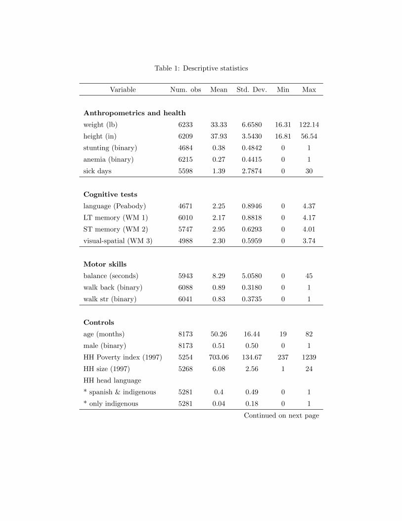
Table 1: Descriptive statistics

Variable Num. obs Mean Std. Dev. Min Max

Anthropometrics and health

weight (lb) 6233 33.33 6.6580 16.31 122.14

height (in) 6209 37.93 3.5430 16.81 56.54

stunting (binary) 4684 0.38 0.4842 0 1

anemia (binary) 6215 0.27 0.4415 0 1

sick days 5598 1.39 2.7874 0 30

Cognitive tests

language (Peabody) 4671 2.25 0.8946 0 4.37

LT memory (WM 1) 6010 2.17 0.8818 0 4.17

ST memory (WM 2) 5747 2.95 0.6293 0 4.01

visual-spatial (WM 3) 4988 2.30 0.5959 0 3.74

Motor skills

balance (seconds) 5943 8.29 5.0580 0 45

walk back (binary) 6088 0.89 0.3180 0 1

walk str (binary) 6041 0.83 0.3735 0 1

Controls

age (months) 8173 50.26 16.44 19 82

male (binary) 8173 0.51 0.50 0 1

HH Poverty index (1997) 5254 703.06 134.67 237 1239

HH size (1997) 5268 6.08 2.56 1 24

HH head language

* spanish & indigenous 5281 0.4 0.49 0 1

* only indigenous 5281 0.04 0.18 0 1

Continued on next page

Table 1 – continued

Variable Num. obs Mean Std. Dev. Min Max

Distribution of birth cohorts

coh97 8173 0.17 0.3793 0 1

coh98 8173 0.21 0.4099 0 1

coh99 8173 0.22 0.4128 0 1

coh00 8173 0.21 0.4085 0 1

coh01 8173 0.18 0.3863 0 1

Shocks by birth cohort

coh97*rain shock 8173 0.11 0.3110 0 1

coh98*rain shock 8173 0.13 0.3351 0 1

coh99*rain shock 8173 0.13 0.3388 0 1

coh00*rain shock 8173 0.13 0.3341 0 1

coh01*rain shock 8173 0.11 0.3186 0 1

Table 2: Exogeneity tests for excessive rainfall shocks.

Columns (1) and (2) present the mean values of each variable

for villages not-exposed to rainfall shocks (rain shockj = 0)

and exposed to rainfall shocks (rain shockj = 1), respec-

tively. Column (3) and (4) report the difference of the two

means and the corresponding t-statistics.

Mean Mean Difference t-statistic

rain shockj = 0 rain shockj = 1

(1) (2) (3) (4)

Village characteristics

male avg. wages 318.3 303.2 15.17 1.248

female avg. wages 41.81 45.44 -3.629 -0.980

Household characteristics and assets

size 6.748 6.827 -0.0792 -0.683

Poverty index 712.7 705.5 7.189 0.670

owns land (ha) 1.749 1.727 0.0215 0.128

own house (binary) 0.940 0.936 0.00387 0.338

electricity (binary) 0.776 0.761 0.0154 0.373

water (binary) 0.0395 0.0448 -0.00533 -0.567

tv (binary) 0.617 0.471 0.147*** 4.360

vehicle (binary) 0.136 0.0599 0.0764*** 4.615

donkeys 0.421 0.384 0.0371 0.691

bullocks 0.130 0.129 0.000910 0.0158

sheep 1.695 1.606 0.0888 0.234

chickens 6.719 7.933 -1.213** -2.666

pigs 1.151 1.322 -0.171 -1.160

Continued on next page

Table 2 – continued

Mean Mean Difference t-statistic

rain shockj = 0 rain shockj = 1

Household migratory characteristics

temporary migrants 0.0463 0.0392 0.00715 1.407

permanent migrants to:

US 0.0392 0.0119 0.0274* 2.548

Mexico 0.0236 0.0221 0.00151 0.186

Head of household characteristics

male (binary) 0.904 0.889 0.0147 1.199

age (years) 43.11 41.79 1.319 1.965

education (years) 3.759 3.597 0.162 1.028

agric worker 0.701 0.738 -0.0373 -1.386

language spoken:

Indigenous 0.00681 0.0357 -0.0289*** -3.469

Spanish & Indigen. 0.177 0.397 -0.220*** -4.704

* p < 0.10, ** p < 0.05, *** p < 0.01

Table 3: Effect of the 1999 September-October rainfall shock on anthropometric indicators

measured in 2003 for children born between 1997 and 2001.

weight (lb)a height (in)a stuntingb anemiac days sickd

(1) (2) (3) (4) (5)

coh97 x rain shocke -0.613 -0.466** . -0.0323 0.346

[0.6137] [0.2190] . [0.0624] [0.2652]

(0.6565) (0.2629) (0.6) (0.2421)

coh98 x rain shock -0.837* -0.709*** 0.127* -0.0132 0.00235

[0.4806] [0.2176] [0.0722] [0.0336] [0.1813]

(0.5352) (0.2475) (0.0712) (0.0394) (0.1781)

coh99 x rain shock -0.733 -0.555** 0.140** 0.00325 -0.232

[0.4399] [0.2483] [0.0672] [0.0368] [0.1860]

(0.4924) (0.2826) (0.0720) (0.0364) (0.2170)

coh00 x rain shock -0.145 -0.426* 0.140** 0.00877 -0.00481

[0.3484] [0.2485] [0.0630] [0.0338] [0.2043]

(0.3378) (0.2514) (0.0658) (0.0368) (0.2007)

coh01 x rain shock -0.468 -0.189 0.115* 0.00671 0.0899

[0.3742] [0.2052] [0.0653] [0.0616] [0.2517]

(0.3991) (0.1867) (0.073) (0.0716) (0.2211)

Observations 3729 3705 2777 3765 3377

R2 0.58 0.76 0.09 0.03 0.02

Mean 33.42 38.08 0.384 0.273 1.282

Controlling for age (months), age2, gender, father’s language, HH structure, cohorts, poverty index (1997).

* p < 0.10, ** p < 0.05, *** p < 0.01.

Standard errors clustered by grid in brakets; Conley standard errors in parentheses (cutoff= 1 degree).

a Weight and height are measures in pounds and inches, respectively.b Stunting is a binary variable = 1 if the child is stunted. Stunting is defined as being two or more standard

deviations below the age-sex standardized height of a healthy reference population [World Health Organization,

1979].c Anemia is a binary variable = 1 if the child is anemic. Anemia is defined as hemoglobin less than 11 g/dL

adjusted for altitude using standard adjustments (Guillermo Jose Ruiz-Arguelles and Antonio Llorente-Peters

1981; Gertler 2004].d Number of days in the previous 4 weeks that the child was reported sick by the mother.e coh97 x rain shock indicates the interaction between the variable coh97 (=1 if the child was born in 1997) and

the variable rain shock (=1 if a rainfall shock occurred in 1999).

Table 4: Effect of the 1999 September-October rainfall shock on cognitive development

indicators measured in 2003 for children born between 1997 and 2001. (Outcomes are the

logarithm of test scores).

Peabody Testa Woodcock-Munoz Testb

long term short term visual-spatial

language memory memory thinking

(1) (2) (3) (4)

coh97 x rain shockc -0.216** -0.194* -0.000168 -0.133***

[0.0967] [0.1042] [0.0257] [0.0424]

(0.1055) (0.1199) (0.0288) (0.0496)

coh98 x rain shock -0.209*** -0.199*** 0.0139 -0.121***

[0.0601] [0.0644] [0.0322] [0.0335]

(0.0679) (0.0817) (0.0363) (0.0398)

coh99 x rain shock -0.148** -0.162*** -0.0532 -0.111**

[0.0682] [0.0598] [0.0370] [0.0493]

(0.0651) (0.0649) (0.0357) (0.058)

coh00 x rain shock -0.0258 -0.147** 0.0173 -0.143**

[0.0672] [0.0568] [0.0374] [0.0541]

(0.0576) (0.0565) (0.0356) (0.0486)

coh01 x rain shock -0.225 -0.0300 -0.0755 0.0364

[0.6933] [0.0549] [0.0552] [0.0899]

( 0.6910) (0.66) (0.0493) (0.1003)

Observations 2835 3522 3385 2967

R2 0.33 0.32 0.48 0.38


* p < 0.10, ** p < 0.05, *** p < 0.01


a Peabody Test measures language development. Peabody test scores are a reliable predictor of achievements in

primary school.b Woodcock-Munoz Test is used to assess a wide range of cognitive abilities: long-term memory, short-term memory

and visual spatial thinking.c coh97 x rain shock indicates the interaction between the variable coh97 (=1 if the child was born in 1997) and


Table 5: Effect of the 1999 September-October rainfall shock on gross motor skills measured

in 2003 for children born between 1997 and 2001. These gross motor skills are central to

the successful performance of school tasks.

balance ability to ability to

(seconds)a walk backwardb walk straightb

(1) (2) (3)

coh97 x rain shockc -0.718** 0.0228 0.0140

[0.3420] [0.0162] [0.0117]

(0.3686) (0.0186) (0.0109)

coh98 x rain shock -0.164 0.0136 0.0220*

[0.2609] [0.0130] [0.0118]

(0.2628) (0.0119) (0.0104)

coh99 x rain shock -0.357 0.0174 -0.0371**

[0.3408] [0.0155] [0.0156]

(0.3452) (0.0152) (0.0134)

coh00 x rain shock -0.210 -0.0216 -0.00701

[0.3739] [0.0283] [0.0374]

(0.2811) (0.0246) (0.0351)

coh01 x rain shock 0.0831 -0.0308 -0.0514

[0.4352] [0.0563] [0.0509]

(0.3796) (0502) (0.0488)

Observations 3563 3693 3663

R2 0.33 0.16 0.24

Mean 8.286 0.891 0.843


* p < 0.10, ** p < 0.05, *** p < 0.01


a The child’s ability to keep her/his balance on one foot is measured in seconds.b The binary variables = 1 if the child was able to successfully complete the task.c coh97 x rain shock indicates the interaction between the variable coh97 (=1 if the child was born in 1997) and


Table 6: Effect of rainfall shocks on income at different periods t, t+1, and t+2; as well as

on the probability of receiving formal and informal transfers immediately after the shock.

Formal transfers include food and other forms of government aid. Informal transfers include

food and other transfers from either a family member or from a neighbor.

Dependent Variables Binary Variable (�) Coefficienta Std Dev

Total household income (log)

incomet -0.395*** (0.052)

incomet+1 -0.291*** (0.052)

incomet+2 -0.263*** (0.042)

Household income from agriculture (log)

agricultural incomet -0.276*** (0.047)

agricultural incomet+1 -0.268*** (0.056)

agricultural incomet+2 -0.181*** (0.044)

=1 if household received government aid

food aidt � 0.047** (0.021)

other aidt � 0.006 (0.034)

=1 if household received informal transfers

from familyt � -0.042 (0.043)

from neighbort � -0.028*** (0.009)

Standard errors clustered by gridcell [in brackets].

* p < 0.10, ** p < 0.05, *** p < 0.01.

a Each line shows the result of separate regressions. Control variables for each model include: (i) household’s head

characteristics (age, male, years of education, language, sector of employment, marital status); (ii) household

characteristics (size, structure, baseline poverty index in 1997); and (iii) village characteristics (average male

and female wage).

Table 7: Effect of rainfall shocks on food consumption, diet composition, child health, and

medicine expenditures. All responses are estimated up to two years (t, t + 1, t + 2) after

exposure to the shock.

Dependent Variables Coefficienta Std Dev

Food consumption (log)

food consumptiont [pesos] -0.100*** (0.035)

food consumptiont+1 [pesos] -0.115*** (0.034)

food consumptiont+2 [pesos] -0.149*** (0.055)

food consumptiont [kg] -0.027 (0.036)

food consumptiont+1 [kg] 0.003 (0.030)

food consumptiont+2 [kg] 0.042 (0.057)

Diet composition (log)

tortilla consumptiont [pesos] 0.132** (0.054)

tortilla consumptiont+1 [pesos] -0.085 (0.064)

tortilla consumptiont+2 [pesos] -0.218*** (0.069)

animal consumptiont [pesos] -0.052 (0.085)

animal consumptiont+1 [pesos] -0.145* (0.075)

animal consumptiont+2 [pesos] -0.171** (0.076)

fruit and vegetable consumptiont [pesos] -0.200*** (0.057)

fruit and vegetable consumptiont+1 [pesos] -0.078 (0.049)

fruit and vegetable consumptiont+2 [pesos] -0.143** (0.056)

Children reported sick by the mother

children sickt (% in the HH) 0.011 (0.022)

children sickt+1 (% in the HH) 0.025 (0.027)

children sickt+2 (% in the HH) 0.016 (0.031)

Medicine Expenditure (log)

medicine expenditurest -0.361*** (0.121)

medicine expenditurest+1 -0.303** (0.113)

medicine expenditurest+2 0.043 (0.128)

Standard errors clustered by gridcell [in brackets]. * p < 0.10, ** p < 0.05, *** p < 0.01

a Each line shows the result of separate regressions. Control variables for each model include: (i) household’s head

characteristics (age, male, years of education, language, sector of employment, marital status); (ii) household

characteristics (size, structure, baseline poverty index in 1997); and (iii) village characteristics (average male

and female wage).

Table 8: The mitigating effect of Progresa in villages exposed to the rainfall shock. These

results are associated to the anthropometric, health, and cognitive development indicators

collected in 2003. Coefficients are estimated using the randomized experiment empirical

specification (equation 2). Outcomes in this model correspond to village level means of

individual observations.

Anthropometric and Health Indicators

weight (lb) height (in) Stunting Anemia Days sick

(1) (2) (3) (4) (5)

Rain shocka -0.516 -0.467** 0.126*** 0.0297 0.0847

[0.4104] [0.2298] [0.0357] [0.0254] [0.1768]

Treatmentb -0.181 -0.0598 0.0118 0.0510* -0.0997

[0.4066] [0.2182] [0.0303] [0.0307] [0.1689]

Treatment x Rain shock -0.702 -0.255 0.00271 -0.0407 0.0485

[0.5705] [0.3153] [0.0505] [0.0374] [0.2321]

Observationsc 259 259 259 258 259

R2 0.06 0.06 0.09 0.01 0.01

Mean 33.92 38.29 0.301 0.261 1.380

Cognitive Development Indicators

Peabody Test Woodcock-Munoz Test



(1) (2) (3) (4)

Rain shocka -0.159** -0.137** -0.100** -0.139***

[0.0762] [0.0684] [0.0406] [0.0439]

Treatmentb 0.0330 -0.00983 -0.0419 -0.0459

[0.0724] [0.0650] [0.0402] [0.0452]

Treatment x Rain shock -0.0197 -0.0463 0.0592 0.0466

[0.0976] [0.0864] [0.0556] [0.0606]

Observationsc 253 259 259 259

R2 0.05 0.06 0.03 0.06

Robust standard errors [in brackets]. * p < 0.10, ** p < 0.05, *** p < 0.01.

a rain shock = 1 if village had a flood occurrence in 1999.b Treatment randomly defined at the village level.c Outcomes are village level means of individual observations.

A M J JJ A S O N

-20

24

97 98 99

Figure 1: Distribution of Monthly Precipitation Standardized Anomalies.

This figure reproduces figure 1 in Vicarelli (2011). The x-axis represents the 1997, 1998 and 1999 agricultural

seasons for maize. The agricultural season lasts eight months, from April to November, and includes the following

phases : planting Phase (April-June); growing phase (July to August); and maturation and harvesting (September

to November). The y-axis represent that average monthly precipitation standardized anomaly for the grid-cells

where the Progresa villages are located. The unit of observation is a 0.5 x 0.5 degree grid-cell (Total=55 grid-cells).

For each grid-cell, the monthly standardized deviation from the 1961-1999 mean is calculated.

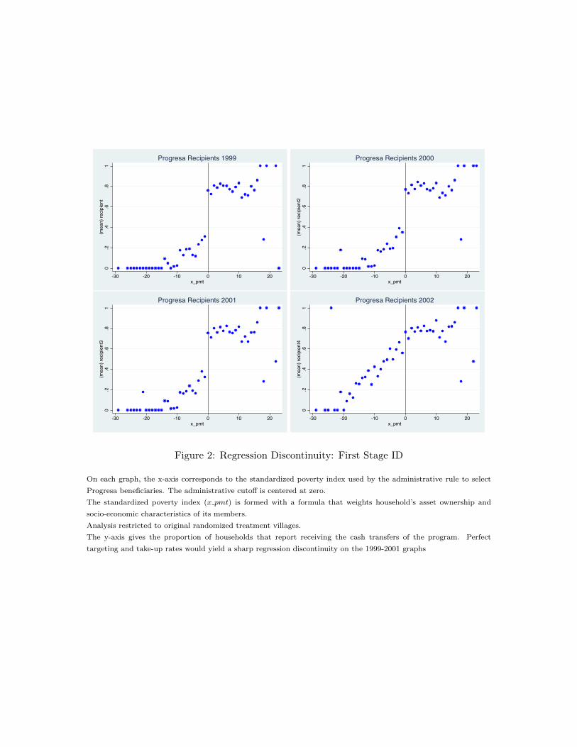
0.2

.4.6

.81

(mea

n) re

cipi

ent

-30 -20 -10 0 10 20x_pmt

Progresa Recipients 1999

0.2

.4.6

.81

(mea

n) re

cipi

ent2

-30 -20 -10 0 10 20x_pmt


0.2

.4.6

.81

(mea

n) re

cipi

ent3

-30 -20 -10 0 10 20x_pmt


.2.4

.6.8

1(m

ean)

reci

pien

t4

-30 -20 -10 0 10 20x_pmt


Figure 2: Regression Discontinuity: First Stage ID

On each graph, the x-axis corresponds to the standardized poverty index used by the administrative rule to select

Progresa beneficiaries. The administrative cutoff is centered at zero.

The standardized poverty index (x pmt) is formed with a formula that weights household’s asset ownership and

socio-economic characteristics of its members.

Analysis restricted to original randomized treatment villages.

The y-axis gives the proportion of households that report receiving the cash transfers of the program. Perfect

targeting and take-up rates would yield a sharp regression discontinuity on the 1999-2001 graphs

2030

4050

-30 -20 -10 0 10 20x_pmt

Weight (lb)

3436

3840

4244

-30 -20 -10 0 10 20x_pmt

Height (in)

Figure 3: Regression Discontinuity Analysis: Anthropometric Outcomes






The y-axis gives conditional means of the individual outcomes. Kis the conditional mean for individuals from villages

affected by a rain shock. #is the conditional mean for individuals from villages not affected by a rain shock.

1.5

22.

53

3.5

4

-30 -20 -10 0 10 20x_pmt

Language (Peabody Test)

1.5

22.

53

3.5

4

-30 -20 -10 0 10 20x_pmt

Long-term Memory (Woodcock-Munoz Test 1)

Figure 4: Regression Discontinuity Analysis: Cognitive Outcomes








Tab

leA

.1:

Su

mm

ary

ofC

onle

yS

Es.

Peabody

Test

Woodcock-M

unoz

Test

Motor

Skills

weig

ht

(lb)

heig

ht

(in)

stunti

ng

anem

iadays

sick

language

long

term

short

term

vis

ual-

spati

al

bala

nce

abilit

yto

abil

ity

to

mem

ory

mem

ory

thin

kin

g(s

econds)

walk

backw

ard

walk

stra

ight

(1)

(2)

(3)

(4)

(5)

(6)

(7)

(8)

(9)

(10)

(11)

(12)

coh97

xra

insh

ock

[0.6

137]

[0.2

190]

.[0

.0624]

[0.2

652]

[0.0

967]

[0.1

042]

[0.0

257]

[0.0

424]

[0.3

420]

[0.0

162]

[0.0

117]

(0.6

565)

(0.2

629)

(0.6

)(0

.2421)

(0.1

055)

(0.1

199)

(0.0

288)

(0.0

496)

(0.3

686)

(0.0

186)

(0.0

109)

(0.6

192)

0.2

881

0.0

571

0.2

301

0.1

20.1

187

0.0

287

0.0

516

0.3

064

0.0

208

0.0

097

coh98

xra

insh

ock

[0.4

806]

[0.2

176]

[0.0

722]

[0.0

336]

[0.1

813]

[0.0

601]

[0.0

644]

[0.0

322]

[0.0

335]

[0.2

609]

[0.0

130]

[0.0

118]

(0.5

352)

(0.2

475)

(0.0

712)

(0.0

394)

(0.1

781)

(0.0

679)

(0.0

817)

(0.0

363)

(0.0

398)

(0.2

628)

(0.0

119)

(0.0

104)

0.6

177

0.2

974

0.0

709

0.0

393

0.1

607

0.0

721

0.0

907

0.0

382

0.0

403

0.2

292

0.0

118

0.0

081

coh99

xra

insh

ock

[0.4

399]

[0.2

483]

[0.0

672]

[0.0

368]

[0.1

860]

[0.0

682]

[0.0

598]

[0.0

370]

[0.0

493]

[0.3

408]

[0.0

155]

[0.0

156]

(0.4

924)

(0.2

826)

(0.0

720)

(0.0

364)

(0.2

170)

(0.0

651)

(0.0

649)

(0.0

357)

(0.0

58)

(0.3

452)

(0.0

152)

(0.0

134)

0.5

619

0.3

272

0.0

806

0.0

343

0.1

896

0.0

612

0.0

735

0.0

345

0.0

592

0.3

557

0.0

156

0.0

135

coh00

xra

insh

ock

[0.3

484]

[0.2

485]

[0.0

630]

[0.0

338]

[0.2

043]

[0.0

672]

[0.0

568]

[0.0

374]

[0.0

541]

[0.3

739]

[0.0

283]

[0.0

374]

(0.3

378)

(0.2

514)

(0.0

658)

(0.0

368)

(0.2

007)

(0.0

576)

(0.0

565)

(0.0

356)

(0.0

486)

(0.2

811)

(0.0

246)

(0.0

351)

0.3

627

0.2

852

0.0

725

0.0

36

0.1

745

0.0

46

0.0

502

0.0

381

0.0

423

0.2

735

0.0

236

0.0

353

coh01

xra

insh

ock

[0.3

742]

[0.2

052]

[0.0

653]

[0.0

616]

[0.2

517]

[0.6

933]

[0.0

549]

[0.0

552]

[0.0

899]

[0.4

352]

[0.0

563]

[0.0

509]

(0.3

991)

(0.1

867)

(0.0

73)

(0.0

716)

(0.2

211)

(0.6

910)

(0.0

66)

(0.0

493)

(0.1

003)

(0.3

796)

(0502)

(0.0

488)

0.3

959

0.1

946

0.0

844

0.0

751

0.1

998

0.6

822

0.0

651

0.0

388

0.0

944

0.3

306

0.0

432

0.0

536

Robust

standard

err

ors

clu

stere

dby

pix

el

are

rep

ort

ed

inbra

ckets

;C

onle

ySE

s,w

ith

cuto

ff=

1decim

al

deg,

are

rep

ort

ed

inpare

nth

ese

s;

and

the

rem

ain

ing

figure

sare

Conle

yst

andard

err

ors

wit

hcuto

ff=

2decim

al

deg.

Table A.2: Robustness check: Effect of the 1999 September-October rainfall shock on an-

thropometric and health outcomes controlling for variables that show significant differences

in the exogeneity testweight (lb) height (in) Stunting Anemia Days sick

(1) (2) (3) (4) (5)

coh97 x rain shock -0.497 -0.448** . -0.0369 0.403

[0.6128] [0.2179] . [0.0614] [0.2723]

coh98 x rain shock -0.715 -0.687*** 0.129* -0.0160 0.0306

[0.4672] [0.2067] [0.0711] [0.0332] [0.1789]

coh99 x rain shock -0.651 -0.507** 0.126** -0.000984 -0.222

[0.4071] [0.2297] [0.0629] [0.0362] [0.1749]

coh00 x rain shock -0.103 -0.401* 0.135** 0.00612 0.0250

[0.3290] [0.2381] [0.0598] [0.0338] [0.2064]

coh01 x rain shock -0.357 -0.140 0.103 0.00328 0.127

[0.3509] [0.1873] [0.0619] [0.0615] [0.2529]

Observations 3730 3706 2776 3764 3376

R2 0.58 0.76 0.10 0.03 0.02

Mean 33.42 38.10 0.384 0.273 1.282

rain shock=1 if child was present in a village with a flood occurrence in 1999


Additional controls: TV and vehicle ownership, chickens owned, permanent migrants to the U.S.

Table A.3: Robustness check: Effect of the 1999 September-October rainfall shock on

cognitive development outcomes controlling for variables that show significant differences

in the exogeneity testPeabody Test Woodcock-Munoz Test



(1) (2) (3) (4)

coh97 x rain shock -0.199** -0.175* 0.00643 -0.123***

[0.0963] [0.1015] [0.0252] [0.0420]

coh98 x rain shock -0.196*** -0.189*** 0.0185 -0.115***

[0.0566] [0.0605] [0.0312] [0.0307]

coh99 x rain shock -0.125* -0.141** -0.0467 -0.101**

[0.0673] [0.0580] [0.0364] [0.0459]

coh00 x rain shock -0.00328 -0.133** 0.0223 -0.132**

[0.0654] [0.0575] [0.0368] [0.0519]

coh01 x rain shock -0.225 -0.0168 -0.0686 0.0489

[0.6753] [0.0524] [0.0552] [0.0911]

Observations 2840 3521 3384 2966

R2 0.34 0.32 0.48 0.39



Additional controls: TV and vehicle ownership, chickens owned, permanent migrants to the U.S

Table A.4: Robustness check: Effect of the 1999 September-October rainfall shock on

gross motor skill outcomes controlling for variables that show significant differences in the

exogeneity testbalance ability to ability to

(seconds) walk backward walk straight

(1) (2) (3)

coh97 x rain shock -0.646* 0.0264 0.0154

[0.3285] [0.0162] [0.0120]

coh98 x rain shock -0.124 0.0154 0.0235*

[0.2588] [0.0132] [0.0123]

coh99 x rain shock -0.289 0.0186 -0.0343**

[0.3319] [0.0155] [0.0155]

coh00 x rain shock -0.169 -0.0194 -0.00535

[0.3763] [0.0287] [0.0378]

coh01 x rain shock 0.157 -0.0295 -0.0486

[0.4289] [0.0561] [0.0514]


R2 0.33 0.16 0.24

Mean 8.286 0.891 0.843


Standard errors clustered by gridcell [in brackets]. * p < 0.10, ** p < 0.05, *** p < 0.01.

Additional controls: TV and vehicle ownership, chickens owned, permanent migrants to the U.S

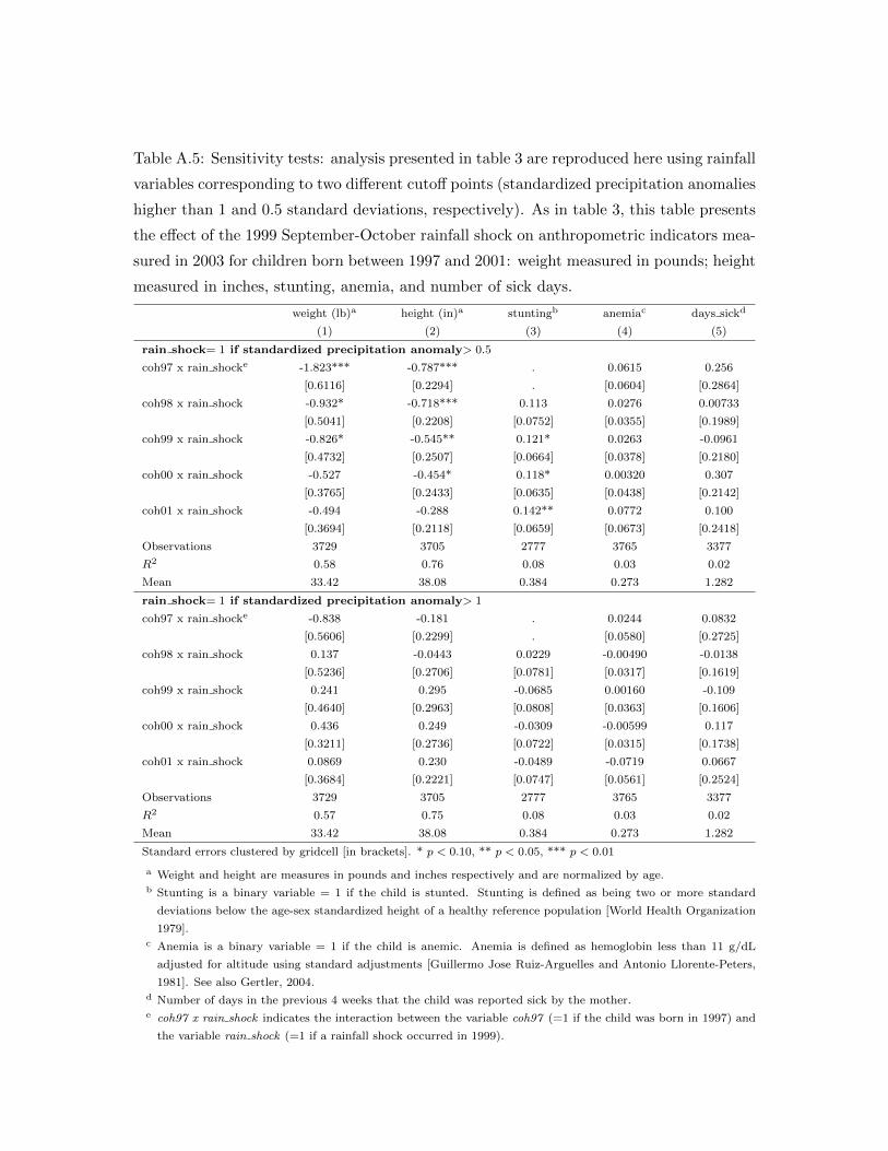
Table A.5: Sensitivity tests: analysis presented in table 3 are reproduced here using rainfall

variables corresponding to two different cutoff points (standardized precipitation anomalies

higher than 1 and 0.5 standard deviations, respectively). As in table 3, this table presents

the effect of the 1999 September-October rainfall shock on anthropometric indicators mea-

sured in 2003 for children born between 1997 and 2001: weight measured in pounds; height

measured in inches, stunting, anemia, and number of sick days.

weight (lb)a height (in)a stuntingb anemiac days sickd

(1) (2) (3) (4) (5)

rain shock= 1 if standardized precipitation anomaly> 0.5

coh97 x rain shocke -1.823*** -0.787*** . 0.0615 0.256

[0.6116] [0.2294] . [0.0604] [0.2864]

coh98 x rain shock -0.932* -0.718*** 0.113 0.0276 0.00733

[0.5041] [0.2208] [0.0752] [0.0355] [0.1989]

coh99 x rain shock -0.826* -0.545** 0.121* 0.0263 -0.0961

[0.4732] [0.2507] [0.0664] [0.0378] [0.2180]

coh00 x rain shock -0.527 -0.454* 0.118* 0.00320 0.307

[0.3765] [0.2433] [0.0635] [0.0438] [0.2142]

coh01 x rain shock -0.494 -0.288 0.142** 0.0772 0.100

[0.3694] [0.2118] [0.0659] [0.0673] [0.2418]

Observations 3729 3705 2777 3765 3377

R2 0.58 0.76 0.08 0.03 0.02

Mean 33.42 38.08 0.384 0.273 1.282

rain shock= 1 if standardized precipitation anomaly> 1

coh97 x rain shocke -0.838 -0.181 . 0.0244 0.0832

[0.5606] [0.2299] . [0.0580] [0.2725]

coh98 x rain shock 0.137 -0.0443 0.0229 -0.00490 -0.0138

[0.5236] [0.2706] [0.0781] [0.0317] [0.1619]

coh99 x rain shock 0.241 0.295 -0.0685 0.00160 -0.109

[0.4640] [0.2963] [0.0808] [0.0363] [0.1606]

coh00 x rain shock 0.436 0.249 -0.0309 -0.00599 0.117

[0.3211] [0.2736] [0.0722] [0.0315] [0.1738]

coh01 x rain shock 0.0869 0.230 -0.0489 -0.0719 0.0667

[0.3684] [0.2221] [0.0747] [0.0561] [0.2524]

Observations 3729 3705 2777 3765 3377

R2 0.57 0.75 0.08 0.03 0.02

Mean 33.42 38.08 0.384 0.273 1.282


a Weight and height are measures in pounds and inches respectively and are normalized by age.b Stunting is a binary variable = 1 if the child is stunted. Stunting is defined as being two or more standard

deviations below the age-sex standardized height of a healthy reference population [World Health Organization

1979].c Anemia is a binary variable = 1 if the child is anemic. Anemia is defined as hemoglobin less than 11 g/dL

adjusted for altitude using standard adjustments [Guillermo Jose Ruiz-Arguelles and Antonio Llorente-Peters,

1981]. See also Gertler, 2004.d Number of days in the previous 4 weeks that the child was reported sick by the mother.e coh97 x rain shock indicates the interaction between the variable coh97 (=1 if the child was born in 1997) and


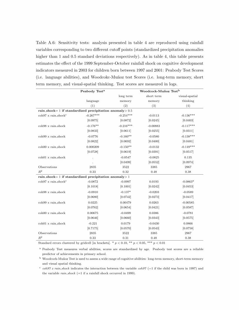
Table A.6: Sensitivity tests: analysis presented in table 4 are reproduced using rainfall


higher than 1 and 0.5 standard deviations respectively). As in table 4, this table presents

estimates the effect of the 1999 September-October rainfall shock on cognitive development

indicators measured in 2003 for children born between 1997 and 2001: Peabody Test Scores

(i.e. language abilities), and Woodcokc-Munoz test Scores (i.e. long-term memory, short

term memory, and visual-spatial thinking. Test scores are measured in logs.

Peabody Testa Woodcock-Munoz Testb



(1) (2) (3) (4)


coh97 x rain shockc -0.267*** -0.254*** -0.0113 -0.136***

[0.0975] [0.0872] [0.0245] [0.0403]

coh98 x rain shock -0.176** -0.216*** -0.00883 -0.117***

[0.0833] [0.0611] [0.0255] [0.0311]

coh99 x rain shock -0.0776 -0.160** -0.0580 -0.138***

[0.0822] [0.0692] [0.0400] [0.0481]

coh00 x rain shock 0.000209 -0.150** -0.0132 -0.149***

[0.0728] [0.0619] [0.0391] [0.0517]

coh01 x rain shock . -0.0547 -0.0825 0.135

. [0.0499] [0.0552] [0.0974]

Observations 2835 3522 3385 2967

R2 0.33 0.32 0.48 0.38


coh97 x rain shockc -0.0872 -0.0997 0.0193 -0.0863*

[0.1018] [0.1001] [0.0242] [0.0453]

coh98 x rain shock -0.0910 -0.137* -0.0203 -0.0589

[0.0680] [0.0742] [0.0273] [0.0417]

coh99 x rain shock 0.0225 0.00479 0.0263 -0.00585

[0.0762] [0.0654] [0.0421] [0.0587]

coh00 x rain shock 0.00675 -0.0499 0.0386 -0.0781

[0.0646] [0.0660] [0.0343] [0.0575]

coh01 x rain shock -0.221 0.0179 -0.0430 0.0866

[0.7175] [0.0570] [0.0543] [0.0758]

Observations 2835 3522 3385 2967

R2 0.33 0.31 0.48 0.38


a Peabody Test measures verbal abilities, scores are standardized by age. Peabody test scores are a reliable

predictor of achievements in primary school.b Woodcock-Munoz Test is used to assess a wide range of cognitive abilities: long-term memory, short-term memory

and visual spatial thinking.c coh97 x rain shock indicates the interaction between the variable coh97 (=1 if the child was born in 1997) and


Table A.7: Sensitivity tests: analysis presented in table 5 are reproduced using rainfall


higher than 1 and 0.5 standard deviations respectively). As in table 5, this table shows

the effect of the 1999 September-October rainfall shock on gross motor skills measured in

2003 for children born between 1997 and 2001: ability to keep their balance on one foot

(measured in seconds), ability to work forward and backward. These gross motor skills are

central to the successful performance of school tasks.

balance on one foot ability to ability to

(seconds)a walk backwardb walk straightb

(1) (2) (3)


coh97 x rain shockc -0.471 0.0392** 0.00646

[0.3474] [0.0186] [0.0130]

coh98 x rain shock 0.143 0.0210 0.0234*

[0.2689] [0.0136] [0.0135]

coh99 x rain shock -0.356 0.0160 -0.0377**

[0.3647] [0.0165] [0.0175]

coh00 x rain shock -0.180 -0.0186 -0.0112

[0.3692] [0.0333] [0.0414]

coh01 x rain shock 0.162 -0.0664 0.0653

[0.4701] [0.0471] [0.0537]


R2 0.33 0.16 0.24

Mean 8.286 0.891 0.843


coh97 x rain shockc -0.242 0.0294** 0.00733

[0.3547] [0.0146] [0.0114]

coh98 x rain shock 0.0606 0.0107 0.0211*

[0.2620] [0.0122] [0.0107]

coh99 x rain shock 0.304 0.0314* -0.0103

[0.3564] [0.0164] [0.0172]

coh00 x rain shock 0.192 -0.0210 -0.0309

[0.3696] [0.0309] [0.0379]

coh01 x rain shock 0.390 -0.00394 -0.0245

[0.3915] [0.0569] [0.0415]


R2 0.33 0.16 0.24

Mean 8.286 0.891 0.843

Controlling for household and individual characteristics.


a The child’s ability keep her/his balance on one foot is measured in seconds.b The binary variables = 1 if the child was able to successfully complete the task.c coh97 x rain shock indicates the interaction between the variable coh97 (=1 if the child was born in 1997) and


Figure A.1: ENSO historical. Precipitation Standardized Anomalies (UEA CRU Ts2p1)

Sep 1974

120˚W 115˚W 110˚W 105˚W 100˚W 95˚W 90˚WLongitude

15˚N

20˚N

25˚N

30˚N

Latit

ude

Oct 1976


15˚N

20˚N

25˚N

30˚N

Latit

ude

Oct 1981


15˚N

20˚N

25˚N

30˚N

Latit

ude

Sep 1984


15˚N

20˚N

25˚N

30˚N

Latit

ude

-2.4 -2 -1.6 -1.2 -0.8 -0.4 0 0.4 0.8 1.2 1.6 2 2.4precipitation

0.2.4.6.81

-30

-20

-10

010

20x_pm

t

Stunting

0.2.4.6.81

-30

-20

-10

010

20x_pm

t

Anem

ia

02468

-30

-20

-10

010

20x_

pmt

Num

ber o

f Sic

k D

ays

(Day

s_si

ck)

Fig

ure

A.2

:R

Dan

alysi

s:A

nth

rop

omet

ric

Ou

tcom

es

On

each

gra

ph

,th

ex-a

xis

corr

esp

on

ds

toth

est

an

dard

ized

pover

tyin

dex

use

dby

the

ad

min

istr

ati

ve

rule

tose

lect

Pro

gre

sab

enefi

ciari

es.

Th

e

ad

min

istr

ati

ve

cuto

ffis

cente

red

at

zero

.

Th

est

an

dard

ized

pover

tyin

dex

(xpmt)

isfo

rmed

wit

ha

form

ula

that

wei

ghts

hou

seh

old

’sass

etow

ner

ship

an

dso

cio-e

con

om

icch

ara

cter

isti

csof

its

mem

ber

s.

An

aly

sis

rest

rict

edto

ori

gin

al

ran

dom

ized

trea

tmen

tvil

lages

.

Th

ey-a

xis

giv

esco

nd

itio

nal

mea

ns

of

the

ind

ivid

ual

ou

tcom

es.Kis

the

con

dit

ion

al

mea

nfo

rin

div

idu

als

from

villa

ges

aff

ecte

dby

ara

insh

ock

.#

isth

e

con

dit

ion

al

mea

nfo

rin

div

idu

als

from

villa

ges

not

aff

ecte

dby

ara

insh

ock

.

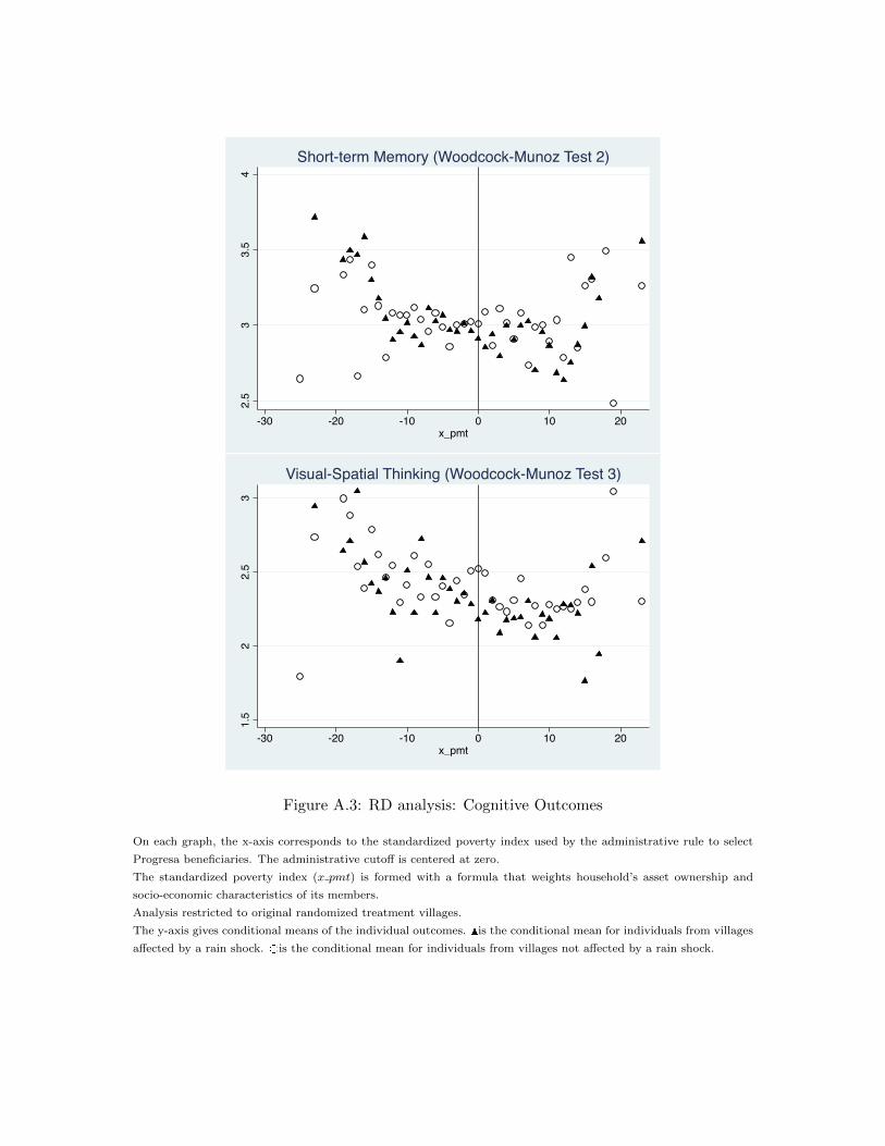
2.5

33.

54

-30 -20 -10 0 10 20x_pmt

Short-term Memory (Woodcock-Munoz Test 2)

1.5

22.

53

-30 -20 -10 0 10 20x_pmt

Visual-Spatial Thinking (Woodcock-Munoz Test 3)

Figure A.3: RD analysis: Cognitive Outcomes








0 Paper Nino 1311

Documents

Transcript of 0 Paper Nino 1311