@ WI LEY-VCH - National Academic Digital Library of Ethiopia
662
J. Ingham, I. J. Dunn, E. Heinzle, J. E. Pienosil Chemical Engineering Dynamics @ WI LEY-VCH
-
Upload
khangminh22 -
Category
Documents
-
view
0 -
download
0
Transcript of @ WI LEY-VCH - National Academic Digital Library of Ethiopia

J. Ingham, I. J. Dunn, E. Heinzle, J. E. Pienosil
Chemical Engineering Dynamics
@ WI LEY-VCH

Also of Interest
Biological Reaction Engineering Principles, Applications and Modelling with PC Simulation I. J. Dunn, E. Heinzle, J. Ingham, J. E. Pfenosil 1992. ISBN 3-527-28511-3
Dynamics of Environmental Bioprocesses Modelling and Simulation J. B. Snape, I. J. Dunn, J. Ingham, J. E. Pfenosil 1995. ISBN 3-527-28705-1

John Ingham Irving J. Dunn Elmar Heinzle JiZ E. Pfenosil
Chemical Engineering Dynamics
An Introduction to Modelling and Computer Simulation
Second, Completely Revised Edition
@ WI LEY-VCH Weinheim . New York - Chichester Brisbane - Singapore . Toronto

Professor Dr. John Ingham Department of Chemical Engineering Departmcnt of Chemical Biochemistry
Professor Dr. Irving J. Dunn Professor Dr. Jifi E. Pfenosil
Professor Dr. Elmar Heinzle Deparment of Technical
University of Bradford Engineering Bradford BD7 1DP ETH Zurich UK CH-8092 Zurich
University of Saarland P.O. Box 15 11 50 D-66041 Saarbrucken
Switzerland Germany
This book was carefully produced. Nevertheless, authors and publisher do not warrant the information contained therein to be free of errors. Readers are advised to keep in mind that statements, data, illustrations, procedural details or other items may inadvertently be inaccurate.
First Edition 1994 Second, Completely Rcviscd Edition 2000
Library of Congress Card No.: Applied for.
British Library Cataloguing-in-Publication Data: A catalogue record for this book is available from the British Library.
Die Deutsche Bibliothek - CIP Cataloguing-in-Publication-Data A catalogue record for this publication is available from Die Deutsche Bibliothek.
ISBN 3-527-29176-6
0 WILEY-VCH Verlag GmbH, D-69469 Weinheim (Federal Republic of Germany), 2000 Printed on acid-free and chlorine-free papcr. All rights reserved (including those of translation into other languages). No part of this book may be reproduced in any form - by photoprinting, microfilm, or any other means-nor transmitted or translated into a machine language without written permission from the publishers. Registered names, trademarks, etc. usedin this book, even when not specifically marked as such, are not to be considered unprotected by law. Printing: Strauss Offsetdruck GmbH, D-69509 Morlenbach. Bookbinding: J. Schaffer GmbH & Co. KG, D-67269 Grunstadt. Printed in the Federal Republic of Germany.

Preface
The aim of this book is to teach the use of modelling and simulation as a discipline for the understanding of chemical engineering processes and their dynamics. This is done via a combination of basic modelling theory and computer simulation examples, which are used to emphasise basic principles and to demonstrate the cause-and-effect phenomena in complex models. In this second edition the examples are based on the use of a new, powerful and easy- to-use simulation language, called Berkeley Madonna. Developed for Windows and Macintosh at the University of California, Madonna represents almost all we have ever wanted in simulation software for teaching. The many programmed examples demonstrate simple modelling procedures that can be used to represent a wide range of chemical and chemical engineering process phenomena. The study of the examples, by direct computer experimentation, has been shown to lead to a positive improvement in the understanding of physical systems and confidence in the ability to deal with chemical rate processes. Quite simple models can often give realistic representations of process phenomena. The methods described in the text are applicable to a range of differing applications, including process identification, the analysis and design of experiments, process design and optimisation, process control and plant safety, all of which are essential aspects of modern chemical technology.
The book is based on the hands-on use of the computer as an integral part of the learning process. Although computer-based modelling procedures are now commonplace in chemical engineering, our experience is that there still remains a considerable lack of ability in basic modelling, especially when applied to dynamic systems. This has resulted from the traditional steady-state approach to chemical engineering and the past emphasis on flow-sheeting for large-scale continuous processes. Another important contributing factor is the perceived difficulty of solving the large sets of simultaneous differential equations that result from any realistic dynamic modelling description. With modern trends towards more intensive high-value batch processing methods, the need for a better knowledge of the plant dynamics is readily apparent. This is also reinforced by the increased attention that must now be paid to proper process control, process optimisation and plant safety. Fortunately the PC and Macintosh computers with suitable simulation software, now provide a fast and convenient means of solution.
In producing this new edition, the major change is, of course, the use of Madonna as the means of solution to the model equations. This enables a more modern, Windows-based (also Macintosh compatible) and menu driven solution. Also, the increased power and speed of solution have allowed us to

VI Preface
extend the scope of our simulation examples quite substantially. In particular, the use of dynamic simulation as a means of making a steady-state analysis to study the variation in the steady-state conditions with changing system parameters is now possible. Regarding the text, we have included several new topics, including chemical waste minimisation, chemical reactor safety, chromatographic separation, and bioreactor operation as significant areas in which simulation methods can have a very important impact. These areas are being increasingly recognised as important components of modern chemical engineering.
Organisation of the Book
The book consists of an introduction to basic modelling presented in Chapters 1 through 4. An introduction to simulation principles and methods and the simulation examples are found in Chapter 5. The first four chapters cover the basic theory for the computer simulation examples and present the basic concepts of dynamic modelling. The aim is not to be exhaustive, but simply to provide sufficient introduction, for a proper understanding of the modelling methodology and computer-based examples. Here the main emphasis is placed on understanding the physical meaning and significance of each term in the resulting model equations. Chapter 5 , constituting the main part of the book, provides the Madonna-based computer simulation exercises. Each of the examples is self-contained and includes a model description, the model equations, exercises, nomenclature, sample graphical output and references. The combined book thus represents a synthesis of basic theory and computer- based simulation examples. The accompanying CD includes the Madonna simulation language for Windows and Macintosh and the ready-to-run simulation example programs. Each program is clearly structured with comments and complete nomenclature. Although not included within the main body of the text, the Madonna solution programs provided on the CD are very simple both to write and to understand, as evidenced by the demonstration program BATSEQ in Sec. 5.1.3. All the programs are clearly structured and are accompanied by clear descriptions, nomenclature and details of any special items of programming that might be included. All programs are therefore very easy to understand, to apply and, if needed, to modify. Further, a clear relationship between the model relationships described in the text and the resulting program remains very apparent.
Chapter 1 deals with the basic concepts of modelling, and the formulation of mass and energy balance relationships. In combination with other forms of relationship, these are shown to lead to a systematic development for dynamic

Preface VII
models. Though the concepts are simple, they can be applied equally well to very complex problems.
Chapter 2 is employed to provide a general introduction to signal and process dynamics, including the concept of process time constants, process control, process optimisation and parameter identification. Other important aspects of dynamic simulation involve the numerical methods of solution and the resulting stability of solution; both of which are dealt with from the viewpoint of the simulator, as compared to that of the mathematician.
Chapter 3 concerns the dynamic characteristics of stagewise types of equipment, based on the concept of the well-stirred tank. In this, the various types of stirred-tank chemical reactor operation are considered, together with allowance for heat effects, non-ideal flow, control and safety. Also included is the modelling of stagewise mass transfer applications, based on liquid-liquid extraction, gas absorption and distillation.
Chapter 4 concerns differential processes, which take place with respect to both time and position and which are normally formulated as partial differential equations. Applications include heterogeneous catalysis, tubular chemical reactors, differential mass transfer, heat exchangers and chromatography. It is shown that such problems can be solved with relative ease, by utilising a finite-differencing solution technique in the simulation approach.
Chapter 5 comprises the computer simulation examples. The exercises are intended to draw the simulator’s attention to the most important features of each example. Most instructive is to study the influence of important model parameters, using the interactive and graphical features of Madonna. Interesting features include the possibility of making “parametric runs” to investigate the influence of one parameter on the steady-state values. When working with arrays to solve multistage or diffusion problems, the variables can be plotted versus the array number, thus achieving output plots as a function of distance.
Working through a particular example will often suggest an interesting variation, such as a control loop, which can then be inserted into the model. In running our courses, the exercises have proven to be very open ended and in tackling them, we hope you will share our conviction that computer simulation is fun, as well as being useful and informative. An Appendix provides an instructional guide to the Madonna software, which is sufficient for work with the simulation examples.
Some of our favourite examples from our previous books “Biological Reaction Engineering” and “Dynamics of Environmental Bioprocesses” have been added to this second edition in a new section of Chapter 5.
We are confident that the book will be useful to all who wish to obtain a better understanding of chemical engineering dynamics and to those who have an interest in sharpening their modelling skills. We hope that teachers with an interest in modelling will find this to be a useful textbook for chemical engineering and applied chemistry courses, at both undergraduate and postgraduate levels.

VIII Preface
Acknowledgements
We gladly acknowledge all who have worked previously in this field for the stimulation they have provided to us in the course of development of this book and our post-experience teaching. We are very fortunate in having the use of efficient PC and Macintosh based software, which was not available to those who were the major pioneers in the area of digital simulation. The modeller is now free to concentrate on the prime task of developing a realistic process model and to use this then in practical application, as was originally suggested by Franks (1967).
We are very grateful to all our past post-experience course participants and university students who have helped us to develop and improve some of the examples.
In addition, we would like to thank the following people at the Saarland University: Susan Lochow for help with the word processing and Patrick Cernko and Stefan Kiefer for converting most of the older ISIM programs to Madonna.
Finally, we are grateful to the developers of Berkeley Madonna for permission to include their software on our CD-ROM.

Table of Contents
Preface ........................................................................................................ V Organisation of the Book .............................................................................. VI Acknowledgements ..................................................................................... VIII
Nomenclature for Chapters 1 to 4 ............................................................ XVII
1 1.1 1.1.1 1.1.2 1.1.3 1.2 1.2.1 1.2.2 1.2.2.1 1.2.2.2 1.2.2.3 1.2.3 1.2.3.1 1.2.4 1.2.4.1 1.2.4.2 1.2.5 1.2.5.1 1.2.5.2 1.2.5.3
1.2.6 1.2.7 1.2.7.1 1.2.7.2
1.3 1.3.1 1.3.2 1.3.3 1.3.4
Basic Concepts ................................................................................. 1 Modelling Fundamentals ................................................................... 1 Chemical Engineering Modelling ...................................................... 1
General Modelling Procedure ........................................................... 3
Material Balance Equations ............................................................... 6 Balancing Procedures ........................................................................ 8 Case A . Continuous Stirred-Tank Reactor ......................................... 8 Case B . Tubular Reactor .................................................................... 9 Case C . Coffee Percolator ................................................................ 11 Total Material Balances ................................................................... 20
General Aspects of the Modelling Approach ..................................... 3
Formulation of Dynamic Models ...................................................... 6
Case A . Tank Drainage ................................................................... 21 Component Balances ....................................................................... 22
Case B . Extraction from a Solid by a Solvent .................................. 25 Case A . Waste Holding Tank ........................................................... 23
Energy Balancing ........................................................................... 26 Case A . Continuous Heating in an Agitated Tank ............................ 33 Case B . Heating in a Filling Tank .................................................... 34 Case C . Parallel Reaction in a Semi-Continuous Reactor with Large Temperature Changes ........................................................... 35 Momentum Balances ....................................................................... 37 Dimensionless Model Equations ...................................................... 38 Case A . Continuous Stirred-Tank Reactor (CSTR) ........................... 39
Chemical Kinetics ........................................................................... 43
Case B . Gas-Liquid Mass Transfer to a Continuous Tank Reactor with Chemical Reaction ................................................................... 41
Rate of Chemical Reaction .............................................................. 4 3 Reaction Rate Constant .................................................................... 45 Heats of Reaction ............................................................................ 46 Chemical Equilibrium and Temperature .......................................... 47

X Table of Contents
1.3.5 I . 4 1 . 5 1 . 5 . 1 I . 5.2 1.5.3
Yield. Conversion and Selectivity .................................................... 47 Microbial Growth Kinetics .............................................................. 49 Mass Transfer Theory .................................................................... 52
Phase Equilibria ............................................................................. 54 Interphase Mass Transfer ................................................................ 55
...................... Stagewise and Differential Mass Transfer Contacting 52
2 2.1 2.1.1 2.1.1.1 2.1.1.2
2.1 . 1 . 3
2.1.1.4 2.1.1.5 2.1.2 2.1.2.1 2.1.2.2
2.1.3 2.1.4 2.2 2.2.1 2.2.1.1 2.2.1.2 2.2.1.3 2.2.1.4 2.2.1.5 2.2.2 2.3 2.3.1 2.3.2 2.3.2.1 2.3.2.2 2.3.2.3 2.3.3 2.3.3.1 2.3.3.2 2.3.3.3 2.3.3.4 2.3.3.5 2.3.4 2.3.4.1 2.3.4.2
Process Dynamics Fundamentals .................................................. 61 Signal and Process Dynamics ......................................................... 61 Measurement and Process Response ............................................... 61 First-Order Response to an Input Step-Change Disturbance ............ 62 Case A . Concentration Response of a Continuous Flow. Stirred Tank ............................................................................................. 63 Case B . Concentration Response in a Continuous Stirred Tank with Chemical Reaction .................................................................. 65 Case C . Response of a Temperature Measuring Element ................. 66 Case D . Measurement Lag for Concentration in a Batch Reactor ..... 68 Higher-Order Responses ................................................................. 7 0 Case A . Multiple Tanks in Series .................................................... 7 0 Case B . Response of a Second-Order Temperature Measuring
Pure Time Delay ............................................................................ 74
Time Constants ............................................................................... 77 Common Time Constants ............................................................... 78 Flow Phenomena ............................................................................ 78
Element .......................................................................................... 7 2
Transfer Function Representation ................................................... 75
Diffusion and Dispersion ................................................................ 7 9 Chemical Reaction .......................................................................... 79 Mass Transfer. ................................................................................ 8 0 Heat Transfer ................................................................................. 81 Application of Time Constants ....................................................... 82 Fundamentals of Automatic Control .............................................. 83 Basic Feedback Control .................................................................. 83 Types of Controller Action ............................................................. 85 On/Off Control ............................................................................... 85 Proportional-Integral-Derivative (PID) Control ............................... 86 Case A . Operation of a Proportional Temperature Controller .......... 88
Trial and Error Method .................................................................. 9 0 Controller Tuning .......................................................................... 89
Ziegler-Nichols Method ................................................................. 9 0 Cohen-Coon Controller Settings ..................................................... 91 Ultimate Gain Method .................................................................... 9 2 Time Integral Criteria ..................................................................... 94 Advanced Control Strategies ........................................................... 94 Cascade Control ............................................................................. 94 Feedforward Control ...................................................................... 95

Table of Contents .
XI
2.3.4.3 2.3.4.4 2.4 2.4.1 2.4.1.1
2.4.2 2.4.2.1 2.4.2.2
2.4.2.3
2.4.3 2.4.4 2.4.5
3 3.1 3.2 3.2.1 3.2.2 3.2.2.1 3.2.2.2 3.2.2.3 3.2.2.4 3.2.2.5 3.2.2.6 3.2.3 3.2.3.1 3.2.4 3.2.4.1 3.2.5 3.2.5.1 3.2.6 3.2.7 3.2.8 3.2.9 3.2.9.1 3.2.9.2 3.2.10 3.2.1 1 3.2.12 3.2.13
Adaptive Control ............................................................................ 9 6 Sampled Data or Discrete Control Systems ..................................... 97 Numerical Aspects of Dynamic Behaviour ...................................... 97
Case A . Optimal Cooling for a Reactor with an Exothermic Optimisation ................................................................................... 97
Reversible Reaction ........................................................................ 9 8 Parameter Estimation ...................................................................... 99 Non-Linear Systems Parameter Estimation ................................... 100
Reversible Esterification Reaction Using Madonna ....................... 102
Reversible Esterification Reaction Using ACSL-Optimize ............. 105 Sensitivity Analysis ....................................................................... 107
Case B . Estimation of Rate and Equilibrium Constants in a
Case C . Estimation of Rate and Equilibrium Constants in a
Numerical Integration .................................................................. 110 System Stability ............................................................................ 113
Modelling of Stagewise Processes ................................................ 117 Introduction ................................................................................. 117 Stirred-Tank Reactors ................................................................... 117 Reactor Configurations ................................................................. 117 Generalised Model Description ..................................................... 119 Total Material Balance Equation ................................................... 119 Component Balance Equation ...................................................... 119 Energy Balance Equation ............................................................. 120 Heat Transfer to and from Reactors .............................................. 120 Steam Heating in Jackets .............................................................. 124 Dynamics of the Metal Jacket Wall ............................................... 125 The Batch Reactor ........................................................................ 128 Case A . Constant-Volume Batch Reactor ...................................... 129 The Semi-Batch Reactor ............................................................... 130 Case B . Semi-Batch Reactor .......................................................... 132 The Continuous Stirred-Tank Reactor .......................................... 132 Case C . Constant-Volume Continuous Stirred-Tank Reactor ......... 135 Stirred-Tank Reactor Cascade ....................................................... 136 Reactor Stability ........................................................................... 137 Reactor Control ............................................................................ 142 Chemical Reactor Safety ............................................................... 145 The Runaway Scenario ................................................................. 145 Reaction Calorimetry .................................................................... 146 Process DeveloPment in the Fine Chemical Industry ..................... 147 Chemical Reactor Waste Minimisation ......................................... 148
Tank-Type Biological Reactors .................................................... 153 3.2.13.1 The Batch Fermenter .................................................................... 155 3.2.13.2 The Chemostat ............................................................................. 156 3.2.13.3 The Fed Batch Fermenter ............................................................. 158
Non-Ideal Flow ............................................................................ 151

Table of Contents XI1
3.3
3.3.1.1 3.3.1.2 3.3.1.3 3.3.1.4 3.3.1.5 3.3.1.6
3.3.1.8 3.3.1.9 3.3.1.10 Staged Extraction Columns .......................................................... 183 3.3.1.1 1 Column Hydrodynamics .............................................................. 186
Stagewise Mass Transfer ............................................................... 159 3.3.1 Liquid-Liquid Extraction ............................................................. 159
Single Batch Extraction ................................................................ 160 Multisolute Batch Extraction ........................................................ 162 Continuous Equilibrium Stage Extraction ..................................... 164
3.3.1.7 Multicomponent Systems ............................................................. 172 Control of Extraction Cascades ..................................................... 173 Mixer-Settler Extraction Cascades ................................................ 174
3.3.2 Stagewise Absorption ................................................................... 188 3.3.3 Stagewise Distillation .................................................................... 191
Simple Overhead Distillation ........................................................ 191 Binary Batch Distillation ............................................................... 193 Continuous Binary Distillation ...................................................... 198
3.3.3.4 Multicomponent Separations ........................................................ 202 3.3.3.5 Plate Efficiency ............................................................................ 203
Complex Column Simulations ...................................................... 204 Multicomponent Steam Distillation ............................................... 205
Multistage Countercurrent Extraction Cascade .............................. 166 Countercurrent Extraction Cascade with Backmixing .................... 168 Countercurrent Extraction Cascade with Slow Chemical Reaction . 170
3.3.3.1 3.3.3.2 3.3.3.3
3.3.3.6 3.3.4
4 4.1 4.1.1 4.1.2 4.2 4.2.1 4.2.2
4.2.3 4.3 4.3.1 4.3.2 4.3.3 4.3.4 4.3.5 4.3.6
4.3.6.1
4.3.7 4.4 4.4.1
Differential Flow and Reaction Applications ............................... 211 Introduction ................................................................................. 211 Dynamic Slmulation ..................................................................... 211 Steady-State Simulation ................................................................ 212 Diffusion and Heat Conduction .................................................... 213
Unsteady-State Heat Conduction and Diffusion in Spherical and
. .
Unsteady-State Diffusion Through a Porous Solid ........................ 214
Cylindrical Coordinates ................................................................ 217 Steady-State Diffusion with Homogeneous Chemical Reaction ..... 217
The Plug-Flow Tubular Reactor .................................................... 220 Liquid-Phase Tubular Reactors ..................................................... 225 Gas-Phase Tubular Reactors ......................................................... 226
Tubular Chemical Reactors ........................................................... 219
Batch Reactor Analogy ................................................................. 229 Dynamic Simulation of the Plug-Flow Tubular Reactor ................ 230 Dynamics of an Isothermal Tubular Reactor with Axial
Dynamic Difference Equation for the Component Balance Dispersion .................................................................................... 233
Dispersion Model ......................................................................... 234 Steady-State Tubular Reactor Dispersion Model ........................... 238
Steady-State Gas Absorption with Heat Effects ............................. 241 Differential Mass Transfer ............................................................ 241

Table of Contents .
XI11
4.4.1.1 4.4.1.2 4.4.2
4.4.3
4.4.4 4.4.4.1 4.4.4.2 4.5 4.5.1 4.5.2
4.5.2.1 4.5.2.2 4.6 4.7 4.8
5
5.1 5.1.1 5.1.2 5.1.3
5.2 5.2.1 5.2.2 5.2.3 5.2.4 5.2.5 5.2.6 5.2.7 5.2.8 5.2.9 5.3 5.3.1 5.3.2 5.3.3 5.3.4 5.3.5
5.3.6
5.3.7
Steady-State Design ...................................................................... 242 Steady-State Simulation ................................................................ 244 Dynamic Modelling of Plug-Flow Contactors: Liquid-Liquid Extraction Column Dynamics ....................................................... 245 Dynamic Modelling of a Liquid-Liquid Extractor with Axial Mixing in Both Phases .................................................................. 249 Dynamic Modelling of Chromatographic Processes ...................... 251 Axial Dispersion Model for a Chromatography Column ............... 252 Dynamic Difference Equation Model for Chromatography .......... 254 Heat Transfer Applications ........................................................... 257 Steady-State Tubular Flow with Heat Loss .................................... 257
Exchanger .................................................................................... 259 Steady-State Applications ............................................................. 259 Heat Exchanger Dynamics ........................................................... 261 Difference Formulae for Partial Differential Equations ................. 265 References Cited in Chapters 1 to 4 .............................................. 266 Additional Books Recommended ................................................. 270
Single-Pass, Shell.and.Tube, Countercurrent-Flow Heat
Simulation Tools and Examples of Chemical Engineering Processes ................................................. 275 Simulation Tools .......................................................................... 276 Simulation Software ..................................................................... 276 Teaching Applications .................................................................. 278 Introductory Madonna Example: BATSEQ-Complex Reaction Sequenze ...................................................................................... 278 Batch Reactor Examples ............................................................... 284 BATSEQ - Complex Batch Reaction Sequence ............................ 284 BATCHD - Dimensionless Kinetics in a Batch Reactor ................. 287 COMPREAC - Complex Reaction ................................................ 290 BATCOM - Batch Reactor with Complex Reaction Sequence ....... 293 CASTOR - Batch Decomposition of Acetylated Castor Oil ........... 296 HYDROL - Batch Reactor Hydrolysis of Acetic Anhydride .......... 300 OXIBAT - Oxidation Reaction in an Aerated Tank ...................... 303 RELUY - Batch Reactor of Luyben .............................................. 306 DSC - Differential Scanning Calorimetry .................................... 312 Continuous Tank Reactor Examples ............................................. 317 CSTRCOM - Isothermal Reactor with Complex Reaction ............. 317 DEACT - Deactivating Catalyst in a CSTR ................................... 319 TANK and TANKDIM - Single Tank with nth-Order Reaction .... 322 CSTRPULSE - Continuous Stirred.Tanks. Tracer Experiment ...... 325 CASCSEQ - Cascade of Three Reactors with Sequential Reactions ...................................................................................... 329 REXT - Reaction with Integrated Extraction of Inhibitory Product ........................................................................................ 333 THERM and THERMPLOT - Thermal Stability of a CSTR .......... 337

XIV Table of Contents
5.3.8
5.3.9 5.3.10 5.3.1 1 5.3.12 5.4 5.4.1
5.4.2
5.4.3 5.4.4 5.4.5 5.4.6 5.4.7 5.4.8
5.4.9 5.5 5.5.1 5.5.2
5.5.3 5.5.4 5.5.5 5.6 5.6.1 5.6.2 5.6.3 5.6.4
5.6.5 5.6.6
5.7 5.7.1 5.7.2 5.7.3 5.7.4 5.8 5.8.1 5.8.2 5.8.3 5.8.4 5.8.5 5.8.6
COOL . Three-Stage Reactor Cascade with Countercurrent Cooling ........................................................................................ 341 OSCIL . Oscillating Tank Reactor Behaviour ............................... 345 REFRIG 1 and REFRIG2 . Auto-Refrigerated Reactor ................. 351 REVTEMP . Reversible Reaction with Variable Heat Capacities ... 354 HOMPOLY . Homogeneous Free-Radical Polymerisation ............ 361 Tubular Reactor Examples ........................................................... 367 TUBE and TUBEDIM . Tubular Reactor Model for the Steady State .................................................................................. 367 TUBETANK - Design Comparison for Tubular and Tank Reactors .............................................................................. 369 BENZHYD - Dehydrogenation of Benzene .................................. 372 ANHYD - Oxidation of 0-Xylene to Phthalic Anhydride ............. 376 NITRO - Conversion of Nitrobenzene to Aniline ......................... 381 TUBDYN - Dynamic Tubular Reactor ......................................... 385 DISRE - Isothermal Reactor with Axial Dispersion ....................... 388 DISRET - Non-Isothermal Tubular Reactor with Axial
VARMOL - Gas-Phase Reaction with Molar Change .................... 397
SEMIPAR - Parallel Reactions in a Semi-Continuous Reactor ...... 401 SEMISEQ - Sequential-Parallel Reactions in a Semi-Continuous Reactor ............................................................. 404 HMT - Semi-Batch Manufacture of Hexamethylenetriamine ........ 407 RUN - Relief of a Runaway Polymerisation Reaction ................... 410 SELCONT - Optimized Selectivity in a Semi-Continuous Reactor 4 17 Mixing-Model Examples .............................................................. 421 NOCSTR - Non-Ideal Stirred-Tank Reactor ................................. 421 TUBEMIX - Non-Ideal Tube-Tank Mixing Model ...................... 425 MIXFLOl and MIXFLO2 - Residence Time Distribution Studies 428 GASLIQl and GASLIQ2 - Gas-Liquid Mixing and Mass Transfer in a Stirred Tank ............................................................ 432 SPBEDRTD - Spouted Bed Reactor Mixing Model ...................... 439 BATSEG, SEMISEG and COMPSEG - Mixing and Segregation in Chemical Reactors .................................................................... 444 Tank Flow Examples .................................................................... 457 CONFLO1, CONFLO 2 and CONFLO 3 - Continuous Flow Tank 457 TANKBLD - Liquid Stream Blending .......................................... 461 TANKDIS - Ladle Discharge Problem ......................................... 464 TANKHYD - Interacting Tank Reservoirs .................................... 468 Process Control Examples ............................................................ 472 TEMPCONT - Control of Temperature in a Water Heater ............ 472 TWOTANK - Two Tank Level Control ........................................ 475 CONTUN - Controller Tuning Problem ....................................... 478 SEMIEX - Temperature Control for Semi-Batch Reactor ............. 482 TRANSIM - Transfer Function Simulation .................................. 487 THERMFF - Feedforward Control of an Exothermic CSTR ......... 4 89
Dispersion .................................................................................... 393
Semi-Continuous Reactor Examples ............................................. 401

Table of Contents ~
xv
5.9 5.9.1 5.9.2
5.9.3 5.9.4 5.9.5 5.9.6 5.9.7 5.9.8
5.9.9 5.9.10 5.9.11 5.9.12 5.9.13 5.9.14
5.10 5.10.1 5.10.2 5.10.3 5.10.4 5.10.5
5.10.6 5.1 1 5.11.1 5.11.2 5.11.3 5.12 5.12.1 5.12.2 5.12.3 5.12.4 5.13 5.13.1 5.13.2 5.13.3 5.13.4 5.13.5
Mass Transfer Process Examples .................................................. 494 BATEX . Single Solute Batch Extraction ..................................... 494 TWOEX . Two-Solute Batch Extraction with Interacting Equilibria ..................................................................................... 496 EQEX . Simple Equilibrium Stage Extractor ............................... 499 EQMULTI . Continuous Equilibrium Multistage Extraction ........ 501 EQBACK . Multistage Extractor with Backmixing ....................... 505 EXTRACTCON . Extraction Cascade, Backmixing and Control ... 5 08 HOLDUP . Transient Holdup Profiles in an Agitated Extractor .... 512 KLADYN, KLAFIT and ELECTFIT . Dynamic Oxygen Electrode Method for KLa ........................................................... 515 AXDISP . Differential Extraction Column with Axial Dispersion . 5 2 1 AMMONAB . Steady-State Absorption Column Design .............. 525
FILTWASH . Filter Washing ........................................................ 534 CHROMDIFF . Dispersion Model for Chromatography Columns 5 3 8 CHROMPLATE . Stagewise Model for Chromatography Columns ....................................................................................... 541
MEMSEP . Gas Separation by Membrane Permeation ................. 530
Distillation Process Examples ....................................................... 545 BSTILL . Binary Batch Distillation Column ................................. 545 DIFDIST . Multicomponent Differential Distillation .................... 548 CONSTILL . Continuous Binary Distillation Column .................. 551 MCSTILL . Continuous Multicomponent Distillation Column .... 556 BUBBLE . Bubble Point Calculation for a Batch Distillation Column ........................................................................................ 559 STEAM . Multicomponent, Semi-Batch Steam Distillation ........... 564 Heat Transfer Examples ............................................................... 567 HEATEX . Dynamics of a Shell-and-Tube Heat Exchanger ........ 567 SSHEATEX . Steady.State, Two-Pass Heat Exchanger ................. 572
Diffusion Process Examples ......................................................... 578 DRY . Drying of a Solid .............................................................. 578 ENZSPLIT . Diffusion and Reaction: Split Boundary Solution ENZDYN . Dynamic Diffusion with Enzymatic Reaction ............. 587 BEAD . Diffusion and Reaction in a Spherical Catalyst Bead ....... 592 Biological Reaction Examples ...................................................... 597 BIOREACT . Process Modes for a Bioreactor .............................. 597 INHIBCONT . Continuous Bioreactor with Inhibitory Substrate .. 602 NITBED . Nitrification in a Fluidised Bed Reactor ....................... 606 BIOFILM . Biofilm Tank Reactor ................................................ 611 BIOFILT . Biofiltration Column for Removing Ketone from Air . 6 15
ROD . Radiation from Metal Rod ................................................ 575
.... 582

XVI Table of Contents
Appendix: Using the Berkeley Madonna Language .................................. 621 1 . A Short Guide to Madonna .......................................................... 621 2 . Screenshot Guide to Madonna ...................................................... 627
Index .................................................................................................... 63 5

Nomenclature for Chapters 1 to 4
Symbols
A A a a B
b C cP CV D D d d, D E E E F F f
G
g G' H AH H H HG HL h h hi J
K
Area Magnitude of controller input signal Specific interfacial area Various parameters Magnitude of controller output signal Various parameters Concentration Heat capacity at constant pressure Heat capacity at constant volume Dilution rate Diffusivity Differential operator Diameter Energy Activation energy Residence time distribution Residence time distribution Volumetric flow rate Frequency in the ultimate gain method Gas or light liquid flow rate Gravitational acceleration Superficial light phase velocity Enthalpy Enthalpy change Height Henry's law constant Rate of heat gain Rate of heat loss Height Fractional holdup Partial molar enthalpy Total mass flux Mass flux Constant in Cohen-Coon method Mass transfer coefficient
Units
m2 various m2/m3 and cm2/cm3 various
various various kg/m3, kmol/m3 kJ/kg K, kJ/mol K kJ/kg K, kJ/mol K l/s m2/s
m kJ or kJ/kg kJ/mol
-
m3/s
l/s m3/s m/S2 m / S
kJ/mol, kJkg kJ/mol, kJkg m bar m3/kg kJ/S
kJ/S
m
kJ/mol kg/s, kmoVs kg/m2 s, mol/m2 s various m / S
-

XVIII
k KGa
kGa KLa
kLa KLX a
KP L L L' M
M m m
N N n n P P
P Pe P
a
Q Q 9 R R R r
rAds ri
rQ rX S S S S S
Nomenclature for Chapters 1 to 4 -
Constant Gas-liquid mass transfer coefficient referring to concentration in G-phase Gas film mass transfer coefficient Gas-liquid mass transfer coefficient referring to concentration in L-phase Liquid film mass transfer coefficient Overall mass transfer capacity coefficient based on the aqueous phase mole ratio X Proportional controller gain constant Length Liquid or heavy phase flow rate Superficial heavy phase velocity Mass
Mass flow rate Slope of equilibrium line Maintenance factor
Mass flux Molar flow rate Number of moles Reaction order Controller output signal Total pressure or pure component vapour pressure Partial pressure Peclet number (L v/D) Products Heat transfer rate Total transfer rate Heat flux Ideal gas constant Reaction rate Number of reactions Reaction rate Adsorption rate of the sorbate Reaction rate of component i Heat production rate Growth rate Slope of process reaction curve/A Selectivity Number of compounds Concentration of substrate Laplace operator
various
l/s us
l/s l/s
kmol/m3 s various m m3/s, moVs d S
kg, mol
kg/s
kg substrate/ kg biomass s kg/m2 s moVs
-
- -
various
bar bar - -
kJ/S
kg/s, molh kJ/m2 s bar m3/K mol kg/s, kmol/s
kg/m3 s, kmol/m3 s g/crn% kg i/m3 s, kmol/m3 s kJ/m3 s kg biomass/m3 h various
-
- -
kg/m3 -

Nomenclature for Chapters 1 to 4 XIX
T t TrA U U V V
w w X X X X
V
X
X
Y Y Y Y
Y Y Z Z
Yi/j
Z
Greek
A @ 0 c a a a, P E
11. 11. P ?L
P Pm
Temperature Time Transfer rate of sorbate Heat transfer coefficient Internal energy Vapour flow rate Volume Flow velocity Rate of work Mass flow rate Concentration in heavy phase Mole ratio in the heavy phase Conversion Biomass concentration Mole fraction in heavy phase Input variable Fractional yield Concentration in light phase Mole ratio in the light phase Yield coefficient Yield of i from j Mole fraction in light phase Output variable Arrhenius constant Length variable Length variable
Difference operator Thiele modulus Dimensionless time Summation operator B ackmixing factor Relative volatility Reaction order Controller error Effectiveness factor Plate efficiency Dynamic viscosity Eigenvalues or root values Specific growth rate Maximum specific growth rate
"C, K h, min, s g / s W/m2 K s Wlmol moVs m3 d S
HIS kgls kg/m3, mol/m3
kg/m3
various -
kg/m3, mollm3 -
various various m m
-
various -
kg m/s 1 I s 11s 11s

xx Nomenclature for Chapters 1 to 4
V e P z z z z TL a
Indices
0 1 1, 2,..,, n A a abs agit aPP avg B
C
D d E eq F f G h ht I
C
1
inert
L m max mix mt n
j
Stoichiometric coefficient Dimensionless temperature Density Controller time constant Residence time Shear stress Time constant Time lag Partial differential operator
-
kg/m3
h and s kg d s 2 h, min, s h, min, s
S
-
Refers to initial, inlet, external, or zero order Refers to outlet or first-order Refers to segment, stage, stream, tank or volume element Refers to component A Refers to ambient Refers to absorption Refers to agitation Refers to apparent Refers to average Refers to component B, base, backmixing, surface position or boiler Refers to component C or combustion Refers to cross-sectional or cold Refers to derivative control, component D, delay or drum Refers to death Refers to electrode Refers to equilibrium Refers to formation or feed Refers to final or feed plate Refers to gas or light liquid phase or generation Refers to hot Refers to heat transfer Refers to integral control Refers to component i or to interface Refers to inert component Refers to reaction j or to jacket Refers to liquid phase, heavy liquid phase or lag Refers to metal wall, mixer or measured Refers to maximum Refers to mixer Refers to mass transfer Refers to tank, section, segment or plate number

Nomenclature for Chapters 1 to 4 XXI
P Q R r S
set SL
St t tot V
S
ss
W -
*
Refers to plug flow, pocket and particle Refers to heat Refers to recycle stream Refers to reactor Refers to settler, steam, solid or surroundings Refers to surface, settler or shell side Refers to setpoint Refers to liquid film at solid interface Refers to steady state Refers to standard Refers to tube Refers to total Refers to vapour Refers to water or wall Bar above symbol refers to dimensionless variable Refers to perturbation variable, superficial velocity or stripping section Refers to equilibrium concentration

1
1 .l
Basic Concepts
Modelling Fundamentals
Models are an integral part of any kind of human activity. However, we are mostly unaware of this. Most models are qualitative in nature and are not formulated explicitly. Such models are not reproducible and cannot easily be verified or proven to be false. Models guide our activities, and throughout our entire life we are constantly modifying those models that affect our everyday behaviour. The most scientific and technically useful types of models are expressed in mathematical terms. This book focuses on the use of dynamic mathematical models in the field of chemical engineering.
1.1.1 Chemical Engineering Modelling
The use of models in chemical engineering is well established, but the use of dynamic models, as opposed to the more traditional use of steady-state models for chemical plant analysis, is much more recent. This is reflected in the development of new powerful commercial software packages for dynamic simulation, which has arisen owing to the increasing pressure for design validation, process integrity and operation studies for which a dynamic simulator is an essential tool. Indeed it is possible to envisage dynamic simulation becoming a mandatory condition in the safety assessment of plant, with consideration of such factors as start up, shutdown, abnormal operation, and relief situations assuming an increasing importance. Dynamic simulation can thus be seen to be an essential part of any hazard or operability study, both in assessing the consequences of plant failure and in the mitigation of possible effects. Dynamic simulation is thus of equal importance in large scale continuous process operations, as in other inherently dynamic operations such as batch, semi-batch and cyclic manufacturing processes. Dynamic simulation also aids in a very positive sense in enabling a better understanding of process performance and is a powerful tool for plant optimisation, both at the operational and at the design stage. Furthermore steady-state operation is then
C h e ~ z ~ ~ ~ ~ ~ i n e e ~ n ~ ~ y n ~ ~ i ~ John Ingham,Irving J. Dunn,Elmar Heinzle and Jiii E. Pienosil
Copyright 0 WILEY-VCH Verlag GmbH, 2000

2 1 Basic Concepts
seen in its rightful place as the end result of a dynamic process for which rates of change have become eventually zero.
The approach in this book is to concentrate on a simplified approach to dynamic modelling and simulation. Large scale commercial software packages for chemical engineering dynamic simulation are now very powerful and contain highly sophisticated mathematical procedures, which can solve both for the initial steady-state condition as well as for the following dynamic changes. They also contain extensive standard model libraries and the means of synthesising a complete process model by combining standard library models. Other important aspects are the provision for external data interfaces and built- in model identification and optimisation routines, together with access to a physical property data package. The complexity of the software, however, is such that the packages are often non-user friendly and the simplicity of the basic modelling approach can be lost in the detail of the solution procedures. The correct use of such design software requires a basic understanding of the sub-model blocks and hence of the methodology of modelling. Our simplified approach to dynamic modelling and simulation incorporates no large model library, no attached database and no relevant physical property package. Nevertheless quite realistic process phenomena can be demonstrated, using a very simple approach. Also, this can be very useful in clarifying preliminary ideas before going to the large scale commercial package, as we have found several times in our research. Again this follows our general philosophy of starting simple and building in complications as the work and as a full understanding of the process model progresses. This allows the use of models to be an explicit integral part of all our work.
Kapur (1 988) has listed thirty-six characteristics or principles of mathematical modelling. Mostly a matter of common sense, it is very important to have them restated, as it is often very easy to lose sight of the principles during the active involvement of modelling. They can be summarised as follows:
1 . The mathematical model can only be an approximation of real-life processes, which are often extremely complex and often only partially understood. Thus models are themselves neither good nor bad but should satisfy a previously well-defined aim.
2 . Modelling is a process of continuous development, in which it is generally advisable to start off with the simplest conceptual representation of the process and to build in more and more complexities, as the model develops. Starting off with the process in its most complex form often leads to confusion.
3 . Modelling is an art but also a very important learning process. In addition to a mastery of the relevant theory, considerable insight into the actual functioning of the process is required. One of the most important

1.1 Modelling Fundamentals 3
factors in modelling is to understand the basic cause and effect sequence of individual processes.
4. Models must be both realistic and robust. A model predicting effects, which are quite contrary to common sense or to normal experience, is unlikely to be met with confidence.
1.12 General Aspects of the Modelling Approach
An essential stage in the development of any model, is the formulation of the appropriate mass and energy balance equations. To these must be added appropriate kinetic equations for rates of chemical reaction, rates of heat and mass transfer and equations representing system property changes, phase equilibrium, and applied control. The combination of these relationships provides a basis for the quantitative description of the process and comprises the basic mathematical model. The resulting model can range from a simple case of relatively few equations to models of great complexity. The greater the complexity of the model, however, the greater is then the difficulty in identifying the increased number of parameter values. One of the skills of modelling is thus to derive the simplest possible model, capable of a realistic representation of the process.
The application of a combined modelling and simulation approach leads to the following advantages:
1 .
2.
3 .
4.
5 .
Modelling improves understanding.
Models help in experimental design.
Models may be used predictively for design and control.
Models may be used in training and education.
Models may be used for process optimisation.
1.1 3 General Modelling Procedure
One of the more important features of modelling is the frequent need to reassess both the basic theory (physical model), and the mathematical

4 1 Basic Concepts
equations, representing the physical model, (mathematical model), in order to achieve agreement, between the model prediction and actual process behaviour (experimental data).
As shown in Fig. 1.1, the following stages in the modelling procedure can be identified:
1 .
2 .
3 .
4.
5 .
The first involves the proper definition of the problem and hence the goals and objectives of the study.
All the available knowledge concerning the understanding of the problem must be assessed in combination with any practical experience, and perhaps alternative physical models may need to be developed and examined.
The problem description must then be formulated in mathematical terms and the mathematical model solved by computer simulation.
The validity of the computer prediction must be checked. After agreeing sufficiently well with available knowledge, experiments must then be designed to further check its validity and to estimate parameter values. Steps (1) to (4) will often need to be revised at frequent intervals.
The model may now be used at the defined depth of development for design, control and for other purposes.

1.1 Modelling Fundamentals
DYNAMIC
Define goals + 1
Collect available knowledge
Make experiment Estimate parameters
Set-up or mise model
I Use model defined at depth I for design, control etc.
a MODEL
Figure 1.1. Steps i n model building.

6 1 Basic Concepts
1.2 Formulation of Dynamic Models
12.1 Material Balance Equations
Steady-State Balances
One of the basic principles of modelling is that of the conservation of mass. For a steady-state flow process, this can be expressed by the statement:
Rate of mass flow Rate of mass flow ( into the system ) = ( out of the system
Dynamic Total Material Balances
Most real situations are, however, such that conditions change with respect to time. Under these circumstances, a steady-state material balance is inappropriate and must be replaced by a dynamic or unsteady-state material balance, expressed as
(Rate of accumulation of Rate of mass in the system ) = (mass flow in) - (m::::: out)
Here the rate of accumulation term represents the rate of change in the total mass of the system, with respect to time, and at steady state, this is equal to zero. Thus, the steady-state material balance is seen to be a simplification of the more general dynamic balance.
At steady state
= 0 = (Mass flow in) - (Mass flow out) Rate of accumulation of mass

I .2 Formulation of Dynamic Models 7
hence, when steady state is reached
(Mass flow in) = (Mass flow out)
Component Balances
The previous discussion has been in terms of the total mass of the system, but most process streams, encountered in practice, contain more than one chemical species. Provided no chemical change occurs, the generalised dynamic equation for the conservation of mass can also b e applied to each chemical component of the system. Thus for any particular component
Rate of
of component in the system into the system of the system
Component Balances with Reaction
Where a chemical reaction occurs, the change, due to reaction, can be taken into account by the addition of a reaction rate term into the component balance equation. Thus in the case of material produced by the reaction
Rate of Mass flow Mass flow Rate of
of component out of component in the system the system the system by the reaction
The principle of the component material balance can also be extended to the atomic level and can also be applied to particular elements.
Thus for the case of carbon, in say a fuel combustion process
Mass flow Mass flow
of carbon mass carbon out
the system
Rate of
of the system in the system
Note that the elemental balances do not involve additional reaction rate terms since the elements are unchanged by chemical reaction.

8 1 Basic Concepts
While the principle of the material balance is very simple, its application can often be quite difficult. It is important therefore to have a clear understanding of the nature of the system (physical model) which is to be modelled by the material balance equations and also of the methodology of modelling.
122 Balancing Procedures
The methodology described below, outlines five steps I through V, to establish the model balances. The first task is to define the system by choosing the balance or control region. This is done using the following procedure:
I . Choose the balance region such that the variables are constant or change little within the system. Draw boundaries around the balance region
The balance region can vary substantially, depending upon the particular area of interest of the model, ranging from say the total reactor, a region of a reactor, a single phase within a reactor, to a single gas bubble or a droplet of liquid. The actual choice, however, will always be based on a region of assumed uniform composition, or on another property as in the case of population balances. Generally, the modelling exercises will involve some prior simplification of the real system. Often the system being modelled will be considered in terms of a representation, based on systems of tanks (stagewise or lumped parameter systems) or systems of tubes (differential systems), or even combinations of tanks and tubes.
1 .2 .2 .1 Case A. Continuous Stirred-Tank Reactor
If the tank is well-mixed, the concentrations and density of the tank contents are uniform throughout. This means that the outlet stream properties are identical with the tank properties, in this case concentration CA and density p. The balance region can therefore be taken around the whole tank (Fig. 1.2).

I .2 Formulation of Dynamic Models 9
Total mass = p V
Mass of A = CAV
Balance region
Figure 1.2. The balance region around the continuous reactor
The total mass in the system is given by the product of the volume of the tank contents V (m3) multiplied by the density p (kg/m3), thus V p (kg). The mass of any component A in the tank is given in terms of actual mass or number of moles by the product of volume V times the concentration of A, CA (kg of A/m3 or kmol of A/m3), thus giving V CA in kg or kmol.
1 .2 .2 .2 Case B. Tubular Reactor
In the case of tubular reactors, the concentrations of the products and reactants will vary continuously along the length of the reactor, even when the reactor is operating at steady state. This variation can be regarded as being equivalent to that of the time of passage of material as it flows along the reactor and is equivalent to the time available for reaction to occur. Under steady-state conditions the concentration at any position along the reactor will be constant with respect to time, though not with position. This type of behaviour, obtained with tubular reactors, can be approximated by choosing the incremental volume of the balance regions sufficiently small so that the concentration of any component within the region can be assumed approximately uniform. Thus in this case, many uniform property subsystems (well-stirred tanks or increments of different volume but all of uniform concentration) comprise the total reactor volume. This situation is illustrated in Fig. 1.3.

10 1 Basic Concepts
Balance region
A0 - Figure 1.3. The tubular reactor concentration gradients.
The basic concepts of the above lumped parameter and distributed parameter systems are shown in Fig. 1.4.
Lumped parameter
(well-mixed) No
Control volume
Spatial variations
Concentration = f(time and position) Distributed parameter
Control volume
Figure 1.4. Choosing balance regions for lumped and distributed parameter systems.

1.2 Formulation of Dynamic Models 11
1.2.2.3 Case C. Coffee Percolator
A coffee percolator operates by circulating a stream of boiling coffee solution from the reservoir in the base of the coffee pot up through a central rise-pipe to the top of a bed of coffee granules, through which the solution then percolates, before returning in a more concentrated state to the base reservoir, as shown in Fig. 1.5.
Coffee grounds packed bed
Liquid I I circulation
Well-mixed liquid
reservoir
Figure 1.5. Conceptual of coffee percolator.
The above system can be thought of as consisting of two parts with 1) the base reservoir acting effectively as a single well-stirred tank and 2) a fixed bed system of coffee granules irrigated by the flowing liquid stream. Solute coffee is removed from the granules by mass transfer under the action of a concentration driving force and is extracted into the liquid.
The concentrations of the coffee, both in the granules and in the liquid flowing through the bed, will vary continuously both with distance and with time. The behaviour of the packed bed is therefore best approximated by a series of many uniform property subsystems. Each segment of solid is related to its appropriate segment of liquid by interfacial mass transfer, as shown in Fig. 1.6.
The resulting model would therefore consist of component balance equations for the soluble component written over each of the many solid and liquid subsystems of the packed bed, combined with the component balance equation for the coffee reservoir. The magnitude of the recirculating liquid flow will depend on the relative values of the pressure driving force generated by the boiling liquid and the fluid flow characteristics of the system.
The concept of modelling a coffee percolator as a dynamic process comes from a problem first suggested by Smith et al. (1970).

12 1 Basic Concepts
Liquid flow
coffee
I
Finite lnterphase difference mass
elements for transfer the solid between
coffee the bed
Liquid phase finite difference elements
grounds elements
Figure 1.6. Modelling concepts for the packed bed solid-liquid extraction. Process of coffee percolation.
I I . Identify the transport streams which f low across the system boundary
Having defined the balance regions, the next task is to identify all the relevant inputs and outputs to the system (Fig. 1.7). These may be well-defined physical flow rates (convective streams), diffusive fluxes, but may also include interphase transfer rates.
It is important to assume transfer to occur in a particular direction and to specify this by means of an arrow. This direction may reverse itself, but the change will be accommodated by a reversal in sign of the transfer rate term.

1.2 Formulation of Dynamic Models 13
lnterphase mass Out by diffusion
Convective flow
Convective flow in
lnterphase mass /
0
In by diffusion
Figure 1.7. mass transfer in and out.
Balance region showing convective, and diffusive flows as well as interphase
I I I . Write the material balance in word form
This is an important step because it helps to ensure that the resulting mathematical equation will have an understandable physical meaning. Just starting off by writing down equations is often liable to lead to fundamental errors, at least on the part of the beginner. All balance equations have a basic logic, as expressed by the generalised statement of the component balance given below, and it is very important that the model equations also retain this. Thus
Rate of Mass flow Mass flow Rate of
of component out of component by in the system the system the system the reaction
This can be abbreviated as
(Accumulation) = (In) - (Out) + (Production)

1 Basic Concepts 14
I V . Express each balance term in mathematical form with measurable variables
A. Rate of Accumulation Term
This is given by the rate of change of the mass of the system, or the mass of some component within the system, with changing time and is expressed as the derivative of the mass with respect to time. Hence
Rate of accumulation of mass of component i within the system
where M is in kg or mol and time is in h, min or s.
are usually the measured variables. Thus for any component i Volume, concentration and, in the case of gaseous systems, partial pressure
dMi d(VCi) - - - - dt dt
where Ci is the concentration of component i (kg/m3). In the case of gases, the Ideal Gas Law can be used to relate concentration to partial pressure and mol fraction. Thus,
where pi is the partial pressure of component i, within the gas phase system, and R is the Ideal Gas Constant, in units compatible with p, V, n and T.
In terms of concentration,
where yi is the mol fraction of the component in the gas phase and P is the total pressure of the system.
The accumulation term for the gas phase can be therefore written in terms of number of moles as
dt dt dt dt

1.2 Formulation of Dynamic Models 15
For the total mass of the system with units
B. Convective Flow Terms
Total mass flow rates are given by the product of volumetric flow multiplied by density. Component mass flows are given by the product of volumetric flow rates multiplied by concentration.
( $Y:e ) (Convective mass flow rate) = (Volumetric flow rate)
for the total mass flow
and for the component mass flow
with units
A stream leaving a well-mixed region, such as a well-stirred tank, has the identical properties as in the system, since for perfect mixing the contents of the tank will have spatially uniform properties, which must then be identical to the properties of the fluid leaving at the outlet. Thus, the concentrations of component i both within the tank and in the tank effluent are the same and equal to Cil, as shown in Fig. 1.8.
Figure 1.8. Convective flow terms for a well-mixed tank reactor

16 1 Basic Concepts
C. Diffusion of Components
As shown in Fig. 1.9, diffusional flow contributions in engineering situations are usually expressed by Fick's Law for molecular diffusion
where ji is the flux of any component i flowing across an interface (kmol/m2 s or kg/m2 s) and dCi/dZ (kmol/m3 m) is the concentration gradient and Di is the diffusion coefficient of component i (m2/s) for the material.
A2
Figure 1.9. Diffusion flux ji driven by concentration gradient (Cio - Cil)/AZ through surface
area A.
In accordance with Fick's Law, diffusive flow always occurs in the direction of decreasing concentration and at a rate, which is proportional to the magnitude of the concentration gradient. Under true conditions of molecular diffusion, the constant of proportionality is equal to the molecular diffusivity of the component i in the system, D i (m2/s). For other cases, such as diffusion in porous matrices and for turbulent diffusion applications, an effective diffusivity value is used, which must be determined experimentally.
The concentration gradient may have to be approximated in finite difference terms (finite differencing techniques are described in more detail in Secs. 4.2 to 4.4). Calculating the mass diffusion rate requires knowledge of the area through which the diffusive transfer occurs, since

1.2 Formulation of Dynamic Models 17
Mass rate Diffusivity Concentration Area [ of 1 = - [ of )r graodfient )(perpendicular) component i component i to transport
The concentration gradient can often be approximated by difference quantities, where
with units m2 kg 1
, 2 = - - - s ,3 m m2 kg s m2
D. Interphase Transport
Interphase mass transport also represents a possible input to or output from the system. In Fig. 1.10, transfer of a soluble component takes place across the interface which separates the two phases. Shown here is the transfer from phase G to phase L, where the separate phases may be gas, liquid or solid.
Phase G F PhaseL
Figure 1.10. Transfer across an interface of area A from phase G to phase L.
When there is transfer from one phase to another, the component balance equations must consider this. Thus taking a balance for component i around the well-mixed phase G, with transfer of i from phase G to phase L, gives
Rate of Rate of interfacial accumulation - mass transfer of i [ o f i 1- - [ fromphaseG ]
in phase G into phase L

18 1 Basic Concepts
This form of the transfer rate equation will be examined in more detail in Sec. 1.4. Suffice it to say here that the rate of transfer can be expressed in the form shown below
Rate of )- (Mass transfer)( Area of )(Concentration mass transfer - coefficient the interface driving force
Q = K A A C
The units of the transfer rate equation (with appropriate molar quantities) are
kmol m 2 kmol m -
S S m - - -
3 -
where Q is the total mass transfer rate, A is the total interfacial area for mass transfer (m2), AC is the concentration driving force (kmol/m3), and K is the overall mass transfer coefficient (m/s). It is important to note that the concentration driving force is represented as a difference between the actual concentration and the corresponding equilibrium value and is not a simple difference between actual phase concentrations. Mass transfer rates can be converted to mass flows (kgh), by multiplying by the molar mass of the component.
E. Production Rate
The production rate term allows for the production or consumption of material by chemical reaction and can be incorporated into the component balance equation. Thus,
Rate of Mass flow Mass flow Rate of
of component out of component by in the system the system the system the reaction
Chemical production rates are often expressed on a molar basis but can be easily converted to mass flow quantities (kgh). The material balance equation can then be expressed as

1.2 Formulation of Dynamic Models 19
Mass rate Reaction Volume [o f production ) = [ y:;:;; ] [ sy;Lm ] of component A
where RA is the total reaction rate. The units are
Equivalent molar quantities may also be used. The quantity rA is positive when A is formed as product, and rA is negative when reactant A is consumed.
V . Introduce other relationships and balances such that the number of equations equals the number of dependent variables
The system material balance equations are often the most important elements of any modelling exercise, but are themselves rarely sufficient to completely formulate the model. Thus other relationships are needed to complete the model in terms of other important aspects of behaviour in order to satisfy the mathematical rigour of the modelling, such that the number of unknown variables must be equal to the number of defining equations.
Examples of this type of relationship, which are not based on balances, but which nevertheless form a very important part of any model are:
Reaction stoichiometry . Reaction rates as functions of concentration and temperature. Equations of state or Ideal Gas Law behaviour. Physical property correlations as functions of concentration, temperature, etc. Hydraulic flow equations. Pressure variations as a function of flow rate. Equilibrium relationships (e.g., Henry's law, relative volatilities, etc.). Activity coefficients. Dynamics of measurement instruments, as a function of instrument response time. Controller equations with an input variable dependent on a measured variable. Correlations for mass transfer coefficients, gas holdup volume, and interfacial area, as functions of system physical properties and agitation rate or flow velocity, etc.

20 1 Basic Concepts
How these and other relationships are incorporated within the development of particular modelling instances is illustrated, throughout the text and in the simulation examples.
123 Total Material Balances
In this section, the application of the total material balance principle is presented. Consider some arbitrary balance region, as shown in Fig. 1.1 1 by the shaded area. Mass accumulates within the system at a rate dM/dt, owing to the competing effects of a convective flow input (mass flow rate in) and an output stream (mass flow rate out).
Mass flow rate out
Mass flow rate in
Figure 1.11. Balancing the total mass of an arbitrary system.
The total material balance is expressed by
Rate of Mass flow ) - (Mass flow out) 1 = (into the system of the system accumulation of mass in the system
- = Mass rate in - Mass rate out dM dt
or in terms of volumetric flow rates F, densities p, and volume V,
When densities are equal, as in the case of water flowing in and out of a tank

1.2 Formulation of Dynamic Models 21
dV dt
- = Fo-Fl
The steady-state condition of constant volume in the tank (dV/dt = 0) occurs when the volumetric flow in, Fo, is exactly balanced by the volumetric flow out, F1. Total material balances therefore are mostly important for those modelling situations in which volumes are subject to change, as in simulation examples CONFLO, TANKBLD, TANKDIS and TANKHYD.
1.23.1 Case A. Tank Drainage
A tank of diameter D, containing liquid of depth H, discharges via a short base connection of diameter d, as shown in Fig. 1.12 (Brodkey and Hershey, 1988).
A
.I t I
Figure 1.12. Liquid discharge from the bottom of a tank
In this case, the problem involves a combination of the total material balance with a hydraulic relationship, representing the rate of drainage.
For zero flow of liquid into the tank and assuming constant density conditions, the total material balance equation, becomes
- = - F dV dt
Assuming the absence of any frictional flow effects, the outlet flow, velocity v, is related to the instantaneous depth of liquid within the tank, by the relationship

1 Basic Concepts 22
v = (2 g h)1’2
where
and
4
v is the discharge pipe velocity, V is the volume of liquid in the tank, h is the depth of liquid in the tank and g is the constant of gravitational acceleration.
The above equations are then sufficient to define the model which has the following simple analytical solution
where H is the liquid depth at time t = 0. However, with a time variant flow of liquid into the tank, then analytical
solution is not so simple. The problem is treated in more detail in simulation example TANKDIS.
12.4 Component Balances
Each chemical species, in the system, can be described by means of a component balance around an arbitrary, well-mixed, balance region, as shown in Fig. 1.13.
Speciesi outflow
Figure 1.13. Component balancing for species i.

1.2 Formulation of Dynamic Models 23
In the case of chemical reaction, the balance equation is represented by
Rate of accumulation
of mass of component i in the system
Mass flow of Mass flow of Rate of
the system the system by reaction
Expressed in terms of volume, volumetric flow rate and concentration, this is equivalent to
d(VCi) = (Fo Cio)-(Fl Cil)+(ri V) dt
with dimensions of masdtime
In the case of an input of component i to the system by interfacial mass transfer, the balance equation now becomes
Rate of accumulation
of mass of component i in the system
Rate of interfacial
of component i into the system
Mass flow of Mass flow of
the system the system
- - d(VCi) - (Fo Cio) - (F1 Cil) + Qi dt
where Qi, the rate of mass transfer is given by
Qi = Ki AACi
1.2 .4 .1 Case A. Waste Holding Tank
A plant discharges an aqueous effluent at a volumetric flow rate F. Periodically, the effluent is contaminated by an unstable noxious waste, which is

24 1 Basic Concepts
known to decompose at a rate proportional to its concentration. The effluent must be diverted to a holding tank, of volume V, prior to final discharge, as in Fig. 1.14 (Bird et al. 1960).
This situation is one involving both a total and a component material balance, combined with a kinetic equation for the rate of decomposition of the waste component. Neglecting density effects, the total material balance equation is
- = Fo-F] dV dt
F I
Figure 1.14. Waste holding tank.
The rate of the decomposition reaction is given by
and the component balance equation by
The tank starts empty, so that at time t = 0, volume V = 0, and the outlet flow from the tank F1 = 0. At time, t = V/Fo, the tank is full; then F1 = Fo =F, and the condition that dV/dt = 0 also applies.
The above model equations can be solved analytically. For the conditions that at time t = 0, the initial tank concentration CA = 0, the tank is full and overflowing and that both F and
CA = where
CAO are constant, analytical solution gives
CAO (1 - Z ) e-zt + z c

1.2 Formulation of Dynamic Models 25
0 0
0 0 0 0 0 O
When the flow and inlet concentration vary with time, a solution is best obtained by numerical integration.
0 0 0
O O 0
O O
1.2.4.2 Case B. Extraction from a Solid by a Solvent
An agitated batch tank, is used to dissolve a solid component from a solid matrix into a liquid sol
Figure 1.15. Agitated tank for dissolving solids.
For a batch system, with no inflow and no outflow, the total mass of the system remains constant. The solution to this problem, thus involves a liquid-phase component material balance for the soluble material, combined with an expression for the rate of mass transfer of the solid into the liquid.
The component material balance is then
Rate of accumulation of the material ] = [ of the solid 1 in the solvent
Rate of transfer
to the solvent
giving
where, VL is the volume of the liquid, CL is the concentration of the component in the liquid, kL is the liquid phase mass transfer coefficient, A is the total interfacial area for mass transfer and CL* is the equilibrium value.
The analytical solution to the above equation, assuming constant VL, kL, A and equilibrium concentration, CL*, is given by

26 1 Basic Concepts
For the case, where the soluble component is leaching from an inert solid carrier, a separate solid phase component balance would be required to establish the solute concentration in the solid phase and hence the time
dependent value of the equilibrium concentration, CL . If during this extraction the volume and area of the solid remains
approximately constant, the balance for the component in the solid phase is
dCS vs - dt
- kL A (CL” - CL)
where
c; = feq (CS)
and the subscript “eq” refers to the equilibrium condition.
125 Energy Balancing
Energy balances are needed whenever temperature changes are important, as caused by reaction heating effects or by cooling and heating for temperature control. For example, such a balance is needed when the heat of reaction causes a change in reactor temperature. This change obviously influences the reaction rate and therefore the rate of heat evolution. This is seen in the information flow diagram for a non-isothermal continuous reactor as shown in Fig. 1.16.

1.2 Formulation of Dynamic Models 27
F
F
Component mass
A 4-
CA
Rate constant
I F
Energy balance
Figure 1.16. Information flow diagram for modelling a non-isothermal, chemical reactor, with simultaneous mass and energy balances.
Energy balances are formulated by following the same set of guidelines as those given in Sec. 1.2.2 for material balances. Energy balances are however considerably more complex, because of the many processes which cause temperature change in chemical systems. The treatment considered here is somewhat simplified, but is adequate to understand the non-isothermal simulation examples. The various texts cited in the reference section, provide additional advanced reading in this subject.
Based on the law of conservation of energy, energy balances are a statement of the first law of thermodynamics. The internal energy depends, not only on temperature, but also on the mass of the system and its composition. For that reason, material balances are almost always a necessary part of energy balancing.
For an open system with energy exchange across its boundaries, as shown in Fig. 1 . I 7, the energy balance can be written as
Rate of Rate of Rate of Rate of work done by the Rate of
of energy

28 1 Basic Concepts
Here, E is the total energy of the system, Ei is the energy per mole of component i, Ni is the molar flow rate of component i, Q is the rate of energy input to the system due transfer and S is the total number of components (reactants and inerts).
Figure 1.17. A continuous reactor showing only the energy-related variables.
The work term can be separated into flow work and other work Ws, according to
S S
i=l i=l
Vi is the molar volume of component i. The energy E i is the sum of the internal energy Ui , the kinetic energy, the potential energy and any other energies. Of these various forms of energy, changes of internal energy are usually dominant in chemical systems. The other terms are usually neglected.
Internal energy, U, can be expressed in terms of enthalpy, H
E = U = H - (PV)
The accumulation term is given only in terms of enthalpies, since the d(PV) term is usually negligible in chemical reactors.

1.2 Formulation of Dynamic Models 29
S dE d - = - x n i h i l
dt . dt h, is the partial molar enthalpy of component i. Combining these equations and assuming the other work Ws = 0, yields the energy balance equation
1=1
S S S
- x n i h i l d = x N i o h i o - x N i l h i l + Q dt . i=l i=l 1=1
Here ni the number of moles of component i , hi the partial molar enthalpy and Q is the rate of energy input from the environment. Enthalpies are generally dependent on temperature where:
The temperature dependency for heat capacity can usually be described by a polynomial expression, e.g.,
cp = a + b T + c T2
where a, b and c are empirical constants.
(e.g., Aris, 1989 and Fogler, 1992). A detailed derivation of the energy balance is given in various textbooks
ahil - ah. With - - cpil and nil x A = 0 , the accumulation term in the energy
dT an k balance equation can be rewritten as
For the solution of the energy balance it is necessary that this is combined with material balance relationships.
Using a general material balance for component i
SQ- = N~~ - N~~ + riv dt
multiplying this equation by hi1 and summing for all the S components gives

30 1 Basic Concepts
Introducing the reaction enthalpy AH
and allowing for R reactions to occur gives the general energy balance as:
where cpi is the partial molar heat capacity of component i, Rij the reaction rate of component i in reaction j , vij the stoichiometric coefficient of component i in reaction j and AHj(T1) is the reaction enthalpy of reaction j at temperature T1*
The heat of reaction AH is defined by
i=l i=l
where AHF; is the heat of formation of component i.
can then be written in the following form Considering the above temperature dependencies, the complete heat balance
This equation can be used directly for any well-mixed, batch, semi-batch or continuous volume element. The term on the left-hand side represents the rate of energy accumulation. The first term on the right-hand side depicts the energy needed to raise the temperature of the incoming reactants, including inert material, to the reactor temperature. The second term describes the heat released by the chemical reactions. Since AH is a function of state, the energy balance could also be formulated such that the reaction is considered to take place at the inlet temperature To, followed by heating the reactor contents to

1.2 Formulation of Dynamic Models 31
temperature T I . The above general energy balance equation is applied in simulation example REVTEMP and in Case C, Sec. 1.2.5.3.
The general heat balance can often be simplified for special situations.
Accumulation Term
At moderate temperature changes, cpi may be assumed to be independent of temperature and therefore
S
i=l
The total heat capacity in the accumulation term must also include the reactor parts. cp is the heat capacity per unit mass (J/kgk). Then
with units
mol (J/mol K) K - m3 ( kg/m3)(Jkg K, - - - J - S S S
Thus the accumulation term has the units of (energy)/(time), for example U s .
Flow Term
At moderate temperature changes cpi is again assumed constant and therefore the flow term is
with the units
32 1 Basic Concepts
energy
This term actually describes the heating of the stream entering the system with temperature To to the reaction temperature T I , and is therefore only needed if streams are entering the system.
Heat Transfer Term
The important quantities in this term are the heat transfer area A, the temperature driving force or difference (Ta-Tl), where Ta is the temperature of the heating or cooling source, and the overall heat transfer coefficient U. The heat transfer coefficient, U, has units of (energy)/(time)(area)(degree), e.g., J/s m2 K.
(heat transfer rate) = U A (Ta - Ti)
The units for U A AT are thus
(area)(degree) energy
area time degree
The sign of the temperature difference determines the direction of heat flow. Here if Ta > T I , heat flows into the reactor.
Reaction Heat Term
For exothermic reactions, the value of AH is by convention negative and for endothermic reactions positive. For a set of R individual reactions, the total rate of heat production by reaction is given by
with the units
energy moles energy [volume time)volume = (c)(x)

1.2 Formulation of Dynamic Models 33
Other Heat Terms
The heat of agitation may be important, depending on the relative magnitudes of the other heat terms in the general balance equation and especially with regard to highly viscous reaction mixtures. Other terms, such as heat losses from the reactor, by radiation or by mixing, can also be important in the overall energy balance equation.
Simplified Energy Balance
If specific heat capacities can be assumed constant and for zero mechanical work done to the system, the energy balance equation simplifies to
V p c p Q = Fopcp(T0-T1) + V rQ + U A ( T a - T 1 ) dt
where the units of each term of the balance equation are energy per unit time (kJ/s). This equation can be applied to batch, semi-batch and continuous reactors. Most of the non-isothermal simulation examples in Chapter 5 use the above form of the energy balance.
1.2 .5 .1 Case A. Continuous Heating in an Agitated Tank
Liquid is fed continuously to a stirred tank, which is heated by internal steam coils (Fig. 1.18). The tank operates at constant volume conditions. The system is therefore modelled by means of a dynamic heat balance equation, combined with an expression for the rate of heat transfer from the coils to the tank liquid.
With no heat of reaction and neglecting any heat input from the agitator, the heat balance equation becomes
V P C P Z dT1 = Fo p cp (To - Ti) + U A (Ts - T i )
where Ts is the steam temperature.

34 1 Basic Concepts
Feedin , 0
Steam in
4
TS
1
Product out
c
T1 ,FO t - Condensate
Figure 1.18. Continuous stirred tank heated by internal steam coil.
1.2.5.2 Case B. Heating in a Filling Tank
The situation is the same as in Fig. 1.18 but without material leaving the reactor. Liquid flows continuously into an initially empty tank, containing a full-depth heating coil. As the tank fills, an increasing proportion of the coil is covered by liquid. Once the tank is full, the liquid starts to overflow, but heating is maintained. A total material balance is required to model the changing liquid volume and this is combined with a dynamic heat balance equation.
Assuming constant density, the material balance equation is
where for time t less than the filling time, VFo, the outlet flow F1, equals zero, and for time t greater than V/Fo, F1 equals Fo.
The heat balance is expressed by

1.2 Formulation of Dynamic Models 35
Assuming A0 is the total heating surface in the full tank, with volume, VQ, and assuming a linear variation in heating area with respect to liquid depth, the heat transfer area may vary according to the simple relationship
V A = AQ-
VQ
More complex relationships can of course be derived, depending on the particular tank geometry concerned.
1.2 .5 .3 Case C. Parallel Reaction in a Semi-Continuous Reactor with Large Temperature Changes
Let us assume an adiabatic, semi-continuous reactor (see Sec. 3.2.4) with negligible input of mechanical energy (Fig. 1.19).
I T, nAi ~ B I nc, "D
1
Figure 1.19. Adiabatic semi-batch reactor.
Two reactions are assumed to occur in parallel
A + B - - > C
A + 2 B --> D
The total energy balance from Sec. 1.2.5 is given by

36 1 Basic Concepts
In this case the number of components, S=4 and the number of reactions, R=2. The reaction enthalpies at standard temperature, Tst, are then
All heats of formation, AHFi, are at standard temperature. Assuming that the temperature dependencies for the specific heats are given
by
and the reaction enthalpies, AH1 and AH2, at temperature T are
AH1 = AHlst + ( ac -aA-ag) (T-Tst) + b C - b A - b B (T2-Tit) 2
(T2 - Tit) b c -bA - 2 b ~
AH2 = AH2st + (ac - aA - 2 aB) (T - Tst) + 2
With stoichiometric coefficients, V A ~ = -1 and vA2 = -1, the total heat of reaction is then
The total heat capacity in the accumulation term is

1.2 Formulation of Dynamic Models 37
With only component B in the feed, the flow term in the energy balance becomes
TO
i=l T
bB T')] S
Fo Cio j c p i d T = FOCBO [a&o-T)+-(To 2 -
Substitution into the energy balance then gives
dt v P cp
1.2.6 Momentum Balances
Momentum balance equations are of importance in problems involving the flow of fluids. Momentum is defined as the product of mass and velocity and as stated by Newton's second law of motion, force which is defined as mass times acceleration is also equal to the rate of change of momentum. The general balance equation for momentum transfer is expressed by
Rate of Rate of
into the system
Force and velocity are however both vector quantities and in applying the momentum balance equation, the balance should strictly sum all the effects in three dimensional space. This however is outside the scope of this text, and the reader is referred to more standard works in fluid dynamics.
As for the mass and energy balance equations, steady-state conditions are obtained when the rate of change of momentum in the system is zero and
Rate of Rate of Sum of momentum momentum the forces
the system

38 1 Basic Concepts
Three forms of force, important in chemical engineering flow problems, are pressure forces, shear or viscous forces, and gravitational forces.
The pressure force is given as the product of pressure and applied area. These are usually taken to be positive when acting on the system surroundings. Shear or viscous forces are also usually taken to be positive when acting on the surroundings and shear force is again the product of shear stress and the applied area. The gravitational force consists of the force exerted by gravity on the fluid and is equal to the product of the mass of fluid in the control volume times the local acceleration due to gravity. The simulation example TANKHYD utilizes a simple momentum balance to calculate flow rates.
12.7 Dimensionless Model Equations
The model mass and energy balance equations will have consistent units, throughout, i.e., kg/s, kmol/s or W/s, and corresponding dimensions of masshime or energykime. The major system variables, normally concentration or temperature will also be expressed in terms of particular units, e.g., kmol/m3 or "C, and the model solution will also usually be expressed in terms of the resultant concentration or temperature profiles, obtained with respect to either time or distance. Each variable will have some maximum value, which is usually possible to establish by simple inspection of the system. Time, as a variable, usually does not have a maximum value, but some characteristic value of time can always be identified. Using these values, a new set of dimensionless variables can be obtained, simply, by dividing all the variables by the appropriate maximum value or by the characteristic time value. This leads to a model composed of dependent variables that vary only between the limits of zero and unity. This means that the solution may, for example, be in terms of the variation of dimensionless concentration versus dimensionless time, and now has a much greater significance, since the particular units of the problem are no longer relevant to the model formulation. The model can now be used much more generally. Furthermore, the various parameters in the original model can be grouped together such that each group of terms also becomes dimensionless. As an added result, the model equations can now be formulated in terms of a fewer number of dimensionless groups than the original number of single parameters. In addition to extending the utility of the mathematical models, the resulting dimensionless groups are especially valuable in correlating experimental data. The above procedure is best illustrated in the simulation examples (BATCHD, TANKD, HOMPOLY, KLADYN, TUBED, TUBDYN, DISRE, DISRET, ENZSPLIT, ENZDYN, and BEAD).

1.2 Formulation of Dynamic Models 39
1.2.7.1 Case A. Continuous Stirred-Tank Reactor (CSTR)
The material balance for a continuous-flow , stirred-tank reactor with first-order reaction is
and this is treated in more detail in Chapter 3. The dimensions for each term in the above equation are those of mass per unit time and the units would normally be kmol/s or kg/s.
Dividing the balance equation by the volume of reactor, V, leads to the equation in the form
This equation has two parameters z, the mean residence time (z = V/F) with dimensions of time and k , the reaction rate constant with dimensions of reciprocal time, applying for a first-order reaction. The concentration of reactant A in the reactor cannot, under normal circumstances, exceed the inlet feed value, CAO, and thus a new dimensionless concentration, C A I , can be defined as
such that CAI normally varies in the range from zero to one. The other variable time, t, can vary from zero to some undetermined value,
but the system is also represented by the characteristic time, z. Note that the value of l/k also represents a characteristic time for the process.
A new dimensionless time variable is defined here as
Alternatively the dimensionless time variable
i = k t could be employed.
In terms of the dimensionless variables, the original variables are

40 1 Basic Concepts
t =z t
dt = z di
When substituted into the model equation, the result is
This equation can now be rearranged such that the parameter for the time derivative is unity. Thus dividing by CAO and multiplying by z gives
- - dCA1 - 1 - C A I - (kz ) CAI di
The parameter term (kz) which is called the Damkohler Number Da, is dimensionless and is now the single governing parameter in the model. This results in a considerable model simplification because originally the three parameters, z, k and CAO, all appeared in the model equation.
The significance of this dimensionless equation form is now that only the parameter (kz) is important; and this alone determines the system dynamics and the resultant steady state. Thus, experiments to prove the validity of the model need only consider different values of the combined parameter (k z).
c ~ 1 , should be plotted
versus dimensionless time, i , for various values of the dimensionless system parameter, (kz). Although k is not an operating variable and cannot be set independently, this type of plot may be useful for estimating a value from experimental data, as illustrated below.
For this, the dimensionless reactant concentration,
At steady state
so that

1.2 Formulation of Dynamic Models 41
Knowing 7 thus permits determination of the value k from experimental data.
stirred-tank reactor becomes Consider an nth-order reaction; the equivalent dimensionless model for the
The variables are defined as previously. Thus if, for example, experimental data is to be tested for second-order reaction behaviour, then data plotted as CAI versus i should be examined from experiments, for which (k z CAO) is kept constant.
1.2.7.2 Case B. Gas-Liquid Mass Transfer to a Continuous Tank Reactor with Chemical Reaction
A second-order reaction takes place in a two-phase continuous system. Reactant A is supplied by gas-liquid transfer, and reactant B is supplied by liquid feed as depicted in Fig. 1.20.
Figure 1.20. Two phase continuous reactor with supply of reactant A from gas phase.
The model equations are

42 1 Basic Concepts
The gas-liquid saturation value, CA*, will be assumed constant.
Dimensionless variables can be defined as
The equations become
where z is the residence time (=V/F). The number of parameters is reduced, and the equations are in dimensionless form.
An equivalency can be demonstrated between the concept of time constant ratios and the new dimensionless parameters as they appear in the model equations. The concept of time constants is discussed in Sec. 2.2.
Thus the variables in this example can be interpreted as follows
1 - Transfer time constant - Convection rate - - - KLa '1: Residence time constant Transfer rate
and
Reaction rate kc,, = Transfer time constant KLa Reaction time constant Transfer rate
- -
Further examples of the use of dimensionless terms in dynamic modelling applications are given in Sec. 1.2.5.1, Sec. 4.3.6.1 and 4.3.7 and in the simulation examples KLADYN, DISRET, DISRE, TANKD and TUBED.

1.3 Chemical Kinetics 43
1.3 Chemical Kinetics
13.1 Rate of Chemical Reaction
By simplifying the general component balance of Sec. 1.2.4. the material balance for a batch reactor becomes
Expressec
Rate of accumulation
of component i in the system
[ ofmass j = ! Rate of production of component i by reaction
in terms of volume V and concenciition Ci, this is equivalent to
d(VC;) _. \ -,, = ri V dt
with units of moledtime. Here the term ri is the rate of chemical reaction, expressed as the change in the number of moles of a given reactant or product per unit time and per unit volume of the reaction system. Thus for a batch reactor. the rate of reaction for reactant i can be defined as
1 dni molesofi V dt volume time
ri = --
where ni = V Ci and it is the number of moles of i present at time t. Alternatively the rate equation may be expressed in terms of mass, kg.
The reactants and products are usually related by a stoichiometric equation which is usually expressed as a molar relationship. For the case of components A and B reacting to form product C it has the form
vi is the stoichiometric coefficient for species i in the reaction. By convention,
the value of v is positive for the products and negative for the reactants. The stoichiometric coefficients relate the simplest ratio of the number of moles of reactant and product species, involved in the reaction.

44 1 Basic Concepts
The individual rates of reaction, for all the differing species of a reaction are related via their stoichiometric coefficients according to
The value of ri is therefore negative for reactants and positive for products.
For the reaction
A + 2 B + 3 P
the individual reaction rates are therefore
Thus in defining the rate of reaction, it is important to state the particular
The temperature and concentration dependencies of reaction rates can species.
usually be expressed as separate functions, for example
The dependency of temperature f l (T) is usually described as the Arrhenius equation, as explained in the next section.
The exact functional dependence of the reaction rate with respect to concentration must be found by experiment, and for example may have the general form
Here k is the reaction rate constant, which is a function of temperature only; CA, CB are the concentrations of the reactants A, B (moles/volume); a i s the
order of reaction, with respect to A; p is the order of reaction, with respect to B;
( a + p) is the overall order of the reaction. Whatever reference quantitiy is used to define specific rates this needs to be stated clearly.
It is important to realize that the reaction rate may represent the overall summation of the effect of many individual elementary reactions, and therefore only rarely represents a particular molecular mechanism. The orders of reaction, a or p, can not be assumed from the stoichiometric equation and must be determined experimentally.

1.3 Chemical Kinetics 45
For heterogeneous catalytic reactions, the rate of reaction is often expressed as the number of moles (or kg) of component reacting per unit time, per unit mass of catalyst. For a batch reactor
1 dnA moles M dt mass time
rA = --
where M is the mass of catalyst. Sometimes the surface area is used as the reference quantity for solid surface reactions.
In vapour phase reactions, partial pressure units are often used in place of concentration in the rate equation, for example
where PA and PB are the gas phase partial pressures of reactants A and B. In this case, k would be expressed in terms of pressure units. Detailed treatments of chemical and biological kinetics are found e.g. in Missen et al. (1999), Gates (1992), Levenspiel (1999), Moser (1988) and Blanch and Clark (1996).
132 Reaction Rate Constant
The reaction constant, k, is normally an exponential function of the absolute temperature, T , and is described by the Arrhenius equation
The exponential term gives rise to the highly non-linear behaviour in reactor systems which are subject to temperature changes.
The parameters Z and E, the activation energy, are usually determined by measuring k, over a range of temperatures, and plotting In k versus the reciprocal absolute temperature, 1/T, as shown in Fig. 1.21.

46 1 Basic Concepts
Figure 1.21. Arrhenius plot for determining activation energy.
High reaction temperatures can cause numerical overflow problems in the computer calculation of k, owing to the very large values generated by the exponential term. This can often be eliminated by defining a value of the rate constant, ko, for some given temperature, To. Thus
E/RTo ko = Z e -
The logarithmic form of the Arrhenius relationship, is then
which permits the calculation of k at any temperature T. The above procedure is used in the simulation examples THERM and THERMPLOT.
133 Heats of Reaction
The heat of reaction, AH, can be calculated from the heats of formation or heats of combustion
n n
i=l i=l

1.3 Chemical Kinetics 47
where AHF~ is the heat of formation of component i, AHci is the heat of
combustion of component i and v i is the stoichiometric coefficient for component i. If heats of formation are not available, heats of combustion can easily be determined from calorimetric heats of combustion data. The resulting heat of reaction, AH, can be calculated and by convention is negative for exothermic reactions and positive for endothermic reactions. The temperature dependence of AH is described in Section 1.2.5. For complex reaction systems, the heats of reation of all individual reactions have to be estimated, and the dynamic heat balance equations must include the heats of all the reactions.
13.4 Chemical Equilibrium and Temperature
Chemical equilibrium depends on temperature as described by the van't Hoff equation
d(1nK) AH - - - - dT R T ~
Here K is the thermodynamic chemical equilibrium constant. If AH is constant,
direct integration yields an explicit expression. If AH is a function of temperature then its dependency on cp can be easily included and integration is again straight-forward. A calculation with varying AH and cp as functions of temperature is given in the simulation example REVTEMP developed in Sec. 1.2.5.3.
1 3 5 Yield, Conversion and Selectivity
The fractional conversion of a given reactant, XA, is defined for a batch system as
moles of A reacted moles of A initially present
XA =
giving

48 1 Basic Concepts
or
and at constant volume
CAO -cA XA = A0
where, nAO is the initial number of moles of A, nA is the number of moles of A at fractional conversion XA and (nA0 - nA) is the number of moles of A reacted. From this it follows for a constant-volume batch system that
"A0 dXA rA = - -- V dt
For a well-mixed flow system at steady state, the fractional conversion XA is the ratio of the number of moles of A converted to the moles A fed to the system
where for equal volumetric flow rates at inlet and outlet (Fo = F1)
This definition is identical to that of the batch case.
Fractional yield is defined by
Moles of A transformed into a given product C
Total moles of A reacted YCIA =
Again it is important that both the particular reactant and product, concerned, should be stated, when defining a fractional yield.
A definition of instantaneous fractional yield is based on the ratio of reaction rates

1.4 Microbial Growth Kinetics 49
where A is the key reactant and C the product. Multiple reaction selectivity can be defined similarly as the ratio of the rate
of formation of the desired product to the formation rate of an undesired product as in a parallel reaction.
where
Here SB,C is the instantaneous selectivity of the desired product B to unwanted product in this parallel reaction.
1 A Microbial Growth Kinetics
Under ideal batch growth conditions, the quantity of biomass, and therefore the biomass concentration will increase exponentially with respect to time and in accordance with all cells having the same probability to multiply. Thus the overall rate of biomass formation is proportional to the biomass itself where
r x = k X
Here rx is the rate of cell growth (kg cell/m3 s), X is the cell concentration (kg cell/m3) and k is a kinetic growth constant ( U s ) . For a batch system, this is equivalent to
where dX/dt is the rate of change of cell concentration with respect to time (kg cell/m3 s). The analytical solution of this simple first-order differential equation is
k t - = e X
XO
where Xo is the initial cell concentration at time t = 0.

50 1 Basic Concepts
The plot of the logarithm of cell concentration versus time will often yield a straight line over a large portion of the curve, as shown in Fig. 1.22.
Stationary Limitation
Exponential
t0 t l Time
Figure 1.22. Biomass concentration during batch growth.
The initial time period up to tl represents a period of zero growth, which is known as the lag phase. In this period the cells synthesise enzymes and other cellular components appropriate to the particular environmental conditions of the fermentation.
An exponential (or logarithmic) growth phase follows the lag phase, and during this period the cell mass increases exponentially. The growth rate is at a maximum during this phase, and the population of cells is fairly uniform with respect to chemical composition and metabolic composition.
The growth of micro-organisms in a batch reactor will eventually end, owing either to the depletion of some essential nutrient or perhaps to the accumulation of some toxic product. The result is that the growth rate gradually slows, and the growth becomes nutrient limited or product inhibited. When the growth rate falls to that of the cell death rate, the cell concentration remains constant, during the stationary phase part of the curve.
Following the stationary phase the rate of cell death exceeds that of cell growth, and the cell number begins to decrease, resulting in the final death rate part of the curve.
The slope of the curve in the limitation region decreases as it approaches t2. The slope represents the growth rate per unit mass of cells or specific growth rate and is given the symbol p ( U s ) , where:
= specific growth rate = p 1 dX dt X dt
- - -- - d lnX
In many processes, cells may die continuously or may start dying (after time, t3) because of a lack of nutrients, toxic effects or cell ageing. This process can typically be described by a first-order decay relationship:

1.4 Microbial Growth Kinetics 51
where rd is the death rate and kd (Us) is the specific death rate coefficient.
The exponential and limiting regions of cell growth can be described by a single relation, in which p is a function of substrate concentration, i.e., the Monod equation
Although very simple, the Monod equation frequently describes experimental growth rate data very well. The form of this relation is shown in Fig.1.23.
KS S
Figure 1.23. Monod relation.
Specific growth rate versus limiting substrate concentration according to the
The important properties of this relationship are as follows:
Pmax s KS
s + o , p + -
Substrate Uptake Kinetics
The rate of uptake of substrate by micro-organisms is generally considered to be related to the rate of growth and to the rate required for maintenance,

5 2 1 Basic Concepts
Here rs is the rate of substrate uptake by the cells (kg substrate/m3 s). Yx/s (kg/kg) is the stoichiometric factor or yield coefficient, relating the mass of cell produced per unit mass of substrate consumed and the maintenance factor m (kg substrate/kg biomass s), represents the utilisation of substrate by the cells for non-growth related functions.
For further details of microbial kinetics refer to Dunn et al. (1992), Moser (1988), and Blanch and Clark (1996).
1.5 Mass Transfer Theory
15.1 Stagewise and Differential Mass Transfer Contacting
Mass transfer separation processes, e.g., distillation, gas absorption, etc., are normally treated in terms of stagewise or differential procedures. In a stagewise procedure, concentration changes are taken to occur in distinct jumps, as, for example, between the neighbouring plates of a distillation column. In a differential procedure the concentrations are assumed to vary continuously throughout the total length or volume of the contactor, as in say, a packed bed gas absorption column. The two different types of operation lead to two quite distinct design approaches, namely a stagewise design and a differential design. Both can be handled to advantage by simulation methods.
Fig. 1.24 shows a countercurrent stagewise mass transfer cascade and the resulting staged profile of the two streams, owing to the mass transfer between the streams.

1.5 Mass Transfer Theory 53
4-
I I I I I I I I I I I I I I I I I I
I I
Figure 1.24. Concentration profiles for countercurrent, stagewise contactor.
I I I I I I I I I I I
I I I I I I I
I
I I I I
I 1 5 I
I 1 1 I I
I -
1 4
I I I I I I I i I
In the stagewise simulation method, the procedure is based on the assessment of the separation achieved by a given number of equilibrium contacting stages. The concept of the equilibrium stage is illustrated, for a particular stage n of the cascade, as shown in Fig. 1.25.
b
Figure 1.25. Equilibrium mass transfer stage.
According to this assumption the two streams are so well mixed that the compositions of each phase within the stage are uniform. Further, the mass transfer is so efficient that the compositions of the streams leaving the stage are in equilibrium.
The actual stage can be a mixing vessel, as in a mixer-settler used for solvent extraction applications, or a plate of a distillation or gas absorption column. In order to allow for non-ideal conditions in which the compositions of the two exit streams do not achieve full equilibriuh, an actual number of stages can be related to the number of theoretical stages, via the use of a stage-efficiency factor. Also it will be seen that a rate approach will account for this.
Fig. 1.26 shows a differential type of contactor as in, say a countercurrent flow packed gas absorption column, together with the resulting approximate continuous concentration profiles.

54 1 Basic Concepts
Figure 1.26. Concentration profiles for countercurrent, differential contactor.
In this type of apparatus, the two phases do not come to equilibrium, at any point in the contactor and the simulation method is based, therefore, not on a number of equilibrium stages, but rather on a consideration of the relative rates of transport of material through the contactor by flow and the rate of interfacial mass transfer between the phases. For this, a consideration of mass transfer rate theory becomes necessary.
1.52 Phase Equilibria
Knowledge of the phase equilibrium is essential for any mass transfer process, since this is, by definition, implicit in the idea of a theoretical stage. It is also important, however, in determining the concentration driving-force term in the mass transfer rate expression. At phase equilibrium conditions, the driving force for mass transfer is zero and therefore further concentration changes via a mass transfer mechanism become impossible. The equilibrium is therefore also important in determining the maximum extent of the concentration change, possible by mass transfer.
Equilibrium data correlations can be extremely complex, especially when related to non-ideal multicomponent mixtures, and in order to handle such real

1.5 Mass Transfer Theory 55
life complex simulations, a commercial dynamic simulator with access to a physical property data-base often becomes essential. The approach in this text, is based, however, on the basic concepts of ideal behaviour, as expressed by Henry's Law for gas absorption, the use of constant relative volatility values for distillation and constant distribution coeficients for solvent extraction. These have the advantage that they normally enable an explicit method of solution and avoid the more cumbersome iterative types of procedure, which would otherwise be required. Simulation examples in which more complex forms of equilibria are employed are STEAM and BUBBLE.
1.5.3 Interphase Mass Transfer
Actual concentration profiles (Fig. 1.27) in the very near vicinity of a mass transfer interface are complex, since they result from an interaction between the mass transfer process and the local hydrodynamic conditions, which change gradually from stagnant flow, close to the interface, to more turbulent flow within the bulk phases.
Interface
Figure 1.27. Concentration gradients at a gas-liquid interface.
According to the Whitman Two-Film theory, the actual concentration profiles, as shown in Fig. 1.27 are approximated for the steady state with no chemical reaction, by that of Fig. 1.28.

56 1 Basic Concepts
Interface
Figure 1.28. Concentration gradients according to the Two-Film theory.
The above theory makes the following assumptions: 1. 2.
3 .
4.
5 .
A thin film of fluid exists on either side of the interface. Each film is in stagnant or laminar flow, such that mass transfer across the films is by a process of molecular diffusion and can therefore be described by Fick's Law. There is zero resistance to mass transfer at the interface, itself, and therefore the concentrations at the interface are in local equilibrium. Each of the bulk phases, outside the films, are in turbulent flow. Concentrations within the bulk phases are therefore uniform and the bulk phases constitute zero resistance to mass transfer. All the resistance to mass transfer, therefore occurs within the films.
Fick's Law states that the flux j (mol/s m2) for molecular diffusion, for any given component is given by
where D is the molecular diffusion coefficient (m2/s), and dC/dZ is the steady- state concentration gradient (mol/m3 m). Thus applying this concept to mass transfer across the two films
where DG and DL are the effective diffusivities of each film, and ZG and ZL are the respective thicknesses of the two films.
The above equations can be expressed as

1.5 Mass Transfer Theory 57
where, kG and kL (mh) are the mass transfer coefficients for the G-phase and L- phase films, respectively.
The total rate of mass transfer, Q (mol/s), is given by
Q = j A = j (a V)
where A is the total interfacial area for mass transfer; a is defined as the specific area for mass transfer or interfacial area per volume (m2/m3). and V is the volume (m3).
Thus
or in terms of a and V
Since the mass transfer coefficient, k , and the specific interfacial area, a, vary in a similar manner, dependent upon the hydrodynamic conditions and system physical properties, they are frequently combined and referred to as a " k a " value or more properly as a mass transfer capacity coefficient.
In the above theory, the interfacial concentrations CGi and CLi are not measurable directly and are therefore of relatively little immediate use. In order to overcome this apparent difficulty, overall mass transfer rate equations are defined by analogy to the film equations. These are based on overall coefficients of mass transfer, KG and KL, and overall concentration driving forces, where
Q = K , A ( c ~ - c & ) = K ~ A ( c,- CL)
and CG* and CL* are the respective equilibrium concentrations, corresponding to the bulk phase concentrations, CL and CG, respectively, as shown in Fig. 1.29.

58 1 Basic Concepts
Figure 1.29. The bulk phase concentrations determine the equilibrium concentrations.
Simple algebra, based on a combination of the film and overall mass transfer rate equations, lead to the following equations, relating the respective overall mass transfer coefficients and the coefficients for the two films
and
1 1 1
where m is the local slope of the equilibrium line
For a non-linear equilibrium relationship, in which the slope of the equilibrium curve varies with concentration, the magnitudes of the overall mass transfer coefficients will also vary with concentration, even when the film coefficients themselves remain constant. The use of overall mass transfer coefficients in mass transfer rate equations should therefore be limited to the case of linear equilibria or to situations in which the mass transfer coefficient is known to be relatively insensitive to concentration changes. Design equations based on the use of film mass transfer coefficients and film concentration driving forces make use of the identity that

1.5 Mass Transfer Theory 59
and that the interfacial concentrations C G ~ and C L ~ are in local equilibrium. Examples with mass transfer are found in Sec. 5.9.

2 Process Dynamics Fundamentals
2.1 Signal and Process Dynamics
2.1.1 Measurement and Process Response
The aim of dynamic simulation is to be able to relate the dynamic output response of a system to the form of the input disturbance, in such a way that an improved knowledge and understanding of the dynamic characteristics of the system are obtained. Fig. 2.1 depicts the relation of a process input disturbance to a process output response.
Input output disturbance
model or
Figure 2.1. Relation of process input to process output
In testing process systems, standard input disturbances, such as the unit step change, unit pulse, unit impulse, unit ramp, sinusoidal, and various randomised signals, can be employed.
All the above changes are easily implementable in dynamic simulations, using Madonna and other digital simulation languages. The forms of response obtained differ in form, depending upon the system characteristics and can be demonstrated in the various Madonna simulation examples. The response characteristics of real systems are, however, more complex. In order to be able to explain such phenomena, it is necessary to first examine the responses of simple systems, using the concept of the simple, step-change disturbance.
C h e ~ z ~ ~ ~ ~ ~ i n e e ~ n ~ ~ y n ~ ~ i ~ John Ingham,Irving J. Dunn,Elmar Heinzle and Jiii E. Pienosil
Copyright 0 WILEY-VCH Verlag GmbH, 2000

62 2 Process Dynamics Fundamentals
2.1.1.1 First-Order Response to an Input Step-Change Disturbance
The simplest response of a linear system, is described mathematically by the following standard form of first-order differential equation
dY 'I: - + y dt = yo
dY - Y o - Y dt 'I:
where y is the measured or process response value, t is time, and z is the equation time constant. In its second form, the equation is often described as a first-order lag equation, in that the response, y, lags behind the input value yo, imposed on the system at time t = 0.
For the step-change condition, shown in Fig. 2.2, the initial conditions are given by y = 0, when t = 0. The solution to the differential equation, with the above boundary conditions, is given by
y = yo(l-e-t'T)
and is shown in Fig. 2.2.
0 z t
Figure 2.2. First-order exponential response to an imposed step-change disturbance.

2.1 Signal and Process Dynamics 6 3
Substituting the value t = 7, gives
YT = yo(1-e-') = 0.632 yo
Hence the value of the equation time constant, z is simply determined as the time at which the response achieves 63% of its eventual steady-state value, when following a step change disturbance to the system.
2.1 .1 .2 Case A. Concentration Response of a Continuous Flow, Stirred Tank
Liquid flows through a tank of constant volume V, with volumetric flow rate F and feed concentration Co, as shown in Fig. 2.3.
F I
Figure 2.3. A continuous stirred-tank reactor.
Assuming well-mixed conditions, the component balance equation is given by
V % = F C o - F C l dt
This can be expressed as
where 7 is V/F.

64 2 Process Dynamics Fundamentals
Note that the equation has the general form
Rate of change of Input variable - Output variable Process time constant (output variable ) = [
Thus the time constant for the process is equal to the mean residence or holdup time in the tank and has units of time, (volume/volumetric flow rate).
Integrating with Cl = 0 when t = 0 gives
The response to a step change in feed concentration is thus given by
~1 = co(1- e-t'z) = cO(1- e - F t / V )
and follows the same form as that shown in Fig. 2.4.
co 0.98 CO
0.63 CO
I
2 42 t 0
Figure 2.4. Step response of a first-order system.
Note that when time, t , tends to infinity, the value C1 approaches Co, and when time, t, is numerically equal to z
C1 = Co (1 - e-') = 0.632 Co
Thus the response is 63.2% complete when the time passed is equal to the time constant, z. Further, for time t equal to four times the value of time constant z,

2.1 Signal and Process Dynamics 6 5
C1 = Co (1 - ec4) = 0.98 CO
then the response is 98% complete.
2.1.1.3 Case B. Concentration Response in a Continuous Stirred Tank with Chemical Reaction
Assuming a chemical reaction in the tank, in which the rate of reaction is proportional to concentration, the component balance equation now becomes
V % = F C o - F C 1 - k C l V dt
where k is the chemical rate coefficient (l/s). This can be rewritten as
V dCI F -+c1 = ~ CO F + k V dt F + k V
and the system time constant now has the value
with high values of k acting to reduce the magnitude of 7. The above equation becomes now
Where C1, is the final steady-state value at t = 00, and is given by
F co c1, = F + k V
Fig. 2.5 illustrates the effect on the process response of increasing values of k . This shows that increasing the value of k will decrease the response time of the system and that the final effluent concentration leaving the tank will be reduced in magnitude. Increasing k has, however, very little influence on the initial rate of response.
Note that for k = 0, with zero reaction, the final steady-state response is given by Co,’ and the response is identical to that of Case A.

66 2 Process Dynamics Fundamentals
c1=1
C1
c 1 =o
0 1 2 3 4 t lz
Figure 2 . 5 . Step response of a stirred tank with first-order chemical reaction (V=l , F=l , k4=O; k3=O.2; k2=0.5; k l = 1 ) .
2 .1 .1 .4 Case C. Response of a Temperature Measuring Element
Instrument measurement response can often be important in the overall system response. The thermal response of a simple thermometer bulb, immersed in fluid, as shown in Fig. 2.6, is the result of a simple heat balance in which
Rate of accumulation Rate of heat transfer (of heat by the bulb ) = ( to the bulb from the fluid
i.e., dT dt
M cp - = U A (Ts - T)
where, M is the mass of the thermometer bulb contents, cp is the specific heat capacity of the bulb contents, U is the film heat transfer coefficient between the fluid and bulb wall, A is the heat transfer surface area and Ts is the temperature of the surrounding fluid. Note that the stirred-tank or lumped-parameter concept has again been adopted in the modelling approach and that the temperature of the fluid within the bulb is assumed to be uniform.

2.1 Signal and Process Dynamics 67
The simple balance equation can be reformulated as
M c p dT - + T = Ts
U A dt
Heat transfer from surroundings
Figure 2.6. Temperature measuring element.
showing that the measurement time constant is
Often an instrument response measurement can be fitted empirically to a first- order lag model, especially if the pure instrument response to a step change disturbance has the general shape of a first-order exponential.
As shown in Sec. 2.1.1.1, the time constant for the instrument is then given as the time at which 63% of the final response is achieved and the instrument response may be described by the simple relationship
where Tsystem, the actual temperature, and Tmeas, the measured temperature, are related by the measurement dynamics, as shown in Fig. 2.7, and T is the experimentally obtained instrument time constant.

68 2 Process Dynamics Fundamentals
Tsystem Tmeas Measurement dynamics d
Figure 2.7. Influence of instrument response on the measured temperature.
The ratio of the time constants, Zmeas and Zsystem, determines whether or not the system value is significantly different from the measurement value when conditions are changing, since the measured value will tend to lag behind that of the system.
For a thermometer to react rapidly to changes in the surrounding temperature, the magnitude of the time constant should be small. This involves a high surface area to liquid mass ratio, a high heat transfer coefficient and a low specific heat capacity for the bulb liquid. With a large time constant, the instrument will respond slowly and may result in a dynamic measurement error.
2.1.1.5 Case D. Measurement Lag for Concentration in a Batch Reactor
The measurement lag for concentration in a reactor is depicted in Fig. 2.8.
Cr Cm Batch reactor - Measurement instrument -
Figure 2.8. Concentration measurement lag
The actual reactant concentration in the reactor at any time t is given by Cr, but owing to the slow response of the measuring instrument, the measured concentration, shown by the instrument, Cm, lags behind C,, as indicated in Fig. 2.9.

2.1 Signal and Process Dynamics 69
t
Figure 2.9. Measured (C,) and actual (C,) concentration responses.
The dynamic error existing between Cm and Cr depends on the relative magnitudes of the respective time constants. For the reactor, assuming a first- order, constant volume reaction
gives a time constant for the reaction
1 Tr = -
k
Assuming that the instrument response is first order, then as shown in Sec. 2.1.1.1, the instrument time constant zm is given by the value of time at the 63% point (response to a step-change disturbance), where
dC, - Cr - C, -
dt Trn
The ratio of the time constants, T J T ~ , which for this case equals (kT,) will determine whether Cr is significantly different from C,. When this ratio is less than 1 .O the measurement lag will be important. If Tr/T, > 10, then C, -- Cr and the measurement dynamics become unimportant.
The effects of measurement dynamics are demonstrated in the simulation examples KLADYN, TEMPCONT and CONTUN.

70 2 Process Dynamics Fundamentals
2.1.2 Higher-order Responses
Actual response curves often follow a sigmoidal curve as shown in Fig. 2.10. This is characteristic of systems having a series of multiple lags and hence of systems which are characterised by several time constants.
YO
Y
0 I I
0 t
Figure 2.10. Higher-order step response.
Examples of higher-order response curves are shown by the following case studies.
2.1.2.1 Case A. Multiple Tanks in Series
Consider the case of three, constant-volume tanks in series, as represented in Fig. 2.11, in which the tanks have differing volumes V1, V2, V3, respectively. Assuming well-mixed tanks, the component balance equations are
for tank 1
V1 % = F C o - F C i dt
for tank 2
V2 %= F C 1 - F C 2 dt
for tank 3
dC3= F C 2 - F C 3 v3 dt

2.1 Signal and Process Dynamics 7 1
F
CO
Figure 2.11. Stirred tanks in series
The above balance equations may be expressed as
v2 dC2 +c2 = c1 ‘t2 = - F
’t2 - dt
and
or as
dC3 v3 73 - + c3 = c2 73 = - dt F
In this case, three time constants in series, 71, ’t2 and ‘t3, determine the form of the final outlet response C3. As the number of tanks is increased, the response curve increasingly approximates the original step-change input signal, as shown in Fig. 2.12. The response curves for three stirred tanks in series, combined with chemical reaction are shown in the simulation example CSTRPULSE.

72 2 Process Dynamics Fundamentals
co
C
0 I I I I I I I I I I
0 1 2 3
Figure 2.12. Step response of n equal volume stirred tanks in series (n=l; 2; 5 ; 10; 20).
2.1.2.2 Case B. Response of a Second-Order Temperature Measuring Element
The temperature response of the measurement element shown in Fig. 2.13 is strictly determined by four time constants, describing a) the response of the bulk liquid, b) the response of the thermometer pocket, c) the response of the heat conducting liquid between the wall of the bulb and the wall of the pocket and d) the response of the wall material of the actual thermometer bulb. The time constants c) and d) are usually very small and can be neglected. A realistic model should, however, take into account the thermal capacity of the pocket, which can sometimes be significant.
Assuming the pocket to have a uniform temperature Tp, the heat balance for the bulb is now
Rate of accumulation Rate of heat transfer (of heat by the bulb) = (to the bulb from the pocket
dT dt
M cp - = U1 A1 (Tp - T)
where, U1 is the heat transfer coefficient from the pocket to the bulb, and A1 is the heat transfer surface between the fluid and the bulb.

2.1 Signal and Process Dynamics
-
73
TS
\
Figure 2.13. Thermometer enclosed within a pocket.
Since the pocket temperature, Tp, is now a variable in the system, an additional heat balance equation is required for the pocket. This is of the same form as for the bulb, except that heat is now transferred both to the pocket from the surrounding and from the pocket to the bulb. Thus
Rate of heat transfer to the pocket from the fluid
Rate of
by the pocket
Rate of heat transfer from the pocket
to the bulb
giving dT
dt MP cPp = U2 A 2 (Ts - Tp) - U1 A1 (Tp - T)
where U2 is the heat transfer coefficient between the fluid and the pocket, A 2 is the heat transfer surface between the fluid and the pocket, Mp is the mass of the pocket, and cpp is the specific heat of the pocket.
The overall instrument response is thus now determined by the relative magnitudes of the two major time constants, where for the liquid in the bulk,

74 2 Process Dynamics Fundamentals
and for the pocket,
MP cPp z2 =
UlAl + U2A2
For accurate dynamic measurement of process temperature, both z2 and 71
should be small compared with the time constant of the actual process.
2.13 Pure Time Delay
In contrast to the prior lag type response signals, time delays give no immediate response until the elapse of a given period of dead time or delay. In flow processes, this is equivalent to the time required for the system to pass through the signal in an otherwise unchanged state. An example would be the time taken to pump a sample from the process to a measuring instrument. In this case the magnitude of the time delay would simply be the time taken for the sample to travel along the pipe or the volume of the sample pipe divided by the sample flow rate, and thus equal to the mean residence time of the sample system.
As shown in Fig. 2.14, the input signal from the process is transmitted through the sample pipe until it arrives at the measuring instrument at a delay time tL. In all other respects, however, the signal arriving at the measurement point is identical to the response of the actual system.
Most simulation languages include a standard time delay function, which is pre-programmed into the language structure. This facility is also available in Madonna and is implemented in several of the simulation examples.

2.1 Signal and Process Dynamics 75
Measurement Process
Time delay t L -I I I
I I
14
I I I
t = O t t = t L
Figure 2.14. Schematic drawing of a process with immediate and time-delayed responses to a step change of an input signal.
2.1.4 Transfer Function Representation
Complex systems can often be represented by linear time-dependent differential equations. These can conveniently be converted to algebraic form using Laplace transformation and have found use in the analysis of dynamic systems (e.g., Coughanowr and Koppel, 1965, Stephanopolous, 1984, Luyben, 1990).
Thus, as shown in Fig. 2.15, the input-output transfer-function relationship, G(s), is algebraic, whereas the time domain is governed by the differential equation.

76 2 Process Dynamics Fundamentals
x(t) I i
Process model YO) (differential equation)
Transfer function G(s) (algebraic equation)
Figure 2.15. Time and Laplace domain representations.
Model representations in Laplace transform form are mainly used in control theory. This approach is limited to linear differential equation systems or their linearized approximations and is achieved by a combination of first-order lag function and time delays. This limitation together with additional complications of modelling procedures are the main reasons for not using this method here. Specialized books in control theory as mentioned above use this approach and are available to the interested reader.
Dynamic problems expressed in transfer function form are often very easily reformulated back into sets of differential equation and associated time delay functions. An example of this is shown in the simulation example TRANSIM.

2.2 Time Constants 77
2.2 Time Constants
As shown in the preceding sections, the magnitude of various process time constants can be used to characterise the rate of response of a process resulting from an input disturbance. A fast process is characterised by a small value of the time constant and a slow process by large time constants. Time constants can therefore be used to compare rates of change and thus also to compare the relative importance of differing rate processes.
The term time constant is more or less equivalent to process time, characteristic time and relaxation time. Relaxation time is often used in physics, but is applied only to first-order processes and refers to the time for a process to reach a certain fraction of completion. This fraction is given by (1-l/e) = 0.63, which for a first-order process, as shown previously, is reached at a time t = z. Time constants also may be used to describe higher-order processes and also non-linear processes. In these cases the time constant is defined as the time in which the process proceeds to a specified fraction of the resultant steady state. Higher-order processes are often more elegantly described by a series of time constants.
A knowledge of the relative magnitude of the time constants involved in dynamic processes is often very useful in the analysis of a given problem, since this can be used to:
- Discover whether a change of regime occurs during scale up. - Reduce the complexity of mathematical models. - Determine whether the overall rate of a process is limited by a particular rate
process, e.g., kinetic limitation or by diffusion, mixing, etc. - Check the controllability of a process. - Check the difficulty of numerical solution due to equation stiffness.
If the differing time constants for a chemical process are plotted as a function of the system variables, it can often be seen which rate process may be limiting. Many dimensionless groups can be considered as a ratio of the time constants for differing processes, and can give a clearer view on the physical meaning of the group. Such factors are discussed in much greater detail in other texts (Sweere et al., 1987), but here the intention is simply to draw attention to the importance of process time constants in the general field of dynamic simulation.
As shown previously, the general form of equation serving to define time constants is as follows
The rate of change Final value - Instantaneous value Time constant [ of thevariable ) = (
However, a more general way to define time constants is

78 2 Process Dynamics Fundamentals
Capacity Rate
Time constant =
In this definition both “capacity” and “rate” have to be used in a rather general way. Some examples are presented in Table 2.1.
Table 2.1. Time constants defined by capacity and flow.
Capacity Rate Time Symbol Dimension Symbol Dimension Constant
L m V d S Travelling time z
V m3 F m3/s Residence time z
v c kmol V kLa C kmol/s Mass transfer time Zmt
v c kmol v rc kmol/s Reaction time zr V p cp dT J U A dT Jls Heat transfer time ‘rht
V p cp dT J v rh Jls Heat production time Zhp
v c kmol A D C/L kmolls Diffusion time Zd
The symbols are defined in the Nomenclature. The choice of capacity is sometimes a problem, and may change according
to the particular circumstance. Sometimes using a definition of time constant, based on the above equations, is not very helpful and other means must be employed. For example, mixing time is a very important time constant relating to liquid mixing, and this is best obtained directly from empirical correlations of experimental data.
22.1 Common Time Constants
2.2.1.1 Flow Phenomena
Some common time constants, relating to particular chemical engineering flow applications, are

2.2 Time Constants 79
Capacity Length Rate Velocity
z = - - = Travelling time
Volume - - = Residence time Capacity z =
Rate Volumetric flow
Zcirc = Circulation time
Various empirical equations are available for the circulation time constant, Zcirc,
in stirred vessels, columns, etc. Usually the value of the time constant, however, will represent a mean value, owing to the stochastic nature of flow.
Mixing time constants, z,ix, are also available based on an empirical
correlation and are usually closely related to the value of Zcirc (Joshi et al.,
1982). A value of T ~ , ~ = 4 zcirc is often used for stirred vessels and a value of
zmix = 2 to 4 ~~i~~ for columns. The exact value strongly depends on the degree of mixing obtained.
2.2.1.2 Diffusion-Dispersion
Diffusion and dispersion processes can be characterised by a time constant for the process, given by
Capacity - - L~ TD = -
Rate D
where L is the characteristic diffusion or dispersion length and D is the diffusion or dispersion coefficient.
2.2.1.3 Chemical Reaction
Chemical reaction rate processes can be described by time constants. In general
Capacity V C - _ C Rate V r r
- - - - z, =
where C is concentration and r is the reaction rate. Hence
for a zero-order process, r = k Zr = C/k

80 2 Process Dynamics Fundamentals
for a first-order process, r = k C 7, = l/k
for a second-order process, r = k C 2 7, = l / k C
2.2.1.4 Mass Transfer
Transfer rate processes can also be characterized by time constants formulated as
1 - - v c - - Capacity Rate V Ka C - Ka 7mt =
where Ka is the mass transfer capacity coefficient, with units (11s). For a first-order process the time constant can be found from the defining
differential equation as shown in Sec. 2.1.1 . l . For the case of the aeration of a liquid, using a stirred tank, the following component balance equation applies
VL %= kLa (CL* - dt
where CL is the concentration of oxygen in the liquid phase (kg/m3), t is time (s), kLa is the mass transfer coefficient (Us), VL is the liquid volume (m3), and CL* is the equilibrium dissolved oxygen concentration corresponding to the gas phase concentration, CG.
By definition, the time constant for the process is thus l/kLa and the dissolved oxygen response to a step change in gas concentration is given by
CL = CL*(l-e -k,at
One has to be careful, however, in defining time constants. The first important step is to set up the correct equations appropriately. If the prime interest is not the accumulation of oxygen in the liquid as defined previously, but the depletion of oxygen from the gas bubbles, then the appropriate balance equation becomes
VG ~ dCG = - kLa (CL* - CL) VL dt
Note that in this case, the gas phase concentration, CG, relates to the total mixed gas phase volume VG, whereas the mass transfer capacity coefficient term is more conveniently related to the liquid volume, VL.

2.2 Time Constants 81
If we consider the case where CL<<CL* and that CL* is related to CG via the Henry's Law coefficient as CL* = Cc/H, we can rewrite the above equation as
The time constant is now given by H VG
Thus for the accumulation of oxygen in the liquid phase
and for the depletion of oxygen from the gas phase
Zmt
thus representing a substantial or( time constants.
:r of difference in magnitude for the two
2.2.1.5 Heat Transfer
Heat transfer processs time constants are formulated as
U is the heat transfer coefficient, M the mass, cp the heat capacity and A the heat transfer area. A knowledge and understanding of the appropriate time constants is important in interpreting many of the simulation examples.

82 2 Process Dynamics Fundamentals
2 2 2 Application of Time Constants
Fig. 2.16 gives an example of a bubble column reactor with growing micro- organisms which consume oxygen. Here the individual process time constants are plotted versus the operating variable, the superficial gas velocity. It can be seen that for high values of the superficial gas velocity (v,) and low rates of oxygen consumption (roz), the time constants for mixing (Tmix) and for the oxygen mass transfer rate (Tmt) are lower in magnitude than the oxygen reaction rate time constant (Tr). For higher reaction rates (e.g., 1-02 = 1*10-3 kg/m3s) and reasonable values of vs, it is impossible to obtain a value of zmiX less than Tr, and therefore mixing and mass transfer processes can become limiting at higher reaction rates.
f 0.0 0.1 0.2 0.3
"s (m/s)
k g l d
0.02 = kgln?
Figure 2.16. Mixing, mass transfer and oxygen consumption in a bubble column bioreactor (Oosterhuis. 1984). Zr - reaction time constant, Zmt - mass transfer time constant, Zmix - mixing time constant. '02 - oxygen consumption rate, vs - superficial gas velocity.

2.3 Fundamentals of Automatic Control 83
2 3 Fundamentals of Automatic Control
Automatic process control involves the maintenance of a desired value of a measured or estimated quantity (controlled variable) within prescribed limits (deviations, errors), without the direct action of an operator. Generally, this involves three steps:
1 . Measuring the present value of the controlled variable. 2 . Comparing the measurement with the desired value (set point). 3. Adjusting some other variable (manipulated variable), which has
influence on the controlled variable, until the set point is reached.
The most important reasons for applying process control are as follows:
- Safety for personnel and equipment. - Uniform and high quality products. - Increase of productivity. - Minimisation of environmental hazards. - Optimisation and decrease of labour costs.
Successful design of a process control system requires the following steps:
1 . Selection of the control variables which are the most sensitive and easily
2. Formulation of the control objective; for example, the minimisation of some
3. Analysis of the process dynamics. 4. Selection of the optimal control strategy.
measurable.
cost function.
Process control is highly dynamic in nature, and its modelling leads usually to sets of differential equations which can be conveniently solved by digital simulation. A short introduction to the basic principles of process control, as employed in the simulation examples of Sec. 5.7, is presented.
23.1 Basic Feedback Control
The concept of an automatic control system is illustrated in Fig. 2.17, based on a temperature-controlled chemical reactor.

84 2 Process Dynamics Fundamentals
I
Desired value
t
4 in
7 PV
1
Manipulated P variable
Thermocouple
Cooling water or steam
b out
Products
Measured variable Process
Figure 2 . 1 7 . Simple feedback temperature control system. M-motor with stirrer, PV-pneumatic valve, TT - temperature measurement, TC - temperature controller.
The components of the basic feedback control loop, combining the process and the controller can be best understood using a generalised block diagram (Fig. 2.18). The information on the measured variable, temperature, taken from the system is used to manipulate the flow rate of the cooling water in order to keep the temperature at the desired constant value, or setpoint. This is illustrated by the simulation example TEMPCONT, Sec. 5.8.1.

2.3 Fundamentals of Automatic Control 85
2.3.2 Types of Controller Action
In the basic conventional feedback control strategy the value of the measured variable is compared with that for the desired value of that variable and if a difference exists, a controller output is generated to eliminate the error.
2.3.2.1 On/Off Control
The simplest and, despite its several drawbacks, the most widely used type of control is the on/off control system. An example is a contact thermometer, which closes or opens a heater circuit. The designation on/off means that the controller output, or the manipulated variable (electric current) is either fully on or completely off. To avoid oscillations around the set point, the real on/off controller has built into it a small interval on either side of the set point within which the controller does not respond, and which is called the differential gap or dead zone. When the controlled variable moves outside the dead zone, the manipulated variable is set either on or off. This is illustrated in Fig. 2.19. Such shifts from the set point are known as offset.
100
Manipulated variable
O t -
Control variable
I- - - - - Set point - - t
Differential gap '
Time Figure 2.19. On/off controller with differential gap or dead zone.
The oscillatory nature of the action and the offset make the resulting control rather imperfect, but the use of on/off control can be justified by its simplicity and low price, and the reasonable control obtained, especially for systems which respond slowly.

86 2 Process Dynamics Fundamentals
2.3.2.2 Proportional-Integral-Derivative (PID) Control
Three principal functional cbntrol modes are proportional (P), integral (I) and derivative (D) control. These are performed by the ideal three-mode controller (PID), described by the equation
t W t ) P = PO + K, &(t) + 5 E(t) dt + K z Ddt
0 Controller modes: P I D
where,
- PO is the controller output for zero error. - K, is the proportional gain. - E(t) is the error or deviation of actual from desired value. - TI is the integral time or reset time constant. - TD is the derivative time constant.
The response of a controller to an error depends on its mode. In the proportional mode (P), the output signal is proportional to the detected error, E. Systems with proportional control often exhibit pronounced oscillations, and for sustained changes in load, the controlled variable attains a new equilibrium or steady-state position. The difference between this point and the set point is the offset. Proportional control always results in either an oscillatory behaviour or retains a constant offset error.
Integral mode controller (I) output is proportional to the sum of the error over the time. It can be seen that the corrections or adjustments are proportional to the integral of the error and not to the instantaneous value of the error. Moreover, the corrections continue until the error is brought to zero. However, the response of integral mode is slow and therefore is usually used in combination with other modes.
Derivative mode (D) output is proportional to the rate of change of the input error, as can be seen from the three-mode equation.
In industrial practice it is common to combine all three modes. The action is proportional to the error (P) and its change (D) and it continues if residual error is present (I). This combination gives the best control using conventional feedback equipment. It retains the specific advantages of all three modes: proportional correction (P), offset elimination (I) and stabilising, quick-acting character, especially suitable to overcome lag presence (D).
Simple control strategies form an integral part of many of the simulation examples, including RELUY, COOL, DEACT, REFRIG, RUN, and EXTRACTCON and the special control examples in Sec. 5.8, TEMPCONT, TWOTANK and CONTUN.

2.3 Fundamentals of Automatic Control 87
Error signal
Fig. 2.20 depicts the responses of the various control modes and their combinations to step and ramp inputs.
7 Step change
Mode
P
I
D
PI
PD
PID
/ Positive ramp
Response
1
/ IJ I
Figure 2.20. function of the error signal.
The performance of different feedback control modes can be seen in Fig. 2.21. The selection of the best mode of control depends largely on the process
characteristics. Further information can be found in the recommended texts listed in the reference section. Simulation methods are often used for testing control methods. The basic PI controller equations are easily programmed using a simulation language, as shown in the example programs. In the simulation examples, the general PID equation is simplified and only the P or P and I terms are used. Note that the I term can be set very low by using a high value for TI.
Response of the most common controller modes for step change and ramp
If desired, the differential term, dddt, can be programmed as follows

8 8 2 Process Dynamics Fundamentals
Since
then E = Y - Yset
de. dy dt dt
-
and this derivative can be obtained directly from the model equations.
,+*' Uncontrolled ,,a' response
I' I
I
__..*
t
Figure 2.21. Response of controlled variable to a step change in error using different control modes.
2.3.2.3 Case A. Operation of a Proportional Temperature Controller
Liquid flows continuously through a tank of volume, V, provided with an electric heater. A controller regulates the rate of heating directly in accordance with the difference between a required set point temperature, Tsetr and the actual temperature, T I , as shown in Fig. 2.22.
The heat balance equation for the tank is similar to that of Case A of Sec. 1.2.5.1, i.e.,

2.3 Fundamentals of Automatic Control 89
but where Q is the rate of electric heating and is expressed by a proportional control equation (omitting the I and D terms)
Q = QO + K p ( Tset - T I )
Fo To Fo To F1 T I I
I I I I I
I I
I I I
t v I
*1 I W I -Q- 11
Tset
Figure 2 .22 . electric heater (Q).
Temperature control, TC, of a continuously operated, stirred tank with an
2 3 3 Controller Tuning
The purpose of controller tuning is to choose the correct controller constants to obtain the desired performance characteristics. This usually means that the control variables should be restored in an optimal way to acceptable values, following either a change in the set point or the appearance of an input disturbance. Simulation examples TEMPCONT and CONTUN, provide exercises for controller tuning using the methods explained below.

90 2 Process Dynamics Fundamentals
2.3.3.1 Trial and Error Method
Controllers can be adjusted by changing the values of gain K,, reset time TI and derivative time TD. The controller can be set by trial and error by ex- perimenting, either on the real system or by simulation. Each time a distur- bance is made the response is noted. The following procedure may be used to test the control with small set point or load changes:
1.
2 . 3 .
4.
5 .
Starting with a small value, K, can be increased until the response is unstable and oscillatory. This value is called the ultimate gain K,o. K, is then reduced by about one-half. Integral action is brought in with high TI values. These are reduced by
factors of 2 until the response is oscillatory, and TI is set at 2 times this value. Include derivative action and increase TD until noise develops. Set TD at 1 /2 this value. Increase K, in small steps to achieve the best results.
2.3.3.2 Ziegler-Nichols Method
This method is an empirical open-loop tuning technique, obtained by uncoupling the controller. It is based on the characteristic curve of the process response to a step change in manipulated variable of magnitude A. The response, of magnitude B, is called the process reaction curve. The two parameters important for this method are given by the slope through the inflection point normalised by A, so that S = Slope/A, and by its intersection with the time axis (lag time TL), as determined graphically in Fig. 2.23. The actual tuning relations, based on empirical criteria for the “best” closed-loop response are given in Table 2.2.

2.3 Fundamentals of Automatic Control 91
0
Time
Figure 2.23. Process reaction curve for the Ziegler Nichols Method.
2.3.3.3 Cohen-Coon Controller Settings
Cohen and Coon observed that the response of most uncontrolled (controller disconnected) processes to a step change in the manipulated variable is a sigmoidally shaped curve. This can be modelled approximately by a first- order system with time lag TL, as given by the intersection of the tangent through the inflection point with the time axis (Fig. 2.23). The theoretical values of the controller settings obtained by the analysis of this system are summarised in Table 2.2. The model parameters for a step change A to be used with this table are calculated as follows:
K = B/A z = B/S
where B is the extent of response, S is the slope at the inflection point, and TL is the lag time as determined in Fig. 2.23.

92 2 Process Dynamics Fundamentals
2.3.3.4 Ultimate Gain Method
The previous transient-response tuning methods are sensitive to disturbances because they rely on open-loop experiments. Several closed-loop methods have been developed to eliminate this drawback. One of these is the empirical tuning method, ultimate gain or continuous cycling method. The ultimate gain, K,o, is the gain which brings the system with sole proportional control only to sustained oscillation (stability limits) with frequency fpo, where l/fpo is called the ultimate period. This is determined experimentally by increasing K, from low values in small increments until continuous cycling begins. The controller settings are then calculated from K,o and fpo according the tuning rules given in Table 2.2.
While this method is very simple it can be quite time consuming in terms of number of trials required and especially when the process dynamics are slow. In addition, it may be hazardous to experimentally force the system into unstable operation.

2.3 Fundamentals of Automatic Control 93 ~~
Table 2.2. Controller settings based on process responses.
Ziegler-Nichols
KP 21 ZD Controller
P PI PID
MTL S) 0.9 / (T~ S) 1 . ~ / ( T L S)
3 . 3 3 T ~ 2TL T L / ~
Cohen-Coon
Controller KP
P
PI
PID
z ( 1 . 2 ) K TL
30 + 3TL / z
'(0'9+&) K TL TL 9+20TL /T
4 TL 3 2 + 6 T L / ~ 4 L(-+-) K TL 3 122 TL 13+8TL/.t TL 12+2TL/2
Ultimate Gain
KP 21 ZD Controller
P PI PID
0.5 Kpo 0.45 Kpo 0.6 K,o
1/1.2 fo 1/2 fo 1/8 fo

9 4 2 Process Dynamics Fundamentals
2.3.3.5 Time Integral Criteria
Several criteria may be used to estimate the quality of control (Stephanopoulos, 1984). One of these is the integral of the time-weighted absolute error (ITAE), where
t
ITAE = It &(t)l (dt) 0
Integral error criteria are ideally suited to simulation applications since only one additional program statement is required for the simulation. The optimal control parameters K,, TI and TD can be then found at minimal ITAE. For this, it is useful to be able to apply the available optimisation tools implemented in such programs as Matlab, ACSL-Optimize or to use the multiple-run facility of Madonna.
23.4 Advanced Control Strategies
2.3.4.1 Cascade Control
In control situations with more then one measured variable but only one manipulated variable, it is advantageous to use control loops for each measured variable in a master-slave relationship. In this, the output of the primary controller is usually used as a set point for the slave or secondary loop.
An example of cascade control could be based on the simulation example DEACT and this is shown in Fig. 2.24. The problem involves a loop reactor with a deactivating catalyst, and a control strategy is needed to keep the product concentration Cp constant. This could be done by manipulating the feed rate into the system to control the product concentration at a desired level, Cyt. In this cascade control, the first controller establishes the set pointfor flow rate. The second controller uses a measurement of flow rate to establish the valve position. This control procedure would then counteract the influence of decreasing catalyst activity.

2.3 Fundamentals of Automatic Control 95
Component sensor
A - P
Figure 2.24. Cascade control to maintain product concentration by manipulating the reactant concentration in the feed.
2.3.4.2 Feedforward Control
Feedback control can never be perfect as it reacts only to disturbances in the process outlet. Feedforward control can theoretically be perfect, because the inlet disturbances are measured, and their effects on the process are anticipated via the use of a model. If the model is perfect then the calculated action to be taken will be exact.
The example simulation THERMFF illustrates this method of using a dynamic process model to develop a feedforward control strategy. At the desired set pointthe process will be at steady-state. Therefore the steady-state form of the model is used to make the feedforward calculations. This example involves a continuous tank reactor with exothermic reaction and jacket cooling. It is assumed here that variations of inlet concentration and inlet temperature will disturb the reactor operation. As shown in the example description, the steady state material balance is used to calculate the required response of flow rate and the steady state energy balance is used to calculate the required variation in jacket temperature. This feedforward strategy results in perfect control of the simulated process, but limitations required on the jacket temperature lead to imperfections in the control.

96 2 Process Dynamics Fundamentals
Feedforward controller
The success of this control strategy depends largely on the accuracy of the model prediction, which is often imperfect as models can rarely exactly predict the effects of process disturbances. For this reason, an additional feedback loop is often used as a backup or to trim the main feedforward action, as shown in Fig. 2.25. Many of the continuous process simulation examples in this book may be altered to simulate feedforward control situations.
Disturbance 4
Figure 2.25. Feedforward control with additional feedback loop.
2.3.4.3 Adaptive Control
An adaptive control system can automatically modify its behaviour according to the changes in the system dynamics and disturbances. They are applied especially to systems with non-linear and unsteady characteristics. There are a number of actual adaptive control systems. Programmed or scheduled adaptive control uses an auxiliary measured variable to identify different process phases for which the control parameters can be either programmed or scheduled. The “best” values of these parameters for each process state must be known a priori. Sometimes adaptive controllers are used to optimise two or more process outputs, by measuring the outputs and fitting the data with empirical functions.

2.4 Numerical Aspects of Dynamic Behaviour 97
2.3.4.4 Sampled Data or Discrete Control Systems
When discontinuous measurements are involved, the control system is referred to as a sampled data or discrete controller. Concentration measurements by chromatography would represent such a case. Here a special consideration must be given to the sampling interval AT (Fig. 2.26). In general, the sampling time will be short enough if the sampling frequency is 2 times the highest frequency of interest or if AT is 0.5 times the minimum period of oscillation. If the sampling time satisfies this criterion, the system will behave as if it were continuous. Details of this and other advanced topics are given in specialised process control textbooks, some of which are listed in the references.
AT-
Figure 2.26. Sampled control strategy.
time
2.4 Numerical Aspects of Dynamic Behaviour
2.4.1 Op timisation
Optimisation may be used, for example, to minimise the cost of reactor operation or to maximise conversion. Having set up a mathematical model of a reactor system, it is only necessary to define a cost or profit function and then to minimise or maximise this by variation of the operational parameters, such as temperature, feed flow rate or coolant flow rate. The extremum can then be found either manually by trial and error or by the use of numerical optimisation algorithms. The first method is easily applied with Madonna, or with any other simulation software, if only one operational parameter is allowed

98 2 Process Dynamics Fundamentals
to vary at any one time. If two or more parameters are to be optimised this method becomes extremely cumbersome. To handle such problems, Madonna has a built-in optimisation algorithm for the minimisation of a user-defined objective function. This can be activated by the OPTIMIZE command from the menu. In Madonna the use of parametric runs for a single variable optimisation is easy and straight-forward. It often suffices to identify optimal conditions, as shown in Case A below.
Basically two search procedures for non-linear parameter estimation applications apply (Nash and Walker-Smith, 1987). The first of these is derived from Newton's gradient method and numerous improvements on this method have been developed. The second method uses direct search techniques, one of which, the Nelder-Mead search algorithm, is derived from a simplex-like approach. Many of these methods are part of important mathematical packages, e.g., BMDP ASCL-Optimize and Matlab.
2.4.1.1 Case A. Optimal Cooling for a Reactor with an Exothermic Reversible Reaction
A reversible exothermic reaction A e B is carried out in a stirred-tank reactor with cooling. The details of the model are given in the simulation example REVTEMP. Specific heats are functions of temperature. The temperature dependency of the reaction rate constants are given by the Arrhenius equation, that of the equilibrium constant by the van't Hoff equation. Adiabatic operation restricts conversion because of an unfavourable equilibrium at high temperature. Early cooling favours the equilibrium conversion but reduces reaction rates, according to the Arrhenius equation. It is assumed that the cooling water temperature is constant, and that the cooling water flow, FC, may be either on or off. At time TIMEON the cooling water flow is set to FCON. A profit function is defined as
CB2 SPTYB = - t
This reflects the desire to have high conversion in a short time period. SFTYB always passes through a maximum during a batch run. The problem is defined as finding the optimal times to switch on the cooling water flow (TIMEON) and to harvest the tank contents (TFIN). The program listing is given on the CD.
Plotting SPTYB versus TIME always gives a maximum. This would be the optimal harvesting time for a preset value of TIMEON. The optimal value for TIMEON is found by Multiple Runs, Initial value = 6, Final Value = 20 and e.g., 40 Runs. Selecting the Mode Parametric Run, choosing SPTYB as
In Madonna this problem is easily solved in the following way.

2.4 Numerical Aspects of Dynamic Behaviour 99
variable and selecting Maximum value gives a plot as depicted in Fig. 2.27a. Increasing TIMEON from 6 to 8 increases SPTMB (max.) dramatically showing a flat maximum between 8 and 10. Inspection of the tabular output gives an optimal value of about 8.5. From making one Run with the optimal value of TIMEON by setting TIMEON = 8.5 in the Parameters window and plotting SPTYB versus TIME the maximum value of SPTYB is directly obtained (Fig. 2.27b). From the shape of the curves it is clearly seen that the system is very robust for values of TIMEON%
In non-linear systems one can usually not predict a priori whether the optimum found is global or whether the optimum obtained represents only a local condition. A good judgement on the behaviour of the model can be seen in contour and three-dimensional plots, which are easily obtained using other alternative software packages, such as ACSL-Optimize or Matlab.
. , olj , , , , , , , 40 60 80
TIME 6 6 10 12 14 16 18 20
TIMEON
Figure 2 . 2 7 a . Parametric run of REVTEM varying variable TIMEON.
Figure 2.2713. Run of REVTEMP with optimal value of TIMEON from Fig. 2.27a.
2.4.2 Parameter Estimation
Having set up a model to describe the dynamics of the system, a very important first step is to compare the numerical solution of the model with any experimental results or observations. In the first stages, this comparison might be simply a check on the qualitative behaviour of a reactor model as compared to experiment. Such questions might be answered as: Does the model confirm the experimentally found observations that product selectivity increases with temperature and that increasing flow rate decreases the reaction conversion?
Following the first preliminary comparison, a next step could be to find a set of parameters, that give the best or optimal fit to the experimental data. This can be done by a manual, trial-and-error procedure or by using a more sophisticated mathematical technique which is aimed at finding those values for the system parameters that minimise the difference between values given by the

100 2 Process Dynamics Fundamentals
model and those obtained by experiment. Such techniques are general, but are illustrated here with special reference to the dynamic behaviour of chemical reactors.
Table 2.3 is used to classify the differing systems of equations encountered in chemical reactor applications and the normal method of parameter identification. As shown, the optimal values of the system parameters can be estimated using a suitable error criterion, such as the methods of least squares, maximum likelihood or probability density function.
Table 2.3. Classification of systems of reactor equations with a set of parameters and time-dependent variables.
Algebraic equations
Differential equations
Examples of linear systems
Steady state of CSTR with first-order kinetics. Algebraic solution and optimisation (least squares, Draper and Smith, 1981).
Batch reactor with first-order kinetics. Analytical or numerical solution with analytical or numerical parameter optimisation (least squares or likelihood).
Examples of non-linear systems
Steady state of CSTR with complex kinetics. Numerical solution and optimisation (least squares or likelihood function).
Batch reactor with complex kinetics. Numerical integration and parameter optimisation (least squares or likelihood).
2.4.2.1 Non-Linear Systems Parameter Estimation
The methods concerned with differential equation parameter estimation are, of course, the ones of most concern in this book. Generally reactor models are non-linear in their parameters, and therefore we are concerned mostly with non-linear systems.
Given a model in the form of a set of differential equations

2.4 Numerical Aspects of Dynamic Behaviour 101
A model described by this differential equation is linear in the parameters kl ... k,, if
but is non-linear, if for at least one of the parameters ki
The application of optimisation techniques for parameter estimation requires a useful statistical criterion (e.g., least-squares). A very important criterion in non-linear parameter estimation is the likelihood or probability density function. This can be combined with an error model which allows the errors to be a function of the measured value.
If basic assumptions concerning the error structure are incorrect (e.g., non- Gaussian distribution) or cannot be specified, more robust estimation techniques may be necessary, e.g., Maria and Heinzle (1998). In addition to the above considerations, it is often important to introduce constraints on the estimated parameters (e.g., the parameters can only be positive). Such constraints are included in the simulation and parameter estimation package ACSL-Optimize and in the Matlab Optimisation Toolbox. Because of numerical inaccuracy, scaling of parameters and data may be necessary if the numerical values are of greatly differing order. Plots of the residuals, difference between model and measurement value, are very useful in identifying systematic or model errors.
Non-linear parameter estimation is far from a trivial task, even though it is greatly simplified by the availability of user-friendly program packages such as a) ACSL-Optimize, b) Madonna, c) a set of BASIC programs (supplied with the book of Nash and Walker-Smith, 1987) or d) by mathematical software (Matlab). Madonna has only limited possibilities for parameter estimation, but Madonna programs can easily be translated into other more powerful languages.

102
2.4.2.2 Case B.
2 Process Dynamics Fundamentals
Estimation of Rate and Equilibrium Constants in a Reversible Esterification Reaction Using Madonna
The objective is to demonstrate the use of Madonna in the estimation of model parameters. Here the parameters are estimated using the CURVE FIT feature of Madonna. This allows data to be imported by clicking the IMPORT DATA in this menu and selecting an external text file. The file must have the time in the first column and the data values in the second column. Two data columns can also be used, but they must correspond to equally spaced times. The number of parameters to be estimated can be one or more.
In this example, ethanol and acetic acid react reversibly to ethyl acetate, using a catalyst, ethyl hydrogensulfate, which is prepared by reaction between sulfuric acid and ethanol.
+ Acetic acid + Ethanol t-- Ethyl acetate + Water
The rate of batch reaction for reactant A (acetic acid) is modelled as
The progress of the reaction is followed by taking samples at regular time intervals and titrating the remaining free acid with alkali (mL).
The table of measured data, time (min) versus titrated volume (mL) is imported into the program from the external file ESTERdat.txt and will be plotted after a graph window is defined. Clicking CURVE-FIT will allow the selection of the variable and the parameters. For each parameter, two preliminary guessed values and the maximum and minimum allowable values can be entered. On running under CURVE-FIT, the values of the required parameters are repeatedly updated, until the final converged values are obtained. The updated values can be found in the Parameter Window. On clicking Run, a final run is made, enabling the final simulation results to be compared with the original data values. The Madonna program ESTERFIT and the graph of the data and the final results of the parameter estimation are shown below.

2.4 Numerical Aspects of Dynamic Behaviour 103
{ESTERFIT)
{Fitting of experimental titration data to determine the rate constants for a reversible reaction: ethanol + acetic Acid <---->ethyl acetate +water)
METHOD Auto STARTTIME = 0 STOPTIME=1200 DT = 0.3
{Initial guess on rate constants, m3/kmol min) kl=0.003 k2=0.001
INIT CA = 5.636 {initial acetic acid, kmol/m3) INIT CB = 5.636 {initial ethanol, kmol/m3) INIT CC = 0 {initial ethyl acetate, kmol/m3) INIT CD = 0.634 {initial water, kmol/m3) CA0=5.636 {initial acetic acid, kmol/m3)
{Batch material balances) d/dt (CA) =-rl+r2 d/dt (CB) =-rl+r2 d/dt (CC) =+rl-r2 d/dt (CD) =+rl-r2
rl=kl*CA*CB r2=k2*CC*CD
MLtitrated=CA/Titfact Titfact=CAO/MLO {Ratio (kmoles/m3)/mL 1 N NaOH) ML0=16.25 {mL titrated for calibration)
File of data (ESTERdat) giving time (min.) versus mL titrated. 0.0 16.25 2.0 15.1 4.0 14.25 6.0 13.8 8.0 12.9 10.0 11.7 15.0 12.1 20.0 11.05 25.0 10.6

104 2 Process Dynamics Fundamentals
30.0 10.45 35.0 10.2 40.0 9.5 45.0 9.5 55.0 8.9 70.0 8.5 103.0 7.5 143.0 7.1 1000.0 6 . 5 1043.0 6 . 5 1100.0 6 . 5
18 -
16 - r".I r
3 1 4 - s d 12 - a! E CI P 1 0 -
8 -
0 0 0
6 J, 1
0 200 400 600 800 1000 1200
TIME
Figure 2.28. Experimental data with fitted profile of mL titrated. Values found: k1=0.00397 and k2=0.00185
From Fig. 2.28 it is obvious that a reasonable fit is easily obtained. A detailed analysis of the results, however, discloses that there seems to be a systematic deviation in the residuals with high predicted values at the equilibrium conditions (TIME > 1000) and a low prediction between TIME around 50 and 150. These differences can be caused by an inadequacy in the model or by systematic experimental errors. A more appropriate objective function may also be desirable.

2.4 Numerical Aspects of Dynamic Behaviour 105
2.4.2.3 Case C. Estimation of Rate and Equilibrium Constants in a Reversible Esterification Reaction Using ACSL-Optimize
Here the objective is to demonstrate the power of other modern simulation packages in the estimation of model parameters. Here the parameters are estimated using the ACSL-Optimize software.
Optimisation with ACSL-Optimize employs the log-likelihood function as the objective function. The statistical procedures are highly sophisticated, and an example output of the statistical information is given below for the simulation example ESTERFIT of Case B.
DESCRIPTION PARAMETER ESTIMATES STANDARD DEVIATION ----------- -------------------
INITIAL FINAL LOG LIKELIHOOD FUNCTION -32.032 -12.593
K1 0.002 0.0037781 0.00023233 K2 0.001 0.0019299 0.00033483
TIME 0 2 4 6 8 15 20 25 30 35 40 45 55 70 103 143 1000 1043
ML
OBSERVED 16.25 15.1 14.25 13.8 12.9 12.1 11.05 10.6 10.45 10.2 9.5 9.5 8.9 8.5 7.5 7.1 6.5 6.5
STATISTICAL SUMMARY
ML
PREDICTED 16.25
15.5869 14.9178 14.4173 13.901 12.3856 11.528 10.8163 10.2228 9.726
9.30886 8.95765 8.4107 7.86511 7.29443 7.01339 6.98599 6.98599
PCT ERROR 0
-3.22442 -5.10702 -4.47333 -7.75937 -2.36043 -4.32616 -2.04017 2.17453 4.6411 2.01198 5.70894 5.4978 7.46154 2.74089 0.37475 -7.47671 -7.41671
MAXIMIZED WT RESID WEIGHTED PERCENTAGE

106 2 Process Dynamics Fundamentals
CORRELATION MATRIX K1 K2
K1 1 K2 0.70455 1
VARIANCE-COVARIANCE MATRIX K1 K2
K1 5.3978e-008 K2 5.4807e-008 1.1211e-007
Optimization Method: Nelder-Mead Nelder-Mead concluded successfully.
Time elapsed: 0.93 seconds Number of function evaluations: 78
The parameter values found by the two programs differ slightly, owing to the different criteria used, which were the least squares method for Madonna and the maximum-likelihood method for ACSL-Optimize. Also the data point at T=10 was included with the Madonna run, whereas in ACSL-Optimize it was marked as an outlying value and was not used for estimation, although it was still plotted. The output curve is very similar and the estimated parameters agree within the expected standard deviation limits. The quality of parameter estimation can also be judged from a contour plot as given in Fig. 2.29, in which the influences of the two parameters are seen. This is important for detecting correlations between parameters

2.4 Numerical Aspects of Dynamic Behaviour 107
XIO-3 Log Likelihood Contour Plot
2 3 K1 6 x10⁻⁸
Figure 2.29. Objective function contour plot using ACSL-Optimize.
2.43 Sensitivity Analysis
The sensitivity of a model or a real system can be determined by making changes in the parameters of interest and noting their influences on each variable. The simplest measure of sensitivity is the derivative of the variable with respect to the change in the parameter, dV/dP. Madonna has an automatic means for making “Sensitivity Runs”. This is done by making two runs, one at the normal value of the parameter and another run using a value which is increased by 0.1%. The sensitivity is calculated using the difference in the variable, AV, divided by the difference in the parameter, AP, to give
dV/dP= AV/AP. These derivative values are plotted for all the selected variables and parameters versus time. Obviously during any simulation, or during a real experiment, the sensitivity of the process to a particular parameter will vary as the conditions vary with time. Such a sensitivity analysis provides guidance as to how accurately a parameter needs to be determined. If the process is not sensitive to a model parameter then sometimes this enables the model to be simplified. Fig. 2.30 illustrates an iterative experimental procedure for parameter estimation, involving sensitivity analysis.

108 2 Process Dynamics Fundamentals
I set up of mathematical model I
Estimate parameter values
Perform new experiments
sensitivity
Figure 2 . 3 0 . Iterative procedure for parameter estimation, sensitivity analysis and experimentation.
Below the results of Sensitivity Runs with Madonna are given from the BIOREACT example that is run as a batch fermenter system. This example involves Monod growth kinetics, as explained in Sec. 1.4. In this example, the sensitivity of biomass concentration X, substrate concentration S and product concentration to changes in the Monod kinetic parameter, Ks, was investigated. Qualitatively, it can be deduced that the sensitivity of the concentrations to Ks should increase as the concentration of S becomes low at the end of the batch. This is verified by the results in Fig. 2.31. The results in Fig. 2.32 give the sensitivity of biomass concentration X and substrate concentration S to another biological kinetic parameter, the yield coefficient Y, as defined in Sec. 1.4.

2.4 Numerical Aspects of Dynamic Behaviour 109
0 2 4 6 8 10 12 14 16 18 20
TIME Figure 2.31. Sensitivity of biomass concentration X and substrate concentration S (AXIAKs
solid line and ASIAKs dotted line) to changes in KS from a batch run of example BIOREACT.
12
10
8
E 6 4
2
0 0 2 4 6 8 1 0 1 2 1 4
TIME
. . . . . . . . . , , . , , 16 18 20
Figure 2.32. Sensitivity of biomass X and substrate concentrations S (AX/AY solid line and
AWAY dashed line ) to changes in the yield coefficient Y from the run of Fig. 2.31.
Sensitivity analysis is a very important tool in analysing the relative importance of the model parameters and in the design of experiments for their optimal determination. In many cases, it is found that a model may be rather insensitive to a particular parameter value in the region of main interest, and then the parameter obviously does not need to be determined very accurately.
Model parameters are usually determined from experimental data. In doing this, sensitivity analysis is valuable in identifying the best experimental conditions for the estimation of a particular model parameter. Sensitivity analysis is easy effected with Madonna, and sensitivity analysis is also provided in other more advanced software packages, such as ACSL-Optimize.

110 2 Process Dynamics Fundamentals
2.4.4 Numerical Integration
Only a very short introduction to numerical integration is given here, simply to demonstrate the basic principles and possible sources of error. In the great majority of simulation studies, the numerical integration will not be found to create problems and a detailed knowledge of the differing numerical integration methods is generally unnecessary. For more complex problems, where numerical difficulties may occur, the reader is referred to more specialist texts, e.g., Press et al. (1992), Walas (1991), Noye (1984).
In the solution of mathematical models by digital simulation, the numerical integration routine is usually required to achieve the solution of sets of simultaneous, first-order differential equations in the form
The differential equations are often highly non-linear and the equation variables are often highly interrelated. In the above formulation, yi represents any one of the dependent system variables and, fi is the general function relationship, relating the derivative, dyi/dt, with the other related dependent variables. The system independent variable, t, will usually correspond to time, but may also represent distance, for example, in the simulation of steady-state models of tubular and column devices.
In order to solve the differential equations, it is first necessary to initialise the integration routine. In the case of initial value problems, this is done by specifying the conditions of all the dependent variables, yi, at initial time t = 0. If, however, only some of the initial values can be specified and other constant values apply at further values of the independent variable, the problem then becomes one of a split-boundary type. Split-boundary problems are inherently more difficult than the initial value problems, and although most of the examples in the book are of the initial value type, some split-boundary problems are presented.
In both types of problem, solution is usually achieved by means of a step-by- step integration method. The basic idea of this is illustrated in the information flow sheet, as shown for the introductory Madonna example in Sec. 5.1.3.
Referring to Sec. 5.1.3, the solution begins with the initial concentration conditions Ao, Bo, Co and Do, defined at time t = 0. Knowing the magnitudes of the kinetic rate constants k l , k2, k3 and k4, thus enables the initial rates of change dCA/dt, dCB/dt, dCc/dt and dCD/dt, to be determined. Extrapolating these rates over a short period of time At, from the initial conditions, Ao, Bo, Co and Do, enables new values for A, B, C and D to be estimated at the new time, t = t + At. If the incremental time step At is sufficiently small, it is assumed that the error in the new estimated values of the concentration, A, B, C and D, will

2.4 Numerical Aspects of Dynamic Behaviour 111
also be small. This procedure is then repeated for further small increments of time until the entire concentration versus time curves have been determined.
In this approach, the true solution is approximated as a series of discrete points along the axis of the independent variable, t. The solution then proceeds step-by-step from one discrete time step to the next. In the simplest case, the time steps will be spaced at uniform intervals, but the spacing can also be varied during the course of solution. Where there are several dependent variables involved, all the variables must be updated to their new value, by projecting all the respective rates of change or concentration-time gradients over the identical time increment or integration step length, h. In order to do this, the integration method has to carry out a number of separate evaluations of the gradient terms. These evaluations are known as the “stages” of the computation.
Thus taking the single rate equation dy/dt = f (y, t) and knowing the solution at any point Pn(yn, tn), the value of the function at the next point can be predicted, knowing the local rate of change dyn/dtn. In the simplest case, this can be approximated by a simple difference approximation
This procedure is illustrated in Fig. 2.33.

112 2 Process Dynamics Fundamentals
Figure 2.33. The difference approximation for rate of change or slope.
Much effort has been devoted to producing fast and efficient numerical integration techniques, and there is a very wide variety of methods now available. The efficiency of an integration routine depends on the number of function evaluations, required to achieve a given degree of accuracy. The number of evaluations depends both on the complexity of the computation and on the number of integration step lengths. The number of steps depends on both the nature and complexity of the problem and the degree of accuracy required in the solution. In practice, an over complex integration routine will require excessive computing time, owing to the many additional function evaluations that are required, and the use of an inappropriate integration algorithm can lead to an inaccurate solution, excessive computing time and sometimes, a complete inability to solve the problem.
It is thus very important that the output of any simulation is checked, using other integration methods. Most simulation languages allow a choice of integration routine which can be made best on the basis of experience. It is important to remember that all methods generate only approximate solutions but these must be consistent with a given error criterion. As the models themselves, however, are also approximate, errors in the numerical solution must be seen in the general context of the problem as a whole. Numerical errors occur in the approximation of the original function and also are due to limits in the numerical precision of the computation. From experience, it can be shown that most cases of “strange” behaviour, in the results of a simulation, can be attributed largely to errors in the model and inadequate model parameter selection, rather than to numerical inaccuracies. Very powerful integration routines for stiff systems are supplied by Matlab.

2.4 Numerical Aspects of Dynamic Behaviour 113
Integration Methods Used by Madonna 1. 2. 3 . 4 . 5 . Rosenbrock Method (Stiff).
Fixed step Euler method (Euler) Fixed step, 2nd-order, Runge-Kutta, method (RK2). Fixed step, 4th-order, Runge-Kutta, method (RK4). Variable step, 5th-order, Runge-Kutta method (AUTO).
Important Integration Parameters and Default Settings
METHOD DT
DTOUT Output time interval STOPTIME Value of the independent variable with which the run is
STARTTIME TOLERANCE
Choice of integration method as above (Euler). Calculation interval or integration step length in fixed step methods 0.25).
terminated (1 2). Value of the independent variable at the start of the run (0). Relative accuracy for the Auto and Stiff methods (0.01).
The most common numerical problem, as shown by some of the simulation examples, is that of equation stiffness. This is manifested by the need to use shorter and shorter integration step lengths, with the result that the solution proceeds more and more slowly and may come to a complete halt. Such behaviour is exhibited by systems having combinations of very fast and very slow processes. Stiff systems can also be thought of as consisting of differential equations, having large differences in the process time constants. Sometimes, the stiffness is the result of bad modelling practice and can be removed by assuming the very fast processes to be virtually instantaneous, as compared to the slower overall rate-determining processes. In this way, the differential equations involving the troublesome very fast processes are replaced by steady- state algebraic equations, in which the rate of accumulation is, in effect, taken to be zero. Solving the implicit equations that result from such procedures often requires a root finder algorithm, as is supplied by Madonna. Unfortunately, this technique is not always possible, and many systems are stiff in their own right and therefore need special integration methods.
2.45 System Stability
System instability can also be a problem in dynamic simulation, and this can originate either from the integration routine or from the model itself. Instability in the integration routine, can arise owing to the approximation of the real functions by finite-difference approximations, which can have their own parasitical exponential solutions. When the unwanted exponentials

114 2 Process Dynamics Fundamentals
decrease with respect to time, the numerical solution will be stable, but if the exponential is positive then this can increase very rapidly and either swamp or corrupt the solution, sometimes in a manner that may be difficult to detect. Many integration algorithms show a dependence of the stability of the solution on the integration step length. There can thus be a critical integration step, which if exceeded can lead to instability. This type of instability can be seen in many of the simulation examples, where an injudicious choice of DT can cause numerical overflow. Reducing the integration step size makes the solution run more slowly, and rounding off errors caused by the limited accuracy of the digital representation may then become important. Practically, one can try to solve such problems by changing the integration routine or by adjusting the error criteria in Madonna.
Model instability is demonstrated by many of the simulation examples and leads to very interesting phenomena, such as multiple steady states, naturally occurring oscillations, and chaotic behaviour. In the case of a model which is inherently unstable, nothing can be done except to completely reformulate the model into a more stable form.
In general, the form of the solution to the dynamic model equations will be in the form
Yi(t) = steady-state solution + transient solution
where the transient part of the solution can be represented by a series of exponential functions
Ytrans = A 1 e + A2 e h2t + .......... + A n e Ant
In the above relationship, the coefficients A 1 to A n depend on the initial conditions of the problem and the exponential values, hi, are determined by the parameters of the system and in fact represent the eigenvalues or roots of the characteristic solution of the system.
In a stable system, the above transient terms must decay to zero to give the steady-state solution. This applies when all the roots are simple negative exponentials. The system is also stable with all the roots occuring as negative real parts of complex roots, causing a decaying oscillatory approach to the eventual steady-state condition. If any of the roots are positive real numbers or complex numbers with real positive parts, the corresponding transient terms in the solution will grow in magnitude, thus directing the solution away from the unstable steady-state condition. Where the roots of the transient solution are pure imaginary numbers, the result is an oscillation of constant amplitude and frequency. The dynamic stability of such systems is often shown most conveniently on a phase-plane diagram, as shown in several of the simulation examples. Model instability is discussed further in Sec. 3.2.7, with regard to the stability of continuous stirred-tank reactors.

2.4 Numerical Aspects of Dynamic Behaviour 115
For a fuller treatment of dynamic stability problems, the reader is referred to Walas (1991), Seborg et al. (1989), Perlmutter (1972) and to the simulation examples THERM, THERMPLOT, COOL, STABIL, REFRIGl , REFRIG2 and OSCIL.

3
3 .l
Modelling of Stagewise Processes
Introduction
The principle of the perfectly-mixed stirred tank has been discussed previously in Sec. 1.2.2, and this provides an essential building block for modelling applications. In this section, the concept is applied to tank type reactor systems and stagewise mass transfer applications, such that the resulting model equations often appear in the form of linked sets of first-order difference differential equations. Solution by digital simulation works well for small problems, in which the number of equations are relatively small and where the problem is not compounded by stiffness or by the need for iterative procedures. For these reasons, the dynamic modelling of the continuous distillation columns in this section is intended only as a demonstration of method, rather than as a realistic attempt at solution. For the solution of complex distillation and extraction problems, the reader is referred to commercial dynamic simulation packages.
3.2 Stirred-Tank Reactors
3.2.1 Reactor Configurations
This section is concerned with batch, semi-batch, continuous stirred tanks and continuous stirred-tank reactor cascades, as represented in Fig. 3.1. Tubular chemical reactor systems are discussed in Chapter 4.
Three modes of reactor operation may be distinguished, batch, semi-batch and continuous. In a batch system all reactants are added to the tank at the given starting time. During the course of reaction, the reactant concentrations decrease continuously with time, and products are formed. On completion of the reaction, the reactor is emptied, cleaned and is made ready for another batch.
This type of operation provides great flexibility with very simple equipment
C h e ~ z ~ ~ ~ ~ ~ i n e e ~ n ~ ~ y n ~ ~ i ~ John Ingham,Irving J. Dunn,Elmar Heinzle and Jiii E. Pienosil
Copyright 0 WILEY-VCH Verlag GmbH, 2000

118 3 Modelling of Stagewise Processes
A
@ Batch
A
=pj Semi-batch
B B C C
+ C
and allows differing reactions to be carried out in the same reactor. The disadvantages are the downtime needed for loading and cleaning and possibly the changing reaction conditions. Batch operation is often ideal for small scale flexible production and high value, low output product production, where the chemistry and reaction kinetics are not known exactly.
In many reactions pure batch operation is not possible, mainly due to safety or selectivity reasons. In semi-batch operation, one reactant may be charged to the vessel at the start of the batch, and then the others fed to the reactor at perhaps varying rates and over differing time periods. When the vessel is full, feeding is stopped and the contents allowed to discharge. Semi-batch operation allows one to vary the reactant concentration to a desired level in a very flexible way, and thus to control the reaction rates and the reactor temperature. It is, however, necessary to develop an appropriate feeding strategy. Modelling and simulation allows estimation of optimal feeding profiles. Sometimes it is necessary to adjust the feeding rates using feedback control. The flexibility of operation is generally similar to that of a batch reactor system.
Continuous operation provides high rates of production with more constant product quality. There are no downtimes during normal operation. Reactant preparation and product treatment also have to run continuously. This requires careful flow control. Continuous operation can involve a single stirred tank, a

3.2 Stirred-Tank Reactors 119
series of stirred tanks or a tubular-type of reactor. The latter two instances give concentration profiles similar to those of batch operation, whereas in a single stirred tank, the reaction conditions are at the lowest reactant concentration, corresponding to effluent conditions.
3 2 2 Generalised Model Description
The energy and material balance equations for reacting systems follow the same principles, as described previously in Secs. 1.2.3 to 1.2.5.
3.2.2.1 Total Material Balance Equation
It becomes necessary to incorporate a total material balance equation into the reactor model, whenever the total quantity of material in the reactor varies, as in the cases of semi-continuous or semi-batch operation or where volume changes occur, owing to density changes in flow systems. Otherwise the total material balance equation can generally be neglected.
The dynamic total material balance equation is represented by
Mass flow rate out of the system
Mass flow rate into the system
Rate of accumulation of total mass in system
3.2.2.2 Component Balance Equation
The general component balance for a well-mixed tank reactor or reaction region can be written as
Rate of accumulation
of component = [ in the 1 system
Rate of flow of
component into
the system
Rate of production of
component the system by reaction
Rate of
from
For batch reactors, there is no flow into or out of the system, and those terms in the component balance equation are therefore zero.
For semi-batch reactors, there is inflow but no outflow from the reactor and the outflow term in the above balance equation is therefore zero.

120 3 Modelling of Stagewise Processes
For steady-state operation of a continuous stirred-tank reactor or continuous stirred-tank reactor cascade, there is no change in conditions with respect to time, and therefore the accumulation term is zero. Under transient conditions, the full form of the equation, involving all four terms, must be employed.
3.2.2.3 Energy Balance Equation
For reactions involving heat effects, the total and component material balance equations must be coupled with a reactor energy balance equation. Neglecting work done by the system on the surroundings, the energy balance is expressed by
Rate of Flow of Flow of Rate of accumulation energy into heat transfer
where each term has units of kJ/s. For steady-state operation the accumulation term is zero and can be neglected. A detailed explanation of energy balancing is found in Sec. 1.2.5, together with a case study for a reactor.
Both flow terms are zero for the case of batch reactor operation, and the outflow term is zero for semi-continuous or semi-batch operation.
The information flow diagram, for a non-isothermal, continuous-flow reactor, in Fig. 1.18, shown previously in Sec. 1.2.5, illustrates the close interlinking and highly interactive nature of the total material balance, component material balance, energy balance, rate equation, Arrhenius equation and flow effects F. This close interrelationship often brings about highly complex dynamic behaviour in chemical reactors.
3.2.2.4 Heat Transfer to and from Reactors
Heat transfer is usually effected by coils or jackets, but can also be achieved by the use of external loop heat exchangers and, in certain cases, heat is transported out of the reactor by the vapourisation of volatile material from the reactor. The treatment here mainly concerns jackets and coils. Other instances of heat transfer are illustrated in the simulation examples of Chapter 5 .
Fig. 3.2 shows the case of a jacketed, stirred-tank reactor, in which either heating by steam or cooling medium can be applied to the jacket. Here V is volume, cp is specific heat capacity, p is density, Q is the rate of heat transfer, U is the overall heat transfer coefficient, A is the area for heat transfer, T is

3.2 Stirred-Tank Reactors 121
temperature, H is enthalpy of vapour, h is liquid enthalpy, F is volumetric flow rate and W is mass flow rate. The subscripts are j for the jacket, s for steam and c for condensate.
I Figure 3.2. Model representation of a stirred-tank reactor with heat transfer to the jacket.
The rate of heat transfer is most conveniently expressed in terms of an overall heat transfer coefficient, the effective area for heat transfer and an overall temperature difference, or driving force, where
Q = UA (T - Tj) H/s
Jacket or Coil Cooling
In simple cases the jacket or cooling temperature, Tj, may be assumed to be constant. In more complex dynamic problems, however, it may be necessary to allow for the dynamics of the cooling jacket, in which case Tj becomes a system variable. The model representation of this is shown in Fig. 3.3.
Under conditions in which the reactor and the jacket are well insulated and heat loss to the surroundings and mechanical work effects may be neglected

122 3 Modelling of Stagewise Processes
Rate of Rate of Rate of Rate of
[ac;mA;ti;] = [ to energyflow the jacket 1 - [ from energyflow the jacket 1 + [heat;;xfer]
in the jacket by convection by convection the jacket
Figure 3.3. Dynamic model representation of the cooling jacket.
or
Assuming the liquid in the jacket is well-mixed, the heat balance equation for the jacket becomes
dT. V . ' c ' = Fj Pj Cpj (Tjin - Tj) + UA(T - Tj) J PJ PJ dt
Here Fj is the volumetric flow of coolant to the jacket, Tjin is the inlet coolant temperature, and Tj is the jacket temperature. Under well-mixed conditions, Tj is identical to the temperature of the outlet flow.
Alternatively neglecting the jacket dynamics and assuming that the coolant in the jacket is at some mean temperature, Tjavg, as shown in Fig. 3.4, a steady- state energy balance can be formulated as
Rate of energy gain Rate of energy transfer by coolant flow ) = (from the reactor to the jacket

3.2 Stirred-Tank Reactors 123
F j Pj cpj (Tjout - T j i d = UA (T - Tjavg = Q
Assuming an arithmetic mean jacket temperature,
Figure 3.4. Steady-state model representation of the cooling jacket.
Tjin +Tjout
2 Tjavg =
Substituting for Tjout into the steady-state jacket energy balance, solving for Tjavg and substitutlng Tjavg into the steady-state balance, gives the result that
Q = U A K1 (T - Tjin) where K1 is given by
2 F j P j cpj
U A + 2 F j p j cPj K1 =
As shown in several of the simulation examples, the fact that Q is now a function of the flow rate, F,, provides a convenient basis for the modelling of cooling effects, and control of the temperature of the reactor by regulation of the flow of coolant.

124 3 Modelling of Stagewise Processes
3.2.2.5 Steam Heating in Jackets
The dynamics of the jacket are more complex for the case of steam heating. The model representation of the jacket steam heating process is shown in Fig. 3.5.
i I : Figure 3.5. Model representation of steam heating in the jacket.
A material balance on the steam in the jacket is represented by
Rate of Mass flow Mass flow of condensate
from the in the jacket jacket jacket
The enthalpy balance on the jacket is given by
where Hj is the enthalpy of the steam in the jacket.

3.2 Stirred-Tank Reactors 125
The saturated steam density, pj, depends on the jacket temperature, Tj, in the first approximation in accordance with the Ideal Gas Law and hence
where R is the Ideal Gas Constant. The jacket steam pressure, Pj, is itself a function of the jacket steam
temperature, Tj, as listed in steam tables or as correlated by the Antoine equation for vapour pressure, where
Pj = e x p [ t + B )
Here, A and B are the Antoine steam constants temperature.
Combining the two equations for steam density equation requiring a numerical root estimation.
and Tj is the absolute steam
and pressure gives an implicit
18 Pj / R pj 0 = Pj - exp
The Madonna root finder provides a powerful means of solution. An example of the use of root finder is employed in the simulation example RELUY for steam jacket dynamics. Other examples of use are in BUBBLE and STEAM.
3.2.2.6 Dynamics of the Metal Jacket Wall
In some cases, where the wall of the reactor has an appreciable thermal capacity, the dynamics of the wall can be of importance (Luyben, 1973). The simplest approach is to assume the whole wall material has a uniform temperature and therefore can be treated as a single lumped parameter system or, in effect, as a single, well-stirred tank.
The heat flow through the jacket wall is represented in Fig. 3.6.

126 3 Modelling of Stagewise Processes
backet I Ti;' I I Reactdr
I
Figure 3 . 6 . Model representation of heat flow through a reactor wall with assumed uniform temperature.
The nomenclature is as follows: Qm is the rate of heat transfer from the reactor to the reactor wall, Qj is the rate of heat transfer from the reactor wall to the jacket, and
Qm = Um A m (T-Tm)
Qj = Uj Aj (Tm - Tj)
Here, Um is the film heat transfer coefficient between the reactor and the reactor wall. Uj is the film heat transfer coefficient between the reactor wall and the jacket. Am is the area for heat transfer between the reactor and the wall. Aj is the area for heat transfer between the wall and the jacket. The heat balance for the wall gives
and the balance for the jacket becomes
dT, J PJ PJ dt
V. . c . = F. j Pj cpj (Tjin - Tj) + Qj
In some cases, it may be of interest to model the temperature distribution through the wall.
This might be done, by considering the metal wall and perhaps also the jacket as consisting of a series of separate regions of uniform temperature, as shown in Fig. 3.7. The balances for each region of metal wall and cooling water volume, then become for any region, n.
Qmn - Qj n

3.2 Stirred-Tank Reactors 127
Vessel Metal contents wall
Cooling water
A I ~ i 4
Qj4, vj4 P
Figure 3.7. Model representation of temperature distribution in the wall and jacket, showing wall and jacket with four lumped parameters.
where Vmn and Vjn are the respective volumes of the wall and coolant in element n. A,, and Ajn are the heat transfer areas for transfer from the reactor to the wall and from the wall to the jacket. Hence:
Q. J" = Uj Ajn (Tmn -Tjn)
Note that the effects of thermal conduction along the jacket wall are assumed to be negligible in this case.

128 3 Modelling of Stagewise Processes
3 2 3 The Batch Reactor
It is assumed that all the tank-type reactors, covered in this and the immediately following sections, are at all times perfectly mixed, such that concentration and temperature conditions are uniform throughout the tanks contents. Fig. 3.8 shows a batch reactor with a cooling jacket. Since there are no flows into the reactor or from the reactor, the total material balance tells us that the total mass, within the reactor, remains constant.
Figure 3.8. The batch reactor with heat transfer.
Component Balance Equation
Rate of production of A by chemical reaction
Rate of accumulation of reactant A
Thus,
or for constant volume

3.2 Stirred-Tank Reactors 129
Energy Balance Equation
Rate of heat
by reaction the surroundings
Rate of heat Rate of
the reactor
dT dt
v p c , - = V r Q - U A ( T -
Here V is the volume of the reactor, p is the density, cp is the mean specific heat of the reactor contents (kJ/kg K) and rQ is the rate of generation of heat by reaction (kJ/s m3).
3.2 .3 .1 Case A. Constant-Volume Batch Reactor
A constant-volume batch reactor is used to convert reactant, A, to product, B, via an endothermic reaction, with simple stoichiometry, A + B. The reaction kinetics are second-order with respect to A, thus
From the reaction stoichiometry, product B is formed at exactly the same rate as that at which reactant A, is decomposed.
The rate equation, with respect to A is
giving the component balance equation as
3 = k CAO (1 - X A ) ~ dt
For the second-order reaction, the term representing the rate of heat production by reaction, simplifies to
rQ V = - rA (-AH) V = k C A O ~ (1 - XA)* (-AH) V
This gives the resultant heat balance equation as

130 3 Modelling of Stagewise Processes
dT dt
V p cp - = k C*02 (1 - X A ) ~ (-AH) V + UA(Tj - T)
where it is assumed that heat transfer to the reactor occurs via a coil or jacket heater.
The component material balance, when coupled with the heat balance equation and temperature dependence of the kinetic rate coefficient, via the Arrhenius relation, provide the dynamic model for the system. Batch reactor simulation examples are provided by BATCHD, COMPREAC, BATCOM, CASTOR, HYDROL and RELUY.
32.4 The Semi-Batch Reactor
A semi-batch reactor with one feed stream and heat transfer to a cooling jacket is shown in Fig. 3.9.
C A O ~ Fo3 ~ A F O ~ To
Figure 3.9. The semi-batch reac
Total Material Balance
'tor.
A total material balance is necessary, owing to the feed input to the reactor, where
Rate of accumulation Mass flow of mass in the reactor ) = ( rate in )

3.2 Stirred-Tank Reactors 131
Here, po, is the feed density.
The density in the reactor, p, may be a function of the concentration and temperature conditions within the reactor. Assuming constant density conditions
- = F dV
dt
Component Balance Equation
All important components require a component balance. For a given reactant A
(Rateof flow)+ ( Rate of production of A by reaction of A in
where NAO is the molar feeding rate of A per unit time. In terms of concentration, this becomes
where F is the volumetric feed rate and CAO is the feed concentration.
1
Note that both the volumetric flow and the feed concentration can vary with time, depending on the particular reactor feeding strategy.
Energy Balance Equation
Whenever changes in temperature are to be calculated, an energy balance is needed. With the assumption of constant cp and constant p, as derived in Sec. 1.2.5. the balance becomes
Note that the available heat transfer area may also change as a function of time, and may therefore may also form an additional variable in the solution. Note

132 3 Modelling of Stagewise Processes
also that although constant p and c, have been assumed here, this is not a restrictive condition and that equations showing the variations of these properties are easily included in any simulation model.
3.2.4.1 Case B. Semi-Batch Reactor
A semi-batch reactor is used to convert reactant, A, to product, B, by the reaction A -+ 2B. The reaction is carried out adiabatically. The reaction kinetics are as before
and the stoichiometry gives rA = - ~ C A ~
The balances, for the two components, A, and B, with flow of A, into the reactor, are now
and the enthalpy balance equation is
since, for adiabatic operation, the rate of heat input into the system, Q, is zero. With initial conditions for the initial molar quantities of A and B (V CA, V
CB), the initial temperature, T, and the initial volume of the contents, V, specified, the resulting system of equations can be solved to obtain the time varying quantities, V(t), VCA(t), VCB(t), T(t) and hence also concentrations, CA, and CB, as functions of time. Examples of semi-batch operations are given in the simulation examples HMT, SEMIPAR, SEMISEQ, RUN and SEMIEX.
325 The Continuous Stirred-Tank Reactor
Although continuous stirred-tank reactors (Fig. 3 .lo) normally operate at steady-state conditions, a derivation of the full dynamic equation for the system, is necessary to cover the instances of plant start up, shut down and the application of reactor control.

3.2 Stirred-Tank Reactors 133
=A v T
Figure 3.10. Continuous stirred-tank reactor with heat transfer.
Total Material Balance
The dynamic total material balance equation is given by
Rate of accumulation Mass flow Mass flow of mass in the reactor ) = [ rate in ) - ( rateout )
dV dt
-= Fopo-Fp
Under constant volume and constant density conditions
- = Fo-F = 0 dV dt
and therefore Fo = F
Component Material Balance Equation
The component material balance equation is given by

134 3 Modelling of Stagewise Processes
[accumulation] Rate of = [ 1 - [ Rate Of 1 [production Rate of of] of component flow out of + component
by reaction in the reactor component component
For a given reactant, A
where, nA is the moles of A in the reactor, NAO is the molar feeding rate of A to the reactor, and NA is the molar flow rate of A from the reactor.
Under constant density and constant volume conditions, this may be expressed as
V - dCA = F C A O - F C A +rAV dt
or
where z (= V/F) is the average holdup time, or residence time of the reactor. For steady-state conditions to be maintained, the volumetric flow rate F, and inlet concentration, CAO, must remain constant and
dCA - 0 dt
hence at steady state
and
or
Energy Balance Equation
This, like the other dynamic balances for the CSTR, follows the full generalised form, of Sec. 1.2.5, giving

3.2 Stirred-Tank Reactors 135
Rate of accumulation of energy in the reactor
Energy needed Rate of Rate of
feed to outlet temperature surroundings
or assuming constant cp
dT V p c p = F o p ~ p ( T 0 - T ) + r Q V + Q
3.2.5.1 Case C. Constant-Volume Continuous Stirred-Tank Reactor
The chemical reaction data are the same as in the preceding example. reaction kinetics are
The
with
and the component balances for both A and B are given by
v % = FCBO - F C B + r g ~ dt
Assuming both constant density and constant specific heat, the heat balance equation becomes
dT V p cP - = F p cP (To - T) + k CA* V (-AH) - UA (T - Tj)
dt
Here cooling of an exothermic chemical reaction, via a cooling coil or jacket, is included.

136 3 Modelling of Stagewise Processes
3.2.6 Stirred-Tank Reactor Cascade
For any continuous stirred-tank reactor, n, in a cascade of reactors (Fig. 3.11) the reactor n receives the discharge from the preceding reactor, n-1, as its feed and discharges its effluent into reactor n+l, as feed to that reactor.
F F
-+
F CAn-l Tn-1
1 n-1 n Figure 3.11. Cascade of continuous stirred-tank reactors.
F F
n+l
Thus the balance equations for reactor, n, simply become
and
Thus the respective rate expressions depend upon the particular concentration and temperature levels, that exist within reactor, n. The rate of production of heat by reaction, rQ, was defined in Sec. 1.2.5 and includes all occurring reactions. Simulation examples pertaining to stirred tanks in series are CSTRPULSE, CASCSEQ and COOL.

3.2 Stirred-Tank Reactors 137
32.7 Reactor Stability
Consider a simple first-order exothermic reaction, A + B, carried out in a single, constant-volume, continuous stirred-tank reactor (Fig. 3 .lo), with constant jacket coolant temperature, where rA = - k CA.
The model equations are then given by
dT dt
V p cp - = F p CP (To - T) + V k CA (-AH) - UA (T - Tj)
At steady state, the temperature and concentration in the reactor are constant with respect to time and
= o dCA=- dT dt dt
Hence from the component material balance
F(CAO - CA) = V k CA
the steady-state concentration is given by
CAO CA = l + k V / F
From the steady-state heat balance the heat losses can be equated to the heat gained by reaction, giving
v k CAO (AH) - F P cP (To - T) + U A (T - Tj) = V k CA (-AH) =
1 + k V / F i.e..
i Net rate of Rate of heat generation [h;atb:;:;rn) = (by chernF:;Etion in
or

138 3 Modelling of Stagewise Processes ~ _ - _ _ _____-
The above equation then represents the balanced conditions for steady-state reactor operation. The rate of heat loss, HL, and the rate of heat gain, HG, terms may be calculated as functions of the reactor temperature. The rate of heat loss, HL, plots as a linear function of temperature, and the rate of heat gain, w, owing to the exponential dependence of the rate coefficient on temperature, plots as a sigmoidal curve, as shown in Fig. 3.12. The points of intersection of the rate of heat lost and the rate of heat gain curves thus represent potential steady-state operating conditions that satisfy the above steady-state heat balance criterion.
Heat quantity
HL
" G or
Temperature
Figure
Fig. 3.12 shows the heat gain curve, HG, for one particular set of system parameters, and a set of three possible heat loss, HL, curves. Possible curve intersection points, A 1 and C2, represent singular stable steady-state operating curves for the reactor, with cooling conditions as given by cooling curves, I and 111, respectively.
The cooling conditions given by curve 11, however, indicate three potential steady-state solutions at the curve intersections, A, B and C. By considering the effect of small temperature variations, about the three steady-state conditions, it can be shown that points A and C represent stable, steady-state operating conditions, whereas the curve intersection point B is unstable. On start up, the reaction conditions will proceed to an eventual steady state, at either point A or
3.12.Heat loss, HL, and heat gain, HG, in a steady-state, continuous stirred-tank reactor.
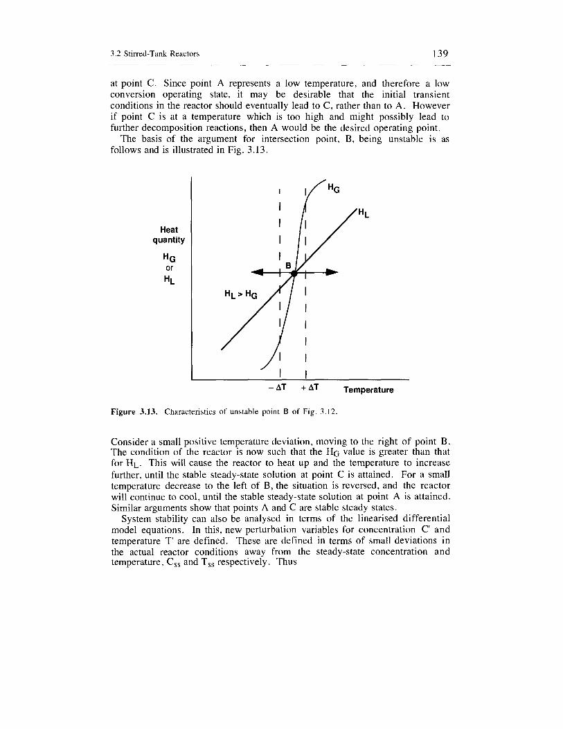
3.2 Stirred-Tank Reactors 139
at point C. Since point A represents a low temperature, and therefore a low conversion operating state, it may be desirable that the initial transient conditions in the reactor should eventually lead to C, rather than to A. However if point C is at a temperature which is too high and might possibly lead to further decomposition reactions, then A would be the desired operating point.
The basis of the argument for intersection point, B, being unstable is as follows and is illustrated in Fig. 3.13.
Heat quantity
HG
HL
or
-AT + A T Temperature
Figure 3.13. Characteristics of unstable point B of Fig. 3.12.
Consider a small positive temperature deviation, moving to the right of point B. The condition of the reactor is now such that the HG value is greater than that for HL. This will cause the reactor to heat up and the temperature to increase further, until the stable steady-state solution at point C is attained. For a small temperature decrease to the left of B, the situation is reversed, and the reactor will continue to cool, until the stable steady-state solution at point A is attained. Similar arguments show that points A and C are stable steady states.
System stability can also be analysed in terms of the linearised differential model equations. In this, new perturbation variables for concentration C' and temperature T' are defined. These are defined in terms of small deviations in the actual reactor conditions away from the steady-state concentration and temperature, C,, and T,, respectively. Thus

140 3 Modelling of Stagewise Processes
C' = C - C,, and T' = T - T,,
The linearisation of the non-linear component and energy balance equations, based on the use of Taylor's expansion theorem, leads to two, simultaneous, first-order, linear differential equations with constant coefficients of the form
-= a l C ' + blT' dC' dt
-= d T a2C' + b2T' dt
The coefficients of the above equations are the partial differentials of the two dynamic balance equations evaluated at C,,, Tss and are given by
where F(C, T) represents the dynamic component balance equation and G(C, T) represents the dynamic heat balance equation.
The two linearised model equations have the general solution of the form
and
The dynamic behaviour of the system is thus determined by the values of the exponential coefficients, h1 and h2, which are the roots of the characteristic equation or eigenvalues of the system and which are also functions of the system parameters.
If hl and h2 are real numbers and both have negative values, the values of the exponential terms and hence the magnitudes of the perturbations away from the steady-state conditions, c', and T', will reduce to zero, with increasing time.

3.2 Stirred-Tank Reactors 141
The system response will therefore decay back to its original steady-state value, which is therefore a stable steady-state solution or stable node.
If h1 and h2 are real numbers and both or one of the roots are positive, the system response will diverge with time and the steady-state solution will therefore be unstable, corresponding to an unstable node.
If the roots are, however, complex numbers, with one or two positive real parts, the system response will diverge with time in an oscillatory manner, since the analytical solution is then one involving sine and cosine terms. If both roots, however, have negative real parts, the sine and cosine terms still cause an oscillatory response, but the oscillation will decay with time, back to the original steady-state value, which, therefore remains a stable steady state.
If the roots are pure imaginary numbers, the form of the response is purely oscillatory, and the magnitude will neither increase nor decay. The response, thus, remains in the neighbourhood of the steady-state solution and forms stable oscillations or limit cycles.
The types of system behaviour predicted, by the above analysis are depicted in Figs. 3.14 and 3.15. The phase-plane plots of Fig. 3.15 give the relation of the dependant variables C and T. Detailed explanation of phase-plane plots is given in control textbooks (e.g., Stephanopoulos, 1984). Linearisation of the reactor model equations is used in the simulation example, HOMPOLY.
System response
Response '
Time
Response
System with complex roots 3 Time
Figure 3.14. Systems response with real and complex roots.

142 3 Modelling of Stagewise Processes
I I I I
a) Stable node b) Unstable node c) Limit cycle
Figure 3.15. Phase-plane representations of reactor stability. In the above diagrams the point + represents a possible steady-state solution, which (a) may be stable, (b) may be unstable or (c) about which the reactor produces sustained oscillations in temperature and concentration.
Thus it is possible for continuous stirred-tank reactor systems to be stable, or unstable, and also to form continuous oscillations in output, depending upon the system, constant and parameter, values.
The linearisation approach, outlined above, also fails in that its analysis is restricted to variations, which are very close to the steady state. While this provides excellent information on the dynamic stability, it cannot predict the actual trajectory of the reaction, once this departs from the near steady state. A full dynamic analysis is, therefore, best considered in terms of the full dynamic model equations and this is easily effected, using digital simulation. The above case of the single CSTR, with a single exothermic reaction, is covered by the simulation examples, THERMPLOT and THERM. Other simulation examples, covering aspects of stirred-tank reactor stability are COOL, OSCIL, REFRIGl, REFRIG2 and STABIL. Phase-plane plots are very useful for the analysis of such systems.
This analysis is limited, since it is based on a steady-state criterion.
32.8 Reactor Control
Two simple forms of a batch reactor temperature control are possible, in which the reactor is either heated by a controlled supply of steam to the heating jacket, or cooled by a controlled flow of coolant (Fig. 3.16). Other control schemes would be to regulate the reactor flow rate or feed concentration, in order to maintain a given reaction rate (see simulation example SEMIEX).

3.2 Stirred-Tank Reactors 143
Figure 3.16. Reactor with control of temperature by manipulating the flow of cooling water.
Fig. 3.17 represents an information flow diagram for the above control scheme.
I Component balance for reactor
Control equation
Jacket heat balance Heat balance for reactor
I T
Figure 3.17. Information flow diagram for the above reactor control implementation.
Assuming the jacket is well-mixed, a heat balance on the jacket gives
dT. V . p . c . J = F. p. c ’ (Tjin - Tj) + U A (T - Tj) J J PJ dt J J PJ
Consider the case of a proportional controller, which is required to maintain a desired reactor temperature, by regulating the flow of coolant. Neglecting dynamic jacket effects, the reactor heat balance, can then be modified to include the effect of the varying, coolant flow rate, Fj, in the model equation, as:

144 3 Modelling of Stagewise Processes
where the mean temperature of the jacket is accounted for by the term, K1, as shown in Sec. 3.2.2.4, and given by
2 Fj P j cpj U A + 2 Fj P j cPj
K1 =
For a proportional controller
where K, is the proportional gain of the controller and the temperature difference term, (T - TSet), represents the error between the reactor temperature T and controller set point Tset. Note that in this conventional negative feedback system, when the reactor temperature, T, is below the set pointtemperature, Tset, the coolant flow is decreased, in order to reduce the rate of heat loss from the reactor to the jacket.
Note also that the incorporation of the controller equation and parameter value, &, into the dynamic model also alters the stability parameters for the system and thus can also change the resultant system stability characteristics. A stable system may be made to oscillate by the use of high values of K, or by the use of a positive feedback action, obtained with the use of the controller equation with K, negative. Thus the reactor acts to provide greater degrees of cooling when, T < Tset, and conversely reduced degrees of cooling when, T > Tyt. This phenomenon is shown particularly in simulation example OSCIL.
This example shows that the reactor may oscillate, either naturally according to the system parameters, or by applied controller action. Owing to the highly non-linear behaviour of the system, it is sometimes found that the net yield from the reactor may be higher under oscillatory conditions than at steady state (see simulation examples OSCIL and COOL). It should be noted also that under controlled conditions, Tset need not necessarily be set equal to the steady-state value, T, and Tset, and that the control action may be used to force the reactor to a more favourable yield condition than that simply determined by steady-state balance considerations.
The proportional and integral controller equation

3.2 Stirred-Tank Reactors I45
where q is the integral time constant and E is the error = (T - TSet) or (CA - CAset) can similarly be incorporated into the reactor simulation model.
Luyben (1973) (see simulation example RELUY) also demonstrates a reactor simulation including the separate effects of the measuring element, measurement transmitter, pneumatic controller and valve characteristics which may in some circumstances be preferable to the use of an overall controller gain term.
3.2.9 Chemical Reactor Safety
A necessary condition for chemical production is the safe operation of chemical reactors and other unit processes (Grewer, 1994). This is best achieved by the design of inherently safe processes, i.e. processes with negligible potential for the release of harmful chemicals. This is often impossible owing to the requirement for active substrates or because of the inherently high reactivity of certain products. The next possible improvement may be made by minimizing the amount of material held under critical conditions or by maintaining process conditions, e.g. pressure and temperature, in the ranges of non-critical conditions. Modelling and simulation provide modern tools for the support of risk analysis and are of major importance for the design of safe chemical reactors and safe operation of chemical reactors (Stoessel, 1995). In the following, safety aspects of batch reactor design and operation are discussed.
3.2.9.1 The Runaway Scenario
A most critical event for an exothermic chemical reaction is that of a cooling failure. Depending on the reactive potential of the process the temperature of the reactor will rise and may thus possibly trigger the formation of unwanted decomposition reactions with often very large potential for possible reactor failure (Fig. 3.18). The thermal runaway of a polymerisation reaction is described in the simulation example RUN. The reactor operation, i.e. feeding of reactants, the selection of process temperature etc., has to be such that a cooling failure will not cause a reaction runaway or that the time-to-maximum rate criterion, TMR,d, is sufficiently long, e.g. 24 hours, to permit the appropriate safety actions to be taken. A proper safety assessment should start

146 3 Modelling of Stagewise Processes
with calorimetric measurements to allow the estimation of ATad,2, the adiabatic temperature rise by decomposition reaction, and also of the time required for this, TMR,d. This study is preferably achieved via the use of differential scanning calorimetry, DSC.
Other simulation examples involving various safety aspects are HMT, THERM, REFRIDGEl, REFRIDGE2 and DSC.
Temperature
ATad2 I
0
-4 - T o -
Tprocess Time
Cooling failure ' Accident
Figure 3.18. Scenario of cooling failure with thermal runaway. ATadl is the adiabatic
temperature rise by desired reaction. ATa& is the adiabatic temperature increase by the decompositiion reaction. The time required for this increase is TMRad.
3.2.9.2 Reaction Calorimetry
In differential scanning calorimetry, the selected chemical reaction is carried out in a crucible and the temperature difference AT compared to that of an empty crucible is measured. The temperature is increased by heating and from the measured AT the heat production rate, q, can be calculated (Fig. 3.19). Integration of the value of q with respect to time yields measures of the total heats released, QR, and QD, from which AHR and &ID, as well as ATadl and ATad2 can be calculated from Fig. 3.18. The estimation of the activation energy, Ea, is possible by the use of isothermal DSC based on the following equation

3.2 Stirred-Tank Reactors 147
q = ko f(c) (-AHR)eXp
or in its logarithmic form
lnq = ln[ko f(c)( -AHR)]-- E a RT
by plotting In q versus 1/T at constant conversion. The pre-exponential factor, ko can be determined knowing f(c), that means conversion and kinetics have to be known. These data permit then a computer simulation of a reactor runaway scenario. Keller et al. (1997) employed a series of chemical kinetic models to simulate the DSC experimental technique suitable for preliminary safety assessment and as an aid to preliminary screening (see simulation example DSC).
Heat production rate qR and qZ w/kSI Decomposition, D
Figure
Reaction (R)
lifferential scanning calorimetry with heat release by desired reaction, R and by decomposition reaction, D.
3.2.10 Process Development in the Fine Chemical Industry
As many other industries, the fine chemical industry is characterized by strong pressures to decrease the time-to-market . New methods for the early screening of chemical reaction kinetics are needed (Heinzle and Hungerbuhler, 1997).

148 3 Modelling of Stagewise Processes
Based on the data elaborated, the digital simulation of the chemical reactors is possible. The design of optimal feeding profiles to maximize predefined profit functions and the related assessment of critical reactor behaviour is thus possible, as seen in the simulation examples RUN and SELCONT.
3.2.11 Chemical Reactor Waste Minimisation
The optimal design and operation of chemical reactors lies at the highest point of the waste minimisation hierarchy, in facilitating a reduction in the production of waste directly at source. Ullmann’s Encyclopedia (1995) describes many significant industrial process improvements that have resulted from direct waste reduction at source initiatives. These include the development of new process routes, equilibrium shifts to improve productivities, improvements in selectivity, new catalyst developments, process optimisation changes, reaction material changes, raw material purity changes, the employment of less harmful process materials and improved recycling and reuse of waste residues. In carrying out such new process initiatives, the combination of chemical reactor design theory and process chemistry is one that provides considerable opportunities for the exercise of flair and imagination. The chemical reactor is now recognised as the single most important key item in the chemical process and especially in regard to waste minimisation, where the emphasis is being applied increasingly to the maximum utilisation of reactants, maximum production of useful products and minimisation of wasteful byproducts. In this, it is important to choose the optimum process chemistry, the best chemical reaction conditions and the most appropriate form and mode of operation for the actual chemical reactor. The importance of the reactor, in this respect, lies in the dependence of chemical reaction rates on reactant concentration and temperature. Thus the manipulation of concentration and temperature levels within the reactor provides an opportunity to directly manipulate relative reaction rates and force reactions towards higher degrees of conversion and towards higher selectivities for the desired products as compared to byproduct wastes.
The above principles have been recognised since the very beginnings of chemical reactor design theory and are well treated in conventional reactor design textbooks. The topic is also given special emphasis with respect to the minimisation of waste by Smith (1995). The importance of the very early consideration of waste minimisation in an integrated process development strategy has also been highlighted by Heinzle and Hungerbuhler (1997). In this latter respect, digital simulation forms a very important adjunct in enabling

3.2 Stirred-Tank Reactors 149
a detailed study of many prospective alternatives at the earliest design stage. An essential part of this process is the application of modelling and simulation techniques, particularly using models that are formulated as simply as possible with minimum complexity; a topic stressed extensively throughout this book. Important aspects of waste minimisation, as allied to chemical reactor design and operation, are illustrated in many of the accompanying digital simulation examples as follows: BATSEQ involving optimum reaction time; BATCOM, HYDROL, RELUY, BENZYD, ANHYD and REVTEMP having optimal temperature or optimum temperature profiling strategies; CASCSEQ, SEMIPAR and SEMISEQ with optimal feed distribution policies; REXT featuring increased conversion via in situ product removal and BATSEG SEMISEG and COMPSEG describing feed segregation effects.
In all these examples, the relevent waste minimisation aspects can be usefully studied simply in terms of the relative distribution of reaction compounds produced, or by an extension of the programs to include possible quantification. A useful method of comparison is the “environmental index” as defined by Sheldon (1994), as the mass ratio of the total waste to that of useful product. He showed that this index is very dependent both on the scale and chemical complexity of the process, with values ranging from about 0.1 for oil refining applications, up to 50 for fine chemical production and up to 100 plus for pharmaceutical operations. It thus reflects both the smaller scale of production, the greater usage of batch and semi-batch operations and the greater complexity of the chemical processes. Sheldon also suggested the use of an environmental quotient, defined as EQ = E Q, where Q is an arbitary quotient related to the degree of environmental damage, with Q varying from 1 for simple compounds and up to 1000 for very destructive compounds.
Heinzle et al. (1998) and Koller et al. (1998) have described a simple but slightly more elaborate methodology to calculate such an environmental quotient based on more detailed material balances. Alternatively in terms of the present simulation examples, the analysis may perhaps be extended simply by means of incorporating a simple weighting or cost factor for each material to account for positive sales value or negative cost values representing the potential damage to the environment, as suggested in simulation example BATSEQ. A full analysis of any reactor or process simulation, must of course take full account of all the relevent aspects, and Heinzle et al. (1998) and Koller et al. (1998) describe detailed studies as to how this might best be achieved.
Simulation Considerations
The waste minimisation reaction related examples in this text are represented mainly by combinations of consecutive and parallel type reactions. Although the major details of such problems are dealt with in conventional textbooks, it may be useful to consider the main aspects of such problems from the viewpoint of solution by digital simulation.

150 3 Modelling of Stagewise Processes
Consider the following first-order consecutive reaction sequence
Solving the kinetic equations clearly demonstrates that the concentration of B passes through a maximum in respect to reaction time. If B is the desired product and C is waste, an optimal time t opt can be defined for the maximum concentration of B and where both the optimal yield and optimum reaction time are functions of the kinetic rate constants kl and k2. In waste minimisation terms, however, the quantity of B obtained both in relation to the unreacted A and waste product C is important, since these may represent quite distinct separation problems and may also have quite distinct associated environmental loadings. In general, one wants the rate of decomposition of A to B to be high relative to the rate of decomposition of B to C. Since these rates are also temperature dependent, a favourable product distribution can also be effected by varying the reaction temperature.
Now consider the following parallel reaction where A and B are reactants, P is useful product and Q is byproduct waste.
A + B k l P
It is obviously important to achieve complete reaction for A and B and high selectivity for the formation of P with respect to Q.
The individual rates of reaction may be given by
and rp= k l CAnA1 CBnB'
nA2 c nB2 'Q = k2 cA B
where nA1 and n ~ 2 and ngl and ng2 are the respective orders of reaction for reactions 1 and 2.
The relative selectivity for the reaction is given by:
2 - $- c (nAl-nA2) c (nB1-nB2)
rQ k2 A B -
Thus if nAl > n ~ 2 , high selectivity for P is favoured by maintaining the concentration of A high. Conversely if nAl c n ~ 2 , high selectivity is favoured by low concentration of B.
With the orders of reaction being equal in both reactions

3.2 Stirred-Tank Reactors 151
where kl and k2 are both functions of temperature, again showing that a favourable selectivity can be obtained by appropriate adjustment of the reactor temperature.
These and other waste minimisation considerations can be explored more fully both by reference to conventional texts and by simulation.
3.2.12 Non-Ideal Flow
The previous analysis of stirred-tank reactors has all been expressed in terms of the idealised concept of perfect mixing. In actual reactors, the mixing may be far from perfect and for continuous flow reactors may lie somewhere between the two idealised instances of perfect mixing and perfect plug flow, and may even include dead zones or short-cut flow. The concept of ideal plug flow is usually considered in terms of continuous tubular or continuous column type devices and the application of this to continuous flow reactors is discussed in Sec. 4.3.1. In ideal plug-flow reactors, all elements of fluid, spend an identical period of time within the reactor, thus giving a zero distribution of residence times. All elements of fluid thus undergo an equal extent of reaction, and temperatures, concentrations and fluid velocities are completely uniform across any flow cross section. For a well-mixed, continuous stirred-tank reactor, however, there will be elements of fluid with, theoretically, a whole range of residence times varying from zero to infinity. Practical reactors will normally exhibit a distribution of residence times, which lie somewhere between these two extreme conditions and which effectively determine the performance of the reactor. The form of the residence time distribution curve can therefore be used to characterise the nature of the flow in the reactor and models of the mixing behaviour can be important in simulations of reactor performance. Often different combinations of tanks in series or in parallel can be used to represent combinations of differing mixed flow regions and provide a powerful tool in the analysis of actual reactor behaviour.
Using Tracer Information in Reactor Design
Residence time distributions (RTD) can be determined in practice by injecting a non-reactive tracer material into the input flow to the reactor and measuring the output response characteristics in a similar manner to that described previously in Sec. 2.1.1.

152 3 Modelling of Stagewise Processes
Unfortunately RTD studies cannot distinguish between early mixing and late mixing sequences of different types. Whereas the mixing history does not influence a first-order reaction, other reaction types are affected; the more complex the reaction kinetics the more the reaction selectivity or product distribution generally will be influenced. Thus for certain kinetic cases a detailed knowledge of the mixing can be important to the reactor performance. In practice this information may be difficult to obtain, In principle, tracer injection and sampling at different points in the reactor can supply the needed information. In practice, the usual procedure is to develop a model based on RTD experiments and the modeller’s intuition. A comparison of the actual reactor performance with the model predictions for known reaction kinetics reveals then whether the model assumptions were correct. The procedure is outlined below in Fig. 3.20.
I
Dynamic tracer experiment
I 1 I i
Reaction kinetics model Kinetic parameters combined with mixing model I
Simulation
Steady-state experiment Revision
I Final design I + Application for control and operation
Figure 3 . 2 0 . Reactor design procedure with reactors having residence time distributions deviating from those of ideal reactors.

3.2 Stirred-Tank Reactors 153
Simulation examples demonstrating non-ideal mixing phenomenon in tank reactors are CSTRPULSE, NOCSTR and TUBEMIX. Other more general examples demonstrating rank based residence time distributions are MIXFLO, GASLIQ and SPBEDRTD
3.2.13 Tank-Type Biological Reactors
Fermentation systems obey the same fundamental mass and energy balance relationships as do chemical reaction systems, but special difficulties arise in biological reactor modelling, owing to uncertainties in the kinetic rate expression and the reaction stoichiometry . In what follows, material balance equations are derived for the total mass, the mass of substrate and the cell mass for the case of the stirred tank bioreactor system (Dunn et al. 1992).
As indicated below in Fig. 3.21, feed enters the reactor at a volumetric flow rate Fo, with cell concentration, Xo, and substrate concentration, So. The vessel contents, which are wellmixed, are defined by volume V, substrate concentration S1 and cell concentration X I . These concentrations are identical to those of the outlet stream, which has a volumetric flow rate F1.
Figure 3.21. Tank fermenter variables.
The general balance equations are based on the relationship:
(Rate of accumulation) = (Input rate) - (Output rate) + (Production rate)

154 3 Modelling of Stagewise Processes
and can be applied to the whole volume of the tank contents. Expressing the balance in equation form, gives:
Total mass balance:
Substrate balance:
Organism balance:
where the units are: V (m3), p (kg/m3), F (m3/s), S (kg/m3), X (kg/m3) with rs
and r x (kg/m3 s).
The rate expressions can be simply given by the Monod Equation:
and
using a constant yield coefficient rX rs = -
YXIS
but other forms of rate equation may equally apply.
cases of bioreactor operation. The above generalised forms of equations can be simplified to fit particular

3.2 Stirred-Tank Reactors 155 ~-
3.2.13.1 The Batch Fermenter
Figure 3.22. The batch fermenter and variables.
an initial quantity of limiting Starting from an inoculum (X at t = O ) and - substrate, S at t = 0, the biomass will grow, perhaps after a short lag phase, and will consume substrate (Fig. 3.22). As the substrate becomes exhausted, the growth rate will slow and become zero when substrate is completely depleted. The above general balances can be applied to describe the particular case of a batch fermentation (constant volume and zero feed). Thus,
Total balance:
- = 0 dV dt
Substrate balance: V - - dS1 - rSV
dt Organism balance:
Suitable rate expressions for rs and rx and the specification of the initial conditions would complete the batch fermenter model, which describes the exponential and limiting growth phases but not the lag phase.

156 3 Modelling of Stagewise Processes
3.2.13.2 The Chemostat
r- s,,x, , v
Figure 3.23. The chemostat and its variables.
The term chemostat refers to a tank fermentation which is operated continuously (Fig. 3.23). This bioreactor mode of operation normally involves sterile feed (Xo = 0) and constant volume, steady state conditions, meaning that dV/dt = 0, d(VSl)/dt = 0, d(VXl)/dt = 0. For constant density the total mass balance simplifies to,
which means that the flow rates in and out of the bioreactor must be equal. The dynamic component balance equations are then,
Substrate balance
!!&!I = F ( S o - S 1 ) + r s V dt
Cell balance VdXl - - - F X l + r x V
dt
where F is the volumetric flow through the system.
At steady state, dSl/dt = 0 and dXl/dt = 0. Hence for the substrate balance:
0 = F ( S o - S l ) + r S V

3.2 Stirred-Tank Reactors 157
and for the cell balance: 0 = - F X l + r x V
Inserting the Monod-type rate expressions, gives:
For the cell balance:
or simply
Here D is the dilution rate and is equal to 1/z, where z = V/F and is equal to the mean residence time of the tank.
For the substrate balance:
F (SO-SI) = - rx v YXIS
from which x1 = yx/s (So- S1)
Thus, the specific growth rate in a chemostat is controlled by the feed flow rate, since p is equal to D at steady state conditions. Since p, the specific growth rate,
is a function of the substrate concentration, and since p is also determined by dilution rate, then the flow rate F also determines the outlet substrate concentration S l . The last equation is, of course, simply a statement that the quantity of cells produced is proportional to the quantity of substrate consumed, as related by the yield factor Yx/s.
If the flow rate F is increased, D will also increase and causes the steady state value of S1 to increase and the corresponding value of X1 to decrease. It can be seen by simulation that when D nears pm, X1 will become zero and S1 will rise to the inlet feed value So. This corresponds to a complete removal of the cells by flow out of the tank, and this phenomenon is known as “washout”.

158 3 Modelling of Stagewise Processes
3.2.13.3 The Fed Batch Fermenter
Figure 3.24. Fed batch fermenter variables.
This bioreactor mode refers to a tank fermenter operated semi-continuously (Fig. 3.24). The rate of the feed flow, Fo, may be variable and there is no outlet flow rate from the fermentor. As a consequence of feeding the reactor volume will change with respect to time.
The balance equations then become for constant density
- = Fo dV
dt
Here the quantities VSl and VX1 represent the masses of substrate and biomass, respectively, in the reactor. In a simulation, dividing these masses by the volume V gives the concentrations S1 and Xlas a function of time and which are needed in the appropriate kinetic relationships to calculate rs and rx.
It can be shown by simulation that a quasi-steady state can be reached for a fed-batch fermenter, where dXl/dt = O and p =F/V (Dunn and Mor, 1975). Since V increases, p must therefore decrease, and thus the reactor moves through a series of changing steady states for which p = D , during which S1 and p decrease, and X1 remains constant. A detailed analysis of fed batch operation has been made by Keller and Dunn (1978).
All three bioreactor modes described above can be simulated using simulation example BIOREACT.

3.3 Stagewise Mass Transfer 159
3.3 Stagewise Mass Transfer
33.1 Liquid-Liquid Extraction
Liquid-liquid extraction is an important chemical engineering separation process and a knowledge of the process dynamics is important since many solvent extraction operations are still carried out batchwise. In addition, although most continuous solvent extraction plants are still designed on a steady-state basis, there is an increasing awareness of the need to assess possible safety and environmental risks at the earliest possible design stage. For this, a knowledge of the probable dynamic behaviour of the process becomes increasingly important. This applies, especially, in the fields of nuclear reprocessing and heavy metal extraction.
The modelling of solvent extraction is also of interest, since the dynamic behaviour of both liquid phases can be important, and because of the wide range of equipment types that can be employed and the wide range of dynamic behaviour that results. The equipment is typified by mixer-settlers at one extreme, often representing high capacity, stagewise contacting devices, in which near equilibrium conditions are achieved with slow, stable, but long- lasting dynamic characteristics. At the other extreme are differential column devices, representing high throughput, low volume, non-equilibrium, differential contacting devices, with fast-acting dynamic behaviour. These columns have a limited range of permissible operating conditions and often an inherent lack of stability, especially when plant conditions are changing rapidly. Truly differential column devices are considered in Chapter 4, but some types of extraction columns can be regarded basically as stagewise in character, since the modelling of the dynamic characteristics of this type of device, leads quite naturally from the equilibrium stagewise approach.
The treatment is confined to the use of two completely immiscible liquid phases, the feed or aqueous phase and the solvent or organic phase. No attempt is made to apply the modelling methodology to the case of partially miscible systems. Although one of the phases, the dispersed phase, will be in the form of droplets, dispersed in a continuum of the other, this is simplified by assuming each liquid phase to consist of separate, well-mixed stage volumes. The modelling approach, shown in this chapter, follows the general modelling methodology, in that it starts with the simplest case of a single component,

160 3 Modelling of Stagewise Processes
batch extraction and then builds in further complexities. Finally a complex model of a non-ideal flow in a multistage, multicomponent, extraction cascade, which includes a consideration of both hydrodynamic effects and control, is achieved.
3.3.1.1 Single Batch Extraction
Volumes VL and VG of the two immiscible liquid phases, are added to the extraction vessel and a single solute distributes itself between the phases as concentrations X and Y, respectively, at a rate, Q, as shown in Fig. 3.25.
Figure 3.25. Single-solute batch extraction between immiscible liquid phases
For batch extraction, with no feed into the system, the component balances on each phase are given by:
Rate of accumulation
the given phase
Effective rate of
or from the phase of solutein ] = [ mass transferto j
Neglecting the effects of concentration changes on solvent density, the phase volumes will remain constant. Thus for the liquid phase with volume VL
and for liquid phase, with volume VG
dY v G - = dt + Q
where Q is the rate of solute transfer with units (molh) or (kg/s)

3.3 Stagewise Mass Transfer 161
Q = KL a (X - X*) V
KL is the mass transfer coefficient for the L phase ( d s ) , a is the interfacial area per unit volume (m2/m3), referred to the total liquid volume of the extractor, V is the total holdup volume of the tank, and is equal to (VL+VG). X* is the equilibrium concentration, corresponding to concentration Y, given by
X* = feq(Y)
as illustrated in Fig. 3.26 below.
X
X*
Y Y*
Figure 3.26. Equilibrium relationship between two liquid phases.
The information flow diagram, Fig. 3.27, for this system shows the two component material balance relations to be linked by the equilibrium and transfer rate relationships.
Note that the transfer rate equation is based on an overall concentration driving force, (X-X*) and overall mass transfer coefficient, KL. The two-film theory for interfacial mass transfer shows that the overall mass transfer coefficient, KL, based on the L-phase is related to the individual film coefficients for the L and G-phase films, kL and kG, by the relationship

162 3 Modelling of Stagewise Processes
A 1 . Q = - KL a (X-X*) V
Figure 3.27. Information flow diagram for simple batch extraction.
where m is the slope of the equilibrium curve, and
- = m dY*
dX
For a linear equilibrium curve with constant film coefficients, kL and kG, the overall coefficient, KL, will also be constant, but for the case of a non-linear equilibrium relationship, the value of m, which is the local slope of the equilibrium curve, will vary with solute concentration. The result is that the overall coefficient, KL, will also vary with concentration, and therefore in modelling the case of a non-linear equilibrium extraction, further functional relationships relating the mass transfer coefficient to concentration will be required, such that
KL = f ( X )
3.3.1.2 Multisolute Batch Extraction
Two solutes distribute themselves between the two phases as concentrations XA and YA, and XB and YB and with rates QA and QB, respectively as shown in Fig. 3.28. The corresponding equilibrium concentrations XA* and XB* are functions of both the interacting solute concentrations, YA and YB, and can be expressed by functional relationships of the form

3.3 Stagewise Mass Transfer 163
Figure 3.28. Two-solute batch extraction.
Typical representations of the way that the two differing equilibrium relationships can interact are shown in Fig. 3.29, and it is assumed that the equilibria can be correlated by appropriate, explicit equation forms.
YA
Increasing XB /
//
Increasing XA
Figure 3.29. Interacting solute equilibria for the two solutes A and B.
For multi-component systems, it is necessary to write the dynamic equation for each phase and for each solute, in turn. Thus for phase volume VL, the balances for solute A and for solute B are
VG - dYA - - + KLA a (XA - XA") VL dt
dYB = + KLB a (XB - XB") VL VG dt
The overall mass transfer coefficients are also likely to vary with concentration, owing to the complex multisolute equilibria, such that:

164 3 Modelling of Stagewise Processes
Again, these functional relationships should ideally be available in an explicit form in order to ease the numerical method of solution. Two-solute batch extraction is covered in the simulation example TWOEX.
3.3.1.3 Continuous Equilibrium Stage Extraction
Here the extraction is carried out continuously in a single, perfectly mixed, extraction stage as shown in Fig. 3.30. It is assumed that the outlet flow concentrations, X 1 and Y 1 , achieve equilibrium and that density variations are negligible.
I
Figure 3.30. Continuous equilibrium stage extraction
Following an initial transient, the extractor will achieve a steady state operating condition, in which the outlet concentrations remain constant with respect to time.
At steady state, the quantity of solute entering the extractor is equal to the quantity of solute leaving. A steady-state balance for the combined two-phase system gives
L X o + G Y o = LX1 + GY1
where for an equilibrium stage extraction
Here, L and G are the volumetric flow rates of the heavy and the light phases, respectively, Xo and Yo are the respective inlet solute concentrations of the two phases, X1 and Y1 are the respective outlet solute concentrations.

3.3 Stagewise Mass Transfer 165
For a linear equilibrium relationship,
Y1 = mX1
A simple substitution of steady-state concentration
the value Y1 in the balance equation enables the X I to be determined, where
The steady-state approach, however, provides no information on the initial transient conditions, whereby the extractor achieves eventual steady state or on its dynamic response to disturbances.
The eventual steady state solution may often be also very difficult to calculate for cases in which the equilibrium is non-linear or where complex interacting equilibria for multicomponent mixtures are involved. In such instances, we have found a dynamic solution to provide a very simple means of solution.
The dynamic component balance equations for each of the two phases in turn.
[accumulation] Rate of = [ Rate flow of in ) - [flow Rate out) of f [of t tEte) of solute of solute of solute transfer
The sign of the transfer term will depend on the direction of mass transfer. Assuming solute transfer again to proceed in the direction from volume VL to volume VG, the component material balance equations become for volume VL
and for volume VG
VG - dY1 = G Yo - G Y1 + Q dt
where Q = KL a(X1 - XI*) VL
For an equilibrium stage, the outlet concentrations leaving the stage are in equilibrium, i .e.
X I " = feq (Yl)
Here an arbitrarily high value for the mass transfer coefficient KL can be used to force a close approach to equilibrium. Thus for a finite value of the rate of transfer Q, the driving force will be very small, and hence the value of X," is

166 3 Modelling of Stagewise Processes
forced to be very close to Xn. The final near equilibrium condition is thus achieved as a result of the natural cause and effect in which equilibrium is favoured by a high mass transfer coefficient, which is used here simply as a high gain forcing factor, in the manner originally suggested by Franks (1 972). Using this technique, some additional problems in solution may be experienced due to stiffness caused by a too high value for KL, but using the fast numerical integration routines of Madonna, such difficulties become rather minimal. This dynamic approach to equilibrium method is used in later examples to illustrate its further application to the solution of complex steady state problems.
Continuous single-stage extraction is treated in the simulation example EQEX. Chemical reaction with integrated single-stage extraction is demon- strated in simulation example REXT.
3.3.1.4 Multistage Countercurrent Extraction Cascade
For a high degree of extraction efficiency, it is usual to connect several continuous flow stages to form a countercurrent flow extraction cascade, as indicated in Fig. 3.3 1.
Figure 3.31. Multistage countercurrent extraction cascade.
In each stage, it is assumed that the two phases occupy well-mixed, constant volumes VL and VG. The phase volumes VL and VG can, however, vary from stage to stage along the cascade. This effect is easily included into any simulation program. Additional complexity, in the formulation of the model, is now provided by the requirement of having to write balance equations for each of the stages of the cascade. The total number of equations to be solved is thus increased, but the modelling procedure remains straightforward.
For any given stage, n, the component material balance equations for each phase are thus defined by

3.3 Stagewise Mass Transfer 167
where
and
as shown in Fig. 3.32.
Figure 3.32. Flow and composition inputs to stage n of the cascade.
Note that the rate of transfer is defined by the local concentrations Xn and Xn" appropriate to the particular stage, n. It is straightforward in the formulation of the model to allow for variations of the parameter values, VL, VG, KL and a from stage to stage and for both KL and a to vary with respect to the local concentration. In order to do this, it is necessary to define new constant values for VL and VG for each stage and to have functional relationships, relating the mass transfer capacity coefficient to stage concentration. In order to model equilibrium stage behaviour, actual values of the mass transfer capacity product term, (KLn a,), would be again replaced by an arbitrary high value of the gain coefficient, KL,, to force actual stage concentrations close to the equilibrium. Multistage extraction is treated in the simulation example EQMULTI, which permits calculation of the dynamics and steady state for situations in which the numbers of stages, flow rate and mass transfer conditions can all become variables in the simulation solution.

168 3 Modelling of Stagewise Processes
3.3.1.5 Countercurrent Extraction Cascade with Backmixing
The extension of the modelling approach to allow for backmixing between stages, cascades with side streams, or multiple feeds is also accomplished, relatively easily, by an appropriate modification of the inflow and outflow terms in the component balance equations. Backmixing reduces the efficiency of countercurrent mass transfer cascades, owing to its effect on the concentration profiles within the cascade and in decreasing the effective concentration driving forces. The effects of backmixing are especially severe in the case of solvent extraction columns. The stagewise model with backmixing is a well-known model representation, but the analytical solution is normally mathematically very complex and analytical solutions, both for steady-state and unsteady-state operating conditions, only apply for single- solute extraction where parameter values remain constant and furthermore where a linear equilibrium relationship applies. Compared to this, the solution of the dynamic model equations by digital simulation using Madonna is far more general, since this has the ability to encompass varying parameter values, non-linear equilibria multisolute systems plus a variable number of stages.
A multistage extraction cascade with backmixing is shown in Fig. 3 .33 . Here the backmixing flow rates LB and GB act in the reverse direction to the main phase flows, between the stages and along the cascade. One important factor in the modelling process is to realise that, as a consequence of the backmixing flows, that since phase volumes remain constant, then the interstage flow rates along the cascade, in the forward direction, must also be increased by the magnitude of the appropriate backmixing flow contribution. With a backmixing flow LB in the aqueous phase, the resultant forward flow along the cascade must now be (L + LB), since the backmixing does not appear exterior to the column. Similarly with a backmixed flow GB, the forward flow for the organic phase is also increased to (G + GB). Taking into account the changed flow rates, however, the derivation of the component balance equations follows normal procedures.

3.3 Stagewise Mass Transfer 169
<& .& X & . + ,&. 1 2 3 4 5 6
Figure 3.33. Multistage extraction cascade with backmixing of both phases.
%-x1,- %-
Y l Y2 . - -
The relative inflow and outflow contributions for each phase of any the cascade is shown in Fig. 3.34.
xg,- xq,- h-
Y3 Y5 . - -
Figure 3.34. Stage n of a multistage extraction cascade with backmixing.
+ y7, G
stage n, of
Allowing for the additional backmixing flow contributions, the component balance equation for the two phases in stage n of the cascade are now
VLn - dXn = (L + LB) Xn-1 - (L + LB) Xn + LB Xn+l - LB X n - Qn dt

170 3 Modelling of Stagewise Processes
or
Although more complex in form, the resulting model equations provide no major additional difficulty, and solution is also easily obtained. Multistage extraction with backmixing is covered in the simulation example EQBACK.
3.3.1.6 Countercurrent Extraction Cascade with Slow Chemical Reaction
A countercurrent extraction cascade with reaction A + B -+ C is shown in Fig. 3.35. The reaction takes place between a solute A in the L-phase, which is transferred to the G-phase by the process of mass transfer, where it then reacts with a second component, B, to form an inert product, C, such that A, B and C are all present in the G-phase.
GI yAl yBl yc1
4-
L, xAO 1 2
G ~ Y A N + i YBN + 1 YCN + 1
n
VLn XAn
Figure 3.35. Solute A is transferred from the L-phase to the G-phase, where it reacts with a component B, to form C.
The general component balance form of equation gives

3.3 Stagewise Mass Transfer 171
Rate of
reaction
Rate of Inflow outflow Rate of
of solute in phase i in phase i in phase i transfer
and for phase G
Components B and C are both immiscible in phase L and remain in phase G . Therefore
where the transfer rate is
and the reaction rate is
Fig, 3.36 shows the graphical output in the G-phase concentrations of component A with respect to time, starting the cascade at time t = 0 with initially zero concentrations throughout. The maximum in the YA1 profile for stage 1 is, due to a delay of reactant B in reaching A. This is because A and B are fed from the opposite ends of the cascade, and thus a certain time of passage through the extractor is required before B is able to react with A in stage 1.

172 3 Modelling of Stagewise Processes
1.6
2.0 1 ! yAi 1.2
Concentration
0.8
0.4
0
’- I /
I I I I I I I
0 2 4 6 Time
Figure 3 . 3 6 . Concentrations in the solvent phases of stages 1 , 2 and 3 in a countercurrent extraction column with slow chemical reaction.
3 .3 .1 .7 Multicomponent Systems
Assuming the liquid phases remain immiscible, the modelling approach for multicomponent systems remains the same, except that it is now necessary to write additional component balance equations for each of the solutes present, as for the multistage extraction cascade with backmixing in Sec. 3.3.1.5. Thus for component j , the component balance equations become
where Qjn = KLjn an (Xjn - Xjn*> V n
The additional number of differential equations and increased complexities of the equilibrium relationships may also be compounded by computational

3.3 Stagewise Mass Transfer 173
problems caused by widely differing magnitudes in the equilibrium constants for the various components. As discussed in Sec. 3.3.2, it is shown that this can lead to widely differing values in the equation time constants and hence to stiffness problems for the numerical solution.
3.3 .1 .8 Control of Extraction Cascades
A typical control problem might be the maintenance of a required raffinate outlet concentration, YN, with the controller action required to compensate the effect of variations in the feed concentration YO, as indicated in Fig 3.37.
Figure 3.37. Maintenance of raffinate outlet concentration, by regulation of solvent flow rate.
The proportional-integral control equation, as given in Sec. 2.3.2.2 is:
t K P L = LO + Kp E(t) + - E(t) dt
0
where L is the manipulated variable, i.e., the solvent flow rate, Lo is the base value for L, K, is the proportional gain, q is the integral action time and E is the error between the actual concentration, YN, and the desired value Yset. These relationships can be directly incorporated into a digital simulation program as shown in example EXTRACTCON. If required, it is also possible to include the dynamic effects of the measuring elements, measurement transmitters, and the

174 3 Modelling of Stagewise Processes
control valve characteristics into the simulation program as shown by Franks (1972) and Luyben (1990).
3.3.1.9 Mixer-Settler Extraction Cascades
The archetypal, stagewise extraction device is the mixer-settler. This consists essentially of a well-mixed agitated vessel, in which the two liquid phases are mixed and brought into intimate contact to form a two-phase dispersion, which then flows into the settler for the mechanical separation of the two liquid phases by continuous decantation. The settler, in its most basic form, consists of a large empty tank, provided with weirs to allow the separated phases to discharge. The dispersion entering the settler from the mixer forms an emulsion band, from which the dispersed phase droplets coalesce into the two separate liquid phases. The mixer must adequately disperse the two phases, and the hydrodynamic conditions within the mixer are usually such that a close approach to equilibrium is obtained within the mixer. The settler therefore contributes little mass transfer function to the overall extraction device.
Ignoring the quite distinct functions and hydrodynamic conditions which exist in the actual mixer and settler items of the combined mixer-settler unit, it is possible, in principle, to treat the combined unit simply as a well-mixed equilibrium stage. This is done in exactly the way, as considered previously in Secs. 3.2.1 to 3.2.6. A schematic representation of an actual mixer-settler device is shown in Fig. 3.38 and an even more simplified representation of the equivalent simple well-mixed stage is given in Fig. 3.39.
Figure 3.38. Schematic representation of a mixer-settler unit.

3.3 Stagewise Mass Transfer 175
Figure 3.39. The well-mixed stage representation of a mixer-settler unit.
A realistic description of the dynamic behaviour of an actual mixer-settler plant item should however also involve some consideration of the hydrodynamic characteristics of the separate mixer and settler compartments and the possible flow interactions between mixer and settler along the cascade.
The notation for separate mixer-settler units is shown in Fig. 3.40, for stage n of the cascade.
Figure 3 . 4 0. The separate mixer and settler compartments for stage n of a mixer-settler cascade.
In this representation, the heavy phase with a flow rate, Ln-1, enters the mixer from the preceding stage n-1, together with solvent flow, G n + l , from stage n+ l . The corresponding phase flow rates, in the dispersion, leaving the mixer and entering the settler are shown as Lmn and Gmn and with concentrations X,, and Ymn respectively. This is to allow for possible changes in the volumetric holdup of the mixer following changes in flow rate. The modelling of the separate mixer and settler compartments follows that of Wilkinson and Ingham (1983).

176 3 Modelling of Stagewise Processes
Mixer Dynamics
Owing to the intensive agitation conditions and intimate phase dispersion, obtained within the mixing compartment, the mixer can usually be modelled as a single, perfectly mixed stage in which the rate of mass transfer is sufficient to attain equilibrium. As derived previously in Sec. 3.3.1.9, the component balance equations for the mixer, based on the two combined liquid phases, is thus given by
where subscript m refers specifically to the conditions, within the mixer and hence to the effluent flow, leaving the mixer and entering the settler.
The total material balance for the mixer is expressed by
(Rate of change of mass in mixer
Neglecting the effects of any density changes, the total material balance then provides the relationship for the change of total volume in the mixer with respect to time.
Under well-mixed flow conditions, it is reasonable to assume that the mixer holdup volumes, VLmn and VGmn will vary in direct proportion to the appropriate phase flow rate, and that the total liquid holdup in the mixer will vary as a function of the total flow rate to the mixer.
The total flow rate, (Lmn + Gmn), leaving the mixer will be related to the total phase volumes VLm and Vcm by a hydrostatic equation, which will depend on the net difference in the head of liquid, between the levels in the mixer and in the settler. The actual form of this relationship might need to be determined experimentally, but could, for example, follow a simple, square-root relationship of the form in which flow rate is proportional to the square root of the difference in liquid head, or indeed to the total volume of liquid in the mixer, e.g.,
The further assumptions are that the respective phase volumes are in direct proportion to the phase flow rate, i.e.,

3.3 Stagewise Mass Transfer 177
VLmn - Lmn vGmn Gmn
and the concentrations leaving the mixer are in equilibrium, according to
These equations complete a preliminary model for the mixer. Note that it is also possible, in principle, to incorporate changing density effects into the total material balance equation, provided additional data, relating liquid density to concentration are available.
Settler Dynamics
The simplest settler model is that in which it is assumed that each phase flows through the settler in uniform plug flow, with no mixing and constant velocity. This has the effect that the concentrations leaving the settler, X, and Y,, are simply the time delayed values of the exit mixer concentrations, X,, and Ym,. In this the magnitude of the time delay is thus simply the time required for the phase to pass through the appropriate settler volume.
The outlet phase flow rates, L, and Gn, may again be related to the inlet settler phase flow rates, Lmn and G,,, and settler phase volumes by hydraulic considerations, using similar formulations to those proposed for the mixer, as required.
In practice, some mixing will, however, occur in each phase of the settler, and various models involving either an arbitrary number of perfect mixing stages or various flow combinations, with and without recycle effects, can be postulated. Some of these are indicated in Fig. 3.41, where Fig. 3.41(A) represents settler mixing, given by a series of stirred tanks, Fig. 3.41(B) a series of well-mixed tanks interconnected to stagnant regions and Fig. 3.41(C) a series of two tanks with recycle. The actual representation adopted for a given situation, would, of course, have to depend very much on the actual mechanical arrangement and flow characteristics of the particular settler design, together with actual observations of the flow behaviour.

178 3 Modelling of Stagewise Processes ~
Figure 3.41. Alternative settler-flow representations, for the separate phases.
A
B
C
Fig. 3.42 shows one possible representation, in which a proportion of each phase, passes through the settler in plug flow, while the remaining proportion is well mixed.
The resultant outlet concentration from the settler is then given by the combined plug-flow and well-mixed flow streams.

3.3 Stagewise Mass Transfer 179
r-- ------I
G
Y
Figure 3.42. Combined plug-flow and well-mixed, settler-flow representation.
The notation for the above flow model, in respect of the aqueous-phase settler volume, is shown in Fig. 3.43.
For each phase
Ln Xn
b
Xsmn
Lmn f Plug flow time delay tDn
Lmn Xmn
Mixed flow
Vsmn
Figure 3 . 4 3 . Combined plug-flow and well-mixed flow representation for the heavy phase settler flow.

180 3 Modelling of Stagewise Processes
If Lmn is the volumetric flow rate of the heavy phase entering the settler from the mixer, and f is the fraction of flow passing through the plug-flow region with time delay tDn, then f Lmn is the volumetric flow passing through the plug- flow region. The concentration at the plug-flow region outlet, Xspn, is the inlet concentration at time t - tDn and is given by
The fractional flow rate, (1 - 0 L,,, is then also the volumetric flow passing through the well-mixed region of settler phase volume, Vmix. The flows leaving the plug-flow and well-mixed regions, Xspn and Xsmn, respectively, then combine to give the actual exit concentration from the settler, Xn.
The model equations for the heavy phase settler region then become for the well-mixed region
and for the combined outlet phase flow
Mixer-Settler Cascade
The individual mixer and settler model representations can then be combined into an actual countercurrent-flow , multistage, extraction scheme representation as shown in Fig. 3.44. This includes an allowance for backmixing, between the stages of the cascade caused by inefficient phase disengagement in the settlers, such that a fraction, fL or fG of the appropriate phase flow leaving the settler is entrained. This means it is actually carried back in the reverse direction along the cascade by entrainment in the other phase. It is assumed, for simplicity, that the total flows of each phase, L and G, remain constant throughout all the stages of the cascade. Entrainment fractions, fL and fG, are also assumed constant for all settlers. The above conditions, however, are not restrictive in terms of the capacity of the solution by digital simulation.

3.3 Stagewise Mass Transfer 181
n
N
Figure 3.44. Multistage mixer-settler cascade with entrainment backmixing. to mixer and S and s to settler; stages are 1 to N.
M and m refers
The conditions in the mixer of any stage n are represented in Fig. 3.45.

I82 3 Modelling of Stagewise Processes
Figure 3.45. One mixer-settler stage, n.
Allowing for the additional flow contributions due to the entrainment backmixing, the component balance equations, for any mixer, n, along the cascade, are now expressed by
and
The settler equations are as shown previously, but must, of course, be applied to both phases.
Fig. 3.46 shows the output obtained from a full solution of the mixer-settler model. The effect of the time delay in the settlers, as the disturbance, as propagated through the system from stage to stage, is very evident.

3.3 Stagewise Mass Transfer 183
5.0
Y1 y2
y4 y5
y3 4.0
3.0 Concentrations
2.0
1 .o
L..-..- xs2
\ xs3
xs4
xs5 -
0 1 I I I I I I 1 0 5 10 15 20 25 30 35
Time
Figure 3 . 4 6 . Computer simulation output for a five-stage mixer-settler cascade with entrainment.
3.3.1.10 Staged Extraction Columns
A wide variety of extraction column forms are used in solvent extraction applications. Many of these, such as rotary-disc contactors (RDC), Oldshue- Rushton columns, and sieve-plate column extractors, have rather distinct compartments and a geometry which lends itself to an analysis of column performance in terms of a stagewise model. As the compositions of the phases do not come to equilibrium at any stage, however, the behaviour of the column is therefore basically differential in nature.
At the prevailing high levels of dispersion normally encountered in such types of extraction columns, the behaviour of these essentially differential type contactors, however, can be represented by the use of a non-equilibrium stagewise model.
The modelling approach to multistage countercurrent equilibrium extraction cascades, based on a mass transfer rate term as shown in Sec. 1.5, can therefore usefully be applied to such types of extractor column. The magnitude of the

184 3 Modelling of Stagewise Processes
mass transfer capacity coefficient term, now used in the model equations, must however be a realistic value, corresponding to the hydrodynamic conditions, actually existing within the column and, of course, will be substantially less than that leading to an equilibrium condition.
In Fig. 3.47, the column contactor is represented by a series of N non- equilibrium stages, each of which is of height H and volume V. The effective column height, Z, is thus given by Z = N H.
i f I No Endstageo mass transfer I Ho
GE
f
End sta e N+l I No massfransfer I H N + ~
Model representation
Figure 3.47. Model representation of a non-equilibrium staged extraction column.
G+GB
The stagewise model with backmixing is an essential component of any model representation of a stagewise extraction column. As shown in Sec. 3.3.1.5 the non-ideal flow behaviour is represented by the presence of the N stages in

3.3 Stagewise Mass Transfer 185
series and the constant backflow contributions, LB and GB, as indicated in Fig. 3.47 by the dashed lines, appropriate for each phase.
Special attention has to be given to the end compartments of an extraction column, since the phase inlet and outlet points are usually located at different points of the column. These are complicated by the presence of phase distributors and at one end by the coalescence zone for the dispersed phase droplets.
In Fig 3.47, the end sections are represented quite simply as well-mixed zones, in which some limited degree of mass transfer may be present, but at which the mass transfer rate is much lower than in the main body of the column.
The standard equations for a stagewise extraction cascade with backmixing as developed in Sec. 3.3.1.5 are
Here an is the interfacial area per unit volume. In extraction column design, the model equations are normally expressed in
terms of superficial phase velocities, L' and G , based on unit cross-sectional area. The volume of any stage in the column is then A H, where A is the cross- sectional area of the column. Thus the volume occupied by the total dispersed phase is h A H, where h is the fractional holdup of dispersed phase, i.e., the droplet volume in the stage divided by the total volume of the stage. The volume occupied by the continuous phase in the stage is (1-h) A H.
Taking the phase flow rate, G', to represent the dispersed phase, the component balance equations now become, for any stage n
In the above equations, KL is the overall mass transfer coefficient (based o n phase L), a is the specific interfacial area for mass transfer related to unit column volume, X and Y are the phase solute concentrations, X* is the

186 3 Modelling of Stagewise Processes
equilibrium concentration corresponding to concentration Y and subscript n refers to stage n of the extractor.
Normally the backmixing flow rates LB and GB are defined in terms of constant backmixing factors, a~ = LB/L and CXG = GB/G. The material balance equations then appear in the form
Considering the end regions of the column as well-mixed stages, with small but finite rates of mass transfer, component balance equations can be derived for end stage 0
Voho dt dYo = (G + GB) (Y1 - Yo) + Qo
and for end stage N
The correct modelling of the end sections is obviously of great importance, and depending on the geometrical arrangement, it is possible to consider the column end sections as combinations of well-mixed tanks, exterior to the actual column.
3.3.1.11- Column Hydrodynamics
Under changing flow conditions, it can be important to include some consideration of the hydrodynamic changes within the column (Fig. 3.48), as manifested by changes in the fractional dispersed phase holdup, h,, and the phase flow rates, Ln and Gn, which, under dynamic conditions, can vary from

3.3 Stagewise Mass Transfer 187
stage to stage. Such variations can have a considerable effect on the overall dynamic characteristics of an extraction column, since variations in h, also affect the solute transfer rate terms Qn, by virtue of the corresponding variation in the specific interfacial area, an.
N A I
LN
Ln %+I
Figure 3.48. Hydrodynamic model representation of an extraction column.
A dynamic balance for the dispersed phase holdup in stage n gives
Since liquid phases are incompressible
and for the overall column L + G = LN + G1
The fractional dispersed phase holdup, h, is normally correlated on the basis of a characteristic velocity equation, which is based on the concept of a slip velocity for the drops, v,lip, which then can be related to the free rise velocity of single drops, using some correctional functional dependence on holdup, f(h).

188 3 Modelling of Stagewise Processes
The normal method of correlating dispersed phase holdup is normally of the form
L G' - Vchar f(h) vsliP = __ - - - (1-h) h
where Vchar is the characteristic velocity for the dispersed phase droplets. Knowing the value of Vchar, the value of h can be determined for any values of L' and G', using an iterative procedure.
In some cases, the characteristic velocity can cause difficulties in solution, owing to the presence of an implicit equation. In this the appropriate value of Ln or Gn satisfying the value of hn generated by the differential material balance equation, must be found by root finding algorithms increasing computation time required.
If necessary, the implicit nature of the calculation may however be avoided by a reformulation of the holdup relationship into an explicit form. The resulting calculation procedure then becomes much more straightforward and the variation of holdup in the column may be combined into a fuller extraction column model in which the inclusion of the hydrodynamics now provides additional flexibility.
The above modelling approach to the column hydrodynamics, using an explicit form of holdup relationship is illustrated by the simulation example HOLDUP.
3.3.2 Stagewise Absorption
Gas-liquid contacting systems can be modelled in a manner similar to liquid- liquid contactors. There are however some modelling features which are peculiar to gas-liquid systems. The single well-mixed contacting stage is shown in Fig 3.56.

3.3 Stagewise Mass Transfer 189
Figure 3.49. Well-mixed gas-liquid contacting stage.
In this, G and L are the volumetric flow rates of the two phases, and X and Y are the concentrations of any component in each phase. Q is the transfer rate of the component.
For single-solute, gas-liquid mass transfer, the component balances are as before
V L ~ = L o x 0 - L1X1 + Q dt
where VG is the volume of the well-mixed gas phase, and VL is the volume of the well-mixed liquid phase.
In the preceding solvent extraction models, it was assumed that the phase flow rates L and G remained constant, which is consistent with a low degree of solute transfer relative to the total phase flow rate. For the case of gas absorption, normally the liquid flow is fairly constant and Lo is approximately equal to L1, but often the gas flow can change quite substantially, such that Go no longer equals G I . For highly concentrated gas phase systems, it is therefore often preferable to define flow rates, L and G, on a solute-free mass basis and to express concentrations X and Y as mass ratio concentrations. This system of concentration units is used in the simulation example AMMONAB.
The transfer term Q is written as
Q = KLa(Xl* - X I ) VL
where a is the transfer surface per volume of liquid, KL is the overall mass transfer coefficient for phase L, VL is the liquid phase volume and X 1 * is given by the equilibrium relation

190 3 Modelling of Stagewise Processes
As shown for the case of extraction, a high value of KLa will result in Xi approaching very close to the value Xi*, and therefore the outlet concentrations of the two phases will be close to equilibrium.
Owing to the substantially greater density of liquids, as compared to gases, the volumetric flow rate of the gas is usually much greater than that of the liquid, or G >> L as a general consequence
vL>> v, L G
meaning that
The significance of 'LALe large difference in the re,dtive magnitudes of the time constants, for the two phases, is that the gas concentrations will reach steady state much faster than the liquid phase.
In the component balance equations, dY I/dt will therefore be zero, whereas dXl/dt may still be quite large. This can obviously cause considerable difficulties in the integration procedure, owing to equation stiffness.
For gas absorption, this problem can often be circumvented by the assumption of a quasi-steady-state condition for the gas phase. In this, the dynamics of the gas phase are effectively neglected and the steady state, rather than the dynamic form of component balance is used to describe the variation in gas phase concentration.
The gas phase balance then becomes for the above situation
0 = GO YO - GI Y1 - Q Hence
Go Yo - KLa(Xl* - Xl)VL Y1 =
G1
Thus Y1 is obtained not as the result of the numerical integration of a differential equation, but as the solution of an algebraic equation, which now requires an iterative procedure to determine the equilibrium value, X 1 *. The solution of algebraic balance equations in combination with an equilibrium relation has again resulted in an implicit algebraic loop. Simplification of such problems, however, is always possible, when X 1 * is simply related to Y1, as for example
XI* = m Y 1
Combining the two equations then gives an explicit solution for concentration Y 1 and hence also X1

3.3 Stagewise Mass Transfer 191
Go Yo + KLa X1 VL G1 + KLa m V,
Y1 =
and the implicit algebraic loop is eliminated from the solution procedure. Assuming equilibrium conditions and a linear equilibrium relationship,
where Y 1 = m X I , and a quasi-steady-state conditions in the gas with dY I/dt = 0 to be achieved, a component balance for the entire two phase system of Fig. 3.49, gives
V L ~ = G Y o + L X o - L X 1 dt
- G m X 1
which can be expressed as
X G Y o + L X o
5- L + G m - dt VL
L + G m This equation has the form
5 - A-Xi dt z
-
where the time constant for the system,Z, is thus shown to be dependent on the
value of the equilibrium constant, m. Since the value of m depends on the nature of the particular solute concerned, this has the consequence that in multicomponent applications the value of the time constant will vary according to the system component. This can cause problems of equation stiffness in the solution of the often quite large sets of simultaneous, multicomponent balance equations. The importance of eliminating unnecessary stiffness, by careful consideration of the relative magnitudes of the various system time constants, thus becomes very apparent.
3 3 3 Stagewise Distillation
3.3.3.1 Simple Overhead Distillation
A simple overhead topping distillation process, without fractionation, is illustrated in Fig. 3.50.

192 3 Modelling of Stagewise Processes
Figure 3.50. Model representation of a simple overhead distillation.
The total material balance is given by
Rate of accumulation [ of mass in the still ) = [ input to the still giving
- - - - v dM dt
where M is the total moles of liquid in the still and V is the vapour removal rate in molesltime.
For a simple binary distillation, the component balance equation becomes
where XA and YA are the liquid and vapour mole fraction of component A of the liquid and vapour phases, respectively, where A is the more volatile component.
The relative volatility, a, is usually related to the compound having the higher boiling point, which in this case is B and hence
Assuming that the liquid and vapour compositions in the still are in equilibrium, i.e., that the still acts as a theoretical stage

3.3 Stagewise Mass Transfer 193
or in terms of relative volatility, a
The combination of the two material balance equations, together with an explicit form of equilibrium relationship gives a system that is very easily solvable by direct numerical integration, as demonstrated in the simulation example BSTILL.
Extending the method to a multicomponent mixture, the total material balance remains the same, but separate component balance equations must now be written for each individual component i, giving
dM X . 1 - - - vyi
dt
and where now the equilibrium condition is given by
Again solution is straightforward, as illustrated in the simulation examples DIFDIST and MCSTILL.
3.3.3.2 Binary Batch Distillation
A batch distillation represents a complete dynamic process since everything, apart from the geometry of the column and the nature of the equilibrium relationship, varies with time. Owing to the removal of a distillate containing more of the volatile component, the compositions of the vapour and the liquid on all plates of the column vary with time. The total quantity of liquid in the still decreases with time, and its composition becomes successively depleted in the more volatile component. This makes the separation more and more difficult, requiring the use of higher reflux ratios to maintain a high distillate composition. The increased reflux increases the liquid flow down the column, and hence the liquid holdup on each plate. As a result of the increasing concentration of less volatile component in the still, the still temperature increases during distillation, thus reducing the rate of heat transfer to the still by reducing the temperature driving force in the reboiler and hence reducing the

194 3 Modelling of Stagewise Processes
vapour boil-up rate. Despite this, conventional textbooks persist in analysing batch distillation in terms of quasi-steady-state graphical techniques applied at different concentration levels during the distillation process. These are also based on rather idealised and unrealistic conditions of operating a batch distillation process, i.e.:
1. Distillation at constant reflux ratio but varying top product composition. 2. Distillation at constant top product composition but varying reflux ratio.
Compared to this a solution approach based on digital simulation is much more realistic.
Consider the binary batch distillation column, represented in Fig. 3.51, and based on that of Luyben (1973, 1990). The still contains MB moles with liquid mole fraction composition XB. The liquid holdup on each plate n of the column is M, with liquid composition xn and a corresponding vapour phase composition Yn. The liquid flow from plate to plate L, varies along the column with consequent variations in M,. Overhead vapours are condensed in a total condenser and the condensate collected in a reflux drum with a liquid holdup volume MD and liquid composition XD. From here part of the condensate is returned to the top plate of the column as reflux at the rate Lo and composition XD. Product is removed from the reflux drum at a composition XD and rate D which is controlled by a simple proportional controller acting on the reflux drum level and is proportional to MD.
For simplicity the following assumptions are made, although a more general model could easily be derived, in which these assumptions could be relaxed.
1 . The system is ideal, with equilibrium described by a constant relative volatility, the liquid components have equal molar latent heats of evaporation and there are no heat losses or heat of mixing effects on the plates. Hence the concept of constant molar overflow (excluding dynamic effects) and the use of mole fraction compositions are allowable.
2. The liquid volumes in the still, reflux drum and on the column plates are well-mixed regions of uniform composition.
3. The dynamics of the overhead pipework and condenser are negligible. 4. The dynamics of the vapour phase in the column are much faster than that
5 . The still provides a constant vapour boil-up rate, which remains constant with
6. The column plates have 100 % plate efficiency and act as theoretical plates.
of the liquid phase and are neglected.
respect to time.
Since the vapour phase dynamics are negligible, the vapour flow rate through the column is constant from plate to plate, at the rate of V, k mol/s. The liquid flow rates Ln, and the liquid holdup on the plate, however, will vary, under changing hydrodynamic conditions in the column. The corresponding notation, for any plate n in the column, is as indicated in Fig. 3.5 1.

3.3 Stagewise Mass Transfer 195
Figure 3.51. Model representation of a batch distillation column and typical plate n, as per Luyben (1973).
Total mass and component material balance equations are written for all the plates of the column, for the still and for the top reflux drum.
Here L, G and D are the molar flow rates and x and y are mol fraction compositions
For plate n the total material balance is given by
= Ln-1 + V n + l - Ln - Vn dM, dt
Since vapour phase dynamics are neglected and “Constant Molal Overflow” conditions also apply, V n + l = Vn = V, and

196 3 Modelling of Stagewise Processes
The component balance equation is given by
= Ln-I xn-1 - Lnxn + V (Yn+l - Yn) d(Mnx, 1 dt
The corresponding equations for the
and
boiler are
= L N - V
where N refers to conditions on the bottom plate of the column.
For the reflux drum
where Lo/D = R is the reflux ratio for the column.
liquid phases, for plate n Assuming theoretical plate behaviour, i.e., equilibrium between the gas and
a X n
1 +(a - l)xn Yn =
where a is the relative volatility.
still, where equilibrium plate behaviour is again assumed.
by the following proportional control equation
The above equation also applies to the liquid and vapour compositions of the
The maintenance of constant liquid level in the reflux drum can be expressed
where Kp is the controller gain and MD(set) is the level controller set point. Automatic control of distillate composition (xD), may also be affected by
control of the reflux ratio. For example to maintain the distillate composition at constant set point ( x D ~ ~ ~ ) .

3.3 Stagewise Mass Transfer 197
Batch distillation with continuous control of distillate composition via the regulation of reflux ratio is illustrated in the simulation example BSTILL. In this an initial total reflux condition, required to establish the initial concentration profile with the column, is represented in the simulation by a high initial value of R, which then changes to the controller equation for conditions of distillate removal.
Changes in the hydraulic hold-up of liquid on the column plates is known to have a significant effect on the separating efficiency of batch distillation columns, and may be relatively easily incorporated into the batch simulation model.
The hydraulic condition of the plates is represented in Fig 3.52.
Figure 3.52. Model representation of the plate hydraulics
A material balance for the liquid on plate n is given by
= L,-1 - Ln dt
In this simplified model, it is assumed that liquid may leave the plate, either by flow over the weir Ln(weir) or by weepage Ln(weep). Both these effects can be described by simple hydraulic relations, in which the flow is proportional to the square root of the available hydrostatic liquid head. The weir flow depends on the liquid head above the weir and hence

198 3 Modelling of Stagewise Processes
Ln(weir) is zero for the condition Mn< Mns. Mn is the mass of liquid on plate n, and M,, is the mass of liquid on the plate corresponding to the weir height or static liquid holdup on the plate. The rate of loss of liquid from the plate by weepage, however, will depend on the total mass of liquid on the plate
The total flow of liquid from the plate, is therefore given by
where K1 is an effective weir discharge constant for the plate, K2 is the weepage discharge constant and Mns is the static holdup on the plate.
3 .3 .3 .3 Continuous Binary Distillation
The continuous binary distillation column of Fig. 3.53 follows the same general representation as that used previously in Fig. 3.51. The modelling approach again follows closely that of Luyben (1990).

3.3 Stagewise Mass Transfer 199
1
12
f
Cooling water
j -
Reflux
MDI XD
v 1
Figure 3 .5 3. Model representation of a continuous binary distillation column. PC is the cooling water controller, LC the reflux controller.
The relationships for the section of column above the feed plate, i.e., the enriching section of the column, are exactly the same as those derived previously for the case of the batch distillation column.
The material balance relationships for the feed plate, the plates in the stripping section, of the column and for the reboiler must, however, be modified, owing to the continuous feed to the column and the continuous withdrawal of bottom product from the reboiler. The feed is defined by its mass flow rate, F, its composition XF and the thermal quality or q-factor, q. The

200 3 Modelling of Stagewise Processes ~~
column bottom product is defined by its mass flow rate, W, and composition, xw and is controlled to maintain constant liquid level in the reboiler.
The liquid and vapour molar flow rates in the enriching section, are denoted by L and V, as previously and in the stripping section as L' and V'. The relationship between L, V, L' and V' is determined by the feed rate F and the thermal quality of the feed "q".
The thermal quality of the feed is defined as the heat required to raise 1 mole of feed from the feed condition to vapour at the feed plate condition divided by the molar latent heat, and the following values apply: q = 0, for saturated liquid feed; q = 1, for saturated vapour feed, and q > 1, for cold feed. The value of q affects the relative liquid and vapour flow rates (L and V) above and (L' and V') below the feed plate, as indicated in Fig. 3.54.
Figure 3.54. Column feedplate f low rates and compositions.
Thus an energy balance around the feed plate can be employed under certain conditions
L ' = L + q F
v = v' - ( 1 - q ) F
and where for a saturated liquid feed, with q = 1
to show that
and L ' = L + F
v = V'

3.3 Stagewise Mass Transfer 20 1
For any plate, n, above the feed, as shown previously for constant liquid holdup conditions
- L(xn-1 - Xn) + V ( Y ~ + I - Yn) M n - dxn -
dt
The component balance for the feed plate is given by
L' Xf + V' Yf+l -
and for any plate m, in the stripping section, below the feed
For the reboiler
MB dx, = L'XN - W XB - V'YB dt
The controller equations w = f(MB)
are also required to complete the model. The relationships around the top part of the column and control of reflux drum level remain the same as those for the batch situation, described in Sec. 3.3.3.2.
If necessary the hydraulic relationships, previously derived for batch distillation are also easily implemented into a continuous distillation model.
Continuous binary distillation is illustrated by the simulation example CONSTILL. Here the dynamic simulation example is seen as a valuable adjunct to steady state design calculations, since with Madonna the most important column design parameters (total column plate number, feed plate location and reflux ratio) come under the direct control of the simulator as facilitated by the use of sliders. Provided that sufficient simulation time is allowed for the column conditions to reach steady state, the resultant steady state profiles of composition versus plate number are easily obtained. In this way, the effects of changes in reflux ratio or choice of the optimum plate location on the resultant steady state profiles become almost immediately apparent.

202 3 Modelling of Stagewise Processes
3.3.3.4 Multicomponent Separations
As discussed previously in Sec. 3.3.1.7, each additional component of the feed mixture must be expressed by a separate component material balance equation and by its own equilibrium relationship.
Thus for component i of a system of j components, the component balance equation, on the nth plate, becomes
where i = 1 to j. Assuming the equilibrium to be expressed in terms of relative volatilities Cti
and theoretical plate behaviour, the relation between the vapour and liquid mole fraction compositions leaving the plate is given by
ain Xin Yin = . 1
or where the equilibrium can be based in terms of K values, the relationship becomes
Using the above form of equilibrium relationship, the component balance equations now become
This again shows that the component balance may thus have different time constants, which depend on the relative magnitudes of the equilibrium constants Ki, which again can lead to problems of numerical solution due to equation stiffness.
One way of dealing with this is to replace those component balance differential equations, having low time constants (i.e., high K values) and fast rates of response, by quasi-steady-state algebraic equations, obtained by setting

3.3 Stagewise Mass Transfer 203
and effectively neglecting the dynamics in the case of those components, having very fast rates of response.
Continuous multicomponent distillation simulation is illustrated by the simulation example MCSTILL, where the parametric runs facility of Madonna provides a valuable means of assessing the effect of each parameter on the final steady state. It is thus possible to rapidly obtain the optimum steady state settings for total plate number, feed plate number and column reflux ratio via a simple use of sliders.
3.3.3.5 Plate Efficiency
The use of a plate efficiency correction enables the simulation of columns with a real number of plates to be simulated. This may be important in the study of real columns, when incorporating an allowance for plate hydrodynamic behaviour.
The situation for any plate n, with liquid composition xn corresponding to an equilibrium vapour composition yn*, but with actual vapour composition yn, is represented on a small section of the McCabe-Thiele diagram in Fig. 3.55.
I
xn X
Figure 3.55. Actual and theoretical plate compositions for plate n.
The actual plate efficiency can be defined as

204 3 Modelling of Stagewise Processes
Actual change of composition ' = Maximum possible change of composition where
Hence by simple algebra
Additional equations, as above, can thus be used to correct the values of Yn", obtained from the equilibrium data to give actual plate values, Yn.
3.3.3.6 Complex Column Simulations
More complex situations where ideal behaviour can no longer be assumed require the incorporation of activity coefficient terms in the calculation of the equilibrium vapour compositions. Assuming ideal behaviour in the gas phase, the equilibrium relation for component i is
where P is the total pressure in the column. Since the saturated vapour pressure of the pure compound i, Pi, is a function of temperature, the calculation of the equilibrium vapour composition requires that a plate temperature must be determined such that the condition Cyi = 1 is obtained. Examples of this technique are illustrated in the corresponding simulation examples STEAM and BUBBLE.
Furthermore heat effects on the plates may also have to be accounted for, by means of a dynamic heat balance for each plate, including allowances for the enthalpies of the liquid and vapour streams, entering and leaving the plate, heat of mixing, etc. This thus represents a much more complicated and time- consuming computational procedure, than has been considered so far. In such cases, it obviously becomes much more meaningful to employ larger simulation packages, with their sophisticated physical property data-bases and estimation procedures. The general principles of the modelling procedure, however, remain very much the same.
Multicomponent equilibria combined with distillation heat effects are discussed in more detail in Section 3.3.4 below.

3.3 Stagewise Mass Transfer 205
3.3.4 Multicomponent Steam Distillation
Steam distillation is a process whereby organic liquids may be separated at temperatures sufficiently low to prevent their thermal decomposition or whereby azeotropes may be broken. Fats or perfume production are examples of applications of this technique. The vapour-liquid equilibria of the three- phase system is simplified by the usual assumption of complete immiscibility of the liquid phases and by the validity of the Raoult and Dalton laws. Systems containing more than one volatile component are characterised by complex dynamics (e.g., boiling point is not constant).
Steam distillation is normally carried out as a semi-batch process whereby the organic mixture is charged into the still and steam is bubbled through continuously, as depicted in Fig. 3.56.
1
J
&
5
m c Q) '0
0
T
m
xi C
"L i
3,
I mw HLw ,
Steam Ws
HS 1
Figure 3.56. Schematic drawing of the apparatus for steam distillation.
As discussed, modelled and simulated by Prenosil (1976), the dynamics of the process bring in the question of steam consumption, steam flow rate, starting time of the distillation, and shut-down time when the desired degree of separation has been reached. The modelling of steam distillation often involves the following assumptions.
1 . Ideal behaviour of all components in pure state or mixture. 2. Complete immiscibility of the water and the organic phases. 3 . Zero temperature gradients in the bulk phases (ideal mixing in the boiler). 4. Equilibrium between the organic vapour and its liquid at all times.

206 3 Modelling of Stagewise Processes
The mathematical model is divided into two time periods: (i) (ii)
The heating period until boiling point is reached. The distillation period after boiling has started.
Heating Period
To describe the dynamic behaviour of this semi-batch process, unsteady-state mass and energy balances are needed. Their interrelationships are depicted in Fig. 3.57.
WS m, xi0
Heat transfer Steam
enthalpy
Enthalpy T
balance
A 7 Molar heat capacities CpLi CpLw
Mass balance
I
Figure 3.57. Information flow diagram for the heating period.
For the water phase,
Here, it is assumed that all the steam condenses in the distillation vessel. In this period, the organic phase component masses remain constant.
The rate of heat accumulation is balanced by the heat of condensation and the heat losses. An energy balance therefore gives

3.3 Stagewise Mass Transfer 207
The enthalpy changes are calculated from molar heat capacities given by the usual functions of temperature, according to
from which it follows that
The heat transfer Q to the surroundings is calculated from the simple relation
Q = UA (TE - T)
The solution of the above model gives the temperature of the mixture at any time during the heating period.
Distillation Period
The distillation starts when the boiling point is reached. Then a vapour stream at flow rate V is obtained, which condenses as a distillate. The material balances can be written as follows:
For water
dm, = ws - v y , dt
For the organic compound i
= - v y i d(m xi 1 dt
and for the total organic phase dm dt - = - v c y i
The energy balance is now
d(mw HLw + m C xi H,i) = W s H s - V H v + Q
dt where
HV = ~w ~ v w + C yi Hvi
The vapour enthalpies are calculated from the molar heat capacity functions for the vapour components and the latent heats of vapourisation at standard

208 3 Modelling of Stagewise Processes
temperature. The vapour overflow, V, is then obtained from the energy balance as
d ( m w H L w + m C x , H L i ) 1 V = W s H s + Q -
dt HV
Phase Equilibria
Assuming ideal liquid behaviour, the total partial pressure of the organic phase is given by the sum of the partial pressures of its components according to Raoult's Law.
- Y i - - pi xi P
where Pi is the vapour pressure of pure component i. For non-idealities, this must be modified with appropriate activity expressions (Prenosil, 1976). For water, the vapour pressure varies only with temperature so that
PW Yw = -
P
Boiling will commence when the sum of the organic partial pressures and the water vapour pressure is equal to the total pressure, or in terms of the mole fractions
c y i + yw = 1
As boiling proceeds, the loss of the lightest organic vapours will cause the boiling point to increase with time. The vapour pressures Pi and Pw of the pure components can be calculated using the Antoine equation
B C + T
lOgP = A - -

3.3 Stagewise Mass Transfer 209
The highly interactive nature of the balance and equilibria equations for the distillation period are depicted in Fig. 3.58. An implicit, iterative algebraic loop is involved in the calculation of the boiling point temperature at each time interval. This involves guessing the temperature and calculating the sum of the partial pressures, or mole fractions. The condition required is that Z y i + yw = l . The model of Prenosil (1976) also included an efficiency term E for the steam heating, dependent on liquid depth L and bubble diameter D.
T
I
Figure 3.58. Information f low diagram for the distillation period.
Multicomponent steam distillation is illustrated in simulation example STEAM.

4 Differential Flow and Reaction Applications
4.1 Introduction
4.1.1 Dynamic Simulation
The main process variables in differential contacting devices vary continuously with respect to distance. Dynamic simulations therefore involve variations with respect to both time and position. Thus two independent variables, time and position, are now involved. Although the basic principles remain the same, the mathematical formulation for the dynamic system now results in the form of partial differential equations. As most digital simulation languages permit the use of only one independent variable, the second independent variable, either time or distance, is normally eliminated by the use of a finite-differencing procedure. In this chapter, the approach is based very largely on that of Franks (1967), and the distance coordinate is treated by finite differencing.
In this procedure, the length coordinate of the system is divided into N finite- difference elements or segments, each of length AZ, where N times AZ is equal to the total length or distance. It is assumed that within each element any variation with respect to distance is relatively small. The conditions at the mid- point of the element can therefore be taken to represent the conditions of the element as a whole. This is shown in Fig 4.1, where the average concentration of any element n is identified by the midpoint concentration C,. The actual continuous variation in concentration with respect to length is therefore approximated by a series of discontinuous variations.
The dynamic behaviour of element n is affected by the conditions in its neighbouring elements n-1 and n+l, and each original partial differential equation is approximated by a system of N simultaneous difference differential equations. In practice, the length of each element AZ may be kept constant or may be varied from segment to segment. A greater number of elements usually improves the approximation of the profile, but the computational effort required is also greater. The approach is demonstrated in the simulation examples DISRET, DISRE, AXDISP, CHROMDIFF, MEMSEP, HEATEX, DRY, ENZDYN and BEAD.
C h e ~ z ~ ~ ~ ~ ~ i n e e ~ n ~ ~ y n ~ ~ i ~ John Ingham,Irving J. Dunn,Elmar Heinzle and Jiii E. Pienosil
Copyright 0 WILEY-VCH Verlag GmbH, 2000

212 4 Differential Flow and Reaction Applications
-L-
Figure 4.1. continuous concentration profile.
Finite-differencing a tubular reactor with the stepwise approximation of the
4.1.2 Steady-State Simulation
Under steady-state conditions, variations with respect to time are eliminated and the steady-state model can now be formulated in terms of the one remaining independent variable, length or distance. In many cases, the model equations now become simultaneous first-order differential equations, for which solution is straightforward. Simulation examples of this type are the steady-state tubular reactor models TUBE and TUBEDIM, TUBTANK, ANHYD, BENZHYD and NITRO.
Some models, however, take the form of second-order differential equations, which often give rise to problems of the split-boundary type . In order to solve this type of problem, an iterative method of solution is required, in which an unknown condition at the starting point is guessed and the differential equation integrated. After comparison with the second boundary condition a new starting point is estimated, followed by re-integration. This procedure is then repeated until convergence is achieved. Madonna provides such a method. Examples of the steady-state split-boundary type of solution are shown by the simulation examples ROD and ENZSPLIT.
In order to overcome the problem of split boundaries, it is sometimes preferable to formulate the model dynamically, and to obtain the steady-state

4.2 Diffusion and Heat Conduction 213
solution, as a consequence of the dynamic solution, leading to the eventual steady state. This procedure is demonstrated in simulation example ENZDYN.
4.2 Diffusion and Heat Conduction
This section deals with problems involving diffusion and heat conduction. Both diffusion and heat conduction are described by similar forms of equation. Fick's Law for diffusion has already been met in Sec. 1.2.2 and the similarity of this to Fourier's Law for heat conduction is apparent.
With Ficks Law
and Fourier's Law
Here j A is the diffusional flux of component A (kmol/m2 s), D is the diffusion coefficient (m2/s), CA is the concentration of component A (kmol/m3), q is the heat transfer flux (kJ/m2 s), k is the thermal conductivity (kJ/m s K), T is the temperature (K) and Z is the distance (m).
In diffusional mass transfer, the transfer is always in the direction of decreasing concentration and is proportional to the magnitude of the concentration gradient, the constant of proportionality being the diffusion coefficient for the system.
In conductive heat transfer, the transfer is always in the direction of decreasing temperature and is proportional to the magnitude of the temperature gradient, the constant of proportionality being the thermal conductivity of the system.
The analogy also extends to Newton's equation for momentum transport, where
where, for Newtonian liquids: p is the viscosity, 7 is the shear stress, v is velocity and Z is again distance.

214 4 Differential Flow and Reaction Applications
4.2.1 Unsteady-State Diffusion Through a Porous Solid
This problem illustrates the solution approach to a one-dimensional, non- steady-state, diffusional problem, as demonstrated in the simulation examples, DRY and ENZDYN. The system is represented in Fig. 4.2. Water diffuses through a porous solid, to the surface, where it evaporates into the atmosphere. It is required to determine the water concentration profile in the solid, under drying conditions. The quantity of water is limited and, therefore, the solid will eventually dry out and the drying rate will reduce to zero.
t f t f t E-!%%€! Diffusion through solid
Figure 4.2. Unsteady-state diffusion through a porous solid.
The movement of water through a solid, such as wood, in the absence of chemical reaction, is described by the following time-dependent diffusional equation
a2c ac at az2
- = - D -
where at steady state, aC/at = 0, and
d2C
dZ2 O = D -
Integrating
- = constant dC dZ
Thus at steady state the concentration gradient is constant. Note that since there are two independent variables of both length and time,
the defining equation is written in terms of the partial differentials, X/at and aC/aZ, whereas at steady state only one independent variable, length, is

4 . 2 Diffusion and Heat Conduction 215
involved and the ordinary derivative function is used. In reality the above diffusion equation results from a combination of an unsteady-state material balance, based on a small differential element of solid length dZ, combined with Fick’s Law of diffusion.
To set up the problem for simulation involves discretising one of the independent variables, in this case length, and solving the time-dependent equations, obtained for each element, by means of a simulation language. By finite-differencing the length coordinate of the solid, as shown in Fig. 4.3, the drying process is approximated to that of a series of finite-differenced solid segments.
Evaporation
Water
4
4
Figure 4.3. Finite-differenced equivalent of the depth of solid.
The diffusional fluxes from segment to segment are indicated in Fig. 4.4.
Figure 4.4.
Note that the segments are assumed to be so small, that any variation in concentration within the segment, with respect to length, can effectively be ignored. The effective concentration of the segment can therefore be taken as that at the midpoint.
Diffusional fluxes from segment to segment.
A component material balance is written for each segment, where
Rate of accumulation) - - (Diffusional) - (Diffusional) in the segment flow in flow out

216 4 Differential Flow and Reaction Applications
Here jn is the mass flux leaving segment n (kg/m2 s), Cn is the concentration of segment n (kg/m3), A is the cross-sectional area (m2), t is time (t) and AVn is
the volume of segment n (m3).
By Fick’s Law
with dimensions
dC dZ
j = - D -
The concentration gradient terms, dC/dZ, both in and out of segment n, can be approximated by means of their finite-differenced equivalents. Substituting these into the component balance equation, gives
where AZ is the length of the segment and AVn = A AZ. Thus
The above procedure is applied to all the finite-difference segments in turn. The end segments (n=l and n=N), however, often require special attention according to particular boundary conditions: For example, at Z=L the solid is in contact with pure water and CN+l=Ceq, where the equilibrium concentration Ceq would be determined by prior experiment.
At the air-solid surface, Z=O, the drying rate is determined by the convective heat and mass transfer drying conditions and the surrounding atmosphere of the drier. Assuming that the drying rate is known, the component balance equation for segment 1 becomes
Rate of input ) - [ Rate of ) by diffusion drying
from segment 2 from surface
Rate of accumulation in segment 1

4 . 2 Diffusion and Heat Conduction 217
Alternatively, the concentration in segment 1 , C1, may be taken simply as that in equilibrium with the surrounding air.
The unsteady model, originally formulated in terms of a partial differential equation, is thus transformed into N difference differential equations. As a result of the finite-differencing, a solution can be obtained for the variation with respect to time of the water concentration, for every segment throughout the bed.
The simulation example DRY is based directly on the above treatment, whereas ENZDYN models the case of unsteady-state diffusion combined with chemical reaction. Unsteady-state heat conduction can be treated in an exactly analogous manner, though for cases of complex geometry, with multiple heat sources and sinks, the reader is referred to specialist texts, such as Carslaw and Jaeger (1959).
4.2.2 Unsteady-State Heat Conduction and Diffusion in Spherical and Cylindrical Coordinates
Although the foregoing example in Sec. 4.2.1 is based on a linear coordinate system, the methods apply equally to other systems, represented by cylindrical and spherical coordinates. An example of diffusion in a spherical coordinate system is provided by simulation example BEAD. Here the only additional complication in the basic modelling approach is the need to describe the geometry of the system, in terms of the changing area for diffusional flow through the bead.
4.2.3 Steady-State Diffusion with Homogeneous Chemical Reaction
The following example, taken from Welty et al. (1976), illustrates the solution approach to a steady-state, one-dimensional, diffusion or heat conduction problem.
As shown in Fig. 4.5, an inert gas containing a soluble component S stands above the quiescent surface of a liquid, in which the component S is both soluble and in which it reacts chemically to form an inert product. Assuming the concentration of S at the gas-liquid surface to be constant, it is desired to determine the rate of solution of component S and the subsequent steady-state concentration profile within the liquid.

218 4 Differential Flow and Reaction Applications
z = 0, cs = cso Quiescent liquid
z A
Z = L
0 L
Figure 4.5. Steady-state diffusion with chemical reaction.
Under quiescent conditions, the rate of solution of S within the liquid, is determined by molecular diffusion and is described by Fick’s Law, where
js = - D - dCs kmol/m2s dZ
At steady-state conditions, the rate of supply of S by diffusion is balanced by the rate of consumption by chemical reaction, where assuming a first-order chemical reaction
rS = - k C s with typical units of kmol/m3s.
depth, dZ, the balance equation becomes Thus considering a small differential element of liquid volume, dV, and
js As = rs dV

4.3 Tubular Chemical Reactors 219
where As is the cross-sectional area of the element and dV = As dZ. Hence
- D - dCs As = - k Cs As dZ dZ
or
where each term has the dimensions mass/time or units (kmol/s). The above second-order differential equation can be solved by integration.
At the liquid surface, where Z=O, the bulk gas concentration, CSO, is known, but the concentration gradient dCs/dZ is unknown. Conversely at the full liquid depth, the concentration Cso is not known, but the concentration gradient is known and is equal to zero. Since there can be no diffusion of component S from the bottom surface of the liquid, i.e., js at Z=L is 0 and hence from Fick's Law dCs/dZ at Z=L must also be zero.
The problem is thus one of a split-boundary value type, and it can be solved by an iterative procedure based on an assumed value for one of the unknown boundary conditions. Assuming a value for dCs/dZ at the initial condition Z=O, the equation can be integrated twice to produce values of dCs/dZ and Cs at the terminal condition, Z=L. If the correct initial value has been chosen, the integration will lead to the correct final boundary condition, i.e., that dCs/dZ=O at Z=L and hence give the correct values of Cs. The value of the concentration gradient dCs/dZ is also obtained for all values of Z throughout the depth of liquid.
Further applications of this method are given in the simulation examples, ENZSPLIT and ROD.
Tubular Chemical Reactors
Mathematical models of tubular chemical reactor behaviour can be used to predict the dynamic variations in concentration, temperature and flow rate at various locations within the reactor. A complete tubular reactor model would however be extremely complex, involving variations in both radial and axial positions, as well as perhaps spatial variations within individual catalyst pellets. Models of such complexity are beyond the scope of this text, and variations only with respect to both time and axial position are treated here. Allowance for axial dispersion is however included, owing to its very large influence on reactor performance, and the fact that the modelling procedure using digital simulation is relatively straightforward.

220 4 Differential Flow and Reaction Applications
4.3.1 The Plug-Flow Tubular Reactor
Consider a small element of volume, AV, of an ideal plug-flow tubular reactor, as shown in Fig. 4.6.
Figure 4.6. Component balancing for a tubular plug-flow reactor.
Component Balance Equation
A component balance equation can be derived for the element AV, based on the generalised component balance expression, where for any reactant, A
Rate of Mass Rate of ( a c c u F F i o n ) = [ - [ flow ] + [ formation 1
of A in of A out of A by reaction
The rate of accumulation of component A in element AV, is (AV dCA/dt), where, dCA/dt is the rate of change of concentration.
The mass rate of flow of A into element AV is F CA, and the rate of flow of A
from element AV is F CA + A(F CA), where F is the volumetric flow rate. The
rate of formation of A by reaction is rAAV, where rA is the rate per unit volume.
Substituting these quantities, gives the resulting component balance equation as

4 .3 Tubular Chemical Reactors 22 1
dCA = - A(FCA) + rA dt AV
The above equation may also be expressed in terms of length, since
AV = AcAZ
where Ac is the cross-sectional area of the reactor.
transformed into the following partial differential equation, where Allowing AV to become very small, the above balance equation is
acA = 1 a(FcA) + rA - - - at A~ az
For constant volumetric flow rate, F, throughout the reactor
where F/A,, is the superficial linear fluid velocity v, through the reactor. Under steady-state conditions
and hence, at steady state
This equation can be integrated to determine the resulting steady-state variation of CA with respect to Z, knowing the reaction kinetics, rA = f(CA) and the initial conditions, CA at Z = 0.
Cases with more complex multicomponent kinetics will require similar balance equations for all the components of interest.
The component balance equation can also be written in terms of fractional conversion, XA, where for constant volumetric flow conditions
and CAO is the inlet reactor feed concentration. Thus

222 4 Differential Flow and Reaction Applications
The material balance, in terms of XA, is thus given by
Reactant A is consumed, so rA is negative, and the fractional conversion will increase with Z.
In terms of molar flow rates
and
where NAO is the molar flow of reactant A entering to the reactor.
Energy Balance Equation
The energy balance, for element AV of the reactor again follows the generalised form, derived in Sec. 1.2.5. Thus
Rate of energy Rate of required to
heat the incoming stream from T to T +AT
+
Rate of energy
generated by reaction atT+AT
Rate of
transfer

4.3 Tubular Chemical Reactors 223
A 2
Figure 4.7.
Referring to Fig. 4.7, the general energy balance for segment n with S components and R reactions is
Energy balancing for the tubular plug-flow reactor.
S S T,-, +AT R
C ("in Cpin 1- dTn = - C N i n - l Scpin-l dT + Z% (-AHjn) - Qn j=1 Vij
i=l T"-, dt
i=l
With more complex cases, cp and AH are functions of temperature, then the substitutions would be as shown in Case C of Sec. 1.2.5.3. This general form, which may give rise to very complex expressions, may be important for gas phase reactions (see also Sec. 4.3.3). Simplifying by assuming only one reaction (R=l) and constant Cpi gives
S
Assuming the total heat capacity to be constant, C ( N i cpi)= F p cp, and
replacing x ( n i n cpin) by AV p cp, the total heat capacity of one element, gives
i=l S
i=l

224 4 Differential Flow and Reaction Applications
The heat loss through the wall to the jacket is
Qn = U AA (Tn - Tj)
The term AT can be approximated by (dT/dZ)AZ (see also Sec. 4.3.5). tube
For a
where d is the tube diameter. Noting further that AV = A, AZ, that the linear
velocity v = F/A, and letting AZ approach zero, gives the defining partial differential equation
For steady-state conditions, the above equation reduces to
This equation can be integrated together with the component balances and the reaction kinetic expressions where the kinetics could, for example, be of the form
thus including variation of the rate constant k with respect to temperature. The component material balance equation, combined with the reactor energy
balance equation and the kinetic rate equation, provide the basic model for the ideal plug-flow tubular reactor.

4.3 Tubular Chemical Reactors 225
z = o + cA = cAO
4.3.2 Liquid-Phase Tubular Reactors
cA CAW Component balance for A b
Assuming the case of a first-order chemical reaction, (rA = - k CA), and a non- compressible liquid system, the generalised mass and energy balance equations reduce to
rA 4
and
‘A = f(CA,T)
where v, p and cp are assumed constant and k is given by the Arrhenius equation, k = ko e - EmT.
The general solution approach, to this type of problem, is illustrated by the information flow diagram, shown in Fig. 4.8. The integration thus starts with the initial values at Z = 0, and proceeds with the calculation of rA, along the length of the reactor, using the computer updated values of T and CA, which are also produced as outputs.
z = o + T=To
T Energy balance
Figure 4.8. Flow diagram for the simultaneous integration of the balances.
The simultaneous integration of the two continuity equations, combined with the chemical kinetic relationships, thus gives the steady-state values of both, CA and T, as functions of reactor length. The simulation examples BENZHYD, ANHYD and NITRO illustrate the above method of solution.

226 4 Differential Flow and Reaction Applications
4.3.3 Gas-Phase Tubular Reactors
In gas-phase reactors, the volume and volumetric flow rate frequently vary, owing to the molar changes caused by reaction and the effects of temperature and pressure on gas phase volume. These influences must be taken into account when formulating the mass and energy balance equations.
The Ideal Gas Law can be applied both to the total moles of gas, n, or to the moles of a given component of the gas mixture ni, where
and
Here P is the total pressure of the system, pi is the partial pressure of component i, V is the volume of the system, T is temperature and R is the Ideal Gas Constant.
Using Dalton's Law Pi = Yip
the relationship for the concentration Ci, in terms of mole fraction yi, and total pressure is obtained as
This can also be expressed in terms of the molar flow rate Ni, and the volumetric flow rate G, where,
N. = Yi P G R T
1
Assuming first-order kinetics, for the reaction, A 3 m B
m k Y A P
R T rg = m k C A =

4.3 Tubular Chemical Reactors 227
NAO
NBO AV
0 z L
Figure 4.9. Material balancing for a gas-phase, tubular reactor.
The steady-state material balance, for a volume element, AV, as shown in Fig. 4.9, for reactant A, is given by
which, since A V =A, A Z, then gives
= rA A, dZ
Similarly for component B,
= rB A, dZ
where A, is again the cross-sectional flow area of the reactor. The variation in molar flow can be written as
dZ dZ
which for constant temperature and pressure conditions becomes
Substituting this and the reaction kinetics rA, into the component balance equation for reactant A gives
Similarly for B

228 4 Differential Flow and Reaction Applications
The volumetric flow rate depends on the total molar flow of the gas, and the temperature and pressure of reaction, where
where the molar flow rates of A and B are given by
Y A G P NA = ~
R T and
The model equations, I to V above, provide the basis for solution, for this case of constant temperature and pressure with a molar change owing to chemical reaction. This is illustrated by the information flow diagram, Fig. 4.10. The step-by-step calculation procedure is as follows:
I Ninert
t- YB YB
Figure 4.10. Information flow diagram for a gas-phase tubular reactor with molar change.
1. The initial molar flow rates of each component at the reactor inlet, (YAG)O and ( Y B G ) ~ , are known.

4.3 Tubular Chemical Reactors 229
2. The component balance equations (I) and (11) are integrated with respect to distance to give the volumetric flow rate of each component, ( Y A G ) ~ and ( Y B G ) ~ , at any position Z, along the length of the reactor.
3. The total molar flow rate of each component, ( N A ) ~ and ( N B ) ~ , can then be calculated at position Z, from equations (IV) and (V).
4. The total volumetric flow rate G, is calculated at each position, using equation (111) and hence:
5 . The composition of the gas mixture at position Z is obtained by dividing the individual molar flow rate by the volumetric flow rate.
The results of the calculation are thus the mole fraction compositions, YA and YB, together with the total volumetric flow rate G, as steady-state functions of reactor length.
The step-by-step evaluation is, of course, effected automatically by the computer, as shown in the simulation example VARMOL.
To obtain the fractional conversion at any position along the reactor the appropriate equation is
where NA = NAO (l-xA)
YA NTot = YAO NTotO (1-XA)
In the case of non-isothermal situations with significant pressure drop through the reactor, the term
dZ
must be retained in the model equations. The variation of reactor pressure with reactor length, (P)z, can be obtained by the use of available pressure drop-flow correlations, appropriate to the reactor geometry and flow conditions. The variation in temperature, with respect to length, (T)z must be obtained via a steady-state energy balance equation, as described in Sec. 4.3.1.
4.3.4 Batch Reactor Analogy
The ideal plug-flow reactor is characterised by the concept that the flow of liquid or gas moves with uniform velocity similar to that of a plug moving through the tube. This means that radial variations of concentration,

230 4 Differential Flow and Reaction Applications
temperature and flow velocity are neglected and that axial mixing is negligible. Each element of fluid flows through the reactor with the same velocity and therefore remains in the reactor for the same length of time, which is given by the flow volume of the reactor divided by the volumetric flow rate. The residence time of fluid in the ideal tubular reactor is thus analogous to the reaction time in a batch reactor.
With respect to reaction rates, an element of fluid will behave in the ideal tubular reactor, in the same way, as it does in a well-mixed batch reactor. The similarity between the ideal tubular and batch reactors can be understood by comparing the model equations.
For a batch reactor, under constant volume conditions, the component material balance equation can be represented by
For a plug-flow tubular reactor, the flow velocity v, through the reactor can be related to the distance travelled along the reactor or tube Z, and to the time of passage t, where
dZ dt = -
V
Equating the time of passage through the tubular reactor to that of the time required for the batch reaction, gives the equivalent ideal-flow tubular reactor design equation as
dCA = rA dZ v
4.3.5 Dynamic Simulation of the Plug-Flow Tubular Reactor
The coupling of the component and energy balance equations in the modelling of non-isothermal tubular reactors can often lead to numerical difficulties, especially in solutions of steady-state behaviour. In these cases, a dynamic digital simulation approach can often be advantageous as a method of determining the steady-state variations in concentration and temperature, with respect to reactor length. The full form of the dynamic model equations are used in this approach, and these are solved up to the final steady-state condition, at which condition

4.3 Tubular Chemical Reactors 23 1
The procedure is to transform the defining model partial differential equation system into sets of difference-differential equations, by dividing the length or volume of the reactor into disc-shaped segments. The concentrations and temperatures at the boundaries of each segment are approximated by a midpoint average. Each segment can therefore be thought of as behaving in a similar manner to that of a well-stirred tank.
This is shown below in Fig. 4.11, where segment n, with volume AV, is identified by its midpoint concentration CAn and midpoint temperature Tn.
F, CAf c, Tf
I I I I I I I I
I
I CAn-1 I CAn I CAn+l I
I Tn-I I Tn I Tn+l
L L L L
I AV 14
Figure 4.11. Finite-differencing for a dynamic tubular reactor model.
The concentration of reactant approximated by the average of given by
entering segment the concentrations
2
Similarly, the concentration of reactant leaving segment n+l, is approximated by
n, from segment n-1, is in the two segments and is
segment n, and entering
2

232 4 Differential Flow and Reaction Applications
This averaging procedure has the effect of improving the approximation. Alternatively, each segment may be treated as a well-mixed tank with the outflow variables equal to the tank values. This simpler approach would require a greater number of segments for the same accuracy.
Applying the generalised component balance equation for component A to each segment n gives
[ Rate of 1 (“10;of) (““s,,”’) [ Rate of 1 accumulation = reactant - reactant + production
of reactant of reactant
and results in
AV - dCAn = F (CAn-12+cAn - CAn + c A n + l ) + r A n ~ ~ dt 2
where AV = A AZ.
similarly in the relationship The application of the energy balance equation to segment n, results
- U AAt (Tn - Tj)
where, the outer surface area for heat transfer in segment n is given by
At is the total surface for heat transfer and for a single tube is given by
where D is the tube diameter and AZ is the length of segment. The resulting forms of the component and energy balance equations are thus
+ rAn dCAn = CAn-l-CAn+l
dt 22,

4.3 Tubular Chemical Reactors 233
The above equations are linked by the reaction rate term rA, which depends on concentration and temperature.
In the above equation, zn is the mean residence time in segment n and is equal to the volume of the segment divided by the volumetric flow rate
AV 2 , = -
F
The modelling of the end sections, however, needs to be handled separately, according to the appropriate boundary conditions. The concentration and temperature conditions at the inlet to the first segment, n = 1, are, of course with no axial dispersion, identical to those of the feed, CAO and To, which gives rise to a slightly different form of the balance equations for segment 1. The outlet stream conditions may be taken as CAN and TN or, more accurately, as suggested by Franks (1967), one may assume an extrapolated value of C ~ + I and T N + ~ through segments N-1, N and N+l. This is treated in greater detail in the following section.
4.3.6 Dynamics of an Isothermal Tubular Reactor with Axial Dispersion
Axial and radial dispersion or non-ideal flow in tubular reactors is usually characterised by analogy to molecular diffusion, in which the molecular diffusivity is replaced by eddy dispersion coefficients, characterising both radial and longitudinal dispersion effects. In this text, however, the discussion will be limited to that of tubular reactors with axial dispersion only. Otherwise the model equations become too complicated and beyond the capability of a simple digital simulation language.
Longitudinal diffusion can be analysed using the unsteady-state diffusion equation
- - _ - ac at
based on Fick’s Law.
distance along the reactor length. flow contribution, and considering D as constant the equation takes the form
In the above case, D is an eddy dispersion coefficient and Z is the axial When combined with an axial convective

234 4 Differential Flow and Reaction Applications
a2c ac at az2
- = v C - D -
where v is the linear flow velocity. Written in dimensionless form, this equation is seen to depend on a
dimensionless group vL/D, which is known as the Peclet number. The inverse of the Peclet number is called the dispersion number. Both terms represent a measure of the degree of dispersion or axial mixing in the reactor. Thus low values of the Peclet number correspond to high dispersion coefficients, low velocities and short lengths of tube and thus characterise conditions approximating to those of perfect mixing. For high values of the Peclet number the converse conditions apply and thus characterise conditions approximating to perfect plug flow.
In the extreme, the Peclet number corresponds to the following conditions
Pe -+ 0
Pe -+ 00 perfect mixing prevails
plug flow prevails
4.3.6.1 Dynamic Difference Equation for the Component Balance Dispersion Model
The development of the equations for the dynamic dispersion model starts by considering an element of tube length AZ, with a cross-sectional area of A,, a superficial flow velocity of v and an axial dispersion coefficient, or diffusivity D. Convective and diffusive flows of component A enter and leave the element, as shown by the solid and dashed arrows respectively, in Fig. 4.12.
A 2
Figure 4.12. Fluxes for the axial dispersion model.
For each element, the material balance is

4.3 Tubular Chemical Reactors 235
Rate of
Rate of loss of A
due to reaction
As before, the concentrations are taken as the average in each segment, and the diffusion fluxes are related to the concentration gradients at the segment boundaries.
The concentrations of reactant entering and leaving section n are
c , - CAn-l+CAn 2 Ain -
and CAn +CAn+l
2 CAout =
The concentration gradients at the inlet and outlet of the section are
- CAn-l-CAn (%Ii, - AZ and
- CAn-CAn+l (%IO", - Az
The convective mass flows in and out are obtained by multiplying the respective concentrations by the volumetric flow rate, which is equal to A, v. The diffusive mass flows are calculated from the inlet and outlet concentration gradients using the multiplying factor of A, D.
Dropping the A subscript for concentration, the component balance for reactant A, in section n, becomes
2 +cn - c n + c n + ' 9 + 2 dC dt
A, AZ 2 = A, v (',-'
cn -',+')- k, C, A, AZ + A, D ( c n - ~ ~ c " - Az
where here, the reaction rate is taken as first order, rA = k CA.

236 4 Differential Flow and Reaction Applications
Dividing by A, AZ gives the defining component material balance equation for segment n, as
A dimensionless form of the balance equation, can be obtained by substituting the following dimensionless variables
The model for section n, now in dimensionless form, yields
where D/Lv = l/Pe, the inverse Peclet number. The boundary conditions determine the form of balance equation for the
inlet and outlet sections. These require special consideration as to whether diffusion fluxes can cross the boundaries in any particular physical situation. The physical situation of closed ends is considered here. This would be the case if a smaller pipe were used to transport the fluid in and out of the reactor, as shown in Figs. 4.13 and 4.14.
Figure 4.13.
Since no diffusive flux enters the closed entrance of the tube, the component balance for the first section, becomes
Inlet section for the tubular reactor.
AcAZ 9 = A, v 'l",) - Ac D - k l C 1 A, AZ dt 2 AZ

4 . 3 Tubular Chemical Reactors 237
Dividing by A, AZ gives
- - dC1 - v (2c, - c1- c2) - D P - c1 -c2 kl C1
dt 2Az Az2
Similarly, the outlet of the reactor is closed for diffusion as shown in Fig. 4.14.
Diffusion ____)
CN ~~
Convection + Figure 4.14.
An extrapolation of the concentration profile over the last half of element N is used to calculate the outlet concentration Gout, giving
Outlet section of the tubular reactor.
CN-l -cN
2 cout = CN-
with the balance for section N becoming
A similar finite-differenced equivalent for the energy balance equation (including axial dispersion effects) may be derived. The simulation example DISRET involves the axial dispersion of both mass and energy and is based on the work of Ramirez (1976). A related model without reaction is used in the simulation example FILTWASH.

238 4 Differential Flow and Reaction Applications
4.3.7 Steady-State Tubular Reactor Dispersion Model
Letting the element distance bZ approach zero in the finite-difference form of the dispersion model, gives
Defining the following dimensionless variables
where z = L/v. The dimensionless form for an nth-order reaction is
At steady state, &A/& can be set to zero, and the equation becomes an ordinary second-order differential equation, which can be solved using Madonna.
Again the entrance and exit boundary conditions must be considered. Thus the two boundary conditions at Z = 0 and Z = L are used for solution, as shown in Fig. 4.15. Note, that these boundary conditions refer to the inner side of the tubular reactor. A discontinuity in concentration at Z = 0 is apparent in Fig. 4.16.

4.3 Tubular Chemical Reactors 239
I Z=O Z=L
Figure 4.15. Convective and diffusive fluxes at the entrance (Z=O) and exit (Z=L) of the tubular reactor.
Balancing the material flows at the inlet gives a relation for the boundary conditions at Z=O
The zero flux condition at the closed outlet requires a zero gradient, thus
According to the boundary conditions, the concentration profile for A must change with a discontinuity in concentration from CAO to (CAO)Z=O occurring at the reactor entrance, as shown in Fig. 4.16.
In dimensionless form, the boundary condition at Z = 0 is represented by

240 4 Differential Flow and Reaction Applications
0 L
Figure 4.16. Concentration profiles in the tubular reactor for extreme and intermediate values of the dispersion number.
- - dCA
dZ and at Z = 1 by - = 0
The solution requires two integrations as shown in Fig. 4.17.
- d2CA d Z 2 L Integration ff Integration L C A
Figure 4.17. disperion model.
Flow diagram for solving the second-order differential equation from the axial
Referring to Fig. 4.15, it is seen that the concentration and the concentration gradient are unknown at Z=O. The above boundary condition relation indicates that if one is known, the other can be calculated. The condition of zero gradient at the outlet (Z=L) does not help to start the integration at Z=O, because, as Fig. 4.17 shows, two initial conditions are necessary. The procedure to solve this split-boundary value problem is therefore as follows:

4.4 Differential Mass Transfer 24 1
1. Guess (CA) ) and calculate (5) from the boundary condition dZ z=o z=o
relation.
2. Integrate to 2 = 1 and check whether
3. Vary the guess and iterate between 2 obtained.
equals zero.
- = 0 and Z = 1 until convergence is
4.4 Differential Mass Transfer
This section concerns the modelling of countercurrent flow, differential mass transfer applications, for both steady-state and non-steady-state design or simulation purposes. For simplicity, the treatment is restricted to the case of a single solute, transferring between two inert phases, as in the standard treatments of liquid-liquid extraction or gas absorption column design.
4.4.1 Steady-State Gas Absorption with Heat Effects
Fig. 4.18 represents a countercurrent-flow, packed gas absorption column, in which the absorption of solute is accompanied by the evolution of heat. In order to treat the case of concentrated gas and liquid streams for which total flow rates of both gas and liquid vary throughout the column, the solute concentrations in the gas and liquid are defined in terms of mole ratio units and related to the molar flow rates of solute free gas and liquid respectively, as discussed previously in Sec. 3.3.2. By convention, the mass transfer rate equation is however expressed in terms of mole fraction units. In Fig. 4.18, G, is the molar flow of solute free gas (kmol/m*s) and L, is the molar flow of solute free liquid (kmol/m*s), where both L, and G, remain constant throughout the column. Y is the mole ratio of solute in the gas phase (kmol solute/kmol solute free gas), X is the mole ratio of solute in the liquid phase (kmol solute/kmol solute free liquid), y is the mole fraction of solute in the gas phase, x is the mole fraction of solute in the liquid phase and T is temperature (K).

242 4 Differential Flow and Reaction Applications
Y + d Y X + d X
YingTG in XOUtl Tout
Figure 4.18. Steady-state gas absorption with heat effects.
Mole ratio and mole fraction contents are related by
y = - and X = - X 1-Y 1-x
X and y = -
l + Y l+x Y
X I -
Subscripts L and G refer to the liquid and gas phases respectively, and subscripts 'in' and 'out' refer to the inlet and outlet streams.
4 .4 .1 .1 Steady-State Design
In the steady-state design application, the flow rates Lm and G,, and concentrations Yin, Xin, YOut and Xout will either be specified or established by an overall, steady-state solute balance, where

4.4 Differential Mass Transfer 243
Temperatures TL in and TG in will also be known. The problem then consists of determining the height of packing required to obtain the above separation.
Component Material Balance Equations
For a small element of column volume dV
Rate of loss Rate of gain [of solute from) = [ of solute in 1 = [ oEzEte )
the gas the liquid transfer
- Gm A, dY = Lm A, dX = K L ~ a ( X* - X) dV
Here KLxa (kmol/m3 s) is the overall mass transfer coefficient for the liquid phase, based on mole fraction in the L-phase, x* is the equilibrium liquid phase mole fraction, and A, is the cross-sectional area of the column (m2). Hence with dV = A, dZ
dY - KLx a (x * -x) - -
dZ Gm and
Energy Balance
It is assumed that there are no heat losses from the column and that there is zero heat exchange between the gas and liquid phases. Consequently the gas phase temperature will remain constant throughout the column. A liquid phase heat balance, for element of volume dV is given by
Rate of generation of heat by absorption
Rate of gain of heat ( by the liquid
or L A, cp dTL = K L ~ a ( x* - x) dV AHabs
where L is the total mass flow rate of liquid (kg/m2 s), cp is the specific heat capacity of the liquid (kJ/kg K) and AHabs is the exothermic heat of absorption (kJ/kmol solute transferred). Hence

244 4 Differential Flow and Reaction Applications
The temperature variation throughout the column is important, since this affects the equilibrium concentration x*, where
Solution of the required column height is achieved by integrating the two component balance equations and the heat balance equation down the column from the known conditions Xi,, yout and TLin, until the condition that either Y is greater than Yin or X is greater than Xout is achieved. In this solution approach, variations in the overall mass transfer capacity coefficient both with respect to temperature and to concentration, if known, can also be included in the model as required. The solution procedure is illustrated by the simulation examples AMMONAB and BIOFILT.
Using the digital simulation approach to steady-state design, the above design calculation is shown to proceed naturally from the defining component balance and energy balance equations, giving a considerable simplification to conventional text book approaches.
4 .4 .1 .2 Steady-State Simulation
In this case, the flow rates L, and G,, concer rations Yin and Xin, temperatures TGin and TLin, are known and in addition the height of packing Z is also known. It is now, however, required to establish the effective column performance by determining the resulting steady-state concentration values, Yout and XOUt, and also temperature TLout. The problem is now of a split- boundary type and must be solved by assuming a value for Yout, integrating down the column for a column distance Z and comparing the calculated value for Yi, with the known inlet gas concentration condition. A revised guess for the starting value Yout can then be taken and the procedure repeated until convergence is achieved. This is easy using Madonna’s split boundary tool.

4.4 Differential Mass Transfer 245
4.4.2 Dynamic Modelling of Plug-Flow Contactors: Liquid-Liquid Extraction Column Dynamics
A plug-flow, liquid-liquid, extraction column is represented in Fig. 4.19. For convenience, it is assumed that the column operates under low concentration conditions, such that the aqueous and organic flow rates, L and G, respectively are constant. At low concentration, mole fraction x and y are identical to mole ratios X and Y, which are retained here in the notation for convenience. This however leads to a more complex formulation than when concentration quantities are used, as in the example AXDISP.
X Y I
I X+(dWdZ)AZ
Figure 4.19. Liquid-liquid extraction column dynamic representation.
Consider a differential element of column volume, AV, height AZ and cross- sectional area, A,, such that AV=Ac AZ. Component material balance equations can be written for each of the liquid phases, where

246 4 Differential Flow and Reaction Applications
Rate of Convective Convective Rate of
of solute solute in solute out transfer [accumulation) = ( flow of - ( flow of ] + [ solute )
The actual volume of each phase in element AV is that of the total volume of the element, multiplied by the respective fractional phase holdup. Hence considering the direction of solute transfer to occur from the aqueous or feed phase into the organic or solvent phase, the material balance equations become: For the aqueous phase
ax ax at at
p~ hL AV - = - L A, -AZ - KLX a (X - X*) AV
for the organic phase
where each term in the equations has units of kmol solute/s and where the symbols are as follows: a
AC G is the molar flow rate of the light, organic phase per unit area
hG hL K ~ x a
L
X X *
Y Z AV
PG
PL
is the specific interfacial area related to the total volume (m2/m3). is the column cross-sectional area (m2)
(kmol / m2s). is the volumetric holdup fraction of the light, organic phase (-). is the volumetric holdup fraction of the heavy, aqueous phase (-). is the overall mass transfer capacity coefficient based on the aqueous phase mole ratio X (kmol/m3s) is the molar flow rate of the heavy, aqueous phase per unit area (kmol / m2s). is the aqueous phase mole ratio (kmol solute/kmol water). is the equilibrium mole ratio in the heavy phase, corresponding to light phase mole ratio Y (kmol solute/kmol water). is the organic phase mole ratio (kmol solute/kmol organic). is the height of the packing (m). is the total volume of one column segment with length AZ (m3).
is the density of the solute-free light phase (kmol/m3).
is the density of the solute-free heavy phase (kmol/m3).
The above balance equations simplify to
ax ax at az p~ hL - = L _- KLX a (X - X*)

4.4 Differential Mass Transfer 247
ay aY az at P G ~ G - = - G -+ KLX a (X - x*)
with the equilibrium relationship represented by
X* = feq (Y)
Thus the system is defined by two coupled partial differential equations, which can be solved by finite-differencing.
Consider a finite-difference element of length AZ, as shown in Fig. 4.20.
L + A L
G 4- 4- G
Figure 4.20. Finite-difference element for the two-phase transfer system.
Approximating the concentrations entering and leaving each section by an arithmetical mean of the neighbouring concentrations, as shown in Sec. 4.3.5, the component balance equations for stage n become
and
where Qn (kmol solute/s) is rate of solute transfer in element n given
Q n = KLX a (X - X*) AV
Hence with AV = Ac AZ
Qn
by

248 4 Differential Flow and Reaction Applications
The boundary conditions are formulated with the help of Figs. 4.21 and 4.22, and in accordance with the methodology of Franks (1967).
Figure 4.21. Aqueous and organic phase streams at the inlet.
I I
Figure 4.22. Aqueous and organic phase streams at the outlet.
This gives for stage 1
L dX1 - -(2X0 -XI -X2) - KLX a (Xi - Xi*)
P L ~ L X - 2AZ
The balances for the end stage, N, thus become

4.4 Differential Mass Transfer 249
4 I L
The representation of the boundary conditions for both the top and bottom of the column are really more mathematical than practical in nature and fail to take into account the actual geometry and construction of the upper and lower parts of the column and the relative positioning of the inlet and outlet connections. They may therefore require special modelling appropriate to the particular form of construction of the column, as discussed previously in Sec. 3.3.1.10.
I A I
G
4.4.3 Dynamic Modelling of a Liquid-Liquid Extractor with Axial Mixing in Both Phases
Axial mixing is known to have a very significant effect on the performance of agitated liquid-liquid extraction columns, and any realistic description of column performance must take this into account. Fig. 4.23 represents a small differential element of column volume AV and height AZ. Here the convective flow rates, as in Fig. 4.19, are shown by the solid arrows, and the additional dispersion contributions, representing axial mixing, are shown by dashed arrows. It is assumed that axial mixing in both phases can be described by analogy to Fick's Law, but using an effective eddy dispersion coefficient appropriate to the respective liquid phase.
iLn k n - 1
k n + l iGn
n-1
f AZ n
L n+l
Figure 4.23.
mixing in both phases.
Differential element of height, AZ, for a liquid-liquid extractor with axial

250 4 Differential Flow and Reaction Applications
Writing unsteady-state component balances for each liquid phase results in the following pair of partial differential equations which are linked by the mass transfer rate and equilibrium relationships
Here the nomenclature is the same as in Sec. 4.4.2. In addition, DG is the effective eddy dispersion coefficient for the organic or extract phase (m2 / s) and DL is the effective eddy dispersion coefficient for the aqueous or feed phase (m2 / s). The above equations are difficult to solve analytically (Lo et al., 1983) but are solved with ease using digital simulation.
Referring to Fig. 4.23, the extractor is again divided into N finite-difference elements or segments of length AZ. The convective terms are formulated for each segment using average concentrations entering and leaving the segment, as shown in Sec. 4.4.2. The backmixing terms j, are written in terms of dispersion coefficients times driving-force, mole-ratio gradients. The resulting equations for any segment n are then for the aqueous feed phase with each term in kmol solute/s.
(xn+l -" - xn -'"-I) - K L X ~ an (Xn - Xn*) AZ A, AZ +PLDLhLnAc AZ
Rearranging
Similarly for the light solvent-extract phase

4 . 4 Differential Mass Transfer 25 1
("-' -yn - yn -"+') + K L X ~ a, (X, - Xn*) AZ A, +PGDGhGnAc Az
Rearranging
Note that the above formulation includes allowance for the fractional phase holdup volumes, hL and hG, the phase flow rates, L and G, the diffusion coefficients DL and DG, and the overall mass transfer capacity coefficient KLX a, all of which may vary with position along the extractor.
Boundary Conditions
The column end sections require special treatment to allow for the fact that zero diffusive flux enters through the end wall of the column. The equations for the end section are derived by setting the diffusion flux leaving the column to zero. In addition, the liquid phase outlet concentrations leaving the respective end sections of the column are approximated by an extrapolation of the concentration gradient from the preceding section. The resulting model equations give the concentrations of each segment in both phases as well as the outlet concentrations, as a function of time. The resulting model formulation is shown in the simulation example AXDISP.
4.4.4 Dynamic Modelling of Chromatographic Processes
Preparative chromatographic processes are of increasing importance particularly in the production of fine chemicals. A mixture of compounds is introduced into the liquid mobile phase, and this then flows through a packed column containing the stationary solid phase. The contacting scheme is thus differential, but since the adsorption characteristics of the compounds in the

252 4 Differential Flow and Reaction Applications
mixture are similar, many equivalent theoretical stages are required for their separation. Chromatographic processes are mostly run under transient conditions, such that concentration variations occur with respect to both time and space, but steady-state and quasi-steady-state systems are also being applied increasingly to overcome the inherent disadvantages of batch operation. The transient operational mode is essentially a scaled-up version of the usual analytical chromatography, but whereas analytical systems are usually run with low concentrations to avoid non-linearities, preparative industrial systems are highly loaded to increase productivity. Counter-current chromatography is still not available, but simulated moving bed chromatography with switching between a series of columns is used increasingly industrially. An important feature of chromatographic process behaviour is that it is generally governed more by the adsorption equilibrium than by the kinetics of adsorption.
The modelling of chromatographic processes is treated in great detail by Ruthven and Ching (1993) and by Blanch and Clark (1996), with two alternative approaches being available. In a most rigorous approach the chromatographic separation column is considered as a plug flow contactor with axial dispersion analogous to previous descriptions in this chapter (Sec. 4.3.6). The second approach is to represent the column as a large number of well- mixed stages, with a treatment similar to that shown in Chapter 3.
The interaction of the two phases can be accomplished either through the assumption of equilibrium or through a transfer rate that will eventually reach equilibrium. The transfer rate approach is closer to the real process and simplifies the calculations for non linear equilibrium. This is similar to the modelling of extraction columns with backmixing as found in Sec. 4.4.3. For linear equilibrium, simplifications in the models are possible. In the following section, the dispersion model is developed and is presented as a simulation example CHROMDIFF. A further simulation example, CHROMPLATE, considers the stagewise model for linear equilibrium. Dynamic modelling and simulation of simulated moving bed chromatography has been studied by and Storti et al. (1993) and Strube et al. (1998).
4 . 4 . 4 . 1 Axial Dispersion Model for a Chromatography Column
Generally for modelling chromatograph systems, component mass balances are required for each component in each phase. The differential liquid phase component balances for a chromatographic column with non-porous packing take the partial differential equation form
a2cL I-& rads
+D--- at az az2 E

4.4 Differential Mass Transfer 25 3
where CL is the liquid phase concentration of each component and D is the axial dispersion coefficient.
The linear superficial flow velocity in the packing voids v, is calculated from volumetric flow rate Lin, voidage fraction of the adsorbant bed E and column diameter d as
The transfer rate of the sorbate from the liquid phase to the solid adsorbant rads can be written as
rads = k(Cg -
Here the rate is specific to a unit volume of solids (g/cm3s) and k is a mass transfer rate coefficient (l/s).
The solid phase concentrations are influenced only by the rate of mass transfer, with convection and dispersion effects both being zero for this phase.
acs = 1--E rads - -
at E
Equilibrium relations are required to calculate the values of Cs*, the solid phase equilibrium concentrations, for each component. For very dilute systems these relations may be of linear form,
where K is the equilibrium constant for the particular component.
and for an interacting two-component system (A and B) may take the form For concentrated systems the Langmuir adsorption form may be appropriate
KA CLA
I + ~ A CLA + b ~ CLB CSA* =
KB CLB 1 + b~ CLA + b~ CLB
CSB* =
Here the constants bA and bB account for the competitive adsorption effects between components A and B.
Writing the model in dimensionless form, the degree of axial dispersion of the liquid phase will be found to depend on a dimensionless group v L / D, or Peclet number. This is completely analogous to the case of the tubular reactor with axial dispersion (Sec. 4.3.6).

254 4 Differential Flow and Reaction Applications __ ._____ -
4.4.4.2 Dynamic Difference Equation Model for Chromatography
Instead of the partial differential equation model presented above, the model is developed here in dynamic difference equation form, which is suitable for solution by dynamic simulation packages, such as Madonna. Analogous to the previous development for tubular reactors and extraction columns, the development of the dynamic dispersion model starts by considering an element of tube length AZ, with a cross-sectional area of A,, a superficial flow velocity of v and an axial dispersion coefficient, or diffusivity D. Convective and diffusive flows of component A enter and leave the liquid phase volume of any element, n, as indicated in Fig. 4.24 below. Here j represents the diffusive flux, L the liquid flow rate and CsA and CLA the concentration of any species A in both the solid and liquid phases, respectively.
I ( ~ - E ) A V
c SAJI -1
iax + - - b
C U , n -1 CLAP -2
. E A V
AV
n I ( ~ - E ) A V (1-E)AV
CSA,n CSA,n+l
'ax - -
CLA, n C LAJl+I C U , n -1 CLA,n
' E A V E A V Lin
AV AV
Figure 4.24. Finite difference axial dispersion model of a chromatographic column.
For each element, the material balance in the liquid phase, here for component A, is
Rate of accum -
ulation of component i A
(Convec -) Rate of
flow of A out transfer A in A out

4.4 Differential Mass Transfer 255
As before, the concentrations are taken as the average in each segment, and the diffusion fluxes are related to the concentration gradients at the segment boundaries.
The concentrations of reactant entering and leaving any section n are
- CLA,n-l +CLA,n
2 CLA,in -
and - CLA,n +CLA,n+l
2 C ~ ~ , o u t -
The concentration gradients at the inlet and outlet of the section are
CLA,n-I - CLA,n
[+)in = AZ and
CLA,n - CLA,n+l
Az
The convective mass flows in and out of the segment are calculated by multiplying the respective concentrations by the constant volumetric flow rate, L,,. The diffusive mass flows are calculated from Fick’s Law, using the inlet and outlet concentration gradients and the area E A,.
The transfer rate of A, TrA (g/s), from liquid to solid is given by
where keff (cm/s) is a transfer coefficient, ap is the specific area of the spherical packing (6/dp) and AVs is the volume of the solid phase. CSA* is given by the equilibrium relation
= fequil (CLA)
The component balance for reactant A in the liquid phase, in any section n, becomes
E A , A Z - dCLA,n - - L,, [‘LA,n-rCLA,n - CLA,n +CLA,n+l dt 2
1 - ( l - rAads Az CLA,n-I - C L A , ~ - CLA,n -CLA,n+l
Az + E A , D

256 4 Differential Flow and Reaction Applications
Here the specific transfer rate rAds is related to the solid phase volume.
for segment n, as Dividing by E A, AZ gives the defining component material balance equation
dCLA,n - - Lin ( CLA,n-I 2 CLA,n+l
dt EA,AZ
(CLA,n-l - 2 C L A , ~ C L A , ~ + l ) 1 - & - - + D rAads,n A z 2 &
A dimensionless form of the balance equation, can be obtained in the same way as described for the tubular reactor (Sec. 4.3.6).
The balance equation for component A in the solid phase balance for any element n is
dCSA,n
dt ( l -&)A, AZ-
or simply dCSA,n -
- rAads,n dt
The formulation of the end section balances needs special attention as already discussed in Section 4.3.6.1
The axial dispersion coefficient may be calculated from a knowledge of the Peclet number, where
The Reynolds number for a particle with diameter D, is defined as
and this is used to determine the Peclet number from a suitable correlation, such as

4.5 Heat Transfer Applications 257
Pe =-+- 0.2 0.011 (r-0.48 -
& &
These equations are applied in the simulation example CHROMDIFF to the case of a two-component separation with linear equilibrium. The situation of a non-linear equilibrium is considered as an exercise in the example.
The simulation program CHROMPLATE uses the plate model for the same column conditions as the simulation model CHROMDIFF. The results obtained are very similar in the two approaches, but the stagewise model is much faster to calculate.
With high concentrations, heat effects in the chromatographic column may be important. This would require the simultaneous application of an energy balance and the introduction of a term reflecting the influence of temperature on the adsorption equilibrium.
4.5 Heat Transfer Applications
4.5.1 Steady-State Tubular Flow with Heat Loss
Here a steady-state formulation of heat transfer is considered (Pollard, 1978). A hot fluid flows with linear velocity v, through a tube of length L, and diameter D, such that heat is lost via the tube wall to the surrounding atmosphere. It is required to find the steady-state temperature profile along the tube length.
Consider an element of tube of length AZ, distance Z from the tube inlet as shown in Fig. 4.28. If the temperature at the inlet to the tube element is T, then the temperature at the outlet of the element can be written as T + (dT/dZ) AZ.

258 4 Differential Flow and Reaction Applications
A2
dT dZ b T + - A Z
T
I Q
b z
Figure 4.28. Tubular flow with heat loss.
The energy balance for the element of tube length can be stated as
Rate of Heating of inlet stream to element
in the element temperature
- [ to :::::s] the wall
As shown in Sec. 1.2.5, the heat balance equation, assuming constant fluid properties, becomes
dT dt
M c p - = W C - U A ( T - T w )
where
A D M T, Tw U v W is the mass flow rate along the tube = (n: D2/4) p v (kg/s).
is the heat transfer surface area for the element = 2 n: D AZ (m2). is the tube diameter (m). is mass of fluid in the element = (n: D2/4) p AZ (kg). is the wall temperature (K). is the temperature of the wall (K). is the heat transfer coefficient between the fluid and the wall (kJ/m2s). is the linear velocity of the fluid (m/s).
Simplifying the above equation gives
dT 4 u (T-T,) - - ~
- dT dt- - v dZ pc ,D

4.5 Heat Transfer Applications 259
- 0, and the resulting temperature profile Under steady-state conditions, - -
along the tube is given by
dT dt
(T-T,) = 0 dT 4U
v- + - dZ pcpD
Assuming constant coefficients, both the dynamic and steady-state equations describing this system can be solved analytically, but the case of varying coefficients requires solution by digital simulation.
4.5.2 Single-Pass, Shell-and-Tube, Countercurrent-Flow Heat Exchanger
4.5.2.1 Steady-State Applications
Fig. 4.29 represents a steady-state, single-pass, shell-and-tube heat exchanger. For this problem W is the mass flow rate (kg/s), T is the temperature (K), cp is the specific heat capacity (kJ/m2 s), A (= .n D Z) is the heat transfer surface area (m2), and U is the overall heat transfer coefficient (kJ/m2 s K). Subscripts c and h refer to the cold and hot fluids, respectively.
Thin - - Th out
A
Figure 4.29. Steady-state, countercurrent flow heat exchange.

260 4 Differential Flow and Reaction Applications
Heat balances on a small differential element of heat transfer surface area, AA, give
[ ~ ? ~ ~ ~ ~ ~ Rate of ] = [hE;Eiifer ] to the element in the element
Thus for the hot fluid
(W cp)h ATh = - U (Th - Tc) AA
and for the countercurrent cold fluid
In the limit, the defining model equations for countercurrent flow become
and
where for co-current flow the sign in the cold-fluid equation would be positive. For design purposes the two equations can be integrated directly starting for
the known temperature conditions at one end of the exchanger and integrating towards the known conditions at the other end, hence enabling the required heat exchange surface to be determined. This procedure is very similar to that of the steady-state mass transfer column calculation of Sec. 4.4.1.1. The design approach for a steady-state two-pass exchanger is illustrated by simulation example SSHEATEX.
However, the simulation of the steady-state performance for a heat exchanger with a known heat transfer surface area will demand an iterative split-boundary solution approach, based on a guessed value of the temperature of one of the exit streams, as a starting point for the integration.

4.5 Heat Transfer Applications 26 1
4.5.2.2 Heat Exchanger Dynamics
The modelling procedure is again based on that of Franks (1 967). A simple, single-pass, countercurrent flow, heat exchanger is considered. Heat losses and heat conduction along the metal wall are assumed to be negligible, but the dynamics of the wall (thick-walled metal tube) are significant.
Fig. 4.30 shows the temperature changes over a small differential element of exchanger length AZ.
A Ts out 1 ws
I I I I
I 4 z
I I
A2
Figure 4.30. Shell-and-tube heat exchanger: differential model.
In this problem W is the mass flow rate (kg/s), T is temperature (K), cp is the specific heat capacity (kJ/kg K), D is the diameter (m), U is the heat transfer coefficient (kJ/m2 s K), Q is the rate of heat transfer (kJ/s), V is the volume (m3), pis the density (kg/m3) and A is the heat transfer area, (m2). The subscripts are as follows: t refers to tube conditions, s to shellside conditions, and m to the metal wall.
Heat balance equations on the element of heat exchanger length AZ, according to enthalpy balance relationship,
Rate of Rate of Flow rate Flow rate [accumulation of enthalpy 1 = [Of ‘ g r p y ] - [Of ::itpy] + [ to heat the transfer element 1
in the element the element the element

262 4 Differential Flow and Reaction Applications
Tsn-1 1.- Tsn AQmn
lead to three coupled first-order partial differential equations, which can be converted into difference equations for simulation language solution using standard finite-difference formulae as mentioned in Sec. 4.6.
Alternatively, the difference-equation model form can be derived directly by dividing the length of the heat exchanger into N finite-difference elements or segments, each of length AZ, as shown in Fig. 4.31.
Shellside fluid d--- Tsn+1 1
Tube wall
L Ttn-1 i) Ttn Qtn It) Ttn+l Tubeside fluid
I I
i I Figure 4.31. Finite-differencing of heat exchanger length.
The heat balance equation can now be applied to segment n, of the heat exchanger. The heat transfer rate equations are given by the following terms:
Rate of heat transfer from tube contents to the metal wall
where Ut is the tubeside film heat transfer coefficient, and AAt is the incremental tubeside area,
AAt = 7~ Dt AZ
Rate of heat transfer from the metal wall to the shellside contents
where Um is the film heat transfer coefficient from the wall to the shell and AAm is the incremental metal wall outside area

4.5 Heat Transfer Applications 263
Using a similar treatment as described previously in Sec. 4.3.5, the resulting finite difference forms of the enthalpy balance equations for any element n become
dt 2 AVt Cpt Pt
where AZK (D: - Dm2)
4 AV, =
Az n: D,2 AVt =
4
AZn: (Dm2 - Dt2)
4 AVm =
B o u n da ry Condition s
The consideration of the boundary conditions again follows Franks ( 1 967). The position at the tube inlet and shell outlet section, segment number 1 is shown in Fig. 4.32.

264 4 Differential Flow and Reaction Applications
Figure 4.32. Tube inlet and shell outlet segment.
Considering segment 1 , the temperature of the entering shell side fluid is (Ts2 + Ts1)/2. The outlet shellside fluid temperature can also be approximated, either as
or TsO = Ts1
Tsl - Ts2 Tso = Tsl + 2
The heat balance equations for end segment 1, thus become
and
cPt pt AVt %= dt Wt cPt (Tto - Ttl -Tt2 2 ) - Q t i
Similar reasoning for the tube outlet and shell inlet segment, number N, gives
For the tubeside fluid
AVtCptPt dt dTtN = wt CPt ( TtN-\-TtN - TtN+l) - QtN
and for the shellside fluid

4 . 6 Difference Formulae for Partial Differential Equations
2 AVS cps Ps - d T s ~ = wscPs ( T , ~ + ~ -
dt
Note that the outlet approximations must be consistent with a final steady-state heat balance. Note also that is easy to allow in the simulation for variations in the heat transfer coefficient, density and specific heats as a function of temperature. The modelling methods demonstrated in this section are applied in the simulation example HEATEX.
4.6 Difference Formulae for Partial Differential Equations
As shown in this chapter for the simulation of systems described by partial differential equations, the differential terms involving variations with respect to length are replaced by their finite-differenced equivalents. These finite- differenced forms of the model equations are shown to evolve as a natural consequence of the balance equations, according to Franks (1967), and as derived for the various examples in this book. The approximation of the gradients involved may be improved, if necessary, by using higher-order approximations. Forward and end-sections can be better approximated by the forward and backward differences as derived in the previous examples. The various forms of approximation based on the use of central, forward and backward differences have been listed by Chu (1969).
a) First-Order Approximations
Central difference as extensively used in this chapter

266 4 Differential Flow and Reaction Applications
Forward difference
Backward difference
u, - 2 un-, + Un-2
AX2 = n
b) Second-Order Central Difference Approximations
- -Un+2 + 16 U n + l - 30 U, + 16 Un-l - Un-2
12AX2 n
4.7 References Cited in Chapters 1 to 4
Aris, R. (1 989) Elementary Chemical Reactor Analysis, Butterworths, S toneham.
Bird, R. B., Stewart, W. E. and Lightfoot, E. N. ( 1 9 6 0 ) Transport Phenomena, Wiley.
Blanch, H.W. and Clark, D.S. (1996) Biochemical Engineering, Marcel Dekker.

4.7 References Cited in Chapters 1 to 4 267
Brodkey, R. S. and Hershey, H. C. (1988) Transport Phenomena, McGraw-Hill.
Carslaw, H. S. and Jaeger, J. C. (1959) Conduction of Heat in Solids, Clarendon Press.
Chu, Y. (1969) Digital Simulation of Continuous Systems, McGraw-Hill.
Coughanowr, D. R. and Koppel, L. B. (1965) Process Systems Analysis and Control, McGraw-Hill.
Dunn, I. J., Heinzle, E., Ingham, J. and Prenosil, J. E. (1992) Biological Reaction Engineering: Principles, Applications and Modelling with PC Simulation, VCH.
Dunn, I. J. and Mor, J. R. (1975) Variable Volume Continuous Cultivation. Biotechnol. Bioeng. 17, 1805-1822.
Draper, N. R. and Smith, H. (1981) Applied Regression Analysis, Wiley,
Fogler, H. S. (1992) Elements of Chemical Reactor Engineering, Prentice-Hall.
Franks, R. G. E. (1967) Mathematical Modeling in Chemical Engineering, Wiley.
Franks, R. G. E. (1972) Modelling and Simulation in Chemical Engineering, Wiley -1nterscience.
Gates, B. C. (1992) Catalytic Chemistry, Wiley.
Grewer, T. (1994) Thermal Hazards of Chemical Reactions, Elsevier Science.
Heinzle, E. and Hungerbuhler, K. (1997) Integrated Process Development: The Key to Future Production of Chemicals, Chimia, 51, 176-183.
Heinzle, E., Weirich, D., Brogli, F., Hoffmann, V., Koller, G., Verduyn, M.A. & Hungerbuehler, K. (1998) Ecological and Economic Objective Functions for Screening in Integrated Development of Fine Chemical Processes. 1. Flexible and Expandable Framework Using Indices. Ind. Eng. Chem. Res. 37, 3395- 3407.
Heinzle, E., Weirich, D., Brogli, F., Hoffmann, V., Koller, G., Verduyn, M.A. and Hungerbiihler, K. ( 1998) Ecological and Economic Objective Functions for Screening in Integrated Development of Fine Chemical Processes. 1. Flexible and Expandable Framework Using Indices. Ind. Eng. Chem. Res. 37, 3395-3407.

268 4 Differential Flow and Reaction Applications
Joshi, J. B., Pandit, A. B. and Sharma, M. M. (1982) Mechanically Agitated Gas-Liquid Reactors. Chem. Eng. Sci. 37, 813.
Koller, G., Weirich, D., Brogli, F., Heinzle, E., Hoffmann, V., Verduyn, M.A. & Hungerbuehler, K. ( 1998) Ecological and Economic Objective Functions for Screening in Integrated Development of Fine Chemical Processes. 2. Stream Allocation and Case Studies. 1nd.Eng.Chem.Res. 37, 3408-3413.
Kapur, J. N. (1988) Mathematical Modelling, Wiley.
Keller, A., Stark, D., Fierz, H., Heinzle, E., Hungerbuhler, K. (1997) Estimation of the Time to Maximum Rate Using Dynamic DSC Experiments. J. Loss Prev. Process Ind. 10, 31-41.
Keller, R. and Dunn, I. J . (1978), Computer Simulation of the Biomass Production Rate of Cyclic Fed Batch Continuous Culture, J. Appl. Chem. Biotechnol. 28, 508-514.
Koller, G., Weirich, D., Brogli, F., Heinzle, E., Hoffmann, V., Verduyn, M.A. and Hungerbuhler, K. ( 1998) Ecological and Economic Objective Functions for Screening in Integrated Development of Fine Chemical Processes. 2. Stream Allocation and Case Studies. Ind. Eng. Chem. Res. 37, 3408-3413.
Levenspiel, 0. (1 999) Chemical Reaction Engineering, Wiley.
Lo, T. C., Baird, M. H. I., and Hanson, C. (1983) Handbook of Solvent Extraction, Wiley.
Luyben, W. L. (1973) Process Modelling, Simulation, and Control for Chemical Engineers, McGraw-Hill.
Luyben, W. L. (1990) Process Modelling, Simulation, and Control for Chemical Engineers, 2nd edition, McGraw-Hill.
Maria, G. and Heinzle, E. (1998) Kinetic System Identification by Using Short- Cut Techniques in Early Safety Assessment of Chemical Processes, J. Loss Prevention in the Process Indust. 11, 187-206.
Missen, R. W., Mims, C. A., Saville, B. A. (1999) Introduction to Chemical Reaction Engineering and Kinetics, Wiley.
Moser, A. (1988) Bioprocess Technology: Kinetics and Reactors, Springer.

4.7 References Cited in Chapters 1 to 4 269
Nash, J. C., Walker-Smith, M. (1987) Nonlinear Parameter Estimation: an Integrated System in BASIC, Marcel Dekker.
Noye, J. Ed. (1984) Computational Techniques for Differential Equations, North-Holland.
Oosterhuis, N. M. G. (1984) PhD Thesis, Delft University, The Netherlands.
Perlmutter, D. D. (1972) Stability of Chemical Reactors, Prentice-Hall.
Pollard, A. (1978) Process Control, Heinemann Educational Books.
Prenosil, J. E. (1976) Multicomponent Steam Distillation: A Comparison between Digital Simulation and Experiment. Chem. Eng. J., 12, 59-68.
Press, W. H., Teukolsky, S. A., Vetterling, W. T. and Flannery, B. P. (1992) Numerical Recipes in C : The Art of Scientific Computing 2"d ed., Cambridge University Press.
Ramirez, W. F. (1976) Process Simulation, Lexington Books.
Ruthven, D.M., Ching, C. B. (1993) Modeling of Chromatographic Processes. Preparative and Production Scale Chromatography. in: Chromatographic Science Series, Vol. 61. Eds. Ganetos, G., Barker, P.E.. Marcel Dekker: N.Y., pp.629-672
Seborg, D. E., Edgar, T. F., Mellichamp, D. A. (1989) Process Dynamics and Control, Wiley.
Sheldon, R.A. (1994) Consider the environmental quotient. ChemTech 24/3, 38-47.
Smith, C. L., Pike, R. W. and Murrill, P. W. (1970) Formulation and Optimisation of Mathematical Models, Intext.
Smith, R. (1995) Chemical Process Design, McGraw-Hill
Stephanopoulos, G. (1984) Chemical Process Control, Prentice-Hall.
Stoessel, F. (1995) Design Thermally Safe Semibatch Reactors. Chem. Eng. Prog., 9, 46-53
Storti, G., Masi, M., Morbidelli, M. (1993) Modeling of Countercurrent Adsorption Processes. Preparative and Production Scale Chromatography. in:

270 4 Differential Flow and Reaction Applications
Chromatographic Science Series, Vol. 61. Eds. Ganetos, G., Barker, P.E.. Marcel Dekker: N.Y., pp. 673-700.
Strube, J., Schmidt-Traub, H., Schulte, M. (1998) Chem.-1ng.-Tech. 70, 127 1 - 1279.
Sweere, A. P. J., Luyben, K. Ch. A. M. and Kossen, N. W. F. (1987) Regime Analysis and Scale-Down: Tools to Investigate the Performance of Bioreactors. Enzyme Microb. Technol., 9, 386-398.
Ullmann’s Encyclopedia of Industrial Chemistry (1995) Production -Integrated Environmental Protection, B8, 21 3-309, VCH.
Walas, S. M. (1 99 1) Modelling with Differential Equations in Chemical Engineering, Butterworth-Heinemann Series in Chemical Engineering.
Welty, J. R., Wicks, C. E. and Wilson, R. E. (1976) Fundamentals of Momentum, Heat and Mass Transfer, Wiley.
Wilkinson, W. L. and Ingham, J. (1983) In: Handbook of Solvent Extraction, Eds. Lo, T. C., Baird, M. H. I., and Hanson, C., Wiley, pp. 853-886.
Additional Books Recommended
Al-Khafaji, A. W. and Tooley, J. R. (1986) Numerical Methods in Engineering Practice, Holt-Rinehart-Winston.
Aris, R. ( 1978) Mathematical Modelling Techniques, Pitman.
Aris, R. and Varma A. (1980) The Mathematical Understanding of Chemical Engineering Systems: Collected Papers of Neal R. Amundson, Pergamon.
Beltrami, E. (1987) Mathematics for Dynamic Modelling, Academic Press.
Bender, E. A. (1978) An Introduction to Mathematical Modelling, Wiley- Interscience.
Bronson, R. (1989) 2500 Solved Problems in Differential Equations, McGraw- Hill.
Burghes, D. N. and Borris, M. S. (1981) Modelling with Differential Equations. Ellis Horwood.

4.8 Additional Books Recommended 27 1
Carberry, J. J. (1976) Chemical and Catalytic Reaction Engineering, McGraw- Hill.
Carberry, J. J. and Varma, A. (Eds.) (1987) Chemical Reaction and Reactor Engineering, Dekker.
Champion, E. R. and Ensminger, J. M. (1988) Finite Element Analysis with Personal Computers, Dekker.
Chapra, S. C. and Canale, R. P. (1988) Numerical Methods for Engineers, McGraw-Hill.
Constantinides, A. ( 1987) Applied Numerical Methods with Personal Computers, McGraw-Hill.
Cross, M. and Mascardini, A. 0. (1985) Learning the Art of Mathematical Modelling, Ellis Horwood.
Davis, M. E. (1984) Numerical Methods and Modeling for Chemical Engineers, Wiley.
Dunn, I. J., Heinzle, E. Ingham, J. and Prenosil, J. E. (1992) Biological Reaction Engineering: Principles, Applications and Modelling with PC Simulation, VCH.
Denn, M. M. (1987) Process Modelling, Longman Scientific and Technical Publishers.
Finlayson, B. A. (1980) Nonlinear Analysis in Chemical Engineering, McGraw- Hill.
Fishwick, P. A. and Luker, P. A. (Eds.) (1991) Qualitative Simulation, Modelling and Analysis, Springer.
Froment, G. F. and Bischoff, K. B. (1990) Chemial Reactor Analysis and Design, Wiley.
Guenther, R. B. and Lee, J. W. (1988) Partial Differential Equations of Mathematical Physics and Integral Equations, Prentice-Hall.
Hannon, B. and Ruth, M. (1994) Dynamic Modeling, Springer.
Himmelblau, D. M. (1985) Mathematical Modelling. In: Bisio, E. and Kabel, R. L. (Eds.) Scaleup of Chemical Processes, Wiley.

272 4 Differential Flow and Reaction Applications
Hines, A. L. and Maddox R. N. (1985) Mass Transfer, Prentice-Hall.
Holland, C. D. and Anthony, R. G. (1989) Fundamentals of Chemical Reaction Engineering, 2nd edition, Prentice-Hall.
Holland, C. D. and Liapis, A. I. (1983) Computer Methods for Solving Dynamic Separation Problems, McGraw-Hill.
Huntley, I. D. and Johnson, R. M. (1983) Linear and Nonlinear Differential Equations, Ellis Horwood.
Hussam, A. (1986) Chemical Process Simulation, Halstead/Wiley.
Kaddour, N. Ed. (1993) Process Modeling and Control in Chemical Engineering, Marcel Dekker.
Kocak, H. (1989) Differential and Difference Equations Through Computer Experiments, With Diskette, Springer.
Korn, G. A. and Wait, J. V. (1978) Digital Continuous System Simulation, Prentice Hall.
Lapidus, L. and Pinder, G. F. (1982) Numerical Solution of Partial Differential Equations in Science and Engineering, Wiley-Interscience.
Leesley, M. E. Ed. (1982) Computer Aided Process Plant Design, Gulf Publishing Company.
Nauman, E. B. (1987) Chemical Reactor Design, Wiley.
Nauman, E. B. (1991) Introductory Systems Analysis for Process Engineers, Butterworth-Heinemann.
Neelamkavil, F. (1987) Computer Simulation and Modelling, Wiley.
Ramirez, W. F. (1989) Computational Methods for Process Simulation, Butterworth-Heinemann.
Rase, H. F. (1977) Chemical Reactor Design for Process Plants. Vol. 11. Case Studies and Design Data, Wiley.
Riggs, J. B. (1988) An Introduction to Numerical Methods for Chemical Engineers, Texas Techn. Univ. Press.
Robinson, E. R. ( 1975) Time-Dependent Chemical Processes, Applied Science.

4.8 Additional Books Recommended 273
Smith, C. A. and Corripio, A. B. (1985) Principles and Practice of Automatic Process Control, Wiley.
Smith, J. M. (1987) Mathematical Modelling and Digital Simulation for Engineers and Scientists 2nd edition, Wiley-Interscience.
Stewart, W. E., Ray, W. H. and Conley, C. C. (1980) Dynamics and Modeling of Reactive Systems, Academic Press.
Tarhan, M. 0. (1983) Catalytic Reactor Design, McGraw-Hill.
Vemuri, V. and Karplus, W. J. (1981) Digital Computer Treatment of Partial Differential Equations, Prentice-Hall.
Walas, S. M. (1989) Reaction Kinetics for Chemical Engineers, McGraw-Hill, reprinted by Butterworths.
Walas, S. M. (1991) Modelling with Differential Equations in Chemical Engineering, Butterworth-Heinemann.
Wankat, P. C. (1990) Rate Controlled Separations, Elsevier Applied Science.
Zwillinger, D. (1989) Handbook of Differential Equations, Academic Press.

5 Simulation Tools and Examples of Chemical Engineering Processes
In this chapter the simulation examples are presented. They are preceded by a short describtion of simulation tools and the Berkeley Madonna program in particular. As seen from the Table of Contents, the examples are organised according to twelve application areas: Batch Reactors, Continuous Tank Reactors, Tubular Reactors, Semi-continuous Reactors, Mixing Models, Tank Flow Examples, Process Control, Mass Transfer Processes, Distillation Processes, Heat Transfer, Diffusion Transfer and Biological Process Examples. There are aspects of some examples that make them relevant to more than one application area, and this is usually apparent from their titles. Within each section, the examples are listed in order of their degree of difficulty.
Each simulation example is identified by a section number, a file name and a title, and each comprises the qualitative physical description with a drawing, the model equation development, the nomenclature, exercises, sample graphical results and literature references. A few selected examples have the Madonna program in the text. The CD in the pocket at the back of the book contains all the programs and the Berkeley Madonna software versions for Windows and Macintosh PowerPC. Guidance for running a Madonna program is given in the Appendix, in the form of both a simplified manual and a screenshot guide.
The objective of the exercises with each example is, of course, to aid in understanding the example models. Usually changes in parameters are suggested, which can either be accomplished by the use of overlay plots and sliders or by multiple runs. Some exercises involve making minor changes in a program statement, some require adding a few lines to the program and some even require writing a new self-standing program. Since the Madonna version on the CD is not registered, it is not possible to save any modified or new programs directly. However, any modified programs can still be run. The CD contains registering information for the full modestly priced shareware to be made available to the reader.
The reader-simulator should try to relate the simulation results to the parameters used and to the model equations. For this understanding, it is necessary to refer back to the model equations and to the program. Most users will find it useful to make notes of the parameters investigated and to sketch the expected graphical results before they are obtained by simulation.
C h e ~ z ~ ~ ~ ~ ~ i n e e ~ n ~ ~ y n ~ ~ i ~ John Ingham,Irving J. Dunn,Elmar Heinzle and Jiii E. Pienosil
Copyright 0 WILEY-VCH Verlag GmbH, 2000

276 5 Simulation Tools and Examples of Chemical Engineering Processes
5.1 Simulation Tools
5.1.1 Simulation Software
Many different digital simulation software packages are available on the market. Modern tools are numerically powerful, highly interactive and allow sophisticated types of graphical and numerical output. Many packages also allow optimisation and parameter estimation. A small selection of available software is given in Table 5.1. Madonna is very user-friendly and is used in this book. This recent version has a facility for parameter estimation and optimisation. ModelMaker is also a more recent powerful and easy to use program, which also allows optimisation and parameter estimation. ACSL-Optimize has quite a long history of application in the control field, and also for chemical reaction engineering.
Both Matlab and ASCL-Optimize include powerful algorithms for non-linear optimisation, which can also be applied for parameter estimation. Optimisation and parameter estimation are also discussed in greater detail in Secs. 2.4.1 and 2.4.2.
Matko et al. (1992) and Wozny and Lutz (1991) have surveyed many of the differing packages now available.

5.1 Simulation Tools 277
Table 5.1 Software Examples
Program Computer Characteristics
BERKELEY PC and Mac MADONNA
Easy to use, powerful, very fast, highly interactive, easy and effective parameter estimation and optimisation.
MODELMAKER PC Easy to use, graphical model represen- tation, parameter estimation and optimi- sation.
ACSL- PC Powerful mathematics, building blocks OPTIMIZE especially for control purposes, includes
powerful and user-friendly optimisation and parameter estimation.
MATLAB- All types Powerful mathematical package especially SIMULINK for linear problems includes optimisation
routines, powerful integration routines, model building blocks and graphical interface.
SPEEDUP PC and larger Dynamic and steady-state simulation of large processes with database.
Software Links
Berkeley Madonna, University of California at Berkeley, http://www.berkeleymadonna.com/; ModelMaker, Cherwell Scientific Publishing Ltd., The Magdalen Centre, Oxford Science Park, Oxford OX4 4GA, http://www.cherwell.com/, UK; Matlab, The Mathworks, Inc., 24 Prime Park Way, Natick, MA 01760, http://www.mathworks.com, USA; ACSL-Optimize, Aegis Research Corporation, 6703 Odyssey Drive, Suite 200, Huntsville, Alabama 35806, http://www.aegisrc.com/, USA; SPEEDUP, Aspen Technology, Inc. Ten Canal Park, Cambridge, Mass. 02141, http://www.aspentec.com, USA.

27 8 5 Simulation Tools and Examples of Chemical Engineering Processes
References
Matko, D., Karbar, R. and Zupancic, B. (1992) Simulation and Modeling of Continuous Systems, Prentice-Hall.
Wozny, G. and Lutz, J. (1991) Dynamische Prozess Simulation in der industriellen Praxis. Chemie Ing. Technik 63, 3 13-324
5.1.2 Teaching Applications
The solution technique, based on the use of a simulation language, is particularly beneficial in teaching, because it permits easy programming, easily comprehensible program listings, a rapid and efficient solution of the model equations, interaction with the model and a convenient graphical output of the computed results. In our experience, digital simulation has proven itself to be the most effective way of introducing and reinforcing new concepts which involve multiple interactions.
5.1.3 Introductory Madonna Example BATSEQ - Complex Reaction Sequence
The complex chemical reaction, shown below, is carried out in an isothermal, constant-volume, batch reactor. All the reactions follow simple first-order kinetic rate relationships, in which the rate of reaction is directly proportional to concentration (Fig. 1).

5.1 Simulation Tools 279
A
C e B
D
Figure 1. Example of a complex reaction sequence.
The model equations for each component of this system are
where CA, CB, C c and CD are the concentrations of components, A, B, C and D, respectively and k l , k2, k3 and k4 are the respective kinetic rate coefficients.
If the number of equations is equal to the number of unknowns, the model is complete and a solution can be obtained. The easiest way to demonstrate this is via an information flow diagram as shown in Fig. 2.

280 5 Simulation Tools and Examples of Chemical Engineering Processes
I , I
Figure 2. Information flow diagram for the complex reaction model equations.
It is seen that all the variables, required for the solution of any one equation block are obtained as results from other blocks. The information flow diagram thus emphasises the complex interrelationship of this very simple problem.
Madonna Program BATSEQ
Madonna provides an effective means of solving very large and complicated sets of simultaneous non-linear ordinary differential equations. The above complex reaction problem is solved with considerable ease by means of the following Madonna program, which is used here to illustrate some of the main features of solution.
{Example BATSEQ}
{COMPLEX BATCH REACTION SEQUENCE}

5.1 Simulation Tools 28 1
METHOD AUTO DTmin = 0.0001; DTmax=l.O STOPTIME= 500 {Time period of simulation, sec.}
K1 = 0.01 {First-order rate constant, l/s} K2 = 0.01 {First-order rate constant, l/s} K3 = 0.05 {First-order rate constant, l/s} K4 = 0.02 {First-order rate constant, l/s}
INIT CA=1 {Initial concentration, kmol/m3} INIT CB=O {Initial concentration, kmol/m3} INIT CC=O {Initial concentration, kmol/m3} INIT CD=O {Initial concentration, kmol/m3}
{Balance equations for components A, B, C and D} d/dt(CA)= rA d/dt(CB)= rB d/dt(CC)= rC d/dt(CD)= rD
{Kinetic rate terms for components A, B, C and D } rA= -Kl*CA rB- Kl*CA-K2*CB+K3*CC-K4*CB rC= K2*CB-K3*CC rD= K4*CB
MOLE = CA+CB+CC+CD {Sum of moles}
Note that the program does not have to have a pre-specified structure, although it is useful for purposes of program clarity, to group like items together. Here the first two program lines are used to describe the file name and title of the program and are bounded by the brace brackets to show that they represent non-executable program statements. The next three lines concern the integration specifications and there are discussed in more detail later. The following four lines are used to give the values of the kinetic rate constants K1 to K4. These are then followed by the initial conditions for each of the four model variables, CA, CB, CC, and CD, using the Madonna prefix of INIT.
The initial structure of the program is then followed by statements reflecting the dynamic model equations. These are also provided with comment lines with surrounding braces to distinguish them from the executable program lines. Note that the kinetic rate equations are expressed separately apart from the balance equations, to provide additional simplicity and additional flexibility. The kinetic rates are now additional variables in the simulation and the rates can also be plotted for further study. Note also the direct relationship between each individual program statement and the corresponding model equation.

282 5 Simulation Tools and Examples of Chemical Engineering Processes
Finally, an algebraic model relationship is included in order to check on the total component material balance achieved in the simulation. The last lines specify the chemical reaction rate terms and calculate the total number of moles present at any time during the reaction.
All the variables appearing on the left-hand side of the program equations are evaluated by the computer, during the simulation and are thus all available for graphing. The derivative notation d/dt(CA) denotes a differential equation, requiring the application of a numerical integration procedure for its solution. Here line 3 of the program specifies the Madonna integration method AUTO, as the means of solution. Numerical integration of all the differential equations comprising the model commences from their initial conditions, as specified by lines 10 to 13, and from an initial time. This may be specified by TIME = STARTTIME, but is usually taken by default as being equal to TIME = 0. Note that the numerical integration proceeds in parallel with all the model variables being updated simultaneously, at the end of each integration step length, with the integration continuing up to the final time of the simulation, set by STOPTIME as specified by line 5. Line 4 determines the increments of time DTmin and DTmax important for the integration routine. A too high value of DTmax can result in a failure of the integration. Too low a value of DTmin may slow the speed of integration and also generate an unduly high quantity of numerical data, which can be compensated by setting an appropriate value for DTOUT.
The program BATSEQ is available on the CD, with this book, but can be copied to an alternative hard disk location, or placed on a floppy disk. The following steps represent a usual run procedure:
1 . Open the file BATSEQ and examine the model equations, using the ModeVEquations menu.
2. Choose Compute/Run and specify the variables to be used in the graph window from ParameterslParameter Window. Click OK and the graph will be made.
3. If the run fails to produce satisfactory values, this may be due to the choice of an inappropriate integration method or an inappropriate choice of the values of DTMIN and DTMAX. Changes in these parameters can then be best achieved by use of the View/Parameters window. Here any other parameter values for the problem can also be changed. Note that when viewing the value of the parameters in this window, a * before a particular value indicates a changed value from that specified in the program. Clicking on Reset will restore the original value.
4. Changing the value of say K1 and clicking on Run will enable a second simulation, based on the changed value of the parameter to be obtained. Note that it may also be necessary to change the value of STOPTIME, to accord either with a shorter or longer run time.
5 . Run a few changes again but first click the 0 Button on the graph to obtain an overlay plot. In this way, each run for each new value of K l

5.1 Simulation Tools 283
will be plotted on top of the previous runs and thus providing an easy means of comparing the effects of system parameter changes.
6. Sliders can also be used to conveniently change parameters. This can be done by going to ParameterdDefine Sliders and choosing the parameter and its desired range. Each time the value of the slider parameter is slid to a new value, a run will be made and the results will be graphed, which can be done either separately or as an overlay plot.
7. A series of runs can be made for a range of parameter values by choosing Parameters/ Batch Runs. The parameter, to be changed, is then defined together with the number of runs and the range of values required. All the results of the runs will then be plotted together.
8 . An automatic, iterrative solution of boundary problems is provided. Boundary conditions can be set by selecting Model/Modules/Boundary Value ODE
9. For a multiple run graph, click on the Lock Button above the graph window. Otherwise the new multiple run will not ask for a new window and the first runs will be lost.
10. Other useful buttons on the graph window are Table output, Legend, Parameters, Colours, Dashed Lines, Data Points, Grid, Readout and Zoom.
1 1 . The axis scales can be rearranged to plot differing variables on either the left and right hand side of the graph, by use of the GraphlAxis Settings. TIME is always displayed on the X axis as the default condition.
The Screenshot Guide in the Appendix provides further explanations for these and other features of Berkeley Madonna.

284 5 Simulation Tools and Examples of Chemical Engineering Processes
5.2 Batch Reactor Examples
5.2.1 BATSEQ - Complex Batch Reaction Sequence
System
The following complex reaction sequence can be used to study various reaction kinetics of interest simply by varying the rate constants.
Figure 1. A complex reaction sequence.
Model
For batch kinetics the model equations become

5.2 Batch Reactor Examples 285
For this batch reaction case, the sum of all the mols must equal the initial mols
charged.
Program
Part of the program is given below.
{Batch mass balances for components A, B, C and D } d/dt(CA)= -rA d/dt(CB)= rB d/dt(CC)= rC d/dt(CD)= rD
{Kinetic rate terms for components A, B, C and D}
rB=Kl*CA-K2*CB+K3*CC-K4*CB rC=K2*CB-K3*CC rD=K4 *CB
rA=-Kl*CA
Nomenclature
Symbols
C k t
Indices
Component concentration
First-order reaction rate constant
Time
Refer to reactions Refer to components
kmol/m3
11s S

286 5 Simulation Tools and Examples of Chemical Engineering Processes
Exercises
1.
2.
3.
4.
5.
6.
7.
Study the effect of varying rate coefficients kl, k2, k3, in the range (0.001 to 0.1) on the time-dependent concentrations of A, B, C and D. Note that CB and Cc pass through maximum values.
Set k3 = k4 = 0, to simulate a simple consecutive reaction sequence.
k l k2 A - B - C
Set k2 = k3 = k4 = 0, to simulate a simple first-order reaction.
A B
Set the initial values for CA = Cc = CD = 0, CB = 1 and kl = k4 = 0, to simulate a simple first-order reversible reaction.
k3
Note that when using the initial conditions of Exercise 4 but with kl = k3 = 0, the program models a simple first-order parallel reaction sequence.
k2 B - C
Write the model and program in terms of mole fractions.
BATSEQ is also one of the first examples that is also of interest to study from the waste minimisation viewpoint. As suggested in Sec. 2.5, this can be achieved by means of incorporating a simple weighting or cost factor for each material to account for positive sales value, negative cost values representing unused or excess reactants and negative penalty cost values representing the potential damage of the waste to the environment. Regarding B and C to be useful products and D to be harmful waste, modify

5.2 Batch Reactor Examples 287
the program to define appropriate cost values ($/kmol) for each compound and define a total environmental cost function. Hence find the optimum reaction time producing the minimum environmental cost and compare this value to that simply based on the maximum concentration of B or C . Vary the relative cost values and study the sensitivity of the process to the harmful nature of the waste.
Results
0 I ,m $10 200 250 3w 350 4w 450 5 M
TIME
Figure 2. Profiles of concentrations versus time as obtained from the rate constants in the
program.
TIME
Figure 3. Changing K4 from 0.02 to 0.002 resulted in these profiles, otherwise the same constants as Fig. 2.
5.2.2 BATCHD - Dimensionless Kinetics in a Batch Reactor
System
An nth-order homogeneous liquid phase reaction is carried out in a batch tank reactor.

288 5 Simulation Tools and Examples of Chemical Engineering Processes --__
Figure 1. Batch reactor with simple n-th order reaction
Model
The batch balance for the reactant A with nth-order kinetics is
dC A V -= - k CLV dt
Dimensionless variables are defined as
CA C A = - -
CAO
where CAO is the initial concentration.
The dimensionless balance equation is then
In this form, the results are independent of k.

5.2 Batch Reactor Examples 289
Nomenclature
Symbols
Concentration of A Dimensionless concentration of A Initial concentration of A Reaction rate constant Reaction order Time
Dimensionless time Volume
kmol/m3
-
S
-
m3
Exercises
1.
2.
3.
For a first-order reaction n=l, the dimensionless time is given by the value of [k t]. Make a series of runs with different initial concentrations and compare the results, plotting the variables in both dimensional and dimensionless terms.
For n=2 the dimensionless time is [k t CAO]. Make the runs and study the results as in Exercise 1. Verify that a change in k and a change in CAO have the same influence as long as the product term k CAO is maintained constant.
The sensitivity of the reaction is given by the order of reaction, n. Experiment with this, changing n in the range 0 to 3.

290 5 Simulation Tools and Examples of Chemical Engineering Processes
Results
Dimensionless and normal output variables are plotted below.
\
0 0 5 1 1 5 2 25 3 35
T
Figure 2. Profile of dimensionless concentration of A versus dimensionless time for n=1,2, and 3. CAO=2.
0 I, , , '- 0 1 2 3 (I 5 6 7 8 9 10
TIME
Figure 3. Profile of concentration A versus time for the same parameters as in Fig. 2.
5.2.3 COMPREAC - Complex Reaction
System
The complex batch reaction between formaldehyde, A, and sodium p-phenol sulfonate, B, proceeds in accordance with the following complex reaction scheme. All the reactions follow second-order kinetics. Components C, D and F are intermediates, and E is the final product.
Reaction Rate Coefficient
A + B + C A + C - + D C + D + E B + D + F C + C + F C + B + G A + G + F A + F + E

29 1 5.2 Batch Reactor Examples
Model
For a constant volume batch reaction, the balance equations for each component
lead to
dC, = - ~ ~ C A C B - ~ ~ C A C C - ~ ~ C A C G - ~ ~ C A C F dt
Nomenclature
Symbols
C Concentration k Rate coefficient R Rate
Indices
A, €3, ..., G 1,2, ..., 8
Refer to components Refer to reactions

292 5 Simulation Tools and Examples of Chemical Engineering Processes
Exercises
1. Vary the initial concentrations of the reactants A and B and observe their effect on the relative rates of the individual reactions and on the resulting product distribution. Note how the distribution varies with time.
2. Write the model in dimensionless form, program it and compare the results with those from Exercise 1.
Results
2 8 4 ,
Figure 1. Concentration-time profiles using the parameters as given in the program
Figure 2. Phase-plane plot showing variation of R2, R3 and R6 versus R1.
Reference
Stults, F.C., Moulton, R.W. and McCarthy, J.L. (1952) Chem. Eng. Prog. Symp. Series, Vol4,38.

5.2 Batch Reactor Examples 293
5.2.4 BATCOM - Batch Reactor with Complex Reaction Sequence
System
Product B is manufactured by the liquid phase batch reaction, whose complexity gives a range of byproducts.
Figure 1. This complex reaction can be altered to fit various situations.
The batch reactor can be run in the temperature range 180 to 260 C. Reactant X is in large excess, and C , D, and E are undesired byproducts.
The reactions follow first-order relationships, where
and
Model
For the batch reactor with these complex kinetics, the batch balances are as follows
5 = - (kl + k2) CA dt

294 5 Simulation Tools and Examples of Chemical Engineering Processes
Program
The program can be used to generate repeated runs for differing values of reactor temperature Tc. The range of interest is 180 to 260°C.
Nomenclature
Symbols
C
k R t
Ea
TK TC Z
Indices
Exercises
Concentration Activation energy Reaction rate constant Gas constant Time Reactor temperature Reactor temperature Arrhenius constant
Refer to components Refer to reactions
kmol/m3 Hjkmol 1 /S kJ/kmol K
K "C 1 /s
S
1. Determine the optimum batch time and batch temperature giving maximum yield of B.

5.2 Batch Reactor Examples 295
2. Under optimum conditions, determine the concentrations of A, B, C, D and E obtained.
3. Check your results with the following analytical solution
kl 'B = (kl +k2-k3) (e -k3 t -
Note: These equations can be easily programmed using Madonna.
4. Introduce a new variable rB describing the net formation rate of B. Use parametric plots to determine the batch time and batch temperature for maximum B formation.
Results
m
Figure 2. Profiles of B versus time for a range of reactor temperatures, TC, from 180 to 260 K.
The optimum corresponds to TR = 220.
Reference
.............................. ..--. ::j:a.L .... ..........
(,,. ............ 0 < o m 2ow $OW 4ow sow sow 7000 B O M 9wo lstd
TIME
Figure 3. Profiles of all concentrations for TC =
220.
Binns, D.T., Kantyka, K.A. and Welland, R.C. (1969) Trans. Inst. Chem. Engrs.
47.53.

296 5 Simulation Tools and Examples of Chemical Engineering Processes
5.2.5 CASTOR - Batch Decomposition of Acetylated Castor Oil
System
The batch decomposition of acetylated castor oil to drying oil proceeds via the following reaction:
Heat Acetplated Castor Oil + Drying Oil + Acetic Acid Vapour
Acetic acid vapor
Figure 1. The reactor for CASTOR, showing acetic acid vapour escaping.
The reaction is endothermic, and heat transfer to the reactor is required in order to accomplish the decomposition of the acetylated oil and to liberate acetic acid vapour. The example has been considered previously by Smith (1972), Cooper and Jeffreys (1971) and Froment and Bischoff (1990). Data values are based on those used by Froment and Bischoff.

5.2 Batch Reactor Examples 297
Model
With respect to the material balances, the solution here treats the process as occurring with variable reactor mass because of the loss of acetic acid vapour.
The rate of production of acetic acid (kg acidkg charge s)
rp = kCA
Here C, is the equivalent mass fraction of acetyl, and the rate constant varies with T as
The acetic acid vapourises immediately, and the total balance is
where mvap = rp.M
The acetyl component balance for variable total mass conditions is given by
where
and the fraction conversion is
According to the derivation given in Sec. 1.2.5 the energy balance equation is
dT MCp - dt = - r , M A H + Q
where the heat of reaction, AH, includes the vapourisation of acetic acid.

298 5 Simulation Tools and Examples of Chemical Engineering Processes
Program
The simplicity of the Madonna program should be compared with the solutions in the literature. PID control has been added to the program to control the heat to the reactor. To turn off the control set Kp =O. Then Q will be equal to Q1, i.e., the base heating rate.
Nomenclature
Symbols
CA C A0
cP AH k M M0 Q ‘P T t
Exercises
1.
2.
3 .
4.
Equivalent acetic acid content Initial equivalent acetic acid content Specific heat Heat of reaction with vapourisation Kinetic rate constant Total mass of castor oil charge Initial total mass of castor oil charge Heat input Rate of production of acetic acid Reactor temperature Time
Study the effect of differing rates of heat input on the fractional conversion X and reactor temperature T, for the range Q = 0 to 200 kJ/s, and note particularly the effect on the reactor time required to obtain a given conversion efficiency.
Repeat Exercise 1 for differing batch starting temperatures.
In your simulations, plot temperature and conversion versus time and also plot temperature versus fractional conversion.
Calculate the temperature drop for adiabatic operation from the equation.

5.2 Batch Reactor Examples 299
Verify this by simulation.
5. Try to operate the reactor isothermally with the PID-control as programmed to control the heat input rate.
6. Add a first-order time delay function to the heater to give a more realistic situation. Experiment with the control settings and compare the results with and without the heater delay.
Results
602
c 695
s8B
9 1
511
607
S M
0 0 1 02 0 3 0 4 05 06 0 7
XA
Figure 2. Temperature versus fractional conversion obtained by setting Q=O, 40, 80, 120 and 160 kJ/s.
629 "!I I - (I 100 200 3w 1M iw Em iw 8W 000 ,ow
TIME
Figure 4. Temperature profile with PID- control. Kp=4.35, TAUINT=0.21, TAUDER= 6.2, DT=O.Ol
References
o l / , , , , , , , , , ,
Figure 3. Conversion-time profiles correspon-
u 2w 4w BM MO lorn 1208 1400 IBW I S M Z O M
TIME
ding to Fig. 2.
1
0 1w 200 300 4w 5M SM iw BW ma I M O
TIME
Figure 5. Heat input with PID-control corresponding to Fig. 4
Smith (1972) Chemical Engineering Kinetics., McGraw-Hill, Vol. 2.

300 5 Simulation Tools and Examples of Chemical Engineering Processes
Cooper and Jeffreys (197 1) Chemical Kinetics and Reactor Design, Chem Engr. Texts.
Froment, G.F. and Bischoff, D.B. (1990) Chemical Reactor Analysis and Design. 2nd edition, Wiley.
5.2.6 HYDROL - Batch Reactor Hydrolysis of Acetic Anhydride
System
The liquid phase hydrolysis reaction of acetic anhydride to form acetic acid is carried out in a constant volume, adiabatic batch reactor. The reaction is exothermic with the following stoichiometry
(CH3C)20 + H20 + 2 CH3COOH + Heat
Figure 1. The adiabatic batch reactor with variables of concentration and temperature.
Model
The acetic anhydride balance can be formulated as

30 1 5.2 Batch Reactor Examples
Rate of accumulation in reactor
Rate of loss due to )= ( chemical reaction
hence, for the first-order reaction
and for constant volume conditions
The fractional conversion for the batch is
The temperature influence on the rate is given by
The heat balance under adiabatic conditions is as follows:
Rate of accumulation of heat in the reactor )= ( by chemical reaction
Rate of heat generation
or
Nomenclature
Symbols
CA
cP
CAO Concentration of A Initial concentration of A Specific heat
kmol/m3 kmol/m3 kJkg K

302 5 Simulation Tools and Examples of Chemical Engineering Processes ~-
E Activation energy A H Heat of reaction k Rate constant M Mass in tank R Gas constant TR Temperature in reactor V Volume of charge X Fractional conversion P Solution density
kJ/kmol kJ/kmol 1 /s kg kJ/kmol K K m3
kg/m3
-
Exercises
1.
2.
3.
Study the effect of differing initial batch charge temperatures on the fractional conversion XA, the reactor temperature TR, and the required batch time.
What initial temperature is required to give 99% conversion if the batch temperature must not exceed 300 K? What is the corresponding batch time required?
What is the batch time requirement for the reactor operating isothermally at 20" C. How must the heat removal requirement vary during the batch in order to maintain the batch temperature constant?
Results
I K I 500
Figure 2. Temperature and concentration variations with time for a range of starting
temperature, TRO.
Reference
300
300 320 340 360 380 400 420 440 480 48(1 ioa
TRO
I/, , , , , , , ,
Figure 3. Variation of fraction conversion
during the runs in Fig. 2 .
Cooper, A.R. and Jeffreys, G.V. (1971) Chemical Kinetics and Reactor Design, Chem. Engng. Texts, 133.

5.2 Batch Reactor Examples 303
5.2.7 OXIBAT - Oxidation Reaction in an Aerated Tank
System
To be investigated are the influences of gassing rate and stirrer speed on an oxidation reaction in an aerated batch reactor. The outlet gas is assumed to be of normal air composition, which eliminates the need of a balance for the well-mixed gas phase, since the gas oxygen composition does then not change.
3 oyo 0 0 30
0 OC
O 0 0
2 A + 0 2 + P
Air
Figure 1. Schematic drawing of the batch enzymatic oxidation reactor.
Model
The reaction kinetics are described by a second-order relation in reactant A and oxygen

304 5 Simulation Tools and Examples of Chemical Engineering Processes
rA = -k,.CACo
The stoichiometry gives 1 2 ro = -.rA
1 2 rp = - -.rA
The batch mass balances are
vdCo = KLa(Co * -Co)V + ro v dt
KLa varies with stirring speec (N) and aeration rate (G) according to
KLa = ktN3
where kt = 23.8 with N in l/s, G in m3/s and KLa in Us.
Nomenclature
Symbols
CO G KLa k kt N P r
Dissolved oxygen concentration Saturation oxygen concentration Aeration rate Transfer coefficient Second-order rate constant Constant in KLa correlation Stirring rate Product concentration Reaction rate
kmol/m3 kmol/m3 m3/s 1 /s m3/kmol s ,2.5/,1.5
1 /s kmol/m3 kmol/m3 s

5.2 Batch Reactor Examples 305
Indices
0 Refers to feed A Refers to reactant 0 Refers to oxygen P Refers to product
Exercises
1.
2.
3.
4.
5.
6.
7 .
8.
Vary the stirrer speed N and aeration rate G and observe the response in dissolved oxygen Co and product concentration C,.
Vary the system operating parameters in the very low C o range (2*1OP6 kmol/m3) and note the influence on the rates.
Graph the oxygen transfer rate and verify that the rate of reaction is limited by oxygen transfer.
Calculate the value of KLa required to give Co = Co*/2 when CA = 0.2. Verify by simulation.
Reduce the aeration rate until the reaction becomes oxygen-limited. Maintain this and then reduce the catalyst amount by 1/2 (reduce k, by one-half). Does the initial rate decrease by 1/2? Is the reaction still oxygen-limited?
Run the process oxygen-limited and observe the increase of Co at the end of the reaction.
Increase N by 25% and notice the change of KLa and Co,
Vary N and G under non-oxygen-limiting conditions. What is the effect on the reaction rate?

306 5 Simulation Tools and Examples of Chemical Engineering Processes
Results
Figure 2. Response of dissolved oxygen and reactant concentration for three stirrer speeds.
TIME
Figure 3. Response of CA and CO profiles
with different gassing rates until the reactant CA is consumed.
5.2.8 RELUY - Batch Reactor of Luyben
System
The first-order consecutive exothermic reaction sequence, A + B + C, is carried out in a thick-walled, jacketed batch reactor, provided with both jacketed heating and cooling, as shown below.

5.2 Batch Reactor Examples 307
Fw
I
c I
Ptt vs
Steam
4-- Pset
7- Water Vw FwTjO
Figure 1. Batch reactor with temperature control, adding steam and water via a split-range valve to
the reactor jacket.
The reactants are charged and the contents heated by steam up to the starting batch temperature via the split range valve V,. Steam to the jacket is supplied until the reactor temperature, TI , reaches the maximum allowable temperature Tmax when the steam flow is then stopped. With cooling control, Tmax is held for a time period and then a linear ramp cooling follows. The cooling water is supplied to the jacket via the split range valve Vw at a controlled rate, set in accordance with a prescribed temperature-time profile, by a controller cam operating on the set point.
Component B is the desired product of the reaction, and the aim is to find the optimum batch time and temperature to maximise the selectivity for B. Saturated steam density data are taken from steam tables and fitted to a polynomial. The model and data for this example are taken from Luyben (1973). Marroquin and Luyben (1973) gave a full comparison of experimental results with a modelling and simulation study.
Model
The balances for the reactor liquid are as follows

308 5 Simulation Tools and Examples of Chemical Engineering Processes
Total mass balance, assuming constant density
-- d(PV) - 0 dt
Thus V = constant.
Component balances
and k2 = Z2 e -E2mT
The reactor energy balance is
The energy balance for the metal wall at constant cp is
For both heating and cooling, the energy balance remains the same except that differing values of the overall heat transfer coefficient now apply. Thus for the coolant Us is replaced by U,.
A mass balance for the jacket is used to calculate the temperature of the saturated steam.
v. dp, = F,-Fc, dt
From steam table relations
Tj = f(Ps)

5.2 Batch Reactor Examples 309
During the cooling period, the energy balance for the jacket is
The steam valve is initially opened slowly by increasing X, from 0 to 1 and then kept open until the reactor temperature, TI , reaches Tlmax. Then it is closed and the temperature is controlled at Tlmax for time TIMEhold. Then the cooling ramp is started.
The temperature transmitter has a range of 283 to 390 K and an output 0.2 to 1 bar. Hence,
where KPT is a constant. For the proportional feedback controller
Ptt = 0.2 + (Ti-283) K ~ T
The set point for the water ramp cooling is given by
Pset = PsetO - Kramp (TIME - (TIM& + TIMEhold))
where TIMEst is the time when the reactor temperature first reaches a temperature Tmax, and TIMEhold is the time period to maintain Tma, constant.
Program
The Madonna program makes use of conditional statements to distinguish between the heating and cooling periods: this is done by switching values of the conditional variables HEAT and COOL, to take values of either 0 or 1 in order to switch the heating or cooling on or off. Heating is accomplished with steam at a mass flow rate of F,. The material balance for the steam jacket determines the steam density ps, which, together with a steam table function, determines the temperature of the steam in the jacket Tj. A root finding routine in Madonna is used to set the initial density of the steam in the jacket.
When the reactor temperature T I becomes greater than the maximum, Tmax, the values of the conditional variables switch to HEAT=O and COOL=l, such that the program turns the cooling water on with a mass flow rate of Fw. This flow is controlled by a proportional controller with control constant K,. The set point for the controller (PSet) is varied according to a time ramp function with a constant Kramp. The output of the controller to the control valve is Pc. The ramp set point remains constant until time period TIMEhold has passed. Then the set pointis decreased linearly. The temperature is sensed using a pressure transmitter with output Ptt. The conditional logic is further described in the program.

310 5 Simulation Tools and Examples of Chemical Engineering Processes
Nomenclature
Symbols
A C
CP
CPm
C"W Ei
Krarnp PO
UW US
Heat transfer area of jacket Concentration Specific heat of vessel contents Specific heat of metal wall Specific heat of cooling water Valve constant for steam Valve constant for water Activation energy of reaction Steam flow rate Cooling water rate Condensed water flow rate Reaction rate constant Constant in steam pressure relation Constant in steam pressure relation Controller constant Ramping constant Controller pressure Controller pressure output Steam vapour pressure Steam supply pressure Set point pressure Pressure of temperature transmitter Water supply pressure Gas constant Temperature in reactor Absolute reactor temperature Temperature of jacket contents Steam supply temperature Temperature of metal wall Water supply temperature Temperature for batch start Time when Tmax is first reached Time period to hold Tmax Heat transfer coeff. contents to wall Heat transfer coeff. wall to coolant Heat transfer coeff. wall to steam
m2 kmol/m3 kJkg K kJ/kg K kJkg K kg/s (bar)o.5 m3/s (bar) 0.5 kJ/mol kg/s m3/s m3/s 11s K
bar/s bar bar bar bar bar bar bar kJkmol K K K K K K K K S
S
kJ/s m2 K kJ/K s m2 kJ/K s m2

5.2 Batch Reactor Examples 311
V
Vj Vm xs x w Zi AHi h P Pj P s Pm Pw
Indices
A B 0 1 2
Exercises
Vessel volume Jacket volume Wall volume Steam valve position Water valve position Arrhenius rate constant Reaction enthalpy Latent heat of steam Density of vessel contents Density of steam in jacket Steam supply density Density of wall Density of cooling water
Refers to component A Refers to component B Refers to inlet Refers to reaction A -> B Refers to reaction B -> C
1.
2.
3.
Vary the temperature of the heating period limit, Tm,,, and note the influence on the concentration profiles.
Study the effects of the parameters of the cooling water ramp function (TIMEhold and Kramp) on the selectivity defined in the program as
CB -cBO SEL = CAO - CA
Investigate the influence of the wall mass and the heat transfer coefficients on the maximum yield of B.

312 5 Simulation Tools and Examples of Chemical Engineering Processes
Results
300 310 320 330 ail 350 360 370 380 JW MO 0 2M0 am0 moo BOM 18 1 I28.1 IS.< 88 1 88 1 28 1
Tlmax TIME
Figure 2. A run with TIMEhold=3000 s
showing the variation of temperature, cooling water flow rate, and concentrations of A and B.
Figure 3. A “parametric plot” varying T1 max to obtain the selectivity at the end of the run.
5.2.9 DSC - Differential Scanning Calorimetry
System
Differential scanning calorimetry (DSC) is a method for measuring the heat effects and temperature stability of reactants with a small scale experiment. Keller et al. (1997) used dynamic simulation to investigate screening methods for the thermal risk of chemical reactions using this method. In this example, the measurement of heat production rate of a consecutive reaction (A->B->C) using DSC is modelled. The sample is filled into the reaction crucible, while a second crucible serves as reference. The experiment is started by slowly increasing the oven temperature. During the process of decomposition caused by the high temperatures, the temperature difference between the two crucibiles is measured. As seen by the simulation results, this temperature difference closely follows the total heat produced by the reaction.

313 5.2 Batch Reactor Examples
Oven
Figure 1. Differential Scanning Calorimeter (DSC). T, - sample temperature, T, - reference
temperature, To - oven temperature.
Model
The total mass is constant, and it is assumed that the volume is constant as well. For the consecutive reactions the two component balances are
The rate constants kl and k2 are functions of the temperature

314 5 Simulation Tools and Examples of Chemical Engineering Processes
The heat production rates are given by
The heat balance for the reference crucible is
The heat balance of the sample crucible yields
Exercises
1. Vary the activation energies of the two reactions and note for which values the reaction can be distinguished from a single decomposition reaction. Compare these results by “turning off’ the second reaction and enhancing the first by setting ko2=O and setting AH1 = -500 000 J/mol.
2. Study the influence of the oven heating rate on the resolution of the two measured peaks.
3. Modify the program to study isothermal differential calorimetry by operating at constant temperature for a series of runs. Estimate the activation energy with Arrhenius plots from the rates observed at constant conversion.
4. Modify the program to study an auto-catalytic reaction (A->B and A+B->2B).

5.2 Batch Reactor Examples 315
5 . Modify the existing program to study adiabatic decomposition. Compare the results those for an adiabatic decomposition of an auto-catalytic reaction.
Nomenclature
Symbols C
cP Ea k k0 m 9 r T UA V AH P z
Indices A B C
0
r S 1 2
Concentration Heat capacity Activation energy Rate constants Pre-exponential factors Mass Heat production rate Reaction rate Temperature Heat transfer coefficient Volume Reaction enthalpy Density Measurement delay
Refers to reactant A Refers to intermediate B Refers to crucible Refers to oven Refers to reference Refers to sample Refers to the first reaction Refers to the second reaction

316 5 Simulation Tools and Examples of Chemical Engineering Processes
Results
Figure 2. Concentration and temperature Figure 3. Temperature difference between profiles in a DSC measurement of a sample and reference crucibles (solid line) and
consecutive reaction. the total heat production (dashed line).
Reference
Keller, A., Stark, D., Fierz, H., Heinzle, E., Hungerbiihler, K. (1997) Estimation of the time to maximum rate using dynamic DSC experiments. J. Loss Prev. Process Ind. 10,31-41.

5.3 Continuous Tank Reactor Examples 317
5.3 Continuous Tank Reactor Examples
5.3.1 CSTRCOM - Isothermal Reactor with Complex Reaction
System
Complex reactions can be conveniently investigated by simulation techniques. In this example from Russell and Denn (1972), the characteristics of the following complex reaction can be investigated.
A + B + kl X
B + X & Y
B + Y & Z
This sequential-parallel reaction has sequential (A + X + Y + Z) as well as
parallel characteristics (B + X, B -+ Y, B + Z).
Figure 1. Stirred tank with series-parallel reaction.
Model
For each component

318 5 Simulation Tools and Examples of Chemical Engineering Processes
(accumulation) Rate of = Fff]- ~ ~ ~ ~ ) + (formation) Rate of in reactor by reaction
All three reactions are assumed to follow simple second-order kinetics, and thus the mass balances become
Dividing by V, the equations can be written in terms of the mean residence time of the reactor, z = F/V.
Nomenclature
Symbols
C F k V
Concentration Flow rate Rate constant Volume
Indices
A,B,X,YZ Refer to components 1, 2, 3 Refer to the reaction steps
Exercises
kmol/m3 m3/s
m3 m3/km01 s
1 . Compare the steady-state values of A, B, X, Y, Z with calculated values obtained by solving the steady-state component balance equations for this problem.

5.3 Continuous Tank Reactor Examples 319
2. Study the effect of varying residence time z (by changing feed rate), feed concentration, and rate constants on reactor performance. This can be done using "Parametric Plot" to obtain plots of the steady state concentrations as final values versus the corresponding change in parameter.
3. Note that when kl = k2 = k3 = 0, CAO = 1, CBO = 0, the program solves the case of a step input of tracer solution, which can be used to generate the typical F-diagram for a single perfectly mixed tank. Compare this result with the analytical solution.
Results
The concentration levels are very sensitive to the kinetic parameters. Using the parameters in the program the following results were obtained
Figure 2. Start up of the reactor for the Figure 3. Start up of the reactor for the F=0.0001, i.e. residence time z =10000 s . F=0.0002, i.e. residence time z =5000 s. The
The components X and Y are present at very components X and Y are present at very small concentrations (Right hand scale). small concentrations (Right hand scale).
Reference
Russell, T.W.F. and Denn, M.M. (1972) Introduction to Chemical Engineering Analysis, McGraw-Hill.
5.3.2 DEACT - Deactivating Catalyst in a CSTR
System
Solid catalysts can be conveniently studied in loop reactors, which allow measuring the reaction rates by concentration difference measurement across the catalyst bed. When operated continuously with high recycle rate, the entire loop usually can be modelled as a single well-stirred tank. Here the case of catalyst deactivation is studied.

320 5 Simulation Tools and Examples of Chemical Engineering Processes -~
Figure 1. A continuous recycle-loop reactor for catalyst studies.
Model
The model mass balances are formulated in mol quantities. assumed to be
The kinetics are
rA = - kCCCA 1 + KACA
and rp = - r ~
The mass balance for component A for the entire loop is
where z is calculated as the volume of the entire loop system divided by the entering flow rate, V F .

5.3 Continuous Tank Reactor Examples 32 1
The mass balance for product P is
The batch balance for the catalyst with first-order deactivation is
Nomenclature
Symbols
C
C C
F k
KA KD
r z
V
Indices
A, C, P 0
Concentration Catalyst concentration
Flow rate Reaction rate constant Kinetic constant Deactivation constant
Reaction rate Residence time in loop
Total loop reactor volume
Refer to reactant, catalyst and product Refers to initial value
Exercises
1 . Observe the influence of the catalyst decay constant, KD, on the outlet product concentration. Make runs for a range of KD values.
2. Design and carry out simulated experiments to evaluate the proposed reaction kinetics expression.
3 . Assuming P can be measured, devise and program a control system to keep the product level constant.

322 5 Simulation Tools and Examples of Chemical Engineering Processes
Results
Figure 2. Long time effect of the catalyst deactivation, Cc, on the concentrations Ca the production rate, rp. and Cp.
Figure 3 . The influence of rc changes on
5.3.3 TANK and TANKDIM - Single Tank with nth-Order Reaction
System
An nth-order reaction is run in a continuous stirred-tank reactor. The model and program are written in both dimensional and dimensionless forms. This example provides experience in the use of dimensionless equations.

5.3 Continuous Tank Reactor Examples 323
Figure 1. A continuous tank reactor with nth-order reaction.
Model
The balance for the reactant A is
Dimensionless variables are defined as
where T, the residence time, is V/F.
The dimensionless balance equation is then
and the rate equation becomes
- = - k CAO" CAI"
Thus the governing dimensionless parameter is [ k z CAOn-']

3 24 5 Simulation Tools and Examples of Chemical Engineering Processes
Program
Program TANK solves the normal dimensional model equation for the problem, whereas TANKDIM is formulated in terms of the dimensionless model equations.
Nomenclature
Symbols
C A0
CAl F k n 7
t V
Feed concentration
Concentration in reactor
Feed Reaction constant Reaction order Residence time Time Volume
Exercises
Starting with program TANK:
1. Run the simulation for a range of residence times. When are the steady states reached?
2. Change the initial concentration and rerun the simulations.
3. Turn off the flow by setting the value of TAU initially very high, and start the reactor as a batch system. Change over to continuous operation using the an IF-THEN-ELSE statement to define a value of TAU.
4. Run for several values of n and plot rA versus CAI for each case. Calculate the steady-state concentrations for n = 0, n = 1 and n = 2.
5 . Compare the results from TANK and TANKDIM for a range of parameters.

5.3 Continuous Tank Reactor Examples 325
6. Calculate the steady state for n = 1 by hand. Run the simulation and compare. Change CAO for this case and run. Compare the effects on CAI and CAI.
7. Investigate the time to reach steady state for various parametric values.
8. With zero initial conditions, run for n = 0, n = 1, n = 1.5 and n = 2. Plot rA versus CAI and compare.
Results
Figure 2. Startup for a range of flow rates using the program TANK.
0 D I 02 03 0 4 0s 0 5 0 7 0 8 0 9 1
Tdimen
Figure 3. Dimensionless results from TANKDIM corresponding to the same flow rates as the run in Fig. 2.
5.3.4 CSTRPULSE - Continuous Stirred-Tank Cascade Tracer Experiment
System
A system of N continuous stirred-tank reactors is used to carry out a first-order isothermal reaction. A simulated pulse tracer experiment can be made on the reactor system, and the results can be used to evaluate the steady state conversion from the residence time distribution function (E-curve). A comparison can be made between reactor performance and that calculated from the simulated tracer data.

326 5 Simulation Tools and Examples of Chemical Engineering Processes
Figure 1. Tanks-in-series with first-order reaction.
Model
Component balances for the three tanks give
Tank 1
v do= F(CA(j-CA1)-VkCA1 dt
Tank 2
Tank 3
or dividing by V - - d(CA1) - ‘AO
- k cA, dt 71
where the mean residence time ‘I: in tank n is given by

5.3 Continuous Tank Reactor Examples 327
Vn 2, = - F
Thus for tank n the balances have the form
- kc,, CAn = CAn-I-CAn dt Zn
where for the tracer experiments, the reaction rate term is, of course, set to zero. Information from tracer experiments can be used to calculate the steady state
conversion according to the following relationship (Levenspiel, 1999)
00
&s= JE(t)ePkt dt ‘A0
The E-curve is evaluated by measuring experimentally the outlet tracer concentration versus time curve from a tracer pulse input and applying the following defining equation
C
Cdt E(t)=-
Program
The program is formulated in vector form, allowing for any number of tanks N in the cascade but with all N tanks having an equal volume, V. The function PULSE is used in the program in relation to the tracer experiments, and the calculation of the actual conversion based on the E curve data is made by the program. Instructions on its use are found within the program.
Nomenclature
Symbols
C h
Ctr
Concentration of A in tank n
Concentration of tracer leaving system
kmol/m3
kmol/m3

328 5 Simulation Tools and Examples of Chemical Engineering Processes
F Flow rate m3/s k Rate constant 11s V Volume of all tanks m3 7, and Tau Residence time in each tank S
E E-curve 1 /s
Indices
0, 1 ,2 ,3 , n Refer to tank number
Exercises
1 .
2.
3 .
4.
5 .
6 .
7 .
Study the effect of varying the total volume V, the number of tanks, and the rate constant on the performance of the reaction cascade.
Compare the steady state concentration values obtained with those from the solution of the steady state balance equations.
Setting k = 0, simulate the response to a pulse of tracer for 3 perfectly- stirred tanks in series. Repeat this for various numbers of tanks and plot E versus dimensionless time for these on an overlay graph.
Use the E-curve from a simulated tracer experiment to calculate the conversion for 3 tanks. Compare this result with that obtained by a simulation with reaction.
Compare the steady-state values obtained with the solution of the steady- state algebraic equations.
Derive the dimensionless form of the balances to show kz to be the governing parameter. Run simulations to confirm this.
Change the program to compare the conversion from various combinations of tank volumes such that the total volume is constant. For a total volume of 10 L this could be a tank of 2.5 L followed by 2.5 L and 5 L, or this sequence could be reversed.

5.3 Continuous Tank Reactor Examples 329
Results
tdim [il
Figure 2. Residence time distribution curves Figure 3. Concentrations in 10 tanks with for N=2, 3, 6,10, 50 and 100. reaction at steady state.
Reference
0. Levenspiel (1999) Chemical Reaction Engineering, 31d Ed. Wiley.
5.3.5 CASCSEQ - Cascade of Three Reactors with Sequential Reactions
System
A cascade of 3 tanks in series is used to optimise the selectivity of a complex sequential-parallel reaction. Depending on the kinetics, distributing the feed of one reactant among the tanks may lead to improved selectivity.

330 5 Simulation Tools and Examples of Chemical Engineering Processes
Fg cAO
cBIO
A+B P
P + B Q
Figure 1. complex reaction.
Stirred tanks in series with feeding to accomplish the best performance with this
Model
The kinetics are rA = - k l C p C?'
The component balances for tank 2 are

5.3 Continuous Tank Reactor Examples 33 1
The other tanks have analogous balances.
Note that the flow rates vary from tank to tank
F1 = F + F g 1
F2 = F + F B ~ + F B ~
F3 = F + F B ~ + F B ~ + F B ~
Nomenclature
Symbols
Initial tank volume
Concentration of A in feed
Concentration of B in feed to tank 1
Concentration of B in feed to tank 2
Concentration of B in feed to tank 3 Flow rates Rate constant reaction 1 Rate constant reaction 2 Reaction order
m3
kmol/m3
kmol/m3
kmol/m3
kmol/m3
m3/s depends on n depends on n -

332 5 Simulation Tools and Examples of Chemical Engineering Processes
Indices
A, B, C, P, Q 1,233 Refer to tanks 0 Refers to inlet Init Refers to initial
Refer to components
Exercises
1.
2.
3.
4.
Set ngl = ng2, and set equal feed concentrations of B and A to tank 1. Keeping F = FBI, vary the volumetric flows to the reactor cascade and study the effect of total holdup time on the maximum concentration of the product Cp3.
Feed B at differing rates into each tank, but maintain the same total molar flow rate of B, as in Exercise 1. Carry out simulations for the kinetic case ngl < ng2 and optimise the resultant selectivity. Show by simulation that high values for Cp3 are given by low values of Cg.
Repeat Exercises 1, 2 for the kinetic case ngl > ng2. Now high Cp3 will be obtained with high Cg. Explain the results obtained with reference to Sec. 3.2.1 1.
By varying k2 relative to kl , investigate the influence of the kinetic constant ratio on the selectivity.
Program
The program calculates some quantities, such as selectivity, that are valid only at the steady state condition.
Results
Startup and steady states are shown for the kinetic case kl=0.1, k2=0.05, nA = 1, np = 1, ngl = 1 and ng2 = 1 or 2.

5.3 Continuous Tank Reactor Examples 333
0 500 two 1m 2033 25w
TIME Figure 2. When all of reactant B was fed into tank 1 with flow rate FBI = 0.003
(curves 1 , 3). the productivity was slightly lower than in case for equal distribution of reactant B to all tanks (2, 4). Higher reaction order with respect to B gave higher productivity (ng2 = 2: curves 1 , 2). The
maximum productivity possible was 0.001,
0 5M 1DX 1533 2WO 25w
TIME
Figure 3. Distributing reactant B with feed rates FBI = F B ~ = F B ~ = 0.001 (curves 2 ,
4) gave lower concentrations of B in all tanks and consequently a higher selectivity. The productivity was also slightly higher (0.13 compared to 0.12). A higher reaction order with respect to B gave high selectivity (ng2 = 2: curves 1, 2).
5.3.6 REXT - Reaction with Integrated Extraction of Inhibitory Product
System
Consider the necessity to extract a product, which impedes a reaction in a continuous tank system. This can be accomplished with an integrated extraction unit, here a liquid-liquid extraction system.

334 5 Simulation Tools and Examples of Chemical Engineering Processes
Figure 1. Integrated reaction and liquid-liquid extraction
Model
The kinetics exhibit inhibition by the product,
The balances for reactant and product in the reactor are for A
and for P
VR = F, c P 2 - (FO + ~ 1 ) c p l + VR rp dt
The single-stage extraction unit is modelled by balances for P in both phases X and Y as follows:

5.3 Continuous Tank Reactor Examples 335
where the equilibrium is given by
Cp3* = m Cp2
The reactant is not removed by the extraction. Thus,
The recycle flow, F1, can be written in terms of fraction recycled R as
Thus,
Program
F1 = R F o
F o + F 1 = (1 + R ) F o
The program anuo calculates the production rate of the ex conversion fraction, product produced/reactant fed.
Nomenclature
Symbols
rac 3r and the
Feed rate of A
Concentration Extraction solvent flow
Product concentration in solvent Recycle ratio Reactor volume
Solvent volume
Extract volume of solvent Reaction constant
Inhibition constant Saturation constant Specific transfer coefficient Total extractor volume
m3/s
kmol/m3 m3/s
kmol/m3
m3
m3
m3 l/s kmol/m3
-
us m3

336 5 Simulation Tools and Examples of Chemical Engineering Processes
Indices
A, P 0, 1, 2, 3 x, Y
Refer to reactant and product Refer to steams Refer to extractor phases
Exercises
1.
2.
3.
4.
Verify that the component balances for the system are correct at steady state.
Vary the main operating variables for the reactor system and note their influence on the conversion efficiency for differing values of the inhibition coefficient, KI.
Study the effect of the extraction stage on reactor performance by varying the magnitudes of the the mass transfer coefficient Ka, the equilibrium distribution ratio m, the recycle ratio R, the relative reactor and extraction volumes and solvent flow rate.
The introduction of a solvent extraction process and an increasing flow of solvent in order to improve extraction efficiency constitute an increased environmental loading on the system. How might one take account of such effects in the simulation program?

5.3 Continuous Tank Reactor Examples 337
Results
0 Bil lSi6 1 is4 lei5 2 - 4 38-5 35t)rs 4e.5
TIME
Figure 2. Startup with recycle ratio R = 0.5 showing the product concentrationsreach- ing steady-state.
1~ ' oMIsd
06855
; om5 .-
: 0684
0 0 6835
0 193 I ow1595 05 0 5 s 0 5 0 6 5 ill 0 7 5 0 8
R
Figure 3. Steady-state fraction conversion and productivity of the process as a function of recycle ratio.
5.3.7 THERM and THERMPLOT - Thermal Stability of a CSTR
System
A first-order, exothermic reaction occurs within a continuous stirred-tank reactor, equipped with jacket cooling, where the kinetics and reactor schemes are
A 3 products +heat
-rA = kCA k = Z e P E l R T R

338 5 Simulation Tools and Examples of Chemical Engineering Processes
Figure 1. Continuous tank with heat transfer to jacket.
Model
The dynamic model involves a component mass balance, an energy balance, the kinetics and the Arrhenius relationship. Hence
V P cp % = F P cp (To - TR) - k V CA (-AH) - UA(TR - Tj) dt
The steady-state equations allow evaluation of the possible steady-state operating points. For the component balance:
Giving CAO
1 + (kV / F ) CA =
Separating the energy balance into heat loss and heat generation terms:
Rate of heat loss (HL) = Rate of heat generation (HG)
F P cp (TR - To) + UA(TR - Tj) = - k V CA (-AH)

5.3 Continuous Tank Reactor Examples 339
which with the mass balance gives
F cP (TR -To) + UA (TR - Tj) = k V CAO AH / (1 + (k V P ) )
Programs
Program THERMPLOT models the steady-state variation in HL and HG as a function of temperature. For the conditions of this reaction, there may be three possible steady-state operating conditions for which HG = HL. Only two of these points, however, are stable.
Program THERM solves the dynamic model equations. The initial values of concentration and temperature can be changed with parametric plots with Madonna or with sliders. Note that for comparison, both programs should be used with the same parameter values.
Portions of the programs are shown below.
{Example THERMPLOT} {TEMP IS CHANGED BY DUMMY INTEGRATION} INIT TR=250 d/dt(TR)=l {TR becomes TR+250)
KO=Z*EXP(-E/(R*273)) K=KO*EXP(-(E/R)*(l/TR-1/273)) {AVOIDS MATH OVERFLOW} CA=CAO/(~+K*V/F) {STEADY STATE MASS BALANCE} HL = F*(TR-TO)/V+UA*(TR-TJ)/(V*RHO*CP) {HEAT LOSS} HG = -K*CA*HR/(CP*RHO) {HEAT GAIN)
{Example THERM}
KO=Z*EXP(-E/(R*273)) {Rate constant at 273 K, l/s} K=KO*EXP(-(E/R)*(l/TR-l/273){Avoids math overflow}
{Dynamic mass balance, first-order kinetics} d/dt(CA) = F*(CAO-CA)/V-K*CA Limit CA>=O
{Dynamic energy balance} {Heat lost, K/s} HL = F*(TR-TO)/V+UA*(TR-TJ)/(V*RHO*CP) HG = -K*CA*HR/(CP*RHO) {Heat gained, K/s} d/dt(TR) = HG-HL {Heat balance, K/s}

340 5 Simulation Tools and Examples of Chemical Engineering Processes
Nomenclature
Symbols
cP
P F V UA AH T TR C Z E R
Indices
0 A J
Specific heat
Density
Volumetric feed rate Reactor volume Heat transfer capacity coefficient Exothermic heat of reaction Feed temperature Reactor temperature
Concentration Collision frequency Activation energy Gas constant
Refers to feed condition Refers to reactant Refers to jacket
kJ/kg K kg/ m3
m3/s m3 kJ/K S
kJ/kmol K K kmol/ m3 11s kJ/kmol kJ/kmol K
Exercises
1 .
2.
3.
Using THERMPLOT, locate the steady states. With the same parameters, verify the steady states using THERM. To do this, change the initial conditions CAI and TRI using parametric plots or sliders. Plot as a phase- plane and also as concentration and temperature versus time.
Make small changes in the operating and design values (V, F, CAO, TO, TJ, UA) separately and note the effect on the steady states, using THERMPLOT. Verify each with THERM.
Choose a multiple steady-state case and try to upset the reactor by changing CAO, F, TO or TJ. Only very small changes are required to cause the reactor to move to the other steady state. Plot as time and phase-plane graphs.

5.3 Continuous Tank Reactor Examples 34 1
Results
Figure 2. Program -LOT provides Figure 3. This plot was made with the graphical steady-state solution. The THERM by changing the initial conditions parameters in the program give two steady TRI and CAI in two “parametric plots” on an states and one unstable state. overlay plot.
Reference
Bilous, O., and Amundson, N. R. (1956) Chem. Eng. Sci., 5 , 81.
5.3.8 COOL - Three-Stage Reactor Cascade with Countercurrent Cooling
System
A cascade of three continuous stirred-tank reactors arranged in series, is used to carry out an exothermic, first-order chemical reaction. The reactors are jacketed for cooling water, and the flow of water through the cooling jackets is countercurrent to that of the reaction (Fig. 1).

342 5 Simulation Tools and Examples of Chemical Engineering Processes
Figure 1. A three-stage reactor system with countercurrent controlled cooling.
A variety of control schemes can be employed and are of great importance, since the reactor scheme shows a multiplicity of possible stable operating points. Obviously the aim in operating the reactor cascade is to ensure operation at the most favourable conditions, and for this both the startup policy and the control strategy are important. This example is taken from thk papei of Mukesh and Rao (1977).
Model
The mass and heat balances in any reactor i are

5.3 Continuous Tank Reactor Examples 343
For the cooling jackets of any reactor i the energy balance is
PcCpcVC dt dTci = Fc pc cpc (Tci-l - Tci) + UA (Ti - Tci)
Nomenclature
Symbols
A
CO cP c P C E F
FC R
P
Pc
Ti TO Tco U V
Z AH and H,
VC
Exercises
Heat transfer area Inlet concentration of A Specific heat Coolant specific heat Activation energy Volumetric flow rate to reactor Coolant flow Gas constant Density
Coolant density Reactor temperature Inlet temperature Coolant inlet temperature
Heat transfer coefficient Reactor volume Jacket volume Frequency factor Heat of reaction
m2 kmol/m3 kJkg K kJ/kg K kJ/kmol m3/s m3/s kJ/kmol K
kg/m3
kg/m3 K K K
kJ/m2 s K m3 m3 11s kJ/kmol
1 . Study the normal start up procedure with the reactors empty of reactant and cold (CAI = CA2 = CA3 = 0, T1 = T2 = T3 = 0) and confirm that the system proceeds to a low yield condition.
2 . By modifying the initial concentration and/or temperature profile along the cascade show that other stable operating conditions are realisable. This can be done by making parametric runs to see how changes in any one parameter influence the steady state.
3 . Investigate alternative start up policies to force the cascade to a more favourable, stable yield condition, as given below.

344 5 Simulation Tools and Examples of Chemical Engineering Processes
3a. Introduction of a feed-preheater and the effect of a short-burst preheat condition can be studied by starting with an increased value of the feed temperature, To, which is returned to normal once the reaction is underway. For this purpose a conditional operator is built into the program. Both the duration and temperature of the preheat can be defined.
3b. Temperature control of feed flow rate can be described by
Proportional control can be based on the temperature of the third stage. Here FO is the base flow rate, KC is the proportional controller gain, and TSET is the temperature set point. Note that in order to guard against the unrealistic condition of negative flow, a limiter condition on F should be inserted. This can be accomplished with Madonna by the following statement LIMIT F>= 0
F = FO - KC * (TSET - T3)
3c. Temperature control of coolant flow can be described by
A limiter on FC should be used as in 3b. FC = FCO - KC * (TSET - T3)
4. The response to step changes in feed flow rate, feed concentration or temperature may also be simulated.

5.3 Continuous Tank Reactor Examples 345
Results
A change in the feed temperature will move the system to another steady state, as these results show.
o y , , , , , , , , , ,
Figure 2. A burst of warm feed at 310 K for the first 1400 seconds causes the system to shift into a higher temperature and higher conversion steady state. The fractional conversion curves A and C are for normal startup and B and D are for the startup with a warm feed period.
0 Iwu 2003 JMxl ,003 M03 6003 ,OM &%a m IS.4
TIME
300 1 , , , , , , , ~ , , ,
Figure 3. Temperature profiles correspond- ing to the conditions for Fig. 2. The curve labels are the same.
0 ,aKl ZWO 3ow I w u mo 6wo ,ow 8w1 rn let.
TIME
Reference
Mukesh, D. and Prasada Rao, C.D. (1977) Ind. Eng. Chem. Proc. Des. Dev. 16, 186.
5.3.9 OSCIL - Oscillating Tank Reactor Behaviour
System
A water-cooled, continuous stirred-tank reactor is used to carry out the following exothermic parallel reactions
k l
k2
2~ -b B+heat(-AH1)
A -b C+heat(-AH2)

346 5 Simulation Tools and Examples of Chemical Engineering Processes
Figure 1. Continuous tank reactor with coolant flow control.
The parameters used in the program give a steady-state solution, representing, however, a non-stable operating point at which the reactor tends to produce natural, sustained oscillations in both reactor temperature and concentration. Proportional feedback control of the reactor temperature to regulate the coolant flow can, however, be used to stabilise the reactor. With positive feedback control, the controller action reinforces the natural oscillations and can cause complete instability of operation.
Model
The reaction kinetics are given by
and
The component mass balances become
where

5.3 Continuous Tank Reactor Examples 347
The heat balance is given by
V P cp 3 = F P cp (To - TR) - UA (TR - Tj) - dt
- kl V C A ~ (-AH1) - k2 V CA (-AH2)
Note that this includes terms for the rates of heat generation of both reactions. As shown in Sec. 1.2.5, the heat balance equation is equivalent to
where
and
UAKF, 1 + KF,
U' =
Both the effects of coolant flow rate and coolant inlet temperature are thus incorporated in the model.
F,, where The effective controller action is represented by its effect on U' and hence on
U' = UO' + Kc (TR - Tset)
Here K, = 0 represents open loop conditions, Kc < 0 represents positive feedback conditions, and Kc > 0 represents conventional negative feedback control.
Program
The constant parameters for the program give a steady-state solution for the reactor, with the following conditions of
T = 333.4 K, CA = 0.00314, CB = 0.000575 mol/cm3

348 5 Simulation Tools and Examples of Chemical Engineering Processes
but the system at this steady-state condition is unstable, and the simple open loop system of the reactor with no imposed controller action is such that the reactor itself generates sustained oscillations, which eventually form a limit cycle. The program can be used to generate time dependent displays of CA, CB and TR for input values of the effective proportional gain KC and set point temperature TSET, for initial conditions CAO = CBO = 0, T = TO at t = 0. Dimensionless variables are defined in the program, where
- __ C* = CA CB and %= TR 7 c B =
CA[steady - state] CB[steady -state] TR[steady - state]
as these are useful in the following phase-plane analysis.
Nomenclature
Symbols
A C cP AH
F k
Kc
P T U U' V Z
Indices
Heat transfer area Concentration Specific heat Exothermic heat of reaction Activation energy Volumetric flow rate Rate coefficient Controller constant
Density Temperature Heat transfer coefficient Heat transfer conductance factor Volume Frequency factor
m2
kmol/m3 kJ/kg K kJ/kmol kJ/kmol K m3/s 11s kJ/m2 K2
kg/m3 K kJ/m2 K kJ/s K m3 1 /s
A and B 1 and 2 0 Refers to inlet
Refer to components Refer to reactions

5.3 Continuous Tank Reactor Examples 349
j in 0 R W
Refers to jacket Refers to inlet Refers to outlet Refers to reactor Refers to coolant water
Exercises
1.
2.
Study the simple, open-loop (KC = 0) and closed-loop responses (KC = -1 to 5 , TSET = TDIM, and 300 to 350 K) and the resulting yields of B. Confirm the oscillatory behaviour and find appropriate values of KC and TSET to give maximum stable and maximum oscillatory yield. For the open-loop response, show that the stability of operation of the CSTR is dependent on the operating variables by carrying out a series of simulations with varying To in the range 300 to 350 K.
Make a dimensionless phase-plane display of BDIM versus ADIM, repeating the studies of Exercise 1. Note that the oscillatory behaviour tends to form stable limit cycles in which the average yield of B can be increased over steady-state operation.
Results
094 I 0 10 20 2z no 50 60 70 80 90 100 0 10 20 30 10 50 60 70 60 90 100
TIME TIME
Figure 2. Dynamic response of dimension- less temperature versus time for three centration of A for the conditions of Fig. 2. setpoints; TSET = 325, 350 and 375 K.
Figure 3. Response of dimensionless con-

350 5 Simulation Tools and Examples of Chemical Engineering Processes
( 1 2 -
1 06 - l i ' CI 0 8
3 1 0 4 -
8 0 6 ~ p 102-
0 4
2
0
0 9 s -
016 -
O W J
Reference
Dorawala, T.G.and Douglas, J.M. (1971) A.1.Ch.E.J. 17, 974.

5.3 Continuous Tank Reactor Examples 35 1
5.3.10 REFRIGl and REFRIG2 - Auto-Refrigerated Reactor
System
In the auto-refrigerated reactor shown below, an exothermic reaction A -+ B is carried out using a low-boiling solvent C. The heat of reaction is removed from the reactor by vapourising the solvent, condensing the vapour in the reflux condenser and returning the condensate as saturated liquid to the reactor. The total holdup of liquid in the reactor is maintained constant, but the temperature of the reactor is controlled by regulating the mass flow of vapour to the condenser. The example is taken from the paper of Luyben (1960).
C O N D E N S E R
Condensate
Figure 1. A schematic drawing of the example REFRIG, showing control of the vapour rate.
Model
The balance equations are as follows:

3 5 2 5 Simulation Tools and Examples of Chemical Engineering Processes
Component balance equation
Energy balance equation
Mc , dTR = Wc,(To-TR)-MkCA(-AHR)-SAH, dt
Arrhenius equation
Control equation
At steady-state conditions
k = Ze-EBTR
S = SO - KP (TSet - TR)
dCA - dTR- 0 dt dt
Rate of Rate of [generation) = [ heat 1
of heat removal
HG = HL
HG = - M CA k (-AHR)
HL = W cp (TR-TO) + S AHv
where
and
From the mass balance
Program
The program REFRIGl calculates the steady-state heat generation and heat loss quantities, HG and HL, as functions of the reactor temperature, TR, over the range 320 to 410 K. It is shown that, according to the van Heerden steady-state stability criterion that the simple loop control response, KP=O is unstable.
Program REFRIG2 simulates the dynamic behaviour of the reactor and generates a phase-plane stability plot for a range of reactor concentrations and temperatures.

5.3 Continuous Tank Reactor Examples 353
Nomenclature
Symbols
M CA t w k cP TO TR AHR S AH" Z E R SO KP Tset HG HL
Mass of reactor contents Reactant concentration Time Mass flow rate Kinetic rate constant Specific heat Feed temperature Reactor temperature Exothermic heat of reaction Vapour reflux rate Latent heat of vapourisation Frequency factor Activation energy Ideal Gas Constant Base level for vapour rate Controller gain Set point temperature Net rate of heat generation Net rate of heat loss
Exercises
1. Using program REFRIGI, find the magnitude of the steady-state vapourisation rate, So, required to give stable operation.
2. Using the value of So = 330 kgh , use program REFRIG2 to find the value of the proportional gain constant Kp required to give stability.

354 5 Simulation Tools and Examples of Chemical Engineering Processes
Results
10.6,
IW I M
TR
Figure 2. Using REFRIGI, the plot of Figure 3. Plots of the concentration- heat-loss and heat-gain terms versus temperature phase-planes, corresponding to temperature exhibits the stable state for the conditions of Fig. 2 using REFRIG2. KP=6.
Reference
Luyben, W.L. (1960) A.I.Ch.E.J, 12, 663.
5.3.11 REVTEMP - Reversible Reaction with Variable Heat Capacities
System
k l k2
A reversible reaction A f B is carried out in a well-mixed, tank reactor,
which can be run in either batch or continuous mode. A high temperature at the beginning of the batch will increase the rate of approach to equilibrium, while a low temperature at the end of the run will give a favourable final equilibrium condition. After starting the reactor under adiabatic conditions, there will be therefore an optimal time to turn on the cooling water. A heat exchanger is used for temperature control. This example is important in understanding the application of the energy balance and related thermodynamic considerations in the simulation of complex reactions with associated heat effects. This simulation example is also used in Sec. 2.4.1.1, Case A, to demonstrate the application of optimization to dynamic models.

5.3 Continuous Tank Reactor Examples 355
Figure 1. Continuous stirred-tank reactor with cooling.
Model
Thermodynamics
The standard heat of reaction can be calculated from the heats of formation as
AHRSt = HFBSt - HFASt
The specific heats of reactant and product depend on temperature, according to
The equilibrium constant for the reaction at standard conditions is
CBE
CAE KESt =-
and its temperature dependency is given by the van't Hoff Equation
where AHR at any temperature is calculated by

356 5 Simulation Tools and Examples of Chemical Engineering Processes
Therefore
or with
this reduces to
Ab AHR= A H R s ~ ~ + AaT + 2 T2
where Aa = ag - aA and Ab = bg - bA.
Integration of the van't Hoff Equation then gives
Material Balance Equations
The total mass balance, assuming constant density is
Thus V is a constant under constant density conditions
The component balances are given by
V Q= -F(CAO-CA) + rAV dt

5.3 Continuous Tank Reactor Examples 357
The kinetics are each assumed to be first-order, where rA = klCA and rg = k2CB
At equilibrium ki CAE = k2 CBE
Since CBE KE = - CAE
then
which allows the kinetics to be written as
The kinetic rate constant kl is a function of temperature according to
Energy Balance Equations
The reactor energy balance as derived in Sec. 1.2.5 is
The individual terms are now
The energy balance for the reactor becomes

358 5 Simulation Tools and Examples of Chemical Engineering Processes
The energy balance for the jacket is
v c cpc Pc - dTc = F, cpc pc (Tco - T,) - U A (T - T,) dt
Optimization
An objective function, SPTYB, is defined for batch operation
CB2 SPTYB = - T
and for continuous operation c B 2 ~
SPTYC = - V
These functions represent space-time yields with special weighting for high conversion.
Program
The reactor is run initially as a batch reactor (F = 0) under adiabatic conditions (Fco = 0) to obtain a high initial rates of reaction. At time TIMEON the cooling flow rate is set to FCON and the reaction temperature reduced to obtain favourable equilibrium conditions.
L TIMEON T (time)
Figure 2. Cooling flow rate profile.

5.3 Continuous Tank Reactor Examples 359
Nomenclature
Symbols
A C cP cPC
Ei F FC HF kA 1 K E ki N or n R SPTYB T1 TC TCO U V
VC AHR
P Pc
Indices
A B 1
2 E 0 St
Exercises
Heat transfer area of jacket Concentration Specific heat of vessel contents Specific heat of cooling water Activation energy of reaction Flow rate to the reactor Coolant flow rate Heat of formation Arrhenius rate constant Equilibrium constant Reaction rate constant Number of moles Gas constant Objective function for batch operation Temperature in reactor Temperature of jacket contents Coolant supply temperature
Heat transfer coefficient Vessel volume Jacket volume Reaction enthalpy
Density of vessel contents
Density of cooling liquid
Indicates component A Indicates component B Refers to reaction A + B Refers to reaction B + A Refers to equilibrium Refers to reactor inlet Refers to standard conditions (298 K)
m2 m0i/m3 kJkg K kJkg K kJ/mol kg/s m3/s kJ/mol 11s
us mol kJ/mol K moP/m6 s K K K
kJ/s m2 m3 m3 kJ/mol
kg/m3
kg/m3
-
1. Compare the batch reactor performance at constant cp with that for variable cp. Do this by setting both cp values constant at a temperature T1 and calculating Cpil = a + b T I for particular values of aA = cpA1, ag = c p ~ l , bA = 0 and bB = 0.

3 60 5 Simulation Tools and Examples of Chemical Engineering Processes
03 -
g i 2
B 0
0 0 ,
0 2 -
2. Optimise the reactor performance (space-time yield SPTB) by varying the value of TIMEON. Compare results obtained with those in Sec. 2.4
CPA
CPB
3. Vary both FO and FCON to obtain the optimum SPTYB.
4. Run the reactor continuously with continuous feed to and from the reactor. Observe the effect of varying space-time on the reaction yield and on SPTYC. Set TIMEON = 0. and to give continuous cooling set FCON to the desired cooling flow rate.
Results
TC
T
Figure 3 . Temperature profiles for the batch reactor, T1, and for the jacket TC, which lags behind. No cooling, TIMEON=1000.
350 1
T
Figure 5 . Temperature profiles caused by turning on the cooling water flow by setting TIMEON to 10.
W M
T
Figure 6 . Space-time yields, SPTYB, pro- files in the batch reactor as a result of varying TIMEON (A - 1000, B - 15, C - 10, D - 5) .

5.3 Continuous Tank Reactor Examples 361
F
I 10 t MO TO I
M T X a
5.3.12 HOMPOLY - Homogeneous Free-Radical Polymer isation
F
I M T
I
" x
System
A certain free-radical polymerisation reaction is described by the following sequence of initiation, addition and termination
Initiation 12 2.R
Addition * R + M + *Mi
* M 1 + M 2 .M2
* M x + M 2 *Mx+l
k Termination M, + My 2 Mx+y
The reaction is carried out in a non-cooled, continuous stirred-tank reactor (Fig. l ) , and it is required to find the effect of changes in the reactor inlet conditions on the degree of polymerisation obtained. The model is that of Kenat, Kermode and Rosen (1967).
Figure 1. The reactor for example HOMPOLY is a constant-volume stirred tank.

362 5 Simulation Tools and Examples of Chemical Engineering Processes
Model
Only the propagation reactions are significantly exothermic and the energy balance is given by
dT F -AHp - = -(To-T)+ rP dt V P cP
the monomer balance is represented by
dM F - = -(Mo-M)- rp dt V
and the initiator balance by
dI F dt V - = -(Io-I)- ri
The reaction kinetics are as follows
1. Initiation or initiation decomposition reaction
ri = 2 f kd I
where f is the fraction of free-radicals, OR, initiating chains.
2. Termination rt = 2 kt Mo2
3. Propagation rp = kp M Mo
Assuming equal rates of initiation and termination
The kinetic rate coefficients h, kt are described by Arrhenius temperature dependencies.
Average chain length

5.3 Continuous Tank Reactor Examples 363
The model equations are expressed in dimensionless form and defining new variables in terms of the fractional deviation from steady state.
Dimensionless perturbation variables are defined as
T-T T' = - -
T F-F F' = - -
F
M-M M' = - - M
X - X X' = ~ - X
, I-I I = .
I Ft
@ = - V
-
where the bar superscripts relate to steady-state conditions, and the dash superscript represents the perturbation from steady state.
The model equations can then be recast into dimensionless form as
-
= (To' +1)= - (T +I) ( F +1)+ 1 - -=- (I' +l)'.'(M +l)exp " ( dQ To T ) ( :) - MO (Mo'+l)--(M+l)
dQ M
(I'+l) 0 5 . (M+l)exp
(E2 -El)- - 1 l + T T I
( M +1) X' = (I' + 1y.5
- -
In the above model equations, the terms k] , g] , k) , El and E2
now represent dimensionless constants, where

364 5 Simulation Tools and Examples of Chemical Engineering Processes
I0 v Ad - - = 1 + y exp (-El) I F
For a full derivation of the above model equations, the reactor is referred to the original paper (Kenat et al., 1967).
Program
The dimensionless model equations are programmed into the Madonna simulation program HOMPOLY, where the variables, M, I, X and TEMP are zero. The values of the dimensionless constant terms in the program are realistic values chosen for this type of polymerisation reaction. The program starts off at steady state, but can then be subjected to fractional changes in the reactor inlet conditions, Mo, 10, To and F, of between 2 and 5 per cent, using the IF-THEN-ELSE statement and parametric plot facility. The value of TIME in the program, of course, refers to dimensionless time.
Nomenclature
Symbols
A
E F I M aM
cP
Arrhenius constant Specific heat Energy of activation Flow rate Initiator's concentration Monomer's concentration Chain radical concentration
l/s or kmol/m3s kJkg K kJ/kmol m3/s kmol/m3 kmol/m3 kmol/m3

5.3 Continuous Tank Reactor Examples -
365
MX
'MY 'R T V X
f k r t 0
r AHP
Indices
d 1
P t
Exercises
1.
2.
Dead polymer chain of x units
Growing polymer chain of y units
Initiator free radical Absolute temperature Reactor volume Average degree of polymerisation or chain length Reactivity fraction for free radicals Rate constant Rate of reaction Time Dimensionless time
Density Heat of reaction per monomer unit
Refers to decomposition of initiator Refers to initiation process Refers to propagation reaction Refers to termination reaction
kmol/m3
kmol/m3
kmol/m3 K m3
-
l/s or m3/km01 s kmol/m3s S
kg/m3 kJ/kmol
Use the program to study the effects of both positive and negative fractional changes in feed temperature, monomer and initiator concentration and feed flow rate. Compare your observations with the results and explanations of Kenat et al.
One of the main conclusions of Kenat et a]., was that the largest changes in polymer mean-chain length occur from the effect of inlet temperature changes and also that, therefore, controlling inlet temperature, rather than reactor temperature, is beneficial to reactor performance. Test this out by simulation.

366 5 Simulation Tools and Examples of Chemical Engineering Processes
Results
/
i; 0 'A
0 0 5 < l 5 2 21 3 31 1 I S 5
TIME
Figure 2 . An increase in the dimensionless feed temperature from 0 to 0.02 results in increased reactor temperature as shown.
Reference
. . , . . . . . . . . . - 0 ,
x - - 0 2
r^ -0 3
-0 4
Fig ure 3 . The temperature change in Fig. 2 causes pronounced decreases in the dimen- sionless concentrations of monomer, initia- tor, and chain length.
Kenat, T.A., Kermode, R.I. and Rosen, S.L. (1967) Ind. Eng. Chem. Proc. Des. Devel, 6, 363.

5.4 Tubular Reactor Examples 367
5.4 Tubular Reactor Examples
5.4.1 TUBE and TUBEDIM - Tubular Reactor Model for the Steady State
System
The tubular reactor, steady-state design equation is of interest here. The dimensional and dimensionless forms are compared for the case of an nth- order reaction.
Figure 1. Isothermal tubular reactor.
Model
The component mass balance at steady state is
where v is the linear flow velocity (= F/A). The kinetics here are
n rA = -k CA
Using the variables = CA/CAO and ?! = Z/L, the dimensionless model is

368 5 Simulation Tools and Examples of Chemical Engineering Processes
Note that the dimensionless parameter PAR is the ratio of the residence time,
L/v, and the reaction time for an nth-order reaction, l/kC&'.
Program
The results for both the separate dimensional TUBE and dimensionless TUBEDIM cases should be the same if the reaction order n and PAR are the same.
Nomenclature
Symbols
A
CA F k n
rA
V
Z
Area of tube cross-section Concentration
Flow rate Rate constant Reaction order Reaction rate Time Flow velocity Length
m* kmol/m3
m3/s various
kmol/m3 s
m/S
m
-
S
Exercises
1. Run TUBE for various k, v and CAO and compare with corresponding runs from TUBEDIM.
2.
3.
Graph CA versus z for n = 1 and various values of PAR.
Repeat Exercise 2 for n = 2.
Results
Using the same set of parameters, the results from both programs will be the same.

5.4 Tubular Reactor Examples 369
8 8 ~ 4
09
0 8
0 1
P 0 6
9 0 5 : 6 2 04
01
5 5 L
- 7 5
~ 6 1
~@ K - 5 1 P
... _......._ a
Reference
Levenspiel, 0. (1999) Chemical Reaction Engineering, 3rd ed., Wiley.
5.4.2 TUBETANK - Design comparison for Tubular and Tank Reactors
System
Steady-state conversions for both continuous tank and tubular reactors are compared for nth-order reaction kinetics.
Figure 1. Comparison of tank and tubular reactors.
The comparison is made by calculating the residence times and volumes required for a particular value of fraction conversion. This allows a comparison

370 5 Simulation Tools and Examples of Chemical Engineering Processes
of the reactor volumes for a given flow rate. Levenspiel (1999) presents design graphs for the steady-state solution, similar to those generated by this program. Onen advantage of this method is an easy use of arbitrary kinetic functions.
Model
For a tank reactor with nth-order reaction at steady state
For n = 1 FCAO = CAO F-kV l-kTTa
CATa = ~
where TTa is the mean residence time for the tank. For a plug-flow tubular reactor with nth-order reaction at steady state,
For n = 1
where the tubular reactor residence time, T T ~ , is equal to Z/v.
calculated from For a given fraction conversion, XA, the residence time for n=l can be
1 1 k 1-X,
T T ~ = -In ~
For nth-order reaction in terms of fraction conversion, XA for a tank
and for a plug-flow tubular reactor (nzl) the integration gives
Program
The problem is not one that would normally be solved with a program such as Madonna. The values for XA generated from an integration are used to calculate quasi backwards the residence time and the volume required from the analytical steady state solutions for tubular and tank reactors. The STOPTIME is renamed XaStop.

5.4 Tubular Reactor Examples 37 1
Nomenclature
Symbols
CA F k n and nO
V Vtuta
Z
V
XA
z
Indices
Tu Ta 0
Concentration of A Flow rate Reaction rate constant Reaction order Flow velocity Volume Volume ratio, tube to tank Fraction conversion Length variable Residence time
Refers to tube Refers to tank Refers to inlet conditions
d S
m3 - - m S
Exercises
1.
3 .
4.
5.
Set the volumetric flow rate and feed concentration for the tank and tubular reactors to desired values. Set also the order of reaction to n = 1.01. Run for a range of fraction conversions from 0 to 0.99. Compare the required volumes for the two reactor types.
Rerun Exercise 1 for n = 2 and compare the ratio of volumes, Vtuta. Compare the required volumes for the two reactor types. Suppose a conversion of 90% is desired, and the flow rate to the tank reactor is to be one-half that of the tubular reactor. What would be the ratio of volumes?
Repeat Exercise 2 with a 2-fold increase in CAO. volumes compare. Repeat for n = 1.01. Explain the results.
How do the required
Use a dynamic model for a tank reactor to verify the values calculated by this program. Do the same for a steady state and dynamic tubular reactor model.

372 5 Simulation Tools and Examples of Chemical Engineering Processes
Results
0 0 7 0 2 03 01 0 5 0 6 0 7 0 8 O P 1
Xa xa
Figure 2. The required volume for a tank Figure 3. The ratio of required residence reactor for reaction order n = 1, 1.5, and 2.0 times, tube to tank, is plotted versus is plotted versus fraction conversion. conversion for reaction orders n = 0.5, 1 ,
1.5, and 2.0
Reference
Levenspiel, 0. (1972) Chemical Reaction Engineering, 3rd ed, Wiley.
5.4.3 BENZHYD - Dehydrogenation of Benzene
System
The gas-phase dehydrogenation of benzene to diphenyl (D) and further to triphenyl (T) is conducted in an ideal isothermal tubular reactor. The aim is to maximize the production of D and to minimize the formation of T. Two parallel, gas-phase reactions occur at atmospheric pressure

5.4 Tubular Reactor Examples 373
Figure 1. The partial-pressure variables for the tubular reactor are shown.
Model
The kinetic model is given in terms of Arrhenius relationships and partial- pressure relationships as
where
k1=1.496E+7*exp ___ (“1
where
k2 = 8.67E+6*exp ~ (83 At steady-state conditions, the mass balance design equations for the ideal tubular reactor apply. These equations may be expressed as
where X I is the fractional conversion of benzene by reaction I , X2 is the fractional conversion of benzene by reaction 2 and z is the reactor space time.
In differential form
1- - -r1 dX dz

374 5 Simulation Tools and Examples of Chemical Engineering Processes
Expressing PB, PD, PH and PT in terms of Xi and X2.
PB = (1 -XI - x 2 )
PH = -+x2 X1 2
PT = x2
Substituting into the mass balance,
Nomenclature
Symbols
Equilibrium constants
Reaction rate constants Partial pressure of benzene Partial pressure of diphenyl Partial pressure of hydrogen Partial pressure of triphenyl Reaction rates Temperature Fractional conversion Space time
l/atm2 h atm atm atm atm l/h K
h
-

5.4 Tubular Reactor Examples 375
Exercises
1.
2 .
3 .
4.
5 .
Study the effect of varying space time on the fractional conversions X1 and X2 and evaluate the compositions of benzene, hydrogen, diphenyl and triphenyl.
Show that the diphenyl composition passes through a maximum.
Study the effect of varying pressure on the reaction by modifying the partial-pressure relationships.
Plot the rates rl and 1-2 as functions of space time.
Study the effects of temperature.
Results
0 0 1 02 03 0 4 0 s 0 6 0 7 0 8 0 9 1
Spacetime
Figure 2. A maximum in the diphenyl (PD) composition is obtained.
References
'1
l o 0 0 1 0 2 0 3 0 4 0 s 0 6 07 0 8 09 1
,J Spacetime
Figure 3 . The reaction rate of the second reaction step exhibits a maximum as a function of reactor space-time.
Smith, J.M. (1970) Chemical Engineering Kinetics, 2nd edition, p. 158, McGraw-Hill.

376
5.4.4
System
5 Simulation Tools and Examples of Chemical Engineering Processes
ANHYD - Oxidation of 0-Xylene to Phthalic Anhydride
Ortho-xylene (A) is oxidised to phthalic anhydride (B) in an ideal, continuous flow tubular reactor. The reaction proceeds via the complex consecutive parallel reaction sequence, shown below. The aim of the reaction is to produce the maximum yield of phthalic anhydride and the minimum production of waste gaseous products (C), which are C02 and CO.
Figure 1. The fixed-bed reactor and the reaction scheme. Symbols: A = o-xylene, B = phthalic anhydride, C = waste gaseous products (C02 and CO).
The reaction is carried out with a large excess of air, and the total gas mass flow rate can be taken as constant.
Froment and Bischoff (1990) have discussed the modelling of the fixed bed production of phthalic anhydride from o-xylene, including both axial and radial temperature profile effects.
Model
Kinetics
The reaction kinetics is as follows

5.4 Tubular Reactor Examples 377
It is assumed that the mole fraction of oxygen does not change, owing to the large excess of air.
The temperature dependencies are, according to Arrhenius,
In k l = - - 27000 + 19.837 RT
In k2 = - - 31400+ 20.86 RT
In k3 = - - 28600+ 18.97 RT
Component Mass Balance Equations
Considering Fig. 2, the steady-state balance around any segment AV, for component A, is given by
FmcpT - -b Fm CpT+A(Fm c ~ T )
A 2
Figure 2. The balance region AV.

378 5 Simulation Tools and Examples of Chemical Engineering Processes
Thus the changes in the molar flow rates (kmol/h m) at steady state can be set equal to the rates of production of each component.
-- dnBF- A c p r g dZ
-- d n c ~ - A~ p rc dZ
The cross-sectional area of the reactor is given by
The total molar flow (mostly air) does not change. Thus,
The mole fractions can be calculated by
"CF
ntF Yc = -
The fractional conversions of A to B, and C are given by

5.4 Tubular Reactor Examples 379
FC xc = ~ A F O - ~ A F
Energy Balance
At steady state the energy balance for element AV is
0 = - A (Fm cpT) + p A V E r AH - U At (T-Tj)
where the heat transfer area, At = ndtAZ, and the element AV = A,AZ Thus,
The above equations are solved with the initial conditions at the reactor entrance, given by
nAF = YAOntF
T = Ti,
Program
The particle diameter (not used in the program) can be used to normalize the length Z. The factors 1000 on k l , k2 and k3 in the program convert gmol to kmol.
Nomenclature
Symbols
Area cross-section Specific heat Heat of reaction A 4 B
Heat of reaction A 4 C Tube diameter Activation energy of reaction Mass flow rate
Superficial mass velocity
m2 kJkg K kJ/kmol
kJ/kmol m kJkmol
k g h kg/m2 h

380 5 Simulation Tools and Examples of Chemical Engineering Processes
k M m n nAF nB F nCF ntF R
P r T and Temp U V Y Z
Indices
A, B, C, 0 2 F j t 1 ,2 , 3 0
Exercises
Rate constant Mean molecular weight Molar flow rate Molar flow rate of A Molar flow rate of B Molar flow rate of C Total molar flow rate Universal gas constant Catalyst bulk density Reaction rate Temperature Heat transfer coefficient Volume Mole fraction Distance along tube
Refer to components Refers to flow Refers to jacket Refers to total Refer to reactions Refers to inlet
kmol/(kg cat.) h kgtgmol kmolh kmolh kmolh kmolh kmolh kJ/kmol K
kg/m3 kmol/(kg cat.) h K kJ/m2 h K m3
m -
1.
2.
3 .
4.
Study the effect of tube diameter on the axial profiles.
Study the effect of inlet temperature with constant jacket temperature. Note the hot spot effect in the reactor temperature profile.
Study the effect of jacket temperature on the temperature profile, by keeping To constant and varying Tj.
Repeat Exercise 1 and 2 setting k3 = 0. Observe that the reaction rate A to C is relatively small but has a large influence on the temperature of the reactor.

5.4 Tubular Reactor Examples 381
Results
0 0 1 o * 03 0 4 0 5 0 6 0 7 08 0 8 I
z
Figure 3. The influence of jacket temperature (TJ = 580 to 590 K) is seen in these steady-state conversion profiles.
- - - - - - _ em
550
0 0 1 02 03 0 4 0 6 0 s 07 0 8 09 1
4 z
Figure 4. The temperature profiles are strongly influenced by the feed temperature, 695 to 700 K.
References
Froment, G.E., and Bischoff, K.B. (1990) Chemical Reactor Analysis and Design, 2nd edition, Wiley.
5.4.5 NITRO - Conversion of Nitrobenzene to Aniline
System
Nitrobenzene and hydrogen are fed at the rate of ntF to a tubular reactor operating at atmospheric pressure and 450 K and containing catalyst with a voidage E.

382 5 Simulation Tools and Examples of Chemical Engineering Processes
Tj A " A t TI CA
NtFOs NAFO b
Figure 1. Tubular reactor with heat transfer.
The heat transfer coefficient, U, to the reactor wall and the coolant temperature is Tj. The nitrobenzene feed rate is NAFO, with hydrogen in very large excess. The heat of reaction is AH. The heat capacity of hydrogen is cp.
The reaction rate is given by
where rA has the units of (kmoles of nitrobenzene reacting) / (m3 of void space h), and CA is the concentration of nitrobenzene (kmol/m3). This problem is considered in many chemical engineering texts, but here the solution by digital simulation is shown to be very convenient.
Model
Mass Balance
Consider the steady state balances around the segment AV, as shown in Fig. 2
where NAF is the molar flow rate of A (kmolh).
0 = (NtF cp T) - (N tF cp T + A(N tF cp T)) + rAAVAH- UA (T - Tj )
where NtF is the total molar flow rate (kmolh), which can be assumed constant owing to the large excess of hydrogen in the feed.

5.4 Tubular Reactor Examples 383
Figure 2. Balance region for a segment.
The changes in the molar flow rate of A with distance Z at steady-state conditions are thus
dNAF = AcrA dZ
where
The fractional conversion of A is
and, dNAF = - NAFO dXA
The balance becomes
rA !!ELL=-- A,
dZ N AFO
Energy Balance
At steady-state for constant N ~ F and cp
0 = - N ~ F c ~ A T + A VrAAH - U At (T-Tj)
where the transfer area At = ndtAZ, and the volume element AV = AcAZ. Thus,
Kinetics

3 84 5 Simulation Tools and Examples of Chemical Engineering Processes
The above equations are solved with the initial conditions at the reactor entrance XA = 0 and T = Tin
Nomenclature
Symbols
AC
At
CA cP AH dt
"4F
Ptot
E
NtF
R
rA T and Temp
U X Z
T.i
Indices
0
Exercises
Cross-sectional area for flow
Transfer area of tube
Concentration of nitrobenzene Heat capacity of hydrogen Heat of reaction Diameter of tube Catalyst with voidage Nitrobenzene molar flow rate Total molar flow rate Total pressure
Gas constant Reaction rate Reactor temperature Coolant temperature Heat transfer coefficient Fraction conversion Reactor length
Refers to entering conditions
m2
m2
kmol/m3 kJ/kmol K kJ/kmol m
kmolh kmolh atm
m3 atm/kmol K kmol/m3 voids h K K kJ/h m2 K
m
1. Run the program for varying inlet temperatures, 350 to 500 K.
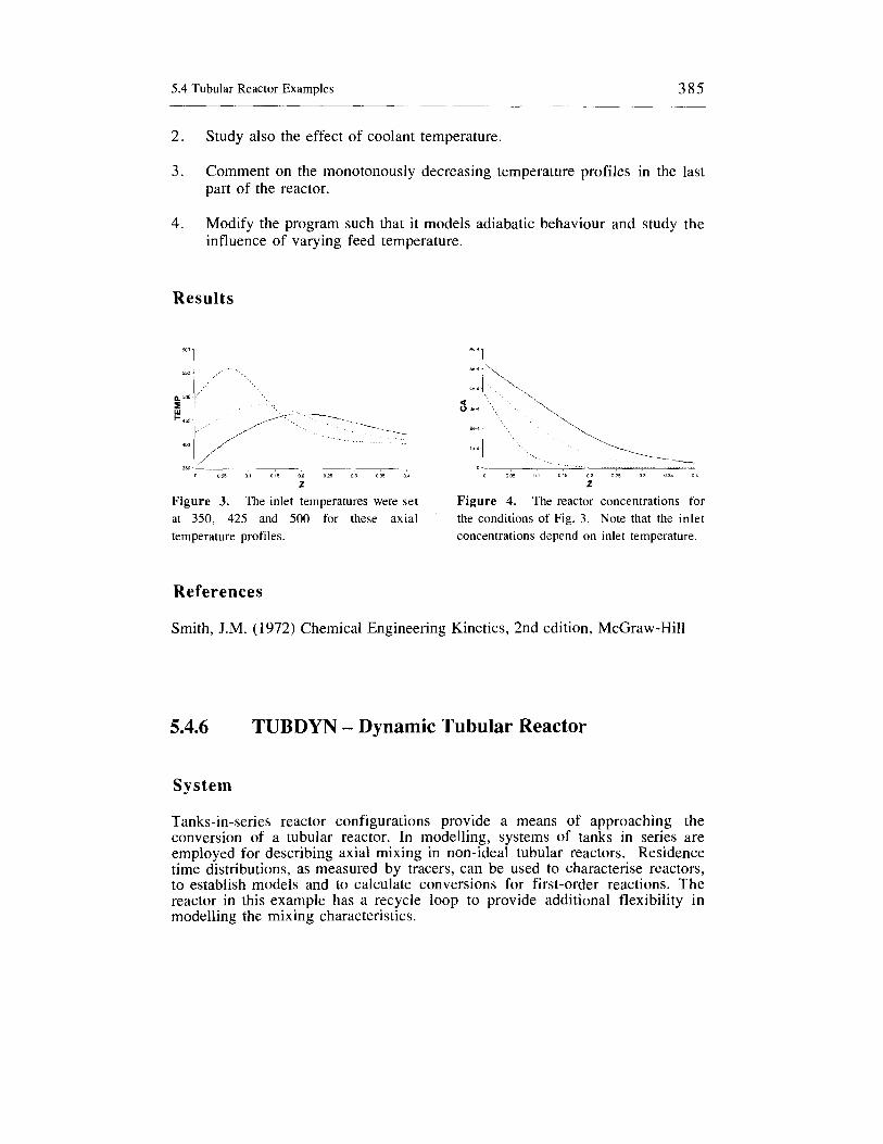
5.4 Tubular Reactor Examples 385
2. Study also the effect of coolant temperature.
3 . Comment on the monotonously decreasing temperature profiles in the last part of the reactor.
4. Modify the program such that it models adiabatic behaviour and study the influence of varying feed temperature.
Results
0 0 0 5 0, 015 0 2 0 2 5 0 3 0 3 5 0 1
z z Figure 3. The inlet temperatures were set Figure 4. The reactor concentrations for at 350, 425 and 500 for these axial the conditions of Fig. 3. Note that the inlet temperature profiles. concentrations depend on inlet temperature.
References
Smith, J.M. (1972) Chemical Engineering Kinetics, 2nd edition, McGraw-Hill
5.4.6 TUBDYN - Dynamic Tubular Reactor
System
Tanks-in-series reactor configurations provide a means of approaching the conversion of a tubular reactor. In modelling, systems of tanks in series are employed for describing axial mixing in non-ideal tubular reactors. Residence time distributions, as measured by tracers, can be used to characterise reactors, to establish models and to calculate conversions for first-order reactions. The reactor in this example has a recycle loop to provide additional flexibility in modelling the mixing characteristics.

386 5 Simulation Tools and Examples of Chemical Engineering Processes
FP CAN Figure 1. Tanks-in-series approximation of a tubular reactor with recycle.
Model
For the nth tank the balance for a single component is
V- dCAn = (F +F,)(CAn-l - CAn) + rAnV dt
If applied to a tracer, rAn is zero. Otherwise the reaction rate is taken as nth- order
n rAn = k c ~ , ,
Residence time distributions can be measured by applying tracer pulses and step changes, and as described in Levenspiel (1999), the pulse tracer response be -used to obtain the E-curve first-order reaction according
and to calculate the steady-state conversion for a to the relationship
m
= jE(t)e-ktdt 0
A0

5.4 Tubular Reactor Examples 387
Program
This program is designed to simulate the resulting residence time distributions based on a cascade of 1 to N tanks-in-series. Also, simulations with nth-order reaction can be run, and the steady-state conversion obtained. A pulse input disturbance of tracer is programmed here, as in example CSTRPULSE, to obtain the residence time distribution E curve and from this the conversion for first-order reaction.
Nomenclature
Symbols
C A0
CAN F k n N R V
Indices
n r t ss
Feed reactant concentration
Concentration in tank N Flow rate Reaction constant Reaction order Number of tanks Reaction rate Total volume of all tanks
Refers to nth tank Refers to recycle Refers to time Refers to steady-state
k g h 3
k g h 3 m3/s various -
kg/m3 s m3
Exercises
1. Set k = 0 and simulate tracer experiments. Vary the recycle flow rate and the number of tanks.
2. Use the E-curve to calculate the conversion for n = 1 and compare with the results obtained by simulation. This requires changing the program.
3. Vary the operating variables of feed flow rate and CAO to see the influence with n = 1 and n = 2.

388 5 Simulation Tools and Examples of Chemical Engineering Processes
0 M i
35
- e 2 5
5 ( 5
0 5
E ;
i:;k 0 M?
0001
4. Calculate the steady-state conversion for 1, 3 and 8 tanks using the same value of total residence time.
/
5 . Experiment with the influence of recycle flow rate and show by simulation that the model has the limits of a well-stirred tank and a plug flow reactor.
Results
References
Levenspiel, 0. (1999) Chemical Reaction Engineering, Third Edition, Wiley.
5.4.7 DISRE - Isothermal Reactor with Axial Dispersion
System
This example models the dynamic behaviour of an non-ideal isothermal tubular reactor in order to predict the variation of concentration, with respect to both axial distance along the reactor and flow time. Non-ideal flow in the reactor is represented by the axial dispersion flow model. The analysis is based on a simple, isothermal first-order reaction.

5.4 Tubular Reactor Examples 389
n
Figure 1. Tubular reactor with finite-difference element n.
Model
The reaction involves the conversion: A + products, with the kinetics
As discussed in Sec. 4.3.6, the axial dispersion flow model is given by
azc, acA - - U - +D7-kC,
at az az where Z is the distance along the reactor, D is the eddy diffusivity and u is the superficial flow velocity.
Thus the problem involves the two independent variables, time t and length Z. The distance variable can be eliminated by finite-differencing the reactor length into N equal-sized segments of length AZ, such that NAZ equals L, where L is the total reactor length. Thus for a segment n omitting subscripts A
Or defining C,' = C,, / Co, Az = A Z / L, 0 = t u / L in dimensionless terms and omitting the primes for simplicity
The term Lu / D is known as the Peclet number, Pe, and its inverse as the dispersion number. The magnitude of the Peclet number defines the degree of axial mixing in the reactor.

3 90 5 Simulation Tools and Examples of Chemical Engineering Processes
Thus,
The dimensionless boundary conditions are satisfied by Co = 1 for a step change in feed concentration at the inlet, and by the condition that at the outlet CN+I = CN, which sets the concentration gradient to zero. The reactor is divided into equal-sized segments.
Program
Array programming is used here to allow the graphing of the axial profile. Closed-end boundary conditions are used for the first and last segments. Also included is a PULSE function for simulating tracer experiments. Thus it should be possible to calculate the E curve and from that the reaction conversion obtained on the basis of tracer experiment. The example CSTRPULSE should be consulted for this.
The full listing of the Madonna program is shown here both to illustrate the use of array programming and also the use of the PULSE function.
{Example DISRE}
{UNSTEADY-STATE FINITE-DIFFERENCED MODEL FOR AXIAL DISPERSION AND REACTION IN A TUBULAR REACTOR} {The reactor length is divided into equal-sized sections, whose number, Nelem, can be varied. The model equations are written in dimensionless form. {The variable Time is dimensionless and equal to
{The Peclet number is equal to Lu/D, where D is the axial diffusivity.} {All concentrations C[i] are dimensionless and equal
tu/L.}
to C/CO}
{From HELP: PULSE(v, f, r) Impulses of volume v, first time f, repeat interval r} {For the nonreacting system with K=O, making a pulse of tracer at the inlet with CO=O and measuring C[Nelem] at the outlet gives information on the degree of axial mixing. This pulse is programmed below and can be activated by removing the brackets. This simulated measurement can be used to calculate the steady state conversion for a first-order reaction.}

5.4 Tubular Reactor Examples 39 1
Method Stiff DT=O .OOl STOPTIME=I
L=10 {Total length, m } U =l {Velocity, m/h) co=1 {Entering dimensionless conc., -} Pe=O. 5 {Peclet number=Lu/D, - } K=O. 01 {Rate constant, l/hr} CI=O {Initial concentration conditions, -} delZ=l.O/Nelem {Dimensionless length increment, -
Dimensionless length has a value of 1.0)
Kl=K*L/U {Dimensionless ratio of reaction rate to convective transport rate}
Nelem=lO {Number of e 1 emen t s } INIT C[l..Nelem-l]=CI {Initial concentrations, - 1
{Dimensionless reactant balances for Nelem sections, with d/dt(C[l])=(CO-C[l])/delZ-(C[l] C[2])/(delZ*delZ*Pe)-Kl*C[l]
” c 10s ed - end ” bound a r y cond it i on s }
d/dt(C[2..Nelem-l])=(C[i-l]-C[i])/delZ+(C[i-l]- 2*C[i]+C[i+l])/(delz*delZ*Pe)-Kl*C[i]
d/dt(C[Nelem])=(C[Nelem-l]-C[Nelem])/delZ+(C[Nelem- 11-C[Nelem])/(delZ*delZ*Pe)-Kl*C[Nelem]
LIMIT C>=O
{Brackets can be set or removed for the pulse of tracer. Set K=O to make a tracer experiment with no reaction.} CO=Pulse(O.Ol, starttime, 1000) Cpulse=C[Nelem] {This is the outlet conc. for the
pulse}

392 5 Simulation Tools and Examples of Chemical Engineering Processes
Nomenclature
Symbols
C D k L Pe t U
Z
0 Z
Indices
A n
Concentration Effective axial diffusivity Rate constant Total length Peclet number (L u / D) Time Velocity Length variable Dimensionless length Dimensionless time
Refers to reactant Refers to increment number Refers to a dimensionless variable
kmol/m3 and -
m2/h l/h m
h m/h m
-
Exercises
1.
2.
3.
4.
5 .
Obtain the tracer response curve to a step input disturbance of tracer solution by setting k = 0.
Study the effect of varying Peclet number, Pe, on the resulting tracer response.
Note that as Pe becomes large, the conditions approach plug flow, and as Pe approaches zero conditions approach perfect mixing.
Study the effect of varying Pe on the performance of the reactor, and compare the resulting performance with perfect plug flow.
Use the E curve from a pulse tracer experiment to calculate the first-order conversion.

5.4 Tubular Reactor Examples 393
Results
“ h
0 5
go* 03
0 2
TIME
Figure 2. Dynamic concentration profiles at each axial position in the reactor for a first-order reaction.
Figure 3. Response of reactor to a pulse input of tracer. The outlet concentration from the last element is graphed separately.
5.4.8 DISRET - Non-Isothermal Tubular Reactor with Axial Dispersion
System
The dispersion model of example DISRE is extended for the case of non- isothermal reactions and to include the axial dispersion of heat from a first- order reaction.
A + B + heat (-AH)
T, cAO CA
AZ
Figure 1. Tubular reactor showing a finite difference segment,

394 5 Simulation Tools and Examples of Chemical Engineering Processes
Model
From the axial dispersion flow model the component balance equation is
a%, - a c A - - -u- +D--kCA at aZ a2z
with the energy balance equation given by
aT aT d2T P C -=-C U-+h--kCA(-AH)
P at p aZ az2
where h is the eddy diffusivity for heat transfer. The reaction kinetics are
rA = kCA
Defining Z = z / L, t = T / To, C = CA / CAO, 0 = D t / L2, the model equations can be recast into dimensionless terms to give the following dimensionless model equations:
Mass Balance
Energy Balance
at at - a a2t ao ~ a z ~ az P2 - - B, B2C e-&It
where
koL2 , B I Z -
U L UL h p1 = -, p2= -, a = - a PCP D D ’
A full treatment of this problem is given by Ramirez (1976, 1989) and by Clough and Ramirez (1 97 l ) ,

5.4 Tubular Reactor Examples 395
Finite-differencing the dimensionless length of the reactor (Z = 1) into N equal-sized segments of length AZ such that N AZ = L, gives for segment n,
and
The boundary conditions used here are Co = to = 1 for a step change of inlet concentration or temperature, and at the outlet by tN+1 = tN and CN+1 = CN.
Program
Array programming is used, which allows the graphing of the axial profiles. Closed-end boundary conditions are used for the first and last segments. PULSE functions could be used for studying the axial dispersion of heat or, alternatively, the axial dispersion of mass (See DISRE).
Nomenclature
Symbols
CA
C A0
cP D AZ E (-AH) L h R
rA
P
TO t
U Z a
Concentration
Inlet concentration Specific heat
Mass transfer eddy diffusiviy Dimensionless length increment Activation energy Heat of reaction Reactor length Heat transfer eddy diffusivity Universal gas constant Reaction rate
Density Time Inlet temperature Flow velocity Frequency factor Diffusivity of heat
kmol/m3
kmol/m3 kJ/kg K m2/s
kJ/kmol kJ/kmol m kJ/m s K kJ/kmol K kmol/m3 s
kg/m3
K 4 s 11s m2/s
S

396 5 Simulation Tools and Examples of Chemical Engineering Processes
Dimensionless Factors
B1 Dimensionless group B2 Dimensionless group C Dimensionless concentration P1 p2 t Dimensionless temperature Z Dimensionless length E Activation energy group
0 Dimensionless time
Peclet number for mass transfer Peclet number for heat transfer
Exercises
1.
2.
3 .
4.
5 .
6.
Setting B1, and hence ko = 0, models the reactor response curve to a step input disturbance CAO = 1.
Vary reactor inlet temperature up to 700 K.
Study the effect of varying mass transfer and heat transfer diffusivities (D and h, respectively) and hence Peclet numbers (PI and P2) on the resulting dimensionless concentration and temperature reactor profiles.
Based on a linearisation approach as applied to the nonlinear model equations, Clough and Ramirez (197 1) predict multiple, steady-state solutions for the reactor. Is this confirmed and if not, why not?
Verify that the unusual mixed units used here actually give the dimension- less groups as stated and that the dimensionless balances are consistent.
Revise the model to allow for open-end boundary conditions. This would be the case if the reactor were a catalytic packed bed with non-catalytic packing beyond the reactor ends (Fig. 2).
Figure 2. Catalytic packed bed reactor with non-reactive end sections

5.4 Tubular Reactor Examples 397
08
0 ,
0 6
05 - Go4
0 3
0 2
0 1
Results
, ,000 950
IM
4 5
- - - 3 5
850 e - ~ j 2 -
n e_ I
~1 E S Z 5 800 Y
’= i P 5 2
‘ C 700
0 I S ~ O B
0 6 o s . . * . . . r . . . . - * - - . - 610
~ 0 1 i 6011
References
Clough, D.E. and Ramirez, W.F. (1971) Simulation, 207.
Ramirez, W.F. (1 976) Process Simulation, Lexington.
5.4.9 VARMOL - Gas-Phase Reaction with Molar Change
System
A tubular reactor is considered in which the gas-phase reaction leads to a change in the molar flow rate and thus in the linear gas velocity. The reaction stoichiometry is represented by
A + m B

398 5 Simulation Tools and Examples of Chemical Engineering Processes
Figure 1. Tubular reactor with variable molar flow.
Model
The model is described in Sec. 4.3.3. The steady-state balances are written in terms of moles. From the molar flow at each point in the reactor, the Ideal Gas Law is used to calculate the volumetric flow rate. This gives also the possibility of considering the influence of temperature and pressure profiles along the tube:
Nomenclature
Symbols
A Cross-sectional area G Volumetric flow rate
m2
m3/s

5.4 Tubular Reactor Examples 399
k m N P R Temp XA Y Z
Indices
0 inerts A B
Reaction rate Stoichiometric constant Molar flow rate Pressure Gas constant Temperature Fraction conversion Mole fraction Length
Refers to inlet Refers to inerts Refers to component A Refers to component B
- kmol/s N/m2 kJ/kmol K K -
m
Exercises
1. Vary the stoichiometry to see the influence of m. must be constant through the reactor.
Note that if m=l, G
2. Set the molar feed rate of inerts to a high value, and note that G does not change much with position.
3. Change the model and program to account for a linear temperature profile.
4. Change the model and program to account for a linear pressure profile, allowing for pressure drop through the reactor.

400 5 Simulation Tools and Examples of Chemical Engineering Processes
Results
Figure 2. Variation of mole fractions YA Figure 3. Outlet mole fraction YA as a and YB and volumetric flow rate G with function of molar flow rate of inerts.
length.

5.5 Semi-continuous Reactor Examples 40 I
5.5 Semi-Continuous Reactor Examples
5.5.1 SEMIPAR - Parallel Reactions in a Semi- Continuous Reactor
System
A semi-continuous reactor is used to carry out the following parallel reaction, where P is valuable product and Q is unwanted waste. The problem is to optimise the feed strategy to the reactor such that the maximum favourable reaction selectivity is obtained, for similar systems but of differing kinetic rate characteristics
Figure 1. Parallel reactions in a semi-continuous reactor.
Model
The total mass balance for constant density is
- = F dV dt

402 5 Simulation Tools and Examples of Chemical Engineering Processes
The mass balances for components A, B, P and Q are
The kinetics for the parallel reactions are
1-2 = k2 C i A 2 CkB2
The relative magnitudes of the orders of reaction, ngl and ng2, determine whether the concentration CB in the reactor should be maintained at a high or low level. For optimum selectivity, the total reaction time must be adjusted such that P is obtained at its maximum concentration as affected by the rate at which B is fed to the reactor.
Program
Note that at high rates of feeding, the maximum reactor volume may be reached before the simulation time is complete. Under these conditions, the feed of B to the reactor will stop. The reaction then continues batchwise until the simulation is complete.
Nomenclature
Symbols
C V F r
Concentration Volume Flow rate Reaction rate
kmol/m3 m3 m3/min kmol/m3min

5.5 Semi-Continuous Reactor Examples 403
Indices
A, B, P, Q F Refers to inlet feed n Refers to reaction orders 1, 2 Refer to reactions
Refer to components
Exercises
1 .
2 .
3 .
4
Study the system for the kinetic case nA1 = n ~ 2 and ng1 < ng2. Run the reactor (i) semi-continuously with slow feeding of B and (ii) as a batch reactor with B charged initially to the reactor and zero feed of B. Compare the results obtained for the two differing modes of reactor operation.
Repeat Exercise 1 but for the kinetic case ngl > ng2.
Study the semi-continuous mode of operation further, using different values of feed rate and feed concentration to the reactor. Determine the feeding conditions that are most beneficial in terms of selectivity.
Assign arbitrary cost values ($/kmol) for the reactants A and B, a profit value for the product P and waste disposal and handling charges for the waste Q. Modify the program to incorporate these cost values, and define a net cost function for the reaction and hence determine the best “environmental” operating condition. Study the effect of differing cost values on the above optimum.
Results
0 2 4 6 B 10 12 11 16
TIME
Figure 2. The concentration of B for five feeding rates from F=0.005 to 0.1 m3/min.
Figure 3. The selectivity for P for the five feeding rates of Fig. 2.

404 5 Simulation Tools and Examples of Chemical Engineering Processes
5.5.2 SEMISEQ - Sequential-Parallel Reactions in a Semi-Continuous Reactor
System
A complex reaction is run in a semi-batch reactor with the purpose of improving the selectivity for the desired product P, compared to that of the waste Q. The kinetics are sequential with respect to components A, P and Q but are parallel with respect to B, The relative magnitudes of the orders of the two reactions determine the optimal feeding policy.
Q k2 P+B
Figure 1. Complex sequential reactions in a semi-continuous reactor.
Model
The total material balance under constant density conditions is
- = k’g dt
and the component balances are

5.5 Semi-continuous Reactor Examples 405
The kinetic model equations are
The relative magnitudes of the orders of reaction, ngl and ng2, determine whether the concentration CB in the reactor should be maintained high or low. The total reaction time must be adjusted such that product P is obtained at its maximum concentration, and this will also influence how B should be fed to the reactor.
Program
If the feeding rate is high the maximum reactor volume may be reached, which will cause the feeding rate of B to stop. The reaction then continues batchwise until the simulation is stopped. In the program the reaction orders are set as; nA1=nP2 and nB1<nB2. The selectivity for the desired product will be highest at the lowest feeding rates, since the desired reaction is then promoted by low concentrations of B.

406 5 Simulation Tools and Examples of Chemical Engineering Processes
Nomenclature
Symbols
C Concentration V Volume F Flow rate r Reaction rate
Indices
Refer to components Refers to inlet feed Refers to reaction orders Refer to reactions
kmol/m3 m3 m3/min kmol/m3 min
Exercises
1.
2.
3.
4.
Determine the optimal time to stop the reaction for a range of input flow rates to the reactor. How do the values of kl and k2 influence this?
Investigate the influence of flow from the standpoint of maximum production of desired product P and for the minimisation of waste Q. Study this for ngl greater and less than ng2. Plot the ratio of reaction rates to understand the system.
Plot the ratio of the reaction rates for a range of conditions as an aid in understanding the effects of Exercise 2.
Assign arbitrary cost values ($/kmol) for the reactants A and B, a profit value for the product P and waste disposal and handling charges for the waste Q. Modify the program to incorporate these cost values, and define a net cost function for the reaction and determine the best operating conditions. Study the effect of differing cost values on the above optimum “environmental effect” costing.

5.5 Semi-Continuous Reactor Examples 407
Results
(I
TIME
Figure 2. Multiple run showing the selectivity for P as a function of time for five feed rates of B between 0.05 and 0.01 m3/min. The lowest feed rate gives the highest selectivity.
I1 32
D i l l 0015 0 0 2 0025 0 0 3 0035 OM 0045 0 0 5
FO
Figure 3. Parametric plot showing the maximum in selectivity for P as a function of feed rate of B for the same runs as Fig. 2.
5.5.3 HMT - Semi-Batch Manufacture of Hexamethylenetriamine
System
Aqueous ammonia is added continuously to an initial batch charge of formaldehyde solution. The reaction proceeds instantaneously and is highly exothermic.
4 NH3 + 6 HCHO + N4(CH2)6 + 6 H20

408 5 Simulation Tools and Examples of Chemical Engineering Processes
Figure 1. Variables for the HMT example.
Model
For the semi-batch operation the total mass balance is
- = w dM dt
For the instantaneous reaction, the rate is equal to the reactant feed rate. The energy balance then becomes
dT dt
M cP - = W cP (To - T) + W XAO (-AH) - UA (T - Tc)
where XAO is the mass fraction of ammonia in the feed stream.
Program
Since the reaction rate is instantaneous, this is set equal to the feed rate of ammonia.
Nomenclature
Symbols
A Heat exchange area cP Specific heat
m* kJ/kgC

5.5 Semi-Continuous Reactor Examples 409
1mo
Y I 12M
i ma -
4 c -
203 -
M Mass in reactor kg T and Temp Temperature C
w Mass feeding rate k g h x A0 Ammonia feed mass fraction k d k g XFO Formaldehyde charge fraction k g k -AH Exothermic heat of reaction kJkg
U Overall heat transfer coefficient kJ/m2C
::!r
Indices
C
F 0
Refers to cooling Refers to formaldehyde Refers to feed values
Exercises
1. Find the size of cooling area required such that the reactor temperature just rises to 100 "C, by the end of the feeding at 90 min. time.
2. Carry out simulations with differing inlet temperatures, initial charges and feeding rates.
Results
The results indicate that the mass flow rate has a strong influence on the reactor
'" I 1 6 0 1 , , , , , , , , , , -
A 0 0 2 0 1 06 D B l P 1 1 1 6 1 8 2
Figure 2. Time profiles for total mass M , Figure 3. A parametric plot giving the mass of formaldehyde MF and temperature. maximum temperature as a function of A A slider for cooling area A was used to find the value necessary to keep T<100 C.

410 5 Simulation Tools and Examples of Chemical Engineering Processes
Reference
Smith, J. M. (1970) Chemical Engineering Kinetics, 2nd edition, McGraw-Hill.
5.5.4 RUN - Relief of a Runaway Polymerisation Reaction
System
The manufacture of a polyol lubricant by the condensation of an alcohol with an propylene oxide in a semi-batch reactor proceeds according to the following reaction
C4H9OH + (n + 1) C3H6O + C4H9 (OC3H6)nOCH2CHOHCH3 + heat
The reaction is highly exothermic, and the reactor contains large quantities of volatile oxide. Careful control of temperature is therefore required to avoid a runaway reaction and excessive pressure generation.

5.5 Semi-Continuous Reactor Examples 41 1
A " I
Oxide feed
Final level M + Initial level
I Recycle
Figure 1.
The alcohol is charged initially to the reactor, and the oxide is then fed to the reactor at constant rate. Heat generated by reaction is removed via an external heat transfer loop. In this, the batch contents are recycled through an external cooler with sufficient capacity to maintain a constant return temperature to the reactor. With high rates of cooling the reactor operation is stable, but a product of low molecular weight is produced. As the cooling is decreased, higher molecular weight product is obtained, but at the risk of a runaway reaction and reactor failure. In the event of this or the case of a cooling failure, a bursting disc in the reactor will rupture, and the feed of oxide would usually be stopped. This will discharge oxide vapour to the atmosphere.
The simulation emphasises that when reactions start to run away, they do so extremely fast. In this example the rate of pressure generation is compounded by the double exponential terms in the Arrhenius and vapour pressure equations.
The polymerisation reactor with its cooling unit and bursting disc.
Model
The total mass balance is

412 5 Simulation Tools and Examples of Chemical Engineering Processes
where M is the reactor mass at time t (kg) and V is the vapour venting rate (kg/min) and F is the feed rate (kg/min).
The oxide component mass balance is
where C is the oxide concentration (kg/kg) and R1 is the oxide reaction rate (kg/min).
The mass of oxide reacted is given by
- = + R 1 dX dt
where X is the mass of oxide reacted at time t. The energy balance is
M c p * = F c p ( T o - T R ) - V h - R l ( -AH)-Q dt
where TR is the temperature of reaction ("C), Q is the rate of cooling (kJ/min) and A is the heat of vapourisation of the oxide. The heat removed via the recirculation through the external cooler is given by
where Fc is the recycle mass flow rate (kg/min). The reaction kinetics are given by
R1 = k MC (kg oxide/min)
where E
R(TR + 273) -
k = Z e

5.5 Semi-Continuous Reactor Examples 413
The polymer molecular weight is
M o + X MW = ~
N
where N is the kmol of initial alcohol charge.
pressure is given by: Assuming instantaneous equilibrium, the reactor pressure and oxide vapour
+1.45*103MW
The vapour discharge rate is given by the following. 1. For normal conditions and up to disc rupture
v = o 2. For sonic discharge to atmospheric pressure
k, 0.85P kg/min for P > 1.9 bar
3. For sub-sonic discharge for 1 < P < 1.9 bar
where kv is the valve discharge coefficient.
Program
The Madonna program RUN with KV = 0 represents operation of the reactor under zero venting (V = 0) conditions, i.e., the bursting disc remains closed. With KV > 0 ( 100 - 1000) the program simulates the performance under emergency venting conditions. The program will continue to run unless coolant failure occurs, corresponding to FC = 0.
The program ensures that the bursting disc remains integral up to the bursting pressure, that the vapour discharge is sonic for reactor pressures greater than critical, that the discharge is subsonic for pressures less than critical and that the discharge stops when the pressure is atmospheric. The feed rate is programmed to either stop or continue following disc failure.

414 5 Simulation Tools and Examples of Chemical Engineering Processes
For convenience, the exit temperature from the cooler, Tc, is assumed equal to the feed temperature, To, i.e., the heat transfer capacity of the cooler is in large excess.
This program contains an example of conditional statements. A conditional variable DISC is defined such that if DISC =1 then the bursting disc is intact, and if DISC =O the disc has burst. The discharge velocity through the disc varies with pressure as given by the complex conditional statement in the partial listing below:
{Example RUN}
{Vapour pressure in reactor}
Limit P >= 1 P = (EXP(-343O/(TR+273)+11.7)+1.45E-3*MW)*C
{Bursting disc control: If Disc=l then bursting disc OK; if Disc=O disc has burst} F = IF (Disc < 1) THEN 0 ELSE FO {Feed flow rate of oxide, kg/min. Oxide feed shuts off on bursting. This can be deactivated to maintain feeding}
(Venting velocity control} V=IF(Disc<l AND P>1.9) {Velocity through disc
varies with P} THEN 0.85*KV*P/SQRT(TR+273)
ELSE IF (Disc<l AND P<=1.9 AND P>1.1) THEN KV*P/SQRT(TR+273)*SQRT(l+(l/P)*(1/P))
ELSE IF P<=l.l THEN 0.0
ELSE 0
MW = (MO + X)/N {Molecular weight of polymer at any
R1 = K*MC {Rate of polymerization reaction, kg
K=Z*EXP(-E/(R*(TR+273))) {Arrhenius relation}
time, kg/kmol)
oxide/min)
(Total mass balance taking into account the initial alcohol MO and the oxide fed and vapourised) d/dt(M) = F-V (Total mass balance} d/dt(MC) = F-V-R {Component mass balance for oxide} LIMIT MC>=O {Prevents negative values} c = MC/M (Mass fraction conc , kg/kg} LIMIT C>=O {Prevents negative values)

5.5 Semi-Continuous Reactor Examples 415
{Heat balance, considering flow, vapourisation, reaction and cooling) d/dt(MTR) = (F*Cp*(TO-TR)-V*LAMBDA-Rl*HR-FC*Cp*(TR- TO))/CP LIMIT MTR>=O TR=MTR/M {Calculation of TR)
d/dt (X) = R1 {Oxide reacted)
{State of the disc, starts at 1 and decreases quickly after bursting; the value of Disc is used to detect if the disc has burst. After bursting Disc-0) d/dt(Disc) = -Fdisc Limit Disc>=O INIT Disc= 1 Fdisc=IF(P>=PBURST) THEN 10 ELSE 0 . 0
{Cooling failure) FC=IF TIME >= TIMEfail THEN 0 . 0 ELSE FC1 {Conditional recycle cooling flow) TIMEfail=1500 {This is the time of failure, min}
Nomenclature
Symbols
C
cP E F FC and FCl h M MC Mw Mol N P P1 P2 R R1 T R
Oxide concentration Specific heat Activation energy Oxide mass feed rate Coolant flow rate Heat of vapourisation of oxide Charge mass of alcohol Mass of oxide Molecular weight Molecular weight of charge Initial alcohol charge Reactor pressure Bursting disc relief pressure Maximum safe working pressure Gas constant Reaction rate Reaction temperature
kglkg kJkg C kJ/mol kglmin kglmin kJkg kg kg kg/mol kglkmol kmol bar bar bar kJ/mol C kglmin C

416 5 Simulation Tools and Examples of Chemical Engineering Processes
t Batch time min TO Charge, feed and recycle temperature C V Venting rate kg/min X Mass of oxide kg Z Frequency factor 1 /min -AH Exothermic heat of reaction 1 /kg
Indices
0 C
Refers to initial and inlet values Refers to cooler
Exercises
1.
2.
3 .
4.
5 .
6.
Study the Madonna program so that the conditional logic based on the IF-THEN-ELSE statements is fully understood.
With the bursting disc remaining closed (KV = 0 and V = O), establish the minimum external recycle cooling flow (Fc 1) needed to ensure stable operating conditions and satisfactory polymer product (Mol wt = 2500). Determine the minimum cooling capacity required of the cooler. Study the effects of “runaway” following coolant failure by interactive computation. By carefully decreasing Fc from an initially “safe” value, the absolute limit of safe operation can be established. In this the reaction starts to run away, but then the reaction corrects itself by having consumed all the oxide and then continues with further stable operation.
Using the value of Fc found in Exercise 1 , study the effect of differing valve discharge capacities (KV) following cooling failure at different stages of reaction time (FC = 0).
Run the simulation under disc-bursting conditions for both with and without shutting off the feed.
As an alternative to venting the vapour to atmosphere, the vapour may be condensed and returned to the reactor. Modify the program accordingly and study the resultant behaviour. See simulation examples REFRIDGE 1 and REFRIDGE2.
Alter the program to include a complete model for the heat exchanger. This will allow a more realistic calculation of the heat removed.

5.5 Semi-Continuous Reactor Examples 417
Results
TIME
Figure 2. Set at the point of stable operation the pressure increases until the oxide MC is consumed (Fig. 3) and then at lower temperature the process continues.
Figure 3 . The run of Fig. 2 , showing the oxide MC falling to zero and the process continuing at lower temperature.
References
Kneale, M. and Forster, G. M. (1968) 1.Chem.E.Symp. Series No. 25, 98.
Kneale, M. and Binns, J. S. (1977) 1.Chem.E.Symp. Series No. 49.
5.5.5 SELCONT - Optimized Selectivity in a Semi- Continuous Reactor
System
Keller (1998) describes the semi-continuous reaction process of a vinylketone K with lithium acetylide LA to yield lithium etinolate LE an intermediate in the vitamin production. In an undesired side reaction an oligomer byproduct BP is produced. During the process, reactant K is fed to the semi-batch reactor at a rate to maximize the selectivity for LE.

418 5 Simulation Tools and Examples of Chemical Engineering Processes
Figure 1. Semi-continuous reactor with feeding of ketone reactant.
Model
The total balance for the semi-batch reactor assuming constant density is
Written in terms of masses (CiV) the component balances are
and the concentrations for each component i are found from relations of the form Ci = C,V/V.
The reaction rates are known to be given by

5.5 Semi-Continuous Reactor Examples 419
An objective function can be defined with respect to the positive impact by the productivity of LE and the negative contribution by that of BP weighted by a factor a.
CLE v - CBp v a t B
OF =
The final time tg is reached when the reactor is full and when the residual concentration of K is 0.01.
Exercises
1. Find the optimal constant feeding rate of ketone to the reactor for a = 50.
2. Investigate the influence of the value of a on the optimum.
3. Try to find a higher value for the objective function by using two time periods with two different constant feeding rates. Find the optimal values for the time periods and the flow rates.
4. Assume a ramp function for the flow rate (F = Fo + k t) and find the values of Fo and k which give the highest value for the objective function. Remember that F must remain positive.
5 . Try to improve the value of the objective function by using a PI-controller to maintain constant selectivity throughout the batch, where
Find the value of the selectivity set point which gives the highest value of the objective function, as defined above with a= 50. Compare the feeding profile found with those found in the previous exercises.

420 5 Simulation Tools and Examples of Chemical Engineering Processes
Nomenclature
Symbols
C k F OF r V
SEL a
TB
Indices
BP K LA LE 1 2
Results
Concentration Rate constants Flow rate of feed Objective function Reaction rate Volume of reactor Penalty constant Selectivity Total time of reaction
Refers to byproducts Refers to vinylketone Refers to lithium acetylid Refers to lithium etinolate Refers to desired reaction Refers to undesired reaction
kmol/m3 m3/km01 h m3 kmol/h kmol/m3 h m3
h
Figure 2. The objective function varying with feed rate, with a maximum at 2.5 m'/h.
Figure 3. Concentrations profiles for a feed rate of 2.5 m3/h. The feed is stopped at
time=3.6 h.
Reference
Keller, A. (1998) ETH PhD Dissertation No. 12607, Zurich

5.6 Mixing-Model Examples 42 I
5.6 Mixing-Model Examples
5.6.1 NOCSTR - Non-Ideal Stirred-Tank Reactor
System
In this model of non-ideal reactor mixing, a fraction, f l , of the volumetric feed rate, F, completely bypasses the mixing in the reactor. In addition, a fraction, f2, of the reactor volume, V, exists as dead space. F3 is the volumetric rate of exchange between the perfectly mixed volume V1 and the dead zone volume V2 of the reactor.
F29 co b
Figure 1. The non-ideal flow reactor model.

422 5 Simulation Tools and Examples of Chemical Engineering Processes -
Model
The reaction is assumed to be first order, where
r = k C
The component mass balances are as follows.
For the well-mixed volume
VldC,= FI(Co - C1) + F3(C2 - Cl) - V1 kl C1 dt
where V1 = (1 - f2)V and F1 = (1 - f1)F.
For the dead space volume
V2 %= F3 (Cl - C2) - V2 k C2 dt
where
and v2 = f2 v F 3 = a F
Note that the dead space is treated as having a region of uniform well-mixed composition.
For the reactor outlet
where F C 3 = F1C1+F2Co
F2 = f l F
For a perfectly mixed tank with outlet concentration C4 and total volume V
Program
Note that in the program that while the bypassing flow fraction f l (FRAC1) can be set to zero, the fractional dead space volume f2 ( FRAC2) cannot be set to zero without modifying the program This would cause the derivative value for C2 to be divided by a zero value for V2.

5.6 Mixing-Model Examples 423
Nomenclature
Symbols
CO
C1
c2
c3 c4
f l
F2 f2
F3 R X
F
a
Indices
Feed concentration
Active zone concentration
Dead zone concentration
Effluent concentration
Ideal tank concentration
Total flow rate Fractional bypass flow
Bypass flow rate Dead volume fraction
Dead zone exchange flow Rate constant Fractional conversion Fractional dead zone flow
3
3
3
3
3
kmollm
kmollm
kmollm
kmollm
kmol/m
m /min
m /min
3 m /min llmin
3
- 3
-
- -
Refers to feed Refers to interchange flow and outlet concentration Refers to dead volume region Refers to dead zone flow Refers to perfectly mixed tank
Exercises
1. Study the effects of fractional bypassing and fractional dead space volume on the steady-state conversion, X3, compared to that of the ideal tank, X4.
2. Note if K = 0, the program generates a tracer step-response curve for the non-ideal reactor.
3. Study the effect of variations in the rate of exchange F3 between the two reactor volumes, by varying the value of ALPHA.

424 5 Simulation Tools and Examples of Chemical Engineering Processes
4. Modify the program to allow for zero dead space volume and study the effect of fractional bypassing only. Compare the results to that for a perfectly stirred tank.
5 . Modify the system to that shown below by Froment and Bischoff (1990), in which the volumetric flow, F, having passed through a partial well- mixed volume, V1, is then diverted such that a fraction, f, passes through the residual volume, V2, before rejoining the main flow stream. Formulate the model equations and record the F-curve response for the system for varying values of V1 and V2 keeping the total volume (V = V1 +V2 ) constant and varying the values of f.
Figure 2. Mixing model of Froment and Bischoff (1990).
Results
_.
::: 11 0 31 , , , , , , , , ,
0 1 2 3 1 s 6 I B 9 10
ALPHA
Figure 3. A parametric plot showing the influence of ALPHA from 0.1 to 10.
1 03
0 5 10 l i 28 25 30 31 40 46 10
TIME
Figure 4. A response of the reactor model to a step change in concentration. The well- mixed case C4 is shown for comparison.

5.6 Mixing-Model Examples 425
Reference
Froment, G.F., Bischoff, K.B. (1990) Chemical Reactor Analysis and Design, 2nd ed., Wiley Interscience.
5.6.2 TUBEMIX - Non-Ideal Tube-Tank Mixing Model
System
Non-ideal mixing conditions in a reactor can often be modelled as combinations of tanks and tubes. Here a series of stirred tanks are used to simulate a tubular, bypassing condition.
Figure 1. A combined tank-tube mixing model.

426 5 Simulation Tools and Examples of Chemical Engineering Processes
Model
For the tubular bypass flow representation, the balances for reactant A have the form
for each of the sections n = 1, 2,. . .N.
The main tank reactor region has the balance
The dead-zone region is balanced by
V3dCA5 = F3 c,44 - F3 c A 5 + r ~ 5 v3 dt
The final outlet concentration is given by the balance at the mixing point
FO c A 6 = F1 c A 3 F2 c A 4
The flow rates are given in terms of the flow fractions as
F1 = FoR1 and
and the volumes are given by Vtub v2 = - R3
and
The reaction rates are rAn = kCAnm
where n refers to the section number and m refers to the reaction order.

5.6 Mixing-Model Examples 427
Program
The program is written in array form so that the number of tanks within the tubular section can be varied.
Nomenclature
Symbols
Feed concentration
Initial concentrations
Concentration in region n
Feed to reactor system
Flow rate to tube
Flow rate to tank
Interchange flow rate Reaction constant Reaction order Feed fraction tubehank Flow fraction F1/Fo Feed fraction tankl/tank2 Flow fraction F3F2 Volume fraction tubehank 1 Volume fraction tankl/tank2
Volume of tank sections in tube
Volume of main reactor section
Volume of dead zone section
Volume of tube reactor
m3/min various -
m3
m3
m3
m3

428 5 Simulation Tools and Examples of Chemical Engineering Processes
Results
Figure 2. Shown here for first-order reaction is a step response of the 5 tanks, as well as the slower responses of CA4 and CA5.
0 IW Z M 9 0 IN 500 6W ,M BW mo 1-
TIME
Figure 3. From the run of Fig. 2, as an overall comparison, are shown the CA6 outlet response and the response for a completely mixed system, given by CAiM.
5.6.3 MIXFLOl and MIXFL02 - Mixed-Flow Residence Time Distribution Studies
System
The following systems represent differing combinations of ideal plug-flow, mixing, dead space, flow recycle and flow bypass.
Figure 1. Mixing model for residence time distribution Case 1.

5.6 Mixing-Model Examples 429
FR c4
Figure 2. Mixing model for residence time distribution Case 2.
It is desired to compare the residence time distributions (RTD) for these cases.
Model
Ideal plug-flow regions, such as VT, are represented by standard Madonna time delay functions.
Case 1
The mixing junction is given by the steady-state balance,
Fo Co + FR C 4 = (Fo + FR) C1
Thus the concentration leaving the junction is
FOcO + FRc4
FO FR c1 =
For the plug-flow region VT, the outlet concentration C2 is equal to the input concentration C1, but delayed in time by
VT -VD FO + FR
The well-mixed region is given by

430 5 Simulation Tools and Examples of Chemical Engineering Processes
V m - dC3 = (Fo + FR - FB) (C2 - C3) dt
The final outlet concentration is given by a steady-state junction relation as,
FBc2 +(FO +FRFB)C3 c4 =
FO + FR Case 2 The relations used here are analogous to Case 1.
For the junction FOcO +FRc4
FO + FR c1 =
For the mixing tank
dC2 = (Fo + FR - FB) (Cl - C2) vm dt For the bypass junction
For the plug-flow time delay C4 is equal to C3 delayed in time by VT -VD
FO + FR
Program
The Madonna program MIXFLOl models the situation of Case 1, and program MIXFL02 models that of the Case 2. The plug-flow section of the plant is fiodelled with the time delay function, DELAYT. This is suitable for residence time distribution studies, but is not suitable to calculate the conversion for non- first-order reactions. The Madonna logic is such that a dynamic concentration mixing point of finite volume is necessary within the program to provide an initial condition, owing to the time delay and the recycle stream.

5.6 Mixing-Model Examples 43 1
Nomenclature
Symbols
V F C
Indices
T m D B R 1 , 2 , 3 , 4
Volume Volumetric flow Tracer concentration
Refers to plug flow Refers to mixing Refers to dead space Refers to bypass Refers to recycle Refer to positions according to figure
Exercises
1. Vary the relative system parameters VT, VD and VM for the two differing flow cases, keeping the total volume of the system constant. Compare the resulting residence time distributions.
2. Keeping the total volume of the system constant, vary the relative flow rates, Fo, FB and FR and note the influence on the RTD's.
3. Evaluate the conversion for first-order reaction from a tracer pulse response curve using the method in example CSTRPULSE. Show that although the residence time distributions may be the same in the two cases, the overall chemical conversion is not, excepting for the case of first-order reaction.

432 5 Simulation Tools and Examples of Chemical Engineering Processes
Results
Figure 3. For MIXFLOl a step in CO creates this response in C 1 , C2, C3 and C4. The time delay function gives a delay between C1 and C2.
O: li . . ; , , , , , , ,-
0 5 10 15 20 25 PO 35 40 45 so TIME
Figure 4. For MIXFL02 a step in CO creates this response in C1, C2, C3 and C4. The time delay function gives a delay between C3 and C4..
Reference
Szekely, J., Themelis, N.J. (1971) Rate Phenomena in Process Metallurgy, Wiley Interscience.
5.6.4 GASLIQl and GASLIQ2 - Gas-Liquid Mixing and Mass Transfer in a Stirred Tank
System
The gas-liquid flow characteristics of stirred vessels depend both on the level of agitation and the rate of gas flow and can vary from the case of bubble column type operation to that of a full circulating tank, as shown in Fig. I . The mixing characteristics and gas distribution obtained obviously exert a considerable influence on the rate of mass transfer obtained (Harnby et al., 1985).

5.6 Mixing-Model Examples 433
n r I I I I
Figure 1. Gas-liquid mixing modes: a) bubble column behaviour (high gas flow, low rotor speed): b) circulating tank behaviour (high rotor speed, reduced gas flow).
In this example it is required to model the behaviour of the mixing vessel according to the conceptual models indicated below.
Liquid Mixing
The basic liquid mixing pattern is assumed to remain constant, as shown in Fig. 2.

434 5 Simulation Tools and Examples of Chemical Engineering Processes
FL1
FL2
FD FD . ___)
FL1
FL2
Figure 2. Model for the liquid mixing pattern in a stirred tank.
In this, the liquid acts as three well-stirred regions, the smaller one representing the region close to the impeller. The two larger ones represent the volumes of liquid above and below the impeller, with the flow from the impeller discharging equally into the two main tank regions.
Gas Mixing
The gas phase mixing is represented by three equally-sized tanks in series. In the case of the full bubble column, the bottom gas phase mixed region is coincident with the impeller, and no significant gas mixing occurs below the impeller, in the lower region of the tank, as shown in Fig. 3. The dashed arrows in Fig. 3 and Fig. 4 represent mass transfer interchange between the gas space and liquid volumes of the tank. The liquid circulation, which is not shown, is identical to Fig. 2.

5.6 Mixing-Model Examples 435
‘03
‘02
\ Q3 \
I /
Q2
I I
/
‘GI Q1
FG’ ‘GO
Figure 3. Gas phase mixing pattern and mass transfer for full bubble column.
‘G3
Figure 4. Gas phase mixing and mass transfer for full circulation case.
With full circulation, substantial gas phase mixing occurs in all tank regions, as shown in Fig. 4.
Model
Bubble Column Operation
Liquid phase balances

436 5 Simulation Tools and Examples of Chemical Engineering Processes
dC VL1 -$= FL2 (CL2-CLl)
Pump discharge rate
Gas phase balances FD = FL1 FL2
Vc1- dCG1 = FG (CGO - CG1) - Q1 dt
The equilibrium relationships are represented by means of Henry's Law where
RTCG3 CL3" = - H
Full Circulation
Liquid phase balances

5.6 Mixing-Model Examples 431
dC 3 = F L ~ ( C L ~ - C L ~ ) + Q3 vL3 dt
Rates of mass transfer Qi = KLa ( CLI" - CLI) VGI
Q2 = KLa ( C L ~ " - C L ~ ) V G ~
4 3 = KLa ( C L ~ " - C L ~ ) v G 3
The equilibrium relationships are represented by Henry's Law as before.
Program
Program GASLIQl simulates the case of the full bubble column and program GASLIQ2 that of the full circulation case. For simplicity a constant value of overall mass transfer capacity coefficient, KLa, is assumed to apply for all the liquid regions, but the value obtained in the case of full circulation is taken as five times that for the bubble column.

438 5 Simulation Tools and Examples of Chemical Engineering Processes
Nomenclature
Symbols
V Volume F Volumetric flow rate C Oxygen concentration Q KLa
Rates of oxygen transfer Mass transfer capacity coefficient
R Ideal Gas Constant T Temperature H Henry's Law constant
Indices
Refer to streams and zones (see figures) Refers to initial value Refers to liquid Refers to gas Refers to recicle Refers to equilibrium
m3 m3/s kmol/m3 kmol/s l/s m3atm/kmol K K m3atmkmol
Exercises
1. Simulated tracer experiments can be performed on either program by setting KLa = 0 and starting with suitable initial conditions and inlet concentrations. The methods given in example CSTRPULSE can be used for this. For example: a) In GASLIQ1 set initial values as follows: C L ~ = 1, C L ~ and C L ~ = 0. Observe the tracer response curve for different values of F L ~ and F L ~ . b) In GASLIQ2 set CGI = 0 and the inflow CGO = 1 . Observe the response of the outflow c G 3 for various values of the circulation flow F G R ~ and ....
2. Set KLa to a suitable value and experiment with the influence of the mixing parameters F L ~ and F L ~ in GASLIQ1 and FGR~ and F G R ~ in GASLIQ2.

5.6 Mixing-Model Examples 439
0 2
Results
0 ZO 10 60 80 *m 120 (40 lbn 180 zw TIME
Figure 5 . GASLIQl with transfer showing the response of CL1 for three values of FLl=FL2 from 0.005 to 0.02 m3/s.
Reference
Hamby, N., Edwards, M.F. and Nienow, A.W. (Eds.) (1985) Mixing in the Process Industries, Butterworths.
5.6.5 SPBEDRTD - Spouted Bed Reactor Mixing Model
System
In this example, a stirred-tank model is employed to model the mixing behaviour of an air-solid, spouted, fluidised-bed reactor. The central spout is modelled as two tanks in series, the top fountain as a further tank and the down flowing annular region of the bed as six equal-sized tanks in series. It is assumed that a constant fraction of the total solids returns from each stage of the annular region into the central two-tank region, as depicted below.

440 5 Simulation Tools and Examples of Chemical Engineering Processes
I F39 c3 1
Annulus
7
Fountain
I I
\ /
A
Air
Figure 1. The spouted bed and its mixing model.
Experimental tracer studies are to be carried out in which the solid in the bottom half of the bed is initially mixed with tracer, the bed started and timed samples taken from various locations in the bed annular region. It is desired to model the resulting tracer distribution in the bed in order to find the fractional slippage rate between the annular tanks and the central bed regions.
Model
The initial expansion of the bed consequent to the start of the air flow is neglected from the analysis. Component balance equations for each region of the reactor are given.
For the bed central flow region

5.6 Mixing-Model Examples 44 1
v2 - dC2 = F1 C1 + F [C4 + C5 + C6] - F2 c2 dt
For the annular flow region
V dC4 = F3 C3 - [F4 + F] C4 dt
V - dC5 = F4 C4 - [F5 + F] C5 dt
V - dC8 = F7 C7 - [F8 + Fl c8 dt
Total bed volume V ~ ~ t ~ l = V1 + V2 + V3 + 6 V

442 5 Simulation Tools and Examples of Chemical Engineering Processes
The initial distribution of tracer within the bed is represented by
Program
If desired, the model and program can be extended by adding a continuous inlet and outlet stream and by incorporating the E-curve methods found in Example CSTRPULSE.
Nomenclature
Symbols
V F C
Indices
0, 1, ... 9
Volume Volumetric flow rate Tracer concentration
Refer to designated regions and flow rates (see Fig. 1).
m3
m3/h mg/m3
Exercises
1. Determine the time required for the tracer to be nearly completely mixed throughout the vessel. Which criterion did you use for uniform mixing?
2. Change the initial conditions to place the tracer at a different region of the vessel. Does this effect the time for complete mixing?
3. Double the flow rates in the vessel, and note the influence on the time for mixing.

5.6 Mixing-Model Examples 443
Results
I IMt
Figure 2. A pulse in compartment 1 mixes with all the compartments in about 3 h.
0°5 ~ / a /
0 1 2 3 4 1 6 7 B 9 10
TIME
Figure 3. As expected, a 10 fold change in
FO from 0.1 to 1.0 m3/s causes a similar difference in the mixing times.

444 5 Simulation Tools and Examples of Chemical Engineering Processes
5.6.6 BATSEG, SEMISEG and COMPSEG - Mixing and Segregation in Chemical Reactors
System
Chemical reactions will take place only when the reactant molecules are in intimate contact. In some cases, especially with very fast reactions or viscous liquids, segregation of the reactants can exist, which make the reaction rates and selectivities dependent on the mixing intensity. In chemical reactor engin- eering, the assumption is usually made that only mean concentrations need be considered. In reality, concentration values fluctuate about a mean, and in some cases these fluctuations must be considered in detail. This field is very complex and is still the subject of much research. This example serves only to introduce these concepts and to show how simulations can be made for certain simple situations.
The concept of segregation and its meaning to chemical reactors was first described by Danckwerts (1953). The intensity or degree of segregation is given the symbol I, which varies between one and zero. Shown in Fig. 1 is a tank with two components, A and B, which are separated into volume fractions, qA and 1 - qA; this condition represents complete initial segregation (1=1). Stirring or mixing this tank would cause the segregation to decay until complete homogeneity would be achieved (I=O). In this situation, the rate of any reaction between the reactants could obviously be influenced by the rate of mixing, as measured by the change in I.
Figure 1. Complete segregation ( I =1) of reactants A and B in two volume fractions.

5.6 Mixing-Model Examples 445
Segregation may also be important if the reactants are fed to a reactor in an unmixed condition. This could be the case in any continuously fed reactor, either tubular (Fig. 2) or tank (Fig. 3).
Figure 2. Feeding of unmixed reactants to a tubular reactor.
Figure 3. Unmixed reactants fed into a continuous stirred tank.
The intensity of segregation, I, can be described in terms of concentration fluctuations, as shown in Fig. 4. Here the time-varying fluctuations above and below an average value are shown.

446 5 Simulation Tools and Examples of Chemical Engineering Processes
Time
Figure 4. Time-variant turbulent fluctuations of concentration about a mean value , showing the fluctuation value CAI.
The unmixedness can be characterised by the mean of the square of the fluctuations or concentration variance, according to
To compare the “state of unmixedness”, Danckwerts introduced the intensity of segregation, which is calculated in terms of the mean square of the fluctuations, as -
where the subscript 0 denotes the initial or feed value. In the case shown in Fig. 1 , the initial mean square fluctuations would be
For unpremixed feed streams, the mean volume fraction is defined in terms of the mean entering flow rates as
-

5.6 Mixing-Model Examples 447
Segregation or unmixedness of non-reactive systems, as measured by I or
[El, can be balanced using the general macroscopic population balance L A
equation as follows
Rate of Flow of [ accumulation ] = [ u n m ~ ~ ~ d n e s s ] - [ unmixedness Flow of ] - of unmixedness out of the system in the system the system
Dissipation rate Rate of - [ of by unmixedness mixing ]
-+ [ o f f ~ ~ ~ ~ ~ ? ~ s s ] in the system in the system
The dissipation rate term, rdm, can be taken as a first-order decay of concentration variance whose rate constant is the inverse mixing time
The mixing time can be related to power per unit volume and the geometry. Turbulent dispersion can produce unmixedness within the system, if there are gradients of mean concentration. This is not considered here. A useful discussion of these equations was given by Brodkey (1975) and Baldyga (1989). This area is treated in a recent book by Baldyga and Bourne (1999).
Model
In what follows, the above balance for unmixedness is applied to individual reactor cases. The relation for reaction rate in terms of I is then considered, and finally this is applied for simple and complex reactions.
Intensities of Segregation in a Batch Reactor
For a batch reactor system only the accumulation and dissipation terms are important. Thus

44 8 5 Simulation Tools and Examples of Chemical Engineering Processes
With the initial value of CA , integration gives
This equation predicts the intensity of segregation to decay with time in the batch reactor. It is also applicable to a steady-state plug flow system, where t is the residence time.
Intensities of Segregation in a Continuous Reactor
For a steady-state continuous tank reactor only the flow terms and the dissipation terms are important. Thus
' 2 1 '2 0 = F [ z ] - F c- -CAV
0 z m
With the mean residence time z = V/F, this becomes
where 0, = T&.
Intensities of Segregation in a Semi-Continuous Reactor
In a semi-batch system the volume varies from zero to Vmax with total flow rate F as
- = F A + FB = F dV dt
or for constant F V = F t

5.6 Mixing-Model Examples 449
During filling, the accumulation, inflow and dissipation terms are important. Thus the balance gives
dI - 1-1 I - -
dt t zrn
where feed and the initial tank contents are completely segregated, i.e., I(0) = 1. Introducing dimensionless time, 0 = t/z, and dimensionless mixing time,
0, = z,/z, during the filling period (0 < 1) gives
dI 1-1 I - - - - - d 0 0 0,
After the reactor is full and overflowing V = V,,,, and therefore z = Vrnax/F. Then 0 2 1 and the outflow term is also important. The balance becomes
I -= 1 - 1 - - dI
d 0 0,
Reaction Rate in Terms of Intensity of Segregation
The rate of a simple A + B + C reaction, which is given by the instantaneous concentrations is expressed in terms of the mean concentrations and the extra variable CA' CB' , becoming
The derivation of this rate expression depends on the theory developed by Toor (1969) and assumes that with and without reaction the covariances of the reactant fluctuations are the same, as given by
Mixing effects are particularly important for complex reactions, since selectivity is changed. The following reaction is considered
A + B kl, R (desired reaction)
R + B k2, S (undesired reaction)

450 5 Simulation Tools and Examples of Chemical Engineering Processes
The kinetics in terms of the intensities of segregation and the mean concentrations can be shown to be
This result was obtained by Toor and Bourne (1977) by neglecting the influence of the covariance, CB' CR' and by assuming that CAI CB' could be estimated by Toor's hypothesis, as explained above. This simplification is restricted to a relatively slow second reaction and to a volume ratio qA/qB near one.
Batch Reactor
The batch reactor balance for a simple A + B + C reaction becomes
- - Dimensionless variables - - can be defined as follows: O = t/Tm, q = CBO /CAO ,
Da = k ~TO 7, and y = CA/CAO . Here ~TO = CBO qB/(qA + qB) and ~TO = CAO qA/(qA + qB). The dimensionless balance becomes
= - D a [ y ( y + q - 1 ) - I q ] = - D a [ y ( y + q - 1 ) - e @ q ] dy dO
where the initial value y(0) = 1. For finite y, when Da + 00 this gives
[ Y ( Y + r l - l ) - I q I + O
and thus y- is given by the quadratic formula

5.6 Mixing-Model Examples 45 1
In this case only the + sign has a physical meaning. The conversion X in the batch tank is given by X = 1 - y, which becomes
dX - = D a [ (1 - X ) ( q - X ) - I q ] = D a [ ( l - X ) ( q - X ) - e @ q ] dO
The above equations also apply to a plug flow reactor, where 0 is the dimensionless residence time, which varies with distance.
Continuous Stirred-Tank Reactor
For a simple A + B -+ C reaction in a continuous stirred-tank reactor, as shown in Fig. 3, in terms of fraction conversion of the reactant A, the balance becomes
X = Da [ ( l - X ) ( q - X ) - I q ]
with the fractional conversion defined as
x = 1-= CA CAO
where CAO = CAO FA/(FA + FB)
then as before If X is to be finite when Da + 03, the term [(l - X) (q - X) - I q] -+ 0, and
X, = (1 + q) f 2/(1+ q)2 - 4q(l- I) 2

452 5 Simulation Tools and Examples of Chemical Engineering Processes
since 0 < X, < 1, only the minus sign has meaning here. Generally
2 (1 + q + &) k i ( l + q + A) - 4q(l- 1)
2 x =
Semi-Batch Reactor For a simple A + B -+ C reaction the semi-batch reactor balance is
using the same dimensionless quantities, this becomes
1 2 = - ( I - y ) - D a [ y ( y + q - l ) - I q l dO A
with y(0) = 1. Here the constant A = 0 during the filling period, and A = 1 after the filling period, when 0 > 1.
The requirement to have y finite when Da + 00 gives,
The component balances for the complex reaction
(desired reaction) k A + B -.!+ R
R + B k2, S (undesired reaction)
become as follows
A-balance
B-balance

5.6 Mixing-Model Examples 45 3
R-Balance
S-Balance
d ( G ) F- -- - - - --Cs + k2 CBCR
dt V
During the filling period V<Vmax,
form of these equations apply both to the filling and full periods. These are When combined with the total balance with constant F, the dimensionless
where - - the dimensionless terms are 0 = t / ~ , q = C ~ O ETo , Da = k2 C ~ O z, y = Ci /CAO and p = kl/k2. Here z = V/F, and the feed concentrations are YAO = I , YBO = q, YRO = 0 and yso = 0. During the filling period A = 0, and A = 1 when 0 > 1. For the desired selectivity, p = kl/k2 > 1 , and q < 1.
Selectivity at any time 0 can be defined as:
2Y s x, = YR +2YS
Here a value of Xs = 1 would mean that no desired product was obtained.
Program
The programs are as follows: BATSEG for a simple batch reactor, SEMISEG for a semi-continuous reactor that fills up and becomes continuous and COMPSEG for the complex reaction in a semi-continuous reactor.

454 5 Simulation Tools and Examples of Chemical Engineering Processes
Nomenclature
Symbols
C
Da
F I 9 t
V X Y P
rl 0 z
Indices
0 dm m max T 00
Exercises
Concentration
Concentration fluctuation variance Damkohler Number (= kG0.r: and k z a o z )
Volumetric flow rate Degree of segregation Fractional flow rate Time
Volume Fractional conversion Dimensionless concentration Ratio of reaction rate constants (= k 1 /k2)
Initial concentration ratio (= CBO /CAO ) Dimensionless time (= t/z) or (=Z/Zm)
Time constant or mean residence time
- -
Refers to fluctuations around mean value Refers to initial or input value Refers to dissipation of unmixedness Refers to mixing Refers to maximum volume Refers to tank Refers to Da = infinity
Refers to mean value
kmol/m3
kmo12/m6
1. Very high values of Da correspond to instantaneous reactions. Verify that simulations with BATSEG and SEMISEG give results corresponding to the quadratic formulae presented.

5.6 Mixing-Model Examples 455
2. Show by simulation that the corresponding conversion of B for instantaneous reaction is given by solving the equation (1-X)(q-X)-Iq= 0
3 . Investigate the influence of concentration ratio, q from 0.05 to 0.8 on the selectivity and concentration of desired product using COMPSEG.
4. With all three programs, vary the Damkohler number, Da, over a range from 1 to 500 and explain the results. Note that when Da no longer has any influence on the rate, then mixing must be controlling.
Results
Figure 5. Program BATSEG: I k m - Figure 6. Program SEMISEG: Varying sionless concentration y versus dimen- THETAMIX (0.03, 0.1, 0.3 and 0 ) gave
sionless time 0 for Da = 0.1, 5.0, and 100. these results for the semi-batch reactor. Shown also is the decay of segregation I Note that when THETA reaches 1.0 the with time. reactor is full and becomes continuous.

456 5 Simulation Tools and Examples of Chemical Engineering Processes
(is 2s
Theta
Figure 7 . Program COMPSEG: Dimensionless concentration of desired product YR versus dimensionless time THETA obtained by varying THETAMIX (0.03, 0.1, 0.3, and 0.6. Parameter values used: ETA=0.3, BETA=2000, DA=l .O.
~- 0 5 1 5 1 5
Theta
Figure 8. Selectivity SEL profiles corresponding to the simulations in Fig. 7 . Low values of SEL are desired. Mixing I $
seen to greatly influence the selectivity, even though the second reaction is much slower.
References
Baldyga, J. and Bourne J. R. (1999) Turbulent Mixing and Chemical Reactions, Wiley.
Baldyga, J. (1989) Chem. Eng. Sci. 44, 1175.
Bourne, J. R. and Toor, H. L (1977) AIChE J. 23, 602.
Brodkey, R. S. (1975) Ch. 2 in “Turbulence in Mixing Operations”, R. S. Brodkey ed. Academic Press.
Danckwerts, P. V (1953) Appl. Sci. Res., A3, 209.
Toor, H. L. (1969) Ind. Eng. Chem. Fundam. 8, 655.
This example was developed by J. Baldyga., Dept. of Chem. and Proc. Eng., Warsaw University of Technology, Poland.

5.7 Tank Flow Examples 457
5.7 Tank Flow Examples
5.7.1 CONFLO1, CONFLO 2 and CONFLO 3 - Continuous Flow Tank
System
Liquid flows from an upstream source, at pressure PI , via a fixed position valve into the tank, at pressure P2. The liquid in the tank discharges via a second fixed position valve to a downstream pressure P3. The tank can be open to atmosphere or closed off to the atmosphere and can work either under isothermal or adiabatic temperature conditions. The detailed derivation of this problem is discussed both by Franks (1972) and Ramirez (1976, 1989). Data values in the problem are similar to those of Ramirez, who also presented simulation studies.
r - 7 - TG PG VG
Figure 1. Schematic of the tank flow problem.

458 5 Simulation Tools and Examples of Chemical Engineering Processes
Model
A mass balance for the liquid gives
dM - dt = F 1 p - F 3 P
For constant density, p
where V = A z. The flow through each fixed-position valve is given by
where Kvl and Kv2 are the effective valve constants.
Tank pressure and temperature
a) For the tank open to atmosphere, the outlet pressure from the tank, P2, is given by
P2 = P o + p g z
b) For a closed tank under isothermal conditions, the air space above the liquid obeys the Ideal Gas Law
P V = n R T so that
where PGO and TGO are the defined initial conditions.
c) Under well insulated conditions, the air in the tank will behave adiabatically and its temperature will change isotropically, where
where y is the adiabatic expansion coefficient for air, equal to 1.4.

5.7 Tank Flow Examples 459
Both the upstream pressure P, and final downstream pressure P3 are fixed, together with the atmospheric pressure Po.
The above model equations are also presented in dimensionless terms by Ramirez (1989).
Program
The cases (a), (b) and (c) are represented respectively by the simulation programs CONFLO 1, CONFL02 and CONFL03.
Nomenclature
Symbols
A
KV
g M n P R
P T V
Y Z
Indices
Exercises
Area Valve proportionality factor
Acceleration of gravity Mass Molar mass Pressure Ideal gas constant Density Temperature Volume Depth of liquid Adiabiatic expansion coeff., cp/cv
Refer to positions (see figures)
m* m4/kNo.s s
m/s2 kg kmol N/m2 kNm/kmol K
kg/m3 K m3 m -
1 . For the open valve case (CONFLOl), make a step change in P1 and observe the transients in flow rate and liquid level. Try this for a sinusoidally varying inlet pressure. Experiment with a sudden change in the outlet valve setting.

460 ___
2.
3.
4.
5 Simulation Tools and Examples of Chemical Engineering Processes
For the closed valve case (CONFL02), repeat the changes of Exercise I , observing also the variation in the gas pressure and volume. Change the gas volume, and note the influence of this variable.
Using CONFL03, determine the importance of including the adiabatic work effects in the model, over a range of flow rate, pressure and valve conditions by following the changes in the gas space temperature and pressure.
Study the dimensionless forms of the model equations given by Ramirez (1989); program these and compare the results.
Results
I
335 1
Figure 2. In CONFLOI, as the liquid Figure 3. In CONFL03, the inlet pressure height drops the inlet and outlet flows was changed at TIME =300 s from 150 t o eventually become equal. 200, kN/m2. Seen here are the temperature
and pressure effects of the adiabatic expansion and compression.
References
Franks, R. G. E. (1972) Modelling and Simulation in Chemical Engineering, Wiley-Interscience.
Ramirez, W. F. (1976) Process Simulation, Lexington Books.
Ramirez, W. F. (1989) Computational Method for Process Simulation, Butterworths.

5.7 Tank Flow Examples 46 1
5.7.2 TANKBLD - Liquid Stream Blending
System
Two aqueous streams containing salt at differing concentrations flow continuously into a well-mixed tank, and a mixed-product stream is removed. In this case, the densities of the streams are not assumed constant but vary as a function of concentration. All three streams can have time varying flow rates, and hence the concentration and volume of liquid in the tank will also vary with time.
I
F1 P1 c1 F2 P2 c2
Figure 1. Tank with density variation.
Model
Total mass balance
Component mass balance

462 5 Simulation Tools and Examples of Chemical Engineering Processes
The density of salt solution varies linearly with the concentration of each stream, according to
p = p o + b C
where b is a constant of proportionality.
analytical solution was obtained. The above system was treated in detail by Russell and Denn (1972), and an
Program
The tank is filled with streams 1 and 2, and when the tank is approximately full, the outlet volumetric flow rate is set to the approximate steady state value, as would be controlled by a pump. This leads to some further volume change as the final product density is reached.
Nomenclature
Symbols
b C F V
P
Coefficient in density relation Concentration Volumetric flow rate Volume Density
Indices
1 , 233 0 Refers to water
Refer to stream values
Exercises
1. Carry out simulations for differing tank volumes, flow rates and feed concentrations, in which the inlet and outlet flow rates are set equal, (F1 + F2 = F3) and observe the approach to steady state. Relate the time taken to approach steady state to the mean tank residence time (z = V/F3).

5.7 Tank Flow Examples 463
2. Study the case of tank washout, with the tank initially full, at high salt concentration and the liquid input streams free of salt, C1 = C2 = 0. Show that the tank concentration, C3, decreases exponentially with respect to time.
3. Russell and Denn, assuming constant liquid density, showed analytically that
where
Here C30 is the starting tank concentration at time t = 0, and Vo is the starting tank volume at t = 0. Compare the results of the simulation to the analytical solution which can also be calculated with Madonna. For the constant density assumption, simply set b = 0.
The analytical solution shows that the approach to steady state is very rapid when V, is small and that the concentration in the tank is always constant, when starting with a relatively empty tank. It also indicates that the rate of change of volume in the tank is equal to the net volumetric flow rate, but only for a linear density concentration relationship. Check the above analytical conclusions numerically and test the case of a non- linear density-concentration relationship by simulation.
Modify the program to enable the outlet flow to vary as a function of 4. liquid depth anddensity, e.g.
F3 = k r n
and test the system with time-varying inlet flows F1 and F2.

464 5 Simulation Tools and Examples of Chemical Engineering Processes
Results
54 - 5 8 1 /
0051 0 0 6 0065 0 0 7 D O 7 6 O D 8 0085 009 0095 0 ,
F2 0 5 I0 l i 20 25 30 35 40 45 50
TIME
Figure 2. Variation of C3 and V during the
approach to steady state. Note that V and a function of F2. RHO3 continue to change after the final value of F3 IS set.
Figure 3. The steady state values of C3 as
Reference
Russell, T.W.F, and Denn, M.M. (1972) Introduction to Chemical Engineering Analysis, Wiley
5.7.3 TANKDIS - Ladle Discharge Problem
System
The discharge of molten steel from a ladle into a vacuum degassing chamber has been treated by Szekely and Themelis (197 1). The transfer is effected via a discharge nozzle, in which the effects of both friction and wear can be important.

5.7 Tank Flow Examples 465
hl - -
h
-
- (1) - - p1
H
i "2
Figure 1. Schematic drawing of the tank discharge problem
Model
Total mass balance
where for the nozzle mass flow
For the cylindrical tank geometry the mass as a function of head is
M = A H p = A p ( h - L ) 7c D2
where A = 7 and gives the result that M
h = A p + L
Neglecting acceleration effects in the metal, the energy balance equation is given by
2 2
+ AHf p2
+ h 2 + - P g
+ h i +- - - P1 "2 v1
2 g P g - 2 g -

466 5 Simulation Tools and Examples of Chemical Engineering Processes
where AHf represents the losses due to friction and
2fLv; AHf = -
DNg
The friction factor, f, depends on the relative surface roughness of the nozzle (E) and the Reynolds number (Re) where
Re = ___
A constant value of the friction factor f = 0.009 is assumed, for fully developed turbulent flow and a relative pipe roughness E = 0.01. The assumed constancy o f f , however, depends upon the magnitude of the discharge Reynolds number, which is checked during the program. The program also uses the data values given by Szekely and Themelis (1971), but converted to SI units.
Since the velocity of the metal at the ladle surface is very low (vl = 0), the metal discharge velocity is then given by
rV2DN
CL
L -+2f- 2 DN
v = v 2 =
Note that a full treatment of this problem would also involve an energy balance and a momentum balance, together with relations for possible physical property changes during discharge and cooling. Acceleration effects are ignored in this analysis, which is solved analytically by Szekely and Themelis.
Nomenclature
Symbols
D DN f
g H h L M P
Tank diameter Nozzle diameter Friction factor Acceleration of gravity Tank height Effective head Nozzle length Mass Pressure
m m
m/s2 m m m kg kglm s2
-

5.7 Tank Flow Examples 467
0 8
I 0 6
0 1
0 2
P Re t V
W CL AHf
Indices
1 2
Exercises
4:
z 35
2 5
( 5
Metal density Reynolds number time Metal velocity Mass flow rate Metal viscosity Pressure head lost by friction
Metal surface Tank outlet
kg/m3 -
S
m / S
kgls kg m s m
1. Compare i,,e rates of discharge with and wit..out allowance for friction.
2. Modify the program to allow for nozzle wear.
3 . How would you expect cooling to affect the discharge rate? How could you make allowance for this in your model?
Results

468 5 Simulation Tools and Examples of Chemical Engineering Processes
Reference
Szekely, T. and Themelis, N.T. (1971) Rate Phenomena in Process Metallurgy, Wiley Interscience.
5.7.4 TANKHYD - Interacting Tank Reservoirs
System
Two open reservoirs with cross-sectional areas Al, A2 and liquid depths hl and h2 are connected by a pipeline of length L and diameter D. The flow of liquid back and forth creates a decaying oscillatory response to a final steady state. Ramirez (1976) provides a detailed model derivation for this problem and shows how the problem is solved by analogue computation. The parameters are the same as those used by Ramirez.
Figure 1. Dynamics of interacting reservoir levels.
Model
The mass balance for tank 1 at constant liquid density is
d ;TI(AI hl) = - F
;TI(A2h2) = F
and for tank 2 d

5.7 Tank Flow Examples 469
where F is the volumetric exchange flow rate between tank 1 and tank 2.
Momentum balance for the pipeline:
[ accumulation) The rate of = (moy:ntum) Rate of - ( B 1 U Z t u m ) Rate of + [ Sum foe;;; of 1 Since the pipeline is of uniform diameter, the rate of momentum at the inlet is equal to that at the outlet and
of momentum
Rate of accumulation Sum of the forces ( of momentum ) = (acting on the pipeline) Thus
where P1 and P2 are the pressure forces acting on the system
and F, is the frictional force, given by the Fanning frictional equation as
8 F2 71: D3 F, = - f P L
where f is the Fanning friction factor, assumed constant in this analysis.
Program
Note that the frictional force must always act in the opposite direction to that of the direction of flow and that this must be allowed for in the program.

470 5 Simulation Tools and Examples of Chemical Engineering Processes
Nomenclature
Symbols
A D F f Fx g h L P t
P
Indices
1.2
Cross-sectional area of tanks Diameter of pipe Flow rate Overall loss factor Frictional force Acceleration of gravity Liquid depth Length of pipe Hydrostatic pressure force Time Liquid density
Refer to tanks 1 and 2
m2 m m3/s -
N m/s2 m m N/m2
kg/m3
S
Exercises
1 . Observe the oscillatory approach to steady-state for different initial liquid depths. Plot the depths and the flow rate versus time.
2. Investigate the influence of pipe length and diameter on the time to achieve steady state.
3. Suppose tank 1 represents a body of tidal water with tidal fluctuations, and tank 2 is a tide meter used to measure the height of the tide. The connection is made by 100 m of pipeline and tank 2 is 1 m in diameter. Assume that the tide varies in a sine wave fashion with an amplitude of 2 m with a wave length of 12 h. Change the program to investigate the minimum pipe diameter required to ensure less than a lcm difference between the actual tide level and the level in the tide meter.

5.7 Tank Flow Examples 47 1
Results
l l - ,
Figure 2. Oscillating heights of the liquid in the tanks.
, J 182 1 3 1 '36 138 1 4 112 >44 146 l a I 5
H I
Figure 3. Phase-plane of liquid height i n tank 1 versus flow rate. Note the reversal in the flow direction.
Reference
Ramirez, W.F. (1976) Process Computation, Lexington Books.

41 2 5 Simulation Tools and Examples of Chemical Engineering Processes
5.8 Process Control Examples
5.8.1 TEMPCONT - Control of Temperature in a Water Heater
System
The simple feedback control system below consists of a continuous-flow stirred tank, a temperature measurement device, a controller and a heater.
rn Measurement
I Water
Figure 1. Feedback control of a simple continuous water heater.
Model
The energy balance for the tank is

5.8 Process Control Examples 473
V p cp %= F p cP (To - TR) + Q dt
where Q is the delayed heat input from the heater represented by a first-order 1%
9- - ( Q ~ -a> dt TQ
The measurement of temperature is also delayed by a sensor lag given by
A proportional-integral feedback controller can be modelled by
Qc = Qo + Kp& + where the control error is given by
= (TRset - Tsens)
Program
Random disturbances in flow rate or feed temperature can be generated using the RANDOM function in Madonna, as explained in the program HELP.
Nomenclature
Symbols
cP f F KP Q T V
P ZD 71
ZQ 'hens
&
Specific heat Frequency of oscillations Flow rate Proportional control constant Heat input Temperature Reactor volume Error
Density Differential control constant Integral control constant Time constant for heater Time constant for measurement
kJ/(kg "C) l/h m3/h kJ/(h "C) kT/h "C m3 "C
kg/m3 h h h h

474 5 Simulation Tools and Examples of Chemical Engineering Processes
Indices
C R sens set 0
Exercises
1.
2.
3.
4.
5 .
6.
7 .
8 .
9.
10.
Refers to controller Refers to reactor Refers to sensor Refers to setpoint Refers to inlet or initial
Disconnect the controller (set Kp = 0), allow the temperature to reach steady state, and measure the temperature response to changes in water flow. Investigate the effects of z, and T~~~~ on the system response.
Repeat Exercise 1 for changes in inlet temperature.
Measure the controlled response to a step change in F with proportional control only (set TI very high). Notice the offset error E and its sensitivity to Kp. Change TI to a low value. Does the offset disappear?
Obtain the process reaction curve for the process with the controller disconnected, as explained in Sec. 2.3.3. Analyse this curve to obtain the parameters for the Ziegler-Nichols Method. Use Table 2.2 to obtain the best controller settings for P and PI control. Try these out in a simulation.
Proceed as in Exercise 4, but use the Cohen-Coon settings from Table 2.2.
As explained in Sec. 2.3.3.1, try to establish the controller settings by trial and error.
With proportional control only, increase K p to Kpo, until oscillations in the response occur. Use this oscillation frequency, fo, to set the controller according to the Ultimate Gain Method ( K p = 0.45 Kpo, TI = 1/1.2fo), where fo is the frequency of the oscillations at Kp = Kpo (see Sec. 2.3.3). Measure the response to a change in To.
Adjust the controller by trial and error to obtain the best results to a change in set point.
Include a loss term in the energy balance.
Change the controller to give PID-control by adding a differential term,

5.8 Process Control Examples 47 5
Results
The results in Fig. 2 and 3 show the approach to the steady-state for a set point of 80°C. The responses of the system to a step change in feed temperature are shown in Figs. 4-and 5.
840 1
Y " 1" I" 4" w /" /" l"
TIME
Figure 2. Approach to the steady-state for a set point of 80 with instant heater (TAUQ goes to zero) and inlet random disturbances. DT=O.I, K,=300, TAUsens=2, and TAUI=9.
Figure 4. Response of the system to a step change T,, from 20 to 40. DT=O.l, KP=50, TAUsens=l and TAUI=5
Figure 3. Approach to the steady-state, PID control. K,=26, TAUI=6, TAUD=7. TAUsens=l, TAUQ=I.
TIME
Figure 5. Response of the system Fig. 2 with disconnected controller, K,=O (Process curve).
5.8.2 TWOTANK - Two Tank Level Control
System
Liquid flows through a system of two tanks arranged in series, as shown below. The level control of tank 2 is based on the regulation of the inlet flow to the tank 1. This tank represents a considerable lag in the system. The aim of the controller is to maintain a constant level in tank 2, despite disturbances that occur in the flow F3.

476 5 Simulation Tools and Examples of Chemical Engineering Processes
FO = 1
Figure 1. Level control in a two-tank system.
Model
Mass balance equations with constant density yields
for tank 1
and for tank 2
A2 %= F1 + F3 - F2 dt
Flow equations are given by
F1 = K l f i
The disturbance is generated with a sine wave
and the proportional control equation is
FO = FO + Kp (h2 - b e t )

5.8 Process Control Examples 477
Program
Note the change in the value of the proportional gain KP is changed at 90 h by use of an IF-THEN-ELSE statement:
KP=IF TIME<=90 THEN 4 ELSE 20
Nomenclature
Symbols
A F h K
KP V
Indices
0 1 2 3 AMP set
Tank area Flow rate Liquid depth Valve constant Controller constant
Volume
Refers to inlet Refers to tank 1 Refers to tank 2 Refers to feed of tank 2 Refers to amplitude Refers to setpoint
Exercises
1.
2.
3.
4.
5 .
With no control Kp = 0 and constant flow of F3, study the response of the levels hl and h2 and final steady-state values for differing flow rates Fo and F3.
Apply sinusoidal variations in the flow rate F3, F ~ A M P = 0.05, and again study the responses in h2 to changes in F3.
Study the influence of the ratio of A2/A1 on the response in h2.
Set F ~ A M P = 0, for constant flow F3 and study the system response to hzset. Repeat the simulations with control added.
Repeat Exercise 3 but with a sinusoidal variation in F3, as in Exercise 2.

47 8 5 Simulation Tools and Examples of Chemical Engineering Processes
6. Change the valve constants and note the influence on the dynamics.
7 . Change the controller constant and note its influence on the levels and the flow rates.
8. Many other simple combinations of filling and emptying tanks, which can be envisaged and programmed to form the basis of simulation examples.
Results
g,
0 20 40 60 80 100 tzil 140 (60 1BU 2w
TIME
Figure 2. At T=90 the value of the Figure 3. The increase in Kp at T=90 gives controller constant was increased (Kp from 4 very high peaks in FO. The sine wave
to 20). disturbance in F3 is shown here.
References
Smith, C.L. Pike, R.W. and Murril, P.W. (1970) Formulation and Optimisation of Mathematical Models, Intext
5.8.3 CONTUN - Controller Tuning Problem
System
The temperature of a continuous flow of material through a steam-heated stirred tank is controlled by regulating the flow of steam. The tank temperature is measured by a thermocouple set inside a thermowell, giving a delayed temperature measurement response. This example is based on that of Robinson (1975).

5.8 Process Control Examples 479
Figure 1. Tank reactor with control.
Model
Tank heat balance
cP dt dTR = W cP (To - TR) + Ws h
where h is the latent heat of the steam entering at the mass flow rate Ws. The temperature of both thermocouple and thermowell are each described by first-order lag equations, so that:
for the thermocouple % = Tw-Tc
dt ZC and for the thermowell
where zc and zw are the lag constants.

480 5 Simulation Tools and Examples of Chemical Engineering Processes
Controller Equation
For proportional and integral control
Nomenclature
Symbols
cP KP 71 M TR t w h z
Indices
C S w 0 I set
Specific heat kJ/kg "C Proportional gain kglmin "C Integral time constant min Mass kg Temperature of tank "C Time min Mass flow rate kglmin Latent heat of vapourisation of steam Time constant min
kJ/kg
Refers to thermocouple Refers to steam Refers to thermowell Refers to feed condition refers to integral control mode refers to setpoint

5.8 Process Control Examples 48 1
Exercises
1. Allow the tank to achieve steady-state operation in the absence of control (KP = 0). Use the resulting process reaction curve to estimate combined proportional and integral control parameters. Then use the obtained steady-state values as the initial values for a following sequence of runs.
2. Using proportional control only (TI very high), vary the proportional gain constant, in conjunction with a temperature set point change of 10" C and determine the critical value of Kp giving continuous oscillation. Tune the controller for both proportional and integral actions using the Ziegler-Nichols-Criteria, given in Sec. 2.3.3.2.
3 . Experiment with the influence of different values of the measurement time constants, TC and zw, Plot all the temperatures to compare the results.
Results
4 I 0 5 5
TIME TIME
Figure 2. Tank temperature versus time for Figure 3. Variations in steam flow two values of KP (1.5 and 2.0), with TI =
10000. The changes at T=10 and T=20 are programmed step changes in the inlet water flow rate. Oscillations and offset are caused by sub-optimal controller tuning.
corresponding to the run in Fig. 1.
References
Robinson, E.R. (1975) Time Dependent Processes, Applied Science Publishers.

482 5 Simulation Tools and Examples of Chemical Engineering Processes
5.8.4 SEMIEX - Temperature Control for Semi-Batch Reactor
System
An exothermic reaction involving two reactants is run in a semi-continuous reactor. The heat evolution can be controlled by varying the feed rate of one component. This is done via feedback control with reactor temperature measurement used to manipulate the feed rate. The reactor is cooled by a water jacket, for which the heat transfer area varies with volume. Additional control could involve the manipulation of the cooling-water flow rate.
Figure 1. Exothermic semi-batch reactor with feed control.
Model
The working volume of the reactor is given by the total mass balance, assuming constant density conditions
- = FB dV dt

5.8 Process Control Examples 483
The component balances with second-order kinetics for the variable volume reactor are as follows:
The reaction rate constant varies with absolute temperature as
The heat balance for the reactor contents assuming constant physical property values, is
which simplifies to
The cooling jacket is assumed to be well-mixed and is modelled by
simplifying to
The level in the tank, h, varies with volume and tank diameter, D, according to
V
n(D / 2)2 h =

484 5 Simulation Tools and Examples of Chemical Engineering Processes
The heat transfer area changes with liquid level as
A = n D h
The reactor temperature is controlled by manipulating the feed rate according to
where E = TRset - TR
A similar equation could be applied to the manipulation of the cooling water flow.
Program
A partial listing is given below. {Example SEMIEX}
TRabs=TR+273 d/dt(V)=Fb {Total balance } A=AO+(V/C) {Variable transfer area} k=kO*EXP(-ER/Trabs {Arrhenius eq.}
{Mass balances} d/dt(VCa)=-k*Ca*Cb*V d/dt(VCb)=Fb*Cbf-k*V*Ca*Cb d/dt(VCc)=k*Ca*Cb*V Ca=VCa/V Cb=VCb /V cc=vcc/v
{Energy balances} Q=U*A*(TR-TC)/(Rho*Cpr) d/dt(TR)=(Fb*(Tf-TR)-Q+H*k*Ca*Cb*V/(Rho*Cpr))/V d/dt(TC)=(Fc/Vc)*(TCin-TC)+U*A*(TR-TC)/(Rho*Cpc*Vc)
{Feed flow rate control) Err=TR-Tset d/dt(Interr)=Err Fb=FbO-Kp*Err-(Kp/TI)*Interr

5.8 Process Control Examples 485
Nomenclature
Symbols
Indices
ab C f I in out set
Initial heat transfer area
Concentration of A in tank
Concentration of B fed into tank Heat capacity of reactor and feed Heat capacity of cooling water Diameter of tank Activation energy / gas constant, E/R Feed rate basis
Cooling water flow Heat of reaction Level of reactor liquid Reaction rate constant Frequency factor
Proportional control constant value of 7c
Density of all streams Initial temperature in tank Absolute reactor temperature Cooling water temperature Feed temperature Integral control constant Reactor temperature
Heat transfer coefficient Initial tank volume
Volume of cooling jacket
Refers to absolute temperature Refers to cooling water Refers to feed values Refers to initial values Refers to cooling water inlet Refers to cooling jacket Refers to set point
m2
kmol/m3
kmol/m3 kJ/kg K kJ/kg K m K
m3/h
m3/h kJ/kmol m m3/kmol h m3/km01 h
m3/h K
kg/m3 "C K "C "C h "C and K
kW/m2 K m3
m3

486 5 Simulation Tools and Examples of Chemical Engineering Processes
Exercises
1 .
2.
3 .
4.
Operate the reactor without control using a constant flow of reactant B. Note the reactor temperature.
Choose a suitable temperature set point and simulate the reactor with control, first with proportional control only and then including integral control. Adjust the controller constants to obtain adequate control.
Using the controller constant found in Exercise 2, make a step decrease in the cooling water flow rate. Did the controller decrease the reactant flow rate to compensate for this change?
Modify the program and change the controller to manipulate the cooling water flow rate. Experiment with this program.
Results
TIME
Figure 2. The feed rate of B, FB, was manipulated by the control equation to
control the reactor temperature. At the end of the batch, when the reaction rate decreased due to decreasing CA, FB increased gradually to its maximum.
TIME
Figure 3. During the run of Fig. 1, the temperature, TR, at first increased to its set point and then decreased at the end of the run. Liquid volume, V, increased throughout the run.

5.8 Process Control Examples 487
5.8.5 TRANSIM - Transfer Function Simulation
System
This is based on the example of Matko, Korba and Zupancic (1992), who describe general methods for simulating dynamic systems, when represented in the form of process transform functions. Here the transfer function is given by
Y(S> - 1-4s G(s) = - -
U(s) (1 + 4s)(l+ 10s)
and this is converted into an equivalent differential equation form for solution by Madonna, via the use of intermediate dummy variables.
Model
The above transfer unit may be written as
where Gl(s), G2(s) and G3(s) disturbance U(s), via the assumed dummy variables W,(s) and W2(s).
relate the outlet response Y(s) to the inlet
Figure 1. Transfer function consisting of three transfer functions in series.
Here

488 5 Simulation Tools and Examples of Chemical Engineering Processes
Hence s w1 = 0.25 u - 0 . 2 5 w1
w2 = w1- 4 s w1
S Y = 0.1w2- 0.1Y
Defining the variables Y, W1 and W2 as deviations from an initial steady state, the original transfer function can now be expressed as
%= 0.25 U - 0.25 W1 dt
w2 = w1-4 - dW1 dt
-= 0.1 w2-0.1 Y dY dt
Exercises
1. Vary the numerical parameters of the transform and study the resulting response characteristics.
2. Modify the form of the transform function, convert this into differential equation format and study the resulting response characteristics.
3 . Use Madonna to study the response for transfer functions including time delays.

5.8 Process Control Examples 489 ____
Results
Figure 2 . Phase-plane output for the transfer function with a sine wave disturbance at a frequency of F=O. 1
Figure 3. Varying F from 0.01 to 0.1 in a parametric plot that plots automatically the frequency and amplitude of the response.
Reference
Matko, D., Korba, R. and Zupancic, B. (1992). “Simulation and Modelling of Continuous Systems: A Case Study Approach”, Prentice-Hall.
5.8.6 THERMFF - Feedforward Control of an Exothermic CSTR
System
A first-order, exothermic reaction occurs within a continuous stirred-tank reactor, via jacket cooling. The kinetics are given by:
A + products + heat
The process model and parameters are the same as in the simulation example THERM.

490 5 Simulation Tools and Examples of Chemical Engineering Processes
In this example, the reactor is equipped with a feedforward controller that calculates the flow rate F and the jacket temperature TJ required to maintain the reactor temperature constant for variations in inlet feed concentration CAO and temperature To.
F (manipulated)
F, CA, TR
Figure 1. Feedforward control of a continuous tank reactor with exothermic reaction
Model
The dynamic process model involves a component balance, energy balance, kinetics and Arrhenius relationship. Hence
V p cp = F p cp (To - TR) - k V CA (-AH) - UA(TR - Tj) dt
The steady-state forms of these equations allow the manipulation of the feed flow rate F and jacket temperature Tj to maintain the steady state set point under conditions of time-varying CAO and To:

5.8 Process Control Examples 49 1
From this equation the steady state, feedforward control value of F can be calculated to compensate for variations in CAO with respect to time and based on the set point values for k and CA.
Using the steady state energy balance
0 = F p cp (TO - TR) - k V CA (-AH) - UA(TR - Tj)
CA may be substituted from the steady state mass balance to give the steadystate feedforward control equation for jacket temperature Tj
Note that the values of TR, CA, and k are evaluated at the desired setpoint, but that both CAO and To may vary with time as represented here by input sine- wave disturbances.
Programs
The program THERMFF solves the same dynamic process model equations as THERM, where it was shown that all the parameters, including the inlet temperature and concentration will influence the steady state. In the case of multiple steady states the values of the steady state parameters cannot be set, because they are not unique. This example should, therefore, be run under parameter conditions that will guarantee a single steady state for all expected values of the CAO and To. These can be selected with the aid of the programs THERMPLOT and THERM.

492 5 Simulation Tools and Examples of Chemical Engineering Processes
Nomenclature
Symbols
C CP E F R T TR UA V Z AH
P
Indices
0 A J
Concentration Specific heat Activation energy Volumetric feed rate Gas constant Feed temperature Reactor temperature Heat transfer capacity coefficient Reactor volume Collision frequency Exothermic heat of reaction Density
Refers to feed condition Refers to reactant Refers to jacket
kmole/ m3 kJ/kg K kJ/kmol m3/s kJ/kmol K K K HK s m3 11s kJ/kmol
kg/ m3
Exercises
1 . Using THERMPLOT, vary F to establish a single steady state at the low temperature, low conversion range. With the same parameters, obtain the steady states values of CA and TR using THERM. Enter these values as CAset and T R ~ ~ ~ in THERMFF. Using sliders vary the values of Fmin, Tjmin and Tjmax.
2. Repeat Exercise 1 for a steady state value of high temperature and high conversion.
3 . Devise a feedback control loop to correct for any imperfections in the feedforward controller.

5.8 Process Control Examples 493
4. Investigate the influence of incorrect parameter values in the feedforward control model. Vary the parameters by 10% effects in the control model only to see the effects of uncertainties. This will involve renaming parameters used in the control algorithm, such that the main process parameters still remain the same.
Results
TIME
Figure 2. Reactor response to sine waves in CAO and TO under feedforward control, manipulating F and TJ. Tjmin was varied from 180 K (perfect control) to 230 K and 260 K
Reference
0 ,000 2000 JOW 4000 moo sou0
TIME
Figure 3. Manipulated variables showing constant F and TJ variations for the three values of Tjmin as in the runs of Fig. 2.
Luyben, M. L. and Luyben W. L. (1997) Essentials of Process Control, McGraw-Hill

494 5 Simulation Tools and Examples of Chemical Engineering Processes
5.9 Mass Transfer Process Examples
5.9.1 BATEX - Single Solute Batch Extraction
System
Consider a batch two-phase extraction system, with a single solute transferring from the feed phase into an immiscible solvent phase. The background to the problem is discussed in Section 3.3.1.1
Figure 1. Batch liquid-liquid extraction.
Solute balances give
For the feed phase, dX
VL-= - KL a (X - X*) VL dt
and for the solvent phase, dY dt
VG-= + K L a ( X - X*)VL
where KL a is the overall mass transfer capacity coefficient (Us), VL and VG are
the relative phase volumes (m3) and where for a linear equilibrium relationship:
m
The fractional extraction is given by:
where Xo is the initial charge concentration (kg/m3)

5.9 Mass Transfer Process Examples 495
Program
The program includes a Pulse function, which has been added to the X phase. This is used to represent the effect of sudden addition of solute to this phase at TIME=Tswitch.
Nomenclature
Symbols
KLa m V X Y
Mass transfer capacity coefficient 1/h Equilibrium distribution constant -
Volume m3
Concentration in X-phase kg/m3 Concentration in Y-phase kg/m3
Indices
* Refers to equilibrium L, G 0
Refers to L and G phases Refers to the feed condition
Exercises
1.
2.
3 .
4.
5 .
6.
Observe the dynamic approach to equilibrium, and show how the driving force for mass transfer changes with time.
Change the value of the mass transfer capacity coefficient KLa and observe how this affects the time to reach equilibrium. Is there a relationship between KLa and the system time constant z?
Vary the value of the equilibrium constant m and study its effect on system behaviour.
Study the effect of varying the solvent to feed charge ratio VL/ VG.
Verify that the total mass of solute is conserved.
Modify the program to allow for a non-linear equilibrium relationship.

496 5 Simulation Tools and Examples of Chemical Engineering Processes
Results
__ ~
21
TIME
:: 1 0 -
TIME
Figure 2. Dynamic concentration profiles: Effect of KLa = 2.5 and 5.0 l/h
Figure3. The X phase IS pulsed to suddenly change the concentration.
5.9.2 TWOEX - Two-Solute Batch Extraction with Interacting Equilibria
System
This example considers the interactions involved in multicomponent extraction and takes the particular case of a single batch extractor with two interacting solutes, as shown in Sec. 3.3.1.2.
Figure 1. Batchwise two-solute batch extraction
Model
Two solutes, A and B, distribute between the feed and solvent phases as concentrations XA and YA, and XA and YB, respectively.

5.9 Mass Transfer Process Examples 497
Balances for the two solutes give:
For the feed phase:
%= - KLB a (XB - XB") dt
and for the solvent phase:
V %= + K L A ~ ( X A - XA*) dt VG
V %= + KLB a (XB - XB*) dt VG
The respective equilibrium concentrations, XA* and X B*, both solute concentrations, where:
XA* = 1.25 YA - 0.2 YB
are functions of
XB" = YB + 0.5 YA*
Nomenclature
Symbols
V Phase volume
X Y KLa Mass transfer capacity coefficient
Solute concentration in the feed phase Solute concentration in the solvent phase
Indices
A, €3 L, G * Refers to equilibrium values
Refer to solutes A and B Refer to feed and solvent phases

498 5 Simulation Tools and Examples of Chemical Engineering Processes
Exercises
1 .
2.
3.
Observe the influence of the mass transfer capacity coefficients KLAa and KLBa on the system dynamics and on the final approach to equilibrium.
Confirm that the total balances for both solutes are correct.
Overall mass transfer coefficients are only constant when both liquid film coefficients are constant and also when the slope of the equilibrium line is constant. Thus, for a non-linear equilibrium relationship, the overall mass transfer coefficient will vary with concentration. How would you implement this effect into the program?
Results
Figure 2. Time dependent concentrations Figure 3. Time dependent concentration for the two-solute extraction. profiles for solute “A”: Effect of phase ratio,
with VG /VL = 1.0 and 4.0.

5.9 Mass Transfer Process Examples 499
5.9.3 EQEX - Simple Equilibrium Stage Extractor
System
This is represented by a single well-mixed, constant volume, continuous flow extraction stage.
Figure 1. Continuous equilibrium stage extraction.
Solute balances for each phase give:
dXi dt
dY 1
dt
VL-= L XO - L X1 -KLa (XI - Xi*)VL
and
VG-= G Y o - GY1 +KLa(X1 - X1")VL
and where for a linear equilibrium relationship,
XI* = Yl/m
As shown in Sec. 3.3.1.3, near equilibrium conditions can be obtained by choosing an arbitrarily high value for the mass transfer capacity constant KLa.

500 5 Simulation Tools and Examples of Chemical Engineering Processes
Nomenclature
Symbols
G KLa L m V X Y
Flow rate Mass transfer capacity constant
Flow rate Equilibrium constant Volume Concentration in X-phase Concentration in Y-phase
Indices
* Refers to equilibrium 0 Refers to inlet 1 Refers to outlet L, G Refer to L and G phases
Exercises
1.
2.
3 .
Vary the system model parameters and see how these affect the time to steady state
Compare the residence time for the L phase, V f i , with the time constant for mass transfer, l/KLa. Maintain a constant ratio of these two time constants but vary the individual parameters. How is the approach to steady state influenced by these changes?
What minimum value of KLa. is required to obtain 99% equilibrium conditions? (Hint - plot X1 versus XI*).

5.9 Mass Transfer Process Examples 50 1
Results
0 6
20 2s
TIME
Figure 2. Approach to steady state [KLa=
1 and 5 l/h]. Note that equilibrium steady state is apparently not attained.
0 1 2 3 I 5 6 7 8 9 10
KLA
Figure 3. A parametric plot showing that equilibrium conditions are not obtained at low KLa.
5.9.4 EQMULTI - Continuous Equilibrium Multistage Extraction
System
A countercurrent multistage extraction system is to be modelled as a cascade of equilibrium stages.
Figure 1. Countercurrent multistage equilibrium extraction unit.

502 5 Simulation Tools and Examples of Chemical Engineering Processes
Model
The solute balances for any stage n, are given by:
and for a linear equilibrium Xn* = Yn/m
As in example EQEX, the mass transfer capacity coefficient KLa may be set high to obtain near equilibrium stage conditions.
Program
Note that the program is written such that the number of stages in the cascade, Nstage, can be varied as an additional parameter in the simulation. The stage numbers can be plotted versus the final values by choosing [i] as the X-axis. In this way the steady state concentration profiles can be graphed. A part of the program is shown below.
{Example EQMULTI} INIT X[l..Nstage]=O INIT Y[l..Nstage]=O
{Mass transfer rates kg/h} Q[l..Nstage]=KLa*(X[i]-Y[i]/M)*VL
{Component balances for stage 1) d/dt(X[l])=(L*XO-L*X[l]-Q[l])/VL d/dt(Y[l])=(G*(Y[2]-Y[l])+Q[l])/VG
{Extract outlet concentration} Y1= Y[1]
{Component balances for stages 2 to Nstage-1) d/dt(X[2..Nstage-l])=(L*(X[i-l]-X[i])-Q[i])/VL d/dt(Y[2..Nstage-l])=(G*(Y[i+l]-Y[i])+Q[i])/VG

5.9 Mass Transfer Process Examples 503
{Component balances for stage Nstage} d/dt(X[Nstage])=(L*(X[i-11-X[i])-Q[i])/VL d/dt(Y[Nstage])=(G*YNstage-G*Y[i]+Q[i])/VG
{ Raffinate outlet concentration} YN= Y[Nstage]
Nomenclature
Symbols
G KLa L m Q V
X1
Y1
Indices
* 0 L, G n
Exercises
Flow rate Mass transfer capacity constant
Flow rate Equilibrium constant Solute transfer rate Volume Concentration in X-phase
Concentration in Y -phase
Refers to equilibrium Refers to inlet Refer to L and G phases Refers to stage
1. Run the m o d for l,,e five-stage model and ascertain if equilibrium is attained for each stage. Reduce KLa by a factor of 10 and check again. Reduce L and G by the same factor. Explain the effects in terms of the process time constants.
Confirm that the overall solute balance is satisfied at steady state. 2.

5 04 5 Simulation Tools and Examples of Chemical Engineering Processes
3 . Carry out further simulations on the model and investigate the number of stages required for say 99 % separation recovery as a function of the other system parameters.
4. Modify the above program to model the case of a discontinuous five-stage extraction cascade, in which a continuous flow of aqueous phase L is passed through the cascade. The solvent is continuously recycled through the cascade and also through a solvent holding tank, of volume Vs, as shown below. This problem of a stagewise discontinuous extraction process has been solved analytically by Lelli (1966).
Figure 2. Modification of EQMULTI with recycle of solvent.
5 . Try to predict the form of the L and G phase responses before carrying out simulations for the above problem
6. Vary L and G and observe the influence on the dynamics. results in terms of the system time constants.
Explain the

5.9 Mass Transfer Process Examples 505
Results
I
_. ..... -I . - - - - - - 0 1 1 3 1 5 6 7 B 9 10
TIME
Figure 3. Approach to near steady state for the L phase solute concentrations.
Figutt 4 . Near steady state concentration profiles showing almost complete extraction to havebeen obtained.
Reference
Lelli, U. (1966) Annali di Chimica. 56, 113.
5.9.5 EQBACK - Multistage Extractor with Backmixing
System
The full model is described in Sec. 3.3.1.5 and consists of a countercurrent stagewise extraction cascade with backmixing in both phases.

506 5 Simulation Tools and Examples of Chemical Engineering Processes
Forward Flow L + LB
Backmixing Flow LB b
4
Backmixing Flow GB
Forward Flow G + GB b
4
Figure 1. Multistage extractor with backmixing.
Model
Allowing for the backmixing flow contributions, the continuity equations for any stage n are
where Q n = KLa (Xn - Xn") VL and Xn" = Yn/m
The model equations are also often written in terms of backmixing factors, where,
UL =LB/LandUG = G g / G
Special balances also apply to the end sections backflow, exterior to the column.
owing to the absence of

5.9 Mass Transfer Process Examples 507
Nomenclature
Symbols
a G KLa L m Q V X Y
Indices
* 0 L, G B n
Backmixing factor -
Flow rate m3/h Mass transfer capacity coefficient l/h
Flow rate m3/h Equilibrium constant -
Transfer rate kg/h Volume m3
Concentration in X-phase kg/m3 Concentration in Y-phase kg/m3
Refers to equilibrium Refers to inlet Refer to L and G phases Refers to backmixing Refers to stage number
Program
Note that the program is written such that the number of stages in the cascade may be used an additional parameter in the simulation.
Exercises
1. Vary the backmixing flows for each phase and notice the effect of changes in conditions between plug flow and full backmixing on the performance of the extractor.
2. For which conditions of backmixing does the extraction process operate best?
3 . Check the steady-state overall solute balances.

508 5 Simulation Tools and Examples of Chemical Engineering Processes
Results
. . . . . . - .
0 2 I 5 8 ( 0 12 1 1 18 18 20
TIME
Figure 2. Time dependent concentrations for the feed phase in stages 1 to 5 [ a ~ = 0.15
and a~ = 0.151,
Figure 3. High backmixing [ a ~ = 5 , a ~ =
51 flattens the steady state concentration profiles and therefore reduces extraction efficiency, as compared to zero backmixing conditions [ a ~ = 0 , a ~ = 01, as seen in this
axial profile plot.
5.9.6 EXTRACTCON - Extraction Cascade with Backmixing and Control
System
In this example of a five-stage extraction column with backmixing, proportional plus integral control of the exit raffinate concentration is to be achieved by regulating solvent flow rate.

5.9 Mass Transfer Process Examples 509
Figure 1. Five-stage extraction cascade with control.
Model
The solute balance equations for each phase are:
(L + LB) (Xn-1- Xn) + LB VL - dXn - Xn) - Qn dt
where Qn = KLa (Xn - Xn*) VL and Xn* = Yn/m
The PI controller equation is:
G = Go + Kce: + --IEdt KC 71

510 5 Simulation Tools and Examples of Chemical Engineering Processes
and X, set is the controller set point.
Program
The simulation starts from initially zero concentration conditions along the cascade. Control is implemented from time t =0, in order to obtain an outlet raffinate concentration equal to the controller set point. The program is essentially the same as that used in EQBACK, but with added controller equations.
Nomenclature
Symbols
G
GO
KC KLa L m Q V X
XSET Y
21
E
Indices
* 0 L, G B n
Flow rate Base solvent flow rate
Proportional control constant Mass transfer capacity coefficient
Flow rate Equilibrium constant Transfer rate Phase volume Concentration in X-phase Raffinate concentration set point
Concentration in Y-phase Controller error Integral control time constant
Refers to equilibrium Refers to inlet Refer to L and G phases Refers to backmixing Refers to stage number

5.9 Mass Transfer Process Examples 51 1
Exercises
1.
2.
3.
Study the response of the system with only proportional control (TI very large) and determine the resultant steady state offset. Add an increasing degree of integral control and study its effect.
Try tuning the controller to obtain the best response to a change in feed concentration and feed rate.
Set the initial concentration profiles in the two phases equal to the steady state open loop response (Kc =O), and study the response of the system to another set point change or flow rate change.
Results
1 -,
20 30 M
TIME
'1
Figure 2. Concentration variations in the feed phase for stages 1 to 5 and for start up from initially zero concentration conditions with full control implementation (KC = 5) .
Figure 3. The corresponding solvent flow variations.

512 5 Simulation Tools and Examples of Chemical Engineering Processes
5.9.7 HOLDUP - Transient Holdup Profiles in an Agitated Extractor
System
The fractional holdup of the dispersed phase in agitated extraction columns varies as a function of flow rate. Under some circumstances it may be important to model the corresponding hydrodynamic effect. The system is represented below as a column containing seven agitated compartments, or stages.
LN GN+l
Figure 1. Seven-stage agitated column contactor.

5.9 Mass Transfer Process Examples 513
Model
The variation in the holdup of solvent dispersed phase is given by:
Since the two liquid phases are also incompressible, then:
Ln-1 + Gn+1 = Ln + Gn
and for the overall column
In this example, it is assumed that the holdup relationship is given as a direct empirical function of the continuous and dispersed phase flow rates. This avoids any difficulties due to a possible algebraic implicit loop in the solution. See Sec. 3.3.1.11.
For a given range of feed flow rate, L, it is assumed that the fractional holdup, h, and the solvent phase flow rate, G, can be correlated in the form:
where “a” and “b” are empirical constants and the flow rates are expressed as superficial phase velocities.
Program
The program is written in array form, with Ncmpts the parameter representing the desired number of compartments in the column. The simulation starts with a uniform holdup distribution throughout the column and with the column operating at steady-state. At time, TSWITCH, the organic solvent flow is suddenly increased, as effected by the use of a Madonna IF-THEN-ELSE command.
Nomenclature
Symbols
a, b G h
Holdup relation parameters Organic, dispersed phase flow velocity Fractional holdup of dispersed phase
-
cm3/ cm2h -

5 14 5 Simulation Tools and Examples of Chemical Engineering Processes ______
Aqueous, continuous phase flow velocity cm3/ cm2h -
L Ncmpts Compartment number t Time h Tswitch Switching time h V Volume cm3
Index
n Refers to compartment number
Exercises
1. Vary the holdup parameters a and b to study their effect on the resulting holdup variations.
2. The holdup changes are the result of interdroplet interactions, which may also have their own dynamics. Assume that this can be represented by a first-order lag equation, and show how this effect may be implemented into the simulation.
3. An important limit to extraction column behaviour is of course that of column flooding. How could this effect also be incorporated into the simulation?
Results
038-4
0 1 2 3 4 5 5 7 B 9 10 0 1 2 3 I 5 6 I 8 0 10
TIME TIME
Figure 2. Holdup response to an increase Figure 3. Response of the continuous in organic (dispersed) phase flow. aqueous phase flow rates for the Fig. 2 run.

5.9 Mass Transfer Process Examples 515
5.9.8 KLADYN, KLAFIT and ELECTFIT - Dynamic Oxygen Electrode Method for KLa
System
A simple and effective means of measuring the oxygen transfer coefficient (KLa) in an air-water tank contacting system involves first degassing the batch water phase with nitrogen (Ruchti et al., 1981). Then the air flow is started and the increasing dissolved oxygen concentration is measured by means of an oxygen electrode.
0 0
CL c 0
0
Figure 1. Aerated tank with oxygen electrode.
As shown below, the influence of three quite distinct dynamic processes play a role in the overall measured oxygen concentration response curve. These are the processes of the dilution of nitrogen gas with air, the gas-liquid transfer and the electrode response characteristic, respectively. Whether all of these processes need to be taken into account when calculating KLa can be determined by examining the mathematical model and carrying out simulations.

516 5 Simulation Tools and Examples of Chemical Engineering Processes
cGO
Gas phase Liquid phase
Measurement
Electrode Electrode diffusion film
Figure 2. Representation of the process dynamics.
Model
The model relationships include the mass balance equations for the gas and liquid phases and equations representing the measurement dynamics.
Oxygen Balances
The oxygen balance for the well-mixed flowing gas phase is described by
V . 9 = G (CGO - CG) - KLa (CL* - CL) VL
where VG/V = ZG, and KLa is based on the liquid volume. The oxygen balance for the well-mixed batch liquid phase, is
V L ~ = KLa (CL* - CL) VL dt
The equilibrium oxygen concentration CL* is given by the combination of Henry's law and the Ideal Gas Law equation where
and CL* is the oxygen concentration in equilibrium with the gas concentration, CG. The above equations can be solved in this form as in simulation example KLAFIT. It is also useful to solve the equations in dimensionless form.

5.9 Mass Transfer Process Examples 517 . -
Oxygen Electrode Dynamic Model
The response of the usual membrane-covered electrodes can be described by an empirical second-order lag equation. This consists of two first-order lag equations to represent the diffusion of oxygen through the liquid film on the surface of the electrode membrane and secondly the response of the membrane and electrolyte:
and -- d C E - cF-cE
dt ZE
TF anc, TG are the time constants for the film and electrode lags, respectively. In non-viscous water phases TF can be expected to be very small, and the first lag equation can, in fact, be ignored.
Dimensionless Model Equations
Defining dimensionless variables as
the component balance equations then become
Initial conditions corresponding to the experimental method are,
t ' = O ; CL =c', = o
In dimensionless form the electrode dynamic equations are

518 5 Simulation Tools and Examples of Chemical Engineering Processes
and
where CF is the dimensionless diffusion film concentration
and CE' is the dimensionless electrode output
As shown by Dang et al. (1977), solving the model equations by Laplace transformation gives
where a is the area above the CE' versus t response curve, as shown in Fig. 3.
Time (s)
Figure 3. Determination of the area ci above the CE' versus time response curve.

5.9 Mass Transfer Process Examples 519
Program
The program KLADYN can be used to investigate the influence of the various experimental parameters on the method, and is formulated in dimensionless form. The same model, but with dimensions, is used in program KLAFIT and is particularly useful for determining KLa in fitting experimental data of CE versus time. A set of experimental data in the text file KLADATA can be used to experiment with the data fitting features of Madonna.
The program ELECTFIT is used to determine the electrode time constant in the first-order lag model. The experiment involves bringing CE to zero by first purging oxygen from the water with nitrogen and then subjecting the electrode to a step change by plunging it into fully aerated water. The value of the electrode time constant, TE can be obtained by fitting the model to the set of experimental data in the file, ELECTDATA. The value found in this experiment can then be used as a constant in KLAFIT.
Nomenclature
Symbols
Indices
E F G L ,
Oxygen concentration Gas flow rate Henry coefficient Oxygen transfer coefficient (Gas constant)(Abs. temp.)/Henry coeff. Time Reactor volume Area above CEl-time (s) curve Time constant
Refers to electrode Refers to film Refers to gas phase Refers to liquid Prime denotes dimensionless variables
S
m3 S
S

520 5 Simulation Tools and Examples of Chemical Engineering Processes
Exercises
1.
2.
3.
1.
5.
6.
7 .
Compare the values of the time constants (ZG, l/KLa, ZF and ZE) and the dimensionless groups. For the parameter values used, can you estimate whether all processes will be influential? Check your reasoning by changing the parameters in the simulations and observing the plots of Q, CL, CF and CE versus time.
Verify by simulation that KLa can be estimated from the value of a, as determined by the area under the curve of Fig. 3.
The textbook method for calculating KLa involves plotting In( 1/( 1-CE')) versus t to obtain KLa from the slope. What is the reasoning behind this? For what parameter values would it yield accurate KLa values? Alter the program to study the characteristics of this plot, investigating its validity for a range of parameters.
Vary the time constants for transfer (l/KLa) and for measurement (ZE + ZF) to demonstrate when the measurement response is important.
Using the simplification of Exercise 4, estimate the time constants and show how their sum can be estimated from the CG = CL' = CE = 0.63 position on the curves?
Determine ZE using the datafile ELECTDATA together with the program ELECTFIT. Use this value in KLAFIT with the datafile KLADATA to determine KLa by fitting the model parameter to the data.
Instead of using the previously found value of ZE, determine both TE and KLa by fitting to the KLADATA file. Compare the fit of the curve and the values of ZE and KLa found in Exercise 5.

5.9 Mass Transfer Process Examples 521
Results
Figure 2. Response of CG, CL and CE versus TIMEdim from KLADYN.
Figure 3. A fit of experimental data (open circles) as dimensionless CE versus time (s) to determine KLA using KLAFIT, which gives 0.136 l/s. Shown also are CG and CL.
References
Dang, N.D.P., Karrer, D.A. and Dunn, I.J. (1977). Oxygen Transfer Coefficients by Dynamic Model Moment Analysis, Biotechnol. Bioeng. 19, 853.
Ruchti, G. Dunn, I.J. and Bourne J.R. (1981). Comparison of Dynamic Oxygen Electrode Methods for the Measurement of KLa, Biotechnol. Bioeng., 13, 277.
5.9.9 AXDISP - Differential Extraction Column with Axial Dispersion
System
A consideration of axial dispersion dispersion is essential in any realistic description of extraction column behaviour. Here a dynamic method of solution is demonstrated, based on a finite differencing of the column height coordinate. Fig. 1 below shows the extraction column approximated by N finite-difference elements.

522 5 Simulation Tools and Examples of Chemical Engineering Processes
AZ = ZdN Section n
Section N r Figure 1. Axial dispersion model for an extractor.
Model
The detailed derivation of the model equations is described in Sec. 4.4.3 but is reformulated here in simple concentration terms. The component balance equations are then
For the L feed phase
and for the G phase

5.9 Mass Transfer Process Examples 523
where the factors Elx and E2y represent the inverse residence times of the phases, and E,, and E,, represent the inverse diffusion times of the phases, in segment n.
For the L phase
where HL is the fractional holdup of the L phase. Similar equations apply to the G phase.
The column end sections require special treatment since diffusive flux is obviously absent exterior to the column. Thus, the column outlet concentrations XN+l and Yo are based on an extrapolation of the concentration profiles over the additional half outlet section of the column, as again described in Secs. 4.4.2 and 4.4.3.
Thus for the L and G phase flows leaving end section 8
The balances for the other end section, n = 1 , take a similar form.
Program
The simulation starts with the initial axial concentration profiles set to zero. Using arrays, the number of sections is set by the parameter Nslabs, allowing the axial concentration profile for each phase along the contactor to be demonstrated.

5 24 5 Simulation Tools and Examples of Chemical Engineering Processes
Nomenclature
Symbols
D El E2 H L and G
Q X and Y Z
Indices
* n L and G
Eddy dispersion coefficient Inverse residence time Inverse dispersion time Fractional phase holdup Superficial phase velocity Mass transfer rate Solute concentration Column height
Refers to equilibrium value Refers to stage n Refers to liquid phase
cm/s g/cm3 s
g/cm3 cm
Exercises
1. The steady-state outlet values should be checked for the overall balance.
2. The extent of extraction can be investigated as a function of solvent flow rate.
3 . The mass transfer coefficient can be increased to obtain an approach to equilibrium conditions.
The dispersion coefficients can be increased to observe an approach to ideal mixing. Setting the coefficients to zero should give the best performance.
4.
5 . The dynamic responses for changes in inlet conditions can be investigated.

5.9 Mass Transfer Process Examples 525
Results
o:: , /---- TIME
Figure 2. Time dependent concentration variations for the L-Phase [ DL = DG = 1001
. \
Figure 3. Steady state concentration pro- files for the L-Phase [ DL = DG = 1001 and [ DL = DG = 201.
5.9.10 AMMONAB - Steady-State Absorption Column Design
System
Ammonia is recovered from an air-ammonia gas mixture by absorption into water, using a countercurrent packed column. The absorption is accompanied by the evolution of heat which causes a rise in the water temperature and hence a change in the equilibrium. The problem and data values are taken from Backhurst and Harker (1990).

526 5 Simulation Tools and Examples of Chemical Engineering Processes
I y
Yin Yin
Xout Xout
Figure 1. Steady-state ammonia absorption column.
Model
The gas is at high concentration and therefore the column component balance equations are based on mole ratio concentration units.
The balance equations for countercurrent flow follow Sec. 4.4.1.
For the gas
For the liquid
The liquid phase energy balance is given by
The temperature in the gas phase is assumed constant with no heat losses and zero gas-liquid heat interchange.

5.9 Mass Transfer Process Examples 527
The equilibrium relationship is represented by
where the equilibrium constant, K, is a function of temperature.
volume NH3. Hence The inlet gas flow is 1.25 m3/m2s measured at NTP containing 5% by
Gm = (1.25)(0.95)/22.4 = 0.053 k mol/m2 s
For Yin equal 0.05
Yin = 0.05/ 0.95 = 0.0526 kmol NH3/kmol air
For 95% ammonia recovery
0'0526*00.05 = 0.00263 kmol NH3kmol air 1 + 0.0526 * 0.05
Yout =
The inlet water flow is 1.95 kg/m2 s, hence
Lm = 195/18 = 0.108 kmol/m2 s
An overall component balance for the column gives
Calculating the concentration in the outlet liquid
= 0.0245 kmol NH3kmol water 0.053 * (0.0526 - 0.00263)
0.108 Xout =
Backhurst and Harker present the equilibrium data as straight line relationships for the temperatures 293 K, 298 K and 303 K. This data was curve fitted to the form
where K = a+bT+cT2, and the constants are given by a = 0.0059, b = 0.1227 and c = 3.01.

528 5 Simulation Tools and Examples of Chemical Engineering Processes
Program
The program starts from the known concentration and temperature conditions at the top of the column and integrates down the column until the condition Yi, (calculated) is equal to the known inlet value Yi,. A variable Yheight is defined in the program to locate the YIN position. Note the use of HEIGHT, instead of TIME, as the independent variable in this steady state example.
Nomenclature
Symbols
cP Gm K KGa
Lm
PT
P T X
Y Y
AH
X
Z
Indices
in, out e
Specific heat Molar flow of inert air Equilibrium constant Overall mass transfer capacity coefficient based on the gas phase Molar flow of solute-free water
Pressure
Density Liquid temperature Mole ratio concentration in the liquid phase Mole fraction concentration in the liquid phase Mole ratio concentration in the gas phase Mole fraction concentration in the gas phase Height of packing Exothermic heat of adsorption
Refer to inlet and outlet conditions Refers to equilibrium
kJ/kmol"C kmol/m2 s
kN/m2
kmol/m3 s Ay kmol/m2 s
kN/m2
kg/m3 "C
m kJ/kmol

5.9 Mass Transfer Process Examples 529
Exercises
1 . Study the effects of varying liquid rate, inlet water temperature, inlet gas concentration and pressure on the absorption.
2. Modify the program so that you are able to graph the driving force for mass transfer (y - Ye) and the resulting “pseudo” equilibrium curve, i.e., (ye versus x), allowing for the changing temperature. Note however that the equilibrium relationship is only valid for the range 293 to 303 K.
3. Develop a dynamic model for the column and compare its flexibility with this steady state model.
Results
/
Figure 2 . Gas and liquid concentrations Figure 3 . The corresponding variation in where the required column height is the liquid phase temperature for the column determined as 1.45 m. of column height of 1.45 m, as determined in
Fig. 2 .
Reference
Backhurst, J.R., and Harker, J.H. (1990). Chemical Engineering, Vol. 5 , Pergamon.

530 5 Simulation Tools and Examples of Chemical Engineering Processes
5.9.11 MEMSEP - Gas Separation by Membrane Permeation
System
An internally-staged, gas-permeation module is used for the oxygen enrichment of air, using the flow arrangement shown in Fig. 1. Enrichment depends on differing membrane permeabilities for the oxygen and nitrogen to be separated. The permeation rates are proportional to the differences in component partial pressures.
Membrane 2
I Section2 RO1~RN1 p2g x2
Membrane 1 Gi
Section 1 Gf -I Feed P Permeate
~ ~~~~
Figure 1. Configuration of the gas-permeation module.
Model
The module system consists of three well-mixed sections, separated by two membranes. Overall steady-state balances can be used to check the computer solution and are given by: Total mass
Oxygen
Nitrogen
Nf = N1 + N2 + N3
Nf XOF = Ni xoi + N2 x02 + N3 xo3
N f ( 1 - XOF) = Ni (1 - xo i ) + N2 (1 - x02) + N3 (1 - xo3)

5.9 Mass Transfer Process Examples 53 1
Steady-state total mass balances can also be written for Sections 1, 2 and 3, based on the flow rates in each section and the permeation rates between sections. Converting from mol/s to m3/s using the Ideal Gas Law gives
Section 1
Section 2
Section 3
The dynamic component mass balances in terms of concentrations are as follows: Section 1
Oxygen
Section 2
Section 3
Oxygen
Nitrogen
Oxygen
Nitrogen
dCN2 - - RN1-G2CN2 - R N 2
dt v2
dC03 = R 0 2 -G3C03
dt v3
dCN3 = R N 2 -G3 CN3
dt v3

532 5 Simulation Tools and Examples of Chemical Engineering Processes
The permeation rate is proportional to the partial pressure difference, the membrane permeability, its area and thickness:
Section 1 to Section 2:
k P o For 0 2 Rol = --(Plxol -P2xO2)A1 d
Section 2 to Section 3:
For 0 2 Ro2 = -(P2xO2 kPO -P3x03)A2 d
For N2
Program
The program employs an IF THEN ELSE statement to switch the feed rates. An alternative with the Windows version of Madonna would be to use the CONTINUE feature. For this, the values of Nf would be changed after the STOPTIME was reached and the run continued with a new value of Nf and STOPTIME,
Nomenclature
Symbols
A C d G
KC
kP N P
Membrane area Concentration Membrane thickness Flow rate Cost constant Permeability coefficient Molar flow rate Pressure
m2
m m3/s 1 /Pa2 mol/m s Pa mol/s Pa
m01/m3

5.9 Mass Transfer Process Examples 533
R Gas constant Rin Permeation rate
V Section volume X Mole fraction of oxygen
Indices
132, 3 0 N f
m3 Pa/mol K mol/s
m3 -
Refers to Sections 1, 2, 3 and membrane 1, 2 Refers to oxygen Refers to nitrogen Refers to feed
Exercises
1. Study the influence of pressures Pi and P3 on the separation performance.
2. Introduce new membranes with improved permeabilities to give better separation and test them by simulation.
3. Define a cost function assuming that the cost increases with P12 and Gf and that the enrichment of stream 3 gives profits according to
COST = Pi2 Gf - K c x03 G3
Use a reasonable value for Kc and then try to find the optimum by varying the pressure in the three stages.

534 5 Simulation Tools and Examples of Chemical Engineering Processes
Results
Figure 2. Mole fractions in the three Figure 3. Influence of P2 on oxygen stages at varying feed flow rate (Gf = 0.05, mole fractions in the third stage,
0.2 and 2 m3 / s). Nf=SOmol/s (Range of P2 = 0.1 to 1.0
lo6 Pa).
Reference
Li, K., Acharya, R. and Hughes, R. (1991) Simulation of Gas Separation in an Internally Staged Permeator, Trans IChemE, 69, Part A, 35-42.
5.9.12 FILTWASH - Filter Washing
System
The washing of filter cake is carried out to remove liquid impurities from the valuable solid filter cake or to increase the recovery of valuable filtrate. Wakeman (1990) has shown that the axial dispersion flow model, as developed in Sec. 4.3.6, provides a fundamental description of cake washing and can take into account the influence of many phenomena. These include non- uniformities in the liquid flow pattern, non-uniform porosity distributions, the initial spread of washing liquid onto the topmost surface of the filter cake and the desorption of solute from the solid surfaces.
Model
As shown by Wakeman, the solute material balance for the flowing liquid phase, allowing for axial dispersion and desorption of solute is given by the following defining partial differential equation
ac (I-&) aq a2c ac at E at ax ax = DL 7 - U - - + --

5.9 Mass Transfer Process Examples 535
The concentration of the solute adsorbed on to the particles is related to the concentration of the solute in the liquid by an equilibrium relationship of the form
= KO + K c1lN
Expressing the model equations in dimensionless form gives
L
where C c' = -
CO
and X x' = - L
W is the wash ratio given by ux=ot W = -
L and P is the Peclet number
p = - DL Ux,OL
For solution by digital simulation the depth of the filter cake is finite differenced, each element having a dimensionless thickness Ax. For any element n, the resulting difference differential equation is given by
where the term Z is given by
In these equations the 'designation for dimensionless concentration, c', has been dropped.
Program
Program FILTWASH models the dimensionless filtration wash curves for the above case of a filter cake with constant porosity, axial dispersion in the liquid flow and desorption of solute from the solid particles of the filter bed.

536 5 Simulation Tools and Examples of Chemical Engineering Processes __
Limit values on concentration are very important in the program, in order to avoid possible numerical overflow problems, caused by zero concentration values in the denominator of the model equations.
Special relationships apply to the end segments, owing to the absence of axial dispersion exterior to the cake.
Nomenclature
Symbols
C
C’
CO
DL
KO
K
L N P S t U
W
X*
rl
X
E
Solute concentration in liquid Dimensionless solute concentration Solute conc. in cake before washing
Axial dispersion coefficient
Constant in equilibrium isotherm
Adsorption equilibrium constant
Cake thickness Reciprocal order of the adsorption Peclet number per unit volume of voids Fractional saturation, volume of liquid Time Pore velocity Wash ratio Distance measured from filter cloth Dimensionless distance Cake porosity Solute concentration on solid
m -
Exercises
1. Use the program to assess the effects of differing degrees of axial dispersion, for values of Peclet number ranging from 0.005 to 0.25. Modify the program to account for zero axial dispersion.
2. Wakeman found that the effect of increasing the equilibrium constant in the description isotherm equation is to increase the wash-ratio required. Is this confirmed by simulation, and what is the explanation of this effect?

5.9 Mass Transfer Process Examples 537
3 . Increasing the value of N (reciprocal power term) reduces the effect of the desorbed solute and agrees ultimately with the case of zero solute desorption. Try this in a parametric plot.
4. In compressible filter cakes, the porosity varies from a minimum next to the filter septum to a maximum at the cake surface. How could you include such a variation within the context of a simulation program? Remember that as the porosity changes, the local fluid velocity will also change as a result of
A necessary assumption would also be that the initial porosity distribution remains constant and independent of flow rate.
5 . The presence of a liquid layer on the surface of the filter cake will cause solute to diffuse from the top layer of cake into the liquid. Also if disturbed, the layer of liquid will mix with the surface layer of filter cake. This effect can be incorporated into a simulation by assuming a given initial depth of liquid as an additional segment of the bed which mixes at time t=O with the top cake segment. The initial concentrations in the liquid layer and in the top cake segment are then found by an initial mass balance. Try altering the model to account for this.
Cases 4 and 5 are solved also by Wakeman (1990).
Results
W
Figure 1. Solute concentration variations Figure 2. Variations in outlet solute as a function of wash ratio. concentrations [DL = 8.5E-81, [DL= 8.5E-71
and [ DL = 8.5E-61.

538 5 Simulation Tools and Examples of Chemical Engineering Processes
References
Wakeman, R.J. (1990) Chem. Eng. Res. Des. 68, 161-171.
Wakeman, R.J. (1986) Chem. Eng. Res. Des. 64, 308.
Wakeman, R.J. (1981) in “Solid-Liquid Separation”, Ed. L. Svarovsky, Butterworths. London.
5.9.13 CHROMDIFF - Dispersion Rate Model for Chromatography Columns
System
As explained in Sec. 4.4.4, the movement of components through a chromatography column can be modelled by a two-phase rate model, which is able to handle multicomponents with nonlinear equilibria. In Fig. 1 the column with segment n is shown, and in Fig. 2 the structure of the model is depicted. This involves the writing of separate liquid and solid phase component balance equations, for each segment n of the column. The movement of the solute components through the column occurs by both convective flow and axial dispersion within the liquid phase and by solute mass transfer from the liquid phase to the solid.
Model
The equations have previously been derived in Sec. 4.4.4 in a form suitable for programming with Madonna. Correlations for the column Peclet number are taken from the literature and used to calculate a suitable value for the dispersion coefficient, for use in the model.
Segment n
n
Figure 1. Chromatographic column showing finite differencing into column segments.

5.9 Mass Transfer Process Examples 539
(1-E) A V
C SAL -1
CLAL -2 1- Lin A V
(1-E) A V
CSA,n
CLA, n
E A v
A V
. D a x ,
CLA,n + Lin
(1-E) A V
CSA,nt 1
IAdr
A V
Dax,
CLAP+ 1
L i n
Figure 2. Structure of the two-phase rate model in finite-difference form.
Program
The model is written in vector form with the last elements taken separately to satisfy the closed end boundary conditions.
Nomenclature
Refer to the nomenclature in the Sec. 4.4.4 and in the program.
Exercises
1. Study the influence of the equilibrium constant ratio KB/KA, for the two components A and B, on the resolution of the peaks, as given by the time difference between the peaks.
2. The liquid flow rate directly influences the dispersion coefficient. Investigate its influence on peak width.
3 . Correlate the degree of separation obtained as a function of column Peclet Number and compare this to the the number of theoretical plates required in simulation example CHROMPLATE for a similar degree of separation obtained.

540 5 Simulation Tools and Examples of Chemical Engineering Processes
4. Investigate the influence of increasing column length on the degree of separation obtained, by varying the increment number NN, but with constant AZ. Keeping NN constant, now vary the length of column by increasing the lenght of each increment.
5 . Amend the program to allow for interacting non-linear Langmuir equilibria for the two components, as given below, using the following numerical equilibrium values, K A = ~ , K B = ~ .8, b ~ = 2 and b ~ = 4 .
Results
Figure 2. Decrease of resolution caused by increasing KB (1 .8 , 2.3 and 2.8) in 3 runs.
Figure 3. Transfer rate at the time of the pulse injection, showing direction reversal.
Reference
Strube, J, (1999), Plant Engineering and Design Course Notes, University of Dortmund.

5.9 Mass Transfer Process Examples 541
5.9.14 CHROMPLATE - Stagewise Linear Model for Chromatography Columns
System
As explained in Sec. 4.4.4, there exists an equivalency between tubular dispersion models and stagewise or tank-in-series models. The stagewise model, used in CHROMPLATE considers the chromatographic column to consist of a large number of well-mixed stirred tanks, arranged in series and thus represents an alternative modelling approach to that of the tubular dispersion model CHROMDIFF. The same two-component separation process is modelled and simulated in both cases.
Each tank contains a known quantity of both solid adsorbant and liquid phase. As depicted in both Fig. 1 and 2, only the liquid phase is mobile, and the solid phase remains static. Both phases contain solute components A and B, which move along the column, from stage to stage, only by convective flow.
Boundary region - Figure 1. Chromatographic column showing a mass balance region
Taking a balance for component A around both phases in stage n gives
Accumulation Accumulation
liquid phase solid phase [ inthe 1 + [ inthe 1 = [Fp) -
d(CLAJJ + (1 - E) Vstage d(CSA,n) = Lin (CLA,n-l - CLA,n) EVstage dt dt

542 5 Simulation Tools and Examples of Chemical Engineering Processes
( 1-E) (I*) Vstage Vstag e
c SAP -1 %A,n
4 4
c LA,n -1 CLA, n CLA p -2 C LA,n -1 CLA,n
’ E Vstage E Vstage Lin b Lin ’
(1-E) Vstage
c SA,m 1
4
CLAP+ 1
E Vstage
Figure 2. Plate model with equilibrium stages.
Taking the balance, around both phases, effectively disregards the rate solute of transfer from liquid to solid, and instead, the assumption of a perfect equilibrium stage is employed to provide a relation between the resulting liquid and solid phase concentrations. For the special case of a linear equilibrium:
Practical adsorption isotherms are usually more complex, especially at high concentrations. But for the linear equilibrium employed here, the analysis becomes very simple. Combining the equilibrium relationship with the balance equation yields
A similar balance equation can be written for the second component B. Thus the resulting model consists of 2*N equations, where N is the number of stages in the cascade. These are then easily solved by simulation.
It should be noted that taking the balance region over both the combined phases, as done in this example, is useful only for linear equilibrium. In general the best method is to use a transfer rate model, as described in Sec. 4.4.4, and to make balances for each component in each phase separately.
Nomenclature
Symbols
Vstage Volume of a single plate section cm3
CL Liquid phase concentration g/cm3
CS Solid phase concentration g/cm3

5.9 Mass Transfer Process Examples 543
d Tube diameter Diameter of packing particle Fraction voids Mass transfer rate coefficient
DP & k and keff K Equilibrium constant Lin Volumetric flow rate Lbed Length of column
Indices
A B in L n S
Refers to component Refers to component Refers to inlet Refers to liquid phase Refers to stage number Refers to solid phase adsorbent
cm cm
11s -
cm3/s cm
Exercises
1. Study the effect of differing number of stages.
2. Investigate the influence of flow rate on the separation.
3. Vary the equilibrium constants to quantify their influence.
4. Choose values of the equilibrium constant so that the separation is difficult. Run simulations with increased column length or number of plates to improve the separation.
5. Write a program for this stagewise model using transfer rates as in CHROMDIFF.

544 5 Simulation Tools and Examples of Chemical Engineering Processes
Results
TIME
Figure 3 . Separation of A and B for 5 0 0 and 5000 plates at center and end of column.
Reference
Figure 4. As KB is increased (1.8, 2.5 and 2.8) the B peak moves toward the A peak.
Strube, J, (1999), Plant Engineering and Design Course Notes, University of Dortmund.

5.10 Distillation Process Examples 545
5.10 Distillation Process Examples
5.10.1 BSTILL - Binary Batch Distillation Column
System
The process is as described in Sec. 3.3.3.2. and consists of a distillation column containing seven theoretical plates, reboiler and reflux drum. Distillation is carried out initially at total reflux in order to first establish the column concentration profile. Distillate removal then commences at the required distillate composition under proportional control of reflux ratio. This model is based on that of Luyben (1973, 1990).
Distillate tank r l
Plate n MB XN+1
Steam I 1 Condensate L Xn VJ,+l
Figure 1. Batch distillation column.
Model
The component balance for plate n, based on the more volatile component, is

546 5 Simulation Tools and Examples of Chemical Engineering Processes
M - dXn = L Xn-1- L Xn + v (Yn+l- Yn) dt
For the still
and
where the suffix N refers to the bottom plate and suffix N+l relates to the still and column base, as represented in Fig. 1 .
For the reflux drum and condenser, assuming constant holdup
The reflux ratio, R, is given by R = Lo/D=L/D
for constant molar overflow, where V
R + l D = -
and L = V - D
Assuming theoretical plate behaviour aXn
1 +(a - l)Xn Yn =
where a is the relative volatility.
The controller equations are given by:
For initial startup R = R initial
and for distillate withdrawal R = Kc (XD - XD set )
Program
Startup is at initially total reflux, with the reflux value set at an arbitrarily high value, R = Rinit. Once the distillate composition, XO, exceeds the set point composition, XOset, control of reflux ratio is effected by varying the reflux ratio according to the proportional control relationship RC=KC*(XOset-XO). The change from initial startup to controlled withdrawal of distillate is effected by means of the logical control variable “Flag”.

5.10 Distillation Process Examples 547
Nomenclature
Symbols
a KC M L V D X Y R
Indices
1 to N 0 B init n set
Relative volatility Controller gain Molar holdup Liquid flow rate Vapour flow rate Distillate rate Liquid phase mole fraction Vapour phase mole fraction Reflux ratio
Refers to plate number Refers to reflux drum Refers to reboiler Refers to initial conditions Refers to n-th plate Refers to controller set point
kmol kmol/h kmol/h kmoljh
Exercises
1.
2.
3.
4.
With only seven plates in the column, it is very difficult to maintain the required top product quality for very long. Study the effect of Kc on (i) the time for which required distillate composition can be maintained and (ii) the quantity of the total distillate of required composition obtained.
Also, as the problem is set up, further distillation should perhaps be discontinued, once the still composition has reached very low concentration levels. Modify the program to include this effect into the simulation.
Increase the number of plates in the column and study this effect on the separation obtained.
Modify the program to allow for continuous feeding of fresh feed into the still during the distillation. The feed rate should be adjusted to equal the

5 Simulation Tools and Examples of Chemical Engineering Processes .-
548
rate of withdrawal of distillate. What is the effect of feeding on the distillation process?
Results
Figure 2. Composition profiles for Figure 3 . The corresponding variation in distillate withdrawal at controlled reflux the controlled value of reflux ratio.
ratio, following the initial startup at total reflux. Number of plates = 7.
Reference
Luyben, W.L. (1973, 1990). Process Modelling, Simulation and Control for Chemical Engineers McGraw-Hill.
5.10.2 DIFDIST - Multicomponent Differential Distillation
System
A mixture of hydrocarbons A, B, C and D is charged to a batch still and is distilled over without reflux.

5.10 Distillation Process Examples 549
Distillate tank
Figure 1. Single multicomponent batch distillation.
Model
Total mole balance for the still
= - v dS - dt
ComDonent mole balance
The equilibrium is represented by UiXi
Yi = - CCXiXi
For the receiver tank dD - = v dt

550 5 Simulation Tools and Examples of Chemical Engineering Processes
where D is the total distillate in tank and Di the mole quantity of component i.
Nomenclature
Symbols
S V
Y X
a
Still liquid quantity kmol Distillate removal rate kmol/h Mole fraction composition in the liquid Mole fraction composition in the vapour Relative volatility -
-
-
Indices
i Refers to component i 0 Refers to initial condition avg Refers to average values in distillate tank
Exercises
1. Vary the relative volatilities of the mixture and study the effect on the distillation.
2.
3 .
Vary the initial proportions of the four components.
Compare the computer predictions with the Rayleigh equation prediction, where:
4. Check the overall material balance in all the above exercises.

5.10 Distillation Process Examples 55 1
Results
Figure 2. Liquid compositions as a Figure 3. The corresponding vapour phase function of time during the course of the distillation.
compositions.
5.10.3 CONSTILL - Continuous Binary Distillation Column
System
A continuous binary distillation column is represented below. The column is shown in Fig. 1 as consisting of eight theoretical plates, but the number of plates in the column may be changed, since the Madonna program is written in array form.

552 5 Simulation Tools and Examples of Chemical Engineering Processes ~~
i
I N
1
L xo I- ,
L Xf-1
Plate f
c Xf+l
4-
- Cooling water
Steam - I
Figure 1. The N-plate continuous distillation column.
Model
The model equations, from Sec 3.3.3.3, are:
Reflux drum:
Mo - dXo = V Y l - ( L + D ) X o dt
Column enriching section:
Column stripping section:

5.10 Distillation Process Examples 553
Column feedplate:
Md(Xf) = L X f - l - L ' X f + V ' Y f + l - V Y f + F X f dt
Reboiler:
MB - d X ~ - - L ' x N - w x W - V ' Y B dt
In the enriching section:
and
In the enriching section:
and
L = R D
V = (R+l) D
L' = L + q F
V = V ' - ( 1 - q ) F
where for a saturated liquid feed with q = 1, L' = L + F and V = V'.
equilibrium vapour compositions are calculated by Assuming theoretical plate behaviour in the column, the corresponding
a xn 1 +(a - l)Xn
Y, =
where a is the relative volatility.
Program
Note that the total number of plates, the feed plate location and reflux ratio can all be varied during simulation. The array form of the program also allows graphing the axial steady state tray-by-tray concentration profile. Part of the program is shown below
{Example CONSTILL}
{CONDENSER AND REFLUX DRUM - index 1) d/dt(X[l])=(V*Y[i+l]-(L+D)*X[i])/MD

554 5 Simulation Tools and Examples of Chemical Engineering Processes
{LIQUID PHASE COMPONENT BALANCES FOR PLATES 2 TO Nplates-1 } d/dt(X[2..Fplate-l])=(L*(X[i-l]-X[i])+V*(Y[i+l]- Y[il))/M {Plates above the feed plate}
d/dt(X[Fplate])=(F*Xfeed+L*X[i-l]-Ll*X[i]+V*(Y[i+l]- Y[il))/M {FEED PLATE}
d/dt(X[Fplate+l..Nplatesl])=(Ll*(X[il]X[i])+V*(Y[i+l l-Y[il))/M {Plates below the feed plate)
{REBOILER AND COLUMN BASE - index Nplates} d/dt(X[Nplates])=(Ll*X[i-11-Vl*Y[i]-W*X[i])/MR
{VAPOUR PHASE EQUILIBRIA) Y[l..Nplates]=A*X[i]/(l+(A-l)*X[i])
{For plotting purposes} XFplate=X[Fplate] Xbottoms=X[Nplates] Xdist=X[ 11
Nomenclature
Symbols
D F M L 9 R V
Y X
a
Indices
0 B f
Distillate rate Feed rate Liquid holdup Liquid flow rate Feed quality Reflux ratio Vapour flow rate Liquid phase mole fraction Vapour phase mole fraction Relative volatility
Refers to reflux drum Refers to reboiler Refers to feed rate
kmol/h kmol/h kmol kmol/h
-
kmol/h -

5.10 Distillation Process Examples 555
n ,
Refers to plate number Refers to flows below the feed plate
Exercises
1.
2.
3.
4.
5 .
6.
Study the response of the column to changes in the operating variables feed rate, feed composition and reflux ratio.
Verify that the overall steady-state balance is attained.
How long does it take for the steady state to be reached?
What influence does the reflux ratio have on the separation?
What influence does the term q have on the separation?
Use sliders for Nplate, Fplate and R with steady state array plots (choosing [i] as the X axis) to optimise the design of the column in terms of column separation efficiency. Compare your results with those obtained by more conventional calculation methods.
Results
0 I 10 l i 20 25 30 35 40 45 50
TIME
Figure 2 . Top product, feed plate and bottoms product composition variations as a function of time.
\
i 0 2 1 6 8 10 12 1 1 16 18 20
[il F igure 3 . Column steady state composi- tion profiles. Note that Nplate, Fplate and R still need further optimisation to ensure good quality product at both ends of the column. Note the pinch region in the vicinity of the feedplate is very apparent.

556 5 Simulation Tools and Examples of Chemical Engineering Processes
5.10.4 MCSTILL - Continuous Multicomponent Distillation Column
System
This problem is similar to CONSTILL except that three components benzene, xylene and toluene are considered.
F, Xi
Benzene Toluene Xylene
Cooling water
I
0 I
I
1 I
Figure 1. The three-component, N-plate, continuous distillation column.

5.10 Distillation Process Examples 557
Model
The component balance equations for reflux drum, column enriching section, feed plate, column stripping section and the column base and reboiler are very similar to those derived previously for the binary distillation example CONSTILL, but are now expressed in multicomponent terms as described in Sec. 3.3.3.4.
Thus for any component i of the mixture in the enriching section of the column
where i = 1 to j, and where the corresponding vapour equilibrium composition is now represented by:
Program
The simulation is based on a fixed vapour boil up rate. Component balance equations are represented for “benzene” and “toluene”. The “xylene” concentrations are determined by difference, based on the sum of the mole fractions being equal to one.
Note that the plate numbering in the program is slightly different to that shown in Fig. 1, owing to the use of the vector notation to include both the reflux drum and the column base. In the program, index number 1 is used to denote the reflux drum and product distillate, and index Nplate+l is used to denote the reboiler and bottoms product. This is convenient in the subsequent plotting of the steady state composition profiles in the column. Both Nplate and the feed plate location Fplate are important parameters in the simulation of the resulting steady state concentration profiles and the resultant column optimisation.
The column start up is from an initial arbitrarily chosen composition profile. The steady state composition profile obtained from the first run can then be then used as the starting profile for subsequent runs. With the Madonna version for Windows, changes in operating parameters, such as feed rate, can be made with the CONTINUE feature. This can be programmed easily with IF- THEN-ELSE statements. In this way realistic dynamics can be obtained for the column conditions moving from one steady state to another.

5 5 8 5 Simulation Tools and Examples of Chemical Engineering Processes
Nomenclature
Symbols
D F M L 9 R V
Y X
a
Indices
,
Distillate rate Feed rate Liquid holdup Liquid flow rate Feed quality Reflux ratio Vapour flow rate Liquid phase mole fraction Vapour phase mole fraction Relative volatility
Refers to flows below the feed plate Reflux drum Reboiler Refers to feed plate Refers to the component i Refers to the number of components Plate number
kmolh kmolh kmol kmolh
-
kmolh -
Exercises
1. Study the response of the column to changes in the operating variables feed rate, feed composition and reflux ratio, while keeping the number of plates Nplate and feed plate location Fplate constant.
2. Verify that the overall steady-state balance is attained.
3 . How long does it take for the steady state to be reached?
4. What influence does the reflux ratio have on the separation?

5.10 Distillation Process Examples 559
5 . Repeat Exercises 1 to 4, but now varying the number of column plates and the feed plate.
6. Use sliders for Nplate, Fplate and R to determine the optimum design conditions for the column. For this the array index [i] can be chosen for the X axis to obtain steady-state axial profiles.
Results
Figure 2 . Column top and bottom product Figure 3. Steady state column compo- compositions approaching steady state from sition profiles for “benzene”. “toluene” and the rather arbitrary feed composition start- “x ylene”. ing point.
5.10.5 BUBBLE - Bubble Point Calculation for a Batch Distillation Column
System
As in Example BSTILL, a column containing four theoretical plates and reboiler is assumed, together with constant volume conditions in the reflux drum. The liquid behaviour is, however, non-ideal for this water-methanol system. The objective of this example is to illustrate the need for iterative calculations required for bubble point calculations in non-ideal distillation systems and to show how this can be achieved via the use of simulation languages.

560 5 Simulation Tools and Examples of Chemical Engineering Processes
l 4 - r - - - - - r - - - ' 2 4 - - r 7-3__4-
I 7 4 LO, xo D,XO 1-
L, Xi-1 V, Yi
L, Xi V,Yi+l
Figure 1. The four-stage batch distillation column.
Model
Component balances for the more volatile component on any plate n give
for the still
where 4 refers to the bottom plate and B to the still and column base.
For the reflux drum and condenser

5.10 Distillation Process Examples 561
where the reflux ratio, R, is given by Lo/D and
V D =
Throughout the column the total mass balance gives
L = V - D
Theoretical plate behaviour in the column is assumed, where the liquid-vapour equilibrium is described by
Pi = Yi Xi Ppi
Here ppi is the vapour pressure of the pure fluid i, xi is its mole fraction in the liquid phase, yi is its activity coefficient and pi is the actual vapour partial pressure.
Vapour pressures ppi are given by
di Ti
l n p . =ci + P'
For the estimation of activity coefficients the Van Laar equation is used.
These equations represent an implicit loop to satisfy the condition

562 5 Simulation Tools and Examples of Chemical Engineering Processes
P = PW + PM = W xw PPW + YM XM PPM
Since P is constant, the temperature will adjust at each plate such that the above equation is satisfied.
Program
For convenience, only four stages were used in this model, since Madonna does not have a ROOTS finder function in an array form. For this reason each stage needs to be programmed separately.
Nomenclature
Symbols
A, B C D d
L M R PP P V
Y
Y
X
a
Indices
Coefficient in Van Laar equation Constant in the vapour pressure relation Distillate rate Constants in the vapour pressure relation Liquid flow rate Molar holdup Reflux ratio Pure component vapour pressure Total pressure Vapour flow rate Liquid phase mole fraction Vapour phase mole fraction Relative volatility Activity coefficient
-
kmolh
-
kmolh kmol
bar bar kmolh -
0 Refers to reflux drum 1 to 4 and i B Refers to reboiler M Refers to methanol w Refers to water
Refers to plate number

5.10 Distillation Process Examples 563
Exercises
1.
2.
3.
4.
Investigate the response of the column to changes in the boilup rate, V.
The program starts up the column at total reflux (R very high). After steady state is reached on all plates, vary the reflux ratio interactively and attempt to carry out the distillation in minimum time, while attempting to maintain a distillate composition, so far as is possible, that xo > 0.9 and note the response of the distillate composition, xo.
Recharge the column by changing XB and MB and note the transients on each plate.
Devise a control scheme, such that the column maintains a distillate composition at xo > 0.9.
Results
loo 1
Figure 2. The column was started with total reflux; the reflux was then reduced to 10 at T = 20.
Reference
Figure 3. The temperature profiles here are from the run of Fig. 2 . The highest tem- perature is in the still (TB) and the lowest is
on the top plate (TI).
Luyben, W.L. and Wenzel, L.A. (1988) Chemical Process Analysis, Prentice- Hall.

5 64 5 Simulation Tools and Examples of Chemical Engineering Processes
T
m
5.10.6 STEAM - Multicomponent, Semi-Batch Steam Distillation
HLi
System
This example is based on the theory and model description in Sec. 3.3.4, and involves a multicomponent, semi-batch system, with both heating and boiling periods. The compositions and boiling point temperatures will change with time. The water phase will accumulate in the boiler. The system simulated is based on a mixture of n-octane and n-decane, which for simplicity is assumed to be ideal but which has been simulated using detailed activity coefficient relations by Prenosil (1 976),
vl Y i l Yw
j 7
xi A
Steam
HS - MS
Figure 1. Schematic of the semi-batch steam distillation.

5.10 Distillation Process Examples 565
Model
The model involves first a heating period and, when the boiling temperature is reached, and then a distillation period.
All the steam is assumed to condense during the heating period, therefore the steam efficiency, E, equals 1.0. The standard state for enthalpy calculations is considered to be that of the pure liquid components at 0°C and 1 bar.
Program
The heating period begins with FLAG set initially to zero. When Cy > 1 then FLAG becomes 1, and the distillation period begins. At each time interval the ROOT FINDER is used to make the iterative bubble point calculation. The component mass balance determines the removal of volatiles in the vapour, where the total molar flow rate, V, is determined from the energy balance.
Nomenclature
Symbols
cP H MS m or M m, or M, P P" PO Q T
TE U V
Y X
Molar heat capacity Enthalpy Flow rate of steam Mass of organic phase in the still Mass of water in the still Total pressure Partial pressure Vapour pressure Heat transfer rate Absolute temperature Absolute ambient temperature Overall heat transfer coefficient Vapour flow rate Mole fraction in the liquid Mole fraction in the vapour
kJ/kmol K kJ/kmol kmol/min kmol kmol bar bar bar kJ/min K K kJ/K min kmol/min

566 5 Simulation Tools and Examples of Chemical Engineering Processes
Indices
0 1,2, i Dist L S V w L
Refers to initial Refers to organic components Refers to distillate Refers to liquid Refers to steam Refers to vapour Refers to water Refers to liquid
Exercises
1. Investigate the response of the system to changes in steam rate Ms.
2. Change the initial composition by varying the mole fractions Xol and x02.
Results
Figure 2. The dynamic changes of the Figure 3. Temperature and water mass organic mole fractions in the gas and liquid variations in the still during the heating and phases are seen here. distillation periods.
Reference
Prenosil, J.E. (1976) Multicomponent Steam Distillation: A Comparison between Digital Simulation and Experiment, Chem. Eng. J. 12, 59-68, Elsevier

5.1 1 Heat Transfer Examples 5 67
5.11 Heat Transfer Examples
5.11.1 HEATEX - Dynamics of a Shell-and-Tube Heat Exchanger
System
A shell-and-tube heat exchanger is to be investigated for both its dynamic and steady-state behaviour.
1 2 3 4 5 6 7 8
Figure 1. Finite differencing the heat exchanger for dynamic modelling.

568 5 Simulation Tools and Examples of Chemical Engineering Processes
Figure 2. Detail of section n showing heat flows, volumes and transfer areas.
Model
The model equations follow from Sec. 4.5.2.2. For section n, the rate of heat transfer from the tube contents to the metal wall is given by
QTn = UTM AT (TTn - TMn)
The rate of heat transfer from metal wall to shellside content is
QMn = UMS AM (TMn - TSn)
CpT PT VT 2 = FT CpT ( TTn-1 - TTn ) - QTn
For the tubeside fluid
For the metal wall dTMn
dt CPM PM VM - = Q T ~ - QMn
For the shellside fluid dT
Cps PS VS FS CPT ( TSn+1 -TSn + QMn dt
The respective volumes and area are calculated by
VT = A L ~ : D T ~ , AT = A L ~ D T
VM = A L ~ : ( D M ~ - D T ~ ) , AM = A L ~ : D M
Vs = A L ~ : ( D S ~ - D M ~ ) , As =ALn:Ds
where DT, DM, Ds are the respective diameters and AT, AM, As are the areas.

5.1 1 Heat Transfer Examples 569
The tube inlet and outlet end sections are modelled by averaging the temperatures entering the section.
For example, for the shell side section 1:
Entering shellside temperature (averaged) =
Leaving shellside temperature = T,, Thus,
(Ts2 + TSl ) 2
Program
The model is programmed using arrays. This permits varying the number of sections. As usual with such finite-differenced models, the end sections are treated separately. Part of the program is shown below.
{Example HEATEX} {SHELL AND TUBE HEAT EXCHANGER}
{ELEMENT 1) QT[l]=UTM*(TT[l]-TM[1]) QM[l]=UMS*(TM[l]-TS[1]) TSO=TS[l]+O.5*(TS[l]-TS[2])
d/dt(TT[l])=ZT*(TTO-O,5*(TT[l]+TT[2]))-QT[l]/YT d/dt(TM[l])=(QT[l]-QM[l])/YM d/dt(TS[l])=ZS*(0,5*(TS[l]+TS[2])-TSO)+QM[1]/YS
{ELEMENTS 2 TO ELEMENT Nelem-1) {TUBE HEAT TRANSFER RATES, kJ/s} QT[2..Nelem-l]=UTM*(TT[i]-TM[i])
{SHELL SIDE HEAT TRANSFER RATES, kJ/s} QM[2..Nelem-l]=UMS*(TM[i]-TS[i])
{TUBE SIDE HEAT BALANCES} d/dt(TT[2..Nelem-l])=ZT*(TT[i-l]-TT[i])-QT[i]/YT
{METAL WALL HEAT BALANCES}

570 5 Simulation Tools and Examples of Chemical Engineering Processes
{SHELL SIDE HEAT BALANCES} d/dt(TS[2..Nelem-l])=ZS*(TS[i+l]-TS[iI)+QM[i]/YS
{ELEMENT Nelem} QT[Nelem]=UTM*(TT[i]-TM[i]) QM[Nelem]=UMS*(TM[i]-TS[i]) TTout=TT[Nelem]-0.5*(TT[Nelem-l]-TT[Nelem]) d/dt(TT[Nelem])=ZT*(O.5*(TT[i-l]+TT[i])-TTout)- QT[i]/YT d/dt(TS[Nelem])=ZS*(TSIN-O.5*(TS[i-l]+TS[i]))+ QM[ i] /YS d/dt(TM[Nelem])=(QT[i]-QM[i])/YM
Nomenclature
Symbols
A C DM DT F HMS
HT
V
P
Transfer area (AA = IT D2 AL) Specific heat Outside diameter of metal wall Internal diameter of tube wall
Mass flow velocity Film heat transfer coefficient from the
wall to the shell Film heat transfer coefficient, tubeside Heat transfer rate Metal wall temperature in element n Shellside temperature in element n Temperature in element n, tubeside Volumes of shell side fluid, tubeside fluid and metal wall in length AL Density of the shellside fluid, tubeside fluid and metal wall
kJ/m2 K s
kJ/m2 K s H/S K K K
m3

5.1 1 Heat Transfer Examples
380 180
370 370
380 360
F: 310 r 1::
G L 4 I F-0 340
- 320
3w $00
280 290
57 1
1 .. -. 1 -
*.
- . . C ..
* * . - - .. ..
* . * . . . .. .
Indices
S Refers to shell M Refers to metal T Refers to tube 1, 2, ..., n Refers to section
Exercises
1.
2.
3.
4.
5 .
6.
Establish that the overall steady-state balance is satisfied.
Investigate the response of the system to a change in entering temperatures.
Increase the heat transfer coefficients and observe the resulting trend in the temperatures TT, TM, and Ts.
Increase the flow of shellside fluid and observe the effect on the inlet shell- side and outlet tubeside temperatures.
Increase the mass of the wall and observe the influence on the dynamics.
Derive a dimensionless form of the equations and thus obtain the important dimensionless groups governing the dynamic behaviour of the heat exchanger.
Results

572 5 Simulation Tools and Examples of Chemical Engineering Processes
Thin +
4 Tcout
5.11.2 SSHEATEX - Steady-State, Two-Pass Heat Exchanger
L Th out t
-----v- Tcr
-/ Tcf
-
System
A purified water stream for a food processing plant is raised to required temperature by heat exchange with warm untreated process water. A conventional two-pass heat exchanger is to be used. This problem is based o n the formulation of Walas (1991) and data taken from Backhurst, Harker and Porter (1 974).
In the first pass, both the hot and cold fluids flow in cocurrent flow through the heat exchanger, whereas in the second pass, the cold fluid now flows countercurrent to the hot shellside fluid. Half the heat exchange area is therefore in cocurrent flow and half in countercurrent flow.
Tcin I I
Figure 1. Two-pass heat exchanger schematic, showing two passes for the cold fluid.
Model
The derivation of the model equations follows that of Sec. 4.5.2.1. For the hot shellside fluid

5.1 1 Heat Transfer Examples 573
For the cold side fluid in forward cocurrent flow
and for the cold side fluid in reverse countercurrent flow
For a given inlet and outlet cold water temperature, the outlet hot water temperature is determined by an overall heat balance where
(w>h (Th in - Th out) = ( w cp>c (Tc out - Tc in)
Program
Starting at the given temperature conditions T, in, Tc and Th in, the model equations are integrated to the condition that Tcf = Tcr, which must be true when the fluid reverses directions. It should be noted that a solution exists only for certain values of initial conditions and flow rates.
Nomenclature
Symbols
A cP L T t U W
Indices
Area Specific heat capacity Length Temperature Time Overall heat transfer coefficient Mass flow rate
m2 kJkg s m K
kJ/m2 s K S
kgls
Refer to hot and cold fluids Refer to the cold fluid in forward (cocurrent) and reverse (countercurrent) flow.

574 5 Simulation Tools and Examples of Chemical Engineering Processes
Exercises
1.
2.
3.
4.
Study the effects of varying flow rates of both hot and cold fluids on the heat transfer area required.
Vary the hot fluid temperature in the range 383 to 353 K and study the effect on the area.
The model assumes a constant specific heat for water, If this varies with temperature, according to cp = a + b T, how could this effect be implemented in the program, and what additional difficulties does it cause?
Is any advantage to be gained by changing the hot fluid to the two-pass arrangement?
Results
3t5
0 5 $ 0 15 20 25 30 35 40 45 50
1 Length
Figure 2. The steady state axial profiles for the cold and hot fluids. The variable REVERSE marks the length of exchanger needed, as shown by the vertical line.
Figure 3. Using an overlay plot gives the solutions for two values of the heat transfer coefficient.
References
Walas, S.M. (199 1) “Modeling with Differential Equations in Chemical Engineering”, Butterworths.
Backhurst, J.R., Harker, J.H. and Porter, J.E. (1974) “Problems in Heat and Mass Transfer”, Edward Arnold.

5.1 1 Heat Transfer Examples 575
t t t t t Heat source Heat conduction 4 at T1
5.11.3 ROD - Radiation from Metal Rod
Heat source at T1
System
A metal rod of radius r is in contact with a constant temperature source at each end. At steady state the heat conducted towards the centre is balanced by the heat loss by radiation. This leads to a symmetrical temperature profile in the rod, as shown.
I I
L 0 Ll2 I
x -
Figure 1. The temperature profile is symmetrical for this heat conduction problem.

576 5 Simulation Tools and Examples of Chemical Engineering Processes
Model
The model is based on the steady-state energy balance combined with Fourier's Law which gives
d2T 2 . 0 dx2 - r . k
- T4 -
or
where a = 1 . 2 5 ~ 1 0 - ~ (l/m2 K3).
Boundary conditions are
At the midpoint of the rod, T1 = 2 0 0 0 K a t x = 0
This boundary condition is deduced from the symmetrical nature of the rod profile. L = 0.5 m.
Program
Knowledge of the derivative at the centre of the rod requires a solution involving repeated estimates of the temperature gradient at the rod end. The integration proceeds from the one end to the rod centre. The required trial and error iteration can be easily done with a slider to adjust the parameter SLOPE.
Nomenclature
Symbols
Temperature Emissivity Conductivity Distance along rod Constant Radius of rod
K kJ/s m2 K4 kJ/s m K m I/ K3 m2 m

5.1 1 Heat Transfer Examples 577
0 8
0 7
0 6
p (15
04
03
0 2
Exercises
\\
--.__ -L-*
1. Experiment with the various parameters of the model to see their influence.
2. Alter the program so that the conductivity and radius can be varied. Using various metals show how the value of k influence the solution.
3. Reformulate the problem in a dynamic form to be solved with respect to time and distance changes along the rod.
Results
0 65
0 15
0 5 0 05 0 15 0 2 0 25
I)) X
Figure 2 . Using a slider for SLOPE the correct value can be found to achieve a zero slope at the centre of the rod at X=0.25.

578 5 Simulation Tools and Examples of Chemical Engineering Processes
5.12 Diffusion Process Examples
5.12.1 DRY - Drying of a Solid
System
A thin slab of solid material resting on a surface dries first by evaporation from the top surface and then by diffusion from the interior of the solid. The water movement towards the top surface is approximated by the diffusion equation
ac a2c at ax2
- = D -
Vapor
-
Figure 1. Finite-differencing of the solid.

5.12 Diffusion Process Examples 579
Model
Surface Drying
Water is removed from the top surface where X = 0. Drying rate
m m 'g - l w M1 = UA ~
AH Water mass evaporated
t
W1 = IMIdt 0
Depth of water at time t w-w,
PA Y =
where the initial water mass in the layer is
w = v o p Solid Drying
At the instant that the depth of the water layer is reduced to zero, the drying of the solid begins. As shown in Fig. 1, the solid is considered as 10 finite difference elements, each of length AX.
For the water balance of element n and applying Fick's law,
with
giving Vn = AAX
C,represents the concentration at the midpoint of element n, and the gradient dC/dX is approximated by ACIAX.
The boundary conditions are as follows:
X = 0, CO = constant.
Corresponding to zero flux at the lower surface,

580 5 Simulation Tools and Examples of Chemical Engineering Processes
- 0 X = L , - - dC dX
This can be approximated by setting C11 = CIO.
The drying rate is obtained by approximating the concentration gradient at the surface,
Cl -co M2 = DA- AX
where Co is the water concentration of the outer solid in equilibrium with the air.
The total water removed from the solid is
t
0
Total water removed in both stages of drying
w3 =w1 +w2 The water remaining is
The percent dryness is W4 = W + ( A L C ) - W 3
( w, ' 100) P =
(W + A . L . C)
Program
The program is written with two logical control variable flags, one takes the value of 1.0 to control the surface evaporation and the other a value of 1.0 to start the diffusional drying process. Array notation for the number of solid segments is used to allow plotting the concentration versus distance at any desired time.

5.12 Diffusion Process Examples 5 8 1
Nomenclature
Symbols
A A C
CO
crl
D AH AX L L M1 M2 P
P T, Tw U V W w1 w2 w3 w4 X Y
Area Surface area Water concentration initially Surface equilibrium concentration
Water concentration of solid
Diffusion coefficient Latent heat of evaporation Depth of finite element Depth of solid Thickness Drying rate of water layer Drying rate of solid Percent dryness Water density Air temperature Water temperature (wet bulb)
Heat transfer coefficient Volume of water layer Initial mass of water layer Water mass evaporated Water removed from solid Total water removed Remaining water Length variable Water layer depth
mL mL kmol/cm3 kmol/cm3
kmol/cm3
m2/s kJ/kmol m m m kmol/s kmol/s
kmol/m3 K K
kJ/m2 K s m3 kmol kmol kmol kmol kmol m m
Exercises
1 . Run the program and graph the water concentrations in the solid versus time. Graph also the rate R1 versus percent dryness P.
2. The drying time for the solid can be characterised by L2/D, a diffusion time. Verify this by simulation by varying D and L separately.
Improve the model by assuming a mass transfer rate at the solid surface, such that M2 = K T A C ~ . Assume a suitable value for KT.
3 .

582 5 Simulation Tools and Examples of Chemical Engineering Processes
Results
Figure 2 . Concentration-time profiles in Figure 3. Drying curve showing rate as a the solid. function of the percent water remaining.
5.12.2 ENZSPLIT - Diffusion and Reaction: Split Boundary Solution
System
A rectangular slab of porous solid supports an enzyme. For reaction, reactant S must diffuse through the porous lattice to the reaction site, and, as shown in Fig. 1, this occurs simultaneously from both sides of the slab. Owing to the decreasing concentration gradient within the solid, the overall rate of reaction will generally be lower than that at the exterior surface. The magnitude of the concentration gradient determines the effectiveness of the catalyst.

5.12 Diffusion Process Examples 583
Biocatalyst matrix
Substrate 4- L +
Producl
PO r
diffusion + diffusion 4
x = o X = L x = o
Figure 1. Symmetrical concentration gradients for substrate and product.
Model
Under steady-state conditions
Rate of diffusion of Rate at which reactant (reactant into the slab) = (is consumed by reaction
A quasi-homogeneous form for the reaction term is assumed.
The boundary conditions are given by
A t X = L
A t X = O s = so. P = Po
= o dS dP dX dX
- - - -

584 5 Simulation Tools and Examples of Chemical Engineering Processes
The external concentration is known, and the concentration profile throughout the slab is symmetrical,
The reaction rate for this enzyme kinetics example is expressed by the Michaelis-Menten equation and with product inhibition.
k E S R =
K,(l+P/KI +S)
where k, KM and K1 are kinetic constants and E and P are the enzyme and product concentrations. At steady state, the rate of diffusion of substrate into the slab is balanced by the rate of diffusion of product out of the slab. Assuming the simple stoichiometry S + P,
dS dP dX dX
Ds -= - D P -
which on integration gives DS P = (So-S) - DP
where P is assumed zero at the exterior surface. Defining dimensionless variables
, s P X s = -, p' = --and X' = - SO SO L
Substituting gives
= o d2S L ~ R ' -- -
dXI2 DSSO where
and DP P' = (1 - S') - DS
The boundary conditions are then given by

5.12 Diffusion Process Examples 585
The catalyst effectiveness may be determined from
where Ro is the reaction rate determined at surface conditions,
Program
The dimensionless model equations are used in the program. Since only two boundary conditions are known, i.e., S at X' = L and dS'/dX' at X' = 0, the problem is of a split-boundary type and therefore requires a trial and error method of solution. Since the gradients are symmetrical, as shown in Fig. 1 , only one-half of the slab must be considered. Integration begins at the centre, where X=O and dS/dX=O, and proceeds to the outside, where X=l and S= 1. This value should be reached at the end of the integration by adjusting the value of Sguess at X=O with a slider.
The Madonna software allows an automatic, iterative solution of boundary value problems. Selecting Boundary Value from the Model menu prompts for the boundary condition input: Set S=l at X=l with unknowns Sguess. Allowing Sguess to vary between 0.5 and 0.6 gives a solution that approaches Sguess=0.562. After an additional RUN command the solution is shown. It is also instructive to use the manual slider method, as explained above.
The Thiele Modulus is also calculated as explained in the program.
Nomenclature
Symbols
D E K k L P
Diffusion coefficient m2/h Enzyme concentration m0i/m3 Kinetic constant kmol/m3 Reaction rate constant l/h Distance from slab centre to surface Product concentration kmol/m3
m

586 __-
5 Simulation Tools and Examples of Chemical Engineering Processes ___-.__
R S X II
Indices
I M P S
0 GUESS
,
Exercises
Reaction rate Substrate concentration Length variable Effectiveness factor
Refers to inhibition Refers to Michaelis-Menten Refers to product Refers to substrate Refers to dimensionless variables Refers to bulk concentration Refers to assumed value
kmol/m3 h kmol/m3 m -
1. Vary the parameters L, Ds, So, k and E, but maintaining the Thiele
parameter [L2 k E/Ds So] at a constant value less than 0.1
Vary the above parameters separately, noting the value of the Thiele parameter (L2 k E/Ds So) and its influence.
Vary KI and KM and note their influence on the gradients and on q .
Alter the program for no reaction by setting E = 0 and note the results. Run with various bulk concentrations.
Alter the program for nth-order kinetics.
2.
3.
4.
5 .

5.12 Diffusion Process Examples 587
Results
0 9
:: 06 0 s 0 4
03 0 2
0 0 3 0 2 03 0 4 0 5 06 0 7 0 8 0 9 1
X
Figure 2. A few iterations were required to find the solution by varying Sguess with a
X
Figure 3. The P and S profiles for the solution found in Fig. 2.
slider to reach S=l at X=l.
5.12.3 ENZDYN - Dynamic Diffusion with Enzymatic Reaction
System
This example involves the same diffusion-reaction problem as in the example, ENZSPLIT, except that here a dynamic solution is obtained, using the method of finite differencing. The substrate concentration profile in the porous biocatalyst is shown in Fig. 1.

588 5 Simulation Tools and Examples of Chemical Engineering Processes
Biocatalyst matrix
Outside Centre
Liquid
SO
S1
s2
s3 s4
I I I I I I I I I I I I I I I I I I
I I k I I I I I I
I I I I I I I I I I I I I I
I I I I I I I I I I I I I I I I I I I I I I I I I I I I u
0 X
Figure 1. Finite differencing for ENZDYN.
L
Model
With complex kinetics, a steady-state split boundary problem as solved in the example ENZSPLIT may not converge satisfactorily. To overcome this, the problem may be reformulated in the more natural dynamic form. Expressed in dynamic terms, the model relations become,
a2s as dt ax2
= DS-- -
a2p ap
at ax = Dp T + R -
where at the centre of the slab
__ -= 0 dP dS
dX dX - -

5.12 Diffusion Process Examples 589
The kinetic equation used here is an enzymatic Michaelis-Menten form with product inhibition
k E S l + P
S+K,- R =
KI
This behaves as a zero-order reaction if S>>KM and P << KI/KM. Using finite-differencing techniques for any given element n, these relations may be expressed in semi-dimensionless form using the definitions,
Here So is the external substrate concentration and AX' is the length of the finite difference element. This gives
and
Boundary conditions are given by the external concentrations So and Po and by setting SN+I = SN and PN+1 = PN, at the slab centre. Catalyst effectiveness may be determined the slope of the reactant concentration, S, at the solid surface
where

590 5 Simulation Tools and Examples of Chemical Engineering Processes -.
Program
The number of increments can be changed using the parameter ARRAY. The boundary conditions dictate the formulation of the first and last segments as follows: Centre of slab (segment ARRAY), dS/dX=O and dP/dX=O; surface conditions (segment 0), PO and SO. With the same parameter values, the results of example ENZSPLIT should be exactly the same as the steady-state of ENZDYN.
Nomenclature
The nomenclature is the same as ENZSPLIT except for the following.
Symbols
A X
Indices
n
Exercises
Increment length m
Refers to segment n
Vary KI and KM and note the inhibition effects. It might be useful to plot the rates of reaction to see when inhibition becomes important.
Vary E and L and note the effect on the gradients and q.
Experiment with parametric changes, while keeping (Ds So/L2 k E) constant. How is q influenced?
Vary L2/Ds, and note that this influences the time to reach steady state,
Compare the steady-state results with those of ENZSPLIT.
Verify the form of the dimensionless equations. Rewrite the program in dimensional form.
Revise the program for a simple nth-order reaction.

5.12 Diffusion Process Examples 59 1
Results
TIME
Figure 2. A plot of P versus time for each segment.
References
Blanch, H.W. and Dunn, I. 97
0 2 I 6 B $ 0 12 $ 4 ,6 IS 20
[il Figure 3. The substrate and product profiles plotted versus segment position for the steady state.
) Modelling and Simulation in Bioc,,emical Engineering. in Advances in Biochemical Engineering Eds. T.K. Ghose, A. Fiechter, N. Blakebrough, Vol. 3, Springer.
Goldman, R., Goldstein, L. and Katchalski, C.I. (1971) in Biochemical Aspects of Reactions on Solid Supports, Ed. G.P. Stark, Academic Press.

592 5 Simulation Tools and Examples of Chemical Engineering Processes
5.12.4 BEAD - Diffusion and Reaction in a Spherical Catalyst Bead
System
This example treats a diffusion-reaction process in a spherical biocatalyst bead. The original problem stems from a model of oxygen diffusion and reaction in clumps of animal cells by Keller (1991), but the modelling method also applies to bioflocs and biofilms, which are subject to potential oxygen limitation. Of course, the modelling procedure can also be applied generally to problems in heterogeneous catalysis.
Sphere
A
\ 3 AV
1
-
n-1 n+l
I-t.; I Rp 4 0 - Rp
Figure 1. The finite differencing of the spherical bead geometry.
Diffusion and reaction takes place within a spherical bead of volume = 4/37rRp3
and area =47rRp2. It is of interest to find the penetration distance of oxygen for given specific activities and bead diameters. As shown, the system is modelled by dividing the bead into shell-like segments of equal thickness. The problem is equivalent to dividing a rectangular solid into segments, except that here the volumes and areas are a function of the radial position. Thus each shell has a

5.12 Diffusion Process Examples 593
volume of 4/3 n (rn3 -
4.n rn2 and its inside area is 471 rn-l*.
The outside area of the nth shell segment is
I
Figure 2. The diffusion fluxes entering and leaving the spherical shell with outside radius rn
and inside radius rn- 1.
Model
Here the single limiting substrate S is taken to be oxygen. The oxygen balance for any element of volume AV is given by
The diffusion fluxes are
Substitution gives
The balance for the central increment 1 (solid sphere not a shell) is

5 94 5 Simulation Tools and Examples of Chemical Engineering Processes
Since rl = Ar, this becomes
The reaction rate is expressed by a Monod-type equation
where X is the biomass concentration (cell number/m3)in the bead, OUR is the specific oxygen uptake rate (mol/cell s) and S, is the oxygen concentration
(mol/m3) in shell n.
Program
The segments are programmed using the array facility of Madonna, numbered from the outside to the centre. The effectiveness factor, expressing the ratio of the reaction rate to its maximum, is calculated in the program, part of which is shown below.
{Example BEAD}
INIT S[l..Array]=O deltar=Radius/Array r[l..Array]=((Array+l)-i)*deltar RS[l..Array]=O
{SUBSTRATE OXYGEN BALANCES FOR EACH DELTA R ELEMENT} {Outer shell} d/dt(S[l])=3*D* ( ((r[l]**2) * (SO-S[l])) - ((r[2]**2) * (S[l]-S[2])) )/(deltar* ((r[l]**3) - (r[21**3)) )+RWI
{Shells 2 to Array-1} d/dt(S[2..(Array-l)])=3*D* ( ((r[i]**2) * (S[i-11- S[i])) - ((r[i+l]**2) *(S[i]-S[i+l])) )/(deltar* ((r[i]**3) - (r[i+l]**3)) )+RS[i]

5.12 Diffusion Process Examples 595
{Inner spherical section} d/dt(S[Array])-3*D*(S[(Array-l)] S[Array])/(deltar**2)+RS[Array] Sinner=S[array] {Defined for graphing}
Nomenclature
Symbols
D
KS OUR (max) r RP
RS S X Ar (Deltar)
Indices
Diffusion coefficient Saturation constant in Monod equation Maximum specific oxygen uptake rate Radius at any position Outside radius of bead
Reaction rate in the Monod equation
Oxygen substrate concentration Biomass concentration Increment length, r/Array
Refers to segment 1 Refers to segment 2 Refers to segment n Refers to particle Refers to substrate
m2/s
mol/cell s m m
mol/s m3
cells/m3 m
m0i/m3
m0i/m3
Exercises
1. Investigate the response of the bead to changes in the outside to the bulk concentrations. Can you relate the time constant to D/r2?
2. Note the position of zero oxygen when changing Do2 and Rp.
3. Change the program to calculate the effectiveness factor.

596 5 Simulation Tools and Examples of Chemical Engineering Processes
4. Write the model in dimensionless form. What are the governing parameters for first and zero-order kinetics? Verify by simulation.
5 . Develop a model and program for a rectangular slab geometry with diffusion from both sides and taking the thickness as Vbead/Abead = Rp. Compare the results for the slab with those for the bead.
Results
TIME [il Figure 2. Profiles of oxygen concentra- Figure 3. Doubling the bead radius causes tions versus time for each shell. oxygen deficiency inside the bead (lower
curve) as these radial profiles show.
Reference
Keller, J. (1991) PhD Dissertation No. 9373, ETH-Zurich.

5.13 Biological Reaction Examples 597
5.13 Biological Reaction Examples
5.13.1 BIOREACT-Process Modes for a Bioreactor
System
The general balance equations for stirred tank bioreactor systems were derived in Section 3.2.7 and then simplified to accord to the three principle modes of operation, i.e., batch, fed batch and chemostat operation, as represented in Fig. 1. Here the important variables are biological dry mass or cell concentration, X, substrate concentration, S , and product concentration, P. The reactor volume V is assumed to be well mixed, and cell growth is assumed to follow Monod kinetics, based on one limiting substrate, as described in Section 1.4. Substrate consumption is related to cell growth by means of a constant yield factor Yx,s. Product formation is the result of both growth and non-growth associated rates of production. The lag and decline phases of cell growth are not included in the model.
'i.; S
P
V
X
V
X
S
P
Batch reactor Fed-batch reactor Chemostat reactor
Figure 1. Three modes of operation for a biological reactor.

598 5 Simulation Tools and Examples of Chemical Engineering Processes
Simple batch fermentation system is simulated within the program by setting the values of the input and outlet flow rates to zero.
For fed-batch fermentation, the model equations need to include the continuous feeding of sterile substrate to the fermenter, but zero outflow. The increase in volume (total accumulation of mass) that occurs in the fermenter due to the feeding is represented by a total mass balance relationship.
For constant volume operation, the inlet volumetric flow rate is equal to that at the output. With this model chemostat startup, resultant steady state-behaviour and cell washout phenomena are easily investigated by simulation.
A continuous fermenter with sterile feed is referred to as a chemostat.
Model
The generalised material balances for a well-stirred tank fermentation can be represented as:
(Accumulation rate) = (In by flow) - (Out by flow) + (Production rate)
Total balance:
Cell balance :
- 1 FO-F, dV dt
d(VX) = - F I X + rxV dt
Substrate balance:
d(VS) = F~ S, - F, s + rsV dt
Product balance:
Knowing the mass quantities, VX, VS, and VP, the corresponding concentration terms are determined as
VP p =- V
vs V
s = - , vx V
x =-,
The kinetic equations for the model are given by:
r x = p X
with p being given by the Monod equation:

5.13 Biological Reaction Examples 599
and the rate of consumption of the limiting substrate,
The rate of product formation is assumed to follow both a growth related and non-growth related kinetic form
where kl is the non-growth associated coefficient, and k2 is the coefficient associated with growth.
Program
The Madonna program, is designed to simulate the three reactor modes of operation by enabling the setting of appropriate values of the input and output flow rates.
Nomenclature
Symbols
D
FO F1 kl and k2
KS M P r S V X Y p and U z
Dilution rate (= Fo/V)
Volumetric feed rate
Volumetric outlet rate Product formation constants
Saturation constant Maintenance coefficient Product concentration Reaction rate Substrate concentration Reactor volume Biomass concentration Yield coefficient Specific growth rate Time lag constant.

5 Simulation Tools and Examples of Chemical Engineering Processes -~
600 ~~ ~
Indices
1 2 Refers to growth-association rate F Refers to feed m Refers to maximum P Refers to product S Refers to substrate X Refers to biomass
Refers to non-growth association rate
Exercises for Batch Operation
1. Vary the kinetic parameters Ks and pm and observe the effects for the case of a batch reactor.
2. Vary the product kinetics constants (kl and k2), and observe the effects. Note the shape of the P versus time curve when S reaches zero.
3. Vary the initial amount of biomass and note its influence on the batch performance.
Exercises for Chemostat Operation
1 .
2.
3.
4.
5 .
6.
Increase the volumetric flow rate successively until washout is obtained.
Change the feed concentration of substrate. Does this alter the steady state value of S in the reactor outlet? Why?
Under steady state conditions, the specific growth rate becomes equal to the dilution rate, p = D. Using the Monod Equation, calculate a set of steady state S versus D values. Verify this result by simulation.
What is the effect of operating the chemostat at a dilution rate of D>pm?
Operate the chemostat initially as a batch reactor with D = 0, and then switch to chemostat operation with D < pm. Note the effect on the startup time.
Plot steady state values of X and S versus D by making a parametric plot.

5.13 Biological Reaction Examples 60 1
Exercises for Fed-Batch Operation
1.
2.
3 .
Start as a batch reactor and then switch to fed batch operation. why this procedure is preferable to starting initially as a fed batch?
Explain
Operate the fed batch with high values of SF and low values of F. Note that is possible to obtain a quasi steady state condition for which p becomes equal to dilution rate D=F/V. It is seen from the simulations that this results in constant values of X but low and slowly decreasing values of s.
Operate at low SF and note the slope of the X versus time curve, which will eventually become linear, and note also that the slope is directly related to the feed rate. Why should this be so?
Results
lo I
TIME TIME
Figure 2. Concentration profiles for a Figure 3* from a fed batch batch reaction. operation. Here both the biomass and the
biomass concentration are plotted.

602 5 Simulation Tools and Examples of Chemical Engineering Processes
Figure 4. Results from a chemostat run, where the steady state values of the concentrations can be observed.
0 . , . . *. .. *. . . . . . .*.*......**- -* 0 05 0 l i 0 2 0 25 U P
FO
Figure 5. A parametric plot for a chemostat varying FO versus final steady state values for X and S . Washout is shown in the region of UM. Here V=l and therefore D=FO.
5.13.2 INHIBCONT - Continuous Bioreactor with Inhibitory Substrate
System
Inhibitory substrates at high concentrations reduce the specific growth rate below that predicted by the simple Monod equation. The inhibition function may often be expressed empirically as
P m S K~ + s+s2 / K ~
P =
where KI is the inhibition constant (kg/m3).
In batch cultures the term S2/K1 may be significant during the early stages of growth, even for higher values of KI, owing to the initially high values of S. If substrate concentrations are low, the inhibition function reduces to the Monod equation. It can be shown that the value of p passes through a maximum at Smax = (Ks KI)O.~.

5.13 Biological Reaction Examples 603
Model
A continuous bioreactor with its variables is represented in Fig. 1.
I
Figure 1. Variables in the continuous bioreactor model.
Biomass balance v - dX = p V X - F X
dt or
- = ( p - D ) X dX dt
where D is the dilution rate (= F/V). Thus steady-state behaviour, where dX/dt = 0, is represented by p = D. Substrate mass balance
P X V dS V - = F ( S 0 - S ) -- Y
dt or
P X = D (SO - S) - dS dt Y
- -
where Y is the yield factor for biomass from substrate. Also from this equation at steady state, since p = D and dS/dt = 0, the steady-state cell concentration is given by
x = Y (So - S)
A continuous inhibition culture will often lead to two possible steady states, as defined by the steady-state condition p = D, as shown in Fig. 2.

604 5 Simulation Tools and Examples of Chemical Engineering Processes
S
Figure 2. Steady states A (stable) and B (unstable) for a chemostat with inhibition kinetics.
One of these steady states (A) can be shown to be stable and the other (B) to be unstable by reasoning somewhat similar to that described in Sec. 3.2.7. Thus only state A and the washout state (S = So) are possible. Using simulation techniques, the behaviour of the dynamic approach to these states can be investigated.
Program
When the system equations are solved dynamically, one of two distinct steady- state solutions is obtained, i.e., the reactor passes through an initial transient but then ends up under steady-state conditions either at the stable operating condition, represented by A, or the washout condition, for which X=O. The initial concentrations for the reactor will influence the final steady state obtained. A PI controller has been added to the program, and it can be used to control a substrate set point below Sm,,. The controller can be turned on setting by K,>O. The control constants $, zI and the time delay zF can be adjusted by the use of sliders to obtain the best results. Appropriate values of control constants might be found in the range 0.1 to 10 for K, and 0.1 to 10 for zI. Note that the control does not pass Smax even though the set point may be above Sma,. Another feature of the controller is a time delay function to remove chatter. The program comments should be consulted for full details.
Nomenclature
Symbols
D F
Dilution rate Flow rate
l/h m3/h

5.13 Biological Reaction Examples
KI
KP KS
S V X Y P (U>
I
F
z
z
Indices 0 I m, max
Exercises
Inhibition constant
Controller constant
Saturation constant
Substrate concentration Volume Biomass concentration Yield coefficient Specific growth rate coefficient
Controller time constant
Time constant controller delay
Refers to inlet Refers to initial value Refers to maximum
1.
2.
3 .
4.
5.
6.
.7.
Vary Ks and KI to observe the changes in the inhibition curve by plotting versus S. Note especially the value of S at the maximum in p.
Start the reactor with the initial concentration conditions of S = 0, X = 2 and D < pm, and observe the approach to steady state. Did washout occur?
Start the reactor with S > S,,, and X = 0.1. What is the steady-state result?
Run a simulation under the conditions of Exercise 3, and program to stop the feed (D = 0) just before washout. Allow S to return to near zero. Plot p versus S.
Rerun Exercise 2 with So = 20. Stop the flow when S > Sma,, and allow the system to return to S < SmaX before starting again.
Operate the model to include feedback control of the feed flow rate and experiment with various values of Kp, T~ and T ~ .
Make suitable changes in the initial conditions of X and S, and plot the phase plane diagram X versus S. By making many runs at a range of initial conditions, the washout region can be identified.

606 5 Simulation Tools and Examples of Chemical Engineering Processes
Results
I S
u) 2 5
21-,
I
TIME
Figure 3. A phase plane made by varying Figure 4. A control simulation of the
the initial conditions for S and X, with two batch runs on an overlay plot.
process with the set point below S,,,.
Reference
Edwards, V. H, KO, R. C. and Balogh, S. A. (1972) Dynamics and Control of Continuous Microbial Propagators Subject to Substrate Inhibition, Biotechnol. Bioeng. 14, 939-974.
5.13.3 NITBED - Nitrification in a Fluidised Bed Reactor
System
Nitrification is the sequential oxidation of NH4+ to NO2- and NO3- which proceeds according to the following reaction sequence
3 NH4+ + 5 0 2 + N02-+ H20 +2H+
1 N 0 2 - + 2 0 2 + NO3-

5.13 Biological Reaction Examples 607
The overall reaction is thus
NH4+ + 202 + NO3-+ H20 + 2H+
Both steps are influenced by dissolved oxygen and the corresponding substrate concentration. The nitrification as a wastewater treatment process benefits greatly from biomass retention, owing to the relatively slow growth rates of the nitrifiers.
In this example, a fluidised biofilm sand bed reactor for nitrification, as investigated by Tanaka et al. (1981), is modelled as three tanks-in-series with a recycle loop (Fig. 1). With continuous operation, ammonium ion is fed to the reactor, and the products nitrite and nitrate exit in the effluent. The bed expands in volume because of the constant circulation flow of liquid upwards through the bed. Oxygen is supplied external to the bed in a well-mixed gas- liquid absorber.
Fluidized bed
I
Absorber
Figure 1. Biofilm fluidised-bed recycle loop reactor for nitrification.

608 5 Simulation Tools and Examples of Chemical Engineering Processes .- -
Model
The model balance equations are developed by considering both the individual tank stages and the absorber. Component balances are required for all components in each section of the reactor column and in the absorber, where the feed and effluent streams are located. Although the reaction actually proceeds in the biofilm phase, a homogeneous model apparent kinetics model is employed, which is justified by its simplicity.
In the absorber, oxygen is transferred from the air to the liquid phase. The nitrogen compounds are referred to as S I , S2, and S3, respectively. Dissolved oxygen is referred to as 0. Additional subscripts, as seen in Fig. 1, identify the feed (F), recycle (R) and the flows to and from the tanks 1, 2 and 3 , each with volume V, and the absorption tank with volume VA.
The fluidised bed reactor is modelled by considering the component balances for the three nitrogen components (i) and also for dissolved oxygen. For each stage n, the component balance equations have the form
= - ( ~ i , ~ - , FR -si,.) - rSin dt V
Similarly for the absorption tank, the balance for the nitrogen containing components include the input and output of the additional feed and effluent streams, giving
The oxygen balance in the absorption tank must account for mass transfer from the air, but neglects the low rates of oxygen supply and removal of the feed and effluent streams. This gives
For the first and second biological nitrification rate steps, the reaction kinetics for any stage n are given by

5.13 Biological Reaction Examples 609
The oxygen uptake rate is related to the above reaction rates by means of the constant yield coefficients, Y1 and Y2, according to
The reaction stoichiometry provides the yield coefficient for the first step
y1 = 3.5 mg 02/(mg "H4) and for the second step
Y2 = 1.1 mg 02/(mg "02)
Nomenclature
Symbols
F FR KLa
K1 K2 0 0s and O* OUR r S V VA Vm
Y
K
Indices
Feed and effluent flow rate Recycle flow rate Transfer coefficient Saturation constants Saturation constant for ammonia Saturation constant for ammonia Dissolved oxygen concentration Oxygen solubility, saturation conc. Oxygen uptake rate Reaction rate Substrate concentration Volume of one reactor stage Volume of absorber tank Maximum velocity Yield coefficient
Refer to rates ammonia and nitrite oxidation, resp. Refer to ammonia, nitrite and nitrate, resp. Refer to stage numbers Refers to absorption tank Refers to feed Refers to substrate i in stage j Refers to maximum

610 5 Simulation Tools and Examples of Chemical Engineering Processes
0 1 and 0 2 s1, s2 S and *
Refer to oxygen in first and second reactions Refer to substrates ammonia and nitrite Refer to saturation value for oxygen
Exercises
1.
2.
3.
4.
5 .
Assuming maximum reaction rates, choose a value of F and SlF, and estimate the outlet substrate concentration at steady state. What oxygen supply rate would be required? Verify by simulation.
Vary KLa to give a low sufficient oxygen transfer capacity and note that low dissolved oxygen concentrations result in high nitrite concentrations. Investigate the reasons for this.
Vary the operating parameters and interpret the results in terms of the axial oxygen gradients in the reactor column.
Vary the rates of substrate and oxygen supply and note the interaction of both these factors on the outlet values of S13 and 0 3 .
Operate the reactor continuously with a KLa value of 40 l/h. With an ammonia feed concentration of 100 mg/L find the feed flow rate which will give 99% conversion to nitrate.
Results
TIME K I A
Figure 2. Dynamic startup of continuous Figure 3. Parametric plot of continuous operation showing oxygen concentrations operation showing oxygen at the column top and nitrate in the effluent. and ammonia in the effluent versus KLa.

5.13 Biological Reaction Examples 61 1
5.13.4 BIOFILM - Biofilm Tank Reactor
System
Active biomass can be retained effectively within continuous reactors by providing a carrier surface upon which a biofilm can develop. Examples are trickling filters (see BIOFILT) and fluidised bed reactors (see NITBED). In this example, biomass is retained within an aerated continuous tank reactor as a biofilm (Fig 1 .). Wastewater entering the reactor is mixed throughout the tank and the pollutant S diffuses into the biofilm, along with oxygen, where it is degraded. The overall reaction rate in such a case will depend on the concentration gradients within the film. A diffusion model can be used to describe the biofilm diffusion-reaction process. As shown in Fig. 2, the biofilm is divided into segments for simulation purposes. Mass balances are written in terms of diffusion fluxes for each segment, and the diffusion fluxes at each position are expressed in terms of the corresponding concentration driving forces. An appropriate kinetic model is used for the local reaction rate, which depends on the local concentration within the segment. The bulk phase is coupled to the biofilm by means of an additional relationship representing the diffusion flux at the liquid-biofilm interface.
KLa ~ a c @ so
Bulk liquid 0 -c L
Figure 1. Continuous tank reactor with biofilm.

612 5 Simulation Tools and Examples of Chemical Engineering Processes
Biofilm with N Segments Wall
SO
0 0 Bulk liquid
b L z - 0
Figure 2. Finite differencing of the concentration profiles within the biofilm into segments 1 to N.
Model
Multicomponent reaction within a biofilm, can be described by diffusion- reaction equations. A component mass balance is written for each segment and for each component, respectively, where:
Accumulation Diffusion Diffusion Production rate ( rate ) = ( rate in 1 - ( rate out ) + [ by reaction )
A AZ dS, = ;n-l A -;, A + rSn A AZ dt
Using Fick’s Law, the diffusional flux can be described by
giving
Thus N dynamic equations are obtained for each component at each position, within each segment. The equations for the first and last segment must be written according to the boundary conditions. The boundary conditions for this case correspond to the following: the bulk tank concentration is So at the external surface of the biofilm where Z = 0; a zero flux at the biofilm on the wall means that dS/dZ = 0 at Z = L.

5.13 Biological Reaction Examples 613 _ _ ~ - ._
The kinetics used here consider carbon-substrate inhibition and oxygen limitation. Thus,
S 0 m r S = - v
K~ +s+(s2 / K ~ ) K, + O
A constant yield coefficient Yos describes the oxygen uptake rate
For the well-mixed continuous-flow liquid phase shown in Fig. 1 , the balance equations for oxygen and substrate must account for the supply of each component both by convective flow and by gas-liquid transfer, as well as by the diffusion rate into the biofilm.
For substrate with continuous inflow and outflow from the reactor:
F so -s, * = -(SF-Sso) - a Ds ~
dt V AZ
For oxygen transferred from the gas phase
0 0 - 0 1 * = KLa ( 0 s - 0 0 ) - a D o dt AZ
In the above equations, symbol “a” represents the area of biofilm per unit volume of bulk liquid. The diffusion rates in and out of the biofilm are driven by concentration differences between the bulk liquid (0) and the outer biofilm segment (1).
Nomenclature
Symbols
a A D F
j KS
Specific area perpendicular to the flux Area perpendicular to diffusion flux Diffusion coefficient m2/h Volumetric flow rate m3/h Diffusion flux glm2 h Saturation constant g/m3
l/m m2

614
KI KLa L 0
0.9
R, r S V
Vm
Z
Indices
0 1 - N I 0 S n F
yas
Exercises
5 Simulation Tools and Examples of Chemical Engineering Processes
Inhibition constant Oxygen transfer coefficient Biofilm thickness Dissolved oxygen concentration Saturation concentration for oxygen
Reaction rate Substrate conc. of carbon source Volume of tank Maximum reaction rate Yield for oxygen uptake Length of element
Refers to bulk liquid Refer to sections 1 - N Refers to inhibition Refers to oxygen Refers to carbon source Refers to section n Refers to feed
g/m3 1/h m
g/m3 g/m3
g/m3h g/m3 m3
g/m3h
m -
1.
2.
3.
4.
5.
Observe the response time of the reactor for changes in the operating para- meters SF, F and KLa. Is the biofilm always the slowest to respond? Relate the response to the diffusion time constant L2/D.
Experiment by varying the magnitude of the parameter KI.
Vary the ratio of substrate and oxygen in the bulk phase, Oo/So, above and below the value of Yos for a series of runs. Note that the steady-state penetration limitation of one or the other substrates depends on whether the bulk ratio is greater or equal to the stoichiometric requirement, Yos.
Vary the amount of biomass by changing the numerical value of vm and note the influence on the reaction rate.
Use the model to perform steady-state experiments to determine the apparent kinetics. Calculate the rates by sampling the substrate in the feed and effluent. Avoid the inhibition effect by setting KI very high, while keeping So high enough to maintain nearly zero order throughout the biofilm. By varying KLa, run the reactor at various bulk dissolved oxygen

5.13 Biological Reaction Examples 615
concentrations. Plot the results as substrate uptake rate versus 00 to determine the apparent Ks value for oxygen.
6. Repeat Exercise 5 for substrate kinetics, while operating at constant 0 0 .
Results
Figure 2. Response of the oxygen in the Figure 3. Oxygen concentrations with 12 segments of the biofilm. distance from the outside (leftside) to the
inside of the film for three values of Kla.
5.13.5 BIOFILT - Biofiltration Column for Removing Ketone from Air
System
Biofiltration is an environmental process for treating contaminated air streams. Moist air is passed through a packed column, in which the pollutants in the contaminated air are adsorbed onto the moist packing. There the resident population of organisms oxidizes the pollutants biologically. Such columns can be run with a liquid phase flow (bio-trickling filter) or only with moist packing (biofilter). The work of Deshusses et al. (1994, 1995), investigated the removal of two ketones, methyl isobutyl ketone (MIBK) and methyl ethyl ketone (MEK) in such a biofilter The kinetics of this multi-substrate system is especially interesting since both substances exhibit mutual inhibitory effects on their rates of degradation. Here the original dynamic model is greatly simplified in this example to calculate the steady-state concentration profiles in the column for the removal of only one component, MEK. The modelling concept is similar to the example of countercurrent gas-liquid absorption Sec. 5.9.10, AMMONAB.

616 5 Simulation Tools and Examples of Chemical Engineering Processes
z I C+dC s
C S+dS I I
b GF I I CEin SE
SEin
dZ
LF
Figure 1. Steady-state biofiltration column with countercurrent f low.
Model
The kinetics can be described approximately according to the Monod-type kinetics. For MEK
VMSE rSE = - sE -k KSE
The steady-state mass balances for countercurrent flow can be formulated by considering changes in the component mass rates over a differential length of column. In this case, the length is measured from the top of the column (Z=O) to the bottom, as shown in Fig. 1. The column is assumed to consist of a moist solid or liquid phase with volume Vs, and a gas phase of volume VG. The actual support volume is included in Vs. Thus for MEK in the gas phase

5.13 Biological Reaction Examples 617
Thus in these equations for the steady-state, the convective terms are balanced by the transfer terms. Here the KLa value is based on the total volume VT and is assumed to have the same value for each component. The linear velocities, expressed in terms of the volumetric flow rates and the empty tube cross- section, are for the gas and liquid phases,
- GF 'ZG - -
AT
Assuming the reaction to occur within the wet packing volume Vs, the liquid phase balance for MEK is:
The gas-liquid equilibrium relationship for the MEK is represented by
Very low liquid flow rates correspond to the case of biofilter operation and higher rates to the case of a trickling filter. The formulation of this problem for the two ketones would best be done with a tanks in series dynamic model. An alternative iterative steady state solution is given in Snape et al. (1995) for the two-component case with recycle.
Program
The program BIOFILT solves the steady-state countercurrent biofiltration operation for MEK removal. The integration is started at the top of the column by assuming a desired concentration in the outlet air. The required column length is determined when the inlet gas concentration exceeds the actual inlet value.

618 5 Simulation Tools and Examples of Chemical Engineering Processes
Nomenclature
Symbols
Indices
E G L M S Z
Cross-sectional area of empty tube
Concentration in gas phase Diameter Gas flow rate Mass transfer coefficient
Monod coefficient
Liquid flow rate Partition coefficient Reaction rate Concentration in moist or liquid phase Maximum reaction velocity Velocity of the gas phase Velocity of the gas phase
Volume of liquid phase
Volume of solid or liquid phase Length or height Bed porosity
Refers to MEK Refers to gas Refers to liquid Refers to maximum Refers to saturation Refers to axial direction
m2
kg/m3s
kg/m3 kg/m3s d S 4 s m3
m3 m
Exercises
1. Investigate the influence of the entering gas flow rate and entering concentration on the column length required to obtain 90% removal of MEK.
2. Alter the program to describe a cocurrent column. Compare the results with the countercurrent case for various extremes of liquid flow rate. Using the length found in Exercise 1, operate the column cocurrently to see whether the same degree of removal can be obtained. Show that the comparison depends on whether the column performance is reaction rate or transfer rate controlled.

5.13 Biological Reaction Examples 619
3. The activity of the organisms VM and the value of the mass transfer coefficient are important to the process. Vary these to determine their influence on the column length required.
4. Operate BIOFILT as a trickling filter by setting reasonably high values of liquid flow and investigate the influence of liquid flow rate.
5. Develop a model and program this for the case of a countercurrent Use a dynamic model to avoid the column removing two components.
difficulty of making iterations for steady state.
Results
z Figure 2. Using two gas flow rates gave Figure 3. Using very low and very high the respective column lengths required. liquid flow rates gave these column lengths
for the desired elimination.
References
Deshusses, M. A (1994) ETH-Zurich, PhD Thesis, No. 10633.
Deshusses, M. A, Hamer, G. and Dunn, I. J. (1995) Part I, Behavior of Biofilters for Waste Air Biotreatment: Part I, Dynamic Model Development and Part 11, Experimental Evaluation of a Dynamic Model, Environ. Sci. Technol. 29, 1048- 1068.

Appendix: Using the Berkeley Madonna Language
1. A Short Guide to Madonna
Computer Requirements
Two Madonna 7.0.1 versions are supplied with this book on a CD, one for Windows (95 or later and NT 4.0 or later) and one for the Apple Macintosh PowerPC. More information with the most recent versions for downloading can be found on the following website: http://www.berkeleymadonna.corn
Installation
The files are compressed on the CD in the same form as they are available on Internet. Information on registering Madonna, which costs $69, is contained in the files. Registration is optional since all the examples in the book can be run with the unregistered version. Registration makes available a detailed manual and is necessary for anyone who wants to develop his or her own programs. Unregistered software does not allow saving, nor can graphs be copied or saved. When they are printed a very large watermark appears.
Madonna now includes a “flowchart editor” that allows developing a program graphically without writing equations. Although this approach is not of specific interest for this book, we have included a flowchart model BATSEQFLOW on the CD. Java software must be installed to use the flowchart editor: For Macintosh MRJ 2.1 or later downloadable from http://www.apple.com/java For Windows JRE 1.1 obtainable from http://java.sm.com/products/jdk/l . l/jre
C h e ~ z ~ ~ ~ ~ ~ i n e e ~ n ~ ~ y n ~ ~ i ~ John Ingham,Irving J. Dunn,Elmar Heinzle and Jiii E. Pienosil
Copyright 0 WILEY-VCH Verlag GmbH, 2000

622 Appendix: Using the Berkeley Madonna Language
Running Programs
To our knowledge, Madonna is by far the easiest simulation software to use, as can be seen on the Screenshot Guide in this Appendix. Running an example typically involves the following steps:
1.
2.
3.
4.
5 .
6.
7 .
8.
9.
10
Open Madonna and open a prepared program file.
Adjust the font and size to suit.
Go to Model/Equations on the menu and study the equations and program logic.
Go to Parametersparameter Window on the menu and see how the values are set. They may be different from those in the program. Those with a * can be reset to the original values. Also, if necessary, here the integration method and its parameters (DT, DTmax, Dtmin, Stoptime, etc.) values can be changed.
Decide which plot might be interesting, based on the discussion in the text.
Go to Graphmew Window and then Graph/Choose Variables to select data for each axis. All calculated results on the left side of the equations are available and can be selected.
Run the program with ComputeRun.
Adjust the graph by setting the legend with the legend button. Perhaps put one of the variables on the right side of the graph with Graph/Choose Variables.
Possibly select the range of the axes with Graph/Axis Settings. colours or line types with the buttons.
Choose
Decide on further runs. It is most common to want to compare runs for different values of the parameters. This is usually done with ParametersBatch Runs and also with ParametersDefine Sliders. If the overlay button is set then more than one set of runs can be graphed on top of the first set. Sometimes more than one parameter needs to be set; this is best done with changes done in the ParametersParameter Window, with an overlay graph if desired.

1 A Short Guide to Madonna 623
As seen at the end of the Screenshot Guide, Parameter Plots are very useful to display the steady-state values as a function of the values of one parameter. For this, one needs to be sure that the Stoptime is sufficient to reach steady-state for all the runs.
When running a program with arrays, as found in the finite-differenced examples, the X axis can be set with [i] and the Y axes with the variables of interest. The resulting graph is a plot of the variable values at the Stoptime in all of the array sections. For equal-sized segments, this is the equivalent of a plot of the variables versus distance. If the steady-state has been reached then the graph gives the steady-state profile with distance. More on running programs is found in Sec. 5.1.3 and in Sec. 2 of the Appendix.
Special Programming Tips
Madonna, like all programming languages, has certain functions and characteristics that are worth noting and that do not appear elsewhere in this book.
Editing text The very convenient built-in editor is usually satisfactory. Also the program can be written with a word processor and saved as a text-only file with the suffix “.mmd”. Madonna can then open it.
Finding programming errors. Look at a table output of the variables. Sometimes programs do not run because of errors in the program that cause integration problems. Some hint as to the location of the error can often be found by making an output table of all the calculated variables. This is done by going to Graphmew Window and then Graph/Choose Variables to select all the variables. Then the program is run and the table button is chosen. Inspection of all the values during the first one or two time intervals will usually lead to an isolation of the problem for those values that are marked in red with NAN (not a number). Also, values going negative can be found easily here and often indicate an integration error.
The program does not compile. Is a bracket missing? Sometimes variables are not found when the program is compiling. Often this can be due to one of the comment brackets missing, usually on the right side. Madonna does not presently test for bracket pairs, and a missing bracket means that the whole program will be read as a comment.
Setting the axes. Watch the range of values. Remember that each Y axis can have only one range of values. This means that you must choose the ranges so that similarly sized values are located on the same axis.

624 Appendix: Using the Berkeley Madonna Language
Are there bugs or imperfections in Madonna? Yes, there are some that we are aware of. You may find some or you may have some special wishes for improvements. The Madonna developers in Berkeley, California would be glad to receive your suggestions at [email protected].
Making a pulse input to a process This can be done it two ways: Either use the pre-programmed PULSE function (see the program CSTRPULSE for an example) or use an IF-THEN-ELSE statement to turn a stream on and off (see example CHROM).
Making a more complex conditional control of a program In general the IF-THEN-ELSE conditional statement form is used, combined with the inequality, and, or possibilities as found in the HELP. This can involve a switching from one equation to another within this statement. Another way is to use flags or constants that take values of 0 or 1 and are multiplied by terms in the equations to achieve the desired results. The programs RUN and RELUY contain such programming. As shown in RUN, nesting of multiple IF statements is possible: V=IF(Disc<l AND P>1.9)
THEN 0.85*KV*P/SQRT(TR+273) ELSE IF (Disc<l AND P<=1.9 AND P>1.1)
THEN KV*P/SQRT(TR+273)*SQRT(l+(l/P)*(l/P))
Parameter estimation to fit parameters to data For fitting sets of data to one or more parameters the data can be added to the program as a Dataset or imported separately and fitted (ParametedCurve Fit). The Edit/Preferences/Graph Window provides the possibility of having the data as open circles. See the program KLAFIT for an example of this. Normally this data would be time in the first column and the measured variable in the second column. If the data is available at equal time increments then two sets of data can be used.
Optimization of a variable There is now a multivariable minimization routine available in Madonna 7.0 under Parameters/Optimize. If the optimization to be made is something simple with one or two parameters, then sliders can be effectively used. If the value of a maximum is sought as a function of a single parameter value, then the Parameter Plot will show the maximum.
Finding the influence of two parameters on the steady state? A Parameter Plot choosing the “final” value can be used to find the influence of one variable on the steady state. The second parameter can be changed in the Parameter Window and additional parametric runs made and plotted with an

1 A Short Guide to Madonna 625
overlay plot. Thus it is possible to obtain a sort of contour plot with a series of curves for values of the second parameter. Unfortunately, no automatic contour plot is yet possible.
Nice looking results are not always correct A warning! It is possible to obtain results from a program that at first glance seems OK. Always make sure that the same results are obtained when DT is reduced by a factor of 10 or when a different integration method is used. Plotting all the variables may reveal oscillations that indicate integration errors. These may not be detectable on plots of the other variables.
Setting the integration method and its parameters? It is recommended to choose the automatic step-size method AUTO and to set equal values of Dtmin and DTMAX. Run the integration once and reduce both parameters by one-half and run again. If the results are good, try to improve the speed by increasing both parameters. Finally it should be possible to set DTMAX higher than DTmin, but sometimes the resulting curves are not smooth if DTMAX is too high. In most cases, good results are obtained with AUTO and DTmin set to about 1/1000 of the smallest time constant.
If no success is found with AUTO, then try STIFF and adjust by the same procedure. Oscillations can sometimes be seen by zooming in on a graph; often these are a sign of integration problems. Sometimes some variables look OK but others oscillate, so look at all of them if problems arise. Unfortunately there is not a perfect recipe, but fortunately Madonna is very fast so the trial- and-error method usually works out.
Checking results by mass balance For continuous processes, checking the steady-state results is very useful. Algebraic equations for this can be added to the program, such that both sides became equal at steady state. For batch systems, all the initial mass must equal all the final mass, not always in mols but in kg. Expressed in mols the stoichiometry must be satisfied.
What is a “Floating point exception”? This error message comes up when something does not calculate correctly, such as dividing by zero. This is a common error that occurs when equations contain a variable in the denominator that is initially zero. Often it is possible to add a very small number to it, so that the denominator is never exactly zero. These cases can usually be located by outputting a table of all the variables.
Plotting variables with distance and time Stagewise and finite-differenced models involve changes with time and distance. When the model is written in array form the variable can be plotted as a function of the array index. This is done by choosing an index variable for the Y axis and the [ ] symbol for the X-axis. The last value calculated is used in

626 Appendix: Using the Berkeley Madonna Language
the plot, which means that if the steady-state has been reached then it is a steady-state profile with distance. An example is given in the “Screenshot Guide” in Sec. 2 of the Appendix and in many other simulation examples.
Writing your own plug-in functions or integration methods Information on using C or C++ for this can be obtained by email from Tim Zahnley, the Madonna programmer-developer, at madonna@ kagi.com

2 Screenshot Guide to Madonna 627 ~
2. Screenshot Guide to Madonna
This guide is intended as a supplementary introduction to Madonna.
{Example BATSEQ)
{COMPLEX BATCH REACTION SEQUENCE}
METHOD AUTO
STOPTIME= 500 (Length of s m u l a t i o n , s e c . )
K 1 = 0 . 0 1 { F i r s t o r d e r rate c o n s t a n t , l /s) K2 = 0 . 0 1 { F i r s t o r d e r ra te c o n s t a n t , l/s) K 3 = 0 .05 { F i r s t o r d e r r a t e c o n s t a n t , l/s) K4 = 0 . 0 2 { F i r s t o r d e r r a t e c o n s t a n t , l / s )
INIT C A = ~ { I n i t i a l c o n c e n t r a t i o n , h l e s l d ) INIT CB=O { I n i t i a l c o n c e n t r a t i o n , k m o l e s / d ) INIT CC=O { I n i t i a l c o n c e n t r a t i o n . kmoles/ld) INIT CD=O ( I n i t i a l c o n c e n t r a t i o n , k m o l e s / d )
{Batch mass b a l a n c e s for components A , B, C a n d D }
{ K i n e t i c rate t e r m s for components A, B, C a n d D)
KB=K~*CA-K~"CB+K~*CC-K~*CB rC=K2 * CB- K 3 * CC
MOLE = CA+CB+CC+CD {Sum of m o l e s )
Figure 1. For the example BATSEQ the Equation Window with Menu and Graph Buttons are seen (From left: Run, Lock, Overlay, Table, Legend, Parameters, Colors, Dashed Lines, Data Points, Grid, Value Output and Zoom).

628
K- New %N New Flowchart O 1 N Open ... 1 0 Close Window XW
Import Dataset... __
Close Model O W Save Model %S Save Model As ... Save Graph As ... Page Setup ... Margin s ... Print Preview Prlnt Graph ... 166p
Quit 1Q
--
1 Cut wx I
I SelectAll %A Balance O%B Show Icon
Insert Plcture... Notes OXT
L ~references.. . I
Appendix: Using the Berkeley Madonna Language
Copy Image Icon Info ... Find Original
Group Ungroup Move To Parent Show Parentwindow
Redraw Change Color... Import Image ... Remove Image Icon Visibili ty...
Tools b b Arrange
Show Flowchart 5 % F Discard Flowchart
_ _ - _ _ - _ _ _ ~ -~
_ I _ _ ~ -
Graph Parameti Compile Integration Method Check DT/TOLEWNCE Run XR
Parameters Wii
StackWlndow Choose Variables.. . I h i s Settings ... Discard Last Run Discard All Runs _ _ __ ______ ___ __
Deflne Sliders... show sileers Batch Runs... XM Repeat Batch Runs O P M
Figure 2. The pull-down menus are shown above.
INIT CA=1 { I n i t i a l c o n c e n t r a t i o n , b l e s / m 3 ) I N I T CB-0 { I n i t i a l roneentrat ion, I c m o l s - / d }
I N I T CD=O { I n i t i a l concentrat ion, L M o l e m / d ) INIT CC=O { I n i t i a l concentration, !moles/m;l)
(Batch mass balances far components a. 0 . C and D I d/d t (CA)= -eA
C u m Fit... Optlmlzc.. Parameter Plot... SensltMty,.
Figure 3. The ModelEquations was chosen. Seen here is also the Parameter Window.


2 Screenshot Guide to Madonna 633
1 mgroup Move To Parent
I Show Parentwindow r Redraw Change Color... Import Image. .. Remove image
I IconViribili ty... I ,I { I
Figure 14. Madonna 7.0 in this book also includes a graphical facility for developing models,
called “Flowchart Editor”, which avoids the writing of differential equations. Shown is a flowchart model for BATSEQ, and this model is included on the CD as BATSEQFLOW.

Index
Absorption, 525
Acceleration of gravity, 466, 470
Accumulation term mass balance, 14, 3 1
ACSL-Optimize, 101
Activation energy, 45
Activity coefficient, 561, 562
Activity coefficient relations, 564
Adaptive control, 96
Adiabatic expansion, 458
Adiabatic tank, 459
Adiabatic, semi-continuous reactor, 35
Adjust the controller constants, 486
Aerated tank with oxygen electrode, 515
Agitated extraction columns, 5 12 Ammonia, 525
Ammonium, 607
Antoine equation, 125
Application of time constants, 82
Arbitrary high value of the gain
coefficient, 167
Area for heat transfer, 126
Arrhenius equation, 45
Automatic control, 83
Auto-refrigerated reactor, 35 1
Average holdup time, or residence time, 134
Axial
- concentration profiles, 523
- dispersion, 521,534, 535
- dispersion coefficient, 535 - dispersion flow model, 534
- dispersion model, 234, 252,522
Axial mixing
- liquid-liquid extraction columns, 249
Backmixing, 180, 505, 506
Backmixing flow rates, 168
Balance region, 8, 13
Balance regions for lumped and
Balances for the end sections, 506
Batch
- distillation, 549
- distillation column, 545, 560
- extraction, 160 - extractor, 496
- fermentation, 155, 598
- fermenter, 155
- liquid-liquid extraction, 494
- operation, 1 18
-reactor, 128,450
- two-phase extraction system, 494
Batch, semi-batch, continuous stirred
distributed parameter systems, 10
tanks, 117 Benzene, 556
Binary batch distillation, 193
Binary batch distillation column, 545 Biofilm diffusion-reaction process, 6 1 1
Biofilm tank reactor, 61 1
Biofilter, 615
Biofiltration, 615
Biofiltration column for removing
Biological flocs and films, 592
Biomass, 155
Biomass retention, 607
ketone from air, 6 15
C h e ~ z ~ ~ ~ ~ ~ i n e e ~ n ~ ~ y n ~ ~ i ~ John Ingham,Irving J. Dunn,Elmar Heinzle and Jiii E. Pienosil
Copyright 0 WILEY-VCH Verlag GmbH, 2000

636 Index
Bioreactor, 597
Bio-trickling filter, 615
Books recommended, 270
Bottom plate, 546 Boundary conditions, 238, 248,251,
Bubble point calculation for a batch
Bubble point calculations, 559
576,579,583,584
distillation column, 559
Cake washing, 534
Calorimetry, 146
- differential scanning, 146, 312
- reaction, 146
Carbon-substrate inhibition, 613
Cascade - control, 94
- of equilibrium stages, 501
- of three reactors, 329
-with side streams, 168
Catalyst effectiveness, 585, 589
Cell concentration, 153
Cell washout, 598
Chemical equilibrium, 47
Chemical kinetics, 43
Chemical reaction time constant, 79
Chemostat, 156, 597
Chromatographic processes - dynamic modelling, 25 1
Chromatography - analytical, 2.52
- axial dispersion model, 252, 537
- cocurrent flow, 572,573 - countercurrent, 252
- difference equation model, 254
- simulated moving bed, 252 - stagewise model, 541 Cohen-Coon controller settings, 474
Coils or jackets, 121 Column hydrodynamics, 188
Complex
-batch reaction sequence, 282,407
- distillation, 204
- reaction, 290
- sequential-parallel reaction, 329
Component balance equation, 119
Component balances, 7 ,22
Computer modelling, V
Concentration
-driving force, 57, 161
-profiles, 54
- profiles for countercurrent, differential
Condenser, 546,560
Constant molar overflow, 194
Continuous
-binary distillation, 198
- binary distillation column, 55 1
- column type devices, 15 1
-distillation column, 552, 556 - equilibrium multistage extraction, 501 - equilibrium stage extraction, 164
-flow, 151
- flow equilibrium stage, 499
- flow reactor, 120
-flow, stirred tank, 63,472
-heating tank, 33
- inhibition culture, 603
- multicomponent distillation column,
- operation, 1 18 - phase, 5 13
- stirred-tank cascade tracer experiment,
- stirred-tank reactor, 8, 39, 132,4.5 1 - stirred-tank-reactor cascades, 117
- tubular type devices, 15 1
Control, 96
-time integral criteria, 94
contactor, 54
556
325

Index 637
- of extraction cascades, 173
- of temperature, 12 1,472
Controller, 474
-equation, 144
-tuning, 89
-tuning problem, 478
-tuning, trial and error, 90
Controller tuning, 89
Cooling jacket, 483 Countercurrent, 259
- cooling, 34 1
- extraction cascade with backmixing,
168
-flow, 572
- multistage equilibrium extraction, 501 - packed column, 525
- stagewise extraction cascade, 505
Cyclic fed batch, 158
Deactivating catalyst, 319
Dead zones, 15 1
Death rate curve, 5 I Degree of segregation, 444
Density, 154
Density influences, 462 Desorption of solute, 534, 535
Difference differential equation, 535
Difference formulae for partial
differential equations, 265
Differential
- column, 159 - control constant, 473
- extraction column with axial
dispersion, 521 - mass transfer, 24 1
Diffusion, 16, 578
- and heat conduction, 2 13 - and reaction, 592
- and reaction in a spherical bead, 592
- and reaction, split boundary solution,
- coefficient, 585
-film, 517
- fluxes, 593,611
- from the interior of the solid, 578
-model, 612
- process examples, 578 - time, 58 1
- with chemical reaction, 217
Diffusional fluxes, 2 13
Diffusion4ispersion time constant, 79
Diffusion-reaction, 587
Dilution rate, 157
Dimensionless, 459
- concentration, 536
- equations, 322
-kinetics, 287
- model, 364
-model equations, 38,585 - solute concentration, 536
- variables, 517,584, 586
Discharge nozzle, 464
Discharge of molten steel, 464 Discrete control systems, 97
Dispersion model, 240
Dispersion number, 240
Dispersed phase, 5 12
Dispersed phase holdup, 185
Dissolved oxygen concentration, 5 15 Distillation, 198
-batch, 549 - batch column, 545, 560 - continuous binary, 198
- continuous binary column, 55 1
- continuous column, 552, 556
- continuous period, 565 Distribution, 442
Distribution of residence times, 152
582
-form, 535,596

63 8 Index
Disturbance, 96
Driving force, 121
Drying, 578
Drying of a solid, 579 Dynamic
- component balances, 156
- diffusion and enzymatic reaction, 587 - method, 5 15
- models formulation, 6
- simulation, 1
-tubular reactor, 230, 38.5
Dynamics of
- cooling jacket, 122
- metal jacket wall, 125 shell-and-tube heat exchanger, 567
E-curve, 327,328
Eddy dispersion coefficient, 524 Effective area for heat transfer, 12 1
Effectiveness factor, 582, 585,595 Eigenvalues, 140
Electrode membrane, 5 17
Electrode response characteristic, 5 15
Endothermic reaction, 129 Energy
-balance, 120,206,472, 526
- balance equation, 120,222,465 -balancing, 26
Enriching section, 200
Enthalpy, 28 Entrainment fractions, 180
Enzyme, 582
Enzyme kinetics, 584
Equation stiffness, 113
Equilibrium, 159,497, 549 - line, 58
- oxygen concentration, 5 16 -relationship, 527, 535
- stage, 53 - stage behaviour, 167
- stage extraction, 164
- stage extractor, 499
Evaporated, 579
Exothermic
- reaction, 137, 337,489
- reaction sequence, 306
-reactor, 410
- semi-batch reactor, 482
Exponential, SO - and limiting growth phases, 155 - response, 62
Extraction
- cascade with backmixing and control,
- cascade with slow chemical reaction,
-vessel, 160
Extractor, 522
508
170
Fanning friction factor, 469
Fed-batch fermentation, 597
Feed
- composition, 558
- control, 482
- or aqueous phase, 159
- plate, 201
Feedback control, 83,472,482
Feedforward control, 95,489,490 Fermentation, 153, 598
Ficks law, 56, 213,216, 579, 612
Filling and emptying tanks, 478 Film heat transfer coefficient, 126, 570
Filter bed, 535
Filter washing, 534
Finite difference, 588 - approximations, 1 13
- elements, 521, 578 Finite differencing, 215,389,567,588,
- a tubular reactor, 2 12
589,592

Index 639
- of heat exchanger, 262 First order
- decay, 50
- differential equation, 49
- lag, 62,479
- lag equation, 5 17
- response, 62
-time lag, 473
Flow
- continuous, 15 1
- continuous equilibrium stage, 499
- continuous reactor, 120
- continuous stirred tank, 63,472
-phenomena time constant, 78
- term energy balance, 3 1
- terms material balance, 15
Fluidised bed, 606
Fourier's law, 213,576
Fractional
- conversion, 221
- holdup of dispersed phase, 5 13
- phase holdup, 523
Free-radical polymerisation, 36 1
Frequency of the oscillations, 473
Friction factor, 466
Frictional force, 469
- holdup, 5 10
Gas absorption, 189
- steady-state design, 242
- steady-state simulation, 244
-with heat effects, 241
Gas separation by membrane
Gas-liquid
- contacting systems, 188
- interface, 55 - mass transfer, 41
- mixing and mass transfer in a stirred
permeation, 530
tank, 432
- transfer, 5 15
Gas-permeation, 530
Gas-permeation module, 53 1
Gas-phase reaction with molar change,
Gas-phase tubular reactors, 226
General aspects of modelling, 3 Growth rate. 155
397
Heat
-balance, 479, 573
- capacity, 29
- conduction, 575
- conductivity, 576 - emissivity, 576
- exchange, 259
- gain curve, 138
- loss by radiation, 575
- of reaction, 30
Heat exchanger, 120,567
-boundary conditions, 263
- differential model, 261
- dynamics, 261
- steady-state, 259
Heat transfer, 120, 567
- area varies with volume, 482
- coefficient, 563,571,573
- examples, 567
- from metal wall, 568
- rate, 570
- IOSS, 138
- steady-state tubular flow, 257 -term energy balance, 32
- time constant, 81
Heater, 472
Heating and boiling periods, 564
Heating period, 565
Heats of reaction, 46
Heavy phase, 175

640 Index
Heerden steady-state stability criterion,
Henry coefficient, 5 19
Henry's law, 5 16
Higher order responses, 70
Holdup, 546 Holdup distribution, 5 13
Hydrostatic equation, 176
Hydrostatic pressure force, 470
352
Ideal gas law, 5 16 Immiscible liquid phases, 159
Implicit algebraic loop, 190
Information flow diagram, 161, 206,
Inhibition function, 602
Inhibitory substrate, 602 Initial conditions, 155
Inoculum, 155 Input rate, 153
Integral control, 508
Integral control constant, 473
Integrated extraction, 333
Integration
- parameters, 1 13
- routine, 113
- step length, 114
Interacting solute equilibria, 163
Interacting tank reservoirs, 468
Interfacial area, 161
Interfacial concentrations, 57 Interphase mass transfer, 55
Interphase transport, 17
Interstage flow rates, 168 Introductory Madonna example, 278
Isothermal
- or adiabatic temperature conditions,
-reactor with axial dispersion, 388
- reactor with complex reaction, 3 17 -tank, 458
-tubular reactor. 372
225,228,280
4.57
Iterative
- calculations, 559
- loop for the bubble point calculation,
-solution of boundary value problems,
209
585
Jacket cooling, 337,489
Jacketed batch reactor. 306
K,a, 515
Lag in the system, 475
Lag phase, 50, 155
Laplace transformation, 5 I8
Latent heat of vapourisation, 479 Least squares, 101
Level control, 475 Light phase, 174
Likelihood or probability density, 101
Limit cycles, 141
Limiting substrate, 155 Linearisation, 140
Liquid
-film, 517
- impurities, 534
- stream blending, 461
Liquid-liquid extraction, 159, 333
- column, 245 - column dynamics, 245
- countercurrent cascade with
backmixing, 168 Liquid-vapour equilibrium, 56 I Logarithmic growth, 50
Lumped parameter, 125
Madonna, V, 102
- short guide, 622 - simulation language, VI - solution programs, VI Maintenance factor, 5 2

Index 64 1
Manipulated variable, 96
Manipulation of the cooling
- water flow, 484
Manipulation of the cooling - water flow
Mass transfer coefficient, 57, 161
-theory, 52
-time constant, 80
Material
-balance, 6, 13, 120
- balance equations, 153 -balancing procedures, 8
Matlab, 101
Maximum likelihood, 100 Measured oxygen concentration
response curve, 5 15
Measured variable, 96
Measurement
- and process response, 61 - dynamics, 67,5 16
- lag, 68
-time constant, 67
Membrane gas separation, 530
Membrane permeabilities, 530 Metal rod, 575
Methanol, 559
Michaelis-Menten, 584,586, 589
Microbial growth kinetics, 49
Mixer, 174
Mixer dynamics, 176
Mixer-settler, 174
- extraction cascades, 174, 18 1
Mixing and segregation in chemical
Mixing history, 152
Mixing model, 421,425,428,440
Mixture of hydrocarbons, 548 Modelling, V, 592
- a non-isothermal, chemical reactor, 27
rate, 482
reactors, 444
- of cooling effects, 123
- procedure, 3
Modes of reactor, 117
Molar feeding rate, 13 1
Mole ratios, 245
Molecular diffusion coefficient, 56
Momentum
-balance, 37,469
- transport, 213
Monod equation, 5 1 Monod-type
- equation, 594
- kinetics, 616
- rate expressions, 157
Multicomponent
- differential distillation, 548 - extraction, 496
- mixture, 193
- semi-batch steam distillation, 564
- separations, 202 - steam distillation, 205
- systems, 170, 564
Multiple steady states, 114
Multisolute batch extraction, 162
Multisolute equilibria, 163
Multistage
- countercurrent extraction cascade, 166
- countercurrent extraction cascade, with
- extractor with backmixing, 505,506 - multicomponent, extraction cascade,
backmixing, 168
160 Mutual inhibition, 615
Naturally occurring oscillations, 1 14 N-decane, 564
Negative feedback, 144
Nelder-Mead search algorithm, 98 Newton's gradient method, 98

642 Index
Nitrate, 607
Nitrification, 606
Nitrite, 607
Nitrogen, 530
N-octane, 564
Non-equilibrium differential contacting,
159
Non-equilibrium staged extraction
Non-ideal distillation, 559
Non-ideal flow, 15 1
Non-ideal liquid behaviour, 559
Non-ideal stirred-tank reactor, 421
Non-linear systems, parameter
estimation, 98, 100
Nozzle mass flow, 465 Nth-order reaction, 322
Numerical aspects of dynamic
Numerical integration, 110 Nutrient limited. 50
column, 184
behaviour, 97
On/off control, 85
Optimisation, 97
Order of reaction, 44
Organism balance, 154
Oscillating tank reactor, 345
Oscillations, 47 1,48 1
Outlet, 158 Output rate, 153
Overall
- heat transfer coefficient, 120
- mass transfer coefficient, 159,497 Oxidation reaction in an aerated tank,
Oxygen, 530,592
- electrode, 5 15
- electrode dynamics, 5 16
- enrichment, 530
303
- limitation, 592,613
- transfer coefficient, 5 15 - uptake rate, 594
Parameter estimation, 99, 100
Partial differential equation, 534
Peclet number, 234, 535
Penetration distance, 592
Perfect mixing, 15 1
Perfectly mixed, 128
Perfectly-mixed stirred tank, 117
Permeabilities, membrane, 532
Permeability coefficient, 532
Permeation rate, 532,533
Perturbation variables, 139
Phase
- equilibria, 54,208
- flow rate, 174
-volume, 163, 176
- plane diagram, 114
PI controller, 604
PID-control, 474
Plant start up, shut down, 132
Plate efficiency, 203
Plate hydraulics, 197
Plug flow, 15 1,507
- reactor, 229
- tubular reactor, 220 Porosity, 535
Porosity distributions, 534
Porous biocatalyst, 587
Porous solid supports, 582
Principles of mathematical modelling, 2 Probability density function, 100 Process control, 472
Process development in the fine
Process modes for a bioreactor, 597 Product inhibited, 50 Product inhibition, 584, 589
chemical industry, 147

Index 643
Production rate, 153
Production rate material balance, 18
Profit function, 97
Proportional
- and integral control, 480,508
- control, 5 11
- control constant, 473
- control equation, 476
- controller, 143
- gain, 142,480
- temperature controller, 88
Proportional-integral feedback
Proportional-integral-derivative (PID)
Pulse tracer experiment, 325
Pure time delay, 74
controller, 473
control, 86
Quantity of biomass, 49
Quasi-steady state, 156, 188
Radiation from metal rod, 575
Raffinate, 173
Rate expressions, 155
Rate of
-accumulation, 14, 153
- chemical reaction, 43
- diffusion, 584
- heat transfer, 126
- solute transfer, 160
- substrate uptake, 52
Rayleigh equation prediction, 550 Reaction
- enthalpy, 30
- exothermic, 300
- fractional conversion, 47
-heat term energy balance, 32 -kinetics, 129
- rate, 449 - selectivity, 49
- yield, 48
Reactor, 153
-cascade, 136,341
-control, 132, 142
- energy balance, 308,357
- stability, 137
-temperature, 309
Reboiler, 545,547, 553, 560
Recovery of valuable filtrates, 534
Rectangular slab, 582
Recycle loop reactor, 607
References cited in chapters 1 to 4,266
Reflux, 560
- drum, 545,546,547,552
- ratio, 194,546, 555, 558, 562, 563
Relative volatilities, 190, 200, 546, 550,
Relaxation time, 77
Residence time, 157,523
Residence time distribution, 428
- function (RTD), 325
Response
- controller, 87
- measuring element, 66
- of a stirred tank reactor, 66
- of the measuring instrument, 68
Reversible reaction, 354
Reynolds number, 466
RTD experiments, 150
553,558
Sampled data, 97
Second-order
-kinetics, 483 - measuring element, 72
- response lag, 5 17
Segregation, 444,445
- in a batch reactor, 447
- in a continuous reactor, 448
- in a semi-continuous reactor, 448 Semi-batch, 407
- operation, 117

644 Index
-reactor, 130, 132,410,452
- system, 564
Semi-continuous reactor, 401,404,482
Semi-dimensionless form, 589
Sensitivity analysis, 107
Sequential reactions, 329
Setpoint, 96
Settler, 174 Settler dynamics, 177
Shell-and-tube heat exchanger, 567
Signal and process dynamics, 6 1, 1 14
Simple overhead distillation, 191
Simplified energy balance, 33
Simulation, 158
- teaching applications, 278
- language, V - software, 276, 277
Single batch extraction, 160
Single solute batch extraction, 494
Slip velocity, 187
Solid drying, 578
Solute, 160
Solvent or organic phase, 159
Specific growth rate, 50, 157
Specific interfacial area, 57
Spherical -bead, 592
- coordinates, 217, 592 - shell, 593
Split-boundary problems, 1 10
Split-boundary type, 585
Spouted bed reactor, 439 Staged extraction columns, 183
Stage wise
- absorption, 188
- and differential mass transfer, 52 - contactor, 53
Short-cut flow, 15 1
-tools, 276
- discontinuous extraction, 504
- distillation, 19 1 - mass transfer, 159
- model with backmixing, I68
- processes, 117
Startup, 557
Stationary phase, S O Steady state, 156,470
- absorption column design, 525
-balance, 558
- conditions, 156
- criterion, 142
-diffusion, 217
- energy balance, 379,576
- feedforward control equation, 49 1
- operation, 120
- simulation, 2 12
- split boundary problem, 588
- tubular reactor dispersion model, 238
- two-pass heat exchanger, 572
Steam distillation, 564
Steam tables, 125
Steam-heated stirred tank, 478 Sterile, 156
Still, 545, 548,549
Stirred-tank
- continuous flow, 63,45 1
- continuous reactor, 8, 39, 132,45 1 -continuous reactor cascades, 117
- reactors, 117 Stoichiometric coefficient, 43
Stoichiometry, 129
Stripping section, 200
Substrate - balance, 154
- concentration, I53 - limiting, 155
- uptake, 5 1 Superficial phase velocities, 185, 524

Index 645
Superficial velocities, 5 13
System stability, 114
Tank, 155
- drainage, 2 1
- mixing, 461
Tanks in series, 70, 151,329,475
- approximation of a tubular reactor, 386
Taylor's expansion theorem, 140
Temperature
- control, 84
- control for semi-batch reactor, 482
- difference, 12 1 - distribution, 126
- measurement, 472,478,482
- measurement device, 472
-profiles, 563, 575
Theoretical plate behaviour, 546, 553,
Theoretical plates, 545, 559
Thermal capacity, 125
Thermal stability of a CSTR, 337,490
Thiele modulus, 585 Thin slab, 578
Time
- constant for heater, 473
- constant for measurement, 473
- constant measurement, 520
- constants, 42, 77
- constants for transfer, 520
- delay, 177
- delayed values, 177 Toluene, 556
Total
- mass balance, 154 - material balance, 6, 20, 119
- reflux, 563
Tracer experiments, 327 Tracer response, 386 Transfer
- function, 75
56 1
- function simulation, 487
- functions in series, 487
- rate relationships, 161
Transient holdup profiles in an agitated
Trial and error method controller tuning,
Tube, 567
Tubular and tank reactors, 369
Tubular reactor, 9,225, 376
-batch reactor analogy, 229
-boundary conditions, 236
- chemical, 2 19
- component balance dispersion model,
- model for the steady state, 367
-with axial dispersion, 233, 393
Tuning
- controller, 89, 5 1 1
- controller problem, 478
- controller, trial and error, 90
Turbulent fluctuations, 446
Two tank level control, 475
Two-film theory, 56, 161
Two-pass heat exchanger, 572
Two-solute batch extraction, 496
Two-solute batch extraction with
extractor, 5 12
90
234
interacting equilibria, 496
Ultimate gain method, 474 - controller tuning, 92
Unmixed reactants to a tubular reactor, 445
Unsteady-state diffusion, 214
Van Laar equation, 561, 562 Van't Hoff equation, 47, 354
Vapour pressure, 125
Variable heat capacities, 354
Variable volume reactor, 483 Volumetric feed rate, 13 1

646 Index ~
Washing of filter cake, 534
Washout, 157
Waste air treatment, 615
Waste holding tank, 23
Wastewater, 61 1
Water, 564
-heater, 472
-jacket, 482
Water-methanol system, 559 Well-mixed, 153 Well-mixed region, 180
Xylene, 556
Yield, 144
Yield coefficient, 154
Zero-order kinetics, 596
Zero-order reaction, 589
Ziegler-Nichols method, 474
- controller tuning, 90
Ziegler-Nichols-Criteria, 48 1

ANNOUNCEMENT OF AN ANNUAL COURSE
Chemical Engineering Dynamics Annually in March, BRAUNWALD, SWITZERLAND
www. access.ch/braunwaldcourses
Mass and Energy Balance Fundamentals Developing Dynamic Balance Models, Simulation Approach to Model Solving
Chemical Reactor Design Chemical Kinetics, Tank and Tubular Reactor Fundamentals, Residence Time Distributions, Multiphase Reaction Systems , Basic Reactor Types, Batch Reactor Dynamics, Semi-batch Reactors, Control and Stability of Non-isothermal Reactors, Complex Reactions with Feeding Strategies, Liquid Phase Tubular Reactors, Gas Phase Tubular Reactors, Axial Dispersion, Unsteady State Tubular Reactor Models
Transfer Process Dynamics Dynamics of Heat Exchangers, Multi-Solute Batch Extraction with Control, Multistage Countercurrent Cascade, Extraction Cascade with Backmixing, Absorption with Chemical Reaction, Membrane Transfer Processes, Chromatography
PC Simulation Workshop Numerous Dynamic Simulation Examples, Hands on Experience with Berkeley Madonna at the PC's, Advance topics including fitting parameters to experimental and optimization.
Registration Dr. I. J. Dunn and Dr. J. E. Prenosil Chemical Engineering Department, ETH, CH-8092 Zurich, Switzerland Telephone: +41 1 632 3041 or 3080. Fax: +41 1 632 1082, Email: dunn@ tech.chem.ethz.ch prenosil63 tech.chem.ethz.ch
Prof. Dr. E. Heinzle Applied Biochemistry, University of Saarland Telephone: +49 - 68 1 - 302 2905 Fax: +49 - 68 1 - 302 4572 Email: [email protected]