{\ J*WGy^ - HKBU-Math

$: {\ J*WGy^ - HKBU-Math$
êÆ=©üù

)71

lE¬ÆêÆX

¶Æ2

IHÜÜ'ÆêÆX

February 5, 2012

1E-mail: [email protected]: [email protected]

ii

c© )7!¶Æcccóóó

êÆSNØ1´<a£¥|¤Ü©§3¤kÆEâ+¥kÃ¡Ã¦

A^"Ïd§êÆêÆüùêÆ<Æâ)ã)"Q,§´gD

4!Æâ61N§J,êÆÆSÚïÄù¡Uå'"

Cc5§I[éEóÀÚ]ÏFìO§EóöïÄ!Ø©§

Þv"=I5¥62011c328F§=IÔí[Æ¬ (The Royal Society of

London) C©ÛL²§¥Ik"32013cLI¤ï¤JuLuÌ"[Æ¬

Ñ¥I8c=ïØ©êþ=guI§=IKü31n "ùãw«§¥I

=©EØ©êþ3LcpkXâ??Ð¶®²Ú\.+k/ "

3Lcp§.êÆ+=©©ÙêþkXãO\"éõrÔ©

ÙuLêþ®²O\ü!Ê§$±þ¶êÆrÔêþ3¤O"c

c SCI êÆrÔØÊ§y3®²Ê§¿3UYO"du««Ï

£)ISéõp¦ïÄ).ckA SCI ©ÙuL¤§¥Iö+Ã/¥ù

=©ÏrJø¤ZþÝv"kêÆÏrÌ?w·§¦rÔcküZ

Ýv§Ù¥5g¥IISö", Ø¯¢´§,éõ©ÙÆâþ

±§´du=©§²~é¯òv"

<Îó JØû§´Ãþ¶Ø¥IÆ)du=1§

"yF~)¹=6¸!"yþÖ=©ÍÅ¬!"yE=Ø©Ô

ö§3Á^=©?1;¡(J§ùÑ´w ´¯¢"ùØ´

ØÑ"éõ¤õ~fÑw·§k%¹¢5Æ!XÚÔö!áÔ!

EJp§óLþ¦ÆâØ©´±£,§pþï©ÙÌ

´ûuïÄ¤J¶¤±·ùpU'%©Ùóþ¤"¹êÆ=é'

ü§kccÔöÒ±ék¤"

Ö±5êÆ=©üù6¶§¶gÂ§8Ò´ÏcÆ)Úcê

ÆóöÆ¬NÐêÆ©Ù!NÐêÆw"§ÌÖöé´ff>

êÆ=©Æ)!ïÄ)Úï<",§Ö¥SNé²~l¯êÆÆ

ÚïÄ<¬kéu¿Â§cÙ´@'u=©ïÄ5Ø©Ú;ÖÙ!"

ùÖ¥SNÌ´'uEØ©!cÙ´êÆØ©Ä~£Ú5¿¯§

¥ëîI[ö'u=©êÆÖ7§kSN´·ü

Üö<*:!@£9²!§¤±¿Ø½´z©zkn§>øÐÆöë

"·F"ÖUåv<^§UÏ@ÐÆE=©ö¦¯/CÙU)

|å5§éd·´&%v"

ó´g1N"du½üùAÌÄK¤¦^äN=Ió¿Ã

'X§ùÖNõÙ!Ø1·û=©êÆ½üù§Ó·ûæ^Ù§ó

Æâ5½üù§g,)·1–¥©"

Ö,Ì¡êÆóö§éuI¦^=©6Ù¦nØÆïÄö§'XO

nØ!nØÔn§ó§OïÄö§'XOåÆ!OÆ§±92ó§!E

â+ó§½Æ+n<Ñ¬k½ëd"

Ö¡Ööéõ´Æ)!ïÄ)½ÐÆE=©ö"éuÆ)5`§AcÆ

iii

ÖÖÆSÏm±\Jøm¹¢Ôö§\©Ù±²LE

?U§ùÑ´BÅ¬§ZØù§ùsm¶k<´Jp=©«

Z/ª"ö3=IÖÆ¬ÏmïÄ6NåÆO§Ñ1Ø©Ý6Nå

ÆÐÏr56NåÆ,6(Journal of Fluid Mechanics§ JFM)¶ùÏr

Ì? George Batchelor§´êxÆ Ç"¦Øé©Ù(Ja,§é

=©£)©Ù(!Úó!(J`²¤~À"öã§Ø

ö)?U§¦w,´3¦IÆ)JøÔö=©¢ÔÅ¬§,¡ù©

Ù´Æ¬Ø©Ì¡§gCÌ´n¤,¯"ù JFM uL©Ùo?

Ulg§c§B¬´Jpö=©Uå"ùN¬`²½

ûJ<Å¬¶ù¬¯õ"

g,ÆuÐ ´3í½ÅÎnØÄ:þïá#nØf§XxxZ/Ä

`íÚ£<gZÊzc÷V/%`§³|Ñ'i©áN¢Ä½æp

¬õØ§OÏd"éØ´éÚî$Ä½Æ?"´§g,Æ

Óó§êÆÕA?3u§ØI¾§#êÆnØ´ÎïÓV<\§

ÃIëoå"3êÆp§®y²ý·K[ý"XIRg<Ê[C

Ü#Å¤`§/÷VNéUNXÚÑØ£±§¦O uÐÑn

XÚ[±("0£Ö1oÙ1n!¤êÆù¯ØÓA:N3§ó

LþµêÆc®¿Â²ÈØP§Ø¤Ä¶êÆVg½ÂîO(§ÃÂ¶

êÆ½ny²ÑlÜ65Æ§±nãØínÙm¶êÆªE|§kÙÌ"

ØJ§êÆVg°(5ÚÃÜÂ5§\þêÆg±5Ú©5§êÆ

JÑp¦§¦+üêÆÏ~´ØJÝº"ù¦Ò´µXÛU4·

NyêÆºXÛU4·©Ù(!ecEé!g6Ä!ÄÅ(Ø4<Ö

gX1XYºXÛU4LÚí¿fà°!9¤ºÄuù§k

¢^ëÖéuÐÆö5`§¬kÏ"ù´·dÖÐ©"

p*ÖSN±uy§Ø3Ù·8¥?ØNùêÆ§Ù§ÔÙpC

X=©êÆ±9k'Ù§¡¡§)ïÄ½nã5Ø©!Ö½Æâ;

Í!½í&!"vw½Öµ"´·vkAOJ9NïÄïÆÖù

ØK"ù´ÏÖÌ¡Æ)Ú=©ÆâåÚö§ >=©ïÄïÆÖ

´=I[½/«ïÄ.ÆÇ¤¯"¦Æâ=©Uå®v/r§Ä

þØIÐÖ75¦N"ØL§·Ö¥ùãNõKÚE|éïÄï

ÆÖk³Ã"

3ÖL§¥§l¢½Æ'JÇ|±"AO§¦Ö¥!£1

nÙ1Ê!¤Jøá"öalE¬Æ!lïÄ]ÏÛ]Ï"ö¶Æ

élE¬ÆnÆ9êÆXé¦ëÖ¯¤9L¿"

Öö,Q3=Æ¼Æ¬Æ §3õc=¸ÆÆÚïÄ)ã¥

È\=©êÆÚüù²§Ø´ù¡;["Ö=F"éÐ

Æ=©c*lJøÏ¶Ö¥Ø½Ø?¹ÖöØ£>

e [email protected] ½ [email protected])"d§XJ[éJ,ùÖþÚ

õUk?ÛU?ïÆ§Hwö§±B·?ÚÆSÚU?"

§·w·Öö*lµ3õÖ!õöSÄ:þ§ÝºE|§Ùö¦^

;.é.Ú(§±¤ÑÐEØ©1Ú"

iv

v

Contents

1 êêêÆÆÆ©©©ÙÙÙ((( 1

1.1 ©ÙK8 . . . . . . . . . . . . . . . . . . . . . . . . . . . . . . . . . . . . . . 4

1.2 ©ÙÁ . . . . . . . . . . . . . . . . . . . . . . . . . . . . . . . . . . . . . . 8

1.3 ©ÙÚó . . . . . . . . . . . . . . . . . . . . . . . . . . . . . . . . . . . . . . 15

1.4 ©ÙÌN . . . . . . . . . . . . . . . . . . . . . . . . . . . . . . . . . . . . . . 24

1.5 ©Ù(å . . . . . . . . . . . . . . . . . . . . . . . . . . . . . . . . . . . . . 29

1.6 Ü© . . . . . . . . . . . . . . . . . . . . . . . . . . . . . . . . . . . . . . . 32

1.7 ë©zN¹ . . . . . . . . . . . . . . . . . . . . . . . . . . . . . . . . . . . . 35

1.8 Ù§5¿¯ . . . . . . . . . . . . . . . . . . . . . . . . . . . . . . . . . . . . . 38

1.9 Ùo( . . . . . . . . . . . . . . . . . . . . . . . . . . . . . . . . . . . . . . . 41

2 êêêÆÆÆ©©©ÙÙÙcccééé 47

2.1 êÆÄc® . . . . . . . . . . . . . . . . . . . . . . . . . . . . . . . . . . . . . 50

2.2 êÆÎÒ9ÙÖ . . . . . . . . . . . . . . . . . . . . . . . . . . . . . . . . . . 62

2.3 ~^á . . . . . . . . . . . . . . . . . . . . . . . . . . . . . . . . . . . . . 70

2.4 ~^êÆó( . . . . . . . . . . . . . . . . . . . . . . . . . . . . . . . . . 74

2.5 k'y²L^ . . . . . . . . . . . . . . . . . . . . . . . . . . . . . . . . . 84

2.6 =ëc . . . . . . . . . . . . . . . . . . . . . . . . . . . . . . . . . . 94

2.7 ÐÚé . . . . . . . . . . . . . . . . . . . . . . . . . . . . . . . . . . . . 98

3 NNN???UUU©©©ÙÙÙ 103

3.1 Æ¬iéí~ . . . . . . . . . . . . . . . . . . . . . . . . . . . . . . . . . . . . . 105

3.2 Æ¬âÑ: . . . . . . . . . . . . . . . . . . . . . . . . . . . . . . . . . . . . . 112

3.3 Æ¬(N . . . . . . . . . . . . . . . . . . . . . . . . . . . . . . . . . . . . . 114

3.4 Æ¬õ^ãL . . . . . . . . . . . . . . . . . . . . . . . . . . . . . . . . . . . . . 121

3.5 ©?U~ù . . . . . . . . . . . . . . . . . . . . . . . . . . . . . . . . . . . . . 123

3.6 ;ÆâQ . . . . . . . . . . . . . . . . . . . . . . . . . . . . . . . . . . . . . 130

vi CONTENTS

4 NNNÖÖÖººº 133

4.1 Oó . . . . . . . . . . . . . . . . . . . . . . . . . . . . . . . . . . . . . . . 135

4.2 L§ . . . . . . . . . . . . . . . . . . . . . . . . . . . . . . . . . . . . . . . 137

4.3 SóÚ8¹ . . . . . . . . . . . . . . . . . . . . . . . . . . . . . . . . . . . . . . 141

4.4 ë©z!¢ÚÚN¹ . . . . . . . . . . . . . . . . . . . . . . . . . . . . . . . . 145

4.5 ÖÑ . . . . . . . . . . . . . . . . . . . . . . . . . . . . . . . . . . . . . . . 147

5 ©©©ÙÙÙÝÝÝvvvLLL§§§ 149

5.1 ÝvcO . . . . . . . . . . . . . . . . . . . . . . . . . . . . . . . . . . . . . 151

5.2 Ýv . . . . . . . . . . . . . . . . . . . . . . . . . . . . . . . . . . . . . . . . . . 156

5.3 â"v¿?U©Ù . . . . . . . . . . . . . . . . . . . . . . . . . . . . . . . . 159

5.4 ©ÙuL . . . . . . . . . . . . . . . . . . . . . . . . . . . . . . . . . . . . . . 166

6 êêêÆÆÆÊÊÊ999©©©ÙÙÙ 171

6.1 nã5©Ù . . . . . . . . . . . . . . . . . . . . . . . . . . . . . . . . . . . . . . 174

6.2 ÖÖwÆ Ø© . . . . . . . . . . . . . . . . . . . . . . . . . . . . . . . . . 178

6.3 êÆ©zDÂ . . . . . . . . . . . . . . . . . . . . . . . . . . . . . . . . . . . . . 181

6.4 <ÔDP . . . . . . . . . . . . . . . . . . . . . . . . . . . . . . . . . . . . . . . 185

7 ÙÙÙ§§§©©©NNNÖÖÖ 187

7.1 & . . . . . . . . . . . . . . . . . . . . . . . . . . . . . . . . . . . . . . . . . 189

7.2 í& . . . . . . . . . . . . . . . . . . . . . . . . . . . . . . . . . . . . . . . . . 192

7.3 "vw . . . . . . . . . . . . . . . . . . . . . . . . . . . . . . . . . . . . . . . 201

7.4 Öµ . . . . . . . . . . . . . . . . . . . . . . . . . . . . . . . . . . . . . . . . . . 208

8 NNNùùùêêêÆÆÆººº 211

8.1 ÄK . . . . . . . . . . . . . . . . . . . . . . . . . . . . . . . . . . . . . . . 213

8.2 üùO . . . . . . . . . . . . . . . . . . . . . . . . . . . . . . . . . . . . . . . 215

8.3 üùE| . . . . . . . . . . . . . . . . . . . . . . . . . . . . . . . . . . . . . . . 218

8.4 Ø©F . . . . . . . . . . . . . . . . . . . . . . . . . . . . . . . . . . . . . . . 221

1

Chapter 1

êêêÆÆÆ©©©ÙÙÙ(((

ùÖÌùŃ^=©êÆ©Ù"êÆ©ÙÚÙ§©Ù§'u

ÄÓk"=©©ÙÓ¥©©Ù§Ñké!é!?`ó9©

iÄ¦"´ÏêÆ©ÙáAÏÆâ5©Ù§§g,kA

O¦"

êÆ©Ù)ïÄØ© (research paper)!nãw (survey)!"vw (referee report)!

ïÄïÆÖ (research proposal)!Öµ (book review)!Ö% (reading notes) "ÃØ

=«êÆ©Ù§Ð§§öÄ)c%¥kê!Ä)¥ÅXókÔ!Ä)

Ø#Pc[ív"

3?\Kc§·kü/!!©ÙcOó±9L§ATÌ

AÄK"

• 1§EØ©8´6ÆâgÚÆuy"ØFPÖö´gC<§©Ù8´4O<Ù/\QãÚLÀÜ"Ä)c§\½²(

©ÙX §\ù©ÙZo§Öö+´=§wÖöÛ«&E§3

öÞMp½kÙVg"Ã¾Ô!Ã¥§´ØÑoÐ©Ù"

• 1§Â8é\¤©Ùk'á§AOkA'©z"ùA'©z¡¦\é8cùïÄK¤9uÐk¤)§,¡±¦\

âNo^"(¹Ú($^Æââ§éEØ©5`´~

"Ðk|ç)§r'©zþ'c½'éfye5§±\©Ù¥

kJ±`Ð/§UÐ^þùc½éfë^"ãã/O

<©Ù´ýéØ#N§lO<©Ù¥ÀÂc½üéf^gCó#

Lã§¬UåTÐ?^"

• 1n§©Ù°(!Ù!'/L\`ÀÜ"ßgUåÙUå´9¤"éuêÆ©Ù§ÄVg½Â!Ì½nQã!y²L§í!Ñ

ATÝ¬ß§ÜnãØªÜ6ín"rT`¯`Ù!`²!

`!ØÏa§`ÒA¥§RöYY§xVv"

• 1o§©ÙÐvÐ§E?U§ØFF"g¤õ"éÐÆö5`§g¤õA´ØU"=B´©ÍX°×§E?UgC©ÙÐv"I®Í¶

êÆ[!êÆpÃÚ¶M#d (Paul Halmos, 1916-2006) `L§¦lØ3

2 êÆ©Ù(

ÖL8g±cuLc (Every single word I publish I write it at least six times)"

Ð(KÖÐÐv§@a!ív©i!Ïéaú"XJaúØé§Òéw

e"'X§¦þ;3üéfp¦^Óc®§$ÖÑÓö§,½)

c the ÚØ½)c a ½I?Ø¶cØ"©ÙõUAg§©Ù(§

I:ÎÒ§Ñc[Ü"©ÙÙU)|§m©õsm§Eív§

´~"

• 1Ê§²)1£$cA¤=©©Ù§ATék=©²<½=1<¬a?Ue§¿Uc[T@éfO<?UÏ"ÏLO<

?U½¿5?1g·Jp§´~kJpY²"<µÙÖ

/nzÄ§Ø¬Ô5¬n"²¤ÖI=©ÆâÖ7!ÏrS.§éJp

E=©UåkÃ"

M#dr/`Ð,¯§½k,¯`0(in order to say something well you

must have something to say) first principle £1K¤"¦\¡µMuch bad

writing, mathematical and otherwise, is caused by a violation of that first principle.£êÆ½

Ù§¡NõÑ´Ï@1K E¤"¤¦r/X 0

1KµWhen you decide to write something, ask yourself who it is that you want to

reach.£\û½ÀÜ§¯¯gC%8¥Öö´X"¤'`§\´4gCw

FPº*l&º´LûÖº;[ÖïÄwº´Æ)^Öº

\ª!Ä:!SNÙÛ!)$ÚÑ´Ööé¼ê"M#do(

µAll writing is influenced by the audience, but, given the audience, the author’s problem

is to communicate with it as best he can . . ..£¤kÑÖöm"´§½Öö§

ö¯KÒ´¦¦¤U6 · · · · · ·"¤3r3¶5NêÆ6(How to write mathematics) [22] 8oÖ¥

)p§M#d^ãV)êÆ°µ

The basic problem in writing mathematics is the same as in writing biology, writing a

novel, or writing directions for assembling a harpsichord: the problem is to communicate

an idea. To do so, and to do it clearly, you must have something to say, and you must

have someone to say it to, you must organize what you want to say, and you must arrange

it in the order that you want it said in, you must write it, rewrite it, and re-rewrite it

several times, and you must be willing to think hard about and work hard on mechanical

details such as diction, notation, and punctuation. That’s all there is to it . . ..

êÆÄ¯KÚ)Ô!`½SCHµ6"ù¿

²x§\7LkÀÜ`§\7Lk`é§\7L|Ð\`§\7L

U\`gSSü§§\7L!2§¿EAg§\7L¿¦M§3

c!PÒ9I:ÎÒù[!þeõÅ"ùÒ´"

3ùÙp§·Ì?Ø=©êÆ©ÙÌ(§¿ÏLäN~f5`²

I5¿¯"

êÆ©ÙdeXAÜ°|¤µ

• K8 (Title)

3

• Á (Abstract)

• Úó (Introduction)

• ÌN £Main body of the article¤

• (å (Conclusions)

• (Acknowledgments)

• ë©z (References)

• N¹ (Appendix)"

©ÙK8Ò´^©i£ã©ÙÌSN"Ïd§©ÙK8½ü²

§¿Ué©ÙÌzåx9:«^"âÚO§©Ù©XJ<Ö

L§@4§K8ò¬Êz<ÖL"cÙ´8&E§dßpé^§

Ú Science Citation Index (SCI) ^§©ÙK8èAÅ¬Uõ"Ð©Ù

K8±ÏÖöû½´Äk7Ö©ÙÁ§½?ÚÖ©ÙÜ°½NSN"

±`§©ÙK8´©Ùé2wc"

©ÙÁ8Ò´/wÖöù©ÙÌSN§ïÄo¯K§ko#(

J½#uy"Áá °§7LJøv&EÖö§¦ÖöEk,eÖ

©Ù©"©ÙÁAw¤´kv&E.©Ù"

©ÙÚó´ÚÖö?\©ÙÌNã§½À\Á§éÁ

[`²Ú*Ð"

©ÙÌN´©Ù¥Ì!Ü©§§)Ì!½n!y²"éu

A^½O.©Ù§)¢½O(J"©ÙÌN°uÜ©3uÑ#(J§½

#§¿é(J½?1Ün©Û½'"ùÜ©Óâ©ÙÜ©Ì§

¦U84:§=¡ÌKâÑ§ØÀ.Ü§4Öö8Ø4¯K¡éÌ(JÚ

)û¯KÌg´Ú"

3e¡A!p§·ò©Ù|Ü©äN©Û"

4 êÆ©Ù(

1.1 ©©©ÙÙÙKKK888

c¡®²J§ ó§©ÙK8¬éõ<Ö§ ©Ù¿Ø½kõ

<[Ö"4õd3Öök,Öù©Ù§Ò3©ÙIKþeõÅ"¤

±©ÙK8½O(!°õ§¿¦þUáÚÖö5¿å"ÐK84ÖöJ#§

¿-åUYÖ©ÙÁ$©""ØL§ÏLK8¥ááü1iÒU¦Öö

©Ì8Úz§Ø´éü¯"

1§©ÙK8AUD4Öö²'u/ù©Ù´Zo0&E§§

Ø¨§Ø¨á"LK8põ¹kÃ';$Ã^c§ùcéUÒ

3K8mÞ§ Studies on§Investigations on Ú Observations on"A¦U;¦^ù

c§Ï§þ¿vkw?Ûk^&E", §LáK8N´4Öö8Ø4©Ù

Ì§wØ§ÌØK½Ì(J"

1§Ø´nã©Ù (review or expository article)§©ÙK8A'äN!

²(§ÐUN©ÙÌz§X

Hilbert’s tenth problem is unsolvableFËA1¯KØ)

A proof of Minkowski’s inequality for convex curvesDÅdÄàØªy²

Nonperiodic deterministic flows±Ï(½56

²~§¦¯ªK8¬k<%uÛ©J"'X§©/I Benoit Mandelbrot(1924-

2010) 1967cuL3I5Æ6(Science) ,þÍ¶Ø© [21] K8

How long is the coast of Britain?=I°Wkõº

½I©ÛÆ[ Ralph P. Boas (1912-1992)u1981cuL35IêÆr6(The American

Mathematical Monthly) þ©Ù [5] K8

Can we make mathematics intelligible?·U4êÆ´Ãíº

4ÖöefÒé©ÙSNÐÛå5"Å=êÆ[ Mark Kac (1914-1984) K Can

one hear the shape of a drum?£<Uf/Gíº¤©Ù [15] 1966c35IêÆ

r6þÑ§ã§ûêÆ¯K8,§Ú<\"§:B´ÙØÙ

Ô%ªÙ(ý©IK"ù©©¦öòüqøÙ (Chauvenet Prize Ú Lester R. Ford

Award) ¦ÂK¥"1992c§Carolyn Gordon < [12] Kac ¯KÄ½£§¦

35IêÆ¬Ï6(Bulletin of the American Mathematical Society) þ©ÙK8

µOne cannot hear the shape of a drum£<ØUf/G¤§ Kac 8cc

©ÙK8A"ù3´ñÄIêÆ.#ª"

1n§©ÙK8¥ØL§

©ÙK8 5

Computational methods for the Navier-Stokes equationsNavier-Stokes §O

Numerical analysis for fluid mechanics6NåÆê©Û

Theoretical studies for the ordinary differential equations~©§nØïÄ

ÑØóÐÀJ"lùK8ÖöÄØ\Ìzó£ù±´

Ö½;ÍÖ¶§ØAT´©ÙK8¤"kK8§'X

An efficient numerical method for solving a class of delay differential equations)a¢©§kê

A new numerical method for solving optimization problems¦)`z¯K#ê

uÖö&Eþ´~k"

,§ØÓïÄ+¬kØÓÀJIKÄ5K½Ï~S."XêÆÚA^êÆ

K8Ø¦§A^êÆÚA^ó§ÆØ©K8k«O"ÐU

õëÓa©ÙIK§2û½oK8"

e¡·ÞÐK8ü~f§øÖöë"M5ó§ÙØ©IK

±'ü²µ

~ 1.1.1µ An algorithm for the machine calculation of complex Fourier seriesÅìOEFp?ê£ù´~kK1¯FpC (FFT) ©ÙIK"§Ñ©ÙÌ

A:µ!Åì$!9EêFp?ê"¤

~ 1.1.2µ Good approximation by splines with variable knotskCþ!^¼êÐ%C£ù´ de Boor 1973c©Ù§JÑ^CÚ5Ð¼ê%C"¤

~ 1.1.3µ Multi-level adaptive solutions to boundary-value problems>¯Kõg·A)£ù´ A. Brandt 1977c©Ù§Ñ^õO>¯KgÚ"¤

~ 1.1.4µ Methods of conjugate gradients for solving linear systems)5XÚÝFÝ£ù´ Magnus R. Hestenes Ú Eduard Stiefel @JÑ^ÝFÝ¦)5§|

©Ù"¤

~ 1.1.5µ A rapidly convergent descent method for minimizationû4z¯Âñeü£ù´ Fletcher Ú Powell @JÑêü¦)`z¯K©Ù"¤

6 êÆ©Ù(

~ 1.1.6µ Viscosity solutions of Hamilton-Jacobi equationsÇî-ä'§Ê5)£ù´ Crandall Ú P.-L. Lions @¡/ïÄÇî-ä'§©Ù"¤

~ 1.1.7µ Period three implies chaos±Ïn¿X·b£ù´oUñÚ J. Yorke 1975cÑ·bêÆ½Â©Ù"¤

~ 1.1.8µ Yet another chaotic attractor,·báÚf£ù´'JÚ T. Ueta 1999cÑ#ÛÉáÚf©Ù"¤

XJ©Ù¤3+,¡®²kéõó§ ©Ùù¡k'§ùÿK8

¥'[`²åJ¬Ð"é`§õ\`²c§rµ`[

"'Xµ

~ 1.1.9µ The optimization of convergence for Chebyshev polynomial methods in an unbounded

domainÃ.«'ÈÅõªÂñ5`z£'cµoptimization of convergence, Chebyshev polynomial methods, unbounded

domain. d©¯lK8þwÒ'Ù"¤

~ 1.1.10µ On one-sided filters for spectral Fourier approximation of discontinuous functions'uØëY¼êFpÌ%Cü>LÈì£'cµone-sided filter, spectral Fourier approximation, discontinuous functions. &

E´võ"¤

~ 1.1.11µ Generation of finite difference formulas on arbitrarily spaced grids?¿©Ùk©úª)¤£'cµfinite difference formula, arbitrarily spaced grids. ùp arbitrarily c~

§åâÑ:^"¤

~ 1.1.12µ Boundary layer resolving pseudospectral methods for singular perturbation problemsÛÉÄ¯K>.)ÛÌ£'cµboundary layer, pseudospectral method, singular perturbation problem. Ó

§ùn"Ø'crïÄ¯K½"¤

~ 1.1.13µ Iterative and parallel performance of high-order compact systemsp;XÚSÚ¿15U£'cµiterative, parallel, high-order, compact system. ùpJø&E´é

õ"¤

~ 1.1.14µ Overcoming corner singularities using multigrid methods^õ5Ñ$Û:£'cµcorner singularity, multigrid methods. ,'cØõ§¿gv

Ù"ù«Ä¶c\ using /ª´«1IK"¤

©ÙK8 7

§·ÞIU?©ÙIK~f"

~ 1.1.15µ Some residual bounds for approximate eigenvalues and approximate eigenspaces

CqAÚCqAmíþ.

ùK8^ü approximate§±í1",K8¥wØÑT©ïÄ´Ý¯

K§\þ matrix cäN"ïÆU

Some residual bounds for approximate matrix eigenvalues and eigenspaces

ÝCqA9Amíþ.

!o(§·ÑIK´©Ùò¡"éÖö5`§©ÙIKû½

(1) ´ÄkUYÖ7¶

(2) ©ÙÌz½M#:¶

(3) ©Ùa.µnã5!nØ5!A^5½¢5"

éö5`§©ÙIK

(1) ¹k½&Eþ§¦Öö±éN´ÏL|¢Ú|\©Ù¶

(2) UáÚÖö5¿å¶

(3) ó¿/Lã©Ùz¶

(4) ÚykIKk½«O"

8 êÆ©Ù(

1.2 ©©©ÙÙÙÁÁÁ

©ÙÁÜ°~§Ù8Ò´r©ÙÌSN^°õóo(å5"

ÖöÏLÖÁ5û½´Äk75Ö©ÙÜ½Ü°SN"Ø©ÁÒ

´©Ù (minipaper)§kÙAÏ^"

Ø©ÁAT

• V)©ÙÌ8!gÚ(J¶• ¦U²£éõêÆ,ÑÁiêþ¶3©ÙÝvcAÖ,öL¤§qkvSN¶

• ^c°(!¿g²(§¦U4õ<ÖÃ\Qã"·~`ïÄ¥kÓ1£'XA^êÆÓ1¤½Ó1£'XOêÆ+¥ ©§

ê)¤"©ÙÌN´Ó1w§ ÁAT¦Ó1UwÃ"

kö~~r©ÙÚó (Introduction) ½ö(Ø (Conclusions) Ü©¥éf

5§©n¤Ø©Á§ù<±XÓaú§´ØïÆ"

Á3©ÙÐv2¤"ùÁ§#m©géf§^©Ù

ÌNÜ©ØÓc(5V)©Ù¤JøÌ&E§4Öö3ÖÁ?\©Ù

,k8#a"

Áãá=§Ï~¹znzi"3yDv&EcJe§Á

áÐ§°õÐ¶Øsm£ã[!"

1.2.1 ÐÐÐ~~~fff

·e¡5wwIOÁ"Á,ØIZÆ§±kéõs"5

`§XêÆØ©Nõ´±y²Ì½n8§ÙÁØ7¶ A^½O

êÆ©Ù¹nØ!ÚOÁ§Ä¡¡õ§ÁþkÒ¤:%

É"·ØkÖÖüÍ¶Ø©Á"1ö´2006c[ø¼ö>ó

Z§1994c[ø¼ö Pierre-Louis Lions ´1ö"

~ 1.2.1µ (Annals of Mathematics, 167, 2008, p. 481)Title. The Primes Contain Arbitrarily Long Arithmetic ProgressionsAbstract. We prove that there are arbitrarily long arithmetic progressions of primes. There

are three major ingredients. The first is Szemeredi’s theorem, which asserts that any subset

of the integers of positive density contains progressions of arbitrary length. The second, which

is the main new ingredient of this paper, is a certain transference principle. This allows us to

deduce from Szemeredi’s theorem that any subset of a sufficiently pseudorandom set of positive

relative density contains progressions of arbitrary length. The third ingredient is a recent result

of Goldston and Yildirim. Using this, one may place the primes inside a pseudorandom set of

“almost primes” with positive relative density.

KKK888µµµ ¤kê¹?¿ê

©ÙÁ 9

ÁÁÁµµµ ·y²k?¿êê"knÌSN"1´Szemeredi½n§§äó

äkÝêf8)?¿ê"1,=£K§§´©Ì#¤©"

ùNN·l Szemeredi ½níÑ§?vÅ8äkéÝ?Ûf8¹k

?¿ê"1n¤©´ Goldston Ú Yildirim C(J"|^§Ur¤kê

?äkéÝ/Aê0Å8"

~ 1.2.2µ (Annals of Mathematics, 130, 1989, p. 321)Title. On the Cauchy Problem for Boltzmann Equations: Global Existence and Weak

StabilityAbstract. We study the large-data Cauchy problem for Boltzmann equations with general

collision kernels. We prove that sequences of solutions which satisfy only the physically natural a

priori bounds converge weakly in L1 to a solution. From this stability result we deduce global ex-

istence of a solution to the Cauchy problem. Our method relies upon recent compactness results

for velocity averages, a new formulation of the Boltzmann equation which involves nonlinear nor-

malization and an analysis of subsolutions and supersolutions. It allows us to overcome the lack

of strong a priori estimates and define a meaningful collision operator for general configurations.

KKK888µµµ Å]ù§Ü¯Kµ35Ú½5ÁÁÁµµµ ·ïÄk-EØÅ]ù§êâÜ¯K"·y²=÷vÔng,

k.)S L1 fÂñ)"lù½5(J·íäÜ¯K)35"

·6uC'uÝ²þ;5(J§ù´Å]ù§955z9g)

Ú)©Û#"§¦·UÑrkO"y¿é(½Âk¿

Â-Ef"

·3e¡ÞÑõ~f§k/Ñµã§øÖöë"

~ 1.2.3µ (Journal of the American Mathematical Society, 9, 1996, p. 605)Title. Splittings of SurfacesAbstract. The main result characterizes small actions of surface groups on R-trees (©Ù

z).

KKK888µµµ ¡©ÁÁÁµµµ Ì(Jx¡+3 R-äþ^"

ùØ©Ì8´y²ö1990c\Ù½n§Á¥§~°

õ"

~ 1.2.4µ (Transactions of the American Mathematical Society, 186, 1973, p. 481)Title. On the existence of invariant measures for piecewise monotonic transformationsAbstract. A class of piecewise continuous, piecewise C1 transformations on the interval [0, 1]

is shown to have absolutely continuous invariant measures (Ì½n).

KKK888µµµ 'uÅ¡üNCØCÿÝ35ÁÁÁµµµ ©y²µaÅ¡ëY!Å¡ C1 «m [0, 1] þCkýéëYØCÿÝ"

T²;Ø©y²½n§Ì(J3éÁ¥`ÙÙ!²"ù

p piecewise continuous qõ§Ï piecewise C1 ®Û¹§"

10 êÆ©Ù(

~ 1.2.5µ (Proceedings of the American Mathematical Society, 129, 2001, p. 1207)Title. On the definition of viscosity solutions for parabolic equationsAbstract. In this short note we suggest a refinement for the definition of viscosity solutions for

parabolic equations (©Ù8). The new version of the definition is equivalent to the usual

one and it better adapts to the properties of parabolic equations (Ì(J). The basic idea is

to determine the admissibility of a test function based on its behavior prior to the given moment

of time and ignore what happens at times after that (g).

KKK888µµµ 'uÔ§Ê5)½ÂÁÁÁµµµ 3ùá©¥·éÔ.§Ê5)½Â°[z"#½ÂÏ~@d§

·AÔ.§á5"Äg´3½cÄuÁ¼ê15(½§Én

5§ Ø+3@u)o"

ÁpÑá©8!#½Â`:±9Ñ§Äg"

~ 1.2.6µ (Journal of Computational Physics, 31, 1994, p. 607)Title. Nonlinearly Stable Compact Schemes for Shock CalculationsAbstract. In this paper the authors discuss the applications of high-order compact finite

difference methods for shock calculations (©Ù8). The main idea is the definition of a

local mean that serves as a reference for introducing a local nonlinear limiting to control spurious

numerical oscillations while keeping the formal accuracy of the scheme (Ìg). For

scalar conservation laws, the resulting schemes can be proven total variation stable in one-space

dimension and maximum norm stable in multispace dimensions (nØ(J). Numerical

examples are shown to verify accuracy and stability of such schemes for problems containing

shocks (O(JÚ8). The idea in this paper can also be applied to other implicit schemes

such as the continuous Galerkin finite element methods (Uí2).

KKK888µµµ -ÅO5½ªÁÁÁµµµ ö3©Ùp?Øp;k©3-ÅO¥A^"Ìg´ÛÜ²þ½

Â§§^±Ú?ê ±ªª°ÝÛÜ5"±y²§¤)

ªéIþÅðÆ ó§3m/Ć½§3õm/´ê½

"Ñê~fé)-Å¯Kyùª°ÝÚ½5"©gû

ëY¿7ùÙ§Ûªª"

ùÍOØ©Á§l8!!nØÚ¢(J§Uí2Ñk!"¿^

céü²"ØLùÁmÞnc In this paper qõ§±í"

~ 1.2.7µ (SIAM Journal on Numerical Analysis, 36, 1999, p. 719)Title. A Fast and Accurate Numerical Scheme for the Primitive Equations of the At-

mosphereAbstract. We present a fast and accurate numerical scheme for the approximation of the prim-

itive equations of the atmosphere (©ÙZo). The temporal variable is discretized by using

a special semi-implicit scheme which requires only to solve a Helmholtz equation and a nonlocal

Stokes problem at each time step; the spatial variables are discretized by a spectral-Galerkin

procedure with the horizontal components of vectorial spherical harmonics for the horizontal

variables and Legendre or Chebyshev polynomials for the vertical variable ()û¯KäN

). The new scheme has two distinct features: (i) it is unconditionally stable given fixed physical

©ÙÁ 11

parameters, and (ii) the Helmholtz equation and the nonlocal Stokes problem which need to be

solved at each time step can be decomposed into a sequence of one-dimensional equations (in the

vertical variable) which can be solved by a spectral-Galerkin method with optimal computational

complexity (Ìz§=JÑ#Ì`:).

KKK888µµµ í©§¯°(êªÁÁÁµµµ ·JÑû%Cí©§¯°(êª"mCþzÚÎ

)²0¿[§ÚÛÜd÷d¯KAÏÛªª5lÑz¶mCþd

Ì-¿7§S5lÑz§ÙY²©þ´ûY²Cþþ¥¡Å§R©þV4½

'ÈÅõª"#ªkü²wAÚµ£i¤½Ônëê§§´Ã^½¶£ii¤z

mÚ¦)²0¿[§ÚÛÜd÷d¯KU©)¤X§£RCþ¤§

§däkÒE,5Ì-¿7§S5¦)"

3ÁpâÑ (highlight) A: (feature)§¦Ööef#`:§¬

¦k,Ööé©Ù),"

~ 1.2.8µ (SIAM Journal on Numerical Analysis, 38, 2000, p. 98)Title. The Fast Multipole Method I: Error Analysis and Asymptotic ComplexityAbstract. This paper is concerned with the application of the fast multipole method (FMM)

to the Maxwell equations (©ÙZo). This application differs in many aspects from other

applications such as the N -body problem, Laplace equation, and quantum chemistry, etc (d¯K

ÚÙ§¯KØÓ). The FMM leads to a significant speed-up in CPU time with a major reduction

in the amount of computer memory needed when performing matrix-vector products. This leads

to faster resolution of scattering of harmonic plane waves from perfectly conducting obstacles

(ùïÄÚÑÐ?). Emphasis here is on a rigorous mathematical approach to the problem.

We focus on the estimation of the error introduced by the FMM and a rigorous analysis of the

complexity (O(n log n)) of the algorithm. We show that error estimates reported previously are

not entirely satisfactory and provide sharper and more precise estimates (Ìz§Ì3n

Ø¡).

KKK888µµµ ¯õ4fIµØ©Ûì?E,5ÁÁÁµµµ ©9¯õ4f (FMM) 3ðd§¥A^"dA^Ù§A^3Nõ

¡Ø§X N -N¯K!.Ê.d§!þfzÆ"FMM CPU ^wÍ\§

~OÅ1Ý-þ¦¤ISm"ùNÚ²¡Å5g?1æNÑ

¯¦)"ùpX:´é¯KîêÆ?n"·ýu FMM 5ØO±9

(O(n log n)) E,5î©Û"·y²§± wØOØ-<÷¿§Ï ·

JøÐõ¿°(O"

ùÍOÁ§'cé is concerned with, differs in many aspects from, leads to,

emphasis is on, focus on, reported previously are not entirely satisfactory, provide sharper and

more precise §©ÙÑNx"

1.2.2 AAA555¿¿¿¯

1§¦þ;3Áp¡ÑyêÆÎÒ§AO´1êÆúª"Áã^Qã5

ó5|¤\©ÙÁ"ùéA^êÆ©ÙcÙ"

12 êÆ©Ù(

~ 1.2.9µ Abstract. In this paper, we consider the hyperbolic conservation laws

ut + f(u)x = 0, x ∈ R, t > 0

and the viscous conservation laws

uεt + f(uε)x = εuεxx, x ∈ R, t > 0.

It will be proved that the error between u and uε is bounded by O(√ε) in the L1-norm. If f ′′ > 0

and u is piecewisely smooth, then the error bound can be improved to O(ε).ÁÁÁµµµ 3ù©Ùp·ÄVÅðÆ

ut + f(u)x = 0, x ∈ R, t > 0

9Ê5ÅðÆ

uεt + f(uε)x = εuεxx, x ∈ R, t > 0.

òy² u Ú uε mØ3 L1-êekþ. O(√ε)"e f ′′ > 0 u ´Å¡1w§KØ

.Uõ O(ε)"

ê¡Qã§·ÒU;êÆúª§¿ULÓ¿g"

Abstract. It is proved that for scalar conservation laws the rate of convergence of viscosity

solutions to the inviscid solution is one-half. If the flux function is strictly convex, and if the

entropy solution is piecewise smooth, then the rate is improved to one.

ÁÁÁµµµ ©y²éIþÅðÆ§Ê5)ÂñÊ5)Âñ´ 1/2"XJ6¼ê´îà

§)Å¡1w§K§Uõ 1"

1§ÁpIÚÔ<©Ù£'X`\ó´,©ÙòY§½,©

(J´\ù©Ù ¤§@o3\Áp±þ"ØþÚ©3ë©

zpSÒ£'X`=10>§,=10>3ë©zp¬Ñ¤"ù:ÌÏ´©

ÙÁ²~¬üÕ<Ñ5£'X`3ïÄÄ7áp§3,p¤§

ùÿë©z¿Ø¬3"ÏùÏ§X(¢I§AÑ©ÙÜ&E

£Ø©ÙIK¤"Þ~Xeµ

~ 1.2.10µ (SIAM Journal on Numerical Analysis, 33, 1996, p. 1484)Title. Local Error Estimates for the Galerkin Method Applied to Strongly Elliptic

Integral Equations on Open CurvesAbstract. Saranen [Math. Comp., 48 (1987), pp. 485–502] proved local estimates in Sobolev

norms for the Galerkin method applied to strongly elliptic equations on smooth closed curves in

the plane. We extend his results to the case of open curves. Of particular interest are weakly

singular and hypersingular integral equations on a slit. An interesting outcome from our result

is that we can judge the orders of convergence of the local errors in some norms that do not exist

in the global sense.

KKK888µµµ ¿7ûmþrý.È©§ÛÜØOÁÁÁµµµ Saranen [Math. Comp., 48 (1987), pp. 485–502] éû1w4þrý.§

¿7y²¢ËÅêeÛÜØ"·ò¦(Jí2m"AOk´

¿þfÛÉÚÛÉÈ©§"·(Jk(J´·UäÛ¿ÂþØ3

,êeÛÜØÂñ"

©ÙÁ 13

©´í2 Saranen ©Ù(J§¤±m©ÒÑ Saranen ©Ù¤J~Ün"

~ 1.2.11µ (SIAM Journal on Scientific Computing, 23, 2001, p. 1000)Title. The Random Projection Method for Stiff Detonation CapturingAbstract. In this paper we present a simple and robust random projection method for underre-

solved numerical simulation of stiff detonation waves in chemically reacting flows. This method is

based on the random projection method proposed by the authors for general hyperbolic systems

with stiff reaction terms [W. Bao and S. Jin, J. Comput. Phys., 163 (2000), pp. 216–248], where

the ignition temperature is randomized in a suitable domain. It is simplified using the equations

of instantaneous reaction and then extended to handle the interactions of detonations. Exten-

sive numerical experiments, including interaction of detonation waves, and in two dimensions,

demonstrate the reliability and robustness of this novel method.

KKK888µµµ Ó¼f5ñÅÅÝKÁÁÁµµµ 3ù©Ùp·Ñ^uzÆA6¥f5ñÅê[ü%rõU

ÅÝK"dÄuöJÑéGäkf5AVXÚÅÝK [W. Bao and

S. Jin, J. Comput. Phys., 163 (2000), pp. 216–248]¶3@p:»§Ý3Ü·«Å

z"|^]A§z,í2?nñA"/2ê¢§)ñ

ÅA§y²ù#5Úr5"

©´^ögC±c©Ù§¤±3Ápr±c@©Ù:Ñ5§´Ü

n"ÚgC©Ù§(^´ . . . proposed by the author(s) . . ."

1n§©ÙÁp:Ñ©ÙÌ(J§ùU¬ÚåO<é\(J5¿"Ò

´`§r\(ØÜ©²/:Ñ5§¿¦UÑ¿©&E§kéf§

A numerical comparison of these methods is presented

ùê'Ð«

Ú

Some numerical experiments have been carried out

êÁ®?1

ù§ØUÖö±v&E"Ø©Ù´nã5©Ù§Úóp½Ñ\©Ù

k#z£#nØ!#!#uy¤"k®²uL©Ù§Áwå5´

ü"'`µ

~ 1.2.12µ (Journal of Computational Mathematics, 11, p. 178)Abstract. This paper develops an optimal-order multigrid method for the TRUNC

plate element.ÁÁÁµµµ © TRUNC ümu`õ"

~ 1.2.13µ (Discontinuous and Continuous Dynamical Systems, 7, p. 801)Abstract. The method of generalized quasilinearization is extended to semilinear de-

generate elliptic boundary value problems.ÁÁÁµµµ 2Â[5zí25òzý.>¯K"

14 êÆ©Ù(

±þÁqLßü§¦O<éJaú\äNz"XJÖÁ§ÖöØ\

©Ùô§o(J"

1o§ÁÐØ± In this paper ½ This paper ùámÞ"ùáõ

§Ï§vk?Û¢5SN"´§§²~Ñy3Nõ©ÙÁp§X!p

O~f"dayu)§Ïr3öLpB¦^ùá"

XJÁ~á§'Xkünéf§½ÜÁ´ãá§QãÐ^

½<¡§Ï~ÊH¦^1n<¡"éu[Á§±Ø7ÕYud§Xþ¡

~ 1.2.11"´ ó§3Áp¦UØ1<¡Ú1n<¡·^§cÙ3Ó

ãáp¶Ð¦^1n<¡"n´3©Ù¥Ø·^«<¡"

, Áp¡óüÙ§¦þ^áé§ ØJÃéf"éõ,

K8ÚÁUÈ¤éõó§JÖéféUØÈ",§?Û

©ÙÑ;Oi§ÁÜ°cÙ"Q;QãþØO(§;=©

Ø"Á½Úó¥Ñ§¬"v<ÚÖööLßo÷<"

!o(§·ÑÁ´©Ù%9"§£µ

1. ©Zoº©9¯Kóº

2. ïÄ¯KXÛ)ûº=óº

3. Ì(Jóº¯K.)û´Ü©)ûº

4. ïÄ(J¿ÂºéÆ½éÖökõÏº

éÖö5`§ÐÁ¿Xß²"§ATµ

(1) ²/ã©Ù(JÚ:¶

(2) 4Öö²(ä©ÙégC´Äk¿Â§´Äk7Öe¶

(3) 4Öö©ÙJ´§Ý"

éö5`§©ÙÁ

(1) úÖö|¢£ÏÁ'IK¹kõ'c¤¶

(2) r©Ùz?Ú£éuK8¤½ß/£ãÑ5"

©ÙÚó 15

1.3 ©©©ÙÙÙÚÚÚóóó

c®´©ÙïÓá§gXïEÂ<¬"`ó4SN´L©Ù<þVs"

Xó2Ð®ìüIzDN§©Ù§Ø+(JõoÐ§ÑI½

C§ CÌÜ©Ò´Úó"ÐE,cÙ5©ÙÚóþ"ÚóAT

'¡/!O(/¿*/0©Ù¥ò?Ø¯KµáÚuÐ§<£

)gC§XJ±cLù¡ó¤éd®z§ù©ÙÄÏ§±9©Ì

(J"5`§ÚóÜ©é²§Azi=§qØLuü½¡¡"

Úó*5~"¡§öégCóV)Qã·¥§égCzµd

Ýº©§í²Ú§Øg·NK§Xe¡éf

Our new result is extremely important toward the proof of von Neumann’s conjecture

·#(J¾·ìùßy²´4Ù

ÒU´§ó"XuÛ (1910-1985) Qw2§©Ù3gC§µd3O<",§Ø

B@$O<ó"3Ú^¦<Ø©z§cÙ3'(J§ØPP%</1

µO<§¿à"µO<¯±3"vw½Öµ2"o§3©Ù§

óþ¬ºÝ¬\I5Ó1¹"XJ\we¡éf¥©z=3>Ò´\gCu

LØ©§\Ò¬n)©Ùo^J>&µ

The result of this paper is most general, a trivial consequence of which is the main result

of [3].

ù©Ù(J´§§²íØ´=3>Ì(J"

=BuyO<©Ùk§3Ñí§Rí'<§¹].³§X

The conclusion of the main theorem of [3] is completely wrong, because the key inequality

in the proof is unfortunately not correct.

=3>Ì½n(ØØé§Ïy²¥'ØªØ3´"

k:IÑ´§Úó¥ØrÙ¦<$gC±c©ÙéfµØÄ/£

L5"XJãã/ìØØ§@Ò´ØUNNÆâ¯K"X·¡r

N§Ú^O<`Léf§½\þÚÒ§¿5²Ñ?§rÚ^©Ø©½;Í

3ë©z¥"

1.3.1 ÚÚÚóóómmmÞÞÞ

Ò1g¡¬Iå¬é1<¤m§©ÙÜ©AT´§

1é"/ÐmàÒ´¤õ0ùé1Äó·^u©iL"Ð

©Ù1éÒ¬^c/áÚÖö§-¦ÎØgþ/UYÖe"

<s£´~w¤mÞU´kÑæêÆÎÒÚ½Â"ù¿Ø´Ø

#N§XêÆ©Ùpkwù/ª§Ïùa©Ù^VgÚPÒUõ§m©

I\±Ú?"´ óAT;3©ÙmÞÒÛ-<)ÎÒ½Â"Ð

16 êÆ©Ù(

ÚóATùm©µkÏfw£ã§ù¬ÖöN´åÞ§±B¦

tgX!k^Ø®/,\¿§?\Ú§¿UJpUYÖe,"Öö3©Ù

ÌN¥-êÆÎÒÚVgÒ¬lNØ½§tAG"ùÚ¡ò?ØNêÆü

ùK´"

©ÙÚóm©ÒATr\¤'%¯KJÑ5§mì!ÌK§ØØX>S/

Qã©Ù¥%'XØ !Ô"^!¦õÖöÑUwÃó

r¯KÑ5"'X'uu¯Kí2©Ù´Xdm©µ

~ 1.3.1µ (Transactions of the American Mathematical Society, 358, p. 5523)Title. Singularities of Linear Systems and the Waring ProblemIntroduction. Edward Waring stated in 1770 that every integer is a sum of at most 9

positive integral cubes, also a sum of at most 19 biquadrates, and so on. Later on Jacobi

and others considered the problem of finding all the decompositions of a given number

into the least number of powers, [Di]. In this paper we are concerned with a similar

question for general homogeneous forms.KKK888µµµ 5XÚÛ:Úu¯KÚÚÚóóóµµµ 1770cOu·u`zê´õ 9 êáÚ§´õ 19

VgêÚ§"5ä'9Ù¦<Äéò½ê©)¤ê8g

Ú¤k©)ù¯K=Di>"©·¤'5´éÛg/ªaq¯K"

ùném|xü´Ã§l;u¯K§ä'ê©)¯K§öïÄÄ

¯K§ef²©Ù¿ã"e'uõ©ÙmÞ´µ

~ 1.3.2µ (Computing, 56, p. 215)Title. Optimal Multigrid PreconditioningIntroduction. Among various techniques for solving partial differential equations,

multigrid methods have proven to be one of the most efficient approaches. The effi-

ciency of those methods, however, depends crucially on appropriate underlying multilevel

structures. As such multilevel structures are not naturally available in most unstructured

grids, multigrid methods are in general not easy to apply.KKK888µµµ `õý?nÚÚÚóóóµµµ 3) ©§«Eâ¥§õ®y²´k?n",

§ùk5þ6uÜ·Ä:õ("Ï3Ü©(z

¥ùõ(ØUg,¼§õ5`Ø´¦^"

ùmÞÒr\¤'%¯KÚ(JÑ5",©ÙmÞr©Ù8á

Ú<\µ

~ 1.3.3µ (BIT, 23, 1983, p.209)Title. How and how not to Check Gaussian Quadrature FormulaeIntroduction. The preparation of this note was prompted by the appearance, in the

chemistry literature, of a 16-digit table of a Gaussian quadrature formula for integration

with measure dλ(t) = exp(−t3/3)dt on (0,∞), a table, which we suspected is accurate

to only 1 ∼ 2 decimal digits. How does one go about convincing a chemist, or anybody

else for that matter, that his Gaussian quadrature formula is seriously defective?

©ÙÚó 17

KKK888µµµ Nu½Øupd¦ÈúªÚÚÚóóóµµµ zÆ©z¥Ñy (0,∞) «mþ'uÿÝ dλ(t) = exp(−t3/3)dt È©

8 êipd¦ÈúªLr¦·¤ù5P"·¦%ùÜLk ê:

°Ý"XU4zÆ[½aqÙ¦<&Ñ¦pd¦Èúªkî"º

ùmÞm©Ò4Öö²xö'%¯K¤3§4Ööû½´Äk,Öe"

c¡!L§ÚómÞÒÚ?êÆÎÒØÐ§k·/Ñ8,ü

ÎÒ¦¡1©CN´"e¡Ò´ù¡~f"

~ 1.3.4µ (Mathematics of Computation, 33, 1979, p. 1289)Title. Estimating the Largest Eigenvalue of a Positive Definite MatrixIntroduction. Let A be a positive definite matrix of order n with eigenvalues λ1 ≥ λ2 ≥· · · ≥ λn > 0 corresponding to the orthonormal system of eigenvectors x1, x2, . . . , xn. In

some applications, one must obtain an estimate of λ1 without going to the expense of

computing the complete eigensystem of A. A simple technique that is applicable to a

variety of problems is the power method.KKK888µµµ O½ÝAÚÚÚóóóµµµ - A ½Ý§äkA λ1 ≥ λ2 ≥ · · · ≥ λn > 0§éA8

AþXÚ x1, x2, . . . , xn"3A^¥<7L λ1 O§ Ø±O

A AXÚd"^«¯KüEâ´"

3þ¡Ú©e5oép§öÑ power method ½Â§`²ùnØ

®²éÐ/n)§¿5¿ùÂñ56uüÏ",©ÛùüÏ"

ùmÞÌK§vk¢"

o ó§ÚómÞAT¢¯¦´!Ù²(§;;;!@"

1.3.2 ÚÚÚóóó¥¥¥mmm

ùÜ©kõ«§³ögdu§`5¹±eA¡µ

1. ½Â¯K (define the problem)¶

2. )ºO)û4¯K (explain what the work attempts to do)¶

3. o(±cÌ¤J9Øv? (summarize the results achieved,

progress made and unsolved problems)¶

4. 0e\)û¯KÌÃ (outline the plan of attack)"

Ø4êUâªmM5ó±£~X#JâÅ (A. Kolmogorov, 1903-1987) k

ÊØ©vk?Ûë©z¤§EØ©Ñ´ïá3®kóÄ:þ§X

½n32/eí2!aU?½í2!,Âñ5y²±9ÂñÝ

O§½Ù§"o(±cÌ¤J§Ò´`ü/£Ú©'óÚuÐ§

´7"3ùp§ÌÚ'©z½J§ùm/L«\éù~

'ó´)§\ó¿Ø´3EO<ó"

18 êÆ©Ù(

ù£LÜ©§ØL©À.Ü§`gCóÃ'X¤uÐ"

Ì´£Ú©'óÚ¤J"AO´@e©ò^Ì(JÚ§ù

pATJ9"

Ñd©ÄÏ (motivation) Ú8 (purpose) ´é7"±cóØv!¢

3(J§8c?nØÜn!½Øk!½Øü§ÑU¤\d©

Ï"Ï,Ø==´ù§7LkÜnÏâU\Ä)"e¡·

ÑAü~f"

~ 1.3.5µ (Proceedings of the American Mathematical Society, 134, p. 3268)Title. A Weyl type formula for Fourier spectra and framesThe main purpose of this paper is (Ñ8) to prove a Weyl type estimate (see e.g. [9,

Ch. 5] for a description of the classical Weyl asymptotics in the context of Riemannian

manifolds (¤ )) for #Λ ∩ R ·K, where K is a convex body in Rd, symmetric

with respect to the origin, in the case when EΛ is an orthogonal basis for L2(Ω). In

analogy with the classical Weyl formula we ask whether

#λ : ‖λ‖K ≤ R = cΩ,ΛRd + o(Rd),

where ‖ · ‖K is the norm induced by K (JÑ¯K).It turns out that the answer is yes, and under some additional assumptions we obtain

more quantitative estimates on the error term. We shall see that our estimates imply

both (1) and (4) at the same time, thus presenting a unified description of geometric

properties of spectra (Ì(J).KKK888µµµ FpÌÚµe.úª©Ì(J´3 EΛ L2(Ω)Ä/y²'u #Λ∩R ·K«.O£~X§iù6/µe²;ì?=9§1ÊÙ>¤§Ù¥ K ´ Rd ¥'u:é¡àN";úªq§·Á¯

#λ : ‖λ‖K ≤ R = cΩ,ΛRd + o(Rd)

´Ä¤á§Ù¥ ‖ · ‖K ´ K ¤pê"¯¢y²§Y´½§¿3,be·'uØõ½þ

O"·òw§ùOÓÛ¹ (1) Ú (4)§Ï ÑÌAÛ5Ú£

ã"

~ 1.3.6µ . . . However, in spite of quite a number of contributions dealing with these effects, there

are no calculations taking into account all influences. To fill this gap (ùpÑÏ),

we present a highly accurate numerical method . . .· · · · · · , §¦+3?nùJþkõz§vkOr¤kKÄ3S"WÖùx§·íÑp°Ýê · · · · · ·

~ 1.3.7µ In this work we will propose a boundary element method for solving the linear Poisson-

Boltzmann equation for two proteins based on a single-layer formulation of the equations.

This gives a simpler set of equations on the boundary and hence a more efficient starting

point for solving them than the direct formulation of the boundary integral equations

©ÙÚó 19

based on Green’s theorem used in previous studies (ùpÑÏ). More importantly,

this will allow us to use a method based on the cell multipole algorithm to rapidly

evaluate the force and . . .3ùóp·òJÑÄu§ü/ª¦)üx5Ñt-À[ù

§>."ùÑ>.þü§|§Ï ¦)§Ñ'kcïÄ¥

æ^Äu½n>.È©§kÑu:"´§ùòNN·

|^Äu[õ4f5×µåÚ · · · · · ·

o ó§Úó¥mATV)\©ÙÌz!Uk¿Â(J§±9

ù(JÚE|"ùÜ©A¢¢33§;;;Lus"

1.3.3 ÚÚÚóóó(((

Ø\©Ù'á§½öØÕ/3Úó¥m(¹ÅÄ/\!¿£~ 1.3.5Ò

´Xd¤§·ïÆ3Úó(?üþ©|¤Ü°"´éu©ÙÚó

¡z!SNþé§V)/wÖöù!´Z4§±

An outline of this paper is as follows

©ÙVXe

½ö´

This paper is organized as follows

©Ù|Xe

½Ù§é.5Úóã1é"

ùÜ©ÐØrz!K8ü/Û3å§ùØ1´ÜBÞ§

kEv"AT^ØÓéÑz!¿ü("e¡ÞA~fµ

~ 1.3.8µ (Transactions of the American Mathematical Society, 357, p. 3462)Title. How to Obtain Transience from Bounded Radial Mean Curvature1.3. Outline of the paper. We devote Section 2 to a discussion of those aspects

of warped products and model spaces which will be instrumental for our comparison

analysis. The general setup for the comparison techniques is then constructed in Section

3. The basic comparison inequalities for the Laplacian are reviewed in Section 4, and

in Sections 5 and 6 we define the capacity of general domains and explicitly calculate

the modified (drifted) capacity of radially symmetric domains in model spaces. A first

glimpse of the ensuing comparison result is given in Example 6.4. The local version of

our main result is then established in Section 7. Finally the proofs of Theorem A and

its corollaries are presented in Sections 8 and 9, respectively.KKK888µµµ Nlk.»²þÇ¼º1.3. ©©©ÙÙÙVVVµµµ 1!^5?ØÈÚ.mkÏu·'©Û@

¡"'Eâò31n!¥E"^u.Ê.dfÄ'Øª31

o!nã§ 31Ê!8!·ò½ÂNþ¿²(O.mp»é

20 êÆ©Ù(

¡«?U£¤£¤Nþ" 5'(J3~ 6.4 ¥ÑÐ½",1Ô!ï

á·Ì(JÛÜ/ª"§½n A 9Ùíny²©O31l!Ê!Ð

y"

~ 1.3.9µ The present paper is built up as follows. The physical, mathematical and numerical

aspects of the Lagrangian scheme are treated in Section 2, while the extra features

needed to incorporate the scheme into a monotonic multi-dimensional Euler’s method

are presented in Section 3. Numerical results for shock tube flow and for supersonic flow

in a wind tunnel with a step are given in Section 4. Finally, Appendix A adds some

mathematical and numerical support to the earlier discussion of the interaction of gas

slabs, while Appendix B discusses various ways to find a representative slope value for a

distribution inside a slab.d©Xe¤: 1!?n.KFªk'Ôn!êÆ9êA¡§ òd

ªüNõî.(Üå¤IA5ò31n!¥Ð«"-Å+6ÚºÉ

Ñ6Úê(Jò31o!¥Ñ"§N¹ A ¥\þ´@k?Øí<

p^êÆ9ê|±§ N¹ BK?Øé+SL5Ç©Ù«"

~ 1.3.10µ The paper is organized as follows. The variational form for w and extraction formula for

λ are developed in Section 2. We establish the well-posedness of the variational form in

Section 3; the finite element method and its error analysis are given in Section 4; proofs

of two lemmas involving lengthy computations are presented in Section 5.©ÙXe|¤µv C©/ª9 λ Júªò31!¥mÐ"31n!·ïáC

©/ª·½5"k±9Ø©Û31o!¥Ñ"9éOüÚn

y²K1Ê!S"

~ 1.3.11µ This paper is organized as follows. In Section 2, we outline the method of our numerical

solution and define the various approximate theories that we shall consider. Results

and the basis for choosing any particular approximation are summarized in Section 3,

which can be read without knowledge of the details of our numerical method presented

in Section 4. Numerical experiments are then presented in the final section, showing that

our proposed approaches are both more robust and orders of magnitude more efficient

than existing methods.©(Xeµ1!·Vãê¦)¿½ÂòÄ«%CnØ"

(JÚÀJAO%Câ31n!o("ùo(ÃI)1o!¥[Ñê

ÒUÖ"!¥yêÁ(J§§w«·JÑ?n'yk

kåþ?k"

±þo~f§Nþ)ÚóÜ©( outline Ü©"ùÜ©,kÙ§

§ÄþÓÉ"AÑ§NõêÆïÄØ©!cÙ´XêÆ+§Ø¬Xþ

/ªz/(åÚó!§ ´Øá@/Ð«(õ5",¡§ÌéïÄ5½

nã5©Ùk¬ÖÑ8¹§Ù!SNVwþÙ§ÒØ7ÕY/2

ùp3Úó"xVv/þz!Zo"

o ó§Úó(éz!SNV)AþIK#ª@28§Ó;;;

¡!IKE"

©ÙÚó 21

äN©ÛÚó¥Ü©Ä§·2grNÚóATvkõ§¦

@rÖöÚ\©ÙØ%"Higham kéÐïÆ ([13], 1 88 )"¦`µ/U?Úó

1´í1é½cAé§Ï§~´Ã'; !"0¦Þ~f´µ

Polynomials are widely used as approximating functions in many areas of mathematics

and they can be expressed in various bases. We consider here how to choose the basis

to minimize the error of evaluation in floating point arithmetic.õª3êÆNõ+p^5%C¼ê§U^«Ä.5L«"ùp·

NÀÄ.±4z2:$DØ"

þã1é´¯¤±~£§Ø72J§1éâ`©ÙÁã)û¯K"Higham rù

üéØ ¤é§¿^´áÚ<¦¯ªµ

In which basis should we express a polynomial to minimize the error of evaluation in

floating point arithmetic?·A^oÄ.5L«õª±4z2:$DØº

¥IÆöÆâØ©ÚóÜ©~¯KÒ´m©ù´<<n"F"

þ¡ü~fé·k¤éu"

k§ÚóÜ©±©ÙÌNÜ©¤2§m©±kÑAJj§

3L§¥±ØäV\5º9N¬§øÚóÜ©ë"éÐ

Úó±ÏöN´n)\©Ù§ÓÏ\o(\ïÄ(J"ÏLùo(§

\±wÑ\ó´ÄÑz§´Ä±5Yó"lùÝ5`§s:m

ÐÚó´~"

1.3.4 ÚÚÚóóó¥¥¥~~~ccc

3êÆØ©¥§kc.Úé.²~Ñy§·31Ù¬0ùc.Úé

."ùp·ü0e3Úó¥~c|ÚS.^"

e¡c.Úé.UÑy3ÚómÞAã"

. . . methods have attracted considerable attention in the . . . community, especially for

the . . ..

· · · · · · 3 · · · · · · ïÄ+N¥®Úå45¿§AOé · · · · · · ó"

. . . is still a controversial issue in the . . . community.

· · · · · · 3 · · · · · · ïÄ+N¥,´Ø?"

In recent years, there has been tremendous interest in developing . . ..

Cc53uÐ · · · · · · ¡®kã,"

In the past two decades, a great deal of mathematical effort in · · · has been devoted to

the study of . . .

3Lc¥§þêÆó®^5ïÄ · · · · · ·

22 êÆ©Ù(

There have been extensive study and application of . . .

éu · · · · · · ®kþïÄÚA^"

Limited work has been done in . . .

'u · · · · · · ®kkó"

We are concerned in this paper with the . . .

©·'5 · · · · · ·

There has been renewed interest in this technique, originated by Smith 100 years ago,

for . . .

éùzccå©u Smith Eâ^u · · · · · · ¡®kE,"

It should be pointed out that a number of issues related to . . . are still unclear. For

example . . .

AÑ§ · · · · · · k'Nõ¯KE,ØÙ"~X§· · · · · ·

e¡c.Úé.UÑy3Úó?ØÜ©"

A key issue for the · · · study is the . . .

ïÄ · · · · · · ':´ · · · · · ·

The main difficulties in . . . are . . .

· · · · · · Ì(J´ · · · · · ·

One of the most interesting and physically important features of . . . is . . .

· · · · · · k¿ÔnþAÚ´ · · · · · ·

This has been proven successful, for instance, in solving . . .

~X§ù3¦) · · · · · · ¡®y²¤õ"

There are some limitations to this approach to . . .

'u · · · · · · ù?nkÛ5"

A related problem was studied by . . .

'¯KQ · · · · · · &?"

The main purpose of this paper is to . . .

ù©ÙÌ8´ · · · · · ·

There are two main motivations for the study of the . . .

küÄÏ5ï? · · · · · ·

The objective of this paper is twofold. The first one is to . . . The other is to . . .

©kV8"´ · · · · · · ,´ · · · · · ·

©ÙÚó 23

An alternative to solving . . . equation is to solve the following equation.

) · · · · · · §,å»´)e§"

Alternative methods to derive . . . are to use . . .

¼ · · · · · · Ù§´^ · · · · · ·

We emphasize that . . .

·rN · · · · · ·

!o(§·ÑÚó´©ÙÃ"ÐÚóAT'5ooµ

1. oy3ïÄùKº£Why now? =5¤

2. où¯Kº£Why this? =ko]Ô5º¤

3. o^\JÑº£Why this way? =\`5¤

4. oÖö¬é\½(Ja,º£Why should the reader care? =é

ÖöáÚå¤'X¯K´Äk#¿§©Ù(J´Ä'O<Ð§´Äk#

uy¶ùÑkUáÚÖö"

24 êÆ©Ù(

1.4 ©©©ÙÙÙÌÌÌNNN

©ÙÌN´©ÙÜ©§§¡ÑöïÄ¤JÚ#(JØy!ínL

§§½#EL§ÚnØ©Û!ê¢" ó§©Ù1!/Úó0Ú

!/(å0m¤k!¤ÌNÜ©"

©ÙÌNÜ©±kõ«|¤(§·3e¡©A«/?Ø"

1.4.1 nnnØØØ555rrr©©©ÙÙÙ

ùa©Ùd±eAÜ©|¤µ

• Preliminaries£ý£¤

• Main results£Ì(J¤

• The outline of proofs£y²¤

• Extensions£ò¤

Preliminary Ü©Ì´Ú?ÎÒ`²ÚVg½Â"nØ5r©ÙÄPÒ (nota-

tion) 'õ§k'Jn)§¤±7LüÕk![\±Ú?Ú)º"3ù!p§

k®égCù©Ùék^(JUIüÕÚÑ5§¤ÃXÚn (Lem-

ma) ù/ª"Xd´e!O§¿U«Oo´\©ÙÌ#(J§o

´±c(J"

3©Ùe!Ì½nÜ© (Main results)§±ÚÑ\Ì(J§¿\±©ÛÚ

?Ø"¦ÖöUn)\(J5§Ú\Ñù(JÌg´§[y

² (Proofs) Ø½êþ\?5§§±32e¡!½3N¹ (Appendix) p"

555¿¿¿¯µ

• kÐÆö3Ì(Jù!pÚÑõ½n§km©ÙØ,kõ½nÚÚn§¿z½nÑ\õ^§ù

«©ÙÖå54<8Ø4:§JØå,§Ð´84(Ø

¤!ü½n§õn!o§ rÙ§Ø(Ø½íØ§½Ñ

?Ø"

• k©Ù3Ñ½nQãc[í§¿3íL§¥Ú?éõ^"´rùí(J¤½n§ ¬rù^#K"ù

´éØ"½n§ ¬w¤é§Ù(ØcÙ§ù

(Ø ´3b (assumptions) ½^ (conditions) e¤á"¤±3

½nQã¥^Ú(ØÑ"

ATµ

©ÙÌN 25

(1) ;;;¦^õÚn§Ø´E|5ér!y²éE,©"Ï~ºõn

ÚnÒ"kb!SNØÚn±/©n03å§òØ

Ó(J^êè£i¤!£ii¤½ 1!2 IÑ§~ØÓÚn¥ÓÜ©E

Ö"y²½nI^=Ü©ÒÚ^@Ü©"

(2) ;;;ò¤kÚnå"(´ò¦guy²I^§

½nc§ùÐ?´BÖöÖn)"

1.4.2 OOO½½½AAA^êêêÆÆÆ©©©ÙÙÙ

ùa©Ùd±eAÜ©|¤µ

• The problem or governing equations (¯K½Ì§);

• The Numerical method or experimental method (ê½Á);

• Theoretical analysis (nØ©Û);

• Numerical results (ê(J);

• Conclusions ((å).

5`§OÆÌ´é;.åÆ¯K!ó§¯K½¢S¯K§'X`í

ÄåÆ!NåÆ!5åÆ!)·Æ!áO!(`z?1ïÄ"ù¯Ko

´Ú©§ (differential equation)!È©§ (integral equation)!f§ (operator

equation)½êÆ5y (mathematical programming) éX3å§¤±ATk!Ú\ù

§½¯K§0AÎÒ§¿Ué§p¼êÚ®¼ê½8I¼êpþ¤é

AÔn¿Â\±)º"k§é\¤ÄA½¯K§·§zék7§ù

êÆ$±3ù!¤"

~ 1.4.1µ The Poisson-Boltzmann equation for the electrostatic potential ψ in a symmetric 1 : 1

electrolyte characterized by a Debye screening parameter κ has the form

∇2y = κ2 sinh y, outside the spheres,

∇2y = 0, inside the spheres,

where y = (zeψ/kBT ) is the scaled nondimensional potential.d~çÀëê κ xé¡ 1 : 1 >)¥·>³ ψ Ñt-À[ù§äk/ª

∇2y = κ2 sinh y, ¥¡,

∇2y = 0, ¥¡S,

Ù¥ y = (zeψ/kBT ) ´ Ãþj³"

~ 1.4.2µ The existence and computation of absolutely continuous invariant measures associated

with nonsingular transformations are two important problems in the application of ergod-

ic theory to physical sciences. The density of such an invariant measure is a fixed point of

26 êÆ©Ù(

the corresponding Perron-Frobenius operator. If S is a nonsingular transformation from

a σ-finite measure space (X,Σ, µ) into itself, then the corresponding Perron-Frobenius

operator PS : L1 → L1 is defined via∫APSfdµ =

∫S−1(A)

fdµ, ∀ A ∈ Σ

for all f ∈ L1.ÛÉC¤éAýéëYØCÿÝ35O´HnØ^uÔnÆ

ü¯K"ØCÿÝÝ´'à-6Û'ZdfØÄ:"e S ´ σ-

kÿÝm (X,Σ, µ) ÙgÛÉC§KéAà-6Û'Zd

f PS : L1 → L1 é¤k f ∈ L1 deª∫APSfdµ =

∫S−1(A)

fdµ, ∀ A ∈ Σ

½Â"

éu'uO©Ù, êª (numerical schemes) ù!AT´\©Ù'

"3ù!pSN§ U´\©Ù°u"lÝ5`§ù! ¿

ØJ§Ï§SN'äN"XJÐg"y²§±ë'©Ù,'Ü

©éu"

ê(J (numerical results) Ü© wå5N´§ÚÑØ½N´"Äk§ÀÐ

^5O~f§´~"éõÆâ¯K (academic problem) ÑkIOëì¯

K (benchmark problems)§ù~f±À^"ÐUÀ^k½JÝëì¯K"

Ø,§ü¯K£'Xéõ~¤vko¿g§ØU`²¯K§w«Ø

Ñ#JÑêª`5"Ðê~f¹Xe'&Eµ#`u8

c®kÙ§"

éõ'uê©Ù¹ê¢(J!*Ú(Ø§Ù8Ì´`²±e

A¯K½Ù¥Ü©µ

• kÏßéOk@£¶• ÏLO(JÚÙ§'(J?1'¶• (½nØýÿ(J(5¶• kOªpk<½Âëê (user-defined parameters)§ê¢

±n)NÀùëê¶

• ,^15Ú5"• Opuy'nØ©Ûê(JÐÀÜ§UeÚnØ©Û9Y5ó"

'Ù§O(!ÐO(Jýé±O\©Ùd§¿U¦"v<k,¦¯

É\©Ù"·/O\ê¢9k/wO(J´~k^"

3ê(Jþ§±eA:5¿µ

©ÙÌN 27

1. £ãê¢L§§¦U[§r¤^ëê (parameters) Ú

¦U[/£ãÑ5§¦U¦Öö3Ö©Ù±EOÑ\(

J (reproduce your results)"

2. ¦U^ã (figures) ½ãL (tables) 5Lã\(J"XJU§Ú±c

½Ù§(J?1'"

3. ¦þ¦^[Ñæ^~"Ð~AT£ã¯K)¯õA5§

¹)û¯K;.(J§Ú¢S¯KéXé;§Ð´°()£,

ù:¹eA´ØU¤"

4. ÐUéêÁ?1µãµ?Ø\O(J£Ú¤`:¶Ú

O<(J£9¤'¶kok¿Â* (observations)¶ÚnØý

ÿ'X"ÐØ==Ñêâ§ vk?Û)ºÚ©Û"

5. ÐÆö3ê¢Ü©§ÐUéÚ\ù!'uL3é=

©r'îÏrþ©Ù§*eO<´N"

AT5¿´©Ù¥;;;¦^õãL"kãL±Ü3å±!m§¿|

uê(Jp'"

1.4.3 wwwOOO(((JJJ~~~^

3wê(J§k~^`"3e¡·òÞ§=øë"Äk´

Lã½ãL~^Lª"'éfp²~k shown, given, display, present,

illustrate üc"

~ 1.4.3µ Figure 2 shows the structure of the exact solution of this Riemann problem.

ã 2 w«ùiù¯K°()("

~ 1.4.4µ Results of these calculations are given (½ shown, presented, plotted) in Figs. 1 and 2.

ùO(Jdã 1 Úã 2 Ñ"

~ 1.4.5µ Fig. 6 shows a comparison between the integration methods versus the dimensional step

size.

ã 6 w«È©ÚêÚm'"

~ 1.4.6µ The two basis functions are distinct quadratic functions as illustrated in Figure 5.2.

üÄ¼êÉgõª¼ê§Xã 5.2 ¤«"

~ 1.4.7µ The density as a function of x is shown in Figure 3.2.

Ý x ¼ê3ã 3.2 ¥w«"

5¿3þ¡©ip§ãk^ Figure §k^ Fig."ùü«^Ñ±§´3Ó

©Ùp7L±"Ò´`§X^ Figure§K©ÙÒØ2·^ Fig. ù "

,§i1 F 7L"

e¡£ãE,:§õ0µ½^c½éf§å5¿ØJµ

28 êÆ©Ù(

~ 1.4.8µ Figure 4.1 shows a computed solution to the Burgers’ equation using a high-resolution

method with a time step that satisfies the CFL condition.

ã 4.1 w« Burgers §^mÚ÷v CFL ^p©EÇ¼O

)"

~ 1.4.9µ Computational results are shown in Figure 3.1, illustrating the oscillations that appear

in this case, again with the first-order Godnunov method.

O(J3ã 3.1 ¥L«§`²3ù/2g Godnunov Ñy"

~ 1.4.10µ These are seen much more clearly in Figure 3.2, which shows the same solution on a

different scale.

ù3ã 3.2 ¥Ù/w§w«3ØÓºÝeÓ)"

3'ã§k¬IL*déC§½é(J"e¡òÑA~f

\±`²"

~ 1.4.11µ Graphically, there is no observable difference between the interactions in these cases,

showing that the effect of the presence of walls is not important under these conditions.

lã/þwù/vkp^m*O§y¢p93K3ù^

eØ"

~ 1.4.12µ As can be seen, there is a good agreement between the present result and the reference

computation.

XUw@§8c(JëOmkÐ¬Ü"

~ 1.4.13µ The streamlines for different values of the parameters, shown in Fig. 3, are in good

agreement with the results published by Li et al. [6] and Zhang [8]. The difference on

the separation points between our results and the results published in these two papers

is less than 5%.

Xã 3 ¤«§ØÓëê6o<=6>±9Ü=8>uL(J¬Ü"·

(JÚ@üØ©uL(J'u©l:Éu 5%"

·~wéõÐÆö3©Ù¥,Ñã§¿vkÑAk)º!'!½í

ÿ"ùÒ¦xã¿Âéõ"`5§¦þÑ~7ã§kÃã

¦UK"

©Ù(å 29

1.5 ©©©ÙÙÙ(((ååå

(åq¡(Ø§§¤©ÙÌÜ©(å!©Ù(åc!"g,¯

K´§Á (Abstract)!Úó (Introduction) Ú(å (Conclusions ½ Concluding remark-

s) .koØÓ? Äþ5`§(åÜ©AÚcüÜ©kNÜ (overlapping)§

Ü©SNAT´Ø"

1.5.1 (((åååAAATTTkkkoooSSSNNNººº

(Ø!AT¹±e&Eµ

• ~á/Ñ©ÙÌz (Provide a summary of the main contribu-

tion)"5¿á (Keep the summary short)§¿ØEÚó½Áp

¡c§¦þ^Ó¿gOc (Use fresh wording)"ù±2E

e\(J5 (Emphasize the importance of your results)"

• )ºe\ÚópJ¯KÚ¦¯"²L©ÙØyL§§3(åÜ©N±!ØÜ©Y (Turn back to something discussed in the

Introduction)"

• Ñdu,Ï£'XÌÏ¤§©ÙvkÄÙ§¡½¯K§¿`²©´Ä±í2ù/"

• !Øe\ùóU5K§±9U¬é)ûÙ§'óÃ? (Explain the implications of your research)"

• Ð"eÚ§Yó±o (Identify the next step or look to the

future)ºXJÜ·§?ØÚó' conjectures"

1.5.2 (((ååå555¿¿¿¯

• ØL©^J§3(?`©ÙY²Øpa (Don’t say something like “I apologize

for the poor quality of my paper”)¶

• ØJo#J±)û¯K (Don’t ask many difficult questions)¶

• ØÚ\# (Don’t bring up completely new ideas)¶

• ØUC©Ù®²/¤óº (Don’t change the tone or style of your writing)¶

• ØJÑÚ©¥?ÛÜ©gñ(Ø½*: (Don’t contradict any part of your paper)¶

• Øí§Ø§¤J (Don’t make exaggerated claims)¶

• ØÅiEÚó§I«` (Don’t restate the Introduction word for word)"

1.5.3 (((ååå¥¥¥~~~^ccc

eLÑc3(åp~µ

30 êÆ©Ù(

.¾ after all X®¤ã as has been said

¯ as matters stand ÃØXÛ at any rate

=¦\¢ even so finally

duùnd for these reasons ó in brief, in short

é in a word o in conclusion

Ñ(Ø in drawing to a close (¢ indeed

ó in general ó in other words

£å5 in retrospect oó in summary, to summarize, to sum up

oNþ on the whole ½á/ or briefly

Q,Xd such being the case o) ó to conclude

Eã to recapitulate EH to repeat

ywÑ we now see v it is enough

Table 1.1: (å¥~^c

k~^c§'X in summary, to summarize, in conclusion, to conclude ²~3©

Ù(?¶e3Ó!ØÊ¦^§U¬¦ÖöaPN§"#¿"

±e4·ww,~fµ

~ 1.5.1µ (Journal of Computational Chemistry §14 (1)(1993), M. Holst and F. Saied)Title. Multigrid Solution of the Poisson-Boltzmann EquationConclusions. The first conclusion to be drawn from the numerical evidence presented

earlier is that the multigrid method is the most efficient method for the two test problems

with a grid size of 65 × 65 × 65. Secondly, the advantage of multigrid grows with the

problem size, as it demonstrates optimal order behavior for our test problems.£µØµ

ùã~Ñ/o(e©z"¤

A point that should be stressed is that the SOR and CG results reported here are based

on highly optimized codes, and these codes ran close to their maximal rates on both

architectures. Based on earlier results [15, 16], we expect a fully optimized multigrid

method to run at rates comparable to the smoothing iteration alone on architectures

such as those considered here. Thus, we expect that the multigrid method can achieve

nearly the peak rate obtained by the SOR iteration. As a consequence of these points,

it should be pointed out that the results presented here for the multigrid method are

conservative, and gave only an indication of its potential for the LPBE.£µØµùã

?ØduóU?Ú(J"¤

Finally, while we have considered only the LPBE in this paper, the multigrid method can

be extended to nonlinear problems through either a combination of Newton’s method and

the linear multigrid algorithm presented here, or a nonlinear multigrid algorithm [13].

These methods have been used successfully for nonlinear problems in computational fluid

mechanics [28] and semiconductor device simulation [29], and their application to the

©Ù(å 31

NPBE will be investigated in a future paper.£µØµùã?Ø?Úí2"ù

ã´ØU Abstract ½ Introduction Ü©"¤K888µµµ Ñt-À[ù§õ)(((ØØØµµµ lkcÐ«êyâ1(Ø´§õéùüÁ¯K´

k§Ùº´ 65 × 65 × 65"1´§õ`³¯Kº

4O \§X§é·Á¯KÐ«`"

IrN:´§ùpw SOR Ú CG (J´ÄupÝ`z§S§ù§S

3ùü«eþ±CÇ$1"â@k(J=15,16>§·Ï"3d?

ÄL@eþüÕU²wS'`zõ"ù§·Ï

õØõU SOR ¼º¸Ç"ùØ:(J§AÑù

pÐyõ(J´Å§==Ñ§é LPBE då,"

§¦+ù©ÙÄ LPBE§õUÏLÚîÚ5õ

|Ü½5õ=13> í25¯K"ù®¤õ^uO6N

åÆ5¯K=28>ÚNì[=29>"§é NPBE A^ò35

©Ù¥&¢"

~ 1.5.2µ Conclusions. What we have seen from the above is the convergence of a piecewise

linear approximation method for the class of Li-Wang piecewise monotone mappings of

the unit interval.£µØµéo(e©Ì(J"¤A different technique

can be used to prove the convergence of the algorithm for the class of piecewise convex

mappings of an interval, and the resulting paper will be published elsewhere. £µØµ

ýwÖöö,k'©Ù"¤(((ØØØµµµ ·Xþ®²w´Å¡5%Céaü «mo-Å¡üNN

Âñ5"^ØÓEâ±y²déu«mþÅ¡àNaÂñ5"A©

Ùò3,?uL"

kö3©Ù(åÜ©¬ýwÖöÙ?ÚóUY©Ù"XdäóI

%§Ïkù5©Ù¿XÏ)§½ÃÏ§$[ØÑy"Økz©

zrº§Ø´¦§±óQÑêJJ"

32 êÆ©Ù(

1.6 ÜÜÜ©©©

éõ©Ù(å3(?ÑküÜ© (Acknowledgments¶=ª=©

Acknowledgements)"éÌ)©ÙJøL¿½JøLÏ<½Å

"ïÄJø]ÏÅõêÿ7LL«a"éõïÄÄ75½¼]Ïö3¤

'©Ù¥7LÙL²¼Ù]Ï§kIÑ¤¼Ä7Òè"

]¶"v<Ø73¥J9§Ï"v´¦£¨¤JøÆâÑÖóÜ©"´§

XJ"v<éU?©Ùþkz§'Xé,½nJøá½¤y²§½

é©Ù=©lÞ?U§@¦"

a^Aü!^c°õ"~X§I would like to thank á¤ I thank"

e¡·ÑA~f"`5Ü©Úe¡~fØõ, ½öò§

kÅ|Ü"

~ 1.6.1µ Acknowledgments. The financial support of the Natural Sciences and Engineering

Research Council of Canada (NSERC) is gratefully acknowledged.£ù´IOé

.§²~±"¤µµµ ©%a\<g,ÆÚó§ïÄÛ]7|±"

~ 1.6.2µ Acknowledgments. The author gratefully (~a-/) acknowledges the support of

the National Science Foundation (NSF) under grant number DMS1234567.µµµ ö~aI[ÆÄ7¬£Ä7Ò DMS1234567¤|±"

~ 1.6.3µ Acknowledgments. This work was supported in part by the US Department of Energy

under Contract #P-WENG04-05.µµµ ùóÜ©dIU Ü]Ï§ÜÓÒ P-WENG04-05"

~ 1.6.4µ Acknowledgments. This work was supported in part by the National Natural Science

Foundation of China under grant number 12345678.µµµ ùóÜ©d¥II[g,ÆÄ7¬]Ï§Ä7Ò 12345678"

~ 1.6.5µ Acknowledgments. We are grateful to the two anonymous (]¶¶dcØ^¥©

ªS. unknown O¤referees for useful comments and suggestions"µµµ ~aü "v<k^µØÚïÆ"

~ 1.6.6µ Acknowledgments. We are grateful to Prof. M.-C. Zhang of Tsinghua University for

many useful discussions. The second author would like to thank Prof. K.-C. Sun for his

hospitality during his visit to Peking University. Part of this work was carried out while

this author was visiting Peking University.µµµ ~auÆÜ%ÇNõkÃ?Ø"1öaÇ3

¯®ÆÏm9"©ÙÜ©óTö3®Æ¯Ïm?1

"

~ 1.6.7µ Acknowledgments. The author is greatly indebted to Prof. K.-C. Sun for many useful

discussions and for (ùpù for ØU¿K) the guidance over the past years.µµµ ö~aÚÇõgk¿Â?Ø±9¦ùAc"

Ü© 33

~ 1.6.8µ Acknowledgments. The author wishes to express his sincere appreciation to all those

who made suggestions for improvements to this paper. Particular thanks go to Professor

K. Wang who critically read the paper and made numerous (d? numerous ' many

") helpful suggestions.µµµ öýªau©JÑïÆÚU?¤k@<"AOaÇ§¦

±1µú1ÏÖ©¿JÑNõk^ïÆ"

~ 1.6.9µ Acknowledgments. The author is indebted to Dr. J. Smith for many helpful discus-

sions, and to Dr. S. Fisher for correcting two errors in an earlier version of the paper.µµµ öa J. Smith Æ¬éõkÏ?Ø§±9 S. Fisher Æ¬?Ø©@Ï

ü?Ø"

~ 1.6.10µ Acknowledgments. The authors would like to thank Dr. J. Smith for valuable com-

ments§and the Nanjing University Research Fund as well as the US National Science

Foundation for the financial support.µµµ öa J. Smith Æ¬kdµØ§±9H®ÆïÄÄ7ÚII[Æ

Ä7¬]Ï"

~ 1.6.11µ Acknowledgments. I am indebted to N. Smith and M. Wang for advices that both

influenced the course of this research and improved its presentation. I also thank M. Fox

for his helpful comments.µµµ ·a N. Smith Ú²éùïÄkK¿Uõ§Lu§Ó

a M. Fox kÏµã"

éuÖ!;Í½Æ Ø©§aÜ©U¬:§a<¬õ:"e¡Þü

;.~f"

~ 1.6.12µ Acknowledgments. My deepest gratitude goes first and foremost to Professor AAA§my

supervisor, for her constant encouragement and guidance. She has walked me through

all the stages of the writing of this thesis. Without her consistent and illuminating in-

struction, this thesis could not have reached its present form. Second, I would like to

express my heartfelt gratitude to Professor BBB, who led me into the world of mathe-

matics. I am also greatly indebted to the professors and teachers at the Department of

Mathematics: Professor CCC and Dr. DDD, who have instructed and helped me greatly

in the past three years. Last, my thanks would go to my beloved family for their love

and confidence in me all through these years. I also owe my sincere gratitude to my

friends and my fellow classmates who gave me their help and time in listening to me and

helping me work out my problems during the difficult course of the thesis.µµµ ·Äké AAA Ç±a§a¨ØäyÚ"¨3ù

Æ Ø©¤kãlÞÚ·"vk¨Úkéu5§©Ø

U±yG¡"Ùg§·é BBB ÇL·©%¿¶¦ò·\êÆ

."·~a-êÆXÇÚP§cÙ´LncS·¿·éÏ

CCC ÇÚ DDD Æ¬"§·a·O[<§ùc5¦u·OÚ&

%"é·*lÚÓÆ·j°ª¿"¦Øf!Øm·6§3

·(JÆ Ø©L§¥Ï·)û¯K"

34 êÆ©Ù(

~ 1.6.13µ Acknowledgments. This research project would not have been possible without the

support of many people. The author wishes to express her gratitude to her supervisor,

Prof. AAA who offered invaluable assistance, support and guidance. Deepest gratitude is

also due to the members of the supervisory committee, Dr. BBB and Dr. CCC, without

their knowledge and assistance this study would not have been successful. Special thanks

also go to her postgraduate friends, especially DD, EE and FF, for sharing the literature

and friendship. The author would also like to convey thanks to the financial support

provided by GH University. Finally, the author won’t forget her beloved family members,

for their understanding and endless love through the duration of her studies.µµµ eÃNõ<|±ùïÄOyUØ¬3"öF"Lé¨ AAA

Ça-"¦JøBÏ!|±ÚÚ"é¬¤ BBB Æ¬

Ú CCC Æ¬·L¿"vk¦£ÚÏùïÄØU¤õ"AOa

¨ïÄ)*l§cÙ´ DD!EE Ú FF"¦¨©zÚlÇ"§öé

¨O[Ì¤3¨¦ÆL§¥n)ÚÃ¦O[Ø#"

ë©zN¹ 35

1.7 ëëë©©©zzzNNN¹¹¹

@©ÙSNk'!¿3©Ù¥Ú^Ø©ÚÖA3ë©z¶e"ÖöÖ

©c²~kèAeë©zÑ]ww´ÄÙG§´ÄgC,k'§±û½

´Äò©ÙÖe"Xdw5§ë©z½ék¿Â"

ë©z¥Ñ©Ù7L)Xe&Eµö¶ (authors)!©Ù¶ (article title)!,

¶ (journal title)!òê (volume number)!©þê (issue number)!Ñc (publication

year)!ê (page numbers)",¶ ÑÙú@/ª§3Ù¥0c'

cÄÑ§X Journal of Mathematical Analysis and Applications 3ë©z¥

¤ J. Math. Anal. Appl."Volume ¤ Vol.§Number K No."ù½¤S

.3ÆâÏrþ?",§IóA^êÆ¬ (Society for Industrial

and Applied Mathematics) SIAM§§áekØ,ÚÙ§ÑÔ"~X§

5ÆO,6,¤ SIAM J. Sci. Comput.§$ ¤ SISC"I5ê

ÆµØ6(Mathematical Reviews¶ MR) ,9ÙÕ£lIêÆ¬ (American

Mathematical Society§¡ AMS) Õ www.ams.org ¥ MathSciNet ?\¤kêÆ,

¶¡IO L"

ë©z¥Ö&EJøµö¶!Ö¶ (book title)!Ñ¶ (publisher)!1A

£XÐ¤ (edition information)!Ñ/£kK¤ (publication city)!Ñc"

XJë©z¥Ñ¬ÆØ©8S©Ù§KØ¹ö¶!©Ù¶!Ñc±9ê

§ÑØ©8Ö¶±9?6ö (editors) ¶i"

k§©Ù¥Ú^,<Æ¬½a¬Ø©§@o3T©zü?wùÆ Ø©¤

áÆ¶¡"~X§

R. Murray, Discrete Approximation of Invariant Densities, Ph.D. thesis, Cambridge U-

niversity, Cambridge, England, 1997.

Ú^\©Ù#(J'c<ó§11J9T©z´Ø§ÏùÖ

öØ@Ø©zÛ§¯K(J?3=p§±9\gCóO<óÉÓ"

\7LÓÑö¶§¿ãÙ\©ÙkéXÌz9)û¯K§\8có

Ñu:"

kü«Ì©zÚ^"«Ñë©z¥Òè§Ï~3)ÒS§3êÆ

©Ù¥'~§X the stability problem was first considered in [7]£½5¯K3=7>¥

1gÄ¤",«Ñö¶£Ï~þ6¤ÚÑc°§¡MÃÚ^§X the

stability problem was first considered by Bellman (1973)£½5¯Kdù (1973) 1

gÄ¤"3MÃÚ^¥§XJÚ^ÓöÓc°AØ©§3c\þ a,

b, c, d «Om5§X The idea of variation was introduced by Smith (1973a) and was

applied to the convergence analysis in Smith (1973b).£C©gd¤d (1973a) Ú?¿3

¤d (1973b) ¥^Âñ5©Ûþ"¤

ë©zIÒ3Ú©¥Ñy/:A±Ö6|9 bO"~X§This bound

was found [10] to be sharp ' This bound was found to be sharp [10] Z"BÖö

I§kÿÐ´r¤Ú©zöúÙ§X This bound was found by

Courant [10] to be sharp"eO\ÖöéAë©z¤a§±2\þc°"ù

36 êÆ©Ù(

Òuü«Ú^å¦^§ Simplicial fixed point methods have been developed by

Scarf (1967) [14], Eaves (1970) [3], and Todd (1976) [16]"-Aö/§

ÌXe.~µüö¶iåÑ§X see Jones and Zhang [5] ½ see Jones and Zhang

(1994)"Xkü<±þ§1gÚ^Ñ¤kö¶§±zgÚ^1ö¶

i2\þ et al.£<¤§X1gÚ^ see Kellog, Li and Yorke (1974)§,zg

Ú^ see Kellogg et al. (1974)"%µet al. ØU¤ et al ½ et. al. ½ et. al",5

¿§etc. ¿g´/!¯!Ô0§= and so on¶XL«/<0KA^ et al.§

á and others ÓÂ"^BJe§i.e.£=¤ Ú e.g.£~X¤ü:ÒÑØU¿"

©¥ÓÚ^A©z§A±IÒ4OgSü§ Ø´U©zÑc°

S§X Several proofs have been given by [4], [8], [12]"d§'Ð´ò§3ë

©zSIÒ3Ó)Òp§ Ø´©OÑ"X¤ We refer the reader to [3, 5,

9]§ Ø´ We refer the reader to [3], [5], [9]"

bX\Ú^Ö½©¥,(J¿F"ÖöU¯/)§[!§\

3Ú^ÓÐÑ©©z¥¤3è!!Ò!½½nÒ"~X§by Banach’s

Lemma ([7]; Theorem 4.5.3)"

ØÓ,ÑkÙgCë©zÖ5"3û½©ÙÝ=Ïr§ATèA

@,év!AOéë©zª¦§¿âùäN¦#"½©Ù¥ë

©z"²¤ÐS.§²~Â8gCïÄk'#©zÑ&E§3

±¶ Reference.bib ;^ë©z©§I\±À^"§±/Ø?>Ì0§

Ãúä§ª?©ÙÚª§#\ó¤."

e¡ÑÓØ©3ØÓÑ<M,Së©z¥Öªµ

AMS: C. Shannon, A mathematical theory of communication. Bell Syst. Tech.

J. 27(1948), 379-423.

Elsevier: C. Shannon, A mathematical theory of communication, Bell Syst.

Tech. J. 27:379-423(1948).

IMA: Shannon, C. 1948 A mathematical theory of communication. Bell Syst.

Tech. J. 27, 379-423.

SIAM: C. Shannon, A mathematical theory of communication, Bell Syst.

Tech. J. 27(1948), pp. 379-423.

Springer-Verlag: Shannon, C. (1948) A mathematical theory of communi-

cation. Bell Syst. Tech. J. 27, 379-423.

World Scientific: C. Shannon, A mathematical theory of communication,

Bell Syst. Tech. J. 27(1948), 379-423.

·XeÑÙ§I5¿¯µ

• )A«\ók'ÆâìN!,9ÙÑÑÔ&E§X SIAM, IMA,

JFM, Elsevier, Springer-Verlag, World Scientific"

ë©zN¹ 37

• ¤kë©zk5 (consistency)"'X§¤kö6Ú¶gS

"3=©¥<¶kü«§´63!¶3c§,´63c!¶3

§§m^ÏÒm§X Mary Carpenter ½ Carpenter, Mary"

• Ñv!(&E§c!òê!ö¶!,¶§"Ø"• ë©zÐ´©Ø©"XJ©Ø§½ÖL§7LÚ^mÚ©§ÖL§ Abstract"XvL©§ëwüÚ^@©ÙØ©"ù

;Ú©¿Ø¹Ú^&E"

• kê,¶iXm?§¥å¬UC§X SIAM J. Sci. Comput. 31993cc

¶i SIAM J. Sci. Stat. Comput. (SISSC (1980-1992)¶SISC (1993 - ))"

• zë©zÑ®3©¥Ú^"k©ÙÑéõ©z§=kÜ©3©¥Ú^§ù´Ø±"Ú^©ÙØU, / uë©zS"kù¬9

Æâ¬1¯K"©ÙÉ¿?ü§k, (X SIAM, AMS) ¬c[uë

©z´Ä©¥Ú^Ü©éA"ØÜö¬4öo3©¥Ú^§oí

"

• ë©zõ TµØ¦KÚ7©z§ØÛõ½\©Ù'XØ©z"Ñ©zAT¹©Ù¤3f+SA'5Ø©§¿3

©¥J9§§y²\éT+¤ÚyGXÝ"

• ¦þØÚ^éJé©z§ÏÖöØ´Ö§",§Ï=©©ÙÖöõØÃ¥©I<§ØmM5Ø©§Ø7Ú^¥©©z"

• êÆ©Ùë©z^SUì1ö=©i1gþ eüS"Ù§ÆØ¦ ,§'`§Ôn©Ùë©züS©¥Ú^gS"d§êÆ©ÙØ

Ñ,¶9©ÙÄ"ê§Ó©ÙK8§ Ôn!zÆÙ§Æ©Ù

Ø©zK8"

• Xþ¤ã§,¶Ìc®^ §Ó, ªATc"• XJ^ TEX ½ÙC« LATEX 9 AMS-LATEX Ø©§3Ú^?¦^·- \citexx§Ù¥ xx ´ë©z©¥Ú^©zÒ"~X§XÚ^Ò tang2010 ©

Ù§3© ©¥Ú^?Ñ\ \citetang2010"

§·ùeN¹^å"N¹éuïÄ5Ø©Ø´7L"NõêÆ©Ù§cÙ

´XêÆ¡§Ø¹N¹"ù´ÏÜ©êÆ½ny²I3½nSNe

åÖ§ A¤kêÆóöXJØÖy²ÒÐéJ«@½n(5",

¡§éõêÆÖ½;ÍÑk½õN¹§Ö1oÙ1o!éd¤?Ø"

Ï¤k/ªN¹õUÓÉ§·ùp==<Ú0eØ©¥N¹^"

êÆ©ÙN¹CÌ´öØ3©S@PE,½ny²"XJòùy

²3©¥½nQãe§U4Öö" )§ÖØe§QN´ä¦

Ög´§$¬ú¦òØ©Ö.]í"cÙ´A^Æ©Ù§¦(J§

Ø¯íÖöVéy²,Øß§ù§N¹ÒåV^µ¡é½nínL

§¡)Öö§¬c[áÃN¹py²¡¡¶,¡§@6Øwy²

<kFN¬þ¢§îÄuEy²¥§`Ø½êÆ(al¥ Ñ k

#uy"

Ïd§¦+fm©kÜ©<ÖN¹§öò§Ú©Ð"§Ø

AÏ©Ù©¡ ÉÀ"

38 êÆ©Ù(

1.8 ÙÙÙ§§§555¿¿¿¯

1.8.1 ©©©ÙÙÙÝÝÝ¶¶¶

8c61©ÙÝ¶kü«µ

1. Ué©ÙzüÝ¶§zü1 §¿gaí¶

2. Uö=©6¼ (family name ½ last name) i1^S5ü¶"

5`§ó§ÆÚ¢Ææ^1«ªõ§ XêÆÚA^êÆõæ

^1«"1ö¬kÐ?§'X`©ÙO<Ú^§²~k1ö¶

iÑy£'`§Liu et al. (1990)¤"k©z¢Ú=U1ö"8cISéõÆ

ÚïÄÅ¬âØ©ü¶gSkà±øy§Ø¦Ün§%´¯¢"

=©êÆØ©öü¶U6¼)xS§Äþ®¤.~§X´S§KL²k'ö

zÙ"Þ~5`§=©6 An £S¤1ö6 Zou £q¤1öÜ

êÆïÄØ©§¿Ø`²1öÒ´z1§½ö`1ö3Ø©¥Ú´

"éêÆØ© ó§Uöü¶û½zù,ÒA"XJ

ö An ü3ö Zou §Ï~)º´ Zuo z' An õ§Ø,kÛ"

k:I5¿§²)1=©©Ù§½û½Ð\¶iÚÙ =©

/ª§(½Ð±ÒÄþØ2UC§Q±§qBuÎ"'X\¶iÜf§

ùò¬kA«/ª=©µZhang Weigang§Weigang Zhang§Wei-Gang Zhang§W.

Zhang ½ W.-G. Zhang"·ïÆ´µ

1. ÐØ^ Zhang Weigang§ÏùéõIÓ1¬±\6 Weigang"

2. ^ Weigang Zhang ½ Wei-Gang Zhang§ /ªÐ^ W.-G. Zhang"=©

´W. Zhang öUkéõ§¶iW.-G. Zhang 5`¬éõ"ù3

©z¢Ú§94\¶iäAÏ5¡¬kÏ"

3. 3\1Ø©uL§(½\¶i=©/ª£'`W.-G. Zhang½Wei-

Gang Zhang¤§±©ÙÝ¶A¦þ±"\5U¬3¥©¶i

§IÆâÓ1½*l¡\uÑBå§\þÜ<¶ (first

name ½ given name) £'X§Steve Wei-Gang Zhang¤§3E©Ù\¶

?§ù Steve ½ S. ØÚ\½=©¶i3å§±Ø@´,<"

©Ùv§3§þ¡ØöÝ¶§Iþ¤köü ¶¡!ÏÕ/±9

>f&/§\þþ¡®²?ØLÁÚ!e¡ò?1?Ø¤FÏ!'

c!IêÆ¬êÆÆ©aÒ"

Eâ55¿¯´©Ù²L"v§ÒØU¿\þ½~,Ó

ö"XdØ§k¿©nd§9,?6[)ºÙ¿¦£¨¤N

"

·rN´§Ø²Ó¿ÒrO<¶£'X\Ø©P¤\

\©ÙÝ¶?ü¡<ÑÝv§cÙd<éT©vk¢5z"§

©ÙöÝ¶§ÝþkI?i"Ø©uL$¼ø§ù¤kö5

Ù§5¿¯ 39

J§©ÙÑ¯K§'X`1µkQv§KöØUíI?§cÙ´

Ý¶3þØATrI?M/íÆ)§ØùÆ)ý´òg!þ¶»»

¶±P¯U½*¦¯uL ö3p"¤±§öÝ¶´î

@ýÞ"·åJ¢¯¦´º§jûéØ¦z¦Ý¶ÆâØà1

"

1.8.2 ©©©ÙÙÙFFFÏÏÏ

©ÙÐv¤FÏÐ5²§àzg?U¤FÏïÆ²"ùkAÐ

?"Äk§\égC©ÙL§Úm~Ù§éØÓÏ?USNXÝ"

Ùg§\©ÙMO<§¦<Iù©Ùóÿ¤§´1Av"ù

O<3Ú^ùvuL©Ù±5þm (. . . 2001§unpublished) ½ (. . .

2001§Private Communication)"

©ÙFÏ3ö¶i1"

1.8.3 ©©©ÙÙÙ'''cccÚÚÚÆÆÆ©©©aaa

éõ,IöJø'c (Keywords)"'c¶gÂ´©Ù'c§Ï Ø

¨õ§/'0õÒ¬/'0¿Â§ÒõAøÒ4<ØD¾"

'c3±e£Ø´©½^VgAOõ§Xe¡~ 1.8.2¤§

§´4I5êÆµØ6êÆØÍ8ÑÖÅUr\Ø©Ù©Oaêâ

¥¥( "ÆÚÎu¢óä SCI (Science Citation Index) |^'c55©

Ù©Oa§ ÖöKâ'cl¯¦ïÄ½,k'©z|¢"

38OÅ&E§'c~§ÏéõÖöUÏL'cÏé¦k,

'©Ù§¤±À^'cØUêm!úÇ"'c¢¦Uu¢(J½Ú^

Øv§N´~O<éùØ©'5§Ý§Ï U¬E¤öóKåü$"

'cØLu<Ú§ computation, fluid mechanics, mathematics§Ø¹ new,

interesting, best ù/Nc"Ðþü¹©ÙØK!<Ú:c§

,\þA'béÄc§'X Numerical approximation, finite element

method, mesh adaptation, local time stepping"

'cØ==ć§k´á§Xþ¡` finite element method"¤k

¶cÐüê/ª§Xþ¡ÞkØ7Ñ finite element methods"´§

¤EêÃä§³öOÐ§Xe¡~ 1.8.1",§kcwþEê§Ù¢´

Øêüê§~X statistics Ú chaos§Ø±Éê§½±´ê¶cüê 2

¤Eê"

k,¦Ýv©ÙJøIêÆ¬êÆÆ©aÒ (AMS Mathematics Subject Clas-

sification Number§PMSC¶duù©aXÚ´2000c½§¤MSC(2000))"

ù%êÆ©aXÚò¤kêÆ©¤ÊoÌÆ (primary classification areas)§

zÆq[©eZfÆ§ù«äG©a¹ÄÔÆ¥©a"k(©a

Ò§Ø=\uLØ©Ñy3êÆY¥Ü·|¤§ d3'Öö¬é¯uy\

©Ù§ùÒuO\©ÙéÐ2w"

40 êÆ©Ù(

Ø AMS Mathematics Subject Classifications 'uêÆ©aXÚ§kO

Æk'©aXÚ The Computing Reviews Classification System "ÔnÆ©aXÚ

kIÔnïÄ¤ (American Institute of Physics§¡ AIP) O Physics and Astron-

omy Classification Scheme (PACS)£~X35OÔnÏÕ6(Communications in

Computational Physics) þ©Ù¥Ñ©aÒ¤"

~ 1.8.1µ (Transactions of the American Mathematical Society, 356, p. 1691)Title. Coordinates in Two Variables over a Q-algebra2000 Mathematics Subject Classification. Primary 13B25, 14J70, 14R10.Key words and phrases. Coordinates, locally nilpotent derivations, embeddings.KKK888µµµ Q-êþVCþI2000 êêêÆÆÆÆÆÆ©©©aaaÒÒÒµµµ 13B25!14J70!14R10"'''cccáááµµµ I!ÛÜ"í!i\"

~ 1.8.2µ (Mathematics of Computation, 75, p. 1931)Title. Iterated Function Systems, Ruelle Operators, and Invariant Projective Measures2000 Mathematics Subject Classification. Primary 28A80, 31C20, 37F20, 39B12, 41A63,

42C40, 47D07, 60G42, 60J45.Key words and phrases. Measures, projective limits, transfer operator, martingale, fixed-

point, wavelet, multiresolution, fractal, Hausdorff dimension, Perron-Frobenius, Julia set,

subshift, orthogonal function, Fourier series, Hadamard matrix, tiling, lattice, harmonic

function.KKK888µµµ S¼êXÚ!Ruelle fÚØCÝKÿÝ2000 êêêÆÆÆÆÆÆ©©©aaaÒÒÒµµµ 28A80!31C20!37F20!39B12!41A63!42C40!47D07!60G42!60J45"'''cccáááµµµ ÿÝ!ÝK4!=£f!!ØÄ:!Å!õ©EÇ!©/!

ÍdÅê!à-6Û'Zd!Á|æ8!f£ !¼ê!Fp?ê!C

çÝ!©!!NÚ¼ê"

1.8.4 ©©©ÙÙÙÙÙÙ!!!IIIKKK

Ù!IK´©Ù"éÖö5`§©Ù(½IK

(1) ¦ÖöN´é¦a,Ü©¶

(2) ¦ÖöN´éöÌz½©Ù:¶

(3) ¦ÖölÜ6þn)ö¿ã"

éö5`§Ù!IK

(1) éAÙ!åx9:«^¶

(2) ÏögCcÑÐJj¶

(3) r©Ùy©¤éÕáÜ©¦85rÖö¤IÜ©"

Ùo( 41

1.9 ÙÙÙooo(((

·®²é=©êÆ©Ù(?1©Û"ù=JøNêÆÄ

ª"rÆâØ©Ð§Ò3ÝºÄ:£Ó§õõÖîêÆ[=

©¬§Øä*¿=©êÆc®þ§3ÞM¥EöS~^áÚS.^£eÙk

[0¤"ùÒU×Jp;=Uå§¤Ôök=©êÆö"

3(åÙc§·2JøÐéf½ãá"

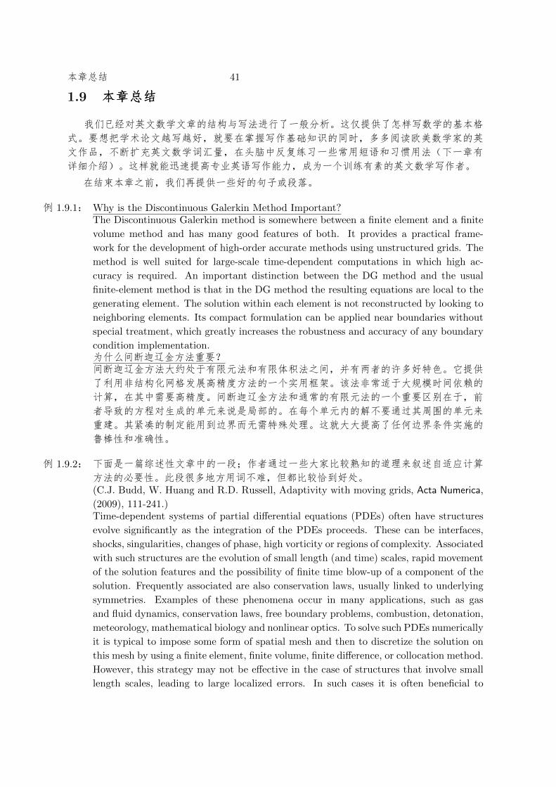
~ 1.9.1µ Why is the Discontinuous Galerkin Method Important?The Discontinuous Galerkin method is somewhere between a finite element and a finite

volume method and has many good features of both. It provides a practical frame-

work for the development of high-order accurate methods using unstructured grids. The

method is well suited for large-scale time-dependent computations in which high ac-

curacy is required. An important distinction between the DG method and the usual

finite-element method is that in the DG method the resulting equations are local to the

generating element. The solution within each element is not reconstructed by looking to

neighboring elements. Its compact formulation can be applied near boundaries without

special treatment, which greatly increases the robustness and accuracy of any boundary

condition implementation.omä¿7ºmä¿7?ukÚkNÈm§¿küöNõÐAÚ"§Jø

|^(zuÐp°Ý¢^µe"T~·u5m6

O§3Ù¥Ip°Ý"mä¿7ÚÏ~k«O3u§c

ö§é)¤ü5`´ÛÜ"3züS)ØÏLÙ±ü5

ï"Ù;n½U^>. ÃIAÏ?n"ùÒJp?Û>.^¢

°5ÚO(5"

~ 1.9.2µ e¡´nã5©Ù¥ã¶öÏL['Ùn5Qãg·AO

75"dãéõ/^cØJ§Ñ'TÐ?"(C.J. Budd, W. Huang and R.D. Russell, Adaptivity with moving grids, Acta Numerica,

(2009), 111-241.)Time-dependent systems of partial differential equations (PDEs) often have structures

evolve significantly as the integration of the PDEs proceeds. These can be interfaces,

shocks, singularities, changes of phase, high vorticity or regions of complexity. Associated

with such structures are the evolution of small length (and time) scales, rapid movement

of the solution features and the possibility of finite time blow-up of a component of the

solution. Frequently associated are also conservation laws, usually linked to underlying

symmetries. Examples of these phenomena occur in many applications, such as gas

and fluid dynamics, conservation laws, free boundary problems, combustion, detonation,

meteorology, mathematical biology and nonlinear optics. To solve such PDEs numerically

it is typical to impose some form of spatial mesh and then to discretize the solution on

this mesh by using a finite element, finite volume, finite difference, or collocation method.

However, this strategy may not be effective in the case of structures that involve small

length scales, leading to large localized errors. In such cases it is often beneficial to

42 êÆ©Ù(

use some form of non-uniform mesh, adapted to the solution, on which to perform all

of the computations. The advantages of doing this can be a reduced overall error,

better conditioning of the system, and better computational efficiency. Unfortunately,

introducing the extra level of complexity to the system through adaptivity can also lead

to additional computational cost and possible numerical instability. Mesh adaptation

should thus be used with care and appropriate analysis where possible. ©§m6XÚäkX ©§È©1? üCwÍ("§

±´.¡!ÀÂ!Û:!C!pµÚE,"ù('´Ý£Ú

m¤ºÝüz!)A5×£Ä±9,)©þkm»U5"²~k'

kÏ~.é¡5ë3åÅðÆ"ùy~fÑy3¯õA^¥§'X

íN½6NÄåÆ!ÅðÆ!gd>.¯K!-!¿!í!êÆ)ÔÆ95

1Æ"ê¦)ù ©§§;.´\,/ªm§,3

ùþò)^k!kNÈ!k©!½:5lÑz", §ùüÑ

39ÝºÝ(/7k§ÛÜzØ"3ù¹e§~~k

´æ^,/ª)·A§3Ùþ1¤kO"ù`³

±´~oØ!XÚÐ^5ÚZOk5"Ø3´§ÏL·A5

5Ú??E,5¬O¤ÚUêØ½5"·A5Ï

d%^§¿kUÒ·©Û"

~ 1.9.3µ e¡©ÙïÄíÄåÆO¥a§Hºª(upwind

scheme)"ö^'ßQã£ãù¤§±9§3õO¥

]Ô5¯K£ã¤"(B. van Leer, Upwind and high-resolution methods for compressible flow: From donor

cell to residual-distribution schemes. Commun. Comput. Phys., 1 (2006), 192-206.)Upwind differencing is a way of differencing the spatial-derivative terms in the advection

equation, and is almost as old as CFD, starting with the work of Courant, Isaacson and

Rees (1952 [12]). In their paper, the choice of an upwind-biased stencil follows rather

naturally from the ”backward” variant of the Method of Characteristics. In the course

of the decades further evidence has been gathered in support of upwind discretizations.

– Godunov, 1959. The Russian mathematician S. K. Godunov [18] favored the

firstorder-accurate upwind scheme among a family of simple discretizations, be-

cause it is the most accurate one that preserves the monotonicity of an initially

monotone discrete solution.

– Fromm, 1968. IBM researcher Jacob Fromm [16] constructed higher-order advection

schemes with low dispersive error, by combining schemes with predominantly nega-

tive and predominantly positive phase errors:“Zero Average Phase Error Method.”

The resulting schemes turn out to be upwind biased.

– Wesseling, 1973. Dutch aerospace engineer (turned numerical analyst) Pieter Wes-

seling [64] used Parseval’s theorem to relate the numerical error committed by

advection schemes to the Fourier transform of the initial-value distribution. For

two different families of advection schemes he found it is an upwind scheme that

minimizes the L2-error made in one time step if the initial values contain a dis-

continuity. This would indicate upwind schemes may be the preferred choice for

Ùo( 43

compressible flows, where shock discontinuities are common and arise even from the

smoothest initial data.

– van Leer, 1986. Reversing Fromm’s procedure, Dutch astrophysicist (turned aerospace

engineer) Bram van Leer [35] developed an operational definition of upwind schemes.

– Jeltsch, 1987. Mathematicians including Swiss Rolf Jeltsch [30], searching for advec-

tion stencils with the greatest potential accuracy for a given number of grid-points,

have proved that these stencils are upwind biased.

The price one has to pay for all this goodness is the computational effort in determining

the advection direction. That is trivial for a linear 1-D advection equation, but a major

effort for nonlinear advection operators hidden in nonlinear systems of multidimensional

conservation laws.Hº©´©²6§¥m-ê«ª§§AÚO6NåÆP§

l Courant, Isaacson Ú Rees ó£1952=12>¤m©"3¦Ø©¥§

HºÀg,/5guA/0C«"LAcmà8?

Úyâ|±HºlÑ"

– Godunov, 1959. ÛdêÆ[ S. K. Godunov=18>3xülÑ¥à°

ÝHºª§Ï§´±Ð©üNlÑ)üN5°("

– Fromm, 1968. IBM ïÄö Jacob Fromm=16>ÏLÜ¿ Ø±KÌÚ±

Ìª E$ÚÑØp²6ªµ/"²þ Ø0"d

d)ª5´ Hº"

– Wesseling, 1973. ûðÊÊUó§£=ê©ÛÆ[¤Pieter Wessel-

ing=64>|^ Parseval ½nò²6ªêØÐ©©ÙFp

CéXå5"éüxØÓ²6ª¦uy§eÐ©¹ØëY:´

HºªòmÚ) L2-Ø4z"ùqL²HºªéØ

6U´ÄÀ§3@pÀÂØëY5i.§$Ñyu1wÐ©êâ"

– van Leer, 1986. ò Fromm §SL5§ûðUNÔnÆ[£=¤ÊÊUó§

¤Bram van Leer=35>uÐÑHºªö5½Â"

– Jeltsch, 1987. ) Rolf Jeltsch=30>êÆ[§3Ïééu½ê8:

äkd3°Ý²6§®²y²ù´ Hº"

é¤kùÐ?¤Gd´û½²6Oãå"§é5²6§´²

§éÛõ3õÅðÆ5XÚ5²6f%´Ìãå"

A§Ø´,þr¤kØ©ÙóÜ©ÑÐ"lÖÙ§Ø©¼

E|§3@k¶"Ïrþé§XIêÆ¬ÑêÆ,"X8./Æâ.

ÑÔû³Øà§,#),o±J|m§o±Eu©Ù8"ØU"3

ùa,¥ÖõÐ©Ù"

-<W*´§Ð©ÙÃ?Ø3§$kéõú@Z"·ïÆ²~èA½°ÖÐr

ÔþÐ©Ù§Ø19)ïÄc÷G¹§Ulùö©Ùié¥Æ¬E

|"

e¡ézÆUi1^SÑÊ¶êÆÏr¶¡µ

44 êÆ©Ù(

• nÜÖÔµThe American Mathematical Monthly; Mathematical Intelligencer;

Notices of the American Mathematical Society; SIAM News; SIAM Review.

• êÆµAmerican Journal of Mathematics; Annals of Mathematics; Inventiones

Mathematicae; Journal of the American Mathematical Society; Transactions

of the American Mathematical Society.

• êØÜ6µAlgebra and Number Theory; International Journal of Number

Theory; Journal of Mathematical Logic¶Journal of Combinatorics and Num-

ber Theory; Journal of Number Theory.

• êAÛµCommunications in Algebra; Journal of Algebra; Journal of Al-

gebraic Geometry; Journal of Differential Geometry; Journal of Group Theory.

• ©ÛÿÀµGeometric and Functional Analysis; Journal of Fourier Analysis

and Applications; Journal of Functional Analysis; Journal of Operator Theory;

Topology.

• ©§ÄåXÚµDifferential Equations with Applications; Ergodic The-

ory and Dynamical Systems; Fractals; Journal of Differential Equations; Jour-

nal of Dynamics and Differential Equations.

• VÇÚOµAnnals of Probability; Annals of Statistics; Journal of American

Statistical Society; Biometrika.

• A^êÆµCommunications on Pure and Applied Mathematics; Journal of

Approximation Theory; Multiscale Modeling and Simulation; SIAM Journal

on Applied Mathematics; SIAM Journal on Mathematical Analysis.

• OêÆµMathematics of Computation; Numerische Mathematik; SIAM

Journal on Numerical Analysis; SIAM Journal on Scientific Computing; Jour-

nal of Scientific Computing.

• lÑêÆµAnnals of Combinatorics; Discrete Mathematics; Journal of Com-

binatorial Theory; Journal of Graph Theory; SIAM Journal on Discrete Math-

ematics.

• `zµJournal of Global Optimization; Mathematics of Operations

Research; Mathematical Programming; SIAM Journal on Control and Opti-

mization; SIAM Journal on Optimization.

• OÔnµJournal of Computational Physics; Journal of Mathematical

Physics; Journal of Statistical Physics; Communications in Computational

Physics.

3î§kZØ©µÀ§e¡Þø¶¡9Ù'øÖöëµ

• 5IêÆr6(The American Mathematical Monthly) Lester R. Ford Ø©øµhttp://www.maa.org/Awards/ford.html

ùøg1965cm©§y®uC40c"

Ùo( 45

• IóÚA^êÆ¬`DØ©ø (The SIAM Outstanding Paper Prizes)µhttp://www.siam.org/prizes/outstanding.htm

ùøg1999cm©"

• IêÆ¬ Levi L. Conant ø (Levi L. Conant Prize)µhttp://www.ams.org/prizes/conant-prize.html

Ìøy3 Notices of the American Mathematical Society ½ Bulletin of the American

Mathematical Society uL©Ù"ùøg2001cm©"

• 5E,5,6`DØ©ø (Best Paper Award for the Journal of Complexity)µhttp://www.ibc-research.org/prizes.html#BPA

ùøg1996cm©"

·Ñ§Ù¤k?Øéu>Æ Ø©kÏ"Æ Ø©ÚÆâØ©«

O§ÒÐ>ÀìÚ>K«O–cöuö"Æ Ø©AUJÑM§X¤þZ

a¬Ø©´&EØIà (Claude Shannon, 1916-2001) u1937c3ænóÆ>

a¬Ø© Symbolic Analysis of Relay and Switching Circuits£¥UÚm'>´ÎÒ©

Û¤" ó§Æ Ø©Ü©SN ´ÆuÐÚyGnã"3ù¿

Âe§§Ö"·31oÙò?ØNÖ"

46 êÆ©Ù(

47

Chapter 2

êêêÆÆÆ©©©ÙÙÙcccééé

dcÙ·®²)êÆ©ÙÄ(Ú+"3ùÙ·XÚ?Ä

=©êÆc®§0~^éÚáA^"

c®´óÄü "ÃØôó§·~kùa>µ¦+·M

pCØ~^c§y^cTÐ?%ØŃ´¯"ÜÆ

<©Ï£U·éuµÃØÆn!Æó!Æ©½ÆÙ§8§Æ!

c?Æ)<©Æ (humanities) 2ÖÓr©cUå4ÐÔö"äNêÆ

¥(^c§M#dw2·µThink about and use with care the small words of

common sense and intuitive logic, and the specifically mathematical words (technical terms)

that can have a profound effect on mathematical meaning.£õ¿%¦^~£ÚúÜ

6c§AO´éêÆ¹ÂkKêÆc®£Eââ¤"¤é&Êâ¶c§¦

? Ñn\äN§wµ

(1) Avoid technical terms, and especially the creation of new ones, whenever pos-

sible.

¦U;Eâc®§cÙ´#E"

(2) Think hard about the new ones that you must create; consult Roget; and make

them as appropriate as possible.

õg¢\½ME#c¶Ûac;¶-§¦UÜ·"

(3) Use the old ones correctly and consistently, but with a minimum of obtrusive

pedantry . . ..

(¿ë0¦^Îc§´¦þØâôs@ · · · · · ·"

·3Ù0êÆcécÚãM#dXþ§w§Ò´F"cÖöUr§À

êÆ¥ec^émµ"

3^=E©Ù§²~9«é.Ú¦^"ù¯K3=Ö

¥k'¦0§ék¥©Ö7;éêÆØ©'c[0"ù

¡=©©ÙÚÖ7éK'õ§'X`=IùdAÆÍ¶êê;[ Nicholas J.

Higham ®2Ö Handbook of Writing for Mathematical Sciences [13] ÚI´ú

48 êÆ©Ùcé

îÆNÚ©ÛÆ[ Steven G. Krantz Ñ A Primer of Mathematical Writing [17] ´'

uêÆ`DÖ"éE=©§·í Jean-Luc Lebrun Cc5Ñ

Ö Scientific Writing [20]"

E=ØÊÏ=@äka5/g§ØäaÚç§L'§

Ù8´¦ÖöNń) Ø)KÃ'õ"Ø²~$^'!ü'!§Ü

?`Ãã§ Ó(L*5Æ§UÜ6gß/£ã¯K"E=c®¿Â'

;!½§AO´þ;¶cÙcÂé½!;"=¦´ do, take, make ù

õcÂÊÏÄc§3E=¥§¿g½'(½§ÙLª'Nń)"

E=Ì´«Ö¡ó§§¦O(!î>!'!6§¿Ø¦3©¥æëuw

c>§§Ø¦ÄBuKÖÚÔJ"3(þ§§²~¦^Ä"

E=¦^ÄÐ?´±¦£ã~Ì*Úç§Or*5§ ÏLÛ<¡

Ì ¦éf¦U'"'Ù§Æ§êÆ©ÙÌÄ^õ§É

¶[à",¡§êÆ¥k^cCzØ´é£ØÙ§EÆc

®XÆ?Úè?'²w¤§¤±Nõ~^êÆc®ATN[º/P3%

¥"

Òóc®¡ ó, E=N´F#ÉÆEâ+SuÐM

#"O(!Æ/éù#uy!u²!nØ?Ð\±ã§Eóö3ec

¡eéõÅ"l,¡w§duêÆýn²åm§Ò½

nüZccF1<îy²y3,k@uØ±m¿=£"Ùg,(J

´êÆc®é'½§ýÜ©ØIè?/UC¿g"¤±·3Ù8¥0

êÆÄc®Úá"

3E=¥²~¦^(õ§XÄé¦^é2"ù´ÏE

©ÙÌ8´ùã*y§0E¤J§¦^Äé'¦^ÌÄéÌ*Ú

ç"Ïd3E=¥§´3ØI½ØUÑ1ÌN|Ü§½ö3IâÑ1

N|ÜÑ¦^Ä", §3ù¡§êÆÙ§EkØÓ"Krantz

[17] *µMost authorities believe that writing in the passive voice is less effective than

writing in the active voice. £Ü©%&^Ävk^ÌÄk"¤ Higham

[13] ïÆµPrefer the active to the passive voice (prefer “X did Y” to “Y was done by

X”). £w^ÌÄ Ø^Äª£/X Y0 Ø´/Y X 0¤"¤3êÆL¥§

ªo'mªÐ"Öö±'

The vector v is multiplied by the matrix A

þ v Ý A ¦

Ú

The matrix A multiplies the vector v

Ý A ¦±þ v

ùü«§=«Ü\º,§XJ\rNÄ1ö§^ÌÄª"´§XJ

þ~¥þ v ÚÉ'5§Ò±^Ä"

Ùk0ÄêÆc®"êÆ=c®'åÙ§Æééõ§Ø)

Ô½Æc®@qqJuÑ§¤±Ýº§éØ¬J",·0êÆÎÒ

50 êÆ©Ùcé

2.1 êêêÆÆÆÄÄÄccc®®®

Xr©Ù'f§c®Ò´ïÓf<Þ"êÆc®,'õ§éÙ§Æ5

`©´'ü"Ýº½êþêÆc®§ü©ÙÒATØ¬kõ

(J"3!p, ·Þ~^êÆc®Úc|"Ñùc®½c|8Ø´J

ø=ÇêÆc;§ ´JøÐÆöÝºùÄc®ÚâA^öS|¤Ú

¢Å¬"½öÖ©Ù§XkØ²xc®§ATë'Vc;£'X5=

ÇêÆc®6[2]¶c®5#=Çc;6[3]¤"êÆ~^á½é.ò3

¡A!ºYÑy"

½Â definition ½n theorem

½ÂÜn well defined ÜÜ6 is logical

Ü6 logic gñ contradiction

Ún lemma íØ!X corollary

ún axiom ·K proposition

ú postulate cJ premise

ß conjecture ¡Þ exhaustion method

ín!íü deduction, deduce êÆ8B mathematical induction

Û¹!%º implication, imply (Ø conclusion, conclude

~£ common sense 7^ necessary condition

¿©5 sufficiency 75 necessity

d5 equivalency äó claim, assert

~f example, e.g. ë©z reference

~ counterexample = i.e., that is, namely

²¡AÛ plane geometry ã graph

áNAÛ solid geometry xAÛ descriptive geometry

AÛ affine geometry ©AÛ differential geometry

KAÛ projective geometry È©AÛ integral geometry

êAÛ algebraic geometry îAÛ non-Euclidean geometry

iùAÛ Riemann geometry VAÛ hyperbolic geometry

¥¡AÛ spherical geometry AÛ©Û geometric analysis

)ÛAÛ analytic geometry OAÛ computational geometry

|ÜêÆ combinatorics ©/AÛ fractal geometry

"AÛ simplectic geometry ¡È area preserving

â arithmetic Oê count, enumerate

\ add, plus \ addition

\5 additivity \ countably additive

Ú sum ¦Ú summation

~ subtract, minus ~ subtraction

difference û difference quotient

¦ multiply ¦ multiplication

Ø divide Ø division

'!'Ç ratio Øê dividend

Ø divisible Ø5 divisibility

ê algebra n trigonometry

êÆÄc® 51

úª formula Lª expression

È©Ò integral sign )Ò parenthesis, bracket, brace

§ equation d'X equivalent relation

g reflexive D4 transitivity, transitive

òz degenerate Z damping

é¡ symmetry, symmetric ¶é¡ symmetric about an axis

da equivalent class ¥%é¡ symmetry about the origin

root ) solution

ª radical ² square root

¯K question, problem b hypothesis, assumption

SK exercise homework

ã/ figure L table

Cþ variable ~ê constant

ÏCþ dependent variable gCþ independent variable

'X relation ¼ê function

(ÜÆ associative law Æ commutative law

©Æ distributive law gÆ reflexive law

éê logarithm g,éê natural logarithm

Ûê odd number óê even number

ýé absolute value ê exponential,exponent

Ý angle lÝ radian

S interior angle b£ð¤ acute (obtuse) angle

complementary angle exterior angle

adjacent angle Ýê degree

éº vertical angle º vertex angle

Ö supplementary angle ¡ dihedral angle

Ó corresponding angle S alternate angle

% central angle ± circumferential angle

Y included angle inclination angle

¡È area NÈ volume

» diameter » radius

u½Æ law of sines u½Æ law of cosines

tangent cotangent

secant cosecant

é> opposite > adjacent

> hypoteneuse q/ similar figure

/ square / rectangle

n/ triangle >n/ equilateral triangle

n/ congruent triangle n/ isosceles triangle

n/ right triangle F/ trapezoid

isogonal o>/ isosceles quadrilateral

²1 parallel line îApún Euclidean axiom

F/ isosceles trapezoid o>/ quadrilateral, quadrangle

!/ lozenge, rhombus ²1o>/ parallelogram

Ê>/ pentagon 8>/ hexagon

Ô>/ heptagon l>/ octagon

52 êÆ©Ùcé

Ê>/ nonagon >/ decagon

(/ star domain QG« saddle region

>/ dodecagon n->/ n-gon

õ>/ polygon õ4 multi pole

õ>/ regular polygon ål distance

/%!% centroid å isometry

circle Ó% concentric circle

Sõ>/ cyclic polygon subscribed circle

p altitude S inscribed circle

concyclic collinear

5 compass º ruler

: tangential point é diagonal

²© internal bisector ¥ median line

Ó congruence, congruent q similarity, similar to

o¡N tetrahedron õ¡N polyhedron

cÎ prism c frustum of pyramid

cI regular pyramid I right circular cone

¥N ball ÎN circular cylinder

ý¥ ellipsoid ^=N solid of revolution

1 generatrix L torsion free

V¡ hyperboloid Ô¡ paraboloid

I circular cone cI pyramid

circular ring ¡ torus

% center l%Ç eccentricity

÷/ sector frustum

± perimeter l arc length

± circumference u chord

¥¡ sphere ¥ hemisphere

curve straight line

R vertical line Y² horizontal line

é¡ line of symmetry ²© bisector

ÃúÝ incommensurable orthogonal, perpendicular

I conic curve ü á unit cube

«m interval ã line segment

²¡ plane ¡ surface

Ç curvature ëê§ parametric equation

7Ç torsion 7Ç secondary torsion

tangent line normal line

5º note, remark ÎÒ notation, symbol

þ unknown ®þ known

¦È product û quotient

©f numerator ©1 denominator

' ratio '~ proportion

' directly proportional ' inversely proportional

z©' percentage, percent ê multiple

Ïf factor Ïª©) factorization

êÆÄc® 53

úê least common multiple úÏê greatest common factor

" zero Ã¡ infinity

Ã¡ infinitesimal ì? asymptote

ê integer ê decimal

?ê binary number g,ê natural number

ª½n binomial theorem V5 bilinearity

êi digit 'A bit

ê!ê prime number )ÛêØ analytic number theory

©ê fraction ê reciprocal

\Ò plus sign ~Ò minus sign

ê positive number Kê negative number

ê opposite number ýé absolute value

knê rational number Ãnê irrational number

¢ê real number Jê imaginary number

transcendental transfinite

¢Ü real part JÜ imaginary part

Eê complex number g power

module Ì argument

þ magnitude, amount þz quantify

² square root á cubic root

oê quaternion g quadratic

üª monomial õª polynomial

!g!Ý degree, order Xê coefficient

ü simple root ê multiplicity

multiple root ª radical

nÜØ synthetic division ½Xê undetermined coefficients

ðª identity ^ conditional

Øª inequality ª equality

nØª triangle inequality ½n Pythagorean theorem

¿ã§ Diophantine equation ¥I½n China’s Remainder Theorem

Ø) unsolvable ½§ over determined equation

ðª identity 1ª determinant

ü! permutation |Ü combination

I¶ coordinate axis ²¡ plane

ëê parameter ëêL« parametric representation

quadrant quadratics

ray 4I polar coordinates

Ô parabola ý ellipse

Ô. parabolic ý. elliptical

V hyperbola V. hyperbolic

Ú spiral Ú^ helix

îI abscissa pI ordinate

O directrix : focus

Ç slope : point

å intercept intersection

K: regular point ÛÉ: singular point

54 êÆ©Ùcé

Q: saddle point .: critical point

$: inflection point Ø: nondifferentiable point

4I polar coordinates ÎI cylindric coordinates

¥ spherical I Cartesian coordinates

ìC5 asymptotic property ìC asymptote

8Ü set S sequence

8 empty set f8 subset

8 intersection ¿8 union

Ö8 complement ;8 compact set

þI superscript eI subscript

Äê cardinal number Sê ordinal number

ê8 countable set Øê8 uncountable set

m8 open set 48 closed set

8 perfect set 8 induced set

n©:8 ternary set ü:8 single point set

neighborhood m£4¤¥ open (closed) ball

C proximity ýf8 proper subset

4: limit point à: cluster point

4 closure >.!>.: boundary, boundary point

S: interior point á: isolated point

8 complete set Èf8 dense subset

z completable k8 directed set

S partially ordered S8 totally ordered set

DÕ nowhere dense x÷n©8 Cantor’s ternary set

üéÏ simply connected Jordan curve

þ£e¤. upper (lower) bound Ã.8 unbounded set

þ(. supremum value e(. infimum value

þ. least upper bound e. greatest lower bound

4 limit þ£e¤4 upper (lower) limit

ê derivative £m¤ê left (right) derivative

Oþ increment Ø½. indefinite form

CzÇ rate of change ²þCzÇ average rate of change

C variation ]CzÇ instantaneous rate of change

ê first derivative ê second derivative

p higher order VÐª Taylor’s expansion

ê partial derivative ê directional derivative

u directional cosine ëY continuously differentiable

Û7©K L’Hopital’s rule Ûª¦ implicit differentiation

¦ÈK product rule ûK quotient rule

ó^K chain rule éê¦ logarithmic differentiation

0 intermediate value ¥m mean value

Ã¡ infinity Ã¡ infinitesimal

4 maximum 4 minimum

ÛÜ4 local extreme value N4 global extreme value

È© calculus © differential

?ê series È© integral, integration

êÆÄc® 55

NÚ?ê harmonic series êN?ê Maclaurin series

?ê alternating series Fá?ê Fourier series

?ê power series V?ê Taylor’s series

þ£e¤ upper (lower) limit ¼ê antiderivative

© partial differential © total differential

Ø½È© indefinite integral ½È© definite integral

È¼ê integrand þ£e¤ upper (lower) limit

È integrable ÙþÈ© Darboux upper integral

2ÂÈ© improper integral '~Ïf propositional divisor

Ú summable ê! countable

È© double integral nÈ© triple integral

õÈ© multiple integral ÅgÈ© iterated integral

©ÜÈ© integration by parts CþO integration by substitution

Ü©©ª partial fraction ýÈ© elliptic integral

È© line integral ¡È© surface integral

úª Green’s formula d÷d½n Stokes’ theorem

Ï) general solution A) particular solution

þ| vector field È© integral curve

ÄgÈ© first integral T©§ exact differential equation

2ÂÈ© generalized integral Ä½n fundamental theorem

ÛÉÈ© singular integral >.È© boundary integral

L« representation ÜÈ©úª Cauchy’s integral formula

¼ê entire function )Û¼ê holomorphic function

æX¼ê meromorphic function Û5 essential singularity

/Nì conformal mapping 3ê½n residual theorem

Âñ convergence uÑ divergence, divergent

Âñ uniformly convergent k. uniformly bounded

ýéÂñ absolutely convergent ^Âñ conditionally convergent

Å: pointwise r£f¤Âñ strongly (weakly) convergent

òÈ convolution N coordination

¼ê one variable function õ¼ê multi-variable function

ëY continuity ëY uniformly continuous

??ëY continuous everywhere ÝëY equi-continuous

Ó homeomorphism mä discontinuous

mä: discontinuous point üëÏ« simply connected region

´ëÏ path connected amä5 jump discontinuity

þ vector Iþ scalar

©þ component ü þ unit vector

ê| array 1£¤þ row (column) vector

Üþ tensor Ýþ moment

.5 inertia % barycenter

Äþ momentum Äþ angular momentum

Ý matrix ü Ý identity matrix

square matrix rectangular matrix

rank £1¤m column(row) space

Am eigenspace 2ÂAm generalized eigenspace

56 êÆ©Ùcé

Ïª©) factorization AÛê geometric multiplicity

Ú direct sum Ö orthogonal complement

5§ linear equation Ä) fundamental solution

^ê condition number ¾¯K ill conditioned problem

éÝ diagonal matrix éÝ diagonalizable matrix

þn upper triangular enÝ lower triangular matrix

ÛÉÝ singular matrix ÛÉÝ nonsingular matrix

_Ý invertible matrix _Ý inverse matrix

DÕÝ sparse matrix [ matroid

IÝ indicator matrix GÝ band matrix

1ª determinant 2Â_Ý generalized inverse matrix

Ìfª principal minor êfª algebraic cofactor

(ª discriminant , trace

ó train ¡ torus

=Ý transposed matrix Ý=Ý conjugated transposed matrix

Ý companion matrix ©¬Ý block matrix

Ý orthogonal matrix jÝ unitary matrix

ÌÝ circular matrix éÓ`Ý diagonally dominant matrix

é¡Ý symmetric matrix KÝ normal matrix

½ positive definite ½Ý positive semidefinite matrix

Ø½Ý indefinite matrix K½Ý negative definite matrix

Ý positive matrix KÝ nonnegative matrix

[Å quasi stochastic ÅÝ column stochastic matrix

Ø irreducible Ý primitive matrix

" nilpotent ÝKÝ projection matrix

ëÝ connection matrix 'éÝ incidence matrix

ä'Ý Jacobian matrix °ÜÝ Hessian matrix

©y partition, division ¬éÝ block diagonal matrix

g. quadratic form IO. normal form

S isotone S antitone

õª minimal polynomial Aõª characteristic polynomial

A eigenvalue Aþ eigenvector

Ì spectrum Ì residual spectrum

ëYÌ continuous spectrum Cq:Ì approximate point spectrum

>Ì peripheral spectrum Ì©) spectral decomposition

Ì» spectral radius A maximal eigenvalue

2Â generalized 2ÂAþ generalized eigenvector

¬ Jordan block IO. Jordan canonical form

N mapping ¼ê inverse function

C transformation pN induced mapping

restriction *Ü extension

ü injection, one-one ÷!Nþ surjection, surjective, onto

kn¼ê rational function Nþ bijection, bijective

ü¸¼ê unimodal function Û£ó¤¼ê odd (even) function

é¡¼ê symmetric function ðÓ¼ê identity function

õ¼ê multi-valued function k.C¼ê function of bounded variation

êÆÄc® 57

NÚ¼ê harmonic function F¼ê step function

±Ï¼ê periodic function 1w¼ê smooth function

A characteristic I¼ê index function

8¼ê set function :-8N point-set mapping

ðÓN identical mapping N*Ü mapping extension

¹N inclusion mapping õ many-valued

transcendental ¼ê differentiable function

ζ ¼ê zeta function 2Â¼ê generalized function

È integrable ýéëY absolutely continuous

ê¼ê exponential function éê¼ê logarithmic function

¼ê power function n¼ê trigonometric function

Ð¼ê elementary function gÅ¼ê automorphic function

EÜ¼ê composite function »Ä.¼ê radial basis function

^¼ê spline function ©ã piecewise

¼êØ function-theoretic ¼f functor

½Â domain range

image _ inverse image

²þ average value ¥½n mean value theorem

½ orientation éA one to one correspondence

üN¼ê monotone function Aþ¼ê eigenfunction

à¼ê convex function ]5 concavity

[à¼ê quasiconvex function à¼ê pseudoconvex function

Óà Schur convex îà¼ê strictly convex function

à8 convex set à|Ü convex combination

à convex hull d · · · · · · ) generated by . . .

àz convexification à4 convex closure

Y²8 level set éS: relative interior point

`5^ optimality condition .KF¦f Lagrange multiplier

C©Øª variational inequality éó5 duality

$: inflection point ²: equilibrium point

FÝ gradient ÑÝ divergence

eü steepest descent ÝFÝ conjugate gradient method

Ý conjugate direction ¦ least squares method

Úî Newton’s method [Úî quasi Newton method

ýÿ- predictor-corrector ©-éó primal-dual

8I¼ê objective function ½5y semidefinite programming

18 feasible set AÛ5y geometric programming

Å5y convex programming |Ü`z combinatorial optimization

C© calculus of variation õ8I5y multi-objective optimization

55y linear programming êÆ5y mathematical programming

g5y quadratic programming Å5y stochastic programming

ê5y integer programming Ä5y dynamical programming

tµCþ slack variable 5Ö linear complementarity

à©Û convex analysis `5^ optimality condition

ä`z network optimization e4¯K postman problem

1w©Û nonsmooth analysis gFÝ subgradient method

58 êÆ©Ùcé

zFÝ reduced gradient &6 trust region method

$ÊÆ operations research üèØ queuing theory

ÙK$Ä Brownian movement BL§ Wiener’s process

éüØ game theory S: interior point method

ûünØ decision theory ý¥ ellipsoid algorithm

E,5 complexity 2:$ floating point operation

ãØ graph theory kã directed graph

Vã bigraph ã complete graph

> edge º: vertex

Ì cycle ´ path

£´ circuit ä tree

'é incident 'éXê incidence coefficients

:È dot product ÜþÈ tensor product

SÈ inner product þÈ cross product

ê norm Cq approximation

? modification \Ø round-off error

1 row column

þm vector space ålm metric space, distance space

ÿÀm topological space ÿÝm measure space

5m linear space ÿm measurable space

SÈm inner product space FËAm Hilbert space

Dm normed space n<âm Banach space

m complete space ©m separable space

VÇm probability space ;m compact space

¦Èm product space ûm quotient space

éóm dual space gm reflexive space

Ûgm homogeneous space "m symplectic space

ÛÜà locally convex 2Â¼êm space of distributions

m spacial space-time

n ideal ring

ü unit 8 coset

+ group field

lattice S8 totally ordered set

Ä+ fundamental group ÓN homology

G+ braid group gÓ+ group of automorphisms

ÓÔ homotopy q variety

ê commutative algebra + permutation group

ü+ simple group k+ finite group

+ semigroup )¤ generator

+ primitive group Ìf+ cyclic semigroup

Ó homomorphism Ó isomorphism

å isometry ÛÜ; locally compact

;z compactification é; relatively compact

CX covering f commutator

êq algebraic variety ê algebraic curve

ê dimension one dimension

êÆÄc® 59

two dimensions õ multi dimensions

k¡ finite dimensional Ã¡ infinite dimensional

Ä. basis Ä orthogonal basis

5|Ü linear combination )¤f generator

5fm linear subspace d · · · · · · Ü¤ spanned by . . .

5' linear dependence 5Ã' linear independence

ü ©) partition of unity ©) orthogonal decomposition

ÝK orthogonal projection C orthogonal transformation

¦ least squares § normal equation

Z%C best approximation 4ê) minimal norm solution

n maximum principle 'n comparison principle

± isoperimetric ^n minimal action principle

K5 regularity property 1w5 smoothness property

5 positivity UþÅð conservation of energy

éuª©Û heuristic analysis î©Û rigorous analysis

N5 consistency ½5 stability

ØO error estimate ÂñÝ©Û convergence rate analysis

lÑz discretization Ú step size

[ simulation [Ü curve fitting

Âñ convergence order `5 optimality

k© finite difference k finite element

N conformal element kNÈ finite volume method

>. boundary element ·Ü mixed element

C©n variational principle C©Øª variational inequality

interpolation £í¤ extrapolation

lÑ discrete pd¦Èúª Gauss quadrature

remainder êª numerical scheme

õ multi-grid method «©) domain decomposition method

" symplectic algorithm ( structure preserving method

Ì spectral method Ã meshless method

[Ü curve fitting >M9ÏO computer-aided design

^¼ê spline function Ä^ B-spline

IOÄ canonical basis Å¡5¼ê piecewise linear function

&Ò?n signal processing ã?n image processing

Å©Û wavelet theory êâ?n data processing

é6 convection *Ñ§ diffusion equation

ÄåXÚ dynamical system ©§ partial differential equation

È©§ integral equation f§ operator equation

©§ difference equation m¢§ time delay equation

Ñt)Ò Poisson bracket uÐ§ evolution equation

-Å shock wave Ì amplitude

\4N Poincare’s map S:!S iterate, iteration

4 limit cycle ²£ï¤: equilibrium point

Ä oscillation ì?½ asymptotically stable

·b chaos ©/ fractal

êÈ© numerical integration ê© numerical differentiation

60 êÆ©Ùcé

ÝK projection method cû forward difference quotient

(½5XÚ deterministic system lÑÄåXÚ discrete dynamical system

ÅL§ stochastic process ëYÄåXÚ continuous dynamical system

m sample space ÿÀÄåXÚ topological dynamical system

&E information entropy Ì!48 recurrence

Ýþ metric entropy 9åÆ thermodynamics

ÚOåÆ statistical mechanics þfåÆ quantum mechanics

õ work ³U potential energy

å force ÄU kinetic energy

Ý velocity, speed \Ý acceleration

position £ displacement

Å| conservative field %å centripetal force

ÅðÆ conservation law ÄåÆ kinetics

ÿÀ topological entropy ÅCþ random variable

êÅó Markov chain Ï" expected value

êÆÏ" expectation martingale

²þ mean ^Ï" conditional expectation

¥m median variance

IO standard deviation 5£8 linear regression

covariance 'éXê correlation coefficient

VÇØ probability theory ªÇ frequency

éÜÝ joint density ÅiÄ random walk

þ!©Ù uniform distribution ©Ù normal distribution

maximum entropy ` optimal control

ÿÝ measure |8 support

ÿÝØ measure theory ÿ¼ê measurable function

ÿ measurable ÛÉC nonsingular transformation

È¼ê integrable function ²È¼ê square integrable function

iùÈ© Riemann integral VÈ© Lebesgue integral

©ÙnØ distribution theory f weakly differentiable

HnØ ergodic theory H5 ergodicity

·Ü5 mixing ÿÀD4 topological transitivity

Ü exact ØCÿÝ invariant measure

ØÄ: fixed point ±Ï:!±Ï periodic point, period

±Ï5 periodicity ªØÄ: eventually fixed point

½ stable, stability ; orbit, trajectory

ì?½ asymptotically stable Ø½ unstable, instability

±Ï aperiodic áÚ basin of attraction

ü½ØÄ: repelling fixed point áÚØÄ: attracting fixed point

·b chaos ·báÚf chaotic attractor

©/ fractal ©/ê fractal dimension

5f linear operator 5C nonlinear transformation

;f compact operator k.5f bounded linear operator

gÝf self-adjoint operator ëYf continuous operator

"m null space, kernel "zf annihilator

¼ functional k.5¼ bounded linear functional

êÆÄc® 61

Ûg homogeneous f; weakly compact

; sequentially compact O; precompact

é; relatively compact i]L«½n Riesz representation theorem

mN½n open mapping theorem _N½n inverse mapping theorem

4ã½n closed graph theorem k.K uniform boundedness principle

ØÄ:½n fixed point theorem Ø N½n contraction mapping theorem

ÿ8 measurable set Âñ½n dominated convergence theorem

A?? almost everywhere üNÂñ½n monotone convergence theorem

:8ÿÀ point set topology êÿÀ algebraic topology

ü/ simplex E/ complex

ÄnØ perturbation theory 2Â¼êØ theory of distribution

Ý(nØ knot theory unØ string theory

Äê abstract algebra õ/ê multilinear algebra

Æ category ¼f functor

©/ª differential form ©ÿÀ differential topology

"ÿÀ symplectic topology © exterior differential

© exterior differential nm fibre bundle

Ìm principal bundle Cê covariant derivative

m tangent bundle ¥4²¡ÝK stereographic projection

5| gauge field ¹ÄIe moving frame

ëIe reference frame o+£ê¤ Lie group (algebra)

éä affine connection Wéä Cartan connection

6/ manifold ©6/ differential manifold

ÿÀ6/ topological manifold ÿÀd topologically equivalent

Ó homeomorphism ©Ó diffeomorphism

Þ!Ø germ Øf divisor

º genus î.«5ê Eular’s characteristic

K regular value Û¼ê½n implicit function theorem

'\½n imbedding theorem ¢ËÅm Sobolev space

,½n trace theorem f) weak solution

Cê covariant derivative ÿ/ geodesic

4¡ minimal surface iùÝþ Riemannian metric

È wedge product ©( differentiable structure

Table 2.1: ÄêÆ¶cÚâ

¥©©Ù)i!c!é!ã"ù¤©ÙÉÚS"Ó§=©©Ù¥´

dc!á!éf!ãá|¤"¤±3=©Ù7LÀücÚé.$^"ATk

¿£/*gCc®þ!áþ"ÏL¢±¬È\c®W"~ó§þÈ

u"Xmí£§Ò¬uúgC5Ñy±c~k/Ã0f¾"Ùö

$^~^êÆc®Úc|á§¬¦6¶"v<ÚÖöÖå5¬ÓÑ"

{\ J*WGy^ - HKBU-Math

Documents

Transcript of {\ J*WGy^ - HKBU-Math