NASA Conference Publication 3095NASA-CP-3095 19910009711

' Joint UniversityProgram for

Air TransportationResearch

1989-1990-:: ,..-- "" ; _ ." . . ":: - .o

, k

. _IJ_'3 ,:"

[AN_LL_ r,.=-:_.",--_.......;-'_".V -. " ' 'o

Proceedings of a conference held inAthens, Ohio

June 14-15, 1990

I

NASA Conference Publication 3095

Joint UniversityProgramfor

Air TransportationResearch

1989-1990

Compiled byFrederick R. Morrell

Langley Research CenterHampton, Virginia

Proceedings of a conference sponsored bythe National Aeronautics and Space Administration

and the Federal Aviation Administration and held inAthens, Ohio

June 14-15, 1990

IXl/_ANationalAeronauticsand

SpaceAdministration

Officeof ManagementScientificandTechnical

InformationDivision

1990

PREFACE

The Joint University Program for Air Transportation Research is a coordinated set of three grants sponsoredby NASA Langley Research Center and the Federal Aviation Administration, one each with the MassachusettsInstitute of Technology (NGL-22-009-640), Ohio University (NGR-36-009-017), and Princeton University (NGL-31-001-252). These research grants, which were instituted in 1971, build on the strengths of each institution.The goals of this program are consistent with the aeronautical interests of both NASA and the FAA in furtheringthe safety and efficiency of the National Airspace System. The continued development of the National AirspaceSystem, however, requires advanced technology from a variety of disciplines, especially in the areas of computerscience, guidance and control theory and practice, aircraft performance, flight dynamics, and applied experimentalpsychology. The Joint University Program was created to provide new methods for interdisciplinary education todevelop research workers to solve these large scale problems. Each university submits a separate proposal yearlyand is dealt with individually by NASA and the FAA. At the completion of each research task, a comprehensiveand detailed report is issued for distribution to the program participants. Typically, this is a thesis that fulfillsthe requirements for an advanced degree or a report describing an undergraduate research projecL Also, papersare submitted to technical conferences and archival joumals. These papers serve the Joint University Programas visibility to national and intemational audiences.

To promote technical interchange among the students, periodic reviews are held at the schools and at a NASAor FAA facility. The 1989-1990 year-end review was held at Ohio University, Athens, Ohio, June 14-15, 1990.At these reviews the program participants, both graduate and undergraduate, have an opportunity to present theirresearch activities to their peers, to professors, and to invited guests from govemment and industry.

This conference publication represents the tenth in a series of yearly summaries of the program. (The 1988/89summary appears in NASA CP-3063). Most of the material is the effort of students supported by the researchgrants. Four types of contributions are included in this publication: a summary of ongoing research relevant tothe Joint University Program is presented by each principal investigator, completed works are represemed byfull technical papers, research previously in the open literature (e.g., theses or joumal articles) is presented in anannotated bibliography, and status reports of ongoing research are represented by copies of presentations withaccompanying text.

Use of trade names of manufacturers in this report does not constitute an official endorsement of suchproducts or manufacturers, either expressed or implied, by the National Aeronautics and Space Administrationor the Federal Aviation Administration.

Frederick R. MorreUNASA Langley Research Center

°oo111

CONTENTS

PREFACE ....................................... iii

MASSACHUSETTS INSTITUTE OF TECHNOLOGY

INVESTIGATION OF AIR TRANSPORTATION TECHNOLOGY AT THEMASSACHUSETFS INSTITUTE OF TECHNOLOGY, 1989-1990................ 3RobertW. Simpson

AUTOMATIC SPEECH RECOGNITION IN AIR TRAFFIC CONTROL: A HUMANFACTORS PERSPECTIVE ................................ 9

Joakim Karlsson

THE TEMPORAL LOGIC OF THE TOWER CHIEF SYSTEM ................. 15Lyman R. Hazelton, Jr.

BUBBLES--AN AUTOMATED DECISION SUPPORT SYSTEM FOR FINAL APPROACHCONTROLLERS .................................... 29

Zhizang Chi

ANALYSIS OF AIRCRAFT PERFORMANCE DURING LATERAL MANEUVERING FORMICROBURST AVOIDANCE ............................... 37

Denise _vila De Melo and R. John Hansman, Jr.

HAZARD EVALUATION AND OPERATIONAL COCKPIT DISPLAY OF GROUND-MEASURED WlNDSHEAR DATA ............................. 45

Craig Wanke and R. John Hansman, Jr.

OHIO UNIVERSITY

INVESTIGATION OF AIR TRANSPORTATION TECHNOLOGY AT OHIO UNIVERSITY,1989-1990. ...................................... 61

Robert W. Lilley

RIDGEREGRESSIONSIGNALPROCESSING........................ 67MarkR. Kuhl

MODELING SELECTIVE AVAILABILITY OF THE NAVSTAR GLOBAL POSITIONINGSYSTEM ........................................ 77

Michael Braasch

ANALYZING THOUGHT-RELATED ELECTROENCEPHALOGRAPHIC DATA USINGNONLINEAR TECHNIQUES ............................... 91

Trent Skidmore

INTEGRATED INERTIAL/GPS .............................. 97Paul Kline and Frank van Graas

PRINCETON UNIVERSITY

INVESTIGATION OF AIR TRANSPORTATION TECHNOLOGY AT PRINCETONUNIVERSITY, 1989-1990 ................................ 105

Robert F. Stengel

V

PROGRESS ON INTELLIGENT GUIDANCE AND CONTROL FOR WIND SHEARENCOUNTER ..................................... 119

D. Alexander Stratton

FLIGHT SIMULATION FOR WIND SHEAR ENCOUNTER .................. 133Sandeep S. Mulgund

STOCHASTIC ROBUSTNESS: TOWARDS A COMPREHENSIVE ROBUSTNESS TOOL ..... 141Laurie Ryan Ray

NEURAL NETWORKS IN NONLINEAR AIRCRAFT CONTROL ................ 151Dennis J. Linse

STABILITY BOUNDARIES FOR AIRCRAFT WITH UNSTABLE LATERAL-DIRECTIONALDYNAMICS AND CONTROL SATURATION ........................ 163

Prakash C. Shrivastava and Robert F. Stengel

RESTRUCTURABLE CONTROL USING PROPORTIONAL-INTEGRAL IMPLICIT MODELFOLLOWING ...................................... 173

Chien Y. Huang and Robert F. Stengel

STOCHASTIC STABILITY AND PERFORMANCE ROBUSTNESS OF LINEARMULTIVARIABLE SYSTEMS .............................. 181

Laura E. Ryan and Robert F. Stengel

SYSTEM IDENTIFICATION FOR NONLINEAR CONTROL USING NEURAL NETWORKS .... 187Robert F. Stengel and Dennis J. Linse

vi

MASSACHUSETTS INSTITUTE OF TECHNOLOGY

INVESTIGATION OF AIR TWNSPORTATION TECHNOLOGY AT THE

MASSACHUSETTS INSTITUTE OF TECHNOLOGY 1989-1990

Robert W. Simpson Flight Transportation Laboratory

Massachusetts Institute of Technology Cambridge, MA

There are one completed project and four areas of research under way under the sponsorship of the FAA/NASA Joint University Research Program during 1990.

The completed project was on "The Integration of Automatic Speech Recognition into the ATC System", Fl-L Report R90-1, January 1990 (see Reference 1). A brief paper on this work is presented here.

The four active research projects are:

An Expert System for Runway Configuration Planning

An Automated Decision Support System for Final Approach Spacing

Modeling of Ice Accretion on Aircraft in Glaze Icing Conditions

Cockpit Display of Hazardous Weather Information

2. AN EXPERT SYSTEM FOR RUNWAY CONFIGURATION PLANNING

The research effort in this area has been exploring the application of expert systems technology to the problem of creating a daily schedule for the operation of runways at major airports of the USA. There are dozens of runway operating configurations when the assignment of aircraft by type, by landing or take-off, under wet or dry surface conditions, etc., are used to define a configuration, and since they can have a wide range of landing and take-off capacities, it is necessary to produce a forecast of the runway operations in order to provide a capacity forecast to the ATC* Central Flow Control Facility. There are a wide variety of rules which constrain the daily schedule, and a set of conflicting objectives: windspeed and direction may

*Air Traffic Control

eliminate some runways; visibility and ceiling may eliminate some ATC proceduresto feed the runways; surface conditions may stop other ATC practices; there may bea need to plan snow removal or runway maintenance; there is a desire to minimizedelays; there is a desire to equalize noise on communities and to grant relief after afew hours of operations on any runway end; there is a desire to avoid frequentchanges, and to avoid scheduling a change when the ATC controller shift ischanging.

Given these rules and the knowledge that they will change over time and aredifferent at each airport, it was decided to explore the use of Expert Systems softwaretechnology as a method of creating a flexible, adaptable decision support tool forATC supervisors. However, it has been found to be sadly deficient in facing up toreal-time, changing inputs and in maintaining a consistent, explainable plan.The challenges of the requirements of this problem havecaused interesting basicresearch of the software technology for Expert Planning Systems to be conducted. Itnow appears that an elegant method of maintaining the relationships for the"truths" of an Expert System when the facts are changing over time has beendiscovered, and that a method to explain not only the reasons for the current plancan be provided, but also an historical explanation of the reasons for the timehistory of plans. Thus, an Expert System for Temporal Planning has been created. Abrief exposition on certain aspects of temporal logic appears here as a brief annotatedpresentation by Lyman Hazelton.

3. AN AUTOMATED DECISION SUPPORT SYSTEM FOR FINAL APPROACHSPACING

Research into this area was initiated during 1990. It is interested in usingimproved display graphics to provide an interactive cueing system which assists theFinal Approach Controller at a busy airport. It assumes the following:

1) An explicit schedule for landings and takeoffs is being constantly produced forall runway operations.

2) Each landing aircraft has declared an IAS* for final approach and is obligated tofly that approach speed.

3) There is a continuous updating of average windspeed on final approach.

The objective is to create an interactive system for providing cues to spacingcommands to landing aircraft by the final approach controller which has thefollowing attributes:

*IndicatedAir Speed

4

a) The cues are adaptive to estimation errors in position and speedderived from a typical radar tracking process, and to the piloting errorsin executionof turnsandcommandedspeed reductions.

b) The cues are responsive to the desires of the ATC controller whoremains in charge of the traffic situation and who can change thelanding sequence, insert a missed approach aircraft into the sequence,increase or decrease spacing for any particular landing aircraft, and can seethe planned insertions of take-offs, etc.

A simple, robust method of creating spacing cues for "Turn to Base", "Turn toIntercept", and "Reduce to Final Approach Speed" has been coded. A method ofmodifying the desired landing schedule by mousing and moving "schedule bubbles"on the extended runway centerline has been developed. Research is under way tocreate a self-adaptive correction to the runway schedule due to final errors inachieving the desired spacing, such that an aircraft which is "out-of-schedule" onfinal approach will cause a modification to the subsequent schedule and its cues.Further plans involve showing the inserted take-offs on the extended runwaycenterline upon request, and making them reactive as the controller shifts landingschedule bubbles; and then to impose a logic which maximizes total runwayoperations by ensuring that landing spacings do not preclude a possible take-offinsertion. This is accomplished by automatically shifting the scheduled landinglater by some small amount. An annotated set of viewgraphs by Robert W.Simpson is shown in this report. The student researcher is Zhihang Chi.

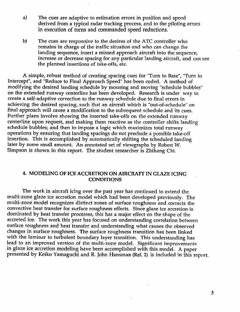
4. MODELING OF ICE ACCRETION ON AIRCRAFT IN GLAZE ICINGCONDITIONS

The work in aircraft icing over the past year has continued to extend themulti-zone glaze ice accretion model which had been developed previously. Themulti-zone model recognizes distinct zones of surface roughness and corrects theconvective heat transfer for surface roughness effects. Since glaze ice accretion isdominated by heat transfer processes, this has a major effect on the shape of theaccreted ice. The work this year has focused on understanding correlation betweensurface roughness and heat transfer and understanding what causes the observedchanges in surface roughness. The surface roughness transition has been linkedwith the laminar to turbulent boundary layer transition. This understanding haslead to an improved version of the multi-zone model. Significant improvementsin glaze ice accretion modeling have been accomplished with this model. A paperpresented by Keiko Yamaguchi and R. John Hansman (Ref.2) is included in this report.

5

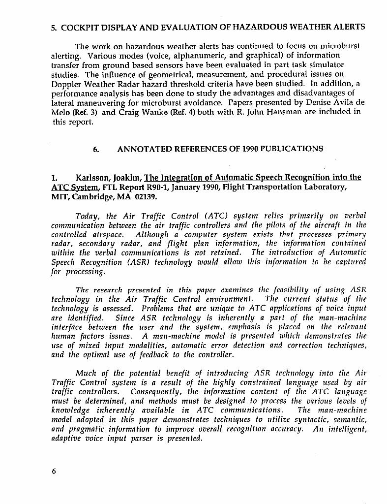
5. COCKPIT DISPLAY AND EVALUATION OF HAZARDOUS WEATHER ALERTS

The work on hazardous weather alerts has continued to focus on microburstalerting. Various modes (voice, alphanumeric, and graphical) of informationtransfer from ground based sensors have been evaluated in part task simulatorstudies. The influence of geometrical, measurement, and procedural issues onDoppler Weather Radar hazard threshold criteria have been studied. In addition, aperformance analysis has been done to study the advantages and disadvantages oflateral maneuvering for microburst avoidance. Papers presented by Denise Avila deMelo (Ref.3) and Craig Wanke (Ref. 4) both with R. John Hansman are included inthis report.

6. ANNOTATED REFERENCES OF 1990 PUBLICATIONS

1. Karlsson, Joakim, The Integration of Automatic Speech Recognition into theFTL Report R90-1, January 1990, Flight Transportation Laboratory,

MIT, Cambridge, MA 02139.

Today, the Air Traffic Control (ATC) system relies primarily on verbalcommunication between the air traffic controllers and the pilots of the aircraft in thecontrolled airspace. Although a computer system exists that processes primaryradar, secondary radar, and flight plan information, the information containedwithin the verbal communications is not retained. The introduction of AutomaticSpeech Recognition (ASR) technology would allow this information to be capturedfor processing.

The research presented in this paper examines the feasibility of using ASRtechnology in the Air Traffic Control environment. The current status of thetechnology is assessed. Problems that are unique to ATC applications of voice inputare identified. Since ASR technology is inherently a part of the man-machineinterface between the user and the system, emphasis is placed on the relevanthuman factors issues. A man-machine model is presented which demonstrates theuse of mixed input modalities, automatic error detection and correction techniques,and the optimal use of feedback to the controller.

Much of the potential benefit of introducing ASR technology into the AirTraffic Control system is a result of the highly constrained language used by airtraffic controllers. Consequently, the information content of the ATC languagemust be determined, and methods must be designed to process the various levels ofknowledge inherently available in ATC communications. The man-machinemodel adopted in this paper demonstrates techniques to utilize syntactic, semantic,and pragmatic information to improve overall recognition accuracy. An intelligent,adaptive voice input parser is presented.

6

2. Yamaguchi, K., and Hansman, R.J.,"Heat Transfer on Accreting Ice Surfaces,"AIAA-90-0200, AIAA 28th Aerospace Sciences Meeting, January 1990.

The influence and modeling of surface roughness for the numericalsimulation of glaze ice accretion is studied. Icing wind tunnel tests are discussedand correlations between experimental and predicted heat transfer coefficients arepresented.

3. Avila de Melo, D. and Hansman, R.J., "Analysis of Aircraft PerformanceDuring Lateral Maneuvering for Microburst Avoidance," AIAA-90-0568, AIAA 28thAerospace Sciences Meeting, January 1990.

An analysis is conducted of a B-737-100 using a nonlinear aircraft dynamicsimulation to evaluate the performance advantages and disadvantages of lateralmaneuvering for microburst avoidance.

4. Wanke, C., and Hansman, R.J.,"Hazard Evaluation and Operational CockpitDisplay of Ground Measured Windshear Data," AIAA-90-0566,AIAA 28thAerospace Sciences Meeting, January 1990.

Information transfer issues and hazard evaluation issues associated withground based doppler weather radar microburst alerts are studied. Part tasksimulator studies and numerical aircraft performance models are used.

AUTOMATICSPEECHRECOGNITIONIN AIR TRAFFICCONTROL:A HUMAN FACTORSPERSPECTIVE*

Joakim KarlssonResearch Assistant

Flight Transportation Laboratory, M.I.T.Cambridge, MA

ABSTRACT

The introduction of Automatic Speech Recognition (ASR) technology into the Air TrafficControl (ATC) system has the potential to improve overall system safety and efficiency. However,because ASR technology is inherently a part of the man-machine interface between the user and thesystem, the human factors issues involved must be addressed. This paper identifies some of therelevant human factors problems and presents related methods of investigation. Research at M.I.T.'sFlight Transportation Laboratory is being conducted from a human factors perspective, focusing onintelligent parser design, presentation of feedback, error correction strategy design, and optimal choiceof input modalities.

INTRODUCTION

In today's ATC system, communication between controllers and aircraft is almost exclusivelyverbal. This is especially true for such critical tasks as the issuing of clearances and vectors, to achievetraffic separation. Although a digital datalink is in development (Mode S), there is no reason tobelieve that voice communication between ATC and aircraft will disappear in the near future. As aresult, most of the information transferred within the system is never captured in machine readableform. Herein lies the promise of introducing ASR technology into the ATC system: it would permitprocessing of ATC clearances, to ensure conformance to safety and separation criteria. It would allowthe ATC computer system to predict the future state of the airspace. The controller could prestoreroutine clearances during periods of little activity. Mode S equipped aircraft could be provided with amachine readable copy of verbal clearances for confirmationpurposes.

Thus, introduction of ASR technology could result in the reduction of human errors, resulting inincreased system safety. However, the dilemma of ASR is that its purported advantages are notautomatically realized by simply making the technology available. Careful human factors design isnecessary to capitalize on its potential [Berman, 1984]. This is especially true in the case of ATC,whichis plagued by human factors problems such as intense levels of workload during traffic peaks intermixedwith controller boredom during low demand periods. Furthermore, the high probability of loss of livesin the case of errors makes it imperative that the human factors problems created by introducing ASRinto the Air Traffic Control system are properly addressed and solved.

The speech recognition devices available today are not sufficiently capable to be usedoperationally within the ATC environment. However, there are units available that are useful for therequired preliminary human factors research. In order to minimize human factors problems, it isnecessary to implement an iterative design cycle that should be continued until the needs of the systemusers are met [Cooper, 1987]. The research presented within this paper should be considered as one stepin that cycle.

*Paper presentedat Militaryand GovernmentSpeechTechnology1989,Nov. 13-15, 1989, Arlington,VA.

9

MODELING HUMAN FACTORS

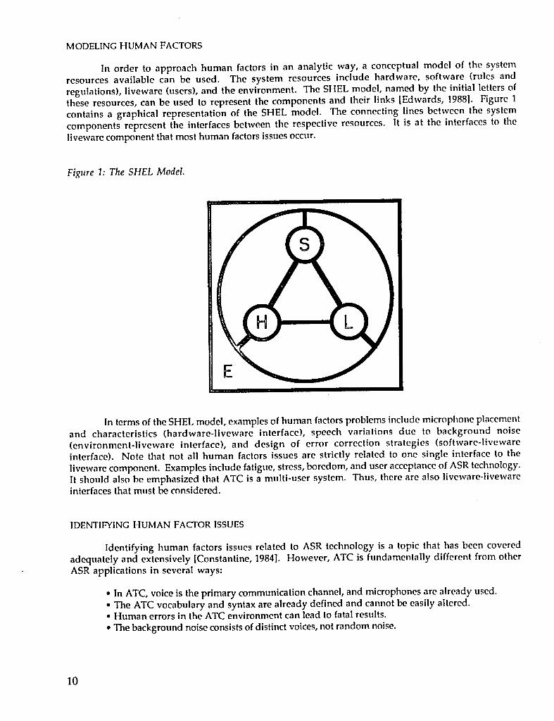
In order to approach human factors in an analytic way, a conceptual model of the systemresources available can be used. The system resources include hardware, software (rules andregulations), liveware (users), and the environment. The SHEL model, named by the initial letters ofthese resources, can be used to represent the components and their links [Edwards, 1988]. Figure 1contains a graphical representation of the SHEL model. The connecting lines between the systemcomponents represent the interfaces between the respective resources. It is at the interfaces to theliveware component thatmost human factorsissues occur.

Figure 1: The SHEL Model.

In terms of the SHELmodel, examples of human factors problems include microphone placementand characteristics (hardware-liveware interface), speech variations due to background noise(environment-liveware interface), and design of error correction strategies (software-livewareinterface). Note that not all human factors issues are strictly related to one single interface to theliveware component. Examples include fatigue, stress, boredom, and user acceptanceof ASRtechnology.It should also be emphasized that ATC is a multi-user system. Thus, there are also liveware-livewareinterfaces that must be considered.

IDENTIFYINGHUMAN FACTORISSUES

Identifying human factors issues related to ASR technology is a topic that has been coveredadequately and extensively [Constantine, 1984]. However, ATC is fundamentally different from otherASR applications in several ways:

• In ATC,voice is the primary communicationchannel, and microphones are already used.• The ATC vocabulary and syntax are already defined and cannotbe easily altered.• Human errors in the ATCenvironment can lead to fatal results.• The background noise consists of distinctvoices, not random noise.

10

Hence, we can consider three categories of human factors issues: common issues that are mutual to bothATC and other ASR applications, unique issues that are typically not encountered in otherapplications, and non-issues -problems that may be significant in other applications, but that do notplay a major role in ATC.

The last group, non-issues, is of course the most trivial to consider: a good example is thehardware-liveware issue of microphone characteristics and placement. Headset mounted noise-cancelling microphones are already in use in the current ATCenvironment, and hence it is an issue thathas been addressed extensively before ASR technology has come under consideration. Also, thesoftware-liveware problem of vocabulary and syntax definition, normally an important human factorsissue, has also been completed: these definitions are controlled by the Federal AviationAdministration (FAA). Another common problem, communication with other people while inrecognition mode, is not likely to occur in ATC, as controllers are already using Push-To-Talk (PTT)switches on their headsets.

Issues thatare common to both ATCand other ASRapplications are abundant, and must not beneglected, although they have already been addressed extensively. These include:

• Speech variations due to stress, fatigue,or backgroundnoise.• Spuriousrecognitiondue to backgroundnoise.• Inter-speaker variations (the "sheep and goats" issue).• User acceptance of the technology.• User motivation.• Presentation of feedback to the user.• Error recognition, presentation, and correction.• User training.• Selection of proper hardware.• Optimal use of mixed input modalities.• Recognition accuracy and use of higher levels of knowledge.• Failure to adhere to the syntax.

Although several of these problems remain unsolved, most have been addressed previously. Theresearch being conducted at the Flight Transportation Laboratory covers some of these issues, sincemuch of the previous work has not been applied specifically to ATC.

The final group, unique issues, includes problems that are either specific to ATC, or that aremore significant in the ATC environment than elsewhere. A typicalexample is stress induced reductionof recognition accuracy, mentioned above as an issue common to other ASRapplications. This is a muchmore critical issue in Air Traffic Control, since the cases where the introduction of ASRhas the greatestpotential of improving safety, are likely to be stressful situations. The possibility of automatingconformance monitoring would greatly benefit the controller during scenarios where a large number ofaircraft are being controlled - a stressful period for the controller. It is exactly in the conditions whereASR technology is needed most, thatit performs worst. To the human factors researcher this points outthe importance of high baseline recognition accuracy, high levels of robustness in the presence of speechvariations, introduction of functional automatic error correction techniques, and the design andimplementation of parsers that make use of higher levels of knowledge such as prosodic, syntactic,semantic, and pragmatic information.

11

Another major issue facing the introduction of ASRtechnology into the ATC environment is thatof cognitive workload. The controllers are already presented with a wealth of information, and if anynew technology is to be introduced it must reduce workload, not increase it. There exists a need to ensurethat the information captured through the use of speech input technology is the same as theinformation transmitted to the aircraft. Hence, the controller must monitor what is understood by themachine, in order to be able to correct it. However, this would introduce another task for the controller,and possibly distract from the visual attention that the radar display demands. This dilemmaunderscores the importance of designing adequatefeedback and error correction strategies.

RESEARCH AT THE M.I.T. FLIGHT TRANSPORTATION LABORATORY

It is within the framework presented above that the ASR research effort at M.I.T.'s FlightTransportation Laboratory has been conducted. Only a brief description of this research can bepresented in this paper -more detailed descriptions are available elsewhere [Karlsson, 1990].Preliminary results include a study to choose the ASR hardware most suited for ATC human factorsresearch, purchase and evaluation of the Votan VPC 2000 and Verbex Series 5000 voice 1/O systems,and design and implementation of a low-cost portable research station using the Verbex Series 5000anda PC based ATC simulator. An extensive annotated bibliography of related papers has also beencompiled.

Future work will concentrate on means to improve recognition accuracy while maintaining a lowworkload level. Techniques will include the use of semantic and pragmatic information, adaptive (on-the-fly) training, introduction of confusability matrices and other automatic error correction techniques[Loken-Kim, 1985], mouse and menu input for error correction, and need-to-know type feedback thatensures that the use of ASR technology remains mostly transparent to the controller. Furthermore, areceiver station has been established to monitor ATCcommunication in the greater Boston area, to studyreal life use of the ATClanguage and provide data for issues such as syntax deviation.

CONCLUSIONS

The importance of the human factors aspects of introducing ASR technology into the ATCenvironment cannot be underestimated. In particular, it must be realized that ATC applications areuniquely different from other applications where voice input may be of benefit. As a result, muchgreater emphasis must be placed on issues such as mental workload, user feedback, mixed use of inputmodalities, intelligent parser design, and improved robustness with respect to speech variations. TheASR research being conducted at the M.I.T.Flight Transportation Laboratory has resulted in a set oftools that can be used to identify, quantify, and provide preliminary solutions to the human factorsissues described within this paper. The results can then be used as a step in an iterative design cycle toobtain a system acceptable to the user.

12

REFERENCES

Berman, J. V. F., "Speech Technology in a High Workload Environment", Proceedings of the 1stInternational Conferenceon Speech Technology, IFS Publications Ltd, Bedford, U.K. (1984), pp. 69-76.

Constantine, Betsy J., "Human Factors Considerations in the Design of Voice Input/OutputApplications", The Official Proceedingsof Speech Tech "84, Media Dimensions, Inc., New York, N.Y.(1984),pp. 219-224.

Cooper, Martin, "Human Factors Aspects of Voice Input/Output", Speech Technology, Vol. 3, No. 4(March/April 1987), pp. 82-86.

Edwards, Elwyn, "Introductory Overview", Human Factorsin Aviation, eds Wiener, Earl L. and Nagel,David C., Academic Press, Inc.,San Diego, CA (1988),pp. 3-25.

Karlsson, Joakim, "Automatic Speech Recognition in Air Traffic Control", Joint University ProgramforAir TransportationResearch- 1988,1989NASA Conference Publication 3063, NASA Langley ResearchCenter, Hampton, VA (1990),pp. 3-15.

Karlsson, Joakim, The Introduction of Automatic Speech Recognition Technology into the Air TrafficControl System, FTLReport 90-1,Flight Transportation Laboratory, M.I.T.,Cambridge, MA (Jan. 1990).

Loken-Kim,K.H., "An Investigation of Automatic Error Detection and Correction in Speech RecognitionSystems", The Official Proceedingsof Speech Tech '85, Media Dimensions, Inc., New York, N.Y. (1985),pp. 72-74.

13

The Temporal Logic of the Tower Chief SystemLyman R. Hazelton, Jr.*

Flight Transportation LaboratoryDepartment of Aeronautics and Astronautics

Massachusetts Institute of TechnologyCambridge, MA

1 Introduction

Human reasoners engage in diverse and powerful forms of cognition. Perhaps themost common mechanism used by humans is induction, which is the usual process oflearning. The most celebrated and well understood process of thought is deduction, themethod employed in mathematical proof. Humans can also make plans, reason aboutevents and causality in an environment which frequently changes and often providesincomplete information. Humans need not be certain about their facts, and can makeassumptions when required information is unavailable.

Classical logic deals almost exclusively with deduction. In chapter 4 of Aristotle'sMetaphysics [1], there is a section regarding the application of logic to predicting thefuture. In that treatise, Aristotle describes what has now become known as the axiomof Excluded Middle. In essence, he states that in his logic a proposition can be eitherTRUE or FALSE, exclusively. No other values for the veracity of a proposition arepossible. There is no middle ground. Because the future is indeterminate, one cannotassign absolute knowledge of a forthcoming event. This is a broad statement which hasfar reaching implications. As pointed out by Bertrand Russell in the early nineteenhundreds, it is not a trifling thing to easily toss aside.

On the other hand, perhaps the interpretation of the axiom of excluded middle hasbeen too broad. Aristotle was seeking truth in a very absolute way. He was quite awareof the works of Zeno and Pythagoras, and to a certain extent his logic was developedfrom his knowledge of their process of mathematical proof. Propositions in mathematicsare universal in their temporal extent. One never hears a geometer state that two linesare parallel from two until four this afternoon. The lines are simply parallel or they arenot. The geometer's proof makes no reference to time, and, in like manner, neither doesAristotle's logic.

One should not lose track of the fact that logic is primarily a model for analysis ofhuman thought. Its utility as a paradigm for symbolic reasoning and computer pro-gramming is secondary to its value as a model of the cognitive process. The restrictionto exclude time simplifies the model and makes it nmch more comprehensible. Therestriction also limits the range of problems to which the model may be successfullyapplied.

Clearly, human reasoners often contemplate the future and create rational plans aboutit. During the last century, logicians have begun to extend classical logic in order to

*Research supported by NASA contract number NGL 22-009-640.

15

better model this kind of cognition. Modal logics have been invented to describe systemsin which propositions may or might be true or false. Defeasible logics and model theoryare used for systems which involve change. And temporal logics have been devised toreason about time. The purpose of this paper is to describe the logic used in the reasoningscheme employed in the Tower Chief system.

2 Classical Logic

Let us begin with a short review of the fundamental ideas of logic. The elementaryoperands of logic are propositions. A proposition is a declarative statement such as,"Socrates was a man", or "There is ice on runway 33." Logic consists of:

1. A set of abstract operations for combining propositions in ways that preserve theveracity of the resulting compound proposition;

2. A mechanism for generating new propositions from (i) knowledge already knownand (ii) general statements called yules. This process is called deduction.

Symbolically, a proposition which is believed to be true may be represented as p.The belief that the same proposition is not true (false) is represented as _ p. Theopposite of a proposition being false is that the proposition is true, or -._(,-, p) = p. Asituation in which p and -._p are claimed to be true is a contradiction. In classical logic,contradictions indicate an error in the logical system in which they occur. 1

Propositions may be combined via conjunction (logical AND) or disjunction (logicalOR). The symbolic representation of the conjunction of two propositions is:

pAq (1)

and that of the disjunction 2 is:

p V q (2)

The laws of commutation and distribution for logical combination operators are re-spectively:

(pAq) = (qAp) (3)

(pVq) = (qVp) (4)

and

-, (p A (q A v)) =-- (p A q) A (p A v) (5)

(p A (q V r)) = (p A q) V (p A r) (fi)

(p V (q V r)) -- (p V q) V (p V r) (7)

(p V (q A v)) -- (p V q) A (p V r) (8)

1Generally caused by an erroneous rule. Read on.2The use of the symbol v for disjunction is from the Latin word vel, meaning "inclusive OR". Unlike

English, Latin possesses a separate word for "exclusive OR", aut.

16

Any combination of two propositions may be treated as a single proposition.

Negation applied to combinations leads to the following relationships, known as De-Morgan's Theorems

_(pAq) = (,_pV ,',_q) (9)

,_(pVq) _ (,-,_p^,--,q) (10)

2.1 Rules

Deductive inference is accomplished through the use of rules.

"A Rule is a hypothetical proposition composed of an antecedent and conse-

quent by means of a conditional connective or one expressing reason whichsignifies that if they, viz. the antecedent and consequent are formed simul-taneously, it is impossible that the antecedent be true and the consequentfalse. ''3

Translated into more modern terms, a rule is a conditional statement, consisting of anantecedent (the set of conditions to be met) and a consequent (the set of inferrences tobe implied if the conditions required in the antecedent are satisfied).

While the laws of logic, such as the commutative law above, and the theorems deriv-able from them, such as DeMorgan's Theorems, are domain independent, rules are basedon semantic information. Thus,

"If it is raining, then the runways are wet." (11)

is a rule. Such a rule is written formally as

p Dq (12)

where p represents the antecedent ("it is raining") and q represents the consequent ("therunways are wet"). The hypothetical nature of the statement is embodied in the symbolD.

Generally, rules have more than one antecedent, and may have more than one conse-

quent. Rules may combine antecedents purely by conjunction, purely by disjunction, orin combination. As an alternative, a disjunctive rule can be split into several simple orconjunctive rules. While this is less efficient from a notational point of view, it avoidsdisjunction altogether. This is valuable when creating a computer program to do logic,because the program need only perform conjunction.

There are six forms in which deductive rules of inference may appear. For the pur-poses of this discussion, the description of two will suffice.

3This definition is from a translation of the fourteenth century logician Pseudo-Scotus (John ofCornubia) whichappears in [1].

17

Modus Ponens This form, properly known as modus ponendo ponens, or the methodof affirmation leading to affirmation 4, comes to the conclusion of the consequent ifthe hypothetical antecedent is declared. For the rule above, the information thatit is raining leads to the inference that the runways are, indeed, wet. Formally

p D q

P

... q (13)

Modus Tolens The correct name is modus tollendo tollens, or the method of denial

leading to denial, s In this form, the negation of the antecedent is concluded if thehypothetical consequent is declared not to be true. The formal definition is

p D q

_q

:. _p (14)

A rule may be thought of as a generalization that can be applied to a domain ofspecific situations. In effect, rules are the analogs of algebraic equations in logic. Thisgeneralization is accomplished, as in algebra, through the use of variables.

Note that the rule stated in (11) is not really correct. Obviously, if the rain is fallingin Boise, there is little effect on the runways at LaGuardia. The rule as stated is notprecise enough. A more precise statement of the intended meaning of rule (11) is

"If it is raining at some airport, then the runways at that airport are wet." (15)

If the airport is represented by the variable az, that it is raining at x by Ra:, and thatthe runways are wet at x by Wx, then the formal statement of rule (15) correspondingto (12) is

Rx D Wx (16)

Further information on topics such as quantification can be found in [2].

3 Defeasible Logics and Truth Maintenance

In a classic paper in 1979, Jon Doyle [3] made a first attempt to create a computer

program employing an extended classical logic for use with dynamic domains. Doyle'sTruth Maintenance is based on the idea that reasoned inferences are supported by evi-

dence. The evidence supporting an inference is composed of the propositions that were

4From the Latin ponere, "to affirm".5From the Latin tollere, "to deny".

18

used as the antecedents of the rule that resulted in the inference. If one or more ofthe evidenciary propositions changes, then the inferred consequent must be examined toverify that it is still true. If an inference is no longer supported by any evidence, thenthe inference must be denied.

More formally, Doyle restricted the application domain to those systems in which allthe propositions which satisfy modus ponens also satisfy

p D q

_p

:. ~q (17)

Propositions which meet this criterion are said to be logically equivalent. An example oflogical equivalence is the state of a switch and the state of the voltage on a line controlledby the switch. When the switch is on, the voltage on the line is on, and while the switchis off, the voltage is off. While there are many examples of natural phenomena whichexhibit this kind of behavior, there are many more which do not.

In Doyle's version of truth maintenance, evidence is kept in a "support list". Inessence, a support list associated with an inference contains those propositions and areference to the rule that were used to conclude it. Consider two rules which conclude

the same propositionR1 :pAqDc (18)

andR_ :aAbD c (19)

These two rules are equivalent to a disjunction which embodies both rules

R3: (p A q) V (a A b) D c (20)

If c is declared true, then its support list will contain one or the other (or both) ofthe conjunctions in the antecedent. If, at some future time, one of the propositions inthe support list changes to false, the conjunction it appears within is removed from thesupport list. If the support list is empty, then by (17) c must be denied.

This scheme works well for the restricted set of domains which satisfy (17). Unfor-

tunately, most processes occurring in nature do not fall into this set, and truth main-tenance cannot be used successfully to reason about their dynamics, s Further, there is

no explicit mention of time in the truth maintenance mechanism, so the length of timethat a proposition might be true cannot be easily specified.

6In classical logic, the form described in (17) is considered to be an error, and is known as "denying

the premise".

19

4 Default Logic

Classical logic treats knowledge in a very restricted way. There is a tacit assumptionthat the reasoner knows all that is necessary in order to proceed. While this may be truein mathematical proof, it is certainly not true in general. Human reasoners are oftenfaced with lack of knowledge.

There is an ambiguity in the standard meaning of _ p. This can be easily demon-strated. Suppose that p represents the statement, "It is raining". One interpretation of--_p is the statement, "It is not raining". Another interpretation is, "No information isavailable as to whether it is raining or not". In either case, it cannot be said that p isTRUE. For the purpose of mathematical proof, either meaning will suffice.

The domain of human reason is not as restricted as that of mathematical logic. Thedifference between knowing something is FALSE or TRUE and not knowing may becrucial. It is very important that the explicit meaning of _ p be well defined andunderstood.

Actually, there is implicit to the statement that someproposition is true the furtherstatement that it is known to be true. When it is stated that, "It is raining", the actualmeaning is that, "It is guaranteed that it is raining". Similarly, when some propositionis reported false, the meaning is that it is certainly NOT true.

Let us look more closely at the meaning of negation. There are statements such as,"Day is not night", in which the negation is a property of the domain. That is, in thecase that the meaning of negation is the opposite state of the proposition, the veracityof the logical connection is semantically derived.

Alternatively,denialofpossessionofknowledgeconcerningthe truth of a propositionhas nothing to do with the domainof discourse. It is a purely logicalmatter, having onlyto do with form. Having or not having knowledge about a proposition has nothing to dowith the semantic content of the proposition.

The importance of this distinction may be exhibited by reference to a rule used in theModus Tolens progression(equation 14). If _ q means that q is known to be false, thenthe result of the progression is that p is known false as well. If, instead, _ q indicatesthat no knowledge is available about whether q is true (or false), then the result is that pis unknown, too. While the results look formally the same, the meaning is very different.In the case that the state of a proposition is known, we may not logically make anyassumption concerning it. But when we have no direct knowledge about a proposition,it is often useful (or indeed, necessary) to make assumptions. For example, suppose thatit is known that the temperature outdoors is 40°F, the dew point is just one degree less,and the humidity high. While it cannot be stated with certainty that there is fog, thereis evidence to support the assumption that there is fog. Of course, if, in addition to theabove, there is specific information that no fog is observable, an assumption about fog

20

should not be made.

This ability to make assumptions is the utility of supporting an ':excluded middle".As a prerequisite, the two ambiguous meanings of not must be formally distinguished.For the remainder of this discussion, ",--" will be used to denote that the opposite of theproposition following it is true, while "_" will signify the lack of verifiable or trustworthyknowledge of the proposition which follows it.

A few rules concerning assumptions are necessary:

• Observation must always take precedence over assumption. This means that ifan assumption has been inferred about sonle proposition, and contradictive infor-mation is subsequently observed concerning the same proposition, the assumptionmust be replaced by the observation.

• All propositions which are concluded from rules in which one or more of the an-tecedent propositions are assumptions, are themselves assumptions.

A new class of rules called assumptive rules may be defined. They are separatedfrom normal rules because all their antecedents contain one (and only one) propositionclaiming lack of knowledge about something, and they conclude an assumption. In thecase of the "fog" example, let Fz indicate the proposition that there is fog at airport z.Let Qz indicate that the dew point is within two degrees of the outside air temperatureat airport z. The assumptive (or default) rule may be written

Fx)^ Qx (21)

to mean, "If it is not known that there is fog at an airport, but it is known that the dewpoint is close to the air temperature at that airport, it can be assumed that there is fogat that airport". The superscript asterisk appended to the conclusion is a reminder thatthis proposition is an assumption.

This particular choice of mechanism for making assumptions is a special case ofReiter's "Default Logic"[4].

The existence of assumptions extends the meaning of contradiction. To appreciatethis, it is necessary to understand the different classes of information which can be presentin a defeasible logic with default rules:

Observations are propositions that are obtained from outside of the logical system.

Inferred Facts are the consequent propositions resulting from rules in which all an-tecedent propositions are either observations or inferred facts.

Fundamental Assumptions are the consequent propositions arising from default rules.

Inferred Assumptions are consequent propositions which derive from rules in whichone or more antecedent propositions are assumptions (of either variety).

21

The meaning of contradiction depends on the classes of the propositions involved inthe inconsistency:

• Observation and observation: One of the observations must be in error. Given

enough domain information (in the form of rules), it may be possible to ascertainwhich proposition to believe, but this is generally dimcult even for humans.

• Observation and Inferred Fact: This situation almost always indicates an erro-neous rule. Some rule in the deductive chain leading to the inferred fact must beresponsible; with luck, there might only be one.

• Two Inferred Facts: A contradiction of this kind is also indicative of an error in a

rule, but the reasoner will require outside assistance to determine the culprit, sincethere is no way to tell which rule is mistaken.

• Observation ov Inferred Fact and Fundamental Assumption: The default rule thatasserted the fundamental assumption is incorrect.

• Observation ov Inferred Fact and Inferred Assumption: This is an interesting case.If only one of the propositions in the antecedent of the rule which inferred the

assumption is an assumption, then the inferred assumption must be denied, andthe assumption which appeared in the antecedent must be denied, and so on backto the fundamental assumption which started that chain of reasoning. This processis called "dependency directed backtracking". If it should happen that there weremore than one assumption in the antecedent of any of the rules in the chain thatled to the discrepancy, then a choice must be made: Which assumption shouldbe retracted? There are various approaches that might be taken to answer thisquestion:

- One could retract the chronologically latest assumption and search for an alter-native.

- One could withdraw the chronologically earliest and search for an alternative.

- Alternative assumptions could be found for each of the candidates, trying eachone until a choice is found which does not cause the contradiction. This maybe very time consuming, or, in fact, undecidable.

• Two Fundamental Assumptions: One of the default rules is incorrect.

In essence, all of these possibilities reduce to two major situations.

1. Contradictions among facts, which indicate errors of some kind.

2. Contradictions among assumptions, which require the replacement of one of the

propositions with another assumption. The difficulty lies in deciding which as-sumption to replace, and with what.

22

The essence of the solution to the problem of replacing an assumption involved in acontradiction is the employment of a class of domain dependent preference rules. Theserules have a general form of "If there is a contradiction involving two assumptions re-garding X, then Y is the preferred assumption to retain (or to retract)."

The idea of preference rules may also be used to decide which of two (or more)conflicting observations to keep. If each observation is tagged with a description ofits origin, then preference rules stating that one origin is more "believable" or more"important" may be used.

5 Temporally Dependent Propositions

Time dependence can be formally introduced into logic by defining

p(r) (22)

to represent that proposition p is true during the time interval r. The interval r is a pair

of numbers, such as Universal Times, such that the first member of the pair precedes oris equal to (i.e., is before or at the same time oj) the second. Formally,

r = (tx,t2), tl -< t: (23)

Having introduced this notion of the interval of veracity or the activity interval of aproposition, its effect upon all of the axioms of logic introduced in the previous sectionmust be explored. It will suffice to examine only Conjunction, Disjunction, and theactivity interval of the consequent of a rule.

The activity interval of a conjunct will be defined as the intersection of the activityintervals of the operands:

p (rl) Aq (r2) = p Aq (rl f3r2) (24)

That this is a reasonable definition can be seen in the following example: If I am in roomA during the time interval from two until four this afternoon (p (rl)), and you are inroom A during the interval from three until five this afternoon (q (r2)), then we are inroom A from three until four this afternoon (p A q (r_ Nr2)).

Nora Bene: This definition of conjunction effectively states that two propositionscan interact if and only if they have overlapping time intervals. This may seem overlyrestrictive at first glance, especially considering the human penchant for describing manyinteracting events as following one another and being causally linked. However, closerexamination reveals that the restriction is completely correct. Temporally disjoint eventswhich seem to interact are invariably connected by some persistent process, produced as

23

an effect of the first event, which remains in effect at least until its time interval overlapsthat of the second event.

The preceding motivates the definition of the activity interval of a disjunctive pairas the union of the activity intervals of the operands:

p (rl) V q (r2) = p V q (7"1 [..J 7"2) (25)

Again, using the room occupancy example: If I am in room A during the time intervalfrom two until four this afternoon (p (rl)), and you are in room A during the intervalfrom three until five this afternoon (q (r2)), then one or the other of us is in room Afrom two until five this afternoon (p V q (7-1U7-2)).

5.1 Evanescence and Persistence

The rules for generating the activity interval of a logical combination of temporallyconstrained propositions allow the computation of the activity interval of the antecedentof a rule. However, the activity interval of the consequent of a rule is not necessarily thesame as that of its antecedent. Processes and physical things whose activity intervals areshorter than the activity intervals of their antecedents are called evanescent. An exampleof an evanescent process is the firing of a gun. When the hammer drops the gun fires.The fact that the hammer remains down does not make the "bang" last longer. Otherthings and processes are persistent, lasting well after the events which created them have

ceased to exist. For example, if the temperature is below freezing on the ground, andit is raining, ice will form on the ground. When the rain stops, the ice does not simplydisappear.

The root of this problem is the domain dependence of the activity interval of aphysical process. While it is true that no process can exist without some fornl of causalprecedent, once formed a process may have an independent existence of its own. In thecase of persistence, quite often the only way to "undo" something which has been "done"is to do something specifically designed to destroy it.

For practical purposes, there are only two classes of consequent

• Inferred propositions with activity intervals which are the same as the computedactivity intervals of their antecedents. In this case, no further information is re-quired in the consequent.

• Inferred propositions with independent activity intervals. Causality requires thatthe beginning of the consequent activity interval be the same as the start of thecomputed antecedent interval, but the domain dependent information to computethe end of the consequent activity interval must be supplied in the rule.

This topic will be discussed in greater detail in a forthcoming paper, "Implementationof the Tower Chief Planning System".

24

5.2 Resource Allocation and Planning

Classical temporal logic is insufficient to describe the do~nain and events which occur in the ATC environment characterized previously. In particular, the infor~nation available about the future state of some value may change during the execution of a plan. For example, there may be a weather prediction at 09:OO that claims that passage of a front with an associated shift in wind direction will occur between noon and one o'clock. A later prognostication, perhaps at 11:00, might change the time of the frontal passage or some parameter associated with it. Such a change may require a ~nodification of a planned configuration shift which may already be in progress. Because of the infeasibility of certain transitions, the modification of one configuration choice may affect those which precede and follow it, and so on.

Preparation for the use of a specific configuration may demand the allocation of resources in advance. In winter, for example, one or more of the runways that are to be used in a future configuration may require snow or ice removal or treatment to prevent ice accumulation prior to being put into service.

In standard expositions on temporal logic, the processes that the system is designed to model usually involve the evolution of some physical quantity such as the position of a ball or the temperature of an object. The rules for this kind of modelling generally look like

~ ( t l , t2) A q(t3, t4) 3 r(t5, t6) (26)

where p(tl , t2) A q(t3, t4) -- p A q [(tl, t2) n (t3, t4)]. If T is a new state that was described previously by p, then t2 3 t5.7 For example, "If some water is in the liquid state (P) during (tl , t2), and is brought in contact with a thermally massive object with a tempefature greater than the boiling point of water (q) during (t3, t4), then the water will be in the vapor phase (r) during (t5, t6)."

A plan, on the other hand, is by definition something that is intended for future execution. Plans are based on what the planner believes is going to happen. Because the future is not fixed, a plan may have to be modified or even abandoned before or during its execution. Actions which are taken for the most part cannot be withdrawn when a plan is deserted. That such actions were based on beliefs which turned out to be false does not change the fact that they were executed. If the planner is to be able to explain the reasons behind its actions, it must recall its prior beliefs even if they were later proven to be wrong. In fact, the planner may change what it believes about the future as a result of its intention to carry out some plan.

Consider the reasoning involved in the allocation of some resource. Let Wr( t l , tz ) indicate that use of resource r is desired during the time interval (tl , tz). Similarly, let Ar( t l , t2) indicate that resource r is available during the time interval, and finally let

71n other words, a thing cannot be in two disjoint states at the same time.

7"[r(tl, t2) represent that the resource has been allocated for the period. Then we mightwrite

}'Yr(tl,t2) ^ Ar(tl,t2) D Hr(tl,t2) ^ ,'_ Ar(tl,tz) (27)

to describe the rule for allocation: "If resource r is required during (tl,t2), and theresource is available during the period, then r is allocated for the interval, and is nolonger available for allocation during that time." There is an apparent paradox in thisformulation, since vZ[r(tl, t2) and ,-_ fl.r(tl, t2) appear at the same time. The reason thatthis problem appears is that the reasoner's belief about the availability of the resourcefor other use during the specified interval changed as a consequence of the reasoningprocess itself.

The last example demonstrates that reasoning about the future may involve non-monotonic logic. However, propositions previously thought to be true cannot necessarilybe simply retracted. They may be in the support lists of later propositions which involveactions or the reasoning process itself. A human reasoner in the resource allocationexample would explain, "Of course, I believed the resource was available before I allocatedits use. Now that I have committed the use of it during the time period, it is no longeravailable for other use." The reasoner is aware of the temporal order of the events of thereasoning process in addition to the projected time of execution of the plan.

There are three time periods associated with the resource allocation problem. First,the time in the future during which the use of the resource is desired. For the sake of

easy reference, let us give that a name: the activity interval. Second, the time duringwhich the planner believes that the resource will be available during the activity period.Third, the time during which the planner believes that the resource has been allocatedfor the activity period and will no longer be available for other use during that interval.Again, for reference, let's call these two periods "belief intervals". If we put the beliefintervals into the logical statement of the resource allocation rule as subscripts to thepropositions, we obtain

}/Yr(_l,_2)(tl,t2) /_ .Ar(_3,_4)(tl,t_.) D 7-[r(_5,_8)(tl,t2) /_ _ Ar(_5,_6)(tl,t2 ) (28)

and the paradox is resolved. The planner can now refer to what it believed prior tomaking its decision as well as its opinion after the act of making the decision.

Since a runway manager's duties include allocation of people and equipment to avariety of tasks, and a manager must take actions based on the current knowledgeabout the domain, the kind of reasoning described above is central to accomplishing thecognitive task of planning runway configurations.

6 Conclusions

The important attributes of this problem are not unique to runway configuration man-agement. Temporal reasoning, default reasoning, and reasoning about the commitment

26

of resources are ubiquitous characteristics of ahnost all process management. Analysis ofthese kinds of cognition led us to a single representation and reasoning paradigm whichintegrates all three.

There is still much to be done. Currently, all input activity intervals must be clocktimes. It would be much more convenient to be able to enter times in qualitative terms byreference to information already known. Clock times often give a false sense of precisionto information whose actual accuracy is fuzzy at best. It is well known that the processof maintaining a temporal database of the kind described here is .A/T-hard. s What savesus is that the rate of change in the systems we have looked at is slow, and the airporteffectively hardware resets every night. If this technology is to be employed in a broaderspectrum of application, such as planning and scheduling of a planetary explorationrobot, this efficiency problem will have to be solved.

7 Acknowledgements

I would like to thank the staff and administration of the Boston TRACON for their

invaluable cooperation and assistance. Thanks also to the staff of the Flight Trans-portation Laboratory, especially Dennis F. X. Mathaisel and John D. Pararas, for manybeneficial discussions.

sA/'7_-hard refers to the computational complexity of the problem. AfT9 means "A/on-deterministic_olynomial, indicating that the computation time for the brute force approach to the computation risesexponentially with the size of the problem. See [10].

27

References

[1] I. M. Bochefiski. A History of Formal Logic. Chelsea Publishing Co., New York,1970.

[2] Irving M. Copi. Introduction to Logic. MacMillan, New York, 1972.

[3] Jon Doyle. A Truth Maintenance System. Artificial Intelligence, 12:231-272, 1979.

[4] Raymond Reiter. A logic for default reasoning. Artificial Intelligence, 13:81-132,1980.

[5] James F. Allen. Maintaining knowledge about temporal intervals. Communicationsof the AGM, 26(11):832-843, November 1983.

[6] James F. Allen and J. A. Kooman. Planning using a temporal world model. InProceedings of the International doint Conference on Artificial Intelligence, pages741-747, 1983.

[7] T. Dean and K. Kanazawa. Probabilistic causal reasoning. In Proceedings of theFourth Workshop on Uncertainty in Artificial Intelligence, pages 73-80, 1988.

[8] Drew McDermott. A temporal logic for reasoning about processes and plans. Cogni-tive Science, 6:101-155, 1982.

[9] Yoav Shohain. Reasoning about Change: Time and Causation from the Standpointof Artificial Intelligence. MIT Press, 1988.

[10] G. Edward Barton, Robert C. Berwick, and Eric Sven Ristad. Computational Com-plexity and Natural Language. MIT Press, Cambridge, Massachusetts, 1988.

28

BUBBLES- An Automated Decision Support Systemfor Final Approach Controllers

Zhizang ChiMassachusetts Institute of Technology

Cambridge, MA

Assumptions-

1. An explicit Schedule exists for landings (and takeoffs) at each runway.2. Each aircraft has declared an IAS for final approach and will be

obligated to fly it as accurately as possible.3. There is a continuous estimate of average windspeed on approach.

Objective-

The Cues have the following characteristics:

1. The cues are adaptive to estimation errors in position and speedby the radar tracking process, and piloting errors in execution ofturns and commanded speed reductions.

2. The cues are responsive to the desires of the human controller;

e.g., change landing sequence, insert a missed approach anywhere,insert planned take-offs between landings, increase/decreasesparing for any particular aircraft

29

The" merging area"

for aircraft arriving from different directions is on the runwaycenterline at 9-20 nm. from the runway. The schedule of landingsand takeoffs is represented by a set of landing "bubbles" and takeoff

"triangles" which move towards the runway at different approachspeeds. Landing aircraft will intercept their bubble at different

points on the extended runway centerline within the merging area.

q )

AIRCRAFT A .... Planned Takeoffs(as desired)

Runway Outer Marker

AIRCRAFTB(Slow) "7 _)

BUBBLES "-

AIRCRAFT,C (Fast)r,t

AIRCRAFTD

Figure 1- Region of Final Traffic Merging and Spacing

3O

There are three planned spacing commands currently:

C1 - Turn to Base Leg

C2 - Turn to Intercept Leg

C3 - Reduce to Final Approach IAS

Cues are given for certain "spacing" commands for arrivals from differentdirections. At present, there are three such commands. A blinking cuegives a countdown to issue the command and anticipates the reaction timeto execute.

6 nm

Figure 2 - Cueing of Spacing Commands

31

The correct Command is called whenever the aircraft reaches the

0_-wand. The angle o_ is constant given the final IAS for each aircraft. Theaircraft can wander in speed and direction, but the correct cue is madewhenever it reaches the wand. Wands will not be displayed to controllers.

Schedule Bubble for Aircraft A

Runway Centerline

Various turns which accommodate errors

o_- Wand forAircraft A

Aircraft A

Various Paths for Aircraft A

(Example of unexpected slow speed)

Figure 3 - ErrorAccommodation of the o_-Wand

32

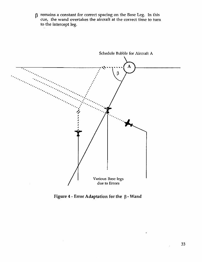
remains a constant for correct spacing on the Base Leg. In thiscue, the wand overtakes the aircraft at the correct time to turnto the intercept leg.

Various Base legsdue to Errors

Figure 4 - Error Adaptation for the [3- Wand

33

Speed Reduction called when aircraft catches up to the _' -wandon the intercept leg close to the runway centerline. Aircraft are keptabove their declared final approach speed by 10-20 knots during earliermaneuvering. Wind speed on approach must be continuously updated.

Early aircraft has alreadybeen reduced to final IAS

Figure 5 - Error Adaptation for the _, -Wand

34

Any Bubble can be selected and moved graphically to a new positionby the Controller. The Spacing Cues will automatically adjust.

The Bubble will blink or change color if the move is not feasible.

A complete slide of all subsequent aircraft can also be done. The plannedinsertion of waiting takeoff aircraft can be displayed during moves oflanding aircraft. The planned landing schedule can be set to automatically

insert another aircraft by a small opening of the landing spacing. Thismaximizes total operational rate of the runway.

Graphical slide of Bubble

lb._w,-

Centerline __(_)

Figure 6 - Changing the Desired Sequence or Spacing

35

Currently, we are introducing a method of automatic adaptationto any residual errors between the aircraft and the bubbleas the aircraftreaches the runway centerline.

Final Error Prediction

Figure 7 - Adaptation to Centerline Errors

Final Error causes an automatic shift of bubble to actual aircraft position if lateand, if necessary, automatically shifts all subsequent bubbles within the limitsof their feasible moves. This keeps the scheduled bubble positions tied to actualperformance of the aircraft over a longer period.

36

ANALYSIS OF AIRCRAFT PERFORMANCE DURING LATERALMANEUVERING FOR MICROBURST AVOIDANCE

Denise A,vilade Melo*Embraer S.A. - Brazilian Aeronautical Enterprise

Sao Jos_ dos Campos, Sao Paulo BRAZIL

and

R. John Hansman, Jr. tDepartment of Aeronautics and Astronautics

Massachusetts Institute of Technology, Cambridge, MA

Abstract Based on the assumption that information about existence andlocation of a microburst is available, studies were conducted to

Much 0f the prior research on aircraft escape procedures evaluate the relative performance loss and recovery capability forduring microburst encounters has assumed that the aircraft microburst escape procedures with and without lateralpenetrates the center of themicroburst in straight flight The maneuvering. Severe and moderate microbursts cases weremicroburst core is the region where the strongest head to tail considered. From the simulation results, recommendations werewind and downburst are present. Aircraft response to a severe made for improving microburst recovery capability.and a moderate 3-dimensional rnicroburst model using nonlinearnumerical simulations of a Boeing 737-100 was studied and the 2.Method of Annroachrelative performance loss was compared for microburst escapeprocedures with and without lateral maneuvering. The results 2. 1 Equations of Motionshowed that the hazards caused by the penetration of amicroburst in the landing phase were attenuated if lateral escape The set of nonlinearequations of motion which describe themaneuvers were applied inorder to turn the aircraft away from aircraftdynamics in the 3-dimensional space arederived inthe microburst core rather than flying straight through. If the Avila de Melo2 in the inertial velocity axes followinglateral escape maneuver was initiated close to the microburst Psiaki and Stengel's3 procedure and using the notation of Etldn4-core, high bank angles tended to deteriorate aircraftperformance. Therefore, lateral maneuvering should be 2.2 Aircraft Dataemployed if the position of the microburst is know, however,only low bank angles should be applied once the core has been The simulations used a simplified nonlinear aerodynamicpenetrated. Lateral maneuvering was also found to reduce the model of the Boeing 737-100 (NASA Langley ATOPS researchadvanced warning required to escape from microburst hazards aircraft)5. The power plant dynamics were approximated as abut required that information of the existence and location of the first order model with a time response of 2 seconds up to themicroburst is available (ie., remote detection) in order to avoid maximum thrust of 13,000 lb.an incorrect turn toward the microburst core.

1. Introduction T = (ST- T)/TR;TR = 2 sec.

In the initial condition, the aircraft was assumed to be at aLow-altitude wind shear presents a significant hazard to constant airspeed of 130 kts, on a 3°glide slope, with angle of

aircraft during landing and take-off operations. Severe attack of 1.3°and weight of 80,000 lb. Landing gear and flapsmicrobursts, storm downdrafts, which are small in horizontal are in the landing configuration. The trim positions of thecross sections and highly transient, present the greatest danger to control devices were the following:aircraft, ranging from small general aviation aircraft to jet

transports. The risks posed by all forms of wind shear can be & = 2.9° - elevator deflection;reduced if information is available to warn the pilot about the & = -5° - spoiler deflection;presence of low level wind shear and if the pilot has the best & = 0° - aileron deflection;available information on escape techniques. Most of the prior & = 0° - rudder deflection;research on aircraft flight dynamics and microburst escape T = 8,081 lb - total thrust.procedures has focused on longitudinal dynamics. This isequivalent to the aircraft penetrating the center of the microburstwhere only the effect of the horizontal head to tail wind 2.3 Microburst Modelcomponents and the vertical downburst are considered.Currently, the FAA Windshear Training Aidt recommends The microburst model used for this study is similar to the 3-microburst escape procedures which are limited to maneuvers in dimensional microburst model by Osegnera and Bowles6.the longitudinal plane. With the advent of systems which can However, for simplicity, the model was made invariant withremotely detect microburst such as Doppler weather radar, the altitude. The maximum intensity horizontal and vertical velocitypossibility of lateral maneuvering for microburst avoidance profiles were used to represent a worst case. It should be notedshould be considered, that this somewhat exaggerates the hazard since the maximum

horizontal and vertical intensity do not normally occur at thesame altitude. Details on the analytic microburst equations are

*Engineer, Flight Mechanics Group given in Avila de Melo2."_AssociateProfessor, Associate Fellow AIAA

Copyright © 1989 by Denise ,i_vilade Melo and M1T.Published by the American Institute of Aeronautics and Preprint AIAA 28th Aerospace Sciences MeetingAstronautics, Inc. with permission. January 8-11, 1990 AIAA-90-0568

37

2.3. 1 Mieroburst Types The longitudinal-only escape maneuver was based on theFAA Windshear Training Aidt . It consisted of:

Two different microburst magnitudes were modeled byspecifying the radius of peak outflow and the maximum wind • Rotating the aircraft to 15° of pitch angle.velocity. The radius of the downdraft is assumed in the • Applying maximum thrust.Oseguera and Bowles model6 to be approximately 89% of the *Maintaining landing gear and flap configuration.radius of peak outflow. In this work the microburst core is *Respecting stick shaker (ie., not allowing angles of attackconsidered to be the region from the peak head wind to the peak greater than the stall angle).tail wind, ie., within the peak outflow velocity contour.

In the longitudinal-only escape maneuver a maximum thrust• Severe Microburst: The severe case was based on the equal to 13,000 lb per engine was applied, the stabilizer wasAndrews AFB event (Camp Spring, Maryland on August 1, deflected to -3.6° and the elevator was controlled to maintain1983)7 with a wind shear intensity approximately 120 kts in either a pitch angle of 15° or the incipient stick shaker. In the4,000 ft. The maximum horizontal velocity was assumed 60 kts cases where the aircraft flew off the microburst axis ofand the maximum vertical velocity was 45 kts (see Fig. 2-1). symmetry, automatic lateral control was required in order to

keep the aircraft flying straight and avoid the aircraft roiling• Moderate Microburst: The moderate case was based on the towards the microburst due to the strong cross-wind component.microburst encountered by Delta Airlines Flight 191 (Dallas/Ft.Worth Airport on August 2, 1985)7 with a wind shear intensity In the lateral escape maneuver, in addition to the longitudinalof approximately 60 kts in 4,200 ft. The maximum horizontal procedure described above, a step command in aileron wasvelocity was 30 kts and the maximum vertical velocity was initially applied within an approximate roUrate of 5°/see. When22 kts. the desired bank angle was reached, theautomatic lateralcontrol

_0. was used in order to maintain the desired bank angle. When the

[] _ aircraft had turned 90° in heading, opposite aileron was applied

so that the bank angle reduced to zero. Sufficient rudder was,o. \ applied to keep sideslip angle close to zero in the case when

there was no microburst (ie., normal coordinated turn).20.

2.4. 3 Nonlinear Model Descriptiono. Nonlinearities such as aerodynamic stall characteristics playimportant roles in limiting microburst penetration capabilities.

-20. Therefore, the simulation of the aircraft nonlinear equations ofmotion and aerodynamic data was essential. Also, deviationsfrom steady motion were not small and the longitudinal and

-40. lateral motions were coupled. It was, therefore, necessary touse the complete set of nonlinear equations of motion in the

-,o- simulation.

F,_ _ _ (n) A program containing the aircraft nonlinear equations ofmotion, the microburst analytic equations and the aircraft

o. _ /--_ aerodynamic data was used to simulate the aircraft flight throughu the 3-dimensional microburst. In the program, the nonlinear

-,._ _ / differential equations were solved by a hamming-predictor

corrector integration routine9. The control laws and guidanceschemes were incorporated in the program in order to simulate

-ts. the escape maneuver actions a pilot would take and to stabilizethe aircraft or keep it flying at the desired attitude. The output

-22.s of the program is in the form of plots of the state variables.

-3o. 3. Flight Through The Microburst Axis ot" Symmetry

In each set of simulations, the performance of the aircraft-3_.5 employing lateral maneuvering to avoid the microburst was

compared with the performance of the aircraft flying straight-,s. through the microburst and applying only the FAA Windshear

--I ..... 7"''_ " _ _ '. _4 Training AidI recommended escape maneuver. Four bankR,_ _ _ (rt) angles were used in the lateral maneuvering cases: 5°, 10°, 15o

and 20°. The aircraft was initially flying in a trajectory along themicroburst axis of symmetry which penetrated the microburst

Fig. 2-1 Horizontal and vertical velocity prof'tlesfor the severe core (see Fig. 3-1). The escape procedure was initiated atmicroburst case. various distances away from the microburst core.

2.4 SimulationDescription 3. 1 Severe Microburst Case

2.4. I Control Laws And Guidance Schemes In the severe microburst case, five sets of simulations wererun. In the ftrst set, the escape maneuver was initiated at the

Linear automatic control laws as described by McRuer et al. s distance of 10,000 ft from the microburst center. This was thewere used in order to simulate pilot control actions or to stabilize point where, due to the outflow, an increase in airspeed ofthe nonlinear aircraft model. For the pitch altitude control, approximately 15kts was detected. This is one of theintegral pitch angle feedback was used to control elevator recommended microburst recognition criteria suggested by thedeflection with integrator. The roll attitude control was FAA Windshear Training Aid1. In the last set, the escapeaccomplished by feeding back roll attitude and roll rate to control procedure initiated at the microburst center where the aircraftaileron deflection, experienced the greatest loss of altitude and change in vertical

38

I.5g4

Velocity Con_m"

5.g3

O, . ........

-5 .Z3

-l.g4 O• t6"t,mkml_ _

1%"• 2o'_f,lt i.11_

-1.5E4 __-i.5£4 -7.5E3 o. 7.5E3 1.5_4

yc0ordirUlle pelillon (ft)

Fig. 3-2 Aircraft trajectory for escape maneuver initiated at peakoutflow velocity of severe microburst.

2.sz3

s.2sz3

_,'r_ _,_ _, ofSr=_ o____. _ /_,__-1.25E3

Fig. 3-1 Flight through the microburst axis of symmetry. \,% ,/-2. 513

speed. In between these two extreme cases, three other ":,_:_,,_. ,intermediate points of escape maneuver initiation were -,_13 _,._r_,,,_. \_/'_.-.. r_considered. The point at 2,000 ft from microburst center was --._,_w,..,_.v.s,._,_, \,_.-/.._approximately the point of peak outflow velocity and peakairspeed increase. The points at 6,000 ft and at 4,000 ft from -__30. ,o. ,o. _zo t_omicroburst center were studied in order to check the effects of T_,_(_)

initiating the escape maneuver while the aircraft was transiting Fig. 3-3 Aircraft altitude for escape maneuver initiated at peakthe region of increasing head wind and before it got into the outflow velocity of severe microburst.microburst core.

An example is shown in Fig. 3-2 and 3-3 which plot of the _ '°1

aircraft horizontal trajectory and altitude versus time, ] /respectively, with and without lateral maneuvering for the case ,0. ,.,.,o-,...,,.,."_"""m. ty _t m_pwhen the escape procedure was initiated at the point of peak _ _,.=_._ /outflow velocity. This point was approximately 2,000 ft from _-

the microburst center. In all escape maneuvers, the aircraft fell _0.below the 3° glide slope line and was in stick shakercondition

_..o__o.°°. ijmaneuver, the aircraft loss of altitude was greater than in thestraight flight. The major reason for that was the very intensetail wind (Fig. 3-4) combined with the loss of lift due to steep -_" "--bank angle. There was not a significant improvement in _performance for the 5° of bank case since the aircraft trajectory \.continues to cross most of the region of high head to tail wind _ "\shear and intense downburst. Some improvement inperformance occurred with 10° of bank angle and the best 0 ,o ,o. _2o _0Dio,,tn_FromMi_x_m_tCeme_"(fl)recovery capability was achieved by banking the aircraft to 15°.The tendency of the aircraft to weather cock towards the Fig. 3-4 Head to tail wind velocity prof'des experienced by themicroburst center for low bank angles can be seen in the aircraft in the various bank angle trajectories fortrajectory plot of Fig. 3-2. escape maneuver initiated at peak outflow velocity of

severe microburst.Recovery is defined as the point where the aircraft assumes a

steady state positive climb rate. Figs. 3-5 and 3-6 show that the aircraft performance varieswith the bank angle but for the cases where escape maneuver

Fig 3-5 shows a comparison of the aircraft altitude versus was initiated before and at the peak outflow velocity point,time plots when the escape maneuvers were initiated at 6,000 ft, banking the aircraft to 10° showed enough capability to fly away4,000 ft, 2,000 ft (peak outflow velocity) from the microburst from the microburst core and significant performancecenter and at the microburst center. For escape procedure improvement when compared with the straight flight. Bankinginitiated before the peak outflow velocity point, lateral the aircraft to smaller angles did not show a significantmaneuvering presents better recovery capabilitythan the straight improvement in recovery capability, while largerbank anglesflight. Lateral maneuvers take the aircraft away from the tend to deteriorate aircraft performance. The deeper the aircraftmicroburst core where there are the strongest head to tail wind is in the microburst core, the greater is the performanceand downburst, degradation due to performance loss at steep bank angles.

39

_ooo7so. _ o

Dmz_.efrom

o. I _ -!000 rn.,€_ cera_r

_. _ -_ -2000 _ 6,000 ft. J'_ "_ -----*,--- 4.000ft

_-- '-= -4ooo-i st3 '""_'_ _ I'o 2'o 3oo• IO'_mk _k_

m. ly _ _s_ Bankangle (des)w • 20"b,_t a_

-2.2sg3 _ •_adt lhlt,er_

o:-- " ,o. ,o. _2o. ,,o. Fig. 3-6 Aircraft altitude deviation from the 3° glide slope path at"r_ (,_ the point of recovery. Positive values mean airr.Taftis

above 3° glide slope line, negative value means below.2.5E3

,1=

3.2 Moderate Microburst Case1.25•3 _ r, In the moderate microburst, five sets of simulations were ran.

o. _ \ _ ._/>" "-- = In the t-n'stset, the escape maneuver was initiated at the distance__/_ _/_ of 6,000 ft from the microburst center, where an increase in_ , airspeed of approximately 15 kts was detected. This is one of the

recommended recognition criteria suggested by the FAA

-,.25,3 / _-_, Windshear Training AidL In the last set, the escape procedurewas initiated at the microburst center, the point where the aircraft

-2._1, experienced the greatest altitude loss and change in vertical,. r_._. speed. In between these two extreme conditions, three otherD• go"tik mill

m ,, _,.,,. intermediate points of escape maneuver initiation were-3.75•3 IV. 20._dt me_ V

_'_1"'_' considered. The point at 2,360 ft from the microburst center_ • _Ke amlmr(_tal_t

-s.,_ was approximately the point of peak outflow velocity and peako. ,o. ,o. _2o. _,o. airspeed increase. The points at 4,000 ft and 3,000 ft from

1-,=.<,,_) microburst center were Studiedin order to check the effects of2.s13 initiating the escape maneuver while the aircraft was transiting

_= the region of increasing head wind and before it got into themicroburst core. Since it is a moderate microburst, the effects of_.2s,3 the wind components in the aircraft performance were not as

.... strong as in the severe case discussed in section 3.1./0.

__--_,//'*'-_--" Fig. 3-7 shows the behavior in the moderate case similar to-'_-------_L the observed for the severe case with significantly less

_ performance loss.

n.lo'_ \k // .;_vIXl•lYb_kil_ _']&..._,f / //_ --

v. _ r,_ \__./-/I _ _ . 3 degglidepaaa

-s.•3 • _ - -__ refen-raceline

o. ,o. too. tzo. *,o. " i -- _... -'a¢1"um(_) • Distat_zfrom

_ _ 4.000(f_)

o. ,_ _ 3.000(h)Peak OU_OWvelocity

.10o0o 1'0 20 30

-2. t3 Blink angle (dell)

/,

"" --'_'--'='_'-'_ T Fig. 3-7 Aizgrdt altitude deviation from the 3° glide slope path att "-- ' the recovery. Positive values mean aJ_rcraftis above 3°

-"'_ glideslopeline,negativevaluemeansbelow.Ii. iretreat_

-,.z_ ,,,.s,,,t,,_ 3.3 Analysis and GeneralResults

o. ,o. ,o. t_o. _,o. For the cases studied, a bank angle of 10° appeared tor,,,,,(,_) provide thebest average performance. Banking too steeply

Fig. 3-5 Comparison of the aircraft altitude versus time plots causes performance loss particularly if the aircraft is deep inwhen escape maneuver is initiated at a) 6,000 ft, microburst core. The deeper the aircraft is in the microburst theb) 4,000 ft, c) 2,000 ft (peak outflow velocity ) from less it should be banked and if it has penetrated the core, nornicroburst center and d) at microburst center, lateral maneuver should be applied.

40

Lateralmaneuveringreducedthe advancedwarningrequired 15_ out_o,,to escapefromthemicroburst. An exampleis shownin VelocityContourFig.3-8 for the severemicroburst.The straightflightescapemaneuvermustbe initiatedat 10,000ft fromthe severemicroburstcentertoprovideapproximatelythesamerecovery T_m Away

capabilityas 10° banklateralmaneuverinitiatedat4,000ftfrom F-,=.Microburstthe severemicroburstcenter. This6,000ftdifferencerepresents Cor_38 see lessrequiredwarningtime in the simulation, l

3.E3

mJm

• I0"dtmi__m_w

//__" _1

-"" "-" --. J'_t_, / FligthOffMicroburstAxisof Symmetry

-,so.... ___ / Fig. 4-1 Flight off microburst axis of symmetry.-l.Sg3 -_

07- " i_7 .... ,o zzo. _60.Time(see) _. I. I Flieht at a Lateral Displacement of a30 ft

Fig. 4-2 shows a comparison of the aircraft altitude when, inFig. 3-8 Comparison of aircraft altitude for straight flight a 10° bank angle, the aircraft turned away or towards the

escape maneuver initiated at 10,000 ft from severe microburst center. In the case of the incorrect lateral maneuver,microburst center and for 10° of bank angle when t the aircraft trajectory took it into the microburst core.the lateralmaneuver was initiated at4,000ft from Consequently, the aircraft was taken to an altitude 40 ft lowerthe severe microburst core. than the straight flight trajectory and 750 ft lower than the turn

away from the microburst core trajectory. There is a significant4. Flight Off The Mieroburst Axis of Symmetry advantage in turning away from microburst core and relatively

minor loss in performance due to the turn towards the core.Simulations were run in order to evaluate the hazards

associated with an incorrect lateral maneuver which would take In this severe microburst case, the weather cocking effect wasthe aircraft towards the microburst core, as shown in Fig 4-1. very strong due to the high intensity of the cross wind velocity atIn each set of simulations, the aircraft was assumed to initially this lateral position. For this reason, it was impossible topenetrate the microburst on a trajectory offset from the simulate the aircraft flying in straight line throughthemicroburst core. Three situations were considered: 1) The microburst. Very high automatic control gains were necessaryaircraft turned towards the microburst core, 2) The aircraft in order to avoid the aircraft's tendency to turn into theturned away from the microburst core, 3) The aircraft flew microburst center. The very high gains increased significantlystraight ahead in an offset trajectory parallel to the microburst the computational time. Therefore, the highest gain value whichaxis of symmetry, did not sacrifice too much the computational time was used to

keep the aircraft flying as close as possible to straight flight. In•The simulations were run considering only the points of real situation, the high required gains would represent a

escape maneuver initiation and the bank angle values that in the significant increase in pilot's workload in order to make coursecase of a turn towards the microburst core would take the aircraft corrections required to keep the aircraft aligned with the nm wayin a trajectory that crossed the microburst core. This was an centerline.approximation of the worst case.

the simulations, it was observed that direct _ 1.B3Duringaxisymmetric penetrations of the microburst core have been a.....found to be less hazardous than those which were slightly offset _ o.from the core. The difference in performance was notsignificant and was thought to be a result of cross windcomponent effects. Also, it was necessary to use automatic -_.,3control to maintain the roll angle close to zero and to compensatefor the rolling effects of the wind, which were quite strong in the -2.tJsevere microburst case. No calculations were done in order toevaluate stick forces, which with the lateral maneuvering may bevery high in order to counter act natural airplane pitching -,.t3tendencies due to the cross wind and to airspeed and lift loss.

-4,g3 fit ' 5mnlkl fliRkt

4.1 Severe Mieroburst Case07- " " 40. B0. 120, l_0.

Two sets of simulation were run. In the first set, the escape r_,__)maneuver was initiated at a lateral position of 430 ft from the Fig. 4-2 Comparison of the aircraftaltitude when the aircraftmicroburst axis of symmetry and at 2,000 ft from microbufst turns away or towards the severemicroburst centercenter. In the second set, the escape maneuverwas initiated at a and when it flies straight through the microburst -lateral position of 3,000 ft from the microburst axis of symmetry lateral displacement of 430 ft.and at 4,000 ft from microburst center.

41

4. 1.2 Flight at a LateralDisplacementof 3.000 ft * The deeper the aircraft penetrated the microburst core, the lessbank should be applied. Significant performance improvement

Fig. 4-3 shows a comparison of the aircraft altitude when, in was obtained in comparison with the straight flight if laterala 15°ofbank turn, the aircraft turned away or towards the escape maneuver was initiated beforeor at thepoint of peakmicroburst center. For this large initial displacement, the outflow velocity, but there was no advantage in lateralrecovery capability in straight flight was about900 ft larger than maneuvering if the aircraft was already located afterthein case of an incorrect lateral maneuver towards the mlcroburst microburst core.core. However, it should be noted that this represented theworst case of incorrect lateral maneuver. • Lateral maneuvering reduced the advanced warning required

to escape from microburst hazards. For example, in thesimulation of a severe microburst encounter, a I0 ° lateral escapemaneuver could be executed up to 38 see later than the

2._I Iongitudinal-oniy maneuver with similar recovery performance.

25g3m

! . " ---;" _'-, • Although the difference was not significant, directo.__......._/_____ _. ', axisymmetric penetrations of the microburst core have found to

.... " ' be less hazardous than those which were slightly offset from the•2st3 ' core.

,"_\ J • For trajectories offset from the microburst axis of symmetry,./ simulation of incorrect lateral maneuver (ie., turning towards the

/ microburst core), resulted in increased performance loss.- ] "'tS[] I T i_lv t_ iw,c_ml

,,._,,,,,_, • Turning away from the microburst core showed the greatestadvantages in all cases.

"5"g30 ..... 40. 80. 120. 160.

r_ (,_) In conclusion, if information about the location of themicroburst core is available and the aircraft has not penetratedthe microburst center yet, a lateral maneuver should be applied in

Fig. 4-3 Comparison of the aircraft altitude when the aircraft order to turn away from the microburst core. If the aircraft istunas away or towards the severe microburst center too close to the microburst core, high bank angles.should not beand when it flies straight through the microburst used because insufficient reduction in the shear magnitude willlateral displacement of 3,000 ft. be obtained to compensate for the performance loss associated

with the turn. For the aircraft studied in this work, the optimalIn this severe microburst, the weather cocking effect of the bank angle for average cases studied was 10°. If there are

cross wind was still strong even at this larger lateral distance, doubts concerning the location of the microburst center, anHowever, the very high control gains were not necessary to incorrect turn toward the core will be more hazardous thanavoid the aircraft's tendency to turn into the microburst center, straight flight if the aircraft incorre.ctturn takes it through the

microburst core. If the aircraft is far from the peak outflow4. 3 Analysis And General Results velocity region, then risks of the incorrect turn are attenuated and

the choice of lateral maneuvering or flying straight shouldThe moderate microburst case showed similar results except depend on the judgement of the pilot based on the data he has

that the difference in performance loss between the turn towards available and visual clues. Inthis case, if the lateralmaneuver isthe microburst center and the straight was more accentuated, chosen, only low angles of bank should be applied. Finally, the

absolute success of lateral maneuveringfor microburstThe recovery capability when theaircraftturnedaway from avoidance is limited to the availability of precise information

the microburst core was, in all cases, greater than when the about the existence and location of the microburst core.aircraft flew straight or turned towards the microburst core. Asexpected, turning towards the microburst core represented adecrease in performance, since besides experiencing thestrongest wind shear and down&aft, the aircraft suffered Acknowledgmentsperformance deterioration due to the bank angle. It shows thatthese incorrect trajectories were selected to penetrate the core Denise Avila de Melo was supported by CAPES (Federaland, therefore, reported the worstcase of incorrect lateral Educational Agency of The BrazilianGovernment) undermaneuvering. Also, if the escape maneuver was initiated at fellowship 27/87-2 and by EmbraerS. A. (Brazilianlarger lateraldistances from the microburstcenterthan the ones Aeronautical Enterprise)during the development of this work asevaluated in these simulations, the risk associated with an a Master of Science thesis research at the Massachusetts Instituteincorrect turn towards the microburst core appeared to be of Technology. R. John Hansman was supported by therelatively minor since the aircraftwould have already have Federal Administration and the National Aeronautics and Spacegained sufficient altitude before getting to the microburstcore. Administration under grants NGL-22-009-640 and NAG- 1-690

and the Mrr Lincoln Laboratoryunder contract BARR-10-119.The authorswould like to thank Richard M. Hueschen fromNASA Langley Research Center for sending the aircraftdata and

In summary, the simulations found: for hisinterest in helping with the researchwork.

• Significant improvementin the escape capabilitywas obtained l_eferenceswith moderate lateral maneuvering. Forthe aircraft studied inthis work, the optimal bank angle for the cases studied appeared 1. U.S. Department of Transportation Federal Aviationto be 10°. Banking the aircraft to smaller angles did not show a Administration Windshear Training Aid Associatesignificant improvement in recovery capability, while larger Administration for Development and Logistics,bank angles tend to deteriorateaircraftperformance. Washington, D. C., February 1987

42

2. Avila de Melo, Denise Analysis of Aircraft PerformanceDuring Lateral Maneuveringfor Microburst AvoidanceMasterof Science Thesis, Departmentof AeronauticsandAstronautics, MassachusettsInstituteofTechnology, Cambridge, MA, September 1989

3. Psiaki, M. L. and Stengel, R. F. Analysis of AircraftControl Strategies for Microburst Encounter JournalofGuidance, Control andDynamics, Vol. 8, No. 5,September-October1985, page 553

4. Etkin, BernardDynamics of Atmospheric Flight JohnWiley & Sons, Inc. 1972

5. Pines, S.; Schmidt, S. F. and Mann,F. AutomatedLanding, Rollout and Turnoff Using MLS and MagneticCable Sensors NASA CR-2907 NationalAeronauticsand Space Administration, Washington, D. C., October1977

6. Oseguera, Rosa M. and Bowles, RolandL. A SimpleAnalytic 3-Dimensional Downburst Model Based onBoundary Layer Stagnation Flow NASA TM- 100632,National Aeronautics and Space Administration LangleyResearch Center, Hampton, VA, July 1988

7. Miele, A., Wang, T., Melvin, W. W. GuidanceStrategies for Near-Optimum Take-off Performance in aWindshear Journal of Optimization Theory andApplications, Vol. 50, No. 1, July 1986

8. McRuer, Duane; Ashkenas, Irving and Graham,Dunstan Aircraft Dynamics and Automatic ControlPrinceton University Press 1973

9. ,_strom, Karl Joham A Simnon Tutorial Department ofAutomatic Control, Lund Institute of Technology,Revised edition, July 1985

10. Dole, Charles E. Flight Theory and Aerodynamics - APractical guide for operationalsafety John Wiley &Sons, inc. 1981

11. Frost, Walter and Bowles, Roland L. Wind ShearTerms in The Equations of Aircraft Motion Journal ofAircraft, Vol. 21, No. 11, November 1984

12. Kermode, A. C. Mechanics of Flight Longman GroupUK Ltd 1987

13. National Research Council (U. S.) Committee on Low-Altitude Wind Shear And Its Hazard to AviationNational Academy Press, Washington, D. C. 1983

14. Roffe, J. M. and Staples, K. J. Flight SimulationCambridge University Press 1986

15. Wolfson, Marilyn M. Characteristics of Microbursts inThe Continental United States The Lincoln LaboratoryJournal, Vol. 1, No. 1 1988

43

Hazard Evaluation and Operational Cockpit Display ofGround-Measured Windshear Data

Craig Wankc* and R. John Hansman Jr.**Deparnnent of Aeronautics and Astronautics

Massachusetts Institute of TechnologyCambridge, Massachusetts

instrumentation, there are many options forAbstract implementation of windshear alerts in the terminalarea

environment. Study is requiredto determinethe bestInformation transferissues associated with the content, format, timing, and cockpit presentation of

dissemination of windshe_ alerts fr_n the grotmdare windshear alerts in the modem ATC environment instudied. Two of these issues are specifically :uldressed: order to best inform the flight crew withoutthe effectiveness of different cockpit inesentafions of significantly increasing crew workload.ground-measured inforrmfon, andassessment of thewind.shearhazardfrom grtmmt-basedmeasurements. 2. Ground.Based Wlndshear Detection andInfo_madon transfer and presentation issues have been Warningexploredthroughpilotsurveysanda part-taskBoeing767 'glass cockpit' simulation. The survey produced an 2.1. Ground-Based Detection Technologyinformation base for studyofc_w-centeredwindsbearalert design, while the part-tasksimulations provided Gmund-_sed windsheardetection will play a largeusefuldamaboutmodesofcockpitinformation roleinnear-termwindshearalertingandavoidancepresentationfor both windshearalert and ATC clearance systems. The cun'ently operational Low-Leveldelivery. Graphical map displays have been observed to Windshear Alert Systems (LLWAS), networks ofbe exceptionally efficient for presentationof position- anemometers around an airportand its approaches, arecriticalalerts,whilesomeproblemswithtextdisplays beingexpandedatsomeairportsandaremorecapableofhave been identified. Problems associated with hazard detecting windshears which impact the groundwithin_ent of gnmmi-measured windshear information the network boundaries. Much more importantly,arealsoidentified, ground-baseddopplerweatherradarsystemssuchas

Terminal Dotvler Weather Radar (TDWR) anddoppler1. Introduction processing of ASR-9 radardataare becoming available

andarecapableoflocatingandmeasuringwindshearLowaltitudewindshearisthe leadingweather- eventsthroughoutthe terminalarea.Thesesystems

related cause of fatal aviation accidents in the U.S. will provide thecore datafor near-termwindshearSince1964, there have been 26 accidents am-ibutedto ale.r_g systems. Airbornepe_lic6ve (look-ahead)windshear resulting in over 500 fntnlities.1"2Low- sensors currently in the R&D phase - such as airbornealtitude windslw.arcan take several forms, including doppler radars,Hdars,andinflateddetectors- willmacroscopic forms such as cold-warm gustfi_nts down supplement ground-deriveddataas they becometo the small, intense downdrafts known as mic_bursts.MicroburstsareparticularlydangerousanddilYmulttodetectdueto theirsmallsize,shortduration,andocc_ underbothheavyIxecipitafionandvirtually _'_:"dryconditions. For these reasom, the r_d.fime _ p,n_sdetectionof windshear hazards is a very active field ofresearch.As detectionsystemsbecomeoperational,ahost of operational issues arise. With the advent of o_digitalground-to-airdatalinksand electronic flight

" Research,M_tant, StudentMemberAIAA** Asux-iamPmfexuT,AssociateFellowAIAA Onx,mom

Copyright© 1989by M.I.T. Publishedby theAmericanInstituteof AeronauticsandAsmynautics,Inc. with Fig. 1: Integrated Ground-Based Wlndshearpermission. Alerting System

45

availableand economicallyfeasible. Airborne in-situ understoodmanner,so as to minimize the time requiredor reactivewindshearsensing,providedthrough forcomprehensionof the alert while still conveyingallcomparisonof airspeedmeasurementswith inertial the necessaryinformation. Uplinkedmessagescan takeaccelerometermeasurements,is a currentlyavailable advantageof the electronicinstrumentationin moderntechnologywhichcan provide flightcrews with a transport-categoryaircraft,suchas movingmapwarningof windshearpenetration, displays, to meet these requirements.

2.2. Integrated Ground-Based Systems 2.3. Research Focus

Assumingthe near-term (early 1990's)deployment The specificfocusof this researchhasbeen theof both ground-baseddopplerweatherradarsand the evaluation,transmission,and presentationof ground-Mode-Sground-to-airdigital datalink,possiblepathsof baseddopplerweatherradarderivedinformationthroughinformationflow are illustrated in Figure 1. In this a limitedbandwidthdigitaldatalink (Mode-S). The flu'stenvironment,data from LLWAS andTDWR sensors issue studiedis the contentand cockpit presentationofcan be combinedwith pilot reports(PIREPs)to form uplinkedwindshearalerts. User inputwas solicitedthe currentwindsheardatabase. These PIREPsmaybe throughpilotopinion surveys, and then used to designverbal,or reportedautomaticallyby an airborneinertial a part-tasksimulationexperiment.Theprimaryresultssensorover the digital datalink. This data can then be dealwith the useof electronicinstrumentationforprocessedto varyingdegrees,and transmittedto the presentationof uplinkedinformation;specificallytheaircraftvia voicecommunicationsor digitaldatalink, relativemeritsanddisadvantagesof voice, alphanumericSeveral issuesare raised by this implementation. One (textual),and graphicalmodesof presentation. In thisof these is the degreeof data processingdone;thiscan context, voice or verbal moderefers tostandardATCrange from transmissionof essentiallyra_' data (as in radiocommunications,alphanumericor textualmodethe originalLLWAS implementation,forexample)or refersto presentation(onsome electronicor papercompleteprocessingof the data intoan executive device)of the literal text of a message,while graphicaldecision to close the runway. One considerationis mode refersto a combinedpictorial/textpresentationofpurely operational;what should be the distributionof the alert informationon some electronic mapor map-decision-makingresponsibilitybetween the pilot and like display. Alphanumericand graphicalpresentationsthe AT(: controller? Anotherconsiderationis presupposethe existenceof a ground-to-airdigitaltechnical;given the availableweather information, datalink.what is the (quantitative)hazardposedby the currentweathersituationto a particularai_raft or aircraft type? The second issueexaminedis the evaluationof

ground-measuredwindsheardata to determinea hazardAnotherof these issues is the "crewinterface",the index. This hazardindexshouldboth accurately

procedureandmethodusedto informthe crewof a quantifythe windshearhazardpresentandbe meaningfulhazard. An essential difficulty in presenting windshear to the flight crew. Overwaming must be minimized,informationis the need foralertsduringdescentand since a largenumber of falseor nuisancealertscanfinalapproach,which are high workloadphases of disruptairportoperationsand damagepilotconfidenceflight. For this reason,design of the crew interface is in the alertingsystem. Preliminaryanalysis hascritical; a poor interface will result in loss of identifiedsome of the issuesand problemsinvolved,informationor increasedcrew workload. The adventof and furtherwork is in progress.elecmaniecockpits anddigitalground-to-airdatalinkopens up a varietyof options for implementationof the 3. Crew Interface Issuescrew interface. Someissues to be examinedinclude:informationcontent,messageformat,and modeof 3.1. Pilot Opinion Surveys

presentation. In order to obtain userinputon both currentThe informationcontent ofaU uplinked alerts is windshearalert systemsand requirementsforfuture

limitedby either messagelength constraintson digital systems, a pilot opinionsurvey hasbeen conducted.informationor the limited time availableon voice With the cooperationof the Airline Pilots Associationchannels. This forcesa tradeoffbetween information and UnitedAirlines,responseshave beencollectedfromcontentand messagelength,requiringdeterminationof 51 line pilotsof translx_ categoryaircraft withwhich informationitemsare most essential to crew autoflight systems (Boeing 757, 767, 747-400).comprehension. If a voicechannel is to be used, the Significantly,51% of the pilots have had what theyformat of the messagemust be designedsuch that the consideredto be a hazardouswindshearencounter;,mostinformationis peaceivedwiththe intendedurgencyand of these occurredat Denver-Stapeltonairlx_'t,a UALdoesnot get lost in the largeamountof voice trafficin hub andan areanoted forheavy microburstactivitythe terminalarea. If the informationis sent via during the summermonths. It should also be noted,datalinl_the data mustbe presentedin an easily however,that pilotswhohave hada hazardous

46

windshearencountermayhavebeen more likelyto defined in Section2.3. Issuesto be consideredincluderespondto the survey. Somegeneralresults: crewworkload,preferences,and thecapabilitiesof the

aircraftinstrumentation.

• Most of the pilots(90%)agreedthat"Microburstspose a majorsafetyhazardto Responsesfromthe pilot surveyindicatethattransportcategoryaircraft." pilotsare receptivetographic displays.(Figure3). The

specificsuggestionof integratingwindshear• Only 15%of the respondentsagreedthat informationwith an EFIS moving map displaywas

"Currentlyavailablewindshearalert datais stronglysupported. Also of interestwas the highsufficientfor safeoperationin the terminalarea," preferencefor ATC voicealerts, which is likelya resultwhile44%disagreed, of a practicedabilityto interpretradiocommunications.

• All but one (98%)of the pilots felt that "a Displayof windshearalertson somealternategraphicalsystem to provide aircrewswith betterandmore display(other than the EHS moving map)was alsotimelywindshearalerts is ll.¢gg,LSa_." rankedabovealphanumericdisplaysand ATIS.

Commentsreceivedindicatedthat the low rankingofATIS wasdue tothe long time betweenupdates.These responsesclearly indicatethat pilotsare

dissatisfiedwith currentwindshearalertdata andwouldbe receptive to improvements. The pilots were alsoasked to ratetheusefulnessof currentlyavailable 5windsheardata (Figure2). Significandy,PIREPsand ,_visual clues areboth consideredmoreusefulfor /windshearavoidancethanLLWAS. However,neitherPIREPs or visual information are always available; this R

emphasizestheneed fora remotedetectionandadvance 2.warningsystem.

5

EHS ATt: mt Ort_ AMut ATtS

T Fig. 3: Pilot rankings of possible2- presentation modes for ground-

• generated windshear alerts

Dueto voicechanneltime anddigitalbandwidtho constraints,the amountof informationspaceavailable

PIREPSVitxutlClanLLWASWettherR_I_ fora given alertis limited. For this reason,messagecontent is critical. A questiondealing with themessagecontentof microburstalertswas includedinthe pilot surveys. The responses indicatethat location

Fig. 2: Pilot ranking of wlndshear and intensityof microburstsareclearly the mostInformation sources importantinformationitems. Size, microburst

movement,andintensitytrendsare of secondarySome of the surveyquestionsweredesignedtoobtaininformatiGnaboutuser needsand preferencesfor importance,andshape data is generallyfelt to be leastimportant. Rankingof this informationallows theuse in the designof windshearalert presentations, design of alerts which fit withinthe messagelengthThesequestionsassume the existenceof a ground-to-airdatalinkand an ElectronicFlight Instrumentation constraintsand still retainenoughrelevant informationSystem (EFIS). Design issues for this scenarioinclude to be useful. In this case, the data indicatesthat adecisionsabout both messagecontentand modeof messagecomposed of location, intensity,and perhapspresentation.Becauseof the high workloadin terminal size wouldbe sufficient.areaoperations,it is importanttoconsiderthemannerin whichinformationis presentedto theflightcrew. Inthe integratedgr_xl-based systemconsideredinSection2, thereare threemodesof informationpresentationavailable in a modemcockpit:verbal,alphanumeric,and graphical Thesemodeshavebeen

47

Lacttk_ 100

so i.,I= -

Sill O_lmllll.¢all_

II_11."n.ll_ _ 20

o l 2 3 4 5 0 ....

Fig. 4: Pilot ranking of mlcroburst Fig. 5: Crew Preference for AutomatedInformation by Importance Aircraft 3

The survey also addressed liming of microburst The crew use pattern of the Electronic Horizontalalerts and threshold shear levels. There was no Situation Indicator (EHSI) was also addressed. Theconsensus as to in what phase of _ght (during the EHSI is a map-like display of the aircraft's currentlyapproach) alerts should be given; the most common l_grammed flight path in addition to weather and otherresponse was "as soon as detected." The respect with navigational information. The data, illustrated inwhich pilots treat the win_ threatwas emphasized Figme 6, demonstrates that the crews use the movingin a question about threshold shear levels. The map mode of this display almost exclusively in almostaverage response was that about I0 knots of headwind- all phases of flight. The exceptions are use of Plantv-tailwind shear component (i.e. airspeed loss) should (north-up) mode during ground operations for flightconstitute a windshear advisory and only 15 knots a path programming and some use of the ILS modewindshear warning. Also, it was almost unanimously during f'malapproach. Since the simulation scenariosexpressed that decisions about the threatposed by a ate set during _t and alTpomch,Map and ILSparticular wimislmar situation should be made entirely modes were included in the EHSI simulation.by the pilot, and the controller's role should be to

maintainsafeseparationduringavoidancemaneave,s, loo /£- z t r-.....t _These re_omce,s all indicate that the pilots would liketo have all the information available as soon as 80.

measured, and the sole responsibility for evaluation of a to.particular hazard situation. Due to crew and ATC k _

saturation problems, it is impractical to plan on 4o. _ _r.s

distribution of all available windshear information to

all aircraft in a congested terminal area. Therefore, a 20. voRuniformhazard_ent criterion needs to be set for

ground-measured information and acorresponding 0 ..... _ _'_"threshold def'medfor which the threatbecomes c;m3 t3_ cRz DES TA FINsignificant.

Fha_ of Flight

Because all of the flight crews included in this Phasesof Flighusurvey were qualified on anmflight aircraft, specific GND= GroundOperations DES =questions on use of cockpit automation systems were DEP= Depmtu_ TA= TerminalAreaincluded. This section was specifically concerned with CRZ = Cruise FIN = FinalAppruachuseofa FrightManagementComputer(FMC)inconcert with an EFIS, and was intended to evaluate Fig. 6: Use of EHSI Modes by Phase ofcrew acceptance and usage patternsof these automated Flight 3systems. In general, regardless of flight hou_ with theFMC, pilots _ a decided p_femxe for An effort was also made to determine theautomated aircraft over non-automated ones (Figure 5). information density of the EHSI in Map mode. FigureAlso, the consensus was that the FMC significandy 7 indicates that the "information load" on the EHSI,reduces workload in most phas_ of flighL with the calculated by averaging pilot need ratings for theexception of the pro-flight programming required.3 discrete items shown on the map display (see Figure 9),

48

peaksduringdescentandterminalareaoperations.This • Alphanumericdisplaywindow,usedfordisplayindicatesa potentialclutterorinformationoverload of alphanumericwindshearalertsproblemforalphanumericor graphicalalertswhichusethemapdisplay,re-emphasizingtheneedfora well- • Sidetaskdisplay: A simplemeterandbuttonsdesignedalertsystem, were displayedbelowtheEHSIto im3videa

mouse-drivenfollowingsidetaskfor workloadmonitoring

vey)aghNe,d5Flight ManagementComputer(FMC):

i 4. __ ° CDU- ControlDisplayUnit: an alphanumeric

displayandkeyboardforpilotinputandcontrol• 3. of theFMC. The simulatorCDUhas "pages"

(displayscreens)forroutelegs (horizontaland-_ verticalpathprogtmnming),direct-to(forflight

2. directlyto afixorwaypoin0, and forsettingthe). intendedlandingairportandrunway.

Veryt.aw n_d ! ..... ControlPaneL,:GN_D• DEP CRZ DES TA FIN

mr., ofru# • Autopilot Glare.shieldPanel: a simulationof thecontrolsfor the757/767autothrottMand

Fig. 7: EHSI InformationLoad by Phase of autoflightsystems,includingLNAV/VNAVFlight 3 flight(followingFMC-Frogrammedlateraland

verticalpaths)and the variouscaptm_and hold3.2. Flight Simulator Study modesfor_, heading,verticalspeed,and

altitudeguidance.3.2.1. Simulator Design: Hardware

• EHSIPanel: allows settingof themapdisplayThe purposeof thepart.tasksimulatorwasto rangefrom 10to 320 nm, switchingbetween

allowcomparisonof presentationmodes- verba/, MAPandILSmodes,andsuppressionof WXR,aipi_mumedc,andgraph/ca/asdefinedinSection2.3- navaid.,intersection,orairportinformationifonamodern'glasscockOt'ai_aft. TheBoeing deslted.757/767 class of aircraftwith its ElectnmicFright • FlapsandGearPanel: includesa switchforInstrumentationSystem (EFIS) has been simulated, landinggearanda rotarydialforflapsetting.This simulator(Figure8) containsthe followingelements: Communications:

ElectronicFlight InstrumentationSystem(EFIS)and • Headsetswerel_vided for thepilotandother instruments: simulationcontrollerforverbalATC

communications;this systemalso provideda• EADI -ElectronicAttitudeDirectorIndicate. switchwhichthecontrollerusedto triggersome

artificialhorizon,autopilotannunciations, simulationevents._ ra_oaltitnde

• EHSI- ElectronicHorizontalSituationIndicator:. The hardwarerequiredto implementthis systemmovingmapdisplaywitheithertrack-upMAP consistsof an IRISgraphicsworkstationforthemode with p_gzmmnedpathandnavigational electronicdisplaysandcalculationof flightdynamicsinformation,or heading-upILS modewith andauto-navigation,an IBM-XTcomputerfor theglideslopeand localizerneedles. Bothmodescan flightmanagementsystem,and a setof threecontrolbe operatedin 6 diffemmrangesandpermit panelboxeswith dataacquisitionhardware.overlayofaldxrmweatherradar(WXR)reflectivity information.The EHSIwas alsoused forgraphicalmicrolmrstwind.hearalert&(Figure9).

• AirspeedUcat, mdmeter,andVertiSpeedIndlcato_.electronic"movingtape" displaysofthese instruments.

• MarkerBeaconindicators.Flapindicatordial.Gearlights

49

IRIS 2400T Display

Spee( Altitude EHSI CONTROLDISPLAYUNITm ADI _ I ,t.,= =.l,,

Controls _ .

.. ©_= m =_o,=0 0 0 0 0

A_I _ WPT wm _ INAV _ml ]

AutopilotKnobStatut Clock t_

Landing & Keyboard

Gear/Flap e_!r

Controls I_ _, m,OL_ _'T mGearStatus

S

id FlapStatus AlphanumericDisplay

AutopilotConb'olPanel

" _=_= EHSI = Electronic Horizontal Situation IndicatorIHDG

V O O _ tI._I'I3LO AD I =1 Attitude Directi°n Jndicat°r

_LT

I.._ , .I .....

Flg. 8: Boeing 7571767 part-task simulatorm _ m

I.-UG M 0835.4z

2g

L_".'.'N-IK p^F_, ,

A I .l_kJ_ KIL _:I1:::II/.X

Fig. 9: Boeing 757/767 EHSI display modes: MAP (left) and ILS (right)

This experiment was concerned with cognitive sidetask compensated for the workload loss. Thedecision-making issues rather than the details of pilot subjects generally agreed that the simulation wasperformance.This allowed the exclusionof controls accurateforthetaskstheywereaskedto perform.andinstrumentsnotrelatedto theparticularcognitive Also.nowindsheardynamicswereincluded,inthatthetaskathand. Thelackof a copilotandimpositionofa dataof interestwasthego/no-godecisionandwhether

5O

or notpenetrationoccurred.The majoradvantagesofthepart-tasksimulatorare theeaseof setupand Microburstalertsalways containedwarningsforalloperationand the flexibilityof theelectronicdisplays, possible approachrunways,not only the one beingAlphanumericand graphicalmessageformatsare easy usedby the approachingaircraft. This wasto ensureto implementandchange, that all modeshad the same informationcontent,and to

measurethe pilot's facilityto determinethreat from3.2.2. Scenario Design non-threatsituationsin all threemodes. Verbal

microburstalertsweregivenas standalonemessagesbyThe inidalset of experimentswasdesignedto thecontroller.Textualmicroburstalertsappearedin an

answerthequestion:whatare theadvantagesand alphanumericwindowjustbeneaththe EHSIdisplay.disadvantagesof graphical,alphanumeric,andverbal A typical verbalor textual alert:"IRIS354, Microburstpresentationsin the contextof both windshearalerts Alert. Expect four-zeroknot loss,2 mile finaland ATCamendments? To accomplishthis goal, a set approachrunwayone-seven-left."Graphicalmicroburstof ninedescentandapproachscenariosintoDenver- alertsappearedin the appropriatelocationonthe EHSIStapeltonairportwas devised. The selectionof the map (in eitherMAPor ILS mode)as flashingwhiteDenverterminalarea is advantageousfor tworeasons: circleswith the intensity(headwind-to-tailwind1)the high incidenceof dry microburstactivity divergencevaluein knots) drawnover them. Anobserved thereand 2) the largenumberof descent exampleis shownon the ILSmode displayin Figureprofile and landing runwaycombinationspossible. The 9. Verbal cues were given (i.e. "IRIS354, Microburstinclusionof both ATC amendmentsand microburst alert.") in all modes, so that the time of notificationalerts into the same scenario was useful in preventing was kept constant; this would not be the case in anthe subjectfrom anticipatingor overreactingto repeated actualcockpit,wherean automatedaudiblealert wouldwindshearalerts, most likely be used. Over the subjects tested,all

scenarioblockswere tested in all the modes,and theEachof the scenarioswas divided into twophases, order in whichthe subjectencounteredthe modeswas

The aircraftwas initiallypositionedat the outerlimit rotated. This processwas used to eliminatelearningof the terminal area, and givenan initial flightplan andscenario-dependenteffects.(pre-programmedinto the FMC). Duringthe descentphase,the pilotwasgiventhreeclearanceamendments 3.2.3. Experimental Procedurewhichrequiredreprogmmmingof the FMC forcompliance. At the start of the session, the pilot wasgiven all

of the appropriatecharts for the Denver-Stapeltonarea,The second phaseof the scenariobeganwhen the the initial clearancesfor the nine scenarios,and the

aircraftwas vectoredonto the final approachcourse. At requiredchecklists. He wasthen askedto completethethispoint,windshearalertscouldoccur. Microbursts firststageof a NASA-designedworkloadevaluation4,werepositionedeither as a threaton the approachpath whichaskedhim to prioritizethe different typesofor as a non-threaton the approachor departureendof workloadfor the specific task of flyinga 757/767anotherrunway. In addition,microburstscould be aircraft. At this point, the featuresof the simulatorpositionedon the missedapproachpath. The alertwas weredemonstrated,and a samplescenarioflowningiven either close in at the outer marker(6 to 9 nm whichall of the threemodes wereencounteredforbothfrom touchdown)or furtherout at 20 runwith a second phasesof flight. After all the subject'squestions weremessageat 10 nm from the runwaythreshold, answered,the testing began. Eachof the nine scenarios

lasted from 20 to 35 minutes. During the flights,oneThe ninegenericscenariosweredividedintothree of the experimentersservedas the ATCcontrollerand

blocksof three by presentationmode. In eachblock, one remainedin the cockpit with the pilot to answerall amendmentsand windsbearalertswere given in the questions about physicaloperation of the simulator.assignedmode: verbal,alphanumeric,or graphical. Aftereachscenario the pilot completedan evaluationVerbalclearanceamendmentsweregivenaccordingto sheetin whichhe describedwhat levelof workloadhecurrentAT(: operatingprocedure. Alphanumeric felt he was under,as well as his level of performance.clearanceamendmentswereactivatedremotelyby the Afterthe scenarioswereall complete,therewas acontroller,generatingan audiblealert, and the textof debriefingsession in whichthe pilot's impressionsofthe messageappearedon the CDU(ControlDisplay both the simulatorand the presentationmodes testedUnit"the inputscreenfortheFMC). Inthe graphical weresolicited.The data takenincluded:mode,clearanceamendmentswhenactivatedappeareddirectlyon the EHSIas an alternateroute(dashedwhite • Computerrecordingofflightdata,controlline),andcouldbe acceptedor rejectedwith a single inputs,sidetaskperformance,and FMCFMC keystroke, programming

51

• Audiotapesof ATCcommunicationsand'cockpit'voices _ 1oo

O"d

• Videotapeof EFISdisplays "_ s0-t_

• NASAsubjectiveworkload _ 6o-evaluationsheets

Q

40"• Post-sessiondebriefing

Fromthisdatawasdeterminedthe _ 2opercentageof "correctdecisions",timetakento makedecisions, level of workload, _. oand a numberof qualitativeobservations. T_ ve,b_a G,_phlc_An "incorrectdecision"was scoredfor Presentation Mode

eithermicroburstpenetrationor a missed Fig. 10: Part-task simulation results - responseapproachin response to a non-threatening performance to wlndshear alerts by modemicroburstalert.

3.2.4. Results50

The majorquantitativeresultsareillustratedin Figures I0 through 12. It u 40-was found from all threefigures of merit- '.=I= '_, 30-performance,workload,andpreference- -, . • _c,,-,bu_A_c_t,

€11that the graphicalpresentationmode was -* 20- [] ATC Amendment_superior. Also, the textual(alphanumeric)presentationmode proved roughlyequalorslightlyinferiorto standardverbalcommunications. This dam set was based oon runswith eight 757/'/67-qualifiedactive Te:xn,ud VerbalGraphicalline pilots,all with considerableFMC Presentation Modeexperience.

Fig. 11: Part-task simulation results - subject workload

Thesenumericaldata wereinterpreted by modebasedon qualitativeobservationsandpilotcomments. In general, the graphicalmodewas most effectivedue to short IOcomprehensiontime. Placing the data on 8the EHSImap displayallowedthe pilot to _,quicklyvisualize the situation,and spend _- °2 6less time orientinghimself to the change " 7 [] MicroburstAlemin conditionsresulting from the _ _ 4 [] ATC Amendment_amendmentor alert. Informationon the 7_EHSI seems to be moreconsistent with the 2cognitive map formedby the pilot. Therapidcomprehensionalsomeanta ominimumof added "head-down"time, Textual Verbal Graphicalwhich appealedto the pilots. Inthe case of Presentation Modemicroburst alerts, the positionalinformationcontained in the graphical Fig. 12: Part-task simulation results - pilot preference bymodemode actually led severalpilots to request

andprogramnon-standardmissedapproach mode foramendmentdelivery is the eliminationofproceduresin advancein orderto avoid thewindshear copyingerrors,especiallywith 5-1etterintersectionareas completely. When the pilots were given the same names. For windshearalerts, whichare notcopiedinformationin the other modes, this was generallynot down,moreerroneousdecisionsare madewith theobserved, textual than with the verbal mode. This implies that

the information,given during the time-criticalfinalEvaluationof the results for textualand verbal approachphase, is more prone to misinterpretationmodeswas moredifficult. One advantageof the textual

52

consistentwith the low preferencerating expressedbythe pilots for the textual microburst alerts. In most 3.3. Crew Interface Research: Summarycases the pilots indicated that theydid not like to lookaway from the instrumentsto read the textualalerts, The consistencybetween the surveyand simulationmost likely leadingto poor comprehension. An results allows the followingconclusionsto be drawn.additionalproblem with textualalerts is due to vision; Pilots appear to be generallyreceptive to the ideaoftextualalerts requirerefocussing,whichwasobserved automatedground-to-airinformationtransferforbothto be more difficult for older pilots, windshearalertsandclearancedelivery. However,the

presentationof the informationis critical. From theVerbalalertsalso scoredlowerworkloadratingsfor pilot opinion survey results, the post-simulation

both experiments,and the performanceadvantageof interviews(pilotpreferences),and the simulationverbalover textualfor the windshearalertswas fairly results(workload,performance)it is clear that graphicallarge. It is apparent that the pilots hada greatdeal of presentationof both windshearalertsandclearanceexperiencein comprehendingandretainingverbally amendmentsis significantlymore effective thanverbaltransmitted information. For this reason, even though communications. This may possiblybe generalizedtothe verbaland textualmodescontainedexactlythe same any situationwhichrequires the pilot to recognizeandinformation,and the textual informationstayedvisible interpretspatial informationquickly;the graphicalfor severalminutes,the verbal alertswere more presentationmode seemsto allow much quickereffective. Some observationstaken from pilot comprehensionof such information. To obtain thiscomments: benefit,the detailedformatof such graphical

informationmust be carefullydesignedto presentonly• Textual alerts in time-criticalsituations- such as the necessaryinformationin clear fashionwithout

finalapproach- requiretoomuclxhead-down clutteror dataoverload.

time. In the caseof windshearalerts, the pilots identified• Digitallytransmitted informationin eithermode, this minimumpresentation to be a simple symbol

textualor graphical, leads to a lossof prosodic showing location,approximatesize, and intensity. The(voice inflection) information. Sincecontrollers proposed Mode-Sdatalink,for example,allows48 bitssometimesuse voice inflectionto distinguish of useful informationevery 4 to 12secondsinurgent alerts from normal communications,this surveillancemode. This minimumalert presentationis in some sense a loss of information, can likely be expressed in 24 bitsor less, allowingtwo

• Digitallytransmittedinformation,if directedto messagesper scan. Therefore,the Mode-Slink canspecificaircraft, preventspilots fromhearing possiblybe used to displayand trackseveralinstructionsgiven to other aircraft in the microbursts,while keeping up with the 1 minuteterminal area. Somepilots stated that hearing updaterate achievedby TDWR in the currentthe communicationsto other aircraft in the configuration.vicinity gave them a better understandingof the Informationreceivedover adigitaldatalinkmayoverall situationand enabledthemto be betterpreparedwhenan alert arrived. Otherpilots alsobe presentedas alphanumeric(textual)messages:again, the surveyand the simulationswere consistentindicatedthat theycould do withoutthe in the results. The textual mode of presentationwasinformation, rated poorlyby the pilots, and did not effecteithera

• Increasingthe level of automation in the cockpit reductionof workloador an improvementinmay lead to a lax attitude on the part of the performance. Pilotsdislikedin particularthe additionalflightcrew, possibly leading to a loss of head-downtimerequiredto readtextualinformation.situationalawarenessand slowreactionsin the The speed ofcomprehensiondid not seem to improvecase of an emergency, with textualwarnings; the familiarityof operational

pilots with verbal communicationsseemedto outweighA final observation that has implicationsfor the the advantageof havingthe text of the message

designof cockpit data presentation is that manypilots displayedindefinitely. However,spellingandtook the most time-criticalportion of a message, pronunciationerrorswere eliminatedwith the textresolved it, and then went on to complete the task when display. Finally, textual messages appear to offer nothe time pressurewas off. This argues for splitting advantageover verbalmessages forcomprehensionoflong or complexmessages into two on more parts for spatial information.transmission and/or presentation to improve the pilot'scomprehensionspeed. 4. Hazard Assessment

The successfulimplementationof ground-measuredwindshearalertsrequiresan effectiveway ofquantifying

53

the windshearhazard. This hazard criterionmust 'nothingwas encountered',while another31% reportedprovide an accurateestimateof the dangerto somethinglike 'nothing much was encountered'. Aapproachingand departingaircraftwhichcan be easily "nuisancealarm"rate this highcan unnecessarilyinterpretedby the flightcrew. In order to maintain disrupt airport operationsas well as damagingpilotpilotconfidencein a ground-basedwindshearavoidance confidencein the windshearalert system.system, an alert mustcorrelate with what the aircraft isexperiencingorwill experience. Otherwise,evenan Anotherspatialproblemrelates to altitudeofaccuratemeasurementwillbe perceivedas a falsealarm, penetration. Microburstwindfields,due to theirsmall

sizeand dynamicnature,can vary stronglyover theThe methodusedin the recentTDWR operational lowest 10130feet above groundlevel. With the current

evaluationsat Denver-Stapeltonand KansasCity alert methodology,the reportedairspeed loss will be theInternationalairportsis basedon horizontalwind same for a microburstoccurringone, two, or threemeasurements. Whena change in low-altitude milesbeforetouchdown. However,the windshorizontalwindsabove a thresholdis measured(radial experiencedalongthe approachwillbe muchdifferent.from the radar),the area is markedandquantifiedby the Using an analytic microburstmodel9, the windsmaximumradial shearmeasured withinit. If thisarea experiencedby an aircrafton finalapproachforis within the segmentsidentified in Figure 13,an alert microburstencountersat 1, 2, and 3 miles from theis issued.6,7 thresholdare plotted in Figure 14.** Changingthe

point of encounter,whichcorrespondsto a change inDeparture Runway Approach_ penetrationaltitude,produceslargechangesin the

I "2 J _ J 1.'_-!_ actual windshear experienced.

-I---l-" ']-2 [- I- Thisaltitudevariabilityisfurtheraggravatedbymeasurementlimitations. Aradar scan beamused to_,_-..-.2 mi,------_ _ 3 mi.--------_ detectmicroburstshas a finitebeamwidthon the order

of 1°. For a radar situatedseveral milesfrom the

The alert corresponding to the 40 knot airport, this meansthat thisscan effectively measuresmicroburstpictured above might be:"United an average radialwind velocityover the lowest500 to226, Denver tower, threshold wind one six 1000 feet. As observed above, microburst windfieldszero at six, expect a forty knot loss on three can vary strongly over the lowest 1000feet. Thismile final." indicates that some possibly important informationis

lost. Some correctionfactor for altitudebased on aFig. 13: Wlndshear Reportinll Zones for 'typical' microburst windfield might improve the

Approach and Departure" 1988 fidelityof the warnings.TDWR Operational Evaluation

One problemwith this system is that a microburst A third problemwith these alerts is the intensitymeasurement used. The windshear quantity used in thewhichoccurs in one of the boxes mayin one case never alerts is derivedfrom the maximumchange in radialencroachon the flightpath, and in anotherbe righton velocityover the areaof shear. This number is reportedthe centerof it. In either case, the same alert is issued, in the alert as an X "...knot airspeed loss." In reality,This means that approachingor departingaircraftmay for a roughly axisymmetricmicroburst, this numberfly through the centerof a microburstor almost representsan X/2 airspeedgain followedby an Xknotentirely miss it,experiencingthe entire event or loss. This is not a reportingerror, but crews shouldbenothing at all. This could be perceivedas a falsealarm aware that the quantitybeing measuredis the totalby the pilot, althoughthe windshearis presentand may horizontaldivergenceover the shear, andthat theeven be fairlyclose to his position. A recentreport maximumairspeedloss relativeto the referenceairspeedabout the 1988TDWR OperationalEvaluation beforepenetrationis actuallyone-halfof the reportedindicates that this could be a major issue.8 Data was value.collected from 111pilots who landed or took off duringalert periods.* Of this group, 34% indicatedthat

** The parameters used for this case were taken,11

Since the microburst alerting software changed over approximately from the sample case given in thethe course of the 1988 Operational Evaluation, the pilot Oseguera and Bowles paper. * The values are: Maximumresponses included in this calculation were those pilots outflow velocity = 40 knots, Altitude of maximumwho not only were alerted but who would have been also outflow = 120 feet, Radius of downburst shaft = 2500alerted by the final version of the warning algorithm, feet. It is important to note that altering theseThe earlier version of the algorithm produced more alerts parameters can significantly change the windsthan the final one. experienced.

54

magnitude shear can cause large deviation ,Microburst Encounter on 1 ,Mile F ina l from the glideslope. In an autopilot 40 30 coupled approach, the effects of these

conditions will be again different. In short.

20 15 the dynamic characteristics of the - . - pilot/autopilot/aircraft system significantly u - n - 1 affect the impact of a certain shear on 3 = 0 0 2 - w x 5 ...... a particular aircraft Y

Wz

3 -20 -15 f One further measurement difficulty which need be noted is due to microburst

-40 -30 asymmetry. The estimation of winds

-30000 -20000 - along the flight path by a dopplcr radar is

Range from Threshold (feet) currently done assuming axisymmeuic microbursts, since the radar scan is in gcncrd not oriented direclly along thc

Xlicroburst Encountcr on t &Tile F ina l flight path. Data shows that microbursts are frequently highly asymmcuic, and that tcchniqucs for detecting this asymmetry could improve estimation of flight path winds c o n s i d c n b ~ ~ . ~ ~

W s wz The difficulty in dcfining a suitable

rncasurc of windshcar intensity is due to thc nature and limitations of the ground- bascd mcasurcmcnts. Knowledge of thc windfield in the earth-fixcd reference fnmc

-30000 -20000 -IMK)O o is different from the rncasurcmcnts takcn Range from Threshold (feet) by an airborne windshcar scnsor. An

airbornc sensor is basically confined to \llcroburst Encounter on 3 M i l e Final taking point mcasuremcnts along thc f l isht 40 30 palh of the aircraft; howcx er. the aircnit

statc is known and can bc incorpomtcd into

20 15 thc warning. The currently acccptcd way of n 'a

n measuring a hazard bascd on this YI - -

3 o information is the 'F-factor', which g o 0 C C - \Vs measures the instantaneous loss of rate-of- ...-... Y

w z s clirnb duc to Lhe windficld immcdiatcly = -20 -15 This mcasurcment is indicative of the loss of escape capability of thc sircnit.

-4 o -30 should a windshear avoidance mancuvcr bc -30000 -Zoo00 -10000 0 necessary. In this case, a warning is

Range from Threshold (feet) gcncmted when F exceeds a threshold vnluc for a prcdctcrmined length of tim?.

Fig. 14: Winds Experienced on Finnl Approach lor a Mlcroburst Encounter nt Three Locations Ground-based mcasurcrncnts: do not

have such a complctc knowlcdgc of aircr31.t state, and it would bc difficult to dcrivc F

Crorn ~ u c h n nlcsurcrncnt. FIowcvcr, a grounti-h:ls\ltl The o f & ~ c c d change ex~ericnccd by dopplcr wc:llhcr r : d x ~ncasurcrncnt can cncornp:~ss 1111:

a particular aircraft is also dependent strongly on the entire windshcar arm and bc uscd to makc an guidance strategy being employed by the pilot or assessment of the overall situation, which is a grcat autopilot. and to some extent on the spatial extent of advantage. The hazard due to a particular microburst the microburst. If the windshear occurs over a short event is strongly dcpcndcnt on the spatial effects (off- distance, even though the airspeed fluctuations may be center microburst penetration, altitude of pcncnation, or large, the deviation from glideslope will be small. If microburst ndius) detailed above. The advantage is that the shear has a Iarge component at the phugoid these effects can be measured and incorporated into a fRquency of the &raft, and no Strong corrective action pund-genemted windsha alert is taken (essentially stick-fixed conditions). a small

from the simulation subjects indicate a strongThe problemis then oneof incorporatingsome or pilot preferenceforgraphicalpresentations.It is

all of these effects into the alert and/orthe intensity believedthat the map representationis moremeasurementto minimizepilot-perceivedfalsealarms consistent with the pilot'scognitive map andor "nuisancealerts." Some of this couldbe that graphicalinformationis thereforemoreaccomplishedby modificationsof the alert format. One quicklyand accuratelyassimilated.suchchange(proposedin Referenceg) is to addthewords 'left', 'right', or 'center' to the alert to indicate the • Presentationof windshearalertsas text on anmicroburstposition relativeto the flightpath. Another electronicdisplayprovedinferiorto stan&ardapproachis to usecorrection factorsforsome of these verbal communicationsin terms of workloadeffects. These can perhapsbe developedfrom flight increase,pilot performance,and pilotpreference.simulationstudies usingboth analyticaland dual- The surveyrespondentsindicatedthat too muchdopplerderivedmicroburstwindfields.One difficulty 'head-down'time is requiredto read textmessageswith a flight simulation studyis the definitionof a duringfinal approach;thiswas corroboratedbybaseline flightcondition. For example,should the the simulation subjects. In time-criticalhazardassessmentrepresenta worstcasescenario (stick- situations (i.e. microburstalerts) it was apparentfixedresponse,no escapeattempted)or includethe that textualmessages weremore subject todamping effects of a 'typical' pilotor autopilot misinterpretationthanverbal ones. In the nonglideslopetracking technique?This wouldalso differ time-criticalcaseof clearanceamendments,for approachingand departingaircraft. Also,a measure textualmessagesdidhave the advantageoverof flightpath deteriorationneedsto be defined, verbal messagesof eliminatingcopying errors:Maximumexcursionbelowglidepath(in degrees or however, no significantimprovementinfeet) is one possibility, performanceor reductionin workloadwas

observed. In either case, the familiarityof pilotsIn additionto a good hazardassessmentcriterion, it with verbal communicationsallowedthem to

is important that crews be better informedabout the comprehendthe messagequickerthan in theworkingsof the system. In particular, the actual textu',flmode.meaningof the alert shouldbe made more clear. Thepossibilityof a microburstbeing to the side of the • Somemore general cockpitdisplaydesignHightpathshould be expressed,and the real meaningof considerationswere observedifithis study. Thethe windsheardivergencevalueshouldbe explained, useof an aircraft-directeddigitaldatalinksuchasCrews should also be awareof the measurement Mode-Sallowsmore sophisticatedinformationlimitationsof the sensing system, presentation,but deprives the flightcrew of

listeningto transmissionsto other aircraft as5. Conclusions wellas prosodic(voice-inflection)information

from the controller. Alsoobserved in the• A pilot opinion survey anda flight simulator simulationswas the fairlyuniversaland

experimenthavebeenperformedin order to consistent practiceof separatinginformationintoexamine issuesrelatedto disseminationof time-criticaland non-time-criticalpieces. Thisground-measuredwindshearinformationto flight could be used to designdisplaysor messagecrews with and withouta digital datalink, formats whichemphasizecertainparts of a

message to eliminatethe time spent prioritizing• Survey results indicatedthat thecurrently the information. Anotherissuediscussed by the

availablewindshearavoidanceinformationis not simulation subjects is a possibledecrease insufficient, and that a better system is highly crewalertnessdue to increasedcockpitdesirable. A preferenceforgraphicallypresented automation.microburst alertswasexpressed,and somespecific questionsabout the makeupand timing • It is critical to the implementationof a ground-of microburstalertswereanswered. The survey based windshearalening system to quantifytheresults were thenused in designof the flight windshearhazardbothaccuratelyand clearly.simulator experiment. Overwarningcan unnecessarilydisrupt airport

operationsas wellas damagingpilot confidence• Simulation experimentalresults indicate that in the windshearalert system. The system used

presentationof windshearalertsas graphical in the 1988TDWR OperationalEvaluationwassymbols on a moving-mapdisplay is shown to result in a significant number ofsignificantly moreeffectivethan verbal alerts. "nuisancealerts," forwhich the pilots reportedPilotperformance improved,and pilot workload experiencinglittle or no windshear.8 To addressdecreased. Both the surveyresultsand comments this problem, it is proposed that 1)a better

56

methodof assessingthe windshearhazardbe like to thank the respondents,Rick Brown,andUniteddeveloped,and that2) flightcrewsbe better Airlinesforassistancewith the pilot opinion survcys.educatedabout themeaningof ground-generated Theauthorswould also like to thank DivyaChandra,windshearalerts. StevenBussolari,Ed Hahn, Amy Pritchett,ALPA, and

especiallythe pilots whovolunteeredtheirtime and• The assessmentof the windshearhaz.ardfrom wisdom,all of whomcontributeclto the succcs_of the

ground-baseddopplerradarmeasurementsis simulatorexperiments.different than fromairbornemeasurements.Theground-measureddatacoversa largerareaaround Refe ren cesthe aircraft flightpath,but lacks specificinformationabout aircraft state. The problems 1. NationalResearch Council, Low Altitude Windinvolved in such a hazard assessmentcan be split ShearandIts llazard to Aviation,Nationalinto two categories: quantificationof the AcademyPress, 1983.windshearhazardfromthe knowledgeof the windvelocitiesand microburstlocations in the earth- 2. Wolfson, M.M.,"Characteristicsof Microburstsinfixedreferenceframe,andconsiderationfor the the Continental UnitedStates," The Lincolnlimitationsof ground-baseddopplerradar LaboratoryJournal. Vol. 1, No. I, Spring 1988,measurements. Problems in the first category pp. 49-74.

includespatial effects(suchas off-center 3. Chandra,Divya,An Evaluationof Automationformicroburstpenetrationand altitudeof FlightPathManagementin TransportCategorypenetration),andaircraft-dependentvariations. Aircraft, MSThesis, Departmentof AeronauticsProblems in the secondcategoryinclude finite and Astronautics, MassachusettsInstituteofradar beamwidth,the inabilityto accurately Technology,Cambridge,MA, August, 1988.measure the verticalvelocityfield,andmicroburst asymmetry. Throughanalysis and 4. Hart, S.G., and Staveland,L.E. (in press).,flightsimulation,an improvedhazard "Developmentof NASA-TLX(TaskLoad Index):assessmentcriterioncan be developed. Results of EmpiricalandTheoreticalResearch."in

P.A. Hancockand N. Meshkati(Eds.), lluman• Educating flightcrewsabout the meaningof Mental 1Vorkload,ElsevierSciencePublishers,

ground-generatedalerts is equallyas importantas Amsterdam.a good hazardcriterion. The microburstalertscurrentlyused,for example,indicate the 5. Targ, R., and Bowles, R.L., "Investigationofmaximum measuredhorizontalwindchangeand AirborneLidarforAvoidanceof Windshearthe approximate location. Pilots should be Hazards,"AIAA Paper 88-4658,Sept. 1988.informed that the microburstas reportedmay lieto one side of the approachor departure flight 6. NationalCenter forAtmosphericResearch,path, and for thisreason little or no windshear "TerminalDopplerWeatherRadar(TDWR):Amay be experienced.In addition,windshear BriefingPaper," July 1, 1988.magnitudecan vary stronglywith altitudeofpenetration. Also, the valuemeasuredis 7. Sand,W., and Biter,C., "TDWR Displaycurrently given as an "airspeedloss." This Experiences,"AIAA Paper89-0807,January 1989.actually indicatesa peak-to-peakairspeedexcursion,a gainof half the reportedvalue 8. Stevenson,Lloyd, DraftCopyof "A PIREP-Basedfollowedby a loss of the reportedvalue. For an Analysisof the CandidateTDWR-BasedPrc_cluct_asymmetricmicroburst,these valuescan further and ServicesEvaluatedat StapeltonInternationalvary. Bybetter informingflight crewsabout the Airport Duringthe Summerof 1988,"Federaldetails of the alerts and the limitationsof the Aviation AdministrationProjectMemorandumsensor system, the inevitable"nuisancealerts" DOT-TSC-FA9E1-89,May 1989.that will be issued will not hurtcrew confidencein the system. 9. Oseguera, Rosa M., and Bowles,RolandL., "A

SimpleAnalytic 3-DimensionalDownburstModelAcknowledgements Basedon BoundaryLayerStagnationFlow,"

NASATM-100632,NASALangleyResearchThis workwas supportedby the MITLincoln Center, Hampton, VA, luly, 1988.

LaboratoryundercontractBARR-10-119,andtheFederalAviationAdministrationandthe NationalAeronauticsandSpace AdministrationundergrantsNGL-22-009-640andNAG-I-690. The authorswould

57

10. Eilts, Michael D., "Estimation of MicroburstAsymmetry with a Single Doppler Radar,"Preprints, Third International Conference on theAviation Weather System, January 30 - February3, 1989, Anaheim, CA.

11. Elmore. Kimberly L., and Sand, Wayne R., "ACursory Study of F-Factor Applied to DopplerRadar," Preprints, Third International Conferenceon the Aviation Weather System, January 30 -February 3, 1989, Anaheim, CA.

12. Bracalente, E.M., Britt, C.L., and Jones, W.R.,"Airborne Doppler Radar Detection of LowAltitude Windshear," AIAA Paper 88-4657, Sept.1988.

13. Adamson, H.P., "Airborne Passive Infrared SystemfortheAdvanceWarningofLow-LevelWindshearand Clear Air Turbulence: 1988 In-Service and

Theoretical Work," AIAA Paper 88-4659, Sept1988.

14. Federal Aviation Administration, Wind, hearTraining Aid, 1987.

15. Hansman, R. J., and Wanke, C., "Cockpit Displayof Hazardous Windshear Information," AIAA Paper89-0808, January, 1989.

16. Frost, W., Chang, H. P., Elmore, K. L., andMcCarthy, J., "Simulated Flight Through JAWSWind Shear: In-Depth Analysis Results," AIAAPaper 84-0276, January, 1984.

17. Campbell, Steven D., and lsaminger. Mark A.,"Using Features Aloft to Improve Timeliness ofTDWR Hazard Warnings," Preprints, ThirdInternational Conference on the Aviation WeatherSystem, January 30 - February 3, 1989, Anaheim,CA.

18. Psiaki, M. L., and Stengel, R. F., "Analysis ofAircraft Control Strategies for MicroburstEncounter," Journal of Guidance, Control, andDynamics, Vol. 8, No. 5, Sept-Oct 1985.

19. A'vila De Melo, Denise, Analysis of AircraftPerformance During Lateral Maneuvering forMicroburst Avoidance, MS Thesis, Department ofAeronautics and Astronautics, MassachusettsInstitute of Technology, Cambridge, MA,September 1989.

58

OHIO UNIVERSITY

59

INVESTIGATION OF AIR TRANSPORTATIONTECHNOLOGY

AT OHIO UNIVERSITY1989-1990

Robert W. LilleyDepartment of Electrical and Computer Engineering

Ohio UniversityAthens, Ohio

SUMMARY OF RESEARCH

The Joint University Program (JUP) offers to students, faculty and professional staff theopportunity to contribute to the utility and safety of air transportation. At Ohio University,the program is structured to offer these opportunities to both graduate and undergraduatestudents. The program demands high-quality technical work, quarterly presentation anddefense of the work, and publication at conferences and in journals. Under the generaldirection of the Principal Investigator, Joint University Program operations are led day-to-dayby a selected Ph.D. candidate, who gains both technical and project leadership skills. During198%90, Frank van Graas, having achieved his Ph.D., has been gradually turning over theprogram to Michael Braasch. The annotated bibliography given below documents the technicalactivities and outputs for the year. Perhaps more important are the continuing careers of1989-90 Joint University Program graduates:

James D. Waid - Graduated with the BSEE. He is currently with NASA Ames ResearchCenter and will begin a Master's program at Stanford University inSeptember 1990.

David S. McIntyre - Received the MSEE and is now with The Analytic Sciences Corporation(TASC), working with aircraft antenna systems.

Craig B. Parker - Completed the MSEE and is now with the Bendix-King Radio Company,a major avionics manufacturer.

Mark R. Kuhl - Received the MSEE and is now with Ashtech Inc., a GPS receivermanufacturer.

Paul A. Kline - Graduated with the BSEE with high honors, and remains with the JointUniversity Program as a graduate intern.

These JUP alumni carry both education and training to their new positions; theyleave to the JUP their accomplishments while in school. The new students joining theprogram build on this plateau.

61

The JUP students have been regular (and very successful) entrants in the RTCA JacksonAward competition. Frank van Graas' receipt of the award for 1989 recognizes both his workand the program which made it possible. Messrs. Michael Braasch and David McIntyre wonhonors at the 2nd International ION Satellite Division meeting. Once again, this demonstratesthe value of the JUP in preparing young engineers and scientists for effective careers.

During 1989-90, five topics received emphasis:

- A spectrum-efficient weather data uplink system was designed, constructed andflight-tested. Benefits from such systems can include an increase in safety by having real-timeweather in convenient graphical form available to the pilot at all times. With datacompression as shown by Craig Parker, existing communication or navigation systems may beused to uplink (broadcast) the data.

- Integrated GPS/INS study continued, utilizing the Redundant Strapdown IMU on loanfrom NASA LaRC. Hybrid and integrated systems will become the norm on all classes ofaircraft, and any added knowledge of multi-sensor navigation and guidance systems will provehelpful. GPS and INS are an ideal hybrid pair, as are GPS and Loran-C and other suchpartners. Increased navigation availability and integrity result.

- The Ridge Regression theory was refined and applied to air navigation scenarios. Theextent to which this technique can improve navigation accuracy with only a modest computingload and its comparison with Kalman filters remain active areas of study. If initial promisingresults are validated, the application of this technique could result in cost savings due to theneed for fewer ground emitters. Alternatively, higher availability and integrity numbers couldresult due to the relaxation permitted in emitter geometries relative to the aircraft.

- System Identification theory was applied to GPS data, to point the way to betterunderstanding of the effects of Selective Availability (S/A) on civilian users of this navigationsystem. Even differential GPS configuration designers need to consider S/A characteristics intheir work.

- JUP meetings provide a forum for reporting on other scientific work of interest to thegroup. Analysis of thought-related (electroencephalographic) signals for application to controlof computer systems could have significancein aid to paraplegics, or for hands-off systemcontrol in industrial or air-traffic control areas.

The FAA/NASA Joint University Program is successfld and mature because (ff ils slabilityof sponsor support. The predictable nature of the JUP attracts quality students at all levels,with the assurance that their academic and research activities can be completed withoutinterruption. These students then produce, in partnership with faculty and staff mentors,quality technical products and build the bases for successful careers supporting airtransportation.

62

ANNOTATED BIBLIOGRAPHY OF 1989-90 PUBLICATIONS

1. McFarland, R. H., and Parker, C. B.: Weather Data Dissemination to Aircraft.Proceedings of the AIAA 27th Aerospace Sciences Meeting, AIAA Paper 89-0809, Reno, NV,January %12, 1989.

Documentation exists that shows weather to be responsible for approximately 40 percent ofall general aviation accidents with fatalities. Weather data products on the ground arebecoming more sophisticated and greater in number. Although many of these data are criticalto aircraft safety, they currently must be transmitted verbally to aircraft. This process is laborintensive and provides a low rate of information transfer. Consequently, the pilot is oftenforced to make life-critical decisions based on incomplete and outdated information.

Automated transmission of weather data from the ground to aircraft can provide aircrewwith accurate data in near real time. The current National Airspace System Plan calls forsuch an uplink capability to be provided by the Mode S beacon system data link. Althoughthis system has a very advanced data link capability, it will not be capable of providingadequate weather data to all airspace users in its planned configuration. This paper delineatessome of the important weather data uplink system requirements, and describes a system whichis capable of meeting these requirements. The proposed system utilizes a run-length codingtechnique for image data compression and hybrid phase and amplitude modulationtechniques for the simultaneous transmission of both voice and weather data on existingaeronautical Very High Frequency (VHF) voice communication channels.

2. Parker, C. B.: A Technique for the Automated Dissemination of Weather Data to Aircraft.Master's Thesis, Ohio University, Department of Electrical and Computer Engineering, Athens,OH, June 1989.

The issue of the provision of weather data products to the aircraft cockpit is addressed.The availabilityof these data in the cockpit is necessary to allow the pilot to make effectivego/no-go decisions when flying in threatening weather conditions. Currently, except for thelimited text capabilities of the ARINC Communication Addressing and Reporting System(ACARS), weather data are disseminated by voice communication between aircraft and airtraffic control (ATC) personnel. This process severely limits the ability of the pilot andaircrew to obtain timely and accurate weather data.

The transmission of weather data products to the aircraft by data uplink is widelyrecognized as the solution to the weather data dissemination problem. An analysis ispresented in this paper which shows that existing VHF communication systems cansimultaneously transmit both analog voice and digital weather data. This hybrid modulationcan be accomplished without unacceptable degradation to either communication mode.

An experimental system for the uplink of graphical weather data products is described. Thissystem was developed in order to provide for the evaluation of graphic weather imagecompression algorithms and cockpit weather displays. Typical compression ratios from 6:1 to9:1 have been demonstrated. These images have been successfullytransmitted in 8 to 12seconds at 2,400 bits per second.

63

Finally, it is proposed that the system developed in this thesis be used for the simultaneoustransmission of both recorded voice and digital weather data from existing Automatic TerminalInformation Service (ATIS) VHF transmitters to the aircraft.

3. Parker, C. B.: 2400 Bit/Second Modem for Audio Channels. Technical MemorandumOU/AEC 30-89TM NASA TRI-U/122, Avionics Engineering Center, Department of ECE, OhioUniversity, Athens, OH, July 1989.

A transmit and receiver modem pair is described which is capable of transmitting digitaldata at a data rate of 2400 bits per second over an audio channel.

4. Mclntyre, D. S.: Integrated GPS/INS Attitude and Heading Determination. Proceedings ofthe 2rid International Satellite Division Meeting of the ION, Student Session, Colorado Springs,CO, September 27-29, 1989.

The phase margin requirements of the effective GPS receiver data rate to the guidance loopof the flight control system are discussed. An in-flightattitude and heading algorithmimplementing the synergistic benefits of an integrated GPSflNS system is also presented. Anoptimum approach to the derivation of position and velocity data to obtain aircraft orientationis outlined. In closure, an application of the GPS/INS algorithm to the attitude and headingdetermination of hypersonicaircraft is presented.

5. Mclntyre, D. S.: GPS Effective Data Rate Characterization with Application to IntegratedGPS/INS Attitude and Heading Determination. Master's Thesis, Ohio University, Departmentof Electrical and Computer Engineering, Athens, OH, June 1989.

The integration of the NAVSTAR Global Positioning System (GPS) with the InertialNavigation System (INS) offers many benefits. INS drift errors may be compensated by thelong-term stability of GPS. Conversely, the short-term stability of the INS can be used tocorrect or substitute for faulty GPS data. Dissimilar redundancy is an additional advantage.

The optimization of the effective GPS data rate is essential for the proper operation of anintegrated GPS/INS. This paper develops a transfer function for the GPS receiver. A receiversimulation was developed and tested to determine if the phase response of the transferfunction was acceptable for an accurate transmission of attitude and heading information tothe flight control system. After the results were interpreted, an integrated GPS/INS algorithmwas presented for providing accurate attitude and heading information to a High Speed CivilTransport (HSCT) aircraft guidance control system.

6. van Graas, F., Waid, J. D., and Kline, P. K.: Flight-Test Results for a Prototype HybridGPS/LORAN Receiver. Proceedings of the 18th Annual Technical Symposium of the WGA,Hyannis, MA, Oct. 29 - Nov. 1, 1989.

Earth-referenced navigation based on the NAVSTAR Global Positioning System (GPS) andthe Long Range Navigation System, LORAN-C, has the potential to satisfy the requirementsfor a sole means of navigation for the conterminous United States. This paper presents the

64

design considerations and architecture of a prototype hybrid GPS/LORAN receiver. Thereceiver is installed in a research aircraft to evaluate the in-flight performance of hybridGPS/LORAN. The flight-test data is referenced to a differential GPS truth trajectory. Initialtest results demonstrate hybrid GPS/LORAN accuracies consistent with current requirementsfor en route and terminal navigation, and non-precision approaches.

7. Vicksell, F. B., Goddard, R. B., Enge, P. K., and van Graas, F.: Analysis of LORAN-C/GPSInteroperability for Air Navigation. Proceedings of the 18th Annual Technical Symposium ofthe WGA, Hyannis, MA, Oct. 29 - Nov. 1, 1989.

Computer runs show that it is likely that in the National Airspace System a hybrid ofLORAN-C and a 24-satellite Global Positioning System can meet aviation sole meansrequirements for availabilityand accuracy, and perhaps integrity as well. A hybridGPS/LORAN system reduces unavailabilityby a factor of 1000 compared to GPS alone.

The GPS and the LORAN-C system signals are well suited for combination in a hybrid fixalgorithm. Virtual synchronization of GPS and LORAN clocks can be achieved by inclusion ofeach LORAN transmitter's offset from Universal Time within the LORAN signal. GPS failurerates and distributions of GPS Selective Availability are not yet known, nor are thecharacteristics of rare high levels of atmospheric noise affecting LORAN measurements known;reasonable estimates were used. An integrity requirement specification would include both amaximum miss rate and a maximum alarm rate along with the radial protection limit. Forintegrity checking, both the maximum separation and least squares residuals techniques wereexamined.

8. Kelly, R. J., van Graas, F., and Kuhl, M. R.: Improved Effectiveness of GPS RAIM throughRidge Regression Signal Processing. Proceedings of the 2rid International Satellite DivisionMeeting of the ION, Colorado Springs, CO, September 27-29, 1989.

A new measurement processing technique is presented which significantlyimproves theeffectiveness of GPS Receiver Autonomous Integrity Monitoring (RAIM). RAIM is asoftware-based algorithm implemented in a GPS receiver to detect satellite signal failures. Thedetection of a satellite failure is based on the consistency of a redundant set of pseudorangemeasurements. GPS positioning requires four satellites to solve for three-dimensional positionand clock offset from GPS time. When five satellites are in view, five different sub-solutionscan be calculated, each omitting one of the five satellites. If no satellite failures are present,the five sub-solutions will be close to one another. However, if one of the satellites has failed,the sub-solutions will be scattered. The integrity alarm is triggered based on comparisons ofthe sub-solutions. Unfortunately, a poor distribution of the satellites also causes the sub-solutions to be scattered. Poor geometry, usually expressed in terms of the horizontal dilutionof precision (HDOP), frequently exists for some sub-solutions, thus limiting the availability ofRAIM. As the HDOP increases, position errors are correspondingly inflated.

In 1970, Hoerl and Kennard developed Ridge Regression to combat near collinearity whenit arises in the predictor matrix of a linear regression model. Since a nearly collinear predictormatrix is directly related to a large HDOP, Ridge Regression processing can be applied toreduce the effect of the HDOP, thus permitting GPS to work. It is also shown that the effectsof near collinearity cannot be reduced by choosing the estimator error covariance matrix Q0

65

such that the innovations of the Kalman filter are minimized. However, a methodology forselecting Q0 is presented which incorporates Ridge Regression into the Kalman filter. Finally,a computer simulation is implemented to illustrate the improved availabilityof GPS RAIM byusing Ridge Regression processing to reduce those sub-solution errors due to a high HDOP.

9. Braasch, M. S.: A Signal Model for the NAVSTAR Global Positioning System.Proceedings of the 2nd International Satellite Division Meeting of the ION, Student Session,Colorado Springs, CO, September 27-29, 1989.

As the development of the NAVSTAR Global Positioning System (GPS) continues, therewill increasingly be the need for a software-centered signal model. This model must accuratelygenerate the observed pseudorange which would typicallybe encountered. The observedpseudorange varies from the true geometric (slant) range due to range measurement errors.Errors in the range measurements stem from a variety of hardware and environment factors.These errors are classified as either deterministic or random and, where appropriate, theirmodels are summarized. Of particular interest is the model for Selective Availability (S/A)which was derived from actual GPS data. The procedure for the determination of this model,known as System Identification Theory, is briefly outlined. The synthesis of these error sourcesinto the final signal model is given along with simulation results.

66

RIDGE REGRESSION SIGNAL PROCESSING

Mark R. KuhlOhio UniversityAthens, Ohio

SUMMARY

The introduction of the Global Positioning System (GPS) into the National Airspace System(NAS) necessitates the development of Receiver Autonomous Integrity Monitoring (RAIM)techniques as identified by RTCA Special Committee 159. In addition, it is anticipated thatfuture multisensor positioning systems will also utilize RAIM schemes to guarantee a high levelof integrity, as evidenced by current FAA programs involvinghybrid positioning systems suchas GPS/LORAN-C.

In order to guarantee a certain level of integrity, a thorough understanding of modernestimation techniques applied to navigational problems is required. In this paper, the extendedKalman filter (EKF) is derived and analyzed under poor geometry conditions. It was foundthat the performance of the EKF is difficult to predict, since the EKF is designed for aGaussian environment. A novel approach is implemented which incorporates ridge regressionto explain the behavior of an EKF in the presence of dynamics under poor geometryconditions.

The basic principles of ridge regression theory are presented, followed by the derivation of alinearized recursive ridge estimator. Computer simulations are performed to confirm theunderlying theory and to provide a comparative analysis of the EKF and the recursive ridgeestimator.

BACKGROUND OF RIDGE REGRESSION

Ridge regression signal processing is introduced in order to counter the effects of poorgeometry on position estimation. Robert Kelly first applied ridge regression to navigationalproblems in 1988 (ref. 1). Many other papers have followed since then explaining the furtherdevelopments of ridge regression (refs. 1-6). The basic idea behind ridge regression ispresented below.

For navigation, the appropriate error criterion is the mean square error (MSE). Itexpresses the deviation of the vehicle with respect to its intended path. The MSE consists ofthe sum of two error components; MSE = Variance + Biasz. For ordinary least squares(OLS) estimation, the position solution is unbiased; therefore, the MSE is only made up of thevariance term. (Note that the Kalman filter is a recursive form of the OLS estimator.) Underpoor geometry conditions, the variance of the position errors inflates significantly,giving aninaccurate position estimate. The ridge estimator takes advantage of an extra degree offreedom in the MSE which is not used by the OLS estimator - the bias term. In effect, smallbiases induced by the ridge estimator decrease the variance term such that the overall MSE is

67

smaller than the MSE obtained from an unbiased estimator, as illustrated in figure 1.

The linear model for a system with an unknown n x I measurement bias vector, aB, and ameasurement noise vector, e, is given by

Y = HB + 8B + e (1)

where __Yis the n x 1 range measurement vector, _Bis the p x 1 unknown system state vector(or parameter vector), and H is the n x p predictor (or design) matrix which relates the rangemeasurement vector to the system state vector. Also, the measurement noise is uncorrelated;cov(e + 613)= [eer] = o'2I,where I is the n x n identity matrix.

The OLS estimate of equation 1 is

B-ors= (H'H)-' HrY (2)

The corresponding ridge estimate of equation 1 is

= (HTH + PR)" H'__Y (3)

where P_ is the ridge parameter matrix (which is formed from the chosen ridge biasingparameters, k 0. When PR consists of zeros, the ridge estimator reduces to the OLS estimator.Adding a non-zero ridge parameter matrix to HTH purposely upsets the balance between thefirst and second moment components of _, thereby introducing a bias.

For a complete discussion on the comparative analysis of the ridge and OLS estimators, seereference 6.

THE EXTENDED KALMAN FILTER (EKF)

From reference 6, figure 2 summarizes how the normal Kalman equations relate to eachother to form the Kalman filter. Since the equations that relate the measurements to the statevector are usually nonlinear (i.e. the H matrix is nonlinear), an extended Kalman filter (EKF)is needed. Therefore, a linearization procedure is performed when deriving the Kalman filterequations, see reference 7.

After the linearization procedure, the recursive update equation for the extended Kalman filteris given by

--Bk= --Bk/k-,+ (Pk_k-,+ H{R-'Hk)"(H{R-'aYk) (4)

where 6Y k is the difference between the actual measurements and the predicted measurements(the innovations) as shown below

aYk = ---Yk"gk(l_k/k-1) (5)

where gk is a nonlinear vector-valued function which relates the system state to themeasurements.

68

An optimum unbiased estimator arises when both the model and the estimator match theprocess which generates the data. Kalman filter optimization techniques include the selectionof the initial error covariance matrix, P0, and the system covariance matrix, Q, based upon pastexperience or by adaptively tuning the filter until its innovations (residuals) become white (i.e.zero mean and random). However, the selection of the proper Q matrix is usually not a veryeasy task (ref. 8).

For example, the system covariance matrix Q is often set artificially high such that theKalman filter can track the vehicle when it encounters dynamics such as turning-inducedaccelerations. Therefore, the Kalman filter allows more noise in the solution during periods oflow dynamics. Although some methods exist for selecting Q adaptively (ref. 9), these arestochastic in nature.

Another problem arises when the Kalman filter is subjected to a poor geometry condition.In the case of inaccurate P0 and Q matrices (a mismatched filter), the filter may becomebiased. The performance of a biased Kalman filter is not readily understood, as the Kalmanfilter is optimal and defined in a Gaussian environment only. Therefore, the performance of aKalman filter for a deterministic maneuver in a poor geometry condition cannot be predictedfrom the regular Kalman filter equations. Furthermore, poor geometry effects cannot beminimized by observing the innovations in the Kalman filter's update equation (see equation4), because these effects only appear in the estimator I_.

In applying the Kalman filter to navigation, the MSE is the appropriate error criterion to beminimized. The MSE of a mismatched Kalman filter is not necessarily the smallest obtainable.Recall that the MSE is the sum of two components: the variance term and bias term squared.Since the Kaiman filter is developed from the OLS estimator, it is inherently an unbiasedestimator. On the other hand, a biased estimator, such as the ridge recursive filter presentedin the next section, is purposely not matched to the process that generates the data in orderto achieve a smaller MSE.

THE RIDGE/EKF FILTER

Extending the work presented in reference 5, the linearized state update equation for theextended Ridge/EKF is obtained as

^ ^ -1 r -1 -1 r -1[_Rk= _-_-Rk/k-1q" (Pk/k-1 + PRk+ HkR Hk) (HkR 6Yk) (6)

where PRkhas been added to the -1 T -1(Pk/k-1+ HkR Hk) term in order to reduce the effects ofpoor geometry. Also, the update equation for the error covariance matrix is given by

Pk -1 H[R-1Hk)-I (7)= (Pk/k-1 + PRk+

Two cases may now be defined in which ridge regression can explain the behavior of theKalman filter. First, in the absence of system dynamics, the ridge parameter matrix, PRkisfunctionally equivalent to the inverse of the state error covariance matrix, p-1 Therefore,k/k- 1"the EKF has similar convergence properties when the model incorrectly represents the systemand Pk/k1 is small. (See reference 6 for a discussion on the convergence properties ofestimators.) Second, if dynamics exist, PRkis related to both P_l/k_1and the system error

69

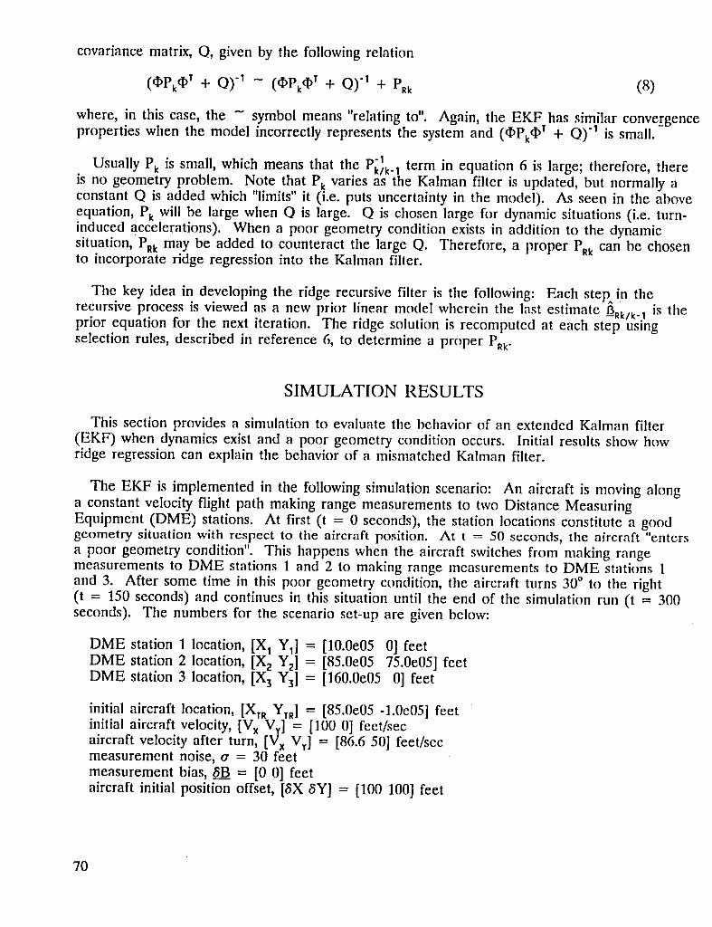
covariance matrix, Q, given by the followingrelation

(_Pk _r "b Q)-I - (_Pk(i)r .t_ Q)-I q_ PRk (8)

where, in this case, the - symbol means "relating to". Again, the EKF has similar convergenceproperties when the model incorrectly represents the system and (€I,Pk(I,r + Q)-I is small.

-1Usually Pk is small, which means that the Pk/k-1term in equation 6 is large; therefore, there

is no geometry problem. Note that Pk varies as the Kalman filter is updated, but normally aconstant Q is added which "limits"it (i.e. puts uncertainty in the model). As seen in the aboveequation, Pk will be large when Q is large. Q is chosen large for dynamic situations (i.e. turn-induced accelerations). When a poor geometry condition exists in addition to the dynamicsituation, P_kmay be added to counteract the large Q. Therefore, a proper PRkcan be chosento incorporate ridge regression into the Kalman filter.

The key idea in developing the ridge recursive filter is the following: Each step^in therecursive process is viewed as a new prior linear model wherein the last estimate --_Rk/k-1is theprior equation for the next iteration. The ridge solution is recomputed at each step usingselection rules, described in reference 6, to determine a proper PRk-

SIMULATION RESULTS

This section provides a simulation to evaluate the behavior of an extended Kalman filter(EKF) when dynamics exist and a poor geometry condition occurs. Initial results show howridge regression can explain the behavior of a mismatched Kalman filter.

The EKF is implemented in the followingsimulation scenario: An aircraft is moving alonga constant velocity flight path making range measurements to two Distance MeasuringEquipment (DME) stations. At first (t = 0 seconds), the station locations constitute a goodgeometry situation with respect to the aircraft position. At t = 50 seconds, the aircraft "entersa poor geometry condition". This happens when the aircraft switches from making rangemeasurements to DME stations ] and 2 to making range measurements to DME stations 1and 3. After some time in this poor geometry condition, the aircraft turns 30° to the right(t = 150 seconds) and continues in this situation until the end of the simulation run (t = 300seconds). The numbers for the scenario set-up are given below:

DME station 1 location, [X1 Y1] = [10.0e05 0] feetDME station 2 location, [X2 Y2] = [85.0e05 75.0e05] feetDME station 3 location, [X3 Y3] = [160.0e05 0] feet

initial aircraft location, [X;RYrR]= [85.0e05 -1.0e05] feetinitial aircraft velocity, [Vx Vy] = [100 0] feet/secaircraft velocity after turn, [Vx Vy] = [86.6 50] feet/secmeasurement noise, a = 30 feetmeasurement bias, 8B = [0 0] feetaircraft initial position offset, [6X BY] = [100 100] feet

70

The aircraft makes 16 measurements to each DME station per second and updates itsposition estimate once every 16TM of a second (i.e. recursive estimation).

The initialization of the tuned Kalman filter is as follows: The initial estimated system statevector and its associated error covariance matrix are

^ _" = -1.0C05 0 1002 0_--0= Vx 0 P0 = 0 0 1002

Vy 0 0 0 01002

The system process covariance matrix is

1 0 0 0 ]

0 1 0 0

Q= 000.10

0 0 0 0.1

And the measurement noise covariance matrix is

302 0 1R = 0 302

The results of the tuned Kalman filter for the above scenario are portrayed in figure 3where the estimated flight path (each estimate is represented by an "o") is compared to thetrue flight path (represented by a straight line). Note that there is some lag in the Kalmanfilter estimates when the aircraft starts to turn. The square root of the MSE is 134 feet. Thisresult shows that the Kalman filter can be properly tuned to handle dynamics when conditionsof poor geometry arise.

Normally, the Q matrix in the Kalman filter is set artificiallyhigh such that the filter canfollow a vehicle through periods when dynamics exist. In order to see how ridge regressioncan reduce the square root of the MSE, implement the same simulation set-up provided abovewith a much higher Q matrix.

500 0 0 !J

0 5(_1 0

Q = 0 0 500

0 0 0 500

The estimated and true aircraft flight paths are shown in figure 4. The square root of theMSE becomes 304 feet.

71

Now, add a proper ridge parameter matrix, PR,to counteract the effects of poor geometry.In effect, adding PRis similar to making Q smaller. Figure 5 depicts the resulting estimatedand true aircraft flight paths. The square root of the MSE reduces to 142 feet. This showsthat a properly selected PRmatrix can give results that are comparable to the tuned Kalmanfilter described above. Efforts are continuing to address the performance of the extendedRidge/EKF in detail.

CONCLUSIONS

Ridge regression signal processing is introduced to explain tile behavior of a mismatchedKalman filter. This paper provides an initial comparison of the extended Kalman filter (EKF)and the recursive ridge filter (the Ridge/EKF). It is shown that a proper ridge parametermatrix PR,may be chosen to counteract poor geometry conditions that may arise whenestimating a position.

REFERENCES

1. Kelly, R.J.: Reducing Geometric Dilution of Precision Using Ridge Regression SignalProcessing. Plans '88, Orlando, FL, November 29 through December 2, 1988.

2. Kelly, R. J.: OMEGA Accuracy Improvement Using Ridge Regression. OMEGA:International and Economic, Proceedings of the Fourteenth Annual Meeting, Long Beach, CA,1989.

3. Kelly, R. J.: Global Positioning System Accuracy Improvement Using Ridge Regression.AIAA Guidance, Navigation and Control Conference, Boston, MA, August 14-16, 1989.

4. Kelly, R. J., van Graas, F., and Kuhl, M. R.: Improved Effectiveness of GPS RAIMthrough Ridge Regression Signal Processing. Proceedings of the 2nd International SatelliteDivision Meeting of the ION, Colorado Springs, CO, September 27-29, 1989.

5. Kelly, R.J.: Reducing Geometric Dilution of Precision Using Ridge Regression. IEEETransactions on Aerospace and Electronic Systems, Vol. 26, No. 1, January 1990.

6. Kuhl, M. R.: Ridge Regression Signal Processing Applied to Multisensor Position Fixing.Master's Thesis, Ohio University, Department of Electrical and Computer Engineering, Athens,OH, June 1990.

7. Ewing, P. L.: The Design and Implementation of Tracking and Filtering Algorithms for anAircraft Beacon Collision Warning System. Master's Thesis, Ohio University, Department ofElectrical and Computer Engineering, Athens, OH, March 1989.

8. Brown, R. G.: Introduction to Random Signal Analysisand Kalman Filtering. John Wileyand Sons, New York, 1983.

9. Sorenson, H. W.: Kalman Filtering: Theory_and Applications. IEEE Press, New York,1985.

72

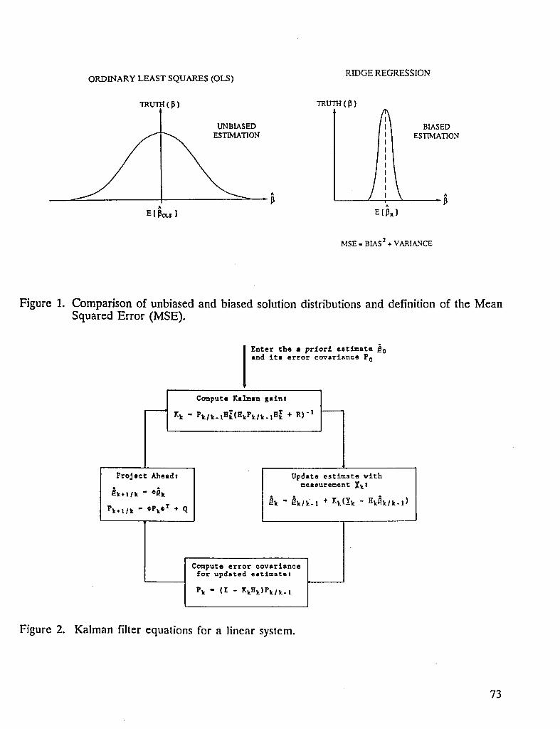
ORDINARY LEAST SQUARES (OLS) RIDGE REGRESSION

TRUTH(B) TRU_(_)

UNBIASED BIASEDESTIMATION ESTIMATION

A ^

E[_o_ ] E [IBR]

MSE = BIAS 2+ VARIANCE

Figure 1. Comparison of unbiased and biased solution distributions and definition of the MeanSquared Error (MSE).

Enter the • pr_or_ estimate _0and its error eovarlanee Po

Compute Kalman galnz

T T IKk - Pklk.lHk(HkPk/k.lHk + R)"

Project Aheadl Update estimate vlthmeasurement _kz

_k " _ktk-,+ Zk(_k- Hk_k/k-,)Pk*l/k " CPkOT + Q

Compute error eovarlancefor updated estimate:

Pk " (Z - KkHk)Pk/k. I

Figure 2. Kalman filter equations for a linear system.

73

xl0 4 Extended Kalman Filter:Properly Tuned

-7 i

-7.5

o -8.5

"7,o

-9.5

-10 ' , , ' ' ' '8.499 8.5 8.501 8.502 8.503 8.504 8.505 8.508 8.507 8.508

X Position (feet) xlO s

Figure 3. Simulation results for a properly tuned extended Kalman filter (small systemcovariance).

xlO' Extended Kalman Filter: Large Q Matrix

-7I

-7.5 _

_ -8.5o

-9.5

-I0 ' ' ' ' ' ' '8.499 8.5 8.501 8.502 8.503 8.504 8.505 8.506 8.507 8.508

X Position (feet) xlO s

Figure 4. Simulation results for an extended Kalman filter allowing for dynamics (large systemcovariance).

74

xl0 4 Extended Ridge/Kslman Filter-7

-7.5

o -8.5

o

_ -9

-9.5

-10 , , , _ _ , ,8.499 8.5 8.501 8.502 8.503 8.504 8.505 8.506 8.507 8.508

X Position (feet) xlO s

Figure 5. Simulation results for a Ridge/EKF filter.

75

MODELING SELECTIVE AVAILABILITY OF THE NAVSTARGLOBAL POSITIONING SYSTEM

Michael Braasch

Ohio UniversityAthens, Ohio

SUMMARY

As the development of the NAVSTAR Global Positioning System (GPS) continnes, there willincreasinglybe the need for a software-centered signal model. This model must accuratelygenerate the observed pseudorange which would typicallybe encountered. The observedpseudorange varies from the true geometric (slant) range due to range measurement errors.Errors in range measurements stem from a variety of hardware and environment factors.These errors are classified as either deterministic or random and, where appropriate, theirmodels are summarized. Of particular interest is the model for Selective Availability (S/A)which was derived from actual GPS data. The procedure for the determination of this model,known as System Identification Theory, is briefly outlined. The synthesis of these error sourcesinto the final signal model is given along with simulation results.

INTRODUCTION

The NAVSTAR Global Positioning System (GPS) is a satellite radionavigation system designedto provide worldwide position, velocity, and time information. The use of GPS may beextended to land, air, sea, and space. For civil air use however, system performance must beproven before regulatory agencies will sanction its use. Strict requirements are imposed anddocumentation must be produced which demonstrates the system's ability to meet theserequirements.

Of these strict requirements, the most difficult to satisfy are low failure probability and highintegrity. The role of the regulatory agencies is also seen in the certification of airborne GPSequipment. Before a GPS receiver is certified, documentation must be produced which detailsthe GPS performance. Since the cost of flight testing is high, the majority of thisdocumentation is produced through simulations. One input to these simulations is a model ofthe navigation system.

This paper presents a signal model which may be used for such purposes. Error sourcealgorithms are generated into one model which computes the observed pseudorange for eachsatellite in view and determines the perturbed user position. This pseudorange model may beused in the performance analysis of GPS, differential GPS (DGPS), and receiver autonomousintegrity monitoring (RAIM) (ref. 1). In addition, the model may be used to determine therequired update rate for DGPS (ref. 2).

77

GPS ERROR SOURCES AND MODELS

The pseudorange observation equation is given by:

Pr = Ps + trcvr " tsv + dtro_ -I- diono + URE + drop+ d,u + dm_,s+ noise + S/A

where:

Pr The observed pseudorange as determined by the receiver, which is the differencebetween the time the signal was transmitted by the satellite and the time the signalarrived at the receiver, multiplied by the speed of light.

Ps The true geometric (slant) range between the satellite and the receiver.

trcvr Receiver clock offset from GPS time, as estimated from observed pseudoranges.

tsv Satellite clock offset from GPS time, as decoded from the satellite navigation data.

dtropo Propagation delay caused by the troposphere.

dio°o Propagation delay caused by the ionosphere.

URE User range error.

d,_ Specular multipath errors.

d,u Receiver hardware delay.

d,_._ Receiver measurement bias errors.

nowiseReceiver measurement noise, clock noise, and diffuse multipath.

S/A Selective Availability.

Both the receiver clock offset and hardware bias are essentially identical for each satellitebeing tracked. As a result, these biases will appear as a clock bias in the user navigationsolution and hardly affect the position solution.

The error models for tropospheric delay, ionospheric delay, and URE have been describedin detail in the literature and require no further comment. It is the random errors whichcurrently pose the greatest challenge.

Receiver noise, satellite clock noise, and Selective Availability are all stochastic processesand therefore cannot be predicted exactly. While the combination of the receiver and satelliteclock noise is basically a white noise process with small variance, S/A is not. Moreover, theexact model which produces S/A is classified for security reasons. Since the actual modelwhich produces S/A is classified, real GPS data from an operational satellite are needed. Oncedata have been collected which contain S/A, a more rigorous analysis may be performed. Inaddition, once S/A waveforms have been derived from the data, a technique is required which

78

determines the model which best fits the process which produced it. This technique is knownas System Identification Theory.

SYSTEM IDENTIFICATION THEORY

Following reference 3, the essence of System Identification Theory will be described. Themain concept is the idea that the data to be identified can be considered the output of alinear filter whose input is white noise. In general, a process may be described by an Auto-Regressive Moving Average (ARMA) model of a given order.

Collected data are passed through a filter whose coefficients are adjusted until its output iswhite noise (with variance trr2). The final filter coefficients can then be used to find theinverse of the signal generator filter. Data which are statisticall_,equivalent to the collected datamay then be generated by passing white noise (with.variance trr") through the inverse filter.This process is depicted in figure 1.

In summary, the steps which lead to the S/A model are:

1) Obtain S/A sample through data collection.

2) Determine a filter whose output is white noise whenthe S/A data sample is passed through it. Calculatethe variance of the white noise output.

3) Construct the inverse of the filter.

4) Statisticallyequivalent S/A data may then beobtained by passing white noise (with variance ascalculated in step 2) through the filter obtained instep 3.

In addition to the determination of the S/A model, System Identification Theory also offersa significant compression of the S/A data. Once the inverse model is determined, only themodel coefficients and the variance of the residuals need to be stored. Based on these fewparameters, virtually an infinite amount of statistically equivalent S/A data can be generated.

GPS DATA COLLECTION

As outlined in the above section, the first step in determining a model for S/A is to collecta sample of S/A. Data were collected from the first operational Block II satellite (SV14).Block II satellites are the first satellites capable of introducing S/A into the GPS signal. Thesatellite was tracked since day 135. On days 189, 190, and 191, error data which are likely tobe caused by S/A were collected. As of the time of this writing, the S/A data presented inthis paper have not been confirmed by JPO. However, this does not present a major problemas will be discussed later.

79

Figures 2 and 3 show plots of SV14 pseudorange residuals. Figure 2 shows the pseudorangeresiduals with S/A turned off. The error is composed mainly of receiver noise. Figure 3shows what appears to be two different models of S/A.

DETERMINATION OF S/A MODELS

As outlined previously, once a data sample has been collected the next step in theidentification process is to determine a proper filter. The proper filter has the followingcharacteristics:

1) Its output is white noise when the data are passedthrough it.

2) It has a minimum number of coefficients.

Once this filter has been determined, tile variance (err2) of the white noise OUtl_utiscalculated. The S/A generator is then composed of white noise (with variance err") input tothe inverse of the above described filter.

This procedure was carried out for the four S/A samples collected on days 189, 190, and191. It is important to note that the data sets analyzed were unfiltered. This was done fortwo reasons. One was to avoid assumptions imposed on the S/A waveforms by the low-passfilter. The second was to more accurately reproduce the SV14 residuals. The generatorgenerates waveforms which are statistically equivalent to the combination of the input S/A andnoise.

The determination of the S/A model is illustrated for the data collected on day 190 (GPStime of the week: 22 - 24 hours). The model chosen was an ARMA model with three polesand two zeros, ARMA(3,2). In order to validate this model, the autocorrelation function ofthe output is calculated to check for whiteness (figure 4). Since it has a spike at lag 0 and itssidelobes are contained in the 95% confidence limits, it may be considered white noise. Anadditional test is to plot the power spectrum of the output. White noise is characterized by aflat spectrum. Again, the conclusion is verified (figure 5).

Now that the optimum filter has been determined, the waveform generator results fromtaking the inverse of the optimum filter. The resulting filter is given by:

1 - 1.5047z-1 + 0.6428z2

H(z)=1 - 2.0833z-1 + 1.2164z"2 - 0.1302z"_

As a further check, data are generated and plotted with the original data (figures 6 ancl 7).Note: the generated data do not look exactly like the original because these data are statisticallyequivalent. The power spectrum of the collected data and the generated data show thespectral similarity (figure 8).

Table 1 gives the models which result from the identification of the four S/A samples. It isinteresting to note that the models for day 189 (166 - 168) and day 190 (22 - 24) are verysimilar. The same is true for day 190 (0 - 2) and day 191 (24 - 26). It is probable that in

80

fact two models were used to create the four S/A waveforms.

This brings up an interesting point. As was mentioned in the Data Collection section, thecollected waveforms have not been confirmed by JPO as S]A. However, if actual S/A turnsout to be different than what has been determined, it is a simple matter to go through the IDprocess again and change the filter coefficients in the model.

SIGNAL MODEL BLOCK DIAGRAM AND SIMULATION RESULTS

The block diagram of the signal model is given in figure 9. The GPS ephemerides, the trueuser state, and the error sources combine in a truth model. The truth model outputs satellitepositions and perturbed pseudoranges to the navigation solution block. The true user state isthen subtracted from the calculated user state resulting in the user state error.

Table 1

MODELS IDENTIFIED FROM THE FOUR S/A SAMPLES

Day (GPS time of Model Crr2week in hours)

1 - 1.6814z1 + 0.8082z2189 (166-168) H(z) = 20.6

1 - 2.3161z"1 + 1.6630z"2- 0.3450z"3

1 - 1.5890z-1 + 0.6744z-2190 (0-2) H(z) = ]7.3

1 - 1.9335z1 + 0.9345z2

1 - 1.5047z1 + 0.6428z2190 (22-24) H(z) = 22.3

1 - 2.0833z"1 + 1.2164z"2 - 0.1302z"3

1 - 1.5703z"1 + 0.6566z-2191 (24-26) H(z) = 16.6

1 - 1.9149z"1 + 0.9168z "2

In order to concentrate on the effects of S/A, all errors other than S/A and receiver andsatellite clock noise were set to zero. In addition, the user position was constant and a fixedsatellite constellation was chosen (figure 10). The horizontal dilution of precision ('HDOP) is2.92, the east dilution of precision is 1.17, and the north dilution of precision is 2.68. Fourthousand data points were taken to show the distribution of the horizontal position errors.

The first scenario was designed to verify the simulation model. Pseudorange errors weretaken from a normal distribution with zero mean and a standard deviation of 5 meters. Aswould be expected, the scatter plot of position errors shows them to be approximatelyGaussianly distributed (figure 11). It is also comforting to see that the error distribution liesalong the line of highest dilution of precision.

81

With the model thus verified, the two filters derived from the S/A waveforms were used toperturb the pseudoranges. The results using the ARMA(2,2) are given in figure 12 and theresults from the ARMA(3,2) are given in figure 13. The position errors again appear to beGaussianly distributed. This is not surprising. By placing S/A on the four pseudoranges andthen computing position, one is essentially convolvingfour random variables. The central limittheorem states that as N increases, the convolution of N random variables will approach aGaussian distribution. For short periods of time, on the order of one hour, the effect of S/Aon the position error is quite different from the effects of the Gaussian noise, however. TheS/A position tends to "wander" around the true user position.

The two dimensional root-mean-squared (2D-rms) position errors for figures 12 and 13 are93.4 and 157.5 meters, respectively. The average HDOP for a 21-satellite constellation isapproximately 1.8 (for an elevation mask angle of 5 degrees). Scaling the simulation resultswith respect to the average HDOP results in 2D-rms position errors of 57.6 and 97.1 meters,respectively.

SUMMARY AND CONCLUSIONS

A signal model is presented which possesses the capability to generate typical errors inpseudorange measurements. The effects of ionc_spheric delay, tropc_spheric delay, and UREare detailed along with the models used to generate them. Two S/A models are derived fromactual GPS data using System Identification Theory. The resulting signal model is then usedto investigate the effects of S/A on position errors. The results satisfy both theory andintuition.

The short term effect of S/A on the horizontal position error is significantlydifferent fromthe effect of Gaussian noise. Therefore, it is recommended that the System Identificationtechnique outlined in this paper be implemented in GPS receiver test equipment. Oneprinciple advantage, as discussed previously, is that the test engineer is not limited to a fewwaveforms of collected S/A. Given the properly identified model, virtually an infinite amountof statistically equivalent S/A data may be generated to exercise the GPS receiver navigationalgorithms.

REFERENCES

1. Kelly, R. J., van Graas, F., and Kuhl, M. R.: Improved Effectiveness of GPS RAIMthrough Ridge Regression Signal Processing. Proceedings of the 2nd International SatelliteDivision Meeting of the ION, Colorado Springs, CO, September 27-29, 1989.

2. Kalafus, R. M., Van Dierendonck, A. J., Pealer, N. A.: Special Committee 104Recommendations for Differential GPS Service. Navigation: Journal of the Institute ofNavigation, Vol. 33, No. 1, Spring, 1986.

3. Braasch, M. S.: A Signal Model for the NAVSTAR Global Positioning System.Proceedings of the 2nd International Satellite Division Meeting of the ION, Student Session,Colorado Springs, CO, September 27-29, 1989.

82

Collected data

1 nl(t) _ H(w,t) / I G(w't) I I n2(t)whitear 2n°ise _ filter _ filter[--_ whitear2nOise

H(w,t) = G'l(w,t)

Or_ = variance

Figure 1. Concept behind System Identification Theory.

l|J| O|y 144

_00

5O

_J

i.

-50

o _SO ! I I I I I I t I

GPS tlsl Of wee_ Im _ourg

Figure 2. Pseudorange residuals (S/A turned off).

83

qSO , _le! Omy, qtt , 150 ISll Oar, 190 .

• _O 5D

: o o

= -SO -50

-109 -t90

-150 I I I -150 ! I I1Be 161.$ 157 1S?.S 16| 0.5 1 1.5

GPS time of wee_ In hours GPS time of wee_ In _ourg

• _o = -_o

-109 -_O0

i i i J i i-_SO -159_! _ S _) 2) $ 24 24 24 $ ?$ 2$,S ?|

GPS tl_O Of wte_ Ifl hour| GPS time of wee_ In _our|

Figure 3. Pseudorange residuals.

Figure 4. Autocorrelation function of the model output.

84

10._ ! J ! , | i , t , s i , ! , i i | J i ! , i , t t:la "l I0"* 10* 10'

frequency

Figure 5. Power spectra of model input and output.

Figure 6. Coilccted S/A data.

85

lJl| Dly 110

- 1!50 I I I I I ! I t t2_ ?2 2 ?2 4 ?Z 6 ?2 | 23 ?3.Z 2) 4 _3.S _3 II 24

GPS tlmo Of veer: trt _ourll

Figure 7. Generated S/A data.

SPlCTnUU

€ollecteO

generl

10!

10.e ! i t i i i I i i t t w i : i , , J i B i i , , I,10 -I 10.q 101 I0 t

freqooncy

Figure 8. Power spectra of collected and generated data.

86

ERRORSOURCE9• SELECTIVEAVAILABILITY• TROPOSPHERICDELAY• IONOSPHERICDELAY USERSTATE• USER RANGE ERROR• RECEIVERNOISE ESTIMATE

k-I t I :1 INAYIOATION

GPSEPHEMERIDES GP5TRU'n-IMODEL r:_OLU'TION9S=e,_ePoe_lone

lCa_ctJaled

TRUEUSERSTATE l_ser State

- _) USERSTATEx - (K.y,1.b) ERROR• STATIC• FLIGHTPATtt

Figure 9. GPS signal model block diagram.

N

100 ...... . ....... ,_

..-'" ............":"- -to:i i i'":' .............::3o.....eo ...-" '... ..._ ......... -_!........... .;.. ..' "-..

3"15 ,-" '...'"" \ i .: .... .. .." "',,s

"'.,o ....""-..:.:....-.,....... ......../..........."....... ",60..'... ..'" ,.. ...''.. ... : .. .. "., ...'..

/ "'.,..." "..." ".. ".. . .: .." ",: "..,..." :.

"° / -..........""... ",..-.",:"kr"::-...,-"...'" e".. ',..: / "'-." -,....... -_ - .......,- ; -- ... _: ...... ... - ...... ._..,. , _ - ... ,..,.,...... .... - .......-, .....:. : "...* • ...1 _..; ." .. ",:. .. ......30

i ......... .".. :'"'. "',." : P: ;'..." .'" : .:..... " "" .........,.':....."....'..'.."..'i/.."i:'...... .....:".........',. ',.,

o ...........i............_............_..........._..:::::i_i:::::::..i............i..........."...........,_:...........• . ..;,....::.:....::.::.::.....;.. • _ ! E'.. " ..'_........ ::' .".."V..',Z',".-:. ".......1... " "

_......... .. ...- .:,. ,. :. ...... :: .... ......... .:.. : .

'°_..........."'."i;""......K ..-"..:"?".:''"..".."..-':.......".......:!...........

- ,0 ": :_"" "- ." .'" "'._"'"'_"'"_.'" ". "',.'" "'_:. ."

-1=0

•_0 :''; "r- ............. .- _ .. ..• : • ....

• . •o ; ..

- 'tOO

_levgtlo_ ver_u_ e/,_ut_

Figure 10. Satellite geometry

87

GsussJBn1o

B : :..o + °. "

• . o°'_ ..• -_..o . .

..:,,

6 " :.'.:; f,_!':..•"_,_,',._-_6./...

.4 "...'.")._ ,h"z-.I. +."."

.:,;+?_+_,>;::+

.,._.l&,+-,,_'._+:_._,:...

++o.+.:€,' ..F! :+.,

. + , .:+;_./:_.+_>,.:+'.•.._.- ,z++.+;- ••"..:_.._+_;.."

• ....+:,+.=?._:..-,,.:': -:., .,':.

+B

i i I"l_tO_ -5 0 5 10

e_st of true (ml

Figure 11. Position errors with Gaussian noise on pseudoranges.

At_M_12.2)500

aoo

3OO

200 -_",

_;__ ",'_

5-!oo ._;t, ,.,,,}C wl,"1,

_+:.':.-_oo _..11..

I.

- 300

-JC,O

-5,30 = ' ' _-£00 -aO0 -200 0 200 aO0 {,00

ellst Of true (m)

Figure 12. Position errors with ARMA(2,2) generated S/A on pseudoranges.

88

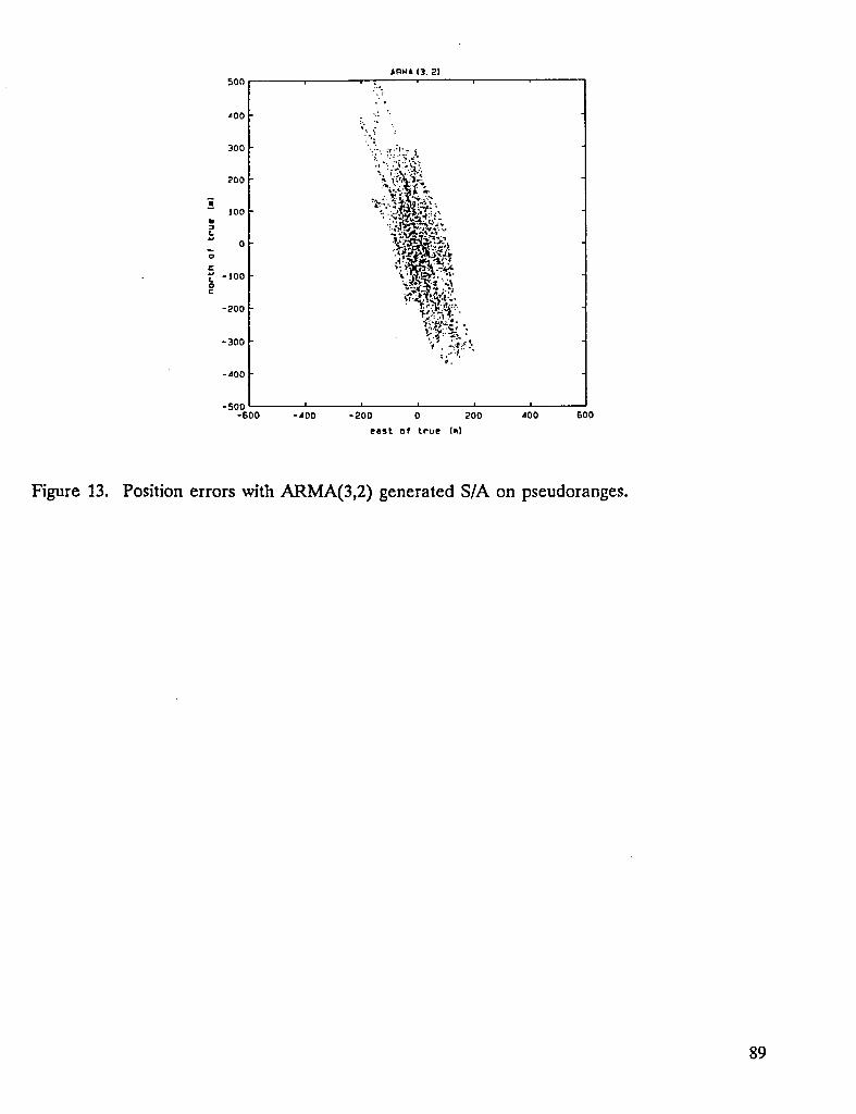
A_WAf3. 2)

50O , .....

zOO ".: '

• .; ;:I

?:.300 ..... :,.:t.

•.:.,:o.._.k:...:.-_:.'_!.

JO0 :...)._, t._ .,.

;_;_ ....

o .4..TaCe,,_(_;_'.:"*,.: ._,._

- I O0 .._

"f_X;"._4."

-300 "_" -e:-<•_..o'4'•

-400

-500 _ ' ' '-600 -,DO -200 0 200 ,00 500

eest of true fro}

Figure 13. Position errors with ARMA(3,2) generated S/A on pseudoranges.

89

ANALYZING THOUGHT-RELATED ELECTROENCEPHALOGRAPITIC DATAUSING NONLINEAR TECHNIQUES

Trent SkidmoreOhio University

Athens, Ohio

SUMMARY

A unique method is presented for collecting, studying and interpreting thought-relatedelectroencephalogram (EEG) data. The use of a chaos-based nonlinear analysis technique isshown to be promising in providing insight into relating conscious thought to specific EEGdata. A discussion of the practical limitations of this technique is also included.

INTRODUCTION

The current primary use of the EEG is in clinical applications. However, because the EEGinvolves conceptually simple instrumentation, is relatively safe, and inherently noninvasive, it iswell worth investigating for possible use in other applications. Specifically, if it were possiblefor a human operator to reliably control some aspect of his/her EEG, a direct human-computer interface could be developed. Thus, the goal of this research is to determine if anoperator can, with their eyes open, consciously control some EEG feature so as to allow acomputer to detect one or more bits of information.

In order to achieve this goal, the laboratory set-up shown in figure 1 was created. The hostcomputer is a Macintosh II utilizing National Instruments' LabVIEW software. The interfaceboard is a National Instruments NB-MIO multifunction A/D converter. The EEG amplifier isa Grass Model 8-16C EEG Instrument. The electrodes are 9 mm silver-silver chloride contactswith collodion adhesive and EEG gel.

The EEG data to be analyzed were obtained during what is called a "Think Math" test.During this test, the subject was instructed to think of a simple math problem (such as 9 x 8= 72) whenever the light-emitting diode (LED) was turned on. The periods when the light isflashing are called Thought-times. During the off-times of the LED (Gap-times), the subjectwas instructed not to think about mathematics or multiplication. This on/off "Think Math"process was repeated for several minutes with the LED flashing periodically two out of everyeight seconds. The data analyzed in this paper were recorded over what is referred to as the"F3 region with respect to Cz" in the 10-20 International System of Electrode Placement(figure 2). Data were sampled at 128 samples per second (T = 7.8125 ms), well above theNyquist minimum for data whose highest significant frequency component appears around 15Hz.

91

CHAOS ANALYSIS OF EEG DATA

The application of chaos theory to biological systems is not a new concept, nor is the studyof the chaotic behavior of the EEG. However, the idea of applying chaos theory to determineif the EEG can be used as a thought/non-thought discriminator appears to be new. Afundamental technique in chaos theory is the reinterpretation of nonlinear time signals asmultidimensional phase-space geometric objects. The goal is to determine if there exists a"strange attractor" in the phase-space diagram of the multidimensional data. A two-dimensional phase-space diagram is generated by plotting the original data sequence, x(nT),against a time-shifted version of the same data, x(nT + "r). Reference 1 suggests that a timeshift (I-) be used which is equal to one-quarter of the period of the most significant frequencycomponent in the EEG signal. The reasoning for this value is based on the "mutualinformation content" of a signal. For the analysis in this paper, a time shift of 23.475millisecondswas chosen. This corresponds to a dominant frequency of 10.6667 Hz. This isintuitivelypleasing since the 10.6667Hz component is in the middle of the alpha region,considered by some EEG researchers as the most important EEG frequency region.

QUANTIFYING THE STRANGE ATTRACTOR

Figure 3 shows a phase-space diagram for x(nT + "r)versus x(nT) for 4 seconds of a 32second "Think Math" test. In order to quantify the chaotic strange attractor generated duringthis test, the Standard Deviation/Moment of Inertia (SDMI) transformation was developed.This transformation consists of first finding the point-by-point moment of inertia about theorigin of the phase-space "cloud." This is denoted by

Ix(nT) = x2(n'F) + x2(nT + r).

The purpose of this transformationis to convertthe two-dimensionalphase-space data intoa positive scalar whose weight is a function of the original signal and the time-shifted version.After this transformation,a moving-average,standarddeviationcalculaticmis performed. Thisis computedas follows:

(k.l)m

or(k) = (l/m) _E(lx(nT) - _k)2 where:n=l.mk

(k+l)m

/xk = F_,(1/m)lx(nT); k=0,1,2,...,(N/m)-In=l*mk

whereN is the total length of the data sequence and m is the standard deviation window length(64 points).

This calculation computes a windowed standard deviation of the moment of inertia of thephase-space "cloud" twice per second (every 64 points). Figure 4 shows the results of this

92

analysis by plotting tr(k) and the thought-times versus time. Note that this entire run containsfour two-second thought times and four six-second gap (non-thought) times.

CONCLUSIONS

For this subject, it is clear that the SDMI analysis produces a significant peak in thestandard deviation plot during the times of transition between thinking and not thinking. Inattempting to generalize the results shown here, the entire test was repeated on several othersubjects. These subsequent tests, which utilized either visual thought cueing or audio cueing,yielded results very similar to that presented here. Further investigation of the raw EEG didindicate the possibility that unwanted artifact (either eye or muscle movement) contributed tothe peaks generated by the SDMI analysis. Thus, some caution is given in interpreting theSDMI peaks as purely thought-related activity. While this research is still in its infancy, it isapparent from these results that this technique may be useful for understanding thought-related EEG data.

REFERENCES

1. Mayer-Kress, G., and Layne, S.: Dimensionality of the ttuman Electroencephalogram.Proceedings of the New York Academy of Sciences Conference on Perspectives in BiologicalDynamics and Theoretical Medicine, Bethesda, MD, April 9-11, 1986.

93

EEGUnit H InterfaCeBoardI

Figure 1. EEG Workstation using a Macintosh II and a Grass Model 8-16C EEG Unit.

FRONT

'g2\

Figure 2. The 10-20 International System of Electrode Placement.

94

300

lOO i:-::+ ..

-100 - " "e'_' "• ,.'.'11 ."• 0IpD (DID

-300-30o -lb0 lbO 300

x(nT)

Figure 3. Chaotie Phase-Space "Cloud" showing x(nT + ,r) versus x(nT) for four seconds ofdata.

.0 1 -- -

._ 0.5

.3

0 I0 20 30

Time (seconds)

Figure 4. Thought-Times and the SDMI EEG data for a 32 second "Think Math" run.

95

INTEGRATED INERTIAL/GPS

Paul Kline and Frank van GraasOhio University

Athens, Ohio

SUMMARY

The presence of failures in navigation sensors can cause the determination of an erroneousaircraft state estimate, which includes position, attitude, and their derivatives. Aircraft flightcontrol systems (AFCS) rely on sensor inputs to determine the aircraft state. In the case ofintegrated Inertial / NAVSTAR Global Positioning System (GPS), sensor failures could occurin the on-board inertial sensors or in the GPS measurements. The synergistic use of both GPSand INS allows for highly reliable fault detection and isolation of sensor failures. IntegratedInertial/GPS is a promising technology for the High Speed Civil Transport (HSCT) and thereturn and landing of a manned space vehicle.

BACKGROUND

The NAVSTAR Global Positioning System is expected to be operational by the year 1993.Presently, ten experimental satellites (Block I) and seven operational satellites (Block II) havebeen successfully launched and are undergoing tests. Navigation with the GPS is based onpseudorange and integrated Doppler shift measurements with respect to GPS satellites. Incombination with ephemeris information, transmitted by the satellites, a receiver can determineits position and velocity with respect to the satellites with a positional accuracy of 16 meters(Precise Positioning Service) and with a velocity accuracy of better than 0.1 meter per second.Differential GPS can result in navigational accuracies of better than 3 meters forpseudoranging and well within 0.2 meter using integrated carrier phase measurements. TheGPS satellite signals can also be used to determine aircraft attitude by making interferometricmeasurements with a minimum of three separate antennas (ref. 1). GPS interferometricattitude determination is expected to be within 0.1 degree for pitch, roll, and yaw angles.

Because of the capabilities described above, the GPS can play an important role in thereliable state estimation of aircraft. Specifically, an integrated Inertial/GPS system couldprovide continuous, high-accuracy attitude information, three-dimensional position and velocity,and time. The system could also provide a high level of fault tolerance, since GPS and inertialmeasurements provide similar information.

The overall objective of an integrated Inertial/GPS system is to provide reliable aircraft stateestimates in the presence of possible failures in the GPS measurements and the on-boardinertial sensors. This involves the design of fault tolerant algorithms, implementation and flightdemonstration of the integrated Inertial/GPS system. Previous research at Langley ResearchCenter demonstrated the capability to provide dual fail-operational performance for a skewedarray of inertial sensors (ref. 2). The redundant strapdown inertial measurement unit

97

(RSDIMU) used for this project will also be used fl_rthe lalx_ratory and flight demonstrationof lnertial/GPS techniques.

OVERVIEW OF RESEARCH

Current efforts are focused on the determination of the effective GPS data rate whichinvolves GPS receiver tracking loop design and simulation, and on fault detection and isolationof GPS measurement errors. In the area of receiver autonomous fault detection, a novelsignal processing technique has been applied to improve the effectiveness of fault detectionalgorithms in the presence of near collinearity (ref. 3).

The GPS receiver simulation program as presented in reference 1 is being extended toaddress the effect of tracking loop bandwidths of the code and carrier tracking loops on theeffective GPS data rate. Figure 1 shows the block diagram of an integrated lnertial/GPS incombination with the AFCS. Both GPS and inertial data are combined by the estimator,which in turn provides the aircraft state estimates to the flight control system. The GPS datarate is required to facilitate the integration of GPS data into the aircraft flight control system,and to determine fault detection capabilities based on GPS attitude information.

Also continuing is the implementation of tlre integrated lnertial/GPS test bed. TireRSDIMU system is currently available for data collection in the laboratory environment. Theinertial system will be combined with a 4-channel GPS receiver. At the same time, provisionsare being made to install the integrated system in Ohio University's Douglas DC-3 researchaircraft, N7AP.

REDUNDANT STRAPDOWN INERTIAL MEASUREMENT UNIT

The inertial sensor used for this project is a Redundant Strapdown Inertial MeasurementUnit (RSDIMU). A block diagram of the RSDIMU is shown in figure 2 (based on ref. 4).The inertial sensors consist of four two-degree-of-freedom accelerometers and gyroscopesarranged in two semi-octahedral arrays. These redundant arrays are interfaced to electronicsboxes which contain analog-to-digital converters. The sensor data are processed by two flightcomputers. The magnetic tape drive is used for in-flightprogram loading. Also used duringsystem testing is a printer for real time data output and a control panel to operate the systemand to inject failures into the measurement data. Power to the inertial sensors is providedthrough a power back-up unit, which allows the sensors to operate for about 20 minutes in theabsence of aircraft power.

The performance of the inertial sensors would support navigation accuracies on the orcter of2 nautical miles per hour. However, the inertial system is only required to provide slmrt-termnavigation data. The GPS will provide the long-term navigation stability for this system.

RSDIMU NAVIGATION MODE PROGRAM FLOW

The RSDIMU has several modes of operation, including coarse and fine alignment, andnavigation. Figure 3 shows the flow diagram for the navigation mode. Each navigation cycle

98

is initiated by a sensor interrupt. The raw sensor data are then scaled and converted to floatingpoint representation. Next, fault detection and isolation routines are carried out, and somedata are fed back to the IMU sensors for corrections. Finally, attitude informaticm is output tothe flight control system and the navigation solution is updated. The subsequent sensorinterrupt initiates the next run through the navigation update cycle. The system operates at anupdate rate of 64 updates per second.

GPS RECEIVER

A four-channel GPS receiver employing continuous carrier tracking is used for this project.Figure 4 shows a simplified block diagram of the GPS receiver tracking loops. The bandwidthof the code tracking loop is as small as 0.01 Hertz when the receiver is in continuous tracking.The carrier tracking loop bandwidth is 32 Hertz and is used to update the code tracking loopevery millisecond to correct for dynamics which cannot be tracked by the code loop. The GPScarrier wavelength at 1575.42 MHz is approximately 19 cm, which provides a trackingresolution of better than 1 cm. In addition, the carrier tracking loop is a second order systemwhich has less than 20 degrees of phase lag at line-of-sightaccelerations of up to 40 m/s',which corresponds to a tracking error of less than 1 cm. The continuous carrier tracking isessentially a dead-reckoning input, similar to Doppler radar.

APPLICATIONS

The integration of GPS and INS has been targeted for several possible applications. Theseapplications actually define the overall system requirements. One application is the HighSpeed Civil Transport (HSCT). GPS/INS can be used for heading and attitude determination.The return of a Space Shuttle from orbit or a Manned Return Vehicle (MRV) from a spacestation is another application. The inertial measurement would provide the short-term stabilityrequired by the flight control system. Differential GPS would be used in the terminal area togreatly improve landing accuracy and to enable the use of candidate landing sites throughoutthe world without the need for a dedicated landing system installation.

CONCLUSIONS

The synergistic integration of inertial measurements and the GPS operated stand-alone or inthe differential mode has many promising applications in the areas of reliable aircraft stateestimation and for use in terminal and landing operations. The RSDIMU test bed isoperational in the laboratory environment, and is being integrated with a GPS receiver toimplement and evaluate the above applications and to develop fault detection and isolationalgorithms.

99

REFERENCES

1. Mclntyre, D. S.: GPS Effective Data Rate Characterization with Application to IntegratedGPSflNS Attitude and Heading Determination. Master'sThesis, Ohio University, Departmentof Electrical and Computer Engineering, Athens, OH, November 1989.

2. Morrell, F. R., Bailey, M. L., and Motyka, P. R." Flight Demonstration of RedundancyManagement Algorithms for a Skewed Array of Inertial Sensors. Proceedings of theAIAA/AHS/ASEE Aircraft Design and Operations Meeting, AIAA Paper 88-4434,Atlanta,GA, September 7-9, 1988.

3. Kelly, R. J., van Graas, F., and Kuhl, M. K.: Improved Effectiveness of GPS RAIMthrough Ridge Regression Signal Processing. Proceedings of the 2nd International SatelliteDivision Meeting of the ION, Colorado Springs, CO, September 27-29, 1989.

4. Bryant, W. H. and Morrell, F. R.: Description of a Fail-Operational Redundant StrapdownInertial Measurement Unit for AvicmicsResearch. Proceedings of the 4th ROLM ComputerUsers Group Meeting, San Diego, CA, February 1981.

100

GPSSIGNA_ "1

l_ON'r- ._D

i GPSRECEIVER

I RE_ ICONTROLS -_ BANDWIDTHI ADJUSTMENT

GPS DATA AT TIEEFFEC'rlVE DATARATE, Roq

CONTROLS

t 'V----1 _r_AS_ p----- DYNAMICS

YAW VELOCITY DATA

cOWrROLSYSTEM

ffcs)

Figure 1. Integrated Inertial/GPS in combination with the Aircraft Flight Control System.

TAPE

_ UNITI / NAVIGATION

IMU I I FLIGHTl.,.4--_Ib.-CONTROLA 1-,_-----I_ COMPUTER [ PANEL

I FIJGIITI P_ER I I TERMINALI I COMPUTER

MEASUREMENTIlMuIUNIT CONDITIONER

COMPUTERPROCESSOR

B

B COMPUTER _. t t . COMPUTERPROCESSOR B CONTROL PANEL

1/O I/O B

Figure 2. Block diagram of the Redundant Strapdown Inertial Measurement Unit (RSDIMU)(based on ref. 4).

101

lWAIT FORSENSOR INTERRUPT

I co_TS_SO_IDATATO FLOATINGPOINTAND SCALE

1FAULTDETEUFION [

AND ISOLATION

1

1DATA OUTPUT

1NAVIGATION [ALGORFI'HM

I

Figure 3. RSDIMU navigation mode flow diagram.

0,01 |1: BANDWlDTI!0.5second

CODE ] 3-5m NOISE PSI_III'_'_RANGF.__ J_

TRACKING I---LOOP

CO RP,.ELATOR ( )

TRACKING _"LOOP (DELTA

PSEUDORANGE)

•41 0.1 mNOISECORRECTIONSTO CODEPOSITION

Figure 4. GPS receiver simplified block diagram of the code and carrier tracking loops.

102

PRINCETON UNIVERSITY

103

INVESTIGATION OF AIR TRANSPORTATIONTECHNOLOGY

AT PRINCETON UNIVERSITY, 1989-.1990

Professor Robert F. StengelDepartment of Mechanical and Aerospace Engineering

Princeton UniversityPrinceton, New Jersey

SUMMARY OF RESEARCH

The Air Transportation Technology Program at Princeton Univer-sity, a program emphasizing graduate and undergraduate student research,proceeded along six avenues during the past year:

• Microburst ttazards to Aircraft• Machine-Intelligent, Fault-Tolerant Flight Control• Computer-Aided Heuristics for Piloted Flight• Stochastic Robustness of Flight Control Systems• Neural Networks for Flight Control• Computer-Aided Control System Design

This research has resulted in a number of publications, including theses,archival papers, and conference papers. An annotated bibliography ofpublications that appeared between January, 1989, and June, 1990, appears atthe end of this report. The research that these papers describe was sup-ported in whole or in part by the Joint University Program, includingwork that was completed prior to the reporting period.

Severe downdrafts and resulting high velocity outflows caused bymicrobursts present a significant hazard to aircraft on takeoff and finalapproach. Microbursts, which are often associated with thunderstormactivity, also can occur in the vicinity of dissipating convective clouds thatproduce no rainfall at ground level. Microburst encounter is a rare butextremely dangerous phenomenon that accounts for one or two air carrieraccidents and numerous general aviation accidents each year (on average).Conditions are such that an aircraft's performance envelope may be inade-quate for safe penetration unless optimal control strategies are known andapplied.

105

Our current wind shear research focuses on avoiding wind shearduring transport aircraft operations, as well as on developing a cockpitsimulation of wind shear encounter. Graduate student Alex Stratton isdeveloping an expert system for wind shear avoidance that extends theFAA Microburst Windshear Guidelines to account for temporal and spatialvariations in the evidence that wind shear is present [1]. The approachbeing taken is to develop a Bayesian Belief Network that relates informa-tion gathered from many sources to determine the probability of encoun-tering a microburst on the intended flight path. Our principal objectivesare to develop methods for assessing the likelihood of wind shear encounter(based on real-time information in the cockpit), for deciding what flightpath to pursue (e.g., abort, go-around, normal climbout, or glide slope),and for using the aircraft's full potential to combat wind shear. This studyrequires the definition of deterministic and statistical techniques for fusinginternal and external information, for making "go/no-go" decisions, andfor generating commands to the aircraft's autopilot and flight directors inautomatic and manually controlled flight.

Graduate student Sandeep Mulgund has begun the development of afixed-base cockpit simulator for microburst studies. The simulation incor-porates a cockpit station with manual input devices and a graphical displayof instruments and the "out-the-window" view. Currently the simulator isprogrammed to simulate a twin-jet transport aircraft and a single-enginegeneral aviation airplane. Displays for the "out-the-window" view and thecontrol panel devices are generated entirely by computers and are pre-sented on color cathode-ray tubes. The external view is generated anddisplayed by a Silicon Graphics IRIS 3020 Workstation. A central comput-ing unit performs dynamic and control calculations, accepts analog inputs,drives the panel displays, and commands the external view. It is a special-purpose Multibus computer employing parallel 80286 processors and spe-cial-purpose graphics boards, which are controlled by an IBM PC-ATcomputer.

Undetected system failures and/or inadequately defined recoveryprocedures have contributed to numerous air carrier incidents and acci-dents. The infamous DC-10 accident at Chicago's O'ttare Airport, inwhich loss of an engine pod, subsequent loss of subsystems, and asymmetricwing stall led to disaster, provides a prototype for the kind of tragedy thatcould be averted by intelligent flight control systems. (An intelligentcontrol system is one that uses artificial intelligence concepts, e.g., anexpert systems program, to improve performance and failure tolerance.)Although many methods of modem control theory are applicable, thescope of the problem is such that none of the existing theories provides a

106

complete and practical solution to the problem. At the same time, heuristiclogic may be applicable, but it has yet to be stated in satisfactory format.

Graduate student David Handelman developed a knowledge-basedreconfigurable flight control system that could be considered a prototypefor a failure-tolerant control system constructed with available hardware.The knowledge-based flight control system is specified initially and testedusing the LISP programming language. When desired logic is determined,the corresponding Pascal code is generated automatically for real-timeimplementation (which has been demonstrated in a laboratory environ-ment) [2,3]. Chien Huang addressed the failure-analysis problem in hisPh.D. thesis [4], and he developed a method for online control reconfigu-ration based on proportional-integral implicit model-following [5]. Par-vadha Suntharalingam examined three alternatives for model-followingcontrol in her M.S.E. thesis [6].

Helpinga pilot make quickdecisions under high workload conditionsis important for aircraft missions of all types. In research principally sup-ported by an Army/Navy grant but reported at numerous quarterly reviewsof the Joint University Program, Brenda Belkin has developed an expertsystem of expert systems called AUTOCREW. In her M.S.E. thesis [7],Ms. Belkin uses the paradigm of a hypothetical aircraft crew to facilitatethe assignment of tasks, rules, and data within parallel knowledge bases.AUTOCREW performs a cyclical search in which the Director expert sys-tem, the electronic analog of the aircraft commander, establishes goals thatinvoke the crew-member expert systems. The crew members then performsuch tasks as observation, monitoring, and control in response to continu-ing needs as well as special requests from the Director. Particular attentionwas paid to the navigation expert system, which manages diverse sensorinputs under varied trajectory and failure scenarios [8].

Control system robustness is defined as the ability to maintain satis-factory stability or performance characteristics in the presence of all con-ceivable system parameter variations. While assured robustness may beviewed as an alternative to gain adaptation or scheduling to accommodateknown parameter variations, more often it is seen as protection againstuncertainties in plant specification. Consequently, a statistical descriptionof control system robustness is consistent with what may be known aboutthe structure and parameters of the plant's dynamic model. Guaranteeingrobustness has long been a design objective of control system analysis,although in most instances, insensitivity to parameter variations has beentreated as a deterministic problem. Graduate students Laura Ryan Ray andChris Marrison are investigating a simple numerical procedure for estimat-

107

ing the stochastic robustness of control systems. Monte Carlo evaluation ofthe system's eigenvalues allows the probability of instability and the relatedstochastic root locus to be estimated. This analysis approach treats not onlyGaussian parameter uncertainties but non-Gaussian cases, including uncer-tain-but-bounded variations [9-13,14,15]. Trivial extensions of the proce-dure admit alternate discriminants to be considered. Thus, the probabilitiesthat stipulated degrees of instability will be exceeded or that closed-looproots will leave desirable regions also can be estimated. Results are par-ticularly amenable to graphical presentation.

There is growing interest in the use of neural networks for compu-tational decision-making and control, brought about by the advent of small,fast, inexpensive computers. The neural network paradigm offers a poten-tially attractive structure for flight control systems that adapt to changingflight conditions and system failures, but much is to be learned about thepracticality of such an approach. Graduate student Dennis Linse has begunto examine this potential. Current research focuses on the use of two typesof neural networks (feed-forward back-propagation network and cerebellarmodel articulation controller) in an adaptive nonlinear controller basedupon feedback linearization [16,17]. In this application, a suite of six neu-ral networks represents the nonlinear aerodynamic/thrust model of the air-craft, and the model can be trained both before and during operationalflight.

Graduate student Subrata Sircar has begun to examine concepts forthe next generation of computer-aided control system design. The princi-pal goal is to add knowledge-based features to the design logic, such asbackground autonomous anticipatory operation, which will keep the com-puter busy performing useful work while the user is evaluating the nextcourse of action, and new graphical output paradigms. The controldesigner should be able to enter the control equations directly, with as fewrestrictions and special conventions as possible. The approach will use theControl Equation Parser (CEP), previously developed at Princeton, whichaccepts symbolic expressions and performs the needed translations usingthe LISP programming language. The present embodiment of CEP hasthree parts (preprocessor, parser, and postprocessor), and it runs on boththe Symbolics 3670 LISP Machine and the NeXT Computer.

108

ANNOTATED REFERENCES OF 1989-90 PUBLICATIONS

1. R. Stengel and D.A. Stratton, An Expert System for Wind Shear Avoid-ance, Engineering Applications of Artificial Intelligence, Vol. 2, No. 3,Sept 1989, pp. 190-197. (also Proceedings of the I989 American ControlConference, Pittsburgh, June 1989, pp. 349-354.)*

A study of intelligent guidance and control concepts for protectingagainst the adverse effects of wind shear during aircraft takeoffs and land-ings is being conducted, with current emphasis on developing an expertsystem for wind shear avoidance. Principal objectives are to developmethods for assessing the likelihood of wind shear encounter (based onreal-time information in the cockpit), for deciding what flight path to pur-sue (e.g., takeoff abort, landing go-around, or normal climbout or glideslope), and for using the aircraft's full potential for combating wind shear.This study requires the definition of both deterministic and statistical tech-niques for fusing internal and external information, for making "go/no-go"decisions, and for generating commands to the aircraft's autopilot andflight directors for both automatic and manually controlled flight. Theprogram has begun with the development of the Wind Shear Safety Advi-sor, an expert system for pilot aiding that is based on the FAA Wind ShearTraining Aid, a two-volume manual that presents an overview, pilot guide,training program, and substantiating data that provides guidelines for this ini-tial development. The Wind Shear Safety Advisor expert system currentlycontains over 200 rules and is coded in the LISP programming language.

2. D. Handelman and R. Stengel, Combining Expert System and AnalyticalRedundancy Concepts for Fault-Tolerant Flight Control, J. Guidance,Control, and Dynamics, Vol. 12, No. 1, Jan-Feb 1989, pp. 39-45.*

A technique for rule-based fault-tolerant control is presented. Theobjective is to define methods for designing control systems capable ofaccommodating a wide range of aircraft failures, including sensor, control,and structural failures. A software architecture that integrates quantitativeanalytical redundancy techniques and heuristic expert system concepts forthe purpose of in-flight, real-time fault tolerance is described. The resul-tant controller uses a rule-based expert system approach to transform the

Archival Papers*Conference Papers**Ph.D. Theses+M.S.E. Theses++

109

problem of failure accommodation task scheduling and selection into aproblem of search. Control system performance under sensor and controlfailures using linear discrete-time simulations of a tandem-rotor heli-copter's dynamics is demonstrated. It is found that the rule-based controltechnique enhances existing redundancy management systems, providingsmooth integration of symbolic and numeric computation, a search-baseddecision-making mechanism, straightforward system organization anddebugging, an incremental growth capability, and inherent parallelism forcomputational speed.

3. Handelman, D.A., A Rule-Based Paradigm for Intelligent AdaptiveFlight Control, Ph.D. Thesis, Princeton University, Report No. 1858-T,April 1989.+

Although fault tolerance always has been an important aspect of air-craft design, the reduced static stability and increased maneuverability ofmodem aircraft complicate the problem by shortening the amount of timeavailable to detect, identify, and adjust for component failures. This dis-sertation investigates the use of highly integrated symbolic and numericprocessing in real-time knowledge-based systems for enhanced automaticaircraft failure accommodation. A rule-based control technique is pro-posed whereby procedural activity is attained through the manipulation ofdeclarative expressions. Rules are used to encode common-sense depen-dencies, to incorporate expert knowledge on specific situations, and toinvoke algorithmic mathematical procedures. Task execution occurs as aby-product of search through these knowledge-base rules. Also proposedis a rule-based controller development system that utilizes a high-levelsymbolic LISP environment for preliminary system design. AutomaticLISP-to-Pascal knowledge-base translation is used to provide dramaticallyincreased execution speed and an environment for highly integrated sym-bolic and numeric computation. The utility of the control technique isdemonstrated through the construction of a multi-processor Rule-BasedFlight Control System (RBFCS) for a Ctl-47 tandem-rotor helicopter. TheRBFCS is shown to accommodate multiple simulated failures affecting theelectrical, hydraulic, and stability augmentation subsystems of the heli-copter. It is concluded that declarative rules with embedded proceduralcode provide a sound basis for the construction of complex control sys-tems.

110

4. C. Huang, A Methodology for Knowledge-Based Restructurable Con-trol to Accommodate System Failures, Ph.D. Thesis, Princeton University,Report No. 1869-T, Aug 1989.+

The problem of dealing with unanticipated failures of dynamic sys-tems is addressed. The solution centers on developing a knowledge-basedapproach to perform online failure isolation and system reconfiguration.The failure analysis employs inference mechanisms and causal relationshipsamong the devices to generate probable failure models, which are prunedand ranked by the use of heuristic measures. Hypotheses for other proba-ble causes are made if the failure model does not adequately account for theanomalies. After the failure source is identified, the system knowledgebase is updated and the impact of failure is assessed. Any degradation ofsystem performance caused by failures is restored by restructuring thecontrol. This issue is studied in depth and addressed by the analysis anddesign of an implicit-model-following control law. The concepts andmethodologies of the approach are illustrated via many examples and fur-ther substantiated using a number of failure scenarios involving a tandem-rotor helicopter. The results show that by providing a form of intelligentself-organization, the knowledge-based restructurable control approachpotentially is capable of accommodating unanticipated failures.

5. C. Huang and R. Stengel, Restructurable Control Using Proportional-Integral Implicit Model Following, J. Guidance, Control, and Dynamics,Vol. 13, No. 2, Mar-Apr 1990, pp. 303-309.*

Studies of a proportional-integral implicit-model-following controllaw are presented. The research focuses on the ability of the control law torecover the performance of a system with failed actuators or structuraldamage to its prefailure level. Properties of the implicit-model-followingstrategy are examined, and conditions for control reconfiguration are

•stated. The control law is applied to the lateral-directional model of afighter aircraft, and control restructuring is shown for changes in controland system matrices. It is concluded that the implicit-model-followingscheme is a good candidate for control reconfiguration.

111

6. P. Suntharalingam, Applications of Computer-Aided Control SystemDesign to Linear Quadratic Model-Following, M.S.E. Thesis, PrincetonUniversity, Report No. MAE-1868-T, Aug 1989.++

This thesis deals with the application of optimal control methods toaircraft flight dynamics. The technique of model-following control hasbeen found to be an effective way of incorporating certain design specifi-cations into the formulation of a linear-quadratic control law. This projectfocused, in particular, on the behavior of the implicit model-follower andthe explicit model-follower. The design criterion for the former con-troller is the minimization of the difference between plant and modeldynamics, and the latter controller is based on minimization of the errorbetween plant and model states. In addition, in an attempt to combine thefavorable aspects of both methods, a hybrid model-follower was developed,incorporating features of both implicit and explicit model-followers.

The relative performance of the three controllers was evaluated byexamining eigenvalues, time responses, robustness, and reconfigurationpossibilities following failure. Results indicate that the explicit model-fol-lower is superior in aspects of robustness and steady-state performance.The implicit model-follower offers specific advantages in the transientresponse to command input and in the use of lower gains. The hybridcontroller combined desirable aspects of the two controllers, yielding thebest overall performance.

7. Belkin, B.L., Cooperative Rule-Based Systems for Aircraft Navigationand Control, M.S.E. Thesis, Princeton University, Report No. MAE-1856-T, June 1989.++

This thesis proposes a design methodology for the development ofmultiple cooperating rule-based systems for aircraft. Nine systems, collec-tively called AUTOCREW, were designed to automate functions and deci-sions. The organization of tasks is described, details of knowledge-basedevelopment and implementation are given, and performance metrics forevaluating the workload of each knowledge base are demonstrated. Severaltest scenarios were evaluated using an interactive graphical simulation onan IBM PC-AT computer. Software tools developed to aid in high-leveldesign also are described. Results show that these tools facilitate rapidprototyping of a complex system exhibiting knowledge-base cooperation,satisfactory logic flow, and human pilot-AUTOCREW interaction.

112

Design of one of the component expert systems, the Navigation Sen-sor Management (NSM) module, was pursued in considerable detail. Thisproblem was chosen because it presented the challenge of designing anexpert system from simulation data, that is, from quantitative test results.The NSM Expert was systematically derived from Kalman filter covariancedata for simulated missions flown with seven different navigation systemtypes. This development used Analysis of Variance (ANOVA) and the"ID3" algorithm. The function of the NSM Expert was to determine opti-mal navigation strategies from a set of available sensors based on a root-sum-square metric. Results show that the NSM Expert predicted positionaccuracy between 65 and 100 percent of the time for a specified "navaid"configuration and aircraft trajectory; hence, this decision-making logiccould be incorporated in a scheme for best navaid selection. The system-atic nature of the ANOVA/ID3 method makes it broadly applicable toexpert system design when experimental or simulation data are available.

8. B. Belkin and R. Stengel, Quantitative Knowledge Acquisition forExpert Systems, presented at the Space Operations, Applications, andResearch Symposium, Albuquerque, NM, June 1990.**

A common problem in the design of expert systems is the definitionof rules from empirical data obtained in system operation or simulation.While it is relatively easy to collect numerical data and to log the commentsof human operators engaged in experiments, generalizing such informa-tion to a set of rules has not previously been a straightforward task. Thispaper presents a statistical method for generating the needed rule base fromnumerical data, motivated by an example based on vehicle navigation withmultiple sensors. The specific objective is to design an expert system thatselects a satisfactory suite of measurements from a dissimilar, redundantset, given an arbitrary navigation geometry and possible sensor failures.

This paper describes the systematic development of a NavigationSensor Management (NSM) Expert System from Kalman Filter covariancedata. The development method consists of the two statistical techniques:Analysis of Variance (ANOVA) and the ID3 algorithm. The ANOVAtechnique indicates whether variation of a problem parameter gives statisti-cally different covariance results, and the ID3 algorithm identifies therelationships between the problem parameters using probabilistic knowl-edge extracted from a simulation example set. ANOVA results show thatstatistically different position accuracies are obtained when differentnavaids are used, the number of navigation aids is changed, the trajectory isvaried, or the performance history is altered. By indicating that these four

113

factors significantly affect the decision metric, an appropriate parameterframework was designed, and a simulation example base was created. Theexample base contained over 900 training examples from nearly 300 simu-lations. The ID3 algorithm was used to determine the NSM Expert's clas-sification "rules" in the form of decision trees. The performance of thesedecision trees was assessed on two arbitrary trajectories, and the perfor-mance results are presented using a predictive metric. The test trajectoriesused to evaluate the system's performance show that the NSM Expertadapts to new situations and provides reasonable estimates of the expectedhybrid performance. The results also show how the NSM Expert choosesoptimal or next-best navigation strategies when limited computationalresources are available; in simple cases, its solutions are commensuratewith the designer's intuition.

9. R. Stengel and L. Ryan, Stochastic Robustness of Linear Control Sys-tems, Proceedings of the 1989 Conference on Information Sciences andSystems, The Johns Itopkins University, Baltimore, Mar 1989, pp. 556-561.**

A simple numerical procedure for estimating the stochastic robust-ness of a linear, time-invariant system is described. Monte Carlo evalua-tion of the system's eigenvalues allows the probability of instability and therelated stochastic root locus to be estimated. This definition of robustnessis an alternative to existing deterministic definitions that addresses bothstructured and unstructured parameter variations directly. "lqaisanalysisapproach treats not only Gaussian parameter uncertainties but non-Gaussiancases, including uncertain-but-bounded variations. Trivial extensions ofthe procedure admit alternate discriminants to be considered. Thus, theprobabilities that stipulated degrees of instability will be exceeded or thatclosed-loop roots will leave desirable regions also can be estimated.Results are particularly amenable to graphical presentation.

10. R. Stengel and L. Ryan, Stochastic Robustness, oral presentation at theSIAM Conference on Control in the 90's, San Francisco, May 1989.**

This paper is an extension of the above paper with extended numeri-cal results for the Doyle LQG counterexample. In particular, the compari-son of stochastic robustness with singular-value analysis is pursued;whereas the latter provides only qualitative guidelines for "loop transferrecovery," the former provides a specific solution for the amount ofrobustness recovery required as a function of parameter uncertainty.

114

11. R. Stengel and L. Ryan, Multivariate tlistograms for Analysis of LinearControl Systems, Proceedings of the I989 American Control Conference,Pittsburgh, June 1989,pp. 937-943.**

A simple numerical procedure for estimating the stochastic robust-ness of a linear, time-invariant system is described. Based on Monte Carloevaluation of the system's eigenvalues, this analysis approach introduces theprobability of instability as a scalar measure of stability robustness. Therelated stochastic root locus, a portrayal of the root probability density,provides insight into robustness characteristics. Parameter variations arenot limited to Gaussian parameter uncertainties; non-Gaussian cases,including uncertain-but-bounded variations, can be considered as well.Confidence intervals for the scalar probability of instability address com-putational issues inherent in Monte Carlo simulation. An example demon-strates stochastic robustness as applied to an aircraft control system inwhich parameters are alternately considered to have Gaussian, uniform, orbinary probability distributions.

12.R. Stengel and L. Ryan, Application of Stochastic Robustness to AircraftControl, Proceedings of the 1989 AIAA Guidance, Navigation & ControlConference, Boston, Aug 1989, pp. 698-708.**

Stochastic robustness, a simple numerical procedure for estimatingthe stability robustness of linear, time-invariant systems, is applied to aforward-swept-wing aircraft control system. Based on Monte Carlo eval-uation of the system's closed-loop eigenvalues, this analysis approach intro-duces the probability of instability as a scalar stability robustness measure.The related stochastic root locus provides insight into robustness character-istics of the closed-loop system. Three linear-quadratic controllers ofincreasing robustness are chosen to demonstrate the use of stochasticrobustness to analyze and compare control designs. Examples are pre-sented illustrating the use of stochastic robustness analysis to address theeffects of actuator dynamics and unmodeled dynamics on the stabilityrobustness of the forward-swept-wing aircraft.

13. R. Stengel, Stochastic and Deterministic Analysis of Nonlinear FlightControl Systems, oral presentation at the NASA Ames-UC Berkeley Non-linear Flight Control Workshop, Berkeley, Aug 1989.**

The flight dynamic equations for aircraft motion are inherently non-linear, yet linear analysis has played a large role in the design and analysisof flight control systems. The principal reason is that the pilot has been

115

able to provide the underlying nonlinear trim control manually, and per-turbations from the trim condition often are small. When large-amplitudeperturbations from trim are important, nonlinear effects need to be consid-ered. Deterministic models provide the basis for all analysis of aircraftmotions. They are used directly to examine stability and response andindirectly to form the underpinnings of stochastic models. Stochasticeffects fall into two distinct categories: uncertain response brought aboutby random inputs and initial conditions, and uncertain response arisingfrom parametric uncertainty.

After briefly reviewing the nature of aircraft dynamics, a progres-sion through four topics is made: locally linearized control laws, adaptivenonlinear-inverse-dynamic (NID) control, analysis of control saturationeffects, and stochastic robustness of closed-loop controllers. Experienceswith multi-input/multi-output linearized models are recounted, leading tovalidation of a linear-quadratic-Gaussian (LQG) pilot model by ground-based simulation and of a gain-scheduled LQG digital controller by heli-copter flight test. Feedback linearization has been applied to the design ofan all-axis controller for a general-aviation airplane, providing inherentprotection against stalls and spins, as well as satisfactory flying qualitiesover the aircraft's entire flight envelope. This NID controller was shownto operate in real time using multiple microprocessors, and a mechanismfor adapting it to the aerodynamic characteristics of individual aircraft wasdeveloped. Phase-plane analysis of the effects of control saturation on theclosed-loop stability of open-loop-unstable aircraft is considered next, withstability boundaries defined by both open and closed regions of piecewise-linear-system trajectories. Finally, the topic of stochastic robustness is pre-sented, based principally on results obtained for linear, time-invariantmodels of aircraft dynamics, with directions for application to nonlinearsystems noted.

14. L. R. Ray and R. Stengel, Stochastic Stability and Performance Robust-ness of Linear Multivariable Systems, Proceedings of the 1990 AmericanControl Conference, San Diego, May 1990.**

Stochastic robustness, a simple technique used to estimate therobustness of linear, time-invariant systems, is applied to a single-linkrobot arm control system. Concepts behind stochastic stability robustnessare extended to systems with estimators and to stochastic performancerobustness. Stochastic performance robustness measures based on classical

116

design specifications are introduced, and the relationship between stochasticrobustness measures and control system design parameters is discussed.The application of stochastic performance robustness and the relationshipbetween performance objectives and design parameters are demonstratedby means of an example. The results prove stochastic robustness to be agood overall robustness analysis method that can relate robustness charac-teristics to control system design parameters.

15. R. Stengel, Analysis of Stochastic Robustness in Linear Systems, oralpresentation at the Eighth Army Conference on Applied Mathematics andComputing, Mathematical Sciences Institute, Cornell University, June 1990.**

This is an oral summary of material presented in earlier papers.

16. D. Linse and R. Stengel, System Identification for Nonlinear ControlUsing Neural Networks, Proceedings of the 1990 Conference on Informa-tion Sciences and Systems, Princeton University, Mar 1990.**

An approach to incorporating artificial neural networks in nonlinear,adaptive control systems is described. The controller contains three prin-cipal elements: a nonlinear-inverse-dynamic control law whose coefficientsdepend on a comprehensive model of the plant, a neural network thatmodels system dynamics, and a state estimator whose outputs drive thecontrol law and train the neural network. Attention is focused on the sys-tem-identification task, which combines an extended Kalman filter withgeneralized-spline function approximation (e.g., basis splines, back-propa-gation feedforward networks, or cerebellar model articulation controllernetworks). Continual learning is possible during normal operation(without taking the system off line for specialized training). Nonlinear-inverse-dynamic control requires smooth derivatives as well as functionestimates, imposing stringent goals for the approximating technique.

17. D. Linse and R. Stengel, Neural Networks for Function Approximationin Nonlinear Control, Proceedings of the 1990 American Control Confer-ence, San Diego, May 1990.**

Two neural-network architectures are compared with a classical splineinterpolation technique for the approximation of functions useful in a non-linear control system. A standard back-propagation feedforward neural

117

network and a cerebellar model articulation controller (CMAC) are pre-sented, and their results are compared with a B-spline interpolation proce-dure that is updated using a recursive least-squares analysis. Each methodis able to accurately represent a one-dimensional test function. Trade-offsbetween size requirements, speed of operation, and speed of learning indi-cate that neural networks may be practical for identification and adaptationin a nonlinear control environment.

ANNOTATED BIBLIOGRAPHY OF 1989-90 PUBLICATION

1. P. Shrivastava and R. Stengel, Stability Boundaries for Aircraft withUnstable Lateral-Directional Dynamics and Control Saturation, J. Guid-ance, Control, and Dynamics, Vol. 12, No. 1, Jan-Feb 1989, pp. 62-70.*

Aircraft that do not possess inherent stability must rely on closed-loopcontrol systems for stable operation. Because there are limits on thedeflections of an aircraft's control surfaces, the region of stable operationalso is bounded. These boundaries are investigated for a lateral-directionalexample in which vertical fin size is inadequate to provide directional sta-bility and where aileron and rudder deflections are subject to saturation.Fourth-order models are used for this study, with flight control logic basedon minimum-control-energy linear-quadratic-regulator theory. It is foundthat the stability boundaries can be described by unstable limit cycles sur-rounding stable equilibrium points. Variations in regions of stability withgain levels and command inputs are illustrated. Current results suggestguidelines for permissible limits on the open-loop instability of an air-craft's lateral-directional modes.

118

Progress onIntelligent Guidance and Control

for Wind Shear Encounter

.D. Alexander StrattonPrinceton, University

Princeton, New Jersey

Low-altitude wind shear poses a serious threat to air safety.Avoiding severe wind shear challenges the ability of flightcrews, as it involves assessing risk from uncertain evidence.A computerized intelligent cockpit aid can increase flightcrew awareness of wind shear, improving avoidancedecisions. This presentation outlines the primary functions ofa cockpit advisory expert system for wind shear avoidance.It also introduces computational techniques beingimplemented to enable these primary functions.

119

WTA Wind Shear Probability Guidelines' i

The Wind Shear Training Aid contains a set of MicroburstWind Shear Probability Guidelines to assist flight crews indetermining the risk of possible wind shear encounter. Theseguidelines relate various types of evidence that might beavailable in the cockpit to a discrete-valued "probability ofwind shear encounter." When evaluating combinations ofevidence, flight crews are instructed to combine the individual"probabilities" according to the rule, "LOW + MEDIUM =HIGH." If available evidence results in a "high probability ofwindshear encounter," the Wind Shear Training Aid states thata decision to avoid is appropriate. If the evidence results in a"medium probability of windshear encounter," thenprecautions are considered appropriate. The guidelinesspecify that the evidence must apply in the airport vicinity,during the intended time of operations, and along thelow-altitude portion of the intended flight path. TheWind ShearTraining Aid also supplies a set of WeatherEvaluation Exercises to demonstrate the use of the guidelines.More importantly, the Wind Shear Trainin_ Aid states that theuse of the guidelines "should not replace sound judgment inmaking avoidance decisions."

OBSERVATION

PRESENCE OF cONVECTIVE WEATHER

NEAR INTENDED FLIGHTPATH:

-Wlthloealzzedstrongwinds ....... HIGH- With heavy precipitation ....... HIGH

- With rainshower ....... MEDIUM

- With lightning ....... MEDIUM

- With vlrga ....... MEDIUM

- With moderate or greater turbulea'ace MEDIUM

- With temperature/dew point spread

between 30 atx:l 50 degrees F ....... MEDIUM

ONBOARD WIND SHEAR DETECTION SYSTEM ALERT

lReported or observed) ....... HIGH

PIREP OF AIRSPIKED LOSS OR GAIN:

- 15 knots or greater ....... HIGH-Lessthan 15 knots ....... MEDIUM

I/WAS ALERT/WIND VEIADCITY CHANGE:

-20 knots or greater ....... HIGH

- Less than 20 knots ....... MEDIUM

FORECAST OF CONVECTIVE WEATHER LOW

Clues are cumulative: LOW + MEDIUM = HIGH

120

Decision Makingfor Wind Shear Avoidance

Wind shear is a spatial or temporal variation of the air aboutan aircraft that causes a deviation of the aircraft from itsintended flight path. The hazard posed by severe low-altitudewind shear has prompted considerable study of the windshear problem by meteorologists and aircraft engineers. Aprimary objective still being addressed is developing systemsfor improved flight crew capability to avoid severe windshear.

A decision to avoid wind shear must be based on predictionsmade from available information. New and improved sensorsystems under development could provide direct evidence ofthe presence of wind shear, but they will not be available inall circumstances. Wind shear avoidance must be based onindirect meteorological evidence when accurate sensors todetermine the presence of wind shear are unavailable. Adecision process based on a combination of meteorologicalevidence can provide better reliability than a decision processbased on a single source.

t"

*Avoidance can enhance safety

*Avoidance involves prediction

Make predictions from current measurements

Interpret predicUve informaUon

•Avoidance involves uncertainty

Wind inputs must be inferred

Uncertain knowledge of wind shear meteorology

Indirect evidence can increase reliability

121

Intelligent Advisor for Wind Shear

Cockpit automation provides an opportunity to assist flightcrews with decisions critical to avoiding low-altitude windshear. The primary goals of a cockpit aid for wind shearavoidance are to increase the likelihood that the flight crewmakes an avoidance decision when severe wind shear actuallywill be present and to decrease the likelihood of a decision toavoid when one is not called for. Technology from therapidly-growing field of artificial intelligence provides a basisfor a wind-shear-avoidance cockpit aid. In an intelligentsystem for decision aiding, the merits of possible decisionalternatives are determined by a machine reasoning processthat is rational and sound, producing results in an intuitiveand meaningful manner. This means that the system iscapable not only of recommending actions but of explainingwhy those actions are being recommended. An intelligentcockpit aid can summarize relevant information from avariety of sources and recommend actions, improvingavoidance decisions.

An expert system for wind shear avoidance, dubbed the WindShear Safety Advisor, is depicted schematically on this slide.It will operate in real time, accepting evidence from on-boardsensors and external evidence (such as pilot reports orPIREPs), perhaps facilitated by a direct data link (representedby a dotted line connecting the external sources to the expertsystem). It will interact with the flight crew, interpreting theirintentions and providing advice and explanations. Thedevelopment and improvement of the Wind Shear SafetyAdvisor are subjects of current research.

F_..x-r1_R,NAL, 1

_eathe_"data ANDHREI:_vcmdahear ak:r't_ SYSTEMSFuture systems

COCKPIT AID

_NOWLEDGEBAsE Ii_q'ERNAL

On-b_ar_ t4_%mors

On-kmard radarVtma,al ,_a-vatloranWlnd_aeJr deteew_"look _'a___d" i_a'anor_

*Aid awareness, increase decision reliability

Summarize a variety, of information

Meteorological knowledge

Real tlme prediction and estimation

Provide step-by-step explanations

Facilitated by direct data link

122

Wind Shear Safety Advisor

Primary Functions and

Proposed Solution Methods

Primary functions of the Wind Shear Safety Advisor (WSSA) maybe divided into the categories of executive, monitoring, predictionand assessment, and planning. Executive is a process of top-levelcontrol, while monitoring is the process of obtaining evidencefrom sources. Prediction is the process of extrapolating thisevidence to the place and time of intended operations, whileassessment is the process of considering the impact of evidence onthe current flight plan. Planning is the process of altering the flightplan to reduce the risk of wind shear encounter. When operatingm real time, these functions are executed in a cyclical fashion,processing evidence continuously. While the architecturecurrently being developed will facilitate real-time implementation,real-time implementation is a follow-on to the current study.

Declarative rule-based techniques and structured data basetechniques have been used extensively in the development of theWSSA to provide a modular and explicit program structure. Todeal with the uncertainw inherent to prediction and assessment,methods for probabilistic Bayesian inference are beingincorporated. Algorithms for interpreting wind data based onstochastic flight path prediction are also being developed for riskassessment and planning.

*EXECUTIVE - Top-level control

Rule-based techniques

*MONITORING - Observe sensors, receive reports,alerts, warnings

Rule-based techniques

Structured data bases

*PREDICTION AND ASSESSMENT - Makepredictions from reports, assess risk ofcontinuing with nominal flight plan

Probabfltstic inference

Stochastic error prediction

*PLANNING - consider flight path revisions andprecautions, receive flight plan revisions

Decision analysis

Rule-based techniques

Stochastic error prediction

123

Wind Shear Training AidModel of Flight Crew Actions

The FAA Wind Shear Training Aid has been a primary sourceof knowledge for the Wind Shear Safety Advisor. Thetwo-volume Wind Shear Training Aid document, preparedwith the support of the Integrated FAA Wind Shear Program,was written by a team from the airframe industry thatinteracted with airlines, government, and academia. TheWind Shear Training Aid is a comprehensive training manualfor flight crews that describes the hazards of wind shear anddetails precautionary and recovery procedures to help escapeinadvertently-encountered wind shear.

Evaluate the Weather _-

[ Avo|d Known Wtnd Shear [

Yes ]No

I I

I[w_d_ Ro_ _e_o l

I Report the Encounter i& J

124

Probability Theory forRisk Assessment

Developing a representation of these guidelines for theWind Shear Safety Advisor that incorporates soundjudgment is complicated by uncertainty surrounding windshear meteorology and the subjective terms used in theguidelines. Use of the guidelines in real situations requirescombined judgments involving uncertainty that thequalitative levels of probability and combination rule cannot represent. Probability theory provides a set of soundand consistent axioms that are understood throughout thescientific community. Probability theory produces resultsconsistent with ordinary logic and stochastic prediction andestimation. Bayesian belief network representation, whichhas been developed primarily by Judea Pearl [12], providesan efficient means to represent uncertain knowledge and toreason in a manner consistent with these axioms, providedsome assumptions are made.

*F.A.A. Wind Shear Training Aid (1986)

Example training program for flight crews

Logical model of flight crew actions

Windshear avoidance guidelines

*Combined judgments involving uncertainty

"Convective weather near flight path"

"LOW," "MEDIUM," and "HIGH" Risk

"LOW + MEDIUM = HIGH"

•Probability and decision theory

Understood by scientific community

Relates to logic, stochastic estimation

•Can incorporate statistical results

Emcient implementation using Bavesiannetwork representation

125

Logical Expert System Techniques

Logical expert system techniques common to expert systemshave been used for initial versions of the WSSA, as waspreviously reported. With rule-based techniques, knowledgepertinent to wind shear avoidance is transcribed as a set ofstatements of the form "If premise is true, then consequentfollows." The expert system's data base is structured bydefining a hierarchy of object structures, calledframes.Structuring the data base adds modularity to rules andpermits clearer explanations to be generated duringexecution.

Execution of the rule base is controlled by an inferenceengine. Forward- and backward- chaining searches,described in an earlier presentation, select rules to evaluateand update the data base through a process of logicaldeduction. As a side-effect of search, quantitativealgorithms may be called as necessary. A recentimplementation of the WSSA on a Symbolics 3670 LISPmachine consists of over 200 rules.

*Declarative knowledge representation"IF-THEN" rules

Symbolic parameters. LISP functionsData base structured with frames

*Inference engine controls rule evaluation

Forward- and backward- chaining

Quantitative algorithms calledconditionally as side-effects of search

*Symbollcs 3670 LISP Machine

212 "IF-THEN_' rules

78 numerical and symbolic parameters15 frame structures

80 functions (& Common LISP)

126

Elements of Probabilistic Reasoning

In a probabilistic model of reasoning, such as a Bayesian network,reasoning is a process of conditioning the probabilities ofhypotheses on the evidence. Bayes's rule is used to accomplishthis. To illustrate the fundamentals of probabilistic reasoning, letH represent a hypothesis that wind shear is on the intended flightpath, and let E1 represent a piece of evidence, such as a windshear detection system alert. From a prior probability that windshear is on the intended flight path, Pr{H}, the posteriorprobability is computed using Bayes's rule. To use Bayes's rule,we must provide the probability of detection of the detectionsystem, Pr{E1 IH}. The prior probability of receiving theevidence, Pr{E1 },must also be specified; however, it is usuallyeasier to provide Pr{E1 I---,H}, the probability of false alarm (thesymbol ---,denotes logical negation), and compute Pr{E1}. Theseequations provide a basis for more general probabilistic reasoning,but additional assumptions must first be made.

To see why this is so, suppose that a second detection system alert,E2, is received. Use of Bayes's rule requires the computation ofPr{E1, E2 1H}, a joint probability distribution. In general, thecomputation of joint probability distributions is a cumbersomeprocess. To simplify the process, we assume that wind shear is thecause of the alerts and that the alerting systems operateindependently of each other. Thus, if wind shear is present, theprobability of receiving the second alert is not changed by thearrival of the first alert. This assumption is known as conditionalindependence, and we say that the effects are conditionallyindependent given the cause. The assumption of conditionalindependence simplifies Bayes's rule, permitting efficientcomputation of the posterior probability of H, based on theprobability of detection and false alarm rate of the individualsystems.

*Condition probabilities of hypotheses onevidence: Bayes's rule

Hypotheses of wind shear (H)

Reports of wind shear (El and E2)

PrlH ]E I.E2} =Pr{E I.E2 [HIPr{H}/Pr{E I .E2}

*Conditional independence assumption:reports independent consequents of wind shear

Pr{H [El.E2} = Pr{E2 [H}Pr{H[EI}/Pr{E2 [El}

*Required statistics:

Prior probability of wind shear. Pr{H}

Probability of detection. Pr[Ei [H}

Probability of false alarm. Pr{Ei [-,H}

127

Bayesian Network Interpretationof Wind Shear Probability Guidelines

A Bayesian network is a probabilistic model of a system.Bayesian networks use graphical representations ofdependency, where a set of discrete random variables arerepresented as nodes and where uncertain relationshipsbetween the variables are represented as links.Cause-effect relationships are represented graphically byadding arrows to the links, pointing from cause to effect.A graphical model of dependencies surrounding themeteorology of wind shear, constructed from theMicroburst Wind Shear Probability Guidelines andextended to include the prediction, is shown here.Elements of the guidelines are represented as randomvariables, which can take one of a set of exhaustive andmutually-exclusive values.

Network representations enable efficient probabilisticreasoning because all of the dependencies betweenvariables are specified by the links. In Bayesian networks,nodes that are "effects" or manifestations of the samecause are assumed to be conditionally independent giventhe cause. With this assumption, all of the informationnecessary to condition the probability distribution at anyparticular node can be obtained from the nodes to which itis directly linked. If reasoning is simulated by sequentialprocessing, the probability distribution at each node can beupdated step by step, permitting explanations to begenerated at each step. Ahernatively, the network couldbe implemented on a set of identical processors,permitting several steps to occur concurrently.

Graphical representation of dependencyProbabilities stored at each node

Nodes updated using Bayes's rule. axioms

128

Requirements for ProbabilisticRepresentation

The constructionof a Bayesiannetworkbeginswith theconstructionof a graphicalmodelof dependency,suchasthe previousslide. Afterconstructingthe graphicalrepresentation,anddetermininga setof valuesfor eachvariable,the knowledgebaseis augmentedby thedefinitionof conditionalprobabilitiesassociatedwitheachlink. For example,completingthe linkbetweennode WindShearand nodeLLWASAlert(whichrepresentsthe stateof the LowLevel Wind ShearAlertSystem)requiresthe estimationof theprobabilitiesshown. Reliabilitystatisticsfor this link werederivedfromdata obtainedforthe enhancedLLWASandincorporatedinto the network. For eachof theotherlinksof the network,a set of conditionalprobabilitiesmustbe defined. Thesesetsof probabilitiesarecalledlinkmatrices.The networkdefinitionis completedby thedefi ifionof priorprobabilitydistributionsat everynodein the network.

Thereare no statisticsavailablefor someofthe windshear link matrices, such as the link betweenPrecipitation and Convective Weather, indicating specificareaswhereadditionalmeteorologicalresearchisrequired. Definition of these probabilities is aided byqualitativeinformationin the Wind ShearTrainingAidandothersources,but theactualvaluesmustbe assignedsubjectively at this time. This is less than desirable, for itaddsa degree of subjectivityto someof theprobabilitiesgenerated by the system during reasoning. Nevertheless,the subjectivity of thevaluescan be reducedby theacquisitionof moreknowledge. Subjectivelanguagecontainedin the MicroburstWind:ShearProbabilityGuidelinesandothersourcesinvites the developertoconsidermoredetaileddefinitionsfor the concepts,guidingthe searchfor additionalmeteorologicalknowledgeand statisticaldata.

Conditional and prior probabilities

Statistical data incorporated

WindShe_r0VS) Some values assigned subjectivelyLLWAS

oa _ia_ p._ Ovsl) o. ai_ path0v_)

LLWA$ Al_ot_ Pr{LA=LA fWS,,WSl] I_{_ IWS=WS_]Wind $1an_(LAI) = 0.71_, = 0_Z7

LLWA.qAI_ ofModm_ Pr{LA=t._ iWS=WSl} Pr{LA=LA2_VS=Wf_}WindSb_r (LAJ0 =0_95 - 0-554

NoLLWA.S Alea (LA_ Pr(_ _¢f,=WS _) Pt{LA._ IWS=W$_]=0.191 .. OAI_'

129

Flight Path Error PredictionWith Wind Statistics

If direct measurements of the winds are available, wind shears thatare truly hazardous to the aircraft can be distinguished from lesshazardous shears. A reasonable approach to distinguish hazardouswind shears using wind measurements is based on flight pathdeviations from the aircraft's nominal flight path. A hazardouswind shear can be distinguished by determining whether or not aperturbed trajectory ties outside a critical region in space. Aperturbation model of the aircraft and control law provides anefficient means to compute trajectory deviations.

Providing a means of distinguishing hazardous wind shear iscomplicated by errors in wind measurements. For example,devices based on the doppler effect can detect only the radialcomponent of winds; vertical winds that can affect the aircraft'sflight path cannot be detected. Stochastic prediction techniquesprovide a means of computing stochastic trajectory errors, such astouchdown dispersion or mean square glide slope error, givenuncertain but statistically defined data from wind sensors.

'IKF.YI I

t-- Pem_bedTraj. 11

*Flight path deviations through wind shear

Wind profile, nominal trajectory, control lawPerturbation model control saturation

*Covariance propagationError statistics of wind data

Correlation of horizontal and vertical winds

Correlation with meteorological parameters

*Stochastic error function computation

Touchdown error, impact velocity

Errors in glideslope, altitude, enel-_V rate

130

Conclusions

Cockpit automation provides the opportunity to aid flightcrew decisions relevant to wind shear and improve flightsafety, but the decision-making process involves themanagement of uncertainty. Bayesian belief networktechniques provide a means torepresent this subjectivemeteorological knowledge so that the knowledge can beused in cooperation with more accurate wind shear detectionsystems. With the probabilistic representation of theMicroburst Wind Shear Probability Guidelines, the door isopen for the incorporation of a wider variety ofmeteorological expert knowledge. This means ofrepresentation also facilitates the incorporation of morereliable wind shear detection systems.

Stochastic prediction algorithms provide a means ofinterpreting uncertain but statistically-defined wind data. Anerror prediction algorithm would incorporate error models ofwind sensors. Stochastic prediction of a trajectory error canprovide the basis for an avoidance decision, once a suitableerror metric is defined.

*Baveslan networks provide a means to interpretWind Shear Tralning Aid avoidance guidelines

Based on probability theory

Enables incorporation of statistical data

Suggests additional meteorological studies

*Stochastic prediction techniques provide a meansto incorporate wind data

Base decisions on error analysis

Requires error model of wind sensors

Requires definition of error metric

131

Flight Simulationfor Wind Shear Encounter

Sandeep S. MulgundDepartment of Mechanical and Aerospace Engineering

Princeton UniversityPrinceton, New Jersey

Introduction

A real-time piloted flight simulator is under development in theLaboratory for Control and Automation at Princeton University. This facilitywill be used to study piloted flight through a simulated wind shear. It will alsoprovide a testbed for real-time flight guidance laws. The hardwareconfiguration and aerodynamic model used are discussed. The microburstmodel to be incorporated into the simulation is introduced, and some proposedcockpit display concepts are described.

133

Simulator Architecture

The simulator presently consists of two computer subsystems. An IBMPC-AT contains the aerodynamic model of the aircraft. This computersamples pilot inputs through a 12 bit A/D board, and integrates the aircraftequations of motion. Aircraft attitude and position variables are transmitted bythe AT to a Silicon Graphics IRIS Workstation, which in turn generates anexternal visual scene and a primary flight instrument display. The presentvisual scene contains a representation of Teterboro Airport and a simplifieddepiction of the Manhattan skyline. The flight instruments are formatted toresemble a modern electronic flight instrumentation system (EFIS). Thedisplay is partitioned so that the top half of the screen contains the out-of-window display, while the bottom half displays the EFIS. A graphicalrepresentation of a Boeing 737 instrument panel has also been developed on theIRIS.

LCA Flight Simulator Hardware Architecture

Pitot

I Y°ke I [ Throttle ]

]Pedals I

naps ISpeedBrakes_Landing Gear / ^_

Converter

Multibus ]

MultibusBit3

Outof Window VisualInterface Scene

AT andBit3 InstrumentationPanel

Interface

I 1

134

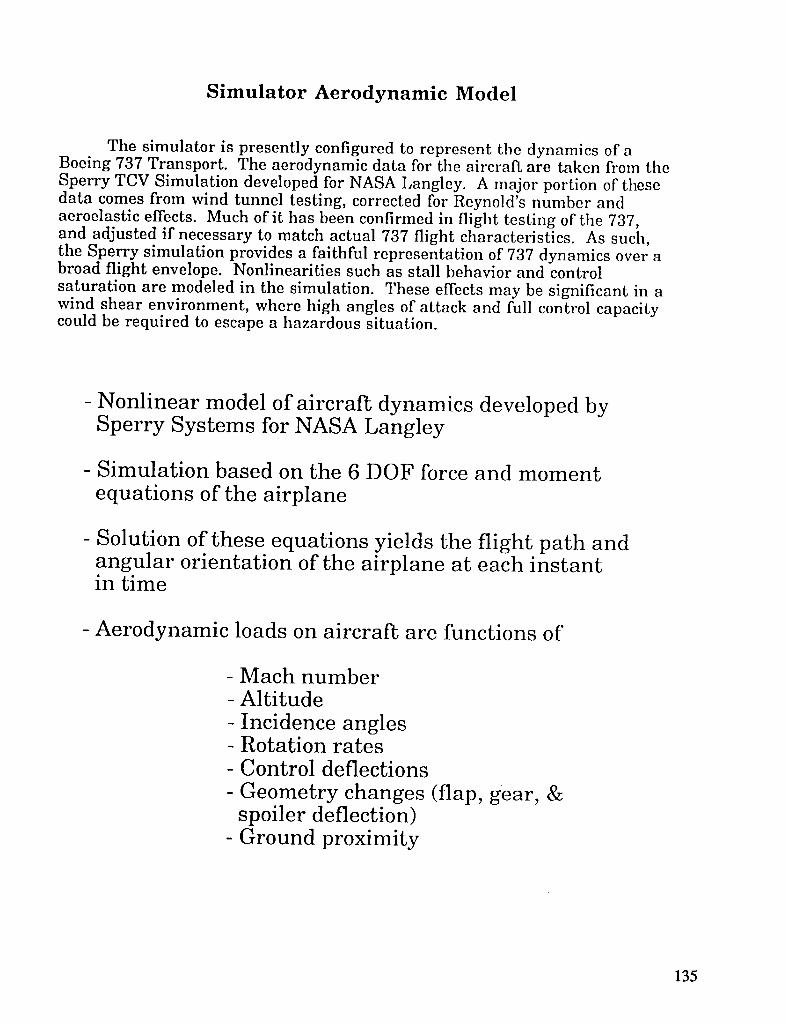
Simulator Aerodynamic Model

The simulator is presently configured to represent the dynamics of aBoeing 737 Transport. The aerodynamic data for the aircraft are taken from theSperry TCV Simulation developed for NASA Langley. A major portion of thesedata comes from wind tunnel testing, corrected for Reynold's number andaeroelastic effects. Much of it has been confirmed in flight testing of the 737,and adjusted if necessary to match actual 737 flight characteristics. As such,the Sperry simulation provides a faithful representation of 737 dynamics over abroad flight envelope. Nonlinearities such as stall behavior and controlsaturation are modeled in the simulation. These effects may be significant in awind shear environment, where high angles of attack and full control capacitycould be required to escape a hazardous situation.

- Nonlinear model of aircraft dynamics developed bySperry Systems for NASA Langley

- Simulation based on the 6 DOF force and momentequations of the airplane

- Solution of these equations yields the flight path andangular orientation of the airplane at each instantin time

- Aerodynamic loads on aircraft are functions of

- Mach number- Altitude- Incidence angles- Rotation rates- Control deflections- Geometry changes (flap, gear, &

spoiler deflection)- Ground proximity

135

Analytic Downburst Model

A microburst model has not yet been interfaced with the aircraftequations of motion. The present plans are to use an analytic model developedby Rosa Oseguera and Rowland Bowles at NASA Langley. This simple time-invariant model permits the simulation of different shears through thespecification of four parameters. Wind components and spatial derivatives areeasily obtained in cartesian coordinates from the velocity equations. Thisdownburst model will be integrated with the equations of motion of the aircraft,and used to study conceptual wind shear hazard and flight guidance displays.

- Developed at NASA Langley by Oseguera and Bowles

- Represents an axisymmetric stagnation point flow,based on velocity profiles from the Terminal AreaSimulation System model

- Time-invariant model

- Altitude dependence includes boundary layer effectsnear the ground, and closely matches real-worldmeasurements

- Permits simulation of different shears throughspecification of four parameters"

1) radius of the downdraft column2) maximum wind velocity (horizontal or

vertical)3) altitude of maximum outflow4) depth of outflow

- Wind components in x,y, and z directions areeasily obtained from velocity equations for a givenaircraft position relative to downburst core

136

Display of Wind Shear Information

Once the microburst has been incorporated into the simulation, it will benecessary to augment the flight displays in some manner to provide the pilotwith some indication of the potential hazard due to the wind shear. The type ofdisplay that will be considered assumes some sort of forward-look wind shearinformation. The hazard to the aircraft will be characterized by the "F-F'actor",a concept developed at NASA Langley. This parameter completely describesthe effect of a wind shear on the performance of an aircraft, in terms of itsconstant speed climb gradient capability. A persistent value of F greater thanabout 0.15 will exceed the climb capability of most transport aircraft.

The display concept under consideration will graphically present theanticipated F-Factor ahead of the aircraft, possibly in a head-up format. Adisplay concept has been developed at NASA Langley that uses anticipated F-Factor to predict the aircraft flight path. Such a display may be developed forthe simulator at Princeton, but initially the F-Factor will be used tocharacterize the wind shear hazard.

- Characterize the intensity of the wind shear usingthe "F-Factor":

Vex WhF- +_g v

where

_)Wxic 0wx _Wx

- F is a function of the aircraft's trajectory, andrelates directly to its constant airspeed climbgradient capability

- Objective is to visually represent the F-Factor aheadof the airplane, to characterize the anticipatedhazard due to the wind shear

- Flight guidance commands must also be presentedto the pilot

137

"Highway in the Sky" Display Concept

In addition to a hazard display, it would be usefill to have some sort offlight guidance command display. Typically, this takes the form of a set ofcommand bars on the artificial horizon. A possible alternative to thisconventional format is the so called "Highway in the Sky". Developed at theFlight Dynamics Laboratory at Wright Patterson Air Force Base, this displaypredicts the future aircraft trajectory based on the current state and theguidance strategy generated by the flight management computers. Ratherthan predicting future aircraft states, it would be interesting to use such adisplay to plot an escape profile out of a microburst. This would require theexistence of an escape strategy, which could include lateral maneuvers. The"highway in the sky" would then display the flight path the pilot should take toavoid the wind shear hazard.

I 040 I

700 178

iiii_iiiii_i_iii!i_i_iii_iiiiiiiiiiiii!i!_ii!ii_iiii_iii_iiiii_i_i_iii!iii_i_ii!!iiiiiiiii!i_iiiiiiiii_i!iiiii_i_iiiiiii)ii_!___iiiiiii_i_!iii!_!_ii__iii_iii!i_iii_i_iiii!iiiiiiii_iii_ii!ii_iii_iiiiiiiiiiiiiiiiiiiiiii_iiiii_iii_i_iii_!_iii_i_i_iii!i!iii!i_iii_i_i_i_i_i_ii_ii!i_iiiii_i_iiiiiiiii!iiiiiiiiiii_i)i_iiiiiii!i_iiiiiiiiiiiiiiiiiiiiiiiiiiiiiiiiii_i_i!iiiiiiiiiiiiiiiiiiiiii_iiiiii!!iiiiiiiiiiiii__iiiiiiiii!iiiiiiiiiii!_iii_i_iiiii_iiiii_iii!!!iii!iiiii_i_iiiiiiii!;ii!ii_!ii_!_iiiiiiiiiii!!iii_iiiii!iii!_i_iiiiiiiiiiii!iiii_i!iii_!_iii_i!_i__iii_i_i_i_i!!_iii!iiiiiii_iiiiiii_iii_ii!i!!iiiiiiii!_i_!iiii_i_i_i_!iiiiiiii_ii!iiiiiiiii!iiiii!_iiiiii!!iiiiiii_iiii!ii_iiiii!!_i)ii_!!iiiiii!ii_i_i_!___i__!i_iii_i_iii_iiiii_i!i!i!iii_i!i_iii_iii_i_iiiii!iiiii_i!i_i_i_ii!!i!iiiii!iiiiiii!iiiiiiiiiii_i_i_iiiiiii_iiiii_iiiii_i_!iiii_i_i__ii_iii!iii_iii_iiiiiiiiiiiii_iiiiiii_i_iiiiiiiiiiiiiiiii_i_iii_i_i!i_iii_iiiiiiiii_iiii!iiiii_i_iiiii_iiiiiii_ii!iiii!iii_ii!iiiiiiiii_iii_i!iii)ii_iii!__ii_iiiiiiiiiiiiiii__iiiiiiiiiiiiiiiiiii__iiii_iii)_i!i_iii!iii!i!iiiiiii_i!i!i!i!_!i_ii__i!iiiiiii_i_i_iii!!ii_i_i_iiiiiii_iii_i_iiiii!iiii

138

Future Work

- Implement the Oseguera-Bowles wind shearmodel in the aircraft's equations of motion

- Develop displays to characterize wind shearhazard, and investigate alternatives to "commandbars"

- Continue development of simulator hardware

139

STOCHASTIC ROBUSTNESS:TOWARDS A

COMPREHENSIVE ROBUSTNESS TOOL

Laurie Ryan Ray

Department of Mechanical and Aerospace EngineeringPrinceton UniversityPrinceton, New Jersey

Stochastic robustness is a simple technique to determine the robustness of linear,time-invariant systems by Monte Carlo methods. Stochastic stability robustness has beendescribed previously. These results are extended here to provide insight into control systemdesign for performance. Together, stochastic stability and perfonnance robustness conceptsconstitute a comprehensive tool that can be used to analyze control system robustnessproperties. As well, they offer control system design insight that can set the stage forstochastic robustness synthesis. The concept of stochastic stability robustness is reviewed,stochastic performance robustness is introduced, and stochastic robustness synthesis isdescribed qualitatively. Confidence intervals necessary for comparing control lawsstatistically are presented.

STOCHASTIC ROB USTNESS ANALYSISStability robustness

Performance robustness

STOCHASTIC ROB USTNESS SYNTHESISDesign insight uncovered by stochastic robustnessConfidence intervals for comparing control laws

SUMMARY

141

STOCHASTIC ROBUSTNESS ANALYSIS

Stochastic robustness is a robustness measure based on the probability of satisfactory stability/perfomance in the face of uncertainty. Stability robustness is described by a single metric: the probability of instability. Because it is a statistical measure of robustness, and because it directly uses knowledge of the statistics of the physical parameter variations, stochastic robustness is inherently intuitive and precise. The physical meaning behind the probability of instability is apparent, and overconservative or insufficiently robust designs can be avoided. Concepts behind stochastic stability robustness can be easily extended to provide insight into control system design for performance. Design specificatioris such :IS

rise time, overshoot, settling time, dead time, and steady-state error are normally used as indicators of adequate performance and lend themselves to the same kind of analysis as described above. Concepts of stochastic stability robustness analysis can be applied to these criteria giving probabilistic bounds on individual scalar performance criteria. Stochastic robustness concepts can be applied to specific aircraft handling qualities criteria as well. Binomial confidence intervals for the scalar probability of instability have been presented, and these apply to performance robustness criteria as well.

STOCHASTIC ROBUSTNESS A robustness nleasrdre based on the

probability of satisfactory stability/perforrnance, given the statistics of a plant's parameter variations

STABILITY ROBUSTNESS: PROBABILlTY OF INSTABILITY

PERFORMANCE ROBUSTNESS: MANY MEASURES Degree of stability

Time response envelopes Hand1 ing qualities criteria

BINOMIAL CONFIDENCE INTERVALS Statistical bounds for the

estimated stability or performance measure

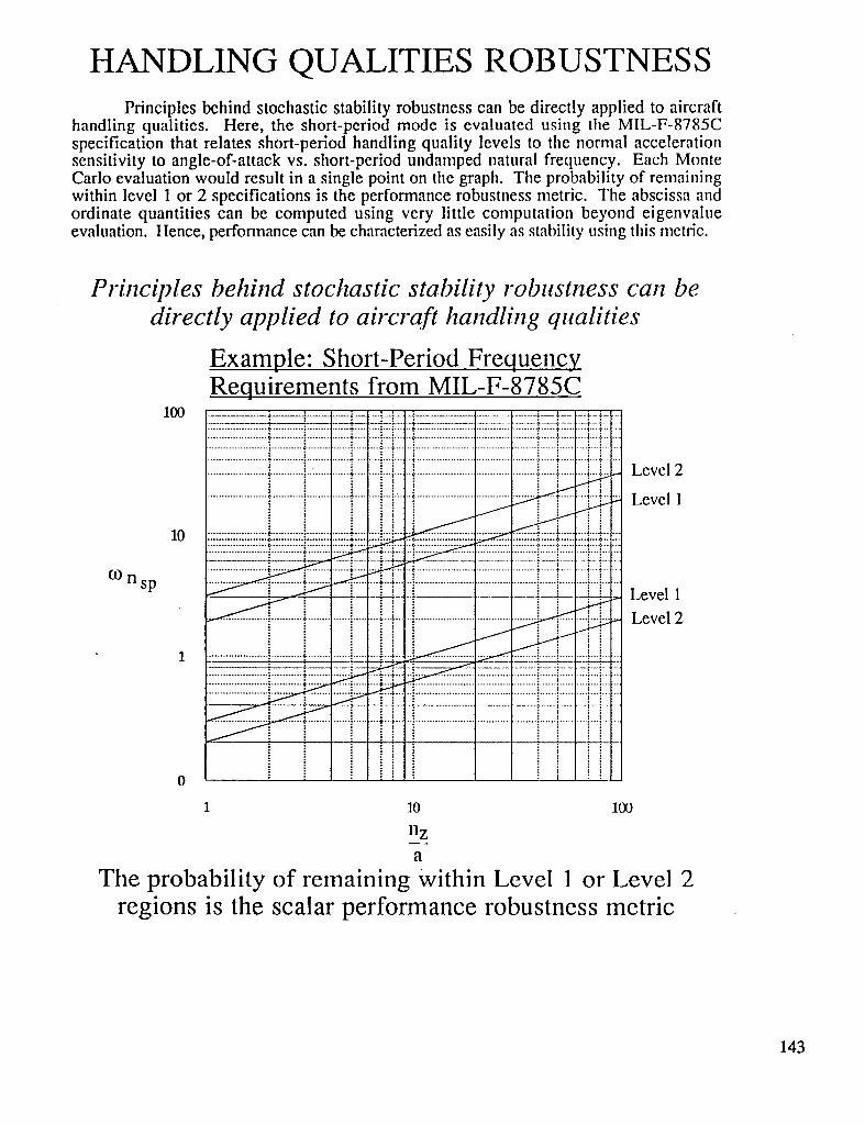
HANDLING QUALITIES ROBUSTNESSPrinciples behind stochastic stability robustness can be directly applied to aircraft

handling qualities. Here, the short-period mode is evaluated using the MIL-F-8785Cspecification that relates short-period handling quality levels to the normal accelerationsensitivity to angle-of-attack vs. short-period undamped natural frequency. Each MonteCarlo evaluation would result in a single point on the graph. The probability of remainingwithin level 1 or 2 specifications is the performance robustness metric. The abscissa andordinate quantities can be computed using very little computation beyond eigenvalueevaluation. Hence, performance can be characterized as easily as stability using this metric.

Principles behind stochastic stability robustness can bedirectly applied to aircraft handling qualities

Example: Short-Period FrequencyRequirements from MIL-F-8785C

10o _ i--_. -'. " _. ! -'. i _ -..................... _............ .:.............. ......... 1...!.... _......................................... :....., ........ :...: ......................... _............ i..............I 4........ 1...!.... _.......................................... L-----_......... _--.';.......................... i ........... _........ i...... _....... $..._..... i ......................................... !......!......... !..A.........................i............_........r..i ........_._....i..........................................i i......1] .........................._............i.:...........4.........i..i...._.........................................._--_.........i--4. Level 2

....................._............!.............."........!4...._.........................................' .4..-.. Level 1

10 ....................._..........._..............i........i.-.i.....'....................._............i.............. _.---:. i --:.... _...................................... i ........... 4.............. • -.-*---_.... i........-- i " - '&--i-- '....................._...... ' --i i...._....................

o.1n sp ............... 4..-._....!..................... Level 1---'_....i..................... Level2

1.....................!...........i-.............. : .-.4--.4.... :....................................i ..........._......... _....' ..:.................................

_i i _____1..................... i ........ ' ..... _.... i.................................

I

o

1 10 100

nz

a

The probability of remaining Within Level 1 or Level 2regions is the scalar performance robustness metric

143

PERFORMANCE ROBUSTNESSMaking the transition from strict stability to degree of stability is simple. Alternate

regions can be described that relate to classical measures of response speed. Alternatediscriminants relate to time-to-half or time-to-double. Sector bounds relate directly todamping ratios and natural frequencies. The probability of closed-loop eigenvaluesremaining within the alternate region is the scalar performance robustness metric. Timeresponse envelopes can be defined as well, and stochastic robustness analysis gives tileprobability of a response remaining within the desired envelope. Using any of these metrics,binomial confidence intervals apply.

Transition from strict stability to degree of stabilityAlternate discriminant Sectorbounds

'jo3 jco

13 CI

Time response envelopesmin max peak overshoot max

i peak_ _,,,;_ak

• "_me max

steady-stateerror

90% min p _ minrise _" m.ax max steady-statetime _" r!se settling

time time error50% min d"

delay / maxtime /" delay

time2' max

r deadtimemaxundershoot

144

TWIN-JET TRANSPORT AIRCRAFT:SHORT-PERIOD MODE EVALUATION

As an example of the above concepts, stochastic performance robustness analysis isapplied to a nonlinear longitudinal model of a twin-jet transport aircraft. Each Monte Carloevaluation consists of linearizing the system around nominal trim conditions and computing

the eigenvalues and nz-- The probability of violating sector bounds and the probability ofo_violating level 1Mil-spec requirements are shown here.

Nonlinear, longitudinal rigid-body model, 22 parameters

..usin_ sector bounds based on Mil-spec damping requirenaentprO.)

Sector bound

..using Mil-spec short-period frequency requiremen!

145

TWIN-JET TRANSPORT AIRCRAFT:CLOSED-LOOP COMMAND RESPONSE

Closed-loop flight-path angle command response is given here, where the controllerwas developed using a Proportional-Filter-Implicit-Model-Following LQR control law.Here, the probability of violating the defined time response envelope and the probability ofcontrol saturation are the performance robustness metrics.

Flight-path-angle command response dislribulion

I1.l Time rcsponse envclope

_" O.0 .......-r........ I

.0 I0.0 20,0 30,11 40.fl 51

i.Ll

l:.lcvalor saturation limit (30 €leg)

D.5

__ t _ ___

30.0 40.0 St

-0,5

Elevator saturation limit (-30 (leg)

time (see)

o"i"" 0,fi

';,4

0.4

p|llP"

0.2

0,0 i , , I

.o io.o 7o.o 3o.o 4o.o s,

time (scc)

/_, = 0.034 (0.0199,0.0539)

i_SE= 0.502 (0.457, 0.547).

146

STOCHASTIC ROBUSTNESS SYNTHESISMetrics resulting from stability and performance robustness can be related to

controller parameters, providing a foundation for design tradeoffs and optimization. This isillustrated qualitatively here. As gain increases along a root locus, uncertainty is magnified,and the "uncertainty circles" associated with the closed-loop root locations enlarge. The firstroot locus demonstrates one where the probability of instability increases monotonically withincreased gain. The shape of the second root locus makes it possible for the uncertaintycircles to initially cross into the right-half plane, remain in the left-half plane as gainincreases, and finally cross into the right-halfplane again for very large gain. The probabilityof instability decreases, then increases, and it has a minimum for some value of gain.

Tradeo.[,f_exist and can provide a foundation for optimization

QUALITATIVE ILLUSTRATION

2_

o

.b

ControlSystemDesignParameter

Closed-loop roots are enclosed by "uncertainty circles"a) Stability robustness decreases as gain increasesb) Stability robustness increases, then decreases

147

STATISTICAL COMPARISONOF CONTROL LAWS

The above analysis qualitativelydemonstrates tradeoffs that can provide a foundationfor optimization. The ability to statistically compare control laws and say with certainty thatone is better than another is another tool necessary for optimization. The Bonferroniinequality can be used to describe confidence intervals for the difference based on individualconfidence intervals. As illustrated, the one control law is statistically better than anotherwhen their individual confidence intervals no longer overlap.

Given binomial confidence intervals for two estimates

Pr(L]< ]?l<U1)=l-_lPr (L2 < ]?2< U2) = 1 - cz2

tile confidence interval for A]?= ]P1- ]72

Pr [(L1 - U2) < A_ < (U1- L2)] > ! - c_

is derived from the Bonferroni inequality

O_= _1 - _2 for dependent intervals= _1 - _2 + _1 _2 for independent intervals

ILLUSTRATION

Number of Evaluations

148

HOW MANY EVALUATIONS ?The number of evaluations necessary to distinguish between two control laws is an

important factor when considering stochastic robustness synthesis using optimization. Here,the number of evaluations necessary for a required interval width is related to the number ofevaluations necessary to distinguish a significantdifference.

Number of Evaluationsfor a Required Interval Width and o_= 0.05

,o+09 i._le+0_ ..............j...........................

!......................___ .___ ........iInterval

z

............................i...........................i....................................._0_le+01

le-06 le-05 le-04 0.001 0.01 0. I { 10.5

lP(0 <IP_<.0.5), or [l -IP] (0.5 <P< 1)

Number of Evaluations Requiredto Identify a Significant Difference

_1 = o_2= 0.050.1

i

i _i J=500,._,0.08 .............................. + "I. ..............................................................

i

0.06

,, ...........................i_ 'i'J-lO00

r"_ 0"040.02_.. .....:._ --...............................J = 5000

. "..............................+J=10000o - J =50000

0 0.1 0.2 0.3 0.4 0.5PI

149

SUMMARYStochastic robustness is a good overall robustness analysis tool. It is intuitive and

simple, and makes good use of engineering knowledg. Both stability and performancemetrics can be identified, and confidence intervals offer statistical significance to the resultingmetrics. It is a good candidate for synthesis techiques as well, because it demonstratesrobustness tradeoffs with control systems design parameters. Confidence intervals for thedifference between two Probabilities provide a tool that can be used in future optimizationstudies.

Good overall robustness analysis tool

Intuitive and simple

Makesuse of engineeringknowledge

Both stability and performancerobustness metrics

Confidence intervals are easily interpreted

Good candidate for control system synthesis

Shows stability and performancetradeoffs with design parameters

Confidence intervals for differences can be defined

150

Neural Networks in Nonlinear Aircraft Control

Dennis J. LinseDepartment of Mechanical and Aerospace Engineering

Princeton UniversityPrinceton, New Jersey

Recent research indicates that Artificial Neural Networks offer interestinglearning or adaptive capabilities. The current research focuses on thepotential for application of neural networks in a nonlinear aircraft controllaw. The current work has been to determine which networks are suitablefor such an application and how they will fit into a nonlinear control law.

151

Parameter Estimation in Nonlinear Control

The equations of motion of an aircraft can be cast into a set of nonlinearordinary differential equations that are linear in the control input, u.Included in the state and output equations is a parameter vector, p.Several methods, including Nonlinear Inverse Dynamics [Lane andStengel, 1988] and decoupling [Singh and Rugh, 1972], are available forgenerating nonlinear feedback laws if the system is known. Using thesetechniques, the feedback laws are determined as functions of theparameter vector, p. p itself is a function of the current state and possiblyexternal states and controls not included in the system dynamics. Themain difficulty is to provide an estimate of the parameters that arepossible complex nonlinear functions of the states.

Given a Nonlinear Dynamic System (e.g. an aircra[_)

i= f(x, p) + G(x, p)u

y ---h(x, p)

and a Nonlinear Feedback Law

u =a(x, p) + B(x, p)v

wbe_

p = p(x, Xext, Uext)

h ow do you e_tlmate the parameterR, p ?

152

Nonlinear Function Approximation

While many techniques exist for nonlinear function approximation, threehave been chosen for further investigation. A B-spline (basis spline)technique with coefficients updated using Recursive Least-Squaresestimation represents a classic function approximation method. Twoneural networks methods are also investigated. The Back-PropagationFeedforward Network [Rumelhart, Hinton, and Williams, 1986] is apopular, widely investigated, model in the neural network community.The Cerebellar Model Articulation Controller (CMAC) [Albus, 1975] is lesswell known, but very useful and powerful in function approximationimplementations.

Three appealing methods

• C1AR_Iemethod

- Recursive Least Sqtmre_ E_tinmtlon uMng B-SplineR

• NeuralmethodA

- Back-PropagationFeedforwardNetwnrk

- Cercbc1|ar Model Articulntion Contr_ller (CMAC) Network

153

Comments on Operation and Learning

Each of the three techniques has different adaptation (or learning)capabilities. The B-spline method requires a matrix inversion that may bevery slow, especially for high input dimension systems. The least-squaresestimation scheme effectively extracts information from the input data,making adaptation fast when measured in terms of number of pointspresented to the estimator. The feedforward network, on the other hand,needs many presentations to accurately approximate the nonlinearfunction. Once trained, it can be extremely fast in operation, especially iffully implemented on a VLSI chip. The CMAC quickly approximates thedesired function in the neighborhood of the training points and providesgood operation speed on a traditional computer architecture.

• Recursive Least._luarea B-Splinea

- Slow learningMatrix inverRion

- Effective learning

• Back-Propagatlon Feedforward Networks

- Relatively Inefficient learning

Many training pcfinhqneeded

- FA.qT nperatlon

• CMAC

- Reaaonable learning and operation

154

Approximation by Neural Networks

The approximation capabilities of traditional spline techniques arerelatively well-known. The capabilities of the neural networks are lesswell-known. The CMAC approximates by a generalized table look-up.Using overlapping, quantized inputs, the CMAC output is a piece-wisecontinuous approximation of the input function. The approximationaccuracy is limited by the size of the table used in the look-up scheme.The feedforward network provides a continuous approximation of thedesired function with the accuracy determined by the number of layersand nodes in the network architecture. There has been much recentinterest in exactly determining the approximation capabilities o["suchnetworks.

• CMAC'a approximate by generalized table Ic_k-up

- Approximation limlted by table size

- Stalr._tep output

• Feedforward network_

- Capacity determined by ncdea and lnyers

- Cnntinuoum nut.put

- Much recent interest in appr_rxlmatlon abilities

155

Back Propagation Neural Networks

A very simple, 2-input / 2-output back-propagation network is given here.The operation of the network can be described by a simple recursiverelationship between the outputs of each layer. At each node, a weightedsum of the outputs from all of the nodes of previous layers is acted on by asimple nonlinear function to provide the output for the node. A fixed,unity input is provided to each node to act as a threshold or bias. Whenthe number of layers and nodes in each layer is chosen, the overallnonlinear function calculated by the network is determined by the valuesof the weights in the interconnections.

W (0) W O)

x1(o)x 1

x ';' x_z)

Thr_hold 1.0

xCk)= s[WCk-Z)xCk-_)]

y --x(N) = f[x¢o)]

156

Exact Representation using Neural Networks

While investigating the limits of neural networks, Hecht-Nielsen [I9871 was able to reinterpret a theorem by Kolmogorov related to the exact representation of a multi-input nonlinear function in terms of simple single-input functions. While back-propagation neural networks can be interpreted in terms of this theorem, the nonlinear function a t each node is fixed by a limiting process which depends explicitly on tllc function to bc represented. Most neural networks, on the other hand, have a common, simple function a t the network node, and use the weighted interconnections to adjust the output of the network. There are many further difficulties with this theorem that limit its usefulness except as the most basic of existence proofs.

Hccht-Nidncnk Inlcrpmbtion oTKolmqomv'n Tt~norcrii

(Solution to Hilbert'n 13th PrAlcm)

- Exact Rcprencntnlion

2n " p - l f(x) = C g( C h. v ( x p tcq) + q )

q = o p = l

- W can be oblained an a uniform limit n fa ncqurncc vr ofconlinuoun

nondccrcaning piecewise linear functions

- W i n dillicult Lo computc

- W in difrcmnt for each Rx)

Approximation Representation for Feedforward Networks

In most instances an approximate representation of a nonlinear function isall that is needed. Many researchers have been investigating theapproximation capabilities of feedforward networks of the type described.These theorems are usually based on results from functional analysis andgive sufficient conditions for the approximation of any continuous functionto any desirable degree of accuracy. In general, they are not based on theKolmogorov's Theorem for exact representation.

• Can feedforward networka approximate nonilnear functinng?

• Recent theoretical remllts by

Funahashi,

Cybenko,

tlecht-Nielsen,

Stincheombe and White,

and many other_

• Based on results from functional analysiR

158

Cybenko's Theorem

As an example of these recent theorems, the version due to Cybenko[1989] is outlined here. Defining a sigmoidal function in the most generalform, Cybenko's Theorem shows that finite sums of sigmoidal functions,exactly the form of a single hidden layer feedforward neural network, aredense in the continuous functions on the unit hypercube. In simplerterms, any continuous function with inputs between 0 and 1 can bearbitrarily closely approximated by a neural network with one hiddenlayer. The other researchers have developed similar results. Thedifferences are usually technical details related to how smooth theapproximated function is and what type of functions are allowed in thenodes of the hidden layer.

While this is a very promising result, it is only an existence proof. Thenumber of nodes necessary in the hidden layer is only specified as finite,and the weight vector is left unspecified.

_: We say that G in sigmoidal if

last _,ooo(t)--* 0 ast-_-*o

_: Let obe any eontinuoun Rigmoidal function. Then finite sums of the form

N

g(X) = j___i_tjfl(wjrx + 0j)

are denne in C([n).

In other words, given f_ C(In) and E>O, there is n _um, g_x), of the above form, fi,r which

x)for all x _ In.

159

Example Functions

The sigmoidal functions, as defined for Cybenko's Theorem, can havemany different shapes, including those shown here. The back-propagationalgorithm requires a differentiable nonlinear function at each node. Inmost implementations the function is similar to the first one shown.

As mentioned previously, the other approximation theorems have differentrequirements on the nonlinearity allowed in the node. Two are shownhere that fail to meet the requirements for Cybenko's Theorem, but areshown to be sufficient for function approximation by others.

• Satisfying Cybenko'M Theorem

I I

• Other Theo_rnR

160

What's Ahead

Future work includes investigating the approximation capabilities ofreasonable sized networks for multi-input functions of the type that willbe found in a nonlinear control law. This will allow for a completeimplementation of a nonlinear control law for the 737 aircraft using neuralnetworks.

• Multidimensional Approximations

• Complete Nonlinear Inverse Dynamicsimplementation for 737

• ImplementNeural Networksin Nil}control law

• HopeforconstructiveresultsregardingNeuralNetworkfunctionapproximation

161

Stability Boundaries for Aircraft withUnstable Lateral-Directional Dynamics

and Control Saturation**

Prakash C. Shrivastava" and Robert F. Stengel'lPrinceton University , Princeton, New Jersey

**Published as 3. Guidance, vol. 12, no. 1, 3an-Feb. 1989.

Aircraft thai do not possess Inherent(aerodynamic) stability must rely on closed-loop control systems forstable operation. Becausethere arelimits on the deflections of an aircraft'scontrolsurfaces, the regionof.stableoperation also Isbounded. Theseboundariesare Investigatedfor a lateral-directionalexample in which verticalfin size is Inadequateto provide directional stability and where aileron and rudderdeflections are subject tosaturation. Fourth-order models are used in this study, with flight control logic based on minimum-control-energylinear-quadratic-regulator)"theory. It is found that the stability boundariescan be describedby unstablelimit cycles surroundingstableequilibriumpoints. Variations in regions of stability with gain levels and com-mand Inputs are Illuslraled. Current results suggest guidelines for permissible limits on the open-loop Instabilityof an aircraft's lateral-directionalmodes.

Introduction Since high-gain controllers often are used to increase the

HE performance and flying qualities of future aircraft system performance, effects of high gains on the regions ofwill be greatly affected by advanced flight control stability are examined. The control saturation analysis is ex-systems, which can augment stability and command response tended to determine the changes in stability boundaries withover the entire flight envelope. Aerodynamic stability need not commands.be built into an aircraft if control effectiveness and power aresufficient to maintain stability by feedback. Unstable aircraft Fundamental Analysis of Control Saturationdepend on their flight control systems to achieve stability, but Control displacement saturation effects are considered us-constraints on the magnitudes of control deflections limit the ing a linear perturbation model of the formregion of stable operation. The size and shape of the region ofstability depend on the degree of instability, the maximum ._=Fx+Gu (I)control forces and moments available, and the feedback con-trol logic. The state vector x contains the yaw rate r, sideslip angle B, roll

In Ref. I, an analysis and design of a stability augmentation rate p, and roll angle _; the control vector u contains ruddersystem (SAS) for an aircraft with longitudinal static instability and aileron positions /fr, _Sa.The matrices F and G containand elevator saturation are presented. Analysis of control dimensional stability derivatives s as defined below. In the ex-saturation in command response of statically unstable aircraft amples considered here, F has eigenvalues with positive realis presented in Ref. 2. In these investigations, the stability and parts, i.e., the system is open-loop unstable, and the controlsaturation boundaries were found to be parallel if a minimum- variable u is constrained to lie within the limits ± u,,,.control-energy (MCE) linear-quadratic (LQ) control law wasused. However, the investigation was limited to the case of a N, N_ Nt, 0

single saturating control with a saddle-point phase-plane -! Y_IVo 0 _ll_singularity. The stability boundaries for single-input systems F_ (21with other types of singularities, e.g., unstable nodes and L, L_ L r 0unstable foci. are presented in Refs. 3 and 4. These analyseswere performed using normal-mode coordinates, which 0 I 0 0simplified determination of the stability boundaries. Thestability boundaries were shown to depend on the type of N,, N,osingularities and the magnitude of the feedback gains. Forunstable nodes and loci, the stability boundaries were shown 0 0to be unstable limit cycles. G = (3)

This paper examines the effects of control saturation on L_, L6aunstable lateral-directional dynamics. Linear dynamic models 0 0of lateral-directional motion are reviewed. Stability bound-

aries are compared for two cases of directional instability. Closed-Loop Control Effects

LQ control theory is used to specify a stability augmenta-Presented as Paper 85-1948 at the AIAA Guidance , Navigation, tion system. * The control law obtained is of the form

and Control Conference, Snowmass,CO, Aug. 19-21, 1985;receivedSept. 9, 1985;revisionreceivedOct. 9, 1987. Copyright © American rInstitute of Aeronautics and Astronautics, Inc., 1987. All rights

"Doctoral Candidate Department of Mechanical and Aerospace u= -Cx= =Engineering;currently, Member of the AdvancedEngineering Staff. _a c21 c:2 c2_ cvt PGeneral Motors C,..tporation.

tProfessor, Department of Mechanical and Aerospace Engineering. qbAssociate Fellow AIAA. (41

163

This LQ closed-loop regulator is guaranteed to remain block-triangular closed-loop systemstable as long as all the controls remain unsaturated; however,

no such guarantee can be made if one or both of the controls [ O_ ] l F_-G_C_ 0 ! [ q. ]are subject to saturation. With no command inputs, trajec- = (9)tortes beginning at certain locations in the state space will con- dis - GsGu F, q_verge to the origin, which is a stable equilibrium point of theunsaturated system, whereas other trajectories will diverge, which'can also be written asStability regions can include regions of saturated control,whereas regions of instability can include regions of un- di_= (Fu-GuC_)q_ (10)saturated control.

The boundaries between saturated and unsaturated regions dh = Fsq _-GsC_q_ (I !)arefounddirectlyfromEq. (4).Eachfixed(saturated)levelofscalar control defines a hyperplane separating saturated and Eigenvectors associated with all the modes are changed. I heunsaturatedregionsin the state space;hence, there are nine equationsof the unstable modes remain uninfluenced by thedistinctly different regions corresponding to no-satuation or stable modes, but the stable mode equation has a driving termto positive-or negative-saturationof one or both controls in that consists of the states of the unstable mode and the feed-this two-contrel example.Within these regions,there are up to back gain. In the steadystate, the originrepresents the stablenine different equilibrium points and four sets of eigenvalues equilibrium point for this system. Since there is no contribu-and eigenvectors.For zero command input, asymptotic tion from the stable modes to the trajectoriesof the unstablestabilityis defined as the tendencyfortrajectoriesto approach modes, the saturation and stabilityboundaries of the entirethe singleequilibriumpointat theorigin;therefore,stable tra- system are confined to the plane of unstable mode coor-jectoriesmay pass throughregionswithpositiveeigenvalues, dinates. Taken twocomponentsat a time,projectionsof era-and unstable trajectoriesmay transit regions with negative jectoriesand intersections of saturation/stabilityboundarieseigenvalues. Whether or not a trajectory is convergent can be plottedin conventional phase-planefashion. Single-dependson the location of equilibriumpoints,as well as the unstable-root cases lead to open stabilityboundaries,whereassigns of the eigenvalues. The same is true for nonzero corn- a pair of real or complex unstable roots causes closed bovnd-mand inputs, except that the stable equilibriumpoint is no aries. Once the boundaries are determined in the normal-modelonger at the origin, space, they can be transformed back to the original state space

using the inverse transformation.MCE Control La.a

The LQ control lag' approaches the MCE solution (in the Determination of Phase-Plane Stability Boundarieslimit) as the diagonal elements of the control weighting matrix Consider the normal-mode equations with positive saturatedapproach infinity. High control weighting leads to low feed- control + u,,,, given byback gains and so saturation tends to occur at high levels offeedback state magnitude. Because the cost on control usage is dh (t) = Xlq t (t) + btu,_ (12)very high, the stable poles are not shifted by the feedback con-trol, but the unstable poles are reflected to their stable left-half q2 it) = ),2q2 (t) + b2u,_ (13)s-plane images. +

The above system has a saddle-point singularity when only oneNormal-Mode Coordinates of the eigenvalues is positive, and it has an unstable node

Analysis of control saturation effects is facilitated by singularity when both the eigenvalues are positive. Thetransforming the original state vector into the normal-mode equilibrium values can be obtained by setting the derivativescoordinates of the open-loop system. The transformation to t_t and t_2 to zero. Then, q_ and q_ are

the normal-mode coordinate system is obtained by q_= -btu,,,/X I (14)

x=Mq (5)q_= - b2ffm/'A2 05)

where M is the modal matrix and q the normal-mode vectorassociated with the diagonal system M-tx. The corresponding Because the LQ control lag' can be written asdynamic equation is

u(t) = -ctlq I (t) --Cl2q2 (t) 06)

d = Aq + Xu (6)the normal-mode saturation boundaries are givenbythe aboveequation,substitutingu-- + u,,,. Since Eqs. 02) and (13)are

where A is a diagonal matrix of eigenvaluesdiag ()'l)'2 .... X,,), decoupled, each can be solved independently, yieldingand E=M-IG.

XI (0This mathematical model can be written as qt (t) = [qw + (btu=)/kl e ] 4- (blu_,)/( --)'t ) (17)

[0] 0][+][o]= 4- u (7) q2(t)= [q2°+ (b2u")/_2e ] + (b2ffm)/l-_k2) (18)

ils 0 F s qs Gs Saddle-Point Case

where q,, and qs represent unstable and stable modal states, The saddle-point case is obtained when ),t <0 and X:>0.the matrices F_and Fs the unstable and stable dynamics,and For those initial conditions that make the signsof the coeffi-G,, and Gs the corresponding control matrix components, cleat of the exponent corresponding to the unstable mode X:

The MCE control law in the normal-mode space is of the [Eq. (18)] and the constant term differ, the trajectories con-form verge toward the saturation boundary; the trajectories diverge

when these terms have the same sign. The system remains at its

qu -I equilibrum value for those initial conditions where the coeffi-u = [ - C,, 0] | (8) cleat of the exponent in Eq. (I 8) vanishes. This requirement is

qs ' met by the axes of the unstable modes passing through thesaturated equilibrium points, which are always located in the

Substitution of this control law into Eq. (7) yields the lower- saturated regions4; hence, they represent parts of the stability

164

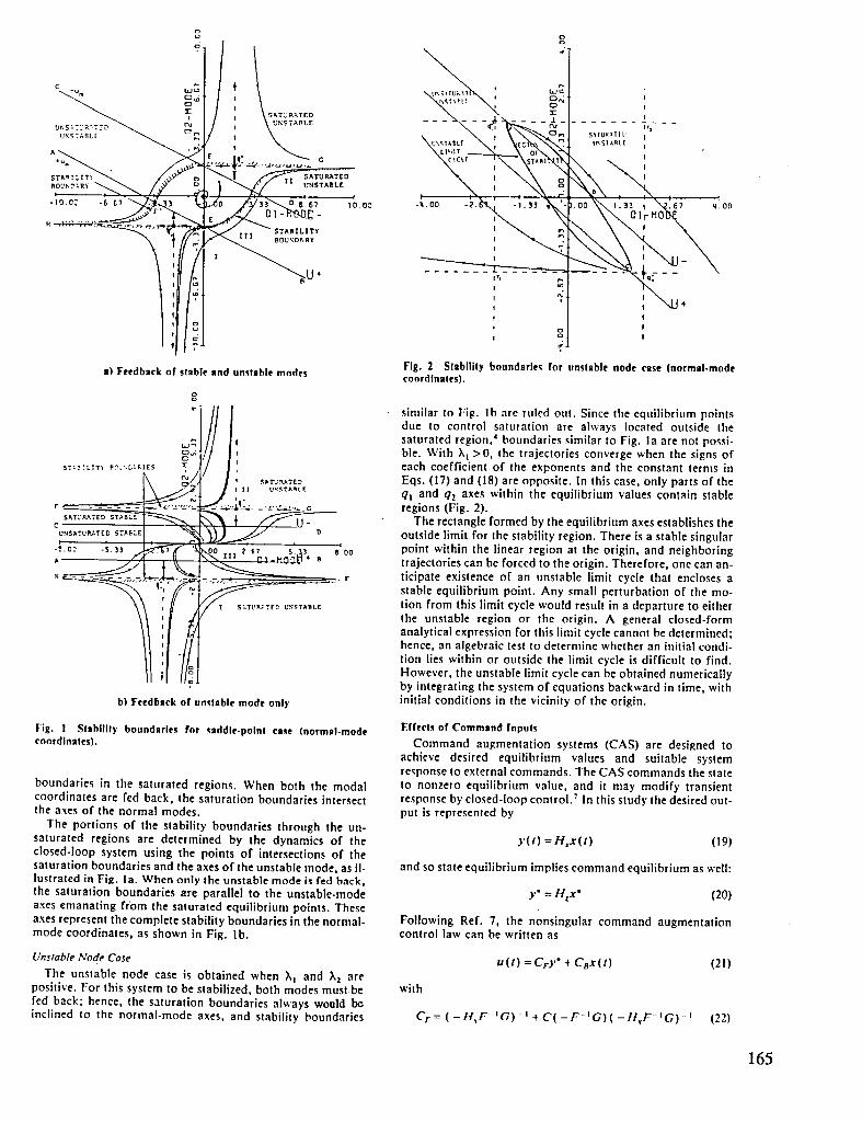
oo do

c -u u.,_ w_ .

_[r SAT_ I_Y,TED

S'_TUk _TI t'

Aq" G

"_r_ . ./_'__._ "..._',_" ".-_._"............ ,,.ST,,_::--':"_-._ /...'_ oI _T _ S^TU,_TED

-,o.o: -6_,_ _.ti._o/_.'-.._ s_6, ,o.o_ -,.- ,.o_

.STABILITY

f III BOUNDARY

a) Feedback of stable and unstable modes Fig. 2 Stability boundaries for unstable node case (normal-modecoordinates).

do

"_- similar to Fig. Ib are ruled out. Since the equilibrium pointsdue to control saturation are ahvays located outside thesaturated region,' boundaries similar to Fig. la are not possi-ble. With Xt >0, the trajectories converge when the signs of

:_: , .,_.: each coefficient of the exponents and the constant terms inEqs. (17) and (18) are opposite. In this case, only parts of theq! and qz axes within the equilibrium values contain stable

i regions (Fig. 2).

The rectangle formed by the equilibrium axes establishes theoutside limit for the stability region. There is a stable singular

'o0 point within the linear region at the origin, and neighboringtrajectories can be forced to the origin. Therefore, one can an-ticipate existence of an unstable limit cycle that encloses astable equilibrium point. Any small perturbation of the mo-tion from this limit cycle would result in a departure to eitherthe unstable region or the origin. A general dosed-formanalytical expression for this limit cycle cannot be determined;hence, an algebraic test to determine whether an initial condi-tion lies within or outside the limit cycle is difficult to find.However, the unstable limit cycle can be obtained numericallyby integrating the system of equations backward in time, with

b) Feedback of unstable mode only initial conditions in the vicinity of the origin.

Fig. ! Stability boundaries for saddle-point case (normal-mode Effects of Command Inputscoordinates). Command augmentation systems (CAS) are designed to

achieve desired equilibrium values and suitable systemresponse to external commands. The CAS commands the state

boundaries in the saturated regions. When both the modal to nonzero equilibrium value, and it may modify transientcoordinates are fed back, the saturation boundaries intersect response by closed-loop control. 7 In this study the desired out-the axes of the normal modes, put is represented by

The portions of the stability boundaries through the un-saturated regions are determined by the dynamics of the y(t) =H_x(t) (19)closed-loop system using the points of intersections of thesaturation boundaries and the axes of the unstable mode, as il- and so state equilibrium implies command equilibrium as well:lustrated in Fig. la. When only the unstable mode is fed back,the saturation boundaries are parallel to the unstable-mode y'= H=x* (20)axes emanating from the saturated equilibrium points. Theseaxes represent the complete stability boundaries in the normal- Following Ref. 7, the nonsingular command augmentationmode coordinates, as shown in Fig. lb. control law can be written as

Unstable Node Case u(t) = Cry* + Cox(t ) (21)The unstable node case is obtained when ;kt and ;_2 are

positive. For this system to be stabilized, both modes must be withfed back; hence, the saturation boundaries always would beinclined to the normal-mode axes, and stability boundaries Cr= (-II, F 'G)-t+C(-F tG)(-It,F IG)l (22)

165

CB= -C (23) Effects of Vertical-Fin-Size Reductionon Lateral-Directional Dynamics

The system's dosed-loop response to the command is des- In conventional aircraft configurations, the lateralcribed by directional dynamics normally are characterized by the Dutch

roll, roll subsidence, and spiral modes; however, reducing the._(t) = (F+ GCe)x(t)+ GCry" (24) vertical fin size alters the aircraft's response modesfl '9 With

sufficient reduction in fin size, the vertical tail contribution toThe eigenvalues and eigenvectors of Eq. (24) are associated the static directional stability derivative is reduced, making the

only with (F+ GCe), and so the choice of the command vec- nondimensional directional stability derivative C,,, negative.tor has no effect on these parameters. From Eq. (21) it is clear The yaw damping derivative C,,., control power derivati\ethat the saturation boundaries vary with changes in the corn- C,,,, and dihedral derivative Cte, are reduced in magnitude,mand vector; therefore, the stability boundaries also vary. whereas the roll derivatives and roll-to-yaw coupling deriva-Nonzero command vectors yield saturation boundaries that tires remain relatively unaffected. The effects on dimensionalare asymmetric with respect to the origin. The feedback gain stability derivatives (e.g., No) are proportional to the changesCe affects only the closed-loop eigenvalues; it has no effect on in the nondimensional derivatives (e.g., C,,). The major ira-the value of u* for a desired command. Control saturation pact of fin-size reduction is felt on Ne, which becomes nega-limits -€-u,,,determine the system's ability to achieve the com- tire, making the aircraft directionally unstable. In Ref. 10 it ismand vectors in the steady state. Desired outputs (i.e., con- shown that there always would be two unstable roots.stant commands) that cause the control to violate the limits

Numerical Models for Analysis

-u,,,<_u'< +u,,, A high-performance fighter aircraft with stable lateral-

cannot be attained. Consequently, the minimum and max- directional dynamics was chosen as a baseline model for thisimum values of the equilibrium states for the above saturation study. Nondimensional derivatives for the unstable lateral-

directional model were computed for several fin configura-limits are given by tions, assuming a sea level, Mach 0.4 flight condition. The

X_a_/mi. = +F-tGu,,, (25) dimensional stability derivatives for three fin configurationsare presented in Table !. Case I represents the stable baselinemodel, and cases 2 and 3 represent the unstable models ob-

and the maximum/minimum values of command vectors that tained by the fin-size reduction. The numerical values assumecan be commanded and achieved are given by that velocity and angles are measured in feet per second and ra-

dians, respectively. The rudder and aileron limits are fixed at'" = H,,x_ .... i,_ (26)3m,,,,,,_, .4-20 deg for all numerical calculations. The eigenvalues of the

open-loop dynamics for the fourth-order models are given inIn state-space coordinates, x" lies on a hyperplane determined Table !.by Eq. (25); therefore, command vectors produce equilibriumstates that lie on this hyperplane. At control saturation limits+u,,,, the saturated and unsaturated equilibrium pointssought by the command vector coincide, and they lie on the Table 1 Dimensional derivativeselgenvalues forsaturation boundary. Variations in the command vector three alrcrsft configurationchange the location of the desired equilibrium point andsaturation boundaries. The locations of equilibrium points Derivative Case I Case 2 Case 3with all controls saturated do not change, but the locations ofequilibrium points with one of the controls saturated change N_, -0.379 -0.209 -0.177with the commands. Because of this change in the single- Nt_ 3.740 -0.865 -2.029control-saturated equilibrium points relative to fixed all- No -0.104 -0.072 -0.070YO/ Vo - 0.258 - 0.207 - O.195control-saturated equilibrium points, the shapes and sizes of Lr 0.736 0.506 0.474the stability boundaries change with the command vector. La - I 1.98 - 5.87 - 4.98

The maximum and minimum values of attainable state L -2.51 -2.49 -2.48equilibrium depend upon the control saturation limits and the ,_€_'_, -6.21 -3.53 -2.96open-loop dynamics, and control saturation limits set bounds Nt,,, 0.287 0.287 0.289on the achievable command vector .!". Although achievable L_, 5.54 i.96 1.39command vectors are independent of the feedback gain CB, L_,, 20.12 20.12 20.12

transient response can impact the region of achievable output Eigenvalues -0.207 4j2.074 -0.857 - 1.396vectors, if, for example, the transient response to an -0.207-j2.074 0.459 1.143"achievable" command momentarily forces the state into a -2.72 -2.642 -2.647

divergent region, then the trajectories can diverge and that -0.012 0.133 0.0363command is not truly achievable.

Table 2 Minimum-control-energy gains for normal-mode and state coordlnales

Normal.mode coordinates State-space coordinates

qj q2 • B P €'

Case 2_r - 0.39 - 0.15 - 0.306 0.2'16 0.015 0.026/_a - 0.04 0.02 - 0.057 0.036 0.005 0.009

Case 3br - 1.33 - 0.06 - 0.737 0.; 0.032 0.0666a -0.24 0.06 -0.141 0.183 0.009 0.019

166

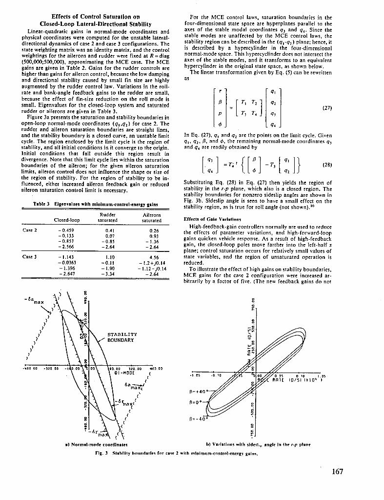
Effects of Control Saturation on For the MCE control laws, saturation boundaries in theClosed-Loop Lateral-Directional Stability four-dimensional state space are hyperplanes parallel to the

Linear-quadratic gains in normal-mode coordinates and axes of the stable modal coordinates q3 and q4. Since thephysical coordinates were computed for the unstable lateral- stable modes are unaffected by the MCE control laws, thedirectional dynamics of case 2 and case 3 configurations. The stability region can be described in the (q_-q2) plane; hence, itstate weighting matrix was an identity matrix, and the control is described by a hypercylinder in the four-dimensionalweightings for the ailerons and rudder were fixed at R = diag normal-mode space. This hypercyclinder does not intersect the(500,000;500,000), approximating the MCE case. The MCE axes of the stable modes, and it transforms to an equivalentgains are given in Table 2. Gains for the rudder controls are hypercylinder in the original state space, as shown below.higher than gains for aileron control, because the low damping The linear transformation given by Eq. (5) can be rewrittenand directional stability caused by small fin size are highly asaugmented by the rudder control law. Variations in the roll-rate and bank-angle feedback gains to the rudder are small, r q=because the effect of fin-size reduction on the roll mode is

small. Eigenvalues for the closed-loop system and saturated B I Tt T2 1 q2-- (27)rudder or ailerons are given in Table 3. P L T_ T4 J q_

Figure 3a presents the saturation and stability boundaries inopen-loop normal-mode coordinates (q_ ,q2) for case 2. The _b q4rudder and aileron saturation boundaries are straight lines,and the stability boundary is a closed curve, an unstable limit In Eq. (27), q_ and q2 are the points on the limit cycle. Givencycle. The region enclosed by the limit cycle is the region of qt, q2, B, and _,, the remaining normal-mode coordinates q._stability, and all initial conditions in it converge to the origin, and q4 are readily obtained byInitial conditions that fall outside this region result in

divergence. Note that this limit cycle lies within the saturation I q, I ([ B I [ q, ]boundaries of the aileron; for the given aileron saturation = T; _ -T s (28)limits, aileron control does not influence the shape or size of q+ €_ q2the region of stability. For the region of stability to be in-fluenced, either increased aileron feedback gain or reduced Substituting Eq. (28) in Eq. (27) then yields the region ofaileron saturation control limit is necessary, stability in the r-p plane, which also is a closed region. The

stability boundaries for nonzero sideslip angles are shown inFig. 3b. Sideslip angle is seen to have a small effect on the

Table 3 Elgenvalueswith minimum-control-energygains stability region, as is true for roll angle (not shown)) °Rudder Ailerons

Closed-loop saturated saturated Effects of Gain VariationsHigh-feedback-gain controllers normally are used to reduce

Case 2 -0.459 0.41 0.26 the effects of parameter variations, and high-forward-loop-0.133 0.07 0.93 gains quicken vehicle response. As a result of high-feedback-0.857 -0.85 - 1.36-2.566 -2.64 -2.64 gain, theclosed-loop poles move farther into the left-half s

plane; control saturation occurs for relatively small values ofCase 3 -1.143 1.10 4.56 state variables, and the region of unsaturated operation is

- 0.0363 - 0.11 - 1.2+j0.14 reduced.- 1.396 - 1.90 - 1.12-j0.14 To illustrate the effect of high gains on stability boundaries,-2.647 -3.34 -2.64 MCE gains for the case 2 configuration were increased ar-

bitrarily by a factor of five. (The new feedback gains do not

-+a "\? \

STABILITY _

,/ I Bou.D,,RY

-+°° ,,°.°°,+°.°°+,.°°, ,.o+..\/ /Jft ,0+,.,0.,

a) Normal-mode coordinates b) Variations wilh sldesl,,, angle in the r-p plane

Fig. 3 Stability boundaries for case 2 with minimum-control-energygains.

167

minimize the original cost function.) Eigenvalues for the closed-loop system and saturated rudder or aileron are given in Table 4. The eigenvalues for MCE and high-gain cases in Tables 3 and 4 show that the high-feedback-gain system is relatively more stable even with saturated rudder or ailerons. Intuitively, the size of the stability region should also increase with increased system stability. The validity of this intuition is illustrated in this example. The saturation and stability bound- aries in normal-mode and physical coordinates are shown in Fig. 4. By comparison to Fig. 3a, the size of the stability region is seen t o be increased; however. the stability boundary in Fig. 4 passes through the saturated-aileron region, and so the stability region depends on the aileron saturation limits.

Consider the case when elements in the control weighting matrices for the rudder and aileron are not the same. High (low) control weighting on rudder and low (high) control weighting on aileron result in low (high) feedback gains for the rudder and high (low) feedback gains for the aileron, respec- tively. Although not MCE, high values of control weightings ensure that there is negligible alteration of stable modes. In such cases, the normal-mode stability regions also are hyper- cylinders parallel to the axes of the stable modes. Thus, the regions of stability in the r-p planes still can be determined us- ing Eqs. (27) and (28). - .

The effects o f low rudder and high aileron weightings (and a) Normal-mode coordinates vice versa) on the stability boundaries are examined, beginning with rudder weighting of 500,000, aileron weighting of 5000, and Q = l (Table 5). Even though the rudder gains are small,

f? 0

saturating the rudder produces a right-half-plane eigenvalue; however, rudder saturation is not likely t o be a problem, as shown by the saturation and stability boundaries of Fig. 5. Saturating the ailerons also produces a right-half-plane eigen- value, indicating that the nominal, two-control system makes use of the yawing moments for both controls. The stability boundaries remain unaffected by the rudder saturation boundary, and the size of this stability region is smaller than that shown in Fig. 3.

The gains and eigenvalues for rudder weighting of 5000 and aileron weighting of 500,000 are given in Table 6, and the

05 I

Tsblc 4 Eigcnvslues with five times minlmum-conlrol-energy galns

Rudder Ailerons Closed-loop saturated saturated

Case 2 - 5.164 0.325 0.249 -0.174 - 0.333 - 0.882 - 2.642 -0.818 - 2.645 -0.174 - 2.682 - 8.443

0.306 Case 3 - 0.221 0.997 - 1.396 - 0.803 - 1.493 b) Variations with sldctlip snple in the r-p plane - 2.646 - 2.778 - 2.668 - 10.40 - 1.283 - 6.778 Fig. 4 Stabllitg boundaries lor cast 2 with five times mlnimum-

control+ncrgy grins.

Tsble 5 Control grins and eigenvalues for case 2 with high rudder weighting

Gains

Normal-mode coordinates State vector coordinates

Eigen values

Rudder saturated

Ailerons saturated

. m_

_-

r_lREGZO.or\

_ A _A REGION OF

a) Normal-mode coordinates a) .V"= (0.0,0.0)

g

:,o-=_/_,.o. =°;°-_/////._,---,o. _ /._,=,o.o,_

, . , . ._. ::. , , , . ///'_I _ STABILITY-_.os -0. o -o. ss///_ _" o._s o._o _.os t0/hl

_:_. _oLL,_,_,E,0,S,t,io,i .i.°s ..,o -Y/i_olov'//_,_]}°:,o,,,o,,:,_s

b) V|riatlons with sideslip angle In the r-p plane b) Variations with sideslipangle In the r-p plane.

I:le. 5 Stability boundaries with high rudder weighting for case 2; Fig. 6 Stability boundaries with hll_haileron weighting for case 2;R = dl=g(500,(H)O;5000). R -- dlag(5000;500,O00).

Table 6 Control 8sins and elgenvaluesfor case2 with high aileron weighting

GainsNormal-mode coordinates State vector coordinates

qi qz r B P

_r -0.44 -0.19 -0.33 0.27 0.015 0.025_a - 0.0002 0.0004 - 0.0005 0,0003 0.00005 0.00001

Eigenvalues

Rudder AileronsClosed-loop saturated saturated

- O.14 0.46 0.26-0.46 0.13 - 1.53-2.64 -2.64 -0.91- 0.86 - 0.86 - 2.64

169

g large stability region, these gains also must satisfy criteria lot___ normal operation in the unsaturated region, which may litnit

-6rma_ -6amax,.. , .,-' the acceptable gain magnitude. Except for tile case of high

)_" rudder weighting, the variations in stability regions with"J sideslip angles are small. Sideslip angle dependency could be

ignored if rolling and yawing rates could be restricted to the

k • x: _STABILITY innermost intersection of all stability regions._OUNDARY Eflects of Command Inputs

._j)_'_ Commanded inputs have an effect on system stabilitybecause they offset the desired equilibrium point from theg origin, and stability boundaries become asymmetrical. The

•t0.oo .,to.0 j- _o."_-"_ ,t0 0,, 6c.oo desired equilibrium point may lie close to a stability boundary,)or and so small disturbances can make the system unstable, lhi_

t.l"-,- is demonstrated for case 3 using a nonsingular "task-tailored"

+6amax command vector, in which yaw rate and sideslip angle arc• • commanded independently. (A more conventional command

vector would be roll rather than yaw rate; this is a singular-

• t'_ command variable in the sense of Ref. 7.) The output matrix is

rrrCt, rr¢.2_cq" _'g then H_=diag(I,l) and, with the feedback-gain matrix inTable 3, the forward-gain matrix is

-'¢ _ [ 0.378 5.762 1Cr = {29)

a) y" = 10,0,) 0.278 5.412

. The desired equilibrium states must lie within the saturationg -6amaF:)" " limits which, themselves, shift with the value of the command.,t .,!-

, ._., j)" Two sets of command vectors are considered. In the first in-.,. stance (Fig. 7a) the commands are zero. The saturation.6_ boundaries are symmetric about the origin, and the stability

boundary generated by backward integration is antisymmetric-J about the normal axes. Case 3 is more unstable than case 2,

and its stability region is, therefore, smaller. Its stabilitySTABILITYBOUNDARY boundary passes through regions in which both rudder and

ailerons are saturated.When the command is changed to y" = (2.3,1.5), the stabil-

ity boundary becomes asymmetrical, and no portion of itpasses through the region of negative aileron satuation (Fig.

40.00 -,_0.0o ,-00 _0.00 7b). Furthermore, portions of the space that were stable v.'ith+lama x

DESIRED zero command are no longer stable regions. For example, if aEQUILIBRIUM disturbance forces the instantaneous (ql,q2) point to be point

A as the pilot commands)" =(2.3,1.5), the system is unstablebecause point A does not lie within the stable region of that€,t

1..• _" command. It can be concluded that the allowable perturbation_"¢ €"¢ _" space is smaller than the zero-command stability boundary

when nonzero commands are issued. Figure 7b also indicatesthat the allowable command space is smaller than the un-saturated region of the system.

\b) .r"_ 12.3,1.S) Conclusions

Fig. 7 Variztlon In stability boundaries with commands: case 3, General conditions for stability boundaries of linear systemsminimum-control-energygains (normal-mode coordinates), containing control saturation have been presented. For linear

• control laws, saturation boundaries always appear assaturation and stabilityboundaries are shown in Fig. 6. The hyperplanesin the normal-mode space. The shape of theregion of stability is larger in size than for the high-rudder- stability boundaries depends on the type of open-loop in-weightingcasebecausehigh-feedbackgainsto therudderpro- stability.Fourth-ordermodelsof lateral-directionalaircraftvide better directional stability augmentation than feedback to motion exhibit two unstable roots that result from the lack ofthe ailerons, and the stability boundary is invariant with directional stability. Stability regions for aircraft with direc-respect to aileron saturation limits. For both cases of unequal tional instability are found to be hypercylinders in the normal-control weightings, the variation in the region of stability with mode space when only unstable modes are fed back; the stablesideslip angle is small (Figs. 5b and 6b). Because feedback regions can be increased in size by increasing the magnitudesgains from bank angle to the rudder and ailerons are small, the of feedback gain. These boundaries transform to hyper-effect of bank angle on the region of stability is small, cylinders in the original state space• For small directional in-

Comparison of the stability boundaries in Figs. 3-7 shows stabilities, variations in stability regions with sideslip and rollthat the largest regions of stability are obtained when the con- angles are small, and the innermost stability region in the rolltrol weightings on the rudder and aileron are equal and that the rate-yaw rate phase plane can represent the overall region ofsize of the stability region increases when the feedback stability. With increased directional instability, the stabilitygain magnitudes increase. The smallest region of stability is region is r, 'uced, and variations in the regions of stabilityobtained for the high-rudder-weighting case. Nevertheless, with side. ,J angle become significant. Stability regions arealthough high-feedback gains are desirable for achieving a command-dependent, and a possibility of departure exists if

170

initial ,:.,_,,itions at the time of ne_, command initiati.._n lie Conference on Information Sciences and Systems. Princeton Univ.,outside the stability region. Princeton, NJ, March 1984.

4Shrivastava, P.C. and Stengel, R.F., "Stability Boundaries forClosed-Loop Systemswith Control Constraints," Proceedings of the23rd IEEE Conference on Decision and Control, IEEE, New York,

Acknowledgments Dec. 1984, pp. 1326-1329.This research was sponsored by NASA Langley Research SSeckel, E., Stability and Control of Airplanes and Helicopters,

Center, Hampton, Virginia, under Grant NGL 31-001-252. Academic Press, New York, 1964.6Stengel, R.F., Stochastic Optimal Control: Theory and Applica-

lion, Wiley, New York, 1986.

References "lStengel, R.F., "Equilibrium Respon,;e of Flight ControlSystems," Automatica, Vol. 18, March 1982, pp. 343-348.

IHanson, G.D. and Stengel, R.F., "Effects of Displacement and 'Roskam, J., Methods for Estimating Stability and Control Deriva-RateSaturation on theControl of Statically Unstable Aircraft," Jour- tires of Conventional Subsonic Airplanes, Univ. of Kansas, Law-hal of Guidance, Control, and Dynamics, Vol. 7, March-April 1984, rence, KS, 1973.pp. 197-205. 9Etkin, B., Dynamics ofF'light: Stability and Control, Wiley, New

2Hanson, G.D. and Stengel, R.F., "Effects of Control Saturation York, 1959.on the Command Response of Statically Unstable Aircraft," AIAA _°Shrivastava, P.C., "Stability Regions of RelaxedStatic StabilityPaper 83-0065, Jan. 1983. Aircraft Under Control Constraints," Ph.D. Thesis, Mechanical and

'Shrivastava, P.C. and Stengel, R.F., "Stability Boundaries for AerospaceEngineering Dept., Princeton Univ., Princeton, NJ, Rept.Systems with Control Constraints," Proceedings of the 18th Annual 1747-T,Oct. 1986.

171

Restructurable Control Using Proportional-IntegralImplicit Model Following**

Chien Y. Huang" and Robert F. StengeliPrinceton University, Princeton, New Jersey 08544

**Published as J. Guidance, vol. 13, no. 1, March-April 1990.

Studies of • proportional-Integral Implicit model-following control law are presented. The research focuses onthe •bility of the control law to recover the performance of • system with failed •ctu•tors or structural d•mageto Its prefailure level. Properties of the Implicit model-following strategy are examined, and conditions forcontrol recon figuration are stated. The control law Is •pplied to the lateral-directional model of • fighter •lrcraft,and control restructuring Is shown for changes In control and system matrices. It is concluded th•t the Implicitmodel-following scheme Is • good candidate for control reconfiguration.

Introduction designed with the same Q and R will have different closed-loop

AULT-TOLERANT control systems typically have one or characteristics. Although the original cost function is, by deft-more of three attributes: robustness, reconfigurability, nition, still optimized, the resulting response may no longer beand restrueturability. Robustness implies insensitivity to varia- adequate in a subjective sense. If similar system behavior istions in the parameters or structure of the system. If physical desired before and after the failure, it would be necessary inparameters change or the nature of system dynamics is altered, most cases to find new values of Q and R, which may be athe robust system continues to operate as originally intended, nontrivial selection process.providing response to inputs and disturbances that is close to Model following is an attractive candidate for the redesignnominal performance. Reconfigurability implies that some of process because the goal is to emulate the performance charac-the control system's parameters can be purposely modified to teristics of a desirable model, with or without failures. Thisaccount for uncontrollable changes in the system, such as can be accomplished explicitly (by requiring the system out-failed sensors, actuators, or damaged structural elements. Re- puts to follow those of the model in a least-squares sense) orstructurability subsumes reconfigurability, implying that not implicitly (by minimizing a quadratic function of the actualonly parameters but the structure of the system itself can and modeled state rates). 2.-_Explicit model following normallybe changed to accommodate uncontrollable changes. Whereas is less sensitive to parameter variations, but the model statesthe robust system obtains fault tolerance with fixed parameters must be generated, and feedback gains may be high for satis-and structure, reconfigurable and restructurable systems are factory performance. Implicit model following can be imple-adaptive, providing some degree of fault detection and identi- me•ted more simply with lower gains, and the weighting ma-fication as well as the ability to alter the system. The latter trices are directly affected by the difference in plant and modelshould achieve satisfactory performance over a wider range of dynamics. Consequently, the effective Q and R of the LQconditions than is obtained by robustness alone; otherwise the problem can be adjusted by known changes in plant dynamicsadded complexity is not warranted. This paper presents a so as to minimize the variation in closed-loop performance.linear-quadratic (LQ) control strategy that is robust and that Model-following criteria were discussed by Erzberger, z whoallows control restructuring to be carried out in a natural showed that explicit and implicit model following are equiva-fashion, lent provided certain conditions are satisfied. The synthesis of

Linear-quadratic control theory inherently provides a num- model-following systems was addressed by Tyler? who ana-ber of useful features, such as direct treatment of multi-input/ lyzed feedback and feed-forward gains in terms of plant andmulti-output problems, easy transfer from continuous- to dis- model characteristics. Chan 4 examined the relative merits ofcrete-time descriptions, and guaranteed stability when certain explicit and implicit model-following controls and concludedcriteria are satisfied. I However, the choice of quadratic state- that the former yielded smaller steady-state error when imper-and control-weighting matrices (Q and R) is not always obvi- feet model following occurred. Asseo _ formulated a type-oneous. This problem is of particular concern when a control perfect model-following control law and found that it reducedsystem is to be reconfigured or restructured in real time follow- sensitivity to parameter variations. Kreindler and Rothschild 6ing failures. Suppose that the chosen Q and R lead to desirable also compared both model-following str.ategies and found thatclosed-loop characteristics for the nominal system (described the implicit model-following method tracked the model better,by system and control matrices, Fn and Gin). If failures cause especially during the initial transient. Broussard and Berry 7the open-loop system to change (to F2 and Gz), a controller considered a different formulation of implicit model follow-

ing, in which feedback gains are determined from algebraicrelationships. They showed that the approach is equivalent topole-placement techniques. Kaufman s employed model-fol-lowing concepts in the design of adaptive control systems.

Prcsented as Paper 87-2312at the AlAA Guidance, Navigation, and Digital implicit model following was studied in Ref. 9, andControl Conference, Monterey, CA, Aug. 17-19, 1987;receivedDec. flight test results for a simple algebraic design method arel, 1987; revisionreceived Dec. 23, 1988.Copyright © 1989AmericanInstituteof Aeronautics and Astronautics, Inc. All rights reserved, presented in Ref. 10.

*GraduateStudent, Department of Mechanicaland AerospaceEn- The subject of restructurable control is an area of ongoinggin€€ring;currently with Grumman Corporation. research. Huber et al. Ij designed a self-repairing control sys-

?Professor, Departmentof Mechanicaland AerospaceEngineering. tern that utilized a control mixer concept to distribute controlAssociate Fellow AIAA. authority after a surface failure to remaining effectors. Os-

173

troff and Hueschen 12applied a command-generator-tracker/ and the cost function becomesproportional-integral filter control law to a commercial air- _.

plane with control surface failures and under turbulence, j= I [I I"[AxrZAx_4 2Axi°SAu +Au'RAu]Idt (10)

Looze et al) _reported on an automatic redesign technique that 2 .,o •restructures control such that a frequency-domain system per-formance metric is maximized, where

mo <,,o,,ow 01 I 0,]ing (PIIMF) control law is outlined, and associated features Z = , S =are discussed. Some properties of the implicit model-following Q_scheme and conditions for control reconfiguration, given

and Qt is the weighting on _. The LQ control obtained bychanges in control and system matrices, are examined. PIIMFcontrol is applied to an example problem based on the lateral- optimizing Eq. (10) is

directional motions.of a typical fighter aircraft. Automatic [ ]

restructuring is illustrated for the changes that might be Au(t)=-CAxo(t)=-[C_ C2l[fix(t)i (11)brought about by control actuator failures or aircraft struc- _(t) Jtural and aerodynamic damage. The results are summarized inthe conclusion. Expanding and rearranging Eq. (1 !), we get

Control Law Formulation u(t) = uo- Cdx(t)-xol + c2 _(0)+ dr (12)Thesystemto becontrolled,thedesireddynamicmodel,and

the cost function to be minimized are, respectively, We can see that the second term on the right side provides pro-portional feedback of the error, whereas the third term pro-

Jr= Fx + Gu (I) vides the integral effect being sought. The dimension of thecommanded input .va is chosen to equal the dimension of u,

Jr,, = F,,x,, (2) reflecting the fact that the number of controllable states isequal to the number of the controls available)

I (Jr_Jr,.)rQ.(Jr_Jr,.) dt (3).t =_ .0 Properties of the Control Lawor We first examine the effect of adding the integral loop. The

steady-state Riccati equation resulting from optimizing Eq.

11:"[xrQx+2xrMu+urRuldt (4) (lO) is2=_ 0

where x and u are actual state and control vectors of dimen- __PI_ PIIJ Isions n x I and r x I, respectively, x,, is an n x I model state

vector, Fand G are system and control matrices for the system [(F 0) [G] [ ]]rlPti P,21to be controlled, F,,, is a model matrix, and Q_ is a weight- -4- - R-i Air 0ing'matrix for the state-rate errors. Substituting Eqs. (I) P[ P22J

and (2) into Eq. (3), and assuming that x = x,,, , leads to Eq. (4), [PH PI2][G] I[Gr ][PI, P,2]where Q=(F-F,,)rQ,(F-Fm), M=IF-F_,)rQ, G, and -[p,r P22] R- 0 pr P.'2]R = GrQ, G. From Eq. (4), we see that the PIIMF controller

generatesacross-weightingmatrixM. Considering optimality (Q0 0)[_0 !] [ ]and pole-assignment requirements, i4'i_ the presence of M is + - R -i M r 0 = 0 (13)essential for achieving complete control over the system. Q_ -

Equation (4) is simply a quadratic cost function of the orig- Expanding along each submatrix, we getinal system [(Eq. (1)]. In addition to the inherent sensitivity

to plant parameter variations,S we can improve the Iow-fre- Pl i(F - GR - IM 7) + (F - GR - IM r)rPi t _ P,IGR - iG TPllquency disturbance-rejection characteristics of the control law

and achieve zero steady-state error command response by add- + Q - AIR -tMr + Pt2H + ItrP r = 0 (14)ing proportional-integral (PI) compensation. Let .vabe the de-

sired equilibrium outputs; then the perturbations around the P[(F-GR -tMr) + P22H - prGR -'Grptl = 0 (15)corresponding set point (x0, u0) are

Ax(t) = x(t) -Xo (5) -PirlGR -IGrPi2 + QI = 0 (16)

The Riccati equation obtained by optimizing the implicitAu(t) = u(t) - uo (6) model-following strategy alone IEq. (4)1 is:

Ay(t) = y(t) - .t'a (7a) P(F - GR -IMr) + (F - GR -IMr)rP

= Hx(t) -ya (7b) - PGR-iGrp + Q - MR-IMr = 0 07)

where H is the output matrix. The output error integral _ is Therefore, the effect of the integration loop is to add the termsdefined as PllH+HrPi r. Since from Eq. (16) we see that PI2 is deter-

, mined by G and Qf, and it is independent of Pit and the model,= _(0) + Ay(r) dr (8) these extra terms constitute a shift or "bias" in state-weightingdO Q.

We now proceed to the analysis of the implicit model-fol-The state variable is augmented to include _, lowing strategy, making comments on the integrator effect

IF 0] [Go] whenever necessary.1f G were invertible (which would requireAJr,(t)= [Air(t) _r(t)]r= Ax,(t)+ Au(t)(9) the number of controls to be equal to the number of states) andQ_were diagonal, then from the definitions of Q, M, and R,

174

(F-GR-'I_Ir)=F-GR-"[(F-F,,,)rQ, G]r (18a) whereG"tistheweightedleftpseudo-inverse'ofG.Whenthestructure of the control matrjx G (of rank r) is such that it

=F-GR-tGTQ,r(F-F.,) (18b) contains an rxr submatrix much larger (in the two-normsense) than the remaining submatrices, and Q, does not change

= F - G(G rQ, G)-tG rQ,r(F-F,.) (18c) the inequality by its choice of weighting, it can be shown 16that

= F-GG-tQ,-IG-rGrQ,(F-F,,) (18d) GG "'1 _ In, (27)

= F- F + F,,, (1Be) where 1,, is a matrix of dimension n xn with • ones in thediagonals and zeros everywhere else. Physically, the require-

= F,,, 080 ment is that • controls have a stronger effect on • state compo-nents (e.g.t the angular rates) and weaker effect on the remain-

GR-,Gr= GR-JGrQ, Q-I = Q,-I (19) ing states (e.g., the angles). Moreover, let l_r be the "com-plement" of 1,,,; that is, I.'. =(I,, -In.), where I,, is the n xn

MR-tM r= (F-Fm)rQiG(GrQ, G)-tGrQ,(F-F,_) (20a) identity matrix: then Eqs. (18) and {20) become

= (F-F,_)rQiGR -IGrQ_(F-F_,) (20b) F - GR -t._f7 = F - GR -IGrQi(F-F,_) (28a)

= (F-F,_)rQ,(F-F,_) = Q (20c) -- F - I,,(F-Fm) (28b)

We have intentionally isolated the term GR -tGTQ,, which is = I_.F,. + lS..F = F" (28c)equal to the identity matrix in this case; its significance willbecome apparent later. Inserting the last three relations into MR- II_tT_ (F-F,.)TI.,Qi(F-F..) (29)Eq. 07), we get

PF,_ + Frp- pQ-tp __0 (21) If we let Q'= Q-(F-Fm)rI_rQ_(F-Fm), the Riccati equa-tion [Eq. (13)1 can be approximated as

This can be construed as a Riccati equation resulting fromoptimizing a model of the form x,,, =F=x,_ +u_, for a cost PF" + F'rp- PI,,Q,-'P + Q' = 0 (30)function consisting of no state weighting and Q, controlweighting. Assuming F,,, is stable, the unique solution to this where F" is defined by Eq. (28). The gain and closed-loopequation is P = 0, which means u,,, = 0; thus, the model system system matrices areis recovered. The feedback gain C and closed-loop system F. ofthe original system become C = G "t [Q,- tp + (F- F,,,)] (31)

C = R-t(Grp + Af r) (22a) F. = i_.F., + ff..F - I..Q,-IP (32a)

= O-'g,-'O-T[GrQ,(F-F..)] (22b) = F ° - I_,Q,-'P (32b)

= G-t(F-F,,,) (22c) = Iw.,(F-F,.) + F,. - I.,Q,-ip (32c)

Fc = F- GC = F.. (23) We note that this development bears resemblance to theTherefore, the gain would be proportional to the available perfect model-following condition as stated by Erzberger _control authority and to the difference between plant andmodel dynamics, whereas the closed-loop dynamics would (GG t -I)(F-F,,)= 0 (33)simply become those of the model. Not surprisingly, Eq. (22)is identical to Erzberger's perfect model-following control From Eq. (28) [or Eq. (18)]. we havelawfl When the integral loop is present, P is no longer zero,and we have GR -IMr = GR-IGrQi(F-F,_) = I_,(F-F=) (34)

C=R -_ IG r 0lip r

[R-'Orp,,+G-'(F-F_) R-'Orp,] (24b) 0= (OR -'Gr@-I,,)(F-F,,) (35a)CL J

= (GG n't-I,,)(F-F_) (35b)

o] The closer GR -_G rQ, is to the quasi-identity matrix I,,.. the

better the plant behaves like the model; the closeness also+ G- I(F-F..) R -tGrp,2 (25a) affects the control restructuring strategy to be described later.As will be shown, Eq. (35a) is one of the control reconfigura-

t.Qt- -JPn[ tion criteria. The effect of the integrator is similar to the caseFr = Fm--.o IPll --QO a (25b) where G has full rank. This can be seen by computing Pt2 from

"1

Hence, the gain is no longer given by Eq. (22), and the closed- Eq. (I 6) using I,,,Q_- i in place of GR - IG r and substituting theresult into Eq. 03).loop system characteristics, as indicated by the damping and

transient behavior, will be diffet:ent from that of the model.

Both attributes are functions of Pm which is determined by Effects of Control Reconfigurationthe weighting matrices Qt and Q, through Eq. (16). Reconflgurttlon with VmrimtionsIn Control Effect

Consider now the term GR -tG rQ_ in the more typical case One case of interest is the degradation of a control effector.with fewer controls than states, This type of failure can be approximated by reducing a column

GR-tGrQi = G(GrQ_G)-tGrQi (26a) of the control matrix by a common factor. This is equivalentto an elementary row operation of matrix algebra. Let E = diag

=GG "'t (26b) [I l.-.t_...l],cr>0, where ot is the factor by which the

175

effectiveness is reduced. If G' (= GE) is the new control ma- lhu_, the gain is altered, but the closed-loop system remainstrix. the weighting matrices and Eqs. (Ig-20) then become essentially the same. As can be seen from Eqs. (32) and (44).

the reconfiguration may not recover the performance if F ischanged along the zero rows of I,,,; that is, the following re-

R' = G'rQ, G ' = ErGrQiGE -- ETRE (36) lation must hold:

M' = (F-F_)Q,G' = ME (37)I*.,(F" -F.,) _ I_,(F-F.,) (45)

(F-G'R'-_M 'r) = (F-GEE-IR -tE-TETM) OSa)

= (F- GR - tMr) (38b) This equation constitutesthe other reconfiguration criterion tobe applied in the case of system dynamic changes. Note that

G'R' - tG" = GEE - IR - tE - TE TG = GR - 'G r (39) since PJ2does not depend on F, changes in the system dynam-ics have no effect on the integral loop.

M' R' - IM" r = MEE- iR - iE- rE rM = MR - tMt (40) Failures are unlikely to cause alterations in the manner de-scribed. Single- or multiple-element failures bydifferent fac-tors are expected, if the reconfiguration criteria are satisfied,

Hence, there is no change in the Riccati equation (Eq. 13 or then the performance will be recovered when the gains are re-Eq. 17). As expected, the gain is altere_ since R is decreased so calculated using F' ( = F + cSF).as to allow additional control activity, but the closed-loop We point out here that reconfiguration is possible withsystem remains unchanged: GR -tG rQ_ not close to I_,, although acceptable performance

may require it. if the expression exhibits a nonidentity matrixC' = R'-I(G' rp + M,r) (41a) structure, then the model is not well followed; consequently,

the performance of the reconfigured system would not be near= E-IR -IE- T(E rG rp + E TM) = E-tC (41b) its nominal values. Moreover, since Ptz does not depend on F,

changes in the system dynamics have no effect on the integralF/= F - G'C" = F - GEE-IC = F - GC = Fc (42) loop; therefore the analysis carries over to the PIIMF control

law. This and other observations are verified numerically in

Since the integral effect enters only through Ptz [Eq. (16)], the next section.\_hich is unaffected by this type of failure, the analysis holds.

The control restructuring process is now clear. When the gains Simulation Resultsare recalculated with G', the original system performance isrestored. Note that these results are independent of the invert- The analysis described in the previous sections is applied toibility of G. the lateral-axis model of the F-4 aircraft. The state vector

If ct = 0, reconfiguration is addressed simply by reducing the consists of roll rate p (rad/s), yaw rate r (rad/s), sideslip Bcontrol vector dimension and adjusting G, R, and M accord- (fad), and roll angle $ (fad); i.e., x = Lor B sir. The controlsingly. In this situation, it is important to insure that control- are rudder _r(in.) and aileron _a(in.); i.e.. u = [_r _a] r. Thelability has been retained with the reduced-dimension con- system, control, and model matrices are6troller.

The effects of single- and multiple-element changes are more [-- 1.768 0.415 - 14.25 0.0 ]difficult to analyze since they no longer can be represented as / ielementary matrix operations. However, Eq. (26a) [or equiva- / -0.0007 -0.3831 6.038 0.0

lently Eq. (35a)1 can still be computed using G" (=G +_SG)in F = |_ 0.0016 -0.9975 -0.1551 0.0586 (46)place of G. As long as the equality [Eq. (27)1 (approximately) |

holds, the controls can force the plant to behave like the [ 1.0 0.0 0.0 0.0 Jmodel. Otherwise, the control matrix must have undergonesubstantial changes, such that the original performance cannotbe approximated by the implicit model-following strategy.

1.744 8.952-2.92 -0.3075

Rrcnnfiguratlonwith Variations in System Dynamics G = (47)%stemdynamicscouldchange, for example,as a conse- ] 0.0243 -0.0036

quence of structural damage. We first examine the reconfigu- t/ 0.0 0.0ration when a row in F changesby a common factor. Row 1_changes are equivalentto premultiplicationby the elementarymatrixE; thatis, F' = EF. If G is invertible,then the previousa,alysis holds, and the performance can be recovered by sire- [--4.0 0.865 - 10.0 0.0ply recalculating the gain using F' instead of F. For nonsquare /G, _shen the changes are along the nonzero rows of I,,,, Q and 0.04 - 0.507 5.87 0.0 (48).\f are modified such that the solution of the Riccati equation F,,, = 1 0.0016 - 1.0 -0.743 0.0586[Eq. (13)] is not significantly affected. In this case, the gain |and the closed-loop system are L i.0 0.0 0.0 0.0

C= R-I(Grp + M 'r) (43a)Q_ = diag[0.01 0.01 0.01 0.01] (49)

G "L[ @- tP + (F' - F,,,)] (43b)QE = diag[I.0 !.0] (50)

[_' _ F" - GC -- El: - GG"tQ_-I P - GG_L(EF-F,_) (44a)The speed of response is determined by the ratio of Q, to Qt"

l_,F,, - l_,EF - I_,Q,-IP (44b) The weighting matrices as shown are chosen to produce rea-sonable tracking; no extensive search for other combinations

- I'_,lF' -F,,) + F,,, - I,,Q, tP = F_ (44c) was conducted.

176

For this system, Eq. (,26a) is found to be

1.0 -6.34× l0 -6 -0.0007 0.0]

-6.256 x 10 -6 !.0 -0.00874 0.01 (51)

GR-_GTQ' = -0.0007 -0.00874 7.7x l0 --_ 0.0

0.0 0.0 0.0 0.0

This can be seen to be approximately equal to 122.Therefore, a loss of aileron surface area that decreases the available roll-two model states (p and r) can be followed, and the reconfig- ing control moment. The failed response is shown as a brokenuration is expected to work well for changes that affect primar- curve in Fig. I. The reconfigured system response is shown asily these two variables, the bold-face curve. Notice that the yaw and roll angle re-

The time histories of the rudder, aileron, sideslip, and roll sponses of the failed and unfailed systems are indistinguish-angle subject to a I rad roll-angle command and 0.5 rad side- able, whereas the aileron exhibits higher activity with no visibleslip (a rather unusual maneuver) are used as performance eval- change in rudder motion. Corresponding gains Ct and C2 foruations. Several failure cases are examined here. this and other cases are listed in Table I.

CnseI Cnse2

Aileron effectiveness is reduced by half; that is, the second The first row of the Fmatrix and the secondcolumn of G arecolumn of G is multiplied by 0.5. This failure is equivalent to reduced by half. This corresponds to an overall decrease in

nominal and recontigurod responses tailed response reconfigured response

b

o+ ta_led,esponse __- nominal,espoose

/--o o*

time. sec time. sec

_- reconfigured response nominal response

.C_ 1 .......... "............ .C_ 1

€5. gured response

2 4 6 8 rO 2 4 6 B 10

time,sec time, sec

+ t /nominal and reconfigured responses tailed response

_ c:;"f.," "--'-f=ile'd,reI _*'-""*'_**" sponse _ """""'""

-- "_o "" ...... • -'- .....

"oP+

nominal and reconfigured responses

• _ , +' ; to 2 4 ; ; ,otime.sec time,sec ..

nominal lind reconfigured responses ""''", _ failed response

ile response _o.u_ esponsos_. o-

oo 2 4 ; ; 10 2 4 S ; 1o

t;me.sec time,sec

Fig. ! ControlIn8 stliteresponsesof theflillure ¢lise1. Fig. 2 Controllind st=reresponsesof the fliilure ¢lise2.

177

Table ! Control Rains for sample scenarios

Scenario Ct Cz

No failure -0.3892 - 1.07871 1.99 - 1.9472 2.9054 - 1.95case 0.517 0.272 - 1.1484 1.36625 0.024 1.3282

Failure -0.3892 - 1.0787 • 1.99 - 1.9472 2.9054 - ! .95case I 1.034 0.544 -2.3 2.7325 0.048 2.656

Failure -0.4 - 1.077 1.909 - 1.948 2.905 - 1.95case 2 1.235 0.497 -0.6733 2.7325 0.0485 2.656

Failure -22.181 -32.4 108.94 - 122.3106 147.287 -152.09case 3 -3.741 6.331 -21.806 23.696 -27.914 30.43

Failure -0.312 -0.795 4.16 - 1.477 3.28 - 1.217case4 0.53 0.1893 - 1.823 1.417 -0.286 1.297

aerodynamic forces and control effectiveness that contribute system performance cannot be totally restored, and the systemto the roll rate, as might result from battle damage to the behavior will depend on how well the remainder of the controlswings. The failed and reconfigured responses are shown in Fig. can achieve the model following.2. Note that the control activity is less in the reconfigured casesince the ratio of control to the aerodynamic effectiveness islarger than that of the nonfailed system. __

reconfigured response

1Case3 _:

The (2,1) element of G (proportional to the aileron yaw ¢-._.effectiveness C,u) is reduced from -2.92 to -0.1 (a signifi- _ _,:

cant change). This cross-coupling alteration may be one of the _ _ faiMd[, responsemany other changes induced by damages; it is isolated here to e- - ........

illustrate its effect. The responses are shown in Fig. 3. For this _,: ................ V-'-o'nm,n'_';-';spolr nso

failure, GR-IGrQ, is: ....2 4 6 8 101

i.0 -0.0003 -0.0012 0.0 / time.sec

J-0.0003 0.934 -0.2484 0.0

GR-tGTQ, = -0.0012 -0.2484 0.0661 0.0 (52) ___ t

"7: _ ..........................no.m_'nall response00 00 0.0 0.0 f ...............0 ,n "till failedresponseBecause the expression departs from its quasi-identity-matrix _ ,-

structure, the reconfiguration is unable to recover the original o ,7_response. ,, *'ttl_ reconfiguredresponse

i- ",,,...

The third row of the system matrix is reduced by a factor of time. sec0.25. The responses are shown in Fig. 4. For this case, Eq. (45)no longer holds, and we expect the reconfiguration to perform °.

poorly. The integral compensator still forces zero steady-state o :_rec°nfigured response

not a physically realizable case since it involves changing a o .pure integration factor. It is used here to illustrate the impor- d_'tance of reconfiguration criterion 2. A more realistic scenario _ ° '"u ....................

and additional cases can be found in Ref. 16. _ o° ..........A few additional observations are due. GR-tGTQi re- 6 [

failed responsemained close to/22 despite the changes in the first two failure _cases where control restructuring performed well. When

7 4 6 8 10

aileron effectiveness was reduced, the reconfigured system time, secsimply increased the aileron motions with no apparent changein rudder activity. This is because the rudder is an ineffective "4

surface for roll control at this flight condition. In a more _ _] failedresponse

cross-coupled system, the control activities would be more ..... [evenly reallocated. To reduce control motions, control-limit- ..'" "............................ing criteria can be incorporated into the cost function. ..'" .......

Similarly, model uncertainty can be taken into account by _ Iloop-shaping techniques at the outset; however, robustness ,_ Iproperties are altered by control reconfiguration. The integral o. nom*na! _nd rnconhgur_d ro_oon_ns

effect is largely unaffected by the failure, even though the //response is different due to different plant dynamics. No up- , ,dating of Qt is necessary if the ratio of the integration rate and _ 4 6 _ _oerror feedback is to be preserved. Complete control failures t;me, secwere not illustrated, but it can be shown (see Ref. 16) that Fig.3 Control and stile responses of the failurecase 3.

178

The implicit model-follo_sing strategy reconfigures the sys-nominal response tailed response tem by rearranging the weighting matrices to preserve closed-

[ J loop characteristics. This is analogous to a pole-placement._ ............. , , technique that assigns the closed-loop poles to the same Ioca-

.....- tions before and after the failure. Hay, ever, implicit modelfollowing does more than positioning eigenvalues and match-_ ing desired eigenvectors; it also addresses command response,o

which is not totally specified by eigenvalues and eigenvectors.

The advantages of the model-following scheme are that, fol-d lowing partial control failure or changes in the system dynamic

€ _ _ lo characteristics, it attempts to maintain the desired eigenstruc-time,sec ture and command response, and at the same time, it allows

-- tradeoffs between control activity and system response.

nominal response .;'"-'"", _ faired response

ode'".... ---' This work was performed under Contract DAAG29-84-K--_ 0048 for the U.S. Army Research Office.t5

References

c, uStengel, R., Stochastic Optimal Control." Theory and Application,:' " _ _ 10 Wiley, New York, 1986.

time. sec _Erzberger, H., "On the Use of Algebraic Methods in the Analysis-- and Design of Model Following Control System," NASA TN D-4663,

1968.

nominal response tailed respons.a ]Tyler, J., Jr., "The Characteristics of Model-Following Systems as

[ .-"''"-. / Synthesized by Optimal Control," IEEE Transactions on Automaticd'q L .. . Control, Vat. A('-15, June 1970, pp. 326-333.

4Chan, Y., "Perfect Model Following with a Real Model," Joint•-o- _ • ......... ",• " t'" -''" .... "''

A uromatic Control Conference Preprints, Inst. of Electrical and Elec-

,ooont, " I tronics Engineers, New York, 1973, pp. 287-291.

ured response -_Asseo, S., "Application of Optimal Control to Perfect Model-Fol-lowing," Journal of Aircraft, Vol. 7, No. 4, 1970, pp. 308-313.

o - . , , , 6Kreindler, E., and Rothschild, D., "Model-Following in Linear2 ,t f; _ lo Quadratic Optimization," AlAA Journal, Vol. 14, No. 7, 1976, pp.

time, see 835-842.

.=-_ 7Broussard, J., and Berry, P., "The Relationship Between Implicit

failed response nominalresponse Model Following and Eigenvalue Eigenvector Placement," IEEE

I Transactions on Automatic Control, Vol. AC-25, June 1980, pp. 591-.'""'"" l 594.o --'---..

9Stengel, R., "Digital Flight Control Design Using Implicit Model_o" Following," AIAA Paper 73.844, Aug. 1973.

t°Grunwald, S., and Stengel, R., "Design and Flight Testing ofDigital Direct Side-Force Control Laws," Journal of Guidance, Con-

o trol, and Dynamics, Vol. 8, No. 2, 1985, pp. 188-193.:, 6 s _o tIHuber, R. R., et al., "Self-Repairing Digital Flight Control Sys-

time, sec tem Stud)'," Air Force Flight Dynamics Lab., Wright-Patterson AFB,OH, TR (draft), Pt. I, July 1984.

Fig. 4 Control and state r_ponses of the failure cm_e4. n2Ostroff, A., and Hueschen, R., "Investigation of Control LawReconfigurations to Accommodate a Control Element Failure," Pro-ceedings of the American Control Conference, Inst. of Electrical and

(_onclusions Electronics Engineers, New York, June 1984, pp. 1746-1754.n_Looze, D., Weiss, J., Eterno, J., and Barrett, N., "An Automatic

An implicit model-following control strategy for restructur- Redesign Approach for Restructurable Control System," Proceedingsing a control system following control-effector failures and of the National Aeronautic Electrical Conference, Inst. of Electricalalterations in system dynamics has been presented. Examina- and Electronics Engineers, New York, May 1985, pp. 570-577.tion of the inherent properties of the control scheme led to the t4Krelndler, E., and Jameson, A., "Optimality of Linear Controlformulation of two reconfiguration criteria that, if satisfied, Systems," IEEE Transactions on Automatic Control, Vol. AC-17,guarantee the performance recovery of a failed system when 1972, pp. 329-351. .--the feedback gains are recalculated using the new dynamics, n_Hedrick' J'' and Youcef-Toumi, K., "Exact Muhi-lnput Pole

Placement by Linear Quadratic Sytqthesis," Proceedings of the Amer-Care must be exercised in applying the strategy since, in some ican Control Conference, Inst. of Electrical and Electronics Engi-cases, higher demand is placed on the remainingcontrol au- neers,NewYork,June1983,pp.905-910.thority. However, when properly used, the proportional-inte- n6Huang, C., "A Methodology for Knowledge-Based Restruc-gral implicit model-following control law is a good candidate turabl¢ Control to Accommodate System Failures," Ph.D. Thesis,for control reconfiguration. Princeton Univ., Princeton, N J, 1989.

179

STOCHASTIC STABILITY AND PERFORMANCEROBUSTNESSOF LINEAR MULTIVARIABLE SYSTEMS

Laura E. Ryan* and Robert F. Stengel **

Department of Mechanical and Aerospace Engiwwcri,uPrinceton University

Princeton, N.J.

ABSTRACT

Stochastic robtt_tness, a simple technique used to estimate applied to these criteria giving probabilistic bounds onthe robustness of linear, time-invariant systems, is applied to a individual scalar performance criteria. Metrics resulting fromsingle-link robot arm control system. Concepts behind stability and perfomaance robustness can be related to controllerstochastic stability robustness are extended to systems with parameters, thus providing a foundation for design tradeoffsestimators and to stochastic performance robustness, and optimization. Details of these extensions and uses ofStochastic performance robustness measures based on classical stochastic robustness are described in the following and aredesign specifications are introduced, and the relationship illustrated by means of an example.between stochastic robustness measures and control systemdesign parameters is discussed. The application of stochastic STOCIIASTIC STABILITY ROBUSTNESSperformance robustness, and the relationship betweenperformance objectives and design parameters aredemonstrated Stochastic stability robustness of a linear, time-invariantby means of the example. The results prove stochastic (LTI) system was described in [31 and is summarized here.robustness to be a good overall robustness an" "ismethod that Consider a LTI system subject to constant-coefficient control:

can relate robustness characteristics to con. ._temdesign x(t) = F(p)x(t) + G(p)u(t) (1parameters.

INTRODUCTION y(t) = ll(p)x(t) (2u(t) = Uc(t) - Cll(p)x(t) (3

Standardlinear control system design techniques rely on

accurate models of the system to be controlled. Because x(t), u(t), y(t), and p are state, control, output, and parametermodels are never perfect, robustness analysis is necessary to vectors of dimension n, m, q, and r, respectively, accompanieddetermine the possibility of instability or inadequate by conformable dynamic, control, and output matrices that mayperformance in the face of uncertainty. Robustness to theseuncertainties, parametric or unstructured, is normally treated be arbitrary functions of p. Uc(t) is a command input vector,deterministically and often without regard to possible physical and, for simplicity, the (m x n) cor.trol gain matrix C isvariations in the system. Consequently, overconservative assumed to be known without error. The n eigenvalues, _.i=control system designs, or designs that are insufficiently robust _i+jtoi, i= 1 to n, of the matrix [F(p) - G(p)Cll(p)]in the face of real world uncertainties are a danger, determine closed-loop stability. The control gain matrix C is

designed using some nominal or "mean" value of the dynamicStochastic robustness, a simple technique to determine the model, denoted F, G, and II, that represents F(p), G(p), II(p)

robustness of linear, time-invariant systems by Monte Carlo evaluated at the nominal parameter vector. The actual systemmethods was introduced in [i] and presented in detail in [2,3]. has an unknown description, denoted FA, GA, and IlA thatThese references described stochastic stability robustnessanalysis and introduced the probability of instability as a scalar depends on the actual (unknown) value of the parameter vectormeasure of stability robustness. Confidence intervals for the p. Environment, variations in the nominal state, systemscalar probability of instability were presented, and the failures, parameter estimation errors, wear, and manufacturingstochastic root locus, or probability density of the closed-loop differences all can contribute to mismatch between the actualeigenvalues, has shown to portray robustness properties system and that used to design the controller. The parametergraphically. Because it is a statistical measure of robustness, vector p is assumed to have a known or estimated probabilityand because it directly uses knowledge of the statistics of the density function, denoted pr(p), that expresses the statistics ofphysical parameter variations, stochastic robustness is parametric uncertainty due to the above factors.inherently intuitive and precise. The physical meaning behindthe probability of instability is apparent, and overconservative System stability requires that no eigenvalues have positiveor insufficiently robust designs can be avoided. Applications real parts. While the relationship between parameters andof stochastic robustness to analyzing full-state feedback aircraft eigenvalues is complicated, estimating the probability ofcontrol systems were described in [4.1. The results presented instability (_) of a closed-loop system from repeated eigenvaluethere illustrated the use of stochastic stability robustness calculation is a straightforward task. Using Monte Carlotechniques in comparing control system designs and in evaluation, the closed-loop eigenvalues are evaluated J timesincluding finite-dimensional uncertain dynamics.

with each element of pj, j = i to J, specified by a random-Concepts behind stochastic stability robusmess can be number generator whose individual outputs are shaped by

easily extended to provide insight into control system design pr(p). The probability-otLinstability estimate becomesfor performance. Design specifications such as rise time, increasingly precise asJ becomes large. Then,overshoot, settling time, dead time, and steady-state error arenormally used as indicators of adequate performance and lend N(o'max < 0)themselves to the same kind of analysis as described above. Pr(stability) -- lim j (4Concepts of stochastic stability robustness analysis can be j _> oo

and* Graduate student**Professor Pr(instability) = P = I - Pr(stability) (5

Presented at the 1990 American Control Conference, SanDiego, California.

181

N(.) is the number of cases for which all elements of c, the stochastic root locus show the possible interaction of dynamicvector of the real parts of the closed-loop eigenvalues, are less and estimator states, and the possible robustness degradationthan or equal to Zero, that is, for which Ontax < 0, where dueto the estimator. Well-known loss of LQ stability margins- when a state estimator is added [9] can be quantified by tileOmax is the maximum real eigenvalue component in o. For probability of instability.less than an infinite number of evaluations, the resuhing Monte

Carlo evaluation is an estimate, denoted _'. STOCIIASTIC PERFORMANCE ROBUSTNESS

Because }' is a binomial variable (i.e., the outcome of While stability is an important element of robustnesseach Monte Carlo evaluation takes on one of two values: stable analysis, performance robustness analysis is vital todetermining whether important design specifications are met.or unstable) confidence intervals are calculated using tilebinomial test, where lower (L) and upper (U) intervals satisfy Stochastic stability robustness is described by a singleparameter, the probability of instability. Adequate[51 performance -- initial condition response, response to

r_ ot comntanded inputs, control authority, and rejection ofPr(X<x-1)= (.l,j) L](1 - L) .I "J = 1 - _- (6 disturbances is difficult to describe by a single scalar.j=0 tlowever, elements of stochastic stability robustness analysis

(e.g., Monte Carlo evaluation and use of the tests described

Pr(X<x)= _(J,j) U](I - U) J'j = _- 2 (7 above for confidence intervals) apply independent of thej=0 performance criteria chosen. This will be demonstrated in the

X is the actual number of unstable cases after J evaluations (X sequel.J_

= J _) and (J, x) is the binomial coefficient, x!(.l-x)------_."Explicit Numerous criteria stemming from classical controlconcepts exist as measures of adequate performance.approximations of the binomial test 16, 7] avoid an iterative Appealing to these, one can begin a smooth transition frontsolution of Eq. 6 and 7 for (L,U) and are accurate to within stability robustness analysis to perfommnce robustness analysis0.1%. Confidence intervals for the unknown, true probability simply by analyzing the degree of stability or instabilityof instability are presented in more detail in 13]. rather than strict stability. As described in [31, one method of

doing this is to shift the vertical discriminant line from zero to EStochastic Stability Robustness of Systems with less than (or greater than) zero (Fig. la). tlistograms andEstimators cumulative distribt,tions for varying degrees of stability are

'r

Stochastic stability robustness analysis is easily extended J_pr(o)dff,to systems incorporating dynamic state estimators. Using FA, readily given by the Monte Carlo estimate of 1 -._.,GA, and IIA as the actual system matrices and F, G, and I1 as ,,,,'hereE represents a maximum real eigenvalue component,the design system, state and estimator equations are [81 and -_< E < o_. The histogram is a plot of

x(t) = FA(p)x(t) + GA(p)u(t) + LA(p)w(t) (8 N[(Y-- 6) < Omax<_-£1 vs. E; A is an increment in _E,NI.] isJthe number of cases whose maximum real eigenvalue

9(t) = Fg(t) + Gu(t) + K[ z(t) - ll_(t)l (9 components lie in the increment, and J is the total number ofevaluations. The histogram estimates the stability probability

u(t) = Uc(t) - C£(t) (I0 density function, pr(E), which is obtained in the limit for acontinuous distribution of E as A -> 0 and J -> oo. Tile

where ¢(t) is the estimated state. I, is the disturbance input cmnttlative prohahility distrihtttion of stability, Pr(E), is. N(_O[m_x.._T.)

matrix, and K is the estimator gain matrix. The measurement is similarly estin]ated and presented as - vs. E, thetaken through the actual output matrix and cnn include Jmeasurement noise: exact distribution being achieved in the limit as J -> _,.

Binomial confidence intervals are applicable to each point of thez(t) = llA(p)x(t) + n(t) (11 cumulative distribution, as there are just two values of interest,

e.g., "satisfactory" or "unsatisfactory". The probability ofStability of the full dynamic compensator is determined by the instability is a special case where E equals zero.combined system. Substituting for the control in Eq. 8 and 9,the eigenvalues of the closed-loop system matrix Fcl must bein the left-half plane for stability: _/ _ o) jo_rr - 1F¢I -- ,.KIIA F - GC - KIIJ (12

In terms of the state (x) and error dynamics (x - £), the _ ocoupling effect of mismatch on the closed-loop system isdirectly app,'u'ent181

[ FA" GAC -GAC ] "Fcl = (F-FA) - (G-GA) - K(ll-IIA) F - (G-GA)C - KI! Figure i Alternateregionsfor probabilityof closed-loopeigenvalue(13 locationtoaidin robustnessanalysisof transientrespond.

a) AlternatediscriminantThe effect of parametric uncertainty on stability robustness is b) Sectordefinedalonglinesofconstantdampingandnaturalfrequency.computed by Monte Carlo evaluation of the eigenvalues of Eq.I0, with F(p), G(p), and ll(p) substituted for FA, GA, and The measure of robustness resulting from the cumulativeIIA. Closed-loop eigenvalue densities portrayed on tile probability distribution is directly related to classical concepts

182

of rates of decay (growth) of the closed-loop response, time-to- input, disturbance, initial condition, or some combination ishalf and time-to double: evaluated J times, and for each evaluation, the trajectory is a

binomial variable; it either stays within the envelope or violates0.693 (14 the envelope. Although computing actual time responses is

t half - _¢0n more computation-intensive than probability-of-instabilityestimation or estinaation of scalar values associated with

0.693 performance robustness, such analysis is well within thei double = " _O_n (15 capability of existing workstations.

Taking degree-of-stability analysis one step further, rather than STOCIlASTIC ROBUSTNESS AS A CONTROl,a vertical discriminant line, one can confine the closed-loop I)ESIGN All)roots to sectors in the complex plane bounded by lines ofconstant damping and lines of constant natural frequency (Fig. Stochastic robustness metrics can and should be related tolb). Roots confined to these sectors would be expected to control system design parameters for robust control systemdisplay a certain transient response speed. Again, the .design. While general "rules of thumb" regarding the design.ofprobability of roots lying within a sector is a binomial variable, robust control systems are useful, stochastic robustness metricsand confidence intervalcalculations presented above apply, can identify non-obvious robustness "structures" of particular

applications. Figure 3 illustrates tradeoffs that can exist and beWhile the speed of the transient response depends on the uncovered by stochastic robustness analysis. Consider Fig.

closed-loop poles, its magnitude and overall shape depends on 3a, which shows the upper-half plane of a plant that has athe coefficients of the characteristic exponential and sinusoidal complex pair of poles and a right-half-plane zero. Hypotheticalterms. Closed-loop zeros, residues, eigenvectors, and steady- "uncertainty circles" are drawn around possible closed-loop-state response are all concepts related to the magnitude of the root locations. As gain increases along the root locus, theresponse. The distribution of closed-loop zeros, of residues, uncertainty is magnified, and stability robustness decreases,of steady-state response, and of important elements of the with possible closed-loop root locations in the right-half planeeigenvectors all can be estimated by Monte Carlo analysis, at high enough gain. This case illustrates one where theHence, a qualitative ideaof the possible closed-loop responses decrease in robustness may be monotonic. Figure 3bcan be obtained without calculating actual time responses, postulatesa system with a real pole and a complex pair of poles

and zeros. In Fig. 3b, the hypothetical root locus nears the jtoTime responses provide the most clear-cut means of axis before ending at the zero in the left-half plane. Again,

evaluating performance, but they are the most computation- uncertainty circles enlarge as gain increases. In this case, it isintensive means as well. If actual time-responses are possible that the root distributions cross into the right-halfcomputed, stochastic performance robustness can be portrayed plane, yet are entirely in the left-half plane as gain increasesas a distribution of possible trajectories around a nominal or further, tlere, stability robustness (as measured by thedesired trajectory. After defining "envelopes" around the probability of instability) may have local or global minima (as anominal trajectory (Fig. 2), the probability of violating the' function of gain). For multivariable systems with manyenvelopes can be computed using Monte Carlo evaluation. The parameters, the intrinsic structure of the problem and theenvelope chosen around the nominal trajectory encompasses tradeoff between the spread in closed-loop-root-locationscalar performance measures; the trajectories in Fig. 2 are uncertainty versus the magnitude of the control gains may notexamples of bounds defined by minimum and/or maximum be immediately evident. Plots of stochastic robustness metricsallowable dead time, delay time, rise time, time to peak versus scalar control design parameters provide the necessaryovershoot, peak overshoot, settling time, and steady-state insight.error. While it is simple to conclnde that a response violatessuch an envelope, individual responses within the envelopemay not be acceptable. In such cases, the derivative of aresponse and envelopes around the derivative also can be usedas performance criteria.

rain max peakovershoot max

max

steady-state Figure3 Illustrationof designinsightrevealedby stochasticrobustnesserror analysis. Solid points indicateclosed-loopeigenvaluesenclosed by90_ I max mln "uncertaintycircles".max

• settling stead)'slate a) Rootlocussketchwherestabilityrobustnessdecreasesmonotonicallytime time error with increased gain.

50% b) Rootlocussketchwherestabilityrobustnessdecreasesthenincreaseswithincreasedgain.

delaytime EXAMPLE: SINGLE LINK ROBOT ARM

de_ _ As an example of the concepts discussed above, stochastictime robustness is applied to the flexible one-link robot described inmax

undershoot Ref. 10. The model retains the first three flexible modes, andFigure2. Exampleof stepre,q'_onmboundsformedbyscalarperformance the tip of the linkis controlled by applying a control torque tocharacterizes, the hub, or base of the link. Because the structure of this

model is representative of a general flexible structure,and theThere is no unique set of criteria defining envelopes that physical parametersareeasily identifiable, it is a good candidate

bound an acceptable time response; the segmented envelopes in for stochastic robustness analysis.Fig. 2 can be smoothed, or other scalars can be used to definepoints on the envelope. Itowever, once an envelope is The dynamic, controleffect, and output matrices are givendefined, time response distributionscan be computed by Monte byCarlo methods. The closed-loop time response to a command

183

Degree of stability is portrayed in Fig. 5 by the histogram0 1 0 0 0 0 0 0 and cumulative distribution of stability around the origin for a0 0 0 0 0 0 0 00 0 0 1 0 0 0 0 bin size of 0.25. (The smaller bin size was chosen for better

resolution.) For binary parameter variations [3] of the same0 0 c021-2_1€Ol 0 0 0 0 magnitude as tile maximum uniform variations, 214 or 16,384

deterministic evaluations give a zero probability of instability asF = 0 0 0 0 0 1 0 0 (16 well. These results indicate good stability robustness in the

0 0 0 0 ct_22-242€,120 0 face of reasonably large uncertainties.

0 0 0 0 0 0 0 1 Moving to performance robustness analysis, Fig. 6 shows

0 0 0 0 0 0 0_2 -24'!_3 a top, contour-shaded view of a stochastic root-locus with- sector bounds defined by 4 <t0n< 65 and_ >0.1. For50,000 evaluations, the probability of having closed-loop

I 0 / eigenvalues outside of these bounds is 0.0147, with 95%

""'1

/ confidence intervals (L,U) = (0.0136,0.01581. While the

1/01(°)l [L0 hi(L) 0 _(L) 0 03(L) 0 ] shape of the time response depends on closed-loop zeros, aG =Trr] o I II = I 0 €,1(0) o 4,}(0) o €_(0)j minimum speed of response can be guaranteed by requiring0"0)-- that all closed-loop eigenvalues lie within a specified sector.

Figure 7a presents example step response envelopes andI_€,_(01/ the response of the tip to a 4.8 cm position command input for

(17,18 500 Monte Carlo evaluations. The control time historycorresponding to the mean response is given in Fig. 7b. The

where x is the length along the arm, _i(x),are the normal transfer function between hub torque and tip position is non-

modes, q_= , L is the length of the ann, and IT is the total minimum phase; thus the step response exhibits an initialresponse in the wrong direction. The time response envelopesinertia of the arm. The measurements taken through I! are the in Fig. 7 indicate the maximum acceptable non-minimum phasetip displacement and hub-rate, respectively. The flexibility of response. For 500 responses, the probability of violating thethe open-loop system is apparent in the open-loop eigenvalues, time response envelope is 0.184 with 95% confidence intervalswhich are 0, 0, -0.177 + 11.81j, -0.432 + 21.61j, and -0.968 (L,U) = (0.151,0.221). Individual responses characteristic of+ 48.37j. The system has a readily identifiable 14-element those evaluated by Monte Carlo analysis are given in Fig. 8.- While the responses fill out the envelope, some of theparameter vector: individual responses within the envelope may not be acceptableP -- 141 ct'_l42 t02 43 t03 _bi(0) _k'_(0)¢r'_(0) L $1(L) 02(L) 03(L) I1"1 in the face of real-world criteria governing rate of change of the

(19 response (Fig. 8c). This is a case where checking envelopesaround the derivative of the response may be necessary.

Details concerning the modeling andparameter identification are Similar analyses can be performed on control trajectories togiven in [101. The linear-quadratic-regulator designed in 1101 make sure bandwidth and control effort limitations are notwas used for demonstration and review of stochastic stability violated during the simulation.robustness analysis. The quadratic performance index weightstip position and tip-rate, and the LQR state-weighting and It is instructive from a design standpoint to plot stochasticcontrol-weighting matrices are robustness measures versus design parameters used to calculate

feedback gains. Since there is only a single control in this

[/ 0] [1 0] example, the control weighting matrix R is a scalar and can beQ = 0.01FTII T IIF + IIT I!, R = 0.001 used as the design parameter. Two stochastic performance(20, 21 robustness measures are plotted versus R in Fig. 9 - the

"probability of violating the time response envelope and theresulting in linear-quadratic regulator gains probability of degree of instability. As control gains increase,

the closed-loop roots are pushed farther into the left half plane,C = 135.4213.38,11.242.65 59.32 -0.67 135.,161.581 (22 but they tend to migrate farther from their nominal values as

and closed-loop eigenvalues -5.41 + 48.8j,-6.47 + 23.8j, well. At some value of control gain, there is a tradeoff- - between how far roots migrate and their location in the left half-6.1 +__2.66 j, -7.7 + 11.42j. plane; thus a local minimum is apparent around R = 0.001 in

A uniform probability density function was chosen to the probability-of-degree-of-instability curves. While degree ofmodel the parameter uncertainty statistics, with variations instability improves for very small R, the control gains for thiscase are unrealistically large. For larger R (smaller controlbetween +2% of the nominal values for L and IT and__+25% gains), the nominal closed-loop roots have real parts in thefor the remaining parameters. The stochastic root locus for50,000 evaluations of the full-state feedback case is given in range of the values of E used; thus the probability of degree ofinstability increases rapidly beyond R = 0.01. The probabilityFig. 4. The nominal eigenvalues are marked, and the possibledistribution is indicated by the height above the complex plane of the violating time response envelopes takes on the samein units of roots/length along the real axis and roots/area in the shape as a function of R as the probability of degree ofcomplex plane. The "bin" size in Fig. 4 is 0.9 along the axis instability. In this example, the probability of instability iszero for all values of R checked, however, minima in theand 0.9 x 0.9 off of the axis. The probability of instability probability of instability versus design parameter curve canestimate (P) for 50,000 evaluations is zero. Each of the four occur as well !11].complex eigenvalue pairs appears in Fig. 4 as a "peak", withsome distribution around the peak due to parametric Figure 10 shows the stochastic root locus for the LQGuncertainty. The peaks can be well-defined (as in the lowest system with estimator gains based on disturbance effect matrixfrequency complex pair) or broad (as in the highest frequency L = G and disturbance and noise covariance matricespair), and the nominal eigenvalues are not necessarily at the

of the distributions. Uncertainties of the magnitude W=I. N= L,,I-0"00'5 i (_l,,Jpeaks (23, 24chosen cause complex pairs to coalesce into real roots resultingin a distribution along the real axis.

184

With estimator states added, the stochastic root locus changes REFERENCESin overall character from the full-state feedback case. Peaks aresharper, and the distribution along the real axis is less 1) Stengel, R.F.,"Some Effects of Parameter Variations on thepronounced. In particular, note the eigenvalues associated Lateral-Directional Stability of Aircraft," AIAA Journal ofwith the largest peaks. In the full-state feedback system (Fig. 4) Guidance and Control, Vol. 3, No. 2, pp. 124-131, Apra broad distribution is associated with these eigenvalues, yet in 1980.Fig. 10, this pair of eigenvalues undergo very little variationfrom theirnominal values! While the extent of the distribution 2) Stengel, R.F., and Ryan, L.E., "Stochastic Robustness ofinto the left half plane is about the same as in Fig. 4, LQG Linear Control Systems", Proceedings of the 1989system eigenvalues do migrate into the right half plane. The Conference on Information Sciences and Systems, pp. 556-probability of instability estimate and 95% confidence intervals 561, March, 1989.for 50,000 evaluations are P = 0.0771, and (L,U) -- 0.0748,0.0795, representing a significant loss in the stability 3) Stengei, R.F., and Ryan, L.E., "Multivariate ttistogramsrobustness characteristic of the LQR system. These results for Analysis of Linear Control System Robustness", Americanreflect the well known fact that guaranteed stability margins of Control Conference Proceedings, pp. 937-943, Pittsburgh,an LQR system are lost when an estimatoris added. PA. June 1989.

Loop Transfer Recovery (LQG]LTR) [12] is a common 4) Ryan, L.E., and Stengel, R.F., "Application of Stochasticdesign technique by which the trade-off between estimator Robustness to Aircraft Control Systems", AIAA Guidance,performance and stability robustness can be made Navigation and Control Conference Proceedings, pp. 698-systematically using a single design parameter. Figure l I 708, Boston, Mass, Aug, 1989.illustrates the LTR mechanism for this example using theprobability of instability as the robustness measure. Ilere 5) Conover, W.J., Practical Non-parametric Statistics,plotting the probability of instability as a function of design John Wiley and Sons, New York, 1980.

parameter v (W = vWo) shows that there is a value of v (v = 6) Anderson, T.W., and Burnstein, H., "Approximating the2) that minimizes the probability of instability. The fact that Upper Binomial Confidence Limit", Journal of the Americansuch a minimum exists may not be apparent by simply Statistical Association, Vol. 62, pp. 857-861, Sept 1967.examining the estimator eigenvalues. The kind of resultspresented in Fig. 11 offer design insight and show robustness 7) Anderson, T.W., and Burnstein, H., "Approximating tilecharacteristics not revealed by other robustness metrics. Lower Binomial Confidence Limit", Journal of the American

Statistical Association, Vol. 63, pp. 1413-1415, Dec 1968.CONCLUSIONS

, 8) Stengel, R.F. Stochastic Optimal Control: Theory andStochastic robustness offers a rigorous yet straightforward Application, John Wiley and Sons, New York, 1986.

alternative to current metrics for control system robustness thatis sit_ple to compute and is unfettered by normally difficult 9) Doyle, J.C., "Guaranteed Margins for LQG Regulators,"problem statements, such as non-Gaussian statistics, products IEEE Transactions on Automatic Control, Vol. AC-23, No.of parameter variations, and structured uncertainty. Principles 4, pp. 756-757, Aug 1978.behind stochastic robustness can be applied to scalarperformance metrics as well as time responses, making it a 10) Cannon, R.J., and Schmitz, E., "Initial Experiments on thegood candidate for overall robustness analysis. Both End-Point Control of a Flexible One-Link Robot", Theperformance and stability metrics resulting from stochastic International Journal of Robotics Research, Vol. 3, No. 3,robustness analysis can provide details relating robustness pp. 62-75, Fall, 1984characteristics intrinsic to a given application and scalar controldesign parameters, making it a good candidate for optimization 11) Stengel, R.F., and Ryan, L.E., "Stochastic Robustness oftechniques as well. Linear Time-lnvariant Systems", to appear in IEEE

Transactiom on Automatic Control.ACKNOWLEDGMENTS

12) Doyle, J.C., and Stein, G., "Multivariable FeedbackThis research has been sponsored by the FAA and the Design: Concepts for a Classical/Modern Synthesis," IEEE

NASA Langley Research Center under Grant No. NGL 31- Transactions on Automatic Control, Vol. AC-26, No. !, pp.001-252 and by the Army Research Office under Grant No. 4-16, Feb 1981.I)AALO3-g9-K-0092.

pt( Z ) Pr( Z )

I

Z Z

Figure 4 ,Stochastic root locus for the single.link robot with uniform Figure 5 Histogram and cumulativedistribution for the single-linkrobot• parameters,50,000evaluations, with uniform parameter.%50,000evaluations.

185

/_.// I] time response envelope

/ _b o.s

o.o._. _. .o 3.o I,o

t._ -o.s

._,o %sq.o15.e I_e

_ mg

o-20

0 ] 2 3 4time(scc) "

Figure 7 Timehistories a_sociatedwith tip position commandof 4.8 cm.a) 500 Monte Carlo evaluations of the tip response. Envelopes are

Figure 6 Top view of a stochastic root locus with sector bounds for the defined by scalar performance criteria. Nominal response is indicated bysingle-link robot, 50,000evaluations, the solid line.

b) Nominal control input.

0,S .. -

0.50

- o, o.......................................................i ........................._. 020 ....

o,o _,g ,.° ,.° ,.° -r,•-, x_

•_i o.so.o_'- - time2'°(see) 3.0 4.0 ,_ _='_0'100040'0__- +..a..=_.. ..............................................................-o.s .=- 0.0,3 ...........................

Figure 8 Examplesof individualtip responses [_ _.,I,.__.. _-..........-.

a) Acceptable responsewithin envelope, i 0.0'2

b) Response violates envelope.

m_yb_ui,_. _ o.ol ........_._::_5_..........;:........................................i.........................: .......

'_ 1_o5 _ -_ool oolR

Figure 9 Stochastic performance robustness metrics vs.control weightingmatrix R.

a) Probabilityof violatingtime response envelopes.b) Probability of degree of instability, for values E along the real axis.

4 "' ,€,-, 0.4 ...............L"

" ] 0.1 ..............

0.1 1 v 10 100Figure 10 Stochastic root locus for the single-link robot with stateestimation(LQG), 50,000 evaluations. Figure ! I Probabilityof Instability vs. LQG/LTR design parameter v.

186

SYSTEM IDENTIFICATION FOR NONLINEAR CONTROLUSING NEURAL NETWORKS

Robert F. Stengel1 and Dennis I. Linse_Department of Mechanical and Aerospace Engineering

Princeton UniversityPrinceton, NJ

computation times and storage requirements.ABSTRACT Neural networks can, in principle, gain efficiency

An approach to incorporating artificial neural net- through automatically identifying and concentrat-works in nonlinear, adaptive control systems is de- ing on significant receptive regions in the inputscribed. The controller contains three principal ele- space [3, 4].

ments: a nonlinear-inverse-dynamic control law Neural networks can be incorporated in nonlinearwhose coefficients depend on a comprehensive control logic in at least two ways. The first is as amodel of the plant, a neural network that models generalized feedforward control function that maps thesystem dynamics, and a state estimator whose out- space of desired command responses into corre-puts drive the control law and train the neural sponding control settings. This neural network isnetwork. Attention is focused on the system-iden- conceptually straightforward, as it is based on thetification task, which combines an extended inverse of the plant's response to control inputs [5].Kaiman filter with generalized-spline function ap- The second is to use the neural network as a modelproximation (e.g., basis splines, back-propagation of plant dynamics, which is embodied in the controlfeedforward networks, or cerebellar model articula- law but is distinct from the command/control spec-tion controller networks). Continual learning is ification [as in nonlinear-inverse-dynamic (NID)possible during normal operation (without taking control]. The first approach may lead to more com-the system off line for specialized training). Non- pact implementation, while the second may pro-linear-inverse-dynamic control requires smooth vide more flexibility for multi-modal or fault-toler-derivatives as well as function estimates, imposing ant control.stringent goals on the approximating technique.

In the remainder of the paper, we discuss elementsINTRODUCTION of the second approach. After briefly stating the

Current research on artificial neural networks has nonlinear control problem and its NID solution, a

been spurred by the need for pattern recognition, learning structure for neural networks based on anoptimization, and control algorithms that can learn extended Kalman filter is described, and details offrom experience. The biological paradigm provides two network formulations are presented. It isan attractive starting point, as learning is the crux of shown that smooth neural network outputs are de-

sirable and, in fact, required for NID control. Theliving activity. Nevertheless, it remains to be seen back-propagation feedforward network has suffi-whether or not biologically-motivated algorithms(i.e., artificial neural networks) are computationally cient smoothness as normally defined, but the cere-bellar model articulation controller network mustappealing, particularly as compared to more con- be modified to eliminate quantization effects.ventional numerical techniques for function ap-proximation. These techniques also can "learn" or THE NONLINEAR CONTROL PROBLEM"be taught," although those terms rarely are usedfor the process of fitting curves or determining coef- Consider the control of a nonlinear dynamic plantficients from empirical data. as de._"ribed by,

The most important question appears to be howwell neural networks generalize multivariate func- i = fix) . g(x, u) + w (1)

tions of high input dimension. Basis splines (or B- y = h(x) (2)splines) represent an efficient, modern, conven-tional technique [1, 2]. A univariate B-spline func- z -- hz(x) + n (3)tion approximation can be trained quickly and accu-rately using deterministic or averaging techniques, with x and w € Rn, u, y € Rm, and z and w € R1. fand the resulting spline approximant has nice nu- and g are smooth vector fields in Rn; h and hz aremerical properties, such as positivity and compact smooth vectors fields in Rm and RI. x representssupport. Multivariate B-splines can be computed, the dynamic state, u is its control, w is the distur-but they may become cumbersome in both training bance input, y is the response vector, z is the mea-and operation if the number of independent vari- surement of the process, and n is the measurementables is much larger than two. Furthermore, the error.multivariate B-spline requires a fairly rigid defini-tion of the input space, resulting in potentially high For illustration, assume that eq. 1 and 2 can be writ-

ten as,

tpr°fess°r i = fix) + G(x) u + w (4)2Graduate Research Assistant

Presented at the 1990 Conference on Information

Sciences and Systems, Princeton, NL March, 1990. 187

y = H x (5) craft system identification applications presented in[11-15]"(Fig. 1), g(t) was treated as an integrated ran-

with w = 0 and z = x. Define the derivative response dom-walk (Gauss-Markov) process, necessitatingvector y(d) by termwise differentiation of eq 5 and the estimation of g(t) and _(t) as well as g(t).substitution of eq. 4, repeated until the control af- Improved estimates were obtained by following thefects each element of y(dFiinearly [6, 7]: filtering step with a reverse-time modified Bryson-

Frazier (MBF) smoothing step [16].J In the currenty(d) = f'ix) + G'(x) u (6) application, the filtered estimates _(t) and _(t_ are

used with u(t) to train the neural network g(x, u).G'(x) is guaranteed to be nonsingular, _ it is possi- Smoothed estimates could be u_ed for further off-ble to construct an integrator-decoupling control law of line training improvement. [See [17] for a relatedthe form, application of filtering and smoothing].

u --c(x) . C(x)v (7) z(t) u(t)

where, (

F.KF Model

and Identifier g Ix,u]c(x) = - [G*(x)]"1f'(x) (9) MBF _(t) and

and v is a command input vector. Together with Smoother Estimatoradditional compensation to provide satisfactoryclosed-loop stability and command response, eq. 7 Figure 1. Basic Estimation Before Modeling.forms a nonlinear-inverse-dynamic control law.

For the airplane example, x(t) is an ll-componentFor typical response vector specifications in aircraft vector representing 3 components (each) of transla-control applications [8, 9], one to three differentia- tional and rotational rates, 4 quaternion compo-fions are required to bring out the control effect in nents, and altitude, fix(t)] represents kinematic andy(d); hence, up to two partial derivatives of fix) and inertial effects, while the vector g(t) has just 6 non-G(x) (with respect to x) must exist in those cases, zero terms due to aerodynamic, thrust, and controlOur goal is to approximate an uncertain but observ- effects. These terms are axial, side, and normal spe-able portion of the system model using neural net- cific forces [X(t), Y(t), and Z(t)] and roll, pitch, andworks. Consequently, neural network outputs yaw specific moments [L(t), M(t), and N(t)]. Conse-must be smooth enough for the differentiation and quently, 6 parallel neural networks would beinversion contained in eqs. 6, 8, and 9 to take place, formed for this application. Aerodynamic effects

can be normalized using air density, airspeed, refer-THE SYSTEM IDENTIFICATION PROBLEM ence area, and reference length; hence, the neural

Consider a system described by eq. 1-3 with w = 0 networks would represent the non-dimensionaland z = x, in which fix) is known without error and coefficients Cx(x,u), Cy(x,u), Cz(x,u), Cl(x,u),g(x,u) is subject to uncertainty or change. Let g(t) Cm(x,u), and Cn(x,u).

represent the value of g(x,u) at time t during some The neural network can be integrated with bUDperiod of system operation; then g(t) could be esti- control, as shown in Fig. 2. The dashed arrow frommated precisely as the estimation model block to the nonlinear con-

trol law block represents an update of the func-g(t) = i(t) - fix(t)] (10) tional form of the control law rather than the direct

feedback path of the other connections.and {g(t), x(t), u(t)} would form a suitable trainingset for a functional approximation to g(x,u). During v(t) [ ] I y(t)the courseof normal system operation,itis as- _ Nonlinear Iu(t)_ [ ,, .

of training sets that were sufficiently rich for func-tion approximation, and it would be possible to"replay" system trajectories off line for improvedlearning. There is no restriction on the form ofg(x,u);itissuggestedherethatg(x,u)be represented : I ^ .

by one or more neural networks. _ L. g(t) ] [, • ...^_l- ,Extendedl

More realistically, w and n are not zero, and z is not I Estimauu_. . ,

usual observabiUtyrequirements,itispossibleto g Filtermake estimatesofg(t)and x(t)usingan ExtendedKalman Filter,as described,forexample,in [I0].Followinga procedureanalogous to EstimationBeforeModeling[II-15],thestatevectorisaugmented Figure2. IntegrationofNeural-NetworkSystemtoincludeg(t)and enough derivativesofg(t)toas- Identificationwith Nonlinear-Inverse-Dynamicsurea smooth estimateofg(t).[Intheoff-lineair- Control.

188

NEURAL NETWORK ESTIMATION SCttEMES algorithm. The choice of activation functions andnumbers of layers and nodes is the subject of much

Back-propagation feedforward neural networks and re,arch [e.g [21]].

CMAC neural networks are particularly suitable for Cerebellar Model Articulation Controllersystem identification. Each represents a differentstructural model of a process and presents unique The Cerebellar Model Articulation Controllercapabilities for the system identification process. (CMAC) neural network [3, 4] is a generalization ofAlthough neural network techniques appear very a simple table look-up of a multi-input/single-out-different from classic techniques such as B-splines, put nonlinear function. Originally modeled on theunder close examination there are strong similari- uniform structure of the cerebellum, the basicties. As discussed in [18], most neural netv.'orks, in- CMAC divides the multi-dimensional input spacecludin_ the two models discussed here, can be into a series of overlapping hypercubes. A weight isviewea as generalized splines. This observation assigned to each hypercube. The output of theopens the door on a large body of knowledge about CMAC for a specific input point is simply the sumfunction approximation. A brief description of the of the weights of those hypercubes enclosing thetwo networks follows. Further details about each input point. Applications to date have been in thecan be found in [19]. areas of function approximation [3, 4, 17], robotics

[5,22,23], and adaptive control [24].Back-Propagation Feedforward Network

Introducing an association space, .fl, the operation ofOne of the simplest, and most used, artificial neural the CMAC is best described by two mappings. Thenetwork is the back-propagation feedforward net- first goes from the input space, X, to the associationwork [20]. A feedforward neural network is con-

structed from a weighted interconnection of simple spacenonlinear elements called nodes. The nodes areseparated into layers, with the input to each node Q," X_ .,q- {0, 1}NA (14)

exclusively from the previous layer and the output The elements of the binary selector vector, a, in theconnected only to the following layer. The orderly NA dimensional .,qare fixed byconstruction leads to a simple recursive definition

t tk)= W(k'l) x(k't) (11) aj = otherwise (15)

x(k)=s(kl[t(k)] (12)where A] is the jth receptive region. The receptive

for layers k = 1 to N. The activation function vector, regions are the overlapping hypercubes that covers(k)[tLis formed by concatenating the scalar activa- the input space. By overlapping the receptive re-tion functions contained in each node of a single gions such that any input lies within exactly C re-layer: ceptive regions, a has C non-zero values. The size

of C controls the generalization capability of thes(k)[t] -- [Ol(tt) ... O'n(tn)]T (13) CMAC.

One input to each layer is fixed at unity and serves The second mapping from a to the scalar output, y,as a threshold, as illustrated by Fig. 3.

wt0t W(l) R: .,_-_ Y (16)is simply a summation of the weights associatedwith the selected receptive regions. Defining aweight vector, w, of dimension NA, the inner prod-

x(0) x (2) uct of w with a generates the desired output

y = wTa (17)

The basic CMAC (Fig. 4) quantizes the inputs basedon the size of the overlap of the receptive regions.Since there is only one further linear operation per-

1.0 1.0 Threshold formed, the output of the CMAC is a piecewise-con-tinuous function.

Figure 3. A Simple Feedforward Neural Network.Since the weights and output are connected by a

Given the form of the activation function (usually simple linear operation, a learning algorithm isthe same in each node), the number of layers, and easy to prescribe. Each weight contributing to apar-the number of nodes in each layer, the back-propa- ticular output value is adjusted by a fraction of thegation rule [20] can be used to update the values of differencebetween the network output and the de-the weights, w(k). The back-propagation rule at- sired output. The fraction added is determined bytempts to minimize the mean-square error of the both the speed of desired learning and the numberdifference between the network output and a de- of weights contributing to the output.sired output value using a gradient-based descent

189

tion function used in each node. One of the most

o(z)- 1 +e-Z Vz_ R (21)

o oool_' ,t __ Since this function is infinitely differentiable, the,/ ,,_ full network also is infinitely differentiable.i I The basic CMAC network is very different from tile

feedforward network, qhe quantization of the in-put space causes the CMAC to have piecewise-con-

Adjustment T tinuous output as demonstrated in Fig. 5 for a+[ coarse quantization of the input value.

Desired 1.5 ....... 7-..... r ..... _--- ".....Input Space Weight Vector Output

Figure 4. The Basic CMAC Architecture. _- _--_ ....1 .i:=" L:_:

By its construction, the fidelity of the learned L)CMAC response is directly related to the quantiza- _ otion of the input space into receptive regions. For "_ 0.5

multi-dimensional input spaces, the number of re- _ __ceptive regions, and therefore the number of L;weights, scales as _ 0 .S [

NA -- O(Qn) (18) _ _ -

where Q is the number of number of divisions in -0.5 .... _.... f .... _ .... _........

each input dimension and n is the number of input -5 0 5 10 15 20 25

dimensions. For even reasonably sized, multi-in- Angle of Attack, a, degreesput problems, the number of weights quickly over-

whelms the memory capacity of most computers. Figure 5. Example CMAC output for very coarseFortunately, in many applications, such as control, receptive regions.only small regions of (or trajectories through) theinput space are used. By implementing a many-to- Although useful in many other situations, the basicfew mapping of the weight vector using a random CMAC cannot be used in NID control because thehash-coding technique [25], the number of necessary control laws require continuous derivatives.weights can be compressed to a reasonable size. For Noticing the similarity between the receptive re-example, in [23], a CMAC was applied to a robotics gions of CMACs and first-order basis splines, Laneproblem with 15 inputs. The weight vector was et al. introduce highcr-order CMACs in [26]. Equationcompressed using a random hash function from 15 is redefined to bethe original large length down to lengths between32,768 and 8 weights. Virtually no degradation in [Bni(X) x €_A j

performance was visible for lengths down to 1024. aj =/O' (22)otherwiseDIFFERENTIABILITY OF THE ESTIMATION

SCHEMES where the basis functions, B, of order, n, differ from

The application to NID control imposes strong re- conventional B-splines [basis functions] [1, 2, 26] tostrictions on the estimation scheme to be used, in- account for differing support (or receptive) regions.cluding the the existence of smooth derivatives. Due to the similarity of the basis functions, higher-The two neural network techniques described have order CMACs inherit the continuity properties of B-differing capabilities in this regard, splines, including (n - 2) continuous derivatives.

The penalty paid for this increase in continuity isRecognizing that the overall function of the feed- the increased computation necessary in eq. 22 whenforward network is compared to eq. 15. An example of receptive re-

gions for a higher-order CMAC is given in Fig. 6.x(N) = g [x (0)] (19) A

the derivative of the network function, 8g/i)x (°), 1can be calculated recursively as / JJL!LL

i)x(k) i)dk)lt(k)]w (k_l (20) I I I I I I -_x(k'l)- _)t(k) _'i-5 _'i-4 _'i-3 _'i-2 _'i-1 _'i

Since the weight matrices are constant, the differen- Figure 6. Receptive Regions of a Higher-Ordertiability of the network is determined by the acfiva- CMAC.

190

ance of the network error is due to the piecewiseEXAMPLE NEURAL NETWORK SYSTEM continuity of the CMAC output, ttigher-order

IDENTIFICATION CMACs will alleviate this problem.

As a preliminary step to the full implementation of 0.05 ....... -_...... 7..... r-_'-_- ..... :--. ....the integrated neural-network. NID control law. asimple investigation of the capabilities of the neu-ral networks was performed. A one-dimensionaltest function representing lift coefficient variation I 7,z

with angle-of-attack for the airplane example is _ _ t[ II !__ _.

given in Fig. 7. _ 0_ _ _i_,_,_i_,,_,!_ltil,,.i_ _It' " _l'"

1.5 .... ,.... 1- _-7-_.--'-_--'_--_"-7 _ .

u ,/ :.-" -_ -0.05 ........ ".......... t.... J .... - ........ j .....

___0.5 -5 0 5 10 15 20 25

_ Angle of Attack, _t, degreest..)

0 Figure 9. CMAC error for lift curve test function

t Further testing of the neural networks, including-0.5 .... ' .... i .... J .... , .... _..__ multi-dimensional inputs and higher-orderCMACs, remains to be completed. Full implemen-

-5 0 5 10 15 20 25 tation of the integrated neural-netv,.ork, NID con-Angle of Attack, ct, degrees trol law (Fig. 2) will follow.

Figure 7. Lift curve test function CONCLUSIONS

The learning capabilities of neural networks were Neural networks provide a feasible alternative fortested by presenting random angles-of-attack be- function approximation in adaptive (or learning)tween -5 ° and 25°, and the corresponding lift coeffi- nonlinear control systems. Parallel neural net-cients to each network. The result after 50,000 ran- works representing generalized forces due to statedom traininl_ samples presented to a back-propaga- and control can be trained using the outputs of antion network with two hidden layers of 10 and 5 extended Kalman filter. Neural network outputsnodes respectively, is given in Fig. 8. The error be- must be continuously differentiable for use withtween the network output and the actual lift curve nonlinear-inverse-dynamic control logic. Back-pro-is very small, indicating a good representation of pagation feedforward neural networks using sig-the original function, moidal activation functions have the necessary dif-

ferentiability. Cerebellar model articulation con-0.05 troller neural networks must be modified to

achieve the required smoothness. Determining theU practicality of neural-network/nonlinear-inverse-I dynamic controllers is an important area for future

Z research.Z,,.2

0 ACKNOWLEDGMENTS

This research has been sponsored by the FAA andt_ the NASA Langley Research Center under Grant

No. NGL 31-001-252 and by the Army ResearchOffice under Grant No. DAAL03-89-K-0092.

-0.05 REFERENCES

-5 0 5 10 15 20 25 1. M.G. Cox, "Practical Spline Approximation",Angle of Attack, _t, degrees in P.R. Turner, Ed., Topics in Numerical Analysis,

Lecture Notes in Malhematics, Vol. 965, Springer-Figure 8. Back-propagation error for lift curve test Verlag, Berlin, 1982, pp. 79-112.

function2. S.H. Lane, "Theory and Development of

The basic CMAC network network is similarly Adaptive Flight Control Systems Using Non-tested by presenting random input/output pairs, linear Inverse Dynamics," Ph.D. Dissertation,The result after 2000 such presentations for a net- Princeton University, June, 1988.work with 100 weights and a generalization value,C, of 10 (Fig. 9) also is very good. The noisy appear-

191

ference, AIAA-87-2622, August, 1987, pp. 452-3. J.S. Albus, "A New Approach to Manipulator 463.

Control: The Cerebellar Model Articulation

Controller (CMAC)," Transactions of the ASME 16. G.J. Bierman, "Fixed Interval Smoothing withJournal of Dynamic Systems, Measurement, and Discrete Measurements," International JournalControl, Vol. 97, September 1975, pp. 220-227. of Control, Vol. 18, No. 1, January, 1973, pp. 65-

75.4. J.S. Albus, "Data Storage in the Cerebellar

Model Articulation Controller (CMAC)," 17. G. Rodriguez, "Kalman Filtering, Smoothing,Transactions of the ASME Journal of Dynamic and Recursive Robot Arm Forward and In-Systems, Measurement, and Control, Vol. 97, verse Dynamics," Journal of Robotics and Auto-September 1975, pp. 228-233. marion, Vol. RA-3, No. 6, December, 1987, pp.

624-639.5. W.T. Miller, R.P. Hewes, F.H. Glanz, and L.G.

Kraft, "Real-Time Dynamic Control of an In- 18. T. Poggio and F. Girosi, "Regularization Algo-dustrial Manipulator Using a Neural-Net- rithms for Learning That Are Equivalent towork-Based Learning Controller," IEEE Trans- Multilayer Networks," Science, Vol. 247,actions on Robotics and Automation, Vol. 6, No. February 23, 1990, pp. 978-982.1, February, 1990, pp. 1-9.

19. D.J. Linse and R.F. Stengel, "Neural Networks6. S.N. Singh and W.J. Rugh, "Decoupling in a for Function Approximation in Nonlinear

Class of Nonlinear Systems by State Variable Control," to be presented at the 1990 AmericanFeedback," Transactions of the ASME, Journal of Control Conference, San Diego, CA, May, 1990.Dynamic Systems, Measurement, and Control,Series G, Vol. 94,1972, pp. 323-329. 20. D.E. Rumelhart, G.E. Hinton, and R.J.

Williams, "Learning Internal Representations7. A. Isidori, Nonlinear Control Systems: An Intro- by Error Propagation," Parallel Distributed Pro-

duction, Springer-Verlag, Berlin, 1989. cessing: Explorations in the Microstructure of Cog-nitions, Volume 1: Foundations, D.E. Rumelhart

8. S.N. Singh and A. Schy, "Output Feedback and J.L. McClelland, Eds., MIT Press, Cam-Nonlinear Decoupled Control Synthesis and bridge, Massachusetts, 1986.Observer Design for Maneuvering Aircraft,"International Journal of Control, Vol. 31, No. 4, 21. G. Cybenko, "Approximation by Superposition1980, pp. 781-806. of a Sigmoidal Function," Mathematics of

Control, Signals, and Systems, Vol. 2, No. 4, 1989,9. S.H. Lane and RF. Stengel, "Flight Control pp. 303-314.

Design Using Nonlinear Inverse Dynamics,"Automatica, Vol. 24, No. 4, July, 1988, pp. 471- 22. D.A. Handelman, S.H. Lane, and J.J. Gelfand,484. "Characteristics of Integrated Rule-Based Sys-

tems and Neural Networks Enabling .Robotic10. R.F. Stengel, Stochastic Optimal Control, Theory Skill Acquisition," Proceedings of the B1RA

and Application, John Wiley & Sons, Inc., New Seminar on Neural Networks, Ghent, Belgium,York, 1986. April 1989.

11. H.L. Stalford, "High-Alpha AerodynamicMod- 23. W.T. Miller, F.H. Glanz, and L.G. Kraft,el Identification of T-2C Aircraft Using the "Application of a General Learning AlgorithmEBM Method," Journal of Aircraft, Vol. 18, 1981, to the Control of Robotic Manipulators,"pp. 801-809. International Journal of Robotics Research, Vol. 6,

No. 2, 1987, pp. 84-98.12. C. Fratter and R.F. Stengel, 'qdenfification of

Aer_ynamic Coefficients Using Flight Testing 24. L.G. Kraft and D.P. Campagna, "A ComparisonData,' AIAA Atmospheric Flight Mechanics Con- of CMAC Neural Network and Traditional

ference, AIAA-83-2099, August, 1983. Adaptive Control," Proceedings of the I989 Ame-rican Control Conference, Vol. 1, 1989, pp. 884-13. M. Sri-Jayantha and R.F. Stengel, "Deter- 889.

ruination of Nonlinear Aerodynamic Coeffi-

cients Using the Estimation-Before-Modeling 25. D.E. Knuth, The Art of Computer Programming,Method", Journal of Aircraft, Vol. 25, No. 9, Vo|. 3, Addison-Wesley Publishing Company,September, 1988, pp. 796-804. Reading, MA, 1973.

14. M. Sri-Jayantha and R.F. Stengel, "Data Acqui- 26. S.H. Lane, D.A. Handelman, and J.J. Gelfand,sition System for High Angle of Attack Para- "Development of Adaptive B-Splines Usingmeter Estimation," Technical Soaring, Volume CMAC Neural Networks," 1989IEEE INNSIX, No. 4, pp. 85-95. International Joint Conference on Neural Networks

15. X. Silhouette and R.F. Stengel, "Estimation of (IJCNN), Vol. 1, Washington, D.C., July 1989,the Aerodynamic Coefficients of the Navion pp. 683-688.Aircraft at High Angles of Attack and Side-slip," AIAA Atmospheric Flight Mechanics Con-

192

Report Documentation Page

3. Recipient's Catalog No. 1. Report No. NASA CP-3095

5. Report Date

December 1990

2. Govenunent Accession No.

6. Performing Organization Code I

4. Title and Subtitle

Joint University Program for Air Transportation Research 1989-1990

9. Performing Organization Name and Address

NASA Langley Research Center Harnpton, VA 23665-5225

7. Author(s)

Frederick R. Morrell, Compiler

10. Work Unit No. 505-66-01 -02

8. Performing Organization %port NO.

16. Abstract This report summarizes the research conducted during the academic year 1989-1990 under the NASAIFAA sponsored Joint University Program for Air Transportation Research. The year-end review was held at Ohio University, Athens, Ohio, June 14-15, 1990. The Joint University Program is a coordinated set of three grants sponsored by NASA Langley Research Center and the Federal Aviation Administration, one each with the Massachusetts Institute of Technology (NGL-22-009-640), Ohio University (NGR-36- 009-017), and Princeton University (NGL-31-001-252). Completed works, status reports and annotated bibliographies are presented for research topics, which include navigation, guidance and control theory and practice, aircraft performance, human factors, and expert systems concepts applied to airport operations. An overview of the year's activities for each university is also presented.

12. Sponsoring Agency Name and Address

National Aeronautics and Space Administration Washington, DC 20546 and Federal Aviation Administration Washington, DC 20546

13. Type of ~ e p o r t and Period Covered

Conference Publication 14. Sponsoring Agency Code

15. Supplementary Notes

17. Key Words (Suggested by Authors(s))

Avionics Aircraft guidance, navigation, and control Human factors Expert systems

18. Distribution Statement

Unclassified-Unlimited

Subject Category 01 19. Security Classif. (of this report)

Unclassified NASA FORM 1626 o m 86 NASA-Langley. 1990

For sale by the National Technical Information Service, Springfield, Virginia 22161-2171

21. No. of Pages

197 20. Security Classif. (of this page)

Unclassified 22. Price

A09

National Aeronautics andSpace Administration SPECIALFOURTH-CLASSRATECode NTT-4 POSTAGE& FEESPAID

NASAWashington, D.C. PermitNo.G-2720546-0001

Official BusinessPenalty for Private Use, $300

POSTMASTER: If Undeliverable (Section IS8Postal Manual) Do Not Return