دكتور فـرحـان عـطـاالله ابـو مـحـفـوظ __ Dynamic and Kinematic...

253

Research Article

International Journal of Current Engineering and Technology ISSN 2277 - 4106

© 2013 INPRESSCO. All Rights Reserved.

Available at http://inpressco.com/category/ijcet

Dynamic and Kinematic Models and Control for Differential Drive Mobile

Robots

Farhan A. Salem a,b*

aMechatronics program, Department of Mechanical Engineering, Faculty of Engineering, Taif University, 888, Taif, Saudi Arabia.

bAlpha center for Engineering Studies and Technology Researches, Amman, Jordan.

Accepted 4 March 2013, Available online 1June 2013, Vol.3, No.2 (June 2013)

Abstract

The two-wheel differential drive mobile robots, are one of the simplest and most used structures in mobile robotics applications, it consists of a chassis with two fixed and in-line with each other electric motors. This paper presents new

models for differential drive mobile robots and some considerations regarding design, modeling and control solutions. The presented models are to be used to help in facing the two top challenges in developing mechatronic mobile robo ts system; early identifying system level problems and ensuring that all design requirements are met, as well as, to simplify and accelerate Mechatronics mobile robots design process, including proper selection, analysis, integration and verification of the overall system and sub-systems performance throughout the development process. Keywords: Wheeled Mobile Robot, Electric motor, Differential drive, Mathematical and simulink models.

1. Introduction

1Mobile robot is a platform with a large mobility within its

environment (air, land, underwater) it is not fixed to one physical location. Mobile robots have potential application in industrial and domestic applications. Accurate designing and control of mobile robot is not a simple task in that operation of a mobile robot is essentially time-

variant, where the operation parameters of mobile robot, environment and the road conditions are always varying, therefore, the mobile robot as whole including controller should be designed to make the system robust and adaptive, improving the system on both dynamic and steady state performances. one of the simplest and most

used structures in mobile robotics applications, are the two-wheel differential drive mobile robots (Figure 1), it consists of a chassis with two fixed and in-lines with each other electric motors and usually have one or two additional third (or forth) rear wheel(s) as the third fulcrum, in case of one additional rear wheel, this wheel

can rotate freely in all directions, because it has a very little influence over the robot’s kinematics, its effect can be neglected. Different researches studied different separate aspects of mobile robot design, modeling and control including; (Ahmad A. Mahfouz et al, 2012 ) studied Modeling,

simulation and dynamics analysis issues of electric motor,

*Farhan A. Salem is working as Ass. Professor

in terms of output speed for mechatronics applications, (Ahmad A. Mahfouz et al, 2013 ) introduce Mechatronics

Design of a Mobile Robot System with overall system modeling and controller selection, in (Bashir M. Y. Nouri , 2005) proposed modeling and control of mobile robot, (Jaroslav Hanzel et al, 2011)studied computer aided design of mobile robotic system controlled remotely by computer, (Emese Sza´et al , 2004) addresses design and

control issues of a simple two degrees of freedom positioning device. (M.B.B. Sharifian et al , 2009) present design and implementation of a PC-based DC motor velocity system using both special optimal control and PID, (Gregor Klanˇcar et al , 2005) present a control design of a nonholonomic mobile robot with a differential

drive, (Tao Gong et al, 2003) discuss architecture, characteristics and principle of mobile immune-robot model are, (Aye Aye Nwe et al, 2008) introduce software implementation of obstacle detection for wheeled mobile robot, avoidance system, (Mircea Niţulescu ,2007)introduce some considerations regarding

mathematical models and control solutions for two-wheel differential drive mobile robots, (J. R. Asensio et al, 2002) to control the motion, a model for motion generation of differential-drive mobile robots is introduced, the model takes into account the robot kinematic and dynamic constraint. This paper presents a new kinematics and

dynamics models for differential drive mobile robots a long with main considerations regarding design, modeling and control solutions.

Farhan A. Salem International Journal of Current Engineering and Technology, Vol.3, No.2 (June 2013)

254

Fig.1(a)

Fig. 1 (b) Fig. 1(a)(b) Mobile platform and circuit, one and four

castor wheels; top view. 2. Mathematical modeling

The actuating machines most used in mechatronics motion control systems are DC machines (motors). The mobile

platform motion control can be simplified to a DC motor motion control. In modeling DC motors and in order to obtain a linear model, the hysteresis and the voltage drop across the motor brushes is neglected, the motor input voltage, Vin maybe applied to the field or armature terminals (Richard C. Dorf et al , 2001), in this paper we

will consider PMDC motor as electric actuator. (Ahmad A. Mahfouz et al , 2013) introduce a detailed derivation of mobile robotic platform model, including modeling of the basic electric motor modeling, as well as, simulink model and function block with its function block parameters window. Considering that system dynamics and

disturbance torques depends on platform shape and dimensions, as well as, environment and the road conditions.

2.1 Basic electric motor modeling

The PMDC motor open loop transfer function without any load attached relating the input voltage, Vin(s), to the output angular velocity, ω(s), is given by Eq(1). The total equivalent inertia, Jequiv and total equivalent damping, bequiv

at the armature of the motor are given by Eq(2), for simplicity, the mobile robot can be considered to be of

cuboide shape, with the inertia calculated by Eq(3),correspondingly, the equivalent mobile robot system transfer function with gear ratio, n, is given by Eq(4):

2

( )( )

( )

( ) ( ) ( )

tspeed

in a a m m t b

t

a m a m m a a m t b

KsG s

V s L s R J s b K K

K

L J s R J b L s R b K K

(1)

2

1

2

2

1

2

equiv m Load

equiv m Load

Nb b b

N

NJ J J

N

(2) 3

12load

bhJ

(3)

2

( )( )

( )

/

( ) ( ) ( )

robot

speed

in

t

a equiv a equiv equiv a a equiv t b

sG s

V s

K n

L J s R J b L s R b K K

(4)

2.2 Sensor modeling Tachometer is a sensor used to measure the actual output angular speed, ωL, Dynamics of tachometer and the

transfer function can be represented using the following equation:

* *

/

out tac out tac

tac out

d tV t K V t K

dt

K V s s

(5)

Tachometer constant: we are to drive our robotic platform system, with linear velocity of 0.5 m/s, the angular speed

is obtained as: V/r 0.5/0.075 6.6667 rad / s,

therefore, the tachometer constant, for ω = 6.6667, is given

as: 12 / 6.6667 1.8tacK

2.3 Accurate dynamics modeling of mobile robotic Platform.

When deriving an accurate mathematical model for mobile system it is important to study and analyze dynamics between the road, wheel and platform considering all the forces applied upon the mobile platform system. (Farhan A. Salem , 2013) introduce accurate modeling and

simulation of mobile robotic platform dynamics, including most acting forces that is categorized into road-load and tractive force. The road-load force consists of the gravitational force, hill-climbing force, rolling resistance of the tires , the aerodynamic drag force and the aerodynamics lift force, where aerodynamic drag force

and rolling resistance is pure losses, meanwhile the forces due to climbing resistance and acceleration are conservative forces with possibility to, partly, recover. Based on equations derived by (Farhan A. Salem , 2013), that describes DC motor system dynamics and sensor modeling, the next open loop transfer function, relating the armature input terminal voltage, Vin(s) to the output

terminal voltage of the tachometer Vtach(s), with most load torques applied are considered:

inV s( )

*

( )

open

tach

tach t

a a m m a a b t

G sV s

K K

L s R J s b L s R T K K

DriveB

att

ery

Control Ref

.Volt.Reg.

Drive

Lift motor

Right motor

Drive

Batt

ery

Control Ref

.Volt.Reg.

Drive

Lift

motor

Right

motor


255

Where: T the disturbance torque, all torques including coulomb friction, substituting and solving gives equation (6) written in the 7

th page of this paper:

2.3 Controller selection and design. Different resources introduce different methodologies and approaches for mobile robot modeling and controller design, for instant; in (Bashir M. Y. Nouri ,2005), introduced and tested Modeling and control of mobile

robot using deadbeat response, by (J. R. Asensio et al, 2002) different control strategies are used and tested for Modeling and controller design of basic used DC motor speed control. Since we are most interested in dynamics, modeling and simulation, we will apply only PID controller, this control block can be replaced with any

other controller type. PID controllers are ones of most used to achieve the desired time-domain behavior of many different types of dynamic plants. The sign of the controller’s output, will determine the direction in which the motor will turn. The PID gains (KP, KI, KD) are to be tuned experimentally to obtain the desired overall desired

response. The PID controller transfer function is given by: 2

2 /I D P I P I

PID P D D

D D

K K s K s K K KG K K K s s s

s s K K

2.4 Differential drive Kinematics and dynamics modeling

To characterize the current localization of the mobile robot in its operational space of evolution a 2D plane (x,y), we

must define first its position and its orientation. Assuming the angular orientation (direction) of a wheel is defined by angle θ, between the instant linear velocity of the mobile robot v and the local vertical axis as shown in Figure 2(a). The linear instant velocity of the mobile robot v , is a result of the linear velocities of the left driven wheel vL

and respectively the right driven wheel vR . These two drive velocities vL and vR are permanently two parallel vectors and, in the same time, they are permanently perpendicular on the common mechanical axis of these two driven wheels. When a wheel movement is restricted to a 2D plane

(x,y), and the wheel is free to rotate about its axis (x axis), the robot exhibits preferential rolling motion in one direction (y axis) and a certain amount of lateral slip ( Figure 2(a)(b)) , the wheel movement ( speed) is the product of wheel's radius and angular speed and is directly proportional by the angular velocity of the wheel, and

given by:

x r r

Where: φ: wheel angular position. Referring to Figure 2(c) ,while the wheel is following a path and having no slippery conditions, the velocity of the wheel at a given time, has two velocity components with respect to coordinate axes X and Y.

sin cos

0 cos sin

x y

x y

r

Fig.2(a) The differential drive motion

(b) Wheel (c)

(d)

Fig. 2(a)(b)(c) Wheel movement kinematics

Fig. 3 circumference movement of mobile robot (Jaroslav Hanzel, 2011)

Assuming the mobile robot follows a circular trajectory

shown in Figure 3, and Δs , Δθ and R are the arc distance traveled by the wheel, and its respective orientation with

Y axis

X axis

Motion

φ

r


256

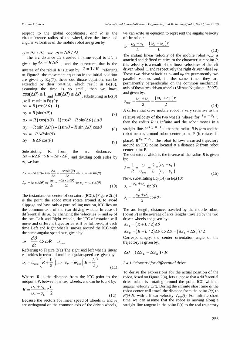
respect to the global coordinates, and R is the circumference radius of the wheel, then the linear and angular velocities of the mobile robot are given by

/ /s t t The arc distance Δs traveled in time equal to Δt, is

given by s R , and the curvature, that is the

inverse of the radius R is given by 1/ R , referring

to Figure3, the movement equation in the initial position are given by Eq.(7), these coordinate equations can be extended by their rotating, which result in Eq.(8),

assuming the time is so small, then we have;

cos( ) 1 and

sin( ) , substituting in Eq(8)

, will result in Eq.(9):

cos( ) 1

(sin( ))

x R

y R

(7)

cos( ) 1 cos sin( )sin

(sin( )) 1)sin sin( )cos

x R R

y R R

(8)

sin( )

cos( )

x R

y R

(9) Substituting R, from the arc distance,

/s R R s , and dividing both sides by ∆t, we have:

sin( )sin( ) sin( )

cos( )cos( ) cos( )

x

y

x sx s

t t

y sy s

t t

(10)

The instantaneous center of curvature (ICC), (Figure 2(a)) is the point the robot must rotate around it, to avoid

slippage and have only a pure rolling motion, ICC lies on the common axis of the two driving wheels. In case of differential drive, by changing the velocities υL and υR of the two Left and Right wheels, the ICC of rotation will move and different trajectories will be followed, at each time Left and Right wheels, moves around the ICC with

the same angular speed rate, given by:

mob

dR

dt

Referring to Figure 2(a) The right and left wheels linear velocities in terms of mobile angular speed are given by

2 2

L mob R mob

L LR R

(11)

Where: R is the distance from the ICC point to the midpoint P, between the two wheels, and can be found by:

*2

R L

R L

LR

(21)

Because the vectors for linear speed of wheels υL and υR

are orthogonal on the common axis of the driven wheels,

we can write an equation to represent the angular velocity of the robot:

R LR Lr

L L

(13)

The instant linear velocity of the mobile robot vmob is attached and defined relative to the characteristic point P, this velocity is a result of the linear velocities of the left driven wheel υL and respectively the right driven wheel υR.

These two drive velocities υL and υR are permanently two parallel vectors and, in the same time, they are permanently perpendicular on the common mechanical axis of these two driven wheels (Mircea Niţulescu, 2007), and given by:

2 2

R LR L

mob

r

(14)

A differential drive mobile robot is very sensitive to the

relative velocity of the two wheels, where: for R L :

then the radius R is infinite and the robot moves in a

straight line. If R L , then the radius R is zero and the

robot rotates around robot center point P (it rotates in

place). If R L : The robot follows a curved trajectory

around an ICC point located at a distance R from robot center point P.

The curvature, which is the inverse of the radius R is given by:

1 2

*R L

mob R LR L

(15)

Now, substituting Eq.(14) in Eq.(10)

sin( )2

cos( )2

R L

x

R L

y

The arc length, distance, traveled by the mobile robot, (point P) is the average of arcs lengths traveled by the two driven wheels and given by:

/ 2

/ 2 / 2

L

R L R

S R L

S R L S S S

Correspondingly, the center orientation angle of the

trajectory is given by:

/L RS S R

2.4.1 Odometry for differential drive To derive the expressions for the actual position of the

robot, based on Figure 2(a), lets suppose that a differential drive robot is rotating around the point ICC with an angular velocity ω(t). During the infinite short time dt the robot center will travel the distance from the point P(t) to P(t+dt) with a linear velocity Vmob(t). For infinite short time we can assume that the robot is moving along a

straight line tangent in the point P(t) to the real trajectory


257

of the robot. Based on the two components of the velocity Vmob(t), the traveled distance in each direction can be calculated (Julius Maximilian, 2003)

( )

( )

x

y

dx t dt

dy t dt

(16)

Substituting υx and υy from Eq.(10) , gives:

sin( ( ))

cos( ( ))

dx t dt

dy t dt

Similarly, the angular position can be found to be :

( )d t dt (17)

Integrating Eqs.(16,17) , substituting Eq.(10) and manipulating, we have:

0

0

0

( ) sin( ( ))

( ) cos( ( ))

( ) ( )

x t t dt x

y t t dt y

t t dt

Substituting Eqs.(13 and 14) and manipulating, we have:

0

0

0

( ) sin( ( ))2

( ) cos( ( ))2

( )

R L

R L

R L

x t t dt x

y t t dt y

t dtL

(18)

3. Simulation of overall mobile robot system response

in MATLAB/simulink

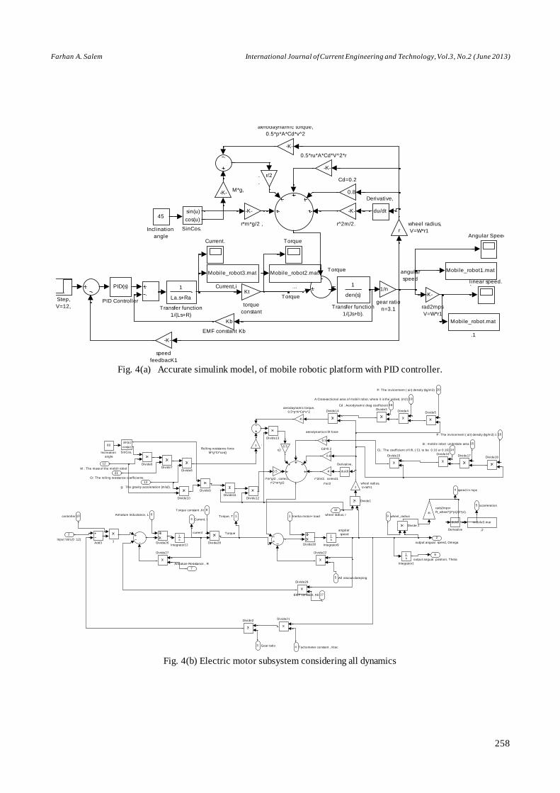
The Simulation of overall mobile robot system, including the basic electric motor, controller, feedback speed sensor considering all dynamics is shown in Figure 4(a) , based

on this model the sub-system model of electric motor , shown in Figure 4(b) can be built, this sub-system will be used to built another internal sub-system, shown in Figure 4(c) , in turn the last sub-system will be used in building Simulation of Differential drive and corresponding kinematics

Now , to test these sub-models, overall sub-system model shown in Figure 4(c), applying PID controller, and resulted responses, by defining used DC motor parameters,

platform shape dimensions, acting forces parameters and coefficients and speed sensor constant to be 1.8 for linear velocity of 0.5 m/s, running the model will result in

response curves shown in Figure 4(c) this model allow designer to evaluate mobile system performance in terms of output speed, angle, torque, acceleration and current, this model in the form of sub-system will be used, as basis, to build the differential drive model

3.1Simulation of Differential drive and whole system

To face the two top challenges in developing mechatronic system; early identifying system level problems and ensuring that all design requirements are met, as well as, to simplify and accelerate Mechatronics mobile robots

design process, including proper selection, analysis, integration and verification of the overall system, as well as, sub-systems performance throughout the development process, and optimize system level performance to meet the design requirements. All the derived equations, including kinematics and dynamic equations, as well as,

simulink sub-system model shown in Figure 4, are used to built an accurate and detailed , single input- multi-outputs dynamics and kinematics model shown in Figure 5(a), running this model will result in visual numerical values of many variables and curves of each of the following; robot linear speed υmob, robot angular speed ωmob, linear speed

of right wheel υR , linear speed of left wheel υL, robot center point P motion , the turning radius of mobile robot R, Robot orientation-Direction angle θ, the curvature, ,as well as, response curves in terms of linear speed/time, torque/time, angular speed/time and current/time response curves

Beside, the general model, based on derived equations given by Eqs.(11-15) additional and supporting simulink sub-models are built to return some of these output quantities, were Figure 5(b) shows additional sub-model to return robot center point P motion in X-Y coordinate ( see Figures 6-7 ). Figure 5(c) shows additional sub-model to

return each of the following , linear speed of right motor , linear speed of left motor, linear speed of whole mobile robot, curvature covered distance S, Robot orientation-Direction angle θ, to plot both linear speed of right wheel υR , linear speed of left motor υL sub-model shown in Figure 5(c) is used. A simplified version of the proposed

model is shown in Figure 5(d)


258

Fig. 4(a) Accurate simulink model, of mobile robotic platform with PID controller.

Fig. 4(b) Electric motor subsystem considering all dynamics

angular

speed

Current,i

Torque

EMF constant Kb

Torque

r

wheel radius,

V=W*r1

Kt

torque

constant

-K-

speed

feedbacK1

-K-

rad2mps

V=W*r1

-K-

r^2m/2.

-K-

r*m*g/2 ,

l inear speed.

1/n

gear ratio

n=3.1

-K-

aerodaynamic torque,

0.5*p*A*Cd*v^2

1

La.s+Ra

Transfer function

1/(Ls+R)

1

den(s)

Transfer function

1/(Js+b).

Torque

Step,

V=12,

Kb

sin(u)

cos(u)

SinCos.

PID(s)

PID Controller

-K-M*g,

45

Inclination

angle

du/dt

Derivative,

Current.

0.8

Cd=0.2

Angular Speed

-K-

0.5*ru*A*Cd*V^2*r

Mobile_robot.mat

.1

Mobile_robot2.mat

...

Mobile_robot3.mat

..

r/2.

.

Mobile_robot1.mat

.

r/2Rolling resistance force

M*g*Cr*cos()

aerodynamics lift force

r*m/2r*m/2

angular

speedTorquecurrent

6

output angual position, Theta

5 acceleration

4 speed in mps

3 Current, I

2

output angual speed, Omega

1Torque, T

1

wheel radius,

V=W*r1

-K-

rads2mps=

R_wheel*(2*pi)/(2*pi).

-K-

r^2m/2. correct1

0.5

r*m*g/2 , correct2

r^2*m*g/2

-K-

aerodaynamic torque,

0.5*p*A*Cd*v^2

sin(u)

cos(u)

SinCos.

1

s

Integrator9

1

s

Integrator12

1

s

Integrator1

60

Inclination

angle

Divide9

Divide8Divide7

Divide6

Divide5Divide4

Divide30

Divide3

Divide29

Divide28

Divide27

Divide26

Divide22

Divide21Divide2

Divide18Divide17

Divide16Divide15

Divide14

Divide13

Divide12Divide11

Divide10Divide1

Divide,1

du/dt

Derivative,

du/dt

Derivative

0.8

Cd=0.2

Add3

mobile3.mat

;2

1

0.5.

.

0.5

.

1,

21

Cr: The roll ing resistance coefficients

20P: The invironment ( air) density (kg/m3)

19A:Cross-sectional area of mobilr robot, where it is the widest, (m2)

18Cd : Aerodynamic drag coefficient

17EMF constant, Kb

16P: The invironment ( air) density (kg/m3) 1

15B : mobile robot underside area

14CL: The coefficient of l ift, ( CL to be 0.10 or 0.16)

13

g: The gravity acceleration (m/s2).

12

M : The mass of the mobilr robot

11

wheel radius, r10controller 9 wheel_radius

8Torque constant ,Kt

7

Armature Resistance , R

6Armature Inductance, L

5 All viscous damping

4 Tachometer constant , Ktac3 Gear ratio

2

Input Volt,(0 :12)

1 Inertia motor+ load


259

Fig.4(c) Actuator sub-system Fig. 4(d) Actuator final sub-system

Fig. 4(c) linear speed/time, torque/time, angular speed/time and current/time response curves of the accurate close loop

mobile robotic platform model with PID controller.

Fig. 5(a) Kinematics and dynamic simulink model

2

wheel position

1

wheel velocity

0.075

r

1

n

0.275

j

9.8

g

Inertia motor+ load

Input Volt,(0 :12)

Gear ratio

Tachometer constant , Ktac

All v iscous damping

Armature Inductance, L

Armature Resistance , R

Torque constant ,Kt

wheel_radius

controller

wheel radius, r

M : The mass of the mobilr robot

g: The grav ity acceleration (m/s2).

CL: The coef f icient of lif t, ( CL to be 0.10 or 0.16)

B : mobile robot underside area

P: The inv ironment ( air) density (kg/m3) 1

EMF constant, Kb

Cd : Aerody namic drag coef f icient

A:Cross-sectional area of mobilr robot, where it is the widest,

P: The inv ironment ( air) density (kg/m3)

Cr: The rolling resistance coef f icients

Torque, T

output angual speed, Omega

Current, I

speed in mps

acceleration

output angual position, Theta

Subsystem

Step

1.25

Rou

Ramp

0.156

R

Manual

Switch

150

M

0.82

L

1.8

Ktach

1.188

Kt

1.185

EMF

0.392

Damp.

0.007

Cr

0.1

Cl

0.1

Cd

0.3

B

1.4

A

mobile4.mat

;3

mobile2.mat

;2

mobile.mat

;1

mobile1.mat

;1

In1

In1

wheel v elocity

wheel position

Subsystem1

0 2 4 6 80

2

4

6

8

Time (seconds)

Rad/s

ec

Angular speed/time

0 2 4 6 80

0.2

0.4

0.6

0.8

Time (seconds)

M/s

Linear speed/time

0 2 4 6 80

1

2

3

4

Time (seconds)

Am

p

Current/time

0 2 4 6 80

2

4

6

Time (seconds)

Nm

Torque/time

V_Robot

m/s

m

m/s

m

Omega=

(Vl-Vr)/Distanc

Turning Radius of Mobile robot

Omega=

(Vl-Vr)/Distanc

from pdf fi le = Kinematics, to take equations from there

1/(Dist_wheels)

-T-

torque1

0

rotor-omeega

0

output torque

inf

output Omega

-T-

omega.

-T-

omega rotor1

0

motor torque

XY Graph1

XY Graph

-T-

W-ROBOT

W VS. V

Velocity of RIGHT wheel

Velocity of LEFT wheel

Velocities of the wheels

V_right wheel

V_left wheel

-T-

V_Robot.'

V_R

V_L

-T-

V-Robot.

-T-

V-Robot

Theta, Robot

orientation-Dirction

Out1

Subsystem6

Torque1

Gear ratio1

Omega input1

Torque output1

Omega output1

Subsystem5

Out1

Subsystem3

Out1

Subsystem2

Out1

Subsystem1

S_lef t

S_right

V_Robot

X

Y

SubsystemStep

V=2

Step

V=12

Step

V=1

Sine Wave

Signal 1

Signal Builder

Scope1

Scope

Saturation1

Saturation

Uin

Wheel Velocity

Wheel Position

Right Motor+Wheel.

[V_L]

Right

wheel

Ramp1

Ramp

0.6254

R_Robot.

R_Robot

Position

PID(s)

PID Controller2

PID(s)

PID Controller1

[theta]

Omega1

-T-

Omega

Out1

Motion profile

0.5001

Linear speed Robot.1

0.5001

Linear speed Robot,

Linear speed

of Robot,

[theta]

Left wheel 2

[theta]

Left wheel 1

Uin

Wheel Velocity

Wheel Position

Left Motor+Wheel

[V_R]

Left

wheel

LINEAR & ANGULAR

velovities of mobile robot

-T-

Goto2

[V_L]

Goto

n

Gear ratio2

0.5

Gain2

0.5

Gain1

1Gain,2

-K- Gain,1

0.5

Gain

[V_R]

From6

[V_L]

From5

-T-

From3

sin(u)

Fcn1

cos(u)

Fcn

Divide5

Divide1

Divide

mobile14.mat

Curvature1

7.427

Curvature covered

distance

Curvature

covered distance

Curvature

Angular speed of Robot

Ang. speed

of Robot,1

mobile10.mat

;2

mobile9.mat

;1

mobile2.mat

;

-K-

1/(Dist_wheels)

mobile5.mat

...

-K-

..

1

s

.,.

.,

-K-

.'

mobile6.mat

,.3

mobile4.mat

,.1

,.'

mobile3.mat

,.

1

s

,,.

[V_R]

,

-C-

(Dist_wheels)/2

1

s

'2

1

s

'1

1

s

'.

''1-K-

''

1

s

'

-T-

Turning Radius

Curvatures covered

distance

Curvature

Curv. Raduis

of L & R wheels

and mobilr robot

Curv, radius of R_ WHEEL

mobile15.mat

2

0.6254

1

-1.139

Theta, Robot orientation

Direction

Turning Radius

of Mobile robot1

Angular speed

of Robot.

Curv. radius of L_ WHEEL

Turning Radius of Mobile robot.

Linear speed of Robot'

Curv. Raduis

of L vs R wheels

Theta, Robot

orientation-Dirction1

Velocities of the two wheels

0.6254

Turning Radius of Mobile robot1

0.7997

Angular speed of Robot.

-1.139

Theta, Robot orientation-Dirction

-0.2277

Curvature covered distance

-K-

feedbacK2

1/r

-K-

feedbacK3

1/r


260

Fig. 5(b) Fig. 5(c-1) Fig. 5(c-2)

Fig. 5(b) additional simulink sum-model to return robot center point P motion in X-Y coordinates, velocities of right and

left wheels υR, υL, Fig. 5(c-1) To return Both υmobile and ωmobile curvature, and Fig. 5(c-2)To return linear speed of ,

mobile, and right and left wheels

Fig. 5(d) Fig. 5(e)

Fig. 5(d) additional simulink sub-model for odometry for differential drive to return each of the following , linear speed

of right motor , linear speed of left motor, linear speed of whole mobile robot, curvature covered distance S, Robo t

orientation-Direction angle θ; Fig. 5(e) additional simulink to plot velocities of right and left wheels υR, υL, as well as

curvature

Fig. 5(f) Simplified model

To simplify the mathematical model, we can assume that the two motors are identical in their behavior, applying similar approaches, and based on derived equations, a position control and simulation for the two-wheel differential drive mobile

robot shown in Figure 5(g), is built.

Fig. 5(g) Position control and simulation

V_Robot

m/s

m

m/s

m

Omega=

(Vl-Vr)/Distanc


Omega=

(Vl-Vr)/Distanc


1/(Dist_wheels)

-T-

torque1

0

rotor-omeega

0

output torque

inf

output Omega

-T-

omega.

-T-

omega rotor1

0

motor torque

XY Graph1

XY Graph

-T-

W-ROBOT

W VS. V

Vrobot



Velocities of

Both wheels

V_right wheel

V_left wheel

-T-

V_Robot.'

V_R

V_L

-T-

V-Robot.

-T-

V-Robot

Theta, Robot


Out1

Subsystem6

Torque1

Gear ratio1

Omega input1

Torque output1

Omega output1

Subsystem5

Out1

Subsystem3

Out1

Subsystem2

Out1

Subsystem1

S_lef t

S_right

V_Robot

X

Y

SubsystemStep

V=2

Step

V=12

Step

V=1

Sine Wave

Signal 1

Signal Builder

Scope1

Scope

Saturation1

Saturation

Uin

Wheel Velocity

Wheel Position

Right Motor+Wheel.

[V_L]

Right

wheel

Ramp1

Ramp

0.6254

R_Robot.

R_Robot

Position

PID(s)

PID Controller2

PID(s)

PID Controller1

[theta]

Omega1

-T-

Omega

Out1

Motion profile

0.5001


0.5001

Linear speed Robot,

Linear speed

of Robot,

[theta]

Left wheel 2

[theta]

Left wheel 1

Uin

Wheel Velocity

Wheel Position

Left Motor+Wheel

[V_R]

Left

wheel

LINEAR & ANGULAR


-T-

Goto2

[V_L]

Goto

n

Gear ratio2

0.5

Gain3

0.5

Gain2

0.5

Gain1

1Gain,2

-K- Gain,1

0.5

Gain

[V_R]

From6

[V_L]

From5

-T-

From3

sin(u)

Fcn1

cos(u)

Fcn

Divide5

Divide1

Divide

mobile14.mat

Curvature1

7.427

Curvature covered

distance

Curvature

covered distance

Curvature


Ang. speed

of Robot,1

mobile10.mat

;2

mobile9.mat

;1

mobile2.mat

;

-K-

1/(Dist_wheels)

mobile5.mat

...

-K-

..

1

s

.,.

.,

-K-

.'

mobile17.mat

,.6

mobile16.mat

,.5

mobile1.mat

,.4

mobile6.mat

,.3

mobile.mat

,.2

mobile4.mat

,.1

,.'

mobile3.mat

,.

1

s

,,.

[V_R]

,

-C-

(Dist_wheels)/2

1

s

'2

1

s

'1

1

s

'.

''1-K-

''

1

s

'

-T-

Turning Radius

Curvatures covered

distance

Curvature

Curv. Raduis

of L & R wheels

and mobilr robot


mobile15.mat

2

0.6254

1

-1.139


Direction

Turning Radius

of Mobile robot1

Angular speed

of Robot.




Curv. Raduis

of L vs R wheels

Theta, Robot



0.6254


0.7997


-1.139


-0.2277


-K-

feedbacK2

1/r

-K-

feedbacK3

1/r

V_Robot

m/s

m

m/s

m

Omega=

(Vl-Vr)/Distanc


Omega=

(Vl-Vr)/Distanc


1/(Dist_wheels)

-T-

torque1

0

rotor-omeega

0

output torque

inf

output Omega

-T-

omega.

-T-

omega rotor1

0

motor torque

XY Graph1

XY Graph

-T-

W-ROBOT

W VS. V

Vrobot



Velocities of

Both wheels

V_right wheel

V_left wheel

-T-

V_Robot.'

V_R

V_L

-T-

V-Robot.

-T-

V-Robot

Theta, Robot


Out1

Subsystem6

Torque1

Gear ratio1

Omega input1

Torque output1

Omega output1

Subsystem5

Out1

Subsystem3

Out1

Subsystem2

Out1

Subsystem1

S_lef t

S_right

V_Robot

X

Y

SubsystemStep

V=2

Step

V=12

Step

V=1

Sine Wave

Signal 1

Signal Builder

Scope1

Scope

Saturation1

Saturation

Uin

Wheel Velocity

Wheel Position

Right Motor+Wheel.

[V_L]

Right

wheel

Ramp1

Ramp

0.6254

R_Robot.

R_Robot

Position

PID(s)

PID Controller2

PID(s)

PID Controller1

[theta]

Omega1

-T-

Omega

Out1

Motion profile

0.5001


0.5001

Linear speed Robot,

Linear speed

of Robot,

[theta]

Left wheel 2

[theta]

Left wheel 1

Uin

Wheel Velocity

Wheel Position

Left Motor+Wheel

[V_R]

Left

wheel

LINEAR & ANGULAR


-T-

Goto2

[V_L]

Goto

n

Gear ratio2

0.5

Gain3

0.5

Gain2

0.5

Gain1

1Gain,2

-K- Gain,1

0.5

Gain

[V_R]

From6

[V_L]

From5

-T-

From3

sin(u)

Fcn1

cos(u)

Fcn

Divide5

Divide1

Divide

mobile14.mat

Curvature1

7.427

Curvature covered

distance

Curvature

covered distance

Curvature


Ang. speed

of Robot,1

mobile10.mat

;2

mobile9.mat

;1

mobile2.mat

;

-K-

1/(Dist_wheels)

mobile5.mat

...

-K-

..

1

s

.,.

.,

-K-

.'

mobile6.mat

,.3

mobile4.mat

,.1

,.'

mobile3.mat

,.

1

s

,,.

[V_R]

,

-C-

(Dist_wheels)/2

1

s

'2

1

s

'1

1

s

'.

''1-K-

''

1

s

'

-T-

Turning Radius

Curvatures covered

distance

Curvature

Curv. Raduis

of L & R wheels

and mobilr robot


mobile15.mat

2

0.6254

1

-1.139


Direction

Turning Radius

of Mobile robot1

Angular speed

of Robot.




Curv. Raduis

of L vs R wheels

Theta, Robot



0.6254


0.7997


-1.139


-0.2277


-K-

feedbacK2

1/r

-K-

feedbacK3

1/r

V_Robot

m/s

m

m/s

m

Omega=

(Vl-Vr)/Distanc


Omega=

(Vl-Vr)/Distanc


1/(Dist_wheels)

-T-

torque1

0

rotor-omeega

0

output torque

inf

output Omega

-T-

omega.

-T-

omega rotor1

0

motor torque

XY Graph1

XY Graph

-T-

W-ROBOT

W VS. V

Vrobot



Velocities of

Both wheels

V_right wheel

V_left wheel

-T-

V_Robot.'

V_R

V_L

-T-

V-Robot.

-T-

V-Robot

Theta, Robot


Out1

Subsystem6

Torque1

Gear ratio1

Omega input1

Torque output1

Omega output1

Subsystem5

Out1

Subsystem3

Out1

Subsystem2

Out1

Subsystem1

S_lef t

S_right

V_Robot

X

Y

SubsystemStep

V=2

Step

V=12

Step

V=1

Sine Wave

Signal 1

Signal Builder

Scope1

Scope

Saturation1

Saturation

Uin

Wheel Velocity

Wheel Position

Right Motor+Wheel.

[V_L]

Right

wheel

Ramp1

Ramp

0.6254

R_Robot.

R_Robot

Position

PID(s)

PID Controller2

PID(s)

PID Controller1

[theta]

Omega1

-T-

Omega

Out1

Motion profile

0.5001


0.5001

Linear speed Robot,

Linear speed

of Robot,

[theta]

Left wheel 2

[theta]

Left wheel 1

Uin

Wheel Velocity

Wheel Position

Left Motor+Wheel

[V_R]

Left

wheel

LINEAR & ANGULAR


-T-

Goto2

[V_L]

Goto

n

Gear ratio2

0.5

Gain3

0.5

Gain2

0.5

Gain1

1Gain,2

-K- Gain,1

0.5

Gain

[V_R]

From6

[V_L]

From5

-T-

From3

sin(u)

Fcn1

cos(u)

Fcn

Divide5

Divide1

Divide

mobile14.mat

Curvature1

7.427

Curvature covered

distance

Curvature

covered distance

Curvature


Ang. speed

of Robot,1

mobile10.mat

;2

mobile9.mat

;1

mobile2.mat

;

-K-

1/(Dist_wheels)

mobile5.mat

...

-K-

..

1

s

.,.

.,

-K-

.'

mobile6.mat

,.3

mobile4.mat

,.1

,.'

mobile3.mat

,.

1

s

,,.

[V_R]

,

-C-

(Dist_wheels)/2

1

s

'2

1

s

'1

1

s

'.

''1-K-

''

1

s

'

-T-

Turning Radius

Curvatures covered

distance

Curvature

Curv. Raduis

of L & R wheels

and mobilr robot


mobile15.mat

2

0.6254

1

-1.139


Direction

Turning Radius

of Mobile robot1

Angular speed

of Robot.




Curv. Raduis

of L vs R wheels

Theta, Robot



0.6254


0.7997


-1.139


-0.2277


-K-

feedbacK2

1/r

-K-

feedbacK3

1/r

V_Robot

m/s

m

m/s

m

Omega=

(Vl-Vr)/Distanc


Omega=

(Vl-Vr)/Distanc


1/(Dist_wheels)

-T-

torque1

0

rotor-omeega

0

output torque

inf

output Omega

-T-

omega.

-T-

omega rotor1

0

motor torque

XY Graph1

XY Graph

-T-

W-ROBOT

W VS. V




V_right wheel

V_left wheel

-T-

V_Robot.'

V_R

V_L

-T-

V-Robot.

-T-

V-Robot

Theta, Robot


Out1

Subsystem6

Torque1

Gear ratio1

Omega input1

Torque output1

Omega output1

Subsystem5

Out1

Subsystem3

Out1

Subsystem2

Out1

Subsystem1

S_lef t

S_right

V_Robot

X

Y

SubsystemStep

V=2

Step

V=12

Step

V=1

Sine Wave

Signal 1

Signal Builder

Scope1

Scope

Saturation1

Saturation

Uin

Wheel Velocity

Wheel Position

Right Motor+Wheel.

[V_L]

Right

wheel

Ramp1

Ramp

0.6254

R_Robot.

R_Robot

Position

PID(s)

PID Controller2

PID(s)

PID Controller1

[theta]

Omega1

-T-

Omega

Out1

Motion profile

0.5001


0.5001

Linear speed Robot,

Linear speed

of Robot,

[theta]

Left wheel 2

[theta]

Left wheel 1

Uin

Wheel Velocity

Wheel Position

Left Motor+Wheel

[V_R]

Left

wheel

LINEAR & ANGULAR


-T-

Goto2

[V_L]

Goto

n

Gear ratio2

0.5

Gain2

0.5

Gain1

1Gain,2

-K- Gain,1

0.5

Gain

[V_R]

From6

[V_L]

From5

-T-

From3

sin(u)

Fcn1

cos(u)

Fcn

Divide5

Divide1

Divide

mobile14.mat

Curvature1

7.427

Curvature covered

distance

Curvature

covered distance

Curvature


Ang. speed

of Robot,1

mobile10.mat

;2

mobile9.mat

;1

mobile2.mat

;

-K-

1/(Dist_wheels)

mobile5.mat

...

-K-

..

1

s

.,.

.,

-K-

.'

mobile6.mat

,.3

mobile4.mat

,.1

,.'

mobile3.mat

,.

1

s

,,.

[V_R]

,

-C-

(Dist_wheels)/2

1

s

'2

1

s

'1

1

s

'.

''1-K-

''

1

s

'

-T-

Turning Radius

Curvatures covered

distance

Curvature

Curv. Raduis

of L & R wheels

and mobilr robot


mobile15.mat

2

0.6254

1

-1.139


Direction

Turning Radius

of Mobile robot1

Angular speed

of Robot.




Curv. Raduis

of L vs R wheels

Theta, Robot



0.6254


0.7997


-1.139


-0.2277


-K-

feedbacK2

1/r

-K-

feedbacK3

1/r

V_Robot

m/s

m

m/s

m

Omega=

(Vl-Vr)/Distanc


Omega=

(Vl-Vr)/Distanc


1/(Dist_wheels)

-T-

torque1

0

rotor-omeega

0

output torque

inf

output Omega

-T-

omega.

-T-

omega rotor1

0

motor torque

XY Graph1

XY Graph

-T-

W-ROBOT

W VS. V




V_right wheel

V_left wheel

-T-

V_Robot.'

V_R

V_L

-T-

V-Robot.

-T-

V-Robot

Theta, Robot


Out1

Subsystem6

Torque1

Gear ratio1

Omega input1

Torque output1

Omega output1

Subsystem5

Out1

Subsystem3

Out1

Subsystem2

Out1

Subsystem1

S_lef t

S_right

V_Robot

X

Y

SubsystemStep

V=2

Step

V=12

Step

V=1

Sine Wave

Signal 1

Signal Builder

Scope1

Scope

Saturation1

Saturation

Uin

Wheel Velocity

Wheel Position

Right Motor+Wheel.

[V_L]

Right

wheel

Ramp1

Ramp

0.6254

R_Robot.

R_Robot

Position

PID(s)

PID Controller2

PID(s)

PID Controller1

[theta]

Omega1

-T-

Omega

Out1

Motion profile

0.5001


0.5001

Linear speed Robot,

Linear speed

of Robot,

[theta]

Left wheel 2

[theta]

Left wheel 1

Uin

Wheel Velocity

Wheel Position

Left Motor+Wheel

[V_R]

Left

wheel

LINEAR & ANGULAR


-T-

Goto2

[V_L]

Goto

n

Gear ratio2

0.5

Gain2

0.5

Gain1

1Gain,2

-K- Gain,1

0.5

Gain

[V_R]

From6

[V_L]

From5

-T-

From3

sin(u)

Fcn1

cos(u)

Fcn

Divide5

Divide1

Divide

mobile14.mat

Curvature1

7.427

Curvature covered

distance

Curvature

covered distance

Curvature


Ang. speed

of Robot,1

mobile10.mat

;2

mobile9.mat

;1

mobile2.mat

;

-K-

1/(Dist_wheels)

mobile5.mat

...

-K-

..

1

s

.,.

.,

-K-

.'

mobile6.mat

,.3

mobile4.mat

,.1

,.'

mobile3.mat

,.

1

s

,,.

[V_R]

,

-C-

(Dist_wheels)/2

1

s

'2

1

s

'1

1

s

'.

''1-K-

''

1

s

'

-T-

Turning Radius

Curvatures covered

distance

Curvature

Curv. Raduis

of L & R wheels

and mobilr robot


mobile15.mat

2

0.6254

1

-1.139


Direction

Turning Radius

of Mobile robot1

Angular speed

of Robot.




Curv. Raduis

of L vs R wheels

Theta, Robot



0.6254


0.7997


-1.139


-0.2277


-K-

feedbacK2

1/r

-K-

feedbacK3

1/r

Omega=

(Vl-Vr)/Distanc

Position control

from pdf paper 62-22-1-PB

V_right wheel1

V_left wheel1

Theta, Robot

orientation-Dirction.

Step

V=3

Saturation3

Saturation2

Uin

Wheel Velocity

Wheel Position

Right Motor+Wheel.1

Ramp1

PID(s)

PID Controller4

PID(s)

PID Controller3

Linear speed

of Robot.

Uin

Wheel Velocity

Wheel Position

Left Motor+Wheel1

0.5

Gain3

sin(u)

Fcn1

cos(u)

Fcn

Curvatures

covered distance.

Ang. speed

of Robot,

-K-

.'1

1

s

'5

1

s

'4

1

s

'2

1

s

'1

''3

''2

''1

''

-K-

feedbacK4

-K-

feedbacK1

Vx

Vy

XY Graph

speed components

Step

V=3

Step

V=1 Saturation3

Saturation2

Ramp1

PID(s)

PID Controller4

PID(s)

PID Controller3

Linear speed

of Robot.

Uin

LINEAR Velocity

LINEAR Position

ANGULAR Velocity

Left Motor+Wheel1

sin(u)

Fcn1

cos(u)

Fcn

Ang. speed

of Robot,

1

s

'7

1

s

'6

1

s

'51

s

'3

''7

''6

''5

''1


261

4. Testing and results

The following nominal values for the various parameters of a PMDC motor used : Vin=12 Volts; Motor torque

constant, Kt = 1.1882 Nm/A; Armature Resistance, Ra = 0.1557 Ohms (Ω) ; Armature Inductance, La = 0.82 MH ;Geared-Motor Inertia: Jm = 0.271 kg.m

2, Geared-Motor

Viscous damping bm = 0.271 N.m.s; Motor back EMF constant, Kb = 1.185 rad/s/V, gear ratio, n=3, wheel radius r =0.075 m, mobile robot height ,h= 0.920 m, mobile robot

width ,b = 0.580 m, the distance between wheels centers = 0.4 m, total mass 100 kg, the total equivalent inertia, Jequiv

and total equivalent damping, bequiv at the armature of the motor are ,Jequiv =0.2752 kg.m

2 , bequiv = 0.3922 N.m.s.

The most suitable linear output speed of suggested mobile robot is to move with 0.5 meter per second, (that is ω=V/r

= 0.5/ 0.075 = 6.6667 rad/s,). Tachometer constant, Ktac = 12 / 6.6667=1.8 (rad/sec), assuming shape of the Frontal area of mobile robot is long cylinder , the aerodynamic drag coefficient, Cd =0.80, the air density (kg/m

3) at STP,

ρ =1.25, The coefficient of lift, ( CL to be 0.10 or 0.16), the inclination angle to be 45

For model shown in Figure 5(a), when subjecting the right motor to step input with final value of 12 V, and Left motor of ramp input with slop of 7 , all the response curves shown in Figure 6 , can be obtained , as well as visual numerical values for these quantities. The sub-models can be used to return, all or only, of the required

response curves.

Fig. 6(a) The robot center point P motion

Fig. 6(b) The Mobile robot linear speed

Fig. 6(c) The mobile robot linear speed/ time, mobile robot angular speed/time, turning radius/time (final value of 0.6523), and mobile robot orientation angle. Time, traveled curvature distance/ time, and curvature/time.

Fig. 6(d) left and right wheels linear and angular speed and position

To further test our model, (differential drive motions) shown in Figure 5(a), by defining DC parameters, platform shape dimensions, acting forces parameters and coefficients , speed sensor constant,, inclination angle, firstly, applying the same inputs to both motors , to have

similar wheels velocities, R L , result in that the radius

R is infinite and the robot moves in a straight line motion as shown in Fig. 7(a); applying different inputs to have

R L , will result in corresponding trajectory, The robot

follows a curved trajectory around an ICC point

0 0.1 0.2 0.3 0.4 0.5 0.6 0.7 0.8 0.9 10

0.1

0.2

0.3

0.4

0.5

0.6

0.7

Met

er ,

M

Mobile linear speed \nu

0 10 20 300

0.2

0.4

0.6

0.8

Mete

r ,

M

Mobile linear speed

0 10 20 30-6

-4

-2

0

2

Mobile

R

ad

Mobile Angular speed Rad/s,

0 10 20 30-200

-100

0

100

200

Time(sec)

Turn

. R

adiu

s R

Mobile turning Radius m,

0 10 20 30-20

-10

0

10

20

Time(sec)

Mobile

orienta

tion a

ngle

Mobile orientation angle,

0 10 20 30-4

-2

0

2

4

Time(sec)

Curv

atu

re M

Traveled curvature distance ,

0 10 20 30-15

-10

-5

0

5

Time(sec)

Curv

atu

re M

curvature ,

0 10 20 30-4

-2

0

2

4

Time(sec)

Curv

atu

re M

Traveled curvature distance ,

0 10 20 30-15

-10

-5

0

5

Time(sec)

Curv

atu

re M

curvature ,

0 5 10 15-1

0

1

2

Time(sec)

M

/s

Left and Right wheels speed

0 5 10 15-2

-1

0

1

Time(sec)

Mete

r ,

M

Left and Right wheels positions S

Right wheel Pos.

Left wheel Pos.

0 5 10 15-6

-4

-2

0

2

Time(sec)

m/s

, R

ad/s

Mobile linear and angular speeds ,

Mobile linear speed

Mobile angular speed


262

Fig. 6(e) Right motor linear speed/time, current/time, angular speed/time, torque/ time response curves. located at a distance R from robot center point P. (Fig. 7(a)

(b) (c)), also for each time, the model is run, we obtain response curves in terms of linear speed/time, torque/time, angular speed/time and current/time response curves.

Fig.7(a) straight line Fig.7(b) circular motion

Fig. 7(c) Double-curvature Fig.7(a)(b)(c) Three different trajectories of the central

point of the mobile robot.

5. Future work; experimental testing; Mobile robot

control and circuit explanation,

Wheeled mobile Robot can be designed and built using the

following components (see Figure 7); chassis with two in-line with each other electric PMDC motors, a PIC microcontroller embedded on the robot and capable of controlling two drive channels (PIC16F84A), two H-bridge control circuits, corresponding sensors, The inputs

to microcontroller are sensors outputs, depending on robot application, sensors may be line detection sensor, ultrasonic range proximity sensor, temperature sensor. , PIC microcontroller is supplied with 5VDC and simple

clock condition with 20 MHz crystal, The H-bridge circuit is supplied with 12VDC and the four bits outputs of microcontroller made this part to drive the desire conditions of DC Motor. A simplified algorithm for a PID control implementation loop is given next:

Read KP, KI, KP previous_error = 0; integral = 0; Read target_position // the required position of robot center. while ( )

Read current_position; //the current position of robot center with respect to the line. error = target_position – current_position ; // calculate error proportional = KP * error; // error times proportional gain

integral = integral + error*dt; //integral stores the accumulated error integral = integral* KI; derivative = (error - previous_error)/dt; //stores change in error to derivate, dt is sampling period derivative = KD *derivative;

PID_action = proportional + integral + derivative; //To add PID_action to the left and right motor speed. //The sign of PID_action, will determine the direction in which the motor will turn. previous_error =error; //Update error end

Fig. 7 Microcontroller based DC motor control system for wheeled mobile robot Conclusions

New models for differential drive mobile robots and some considerations regarding design, modeling and control solutions are presented. The presented models allow designer to have maximum desired informations in the form of curves and visual numerical values of all variables

0 10 20 300

1

2

3

4

Time(sec)

Moto

r T

orq

ue,

Nm

Right Motor Torque Nm/Time

0 10 20 300

0.5

1

1.5

2

lin

ear

speed.

M/s

Right Motor linear speed M/s

0 10 20 300

1

2

3

Curr

ent,

A

mp

Right Motor Current Amp/s,

0 10 20 30-5

0

5

10

15

Time(sec)

,

Rad

RightMotor Rad/s


263

required in designing and controlling of a wheeled mobile robot, that can be used to face the two top challenges in developing mechatronic system; early identifying system level problems and ensuring that all design requirements

are met, as well as ,to simplify and accelerate Mechatronics mobile robots design process, including proper selection, analysis, integration and verification of the overall system, as well as, sub-systems performance throughout the development process, and optimize system level performance to meet the design requirements. The

testing results show the simplicity, accuracy and applicability of the proposed models in mechatronics design of mobile robots.

Acknowledgement

Author would like to express his sincere thanks to Ahmad

Ismaiel Abu Mahfouz, for his valuable help, suggestions and support during the development of the current work.

References.

Ahmad A. Mahfouz, Mohammed M. K, Farhan A. Salem (2012), Modeling, simulation and dynamics analysis issues of electric motor, for mechatronics applications, using different approaches and verification by

MATLAB/Simulink (I)''. accepeted but not published yet to I.J. Intelligent Systems and Applications, Submission ID 123.

Ahmad A. Mahfouz, Ayman A. Aly, Farhan A. Salem, (2013),

Mechatronics Design of a Mobile Robot System, IJISA, vol.5, no.3, pp.23-3.

Bashir M. Y. Nouri (2005), modeling and control of mobile robot , Proceeding of the First International Conference on

Modeling, Simulation and Applied Optimization, Sharjah, U.A.E. February 1-3.

Jaroslav Hanzel, Ladislav Jurišica, Marian Kľúčik, Anton Vitkor, Matej Strigáč , (2011), experimental mobile robotic

systems', modeling of mechanical and mechatronics systems.

Emese Sza Deczky-Krdoss, Ba Lint Kiss (2004) , design and control of a 2-DOF positioning robot Methods and Models

in Automation and Robotics, Miedzyzdroje, Poland. M.B.B. Sharifian, R.Rahnavard and H.Delavari (2009), Velocity

Control of DC Motor Based Intelligent methods and Optimal Integral State Feedback Controller , International

Journal of Computer Theory and Engineering, Vol. 1, No. 1, April 2009 1793-8201.

Gregor Klanˇcar, Drago Matko, Saˇso Blaˇzi c (2005), Mobile Robot Control on a Reference Path, Mediterranean

Conference on Control and Automation Limassol, Cyprus, June 27-2,.

Tao Gong , Zixing Cai (2003), Mobile Immune-Robot Model'',

International conference on robotics, intelligent systems

and signal processing.

Aye Aye Nwe, Wai Phyo Aung , Yin Mon Myint (2008), software implementation of obstacle detection and for Wheeled Mobile Robot. avoidance system, World Academy

of Science, Engineering and Technology 42. Mircea Niţulescu (2007), solutions for modeling and control in

mobile robots'' , CEAI, Vol. 9, No. 3;4, pp. 43-50, Romania. J. R. Asensio. L. Montano, (2002) Akinematic and dynamic

model-based motion controller for mobile robot , 15th Triennial World Congress, Barcelona, Spain

Richard C. Dorf and Robert H. Bishop (2001),Modern Control Systems. Ninth Edition, Prentice-Hall Inc., New Jersey,.

Farhan A. Salem (2013), Accurate modeling and control for Mechatronics design of mobile robotic platforms'' submitted to Estonian Journal of Engineering,.

Jose Mireles Jr. (2004) ,Kinematics of Mobile Robots , Selected

notes from 'Robótica: Manipuladores y Robots móviles' Aníbal Ollero.

Julius Maximilian (2003), Kinematics of a car-like mobile robot

Mobile robot basic – differential drive'', Institute of

Informatics VII, experiment notes D. Honc P. Rozsíval F. Dušek (2011), Mathematical model of

differentially steered mobile robot'' , 18th

International Conference on Process Control , Tatranská Lomnica,

Slovakia Khatib, M., H. Jaouni, R. Chatila and J. P. Laumond (1997).

Dynamic Path Modification for Car-Like Nonholonomic Mobile Robots. In: IEEE Intl. Conf. on Robotics and

Automation. pp. 2920–2925. Topalov, A. V., D. D. Tsankova, M. G. Petrov and T. Ph.

Proychev (1998). Intelligent Sensor-Based Navigation and Control of Mobile Robot in a Partially Known Environment.

In: 3rd IFAC Symposium on Intelligent Autonomous Vehicles, IAV’98. pp. 439–444.

Dudek Gregory, Michael Jenkin (2000), Computational principles of mobile robotics. Cambridge university press.

Egerstedt, M., X. Hu and A. Stotsky (2001) , Control of mobile platforms using a virtual vehicle approach,” IEEE Trans. on automatic control, Vol. 46, No. aa, p1777-1782.

S. Noga (2006), Kinematics and dynamics of some selected two-

wheeled mobile robots'' archives of civil and mechanical engineering , Vol. VI, No. 3

Author’s Profile:

Farhan Atallah Salem Abu Mahfouz:

B.Sc., M.Sc and Ph.D., in Mechatronics of production systems, Moscow state Academy. Now he is ass. Professor in Taif University, Mechatronics program, Dept. of Mechanical Engineering and gen-director of alpha center for engineering

studies and technology researches. Research Interests; Design, modeling and analysis of primary Mechatronics Machines. Control and algorithm selection, design and analysis for Mechatronics systems. Rotor Dynamics and Design for Mechatronics applications

دكتور فـرحـان عـطـاالله ابـو مـحـفـوظ __ Dynamic and Kinematic...

Documents

Transcript of دكتور فـرحـان عـطـاالله ابـو مـحـفـوظ __ Dynamic and Kinematic...