-CBIO 16-4 - Ingenta Connect

Cur

rent

Bio

info

rmat

ics

��

��

�� !"� ! ��#��

Send Orders for Reprints to [email protected]

Current Bioinformatics, 2021, 16, 583-600

583

RESEARCH ARTICLE

Colorectal Cancer Classification and Survival Analysis Based on an Integrated RNA and DNA Molecular Signature

Mohanad Mohammed1,*, Henry Mwambi1 and Bernard Omolo1,2,3

1School of Mathematics, Statistics, and Computer Science, University of KwaZulu-Natal, Pietermaritzburg, Private Bag X01, Scottsville 3209, South Africa; 2Division of Mathematics & Computer Science, University of South Carolina-Upstate, 800 University Way, Spartanburg, USA, 3School of Public Health, Faculty of Health Sciences, University of the Witwatersrand, Johannesburg, South Africa

� Abstract: Background: Colorectal cancer (CRC) is the third most common cancer among women and men in the USA, and recent studies have shown an increasing incidence in less developed regions, including Sub-Saharan Africa (SSA). We developed a hybrid (DNA mutation and RNA expression) signature and assessed its predictive properties for the mutation status and survival of CRC patients.

Methods: Publicly-available microarray and RNASeq data from 54 matched formalin-fixed paraffin-embedded (FFPE) samples from the Affymetrix GeneChip and RNASeq platforms, were used to obtain differentially expressed genes between mutant and wild-type samples. We applied the support-vector machines, artificial neural networks, random forests, k-nearest neighbor, naïve Bayes, negative binomial linear discriminant analysis, and the Poisson linear discriminant analysis algorithms for classification. Cox proportional hazards model was used for survival analysis.

Results: Compared to the genelist from each of the individual platforms, the hybrid genelist had the highest accuracy, sensitivity, specificity, and AUC for mutation status, across all the classifiers and is prognostic for survival in patients with CRC. NBLDA method was the best performer on the RNASeq data, while the SVM method was the most suitable classifier for CRC across the two data types. Nine genes were found to be predictive of survival.

Conclusion: This signature could be useful in clinical practice, especially for colorectal cancer diagnosis and therapy. Future studies should determine the effectiveness of integration in cancer survival analysis and the application on unbalanced data, where the classes are of different sizes, as well as on data with multiple classes.

A R T I C L E H I S T O R Y�

Received: April 19, 2020 Revised: April 24, 2020 Accepted: June 06, 2020 DOI: 10.2174/1574893615999200711170445 �

Keywords: Colorectal cancer, FFPE, microarray, RAS pathway signatures, RNASeq, molecular.

1. INTRODUCTION

Colorectal cancer (CRC) is one of the major emerging causes of mortality and morbidity around the world [1]. CRC is also the third leading cause of death among men and women [2-6]. According to the World Health Organization (WHO), there were about 1.80 million new cases and 862,000 deaths in the year 2018 [7]. Furthermore, in 2019, CRC was reported to be the third most prevalent cancer among men and women and an estimated 101,420 and 44,180 new cases of colon and rectal cancer, respectively, and 51,020 deaths in the USA alone [2, 8, 9].

Although the incidence rates of CRC are lower in developing countries than in developed countries, recent *Address correspondence to this author at the School of Mathematics, Statistics, and Computer Science, University of KwaZulu-Natal, Pietermaritzburg, Private Bag X01, Scottsville 3209, South Africa; E-mail: [email protected]

studies have shown an increase in the incidence rates in Sub-Saharan Africa [10]. Many cancer types that are relatively curable in developed countries are detected only at advanced stages in developing countries, due to late or inaccurate diagnoses [11]. Cancer tumor classification based on morphological characteristics alone has been shown to have serious limitations in some studies [12]. Physicians aim to diagnose CRC as early as possible to design optimal treatment strategies that are patient-specific. Therefore, using genetic mutation and features of the tumor would most probably lead to better understanding and early detection of the disease and lead to finding suitable and targeted strategies [13].

Previously, most of the cancer classification research was based on clinical features of the tumors, which lacked the accurate diagnostic ability, hence the need to develop new methods that will better address this critical problem [12, 14]. Recently, DNA microarray technology has greatly

2212-392X/21 $65.00+.00 © 2021 Bentham Science Publishers

http://crossmark.crossref.org/dialog/?doi=10.2174/1574893615999200711170445&domain=pdf

584 Current Bioinformatics, 2021, Vol. 16, No. 4 Mohammed et al.

improved the classification of diseases into sub-types, particularly cancer. This technology allows the processing of thousands of genes simultaneously, hence providing critical information about a disease [15, 16]. Microarray gene expression data have been used widely for cancer detection, prediction, and diagnosis [17]. In the last decade, next-generation sequencing (NGS) technology has emerged as an advancement in cancer and other disease research, based on RNA sequencing methodology. NGS platforms that are most common include Illumina, SOLiD, Ion Torrent semi-conductor sequencing, and single-molecule real-time sequen-cing [18].

NGS technology has been the most attractive, and its application dramatically improved over the last few years. This technology is high-throughput and has become popular in the detection and analysis of differentially expressed genes [18, 19]. More recently, RNASeq data has been shown to be better than microarray data in terms of quality and accuracy in estimating transcript abundance. However, the two methodologies are different in design and imple-mentation [19-21]. Although RNASeq experiments are expensive, in contrast, they have many advantages over microarrays. RNASeq allows detecting the variation of a single nucleotide, does not require genomic sequence knowledge, provides quantitative expression levels, provides isoform-level expression measurements, and offers a broader dynamic range than microarrays [20]. Moreover, RNASeq allows the detection of novel transcripts, low background signal, and increased specificity and sensitivity [22]. However, our view is that integrated use of data from both technologies may be the best approach, given the available information from both technologies.

Microarray and RNASeq technologies produce gene expression data in different forms. The structure of gene expression produced using microarrays is continuous data, while RNASeq provides a discrete Type of data [23]. What is common between the two technologies is that both generate big datasets consisting of a few sample sizes, where each sample has a large number of genes. Many areas of research, such as clinical, medical, biological, and agriculture, apply the RNASeq technology [24, 25].

Many statistical and machine learning methods have been used to analyze and extract information from massive amounts of gene expression data. These methods include the Poisson linear discriminant analysis (PLDA), negative binomial linear discriminant analysis (NBLDA), support vector machines (SVM), artificial neural networks (ANN), linear discriminant analysis (LDA), and random forests (RF).

These methods have been used and examined in many studies based on RNASeq and microarray data. For example, Aziz et al. [26] assessed the ANN performance based on microarray data using six hybrid feature selection methods. Five gene expression datasets were used for evaluating these methods and for understanding how these methods can improve the performance of ANN. Statistical hypothesis tests were used to check the differences between these methods. They showed that the combination of independent component analysis (ICA) and genetic bee colony algorithm had superior performance. Salem et al. [27] proposed a new

methodology for gene expression data analysis. They combined information gain (IG) and standard genetic algorithm (SGA) for feature selection and reduction, respectively. Their approach was tested on seven cancer datasets and then compared with the most recent approaches. Their results show that the proposed approach outperformed the most recent approaches. Jain et al. [28] presented a two-phase hybrid method for cancer classification using eleven microarray datasets for different cancer types. They combined correlation-based feature selection (CFS) and improved-binary particle swarm optimization (IBPSO). Naive Bayes with 10-fold cross-validation was used for assessment. Results indicated that their approach had better performance in terms of accuracy and the number of selected genes.

Anders and Huber [29] conducted differential expression analysis based on the negative binomial distribution, with variance and mean linked by local regression, for count data. Their proposed method controls the type I error and gives good detection power. Zararsiz et al. [23] presented a comprehensive simulation study on RNASeq classification using PLDA, NBLDA, single SVM, bagging SVM (bagSVM), classification and regression trees (CART), and RF. Their simulation results were applied and compared to two miRNA and two mRNA real experimental datasets. They found that the power-transformed PLDA, RF, and SVM were the best in classification performance.

Due to the small number of samples for gene expression data, combining independent datasets is novel in order to increase sample size and statistical power. Taminau et al. [30] worked on the integration of gene expression analysis using two approaches based on merging and meta-analysis. They used six gene expression datasets. Results showed that both meta-analysis and merging did well, but merging was able to detect more differentially expressed genes than meta-analysis.

Recently, combining two different gene expression data sources has been shown to improve classification accuracy as opposed to using only one source. Castillo and co-workers [20] introduced the integration of multiple microarrays and RNASeq platforms. They first carried out a differential expression analysis, then applied the minimum-redundancy maximum-relevance (mRMR) feature selection approach for further reduction of the gene-list. The top 10 genes were selected and evaluated using four classification methods: k-nearest neighbor (KNN), naive Bayes (NB), RF, and SVM. Their results showed the highest accuracy and f1-score for the KNN. In this study, we combined RNASeq and DNA expression data from colorectal cancer patients. We obtained a hybrid gene-list from the RNASeq and microarray datasets and assessed its classification performance based on the PLDA, NBLDA, SVM, RF, ANN, KNN, and NB algorithms.

The paper is structured as follows. Section 2 discusses the methods and the datasets used in the study. Section 3 shows the classification results of the microarray, RNASeq, hybrid gene lists, and survival analysis. Discussion and conclusions are presented in Sections 4 and 5, respectively.

Colorectal Cancer Classification and Survival Analysis Current Bioinformatics, 2021, Vol. 16, No. 4 585

2. MATERIALS AND METHODS

2.1. Datasets

We used publicly available microarray and RNASeq data that is also reported in Omolo et al. [4]. The data consists of 54 matched formalin-fixed paraffin-embedded (FFPE) samples from colorectal cancer patients and is available in the gene expression omnibus (GEO) repository under the accession numbers GSE86562 and GSE86559 for RNASeq and microarray data, respectively. The microarray gene expression data consists of 60,607 genes on 54 colorectal patients. We used the KRAS mutation status as a class variable. As a first step, the Affymetrix microarray data were log2-transformed and quantile-normalized, and genes with more than 50% missing values were filtered out. After that, we performed class comparison using the two-sample t-test at the 0.005 significant level threshold, which yielded 165 differentially expressed genes.

The RNASeq dataset contained 57,905 genes from the same colorectal cancer patients used to generate the microarray data. This data is in the form of counts, i.e., discrete. For this data, first, filtration was done to remove the genes with more than 50% of zeros across the samples, using the counts per million (CPM) method [31]. We retained genes whose CPM values are greater than 0.5. Thus, the dimension reduced to 17,473 genes. We performed differential expression analysis using the DESeq2 package in R. This step reduced the genes to 282 genes using the 0.005 significance threshold level. The differential expression analysis tool in DESeq2 uses a generalized linear model (GLM) of the following form:

�� (1)

where �� is the counts for gene � in sample �. These counts are modeled using a negative binomial distribution with fitted mean �� and a gene-specific dispersion parameter ��. The fitted mean is decomposed into a sample-specific size factor �� and a parameter �� proportional to the expected true concentration of fragments for sample �. The coefficients �� represent the log2-fold changes for gene � for each column of the model or design matrix X. Note that the model can be generalized to use a sample- and gene-dependent normalization factors ��.

The dispersion parameter �� defines the relationship between the variance of the observed count and its mean value. That is, how far we expect the observed count to be from the mean value, which depends both on the size factor �� and the covariate-dependent part �� as defined above. Thus, the variance function is given by:

��

� (2)

The steps performed by the DESeq function in DESeq2 package are the estimation of ��, and ��, and fitting negative binomial GLM for �� and Wald statistics by nbinomWaldTest.

We computed counts per million as: ��

��

�� (3)

where �� denotes the counts observed from a gene of interest i, and N is the number of sequenced fragments.

RNASeq and microarray data integration may help improve cancer classification accuracy. Several studies have addressed the classification problem using RNASeq, microarray, or a combination of both, based on hetero-geneous samples [20, 32, 33]. Our study aimed to integrate homogeneous samples from the RNASeq and microarray platforms. In this regard, we obtained the differentially expressed genes from the two platforms based on the same set of samples. After that, we used the database for annotation, visualization, and integrated discovery (DAVID) [34] and catalogue of somatic mutations in cancer (COSMIC) tools, to annotate the RNASeq transcripts list. The microarray genes symbol names were obtained from the dataset in [4]. We then obtained the intersection, complement of the intersection, and union between the two annotated lists.

Integration was done using the intersection, complement of the intersection, and the union of the two lists of genes. Due to the different nature of the two datasets, RNASeq was log2 transformed and quantile-normalized to make both types of data consistent with each other. Subsequently, the integration was done based on binding the two gene-lists from the RNASeq and microarray datasets. To transform the RNASeq data, we let:

�� (4)

where G is the RNASeq counts data matrix, and G + 1 is the RNASeq counts data matrix with all zero counts changed to one.

Quantile normalization ensures that probe intensities of each array in a set of arrays have the same distribution. A quantile-quantile plot would help to confirm if two probe vectors have the same distribution (quantiles lie on the diagonal line) or not. This approach can be extended to n-dimensional data. Let ��

�, k= 1, …, P, be the vector of the kth quantiles for all n arrays, and � ��

��

�

�� be the unit diagonal. To transform from the

quantiles so that they all lie along the diagonal, we projected � on to � as below [35]:

��

�

��

�

�

�� (5)

2.2. Data Integration

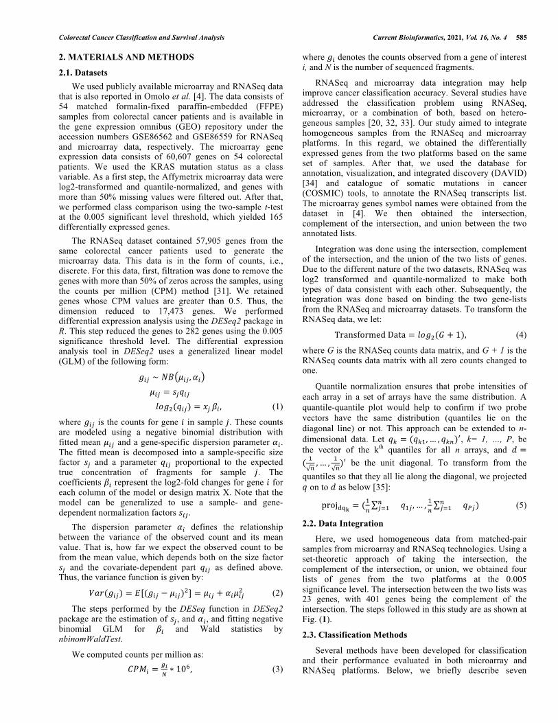
Here, we used homogeneous data from matched-pair samples from microarray and RNASeq technologies. Using a set-theoretic approach of taking the intersection, the complement of the intersection, or union, we obtained four lists of genes from the two platforms at the 0.005 significance level. The intersection between the two lists was 23 genes, with 401 genes being the complement of the intersection. The steps followed in this study are as shown at Fig. (1).

2.3. Classification Methods

Several methods have been developed for classification and their performance evaluated in both microarray and RNASeq platforms. Below, we briefly describe seven


classification methods and how to evaluate their performances based on the integration of the two platforms.

2.3.1. Poisson Linear Discriminant Analysis

The PLDA classifier was proposed by Witten [36]. Witten used the Poisson log-linear model and developed an analog of diagonal linear discriminant analysis for sequence data.

Let � denote a � � � matrix of read counts data, where � denotes the number of observations (samples), and � the number of genes. Let �� be the counts or reads for gene � in sample �; it is reasonable to assume that:

�� (6)

where �� . To avoid identifiability issues, one can require �

�� , where �� is the number of counts per sample �, and �� is the number of counts per gene �.

Suppose that we have � different classes of samples. Then we can write:

�� (7)

where �� denotes the class of the �th sample

(�� ) and �� denotes a measure of the level of the �th gene to be differentially expressed in class �.

Let �� indicate the entries of row �

in the � matrix, which are the gene expression levels of sample �. Let, ��

�� , ��

�� , and �� denote the column, row, and the overall totals, respectively. The maximum likelihood estimate (MLE) for �� assuming independence is ��

��

��

��, and

�� yields the estimates ��

��

�� and ��

�� .

�� is the estimate of the size factor for sample �. Maximum likelihood estimation provides the estimate of �� as

��

��

, where �� denotes the class of an

observation.

If �� , then the �th gene is overexpressed relative to the baseline in the �th class, and if �� , then the �th gene is under expressed relative to the baseline in the �th class. If �� (an event that is not unlikely if the true mean for �th gene is small), then the maximum likelihood estimates for �� equals zero.

Assume that we want to classify a new observation ��

�� , and let �� indicate the unknown class

label. By Bayes rule,

�� (8)

where �� is the density of a sample in class � and �� is the prior probability that an observation belongs to class �. Then, if �� is a normal density with a class-specific mean and common covariance, PLDA classifies a new sample to class �, which maximizes equation (8). Consequently, the discriminant score of PLDA is:

��

��

�� (9)

PLDA is implemented using the R package MLSeq.

2.3.2. Negative Binomial Linear Discriminant Analysis

Recently, Dong et al. [22] proposed NBLDA for RNASeq data analysis. NBLDA and Poisson linear discriminant analysis (PLDA) were considered the most suitable classifiers for RNASeq data due to the discrete nature of data [22, 36].

Let �� denote the number of reads in sample �, and gene �, � � �� and, � � �� . Then �� is assumed to follow the negative binomial distribution:

�� (10)

where �� is the size factor, used to scale gene counts for the �

th sample due to different sequencing depth, �� is the total number of reads per gene, and �� is the dispersion parameter. The mean and variance of the negative binomial distribution are given by:

� ��

�� (11)

Suppose that we have � classes. Let �� be an indicator variable such that �� . Then, the model for RNASeq data is:

�� (12)

where �� denotes the differences among the � classes, and �� denotes the class of samples �. The assumption is that all the genes are independent.

Fig. (1). Flow-chart of the analysis.

Microarray Analysis

RNASeq Analysis

Extract DEGs from

each platform

Microarray & RNASeq Integration

Classification and Survival

Analysis Process


Let ��

�� be a new sample whose class is to be predicted, �� is the size factor, and ��

� the class label value. By Bayes' rule, we have:

�� (13)

where �� is the �� of the sample in class �, and �� is the prior probability that a sample comes from class �. The �� of �� in equation (12) is:

��

��

��

��

��

��

�

��

(14)

Thus, the discriminant score for NBLDA can be constructed from (13) and (14) as:

��

��

��

��

�� (15)

where � is a constant independent of �. The class �, which maximizes the score in equation (15) will be assigned to the new sample ��. NBLDA is implemented using the R package MLSeq.

2.3.3. Support Vector Machines

The SVM method was first proposed by Boser, Guyon, and Vapnik [37] at the Computational Learning Theory (COLT92) ACM Conference in 1992. The method is based on the idea of a hyperplane that lies furthermost from both classes. This plane is known as the optimal (maximum) margin hyperplane. The hyperplane is completely deter-mined by a sub-set of the samples known as the support vectors [38]. SVM has the ability to handle problems where the data are not linearly separable by transforming the data using mapping kernel functions such as the radial basis function (RBF) kernel, polynomial function, and the linear function [39]. In addition, SVM can handle high dimensional data, which is an essential advantage in dealing with genetic data from cancer studies. This attribute makes SVM widely appealing and applicable to real-life data analysis problems such as handwritten character recognition, human face recognition, radar target identification, speech identification, and, quite recently, to gene expression data analysis [40, 41].

Suppose we have � samples and � genes. Further, assume samples belong to two distinct outcome classes represented by �� or �� and a feature vector �� such that �� , where ��

� is the sample profile (vector) and �� is the outcome class dichotomy. The goal is to classify the samples into one of the two classes by training the SVM which maps the input data (using a suitable kernel function) onto a high-dimensional space (feature space) ��

� . This is achieved by constructing an optimal separating hyperplane that lies furthest from both classes.

The general form of a separating hyperplane in the space of the mapped data is defined by:

�� (16)

Here, � � �� is the weight vector. We can

rescale the � and � such that the following equation determines the point in each class that is nearest to the hyperplane defined by the equation:

�� (17)

Therefore, it should follow that for each sample �, � � �� ,

�� (18)

After the rescaling, the distance from the nearest point in each class to the hyperplane becomes �

��. Thus, the distance

between the two classes is �

��, which is called the margin.

The solution of the following optimization problem is obtained to maximize the margin:

��

��

��

�� (19)

The square of the norm of � is considered to make the problem quadratic. Suppose �� and �� are the solutions to the optimization problem (19) above. Then this solution determines the hyperplane in the feature space where �� . The points �� that satisfy the qualities ��

�� are called support

vectors [38]. The SVM method is implemented using the R package kernlab [42].

2.3.4. Random Forests

Random forests were first introduced in 2001 [43, 44]. They are an extension of classification and regression trees, and also an improvement over bagged trees by further modification using a random small tweak to de-correlate the trees. Growing random forests leads to an improvement in prediction accuracy compared to single or bagged trees [45].

We build a number of forests of decision trees on bootstrapped training samples from the original data. A tree is obtained by recursively splitting the genes such that at each node of the tree, a candidate gene for splitting is obtained from a random sample of size �. A typical choice for � is such that � � �, where � is the number of candidate genes for splitting.

We then grew the trees to maximum depth. Therefore, the two-step randomization process helps to de-correlate the trees [46]. To determine the prediction for an unknown sample, an average over all the trees is taken for a regression problem and a majority vote for a classification problem [43, 47, 48]. Random Forest Algorithm for Regression or Classification [43] can be implemented as follows

1. For � � � to � (# random-forest trees):

• Draw a bootstrap sample of size � from the training data.

• Grow a random-forest tree, �� to the bootstrapped data, by recursively repeating the following steps for each terminal node of the


tree, until the minimum node size, ��, is reached.

• Select � genes at random from the � genes.

• Pick the best gene to split on among the � based on an impurity measure.

• Using the selected gene, split the node into two daughter nodes.

2. To predict a new sample �: Let �� be the class prediction of the �-th random-forest tree. Then ��

��

��

RF is implemented using the R package randomForest [49].

2.3.5. Artificial Neural Networks

Artificial neural networks (ANN) are multi-layered models that are constructed from three layers, each layer consisting of nodes called neurons [50]. The input layer contains nodes whose number is based on the input features. The output layer contains nodes equal to the number of classes, and finally, the hidden layer contains nodes determined by the level of tuning required. The inputs are weighted by multiplying each input by weight as a measure of its contribution. The layers are connected together via connection weights. These weights are determined through stages of model fitting. The hidden nodes receive the sum weighted from the input layer plus some bias. This summation is passed onto the transform function (activation function) to generate the results. These results are called outputs and interpreted as a class probability in our case.

There are many types of architecture of ANN. Neural networks are used widely in different fields, such as prediction in time series models, economic modeling, and medical applications [39]. Also, ANN can be applied to the classification problem using microarray gene expression data [50]. In this paper, we apply the method to both microarray and RNA Sequencing gene expression data.

Consider the simplest multi-layered network with one hidden layer. Assume we have gene expression data where � denotes the number of genes. Then the input layer receives the � gene expression levels for a sample, each multiplied by the corresponding weight, �

��

��, as shown in equation (20),

below:

��

��

�� (20)

where � � �� is a vector of input features

and �� is a constant input feature that with weight ��. The quantities, ��, are called activations, and the parameters ��

�� are the weights. Note that alternatively �� can be viewed as a summary of the � genes from sample �. The superscript �� indicates that this is the first layer of the network. Each of the activations is then transformed by a nonlinear activation function �, typically a sigmoid, as in equation (21) below:

��

�� (21)

The quantities �� are interpreted as the output of hidden units, so-called because they do not have values specified by the problem (as is the case for input units) or target values used in training (as is the case for output units).

In the second layer, the outputs of the hidden units are linearly combined to give the activations:

��

��

�� (22)

Again, �� corresponds to the bias. Weights ��

�� parameterize the transformations in the second layer of the neural network. The output units are transformed using an activation function. Again, a sigmoid function may be used as shown below:

��

�� (23)

These equations may be combined to give the overall equation describing the forward propagation through the network, and describes how an output vector is computed from an input vector, given the weight matrices as:

��

��

��

��

�� (24)

ANN is implemented using the R package nnet [51].

2.3.6. Naïve Bayes

The Naive Bayes classifier uses probability theory to find the most likely of the possible classes in a classification problem. The NB classifier relies on two assumptions, namely, that each attribute is conditionally independent of the other attributes given the class and that all the attributes have an influence on the class [52]. The popularity of this classifier is mainly due to its simplicity, yet exhibiting a surprisingly competitive predictive accuracy. The NB classi-fier has previously been applied in many fields, including microarray gene expression data [39, 50].

Consider an � � � gene expression data matrix, where � is the number of the samples, and � is the number of the genes (features). Let �� , denote the �th gene on the �th sample. Let �� be the �th class, � � �� . The Naive Bayes classifier uses the maximum a posteriori (MAP) classification rule to classify these samples. The probability of the �th sample gene information vector, ��

�, is calculated, and then the sample is assigned the class with the largest probability from � conditional probabilities.

Let �� denote the set of � conditional probabilities. The NB classification depends on the Bayes rule, which states that a posterior probability:

� ��

� �� (25)

where �� is considered a common normalizing factor for all the � probabilities.

The NB classification assumes that all input features are conditionally independent, that is,


��

��

��

�� (26)

Ultimately, NB classifies a new sample, ��, according to the model with MAP probability given the sample, as:

�� (27)

NB is implemented using the R package naivebayes.

2.3.7. k-Nearest Neighbors

The k-nearest neighbor classifiers (KNN) are known to be the most useful instance-based learners. KNN is a non-parametric model [51]. If the classification is based on Euclidean distance in a feature space, then k determines the number of neighbors to be used. In the testing set, the new sample is assigned to the class that is most likely among the k neighbors. Then the number of neighbors can be tuned to choose the optimal fitted model parameters [39, 50].

The KNN uses the Euclidean distance measure to find the closest samples for the new sample. Suppose we have two samples, each one with � genes. Denote the two samples as ��

� and �� . Then

the Euclidean distance is calculated as the square root of the sum of the squared differences in their corresponding values. Using the Euclidean distance formula, the distance between two points, �� , is given as:

��

� (28)

where a large �� means the two samples belong to different classes, and values near zero suggest that the samples are homogeneous. KNN is implemented using the R package caret.

3. RESULTS

The analysis of RNASeq data using the integrated list of genes was performed using R statistical software. Assessment of the methods was done using 10-fold cross-validation. Here, the 54 CRC samples were divided into 10-folds randomly, with each fold consisting of about 5 - 6 samples. After that, we used a nine-folds for model-building and one-fold for the testing and validation. Thus, this process

was self-iterated ten times, and the average of the ten iterations used to obtain the model performance measures. Several performance measures exist in the literature that can assess classification based on microarray and RNASeq gene expression data. The metrics include accuracy, sensitivity, specificity, kappa coefficient, AUC, and balanced error rate (BER) [54, 55].

Table 1 provides the number of genes obtained through the intersection, complement of the intersection, and union of the gene-lists from differential expression analysis (RNASeq: GSE86562, Microarray: GSE86559). There were 165 and 282 total DEGs in the GSE86559 and GSE86562 datasets, respectively. We obtained 23 genes through the intersection, 142 from a complement of GSE86559, 259 a complement of GSE86562, and 424 from a union (Table 1).

The 23 genes obtained from the intersection of the RNASeq and microarray gene expression data, their official gene symbols, and names are in Table 2.

We performed an exploratory analysis of the RNASeq data. Fig. (2) shows the most meaningful changes at the 0.005 significance level among the genes between the two conditions, based on the volcano plot [56]. The volcano plot shows the genes with smaller p-values (higher �� values) in red.

Fig. (3) illustrates the estimated dispersion of the RNASeq data using the DESeq2 package, with each gene having a gene-specific dispersion parameter. Good estimates of dispersion parameters lead to accurate detection of differen-tially expressed genes. Underestimating the dispersion parameters might lead to false positives (i.e., declaring genes to be differentially expressed when they are not truly differentially-expressed). On the other hand, overestimating the dispersion parameters might lead to false negatives [57].

Tables 3-6 show the performance of the gene-lists in predicting mutation status, based on seven methods (algorithms), at the 0.005 significance level: the 282 gene-list (Table 3); the 23 gene-list (Table 4); the 424 gene-list (Table 5); and the 401 gene-list (Table 6).

It is apparent from Table 3, compared to Table 4 below that NB, ANN, KNN, and PLDA were improved in the common 23 genes in terms of all performance measures, while RF and NBLDA had the same performance. SVM had a better result on the full list of 282 genes. Therefore, in general, four methods out of seven were improved on the 23 gene-list compared to the 282 genes-list. From Fig. (4a and b), we notice NBLDA works very well in both lists of genes.

Table 1. The number of genes obtained through the intersection, the complement of the intersection, and union of the gene-lists

from differential expression analysis (RNASeq: GSE86562, Microarray: GSE86559).

Dataset Total of DEGs Intersection Complement of Intersection Union

GSE86559 165 23

142 424

GSE86562 282 259


Table 2. The official gene symbols and the corresponding gene names.

Ensemble Gene ID Official Gene Symbol Name

ENSG00000108511 HOXB6 Homeobox B6(HOXB6)

ENSG00000169247 SH3TC2 SH3 domain and tetratricopeptide repeats 2(SH3TC2)


ENSG00000025293 PHF20 PHD finger protein 20(PHF20)

ENSG00000136997 MYC v-myc avian myelocytomatosis viral oncogene homolog (MYC)

ENSG00000143882 ATP6V1C2 ATPase H+ transporting V1 subunit C2(ATP6V1C2)

ENSG00000003096 KLHL13 Kelch like family member 13(KLHL13)

ENSG00000131746 TNS4 Tensin 4(TNS4)

ENSG00000196532 HIST1H3C Histone cluster 1 H3 family member c(HIST1H3C)

ENSG00000233101 HOXB-AS3 HOXB cluster antisense RNA 3(HOXB-AS3)

ENSG00000204104 TRAF3IP1 TRAF3 interacting protein 1(TRAF3IP1)

ENSG00000126003 PLAGL2 PLAG1 like zinc finger 2(PLAGL2)

ENSG00000120875 DUSP4 Dual specificity phosphatase 4(DUSP4)

ENSG00000164070 HSPA4L Heat shock protein family A (Hsp70) member 4 like (HSPA4L)

ENSG00000111057 KRT18 Keratin 18(KRT18)

ENSG00000260807 LMF1 Lipase maturation factor 1(LMF1)

ENSG00000174136 RGMB Repulsive guidance molecule family member b(RGMB)

ENSG00000197818 SLC9A8 Solute carrier family 9 member A8(SLC9A8)

ENSG00000187372 PCDHB13 Protocadherin beta 13(PCDHB13)

ENSG00000140526 ABHD2 Abhydrolase domain containing 2(ABHD2)

ENSG00000166068 SPRED1 Sprouty related EVH1 domain containing 1(SPRED1)


ENSG00000101193 GID8 GID complex subunit 8 homolog (GID8)

Fig. (2). Volcano plot of the RNASeq dataset shows the 282 differentially expressed genes in red points (α = 0:005).


Fig. (3). Dispersion for the RNASeq data.

Table 3. Performance of the classification methods for the 282 gene-list, on the RNASeq dataset (� � ��).

Metric Methods

SVM NB RF ANN KNN NBLDA PLDA

Accuracy

(95% CI)

0.80

(0.66, 0.89)

0.76

(0.62, 0.87)

0.83

(0.71, 0.92)

0.72

(0.58, 0.84)

0.72

(0.58, 0.84)

0.89

(0.77, 0.96)

0.80

(0.66, 0.89)

Sensitivity

(95% CI)

0.89

(0.71, 0.98)

0.59

(0.39, 0.78)

0.78

(0.58, 0.91)

0.78

(0.58, 0.91)

0.67

(0.46, 0.83)

0.81

(0.62, 0.94)

0.81

(0.62, 0.94)

Specificity

(95% CI)

0.70

(0.50, 0.86)

0.93

(0.76, 0.99)

0.89

(0.71, 0.98)

0.67

0.46, 0.83)

0.78

(0.58, 0.91)

0.96

(0.81, 1.00)

0.78

(0.58, 0.91)

Kappa

(95% CI)

0.59

(0.38, 0.80)

0.52

(0.30, 0.73)

0.67

(0.47, 0.86)

0.44

(0.21, 0.68)

0.44

(0.21, 0.68)

0.78

(0.61, 0.94)

0.59

(0.38, 0.81)

AUC 0.86 0.77 0.87 0.72 0.78 0.94 0.80

BER 0.19 0.21 0.16 0.28 0.28 0.10 0.20


Table 4. Performance of the classification methods for the 23 gene-list, on the RNASeq dataset (� � ��).

Metric Methods

SVM NB RF ANN KNN NBLDA PLDA

Accuracy

(95% CI)

0.78

(0.64, 0.88)

0.80

(0.66, 0.89)

0.83

(0.71, 0.92)

0.80

(0.66, 0.89)

0.76

(0.62, 0.87)

0.89

(0.77, 0.96)

0.87

(0.75, 0.95)

Sensitivity

(95% CI)

0.81

(0.62, 0.94)

0.70

(0.50, 0.86)

0.78

(0.58, 0.91)

0.81

(0.62, 0.94)

0.70

(0.50, 0.86)

0.85

(0.66, 0.96)

0.85

(0.66, 0.96)

Specificity

(95% CI)

0.74

(0.54, 0.89)

0.89

(0.71, 0.98)

0.89

(0.71, 0.98)

0.78

(0.58, 0.91)

0.81

(0.62, 0.94)

0.93

(0.76, 0.99)

0.89

(0.71, 0.98)

Kappa

(95% CI)

0.56

(0.33, 0.78)

0.59

(0.38, 0.80)

0.67

(0.47, 0.86)

0.59

(0.38, 0.81)

0.52

(0.29, 0.75)

0.78

(0.61, 0.94)

0.74

(0.56, 0.92)

AUC 0.80 0.82 0.91 0.84 0.78 0.89 0.91

BER 0.22 0.19 0.16 0.20 0.24 0.11 0.13

Table 5. Performance of the classification methods for the 424 gene-list, on the combined RNASeq and microarray datasets

(� � ��).

Metric

Methods

SVM NB RF ANN KNN

Accuracy (95% CI) 0.98 (0.90, 1.00) 0.93 (0.82, 0.98) 0.93 (0.82, 0.98) 0.98 (0.90, 1.00) 0.83 (0.71, 0.92)

Sensitivity (95% CI) 1.00 (0.87, 1.00) 0.89 (0.71, 0.98) 0.89 (0.71, 0.98) 1.00 (0.87, 1.00) 0.74 (0.54, 0.89)

Specificity (95% CI) 0.96 (0.81, 1.00) 0.96 (0.81, 1.00) 0.96 (0.81, 1.00) 0.96 (0.81, 1.00) 0.93 (0.76, 0.99)

Kappa (95% CI) 0.96 (0.89, 1.00) 0.85 (0.71, 0.99) 0.85 (0.71, 0.99) 0.96 (0.89, 1.00) 0.67 (0.47, 0.86)

AUC 1.00 0.94 0.96 1.00 0.89

BER 0.02 0.07 0.07 0.02 0.15

Table 6. Performance of the methods for the 401 gene-list, on the RNASeq dataset (� � ��).

Metric Methods

SVM NB RF ANN KNN

Accuracy (95% CI) 0.98 (0.90, 1.00) 0.93 (0.82, 0.98) 0.93 (0.82, 0.98) 0.96 (0.87, 1.00) 0.83 (0.71, 0.92)

Sensitivity (95% CI) 1.00 (0.87, 1.00) 0.89 (0.71, 0.98) 0.89 (0.71, 0.98) 0.96 (0.81, 1.00) 0.74 (0.54, 0.89)

Specificity (95% CI) 0.96 (0.81, 1.00) 0.96 (0.81, 1.00) 0.96 (0.81, 1.00) 0.96 (0.81, 1.00) 0.93 (0.76, 0.99)

Kappa (95% CI) 0.96 (0.89, 1.00) 0.85 (0.71, 0.99) 0.85 (0.71, 0.99) 0.93 (0.83, 1.00) 0.67 (0.47, 0.86)

AUC 1.00 0.91 0.96 1.00 0.89

BER 0.02 0.07 0.07 0.04 0.15

Table 5 presents the integration results using the union

approach, and it is clear that SVM, NB, RF, ANN, and KNN methods were improved compared to the case of 282 differentially expressed genes. Fig. (4a and c) confirm these results. Moreover, SVM and ANN had a higher accuracy than the other methods.

As can be seen from Table 6 above, the methods performed better for the gene-list of 401 genes, compared to the 282 gene-list. Furthermore, Fig. (4d) confirm these results.


We compared our gene-list of 23 genes with the 18-gene RAS signature (DUSP4, DUSP6, ELF1, ETV4, ETV5, FXYD5, KANK1, LGALS3, LZTS1, MAP2K3, PHLDA1, PROS1, S100A6, SERPINB1, SLCO4A, SPRY2, TRIB2, and ZFP106) as reported by Dry et al. [58] and found only one overlapping gene (DUSP4). It turned out that this was also the most predictive of the seven genes (DUSP4, DUSP6, ETV4, ETV5, PHLDA1, SERPINB1, and TRIB2) that were discussed in Omolo et al. (2016) [4].

We performed an additional analysis to assess whether the 23 gene-list was predictive of overall survival (OS). We used the mutation status as a group variable and vital status (dead or alive) as the censoring variable in this analysis. Overall, there were 20 deaths out of the 54 samples. The results shows that the median OS was 1692 days for the 54 samples. We used the Kaplan-Meier curves to graphically compare survival probabilities (Fig. 5) between the two mutation groups (RAS-mutant vs. wild-type), and the log-rank test using the RAS mutation status as the group variable. There no significant difference in OS between the

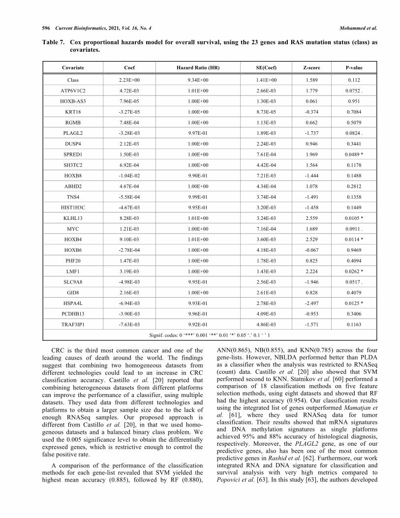
two groups (log-rank = 1.8, p-value = 0.2). We then applied the Cox proportional hazards (CPH) model was to assess the significance of the 23 genes and RAS mutation status. The results show that 9 of 23 genes were significantly associated with OS, including SPRED1, KLHL13, HOXB4, LMF1, HSPA4L at the 0.05 level, and ATP6V1C2, PLAGL2, MYC, SLC9A8 at the 0.1 level (LRT = 56.85, p-value = 0.0002) as can be seen in Table 7.

We further performed an analysis of the top nine genes using gradient boosted trees and Shapley additive explanations (SHAP) methods to identify the top-K genes (1 < K < 9) [59]. The SHAP approach determined the order of importance of our nine genes. SHAP values give the importance of a gene by comparing what a model predicts with and without the gene. A SHAP value of 0 means that the gene does not affect the prediction, as shown in Fig. (6). The vertical axis shows the gene names, arranged in the order of importance, from top to bottom while the adjacent value next to the gene name is the mean SHAP value. The horizontal axis shows the SHAP value, which indicates how

Fig. (4). ROC curves based on the (a) 282 gene-list for the RNASeq data, (b) 23 gene-list for the RNASeq data, (c) 424 gene-list for the RNASeq and microarray datasets, and (d) 401 gene-list for the RNASeq and microarray datasets, under (α = 0:005).

False positive rate

True

pos

itive

rate

0.0 0.2 0.4 0.6 0.8 1.0

0.0

0.2

0.4

0.6

0.8

1.0

SVM

NB

RF

ANN

KNN

False positive rate

True

pos

itive

rate

0.0 0.2 0.4 0.6 0.8 1.0

0.0

0.2

0.4

0.6

0.8

1.0

SVM

NB

RF

ANN

KNN

False positive rate

True

pos

itive

rate

0.0 0.2 0.4 0.6 0.8 1.0

0.0

0.2

0.4

0.6

0.8

1.0

SVM

NB

RF

ANN

KNN

NBLDA

PLDA

False positive rate

True

pos

itive

rate

0.0 0.2 0.4 0.6 0.8 1.0

0.0

0.2

0.4

0.6

0.8

1.0

SVM

NB

RF

ANN

KNN

NBLDA

PLDA

a

c

b

d


much the change was in log-odds. From the log-odds, one can obtain the probability of success. The gradient color indicated the original value for that gene. Genes pushing the prediction higher are colored blue, while those pushing the prediction lower are colored yellow. Each point represents a row from the original dataset.

4. DISCUSSION

The development of molecular signatures is a significant step towards understanding the molecular mechanisms of tumor genesis, which could help with accurate prognosis and diagnosis and thus allow physicians to prescribe suitable patient-specific therapies.

Several studies have done cancer classification using either microarray or RNASeq data only, and few have shown integration of both types of data, based on heterogeneous datasets. To the best of our knowledge, no cancer classification study has employed the integration of a homogeneous datasets approach. In this study, we integrated homogeneous microarray and RNASeq datasets and assessed whether such an approach could improve the classification accuracy using seven methods, namely, SVM with radial basis function kernel, NB, RF, ANN, KNN, NBLDA, and PLDA. We implemented the classification of the mutation status of CRC samples, using gene-lists obtained through the intersection, the complement of an intersection, and the union of differentially-expressed genes from microarray and RNASeq datasets.

Fig. (5). Kaplan-Meier curves for overall survival (in months).


Fig. (6). Genes in ascending order of importance (Note: dots represent SHAP values of specific features).

��

��

��

��

��

��

��

��

�� SLC9A8

HOXB4

KLHL13

SPRED1

PLAGL2

HSPA4L

LMF1

MYC

ATP6V1C2

-0.4 0.0 0.4SHAP value (impact on model output)

Low High Feature value


Table 7. Cox proportional hazards model for overall survival, using the 23 genes and RAS mutation status (class) as

covariates.

Covariate Coef Hazard Ratio (HR) SE(Coef) Z-score P-value

Class 2.23E+00 9.34E+00 1.41E+00 1.589 0.112

ATP6V1C2 4.72E-03 1.01E+00 2.66E-03 1.779 0.0752 .

HOXB-AS3 7.96E-05 1.00E+00 1.30E-03 0.061 0.951

KRT18 -3.27E-05 1.00E+00 8.73E-05 -0.374 0.7084

RGMB 7.48E-04 1.00E+00 1.13E-03 0.662 0.5079

PLAGL2 -3.28E-03 9.97E-01 1.89E-03 -1.737 0.0824 .

DUSP4 2.12E-03 1.00E+00 2.24E-03 0.946 0.3441

SPRED1 1.50E-03 1.00E+00 7.61E-04 1.969 0.0489 *

SH3TC2 6.92E-04 1.00E+00 4.42E-04 1.564 0.1178

HOXB8 -1.04E-02 9.90E-01 7.21E-03 -1.444 0.1488

ABHD2 4.67E-04 1.00E+00 4.34E-04 1.078 0.2812

TNS4 -5.58E-04 9.99E-01 3.74E-04 -1.491 0.1358

HIST1H3C -4.67E-03 9.95E-01 3.20E-03 -1.458 0.1449

KLHL13 8.28E-03 1.01E+00 3.24E-03 2.559 0.0105 *

MYC 1.21E-03 1.00E+00 7.16E-04 1.689 0.0911 .

HOXB4 9.10E-03 1.01E+00 3.60E-03 2.529 0.0114 *

HOXB6 -2.78E-04 1.00E+00 4.18E-03 -0.067 0.9469

PHF20 1.47E-03 1.00E+00 1.78E-03 0.825 0.4094

LMF1 3.19E-03 1.00E+00 1.43E-03 2.224 0.0262 *

SLC9A8 -4.98E-03 9.95E-01 2.56E-03 -1.946 0.0517 .

GID8 2.16E-03 1.00E+00 2.61E-03 0.828 0.4079

HSPA4L -6.94E-03 9.93E-01 2.78E-03 -2.497 0.0125 *

PCDHB13 -3.90E-03 9.96E-01 4.09E-03 -0.953 0.3406

TRAF3IP1 -7.63E-03 9.92E-01 4.86E-03 -1.571 0.1163

Signif. codes: 0 ‘***’ 0.001 ‘**’ 0.01 ‘*’ 0.05 ‘.’ 0.1 ‘ ’ 1

CRC is the third most common cancer and one of the leading causes of death around the world. The findings suggest that combining two homogeneous datasets from different technologies could lead to an increase in CRC classification accuracy. Castillo et al. [20] reported that combining heterogeneous datasets from different platforms can improve the performance of a classifier, using multiple datasets. They used data from different technologies and platforms to obtain a larger sample size due to the lack of enough RNASeq samples. Our proposed approach is different from Castillo et al. [20], in that we used homo-geneous datasets and a balanced binary class problem. We used the 0.005 significance level to obtain the differentially expressed genes, which is restrictive enough to control the false positive rate.

A comparison of the performance of the classification methods for each gene-list revealed that SVM yielded the highest mean accuracy (0.885), followed by RF (0.880),

ANN(0.865), NB(0.855), and KNN(0.785) across the four gene-lists. However, NBLDA performed better than PLDA as a classifier when the analysis was restricted to RNASeq (count) data. Castillo et al. [20] also showed that SVM performed second to KNN. Statnikov et al. [60] performed a comparison of 18 classification methods on five feature selection methods, using eight datasets and showed that RF had the highest accuracy (0.954). Our classification results using the integrated list of genes outperformed Mamatjan et al. [61], where they used RNASeq data for tumor classification. Their results showed that mRNA signatures and DNA methylation signatures as single platforms achieved 95% and 88% accuracy of histological diagnosis, respectively. Moreover, the PLAGL2 gene, as one of our predictive genes, also has been one of the most common predictive genes in Rashid et al. [62]. Furthermore, our work integrated RNA and DNA signature for classification and survival analysis with very high metrics compared to Popovici et al. [63]. In this study [63], the authors developed


a classifier using 64 genes for detecting BRAF mutant tumors for colon cancer. Also, they found DUSP4 to be one of the top 50 differently expressed genes.

Survival analysis results showed that 9 of 23 genes were prognostic for overall survival for CRC patients. Upon subjecting the nine genes to the Shapley additive explanations (SHAP) method to rank the genes in order of importance, the top-5 genes to emerge were ATP6V1C2, MYC, LMF1, HSPA4L, and PLAGL2.

Our findings are consistent with other published molecular signatures from previous studies [64, 65, 66]. Zumwalt et al. [64] showed that ATP6V1C2 expression successfully distinguished between cancerous and non-cancerous samples in CRC. He et al. [65] reported that the expression of c-Myc, which was one of the three related human genes encoded under MYC genes family, was observed in many human cancers and was elevated in up to 70 - 80% in CRC. Liu et al. [66] identified ten lncRNAs related to crucial outcomes in CRC, and one of these was LMF1. Zhang et al. [67] obtained 34 genes using minimal redundancy maximal relevance (mRMR) and incremental feature selection (IFS) methods. They found that the HSPA4L gene was the most highly expressed in CRC patients with chromosomal instability (CIN) mechanism. Zheng et al. [68] reported that the PLAGL2 gene was vital in increasing the effect on glioblastoma and colorectal cancer. Su et al. [69] reported that PLAGL2 served as an oncogenic function in multiple human malignancies, including colorectal cancer (CRC).

This study was limited by the available number of homogeneous RNASeq and microarray datasets. Only one matched-pair set of 54 CRC samples was analyzed. Future studies should extend the approach to more than one cancer type and multiple datasets. However, the number of samples in each dataset (n = 54) ensured that the training and validation sets were large enough for the magnitude and statistical significance of the classification accuracies.

CONCLUSION

In summary, data integration by taking the intersection of the individual gene-lists from the two data types improved the classification accuracy of CRC. However, laboratory experiments should be conducted on this 23-gene signature to further assess its clinical significance in CRC research. NBLDA method was the best performer on the RNASeq data. Results suggest that the SVM method was the most suitable classifier for CRC across the two data types and had high accuracy before and after the integration. Future studies should determine the effectiveness of integration in cancer survival analysis and the application on unbalanced data (where the classes are of different sizes) as well as on data with multiple classes.

LIST OF ABBREVIATIONS

CRC = Colorectal Cancer

SSA = Sub-Saharan Africa

EGFRi = Anti-epithelial Growth Factor Receptor Inhibitor

FFPE = Formalin-Fixed Paraffin-Embedded

AUC = Area Under the ROC Curve

WHO = World Health Organization

NGS = Next-Generation Sequencing

PLDA = Poison Linear Discriminant Analysis

NBLDA = Negative Binomial Linear Discriminant Analysis

SVM = Support Vector Machines

ANN = Artificial Neural Networks

LDA = Linear Discriminant Analysis

RF = Random Forests

NB = Naive Bayes

KNN = k-Nearest Neighbors

IG = Information Gain

SGA = Standard Genetic Algorithm

CFS = Correlation-based Feature Selection

IBPSO = Improved-Binary Particle Swarm Optimization

bagSVM = Bagging SVM

CART = Classification and Regression Trees

mRMR = Minimum-redundancy Maximum-Relevance

GEO = Gene Expression Omnibus

CPM = Counts Per Million

GLM = Generalized Linear Model

DAVID = Database for Annotation, Visualization, and Integrated Discovery

COSMIC = Catalogue of Somatic Mutations in Cancer

MLE = Maximum Likelihood Estimate

RBF = Radial Basis Function

MAP = Maximum a Posteriori

BER = Balanced Error Rate

TP = True Positive

TN = True Negative

FP = False Positive

FN = False Negative

RA = Random Accuracy

OS = Overall Survival

CPH = Cox Proportional Hazards

SHAP = Shapley Additive Explanations

IFS = Incremental Feature Selection


CIN = Chromosomal Instability

HR = Hazard Ratio

AUTHORS’ CONTRIBUTION

BO conceived the study. MM performed all the analyses. MM and BO drafted the manuscript. MM, HM, and BO proof-read, discussed, and approved the final manuscript.

ETHICS APPROVAL AND CONSENT TO

PARTICIPATE

Not applicable.

HUMAN AND ANIMAL RIGHTS

No animals/humans were used for studies that are basis of this research.

CONSENT FOR PUBLICATION

Not applicable.

AVAILABILITY OF DATA AND MATERIALS

The datasets supporting the results of this article have been deposited to the public repository (GEO) under the series accession number GSE86566 https: //www.ncbi.nlm.nih.gov/geo/. The individual datasets are accessible under the accession number GSE86559 for the microarray data and GSE86562 for the RNASeq data. The mutation and overall survival data are available upon request from BO.

FUNDING

This work was funded by GSK Africa Non-Communicable Disease Open Lab through the DELTAS Africa Sub-Saharan African Consortium for Advanced Biostatistics (SSACAB) Grant No. 107754/Z/15/Z- training programme. The views expressed in this publication are those of the author(s) and not necessarily those of GSK.

CONFLICT OF INTEREST

The authors declare no conflict of interest, financial or otherwise.

ACKNOWLEDGEMENTS

The authors wish to thank Prof. Bob Gagnon (GlaxoSmithKline (GSK)).

REFERENCES

[1] Gandomani HS, Yousefi SM, Aghajani M, et al. Colorectal cancer in the world: incidence, mortality and risk factors. Biomed Res Ther 2017; 4(10): 1656-75.

http://dx.doi.org/10.15419/bmrat.v4i10.372 [2] Siegel RL, Miller KD, Jemal A. Cancer statistics, 2019. CA Cancer

J Clin 2019; 69(1): 7-34. http://dx.doi.org/10.3322/caac.21551 PMID: 30620402 [3] Word Cancer Research Fund. colorectal cancer statistics. Available

at: www.wcrf.org/dietandcancer/cancer-trends/colorectal-cancer-statistics. (Accessed on August 2, 2019).

[4] Omolo B, Yang M, Lo FY, et al. Adaptation of a RAS pathway activation signature from FF to FFPE tissues in colorectal cancer. BMC Med Genomics 2016; 9(1): 65.

http://dx.doi.org/10.1186/s12920-016-0225-2 PMID: 27756306 [5] Mármol I, Sánchez-de-Diego C, Pradilla Dieste A, Cerrada E,

Rodriguez Yoldi MJ. Colorectal carcinoma: a general overview and future perspectives in colorectal cancer. Int J Mol Sci 2017; 18(1): 197.

http://dx.doi.org/10.3390/ijms18010197 PMID: 28106826 [6] Granados-Romero JJ, Valderrama-Treviño AI, Contreras-Flores

EH, et al. Colorectal cancer: a review. Int J Res Med Sci 2017; 5(11): 4667-76.

http://dx.doi.org/10.18203/2320-6012.ijrms20174914 [7] WHO, WHO: Cancer. Available at https://www.who.int/news-

room/fact-sheets/detail/cancer. [Cited August 14, 2019]. [8] DeSantis CE, Miller KD, Goding Sauer A, Jemal A, Siegel RL.

Cancer statistics for African Americans, 2019. CA Cancer J Clin 2019; 69(3): 211-33.

http://dx.doi.org/10.3322/caac.21555 PMID: 30762872 [9] American Cancer Society. Cancer facts & figures 2015. American

Cancer Society 2015. [10] May FP, Anandasabapathy S. Colon cancer in Africa: Primetime

for screening? Gastrointest Endosc 2019; 89(6): 1238-40. http://dx.doi.org/10.1016/j.gie.2019.04.206 PMID: 31104752 [11] World Health Organization. National cancer control programmes:

policies and managerial guidelines. World Health Organization 2002.

[12] Golub TR, Slonim DK, Tamayo P, et al. Molecular classification of cancer: class discovery and class prediction by gene expression monitoring. Science 1999; 15286(5439): 531-7.

[13] Wang J, Tan AC, Tian T, Eds. Next generation microarray bioinformatics: methods and protocols. Humana Press 2012.

http://dx.doi.org/10.1007/978-1-61779-400-1 [14] Tan AC, Gilbert D. Ensemble machine learning on gene expression

data for cancer classification. Appl Bioinformatics 2003; 2(3 Suppl): S75-83.

[15] Ca DA, Mc V. Gene expression data classification using support vector machine and mutual information-based gene selection. Procedia Comput Sci 2015; 47: 13-21.

http://dx.doi.org/10.1016/j.procs.2015.03.178 [16] Blagus R, Lusa L. Class prediction for high-dimensional class-

imbalanced data. BMC Bioinformatics 2010; 11(1): 523. http://dx.doi.org/10.1186/1471-2105-11-523 PMID: 20961420 [17] Rajeswari P, Reena GS. Human liver cancer classification using

microarray gene expression data. Int J Comput Appl 2011; 34(6): 25-37.

[18] Datta S. Statistical analysis of next generation sequencing data. New York: Springer 2014.

http://dx.doi.org/10.1007/978-3-319-07212-8 [19] Rai MF, Tycksen ED, Sandell LJ, Brophy RH. Advantages of

RNA-seq compared to RNA microarrays for transcriptome profiling of anterior cruciate ligament tears. J Orthop Res 2018; 36(1): 484-97. PMID: 28749036

[20] Castillo D, Galvez JM, Herrera LJ, et al. Leukemia multiclass assessment and classification from microarray and RNA-seq technologies integration at gene expression level. PLoS One 2019; 14(2): e 0212127.

http://dx.doi.org/10.1371/journal.pone.0212127 PMID: 30753220 [21] Zhang W, Yu Y, Hertwig F, et al. Comparison of RNA-seq and

microarray-based models for clinical endpoint prediction. Genome Biol 2015; 16(1): 133.

http://dx.doi.org/10.1186/s13059-015-0694-1 PMID: 26109056 [22] Dong K, Zhao H, Tong T, Wan X. NBLDA: negative binomial

linear discriminant analysis for RNA-Seq data. BMC Bioinformatics 2016; 17(1): 369.

http://dx.doi.org/10.1186/s12859-016-1208-1 PMID: 27623864 [23] Zararsız G, Goksuluk D, Korkmaz S, et al. A comprehensive

simulation study on classification of RNA-Seq data. PLoS One 2017; 12(8): e0182507.

http://dx.doi.org/10.1371/journal.pone.0182507 PMID: 28832679 [24] Kulski J, Ed. Next Generation Sequencing: Advances, Applications

and Challenges. BoD–Books on Demand 2016.14. http://dx.doi.org/10.5772/60489


[25] Wang S, Huang H, Han R, et al. BpAP1 directly regulates BpDEF to promote male inflorescence formation in Betula platyphylla × B. pendula. Tree Physiol 2019; 39(6): 1046-60.

http://dx.doi.org/10.1093/treephys/tpz021 PMID: 30976801 [26] Aziz R, Verma CK, Srivastava N. Artificial neural network

classification of high dimensional data with novel optimization approach of dimension reduction. Annals of Data Science 2018; 5(4): 615-35.

http://dx.doi.org/10.1007/s40745-018-0155-2 [27] Salem H, Attiya G, El-Fishawy N. Classification of human cancer

diseases by gene expression profiles. Appl Soft Comput 2017; 50: 124-34.

http://dx.doi.org/10.1016/j.asoc.2016.11.026 [28] Jain I, Jain VK, Jain R. Correlation feature selection based

improved-binary particle swarm optimization for gene selection and cancer classification. Appl Soft Comput 2018; 62: 203-15.

http://dx.doi.org/10.1016/j.asoc.2017.09.038 [29] Anders S, Huber W. Differential expression analysis for sequence

count data. Nat Prec 2010. https://doi.org/10.1038/npre.2010.4282.2 [30] Taminau J, Lazar C, Meganck S, Nowé A. Comparison of merging

and meta-analysis as alternative approaches for integrative gene expression analysis. ISRN Bioinform 2014; 2014: 345106.

http://dx.doi.org/10.1155/2014/345106 PMID: 25937953 [31] Lai Y. Differential expression analysis of digital gene expression

data: RNA-tag filtering, comparison of t-type tests and their genome-wide co-expression based adjustments. Int J Bioinform Res Appl 2010; 6(4): 353-65.

http://dx.doi.org/10.1504/IJBRA.2010.035999 PMID: 20940123 [32] Castillo D, Gálvez JM, Herrera LJ, Román BS, Rojas F, Rojas I.

Integration of RNA-Seq data with heterogeneous microarray data for breast cancer profiling. BMC Bioinformatics 2017; 18(1): 506.

http://dx.doi.org/10.1186/s12859-017-1925-0 PMID: 29157215 [33] Gomez-Cabrero D, Abugessaisa I, Maier D, et al. Data integration

in the era of omics: current and future challenges. BMC Syst Biol 2014; 8(Suppl 2).

http://dx.doi.org/10.1186/1752-0509-8-S2-I1 [34] Huang DW, Sherman BT, Tan Q, et al. DAVID bioinformatics

resources: expanded annotation database and novel algorithms to better extract biology from large gene lists. Nucleic Acids Res 2007; 135(Suppl_2): W169-W175.

http://dx.doi.org/10.1093/nar/gkm415 [35] Bolstad BM, Irizarry RA, Åstrand M, Speed TP. A comparison of

normalization methods for high density oligonucleotide array data based on variance and bias. Bioinformatics 2003; 19(2): 185-93.

http://dx.doi.org/10.1093/bioinformatics/19.2.185 PMID: 12538238 [36] Witten DM. Classification and clustering of sequencing data using

a Poisson model. Ann Appl Stat 2011; 5(4): 2493-518. http://dx.doi.org/10.1214/11-AOAS493 [37] Boser BE, Guyon IM, Vapnik VN. A training algorithm for optimal

margin classifiers. Proceedings of the fifth annual workshop on Computational learning theory. 1992; pp. 144-52.

http://dx.doi.org/10.1145/130385.130401 [38] Moguerza JM, Muñoz A. Support vector machines with

applications. Stat Sci 2006; 21(3): 322-36. http://dx.doi.org/10.1214/088342306000000493 [39] Stephens D, Diesing M. A comparison of supervised classification

methods for the prediction of substrate type using multibeam acoustic and legacy grain-size data. PLoS One 2014; 9(4): e93950.

http://dx.doi.org/10.1371/journal.pone.0093950 PMID: 24699553 [40] Brown MP, Grundy WN, Lin D, et al. Support vector machine

classification of microarray gene expression data. University of California, Santa Cruz, Technical Report UCSC-CRL-99-09 1999 Jun; 12.

[41] Chu F, Wang L. Gene expression data analysis using support vector machines. Proceedings of the International Joint Conference on Neural Networks, 2003.

[42] Karatzoglou A, Smola A, Hornik K, Karatzoglou MA. Package ‘kernlab’. Technical report, CRAN, 03 2016 2019 Nov; 12.

[43] Friedman J, Hastie T, Tibshirani R. The elements of statistical learning. Springer series in statistics. New York 2001.

[44] Breiman L. Random forests. Mach Learn 2001; 45(1): 5-32. http://dx.doi.org/10.1023/A:1010933404324 [45] Qi Y. Random forest for bioinformatics in ensemble machine

learning. Boston, MA: Springer 2012; pp. 307-23.

[46] Chen X, Ishwaran H. Random forests for genomic data analysis. Genomics 2012; 99(6): 323-9.

http://dx.doi.org/10.1016/j.ygeno.2012.04.003 PMID: 22546560 [47] Pappu V, Pardalos PM. High-dimensional data classification

InClusters, Orders, and Trees: Methods and Applications. New York, NY: Springer 2014; pp. 119-50.

[48] Do TN, Lenca P, Lallich S, Pham NK. Classifying very-high-dimensional data with random forests of oblique decision trees InAdvances in knowledge discovery and management. Berlin, Heidelberg: Springer 2010; pp. 39-55.

[49] RColorBrewer S, Liaw MA. Package ‘randomForest’. Berkeley, CA, USA.: University of California Berkeley 2018.22.

[50] Dwivedi AK. Artificial neural network model for effective cancer classification using microarray gene expression data. Neural Comput Appl 2018; 29(12): 1545-54.

http://dx.doi.org/10.1007/s00521-016-2701-1 [51] Ripley B, Venables W, Ripley MB. Package ‘nnet’. R package

version 2016 Feb; 27: 3-12. [52] De Campos LM, Cano A, Castellano JG, Moral S. Bayesian

networks classifiers for gene-expression data. 11th International Conference on Intelligent Systems Design and Applications. IEEE 2011.

http://dx.doi.org/10.1109/ISDA.2011.6121822 [53] Yao Z, Ruzzo WL. A regression-based K nearest neighbor

algorithm for gene function prediction from heterogeneous data. BMC Bioinformatics 2006; 7: 11.

http://dx.doi.org/10.1186/1471-2105-7-S1-S11 [54] Tharwat A. Classification assessment methods. Appl Comput

Informatics 2018; 17(1): 168-92. http://dx.doi.org/10.1016/j.aci.2018.08.003 [55] Mohammed M, Mwambi H, Omolo B, Elbashir MK. Using

stacking ensemble for microarray-based cancer classification. International Conference on Computer, Control, Electrical, and Electronics Engineering (ICCCEEE). IEEE 2018; 1-8.

http://dx.doi.org/10.1109/ICCCEEE.2018.8515872 [56] Li W. Volcano plots in analyzing differential expressions with

mRNA microarrays. J Bioinform Comput Biol 2012; 10(6): 1231003.

http://dx.doi.org/10.1142/S0219720012310038 PMID: 23075208 [57] Landau WM, Liu P. Dispersion estimation and its effect on test

performance in RNA-seq data analysis: a simulation-based comparison of methods. PLoS One 2013; 8(12): e81415.

http://dx.doi.org/10.1371/journal.pone.0081415 PMID: 24349066 [58] Dry JR, Pavey S, Pratilas CA, et al. Transcriptional pathway

signatures predict MEK addiction and response to selumetinib (AZD6244). Cancer Res 2010; 70(6): 2264-73.

http://dx.doi.org/10.1158/0008-5472.CAN-09-1577 PMID: 20215513 [59] Lundberg SM, Lee SI. A unified approach to interpreting model

predictions. InAdvances in neural information processing systems. 2017; pp. 4765-74.

[60] Statnikov A, Henaff M, Narendra V, et al. A comprehensive evaluation of multicategory classification methods for microbiomic data. Microbiome 2013; 1(1): 11.

http://dx.doi.org/10.1186/2049-2618-1-11 PMID: 24456583 [61] Mamatjan Y, Agnihotri S, Goldenberg A, et al. Molecular

signatures for tumor classification: an analysis of the cancer genome atlas data. J Mol Diagn 2017; 19(6): 881-91.

http://dx.doi.org/10.1016/j.jmoldx.2017.07.008 PMID: 28867603 [62] Rashid M, Vishwakarma RK, Deeb AM, Hussein MA, Aziz MA.

Molecular classification of colorectal cancer using the gene expression profile of tumor samples. Exp Biol Med (Maywood) 2019; 244(12): 1005-16.

http://dx.doi.org/10.1177/1535370219850788 PMID: 31091989 [63] Popovici V, Budinska E, Tejpar S, et al. Identification of a poor-

prognosis BRAF-mutant-like population of patients with colon cancer. J Clin Oncol 2012; 30(12): 1288-95.

http://dx.doi.org/10.1200/JCO.2011.39.5814 PMID: 22393095 [64] Zumwalt TJ, Shigeyasu K, Weng W, Okugawa Y, Miyoshi J, Goel

A. The ATP6V1C2 (a vacuolar-ATPase gene) is a novel early prognosticator for colorectal cancer. Cancer Res 2016.

DOI: 10.1158/1538-7445.AM2016-768 [65] He WL, Weng XT, Wang JL, et al. Association between c-Myc

and colorectal cancer prognosis: a meta-analysis. Front Physiol 2018; 9: 1549.

http://dx.doi.org/10.3389/fphys.2018.01549 PMID: 30483143


[66] Liu H, Gu X, Wang G, et al. Copy number variations primed lncRNAs deregulation contribute to poor prognosis in colorectal cancer. Aging (Albany NY) 2019; 11(16): 6089-108.

http://dx.doi.org/10.18632/aging.102168 PMID: 31442207 [67] Zhang TM, Huang T, Wang RF. Cross talk of chromosome

instability, CpG island methylator phenotype and mismatch repair in colorectal cancer. Oncol Lett 2018; 16(2): 1736-46.

http://dx.doi.org/10.3892/ol.2018.8860 PMID: 30008861

[68] Zheng H, Ying H, Wiedemeyer R, et al. PLAGL2 regulates Wnt signaling to impede differentiation in neural stem cells and gliomas. Cancer Cell 2010; 17(5): 497-509.

http://dx.doi.org/10.1016/j.ccr.2010.03.020 PMID: 20478531 [69] Su C, Li D, Li N, et al. Studying the mechanism of PLAGL2

overexpression and its carcinogenic characteristics based on 3′-untranslated region in colorectal cancer. Int J Oncol 2018; 52(5): 1479-90.

http://dx.doi.org/10.3892/ijo.2018.4305 PMID: 29512763 �

�

�

�

-CBIO 16-4 - Ingenta Connect

Documents

Transcript of -CBIO 16-4 - Ingenta Connect