# 40315 C U N I T 5 @BULLET B I N O M I A L D I S T R I B U T I O N S A N D S T A T I S T I C A L I...

# 40315 C Gl M G /Hill A C Pl P N 300

300 U N I T 5 • B I N O M I A L D I S T R I B U T I O N S A N D S T A T I S T I C A L I N F E R E N C E

Characteristics of BinomialDistributions

Lesson2In the last lesson, you constructed several binomial distributions, observed theirshapes, and estimated their means and standard deviations. In Investigation 1 ofthis lesson, you will learn how to visualize the shape of a binomial distribution ifyou know n and p. In Investigation 2, you will discover simple formulas for themean and the standard deviation of a binomial distribution. But first, consider thefollowing situation.

According to an annual nation-wide survey of college freshmen,two-thirds of both male and femalefreshmen planned to earn a graduatedegree (master’s or doctorate) or anadvanced professional degree (suchas law or medicine). (Source: HigherEducation Research Institute, Annu-al Freshman Survey UCLA, 1997.)Suppose you have a random sampleof 200 college freshmen and countthe number who say they plan to getan advanced degree. The graph of the binomial distribution of the number offreshmen who plan to get an advanced degree is shown below.

100 110 120 130 140 150 160

Number of Freshmen

Pro

bab

ilit

y

0

0.01

0.02

0.03

0.04

0.05

0.06

SE5.2_CP4_827549 11/27/02 5:00 PM Page 300

L E S S O N 2 • C H A R A C T E R I S T I C S O F B I N O M I A L D I S T R I B U T I O N S 301

Think About This Situation

Examine the binomial distribution on the previous page.

What is the approximate shape of the graph? Explain what the heightof the bar between 140 and 141 means.

How many freshmen in a random sample of 200 would you expect tosay that they plan to earn advanced degrees?

How can you find the standard deviation of this probability distribu-tion? What information does the standard deviation give you?

How do you think the shape, center, and spread would change if thesample size was much larger? Much smaller?

How do you think the shape, center, and spread would change if yougraphed the proportion of successes rather than the number of successes?

The Shapes of Binomial Distributions

The graph of the binomial distribution for the number of freshmen who plan toget advanced degrees looks approximately normal. In this investigation, you willsee that not all binomial distributions are approximately normal in shape. How-ever, you will be able to predict when they will be if you know the probability ofa success p and the sample size n.

1. According to the 2000 U.S. Census, about 20% of the population of the Unit-ed States are children; that is, age 13 or younger. (Source: “Age: 2000,”Census 2000 Brief, October 2001 at www.census.gov/prod/2001pubs/c2kbr01-12.pdf) Suppose you take a random sample of people from the Unit-ed States. The following graphs show the binomial distributions for thenumber of children in random samples varying in size from 5 to 100.

e

d

c

b

a


INVESTIGATION 1

Sample Size n = 25

0 10 20 30

0

0.05

0.1

0.15

0.2

Pro

bab

ilit

y

Number of ChildrenNumber of Children

Sample Size n = 10

0 10 20 300

0.1

0.2

0.3

0.4

Pro

bab

ilit

y

Sample Size n = 5

0 10 20 300

0.1

0.2

0.3

0.4

0.5

Pro

bab

ilit

y

Number of Children

SE5.2_CP4_827549 11/27/02 5:00 PM Page 301

a. Determine the exact height of the tallest bar on the graph for a sample sizeof 10.

b. Why are there more bars as the sample size increases? How many barsshould there be for a sample size of n? Why are there only 7 bars for asample size of 10?

c. What happens to the shape of the distribution as the sample size increases?

d. What happens to the mean of the number of successes as the sample sizeincreases?

e. What happens to the standard deviation of the number of successes as thesample size increases?

2. Examine the following graphs. They show binomial distributions for thenumber of heads when a fair coin is tossed various numbers of times.

0.2

0.1

0.0

n = 60

0 10 20 30 40 50 60 70

Number of Heads x

0.2

0.1

0.0

n = 50

0.2

0.1

0.0

n = 40

0.2

0.1

0.0

n = 30

0.2

0.1

0.0

n = 20

0.2

0.1

0.0

n = 10



Sample Size n = 100

0 10 20 30 40 50

0

0.02

0.04

0.06

0.08

0.1

Pro

ba

bilit

y

Number of Children

Sample Size n = 50

0 10 20 300

0.05

0.1

0.15

Pro

ba

bilit

y

Number of Children

Pro

bab

ilit

y

SE5.2_CP4_827549 11/27/02 5:00 PM 02


a. What happens to the shape of these distributions as the sample size nincreases?

b. What happens to the mean of the probability distribution as n increases?

c. What happens to the standard deviation as n increases?

3. Now consider what happens when the sample size is fixed and the probabil-ity of success varies. The set of graphs below show the binomial distributionsfor a sample size of 40 and probabilities of success varying from 0.10 to 0.90.

0.2

0.1

0.0

p = 50%

0 5 10 15 20 25 30 35 40

Number of Successes

0.2

0.1

0.0

p = 40%

0.2

0.1

0.0

p = 30%

0.2

0.1

0.0

p = 20%

0.2

0.1

0.0

p = 10%

706050403020100

0.2

0.1

0.0

n = 100

Number of Heads x

0.2

0.1

0.0

n = 90

0.2

0.1

0.0

n = 80

0.2

0.1

0.0

n = 70


Pro

bab

ilit

yP

rob

ab

ilit

y

SE5.2_CP4_827549 11/27/02 5:00 PM Page 303

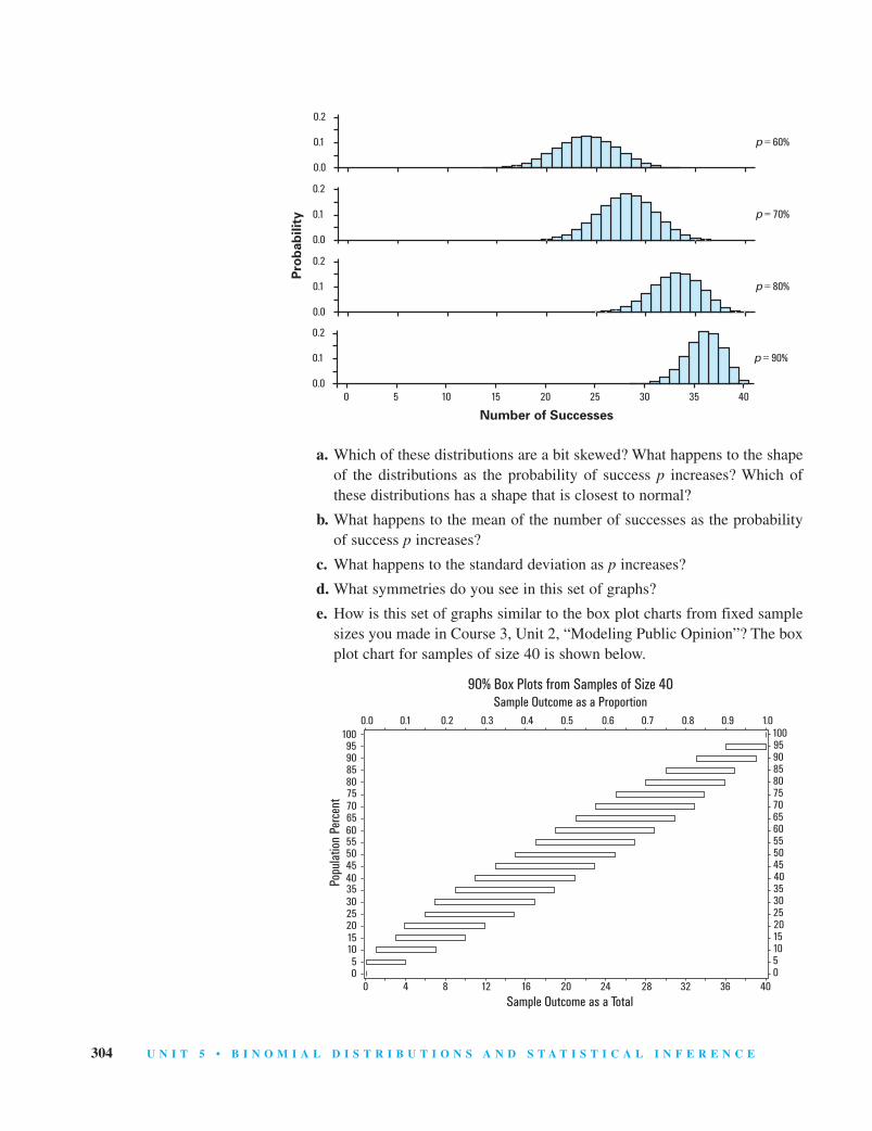
a. Which of these distributions are a bit skewed? What happens to the shapeof the distributions as the probability of success p increases? Which ofthese distributions has a shape that is closest to normal?

b. What happens to the mean of the number of successes as the probabilityof success p increases?

c. What happens to the standard deviation as p increases?

d. What symmetries do you see in this set of graphs?

e. How is this set of graphs similar to the box plot charts from fixed samplesizes you made in Course 3, Unit 2, “Modeling Public Opinion”? The boxplot chart for samples of size 40 is shown below.

4035302520151050

0.2

0.1

0.0

p = 90%

Number of Successes

0.2

0.1

0.0

p = 80%

0.2

0.1

0.0

p = 70%

0.2

0.1

0.0

p = 60%



05

25201510

5045403530

7570656055

10095908580

90% Box Plots from Samples of Size 40Sample Outcome as a Proportion

Sample Outcome as a Total

05

25201510

5045403530

7570656055

10095908580

Popu

latio

n Pe

rcen

t

0.0 0.1 0.2 0.3 0.4 0.5 0.6 0.7 0.8 0.9 1.0

0 4 8 12 16 20 24 28 32 36 40

Pro

bab

ilit

y

SE5.2_CP4_827549 11/27/02 5:00 PM Page 304


4. Based on your work in Activities 1 through 3, draw conclusions about theeffect of sample size or value of p on the shape of the graph of a binomialdistribution.

a. Complete each sentence using the word “more” or “less.”

� With a fixed sample size, the farther p is away from 0.50, the skewed the binomial distribution.

� Usually, with a fixed value of p, the larger the sample size, the skewed the binomial distribution.

b. What are the exceptions to the statement in the second item of Part a?

5. To predict whether the graph of a binomial distribution will look approxi-mately normal, compute both np and n(1 – p) and check to see if both are atleast 10.

a. The value np can be interpreted as the expected number of successes. Howcan you interpret n(1 – p)?

b. Which of the distributions in Activity 1 can be considered approximatelynormal using the above guideline? Does this agree with your visualimpression?

c. Which of the distributions in Activity 2 can be considered approximatelynormal using this guideline? Does this agree with your visual impression?

d. Which of the distributions in Activity 3 can be considered approximatelynormal using this guideline? Does this agree with your visual impression?

6. Imagine the binomial distribution with n = 35 and p = 0.2.

a. Is this distribution skewed left, skewed right, or symmetric?

b. Where is it centered? Estimate its standard deviation.

c. Check your answers to Parts a and b using the binomial function capabil-ities of your calculator to make a graph of this distribution.

Checkpoint

Think about a binomial distribution with probability of a success p and sam-ple size n.

As n increases, but the probability of a success p remains the same,what happens to the shape, center, and spread of the binomial distribu-tion for the number of successes?

As p increases from 0.01 to 0.99, but n remains the same (for example,n = 50) what happens to the shape, center, and spread of the binomialdistribution for the number of successes?

Be prepared to discuss your descriptions of changes in the

binomial distributions.

b

a


SE5.2_CP4_827549 11/27/02 5:00 PM Page 305

On Your Own

Think about patterns of change in binomial distributions as the sample size orprobability of success varies.

a. How does the binomial distribution for the number of successes in a sampleof size 25 and probability of success 0.3 differ from a binomial distributionwith sample size 50 and probability of success 0.3?

b. How does the binomial distribution for the number of successes in a sampleof size 25 and probability of success 0.3 compare to the binomial distributionwith sample size 25 and probability of success 0.7?

In the first part of this investigation, you examined the shape, center, and spreadof binomial distributions of the number of successes in a random sample. Nowexamine these same characteristics of distributions of the proportion p̂ of suc-cesses.

7. How do you convert the number of successes in a binomial situation to theproportion of successes?

8. Recall from Activity 1 (page 301) that about 20% of the population of the Unit-ed States are children age 13 or younger. Shown below are the graphs fromActivity 1 with the scale on the x-axes changed to one that gives the proportionp̂ of children in random samples, for sample sizes varying from 5 to 100.

a. What happens to the mean of the sample proportions as the sample sizeincreases?

b. What happens to the standard deviation of the sample proportions as thesample size increases? Why does this make sense?



Sample Size n = 100

0 0.1 0.2 0.3 0.4 0.50

0.02

0.04

0.06

0.08

0.1

Pro

ba

bil

ity

Proportion of Children

Sample Size n = 50

0 0.2 0.4 0.60

0.05

0.1

0.15

Pro

bab

ilit

y


Sample Size n = 25

0 0.4 0.80

0.05

0.1

0.15

0.2

Pro

bab

ilit

y

Proportion of ChildrenProportion of Children

Sample Size n = 10

00

0.1

0.2

0.3

0.4

Pro

bab

ilit

y

1.00.5

Sample Size n = 5

00

0.1

0.2

0.3

0.4

0.5

Pro

bab

ilit

y


1.0

SE5.2_CP4_827549 11/27/02 5:00 PM Page 306


9. On a copy of each of the graphs from Activity 2, change the scale on the x-axis to one that gives the sample proportion of heads, p̂.

a. What happens to the mean of the proportion of heads as the sample sizeincreases?

b. What happens to the standard deviation of the proportion of heads as thesample size increases?

Checkpoint

Consider a binomial situation with probability of success p and sample size n.

If n increases but p remains the same, what happens to the shape, cen-ter, and spread of the distribution of the sample proportions?

Compare the graphs of the distributions of ̂p and of 1 – p̂ for a fixed sam-ple size n.

Summarize the differences between the binomial distribution for thenumber of successes and the distribution for the corresponding sampleproportions.

Be prepared to discuss the variations in the distributions.

On Your OwnThink about patterns of change in distributions for the sample proportion p̂ as thesample size, or probability of success varies.

a. How does the distribution of the sample proportion p̂ from a sample of size 25and probability of success 0.3 differ from the distribution with sample size 50and probability of success 0.3?

b. How does the distribution of the sample proportion p̂ from a sample size of25 and probability of success 0.3 compare to the distribution with sample size 25and probability of success 0.7?

c. Compare your answers for Parts a and b with your corresponding answers toParts a and b of the “On Your Own” on page 306.

Simple Formulas for the Mean and theStandard Deviation

Recall that the formula for the mean of a probability distribution is

� = ∑ x � p(x)

Similarly, the formula for the standard deviation of a probability distribution is

� = �∑� (�x�–� ��)2� �� p�(x�)

c

b

a


INVESTIGATION 2

SE5.2_CP4_827549 11/27/02 5:00 PM Page 307

In this investigation, you will see that these formulas can be simplified in the caseof binomial distributions.

1. According to the 2000 U.S.Census, about 20% of the popu-lation of the United States arechildren (aged 13 or younger).Suppose you take a randomsample of four people living inthe United States and count thenumber of children.

a. Complete this probabilitydistribution table for thenumber of children in your sample of size 4.

b. Use the formulas at the bottom of page 307 to compute the mean and stan-dard deviation of the probability distribution in Part a.

c. In computing the mean of the above distribution, you could also simplyreason that if 20% of the population are children, the mean number of chil-dren in a random sample of four people should be 20% of 4 or 0.8.Compare this value with the mean value you computed in Part b.

2. Part c of Activity 1 illustrates a general formula for computing the mean of abinomial distribution. The mean number of successes in n trials with proba-bility of success p is

� = np

There is also a much simpler formula for the standard deviation of a binomi-al distribution:

� = �n�p�(1� –� p�)�

a. Verify that this formula for the standard deviation gives the same result asthat in Activity 1 Part b.

b. Now refer back to the graphs in Activity 1 of Investigation 1 of this les-son. Complete the table at the top of page 309 for those graphs. In eachcase, p = 0.2.



Number of Children x Probability p(x)0 0.4096

1 0.4096

2 0.1536

3

4 0.0016

SE5.2_CP4_827549 11/27/02 5:00 PM Page 308


c. If you double the sample size, what happens to the mean? To the standarddeviation?

d. How does the mean vary with the sample size? How does the standarddeviation vary with the sample size?

3. Consider this table for binomial distributions with n = 9 and various valuesof p. The variance �2 is the square of the standard deviation.

a. Complete the table.

b. What patterns do you see in the table?

c. Plot the points (p, �2). What type of function would model the pattern ofchange shown in the graph?

d. Describe at least three possible methods for finding an equation showingthe relationship between the probability of success and the variance.

e. Use two of these methods to find an equation.

4. About 26% of the U.S. population 25 and over have completed a bachelor’sdegree. (Source: “Educational Attainment in the United States (Update).”Current Population Reports, March 2000, U.S. Census Bureau.)

a. Describe the shape, mean, and standard deviation of the binomial distrib-ution for samples of size 1,000 for this situation.

b. What numbers of people with bachelor’s degrees would be rare events?


Probability of a Success p Mean � = np Variance � 2

0.1 0.9 0.81

0.2 1.8 1.44

0.3 2.7 1.89

0.4 3.6 2.16

0.5 4.5 2.25

0.6

0.7

0.8

0.9

Sample Size n Mean � Standard Deviation �

5

10

25

50

100

SE5.2_CP4_827549 11/27/02 5:00 PM Page 309

5. You can use the formulas for the mean and standard deviation of the numberof successes to derive corresponding formulas for the proportion of successes.

a. If the mean number of successes is � = np, what computation would youdo to get the mean proportion of successes? Write the formula for themean proportion of successes.

b. Why does the result in Part a make sense intuitively?

c. If the standard deviation of the number of successes is � = �n�p�(1� –� p�)�, whatcomputation would you do to get the standard deviation of the proportionof successes? Write the formula in the simplest form possible.

d. By examining your formula from Part c, what can you determine about thestandard deviation for the proportion of successes as the sample size increases?

e. Why does the result in Part d make sense intuitively?

Checkpoint

When studying a binomial situation, it is often helpful to know the mean andstandard deviation of the number of successes or the proportion of successes.

Compare the formulas for the mean and standard deviation of the num-ber of successes in a binomial distribution to the corresponding formu-las for the proportion of successes.

Suppose you fix a value of p and n and construct the probability distri-butions for the number of successes and the proportion of successes.Describe how the shape, mean, and standard deviation of each distrib-ution changes if you increase n but keep p fixed.

Be prepared to share your comparison and explanation

with the class.

On Your Own

Consider a binomial distribution with n = 3 and p = 0.45.

a. Make a probability distribution table giving the number of successes.

b. Find the mean of the number of successes using the formula � = np and thenusing the formula � = ∑ x � p(x).

c. Find the standard deviation of the number of successes using the formula� = �n�p�(1� –� p�)� and then by using the formula � = �∑� (�x�–� ��)2� �� p�(x�)�.

d. Find the mean and standard deviation of the distribution of the sample pro-portion p̂.

b

a



SE5.2_CP4_827549 11/27/02 5:00 PM Page 310

# 40315 C U N I T 5 @BULLET B I N O M I A L D I S T R I B U T I O N S A N D S T A T I S T I C A L I...

Documents

Transcript of # 40315 C U N I T 5 @BULLET B I N O M I A L D I S T R I B U T I O N S A N D S T A T I S T I C A L I...