遥感地表温度降尺度方法比较——性能对比及适应性评价

374 Journal of Remote Sensing 遥感学报 2013，17( 2)

遥感地表温度降尺度方法比较———性能对比及适应性评价

全金玲，占文凤，陈云浩，刘闻雨

北京师范大学资源学院地表过程与资源生态国家重点实验室，北京 100875

摘要: 在归纳现有遥感地表温度降尺度方法的基础上，选取 3 种代表性方法: Normalized Difference Vegetation Index( NDVI) 、Pixel Block Intensity Modulation ( PBIM) 和 Linear Spectral Mixture Model ( LSMM) 方法进行实验比较，并建立了一种

纹理相似性度量指标 CO-RMSE ( Co-Occurrence Root Mean Square Error) 。结果表明: ( 1) NDVI 方法受季节影响最严重，不

适于春、冬季，其次为 PBIM 方法; ( 2) LSMM 方法受分辨率限制最大，低分辨率时丢失大量纹理信息，NDVI 方法在较高分

辨率时优于 PBIM 方法，较低分辨率时则相反; ( 3) 3 种方法的适用区域分别为植被与裸土像元并存区域，山区和反照率变

化较大区域，以及类别间温差较大区域; ( 4) NDVI 方法操作最简单，LSMM 方法最复杂。分析认为，尺度因子是决定方法

性能的关键，应根据季节、分辨率、地表覆盖、应用目的和操作性等综合选择。

关键词: 地表温度，降尺度，尺度因子，CO-RMSE

中图分类号: TP79 文献标志码: A

引用格式: 全金玲，占文凤，陈云浩，刘闻雨． 2013．遥感地表温度降尺度方法比较．遥感学报，17( 2) : 361 －387Quan J L，Zhan W F，Chen Y H and Liu W Y． 2013． Downscaling remotely sensed land surface tempera-tures: A comparison of typical methods． Journal of Remote Sensing，17( 2) : 361 －387

收稿日期: 2012-01-10; 修订日期: 2012-05-31基金项目: 国家自然科学基金( 编号: 41071258) ; 地表过程与资源生态国家重点实验室开放基金( 编号: 2010 － ZY － 06) ; 高等学校博士学科点专项

科研基金( 编号: 20100003110018)

第一作者简介: 全金玲( 1987— ) ，女，北京师范大学博士研究生，主要从事资源环境遥感方面的研究。E-mail: quanjinlin_@ 126． com通信作者简介: 陈云浩( 1974—) ，男，教授，主要研究领域为城市热红外遥感。E-mail: cyh@ bnu． edu． cn

1 引言

地表温度( LST) 广泛应用于城市热岛效应研究

( Voogt 和 Oke，2003 ) 、土壤湿度估算 ( Gillies 和

Carlson，1995 ) 、地表通量估计 ( Bastiaanssen 等，

1998) 、森林火灾监测( Lentile 等，2006 ) 和地质资源

考察( Christensen 等，2000) 等领域。但是，目前基于

热红外遥感反演的地表温度空间分辨率普遍较低，

像元混合严重，因而限制了其充分应用。地表温度

降尺度是改善该境况的有效途径。目前地表温度降尺度方法很多。许多学者从

图像融合( fusion，sharpening 或 merging) 的角度提出

了 Principal Component Analysis ( PCA ) 、Gram-Schmidt、Generalized Laplacian Pyramid ( GLP) ( Aiazzi等，2005)、贝叶斯( Fasbender 等，2008 ) 、协-克里金差

值( Pardo-Igúzquiza 等，2006; Atkinson 等，2008 ) 、人

工神经网络 ( Lemeshewsky，1998; Lemeshewsky 和

Schowengerdt，2001) 等方法。但是此类方法通常忽

略了明确的物理背景和热红外遥感的定量需求

( Zhan 等，2011) 。有些学者从尺度因子( Scale Factor) ( Stathopou-

lou 和 Cartalis，2009 ) 的角度探索，着重于研究影响

LST 变化的物理因素，以及保障降尺度前后热辐射

信息的一致性。主要分为 3 类: 基于统计、基于调制

分配和基于光谱混合模型的方法。( 1) 基于统计的方法中，统计回归是其主要计

算手段。它假定“关系尺度不变”，将低分辨率地表

温度与回归核的统计关系应用到高分辨率上。回

归核包括 NDVI ( Kustas 等，2003; Agam 等，2007 ) 、反照率( Dominguez 等，2011) 和组分权重( Gustavson等，2003; Liu 和 Pu，2008 ) 等，其中，NDVI 的使用较

多。Kustas 等人( 2003) 将 LST-NDVI 负相关关系应

用于地表温度的降尺度，结果表明该方法有效; 鉴

于 NDVI 在高密度植被区的饱和性，Agam 等人

全金玲等: 遥感地表温度降尺度方法比较 375

( 2007) 探讨了以植被覆盖率作为回归核的降尺度

效果，以及 LST-NDVI 非线性关系; 在此基础上，Je-ganathan 等人( 2010 ) 讨论了全局、局域、分辨率调

节、分段回归和土地利用 /覆盖( LULC) 分层的降尺

度模型; Dominguez 等人( 2011 ) 则考虑到城市地表

特性，提出了 NDVI 结合反照率的多元回归模型。( 2) 基于调制分配的方法是将低分辨率 LST 按一定

比例分配给各子像元，分配因子包括全色波段( Liu和 Moore，1998) 、发射率( Nichol，2009) 、同季节其他

高分辨率传感器获得的 LST、高分辨率 LST 初始估

计值以及发射率同 LST 的组合( Stathopoulou 和 Car-talis，2009) 等。( 3 ) 基于光谱混合模型的方法是根

据线性光谱混合模型，直接关联高、低分辨率 LST，

进而回归求解高分辨率 LST，如( Zhukov 等，1999;

Liu 和 Pu，2008) 。最近，Zhan 等人( 2011) 从数据同

化的角度建立了地表温度降尺度方法的统一理论

框架，并就回归核进行了讨论。以上方法在特定区域得到了很好应用。但是，

由于地表环境和气候的复杂性，在实际应用中，方

法选择的随意性较大，其参数的选择也受到较强的

主观影响。目前，尚缺乏这方面统一的定量比较与

总结。鉴于此，本文在第 2 组的 3 类地表温度降尺

度方法中各选取一种代表性方法，在不同季节、分

辨率层级和地表覆盖下开展比较实验，旨在为方法

的选择和使用提供一定依据。

2 方法

2. 1 降尺度方法

基于统计的方法中，NDVI 是目前最常用的回

归核，且易于获取，是许多此类方法的基础。以 ND-VI 的变换形式作为回归核( Agam 等，2007 ) 或结合

反照率构成多元回归( Dominguez 等，2011 ) 的方法，

在精度和操作简易性上并无明显优势。基于调制分配的方法中，以发射率为分配因子

的方法( Nichol，2009 ) 对影像空间分辨率的要求较

高，且发射率的计算精度难以得到保证。与此相

比，Pixel Block Intensity Modulation ( PBIM) 方法的

理论背景更加成熟，全色波段辐亮度 / Digital Num-ber ( DN) 值的获取精度更佳。

基于光谱混合模型的方法中，LSMM ( LinearSpectral Mixture Model) 方法的引用较高( ［2012 －03 － 27］ http: / / scholar． google． com /scholar? hl = zh－ CN＆q = Unmixing － based＆btnG = ＆lr = ) ，且在此

类方法中操作相对简单。因此，本文选择 NDVI、PBIM 和 LSMM 方法分

别作为 3 类地表温度降尺度方法的代表，开展实验。在本文中低分辨率记为 LR，高分辨率记为 HR，地表

温度记为 T。2. 1. 1 NDVI 方法

NDVI 方法( Kustas 等，2003) 是以 NDVI 作为尺

度因子的统计回归方法。该方法假定 NDVI 与 LST间存在某种映射关系，且此关系在各空间分辨率上

均成立。因此，在低分辨率下建立 NDVI 与 LST 的

回归模型，再将此回归函数作用于高分辨率，从而

建立起两者关联，最后添加回归误差即求得 THR，如

下式所示。THR = f( NDVIHR ) + ΔTLR ( 1)

ΔTLR = TLR － f( NDVILR ) ( 2)

式中，f 为 NDVILR与 TLR间的回归函数; ΔTLR为回归

误差。常用的回归函数有( Agam 等，2007) :

f( NDVI) =

a0 + a1NDVI

a0 + a1NDVI + a2NDVI2

a0 + a (1 1 － NDVImax － NDVINDVImax － NDVI( )

min)0. 625

a0 + a1 ( 1 － NDVI)

0. 625

( 3)

式中，a0、a1 和 a2 为回归系数; NDVImax和 NDVImin分

别为区域内 NDVI 的最大值和最小值，在实际处理

中，采用置信区间获取。2. 1. 2 PBIM 方法

PBIM 方法( Liu 和 Moore，1998 ) 是以全色波段

作为尺度因子的调制分配方法。它假定 TLR 是各

THR的平均值，且各子像元反照率相同。基于该假

设，由遥感图像物理方程，可推导出全色波段与 LST之比尺度不变( Wang 等，2005) ，从而求得 THR，如式

( 4) 所示。反照率异质性较强的 LR 像元则区分亮、暗面后分别计算，如式( 5) ( 6) 所示。

THR = ( PANHR /PANLR ) × TLR ( 4)

当 PANs≥Cr 时:

TB_HR = ( PANB_HR /PANB_m ) × TLR ( 5)

TD_HR = ( PAND_HR /PAND_m ) × TLR ( 6)

式中，PAN 为全色波段的 DN 值; PANs 为 LR 像元内

PANHR的方差; Cr 为反照率异质性判断阈值，当

PANs ＞ Cr 时，认为该 LR 像元异质性较强; TB_HR 为

亮面 THR ; PANB_HR和 PANB_m分别为亮面 PANHR及其


均值; TD_HR为暗面 THR ; PAND_HR 和 PAND_m 分别为暗

面 PANHR及其均值。其中 PAN 大于 PANLR的 HR 像

元归为亮面，其余为暗面。2. 1. 3 LSMM 方法

LSMM 方法( Zhukov 等，1999 ) 是以分类图作为

尺度因子的线性光谱混合模型方法。它假定 TLR是

各类别 THR 的线性加权混合，则高、低空间分辨率

LST 间存在如式( 7 ) 所示的关联。首先，确定一个

滑动运算窗口，则窗口内各 LR 像元分别形成一个

线性加权混合方程; 然后，利用最小二乘等方法求

解窗口内方程组，获得各类别 THR ; 最后，赋予窗口

中心 LR 像元内各 HR 像元其类别 THR，如式( 9 ) 所

示。

TLR = ∑K

k = 1w( k) THR ( k) + ΔT ( 7)

式中， w( k) = ∑c( i，j) = k

PSF( i，j) ( 8)

THR ( i* ，j* ) = THR ( c( i* ，j* ) ) ( 9)

式中，w( k) 为 HR 类别 k 在 LR 像元中的权重;

THR ( k) 为类别 k 的平均地表温度; K 为类别总数;

ΔT 为模型误差; PSF( i，j) 为 HR 像元 ( i，j) 对 LR像元的点扩散函数( PSF) ; c( i，j) 为 HR 像元( i，j)的类别; ( i* ，j* ) 为运算窗口中心 LR 像元内的 HR像元。其中，经常采用高斯 PSF 建模 ( Liang，

2004) ，而后对 PSF( i，j) 进行归一化，以确保权重和

为 1。若不考虑 PSF，则可通过各 HR 类别的面积百

分比确定权重( Liang，2004) 。

2. 2 相似性度量指标

2. 2. 1 RMSE为了定量评价降尺度结果，本文选取均方根标

准差( RMSE) 作为降尺度结果与目标温度间的相似

性度量指标:

RMSE =∑

N

n = 1( T n

HR － T nREF )[ ]2

槡 N ( 10)

式中，THR为降尺度后温度; TREF为目标温度; N 为像

元总数。RMSE 以( ℃ ) 为单位，值越小，表明降尺度

定量精度越高。2. 2. 2 CO-RMSE

RMSE 难以表达像元与邻域间关系，无法对两

影像 LST 的纹理差异给予恰当估计，在描绘热环境

格局或温度等级分布时不宜单独作为评价指标( 详

见 5. 3 节) 。因此，在 RMSE 的基础上，本文构建了

以温度共生矩阵为比较对象，着重描述 LST 纹理特

征差异的指标 CO-RMSE ( Co-Occurrence Root MeanSquare Error) :

CO － RMSE =∑

M

m = 1∑

N

n = 1( C( m) n

HR － C( m) nREF ) 2

槡 /N

M( 11)

式中，C( m) HR和 C( m) REF分别表示降尺度结果和目

标温度的共生矩阵第 m 个特征值; N 为像元总数; M为共生矩阵特征参数的总数。

共生矩阵是目前最常用的纹理特征分析方法

之一，有 15 个特征参数 ( Baraldi 和 Parmiggian，

1995) 。本文采用平均值、变异性、协同性、对比度、相异性、熵、二阶矩和相关性 8 个特征值( Anys 等，

1994) ，各特征值经归一化后参与计算以综合估计

纹理特征差异。CO-RMSE 无量纲，值越小，表明降

尺度纹理精度越高。

3 数据

3. 1 研究区

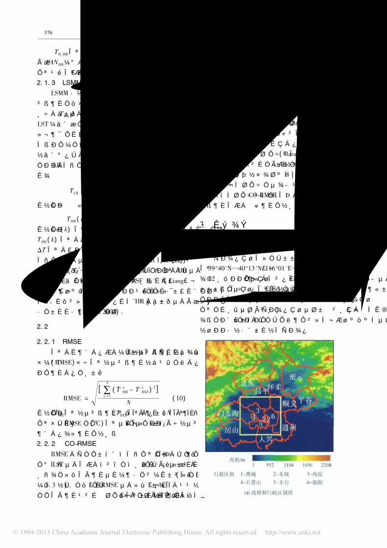
研究区位于北京市及其郊区( 图 1) ，其范围约

为 39°40'N—40°13'N，116°01'E—116°46'E，涵盖北

京 12 个行政区，东南部为平原，属于华北平原的西

北边缘区; 西部为山地，属于太行山脉的东北余脉;

中心为城区，主要由不透水层覆盖; 周边为郊区，主

要由耕地覆盖。该研究区地表覆盖类型十分丰富，

具有代表性，有利于针对不同气候和地表覆盖类型

进行方法比较研究。


图 1 研究区

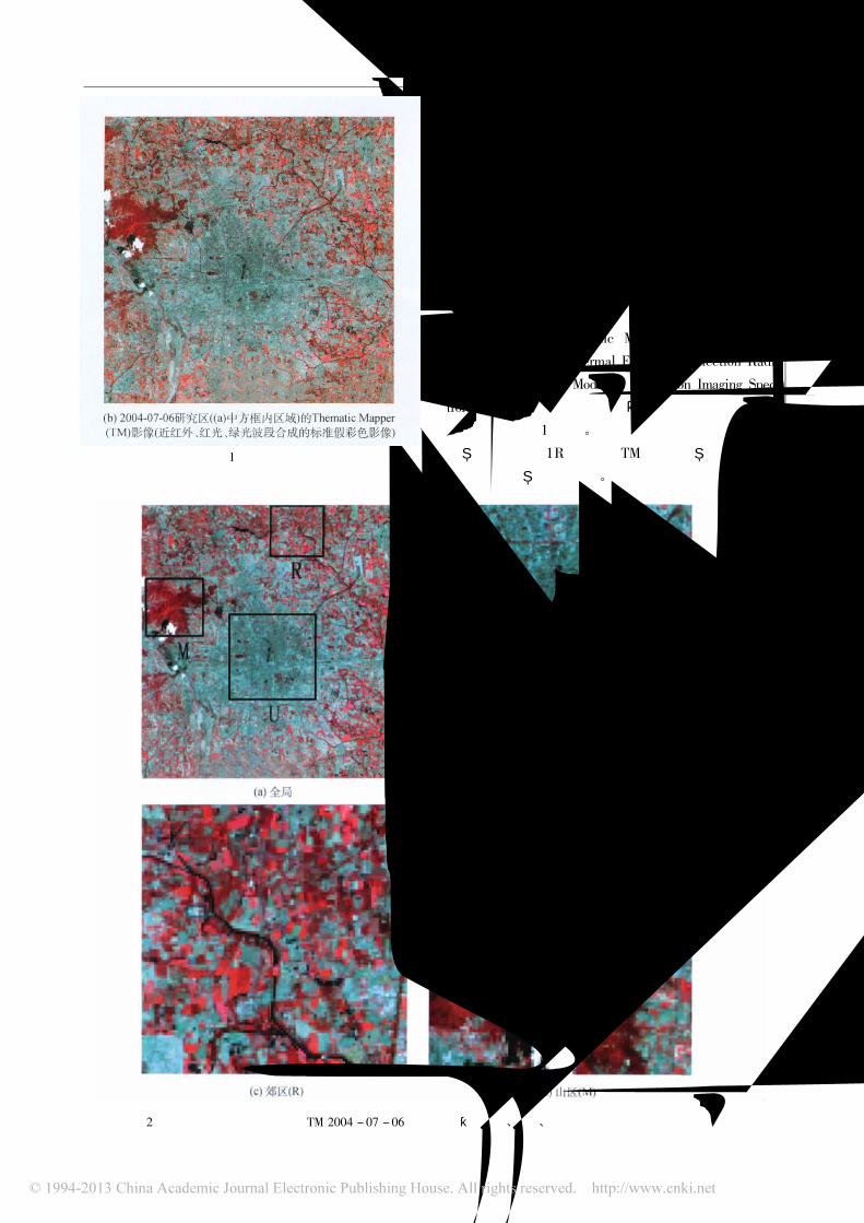
3. 2 地表覆盖分区

为了比较分析各降尺度方法针对不同地表覆

盖类型的适应性，将研究区下垫面划分为 3 个区

域———城区( U)、郊区( R) 和山区( M)。城区主要为 5环以内区域，主要覆盖类型为不透水层、植被和水体;

郊区为东北部农作物区; 山区为小西山区域，如图 2所示。

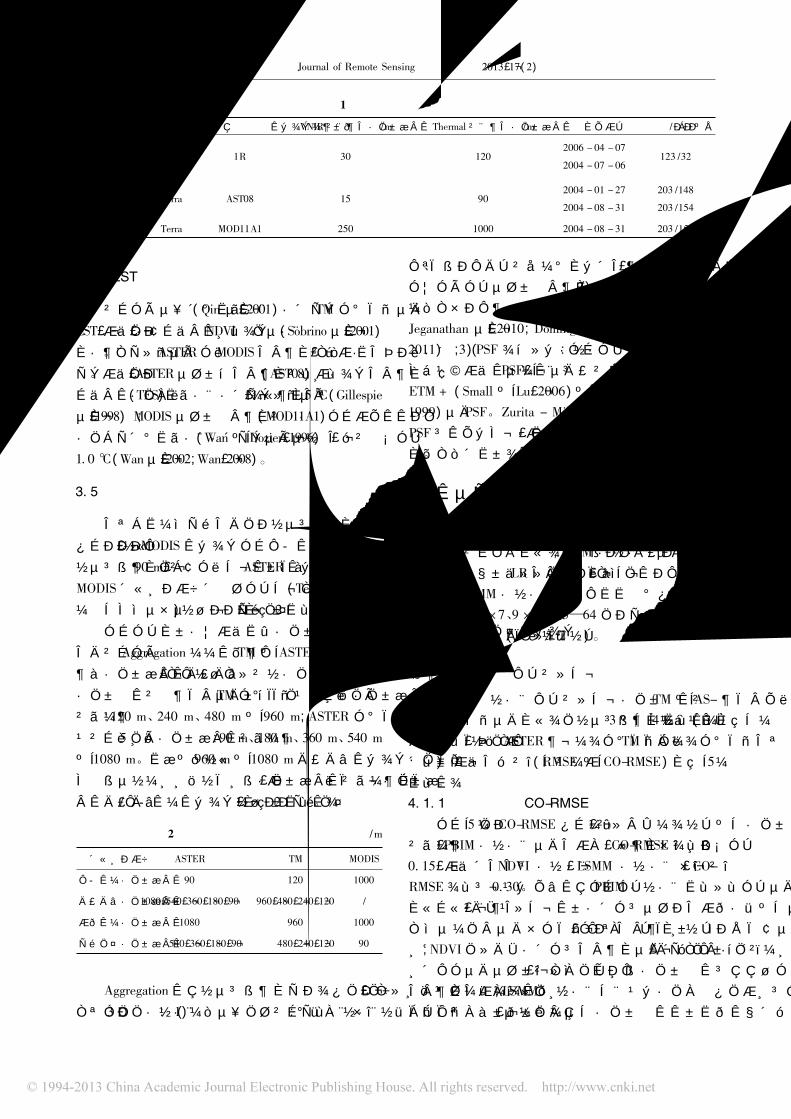
3. 3 卫星数据

采用 TM ( Thematic Mapper ) 、ASTER ( Ad-vanced Spaceborne Thermal Emission Reflection Radi-ometer) 和 MODIS ( Moderate Resolution Imaging Spec-troradio-meter) 晴空过境影像，裁剪至研究区范围，其

基本信息如表 1 所示。对少量含有云和阴影的影像

进行掩膜处理; 1R 级别的 TM 数据进行辐射定标;

所有数据进行几何配准。

图 2 地表覆盖分区示意图( 以 TM 2004 － 07 － 06 数据为例，近红外、红光、绿光波段合成的标准假彩色影像)


表 1 实验数据的基本信息

传感器卫星数据级别 VNIR 波段分辨率 /m Thermal 波段分辨率 /m 日期列 /行号

TM Landsat 5 1R 30 1202006 － 04 － 07

2004 － 07 － 06123 /32

ASTER Terra AST08 15 902004 － 01 － 27

2004 － 08 － 31

203 /148

203 /154

MODIS Terra MOD11A1 250 1000 2004 － 08 － 31 203 /154

3. 4 LST 反演

采用单窗算法( Qin 等，2001) 反演 TM 影像的

LST，其中，发射率根据 NDVI 阈值法( Sobrino 等，2001)

确定。已获得ASTER 与MODIS 温度产品，因此无需反

演。其中，ASTER 地表温度产品( AST08) 根据温度发

射率分离( TES) 算法反演获得，精度为1. 5 ℃ ( Gillespie等，1998) ; MODIS 地表温度产品( MOD11A1) 由普适性

分裂窗算法反演得到( Wan 和 Dozier，1996) ，误差小于

1. 0 ℃ ( Wan 等，2002; Wan，2008)。

3. 5 多分辨率模拟

为了检验文中降尺度方法针对真实遥感影像的

可行性，将 MODIS 数据由原始空间分辨率( 1000 m)

降尺度至 90 m，并与同时相 ASTER 数据( ASTER 与

MODIS 传感器搭载于同一卫星平台( Terra) ，成像时

间和天底点相同) 进行验证，如表 2 所示。由于缺乏其他分辨率层级的真实验证数据，本

文采用 Aggregation 技术对 TM 和 ASTER 数据进行

多分辨率模拟，以进一步分析各降尺度方法在不同

分辨率层级下的表现。TM 影像共设置 4 个分辨率

层级: 120 m、240 m、480 m 和 960 m; ASTER 影像

共设置 5 个分辨率层级: 90 m、180 m、360 m、540 m和 1080 m。随后将 960 m 和 1080 m 模拟数据分别

提高到几个较高分辨率层级上，其结果与相同分辨

率模拟 /原始数据进行验证，如表 2 所示。

表 2 多分辨率实验数据模拟 /m

传感器 ASTER TM MODIS

原始分辨率 90 120 1000

模拟分辨率 1080，540，360，180，90 960，480，240，120 /

起始分辨率 1080 960 1000

验证分辨率 540，360，180，90 480，240，120 90

Aggregation 是降尺度研究中一个关键技术，主

要有 3 种方法: ( 1) 简单重采样方法: 包括最近邻像

元、线性内插及三次多项式内插等，此类方法极少

应用于地表温度的升尺度; ( 2) 聚合平均方法: 因其

简易性而常被使用( Kustas 等，2003; Agam 等，2007;

Jeganathan 等，2010; Dominguez 等，2011; Zhan 等，

2011) ; ( 3) PSF 卷积方法: 由于许多传感器都没有

提供其实际的 PSF，通常采用高斯函数代替 TM /ETM + ( Small 和 Lu，2006 ) 和 ASTER ( Zhukov 等，

1999) 的 PSF。Zurita － Milla 等人 ( 2007 ) 指出，当

PSF 呈正态分布时，其对降尺度结果的影响十分微

弱。因此本文采用聚合平均的方法，而不考虑 PSF。

4 实验结果

本文实验均在 ENVI_IDL 平台上运行。NDVI方法采用全局线性模型; PBIM 方法的全色波段数

值范围变换至与 LR 温度相同，异质性判断阈值 Cr设为 10; LSMM 方法的运算窗口和类别个数分别从

3 × 3、5 × 5、7 × 7、9 × 9 和 3—64 中选择使其降尺度

效果最佳的一项( 详见 5. 2 节) 。

4. 1 模拟数据的结果

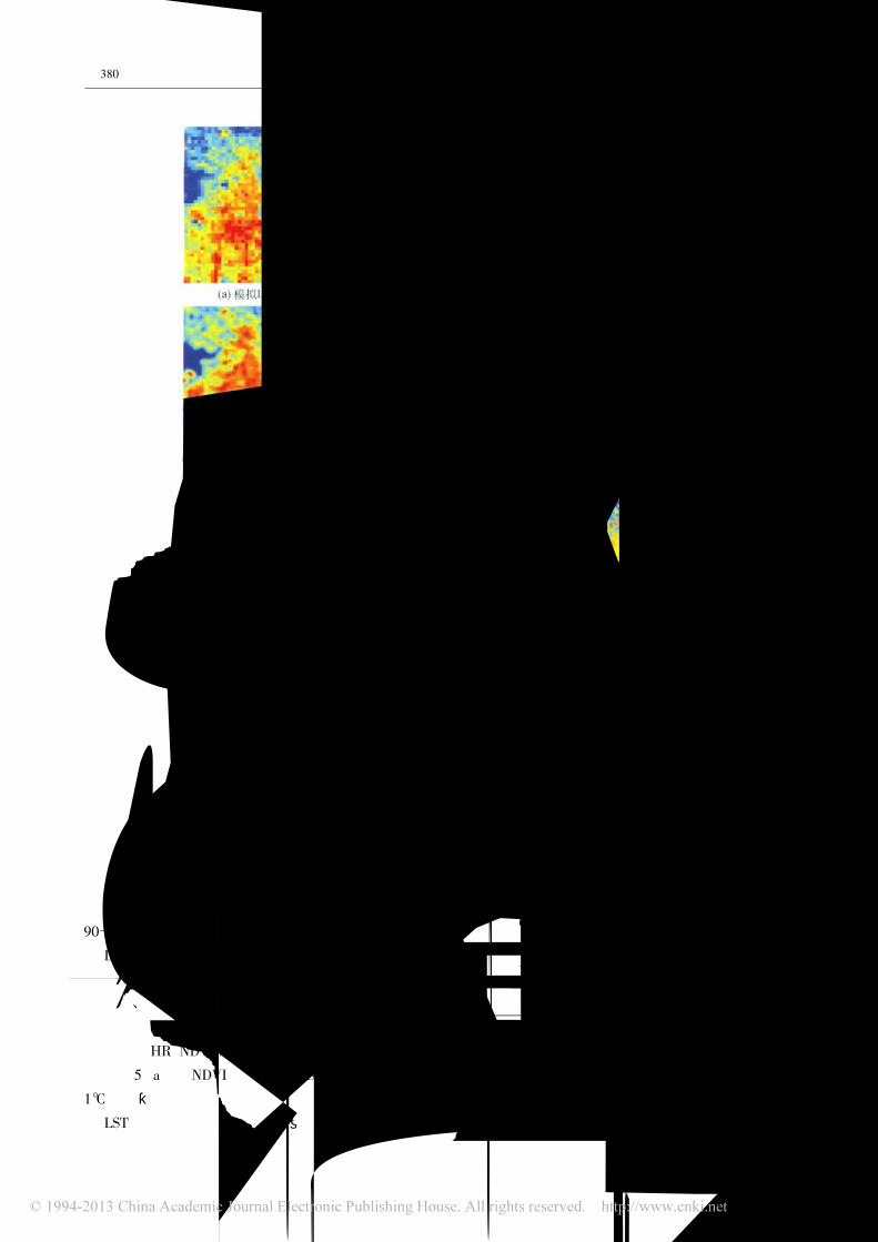
3 种方法在不同分辨率层级下针对 TM 和 AS-TER 影像的全局降尺度结果如图 3 和图 4 所示( 受

篇幅限制，仅以 ASTER 冬季影像与 TM 夏季影像为

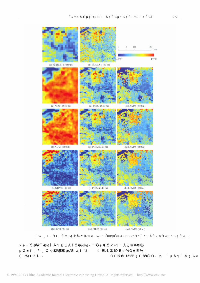
代表) ，其误差统计 ( RMSE 和 CO-RMSE ) 如图 5所示。4. 1. 1 纹理精度( CO-RMSE)

由图 5 中 CO-RMSE 可见，不论季节和分辨率

层级，PBIM 方法的纹理精度最高，CO-RMSE 均小于

0. 15，其次为 NDVI 方法，LSMM 方法最差，CO-RMSE 均超过 0. 30。这是由于 PBIM 方法所基于的

全色波段，能够同时反映地形起伏和地表反照率差

异导致的子像元温度变异，有利于细节信息的恢

复; NDVI 只能反映温度的大致分布格局，难以表达

复杂的地表异质性，不利于高分辨率城区影像的

温度纹理恢复; LSMM 方法通过分类强制赋予各子

像元类别标记，导致低分辨率时损失大量像元内


图 3 各分辨率层级下 NDVI、PBIM 和 LSMM 方法针对 ASTER 2004 － 01 － 27 影像的全局降尺度结果

组分信息，抹平温度的细节变化。3 种方法针对各

地表覆盖分区的 CO-RMSE 比较结果与全局

( 图 5 ) 相同。

4. 1. 2 定量精度( RMSE)

4. 1. 2. 1 全局比较

由图 5 中 RMSE 可见，3 种方法的定量精度比


图 4 各分辨率层级下 NDVI、PBIM 和 LSMM 方法针对 TM 2004 － 07 － 06 影像的全局降尺度结果

较在 180—240 m 分辨率间发生了变化，因此将

90—180 m 分辨率归为 HR，240—540 m 分辨率归

为 LR。则 3 种方法的精度由高到低排序为:

春、冬季 LR: PBIM ＞ LSMM ＞ NDVI;春、冬季 HR: LSMM ＞ PBIM ＞ NDVI;夏季 LR: PBIM ＞ NDVI ＞ LSMM;

夏季 HR: NDVI ＞ PBIM ＞ LSMM。图 5 ( a) 中 NDVI 方法的 RMSE 高于图 5 ( d)

1℃以上，表明其具有明显的季节差异。夏季 NDVI与 LST 之间存在明显的负线性关系( 图 6 ( a) ) ，然

而在植被稀少的冬季，散点图近似饼状，使得难以

确定稳定的关系函数( 图 6 ( b) ) 。因此冬季 NDVI方法的误差显著大于 PBIM 和 LSMM 方法。

夏季 HR 时 NDVI 方法的精度高于 PBIM 方法，

LR 时却相反，其主要原因可能是 LR 像元混合使得

LST-NDVI 关系接近于图 6 ( b) ，不利于子像元温度

的预测。另外，无论季节，3 种方法的 RMSE 都呈现随目

标分辨率的提高而不断增加的趋势，这与 Agam 等

人( 2007 ) 的结论一致。随着目标分辨率的提


高，子像元个数及其温度变异复杂性必然随之增加。

4. 1. 2. 2 地表覆盖分区比较

3 种方法在不同分辨率层级下针对 U、R 和 M的降尺度误差统计如图 7 所示。

( 1) 地表覆盖分区的方法适应性评价

由图 7 可见，针对各地表覆盖分区，3 种方法的

定量精度由高到低排序为:

U ( LR) : 春、冬季为 PBIM ＞ LSMM ＞ NDVI，夏季为 PBIM ＞ LSMM ＞ NDVI;

U ( HR) : 春、冬季为 LSMM ＞ PBIM ＞ NDVI，夏

季为 NDVI ＞ LSMM ＞ PBIM;

R: 春、冬季为 LSMM ＞ PBIM ＞ NDVI，夏季为

PBIM ＞ NDVI ＞ LSMM;

M: 春、冬季为 PBIM ＞ LSMM ＞ NDVI，夏季为

PBIM ＞ NDVI ＞ LSMM。无论地表覆盖分区，NDVI 方法始终在春、冬季

表现最差; 针对夏季城区，HR 时 NDVI 方法优于


图 7 各分辨率层级下 NDVI、PBIM 和 LSMM 方法针对各日期的城区( U) 、郊区( R) 和山区( M) 影像的降尺度误差

PBIM 方法，LR 时则相反; 针对 LR 城区，无论季节，

PBIM 方法的误差均最小，NDVI 方法则最大。此外，无论季节，在山区 PBIM 方法始终最优。

这是因为它更能体现影响山区 LST 差异的主要因

素———地形变化，且其亮、暗面区分计算的策略有

助于恢复山脊线、山谷线等线状分布的 LST ( Liu 和

Moore，1998) 。( 2) 降尺度方法的地域依赖性比较

由图 7 可见，各降尺度方法作用于 3 种地表覆

盖分区的定量精度由高到低排序为:

NDVI 方法: 春、冬季为 U ＞ R ＞ M，夏季为 R ＞M＞U;

PBIM 方法: 春、冬季为 U ＞ M ＞ R，夏季为 R ＞M＞U;

LSMM 方法: 春、冬季为 U ＞ R ＞ M，夏季为 U ＞R ＞ M。

首先，夏季郊区植被生长旺盛，与田间道路、裸地等非植被像元分别控制了 NDVI 的高、低值区，使

得 LST-NDVI 负线性关系清晰; 山区 /城区的 NDVI则普遍较高 /较低，LST-NDVI 关系不稳定，因此夏季

NDVI 方法针对郊区的表现优于山区和城区。从而

进一步说明该方法的精度不取决于植被覆盖度，而

是依赖于植被与非植被像元的共存。冬季该方法

针对城区的精度高于郊区和山区也正因如此。其次，夏季 PBIM 方法针对郊区的精度高于城

区的主要原因是郊区 LST 按照田块状分布，与 LST呈点状分布的城区相比，更适于根据亮、暗面区分

反照率的简单处理; 冬季，该方法针对郊区的精度

低于城区的主要原因则是冬季郊区以裸土覆盖为

主，反照率无明显差异，与下垫面反照率变化较大

的城区相比，不利于子像元温度分配。最后，无论季节，LSMM 方法始终在城区精度最

高，山区最差。其主要原因可能是分类能够区分下

垫面材质特性，以表达城区 LST 差异，却难以反映

决定山区 LST 差异的植被、地形等信息。

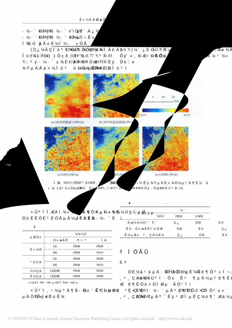
4. 2 MODIS 数据的结果

3 种方法针对 MODIS 影像的全局降尺度结果

如图 8 所示。( 1) 考虑误差相对值，从纹理精度上看，PBIM


方法最高，LSMM 方法最低; 从定量精度上看，NDVI方法最高，LSMM 方法最低，与同时相模拟误差( 见

图 5( d) ) 的比较结果一致。( 2) 考虑误差绝对值，3 种方法的 RMSE 较模拟

误差( 见图 5( d) ) 分别高出 0. 51 ℃、0. 77 ℃和 0. 83℃。除方法本身的误差外，1 ) MODIS 与 ASTER 数

据的配准误差增加了验证误差( Gao 等，2006 ) ; 2 )

在地形起伏较大的山区，邻近效应和角度效应带给

尺度转换较大误差 ( Liu 等，2006 ) ; 3 ) ASTER /LST与 MODIS /LST 的反演误差( 分别为 ± 1. 5 ℃ 和 ±1. 0 ℃ ) 即可造成 ± 2. 5 ℃ 的偏差，考虑到大气纠

正、传感器信噪比、局地特征等影响，该差异还将

增大。

图 8 NDVI、PBIM 和 LSMM 方法针对 MODIS 2004 － 08 － 31 数据的全局降尺度结果

( ( c) 、( d) 和( e) 中的 RMSE 分别为 2． 69℃、3． 00℃和 3． 15℃，CO-RMSE 则分别为 0. 14、0. 12 和 0. 19)

4. 3 综合比较结果

综合纹理精度和定量精度，针对不同季节和地

域适宜采用的降尺度方法如表 3 所示:

表 3 针对不同季节和地域适宜采用的降尺度方法

地域季节

分辨率春、冬夏

全局LR PBIM PBIM

HR PBIM NDVI

城区LR PBIM PBIM

HR PBIM NDVI

郊区 LR，HR PBIM PBIM

山区 LR，HR PBIM PBIM

注: LR 为 90—180 m; HR 为 240—540 m

综合各降尺度方法受季节、分辨率和地表覆盖

的影响，如表 4 所示:

表 4 各降尺度方法受季节、分辨率和地表覆盖的影响

影响因素方法

NDVI PBIM LSMM

随季节波动强中弱

受分辨率限制中弱强

受地表覆盖约束强中弱

5 讨论

5. 1 方法的选择

由结果的分析中可见，3 种方法针对不同地表

覆盖类型、季节和分辨率层级的降尺度效果主要受

其尺度因子特点的影响。首先，NDVI 方法的尺度因子( NDVI) 反映植被

覆盖信息，与 LST 的函数关系是决定其降尺度结果


的主要因素。当区域内同时含有裸地和高植被区

域时，LST-NDVI 相关关系得到最佳体现。进而推

断，其他因素( 如土壤湿度、下垫面材质特性等) 对

地表温度的作用较强时，该方法则难以表达地表温

度的异质性。Zhan 等人 ( 2011 ) 认为 TemperatureVegetation Dryness Index ( TVDI) ( Sandholt 等，2002) 结

合 NDVI 提取干边和湿边，有助于反演由土壤湿度

引起的地表温度差异。其次，PBIM 方法的尺度因子( 全色波段) 是多光

谱波段的综合，反映反射光照强度，对地物的特征吸

收、反射并不敏感，因此适于太阳光照差异较大的区

域，在地形起伏明显的地区表现出优于 NDVI 和

LSMM 方法的潜质。同理，该方法不适用于太阳光照

角度非常低的高纬冬季( Liu 和 Moore，1998) 。此外，

全色波段在一定程度上反映地表反照率特性，因此适

于下垫面材质差异较大的区域。但是以全色平均值

区分亮、暗面的简单处理方式在反照率波动剧烈的区

域极易产生噪声。进而推断，该方法可能不适用于高

分辨率、反照率异质性很强的区域。最后，LSMM 方法的尺度因子( 硬分类图) 将原

本连续的信息离散化，必将丢失部分信息。随着分

辨率层级的降低，像元混合加重，分类界限越加模

糊，加大了类内、类间误差，纹理信息损失随之加

剧。此外，在分类特征波段上相似的地物不一定具

有相同的地表温度( Zhukov 等，1999 ) ，尤其在低分

辨率影像中难以满足同物同温假设。因此，该方法

受分辨率约束较大，鉴于本文实验结果，认为其可

能不适于低于 90 m 的分辨率。可见，以影响区域地表温度变化的主要因素作

为尺度因子，是方法选择的关键。

5. 2 参数的选择

由于不同参数造成降尺度结果的差异较大，有

必要探讨各方法参数选择的依据及存在的问题。首先，NDVI 方法中运算窗口大小和 LST-NDVI

回归函数难以确定。( 1 ) 扩大窗口，易引入无关像

元，造成数据冗余，影响真实的 LST-NDVI 回归关

系; 缩小窗口，则回归函数对噪声敏感，预测性差，

不利于推广至高分辨率。Jeganathan 等人( 2010 ) 认

为 5 × 5 的窗口较适宜; Prihodko 和 Goward ( 1997 )

则得出 13 × 13。这些结论具有较强的地表依赖性，

难以广泛应用。根据影像特征自动确定合适的运

算窗口形状及大小是改进该方法的途径之一，半方

差函数是一种有效的实现方法 ( Zhan 等，2012 ) 。

( 2) LST-NDVI 相关关系与地表覆盖状况( Smith 和

Choudhury，1991 ) 、土壤湿度( Carlson 等，1990 ) 、空

间尺度( Prihodko 和 Goward，1997 ) 、日变化( Goetz，1997) 、纬度、地形地貌、云等密切相关。其中，土壤

湿度是主要影响因素之一。可以将 LST-NDVI 特征

空间( 梯形或三角形) 看作由一组土壤湿度等值线

构成，区域内土壤湿度变化越大，两者回归关系越

复杂。目前主要有线性和非线性两种回归形式( 如

式( 3) ) 。线性函数简单、稳定性好、鲁棒性强，但在

NDVI 变化范围较小时，不宜采用，如在林地，不易

得到两者直线关系( Smith 和 Choudhury，1991 ) 。多

项式函数缺乏物理意义，且对极值极度敏感，如

Agam 等人( 2007 ) 和 Zhan 等人( 2011 ) 发现其未能

提高降尺度精度，反而使结果不稳定。若将 NDVI的函数( 如植被覆盖度) 作为自变量，则若干非线性

关系得以转化为线性函数。此举与变更回归核的

含义相似。其次，PBIM 方法中全色波段的变换范围和反

照率异质性判断阈值 Cr 与噪声和格网效应( Rectan-gular pseudo-edges) 密切相关。实验发现: ( 1) 全色

波段值域拉伸较大时，极值噪声明显; 压缩较大时，

格网效应严重。这是因为全色波段与温度以乘除

法计算，使得全色波段的变换范围基本决定了降尺

度后地表温度的波动范围。本文将全色波段变换

到与 LR 地表温度取值相近的范围，使噪声和格网

效应得到折中。( 2) 全局采用统一 Cr，则城区地表

温度反演较好时，山区格网效应明显; 调节 Cr 使得

山区无格网时，城区随即产生强烈噪声。这是不同

地表覆盖区域内反照率差异不同所致，这时建议采

用局域 Cr。最后，LSMM 方法除了同样面临着运算窗口大

小确定困难的问题之外，类别个数也难以确定。增

加类别个数有利于综合各组分信息，减少类间误

差，但类别过多会引入大量噪声，且不易求得稳定

解; 减少类别个数有利于提高计算速度，但类别过

少会丢失大量纹理细节，且同物异温问题显著。可见，3 种方法的参数设置均没有明确标准，依

赖于数据特征，受主观影响较大。其中，NDVI 方法

的参数设置对结果的影响较小，操作较为简单;

PBIM 方法的参数需要折中选择，人为因素作用较

大，使结果差异较大; LSMM 方法通常需要反复实

验，耗时严重，操作较为复杂。挖掘参数与数据特

征的相关性，有助于实现参数选择的自动化和客观

化，提高降尺度效率。


5. 3 评价指标的选择

由图 5 可知，RMSE 和 CO-RMSE 的评价结果不

一致，尤其对 LSMM 方法的评价差异很大。目前地

表温度降尺度方法的验证普遍采用 RMSE，但是其

对格网效应及温度纹理信息不敏感，如图 9 所示。

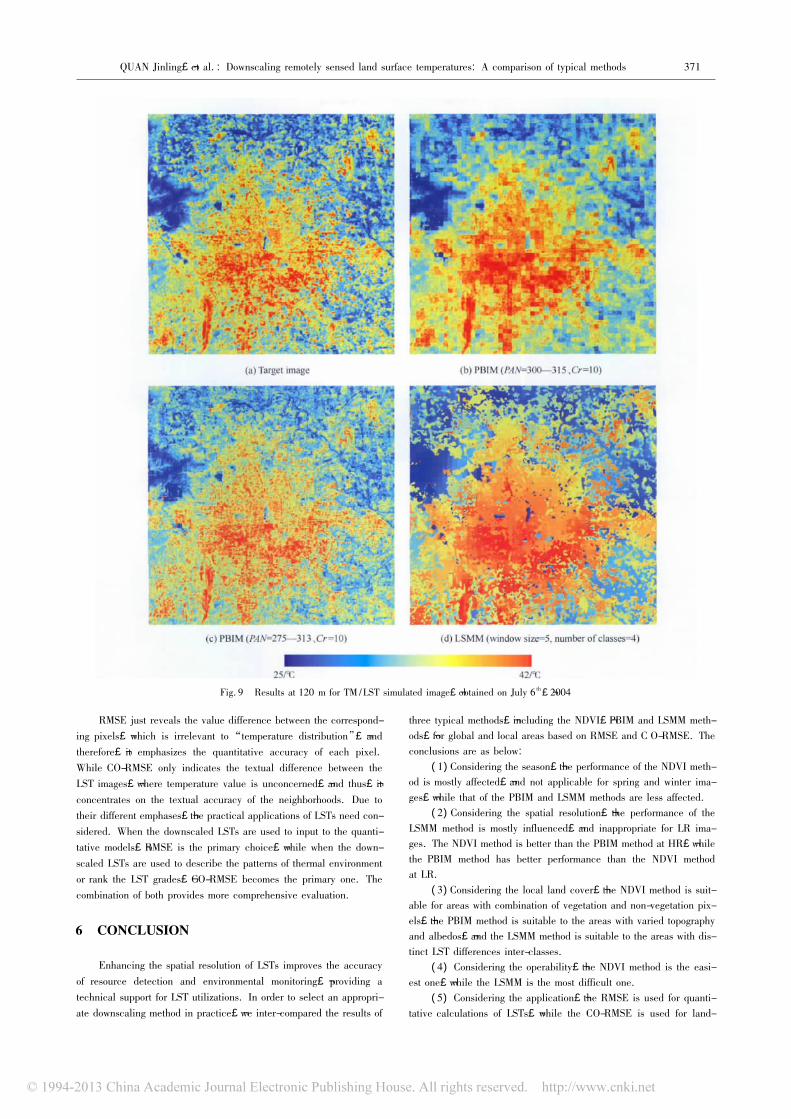
图 9 TM 数据 2004 － 07 － 06 在 120 m 分辨率下的降尺度结果

( ( b) RMSE = 1. 94 ℃，CO-RMSE = 0. 11; ( c) RMSE = 2. 21 ℃，CO-RMSE = 0. 10; ( d) RMSE = 2. 03 ℃，CO-RMSE = 0. 21)

从图 9 得出，图 9 ( b) 有明显的格网效应，图 9( d) 的纹理过于平滑; 相较图 9 ( b) 、图 9 ( d) ，图 9( c) 与图 9 ( a) 更相似，但其 RMSE 最大，CO-RMSE则最小。RMSE 仅反映对应像元的数值差异，与“温

度分布”无关，注重单像元温度的定量精度; CO-RMSE 仅反映两影像的温度纹理特征差异，与“温度

数值”无关，注重温度的纹理精度。它们侧重点不

同，需根据地表温度的实际应用目的做选择。当地

表温度作为定量模型的输入数据时，应着重使用

RMSE; 当用于描绘热环境格局或等级分布时，应着

重使用 CO-RMSE。两者结合有助于综合评价。

6 结论

提高地表温度的空间分辨率有助于提高资源

探测和热环境监测的精度，为更好地利用地表温度

提供技术支撑。为了便于实际应用中地表温度降

尺度方法的选择和使用，本文利用 RMSE 和 CO-RMSE 指标，对具有代表性的 NDVI、PBIM 和 LSMM方法在全局及各地表覆盖分区影像中的降尺度结


果进行了比较和分析。结果发现:

( 1) 从季节上考虑，NDVI 方法的降尺度效果随

季节波动严重，不适于春、冬季; PBIM 和 LSMM 方

法则受季节影响较弱。( 2) 从分辨率上考虑，LSMM 方法受分辨率限

制，不适宜低分辨率; NDVI 方法在 HR 时表现优于

PBIM 方法，LR 时则相反。( 3) 从地域上考虑，NDVI 方法适宜植被与非植

被像元共存的区域; PBIM 方法适宜地形或反照率

变化较大的区域; LSMM 方法适宜类别间温差较大

的区域。( 4) 从操作简易性上考虑，NDVI 方法最简单;

LSMM 方法相对最复杂。( 5) 从应用目的上考虑，地表温度参与定量计

算时采用 RMSE; 用于热环境景观分析时宜采用 CO-RMSE评价。

在实际应用中应综合考虑以上因素，选择一种

以决定地表温度差异的主要因素为尺度因子的方

法。下一步工作主要有( 1) 方法参数与数据特征的

相关性研究; ( 2 ) 根据具体应用目的设计合适的降

尺度评价指标; ( 3) 加入地表温度的时间序列模型，

改进 Gao 等人( 2006 ) 提出的 STARFM ( Spatial andTemporal A daptive Reflectance Fusion Model) ，以适

应地表温度的降尺度。

参考文献( References)

Agam N，Kustas W P，Anderson M C，Li F Q and Neale C M U． 2007．A vegetation index based technique for spatial sharpening of thermalimagery． Remote Sensing of Environment，107 ( 4 ) : 545 － 558［DOI: 10． 1016 / j． rse． 2006． 10． 006］

Aiazzi B，Alparone L，Baronti S，Santurri L and Selva M． 2005． Spatialresolution enhancement of ASTER thermal bands． Proceeding ofSPIE Image and Signal Processing for Remote Sensing XI． Brugge:

Lorenzo Bruzzone，5982: 1 － 10Anys H，Bannari A，He D C and Morin D． 1994． Texture analysis for

the mapping of urban areas using airborne MEIS-II images． Proceed-ing of the 1st International Airborne Remote Sensing Conference andExhibition． Strasbourg: Environmental Research Institute of Michi-gan，Ann Arbor，3: 231 － 245

Atkinson P M，Pardo-Igúzquiza E and Chica-Olmo M． 2008． Downscal-ing cokriging for super-resolution mapping of continua in remotelysensed images． IEEE Transactions on Geoscience and R emote Sens-ing，46( 2) : 573 －580［DOI: 10． 1109 /TGRS． 2007． 909952］

Baraldi A and Parmiggian F． 1995． An investigation of the textural char-acteristics associated with gray level cooccurrence matrix statisticalparameters． IEEE Transactions on Geoscience and Remote Sensing，

33( 2) : 293 － 304 ［DOI: 10． 1109 /36． 377929］

Bastiaanssen W G M，Menenti M，Feddes R A and Holtslag A A M．

1998． A remote sensing surface energy balance algorithm for land

( SEBAL) ． 1． Formulation． Journal of Hydrology，212 － 213: 198

－ 212 ［DOI: 10． 1016 /S0022 － 1694( 98) 00253 － 4］

Carlson T N，Perry E M and Schmugge T J． 1990． Remote estimation of

soil moisture availability and fractional vegetation cover for agricul-

ture field． Agriculture and Forest Meteorology，52: 45 － 49 ［DOI:

10． 1016 /0168 － 1923( 90) 90100 － K］

Christensen P R，Bandfield J L，Hamilton V E，Howard D A，Lane M

D，Piatek J L，Ruff S W and Stefanov W L． 2000． A thermal emis-

sion spectral library of rock-forming minerals． Journal of Geophysical

Research，105( E4) : 9735-9739 ［DOI: 10． 1029 /1998JE000624］

Dominguez A，Kleissl J，Luvall J C and Rickman D L． 2011． High-resolu-

tion urban thermal sharpener ( HUTS ) ． Remote Sensing of Environ-

ment，115( 7) : 1772 －1780［DOI: 10． 1016 / j． rse． 2011． 03． 008］

Fasbender D，Tuia D，Bogaert P and Kanevski M． 2008． Support-based im-

plementation of Bayesian data fusion for spatial enhancement: a

pplications to ASTER thermal images． IEEE Geoscience and R emote

Sensing Letters，5 ( 4 ) : 598 － 602 ［DOI: 10． 1109 /LGRS． 2008．

2000739］

Gao F，Masek J，Schwaller M and Hall F． 2006． On the blending of the

Landsat and MODIS surface reflectance: predicting daily Landsat sur-

face reflectance． IEEE Transactions on Geoscience and Remote Sens-

ing，44( 8) : 2207 －2218［DOI: 10． 1109 /TGRS． 2006． 872081］

Gillespie A，Rokugawa S，Matsunaga T，Cothern J S，Hook S and Kahle A

B． 1998． A temperature and emissivity separation algorithm for Ad-

vanced Spaceborne Thermal Emission and Reflection Radiometer ( AS-

TER) images． IEEE Transactions on Geoscience and Remote Sensing，

36( 4) : 1113 －1126［DOI: 10． 1109 /36． 700995］

Gillies R R and Carlson T N． 1995． Thermal remote sensing of surface soil

water content with partial vegetation cover for incorporation into climate

models． Journal of Applied Meteorology，34 ( 4 ) : 745 － 756 ［DOI:

10． 1175 /1520 －0450( 1995) 034 ＜0745: TRSOSS ＞2． 0． CO; 2］

Goetz S J． 1997． Multi-sensor analysis of NDVI，surface temperature and

biophysical variables at a mixed grassland site． International Journal

of Remote Sensing， 18 ( 1 ) : 71 － 94 ［DOI: 10． 1080 /

014311697219286］

Gustavson W T，Handcock R，Gillespie A R and Tonooka H． 2003． An

image sharpening method to recover stream temperatures from A

STER images． Proceeding of SPIE Remote Sensing for Environmen-

tal Monitoring，GIS applications and Geology II． Bellevue: Manfred

Ehlers，4886: 72 － 83

Jeganathan C，Hamm N A S，Mukherjee S，Atkinson P M，Raju P L N

and Dadhwal V K． 2010． Evaluating a thermal image sharpening

model over a mixed agricultural landscape in India． International

Journal of Applied Earth Observation and Geoinformation，13 ( 2 ) :

178 － 191 ［DOI: 10． 1016 / j． jag． 2010． 11． 001］

Kustas W P，Norman J M，Anderson M C and French A N． 2003． Esti-

mating subpixel surface temperatures and energy fluxes from the veg-

etation index-radiometric temperature relationship． Remote Sensing

of Environment，85( 4) : 429 － 440

Lemeshewsky G P． 1998． Neural network-based sharpening of Landsat

thermal-band images． Park S K，Juday R D，eds． Proceeding of


SPIE Visual Information Processing VII． Orlando，3387: 378 － 386Lemeshewsky G P and Schowengerdt R A． 2001． Landsat 7 thermal-IR

image sharpening using an artificial neural network and sensor model． Park S K，Rahman Z，Schowengerdt R A，eds． Proceeding ofSPIE Visual Information Processing X． Orlando，4388: 181 － 192

Lentile L B，Holden Z A，Smith A M S，Falkowski M J，Hudak A T，

Morgan P，Lewis S A，Gessler P E and Benson N C． 2006． Remotesensing techniques to assess active fire characteristics and post-fireeffects． International Journal of Wildland Fire，15 ( 3 ) : 319 － 345［DOI: 10． 1071 /WF05097］

Liang S L． 2004． Quantitative Remote Sensing of Land Surfaces． Hobo-ken，New Jersey: John Wiley and Sons，Inc． : 18 － 462

Liu D S and Pu R L． 2008． Downscaling thermal infrared radiance forsubpixel land surface temperature retrieval． Sensors，8( 4) : 2695 －2706 ［DOI: 10． 3390 /s8042695］

Liu J G and Moore J M． 1998． Pixel block intensity modulation: addingspatial detail to TM band 6 thermal imagery． International Journal ofRemote Sensing，19 ( 13 ) : 2477 － 2491 ［DOI: 10． 1080 /014311698214578］

Liu Y B，Hiyama T and Yamaguchi Y． 2006． Scaling of land surface temperature using satellite data: a case examination on ASTER andMODIS products over a heterogeneous terrain area． Remote Sensing ofEnvironment，105( 2) : 115 － 128 ［DOI: 10． 1016 / j． rse． 2006． 06．012］

Nichol J． 2009． An emissivity modulation method for spatial enhancement ofthermal satellite images in urban heat island analysis． Photogram-metric Engineering and Remote Sensing，75( 5) : 1 － 10

Pardo-Igúzquiza E，Chica-Olmo M and Atkinson P M． 2006． Downscalingcokriging for image sharpening． Remote Sensing of Environment，102( 1 /2) : 86 － 98 ［DOI: 10． 1016 / j． rse． 2006． 02． 014］

Prihodko L and Goward S N． 1997． Estimation of air temperature fromremotely sensed surface observations． Remote Sensing of Environ-ment，60 ( 3 ) : 335 － 346 ［DOI: 10． 1016 /S0034 － 4257 ( 96 )

00216 － 7］Qin Z，Karnieli A and Berliner P． 2001． A mono-window algorithm for

retrieving land surface temperature from Landsat TM data and its ap-plication to the Israel-Egypt border region． International Journal ofRemote Sensing，22 ( 18 ) : 3719 － 3746 ［DOI: 10． 1080 /01431160010006971］

Sandholt I，Rasmussen K and Anderson J． 2002． A simple interpretationof the surface temperature /vegetation index space for assessment ofsurface moisture status． Remote Sensing of Environment，79( 2 /3) :

213 － 224 ［DOI: 10． 1016 /S0034 － 4257( 01) 00274 － 7］Small C and Lu J W T． 2006． Estimation and vicarious validation of u

rban vegetation abundance by spectral mixture analysis． RemoteSensing of Environment，100 ( 4 ) : 441 － 456 ［DOI: 10． 1016 / j．rse． 2005． 10． 023］

Smith R C G and Choudhury B J． 1991． Analysis of normalized differ-

ence and surface temperature observations over southeastern Australia． International Journal of Remote Sensing，12( 10) : 2021 －2044 ［DOI: 10． 1080 /01431169108955234］

Sobrino J A，Baissouni N and Li Z L． 2001． A comparative study of landsurface emissivity retrieval from NOAA Data． Remote Sensing of En-vironment，75( 2) : 256 － 266 ［DOI: 10． 1016 /S0034 － 4257( 00)

00171 － 1］Stathopoulou M and Cartalis C． 2009． Downscaling AVHRR land surface

temperatures for improved surface urban heat island intensity estima-tion． Remote Sensing of Environment，113 ( 12 ) : 2592 － 2605［DOI: 10． 1016 / j． rse． 2009． 07． 017］

Voogt J A and Oke T R． 2003． Thermal remote sensing of urban cli-mates． Remote Sensing of Environment，86( 3) : 370 － 384 ［DOI:10． 1016 /S0034 － 4257( 03) 00079 － 8］

Wan Z M． 2008． New refinements and validation of the MODIS Land-Surface Temperature /Emissivity products． Remote Sensing of Envi-ronment，112( 1) : 59 － 74 ［DOI: 10． 1016 / j． rse． 2006． 06． 026］

Wan Z M and Dozier J． 1996． A generalized split-window algorithm forretrieving land-surface temperature from space． IEEE Transactionson Geoscience and Remote Sensing，34( 4) : 892 － 905 ［DOI: 10．1109 /36． 508406］

Wan Z M，Zhang Y L，Zhang Q C and Li Z L． 2002． Validation of theland-surface temperature products retrieved from Terra ModerateResolution Imaging Spectroradiometer data． Remote Sensing of Environment，83 ( 1 /2 ) : 163 － 180 ［DOI: 10． 1016 /S0034 － 4257( 02) 00093 － 7］

Wang Z J，Ziou D，Armenakis C，Li D and Li Q Q． 2005． A compara-tive analysis of image fusion methods． IEEE Transactions on Geosci-ence and Remote Sensing，43( 6) : 1391 － 1402 ［DOI: 10． 1109 /TGRS． 2005． 846874］

Zhan W F，Chen Y H，Wang J F，Zhou J，Quan J L，Liu W Y and LiJ． 2012． Downscaling land surface temperatures with multi-spectraland multi-resolution images． International Journal of Applied EarthObservation and Geoinformation，18: 23 － 36 ［DOI: 10． 1016 / j．jag． 2012． 01． 003］

Zhan W F，Chen Y H，Zhou J，Li J and Liu W Y． 2011． Sharpeningthermal imageries: a generalized theoretical framework from an as-similation perspective． IEEE Transactions on Geoscience and Re-mote Sensing，49 ( 2 ) : 773 － 789 ［DOI: 10． 1109 /TGRS． 2010．2060342］

Zhukov B，Oertel D，Lanzl F and Reinhckel G． 1999． Unmixing-basedmultisensor multiresolution image fusion． IEEE Transactions on Geoscience and Remote Sensing，37 ( 3 ) : 1212 － 1226 ［DOI: 10．1109 /36． 763276］

Zurita-Milla R，Kaiser G，Clevers J P G W，Schneider W and Schaep-man M E． 2007． Spatial unmixing of MERIS data for monitoringvegetation dynamics． Proceedings of Envisat Symposium． Montreux:

ESA SP － 636: 23 － 27

1007-4619( 2013) 02-0361-27 Journal of Remote Sensing 遥感学报

Downscaling remotely sensed land surface temperatures:A comparison of typical methods

QUAN Jinling，ZHAN Wenfeng，CHEN Yunhao，LIU Wenyu

College of Resources Science ＆ Technology，State Key Laboratory of Earth Surface Processes and Resource Ecology，Beijing Normal University，Beijing 100875，China

Abstract: Remotely sensed Land Surface Temperatures ( LSTs) usually have low spatial resolutions． Downscaling is an effectivetechnique to enhance the spatial resolutions． Current methods for downscaling remotely sensed LSTs were summarized． Using satellitedata，we made an inter-comparison among three typical methods，including the Normalized Difference Vegetation Index ( NDVI)method，the Pixel Block Intensity Modulation ( PBIM) method，and the Linear Spectral Mixture Model ( LSMM) method． We furtherdesigned an index，Co-Occurrence Root Mean Square Error ( CO-RMSE) ，for measuring the textural similarity in inter-comparisons．Results indicate that ( 1) the performance of the NDVI method is most affected by the season，followed by the PBIM method; ( 2) theperformance of the LSMM method is most influenced by the spatial resolution; the NDVI method has an advantage over the PBIMmethod at high resolutions，while at low resolutions，the performance of the PBIM method is better than that of the NDVI method;( 3) these three methods are suitable for areas with combination of vegetation and bare ground，areas with varied t opography and al-bedo，and areas with distinct LST differences in different classes，respectively; ( 4) the NDVI method is the easiest to implement，while the LSMM method is the most difficult． Further analysis showed that scale factor is the key issue to the LST downscaling and itneeds to be carefully selected regarding the season，spatial resolution，land cover，application and the operability．Key words: land surface temperature，downscaling，scale factor，CO-RMSECLC number: TP79 Document code: A

Citation format: Quan J L，Zhan W F，Chen Y H and Liu W Y． 2013． Downscaling remotely sensed land surface temperatures: A comparison of typical methods． Journal of Remote Sensing，17( 2) : 361 －387

Received: 2012-01-10; Accepted: 2012-05-31Foundation: National Natural Science Foundation of China ( No． 41071258) ; The State Key Laboratory Program of Earth Surface Processes and Resource E

cology ( No． 2010 － ZY －06) ; Specialized Research Fund for the Doctoral Program of Higher Education of China ( No． 20100003110018)First author biography: QUAN Jinling ( 1987— ) ，female，Ph． D． candidate． She majors in application of remote sensing to resource and environment． E

-mail: quanjinlin_@ 126． comCorresponding author biography: CHEN Yunhao ( 1974— ) ，male，professor． His research interest is thermal remote sensing of urban areas． E-mail: c

yh@ bnu． edu． cn

1 INTRODUCTION

Land Surface Temperatures ( LSTs ) have utilities in various applications，such as the urban heat island ( UHI) observation ( Voogt ＆Oke，2003) ，the surface soil moisture estimation ( Gillies ＆ Carlson，1995) ，the surface energy budget derivation ( Bastiaanssen，et al．，1998) ，the forest fire monitoring ( Lentile，et al．，2006) and the geo-logical resource exploration ( Christensen，et al．，2000) ． However，remotely sensed LSTs usually have low spatial resolutions，causing aprevalent mixture effect． Therefore，downscaling，an effective tech-nique to derive higher spatial resolution LSTs，is desirable．

Many downscaling methods have been proposed． In the perspective of image fusion，sharpening and merging，this group includes principal component analysis，Gram-Schmidt，generalizedLaplacian pyramid ( Aiazzi，et al．，2005) ，Bayesian ( Fasbender，etal．，2008) ，co-Kriging ( Pardo-Igúzquiza，et al．，2006; Atkinson，etal．，2008) ，artificial neural network ( Lemeshewsky，1998; Lemesh-ewsky ＆ Schowengerdt，2001) and so on． Most of them，however，neglect the physical background and quantitative requirements of re-mote sensing ( Zhan，et al．，2011) ．

While some other researchers focused on scale factors ( Statho-

poulou ＆ Cartalis，2009) ，in order to maintain the physical signifi-cance and spectral consistency． This group can be categorized intothree classes: statistical regression methods，modulation methods andspectral mixing methods．

( 1) Statistical regression methods apply the relationship betweenLSTs and regression kernels derived at lower resolutions to the kerneldata at higher resolutions，and the LSTs of finer resolutions are thenobtained under the condition that the relationship is scale-invariant．The kernels utilized usually include Normalized Difference VegetationIndex ( NDVI) ( Kustas，et al．，2003; Agam，et al．，2007) ，albe-do ( Dominguez，et al．，2011) ，and component fraction ( Gustavson，et al．，2003; Liu ＆ Pu，2008) ． Among these kernels，NDVI is themost frequently used one． Kustas，et al． ( 2003 ) effectively down-scaled LSTs using LST-NDVI linear inverse relationship． Considering the NDVI saturation effect over dense vegetation，Agam，et al． ( 2007) adopted LST-NDVI nonlinear relationship，taking thefractional vegetation cover as a regression kernel． Jeganathan，et al．( 2010) discussed the global，resolution-adjusted global，piecewise，stratified and local regression models． In consideration of land covercharacteristics，Dominguez，et al． ( 2011 ) proposed a multi-factorregression model combining NDVI with albedo． ( 2) Mo dulation


methods distribute lower resolution LSTs to sub-pixels based on themodulation factors，such as panchromatic band ( Liu ＆ Moore，1998) ，effective emissivity ( Nichol，2009 ) ，LSTs of the corre-sponding season retrieved from other thermal sensors with higher res-olutions，LSTs estimated from near time-coincident sensors withhigher resolutions， and the combination of emissivity and LST( Stathopoulou ＆ Cartalis，2009 ) ． ( 3 ) Spectral mixing methodsstraightly connect LSTs of different resolutions based on the linearspectral mixing model． A least square method is then used to derivethe LSTs of finer resolutions ( Zhukov，et al．，1999; Liu ＆ Pu，2009) ． Recently，Zhan，et al． ( 2011 ) constructed a generalizedtheoretical framework for LST downscaling from an assimilation per-spective，and further evaluated different regression kernels．

Though the methods mentioned above have been used in variousfields，it is difficult to choose a proper one in practice because of thecomplexity of surface environment and climate conditions． Besides，the setting of parameters for each method is quite subjective． Thequantitative comparison of various downscaling methods is still rare．To provide references for their practical utilizations，in this study，wecompared three typical methods from the s econd group using satelliteLSTs of different seasons，spatial resolutions and land covers．

2 METHODOLOGY

2． 1 Downscaling LSTs

Among statistical regression methods，the NDVI method is themost regularly used one and has become a foundation of this class．The methods that transform NDVI to fractional vegetation ( Agam，etal．，2007 ) or combine NDVI with albedo ( Dominguez，et al．，2011) ，have no significant advantages in operability and accuracy．

Among modulation methods，the one that adopts emissivity asmodulation factor ( Nichol，2009 ) requires fine spatial resolutionsand high emissivity retrieval accuracy． Relatively，the Pixel BlockIntensity Modulation ( PBIM ) method has more mature theoreticalbackground，and the derivation of panchromatic band is more relia-ble．

Among spectral mixing methods，the Linear Spectral MixtureModel ( LSMM ) method is easy to implement and is highly cited( ［2012 － 03 － 27］http: / / scholar． google． com /scholar? hl = zh-CN＆q = Unmixing-based＆btnG = ＆lr = ) ．

Therefore，the NDVI，PBIM and LSMM methods are chosen asthree representatives． In the following，LR and HR are short for lowand high spatial resolutions respectively，and T represents LST．2． 1． 1 NDVI method

The NDVI method ( Kustas，et al．，2003 ) is a statistical re-gression method，which considers NDVI as the scale factor． It assumes that there is a unique relationship between LST and NDVI atmultiple spatial resolutions． First，perform a statistical regression be-tween TLR and NDVILR ; Then，apply the regression function to NDVIHR ; Last，add regression residuals to the downscaled LSTs，as:

THR = f( NDVIHR ) + ΔTLR ( 1)

ΔTLR = TLR － f( NDVILR ) ( 2)where f is the regression function between LST and NDVI，and ΔTLR

is the regression residual． f has four forms ( Agam，et al．，2007) :

f( NDVI) =

a0 + a1NDVIa0 + a1NDVI + a2NDVI

2

a0 + a (1 1 － NDVImax － NDVINDVImax － NDVI( )

min )0. 625

a0 + a1 ( 1 － NDVI)

0. 625

( 3)

where a0，a1 and a2 are the regression coefficients，NDVImax and NDVImin are the maximum and minimum NDVI in the area，respective-ly，and they are determined by confidence intervals in practice．2． 1． 2 PBIM method

The PBIM method ( Liu ＆ Moore，1998) is a modulation meth-od，which considers panchromatic band as the scale factor． It as-sumes that TLR equals the average LST of sub-pixels in LR pixelblock，and each sub-pixel albedo is identical． Under this condition，the ratio of LST to panchromatic band is derived to be scale-invariantfrom the physical principle of image formation ( Wang，e t al．，2005) ，and THR is then obtained ( Eq． ( 4) ) ． For a pixel block withsignificant albedo varieties，it is necessary to treat the bright side anddark side separately ( Eq． ( 5) and Eq． ( 6) ) ．

THR = ( PANHR /PANLR ) × TLR ( 4)When PANs ＞ Cr

TB_HR = ( PANB_HR /PANB_m ) × TLR ( 5)

TD_HR = ( PAND_HR /PAND_m ) × TLR ( 6)

where PAN is Digital Number ( DN) of panchromatic band，PANs isstandard deviation of PANHR within a LR pixel block，Cr is a criteri-on for detecting albedo varieties within a LR pixel block，and PANs

＞ Cr suggests an obvious albedo varieties，TB_HR，PANB_HR andPANB_m are THR，PANHR and the mean PANHR at the bright side respectively，TD_HR，PAND_HR and PAND_m are THR，PANHR and themean PANHR at the dark side respectively． The bright side here indi-cates the sub-pixels with higher panchromatic values than PANLR，while the dark side indicates those with lower ones．2． 1． 3 LSMM method

The LSMM method ( Zhukov，et al．，1999) is a linear spectralmixing method，which considers class image as the scale factor． Itassumes that TLR is linearly mixed by THR ． First，define a movingwindow containing several LR pixels，each of which corresponds toan equation as Eq． ( 7 ) ; Then，a least-square technique is per-formed to solve the equation set within the window; Last，allocate thederived THR ( Eq． ( 9) ) ．

TLR = ∑K

k = 1w( k) THR ( k) + ΔT ( 7)

w( k) = ∑c( i，j) = k

PSF( i，j) ( 8)

THR ( i* ，j* ) = THR ( c( i* ，j* ) ) ( 9)

where w( k) is the weight of class k in LR pixel block，THR ( k) is themean THR of class k，K is the number of classes，ΔT is the model error，PSF( i，j) is Point Spread Function ( PSF) of HR pixel ( i，j) toLR pixel，c( i，j) is the class of HR pixel ( i，j) ，( i* ，j* ) is the HRpixel in the central LR pixel block of the moving window． The PSF( i，j ) is often modeled by Gaussian function ( Liang，2004 ) andneeds normalized to 1． Without it，areal proportion of each class isanother option ( Liang，2004) ．

2． 2 Evaluation criteria

2． 2． 1 RMSERoot Mean Square Error ( RMSE) is adopted to evaluate the ex-

perimental results，

RMSE =∑

N

n = 1( T n

HR － T nREF )[ ]2

槡 N ( 10)

where THR is the downscaled LST，TREF is the target LST，N is thenumber of HR pixels． Its unit is ℃，and the smaller RMSE indicatesthe better quantitative result．

QUAN Jinling，et al． : Downscaling remotely sensed land surface temperatures: A comparison of typical methods 363

2． 2． 2 CO-RMSERMSE does not involve the contribution of neighborhoods，and

thus it is unable to make a proper evaluation for LST textural similar-ity ( details in section 5． 3) ． Therefore，we propose a textural simi-larity measure， named Co-Occurrence Root Mean Square Error( CO-RMSE) ，

CO-RMSE =∑

M

m = 1∑

N

n = 1( C( m) n

HR － C( m) nREF ) 2槡 /N

M ( 11)

where C( m) HR and C( m) REF denote the feature m of co-occurrencematrices derived from the downscaled LSTs and target ones，respec-tively，N is the number of pixels，M is the feature number of co-occurrence matrices．

Co-occurrence matrix is frequently used to analyze the texturalfeatures． It provides 15 features ( Baraldi ＆ Parmiggian，1995 ) ，eight of which are involved in this study，including mean，variance，homogeneity，contrast，dissimilarity，entropy，second moment andcorrelation ( Anys，et al．，1994) ． The feature values need to be normalized in order to synthesize the textural differences． CO-RMSEhas no unit，and the smaller CO-RMSE indicates the better texturalresult．

3 DATA

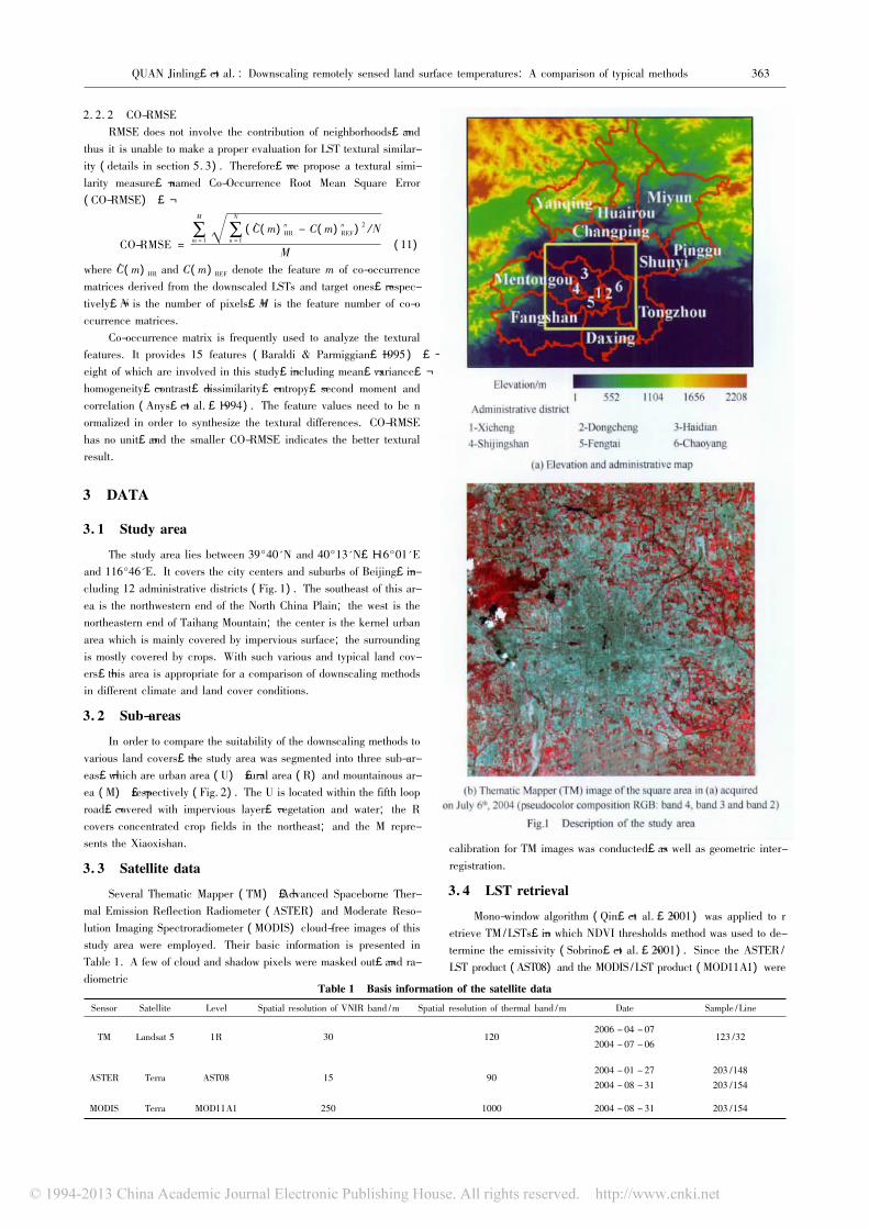
3． 1 Study area

The study area lies between 39°40'N and 40°13'N，116°01'Eand 116°46'E． It covers the city centers and suburbs of Beijing，in-cluding 12 administrative districts ( Fig． 1) ． The southeast of this ar-ea is the northwestern end of the North China Plain; the west is thenortheastern end of Taihang Mountain; the center is the kernel urbanarea which is mainly covered by impervious surface; the surroundingis mostly covered by crops． With such various and typical land cov-ers，this area is appropriate for a comparison of downscaling methodsin different climate and land cover conditions．

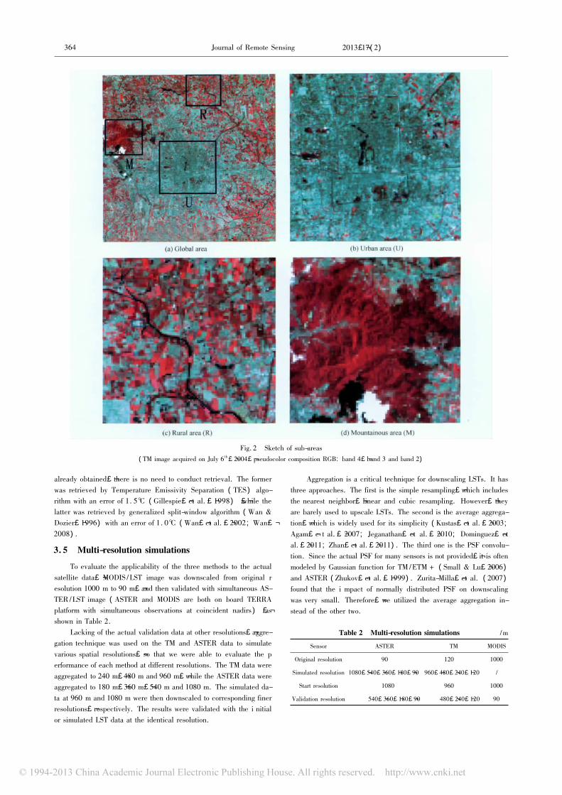
3． 2 Sub-areas

In order to compare the suitability of the downscaling methods tovarious land covers，the study area was segmented into three sub-ar-eas，which are urban area ( U) ，rural area ( R) and mountainous ar-ea ( M) ，respectively ( Fig． 2) ． The U is located within the fifth looproad，covered with impervious layer，vegetation and water; the Rcovers concentrated crop fields in the northeast; and the M repre-sents the Xiaoxishan．

3． 3 Satellite data

Several Thematic Mapper ( TM) ，Advanced Spaceborne Ther-mal Emission Reflection Radiometer ( ASTER) and Moderate Reso-lution Imaging Spectroradiometer ( MODIS) cloud-free images of thisstudy area were employed． Their basic information is presented inTable 1． A few of cloud and shadow pixels were masked out，and ra-diometric

calibration for TM images was conducted，as well as geometric inter-registration．

3． 4 LST retrieval

Mono-window algorithm ( Qin，et al．，2001 ) was applied to retrieve TM /LSTs，in which NDVI thresholds method was used to de-termine the emissivity ( Sobrino，et al．，2001) ． Since the ASTER/LST product ( AST08) and the MODIS/LST product ( MOD11A1) were

Table 1 Basis information of the satellite dataSensor Satellite Level Spatial resolution of VNIR band /m Spatial resolution of thermal band /m Date Sample /Line

TM Landsat 5 1R 30 1202006 － 04 － 072004 － 07 － 06

123 /32

ASTER Terra AST08 15 902004 － 01 － 272004 － 08 － 31

203 /148203 /154

MODIS Terra MOD11A1 250 1000 2004 － 08 － 31 203 /154


Fig． 2 Sketch of sub-areas( TM image acquired on July 6th，2004，pseudocolor composition RGB: band 4，band 3 and band 2)

already obtained，there is no need to conduct retrieval． The formerwas retrieved by Temperature Emissivity Separation ( TES ) algo-rithm with an error of 1． 5℃ ( Gillespie，et al．，1998 ) ，while thelatter was retrieved by generalized split-window algorithm ( Wan ＆Dozier，1996) with an error of 1． 0℃ ( Wan，et al．，2002 ; Wan，2008) ．

3． 5 Multi-resolution simulations

To evaluate the applicability of the three methods to the actualsatellite data，MODIS /LST image was downscaled from original resolution 1000 m to 90 m，and then validated with simultaneous AS-TER/LST image ( ASTER and MODIS are both on board TERRAplatform with simultaneous observations at coincident nadirs ) ，asshown in Table 2．

Lacking of the actual validation data at other resolutions，aggre-gation technique was used on the TM and ASTER data to simulatevarious spatial resolutions，so that we were able to evaluate the performance of each method at different resolutions． The TM data wereaggregated to 240 m，480 m and 960 m，while the ASTER data wereaggregated to 180 m，360 m，540 m and 1080 m． The simulated da-ta at 960 m and 1080 m were then downscaled to corresponding finerresolutions，respectively． The results were validated with the i nitialor simulated LST data at the identical resolution．

Aggregation is a critical technique for downscaling LSTs． It hasthree approaches． The first is the simple resampling，which includesthe nearest neighbor，linear and cubic resampling． However，theyare barely used to upscale LSTs． The second is the average aggrega-tion，which is widely used for its simplicity ( Kustas，et al．，2003;Agam，e t al．，2007; Jeganathan，et al．，2010; Dominguez，etal．，2011; Zhan，et al．，2011) ． The third one is the PSF convolu-tion． Since the actual PSF for many sensors is not provided，it is oftenmodeled by Gaussian function for TM /ETM + ( Small ＆ Lu，2006 )and ASTER ( Zhukov，et al．，1999) ． Zurita-Milla，et al． ( 2007 )found that the i mpact of normally distributed PSF on downscalingwas very small． Therefore，we utilized the average aggregation in-stead of the other two．

Table 2 Multi-resolution simulations /m

Sensor ASTER TM MODIS

Original resolution 90 120 1000

Simulated resolution 1080，540，360，180，90 960，480，240，120 /

Start resolution 1080 960 1000

Validation resolution 540，360，180，90 480，240，120 90


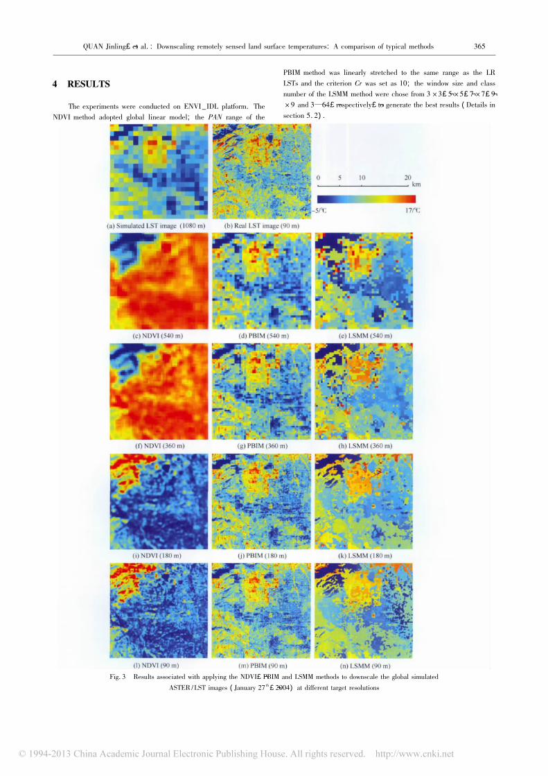
4 RESULTS

The experiments were conducted on ENVI_IDL platform． TheNDVI method adopted global linear model; the PAN range of the

PBIM method was linearly stretched to the same range as the LRLSTs and the criterion Cr was set as 10; the window size and classnumber of the LSMM method were chose from 3 × 3，5 × 5，7 × 7，9× 9 and 3—64，respectively，to generate the best results ( Details insection 5． 2) ．

Fig． 3 Results associated with applying the NDVI，PBIM and LSMM methods to downscale the global simulatedASTER /LST images ( January 27th，2004) at different target resolutions


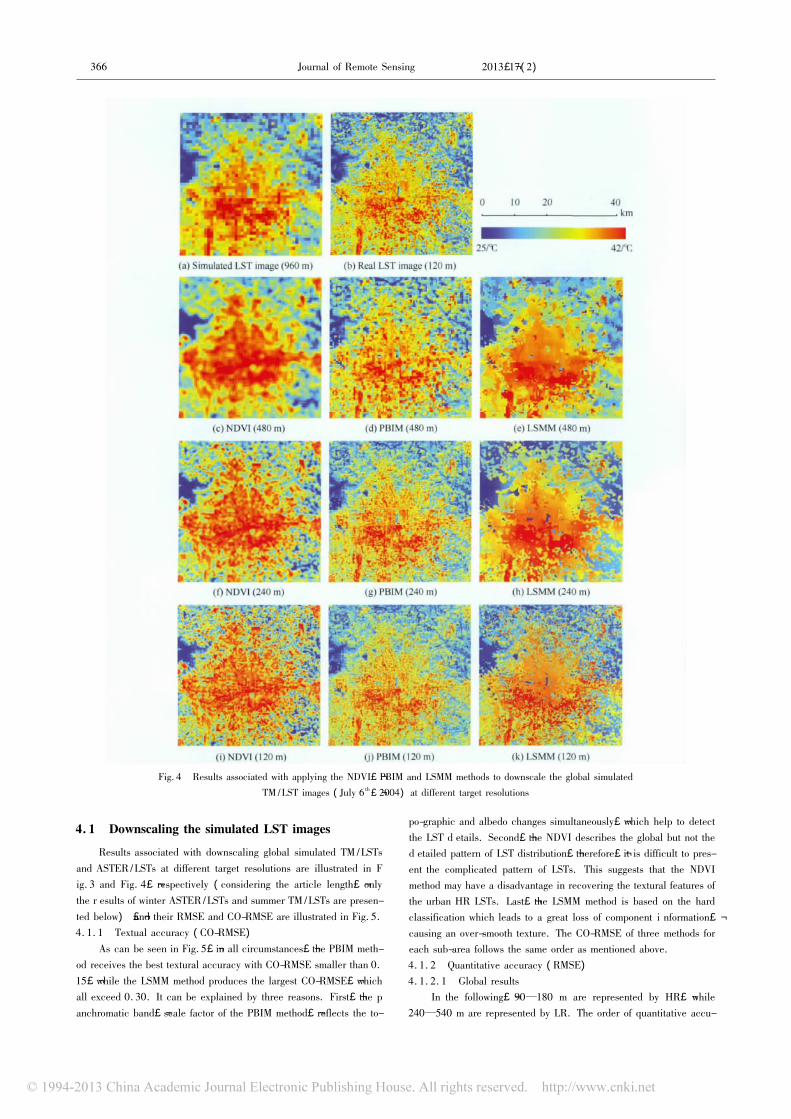
Fig． 4 Results associated with applying the NDVI，PBIM and LSMM methods to downscale the global simulatedTM /LST images ( July 6th，2004) at different target resolutions

4． 1 Downscaling the simulated LST images

Results associated with downscaling global simulated TM /LSTsand ASTER/LSTs at different target resolutions are illustrated in Fig． 3 and Fig． 4，respectively ( considering the article length，onlythe r esults of winter ASTER/LSTs and summer TM /LSTs are presen-ted below) ，and their RMSE and CO-RMSE are illustrated in Fig． 5．4． 1． 1 Textual accuracy ( CO-RMSE)

As can be seen in Fig． 5，in all circumstances，the PBIM meth-od receives the best textural accuracy with CO-RMSE smaller than 0．15，while the LSMM method produces the largest CO-RMSE，whichall exceed 0． 30． It can be explained by three reasons． First，the panchromatic band，scale factor of the PBIM method，reflects the to-

po-graphic and albedo changes simultaneously，which help to detectthe LST d etails． Second，the NDVI describes the global but not thed etailed pattern of LST distribution，therefore，it is difficult to pres-ent the complicated pattern of LSTs． This suggests that the NDVImethod may have a disadvantage in recovering the textural features ofthe urban HR LSTs． Last，the LSMM method is based on the hardclassification which leads to a great loss of component i nformation，

causing an over-smooth texture． The CO-RMSE of three methods foreach sub-area follows the same order as mentioned above．4． 1． 2 Quantitative accuracy ( RMSE)

4． 1． 2． 1 Global resultsIn the following，90—180 m are represented by HR，while

240—540 m are represented by LR． The order of quantitative accu-


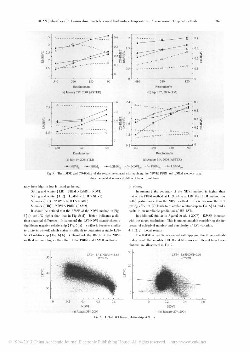
Fig． 5 The RMSE and CO-RMSE of the results associated with applying the NDVI，PBIM and LSMM methods to allglobal simulated images at different target resolutions

racy from high to low is listed as below:Spring and winter ( LR) : PBIM ＞ LSMM ＞ NDVI;Spring and winter ( HR) : LSMM ＞ PBIM ＞ NDVI;Summer ( LR) : PBIM ＞ NDVI ＞ LSMM;Summer ( HR) : NDVI ＞ PBIM ＞ LSMM．It should be noticed that the RMSE of the NDVI method in Fig．

5( a) are 1℃ higher than that in Fig． 5 ( d) ，which indicates a dis-tinct seasonal difference． In summer，the LST-NDVI scatter shows asignificant negative relationship ( Fig． 6( a) ) ，while it becomes similarto a pie in winter，which makes it difficult to determine a stable LST-NDVI relationship ( Fig． 6 ( b) ) ． Therefore，the RMSE of the NDVImethod is much higher than that of the PBIM and LSMM methods

in winter．In summer，the accuracy of the NDVI method is higher than

that of the PBIM method at HR，while at LR，the PBIM method hasbetter performance than the NDVI method． This is because the LSTmixing effect at LR leads to a similar relationship in Fig． 6( b) and results in an unreliable prediction of HR LSTs．

In addition，similar to Agam，et al． ( 2007 ) ，RMSE increasewith the target resolutions． This is understandable considering the in-crease of sub-pixel number and complexity of LST variation．4． 1． 2． 2 Local results

The RMSE of results associated with applying the three methodsto downscale the simulated U，R and M images at different target res-olutions are illustrated in Fig． 7．

Fig． 6 LST-NDVI linear relationship at 90 m


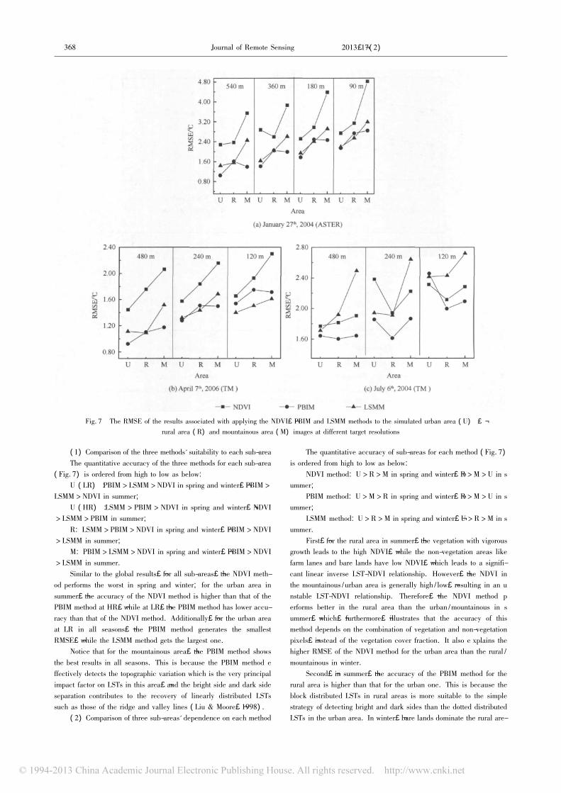
Fig． 7 The RMSE of the results associated with applying the NDVI，PBIM and LSMM methods to the simulated urban area ( U) ，

rural area ( R) and mountainous area ( M) images at different target resolutions

( 1) Comparison of the three methods' suitability to each sub-areaThe quantitative accuracy of the three methods for each sub-area

( Fig． 7) is ordered from high to low as below:U ( LR) : PBIM ＞ LSMM ＞ NDVI in spring and winter，PBIM ＞

LSMM ＞ NDVI in summer;U ( HR) : LSMM ＞ PBIM ＞ NDVI in spring and winter，NDVI

＞ LSMM ＞ PBIM in summer;R: LSMM ＞ PBIM ＞ NDVI in spring and winter，PBIM ＞ NDVI

＞ LSMM in summer;M: PBIM ＞ LSMM ＞ NDVI in spring and winter，PBIM ＞ NDVI

＞ LSMM in summer．Similar to the global results，for all sub-areas，the NDVI meth-

od performs the worst in spring and winter; for the urban area insummer，the accuracy of the NDVI method is higher than that of thePBIM method at HR，while at LR，the PBIM method has lower accu-racy than that of the NDVI method． Additionally，for the urban areaat LR in all seasons， the PBIM method generates the smallestRMSE，while the LSMM method gets the largest one．

Notice that for the mountainous area，the PBIM method showsthe best results in all seasons． This is because the PBIM method effectively detects the topographic variation which is the very principalimpact factor on LSTs in this area，and the bright side and dark sideseparation contributes to the recovery of linearly distributed LSTssuch as those of the ridge and valley lines ( Liu ＆ Moore，1998) ．

( 2) Comparison of three sub-areas' dependence on each method

The quantitative accuracy of sub-areas for each method ( Fig． 7)is ordered from high to low as below:

NDVI method: U ＞ R ＞ M in spring and winter，R ＞ M ＞ U in summer;

PBIM method: U ＞ M ＞ R in spring and winter，R ＞ M ＞ U in summer;

LSMM method: U ＞ R ＞ M in spring and winter，U ＞ R ＞ M in summer．

First，for the rural area in summer，the vegetation with vigorousgrowth leads to the high NDVI，while the non-vegetation areas likefarm lanes and bare lands have low NDVI，which leads to a signifi-cant linear inverse LST-NDVI relationship． However，the NDVI inthe mountainous /urban area is generally high / low，resulting in an unstable LST-NDVI relationship． Therefore， the NDVI method performs better in the rural area than the urban /mountainous in summer，which，furthermore，illustrates that the accuracy of thismethod depends on the combination of vegetation and non-vegetationpixels，instead of the vegetation cover fraction． It also e xplains thehigher RMSE of the NDVI method for the urban area than the rural /mountainous in winter．

Second，in summer，the accuracy of the PBIM method for therural area is higher than that for the urban one． This is because theblock distributed LSTs in rural areas is more suitable to the simplestrategy of detecting bright and dark sides than the dotted distributedLSTs in the urban area． In winter，bare lands dominate the rural are-


a and thus generate homogeneous albedo，which is adverse to theLST assignation． Consequently，this method illustrates a lower accu-racy for the rural area than the urban one in winter．

Last，in all seasons，LSMM method behaves the best for the urban area，while the worst for the mountainous area． This may be at-tributed to the classification which，to some extent，expresses thecharacteristics of the substrate materials in the urban area，but notthe topography and vegetation condition in mountainous and rural ar-eas．

4． 2 Downscaling the MODIS /LST image

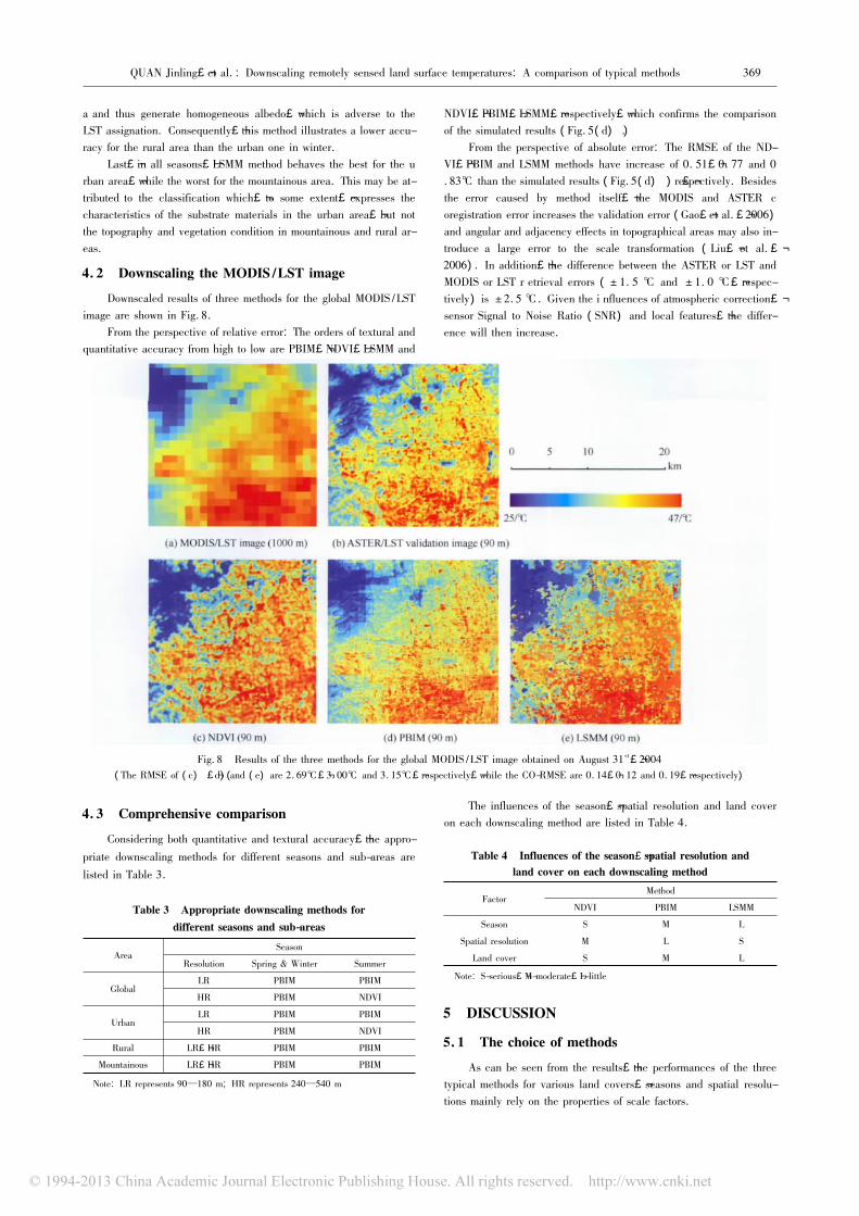
Downscaled results of three methods for the global MODIS /LSTimage are shown in Fig． 8．

From the perspective of relative error: The orders of textural andquantitative accuracy from high to low are PBIM，NDVI，LSMM and

NDVI，PBIM，LSMM，respectively，which confirms the comparisonof the simulated results ( Fig． 5( d) ) ．

From the perspective of absolute error: The RMSE of the ND-VI，PBIM and LSMM methods have increase of 0． 51，0． 77 and 0． 83℃ than the simulated results ( Fig． 5( d) ) ，respectively． Besidesthe error caused by method itself， the MODIS and ASTER coregistration error increases the validation error ( Gao，et al．，2006)and angular and adjacency effects in topographical areas may also in-troduce a large error to the scale transformation ( Liu，et al．，2006) ． In addition，the difference between the ASTER or LST andMODIS or LST r etrieval errors ( ± 1． 5 ℃ and ± 1． 0 ℃，respec-tively) is ± 2． 5 ℃ ． Given the i nfluences of atmospheric correction，sensor Signal to Noise Ratio ( SNR) and local features，the differ-ence will then increase．

Fig． 8 Results of the three methods for the global MODIS /LST image obtained on August 31st，2004( The RMSE of ( c) ，( d) and ( e) are 2． 69℃，3． 00℃ and 3． 15℃，respectively，while the CO-RMSE are 0． 14，0． 12 and 0． 19，respectively)

4． 3 Comprehensive comparison

Considering both quantitative and textural accuracy，the appro-priate downscaling methods for different seasons and sub-areas arelisted in Table 3．

Table 3 Appropriate downscaling methods fordifferent seasons and sub-areas

AreaSeason

Resolution Spring ＆ Winter Summer

GlobalLR PBIM PBIM

HR PBIM NDVI

UrbanLR PBIM PBIM

HR PBIM NDVI

Rural LR，HR PBIM PBIM

Mountainous LR，HR PBIM PBIM

Note: LR represents 90—180 m; HR represents 240—540 m

The influences of the season，spatial resolution and land coveron each downscaling method are listed in Table 4．

Table 4 Influences of the season，spatial resolution andland cover on each downscaling method

FactorMethod

NDVI PBIM LSMM

Season S M L

Spatial resolution M L S

Land cover S M L

Note: S-serious，M-moderate，L-little

5 DISCUSSION

5． 1 The choice of methods

As can be seen from the results，the performances of the threetypical methods for various land covers，seasons and spatial resolu-tions mainly rely on the properties of scale factors．


First，the scale factor ( NDVI) of the NDVI method reflects thevegetation cover condition． Its relationship with LSTs almost controlsthe downscaled results，and the optimal one is obtained in areas withboth bare lands and dense vegetation covers． It can be inferred thatthis method would be not effective when other factors，such as soilmoistures and substrate characteristics，have a great controlling onthe LST changes． Zhan，et al． ( 2011 ) found that combining Tem-perature Vegetation Dryness Index ( TVDI ) ( Sandholt，et al．，2002) with NDVI to extract the dry edge and wet edge improved therecovery of LST changes caused by soil moisture．

Second，the scale factor ( Panchromatic band ) of the PBIMmethod is a combination of multi-spectral bands，which presents thereflected solar illumination intensity，and thus insensitive to the characteristic absorption and reflection． Therefore， this method issuitable for areas with a great solar illumination difference and moreeffective in the areas with varied topography than the NDVI andLSMM methods． While it is unsuitable for areas with very low sun il-lumination angle，such as winter images of high latitude ( Liu ＆Moore，1998 ) ． In addition，the panchromatic band somewhat re-flects the land surface albedo variation，resulting in a good applica-tion in the areas with heterogeneous substrate characteristics． Where-as，the strategy that regarding the mean PAN as a threshold for dis-criminating the bright and dark sides，is too simple to be applied tothe areas with large albedo variation because of quantities of n oises．It is further inferred that this method may be not applicable for areaswith high resolutions and very heterogeneous albedo．

Last，the scale factor ( Hard classification map) of the LSMMmethod discretizes a continuous property，certainly causing the lossof partial information． With a decrease of the spatial resolution，themixing effect and unclearness of the classification boundaries aggra-vate，which increase the error of inter- and intra- classes as well asthe loss of textural details． Moreover，the similar pixels in the classi-fication band do not necessarily have the identical LST ( Zhukov，et al．，1999) ，especially at low resolutions． Therefore，this method ishighly influenced by the spatial resolution，and may be not applicablefor images with resolution lower than 90 m based on our experiments．

In general，the key issue to the choice of methods is to find thedominating impact factor on the LST variation as the scale factor．

5． 2 The choice of parameters

Due to the quite distinct results with different parameters，it isnecessary to discuss the standards and issues for the choice ofp arameters．

First，for the NDVI method，it is difficult to decide the windowsize and the LST-NDVI regression function． ( 1 ) Extending the window size would bring in irrelevant pixels easily，causing data redundancy and an unreal LST-NDVI relationship． While narrowing itwould make the regression very sensitive to noises and a poor prediction for the high resolution． Jeganathan，et al． ( 2010) believedthat a window size of 5 × 5 is appropriate，while Prihodko andGoward ( 1997) found it as 13 × 13． These findings are highly scene-dependent and thus cannot be universally applied． To automaticallydecide an appropriate window size based on the image properties is away to improve this method，and semi-variance is an effective solu-tion ( Zhan，et al．，2012 ) ． ( 2 ) The LST-NDVI relationship isclosely related to the land cover ( Smith ＆ Choudhury，1991) ，soilmoisture ( Carlson，et al．，1990 ) ， spatial scale ( Prihodko ＆Goward，1997 ) ，d iurnal change ( Goetz，1997 ) ，latitude，topo-graphic and geomorphic conditions，cloud and so on． In these varia-bles，soil moisture is one of the most principal factors． The LST-ND-

VI feature space ( triangular or trapezoidal) can be considered as abatch of soil moisture isolines，and the more distinct moisture varia-tion indicates the more complex regressions． Linear and nonlinear re-gression functions are now commonly used ( Eq． ( 3 ) ) ． The linearones are simple，stable and robust，but they are not applicable in theareas with a narrow NDVI range such as forest where the linear LST-NDVI relationship is unavailable ( Smith ＆ Choudhury，1991 ) ．While the polynomial ones lack of the physical significance and arevery sensitive to extremums． Agam，et al． ( 2007) and Zhan，et al．( 2011 ) found that it can lead to unstable results instead of betterones． If the transformation of NDVI is regarded as an independentvariable of the regression，then some nonlinear functions are equal tothe linear ones with kernels of NDVI functions．

Second，for the PBIM method，the PAN range and the criterion Crare closely related to the noises and rectangular pseudo-edges． Stretc-hing PAN range would generate the noises easily，while compressing itwould exchange the rectangular pseudo-edges． This is due to the multi-plying-dividing calculation between PAN and LST，which impels that thedownscaled LST range is controlled by the PAN range． In this study，itwas linearly stretched to the same range as the LR LSTs and was foundto be a compromise between the noises and rectangular pseudo-edges． Inaddition，a global Cr would lead to a fine urban LST recovery with therectangular pseudo-edges in the mountainous areas or a fine mountainousLST recovery with many noises in the urban areas． This is due to thedifferent albedo fluctuations in diverse land cover areas． A local Cr isrecommended in this circumstance．

Last，for the LSMM method，the class number is the hardchoice，besides the window size． A big one would synthesize compo-nents information and reduce the inter-classes error，but it also intro-duces noises and an unstable solution． While a small one wouldaccelerate the calculation，but it also eliminates many textual detailsand aggravates the issue of the same class with different temperatures．

As can be seen above，setting parameters for the three methodshas no specific standards． It depends on the data properties and is usually subjective． Generally，for the NDVI method，it brings no significant difference to the downscaled results，and thus makes thismethod easy to implement; for the PBIM method，it needs a compro-mise and therefore there are multiple possibilities of results becauseof the anthropic factors; for the LSMM method，it is usually decidedthrough repeat experiments which is time-consuming and complicat-ed． Therefore，exploring the relationship between the p arametersand data properties is necessary in order to make the choice of pa-rameters automatically，objectively and high-effectively．

5． 3 The choice of evaluation criteria

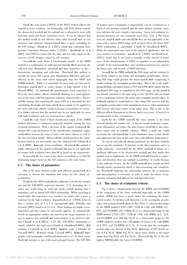
Fig． 5 shows a disagreement between the RMSE and CO-RMSEin the comparison of the three methods，especially on the LSMMmethod． RMSE has been a usual choice for evaluating the down-scaled results． It is，however，insensitive to the rectangular pseudo-edges and textural details，shown in Fig． 9( b) is a downscaled imageby the PBIM method ( PAN = 300—315，Cr = 10) with RMSE of 1．94℃ and CO-RMSE of 0． 11，Fig． 9( c) is a downscaled image by thePBIM method ( PAN = 275—313，Cr = 10 ) with RMSE of 2 ． 21℃and CO-RMSE of 0． 10，Fig． 9 ( d ) is a downscaled image by theLSMM method ( window size = 5，number of classes = 4) with RMSEof 2． 03℃ and CO-RMSE of 0． 21． It reveals that the rectangularpseudo-edges are obvious in Fig． 9( b) ，and many of LST details arelost in Fig． 9( d) ，while Fig． 9 ( c) shows more similar to the targetimage than Fig． 9( b) and Fig． 9 ( d) ． However，Fig． 9 ( c) has thehighest RMSE，while the lowest CO-RMSE．


Fig． 9 Results at 120 m for TM /LST simulated image，obtained on July 6th，2004

RMSE just reveals the value difference between the correspond-ing pixels，which is irrelevant to“temperature distribution”，andtherefore，it emphasizes the quantitative accuracy of each pixel．While CO-RMSE only indicates the textual difference between theLST images，where temperature value is unconcerned，and thus，itconcentrates on the textual accuracy of the neighborhoods． Due totheir different emphases，the practical applications of LSTs need con-sidered． When the downscaled LSTs are used to input to the quanti-tative models，RMSE is the primary choice，while when the down-scaled LSTs are used to describe the patterns of thermal environmentor rank the LST grades，CO-RMSE becomes the primary one． Thecombination of both provides more comprehensive evaluation．

6 CONCLUSION

Enhancing the spatial resolution of LSTs improves the accuracyof resource detection and environmental monitoring，providing atechnical support for LST utilizations． In order to select an appropri-ate downscaling method in practice，we inter-compared the results of

three typical methods，including the NDVI，PBIM and LSMM meth-ods，for global and local areas based on RMSE and C O-RMSE． Theconclusions are as below:

( 1) Considering the season，the performance of the NDVI meth-od is mostly affected，and not applicable for spring and winter ima-ges，while that of the PBIM and LSMM methods are less affected．

( 2) Considering the spatial resolution，the performance of theLSMM method is mostly influenced，and inappropriate for LR ima-ges． The NDVI method is better than the PBIM method at HR，whilethe PBIM method has better performance than the NDVI methodat LR．

( 3) Considering the local land cover，the NDVI method is suit-able for areas with combination of vegetation and non-vegetation pix-els，the PBIM method is suitable to the areas with varied topographyand albedos，and the LSMM method is suitable to the areas with dis-tinct LST differences inter-classes．

( 4) Considering the operability，the NDVI method is the easi-est one，while the LSMM is the most difficult one．

( 5) Considering the application，the RMSE is used for quanti-tative calculations of LSTs，while the CO-RMSE is used for land-


scape analysis of thermal environment．In practice，it is necessary to synthesize each factor mentioned

above and pick one method whose scale factor is the principal influ-ence on the LST variation． Some prospects are put forward for thenext stage: exploring the relationship between the parameters and da-ta properties，designing a proper evaluation criteria for the downscal-ing LSTs based on the specific purpose of applications and a dvancingthe Spatial and Temporal Adaptive Reflectance Fusion Model( STARFM) ( Gao，et al．，2006) by adding a temporal LST model，in order to applied it to downscale LSTs．

REFERENCES

Agam N，Kustas W P，Anderson M C，Li F Q and Neale C M U． 2007．A vegetation index based technique for spatial sharpening of thermalimagery． Remote Sensing of Environment，107 ( 4 ) : 545 － 558［DOI: 10． 1016 / j． rse． 2006． 10． 006］

Aiazzi B，Alparone L，Baronti S，Santurri L and Selva M． 2005． Spatialresolution enhancement of ASTER thermal bands． Proceeding ofSPIE Image and Signal Processing for Remote Sensing XI． Brugge:

Lorenzo Bruzzone，5982: 1 － 10Anys H，Bannari A，He D C and Morin D． 1994． Texture analysis for

the mapping of urban areas using airborne MEIS-II images． Proceed-ing of the 1st International Airborne Remote Sensing Conference andExhibition． Strasbourg: Environmental Research Institute of Michi-gan，Ann Arbor，3: 231 － 245

Atkinson P M ，Pardo-Igúzquiza E and Chica-Olmo M． 2008． Downscal-ing cokriging for super-resolution mapping of continua in remotelysensed images． IEEE Transactions on Geoscience and R emote Sens-ing，46( 2) : 573 － 580 ［DOI: 10． 1109 /TGRS． 2007． 909952］

Baraldi A and Parmiggian F． 1995． An investigation of the textural char-acteristics associated with gray level cooccurrence matrix statisticalparameters． IEEE Transactions on Geoscience and Remote Sensing，

33( 2) : 293 － 304 ［DOI: 10． 1109 /36． 377929］Bastiaanssen W G M，Menenti M，Feddes R A and Holtslag A A M．

1998． A remote sensing surface energy balance algorithm for land( SEBAL) ． 1． Formulation． Journal of Hydrology，212 － 213: 198－ 212 ［DOI: 10． 1016 /S0022 － 1694( 98) 00253 － 4］

Carlson T N，Perry E M and Schmugge T J． 1990． Remote estimation ofsoil moisture availability and fractional vegetation cover for agricul-ture field． Agriculture and Forest Meteorology，52: 45 － 49 ［DOI:10． 1016 /0168 － 1923( 90) 90100 － K］

Christensen P R，Bandfield J L，Hamilton V E，Howard D A，Lane MD，Piatek J L，Ruff S W and Stefanov W L． 2000． A thermal emis-sion spectral library of rock-forming minerals． Journal of GeophysicalResearch，105( E4) : 9735-9739 ［DOI: 10． 1029 /1998JE000624］

Dominguez A，Kleissl J，Luvall J C and Rickman D L． 2011． High-reso-lution urban thermal sharpener ( HUTS) ． Remote Sensing of Envi-ronment，115( 7) : 1772 － 1780 ［DOI: 10． 1016 / j． rse． 2011． 03．008］

Fasbender D，Tuia D，Bogaert P and Kanevski M． 2008． Support-basedimplementation of Bayesian data fusion for spatial enhancement: applications to ASTER thermal images． IEEE Geoscience and Remote Sensing Letters，5 ( 4 ) : 598 － 602 ［DOI: 10． 1109 /LGRS．2008． 2000739］

Gao F，Masek J，Schwaller M and Hall F． 2006． On the blending of theLandsat and MODIS surface reflectance: predicting daily Landsatsurface reflectance． IEEE Transactions on Geoscience and RemoteSensing，44 ( 8 ) : 2207 － 2218 ［DOI: 10． 1109 /TGRS． 2006．872081］

Gillespie A，Rokugawa S，Matsunaga T，Cothern J S，Hook S and Kahle

A B． 1998． A temperature and emissivity separation algorithm forAdvanced Spaceborne Thermal Emission and Reflection Radiometer( ASTER) images． IEEE Transactions on Geoscience and RemoteSensing，36( 4) : 1113 － 1126 ［DOI: 10． 1109 /36． 700995］

Gillies R R and Carlson T N． 1995． Thermal remote sensing of surfacesoil water content with partial vegetation cover for incorporation intoclimate models． Journal of Applied Meteorology，34( 4) : 745 － 756［DOI: 10． 1175 /1520 －0450( 1995) 034 ＜0745: TRSOSS ＞2． 0． CO; 2］

Goetz S J． 1997． Multi-sensor analysis of NDVI，surface temperature andbiophysical variables at a mixed grassland site． International Journalof Remote Sensing，18( 1) : 71 －94［DOI: 10． 1080 /014311697219286］

Gustavson W T，Handcock R，Gillespie A R and Tonooka H． 2003． Animage sharpening method to recover stream temperatures from ASTER images． Proceeding of SPIE Remote Sensing for Environmen-tal Monitoring，GIS applications and Geology II． Bellevue: ManfredEhlers，4886: 72 － 83

Jeganathan C，Hamm N A S，Mukherjee S，Atkinson P M，Raju P L Nand Dadhwal V K． 2010． Evaluating a thermal image sharpeningmodel over a mixed agricultural landscape in India． InternationalJournal of Applied Earth Observation and Geoinformation，13 ( 2 ) :

178 － 191 ［DOI: 10． 1016 / j． jag． 2010． 11． 001］Kustas W P，Norman J M，Anderson M C and French A N． 2003． Esti-

mating subpixel surface temperatures and energy fluxes from the veg-etation index-radiometric temperature relationship． Remote Sensingof Environment，85( 4) : 429 － 440

Lemeshewsky G P． 1998． Neural network-based sharpening of Landsatthermal-band images． Park S K，Juday R D，eds． Proceeding ofSPIE Visual Information Processing VII． Orlando，3387: 378 － 386

Lemeshewsky G P and Schowengerdt R A． 2001． Landsat 7 thermal-IRimage sharpening using an artificial neural network and sensormodel． Park S K，Rahman Z，Schowengerdt R A，eds． Proceedingof SPIE Visual Information Processing X． Orlando，4388: 181 － 192

Lentile L B，Holden Z A，Smith A M S，Falkowski M J，Hudak A T，

Morgan P，Lewis S A，Gessler P E and Benson N C． 2006． Remotesensing techniques to assess active fire characteristics and post-fireeffects． International Journal of Wildland Fire，15 ( 3 ) : 319 － 345［DOI: 10． 1071 /WF05097］

Liang S L． 2004． Quantitative Remote Sensing of Land Surfaces． Hobo-ken，New Jersey: John Wiley and Sons，Inc． : 18 － 462

Liu D S and Pu R L． 2008． Downscaling thermal infrared radiance forsubpixel land surface temperature retrieval． Sensors，8( 4) : 2695 －2706 ［DOI: 10． 3390 /s8042695］

Liu J G and Moore J M． 1998． Pixel block intensity modulation: addingspatial detail to TM band 6 thermal imagery． International Journal ofRemote Sensing，19 ( 13 ) : 2477 － 2491 ［DOI: 10． 1080 /014311698214578］

Liu Y B，Hiyama T and Yamaguchi Y． 2006． Scaling of land surface temperature using satellite data: a case examination on ASTER andMODIS products over a heterogeneous terrain area． Remote Sensingof Environment，105( 2) : 115 － 128 ［DOI: 10． 1016 / j． rse． 2006．06． 012］

Nichol J． 2009． An emissivity modulation method for spatial enhancement ofthermal satellite images in urban heat island analysis． Photogram-metric Engineering and Remote Sensing，75( 5) : 1 － 10

Pardo-Igúzquiza E，Chica-Olmo M and Atkinson P M． 2006． Downscalingcokriging for image sharpening． Remote Sensing of Environment，102( 1 /2) : 86 － 98 ［DOI: 10． 1016 / j． rse． 2006． 02． 014］

Prihodko L and Goward S N． 1997． Estimation of air temperature fromremotely sensed surface observations． Remote Sensing of Environ-ment，60 ( 3 ) : 335 － 346 ［DOI: 10． 1016 /S0034 － 4257 ( 96 )

00216 － 7］Qin Z，Karnieli A and Berliner P． 2001． A mono-window algorithm for


retrieving land surface temperature from Landsat TM data and its ap-plication to the Israel-Egypt border region． International Journal ofRemote Sensing，22 ( 18 ) : 3719 － 3746 ［DOI: 10． 1080 /01431160010006971］

Sandholt I，Rasmussen K and Anderson J． 2002． A simple interpretationof the surface temperature /vegetation index space for assessment ofsurface moisture status． Remote Sensing of Environment，79( 2 /3) :

213 － 224 ［DOI: 10． 1016 /S0034 － 4257( 01) 00274 － 7］Small C and Lu J W T． 2006． Estimation and vicarious validation of u

rban vegetation abundance by spectral mixture analysis． RemoteSensing of Environment，100 ( 4 ) : 441 － 456 ［DOI: 10． 1016 / j．rse． 2005． 10． 023］

Smith R C G and Choudhury B J． 1991． Analysis of normalized differ-ence and surface temperature observations over southeastern Australia． International Journal of Remote Sensing，12( 10) : 2021 －2044 ［DOI: 10． 1080 /01431169108955234］

Sobrino J A，Baissouni N and Li Z L． 2001． A comparative study of landsurface emissivity retrieval from NOAA Data． Remote Sensing of En-vironment，75( 2) : 256 － 266 ［DOI: 10． 1016 /S0034 － 4257( 00)

00171 － 1］Stathopoulou M and Cartalis C． 2009． Downscaling AVHRR land surface

temperatures for improved surface urban heat island intensity estima-tion． Remote Sensing of Environment，113 ( 12 ) : 2592 － 2605［DOI: 10． 1016 / j． rse． 2009． 07． 017］

Voogt J A and Oke T R． 2003． Thermal remote sensing of urban cli-mates． Remote Sensing of Environment，86( 3) : 370 － 384 ［DOI:10． 1016 /S0034 － 4257( 03) 00079 － 8］

Wan Z M． 2008． New refinements and validation of the MODIS Land-Surface Temperature /Emissivity products． Remote Sensing of Envi-ronment，112( 1) : 59 － 74 ［DOI: 10． 1016 / j． rse． 2006． 06． 026］

Wan Z M and Dozier J． 1996． A generalized split-window algorithm for

retrieving land-surface temperature from space． IEEE Transactionson Geoscience and Remote Sensing，34( 4) : 892 － 905 ［DOI: 10．1109 /36． 508406］

Wan Z M，Zhang Y L，Zhang Q C and Li Z L． 2002． Validation of theland-surface temperature products retrieved from Terra ModerateResolution Imaging Spectroradiometer data． Remote Sensing of Environment，83 ( 1 /2 ) : 163 － 180 ［DOI: 10． 1016 /S0034 － 4257( 02) 00093 － 7］

Wang Z J，Ziou D，Armenakis C，Li D and Li Q Q． 2005． A compara-tive analysis of image fusion methods． IEEE Transactions on Geosci-ence and Remote Sensing，43( 6) : 1391 － 1402 ［DOI: 10． 1109 /TGRS． 2005． 846874］

Zhan W F，Chen Y H，Wang J F，Zhou J，Quan J L，Liu W Y and LiJ． 2012． Downscaling land surface temperatures with multi-spectraland multi-resolution images． International Journal of Applied EarthObservation and Geoinformation，18: 23 － 36 ［DOI: 10． 1016 / j．jag． 2012． 01． 003］

Zhan W F，Chen Y H，Zhou J，Li J and Liu W Y． 2011． Sharpeningthermal imageries: a generalized theoretical framework from an as-similation perspective． IEEE Transactions on Geoscience and Re-mote Sensing，49 ( 2 ) : 773 － 789 ［DOI: 10． 1109 /TGRS． 2010．2060342］

Zhukov B，Oertel D，Lanzl F and Reinhckel G． 1999． Unmixing-basedmultisensor multiresolution image fusion． IEEE Transactions on Geoscience and Remote Sensing，37 ( 3 ) : 1212 － 1226 ［DOI: 10．1109 /36． 763276］

Zurita-Milla R，Kaiser G，Clevers J P G W，Schneider W and Schaep-man M E． 2007． Spatial unmixing of MERIS data for monitoringvegetation dynamics． Proceedings of Envisat Symposium． Montreux:

ESA SP － 636: 23 － 27

遥感地表温度降尺度方法比较——性能对比及适应性评价

Documents

Transcript of 遥感地表温度降尺度方法比较——性能对比及适应性评价