


Bahasa
Halaman
Hukum


VOLTAGE STABILITY ANALYSIS USING SIMULATED SYNCHROPHASOR
MEASUREMENTS
A Thesis
presented to
the Faculty of California Polytechnic State University,
San Luis Obispo
In Partial Fulfillment
of the Requirements for the Degree
Master of Science in Electrical Engineering
by
Allan Agatep
May 2013

ii
© 2013
Allan Agatep
ALL RIGHTS RESERVED

iii
COMMITTEE MEMBERSHIP
TITLE: VOLTAGE STABILITY ANALYSIS USING SIMULATED
SYNCHROPHASOR MEASUREMENTS
AUTHOR: Allan Agatep
DATE SUBMITTED: May 2013
COMMITTEE CHAIR: Dr. Ahmad Nafisi, Professor
Electrical Engineering Department
COMMITTEE MEMBER: Dr. Taufik, Professor
Electrical Engineering Department
COMMITTEE MEMBER: Dr. Ali O. Shaban, Professor
Electrical Engineering Department
iv
ABSTRACT
VOLTAGE STABILITY ANALYSIS USING SIMULATED SYNCHROPHASOR
MEASUREMENTS
Allan Agatep
An increase in demand for electric power has forced utility transmission systems
to continuously operate under stressed conditions, which are close to instability limits.
Operating power systems under such conditions along with inadequate reactive power
reserves initiates a sequence of voltage instability points and can ultimately lead to a
system voltage collapse. Significant research have been focused on time-synchronized
measurements of power systems which can be used to frequently determine the state of a
power system and can lead to a more robust protection, control and operation
performance. This thesis discusses the applicability of two voltage stability
synchrophasor-based indices from literature to analyze the stability of a power system.
Various load flow scenarios were conducted on the BPA 10-Bus system and the IEEE 39-
Bus System using PowerWorld Simulator. The two indices were analyzed and compared
against each other along with other well-known methods. Results show that their
performances are coherent to each other regarding to voltage stability of the system; the
indices can also predict voltage collapse as well as provide insight on other locations
within the system that can contribute to instability.
Keywords: voltage stability, voltage stability index, synchrophasors

v
ACKNOWLEDGMENTS
First and foremost, I would like to express my deepest gratitude to my advisor Dr.
Ahmad Nafisi for his wisdom and encouragement. This thesis would not have been
possible to accomplish without the help and guidance he has provided me throughout the
entire process.
I would like to thank Dr. Taufik and Dr. Ali Shaban for serving as members on
my thesis committee. I would also like to thank them for their lectures they teach. Their
knowledge has been a great resource, which has initially inspired me to pursue power
electronics and power systems engineering in the first place.
I would also like to express my dearest appreciation to my friends and fellow
colleagues, especially: Abby Cansanay, Alex Morales, Chris Nguyen, Joanne Cho,
Mason Ung, Nelson Lau and M.S Rithy Chhean. The discussions and times I’ve shared
with them have helped me get through the most challenging times. Thank you for
providing me with most valuable advice and motivation.
Last but not least, I would like to thank my family – especially my parents Noel
and Laureen Agatep. My family has always guided me along the right path and has
provided me with the inspiration to accomplish great things. They have always been there
to help me in any way they can. For all these reasons and more, I am truly grateful.
vi
TABLE OF CONTENTS
Title Page
LIST OF TABLES............................................................................................................. ix
LIST OF FIGURES ........................................................................................................... xi
CHAPTER 1 INTRODUCTION..................................................................................... 1
1.1 Introduction ..................................................................................................................... 1
1.2 Thesis Objectives............................................................................................................. 2
1.3 Thesis organization.......................................................................................................... 3
CHAPTER 2 VOLTAGE STABILITY OVERVIEW.................................................... 4
2.1 Power System Stability.................................................................................................... 4
2.1.1. Rotor Angle stability ............................................................................................... 5
2.1.2. Frequency stability .................................................................................................. 6
2.1.3. Voltage Stability...................................................................................................... 6
2.2 Voltage Stability.............................................................................................................. 6
2.2.1. Classifications.......................................................................................................... 7
2.3 Voltage Stability Limitations .......................................................................................... 8
2.3.1. Voltage Collapse Incidents.................................................................................... 10
2.4 Voltage Stability Analysis............................................................................................. 11
2.4.1. Power-Flow Analysis [11]..................................................................................... 11
2.4.2. PV and QV Curves [8] .......................................................................................... 12
2.4.3. Voltage .................................................................................................................. 16
2.4.4. Analysis Methods .................................................................................................. 17
2.5 Synchrophasors ............................................................................................................. 18
CHAPTER 3 EVALUATION OF VOLTAGE STABILITY INDICES ...................... 23
3.1 Index from Load Flow Jacobian.................................................................................... 23
3.1.1. Modal Analysis of Power Flow Model.................................................................. 23

vii
3.2 Indices Based on Phasor Measurement Units................................................................ 29
3.2.1. Algorithm for Equating Thevenin Equivalent Parameters [26-27] ....................... 30
3.2.2. Line Stability Index ............................................................................................... 32
3.2.3. Fast Voltage Stability Index .................................................................................. 33
3.2.4. LQP index.............................................................................................................. 33
3.2.5. VSI based on Maximum Power Transfers............................................................. 34
3.2.6. VCPI...................................................................................................................... 35
CHAPTER 4 IMPLEMENTATION OF INDICES AND TEST NETWORKS........... 36
4.1 PowerWorld Simulator.................................................................................................. 36
4.2 Test Systems.................................................................................................................. 37
4.2.1. BPA 10-Bus System.............................................................................................. 37
4.2.2. IEEE 39-Bus System ............................................................................................. 38
4.3 Test Cases...................................................................................................................... 42
4.3.1. Verification of Index Performance Using 10-Bus Case ........................................ 42
4.3.2. Increase All Loads................................................................................................. 43
4.3.3. Reactive Load Increase.......................................................................................... 43
4.3.4. Contingency........................................................................................................... 44
4.3.5. Intermittent Generation ......................................................................................... 44
4.3.6. Wind Farm Aggregation........................................................................................ 45
CHAPTER 5 SIMULATION AND RESULTS............................................................ 47
5.1 BPA 10-Bus: Verification of Index Performance.......................................................... 47
5.2 Case 1: IEEE 39-Bus: Increase all loads ....................................................................... 52
5.3 Case 2: 39 Bus - Reactive power case........................................................................... 60
5.3.1. Voltage Collapse Predictability From Indices....................................................... 64
5.4 Case 3: IEEE 39 Bus System -Loss of transmission line .............................................. 67
5.5 Case 4: IEEE 39 Bus System – Intermittent Generation ............................................... 76

viii
5.6 Stability Margin............................................................................................................. 78
5.7 Weakest Bus .................................................................................................................. 79
CHAPTER 6 CONCLUSION AND RECOMMENDATIONS.................................... 83
WORKS CITED ............................................................................................................... 85
APPENDIX A- Matlab Code............................................................................................ 88
APPENDIX B- Power Flow and Line Loses for Case 3 .................................................. 95
APPENDIX C- QV Analysis Calculations for IEEE-39 Bus System .............................. 96
APPENDIX D- Modal Analysis Calculations for IEEE-39 Bus System ......................... 97

ix
LIST OF TABLES
Table Page
Table 2-1 Voltage Collapse Incidents [8] ......................................................................... 10
Table 3-1: Eigenvalues for a given load increase ............................................................. 27
Table 3-2 Participation Factors For Each Modal Variation (Initial Conditions) .............. 28
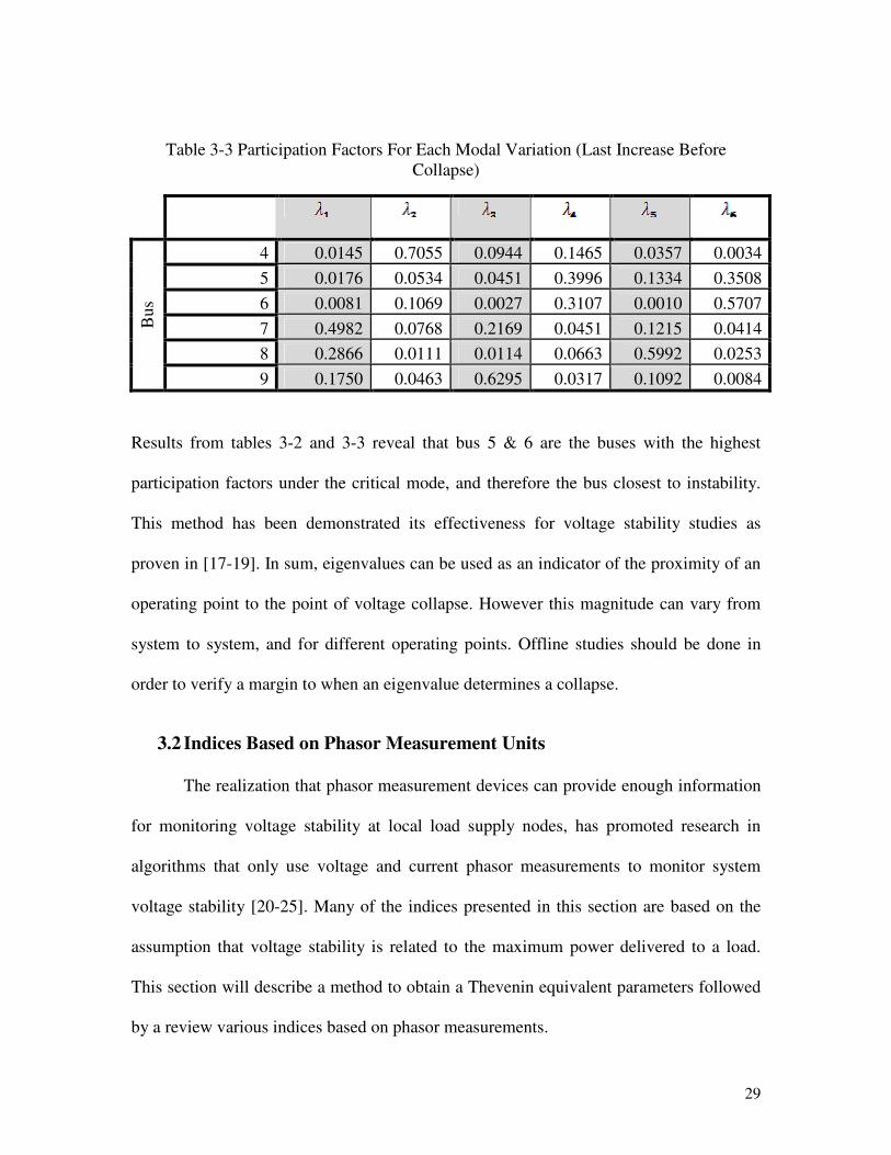
Table 3-3 Participation Factors For Each Modal Variation (Last Increase Before
Collapse).................................................................................................................... 29
Table 4-1 IEEE 39 Bus Parameters- Load and Generation .............................................. 40
Table 4-2: IEEE 39 Bus Parameters- Line Data ............................................................... 41
Table 4-3 IEEE 39 Bus Parameters- Generator Data........................................................ 42
Table 4-4 Summary Of Selected Indices .......................................................................... 43
Table 5-1 Load Factor with Corresponding Total System Laod ...................................... 52
Table 5-2: Load Bus VSI for Various Load Factors......................................................... 53
Table 5-3 Load Bus VCPI for Various Load Factors ....................................................... 54
Table 5-4 Load Bus Voltages, Case 1............................................................................... 56
Table 5-5 Load Bus VSI for Case 2.................................................................................. 62
Table 5-6 Load Bus VSI for case 2(Cont.) ...................................................................... 62
Table 5-7 Load Bus VCPI for Case 2 ............................................................................... 63
Table 5-8 Load Bus VCPI for Case 2 (cont.).................................................................... 63
Table 5-9 Indices before collapse: Case 1 and 2............................................................... 65
Table 5-10 Before and After Line Tripped ....................................................................... 69
Table 5-11 Load Bus Indices for Case 3, before and after collapse ................................. 71
Table 5-12 Power Flow and Line Losses: Before and After Line Trip ............................ 72

x
Table 5-13 Generation and Loads before and after Line Trip .......................................... 73
Table 5-14 Line Losses Before and After Line Trip......................................................... 75
Table 5-15 Comparison Of Rankings Between Various Methods: First Load Increase... 80
Table 5-16 Comparison Of Rankings Between Various Methods: Final Load Increase.. 81
xi
LIST OF FIGURES
Figure Page
Figure 2.1 Power System Stability Classifications [8] ....................................................... 5
Figure 2.2 Two Bus System.............................................................................................. 13
Figure 2.3 PV curves for corresponding power factors: (1) φ=45° lagging, (2) φ=30°
lagging, (3) φ=0, (4) φ=30° leading .......................................................................... 14
Figure 2.4 QV curves for various load levels. [13]........................................................... 15
Figure 2.5 Convention for Synchrophasor Representation [14] ....................................... 19
Figure 2.6 Two-bus Pi-Model Equivalent ........................................................................ 20
Figure 3.1WSCC 9 Bus System........................................................................................ 26
Figure 3.2 Three Lowest Eigenvalues Under System Load Changes............................... 28
Figure 3.3 Thevenin Equivalent with coupling and open circuit voltage ......................... 31
Figure 3.4 Simplified Thevenin Network ......................................................................... 32
Figure 4.1 BPA 10 bus Test System ................................................................................. 38
Figure 4.2 IEEE 39-Bus Test System ............................................................................... 39
Figure 5.1 Algorithm for Computing VCPI...................................................................... 48
Figure 5.2 Algorithm for Computing VSI ........................................................................ 49
Figure 5.3 VSI for 10-bus system..................................................................................... 50
Figure 5.4 VCPI for 10-bus system .................................................................................. 51
Figure 5.5 VSI for Load Buses 4, 7, 8, 20 ........................................................................ 55
Figure 5.6 VCPI for Load Buses 4, 7, 8, 20...................................................................... 55
Figure 5.7 Load Buses with respect to nearest generation units....................................... 57
Figure 5.8 VSI and Their Respected Bus Voltages .......................................................... 59
xii
Figure 5.9 VCPI and Their Respected Bus Voltages........................................................ 59
Figure 5.10 VSIs for Case 2: Bus 4, 20, and 27................................................................ 61
Figure 5.11 VCPIs for Case 2: Bus 4, 20, and 27............................................................ 61
Figure 5.12 VCPI vs. Apparent Power Margin for Case 1 and 2 ..................................... 66
Figure 5.13 VSI vs. Apparent Power Margin for Case 1 and 2 ........................................ 67
Figure 5.14 Line 10-13 Trip.............................................................................................. 68
Figure 5.15 VSIs for Case 3: Bus 4, 6, 8, 12 and Global.................................................. 70
Figure 5.16 VCPIs for Case 3: Bus 4, 6, 8, 12 and Global ............................................... 70
Figure 5.17 Case 4 Area of Interest .................................................................................. 76
Figure 5.18 Bus 18 VSI for various Wind Generation output .......................................... 77
Figure 5.19 Bus 18 VCPI for various Wind Generation output ....................................... 78
1
CHAPTER 1
INTRODUCTION
1.1 Introduction
As a result of recent increases in demand for electric power, utility transmission
systems have been forced to operate under stressful conditions, often close to instability
limits. Efforts to construct new transmission lines or enlarge networks are limited due to
economic and environmental constraints. According to U.S. Department of Energy, since
1982, the growth in peak demand for electricity has exceeded transmission growth by
almost 25% every year. The deregulation of electricity market has resulted in increased
bulk power across interconnected systems. In some utilities, the amount of transactions
previously purchased in a year is now managed in one day [1]. Operating power systems
under such conditions along with inadequate reactive power reserves initiates a sequence
of voltage instability points and can ultimately lead to a system voltage collapse.
Special attention is being paid to determine methods for assessing voltage
stability in real time and developing strategies to mitigate instability issues once they
have been detected. Synchronized phasor measurement technology, which is already
available at most substation location through protection relays for instance, is capable of
directly measuring power system variables (voltage and current phasors) in real time,
synchronized to within a millisecond. Together with the improvements on high-speed
communication infrastructures, it is possible to build wide area measurement and
protection systems [2] to complement classic protection, supervisory control and data
acquisition (SCADA), Energy Management Systems (EMS) applications and to
2
prevent cascading system level outages. With this new direction on wide area
measurement systems, come new approaches for wide area protection and control
functions including generating indices for voltage collapse prevention. There are many
studies on voltage stability indices including those based on phasor measurements. Some
comparisons between these different indices can be found in the literature, such as [3-6]
1.2 Thesis Objectives
The main objective of this thesis is to investigate the voltage stability
phenomenon using indices based on simulated synchrophasor data. The analysis will
consider proximity to voltage collapse: “How close is the system to voltage instability?”
and mechanism of voltage instability: “What are the voltage-weak areas?”
In consideration of these questions, this thesis will begin with a discussion on
conventional and newer voltage stability methods presented in literature. Next, an
analysis and comparison of two indices based on synchrophasor data using static analysis
will be conducted and discussed. Various cases, such as increasing system
load/generation and/or N-1 contingency will be created to demonstrate the application of
indices in voltage stability analysis. Results will reveal their overall effectiveness in its
application to the voltage stability problem. An application of these analyses is then
briefly discussed in an investigation on the impact of wind generation on voltage stability
considering the intermittent nature of wind generation and penetration level. The studied
indices will be used in a case where a modeled wind farm is placed on a bus. Indices will
be generated for various test cases. Lastly, an analysis will be conducted to demonstrate
their significance in the voltage stability problem. Studies and analysis will employ use

3
of PowerWorld Software for load flow simulation and Matlab as a post processor tool to
calculate indices.
1.3 Thesis organization
Chapter 1 introduces the motivation and purpose of this thesis. A survey of
literature on the topic of voltage stability indices is briefly discussed and identified. An
aim and an appropriate research method are formulated.
Chapter 2 presents the theoretical concepts of voltage stability. A basic overview
on power system stability is given before dedicating the remainder of the chapter to
explaining voltage stability and methods to analyze the phenomenon.
Chapter 3 explains various indices proposed in literature and their methods used
to evaluate the voltage stability of power systems.
Chapter 4 provides a detailed description of two different test networks. The
methodology to demonstrate the predictive ability of two indices are formulated
In Chapter 5, the indices chosen are applied according to the methodology from
Chapter 4. The results are analyzed and discussed to verify the proposed indices on their
applicability to determine voltage stability.
Concluding the thesis will be chapter 6. A review of the results and its
implications are stated with recommendations for future work.

4
CHAPTER 2
VOLTAGE STABILITY OVERVIEW
An overview on power system stability which is based on [7] will be given to
provide a global perspective before voltage stability is defined.
2.1 Power System Stability
Power system stability is the ability of an electric power system, for a given initial
operating condition, to regain a state of operating equilibrium after being subjected to a
physical disturbance, with most system variables bounded so that the system remains
intact. Due to the various types of disturbances introduced, power system stability can be
further classified into appropriate categories: Rotor angle, frequency, and voltage
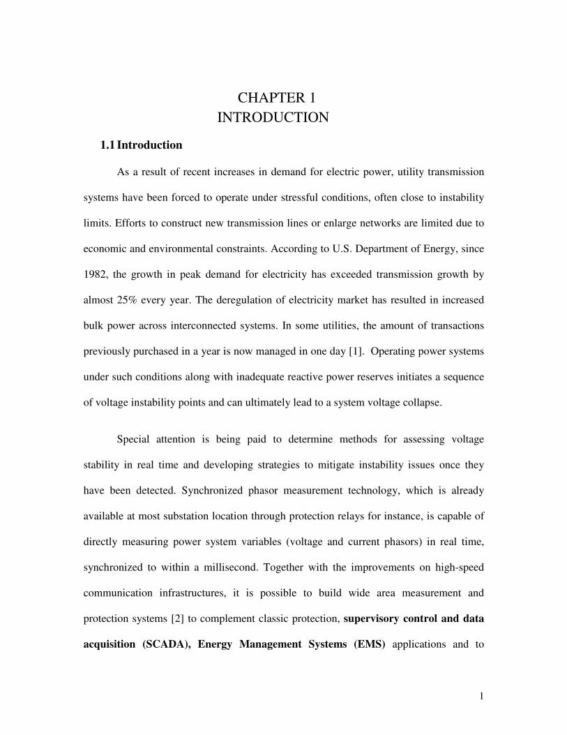
stability. These system variables are categorized, as shown in figure 2.1, based on
disturbance magnitude and time response. In any given situation, one form of instability
can possibly lead to another form. However, distinguishing between different forms can
provide convenience in identifying the underlying causes of instability, applying an
appropriate analysis and ultimately taking corrective measures to return the system to a
stable operating point.
5
Figure 2.1 Power System Stability Classifications [8]
2.1.1. Rotor Angle stability The rotor angle stability is defined as the ability of interconnected synchronous
machines to remain in synchronism under normal operating conditions and after being
subjected to a disturbance. In general, the total active electrical power fed by the
generators must always be equal to the active power consumed by the loads; this includes
also the losses in the system. This balance between the load and generation can be
associated to the balance between the generator input, or mechanical torque, and the
generator output, or electrical torque. A disturbance to the system can upset this
equilibrium, which results in the acceleration or deceleration of the rotors of the
generators. If one generator temporarily runs faster than another, the angular position of
its rotor relative to that of the slower machine will increase. The resulting angular
difference transfers a part of the load from the slow machine to the fast machine,
depending on the theoretically known power angle relationship. This tends to reduce the

6
speed difference and hence the angular separation. A further increase in angular
separation results in a decrease in power transfer, which can lead to further instability.
2.1.2. Frequency stability Frequency stability refers to the ability of a power system to maintain steady
frequency following a severe system upset, resulting in a significant imbalance between
generation and load. It depends on the ability to maintain or restore equilibrium between
system generation and load, with minimum unintentional loss of load. Instability that may
result occurs in the form of sustained frequency swings. A typical cause for frequency
instability is the loss of generation causing the overall system frequency to drop.
Generally, frequency stability problems are associated with inadequacies in equipment
responses, poor coordination of control and protection equipment, or insufficient
generation reserve.
2.1.3. Voltage Stability
The third power system stability problem is the voltage stability and is elaborated
in section 2.2. Further analyses and the method proposed in the framework of this thesis
are focused only on this last type of power system stability.
2.2 Voltage Stability
Voltage stability is a subset of overall power system stability. It refers to the
ability of a power system to maintain steady voltages at all buses in the system after
being subjected to a disturbance from a given initial operating condition.
The voltage stability definitions according to [8] are as follows:
7
A power system at a given operating point is small-disturbance voltage
stable if, after a small disturbance, voltages near loads are similar or identical to
pre-disturbance values.
A power system at a given operating point and subject to a given
disturbance is voltage stable if voltages near loads approach post disturbance
equilibrium values.
A power system at a given operating point and subject to a given
disturbance undergoes voltage collapse if post-disturbance equilibrium voltages
are below acceptable limits. Voltage collapse may be system wide or partial.
The main factor contributing to voltage instability is usually the voltage drop that
occurs when real and reactive power flow through inductive reactance’s associated with
the transmission network; as the line currents during various power flow conditions
increase, the reactive losses increase. When reactive losses increase, the voltage
magnitude decreases. Therefore, as the real power flow increases the voltage magnitudes
tend to decrease. There is a point that the system can no longer support the real power
flow on the lines and maintain a stable voltage. Thusly the voltage collapses.
2.2.1. Classifications As previously mentioned, voltage stability can be classified according to the type
of disturbance or to time frame. Small disturbance voltage stability is concerned with a
system’s ability to control voltages following small perturbations such as incremental
changes in system load. This form of stability is determined by the characteristics of
loads, continuous controls, and discrete controls at a given instant of time.

8
Large disturbance voltage stability is concerned with a system’s ability to control
voltages following large disturbances such as system faults, loss of generation, or circuit
contingencies. This ability is determined by the system-load characteristics and the
interactions of both continuous and discrete controls and protections.
In short-term (transient) voltage stability the time frame ranges from zero to ten
seconds and involves dynamics of fast acting load components such as induction motors,
electronically controlled loads, and HVDC converters. Long term transients on the other
hand, correspond to stabilizing elements. This includes load tap changers, voltage
regulators, and compensators and their responses to the system changes and the new
system conditions. While stabilizing the system, if these elements exceed their operating
limits, they will be removed from system operation. This will then drive the system to
more severe operating conditions that are uncontrollable. This particular time period may
extend to several or many minutes.
In summary, in any given situation, each form of stability are closely associated
with one another, and thus one form of instability can possibly lead to another form.
Distinguishing between these different forms can provide convenience in identifying the
underlying causes of instability, applying an appropriate analysis and ultimately, taking
corrective measures to return the system to a stable operating point. With this in mind,
the following section will provide an overview on the existing methods used to analyze
voltage stability.
2.3 Voltage Stability Limitations
Various system aspects may cause voltage instability. Amongst the most
important aspects are generators, transmission lines, and loads. [9]
9
Generators play an important role for providing adequate reactive power support
for power systems. Reactive power is produced by generators and therefore limited by the
current rating of the field and armature windings. Since there are levels to how much
current or heat the exciter winding can take before the winding becomes damaged, the
maximum reactive power output is set using an over excitation limiter (OXL). When the
OXL hits the limit, the terminal voltage is no longer maintained constant. Therefore the
power transfer limit is further limited, resulting in long-term voltage instability.
Transmission networks are other important constraints for voltage stability. Under
a deregulation environment where bulk power is transferred across long distances, the
maximum deliverable power is limited by the transmission system characteristics. Power
beyond the transmission capacity determined by thermal or stability considerations
cannot be delivered.
The third major factor that influences voltage instability is system loads. Voltage
instability is load driven. Following a change in the demand, the load will at first change
according to its instantaneous characteristic such as, constant impedance or current. It
will then adjust the current drawn from the system until the load supplied by the system
satisfies the demand at the final system voltage. Similarly when there is a sudden change
in system voltage, such as, following a disturbance, the load will change momentarily. It
will then adjust the current and draw from the system, whatever current is necessary in
order to satisfy the demand. [10]
Another important load aspect is the Load Tap Changing (LTC) transformer,
which is one of the key mechanisms in load restoration. In response to a disturbance, the
LTC tends to maintain constant voltage level at the low voltage end. Therefore, load

10
behavior observed at high voltage level is close to constant power, which may aggravate
voltage instability problems.
2.3.1. Voltage Collapse Incidents Many voltage instability incidents have occurred around the world. Table 2-1
groups several known incidents and their time frame.
Table 2-1 Voltage Collapse Incidents [8]
Date Location Time Frame
1-Dec-87 Western France 4-6 minutes
22-Aug-87 Western Tennessee 10 seconds
23-Jul-87 Tokyo, Japan 20 minutes
30-Nov-86 SE Brazil, Paraguay 2 seconds
27-Dec-83 Sweden 55 seconds
30-Dec-82 Florida 1-3 minutes
4-Aug-82 Belgium 4.5 minutes
19-Dec-78 France 26 minutes
22-Aug-70 Japan 30 minutes
From table 2-1 voltage collapse incidents dynamics span can range from seconds to as
long as tens of minutes. Since the voltage instability issue started to emerge, research
efforts from the power engineering community have been dedicated to studying the
voltage instability mechanism and to developing analysis tools and control schemes to
mitigate the instability.

11
2.4 Voltage Stability Analysis
In large complex meshed networks, power-flow analysis is commonly used. In
this section an introduction to power-flow, or load flow, analysis and its application to
voltage stability will be given in order to understand the voltage stability indices exposed
in the next chapter.
2.4.1. Power-Flow Analysis [11]
For load flow studies, a balanced three-phase steady-state system is assumed, and
thus positive sequence networks are only used. There are four variables associated with
each bus in a system: voltage magnitude, phase angle, net real power, and reactive power
supplied to each bus. At each bus two of these variables are specified. Each bus is further
categorized into one of the following bus types:
1. Swing bus – There is only one swing bus which serves as a reference bus for
which , typically per unit, is the input data.
2. Load bus – P and Q are the input data. V and δ are computed
3. Voltage controlled bus – P and V are input data. Q and δ are computed.
The network equations in terms of the bus admittance matrix can be written as follows:
(2.1)
Where
n is the total number of buses.
is the self admittance at node i.
12
is the mutual admittance between buses.
is the phasor voltage to ground at bus i.
is the phasor current at bus i.
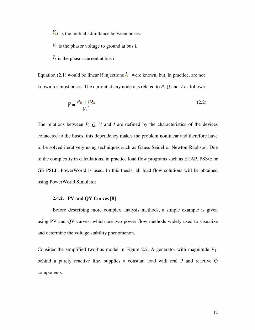
Equation (2.1) would be linear if injections were known, but, in practice, are not
known for most buses. The current at any node k is related to P, Q and V as follows:
(2.2)
The relations between P, Q, V and I are defined by the characteristics of the devices
connected to the buses, this dependency makes the problem nonlinear and therefore have
to be solved iteratively using techniques such as Gauss-Seidel or Newton-Raphson. Due
to the complexity in calculations, in practice load flow programs such as ETAP, PSS/E or
GE PSLF, PowerWorld is used. In this thesis, all load flow solutions will be obtained
using PowerWorld Simulator.
2.4.2. PV and QV Curves [8]
Before describing more complex analysis methods, a simple example is given
using PV and QV curves, which are two power flow methods widely used to visualize
and determine the voltage stability phenomenon.
Consider the simplified two-bus model in Figure 2.2. A generator with magnitude V1,
behind a purely reactive line, supplies a constant load with real P and reactive Q
components.
13
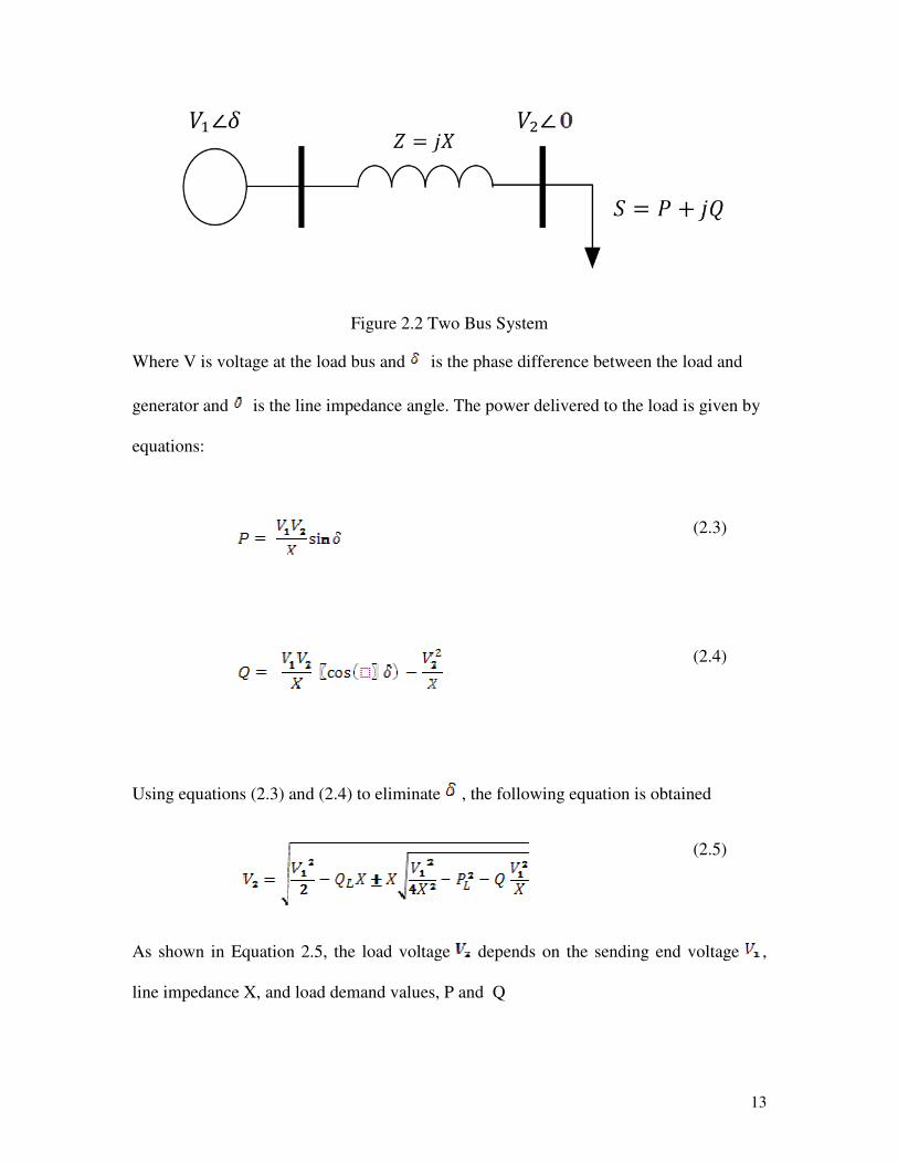
Figure 2.2 Two Bus System
Where V is voltage at the load bus and is the phase difference between the load and
generator and is the line impedance angle. The power delivered to the load is given by
equations:
(2.3)
(2.4)
Using equations (2.3) and (2.4) to eliminate , the following equation is obtained
(2.5)
As shown in Equation 2.5, the load voltage depends on the sending end voltage ,
line impedance X, and load demand values, P and Q

14
The solutions of (2.5) with respect to load voltage V for different power factors
(Q=P(tanφ)) are shown in figure 2.3
Figure 2.3 PV curves for corresponding power factors: (1) φ=45° lagging, (2) φ=30°
lagging, (3) φ=0, (4) φ=30° leading
For each PV curve there are two equilibrium points, one at high voltage and therefore low
current, and the other at low voltage at high current. In practice the high voltage
equilibrium is the more stable and the equilibrium at which a power system operates. The
tip of the curve represents that maximum power delivered. At leading power factors the
maximum power is higher. Using this method, changes in voltage with respect to power
can be observed. The plots can serve as a visual on how far the bus is from instability
[12]; however there are several disadvantages of this method. Typically power flow can
only compute the upper part of the curve up to maximum loading point, beyond this
point, the load flow will diverge because it cannot find a solution.
Now, considering the same circuit in figure 2.2, QV curves can be plotted for the
load bus. QV curves represent a plot of reactive power versus voltage for a particular bus.

15
In order to create a QV curve, a constant real power load is assumed and a fictitious
synchronous condenser with infinite reactive capability is placed on the test bus. The
voltage of the synchronous condenser is then varied, and the VAR output is allowed to be
any value to meet the scheduled voltage. Reactive power demand is plotted for various
voltage schedules as shown in figure 2.4.
Figure 2.4 QV curves for various load levels. [13]
From figure 2.4, the x-intercept of the curve on the positive slope represents the base case
operating point. Tracing downward along the curve represents an increase in MVAR load
along with a corresponding decrease in voltage. The positive slope of the QV curve,
where dQ/dV > 0,is the stable region and the negative slope of the QV curve where
dQ/dV < 0, is the unstable region. The bottom of the curve where dQ/dV = 0 shows the
minimum reactive power required for stable operation, as well as the minimum voltage
that the bus can withstand. Curve 1 shows a positive reactive margin, and thus is more
robust in terms of voltage stability. Curve 2 has little or no margin, and is therefore
16
marginally stable. Any further increase in demand will result in voltage collapse. Curve
3, has no x-intercept, has a negative margin and therefore the system has collapsed. As a
result the system will require additional MVAR support in order to come out of the
collapse.
This method is useful as it provides the reactive power margin with respect to
reactive power injections at the test bus. In conjunction to PV-curves, these two methods
are useful for studying voltage stability for small networks, especially radial systems.
However, it is not efficient for large meshed systems since it requires extensive
computation and may contain more than one critical bus to be analyzed.
2.4.3. Voltage
Voltage is probably the most intuitive index for quantifying voltage stability.
Monitoring voltage magnitudes have been a widely accepted index to initialize remedial
actions such as undervoltage load shedding schemes in order to prevent voltage collapse.
Typically, a voltage margin is set between 85%-90% of the nominal voltage. At this point
a designated relay will trip, or dispatchers can act accordingly to drop a load in order to
prevent voltage collapse.
The limitation of the voltage-based index is that it cannot quantify the distance to
the voltage marginally stable point. The bus with the lowest voltage is not necessarily the
one closest to the voltage collapse point. As shown in figure 2.3 - curve 4, a load bus with
high reactive power compensation may not show any significant low voltage problems
even if the power transfer is close to the system transmission limit and the system is close
to the voltage marginally stable point.

17
2.4.4. Analysis Methods
Methods for analysis voltage stability can by classified into two separate
categories: Dynamic analysis or Static analysis. Each method is specific in addressing
particular problems and has its advantages and disadvantages.
Dynamic analysis can provide information on system performance with respect to
time usually ranging from seconds to several minutes. Using dynamic simulations,
analyses can be conducted on coordination of equipment where time frames are
overlapping; e.g. generator controls, switched capacitor banks and undervoltage load
shedding. Dynamic simulations have also proven useful for presenting the system
performance during the final stages of collapse such as motor stalling, changes in load,
and recovery resulting in voltage collapse or stability respectively. This extra dimension
of time adds another layer of complexity in the representation of the system. Each piece
of equipment requires detailed set of parameters and equations, and for large systems
requires extensive computing power in order to cope with the nonlinearities and
switching events.
On the other hand static analyses are often adequate in addressing the slower
forms of voltage stability. Indices can be also generated which define areas prone to
voltage instability and indicate elements, which are important in the instability
phenomenon. These methods are often computationally less intensive, which makes it
suitable for online, and offline applications.
18
2.5 Synchrophasors
As the improvement of the transmission network becomes more complex, the
need for faster clearing times, pilot protection schemes and more wide-area protection
and control systems to ensure that these lines are being most utilized, has increased.
Protection and control systems must adapt to constant changes in the network. The
variability on both the supply and demand side increases the importance of having wide-
area protection, control and monitoring systems that are secure, reliable, and simple as
possible. At the heart of these new wide-area systems are time synchronized phasor data
known as synchrophasors. Phasor representation of sinusoidal signals is commonly used
in ac power system analysis. The sinusoidal waveform defined in equation (2.5):
(2.5)
The synchrophasor representation X of a signal x(t) is the complex value given by:
(2.6)
Where the magnitude is the root-mean-square (rms) value, Xm /√2, of the waveform, and
the subscripts r and i signify real and imaginary parts of a complex value in rectangular
components.

19
Figure 2.5 Convention for Synchrophasor Representation [14]
In power systems it is common to represent X in phasor notation: . The
phase angle φ depends on the time scale, particularly where t = 0. It is important to note
this phasor is defined for the angular frequency ω given by where is the
frequency. The representation of a synchrophasor is shown in figure 2.5. IEEE Standard
C37.118.1 defines synchrophasors as precise time-synchronized measurements of certain
parameters on the electricity grid from phasor measurement units (PMUs). PMUs
measure voltage, current and frequency and calculate phasors, and this group of time
synchronized grid condition data is called phasor data. Each phasor measurement is time
stamped against Global Positioning System universal time. This allows measurements
taken by PMUs in different locations or by different owners, to be transmitted over
standard communication systems including Ethernet, phone modem, or just an EIA-232
cable from the PMU, then to be synchronized to a computer at each end of the line [15].
20
Now that these values are available from devices on the power system, the
question is how to make it available to use this value. One example is using the
synchrophasors to define an accurate system model [15]. System models are useful to a
system operators and operations engineers as they can provide insight to how power is
directed when the network topology is subject to changes. Changes that maybe beneficial
to an economic standpoint, such as importing bulk power across line, can be undesirable
from a stability standpoint, such as loading the line to its maximum ratings. By having an
accurate model of the system, both security and economic factors can be optimized.
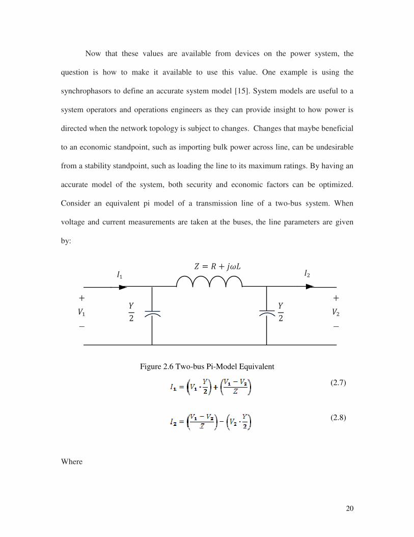
Consider an equivalent pi model of a transmission line of a two-bus system. When
voltage and current measurements are taken at the buses, the line parameters are given
by:
Figure 2.6 Two-bus Pi-Model Equivalent
(2.7)
(2.8)
Where
21
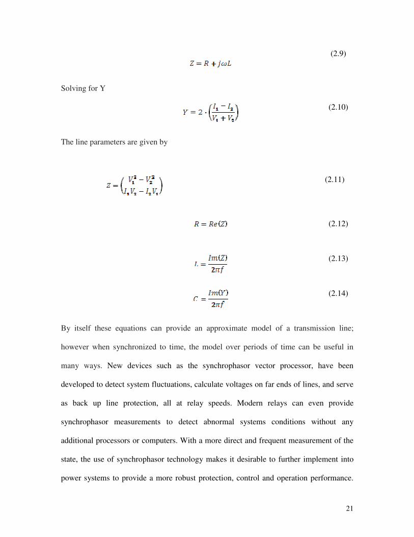
(2.9)
Solving for Y
(2.10)
The line parameters are given by
(2.11)
(2.12)
(2.13)
(2.14)
By itself these equations can provide an approximate model of a transmission line;
however when synchronized to time, the model over periods of time can be useful in
many ways. New devices such as the synchrophasor vector processor, have been
developed to detect system fluctuations, calculate voltages on far ends of lines, and serve
as back up line protection, all at relay speeds. Modern relays can even provide
synchrophasor measurements to detect abnormal systems conditions without any
additional processors or computers. With a more direct and frequent measurement of the
state, the use of synchrophasor technology makes it desirable to further implement into
power systems to provide a more robust protection, control and operation performance.
22
For the most part, this thesis will focus on using the steady state measurements, and
individual snapshots in time, to generate an analysis. Since actual synchrophasor data are
continuous measurements, a continuous analysis can be conducted using a simple
microprocessor to compute and process the information on a real time basis.
23
CHAPTER 3
EVALUATION OF VOLTAGE STABILITY INDICES
In voltage stability studies, it is crucial to have an accurate knowledge of how
close a power system’s operating point is from the voltage stability limit. It has been
observed that voltage magnitudes alone, do not give a good indication of proximity to
voltage stability limit. Therefore, it is useful to assess voltage stability of a power system
by means of a voltage stability index (VSI), a scalar magnitude that can be monitored as
system parameters change. These indices should be capable of providing reliable
information about the proximity of voltage instability in a power system and should
reflect the robustness of a system to withstand outages or load increase. Likewise, these
indices should be computationally efficient and easy to understand. Therefore operators
can use these indices to know how close the system is to voltage collapse in an intuitive
manner and react accordingly. This section will provide an overview on various indices
proposed in literature. Their characteristics and classifications will be reviewed in their
application to analyze voltage stability.
3.1 Index from Load Flow Jacobian
3.1.1. Modal Analysis of Power Flow Model
Gao, Morison and Kundur [16] introduce an index based on the Jacobian matrix using
modal analysis techniques. The Jacobian matrix equation (3.1) is obtained through load
flow solutions for a system operating under stable conditions. Given the fact that the
system voltage is affected by both changes in real and reactive power, the Jacobian is

24
useful as it can provide information on voltage stability.
(3.1)
(3.2)
By letting a linearized relationship between the incremental changes in bus
voltage and bus reactive power injection can be represented by equation (3.3)
(3.3)
Where is the reduced jacobian and given by
(3.4)
The modes of the system can be defined by the eigenvalues and eignvectors of
Assume
(3.5)
Where is the right eigenvector matrix of is the diagonal eigenvalue matrix
of ; is the left eigenvector matrix of . Then
(3.6)
Incremental changes in reactive power and voltage are related by equation 3.3.
Substituting equation 3.5, then
25
(3.7)
Or
(3.8)
Where is the ith eigenvalue, is the ith column right eigenvector, and is the ith row
left eigenvector. Therefore the ith modal reactive power variation is
(3.9)
Where is a normalization factor such that
(3.10)
The ith modal variation can be written
(3.11)
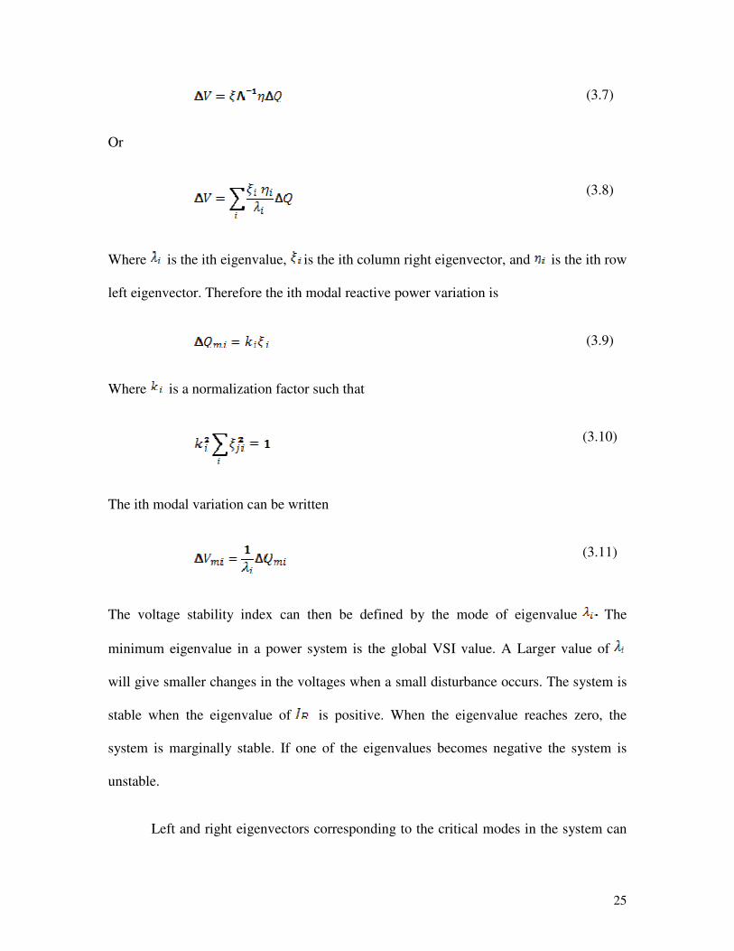
The voltage stability index can then be defined by the mode of eigenvalue The
minimum eigenvalue in a power system is the global VSI value. A Larger value of
will give smaller changes in the voltages when a small disturbance occurs. The system is
stable when the eigenvalue of is positive. When the eigenvalue reaches zero, the
system is marginally stable. If one of the eigenvalues becomes negative the system is
unstable.
Left and right eigenvectors corresponding to the critical modes in the system can
26
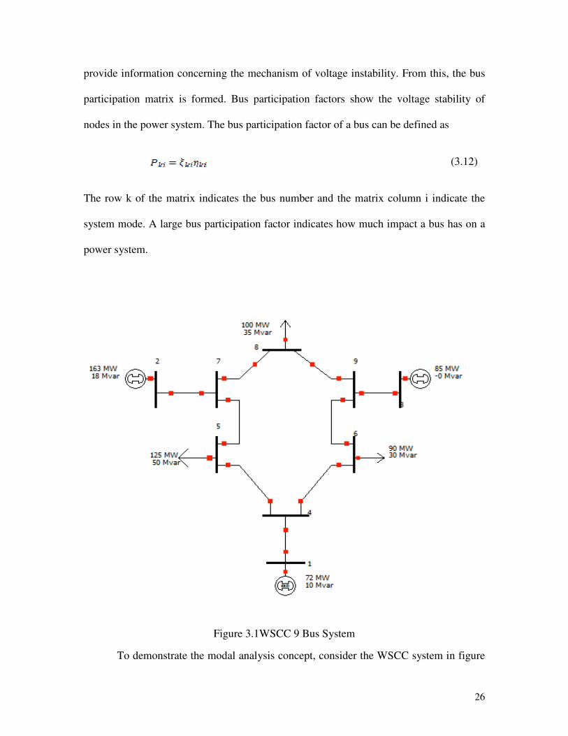
provide information concerning the mechanism of voltage instability. From this, the bus
participation matrix is formed. Bus participation factors show the voltage stability of
nodes in the power system. The bus participation factor of a bus can be defined as
(3.12)
The row k of the matrix indicates the bus number and the matrix column i indicate the
system mode. A large bus participation factor indicates how much impact a bus has on a
power system.
Figure 3.1WSCC 9 Bus System
To demonstrate the modal analysis concept, consider the WSCC system in figure
27
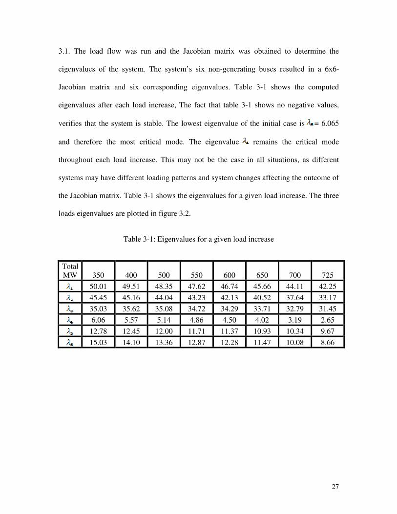
3.1. The load flow was run and the Jacobian matrix was obtained to determine the
eigenvalues of the system. The system’s six non-generating buses resulted in a 6x6-
Jacobian matrix and six corresponding eigenvalues. Table 3-1 shows the computed
eigenvalues after each load increase, The fact that table 3-1 shows no negative values,
verifies that the system is stable. The lowest eigenvalue of the initial case is = 6.065
and therefore the most critical mode. The eigenvalue remains the critical mode
throughout each load increase. This may not be the case in all situations, as different
systems may have different loading patterns and system changes affecting the outcome of
the Jacobian matrix. Table 3-1 shows the eigenvalues for a given load increase. The three
loads eigenvalues are plotted in figure 3.2.
Table 3-1: Eigenvalues for a given load increase
Total
MW 350 400 500 550 600 650 700 725
50.01 49.51 48.35 47.62 46.74 45.66 44.11 42.25
45.45 45.16 44.04 43.23 42.13 40.52 37.64 33.17
35.03 35.62 35.08 34.72 34.29 33.71 32.79 31.45
6.06 5.57 5.14 4.86 4.50 4.02 3.19 2.65
12.78 12.45 12.00 11.71 11.37 10.93 10.34 9.67
15.03 14.10 13.36 12.87 12.28 11.47 10.08 8.66

28
Figure 3.2 Three Lowest Eigenvalues Under System Load Changes.
The participation factor P of each bus for a given modal variation, for the first and last
load increases are shown in table 3-2.
Table 3-2 Participation Factors For Each Modal Variation (Initial Conditions)
4 0.391 0.399 0.002 0.129 0.070 0.009
5 0.101 0.022 0.040 0.280 0.027 0.530
6 0.063 0.034 0.052 0.289 0.223 0.338
7 0.233 0.282 0.241 0.084 0.146 0.013
8 0.129 0.200 0.011 0.147 0.487 0.025
Bus
9 0.082 0.062 0.654 0.070 0.046 0.085
29
Table 3-3 Participation Factors For Each Modal Variation (Last Increase Before
Collapse)
4 0.0145 0.7055 0.0944 0.1465 0.0357 0.0034
5 0.0176 0.0534 0.0451 0.3996 0.1334 0.3508
6 0.0081 0.1069 0.0027 0.3107 0.0010 0.5707
7 0.4982 0.0768 0.2169 0.0451 0.1215 0.0414
8 0.2866 0.0111 0.0114 0.0663 0.5992 0.0253
Bus
9 0.1750 0.0463 0.6295 0.0317 0.1092 0.0084
Results from tables 3-2 and 3-3 reveal that bus 5 & 6 are the buses with the highest
participation factors under the critical mode, and therefore the bus closest to instability.
This method has been demonstrated its effectiveness for voltage stability studies as
proven in [17-19]. In sum, eigenvalues can be used as an indicator of the proximity of an
operating point to the point of voltage collapse. However this magnitude can vary from
system to system, and for different operating points. Offline studies should be done in
order to verify a margin to when an eigenvalue determines a collapse.
3.2 Indices Based on Phasor Measurement Units
The realization that phasor measurement devices can provide enough information
for monitoring voltage stability at local load supply nodes, has promoted research in
algorithms that only use voltage and current phasor measurements to monitor system
voltage stability [20-25]. Many of the indices presented in this section are based on the
assumption that voltage stability is related to the maximum power delivered to a load.
This section will describe a method to obtain a Thevenin equivalent parameters followed
by a review various indices based on phasor measurements.

30
3.2.1. Algorithm for Equating Thevenin Equivalent Parameters [26-27]
The buses in a power system can be classified into three categories: load bus, tie bus, and
generator bus. A bus with a load attached to it is considered a load bus. A tie bus refers to
a bus with no load or any generation device attached. A generator bus includes a bus
whose voltage is regulated by an attached generator, as well as a boundary bus, which is
modeled by PV bus. A generator bus becomes a load bus if its attached generator reaches
its reactive power limit. The injection currents into the system can be written as
(3.13)
Where the Y matrix is known as the system admittance matrix, V and I stand for the
voltage and current vectors. The elements of the admittance matrix with the
corresponding voltages can be reorganized into the three types of buses can be expressed
as
(3.14)
The subscripts L, T and G represent load bus, tie bus and generator bus, respectively.
The load voltage can be expressed by
(3.15)
Where
(3.16)

31
(3.17)
(3.18)
The term represents the open-circuit voltage and is the self-impedance at the
jth load bus. Considering the effect of the other loads, equation (3.19) introduces a
coupling voltage term which is related to the mutual-impedance and written as.
(3.19)
The coupling term is then combined with the open-circuit voltage term to form the
equivalent voltage as shown in figure 3.3.
Figure 3.3 Thevenin Equivalent with coupling and open circuit voltage
Thus, the Thevenin parameters expressed by

32
(3.20)
Where M is the number of source buses and N is the number of load buses and
(3.21)
Figure 3.3 can then be redrawn as shown on figure 3.4
Figure 3.4 Simplified Thevenin Network
From equations (3.20-3.21) the following observations can be made: The equivalent
voltage source, Veq, is a function of the true voltage sources and other system loads and
thus Veq decreases as other system loads increase. The equivalent impedance, Zequ, only
depends on the system topology and line characteristics. To a power system with a fixed
topology, the equivalent impedance remains constant.
3.2.2. Line Stability Index
An index based on the power flow concept of a two bus equivalent network has
been introduced by Moghavvemi in [28]. The index predicts the stability of a line
between two buses and is given by equation (3.22)
(3.22)
33
Based on the value of the indices of lines, voltage collapse can be predicted. As long as
the stability index remains less than 1, the system is stable. When the index becomes
greater than one, the whole system loses its stability and voltage collapse occurs.
Therefore the index can be used in voltage collapse prediction.
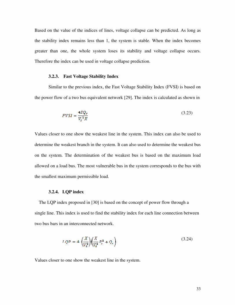
3.2.3. Fast Voltage Stability Index
Similar to the previous index, the Fast Voltage Stability Index (FVSI) is based on
the power flow of a two bus equivalent network [29]. The index is calculated as shown in
(3.23)
Values closer to one show the weakest line in the system. This index can also be used to
determine the weakest branch in the system. It can also used to determine the weakest bus
on the system. The determination of the weakest bus is based on the maximum load
allowed on a load bus. The most vulnerable bus in the system corresponds to the bus with
the smallest maximum permissible load.
3.2.4. LQP index
The LQP index proposed in [30] is based on the concept of power flow through a
single line. This index is used to find the stability index for each line connection between
two bus bars in an interconnected network.
(3.24)
Values closer to one show the weakest line in the system.
34
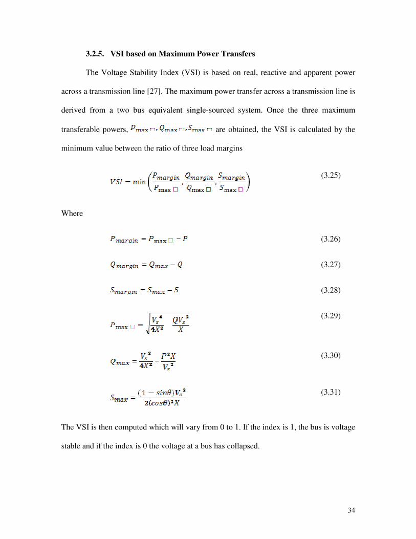
3.2.5. VSI based on Maximum Power Transfers
The Voltage Stability Index (VSI) is based on real, reactive and apparent power
across a transmission line [27]. The maximum power transfer across a transmission line is
derived from a two bus equivalent single-sourced system. Once the three maximum
transferable powers, are obtained, the VSI is calculated by the
minimum value between the ratio of three load margins
(3.25)
Where
(3.26)
(3.27)
(3.28)
(3.29)
(3.30)
(3.31)
The VSI is then computed which will vary from 0 to 1. If the index is 1, the bus is voltage
stable and if the index is 0 the voltage at a bus has collapsed.
35
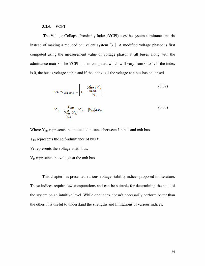
3.2.6. VCPI
The Voltage Collapse Proximity Index (VCPI) uses the system admittance matrix
instead of making a reduced equivalent system [31]. A modified voltage phasor is first
computed using the measurement value of voltage phasor at all buses along with the
admittance matrix. The VCPI is then computed which will vary from 0 to 1. If the index
is 0, the bus is voltage stable and if the index is 1 the voltage at a bus has collapsed.
(3.32)
(3.33)
Where Ykm represents the mutual admittance between kth bus and mth bus.
Ykk represents the self-admittance of bus k.
Vk represents the voltage at kth bus.
Vm represents the voltage at the mth bus
This chapter has presented various voltage stability indices proposed in literature.
These indices require few computations and can be suitable for determining the state of
the system on an intuitive level. While one index doesn’t necessarily perform better than
the other, it is useful to understand the strengths and limitations of various indices.
36
CHAPTER 4
IMPLEMENTATION OF INDICES AND TEST NETWORKS
This chapter will first introduce PowerWorld Simulator and the assumptions used
for the analysis. A detailed description of two test-networks will be presented. Two
indices from chapter 3 will be chosen for analysis. The algorithm used to implement the
indices and test cases will be explained.
4.1 PowerWorld Simulator
The majority of the works presented are based on simulation done in Powerworld
Simulator. PowerWorld is a commercial program used by many utilities in the nation.
The program is capable of analyzing a power system in many ways including area
transaction economic analysis, power transfer distribution factor (PTDF) computation,
short circuit analysis and contingency analysis, and PV/QV analysis. At the core of the
software is a robust load flow solution engine. System models can be implemented
through its drag and drop visual interface or through a common text input.
For this study, the following load flow assumptions are made: The System
frequency is uniform at 60Hz with a 100MVA base. All buses contain PMUs, therefore
the entire system is observable and can output measurements as described in previous
chapters. All generator AVRs regulate at scheduled voltage for all generator bus until the
MVAR capability limit has been reached. Loads are constant power loads, unless
mentioned otherwise. Transmission lines are based on the equivalent Pi-model containing
an equivalent resistance, reactance, and shunt impedance. All lines will assume infinite
37
ampacity; however, ratings will be used for analysis purposes only. Lastly, the voltage
collapse point is assumed to be when the power flow does not converge to a solution.
4.2 Test Systems
This section introduces two test systems to conduct analyses. These systems have
been used broadly in literature to verify different aspects of voltage instability. Initially,
the power flow is solved to verify the validity of the data. The results are compared with
other references available.
4.2.1. BPA 10-Bus System
This 10-bus system was modeled after Bonneville Power Administration (BPA)
[7]. In this system, three generators feed around 6000 MW of load. One load is a constant
power aggregated industrial load and the other is a half constant power, half constant
current aggregated residential load. Generators 1 and 2 feed approximate 5000 MW into
the load area across five 500-kV transmission lines. The receiving end is heavily VAR-
compensated by three shunt capacitor banks.

38
F
igure 4.1 BPA 10 bus Test System
4.2.2. IEEE 39-Bus System
The IEEE 39-Bus power system is based on a 345kV transmission system in New
England Power System as shown on figure 4.2. The system, which is modeled on 100
MVA base, contains 10 machines, 46 lines and 19 Loads. Buses 31 and 39 serve as
boundary buses, which is modeled by an aggregated generator and constant power load,
contains a reduced network equivalent of the neighboring network.

39
Figure 4.2 IEEE 39-Bus Test System
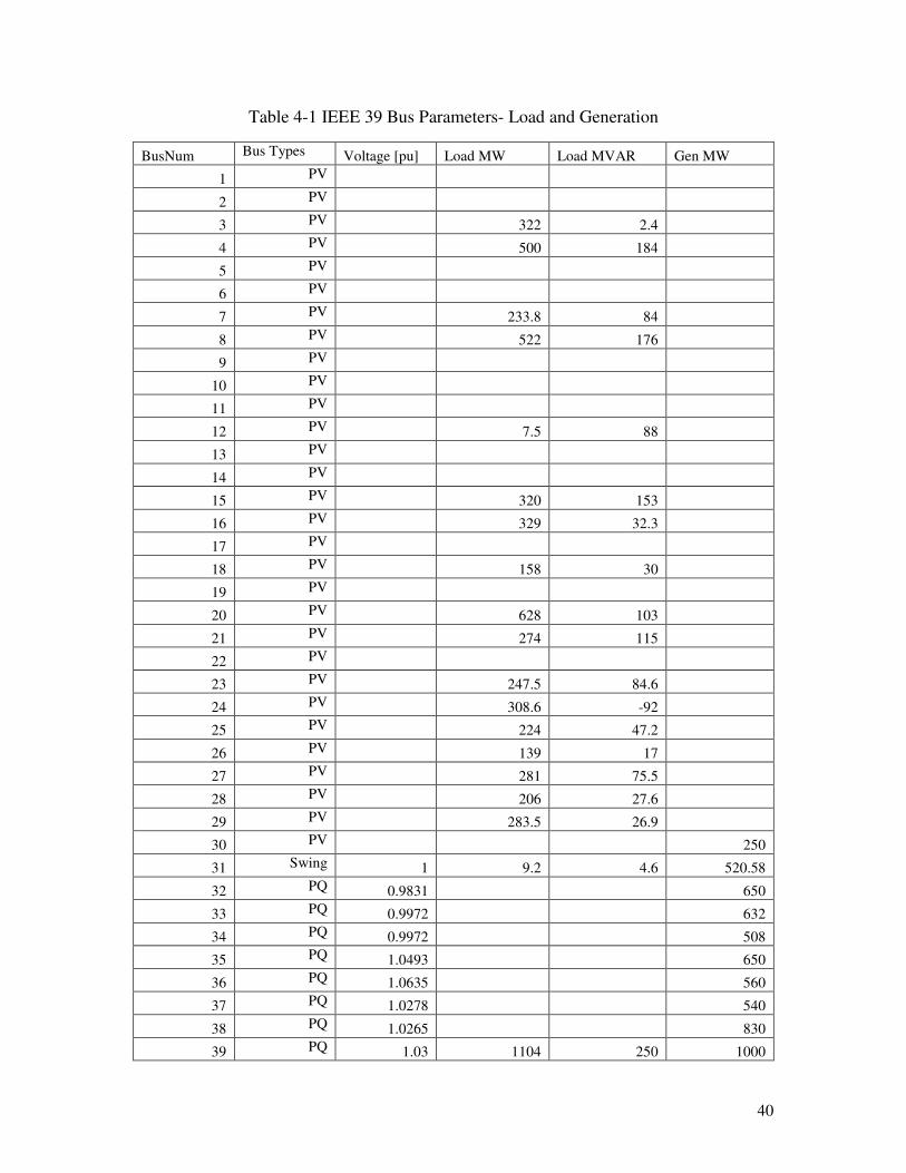
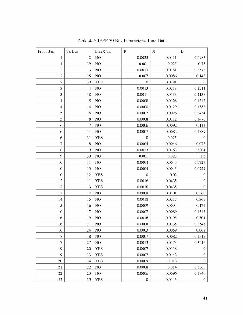
The system base case conditions are given in per unit values, unless specified otherwise
and are shown on tables 4-1,4-2 and 4-3.
40
Table 4-1 IEEE 39 Bus Parameters- Load and Generation
BusNum Bus Types Voltage [pu] Load MW Load MVAR Gen MW
1 PV
2 PV
3 PV 322 2.4
4 PV 500 184
5 PV
6 PV
7 PV 233.8 84
8 PV 522 176
9 PV
10 PV
11 PV
12 PV 7.5 88
13 PV
14 PV
15 PV 320 153
16 PV 329 32.3
17 PV
18 PV 158 30
19 PV
20 PV 628 103
21 PV 274 115
22 PV
23 PV 247.5 84.6
24 PV 308.6 -92
25 PV 224 47.2
26 PV 139 17
27 PV 281 75.5
28 PV 206 27.6
29 PV 283.5 26.9
30 PV 250
31 Swing 1 9.2 4.6 520.58
32 PQ 0.9831 650
33 PQ 0.9972 632
34 PQ 0.9972 508
35 PQ 1.0493 650
36 PQ 1.0635 560
37 PQ 1.0278 540
38 PQ 1.0265 830
39 PQ 1.03 1104 250 1000
41
Table 4-2: IEEE 39 Bus Parameters- Line Data
From Bus To Bus LineXfmr R X B
1 2 NO 0.0035 0.0411 0.6987
1 39 NO 0.001 0.025 0.75
2 3 NO 0.0013 0.0151 0.2572
2 25 NO 0.007 0.0086 0.146
2 30 YES 0 0.0181 0
3 4 NO 0.0013 0.0213 0.2214
3 18 NO 0.0011 0.0133 0.2138
4 5 NO 0.0008 0.0128 0.1342
4 14 NO 0.0008 0.0129 0.1382
5 6 NO 0.0002 0.0026 0.0434
5 8 NO 0.0008 0.0112 0.1476
6 7 NO 0.0006 0.0092 0.113
6 11 NO 0.0007 0.0082 0.1389
6 31 YES 0 0.025 0
7 8 NO 0.0004 0.0046 0.078
8 9 NO 0.0023 0.0363 0.3804
9 39 NO 0.001 0.025 1.2
10 11 NO 0.0004 0.0043 0.0729
10 13 NO 0.0004 0.0043 0.0729
10 32 YES 0 0.02 0
12 11 YES 0.0016 0.0435 0
12 13 YES 0.0016 0.0435 0
13 14 NO 0.0009 0.0101 0.366
14 15 NO 0.0018 0.0217 0.366
15 16 NO 0.0009 0.0094 0.171
16 17 NO 0.0007 0.0089 0.1342
16 19 NO 0.0016 0.0195 0.304
16 21 NO 0.0008 0.0135 0.2548
16 24 NO 0.0003 0.0059 0.068
17 18 NO 0.0007 0.0082 0.1319
17 27 NO 0.0013 0.0173 0.3216
19 20 YES 0.0007 0.0138 0
19 33 YES 0.0007 0.0142 0
20 34 YES 0.0009 0.018 0
21 22 NO 0.0008 0.014 0.2565
22 23 NO 0.0006 0.0096 0.1846
22 35 YES 0 0.0143 0
42
23 24 NO 0.0022 0.035 0.361
23 36 YES 0.0005 0.0272 0
25 26 NO 0.0032 0.0323 0.513
25 37 YES 0.0006 0.0232 0
26 27 NO 0.0014 0.0147 0.2396
26 28 NO 0.0043 0.0474 0.7802
26 29 NO 0.0057 0.0625 1.029
28 29 NO 0.0014 0.0151 0.249
29 38 YES 0.0008 0.0156 0
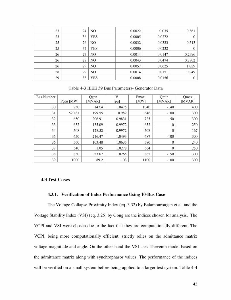
Table 4-3 IEEE 39 Bus Parameters- Generator Data
Bus Number
Pgen [MW]
Qgen
[MVAR]
V
[pu]
Pmax
[MW]
Qmin
[MVAR]
Qmax
[MVAR]
30 250 147.4 1.0475 1040 -140 400
31 520.87 199.55 0.982 646 -100 300
32 650 206.91 0.9831 725 150 300
33 632 135.09 0.9972 652 0 250
34 508 128.52 0.9972 508 0 167
35 650 216.47 1.0493 687 -100 300
36 560 103.48 1.0635 580 0 240
37 540 1.05 1.0278 564 0 250
38 830 23.67 1.0265 865 -150 300
39 1000 89.2 1.03 1100 -100 300
4.3 Test Cases
4.3.1. Verification of Index Performance Using 10-Bus Case
The Voltage Collapse Proximity Index (eq. 3.32) by Balamourougan et al. and the
Voltage Stability Index (VSI) (eq. 3.25) by Gong are the indices chosen for analysis. The
VCPI and VSI were chosen due to the fact that they are computationally different. The
VCPI, being more computationally efficient, strictly relies on the admittance matrix
voltage magnitude and angle. On the other hand the VSI uses Thevenin model based on
the admittance matrix along with synchrophasor values. The performance of the indices
will be verified on a small system before being applied to a larger test system. Table 4-4
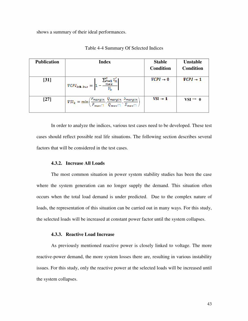
43
shows a summary of their ideal performances.
Table 4-4 Summary Of Selected Indices
In order to analyze the indices, various test cases need to be developed. These test
cases should reflect possible real life situations. The following section describes several
factors that will be considered in the test cases.
4.3.2. Increase All Loads
The most common situation in power system stability studies has been the case
where the system generation can no longer supply the demand. This situation often
occurs when the total load demand is under predicted. Due to the complex nature of
loads, the representation of this situation can be carried out in many ways. For this study,
the selected loads will be increased at constant power factor until the system collapses.
4.3.3. Reactive Load Increase
As previously mentioned reactive power is closely linked to voltage. The more
reactive-power demand, the more system losses there are, resulting in various instability
issues. For this study, only the reactive power at the selected loads will be increased until
the system collapses.
Publication Index Stable
Condition
Unstable
Condition
[31]
[27]
VSI 0

44
4.3.4. Contingency
In actual power systems the network undergoes several changes in topology as a
result of forced or unexpected outages. Certain lines within the system are very sensitive
to changes in power flow, while others may be able to handle excess flow. Often times
forced outages of specific lines can redirect power flow towards more lightly loaded lines
and allow alleviation overloaded lines while still supplying the power demanded by all
loads. During high demand times, loss of certain transmission lines can result in other
lines to become overloaded and may lead to abnormal operating conditions. It is
therefore useful to consider various contingencies when performing voltage stability
analysis to determine the effects of increased system loading as well as the lines that are
most likely to overload.
4.3.5. Intermittent Generation
The intermittent nature of wind generation has brought new challenges to the
planning and operation of interconnected power systems with high penetration of grid
connected wind farms. Therefore it is possible that the output power of a wind turbine
can be significantly lower than the actual installed capacity. This deviation can lead to
potential fluctuations in system frequency and voltage causing power system behavior to
be more complex. Detailed studies that consider the various effects of wind generation to
supply electricity demand are presented in [32-33]. The model chosen to represent the
intermittent nature of wind is based on the aggregation of several wind turbines, which is
elaborated in the following section.
45
4.3.6. Wind Farm Aggregation
In order to harvest the most electrical energy from wind, many wind turbines are
installed on the same location called “wind farms”. As a result a large wind farm can
have several hundreds of wind turbines covering an area of hundreds of square miles.
Modeling of each individual unit for power systems analysis may result in large
computation times may require extensive processing power. To overcome this issue, the
wind turbines may be reduced to an equivalent single wind turbine generation unit.
Aggregation techniques of variable speed wind turbines have been thoroughly discussed
and their significance described in [34]. Studies comparing the results between detailed
and aggregated models conclude that an aggregated electrical system and non-aggregated
mechanical system is an efficient and accurate model for mid and long term simulations.
[35]
Considering the aforementioned, the following test cases have been formulated for the
IEEE 39-Bus system:
Case 1: Starting from a steady state base case, the real power (MW) will
be increased at constant PF for all loads by 5% of base case until the
system collapses.
Case 2: Starting from a steady state base case, the reactive power will be
increase (MVAR) for all loads by 5% of base case until the system
collapses.
Case 3: Starting from a steady state base case, the real power (MW) will
be increased at constant power factor by 2.5% of base case. In between
46
two load increases a line will be removed to simulate a line tripping. Load
demand will continue to increase at the same rate until the system
collapses.
Case 4: Starting from a steady state base case, the system will be
partitioned into areas. A load will be increased by 66% of its initial base
load. The generation in that area will be adjusted to simulate various wind
scenarios.
47
CHAPTER 5
SIMULATION AND RESULTS
5.1 BPA 10-Bus: Verification of Index Performance
To verify the performance of each index, a series of load flows were conducted on
PowerWorld Simulator. The synchrophasor variables: voltage magnitude, voltage angle,
load powers and admittance matrix after each load increase were then outputted to
MATLAB, which was then used to determine the VCPI at the bus. The algorithm for
obtaining the VCPI and VSI are show in figures 5.1-5.2 respectively.

48
Figure 5.1 Algorithm for Computing VCPI

49
Figure 5.2 Algorithm for Computing VSI
50
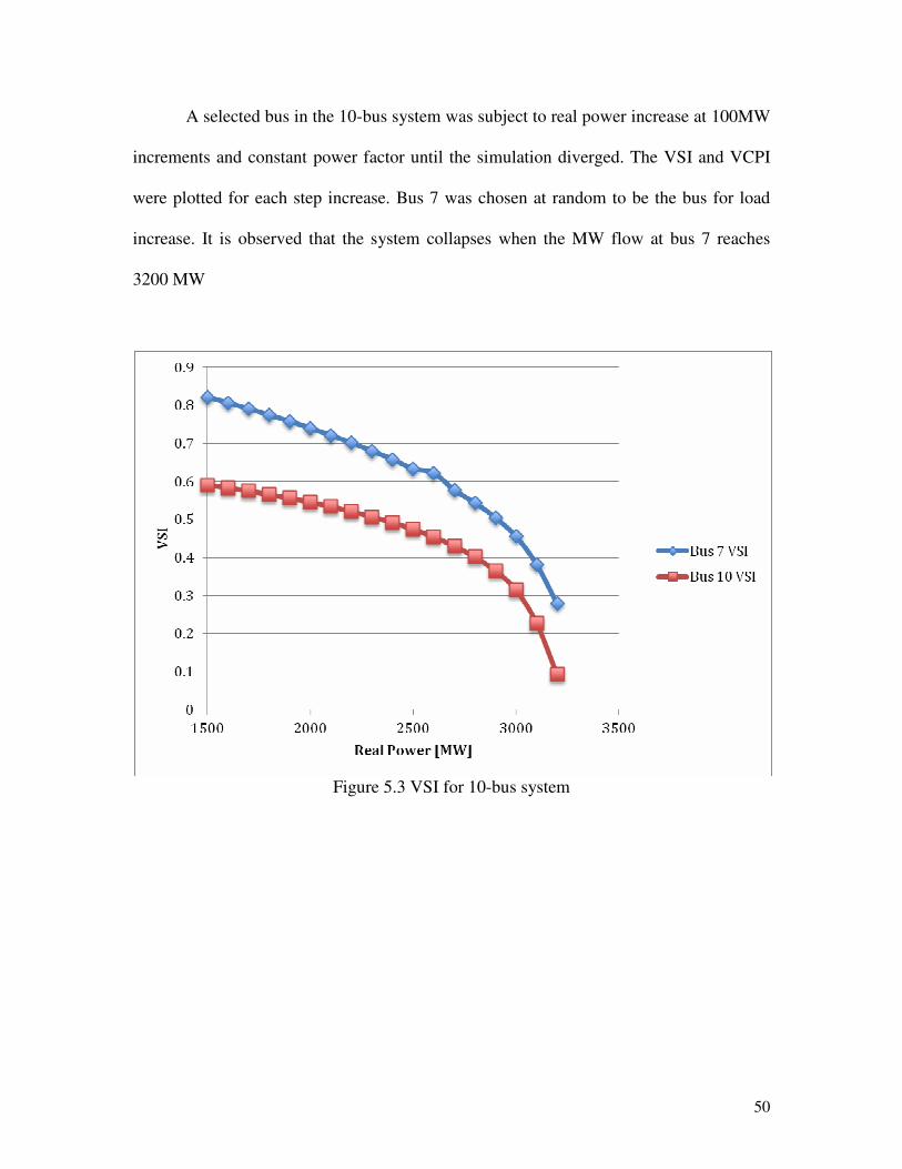
A selected bus in the 10-bus system was subject to real power increase at 100MW
increments and constant power factor until the simulation diverged. The VSI and VCPI
were plotted for each step increase. Bus 7 was chosen at random to be the bus for load
increase. It is observed that the system collapses when the MW flow at bus 7 reaches
3200 MW
Figure 5.3 VSI for 10-bus system
51
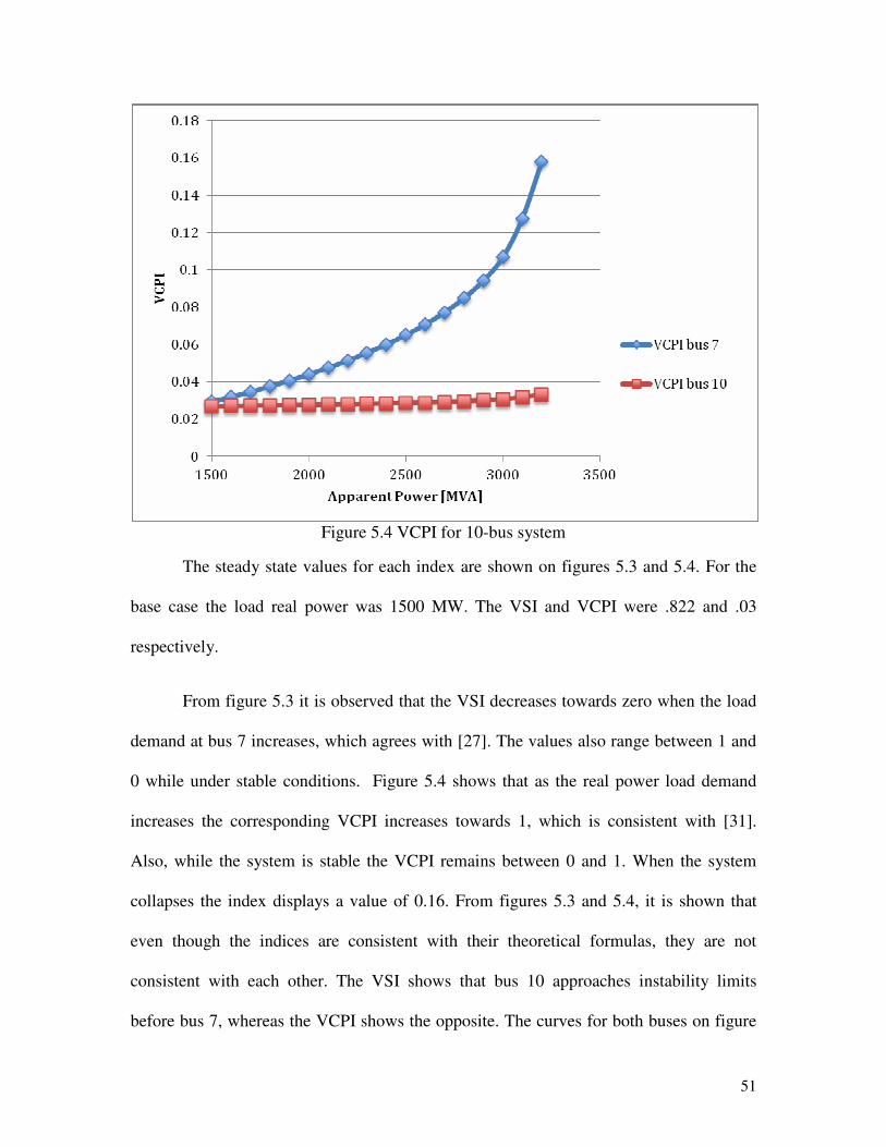
Figure 5.4 VCPI for 10-bus system
The steady state values for each index are shown on figures 5.3 and 5.4. For the
base case the load real power was 1500 MW. The VSI and VCPI were .822 and .03
respectively.
From figure 5.3 it is observed that the VSI decreases towards zero when the load
demand at bus 7 increases, which agrees with [27]. The values also range between 1 and
0 while under stable conditions. Figure 5.4 shows that as the real power load demand
increases the corresponding VCPI increases towards 1, which is consistent with [31].
Also, while the system is stable the VCPI remains between 0 and 1. When the system
collapses the index displays a value of 0.16. From figures 5.3 and 5.4, it is shown that
even though the indices are consistent with their theoretical formulas, they are not
consistent with each other. The VSI shows that bus 10 approaches instability limits
before bus 7, whereas the VCPI shows the opposite. The curves for both buses on figure
52
5.3 follow a similar decreasing pattern. Whereas the slope for the VCPI on bus 7
increases at a faster rate for each load increase compared to bus 10. From the VCPI
perspective, a load increase on bus 7 will only show noticeable index changes on bus 7.
On the other hand, from the VSI perspective it is seen that a load increase on bus 7 will
affect the maximum power delivered and therefore the margins on bus 10. This suggests
a stressed bus may not necessarily be the bus contributing to instability.
From this small system both indices are consistent with theoretical formulas;
further investigation will be carried out with the larger 39-bus system in order to identify
other characteristics as well as their application in voltage stability analysis.
5.2 Case 1: IEEE 39-Bus: Increase all loads
The loads in the 39-bus system were subject to real power increase at constant
power factor. Each load was increased by 5% of the initial base case until the system
collapsed, which is observed when the load is increase by 1.35 times the base case. Table
5-1 shows the total loads for each case.
Table 5-1 Load Factor with Corresponding Total System Laod
Load
Factor
Base
Case
1.05 1.1 1.15 1.2 1.25 1.3
Load
Demand
[MW]
5278.9 5521.1 5784.0 6046.9 6309.8 6572.7 6835.6
Initially the system is operating under base case conditions. Upon increasing the system
load to 1.10 times the base case, generator 31 is the first to reach its reactive limit. Even

53
though it is declared as the swing bus, the VSI algorithm is dependent on device status
and must be updated. When the system load is increased by 1.20 times the base case,
generators at buses 32 and 34 reach their reactive limits and can no longer sustain their
scheduled voltages. Upon the next load increase, 1.25% of the base case, generators at
buses 33 and 35 reach their limits as well. Finally the system load is increased again by
5% of its initial base case and the system can no longer maintain its stability, resulting in
a system collapse. The VSI and VCPI for each load increase are tabulated in tables 5-2
and 5-3.
Table 5-2: Load Bus VSI for Various Load Factors
Factor
Bus # 1 1.05 1.1 1.15 1.2 1.25 1.3
3 0.926 0.922 0.914 0.909 0.891 0.866 0.585
4 0.833 0.823 0.781 0.766 0.661 0.580 0.104
7 0.905 0.899 0.861 0.850 0.778 0.729 0.293
8 0.804 0.792 0.721 0.701 0.576 0.497 0.018
12 0.894 0.887 0.872 0.863 0.804 0.765 0.539
15 0.868 0.860 0.848 0.839 0.802 0.708 0.326
16 0.939 0.935 0.930 0.926 0.912 0.831 0.494
18 0.949 0.946 0.942 0.938 0.929 0.906 0.745
20 0.841 0.833 0.825 0.816 0.588 0.262 0.056
21 0.901 0.896 0.890 0.884 0.873 0.771 0.416
23 0.935 0.932 0.928 0.925 0.920 0.857 0.457
24 0.925 0.921 0.916 0.911 0.899 0.830 0.508
25 0.946 0.943 0.940 0.937 0.933 0.927 0.852
26 0.951 0.949 0.946 0.943 0.938 0.930 0.882
27 0.876 0.870 0.862 0.854 0.841 0.809 0.640
28 0.901 0.896 0.891 0.885 0.879 0.871 0.849
29 0.924 0.920 0.916 0.912 0.908 0.902 0.889
Global Index 0.804 0.792 0.721 0.701 0.576 0.262 0.018

54
Table 5-3 Load Bus VCPI for Various Load Factors
Factor
Bus # 1 1.05 1.1 1.15 1.2 1.25 1.3
3 0.163 0.172 0.181 0.192 0.205 0.223 0.267
4 0.258 0.274 0.293 0.315 0.346 0.394 0.534
7 0.076 0.081 0.087 0.094 0.104 0.120 0.168
8 0.164 0.175 0.187 0.202 0.224 0.258 0.358
12 0.134 0.146 0.160 0.177 0.203 0.244 0.371
15 0.220 0.233 0.248 0.264 0.285 0.315 0.401
16 0.061 0.064 0.067 0.071 0.076 0.082 0.100
18 0.076 0.080 0.085 0.090 0.096 0.104 0.125
20 0.662 0.687 0.713 0.740 0.770 0.812 0.957
21 0.186 0.197 0.208 0.220 0.233 0.252 0.301
23 0.137 0.145 0.152 0.160 0.169 0.180 0.206
24 0.155 0.163 0.172 0.181 0.193 0.208 0.249
25 0.141 0.147 0.153 0.160 0.167 0.175 0.190
26 0.125 0.128 0.132 0.136 0.141 0.147 0.159
27 0.211 0.223 0.236 0.249 0.265 0.286 0.331
28 0.217 0.228 0.240 0.251 0.264 0.278 0.301
29 0.218 0.225 0.232 0.240 0.248 0.257 0.270
Global Index 0.662 0.687 0.713 0.740 0.770 0.812 0.957
To illustrate an overall pattern, the VSIs that showed the lowest index before collapsing
are plotted on figure 5.5. Once again, a collapse is defined when the load flow diverges.
From figure 5.5, the VSI follows a linear trend for the first several load increase, which is
until the reactive capability of generator 1 has been exceeded. Beyond this point, each
index shows various nonlinearities. At base case conditions, Bus 7 shows the highest
signs of stability with an index of 0.89. Bus 20 shows the most sensitive reactions to
increases in load with the lowest value before diverging being 0.26
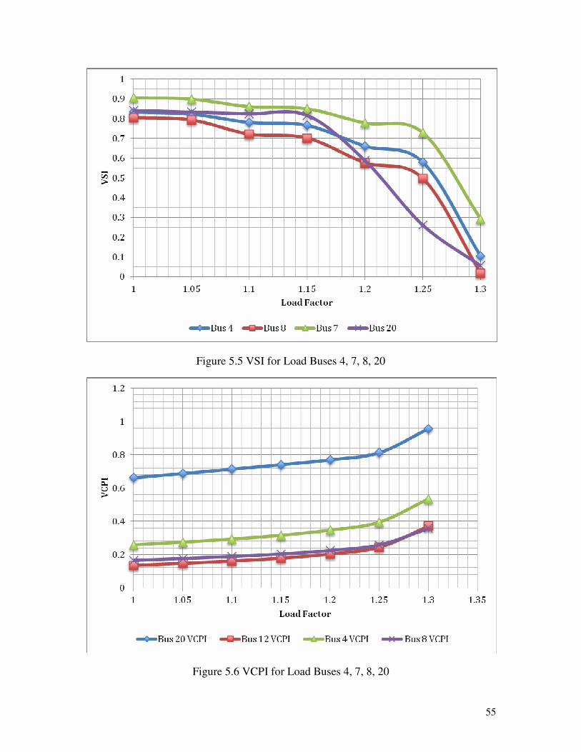
55
Figure 5.5 VSI for Load Buses 4, 7, 8, 20
Figure 5.6 VCPI for Load Buses 4, 7, 8, 20
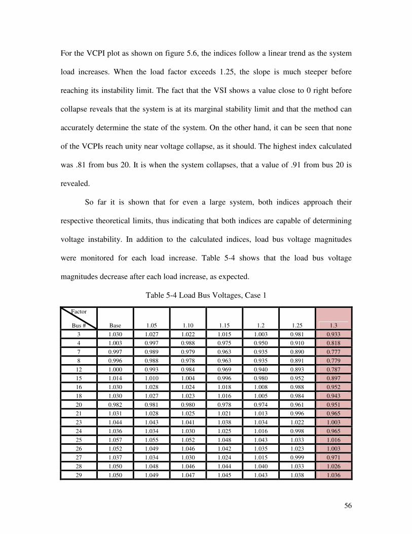
56
For the VCPI plot as shown on figure 5.6, the indices follow a linear trend as the system
load increases. When the load factor exceeds 1.25, the slope is much steeper before
reaching its instability limit. The fact that the VSI shows a value close to 0 right before
collapse reveals that the system is at its marginal stability limit and that the method can
accurately determine the state of the system. On the other hand, it can be seen that none
of the VCPIs reach unity near voltage collapse, as it should. The highest index calculated
was .81 from bus 20. It is when the system collapses, that a value of .91 from bus 20 is
revealed.
So far it is shown that for even a large system, both indices approach their
respective theoretical limits, thus indicating that both indices are capable of determining
voltage instability. In addition to the calculated indices, load bus voltage magnitudes
were monitored for each load increase. Table 5-4 shows that the load bus voltage
magnitudes decrease after each load increase, as expected.
Table 5-4 Load Bus Voltages, Case 1
Factor
Bus # Base 1.05 1.10 1.15 1.2 1.25 1.3
3 1.030 1.027 1.022 1.015 1.003 0.981 0.933
4 1.003 0.997 0.988 0.975 0.950 0.910 0.818
7 0.997 0.989 0.979 0.963 0.935 0.890 0.777
8 0.996 0.988 0.978 0.963 0.935 0.891 0.779
12 1.000 0.993 0.984 0.969 0.940 0.893 0.787
15 1.014 1.010 1.004 0.996 0.980 0.952 0.897
16 1.030 1.028 1.024 1.018 1.008 0.988 0.952
18 1.030 1.027 1.023 1.016 1.005 0.984 0.943
20 0.982 0.981 0.980 0.978 0.974 0.961 0.951
21 1.031 1.028 1.025 1.021 1.013 0.996 0.965
23 1.044 1.043 1.041 1.038 1.034 1.022 1.003
24 1.036 1.034 1.030 1.025 1.016 0.998 0.965
25 1.057 1.055 1.052 1.048 1.043 1.033 1.016
26 1.052 1.049 1.046 1.042 1.035 1.023 1.003
27 1.037 1.034 1.030 1.024 1.015 0.999 0.971
28 1.050 1.048 1.046 1.044 1.040 1.033 1.026
29 1.050 1.049 1.047 1.045 1.043 1.038 1.036

57
When the base case system load is increased by a factor of 1.25, Bus 4, 7,8 and 12 show
the largest signs of low voltage problems, ranging from 0.09 to 0.11pu drop. Considering
that the nearby generator at buses 31 and 32 have reached their reactive limits at 1.2
times the base case, and therefore limiting the capacitive VAR support, the large voltage
drop at buses 7,8 and 12 is expected. At this point the buses are still voltage stable,
however any large disturbance such as large load increase or a loss of any major element
can cause the system to lose its stability. Upon increasing the system load by a factor of
1.3 times the base case, buses 4, 7, 8 and 12 are well below nominal operating conditions
and therefore collapsing.
Figure 5.7 Load Buses with respect to nearest generation units

58
Chapter 3 has mentioned voltage magnitudes alone do not give a good indication of
proximity to voltage stability limit, especially for a system with high reactive power
compensation. However in most situations, systems are often lacking reactive power
resulting in low voltages when load is increased. By analyzing and comparing bus
voltages with index values, it is possible to determine whether low voltages or even
voltages alone are capable of determining whether the system is stable or not.
Indices and voltage magnitudes for buses 8 and 12 are plotted for each load
increase as shown in figures 5.8-5.9. These buses are significant since they show the
lowest voltage magnitudes before collapse. When the system load is increased by 1.25
times the base case, it is seen that even though these two buses experience about .1 pu
reduction in voltage, both indices indicate that bus 12 is voltage stable and bus 8 can be
either stable or unstable, depending on where the margin of instability is placed.
Similarly, the load bus having the next lowest voltage, bus 7, also experiences voltage
reduction at its terminals with only a minimal change in VSI and VCPI values indicating
that they are voltage stable.

59
Figure 5.8 VSI and Their Respected Bus Voltages
Figure 5.9 VCPI and Their Respected Bus Voltages

60
It is clear that monitoring only the voltage at a bus might lead to a false prediction of an
upcoming voltage collapse. By using indices that consider not only voltage at the buses,
but also other relevant system parameters such as topology, determining the likelihood of
a voltage collapse scenario is much more accurate.
5.3 Case 2: 39 Bus - Reactive power case
The loads in the 39-bus system were subject to reactive power increase. Each load
was increased by 5% of the initial base case until the system collapsed. At 1.35 times the
initial base case, the generator at bus 34 is the first to reach its reactive limit. By the time
the total reactive demand reaches 1.8 times the initial base case the generators at buses
32, 33, 35,36 reach their reactive limits and these buses suffer severe low voltage issues.
The system finally collapses once the total reactive load was increased past 1.95 times the
initial base case. The indices for selected buses are plotted in figures 5.10 and 5.11. The
rest are tabulated in tables 5-5 through 5-8.
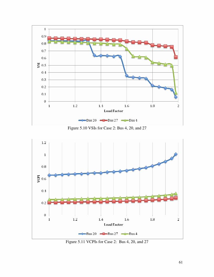
61
Figure 5.10 VSIs for Case 2: Bus 4, 20, and 27
Figure 5.11 VCPIs for Case 2: Bus 4, 20, and 27
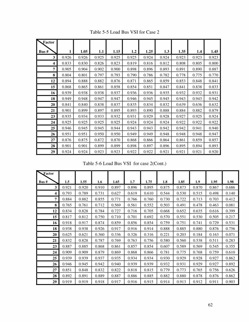
62
Table 5-5 Load Bus VSI for Case 2
Factor
Bus # 1 1.05 1.1 1.15 1.2 1.25 1.3 1.35 1.4 1.45
3 0.926 0.926 0.925 0.925 0.925 0.924 0.924 0.923 0.923 0.923
4 0.833 0.830 0.826 0.823 0.819 0.816 0.812 0.808 0.805 0.800
7 0.905 0.904 0.902 0.900 0.898 0.896 0.893 0.891 0.890 0.887
8 0.804 0.801 0.797 0.793 0.790 0.786 0.782 0.778 0.775 0.770
12 0.894 0.888 0.882 0.876 0.871 0.865 0.859 0.853 0.848 0.841
15 0.868 0.865 0.861 0.858 0.854 0.851 0.847 0.841 0.838 0.833
16 0.939 0.938 0.938 0.937 0.936 0.936 0.935 0.932 0.932 0.931
18 0.949 0.948 0.947 0.947 0.946 0.945 0.945 0.943 0.943 0.942
20 0.841 0.840 0.838 0.837 0.835 0.834 0.832 0.639 0.636 0.632
21 0.901 0.899 0.897 0.895 0.893 0.890 0.888 0.884 0.882 0.879
23 0.935 0.934 0.933 0.932 0.931 0.929 0.928 0.927 0.925 0.924
24 0.925 0.925 0.925 0.925 0.924 0.924 0.924 0.922 0.922 0.922
25 0.946 0.945 0.945 0.944 0.943 0.943 0.942 0.942 0.941 0.940
26 0.951 0.951 0.950 0.950 0.949 0.949 0.948 0.948 0.948 0.947
27 0.876 0.875 0.872 0.870 0.868 0.866 0.864 0.861 0.859 0.857
28 0.901 0.901 0.899 0.899 0.898 0.897 0.896 0.895 0.894 0.893
29 0.924 0.924 0.923 0.923 0.922 0.922 0.921 0.921 0.921 0.920
Table 5-6 Load Bus VSI for case 2(Cont.)
Factor
Bus # 1.5 1.55 1.6 1.65 1.7 1.75 1.8 1.85 1.9 1.95 1.98
3 0.921 0.920 0.910 0.897 0.896 0.895 0.875 0.873 0.870 0.867 0.686
4 0.793 0.789 0.731 0.627 0.619 0.610 0.544 0.530 0.515 0.498 0.140
7 0.884 0.882 0.855 0.771 0.766 0.760 0.730 0.722 0.713 0.703 0.412
8 0.765 0.761 0.712 0.569 0.561 0.552 0.503 0.491 0.478 0.463 0.081
12 0.834 0.828 0.784 0.727 0.716 0.705 0.668 0.652 0.635 0.616 0.399
15 0.817 0.812 0.750 0.710 0.701 0.692 0.570 0.551 0.530 0.505 0.217
16 0.918 0.917 0.874 0.859 0.856 0.854 0.759 0.751 0.741 0.729 0.531
18 0.938 0.938 0.926 0.917 0.916 0.914 0.888 0.885 0.880 0.876 0.756
20 0.625 0.621 0.360 0.336 0.326 0.316 0.221 0.203 0.184 0.163 0.071
21 0.832 0.828 0.787 0.769 0.763 0.756 0.580 0.560 0.538 0.511 0.283
23 0.887 0.885 0.868 0.861 0.857 0.854 0.607 0.589 0.569 0.545 0.355
24 0.909 0.909 0.879 0.869 0.868 0.866 0.781 0.775 0.768 0.759 0.610
25 0.939 0.939 0.937 0.935 0.934 0.934 0.930 0.929 0.928 0.927 0.862
26 0.946 0.945 0.942 0.940 0.939 0.939 0.932 0.931 0.929 0.927 0.892
27 0.851 0.848 0.832 0.822 0.818 0.815 0.779 0.773 0.765 0.756 0.626
28 0.892 0.891 0.889 0.887 0.886 0.885 0.882 0.880 0.878 0.876 0.862
29 0.919 0.919 0.918 0.917 0.916 0.915 0.914 0.913 0.912 0.911 0.903
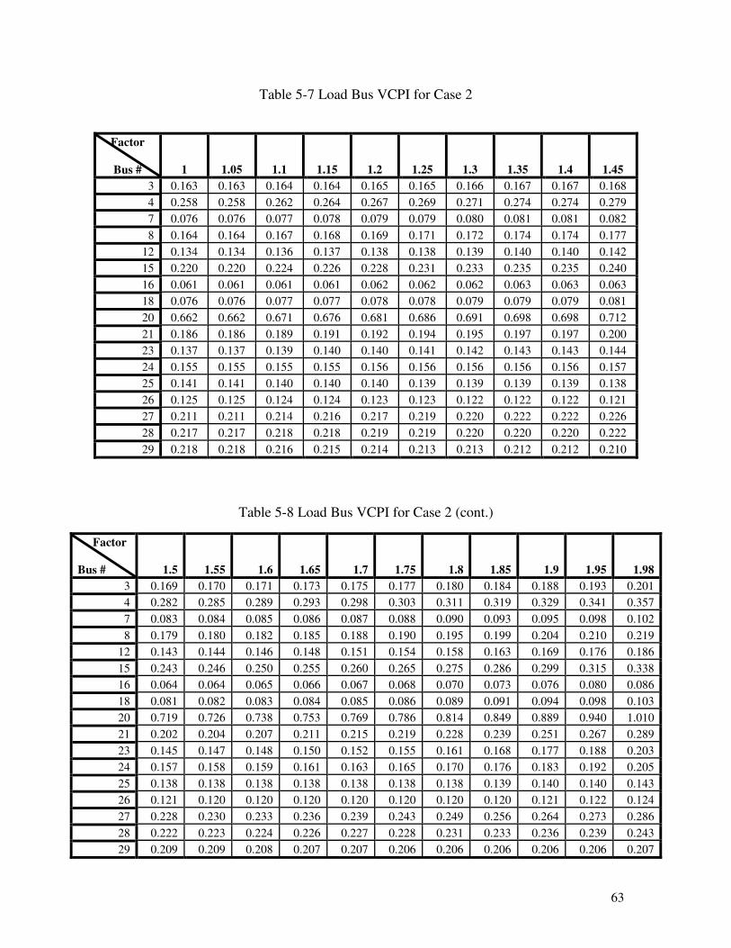
63
Table 5-7 Load Bus VCPI for Case 2
Table 5-8 Load Bus VCPI for Case 2 (cont.)
Factor
Bus # 1.5 1.55 1.6 1.65 1.7 1.75 1.8 1.85 1.9 1.95 1.98
3 0.169 0.170 0.171 0.173 0.175 0.177 0.180 0.184 0.188 0.193 0.201
4 0.282 0.285 0.289 0.293 0.298 0.303 0.311 0.319 0.329 0.341 0.357
7 0.083 0.084 0.085 0.086 0.087 0.088 0.090 0.093 0.095 0.098 0.102
8 0.179 0.180 0.182 0.185 0.188 0.190 0.195 0.199 0.204 0.210 0.219
12 0.143 0.144 0.146 0.148 0.151 0.154 0.158 0.163 0.169 0.176 0.186
15 0.243 0.246 0.250 0.255 0.260 0.265 0.275 0.286 0.299 0.315 0.338
16 0.064 0.064 0.065 0.066 0.067 0.068 0.070 0.073 0.076 0.080 0.086
18 0.081 0.082 0.083 0.084 0.085 0.086 0.089 0.091 0.094 0.098 0.103
20 0.719 0.726 0.738 0.753 0.769 0.786 0.814 0.849 0.889 0.940 1.010
21 0.202 0.204 0.207 0.211 0.215 0.219 0.228 0.239 0.251 0.267 0.289
23 0.145 0.147 0.148 0.150 0.152 0.155 0.161 0.168 0.177 0.188 0.203
24 0.157 0.158 0.159 0.161 0.163 0.165 0.170 0.176 0.183 0.192 0.205
25 0.138 0.138 0.138 0.138 0.138 0.138 0.138 0.139 0.140 0.140 0.143
26 0.121 0.120 0.120 0.120 0.120 0.120 0.120 0.120 0.121 0.122 0.124
27 0.228 0.230 0.233 0.236 0.239 0.243 0.249 0.256 0.264 0.273 0.286
28 0.222 0.223 0.224 0.226 0.227 0.228 0.231 0.233 0.236 0.239 0.243
29 0.209 0.209 0.208 0.207 0.207 0.206 0.206 0.206 0.206 0.206 0.207
Factor
Bus # 1 1.05 1.1 1.15 1.2 1.25 1.3 1.35 1.4 1.45
3 0.163 0.163 0.164 0.164 0.165 0.165 0.166 0.167 0.167 0.168
4 0.258 0.258 0.262 0.264 0.267 0.269 0.271 0.274 0.274 0.279
7 0.076 0.076 0.077 0.078 0.079 0.079 0.080 0.081 0.081 0.082
8 0.164 0.164 0.167 0.168 0.169 0.171 0.172 0.174 0.174 0.177
12 0.134 0.134 0.136 0.137 0.138 0.138 0.139 0.140 0.140 0.142
15 0.220 0.220 0.224 0.226 0.228 0.231 0.233 0.235 0.235 0.240
16 0.061 0.061 0.061 0.061 0.062 0.062 0.062 0.063 0.063 0.063
18 0.076 0.076 0.077 0.077 0.078 0.078 0.079 0.079 0.079 0.081
20 0.662 0.662 0.671 0.676 0.681 0.686 0.691 0.698 0.698 0.712
21 0.186 0.186 0.189 0.191 0.192 0.194 0.195 0.197 0.197 0.200
23 0.137 0.137 0.139 0.140 0.140 0.141 0.142 0.143 0.143 0.144
24 0.155 0.155 0.155 0.155 0.156 0.156 0.156 0.156 0.156 0.157
25 0.141 0.141 0.140 0.140 0.140 0.139 0.139 0.139 0.139 0.138
26 0.125 0.125 0.124 0.124 0.123 0.123 0.122 0.122 0.122 0.121
27 0.211 0.211 0.214 0.216 0.217 0.219 0.220 0.222 0.222 0.226
28 0.217 0.217 0.218 0.218 0.219 0.219 0.220 0.220 0.220 0.222
29 0.218 0.218 0.216 0.215 0.214 0.213 0.213 0.212 0.212 0.210
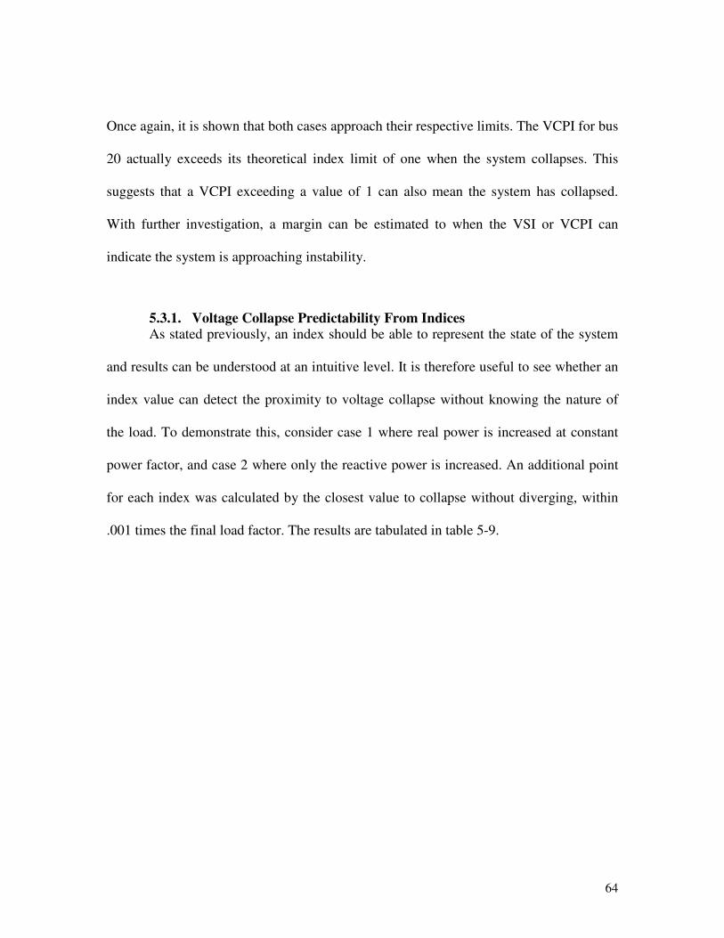
64
Once again, it is shown that both cases approach their respective limits. The VCPI for bus
20 actually exceeds its theoretical index limit of one when the system collapses. This
suggests that a VCPI exceeding a value of 1 can also mean the system has collapsed.
With further investigation, a margin can be estimated to when the VSI or VCPI can
indicate the system is approaching instability.
5.3.1. Voltage Collapse Predictability From Indices As stated previously, an index should be able to represent the state of the system
and results can be understood at an intuitive level. It is therefore useful to see whether an
index value can detect the proximity to voltage collapse without knowing the nature of
the load. To demonstrate this, consider case 1 where real power is increased at constant
power factor, and case 2 where only the reactive power is increased. An additional point
for each index was calculated by the closest value to collapse without diverging, within
.001 times the final load factor. The results are tabulated in table 5-9.
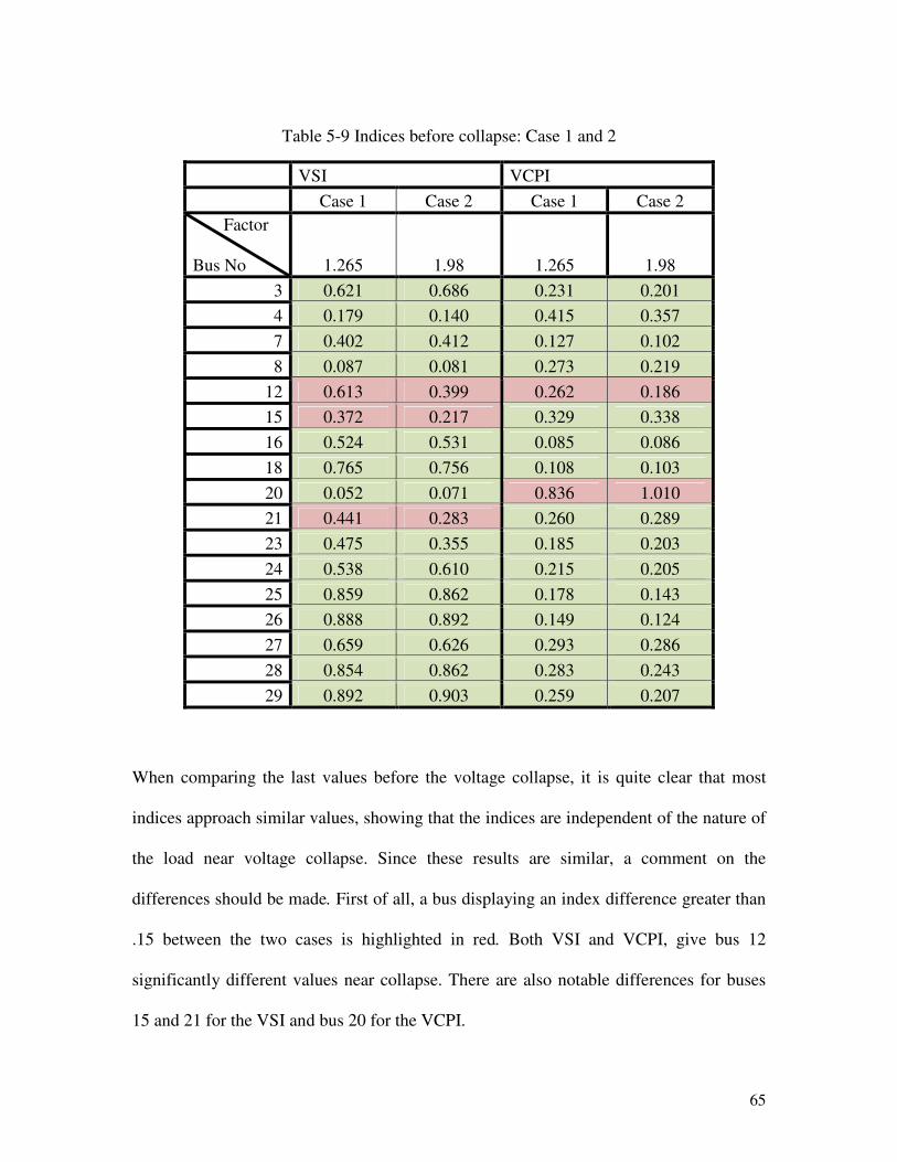
65
Table 5-9 Indices before collapse: Case 1 and 2
VSI VCPI
Case 1 Case 2 Case 1 Case 2
Factor
Bus No 1.265 1.98 1.265 1.98
3 0.621 0.686 0.231 0.201
4 0.179 0.140 0.415 0.357
7 0.402 0.412 0.127 0.102
8 0.087 0.081 0.273 0.219
12 0.613 0.399 0.262 0.186
15 0.372 0.217 0.329 0.338
16 0.524 0.531 0.085 0.086
18 0.765 0.756 0.108 0.103
20 0.052 0.071 0.836 1.010
21 0.441 0.283 0.260 0.289
23 0.475 0.355 0.185 0.203
24 0.538 0.610 0.215 0.205
25 0.859 0.862 0.178 0.143
26 0.888 0.892 0.149 0.124
27 0.659 0.626 0.293 0.286
28 0.854 0.862 0.283 0.243
29 0.892 0.903 0.259 0.207
When comparing the last values before the voltage collapse, it is quite clear that most
indices approach similar values, showing that the indices are independent of the nature of
the load near voltage collapse. Since these results are similar, a comment on the
differences should be made. First of all, a bus displaying an index difference greater than
.15 between the two cases is highlighted in red. Both VSI and VCPI, give bus 12
significantly different values near collapse. There are also notable differences for buses
15 and 21 for the VSI and bus 20 for the VCPI.
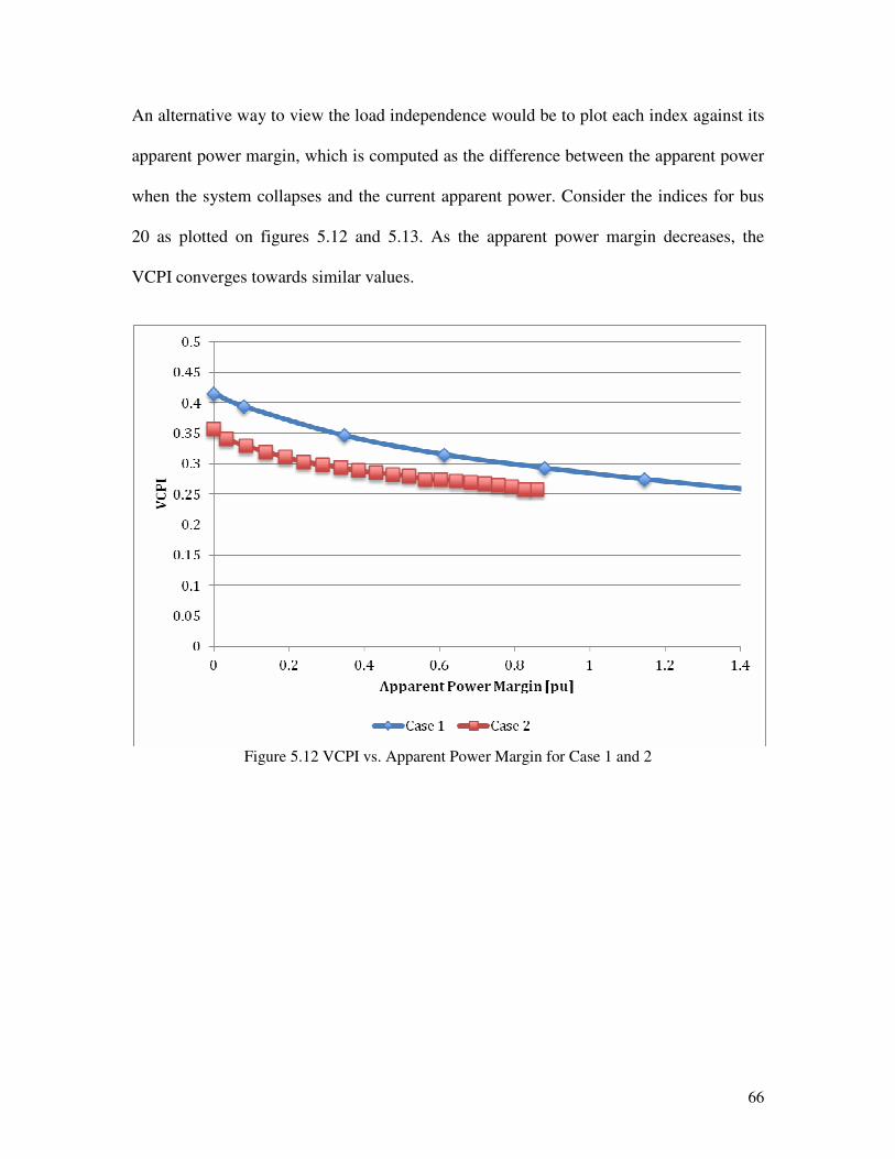
66
An alternative way to view the load independence would be to plot each index against its
apparent power margin, which is computed as the difference between the apparent power
when the system collapses and the current apparent power. Consider the indices for bus
20 as plotted on figures 5.12 and 5.13. As the apparent power margin decreases, the
VCPI converges towards similar values.
Figure 5.12 VCPI vs. Apparent Power Margin for Case 1 and 2

67
Figure 5.13 VSI vs. Apparent Power Margin for Case 1 and 2
From these comparisons, the indices are capable of providing information on how far the
system is to the voltage collapse regardless of the characteristic of the load. This can be
understood as how the index itself can give insight without knowing any other parameters
of the system.
5.4 Case 3: IEEE 39 Bus System -Loss of transmission line
Similar to the first case, the loads in the 39-bus system were subject to real power
increase at constant power factor. Each load was increased by 2.5% of the initial base
case until the system collapsed. However, on the sixth load increase, a transmission line
was removed to simulate the loss of a heavily loaded line. The line chosen was based on
the limit of the line; the line that had the most amount of apparent power flowing with

68
respect to maximum ampacity, was removed. After each load increase, the indices were
computed as prescribed by the algorithms according to figure 5.1 and 5.2. Initially the
system is running under normal operating conditions. Each load is increased as
previously mentioned. On the sixth load step, line 10-13 is tripped having been loaded
82% of its 600MVA line rating.
Figure 5.14 Line 10-13 Trip
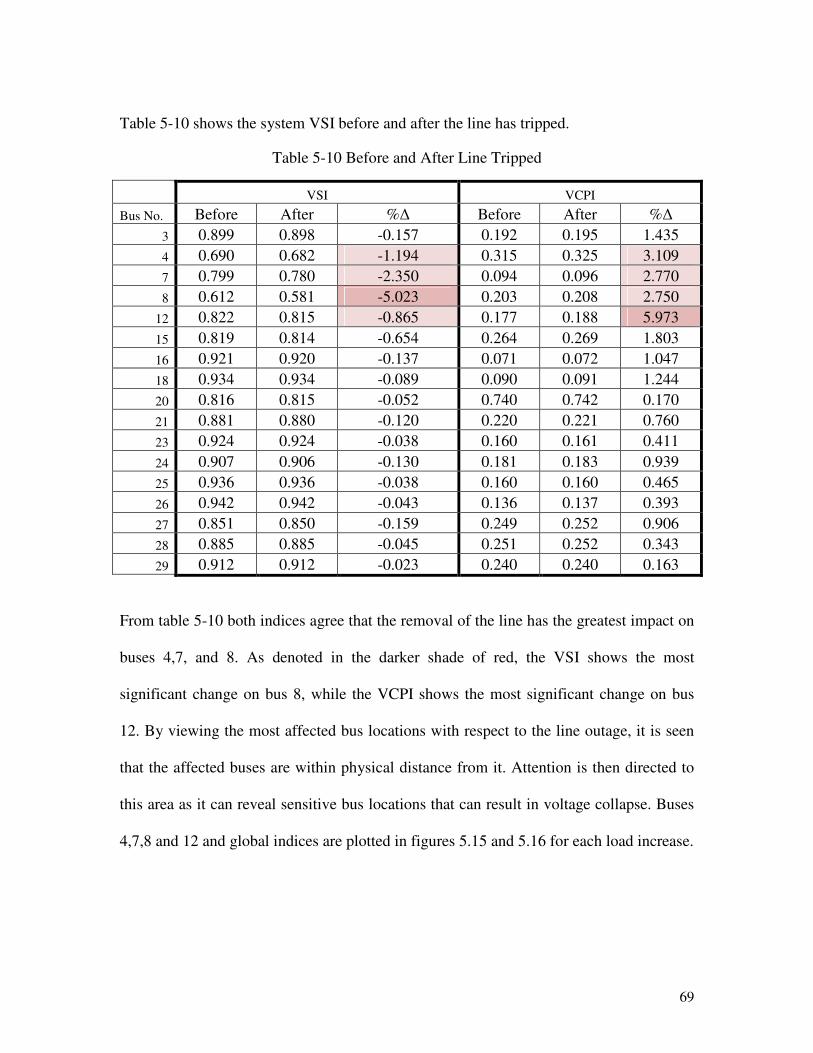
69
Table 5-10 shows the system VSI before and after the line has tripped.
Table 5-10 Before and After Line Tripped
VSI VCPI
Bus No. Before After %∆ Before After %∆
3 0.899 0.898 -0.157 0.192 0.195 1.435
4 0.690 0.682 -1.194 0.315 0.325 3.109
7 0.799 0.780 -2.350 0.094 0.096 2.770
8 0.612 0.581 -5.023 0.203 0.208 2.750
12 0.822 0.815 -0.865 0.177 0.188 5.973
15 0.819 0.814 -0.654 0.264 0.269 1.803
16 0.921 0.920 -0.137 0.071 0.072 1.047
18 0.934 0.934 -0.089 0.090 0.091 1.244
20 0.816 0.815 -0.052 0.740 0.742 0.170
21 0.881 0.880 -0.120 0.220 0.221 0.760
23 0.924 0.924 -0.038 0.160 0.161 0.411
24 0.907 0.906 -0.130 0.181 0.183 0.939
25 0.936 0.936 -0.038 0.160 0.160 0.465
26 0.942 0.942 -0.043 0.136 0.137 0.393
27 0.851 0.850 -0.159 0.249 0.252 0.906
28 0.885 0.885 -0.045 0.251 0.252 0.343
29 0.912 0.912 -0.023 0.240 0.240 0.163
From table 5-10 both indices agree that the removal of the line has the greatest impact on
buses 4,7, and 8. As denoted in the darker shade of red, the VSI shows the most
significant change on bus 8, while the VCPI shows the most significant change on bus
12. By viewing the most affected bus locations with respect to the line outage, it is seen
that the affected buses are within physical distance from it. Attention is then directed to
this area as it can reveal sensitive bus locations that can result in voltage collapse. Buses
4,7,8 and 12 and global indices are plotted in figures 5.15 and 5.16 for each load increase.
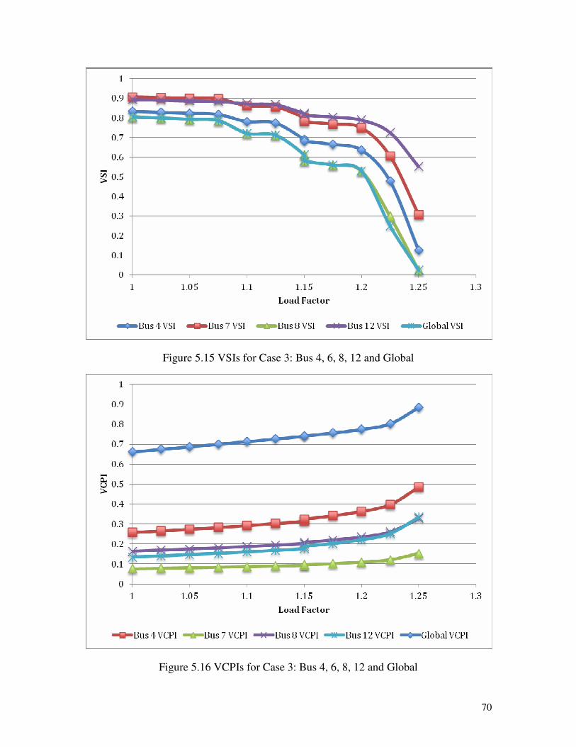
70
Figure 5.15 VSIs for Case 3: Bus 4, 6, 8, 12 and Global
Figure 5.16 VCPIs for Case 3: Bus 4, 6, 8, 12 and Global
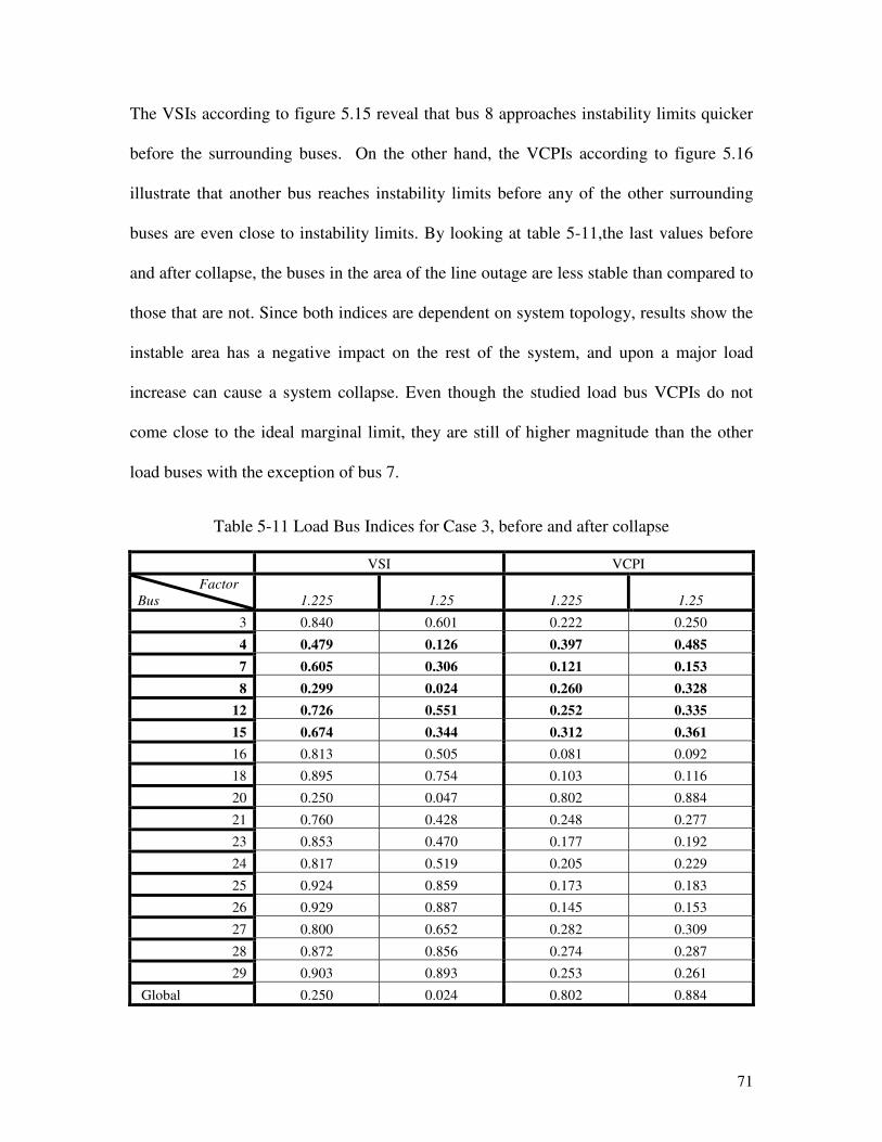
71
The VSIs according to figure 5.15 reveal that bus 8 approaches instability limits quicker
before the surrounding buses. On the other hand, the VCPIs according to figure 5.16
illustrate that another bus reaches instability limits before any of the other surrounding
buses are even close to instability limits. By looking at table 5-11,the last values before
and after collapse, the buses in the area of the line outage are less stable than compared to
those that are not. Since both indices are dependent on system topology, results show the
instable area has a negative impact on the rest of the system, and upon a major load
increase can cause a system collapse. Even though the studied load bus VCPIs do not
come close to the ideal marginal limit, they are still of higher magnitude than the other
load buses with the exception of bus 7.
Table 5-11 Load Bus Indices for Case 3, before and after collapse
VSI VCPI
Factor
Bus 1.225 1.25 1.225 1.25
3 0.840 0.601 0.222 0.250
4 0.479 0.126 0.397 0.485
7 0.605 0.306 0.121 0.153
8 0.299 0.024 0.260 0.328
12 0.726 0.551 0.252 0.335
15 0.674 0.344 0.312 0.361
16 0.813 0.505 0.081 0.092
18 0.895 0.754 0.103 0.116
20 0.250 0.047 0.802 0.884
21 0.760 0.428 0.248 0.277
23 0.853 0.470 0.177 0.192
24 0.817 0.519 0.205 0.229
25 0.924 0.859 0.173 0.183
26 0.929 0.887 0.145 0.153
27 0.800 0.652 0.282 0.309
28 0.872 0.856 0.274 0.287
29 0.903 0.893 0.253 0.261
Global 0.250 0.024 0.802 0.884
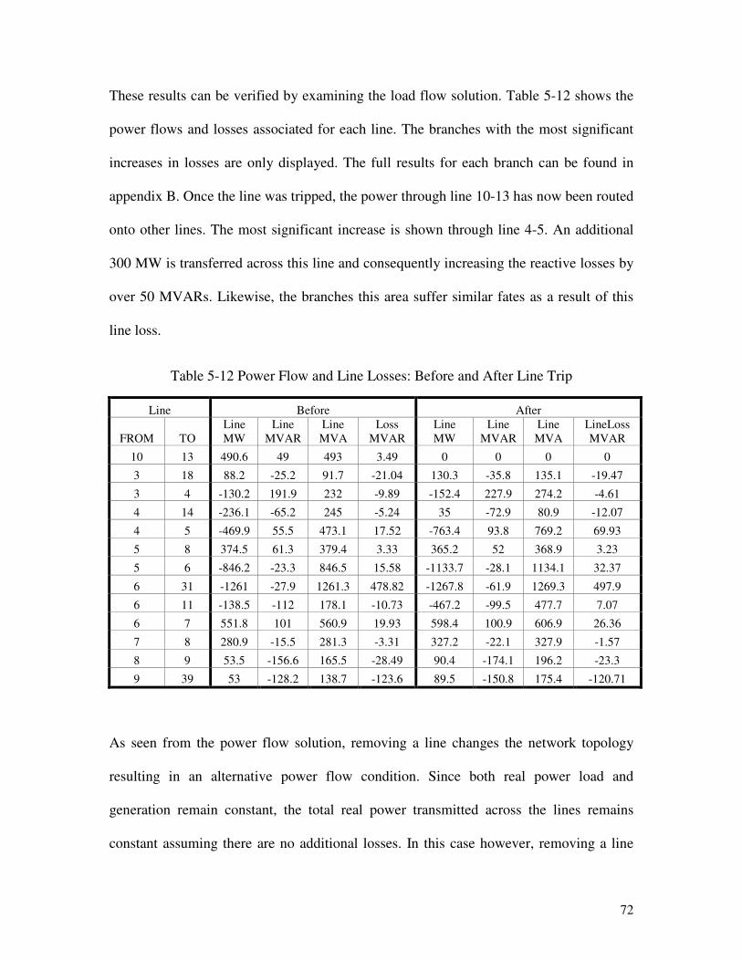
72
These results can be verified by examining the load flow solution. Table 5-12 shows the
power flows and losses associated for each line. The branches with the most significant
increases in losses are only displayed. The full results for each branch can be found in
appendix B. Once the line was tripped, the power through line 10-13 has now been routed
onto other lines. The most significant increase is shown through line 4-5. An additional
300 MW is transferred across this line and consequently increasing the reactive losses by
over 50 MVARs. Likewise, the branches this area suffer similar fates as a result of this
line loss.
Table 5-12 Power Flow and Line Losses: Before and After Line Trip
Line Before After
FROM TO
Line
MW
Line
MVAR
Line
MVA
Loss
MVAR
Line
MW
Line
MVAR
Line
MVA
LineLoss
MVAR
10 13 490.6 49 493 3.49 0 0 0 0
3 18 88.2 -25.2 91.7 -21.04 130.3 -35.8 135.1 -19.47
3 4 -130.2 191.9 232 -9.89 -152.4 227.9 274.2 -4.61
4 14 -236.1 -65.2 245 -5.24 35 -72.9 80.9 -12.07
4 5 -469.9 55.5 473.1 17.52 -763.4 93.8 769.2 69.93
5 8 374.5 61.3 379.4 3.33 365.2 52 368.9 3.23
5 6 -846.2 -23.3 846.5 15.58 -1133.7 -28.1 1134.1 32.37
6 31 -1261 -27.9 1261.3 478.82 -1267.8 -61.9 1269.3 497.9
6 11 -138.5 -112 178.1 -10.73 -467.2 -99.5 477.7 7.07
6 7 551.8 101 560.9 19.93 598.4 100.9 606.9 26.36
7 8 280.9 -15.5 281.3 -3.31 327.2 -22.1 327.9 -1.57
8 9 53.5 -156.6 165.5 -28.49 90.4 -174.1 196.2 -23.3
9 39 53 -128.2 138.7 -123.6 89.5 -150.8 175.4 -120.71
As seen from the power flow solution, removing a line changes the network topology
resulting in an alternative power flow condition. Since both real power load and
generation remain constant, the total real power transmitted across the lines remains
constant assuming there are no additional losses. In this case however, removing a line
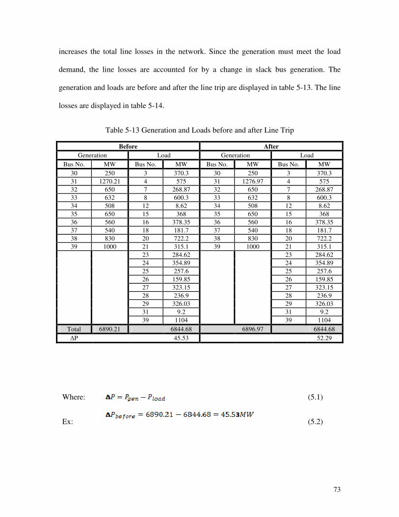
73
increases the total line losses in the network. Since the generation must meet the load
demand, the line losses are accounted for by a change in slack bus generation. The
generation and loads are before and after the line trip are displayed in table 5-13. The line
losses are displayed in table 5-14.
Table 5-13 Generation and Loads before and after Line Trip
Before After
Generation Load Generation Load
Bus No. MW Bus No. MW Bus No. MW Bus No. MW
30 250 3 370.3 30 250 3 370.3
31 1270.21 4 575 31 1276.97 4 575
32 650 7 268.87 32 650 7 268.87
33 632 8 600.3 33 632 8 600.3
34 508 12 8.62 34 508 12 8.62
35 650 15 368 35 650 15 368
36 560 16 378.35 36 560 16 378.35
37 540 18 181.7 37 540 18 181.7
38 830 20 722.2 38 830 20 722.2
39 1000 21 315.1 39 1000 21 315.1
23 284.62 23 284.62
24 354.89 24 354.89
25 257.6 25 257.6
26 159.85 26 159.85
27 323.15 27 323.15
28 236.9 28 236.9
29 326.03 29 326.03
31 9.2 31 9.2
39 1104 39 1104
Total 6890.21 6844.68 6896.97 6844.68
∆P 45.53 52.29
Where:
Ex:
(5.1)
(5.2)

74
Table 5-14 Line Losses Before and After Line Trip
Branch Line Loss [MW]
From To Before After
1 2 0.09 0.01
1 39 0.07 0.04
10 13 0.99 0
10 32 0 0
10 11 0.19 1.9
12 11 0.04 0.63
12 13 0.05 0.56
13 14 2.32 0.31
14 15 1.35 0.96
15 16 0.57 0.85
16 19 2.66 2.73
16 17 0.2 0.09
16 24 0.05 0.05
16 21 0.57 0.58
17 27 0.09 0.07
17 18 0.07 0.03
19 20 0.35 0.35
19 33 3.01 3.04
2 30 0 0
2 3 1.67 1.97
2 25 1.29 0.96
20 34 2.55 2.57
21 22 2.76 2.8
22 35 0 0
22 23 0.04 0.04
23 36 1.46 1.47
23 24 2.28 2.31
25 37 1.67 1.67
25 26 0.64 0.8
26 29 1.32 1.32
26 28 0.41 0.41
26 27 0.92 1.05
28 29 1.48 1.48
29 38 5.25 5.26
3 18 0.09 0.19
3 4 0.74 1.03
4 14 0.5 0.05
4 5 1.89 5.14
5 8 1.23 1.19
5 6 1.51 2.8
6 31 0 0
6 11 0.22 1.72
6 7 1.99 2.39
7 8 0.34 0.48
8 9 0.55 0.84
9 39 0.07 0.16
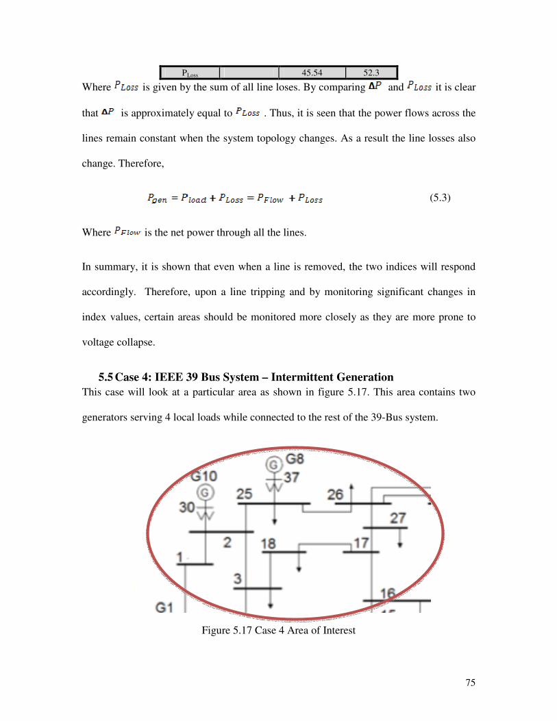
75
PLoss 45.54 52.3
Where is given by the sum of all line loses. By comparing and it is clear
that is approximately equal to . Thus, it is seen that the power flows across the
lines remain constant when the system topology changes. As a result the line losses also
change. Therefore,
(5.3)
Where is the net power through all the lines.
In summary, it is shown that even when a line is removed, the two indices will respond
accordingly. Therefore, upon a line tripping and by monitoring significant changes in
index values, certain areas should be monitored more closely as they are more prone to
voltage collapse.
5.5 Case 4: IEEE 39 Bus System – Intermittent Generation
This case will look at a particular area as shown in figure 5.17. This area contains two
generators serving 4 local loads while connected to the rest of the 39-Bus system.
Figure 5.17 Case 4 Area of Interest

76
Bus 18 will be loaded to 66% (at constant power factor) of its maximum load capacity in
order to simulate a loaded situation. An offline study was done to verify the maximum
load bus 18 could handle before collapsing. This value was 1317 MW at a power factor
of 0.98. The load for bus 18 at 66% of its maximum capacity was 869MW and 165
MVAR. The generation at bus 30 was varied for different levels to represent different
levels of wind. The amount of wind generation will be randomly varied from 0 to 550
MW for a period of 24 hours, measurements were take every one hour.
Figure 5.18 Bus 18 VSI for various Wind Generation output
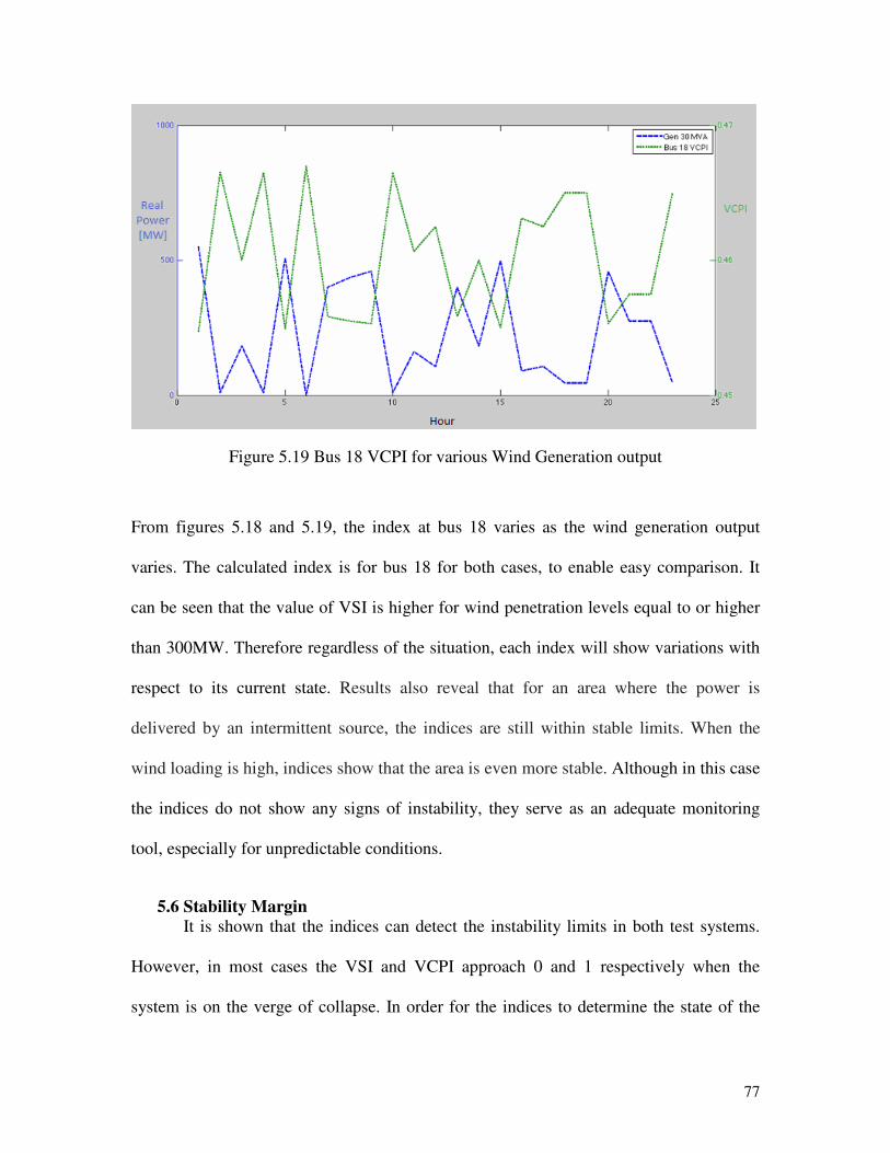
77
Figure 5.19 Bus 18 VCPI for various Wind Generation output
From figures 5.18 and 5.19, the index at bus 18 varies as the wind generation output
varies. The calculated index is for bus 18 for both cases, to enable easy comparison. It
can be seen that the value of VSI is higher for wind penetration levels equal to or higher
than 300MW. Therefore regardless of the situation, each index will show variations with
respect to its current state. Results also reveal that for an area where the power is
delivered by an intermittent source, the indices are still within stable limits. When the
wind loading is high, indices show that the area is even more stable. Although in this case
the indices do not show any signs of instability, they serve as an adequate monitoring
tool, especially for unpredictable conditions.
5.6 Stability Margin It is shown that the indices can detect the instability limits in both test systems.
However, in most cases the VSI and VCPI approach 0 and 1 respectively when the
system is on the verge of collapse. In order for the indices to determine the state of the
78
system, a margin should be made which distinguishes, when the system is near a
collapse. By analyzing the global index at the last load increase before collapse for case 1
and case 2, the VSI provides an index of 0.262 and .163 respectively. Likewise, the VCPI
provides an index of .812 and .94 respectively. Recalling the fact that a system wide
collapse can occur within seconds, the margin should be established to give ample time to
analyze and react to the situation. For both indices, a 0.3 index margin should be
appropriate.
5.7 Weakest Bus In traditional studies it is often useful to consider ranking the strength of each load
bus. As previously mentioned, these indices can be used to determine the strength of each
bus depending on the value of each index. The indices presented in chapter 3, propose
methods that show their ability to determine weak branches and or buses. However, the
analyzed indices in this chapter do not present any method to determine the weak buses.
An attempt to determine the weak bus is initiated first by considering indices at the first
load increase, and the last increase before collapsing.
Table 5-15 and Table 5-16 show the rankings for a given analysis for the base
case and 6th
load increase. In addition, well known computations, QV and modal analysis
were performed on all load buses in order to give an adequate comparison. Full
calculations for QV and modal analysis are shown appendix C and D respectively.

79
Table 5-15 Comparison Of Rankings Between Various Methods: First Load Increase
VSI VCPI MODAL QV
Ranking Bus No Index Bus No Index Bus No Participation
Bus
No Margin
1 8 0.792 20 0.662 12 0.1085 20 -460.83
2 4 0.823 4 0.258 7 0.0669 29 -490.19
3 20 0.833 15 0.220 8 0.0646 28 -512.83
4 15 0.860 29 0.218 4 0.0631 23 -559.8
5 27 0.870 28 0.217 15 0.0441 12 -595.89
6 12 0.887 27 0.211 18 0.0379 21 -633.1
7 28 0.896 21 0.186 3 0.0331 24 -745.75
8 21 0.896 8 0.164 27 0.0311 16 -811.01
9 7 0.899 3 0.163 16 0.02792 15 -811.21
10 29 0.920 24 0.155 24 0.0261 26 -890.19
11 24 0.921 25 0.141 26 0.0195 27 -917.6
12 3 0.922 23 0.137 21 0.0177 18 -986.68
13 23 0.932 12 0.134 28 0.0086 8 -1002.09
14 16 0.935 26 0.125 25 0.0069 7 -1008.73
15 25 0.943 18 0.076 23 0.0063 4 -1043.78
16 18 0.946 7 0.076 29 0.0040 25 -1074.78
17 26 0.949 16 0.061 20 0.0017 3 -1087.59
For the base case it is quite clear that a majority of the values disagree over which bus is
the critical bus. The only similar ranking is between the VSI and VCPI for bus 2,
denoting that it is the second weakest load bus. In the previous analysis it had shown that
for base case operating conditions, the system is a stable system. So far, there is
insufficient information to make any concrete conclusion on any rankings. Next, consider
the case when the load is near its collapse point, the sixth load increase.
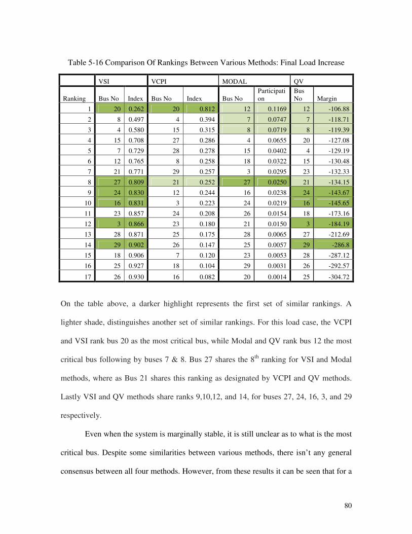
80
Table 5-16 Comparison Of Rankings Between Various Methods: Final Load Increase
VSI VCPI MODAL QV
Ranking Bus No Index Bus No Index Bus No
Participati
on
Bus
No Margin
1 20 0.262 20 0.812 12 0.1169 12 -106.88
2 8 0.497 4 0.394 7 0.0747 7 -118.71
3 4 0.580 15 0.315 8 0.0719 8 -119.39
4 15 0.708 27 0.286 4 0.0655 20 -127.08
5 7 0.729 28 0.278 15 0.0402 4 -129.19
6 12 0.765 8 0.258 18 0.0322 15 -130.48
7 21 0.771 29 0.257 3 0.0295 23 -132.33
8 27 0.809 21 0.252 27 0.0250 21 -134.15
9 24 0.830 12 0.244 16 0.0238 24 -143.67
10 16 0.831 3 0.223 24 0.0219 16 -145.65
11 23 0.857 24 0.208 26 0.0154 18 -173.16
12 3 0.866 23 0.180 21 0.0150 3 -184.19
13 28 0.871 25 0.175 28 0.0065 27 -212.69
14 29 0.902 26 0.147 25 0.0057 29 -286.8
15 18 0.906 7 0.120 23 0.0053 28 -287.12
16 25 0.927 18 0.104 29 0.0031 26 -292.57
17 26 0.930 16 0.082 20 0.0014 25 -304.72
On the table above, a darker highlight represents the first set of similar rankings. A
lighter shade, distinguishes another set of similar rankings. For this load case, the VCPI
and VSI rank bus 20 as the most critical bus, while Modal and QV rank bus 12 the most
critical bus following by buses 7 & 8. Bus 27 shares the 8th
ranking for VSI and Modal
methods, where as Bus 21 shares this ranking as designated by VCPI and QV methods.
Lastly VSI and QV methods share ranks 9,10,12, and 14, for buses 27, 24, 16, 3, and 29
respectively.
Even when the system is marginally stable, it is still unclear as to what is the most
critical bus. Despite some similarities between various methods, there isn’t any general
consensus between all four methods. However, from these results it can be seen that for a

81
large system, determining a critical bus requires more factors as to what makes the bus
critical. Since both QV and Modal analyses are closely related to reactive power, it is
most likely that bus 12 and 7 are the most sensitive to changes in reactive power. Even
though reactive power is an important contribution to the voltage stability problem, it
may not necessarily be the sole cause of collapse. On the other hand it is unclear why
bus 20 is defined the critical bus according to the indices. The fact that the VSI and VCPI
also consider factors including apparent power, real power, and admittances, suggest that
other quantities and their combinations can lead to a collapse. Thus, additional studies
should be done in order to establish an appropriate relationship between instability and
various quantities.
82
CHAPTER 6
CONCLUSION AND RECOMMENDATIONS
This thesis investigated several key aspects of voltage stability using simulated
synchrophasor data. Two indices from literature, VSI and VCPI were investigated in
order to show how the synchrophasor data can be used to determine how far the entire
system is from its voltage collapse point, as well as the weak points in a system. Steady
state analysis was conducted using PowerWorld Simulators, and the indices were
generated in MatLab. The performances of the indices were tested in the 10 bus- 3-
generator system, and a larger network consisting of 39 buses and 10 generators. Results
show that their performances are coherent to each other with respect to voltage stability
of the system. All indices fall between 0 and 1 when the system is stable. The VCPI can
exceed 1 when the system is unstable.
When comparing the two studied indices, the predictive ability of the VSI is able
to provide a more intuitive index compared to the VCPI. For almost all buses the VCPI
does not give any predictable value at the voltage stability boundary. So they cannot
estimate the voltage stability margin but may be used to determine critical lines or critical
buses in a given load level. When looking at the global index, a .3 index margin should
be considered which could allow operators to initiate the remedial actions necessary to
prevent voltage collapse.
The characteristics of the two indices can be summed up as follows:
83
Voltage collapse can be predicted from the index, and regardless of load type the
index will still approach the same value. The curve shows a nonlinear trend near the
voltage collapse point. Each index changes automatically with different operating
conditions and does not depend on any particular scenario. Low voltages, and reactive
margin alone conditions do not necessarily indicate a critical bus. Additional parameters
such as powers, and system topology should be considered when making such an
analysis.
One of the mains objectives of this thesis was investigate if the state of the system
could be determined by looking at only the index values. Therefore a majority of the plots
presented only show the index values per a given variable. It may be useful to plot
voltage values along side with the indices in order to define other relationships between
indices and voltage.
Since this thesis investigated these two indices using a steady state analysis
approach, a natural extension to this study would be to conduct similar studies using a
time-based dynamic analysis approach. As mentioned in the early chapters, this would
require an accurate model of the system that represents the transients associated with a
voltage collapse. A dynamic simulation can demonstrate the time-response of the system
voltage with respect to a series of events. Therefore, helping to identify whether the
system voltage is stable or not. Using this approach, an analysis can reveal the actual
mechanisms of voltage instability and how the indices respond to it.
84
WORKS CITED
[1] DOE’s Office of Electricity Delivery and Energy Reliability, “The Smart Grid: An
Introduction”, URL: http://www.oe.energy.gov/1165.htm
[2] Altuve, Ferrer Hector J., and Edmund O. Schweitzer. Modern Solutions for
Protection, Control, and Monitoring of Electric Power Systems. Pullman, Wash. (2350
NE Hopkins Court, Pullman, WA 99163 USA): Schweitzer Engineering Laboratories,
2010. Print
[3]S. Massuco et al, “Evaluation of some indices for voltage stability assessment”, IEEE
Bucharest Power Tech Conference, 28th June-2nd July, Bucharest, Romania, pp.1-8.
[4]Reis, C.; Barbosa, F.P.M., "A comparison of voltage stability indices,"
Electrotechnical Conference, 2006. MELECON 2006. IEEE Mediterranean , vol., no.,
pp.1007,1010, 16-19 May 2006
[5]Cupelli, M.; Doig Cardet, C.; Monti, A., "Voltage stability indices comparison on the
IEEE-39 bus system using RTDS," Power System Technology (POWERCON), 2012
IEEE International Conference on , vol., no., pp.1,6, Oct. 30 2012-Nov. 2 2012
[6]Massucco, S.; Grillo, S.; Pitto, A.; Silvestro, F., "Evaluation of some indices for
voltage stability assessment," PowerTech, 2009 IEEE Bucharest , vol., no., pp.1,8, June
28 2009-July 2 2009
[7] Kundur, P., Neal J. Balu, and Mark G. Lauby. Power System Stability and Control.
New York: McGraw-Hill, 1994. Print.
[8] Taylor, Carson W., Neal J. Balu, and Dominic Maratukulam. Power System Voltage
Stability. New York: McGraw-Hill, 1994. Print.
[9] Ajjarapu, Venkataramana. Computational Techniques for Voltage Stability
Assessment and Control. New York, NY, USA: Springer, 2006. Print.
[10] Pal, M.K.; , "Voltage stability conditions considering load characteristics," Power
Systems, IEEE Transactions on , vol.7, no.1, pp.243-249, Feb 1992
[11] Glover, J. Duncan., and Mulukutla S. Sarma. Power System Analysis and Design.
Boston: PWS Pub., 1994. Print.

85
[12] C. Canizares, "Voltage Stability Assessment: Concepts, Practices and Tools,"
IEEE/PES, 2003]
[13] A.C. Zambroni de Souza, Fritz W. Mohn, Isabella F. Borges, Tito R. Ocariz, Using
PV and QV curves with the meaning of static contingency screening and planning,
Electric Power Systems Research, Volume 81, Issue 7, July 2011, Pages 1491-1498]
[14] "IEEE Standard for Synchrophasor Measurements for Power Systems," IEEE Std
C37.118.1-2011 (Revision of IEEE Std C37.118-2005) , vol., no., pp.1-61, Dec. 28 2011
[15]Moxley, Roy. Synchrophasors in the Real World. Tech. Pullman: Schweitzer
Engineering Laboratories, 2006. Print.
[16] Gao, B.; Morison, G.K.; Kundur, P., "Voltage Stability Evaluation Using Modal
Analysis," Power Engineering Review, IEEE , vol.12, no.11, pp.41,, November 1992
doi: 10.1109/MPER.1992.161430
[17]Sharma, C.; Ganness, M.G., "Determination of the applicability of using modal
analysis for the prediction of voltage stability," Transmission and Distribution
Conference and Exposition, 2008. T&D. IEEE/PES , vol., no., pp.1,7, 21-24 April 2008
[18]El-Sheikhi, F.A.; Saad, Y.M.; Osman, S.O.; El-Arroudi, K.M., "Voltage stability
assessment using modal analysis of power systems including flexible AC transmission
system (FACTS),"Power Engineering, 2003 Large Engineering Systems Conference on ,
vol., no., pp.105,108, 7-9 May 2003
[19] Rios, M.A.; Zapata, C. J.; Gomez, O.; Sanchez, J.L., "Voltage Stability assessment
with Ranking of Contingencies using QV sensibility," Latin America Transactions, IEEE
(Revista IEEE America Latina) , vol.7, no.6, pp.665,672, Dec. 2009
[20] Salehi, V.; Mohammed, O.; , "Real-time voltage stability monitoring and evaluation
using synchorophasors," North American Power Symposium (NAPS), 2011 , vol., no.,
pp.1-7, 4-6 Aug. 2011
[21] Moghavvemi, M.; Omar, F.M.; , "Technique for contingency monitoring and voltage
collapse prediction," Generation, Transmission and Distribution, IEE Proceedings- ,
vol.145, no.6, pp.634-640, Nov 1998
[22] A. Berizzi, P. Finazzi, D. Dosi, P. Marannino and S. Corsi, “First and second order
methods for voltage collapse assessment and security enhancement”, IEEE Trans. on
Power Systems, vol. 13, no. L10 & L11 2, May 1998, pp. 543-551
[23] K. Chen, A. Hussein, M. E. Bradley and H. Wan, “A performance-index guided
continuation method for fast computation for saddle-node bifurcation in power systems”,
IEEE Trans. on Power Systems, vol. 18, no. 2, May 2003, pp. 753-760.
86
[24] De La Ree, J.; Centeno, V.; Thorp, J.S.; Phadke, A.G.; , "Synchronized Phasor
Measurement Applications in Power Systems," Smart Grid, IEEE Transactions on ,
vol.1, no.1, pp.20-27, June 2010
[25]M. Zima, M. Larsson, P. Korba, C. Rehtanz and G. Andersson, “Design aspects for
wide-area monitoring and control systems”, Proceedings of the IEEE, Vol. 93, No. 5,
May 2005, pp.980-996.
[26] Li, W.; Wang, Y.; Chen, T., "Investigation on the Thevenin equivalent parameters
for online estimation of maximum power transfer limits," Generation, Transmission &
Distribution, IET , vol.4, no.10, pp.1180,1187, October 2010
[27]Yanfeng Gong; Schulz, N.; Guzman, A., "Synchrophasor-Based Real-Time Voltage
Stability Index," Power Systems Conference and Exposition, 2006. PSCE '06. 2006 IEEE
PES , vol., no., pp.1029,1036, Oct. 29 2006-Nov. 1 2006
[28] M. Moghavvemi, “New method for indicating voltage stability in power system”
Proceedings of IEEE International Conference on Power Engineering, Singapore, IPEC,
1997, pp. 223-227.
[29] I. Musirin and T.K.A. Rahman, “Novel Fast Voltage Stability Index (FVSI) for
Voltage Stability Analysis in Power Transmission System”, 2002 Student Conference on
Research and Development Proceedings, Shah Alam, Malasia, July 2002.
[30] A. Mohamed, G. B. Jasmon and S. Yusoff, “A static voltage collapse indicator using
line stability factors”, Journal of Industrial Technology, Vol. 7, No. 1, 1989, pp. 73-85.
[31] V. Balamourougan, T. S. Sidhu, and M. S. Sachdev,
“Technique for online prediction of voltage collapse,” IEEE Proceedings in Generation,
Transmission and Distribution, Vol. 151, No. 4, July 2004, pp. 453–460.
[32]Hart, E.K.; Stoutenburg, E.D.; Jacobson, M.Z.; , "The Potential of Intermittent
Renewables to Meet Electric Power Demand: Current Methods and Emerging Analytical
Techniques," Proceedings of the IEEE , vol.100, no.2, pp.322-334,
[33]Weng, Z. X.; Shi, L. B.; Xu, Z.; Yao, L. Z.; Ni, Y. X.; Bazargan, M.; , "Effects of
wind power variability and intermittency on power flow," Power and Energy Society
General Meeting, 2012 IEEE , vol., no., pp.1-7, 22-26 July 2012]
[34] [J.G. Slootweg, W.L. Kling, “Aggregated modeling of wind parks in power system
dynamics simulations,” Power Tech Conference Proceedings, 2003 IEEE Bologna.]
[35] Konopinski, Ryan, "Voltage security assessment with high penetration levels of
utility-scale doubly fed induction generator wind plants" (2009). Graduate Theses and
Dissertations. Paper 10606.

87
APPENDIX A- Matlab Code %**************************************** % This Computes the Eigenvalues and participation factors % %Inputs: % Jacobian Matrix from power world % Author: Allan Agatep % California Polytechnic State University % Email: [email protected] % Last revision: 25-Jan-2012 %------------- BEGIN CODE --------------
Jpt=Jac(1:29,1:29); Jpv=Jac(1:29,40:68); Jqt=Jac(40:68,1:29); Jqv=Jac(40:68,40:68); %Reduced jacobian matrix Jr=Jqv-Jqt*inv(Jpt)*Jpv; %Determine Eigenvalues [eigen,d] = eig(Jr); %right & left eigenvalues righteigs=eig(Jr); n_max=length(Jr); rightE = eigen; leftE = (inv(eigen'))'; %compute participation factors for k=1:n_max for i=1:n_max particip(k,i)=rightE(k,i)*leftE(i,k); end end %**************************************** % mvsi - This Code Computes the VSI based on [gong] % %Inputs: % none % % Outputs: %

88
% % Other m-files required: thevequiv.m % % Subfunctions: none % MAT-files required: none % % Author: Allan Agatep % California Polytechnic State University % Email: [email protected] % Last revision: 25-Jan-2012 %------------- BEGIN CODE -------------- %computes the Pmax Qmax and Smax %Obtain Thevenin Perameters compVSI = 0; for j=1:8 %j is the number of sequences in the case [Vx,Z,Spower,Y] = thevequiv(j); Ybus=Y; for i =1:17 R=real(Z(i)); X=imag(Z(i)); S = abs(Spower(i)); P = real(Spower(i)); Q = imag(Spower(i)); Vs = abs(Vx(i)); theta = atan(Q/P); %in radians Pmax = (Q*R/X)-((Vs^2)*R)/(2*X^2)+abs(Z(i))*Vs*sqrt((Vs^2)-4*Q*X)/(2*X^2); Qmax = ((Vs^2)/(4*X)-(P^2)*X/(Vs^2)); Smax = (Vs^2)*(abs(Z(i))-(sin(theta)*X+cos(theta)*R))/(2*(cos(theta)*X-sin(theta)*R)^2); %calculate Margins Smargin = Smax - S; Pmargin = Pmax -P; Qmargin = Qmax - Q; %compute individual VSI VSI=[Pmargin/Pmax, Qmargin/Qmax, Smargin/Smax]; %load bus VSI compVSI(i,j)=min(VSI); end end

89
%**************************************** % thevequiv() - This Code Computes the Thevenin Parameters function [Vth,Zth,powers,Yx] = thevequiv(casenum) % %Inputs: % none % % Outputs: % Vth - Complex Voltage Phasor in form x+jy % Zth - Comples Impedance in form x+jy % powers - load powers % Yx – updated admittance matrix % Other m-files required: synchrophasor.m updateHLG.m % Author: Allan Agatep % California Polytechnic State University % Email: [email protected] % Last revision: 25-Jan-2012 %------------- BEGIN CODE -------------- %specify case for test [V,S,gens,ybus] = synchrophasor(casenum); %Partition The Vmatrix Vector [YLL,YLT,YTT,YTL,YTG,YLG,Y] = updateHLG(gens,ybus); [r,c]=size(YLL); uVal = c-17; VL = V(1:17+uVal); VT = V(18+uVal:29+uVal); VG = V(30+uVal:39); %Partition The Ymatrix %n = #of load buses %M = #of sourcebuses ZLL = (YLL-(YLT*(YTT^-1)*YTL))^-1; HLG = ZLL * (YLT*(YTT^-1)*YTG-YLG); I = Y*V; for i =1:c Eeq(i,1) = V(i)+ZLL(i,i)*(-I(i)); end %calculate Thevenin Equivalent voltages = HLG*VG; for j = 1:17
90
Zllsum=0; for i =1:c if i == j continue else Zllsum =Zllsum + ZLL(j,i)*(-I(i)); end end Veq(j,1)=voltages(j)-Zllsum; Zeq(j,1)=ZLL(j,j); end Vth = Veq; Zth = Zeq; powers=S; Yx=Y;
%****************************************
function [YLL,YLT,YTT,YTL,YTG,YLG,Ybus] = updateHLG(busnum,syncYbus) % updateHLG - This Code Updates the ZLL and HLG Matrix When the Reactive % capability of Generator goes out % %Inputs: % Ybus- the modified system admittance matrix % busnum - the bus number vector to be updated; with x number of columns % Outputs: % YLL,YLT,YTT,YTL,YTG,YLG - parameters for HLG and ZLL % % Author: Allan Agatep % California Polytechnic State University % Email: [email protected] % Last revision: 25-Jan-2012 %------------- BEGIN CODE -------------- Ymatrix = syncYbus; Ybustemp = Ymatrix; newYbus=Ybustemp; if busnum == 0
91
YLL = Ybustemp(1:17,1:17); YLT = Ybustemp(1:17,18:29); YTT = Ybustemp(18:29,18:29); YTL = Ybustemp(18:29,1:17); YTG = Ybustemp(18:29,30:39); YLG = Ybustemp(1:17,30:39); Ybus=Ybustemp; else [r,c] = size(busnum); %the number of rows and columns. Should be 1 row %construct new Ybus for i=1:c gencol = Ybustemp(:,busnum(i)); genrow = Ybustemp(busnum(i),:); selfgen = gencol(busnum(i),1); genrow(1,busnum) = 0; if abs(sum(genrow(1:17)))>1 else genrow = circshift(genrow,[0,i-1]); end gencol(busnum,1)=0; if abs(sum(gencol(1:17)))>1 else gencol = circshift(gencol,i); end gencol(17+i,1) = selfgen; newYbus = insertrows(newYbus,genrow,17+i-1); newYbus(busnum(i)+1,:)=[]; newYbus = insertrows(newYbus',gencol',17+i-1)'; newYbus(:,busnum(i)+1)=[]; end Y= newYbus; YLL = Y(1:17+c,1:17+c); YLT = Y(1:17+c,18+c:29+c); YTT = Y(18+c:29+c,18+c:29+c); YTL = Y(18+c:29+c,1:17+c); YTG = Y(18+c:29+c,30+c:39); YLG = Y(1:17+c,30+c:39);

92
Ybus=Y; end %computes the VCPI for one case % capability of Generator goes out % %Inputs: % Ybus- the modified system admittance matrix % busnum - the bus number vector to be updated; with x number of columns % Outputs: % YLL,YLT,YTT,YTL,YTG,YLG - parameters for HLG and ZLL % % Author: Allan Agatep % California Polytechnic State University % Email: [email protected] % Last revision: 25-Jan-2012 %------------- BEGIN CODE -------------- vcpi = 0; for x = 1:8 %run for each test-run 8 is number of runs [ymatrix,V] = synchrophasor(x); indexCreate=0; Vmpsum =0; indices = 0; [r,c] = size(ymatrix); bus = r; %get VCPI at bus k %create Ykj summations Ykj = 0; ysum = 0; for i=1:bus ysum = 0; for j = 1:bus if j ==i continue else ysum = ysum + ymatrix(i,j); end end Ykj(i) = ysum; end for k=1:bus
93
Vmpsum = 0; for m = 1:bus if m == k continue else Vmpsum = Vmpsum + V(m)*ymatrix(k,m)/Ykj(k); end end index(k,1) = abs(1-Vmpsum/V(k)); end loads=[3,4,7,8,12,15,16,18,20,21,23,24,25,26,27,28,29]; for i =1:17 vcpi(i,x)=index(loads(i),1); end end

94
APPENDIX B- Power Flow and Line Loses for Case 3
Branch Before After
FROM TO
Line
MW
Line
MVR
Line
MVA
Loss
MVR
Line
MW
Line
MVR
Line
MVA
Loss
MVR
1 2 -51.2 -26.6 57.7 -75.3 -14.7 -24.8 28.8 -75.93
1 39 51.2 26.6 57.7 -79.22 14.7 24.8 28.8 -79.76
10 13 490.6 49 493 3.49 0 0 0 0
10 32 -650 -193 678.1 106.95 -650 -191.7 677.7 108.33
10 11 159.4 144.1 214.9 -5.06 650 191.7 677.7 13.4
12 11 -20.4 -46.7 51 1.22 -178.6 -54.6 186.7 17.06
12 13 11.8 -54.5 55.8 1.46 169.9 -46.6 176.2 15.19
13 14 501.4 -10.5 501.5 9.23 169.4 -61.8 180.3 -12.68
14 15 262.4 -79.7 274.3 -19.64 204 -109.9 231.8 -23.4
15 16 -106.9 -236.1 259.1 -11.35 -164.9 -262.5 310 -8.24
16 19 -409.2 -85.6 418.1 0.19 -409.1 -102.3 421.7 1.25
16 17 171.6 -36.1 175.4 -11.33 113.1 -29.8 117 -12.63
16 24 24.5 -129.7 132 -6.16 24.5 -137.2 139.4 -5.97
16 21 -272.7 -10.5 272.9 -16.79 -272.7 -22 273.6 -16.45
17 27 77.7 -50.5 92.7 -32.4 61.4 -54.9 82.4 -32.38
17 18 93.7 25.8 97.2 -12.89 51.6 37.7 63.9 -13.14
19 20 217.1 22.2 218.2 6.82 217.1 16.6 217.7 6.81
19 33 -629 -107.9 638.2 61.12 -629 -120.2 640.3 61.76
2 30 -250 -158.2 295.8 15.27 -250 -173.2 304.1 16.23
2 3 329.9 161.5 367.3 -7.93 350.2 190.8 398.8 -4.08
2 25 -131.1 45.4 138.8 -14.4 -114.9 33.6 119.7 -14.71
20 34 -505.4 -103.1 515.9 51.01 -505.4 -108.6 517 51.35
21 22 -588.4 -126 601.7 20.91 -588.3 -137.8 604.3 21.79
22 35 -650 -192.7 678 63.39 -650 -206.2 681.9 64.38
22 23 58.8 45.9 74.6 -19.42 58.9 46.6 75.1 -19.34
23 36 -558.5 -47.7 560.6 79.29 -558.5 -55.3 561.3 79.81
23 24 332.7 15.7 333.1 -2.09 332.7 24 333.6 -1.48
25 37 -538.3 24.2 538.9 64.4 -538.3 11.6 538.5 64.66
25 26 148.3 -18.7 149.5 -51.5 164.9 -17.7 165.8 -49.56
26 29 -157.7 -40.5 162.8 -97.59 -157.7 -43.9 163.7 -97.05
26 28 -100.9 -35.3 106.9 -80.35 -100.9 -38.7 108.1 -79.9
26 27 246.4 89 262 -15.94 262.8 95 279.5 -14.36
28 29 -338.2 13.3 338.5 -11.21 -338.2 9.4 338.4 -11.1
29 38 -824.7 50.7 826.3 102.39 -824.7 42.8 825.9 102.52
3 18 88.2 -25.2 91.7 -21.04 130.3 -35.8 135.1 -19.47
3 4 -130.2 191.9 232 -9.89 -152.4 227.9 274.2 -4.61
4 14 -236.1 -65.2 245 -5.24 35 -72.9 80.9 -12.07
4 5 -469.9 55.5 473.1 17.52 -763.4 93.8 769.2 69.93
5 8 374.5 61.3 379.4 3.33 365.2 52 368.9 3.23
5 6 -846.2 -23.3 846.5 15.58 -1133.7 -28.1 1134.1 32.37
6 31 -1261 -27.9 1261.3 478.82 -1267.8 -61.9 1269.3 497.9
6 11 -138.5 -112 178.1 -10.73 -467.2 -99.5 477.7 7.07
6 7 551.8 101 560.9 19.93 598.4 100.9 606.9 26.36
7 8 280.9 -15.5 281.3 -3.31 327.2 -22.1 327.9 -1.57
8 9 53.5 -156.6 165.5 -28.49 90.4 -174.1 196.2 -23.3
9 39 53 -128.2 138.7 -123.6 89.5 -150.8 175.4 -120.71

95
APPENDIX C- QV Analysis Calculations for IEEE-39 Bus
System
Reactive Margin [MVAR]
Bus
Number
Load
Factor =
1.0
Load
Factor =
1.05
Load
Factor =
1.10
Load
Factor =
1.15
Load
Factor =
1.20
Load
Factor =
1.25
3 -1087.59 -1017.63 -912.03 -758.12 -537.5 -184.19
4 -1043.78 -957.24 -829.07 -654.45 -425.6 -129.19
7 -1008.73 -920.28 -793.68 -623.51 -401.46 -118.71
8 -1002.09 -915.2 -790.37 -621.92 -401.4 -119.39
12 -595.89 -567.52 -522.09 -446.45 -321.55 -106.88
15 -811.21 -760.08 -681.33 -565.13 -394.18 -130.48
16 -811.01 -768.58 -696.87 -585.29 -417.33 -145.65
18 -986.68 -927.21 -835.05 -697.58 -497.28 -173.16
20 -460.83 -439.85 -410.58 -369.98 -298.95 -127.08
21 -633.1 -603.2 -558.83 -485.94 -363.45 -134.15
23 -559.8 -534.34 -497.55 -442.66 -341.8 -132.33
24 -745.75 -710.44 -651.75 -555.81 -403.18 -143.67
25 -1074.78 -1025.02 -943.96 -812.67 -617.68 -304.72
26 -890.19 -860.33 -812.23 -739.28 -611.46 -292.57
27 -917.6 -874.61 -813.5 -725.03 -563.63 -212.69
28 -512.83 -507.05 -497.29 -479.25 -443.93 -287.12
29 -490.19 -485.02 -475.88 -460.09 -430.85 -286.8

96
APPENDIX D- Modal Analysis Calculations for IEEE-39 Bus
System
Eigenvalue
Mode
Load Factor=1.0 Load Factor=1.25
1034.70 922.97
785.56 709.81
674.14 646.51
525.53 468.90
410.53 377.28
393.17 369.79
354.38 344.50
350.79 342.66
332.44 300.99
232.49 224.36
229.17 217.43
220.38 203.93
208.95 200.25
194.97 192.36
176.08 166.01
152.08 147.16
137.24 8.39
9.73 125.85
19.83 18.44
112.92 107.54
32.90 31.71
39.21 34.81
50.40 49.00
96.90 93.07
62.61 61.67
64.88 60.53
86.27 81.34

97
80.02 75.82
76.34 73.65
Bus Participation Factors, (Load Factor = 1)
Bus
1 0.00000 0.00000 0.00000 0.00000 0.00000 0.00050 0.00354
2 0.00000 0.00000 0.00001 0.00000 0.00048 0.08034 0.44594
3 0.00001 0.00001 0.00018 0.00004 0.00112 0.11361 0.06380
4 0.00346 0.00099 0.00000 0.00145 0.00114 0.01811 0.03054
5 0.38602 0.02208 0.00000 0.01447 0.08448 0.00577 0.00633
6 0.53326 0.00508 0.00000 0.02107 0.01046 0.00418 0.00732
7 0.02248 0.00155 0.00000 0.45672 0.01401 0.00060 0.00084
8 0.01564 0.00230 0.00000 0.49269 0.00002 0.00061 0.00152
9 0.00001 0.00000 0.00000 0.00183 0.00000 0.00000 0.00001
10 0.00860 0.58204 0.00005 0.00119 0.00041 0.00090 0.00219
11 0.02943 0.18111 0.00003 0.00461 0.36721 0.00639 0.00025
12 0.00002 0.00073 0.00000 0.00000 0.00000 0.00000 0.00001
13 0.00105 0.19693 0.00000 0.00477 0.37750 0.00412 0.00026
14 0.00000 0.00712 0.00037 0.00112 0.13107 0.00238 0.01183
15 0.00000 0.00005 0.03276 0.00001 0.00440 0.00793 0.00058
16 0.00000 0.00002 0.73872 0.00000 0.00000 0.03093 0.00837
17 0.00000 0.00000 0.09013 0.00000 0.00455 0.36268 0.13648
18 0.00000 0.00000 0.00677 0.00001 0.00283 0.28546 0.03140
19 0.00000 0.00000 0.00903 0.00000 0.00000 0.00240 0.00107
20 0.00000 0.00000 0.00015 0.00000 0.00000 0.00016 0.00010
21 0.00000 0.00000 0.01621 0.00000 0.00000 0.00391 0.00446
22 0.00000 0.00000 0.00035 0.00000 0.00000 0.00067 0.00841
23 0.00000 0.00000 0.00022 0.00000 0.00000 0.00009 0.00156
24 0.00000 0.00000 0.10387 0.00000 0.00000 0.02747 0.00997
25 0.00000 0.00000 0.00000 0.00000 0.00010 0.01996 0.19247
26 0.00000 0.00000 0.00002 0.00000 0.00001 0.00049 0.01281
27 0.00000 0.00000 0.00112 0.00000 0.00023 0.02034 0.01786
28 0.00000 0.00000 0.00000 0.00000 0.00000 0.00000 0.00006
29 0.00000 0.00000 0.00000 0.00000 0.00000 0.00000 0.00003
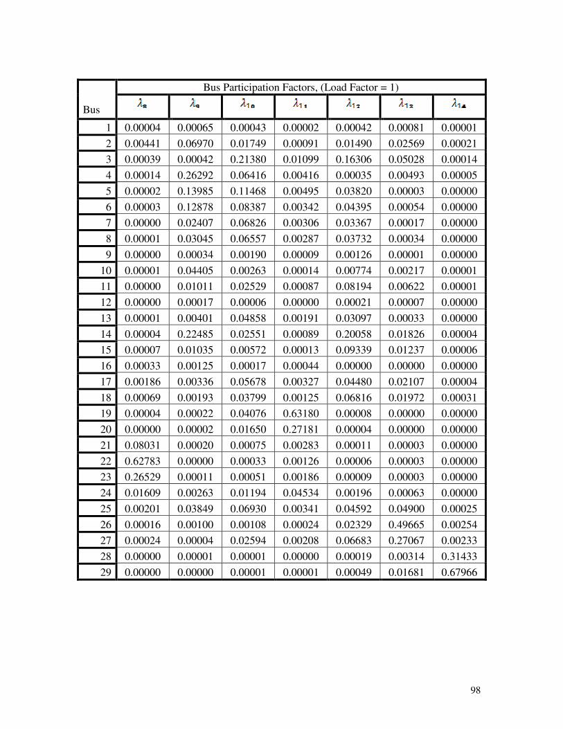
98
Bus Participation Factors, (Load Factor = 1)
Bus
1 0.00004 0.00065 0.00043 0.00002 0.00042 0.00081 0.00001
2 0.00441 0.06970 0.01749 0.00091 0.01490 0.02569 0.00021
3 0.00039 0.00042 0.21380 0.01099 0.16306 0.05028 0.00014
4 0.00014 0.26292 0.06416 0.00416 0.00035 0.00493 0.00005
5 0.00002 0.13985 0.11468 0.00495 0.03820 0.00003 0.00000
6 0.00003 0.12878 0.08387 0.00342 0.04395 0.00054 0.00000
7 0.00000 0.02407 0.06826 0.00306 0.03367 0.00017 0.00000
8 0.00001 0.03045 0.06557 0.00287 0.03732 0.00034 0.00000
9 0.00000 0.00034 0.00190 0.00009 0.00126 0.00001 0.00000
10 0.00001 0.04405 0.00263 0.00014 0.00774 0.00217 0.00001
11 0.00000 0.01011 0.02529 0.00087 0.08194 0.00622 0.00001
12 0.00000 0.00017 0.00006 0.00000 0.00021 0.00007 0.00000
13 0.00001 0.00401 0.04858 0.00191 0.03097 0.00033 0.00000
14 0.00004 0.22485 0.02551 0.00089 0.20058 0.01826 0.00004
15 0.00007 0.01035 0.00572 0.00013 0.09339 0.01237 0.00006
16 0.00033 0.00125 0.00017 0.00044 0.00000 0.00000 0.00000
17 0.00186 0.00336 0.05678 0.00327 0.04480 0.02107 0.00004
18 0.00069 0.00193 0.03799 0.00125 0.06816 0.01972 0.00031
19 0.00004 0.00022 0.04076 0.63180 0.00008 0.00000 0.00000
20 0.00000 0.00002 0.01650 0.27181 0.00004 0.00000 0.00000
21 0.08031 0.00020 0.00075 0.00283 0.00011 0.00003 0.00000
22 0.62783 0.00000 0.00033 0.00126 0.00006 0.00003 0.00000
23 0.26529 0.00011 0.00051 0.00186 0.00009 0.00003 0.00000
24 0.01609 0.00263 0.01194 0.04534 0.00196 0.00063 0.00000
25 0.00201 0.03849 0.06930 0.00341 0.04592 0.04900 0.00025
26 0.00016 0.00100 0.00108 0.00024 0.02329 0.49665 0.00254
27 0.00024 0.00004 0.02594 0.00208 0.06683 0.27067 0.00233
28 0.00000 0.00001 0.00001 0.00000 0.00019 0.00314 0.31433
29 0.00000 0.00000 0.00001 0.00001 0.00049 0.01681 0.67966
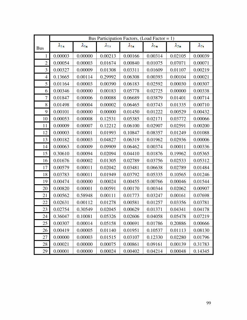
99
Bus Participation Factors, (Load Factor = 1)
Bus
1 0.00003 0.00000 0.00213 0.00166 0.00314 0.02105 0.00039
2 0.00054 0.00003 0.01674 0.00840 0.01075 0.07071 0.00071
3 0.00327 0.00009 0.01308 0.03311 0.01609 0.01107 0.00219
4 0.13665 0.00114 0.29992 0.06308 0.00393 0.00104 0.00021
5 0.01164 0.00003 0.00390 0.06183 0.02592 0.00030 0.00307
6 0.00346 0.00000 0.00183 0.05778 0.02725 0.00000 0.00338
7 0.01847 0.00006 0.00088 0.06689 0.03879 0.01401 0.00714
8 0.01498 0.00004 0.00002 0.06465 0.03743 0.01335 0.00710
9 0.00101 0.00000 0.00000 0.01450 0.01222 0.00529 0.00432
10 0.00053 0.00008 0.12531 0.05385 0.02171 0.03772 0.00066
11 0.00009 0.00007 0.12212 0.06100 0.02907 0.02591 0.00200
12 0.00003 0.00001 0.01993 0.10847 0.08357 0.01249 0.01088
13 0.00182 0.00003 0.04827 0.06319 0.01962 0.02936 0.00006
14 0.00063 0.00009 0.09909 0.06462 0.00374 0.00011 0.00336
15 0.30610 0.00094 0.02094 0.04410 0.01876 0.19962 0.05365
16 0.01676 0.00002 0.01305 0.02789 0.03756 0.02533 0.05312
17 0.00579 0.00011 0.02042 0.03481 0.06638 0.02789 0.01484
18 0.03783 0.00011 0.01949 0.03792 0.05335 0.10565 0.01246
19 0.00474 0.00000 0.00024 0.00455 0.00766 0.00046 0.01544
20 0.00820 0.00001 0.00591 0.00170 0.00344 0.02062 0.00907
21 0.00562 0.58948 0.00111 0.01773 0.03247 0.00161 0.07698
22 0.02631 0.00112 0.01278 0.00581 0.01257 0.03356 0.03781
23 0.02754 0.30549 0.02045 0.00629 0.01371 0.04341 0.04178
24 0.36047 0.10081 0.05326 0.02606 0.04058 0.05478 0.07219
25 0.00307 0.00014 0.05158 0.00691 0.01786 0.20886 0.00666
26 0.00419 0.00005 0.01140 0.01951 0.10537 0.01113 0.08130
27 0.00000 0.00003 0.01515 0.03107 0.12330 0.02280 0.01796
28 0.00021 0.00000 0.00075 0.00861 0.09161 0.00139 0.31783
29 0.00001 0.00000 0.00024 0.00402 0.04214 0.00048 0.14345

100
Bus Participation Factors, (Load Factor = 1)
Bus
1 0.00139 0.20932 0.06536 0.59969 0.01289 0.05105 0.02479 0.00070
2 0.00160 0.08450 0.09381 0.01460 0.00006 0.03053 0.00683 0.00011
3 0.00493 0.08906 0.01149 0.00132 0.00703 0.11707 0.07160 0.00075
4 0.01086 0.00719 0.01063 0.00004 0.05200 0.00037 0.02031 0.00023
5 0.04231 0.00068 0.00186 0.00000 0.00449 0.00818 0.01627 0.00264
6 0.03120 0.00110 0.00149 0.00000 0.00361 0.00461 0.01954 0.00282
7 0.10132 0.00569 0.02437 0.00000 0.00278 0.03226 0.05639 0.00552
8 0.10861 0.00618 0.02080 0.00000 0.00871 0.02655 0.03885 0.00339
9 0.09757 0.01446 0.02024 0.00000 0.48171 0.06631 0.23254 0.04436
10 0.00736 0.00004 0.02268 0.00003 0.02899 0.04840 0.00053 0.00000
11 0.00210 0.00018 0.00970 0.00001 0.01521 0.01691 0.00169 0.00048
12 0.56144 0.00230 0.01383 0.00017 0.13589 0.04895 0.00077 0.00000
13 0.01630 0.00000 0.02866 0.00005 0.04111 0.07366 0.00703 0.00041
14 0.00114 0.00006 0.01329 0.00012 0.07788 0.07391 0.03442 0.00349
15 0.00119 0.01365 0.04873 0.00120 0.01917 0.06552 0.02450 0.01412
16 0.00046 0.01283 0.02651 0.00058 0.00006 0.00158 0.00062 0.00338
17 0.00008 0.01160 0.05550 0.02595 0.00210 0.00532 0.00360 0.00060
18 0.00160 0.05810 0.04070 0.02721 0.00003 0.09408 0.05326 0.00170
19 0.00017 0.00799 0.00806 0.00101 0.00015 0.00447 0.04443 0.21523
20 0.00012 0.00725 0.05598 0.00133 0.00021 0.01569 0.11395 0.46772
21 0.00095 0.06282 0.01395 0.02772 0.00890 0.00320 0.00309 0.04555
22 0.00054 0.04573 0.06191 0.02803 0.00959 0.00776 0.00583 0.07169
23 0.00060 0.05158 0.07599 0.03215 0.01103 0.00928 0.00689 0.08402
24 0.00073 0.02931 0.03487 0.00443 0.00103 0.00118 0.00023 0.00016
25 0.00071 0.06571 0.19894 0.00316 0.00166 0.01215 0.00001 0.00170
26 0.00016 0.00838 0.02831 0.03457 0.01492 0.06096 0.07134 0.01012
27 0.00002 0.02686 0.00422 0.11710 0.03140 0.09353 0.09739 0.01149
28 0.00314 0.12312 0.00589 0.05558 0.01920 0.01886 0.03069 0.00537
29 0.00141 0.05428 0.00224 0.02395 0.00821 0.00767 0.01263 0.00224

101
Bus Participation Factors, (Load Factor = 1.25)
Bus
1 0.00000 0.00000 0.00000 0.00000 0.00068 0.00006 0.00382
2 0.00000 0.00000 0.00001 0.00001 0.10266 0.00803 0.45917
3 0.00001 0.00001 0.00018 0.00006 0.11082 0.00620 0.04629
4 0.00364 0.00101 0.00000 0.00160 0.01265 0.00001 0.00689
5 0.38672 0.02275 0.00001 0.01450 0.00139 0.08300 0.00040
6 0.53034 0.00576 0.00000 0.02084 0.00021 0.01101 0.00083
7 0.02241 0.00154 0.00000 0.45597 0.00052 0.01378 0.00003
8 0.01579 0.00225 0.00000 0.49238 0.00031 0.00001 0.00017
9 0.00001 0.00000 0.00000 0.00202 0.00000 0.00000 0.00000
10 0.00933 0.58208 0.00009 0.00108 0.00072 0.00031 0.00023
11 0.03055 0.17901 0.00004 0.00515 0.01526 0.35635 0.00001
12 0.00002 0.00071 0.00000 0.00000 0.00000 0.00000 0.00000
13 0.00117 0.19744 0.00000 0.00507 0.01802 0.36350 0.00015
14 0.00000 0.00729 0.00029 0.00128 0.01985 0.11707 0.00146
15 0.00000 0.00006 0.03148 0.00002 0.00967 0.00173 0.00145
16 0.00000 0.00006 0.73879 0.00000 0.02714 0.00274 0.00824
17 0.00000 0.00000 0.08987 0.00001 0.33770 0.01554 0.14168
18 0.00000 0.00000 0.00669 0.00001 0.26435 0.01393 0.03783
19 0.00000 0.00000 0.00940 0.00000 0.00226 0.00025 0.00107
20 0.00000 0.00000 0.00016 0.00000 0.00016 0.00002 0.00010
21 0.00000 0.00000 0.01639 0.00000 0.00358 0.00041 0.00911
22 0.00000 0.00000 0.00037 0.00000 0.00074 0.00010 0.03050
23 0.00000 0.00000 0.00023 0.00000 0.00006 0.00000 0.00875
24 0.00000 0.00001 0.10485 0.00000 0.02440 0.00268 0.00741
25 0.00000 0.00000 0.00000 0.00000 0.02780 0.00238 0.20313
26 0.00000 0.00000 0.00002 0.00000 0.00030 0.00000 0.01324
27 0.00000 0.00000 0.00113 0.00000 0.01876 0.00089 0.01794
28 0.00000 0.00000 0.00000 0.00000 0.00000 0.00000 0.00007
29 0.00000 0.00000 0.00000 0.00000 0.00000 0.00000 0.00003
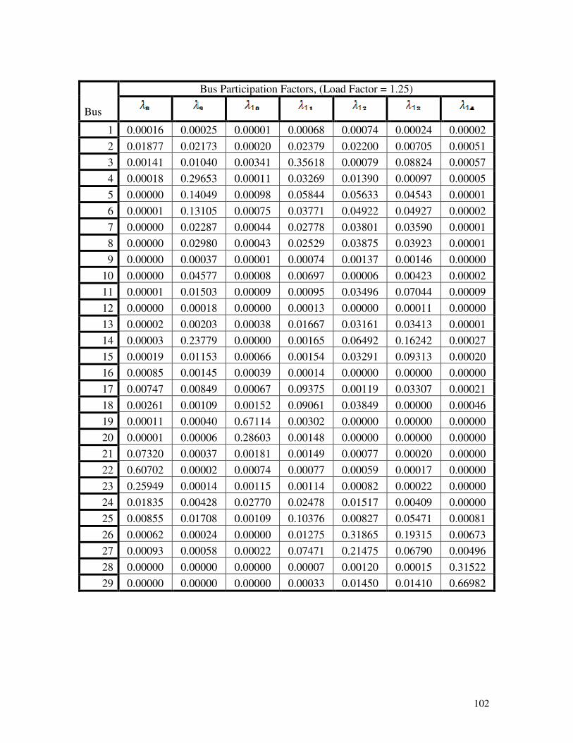
102
Bus Participation Factors, (Load Factor = 1.25)
Bus
1 0.00016 0.00025 0.00001 0.00068 0.00074 0.00024 0.00002
2 0.01877 0.02173 0.00020 0.02379 0.02200 0.00705 0.00051
3 0.00141 0.01040 0.00341 0.35618 0.00079 0.08824 0.00057
4 0.00018 0.29653 0.00011 0.03269 0.01390 0.00097 0.00005
5 0.00000 0.14049 0.00098 0.05844 0.05633 0.04543 0.00001
6 0.00001 0.13105 0.00075 0.03771 0.04922 0.04927 0.00002
7 0.00000 0.02287 0.00044 0.02778 0.03801 0.03590 0.00001
8 0.00000 0.02980 0.00043 0.02529 0.03875 0.03923 0.00001
9 0.00000 0.00037 0.00001 0.00074 0.00137 0.00146 0.00000
10 0.00000 0.04577 0.00008 0.00697 0.00006 0.00423 0.00002
11 0.00001 0.01503 0.00009 0.00095 0.03496 0.07044 0.00009
12 0.00000 0.00018 0.00000 0.00013 0.00000 0.00011 0.00000
13 0.00002 0.00203 0.00038 0.01667 0.03161 0.03413 0.00001
14 0.00003 0.23779 0.00000 0.00165 0.06492 0.16242 0.00027
15 0.00019 0.01153 0.00066 0.00154 0.03291 0.09313 0.00020
16 0.00085 0.00145 0.00039 0.00014 0.00000 0.00000 0.00000
17 0.00747 0.00849 0.00067 0.09375 0.00119 0.03307 0.00021
18 0.00261 0.00109 0.00152 0.09061 0.03849 0.00000 0.00046
19 0.00011 0.00040 0.67114 0.00302 0.00000 0.00000 0.00000
20 0.00001 0.00006 0.28603 0.00148 0.00000 0.00000 0.00000
21 0.07320 0.00037 0.00181 0.00149 0.00077 0.00020 0.00000
22 0.60702 0.00002 0.00074 0.00077 0.00059 0.00017 0.00000
23 0.25949 0.00014 0.00115 0.00114 0.00082 0.00022 0.00000
24 0.01835 0.00428 0.02770 0.02478 0.01517 0.00409 0.00000
25 0.00855 0.01708 0.00109 0.10376 0.00827 0.05471 0.00081
26 0.00062 0.00024 0.00000 0.01275 0.31865 0.19315 0.00673
27 0.00093 0.00058 0.00022 0.07471 0.21475 0.06790 0.00496
28 0.00000 0.00000 0.00000 0.00007 0.00120 0.00015 0.31522
29 0.00000 0.00000 0.00000 0.00033 0.01450 0.01410 0.66982

103
Bus Participation Factors, (Load Factor = 1.25)
Bus
1 0.00002 0.00000 0.00134 0.00482 0.00321 0.02872 0.00054
2 0.00032 0.00001 0.00707 0.02724 0.01159 0.07785 0.00103
3 0.00038 0.00002 0.02951 0.00740 0.02041 0.00654 0.00175
4 0.12714 0.00055 0.06549 0.32048 0.00179 0.00100 0.00045
5 0.01702 0.00003 0.06804 0.00452 0.02262 0.00017 0.00290
6 0.00688 0.00000 0.06384 0.00164 0.02430 0.00020 0.00320
7 0.02214 0.00005 0.07472 0.00176 0.03575 0.00918 0.00751
8 0.01847 0.00003 0.07192 0.00023 0.03430 0.00933 0.00748
9 0.00122 0.00000 0.01418 0.00003 0.00998 0.00355 0.00421
10 0.00019 0.00001 0.05667 0.11056 0.01797 0.04304 0.00025
11 0.00125 0.00001 0.06511 0.11084 0.02503 0.03392 0.00134
12 0.00001 0.00000 0.11689 0.01609 0.07778 0.01120 0.00755
13 0.00307 0.00001 0.06602 0.03943 0.01532 0.02734 0.00002
14 0.00438 0.00001 0.06574 0.10083 0.00149 0.00473 0.00512
15 0.27987 0.00083 0.04023 0.00319 0.02604 0.20023 0.05747
16 0.02189 0.00000 0.02383 0.01556 0.04365 0.01509 0.05155
17 0.00308 0.00004 0.02913 0.01489 0.07393 0.04145 0.01237
18 0.03692 0.00008 0.03224 0.01522 0.06123 0.12588 0.01039
19 0.00430 0.00000 0.00382 0.00006 0.00852 0.00047 0.01463
20 0.00944 0.00000 0.00143 0.00775 0.00381 0.01361 0.00865
21 0.00485 0.58648 0.01504 0.00005 0.03674 0.00174 0.07463
22 0.03007 0.00198 0.00490 0.01574 0.01379 0.02132 0.03594
23 0.03227 0.31243 0.00529 0.02185 0.01501 0.02683 0.03962
24 0.37158 0.09736 0.02193 0.05328 0.04628 0.03093 0.06954
25 0.00083 0.00004 0.00570 0.07215 0.01825 0.22491 0.00788
26 0.00229 0.00002 0.01538 0.00976 0.10350 0.01866 0.09035
27 0.00001 0.00001 0.02503 0.02358 0.12703 0.01861 0.02370
28 0.00012 0.00000 0.00647 0.00078 0.08268 0.00260 0.31734
29 0.00001 0.00000 0.00305 0.00026 0.03798 0.00089 0.14262
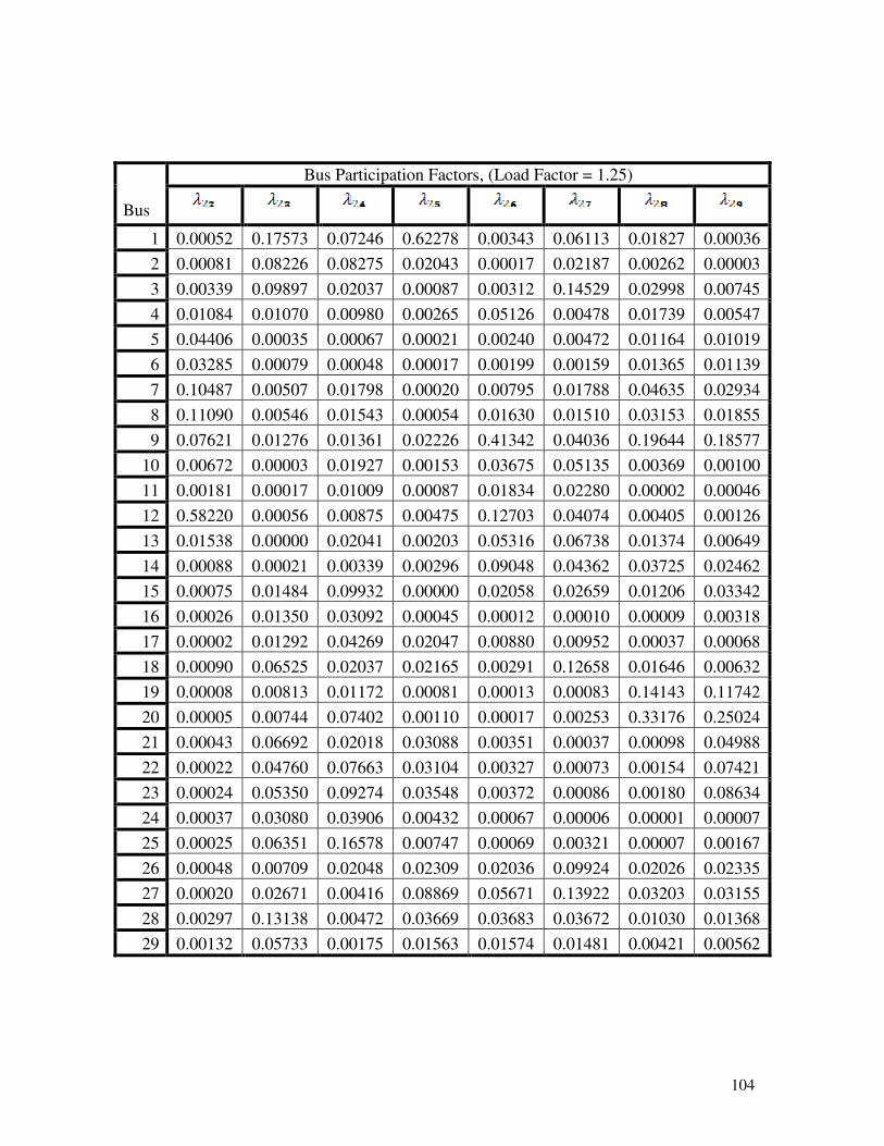
104
Bus Participation Factors, (Load Factor = 1.25)
Bus
1 0.00052 0.17573 0.07246 0.62278 0.00343 0.06113 0.01827 0.00036
2 0.00081 0.08226 0.08275 0.02043 0.00017 0.02187 0.00262 0.00003
3 0.00339 0.09897 0.02037 0.00087 0.00312 0.14529 0.02998 0.00745
4 0.01084 0.01070 0.00980 0.00265 0.05126 0.00478 0.01739 0.00547
5 0.04406 0.00035 0.00067 0.00021 0.00240 0.00472 0.01164 0.01019
6 0.03285 0.00079 0.00048 0.00017 0.00199 0.00159 0.01365 0.01139
7 0.10487 0.00507 0.01798 0.00020 0.00795 0.01788 0.04635 0.02934
8 0.11090 0.00546 0.01543 0.00054 0.01630 0.01510 0.03153 0.01855
9 0.07621 0.01276 0.01361 0.02226 0.41342 0.04036 0.19644 0.18577
10 0.00672 0.00003 0.01927 0.00153 0.03675 0.05135 0.00369 0.00100
11 0.00181 0.00017 0.01009 0.00087 0.01834 0.02280 0.00002 0.00046
12 0.58220 0.00056 0.00875 0.00475 0.12703 0.04074 0.00405 0.00126
13 0.01538 0.00000 0.02041 0.00203 0.05316 0.06738 0.01374 0.00649
14 0.00088 0.00021 0.00339 0.00296 0.09048 0.04362 0.03725 0.02462
15 0.00075 0.01484 0.09932 0.00000 0.02058 0.02659 0.01206 0.03342
16 0.00026 0.01350 0.03092 0.00045 0.00012 0.00010 0.00009 0.00318
17 0.00002 0.01292 0.04269 0.02047 0.00880 0.00952 0.00037 0.00068
18 0.00090 0.06525 0.02037 0.02165 0.00291 0.12658 0.01646 0.00632
19 0.00008 0.00813 0.01172 0.00081 0.00013 0.00083 0.14143 0.11742
20 0.00005 0.00744 0.07402 0.00110 0.00017 0.00253 0.33176 0.25024
21 0.00043 0.06692 0.02018 0.03088 0.00351 0.00037 0.00098 0.04988
22 0.00022 0.04760 0.07663 0.03104 0.00327 0.00073 0.00154 0.07421
23 0.00024 0.05350 0.09274 0.03548 0.00372 0.00086 0.00180 0.08634
24 0.00037 0.03080 0.03906 0.00432 0.00067 0.00006 0.00001 0.00007
25 0.00025 0.06351 0.16578 0.00747 0.00069 0.00321 0.00007 0.00167
26 0.00048 0.00709 0.02048 0.02309 0.02036 0.09924 0.02026 0.02335
27 0.00020 0.02671 0.00416 0.08869 0.05671 0.13922 0.03203 0.03155
28 0.00297 0.13138 0.00472 0.03669 0.03683 0.03672 0.01030 0.01368
29 0.00132 0.05733 0.00175 0.01563 0.01574 0.01481 0.00421 0.00562
Top Related

Copyright © 2022 FDOKUMEN

