USE OF ARTIFICIAL NEURAL NETWORKS FOR PREDICTION OF CODFISH DRYING OPTIMAL PARAMETERS

Camila N. Boeri*, Fernando J. Neto da Silva and Jorge A. F. Ferreira Department of Mechanical Engineering, Centre for Mechanical Technology & Automation,

University of Aveiro, Aveiro, Portugal *email: camilaboeri@ua.pt

Abstract An artificial neural network was developed for codfish drying to predict the dimensionless moisture content. Four drying parameters (drying time, temperature, air velocity and relative humidity) were the inputs of the neural network. The standard error was 0.96%, average error of 2.93% with average relative deviation of 3.70 for twenty predictions of drying curves. Using a programming for optimization of the drying parameters development in the Matlab platform with the neural network obtained for codfish drying, the optimal values for desired final moisture of 0.60 are drying time of 70h, temperature of 22.85°C, relative humidity of 41.26% and air velocity of 1.5m/s. Keywords: drying; optimization; artificial neural network; codfish 1. Introduction As all fish, fresh codfish (Gadus Morhua) is susceptible to deterioration by fast destructive action of enzymes, oxidation of lipids, high pH, high water activity, with formation of accentuated contents of non-protein nitrogen substances (Oehlenschläger and Rehbein, 2009). Accordingly, it is of critical importance to adopt measures ensuring perfect conservation immediately after capture and during distribution and commercialization. Convective drying is of prime importance in the food preservation industry and has been constantly studied and improved to obtain products with higher quality and lower processing time. The correct definition of drying procedures of a vast range of products is crucial in what concerns energy minimization and minimal time of kiln residence without compromising the final product quality. Several parameters influence the time required to reduce the moisture content of the codfish. The principal external factors to consider are air temperature, relative humidity and velocity. Whole salted codfish drying prevents the utilization of temperatures above 20°C-22°C, since they lead to an inevitable deterioration of the product. Hence convective drying must be conducted without exceeding the required temperature limits. These limitations seriously increase both the drying time and the energy consumption. According Zhang et al. (2002), artificial neural networks (ANNs) are used to solve a wide variety of problems in science and engineering, particularly for some areas where the conventional modelling methods fail. A well trained ANN can be used as a predictive model for a specific application, which is a data-processing system inspired by biological neural system. The predictive ability of an ANN results from the training on experimental data and then validation by independent data (Mittal and Zhang, 2000). In the literature, there are several studies about drying of salted fish and fresh fish. Due to the particular product used in this study, no data for comparison of results for modeling with artificial neural networks was available. However, for other types of products, the neural network has been used to simulate the drying process. Cubillos et al. (1996) simulate the process of solid particles drying by neural networks and the analytical model, from data collected by the equations of mass and energy balance. The objective was to predict the behavior of the drying process by the fluidized bed. The networks performed

Camila N. Boeri, Fernando J. Neto da Silva and Jorge A. F. Ferreira, G. J. P&A Sc and Tech., 2011v01i2 (1-14) ISSN: 2249-7188

GJPAST | SEP - OCT 2011 Available online @www.gjpast.com

1

better than the phenomenological models, although still the transport mechanisms involved in this operation are not easily explained mathematically. The modeling of an industrial dryer gelatin through the use of artificial neural networks was studied by Francisco (2000). By means of a neural network for direct feed, consisting of three layers was made for the final moisture of the gelatin industry out of the dryer, and these values were compared to measurements of moisture held in the laboratory. Actual data of the drying process gelatin were also used in the training phase of the network, and for this, used the Levenberg-Marquardt algorithm. The results of simulations indicate great potential of using RNA for modeling the drying system, thus enabling the prediction of moisture content of the gelatin to the end of the drying stage. Chen et al. (2001) trained neural network to optimize the quality changes during osmotic and convective drying of blueberries using the backpropagation learning algorithm and multilayer neural model (ranging from 1 to 3) with three inputs (contact time, temperature and osmotic solution concentration) and 4 outputs (convective drying time, color, texture and rehydration ratio). The best performance of the network was chosen by varying the parameters, transfer function (sigmoid, hyperbolic tangent and linear), number of neurons in the hidden layer (5-15) and layers (1-3) hidden, number of presentations (2000 to 20000) and the factor of learning that was dynamic. They confirmed the better performance of the neural network model for optimization of the process with a hidden layer and 10 neurons in the hidden layer, 20000 presentations and hyperbolic tangent transfer function. With neural networks resulted in an excellent predictor of the process was better when compared to multiple regression. Zhang (2002) developed a neural network for drying paddy rice to predict six performance indicators: energy consumption, cracks, final moisture content, moisture removal rate, intensity of drying and removal rate of the water body. Four drying parameters (thickness of the rice, hot air flow, temperature and drying time) were the inputs of the neural network. After evaluating a large number of tests with different ANN architectures, the ideal model consisted of four layers, with 8 and 5 neurons in the first and second hidden layers, respectively. The effectiveness of the proposed model is demonstrated through comparison with experimental data, where the mean relative error ranged from 2.0 to 8.3% for six predictions, with an average of 4.4%. The properties of the drying air were also provided by the neural network model. Mittal and Zhang (2003) developed a neural model with multiple hidden layers of neurons, based on the psychometric chart for calculating real-time properties of air required for drying post-harvest food. The data file for training and testing the network was generated from mathematical models was studied. The relative error generated to predict the characteristics of the air was less than 5%. Islam et al. (2003) presented a model in artificial neural networks to predict the drying rate curves for convective drying of potato slices under different operating conditions of speed, temperature and relative humidity. The objective was to find the parameters of Page’s model of (outputs of the ANN) to optimize the drying time needed to reduce the initial water content of the product. Erenturk et al. (2004) studied the kinetics of drying of medicinal root Echinacea angustifoliais and made a comparative study between the simulations and regression analysis using a multilayer feedforward neural network to estimate the dynamics of drying. Tests were performed at temperatures of 15, 30 and 45°C with air velocities of 0.3, 0.7 and 1.1 m/s, and root diameters of 3mm or less, between 3 and 6mm and 6mm or more. An ANN with three layers was used to estimate the drying curves of the roots. Comparing the values of errors between the mathematical

Camila N. Boeri, Fernando J. Neto da Silva and Jorge A. F. Ferreira, G. J. P&A Sc and Tech., 2011v01i2 (1-14) ISSN: 2249-7188

GJPAST | SEP - OCT 2011 Available online @www.gjpast.com

2

models and neural network analysis, we concluded that RNA is better drying characteristics than the mathematical models. Movagharnejad and Nikzad (2007) studied the drying of tomatoes in a tray dryer at different temperatures and air velocities. The data were modeled using artificial neural networks and empirical models. The simulation results were compared with experimental data and found that the predictions of ANN fit the experimental data with greater accuracy compared with empirical models. The kinetics of drying of pistachio (Akbari v.) was simulated using a multilayer neural network feedforward by Omid et al. (2009). Tests were conducted to five drying air temperatures (ranging from 40 to 80°C) and four air velocities (ranging from 0.5 to 2 m/s), with three replicates in a thin layer dryer. To find the optimal model, different network topologies were trained, with one or two hidden layers of neurons, and their predictive performances were evaluated. A network with eight neurons in first hidden layer and five neurons in the second hidden layer resulted in the most appropriate model to estimate the moisture content of pistachios for all tests. Çakmak and Yildiz (2011) presented an application that uses the feedforward neural networks to model the nonlinear behavior of drying grapes. Through ANN, they estimated the values of drying rates of grapes, comparing them with the values obtained by nonlinear regression. The results obtained by the authors indicate that the neural network is more accurate and performed more consistently than the alternative approaches employed in estimating the rate of drying. The objectives of this study were to develop an artificial neural network for predicting the codfish drying curves using experimental data and to optimize the drying parameters using the chosen ANN. 2. Materials and Methods 2.1. Experiments The experiments were conducted for salted codfish drying in a convective dryer using four temperatures (15°C, 18°C, 20°C and 23°C), six relative humidities (40%, 45%, 50%, 55%, 60% and 65%) and two air velocities (1.5m/s and 2m/s). The experimental installation consists in a centrifugal blower, driven by a variable velocity AC motor which defines the air velocity control within the drying chamber. The air is forced through electric heating resistances allowing the air temperature control to be raised. Steam at atmospheric pressure is used for humidification and a dehumidifier is used for cooling and dehumidifying the air. The air velocity is measured by an air velocity transmitter (Omega, model FMA 1000). The air temperature and the relative humidity are acquired through a digital thermo-hygrometer (Omega, model RH411).

Figure 1: Experimental installation scheme

Camila N. Boeri, Fernando J. Neto da Silva and Jorge A. F. Ferreira, G. J. P&A Sc and Tech., 2011v01i2 (1-14) ISSN: 2249-7188

GJPAST | SEP - OCT 2011 Available online @www.gjpast.com

3

The codfishes were cut into samples (filleted form), with an approximate mass of 100g each (Figure 2) and kept until utilization tightly wrapped in plastic bags in a refrigerator at 5ºC. The samples had an average thickness of 2.5cm. The oven drying method was used to determine the initial and the final moisture contents of the samples, based on the AOAC 1990 protocol (Cunniff, 1998). The method implied extracting small parts from the cut samples and their drying in a controlled temperature environment at 105±2ºC during, at least, 48 hours. The average initial moisture content of all samples was 62% with a standard deviation of 3.83% which shows that, since the samples were extracted from different parts of the fishes, the initial water content is more or less uniform throughout the fish. This result is not unexpected since, previous to drying, the fish was kept in salt for four weeks and then stored in a refrigerated chamber. These features of the codfish processing industry allow for a good degree of homogeneity in what concerns moisture distribution. The average final moisture content of all samples was 46.89% with a standard deviation of 3.18%. The equilibrium moisture content of the codfish was determined experimentally in a hygrometric chamber, where the desired values of relative humidity and temperature were controlled.

Figure 2: Codfish sample

The dimensionless moisture content was computed with the following equation:

(1)

where X is the instantaneous moisture content of the product, Xf is the final moisture content and X0 is the initial moisture content. 2.2. Artificial Neural Network The neural networks are a problem solving concept which represents an alternative to conventional algorithmic methods (Kalogirou, 2000). The steps for creating a neural network are: Setting standards, initialize the network, define the training parameters, train the network and test the network. To get the best prediction by an ANN, several network architectures were evaluated. There are four drying parameters and one performance indices in the prediction model for salted codfish drying. The four drying parameters are drying time (h), temperature (°C), relative humidity (%) and air velocity (m/s), which are the inputs to the proposed artificial neural network. The performance indices for evaluating the drying process with different drying parameters is the moisture content (dimensionless) which is the output of the ANN.

Camila N. Boeri, Fernando J. Neto da Silva and Jorge A. F. Ferreira, G. J. P&A Sc and Tech., 2011v01i2 (1-14) ISSN: 2249-7188

GJPAST | SEP - OCT 2011 Available online @www.gjpast.com

4

For the modeling of the drying process, were used a neural network with an input layer, consisting of four neurons, one hidden layer and an output layer formed by one neuron, according to the scheme shown in figure 3:

Input Hidden Output

Drying time

Temperature

Relative Humidity

Air velocity

Moisture content

Figure 3: ANN architecture proposed for the codfish drying process

At this stage of modeling is determined the best architecture of the neural network representing the process. The networks have tested a single hidden layer of neurons, as this simple architecture has the advantage of fewer network parameters to be adjusted (Cocco, 2003). Tests were conducted with two different network configurations, varying the number of neurons in the hidden layer. According to Hecht-Nielsen (1989), the hidden layer must have a value close to 2i +1 neurons, where i is the number of input variables. Since Lippmann (1987) states that in the case of only one hidden layer, it should be s(i +1) neurons, where s is the number of output neurons and i is the number of neurons in the input. Thus, networks were tested with 5 and 9 neurons in hidden layer. The architecture of the neural network used in this work is the feedforward network (propagation) multilayer, and his training is related through the backpropagation learning algorithm. The transfer functions were chosen after several tests to see which ones best performance. For training the network were used the Levenberg-Marquardt algorithm, due to the robustness of this method. This algorithm is the fastest method for training feedforward backpropagation network, which has a moderate amount of synaptic weights. To speed up the training process, this algorithm is based on the determination of second derivatives of the squared error with respect to the weights, differing from the traditional backpropagation algorithm considers the first derivatives (Barbosa, Davis and Snow, 2005). The steps of training and validation of the neural network were performed using the Neural Network Toolbox of Matlab ®. The training step the network is to adjust the weights of the connections of neurons, so as to have the best representation of the relationship between pairs of input data from the network (drying time, temperature, relative humidity and air velocity) and its output (moisture content). Thus, a set of samples is used to perform the step of training the neural network, going well, learning the

Camila N. Boeri, Fernando J. Neto da Silva and Jorge A. F. Ferreira, G. J. P&A Sc and Tech., 2011v01i2 (1-14) ISSN: 2249-7188

GJPAST | SEP - OCT 2011 Available online @www.gjpast.com

5

network of relationships between the variables of input and output of this process. The training set is given by a matrix of dimension 1650x4. For this step, is needed to set some parameters to the function of training. Initially, were defined the criteria for stopping the training of the network, which are two key parameters:

net.trainParam.epochs = 5000; net.trainParam.goal = 10-6

Once trained the network, a new set of pairs of input data (which were not used during the training process) are presented to the network, thus obtaining, for simulation with the weights obtained during training, the data for desired output, ie the codfish moisture content. The moisture content calculated by the model is then compared to the actual value obtained experimentally for that sample, verifying thus the performance of the modeling performed for the process.

2.3. Optimization of Drying Parameters The model obtained by neural network was subjected to an optimization algorithm, in order to find the ideal parameters of drying, minimize the processing time and maximize codfish water loss. For optimization, a computer program was developed using MATLAB based on enumerative method. Each solution within a specific range of the drying parameters was evaluated by the objective function. The optimal solution within a specific range was provided by the program. The parameters subject to optimization are the inputs of the neural network: drying time, temperature, relative humidity and air velocity. 3. Results and Discussion 3.1. Neural network simulations The configuration chosen to represent the drying process is shown in table 2:

Table 1: Configuration parameters of the neural network chosen to represent the codfish drying process Parameters Values Number of inputs 4 Number of output 1 Number of sets made for training 33 Number of sets made for testing 20 Number of neurons in the hidden layer 9 Transfer function in hidden layer Sigmoid function Transfer function in output layer Linear function Network training algorithm Levenberg-Marquardt Number of iterations 147 Mean square error of the training 0.000038 Mean square error of the test 0.00011 The best results were obtained for the trained network with 9 neurons in hidden layer. Figures 4 and 5 present the results for train at 5 and 9 neurons.

Camila N. Boeri, Fernando J. Neto da Silva and Jorge A. F. Ferreira, G. J. P&A Sc and Tech., 2011v01i2 (1-14) ISSN: 2249-7188

GJPAST | SEP - OCT 2011 Available online @www.gjpast.com

6

Figure 4: Performance and regression line for the network with 9 neurons

Figure 5: Performance and regression line for the network with 9 neurons

The weight matrix of hidden layer (IW) showed the following values:

0,0369 9,5237 0,2149 0,64940,1063 6,0676 0,8265 2,65690,0560 24,4957 0,0051 1,2625

0,0313 4,2962 0,1113 0,13640,0392 6,3868 0,1046 0,80420,0489 7,2864 0,1132 0,1055

0,2965 4,1949 0,0289 0,79200,0510 0,0669 0,010

−− −

− −−

−−

− − −− − − 0 0,01910,0366 6,2043 0,1211 0,6875

Since the weight matrix of output layer is given by:

[ ]0,0953 0,0738 0,0574 0,0793 0,1291 0,0497 0,0060 0,4331 0,0957LW = − − − −

Camila N. Boeri, Fernando J. Neto da Silva and Jorge A. F. Ferreira, G. J. P&A Sc and Tech., 2011v01i2 (1-14) ISSN: 2249-7188

GJPAST | SEP - OCT 2011 Available online @www.gjpast.com

7

The bias vector of hidden layer and output layer are shown below:

1

14,85505,8286

22,89605,73751,1892

18,184916,3718

0,552027,5025

b

− − − − = − − −

−

[ ]2 1,3527b = Based on the configuration obtained, the model that describes the neural network used to describe the kinetics of drying of cod can be written as in equation:

1 2[ tan ( ) ] (2)Output purelin LW sig IW inputs b b= ⋅ ⋅ + +

where: purelin (n) = n (3)

( ) ( 2 )

2 (4)(1 ) 1ntansig n

e −=+ −

Using the functions (3) and (4), the output of the neural network can be displayed as shown by equation (5). This is the model that will be used in the optimization algorithm:

1

2

2( )

2 (5)1 1IW inputs b

output LW be− ⋅ +

= ⋅ + + −

For the validation of the neural network was used 20 experiments that had not been used in the training phase of the network. Figures 6 to 11 show the comparison between the experimental data and simulated by the neural network:

Camila N. Boeri, Fernando J. Neto da Silva and Jorge A. F. Ferreira, G. J. P&A Sc and Tech., 2011v01i2 (1-14) ISSN: 2249-7188

GJPAST | SEP - OCT 2011 Available online @www.gjpast.com

8

Figure 6: Comparison between experimental and simulated data by ANN - T=20°C, RH=45%, v=1,5m/s

Figure 7: Comparison between experimental and simulated data by ANN - T=18°C, RH=50%, v=2m/s

Camila N. Boeri, Fernando J. Neto da Silva and Jorge A. F. Ferreira, G. J. P&A Sc and Tech., 2011v01i2 (1-14) ISSN: 2249-7188

GJPAST | SEP - OCT 2011 Available online @www.gjpast.com

9

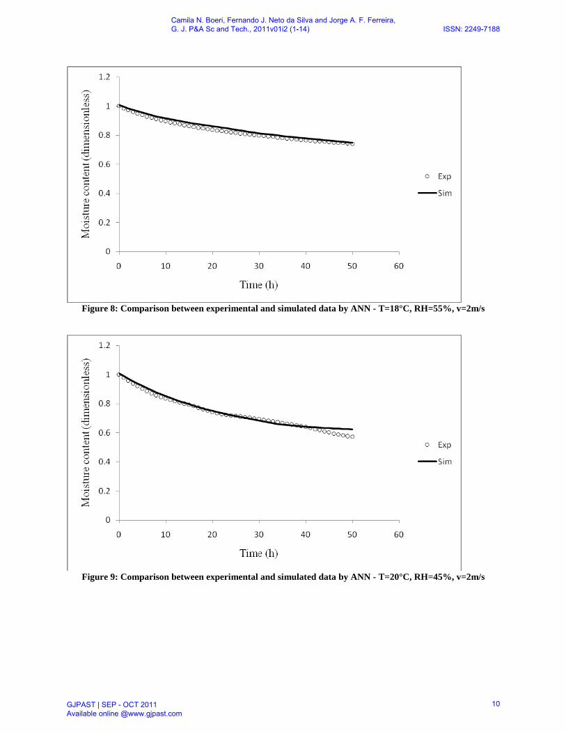
Figure 8: Comparison between experimental and simulated data by ANN - T=18°C, RH=55%, v=2m/s

Figure 9: Comparison between experimental and simulated data by ANN - T=20°C, RH=45%, v=2m/s

Camila N. Boeri, Fernando J. Neto da Silva and Jorge A. F. Ferreira, G. J. P&A Sc and Tech., 2011v01i2 (1-14) ISSN: 2249-7188

GJPAST | SEP - OCT 2011 Available online @www.gjpast.com

10

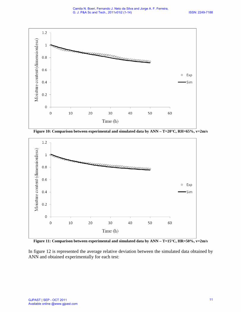
Figure 10: Comparison between experimental and simulated data by ANN – T=20°C, RH=65%, v=2m/s

Figure 11: Comparison between experimental and simulated data by ANN – T=15°C, HR=50%, v=2m/s

In figure 12 is represented the average relative deviation between the simulated data obtained by ANN and obtained experimentally for each test:

Camila N. Boeri, Fernando J. Neto da Silva and Jorge A. F. Ferreira, G. J. P&A Sc and Tech., 2011v01i2 (1-14) ISSN: 2249-7188

GJPAST | SEP - OCT 2011 Available online @www.gjpast.com

11

Figure 12: Average relative deviation for the values obtained experimentally and calculated by the neural

network In table 3 are the results of the statistics analysis obtained through the simulations by artificial neural networks.

Table 3: Statistics analysis Test | T – v - RH Standard Error (%) Average error (%) Relative deviation 1 | 20 – 2 – 45 1.566 1.386 2.017 2 | 20 – 2 – 50 1.357 1.919 2.557 3 | 20 – 2 – 55 0.698 2.614 3.899 4 | 20 – 2 – 60 0.531 3.457 4.713 5 | 20 – 2 – 65 1.144 1.954 2.367 6 | 20 – 1.5 – 45 0.482 2.407 3.484 7 | 20 – 1.5 – 50 0.996 3.703 5.184 8 | 20 – 1.5 – 55 1.207 2.756 3.556 9 | 20 – 1.5 – 60 0.935 3.456 4.041 10 | 20 – 1.5 – 65 1.301 6.991 7.538 11 | 18 – 2 – 45 0.785 3.498 5.001 12 | 18 – 2 – 50 0.574 1.125 1.367 13 | 18 – 2 – 55 0.486 1.666 2.001 14 | 18 – 2 – 60 1.966 2.113 2.324 15 | 18 – 1.5 – 65 1.501 5.270 6.159 16 | 15 – 2 – 40 1.055 1.394 1.604 17 | 15 – 2 – 50 0.525 1.629 1.966 18 | 15 – 1.5 – 50 0.439 3.323 4.180 19 | 15 – 1.5 – 55 0.718 5.529 7.025 20 | 23 – 1.5 – 50 0.997 2.409 3.014 Average 0.963 2.930 3.700

Camila N. Boeri, Fernando J. Neto da Silva and Jorge A. F. Ferreira, G. J. P&A Sc and Tech., 2011v01i2 (1-14) ISSN: 2249-7188

GJPAST | SEP - OCT 2011 Available online @www.gjpast.com

12

3.2. Optimization of drying parameters In order to meet the installation limitations, and restrictions temperature for codfish drying and time of drying, some limits on the values were established in the optimization program:

Time: [40 70] Temperature: [15 23] Relative humidity: [40 65] Air velocity: [1,5 2] Table 4 presents the values obtained in the optimization, varying the values for the desired final moisture.

Table 4: Convective drying conditions to obtain different dimensionless final moisture

Desired final moisture (-)

Time (h)

Temperature (°C)

Relative humidity (%)

Air velocity (m/s)

0.85 65.68 22.65 63.40 1.50 0.80 69.16 22.26 60.60 1.50 0.75 69.97 21.61 58.59 1.50 0.70 68.58 20.73 57.39 1.51 0.65 68.58 21.45 51.58 1.50 0.60 69.66 22.85 41.26 1.50

4. Conclusions An artificial neural network was developed to predict the drying curves of salted codfish. The predictions were very close to the experimental data, with the standard error of 0.96%, average error of 2.93% and average relative deviation of 3.70 for twenty predictions of drying curves. From the model obtained with the best trained neural network configuration, were developed an optimization algorithm in order to obtain the optimal values for codfish drying. The optimal values for desired final moisture of 0.60 are drying time of 70h, temperature of 22.85°C, relative humidity of 41.26% and air velocity of 1.5m/s. References Barbosa, A. H.; Freitas, M.S.R. and Neves, F.A. (2005). Confiabilidade estrutural utilizando o

método de Monte Carlo e redes neurais. Revista da Escola de Minas, 58 (3), 247-155. Çakmak, G. and Yıldız, C. (2011). The prediction of seedy grape drying rate using a neural

network method. Computers and Electronics in Agriculture, 75 (1), 132-138. Chen, C.R.; Ramaswamy, H.S. and Alli, I. (2001). Prediction of quality changes during osmo-

convective drying of blueberries using neural network models for process optimization. Drying Technology. 19 (3-4), 507-523.

Côcco, L.C. (2003). Aplicação de redes neuronais artificiais para previsão de propriedades da gasolina a partir de sua composição química. Setor de Tecnologia. Mestrado em Processos Químicos. Universidade Federal do Paraná, Curitiba, Brasil.

Cubillos, F.A.; Alvarez, P.I.; Pinto, J.C. and Lima, E.L. (1996). Hybrid-neural modeling for particulate solid drying processes. Powder Technology, 87, 153-160.

Erenturk, K.; Erenturk, S. and Tabil, L.G. (2004). A comparative study for the estimation of dynamical drying behavior of Echinacea angustifolia: regression analysis and neural network. Computers and Electronics in Agriculture, 45 (1-3), 71-90.

Camila N. Boeri, Fernando J. Neto da Silva and Jorge A. F. Ferreira, G. J. P&A Sc and Tech., 2011v01i2 (1-14) ISSN: 2249-7188

GJPAST | SEP - OCT 2011 Available online @www.gjpast.com

13

Francisco, C.D.O. (2000). Modelagem e simulação de um secador industrial de gelatinas através de redes neurais artificiais. Dissertação de Mestrado, Faculdade de Engenharia Química. Universidade de Campinas, Campinas, Brasil.

Hecht-Nielsen, R. (1989). Theory of the backpropagation neural network. Neural Networks, IJCNN., International Joint Conference on.

Islam, M.R.; Sablani, S.S. and Mujumdar, A.S. (2003). An Artificial Neural Network Model for Prediction of Drying Rates. Drying Technology, 21 (9), 1867-1884.

Kalogirou, S. A. (2000). Applications of artificial neural-networks for energy systems. Applied Energy, 67, 17–35.

Lippmann, R. (1987). An introduction to computing with neural nets. IEEE Signal Processing Magazine, 4 (2), 4-22.

Mittal, G. S. and Zhang, J. (2000). Prediction of temperature and moisture content of frankfurters during thermal processing using neural network. Meat Science, 55, 13–24.

Mittal, G.S. and Zhang, J. (2003). Artificial neural network-based psychometric predictor. Biosystems Engineering, 85 (3), 283–289.

Movagharnejad, K. and Nikzad, M. (2007). Modeling of tomato drying using artificial neural network. Computers and Electronics in Agriculture, 59 (1-2), 78-85.

Oehlenschläger J. and Rehbein H. (2009). Basic facts and figures, in: H. Rehbein and J. Oehlenschläger (Eds.), Fishery products: quality, safety and authenticity, Blackwell Publishing Ltd, John Wiley & Sons, United Kingdom, 1-18.

Omid, M., Baharlooei, A. and Ahmadi, H. (2009). Modeling Drying Kinetics of Pistachio Nuts with Multilayer Feed-Forward Neural Network. Drying Technology, 27 (10), 1069-1077.

Zhang, Q., Yang, S. X.; Mittal, G. S. and Yi, S. (2002). Prediction of Performance Indices and Optimal Parameters of Rough Rice Drying using Neural Networks. Biosystems Engineering, 83 (3), 281–290.

Camila N. Boeri, Fernando J. Neto da Silva and Jorge A. F. Ferreira, G. J. P&A Sc and Tech., 2011v01i2 (1-14) ISSN: 2249-7188

GJPAST | SEP - OCT 2011 Available online @www.gjpast.com

14