


Bahasa
Halaman
Hukum

IJATIONAL A E R O N A U T I C S AND S P A C E A D M l N l S T R A T l O i J
Technical Report 32-1526
Volume XIX
The Oeep Space Network
Progress Report For November and December 7973
(NASA-CZ-136730) T f l E DEEE S F A C E dEIUdbK, Y7U- 15846 V O L U H E 19 Eroqress Beport, lov. - Cec. 1973 (Jet F r o p u l s i o n L a b . ) 2 4 1 F liC S l U . 2 5 CSCL 171 Uncias
G3/07 29034
J E T P R O P U L S I O N L A B r R A T O R Y C A L I F O R N I A I N S T I T U T E OF T E C H N O L O Q Y
P A J A B I I I A , F A C ~ F O R N I A
February 15,1974
https://ntrs.nasa.gov/search.jsp?R=19740007733 2020-03-23T12:41:07+00:00Z
NATIONAL AERONAUT!CS AND SPACE ADMINISTRATION
Technical Report 32-1526 Volume XIX
The Deep Space Network
Progress Repod For November and December 1973
J E T P R O P U L S I O N L A B O R A T O R Y C A L I F O R N I A I N S T I T U T E O F T E C H N O L O G Y
P A S A D E N A , C A L I F O R N I A
February 15. 1974

Preface
This r c p r t prt-wnts DSS progrc.ss in fliqht project support. TD.\ rt.scarch and tt.chnoloqy. nehvork cnqincyring. hardware. arid sofhv:.-s\ inipknicntation. and operations. Each issrw presents matrrial in sonic’. but not all. of thc follo\viliu cattTori2.s in thc order indicattd:
Description of thc DSS
blission Support 1ntt.rplant.ta~ Flight Projects P1,inctary Flirht Projects Jlanntd Space Fli$ht Frojecfs .\d\-ancwl Flicht ProjtTts
Radio Science
Supporting Research and Twhnolocy Tricking and Ground-Bawd Lnigation Communications. Spamraf t/Ground Station Control and Operations Ttuhnoloq Schvork Control and Data Processing
Sthvork Enqint-ering and 1mp)enientation Sctwork Control Systeni Croxcd Cornmanications Dccp Space Stations
0pr:itions 2nd F.1 .c1 ‘1 itif3 Sehvork Operations Setwork Control S!-stem Operations Ground Communications Deep Spacr Stations Facility Engintserinq
In cwh issue. the part entitled “Description of the DSS” describes the func- tions and facilities of the DSS and ma!- report the current confifuration ol one of the fiw DSS systems {Tracking. Te\emctr!-. Command. Yonitor and Cmtrol. and Tcst and Training).
The \wrk described in this report series is c3itht.r performed or nianagrd by the Tracking and Data .\cquisition or! inizstion ot JPL for S.4’5.1.
JPL TECHNICAL REPORT 32-1126, ML XIX iii

Contents
DESCRIPTION OF THE DSN
DSN Functions and Facilities . . . . . . . . . . N. A. Renzetti
DSN Command System Mark 111-74 . W. G. Stinnett NASA Code 311-03-42-94
MlSSiON SUPPORT
Planetary Flight Projects
Yiking Mission Support. . . . . . . . . . . D. J. Mudgway and 0. W. Johnston NASA Code 311-03-21-70
Pioneer 10 and 11 Mission Support . R. 8. Miller NASA Code 311-03-21-20
1c
23
Summary Report on the Mariner Vmus/Mercury 1973 Spacecraft/
A. I . Bryan NASA Code 311-03-22-10
Deep Space Network Test Program . . . . . . . . . . . . 25
SUPPORTING RESEARCH AND TECHNOLOGY
Tracking and Ground-&ased hawgation
The Mariner Quasar Experiment: Part I . . . . . . . . . . . 31 M. A, Slade. P. F. MacDoran. I. I. Shapiro, D. J. Spittmesser. J. Gubbay. A. Legg, 0. S. Robertson, and L. Skjerve NASA Code 310-10-60-56
Radio Interferometry Measurements of a 16-km Baseline
J. B. Thomas, J. L. Fanselow, P. F. MacDoran, 0. J. Spitzmesser, and L. Skjerve NASA Code 310- 10-60-50
With 4-cm Precision . . . . . . . . . . . . . . . . . 36
Improved Dichroic Reflector Design for the 64-m Antenna S- and
P. D. Potter NASA Code 310-10-61-04
X-Band F e d Systems . . . . . . . . . . . . . . . 55
Range Measurements to Pioneer 10 Using the Digitally Controlled Oscillator . . . . . . . . . . . . . . . . . . . . 63 A. S. Liu NASA Code 310-10-€0-50
V
Contents (zontti)
S/X Open-Loop Receiver H. G. Nishirnura NASA Code 310-io-64-05
X-Band Radar System . R. L. Leu NASA Ccde 310-10-64-01
. 71
. 77
Communications, SpacecrafVGround
. 82 An Algorithm for the Computation of Linear Forms . . . . . J. E. Savage NASA Code 310-20-67-08
Radio Metric Applications of the New Broadband Square Law Detector ~
R. A. Gardner. C. T. Steizricd. and M. S. Reid NASA Code 310-20-66-06
. 89
Low-Noise Receivers: Microwave Maser Development . . 93 R. Clauss and E. Wiebe NASA Code 310-20-66-01
System Noise Temperature Calibrations of the Research and
M. S. Reid and R. A. Gardner NASA Code 310-20-66-06
Development Systems at DSS 14 . . . . . . . . . . . 100
The Design and Performance of a Programmed Controller. 0. B. Parharn NASA Code 3 10-20.66-06
. 105
Radio Frequency Performance of DSS 14 64-m Antenna at 3.56- and
A. J. Freiley NASA C d e 3 10-20-65-03
1.96-cm Wavelengths . . . . . . . . . . . . . . . l l O
Optimal Station Location for Two-Station Tracking E. R. Rodemich NASA Code 310.20-78.08
. 116
Station Control and Operations Technology
Ban :width Selection for Block V I SUA . . . . . . . . . . . 122 R. B. Crow NASA Code 310-30-68-;0
Frame Synchronization Performance Analysis for MVM’73 Uncoded
B. K. Levitt NASA Code 310.30-c3-01
Telemetry Modes. . . . . . . . . . . . . . . . . . 126
vi JPL TECHNICAL REPORT 32-1526, VOL. XIX
Contents (contd)
DSN Research and Technology Support . E. B. Jackson NASA Code 310-30-69-02
- 137
Design of a High-speed Reference Selector Switch Module for the
T. K. Tucker NASA Code 310-30-68-10
Coherent Reference Generator Assembly . . . . . . . . . . . 141
Network Control and Data Processing
A Scaled-Time Telemetry Test Capability for Sequential Decoding . . . 144 S. Butman, J. Layland, J. MacConnell. R. Chernoff, N. Ham, an3 J. Wilcher NASA Code 31040-72-02
NETWORK ENGINEERING AND IMPLE' ENTATION
Network Control System
NCS Standard Computer Interface Hardware, Its Timing and Timing
T. 0. Anderson Control Logic . . . . . . . . . . . . . . . . . . . 152
NASA Code 311-0341-11
Ground Communications
High-speed Dataoutage Distribution. . . . . . J. P. McClure NASA Code 31 1-06-04-00
Deep Space Stations
Planetary Ranging . . . . . . . . . R. W. Tappan NASA Code 31 1-03-42-52
Adjustable Tuner for W a n d High-Power Waveguide J. R. Lorernan NASA Code 311-03-14-21
.
X-Band Antenna Feed 3 Assembly . . R. W. Hartop NASA Code 31 1-03-4248
Variable S-Band High-Power Tuner H. R. Buchanan NASA Code 311-03-14.21
. . 161
. 165
. 169
. 173
. 176
JPL TECHNICAL REPORT 32-1526, VOL. XIX vii

Contents (contd)
A No-Load RF Calorimeter . R. C. Chernoff N A S A Code 311-03-14-52
Dual-Carrier Preparations for Viking D. A. Bathker and D. W. Brown N A S A Code 311-03-14-52
. 179
. 186
Network Operations
Computer Program Copy-Verify and Load Check System . R. Billings N A S A Code 31 1-03-14-42
. 193
Network Telemetry System Performance Tests in Support of the
R. D. Rey and E. T. Lobdell N A S A Code 311-03-14-52
MVM'73 Prgjext . . . . . . . . . . . . . . . . . . 196
Deep Space Stations
Analysis of Staffing and Training Policies for a DSN Tracking Station A. Bahadur and P. Gottlieb N A S A Code 311-03-13-30
. . 20''
The DSN Hydromechanical Service Program-A Second Look . . 521 R. Smith and 0. Sumner N A S A Code 31 1-03-1464
Network Command System Performance Test Report for Mariner
E. Falin N A S A Code 311-03-14-52
Venus/Mercury 1973 . . . . . . . . . . . . . . . . 224
Bibliography . . . 227
JPL TECHNICAL REPORT 32-1526, VOL XIX

DSN Functions and Facilities N. A. Renzetti
Mission Support Office
The objectiws, functions, and organization of the Deep Space Network are summarized. The Dee? Space lnstrurnentation Facility, the Ground Cornmunica- tions Facility, arid the Network Control System are described.
The Deep Space Network (DSN), established by the National Aeronautics and Space Administration (NASA) Office of Tracking and Data Acquisition under the sys- tem management and technical direction of the Jet Pro- pulsion Laboratory (JPL), is designed for twc-way com- munications with unmanned spacecraft traveling approxi- mately 16,000 km (l0,OOO mi) from Earth to planetary distances. It supports or has supported, the following NASA deep space exploration projects: Ranger, Surveyor, Mariner Venus 1962, Mariner Mars 1984, Mariner Venus 67, Mariner Mars 1969, Mariner Mars 1971, Mariner Venus-Mercury 1973 (JPL); Lunar Orbiter and Viking (Langley Research Center); Piorieer ( Ames Research Center); Helios (West Germany); and Apollo ( Manned Spacecraft Center), to supplement the Spaceflight Track- ing and Data Network (STDN).
'L'he Deep Space Network is one of two NASA net- works. The other, STDN, is under the system manage- ment and technical direction of the Goddard Space Flight Center. Its function is to support manned and unmanned Earth-orbiting and lunar scientific and communications satellites. Although thc DSN was concerned with un- manned lunar spacecraft in its early years, its primary objective now and into the future is to continue its support of planetary and interplanetary flight projects.
A development objective ha; been to keep the network capability at the state of the art of telecommunications and data handling and to support as many flight projects as possible with a minimum of miasion-dependent hard- ware and software. The DSN provides direct support of each flight project through that project's tracking and
JPL TECHNICAL RE- 32-1126, VOL. XIX 1
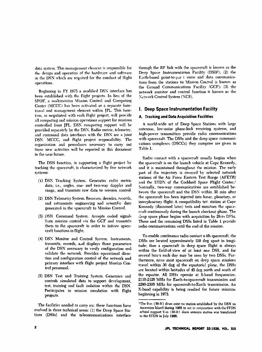
data system. This management element is responsible for the design and operation of the hardware and software in the DSN which are required for the conduct of flight operations.
Beginning in FY 1973 a modified DSN interface has been established with the flight projects. In lieu of the SFOF, a multimission hlission Control and Computing Center (MCCC) has been activated as ;t separate func- tional and management elexent within JPL. This func- tion, as negotiated with each flight project, will provide all computing and mission operations support for missions controlled from JPL. DSN coniputing support will be provided sepal ately by the DSS. Radio metric, telemetry. and command data interfaces with the DSK are a joint DSN. MCCC, and flight project responsibility. The organization and procedures necessary to carry out tnese new activities will he reported in this document in the irear future.
The DSN function, in supporting a flight project by tracking the spacecraft, is characterized by five network systems:
(I) DSN Tracking System. Generates radio metric data; Le., angles. one- and two-way doppler and range, and transmits raw data to niission control.
(2) DSN Telenetry System. Receives, decodes, records, and retransmits engineering and scientific data generated in the spacecraft to Mission Control.
(3) DSK Command System. Accepts coded signals from mission control via the GCF arid transmits them to the spacecraft in order to initiate space- craft functions in flight.
through the R F link with the spacecraft is known as the Deep Space Instrumentation Facility (DSIF); (2) the Earth-based point-to-poi- i voice and data communica- tions from the stations to Mission Control is known as the Ground Communications Facility (GCF); (3) the network monitor and control function is known as the Setwork Control System (SCS).
1. Deep Space Instrumentation Facility A. Tracking and Data Acquisition Facilities
A world-wide set of Deep Space Stations with large antennas, low-noise phase-lock receiving systems, and high-power transmitters provide radio communications with spacecraft. The DSSs and the deep space communi- cations complexes (DSCCs) they comprise are given in Table 1.
Radio contact with a spacecraft usually begins when the spacecraft is on the launch vehicle at Cape Kennedy, and it is maintained throughout the mission. The early part of the trajectory is covered by selected net=.vork stations of the Air Force Eastern Test Range (AFETR) and the STDN of the Goddard Space Flight Center.' Normally, two-way communications are established be- tween the spacecraft and the DSN within 30 min after the spacecraft has been injected into lunar, planetary, or interplanetary flight. A compatibility test station at Cape Kennedy (discussed later) tests and monitors the space- craft continuously during the launch checkout phase. The deep space phase begins with acquisition by 26-m DESs. These and the remaining DSSs listed in Table 1 pmvide radio communications until the end of the mission.
(4) DSN Monitor and Control System. Instruments, transmits, records, a,id displays those parameters of the DSN necessary to verify configuration and validate the network. Provides operational direc- tion and configuration control of the network and primary interface with flight project Mission Con- trol personnel.
(5) DSN Test and Training System, Generates and the equator. All DSSs operate at S-band frequencies: controls data to de,,elopment, 2110-2120 MHz for Earth-to-spacecraft transmission and test, training and fault isolation within the DSN. 2290-2300 hlHz for spacecraft-to-Earth transmission. An Participates in mission with flight X-band capability is being readied for future missions projects. beginning in 1973.
To enable continuous radio contact v ith spacecraft, the DSSs are located approximately 120 deg apart in longi- tude; thus a spacecraft in deep space flight is always within the field-of-view of at least one DSS, and for several hou-s each day may be seen by two DSSs. Fur- thermore, since most spacecraft on dpep space missions travel within 30 deg of the equatorial plane, the DSSs are located within latitudes of 45 deg north and south of
'The 9-m (No-ft) d h m antema station established by the DSN on Ascension during 1985 to act in ~c?Ljunction with the STDN orbital support 9-m (m-ft ) ciiam antenna station was transferred
The facilities needed to carry o:i; these ftinctions have evolved in three technical areas: (1) the Dcep Space Sta- tions (DSSs) and the telecommunications interface to the STDN in July 1988.
JPL TECHNICAL REPORT 32.1126. VOL. XIX 2
To provide sufficient tracking capability to enable returns of useful data from around the planets and from the edge of the solar system, a 64-m (210-ft) diam antenna subnet will be required. Two additional 64-m (21U-ft) diam antenna DSSs are under conFtruction at Madrid and Canberra and will operatc? in conjunction with DSS 14 to provide this capability. These stations are scheduled to be operational by the middle of 1973.
B. Compatibility Test Facilities
In 1959, a mobile L-band compatibility test station was established at Cape Kennedy to verify flight-space- craft/DSN compatibility prior to the launch of the Ranger and Manner \. enus 1962 spacecraft. Experience revealed the need for a permanent facility at Cape Kennedy for this function. An S-band compatibility test station with a 1.241 (4-ft) diameter antenna became operational in 1%. In addition to supporting the preflight compatibility tests, this station monitors the spacecraft continuously during the launch phase until it passes over the locaI horizon.
Spacecraft telecommunications compatibility in tl design and prototype development phases was formerly verified by tests at the Goldstone DSCC. To provide a more economical means for conducting such work and because of the increasing use of multiple-mission telem- etry and command equipment by the DSN, a Compati- bility Test Area (CTA) was established qt JPL in 1968. In all essential characteristics, the configuration of this facility is identical to that of the 26-m (85-ft) and 64-m (210-ft) diameter antenna stations.
The JPL C T A is used during spacecraft system tests to establish the compatibility with the DSN of the proof test model and development models of spacecraft, and the Cape Kennedy compatibility test station is used for final flight spacecraft compatibility validation testing prior to launch.
II. Ground Communications Facility The GCF provides voice, high-speed data, wideband
data, and teletype communications between the Mission Operations Center and the DSSs. In providing these capabilities, the GCF uses the facilities of the worldwide NASA Communications Network (NASCOM)* for all long
*Managed and directed by the Goddard Space Flight Center.
distance circuits, except those between the Mission Operations Center and the Goldstone DSCC. Communi- cations between the Goldstone DSCC and the Mission Operations Center are provided by a microwave link directly leased by the DSN from a common carrier.
Early missions were supported by voice and teletype circuits only, but increased data rates necessitated the use of high-speed and wideband circuits for DSSs Data are transmitted to flight projects via the GCF using standard GCF/NASCOM formats. The DSN also sup- ports remote mission operations centers using the GCF/ NASCOM interface.
111. Network Control System The DSN Network Control System is comprised of
hardware, qoftware, and operations personnel to provide centralized, real-time control of the DSN and to monitor and validate the network performance. These functions are provided during all phases of DSN support to flight projects. The Network Ormations Control Arca is iocated in JPL Building 230, adjacent tc tLe locai iviissioii Clpwa- tions Center. The NCS, in accomplishing the monitsr itlid
control function does not alter, delay, or serially process anv inbound or outbound data between the flight project and tracking stations. Hence NCS outages do not have a direct impact on flight project support. Voice communi- cations are maintained for nperations control and co- ordination between the DSN acd flight projects, and for minimization of the response time in locating and cor- recting system failures.
"be NCS function will ultimately be performed in data processing equipment separate from flight project data processing and specifically dedicated to the NCS func- tion. During FY 1973, however, DSN qperations control and monitor data will be processed in the JPL 360/75 and in the 1108. In FY 1974 the NCS data processing function will be partly phased over to an interim NCS processor, and finally, in FY 1975, the dedicated NCS data processing capability will be operational. The final Network Data Processing Area will be located remote from the Network Operations Control Area so 3s to pro- vide a contingency operating location to minimize single point of failure effects on the network control function. A preliminary description of the NCS appears elsewhere in this document.
JPL TECHNICAL RE#)RT 32.1526, VOL XIX 3
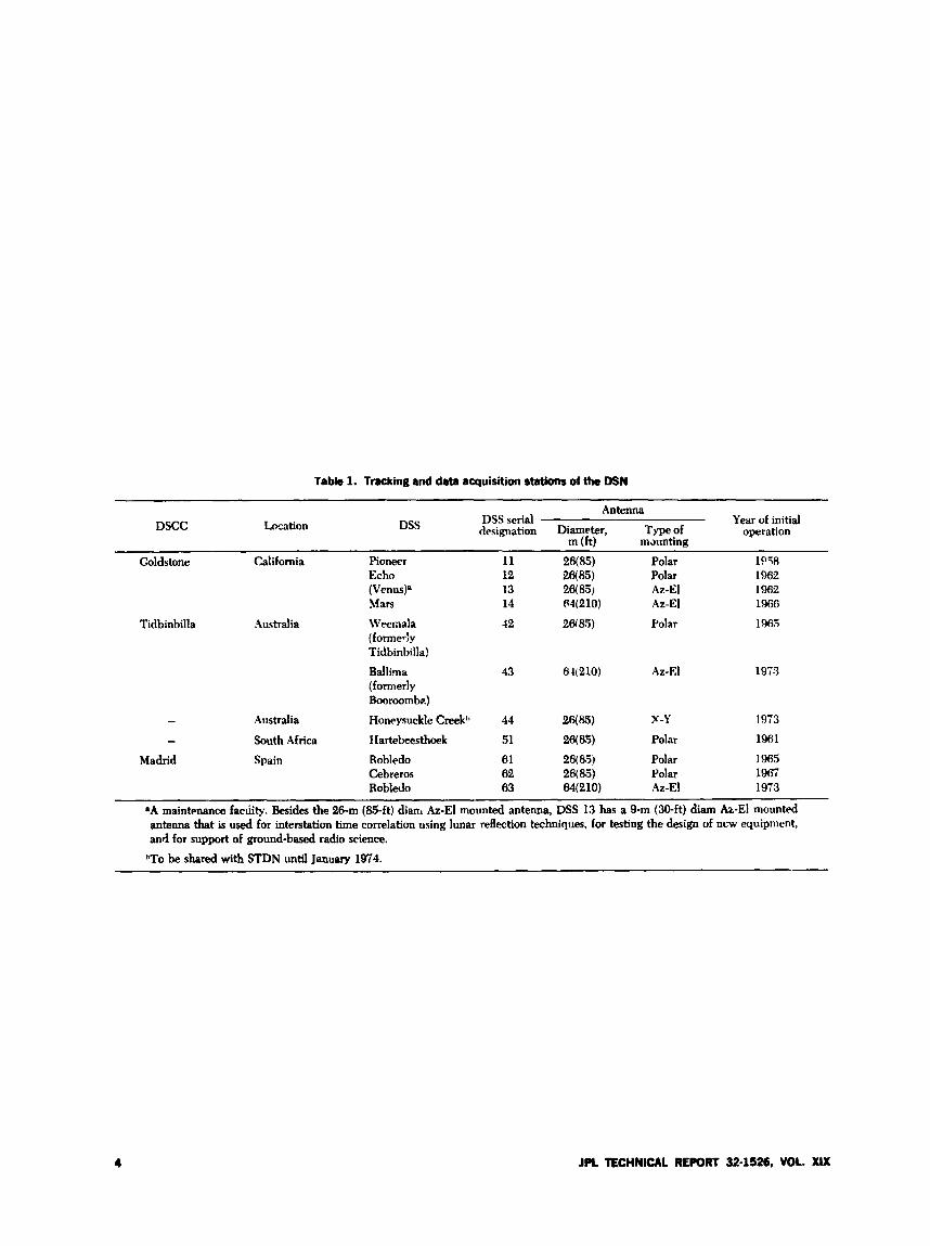
Table 1. Tmking and data acquisition stations of the DSN
Antenna DSS serial Year of initial
designation Diameter, Type of operation DSCC Location DSS m (ft) maunting
Goldstone California Pioneer 11 2W5) Polar 1958 Echo 12 2 ~ 3 5 ) Polar 1962 (Venusp 13 2 ~ 5 ) Az-El 1962 Mars 14 64(210) Az-El 19G6
Tidbinbilla Australia Weenala 12 2sC8S) Polar 196.5 (formerly Tidbinbilla) Ballima 43 61(210) h - E I 1973 (formerly Booroomb?.)
- Australia Honeysuckle Creek” 44 26(w X-Y 1973
- South Africa Hartebeesthoek 51 28(85) Polar 1961
Madrid Spain Robledo 61 26(853 Polar 1965 Cebreros 62 26(85) Polar 1967 Robledo 63 M(210) Az-El 1973
*A maintenance faciiity. Besides the 26-rn (85-ft) dian. Az-El mounted antenna, DSS 13 has a 9 r n (30-ft) diam h - E l mounted antenna that is used for interstation time correlation using lunar reflection techniques, for testing the design of ncw equipment, and for support of ground-based radio science.
hTo be shared with STDN until January 1974.
4 JPL TECHNICAL REPORT 32.1126, VOL. XIX
DSN Command System Mark 111-74 W. G. Stinnett
DSN Systems Engineering Office
A general description is presented of the DSN Command Systew softwre changes that are being implemented to support the Helios anti Viking missions. Comparisons are mude between the present system (Mark 111-71) arid the new system (Mark 111-74). Included are the reasons for the changes, and the DSN plans to phase all mis.&n support ocer to the Mark 111-74 system.
1. Introduction The DSN Multiple Mission Command (MMC) Sya-
tem has successfully supported the Mariner Mars 1971 (MM71) mission and the Pioneer 10 mission to Jupiter. The system is now supporting the ongoing Pioneer 10 mis- sion, the Pioneer 11 mission to Jupiter, and the Mariner Venus/Mercury 1973 (MVM73) mission. All of these mis- sions have been supported with the same DSN hardware.
The command software provided by the DSN in the Deep Space Stations' (DSSs) telem. try and conimand processors (TCPs) has been basirally the same from mis- sion to mission. The commant ! requirements for each missin;: have been similar, and thus the software has re- mained basically the same as that designed for the MM71 mission (heredftpr referred to as the CSN Mark 111-71 Command System).
The DSS TCP is an XDS 920 computer. The DSN im- plemented the DSS telemetry and command functims into this computer for all the missions. One cf the primary problems in implementing the command portion of the software was timing. These timing problems had to be overcame in the software used during the Mark 111-71 em All the misa;ons supported during this era required the same transmission rate (1 bit/s\; thus, the software timing considerations were similar.
The DSN is presently implemmting significant changes in the DSN MMC System (the DSN Mark 111-74 Com- mand System). The Helios and Viking mission command transmission rates are 8 symbols per sycmd (SPS) and 4 bitsis, respectively. The software timing considerations are significantly increased over tho.= missions supported during the Mark 111-71 era. For this reason, the Comr nd System is undetgoing extensive software changes.
JPL TECHDilCAL RlEWR7' 32.1526, VOL. XIX I
II. Mark Ill-74-Command System CI 2ges A. Transfer of System Functions
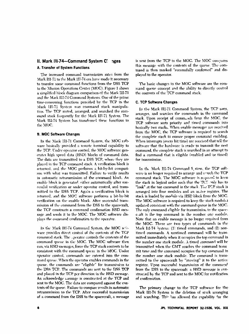
The increased command transmission rates from the hlark 111-71 to the Mark IIJ-74 e n have made it necessary to transfer some command functions from the DSS TCP to the llission Operations Center (XIOC). Figure 1 shows a simplificd block diagram comparison of the hlark 111-71 and thc Mark 111-74 Command Systems. One of the prime time-consuming functions provided by the TCP in the >lark 111-71 System was command stack manipula- tion. The TCP sortcd, arranged, and searched the corn- mand stack frequently for thn \lark 111-71 System. The Mark 111-74 System has transfcrred these functions to the XIOC.
B. MOC Software Changes
In the Xlark 111-71 Command Slstem, the MOC soft- ware basically providcd a rcmote tcrminal capability to the TCP. Under opcrator control, thc Bloc software gen- eratcs high speed d:ita (HSD) blocks of command data. The data arch transmitted to a DSS TCP, whew they are placcd in the TCP command stack. A verification block is rcturneci. and the. MOC performs a bit-by-bit compari- son with what was transmitted. Failurt to verify results in automatic retransmission of the command block. An enablc block is gcwmtccl. cithcr automatically after suc- cessful verification or under opwator contrd, and trans- mitted to thc DSS TCP. Again a verification block is rvturncd, anc! the MOT softwnrc performs a bit-by-bit wrification on thc enable block. After successful trans- mission of thc commmcl from the DSS to the spaewraft, the TCP constructs a command confirmatian HSD mrs- sage and sends it to thr MOC. The hIOC softwire dis- plays the coininand confirmation to thc, oprrator.
la the. >lark 111-71 Commnrid Spsttom, the MOC S(’:‘i-
wart- provides dirwt controi of the conttwts of the TCP command stack. The .,perator cantrols the contents of the command qwue in tile MOC. The MOC software then can, via HSD nirssages, force thr TCP stack contents to be consistent with the command qucui in the MOC. Under operator control, commands are entered into the com- mand q w w . \\’hen the operator cnablcs command5 in the qurue. the commands arc “eligiblc” for transmission to thr DSS TCP. The cominands arc scwt to the DSS TCP and placed in the TCP pcr direction in thc HSD message. An acknowlcdgc i.iessagc’ is constructed Pt the TCP and sent to the MOC. The data are compared against the con- tents of the queue. Failurc to compare results in automatic retransmission to the TCP. After siiccessfril transmission of a command from the DSS to the spacecraf&, a message
is sent from the TCP to the h4OC. The hlOC coniimes this message with the contents of the queue. The com- mand is then marked “successfully confirmed” and dis- played to the operator.
The basic changes to the MOC software are the com- mand queue concept and the ability to directly control the contents of the TCP command stack.
C. TCP Software Changes
In the Mark 111-71 Command System, the TCP sorts, arranges, and searches the commands in the command stack. Upon receipt of comm,:rds from the MOC. the TCP software sorts priority and timed commands into hasically two stackb. Whcn enable message? aie received from the MOC, the TCP software is required to search the complete stack to ensiire proper command enabling. When interrupts (every bit time) are received that tcll the softuare that the hardware is readv to transmit the next command, the complete stack is searched in an attempt to find a command that is eligible (mabled and ’or timed) for transmission.
In th, Mark 111-74 Command S - stem, the TCP soft- ware is no longer required to arrar,gf and s-vch the TCP command stack. The MOC software is rcquil.cd to kccn the stack in logical order such that the TCT’ lniy has to “look” ‘it the ton command in the stack. ‘G1e T‘JP stack is arranged into four modules and an arlive register. The stack is loaded by moh le via IISE block from the MOC. The MOC software is required to keep thc stack modules updated consistent with thc command queue in the XlOC. The only command c4giblc for transmissioi. to the space- c:aft is the top command in the number onc module. Note that an enable message is no longer required from the MOC. There are two types of commands in the lfark 111-74 ;ysterbi: (1) timed commands, and (2) non- timed commands. A nontimed command will he trans- mitted immediately when it ocmpies the top command in the number one stack module. A timed mmmand will be transmitted whrn the GMT reaches the command trans mit time and the command occupies the top command in the number one stack module. R e command is trans- mitted to the spacecraft b y “moving” it to the activc register. LTpon successfill transmission of the commsncl from the DSS to the spacecraft a HSD message is <.on- struc:ed by the TCP arid sent to the MOC for notification of Confirmation.
The primary change to the TCP software for the Mark 111-74 System is the deletion of stack arranging and watching. Th;. bas allowed the cspahility for the
6 JPL TECHNICAL REPORT 32-1526, VOL. XIX

software to peiform more important functions at the higher command bit rates. The same types of hardware check provided at 1 hit/s for the Mark 111-71 System can be provided for the Helios command rate of 8 SPS.
111. Mark 111-74 Command System- Mission Support Plans
It is desirable from an operational and sustaining engi- neering viewpoint that all missions supported by the DSN be supported by the Same DSN Command System. An
operational consideration is that two-system operation can lead to confusion when different characteristics exist. Another operational consideration is that personnel train- ing is simplified when one system is used. The sustaining engineering consideration is, of course, less cost. For these reasons, the DSN plans to phase all mission support over to the Mark 111-74 Command System. The present plans for phase-over of all support is shown in Table 1. All missions will be phased over after critical events are complete. The Hdios and *, iking test periods and flight operations will be supported entirely by the Ma;k 111-74 Command System.
JPL TECHNICAL REmR'T 32-1526, VOL XIX 7

8 JPL TECHNlCAL 32-lS2& VOL mt
Dss E W P Y ANiJCOMM*NDrtOCESSOII COw,w.NM,
COMMAND S T X U
T M D nK3(11w
C M D l C M D l C M D 2 C U D 2
C M D N C M D N
TO DSS EXCITE, W S M l T l B . ANTENNA S w s Y s l E M S
CMD 6
I . I I -
t
KKNOWZPDGI I CCMPAm TO
I I J e C Q N F M T D N I COWARE TO
arrtn
I
9

Viking Mission Support D. J. Mudgway
DSN Systems Engineering Office
3. W. Johnston Network Operations Office
This article describes the Setu-otc- Operations Phn for Viking 1975 and includes some DSS support requirements unrque to 1'ikin.g which hace resulted in unusual attention to Deep Space Ctcltion hardrrwre failure mode configurations. Also dis- cussed are samples of the sin@ point failrrre strategies incorporated in the 1'iking 1975 Deep Space Station telemet y hardware configurations. The mtiomle for the implementation of 100-kW transmitter capability at DSSs 43 and 63 is also gioen.
1. Network Operations Plan for Viking
The public-5on of the Sehvork Operations Plan for Viking 19Z (Ref. 1) constitutes a further milestone mark- ing the initial point at which the DSN operations per- sonnel in general became directly involved with the Yiking Project. This document interprets all the Project requirc.ments levied on the Deep Spacc Network to sup- port the \'ikina 1975 mission. It specifies the required hwian and technical interfaces a i d the maimer in which the DSS capabilitie, described in the DSN Preparation Plan for Viking 1975 Projcct (Ref. 2), will be employcd hy Srhvork Operptions to support Viking pre-launch and flight opcrations activities. Finally. this constitutes the prim(. refrrcwce regarding the Viking DSN training, trst- ing. configurations, procedures, and operations, for all prsonncl in the DSS Operations Office.
II. Unique Viking Requirements In pre\<ous missions, during the limited critical and/or
estremely high-activity periods, the requirement for hard- ware failure backup has been met at the Deep Space Stations by scheduling a second station in parallel and/ or the use of complete parallel strings of equipment readied in a "standby" state.
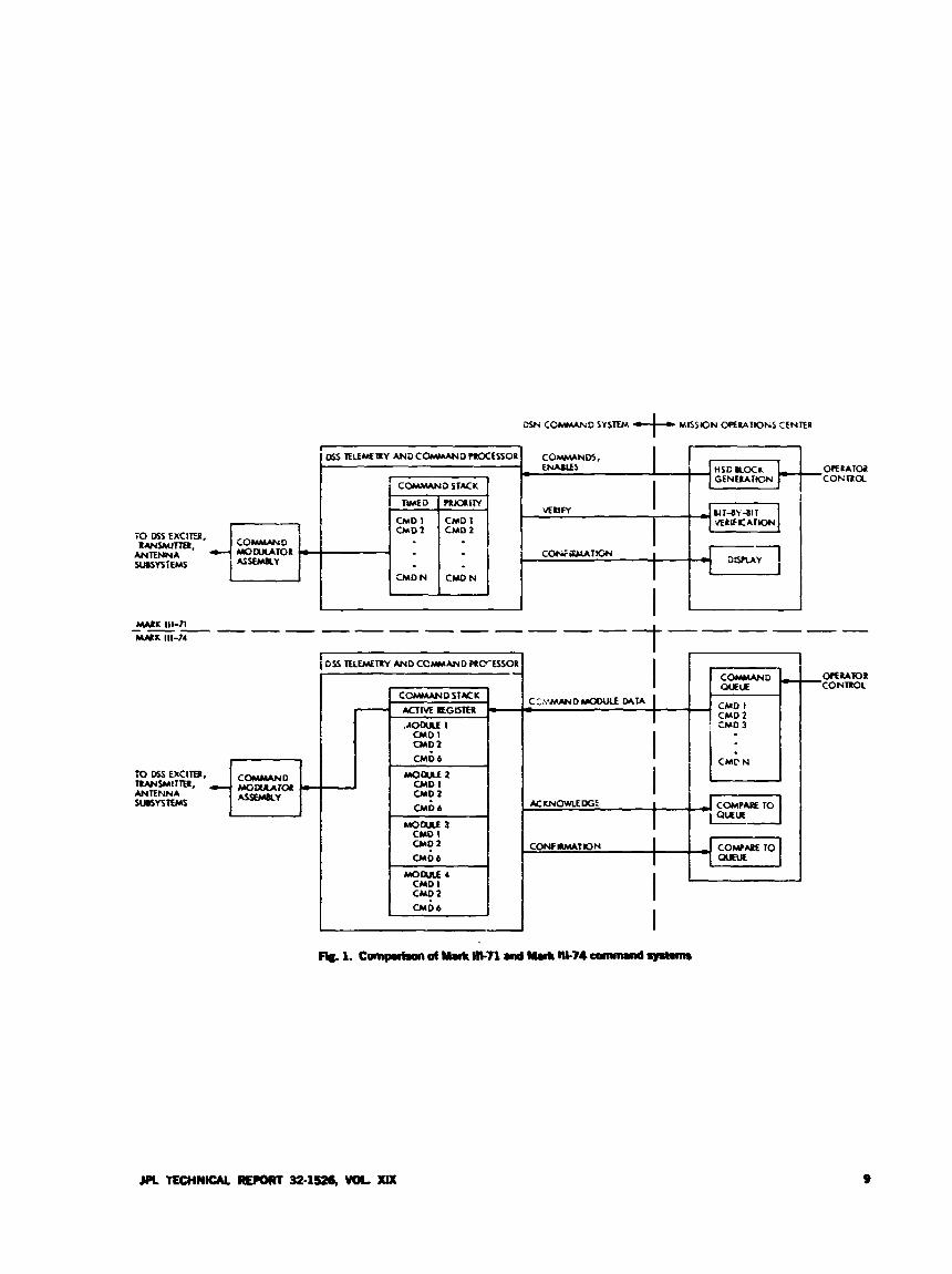
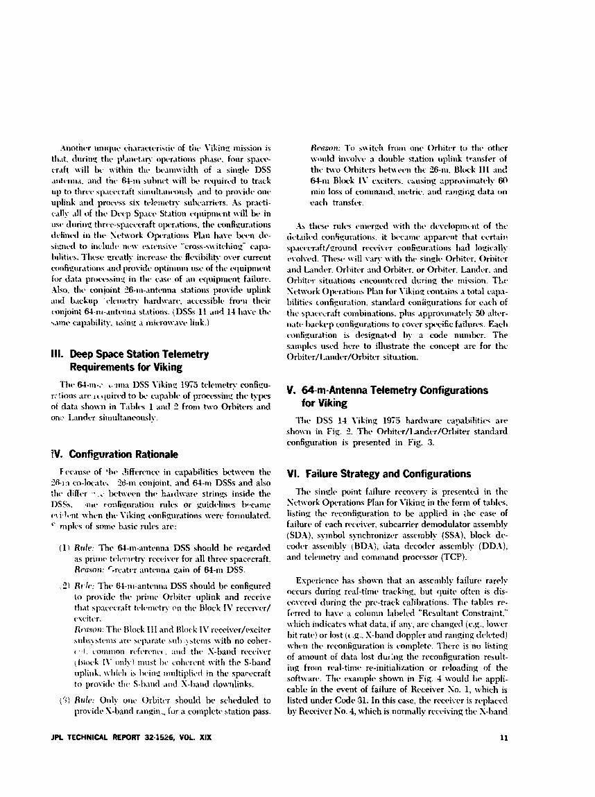
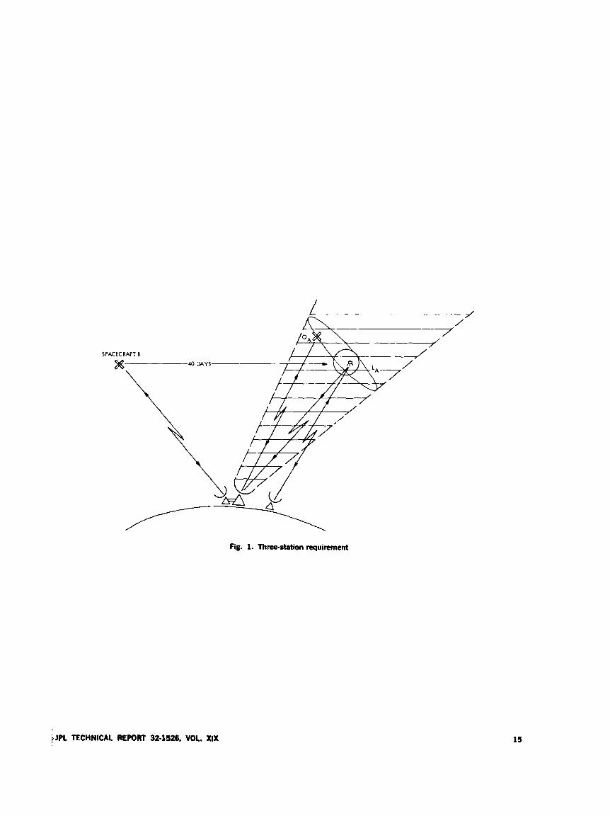
The Viking 1975 mission is unique in this respect in that: (1) the critical/high-activity periods will estend for up to 5 months continuously, (3) three DSSs 21 each loa- tion will be required for 2 months, 7 days I r week (EO
backup stations) (see Fig. l), and (3) 'he 5-month period requires the simultaneous use of six rlemetry l-:.rdware strings out of a total station complement of six strings (no backup strings) at each 61-m-antenna DSS.
10 JPL TECHNICAL REPORT 32-1526, YOL ' IX
111. Deep Space Station Telemetry Requirements for Viking
Thc. 6- t1 - i i1 - .~ t. mna DSS Yikinz 1975 t r l t m t . t ~ conficu- rl tions arc I < quircd to be cap;iblc of prnccssinq the t!-lws of data showi in TiiI~lcs 1 and 2 from two Orbiters and on!: I.;indcr siiiiultaiirousl!-.
PV. Configuration Rationale F ~ c m s c of ‘hi, rlifftwnw in capabilities between the
26-111 co-lncitc., 2d-rn conjoint. and 64-ni DSSs and also t h c t diffcr 1. ... Iw.t\vt*c*n thv halciwirr strings inside the DSSs. mi(* rcnfiqurntion riilrs or guidthcs lvcanic i s \ iJ,*nt whtm tlic. Yiking configurations wcrv formulated. c . niplcs of sonic- hisic r&s arc’:
(1 ) Rule: Thr 64-m-antcwxi DSS should lw regarded as prinw tchic*try rrcchbr for all thrcr spaircraft. RCYJ.WII: Srratc.r nntenna gain of 64-ni DSS.
( 3 ) Rrtlc: Only ont’ Orbitcr should br. schc*dulcd to providc S-band riingill., for a coniplctc, station pass.
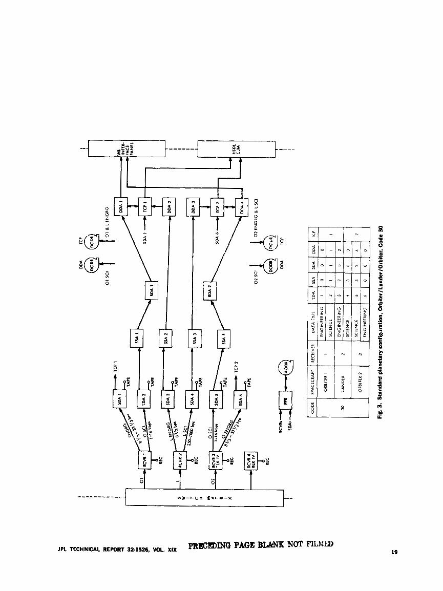
.& tlitsc rult.s cnicrgcul with tlic dcvc-lopnit.nt of tht. tit~tciikd miifi5urations. it Ix-c:iint- appsrtmt that cert;iiv s~~ac(~cr;ift/sround r(y.civi7 conficuratioiis had lo~ieally c~volvtd. Thew \vi11 v a n with the singlc. Or!)itcr. 0ri)itc.r r i n d Lindvr. Orliitc-r ;ind Orbittar. or Orl>itc.r. Landixr. and Or1)itc.r situ,itions tncoiintt.rtd dwina, the inixsion. Thc Sctivork Op’r.itions Plnii for Yikiiic cvIit.lii?s A total cap;^- bilities confiFurrttion, staiiclard cuniiSrirations for tach of thc sp.ict.Lxift cnnibin:itiom. plus approxiniiitc-ly 3) ii1tc.r- nate backrp onfiprations to covcr specific failurcs. Each coiifiFuration is dfsignatd by a code nuiii1x.r. The suinplcs uwd here to illustrate thc coiiccpt ;ire for the Orbitt.r/Laiidc.r/Orbitcr situation.
V. 64-m-Antenna Telemetry Configurations for Viking
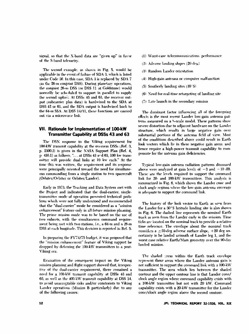
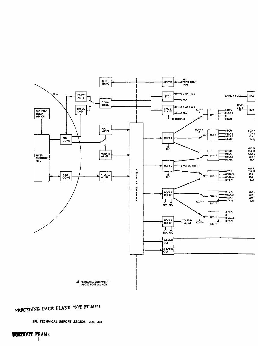
Tlic DSS 11 Yiking 1975 hardwire ca?abilitic.c are shown in Fig. 2. Thr Or\)itcr/Lander/@rLiter standard configuration is presented in Fig. 3.
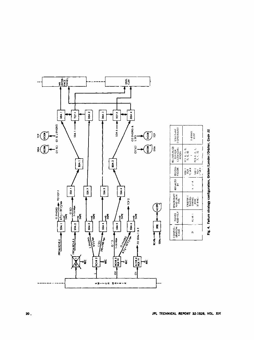
VI. Failure Strategy and Configurations Thc singlr point f‘iilure rccovc’ry is prcsentrcl in the
Srt\vork Operations Plan for Viking in the form of tables, listinfi t h r weonfiguration to be upplird in :he cast' of failure of cach rcccivrr. subcarrier demodulator assemhly (SD.4). syniFK,l synchronizer asscwbly (SSA), block dr- coder assembly (HD.i), data decoder assembly (DD.4), and tclrmctry iind cornniand processor (TCP).
Expcaricmx. has shown that an asscmbly failurr. rarely occurs during rcd-tinic tracking. but quitc often is dis- ccvcrcd during the pre-track calibrations. Thc tables rc- f c m d to havc a colun:n labelrd “Rcsultant Constraint,” which inclicatcs \\hat data, if any, arc cliangcd (e.%., lower bit rat(.) or lost ( I .g., S-band dopplcr and ranging drleted) \vhrn the rwonfiguratinn is complete,. There is no listing of amount oi data lost dut :ng the reconfiguration result- ing from rt-al-tinic> re-initialization or rc4oading of the soft\varct. Thc rsaniplc. shown in Fig. 4 would hc appli- cable in the event of failure of Receiver So. 1, which is listcd under Code 31. In this case, thc recrivcr is rvplacrd by Receiver No. 4, which is normally rrccbiving the S-band
JPL TECHNICAL REPORT 32-1!26, VOL. XIX 11
signal, so that the S-band data are “given up” in favor of the S-band telemew.
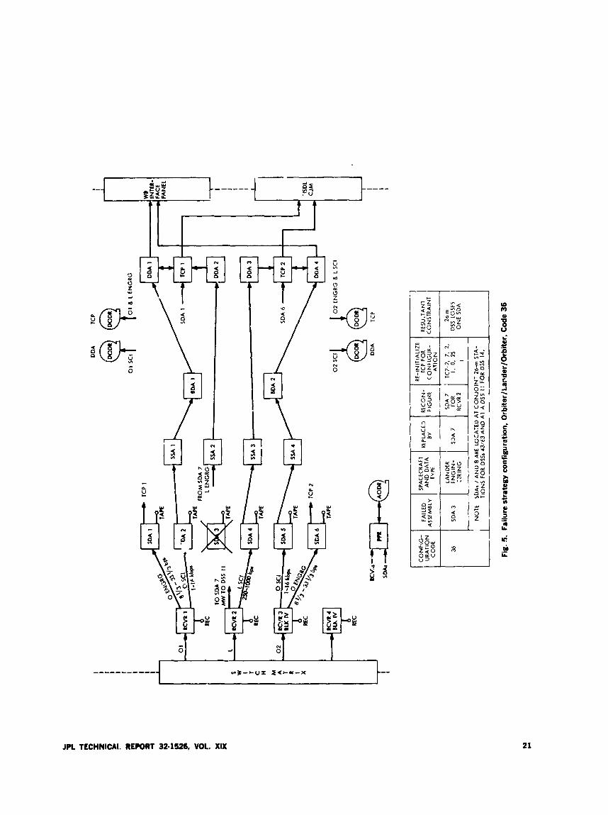
The srwnd esample. as sho\vn in Fig. 5, would be applicable in thc. event Of failure of SD.43. which is listed under Code 36. In this case, SD-4 3 is replaced by SD.9 7 \ i i t tlir 26-n1 canjoint DSS). During planetary oprations, tlic conjoint LB-n~ DSS (or DSS 11 at Goldstone) would nornizlly be schcdulcd to support in parallel to supply the s t a n d uplin:<. At DSSs 43 and 6;3. the rectlivcr out- put (subcarrier plus data) is hardwired to the SDA at DSS 12 or 61, and the SD.4 output is hardwired back to the 64-nj SS.4. At DSS 11/11, thtw functions are carried out via a microwave link.
VII. Rationale for Implementation of 1OO-kW Transmitter Capability at DSSs 43 and 63
The DSN response to the Viking requirement for IWkW transmit capability at the overseas DSSs (Ref. 3, p. 2300.2) i s given in the N.4S.4 Support Plan (Ref. 4, p 430.1) as follows; -. . . at DSSs 43 ai-d 63, 100 h-v trans- mitter \vi11 provide dual links at 10 kw each.” .4t the time this was written, the requirement and its response were principally oriented toward the need for simultane- ous commanding from a single station to two spacecraft (Orhiter/Orbiter or Orbiter,’Lander).
Early in 1973. the Tracking and Data System met with the Project and indicated that the dualcarrier, sinsle- transmitter mode of operation presented technical prob- lems w!rich were not fully understood and recommended that the “dual-carrier” mode be considered as a “inission cnhancement” feature o d y in all future mission plaming. The prime missioii mode \vas to be based on the use of two subnrts, with the simultaneous command require- ment being met with two stations, i.e., a 64-m and a 26-m DSS at cwh longitudr. This decision is reported ii; Ref. 5.
In preparing thc FYT4fiT5 budget, it was proposed that the “mission enhancement* feature of Viking support be dropped by dciferring the 10O-kW transmitters to a post- Viking era.
Evaluation of the consequent impact on the Viking mission planning and flight support showed that, irrespec- tive of the dual-carrier requirement, there remained a nrcd for a lW-kW transmit capability at DSSs 43 and 6‘3, as wrll as thc 400-kW transmit capability at DSS 14, to avoid unaccrptable risks and/or constraints to Viking Lander operations (Mission B particularly) due to any of the following causes:
b’orstcase teItu.ommriiiications pcrforinance
.idvcmch landing slopes (20 deg;
Random Landcr orientation
High-gain antenna or computer malfunction
Southerly landing sites (:3O’Si
Seed for real-time retargetin? of 1ai;ding site
Late launch in the secondary mission
The dominant factor influencing all of the foregoing effects is the most recent Lander low-gain antenna pat- terns measured on a %-scale model. These patterns show severe distortion due to adjaccnt hardware on the Lander structure, which results in large negative gain over substantial portions of the antenna field of view. Most of the conditions described above could result in Earth look vectors which lie in these negative gain areas, and hence require a high-power transmit capability to mm- pensate for the antenna gain deficiencies.
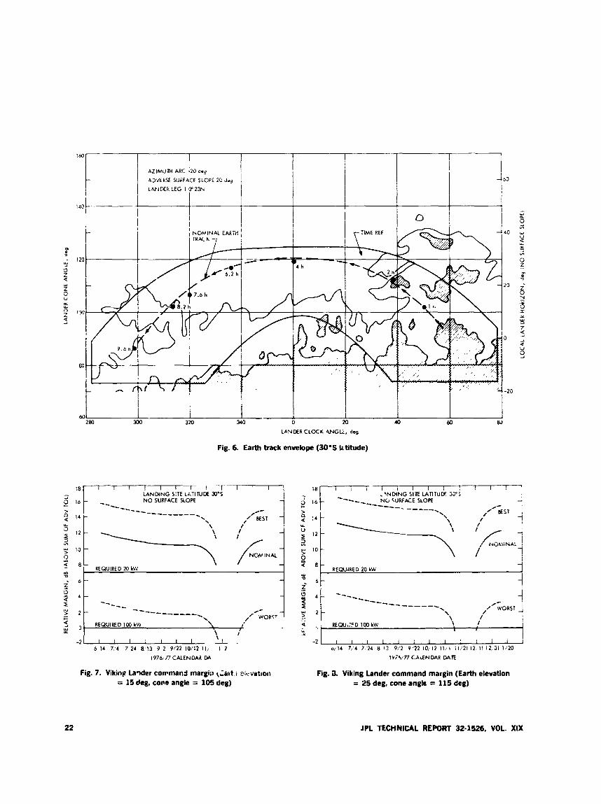
Typical low-gain antenna radiation patterns discussed above were analyzed at gain levels of -3 and - 10 dR. Thew are the levels required to support the command link for 10- and 1oO-kjV transmitters. This analysis is summarized in Fia. 6, which show the Lander cone and clock angle regions where the low-gain antcnna covcrage is adequate to support the command link.
The history of the look vector to Earth as sew from the Lander for a .30cS latitude landing site is also shown in Fig. 6. The dashed line represents the nominal Earth track as seen from the Lander early in the mission. Time ticks arc located on the nominal track to provide a relative time reference. The envelope about the nominal track considers a r20-deg adverse surface slope, $20 deg un- certainty in he landed azimuth of Lander leg 1, and the worst case relative Earth/Mars geometry over the W-day 1andc.d mission.
The shaded nreas within the Earth track envelope reprcasent those areas where the Lander antenna gain is not sufficient to support the command link with a lW-k\V transmitter. The area which lies between the shaded contour and the upper contour line is that Lander cone/ clock angle region where command capability exists with a 100-kW transmitter but not with 20 k W . Command capability exists with a 20-kW transmitter for the Lander cone/clock angle region above the second contour.
12 JPL TECHNICAL REPORT 32-1526, VOL XIX
Ob\iously, the opportunity to command the Lander over the low-gain antenn:? is w.~:.!:.. :;cliittd ior the 30-S latitude landing site. Only one half of the total daily Earth view period is available for Landcr command with a ?O-k\V transmitter.
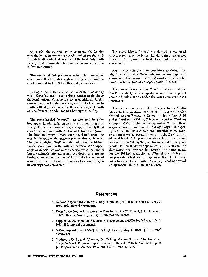
The command link performance for this same set of conditons (30‘s latitude) is given in Fig. 7 for no-slope conditions and in Fig. 8 for 3-deg slope conditions.
In Fig. 7, the perforinam.- is shown for the time of day when Earth has risen to a 15-deg elevation angle above the local horizon. No adverse slop- is considered. .4t this time of day, the Lander cone ansle d the look vector to Earth is 105 deg, or conversely, the aspc i .male of Earth as seen from the Lander antenna boresight i s is leg.
The c u n r labeled “nominal” \vas generated from the free space Lander gain pattern at an aspect angle of 75 deg. This cun-e shows a margin of approximately 3 dB above that required with 20 kW of transmitter power. The bcs: and worst curves were developed from the installed %-scale model antema pattern data as follows: The curve labeled ”best” was derived from the highest Lander gain found on the installed patterns at an aspect angle of 75 deg. Because of the uncertainty in the landed Lander azimuth orientation and the desire to place no further constraint on the time of day at which a command session can occur, the entire Lander clock angle region (a;360 deg) was considered.
Thcb c‘iirvch labclcd “\\.orst” \viis dcrivvd :is c.ipl?ined abw.~.. except that the lowest Landcr 9,iin at ;in :ispect
considered. anqle of 7.5 deg over the total clock angle re&’ ’1011 \vas
Figure S rcflects the sa~nc conditions as dcfined for Fig. 7, except thdt a 20-deg adverse surface slope \vas considcd. The noniin,d. best. and worst curves considcr Lander antenna gain at an aspect an& .,f Q5 dcg.
The cur%-cs shown in Figs. i and 8 indicate that the 3Ml’ capability is inadequate to m e t the rvquired command link margins under the worst-case conditions crnsidercd.
These data \vcw prcsmttd in oven-iew by the Martin Uarietta Corporation (UbIC) at th r Viking Lander Critical Design Review in Denver on September 19-20 a.14 in detail to the Viking Tclecomniunications Working Croup a: \lMC in Dcmver on September 21. Both these organizations, 2s \vel1 as the Viking Project Manager. agreed that the 100-23’ transmit capability at the over- seas stations \vas a nccessar) dPmcmt in the DSS support planr zd for the Viking mission. Accwdingly, the current revision to the k’iking Support Instrumentation Require- ments Document, dated September 17. 197:3, deletcs the dual-carrier requircment, but restatcs the requirements for the 1 0 - k W capabiliv at DSSs 4.3 and 63 for the purposes describtd above. Iinplenientntioli of this capa- bility has since been reinstate& and is proceeding toward an operational date of January 1, 1976.
References
1. Network Operations Plan for Viking 75 Project, JPL Document 614-21, Nov. 1, 1973 (JPL internrl document).
2. Deep Space Network, Preparation Plan for Viking 75 Project, JPL Document 614-20, Rev. A, Nov. 15, 1973 (JPL internal document).
3. Support Instrumentation Requirements Document (‘SIRD) for Viking, July I, 1971 (JPL internal document).
4. NASA Support Plan (NSP) for Viking, Rev. 0, May 1, 1972 (JPL internal document).
5. hhdgway, D. J.? and Johnston, D., “Viking Mission Support,” in The Deep Space Network Progress Report, Technical Report 32-1526, Vol. XVII, p. 9, Jet Propulsion Laboratow, Pasadena, Calif., Oct:15, 1973.
JPL TECHNICAL REPORT 32-1626, VOL Xu1 13
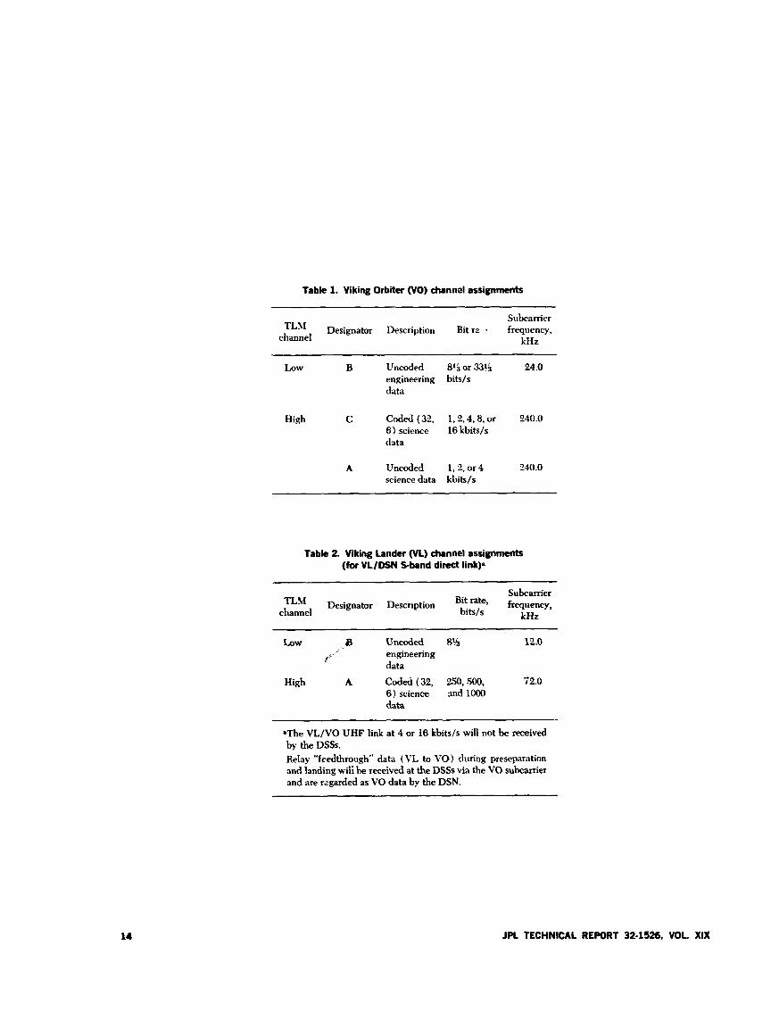
Table 1. Viking Orbiter (VO) channel assignments
Subcamer TL‘l Designator Description Bit rz 3 frequency,
channel kHz
Low B Uncoded 81ior33Lj 24.0 engineering bits/s data
High C Coded (32, 1,2,4,8, or 240.0 6) science 16 kbits/s data
A Uncoded 1.2, or 4 “0.0 science data kbits/s
Table 2 Viking Lander (VL) channel assignments (for VL/DSN S-band direct link).
Subcamer rate* frequency,
kHz bits/s
8 Uncoded 8% 12.0 ;. LOW engineering data
High A Coded (32, 250,500, 72.0 6) science md lo00 data
LL’
aThe VL/VO UHF link at 4 or 16 kbits/s will not be received by the DSSs. Relay “feedthrough” data (VL to VO) during prescparatinn and landing wiii be received at the DSSs via the VO subcamer and are regarded as VO data by the DSN.
14 JPL TECHNICAL REPORT 32-1526, VOL XIX
4 /
SPACECRAFT B
x
Fig. 1. Three-station requirement
iJPL TECHNICAL REPORT 324526. VOL. XIX 15

I A 6 PAPER DRIVE TAPE
RCVh 3
FIXED
REFL
/// 1 INDICATES EQUIPMENT
ADDED POST LAUNCH
I
I
---I / RCVR4 TCR S M 1
SSA 1 SDA : su 2 SDA TAPE TAPL
- SDA 2
RCVR 1
hW FR DSS 11 S M i SDA - TAP
SM . IDA
SSA 4 SDA . X TAPE TAP
IDA R K
3-c IDA REC
1 S-BAND ou X-BAND ou
QCVR, 3
TCPI
TAPE
TAPE
SSA 4 TAPE
TC Pz
TAPE BLK IV
WEATHER DATA
TO EXC
HSDL RCVk
-2 DOPPLER
MW FROM DSS 11
TAPE DDA 2
Mw FROM DSS 11
TAPE BDA 2
U
Q DDA 1 OR 2
RCVR PPR
SDA
t
DDA a
U
pEXC 1 & 2
EXC 1.2
I I I
DDA 1
INTER-
PANEL
SCA - DIS 1 TCP 1 - TCP 2 - DDAl- DDA 2- DDA 3- DDA4-
i 1 i I I L
HSDL CJM
-r I I
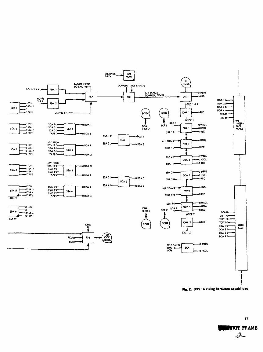
Fig. 2. DSS 14 Viking hardware wpabiliticn
17
FRAME A-

1
mKZ!lINQ PAGE BLArNg NO" E'JIMZJI JPL TECHNICAL REPORT 32.15226, VOL. XIX 19
0
.
- f Y
JPL TECHNICAL REPORT 32-1526, VOL. XIX
- 0 8
JPL TECHNICAL. RE#)RT 32-1526, VOL. XIX 21
m 3
Fig. 6. Earth track envelope (30's Irtitude)
LANDING S:TE LATIRIDE 33"s NO SURFACE SLOPE
,--- ,' E S T 1 -----_____- .
i
REQUIRED IM) kW \ #'
Fig. 7. Viking Laider command margiii t A I t , i %-YatiOil
= 15 deg, cone angle = 105 deg)
I I ! ' I
a * - REQUlRED2OkW 1 - U . 6 -
- 2 1 I I I I I I I I ! I I I 1 o/l4 7i4 7.'24 8 13 9,'2 9'22 10,.12 1 1 / 1 i l ~ 2 l l 2 , I l I 2 , S i 1,'20
l'r;V?7C.ALENDAR DATE
Fig. a. Viking Lander command margin (Earth elevation = 25 deg, cone angle = 115 deg)
22 JPL TECHNICAL REPORT 32-1526, VOL. XIX
Pioneer 10 and 11 Mission Support R. B. Miller
DSN Systems EngineeTklR Office
This article describes si,cnificant uspects of the .wcce.ssfril Pion?cr 10 encouider of the p h e t Jupiter.
1. Encounter Summary
t\t the time of writing. Pionwr 10 had complrtcd all but 1 week of the 60-da); cncountrr of thc plant Jupiter. The Jiipitcr environment was f o v d to be much more complex and interesting than had btm anticipated. The field and particle environment is not simply a dipole field with trappvd particles interacting with the solar wind in a semi-static fashion. Tremendous fluctuatiorrs in the extent of the bow shock were observed, apparently related to the changes in intensity of the solar wind. CDm- picx stnicture was ohsewed inside of the bow s h d . and a radiation intensity loo0 tinies higher than is con- siderrd lrthal to a hnnian being, although the actual magnrtic field strength measured was at the lowcxr end of the prrflight range of rstimatcs.
Ciosc-st approach to Jupiter was reachpd at 02 2.519 Greenwich mean tiinc on December 4, 1973, at a rang' of 2.88 Jupiter radii, 203,250 km from the mnter of the planet (the radius of t h c visible disk is a b u t i1,W kin), or 132.250 km froin the visible surface. The spacecraft iippcars to have rspt.rirnc1.d nearly t h ~ maximum radia- tion dose it could take without catastrophic damage to equipment and iwtruments. Temporary f reversible)
Thc. occultation txprinwnt \vas snctyssful: an iono- sphcrr $vas d c t w t d on the moon Io, and a11 data \vcw obtained during thr c:itv and cuit phascs of thc Jupitcr occultation. Thc wi.ultation c~pcrimcmt s c d i s to detcr - mine ;Itmosphcric charactc ristio by rroilld-bastul ~ M X -
surcnicnt of t h r rffrcts on thc- S-hand radio link ;u it trxismits thrmgh the atinosphcw. T h c - Jupi tc~ .thiio-
sphcrc i s apparcmtly vc-ry complcs, and much an.ilysis by thc cspcri:iicmtrr will Iw iic*cc*ss;iry to model the ohsc.rvcd effwts.
'I he imaging photoplarinictcr rvturnrd inany in- triguing pictiirrs of thv planct. Thc radiation nicwur(*. nirnts by other instrumcnts p&d at somclthing like. &IO niil1io:i .W->leV electrons and 4 million 3-S1c.V pro- tons pcr quart' centiinetvr p r stmnd. The tempt-raturr ineasurements showtd that the planet radiatrs a h i t
JPL TECHNICAL REPORT 32-1526, VOL. XIX 23
The hi$ Icwl of mmmand loading acd the potentially srriou\ effect of interruptions in command capabi!ity on tliv cnrvuntcr s q u t m e \ v t w rtr0gnizr.d. and the priman activih in prtpmtiiiq the proand s>stem for this tmrauntc-r \vas to s;cr.k nitbans to impmvr total com- mand r&tl)ility. Iniprovc-nicnt of thv cumnand system reliability inmlvcd making \-cry minor c h i m p in DSS sofhwrc.. but then- \ v t w no hardware c h a n q s Improve- ment in reliability camc principilly from changes in pr0c.cdurc.s. hcm-y traininq activity. and providing maxi
A further assprt of the slxicxvraft tltsigii that rdlcrttd on mund s>-stcwi rei iddih was the lack of ;in on-lmartl data rtvrdin9 s?->?;tc*ni to allow for data playback. The data rc-wivd iii rval tinw at the DSS \wrv the only datii acquircd. In this regard. thc telcnwtv system wliability prfornlanw wa.. :~l.w rswllcnt. with only a f c v niinutts of data lost on a sin&. day during cmmunter 'Sovc~nilx~ 9). whcn st.veriil mtcnn;i stoppages \ v t w cspericnrrd.
Thcrt-fort-. with a statistical saiiiplc* of one. thr capa- bility of having ;I highly sucwssful plant*tan mcountc-r usinp a low-cmt spctrraf t with limited automatic opc.~i- tion and hw\-y rc4ianc-r on ground system rcliubility \vas demonstratrd.
24 JPL TECHNICAL R W R T 32-1526, VOL. XIX
Summary Report on the Mariner Venus/Mercury 1973 Spacecraft/Deep Space Network Test Program
A. I . Bryan DSN Systenis Engineering Office
The Mariner Venus Mtrnrry 1973 (hiVZ!’73) Spcecraft/Deep S p a c e Network ( D S N ) compatibility test program consisted of three phases oj testing. Subsystem clesign, sy.ptem design, and system wrification tests were paformed at JPL and Cape CmiceroI. Preliminary design tests, in;tiated in late 1.971, preceded the formal annpatibility test program that culminated in finai uerijication of DSN! MVM’73 Spacecmft compatibilitg on October 2& 1973. This report describes the tests a d test results thut provided the basis for establishment and continrim c- of DSN MVW73 Spacecraft compatibility.
1. Introdwtian The initial etforts to establish DSNlMVM73 Space-
craft compatibility consisted of an intensive series of tests to determine the Tplemetry and Command Data Han- dling (TCD) Subsystem performance for MVM73 telem- etry modes, The tests were performed in late 1971 at the Compatibility Test Station (DSS 71), the Compatibility Test Area (CTA 211, and the Telemetry Development Laboratory (TDL) utilizing telemetry simulators and test software.
Preliminary design tests utilizing MVM73 Spacecraft components were perfomtd at CTA 21 and TDL during the early part of 1979. These tests were accomplished with TCD software that consisted of modified Manner Mars 1971 (MM?I) operational software and revised TCD test software.
Phase I of a threc-phase test program to establish DSN/ MVM”73 Spacecraft compatibility was performed with CTA 21 and TDL starting in September, 1972. This phase
25
of tc.stiiig coittinucd throrigl~ April 1973, and demon- striitrd tlesipi r.oiiip;itil,ility bct\vt.cm the spactbcraft tele- caininrinicat ion‘. 5 ti!) \ vs; cm:\ ;i*id thc ESS
measured test results iire r.ontaincd iii + ,-.: - _ proce- dures prtpired in response to PD 613-1 15 and in Office 420 : :O test reports.
;P!ia,,c. 11 of the. tcst progriiiii \vas pc. rotincd Ivith CY.\ 21 in July 1973. The ohjc-ctivt- of this series of tests \\.IS to c.st.iblish syct tm design compatibility bet\veen the fright spicxuiift aiid the DSS. Operational TCD software \viis iitiliwd by CT.1 21. ;ind th(. spacwraft \vas located in thc tlrc.rin;il-\.iciirlm facility ;it JYL.
Pliiisc I l l c-omp”ti\,ility trsts \vert. performed at C a p Crna\x.ral bc~t\veen DSS 71 and Imth of the M i X i 3 flight Spacwraft locatcd in thc .4sscnibly and Chtvlkout Facility (Building .io\. thc. Explosive SJfch Facility (ESF), and L;wnr.h Coniples .%. The objective o f these tests \vas to vcsrify continricd intcrfxc intcqrity rind maintenance of compatibility driring prrlaunch prvparations.
II. Test Report Initial tests to dcteriiiiiw the TCD performance for
\ lVWi3 telrmctry modcs were performed at DSS 71 in Septenibcr 1971. Thcw tests indicated losses that were higher than predicted for the high-rate modes, and minor operational difficulties with the low-rate modes. These tvst results promptcd an intensive series of tests at TDL and CT.1 21 in an effort to better understand the TCD prformancr for XlV1173 tclcmetry. These tc-sts utilized simulatcd 1\I\.’X173 tc4rmetp-, 5¶1\171 hardware, and soft- *.vim’ that cvnsisted of modifird 51!d’71 operational soft- ware combined with rwiscd TCD test software. Details concvning test configuration and measurcd test results arc cont,iincd in Division 33 correspondence and reports.
Prcliminxy design tests with spacecraft components \ v t w pcrformrd at CT.2 21 and TDL during the period April through .hgust 1972. This series of tests could not demonstrate subsystem design compatibility because TCD opcwtional software \vas not available and the spacccriift components consisted of breadboards. The pri- mary objective of thew tcsts was to provide insight into spacrcraft iind DSN pcrform,ince capabilities and to en- hance aiialysis and conclusions dwived from compatibility testing.
In Svptcmbrr 1972. the, thrcvphase test program to cstablish D5S Xlt’X1’73 Spacrcraft compatibility was initiatcd. Each pbasc of testing was divided into seg- mmts as shown in Fig. 1; the individual tests performed in each phase and segment arc shown in Table 1. Test descriptions for all test phases arc contained in Ref. 1. Drtails concerning spacrcrait modes, test criteria, and
A. Phase I Tests
h .+j.v!ivr of ttbsts ;.- +l\’p phase was to demonstrate design compatibility bt~t\vwn the 1\1V\I”T3 spacecraft tc.lc.cui..,rliinications siihsysteins and the DSS.
1. Flight No. 1 tests. Thcsc, tests \vcms conductcd ;it
CT.i 11 on Sey‘tmbt.r 29. 197.‘. utilizing Flight So. 1 spacecraft compontmts and TCD test software. .Whough S-band RF interface testing \viis emphasized. prt&ninary tt.lenirtV and command tests werca performed. The use of TCD test soft\varc did not ensure subsystem design coin- patihilit?.. but did provide a functioniil test of the DSS aiid spacecraft hardware.
1-
2. Flight No. 2 tests. Tests \vert’ performed in Dc- ceinber 1972, and J. t u . q 1973. with CTA 21 and tht. hfVM’73 Flight 11 radio frtquenc!- subsystem (RFS) and modulation demodubtion subsystem (MDS). Emphasis was placed on the R F and command interfaces. .4 total of eighteen tests \vert successfully completed with no anom- alies obsen-ed. .411 trlemetry tests were perforrxd as fiinc- tional tests siiic ,- operational software had not yet heen dt-\dopt.d.
3. Command and telemetry tests. Formal compatibility testing was changed to informal software checkout and development testing status. This action was the result of delays in acceptance testing of the operational software, and was performed over the time period April through July 1973. Several problems with the software were dis- covered. Most of these problems were related to the in- ability to acquire 8 5 bitsis at high signal conditions. Of lesser significance was loss of TCD program control when selecting a redundant Subcamer Demodulator Assembly (SD.4) or initialization of 490 bits s.
Hardware problcms uncovered were a possible align- ment problem with the SDA and an interference problem using the discrete spectrum from the Planetary Ranging Assembly (PRA). With the former problem, one of the two SD.4s at CTA 21 would not acquire at the project- specified Jfcwtiry cncounter tclemctry threshold STI, N,, (0.63 dB).
A special alignment of the SDA was considered to be a resolution to the problem. With the latter problem, the telemetry signal-to-noise ratio (SNR) estimators in both telemetry channels (22.0512.45 kilobits/s) indicated an incrcasr in SNR with the PRA discrete spectrum ranging as opposed to the Mark I-A continuous ranging.
26 JPl TECHNICAL REPORT 32-1526, YOL. XIX
4. Block IV exciter tests. Block IV esciter (S-band) command capability w a s established dui ing tests on August 3, 1973. utilizing a tlight radio (S. N 006, and the prototype command unit. The S S-band receiver tests were not accomplished because of the nonavailability of Block I\’ receiver equipment.
6. Phase II Tests: Flight No. 2 Spacecraft/ CTA 21 Testing
This testing was performed during the month of July 1973 with the spacwraft located in the Thermal Vacuum Chamber. Testing was conducted at various sun levels to simulate: (1) 1.0 Sun, (2) 2.0 Sun, (3) 4.8 Sun, and (4) Am- bient. Several problem areas were uncovered and are listed below :
(11 The SD.4 lock indicator would not indicate in-lock at threshold, 5 X lo-? data bit error rate (BEH), fcr 93 kilobits s, block coded data.
( 9 ) For some SDA Symbol Synchronizer Assembly (SSA) combinations, insufficient SDA correlation voltage was achieved for 22 kilobits ‘s block coded data to achieve SSA lock.
(3) The Mission and Test Computer (MTC) eqxri- e n d difficulty in achieving frame sync at threshold for 32 kilo bits;^, block coded data.
(4) The operational software (DSN Program Libra? Software No. (DOIsojo-OP) would not achieve rehble bit sync lock for 8% hits/s at high signal level conditions.
These problems werc not resolved during the July 1973 testing at C T A 21, but were given high priority for con- tinued investigation during the Flight No. 1 testing to be conducted at DCC 71. All other objectives of the test plan for Flight No. 2 spacecraft were successfiilly completed during this phase.
C. Phase 111 Tests
1. Flight No. 1 compatibility verification tests. This testing was performed at Cape Caiiaveral on August 26, 1973. The spacecraft was located in Building A 0 2nd an R F link was established to DSS 71; however, Revision A of the operational TCD software was not abdilable. Spe- cial emphasis was placed on problems uncovered at C T A 21 during Flight No. 2 testing. A summary of the trsting and results is as follows:
(1) Command: the DSK Spacvcraft command system design was declared compatible. There were no outstanding problems remaining upon completion of this testing.
Tchmetn: the SDA and SS.1 lrxk prohltms dis- cussed tinder Phaw II testing wcrr tested exten- sively during this period. A standard alignment of the SD-4s was performed follo\vrd by a series of acquisition tests at an STH S,, of 0.63 f c r 22 kilo- bits s coded data.
The SDA ,SS.4 combination acquired and pcr- formed without any difficulty. -4 decision \vas made to abandon further tests. .\ltliough the telecorn- munications system \vas designtd to operate at a point below SDA SSA design threshold, there appeared to be no prob1c.m in mtvtinp project re- quirements at Sfercu? encounter.
Ranging: an interference problem in the telemetry signal-to-noise estimator ocuurred when the PRt\ discrete code was applied to the up-link. This prob- lem was manifested by higher-than-normal S S R printouts. An operational resolution of this coni- patibility problem was to operate the uplink R F signal at or ’below - 100-dB signal levels.
R F tests: all R F tests were successfully completed and compatibility was declared satisfactory.
2 Flight No. 2 compatibility verification tests. This test was performed on September 22 and October 23, 1973 at Cape Canaveral. The spacecraft was located in Ruild- ing A 0 for the September 23 test, and Launch Com- plex 36 for the October 23 test. All testing was performed via an RF link and the launch version (Revision A) of the TCD operational software was utilized successfiilly.
Tests pwformed on September 22, 1973 cleared an out- standing compatibility problem. For the first time, a video picture was sent from the spawcraft to MTC and fully reconstructed. Data rate for this event was 22 kilobits./s. block coded. The X26X software module was also suc- cessfully exercised during this test. ,411 other objectives of testing on this date were successfully completed.
Following completion of these tests. an operational readiness revitw was held on September 26, 1973 with a report of compatibility status as follows:
(I) Command design compatibility established.
(2) Telemetry daign compatibility established with additional testing of DOI-5050-OP-A scheduled for October 23, 1973.
(3) RF design compatibility es*ablished.
JPL TECHNICAL REPORT 32-1526, VOL. XIX 27
(4)
on
Ranging design compatibility established with additional operational testing scheduled for Octo- ber 23,1973.
October 23, 1973, final compatibi!ity testing was
111. Conclusions The successful conclusion of the foxmal DSN/MVM’T3
compatibility program enabicd the establishment of tele- communications compatibility as evidenced by the suc- cessful launch of the 51VW73 spacrcraft on November 3,
conducted with tlie Flight No. 2 sp&craft encaprilated in its launch configuration and located at Launch Com- plex 36. All cwmpatibility deficiencies encountered during the September 22, 1973 testing were resolved. Therefore, complete compatibility was established for all elements of tho Spacecraft DSN interface.
1973.
The importance of the performance of a formal mm- patibility test program is clearly demonstrated hv the problem areas uncovered, verified. and resolved during the DSN 51VM73 testing.
Reference
1. Mariner Vemrs/Mercuy 1973 DSNSpacecraft Compatibility Test Plan, Project Document (PD) 615-115. Jet Propulsion Laboratory, Pasadena, Calif., Feb. 12, 1973. (JPL internal document.)
28 JPL TECHNICAL R E m 32-1526. VOL XIX
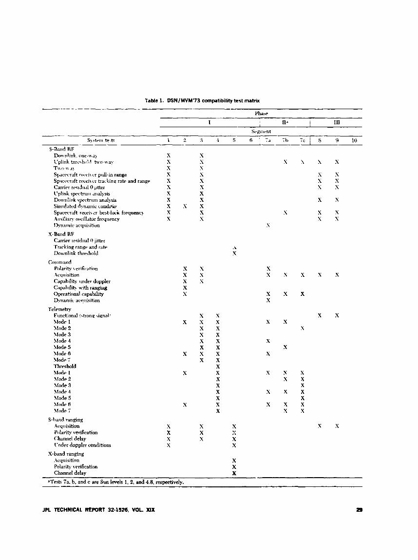
TaMt 1. DSN/MVM'73 compatibility test matrix
S-3and RF Do\\ nlink. one-na? l'plink tnrc\hirlrl two-\\ ay Tni1-n .t?
SpxwrJft rtr.ri\ t'r pud-in range Spacwmft recei\ c'r trackinq rzte and range Carrier rcsi3ii.d O litter t'plink spectruiii aiialysis h n v n l i n k spectrrin, andysis Siniiilntcd dynamic conditio- Spacwraft recei\ cr he>t-l& f i q u a c ! .Xii\i!kary oscillator frequency I)?namic acqiii\ition
?(-Band RF Carrier rrsidrial 0 jitter Tracking range and rate humlink threhhold
Coniniand Polarity lerificatinn .-\cqirisition Capahility under doppler Capabilie with ran& Operational capability Dynamic ncq::isitron
Telemetr?; Functional f<trone \ienall Slode 1 Mode 2 Mode 3 Mode 1 Mode 5 Mode 6 \lode 7 Threshold Mode 1 \lode 2 Mode 3 Mode 4 Mode 5 Mode 6 %lode 7
S-hand ranging Acquisition Polarity verification Channel delay Vnder doppler conditions
X-band ranging .\cquisition Polarity verification Channel delay
s s s s
s s S
x x ?( S
s x x s
S
x x S X s
X
X
X
X
s s x s s ?( X X X s s
s s S
N x X S S X S x
s X x
x x X X x X X X X X X X X X x X
S
s s x
x
s s x s s s
X S X x
x x s x
S
X
s X
s x s s x
X s x x
X x x x
X X
X V 1.
X x
X X X
x s
*Tests 7a b, and c are Sur. levels 1, 2, and 4.8, respectively.
JPL TECHNICAL REPORT 32-1526, VOL. MIX 29
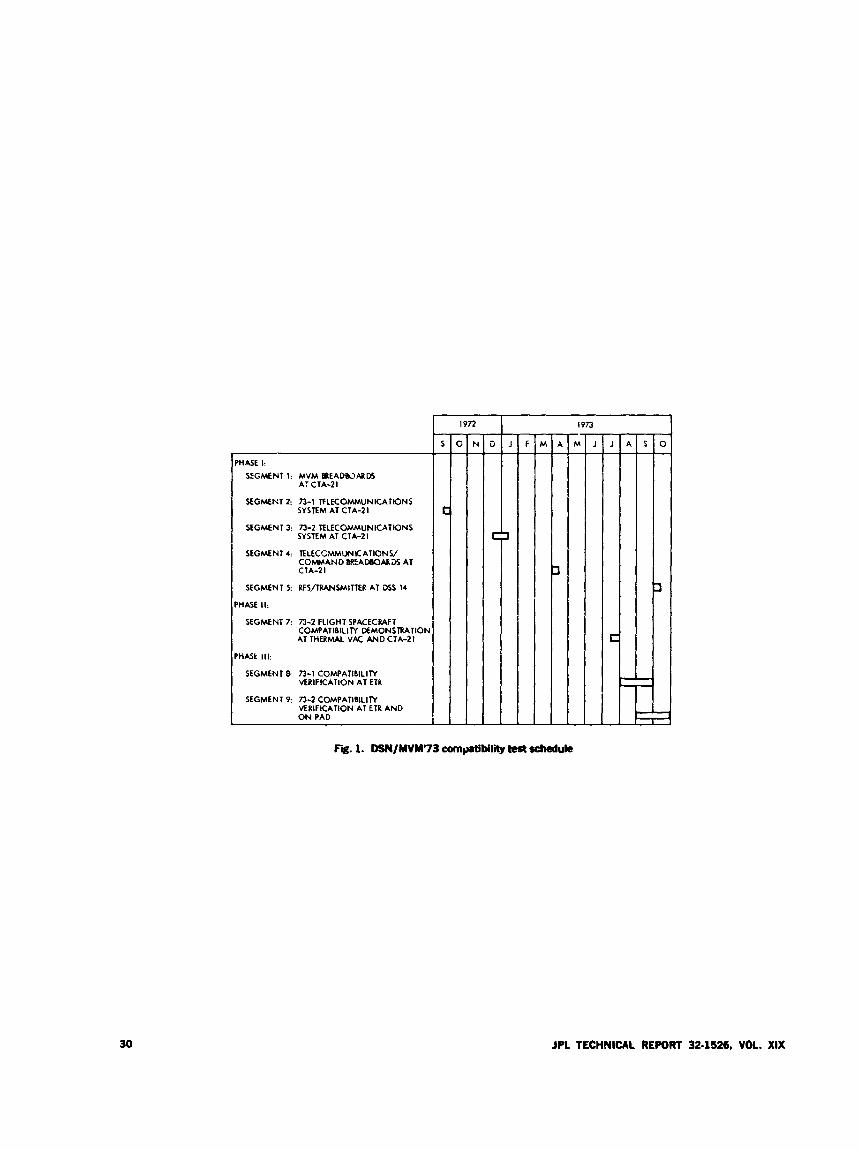
HASE I: SEGMENT 1: MVM BREADb3ARDS
A: CTA-21
SEGMENl 73-1 TELECOMMUNICATIONS SYSTEM AT CTA-21
SEGMENT 3: 73-2 TELECOMMUNICATIONS SYSTEM AT CTA-21
SEGMENT 4: TELECCMMUNYCATIONV COMMAND W A O M ) A R Z AT CTA-21
SEGMENT 5 RFS/TRANSMITfER AT MS 14
HASE 11:
SEGMENT 7: 73-2 FLIGHT SPACECRAFT COMPATlBlLllY LXMONSlRATlOF AT THERMAL VAC A N D CTA-21
HASt 111:
SEGMENT & 73-1 COMPATIBILITY VERIFICATION AT ETR
SEGMENT 9: 73-2 COMPATIBILITY VERIFICATION AT ER AND ON PAD
1972 I N S J
n
Fig. 1. DSN/MVM'73 comprtibilii test schedule
1973
hl
30 JPL TECHNICAL REPORT 32-1526, VOL. XIX
The Mariner 9 Quasar Experiment: Part I M. A. Slade and P. F. MacDoran
Tracking and Orbit Determination Sectioii
I. I. Shapiro Massachusetts Institute of Technology
D. J. Spitzmesser Network Operations Section
J. Gubbay. A. Legg, and D. S. Robertson Weapons Research Establishment, Australia
L. Skjerve Philco-Ford Corporation
Differentia2 oery long baseline interferometry (VLBI) experiments were con- ducted in 1972 between Mariner 9 and various quasars. Thz objective bf these experiments ~LIQS to determine the position of Mars in the VLBI rcfmence frame. This first of tuw articles gives background and describes experimental procedures. A subsequent article udl describe the analysis of the data and the result obtained for the differential position.
1. Introduction The technique of very long baseline interferometry,
presently under rapid development, holds promise of mak- ing important contributions to spacecraft navigation. Through VLRI observations of extragalactic radio sources, many of them quasars, it will be possible to determine Earths orientation (UTI and polar motion) accurately with respect to the inertial framr formed by these sources. Our expectation is that within the next 5 years VLBI will be ablr to provide, for example, measurements of UTI routinely with uncertainty below the 1-ms level, which
projects to a position error of about 10 km at a g-wentric dietance of 1 AU (still by no means the theoretical limit of the technology). In order to utilize this accuracy for inter- planetary spacecraft navigation, we must know the orien- tation of the planetary system with iespect to the same inertial frame. Since the planets are not themselves suit- able targets for VLBI observations, an indirect approach is necessary. It was therefore suggested by one of us (I.I.S.) that a spacecraft in orbit about another planet would be an appropriate target.
JPL TECHNICAL REPORT 32-1526, VOL. XIX 31
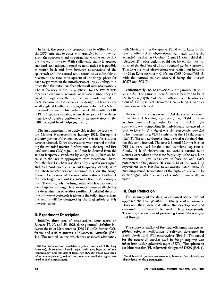
In bricf, the prccrliure prop0sC.d \vas to utilizc in.9 c?f
the DSN antennas to observe alternately, but in synchro- nism, the spacecraft and an estragnlactic radio source that lies nearby in the sky. with sufficiently stable frequency standards and adequate signal-to-noise ratios, it is possible to switch back and forth bet\vtvn observations of the spacecraft and the natural radio source' so a s to be able to determint, the time development of the fringe phase for each target without the introduction of any 2- ambiguities other than the initial one that affects all such observations. The differences in the fringe phases for the two targets represent extremely accurate observiibles sinct. they are freed, through cancellation, from most instrumental ef- fects. Because the two sources, by drsign. subtend a very small angle at Earth, the propagation-medium effects tend to cancel as well. This txhnique of differential VLBI (AVLRI: appears capable, when developed, of the deter- mination of relative positions with an uncertainty at the milliarcsecond level. (Also see Ref. 1.:
with Mariner 9 \va> the quasar PO106 - 01. Later in the year, another set of obscrvations was madc during the extended mission on October 13 and 17. On a third dny (October 27‘ , obscrvations could not bc carried out hc- cause of the final loss of altitudt, control gas by llarincr $1. This later series of obscnations \vas carried out hrtwcw the 26-m Echo nntcmna at Goldstone (DSS 12) ant1 IISS 41. \vith the natural sources o h s i n d being tht. qrlas;irs 3C273 and 3C279.
LTnfortunatt4y. no observations after J,inudry 20 \vere succcssful. The caust. of thew failurc? i~ htBlicaved to be in the frequency system of ont’ or both stations. The obscm~~- tions of 3C273 yirlc1t.d intcmiitttmt. u vak frinp-s; no othw signals were drtcctrd.
The first opportunity to apply this technique arose with the Mariner 9 spacecraft in January 1972. During this primary portion of the mission, several sets of observations were conducted. Other observations were carried out dur- ing the extended mission. Unfortunately. the required first local oscillator (LO) signal could not be derived from the station frequency standards by integer multiplication he- cause of the lack of appropriate instrumentation. There- fore, the first LO chain was driven by a synthesizer signal and, as a consequence, sufficient frequency stability with the interferometer was not obtained to allow the fringe phase to be “connected between observations of either of the two targets without the introduction of 27 ambigui- ties.’ Therefore, only the fringe rates, which are inherently unambiguous although less accurate, were available for :he determination of relative position. A detailed descrip- tion of these experiments is given in the followhg sections; the results will be discussed in the final article of this two-part series.
The accuracy of the data, as explained above, did not approach the level for this type of experiment. However. these datd did allow the development and checkout of software to be usrd in later expcriments. Therefore. thr exercise of processing these data was car- ried through. II. Experiment Description
Initially, three sets of observations were taken on January 17, ?O, and 25, 1972, during mutual visibility be- tween the 84-m hlars antenna (DSS 14) at Goldstme, Cali- fornia, and a 26-m antenna at \Yoomera, Australia (DSS 41). The natural soiirce which was observed alternately
‘Had four antennas been availahle (a pair at each end of the long baseline), observations of each target muld have been carried out continuously, and this lack of frequency st;bility woull have been of no consequence (provided the same local oscillator signal was used at each antenna pair).
On ewh of the 2 days \\-hen iiwful data wtw obtaintd, three kinds of tracking were porformcd. Tithlc 1 siini- marizrs these trackicg modes. During the first 2 h, the spa-vcraft was completing its high-bit-rate science play- back to DSS 14. This signal \vas simultanc~ously recorded to be processed in a VLBI mode using the 24-kHz systc-m (Ref. 2). Three-way doppler data were also obtained dur- ing this same interval. The ntxt 2 11, until Xlariner 9 .;et at DSS 14, were used for the actual switching experiment. Finally, 4 h of obsert.ations on vari.)ris natural radio sources were taken at the same frequcllcy as the switching experiment to give scnsitiv;?; ro haselinc and clock parameters.“ On January 20, runs 9-13 of the switching esperiment were lost dur to an unanticipated, although mission-planned, termination of thc high-rate science sub- carrier signal which servcd as the interferometer illumi- nator.
111. Data Reduction
The cross-correlation of the magnrtic tapes was acmm- plished using a modification of software developvd for Earth physics and UTI observations (Ref. 3). The model for the spacecraft motion used in fringe stopping was taken from probQB ephemeris tapcs (PETS). The ephemeris for Mars was the JPL ephemeris designated DE69 (Ref. 4).
?The differential position meawrement, however, has virtually no dependence on these parameters.
32 JPL TECHNICAL REPORT 32-1526. Vot XIX
Figuri. 1 shows typical residual sine fringes for Mariner 9 over a small portion of one VLBI tape pair on January 17. Thv best-fitting sine wave over this interval is also shown.
The fringes which resuited from the cross-correlation were thpn analyzed to extract the information about the time developmeht of the fringe phase (Ref. 3). Differenc- ing the relative fringe phase at different times for a given source then yielded average fringe rates over these inter- vals. The results from one such analysis are shown in Fig. 2 for a tape taken on January 20. The resic!usl phase after a constant fringe rate was removed is plotted as a function of time from the beginning of the tape. The figure also illustrates the antenna switching sequence followed in all
the switched observations. The spacecraft phase points are more finely spaced because the higher signal-to-noise ratio for Nariner 9 a l l o \ d h shorter averaging time (12.8 s compared to 57.6 s). Note that the scale of the abscissa is ~ ‘ 3 cycle of S-band phase (-4 cm light-time equivalent:.
TSe final step in the processing of the raw observations was the removal of the phas models used in fringe stop- ping €or the two sources. The resulting “total” fringe rates were then analyzed using programs with more so, histi- cated modeling of t!w theoretical expression for the motion of Earth and the spacecraft. The result of this analysis is to be the subject of the final article of this two-part sequence.
Acknowledgments
The authors wish to acknowledge the contribution of J. Gunckle of the JPL st&, and the personnel of DSS 14, 12, and 41, particularly the servo, digital, and micro- wave subsystems. The PET ephemeris for Manner 9 was kindly supplied by R. K. Hylkema. W e also thank H. PeLers of Goddard Space Flight Center for the loan of a hydrogen maser at the Woomera station.
References
1. Couselman, C. C., Hinteregger, H. F , and Shapiro, I. I., “Astronomical Applica- tioiis of Differential Interferometry,” Science, Vol. 179. p. 807, 1972.
2. Fanselow, J. L., MacDoran, P. F., Thomas, J. B., Williams, J. G., F’innre, C. J., Sato, T., Skjerve, L., and Spitzmesser, D. J., “The Goldstone Interferometer for Earth Physics,” in The Deep Spacs Netmrk Progress Report, Technical Report 33-1526, Vol. V, pp. 45-57, Jet Propulsion Laboratory, Pasadena, Calif., Oct. 15, 1971.
3. Thomas, J. B., ‘An Analysis of Long Baseline Interferometry, Part 111,” in The Deep Space Network Progress RepGrt, Technical Report 32-1526, Vol. XVI, pp. 47-64, Jet Propulsion Laboratory, Pasadena, Calif., Aug. 15, 1973.
4. OHandley, D. A., Holdridge, D. B., Melbourne, W. G., Mulholland, J. E., JPL DeueZupment Ephemeris Number 69, Technical Report 32-1465, Jet Propulsion Laboratory, Pasadena, Calif., De. 15, 1969.
4 . J R TECHNICAL RE- 32-1526, VOL. XIX 33
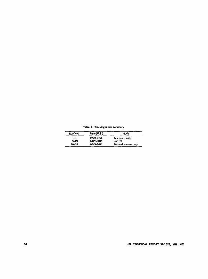
Table 1. Tracking mode summary
Run Nos. Time (U.T.) Mode 1-8 02204420 Mariner Q only 9-19 0427-0647 AVLBI
20-35 0649-1041 Natural sources only
34 JPL TECHNICAL REPORT 32-1526, VOL XIX
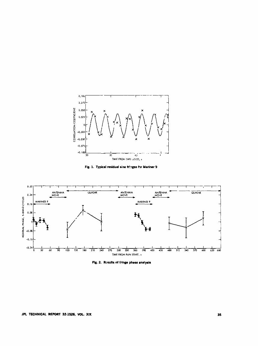
Fig. 1. Typical residual sine trIages fw Mariner 9
0.32
0.24 VI w
il $ 0.16
3 n
I 1 I I I I I I I I I l *
c-- - II. - ANTENNA QUASAR ANTENNA ANTENNA - MOVE MOVE MOVE - -
MARINER 9 MARINER 9
Fig. 2. Rcm~lts of fdnp phase analysis
- v) w
-0.16
-0.24
JPL TECHNICAL REPORT 32.15226, VOL. XIX
- - - 1 I I I I I 1 I 1 I 1 I 1 I 1 I I I I I I
35
Radio Interferometry Measurements of a 16-km Baseline With 4-cm precision
J. B. Thomas, J. L. Fanselow, and P. F. MacDoran Tracking and Orbit Detarmination Section
0. J. Spitzmesser
L. Skjerve Philco-Ford Corporation
Barstow. California
Network Operations Office
In order to demonstrate the feasibility of eventuaUy using radio interferometry techniques to measure tectonic motion, a series of interferometry experiments has been conducted between two antennas at the Colddone Deep Space Communi- cations Complex. The primary objective of these experiments ulos to deuebp independht-station instrumentation capable o f making three-dimensimal baseline measurements with an accuracy of a feu; centimeters. To meet this obiectioe, phase-stable instrumentation tcap developed to precisely metare the time delay by meam of two-channel bandwidth synthesis. Delay measurements produced by this instrumentation lead to three-dimensional base!ine measurements with a precision o f 25 cm for the components of a 16-km baseline.
1. Introduction In the last few years, there has been increasing interest
in developing a system capable of accurately measuring the relative motion of points separated by distances rmg- ing from 100 Inn up to intercontinental distances on the Earths crust. Information concerning this far-field motion is of critical importance in the development c,f theoretical models of crustal dynamics. Since crustal motion is about 3-10 cm/year, the measurement accuracy should be about 1-3 cm with about 1 week of data. Radio interferometry is one technique that holds great promise for fulfilling tnis accuracy requirement.
In order to begin devehpment of a radio system with few-centimeter accuracy, a series of interferometry experi- nrents has been canducted between two mtennas at the Goldstone Deep Space Communications Ccmplex. The primary objective of these experiments was to develop independent-station instnimentation capable of making three-dimensional baseline measurements with an accu- racy of a few centimeters. A short Goldstme baseline (16 km betweea DSS 12 and DSS 14) was selected so that transmirsion media uncertainties and astronomical param- eters would be relatively unimportant compared with
34 JPL TECHNICAL REPORT 32.1126. VOL. x1X
radio system limitations. These experiments I d to the refinement of a two-channel approach to bandwidth syn- thesis, a technique for measuring time delay that was originally developed by A. E. E. Rogers (Ref. 1). In this report, the instrumentation, analysis, and results of these Goldstone experiments are presented.
II. Radio Interferometer Technique In the radio interferometry rneasurq-nents d.scribed in
this report, two antennas simultaneously receive the radio noise generated by an extragalactic radio source, as shown in Fig. 1. Because of a difference in ray paths, a given wave front will reach the two antennas at diflerent times. This difftrence in arrival times is called the time delay T.
In this section, the technique for the measurement of this delay is described, while a mathematical model for this quantity is discussed in Sectioir 1V.
Since the radio interferometry method has been ana- lyzed in detail in other papers (Refs. la), it will be described only briefly in this report. Single-channel inter- ferometry will be reviewed first. followed by an outline of two-channel bandwidth synthesis.
In single-channel measurements, each antenna system records on magnetic tape radio noise centered at fre quency with bandwidth W,. The t q x s are then carried to a central site for Agital processing. In this reduction, the two data streams are processed to obtain the stopped fringes (Ref. 5), which. for channel a, are given by
where the stopped phase is given by
In addition.
Sr, = tp + rt + t r + T~ - T,,, (2)
In these expressions,
W, = single-channel bandwidth
= effective interferometer bandpass center
= instrumental phase drifts
C, = diflerential charged-particle phase shift
R,, = brightness transform phase
tp = geometric delay
T t = dii€erential tropospheric delay
te = daerential ionospheric delay
= instrumental delap plus clock synchronization error
T, ‘= modeldelay
E anslytical frequency otTset
4.T = peak amplitude
Thus the stopped fringes are a product of an amplitude factor An, a delay cune. sin ( :WBST, ) ( Y W ~ T , ) , and a sinusoidal function, cos +*. The amplit& factor dqwnds on the brightness transform in addition to signal and 9-s- tem noise temperatures. The delay curve is a measure of bit stream alignment in the time domain. i n c l u h g all group delay effects. This particular form for the delay curve assumes that the system bandpass b rectangular with .A linear phase-versris-frculiilpncy response. an approxi- mation of negligible tarfor for the purposcs of t h i tsperi- ment. Finally, dcwribts the phase hJm-ior of the sys- tem. In this phase is buried the geometric delay ;$. the observable of primary interest in these mcasuremcnts. Note that. since the ionosphere is a dispersive medium. the ionosphere effect has been exprtsstd as a phase shift in the fringe phase and as a delay in the total p w p delay.
The nest step in the data reduction is to determine the fringc phase +# by a p rwru known as phase tracking (Ref. 5) , a tcrhnique that fits a least-squares sinusoid to the stopped fringes ivn. .%fter 4, (t) is extiacted as a func tion of time. thc analytical offset et is removed in a man- ner that gives the correct sign (Ref. 5) to the resulting residual phase. The theoretical behavior of this measured residual phase A+, is given by
The adjective “residual” denotes the fact that, in e&&, the data reduction process subtracts a model delay (tn) from the fringe phase. This ”phase stopping” procedure removes most of t!ie time-varying components of the tgtal delay.
Because fringe phase CUI be Jetemincd ody tu wiilriij a constant (2n,), narrow-band, single-channel interferom- etry can essentially measure only phase changes. There- fore, ii residuai phase is measured over a short time interval, it is essentially a measure of residual fringe fre- quency given by
37
\vlit.rc A& is the time derivative of the phase e-xtracted from *lie fringes. This time derivative is insensitive to the ;comlmwiit of the baseliiw, since that particular pmjec- tion does not change apprtviably as the Earth rotates. Conwqucntly. a mt~asuremcnt of dt-hy is essential if three- dinicmsional bast-lint- nivsuremcmts arc- to b c b made. This rtqiiirtm.rnt for Jday nir;uurements lead to the develop iiwit 0; t ~ w - ~ l ~ : t i ~ d hiidwidth s;.nthesis.
In hw-chaiinc.1 bandwidth synthesis. the output of eac!t aiitenna system is alternately switched between two namnv-hand channrls. For example. during even seconds. twth systcmls would rcxvrd ;I bandpass centered at ,%.
w4iilc- during c d d d stu-onds. both would rtvnrd at e b . For cliaiiiic4 L . l t l ic. stopptd fringrs and fring, phase e-xpres- sions worrld h. idoitic;rl to Eq. ( 1 and Eq. (3. escept that thc subscript a is r tphctd by b. An example of hw- clianncl stopptd fringcs (Eq. 1' with onc--smnd switch- ing is sho\vn in Fig. 2. 0.1 this Goldstoiw baseline. this radio courcv. X -W.3. has a c.orrc4atr.d flus strength of a h u t 10 flux units tonv flux unit = 10 \V m: Hz'. The aiiiplitridv noise. on tht- fringbs CQIII(-S primarily fmni sys- tcmi noisc- i rt.rcivrr. soiirc(*. ;id hack~grorind noise:. This plot. which e 4 d ) i t s thc- first .#) s from ;I 6 0 - s tap-pair. displays frmgv poitits m i t a i n i i i ~ 0.3 s of data rcuvrdtd at a 45-kilol)it s ratr. .-\ltc.ni:ttc. strands in the plot s\\ itch I n t n x w i f r i n y fmni two ch;innt.ls c.c*ntcrcd at 2270 SIHz itntl 310 5111~. Tlic- stopixd fringe frtpiicbnc>- is ahout 0.1 Ffz in Iwth cli;tnnc4s and is due primarily to an ana- lyticd ratr offst-t E in thc pliasr niodc4 iistd in fringe stop- ping. This offsvt nllo\vs a cIrtcmiin;ttion of the si.p (Ref. 5) of thc rc.sidiia1 fringe frtqwnc? AI .: ant1 ii (Eq. 4).
Frirgv phnsc. plots ohtaiiitd from thtw fringes are shown in Fig. 3. Each phaw point runtains 50 s of data (im Frinp p:xn,s ot the t!.;x. in Fig. 3. whilp the entire plot covt'rs a mmplctr tapepair (600 S I . In the plot, the crror hars on thc. pliasc. points represent the phase error produced hy thc actual ampliiudr noise on the fringes. The s l o p of each of thtst. phase plots is a measurement of rcdiial fringr frcpucnq rcprtwnted analytically in Eq. (4'. Sincr an accurate. model delay was used in the data reduction. the phasc slopcs arc relatively constant owr o n c tapc. Thc small nonlinear trends (-0.03 cycle = 0.4 mi that ar" ~ r r s r ~ ! m.~!zI *be due to ionospheric effects. (Nonlinear trends due to large u priori delay errors .vould hr rpadratic in apprarancr over this short time interval. 1 Fringc frcqurncy valucs obtained from the phases slopes arc. impnrtant interfcromcter ohsenables and arc. ritilizcd :is shown in Section V.
In addition to thv froqiwncy observable. thc. measured tlday \ A i r s can he obtained by combining thv Fhase out-
put of the two channels as follows:
This csmputtd value \\ill be r e f rmcd to as the a priori residual delay. The IIW of the term ~residud" mems that a mde1 drla!- hit% in c-ffc'trt htvn subtracted from thc total clelay. leavinc a much smaller \-due. In comhining tlir two phase. outputs. cart. must lw taken to avoid & ambipiticbs i Rcf. T. \Vhrn computing -\:. one can assume that thc channel separation Q: is essentially exactly ho\vn. sinw frcqricmw c-dihration is ;~ccutxtr. to parts in IO".
An example of a delay calculation is shown in Fig. 4. where the phase values have been combined from Fig. 3. Sote how the systematic phase trends in Fig. 3 have dis- appeared in the difTertmcu, which in effect has scaled phase variations at S-band down to much lower levels at 40 VHz. the s>-nthtsiztul bx.dwidth. A covarianw analy- sis indicates that the obsentd noise on these delay valries comes almost entirely from the amplihide noise on thr fringes. Over one tapc. the residual dela! AST is tsscnti.illy constant dii to an wxxir;tte d&\- model T,,,. Therefore. thew dchy v&es are a\eragtul to produce one delay measurement for each tape-pair. .\ftt>r a\-eraging, the resulting delay rAicu, one for cich tape-pair. become the primary ohsen-ablw of the inttderometer system.
Sote that, if thc phase error in A+ and A+, is indepen- dent of frequcnq. the delay precision improves as the channel separation. wun - mh. increases. For this reason, the observing frequencies are generally separated as far as p s i b i e . .4s discussed in Section 111. the maximum chan- nel separation is dctenninc-d by the handpass limits of the antenna system.
The theoretical beha\-ior of the measured delay is given by thr. rspression (Ref. 3
In the present measurements, the instrumental phase dif- ference I)* - $ 0 introduces a long-tvrm linear drift in the measured delays. This drift is due primarily to a fre- quency offset between thc frrqucnq standard5 at the two stations. This term, as well as the other components of the mrasured delay, will he modeld in Section IV.
In summary. the data on each tape-pair are reduced to two observahle valucs-time delay and fringe frequency.
38 JPL TECHNICAL REPORT 32-1526, VOL. XIX

Before proceeding to a discussion of the mathematical d e l for delay and the fitting procedure, the experi- ments and their instrumentation will he described.
tions of the DSK antenna systems. In the final system, the maximum separation \vas defined by the limits of the traveling wave maser ("IVM, receiver bandpass.
111. Experiment Description Over the last two years, five separate radio interferom-
etry experiments. which arc siimniarizd in Table I. have been conducted behvwn DSS 12 and DSS 11 at the Goldstone Deep Space Communications Complcs. All experiments invoIved S-band observations. JPL H-maser frequency standards. aid a 44-kHz bandwidth digital recording system developed by D. S. Robertson and A. H. Legg of the \Veapons Research Establishment. Australia. As indicated in Table 1, the various esperi- mrnts were behvwn i and 14 hours in duration and invo:vcd 13 to 18 radio sources. The sources used in the last four experiments are described in Table 5.
In the first Goldstone rsperinient (Ref. &), one narrow- band (24-kNz bandwidth' channel of radio noise \\-as recorded, so that only the fringe frequency observable wss precisely obtained. An analysis of the resulting fre- quency obsen-ables reveal4 frequency instability at the 1-mHz level (J , ' f 5 X lo-'?) over severa! hours. '4s indicated iii Ref. 2. the HP5100 synthesizers associated with the first lwd oscillator (LO) signal were the most likely source of this instability. Consequently. in subse- iuent experiments. the synthesizers \vert' replaced by more stable X7 multip'iers. which will be described below.
After this first experiment. instrumentation was also developed to measure time delay in addition to fringe fre- qtiency. The technique adopted for delay measurements required the measurement of more than one channel of radin noise. This technique. commonly called bandwidth synthesis (Refs. 1 and 5). comhines, either directly or indirectly. the fringe phase information of band-limited channels record4 at frequencies whose separations are largc. compared to that of the siiiglr-channel bandwidth.
In thc original application of thc bandwidth synthesis technique (Ref. 1). six channels wcre recorded in a time- shared mode. Howrver, because of signal-to-rloisc ratio (SXR improvement and simplification of instrumenta- tion, w c employed instrumrntation that recorded only two channck Thr only disadvantage of the two-channel systvm is that sufficiently prccisc Q priori delay informa- tion is requirrd to avoid 2- ambiguities (Ref. 5). Since delay measuremcnt prwisinn improves as channel separa- tion incrrases. the gcal of the instrumental design was to obtain maximum channcl separation within the restic-
For the second experiment, a relatively simplc instru- mental configuration was de\-ised to demonstrate the feasibility of the two-channel approach to bandwidth synthesis. In this intermcdiatc. system, which will not bt. descrild here in detail, two channels separated by 10 JlHz at S-band were heterodyned to intermediate frc- qiicncy (IF? and added. This combined sign,al was then heterodyned to baseband and continuously samplcbd at a 1 6 - k i l d d s rutc.. \Vhile this system pays a price in SNR, it avoids the complications of simultaneous rcyorder chan- nel switching at the two stations. This internicdiatr instru- mentation demonstrated the feasibility of tlie t\vo-char~ncI approach and hvlped pcrfect the final instniiwntation described helob:.
Thc final canfiguration u s e d for bandwidth synthesis is shown in Fig. 5. In this system. ;i 10-blHz signal from the H-maser is converted to a 340-1\IHz first LO signal by using only multipliers-the standard S1S8 multipliers of the DSK system and a new Xi multiplier. This S7 multi- plier, which was constructed' to a\.oid the use of a synthe- sizer, convt-rts the input sinusoid to a square wave, then filtcrs and amplifir; the scvcnth harmonic.
In order to achic.ve masinirim channel separation and better delay prtrision. thc S-hand trawling wave m:iser receiver bandpass \vas broadewd by retuning the trim coil currents. In this retuned statr, thc. rccvivcr cshibitcd ample amplification over a IO-YlHz intcrvi.1 (&E(! to 2310 MHz) whilr maintaining an operating system noise tcmprraturr less than 30 K. Therefore. aftcar mixing \vith the first LO signal at 2240 MHz, the tdgrc of the rcw3vc.r paqshand were placed at 30 AlHz and 70 MHz. However, this frequency spread exceeded the bandpass of the stan- dard first mixer preamplifier, which p o s s ~ ' ~ ~ s ~ s adequate gain only over 45 to 5.5 MHz. Consequcntly, thc standard miser preamplifier \vas replacrd by a similar modiile with a bandprFs hct\vc.cn 10 and 160 MHz, thcwhy making the system TWlI-limitcd. This IF passhand was them filtervd iiito two channels-one centered at 30 MHz and tho othcr at 70 hlHz. Each channel was mixrd with a 20-bIHz signal derived froiii the F1-mascr and cach mixer response was approp;iatdy filtcrecl to placr both channels at SO MHz. At this point, each chnnnzl was traiisfcrrvd on altcmate seconds to the vidm convrrtcr. The vidcc wnverter mixed the input IF signal to haschand with a tSO-AfHs! signal derived from the H-maser. T h c b rtwlting time-shared
'R. L. Sydnor. Telcconimunicntion Rrwarrh Srction. JPL.
JPL TECHNICAL R E M 32.1526, YOL XIX 39

baseband signal was then passed through a 24-kI-I~ band- pass filter before digital sampling and recording at a 4S-kilobit/s rate.
IV. Time Delay Model Thc residual delay AT observed in radio interferometry
measiirements is a sum of geometric, instrumental, and transmission media drlays, as indicated in Eq. (6). This section outlines the model adopted for these terms in the observed delay, starting with :he largest and most impor- tant term, the geometric delay.
As indicated in Fig. 1, a given wave front will reach the two antennas of the interferometer at daerent times. It is readily shown that the geometric delay is given by the expression (Ref. 3)
(7’)
where B is the baseline vector between the two antennas, S is the apparent source direction, V2 is the velocity of antenna 2, and c is the speed of light. Note that the geo- metric delay is essentially the instantaneous geometric path dilference multiplied by a small correction that accounts for the motion of antenna 2 diiring the wave transit.
In the present analysis, tnie equatorial coordinates of date (TECD) are chosen as the coordinate frame for geo- metric delay calculations. In this Earth-centered right- handed frame, the z-axis is along the instantaneous spin axis of Earth while the x-axis is along the tnie equiyx of date. The source vector B and the baseline vector S can be expressed in terms of these coordinates as follows.
In TECD, the source vector S is usually characterized by two angles-apparent declinations 6. and apparent right ascendon a,. These angles lead to the usual expres- sion for the source vector:
A S = (cos 8 , cos a*, cos 8, sin a*, sin 8,) (8)
The term “apparent” indicates the presence of a correc- tion to the source direction that accounts for aberration diie to the Earth‘s orbital motion (Refs. 3 and 71. In addi- tion, prccession and natatiov of the Earth‘s spin axis (Refs. 7 and 8: are included to rotate to TECD from mean equatorial coordinates of 1950.0 since the 1950.0 frame is conventionally used to catalogue source positions. In the present short-baseline measurements, these corrections are easily made with adequate accuracy.
The baseline vector B must include two general fea- tures: an Earth-fixed definition and Earth orientation fac- tors. The Earth-fixed vector, B,,:. is defined in twns of a right-handed coordinate frame with a z-axis townrd the Conventional International Origin (CIOI pole and X-axis along the Greenwich meridian. It will be represented in Cartesian mrdiwtes as follows:
where xb.tJ( are the equatorial components and z b is the :-component. as schematically indicated in Fig. 1.
At this point in the discussion of the baseline vector. a definition of antenna location is desirable. The effective location of an antenna depends on antenna structure. Most directional antennas ha\-(, two primary axes of rotation that allow antenna orientation. For DSS 14, an azimuth /elevation antenna, the rotation axes intersect. By geometrical considerations, one can show that this point of intersection is the efftbctive antenna location.
On the other hand, DSS 12 is a polar mount. for which the rotation axes are nonintersecting. In this case, the effective location is the point at which the hour-angle axis orthogonally intersects a plane containing the decli- nation axis. Thercfore, for this polar mol. t, one must include the correction factor b cos 6 , in delay calculations, where b is the shortest distance between the twc axes. This correction factor acroiinh for the fact that this type of antenna “stretches toward low-declination objects. For DSS 12, the axis separdtion b is 6.706 m and is easily accounted for with adequate precision.
The baseline vector B rotates in space as R result of polar motion and EartL spin. To account for those mo- tions, the Earth-fixed baseline vector is rotated to its instantaneoris orientation in ‘TECD a b follows:
where the Earth spin matrix is given by the expression
and the polar motion matrix is given by
R , = 0 Y, a
\X,/a --Y,?l 1 J
40 JPL TECHNICAL REPORT 32-1526. VOL. XVlll
In these expressions, the angle ac is the hour angle of the equinox at the time of interest and is easily obtained from universal time (UT1). Parameters X, and Y, are the polar displacements relative to the CIO pole, while a is the polar radius. See Ref. 3 for more detail concerning these Earth orientation factors.
A The expressions above for B and S are easily combined
to calculate the geometric delay for a given source. It should be noted that the model for the geometric delay outlined above neglects general relativistic effects which, for longer ha3elines, may he significant.
In these experiments, no corrwtions were made for ionospheric effects. In all the measurements reported here. radio sources werc observed at night when ionospheric delays, inhomogeneities, and turbulence were at a mini- mum. ,4t S-band, the nighttime ionosphere causes about a 1-m dclay along a single ray path at a typical eleva- tion angle ( ~ 3 0 dtg). However, the diference in iono- spheric delays along the two iuterferometer ray paths is the important quantity in dclay measuremerlts. Since nighttime observations involve a relatively homogeneous ionosphere, this difference for a 16-km baseline will be a small fraction of a single ray-path delay. As we shall see, the delay residuals in the present experiments stronglv indicate that differential ionosphere delays were less than 6 cm. Below the 6-cm level, differential ionosphere correc- tions, even if they were available, would be of marginal value in the present delay measurements. However, as discussed in Section \-I, the frequency residuals contain an unmodeled noise term at the 0.1-mHz level that could possibly be an ionospheric effect.
The total troposphere delay for a single ray path is ribout 4 m for a typical elevation angle. In the present work, small corrections are made to the delay observables to remove small known differences ( 515 cm) in tropo- spheric delays along the two ray paths. These differences are a consequence of Earth curvature as well as a slight altitude difference (40 m) between the two antennas. The altitude difference produces a 1-cm difference in the ”dry” component of the zenith tropospheric delay. The Earth‘s curvature leads to elevation angle differences that cause differential troposphere corrections as large as 10 cm. It is believed that, with these CorrecFnns, the differential “dry” troposphere delay becomes a negligible source of error. The total “wet” troposphere delay for one ray path at Goldstone is mly 1&20 centimeters at typical elevation angles. For a 16-km baseline with only small changes in altitlide, the difference in the wet troposphere between ray paths should be only a small fraction (<lo$) of the
single ray path delay. It is estimated that. with the listed corrections, the total troposphere effect in the delay ob- servable becomes a negligible source of error (5 3 cm).
Finally, with regard to the present instrumentation, tlie instrumental terms (T,, - <b) in the measured delay (Eq. 6) can be adequately .*(>deled as a constant plus a linear drift, where the constant and slope are used as solve-for parameters.
V. Fitting Procedure As outlined in Section 11, the reduction of each tape-
pair gives the residual delay AT and fringe frequency a v for a particular radio source observed for a 12-min inter- val. In order to extiact the baseline vector, the delay and frequency values from many tape-pairs recorded for many radio sources must be sirnultaneoiisly fit by a least- squares technique using a model for the delay. The con- struction of a mathematical model for the geometric de- lay was outlined in Section IV. This section outlines the wcighted least-squares fitting procediire used to extract the Goldstone baseline.
In these short-baseline measurements, uncertainties in the geometric delay due to errors in source location and Earth orientation factors (polar motion, UT1, precession, nutation) are small compared with instrumental errors. That is, all of these factors have been measured with suffi- cient accuracy by other methods so that they mav be treated as “known” quantities in delay calculations. For the radio sources in these experiments, source locations have been independently measured with an accuracy of 0:u).9 Y-c seconds, as indicated in Table 2. The posi- tion errors in this table represent approximate external accuracy, conservatively estimated in some cases by root-sum-squaring the quoted internal errors with 0.3 arc second. The adequacy of these measurements can be demonstrated by the following approximnte calculation. A typical value for the sensitivity partials in the presmt experiments is approximately 0.1 ns/arc second. When this sensitivity is multiplied by a typical source location error of about 0.5 arc second, a delay error equal to 0.05 ns (1.5 ;.m) results. This delay error is small compared with a typical system noise error of about 7 cm. Similar detailed calculations for all sources in Table 2 indicate that these source positions are adequate for present delay modrl cal- culations. By similar arguments, one can show that polar motion and UT1, which are known with about 0.03 arc second accuracy (Ref. 9), also contribute negligible errors in delay calculations. The BIH values fo. UT1 - UTC and polar motion parameters are listed in Table 3. Finally,
JPL TECHNICAL REWRT 32.1- XIX 41
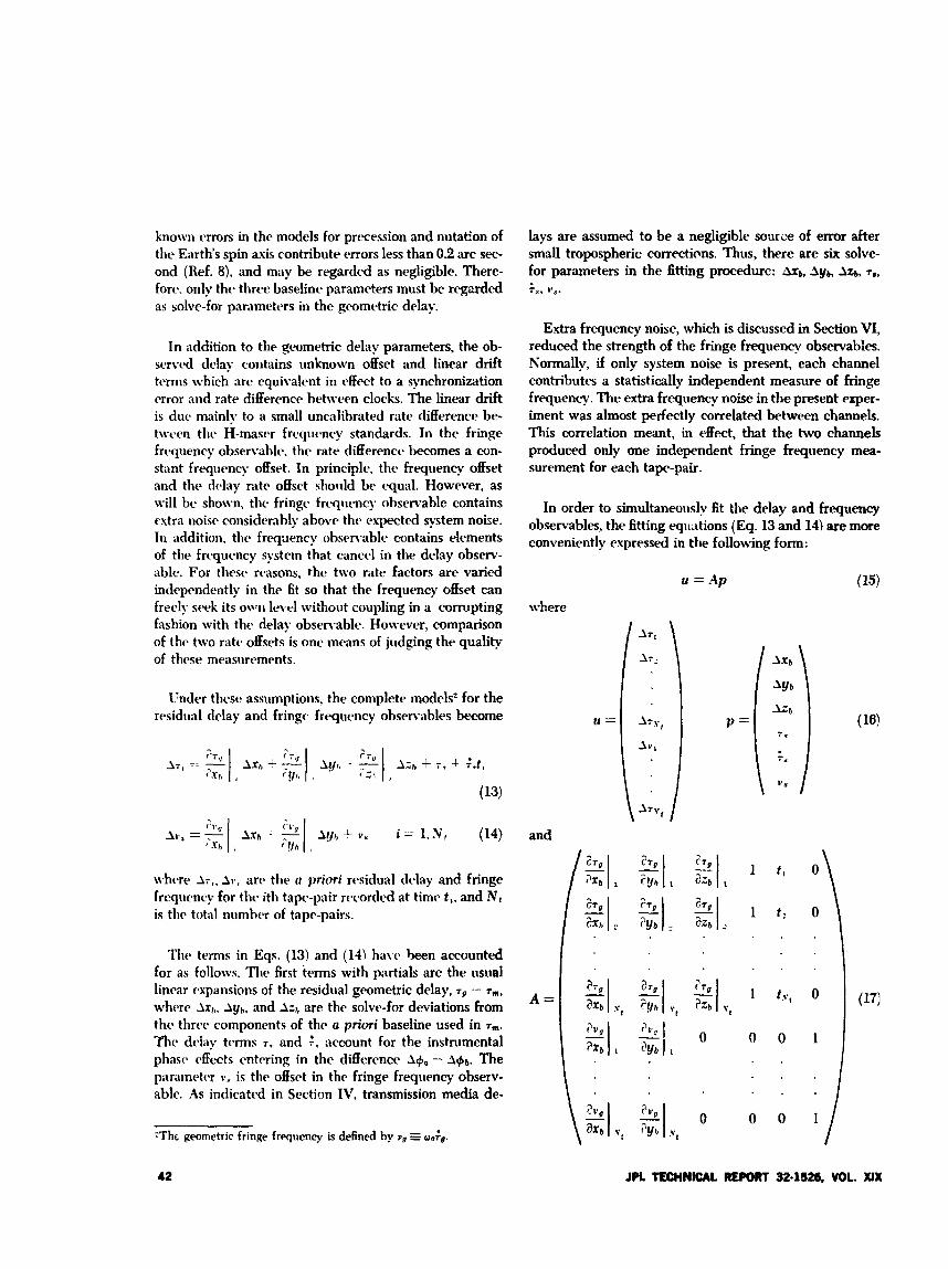
known crrors in thc models for precession and nutaEon of the Earths spin axis contribute errors less than 0.2 arc sec- ond (Ref. 8). and may be regarded as negligible. There- for<.. only the three baseline parameters must be regarded as solve-for parameters in the geometric delay.
In addition to the gcwmetric delay parameters, the ob- served delay contains unknown offset and linear drift terms which are equivalent in effect to a synchronization error and rate difference between clocks. The linear drift is due mainly to a small uncalibrated rate difference be- t\vc.en tlir H-maser frcqucncy standards. In the fringe frtquenry observable-. thc, rate difference becomes a con- stant frequency offset. In principle, thca frequency offset and the dc-lay rate offset shoiild he equal. However, as will bc shown, the fringy frequency observable contains extra noise considrrahly above the expected system noise. 111 addition. the frrquency obs(m&lcb contains elements of the frequency system that cancel in the delay observ- able. For these reasons. the two rate factors are varied independently in the fit so that the frequency offset can freely s t ~ k its owi level without coupling in a corrupting fashion with the delay obsen-able. However, comparison of thc two rate offsets is one means of judging the quality of these measurcments.
L'nder thcsc assumptions, the complete models? for the residrinl dclay and fringe frequency ohservables become
\vhcre AT,. AI, , arc. the o priori rcsidual delay and fringe frequency for thc ith tap-pair rworded at timc t,, and N t is the* total nurnbrr of tape-pairs.
Tht. terms in Eqs. (13) and (141 havc been accounted for as follows. The first terms with partials are the usual lincar expansions of the residual geometric delay, T, - T,,,,
whcre Axf3, &&,, and &h are the solve-for deviations from thcx t1irc.c components of the a priori baseline used in z ~ .
Thr dciay terms T , and 2, account for the instrumental phasc effects entering in the differencc - A+b. The paramrtt.r r2 is thr offsrt in the fringe frequency observ- able. As indicated in Section IV. transmission media de-
'Tht geometric fringe frqricncy is defined by vg = &.
42
lays are assumed to be a negligible source of error after small tropospheric corrections. Thus, there are six solve- for parameters in the fitting procedurc: &tb, Ayb, &b, r,, T*. 1'8-
Extra frequency noise, which is discussed in Section VI, reduced the strength of the fringe frequency observables. Normally, if only system noise i s present, each channel contributes a statistically independent measure of fringe frequency. The extra frequency noise in the present exper- iment was almost perfectly correlated between channels. This correlation meant, in effect, that the two channels produced only one independent fringe frequency mea- surement for each tape-pair.
In order to simultaneouslv fit the delay and frequency observables, the fitting equations (Eq. 13 and 14) are more conveniently expressed in the following form:
u = A p
where
and
A =
. .
. .
JPL TECHNICAL REPORT 32.1126. VOL. XIX
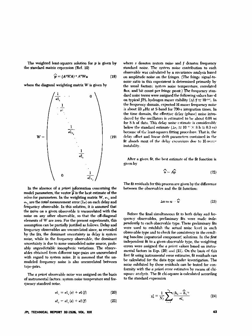
The weighted least-squares solution for p is given by the standard matrix expression (Ref. 10)
p = (AWA)- lAIWu
-
A
where the diagonal weighting matrix W is given hy
W =
" \ I
1
\ \ O
In the absence of a ptiori in nnation concerning the model parameters, the vector is the best estimate of the solve-for parameters. In the weighting matrix W, uri and uVi are the toto2 measurement error (10) on each delay and frequency observable. In this solution, it is assumed that the noise on a given observable is uncorrelated with the noise on any other observable, so that the off-diagonal elements of W are zero. For the present experiments, this assumption can be partially justified as follows. Delay and frequency observables are uncorrelated since, as revealed by the fits, the dominant uncertainty in delay is system noise, while in the frequency observab!e, the dominant uncertainty is due to some unmodeled noise source, prob- ably unpredictable ionospheric variations. The observ- ables obtained from different tape-pairs are uncorrelated with regard to system noise. It is assumed that the un- modeled frequency noise is also uncorrelated between tape-pairs.
The a priori observable noise was assigned on the basis of instrumental factors: system noise temperature and fre- quency standard noise.
where s denotes system noise and f denotes frequency standard noise. The system noise contribution to each observable was calculated by a covariance analysis based on amplitude noise on the fringes. (The fringe signal-to- noise ratio in this experiment is determined primarily by the usual factors: system noise temperature, correlated flux. and bit count per fringe point.) The frequency stan- dard noise terms were assigned the following values baspd on typical JPL hydrogen maser stability ( ~ f / f zz 1O-l'). In the frequency domain, expected H-maser frequency noise is about 23 pHz at S-band for 700-s integration times. In the time domain, the effective delay (phase) noise intro- duced by the oscillators is estimated to he about 0.08 ns for 8 h of data. This delay noise rstimntv is considerably below the standard estimate (AT, 0.3 11s) because of tlw least-squares fitting procedure. That is, the delay off set and linear drift parameters contained in the fit absorb most of the delay excursions due to H-m::.s:.- instability.
10.'' X 8 h
After a given fit, the best estimate of the fit function is given by
A A u = Ap
The fit residuals for this process are given by the difference between the observables and the fit function:
Before the final simultaneous fit to both delay and fre- quency observables, preliminary fits were made inde- pendently to each observable type. These preliminary fits were used to establish the actual noise level in each observable type and to check for consistency in the result- ing baseline (equatorial component) solutions. In the first independent fit to a given observable type, the weighting errors were assigned the a priori values based on instru- mental factors in Eqs. (20) arid (21). On the basis of this first fit using instrumental error estimates, fit residuals can be calculated for the data type under investigation. The noise exhibited by these residuals can be tested for con- formity with the (I priori ermr estimates by means of chi- squarc analysis. The fit chi-square is calculated according to the standard expression
JPL TECHNICAL RE- 32-1526, VOL. XIX 43
where h denotes either the delay or the frequency data type and q, is the a priori error in each Observable. The quantity N, is the number of degrees of freedom gwen by
where N, is the number of solve-for parameters ( Np is 3 for frequency observables and 5 for delay) If the fitting assumptions are correct, it can be shown that the chi- square value will be given on the average by
I < x; > = 1.0 -c - (BN,)H
If the preliminary chi-square, based on instrumental noise, falls considerably above this range (> 3 ). then either the observable model is inadequate or the observable noise is higher than expected.
In the present data reduction efforts, the preliminary chi-square for a given data-type did fall above the allowed range in certain cases. However, in those cases, the extra noise on the residuals appeared to be uniformly distrib- uted with no trends or singularly bad points. Therefore, the total noise on that observable type was uniformly increased by adding an extra error term as follows:
for delay observables and
u:, = u:, (s) + d ( f ) + N: (28)
for frequency observables. The least-squares fit was then rerun for that data-type and the extra error term (N, or N,) was adjusted to make chi-square equal to 1.0. Formally, this procedure assumes that the total observable noise con- tains, in addition to the expected instrumental noise, an extra noise source that affects all tape-pairs equally with- out correlations between tape-pairs. The principal argu- ment in favor of this error adjustment proceduie is that it is the simplest reasonable assumption that one can make when confronted with large, uniformly random residuals due to an unmodeled noise source. Furthermore, since large uniform resiJvals indicate degradation of the solu- tion, this procedure, in a gross sense, accounts for this degradation in the fit and in the resulting covariance analysis for parameter errors.
After the observable noise was determined indepen- dently for each observable type by means of the chi- square analysis outlined above, the resulting observable
Reighting errors were used in a simultaneous fit to the delay ana frequency observables to determine the base- line. This procedure was repeated for each experiment in Table I, producing one baseline measurement per experiment.
After the final simulhneous fit, including error adjust- ments, the covariance error for the solve-for parameters was calculated by the standarci expression (Ref. 10)
(a,)$ = (ArWA)g k = 1, N,, (29) where
= OVb, uZb, u 7 a ~ u;,? Ova)
These covariance error values will be referred to as the formal precision.
VI. Results and Discussion The Goldstone baseline has been measured in five sepa-
rate experiments by means of radio interferometry. The first of these experiments, in January, 1971, involved only fringe frequency nieasurements. Since that experiment has been described in a previous report (Ref. 2), only the resultipq baseline value will be included here. This sec- tion will outline the fitting results for the four subsequent bandwidth synthesis experiments. The fits to the delay observable will be discussed first, followed by the fringe frequency results.
The delays observed in the first bandwidth synthe- sis experiment are shown in Fig. 6. This set of observa- tions covered about 14 h and involved 15 separate radio sources. Each data point represents the delay value ob- taiped from one 12-min tape-pair. These delays were mea- sured using two 24-kHz channels separated by 10 MHz at S-band with H-maser frequency standards at each sta- tion. Note the delay offset and the linear drift that has been i itroduced by the instrumentation. The scatter in these delay values is due to an intentional 4-m bias in the Q priori baseline that maps into a delay error which changes as the antennas move from source to source. After a least-squares fit for the baseline vector, delay offset, and delay rate, the delay values in Fig. 6 produce the reduced residuals in Fig. 7. Note that these residuals exhibit a fairly uniform scatter and an RMS spread of 4.7 ns.
Delay values measured in the second experiment (8/16/72) are shown in Fig. 8. In this case, the two 24-kHz channels were separated by 40 MHz, as discussed in Sec- tion 111. This set of observations covered about 8 h and
44 JPL TECHNICAL R E W 32-1826, VW XIX
involved 15 separate radio sources. Again, the scatter in delay values is due to an intentional error in the u priori baseline. After the least-squares fit, this wide scatter is reduced to the small delay residuals in Fig. 9 with an RMS spread of 0.5 11s. By contrasting these residuals with the residuals of the IO-MHz system in Fig. 7, one readily sees the improved prr.ision of the larger synthesized bandwidth (note the scale change).
For the 4@MHz system, delay noise due to system noise temperature was 0.1-1.0 ns foi correlated source strengths between 1 and 10 flux units. H-maser flicker noise ( ~ f , f 10-l') should contribute negligible delay noise ( ~ 0 . 0 8 ns) for 8-h fit intervals. In the fit to the delay observables in the first 40-MHz experiment (Fig 9), an additional noise term N, equal to 0.25 ns had to be included to bring the delay chi-square value down to its proper range (see Sec- tion V for a discussion of observable noise adjustment). Because of this cstra no;se, the instrumentation configura- tion was checked for possible noise sources. In that con- figuration, ihe upper channel uas on the wing of the system bandpass, down 30 dB from the bandpass center. In order to eliminate the possibility of differential phase instability due to this situation, the system bandpass was broadened by removing the S-band preselect3r in the DSIF receiver and by adjusting the maser magnetic field for the last two experiments. When the delay data were analyzed for these two reconfigured experiments, no extra delay noise was required to place the delay chi-square in its proper range. This fitting result is readily ascertained graphically by nc:ing that the delay residuals for the last two experiments, Figs. 10 and 11, are less noisy than the residuals in Fig. 9. An upper limit on possible unmodeled noise sources can be established by increasing the noise term N , to the level that causes x', to fall below 1.0 by 2a. For the last two experiments, the value of N , required for such a x2 reduction is 6 cm. This result indicates that no unexpected (e.g., noninstrumental) noise sources greater than 6 cm were present in the delay observable.
The fact that the delay residuals were at the system noise limit places an upper bound on the differential iono- sphere delays since the ionosphere effect should exhibit a fairly random sign and magnitude. That is, as the an- tennas move from source to source, the interferometer ray paths pierce areas of the ionosphere hundreds of kilometers apart. Since one would expect localized spatial inhomogeneities (I 16 km) to be dissimilar over such a wide range, the differential ionosphere delays are prob- ably fairly random and appear as delay noise. Therefore, because the delay residuals place a limit on additional noise, the differential ionosphere delays were evidently less than 6 cm.
In the fringe frequency fits, the residuals exhibited a random distribution with an m spread of 0.1-0.2 mHr. An example of the frequency residtvals is shown in Fig. 12. In all experiments the noise observed in the frequency residuals was considerably above the expected instru- mental noise. For example, the exzected instrumental frequency noise due to system noise temperature is 20- 60 pHz for correlated source streigths between 3 and 10 flux units. In addition, H-maser flicker noise can con- tribute an uncertainty of about 25 pHz. However, fer the last bm experiments, the fitting procedure outlined in Section V required an additional noise term N, equal to 0.1-0.2 MHz to bring the frequency chi square down to its proper range. The origin of tLs extra noise could easily be the ionosphere. For esample, if thc diilerentia: iono- spheric delay changed by 1 CIA in 700 s (one tape-pair), the frequency effect would be 0.15 mHz Lt S-bad. Since the ionosphere delay for a single ray path is 1 m, diqeren- tial delay changn of this magnitude (1%) seem : 2ssvnable.
The baseli.:: compcments p.,duced by all live expcri- ments are shown in Tablc 4 and in Figs. 13 and '4. Xote that as the frequency system stadiity mproved and as bandwidth synthesis was introduced, the forma1 precision in the equatorial components steadily improved from 30 cm to about 3 5 cw. For the z-compn mt, the impmw- ment in measuremerrc precision is even mr.e dramatic. The first experiment (January, 72) did not determim the z-component, since only fringe freqwncy was measureci. The second experiment (April, 72). with a 10-MHz syn- thesized bandwidth, measured the z-component with a formal precision of 45 cm. The last two experiments, utilizing a 40-MHz synthesized bandwidth, determined the z-component with a formal precisic.1 of about 3 cm. The three baseline components are easily combined to give the total length plotted in Fig. 14. Note that for all three components and the total length, all interferometry baseline measurements are in excellent agreement within the formal precision. This agreement indicates that the formal covariance errors described in Section V are accu- rate estimates of actual precision for the present system.
The baseline vector between DSS 12 and DSS 14 has also been determined by conventional survey techniques (Ref. 11) as indicatcd in Figs. 13 and 14 and in Table 4. Note that the length of the baseline vector obtained by geodetic traverse is in excellent agreement with the inter- ferometry result. However, the results for the three com- ponents do not agree. particularly the z-component where the disagreement is about 60 cm (30). Both the interfer- ometry and survey techniques are being investigated to determine the source of this disagreement.
VII. Summary and Conclusions A series of Goldstone baseline (16-km) measurements
bave been wnducted to demonstrate the feasibility of eventually using radio interferometry to monitor tectonic motion. In the course of these experiments, frequency- and phars-stable instrumentation was developed to allow delay measurements by means of two-channel band- width synthesis. The final system synthesized a 40-MHz hadwidth using a !&kHz bandwidth digital recording system and H-maser frequency standards. The delay measurements produced by this system lead to precise three-dimensional baseline measurements. Because of instmmental improvements, the formal baseline precision improved from 30 cm to 4 em with about 8 hours of data. In the last measurements, the delay residuals were found to lit at the system noise limit. ??lis fact indicates that those delay observables were free of unmodeled noise
above the 6-cm leve!. In addition, the three most pr2- cise baseline measurements were in excellent agreemt-t within the expected statistics, which indicated a formal precision of 25 cm for the various components. This agreement strongly indicates that formal baseline errors produced by covariance analysis were good estimates of the actual precision of the present system.
Since instrumental precision is independent of baseline length, these Goldstone measurements demonstrate the feasibility of measuring baseline vectors of several thou- sand kilometers with ultimate accuracies of 14 cm. How- ever, attainment of this accuracy for longer baselines will require additional calibrations for transmission media effects and whole-Earth motions such as universal time (UTl), polar motion, precession, and nutation.
Acknowledgments
The authors wish to acknowledge the contributions of C. J. Finnie, H. F. Fliegel, J. Gunckle, S. Petty, T. Sato, R. Sydnor, and J. G. Williams, of the JPL staff, and the personnel of the DSN Mars and Echo stations, particularly the servo, digital, and microwave subsystem operators.
References
1. Rogers, A. E. E., “Very Long Baseline Interferomehy with Large Effective Bandwidth for Phase-delay Measurements,“ Radio Science, Vol. 5, No. 10, p. 1239, Oct. 1970.
2. Fanselow, J. L., et al., The Goldstone Interferomder for Earth Physics, Tech- nical Report 32-1526,Vol. V, p. &, Jet Propulsion Laboratory, Pasadena, Calif., Oct. 15,1971.
3. Thomas, J. B., “An Analysis of Long Baseline Radio Interferometry,” in The Deep Space Network Progress Report, Technical Report 32-1526, Vol. VII, p. 37, Jet Propulsion Laboratory, Pasadena, Calif., Feb. 1972.
4. Thomas, J. B., “An Analysis of Long Baseline Radio Interferometry, Part 11,” in The Deep Space Network P-ogress Report, Technical Report 32-1528, Vol. VIII, p. 20, Jet Propulsion Laboratory, Pasadena, Calif., May 1972.
46 IPL TECHNICAL REWRT 32-1526, VOL XIX
References (contd)
5. Thomas, J. B., “An Analysis of Long Baseline Radio Interferometry, Part 111,” in The Deep Space Network Progress Report, Technical Report 32-1526, I’i,.. XVI, p. 47, Jet Propulsion Laboratory, Pasadena, Calif., Aug. 15, 1973.
6. Swenson, F. W., and Mathur, N. C., “The Interferometer in Radio Astronomy,” Proc. ZEEE, Vol. 58, p. 2114,1968.
7. Explanatory Supplemerit to thr Ephemeris, H. M. Stationery Office, London, 1961.
8. Melbourne, W. G., et al., Constants and Related Z n f m t i o n for Astrody- mnzic Calculations, 1968, Technical Report 32-1306, Jet Propulsion Laboratory, Pasadena, Calif., July 1968.
9. Notice to Users of Circular D, Bureau International de l’Heure, Paris, March 2, 1971.
10. Solloway, C. B., Ekments of the Theoy of Orbit Detemination, JPL Engi- neering Planning Document W , Dec. 1964 (JPL internal document).
11. Meade, B. K., National Geodetic Survey, Rockville, Maryland, private com- munication for survey between Goldstone benchmarks at ECHO and MARS. W. Bollinger, JPL, private communication for surveys between DSS 12 and 1 14 and their respective ground level benchmarks.
i2. Kristian, J., and Sandage, A., Astrophys. 1. 162. p. 391498, 1970.
13. Fanselow, J. L., JPL, private communication.
14. Argue, A. N., and Kenworthy, C. M., Nature, Vol. 228, p. 1076,1970.
15. Hunstead, R. W., Mon. Not. R. Ash. SOC., Vol. 152, p. !227-294,1971.
16. Adgie, R. L., Crowther, J. H., and Gent, H., Mon. N o t . R. Astr. SOC., Vol. 159,
17. Hazard, C., et al.! Nat. Phys. Sci., Vol. 233, p. 89, 1971.
18. Veron, M. P., Astron. and Astrophys., Vol. 20, p. 471473, 1972.
p. 233-251, 1972.
JPL TECHNICAL REFORT 32-1528, WK. XIX 47
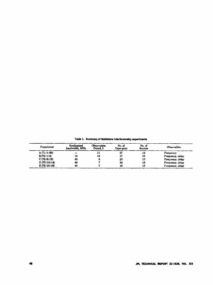
Table 1. Summary of GoMsbne interferometry qer imentr
Observable Synth&zed Observation No. of No. of bandwidth, MHz Period. h TaDtDairs SOUrceS Erperimcnt - -
11 37 14 Frequency A (71/1/29) - B (72/4/4) 10 14 s7 15 Frequency, delay C (72/8/16) 40 8 25 15 Frequency. delay 1) (73/10/14) 40 7 24 18 Frequency, deby E (72/10/18) 40 7 19 13 Frequency, delay
JPL TECHNICAL REWHIT 32-1526, VOL. XIX
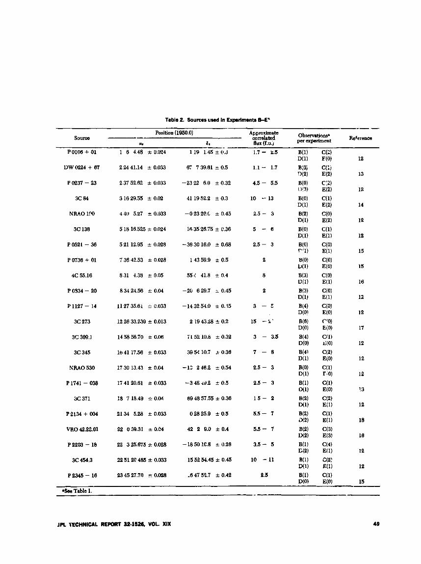
Table 2. Sources used in Experiments 6-E"
Observations* Position (1950.0) Approximate source - correlated per erperimmt Rokencs
la 81 flux (f.u.i . . -- - PO108 + 01
DW 0224 + 87
Po237 - 23
3 c 84
NW.0 1%
3c 138
P 0521 - 38
PW38 + 01
4C 55.16
P 0334 - 20
P 1127 - 14
3C 273
3 c 309.1
3c 345
NRAO 530
P1741 - 038
3C 371
P2134 + 004 VRO 42.22.01
P2203 - 16
3c 454.3
P2345-16
1 6 4.48 f 0.024 119 1.45 f 0.J 1.7 - 2.5
2 24 41.14 f 0.033
2 37 52.62 f G.033
3 16 29.55 & 0.02
4 4U 5.27 f 0.033
5 18 16.525 & 0.024
521 12.95 f 0.028
7 38 42.53 k 0.028
831 4.38 & 0.05
83424.58 f 0.04
11 27 35.81 2 0.033
12 26 33.239 f 0.013
14 58 58.70 f 0.08
1641 17.58 f 0.033
17 30 13.43 f 0.04
17 41 U.81 f 0.033
18 7 18.49 i- 0.04
21 34 5.28 k 0.033
22 0 39.31 f 0.C4
22 3 25.675 * 0.028
22 51 2C 485 f 0.033
23 45 27.70 + 0.028
8'7 739.81 f 0.5
-2322 8.0 f 0.32
41 19 52.2 f 0.3
-0 23 2Q.L f 0.45
16 35 28.75 f c.36
-38 30 18.0 f 0.68
1 4 3 59.9 k 0.5
5 5 4 41.8 f 0.4
-20 829.7 i 0.45
-14 32 54.0 f 0.15
2 19 43.18 f 0.2
T I Sf! 10.b -c 0.32
3954 10.7 k 0.36
-1.2 2 48.2 f 0.54
-3 48 -13.2 * 0.5
89 48 57.55 f 0.36
02825.9 f 0.5
42 2 9.0 f 0.4
- 18 SI ie.8 f 0.28
15 52 54.45 f 0.45
-8 47 52.7 f 0.42
1.1 - 1.7
4.5 - 5.5
10 - 13
2.5 - 3
5 - 6
2.5 - 3
2
8
2
3 - 5
1s -L'
3 - 3.5
7 - 8
2.5 - 3
2.5 - 3
1 5 - 2
5.5 - 7
5.5 - 7
3.5 - 5
10 - 11
2.5
12
13
12
14
12
12
15
15
18
12
12
17
12
12
12
13
12
18
16
12
12
15
-- *!be Table 1.
JPL IECHNICAL REPORT 32-1526, VOL XIX 49
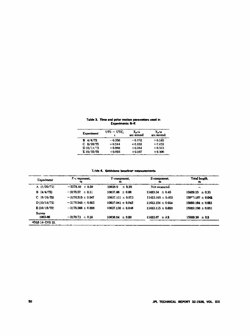
B 4/4/72 - 0.356 -0.192 + 0.185 C 8/16/73 + 0.244 +0.102 4 c.433 D 10;14/72 + 0.063 +0.164 +0.315 E 10/18/7!2 + 0.055 +0.167 + 0.306
z-companent, m
T d k g t h , m
A (1/29/71) -3178.40 f O B 10636.9 It 0.30 Not measured - B (4/4/72) -3178.57 f 0.11 10637.08 kO.08 11423.34 *0.45 15929.33 *0.33 C (8/16/72) -3178.515 0.047 10637.111 -t 0.073 11423.103 2 0.GS 15w7.167 f 0.049
D (10/14/72) -3178.548 0.025 10637.041 rt 0.045 11423.154 rt 0.w 1!5929.184 * 0.m E (10/18/72! -3178.588 * 0.026 10637.132 2 0.0s 11423.115 -c 0.033 15829.198 f 0.031 S w e Y 1983-68 -3178.73 5 0.20 10838.64 *om 11433.87 rt 33 159e9.30 *oe
.DSS 14-DSS 1%
JPL TECHNICAL REPORT 32-1126, VOL XIX
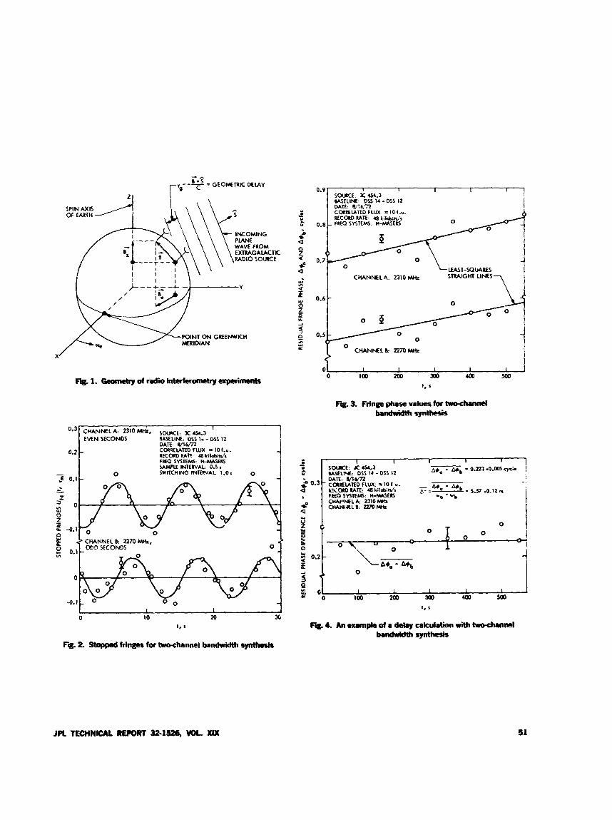
Y
POINT ON GilLEWlCH
0.3
0.2
- ,E 0.1
.. Y
z 3 - 0 w
E e 0.1
2 w -0.1
a
m
0
-0. :
0-9r 0.8 ..
0.7
7 1 CHANNEL A: 2310 MHz SntAKjHT LINES
0.6 - 0
0
CHANMLk 2 2 M W ' 0
? I 01 I I I I I
0 100 200 Joo ux) m t, =
0 0 ' CHANNEL 8: 2270 M H z ,
Ob0 SECONDS 0 3
I I 1 10 20 XI
t. a Fig. 4. An uampk of a delay cakulatifm with two4anneI bandwidth synthds
Fa. 2. Stopped fringo for hrochannel bandwidth rymhech
JPL TECHNlCAL RE#)IpT 32-1- WK. XIX 51
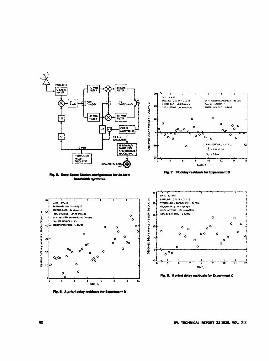
2270-2310 cia I I I
1
3 x
Q CL. I
0
00 0
*o 0 0
O 0 0
0 0 0
0 0
0
0
a0 0
I I o 0
O 0 0
O O 0
0
0 0 & o o n a n " o o o
0 a 4
0 uo- I 0 0
RM R E S W L e 4.7 .a -10 0 - .: = 1.0 ..C.Id
NT = 3.0- -m - I I I I I I
0 - 4 6 8 IO 12 14 16
GUT, h
-7. F i t i t m s i d u 8 k t a E x p e f i ~ B
I 0 I 0 0
0 - -. i O 0 0
-51 - I I I I I 9 IO 11 12 0 . 5 6 7 8
GUT, h
JPL TECHNICAL R L m 324526, VOL XIX
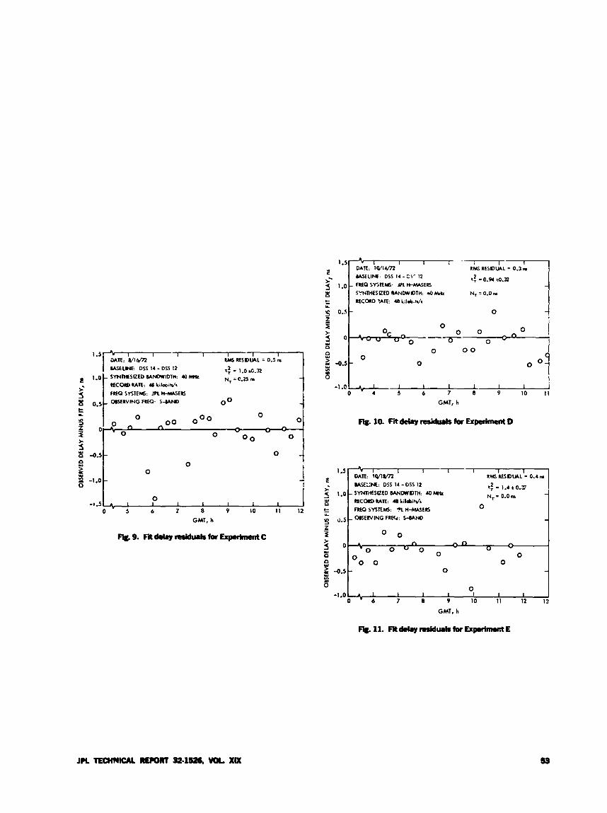
0
L
3
8 5 0
Y n o g "0.5-
8 -1.0
0
0 0 n n C l
0 - 0 0 - 0
1 I 1 I 9 I I
Av 0 0 "
0 0 0 0
0 -1.5 A I 1 I I I I
0 ' 5 6 f 8 9 10 11 12
GMT, h
DATE: IVl4/77. MSELINF. DSS I4 - 3)' I2 FLK~ s v m s JPL H-MASERS
>' 5 1.0 8 SYNTHESIZED UNWDM: 40 Mrb N,=O.Ona
RECORD 'ATE: 48 k i I a b . M r t Y
I I 9 10 11 5 6 7 8
- l . @ L + - I 0 4
GMT, h
-10. Fitdei8yresidrukfarExpsrimcntD
If = 1.4 f 0 . 3 MSE':N: DSS 14 - DSS 12
N, = 0.0 tu RECORD RATE: 48 k i l a b i M s
RH) SYSTEM: 'PL H - M E I S OEEENINGFRE6: S-MND
0 8 Y
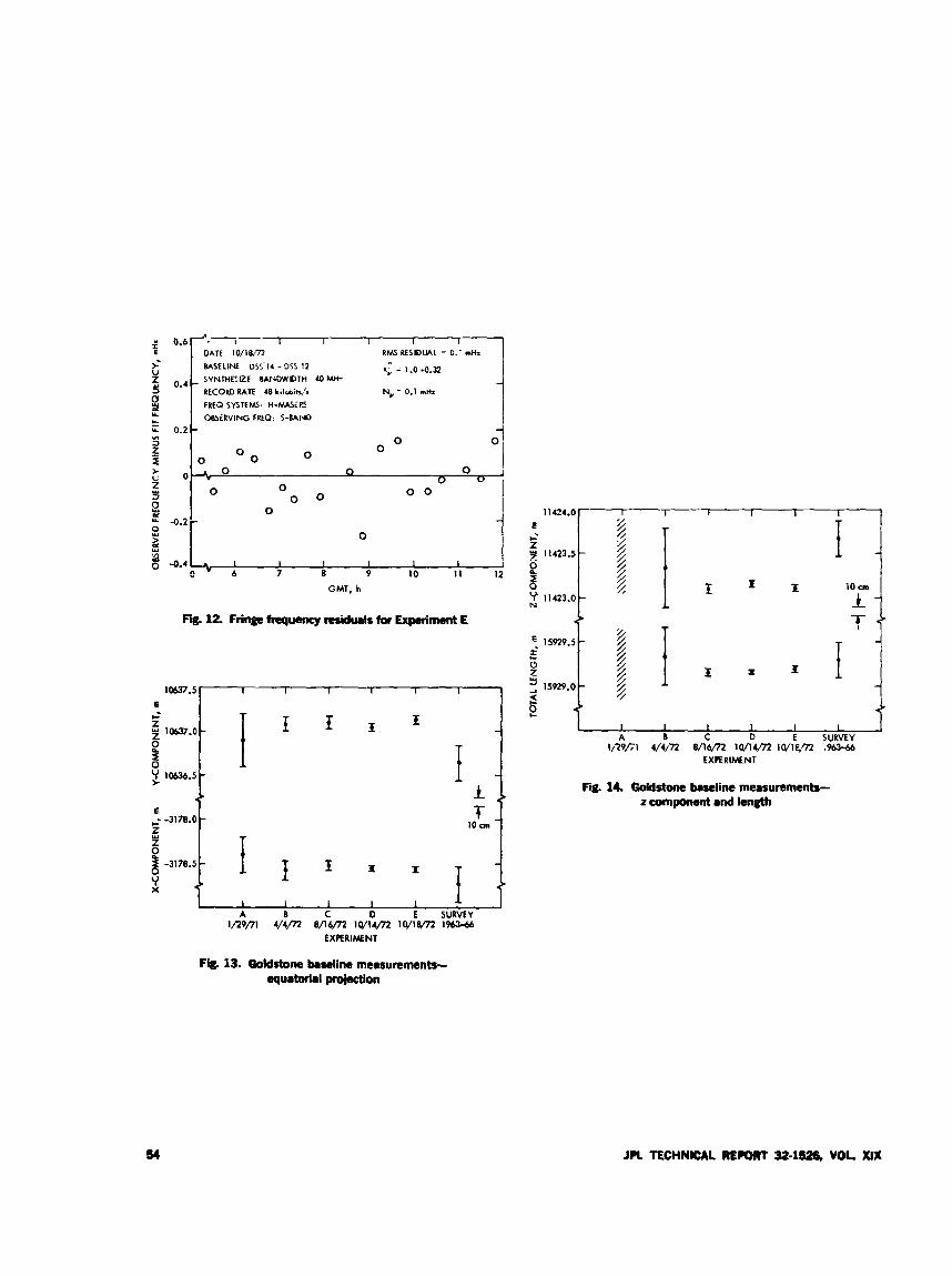
p 0.6
s 5 0.4 0
c y 0.2
E
U
z
I I I , I
DATE l O / l W 7 7 RMS RESIDUAL = 0.’ mHx
BASELINE 05s-14 - DSS 12 XI = 1 .o 4.a - SYNTHE’.QE EANDWDTH 4 0 M RECORD RAE 48 kilubim’s N, - 0.1 m t b
FRECI SYSTEMS, H-NASEPJ OBSRVING FEQ: S-BANI) -
w
I I 1 1 I C 6 7 8 9 10 1 1 I2
GMT, h
f3g. 12. Fringe frequency residuals for Experiment E
I I I I I I 1 1 A B C D E SURVEY
1/29/71 4/4/72 8/16/72 10/14/72 l0/lW 1942-46 EXPERIMENT
Fig. 13. Goldstone baseline measumnents- eqU8bd8l
I
11c4.0
11423.0
E 15929.5 i 0 z
U 15929.0
E
f 11423.5
s 0
c
5
10 Qn
f [ I T
I I I I I I I J A B C D E SURVEY
1/29/;I 4/4/72 8/16/72 lO/l4/72 10/le/72 ,96366 EXRRIMENT
F i i 14. Goldstone baseline measurements- I C O m w 8nd length
54 JPL TECHNICAL RE- 32-1526, VOL. XIX
Improved Dichroic Reflector Design for the 64-m Antenna S- and X-Band Feed Systems
P. 0. Potter Communications Elements Research Section
In support of the Mariner VenuslMercuy 1973 (MVM73) X-band expedment and planned future Mariner missions, the 64-m antenna network is being supplied with S- and X-band refrer feed systems. The initial instullath, for MWf73, u;as implemented at DSS 14 and prmides satisfactory performance for I .t mission. The X-band performance of the dichroic rejlector is, however, not acc ytuble for planned future missions which h u e more stringent X-banrl performance require- ments. A new dichroic reflector which grossly reduces the X-band ellipticity and noke temperature degradation has been designed. In this reporting, the thaoy and experimental performance of this new design is reported.
1. Theory of Operation The design and performance of the existing DSS 14
reflex feed dichroic reflector (plate) was described in Ref. 1 and is shown in Fig. 1. The plate is 3.576 cm thick, with an array of hexagonally packed 2.273-cm-diameter holes drilled normal to the plate surfaces. The center-to- center hole spacing is 2.388 cm, and the required fre- quency of operation is 8.415 GHz.
As described in Ref. 1, the E- and H-plane plate reso- nant frequencies (frequencies of complete transparency) are displaced because of a difference in the E- and
H-plane free-space-to-circular waveguide transition dis- continuity at the (tilted) plate surfaces. Since the plate is used with circular polarization, this resonant frequency difference causes a diilerential phase shift between the E- and H-plane, resulting in depolarization of the circu- larly polarized incident wave. Additionally, because the plate is not reffectionless for all polarizations (at a fixed frequency), a serious (approximately 2-K) noise tempera- ture contribution results from ground radiation. Actual calculations using the Chen Holey Plate Computer Pro- gram (Ref. 2) show that the plate E- and H-plane resonant frequencies (30 deg incident wave tilt from normal) are 8.481 and 8.363 GHz, respectively. At the operation he-
JPL TECHNICAL RE#)RT 32-1526, VOL XIX
quency of 8.415 GHz, a differential phase shift of 11.3 deg
sured ellipticity was 1.84 dB. The reflected energy level is - 18 dB at 8.415 GHz.
i t i d air e!Lp&it?- 3f 1.75 JE cxc p ~ & c : d . k t d ami-
The approach taken to cure the dichroic plate depolar- ization described above was to make the holes slightly noncircular in cross section, thus introducing a daerential E- and H-plane phase shift within the plate to counteract the 11.3-deg phase shift. This change is in the nature of a perturbation on the original design, rather than a re- design; the original plate thickness and hole center spac- ing are retained. The particular hole cross sectior, selected is “Pyleguide” (Ref. 3). This type of guide, circular with a pair of flats on opposite sides, is used by JPL in the 64-m antefina feed system polarizcrs. Pyle’s (1964) analysis (Ref. 3) is approximate. It is now practical to numericdly solve the wave equation in a cylindrical waveguide of arbitrary cross section, yielding highly accul ate guide wavelength numbers as a function of geow4ry. An excel- lent computer program for this purpose * - - developed by b u d Pontoppidan, formerly of the Tec!micb Univer- sity of Denmark (Ref. 4). The Pontoppidan program was modified for use on the JPL Scientific Computing Facility (SCF) t’nivac 1108 and set up for Pyleguide calculations.
Figures 2a and 2b show the cutoff wavelength h, as a function oI’ Pyleguide geometry for the E- and H-planes. The design procedure for the Pyleguide dichroic plate \vas to adjust the guide gometry (using the Pontoppidan computer program) until the plate electrical thickness at 8.415 GHz for the E- and H-planes corresponded to those in the original circular hole plate at 8.481 and 8.363 GHz, respectively. The resulting geometry is shown in Fig. 3. The hole diameter is 0.013 cm larger than the original circular hole design, and the flat depth is 0.043 cm. Thus, the redesign is only a small perturbation on the original design.
To test the Pyleguide dichroic plate design, a sample section of plate 35 X 53 cm in size was fabricated. The holes were made with a broach, allowing tight tolerances (+-0.005 cm) to be held on all hole dimensions. Although performance of this type of dichroic plate is relatively noncritical with regard to tolerences, the strict control was imposed both as an experiment in fabrication tech- nique (there were no problems) and also to provide a good check betwer. predicted and measured perform- ance. Figure 4 is a photograph of the sample Pyleguide dichroic plate. The following section describes the mea- sured performance.
II. Experimental Results The X-band performance oi the Pyleguide dichroic
plate sample was measured in the JPL Mesa Antenna Range anechoic chamber facility. Complete pattern data were taken at the design (ai ! operational) frequency of 8.415 GHz; frequency-scanned pattern data were taken in the reflex feed symmetry plane. Optimum performance was observed at the design frequency of 5.415 GHz. No pattern distortion, grating lobe response, 3r other un- expected behavior was observed.
Figure 5 shows the radiation pattern of the corrugated feedhom by itself. Figure 6 illustrates the pattern of the feedhornhilted dichroic plate combination in the plant. containing the horn axis and the plate normal (symmetry plane). For these patterns, the horn was circularly polar- ized and the illuminator was !inearly polarized but rapidly rotating about its axis. Thus, at each point in the radiation patterns, the ellipticity is displayed as a rapidly modu- lated signal level. As seen in Fig. 6, the ellipticity nulls out at a point 3 deg off axis and is 0.4 dB on axis. From symmetry considerations, the antenna secondary pattern axial ellipticity will be nearly the same as the feed system axial ellipticity.
In Fig. 6, the large lobe in the region of 120 deg is the reflection from the horn side of the dichroic plate. This reflection gives rise to a mise temperature contribution from ground thermal radiation when the antenna is at low elevation angles. The power-average level for the Pyk- guide dichroic plate is -24.5 dB, yielding a maximum noise temperature contribution of 0.7 K. The original round-hole plate has a power-average reflection lobe level of - 18.6 dB, yielding a noise contribution of 2.7 K. This latter figure has been experimentally observed at DSS 14 (see Fig. 8 of Ref. 1).
111. Conclusion A different type of hole, “Pyleguide,” has been incorpo-
rated into the reflex feed dichroic plate design to alleviate polarization degradation and noise temperature contribu- tion due to plate mismatch (reflection). The plate ellip ticity degradation has been reduced thereby from 1.8 to 0.4 dB; the maximum noise temperature contribution has been reduced from 2.7 to 0.7 K. The ideal hole shape is a function of its location on the plate. The Pyleguide plate tested had all identical holes. Further performance im- provement, if required, appears possijle by use of non- identical holes. The ability to pedorm this type of design entirely analytically has been demonstrated.
56 JPL TECHNlCAL RE= 32-1S26, VOL XIX
References
1. Potter, P. D., “S- and X-band RF Feed System,” in The Deep Space Network Progress Report, Technical Report 32-1526, Vol. XV, pp. 54-62, Jet Propulsion Laboratory, Pasadena, Calif., June 15, 1373.
2. Chen, C. C., “Transmission of Microwave Through Perforated Flat Plates of Finite Thickness,” ZEEE Transactions on Microwave Themy and Techniques, Vol. MTT-21, No. 1, pp. 1-6, Jan. 1973.
3. Pyle, J. R., “Cutoff Wavelengths of Waveguides with Unusual Cross Sections,” ZEEE Tranwctwns on Xficroocrw Theory and Techniques, Vol. MTT-12, No. 5, pp. 5!3%557, Sept. 1964, Correspondence.
4. Pontoppidan, Knud, “Finite-Element Techniques Applied to Waveguides of Arbitrary Cross Sections, Parts I and 11,” Ph.D. Thesis, The Technical Univer- sity of Denmark, Lyngby, Denmark, Sept. 1971.
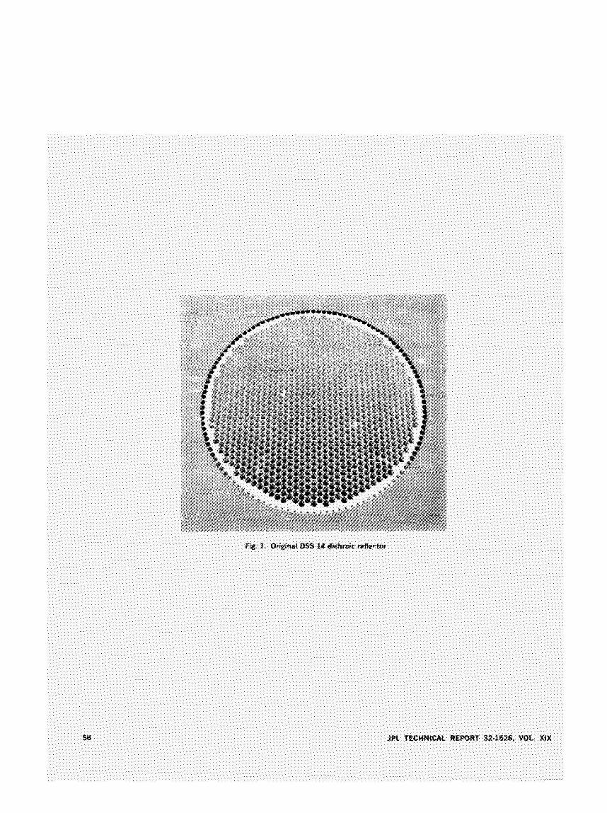
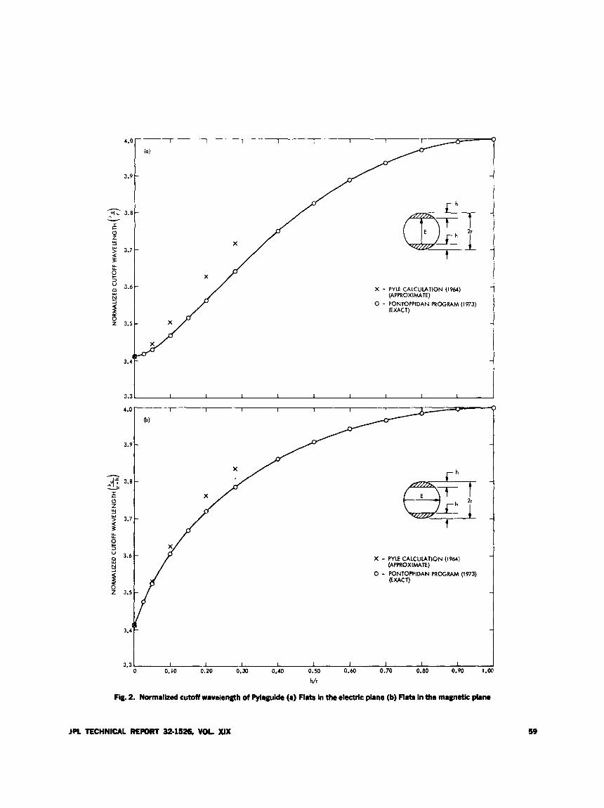
4.(
3.5
h YI L 3.t
* ; Y
I I-
(3 z
> 3.7 2 f 0, Y Y
3 U 3.c Y
N-
I e 3.5
3.4
3.2
4.0
3.9
h
3.8 I
X
5 t -1 Y
> 3.7
3 4
Y
6 f 9 " 3.6
! P 3.5
3.4
3.3
X - PYLE CALCULATION (1964)
0 - PONTOPPIDAN PROGRAM (1973) (APPRDXIMATE)
(EXACT)
X - PYLE CALCULATION (1964)
0 - PONTOPPIDAN PROGRAM (1973) (APPRDXIMATE)
(EXACT)
X - PYLE CALCULATION (1964)
0 - PONTOPPIDAN PROGRAM (1973) (APPROXIMATE)
(EXACT)
X - PYLE CALCULATION (1964)
0 - PONTOPPIDAN PROGRAM (1973) (APPROXIMATE)
(EXACT)
I L J I I 1 I 1 I 0.10 0.20 0.30 0.40 0.50 0.60 0.70 0.80 0.90 I .
h/r
Fig. 2. Normalized cutoff wavelength of PylquMe (a) Flats In the electric plane (b) Fbts in the ~agnetic plane
JPL TECHNICAL REmRT 32-1526, VOL XIX 59
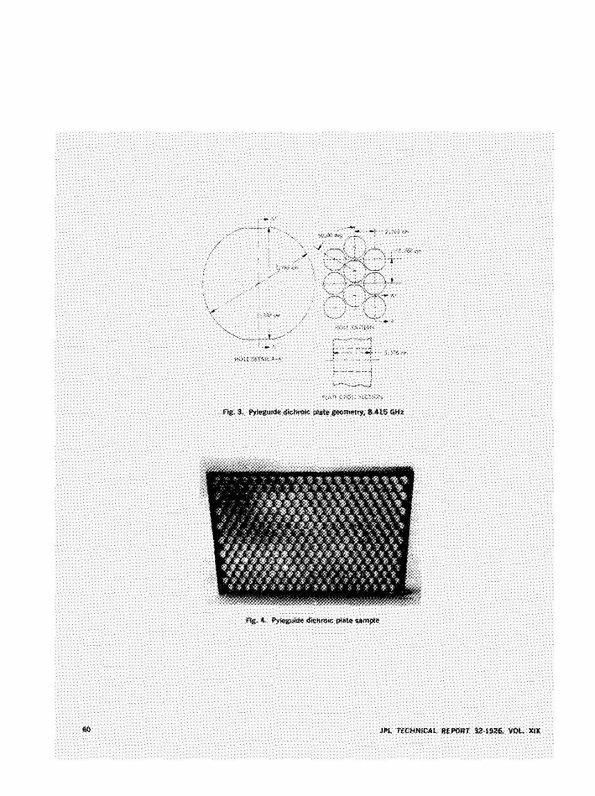
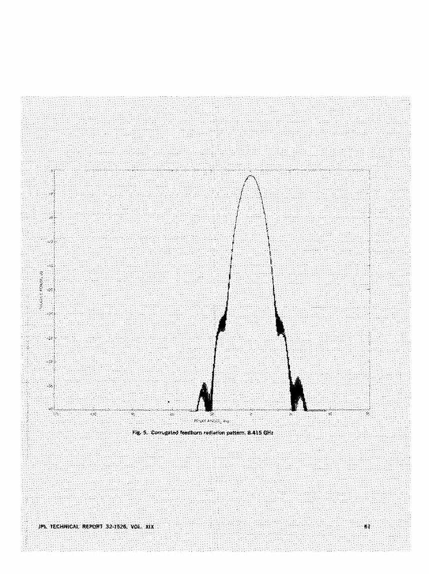
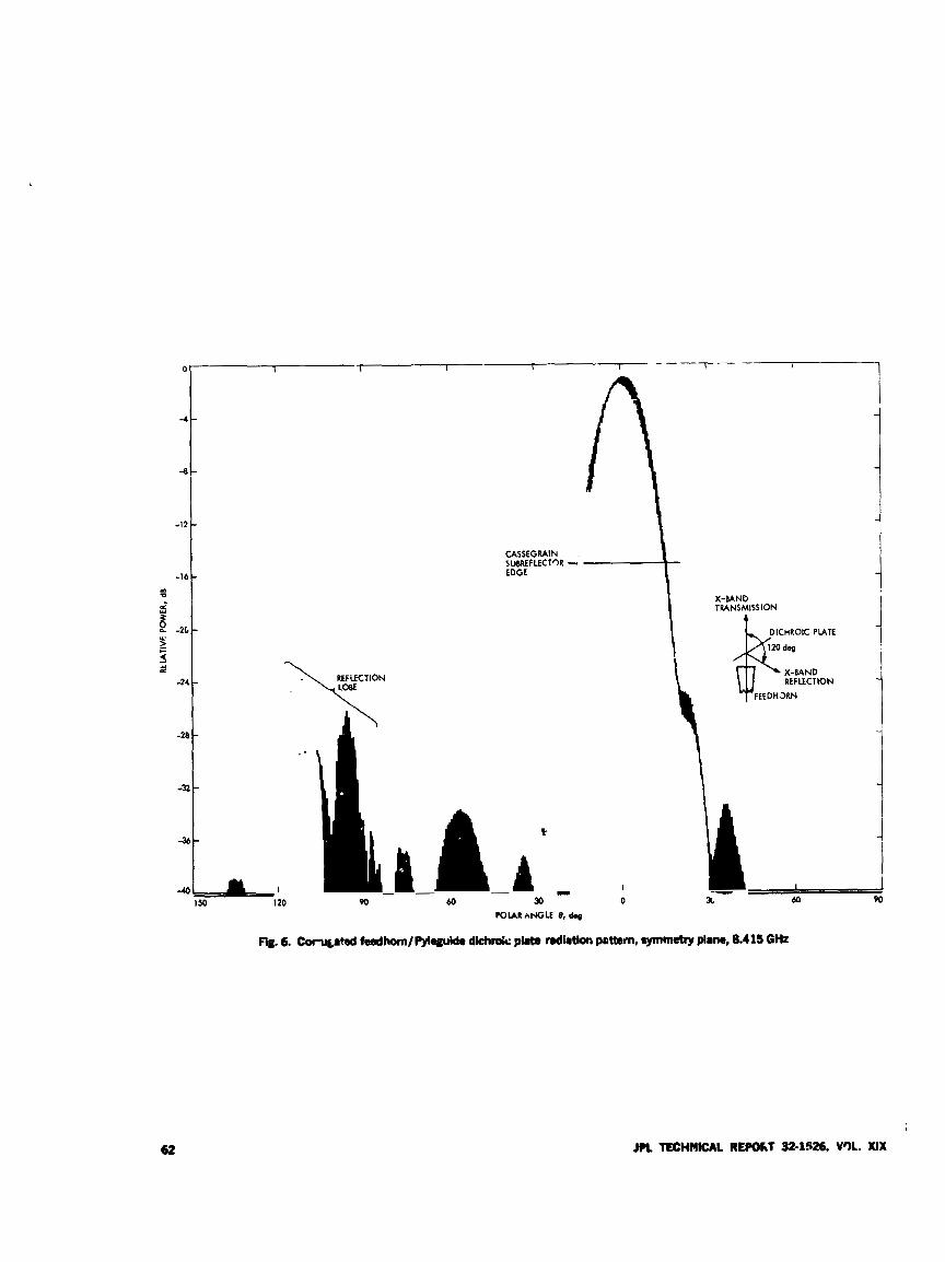
-4
-a
-12
-16 m a & Y
B -26 5 E
CASSEGRAIN SUBREFLECTqR - EDGE
\:CTION
X-BAND TRANSMISSION
t
X-BAND R€FLECTION
FEEDHJRN
POLAR ANGLE e,
Fig. 6. coru6.ted feedhom/PyieguMe dkhmk plate radiation pattern, symmetry plane, 8.415 GHz
Range Measurements to Pioneer 10 Using the Digitally Cmtrolled Oscillator
A. S. Liu
Analysis of the new doppler data from DSS 14 usins t l e .ligitally Controlled Oscillator (DCO), has establiyhed that ramping the CGi'rier frequency by the DCO will enable us to obtain range measurements to Pioneer 10 without ?he use g f a ranging system per -8. The accuracy of these mca~crements is on the ordgr of 10 km.
1. Introduction The tuned oscillator range analysis (TORA) experi-
ment utilize the new DSN programmed oscillator de- vice at DSS 14. This ne' equipmeqt was added to DSS 14, Goldstone, California, a n i DSS 43, Canberra, Australia, for the purposr of tracking Pioneer 10 during Jupiter flyby. It was noted that ranging information could 5, obtained when the transmitted frcquency was ramped by illrans of a digitally controlled oscillator (DCO). The returntad signal shows a pattern that is dependent upon the round-trip light time, enabling measurements to be made of the distance from the statior, to the spacecraft.
Since the priiriary purpose of the installation of the DCOs was to support Pioneer 10 commanding duririg Jupiter cncountcr, training exercises were scheduled to pcricit station oprrators to become familiar with the new equipment and to establish working procedures for <he Jupiter Syby. Data taken from DSS 14 were utiiized during several of these training exercises, and processing ot the data was begun to see if range information could be extracted. Supglied with information about tEe fre-
qurncy rates and ir:tiation times of the DCO dnring those passes, the data were succes. fully amlvzed and several round-trip range estimates of the Pioneer 10 spacecraft were made.
The concept of using ramped frequency doppler for ranging is analogous to inferring distances ,jy an echo. By ramping the carrier frequency, a unique corrcspon- denre between time of transmission and frequcncy of transnrission ir -Ct?b;:shed. r clrther, by noting the t i m and frequenc dt reccption, one can then associat2 a time of transmi;sion with that frequency, thus a time delay, or round-trip distance, is inferrd.
Figurc 1 is an illustration of this priaciple. It shows thc Joppler counter rcidings after s3btraction of reasonable estiintes of shifts due to Earth and spacerraft .notion, ctc., mrnlwted as ordhary doppler at the hitial trans- mitted frequencv. The ddshrd line indicates the tuning p ofilc of the twiter at DSS 14 as a function of time. The cm!er is also iisrd as a reference signal to heterodyne thc time-delay:l received signal from Pioneer 10 (effects on residuals shown as ;? solid line). Thf difference between
JPL TECHNICAL REPORT 32.1126, VOL. XIX 63
II. Data Analysis Two iets of DSS 14 Pioncer 10 data wvre malyzcu!. The
r.imp patterns are tabulated in Tables 1 aiid 2. Thc. first 1nss of data (Pass I j \ v u taken on June 19. 1973, and the second (Pass 11) cn July lo, 1973.
A. Pass1
To andyze this pass. w e used the initial a .iditions of Pioneer 10, supplid hy Pioneer Projezt Savigation. Based upon this orbit, round-trip lisht times for eacl- data point \v tw c iputcd. The e-itra cycles were removed from the data according to the requircd light time transit.
The result is presented in Fig. 2. It is interesting to note the stvp rcsiduals dut. to the misplacement of Pionrer 10 in this assumed trajectory by al>prodmately 2 3 ki- . The ramped doppler data provide an additional mcasurement dimw ion. not readily or dirwtly available from conventional dopp!er. The unramped doppler yields a solution of the orbit by inference through the accelera- tiqn dynamics aftrr sufficient spatial motion has occurred (about 6 \vcehs or longer).
Thz stcp bise5 are drw to a trajectory rt,und-trip light- tinw error tiines a ramp rate. Since we niay regard the orbit error to be a constant ovrr one pass, the offscts are due only to diffvring ramp rates. Thus, the largest offset is due to R ramp rate of lFi0 )r ‘.. Halfway between, onc sees a bias of hali that ;-s . from a ramp rate of 7 4 . W Hz/s. Centered ,.* 2: &,‘ro arc the twc offsets caused by a ranip rate of 530 Hz/s.
B. Pass11
A second set of data, taken on July 10, 1973, was analyzed. In the intervening period, a trim maneuver had taken place. This necessitated a solution for the nev- wbit. Additions were. made to the code ii. .le Planetary Orbiter Error Analysis Study (POEM) qrogram, which included the new data and partial derivatives required tor an automatic least-squares differential-correction process. The July 10 data were sent through POEAS, and auto-
IVhen thc ‘blundc.r pints” wtw reniovrd. we 11 ere able to adjust the orbit so that thc data rcsidu;iij were on the ordc-r of 1,’lOOO Hz. Figure 1 shwvs the rj-sult of tliis solution.
Thc fiqurr sho\vs the level to \vltich thf. ramp frequency data c;in be fit when all the b1undr.r points have hben rcinowd. It is c\-ident that thc oiil). noise conponmt remaining is the high-frmlucncy componcnt. and whcm the ramp pattern is includcd in the data aiulysis. thc new DCO doppler data res;duals look thc. a.iiiie as thc CQII-
vcntional unrarnpcd d‘tta rcsiduals.
111. Conclusions and Summary Based on the analysis of two srts of Pioncer 10 ramping?
doppler data from DSS 14, the system shows promise of providing a ntw nicasuremcwt dimension (i.e., ranqe) froni dopplcr data. The problems at present srcm tr;ictablc.
Our iiitt.tpetation of the data wcms sound, and its ;ncorpration into cc!nputer prosranis yielded reasonablr rcsults. The prototypc program furnishes us with insights into the procculures for developing the navigation pro- grains to account for this new data hpe in 3 logic‘il manner.
In summary, as a demonstration cxercise, we have
(1) Obtained some understanding of the POCA.
(2) Developed the softwarc required to analyze the data from an orbital correction ap2roach.
(3) Interpreted our rrsults in tcrms cf a new data t-1.e corresponding to topocentric range to the spa,.ecraft.
JPL TECHNICAL REPORT 3?-:526, VOL. XIX
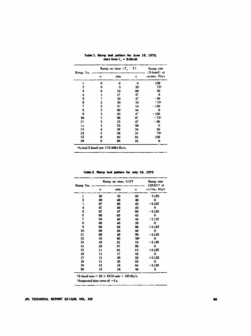
Ramp on time (T,, - f ) U p rate Ramp So. ( S-band) at
n min 5 exciter, Hz/s
1 2 9 4 5 6 7 8 9
10 11 1 1 JS 14 15 16
0 0 0 I ! e 2 3 3 2 3 4 4 5 6 6
0 9
10 27 32 50 si 00 05 09 15 33 58 56 03 06
0 20 00 47 4 i M 11 34 47 0; 4 i 34 34 21 01 21
150 7 3 ;io 0
-30 - 7 3 - 150
0 - 150 - 7 3 -30
0 30 13
150 0
*Artual S-band rate %‘4.99?34 k/s.
T a b 2 ibmp tat p.tban for h l y 10,1973
Rvnp on time, GVT Ramp late Ramp No. (DCOP at
n mm s exc%ff, Hz/s
i iwi 30 36 3.125 2 06 46 40 0
07 09 43 -3.125 4 m 243 23 0 5 07 47 03 -3.125 8 os 03 43 0 ? 08 26 46 f 3 x 5 8 os 43 m 0 9 09 04 a3 +3.125
10 09 20 46 0 11 09 4.9 56 -3.125 12 10 00 39b 0 13 10 21 19 -3.i25 I4 10 37 58 0 15 11 01 c2 +3.125 18 11 17 43 0 15 11 38 22 +3.125 18 11 55 02 0 19 12 18 04 -h125 20 12 34 44 0
I-
aS-bPnd rate = 32 X DCO rpte = 100 H ~ s . bsurpected time m r of -5 s.
JPL TECHNICAL RE- 32-1526, WK. XIX

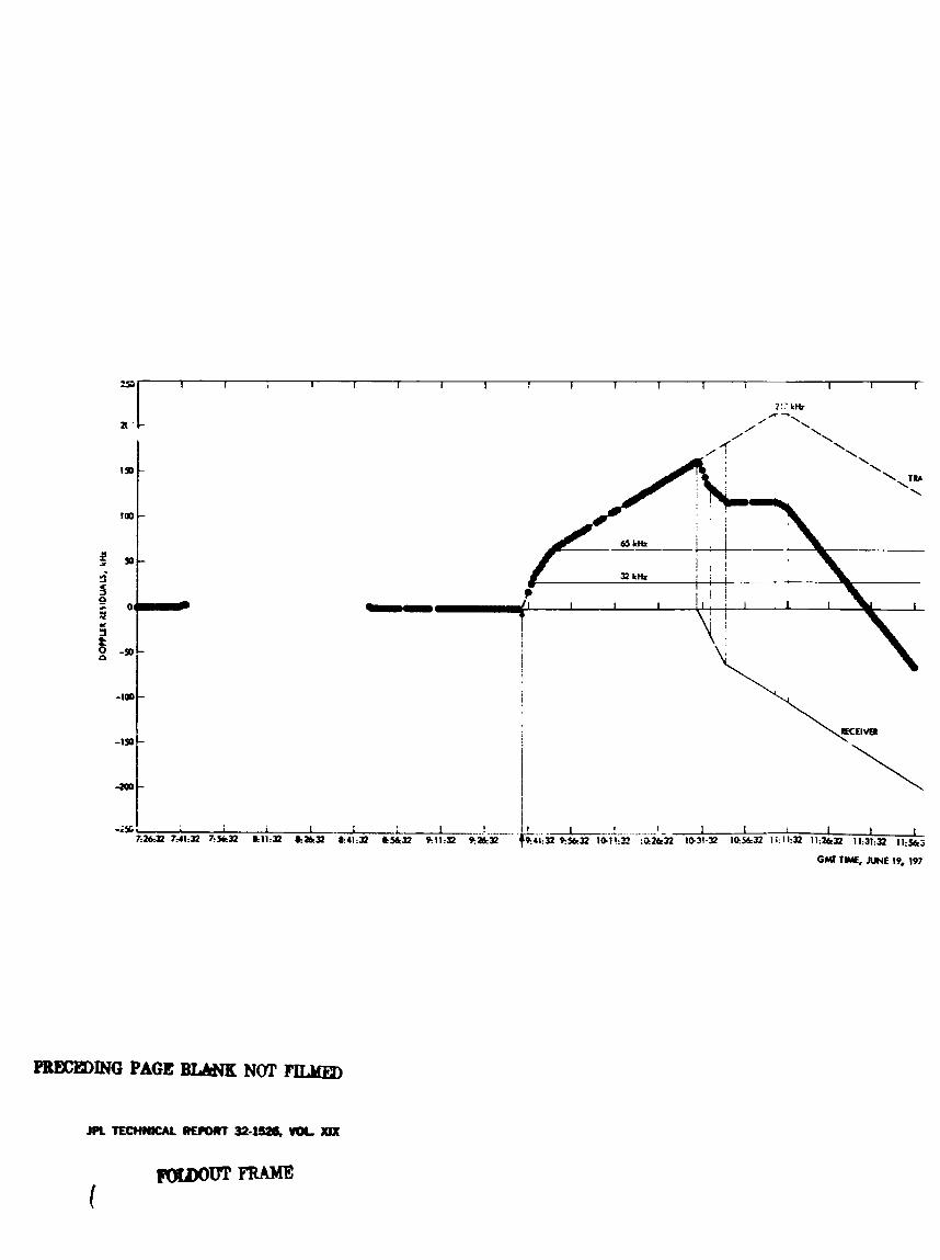
2 s I I I 1 I I I I I I 1 I I 1 I
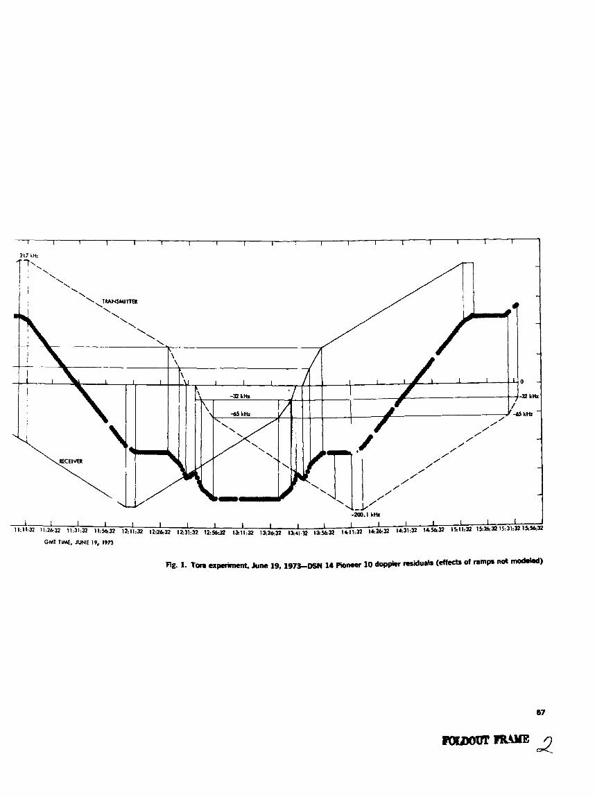
67
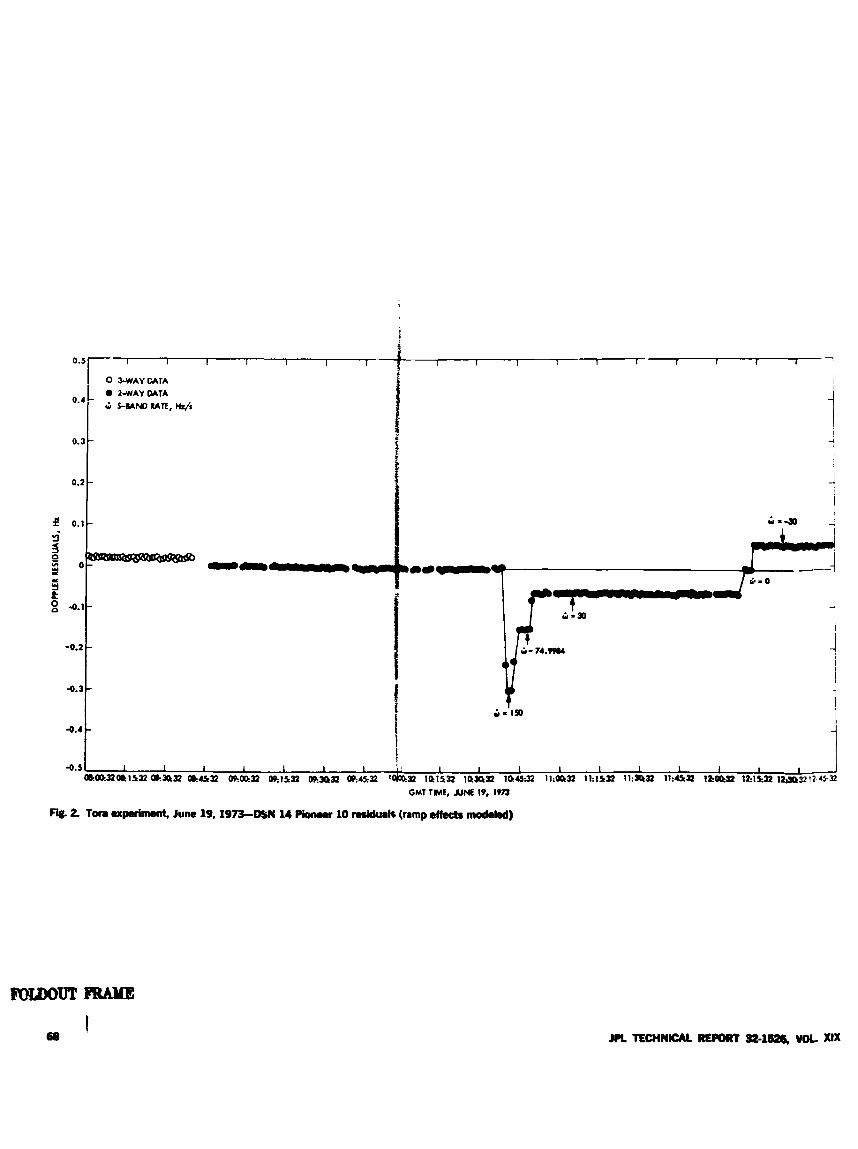
a
J 0 . 5 1 I I I I I I I I I I I I I I I I I I
0 W A Y G A T A 0 2-WAY DATA 3 S-M*No RATE, th/s ::I
P 0.1
i 4 v) Y L
5 8 e
-0.2
9.4

0.5 I I I I I I I I I I I I I 1 I
0.4
0.3
0.2
p 0.1
3
-
-
0 -
-
3 = loo
5 8 -0.1- 0
0 . 2
-0.3
-
-
" i
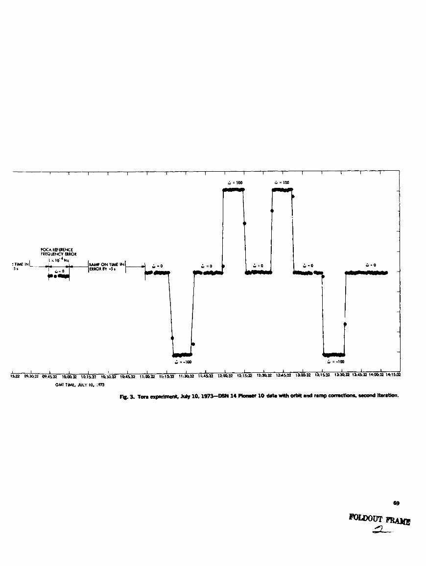
I I I I I I I I I I 1 I I I I I
6 = 100 w = 100 I - l
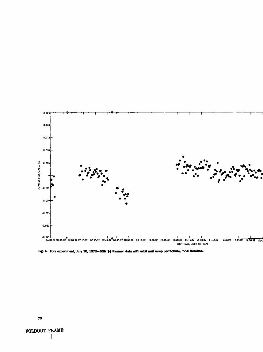
0.W
0. oac
0.01 5
0.010
" I 0.005
: 3
; a
8 -0.005
a
YI 2
4.010
-0.015
4.020
-0.025 06:
/ = I I 1 1 ' 1 1 1 I I I I 1 I I I I I m
e
e
I n 1 I 1 I I I I I I I I I I I I 32 obr15.j2u07:W..P 07:1532 0 7 : a X 07:4S32'W453 140@32 10.1532 lR3&P 144532 11:4132 11:15:32 11:3432 11:45:32 12:OQ32 1Z1532 1 2 a 3 2 18:
GMT TIME, JULY 10, 1973
Fig. 4. Tom experiment. July IO. 1973-DSN 14 Pioneer data with orbn 8nd nmp eomctkm. fin81 Fkmtkn.
70


S/X Open-Loop Receiver H. G. Nishimura
R. F. Systems Development Section
An operational DSN S-band receioer having two independent channels was modified to provide capability for coherent reception at S- and X-bands simul- taneously. Coherence at both bands was accomplished by usin2 a base-frequency multiplier tchich was common to both the S - and X-band local oscilhtor multi- plier chains.
1. Introduction
In order to mrrt tht occultation experiment rcquire- nirnts for cohcrent downlink phase information from a spacecraft at S- and S-bands, the DSN S-band open-loop receiver at DSS 14 was modified. Presently, the open- loop rrccivrr has two independent S-band channels. Chairiiel2 was modified to receive at X-band. This modi- fication was made without disturbing either S-band link. To meet the requirements, Channel 2 was preceded by an S- to S-band down-converter. Switching networks were addrd so that in the new S/X-band mode, occulta- tion espcriments can be carried out simultaneously at S- and S-bands. Coherence requirements for the two downlink signals were met by utilizing a common base- frequency for both the s- and X-band local oscillator (LO) chains. Whenever possible, components and modules
already designed or in DSN use were employed in order to minimize replacement spares and cost.
II. Physical Description
The S/X open-loop receiver c.:nsists hesicall) nf b:o assemblies mounted in the tricone at 9 S S 14. One xsc ' in- bly, called the S/X open-loop rewiver panel (pan:,\), contains the time> -ixteen ( X 18) base-frequency multi- plier and other iower-frec,:iency multii)liers to generate the LO signal 101 the exis:iv:g S-band mixers jsec Fig. 1). The panel, morinttr! in receiLr.1 cabinet 9, .s 43 cm wide, 51 cm long, and c, -11. high.
The other assembly, S/X open-loop receiver box (box), consists of a weather-resistant enclosure containing the
JPL TECHNICAL REPORT 32.1526, VOL. XIX 71
components required in the generatior and conversion of the higher S-band frequency (Fig. 2). The Box measures approximately 41 X 51 i( 15 cm deep.
111. Development Figure 3 shows a block diagram of the S/S open-loop
receiver. Basically, the system consists of two reference frequency sources which drive frequency multiplier chains to supply the LO signals for the existing S-band mixers and the new X-band mixer. The X16 base- frequency multiplier, which is common to both multiplier chains, has dual outputs. One output provides the drive for the S-band LO chain, while the other provides the drive for the X-band LO chain. Coaxial RF switches select either normal S-band operation or the new S/X-band mode. In the normal S-band mode, the existing S-band LO signals are switched into the existing S-band mixers. In the S/X-band mode, the new coherent S-Land LO is switched to the existing Chaiillel 1 S-band mixers, and simultaneously, the X-band LO is switcIied to the new X-band mixer in Channel 2.
Starting at the upper left in Fig. 3, reference frequency source fl drives the dual output X 16 base multiplier. One output of the X16 multiplier drives a X 3 multiplier, which generates the nominal 2245-MHz LO for the existing S-band mixers. This LO signal is split by a 3-dB hybrid and followed by bandpass filters FL1 and FL2. Switches S1 and S2 are operated simultaneously and, for S/X-band operation, select the new coherent LO gener- ated by the X16 and X 3 multipliers. For normal S-band operation, S1 and S2 select the existing S-band LO signals. Either set of LOs is applied to the existing S-band mixers in Channels 1 and 2.
The other output from the X 16 base multiplier is used to further develop the LO for the new X-band mixer. A t the left in Fig. 3, reference frequency source f z drives a X1/3 frequency multiplier. The output is mixed with tlic output from the X16 multiplier. The resultant sum frequency, 2 nominal 765 MHz, is further multiplied by a X 8 multiplier to provide the 6120-MHz LO drive for the X-band mixer. The LO is procewd through band- pass filters and isolators HY2, FL3, HY3, FL4, and HY4 before being applied to the X-band mixer. The X-band downlink signal, nominally at 8415 MHz, comes in through the preselector filter and mixes with the 6120- MHz X-band LO in X-band mixer M1. The resulting difference intermediate frequency at 2495 MHz is ampli- fied by AR1. Switch S3 operates tcgether with switches
S1 and S2, and when it is in the S/X-\>and mode, selects the 2295-MHz S-band IF gmerated by the X- to S-band mixer. When the switch is in the normal S-band mode, it selects the normal 9295-hIHz S-band signal to Channel 2. The signal is then fed to the S-band mixer in Chan- nel 2. The various signal frequencies are shown in the diagram.
Perhaps the most significant area of development dealt with the suppiession of spurious signals generated by the 6120-MHz X 8 frequency multiplier in the X-bad LO chain.
liitermodulatian products are generdted in the mixer following the X 8 multiplier due to mixing of harmonics and sidebands of the X 8 multiplier output. Since the S- and X-bands are coherently related, the X 3 sideband at the output of the X 8 multiplier is at the same fre- t,uency as the IF from the X-band rnixer. In addition, the X 5 and X11 sidebands mix with the X 8 output also to generate an interference signal at the same frc- quency. The intcrference signals coulrl mask the real signals if they were not adeq..ately attenuated. Faced with these possibilities, the best approach was to sup- press every harmonic of the X 8 input frequency appear- ing at the multiplier output except the required LO for the X-band mixer.
Bandpass filters FL3, FL-I and wideband isolators HY2, HY3, HY4 were used for this purpose. Typical microwave filters are of the reflective type, wherein high voltage standing wave ratio (VSWR) is exhibited in the reject band. The addition of an isolator at the inpa t port allows ttc isolator to absorb the out-of-band reflected signals by an order of about 20 dB per unit. The isolator also helps in creatir:; a better match for the in-band frequencies.
Before one can realize higher orders of suppression, RF leakage must be eliminated or at least minimized. Therefore, special precautions were taker in packaging the X 8 multiplier, isolator HY2, and filter FL3 (Fig. 4). The X 8 multiplier and HY2 were mounted within an RF-shielded enclosure. The input interface of F'J was mounted flush against one exterior surface of the enclos- ure, with the input connector protruding into the enclos- ure through a clearance hole. The two mounting surfa-es were machined smooth in order to minimize leakage. With this arrangement, the filter input was virtually RF- isolated from its output. Skin currcnts a t the input were
.
72 JPL TECHNICAL REWRT 32-1526, VOL. XIX
contained within thrb enclosure. Test results confirmed excellent containment of leakag- in the area of the x8 and FL3.
Before the filtering was added, the interference signal levels were approximately -85 dBm following the X- to S-mixer. With the addition of HY2 and FL3, this level was rduced to -141 dBm, a reduction of 56 dB. A second suppression stage, : :misting of HY3 and FL4 was added, and this reducec; the spurioas L ~ e l s well below threshold signal levels. Because of reactive cou- pling between FL4 and the S-band mixer, HY4 was added to insure a better VSWR.
Certain precautionary measures had to I J ~ observed when working with these high attenuation levels:
Coniiectors had to be clean at their mating sur- faces. Slight amounts of %reign matter tan easily influence test results. In this respect, the smaller connectors, such as SMA, are notorious for gen- erating metal flaking from their threads. Both con- nector ends should always be exznined for cleanliness before mating.
SMA connections easily become loose during the course of testing and development. Best results
were obtained when thew connections wrre torqued to aboilt 12.4 g.cm (9 in.-lb) brforc starting tests.
IV. Discussion The S/’S modification is an R & D type of installation.
Work ivill shortly be under way to provide a prrinancmt unit at DSS 14 which will replace the R&D system. .411 S/X open-loop receiver will also be providd at DSS 43.
Because of the space limitations in receiver cabinet 9, the present S/X open-loop receiver panel will be recon- figured, possibly by relocating the X 1/3 multiplier-mixcr to the box assembly.
Additional trimmer attenuators may be added to further balance the S-band LO signals. A crystal detector monitor will be added to provide control rooin personncl with an indication of the X-band and LO signal.
The X8 multiplier will be replaced by a X 2 multi- plier, followed by a X 4 multiplier. This change in the X8 multiplier chain should reduce the levels of unde- sirable S-band signals appearing at the nutput of the ?<-band mixer.
IPL ESHNICAL REPORT 32-1526, VOL. XIX 73
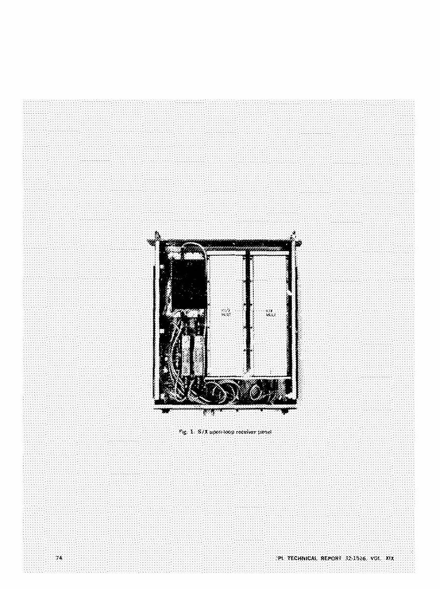
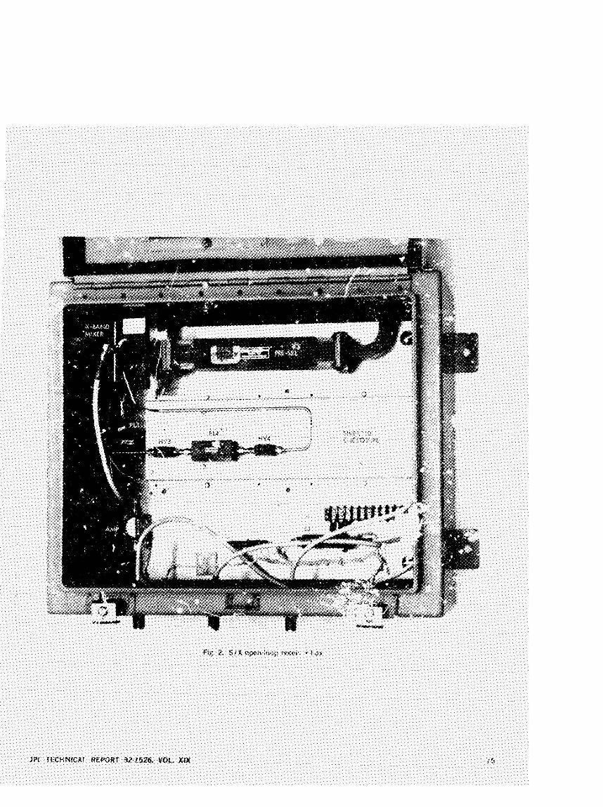
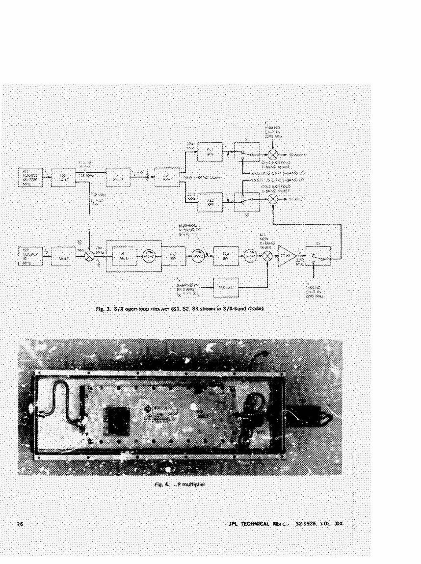
X-Band Radar System R. L. Leu
R. F. Systems Development S e c t i i
The radar deoelopment e@t will pmide the technology neresso y for Uidm bandwidths at increased mnges. This technology u5R be applicable for tise in uplink and downlink communications with future spucecruft.
1. Introduction ' 8 : dadar development effort will provide the tech-
nology necessary for wiler bandwidths at increased ranges. This technology will be applicable for use in uplink and dowiilink communications with future spacecrait.
The increased antenna gain (approximately 7 dB) \vi11 decrease the observation 5me for radar targets by a factor of :?o. The wider bandwidth will allow faster ranze codes for improved ranging resolution. Tbc 4rst use of the new radar system will be to study thc rings of Satum as a possible hazard to tis- 'pation. This q p r - tunity will start in Dcxembcr 1974.
Altho7 SZh therr have been some developmental grob- iems with the 2WkW klystrons, waveguide couplers, a d stveral control assemblies, tne scheduled o p a - t i o d date of December 1974 appem realistic. In addition to &he teclinicai difErt?lties discussed in this article, the other major obstacle is obtaining s&cient antenna time for installa'ion and checkout on the 84-m antnna at DSS 14.
I!. Radar System The radar syitem as d i s c 4 in Ref. 1 has under-
gone some changes. The system specifications are given in Table 1, and a block dia.am is presented in Fig. 1. The radar will use a m m f d mangenient as shown only if a high-power polarizer (more specifically, the rotary joints in the polarizer) m n o ; ae developed prior to the radar installation for the rings of Sturn oppor- tunity. The transmit feed (Fig. 1, feed A) will be used as the transmit-receive feed, awl the receiver ftod (B) will be used as a backup. The two-feed arrangemat is undesirable for optimum performance and will be used oniy as a Last resort.
With a two-fed system and the prestnt subreflector p'n locations, the radar will have worst-case antenna degradation -f approximately 1.3 dB. The 64-m antenna subrehector tvki rot designed for contind focusing opration. It k:ix have to remain in a fixed position and not moved between the transmit and re- ceive feeds. If the subdector is focused at a point .r,id.way betweell tlie fee& (Fig. I), the degradatim will be aproximately 0.5 dB. As the radar is switched
n

froin rtxvive to transmit mode or reversed mode, the antcmna pointing wili be changed automati~dlly \\-ith the camputt-rani . i t d airtcwu pointing s>*stem to cor- rcu-t for the ~ .~ - t - rgenw of the hailsmit and receive ailtcmn:i t x ~ i ~ s . ?“le soft\\-src nquired to perfom, this operation was dr\-eloped €or another project. To im- provt- the pec.rftJmIanCe of a two-fed sy3em. a con- figuration worth cansidering would locate the ht-0 feeds sidc by side (Fig. %!. This would q u i r e m n 6 ~ t i o n of thc cane layout and provision of new pin locations for tire subreflcctor. Thc performanct. drgradation \\-ou~ 1 be 025 dB.
-4s indicated in Table 1, the tnnsrnit-receive cycle \\-ill \-ary in duration dqwndinq on the t q e t being observed. The round-trip time for the rings of s;bturn is 2% h. DurinR the trmsmit cycle, the radiated RF po\\.er must h t a switched on and off at a :B-s rate. This is disastrous to the klystron amplifiers, as discwed in Ref. 2. References 2 and :3 discuss an approach being iniplrmcnted in the radar system for s\\-itdr?’nS thc- radiated RF power on and off. -4 scwnd nwthod, now bcing used in the S-band radar. that shifts the RF carrier in frequency (about 1 MHz) at a :31-s rate, will also be available.
111. Transmitter At the time of this writing. three %O-kW klystrons,
sis u-aterloads, three dual directional \\-aveguide couplers, and most of the electronic. wemblies have been delived. One klystron \vas operated at ?2.j kW for a shor! +;-.e before failure One of the w-aveguide couplers was defec- tive. and the other t.vo malfunctioned at 125 to 150 kW. The malfunction w a s due to improper design of the terminations in the semndary a m of the couplers. They have been rebuilt and will be retested. Because of the shortage of materials and components in the electroiic industry, se .Bra1 of the dsxironic control and monitor assemblies are late in delivery. This is not expected to c a . w anv rlr4ay in the schedule.
IV. Microwave Components Two hybrid com\:.ners (Ref. 4) have been delivered,
and ow unit was tasted in excess of 22!5 kW at one port. Trsting of the hybrid with two 2MLkW inp& will take place in the third quarter of FY”74. Waveguide switches, waveguide test equipwent (slotted line, precision sliding load, sliding short, etc.) and waveguide compoaents have been delivered. The switches a d . ..oille wawquide corn- ponents will be tested at 250 kW by January 1, 1974.
V. Feed The basic feed horn design has been completed and is
presently being fabricated. The feed horn \\-ill be ready for RF power testing by January 1974. The polarizer. i d u d i n p rotary joints. will be ready for testing in Fc-bruary 1974.
Thv polarizer is the pfiinary susp1’(* area for break- duwi from arcinc and COI-OIM in the feed systrm. -4s discussed preriously, should the rotary joints not handle the UlO-liiV power. they \\-ill be temponrily r e p l a d with straight sections of wav-ide in order to nreet the D m m b e r 19i4 operational date. Development of the polarizer would continue. and it would be installed at a later time. The fwd horn design \\iU be the same for both f t d s (transmit and receive). The m P * : frcd will use the moctble polarizer as a backup :x th-. trmsmithceive ftpd.
VI. Exciter The exciter is required to generate the 8.495;GHz
frequency and +lO-blHz phase modulation Landwidth for the radar. The output of the exciter drives the bufkr amplifier assembly, which drives the dual H > m n ampli- fiers. The exciter is extension of the Block 1V exciter that h.-- - .witched output (530 MHz) for the X-band radar. This output drives a multiplier ( X 16) to obtain 8.495 GHz. The X I 6 multiplier has been designed, pro- cured, and delivered and will be located in tb- buffer amplifier assembly, as shown in Fig. 1.
VII. Rmxiver The receiver \vi11 consist of the esisting Block I V re-
ceiver X-band channel and the X-band traveling-wave maser (77Vh.) now located in the mdti X-band/K-band (MXK) feed cone at DSS 14. The Block IV receiver is presently being tested at DSS 14 and will be available in time for the December 1974 cperational date.
VIII. C ding C d i n g water is required for the klystron, waterloads,
waveguide components, and feed. The coolant i s provided by modification to the existing transmitter coolant assem- bly and the waveguide coolant assembly. The modifica- tion to the former has bem completed, and the waveguirle wlant swtem modification wi!l be ready prior to the radar installation.
m

References
1. \Vigins, C. P., “S-band Radar Developnient,” in The Deep Space Sdtro~I; Pro,nr;.ss Report. Technical Report 32-1526, Vol. SII, pp. 1!3-2 Jet Propulsion Liboratory, Pasadena. Calif., Dec. 15, 19i2.
2. \\i!g$ns, C. P.. Buchanan, H. R., Leu, R. L., “High Power \licrowaw Trans- niittcr Switch,” in The Deep Space Settcork Progress Report, Technical Report 32-1526, Vol. XVII, pp- 21-27, Jet Propulsion Laboratory, Pasadena. Cdir., Oct. 15. 1973.
3. Kolblg. R. B.. -High Power Switching a d Combining Technique.” in The Deep S.mce Setrrork Progress Report, Technical Repoit 32-1526, Vol. SW, pp. 1C6-109, Jet Propulsion Laboratoiy, Pasadena, Cait., A1.g. 15, 1W3.
4. Hartop, R. If’., ‘S-Band Hgbrfd Combiner,” in The Deep Space SetcL.c* Pi ogress Report, Technical Report 32-1526, \’oL XU, pp- 4246, Jet Propulsion Laboratory, Pasadena, Calif., .4ug. 15, 19i3.
JPi TECHNICAL REFORT 32-1526, VOL. Xu1
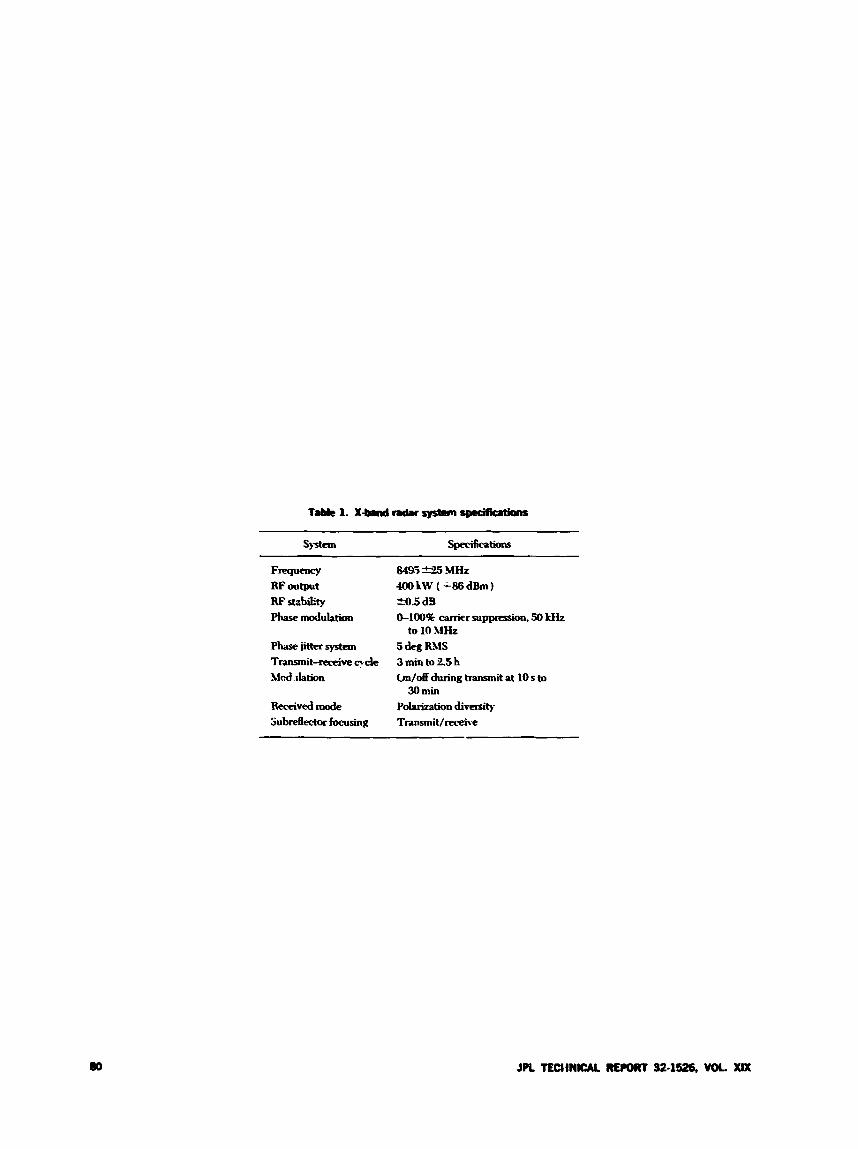
S,*m SpeCibtiOllI
Fresllency &95 S25 MHz RFoutput 4OOkW (-86dBm) RF rtabhty rto.5 dS phvedulat ion
phaseiittersystrm 5 deg RMS Truranit-receive pde Mcd .dation
Receivedmode Polarization divusity SubreR&or focusing Transmit/receive
Cb100k carrier suppression, 50 kHz to 10 hiHz
3 min to 2.5 h On/& during hannnit at 10 s to 30 min
JPL TEU1N1cAL RE#)RT 32-1526, VOL. XIX
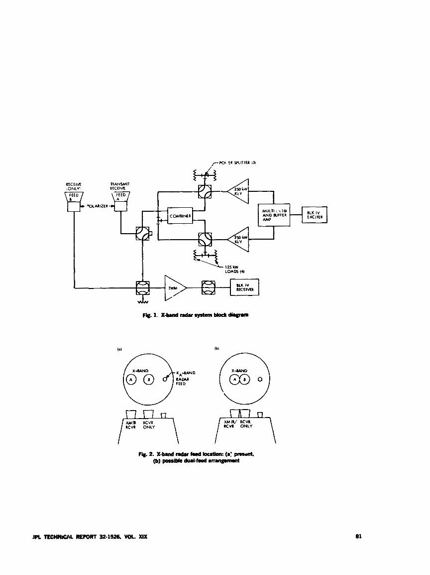
70 ER SPLITTER (3)
L
J E TECWNCAL REPORT 32.1526, VOL. XIX 81
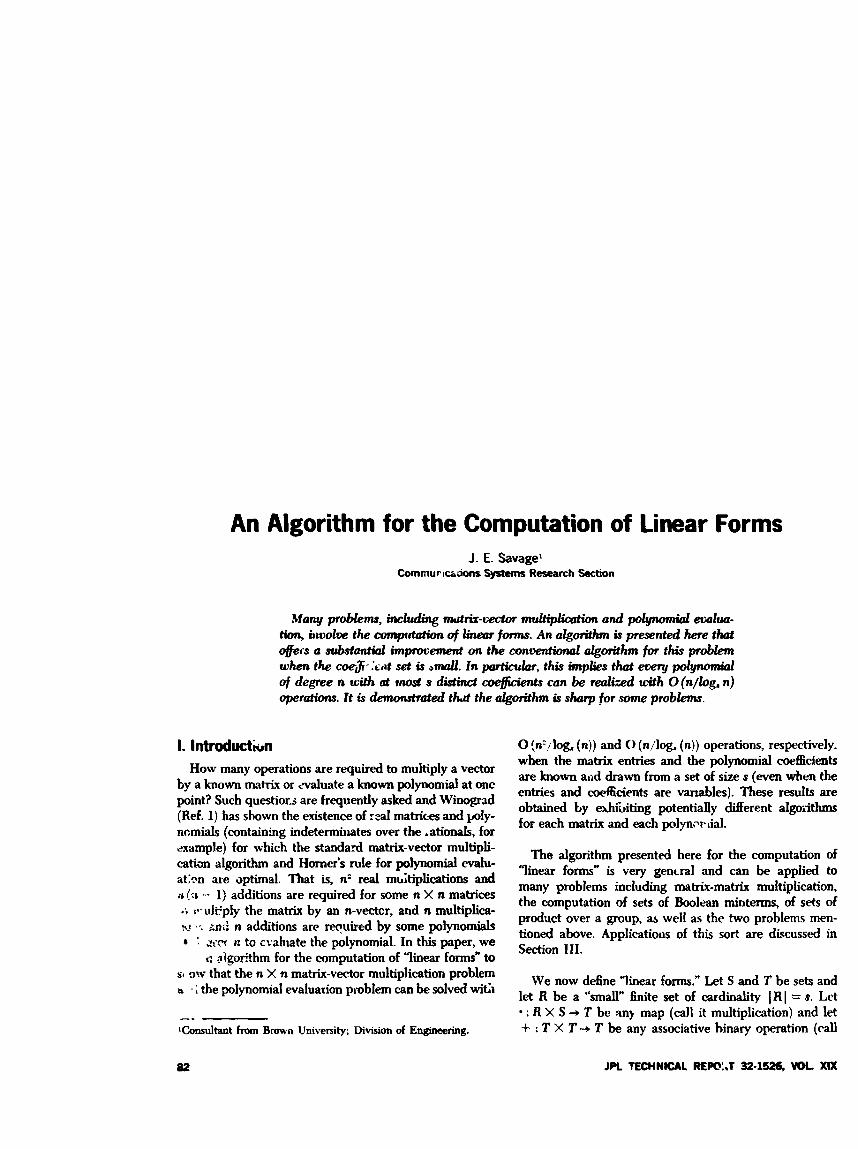
An Algorithm for the Computation of Linear Forms J. E. Savage'
Commuritxjons Systems Research section
Many problems, including nutrix-r;ector muhiplicutkm and polymmial eoalua- tion, uiodoe the oomprkrtion of linear fonns. An algorithm is presented here that 4 e i - s a substantial impt0r;ement on the conDentioAol algorithm for this problem when the -8- .bit set is +mall. In pmtidar, this implies that e w y polymmial of degree n with at r e s distinct awfchts can be r d k d u3th 0 (n/log. n) operations. It is dimo&mted t u the algorithm is s h a r ~ for some problems.
1. Introductii How many operations are required to multiply a vector
by a known matrix or daluate a known polynomial at one point? Such questiocs are frequently asked and Winopad (Ref. 1) has shown the existence of real matrices and p I y - nnmials (containing indetermiuates over the .ationals, for example) for which the standard matrix-vector multipli- catiin algorithm and Homer's rule for polynomial evalu- at:9n are aptimal. That is, n: real mGtiplications and i b b b .- 1) additions are required for some n X n matrices .; v-uli'ply the matrix by an n-vectcr, and n multiplica- IO ". mii n additions are required by some polynomials
dicr IZ to cvahate the polynomial. In this paper, we t: $gorithm for the computation of "linear forms" to
sa ~ t v that the n X n matrix-vector multiplication problem a 8 : the polynomial evaluation problem can be solved with
-- Gnsultant from Bmwn University; Division of Engineering.
0 /,n'/log, (n)) and 0 (n/log. (n)) operations, respectively. when the matrix entries and the polynomial coefficients are known aad drawn from a set of size s (even when the entries and coe6cients are vanables). These results are obtained by ehiioiting potentially a e r e n t alg0;ithms for each matrix and each po1ynm:ial.
The algorithm presented here for the computation of "linear forms,, is very gentral and can be to many including matrix-matrix multiplication, the computation of sets of Boolean mintexms, of sets of product over a group, as well as the two problems men- tioned above. Applications of this sort are discussed in section 111.
We now define Tinear forms." Let S and T be sets and let R be a "small" finite set of cardinality IRI = s. Let : R X S + T be m y map (call it multiplication) and let
+ : T X T + T be any associative binary operation (call
82 JPL TECHNICAL REmL.1 32-1526, WK. XIX
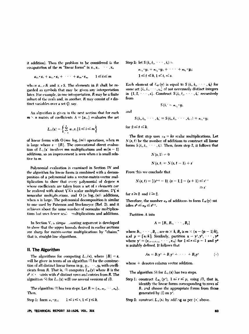
it addition). Then the problem to be considered is the Step 2: let S (4, i2, . * . , i J =
C:!'y, t ui;y, + - . . + a i , - y r ; coi.iputation of the m "linear forms" in xl, x,. . . , Xn
+ uin-x,,, 1 L i L m 1 L I' 4 k, 1 4 i j 4 s. U i , ' X , + U i - ' X z + . . .
whe-e u , , F li and x, F S. The elements in fi shall be re- gardd s,-mb& that may h x given any interpretation later. For esamplc, in one interpretation. R may be a finite subset of the rcals and. in another. R may consist of s dis- tinct variables over a set Q. say.
Each element of CB (y) is equal to s (it , i:, . . . , &) for some set { i l , i,, - . . , of not necessarily distinct integers in { 1,2, . . . , s i . Constnict S <iI, i,, . . . , i,) recursively from
S ( i l l = a:: m y ,
An algorithni is given in the nest section that for each n niatris of wfficicnts A = (a, ,) evaluates the set , i,) = S (il. i,, . . . , i l . l ! + uil -rjl S (i,, iz, . . - m
of linear forms with 0 (mri log.. (m)) operations, d i e n m is large where s = I R I . The conventional direct evalua- tion cf L , (x' involves mn multipli~itions and m(n - 1) additions, so an improvement b seen when s is small rela- tive to m.
Polynomial evaluation is examined in Scdion IV and the algorithm for lincar forms is combined with a decom- position of a pol~momiaI into a vector-matrix-vector mul- tiplication to show that r v c ~ y lalynomial of degree n whose coc.fficicnts ;trr taken from it set of s dements 2.w bc. realized with d m i t 1 5 s scalar multiplications, 21. ti nonscalar multiplic.itions, and 0 ( 1 1 ,'log. (n)) additions, when 11 is large. The polynomial decomposition is similar to onc ustd by Paterson and StocLmqer (Ref. 2). and it nchievcs ahout the same number of nonscalar multiplica- tions h i t uscs fcwcr S C : ~ .rnltiplications and additions.
In Section \', A simplr .,hunting argumcnt is developed to show that thr upper boiiilds derived in earlier sections are sharp for matrix-vector multiplications by "chains," that is, straight-linc algorithms.
II. The Algorithm The algorithms for mmpoting L I fx), where 1 R I = S,
will be givrr in terms of an algxithin ril f9r thc construc- tion of all distinct linear forms in y,, g2, . . , y k with coefii- cients from R. That is, fl computes L , ( y ) where B is the sk x vtrix with $ distinct rows and entries from R. The algorittm ';i for I, I (x) will use severai versions of a.
The algorithm (7i has two stpps. Let. R = { sl. u2, . . . , Q,}. Then.
Step1: form v,*y,; 1 L i L v . 1 d i i L .
The first step uses = ks scalar multiplications. Let N (3, I ) be the number of additions to construct all linear forms 5 (i,, i,, . - , i ,) . Then, from step 2, it follows that
N(s, I ; = S(s , f -- 1) i- s'
From 'his w e conclude that
N(s, I) = [(s'-1 - 1). (s - 1;] - (s + 1) L . 9 - 1
1 s '
for a h 2 and i 1 2 .
Therefore, the number uII of addition,. to form LR (y) sat isfies Sr 4 uB 4 .+I.
Partition A into
where b,, . . . , are m X k, B, is m >: (n - ( p - 1) k), a.td p = fn/kl. Similarly, partition x = y1,y2, . . . , y' where y' = ( x , ~ - ~ , C r i , . . . , x,k) for 1 L r L p - 1 and y p
is suitably defined. It follows that
where + denotes column vector addition.
The algorithm 9 for LA (x) has two steps.
Step 1: construct LR, (yr), 1 G t p, rising fl, that is, identify the linear forms corresponding to rows 0;
B , aqd choose the appropriate fmns from those generated by on y'.
Step 2: construci L., (x j by addhg as per ( * ) above.
JPL TECHNICAL REPORT 32-1526, VOL. XIX a3
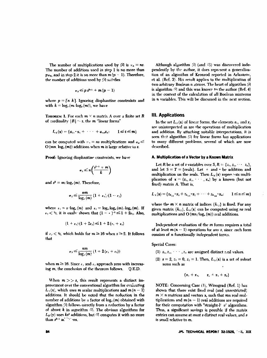
The number of mukiplications used by GI is zA = 11s. The number of additions used in step 1 is no more than pR, and in step 2 it is no more than m (p - 1). Therefore, the number of additions used by -54 satisfies
where p = rn kl. Ignoring diophantine constraints and with k = log, (milog, (m)), we have
THEOEEM 1. For each m '.! n matris -4 over a finite set R of cardinality I R I = s. the m "linear forms"
L.,(x) = {ail*xl + . . . +a,sx.: I L i l m }
can be computed with 7 , = ns multiplication. and U~ 4 0 (mn, log, (m)) additions when m is large relative to s.
Proof: Ignoring diophantine constraints, we have
,L.(-k) $-I t m
and 9 = m/log, (m). Therefore,
nm log. (m) 0.; 4 - (1 f F i ) / ( l - E ? )
where = s flog, (m) and FI' = Io& log, (m): log, (m). If E.. < %, it is easilv shown that (1 - c )-I 4 1 + 2 ~ ~ . Also,
if F : < W, which holds for i n s 16 when s that
2. It follows
when m A 16. Since F , and F? approach zero with increas- ing m, the conclusion of the theorem follows. Q.E.D.
Mhen m >> s, this result represents a distinct im- provement over the conventional algorithm for cvaitiating L I (x), which uses m scalar multiplications and m (n - 1) additions. It should be noted that the reduction in the number of additions by a factor of log, (m) obtained with algorithm B follows uirectly from a reduction by a factor of about k in algorithm f l . The obvious algorithms for LB (y) uses ksk additions, but CR computes it with no more than sl" a i - ' + ' ms.
Although aIgorithm fl (and 43) was discovered inde- pendently by thc author, it does repri-sent a generaliza- tion of an algorithm of Kronrod reported in Arlazarov, et al. (Ref. 3). His result applies to the multiplication of two arbitrary Boolean n &trices. The heart of algorithm GI is algorithm ri3 and this was knowvr to the author (Ref. 4) in the context of the calculation of all Boolean minterms in n variables. This will be discussed in the next section.
I I I. Applications In the set LA (x) of lincar forms, the elements a,, and x,
are uninterprcted as are the operations of multiplication and addition. By attaching suitable interpretations, it is seen th:it algorithm for linear forms has applications to many different problems, several of which are now described.
A. Multiplication of a Vector by a Known Matrix
Let R be a set of s variables over S, R = { z , , z-, . . . zn } , and let S = T = (reals}. Let + and be addition and multiplication on the reals. Then L, (x) repre%?.its multi- plication of x = (xi, x:, . . . , x.) by a known (but not fixed) matrix A. That is,
where the m X n matrix of indices {hi) is fixed. For any given matrix ( k i j ) , L, (x) can be computed using ns real multiplications and 0 (mn/log, (m)) real additions.
Independent evaluation of the m forms requires a total of at least m (n - 1) operations for anv s, since each form consists of n functionally independent term.
Special Cases:
(1) zI,z2, . . . , z . are assigned distinct r a l values.
(2) s = 3, = 0, z2 = 1. Then, L., (x) is a set of subset sunis such as
NOTE: Concerning Case (1 j, Winograd (Ref. 1) has shown that there exist fixed red (and unrestricted) m X n matrices and vectors x, such that mn real mul- tip!ications and m (n - l) reai additions are required for their computation with 'straight-1: e" algorithms. Thus, a significant savings is possible if the matrix entries can assume at most s distinct real values, and s is small relative to m.

B. Matrix-Matrix Multiplication AX, A Known x a = l 1- x a = O = . x =-
Let R and S be as above and let T be the pfold car- tesian product Q P , Q = {reals}. Let * be conventional scalar multiplication (consisting of p real multiplications) and let + be vector addition on the reals (consisting of p real additions). Then, L, (x! represents multiplication of the n X p matrk X over the reah by a known (but not fixed) m X n matrix L L That is,
where TI denotes the I-th row of X and the m X n matrix of indices { k , j } is hed. For any given matrix {kij}, LA (x) can be computed using nps real multiplications and 0 (mnp/log, (m)) real additions.
NOTE: When n = m = p , Strassen's algorithm (Ref. 5, for matrix-matrix multiplication can be used at the cost of at most (4.7) n'"fs; binary operations. As a consequence, Strassen's algorithm is asymp- totically superior to algorithm GI for this problem. However, when s = 2, algorithm (;n 5 the superior algorithm for n 4 10IO!! ' [oral: bew;.re of arguments based upon asymptotics.
C. Boolean Matrix Multiplication
Let R = S = {0, l}, T = {O,l}p, let be Boolean vector mnjunction, and let + be Boolean vector disjunction. Then, L,,(x) represents the multiplication of a known Boolean m X n mahix A by an arbitrary Boolean n X p matrix X. That is,
where X denotes the Bmlean inverse. Then, LA (x) repre- sents a set of mintem-s such 3s
NOTE: The set of al! P distinct minterms, suitably ordered, reprtxnts a map from the binary to positional representation of the integers (0,1,2, . . . ,2" - I}. This map Lan be realized with at most 2"+' conjunc- tions and is a map that is useful in many construc- tions, such as those in Ref. 4.
E. Roducts in a Group G
L e 1 R = {-1,O, i}, S = T = G, let a * r = i (raise to a power), and lct + be group multiplication. Then LA (x) represents a set of m products of n terms each. For example.
(a b-I c d-I, b c-', a-' c-' d-:)
is such a set, where x-l is the group inverse of x and nb is the group identity that is suppressed.
IV. Polynomial Evaluation We turn next to the evaluation of polynomials of de-
gree n. Let
p ( r ) =a ,+c , * r '+o , *x *+ . . - + 0,X"
- - +ain-3Tn: 1 L i L m ) where L and represent vector addition and scalar multi- pli+iox where x' = r, xi = %*xi-' , and rppresents vec- tor mult$iat;on. Let ai E a, x T and
L ~ ( X ~ = { a , , * X , + a i z * X * + . . .
where TI is tl e I-th TOW of the n X p matrix X. The dgo- rithm for computing AX uses no multiplications and 0 (mnpllog, (m)) additions. 9 : R x T + T
NOTE: If A is an arbitrary &lean matrix and if the selection procedure of step 1 of a!gorithm 9 cp.3 bs exectited without cost, the algo.ithm cf K*onrod i k f . 3; results. "lie number of operations pifornled, exclusive of selection, equals that given above. The Kronrod algorithm uses more operations because of a y: I choice of thc parameter k.
D. Boolean Minterrns
tion, and let be defined by I*et R = S = 7' = {0,1}. let + be the Boolean conjunc-
+ : T X T + T : T X T + T
where + and are associative and distributes over +. We shall construct an algorithm 8 for polynomial e d u a - tion, which employs algorith GI for linear forms.
Algorithm B has three steps. Without great loss of gen- eidity, let n = k f - 1, and assume that a = (ao, a,, . e a , G) n .s entries from L set of si7s s.
Step 1: construe. 9, ra, +*
JPL TECHNICAL REFORT 32.1526. VOL. XIX
Step 2: construct the ic linear form. in 1, r, P, . . . ,i-' [ :~1]~~[_'::.^1 [ ;;] rl. I (x) alk-i)f ' ' . akr 1
using algorithm 5%
Step 3: construct p (x, = r,, (x) + rl ( r ) * r' + . . . + r k - ] (r) *x+I ) l usin& Homer's rule. Let up denote the number of vector additions used by 8, rp the number of scalar multiplications and p p the num- ber uf vector multiplications. Since the forms re- quired in step 1 can be rcalized with I - 1 vector multiplications and step 3 with k - 1 such multi- plications ai.d k - 1 additions, we have
U, L 0 ( ( n + l)/log, (k)) + k - 1
T,, = Is
p p = I L k - 2
since kt = n + 1. If we ignore diophantine con- straints and choose k = V (n + I), to minimize rr, we L w e :
THEOREM 2. For each a = (a,,,ul, . . . ,un) E R"+' with R a set of cardinality I R I = s, p (x) = a,, + alr + . . . + an%" can l e evaluated with up vector additions, rp ,calar multi- plications and p,, vector multiplications where
when n is large da t ive to s.
Homer's rule, which is the optimal procedure for evalu- ating Ln arbitrary polynomial on the reals, uses n multi- plications and n additions. Even when a and r assume fixed real values, there exist vectors a and values r for which Horner's rule is still optimal (Ref. 1). When the coefficients are drawn from a set of size s, however, Horner's rule can bc improved upon by a significant fac- tor when n is large relative to s.
The decompositiov of p ( r ) used by algorithm 8 is very similar to that used by Paterson and Stcckmeyer (Ref. 2) ia their study of polynomials with rational coefficients. They have shown that 0 (c) vector multiplications
are necessary and su5cient for such polynomials, but their algorithms use 0 (n) additions. Algorithm Q achieves 0 (fi) vector multiplications but requires only 0 (n/log, (n)) additions when n is large relative to s. Clearly, algorithm Q can be applied to any problem in- volving polynomial forms.
V. Some Lower Bounds The purpose of this section is to demonstrate the exis-
tence of problems for which the performance of algorithm 9 can be improved upon by at most a constant factor. To do this, we must carefully defirn the class of algoriiLms that are permissible. Then, we count the number of algo- rithms using C or fewer operations and show tl-at if C is not sufficiently large, not all problems of a given type (such as matrix-vcctor multiplication) can be realized with C or fewer operations.
A chain p is a sequence of steps pl,p2, . . . ,pL of two types: data steps, in which Bi E {yl,yl, . - . ,yn) U K (yi j K , yi # y,, i # j and K C Q i s a finite set of con- stants), or computation steps, in which
pi = pj O P k i, k < i and o : Q X Q + Q denotes an operation in a set Q.
Associated with each step pi of a chain is a function pi. which is pi if pi is a data step and
Pi = 0 (p i , 7%) if pi is a computation step. Clearly, ai Q" + Q. A chain p is said to compute m functions f l , j 2 , . . . , fm, f , : Q"-+ Q if there exists a set of m steps pi,, . . . , $4, such that pi, = f,, 1 4 I L m .
We now derive an upper bound on the number N (C,m,n) of sets of m functions {f,, . . . ,fm} that can be realized by chains with C or fewer computation steps.
LEMMA. N ( C , n. - ~ 0 4 ~ , i 1 = C + n + m + IKl+ 1 if C h i n p 2
Proof: .4 chain will have 1 4 d 4 n + I K I data steps and without loss of generality they mav be chosen to precede computation steps. Similarlv, the order of their appear- ance is immaterial, SG there are at most
ways to arrange the d data steps.
86 JPL TECHNICAL REPORT 32-1526, VOL X I X
Let the chain have t computation steps. Each step may correspond to at most I R I operations and each of tht two operands may be one of at most t + d steps. Thus, there are at most 1 0 1 ' (t + d)*' ways to asign computatirn steps and at most 2"""' 10 I (t + d)z t chains with d data steps and t computation steps. A set of m functions can be assigned in at most ( t + d)'" ways.
Combining these results, w. see that the number of dis- tinct sets of m functions that can he associated with chains that havr C or fewer computation steps is at most
But
(t + d ) * ' + m
where v = C -& n + E? + IKI +l. Q.E.D.
In the intcres: of deriving a bound quickly, the counting argunrents given above are loose. Nevertheless, the bound can at best be improved to about u". As seen below, this means a factor of about 4 loss in the complexity bound.
Consider the comgutation of m subset sums of {xl, zlr * . . , xn), xi E {reals], as defined in Special Case (2) of Subsection 111-A. In the chain defined above let Q = { reals) and let ,R = { + , addition on the reals). There are 2" distinct subbet sums and the number of sets of m lis- tinct subset $urns is the binomial coefficient
F = ( i ) Fix 0 < c < 1. If C, n, and m are such that N (C, n, m) 4
then there cxists at least one set of VI distinct slabset sums that require C or more additions.
Tmomh.13. Algorithm .fl is sharp for some problems, that is, there exist problems, namely, the computation of m sutset sums over the reals, that require 0 (rnn/log, (m)) operations with any chain or "straight-line" algorithm, when m = 0 (n).
Proof: Set 0'" = F1-c where v = C + n + m + IKI + 1. Then, N (C, m, n) A F e. For large F, the solution for u is
v = ( f In F 1 - - c ) / Ir, ( f FI-' ) Since m = 0 (n), it can be shown from Stirling's approxi- matioq to factorials an? an examination of the binoniial coefficient F that 1nF is asymptotic to nm In (8). From this the corrclusion follows. Q.E.D.
The col;zting argument given above could also be applied to matrix .vector multiplication, Subsection 111-A, and to polynomial evaluation on the reals, as described in Section 'V, tc, .ha w that the u p p ~ bounds given for these problem <.re also, sharp.
VI. Ccxlusions The algorithm presented here for the evaluation of a
set of h e a r forms derives its importance from thc minhal sct of conditions required of the two operacioiis. In fact, th.: only condition required is that addition be ,sociative. 1s a consequence, the algorithm applies to a 1arz.e class of
apparently disparate problcrns having in co' . mon the fact that they can be represented in terms of Iin:.ar foms this gen: ' iature.
The alg~rithm allows us to treat two important prob- iems, matrix multiplication with a known matrix and poly- nomial evaluation with a mown polynomial. In both cases an algorithm is constncted that depends explicitly on the matrix entries and the polynomiai coefficients. When the entry set of the matrix or of the polynomial coefficients is fixed and the dimensions of either prohlem arc large, a sizable savings in the n u d of r - 7 ,!rPd
computations is obtained.
The genxality of the algorithm for evaluation of linear forms suggests that it may have application to many im- portant problems not mentioned in this paper.
JPL TECHNICAL REPORT 32.1526, VOL. XIX 87

Acknowledgment
The author acknowledges several important conversations v-ith Dr. Charles M. Fiduccia, which resulted in the generalization and clarification of the principal algorithm for linear forms.
References
1. Winograd, S., “On the Number of Multiplications Necessary to Compute Cer- cain Fmctiocs,’‘ Comm. Pure and Applied Math., Vol. 23, pp. 165-179.1970.
2. Paterson, M., and Stoc!meyer, L., ”Bounds on the Evalvation Time for Rational Polynomials,” in Proceedings of the Twelfth IEEE Sym;,osiun. on Switching and Automata Theory, pp. 140-133, Oct. 2971.
3, Arlazarov, V. L., et al., “On Economicd Construction of th3 Transitive C!osure of all Oriented Graph,” Sou& Mathematics Doklady, 1’01. 11. No 5. pp. 1 s 1210,1970.
4. Savage, J. E., “Cc-mputational Work and Time on Finite MacLnes,” I . h o c . Comput. Mach, Vnl. 19, No. 4, p. 673, Oct. 1972.
5. Strassen, V., “ G ~ m i a n Elimination is Not Optimal,” A’umer. Math., Vol. 13, pp. 35446,1969.
Radio Metric Applications of the New Broadband Square Law Detector
R. A. Gardner, C. T. Stelzried, and M. S. Reid Communications Elements Research Section
Previous articles hove discussed tke cieoelopment and pprfonanc t't a new r ,Want law detector. The new detector k c a wide. dynamk range and a mwe accurate square 2aw rec'wnse than luu been availaL-s in the past. This article discusses the w e and F.?rformance of this detector in c1 noise-adding rudiotneter system at DS8 13.
1. Introduction
ment and perfor. of a new constant law detector. "'iris new detector has a wider dyramic range and a more accurate square law response than has been avai!rble in the past. ther desirable characteristics of the dt\xtor are high-level dc oitpitt with immunity to ground lonp prob- lems, fast respoxe times, ability .o insert known time constants, and good thermal stability. This art- dis- cusses th, use mind performance of the new detector ir, a noix-adding radiometer (WAR) (3ef. 3) system.
oider to desensitize a r&li.+irig syqtte..r from gain changes, a noise-adding rad; , n e t t .nay be used. If a known aiid
a: a reference, then it is possible to obtain a ratio of output p ,wers ;Y-Cr.ctors) with the noise refpren,. F 4ource on and off. n u s .
(Refs* 2, discussed the constant dmount of is to the system and used
and
II. The Noise-Adding Radiometer System In a total-power raJiometer, the output system noise
temperature To, is given by
To, = GKV
where G is the sy,;em gaiq V ;s the voltage oritput from tht square 1- u' detector, and K !s a scaling constant. In the total-power radiometer system, g dn changes cannot be distingubhd fro- real a n t m u temperature changes. hi
where T x is the equivalent noise tcrnpera:ble of the noise reference. It has been fc: .id that a tem?er;iture-stab&/~d solid-state noise diode is sufficiently stablt fw noise- adding radiometer apnlications (Ref. 3). If the Y-factors are meawred at ;I **atr: much faster than the gaL, <:ranges in the receiving s,,cer-, .he effect of gain iiuctuatiors is cancelled.
A noise-adding radiometer system has been 'eeigwd 3 26-rn
1.mplifler operates in a c!osd-qcle and constrwtsd at USS 13 for operation with antenna. The maser
JPL TECHNICAL R E M 324526, YOL. XIX 89
refrigerator (CCR). The CCR compressor cycles at a 1.2-Hz rate which is determined by the ac power-line fre- quency. Sintv the maser gain fluctuates at this rate, it is desirable t-. I. itch Ts at a rate greater than 8 Hz. It is also important .o h o s e a rate that will not cohere with the 1.2-Hz CCR rate. The resolution of the radiometer, for a switching rate of 8 Hz (which corresponds to a measure- ment time G f 0.125 s;, is given by
zz 0.1K 2T.,( 1 + 2)
- - 1- \Ta x lo-' x 10 x 1@ AT=--
where T is the measurement time for one Y-factor and B the system bandwidth. Thus, the resolution is 0.1K for a single measurement of T , , from one Y-factor for the DSS 13 radiometer. This resolution is improved, by aver- aging a number of individual measurements. by the factor 1 1' N. This results in a radiometer system with a mea- surement resolution on the order of a milli-Kelvin.
Figure 1 shows a block diagram of the DSS 13 NAR system. In the figure, SD is the solid-state noise diode in an oven. The detector is the unit described in Refs. 1 and 2. Any detector departure from true square law has two effects: (1) measurement inaccuracy and (2) suscepti- bility to gain fluctuation. Thus. all measurements are cor- rected by a factor Q, as described in Ref. 2, so that the measurement Y-factor is given by
where V, and V, are the detector output voltages with the noise diode off and on, respectively. The IF bandwidth at the input to the detector is 5 MHz. The frequency out- put from the detector is fed to the compv.ting counter.
The computing counter is Model H.P. 5360A, and the computing counter programmer is Model H.P. 6376A. These two units comprise a small computing system with input .'output capability, which is capable of executing 200 program steps with an average execution time of 15 ps per step. It is also capable of accepting input data in BCD form, reading an externally generated frequency, and per- fonning various external functions by means of "I,-type signal levels. In addition, sixdigit constants are available in thumbnheel form for use in the program. The pro- grammer commands the noise source driver which turns the noise diode on and off.
The programmed controller, Model 601, commands the computing counter and interfaces with the station
XDS 910 camputer, as shown in the figure. The pro- grammed controller commands the 910 with azimuth and elevation offset functions, and the 910 drives the antenna servo in the usual way. The programmed controller is described in detail in Ref. 4.
111. Method of Operating the NAR System The detector correction factor a is first measured and
then set on the thumbwheels as a system coastant for the duration of the NAR observing period. To determine the correct value for the correction factor, the a-thumbwheels are first set to zero, the waveguide switch is switched to the ambient load, the NAR is run, and the detected out- put level is set to 1.8 V, with the noise diode on. The ambient load is connected to the maser input to ensure a constant system temperature during the measurement of a. There is the possibility of radio sources passing into or out of the antenna beam if the maser were connected to the horn at this time. The IF input level to the detector is then reduced by 10 dB, and a new system temperature is computed. If the system temperature at the lower gain setting is lower than the system temperature at the higher gain, a greater value for a is required. The correct value for Q is found experimentally by determining that value r.f Q which produces the same value of To, for both gain s-Kings.
The second system constant that must be determined is the correct value for Ts. When this is found, it is entered in the second set of thumbwheels and held constant for the duration of the experiment. With the ambient termi- nation on the maser input, the system temperature is given by
Top = T p + TM + T p
where
T p = physical temperature of the ambient termination measured with a quartz thermometer probe.
Ty = equivalent input noise terrperature of the maser.
T, = equivalent input noise temperature of the folIow-
If the maser is turned on and off, a Y-factor ratio Y,,,, is measured. This ratii, is given by
up receiver.
With e knowledge of Tu and T p and a measurement of Yo,, .,* can be calculated. The system temperature with the ambient termination on the maser input is then known.
90 JPL TECHNICAL RE= 32-1126, WL XIX
The T , thumbwheel is adjusted until the NAR computes the correct system temperature. The maser input is then switched to the antenna. and the NAR computes the sys- tem temperature on the antenna.
The third thumbwheel constant to be determined is N, the number of measurements which are averaged to yield the output system temperature Top Since measurement certainty is given by
where AT is the measurement resolution as stated above, a value for N may be chosen that \vi11 produce the desired radiometer resolution. If the antenna is moving in eleva-
tion during the measurement, N should be kept suffi- ciently small so that the real change in antenna tempera- ture does not exceed the desired ATNS.
The noise diode is enclosed in a constant-temperature (50°C) oven. Repeated measurements over an extended period of time have shown that the value of TN varies approximately 2 2 % in a 24-h period in S-band systems. This fluctuation in the value of T , seem to follow am- bier.t temperature variations. Recent laboratory work indi- cates that the coupling factor of the waveguide coupler used to inject T , varies as a function of ambient tempera- ture. Further work is in progress on this problem.
A number of NAR programs are available for various engineering and radio science applications.
References
1. Reid, M. S., Gardner. R. A., and Stelzried, C. T., “A New Broadband Square Law Detector,” in The Decp Space N e t u w k Progress Report, Technical Report 32-1526, \‘ol. XVI, pp. ‘i8-86, Jet Propulsion Laboratory, Pasadena, Calif., Aug. 15, 1973.
2. Reid, M. S., Cardner, R. A., and Stelzried, “Improvement in the Accuracy of the New Br0adbar.d Square Law Detector,” in The Deep Space Netwvrk Progress Report, Technical Report 32-1526, Vol. XVIII, pp. 94-98, Jet Propulsion Labora- tory, Pasadena, Calif., Dec. 15, 1973.
3. Ratelaan, P. D., Goldstein, R. M., and Stelzried, C. T., “A Noise-Adding Radi- ometer for Use in the Df‘T .,” in 7he Deep Space Network, Space Programs Sum- m,ary 37-65, Vol. 11, pp. 66-69, Jet Propulsion Laboratory, Pasadena, Calif., Sept. 30, 1970.
4. Parham, 0. B., ‘The Design l;nd Performance of a Programmed Controller,” in this issue.
JPL TECHNICAL REPORT 32-1526, VOL. XIX 91
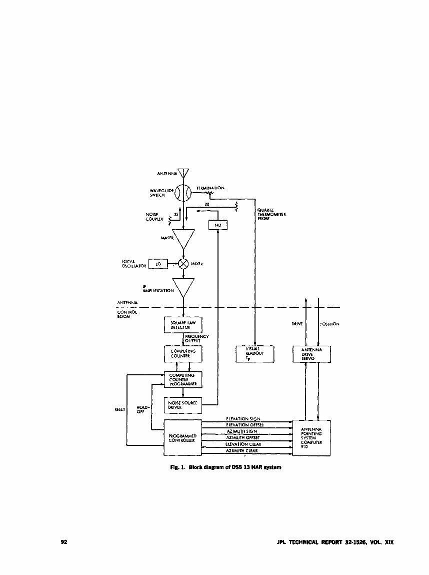
Y ANTENNA
AMPLIFICATION
DETECTOR
ANTENNA
CONTROL ROOM
-----
RESEl
OUTPUT
COMPUTING COUNTER
COMPUTING COUNTER
NOISE SOURCE
P U R R THERMOMETER PROBE
ELEVATION SIGN ELEVATION OFFSkT AZIMUTH SIGN ANTENNA
POINTING
COhiPUlER PROGRAMMED AZIMUTH OFFSET CONTROLLER
ELEVATION CLEAR
Fig. 1. Block diagram of DSS 13 NAR system
92 JPL TECHNICAL R E M 32.1526, VOL XIX

Low-Noise Receivers: Microwave Maser Development R. Clauss and E. Wiebe
Communications Elements Research Section
Two S-band w e r systenrp with equioabnt input noise temperatures of i 2 K have been supplied to the Deep Space Network. These masers will be med on d - m antennas at Deep Space Stations 14 and 43 to meet special requirements of the Manner Venus/Mercuy (MVM73) mission. The masers use a new shortened and cooled Signal input transmission line to reduce noise and are equipped with super- conducting magnets to ptooide the best possible stability performance.
1. Introduction Special requirements far the Mariner Venus/ Mercury
mission showed a need for S-band masers with improved sensitivity and stability characteristics. Two new systems for DSSs 14 and 43 have been built in response to these requirements. The maser systems have new shortened and cooled input transmission lines which reduce the noise temperature as compared to previous systems. Supercon- ducting magnets are used to improve maser gain, phase, and group delay stability. Optimum maser performance is achieved at 2295 MHz; the maser equivalent input noise temperature is 2.1 K at 22% MHz. An overall sys- tem temperature of 8.3 K was measured during the cvdua- tion of these new systems.
II. Input Transmission Line A new signal input transmission line has resulted in a
substantial reduction of maser equivalent input noise tern-
perature. Previously reported systems (Refs. 1 and 2) were measured to have maser input noise temperatures of between 4 and 8 K at the S-band waveguide interface (2.1 K was contributed by the signal input transmission b e ) . The new signal input transmission line described bebw contributes 0.4 K to the mascr noise temperature. The improvement is achieved by coo!ing the center con- ductor of the coaxial line to 4.5 K, by shortening the line length to I8 cm, and by using a very-low-loss vacuum seal.
The new transmission line, asscmbld with an S-band maser and closed-cycle helium refrigerator (CCR), is shown in Fig. 1. The superconducting magnet, radiation shields, and the vacwum jacket cover have been remov,:. Figure 2 is a sketch identifying important features of the assembly.
A fused quartz dome provides part of the vacuum seal. The quartz dome is attached and sealed to the WR 430 input waveguide with flexible epoxy. An O-ring vacuum
JPL lECHNlCAL RE#NIT 324526, WH. XIX 93
seal is used between the waveguide and the adapter plate. The waveguide and fused quartz dome assembly can be replaced without disturbing other input line m,nponents; it is a field-replaceable assembly.
The coaxial transmission line outer conductor is made of thinwall (0.25-mm) stainless steel tubing; the inside is plated with rdO25-mm capper and 0.0003-mm gold. This combination $ves low microwave loss and adequate ther- mal isolation. Mechanical support for the transmission line is obtained by clamping a flange at the room tempera- ture end of the outer conductor, between the adapter plate and the WR 430 waveguide. Thermal connections to the 80-K and 4.5-K CCR stations are made with flexible capper straps.
The transmission line center conductor contacts the outer conductor at the 4.5-K SMA connector and at the support clamp (which is thermally connected to the 4 . 5 4 CCR station). A vacuum, common to the CCR vacuum jacket, provides thermal insulation between the coaxial line center conductor and its surrounding parts (outer con- ductor and quartz dome). The center conductor is made of gold-plated, polished copper. Refrigeration capacity measurements show that the total heat transferred to the 4.5-K CCR station (by radiation to the center conduc- tor and by conduction through the outer conductor) is approximately 100 mW. The voltage standing wave ratio (VSWR) of the transmission line and waveguide assembly is less than 1.15 to 1 from 2050 to 2650 MHz. Q measure- ments, insertion loss, and temperature gradient calcula- tions were used to determine the 0.4-K noise contribution of this transmission line assembly.
The new transmission line assembly is adaptable to all S-band maser systems presently used in the DSN. The con- version requires installation of a superconducting magnet.
IV. Maser for SMT Cone The maser currently in use in the S-band mega..vatt
transmit (SMT) conC at DSS 14 uses the new input trans- mission line and achieves a noise temperature of 2.1 K at 2295 MHz. The maser comb structure is of the Block I11 type, with modified ruby shape (loadingj to achieve a wide tuning range. The maser can provide more than 40 dB net gain at any frequency between 2m and 2400 MHz. A maximum gainlbandwidth product is ob- tained when the maser is centered at 2285 MHz. Excess gain can be traded for bandwidth by use of field stagger- ing co9s within the supcrconducting magnet. A frequency response flat within 1 dB from 2270 to 2300 MHz is avail- able at 42 dB net gain.
V. Maser for DSS 43 A second maser with a noise temperature of 2.1 K has
been built for use at DSS 43. A previouslv built maser comb structure (Ref. 2) was used to save on system con- struction time and cost. The maser is not capable of the large gain bandwidth product achieved by the maser for the SMT cone. The maser provides an S-MHz, 1-dB band- width at 44 dB net gain at 2295 MHz center frequency. The pump klystron used with the DSS 43 system is iden- tical to those presently used with Block I11 maser sys- tems and does not provide 2388-MHz operation. The low forward loss of this particular maser is equal to that of the SMT cone unit, and identical noise performance at 2295 MHz is ach ievd
VI. Noise Temperature Measurements Comparative system temperature measurements of
masers described here have been made. A photograph of the maser/CCR package for the SMT cone, with horn and ambient temperature microwave-absorbing material, is shown in Fig. 3. Precision power measurements with and without the absorber material over the horn resrilted
111. Superconducting Magnet The use of a superconducting magnet, rather than a
large, external permanent magnet, has several advan- tages: (1) it improves maser gain, signal phase, and group delay stability (Ref. 3); (2) the overall package weight can
permits connection of the signa1 input waveguide in close proximity to the 4.5-K CCR station. A Block I11 maser system (Ref. 1) has been retrofit with a superconducting magnet and is currently used for two-way tracking on the 04-m antenna at DSS 14. (This maser system does not have the new input transmission line.)
in a total operating system noise temperature of 8.4 K. Best estimates of noise contributions for the parts of the system are given in Table 1. Measurements of the maser system previously used with :he SMT cone showed a total operating system temperature of 10.7 K. Laboratory mea- surements using a liquid-helium-cooled waveguide ter-
the o?der SMT maser (Ref. 2).
be reduced from 2oo to m kg; and (3) the reduction mk,ation indicated a 4.4-K maser noise temperature for
Measurements of the maser for DSS 43 gave the lowest overall noise temperature values. The system was mea- sured in the same configuration as that planned for in-
94 JPL TECHNICAL REPORT 32-1126, VOL XIX
stallation on the 64-m antenna at DSS 43. A calibrating coupler and polarizer were included in the waveguide system. The slight loss of these components was offset by
the use of a better horn than was used in the carlier tests. A total operating system temperature of 8.3 K was measured.
References
1. Trowbridge, D. L., “Block 111 Maser Implementation Program,” in The Deep Space Network Progress Report, Technical Report 32-1526, Vol. XVIII, pp. 130- 135, Jet Propulsion Laboratory, Pasadena, Calif., Dec. 15, 1973.
2. Clauss, R., and Quinn, R., “Low Noise Receivers: hlicrowave Maser Develop- ment,” in The Deep Space Network, Space Programs Summary 37-58, Vol. 11, pp. 5052, Jet Propulsion Labxatory, Pasadena, Calif., July 31, 1969.
3. Clauss, R., Wiete, E., and QJinn, R., “Low Noise Receivers: Microwave Maser Development,” in The Deep Space Netwwrk Progress Report, Technical Report 32-1526, Vol. XI, pp. 71-80, Jet Propulsion Laboratory, Pasadena, Calif., Oct. 15, 1972.
JPL TECHNICAL REPORT 32.1526. VOL. XIX 95

Part of system Noise contribution, K Sky (includes atmosphere and cosmic
Horn and mode generator 1.2
4.9 background)
Maser 2.1 Follow-UD receiver 0.2
Total operating system temperature 8.4
JPL TECHNICAL RE- 32-1526, Va xu(
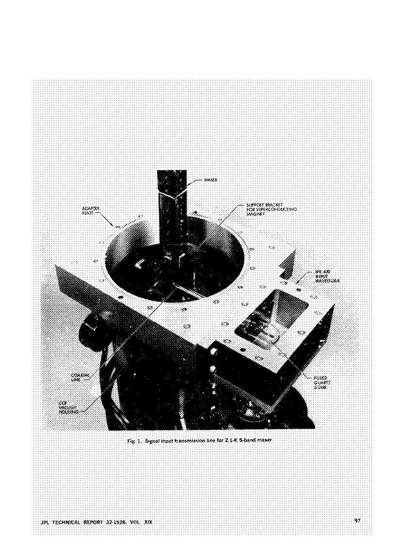

O-RING SUPPORT FLANGE VACUUM FOR OUTER CONDLKTORT SEAL i
WRWO INPUT
FLEXIBLE \ EPOXY T
SOLID C I I rc_L!z,p. :OPPER
WAVEGUIDE --, I I 1
FUSED QUARTZ DOME
80-K HEAT STATION FOR OUTER CONDUCTOR
I I
4.5-K HEAT STATION AND CLAMP TO SUPFORT CENTER CONDUCTOR
- ADAPTER PLATE
JPL TECHNICAL REPORT 32.1526, VOL.
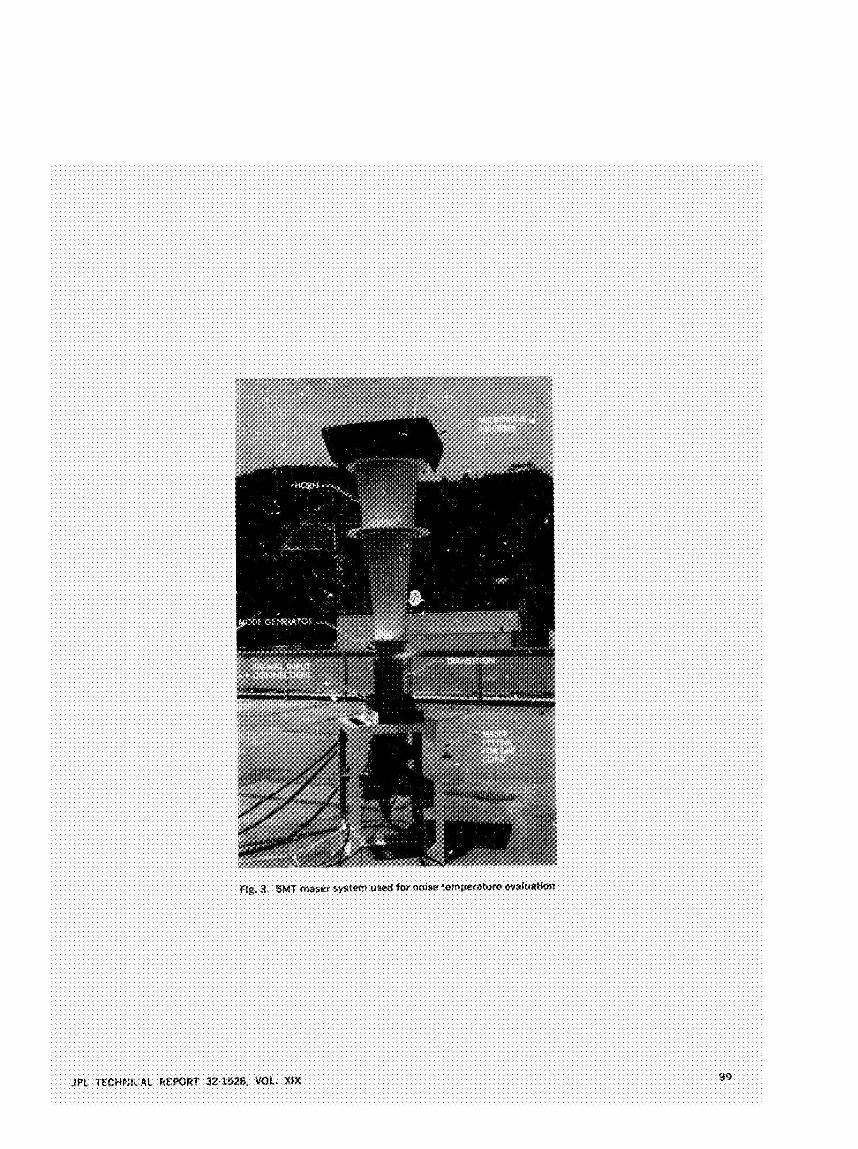
System Noise Temperature Calibrations of the Research and Development Systems at DSS 14
M. S. Reid and R. A. Gardner Communications Elements Research Section
This article rqnnts recent precision system noise temperature measurements made with the X- and S-band systems as they will be used for the Mariner Venus/ Mercury 1973 (MVM’73) mission. Eleuotion and azimuth profiles for both the S-band and X-band systems are also presented. A summary of the zenith qstem mise temperature meawremnts for calendar year 1973 for the diplexed S-band system at DSS 14 is described and plotted.
In a previous article (Ref. l), system temperature mea- surements were made at DL:S 14 of the S-band Megawatt Transmit (SMT) cone S-bar) I system and the multifre- quency X- and K-band (MXK) Lane X-band system. Thebe measurements were elevatior profiles with the reflex feed system both extended and retracted. Since these measure- ments were nade, certain improvements (Ref. 2) have been made to the maser in the SMT cone, the effect of which has been to reduce the SMT system operating noise temperature. Other impro-iements since previous reports
(Ref. 3) have included the taping of the 64-m antenna sur- face. This article reports recent precision system tempera- ture measurements made with the X- and the improved S-band systems, as they will be used for the MVM73 mission. The present measurements were made with the Noise-Adding Radiometer (Ref. 4) and the ambient lw,d terminGtions. Verification tests of the ambient load were made with a microwave absorber over &e horn, and volt- age standing wave ratios of the ambient load and horn were checked.
100 J M TECHNICAL REPMn 32-1526. w)L XIX
Figure 1 shows elevation profiles for the S- and X-band systems. The S-band data were obtained with maser serial number 80S2 in the SMT cone and the X-band data with maser serial 150x2 in the MXK cone. The dichroic feed system was extended, the atmosphere was clear, and the antenna azimuth was fixed at 180 deg. The masers were tuned to 2295 and 8415 MHz, respectively, and the iollow-up receiver contribution was measured as less than 0.1 K in each case.
Table 1 is a sun.mary of the system operating noise tem- perature performance of the SMT and MXK cones. The dichroic feed system does not degrade the S-band system temperature at high elevation angles (above 30 deg). The S- and X-band system temperature at zenith was mea- sured as 12.4 and 21.1 K, respectively, with the dichroic feed system extended.
Figure 2 shows S-band azimuth profiles for three dif- ferent elevation angles. The azimuth angles were chosen to correspond approximately to the angles at which the MVM’73 spacecraft will be tracked. These profiles were
made with the SMT cone system tuned to !2295 MHz u ~ . l
the dichroic feed system extended.
Figure 3 shows similar X-band profiles for the same thiee elevation angles and the same azimuth angles. These profiles were made with the MXK system tuned to 8415 MHz and the dichroic feed system extended.
Table 2 lists the horizon mask data in tabular fcrm for reference.
Figure 4 shows a summary of zenith system noise tem- perature measurements for calendar year 1973 for the S-band systems at DSS 14. The crosses are the data for maser serial number 9653 in the po:arization diversity S-band (PDS) cone operating in the diplexed mode. The circles are the data for the maser in the Module 3 area operating in the diplexed mode through the pP’ ” cone.
tion personnel at DSS 14) were made w. Y-factor technique of switching bebeen an amL,a.. +?miination and the horn, but without regard for weather conditions.
All these measurements (most of which w- by ~ t a -
References
1. Reid, M. S., Gardner, R. A., and Freiley, A. J., “Precision System Temperature Measurements at Goldstone,” in The Deep Space Network Progress Re*, Technical Report 32-1526, Vol. XIV, pp. 80-87, Jet Propulsion Laboratory, Pasadena, Calif., Apr. 15, 1973.
2. Clauss, R. C., and Wiebe, E. R., “Low-Noise Receivers: Microwave Maser Devel- opment,” in this issue.
3. Reid, M. S., “System Operating Noise l‘emperature Calibrations,” in The Deep Space Network Progress Report, Technical Report 32-1528, Vol. X, pp. 123-128, Jet Propulsion Laboratory, Pasadena, Calif., Aug. 15, 1972.
4. Batelaan, P. D., Goldstein, R. M., Stelzried, C. T., “A Noise Adding Radiometer for Use in the DSN,” in The Deep Space Network, Space Programs Summary 37-65, Vol. 11, pp. 60-6Q, Jet Propulsion Laboratory, Pasadena, Calif., Sspt. 1970.
J M TECHNICAL RECORT 324S26, VOL. XlX 101

Table 1. Summary of system operating noise temperature performance of SMT and MXA cones
~ ~~
Dichroic feed system ~ Dichroi&ed system -- Elevation extznded retracted
andel SMT cone WXK cone SMT cane MXK cane 2295 MHz, 8.115 MHz, 2295 MHz, 8415 MHz,
K i( K K 88 12.4 21.1. 12.4 19.5 60 12.9 21.8 12.9 21.2 30 16.3 25.7 16.3 25.1
Table 2. Horizon masks at S and X-band for three eisvation angles
Azimuth angle, deg
Elevation Elevation Elevation
- 8:; l7pl’e”B lagn&g
SMT, MXE, SMT, MXK, SMT, MXK, K K K K K K
io5 115 125 125 145 155 165 175 180 185 195 205 215 825 235 245 255
30.3 47.0 24.7 38.7 20.9 33.6 31.0 48.8 24.7 38.5 21.2 33.6 31.4 47.4 25.0 39.0 21.0 33.9 32.1 48.8 25.4 39.6 21.2 3 . 9 33.1 50.1 260 39.9 21.5 34.7 34.4 51.6 26.2 40.8 21.6 35.2 33.7 51.0 26.2 40.2 21.6 35.2 33.3 5n.9 L3.1 10.7 21.6 34.9 33.1 50.5 26.1 40.7 21.6 35.1 32.8 50.0 2S 9 40.5 21.4 34.9 32.4 49.2 25.6 39.9 21.4 34.2, 32.2 48.4 35.5 39.5 21.3 34.8 32.1 49.2 25.4 39.5 21.3 34.7 32.1 48.8 25.6 39.7 21.3 34.7 32.4 49.6 25.6 40.9 21.4 34.7 32.3 49.0 25.6 39.9 21.3 34.6 32.3 49.0 25.6 39.8 21.3 34.6
102 JPL TECHNICAL REPORT 32-1526, WL XIX
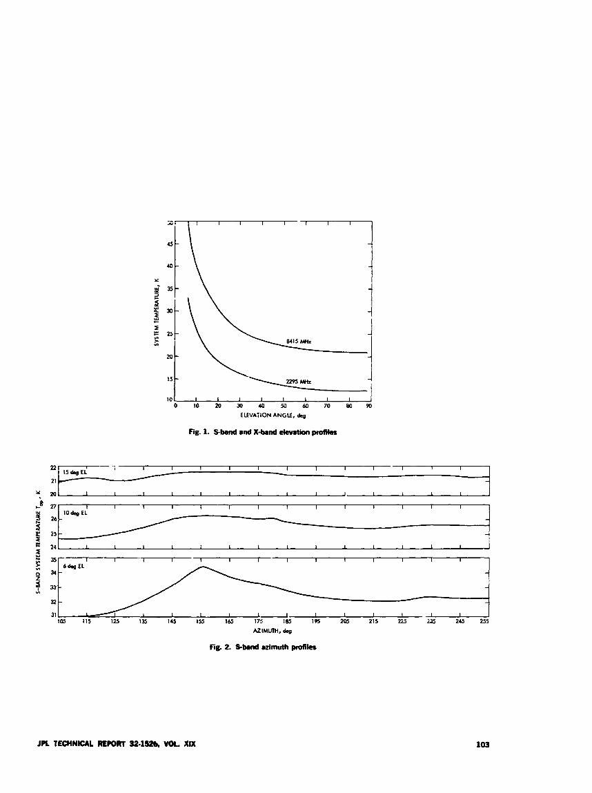
Y
yi
5 5 L L
z w I-
Y I- - VI >
w 5 26-
8! 25 2
2 ‘L 24
I I 1 -.. . .lu*
10% EL - - -
I I I I I I I I I I I I I
:I 35
25
2 P 34- z ? 33- VI
32-
31.
l5 t
I I 1 I 1 I I I I I I I I I 6 4 E L -
- -
I I I
l0L I I 1 I I 1 I I 0 10 20 30 40 W 60 70 80 90
ELEVATION ANGLE, Qs
Fig. 1. S-band and X-band elevation profib
I I I I I I I I I I
JPL TECHNICAL REPORT 32.1- VOL. Xu( 103
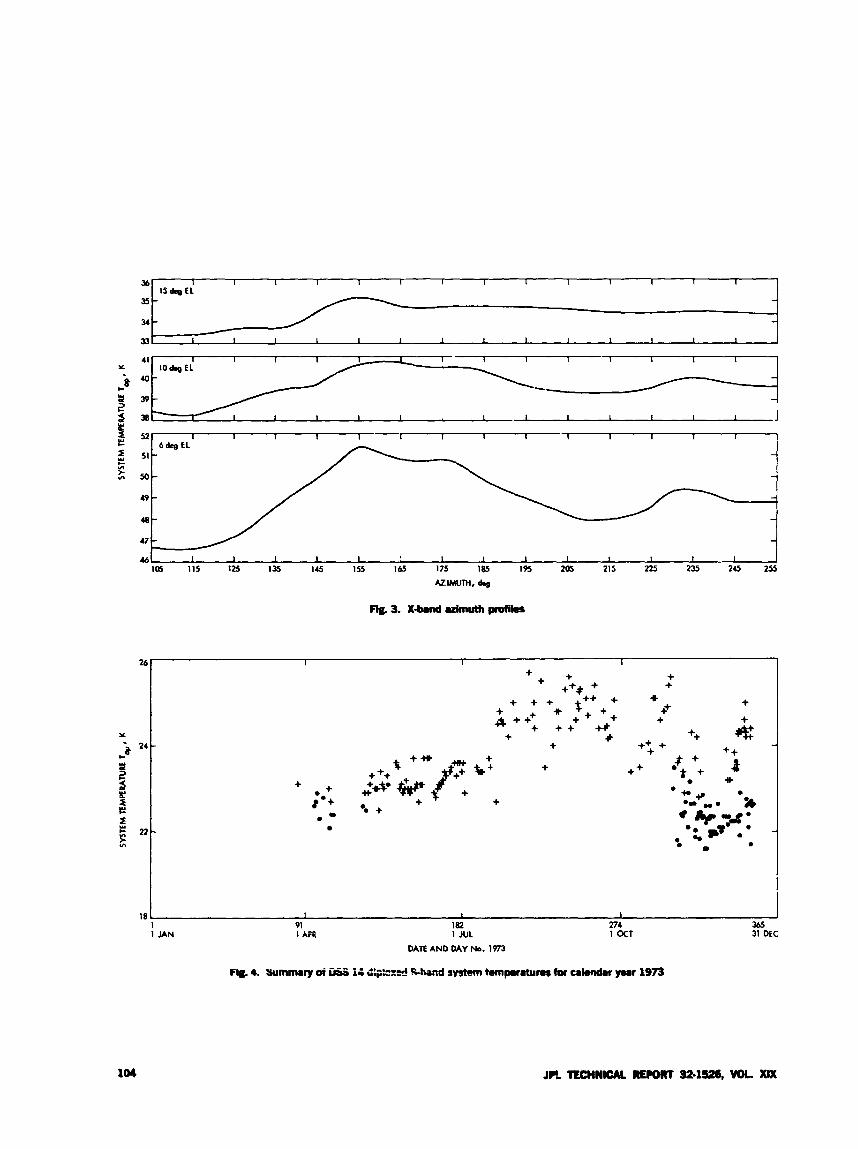
36 I I I I I I I 1 I 1 1 1 I 1
35-
34- - 33 I I I I I I I I I 1 1 I I 1
1 5 6 0 EL - - 41 I 1 I I 1 I I I I I
40-
39-
lo* EL
38 I 1 I 1 I I I I I I I 1 J 52 I I I I I 1 1 I 1 1 1 I I I
51
50- - 49-
48-
6 h E L - -
46!m 115 125 135 14 155 165 175 185 1% M5 215 225 235 245 255 I I I I I I I 1 I I I I I 1
1 I I
+ + + +++ +
+ + . . .
* + + + + + 4
+ + + + +++
+ * + +
++ k ++
+= +
* + h *.+ * ++
I 1 I
1 91 182 274 365 1 JAN 1 APR 1 JUL 1 OCT 31 DEC
DATE AND M Y No. 1973
104
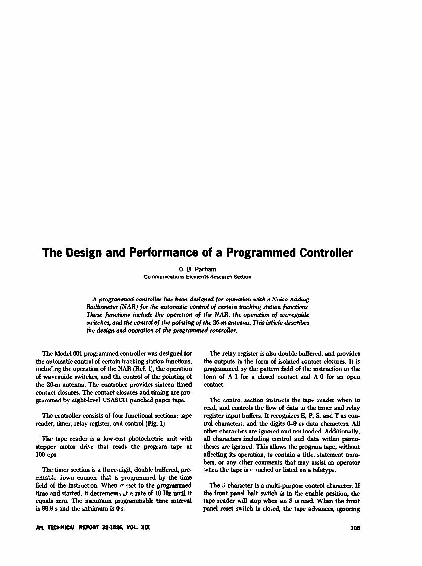
The Design and Performance of a Programmed Controller 0. 8. Parham
Communications Elements Research Section
A programmed controller has been designed for opemtion with a Noise Adding Radiometer (NAR) for the cartomatic control of certain tracking station functions These fundons include the operation of the NAR, the operation of ux.*-eguide switche, and the control of the pointing of the 26-m antenna. This article desrribes the &sign and operation of the progrcnmed controller.
The Model 601 programmed controller was designed for the automatic control of certain tracking station functions, incluhg the operation of the NAR (Ref. l), the operation of waveguide switches, and the control of the pointing of the 26-m antenna. The controller provides sixteen timed contact closures. The contact closures and timing are p m grammed by eight-level USASCII punched paper tape.
The controller consists of four functional sections: tape reader, timer, relay register, and control (Fig. 1).
The tape reader is a low-cost photoelectric unit with stepper motor drive that reads the program tape at loo cps.
The timer section is a three-digit, double b&ered, pre- scttalu:e down counter [ha? IS programmed by the time field of the instruction. When c.’ -?set to the programmed time and started, it decremm3 &t a rate of 10 Hz until it equals zero. The maximum programmable time intend is 99.9 s and the idnimum is 0 s.
The relay register is also double buffered, and provides the outputs in the form of isolated contact closures. It is programmed by the pattern field of the instruction in the form of A 1 for a closed contact and A 0 for an open contact.
The control section instructs the tape reader when to red , and controls the flow of data to the timer and relay register kput b h r s . It recognizes E, P, S, and T as con- trol characters, and the digits 0-9 as data characters. All other characters are ignored and not loaded. Additionally, all characters including control and data within paren- theses are ignored. This allows the program tape, without decting its operation, to contain a title, statement num- bers, or any other comments that may assist an operator wheu the tape is r..inched or listed on a teletype.
The :i character is a multi-purpose control character. If the front panel halt switch is in the enable position, the tape reader will stop when an S is read. When the front panel reset switch is closed, the tape advances, ignoring
all instructions, and halts on the next S character. At this point, the program may be started by closing the front panel start switch. Additionally, an alarm, that can be enabled by front panel control, is provided to signal an operator that the tape is stop,,d on a halt. With one S character located at the beginning of a program tape, these functions allow an operator to load a program tape at any position in the program, initialize the program tape to the beginning, and execute the program continu- ously, or once and halt.
The contents of the timer snd the relay register are displayed on the front panel for operation verification. An additional front panel control, the mode switch, is pro- vided to allow program checking. Each time it is closed in the step position, an instruction is read and displayed.
In normal operation, with the mode switch in the run position, as an instruction is read, the characters follow- ing a P character are loaded one at a time into the right end of the relay register input buffer. As each new char- acter is read in, the previously loaded characters are shifted left one place. This process continues until a T or E character is read. The characters following a T are loaded into the timer input buffer in the same fashion as the relay register was loaded. Again this action continues until a P or E character is read.
When an E is read, this indicates the end of the ~ r > s t r u c - tion. First, the contents of the timer input buffer are loaded into the timer and, at the same time, the relays
are set; then, a few microseconds later, the timer is started and both input buffers are cleared.
The tape reader continues, reading the next instruction until another T is read. At this point, the timer is tested. If the timer has reached zero, the rest of the instruction is read and executed, and the following instruction is read. If the timer has not reached zero when the T character is mad, the tape reader stops and waits. When the timer reaches zero, the tape reader restarts and finishes reading the instruction.
The program tape is normally in the form of an endless loop. The instruction format is flexible in that the time and pattern fields may be interchanged, and the data in each field are right-justified as they are read. The omis- sion of unnecessary zeros allows the instructions to be compact. Table 1 shows some examples of various pro- gram instructions.
Figures 2 and 3 are phr’ -qaphs of the standard rack- mounted Model 601 programmed controller.
A Model E?: egramnred conti-oller is currently being used at DSS lb .o control the operation of an NAR, the operation of waveguide switches, and the pointing of the computer-driven %m antenna. Programs for the codgu- ration include bore-sighting, on-source/off-source track- ing, radio source drift curve generation, and radiometer calibration. This has been described in an accompanying article (Ref. 2).
References
1. Batelaan, P., Goldstein, R. M., and Stelzried, C. T., “A Noise Adding Radiometer for Use in the DSN,” in The Deep Space Network, Space Programs Summary 37-65, Vol. 11, pp. 66-69, Jet Propulsion Laboratory, Pasadena, Calif., Sept. 1970.
2. Gardner, R. A., Stelzried, C. T., Reid, M. S., “Radio Metric Applications of the New Broadband Square Law Detector,” in this issue.
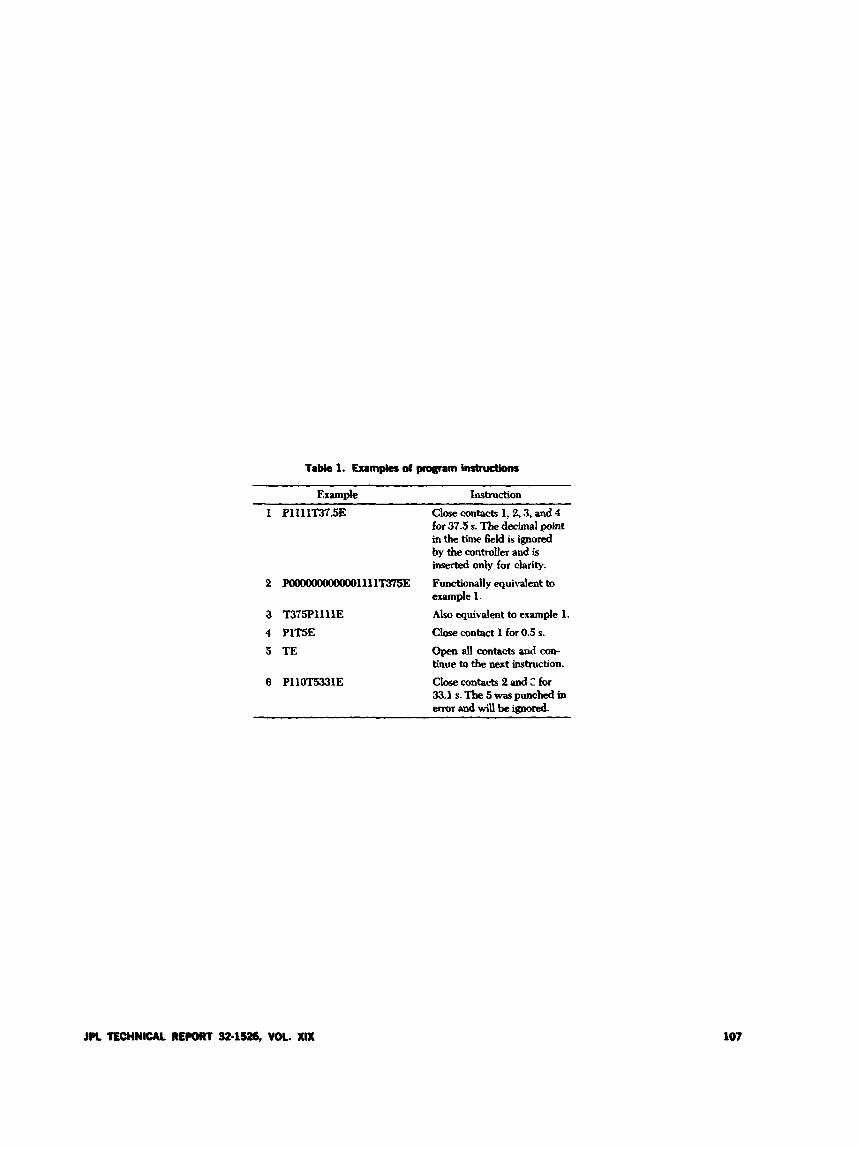
Tabk 1. Examples of program inrtructiom
Example Instruction 1 Pilll"37.5E Close contacts 1,2.3, and 4
for 37.5 s. The decimal point in the time field is ignored by the controller and is inserted only for clarity.
2 POOOOOOOOOOOOllllmSE Functionally equivalent to
3 T375PllllE Also equivalent to example 1. 4 PIT5E Close contact 1 for 0.5 s.
example 1.
5 TE Open all contacts and con- tinue to the next instruction.
6 PllOT5331E Clare contacts 2 and C for 33.1 s. The 5 was punched in error and will be ignored.
JPL TECHNICAL RE- 32.1526, V O L XIX 107
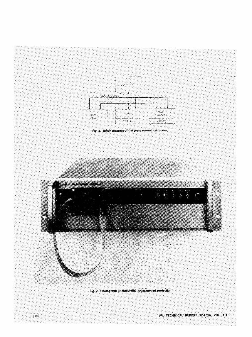
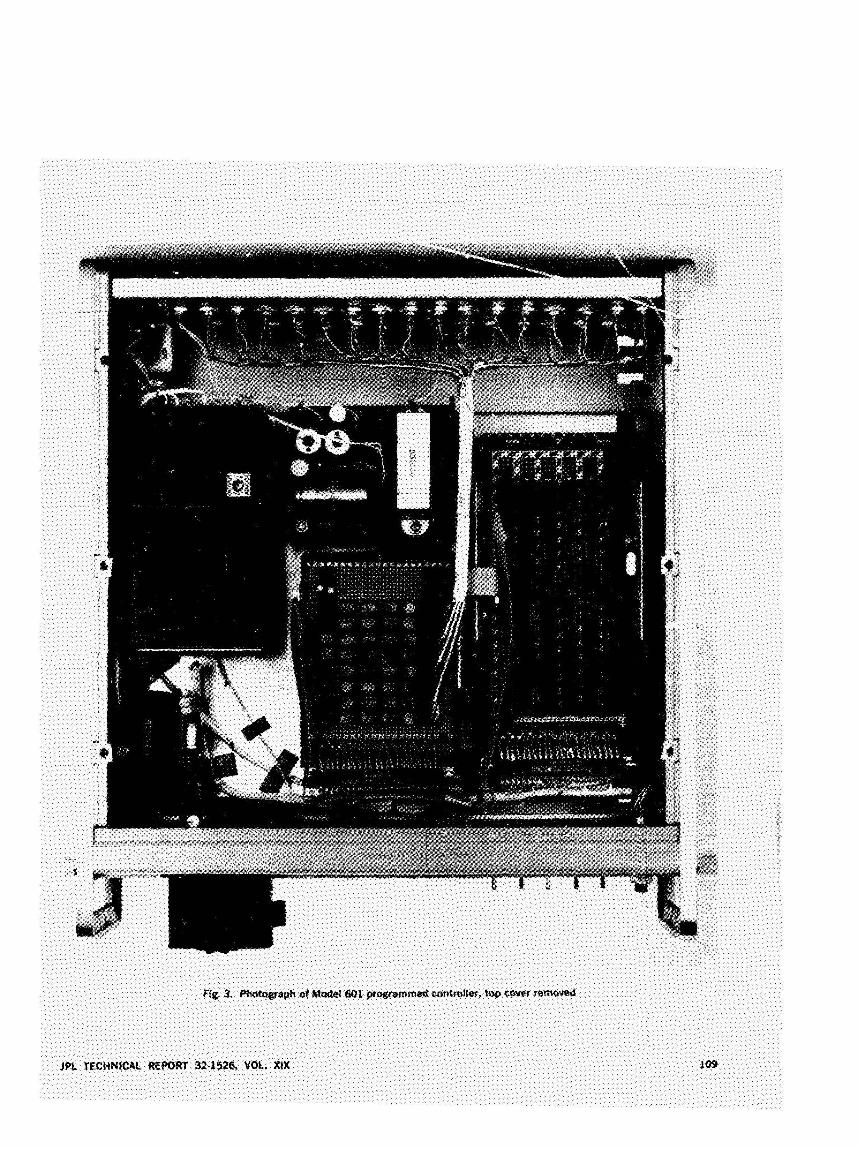
Radio Frequency Performance of DSS 14 64-m Antenna at 3.56- and 1.96-cm Wavelengths
A. J. Freiley Communications Elements Research Section
During F e b w y and March 1973, the DSS 14 64-m antenna was fitted with maim structural braces, and other structural modifications were made to improue low angle elevation system gain performance at centimeter wavebngths. The neu; system performance, as defined by the radiometric measurements of May 1973, is compared to the previous performance, with rcspect to system &iercy, sub- reflector focus, and equivalent radio frequent!! (RF) surface tolerance. The evaluation shows that the predicted efect of ihe structural braces has been achieoed; however, either the main reflector M subreflector surface tolerance, OT both, have been degraded. The degradation is well defined at X- and Ku-band frequencies; at S-band the effect is near& negligible.
1. Introduction The radio frequency (RF) performance of the DSS 14
64-m antenna was measured to evaluate the effectiveness of the antenna modifications undertaken during February- March 1973. These modifications consisted of the instal- lation of major structural braces and other modifications to the structure fnr noise abatement (Refs. 1, 2). To obtain the total antenna performance, radiometer mea- surements of selected radio sources were undertaken at X- and Ku-bands prior to and after the modifications. These radio sources were selected to eliminate the un- certainty associated with less accurately known sources and to maintain consistency with previous measurements. The results show a pronounced change in the antenna RF
performance, most likely attributable to a change in antenna surface tolerance.
!I. Antenna Modifications Three major activities occurred during February-
March 1973: The first was the installation of the structural braces (Refs. 1, 2) to improve the RF surface tolerance at elevation angles between 6 and 45 deg. Another activity was the resetting of the main reflector panels after the installation of the structural braces. The third activity was the welding of the panels of the subreflector to reduce the noise associated with diplexed high-power microwave transmission.
110 JPL TECHNICAL REPORT 32.1126, VOL. XIX
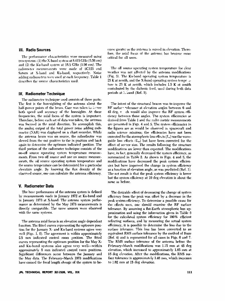
111. Radio Sources Thc perfarniancc chaiactcristics were measured using
two systems: (1) the S-band qsteni at 8.415 GHz (3.56 cni) and (2) the Ku-band systcni at 15.3 GHz (1.96 cm). The radionit1tc.r n ~ ~ a ~ ~ r ~ ~ r n e n t s were made of SCI 23 m d Saturn at S-band and Ku-band, respectively. Noise adding racliomrtcrs w e r c used at each frcquency. Table 1 describes the soiirce charactclristics used.
IV. Radiometer Technique The radiometer technique med consists of three parts:
The first is the boresighting of the antenna about the half-power points of the beam. Care was taken tu Lwre both speed and accuracy of the boresights. At these frequenrcies, the axial focus of the system is importapt. Therefore, before each set of data was taken, the avtenna was focused in the axial direction. To accomplish this, the analog output of the total power noise adding radi- ometer (NAR) was displayed on a chart recorder. Whilz the antenna beam was on source, the subreflector was slewed from the out position to the in position and back again to determine the optimum indicated position. The third portion of the radiometer technique consists of the on-off source operating system temperature measure- ments. From two off source and one on source measure- ments, the off murce operating system temperature and the source temperature can be determined for a particular devation angle. By knowing the flux density of the observed source, one can calculate the antenna efficiency.
V. Radiometer Data The basr performance of the antenna system is defined
by measurements made in January 1972 at Ku-band and in January 1973 at X-band. The antenna system perfor- mance as detcrniined by the May 1973 measurements is directly comparable. The same sources were observed with the same systems.
The antenna axial focus is an elevation angle dependent function. The fitted curves representing the optimum posi- tion for the January X- and Ku-band systems agree very well (Figs. 1, 2) . The agreement is within approximately 2.5 mm indicated control room position. The fitted curves reprcsriiting the optimum position for the May X- and Ku-band systems also agree very well-within approximately 5 mm indicated control mom positions. Significant diffcrcnces occur between the January and the May data. The February-March 1973 modifications have caused thc. focal length changc of the system to be-
come greater as the antenna is mowd in elevation. Thcre- fore, the axial focus of the antrnnn has become more critical for all users.
The off source operating system temperature for clear weather was not affected by the antenna modifications (Fig. 3). The Ku-band operating system temperature is 25 K at zenith, and the X-band operating system tcmpe A-
ture is 33 K at zenith, which includes 1.5 K at zenith contributed by the dichroic feed, used during bqth data periods at >. band (Ref. 3).
The intent of the structural braces was to improve the RF surfac- *olerance at elevation angles between 6 and 45 deg, v ch would also improve the RF system effi- ciency between those angles. The system efficiencies as derived from Table 1 and the radio metric measurements are presented in Figs. 4 and S . The system efficiencies in the figures are as would be ohserved in spacecraft and radio science missions; the efficiencies have not been corrected for the atmospheric loss effects (I, , , , ) nor the wave- guide loss effects (L,) but have been corrected for the effect of solwe size. The results following the structure modifications are lower than espected. The modifications have, in fact, generally decreased the system efficiency, as summarized in Table 2. As shown in Figs. 4 and 5, the modifications have decreased the peak system efficien- cies but have improved the change in system cfficiency as a function of elevation angle, as was predicted (Ref. 1). The net result is that the peak system efficiency is lower but the system efficiency at 10 deg elevation is about the same as before.
The desirable effect of decreasing the change of system efficiency from the peak was offset by a decrease in the peak sjvstem efficiency. To determine a possible cause for the effects seen, one should examine the RF surface tolerance. By assuming a flat-Earth atmospheric loss ap- proximation and using the information given in Table 3 for the calculated system efficiency for 100% efficient reflecting surfaces, and by measuring the actual system efficiency, it is possible to determine the loss due to the surface telerance. This loss has been converted to an equivalent RMS surface tolerance by the method of Ruze (Ref. 4) and is represented for all cases in Figs. 6 and 7. The RMS surface tolerance of the antenna before the Fcbruary-March modifications was 1.15 mm at 45 deg elevation, which increascd to approximately 1.65 mm at 15 deg clevation. After the modifications, the RMS sur- face tolerance is approximately 1.46 mm, which increases to 1.62 mm at 15 deg elevation.
JPL TECHNICAL REPORT 32.1526, VOL. XIX 111
VI. Conclusions The modifications to the DSS 16 64-m antenna accom-
plished during February-March 1973 have been evaluated at X- and Ku-bands using radiometer techniques. The peak system efficiency at 45 deg elevation angle has decreased at both bands, but the change in system efficiency with elevation angle has been improved.
The conclusions reached are that (1) the structural braces have decreased the effect of the RMS surface toler- ance change with elevation angle, and (2) the combination of the main reflector rex: and the welding of the sub- reflector has increased the overall RMS surface tolerance. Another way of stating this is to say that the dynamic
distortions (elevation angle dependent gravity induced deformations to the main reflector backup structure) have been improved; the static distortion component (elevation angle independent settir.g precisioii of either one or both reflector panels) has been degraded. The reason for the increased axial focus sensitivity as a function of elevation angle is not understood.
The peak system efficiency at 45 deg elevation angle has been reduced 0.5 dB at X-band and 1.6 dS at Ku-band. Using the surface tolerance values obtained from these short-wavelength observations, a predicted change of 0.04 dB at S-band at 45 deg elevation angle is obtained. This loss is reduced at lower elevation angles.
Refw-ences
1, Katow, M. S., “210-ft-diam Antenna Reflector Upgrade Study-Phase 1,” in The Deep Space Network, Space Programs Summary 3782, Vol. 11, pp. 109- 113, Jet Propulsion Laboratory, Pasadena, Calif., March 31, 1970.
2. Lobb, V. B., and Katow, M. S., “64 Meter-Diameter Antenna with New Braces: lnstallation Description and Computed Performance for Gravity Loads,” in The Deep Space Network PrGgress Report, Technical Report 32-1526, Vol. XVII, pp. 93-99, Jet Propulsion Laboratory, Pasadena, Calif., Oct. 15, 1973.
3. Bathker, D. A., “Dual Frequency Dichroic Feed Performance,” presented to the XXVI Meeting of the Avionics Panel, NATO/AC-ARD, Munich, Germany, November 26-30, 1973.
4. Ruze, J., “Antenna Tolerance Theory-A Review,” hoc. ZEEE, Vol. 54, No. 4, April 1966.
112 JPL TECHNICAL REPORT 32-1526, VOL. X U
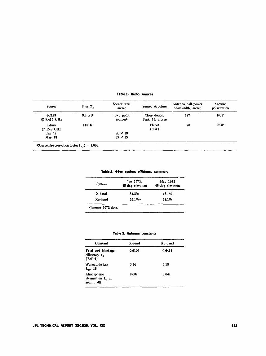
Table 1. Radio sources
Source size, Antenna half-power Antenna arcsec Source beamwidth, arcsec polarization source S or T,
3C123 9.4 FU Two point Close double 137
Saturn 145 K Planet 70
Jan 72 20 x 18 May 73 17 X 15
@ 8.415 CHz SOUTCeS. Sept. 13, arcsec
@I 15.3 CHz ( disk )
RCP
RCP
*Source size correction factor ( cs) = 1.003.
TaMe2. 64-m system efficiency summary
Jan 1973, May 1973 45-deg elevation 45-deg elevation System
X-band 51.3% 40.1% Ku-band 35.1%. 24.1%
.January 1972 data.
Table 3. Antenna constants
Constant X-band Ku-band
Feed and blockage 0.6190 0.8411 efficiency I),, (Ref. 4 ) Waveguide loss 0.14 L,, dB
0.10
Atmospheric 0.037 0.047 attenuation Lo at zenith, dB
JPL TECHNICAL MWRT 32.1526, VOL XIX 113

0.4
-
- - - - -
0.2
C .- i o Q c 2 I 0 -0.4 0, -I 2 -0.6 Z
8 -0.8 P 2 z
-1.0
-1.2
-1.4
-5
-10
E -15
-20
-25
-30
PFA B 45
40
Y
2i 35- 2 s $ 3 0 -
e 25
20
6
I I I I I I l l 1
- -
- I I I 1 I l l I I I I
u 10.0 20.0 30.0 40.0 50.0 60.0 70.0 80.0 90.0
ELEVATION ANGLE, dog
Fig. 1. Axkl focus, X-band
0.2
.{ i O - o_ e
4 8 -0.4
2 -0.6- z
8 -OS2
u .-1
I-
-
-
- - - - - - -
-5
-10
I -15
-20
-25
-30
-1 4 I I I 1- I - 3 . 5 A
20.0 m'om 0 10.0 20.0 30.0 40.0 50.0 60.0 70.0 80.0 90
ELEVATION ANGLE, deg
Fig. 4. System efficientiar X-band, 8.42 GHz
114 JPL TECHNICAL R W R T 32.1526, VOL. XIX
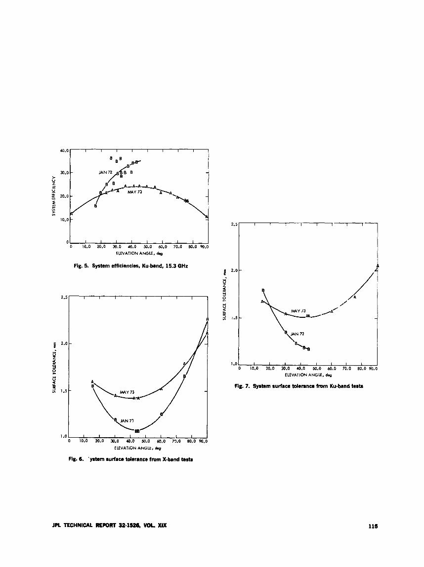
01 I I I I I I I I I 0 10.0 20.0 30.0 40.0 50.0 60.0 70.0 80.0 90.0
ELEVATION ANGLE, dag
Fig. 5. System efficiencies, Ku-band, 15.3 GHz
I I 1 I 1 I - 10.0 20.0 30.0 40.0 50.0 60.0 73.0 80.0 90
ELEVATION ANCiLt, d q
Fie. 6. 'ystem surface tolerance from X-band tests
JPL TECHNICAL REPORT 324526, VOL XIX
2.5
2.0
B d e 3 Y U
1 .o
I 1 I I I '1
0 10.0 20.0 30.0 40.0 50.0 60.0 70.0 80.0 90.0 ELEVATION ANGLE, deg
Fig. 7. System surface tolerance from Ku-band tests
111

Optimal Station Location for Two-Station Tracking E. R. Rodemich
Communications Systems Research Section
A problem related to the optimal placement of three tracking stations for pur- poses of tuv-station tracking is fonnutated and solved.
1. Introduction It is k n o w (and easy to see) that three tracking an-
tennas, however they are placed on the globe, cannot provide total coverage of the celestial sphere. However. since most interesting deep-space ienomena (spacecraft and natural astronomical objects) have small declinatior,s, this fact is of little practical importance. For example, the DSNs 64-m antennas cannot “see” urtain points on the celestial sphere at declinations of 28 deg or so.
Of course there is typically much overlap in the cover- age of the celestial sphere provided by three stations, mnd this overlap can be used to good advantag since simul- taneous two-station tmcking is possible in these Joubly- covered regions. Two-station tracking is useful for a variety of reasons. For example, since the diurnal doppler amplitude is proportional to the cosine ~f the declination, accurate determination of space\: ,aft declination using doppler is quite dificalt at declinations near zero. Two-
station tracKing ran however be used for accurate goni- ometry at all declinations. Also, accurate tracking of coirstaritly accelerating spacecraft could best be done with two stations. Finallv, important astronomical knowledge can be gained from interferometric data.
Thus it is desirabie to have as much of the celestial sphere as possible doubly covered. It is easy to see, how. evei, that if no point on the celestial sphere is visible from all three stations simultaneously, the total area that is doubly covered is always the same. We therefore arrive at the question answered in this article: K%at is the maxi- mum overlap possible b&ween the cover.-ges of the celes- tial sphere provided by two of the antcnnas, given that 311 three cover all celestial declinations that are less than a R x d imount?
More precisely, let us assume that the three antennas each cover a circular cap of angular radius p on ?he celes- tial spherc, and that it is required that h a three C: ,cular
116 JPL TECHWlCAC REm 32-1526. VOL. XIX
caps cover all objects with declinations in the range [ -a, a] . Then we \-ish to maximize the region of intersec- tion of two of the caps. Surprisingly, the optimal configu- ration does wt aiways have all three stations centered on the equator.
In the case of the 64-m net, B = 8 4 O and a is about Bo. It will turn out that there is a configuration of three a = &Lo circular ( 2s cowring the band of declinations between +?8O with two of the stations separated by only no on the globe. (This configuration has RU three stations on the equator.) However, the closest pair of stations on the 64-m net (Goldstone and Madrid) are separated by 8 2 O . Thus as far as two-station tracking is concerned, the 64-m net is far from optimally arranged.
II. Solution to the Problem Three spherical caps of ang-ikr radius p (0 < 19 < 7 '2)
are to cover the band on the sphere with latitudts between -a and P (0 4 ?I < :/2). We want to maximize the area of the region of inter rtion of two of thc caps.
Denote latitude on the sphere by 8, and let + measure longitude west from some reference point. Let the cap Cj have center at (8,,+j). Since each cap covers less than half 'he equator, following the equator around we see the caps in a cyclic order C,, C?, and C, such that 0 < 41 - +j-, (mod2r) < P. It c a ~ ~ be shown that the caps aver the whole band in the same order that they cover the equator: if C, intersects the band in the region S i , then the band is the union of six disjoint regions
and S, n SI, each of which extends across the band. s, - S, - s,, S, n sz, s, - S, - s,, S, n s,, S, - S, - s.,
C, contains the points (8,+) that sahsfy the hequality
COS~~CXX~COS(+ - +j) + s i n $ j s h 8 ~ . ~ 0 ~ / 3
The boundary of Cj intersects the boundaries of the band in bur points A;,Aj. B;. and Bj, with coordinates
cos p T sin 8j sin a
cos 8 f cas a Aj : 8 = +a,+ = +j + COS-'
@ Aj .
I
i
ii'r ]lave a covering if 4. and A; are in C,,,, and B; and B; are in Cj-,.
Our prablem is to maximize the tfea of C, n C,. This is equivalent to maximizing the cosine of the angle between the centers cf C, and C,, which is
cos BIZ = cos 6, cos 8? cos (4, - +) + sin 8, sin 6, (2)
There is an extrema1 covering for this problem, if and /3 are such that some coverings exist. Hence it is suf6cient to consider only those coverings for which there is no obvi- ous variation that increases cos O12.
If we move each cap C, to a position centered on the equator at (O,+j), we preserve the covering or the band. For, if we denote the points A;, etc., in the new &tion by bars, and are diametxically opposite on the cap, hence
By symmetry, this is equivalent to
Similarly
If '.qe started with a covering of the band, Cj and Cj.l meet on each boundary of the band, which makes
Hence adding the preceding inequalities, we get
I' . ,.:. . It C, and Cj-, overlap on each boundary of the - . proves the assertion, that the new configura-
:".- .; in the band. By Eq. (3),
JPL TECHNICAL REm 32-1526, VOL XIX 117
The upper boundary of the band can be covered by three arcs with this change in longitude only if
or
This is a necessary and sufficient condition for the exis- tence of coverings.
One way to increase cos e,, is to move the center of C, directly toward the center of C,. The covering is pre- served unless A; or A; goes out of C,. Hence, for an ex- tremal covering, one of these points must lie on the bound- ary of C,, so that 4 = & or A; = B;. Similarly, B; = k2 or B; = A;.
By reflecting across the equator, we can make A; = B;. Suppase first that the only other one of these relations that holds is B j = A;. Move the center of C, along the great circle equidistant from 4 and B;. There is a nearby posi- tion where A: and B; fall inside C,, unless the center of C, is on the &eat circle arc from A; to B;. Then, A; and B; are at the ends of 3 diameter of C,, so 8s = 0. Since A; and B: are inside C,, 8, > 0 md S2 < 0. If we go to the cover- ing with centers on the equator at (O,+,) as described above, then by Eq. (3j, cos 6,; is increased. Hence we are not at an extrema covering.
This shows that we need only consider coverings with A; = B; and B; = A;. Since B; and A: are in C,.
81% - 8 3 , S 2 2 = 8 ? (5)
Now we prove a lemma.
LEMMA. A covering with < 0, A; = B;. B; = A; and 8 , > -8* cannot be extremal unless A; = R; and 1, = 02.
Proof: First suppose A; # B;. Then C, can be rotated about A; in either direction without destroying the cover- ing. If the covering is extremal, cose12 is at a stationary point under this rotation, which implies that the center of C, lies on the gr'ezl?: ckl ,? t.krouC5 3;. nd the center of C,.
If 8- > -8s, we find likewise that this circle go thro~lgh B;. By ~ y m m e t ~ ~ , Then by Eq. (3,
= a1 and - +? = +, - hQ.
C O S B ~ ~ = C O S ~ ~ ~ C O S [ ~ ~ - ~ ( + , +sinz8, = 1 - 2[cos11sin((P, -+a ) ] '
!f we vary 8 , and ti2, keeping 8, = 6, and the hypotheses of the lemma, cos 8 , sin (+, - +:J, which is the distance of the center of C, from the vertical plane through the center of the sphere and the center of C?, has a relative maxi- mum for the given configuration. Hence cos 8,: is at a rela- tive minimum, and can be increased by varying 8 , in either direction.
For 82 = -8, , B = A+,. and we can only rotate C, u p wards about B;. If this does not increase cos BIZ, the great &cle through the centers of C, and C, must pass above B;. Let the highest point on this circle have longitude +4,
and let it cross 8 = -a at +5 after passing h o u g h the center of C2. Then we have +5 - = +4 - +(A;). Since
Also, 8, > & implies Q, (B;) - +? > 4, - + (A;), hence +s - +? < (B;) - 4,. But this makes the circle pass below B;. a contradiction.
81 > st, 19, - ++ I < 4, - $4, and SO 65 -4: < dl - Q (Ai).
Now we know that A; = B;. The circle S = -a is parti- tioned by C,, C2, and C, into three parts. On each part, the variation in + can be found from Eq. (1). Since the total variation is 27, we get
or
CGS /3 + sin 8 , sin a
cos 8 , cos a + cos-1 -. cosp + sins, sinn
COS 81 COS P COS-'
_ - - cos p + sin S., sin a cos s < cos (I
+ cos-'
where uj = COS^ + sintIj sina)/(cos 8 j cosa) . Hence the range of 81 satisfying Eqs. (5) and (6) is an interval with 8 , > 8 , = l8,l at one end, 8 , > 8 , = l8,l at the other end. Differentiate Eq. (2) with respect to 8 :
d8, [-cos 8 , sin 8, cos (+, - +2) + sin 8, cos 8.4 - d,
118 , JPL TECHNlCAL R E M 32-1526, VOL XIX
By using Eq. ('7) and the relation
this can be reduced to
d COS 61: -- - (positive quantity) (sin 8? - sin 8 , ) ds I
It follows that cos6,. ' has a maximtm at 8, = &, which proves the lemma.
Now w e continue with considering all coverings for which A; = B; and B; = A;. There are essentially three classes:
class (I): .%and B; interior to C,
class (11): A; = Bi, B; interior to C ,
class (111): A; = B: and B; = A;
For a covering in class (I), the center of C; may be moved along its meridian to bring A; and B; inside C3, unless the center is already at the closest point to A; and B;. Then A; and B; are at the ends of a diameter of C,, which occurs for
8., = - sin-' (sin a/cos /3) (8)
The hypotheses of the lemma are satisfied, so A; = 8; and 8- = 8,. Equation (6) becomes
cas + sin 8 , sin e - _. - cos p + sin 8 , sin a
2 cos-' + cos-' cos 8' COSU cos 8, cos a
Transpose the last term on the left and take the cosine of each side. By the use of some trigonometric formulas, the result is
cosp f sin8,s in~ = 1 (9)
81 cos (I cos 8 , cosa
From Ec,. (2),
(10) cos /3 + sin 8, sin a
COS 8 , COS a cosO12 = sin2 8, - cos2 8 ,
This gives a possible extremal covering.
For a covering in class (11). the center of C, can be varied along the great circle equidistant from A; and B;. If 8n > 0, varying in the direction of decreasing latitude
brings all the points A;. B; and B; inside C,. Hence 8,4 0. If 8 , = 0, S, = 0 and SI > 0. Then moving the center of C, to (0, 4,) gives a covering for which cos e,, is larger. If 8 , < 0, 8' > 8, = -&. The lemma applies, and gives a contradiction. Hence there are no extremal coverings in class (11).
For a covering in class (111), 8 , = SL = -a3. We can reflect the covering in the equator to make 8 , A 0. Then we have a covering if C , and C, overlap on the lower boundary of the band. The condition for this is
cosP+sinS,sina cas f i - sin 8 , sin 0 2 cos-' cos-' a, (11)
M S 8 1 c o S a C o s S 1 c o s a
The left side of Eq. (11) is a decreasing function of 8 , 0, so we have an interval 0 L 8 , 4 ti,,, to consider, where equality occurs in Eq. (11) at 8 = 810.
Put
u = (cosfi+sin8,sin~):'jcos8,cosa)
u = (cosB-sinS1sina)/(cos8,cosa)
and
By symmetry, + - 4, + 2y = 27, and
cos e,, = cos2 Sl cos (2, - 27) + sin2 8,
= 1 - 2cos28, sin2y
(1 - coS0',)/2
COS28' [ u r n - + 4 T T p (12)
cos2 8, sin2 y
Eliminating radicals,
In the range of 8' of interest, u2 and o2 are less than 1, and Eq. (13) has real roots for R. The right side of Eq. (13) becomes negative when we pass 8 , = B - a, where u be-
JPL TECHNICAL REFORT 32-1526, VOL XIX 119
comes greater than 1. Those points (8,, R) with 0 4 81 4 B - a, which satisfy Eq. (13), form one connected curve in the SIR plane. If we multiply Eq. (13) by cos'acos' 8,, it can be put in the form
where the left side is a quadratic function of cos' 8 I .
ThepointsoftheL,RplanewithO~~,--L~-awhich satisfy Eq. (14) lie on a curve with its end points on 8, = 0, at R = O a n d R = R , = 4 c o s z ~ ( c o s 2 ~ - ~ 2 ~ ) / C O S t a . Since Eq. (14) is quadratic in cos2 a1, each value of R can correspond to at most two values of 8,. This implies that the m e passes through 0 < R < R, just once, monotonically.
An extremal covering minimizes R. R, is the value for a cu..-crhg with 8, = 0. Since there is no local minimurn on (0, R,,), only 8, = 0 or a1 = a,, can give extremal coverings.
This gives the following three coverings to consider:
(1) lil = 82 = as = 0. Here ~ e l 0 = 1 - 2R, = 1 - ~ C O S ~ / ~ ( C O S * ~ - C O S ~ ~ ) / C O S ' ~
(2) 8, = 8, = -8, > 0. We need equality in Eq. (11). Then Eq. (9) applies with 8% = -al, or 2u2 + u = 1. Then from Eq. (12),
+ 2(cOsB + sin8,sina)~/cos'a (15)
The condition of Eq. (9) is
We also have 'he covering found in class (I):
(3) 8, = -sin-' (sin a/cos p), 81 = 8* > -1,. Here 8, satisfies JQ. (9) and nl5 B I Z is given by Eq. (10).
For any U, fl, the optimal covering mu : bc one oi: these three. The covering (2) is better than (1) if
4 cos' p (cos' a - 3s' 8) A = - COS'8, cos' a
> o (cos /3 + sin 6 , sin a)? cos' a
+
where 8, satisfies Eq. (16). Equation (16) lads to a 4th- degree equation in sin 8,. If we eliminate sin 8, between this equation, and the equation A = 0, we get a rehtion between a and /I that holds on the curve separating the regions where (I) or (2) is better. '"his equation has the following patmetric solution:
9 x 3 - 6 r ' t x y = l O r J - l 3 r ' t & - l
t = r(y - 1)
S i n a = p
CQSp=COSa-
The curve is generated by 3 4 x 1 3 + fl When the covering (3) exists, sin a 4 COS p, which
already implies that (2) is better than (1). Hence the region of [a, p) for which (3) is extremal lies in the region where (2) is better than (1). Whenever :3) exists, the value of 8, for (2) is greater than sin-' (sin altos B). This implies that (2) is not extremal, for varying toward 0 m (2) brings the points B;,A; inside Cs. Hence (3) is extremal when it exists, and the boundary of the regmn of (a, p) for which this occufs is the curve on which Eq. (15) is satisfied by 8, = sin-'(sinC,'cosp), or
2(cas*p + sin*a)2 + cosa(cQs*/3- S i n Z U ) ' ~ =
a * a ( c d p - sin's)
Rationalizing, we get a 4th-degree equation for cas'p m terms of a. This equation has the parametric so~~ltion
(1 - 9) (3x + 5) y = 2w + 5w + 42x + 8
In Fig. 1, the region cos p I 1/2 cos a is shown, divided into tlie regions wbere each configuration is optimal.
120
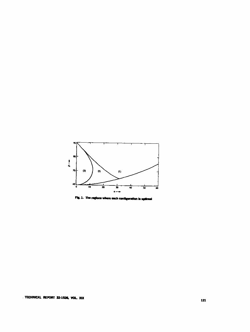
121

Bandwidth Selection for Block IV SDA R. 6. Craw
RF. Systems Dmlopmcnt Section
A recieu: of the bandcaidth selection for the Block 111 Sidmuder Demodulator Assembly (SDA) i s g h n , along t&h the design p h b o p h y as bnplementen in the engineering model of the Block N SDA.
Historically, the Block 111 SDA bandwidths were chosen for a number of reasons. The wl,, = 0.03 Hz loop bandwidth was the narrowest l o g that could be &- ciently obtained in terms of hardware stability, cost, and acquisition time, while the 1.5-Hz loop bandwidth was compatible with the Block 111 receiver wl,, = 152 Hz and was required for high-acceleratioc tracking at launch. The wl, = 0.375 Hz loop bandwidth was a compromise in an &rt to retain reasonable noise performance in the pres- ence of dynamic signal input (ie., doppler rate!.
During the past 6 years, mission requirements have undergone considerable change, and S-band doppler rates as high as 180 Hz,’s can be expected in close flybys of the larger planets (e.g., Pioneer 1.3-radius, Jupiter flyby).
Tbe basic philosophy regarJing bandwidth selection
(1) A narrow bandwidth (wl,, = 0.03 Hz), so that M) penalty is suffered in using the Block IV SDA at
for the Block IV SDA requires
low symbol rates.
(2) A wide bandwidth that is ds narrow as possible while still maintaining sufficient gain (at design point) to handle the maximum doppler rate at the highest subcarrier frequency.
(3) An adaptive gain control that can be raised quickly tc, improve the loop acquisition characteristic but lowered slowly at a rate depending on which band- width is being used, thus offering a convenient
I22
(4)
means of increasing the loop gain (it. , bandwidth), which can be smoothly redaced (to reduce the phase transient due to loop gain change).
A Imp gain increase of 1O:l to give a reasonable increase in tracking acquisition performance with- out increasing the loop jitter beyond usable limits. (At design point, the narrow-bandwidth loop has a jitter of 4 deg RhlS. while the narrow-acquisition- bandwidth loop will have 11 deg RMS phase jitter.)
Figure 1 is a plot of loop bandwidth vs. input sideband signal-to-noise energy ratio per bit (ST,, ’N,,) for both the Block 111 and IV SDAs. It can be noted that a more adap- tive bandwidth is available in the Block IV design because of a different IF bandwidth and a different ratio of input
limit leve1,virtual input signal (i.e., V ) (Ref. 1). It is also apparent that the narrow bandwidth is approximately the same for Blocks 111 and IV up to ST,, /N, 21 +IO La, while the Block 111 medium bandwidth is approximately the same as the Block IV wide bandwidth.
From Fig. 1 and Tables 1 and 2, it is apparent that many missions previously handled by the Block I11 medium bandwidth can now be handled by the Block IV narmw- bandwidth loop (because of increased gain).
All other missions requiring high doppler rate tracking can we the Block IV wide bandwidth (with little increase in noise degradation compared to the Block 111 medium and with large improvement in rate tracking error).
Reference
1. Brockman, M. H., “An Efficient and Versatile Telemetry Subcarrier Demodu- ‘ator Technique for Deep Space Telecommunications,” Paper No. A-I, 2, Fourth Hawaii International Conference an System Science, Jan. 1971, University of Hawaii, Honolulu, Hawaii.
JPL TECNNEAL RE- 32.1526, VOL. XIX 123
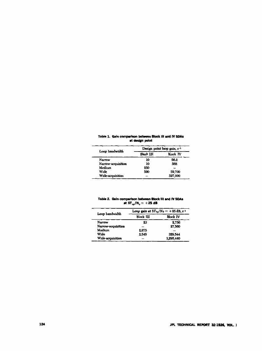
wgn point loop pain, rl Loop -width
Block 111 B i d IV NaITOW 10 56.8 Narrow-Pcquisition 10 588 Medium 250 - Wi& 500 59,700 Wide-acquisition - 597.000
Tabk 2. Gain awnprison bdweten Block 111 .nd IV SOCLI at STsv/N, = +25 dB
Loop gpin at S T ~ N O = +25 dB, s-1 Loop bandwidtb
Narrow 23 %750 N m - m u i s i t i c m - 27,580 M e d i m 2.675 - Wide 2,549 339,544
3w,440 Wideacquisition -
Block 111 Block W -
124 JPL TECHNICAL RE- 324526, VOL 1
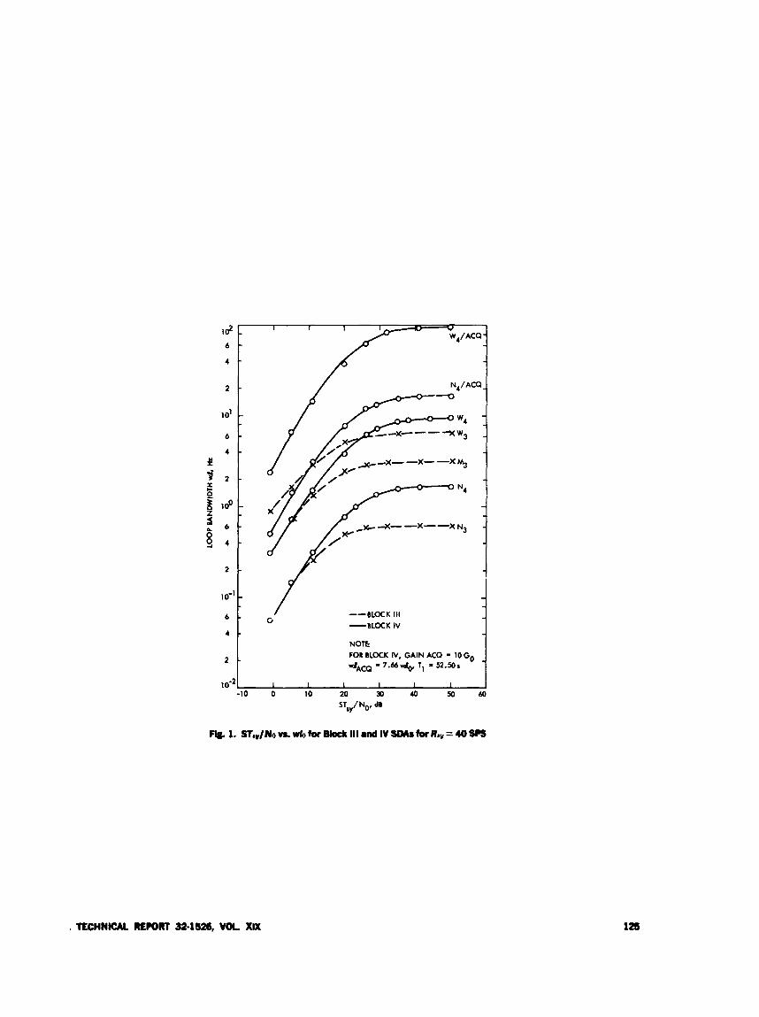
Id 1 I 1 I
6 -
4 -
2 -
IO'
6 -
4 - i!
E $ 2 -
i 100
f 6 : 8 9 4 -
2 -
lo"
6 -
4 -
2 -
-
-
-
A--x--x--
-
- * 4 - - x - - XN3 -
BLOCK 111 -BLOCK IV
NOTE FOR OLOCK IV, GAIN ACQ - 10 Go
wlAm 7.66% TI = 52.50s
-- G
TECHNICAL MrORT 32-1- VOL XIX
Frame Synchronization Performance Analysis for MVM’73 Uncoded Telemetry Modes
B. K. Levitt Communications Systems Research Section
This paper describes a practical frame synchronization (sync) acquisition and maintenance algorithm based on the Hamming distance met-:.; which is a gm- eralidion of the scheme developed for the 1973 Mariner mission to Venus and Merccry (MVM73). For the special case of uncoded phase-shift-keyed duta re- ceived mer the binary symmetric channel, formulas are derived for computing an upper bound on the probability af false sync acquisition, the mean time to sync acquisition, and the mean time to the subsequent loss of sync, as a function of the bit error rate, frame length, sync word length, and algorithm parameters. These formulas are directly applicable to the uncoded MVM’73 telemety modes, and a numerical example relating to the 117.6 kilobits/s real time TV mode is inc!uded.
1. Introduction The problem of establishing frame synchronization
(sync) usually involves the identification of received sync words periodically interspersed with random data (Ref. 1). For uncoded binary signals received over the additive white Gaussian noise channel, the frame sync words are often located by finding segments of the raxived data that are highly correlated with the transmitted sync word (Ref. 2). Massey (Ref. 3) has in fact shown that the opti- mum sync word seerch requires the addition of a correc- tion term to this correlation rule. If hard decisions are made 011 the received data prior to the acquisition of frame synchronuation, the problem is reduced to detect- ing the sync words in uncoded data received over the
binary symmetric channel: in this case, the optimum frame sync decision is based on the Hamming distance metric.
This article examines the performance of a practical frame sync acquisition and maintenance algorithm for uncoded phase-shift-keyed (PSK) data received over the binary symmetric channel. Because the detected PSK data necessarily have a binary phase ambiguity that cannot be resolved until frame sync is established, the algorithm bases its sync decision on a modified Hamming distance rule. Instead of making a hard sync decision over a single frame of received data, the algorithm scans the detected bit stream, searching for a sequence whose Hamming dis- tance from the sync word satisfies a threshold test. When
126 JPL TECHNICAL RE#)RT 32-1=, WL XIX
the bit error rate is high and the threshold is stringent, the reliability of the sync decision is improved dt the expense of delaying that decision for several frames. For addi- tional reliability, a hard sync decision is made only when two received sequences one frame apart both satisfy the threshold test.
The frame sync algorithm described herein is not excep- tionally innovative, and variations on the same approach have been used on past Mariner missions. It is in fact a two-threshold generalization of the particular acquisition and maintenance algorithm that was developed for use with the uncoded and biorthogonally coded telemetry modes of the Mariner 10 spacecraft (MVM73‘. The prin- cipal purpose of this brticle is to document the perform- ance analysis of this algorithm for uncoded PSK data received over the binary symmetric channel. Markov models arc employed in this analysis to dcrive formulas for computing an upper bound on the probability of false sync acquisition, as well as the mean time to sync acquisi- tion, and the mean time to thc subsequent loss of sync, for arbitrary bit error rates, frame lengths, sync word lengths, and thresho!d values. These formulas are directly applicablc to the uncoded MVM’73 telemetry modes, and, as a numerical example below, they are x e d to determine optimum threshold values as a function of the channel bit error rate for the high-rate (117.6 kilobits/s) real time TV data modc. It should be noted here that the author has
L-tuple p,, = (r,,, r,n+l. . . . , r,,,+I,~l). The frame s)nc objec- tive is to identify which of the pn,’s are received frame sync words. When a binary PSK signal is demodulated using a carrier reference derived from the modulated s i g nal, there is an inherent binary phase ambiguity in the detector output: that is, the received bit stream can be inverted data (data) with probability %. Consequently, for low bit error rates, if a particular p,,, is in fact a received sync word, its Hamming distance d,, from the transmitted sync word is equally likely to be near 0 or L. As indicated in Figs. 1 and 2, the algorithm threshold test reflects this property.
Suppose the receiver is out of sync, and the acquisi- tion mode is initiated. The overlapping L-bit received sequences p,, p-, p.<, . ‘ . are examined in succession, and the corresponding Hamming distances dl, d., d., . . . from the sync word are computed. The algorithm uses two thrcshold tests: d,,, 4 T,, and d,,S L - TI (the latter indi- cating the detection of data). If it finds a sequence pk which satisfies eithor threshold test, and if the sequence plAM one frame ahead satisfies the same threshold test, frame sync is established. That is, a hard decision is made that pfi; is a received sync word. the data polarity is de- duced accorditrg to which of the two threshold tests was satisfied by pc; and p&M, and the maintenance mode is entered.
extended the algorithm performance analysis to include If the communication link consisted only ,,f a binary thC MVM’73 cmP1oYing a (3236) symmetric channel, there would be no need for a frame thogonH1 code, although the work has not been published sync maintenance mode. If bit synchronization could be to date. However, numerical results for the 22.05 kilobits/s
algorithm thrcshold values for the MVM’73 mission.
maintained perfectly Once frame sync was a
Unfortunately, in practice, interface buffers within the overall communication link typically result in random deletions and insertions of bits in the received data stream. It is the function of the frame sync maintenance inode to detect these occurrences, and to signal the result- ing loss of frame sync.
coded TV mode ‘Ised ‘0 selCCt Proper simple bit counter could maintain frame sync indefinitely.
II. Frame Sync Algorithm Thc operation of the acquisition and maintenance
modes of the frame sync algorithm are detailed in the flow diagrams of Figs. 1 and 2. A brief description of the algorithm now follows to establish some notation that will he needed later for the performance analysis.
Assume that the transmitted information is organized into M-bit frames composed of an L-bit Jync word fol- lowed by M - L statistically independent, cqually likely data bits. The detected bit stream contains independent bit errors: a particular bit will be incorrect with proba- bility F .
Let the reccived bit stream bc represented by the binary sequence rI, r2, r , . . . , and define an arbitritry
Referring to the flow diagram in Fig. 2, it is seen that the data polarity decision made when frame sync was established confines the maintenance mode to one of the two threshold tests, a,,, 4 T, and d, L - T,. (Note that the acquisition and maintenance modes use different thresholds in general.) In the acquisition mode, it was decided that p l was a received frame sync word, since & and satisfied the same T, threshold test. The maintenance mode examines only presumed received sync words of the form p$+kY, where k is a positive inte- ger. If T, h T, (see discussion below), d2 and &;+Y must satisfy the T, threshold test; consequently, the mainte-
JPL TECHNICAL RE#)RT 32-1526, VOL. XIX 127

nance mode can start with pfa+2y, as hdicated in the dia- gram. When two consecutive sequences that should be received sync words fail the threshold test, the receiver is declared to be out of sync, and the algorithm reverts to the acquisition mode.
in this article.) To maximize MTLS, T2 should be as large as possible; a threshold near L/4 is compatible with this objective. In conclusion, T , should be near Lj4, and TI should be closer to zero.
The following design objectives influence the selection of the thresholds T I and T,. For convenience, use the following terminology:
Fr [ F S ] :
MTS:
probability of false sync acquisition.
mean time to sync acquisition, in frames (expected value of &/M), conditioned on a correct sync decision (assuming Fr [ F S ] < < 1).
mean time to loss of sync following correct sync acquisition, in frames, neglecting bit insertions or deletions.
M T L S :
Ideally, we would like P r [ F S ] and, M T S to be small, while MTLS is large. However, for fixed values of E , L, and M, Pr[FS] decreases while MTS increases mono- tonically as TI decreases, and the reverse condition also holds. So the selection of TI involves a tradeoff between Fr [ F S ] and MTS. Typically T, is made relatively small, favoring Pr [ F S ] , so that when a frame sync decisiob is made, it: is likely to be correct. Fortunately, it will be evi- dent in the numerical examples below that TI d m not have to be too large for MTS to be near the minimum value of M.
With regard to the selection of T?, it should be noir-cl that following the acquisition of frame sync, there are two situations that would cause the maintenance mode to decide that sync is lost. If one or more bits are e m neously deleted or inserted into the received data stream, thereafter, the received sync words would not coincide with the L-bit sequences examined by the maintenance mode. If the sync word is a Barker (Ref. 1) or a Neuman- Hofman (Ref. 4) sequence, its correlation properties would ensure that the Hamming distances of the L-bit received sequences from the sync word are likely to be near L/2. In this case, a threshold T , on the order of L,/4 would be small enough to signal the loss of s y n ~ On the criiier hand, if the channel state is such that no bit dele- tions or insertions are occurring, the maintenance mode will still declare a loss of sync, falsely, if two consecutive received sync words contain more than T , bit errors. It is thii, circumstance, relating only to the binary symmetric channel model, that is measured by the parameter MTLS defined above. (To include the random deletions and insertions in the channel model, a multi-state Markov approach would be required; this coniplication is avoided
111. Algorithm Performance The following formulas relating to the performance of
the f r a e sync algorithm for uncoded PSK data received over the binary symmetric c’.mnel are derived in the Appendix:
Pr [ FS] L
1 ( M - 1 ) 2 + m i n A,(M-1)A;Z+$L-1)y2 y? 3 4
(1) where it is assumed that M > > L, and
I E O
(3)
(4)
MTS = - + + A frames; Pr [ F S ] < < 1 (5) 2Af
Parameters y and 7 (7‘) have physical interpretations:
y : the probability that a p t i c ~ l ~ Gbit received sequence, composed of independent, equally likely l’s and O’s, sztisfies either acquisition threshold test (probability of a “false alarm”).
the prohability that a particular received sync word (or complemented sync word if data is detected) has more than T bit errors, and fails the corresponding threshold test (probability of a “miss”).
9 ( T ) :
A numerical exampie will serve to demonstrate the behaviour of P f [ F S ] , MTS, and MTLS as a function of threshold values for fixed L, M, and e. The 1973 Mariner 10 mission to Venus and Mercury has a high- rate (117.6 Idlobits/s), u n d e d PSK telemetry mode for
128 JPL TECHNICAL ffEcolcT 92.1526, w)L XIX
transmitting real time TV data to Earth. This mode has a frame length M = 7058 bits, and a sync word length L = 31 bits (a pseudo-noise or PN sequence). As the spacecraft-to-Earth range varies durh, the mission, SO
does the bit error rate C; it is anticipated that during the primary mission, E will not exceed MO. On this mission, the acquisition and maintenance thresholds are identical, and are denoted by 7’. For bit error rates in the range %J 4 E L ‘hoo, the frame sync algorithm performance is summarized in Table 1. A single TV picture is composed of 700 frames of data; one of the design objectives in selecting T was that MTLS exceed 700, so that frame sync would be likely to be maintained over a TV picture. Subject to this c nstraint, as well as the threshold trade- offs discussed earlier, the recommended vzlues of T are circled in Table 1. It is evident from the table that if T is adjusted for changes in E, MTS will be near %, MTLS will exceed 700, while Pr [ F S ] is less than 2 X for F less than %.
IV. Summary This paper has considered the problem of acquiring
and maintaining frame synchronization in uncoded PSK data received over the binary symmetric channel. To this end, a practical algorithm was described that computes the Hamming distances of L-bit segments of the received
blc stream from the L-bit sync word, and applies these distances to a threshold test.
In the acquisition mode, the algorithm ensures a reli- able frame sync decision by requiring that two consecu- tive L-bit received sequences one frame apart satisfy a stringent threshold test. The maintenance mode is de- signed to flag the loss of frame sync due to random deletions or insertions of bits in the received data stream; at the same time, its threshold test allows sufficient errors in the received sync words to pass so that the loss of sync is not likely to be declared falsely.
The performance of this algorithm was analyzed with the aid of Markov models of the threshold test operation. An upper bound for the probability of false sync acquisi- tion, the mean time to sync acquisition, and the mean time to loss of sync were computed as a function of the bit error rate, frame length, sync word length, and algo- rithm threshold values.
This algorithm is a generalization of the scherirc devel- oped to provide frame synchronization on the Manner 10 spacecraft-to-Earth telemetry link. As a numerical exam- ple, the derived formulas were used to predict the algorithm performance for the spacecraft’s high-rate, real-time TV data mode.
References
1. Barker, R. H., “Croup Synchronization of Binary Digital Systems,” Communi- cation Theory, Edited by Jackson. Butterworth, London, pp. 2’73487,1953.
3. Stiffler, J. J., Theory of Synchrmmu Communications. Prentice-Hall, Engle- wood Cliffs, N.J., 1971.
3. Massey, J . L., “Optimum Frame Synchronization,” W E E Trans. Commun., Vol. COM-20, pp. 155-169, Apr. 1972.
4. Neuman, F.. and Hofman, L., “New Pulse Sequences With Desirable Correla- tion Properties,” Proc. N a t . Telemetry Conf., Waskington, D.C., pp. 271-282, Apr. 1971.
129
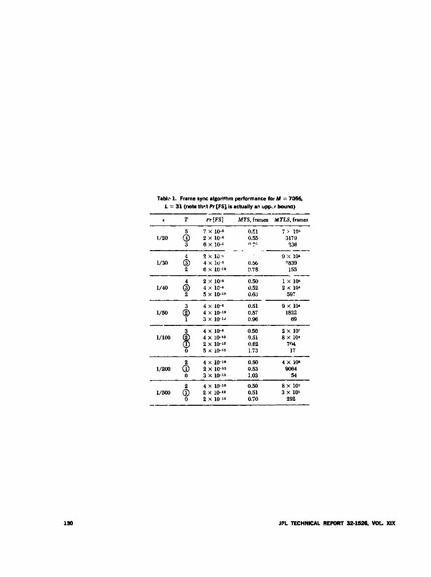
Table 1. Frame sync algori+hm performance for M = 7356, L = 31 (nota thr.t Pr [FS] is actually an upp-r bouna) -
e T rr [FS] MTS, frames MTLS, frames - 7 x 10⁻⁵ 0.El 7 z 104
1/20 6 2 x 10⁻⁶ 0.55 3179 3 6 X 10⁻⁶ n 7 0 238 - - --
9 x 10-b 9 x 101 1/30 6 4 x 10⁻⁸ 0.56 %39
1/40 6 4 X 1C-8 0.52 2 x 101
2 6 x 10⁻¹⁰ 0.78 155 -- 2 x 10⁻⁶ 0.50 1 x 1w
2 5 x 10⁻¹⁰ 0.63 597
4 x 10⁻⁸ 0.51 9 x 10⁴ 1/50 4 x 10⁻¹⁰ 0.57 1822
1 3 x 10-12 0.96 69 ~~ ~~~~ ~ ~ ~ ~ ~ ~-
4 x 10⁻⁸ 0.50 2 x 10⁷ 1/100 4 x 10⁻¹⁰ 9.51 8 x 10⁴
2 x lo-= 0.62 7 4 o 5 x 10-15 1.73 17
__.
4 x 10⁻¹⁰ 0.50 4 x 10s 0.53 Ww4
o 3 x 10-15 1.03 54
4 x 10⁻¹⁰ 0.50 8 X 10⁹ 0.51 3 x 10⁶
o 2 x 10-15 0.70 202 --
130 JPL TECHNICAL R m 32.1526, VOL XIX
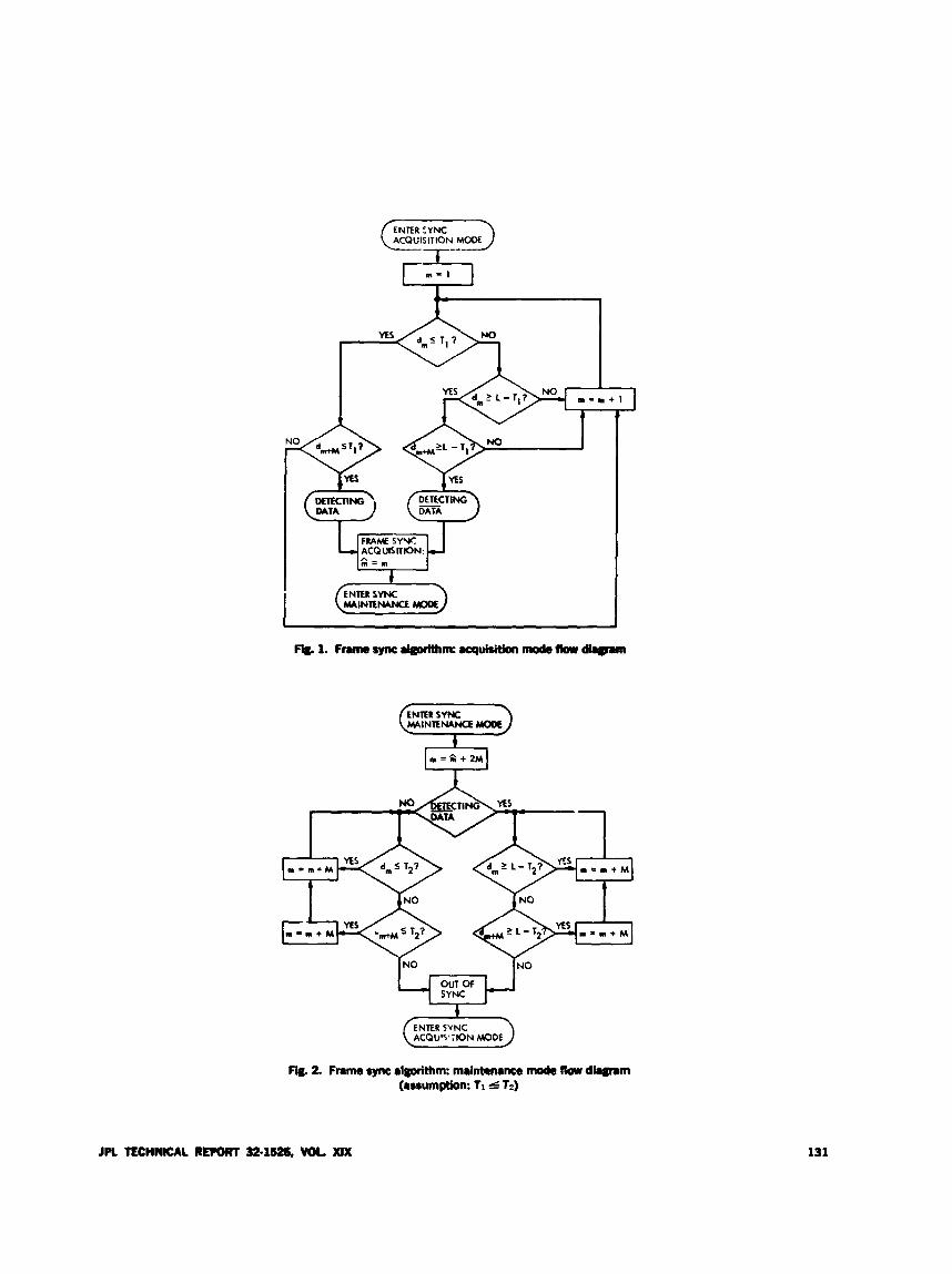
ENTER S Y N C
ACQU'S'7ION MODE
Flg. 2. Frame sync algorithm: maintmmm mock Ilow diagram (assumption: TI 4 1 2 )
JPL TECHNICAL RE- 32-1526, Ua XIX 131
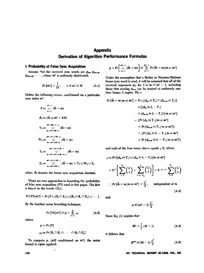
Appendix Derivation of Algorithm Performance Formulas
m e - i
[:ill 1 m = i p = P r u $=m) L Pr[A=m)m#m*]
Under the assumption that a Barker or Neuman-Hofman frame sync word is used, it will be assumed that d of the received sequences p,,, for I 4 m L m* - I, including those that overlap pm,, can be treated as unifonnly ran- dom binary L-tuples. Thtrr
I. Probability of False Sync Acquisition Assume 'hat the received sync words are p,,,., pur+,,,
, where m* is uniformly distriLuted: P W Z M , ' .
(~-1) Pr[m*] =-; l 4 m ' L M
Deiine the foJlowing eveuts, wnciitioned on a parti&
1 A i
sync index m*:
Ill*-1 A P= u ( m = m )
&=(i;i#m* -I- kM)
m:1
where 6i denotes the frame sync acquisition decision.
There are two approaches to bounding the probability of false sync acquisition (FS) used in this paper. The &st is basd on the events {xk} :
By the familiar union bounding t&hnique,
where
p = Pr [PI
To compute p, (still conditioned on m*), the union bound is qain applied:
132 9
yz independentofm :.Pr[m=mlm#m*] = - 2 ' A
(A-3)
and
YZ p 4 ( m * - 1 ) ~
Since Eq. (1) implies that
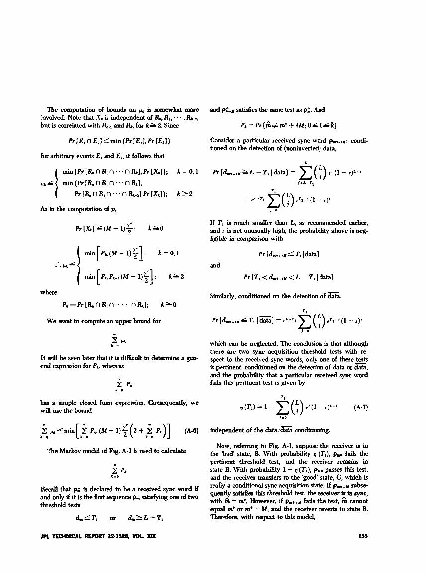
The computation of bounds on is somewhat more favolved. Note that x k is independent of &, R,, . - - , &-*, but is correlated with &+ and &, for k A 2. Since
and p$+r satisfies the same test as pl=. And
Pk = Pr [;;i+m* + !AI; OL i ~ k ]
Consider a particular rcccivcd sync word pI.+lr: condi- tioned on the detection of (noninverted) data.,
Pr [ E , n EZ] l m i n (Pr [E,j, Pr [ E , ] )
for arbitrary events E, and E,, it follows that
( Pr [& n R, n . . . n &-,I Pr [ X k ] ) ; k l 2
As in the computation of p,
If TI is much smaller than L, as recommended earlier, and I is not unusually high, the probability above is neg- ligible in comparison with
P r [ X k ] L ( M - l ) Y ' ' 2 ' k'-o
min P k , ( M - 1 ) ~ - ; k = 0 , 1 Pr [d,++,rLTlldatal
m h P k , P k - Z ( M - l ) - ; k 1 2 Pr [T , < &++w < L - TI I datal
and :.+j c y2 1
2
Simhly, conditioned on the detection of data, [ ':I
where
P , = P r [ & n R , n . - - n&]; k L 0
We want to compute an upper bound for Pr [dn++lu L T, I data] =-€'-TI &)P*-j( l - e ) J
j =o
k = O L k which can be neglected. The conclusion is that although there are two sync acquisition threshold tests with re-
is pertinent, conditioned on the detection of data or data, and the probability that a particular received sync word fails thie pertinent test is given by
It will be seen later that it is difficult to determine a g- sped to the rwi\ped sync m&, only one of these t e eral expression for pk. whe.xas
pk k : o
2.
has a simple closed form expression. Comequently, we will use the boiind
The Markov model of Fig. A-1 is used to calculate
pk k=O
Recall that p; is declared to be a received sync word if and only if it is the first sequence pn sahsfylng one of two threshold tests
d,,,4T1 or L h L - T ,
T)(T,) = 1 - C(5) €'(I - €)'-I (A-7) 110
independent of the data/dza conditioning.
Now, referring to Fig. A-1, suppose the receiver is in the "bad' state, B. With probability 9 (TI), pmI fails the pertinent threshold test, md the receiver remains in state B. With probability 1 - v(T,), pns passes this test, and the leceiver transfers to the 'good' state, G, which is really a conditional sync acquisition state. If pu+v subse- quently satisfies this threshold test, the receiver is in sync, with fh = m'. However, if pn++,, fails the test, 6 cannot equal m* or m* + M, and the receiver reverts to state B. Therefore, with respect to this model,
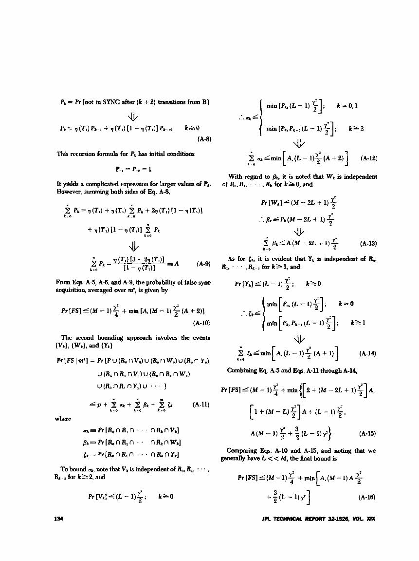
From Eqs .45, A-6, and A-9, the probability of fdse sync acquisition, averaged over m', is given by
Pr [Y,] 4 (L - 1) 2; " k l 0
I):]; k h l
.II.
YZ Y= Pr [ FS] 4 (M - 1) 7 + min [A, (A4 - 1) (A + 2)]
(A-lo)
The second bounding approach involves the events
- W k } , {Wd, and {Yk}
A , ( L - l ) $ ( A + l ) ] (A-14) Pr[FSIm*] = Pr[PIJ(R,nV,)U(R,nW,)U(R,n Y,) k = o
Combining Eq. A 5 and Eqs. A-11 through A-14, u (R, n R, nv,) u (R, n R, n W l )
u ( R o n R , n Y , ) u . * . ]
Y= 1 + ( M - L ) y A + ( L - 1)-, "I 2
(A-15) ra 3 A (M - 1) + -j ( L - 1) y z }
L P + $ ~ f ~ ~ k + ~ ~ k (A-11) k = o k = O k = O
where
a s P r [ R o n R , n - . . nRknV,]
p k = P r [ & n R , n . . nR,nw,] f=pr[RonRln . . n&nYk] Comparing Eqs. A-10 and A-15, and noting that we
generally have L < < M, the final bound is
(A-18)
To bound a, note that vk is independent of R,,, R1, * . . , for k L 2 , and Pr [FS] 4 (M - 1) v' + min
4
p r [ v k ] L ( L - 1 ) 3 ; Y2 k h O + $ ( L - l)y']
134 JPL TECHNlCAL lpEpoRt 32-1526, VDL XIX
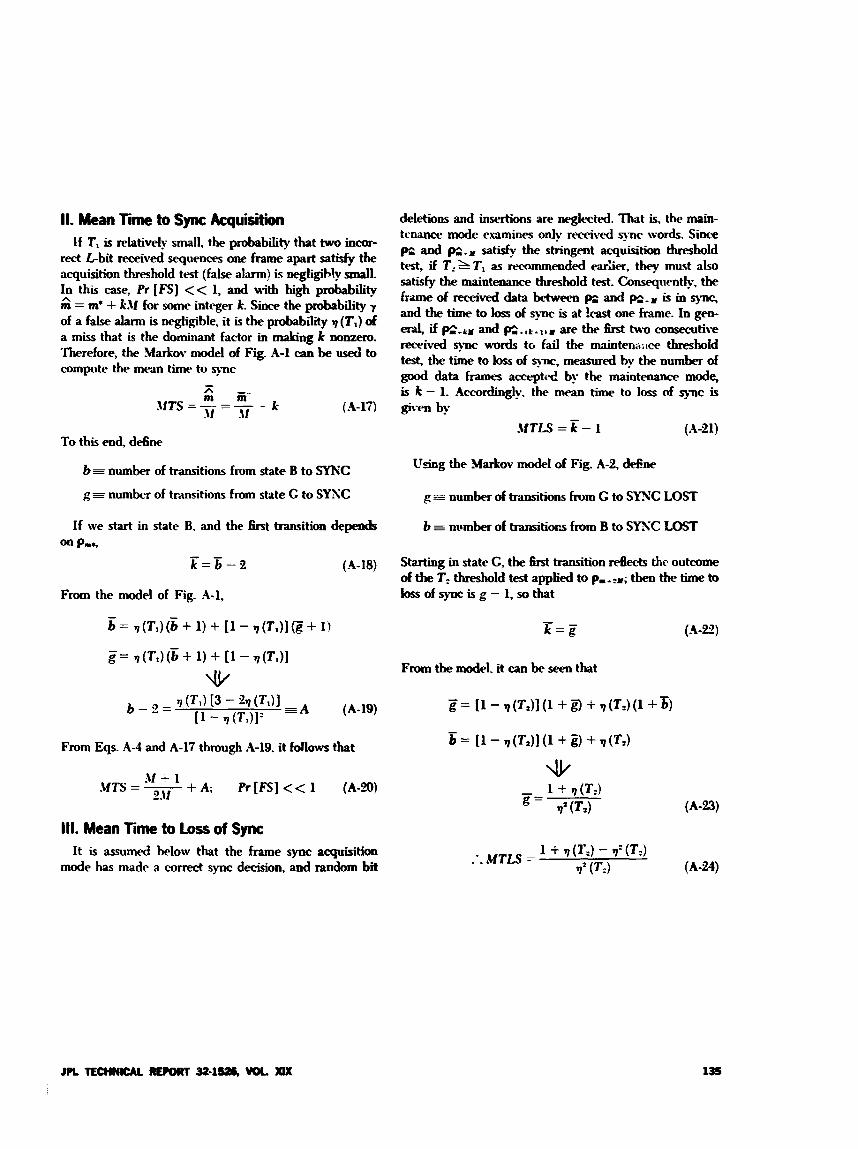
II. Mean Time to Sync Acquisition If TI is relatively small, the probability that two incor-
rect Lbi t received sequences one frame apart satisfy the acquisition threshold test (false alarm) is negligibly d l . In this case, Pr [ FS] < < 1, and u-itb high probability 2 = m' + k31 for some integer k. Since the probability y of a false alann is negligible, it is the probability 7 (TI) of a miss that is the dominant factor in making k nonzero. Therefore, the Markov model of Fig. A-1 can be used to compute the mean time to sync
To this end. ddne
(A- 17
b= number of transitions from state B to SYNC
g= number of transitions from state G to SYSC
If we start in state B. and the first transition depends on Pn8- -
k = $ - e (A-18)
From the model of Fig. -4-1,
From Eqs. A 4 and A-17 through A-19, it follows that
A I + 1 2.v .UTS = - + A ; Pr[FS] << 1 (A-20)
111. Mean lime to Loss of Sync It is assumed below that the frame sync acquisition
mode has made a correct sync decision, and random bit
deletions and insertions are neglected. That is. the main- tcnamx mode esamines only received s ? ~ words. Since p= and e.x satisfy the stringent acquisition threshold test, if T,AT, as recommended e a r h , they must also satisfv the maintenance threshold test. Consequently, the frame of received data between p= and is in sync, and the time to loss of sync is at !east one frame. In gen- eral, if e+tr and p = - , k L I , I are the fust h s - ~ consecutive received sync words tc, fail the maintena:ice threshold test, the time to loss of s)m, measured by the number of good data frames accepted by the maintenance mode, is k - 1. Accordingly, the mean time to loss d sync is given by
MTLS = E - I (A-21)
U,+g the Markov model of Fig. A-2, d&ne
g E number of transitions hum G to S Y ? K LOST
b number of transitiws from B to SYXC LoSr
Starting in state G, the first bansition the outcome of the T, threshold test applied to pmA2r; then the time to lossofsyncisg-1,sothat
From the model. it can be seen that
(-4-22)
JPL TECHNCM RL#HIT 32.1- Ya Xar
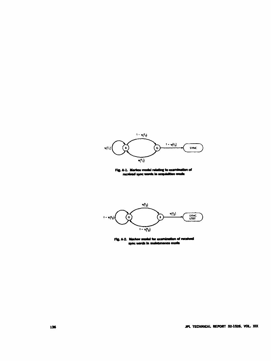
I -
136
OSN Research and Technology Support E. B. Jackson
R. F. Systems Development Section
The actioities of the DeuerOpment Support Group in opemting and maintain- ing the Venus Station (DSS 13) are discussed and progress noted. Actioities included prOnetay mdot experiments (Venus and Mercury), d o source sky suroey using the 26-m antenna, Faraday rotation data cdlection, weak radio source flux dew measurement, X-band 4oo-kW radar der;elopment and testing, Block N receber/exciter inotcrllrdion and testing/checkout, 26-m antenna re- ceioing system temperature impmement, d i f f e r 4 m’y long baseline inter- ferometry (VLBI) experiments, clock synchronization tmnsmissiorrp, DSS 14 high-power transmitter maintenance support, and Pioneer 10 science support.
During the two month period ending December 15, 1913, the Development Support Group operated the Venus Station (DSS 13) and performed the following activities.
1. In Support of Section 331 A. PlanetaryRadar
For a total of five and one-half hours, DSS 13 supported thc ranging of the planet Venus to gather data for use by the MVM73 project. Pseudonoise (PN) code and code riming pulses were supplied, via microwave link, to DSS 14 for use as a modulating signal for the uw)-kW RhD transmitter, and to synchronize the demodulating
system. In addition to these ranging efforts, five and one- half hours of special Mercury ranging were supported in a similar fashion, with 10 data runs being completed. Additionally, preliminary testing, with DSS 14 transmit- ting and both DSS 14 and DSS 13 receiting, of a proposed ‘active VLBI” experiment was performed. This experi- ment, with Greenbank Radio Observatory as the coop- erating station, is scheduled for early in 1974.
B. Station Monitor and Control (RTOP-68)
As part of the work being done -der Researcb and Technology Operating Plan 68 (RTOP-68). the SDS-930 computer and DSS 13 2Bm antenna were used for six hours to amtinue testing of a developmental conical
scanning antenna drive program destined to be used at DSS 14.
111. In Support of Section 335 A. X-Band Radar (400 kw)
II. In Support of Section 333 A. Skysurvey
Using the noise adding radiometer (NAR) and the 26-m antenna in a fixed position( usually 180" az and 80-87" el), data are collected on the total antenna system tempera- ture as the Earth's rotation sweeps the antenna beam across the sky. This observing, conducted automatically during the hours when the station is closed (nights, holi- days, and weekends) collected a total of 534 hours of data during this period.
6. Faraday Rotation
In anticipation of the launch of the MVM73 spacecraft, it was decided to provide backup for the single receiver being used to collect Faraday rotation data. Purchase orders have been placed for two more receivers for evalu- ation but, pending their arrival, a receiver was obtained on loa;- from Teledyne Corporation. After extensive modification of the antenna previously used with the Smythe receiver, the Teledyne receiver was placed into service and is currently collecting data. Stanford Research Institute delivered and installed a second receiver but the antenna drive mechanism failed and this receiver is currently not functioning. At the end of the period, both the Teledyne and one Stanford receiver are collecting data from .4pplications Technology Satellite 1 (ATS-l), data that will be used by the MVM73 project to provide ionospheric correction for the spacecraft ranging and doppler data.
C. WeakSource
With the reinstallation of the S-band radar operational (SRO) feedcone onto the DSS 13 26-m antenna and the relocation of the maserhefrigerator from the electronics room into this feedcone, the resulting low receiving system temperature has made it feasible to again measure the strength of weak radio sources. Late in November th is project was resumed with 13 hours of data being collected on radio sources 3C123,3C138,3C147,3C353, NGC7027, PO 237-23. and PO 2345-23.
In anticipation of full-scale resumption of the associ- ated antenna gain measurement portion of this program, the standard gain feedhorn was removed from the 26-m antenna and returned to Section 333 for examination and calibration.
The first klystron (VA-949J) was installed into the modified test bed and tested at a power output of just over 200 kW. During this testing, three directional cou- plers failed, two with overheated internal matching loads and one with water leaks in the cooling tubing. On December 6,1973, this first klystron apparently failed and was removed from the test setup.
A replica of the inside framework of a 64-m-type feed- cone has been constructed at DSS 13. A 2aal klystron power amplifier with combiner, water loads, and couplers, as required for complete testing, will be constructed in this replica. Available space is limited and integration of the two klystron power amplifiers into the cone will be difficult. Pending the availability of the actual feedcone, this replica will enable construction, fitting, and testing to take place.
6. Block IV Receiver/Excitcr
We continued to provide support to the installation and checkout of the Block IV receivedexciter at DSS 14. Installation is now complete and, working until the con- figuration at DSS 14 was frozen for MVM73 launch, testing and checkout were supported with a total of 273 manhours. The Block IV receivedexciter is now par- tially operational and is being used to support MVM"73.
C. Antenna Pointing (26-m)
Inasmuch as we were resuming normal receive capa- bility operation, and reinstallation of the SRO feedcone may have resulted in a change in the agreement of the radio frequency axis of the antenna with the mechanical axis, some test tracking was done with the scan and correct using receiver (SCOUR) computer program. In three hours of tracking using Cassiopeia A and Cygnus A as sources, a new s e t of preliminary azimuth and eleva- tion offsets was obtained for use during other tracking activities.
D. Receiving System Temperature Improvement (26-m)
With the completion of the first phase of the dual uplink carrier testing, it was felt that the maser/ refrigerator could be relocated from the electronics room into the feedcone and thus improve the receiving system temperature from 29 K to approximately 17 K at zenith. This relocation was effected and the maser compressor was aka reinstalled into the closed cycle refrigerator
138 JPL TECHNICAL REFORT 32-1526, VOL. XIX
(CCR) room on the antenna (vice the outboard elevation bearing platform). Unfortunately this compressor soon failed and was replaced by the spare. The failed unit has been repaired and is ready for reinstallation if necessary.
IV. In Support of Section 391 In an investigation of its application to spacecraft
positioning, a diff erential very long baseline interferome- try (VLBI) experimcnt was carried out with Pioneer 10 and a radio source as signal sources; the cooperating stations were DSS 13 and DSS 42. A total of 18% hours on four separate passes were spent observing, in the VLBI mode, the spacecraft Pioneer 10 and radio source OW-174.
V. In Support of Section 422 A. Clock Synchronization Transmissions
Regular clock synchronization transmissions have not yet been scheduled by DSN scheduling but special trans- missions were made to DSSs 42 and 43. These trans- missions, along with the regularly scheduled maintenance, disclosed some system problems. Marginal radio fre- quency (RF) drive to the 100-kW klystron way corrpcted by replacement of the X 14 multiplier in the exciter chain. A synthesizer failcd and was replaced in the programmed oscillator used for frequency control. A total of nine transmissions have been made during the last two months.
B. DSS 14 High-Power Transmitter Maintenance
In preparation for the launch of the MVM’73 space- craft, the complex spare 20-kW klystron was installed at the Microwave Test Facility and correct operation assured. Some minor tuning was accomplished, then the klystron, with a complete set of operational data, was shipped to DSS 14 in case of need.
During a routine checkout, the lW-kW DSN trans- mitter was discovered to be inoperational. With the assistance of the DSS 14 steff, DSS 13 personnel replaced the klystron, socket tank and magnet, and restwed the systein to operational condition. Due to schedule require- ments at DSS 14, this work was accomplished during four consecutive nighi operations.
The previously reported (Ref. 1) difficulty with re- flected power on the R&D 400-kW transmitter was found to be spurious signals caused by a defective radio frequency connector in the input line to the frequency multiplier. Replacement of this connector cleared up the poorly transmitted spectrum and full 400-kW operation is now possible without reflected power “kickoffs.”
C. Pioneer 10Tracking
If the tracking load at DSS 14 can be relieved, a planetary radar experiment is planned with the comet Kohoutek as a target. It is proposed that DSS 13 take over tracking Pioneer 10 for several days during early January, 1974. In validation of DSS 13’s capability to receive good data, and with the cooperation of DSS 12 for telemetry reduction, a test track was made of Pioneer 10 with the telemetry subcamer being trans- mitted to DSS 12 via the intersite microwave link. Good data were obtained with the telemetry S/N ratio being 2.5 from DSS 13 vs 2.8 with DSS 12 receiving.
VI. In Support of Section 825 With the closer approach of Pioneer 10 to Jupiter, a
stepped-up level of radiation monitoring was provided from DSS 13. The radiation at 2295 MHz from Jupiter was monitored for a total of 87.5 hours. Radio star cali- brators, as tabulated in Table 1, were also observed for 122 hours.
Reference
1. Jackson, E. B., “DSN Research and Technology Support,” in The Deep Space Network Progress Report, Technical Report 32-1526, Vol. XVII, pp. 1M)-102. Jet Propulsion Laboratory, Pasadena, Calif., Oct. 15, 1973.
JPL TECHNICAL REWRT 32.1526, VOL. XIX 139
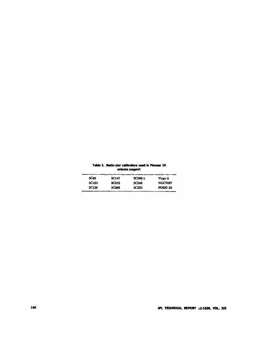
140
3(;48 3C147 3C309.1 Virgo A 3C123 3C218 3c348 NCC70e7 3C138 3mM x353 Porn-23
Design of a High-speed Reference Selector Switch Module for the Coherent Reference
Generator Assembly T. K. Tucker
R. F. Systems Development Section
Design efort wos started in A p d 1973 to dewlop and fabricate a high-speed switch nwdtale for the Coherent Reference Generator Assembly. The major design gaal was to deoelop a high-speed switch capable of switching between frequency standards in less than 400 M in the event of a primary standard failure, thus ptooiding a constant failsafe I-MP: reference signal to the station cbcks. This report reuiews the merd &sign and prouides a general memiew of the com- pleted module.
The engineering model of the Coherent Reference Generator Assembly (CRG) was installed and imple- mented at DSS 14 during July 1973. Included in this installation was an engineering prototype of the 1-MHz clock reference switch module (switch module), which supplies 1-MHz reference signals to the frequency and timing subsystem (FTS) clock and timing circuits.
The following significant features of the Switch Mod- ule will be discussed in this report:
(1) Design objective.
(2) System application
(3) Description.
(4) Present status.
1. Design Objective The major design objective for the switch module was
to provide a mutant 1-MHz reference to the station clock by automatically switching to a backup reference source in less than 400 ns in the event of a primary source failure.
II. System Application (Fig. 1) Inputs to the CHG are obtained directly from the
station frequency standards that, during the next few years, may be two rubidium standards (Rb) or two hydrogen maser (HM) standards.
The primary input ti, the FI'S clock system from the CRG s a failsafe 1-MHz reference derived from either
J R TECHNICAL REPORT 32.1528, Va xnt 141

the present rubidium standards or the future ultrastable hydrogen maser standards. Once a class of standard is chosen (either ruhidium or hydrogen maser), the sec- ondar). (ic backup reference is derived from the same generic type (;,e., if hydrogen maser No. 2 is chosen as the prime standard. I i ~ ~ r o g e n maser No. 1 would be the backup unit).
Both the primary and sewndary standard 1-MHz references are made available to the FTS so that d pli- cate clocks can be operated for long-term stability an6 standard performance determination.
111. Description (Fig. 2) The switch module is housed in a standard Block IV
RF module and has been designed to operate without operator adjustment or alignment.
The switch module has been designed with a “failsafe” dc power system. In the event of a dc power loss from the CRG power supplies, the module automatically switchFs to a battery backup source located in the FTS, thus assuring coniinu,,J: 1-MHz references to the sta- tion clock.
Two input references are selected, within the module, by a solid-state multiplexer that is addressed externally by the CRG control and monitor panel. The multiplexer’s logic assures that the primary signal is obtained from the selected frequency standard and the secondary, or back- lip, is derived from the other like standard.
The key idea of the overall switch design is to use digital switching techniques to accomplish the high- speed switching. To accomplish this, both the primary and secondary standard inputs are passed through Schmitt triggers and converted to transistor-transistor logic (TTL) levels,
To detect primary standard failure, two parameters must be considered: (1) instantaneous signal presence, and (2) the average input power level.
Instantaneous failure sensing and switching is accom- plished through an unusual application of a zero cross- over detector circuit, which consists of two voltage comparator integrated circuits interconnected and biased to provide full 360-deg signal presence sensing of the primary input signal.
If the input signal is present, the failure sensor remains at a logical “1” level. If ti..: input signal should disappear
for a time interval in excess of approximately 250 ns, the sensor output assumes a logical “0“ level thus initiating a failure mode signal. The 250-ns decision time is estab- lished by a simple resistor-capacitor (X) filter in the sensor output, which prevents switch operation on minor noise disturbances.
The failure mode signal triggers a one-shot retriggrr- able multivibrator circuit initiating the switching gate that gates off the primary signal channel and enables the secondary in its place. The transfer from primary to secondary signal, after primary failure, is accomplished in less than 400 ns.
The one-shot multivibrator serves an essential func- tion by assuring that once a failure has been sensed and a transfer between standards effected, approximately a ote-half second delay is required before the circuit can revert back to normal operation. This prevents the switch from chattering on an intermittent input signal.
Average power sensing and switching are accomplished by measuring the primary input powcr with a signal level detector. If the input power remains above a pre- set level of approximately +9 dBm, the primary level sense signal remains at a logical “1.” If, however, the input level falls below this preset level, the prir. .ary level sense signal assumes a logical “0” state initiating a switching gate to disable the primary channel and enable the secondary in its place.
Level monitor logic is also designed to provide con- tinuous module status information to the CRG control and monitor panel. Input and output signal power levels are monitored in individual level detector circuits and are compared in an exclusive “or” circuit. If inputs are above the preset level of approximately +9 dBm, output from ihc module must also be present and ai. we +9 dBm, or the module “output failure” signal will be initiated. If no inputs are present or they fall below the +9-dBm level, outputs are not expected and only the “input failure” signals will be initiated.
The TTL signals are filtered at the switch output to provide sine wave outputs, at nordnal %-ohm imped- ance, so that no changes to the existing FTS are required.
IV. Status DocumentaYon is complete and the first production
model of the switch module has been built and tested Ivstallation at DSS 14 wiil be accomplished as soon as the station operational freeze is lifted.
142 JPL TECHNICAL REPORT 32-1526, VOL. XIX
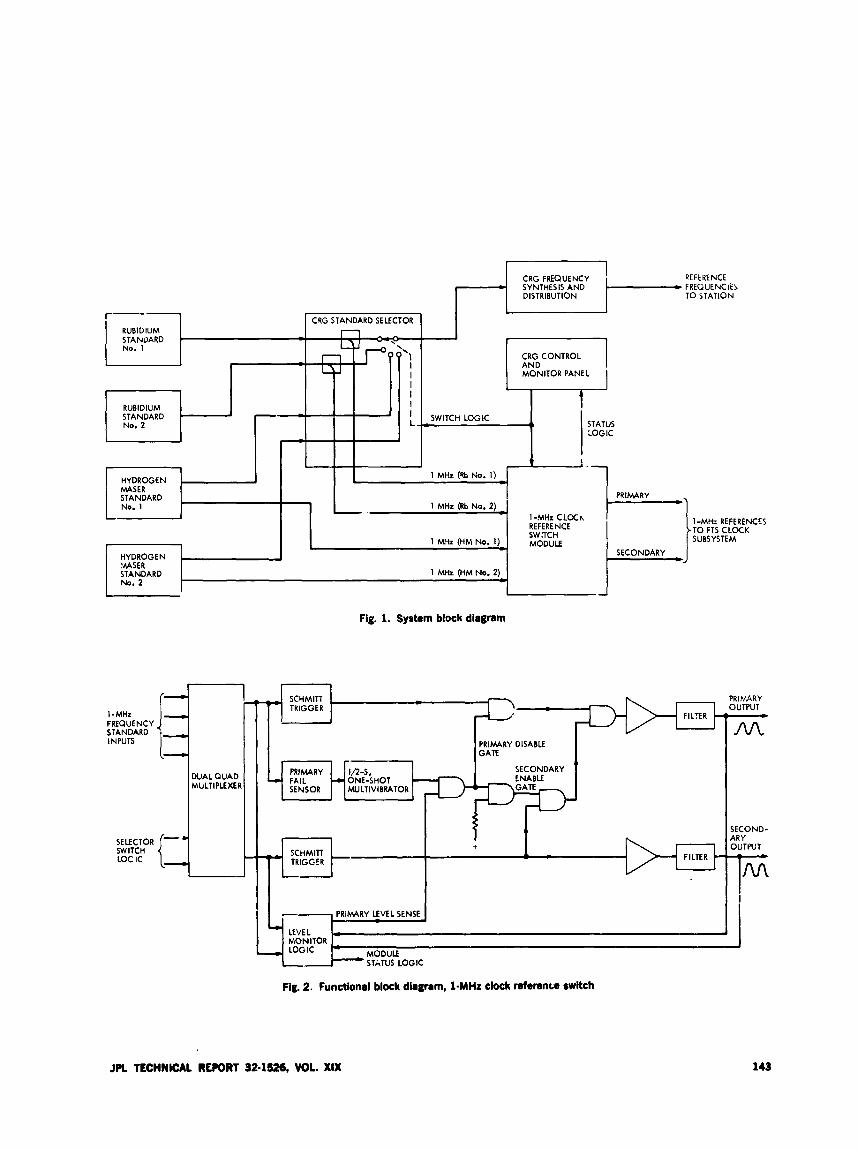
CRG FREQUENCY SYNTHESIS AND DISTRIBUTION
,
9E FE RE NCE
TO STATION 7 D FREQUENCIE5
1 - MHz FREQUENCY 5 TAN DARD INPUTS
DUAL QUAD MbLTIPLEXER
SWITCH LOC IC
-
-
N L
SECOND- ARY OUTPUT
1N\ I
- SCHMITT TRIGGER
LEVEL e MONITOR LOGIC *
MODULE STATUS LOGIC
, - PRIWRY
Fig. 2. Functional block diagram, laMHz clock reference switch
PRIMRY DISABLE GATE
/ I PRIMARY 1/2-S, SECONDARY
JPL TECHNICAL RECORT 32-1526. VOL. XIX
4 ONE-SHOT -C FAIL
143
ENABLE GATE SENSOR WLTIVIBRATOR
SCHMITT TRIGGER
1 ,
FILTER
I ,
I i
A Scaled-Time Telemetry Test Capability for Sequential Decoding
S. Gutman, J. Layland, and J. MacConnell Communications 9ystems Research Section
R. Chmoff and N. Ham R. F. Systems Development Section
J. WiIct\er DSlF Digital Systems Devalopment Section
This article describes the mtiuation for, and deuelopment L.UI initial testing 0,
a .waled-iime telemetry test capability. The immediate need for this ca,whility is to establish the sequentiul decoding petfomnce of the data decoder assembhj (DDA) for HeliDs and Plower, and the tests . h e been aimed at eualuating the suitability of the scaled phase-locked loop (PLLI for this task. The ,eleuant parameters of limiter suppression, phase jitter uariance, and phuse jitter auto- correlation h o e been measured, a . d nc discrepamti WCJS found between thr X16-scaled PLL and the 12-Hz loo- of the DSN receiver. Comparatiue Fequentio' decoding tests have also been performed for 128-bit/s data; no discrepancy was found between scaled and unrcaled performance at ary modulation index, either near-optimum or high (70 deg), diere the carrier reference noise is dominant.
1. Introduction The purpose of this artirlr is to describe the experi-
mental setup and preliminary results of a time-scaled simulaticn of a convolutionally ccded, sequentially de- coded. coherent telernetry liik. The need for such an approach arose when it becime necessary to le the Helios project as well as future Pioneer projec. with an accurate estimate of link performance and design trade- offs at medium data rates. Medium rates are by definition data fides of the same order of magnitude as the band-
width of the phase error prucess in the coherent reference signal, or more generally, data rates at which decoder memory is camparitb!e tr th5 memory of the phase-locked kiop.
Such conditions ariw at low reczived signal levels at end and post-end of missiom and at stronger signal levels when transmission is mntaminated by a turbulent medium like the solar corona, a planetary atmosphere, or during rapid descent of a probe.
1u JPL TECHNICAL REWRT 32-1526, VOL XIX
Experimental nerformance estimJtion through simula- hon is necessary under the above conditions because accurate theoretical models of decoder behavior when the phase is nct constant are not yet in existence (Ref. 1). The current s; f decoding theory can accurately prc- dict decoder performance only when the phase is constant over many constraint lengths. Finally, scaling up of the simulations to a higher speed than under normal oper- ating conditions is necessary in order to accumulate the required amount of statistical data 111 a reasonable length of hme. For example, to establish with reasonable confi- dence a bit error probability of l(r requires about 10s bits. To gather this amount .._ data at 100 bits/s would take over 10 days. Similarly, establishing a block erasure probability (decoder wedow) of le3 for blocks of loo0 bits, would take 10 days.
II. Scaling the Tests The block diagram in Fig. 1 depict3 the system elements
which require modification to provide a high-speed version of actual behavior at normal operating conditions. It is assumed that the front end noise is wideband, with a oae-sidJ spectral density N,. Primed variables denote scaled versions of the normal iinscded quantities, and x +wtes the scale factor. There are several ways to achieve the required scaling of the system dynamics. The method we selected may be described as follows:
N: = N o ,-5 = XP,
tu:, = XWL
f = r
R' = x R
a' = a
Wideband noise level unchanged
Total signal power scaled up
Bit rate scaled up
Loop bandwidth sca ld up Damping ratio unchanged to pre- serve relative dynamics
Limitersuppressim factor unchanged to preserve relative dynamics
Prefiltqr bandwidth increase required to mpintain the same input signal-to- noise ratio (SNR) to the limiter for a? --
Loop SNR unchanged
Bit SNR unchanged
Modulation index unchanged
Loop filter time constants reduced
Loop gain increased
- u
The above quantities obey &e following relationships, which are documented by Tausworthe (Ref. 2)
and
a = 4pH) where
pfr = (1 - m2)PT/Nowrr m = sin 8, where 6 is the modulation angle
Inserting the scaled parameters into the above formulas will verify that all the scale changes are achieved and the relative dynamics preserved where necessary.
Tiiiw-scaling of the subcarrier demodulator and symbol synchronizer assemblies (SD.4 and SSA) is accom2lished through switch-selectable operating modes which match the actual (Le., upscaled) daia rates. Moreover, the loss^ in these assemblies are small and relttively insensitive to rate changes.
Ill. Test Techniques Thr agproach followed in evaluating the scaled-time
telemetry test capability. must minimize the test time required to build confidence in the correctness of the scaled parameters. The first tests therefore measured the glohaI static PLL parameters, limiter suppression a, and phase jitter variance u&, at specific signal stre* gths and compared these measurements with published results for the 12-Hz DSN PLL. Dynamics cf the PLL behavior also influence strongly the performance of medium-rate telemetry, necessi'-ting their measurement, in the form of the phase jitter . :ocorrelation function. In this case, both the 12-Hz DaN PLL and the scaled PLL had to be measured, as the desired parameters wcre not geneally documented.
The ultimate criterion f o r acceptance of the results of the scaled telemetry tests is, of course, the equivalence of measured telemetry pertormance in both normal and scaled-time modes. This is most economically used at the mid-range data rates only (e.g., 128 bit&), where reasonable duration tests can define the system perfor- mance. The anticipated plan is to tmt at 128 bits/s over a set of modulation indices near optimum, and to spot- check many data rates at oiie very high modulation index. For each data rate c!wcked in this fashion, the modulation inder will be set wfficiently high for the
JPL TECHNICAL REPORT 32-1526, VOL. XIX 145
noisy carrier reference to be the dominant source of noiscb, and so that performance is poor enough to be mea- sured in reasonable time .vithol;t sca!irig. The total re- ceived power level will be set high enough so that the dcsircd lei deletion probability could bc achieved with a lower niodulation indes. -2 successful match of piformancc at the high mod-index will, of course, indi- cate that the noisy reference losses are correctly scaled. Since we belive that the additive receiver noises will scale correctly, successful high inod-index comparison should also indicate overall success of the scaled test setup. Some prior test data (Ref. 3) esist for normal-time test: of per- formance near the optimum mod-index which can be compared against the scaled tcsts to identify any un- expected errors in the scaling assumptions.
No plans esist presently to test the scaled-time test con- figuration for uiicoded tclc~n~tr).. Since performancr of sequential decoding is very critically dependent upon the adjacent-symbol correlation of the carrier reference noise, correct scaled-time performance of sequential decoding almost certainly implies that scaled-time tests of uncoded telemetry will also be correct. Future users of the scaled-time test capability for uncoded data will, of course, have the option of accepting this hypothesis or performing whatever additional tests they might need to validate the scaled-time performance for uncoded telemetry.
IV. The Scaled Loop Hardware Design and Initial Testing
The preceding sections have shown that, by scaling the receiver 12-Hz loop bandwidth, statistical data on bit error rates can be 7btained in a time inversely propor- tional to the scaling number N used on the receiver. It was decided to scale the ipceiver loop bandwidth by 16, a factor which allowed a reascnable improvement in the speed of data acquisition WithoLt causing the data rates €or the faster bit rates to exceed the capabilities of the telemetry decoding cquipment.
For the scaling number under consideration (16), it was necessary only to scale the tracking filter and the predetection filter. (If extremely high scaling numbers are used, it may be necessary to increase the bandwidth of the IF amplifiers). Since Bt is being scaled, it can be shown that it is necessary to decrease T , by and 7 2
by N: where t l = R,C and t? = (R, + RJC in Fig. 2. For the case being evaluated (N = le), T , b m e s 9.887 s and T~ becomes 8.5 X s. The hardware implementa- tion of the tracking filter consisted of modifying the
values of R,, R,, and C in 11 standard DSN cracking filter module to provide the new time canstants. The only other hardware inodification required w a s the predetec- tion filter amplifier. The b;ind\\.idth (BCV) of this anipii- fier must be scaled (increased) by the scaling number N. For this test, the bandwidth was increased from the normal 12-Hz loop value of 2 kHz to the new cdue of 32 kHz noise BW. The hardware implementation consists of a four-stage, synchronously tuiied amplifier. (The gain of this filter amplifier must be the same as that of the normal amplifier in order not to disturb the automatic gain control (.4GC) performance of the receiver). For future esperiments, the predetection filter could be a commercial crystal filter. This would enable tighter con- trol of the bandwidth behveen units, as well as better bandwidth stability vs. trmperature. The changc ’ mod- ules nre identified in Fig. 3.
In order to verify that the receiver bandwidth had been properly scaled, several experiments were run. ’nput carrier power was set for all tests by the Y-Factor Tecn- nique (Ref. 4). First, the limiter suppression (u) char- acteristic was checked by measuring carrier power at the limiter output vs. loop threshold margin. This measure- ment was performed by a coherent amplitude detector and vacuum tube volt meter (VTVM). The results of the test can be seen in Fig. 4. Ideally, the scaled and un- scaled a C U N ~ S should be identical. If the a characteristic levels off at a lower margin in thz scaled case, it vvould probably indicate an IF amplificr or limiter of insufficient bandwidth, or an insufficient noise bandwidth iv *he predetectim filter amplifier. (If high-scaling numb.m are mal, it may be necessary to increase the BW of the IF amplifiers. This will prevent their influencing the pre- detection bandwidth, which should ideally be determined solely by the predetection filter amplifier). Since the curves for the scaled and unsca!ed cases are nearly identical, it appears that the predetection filter is indeed the determined BW, as desired.
The second test consisted of measuring the phase jitter (&) of the receiver voltage-controlled oscillator (VCO) as a function of margin. These data were obtained by employing the test translator as a signal source, and the UHF doppler detector as a dual phase detector, which allowd measuring the variance of the phase noisc present on the VCO. The test configuration for this mea- surement is shown in Fig. 3. The UHF doppler signal (zero doppler + phase jitter) is phase d&ected against the station frequency standard. The phase shifter is re- quired to set the reference phase in quadrature (to enable Fhase detection), with either of the two signals being
146 JPL TECHNICAL REPORT 32-1526, VOL XIX
phastl cletwtd in the dual phase detector. (The other signal is being amplitudch dvtwttd.) For Ydch data point (valuc of margin), both channels are sampled and recorded by thc digital instrumentation system ( DISI. Tht, netd for sanlplinq both channels arises \vhcn a cycle slip occurs. For each cycle slippcd at S-band, there appears a 90-dcg shift in the phase at the W I F doppler cktvctor. (This is due to ;3 X 4 multiplication behveen the point at which the L’HF doppler is extracted and the S-band local oscillator output.) Therefore, if a cycle is slipped, the channel that was phase detecting is now amplitude detecting and vice versa. To prevent loss of phase data following cycle slip, both channels are rcmrdccl. \Vhen the tapes are FrOCeSSed, only the chan- nel that is phase detecting is uscd. From those data, the variance (0 : ) is calculated. As can In. seen in Fig. 5, the d a b follow wry closely those obtained with the normal E-Hz loop. This further indicates that thc rewiver seems to be properly scald.
The third test consisted of taking the autmrrelation of the phase jitter data. Each autocori-lation plot shows the time response of the loop at a particular margin. By plotting T from each of these plots vs. margin, a plot is obtained that illustrates loop rpsponse vs. margin. Figure 6 is such a plot for both the scaled and unscaled loops. If the loop is properly scaled, the scaled loop will have a value of T equal to 1/N of the unscaled loop at each margin. For convenience, the time ( 7 ) scales of the two Jata sets shown in Fig. 5 are scaled by the scaling factor A’. Therefore, the two curves will coincide if the loop is properly scaled. A s can be seen. there is very close agreement between these hvo curves.
The results of this group of three tests seem to indi- cate that the receiver loop bandwidth was indeed scaled the desired amount over the r a q e of loop margins con- sidered.
V. Telemetry Tests Testing of the scaled-time telemetry test capability
using sequential decoding requires that ceveral decoding test runs be performed using both the 192-Hz loop and the 12-Hz DSN receiver at identical (scaled equivalent) test ccnditions. To be convincing, these test runs must cover the rangc of data rates, SNRs, and modulation indices for which scaled tests are expected to be used. The scaling can be used at data rates of 256 symbols cr srmnd (SPS) (scaled to 4096 SPS) and lower. At scaled 512 SPS (8192 SPS) an4 above, the data decoder assembly (DD.4) cannot operate succ:ssfully.
The test configuration for sequential decding testing with scaling is sho\vn in Fig. 7. It is identical to the con- figurations ustd for normal DSN tcsting of sequential dtvoding for Pioneer or Helios, rsccpt that the receiver niodules for the 192-Hz loop arc substitutcd for those of the 12-Hz DSS receiver PLL. The output from the test is s map+c. t a p orisinal data record (ODR) containing, for each data frame processed by the DD.4, the number of decoding computations which were used in processins it. These ODR tapes are later analyzed off-line to deter- mine the cumulative distribution of computations, which is then used to evaluate system performance. In tht DSS station, the tests require the use of the sinw’ation con- version assembly (SC.\), the test transmitter. the antenna microwave assemid;., the Y-factor assembly. a receiver and SDA. t\vo telenietq/command processors (TCPs) with SS.4s. and one DD.4. The TCP-DDA4SA string operates under control of nonstandard DSIF software- the DDA stand-alone-TCP verification program-and provides the ODR end-product of the tests. The second TCP-SSA4 string operates with the Ylariner Mars 1971 ( M S I X ) Test Program No. DOI5087-T€ and acts as a monitor for the telemetry channel, to ver ‘y station setup accuracy and identify drifts in parame1,:rs.
The SCA provides a pseudo-random t lata sequence for the test transmitter. The subcarrier frequency used is 2,W3 Hz, and data rates of interest range from 16 to 4096 SPS. The biphase-modulated subcarrier in turn phase-modulates the carrier at the test transmitter, with a modulation inclen which may vary from ,% to 75 deg, depending upon data rate and other factors. This simu- lated telemetry signal is then processed by the station receiving equipment, much like the signal from a space- craft. The “received signal strength is set as required using the Y-fa;tor measurement technique (Ref. 4) prior to the start of a test. The modulation indices are set by precision attenuators. Extreme care is required in this setup because of the sensitivity of decoding performance: the decoding erasure rate can vary by an order of magni- tude with a 0.5-dB change in signal strength. After setup, the Test Program 5087 output monitors charr,rel statistics, and when stable operation of the receiver and SDA i s observed, the TCP/DDA program is activated to develop the ODR of decoder perfomlance. The format of these ODR tapes is shown in Fig. 8.
Tests with the scaling test facility have been performed and the data analyzed for a real data rate of 2.56 SPS (scaled for 4096 SPS). The signal strength was set to that which would provide an STJN, of 2.7 dB at 45-deg modulation index for both scaled and nonscaled tests. This value will produce an erasure rate of between 1W
JPL TECHNICAL REWRT 32.1526. VOL. XIX 147
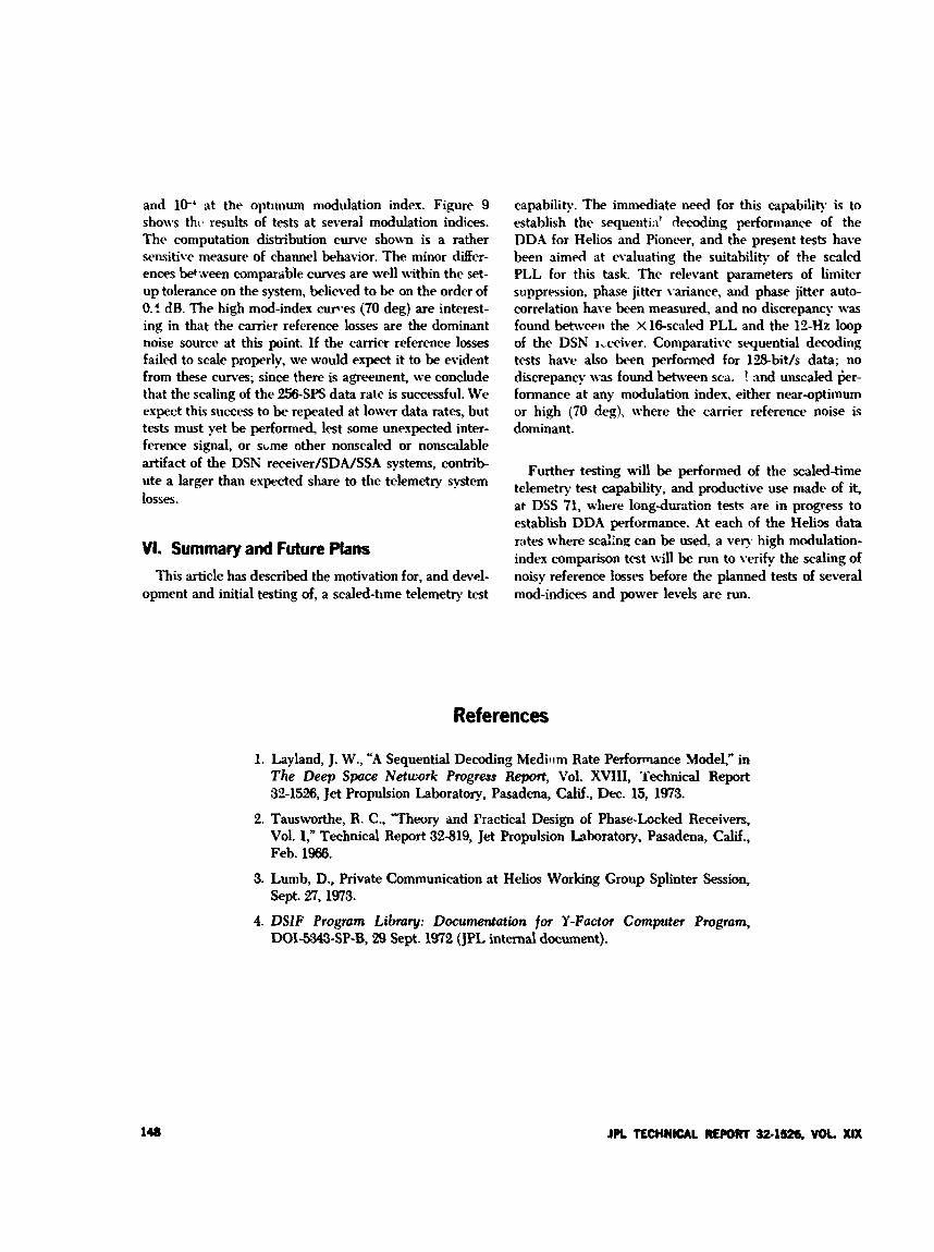
and 1 W at the opnmum modulation index. Figure 9 shows t h c x results of tests at several modulation indices. The computation distribution curve shown is a rather sensitive measure of channel behavior. The minor differ- ences between comparable curves are well within the set- up tolerance on the system, believed to be on the order of 0.4 dB. The high mod-index cw-es (70 deg) are interest- ing in that the carrier reference losses are the dominant noise source at this point. If the camer reference losses failed to scale properly, we would expect it to be evident from these curves; since there is agreement, we conclude that the scaling of the 2.56-SPS data rate is successful. We expect this siiccess to be repeated at lower data rates, but tests must yet be performed, lest some unexpected inter- ference signal, or sbme other nonscaled or nonsalable artifact of the DSN receiver/SDA/SSA systems, contrib- ute a larger than expected share to the telemetry system losses.
VI. Summary and Future Plans This article has described the motivation for, and devel-
opment and initial testing of, a scaled-time telemetry test
capability. The immediate need for this capability is to establish the sequei1ti;i’ decoding perfomlance of the DD.4 for Helios and Pioncur, and the present tests have been aimed at evaluating the suitability of the scaled PLL for this task. The relevant parameters of liniitcr suppression, phase jitter \-ariame, and phase jitter auto- correlation have been measured, and no discrepancy was found behvcen the X16-scaled PLL and the 1.7-Hz loop of the DSN 1,ceiver. Comparative sequential decoding tests have also been performed for lB-bit/s data; no discrepancy \vas found between scaa ? and unscaled h r - formance at any modulation index either near-optimum or high (70 deg), where the carrier reference noise is dominant.
Further testing will be performed of the scaled-time telemetry test capability, and productive use made of it, at DSS 71, where longduration tests are in progress to establish DDA performance. At each of the Helix data rates where x d h g can be used, a ven- high mddation- index comparison test will be run to verify the scaling of noisy reference losses before the planned tests of several mod-indices and power levels are run.
References
1. Layland, J. W., “A Sequential Decoding Medilrm Rate Performance Model,” in The Deep Space Network Progress Report, Vol. XVIII, ‘I’echnical Report 32-1526, Jet Propulsion Laboratory, Pasadena, Calif., Dee. 15, 1973.
2. Tausworthe, R. C., Theory and Fractical Design of Phase-Locked Receivers, Vol. 1,” Technical Report 32-819, Jet Propulsion Laboratory, Pasadena, Calif., Feb. 1966.
3. Lumb, D., Private Communication at Helios Working Croup Splinter Session, Sept. 2‘7,1973.
4. DSlF Progmm Libmy: Documentation for Y-Factor Computer Program, DOIW-SP-B, 29 Sept. 1972 (JPL internal document).
148 JPL TECHNICAL RE#)RT 32-1526, WK. XIX
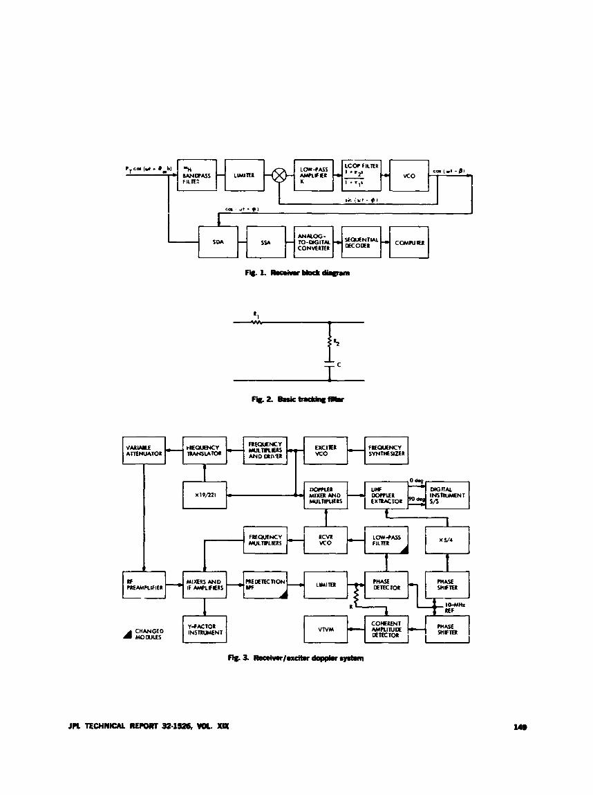
w I
P W PHASE DETECTOR SHFiEI MIXLRS AND ~ I m K T I O N - LIMITER -
A & UF PREAMPLIFIER IF AMTLFERS - ON
I 4 f IO-MH. 8 REF
PHASE SnlF 78
COHERENT
E TEC TOR C H A N C E D I N S T R W E N T VTVM - AMfLllUcE Y-FKTOR
.u A MOWLES
-3- -l.x*doppkrsYstan
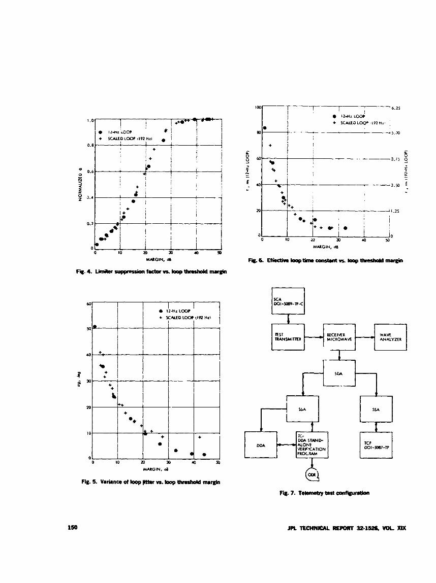
1 .o I 1 !
EST RECEIVER TIUNSMIlXR ' * MICROWAVE -
0.2
I *' ' , 0
0 10 m a 4
1
WAVE ANALYZER
s 3
MARGIN, d
Fii. 5. Variance of kop jltter vs. kop threshdd margin
I + i !
20 11 + 04
t I .25
+ Y i .
0 0 0 10 20 a 40 E)
MMGIN, d8
150 JPL TECHNICAL RE#)Rf 32-1526, WK. XIX
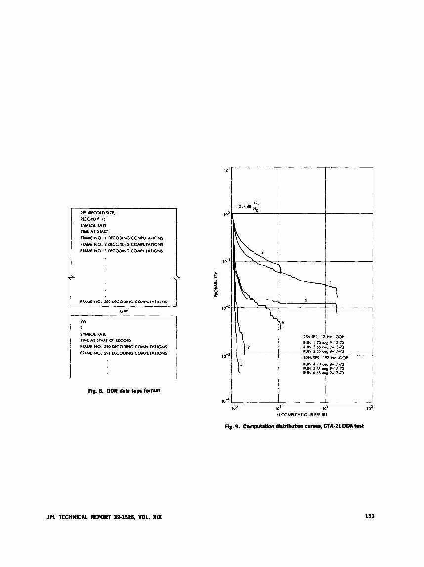
293 (ECOID SIZE)
SYMBOL RATE TlME AT START FRAME NO. I LKODING COWLITATIONS F U M hO. 2 LKC XNG COMPUTATIONS F U M E NO. 3 DECODING COWUTATIONS
RECORD ' (1)
+
F U M E NO. 289 OECODlNG COWPUTATIONS
293 2 SYMBOL RATE TLME AT START OF RECOPD F W NO. 290 OKOZJING COMPUTATIONS F R M N NO. 291 OKOMNG COMPUTATIONS
Fi.8. OMZdatatapefomut
L
IO'
I00
10-1
c d 0
3 0'
10-2
IO-^
10'4
*T. - 2 . 7 a - N O
\
RUN 4 m dag 9-17-73 RUN 5 55 &g 9-17-73 RUN 6 65 9-17-73
I
IO0 101 12 N COWUTATIONS PER BIT
Fig. 9. Cotnputrtim distribution CU-, CTA-21 DDA krt
JPL TECHNICAL R E M 32-1526, VOL XIX 151
NCS Standard Computer lnterface Hardware, Its liming and Timing Control Logic
T. 0. Anderson
This article describes the Network Control System (NCS) Standard Computer lnterface hardware, including the interface cable, the line drioers, line receitiers and line terminating network. I t describes in corrciidrrable detail the timing specificcrtions for the interface timing control signals for continuous &a transfer as weU as for asynchronous byte transfer. A set o f control logic which complies with these timing specifications has been designed for and succcssfuUy checked out in connection with the Star Switch Controller (SSC). This control logic, which includes .ynchronization and noise filter operations, is described in detail. Trans- fer rates for uariablr table lengths a r ~ listed.
1. Introduction The NCS standard computer interface hardware con-
tains 14 parallel data-transmission lines. Eight of these lines are data lines, four are timing and control lines, and two are function lines (see Fig. 1'
Of the interface timing control lines for asynchronous data transmission, two are unidirectional request line;, one in each direction; onc is a bidirectional half-duplex response line; and one is a bidirectional half-duplex ready lint. The linear bit operation of these lines and the operation of the control logic to perform these operations is specified in detail. The control logic synchronizes the input signals to the local service clocks, and filters out spurious noise pulses of short duration, Both the control
logic and its operation are described in detail, as are the cable, line drivers, receivers, and line termination.
11. Cable, Drivers, Receivers, and Line Termination
The NCS standard interface cable is a twisted pair cable, with line drivers and line receivers, as shown in Figs. 2 and 3. 'I ne cable itself is shown in Fig. 4. All con- nectors, physically and functionally, mate with connec- tors n r h JS that shown in Fig. 4. Pin assignments for the timing control lines, data lines, and function lines are also shown in Fig. 4. (Figures 2, 3, and 4 are taken from JPL Specification ESSO%'M A, May 1973, a JPL internal dw ,In.*.Tit.)
152

As shown in the figures, twisted pair, #%-gauge, 100-n lines are used. The drivers are 7438 open collector, high current TTL-buffer, 2-input NAND-gates, and the re- ceivers are regular 7400 NAND inputs. Both ends of the lines are terminated with 150 R to +5V and 330 R to ground. The common term is terminated on the CND pin of the drivrr and receiver chip, respectively.
111. Signal Sync and Noise Filter In order to combat noise and to synchronize the inter-
face timing control signals with the internal service clock of the computer, a signal transition is recognized only upon the second consecutive sample of the internal clock. This specification is valid for transitions in either direc- tion. Stated differently, a single noise pulse of either polarity of a duration of less than two clock periods occurring at any time will have no &ect on the true operation of the line receiving logic.
IV. Timing Control Line Operation Figure 1 shows the selected set of computer interface
timing control lines together with eight data lines. The request-to-transmit line is unidirectional, while the return response and data lines are half-duplex bidirectional. For ;-ici.t ectional communication, two request-to-transmit lilies are theri required, one in each direction, as shown. fl’ip,wc 5 is a simple block diagram and timing chart wbch show. the detailed operation of the timing control lines ‘R;e Arne sequence for the various control lines, whirh is ripeated for each linear bit or parallel byte, is listed as fo lows:
An oidxmnd request line is asserted by the trans- mitting <,-vice.
The assertion of an inbound request line is sampled and synchronized by the recipient device.
The synchronized inbound request signal causes assertion of the outbound return response line.
The return response line inbound to the transmit- ting device is sampled and synchronized and causes assertion of the outbound ready line.
The ready signal inbound to the recipient device is sampled and synchronized, and used to form a data-strobe pulse for sampling the received data.
(6) Upon sampling the received data, the inbound ready signal is used to turn off the outbound response line.
(7) Turnoff of the outbound responsc line will in turn cause turnoff of the inbound rcady line.
(8) Turnoff of the inbound ready line will again cause the outbound response line to turn on, conditional on the request linc. being on, for receiving of the next character.
(9) At the end of a block transmission, the request line is turned off by the transmitting device simul- taneously with the ready line, outbound from the transmitting device, for the last character being turned on.
A. Control Logic Operation
The operation of a signal synchronizing and noise control receiving register for thc transmission interface timing controI signals, in general, and for the ready line register, in particular, is specified as follows:
(1) A signal change is recognized only if the signal remains in its new state for two consccutive clock periods after the signal has remained in its prior state for at least two clock periods.
(2) A data strobe will be generated only for a unidirec- tional change of the input signal.
(3) Once a data-strobe pulse has begun to form, it will be completed independently, and the fact that it was completed will be independently reported. Independently, as used here, implies independence of what is happening on the input signal line.
(4) A noise spike of either polarity of a duration less than two clock periods occurring at any time must not be the cause of a double data-strobe pulse, nor should such a noise spikc interrupt the forming of a data-strobe pulse or the subsequent r e p r t signal that a data-strole pulse -.vas formed.
B. Request Line Sync Register
Figure 6 shows the interface timing control logic. The logic is implemented with a SN5495 universal 4-bit, shift- right, parallel-load register with no additional gating. The input signal is used as a mode control and the parallel entries are connected so that the register, when it is in the parallel load mode, will shift left. The shift- right/shift-left data entries are fixed-wired as “1” and “0,” respectively. The desired output level is achieved by correlating the input mode control signal with the fixed -.vii.d data inputs; e.g., SR = 1, SL = 0, or vice versa.
JPL TECHN?CAL REPORT 32-1526, VOL. XIX
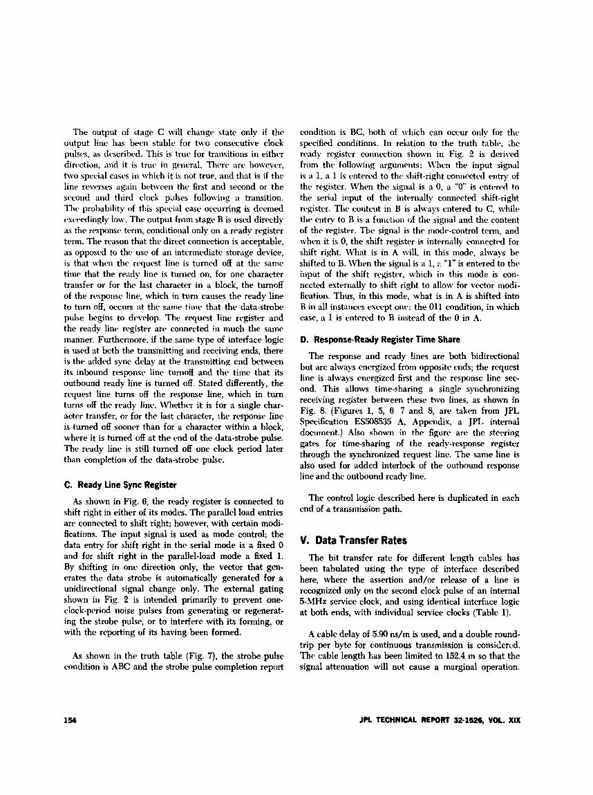
The output of stage C will change state only if thr output line has been stable for two consecutive clock pulscs, as described. This is true for transitions in either direction, and it is true in general. There are however, two spclc.ial cases in which it is not true, and that is if the line reverses again bt.t\vcwn the first and second or the stwnd and third clock pulses following a transition. The probability of this special case occurring is deemed exceedingly low. The output from stage B is used directly as the response term, conditional only on a ready register term. Thth reason that the direct connection is acceptable, as opposed to the use of an intermediate storage device, is that when the request line is turned off at the same time that the ready line is turned on, for one character transfer or for the last character in a block, the turnoff of the responsc line, which in turn causes the ready line to turn off, occurs at the same tiwe that the data-strobe pulse begins to dcvelop. The request line register and the ready line register are connected in much the same manner. Furthermore, if the same type of interface logic is used at bcth the transmitting and receiving ends, there is the added sync delay at the transmitting end between its inbound response line turnoff and the time that its outbound ready line is turned off. Stated differently, the rcquest line turns off the response line, which in turn turns off the ready line. Whether it is for a single char- acter transfer, or for the last character, ihe response line is turned off sooner than for a character within a block, where it is turned off at the end of the data-strobe pulse. The ready line is still turned off one clock period later than completion of the data-strobe pulse.
C. Ready Line Sync Register
As shown in Fig. 6, the ready register is connected to shift right in either of its modes. The parallel load entries are connected to shift right; however, with mrtain modi- fications. The input signal is used as mode control; the data entry for shift right in thc serial mode is a fixed 0 and for shift right in the parallel-load mode a fixed 1. By shifting in one direction only, the vector that gen- erates the data strobe is automatically generated for a unidirectional signal change only. The external gating shown ill Fig. 2 is intended primarily to prevent one- clock-period noise pulses from generating or regenerat- ing the strobe pulse, or to interfere with its forming, or with the reporting of its having been formed.
As shown in the truth table (Fig. 7), the strobe pulse condition is ABC and the strobe pulse completion report
condition is BC, both of \vliich can occur only for the specified conditions. I n relation to the truth table, :he ready register connection shown in Fig. 2 is dcrivcd from the following arguments: \i7hen the input signal is a 1, a 1 is entered to the shift-right connected entry of the register. \Vhen the signal is a 0, a “0” is entered to the serial input of the internally connected shift-right register. The content in B is always entered to C, while the entry to B is a function of the signal and the content of the register. The signal is thc mode-control term, and when it is 0, the shift register is internally connected for shift right. What is in A will. in this mode, always be shifted to B. When the signal is a 1, c “1” is entered to the input of the shift register, which in this mode is con- nected esternally to shift right to allow for vector modi- fication. Thus, in this mode, what is in A is shifted into B in all instances except one: the 011 condition, in which case. a 1 is entered to B instead of the 0 in A.
D. Response-Ready Register Time Share
The response and ready lines are both bidirectional but are always energized from opposite ends; the request line is always energized first and the response line sec- ond. This allows time-sharing a single synchronizing receiving register between these two lines, as shown in Fig. 8. (Figures 1, 5, 6 7 and 8, are takvn from JPL Specification ES508535 A, Appendix, a JPL internal document.) Also shown in the figure are the stepring gates for time-sharing of the ready-response register through the synchronized request line. The same line is also used for added interlock of the outbound response line and the outbound ready line.
The control logic described here is duplicated in each end of a transmission path.
V. Data Transfer Rates The bit transfer rate for different length cables has
been tabulated using the type of interface described here, where the assertion and/or release of a line is recognized only on the second clock pulse of an internal S-hIHz service clock, and using identical interface logic at both ends, with individual service clocks (Table 1).
A cable delay of 5.90 ns/m is used, and a double round- trip per byte for continuous transmission is consiclered. The cable length has been limited to 152.4 m so that the signal attenuation will not cause a marginal operation.
154 JPL TECHNICAL REPORT 32.1526, VOL. XIX
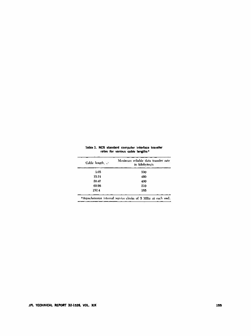
Table 1. NCS standard computer interface transfer rates for various cable lengths'
Maximum reliable data transfer rate in kilobytes/s Cable length, .:
3.05 530 15.24 460 30.48 400 60.96 310 152.4 185
8Asyiichronous internal senice clocks of 5 MHz at each end.
JPL TECHNICAL REPORT 32.1126, VOL. XIX
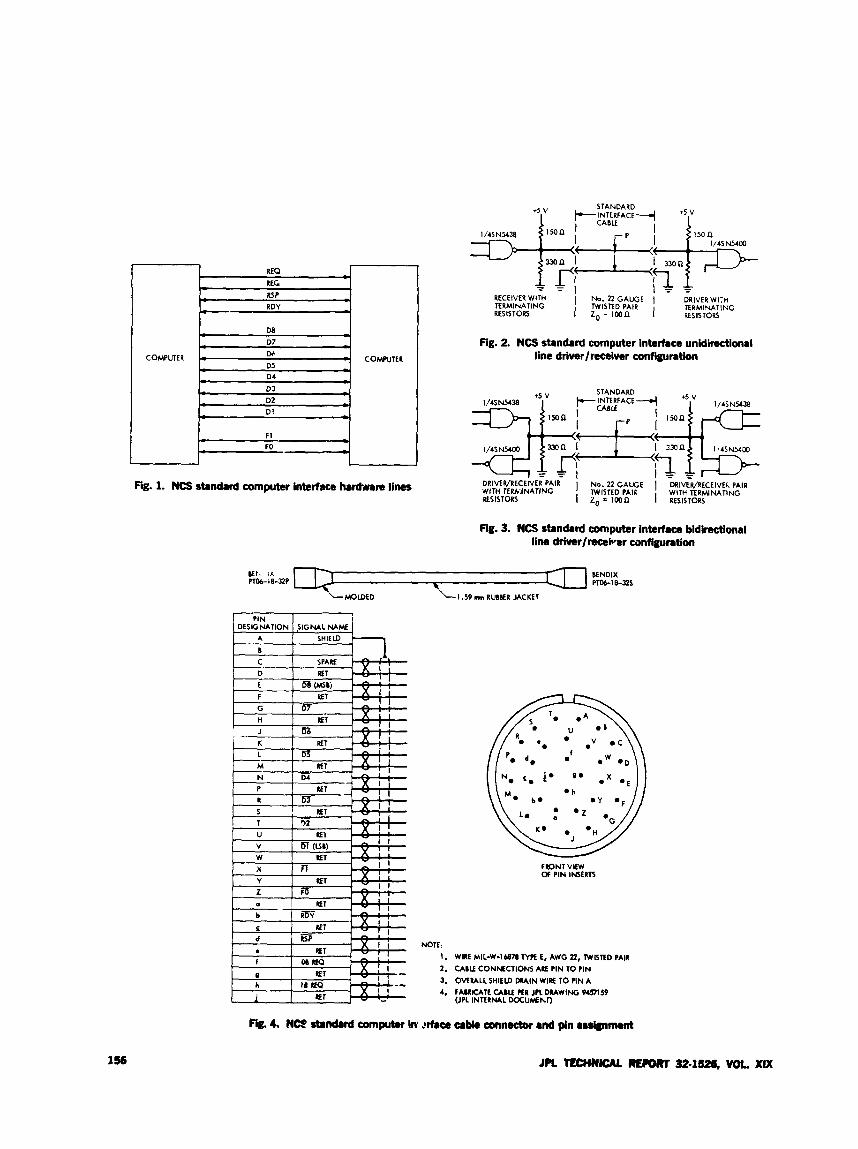
I
COMPUTER
1%
REQ
R E G U P RDY
c * - >
- I
D8 D7 D6
D5 0 4
I
I
* COMPUTER 0
I I
Fig. 1. NCS standard computer interhca hardware lines
0 D 3 D2 DI
L - * F I
L - FO
RECEIVER WITH No. 22 GAUGE I DRIVERWITH TERMINATING ' WISED PAIR TERMINATING RESISTORS I z0 - icon I RES~STORS
Fig. 2 NCS standard computer interface unidirectionri line drivar/rresiver configuration
Fig. 3. NCS standard computer interlace bidirectional line ddWf/receW8r configuration
~ M O I D E D I .59 mm R M D E R JACKEI
NOTE: 1. 2. 3. 4.
FRONT VIEW Of PIN INSERTS
WIRE MIL-W-IU~ TYR E, AWG P, wnm PAIR CABU CONNECTIONS A l PIN TO PIN OMRALL SHIELD W I N WllE TO PIN A FABRICATE CABLE RR JCL DRAWING 9457l59 UPL INTERML DocUMhI)
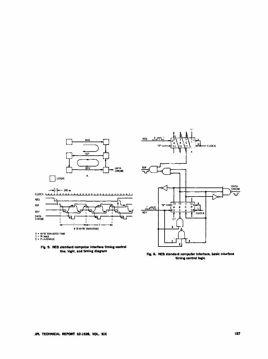
0 LOGIC
UATA STROBE
A
DATA I w STROBE I I I
I I I -1-1------L(
B &BYTE TRANSFER)
I I
T = BYTE TRANSFER TIME T = P I M u ( T 7t AVERAGE
Fig. 5. NCS standard computer int.rhce timing contrd lik, logic, and timing diagram
Fig. 6. NCS standard computer interface, baric inturface timing control logic
J K TECHNSICAL RE- 32-1526, V O L XIX
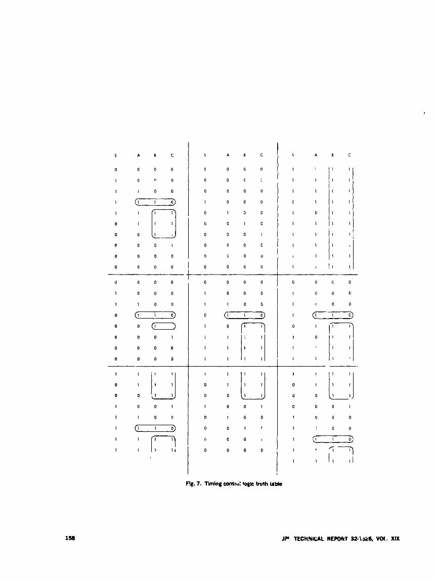
5
0
1
1
1
I
0
0
0
0
0
0 0 0 0
A 0 C
0 0 0 0
0 0 0
0 0 0
I
I 1
1 I
1 0 0
1 1 0
1
1 1
1 1
o s 1
0 0 0
1
1
1 1
0 0 0
: I 1
1
S A
0 0
0 0
0 0
1 0
0 1
0 0
0 0
0 0
0 0
0 0
B
0
C
0
0
3
1
0
0
0
0
C
0
0
0
0
0
1
C
U
0
1 0 0 0
1 1 0 0
0 (-0) 0 O a
0 0 0 1
0 0 0 0
0 0 0 0 --
: 1; 3 1
0
0 0
1 0 0 1
1 1 0 0
1 1 1 0
I r - 7 1
I
1
: 1; J 1
0
0 0
1 0 0 1
0 1 0 0
0 1 0 r
0 0 0 I
0 0 0 0
S A
1 1
1 1
1 1
0 1
1 0
1 1
1 1
I 1
I 1
1 I
0
1 : 1
1
1
1
1
1
1
11
C
1
1
1
1
1
1
1
1
1
1
0 0 0 0
0 0 0 I
1 1 0 0
1 1 1 0
0 1 0 : Lij 0
a 0 0 1
0 0 0 I
0 0 1 1
1 {I 1 0 :
I
Flg. 7. liming contrd logic truth trbk
J P TECHNICAL REPOkf 32*\&6, VOL. XIX
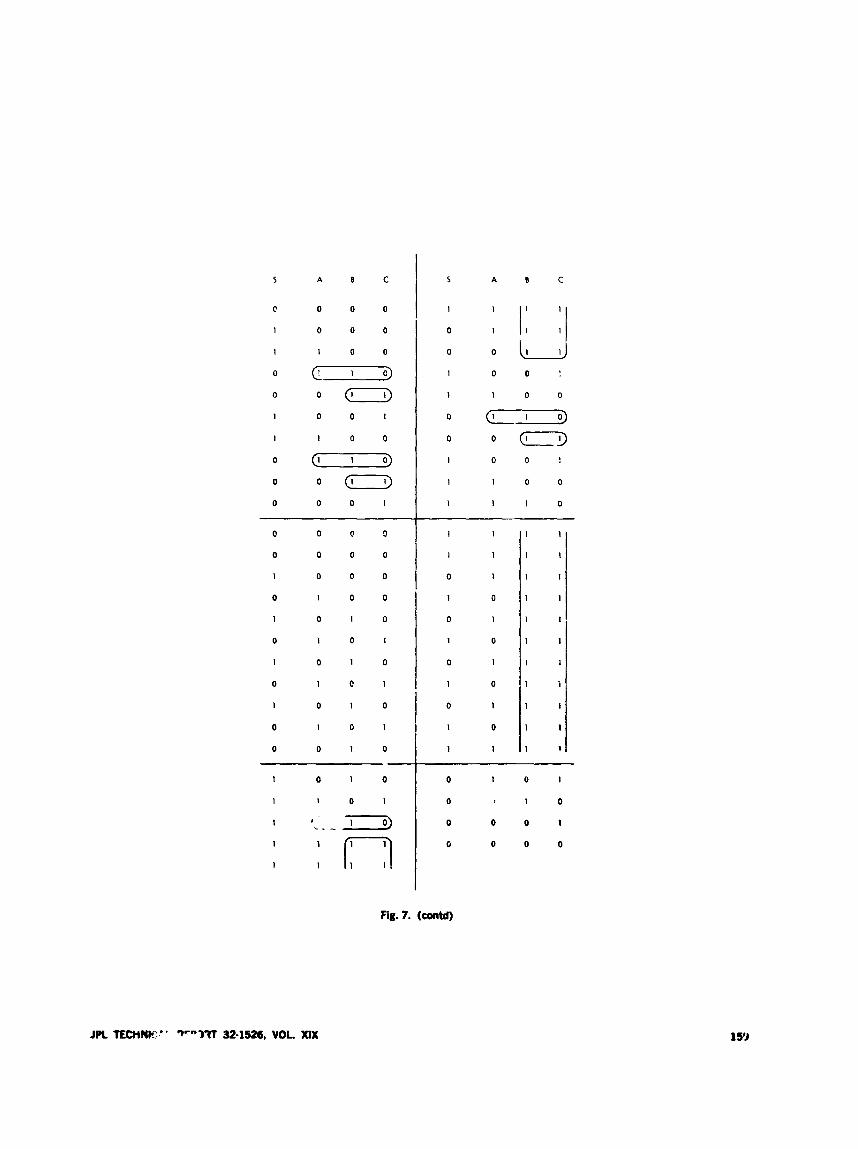
5
P
1
1
0
0
1
I
0
0
0
1 0 1 0
0 1 0 1
0 0 1 0
A B C
0 1
1 0
I 1
0 0 0
0 0 0
1 0 0
c 1 0
0 ( i i ]
0 0 1
1 0 0
1 1 0
0 (I] 0 0 1
0 0 1 )
0 0 0
0 0 0
1 0 0
0 1 0
1 0 1
0 1 0
1 0 1
A B C 5
I
0 I [ 1 3 0 0 1
1 0 0 :
1 1 0 0
0 1 1 0
0 0 (j-9 I 0 0 :
0 0 1 I
1 1 1 0
1 I
1 1
0 1
1 0
0 1
1 0
0 1
1 0
fig.7. (COnW)
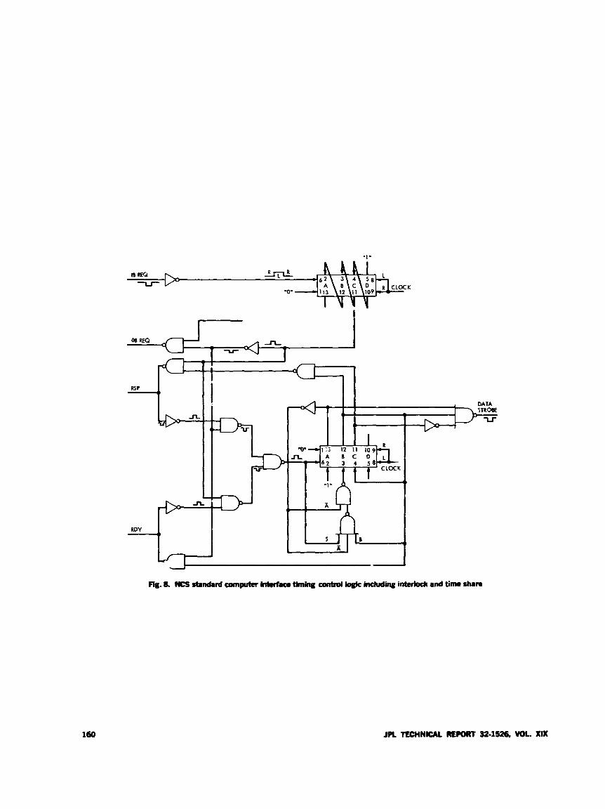
160
RSP - I
JPL TECHNICAL R E M 32.1526, VOL. XlX
High-speed Data Outage Oistribution J. P. McClure
DSlF Digital Systems Development Section
The outages experienced on the present Ground Communiaations Facility (CCF) 48Wbits/s high-speed &to wbsysten hatie been examined. An outage is defb* I as any interval when 10 01 more conrecutfoe high-speed data (HSD) blocks were receitied in err01 01 were not receioed at all. For a 3-month period in 1973, outages ranged from 2.5 s to 4.8 h in length. The median outage wos 15 s. Apprmhately 16!Z of the outages exceeded 1 min, and only I.% exceeded 15 min duration.
1. Introduction The GCF provides high-speed data transmission at a
rate of 4800 bits/s, using NASCOM circuits and Western Electric IEOiJA data sets. Data are divided into 1200-bit blocks, transmitted at four blocks per second. If no data are available for transmission, the GCF generates and sends filier blocks in order to keep the circuit active and provide block synchronous operation. Before transmission, an error detection code is calculated and included in the block. At the receiving end, a GCF decoder checks the received code and sets status bits if transmission errors are present. If blocks are not received at all, the decoder goes out of lock (into search) for an integral number of block times until flow is re-establiqhed. The receive cldta set carrier failure signal also comes on d u n g local circuit failures.
The information available from the CCF decoder has been studied to determine the distribution of the outages experienced in the data forwarded from the DSSs to JPL.
11. Outages For this study, an outage was defined as any interval
when 10 or more consecutive HSD blocks were received in error or not received at all. Intervals of less than ten blocks were considered to be error bursts. This definition is a bit arbitrary; however, 10 block times (2% I is an improbably long error burst, hence there is some justification for this choice.
For outage study purposes, slightly less than three months of 1973 data were analyzed. These data were col- lected from the normal HSD operational circuits during regular tracking passes. No attempt was made to sort the data, thotigh some data reflecting equipment malfiindions were discarded.
Outages ranged from IS blocks (2% s), to 17,513 blocks (4.8 h) in length, with long outages being in the minority. Table 1 lists outage parameters for each of the DSS gee
JPL TECHNICAL R E M 32.1- Va XIX 161
graphical areas, plus a total of all four DSS arm. Infor- mation on the performance of the Ames-JPL circuits is also ;hown.
As indicated in the tabulation, the median outages ranged from 58 to 63 blocks (14.5 to 15.75 s), a very close span considering the widely different transmission dis- tances involved.
111. Distribution The outage distribution for the combined DSSs is shown
in Fib. 1. On this plot, the abscissa indicates the percentage of the outages which had lengths equal to or less than the X-wordinate value. For instance, 71% of the outages were 100 blocks or less in length.
The abrupt breaks in the curves in the 30- and 50-block areas are caused by data set retrain characteristics. When a high data ?nor rate condition occurs, the transmit and receive data sets intempt the data flow and perform an internal readjustment sequence to compensate for changed circuit conditions. These interruptions cause data outages.
The GCF has a current commitment to restore seMce in 15 min or less. As measured, only 1.5% of the outages ex- ceed 3600 blocks (15 min). In fact, only If% of the outages exceed 1 min (240 blocks). A different definition of an outage would vary these findings; however, the GCF is definitely meeting its restoral commitment.
A future report will dlscuss the burst characteristins of faulty blocks.
162 JPL TECHNICAL RERWIT 32-1526, VOL. XIX
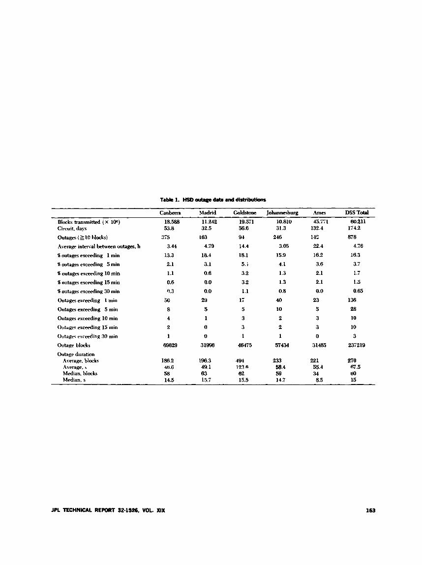
Table 1. HSD oubge data and dMbutions
Canberra Madrid Goldstone Johannesburg hmes DSS Total Blocks transmitted !X 106) 18.588 ll.24!2 19.571 10.81U 45.71 60.211
Outages ( 2 10 blocks) 375 163 94 246 142 ai8
Circuit, days 53.8 32.5 56.6 31.3 132.1 li4.2
.4verage interval between outages, h 3.44 4.79 14.4 3.05 22.4 4.76
% outages exceeding 1 min 13.3 18.4 18.1 15.9 16.2 16.3
% outages exceeding 5 min 2.1 3.1 5. ; 4.1 3.6 3.i
% outages exceeding 10 min % outages exceeding 15 min
% outages exceeding 30 min
Outages exceeding 1 min
1.1 0.6 3.2 1.3 2.1 1 .i 0.6 0.0 3.2 1.3 2.1 1.5
0.3 0.0 1.1 0.8 0.0 0.65
50 29 l i 40 23 136 Outages exceeding 5 min 8 5 5 10 5 28 Outages exceeding 10 min 4 1 3 2 3 10
Outages exceeding 15 min
Outages exceeding 30 min
Outage blocks
e 0 3 2 3 10
1 0 1 1 0 3
69829 31996 46475 51434 31485 237219
Outage duration Average, blocks 186.2 196.3 494 233 221 e70 Average, 5 46.6 49.1 123.6 58.4 55.4 W.5 Median, blocks 58 63 62 59 34 ti0 Median, s 14.5 15.7 15.5 14.7 8.5 15
JPL TECHNICAL REPORT 32-1526, VOL XIX 163

f
164
Planetary Ranging R. W. Tappan
DSN Data Systems Development Section
The phnetary mnging d l t J (PRA) determines the range, or distance, to qmmxmft thaf 01s tmceUing at Pronetary distancesfnnn Earth by measuring the time required for ri tndio signal to tmml to the spacecmfl and back. The m g e
and to provide informcdion concenring the charged particle content of spuce. dato are tlsed t6 impnwe the aocumcy of the c u h h c m * ojthespacectoft'sorbit
The P R A is able to opr?rate at the reduced Signor leoets because of improcentents in the method of mahtnining coder lock and &ecting the signal in the presence of spuce noise. I t is capable of opemtion with either S-bond OT X-bond u h e r frequencieJ and o#m soleaable code types to enable each p r q d to specify the opcmting d best suited to its particular misrsion.
The planetary ranging assembly was installed in the k p Space Instrumentation Facilitv (DSIF) to support Mariner Venus, Mercury 1973 and subsequent planetary missions. The PRA installation was necessu). because the Mark 1A lunar rangirrg cannot operate at the signal levels received from spacecraft travelbg at planet- distances. The range data are used to improve :he space- craft orbit prediction and to provide information concern- ing the charged particle con:mt of space in the path between the ground station atd the spacecraft.
The phnetar>. ranzitid as.errlbly contains digital hard- ware that performs qxxial control and dak collecting furtdions and a small general purpose computer that handles scheduling, computation, and data h a t t i n g .
The PRA is part of a ranging system that measures the round-trip time of a radio signal which trawls from a ground tracking station to B spaceaaft and back. A dtd
signal is modulated on an S-band carrier and transmitted to the spacecraft, which detects a i d rekdnsmits the signal to the tracking ,*tion. The signal received at the tracking station is delayed in time by its mid trip through space and is shifted in frequency by the doppler dect because of the relative motion between the spacecraft and tracking station. The delay is measured by synchronizing a local model of the code with the transmitted code and then shifting it into alignment with the received signal. In order to detect alignment between ths local code (receiver code) and the received signal, it is neceSSary to clock the receiver d e r at the same bit rate that is present on the received signal. This is accomplished by adding the frequency ofbet due to the L,ppler deet to the clock frequency 3f the transmitted signal. The doppler signal derived fmm the S-band carrier is SCP' ' md uwd for this purpose. Although the scaling is exact, there is a slow driit between the receiver d e r and the received signal because the carrier and the modulation are not delayed by the m e
JPL TECHNICAL 32-1- WK. XIX 146
amount when they pass through a medium containing charged particles. This difference, called diffrrenced range vs integrated doppler (DRVID), is mt.asured and output as a data type.
The PRA operates at much lower received signal levels, and therefore at greater distances, than the lunar ranging, primarily because it is implemented to use the camer doppler signal to keep the receiver coder in step with the received signal, rather than extracting the d e r clock directly from the signal. Performance has also been im- proved by optimizing the ranging code to improve the efficiency of detection, and employing a computer to nurr,erically average the received signa! 2nd thus extend the signal range over which useful information can be recovered.
The elements of the PRA that communicate with the computer do so using the DSIF Standard 14-line inter- face. This computer interface is designed to transfer data reliably over relatively long distances in the electrically noisv environnient of t5e trackhig station. The use of a standard interface makes the equipment &.sign indepen- dent of the computer assigned to it and enables equipment configurations to be changed more easily.
The PR.4 provides capability for ranging with either an S-hand receiver or an S-band receiver by using the dop- pler signal from each receiver to generate a clock signal. Either of these clocks may be selected to drive the receiver coder; the other one automatically drives a clock generator which permits measurement of DRVID only using the receiver not selected for ranging.
'4 fixed-frequency relationship must exist between the transmitter coder frequency and the S-band camer in order for the doppler rate aiding scheme to be workable. The same reference frequency that drives the S-band ex- citer is used to generate the tiansmitter coder, making the ratio between the carrier frequency and the transmitter coder frequency a fixed ratio of 1/u)Q8. The clock that drives the receiver coder is dcrived in a similar manner, except that the doppler adder adds the doppler frequency offset, proprrly scaled. A doppler signal to which a bias reference frequency has been added is used to avoid the cycle detection problems encountered near zero-frequency doppler. The bias is removed digitally by the doppler
adder. High-frequency logic is required to implemcnt the doppler adder, since additions and subtractions must be perfornied at an intennediatck frequency (66 mHz) to minimize the phase jitter introduccd in the receivcr cndvr by the stepwise adjustment of its clock phase. The inter- mediate frequency is the highest frrqurncy compatihle with the high-speed logic used.
The transmitter and receiver coders generate both con- tinuous spectrum and discrete spectrum codes. The code t?;pe to be used for the acquisition is selt*ctahle at the beginning of each ranging acquisition to enable each proj- ect to specify the code type best suited for its partioilar mission. The continuous spectrum code is a pseuJo-noise code composed of six components which are combined into a composite code that is transmitted continuously to the spacecraft. The code power at any one frequency is small, minimizing the possibility of interference with other spacecraft operations; however, only a fraction of the total code power is available to align each of the individual components. The discrete spectrum d e is composed of 20 square waves whose frequencies range from approximately 50 liHz to approximately 1 Hz. Each of the frequencies is sequentially transmitted to the space- craft, so that the total code power is available to align it. The discrete spectrum code can therefore be used at lowcr received signal levels than the continuous spectrum code. The possibility of interference with other spacecraft operations has been reduced hg mixing all components of this code with the highest frequency component.
The planetary ranging assembly was installed in the DSIF to provide range and DRVID data from spacecraft traveling at planetary distances. The measurement of range is used to improve the prediction of the spacecraft's orbit, and the DRVID data disclose information concern- ing the charged particle content of space.
Ranging at planetary distances is possible because of the performance improvement resulting from the incor- poration of doppler rate aiding, code optimi;ration, and numerical averaging of the received signal.
The PRA incorporates the flexihility necessary to sup- port future missions by providing both continuous and discrete spectrum codes which may be used with either S-band or X-band carriers.
JPL TECHNICAL RE= 32-11126, VOL. X I X
Bibliography
1. Tausworthe, R. C., “Ranging Measurement,” in Supporting Research and Ad- vanced Deueloptnent, Space Programs Summary 37-42, Vol. 111, Jet Propulsion Laboratory, Pasadena, Calif., Nov. 30, 1966, pp. 5256.
2. Tausworthe. R. C., “Communications Systems Development Minimizing Range Code Acquisition Time,” in Supporting Research and Advanced Deoelopment, Space Programs Summary 37-42, Vol. IV, Jet Propulsion Laboratory, Pasadena, Calif., Dec. 31. 1966, pp. 198-200.
3. Martin, W. L., “Special Equipment for Mariner Venus 67 Ranging System,” in Supporting Research and Admnced Development, Space Programs Summary 37-48, Vol. 111, Jet Propulsion Laboratory, Pasadena, Calif., Nov. 30, 1987,
4. Lushbaugh, W. A., “Mariner Venus 67 Ranging System Digital Rack,” in The Deep Space Network, Space Programs Summary 37-50, Vol. 11, Jet Propulsion Laboratory, Pasadena, Calif., March 31, 1968, pp. W1.
S. Goldstein, R. M., “Ranging With Sequential Components,” in The Deep Space Network, Space Programs Summary 37-52, Vol. 11, Jet Propulsion Laboratory, Pasadena, Calii., July 31, 1968, pp. 4649.
6. Martin, W. L., “A Binary-Coded Sequential Arquirition Ranging System,” in Th I Deep Space Network, Space Programs Summaiy 37-57, Vol. 11, Jet Propul- sic.) Laboratory, Pasadena, Calif., hlay 31, 1969, pp. 72-81.
7. Lindley, I. P., The P N Technique of Ranging as Applied in the Ranging Sub- sysfem Mark I , Technical Report 32-81 1, Jet Propulsion Laboratory, Pasadena, Calif., Nov. 15, 1965.
8. Planeta-, Sanging Assembly Firnctwnul Requirements Document, FM509136, Sept. 27, 1973 (JPL internal document).
9. Plunetay Ranging Assembly Technical Manual, TM509201, Sept. 15, 1973 (JPL internal document}.
pp. 63-67.
JPL TECHNICAL REPORT 32.1526, VOL. XIX 167
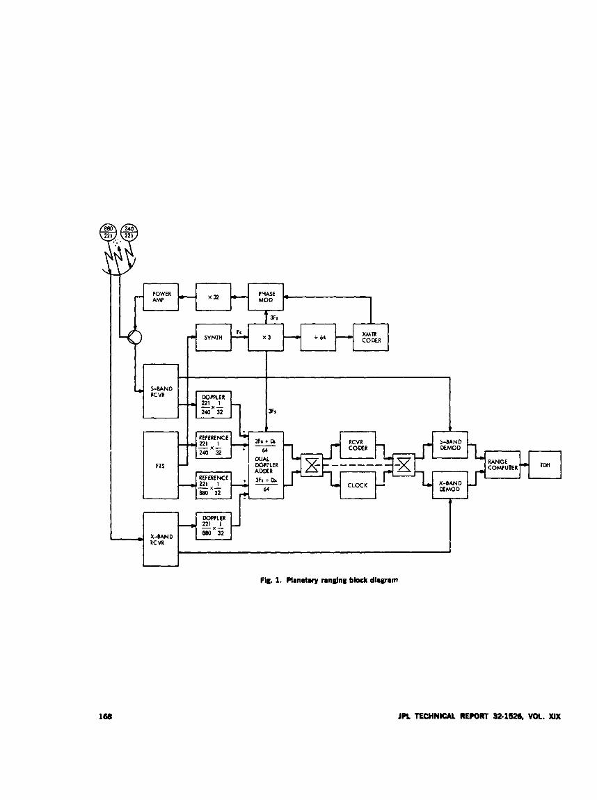
RANGE COMPUTER.C
DOPPLER
880 32 - - 221 xL
X-BAND RCVR
1
rw
168
Fig. 1. Planetary ranging bladr diagram
JPC TECHNICAL REPORT 32-1526, WK. Xu(

Adjustable Tuner for S-Band High-Power Waveguide J. R. Loreman
R. F. Systen s Development Section
As part of an effort to reduce the DSN trancmitter backyntiw ut DSS 14, an adjustable S-band icaueguide tuner for use crt 400 kW has been dpueloped. The tuner will be used to improoe the match of the transmitter waueguide to the antenna feed system at DSS 14 in an efort to reduce transmitter back power at certain operating frequencies caused by high uoltage standing waue &io (VSWR) in the feed.
because of various waveguide modifications to the transmitter waveguide run at DSS 14 (Ref. l), the wave- guide match of the run has changed, causing high trans- mitter back power. Measurements have been conducted in an effort tn determine the corrective measures re- quired (Ref. 2). The measurements, as well as reports by operating personnel, indicated that the S-band polariza- tion divvrsity (SPD) cone configuration in particular requires an effort to reduce back power at certain oper- ating frequencies. Zigures 1 and 2 show the voltage standing wave ratio plot of the waveguide from the DSN transmitter through the SPD cone in right circular polar- ization (RCP) and linear polarization, Calculated back power for each VSWR has been included on the charts.
Further measurements have been made at DSS 14 to determine the effect of a waveguide ttining section on the VSWR. The tuning section used was a low-power broad wall vane type tuner and, though not of a design applicable to high microwave power, its characteristics approximate deflection of the broad waveguide wall, a
technique frequently used for tuning of high-power waveguides. Figurc 3 shows the match a; low p c w r through the SPD cone in linear pdarization, with the tuner at the transmitter input to the waveguide. The effect on the VSWR with respect to frequency is ap- parent when this figure is compared with Fig. 2. From the testing, it was apparent that a simple tuner based on the controlled deflectior of the waveguide broad wall would probably have sufficient tuning effect to rfduce the VSWR of the SPD cone configuration to approxi- matsly 1.12 across the band of 2110 to 2120 MHz. The advantages of such a tuner are simplicity; direct a. ;ilica- tion to the high-power configuration, as the tuner could be easily water-cooled; small size, as no auxiliary cavities would be required; and simple mechanical design. The main disadvantages are felt to be a limited frequency effect and limited retuning capability due to work- hardening of the copper waveguide. Both of these dis- advantages may be crucial to the acceptability of such a simple design, as the changing of any one of the major reactive components in the waveguide run or cone will
JPL TECHNICAL REPORT 32-1526, VOL. xu(
rcquirc. rctuning. niid thc. cotiiplcs nature of the niis- tnatcli tnay rqui rc sc.\wral tuncm of this type. For thcw reasons, a parnllcl tunw drdopnieii t bascd on the cnu- pling of a \va\-c.guidi. section to aii adjustablcx cavity through thc narrow \viill is being pursued (Ref. 3).
H a s d on ;i simplt. \vaveguide broad wall dc4irction sthenic,, a prototype adjustable tuner has been dcsignid ;ind fubricatcd ( SCT Fig. 4). Thr. broad \valls havc. btwi tiiacltintd to appro\iiiifitcdy 0.25 cni to minimize work- burdening of the coppcr wall, and \vntc.r-cooling ducts a rc providcd 011 both narrow \valls. The n ~ c h i ~ n i s i ~ i allo\vs bidirt.ctiona1 cfeflection of both \vaveguide broad walls. \Vavcguide structural rigidity is provided by both thc water-cooling ducts and thc. stainless stecl deflection
bars. Laboratory tests indicate. that the tuiicr caii uti
adjustrd from a YSWR ot 1.01 to 1.15 up to four tiiiic~s I)cforv thc cop pi^ \vavt.g“id(. \valls begin to visually show \vorL-Iiardcnin~. Thus, it appcars niorc tliniiig flcsibility niay c G t than \vas cywcted. Thc prototgxx tuner h:.s 1,iwi operated at ;i power Icvd of 100 L\V for several liours \vith 110 heat buildup on the thinricd broad \valls of thr \vavr.guitlc.. I t apptws that thc tuurr ;it its orcsent level of dc~velopincwt m a y bc oprmtionally installrd. Sevcral additional tuntw have bc.cm fabricated, and one tuner will be installed at DSS 14 in the 4OO-k\V radio sciencr transniitter waveguide run to the SPD cone in January 1974. Rased on the results of this instilllation, the tuner may be installed in the DSN high power trans- mitter \vavc.guidc run on an interim basis.
Ref e re n ces
1. Leu, R. L., “X-Band Filter,” in The Daep Space Neticurk Progress Report, Technical Report 32-1526, Vol. XVI, Jet Propulsion Laboratory. Pasadena, Calif., Aug. 15, 1973.
2. Loreman, J. R., “Waveguide Installation Measurements at DSS 14.” in The Deep Space Network Progress Report, Technical Report 32-1526, Vol. XVI, Jet Propulsion Laboratory, Pasadena, Calif., Aug. 15, 1973.
3. Buchanan, H. R., “Variable S-Band High-Power Tuner,” i . 3 .-..e.
170 JPL TECHNICAL REPORT 32.1521, VOL. XIX

I 1 2110 2115 2120
FREQllEl :Y, MHz
Fig. 1. VSWR 400-kW tranom.tter through SPD cone (RCP)
JPL TECHNICAL RE#)RT 32,1526, VOL. XIX
t +'
x U s
FREQUENCY, M l z
Fig. 2. VSWR 400-kW transmitter through SPD cone ,linear polarization, 359 deg)
1.12
1.57
1 * 0 4 t I
l x 126 2 1 LINEAR POLARIZATION
359 deg
1.02 L L 140 2110 21 I5 2120
FREQUENCY, MHr
Fig. 3. VSWR 4OO.kW tnnrmittor through SPD cone, vane-typa tuner iiistrlld
171
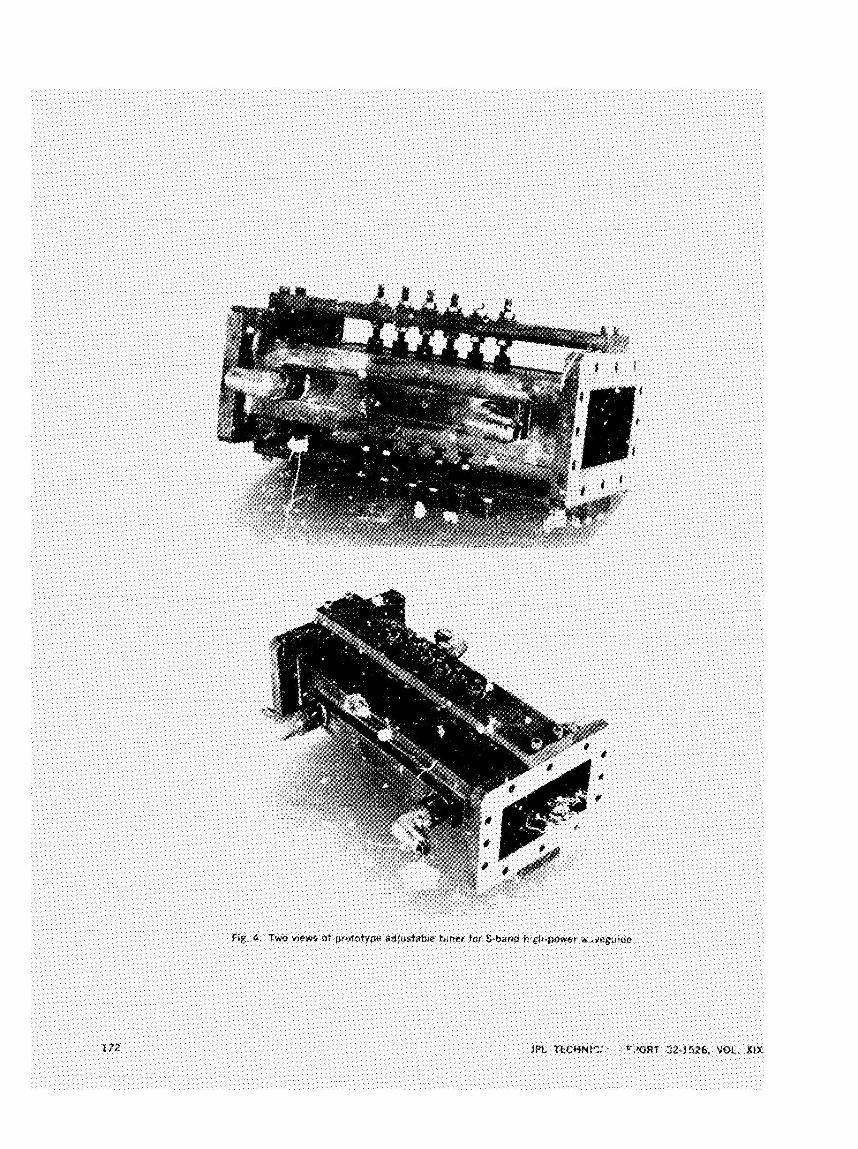
X-Band Antenna Feed Cone Assembly R. W. Hartop
R. F. Danbpnmt Secti0.i
'The new X'Smr, feed cone d i e s for the DSN 64-m antenna siations am & rondruction. The feed S u W l i e J haace been cmpleted, and r l ther progress to date is rrprted.
In trpporr of Viking a d future p~jecb, the DSN mwt proviuc fa-. X-band sign31 -or. at the three existing 64-m antenna stations. The L i g n of a new feed mne assembly for this purpose was descrhed in Rd. i.
The feed sibasscmblia for the three cones have now been completed and are shown in Fig. 1. "be top plate, %-hi& s-a! the cone openiag a d su;ymrts the feed without Additional members, i: shown resting on a w d e n frame that serves z.= b storage and *.:portation cnclosure.
Not yet mounted on t? assembly is the X-band ..vaveguide switch to -!d either the feed 3' P calibrated load for the traveling wave maser. Its i. .wntilg; plate may be s a n at the lowcr end oi the feed.
The lowest com;mnent in t'ie f e d , wl. .vi11 attach directly to the waveguide switch, is !I 2 circular-to- rectangular wavguide transitiorl. This uc?ifonn trancicion is i~rmed by electroadischarge mac'lining of a =!id
copper forging with a tool &e that s h r n on the righ. in Fig. 2
The tool illustrated is a funning tool that is a copy of a master tool pwxated on a pmgrammed machine. several of these tools are used as elearodes to form a transition wch as th: alumirtum t a t piece also shown in Fig. 2. Thc trans;tion. when hished, is 10.16 cm (4.000 in.) long and unifvmly transfonm a 3.477-ctn (1.389-in.) diameter circular wav,.guide intu a 3.175 X 1.587 cm (1.250 X 0.625 in.) rectangcbr waveguide.
The next section above t'r.e trmsition is a circular waveguide section that serges as a higher-9de cootrol between the tiansition and polarizer, which is the third section. Both components are made from soSd coppm forgings, tile polarizer by electrondischarge machining, and thlp ciri.uhr waveguide section by conver~tional Tachining.
The polarizer is a quarter-wave plate dcsign and is the same z that used successfulljr in the Opera..ond Tinle
Sync Jlicro\va\ e Subs>-stem (Ref. 2). escept for dimen- sional scding to this frcqucwcy band.
Tht tourth wivtxwide section is another circular wive- ,ui~lc 5pct-r identicd to the second stytion. Besides pro\ idinq additiona! nlodc control, these hvo spacer sw- tions. totaling 3.2 m i :S in.) in iength. will provide for future tnadific--tions it. the f e d without greatly increas- ilkg its leneh. For c-.ump:e. rotary joints for the polarizer could tw added without changing the overdi length by substituting shorter spacer sections along with the new rotary joints.
The fwd horn is fabricated in four sections. of which the top three are aluniinum for weight reduction and cost saving. and the lower wxtion (seen with a support clamp in Fig. 1: is OFHC copper. The horn is othenvise
identiwl to that in the Time Sync Systcwi (Ref. 2). cscvpt that the honi throat \vas not modified. Thus, the 3.-K-cni 1.369-in.) dianwtcr circdar \\-avc*guide is maintaintd
throughout the fed
The voltage staading \\-ave ratio (VSn'Rl of one of the f c w l asscmblie. canialcte with the tmn>ition. is shown in Fig. 3 over a \vide bandwidth. The actual operation of these ft& in the near future \vi11 be over a narrow band near sulo Jf!iz.
The intc-nial B m r s and ladders for the cane assemblies hart kvn f;ibricattd. ;tlong \vith variotis brackvts and panels. ..\ssemll? of these parts and the f t d subassem- blies into the COW s t d b has begun, \\ith completion scheduled More the end ot the 6rst quarter of calendar y w r 1974.
References
1. Hartop, R. W., 'S-Band Antenna Feed Cone r\Jsembly." in The Deep Space h'etrcork Pmcress Repcrt, Technical Report 32-lS26, k'ol. SVII, pp- 131-133, Jrt Propulsion L a h t o r y . Pasadena. Calif., Oct. 15.1W3.
Spnce K'etrcork Progress Report, Technical Report 32-1526. V 1. VI. pp. 165- L E , Jet Propulsion Laboratory. Pzsadena, Calif., Dec. 15, 197.
2. Hartop, R M'., Tlperationai TI~IW Sync \ticis.i;avc E&y;.tern," IP The D R ~
174 JPL TECHNICAL REPORT 32.1- VOL. XIX
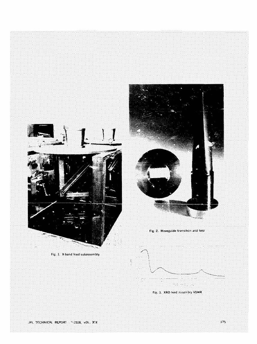

Variable S-Band High-Power Tuner H. R. Buchhnan
R. F. SymmS D ~ d ~ p m c n t Section
A wriablc, high-poum ux~lieguide tuner that can be remotely contrdled is being deoeloped. satisfacto?( opemtion at a 400-kW poccer leGel is the god. Progrm to &e i s reported.
1. Introduction Recent -neasufements of the DSS 14 transmitter wave-
gxide installation (Ref. 1) have emphasized the need for a rompect tuning device that can be used at strategic points in the waveguide system to improve the match. This device must operate at 400 kW and have the capa- bility of correcting 1 mismatch in ?he order of 1-10 to 1.15 voltage standing wave ratio (VSWR). A m a n d y adjustable device that can be retuned a limited number of times has been developxi far the immediate need (Ref. 2). Tbis report d d b e s 'a longer range develop ment of a variable tuner that can be adapted for retrote control and. if required, programmed control.
11. -of Operation
type 17 ith a restricted range of motion to avoid operation at or near resonance. The short is an exjsting design that has been used satisfactorily at 20 kW.
The power level coupled into the H-plane arm is con- trolled by the diameter of the circuIar aperture in the sid- wall t,f the main waveguide. Figure 2 indicates the theoretical coupling as a function of the hole diameter with correction for the waveguide wall thickness (Kef. 1). When the H-plane ann is tminated bv a short circuit, the mismatch introduced into the main waveguide is a function of the power coupling and the short position. Figwe 3 id' i t a &e theoretical SuSCcPt;dnce variation (Ref. i\ .i!culateci for aperture diameters of 3.81 and 4.70 &m. It is noted that the larger aperture &or& a krger tuning range with a less steep slope in the hegative susceptance region.
111. RatotypeTests Thc miLmwave circuit of the vari?Yc tuner is depicted in Fig. 1. A pottion oi the main WR 430 wavegiide sig- r -' is coupled to an H-plane arm terminated in a variable position short. The short is a movable, iioncontachng
A waveguide test samp!e has been fabricated and tested at low power, using several coupling apertuo
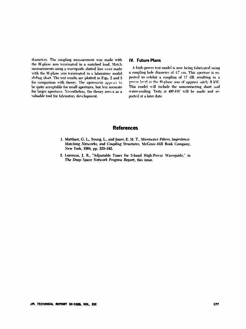
diameters. The coupling meaurement was made with the H-plane arm terniiiiated in a niatched load. Match measurements using a waveguide slotted line were made with the H-plane m terminated in a laboratory model slidiiig short. The test results are plotted in Figs. 2 and 3 for comparison with theoy. The agreenient ;il-.p,ri-s ts be quite acceptable for sniall apertures, but less accurate for larger apertures. Severtheless, the theory servLs as a valuable tool for labraton; development.
IV. Future Plans -4 hikh-power test model is now being fabricated using
a coupling hole diameter of 4.7 cm. This aperture is es- pecttd to eshibit a coupling of 17 dB. resulting in it
p.-.-t~ !e*.-?! ir? the H-plane arm of approsi ,hate!? 8 U V . This model \ d l include the noncontactirrg short slid water-cooling. Tests at W-kif' will b made and re- ported at a later date.
References
1. Matthaei, G. L., Young. L., and Jones, E. M. T., 3ficrou-'ace Filters, Impedance- Matching Networks, and Coupling Structures, McGraw-Hill Book Company, Sew Yo&, 1964, pp. 229-242.
2. hreman, J. R., sAdjustable Tuner for S-band High-Power Waveguide," in The Deep Space Network Progress Report, this issue.
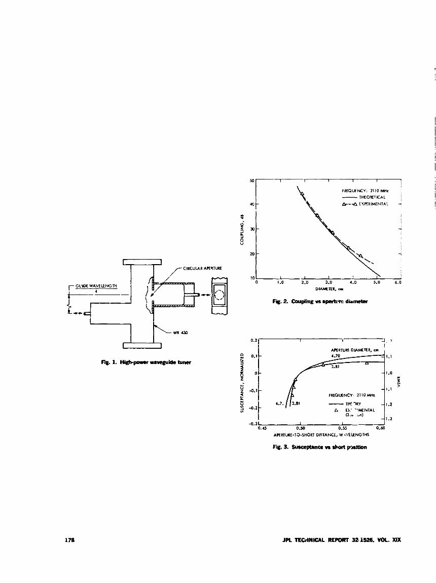
I /CIRCULAR APKPTURE I
: 0.1
6 O '
E z -0.1'
h
ii z
<
Fii. 1. H i - m -ids tu-
APERTURE DLAMETER, an , '
i
- THEOLTKAL ' i i k-4 EYERMNTAL 1 40
20
!O 5.0 6.0 0 1 .o 2.0 3.0 4.0
DIAhKTER, cat
4.70 2
a
-
- FREQIXNCY. 21 10 W
- THT7RY -
Fa. 2 Couplii VI rpcrtr?rc d i
1.1
1.0 d
F 1.1
1.2 A EX' ''MENTAL
0.b 4 - 1.3
APERTURE-TSSHORT DISTANCE, W h'/ELENGMS
Fig.3. SutccpZ.ncendortp#itkn
JPL TECdNlCAL RE- 32.1526. VOL. XIX
A No-Load RF Calorimeter R.C c'nerqoff
R. F. Systems Dewcpment Section
A ~ t e l RF calorimeter is described a d anabp?d. The dmice combines the comercation of e.iergy principle with the dc substitution idea to eliminate the need for RF and/or de loads, thereby prmiding highly accurate "on-line" mcasut&me~lts o\ RF PPCP ..; low c a t . Breadhnard tes: d c t ~ cii-c' rcyortcd.
1. General Description Consider any source, 9 of power that accepts dc (or
low-frequency) power, Pdr, produces output power, P,,, and rejects dissipated power, P d i r r , to an external heat sink, If Pdc, P,, and Pd,** arc considered average values, conscmation of energy implies
v-K..I in turn suggests the analog circuit of Fig. 1 for 1 .I$ P.8.
I . 1
' . 1 , .
* I ' -1 ot thc device consists of correct adjustment r: 11 scale deflection and zero of the P, meter.
F d i . . input to the analog subtractor dis- _. it -1town value of P,,. is applied to the source.
7' .;.i "Pd,," ;.e., tnat voltage (preferably at or .it., corresponding to Pdr. Secondly, the P,
I . I w t v ;c, :hen adjusted by meam of potentiometer
(: .* ,
meter zero is set by pt R2 under the following condi- tions: (1) Pdlrr inputs is reconnected, (2) some value of P d , > 0 is applied to the source, (3) the source is ad- justed far zero output.
Since the mnservation of energy principle applies to evrry form of energ), P,, ckn be any kind of power whatever; the utility of the device dep-1 3s only on whether Pdc is easier to measure <:;an Po, ..,id not on the "species" of either. But the most obvious application, and the only one considered here, is to RI' power sources, although for our purposes the term "RF source" can be very bnadly interpreted to include any dc (or 60- or 400-Hz) powered source of electromagnetic powcr, P,, from very low frequency (VLF) to light.
The principal advantage of this device over conventional RF power messurement devices is that it enables "on-line" mehsurements, i.e., measurements of radiated power, with accuracy hitherto attainable only with dc substitution
calorimeters (Rtf. 1). It is. in fact, a kind of dc substitu- tion nlorimeter in \vhich the source itself serves as the dc load, but since it does not require an RF load (or an external dc load for dc substitution), it i s much cheaper than a conventional R F calorimeter. For this reason one is tempted to call it a ''poor man's calorimeter," but we will stick with "no-load calorimeter" (NLC) for the pur- poses of this a-ticle.
The principal limitations on the applicabilit:.r of the NLC are: (1) scurce efficiency must be relativel\ high to obtain good accuracy. (2) it must be possible to operate the source in a P, = 0, Pdr > 0 mode to set the P,, meter zero (this is difEcult or impossible for some oscillators, e.g., magnetrons), and (3) the device can only measure the power at the output port of the source, not at some remote point in a transmission line or in free space.
II. Error Model Figure 2 is an approximate lumped equivalent circuit
for beat flow in a typical fluid cooled R F source. Most of Pd,,,, viz PI flows from dissipation sites within the source (e.g., a tube anode) through an internal heat exchanger (e.g., coolant passages or fins in the anode) to the coolant. R , , represents the thermal resis%ance of the internal heat exchanger. The coolant then carries PI to an external heat exchanger that re ice it to an infinite heat sink a; T, through equivaltnt thermal resistance BIZ. If the cooling system is closed, R,Z is shunted by thermal capacitance C, which represents the finite heat capacity of the circu- lating coolant. Pp is the fluid frictional loss in the internal heat exchanger. Heat le;*kage fnn the source is repre- sented by the shunt F. ;e infinite heat sink at T,.
From Eq. (1) and e1emc:tary circuit theory we have
where
and
is an error sinks at T, In general. of time.
180
term due to P, plus the heat flow between and T, through leakage conductance l/R2. T, and To, hence P,, are random variables
We assume that only P,, the heat carried from the source to the external heat exchanger by the coolant, is sensed, so that the output voltaqe, c,,, of :he NLC is
I;, at some time, sa)- t = 0, and at some positive value, Pdp(0), of Pdcr we adjust the zero of the P, meter in the manner described above. we set
11 = a (1 + a)/( 1 + e,,) (5)
where E,, = P,(O)/P,,,(O), and Pr(0) is the value of P, at that time. From Eqs. (2), (4). and (5 ) we find that at any future time, t ,
where APr(t) = Pc(t) - Pr(O) , and we have assumed eo small enough to write Q = d ( 1 + E,,). From Eq. (3) we see that Pr, hence APr(t), is independent of Pa,, hence of Pd,.,, SO the two terms of AP, are uncorrelated, and the r m ~ value of APn, ntls(APn), assumes its minimum value,
at J d,+.(t) = pdc(0). To minimize rms(AP,,), therefore, one must not only be able to estimate the value of Pdisn but one must also rezero the Po meter \\irtx.ever Pzinr changes. The obvious way to get around this difficulty is to add a signal proportional to P,(O) to the analog computation of Po as, for example, in the circuit shown in Fig. 3. The P,, meter zero is first set with the P, compensation pot, RS, at P d r = 0. Then, with Pd, > 0, the Pn meter is again zeroed with R2 as previously described. This adjustment eliminates the Pdr(0) - Pd,,, bias term from Eq. (6).
Theoretically, the Fr compensation enables one to realize nnS( APn) = min [ rms(APn)] = m [Ape( t ) ] , i.e., elimination of all errors except those due 10 random fluctuation of Ti - To. The cost is ;light: one addi..mal adjustment making three in all (51, IZ2, a:rd h3), none of which need be repeated when P d c or I 'dins change. On the other haid, the benefit may ilso be slight if, for example, rms [APe(t)] )> ave (Pe ) , or if instrumentation errors swamp both.
Note that leakage conductance l/R, enters into the error term P, only through the relatively small gradient T i - To, not through the large gradient between the
JP, TECHNICAL REPORT 32-1a . WK. XIX
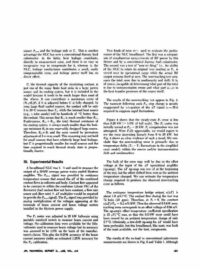
source P,,ixa and the leakage sink at T,. This is another advantage the NLC has over a conventional dummy load calorimeter: in the latter, heat leakage contributes directly to measurement error, and there is no easy or inexpensive way to compensate for it, whereas in the NLC, leakage coiiductance contributes a small, easily compensatable error, and leakage power itself has no
. direct effect.
C, the thermal capacity of the circulating coolant, is just one of the many finite heat sinks in a large power source and its cooling system, but it is included in the model because it tends to be much larger than most of the 3thers. I t can contribute a maximum error of ( R , , / R , ) P , if h is adjusted before C is fully charged. In most large fluid cooled sources, the coolant will be only 5 to 10°C warmer than T,,, while the internal heat source (e.g., a tube anode) will be hundreds of "C hotter than the mian t . This means that R,2 is much smaller than R, , . Furthermore, R,, -k R l z , the total thermal resistance of the cooling system, is always much smaller than the leak- age resistance R? in any reawnably designed large source. Thertfore, R,?<< R, and the error caused by premature adjustment of b is very small. This rezoning may not hold for small sources that have relatively large heat leakage, but C is proportionally smaller for small sources and the time required to reach thermal steady state is propor- tionally shorter.
111. Experimental Results A breadboard NLC was b It and used to measure the
output of a 10-kW average power water cooled klystron amplifier. The P d i r a signal was provided by resistance temperature sensors that sensed the AT of the combined coolant flows in collector and body. Coolant flow appeared to be constant to within the resolution (about 1%) of the flowmeter (hac! coolant flow not been constant, a flow rate sensor and (flow rate) X AT multiplier would be required to provide the P,,,,, signal). The I'dc signal was provided by analog multiplication of the voltages appeuing at the terminals of beam current and beam voltage meters installed in the klystron power supply.
Two kinds of tests WP. used to evaluate the perfor- mance of the NLC breadboard. The first was a compari- son of simultaneous measurements of RF power by this device and by a conventional dummy load calorimeter. The second was a test of "zero tr.-:king," i.e., the ability .of the NLC to retain its original ?ero reading 3s P,,, is varied over its operational range while the actual RF output remains fixed at zero. The zero-tracking test mea- sures the total error due to nonlinearity and drift. It is, of course, incapable of determining what part of this total is due to instrumentation errors and what part in the heat transfer processes of the source itself.
The results of the zero-tracking frst appear in Fig. 4. The transient following each P+ step change is greatly exaggerated by iiitcgration of the AT signal (7 = 25 s) required to suppress rapid fluctuations.
Figure 4 shows that the steady-state P,, error is less than 0.20 kW (= 1.0% of full scale). The Po irieter was initially zeroed at P,Ir = 20 kW. P, compensation was not attempted. Were P,(O) appreciable, we would expect to see the error increasing linearly from 0 to 20 kW, but Fig. 4 shows no clear evidence of such a trend. We con- clude that the zero-tracking error is primarilv due to temperature drifts (Ti - 2'" fluctuations in the simplified error model) within the source and/or instrumentation drift and nonlinearities.
The bulk of the error may well be due to the offset voltage at the input of the AT operational amplifier (op-amp). The AT op-amp was ze rcd at the beginning of the test, but the offset drifted from zero as the ambient temperature changed. We can estimate the temperature change required to produce the observed zero-tracking error as follows.
The resistance temperature bridge output, u(AT), is about 1.0 mV/"C. The coolant flow during the test was ?fL lmin (19 gpm). Therefore, at Po = 0, the constant c(hT)/P,, = 0.2 mV/kW. Thus the observed 0.2-kW zero- tracking error corresponds to an offset voltage of 0.04 mV. The op-amp's offset temperature coefficient specification is 15 ;V/"C max, so that the 0.2-kW ezor Auld have been cniised by an ambient temperature 2hange of only 2.7"C. Obviously, a Iow-drift op-amp foi AT would have been preferable, but this breadboard, like most, was built of the most avai!able, not the best, compouents.
The P , meter waq adjusted to 20 kW full-scale using portable standard meters to measure beam current and voltage. No Calibration data were av.dable for the kilo- voltmeter used to measure beam voltage but its accuracy was assumed to be 1.0% on the basis of the manufac- turer's claims. This plus the 0.25% accuracy of the beam current ammeter yields an estimated 1.255% accuracy for the P d c calibration.
The resiits oZ the no-load vs conventional calorimeter measurenients are shown in Fig. 5 and Table 1. Although
JPL TECHNICAL REPORT 3L -526, VOL YIX 181
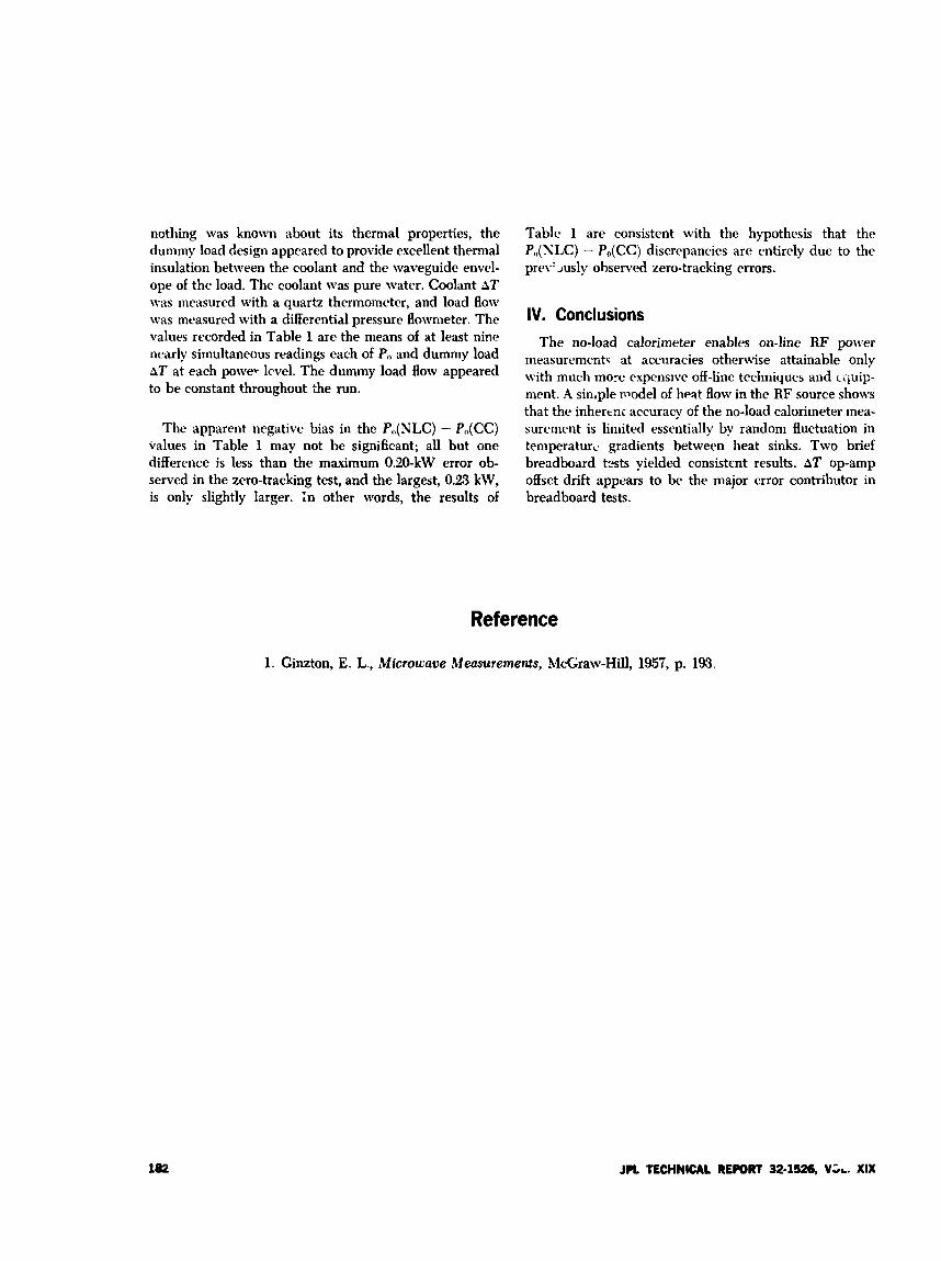
nothing was known about its thermal properties, the dummy load design appeared to provide excellent thermal insulation between the coolant and the waveguide envel- ope of the load. The coolant was pure water. Coolant AT mas measured with a quartz thermometer, and load flow was measured with a differential pressure flowmeter. The values recorded in Table 1 are the means of at least nine nearly simultaneous readings each of Po and dummy load AT at each pO\ve. lcvel. The dummy load flow appeared to be constant throughout the run.
The apparent negative bias in the P,(NLC) - P,(CC) values in Table 1 may not be significant; all but one difference is less than the maximum 0.20-kW error ob- served in the zero-tracking test, and the largest, 0.23 kW, is only slightly larger. In other words, the results of
Table 1 are consistent with the hypothesis that the P,,(NLC) - P,(CC) discrepancies are entirely due to the prey: Jusly observed zero-tracking errors.
IV. Conclusions The no-load calorimeter enables on-line R F power
measurement< at accuracies otherwise attainable only with much more expensive off -line techniques and ccjuip- ment. A sin,ple alodel of heat flow in the RF source show that the inherenc accuracy of the no-load calorimeter mea- surement is limited essentially by random fluctuation in temperature. gradients between heat sinks. Two brief breadboard t s t s yielded consistrnt results. AT op-amp offset drift appears to be the major error contributor in breadboard tests.
Reference
1. Ginzton, E. L., Microwaue Measurements, Maraw-Hill, 1957, p. 193.
182 JPL TECHNICAL RE#)RT 32.1526. V L . XIX
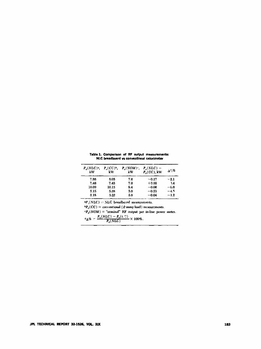
Tablal. Comparison of RF output measurements: NLC breadboard vs conventional calorimeter
P,(NLC)a, P,(CC)b, P,(NOM)c, P”(NLC) - k\V kW kW P,(CC), kW *‘*%
7.88 8.05 7.6 -0.17 -2.1 7.46 7.43 7.0 i 0.03 1.4
10.09 10.15 9.4 -0.08 -0.6 5.15 5.38 5.0 - 0.23 - 4.5 3.18 3.22 3.0 -0.04 - 1.2
--
*P,( N E ) = KLC breadboard measurements. bP,( C C ) = conventional (dwnmy load) measurements. cP,(NOM) = “nominal” RF output per in-line power meter.
JPL TECHNICAL REPORT 32-1526, VOL. XIX 183
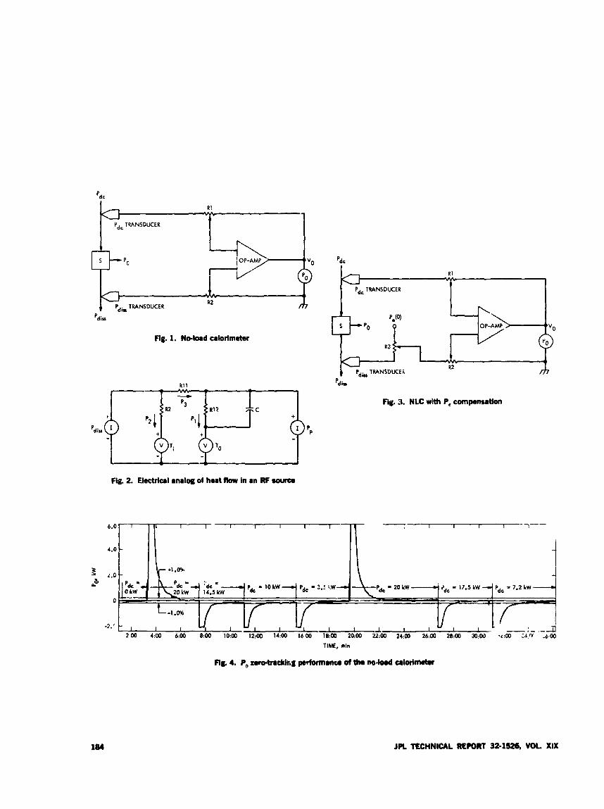
'dc
R1
Pdc TRANSDUCER
'diu
Fig. 1. No-load crlorimeter
Y I 1
Fig. 2. Elcctritll analog of hert flow in an RF source
?
= P b ::I;* 0 -
'dc
RI
Pdc TRANSDUCER
' d i e
Fig. 3. NLC with P, compensation
' Pd, - 20kW
184 JPL TECHNICAL R€.pORT 32-1526, VOL. XIX
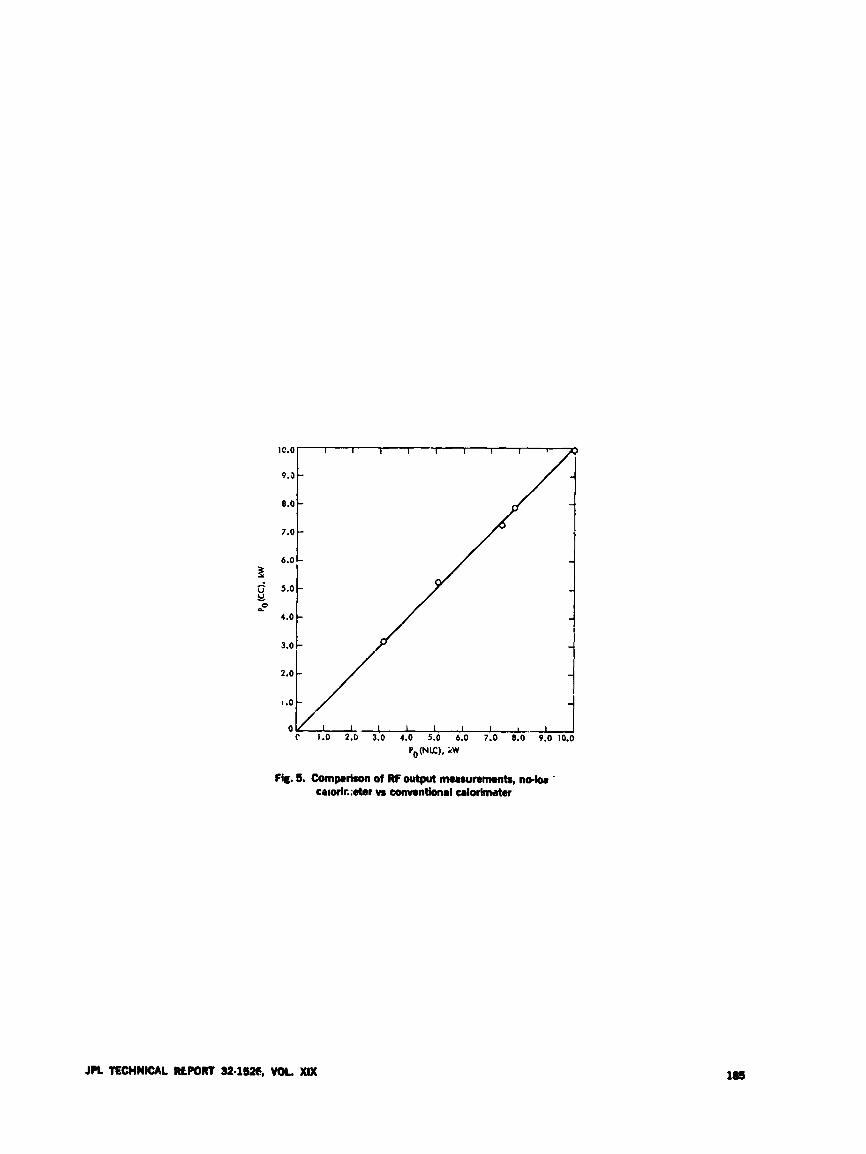
Fig. 1. ComplrirOn of RF output mrrunments, n e b . coiorir.:eter VI tonvontional ulorinwbr
J n TECHNICAL RLPORT 32.1526, WK. XIX
Dual Carrier Preparations for Viking D. A. Bathner
Communications Elemevts 3esearch Section
0. W. Brown R. F. Systems Develbpment Section
While simultaneous t-ansmission of :bo S-Land carrisrs from a siuyle Deep Space Station is no Zonger n comnittcd operb.ting m i l e fof Viking Project sup- port, thc program of investigi tior and ahatcment of noise bursts a d : +et- mcduktron intetjcrenct! has continued through the fitst three calerdar qrcctd 'P of 1973. At DSS 14, internal waoeguide nnrl extsrnal antenna **.ark :iirlded m i G r
-eductions in both types of interferencq. Suppoi.ing inocstigation : were dso conducted at JPL and at DSS 13 during this pdriod. Conclusions and recom- mendations for futuro work w e presented.
1. lntroducticn The continuing program of investigation and ai .?lent
Df interfcrence arising from single- and dual carrier t rax- inis.ion from a Deep Space Station shifted emphasis to D5.< 14 ear!y in 1973. The exteniive work at 3 S S 13 dur tIg 1972 (Refs. 1 and 2) was continued in the first half of 1972. in order to obtain long-term data ari: ti)
perform speci6c expvrin.ents in support of thc 6 4 - . i s antcnna effort. This work has been reported in detail by Petty and Jackson (Refs. 3 and 4). This a "icle will emp' a- Eize results at DSS 14 and, with the aid of an extensive rcfermcc. list, will serve as a final report for the 19721973 program.
On the '\* hclr , the eifori at 3 S S 13 served the inteirded purpose of confiiming prior hypotheses, ideaitifying
sources of interference, developing ron;e;ia! .ocedures, and esiablishing imprwed methods cjf iri:trv*nenta:inn. Although sic:.:ifii.nnt reductio11 of internal soil. ce: a:td of selected poriioirs of t k external 9ystcr.r at USS I!! was achieved litt!t. was tu be gaiwcl by further u .-k on t i 2 DSS 13 unique atitmi? str~:cture.
II. Supporting Investigations Analysis and modeling of various aspects of the dual-
carrier poblem havu rontinded, with the o t , ' ~ five of backing the em, .ncq1 iield work with sound theol;. (Refs. 5-9). Of particular interest is the work by Higrr and others (Ref. ?), inclding laboratory generation of broad- !land noise and i&ermodulation products (1V-e) in thr receive b:,nc! by meam of RF-illuminated j. .ions of
186 JPL TECHNICAL REPORT 32.1526, WL. XIX
oxidized aluminum. More rtwntly, ;I quantum physics model has bwn applied (Ref. 9), largely confirming past hypotli, ws of tunneling cffects in the myriad metal- osirl. -* ..tal junctions in the external antenna.
hlore closely allied to the field activities was the rvpluation by Kent (Ref. 10) of the degradation of tele- metry and doppler dat . in the interference environment. With the aid of ;i controllable IMP generator (Ref. ll), a range of performanw was obtained, yielding the con- clusion that, in general, for carrier loop margins near BO dB (typical of Viking orbital operations), the presence of detectable receive band IMPS will produce detectable data degradation.
In yet a different context-Viking orbiter uplink and downlink spectrum analysis-Koerner has included the ISIPS along with modulation sidebands and the multiple carriers in determining mutual interference in communi- cation links (Refs. 12 and 13).
111. Summary of DSS 14 Activity As indicated at the close of the last major dual-carrier
activity report (Ref. 2), a return to DSS 14 was authorized at the beginning of 1973. The initial scope was set at thc accomplishment of whatever modifications could be made during the then scheduled station down time in February and hlarch. In addition to a work plan for this period, tests were designed and scheduled for “before and after” interf,Irence performance during January and April-May. As of the end of May, the ten-fold improve- ment achieved (morc on this in the next section) was sufficient to uncover a level and type (spectral quality) of interference which pointed strong!!, to the highly illa- minated ired coma with their newly installed S/X-band hardware. This latter equipment was added during the aforementioned down time and consists of an ellipsoidal rcflector atop the S-Band Megawatt Transmit (SMT) cone and a dichroic plate over the Multiple-frequency X- and K-Band (MXK) cone (Ref. 14). It had been anticipated that these items with their piece-part construction (rivets, etc.) and hydraulic retraction mechanisms would prove to ‘>e troublesome in the interference sense.
Because of the then approaching Mariner Venus/ Mercury 1973 (MVM’73) preparations and Pioneer 10 configiaration freeze, it was considered inadvisable to undertake any modifications to this critical equipment for the purposes of interference abatement. However, in order to capitalize on the gains already achieved, a plan
was devised to remove intact the SNT and hlXK cones with thc primary intent of evaluating the basic antenna with only the relatively simple (externally speaking) Polarization Diversity S-Rand (PDS) cone in place. Evalu- ation in this configuration not only indicated further reduction in interference level but uncovered yet new clues pointing primarily to the quadripod apex and legs. Here again, a work plan was developed to complement an already scheduled survey and reconditioning of the main reflector. In order to maintain test c.onfigurations as orderly as possible, the re-installation of the cones was delayed somewhat, with the hiXK going up sear the first of August and the Sl1T about one month later.
More test time during and after this effort would have allowed more satisfying cause-and-effect conclusiom to be drawn, but thanks to the extraordinary efforts of DSK scheduling, station personnel, and key people from Sections 332, 33.3 and 731, additional improvements of 100-fold and more (30 dB since January) were obtained with sufficient control to firmly establish the re-installed cones and related equipment as the limiting interference sources.
Table 1 attempts to summarize these DSS 14 activities for the purpose of establishing a time line for the discus- sion to follow, which will present the performance achieved at each step. The iniportant detail behind the modification summary given above will be reported separately’ (see also Ref. 15).
IV. Performance Results At DSS 14 Considering the completion times of Table 1 as the
abscissa and the IMP mean averaged over the available test periods as the ordinate, we obtain Fig. 1. As noted, all performance data are for the standard test conditions of dual 40-kW carriers at approximately 6-MHz spacing (N = 31)2.
The “pre-1973” data point is typical of observations in 1972 and prrhaps eariier. The 2- to 3-dR improvement indicated in the first intrrval is illustrative i ~ f t l i c - concept that for many discrete interference sourc’ I . eradication of less than a majority (assuming equal intensity for each) will result i.1 less than 3-dB reduction in overall level.3 Keeping Table 1 in mind, we see a 10-dB reduction
*To be published. 2.
(Ref. 2). 3See first part of Ref. 15 for “pre-1973” modifications.
is the index of the Nth spectral line above the upper camer
JPL TECHNICAL REPORT 32-1526, VOL. XIX 187 9
achieved in the next interval, which represents the addi- tion of the S/X feed cones, down time modifications, and replacement of such internal waveguide items as switches and diplexer. While some data were taken in the SMT diplex mode as well as with the PDS cone, which proved helpful on a detailed diagnostic level, in general, the interference performance was essentially the same with either cone active (Ref. 16). For the purposes of this article, it is sufficient to consider all data as taken in the PDS mode.
As of late May, the IMP mean had not only been reduced to typically -150 dBm (from -140 dBm in January), it had also taken on a more stable character (Le., less variance). Similarly, the single- and dual-carrier noise burst (NB) performance had made proportional improvements (Fig. 2). As noted in the pxceding section, the SMT and UXK feedcones were then removed, with an immediate 6 to 10-dB improvt-,ient. By late July, minor modifications primarily near the surface of the main reflector, had yielded exceptionally interference- free performance: IMP means of -170 dBm and kss and NB peaks in the 3-K range, except upon mechanical agitation of the quadripod apex/scbreflector assemblies. As indicated in Fig. 1, this effect had first been uncovered during the prior test period, and wirs a primary considera- tion in the formulation of the Au,wt wmk plan (see Table 1).
Station commitments forced the re-installation of the MXK cone during the August modifications, with a result that prechded the possibility of observing a probably stable interference level of -110 dBm or less. Nonethe- less, evidence in mid-August stro-Tly indicates that the intermittence had been subdued, even though a new stable IMP level of - le0 dRm resulted in this configura- tion. By late August, with essentidy all modifications complete, the IMP level had apparently risen to - 155 dBm. As Table 1 indicates, the main reflector had been stripped of tape and retaped during this month, but with lry weather in this period, it ic believed that tape was not a fictor in the August p’erformance data.
Twc a p p m d y unrelated circumstances are of interest for thic period. First, as noted in Table 1, the 400-kW klystron f L i l d at about the time the feed cones were remove4, and hecause spares had been temporarily con- sumed by nther high-power transmitter problems, it was necessary LO adopt the 100-kW configuration as planned for DSS 43 and 63. In order to maintain continuity of test condition, dual 40-kW operation with the 100-kW klys- tron was attempted and just achieved with close moni- toring of cperating conditions (i.e.> RF drive, beam
voltage, etc.). While this mode consi3erably exceeded the 10% per carrier nominal operating power (Ref. 2), with resulting increased level of low-order (uplink) inter- modulation sidcbands in the transnritter output, special tests were conducted which indicated that tile receiue band IMPs were probably typically generated and, if anything, this configuration would yield data on the conservative side. This transmitter configuration prevailed throughout the balance of the year.
secondly, beginning at the mid-August tests and con- tinuing thereafter, the prevailing IMP levels of -163, - 155, and finally -- 150 dBm in September became con- sistently more sensitive to carrier operating level. As seen in Fig. 3, a 3-dB reduction (to dual 20 kW) produced less receive band IMPs in ratios approaching 30 dB ( - 150 to -180 dBm). All prior experience-early 1973 as well as both DSS 13 and DSS 14 in 1972-suggested a cube law effect (approximately 9 dB per 3 dB) (see Fig. 2 of Ref. 2). The clear implications here are that the July and August effort not only subdued the dual 40-kW intermittent but achieved a lasting reduction of the cube law mechanism by as much as 20 to 30 dB (referred to the 20-kW level), and that the implied interference sources associated with cone re-installation are of intrinsically different type from those generally observed prior to that time. This con- clusion reinforces earlier hypotheses concerned with loose as opposed to tight RF joints and the various intermediate solid-state junctions.
Largely unresolved at this time are the weather- dependent characteristics of the IMPs and NBs. Prior experience suggests that the August retaping of the main reflector (using latest techniques of insulation between overlapping tape junctiow) will improve performance in this respect, but, as indicated by the termination of the top m e of Fig. 2, there has been no opportunity to make this evaluation.
V. Conclusions 1. Single- as well as dual-carrier noise bursts have been
diminished to insignificance to the benefit of all missions. The only reservations concern the weather {as discwed above) and the presently unknown maintenance require- ments (discussed or implied in many earlier reports-Refs. 3 and 17, in particular).
2. With the DSS 14 antenna and microwave equipment in “as is” condition (September 1973), the dual-carrier performance at 20 kW is more than adequate to support the Viking application, as indicated in Fig. 4. Note that the upper curve is taken from Fig. 3 and that the worst-
JPL ‘TECHNICAL RtrORT 32-1526, VOL. XIX
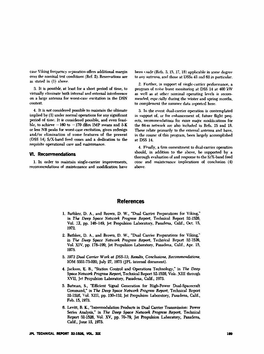
case Viking frequency separation offers additional margin over the nominal test conditions (Ref. 2). Reservations are as stated in (1) above.
3. It is possibl, at least for a short period of time, to virtually eliminate both internal and external interference on a large antenna for worst-case excitation in the DSN context.
4. It is not considered possible to maintain the ultimate implied by (3) under normal operations for any significant period of time. It is considered possible, and even feasi- ble, to achieve -160 to -170 dBm IMP means and 3-K or less NB peaks for worst-case excitation, given redesign and/or elimination of some features of the present (DSS 14) S/X-band feed cones and a dedication to the requisite operational care and maintenance.
VI. Recommendations 1. In order to maintain single-carrier improvements,
recommendations of maintenance and modification have
been made (Refs. 3, 15, 17, 18) applicable in some degree to any antenna, and those at DSSs 43 and 63 in particular.
2. Further, in support of single-carrier performance, a program of noise burst monitoring at DSS 14 at 400 kW as well as at other nominal operating levels is recom- mended, especially during the winter and spring months, to complement the summer data reported here.
3. In the event dual-carrier operation is contemplated in support of, or for enhancement of, future flight proj- ects, recommendations for more major modihcations for the 64-m network are also included in Refs. 15 and 18. These relate primarily to the external antenna and have, in the course of this program, been largely accomplished at DSS 14.
4. Fhally, a firm commitment to dual-carrier operation should, in addition to the above, be supported by a thorough evaluation of and response to the S/X-band feed cone and maintenance implications of conclusion (4) above.
References
1. Bathker, D. A., and Brown, D. W., “Dual Carrier Preparations for Viking,” in The Deep Space Network Progress Report, Technical Report 32-1526, Vol. XI, pp. 146.149, Jet Propulsion Laboratory, Pasadena, Calif., Oct. 15, 1972.
2. Bathker, D. A., and Brown, D. W., ‘Dual Carrier Preparations for Viking,” in The Deep Space Network Progress Report, Technical Report 32-1526, Vol. XIV, pp. 178-199, Jet Propulsion Laboratory, Pasadena, Calif., Apr. 15, 1973.
3. 1973 Vual Carrier Work at DSS-13; Results, Conclusions, Recommendutions, IOM 3331-73-020, July 27, 1973 (JPL internal document).
4. Jackson, E. B., ‘Station Control and Operations Technology,” in The Deep Space Network Progress Report, Technical Report 32-1528, Vols. XI11 through XVII, Jet Propulsion Laboratory, Pasadena, Calif., 1973.
5. Butman, S., ”Efficient 9ignal Generation for High-Power Dual-Spacecraft Command,” in The Deep Space Ndwork Progress Report, Technical Report 32-1526, Yol. XIII, pp. 130-132, Jet Propulsion Laboratory, Pasadena, Calif., Feb. 15,1973.
6. Levitt, B. K., “Intermodulation F’roducts in Dual Carrier Transmission: Power Series Analysis,” in The Deep S p e Network Progress Report, Technical Report 32-1528, Vol. XV, pp. 70-79, Jet Propulsion hboratory, Pasadena, Calif., June 15, 1973.
JPL TECHNICAL R E m 32.1526, VOL. XIX
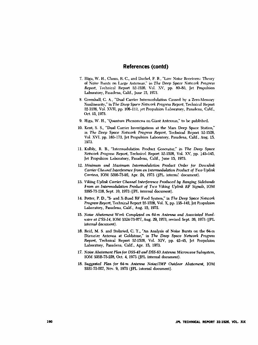
References (contd)
7. Higa, W. H., Clauss, R. C., and Dachel, P. R , “Low Noise Receivers: Theory of Noise Bursts on Large Antennas,” in The Deep Space Network Progress Report, Technical Report 32-1526, Vol. SV, pp. 80-83, Jet Propulsion Laboratory, Pasadena, Calif., June 15, 1973.
8. Greenhall, C. A., “Dual Carrier Intermodulation Caused by a Zero-Memory Nonlinearity,” in The Deep Space Nettcork Progress Report, Technical Report 32-1526, Vol. XVII, pp. 1W112, jet Propulsion Laboratory, Pasadena, Calif., Oct. 15, 1973.
9. Higa, W. H., “Quantum Phenomena on Giant Antennas,” to be published.
10. Kent, S. S., “Dual Carrier Investigations at the Mars Deep Space Station,” in The Deep Space Network Progress Report, Technical Report 32-1526, Vol. XVI, pp. 163-173, Jet Propulsion Laboratory, Pasadena, Calif., Aug. 15, 1973.
11. Kolbly, R. B., “Intermodulation Product Generator,” in The Deep Space Network Progress Report, Technical Report 32-1526, Vol. XV, pp. 143-145, Jet Propulsion Laboratory, Pasadena, Calif., June 15, 1973.
12. hjinimum and hfaximum Zntennodulution Product Order for Dorcdink Cam’er Chime1 Interference from an Zntermodutation Product of Two Uplink Carriers, IOM 3395-73-92, Apr. 2A, 1973 (JPL interna! document).
13. Viking Uplink Carrier Channel Interference Produced by Ranging Sidebands From an Intermodulation Product of Two Viking Uplink RF S i g n d s , IOM 3395-73-216, Sept. 10, 1973 (JPI, internal document).
14. Potter, P. D., “S- and X-Band R F Feed System,” in The Deep Space Network Progress Reycrt, Technical Report 32-1526, Val. X, pp. 135-142, Jet Propulsion Labrator);, Pasadena, Calif., Aug. 15, 1972.
15. Noise Abatement Wmk Completed on 64-m Antenna and Associated Hard- ware at L‘SS-14, IOM 3324-73-077, Aug. 29, 1973, revised Sept. 26, 1973 (JPL internal document).
16. Reid, M. S. and Stelzried, C. T., “An Analysis of Noise Bursts on the 64-m Diameier Antenna at Goldstone,” in The Deep Space Network Progress Report, Technical Report 32-1526, Vol. XIV, pp. 42-45, Jet Propclsion Laboratory, Pasadena, Calif., Apr. 15, 1973.
17. Noise Abatement Plan for DSS-43 and DSS-63 Antenna Micrwaue Subsystem, IOM 335B-73-228, Oct. 4, 1973 (JPL internal document).
18. Suggested Phn for 64-m Antenna Noise/lMP Outdoor Abatement, IOM 3331-73-027, Nov. 9, 1973 (JPL iiiternal document).
190 JPL TECHNICAL REPORT 32-1526, VOL. XI%
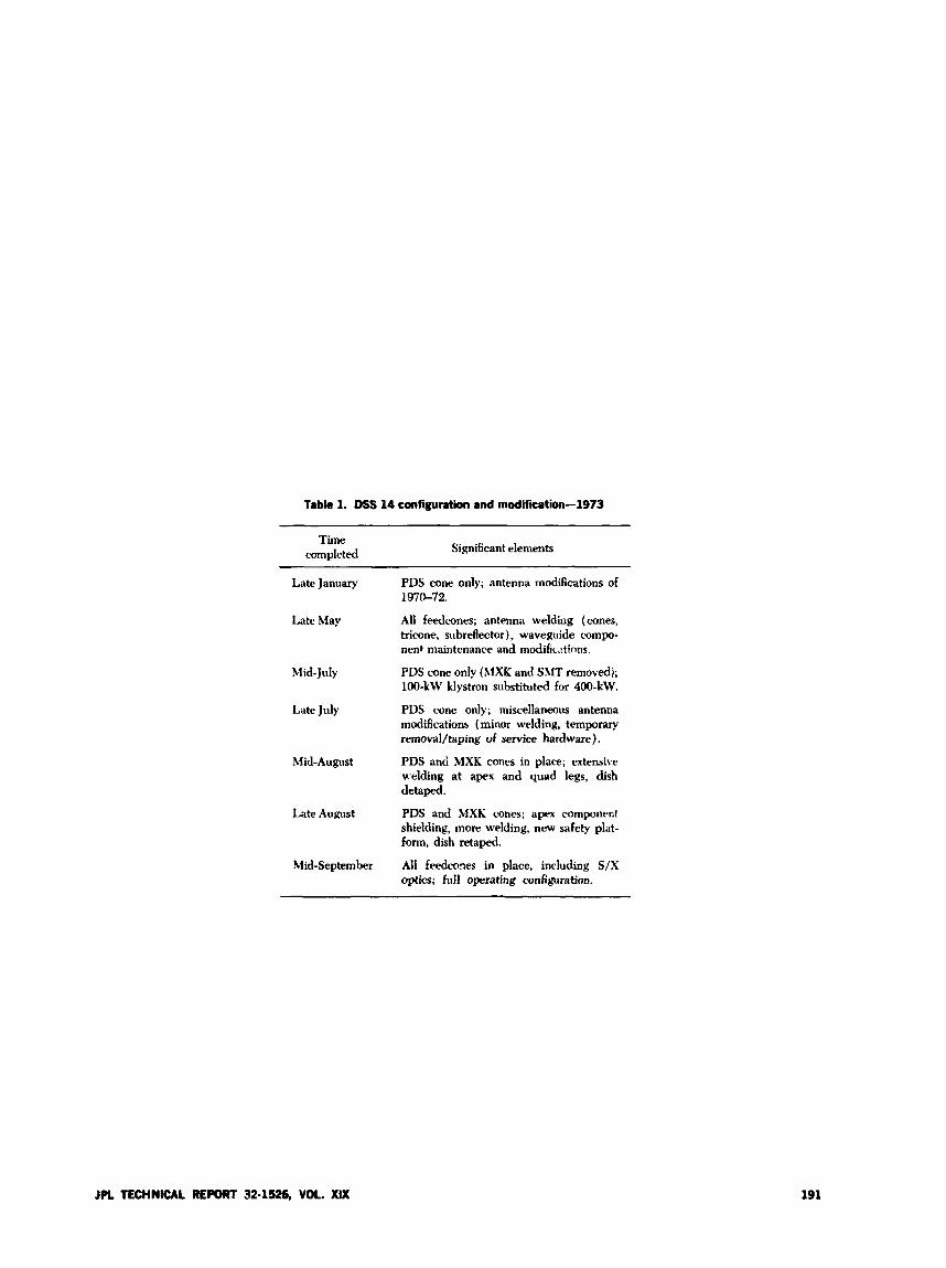
Table 1. DSS 14 configuration and modification-1973
Time completed Significant elements
Late January PDS cone only; antenna modifications of 197672.
Late May All feedcones; antenna welding (cones, tricone, subreflector), waveguide compo- nent maintenance and modific.ctinns.
PDS cone only (MXK and ShfT removed); 100-kW klystron substituted for 400-kW.
Late July PDS cane only; miscellaneous antenna modifications (minor welding, temporary removal/taping of service hardware).
PDS and MXK cones in place; extensive welding a t apes and quad legs, dish detaped.
PDS and MXK cones; apex component shielding, more welding, new safety plat- form, dish retaped.
Mid-September All feedcones in place, including S/X
Mid-July
Mid-August
Late August
optics; full operating configmation.
JPL TECHNICAL RE#)RT 32-1526, VOL. XIX 191
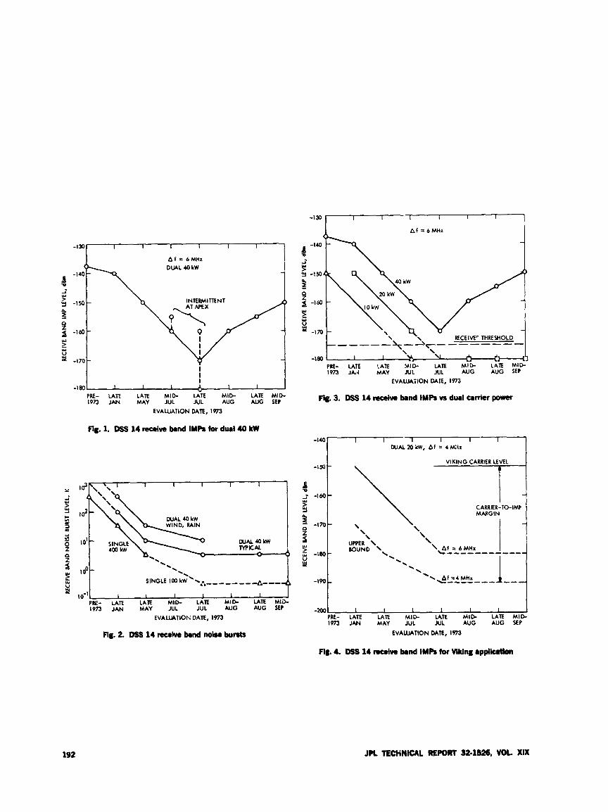
-130 I I I I I I
A f = 6 M H z
-130 I I I I I 1
a f 6MHt D W L 40 kW
-140 - 1 2-
9 y -150-
4
- 0
INTERMITTENT 0
0
y1
L J
-170 I I
~~
PRE- LATE LATE MID- L& MID- LATE MID- 1973 JAN MAY JUL JUL AUG AUG SEP
EVALUATION DATE, 1973
Fig. 1. DSS 14 racdve bnd IMPS for dual 40 kW
P I I A I M UU
I
l o o t
PIE- LATE LAR MID- LAW M l b LA‘E MI& 1973 JAN MAY JUL JUL AUG AUG SEP
EVALUATION DATE, 1973
Fig. 2. 0% 14 recoive band noise bursts
i
\ I I \I A A ”
\ -1 80
PRE- LATE ?AT€ M I D LATE M I L LATE M I L 1973 JA4 MAY JUL JUL AUG AUG SEP
EVALUAilON DATE, 1973
Fig. 3. DSS 14 receive bnd IMPS vs dual carrier power
-150
d j -160 5 H1 4 0 -170
5 -180
0
f Y >
Y
-200 PRE- LATE LATE MID- LATE M I L LATE MIL 1973 JAN MAY JUL JUL AUG AUG SEP
EVALUATION DATE, 1973
Flg. 4. WS 14 ncrk band IMPS for Viking applkrtbn
192 JPL TECHNICAL RLPORT 32-1526, VOL. XIX
Computer Program Copy-Verify and Load Check System R. Billings
Network Operations Office
The Computer Program Copy-Verify and Lwrl Check System cmsists of two programs, D01-5352-SP and DOZ5379-SP. The system asslues the integrity of a DSN program tape at two critical points-reproduction and hading. The Mag Tape Copy Routine DO15352-SP verifies the tape os it is being copied. The Mag Tape Load Check Loader Program interacts with parts of the Mag Tape Copy Routine to check the ualfdity of a h d in progress.
1. Introduction Some DSN computer programs have presented a prob-
lem to the DSN Program Library because thert! is no direct way of reproducing their tapes. These programs are those which occupy almost all of the 16K memory loca- tions in the XDS 920 computers; they are too large to be copied by a standard mag tape copy routine. This con- straint also precludes the verification of a copied tape. The loading of these programs has also posed a problem be- cause most of them are mission-critical real-time programs in which an unrevealed loading error could cause data loss or command malfunction. Procedures were needed to ensure that such tapes were copied accurately and loaded correctly.
The usual procedure for making mag tape copies w a s to incorporate a self-dump routine in the program itself; this routine dumped all of core memory as a single r w r d on tape. The program was loaded intc memory, and then a
branch was made to the self-dump routine. The routine allowed the program to be dumped as many as nine times, but there was no way of checking that the dump was cor- rect or even whether tke program was loaded accurately in the first place.
A reload routine was also incorporated in the program so that another record codd be loaded in the event of a bad load or subsequent failure. The capability of reloading the program from the extra records on tape provided some insurance against bad recordings and stretching or other physical damage. However, this insurance did not prevent loss of data from program hangups and other failures, many .7f which were blamed on “bad loads” for want of a definite cause, although they could have ster-imed from copj 0~fox-s or loading errors.
From the point of view of the DSN Program Library, the procedure is unsatisfactory. The Program Library is
JPL TECHNICAL RvQllT 32.1826, VOL. XIX 193
charged with the responsibility for the accurate duplica- tion of mag tapes, and this procedure does not ensure accuracy. The self-dump technique provides a means of making copies of R tape, but, except for parity checkhg in the computer and tape units, it does not verify that the copies are 100% accurate. To ensure accurate duplication, IOOS verification is considered necessary.
The self-dump routine .vas therefore rewritten to in- clude a verification sequenc: the new program is titled Mag Tape Copy Routine DOI.5352-SP and has been dis- tributed to personnel engaged in programming for the Deep Space Network XDS 9.20 computers. The program occupies 400, locatioiis in memory starting at location 38oo0,. The program dumps core into mag tape as many times as requested, rewinds, and then performs a word-by- word comparison between core and the records on tape. Typewriter messages indicate successful verification or comparison errors; in the latter case, the whole procedure is restarted.
Mag Tape Copy Routine DOI-5352-SP also includes a load-check routine, which is used in conjunction with Mag Tape Load-Check Loader DOI-5379-SP to ensure a cor- rect load. Following the load from mag tape, the program branches to the load-check routine, reads another record from tape, and compares it word by word with the record already loaded in core. Typewriter messages indicate whether or not the comparison (and, hence, the load) is successful. Together, these two programs comprise a sys- tem which ensures against copy errors and '"bad loads."
II. Program Description MMag Tape Copy Routine DOI-5352-SP, written in XDS
9.20 symbol language, is essentially in two parts: a dump sequencl which a requested number of records is writ- ten on tape, and a verify sequence, in which the tape is compared word by word with core memory. The routine checks for buffer errors in the dump sequence and for comparison errors in the verify sequence. If a buffer error occurs, the tape erases backwards over the entire record, and then erases forward over half the record to get the tape quickly by any bad areas. Comparison errors are indi- cated by an error message; the tape rewinds to load point for another start.
No comparison is made of the area in which the copy routine is located (36OOO,-36377,). Since values are chang-
ing in these locations during the comparison sequence, the whole area is bypassed. Copy errors in this section would be inconsequential because tapes are ordinarily copied from a single master and not from other copies.
A feature of this program is that either buffer may be connated to the tape units; the program automatically determines which buffer is connected and sets up all the mag tape instructions accordingly. The buffer test is per- formed using the end-of-tape test as a pseudo-instructicn. If the tape is not at the end of the reel, a \V-buffer end-of- tape test will cause the next instruction to be executed provided the tape unit is cmnected to the Y-buffer, or it will cause the next instruction to be skipped if the tape unit is connected to the \+'-buffer.
The load-check routine is incorporated in this program and shares subroutines with the dump and verify se- quences as needed. Mag Tape Load-Check Loader DOI- 5379-SP branches to this routine after loading a program from mag tape. The load-check routine reads the next record from tape and compares it word by word with core memory. If the cornparison is successful, a LOADCHECK OK message is typed out; if a comparison error is found, the operator is alerted with an error message and the program branches back to the loader to begin the opera- tion again.
Some features of Mag Tape Load-Check Loader DOI- 5379-SP are that it will operate with either buffer, it zeroes core memory before loadirlg a program from mag tape, it rejects any record on tape that is shorter than normal and reads instead the next record. and it branches to location 1 (where it expects to find a branch to the be- ginning of the program) after loading and verifying that the proper load was achieved.
Ill. Conclusion The success obtained with this copv-verify and load-
check system indicates that it is a feasible and practical way of verifying tape duplication and loading. Its use by programmers is encouraged to provide the DSN Program Library with a convenient means of verifying that tapes are copied accurately and to provide Deep Space Stations with assurance f hat programs are loaded correctly. The next step is to Izxpand the system to include those tapes which are reco1.ded with subprograms following the main records and those which are recorded in modular form.
194 JPL TECHNICAL RE-1 32-1526, VOL. XIX
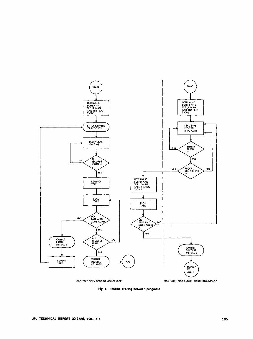
DETERMINE BUFFER AND SET UP MAG TAPE INSTRUC- r-l TIONS
I No& FRITTEN
l+l REWIND
NO
m OUTPUT ERROR MESSAGE
I
READ TAPE
INTO CORE
c- - RECORD
-
BUFFER ERROR YES
NO
DETERMINE BUFFER AND SET UP MAG TAPE INSTRUI. TlOhS
READ TAPE I
I .I
I I I I
OUTPUT succiss
I
i ' 0 BRANCH
MAG TAPE COPY ROUTINE DOI-5352-SP MAG TAPE LOAD CHECK LOADER OOI-537RP-SP
Fig. 1. Routine staring betnean programs
JPl TECHNICAL REPORT 32-3526, VOL. XIX
Network in
Telemetry System Performance Tests Support of the MVM'73 Project
R. D. key and E. T. Lobdell Network Operations Officc
ThiP article presents a description of Network Telemehy System Performance Tmts that were enecuted throughout the DSE' in support of the MVM'73 project.
1. Introduction System Performance Tests (SPTs) are executed through-
out the DSN whenever a modification is made to the Net- work Telemetry System that affects its performance. This is the case when new software or hardware is added, as was required for the support of Marint! 10. The purpose oi this article is to describe the effort that was undertaken in executing telemetry SPTs throughout the DSN and to present the test results. The philosophy and the objectives of the SPTs will be discussed so as to demonstrate the benefits gained by performing these tests. A description of the telemetry SPTs will be presented, along with a description of the test procedure and test software. A summary of the results and the status of the Netwoik Telemetry System will be presented.
II. Objectives of System Performance Testing The development of test procedures, test softw Ire, and
the execution of the telemetry SPTs are performed to accomplish certain objectives. The overd objective is to
guarantee that the Network Telemetry System can meet specifid operational capabilities. These apabilities are defined in various documexits; those of particular impor- tance are given in Refs. 1 through 3. The SPT must verify that the telemetry system configurations and interface requirements are satisfied. They must also evaluate the ability of the Telemetry System to meet performance requirements.
The telemetry SPT is designed so that it can be used to locate or diagnose system problems. The problems may occul during the installation of new equipment or soft- ware, or they may be the results of system failures un- covered during DSN real 'ime tracking operations. Some of the latter type problems have been discovered when portions of the SPT are used during countdown tests.
Use of SPTs for prepass readiness tests is another ob- jective that requires thkt the SPT procedure be modular. Thus, the various classes and levels of prepass readiness tests can be accomplished by executing the appropriate sections of the procedure.
1% JPL TECHNML MCORT 32-1526, w)L x1?:
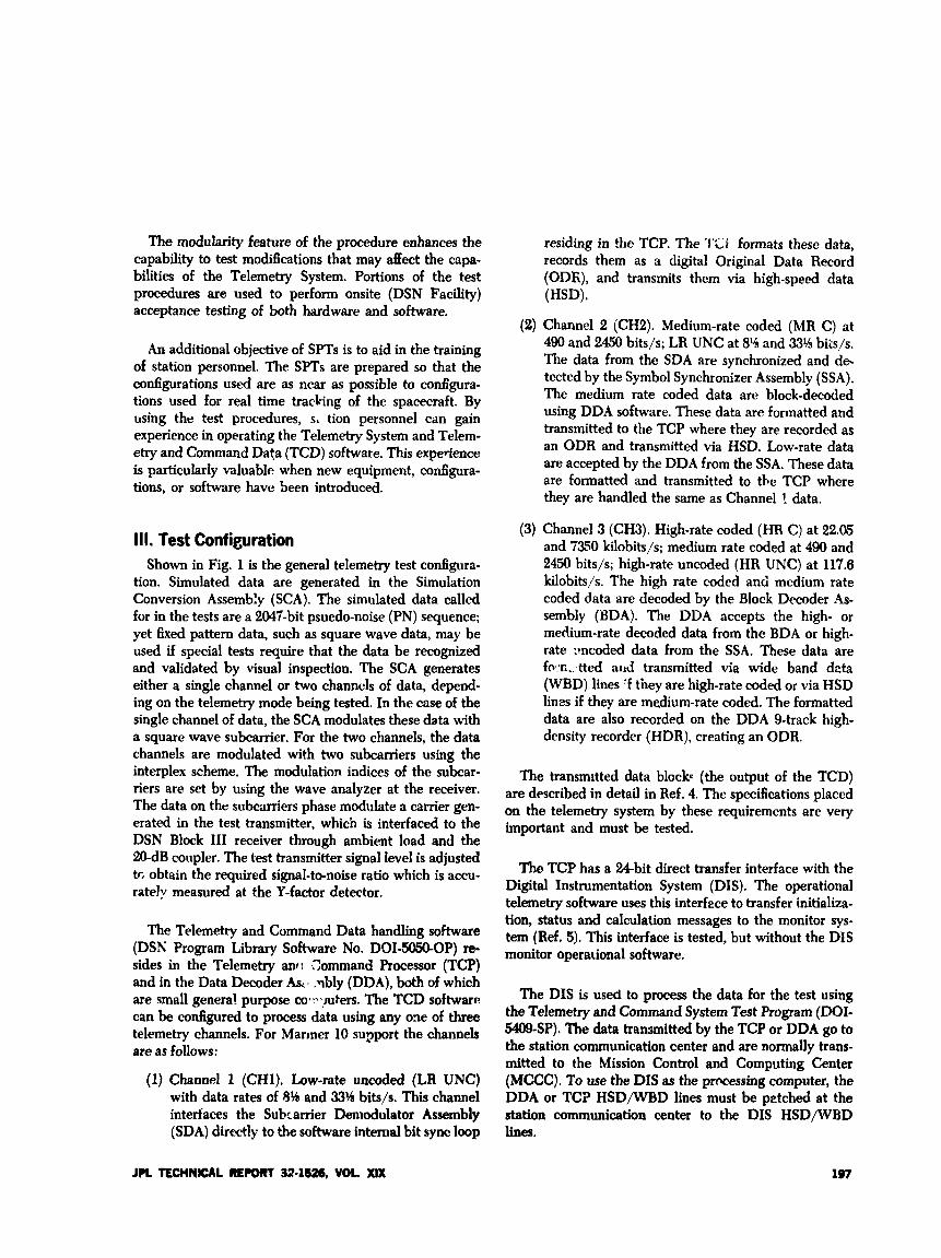
The modularity feature of the procedure enhances the capability to test modifhations that may deet the capa- bilities of the Telemetry System. Portions of the test procedures are used to perform onsite (DSN Facility) acceptance testing of both hardware and software.
An additional objective of SPTs is to aid in the training of station personnel. The SPTs are prepared so that the configurations used are as near as possible to configura- tions used for real time tracking of the spacecraft. By using the test procedures, s. tion personnel can gain experience in operating the Telemetry System and Telem- etry and Command Data (TCD) software. This experience is particularly valuable when new equipment, configura- tions, or software have been introduced.
111. Test Configuration Shown in Fig. 1 is the general telemetry test configura-
tion. Simulated data are generated in the Simulation Conversion Assembly (SCA). The simulated data called for in the tests are a 2047-bit psuedo-noise (PN) sequence; yet fixed pattern data, such as square wave data, may be used if special tests require that the data be recognized and validated by visual inspection. The SCA generates either a single channel or two channels of data, depend- ing on the telemetry mode being tested. In the case of the single channel of data, the SCA modulates these data with a square wave subcarrier. For the two channels, the data channels are modulated with two subcarriers using the interplex scheme. The modulation indices of the subcar- riers are set by using the wave analyzer at the receiver. The data on the subcarriers phase modulate a carrier gen- erated in the test transmitter, which i s interfaced to the DSN Block 111 receiver through ambient load and the 20-dB coupler. The test transmitter signal level is adjusted tr, obtain the required signal-to-noise ratio which is accu- rately measured at the Y-factor detector.
The Telemetry and Command Data handling software (DSN Program Library Software No. DOI-!XWOP) re- sides in the Telemetry an1.i Zommand Processor (TCP) and in the Data Decoder As;. .?My (DDA), both of which are small genera! purpose co*?*!uters. The TCD software can be configured to process data using any one of three telemetry channels. For Mariner 10 support the channels are as follows:
(1) Channel 1 (CH1). Low-rate uncoded (LR UNC) with data rates of 8% and 33% bits/s. This channel interfaces the Subrarrier Demodulator Assembly (SDA) directly to the software internal bit sync loop
residing in the TCP. The ‘I‘Ci formats these data, records them as a digital Original Data Record (ODR), and transmits them via high-speed data (HSD).
Channel 2 (CH2). Medium-rate coded (MR C) at 490 and 2450 bits/s; LR UNC at 8% and 33% bi;s/s. The data from the SDA are synchronized and de- tected by the Symbol Synchronizer Assembly (SSA). The medium rate coded data are block-decoded using DDA software. These data are formatted and transmitted to the TCP where they are recorded as an ODR and transmitted via HSD. Low-rate data are accepted by the DDA from the SSA. These data are formatted and transmitted to the TCP where they are handled the same as Channel ’! data.
Channel 3 (CH3). High-rate coded (HR C) at 22.05 and 73SO kilobits/s; medium rate coded at 490 and 2450 bits/s; high-rate uncoded (HR UNC) at 117.6 kilobits/s. The high rate coded and medium rate coded data are decoded by the Block Decoder As- sembly (BDA). The DDA accepts the high- or medium-rate decoded data from the BDA or high- rate irncoded data from the SSA. These data are fw:c..~tted a d transmitted via wide band drta (WBD) lines ‘f they are high-rate coded or via HSD lines if they are medium-rate coded. The formatted data are also recorded on the DDA 9-track high- density recorder (HDR), creating an ODR.
The transmitted data block. (the output of the TCD) are described in detail in Ref. 4. The specifications placed on the telemetry system by these requirements are very important and must be tested.
The TCP has a 24bit direct transfer interface with the Digital Instrumentation System (DIS). The operational telemetry software uses this interfece to transfer initializa- tion, status and calculation messages to the monitor sys- tem (Ref. 5). This interface is tested, but without the DIS monitor operational software.
The DIS k used to process the data for the test using the Telemetry and Command System Test Program (DOL 5409-SP). The data transmitted by the TCP or DDA go to the station communication center and are normally trans- mitted to the Mission Control and Computing Center (MCCC). To use the DIS as the prmessing computer, the DDA or TCP HSD/WBD lines must be petched at the station communication center to the DIS HSD/WBD lines.
JPL TECHNSAL MPO#T 32-1526, VOL XIX 197
IV. Telemetry System Test Software The Telemetry and Command System Test Program,
DOI-5409-SP, resides in the DIS computer. I t contains two subprograms: a telemetry subprogram and a com- mand subprogram, both under the control of an Executive Program. The progrcm interfaces with the TCD string to be tested through the HSD/WBD on-site GCF equipment (station communications center), and the 24-bit monitor interface. By virtue of these interfaces, the TCD and its operational roftware are tested in an operational environ- ment. That is, the telemetry system test validatv data as they are transmitted externally from the TCD system.
(3) Binary time and multisecond clock differences.
(4) GCF errors.
The telemetry system soitware is an invaluable tool, which has done much to facilitate and ease the execution of the Telemetry System Performance Tests.
V. Test Procedure Format The P.etwork Telemetry System Performance Tests for
Mariner 10 were executed using Ref. 6. In this section, the format of the procedure will be presentcd to provide a description of the tests that are performed at the Deep Space Stations.
The overall test is divided into threc main tests. Each test contains a number of su5,ests th, ‘ modular so that any test can be run independr .is allows the procedures to be used for prepass tests, trouble- shooting, and new equipment or softu .Ire tests. It also allows for reduced testing when resources so demand.
The software receives the monitor data, and formats and prints the results selectively on thc DIS 1/0 type- writer or line printer. Due to the greater print speed of the line printer, it is normally used dcring the tests. The monitor data displayed are initialization messages, status messages, and the calculation messages. These messages are validated by visual inspection for correctness and com- pleteness in compliance with Ref. 5.
The telemetry data HSD’WBD blocks may be dis- played on the line printer for visual inspection, although normal operation consists of permitting the software to output the following:
(1) Standard block header information consisting of source, destination, data-dependent type (DDT), user-dependent type (UDT), spacecraft identifica- tion, and day of the year and the time of the block formation.
(2) Formatted configuration and lock status with re- ceiver AGC or signal level in dBm, and the TCE software channel in use.
(3) The bit error rate (BER) or word error rate (WER) measured over a given period; the bit rate and data format.
In the bit error rate test, the data may be either PN or a fixed pattern. The test software synchronizes to the data and dops a bit-by-bit comparison. The WER/BER accu- mulation may be over any chosen interval resulting in a grand total, while statistics can be displayed as interim summaries at intervals as required.
Although the AGC,/dBm conversion test and the signal- to-noise ratio (SNR) calculation test dre separate sections of the test procedure, they are normally run with the configurat’.on and interface tests. The AGC/dBm cor. ::r- sion test verifies that software can perform a correc! con- version from AGC volts to signal level in dBm. The conversion parameters are entered in the program, and accuracy of the conversion is checked io see t it it is
the test is being executed, the test software detect errms and display error messages as follows:
(1) me A’ between telemew HSD’WBD blocks are not within specifled tolerances.
(2) Excessive bit error or incorrect data type, as mi- denced by the inability to achieve synchronizatior:.
The three ..sts are the Configuration and Interface Tests, the Telemetry Performance Tests and the Non-Real Time Capability Tests. These tests all call out a Test Prep- aration Section as needed. The complete test, two TCD strings, can be accomplished in 40 hours.
A. Configuration and Interface Tests
The Configuration and Interface Tests are performed on the three telemetry channels (CH1, CH2, and CH3). They test the telemetry operational software and hard- ware interfaces using all the operational configurations planned for Mariner 10 support. This test contains HSD. and WBD interface tests that verify the HSJ>/WRL blocks. The blocks are verified by inspection of the for- matted block headers, configuration and lock indicators that are formatted for ease of interpretation, and by the absence of error messages. This section contains a set of TCP-DIS mrmitor message verification tests that verify that the initialization, status, and calculation messages are correct as specified.
198 JPL TECHNICAL REPORT 32.1526, VOL. XIX
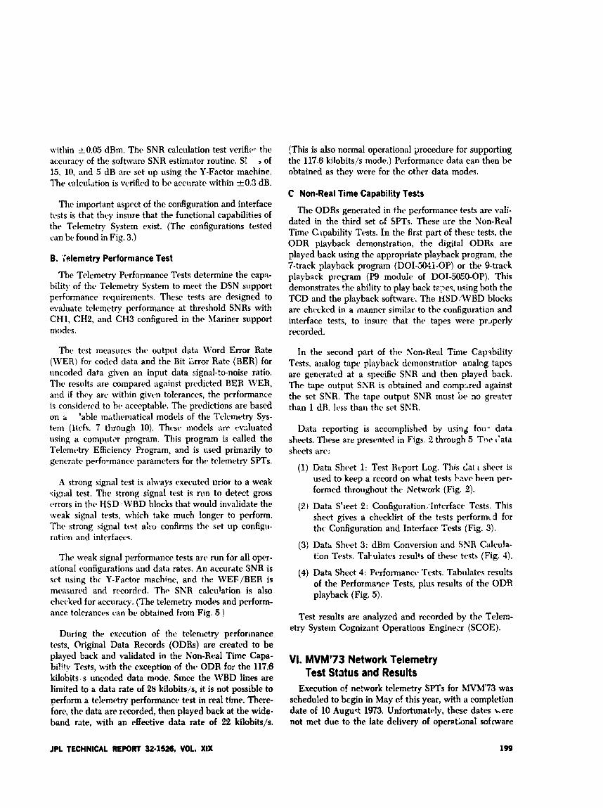
within 20.05 dBm. The SNR calculation test verifier the accuracy of the software SNR estimator routine. SI 3 of 15, 10, and 5 dB are set up using the Y-Factor machine. The calculation is verified to bc accurate within kO.3 dB.
The important aspect of the configuration and interface trsts is that they insure that the functional capabilities of the Telemetry System exist. (The configurations tested can be found in Fig. 3.)
B. ';elemetry Performance Test
The Telemetry Performance Tests determine the capa- bility of thr Tclcmetry System to meet the DSN support performance wquirements. These tests are designed to evaluate telemetry performance at threshold SNRs with CH1, CH2, and CH3 configured in the Mariner support modes.
Thr test measurcs the output data Word Error Rate (WER) for coded data and the Bit Lrror Rate (BER) for uncoded data given an input data signal-to-noise ratio. The results are compared against predicted BER IVER, and if they arc within given tolerances, the pcrformance is considered to Iw acceptable. The predictions are based on :I 'able m;ithrmatical models of the Telemetry Sys- tem (kicfs. 7 through 10). These models are evaluated usiiig a compiitcr program. This program is called the Tc4cxmr.try Efficiency Program, and is ised primarily to gtwrate performance parameters for thv telemetry SPTs.
A strong signal test is always executed mior to a weak Ggrd test. The strong signal test is nin to detect gross crrors in tlw HSD WBD blocks that would invalidate the weak signal tests, which take much longer to perform. The strong signal test a h confirms thc set up configu- ration a i d interfaces.
The weak signal performance tests arc run for all oper- ational configurations and data rates. An accurate SNR is sct using tlic Y-Factor machine, and the WEF/BER is mrasurrd and rrcordcd. Thr. SNR calculation is also checked for accllrdcy. (The te!emetry modes and perform- ance tolerances can be obtained from Fig. 5 )
During the execution of the telenietry perfonnance tests, Original Data Records (ODRs) are created to be
(This is also normal operational procedure for supporting the 117.6 kilobits/s mode.) Performance data can then be obtained as they were for the other data modes.
C Non-Real Time Capability Tests
The ODRs generated in the performance tests are vali- dated in the thud set c;f SPTs. These are the Non-Real Time C,ipability Tests. In the first part of these tests, the ODR plavback demonstration, the digital OD& are played back using the appropriate playback program, the 7-track playback program (DOI-mi-OP) or the 9-track playback p ~ c g a m (P9 module of DOI-5050-OP). This demonstrates the ability to play back taYe5, using both the TCD and the playback software. The HSD/WBD blocks are checked in a manner similar to the configurntian and interface tests, to insure that the tapes were pruperly recorded.
In the second part of the Non-Heal Time Capeability Tests, analog tape playback demonstratior analog tapcs are generated at a specific SNR and then played back. The tape oatput SNR is obtained and compxed against the set SNR. The tape output SNR must be no greater than 1 dR. ICW than the set SPIR.
Data reporting is accomplishzd by using fou- data sheets. These are presented in Figs. 2 through 5 T w (:ala sheets are:
(1) Data Shret 1: Test Report Log. This i a t I sheer is used to keep a record on what tests have been per- formed throughout the Network (Fig. 2).
(2) Data S'ieet 2 : Configuration/'Interface Tests. This sheet gives a checklkt of the tests performcd for thc Configuration and Interface Tests (Fig. 3).
(3) D a h Sheet 3: dBm Conversion and SKR Calcula- tion Tests. Tal-ulates results of these tests (Fig. 4).
(4) Data Sheet 4: Performance Tests. Tabulates results of the Performawe Tests, plus results of the ODR playback (Fig. 5) .
Test results are analyzed and recorded by the Telem- etry System Cognizant Operations Engine3r (SCOE).
played back and validated in the Non-Real Time Capa- bility Tests, with the exception of the ODR for the 117.6 kilobits s uncoded data mode. Since the WBD lines are
VI. MVM973 Network Telemetry Test Status and Results
limited to a data rate of 28 kilobits/s, it is not possible to perform a telemetry performance test in real time, There- fore, the data are recorded, then played back at the wide- band rate, with an effective data rate of 22 kilobits/s.
Execution of network telemetry SPTs for MVM'73 was scheduled to begin in May of this year, with a completion date of 10 August 1973. Unfortunately, these dates here not met due to the late delivery of operational sofware
JPL TECHNICAL REPORT 324526. VOL. XIX 199

and hardware. The tests were s t i l l being executed after the Mariner 10 launch; however, all of the Configuration and Interface Tests plus those capabilities that were re- quired for launch had been completed prior to launch. The tests were required to be perfonned at the following stations:
Goldstone, California: CSS 12 and DSS 14.
Tidbinbilla, Australia: DSS 42 and DSS 43; con- joint stations.
Madrid and Ceberos, Spain: DSS 62 and DSS 63.
The tests were conducted by station personnel. In a number of cases the SPTs uncovered station problems, which, when corrected by the station personnel, required a rerun of system tests. The station personnel also made recommendations on modifications or corrections of the procedures.
Data taken during the tests were transmitted to the telemetry SCOE. The data were analyzed and saved. To evaluate the status of the Telemetry System, a Telemetry Test Status Board was created. The most recent data from each station are recorded on this Board, and are presented in Fig. 6.
The Telemetry Test Status Board presents the date that the Cmfiguration and Interface Tests, including AGC/ dBm and SNR tests, were completed. It also presents the results of the performance tests (1-1 through 7) and the date that these tests were Completed. For the performance tests, the data rate, input SNR, allowable WER/SER, and allowable SNR with tolerances are presented. The Board shows whi-h tests are not completed and due, are out of tolerance, and are not required from a particular station.
All of the Configuration and Interface Tests (including the AGC/dBm and SNR tests) were successfully com- pleted prior to Mariner 10 launch. The Telemetry Per- formance Tests were not completed. Some of the tests were run, but the results were not within tolerance. These results wwe accepted since they were nearly within speci- fication, and it was deemed that the station resources not be loaded by further testing except on a best ehr t s basis.
In some cases, rhta from the tests were not available. These tests were not completed due to hardware prob- lems that were uncovered prior to or during the tests. Since the tests were run late, many problems were dis- covered just prior to Mariner 10 launch. The problems could nr: he corrected due to the Mariner configuration freeze, and then the X . r e e r 10 con6guration. The prob- lems are now being correct& a 3 the tests will be run after the termination of the Piorter configuration freeze.
The Non-Real Time Tests were executed prior to
(1) All TCP ODRs were validated.
(2) DDA OD& at DSSs 14 and 63 have been validated.
(3) Hardware problems with the DSS 43 DD! OD%
(4) All %meter-antenna DSS analog tape ODRs have been validated.
(5) h h l e m s with the recorder track assignments of the &%meter-antenna DSS Analog Tape ODRs have been uncovered.
Overall, the performance as demonstrated by the Telem- etry SPTs, has been acceptable.
Mariner launch with the following results:
have been uncovered.
References
1. Deep Space h’etwork System Requirements-Detailed lnterfoce Design, Docu- ment No. 820-13. Jet Propulsion Laboratory, Pasadena, Calif., Feb. 1, 1971. (JPL internal document.)
2. Deep Space Network Support Requirements for AfVM’73 Project. Document No. 615-15-Rev. A. Jet Propulsion Laboratory, Pasadena, Calif., Jan. 15,1973. (JPL internal document.)
3. GCF-NASCOM lliVM’73 Prqect Support Communications Capabilities, Con- figurations, and Operational Support Procedures-Netuork Operations Plan for MVM’73 Project, Document No. 615-9341. Jet Propulsion Laboratory, Pasadena, Calif., Sept. 20, 1973. (JPL internal document.)
4. Telemetty System Wideband and High Speed Data lntetfaces, Document KO. TLM-35, listed in Deep Space Network System Requirements-Detailed lntetface Design, Document No. 820-13. Jet Propulsion Laboratory, Pasadena, Calif., May 1, 1973. (JPL internal document.)
5. DSS Monitor System lntetfaces with DSS monitor Program DO1-5046-of’, Document No. 820-13, MON 5-4, listed in Deep Space Network System Requirements-Detailed interface Design, Document No. 820-13. Jet Propul- sion Laboratory, Pasadena, Calif., Feb. 28, 1973. (JPL internal document.)
6. DSIF Standurd Test Procedure Telemetry System Performcrnce Test AlVAi‘73 Version, Document No. 853-61; 2A-07. Jet Propulsion Laboratory, Pasadena, Calif., Dec. 28, 1973.
7. Brockman, M. H., “MMT Subcarrier Demodulator,” in The Deep Space Net- work, Space Programs Summary 37-46, Vol. 111, pp. 189-2M. Jet Propulsion Laboratory, Pasadena, Calif., July 31, 1967.
8. Burt, R. W., “DSIF System Verification Tests,” jn The Deep Space Network, Space Programs Summary 37-51, Vol. 11, pp. 132-136. Jet Propulsion Labora- tory, Pasadena, Calif., May 31, 1968.
9. Edelson, R. E., Telecommuniccrtions Syst,ms Design Techniques Handbook, Technical Memorandum 33-571. Jet PropuLicn Laboratory, Pasadena, Calif., July 15, 1972.
10. Tausworthe, R. C., *Communications Systems Development: E5ciency of Noisy Reference Detection,” in The Deep Space Network, Space Programs Summary 3754, Vol. 111, pp. 19!%201. Jet Propulsion Laboratory, Pasadena, Calif., Dw. 31, 1968.
JPL TECHNICAL REWRT 32-1526, VOL XIX 201
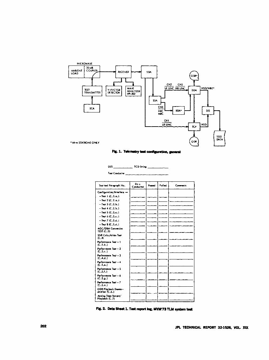
MKROWAVE
2 0 4 I
SM
TEST y-f/?c:CTa 2EYZER TRANSMITTER DZTECTOR HP-J)2
t * SSA
SCA
M R C -
CH 1
TCP
DATA -64-m STATIONS ONLY
DSS TCD String
Tar, Conducts
P r f a m m c . T a t - 1 (C.5. b.) PufanaKe T a t - 2 (C.5.C.) PufarnoK. Test - 3 (C.4.d .) PrhrmoKe Test - 4 (C.5 ... )
Pr farmma T r t - 5 (C.5.f.)
- Tart 1 (C.2.a.) -Tart 2 (C.2.0.) - 1-1 3 (C.2.b.) - Tw 4 (C.2.b.) - T.lr 5 (C.2.C.) - T a t b(C.2.c.) -1-t 7 (C.2.d.) - T a t 8 (C.2.d.)
A G C D B M Convhon
SNR Colcdatiar T.rr r w (c.3)
IC .4)
--- /-I+ Prhr-a T a t - 6 (C.5.g.) P r f a m a w Test - 7 (C.5.0.) DDRPI b a k D m - 1tratian7.6.) Lnalag Tap. h a r d / P l q b a k (C.7)
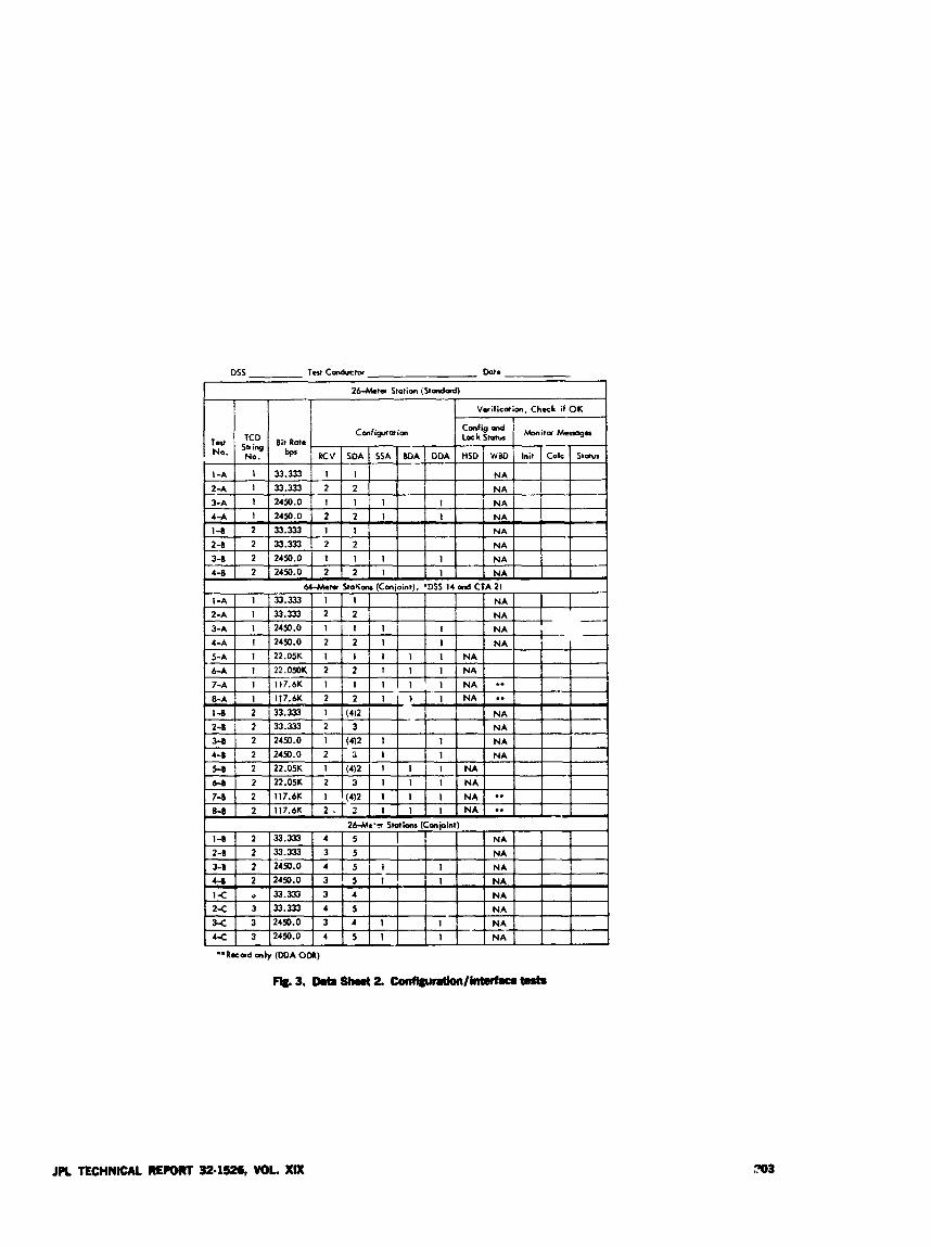
26-Mt.9 S r o t i m i (Canpint)
1-0 2 33.333 4 5 I N A 2-B 2 33.333 3 5 N A 3-B 2 249 .0 4 5 1 I 1 N A

SNR Calculotim Tclt:
1-1
1-2
2-1
S N R Input S T b M o Allaroble
15.0dB 15.0dB tO.3dB
10.0 dB 9.3 dB *0.3 dB
5.0 dB 4.3dB t0.4dB
117.6 kbpr UNC 5 min 2.5 0.040 to 0.050
2450.0bprB.C. JOmin *10.17 <O.ooOoI
22.05kkmB.C. Smin 2.0 0.OMtoO.WO 1 . 4 i 0 . 5 1
oss Test cmdwtu
Date
2-2
3-1
3-2
TCP 1 TCP 2 TCP 3
- ~~
245Q.Ot~sB.C. 30mm '7.7 <O.ooQu 7.5 t0.8
735Q.ObprB.C. J O m h 5.0 O.M)(MtoO.002 4.9i0.5
490.obp1B.C. 3Omin '12.9 ~O.ooOo1 12.8 t0.9 -
I I I I 1
4 24.50.0LprB.C. 30min 3.0 0.017toO.W5 2.0t0.5 I 5
6
7
4W.ObprB.C. 30min 4.0 0.013to0.030 2.710.5
U.333bpslJNC 3Omin 5.0 0.014to0.025 3.9 *0.5
R.333baUNC 2.5h 6.0 0.020t00.040 3.610.5
204 JPL TECHNICAL REPORT 32.1526, VOL XIX

MVM 73 NETWORK TELEMETRY TEST STATUS
I BIT WTE :WS)
TEiT DATATYPE
C O N F I G -- INTERFACE
A G ~ W --
INPUT TCP I TU' 2 TCP 1 TCP 1 S T d r J , WEVEER SNR 0 8 ) (De) ALLOWABLE ALLONABLE W E m R SNR DATE W E W R SNR DATE WEP/ER SNR DATE WEvsER SNR DATE WER
- 7-23 -- -- 10-1 - -- -- -- -- -- 7-23 - -- 7-23 -- -- -- -_ - -- 7-23 -- - 7-23 -- __ 7-23 __ _- 10-2 -
1 - I 1 - 2
2-1
0.017 2.1 7-23 NR NR NR -- -- -- 117.6 K U N C 2.5 c.o4(M.m 2.Ot 0.3 -- -- -- 2450.0K 10.17 <O.ooOOl 10.0t 1.0 0.0 9.7 7-23 NR NR N R 0.0 10.5 10-17 0.0 10.43 10-15 1.2r
22.05BC 2.0 0.050-0.070 0.8 tO.3 - I -- - 0.068 0.5 7-23 NR NR NR - -- --
JPL TECHNICAL REPORT 32-1526, VOL. XIX
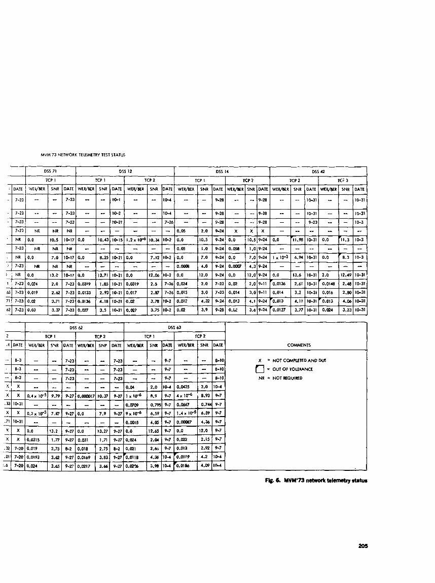
MVM 73 NETWORK TELEMETRY TEST STATUS
I DSS 62
TCP 1 I TCPZ 2
1R DATE WEWBER SVR DATE W E W R S N P DATE
I I I
7-23
x 1 x 1 0 . 2 ~ lrr51 7.87 1 9-27 y$+-p 0.0315 1.77 9-27
L I - 1 - I 7-23
O.ooOo17 10.37 9-27 :* I I
0.0 / 7.9 7 9-27
DI
WEWR SNR DATE
2.0 10-4 %+$ o.wo9 0.795 9-7
0.- I 3.98 110-4
~ ~ ~~ ~
63
TCP 2 - W E m R SNR DATE COMMENTS
- -- 8-10 X = NOT CWPLETED AND DUE
-.. - 6-10 0 = OUT OF TOLERANCE
I - 8-10 N R NOTREQUIRED
0.0425 2.0 10-4
4 x I @ 8.93 9-7
0.0667
I.4r 1U:
0.-
0.0
0.022
0.013
2.01 19
‘0.0les
0.744 V-7
6.39 9-7
4.36 9-7
12.0 9-7
2.15 9-7
2.92 9-7
4.2 IM
4.09 10-4
Fig. 6. MVM’73 networL tehneby status

Analysis of Staffing and Training Policies for a DSN Tracking Station
A. Bahadur and P. Gottlieb Systems Analysis Section
This article presents a method for analyzing the efects of training and stGng policies, and for sekcting optimum policies which minimize the expenditures for training and salaries while maximizing the performance of the tracking station. Two models haoe been deoeloped which represent increasing levels of sophistication. The first characterizes steady-date behavior under the optimizat& o f training, average capability, and crew size. The second, which is the dynamic model, opti- mizes the operating policy over a sequence of time segments. Each segmt..,' is characterized by a performance requirement (dependent on the phase o f the mis- sion), turnover, and training allocation with a corresponding change in average ccrpability. With inputs such as required minimum station performance, training availability, current crew capability, and expected turnover, the output of the model will be the change in average crew capability, the percentage of time allocated for training, and thd corresponding minimum cash expenditure for sakzries and training.
I, Introduction This article presents a methodology for analyzing the
staffing and training requirements for operating a DSN tracking station. This analysis is part of a study made to develop tools to assist the management of the Deep Space Network in the planning and operation of the tracking stations.
In order to meet tracking commitments, the manage- ment of the t sacking stations allocates personnel and financial resources among operations, maintenance, and training. Training is not only for new personnel and opera- tors of new equipment, but also for upgrading the skills of veteran personnel. This article discusses the methods
developed to assess the changing demands in these areas and to formulate an operating and training policy to sat- isfy requirements in a cost-effective manner.
Work is continuing, especially in the area of training effectiveness, to represent more characteristics of the staff- ing and training policy with our model, and to generate optimal training and staffing policies of practical value, using DSS 12 as the main example. The specific acwm- plishments expected :rr the near future from these efforts are listed in Section IX.
We begin with a discussion of the general features of the tracking station represented by our model.
JPL TECHNICAL R E M 32-1526, VOL. XIX 207 . PRECEDING PAGE B W K NOT F-
11. Characteristics of the Model Hiring is done to either add to, or replace, the people
Optimizztion of performance. The performance of the tracking station in carrying out the different tasks may be measured by certain selected param- eters. These parameters are treated as an output of the system, e.g., system availability, data recovery, number of data outages, etc. A maximization (or minimization) of one or more parameters provides the basis for the optimal operating policy.
Relationship between performance (output) and capability (skills available). There exists a relation- ship between the capability of the men and the quality of the station performance, which in turn is explicitly related to the parameter being optimized. These relationships between capability and per- formance are dtimately expressed in quantitative terms.
Training to increase capability. Training methods, which may be of varying effectiveness, are available to increase the capability of the men to perform their tasks. This may be either through increased proficiency in familiar subsystems or the develop- ment of proficiency in different or new subsystems.
Constraints. There are constraints on the system, which are parameterized and which may vary with time. Typical constraints are the type of training methods available, the amount of time and man- power available for training, minimum performance requirements, and the number of crews required.
Costs associated with maintaining and improoing performance. These costs include operating ex- penses such as salaries, and some forms of capital investment such as training of new technicians.
- - working at the station. The “world” represents the awil- able manpower pool, and includes former vmployees.
The tracking station (the operating system) transforms the inputs into a tangible, measurable quantity. This is the output or performance of the system.
Two methods of training are considered, formal train- ing a d m-the-job training. The employees at the tracking station have the same general background, since they sat- isfy certain basic selection and hiring criteria. Thus, it is assumed in this model that the different training methods are mually effective for all employees. Further work is nec‘ dry to delineate the difference in the effectiveness of training by method, background of the individual, and the length of his employment at the tracking station.
IV. The Internal Environment of the Tracking Station
The people at the station may be divided into two categories:
(1) Administrative personnel. This category includes the station managers, secretaries, schedulers, etc., who perform the administrative tasks at the station.
(2 ) Maintenance and operations personnel. These in- clude the operators and technicians who maintain and operate the station equipment.
Henceforth, for convenience, any reference to an indi- vidual at the station will imply an individual from cate- gory (2).
These five features provide the basic structure and inter- relationships for constructing the model. Within this basic framework, the model attempts to determine the “operat- ing policy” which optimizes a given parameter while the tracking station is under a speified set of constraints.
Station personnel, both new employees and veteran personnel, receive training to increase their operations and maintenance skills in various subsystems. As men- tioned previously, two methods of training are considered: formal training and on-the-job training.
111. The External Environment of the Tracking Station
The block diagram shown in Fig. 1 illustrates the re- lationships between the tracking station and its envi- ronment. The rectangular area within the dashed line represents the tracking station. The area outside the rec- tangle is the external environment of the trackiag station. The significant relationships between the tracking station and areas in its external environment are identified.
Formal training, as the name suggests, consists of classroom-type multimedia instruction. A group of trainees is taught a specific skill by a qualified instructor. Under the present Deep Space Network configuration, the Train- ing Center develops, with the assistance of the Technical S t d , h e instruction material and provides the instructors. During the time that a trainee is undergoing formal train- ing, he cannot participate in station operations. Thus, the trainee performs no “useful work” during formal training, and a11 of his time is devoted io tiaixiing.
2oa JPL TECHNICAL REPORT 32.1526, VOL. XIX
On-the-jul-, training takes placc. within the station. A trainee working with an already trained man acquires the iiccessary skills through observation and practice. Expe- rience suggests that half the combined time of trainee and trainer rrsiilts in uscful \vork. The ot1it.r half is devoted to learning, and consrquently the prorrss of on-the-job train- ing is not a s efficient timewisc ;is formal training.
To express this distinction. \ve define the c,ff ectiveness of a training method to be the ratio of the time required to acquirca the skill with thr give11 method compared to a ‘‘Ftandard training mcdiod. For convenience, \\’e take the more efficient formal training to be the standard. E v e - rienre suggrsts that trainers’ time spent in on-the-job trainin5 is only 40% as rffective RS formal training (Ref. 1).
The operations and maintenance skills in different sub- systems acquircd by an individual througli the process of training may he transli‘ted into a measure called the “capability” of tho individual. The division of the tracking station into subsystems may be along hardware lines or along fiinctional 1inc.s as is prrsently the case, with the number of subsystcms ranging from 14 to 36. Henceforth, the usc of the word capability will hr restricted to the above definition.
The capability of an individual is measured in terms of the number of subsystems that lie can operate andjor maintain. This measure is \wightcd by the relative d f i - culty factor of each siibsystrm, in the followiag manner (Ref. 2),. The number of days of formal training required to train a man to opcr,tte and maintain a subsystem is determinrd. The rapability of an individiial is then deter- mined by the subsystems that he can operate and main- tain in terms of fo:mal training days. If an individual has partial proficirncy in a subsystem, the corresponding per- centage of the total for that siihsystem is added to his rapability .
Rrtween August 1971 and June 1972, DSS 12 was dividcd into 14 hardware suhsystems. The average train- ing time in a siihsystrm for operations and maintenance was 22 days (u = 15.6) and 70 days (u = 42), respectively. During this tirnr period, thr average individual capability varied between 191 and 241 days. Let
K; = capability of the ith individual (formal training
K = average capability of the individuals in the station (formal training days)
N = number of men in the station
days)
then
Far every “pass” (tlir. continuous tracking period of a given sp,.cecraft), the total amount of data available for collectioo can bc determined irom thc spacecraft tracking and testinp schedule. This total represents the maximum output of the system.
We define the data acquisition efficiency 71 = (actual data gathered availablt. data) for an averagr view prriod. The two factors which have the grratest influence on data acquisition efficiency (Ref. 3) arr
(1) Capability of the statim personnel
(2) Man hours spent in actual operations and mainte- nance (a< opposed to training)
The men at the station are divided into sevrral crews (1 to 4). dependiiig on the number of shifts that the station operates. If the nirn are divided among the crews so that the total capability of the men in each crew, called crew capability, is the same for all crcws, then
7 = f (crew capability, percentage of time spent in operations)
where
h’ K crew capability = - nf
M = number of crews
and
i ~ n i a
Let
t , = fractional time spent in operations by the average
t , = fractional timc spent in formal training by the
t , = fractional time spent in on-the-job training by the
individiial
averagc. individual
average individual
Clearly,
t , + t z + t , = 1 and
‘I = f ( $ t , )
JPL TECHNICAL REPORT 32.2526, VOL. XIX 209
The data collected on station operations suggest an exponential relationship between capability and perform- ance. This relationship exhibits the characteristic “knee” (Refs. 4,5,6) of learnins curves, and a saturation effect:
where
al = exponential index
F, = performance factor
We choose a value of a1 = 0.0034 on the basis of a best fit of the historical data.
To obtain a reasonable functional form for F P ( t l ) , we select the following empirical relationship based on his- torical station data:
. - Fp = (4)
O L t , 40.685
This relationship is a reflection of the fact that the sta- tion can devote up to 20% of its man hours to training before operations begin to be seriously affected. The effect of t , , for a, = -0.0034, on data acquisition efficiency ‘7 is shown in Fig. 2. Recall that (1 - t,) is the fractional time spent in training.
V. Identification of Costs Our model is based on the cost equation
CVL =CH + CA + CF + CS + CT + CP where
CVL = overall cost
CH = hiring cost
CA = cost of attrition
CF = cost of overhead personnel
CS = cast of salaries of operations personnel
CT = cost of traking
CP = cost of lost performance
210
Salaries:
CF = average salary of administrative personnel times nvmber of administrative personnel;
in) CF = 12 X 3 = 36 ($K/year)
C S = C K X N (7) where
CK = average salary of an individupl of capability K;
This linear relationship between capability and salary fits some recent, randomly selected data fairly well (Ref. 7).
Hiring and attrition:
CH = cost of hiring cne man (= $500) times number of men hired
CH = 0.5 X number of men hired ($K/year)
CA = cost of termination processiug of one man (= $50) times number of men that leave
CA = 0.03 X number of men that leave ($K/year)
Training costs:
CT = cost of training = cost of formal trainirig + cost of on-the-job training
CT = N x cs (a* x t* + ts) (9)
az = formal training cost factor = 2 (being twice as expensive as on-the-job training on a per-trainee- hour basis, since extra costs such as lecture prep- aration and instmctor t r a i h g must be included). This factor is determined by analysis of histori- cal cost and operating data from the Technical Staff and Training Center.
Performance is a benefit, but one way of quantifying it is in terms of lost performance. Lost performance can be considered either in terms of inefficiency or lost data. For one optimization policy, we need to parameterize lost data by assigning a value to the available data. This value of the available data is dependent on the mission, its phase, and competing priorities (Refs. 3.8). The cost of IVLZ per-
JPL TECHNICAL RE- 32-1526, VOL. m
formance, expressed in $K/year, may be expressed by the following linear relationship:
VII. The Steady-State Model For this model, we assume that the station requirements
and crew capabilities do not change with time. The dy- namic model will address the problem of changing capa- bility due to turnover and training.
CP = (1 - 9 ) X value of available data ($K/year) (lo)
Since the optimal policies will be in the range of 9 greater than ~(Yx;, the assumption of linearity in the range
adequate. If one were interested in values of 50% and lower, nonlinear factors, which describe the penalty of poor performance, might have to be htro- duced.
The steady-state requirement implies that the number of people hired equals the number that leave and that the new hires are brought U P to the average capability through the process of training. For convenience of illus- tration, we make the following additional assumptions:
to l00g will
VI. Optimization Technique (1) The time period is 1 year, consisting of 250 working
days for each man.
Figure 3 is a detailed representation of the station operating system shown in Fig. 1. Optimization occurs at two points (Refs. 9, 10):
(2) There are three crews (hi = 3).
The following examples illustrate the typical results which can be obtained with the steady state model.
A. Minimum Cash Expenditure to Obtain
(1) Distribution of time between operating and training
(2) Distribution of training time between formal and on-the-job training a Required Efficiency
The allocation of time between the two methods of training and operating can be optimized according to one of the following policies:
(1) Minimization of the cash expenditure (CE), subject to a required minimum data recovery efficiency con- straint, where cash expenditure is
CE = CH + CA + CF + CS + CTexpressed in $K/year
In this example, the operating policy is obtained as a result of minimizing the cash expenditure CE. For a 204, annual turnover, Fig 3 shows the cash expenditure re- quired to provide a minimum data recovery efficiency. This relationship is proyided for a family of values of station size (N\ and average indiviclual capability (K).
Station size varies from 15 to 36, which corresponds to crew sizes of 5 to 12. A crew size of 5 is typical of the cur- rent staffing at DSS 12 under the operating philosophy of a central console and “operations engineers.” (Refs. 11, 12,13). A crew size of 10-12 was typical at DSS 12 in 1970 and is also typical of the larger stations, like DSS 14.
(2) Minimization of the overall cost (CVL): which in- cludes the value of lost dzta:
CVL = CE + CF Tvmover is treated. x ~2 independent parameter (ex-
ternal constraint), either ar ai absolute number or as a percentage of the total nunrber of men in the station.
For convenience of illustration, we have considered the average capability of those that leave to be the same as the station average, and that of people who are hired to be zero. This assumption is in accord with past experience, but the model does have the flexibility to spec* other values of capability for the departing individuals and the new hires. This implies that whenever there is turnover, new hires will have to be given hsining to maintain the average station capability.
Average individual capability is considered from 50 to 200 day:.. Though some individuals have capability greater than 200 days, the average is unlikely to exceed that value. Thus, 200 days is used as thc upper bound. In each figure, the comparisons of N and K which p. Jvide the maximum information are illustrated.
In Figure 4, values of K above 95 are bunched closely together, which indicates that increasing capability does not increase efficiency for constant N. The reason is obvious. At high turnover and high capability, most of the time is spent in training to regain the lost capability rather than in operations. Curves for N = 15 to 18 terminate at the point corresponding to K = 200.
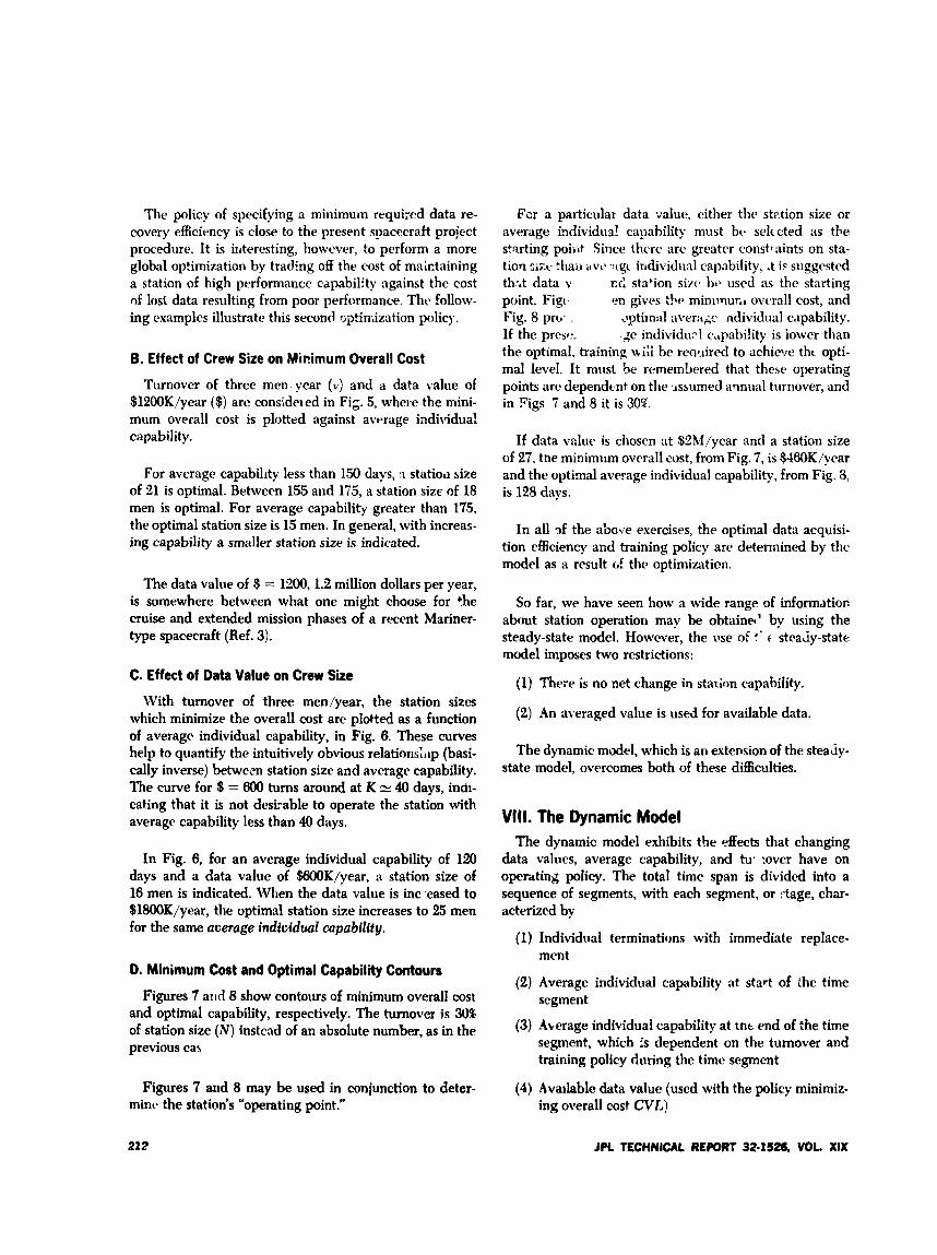
The policy of specifying a minimum requixd data re- covery efficiency is close to the present snacecrait project procedure. It is interesting, however, to perform a more global optimization by trading off the cost of maktaining a station of high performance capability against the cost nf lost data resulting from poor performance. The follow- ing examples illustrate this second rjptirrization policy.
6. Effect of Crew Size on Minimum Overall Cost
Turnover of three men, year ( v ) and a data value of $1200K/year ($) are consldeied in Fig. 5, where the mini- mum overall cost is plotted against avrrage individua! capability.
For average capability less than 150 clays, :I statio11 size of 21 is optimal. Between 155 and 175, a station size of 18 men is optimal. For average capability greater than 175, the optimal station size is 15 men. In general, with increas- ing capability a smaller station size is indicated.
The data value of $ = 1200,l.B million dollars per year, is somewhere between what one might choose for +he cruise and extended mission phases of a recent Mariner- type spacecraft (Ref. 3).
C. Effect of Data Value on Crew Size With turnover of three men/year. the station sizes
which minimize the overall cost are plotted as a function of average individual capability, in Fig. 6. These curves help to quantify the intuitively obvious relationshp (basi- cally inverse) between station size and average capability. The curve for $ = 800 turns around at K 2: 40 days, indi- cating that it is not desirable to operate the station with average capability less than 40 days.
In Fig. 6, for an average individual capability of 120 days and a data value of $BOOK/year, a station size of 16 men is indicated. When the data value is inc .eased to $1800K/year, the optimal station size increases to 25 men for the same average individual capability.
D. Minimum Cost and Optimal Capability Contours
Figures 7 and 8 show contours of minimum overall cost and optimal capability, respectively. The turnover i s 30% of station size (N) instcad of an absolute number, as in the previous cas
Figures 7 and 8 may be used in conjunction to deter- mints the station's "operating point."
For a particular data d u e , either the st2,tion size or average individus! capbility must bc. selt cted as the starting poiiit Since thcre arc greater consttaints on sta- tiorl sizr thaii avr' .:rgc irrdividud capability, .t ir suggested th:d data v .cd st;lcion siyc. 1 1 t h used as the starting point. Fig(. cm gives the, minimur.1 ovcrall cost, and Fig. 8 pro. . - ,)ptim;il aver;;< ndividual c'tpability. If the presrt; .de individupl c,,pability is iower than the optimal, training uiii he rewired to achieve tht opti- mal level. It must be remem!med that these operating points are dependent on the xssumed amual turnover, and in Sigs 7 and 8 it is 30%.
If data value is chosen at $%/year and a station size of 27. the minimum overall cost, from Fig. 7, is $480K/year and the optimal average individual capability, from Fig. 8, is 128 days.
In all 3f the above exercises, the optimal data acquisi- tion efficiency and training policy are determined by the model as a result of the optimization.
So far, we have seen how a wide range of informatior. about station operation may be obtainec' by using the steady-state model. However, the use of :* f stea\iy-state model imposes two restrictions:
(1) There is no net change in statinn capability.
(2) An averaged value is used for available data.
The dynamic model, which is an extension of the steady- state model, overcomes both of these difficulties.
VIII. The Dynamic Model The dynamic model exhibits the effects that changing
data values, average capability, and tu. :over have on operating policy. The total time span is divided into a sequence of segments, with each segment, or ftage, chnr- acterized by
(1) Individual terminations with immediate replace-
(2) Average individual capability at start of the time segment
(3) Akerage individual capability at tnt end of the time segment, which is dependent on the turnover and training policy during the time segment
ment
(4) Available data value (used with the policy minimiz- ing overall cost CVL)
212 JPL TECHNICAL R E W f 32.1526. VOL. XIX
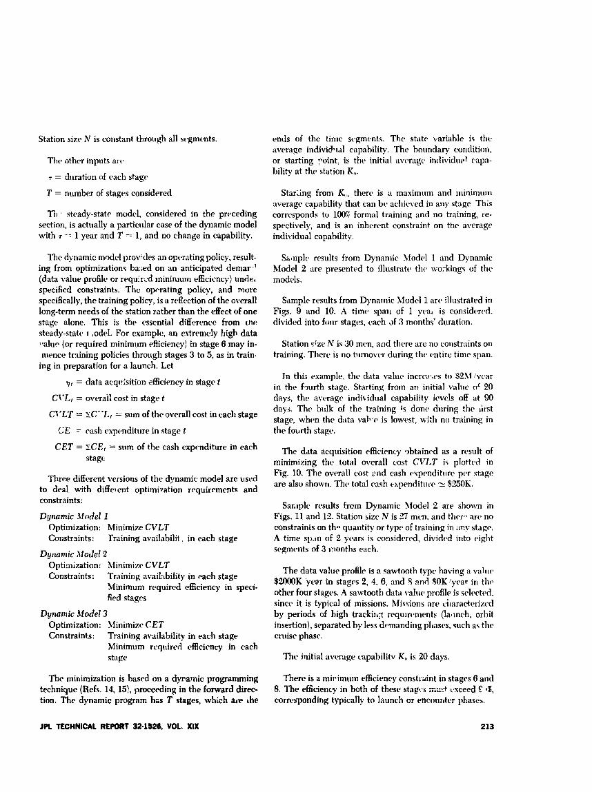
Station sizc N is constant through all segments. ends of the tinw segments. The state variable is the average individd capability. The boundary condition, or starting yoint, is the initial averagr individurl capa- bility at the station K, , .
The other inputs art'
T = duration of each stage
T = number of stages considered
Til . steady-state model. considered in the preceding section, is actually a particular case of the dynamic model with T = 1 year and T = 1, and no change in capability.
Stariing from K , , , thew is a masimiim and minimum average capnbility that can bta achieved in any stage This corresponds to 100% formal training and no training, re- spectively, and is an inhermt constraint on thc average individual capability.
The dynamic model provides an oprrating policy, result- ing from optimizations ba4;ed on an anticipated demar 7' (data value profile or requirc.d mininium efficicncy) unde. specified constraints. The opwating policy, and more specifically, the training policy, is a reflection of the overall long-term needs of thc station rather than the effect of one stage alone. This is the esscntial difference from the steady-state I .odel. For example, an extremely high data d u r (or required minimum efticiency) in stage 6 may in- iuence trnining policies through stages 3 to 5, as in train.
ing in preparation for a launch. Let
q t = data acquisition efficiency in stagr t
Cl'L, = ovrrai: cost in stage t
Sbbnple results from Dynamic hfodrl 1 and Dynamic Model 2 are presented to illustrate thv wo-kings of the modcls.
Samplc results from Dynamic Modc-1 1 arc. illustrated in Figs. 9 and 10. A time spar1 of 1 yeal is considered. divided into four stages, each af 3 months' duration.
Station +ze AT is 30 men, and thcre are no constraints on training. Tliere is no trimowr during the cntire time span.
Jn this example, thc data valur incrriiws to $2hf /war in the f?urth stage. Starting from an initial value or 20 days, the average indicidrial capabiiity ievels off at 90 days. The iirilk of the training i s done during the lirst stage, when the data Val*-cb is lowest, with no training in CI'LT = xC'L, = sum of the overall cost in each stage
CE = cash expenditure in stage t the-fourth stage.
CET = XCEf = sum of the cash expenditure in each The data acquisition efficiency ,,btainc.d as a result of minimizing the total owrall cost CVLT is plottcd in stage - Fig. 10. The overall cost 2nd cash espenditurr pcr stage are also shown. The total cnsh e-xpendituw = $%OK. Three different versions of the dynamic model are used
to deal with different optimii-ation requirements and constraints:
Dynamic Model 1 Optimization: Minimize CVLT Constrsints:
Dytiamic Afotle! 2
Sar.iplr results from Dynamic Model 2 are shown in Figs. 11 and 12. Station size N is 27 men, and thevi arc no constraints on thp quantity or typ(1 of training in m y stag(>. A time spin of 2 ycws is mnsidcred, dividcd into Piglit segments of 3 inonths each.
Training availabilit , in each stage
optimization: hlinimizr CVLT Constraints: The data vahe profile is a sawtooth type having a valrir
$ZooOK 'yesr in stages 2, 4, 6, nnd 9 and BOK 'year in thr. other four stages. A sawtooth data valuc. profile is selrcted. sincc it is typical of missions. Missions are ciiaraderizcd
Training availnbility in each stage Minimum requircd efficiency in speci- fied stages
. - Dynun1.k Model 3 by periods of high trackirq requirerrients (lalmch, orbit
insertion), separated by less dcBmanding pllasvs, such as thr Optimization: Minimizc CET Constraints: Training availability in each stage cruise phase.
Minimum required efficiency in each stage The initial average capabilitv K , , is 20 days.
The mirimizatioa is based on a dypamic programming technique (Refs. 14, 15), proceeding in the forward direc- tion. The dynamic program has T stages, which alee ihe
There is a mirimum efficiency constraint in stages 6 and 8. The efiiciency in both of these s t aps i;'.xt cxcecd C ' I b , corresponding typically to launch or encouritw phases.
JPL TECHNICAL REPORT 32.1526, VOL. XIX 213
The turnover profile was generated by sanipling from a Poisson distribution. The turnover through stages 1 to 8 is 3, 5, 7, 7, 2, 1, 5, 2 men, respectively. This is 81% and .37% turnover for the 2 years, respectively.
It is desired to find the operating policy to minimize the total overall cost CVL under the given constraints and input conditions.
hlaximum capability increases to 200 by the end of stage 5 and levels off, since, in practice, individuals seldom exceed this by much.
Minimum capability decreases gradually (due to turn- over) to a level of 15 and then jumps to 160 in the sixth stage. This is the effect of a minimum c4kiency constraint of %?& in stage 6. A capability of less th.m 160 would result in the minimum efficiency constraint being violated.
The: optimal apability increases, thrmsh trrinhg, to reach 160 days at the start of the sixth stage. Training follows a Sawtor th patterii which is a complement of the data value profile.
In Fig. 12, the actual efficiency in stages 2 and 4 is in- fluenced by the data value in those stages. However, in stages 6 and 8, the minimum efficiency constraint is clearly the dominating influence. The actual efficiency, in general, has a profile similar to the data value, a conclu- sion which is not unexpected.
The overall cost and cash expenditure through the stages are also shown in Fig. 12. The cash expenditure in
stapf- I, 3 and 5 is high because of the training costs (loOg bining in each stage). The cash expenditure averages to $45OK, YW.
Thus, the dynamic model provides an estimate of the demands that are placed upon the station, in terms of training and cash expenditure, to assist in formulating an operating policy which will meet future commitments.
IX. Further Efforts We are presently in the process of applying this analysis
to the recent developments at DSS 12, and expect to report on the following specific items:
Statistical relationship between salary and capa- bility (based on the new subsystem breakdown which became effective in lul? 1973)
Analysis of the capability lost during the actual attrition process
Analysis of the relationship between the quali6ca- tion and cerlification program at DSS 12 and our method of measuring capability
Measures of past station performance which can be related to crew capability
We are also developing a distributed capability model which will be able to optimize the allocation of individuals at the station to crews and training programs. A pre- liminary report of some of this work has been given in Refs. 1 and 3.
References
1. Bahadur, A., and W e b , P., Final Report, Maintenance and Operations Study of the DSZF, Document 8Nl-37, Sept. 1913 (JPL internal docriment).
2. Eyres, R., ai ' 'Towe, J., Building a Hardware Maintenance Team, Datamation, Nov. 1972.
3. Bahadur. A., and Goti'it' .;nil &.w&I Report .f Maintenance and Cpemtions Sf'*:dy of n i- . I. -:I-. W-19 Rev. A, Jan. 1972 (JPL internal document).
4. Berelson, B., ar ' .I ,. .$tun Behauior, Harcourt, Brace and World, lnc., 1964, pp. 137-IG.
5. 'Ghiselli, E. E., and Brown, C. W., Personnel and Zndustrial Psychology, 2nd Edition, Mdraw-Hill Book Co., 1955, pp. 78-81,258-!267.
214 J R TECHNICAL REPORT 32.1526. VOL XIX
References (contd)
6. Deese, J., The Psychobgy of Learning, 2nd Edition, McGraw-Hill Book Co., 1958, pp. 181-199.
7. Bahadur, A., r4nalysis of the Rela thhip Between Salary and Selected Param- eters, IOM 393.2-248, Oct. 1972 (JPL internal document).
8. Bahadur, A., Gottlieb, P., Hagen, P., and Meares, D., Interim Report of Main- tenance and Operations Systems Study, IOM W.2-98, June 30, 1971 (JPL internal document).
9. I&, G. J., An Approach to General Systems Theory, Van Nostrand Reinhold Company, 1969.
10. Hillier, F. S., and Lieberman, G. J., Zntrductwn to Opmztions Research, Holden-Day, Inc., 1987.
11. Younger, H., Training of Operations Systems Engineers, IOM 4223D-73-010, Feb. 27, 1973 (JPL internal dwument).
12. Bell, W., Preliminary P h for Training Operdion System Engineers, IOM 12-73-252, March 5, 1973 (JPL internal document}.
13. Patterson, L., Burford, A., and Bearden, P., Network Operations Perfonmnce Analysis Task SMC-75 Final Report, 422MA2, July 30, 1973 (JPL internal document).
14. Kaufmann, A., Dynamic Programming and Finite Games, Academic Press, 1967.
15. Bellman, R. E., and Dreyfus, S., Applied Dynamic Programming, Princeton University Press, 1962.
215
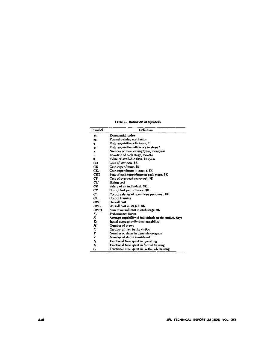
Table 1. Definition of Symbols
a1 a2
9 91
I
I
$ CA CE CEr CET CF CH CK CP cs CT CVL CVLt CVLT F P K Ko M 7.- P T tl t 2
t5
Exponential index Formal training cost factor Data acquisition efficiency, % Data acquisition efficiency in stage f Number of men leaving/year, men/year Duration of each stage, months Value of available data, $K/year Cost of attrition, $K Cash expenditure, $K Cash expenditure in stage t , $K Sum of cash expenditure in each stage, $K Cost of overhead pemnnel. $K Hiring e s t Salary of an individual, SK Cost of lost performance, SK Cost of salaries of operations personnel, SK Cost of training Overall cost Overall cost in stage t , $K Sum of overall cost in each stage, $K Performance factor Average capability of individuals in tbe station, days Initial average individual capability Number of crews S:iii:Lc. of mea in th- ststion Number of states in dynamic program Number of star- considered Fractional time spent in operating Fractional time spent in formal training Fiactiond trine spent In un-tkpb uai rhg
216 JPL TECHNICAL REPORT 32.12126, VOL XIX
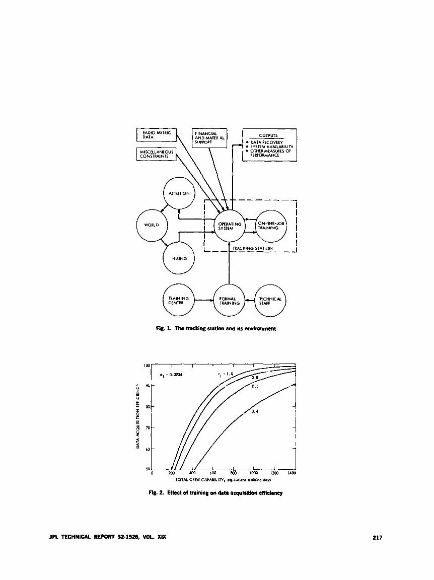
HIRING U TRAINING TKHFIKAL CENTER TRAINING
Fig. 2. The tracking station and its amhonment
100 I I 1 I I
a, = 0.m34
1 I I I 1 0 200 400 600 Boo loo0 1200 1400
TOTAL CREW CAPABILITY, w i v a l m t training d a y
Fie. 2. Effect of mining on bl. acquisition ef fkhcy
JPL TECHNICAL REPORT 32-1526, VOL. XIX 217

z
ON-THE-JOB TRAINING EFFECTNENESS
> V z w u U. v Y
T I M E SPEND IN ON- oN-Tw-~B -. ~ -:r 3 PUNING
i
TRAINING - -1 -
INCREASE IN CAPMLITY ATTRITION
15 18 21 24 27 30 33 36 1
FORMAL TiUlNiPiG FORMAL TRAINING
I ____ - -
3 6
b
CAPMLITY LOSS
w- I I 1 I I I L=1200,v=3mal /ywa
-
340-
110 140 i w l 160 izu im ipo 200 AXRAGF INDIVIDUAL CAPMIUPI I(, &IF
INCEASED TIME SPENT CAPMILIN IN FORMU
TRAINING
218
CEW B
INITIAL -t 1YHk SPCNI IN CAPABLIN OPEILATIONS CEW c
w
JPL TECHNKAL REPORT 32-1526, VOL. XIX
87
8 3 -
-
7p-N= N = STATION SIZE
I I I I I 1 I I 1 I
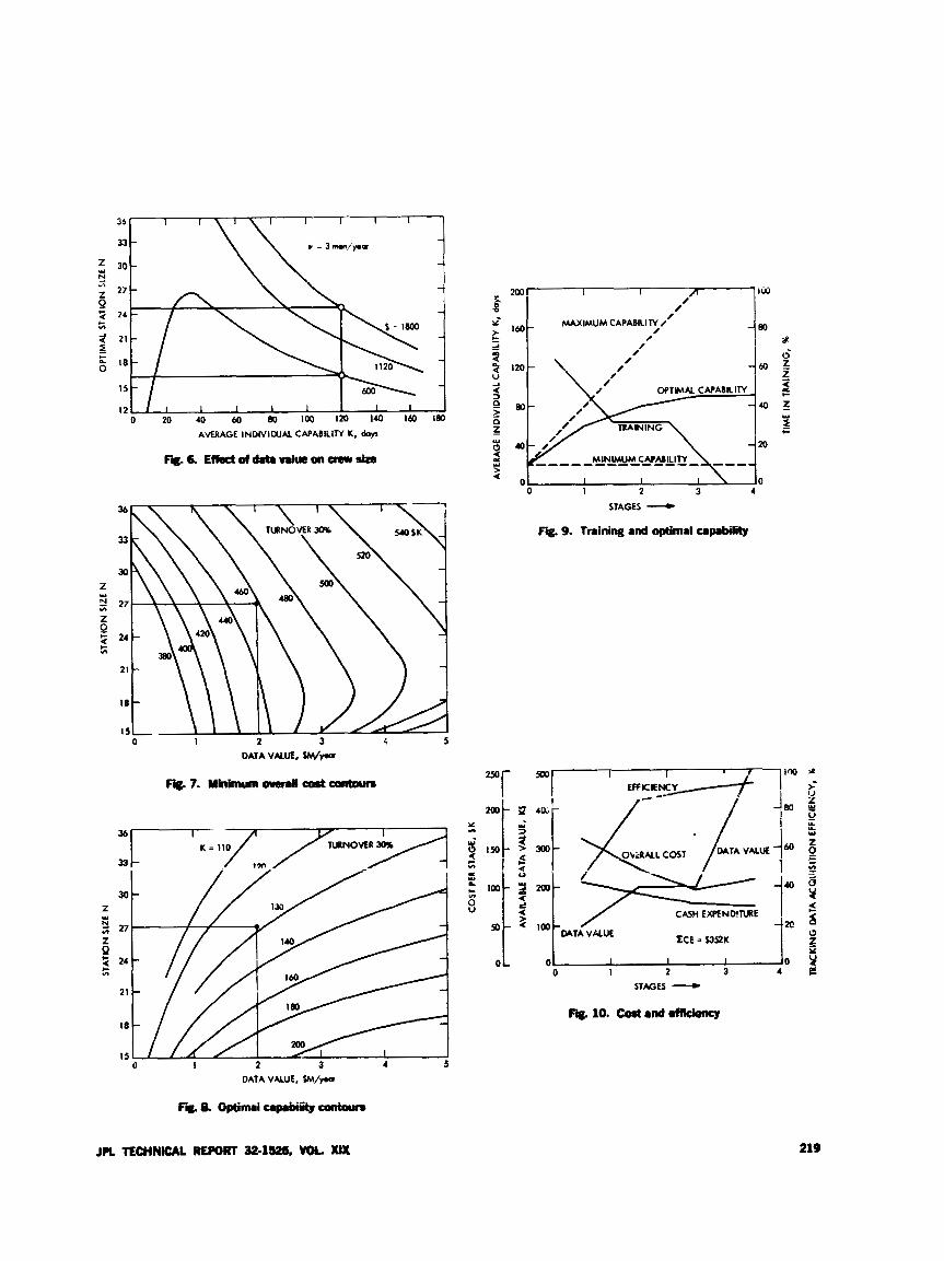
STAGES - Fig. 9. Training and optimal capability
0 1 2 3 5 DATA VALUE, wpa
Fig. 7. Mkimun -n cast collbws
0 I 2 3 4 5 DATA VALUE, W/px
~ i i a optimi ~ r p r w i - 0 t
219
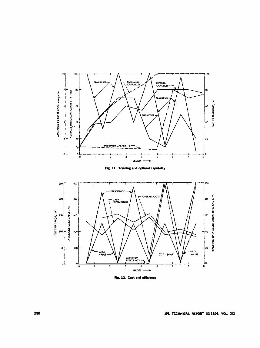
0 .- t c
d E 2 Y 0
Y I + z 0 z c 5
OL 0 I 2 3 4 5 6
STAGES 4
Fig. 11. Training and optimal capability
220
0 1 2 3 4 5 6 7 8 STAGES -
Fig. 12. Cost and eftkkncy
The DSN Hydromechanical Service Program- A Second Look
R. Smith and 0. Sumner DSN Facility Operations Office
The DSN Hydromechanical Semice Program has progressed satisfactorily along the lines originally ktended. The restilts of oil sampling a d analysis haue been particularly retcurciing, cleteding early signs of wear and forestalling catastrophic failures.
Sincv thc status rrqmt in Technical Report 32-1526 (Vol. SIV, pp. 216-%2), the program has progressed with gratifying results. Oil analysis is now being routinely per- formed for ..? 26 , stations and, on request, at the 64-m stations.
Thc past year of operation (Dec. 1972-Oct. 1973) has providd many csaniples of the value of a centralized oil m ~ ! y + program and a hydrttrt?t.rhsr:it! repsir faci!ity in discowring anomalous conditions and providing restor- ative service:
(11 A scno puiiip from DSS 12 showtd an incrcwe in metal particle count and was also reported to be s,mic*\vhat noisy. Disassembly and an inspection rtwalcd a missing spring retainer pin, excessive tvc-3~ in the p:ston and shoe assembly, excessive w u r in the creep plate, bad shaft bearings, dam- agtd hanger clevis, and splitting of the shaft sed. It can bc assumed that fililurc was imminent and that H catastrophic failurc was averted as a result of oil analysis. Thp pump was overhauled, tested, and returned to service.
(2) A new €4-m antenna drive motor was received for testing prior to shipment to DSS 14. The test failed due to a seized check valve in the crosschcck mani- fold. Phc motor was returned to the manufacturer under warranty. If this motor had not been tested prior to installation, it would have resulted in a failure at DSS 14. The motor was retested after the rcpsir did tile test was satbactory. The motor is currcntiy in operation at DSS 14.
(3) In December 1972, all 26-m antenna drive motors were drawn from network spares and shipped to the DSN hlaintenance Center for tmting prior to use in an rxchange program. It was found that none of the motors was operational, and a major over- haul effort was required.
(4) In I?-cembcr 1972. an analysis of DSS 12 hydraulic oil revealed a high concentration of metal from pump number two. An inspection performed by station prsonnc4 rev~a1e.d 3 f ailcd hanger ncrdlr bearing.
JPL TECHNICAL REPORT 32-1526, VOL. XtX 221
(5) In May 1973, an analysis of DSS 62 hydraulic oil revealed a high concentration of metal from pump number two and severe depletion of oil viscosity improver. The station was subsequently requested to change the pump and to drain, clean and refill thc system. The pump was returned to the DXiC for maintenance.
(6) In June 1973, an analysis of DSS 61 gear reducer oil revealed a high concentration of water in the hour-angle east gear reducer. A recommendation was made to drain the gear reducers. spray the interior with isopropyl alcohol to absorb the water, add approximately 76 1 of new oil and agitate with compressed air for 2 h, then drain the gear reducer and refill with new oil. After 30 days of operations, a sample :vas submitted for analysis and showed water content well below the oil specifications.
(7) In July 1973, an analysis of DSS 14 gear reducer oil revealed high metal concentration and depletion of viscosity improver. Oil was changed on all gear reducers.
(8) In August 1973, an analysis of DSS 43 and DSS 63 gear reducer oil revealed very heavy contamination. The two systems were drained, flushed, inspected,
and refilled. An analysis of the oil presently in use will be done in the near future.
(9) Figures 1 and 2 show the rotating group of a 6.i-m antenna drive motor removed from DSS 42 becausc of blown seals and a faulty crossfeed valve. 1ntt.r- nal inspection revcaled that a complete separation of the rotating group had occurred, resulting in sevtw damage to the cylinder block, seizure of one piston in the biock, and separation of the piston from thc shoe. A new rotating group was installed, and the motor was tested for smooth operation and static tested prior to being returned to the station.
A complete change of pumps and motors is near coni- pletion at DSSs 11 and 12. Already there has bcen a sig- nificant improvement in the contamination levels from these two stations during routine oil analysis.
In the near future, routine oil analysis will be facili- tated for the 64-m antenna systems. The prograin to exchange hydraulic components with rebuilt and serial- ized components will continue until all stations are com- pleted. Then the equipment will be monitored through oil analysis and recording of operational time on thr components. These two factors will determine frequency of replacement.
222 JPL TECHNICAL REPORT 32.1526, VOL. XIX

Network Command System Performance Test Report for Mariner Venus/Mercury 1973
6. Falin Network Operatiorls Office
This article presents a &scription of Network Command System Perfonname Tests that were executed throughout the DSN in support of the MVM'73 project.
I. Introduction The purpose of this article is to describe the Network
Command System Perfoimance Test (SF'T) conducted at each DSN station in preparation for the MI'hf'73 mission, and to report the status of each station at the time of launch. The objectives of the performance tests will be discussed, along with a description of the various sections of the test procedure. Problems uncovered and their solu- tions will also be discussed. The SPT is contained in Sec- tion I1 of Ref. 1.
II. Objectives The overall objective of the Network Command SPT
is to verify that the Network Command System can sup-
port MVM"13 operational capabilities. These capabilities are defined in various documents, such as Refs. 2 and 3. A more general statement would be lo v e d y each 5 L - tion's capability to provide the correct modulation mode, phase-shift keyed (PSK) with pseudo-noise (PN) synchro- nization (sync). More specific objectives are:
(1) To perform integration testing on telemetry and command processor (TCP) operational software.
(2) To verify station capabilities after hardware or soft- ware changes.
(3) To verify command capability while processing telemetry in the same TCP computer.
(4) To train station personnel with TCP operational software.
224 JPL TECHNICAL RE#)RT 324526, VOL. XIX

(5) To provide the stations with a prepass readiness test.
During the SPT, the telemetry and command data handling subsystcm ('TCD) operational program DOI- 5050-OP Model A, was exrlusively used in the TCP.
111. Test Procedure Format In this section, the format of the SPT, which will pro-
vide a description of the tests that were performed, will he presented. The SPT is divided into four main sections: Countdown, Manual Mode, Automatic Mode, and Reli- ability. The complete testing can be performed in approxi- mately six hours per TCD.
A. Countdown
The Countdown section is used as a prepass readiness test that is performed prior to the data transfer test with Nctwork Oprations. Using the appropriate TCP opera- tional software. commcnd capability is verified in the manual and remote mode of operations. The modulation index is adjusted and measured. Monitor interface is veri- fied. Both timed and nontimed commands are transmitted.
B. Manual Mode Tests
In this section, the samc type of testing is performed as in the Countdown section. Additional tests arc performed on dommand Modulator -4ssembly (CMA) configurations and TCP program manipulation. The ability to record .-Id recover command data from an analog tape is performzd.
C. Automatic Mode Tests
The automatic test uses the digital instrumentation subsystem (DIS) computer to simulate remote command operations. Special ttst software is used in the DIS to procm certain piogrammcd test sequences that can he i d y w d e n t l y svlccted I y an opcrator. Each test aequenre generates the command data, predicts results and verifies command data from the TCP, by utilizing high-+speed data (HSD) interface to the TCP. These test sequences are processed automatidy, and the resiilts are output to the operator. All HSD blocks are automatically checked against Ref. 2. The programmed test sequences are:
(1) CMA mode changes.
(2) Monitor interface.
(3) CMA operational alarms and aborts.
(a) Synibol rate.
(b) Sutcankr frequency.
(c) Command register and marker bit failure
(d) PN sync quality.
(e) Data quality.
(f) PSK data to PN sync ratio.
(4) Exciter interface alarms and aborts.
(5) Time command accura y.
(6) Stack warnings.
(7) PN generator failure detection.
detection.
0. Reliability Tests
In the reliability tests, the capability to command and to process telemetry in the same computer is demon- strated. Continuous commanding is exercised while processing telemetry at bit rates of 335, 2450, and 117.6 kilobitsj's. Commanding consists of pricrity commands on 26-s centers and timed commands on 30-s centers. The DIS computer is used to generate the command data, to process the commatd data from the TCP, and to process the telemetry data for errors. This type of testing is per- formed continuously for four hours per TCD.
An appendix has beer! added to the reliability section giving the stations the cspahility to test the PN generators used to generate the PN sync signal. ;his was developed after detecting bit rate alarms at some sthtions during the first SPTs. In this peculiar test, the 511-bit PN sequences generated by the CMA are processed as a 51 \-bit/s telem- etry channel. The processed telemetry is dhecked at the DIS for bit errors in the PN sequence. PN sequences con- taining bit errors are dumped on a 1ir.e printer.
IV. Problems In the following paragraph, .he problems uncovered
and the solutions to them will be discussed.
A. PSK Data to PN Sync Ratio
The majority of the stations did not have the correct ratio. Analog adjustments within the CMA were made to obtain the correct ratio. The repair depot procedures U * L A ~
changed to reflect the correct ratio adjustments on the CMA analog drawers.
B. Subcanier Frequency Alarms atid Aborts
Two stations experienced this problem only during reliability testing while processing 2450-bit/s telemetry.
JPL TECHNICAL RI#wlt 32.1526, WL XIX 22s
Engineering change order (ECO) 73-023 was installed in the CMA clock counter interface to eliminate the noise problem on TCP pin/pot h e s .
C. Bit Rate Alarms and Watch Dog Time Failures
DSSs 12, 14, and 42 experienced this problem. This cor?dition was corrected at DSSs 12 and 42 by analog adjustments. However, at Station 14, an emergency ECO was installed as a temporary solution. The final solution for all DSSs is currently being implemented by the Cogni- zant Operating Engineer (COE). During operations, the bit rate warning limits are narrow to en2.ble dstection of 5it *ate errors caused by PN generator failures.
D. Exciter Confirmation Phass Detector
Most stations reported excessive dc drifting on the out. put of the exciter’s confirmatioi rbase detector. The drid
was more pronounced at some stations. As a result, mm- mand confirmation was changed to use the local confirma- tion within the CMA. During the investigation, a wrong value capacitor that had been installed at the factory was discovered. Installing a capacitor of the corrxt value enabled the 2Em DSSs to meet specifications. ilowever, a different problem exists at the 64-m DSS with Pro- grammed Oscillator Control Assembly (POCA) installa- tion. The development section is still working on a solution to this problem.
V. Status at Launch DSSs 12, 14, 62, 63, and 71 had successfully completed
and passed all command system tests. DSS 42/43 com- pleted and passed approximately 80% of the command sys- tem test. DSSs 11 and 51 were not required to perform the tests.
References
1. DSlF Standard Test Procedure No. 853-62; 2A-08, Command System Test for MVM’73, Document No. 853. Jet Propulsion Laboratory, Pasadena, Calif. (JPL internal document in preparation.)
2. Deep Space Network System Requirements-Detailed lntetface De&:, Doc.*- ment No. 82C13. Jet Propulsion Laboratory, Pasadena, Calif., Feb. 1,1971. (JPL internal document.)
3. Deep Space Network Support Requirements for MVM’73 Project, Document NO. 615-15-Rev. A. Jet Propulsion Laboratory, Pasadena, Calif., Jan. 15, 1978. (JPL internal document.)
226

Bibliography
Andcrson, J. D., Determination of the Illasses of tlre Moon and l’etiirs cnid the A.stronomica1 Unit f rom Radio Trucking Data of ! h ~ Mariner ZZ Spacecruft, Technical Report 32-816. Jct Propilsion Laboratory, Pasadma, Calif., July 1, 1967.
Anderson, J. D., f a t al., “The Radius of Vcmus as Dctrrminc~l 5> Pl;,nrtary Rac!ar and Mariner V Radio Tracking Data,” 1. Atmos. Sci. 1)p. 1171-1 171 Scpt. 25. 1968.
Anderson. J. i)., “Determination c , f Astroclpnamic (:onstants and a Test of ihc, General Relativistic Time Delay \\’ith S-Rand Range and nopplcbr Dnta From Mariners 6 and 7,” Space Research, Vol. SI, pi). 10s-112. i’.’-ad(.niic,-Vc.rlng. krlin. 1971.
Rarnum. P. ’VV., et al., Tracking and Ps ta S ! y s t ~ i n S u p p r t for tliz M u r i w r Mar,? 1971 Alission: Orbit ftisertion Thrmrgl! Err1 of Priwar!r Jlkoion. Tcchnical hiemorandurn 33-523. Vol. 111. Jct P;opul;ion L,nForator;,f. Pttsadcm, Cdif.. May 15, 1973.
Bathker, D. A., Predicted and hleasurec! t J ‘, Dcscription of Q LAIT~P Grorrnd Aficrowaoe System, Tcdinical Mr*inor;dliiti ?.?--i>3. Jct Fropul>,:on Laboratory, Pasadena, Calif.. Apr. 15, 1971.
,.:.
Berman, A. L., Tracking System Data Annlysis Rcport. Ranger VI1 Find R e p r t , Technical Report 32-719. let Propulsion Laboratorv Pm&.rla, Cal’f.. June 1, 1965.
Butman, S., “Rate Distortion Over Rmd-Limitcd Fcetlbwk Ch;innc.ls.” ZEEE Trans. Inform. Theory, \’ol. IT-17, No. 1, pp. 110-112, Jm. 1971..
Butmnn, S., and Timor, U., “Interplex-An Efficient Multichannel PSK , P k Tvlem- d r y System.” ZEEE Trans. Commtrn., Vol. COM-20. No. 3. r2. 41.549. June 1972.
Cain, D. L., and Hamilton, T. If’., Detcrmirration of Tracking Station Locations by Doppler and Range Measurements to an Earth Satellite. Technical Report 32-534. Jet Propulsion Laboratory, Pasadena, Calif., Feb. 1, 1964.
Carey, C. N., and Sjogren, W. L., “Gravitation;il Inconsistency in thr Lunar Theory: Confitmation by Radio Tracking,” Science, Vol. 160, pp. 87S-876, April- Junc 1968.
Chadwick, H. D., and Springett, J. C., “The Des\ gn of a Low Data Riltc. hlSFK Communication System,’’ l E E E Trans. Commun. Technol., Vol. COLI-18, No. 8, pp. 740-750, Dec. 1970.
Clark, B. G., ct al., “High Resolution Observations of Compact Rcidio Sources at 13 cm,” Astrophys. J., Vol. 161, pp. fN3-809, Sept. 1970.
Curkendall, D. W., and Stephcnson, R. R., “Earthbased Tracking and Orbit Deter- mination-Backbone of the Planetary Navigation System,” Astronarit. Aeronaut., VOl. 7, Mny 1970.
Curkendall, D. ’,’,’., Lxta ry Navigation: The New Challenges,” Astronaut. Aeronaut., Vol. 7, Aa, 16‘0.
JPL TECHNICAL REPORT 32.1126, VOL. MX 227
Bibliography (contd)
Downs, G. S., and Reiclrley, P. E., “0bsw:ations qf Interstellar Scintillations of Pulsar Signals at 2388 MHz,” Astrophys. J. , Vol. 163, KO. 1, Pt. 2, pp. L11-I 16, Jan. 1971.
Downs, C. S., et al., “Mars Radar Obsewation, A Preliminary Report.” Science, Vo!. 174, No. 4016, pp. 1354-1327, De. 24, 1971.
Efmn, L., and Solloway, C. B., Proceedings of the Conference on Scientific .4ppli- cations of Radio and Radar Tracking in the Space Program, Technical Report 32-1475. Jet Propulsion Laboratory, Pasadena, Calif., July 1970.
Flanagan, F. 11.. et al., Deep Space Network Support of the Manned Spme Flight Nctuwk for Aydlo- 1W2-1968, Technical Memorandum 33-452. Vol. I. Jet ho- pulsion Laboratory, Pasadena, Calif., July 1970.
Flanagan, F. \I., et al., Deep Space Setwork Support of the ?.fanned Space Flight Netuxwk for Apdlo: 1969-1970, Technical Memorandum 33-452. Vol. 11. Jr t Pro- pulsion Laboratory, Pasadena, Calif., May 1, 1671.
Fjeldbo, G., and Eshlrman, V. R., “Radio Occultation Measurements and Inter- pretations,“ in The Atmospheres of Venus and Mars, p. 225. Gordon and Breach, Sciency Publishers, Inc., New York. N.Y
Cmrgevic, R. M., Mathematical Model of the Solar Radktion Force and Torques Acting on the Components of a Spacccraft, Technical Memorandum 33-494. Jet Propulsion Laboratory, Pasadena, Calif., Oct. 1, 1971.
Goldstein, R. M., ”Radar Time-of-Flight Measurements to Venus.“ Astron. I.. Vol. 73, No. 9, Aug. 1968.
Coldstein, R. M., “Radar Observations of Mercury.” Astron. J., Vol. 76, No. 10, pp. 1152-1154, Dec. 1971.
Gordon, H. J., et al., The Mm’ner 6 and 7 Fl&t Paths and Their Determination From Tracking Data, Technical Memorandum 33-469. Jet Propulsion Labora- tory, Pasadena, Calif., Dec. 1, 1970.
Gray, R. M., and Tausworthe, R. C., ”Frquen*.y-Counted Measurements, and Phase Locking to Noise Oscillators,” ZEEE Tmns. Commun. Technol., Vol.
Gulkis, S., and Gary, B., “Circular Polarization and Total-Flux Measurements of Jupiter at 13.1 cm Wavelength,” Astron. J., Vol. 76, No. 1, pp. lZ l6 , Feb. 1971.
Hall, J. R., Tracking and Data System S~qqwrt for Lunar orbiter, Technical Memo- randum 33-45(! Jet Propulsion Laboratory, Pasadena, Calif., Apr. 1970.
Hamilton, T. W., et al., The 3anger N Flight Path and I t s Determination From Tracking Data, Technical Report 32-345. jet Propulsion Laboratory, Pasadena, Calif., Sept. 15, 1962.
Holmes, J. K., “First Slip Times Versus Static Phase Error Mset for the First and Passive Secmd-Order Phu.e-Locked Loop,” IEEE Trans. Commun. T e c h d . , Vol. COM-19, NO. 2, pp. 234-235, Apr. 1911.
Holmes, J. IC., and Tegnelia, C. R., Digital C:ommarUi S p t e m Second-Order Sub- currier Tracking Perfonnnnc~, Technical Report 32-1540. Jet Propulsion Labora- tory, Pasadena, Calif., Oct. 1, 1971.
COM-19, NO. 1, pp. 21-30, F&. 1971.
J R TECHNICAL RE- 32.1- VOL Xar

Bibliography (contd)
Holmes, J . K., “Performince of a First Order Transition Sampling Digital Phase- Locked Loop Vsing Random-\\’alk Models,” ZEEE Tmns. Commun.. Vol. COM-LO. So. 1. pp. 119-131, Apr. 1972.
Kliore, A., “Sadio Oc-cultation Measurements of the Atmospheres of S!PF 2nd \~c~nus,” in The -4tnw.rpheres of Venus and Mars, by J. C . Brandt and .\I. E. SIcElrow. p. LYE. Gordon and Breach Scicmce Ptihlishers. Inc.. Sew Tork, N.Y.. 196s.
Kliort., 4. J.. t b t al.. YhrnmaT of Mariner 6 and 7 Radio Occultation Results on the ?tmorpherr. of Mars.” Spce Research. Vol. SI, pp. 16%17S, Akademie-Verlag. Berlin. 1971.
Labnim. R. C.. t-t al.. The Sumeyor \-. i‘l. c i i d 1711 F!i@ paths C i i d Their Deter- mination f rom Tracking Data. Technical Repctrt 31-1m2. Jet Propulsion Labora- tory. Pasadena. Calif.. Dw. 1, 1968.
Laeser, R. P.. et al.. Tmcking and Data System Support for the Jfnriner Mars 1971 Mission: Prelaunch Phase Through First Trajectory Correction Maneuter. Tech- nical 3:cmorrii:2unb 33-53, Vd. I. Jrt Propl;im Labora;c?ry, Pzza3cnn. Calif., blar. 15. 1972.
Layland, J. lV., and Lushbaagh. IV. -4.. “A Flesible High-speed Sequential Decoder €or Deep Space Channels.” lEEE Tmnr. Cornnuin. Technol.. Vol. COM-15 So. 5. pp. 81.3-8X. Oc-t. 1971.
Lcavitt. R. K.. The Least-Squares Process of MEDIA for Computing DRVID Cali- bration PoZynomiuLs, Technical Memorandum 23542. Jet Propulsion Laboratory, Pasadcm. Calif.. May IS. 1972.
Lieskc. J. H., and Null, G. W., “Icarus and the Determination of Astronomica! Con- stant;.” Astron. I., Vol. 74. No. 2, Mar. 1968.
Lindsey. \Ir. C.. and Simon, M. K.. ‘The Effect of Loop Stress on the Performance of Phase-Coherent Coriimunication Systems, ZEEE Tram. Commun. Technd., \oi. COM-IS. Nc: 5, pp. 39-556. oct. i970.
Lindsey, W. C., and Simon. M. K., ”Carrier Synchronization and Detection of Poly- phase Sip&“ lEEE Trans. Commun., Vol. COhl-20, No. 3, pp. 441-454, June 1972.
Lorell, J., and Sjogren, W. L., Lunar Orbiter Data Anulysis, Technical Report 32-1220. Jet Ropulsion Laboratory, Pasadena, Calif.. Nov. 15. 1987.
Lorell, J. , Lunur Orbitct Craoity AnuZ~~sk, Technical Report 32-1387. Jet Propulsion laboratory. Pasadena. Calif.. June 15, 1969.
Lorcll. J.. ct al., ”Icarus: Celestial Wchanics Experiment for Mariner.” Znt. I. SOL Sys., Vol. 12, Ian. 1970.
Ludwig, A. C., et a]., Cain Calibration of a Horn Anfennu Using Puilmr Ztifcgm- tion, Technics! Rcport 32-1512. Jet Propulsion Laboratory, Pasadena, Calif., Oct. 1,1972.
McNeal, C . E., Ranger V Tracking Systems DBto Am4sis Final Report, Technical Report 32-702. Jet propllsion Laboratory, Pasadena. Calif., Apr. 15, 1W5.
229
Bibliography (contd)
Melboiime. \\.. G., et ai., Cot~s ia~ l t .~ urid Reluted Iiiformution for -4sttodytlcrmkd Cuic~tlutions, Technical R q m t 32-1306. Jet Propulsion Laboratory. Pasadena. Cdif.. July 15, 1968.
hfelbaui-ne. \Y. G.. “Planetary Ephemeri(1c.s.” .Wronuuf. Aeronnut.. Vol. 7. Slay 1970.
Miller, L., et al., The Atka ”entaur VI Flight Puth u1ul Its Detrrmir~ution from Tracking Datu, Technical Report 32-91 1. Jet Propulsion Laboratoq-. Pssadtma, Calif., Apr. E. la&.
htoyer, T. G., -ifiA?niiticd Fomr:lutioi cf the Dmthle-Precision Orbit Detaminu- tion Progrum (DPODP), Technical Report 32-1527. Jct Prcplsion L:iboratoq-. Pasadena. Calif., \lay 17. 1971.
Mulhall, B. D., et al.. Tracking System .Analytic Calibration Acticities for the Mariner .\furs 1!XB Jfission, Technical Report 32-1499. Jct Propulsion Lahnra- tor?;. Pasadr-za, Calif., Kov. 15, 1970.
?rlulholland. J. D., and Sjogren, W. L., Lunar Orbiter Ranging Doto. Tcchnical Rrpnrt .32-1087. Jet Propulsion Labrator).. Pasadena. Calif.. Ian. e, 1967.
hiulholland, J. D.. Proceedings of the Symposium on Obserrcition. Analysis. and Space Research Applicutions of the Lunur Motion, Technical Report 32-1386. Jet Propulsion hlwratnp. Pasadena. Calif.. Apr I=.
3iiiller. P. hi., and Sjogwn, IV. L., Consistency of Lunar Orbiter Residrrals With Trujectoy and Local Gracity Efeds, Technical Report 32-1307. Jet Propulsion Laboratory, Pasadena, Calif., Sept. 1, 1968.
Muller, P. M.. and Sjogren. IV 1 . I.rtnor 3 f m Concztitrutiotw. Technical Rcport
Kull, G. \V., et al., Mariner W Flight Puth urd its Determination From Trucking D&d, Tcc!tirit n: nt-pjrl 32-110s. Jt-t PropuLioii Lahratoi-).. Pasadena. Calif..
UXeil. W. J., ct al., The Strm~yor Ill u14 Stmm~or n’ Flight Paths and Their nrfvm;wtion From Tracking Datu, Technical Rrport 3.’- 12‘32 Jet Propulsion Laboratory, Pasadma, Calif.. .4ug. 15, 1W.
32-13’39. Jet Propulsion Laboratory, Pasadena. Calif.. Aug. 16, 1968.
Aug I, 1967.
Otoshi, ‘I. Y.. and Steizrid. C. T.. “;Z Precision Compact Rntnr)- I’anc .\ttcr,cntci.” I E E E ?mi:;. .?fi:rc. T?icor Twhni7vrn I’d. \UT-19. No. 11. pp. M, Nov. 19il.
Pcase, G. E.: et al.. The Mariner V Flight Path and Its Determination F r o m Truck- ing Datu, Technical Report 32- I.%?. Jct Propdsion Lahoratvy. Pasadena, Calif., July 1. 1969.
Renzetti, S. A., Trucking a d nuto Acquisition for Ranger Afi&ons I-V, Technical Memorandum 33-174. Jet Prnpalsinn Laboratory, Pasadena, Calif., July 1, 1964.
Renzetti, N. A.. Trucking and Datu Acquisition for Ranger Aflssiuns VI-IX, Tech- nical Memorandum 33-275. Jet Propulsion Labratow, Pasadena. Calif.. Sept. 15, 1956.
JPL TECHNICAL RE#)RT 32.1526. VOL XIX

Bibliography (contd)
Renzctti, N. A., Trackin? nnd Do+a Acquisition Support for the Mariner Venus 1962 Afission, Technical Memorandum 33-212. Jet Propulsion Laboratory, Pasadeiia, Calif., July 1, 1965.
Renzctti, N. A., Tracking and Data Acquisition Report, Mariner Mars I 9 6 4 Mission: Near-Earth Trajectoy Phase. Technical Memorandum 33-39, Vol. I. Jet Propnl- sion Laborator?. Pttsadcna, Calif.. !an. I, 1965.
Renzetti, X. A.. Tracking and Data Acquisition Repcrt, Mariner .\furs 1964 3lision: Cruise to Post-Encounter Phase, Technical Memorandum 33-239. Vol. 11. Jet Pro- pulsion Laboratory, Pasadens, Calif., Oct. 1, 1967.
Renzetti. N. A.. Tracking and Data Acquisition Report, Mariner Mars 1!%4 Afission: Extended Mission, Technical hlemorandum 33-239, Vol. 111. Jet Propulsion Lab- oratory, Pasadena, Calif., Dee. 1, 1968.
Renzetti, h. -4., l'racking and Data Systcm Suppc? 5~ S . I ' Z C ~ : ?.!isimi I and I!, Trchniral SIemorandun: 33-301. 1'01. I. Jet Propulsion Laboratory, Pasadena. Calif., July 15, 1969.
Renzetti, K. A., Tracking and Dutu Sy~tenr Support for Surceyor: Missiuis 111 and ZV, Technicai iCtt.morandim XK101. Vol. 11. Jet Pmpiilsion Ishratory, Pasadcna, Calif., SCpt. 1. 1969.
Renzetti, N. A., Tracking and Data System Support for Sumeyor: itfission V, Tech- nical Memorandum 33-301, Vol. 111. Jet Propulsion Laboratory, Pasadena, Calif., Dec. 1,1969.
Renzetti, Pi. A., Tracking and Data System Suppori joi. Surceyor: Mission VI, Tech- nical Memorandum 33-301, Vol. IV. Jet Propulsion laboratory. Pasadena. Calif., Dw. 1,1969.
Renzetti, K. A., Tracking and Data S y s t e m Support for Sumeym: lMission Vi i , Technical Memorandum 33301. Vol. V. Jet Propulsion Laboratory, Pasadena, Calif., Dec. 1, 1969.
Renzetti, N. A., Tracking and Data System Support for the Mariner Venus 67 Mis- sion: Planning Phase Through Midcourse Maneuver, Technical Memoranaum XXM.5, Vol. I. Jet Propulsion Laboratory, Pasidxx, Cr.lif CC?+ l, IC%.
Rcnzetti, N. A., Tracking and Data System Support for the Mariner Venus 6'i Mis- sion: Midcourse Manewer Through End of Mission, Technical Memorandum 2-3, l'd. 1;. ;ct PiCrprtLiua La'hzatx>, Fasdci,a, Z nlif., Sept. 1, 1969.
Remetti, N. A., Tracking and D d a System Support for the Pioneer Project. Pioneer VI. Prelaunch to End of Nominal Mission, Technical Memorandurn 33-426, Vol. 1. jet Propulsion Laboratory, Pasadena, Calif., Feb. 1, 1WO.
Renzetti, hi. A., Tracking and Datu System S u p p d for the Pioneer Project. Pioneer VU. Prelaunch to End o f Nominal Mission, Technical Memorandum 33-428, Vol. 11. Jet Propulsion Laboratory, Pasadena, Calif., Apr. i5, 1970.
Renzetti, N. A., Tracking and Data System Support for the Pioneer Prdect. Pioneer VIIZ. Prelaunch Through May lW, Technical Memorandum 33-426, Vol. 111. Jet Propulsion Laboratory, Pasadena, Calif., July 15,1970.
JPL TECHNICAL REPORT 32.1526, VOL. XIX 231

Bibliography (contd)
RtmLetti, N. ,4., Tracking nnd Dntn System Support for the Piuneer Project. Pioneer ix. Prelaunch Through June 1969, Technical Memoranduni 33-426, Vol. 11’. Jet Propulsion Lahoratoy. Pasadena, Calif., Nov. 15. 1970.
Renzetti, N. A., Tracking and Data System Support for the Pioneer Proiect. Pioneer VI. Extended Mission: July I , 1%6-July I , 1.969, Technical Memoran- dum 33-426, Vol. V. Jet Propulsion Laboratory, Pasadena, Calif., FA. 1, 1971.
Renzetti, N. A., Tracking and Data System Support for the Pioneer Project. Pioneer VU. Extended Mission: February 24,1967-July I. 1968, Technical Mem- orandum 33-426. Vol. VI. Jet Propuhor. Laboratory. Pasadena, Calif., Apr. 15, 197;.
Renzetti. N. A., Tracking and Data System Support for the Piotteer Proiect. Pioneer VIl. Extentied Mission: July I , 19W-Jrrly 1. 1W. Technical Memoran- dum 33-426, Vol. VII. Jet Propulsion lalmatory, Pasadena. Calif., Apr. 15. 1971.
Renzetti, E. A., Tracking and Data System Support for the Pioneer Prqect. Pioneer VZIZ. Extended Mission: lune 1,19f%July I, 1969. Technical Memoran- dum 33-426, Vol. VIII. jet Propulsion Laboratory, Pzsadenu, Calif., May 1,1971.
Renzetti, N. A., Tracking and Doto Sgstem Support for th r Pinnew Prqect. Pioneers VI-ZX. Exlended Jfigsims: ;dij ?./$?fB-Jrily 1. 1.970. Technical Memo- randum 33-426, Vol. IX. Jet Propulsion Laboratory P ~ s a d e n ~ . G l ? . Aog. 15, iSi 1.
Renzetti, N. A., and Siegmeth, A. J., Tracking and Data System Support for the Pioneer Prqect. Pioneers 6-9. Extended Missions: July 1. Z97Z-July I , 1972, Technical Memorandum 33-426, Vol. XI. Jet Propulsion Laboratory, Pasadena, Calif., May 1, 193 .
Siegmeth, A. J., Purdue, R. E., and Ryan, R. E., Tracking and Data System Sup- port for the Pioneer Project. Pioneers 6-9. Extended Missioru.: 3 4 I , Z970- 3uZy I, 1971, Technical Memorandum 33-426. Vol. X. Jet Propulsion Laboratory, Paszdena, Calif., Aug. 15, 1972.
Siegnwth, A. J., et al., Tracking utd Daw S y ~ i t m Support for the Pioneer Prqect: Pioneer 10-Prelaunch Planning Through Second Traiecto y Comertion Decem- bcr 1, 1969 to April I, 1972, Technical Memorandum 33-584 Yd. I. Jet Propul- sion Laboratory, Fasadem, CdIif., Ap:. 1, !E?.
Simon, hl. K., “Nonlinear Anaiysk of an L\b50!utt. F’alue T y p of an Early-Late Gate Bit Synchronizer,” IEEE Tmns. Commun. Technol., Vol. COM-18, No. 5, pp. 58!3-596, Oct. 1970.
Simon, M. K., qnd Lindsey, ii;. C., “Data-AiJd Chrricr Trxking Loops,” ZEEE Truns. Comtnun. Tecknol., Vol. COM-19, No. ?, pp. 157-168. Apr. 1971.
Simon, M. L, “On the Selection of an Optimum Design Point for Yhase-Coherent Receivers Employing Bandpass Limiters,” ZEEE Trans. Commrrn., Vol. COM-20,
Simon, M. K., “On the Sdectition nf B Sampling Filtw Rmdwidtt., for a Digital Dam Detector,” IEEE Trans. Commun., Vol. COM-20, No. 3, pp. 43-441, june 1972.
No. 2: 1y). 210-214, Apt. 1972.
232 JPL TECHNICAL REWRT 32.1526, VOL. XIX

Bibliography (contd)
Sjogrcm. IV. L., et al.. The JLii:gCr ‘i; Fight Path and Its Lletemiiwtion From Tracking Data, Technical Report 3256.2 Jet Propulsion Laboratory. Pasadena, Calif., Dtr. 6, 1963.
Sjogren, 11’. L.. et al., ‘1 he Ronger VI Flight Path and Its Drtermirlatiori From Tracking Data. Technical Report 32-605. let Propulsion Labratory, Pasadena, Calif., DeL. 1.5. 1964.
Sjogren, W. L.. The Ranger IIZ Flight Path and Its Detemhatimi Froin Ttucking Data, Technical Report 32-.563. Jet Propulsion 1,aImrato~. Pasadena. Calif ,. Sept. 1.5, 1965.
sjngrm. IV L.. 1.t ai.. Phy.sica1 Constants Q-s Detemtiried From Radio Tracking of the Ranger Lunar Prohe.$, Tcuhnical Report 32-1&7. Jet Propalsion f,aboratory, Pasndcna, Calif.. Dec. 30, 1966.
Sjogren, \Y. L., Proceediiigs o f the JPL Seminor on I’ncertcinties in the Lunar Ephemeris. Technical Report 32-12-47. Jet Pmpulsion Laboratory, Pasadena. Calif., M a y 1. 1 W .
Sjogren. IV. L.. “Lunar G~avity L t i i i i k t t . !iic?+cz&.~t Confirmation.” I. Chph!/s. So.. ‘,’d 76. So. 29, Oct. lG. i97i.
Sjogren, W. L.. et ai., ‘Lunar Lravity via .4pollo 11 Doppler Radio Tracking.” Science. L7o1. 175, So. 4018, pp. 16168. Jan. 14. 1979.
Spirr. G. W., Design and Implementation of .\fOciels for the Double Precision Tra- iectory Program (DPTRAJ). Technical ~1r~rnorr;ndum 33-451. Jet Propulsion Liboratory. Pasadena, Calif., ’4pr. 15, 1971.
Springc!t, J C.. and Simon, 31. K.. “An -4nalysis of the Phase Coherent-Incoherent Output 4 thc Bnndpass Limitcr,” JEEE Truits. Commtm. Technol., Vol. COM-19, So. 1. pp. 4249 . Fc+. 1971.
Stelzried. C. T.. A Faraday Rotation Measurement of a 13-cm Signal in the Solar Coruttu, Ttrlinieal Rtport 32-1401. Jrt Propulsion Libratory. Pasadena, Calif.. July 15. 1970.
Stclzried. C. T., t b t nl., “Thc Quasi-Stationary Coronal Magnetic Firld and Elcutron Density as Determined From a Faraday Rotation Experimc-nt.” Sol. Phis.. 1’01. 14, s.3. 2. pp. 113-4.x. Oct. 19770.
S t t h k d , c‘. *f., ‘.Gpt*i .i;i.ib N~is~-T[.mycrTtiin. Cithbrations of hw-Noise Receiv- ing Systems,” Aficrowace J., 1’01. 14, KO. 6, pp. 3146.48, June 1971.
the Plane of the Ecliptic,“ J. Space. Rock.. Vol. 9, No. 2, pp. 69-70, Feb. 1972.
Ltmps U‘ith Stcady-State Phase Error,” ZEEE Trans. Cmmun. , Vol. COM-20, No. 3, pp. 331-337. June 19’72.
Ttxtor, G. P.. K d y , L. B., and Kelly, M., Tracking and Data System Support for the Mariner Mars 1971 Aiis.~ion: First Trajecto y Correction Maneuwr Through Orbit Znscrfion, Trchnical Memorandum 33-523, Col. 11. Jet Propulsion Labora- tory, Pasadeiia, Calif.. June 15. 1972.
Stcl7ric-d. C. T.. rt al.. “Transformation of Rwx~iwd Signal Folarization .4nglc to
T. ‘lris\\orthc. . . R. C., “Simplified Forintila for hlcan-Slip Time of Phase-Locked
JPL TECHNICAL REPORT 32-1526, VOL. XIX 233

Bibliography (contd)
Thornton, J. H., Jr., The Sumeyor I and Surceyor I1 Flight Paths and Their Deter- minution From Trucking Data, Technical Report 32-1285. Jet Propulsion Lbora- tory, Pasadena, Calif., Aug. 1, 1968.
Timor, U., “Equivalence of Timc.-hltiplexed and Frequency-Multiplexed Sig- nals in Dieit91 Commrnications,“ IEEE Truns. Cornmun., 1’01. COXI-20, No. 3, pp. 435438. Jiine 1972.
Vega. C . I., c! a?., Tbe Rmy:C? IX Flight Path and Its Determination From Track- ing Data, Technical Report 32-767. Jet Propulsion Ldmratory, Pasadena, Calif., Nov. 1. 1968.
Winn, F. B., Sebnugrupltic Location of Surceyor VI, Sumeyor 1’1 Mission Report: Part ZI . Science Results, Technical Report 31-1262. jet Propulsion Laboratory, Pasadena, Calif., Jan. 10, 1968.
Winn, F. E., “Pus: Landing ‘l’racking Data .4calysis,” in Surc~yur \’!Z liission Report: ?ut? II. Science Results, Technical Rrport 32-1264. Jet Propulsion Lah- oratory. Pasadena. Calif., Mar. 15, 1968.
!%‘inn. F. B., “Post Lunar Touchdown Tracking Data Analysis,” in Srirceyor Prqect F i n d Report: Part 11. Scizrccc Rcsuf:.;, ’fcchnicai kport 32-1265. Jet Propulsion Laboratory, Pasadena, Calif., June 15, 1968.
Winn, F. B., Surveyor Pnsttmichdolan Anu!yse:s of Trocking Dnta, ??.%SA S P - I S . National Aeronautics and Space Administration, N~asshington, D.C., p. 369.
Wollenhaupt, W. R., ct al.. The Ranger VI1 Flight Path and Its Determination From Trucking Data, Technical Report 32-694. Jet Propulsion Laboratory, i‘asadcna, Calif., Dec. 15: i96-i.
JPL TECHNICAL REPORT 32-1526, VOL. XIX NASA - Pl - 6 m l , 1.A .Calif
Top Related
Copyright © 2022 FDOKUMEN

