


Bahasa
Halaman
Hukum


THE EFFECT OF PRICING ON MARKET SHARE OF SUPERMARKETS IN THE
NGAKA MODIRI MOLEMA DISTRICT OF THE NORTH-WEST PROVINCE OF
SOUTH AFRICA
ATEBA BENEDICT BELOBO
21994358
A dissertation submitted in fulfilment of the requirements for the degree
Magister Commerci: Marketing Management
Promoter: Prof. J.J. Prinsloo
October 2014
in the
Faculty of Commerce
at the
North West University
Mafikeng campus

DECLARATION
Academic Administration (Mafikeng Campus)
SOLEMN DECLARATION (for Masters and Doctoral Candidates)
Solemn declaration by student
HUPn l '8[\~i UUiVCf~S!TY ';IYliBESI7: 'il·. llOVJ)i·li:·!JOPHIFII·'•\ t\0(.\RLNII"~i-tHIIVlk;\ n i1
N1i\Fif{Fr·1Ci C.MM'U~:;
___________ declare herewith that the mini-dissertation/dissertation/thesis entitled,
which I herewith submit to the North-West University as completion/pmtial completion of the requirements set for the degree, is my own work and has not already been submitted to
any other university.
I understand and accept that the copies that are submitted for examination are the property of the University.
Signature of candidate ___________ University-number __________ _
Signed at. _________ this __ day of ________ 20
Declared before me on this ____ day of ________ 20
Commissioner of Oaths: -------------
Declaration by supervisor/promoter
The undersigned declares:
that the candidate attended an approved module of study for the relevant qualification and that the work for the course has been completed or that work approved by the Senate has been done
the candidate is hereby granted permission to submit his/her mini-dissertation/dissertation or
thesis

that registration/change of the title has been approved;
that the appointment/change of examiners has been finalised and
that all the procedures have been followed according to the Manual for post graduate studies.
Signature of Supervisor: _______________ Date:. ________ _
Signature of School Director: _________ _ Date: ---------
Signature of Dean: __________ _ Date: ---------
ii

DEDICATION
I dedicate this study to the Almighty God for all academic successes to this moment. I
sincerely thank Him for His love and plans in my life.
iii

ACKNOWLEDGEMENTS
• Special thanks to my supervisor, Prof JJ Prinsloo for his guidance and continued support
throughout, and his explicit meaningful comments and critiques, to the study.
• I am deeply indebted to Mr. Andrew Maredza for his continuous support and
encouragement throughout this study.
• My family Mr. and Mrs. Ateba, Dr. Ateba, my sister Ewokolo and my friend Mbougni
Michel.
• I cannot forget the moral suppmi of my mentors Mr. Butuna and Prof. Am be.
• My endless thanks and gratitude to all supermarkets who participated in this study.
• Special acknowledgement to all the authors and writers whose works provided a firm
foundation to my ideas.
iv

DECLARATION FROM ENGLISH EDITOR
DEI'AltTi\lF.NT C IF I<Nf;LISll
HS AIJC;tiSI' :!CII-4
TO \VII0!\1 IT 1\tA \' CONCEI~r-.
HE: EUl'l'IN<> <IF TilE UISSEUT,\TU)N OF ATI•:.UA BI<NI•;UI< T HELC)HC)
TITLI•:: l'IUCIN<; AS A i\IAIHOO'INC; 1\li:X Ll.l•:i\H:NT I·~FFI':CT ON
S{II'I·:I~:\IAIH>(KJ'S IN TilE Nc;,\I..;A MOIHRI 1\'lOJ.EI\IA IHSTI{JCT OF
I'IIE NOHTII WEST I'HOVINfT OF SOt ITJI AFRICA
t \II'.:; ::~'1 Vh' .. to \'nntlrru 1111d l,:,~rtif>' that lht.' Llli).:I;H!W 1Hid rrdt~nnati~:,d t,'ITor•; 111 lit~' t~boVt> IHciltil)tidJ r;:~;L·.:~rdl ~.lU\l.\- hti\'t.' lw.;n ('UHt•t.~t·d rlw t',tndltl.tk h;F• lh.:\·11 whi; ... ~·d uo (ht•
"-'OIT\ .. 'dlli..';{~ HHd 11'-<H~i,t• uf l; ngli-oh ,H\d I he 1\U."t: "'i<lfY aiiH'J\Iiii!I.'IJI", ha\•t_• I qTil t•l r"-'dt•d h) thL' bJ."'·-1 nl
IHY "JH)~\'lt•dp,t_•
v

DECLARATION FROM STATISTICIAN
1vlr. A l"larcdza S<:h<lOI ot t:conntlllt' & D.:d•>ion S<:i<.'llccs
Fmail: 1\lli!t\'\',:.]v1M.o;:li!"{t}Jl\\'\l.ac ./.1
1\•/: ( :r/J HIS J!l'> 2810
r., Whtllll II Muy Conc(•rn
l':wcl U;tlll Amtlysis fur Ma~h.'t''s lll~.~~·rtnllun
Dal>~ analy~.is w:~> f\.'~lrictcd to a:;:;i~till!-1 the ~tilden\ with the p1diminaty 11reparallon of the dat•• .• HH>dd von<tm~tion, cstiHHltiLIIl nr tlw 111udd, interpr\'lalioll 1\'i well 'IS nmying •lillb'-lioslic k~t to dt.;\'k ntndel ade,tnn,:y. l'lw decision to ae,:cpl und ilnpklll,'lll tlw a hove rest' ~;nft:ly 011 the cundiJall'.
l he nanw .. r th~ Pand Data i\tmlyst whu ~t:nden:d th" :.;crvk,· to the student has bt.:en tlrovidetl
h\.'lnw.
<'anditl~te'N Nun11:: ATJ.o:BA BI:';NEIHJ'T UEI.OilO j2I'>'J43!'!1j
lh"'lis titk: I'RICJN<; ,\S A 1\IL\RKETING 1\IIX l<:l..JTh!F.N'l EFI'ECT ON MAH.KET SIIAHE OF Sl!PEHMI\H.l(IUS IN Tilt>: NGAI<A ~!!ill!.!!LM!li·~:M.~
JliSTIUCT OF Tim NOlHII W~ST PHOVIN< 'I<: OF SO liT II AFRICA.
nata AtHtlyst's N11mc:
I d~:<:l~rc that I hav~: p,·r!i•nnetl pand datu annlysi" 1\tl' th,.· itbuvc titkd di''"-'rlatinn in compli<lllt:.; with the ahnvc' ,,m,dilions, ns in~tnwtcd whtn <'11)!}1gc-d hy the t:t~mlhlat.:.
- ., (')' I/,.~~.-~ ··j··; _ ·-- 1 lute·: ...S .L'-L ' . ._L ''" ''' ;cr-
vi
l

Abstract
This study propped up as a result of the lack of awareness on the role of pricing in market
share gain or loss among retailers in general. The empirical focus of the study was in the
Ngaka Modiri Molema district. The study was performed on the three largest supermarkets in
the fast consumer goods retail sector within the Ngaka Modiri Molema district (Pick n Pay,
Spar and Shoprite). The research objectives were to:
• To examine the impact of pricing on the market share of the three largest grocery retailers
in the Ngaka Modiri district.
• To investigate the type of pricing decisions made by the three largest grocery retailers in
the Ngaka Modiri district.
• To examine the challenges face by these supermarkets in making pricing decisions.
• To determine the influence of these pricing decisions on their consumer's behaviour and
market share performance.
• To determine the importance of market share for Ngaka Modiri Molema grocery
supermarkets.
• To recommend possible pncmg decision maJors that can be use by Ngaka Modiri
Molema retailers to gain market share.
Literature review was done on pricing and market share related issues. The research methods
employed were exploratory and a quantitative research design. The population of the study
comprised of the three largest supermarkets in the Ngaka Modiri Molema district. Focus was
in the Ditsobotla, Mafikeng and Ramotshere local municipalities. The head quarters of each
of the focus local municipalities comprised the targeted area for selected participating
supermarkets. Purposive sampling was used in selecting participating supermarket stores.
Participating employees included the regional and branch managers of each sampled
supermarket brand. Data collection involved the selling price index (SPI) and the sales
figures for 11 selected items commonly available in the database of the selected supermarkets
(Appendix 4). The data analyses employed an ordinary linear simple regression model
specification and a panel data analyses technique.
The study revealed that pricing play a major role in market share gain or loss among Ngaka
Modiri Molema retailers. Hence, there is need to increase retailers awareness with regards to
the mentioned finding. Practical recommendations were made and a pricing decision suppoti
system suggested to assist Ngaka Modiri Molema retailers
vii

Re'sume
Ce projet de recherche resulte d'un manque de prise de conscience sur Ia question de
!'importance de !'elaboration des prix de ventes en ce qui concerne les acquis ou les pertes
depart de marches dans le secteur de Ia revente en general. Le point focal de cette etude est
base dans l'espace geographique du district de Ngaka Modiri Molema. Ce projet de recherche
met un accent particulier sur les trois plus larges supermarches de Ngaka Modiri Molema,
faisant dans Ia revente des produits de grande consommation (Pick n Pay, Spar and Shoprite ).
Les principaux objectifs consistentent done:
• A examiner I' impact de la detennination des prix sur Ia part demarche des trois plus grand
magazins du district de Ngaka Modiri.
• D' enqueter sur Ia fix'ation des prix etablie par les trois plus large magazin de revente de
Ngaka Modiri.
• D' etudier les difficultes dont font face les magazins en question dans la fixation des prix.
• D' etablir I' influence de ces decisions de prix sur I' attitude de la clientele et les ventes.
• De determiner I' importance des parts demarche des grand supermarches de Ngaka Modiri.
• De recommander ce1iaines measures de prise de decision a adopter concernant Ia fixation
des prix par les grands magazins de revente de Ngaka Modiri Molema question d'ameliorer
respectivement leurs parts demarche.
La revue de Ia litterature en matiere de fixation des pnx et pmi de marche a ete
soigneusement faite. Ainsi la methode utilisee dans cette recherche consiste a un
echantillonage quantitative. La population etudiee comprend les trois plus grand
supermarches du district de Ngaka Modiri Molema, plus precisement dans les municipalites
de Ditsobotla, Mafikeng et de Ramotshere. Les chef lieux de chaque municipalite choisie
comprend des coins a grand interet, pour chaque supermarche selectione. Un echantiollonage
resolu est utilise dans les magazins participants. Parmis les employes participants l' on
compte entre autre: les directeurs regionaux et chefs de branches de chaque echantillon par
marque de magazin choisi. Les donnees statistiques ont ete collectee de sources secondaires.
Elles comprennent I' index des prix de vente et les figures d' onze produits communement
disponible dans Ia base de donnee des supermarches choisis (voir appendice 2). L'analyse des
donnees emploie le model ordinaire de simple regression lineaire et Ia technique d'analyse
des donnees de panel. L' etude revele que les prix jouent un role majeur dans les acquisitions
ou les pertes des pa1is demarche chez les revendeurs de Ngaka Modiri Molema. De ce fait, il
s'y trouve un besoin imminent d' augmenter Ia prise de conscience au regard des
viii

constatations faites. Des recommendations pratiques ont ete faites et un systeme de soutient a
ete mis sur pied question d' assister les grands magazins de reventes de Ngaka Modiri
Molema dans les choix des prix de reventes.
ix

TABLE OF CONTENTS
DECLARATION ....................................................................................................................... i
DEDICATION ........................................................................................................................ iii
ACI<NOWLEDGEMENTS ................................................................................................... iv
DECLARATION FROM ENGLISH EDITOR .................................................................... v
DECLARATION FROM STATISTICIAN .......................................................................... vi
Abstract ................................................................................................................................... vii
Re'sume ................................................................................................................................. viii
CHAPTER ONE: INTRODUCTION AND BACKGROUND TO THE STUDY ............ 1
1.1 INTRODUCTION ............................................................................................................... 1
1.2 MOTIVATION FOR THE STUDY .................................................................................... 2
1.3 BACKGROUND OF THE STUDY .................................................................................... 2
1.4 LITERATURE STUDY ....................................................................................................... 3
1.4.1 Marketing mix ................................................................................................................... 3
1.4.2 Marketing 1nix development ............................................................................................. 5
1.4.3 Marketing mix development in the Ngaka Modiri Molema district ................................. 5
1.4.4 Pricing in the market ......................................................................................................... 7
1.4 .5 Market and market share defined ...................................................................................... 8
1.4 .6 Pricing influence on market share in the retail market sector ........................................... 9
1.5 PROBLEM STATEMENT ................................................................................................ 11
1.6 RESEARCH OBJECTIVES .............................................................................................. 12
1.6.1 Main objective ................................................................................................................ 12
1.6.2 Secondary objectives ....................................................................................................... 12
1.7 RESEARCH QUESTION .................................................................................................. 13
1. 7.1 Primary research question ............................................................................................... 13
1.7.2 Secondary research questions of the study was as follows: ............................................ 13
1.8 RESEARCH METHODOLOGY ....................................................................................... 13
1.8 .1 Population ....................................................................................................................... 13
1.8.2 Sampling ............................................. : ........................................................................... 13
1.8.3 Data collection method ................................................................................................... 14
1.9 DATA PROCESSING AND ANALYSIS ......................................................................... 15
1.9.1 Model specification ......................................................................................................... 15
1.9.2 Analytical technique ....................................................................................................... 15
X

1.10 LIMITATIONS ................................................................................................................ 16
1.11 ETHICAL CONSIDERATIONS ..................................................................................... 16
1.11.1 Gaining access .............................................................................................................. 16
1.12 CONCLUSION ................................................................................................................ 16
CHAPTER TWO ................................................................................................................... 18
THE RELATIONSHIP BETWEEEN PRICING AND MARKET SHARE .................... 18
2.1 INTRODUCTION ............................................................................................................. 18
2.2 MARKETING .................................................................................................................... 18
2.3 PRICING DECISION MAKING ...................................................................................... 19
2.3.1 Pricing objectives ............................................................................................................ 20
2.3.1.1 Quantitative objectives ............................ : .................................................................... 21
2.3.1.2 Qualitative objectives ................................................................................................... 21
2.3 .2 Developing pricing strategies ......................................................................................... 22
2.3.2.1 Cost-plus pricing .......................................................................................................... 22
2.3.2.2 Mark-up pricing ........................................................................................................... 23
2.3.2.3 Customary pricing ........................................................................................................ 23
2.3.2.4 Price skimming ............................................................................................................ 23
2.3.2.5 Penetration pricing ....................................................................................................... 24
2.3.3 Determine demand .......................................................................................................... 25
2.3.3.1 Pure competition/perfect competition .......................................................................... 26
2.3 .3 .2 Monopoly/imperfect competition ................................................................................ 26
2.3.3.3 Monopolistic competition ............................................................................................ 27
2.3.3.4 Oligopoly ..................................................................................................................... 27
2.3.4 Cost ................................................................................................................................. 28
2.3.4.1 Profit maximisation pricing ......................................................................................... 28
2.3.4.2 Break even analysis ...................................................................................................... 29
2.3.5 Reviewing competitors offerings .................................................................................... 29
2.3.6 Pricing method ................................................................................................................ 30
2.3 .6.1 Cost-based pricing ....................................................................................................... 30
2.3.6.2 Competition-based pricing ........................................................................................... 31
2.3.6.3 Customer-based pricing ............................................................................................... 31
2.3. 7 Establishing pricing policies/practices ............................................................................ 32
2.3.7.1 Discounts ...................................................................................................................... 32
xi

2.3.7.2 Allowances ................................................................................................................... 33
2.3.7.3 Protnotional pricing ..................................................................................................... 33
2.3.7.4 Special pricing ............................................................................................................. 34
2.3.7.5 Geographic pricing ....................................................................................................... 35
2.3.7.6 Psychological pricing ................................................................................................... 36
2.3.7.7 Dynamic pricing ........................................................................................................... 37
2.3.8.Determine prices ............................................................................................................. 37
2.4 OTHER ELEMENTS INFLUENCING PRICING DECISIONS ...................................... 38
2.4.1 Internal factors ................................................................................................................ 38
2.4.1.1 Marketing objectives and marketing strategy .............................................................. 38
2.4.1.2 Organisational structure and organisational culture .................................................... 39
2.4.1.3 Product life-cycle ......................................................................................................... 39
2.4.2 External environment ...................................................................................................... 40
2.4.2.1 Economic conditions .................................................................................................... 40
2.4.2.2 Demographic/psychological conditions ....................................................................... 40
2.4.2.3 Social environment ...................................................................................................... 41
2.4.2.4 Laws or legislations ..................................................................................................... 41
2.4.3 ETHICAL PRICING ...................................................................................................... 42
2.4.3.1 Price discrimination ..................................................................................................... 42
2.4.3.2 Price fixing ................................................................................................................... 43
2.4.3.3 Predatory pricing .......................................................................................................... 43
2.4.3.4 Deceptive pricing ......................................................................................................... 43
2.5 PRICE INDEX ................................................................................................................... 44
2.5.1 Consumer price index defined ........................................................................................ 44
2.5.2 Consumer price index and price setting .......................................................................... 44
2.5.3 Consumer price index as the benchmark of all prices by using the Time Change Le'vy
Model ....................................................................................................................................... 45
2.5.4 South African consumer price index .............................................................................. .45
2.5.5 Developments in the South Africa's consumer price index ............................................ 46
2.5.6 Retail price index (RPI) defined .................................................................................... .47
2.5.7 Relationship between consumer price index and retail price index ................................ 47
2.6 MARICET SHARE ............................................................................................................. 49
2.6.1 The relationship between price and market share .......................................................... .49
xii

2.6.2 Price relationship with sales and consequent effect on market share ............................. 50
2.6.3 Market share developn1ent .............................................................................................. 51
2.6.3.1 Naive technique ................................................................................... , ....................... 52
2.6.3 .2 Simulation~based 1nethod ............................................................................................. 53
2.6.4 Advantages of a good market share position .................................................................. 53
2.6.4.1 Customer relationships and loyalty .............................................................................. 53
2.6.4.2 Innovation and product development.. ......................................................................... 54
2.6.4.3 Benefits from strategic alliances .................................................................................. 55
2.6.4.4 Market control .............................................................................................................. 55
2.6.4.5 Brand identity or corporate image ............................................................................... 55
2.6.4.6 Low cost and profitability ............................................................................................ 56
2.7 CONCLUSION .................................................................................................................. 56
CHAPTER THREE ............................................................................................................... 57
RESEARCH METHODOLOGY .................................................................. , ...................... 57
3.1 INTRODUCTION ............................................................................................................. 51
3.2 RESEARCH DESIGN ............................................................................................ , .......... 57
3.2.1 Population ... , ................................................................................................................... 58
3.2.2 Sampling ................. , ....................................................................................................... 59
3.3 DATA SOURCING ........................................................................................................... 61
3.3.1 Data description .............................................................................................................. 62
3.4 MODEL SPECIFICATION ............................................................................................... 64
3.5 ANALYTICAL TECHNIQUE .......................................................................................... 65
3.5.1 The unit root tests ............................................................................................................ 66
3.5.1.1 Levin, Lin and Chu test (LLC) .................................................................................... 66
3.5.1.2 Im, Pesaran and Shin test (IPS) .................................................................................... 67
3.5.1.3 Combining p- value (Fisher Chi-square) test .............................................................. 67
3.5 .2 Poolability test ................................................................................................................ 67
3.5 .2.1 Pooled model versus fixed effects and model estimation ............................................ 68
3.5.3 Diagnostic tests ............................................................................................................... 69
3.5.3.1 Normality test. .............................................................................................................. 69
3.5.3.2 Test for serial correlation ............................................................................................. 70
3.5.3.3 Heteroscedasticity ........................................................................................................ 71
3.5.4 Forecasting of model estimation ..................................................................................... 71
xiii

3.6 ETHICAL CONSIDERATIONS ....................................................................................... 72
3.6.1 Gaining access ................................................................................................................ 72
3.6.2 Validity ........................................................................................................................... 72
3.6.3 Reliability ........................................................................................................................ 73
3.7 CONCLUSION .................................................................................................................. 73
CHAPTER FOUR .................................................................................................................. 74
DATA ANALYSIS AND INTERPRETATION .................................................................. 74
4.1 INTRODUCTION ............................................................................................................. 74
4.2 DATA ANALYSIS PROCESS ......................................................................................... 74
4.3 INTERPRETATION OF RESULTS ................................................................................. 75
4.3.1 Interpretation of the unit root test ................................................................................... 76
4.3.2 Poolability test and model estimation results .................................................................. 78
4.3.3 Interpretation of normality test results ............................................................................ 81
4.3 .4 Results and interpretation for serial correlation test ....................................................... 84
4.3 .5 Results and interpretation for heteroscedasticity ............................................................ 86
4.3.6 Forecasting of model estimation ..................................................................................... 86
4.4 CONCLUSION .................................................................................................................. 86
CHAPTER 5 ........................................................................................................................... 87
RECOMMENDATIONS AND CONCLUSIONS ............................................................... 87
5.1 INTRODUCTION ............................................................................................................. 87
5.2 SUMMARY OF THE STUDY .......................................................................................... 87
5.3 DISCUSSION OF RESEARCH FINDINGS .................................................................... 88
5.3.1 Research objective 1 .................. , .................................................................................... 88
5.3.2 Research objective 2 ....................................................................................................... 89
5.3.3 Research objective 3 ....................................................................................................... 90
5.3.4 Research objective 4 ....................................................................................................... 91
5.3 .5 Research objective 5 ....................................................................................................... 91
5.4 GENERAL CONCLUSIONS ............................................................................................ 92
5.5 RECOMMENDATIONS ................................................................................................... 96
5.5.1 Recommendation with regard to objective 1 (impact of pricing on the market share) .. 96
5.5.2 Recommendation with regard to objective 2 (pricing decisions made by grocery retailers) ....................... : ........................................................................................................... 96
5.5.3 Recommendation with regard to objective 3 (challenges faced by sampled supermarkets . k' . . d . . ,) 96 !11 111a 111g pt!CT11g eC!S!Ol1S; .................................................................................................. ..
xiv
5.5.4 Recommendation with regard to objective 4 (the influence of implemented supermarket
pricing decisions on consumers' behaviour and market share performance) ......................... 97
5.5.5 Recommendations with regard to objectives 5 (the importance of market share for
Ngaka Modiri Molema grocery supermarkets) ........................................................................ 97
5.5.6 Recommendations with regard to objectives 6 (proposing a pricing decision support
system that could be use by the Ngaka Modiri Molema retailers to gain market share) . ....... 97
5.5.6.1 Requirements for the framework application .............................................................. 99
5.5 .6.2 Steps for estimating the framework ............................................................................. 99
5.5.6.3 Advantages ofthe proposed framework ...................................................................... 99
5.5.6.4 Drawbacks of the proposed framework ..................................................................... ! 00
5.6 CONCLUSION ................................................................................................................ lOO
App~ndix 1 ............................................................................................................................ 117
Appendix 2 ............................................................................................................................ 120
Appendix 3 ............................................................................................................................ 121
Appendix 4 ............................................................................................................................ 162
Appendix 5 ............................................................................................................................ 163
XV

LIST OF TABLES
Table 1.1 Tastic rice (2kg) and White star ( 5kg) supermarkets' prices and sales for January
2014 .......................................................................................................................................... 12
Table 3.1 Summary ofvariables ............................................................................................... 63
Table 4.1 Summary of cross section code ................................................................................ 75
Table 4.2 Summary of item codes ............................................................................................ 75
Table 4.3 Summary of key elements and their measures from regression analysis ................. 76
Table 4.4 Unit root tests result for price data ........................................................................... 77
Table 4.5 Unit root tests result for turnover data ..................................................................... 77
Table 4.6 Results for fixed effects model testing ..................................................................... 78
Table 4.7 Summary offixed effects results ............................................................................... 79
Table 4.8 Normality test results for Pick n Pay supermarket.. ................................................. 82
Table 4.9 Normality test results for Spar supermarket.. ........................................................... 83
Table 4.10 Normality test results for Shoprite supermarket.. .................................................. 83
Table 4.11 Serial correlation results for Pick n Pay supermarket.. .......................................... 84
Table 4.12 Serial correlation results for Spar supermarket.. ................................................. , .. 85
Table 4.13 Serial correlation results for Shoprite supermarket.. .............................................. 85
Table 5.1 General conclusion for Pick n Pay ........................................................................... 93
Table 5.2 General conclusion for Spar ..................................................................................... 94
Table 5.3 General conclusion for Shoprite ............................................................................... 95
xvi

LIST OF FIGURES
Figure 1.1 Ngaka Modiri Molema municipalities .................................................................. 3
Figure 1.2 Demand and price ................................................................................................. 7
Figure 1.3 Elasticity of de1nand ........................................................................................... 1 0
Figure 2.1 Pricing process .................................................................................................... 20
Figure 2.2 Relationships between pricing objectives, pricing strategy and product categories ................................................................................................................................. 24
Figure 2.3 Demand price ..................................................................................................... 25
Figure 2.4 South African CPI 2002 to 2012 ....................................................................... .46
Figure 2.5 South African Retail sales 2006 to 2012 .......................................................... .49
Figure 2.6 Buying model. .................................................................................................... 51
Figure 2.7 Market share index ............................................................................................. 52
Figure 3.1 Ngaka Modiri Molema municipalities ............................................................... 59
Figure 3.2 Sample representation ........................................................................................ 61
Figure 3.3 Summary of data sourcing ................................................................................. 62
Figure 5.1 Pricing decision support system for Ngaka Modiri Molema retailer ................. 98
xvii
CHAPTER ONE
INTRODUCTION AND BACKGROUND TO THE STUDY
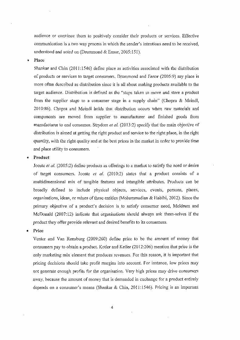
1.1 INTRODUCTION
Rapsomanikis and Sarris (2009-2010) states that the world has currently experience a
dramatic increase in the prices of commodities like maize, rice and wheat. Although the
prices of such commodities have now declined, they continue to remain at a significantly
high rate compared to the prices pre 2005. Rapsomanikis and Sarris allude that in general, the
changes in commodity prices are characterised by the increase or decrease in purchase. This
is because these fluctuations in prices present a serious challenge to consumers buying power.
Balcombe (2009-20 1 0) indicate that changes in price, either increase or decrease impact on
the trading position of producers and retailers in a long-term. Whitehouse and Associates
(2007:35) maintain that the Bureau of Marketing Research predicted a slower average growth
in the South African fast moving consumer goods market from 2007 due to the economic
recession, which generated an indirect decline in consumers' income. Claessen et al. (2009)
points out that an economic recession like the one in 2008, can affect consumers'
consumption by more than one percent ~fter every qumier in any economy. In such situations,
consumers become very price sensitive.
Bruweri and Watkins (20 I 0) state that the downturn experienced in 2008 had negative effects
on the South African fast moving consumer goods retailers in general. Roger (2003:1-2)
argues that this meant retailers had to adopt their marketing mix strategy to changing
consumer behaviour tendencies. Pricing has been referred by most researchers to be the key
element among all marketing mix elements. As indicated by Lee and Griffith (2004),
adjustment of prices to market conditions has a positive influence on the market share and
adaptation of the pricing strategy could increase the market share of a business. This study
seeks to investigate the degree to which pricing strategies used by the three largest
supermarket retailers (Shoprite holdings, Pick n Pay and Spar Group) in the Nkaga Modiri
Molema district of the North-West Province (NWP) of South Africa play a role in
determining their market share.
1

1.2 MOTIVATION FOR THE STUDY
Avlonitis and Indounas (2004) indicate that pricing remains one of the least research areas of
marketing. Delatolas and Jacobson (2012:2-3) argue that pricing is a complex issue but
constitutes an important process that has a large influence on the performance of a business.
However, few managers utilize the ability of pricing effectively to increase their business
market share. Limited research on pricing strategies and the lack of adequate pricing abilities
by retailers may lead to negligence of the importance of price in generating market share.
The limited research on pricing strategies and the lack of awareness on the impmiance of
price in gaining market share motivated the researcher to conduct the study. The researcher
saw the need to prove to retailers in the Ngaka Modiri Molema district that price is a valuable
tool in gaining market share. Also, a framework that will assist these retailers as a
quantitative tool for future pricing decisions was developed.
1.3 BACKGROUND OF THE STUDY
Referring to Mokgele (2012/2013:3), Ngaka Modiri Molema district municipality is one of
the four district municipalities in the North-West province of South Africa. It is a category C
district bordered by Ruth Mompati district in the west, Bojanala platinum district in the east,
Dr Kenneth Kaunda district in the south and Botswana in the north. Mojaki (2012/2013:7)
indicate that it is home to nearly 800,000 inhabitants, estimated households over 1,835,000
and its principal towns being Mafikeng, Zeerust and Lichtenburg. Mojaki further indicates
that Ngaka Modiri Molema district is made up of five local municipalities namely: Mafikeng,
Rl;ltlou, Ramotshere Moiloa, Ditsobotla and Twaing. Figure 1.1 reflects the different local
municipalities with reference to areas and demographic size.
2

Figure 1.1 Ngaka Modiri Molema municipalities
Source: NMMDIDP (2013/14:6)
1.4 LITERATURE STUDY
In the following section, the development of the marketing mix elements and their
contributing role to market share gain in general will be briefly discussed. The role of price in
the market and its role as an important tool for market share gain will conclude this section.
1.4.1 Marketing mix
Marketing mix is the set of controllable marketing tools consisting of products, price, place
and promotion (Shankar & Chin 2011: 1542). Each of these tools is explained below.
• Promotion
Drummond and Ensor (2005:9) indicate that promotion is the way a business creates
awareness of its product offerings to its target consumers. Promotion decisions consist of
sales promotions, sales force, public relations, direct marketing, word of mouth
communication and point of sales displays (Shankar & Chin 2011 :1542). Drummond and
Ensor (2005:9) contend that a blend of all these elements of promotion can be referred to
as the communication mix. Meldrum and McDonald (2007:12) equate promotion to
communication because it is all about how businesses communicate with their target
3
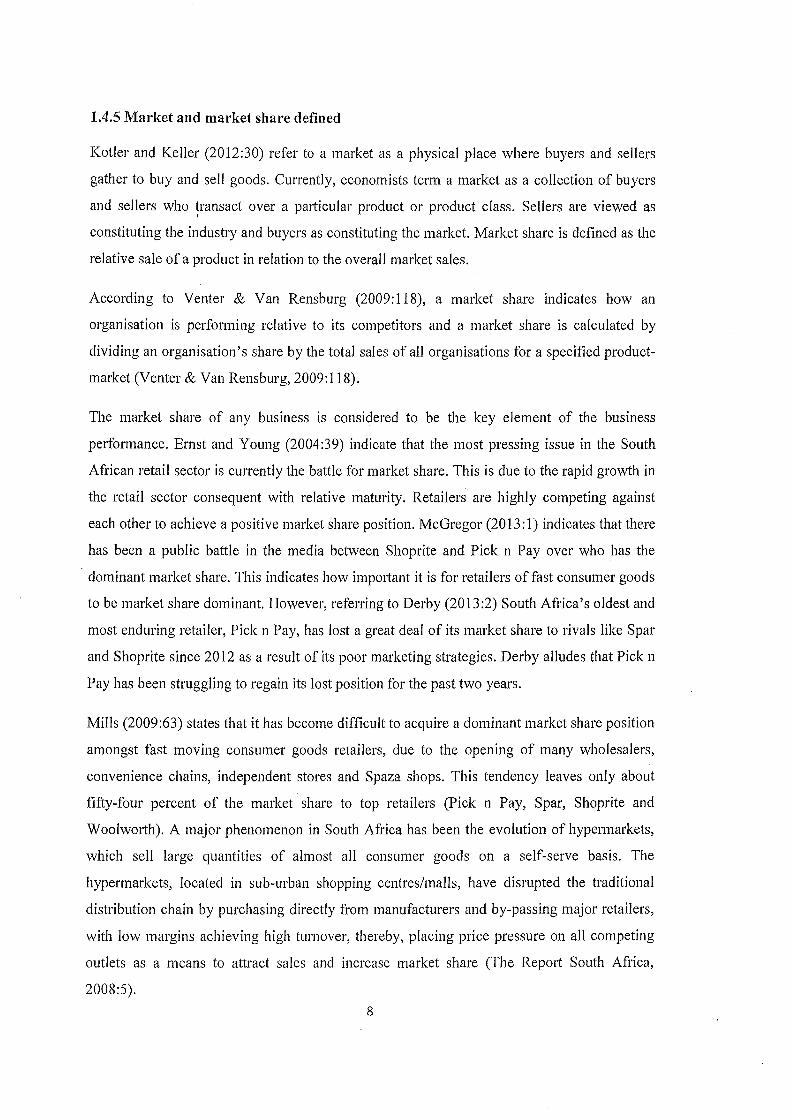
audience or convince them to positively consider their products or services. Effective
communication is a two way process in which the sender's intentions need to be received,
understood and acted on (Drummond & Ensor, 2005:151 ).
11 Place
Shankar and Chin (20 11: 1546) define place as activities associated with the distribution
of products or services to target consumers. Drummond and Ensor (2005:9) say place is
more often described as distribution since it is all about making products available to the
target audience. Distribution is defined as the "steps taken to move and store a product
from the supplier stage to a consumer stage in a supply chain" (Chopra & Meindl,
2010:86). Chopra and Meindl holds that distribution occurs when raw materials and
components are moved from supplier to manufacturer and finished goods from
manufacturer to end consumer. Strydom et al. (2013:2) specify that the main objective of
distribution is aimed at getting the right product and service to the right place, in the right
quantity, with the right quality and at the best prices in the market in order to provide time
and place utility to consumers.
11 Product
Jooste et al. (2005:2) define products as offerings to a market to satisfy the need or desire
of target consumers. Jooste et al. (2010:2) states that a product consists of a
multidimensional mix of tangible features and intangible attributes. Products can be
broadly defined to include physical objects, services, events, persons, places,
organisations, ideas, or mixes of these entities (Mohammadian & Habibi, 2012). Since the
primary objective of a product's decision is. to satisfy consumer need, Meldrum and
McDonald (2007:12) indicate that organisations should always ask them-selves if the
product they offer provide relevant and desired benefits to its consumers.
11 Price
Venter and Van Rensburg (2009:260) define price to be the amount of money that
consumers pay to obtain a product. Kotler and Keller (2012:206) mention that price is the
only marketing mix element that produces revenues. For this reason, it is impotiant that
pricing decisions should take profit margins into account. For instance, low prices may
not generate enough profits for the organisation. Very high prices may drive consumers
away, because the amount of money that is demanded in exchange for a product entirely
depends on a consumer's means (Shankar & Chin, 2011: 1546). Pricing is an important
4

element of marketing with tremendous potential for an organisation. If mismanaged, this
can bring a business to its knees (Meldrum & McDonald, 2007:11).
1.4.2 Marketing mix development
Constantinides (2006) states that the term 'marketing mix' as identified by Neil Borden, was
only introduced in the marketing field during the 1960's with twelve controllable marketing
elements (product planning, pricing, branding, channels of distribution, personal selling,
advertising, promotion, packaging, display, servicing, physical handling and fact finding and
analysis). Marketing mix was later reduced to the four-element framework (product, price
place and promotion) by Jerome McCarthy in 1964. Goi (2009) indicate that the marketing
mix elements (price, promotion, product and place) are the main tools in pursuing the
marketing objectives of a business. Goi also mentions that the marketing mix elements are
currently seen to be the basis of the five sub-disciplines of marketing management which
include consumer, relationship, services, industrial and retail-marketing. However, Moller
(2006) asserts that several criticisms about the effectiveness of marketing's 4p's have
appeared in recent studies. Some of these researchers have gone as far as rejecting the 4p's
and have come up with their own proposed alternative marketing mix frameworks.
The seven marketing mix elements seem to be the most popular of these alternative
marketing mix elements as indicated by Goi (2006) and introduced by Booms & Bitner in
1981. The 7p's include all the elements of the 4p's with people, packaging and process being
the additional elements. Other researchers like Wood (2008) and Gandolfo (2009) argue that
that the 4p's of marketing are the milestone of marketing theories. However, there is a need
to review the 4p' s paradigm due to the fact that there have been some evolutions in the
marketing discipline, especially in commercial marketing where the 4p's cannot effectively
adapt to certain aspects. Farshid and Amir (2012) maintain market share responds to elements
of the marketing mix (4p's) and that the marketing mix is the most impotiant entity that can
affect the market share of a business.
1.4.3 Marketing mix development in the Ngaka Modiri Molema district
Information provided by Managers of the selected supermarkets (Shoprite, Pick n Pay and
Spar) indicated that centralisation is a primary factor that affects performance. Thus, one can
say the high level of centralisation practised by these supermarkets is a clear indication of
limited application of the marketing mix elements. Guruprakash and Sohn (2008 :9) state that
5

centralisation impede the ability of departmental stores to appropriately respond to customer
needs and improve customer service. According to De Jager (2004: 112-113 ), Pick n Pay and
Shoprite (NWP, Potchefstroom) in the Dr Kenneth Kaunda district used the Living Standard
Model (LSM) to target consumers. Results obtained include:
• Current market segment targeted by these retailers differ from their actual target market.
• The marketing mix elements in place were not in any way appropriate to what was seen to
be the actual market of these retailers.
De Jager's findings indicate a clear misapplication of the marketing mix. He fmiher assumes
that an inappropriate marketing mix to wrong target markets is likely to also be the case
among supermarkets in other areas of the North-West Province (NWP).
Furrier et al. (2007) have stressed that marketing activities has a great impact on the
performance of a business in the market place or to achieve its market share. A large number
of supermarket retailers in the Ngaka Modiri Molema district can be seen to be offering poor
business services. As confirmed by the Southern African Legal Information Institute
(SAFLII) (2012) database, there were 14 court cases in the Ngaka Modiri Molema magistrate
court in Mafikeng concerning poor customer service during 2012. The inability to structure
efficient business plans and objectives by most business enterprises in the Ngaka Modiri
Molema district stem from government's failure to implement efficient support programmes
for these businesses.
Bafana (2011 :7) highlights that the marketing unit of the North-West Province as a whole has
registered a number of failures based on internal reasons. Mojaki (2012/2013:22) indicates
that the 2012 Ngaka Modiri Molema local government effort to support business enterprises
did not meet its set target. Only 6 % growth success after a one million seven hundred
thousand rand investment by local government has been acquired. Mojaki fmiher indicates
that during the first qumier of the 2012/21 03 government calendar, only a one percent growth
rate has been achieved, (quatier-two and three), 2% performance respectively and by quarter
four performance dropped back to 1%. This may seem like the government does not actually
put enough effo1i to support trading, which confers with Spaku and Majoki's (2012:17)
statement that retail and trade are the fourth largest contributor to the economy of the Ngaka
Modiri Molema district.
6

1.4.4 Pricing in the market
Reviere (2009: 1) highlights that the price concept differs whether a person lives in a market
economy, planned, command or traditional economy. Because pricing influences the
economic actions in a market economy, it is best to discuss pricing concept on a market
economy basis. Palley (2004:1-2) argues that in a market economy, the contemporary
framework of neoliberalism emphasises the efficiency of market competition, which is based
on the microeconomic theory of pricing, the key variable influencing the demand and supply
in the market place. Pitner (2007:1) indicates that when understanding price in the market or
how it works in business, all is about the demand and supply functions. Pitner (2007:1)
further points out that from the supply perspective, the higher the price of a product, the
higher the supply, the lower the price of a product, the lower the supply. The demand
perspective is connected to consumer behaviour in that, if pricing affects consumers' buying
behaviour negatively, the demand curve will slope downward, meaning a drop in purchase
behaviour. Alternatively, if pricing is positive, consumer buying power will increase, leading
to the demand curve sloping upward, more sales and market performance for the business.
From the afore discussion of price influence 'in the market, this study focuses on showing that
price is an important tool for Ngaka Modiri Molema retailers in gaining market dominance.
The downward and the upward movement of the demand curve with respect to price is
further illustrated in figure 1.2
Price
s
D
Figure 1.2 Demand and price Output
Colander (2004:99)
7
1.4.5 Market and market share defined
Kotler and Keller (2012:30) refer to a market as a physical place where buyers and sellers
gather to buy and sell goods. Currently, economists term a market as a collection of buyers
and sellers who transact over a particular product or product class. Sellers are viewed as I
constituting the industry and buyers as constituting the market. Market share is defined as the
relative sale of a product in relation to the overall market sales.
According to Venter & Van Rensburg (2009:118), a market share indicates how an
organisation is performing relative to its competitors and a market share is calculated by
dividing an organisation's share by the total sales of all organisations for a specified product
market (Venter & Van Rensburg, 2009:118).
The market share of any business is considered to be the key element of the business
performance. Ernst and Young (2004:39) indicate that the most pressing issue in the South
African retail sector is currently the battle for market share. This is due to the rapid growth in
the retail sector consequent with relative maturity. Retailers' are highly competing against
each other to achieve a positive market share position. McGregor (20 13: 1) indicates that there
has been a public battle in the media between Shoprite and Pick n Pay over who has the
, dominant market share. This indicates how important it is for retailers of fast consumer goods
to be market share dominant. However, referring to Derby (2013:2) South Africa's oldest and
most enduring retailer, Pick n Pay, has lost a great deal of its market share to rivals like Spar
and Shoprite since 2012 as a result of its poor marketing strategies. Derby alludes that Pick n
Pay has been struggling to regain its lost position for the past two years.
Mills (2009:63) states that it has become difficult to acquire a dominant market share position
amongst fast moving consumer goods retailers, due to the opening of many wholesalers,
convenience chains, independent stores and Spaza shops. This tendency leaves only about
fifty-four percent of the market share to top retailers (Pick n Pay, Spar, Shoprite and
Woolworth). A major phenomenon in South Afi·ica has been the evolution of hypermarkets,
which sell large quantities of almost all consumer goods on a self-serve basis. The
hypermarkets, located in sub-urban shopping centres/malls, have disrupted the traditional
distribution chain by purchasing directly from manufacturers and by-passing major retailers,
with low margins achieving high turnover, thereby, placing price pressure on all competing
outlets as a means to attract sales and increase market share (The Repott South Africa,
2008:5).
8

New supermarket brands scrambling for market share is also the case in the North-West
Province. Dirkie (20 11/2012: 15) has indicated how supermarket retailers like Chop pies
Limited (ltd) are performing relatively well. This performance has contributed to its growing
market share. Chop pies is busy aligning with the North-West government and other blue chip
companies to improve its operations. This has made Choppies a faster growing retailer in the
North-West province compared to its competitors in terms of market share since its
introduction in 2008 into the province. Keeping satisfying consumers loyal is a common
tactic to increase sales and market share since supermarkets are often located within close
proximity and sell more or less the same products. Thus, each retailer's ability to sell its
merchandise sustainably, largely depends on the strength of its marketing mix activities
(Marriri & Chipunza, 2009).
1.4.6 Pricing influence on market share in the retail market sector
Lawrence and Lawrence (2008:1) indicate that before 1995, during the civil differences in
South Africa, trade protection and other economic bands s(;(riously impeded the South African
economy. This made South Africa's economy to depend on external global commodity prices
trends to avoid running into an external constraint. Thus, during such period, price had a little
role to play in the South African economy. During the period before 1995, a section of the
Nmth-West was a separate entity ("Homeland") in charge of its own economic decisions
under the presidency of Hon. Lucas Magope. Francis (2002:2-4) indicates that Magope's
regime was based on personal rule on all state matters, including trade and commerce which
affected the traditional flow of the economy.
According to Du Plessis and Smith (2007: 1-2), there has been a lot of growth in the South
African economy since 1995, due to the introduction of a more market economy backed by
microeconomic variables. Euromonitor International (EI) (20 12:8) maintain that presently,
supermarket retailers like Shoprite and Spar Group have increased their market share
position, due to their ability to implement pricing strategies that will provide commodities to
consumers at reasonable prices.
According to Roger (2009:292), a business organisation's market share should increase if
those in marketing can deliver more volumes in terms of sales. Venter and Van Rensburg
(2011:118), Donaldson (2007:133) and Fok and Franses (2000:3) points out that, there is a
positive relationship between sales and market share. Roger also holds that the only way to
achieve the objective of increasing market through sales depends on the careful application of
9

pricing. It should be noted, however, that, market share is obtained in both sales value and
sales volume. Thus, Mohr and Fourie (2004:182) explicitly show the influence price has on
market share through the concept of price elasticity of demand, which is all about an increase
or decrease in sales as price changes. Ferrel and Hartline (2008:234) refer to price elasticity
of demand as customers' responsiveness or sensitivity to changes in price and pricing
strategies. This concept is further illustrated in figure 1.3
I i ·~ ed)
I ] £!'
·-~,·---~L~-·---·~----
Y+
J ~I c ,.,., a; r--·"'-------·- ·-a.)
y
I '----------~
0 QUANTITY X 0 QUANTITY X 0 QUANTITY X (fl)
yt I
UJ I c '7 ' •• ---~-~ t------
l !-----~--"·,. , ........
0 QUArffiTY X (d)
(b)
Figure 1.3 Elasticity of demand,
Philip & Fourie (2007:184)
0 OUANTITY X (o)
Figure 1.3 (a): Perfectly inelastic demand ( ep = 0)
{c)
This describes a situation in which change in price shows no change in demand (sales) as
revealed in the vertical straight line.
Figure 1.3 (b): Perfectly elastic demand ( e = oo)
Perfect elasticity is experienced when the demand is extremely sensitive to the changes in
prices. Price elasticity occurs when an insignificant change in price produces tremendous
change in demand.
Figure 1.3 (c): Unitary elasticity demand (e = 1)
This is a case when the percentage change in price produces equivalent percentage change in
demand.
Figure 1.3 (d): Elastic (more elastic) demand ( e > 1)
10

This is when the demand for certain commodities are more responsive to the change in price.
Figure 1.3 (e): Inelastic (less elastic) demand ( e < 1)
This is a situation where the proportionate change in demand is smaller compared to the
change in price. It is mostly theoretically concluded that just five different types of price
elasticity exist. However, in practice, Mohr and Fourie (2004:183) and Mohr and Fourie
(2007:184) indicate that two extreme cases are included which are perfectly elastic and
perfectly inelastic. These two cases are often mentioned because they are rarely experienced.
1.5 PROBLEM STATEMENT
Referring to Farshid and Amir (2012), the marketing mix elements (product, price, promotion
and place) are the most impotiant elements for a firm to enhance its market share. This
statement is supported by the results of a study by Farshid and Amir undertaken within the
polymer sheet market in Iran. The outcome showed that the marketing mix elements and their
sub-elements are the primary instruments influencing market share gain. Munusamy and Hoo
(2008) used a simple regression to determine the relationship between the marketing mix and
consumer motives. Their aim was to determine which marketing mix element was the most
appropriate for the Malaysian fast consumer good industry. Using Tesco (a supermarket
chain) in their study, results revealed that pricing had a direct, either positive or negative
impact on consumer behaviour. Pricing thus is being emphasised as a direct influence on
market share, even when the other mix elements (place, promotion and product) tested
negative amongst respondents.
Although this empirical study focuses solely on the influence of price on market share, the
need and importance of price in gaining market share compared to the other mix elements as
indicated by Munusamy and Hoo, already establish the relevance for the awareness of price
to businesses. According to Axaloglou (2007), the poor application of pricing strategies and
the lack of relevant knowledge regarding the role of pricing in expanding market share could
have a negative effect on the financial functioning of a business. During the pilot
investigation, it was found that price is an impmiant tool for supermarkets in the Ngaka
Modiri Molema district in gaining market share over their rivals. Despite the role price has in
gaining market share, limited attention is given to price. Using just Tastic rice (2kg) and
White star maize meal 5kg, market results for January 2011 for sampled supermarkets in the
Ngaka Modiri Molema district were as follows:
11

Table 1.1 Tastic rice (2kg) and white star maize meal (5kg) supermarkets prices and sales
for January 2014
Supermarket Tastic rice 2kg White star maize meal Skg
Price Sales Price Sales Pick n pay R27.79 1200 R19.99 1742 Spar R28.92 50 R20.25 1127 Shoprite R28 1023 R19.39 2262
Based on the evidence provided by Munusamy and Hoo (2008), Axaloglou (2007), Farshid
and Amir (2012) as well as indications from the preliminary study done to investigate the
effectiveness of price implications on the market share of the Ngaka Modiri Molema district
retailers, there seems to be a consensus that retailers in general do not realise the importance
of implementing adequate pricing strategies as a basis for gaining market share. Thus, the
problem indentified in this study relates to the neglect of the importance of price as a primary
tool in gaining market share by Ngaka Modiri Molema retailers. This tendency can contribute
to a lack of market share growth and growth in general amongst these retailers.
1.6 RESEARCH OBJECTIVES
1.6.1 Main objective
The primary objective of this study was to examine the impact of pricing on the market share
of the top three grocery retailers in the Ngaka Modiri Molema district.
1.6.2 Secondary objectives
In order to achieve the main objective of the study, the following secondary objectives were
raised:
• To investigate the type of pricing decisions made by the three largest grocery retailers in
the Ngaka Modiri Molema district.
• To examine the challenges faced by these supermarkets in making pricing decisions.
• To determine the influence of these pricing decisions on consumers' behaviour and
market share performance.
• To determine the importance of market share for Ngaka Modiri Molema grocery
supermarkets.
12

• To recommend possible pricing decision maJors that can be used by Ngaka Modiri
Molema retailers to gain market share.
1.7 RESEARCH QUESTION
1.7.1 Primary research question
• To what extent does pricing affect the market share of supermarket retailers in the Ngaka
Modiri Molema district?
1. 7.2 Secondary research questions of the study was as follows:
• Which pricing decisions are made by the top grocery retailers in Ngaka Modiri Molema?
• What challenges do these supermarkets face in making pricing decisions?
• How does these pricing decisions impact on pricing behaviour and its effects on market
share?
• What is the importance of market share for Ngaka Modiri Molema grocery supermarkets?
• How can pricing be better applied by Ngaka Modiri Molema top grocery retailers to
improve their market share?
1.8 RESEARCH METHODOLOGY
Wilson (2009:5) refers to methodology as a plan of action that informs and links the methods
used to collect and analyse data to answer postulated research questions. The research design
to be applied in this study was a quantitative approach.
1.8.1 Population
Bickman and Rog (2009:77) refer to population as the large group to which a researcher
wants to generalise his or her sample results. In other words, it is the total group that a
researcher is interested in learning more about. The population in this study included the
three largest grocery supermarkets in the Ngaka Modiri Molema district. Three towns in the
district (Lichtenburg, Mafikeng and Zeerust) were targeted in order to select participating
supermarkets for the study. The district marketing-managers and branch managers of these
stores were the patticipating employees.
1.8.2 Sampling
A sample according to Smith et a!. (20 13: 162) is a subset of the whole population, actually
investigated by a researcher whose characteristics will be generalised to the entire population.
13
To this effect and according to these researchers, sampling refers to the process of drawing a
sample from a population. Researchers sample in order to study the characteristics of the
larger group and to understand the characteristics of the larger group. Researchers must carry
out a sampling process because factors such as expense, time and accessibility frequently
prevent researchers from gaining information from the whole population. For the purpose of
this study, a purposive sampling approach was used to select supermarkets and supermarket
employees to participate in this study.
Cohen et al. (20 11: 156) refer to purposive sampling as a non-probability sampling method
which involves purposive or deliberate selection of particular participants from the sample
considered to have the needed or actual information of the study. Purposive sampling was
used because just one of each sample supermarkets store was selected as participant based on
accessibility of needed data. It was aimed at targeting which supermarket employee was most
appropriate in providing the needed information for the study. Only one of each sampled
supermarket stores were selected as participant making a total of 3 stores. Employees in the
study included the marketing manager of each supermarket brand and the managers of each
selected sample store. This gave a total of 6 employees who patiicipated in the study. Data
collected from all 3 patiicipating stores were done on a monthly basis from January 2011 to
June 2013. This gave the sum of 30 observations per supermarket, amounting to a total of 90
observations.
1.8.3 Data collection method
Data was obtained in this study from both available literature and an empirical investigation.
Literature data was obtained through journals, articles, books, magazines and internet
sources. Literature data was based on marketing and price, price index, pricing process, ethics
of pricing, competitors and their pricing framework, the influence on pricing on sales
performance, market share index/matrix, competitors and their market share positions and the
importance of market share advantage in the market.
Empirically, data gathering involved the obtaining of the Selling Price Index (SPI) and sales
figures for 11 selected items (appendix 4) commonly available in the database of the selected
supermarkets (Shoprite, Pick n Pay and Spar). Information obtained was used to determine
the relationship between price changes and its impact on market share of the participating
supermarket retailers.
14

1.9 DATA PROCESSING AND ANALYSIS
The model specification of the regression type employed in this study and the analytical
technique used to analyse empirical were as follows.
1.9.1 Model specification
The model specification employed in this study was the Panel Ordinary Least Square (POLS)
regression method. This is because the main objective of the study was that, price as the
explanatory variable is the main factor influencing market share, the dependent variable and
fits with the main rule of linear regression.
The formula layout of the POLS regression method is as follows:
Least Square regression is denoted as y =Po+ p1x + E Formula (1.1)
y =dependent variable or the explained variable.
Po= the intercept of the equation.
PI =the slope coefficient of the price variable.
x = the independent variable or explanatory variable.
E = the error tem or the disturbance variable.
In this study, market share was the dependent variable represented by sales figures and
pricing the independent variable. Thus, the main aim was to verify if price has a linear effect
on market share of the top three fast moving consumer good supermarkets in the Ngaka
Modiri Molema district. As the rule of linearity implies, a unit change in x will have the same
effect on y if there is a relationship.
1.9.2 Analytical techni9ue
The study made use of a simple panel data analysed through the Eviews software. A panel
matrix was appropriate for the study because it allows data analysis across more than one
entity since it contains both cross-sections (N) and time period information (t). Findings from
the linear regression were represented graphically on a scatter plot graph and a histogram to
display the potential relationship between price and market share on top of four supermarket
retailers in the Ngaka Modiri Molema district.
15

1.10 LIMITATIONS
The study was originally designed to investigate the relationship between price and market
share for the top four supermarkets (Pick n Pay, Shoprite, Spar and Woolworth). After an
extensive and accurate investigation, all Woolworth supermarkets in the district did not
provide any of the item categories that were considered appropriate to test this study. For this
reason, Woohvorth was disqualified as one of the selected samples for this study.
1.11 ETHICAL CONSIDERATIONS
Neuman (2003: 116-118) indicates that the researcher has a moral and professional obligation
to be ethical, even if patticipants are unaware of or unconcerned about ethics. The ethical
considerations in this study followed Trochim's (2006:42) ideas of a perfect ethical
consideration of research. It includes the principle of voluntary participation, requirement of
informed consent, principle of anonymity and guarantee of confidentiality. Other ethical
considerations included the following:
1.11.1 Gaining access
The researcher obtained a letter of permission from the department of management, North
West University, Mafikeng Campus in order to gain access to selected supermarkets. With
this letter, the researcher approached participants in the study to seek information.
1.12 CONCLUSION
This presented a detail introduction and background of the study. An organisation of the
study is represented as followings.
Chapter One: Introduction
In this chapter, the statement of the problem, the motivation, background, objectives, research
questions, ethical considerations of the study were discussed.
Chapter Two: Literature review
Literature review was conducted on pricing issues and its impact on the market share of
supermarket retailers.
16

Chapter Three: Research methodology
In this chapter, a detailed explanation of the research procedure in terms of research design
used, research strategy, data collection, sample selection and population was presented.
Chapter Four: Data analysis and presentation
In this chapter, data collected from the previous chapters were analysed according to the
objectives of the study and findings from the literature.
Chapter Five: Discussion and recommendations
This chapter reported the findings from the analysis covered in the previous chapter.
Conclusions of the study were drawn from the findings and recommendations be made in
relation to the outcome ofthe study.
17

CHAPTER TWO
THE RELATIONSHIP BETWEEEN PRICING AND MARKET SHARE
2.1 INTRODUCTION
A literature review provides a summary of existing studies on the main subjects of the study
and the methods employed by others and their results. The literature review in this study was
both theoretical and empirical. Empirical literature provided a summary of what methods
were used in this research and the findings, relating it to the theoretical literature.
Theoretical literature explores theories related to the following focus areas; marketing and
price, price index, pricing process, ethics of pricing, competitors and their pricing framework,
the influence of pricing on sales performance, market share index, competitors and their
market share positions, importance of market share advantage in the market.
2.2 MARKETING
Kazmi (2007:6) defines marketing as a means of creating superior value and delivering high
levels of customer satisfaction. Kazmi further states that marketers should therefore
endeavour to understand customers' needs and wants, carefully study competition, make
products available at places convenient to customers, communicate with them effectively and
efficiently and finally, offer superior value at a reasonable price. Smith (2002) holds that the
focus of marketing is customer needs and wants. Through these, marketers are also obliged to
offer solutions to clients, not just tangible goods and services. The researcher further alludes
that each element of the marketing mix product, price, promotion and place are the centre in
achieving this marketing objective. Smith further points out that price play an important role
among all other elements in the marketing mix. According to Weitze and Wens ley
(2005:267), pricing has received so much attention above the other factors not only due to its
key role in business but also because of its interdisciplinary nature.
In the business environment, organisations operate either on profit making or non-profit
making bases. Ballasy (200:4) indicates that non-profit making organisations are referred to
as savvy marketers as they practise a marketing style called social marketing. Social
marketing is oriented on improving the lives of individuals in a specific way. Schindler
(2012:365) however, states this does not mean they ignore making high revenue, since more
18
money make available additional beneficial services. On profit making bases, marketing can
be defined as a process and a set of tools used to get things done either to achieve a goal,
solve a problem or take advantage ot'an opportunity (Ballasy, 2004:7). For a marketer to take
advantage of an oppotiunity, a good or service is to be offered to the consumer who has to
pay for the good or service. According to Ferrell and Hatiline (2008:226), what the customer
pays for, include everything the customer must give up such as money, time, effort and all
non-selected alternatives. Value is a key component in setting price; the relationship between
pricing and value is intricately tied to every element in the marketing programme. Schindler
(20 12:6) states that the marketing concept points out that price setters should also consider
customers' value as a very important element when setting prices. This is because consumers'
feeling about the final price charge is also vital.
2.3 PRICING DECISION MAKING
Indounas and A vlonitis (2009) posit that pricing is an important management tool to achieve
the objectives of the organisation. Pellinen (2003) also mention that pricing is one of the most
important or central management tasks for any business. As earlier indicated by Chattered
Institute of Marketing (CIM) (2009:5) pricing is the only function in the marketing mix that
generates revenue for a businyss, all others are cost. According to Dutta et al. (2003),
businesses without efficient pricing processes may be unable to set prices that reflect the
wishes of its target customers. Blyth (2006:448) and Escalana et al. (2012: 159) indicate that
the pricing process involves all the steps in determining the final price for products or
services. The researchers fmiher state that a pricing process should involve setting pricing
objectives, developing a pricing strategy, determining the demand for various levels, estimate
cost, review competitive offerings, select pricing methods, establish pricing policies and
determine prices. This is fmiher illustrated in figure 2.1. Referring to Hinterhuber and Liozu
(2012), implementing a pricing structure requires a high degree of discipline from any
business, and any business can improve its pricing performance so far as its pricing
approaches are well-structured.
19

Set prices and objectives
Develop pricing strategy
Estimate cost
Review competitive offerings
Select pricing strategy
Select pricing method
Establish pricing policies
Determine final price
Figure 2.1 Pricing process,
Blyth (2006:448)
2.3.1 Pricing objectives
According to Snieskiene and Pridotkiene (20 I 0), the process of identifying pricing objectives
is the starting point for any organisation or business to achieve its pricing goals. This is
because pricing objectives constitutes the basis on which pricing methods and policies are
formulated. According to Indounas and A vlonitis (2009), there should be a correlation
between the pricing objectives and entire pricing process for better understanding of the
overall pricing structure. Avlonitis eta!. (2005) and Avlonitis and Indounas (2004) holds that
pricing objectives can be divided into quantitative and qualitative categories. Quantitative
objectives include financial indicators such as profits, sales, market share and cost coverage,
while qualitative objectives put more focus on the relationship with customers and
competitors, the long-term survival of the business and the achievement of social goals.
Avlonitis and Indounas (2004) argue that the main advantage of quantitative pricing
objectives relate to the fact that they can be measured easily and straightforwardly, while the
main contribution of qualitative objectives lies in the fact that they help organisations in
adopting a market orientation towards its pricing decision. Quantitative objectives tend to be
regarded as more important than qualitative with particular emphasis placed on profit
considerations (A vlonitis & Indounas, 2004).
20

Avlonitis et al. (2005) and Avlonitis and Indounas (2004) also allude that with reference to
time frame of attainment, pricing objectives may be divided into short-term and long-term
objectives. Shmi-term objectives are mainly quantitative goals, while long-term objectives
are fundamentally qualitative goals. A vlonitis and Indounas (2004) state that most often, an
excessive emphasis on shmi-term objectives may risk the long-term position of a firm in the
market. Although Snieskiene and Pridotkiene (20 1 0) points out that there is no single pricing
objective that serves as definite benchmark for all situations, Indounas and A vlonitis (2009)
point out that, a factor analysis indicates that pricing objectives can be summarised into eight
underlying factors placed under a quantitative or qualitative category. Indounas and
Avlonitis' classification covers all what others have indicated. The classification is further
indicated below.
2.3.1.1 Quantitative objectives
As earlier indicated, quantitative objectives include those objectives that can be seen to be
financial indicators. They are fmiher explained as follows:
• Financial objectives
It represents the effmi to achieve liquidity and satisfactory return assets and potential
investments.
• Achieving satisfactory profits and sales objectives
This objective is aimed at ensuring adequate financial results in terms of profits and sales and
covers the cost of delivery services and products.
• Market share and capacity-related pricing objectives
The objective relates to increasing market share and managing the existing capacity.
• Maximisation of profits and sales objectives
It is all about achieving maximum financial results by high sales to achieve high profit
values.
2.3.1.2 Qualitative objectives
Qualitative objectives were earlier indicated to be elements that put more emphasis on
customers and competitors.
21
• Stability in the market objectives
Stability in the market is related to achieving price and sales stability, satisfying distributors'
needs, developing the existing market and determining fair prices for customers.
• Customer- related pricing objectives
The effort here is to retain existing customers and satisfy their needs without disregarding the
acquisition of new customers, the achievement of social goals and long-term survival.
• Service quality-related pricing objectives
This objective is out to create prestigious image in terms of quality while differentiating
prices across different categories of customers.
• Competition-related pricing objectives
It involves avoiding price wars, offering similar prices to match the prices of competitors and
discourage the entrance of new competitors in the market.
2.3.2 Developing pricing strategies
Blyth (2006:450) maintains that developing a pricing strategy needs to fit within the overall
corporate vision. According to Lamb et a!. (2009:372), a pricing strategy is simply a
statement of what the business or organisation is trying to accomplish with a given product or
service at during its life-cycle. Dutta et a!. (2003) argue that strategists should develop or
consider pricing strategies that will create value for the customer to gain a competitive
advantage. Garrett (20 11:1) holds that pricing is ultimately pati of an organisation's system,
therefore, it should be aligned to the overall strategic planning and mission of the
organisation. This is because an organisation's purpose, self-perception, position in the
market and ethics are clearly spelt out in the overall organisation's strategy and are elements
that must be incorporated in the pricing strategy. Most common pricing strategies used by
business organisations are further discussed below.
2.3.2.1 Cost-plus pricing
Blyth (2006:458) indicates that cost plus pricing works by calculating the cost of producing
the product, then adding on the fixed percentage profits to the total. Although this pricing
method appears logical and straightforward, it is actually fairly dangerous because it takes no
account of the market place. Hinterhuber and Liozu (20 12) argue that cost-plus is currently
being been criticised for neglecting the market place because aspects related to demand and 22
competitor are usually ignored. Cant (2005:61) posits that is the most popular among retailers
and wholesalers who have to decide on the prices of so many items.
2.3.2.2 Mark-up pricing
According to Blyth (2006:459) mark-up pricing is similar to cost-plus pricing, and is the
method used by most retailers. Blyth fmiher states that the only difference from cost-plus is
that retailers are usually in close contact with customers and can therefore, develop a good
feel for what customers will be prepared to pay for. Secondly, retailers practising mark-up
pricing have ways of disposing of unsold stock. It is typically when a retailer buys in stock
and adds on a fixed percentage to the bought-in price in order to arrive at the shelf price. Cant
(2005 :63) argues that the level of mark-up will vary from retailer to retailer depending on the
product category because there is usually a standard mark-up for each product category.
Retailers use this method because of the number of lines the shop may be carrying, since it
may be clearly impossible to carry out market research with customers for every line (Blyth,
2006:459).
2.3.2.3 Customary pricing
Cant (2005 :86) indicates that customary pricing is when products and services are priced
based on the tradition and the prices of competitors. It can also be referred to as the practice
of maintaining the retail price of a product at the same level over long periods (Cant,
2005:86).
2.3.2.4 Price skimming
Kazmi (2007:514) refers to market skimming as the act of charging the highest possible price
that a sufficient number of the most desirable customers are willing to pay for. Skimming is
best practised under circumstances when consumers are willing to buy the product for its
unique advantage and in a case where production cannot be expanded rapidly because of
technology difficulties, shortages or constraints imposed by the skill and time required to
produce a product (Lamb et al., 20009:373). Kazmi (2007:514) holds that the approach offers
efficient profits to pioneers in a product's introductory stage due to the absence of
competitors. However, Esclana eta!. (2012:172) point out that skimming comes with future
challenges since competitors may have developed ways to challenge existing organisations in
the long-run.
23
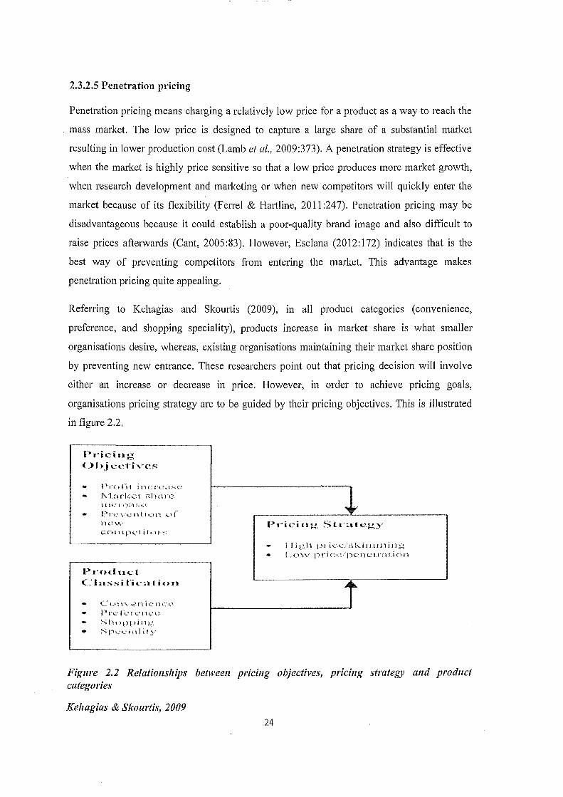
2.3.2.5 Penetration pricing
Penetration pricing means charging a relatively low price for a product as a way to reach the
mass market. The low price is designed to capture a large share of a substantial market
resulting in lower production cost (Lamb et al., 2009:373). A penetration strategy is effective
when the market is highly price sensitive so that a low price produces more market growth,
when research development and marketing or when new competitors will quickly enter the
market because of its flexibility (Ferrel & Hartline, 2011 :247). Penetration pricing may be
disadvantageous because it could establish a poor-quality brand image and also difficult to
raise prices afterwards (Cant, 2005:83). However, Esclana (2012: 172) indicates that is the
best way of preventing competitors from entering the market. This advantage makes
penetration pricing quite appealing.
Referring to Kehagias and Skomiis (2009), in all product categories (convenience,
preference, and shopping speciality), products increase in market share is what smaller
organisations desire, whereas, existing organisations maintaining their market share position
by preventing new entrance. These researchers point out that pricing decision will involve
either an increase or decrease in price. However, in order to achieve pricing goals,
organisations pricing strategy are to be guided by their pricing objectives. This is illustrated
in figure 2.2.
1• r·it..'ing ()bjectivc·s
Pn-, l'i t i IH.'I'L~'tsc· '" l'vl n ck .;.•1. Fl Hll c
Product C:lassi fi<.~a lion
( _ _:£ Lt t \ "\.i C' l l i c~ I .i C t~~
• f 1 t•\....• CCt'CllL~\...~·
SIJ, 'PPi 11g Sjh:eiulit.Y
f {)g]l pll'·'L'/skit Ill! til I~ .. I .C'I\V p1·icc,lpcnvu·n 1 inn
Figure 2.2 Relationships between pricing objectives, pricing strategy and product categories
Kehagias & Skourtis, 2009 24

2.3.3 Determine demand
Lamb eta!. (2009:360) define demand as the quantity of goods and services that will be sold
in the market at various prices in a given period. The quantity of products or services that will
be purchased in a specific period will largely depend on its price. Concurring with Pindick
and Rubinfeld (2013:40) this means the higher the price, the fewer goods or services
consumers will demand, so too conversely, the lower the price, the more products or service
consumers will demand. Kazmi (2007:509) states that the determination of the quantity
demanded of goods and services is the responsibility of the marketing department, aided by
research personnel's and forecasters with respect to the set price. Kotler and Armstrong
(20 1 0:317) maintain that the relationship between the demand for goods and services and
price is inversely proportional. This is better illustrated in the figure 2.3.
Price
Figure 2.3 Demand price
Mohr and Fourie (2007:138)
Dl
Output
In the figure above, Kazmi (2007:509) indicates that the original demand for goods and
service is D 1, negative behaviour from factors determining demand may lead to increase in
price of goods and services from P 1 to P2, causing the demand to drop and the demand curve
to shift from D 1 to D2. However, the supply function can also play a role in the market prices
of goods and services. The relationship between price change and quantity demanded is more
explicit in theory of Price Elasticity of Demand (PED) illustrated and discussed in chapter
one (figurel.3). Colander (2004:132) defines elasticity of demand as consumers'
responsiveness or sensitivity to changes in price. Referring to Colander's (2004:133), price
elasticity of demand is denoted as:
25

PED = %change in quantiy demanded
%change in price Formula (2.1)
The aforementioned formula simply indicates that as changes in price lead to changes in
quantity demanded, the total percentage change in quantity demanded is divided by the total
percentage change in price to get the price elasticity of demand. Ferrel and Hartline
(20 11 :242) and Lamb et a!. (2009:365) point out factors that influence price elasticity to
include; availability of substitutes, price relative to purchasing power, product durability and
other product uses. Kotler and Armstrong (2010:315) states that the seller's pricing freedom
depends on the type of market the seller belongs, thus, Jehle and Reny (20 11: 164) points out
that economists recognise four types of markets as follows; pure competition, monopolistic,
oligopolistic and pure monopolistic competitions with each of these markets presenting a
different pricing challenge. Each of these markets are further discussed below.
2.3.3.1 Pure competition/perfect competition
Con cutTing with Jehle and Reny (20 11: 165) a market is where buyers and sellers are
sufficiently large in number to ensure that no single one of them acquires the power to
determine the market price of goods and services. Colander (2004:242) states that both
buyers and sellers are price takers rather than price makers, meaning price is determined in
the market by market supply and demand. Cant et a!. (2010:238) also mention that in a
perfect competitive market, products offered by marketers are largely homogenous and prices
are the same, these make consumers to purchase from which ever seller they wish.
2.3.3.2 Monopoly/imperfect competition
Jehle and Reny (20 11: 170) define this type of market to be a market where there is a single
seller of a product or service for which there is no close substitutes in consumption, and the
entry into the market is completely blocked. Depken (2006: 170) states that barriers
preventing entry into a monopoly market can be either legal or natural. Legal barriers to entry
are laws passed at local, regional or national level that makes it illegal to enter the market and
compete. Natural barriers on the other hand, are those that can be caused by geographical or
technological factors. Colander (2004:267) indicates that monopolists use the general rule
that any organisation must follow to maximise profit which is to produce the quantity at
which Marginal Cost (MC) = Marginal Revenue (MR). That quantity determines the price a
business will charge for its goods or services.
26
2.3.3.3 Monopolistic competition
According to Jehle and Reny (20 11: 177), monopolistic competition is a situation where
relatively large groups of businesses provide differentiated products and services that
consumers view as close substitutes for one another. Within these circumstances, each
business enjoys a limited degree of monopoly power for its particular product variants,
though the markets for different variants are closely related. Jehle and Reny (20 11: 177)
mentions that the demand for a product depends on its own price and the prices of all other
variants. This means an organisation's profit depends on the prices of all other variants being
the change between revenue and cost.
2.3.3.4 Oligopoly
According to Depken (2006:200), oligopoly is a market structure in which a few firms
compete with each other, typically in a strategic fashion. Oligopoly models explicitly
recognise that the decision of one business organisation likely impacts the decision of others.
Jehle and Reny (2011:174) indicate that oligopoly can be sub-divided into Cournot and
Bertrand oligopolies. The Cournot model involves firms that sell output on a common
market, where market price depends on the total output sold to all firms in the market. The
price of goods and services will approach marginal cost as the number of competitors grew.
Sunil and Steenburgh (2008:6-8) highlights three main approaches to which demand can be
better applied, with any of the marketing functions. These approaches are as follows:
• Decision calculus approach
Decision calculus provides means of applying pnce and demand through managerial
judgement. When an organisation does not have historic data and cannot afford either due to
lack of money or time.
• Experiment approach
Experiments provide a useful way to experience consumer response to a certain price. It is all
about gauging consumer response to new prices which have not been implemented before by
the organisation.
• Economic approaches
This is achieved by using academic studies that have built models to understand the
effectiveness of demand and price. An example is the elasticity of demand theory.
27

2.3.4 Cost
Jehle and Reny (20 11: 135) define business cost to include all expenditures incurred in
acquiring the inputs used to produce a good or service. Ferrel & Hartline (2011 :237) maintain
that the cost of producing and marketing a product is mostly used as the benchmark in setting
the selling price of products. Kazmi (2007 :511) concurs by indicating that the purpose of
price setting for a business is to set a price to cover costs involved in a product's or service
production, selling, distribution and ultimately to obtain some desired level of profit for its
effort and risk. Kazmi (2007:511) also states that it is important that prices must exceed
average unit cost to earn a profit. Cant et al. (2010:236) states that the costs involved in
providing a good or service for consumers, include fixed, variable, marginal and total cost.
Kotler and Armstrong (2010:308) indicate that fixed cost constitutes costs that do not vary
with production or sales. Examples of fixed costs include bills for rent and salaries. Boukhari
(2007:7) adds that, fixed cost also includes activities like expenditures for fielding a sales
force and carrying out an advertising campaign. Kazmi (2007:511) also points out that
average fixed cost can be obtained by dividing the fixed costs by the total number of units
produce.
Lamb et al. (2009:365) define variable cost as those costs that change with changes in the
level of production, like the cost of material. Kazmi (2007 :511) also say that an average
variable cost can be obtained by dividing the total variable costs by the number of units
produces. According to Kazmi (2007:512), total variable cost is the sum of total fixed cost
and total variable cost. Average total cost is obtained by summing up average fixed cost and
average variable cost.
Pindyck and Rubinfeld (2013:236) holds marginal cost also known as incremental cost, as the
increase in cost that results from producing one extra unit of output. Ferrel and Hartline
(20 11 :237) state that the most popular ways of associating cost and price is by means of
profit maximisation and break even analysis. These two elements are further discussed in the
following section.
2.3.4.1 Profit maximisation pricing
Lamb et al. (2007:367) state that profit maximisation occurs when marginal revenue equals
marginal cost. As earlier indicated that marginal cost is the change in the total cost associated
with a one unit change in output, so too is marginal revenue the extra revenue associated with
28

selling an extra unit of output. Jehle and Reny (20 11: 135) point that if the aim of a business is
to maximise profit, it should choose the least costly, or cost-minimising production plan for
every level of output to be able to set its prices rightly without affecting the prevailing market
pnce.
2.3.4.2 Break even analysis
According to Cant (2005:55) break-even analysis should be used in the pricing process
because it determines whether the business will be able to break even or shield all its costs
with a pmticular price. Kotler and Armstrong (2010:312) add that break-even analysis can be
used to determine the sales volume needed at a certain price to cover costs. The level of sales
at which total revenue equals total cost is called the break-even point. Ferrel & Hartline
(2011 :237) maintain that a business must look at the feasibility of selling more than the
break-even point in order to make a profit. Lamb et al. (2009:368) indicate that an advantage
of break-even analysis is that it provides a quick estimate of how much profit can be made if
higher sales volumes are produced. Break even analysis can be denoted as:
. Total fixed cost Break even quantity= Formula (2.2)
Price - variable cost
2.3.5 Reviewing competitors offerings
Blyth (2006:457) states that understanding competitive offerings and prices by rivals is an
impotiant issue that a business should not neglect. This is because assessment of competitor's
reaction of either increasing or decreasing price may determine a better pricing strategy to be
adopted. Kotler and Armstrong (20 1 0:319) reveal that for a business to better analyse its
competitors, it is to answer four essential questions which include: Firstly, the business
should ask, how does the business market offerings compare with competitors' offerings in
terms of customer value? If consumers perceive that one business' products and services
provide greater value, the firm may charge a higher price. Alternatively, if consumers
perceive less value relative to competing products, the business should either charge lower
prices or change customer perception to justify a higher price. Secondly, a business should
ask how strong are current competitors and what are their current pricing strategies? If the
business faces a large number of smaller competitors charging high prices relative to the
value they deliver, it might charge lower prices to send weaker competitors out of the market.
Thirdly, the business should ask, how does the competitive landscape influence customer
price sensitivity? Customers will be more prices sensitive if they see few differences betv,reen
29

competing products or services. They will buy which ever products or services at the lowest
price. Finally, the last question should be the decision about what price to charge relative to
those of competitors? A business should always charge prices whether high or low to give
customers superior value for that price. However, Blyth (2006:465) states that businesses
with a larger market share will common!)' be leaders in all pricing decision-making.
2.3.6 Pricing method
Blyth (2006:458) states that there are three methods of pricing an organisation can use which
are: cost-based, competition-based and customer-based pricings. Each of these pricing
methods will be further discussed below.
2.3.6.1 Cost-based pricing
Schindler (2012:21) defines cost-based pricing as the method that entails that the selling price
of items should be greater than what it costs to produce or acquire the item. Cost-based
pricing uses the inf01mation supplied by the management accounting system of the business
to determine prices. This means that, among other things, the fixed and variable component
of the product or service must be determined (Esclana, 2012:171). According to Kazmi
(2007 :515), cost-based pricing does not take into consideration factors such as supply and
demand, competitors' prices and they are not necessarily connected to pricing policies or
objectives. Blyth (2006:458) points out that the cost-based method contains two pricing
strategies which are: cost-plus and mark-up pricing strategies. Schindler (2012:27) declares
that the main advantage of cost-based pricing is because of its simplicity, based on the fact
that the idea of statiing with cost is intuitive and cost-based prices are relatively easy to
calculate.
Another advantage is that cost-based pricing stems from the common practice of using
standard mark-up or margin levels in an industry or for a patiicular type of product. This is
because applying a standard mark-up or margin reduces the need to carry out research on
competitors' prices (Schindler, 2012:27). Cant (2005:60) adds that cost-based pricing leads to
more stable prices over time since prices are set dependent on internal factors of the
organisation such as labour cost and availability of raw materials. However, Cant (2005:60)
highlights some limitations of cost-based pricing as follows: ignoring consumer demand
prices could be set at unrealistic levels and a high cost organisation can set prices higher than
what customers are willing to pay. Schindler (2012:27) states that such may lead to few items
30
being sold as a result of the high prices leading to low profits made. Cant (2005:60) also adds
that alternatively, low cost organisation can set price levels well below than what consumers
are willing to pay. The result of this could be a level of total profits far lower than could
otherwise have been made (Schindler, 2012:27).
2.3.6.2 Competition-based pricing
Competition-based pricing pushes the costs and revenues as secondary considerations and the
main focus is on competitors' prices. This pricing acquires more importance when different
competing brands are almost homogeneous and price is the major variable in the marketing
strategy (Kazmi, 2007:516). Cant (2005:84) points out that there are two aspects of
competition that influences an organisation's pricing. The greater the number of competitors,
the closer to perfect competition and less autonomy an organisation has in price setting.
Another competitive factor is the product's perceived value in the market. In other words, the
more differentiated an organisation's product is from competition, the more its pricing (Cant,
2005:84). Referring to Blyth (2006:465), a competition-based organisation can play around
two decisions as follows: a meet-the-competition decision which has an advantage of
avoiding price wars, thus, maintaining profitability. Another decision is the "undercut-the
competition" which is common among retailers with little control over the promotion of the
products they stock. However, Blyth (2006:465) adds that the danger of starting price wars
when using an undercut decision can affect total profits.
2.3.6.3 Customer-based pricing
Rather than starting with costs or competitors' prices, the price setting process in a customer
based pricing begins with thinking about the customer's needs, especially the ability of the
seller's product to satisfy those needs (Schindler, 2012:30). According to Ferrel and Hartline
(20 11 :248), businesses that use value-based pricing or approaches set reasonable low prices
but still offer high-quality products and adequate customer service. Many different business
types use value-based pricing. It is currently widely embraced by the retailing sector (Ferrel
& Hartline, 2011 :248). Cant (2005:74) adds that this pricing strategy considers all the
marketing mix variables before the price is set. However, Hinterhuber and Liozu (2012) point
that it is a mistake to assume that customers will immediately recognise and pay for truly
innovative and superior product. The researcher further suggests that since value created by a
product is the main element to satisfy customers' needs and wants, there needs for a careful
selection for each value creating ways needed to satisfy customers.
31

2.3.7 Establishing pricing policies/practices
Ahmetoglu et al. (20 1 0:5) posit that pricing policies or practices are used to advertise
products or services to consumers during a time period of about a week to a month, to
increase benefits from a product or service. A rich literature on sales has shown that this
short-term strategy has positively been beneficial for organisations sales performance during
such periods (Ahmetoglu, 2010:7). Commonly used pricing policies by most retailers will be
discussed in the following sections.
2.3.7.1 Discounts
According to Kazmi (2007: 518), discounts is the reduction of the list price that the seller
offers to the buyer for either giving up or providing some marketing function themselves in a
purchase. Lamb et a!. further point out that the base price of a good or service is commonly
lowered through the use of discounts. A summary of the most common discount tactics are as
follows:
• Quantity discount
Lancastar and Reynolds (2005: 143) indicate that quantity discount occurs in situations where
a customer may buy goods in large quantities, a reasonably lower price may be charged for
goods purchased in bulk than that charged to smaller purchases. Lamb eta!. (2009:375) point
out that quantity discounts can further be divided into cumulative and non-cumulative
quantity discount. Cumulative discount is a reduction from list price that applies to the buyers
total purchases made during a specific periods, it is intended to encourage customer loyalty
(Lamb et al., 2009:375). A non-cumulative discount is a deduction from the list price that
applies to a single order rather than to the total volume of orders placed during a certain
period. It is intended to encourage orders in large quantity (Lamb eta!., 2009:375).
• Seasonald~count
It encourages customers to purchase earlier than present demand requires. This can help
fluctuate sales to stabilise (Kazmi, 2007:518). Kotler and Armstrong (2010:335) add that
seasonal discounts allow the seller to keep production steady during the entire year.
32

11 Cash discount
It is the price reduction offered to a buyer in return for prompt payment. Prompt payment
saves the seller carry finance charges and invoicing expenses and allows the seller to avoid
bad debts (Lamb et al., 2009:375).
11 Functional/trade discount
This discount is offered by the seller to trade-channel members who perform certain
functions, such as selling, storing and keeping records. Manufacturers may offer different
functional discounts to different trade channels because of the varying services they perform,
but manufacturers must offer the same functional discount within each trade category (Kotler
& Armstrong, 2010:335).
2.3.7.2 Allowances
Kotler and Armstrong (2010:335) state that allowances can be divided into trade-in and
promotional allowance. Trade-in allowance is when price reduction is given for turning in an
old item when buying a new one (Kotler & Armstrong, 2010:335). Promotional allowance is
payment to a retailer for promoting the manufacturer's product (Lamb et al., 2009:375).
2.3.7.3 Promotional pricing
Kotler and Armstrong (20 10:33 7) state that in promotional pricing, the seller will temporarily
price products below list price and sometimes, even below cost to create excitement and
urgency on consumers. The most commonly used promotional pricing tactics are as follows:
• Rebates
According to Lamb et al. (2009:375), a rebate is the amount of cash refund to the purchaser
for purchasing a product or service during a specified period. Lamb et al. adds that the
advantage of using it is that, rebates are temporary inducement that can be taken away
without altering the basic structure.
• Loss leader pricing
Esc lana (20 12: 171) maintains that loss leader pricing is an attempt used by the seller of a
product or service to price at or below cost in order to attract customers. In such situations,
the business hopes that the customers will also buy high-margin products and thereby
increase the sales volume and profits of the organisation. Lamb et al. (2009:377) remark that
this type of pricing commonly appear on newspaper adverts of supermarkets, speciality and 33

departmental stores. Cant (2005:87) mentions that this tactic is commonly used by new stores
with the objective of encouraging customers to visit more often.
2.3.7.4 Special pricing
Lamb et al. (2009:376) state that special pncmg are very umque tactics that defy
categorisation. Special pricing is use for stimulating the demand for a specific product or to
increase store patronage. Special pricing alternatives are as follows:
• Bait
Ahmetoglu et al. (2010:23) argue that rebates are deceptive because during the bait,
consumers are enticed with a price discount but end up acquiring subsequent purchases more
expensive. Also during a bait, there may be few products available or indeed no items
available at the discount price.
• Odd-even pricing
According to Cant (2005:77) odd-even pricing refer to prices that end in odd numbers or
prices ending just under round figures. The reason is that marketers have assumed that there
is a psychological response to odd prices that differs from the response to even prices (Cant
2005:77). Lamb et al. (2009:378) point out that most retailers like supermarkets, use odd
number pricing because consumers perceive it to be the lowest possible price, thereby,
encouraging them to buy the products or visit the store again.
• Price bundling
According to Lancaster and Reynolds (2005: 142), bundling is defined as the sale of two or
more products in a single package at a discount. The bundle is considered to be far cheaper
compared to adding together the price of individual items in the bundle, if sold separately.
Cant et al. (2010:256) state that bundling can be divided into pure bundling and mixed
bundling. An organisation using pure bundling offers its products only as part of a bundle.
Alternatively, mixed bundling is mostly used by organisations that provide electronic
services. Lamb et al. (2009:378) argue that a related tactic to bundling is unbundling, which
is all about reducing the bundle of services that comes with a product.
• Two-part pricing
Kazmi (2007:517) maintains it is a method common with service providing organisations that
charge a fixed price for providing the basic service plus a variable usage rate. Lamb et a!.
34

(2009:378) state that people who use a service, most often pay a higher total price. Thus, two
part pricing can increase seller's profits by attracting consumers who would not pay anything
high, even for unlimited use. Cant et a!. (20 1 0:256) note that in the case of a product, once a
buyer pays the set price of a product, any subsequent purchase is done at a discount.
• Price lining
Price lining means that marketers set a limited number of different specific prices, called
price points for items in a product line (Cant, 2005 :78). Marketers insist that lining is a good
tactic because it is a good way to maximise profits. Lamb eta!. (2009:377) state that price
lining reduces confusion among the seller and the customer. Price lining also presents certain
drawbacks, especially if costs are continually rising. Rising cost may cause issues like
stocking low quality products, changing prices of products and sellers accepting lower profit
margins whilst holding quality and prices constant (Lamb eta!., 2009:377).
2.3.7.5 Geographic pricing
This is a price where the selling organisation often quotes prices in terms of reduction or
increases, based on transportation cost or the actual physical distance between the seller and
the buyer (Ferrel & Hartline, 2011:252). Lancaster and Reynolds (2005:114) indicate that
organisations that deal with imports should expect geographic pricing, both international and
locally. Geographic pricing commonly used by organisations are as follows:
• Free on board pricing (FOB)
According Lamb et al. (2009:375) FOB is a price tactic that requires the buyer to absorb the
freight cost from the shipping point. Kotler and Armstrong (2010:106) states this pricing
entails, that the responsibility of paying freight is passed on to the customer at the point of
purchase, making it very expensive in the case of distant customers. Cant (2005:106) also
maintains, if an organisation wants to minimise freight cost in terms of distant, it can adopt a
freight-absorption pricing approach. Using this strategy, the seller might reason that if it can
get more business, its average cost will fall and more than compensate for its extra freight
cost (Kotler & Armstrong, 2010:339).
• Uniform-delivered pricing
Lamb eta!. (2009:376) states that if a business aimed for total cost, including freight, to be
equal for all purchasers of identical products, the organisation will adopt uniform delivered
pricing. This pricing tactic involves that the seller pays the actual freight charges and bills as 35
every purchaser, identical, flat charge, irrespective of where the goods are transported from.
Kotler and Armstrong (20 1 0:339) maintain the advantage of this method of pricing is that it
is easier to administer and allows organisations to advertise prices internationally.
• Zone pricing
According to Kotler and Armstrong (2010:339), zone pricing is a pricing policy where the
selling organisation sets up two or more zones of its customers' base. All customers within a
given zone pay a joint total price and the more distant a zone, the higher the price charged. In
this case, customers within a given price zone receive no price advantage from the fitm.
• Base-point pricing
With base-point pricing, the seller designates a location as a base point and charges all buyers
the freight cost from that point, regardless of the city from which the goods are shipped
(Lamb et al., 2009:376). Some businesses set up multiple base-points to create more
flexibility (Cant, 2005:1 06).
2.3.7.6 Psychological pricing
Psychological pricing approach occurs when consumers' purchases are based more on
feelings or emotional factors than rational, such as love, affection, prestige and self-image.
This is because technological advancement is making product differentiation difficult, thus
businesses attempt to differentiate their offers, based on non-functional product attributes
such as image and lifestyle (Kazmi, 2007:514). Psychological pricing include the following:
• Reference pricing
According to Ferrel and Hartline (20 11 :250), reference price is when the actual price is used
as a benchmark to the internal or external price. In this situation, all customers use the
internal reference price, or the internal expectation for what a product should cost.
Ahmetoglu et a!. (2010:116) state that reference pricing can be practised on three
perspectives, as follows: comparing advertised price to a price the retailer formerly charges
for the product, comparing advertised price to a presumably charged price by other retailers
in the same trade area, and finally comparing an advertised price to a manufacturer's
suggested retail price. Ferrel and Hartline (2011 :250) indicate that reference price also
involves fake referencing which are prices that are compared to either an original or
recommended price, which may not be accurate or verifiable.
36

• Prestige pricing
Esclana (2012:172) states that a prestige price is used to indicate the quality or prestige of a
product or service. Ferrel and Hartline (2011:247) argue that organisations use prestige
pricing in situations where it is difficult to objectively judge the true value of a product. In
such a situation, the retailer may use higher prices to indicate a better quality. Cant (2005:77)
criticised this tactic on the grounds that consumers mostly make poor rational decisions on
prestige priced products, because during the purchase consumers lack all the information
needed to figure out whether the price they pay is good value for money.
2.3.7.7 Dynamic pricing
Kotler and Armstrong (2010:339) state that dynamic pricing is all about matching prices
continuously to meet the needs and characteristics of individual customers and situations.
Rohani and Nazari (201 0) argue that these changes are made in response to the marketplace's
demand. Referring to Sahay (2007), it is a very profitable policy that can reallocate demand
to more appropriate times and manage a limited supply base. Rohani and Nazari (2012) state
that dynamic pricing concepts helps a business to sell the right inventory to the right
consumers at the right time and the right price.
2.3.8 Determine prices
Kazmi (2007:520) posits that after the pricing process have been produced and the pricing
objectives well directed to satisfy the needs and wants of target customers, the final price can
be set. Esc lana (20 11:17 5) mentions that the prices retailers commonly set as final price for
consumers is mostly the list price. Garrett (20 11 :5) adds that this is because after the pricing
processes, an organisation would have first-hand information like: what customers are willing
to pay?, what is likely to be demanded by them?, what are competitors' products pricing, how
they compete? and finally the resultant costs, revenues and profits arising from specific price.
Garret also states that it is not an easy task to determine the final price because markets are
often volatile. Thus, prices might need to be reviewed and changed frequently. Esclana eta!.
(20 12: 162) however, state that the final price for a product or service should be determined
by the demand as well as the supply of the product or service.
37
2.4 OTHER ELEMENTS INFLUENCING PRICING DECISIONS
Researchers such as Garrett (2011:1), Esclana (2012:159) and Kotler and Armstrong
(20 1 0:305) points out that the pricing process can be referred to as elements influencing
pricing decisions, but there are also other factors influencing pricing decisions in the business
environment. Alkali and Isa (20 12) define a business environment to be factors or variables,
both inside and outside the organisation that may influence the continued success of an
organisation.
2.4.1 Internal factors
Esclana (2012:160) defines internal factors influencing pncmg as an organisation's
uncetiainties surrounding its internal pricing capabilities. Boukhari et a!. (2007:5) indicate
that internal factors can be controlled and even altered by an organisation. Stucki (2009:4)
maintains, despite an organisation's best efforts to succeed, the way people relate to
processes will be the final determinant of an organisation's success in any organisational
function. Internal factors influencing pricing decisions are as follows:
2.4.1.1 Marketing objectives and marketing strategy
According to Kotler et a!. (2005 :24), marketing objectives refer to the goals that an
organisation wishes to attain through its overall marketing programme. For instance, Kotler
and Armstrong (20 1 0:313) states that if a business marketing objective may include increased
current profit maximisation, market share leadership and customer retention, its pricing
strategy should be towards attracting new customers or retaining existing ones, setting lower
prices to prevent competition and to keep customers loyal.
Kotler et a!. (2005:71) indicate that marketing strategy integrates the process of analysing
market opportunities, selecting target markets, developing marketing mix and managing the
marketing effort. Price, of course, is one of the key marketing mix decisions and since all
marketing mix decisions must work together, the final price will be impacted by how other
marketing decisions are made. For instance, marketers selling high quality products would be
expected to price their products in a range that will add to the perception of the product being
at a high-level (Boukhari et a!., 2007:6). Indounas and Avlonitis (2009) advise that the
overall marketing objectives and strategy should be incorporated in the pricing strategy.
38

2.4.1.2 Organisational structure and organisational culture
Referring to Indounas and A vlonitis (2009), organisation structure determines the manner and
extent to which roles, power and responsibilities are delegated, controlled and co-ordinated
and how information flows between levels of management while an organisation's culture is
a system of values and beliefs shared by people in an organisation. In most cases, the
marketing department champions this role but presently, most organisations solely rely on
cross-functional collaboration or top management decisions when setting prices (Indounas &
A vlonitis, 2009). Kotler and Armstrong (20 1 0:315) allege that most organisations that
consider pricing to be a key factor for their business performance, have depmiments to set the
best prices. These depatiments can either report to marketing or top management.
2.4.1.3 Product life-cycle
Esclana et al. (20 12: 160) state that as a product moves through its life-cycle, it influences
setting of price because the demand for the product and the competitive conditions tend to
change with the change in the product life cycle. Wong and Ellis (2007) indicate that a
product's life cycle is a framework that classifies the evolution of the product or service
through the introductory, growth, maturity and decline stages. Lamb et al. (2009:369)
maintains that in the introductory stage, management usually sets high prices to recover its
development costs as quickly as possible and then, gradually lowers them, by the growth
stage, prices generally begin to stabilise due to three main reasons: first, competitors have
entered the market increasing the available supply, secondly, the product has begun to appeal
to a broader market and finally, because the economies of scale naturally lowering costs.
During the maturity stage, prices decrease as competition increases and inefficient, high-cost
organisations drop out of the market.
Wong and Ellis (2007) argues that during the decline stage, the overall market sales begin to
fall. Products are withdrawn from the market or organisations reduce their expenditure to cut
costs. Sychrova (2012) however, points out that a product or service's life cycle appropriately
involves five stages consisting of development, introductory, growth, maturity and decline
stages. Sychrova fmiher states that none of these stages should be neglected since they are all
involved in every product or service's life span and prices are set according to the cost
incurred at each stage in the product's life cycle.
39

2.4.2 External environment
Alkali and Isa (2012) consider the external environment to constitute the initial conditions
faced by entrepreneurs in any economy. Boukhari et al. (2007:7) state that the external
environment is very complex and organisations may have little or no control over it. External
factors that commonly influence the pricing decisions of organisations are as follows:
2.4.2.1 Economic conditions
According to Kotler and Armstrong (20 1 0:320), economic conditions such as recession and
inflation strongly impact on pricing decisions because they affect both consumers' perception
of a product or service price and value or cost of producing a product. Esclana (2012:163)
argues that economic crisis leads to increase in price sensitivity on the part on customers.
Economic conditions will influence pricing decisions based on the type of product or service
a retailer sells. Lamb et al. (2009:379) reveal ways in which better pricing decisions can be
made during recession and inflation as follows:
• Recession
During recession, value pricing and bundling are the best pricing tactics to build market
share. This is because value pricing emphasises to customers that they are getting good value
for money while bundling gives customers the perception that an offering has a greater value.
Lamb et al. also indicate retailers can use pruning which involves taking out unprofitable
items from the product line.
• Inflation
During inflation, cost-oriented or demand-oriented tactics can be used. Cost-oriented tactic is
the culling of items with low profit margin. Quotation or escalator pricing can also be used,
this involves not setting prices on products until the item is either completed or delivered.
Demand-oriented tactics uses either price shading which involves using discounts for one or
more products, or making a product or service more price inelastic.
2.4.2.2 Demographic/psychological conditions
Ellickson and Misra (2008) points that marketing literature confirm demographics to be an
important factor, influencing pricing decisions. They fmther suggest that most pricing models
are built based on spatial discrimination. Indounas and A vlonitis (2009) argue that individual
demographic factors such as age, income, marital status and education will greatly influence
40
the final price. Jayne and Dipboye (2004) state that demographic diversity is an important
factor for any organisation since it unleashes creativity and innovation by striving to satisfy
different consumers, which also enhance the competitiveness of an organisation.
Psychological characteristics such as consumer's lifestyle and values will also impact on the
buying decision.
2.4.2.3 Social environment
According to Kotler and Atmstrong (20 1 0:320), it is impotiant for an organisation to take
social concerns into consideration, before setting prices, because shmi-term sales, market
share and profits are usually tempered by broader societal considerations. Ndagijimana and
Musonera (2012:6) are of the believe that the social environment in which an organisation
operates relates to terms of the society's basic values, perceptions and preferences which all
impact on a business's pricing practice. For instance, cross-cultural differences among
countries affect specific pricing policies. High prices are taken as indicators of quality in
western countries: this is in contrast to less developed countries, where high prices might be
seen as taking advantage of customers (Kotabe & Helsen, 2004:550).
2.4.2.4 Laws or legislations
Kotler et a!. (2005) state that regulations concerning pricing practices are other important
elements affecting pricing decisions. These laws or bills limit the organisation's pricing
practices. Esclana et a!. (20 12: 163) maintain that legislations instituted by the government
sometimes exeti an influence on the final price that costumers are to pay. Price regulations
can come from any level of government and vary widely in their requirements. For instance,
in some industries, government regulations may set price ceilings, ('how high price may be
set') while in other industries, there may be price floors, ('how low price may be set')
(Boukhari et al., 2007:8). Mohr and Fourie (2004:162 &168) argue that both the maximum or
minimum price can be either set below or above the equilibrium price, depending on the
situation at hand. Referring to Bond and Goldstein (2012:1), efficient government
intervention depends on effective knowledge on organisation activities and information on
economic conditions. Without these, appropriate policies will not be made. It is important to
follow government policies because 'vhat began in many organisations as an effoti to meet
governmental and legal requirements has evolved into a strategic priority aimed at
positioning organisations, more competitively in the market place (Jayne & Dipboye, 2004).
41
2.4.3 ETHICAL PRICING
William Sauser (2005) in Sinha and Mishra (20 11) refer to business ethics to be generally the
extent to which a person's behaviour measures up to such standards as the law, organisational
policies, professional and trade association codes, popular expectations regarding fairness and
what is right, together with a person's own internal moral standards. Referring to Ferrel and
Hmiline (20 11 :255), pricing is the most monitored and regulated marketing activity. It is
certain that a difference in price can create a significant competitive benefit, any effort to
insincerely give one organisation an edge over another is subject to legal or regulatory
intervention. Venter and Van Rensburg (2009:347) state that the most common legal and
ethical issues in pricing include price discrimination, price fixing, predatory pricing and
deceptivepricing. Each of these ethical issues are fmiher explained in the following section.
2.4.3.1 Price discrimination
Venter and Rensburg (2009:347) consider price discrimination to be when a dominant
organisation without any justifiable reasons, charges different prices to buyers of equivalent
transactions. According to Ferrel and Hmiline (2011 :255), price discrimination is illegal
except when the price difference has a basis in actual cost differences in selling products to
one customer relative to another. Cant eta!. (2010:253) argue that discrimination can either
be customer-based, time-based or value-based. Customer-based discrimination is offering
better offers to bigger buyers compared to smaller buyers. Time-based discrimination is all
about offering low prices during poor business seasons.
The objective is to attract customers who might not have considered consuming the product
or service. Value-based discrimination is when, due to minor modifications to a product or
service, it attracts a new market segment to which an organisation can apply a discriminatory
price that is dispropmiionate to the added value (Lancaster & Reynolds, 2005:147). There are
two ways to defend price discrimination: Firstly, it is to base the difference on the lower costs
of doing business with one customer compared to another. These costs savings must be
documented, and the price reduction should not exceed the amount of savings. Secondly, the
other defence occurs when one consumer receives a lower price offer in order to meet the
price of a competitor (Ferrel & Hmiline, 2011 :255).
42

2.4.3.2 Price fixing
Price fixing is an agreement between two or more organisations on the prices they will charge
for their products or services (Lamb et al., 2009:374). FetTe! and Hmtline (2011 :255) states
that such collaborations between organisations is illegal and offenders can be punished with
heavy fines and prison terms. Venter and Van Rensburg (2009:347) suggest that in South
Africa, price fixing could lead to market divisions and collusion tendering. Market division
occurs when organisations distribute customers between themselves, or divide products and
zones in order to avoid competing with each other in a particular market. Collusion tendering
occurs when collaborating competitors decide in advance who will deliver the lowest price
offer. These acts work against the benefits of competitive economic process such as
efficiency, choice and innovation.
2.4.3.3 Predatory pricing
Lamb et al. (2009:374) consider predatory pricing practice as the act of charging low prices
for products and services with the aim of driving weak competitors out of business or market.
After these competitors must have been taken out of the market, the organisation immediately
raises prices again. Ferrel and Hmtline (2011 :257) state that predatory is illegal but very
difficult to deal with in a comt of law. The researcher fmther specifies that the challenge in
predatory pricing is to prove that the act was wilfully intended to ruin weaker competitors out
of the market.
Venter and Van Rensburg (2009:349) explain why predatory pricing is difficult to prove is
because it exercises all the signs and indicators of competition like ruthless rivalry, low
prices, companies exiting and survivors expanding. However, authorities are now using two
key tests of cost and recoupment to differentiate between predatory pricing and competition
(Venter & Van Rensburg, 2009:349). Cost or price test is to determine if an organisation has
set its prices below a certain measure of cost, usually marginal cost or average variable cost.
Recoupment test is to determine if an organisation has been able to raise prices after an
episode of pricing at predatory levels, in order to recoup its losses.
2.4.3.4 Deceptive pricing
Ferrel and Hartline (2008:257) maintain deceptive pricing occurs when an organisation
advertises a sale price as a reduction below the normal price, when it is not the case. This is
so because the organisation will not sell the product or service in any meaningful quantities
43
and the sale price period may be excessively long. Mullikin and Petty (20 11) argue that
deceptive prices are not ethical because most often, consumers make their purchase when a
retailer is assured that the deal is a bargain. The use of bargain assurance creates two main
public policy concerns as follows: Firstly, consumers select a price offering because the
bargain assurance may mislead the degree to which the offering represents a bargain.
Secondly, the use of bargain assurance partially substitutes for actual price competition,
which public policy steadfastly recognise as beneficial to consumers (Mullikin & Petty,
2011). However, Eriksson and Simpson (2007) mentions that after carrying out an effective
investigation on deceptive, pricing their finding revealed that retailers practicing in deceptive
pricing tend to offer cheaper prices than honest price setters. Thus, there is actually very little
gain from deceptive pricing.
2.5 PRICE INDEX
According to Hill (2004:24), price index is a measure of the proportionate or percentage
changes in a set of prices over time. Price index can also be used to measure differences in
the price levels between different cities, regions or countries at the same point in time. Since
the price of different goods and services do not all change at the same rate, price index can
only reflect their average movement. Such changes affect the real purchasing power of
consumers. Even though price has been indicated by most researchers to be very important,
Dutta et al. (2003) argue that very little research has been done to investigate how businesses
set or change prices. Two major price indices influencing an economy and its business sector
consist of the Consumer Price Index (CPI) and the Retail Price Index (RPI). The CPI and the
RPI will be further discussed in the following sub sections.
2.5.1 Consumer price index defined
CPI measures the changes in the prices of goods and services that households consume. Such
changes affect the real purchasing power of consumers (Hill, 2004:1). It can also be defined
as a monthly or qumierly price index compiled and published by an official statistical agency
that measures changes in the price of goods and services acquired or used by households. The
exact definition may vary from country to country (Stat S.A CPISMM, 2009:28).
2.5.2 Consumer price index and price setting
According to Aucremanne and Dhyne (2004:6), price setting is very heterogeneous, both
across and within product categories, even among sellers of homogeneous products. CPI has
44

been indicated by most researchers, to be the main influence of price changes in an economy.
Klenow and Willis (2007) have indicated CPI influence on price changes does not only
depend on the current CPI situation. According to these researchers price changes by
businesses may not only reflect the CPI most recent price innovations, reason that older CPI
weight innovations can also lead to such changes since macro elements can have a long- term
shock effect in an economy. Officer (2013:4) proved this by merging old CPI series to new
series in the United States of America (U.S.A) from 1774 to 2012, to investigate ifthere is a
link between an old and new CPI series in an economy. The investigation turned out positive,
indicating there was a consistency, meaning CPI is chain indexes even though the chains
occur discretely.
2.5.3 Consumer price index as the benchmark of all prices by using the Time Change Le'vyModel Referring to Carr and Wu (2004), the Time Change Le'vy Model shows that the activities of
a dependent and independent variable follows a Brownian motion with respect to time. This
is because time changes come with uncertainties in the future which may affect the
performance of all business functions, either positively or negatively. United State Agency
for International Development (USAID) (2009:2) indicates that inflation is the main element
that leads to increase in prices in an economy with an after effect of drop in consumers'
buying power. Beltski (2006:18) fmther describes the reaction of price to time change as a
Brownian motion by considering a continuous trading economy, where the uncertainty in the
economy is characterised by the complete probability space (O,F,Q), where n is the state
space, F is thea -algebra representing measurable events and Q is a risk neutral probability
measure. Information evolves over the trading interval [0, T] , T < oo, according to the
augmented, right continuous, complete filtration {Ft}tE[O,T ] generated by the standard
Brownian motion{WI (t)}tE[O,T ], under the risk neutral probability measure Q , in R
initialised at zero.
2.5.4 South African consumer price index
South Africa considers CPI to mean a current social and economic indicator that is
constructed to measure changes over time in the general level of prices of consumer goods
and services that households acquire, use, or pay for. The index aims to measure the change
in consumer prices over time. This may be done by measuring the cost of purchasing a fixed
basket of consumer goods and services of constant quality and similar characteristics, with
the products in the basket being selected to be representative of households' expenditure 45

during a year or other specified period. Such an index is called a fixed-basket price index.
The index also aims to measure the effects of price changes on the cost of achieving a
constant standard of living (i.e. level of utility or welfare). This concept is called a cost-of
living index (Stat S.A CPISMM, 2009:1). Figure 2.4 indicates South African's CPI from
January 2000 to December 2012.
SOUTH AFRICA CONSUI'.ER PRICE INDEX (CPII
140 140
120 120
100 100
80 so
60-JiiL------.---...,---.......,.----.----........ ----.-----.L.60 Jan/00 Jan/02 Jan/04 Jan/06 Jan/08 Jan/10 Jan/12
Figure 2.4 South Africa's CPI 2002 to 2012
Source: www.tnulingeconomics.com I statistic South Africa
Figure 2.4 indicates that South Africa's CPI has been constantly rising in recent times.
Historically, from 1960 to 2013, South Africa's CPI average has thirty four point five-four
index points, reaching an all-time high of one hundred and twenty-six point seventy index
point in December 2012.
2.5.5 Developments in the South Africa's consumer price index
The South African CPI originated in 1917, covering large urban areas only. Smaller urban
areas were only included in 1997. The CPIX (CPI excluding interest rates on mortgage
bonds) was introduced for the first time in January 1997, together with the current list of nine
provinces. During January 2000 the rural and total country indices were introduced. A direct
collection methodology that entailed collecting prices on goods, directly from retail outlets,
was piloted in July 2004. This direct collection methodology was rolled out region by region.
Since January to June 2006, the CPI has been compiled using the prices of goods from the
direct collection methodology in metropolitan (primary) areas and in other urban (secondary)
areas respectively (Stat S.A CPISMM 2013:1a).
46
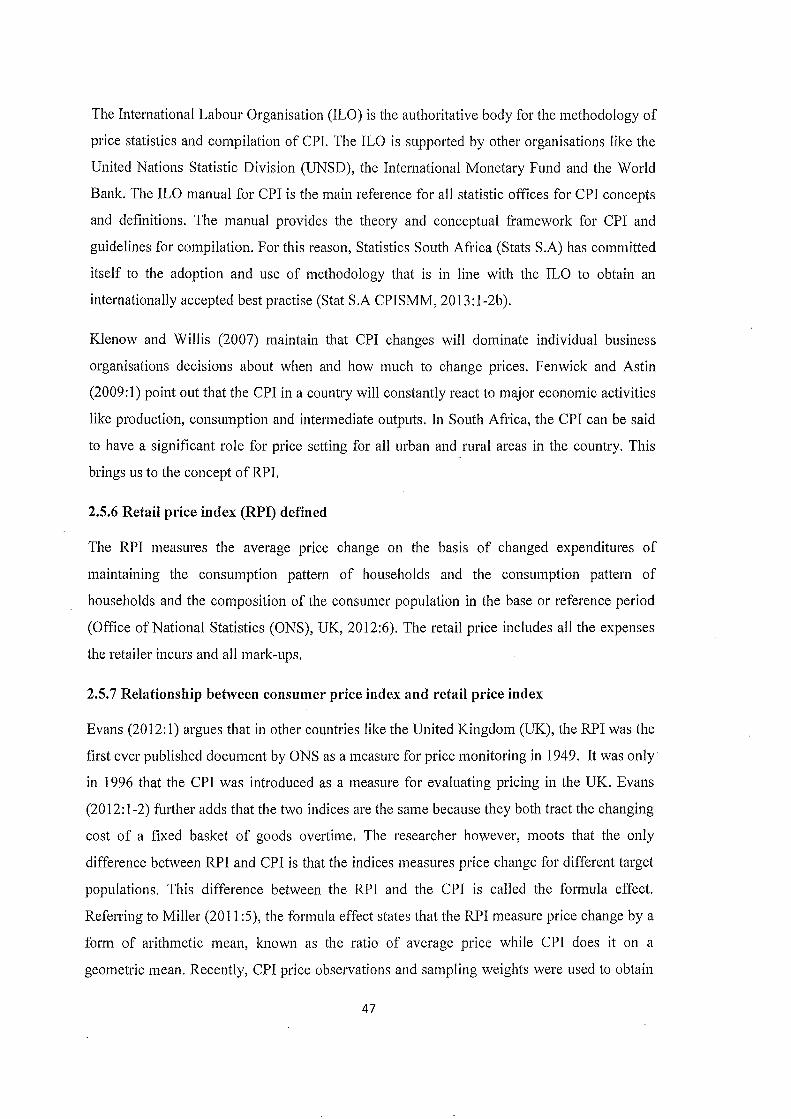
The International Labour Organisation (ILO) is the authoritative body for the methodology of
price statistics and compilation of CPl. The ILO is supported by other organisations like the
United Nations Statistic Division (UNSD), the International Monetary Fund and the World
Bank. The ILO manual for CPI is the main reference for all statistic offices for CPI concepts
and definitions. The manual provides the theory and conceptual framework for CPI and
guidelines for compilation. For this reason, Statistics South Africa (Stats S.A) has committed
itself to the adoption and use of methodology that is in line with the ILO to obtain an
internationally accepted best practise (Stat S.A CPISMM, 2013:1-2b).
Klenow and Willis (2007) maintain that CPI changes will dominate individual business
organisations decisions about when and how much to change prices. Fenwick and Astin
(2009: 1) point out that the CPI in a country will constantly react to major economic activities
like production, consumption and intermediate outputs. In South Africa, the CPI can be said
to have a significant role for price setting for all urban and rural areas in the country. This
brings us to the concept of RPI.
2.5.6 Retail price index (RPI) defined
The RPI measures the average price change on the basis of changed expenditures of
maintaining the consumption pattern of households and the consumption pattern of
households and the composition of the consumer population in the base or reference period
(Office of National Statistics (ONS), UK, 2012:6). The retail price includes all the expenses
the retailer incurs and all mark-ups.
2.5.7 Relationship between consumer price index and retail price index
Evans (2012:1) argues that in other countries like the United Kingdom (UK), the RPI was the
first ever published document by ONS as a measure for price monitoring in 1949. It was only
in 1996 that the CPI was introduced as a measure for evaluating pricing in the UK. Evans
(20 12: 1-2) fwther adds that the two indices are the same because they both tract the changing
cost of a fixed basket of goods overtime. The researcher however, moots that the only
difference between RPI and CPI is that the indices measures price change for different target
populations. This difference between the RPI and the CPI is called the formula effect.
RefelTing to Miller (20 11 :5), the formula effect states that the RPI measure price change by a
form of arithmetic mean, known as the ratio of average price while CPI does it on a
geometric mean. Recently, CPI price observations and sampling weights were used to obtain
47
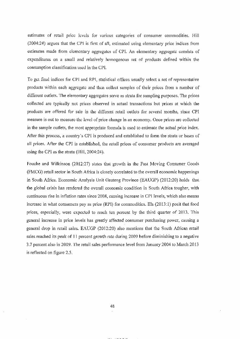
estimates of retail pnce levels for vanous categories of consumer commodities. Hill
(2004:24) argues that the CPI is first of all, estimated using elementary price indices from
estimates made from elementary aggregates of CPl. An elementary aggregate consists of
expenditures on a small and relatively homogenous set of products defined within the
consumption classification used in the CPl.
To get final indices for CPI and RPI, statistical offices usually select a set of representative
products within each aggregate and then collect samples of their prices from a number of
different outlets. The elementary aggregates serve as strata for sampling purposes. The prices
collected are typically not prices observed in actual transactions but prices at which the
products are offered for sale in the different retail outlets for several months, since CPI
measure is out to measure the level of price change in an economy. Once prices are collected
in the sample outlets, the most appropriate formula is used to estimate the actual price index.
After this process, a country's CPI is produced and established to form the strata or bases of
all prices. After the CPI is established, the retail prices of consumer products are averaged
using the CPI as the strata (Hill, 2004:24).
Fouche and Wilkinson (2012:27) states that growth in the Fast Moving Consumer Goods
(FMCG) retail sector in South Africa is closely correlated to the overall economic happenings
in South Africa. Economic Analysis Unit Gauteng Province (EAUGP) (2012:20) holds that
the global crisis has rendered the overall economic condition in South Africa tougher, with
continuous rise in inflation rates since 2008, causing increase in CPI levels, which also means
increase in what consumers pay as price (RPI) for commodities. Els (20 13: 1) posit that food
prices, especially, were expected to reach ten percent by the third quatier of 2013. This
general increase in price levels has greatly affected consumer purchasing power, causing a
general drop in retail sales. EAUGP (2012:20) also mentions that the South African retail
sales reached its peak of 11 percent growth rate during 2009 before diminishing to a negative
3.7 percent also in 2009. The retail sales performance level from January 2004 to March 2013
is reflected on figure 2.5.
48
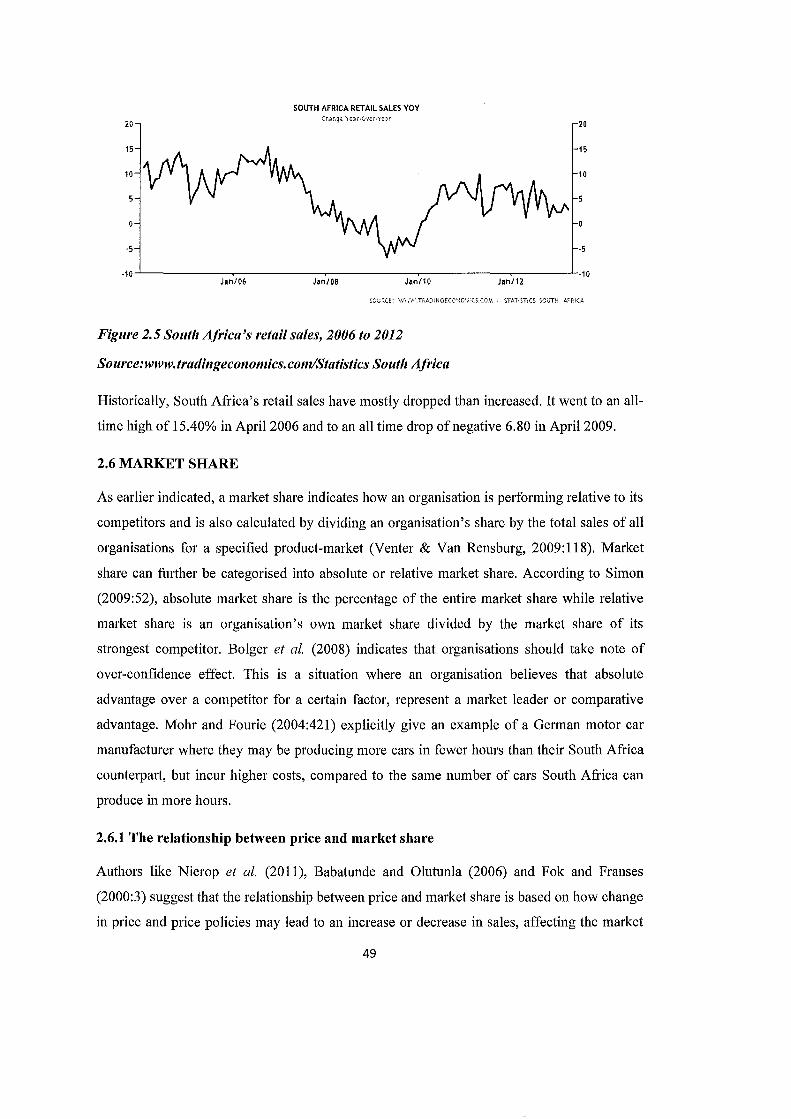
SOUTH AFRICA RET AIL SALES YOY
Jan/06 Jan/08 Jan/10 Jan/12
SOURCE: \'i\','\',•.n:~.DlNOECCtlC.WC$.(0>,\ j STATISTiCS. SOUTH tFRiCA
Figure 2.5 South Africa's retail sales, 2006 to 2012
Source:www. tradingeconomics. com/Statistics South Africa
Historically, South Africa's retail sales have mostly dropped than increased. It went to an all
time high of 15.40% in April2006 and to an all time drop of negative 6.80 in April2009.
2.6 MARKET SHARE
As earlier indicated, a market share indicates how an organisation is performing relative to its
competitors and is also calculated by dividing an organisation's share by the total sales of all
organisations for a specified product-market (Venter & Van Rensburg, 2009:118). Market
share can further be categorised into absolute or relative market share. According to Simon
(2009:52), absolute market share is the percentage of the entire market share while relative
market share is an organisation's own market share divided by the market share of its
strongest competitor. Bolger et a!. (2008) indicates that organisations should take note of
over-confidence effect. This is a situation where an organisation believes that absolute
advantage over a competitor for a certain factor, represent a market leader or comparative
advantage. Mohr and Fourie (2004:421) explicitly give an example of a German motor car
manufacturer where they may be producing more cars in fewer hours than their South Africa
counterpart, but incur higher costs, compared to the same number of cars South Africa can
produce in more hours.
2.6.1 The relationship between price and market share
Authors like Nierop et al. (2011), Babatunde and Olutunla (2006) and Fok and Franses
(2000:3) suggest that the relationship between price and market share is based on how change
in price and price policies may lead to an increase or decrease in sales, affecting the market
49

share negatively or positively respectively. Fok and Franses (2000:3) indicate that
determining market share from sales performance assumes a multiplicative specification to
relate explanatory variables such as prices effect on current sales. This is further explained by
the following formula:
I K
Si,t = exp(Jti + C:i,t) IT IT exp(xk,j,t)~k,j,i, j;lk=l
Formula (2.3)
In this equation, Et = (E1;t; ... ;EI;t)'~N(O; I:) and k;j;t denote the k-th explanatory variable (for
example, price) for brand j at time t and pk;j;i is the corresponding coefficient for brand i.
The normality assumption for the error terms is not strictly necessary, although with this
assumption, the least-squares estimates are the maximum likelihood estimates.
2.6.2 Price relationship with sales and consequent effect on market share
Moutinho and Chien (2008: 162) point out that even though in recent decades other factors are
also now playing a role in influencing consumer behaviour or decision to make a purchase,
price still remains the most important element determining a business sales, profitability and
market share. Wiid (2012:6) said consumers will always attach a certain value for the product
they want to buy and these values are always reflected in the price of the product. The
influence of price on sales and its consequent effect on market share can be analysed on the
consumer decision model. Plessis and Rousseau (2007:260) refer to the consumer decision
making model as the primary decisions consumers make whether to purchase or not, to spend
or save their money when engaged in a particular buying situation.
Plessis and Rousseau (2007:263) and Egan (2007:54) specify that the decision to make a
purchase involves problem recognition, information search, evaluation, decision, purchase
and post-purchase evaluation. If price is applied in the consumer decision model, it will be as
follows: available income compared to offered price by the retailer to satisfy the need,
information on different price offers, evaluating the best price offer, purchasing the product
with the best price and if there is value for the price paid. According to Khan (20 11 :43), the
consumer behaviour model is a good determinant to identify cause and effect relation in the
market. Skitmore and Smyth (2006:7) say that generally, consumer behaviour influences
price setting, because product prices are set based on available data about consumers'
so
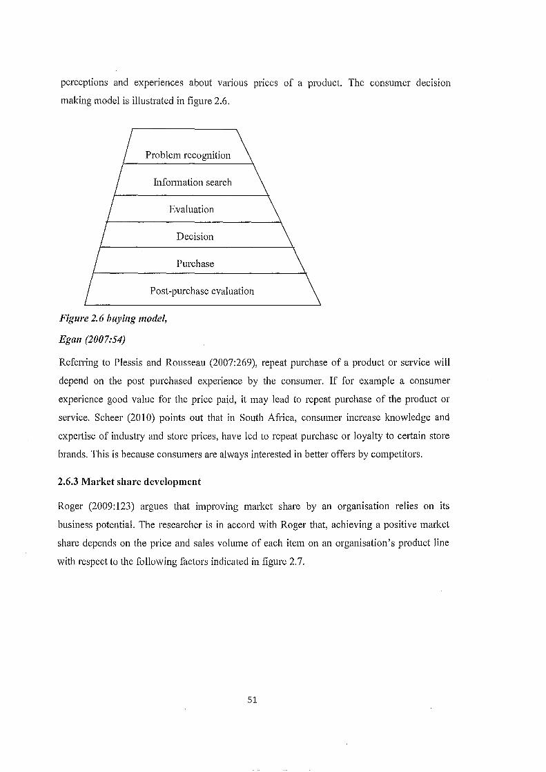
perceptions and experiences about vanous pnces of a product. The consumer decision
making model is illustrated in figure 2.6.
Problem recognition
Information search
Evaluation
Decision
Purchase
Post-purchase evaluation
Figure 2.6 buying model,
Egan (2007:54)
Referring to Plessis and Rousseau (2007:269), repeat purchase of a product or service will
depend on the post purchased experience by the consumer. If for example a consumer
experience good value for the price paid, it may lead to repeat purchase of the product or
service. Scheer (20 1 0) points out that in South Africa, consumer increase knowledge and
expertise of industry and store prices, have led to repeat purchase or loyalty to certain store
brands. This is because consumers are always interested in better offers by competitors.
2.6.3 Market share development
Roger (2009:123) argues that improving market share by an organisation relies on its
business potential. The researcher is in accord with Roger that, achieving a positive market
share depends on the price and sales volume of each item on an organisation's product line
with respect to the following factors indicated in figure 2. 7.
51

Not Aware of Product
Figure 2. 7 Market share index,
Roger J. Best (2009:122)
Prlc• TooHieh
Total
Mati<et Sh~re Index
Fok and Franses (200:4) suggest that the most appropriate method to establish a proper
relationship between sales and market share is the naive and simulation techniques. Detailed
illustrations of these techniques by Fok and Franses are as follows:
2.6.3.1 Nai've technique
The nai've technique holds that, the market share of a brand i and t, denoted as Mit, is broader
defined as:
M.;.,t-Formula (2.4)
This expression is called a naive expectation because it is not possible to obtain market shares
value directly from sales information. A further complication is that it is also not trivial to
obtain a forecast of Si;t+ 1, as the sales model is defined in logs, and also well known that
exp(E[logX])= E[X]. Therefore, forecasts of log sales cannot simply be transformed to sales
forecasts using the exponential function. The naive method can obtain approximate
confidence intervals by using the delta tactic defined as follows:
Formula (2.5)
52

2.6.3.2 Simulation-based method
Simulation is done by using the estimated probability distribution of sales to generate
artificial realisations of the sales. Based on each of these realisations of all brands, the market
shares can be calculated. This is achieved by using the following formula:
)l) - (jl) )1) )' f M (0 ,;) 'HI- tl:tfll"''cl:itl f0ll1.i~ l!.J
l K J P S(l) ( ,, (1\ ) 1111 ( ) ·. '' 1111 sa '. . - exp II I " ' exp x 8r.,tl . p,;,. ·i,t+J - ,, ri T "'iHl \ 'kd;t+l ',) jM1-p
Formula (2.6)
j=lk=l j=lp=l
In the above formula, the index 1 denotes the simulation iteration. For every draw of "(l)t+ 1,
the corresponding realisation of the sales is calculated, S(l)i;t+ 1. With a simulated realisation
of the sales, the corresponding realization ofthe market shares can be calculated as:
lvl~t) t,t+l Formula (2.7)
'\'! ..,(l) • LIJ=l sj,t+l
2.6.4 Advantages of a good market share position
Referring to Nissan (2003), past literature has long confirmed market share 'to have a better
relationship with relative advantage. Bode and Scharafi (2007) state that it is important to
have a strong market share position in the market because organisations with a better market
share have an edge over their competitors in formulating or executing business strategies.
Some ofthe advantages of a strong market share position are as follows:
2.6.4.1 Customer relationships and loyalty
Liu and Yang (2009) points out that the competitive position of an organisation will
determine its level of consumer loyalty because consumers often link value with respect to an
organisation's status. Gaunaris and Stathakopoulos (2004) say that brand loyalty reflects the
possibility of a consumer to rebuy an organisation's product. This can also lead to
relationships since an emotional and normative attachment is established between consumer
53
and the brand. Kana gal (2009) argues that a retailer's relationship with consumers has
become so important that organisations' profitability recently been associated more with
satisfying existing customers. Gehrig et al. (2009: 1) mentioned that new consumers can be
targeted by aggressive price offers that can induce them to terminate already existing
customer relationships. Etro (2007:8) adds that competitors with strong market share
positions can act independently from weak rivals, like being aggressive in their pricing
strategies. According Luarin and Lin (2003), relationship will lead retailers to offer better
deals to consumers thus, leading to better trade leverage and more strength of an
organisation's market share.
2.6.4.2 Innovation and product development
According to Lee and Kim (2013) organisations with a bigger market size are more
opportune to come up with innovative ideas because innovative capabilities depend on an
organisation's strengths. Hunt and Arnett (2006) indicates innovation can either be proactive
or reactive and each occur und~r the following circumstances. Proactive innovation occurs
when the market research department identifies a previously unserved market segment and
tailors a market offering for it or when an organisation engages in continuous process
improvements. When proactive innovative activities successfully produce innovations that
contribute significantly to efficiency/effectiveness, firms will be rewarded by marketplace
positions of competitive advantage. Reactive innovation occurs when inferior financial
performance signals firms that their comparative disadvantage in resources has resulted in
their occupying marketplace positions of competitive disadvantage.
Veyzer (2003) holds that innovation is vital for organisations on the following grounds, (1)
rapid technological changes quickly render certain products obsolete, (2) there is the
tendency by competitors to copy a successful product which can neutralise an innovative
product's advantage. Dovey and White (2005) points out that product innovation should not
be assigned to one department. This is because product innovation demands the integration of
many actors of different knowledge and expertise in order to develop a higher technological
product. Sarin and O'Connor (2009) posit that if innovation of a new product is to be
successful, support is needed from the entire organisational structure. Venter and Rensburg
(20 11: 188) states that an organisation can perform better only when accumulated knowledge
is utilised. Simon (2009:42) specifies that innovation is an outstanding engine of growth since
54

it will lead to revenue increase from increased volume sold giving an organisation an
advantage over rivals.
2.6.4.3 Benefits from strategic alliances
Todeva and Knoke (2005) argue that international business literature has acknowledged a
number of positive outcomes for organisations that actively engaged in strategic alliances.
Kotler and Keller (2012:163) maintain organisations with a strong market position, like
market leaders penetrate into different markets due to their strength. Holmberg and
Cummings (2009) states that strategic business alliances are a critical component for any
organisation to better succeed in an industry, but it should be noted that too many strategic
alliances fail to meet their business partners' objective. However, effective alliance should
reflect the desire of the parties to create a solid foundation for their relationship based in
order on trust and mutual interest to achieve a positive atmosphere among partners.
2.6.4.4 Market control
Helfat and Lieberman (2002) indicate that the capabilities of an organisation's entrance into a
competitive industry and its possibility of survival depend on strengths. According to
Drummond and Ensor (2012:197), an organisation's control over a market comes as a result
of its dominant market share. Venter and Rensburg (20 11:184) mention that an organisation
with a strong market position will have an efficient access to resources as compared to its
rivals. Hunt and Arnett (2006) indicates that the marketing practice holds firm on the basis of
the R-A theory which emphasises that organisations competency rely on available assets.
This leads to an increase in the availability of resources. Sunil and Steenburgh (2008:2-3)
adds that the marketing function requires a large amount of resources to meet its demand.
2.6.4.5 Brand identity or corporate image
According to Hoeffler and Keller (2003), building a strong brand has become an important
priority to target customers. This is because organisations achieve a good number of benefits
as a result of a strong brand. Ailawadi et al. (2003) maintain that marketers have long
indicated the benefit of a brand that accrues from marketing activities like cash flow, image
and market share. Balakrishnan and Mahanta (2004) argue that there is nothing that travels
faster about a retailer compared to stories of bad product or service performance as well as a
well performing retailer. A "brand's personality" stage mark an important transition phase
since not all brands evolve into consumer icons, especially if the consumers do not relate to,
55
or believe in, or they sense some inconsistencies with brand's communication (Wee & Ming,
2003). Sherrington (2003:21) specifies that a brand's personality provides a richer source of
competitive advantage than any functional feature can do.
2.6.4.6 Low cost and profitability
According to Drummond and Ensor (20 12: 196), organisations with a dominant position in an
industry easily achieve economies of scale. Mohr and Fourie (2004:243) define economies of
scale as a situation when costs per unit of output fall as the scale increases, leading to low
cost in production. Mohr and Fourie (2004:268) hold that profitability occurs when an
organisation produces at the lowest unit cost. Armstrong and Green (2007) confirm that 48
econometric studies have identified a positive and correlated relationship between market
share and profitability. Simon (2009:52-53) agree that profitability will improve market share
but the hypothesis that a large market share automatically leads to higher profitability is the
biggest management misunderstanding of present times because a good market performance
is no guarantee for profitability.
2.7 CONCLUSION
This chapter broadly discussed and reviewed important and relevant literature to the study.
The review was done in two phases as follows: elements that influence pricing decision and
the impact of pricing on market. Main subjects discussed in the first phase included
marketing and marketing mix, different pricing methods, strategies and policies as well as
unethical pricing. Finally, the influence of the price indices as the main determinant of
pricing was also elaborated. The main subjects discussed in the second phase included the
relationship between price and market, the importance of sales performance of a product to
market share and the advantages of being market share dominant. From literature gathered it
was revealed that, there are numerous options for a retailer to make pricing decisions. Due to
the different options in pricing decision, it can be possible for different sellers to develop
their own unique pricing characteristics. Based on the literature gathered, it could be
concluded that pricing decisions made by a retailer will greatly impact on its business market
share gain or lost and retailers in general are not aware of this.
56

CHAPTER THREE
RESEARCH METHODOLOGY
3.1 INTRODUCTION
Rajasekar et al. (2006:2) define research methodology as a systematic way to solve a problem
scientifically or the procedures that researchers use to go about their work of describing,
explaining and predicting phenomena. Wilson (2009:5) refers to methodology as a plan of
action that informs and links the methods used to collect and analyse data to answer
postulated research questions. Existing secondary data and literature review were used in
analysing the research questions in order to obtain a detailed result of the relationship
between price and market share in the Ngaka Modiri FMCG market.
3.2 RESEARCH DESIGN
According to Creswell (2009:3), research design is a plan and procedures for research that
span the decisions from broad assumptions to detailed methods of data collection and
analysis. It is simply the plans for addressing the research objectives or problem and
developing a framework to answer the research problem. Punch (2009:112) specified that
research design situates the researcher in the empirical world and connect the research
questions to data. This therefore shows that research design is a basic plan for a research
project. The research design used in this study was mainly a quantitative approach.
Quantitative research essentially refers to the application of systematic steps of scientific
research, while utilising quantitative properties in the study (Edmonds & Kennedy, 2013:20).
In this approach, the occurrences of behaviour are counted, correct answers or errors are also
counted and any other types of measures are recorded (Drew et al., 2008:20). A quantitative
study provides a chance for numerical interpretation of findings.
Within this design the parameters of an exploratory strategy was used. Marshall and Rossman
(2011 :69) consider exploratory research to be a study that involves investigating little
understood phenomena by identifying or discovering important categories of meaning and to
generate suggestions for fmiher research. An exploratory research strategy was considered
due to limited research done on the identified problem within the specified geographical area.
57

3.2.1 Population
Bickman and Rog (2009:77) refer to population as the large group to which a researcher
wants to generalise his or her sample results. In other words, it is the total group that a
researcher is interested in learning more about. The population of this study included the
three largest grocery supermarkets in the Ngaka Modiri Molema district. Referring to
Mokgele (2012/2013:3) Ngaka Modiri Molema district municipality is one of the four district
municipalities in the North-West province of South Africa. It is a category C district,
bordered by Ruth Mompati district in the west, Bojanala Platinum district in the east, Dr.
Kenneth Kaunda district in the south and Botswana to the North. Bogapane (2012) indicates
that it is home to over 800,000 inhabitants and divided into five local municipalities namely:
Mafikeng, Ratlou, Ramotshere Moiloa, Ditsobotla and Tswaing. Statistics South Africa
This study's empirical focus was on Ditsobotla, Mafikeng and Ramotshere Moiloa. These
focus municipalities represent almost 80% of the total population of Ngaka Modiri Molema
district. The three municipalities were targeted since the researcher aimed at selecting only
supermarket stores with a large client base, as reflected in the focus municipalities. The
headquarters of each focus local municipality comprised the target area for selecting
participating supermarkets. These towns included Lichtenburg, Mafikeng and Zeerust. These
towns are also the headquarters of Ditsobotla, Mafikeng and Ramotshere Moiloa
municipalities respectively. All selected supermarkets for this study experienced a sales
turnover above 15,000 product units (regardless of brand or trademark) and client base above
10,000 monthly. Community Survey (Stat SACS) (2009:6-7) gives a detailed break down of
the different Ngaka Modiri local municipalities in terms of population size and household
distribution as shown in figure 3.1
58

Ngaka Modiri District
Mafikeng Ratlou Ditsobotla Tswaing
Population Population Population Population Population
size size size size size
290229 98102 200150 81004 129301
Households Households Households Households Households
68698 23591 38608 22201 30302
Percentage of Percentage Percentage of Percentage of Percentage of
population population population population population
36.33% 12.28% 25.06% 10.14% 16.19%
Figure 3.1 Ngaka Modiri municipalities
Source: Stat SA (2009)
3.2.2 Sampling
According to Smith et a!. (2013:162), a sample is a subset of the whole population
investigated by a researcher whose characteristics will be generalised to the entire population.
Smith eta!., states sampling refers to the process of drawing a sample from a population.
Researchers sample in order to study and understand the characteristics of the larger group.
Researchers must carry out a sampling process because factors such as expense, time and
accessibility frequently prevent researchers from gaining information from the whole
population. No sampling strategy is guaranteed to be the best for a researcher to actually
answer research questions (Maxwell, 2012:95). Despite this, data can be collected from the
59

subset of the total population in such a way that the knowledge gained is a true reflection of
the total population (Cohen eta!., 2011: 143). Therefore, the best approach is the one that fits
into the research context and the research objectives (Maxwell, 2012). For the purpose of this
study, the researcher made used of purposive sampling based on which supermarkets had
access to reliable information for this study.
Cohen et a!. (20 11: 156) refer to purposive sampling as a non-probability sampling method
which involves purposive or deliberate selection of particular participants from a sample
relevant to the study. This approach was employed in order to enable the researcher to select
supermarkets with qualified reliable and applicable information. One single supermarket
store was selected from each sampled supermarket brand in this study. Participating
employees included the regional marketing manager and the branch manager of each
supermarket brand. Thus, two employees participated from each supermarket brand. A total
of six employees from various sampled supermarkets patiicipated in the study. Figure 3.2
gives a visual representation of the sample.
60
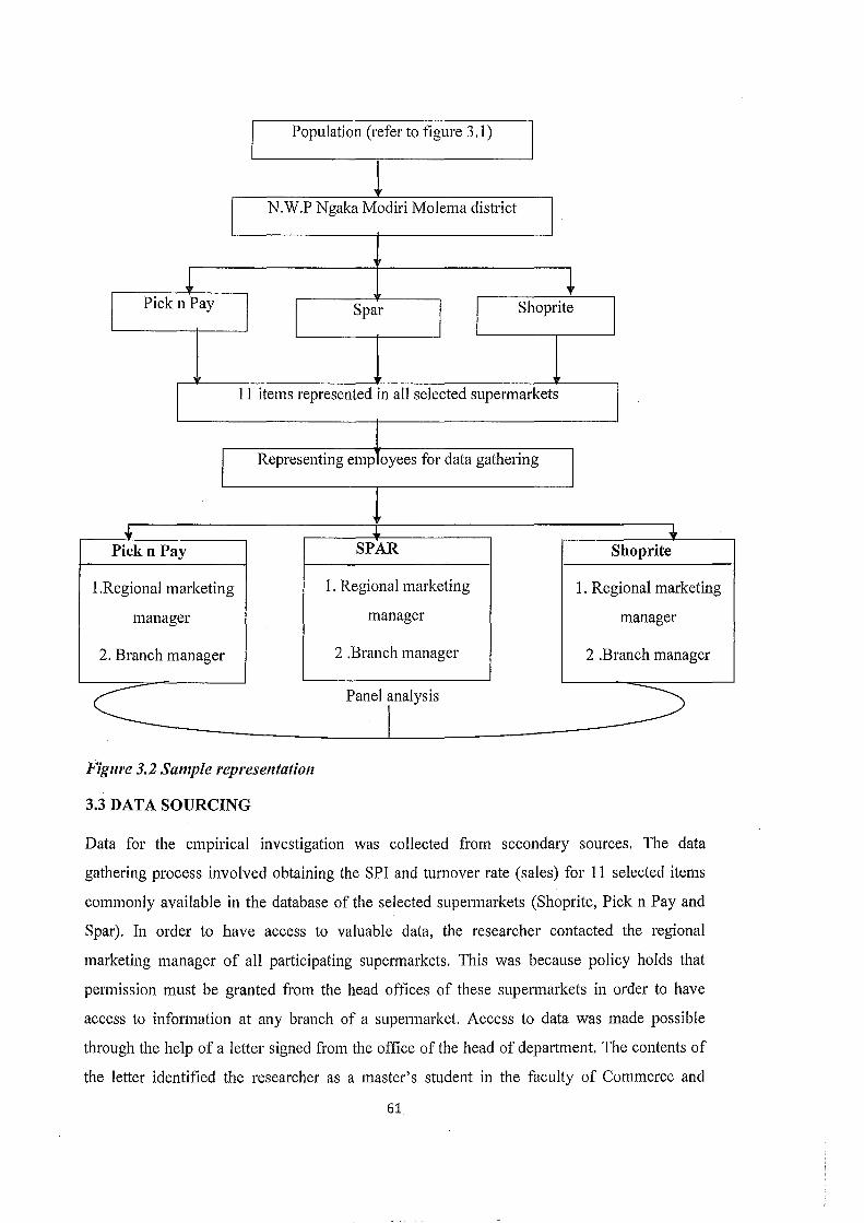
Population (refer to figure 3.1)
I N.W.P Ngaka Modiri Molema district
I
~ -l I
Pick n Pay
I Spar
I I Shoprite
I
I 11 items represented in all selected supermarkets
I
I Representing emp oyees for data gathering
I
... ... Pick n Pay SPAR Shoprite
!.Regional marketing 1. Regional marketing 1. Regional marketing
manager manager manager
2. Branch manager 2 .Branch manager 2 .Branch manager
c_ Panel ralysis =::s Figure 3.2 Sample representation
3.3 DATA SOURCING
Data for the empirical investigation was collected from secondary sources. The data
gathering process involved obtaining the SPI and turnover rate (sales) for 11 selected items
commonly available in the database of the selected supermarkets (Shoprite, Pick n Pay and
Spar). In order to have access to valuable data, the researcher contacted the regional
marketing manager of all participating supermarkets. This was because policy holds that
permission must be granted from the head offices of these supennarkets in order to have
access to information at any branch of a supermarket. Access to data was made possible
through the help of a letter signed from the office of the head of department. The contents of
the letter identified the researcher as a master's student in the faculty of Commerce and
61
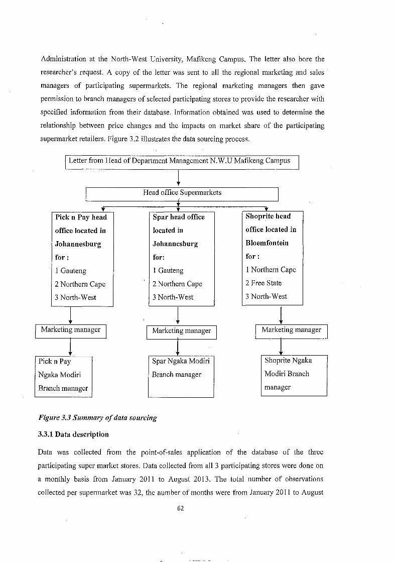
Administration at the North-West University, Mafikeng Campus. The letter also bore the
researcher's request. A copy of the letter was sent to all the regional marketing and sales
managers of participating supermarkets. The regional marketing managers then gave
permission to branch managers of selected participating stores to provide the researcher with
specified information from their database. Information obtained was used to determine the
relationship between price changes and the impacts on market share of the participating
supermarket retailers. Figure 3.2 illustrates the data sourcing process.
Letter from Head of Department Management N. W .U Mafikeng Campus
I Head office Supermarkets I • 'f 'f ..
Pick n Pay head Spar head office Shoprite head
office located in located in office located in
Johannesburg Johannesburg Bloemfontein
for: for: for:
1 Gauteng 1 Gauteng 1 Nmthern Cape
2 Northern Cape 2 Northern Cape 2 Free State
3 Nmth-West 3 Nmth-West 3 Nmth-West
l l l Marketing manager I I Marketing manager I I Marketing rna nager
~ ~ 1 Pick n Pay Spar Ngaka Modiri Shoprite Nga ka
Ngaka Modiri Branch manager Modiri Branc h
Branch manager manager
Figure 3.3 Summary of data sourcing
3.3.1 Data description
Data was collected from the point-of-sales application of the database of the three
participating super market stores. Data collected from all 3 participating stores were done on
a monthly basis from January 2011 to August 2013. The total number of observations
collected per supermarket was 32, the number of months were from January 2011 to August
62
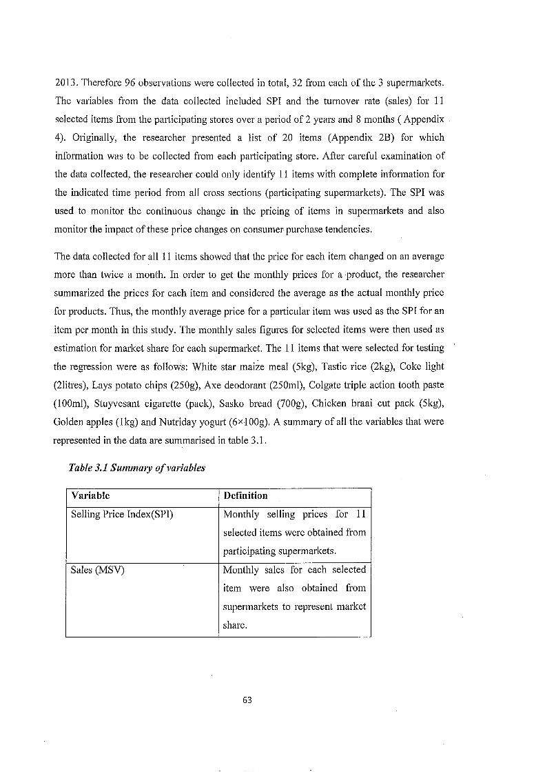
2013. Therefore 96 observations were collected in total, 32 from each of the 3 supermarkets.
The variables from the data collected included SPI and the turnover rate (sales) for 11
selected items from the participating stores over a period of 2 years and 8 months ( Appendix
4). Originally, the researcher presented a list of 20 items (Appendix 2B) for which
information was to be collected from each pa1iicipating store. After careful examination of
the data collected, the researcher could only identify 11 items with complete information for
the indicated time period from all cross sections (participating supermarkets). The SPI was
used to monitor the continuous change in the pricing of items in supermarkets and also
monitor the impact of these price changes on consumer purchase tendencies.
The data collected for all 11 items showed that the price for each item changed on an average
more than twice a month. In order to get the monthly prices for a product, the researcher
summarized the prices for each item and considered the average as the actual monthly price
for products. Thus, the monthly average price for a pmticular item was used as the SPI for an
item per month in this study. The monthly sales figures for selected items were then used as
estimation for market share for each supermarket. The 11 items that were selected for testing
the regression were as follows: White star maize meal (5kg), Tastic rice (2kg), Coke light
(2litres), Lays potato chips (250g), Axe deodorant (250ml), Colgate triple action tooth paste
(lOOm!), Stuyvesant cigarette (pack), Sasko bread (700g), Chicken braai cut pack (5kg),
Golden apples (lkg) and Nutriday yogurt (6xl OOg). A summary of all the variables that were
represented in the data are summarised in table 3 .1.
Table 3.1 Summmy of variables
Variable Definition
Selling Price Index(SPI) Monthly selling prices for 11
selected items were obtained from
participating supermarkets.
Sales (MSV) Monthly sales for each selected
item were also obtained from
supermarkets to represent market
share.
63

3.4 MODEL SPECIFICATION
A model specification is a standard that lays requirement against other specifications by using
a set-theoretic description of those specifications based on their structure as organised sets of
criteria, those that are to be tested (requirements) and those that are not tested
(recommendations). All specifications, formally or informally, create an abstraction of the
things to which they apply in order to provide a context for stating requirements. This
standard is considered one of its own standardisation targets and thus a subject of its own
requirements (Whiteside eta!., 2008:9). The model specification adopted in this study was
the POLS linear regression. According to Wooldridge (2006:25), the formula layout of the
POLS regression model is as follows:
Least Square regression is denoted as 1';1 =fJ0+/]1X;1 + &u Formula (3.1)
Where:
Y = dependent variable the equation is trying to predict.
{3 o= the intercept of the equation.
~1 = the slope coefficient.
X= the independent variable that is used to predict the dependent variable.
E =the error term or the regression residual variable.
Following from the indications mentioned, Wooldridge's specification from formula 3.1 was .
adjusted to fit the context of this study as follows:
The model specification (relationship between the dependent - market share, and the
independent variable- pricing) of this study was then equated as:
With reference to formula (3.2) indications represented are as follows:
Market Share Value (MSV)= the dependent variable that the model is trying to predict.
64

{J o= the intercept of the equation.
~1 =the slope coefficient of the price variable.
Price (P) = the independent variable used to predict the dependent variable.
c = the error term or the regression residual variable. It represented all other variables such as
quality and advertising that could have an effect on the market share other than the
independent variable (P).
i =all the cross section (supermarkets) that participated in the study.
t= the time period under study (January 2011 to August 2013).
Formula 3.2 is a variation of the original model (formula 3.1). The objective of this study was
to determine relationships between the dependent and independent variables. Based on this,
POLS seem best suited in determining the mentioned relationships.
3.5 ANALYTICAL TECHNIQUE
The analytical technique used in this study was based on the panel data analysis. The
researcher used a panel of the three largest fast consumer goods retailers in the Ngaka Modiri
Molema district to establish the relationship between their pricing and its effect on market
share gain or loss. A panel data refers to pooling of observations from a cross-section of
households, countries or business organisations and following them over several time periods
(Baltagi, 2008:1). In other words, panel data are repeated observations over time for the same
set of cross sectional units (lee, 2006: 12). In a panel data equation as in formula (3.2), the
cross-section variables are denoted as (i) and the time periods as (t).
A panel data analysis was best suited for this study because it takes an organisation's specific
heterogeneity into consideration. A second reason is that due to the repeated cross section of
observations, panel data are better suited to studying the dynamics of change. Lastly, panel
data analyses are very effective in evaluating strategies or policies in organisations. It was
thus clear that the researcher could effectively achieve the objective of the study by
employing a panel data analysis. This objective was to investigate the degree to which
constant changes in pricing decisions by the three largest FMCG retailers in the Ngaka
Modiri district impact on their market share gain or share loss. In order to run the linear
regression, three panel data tests were run. These tests involve the panel unit root tests,
65
3.5.1.2 Im, Pesaran and Shin test (IPS)
Baltagi (2009:57) states the IPS test suggests an alternative testing route based on averaging
the unit root ADF test statistics for each individual cross-section. Baltagi (2008:278) further
indicated that this means the null hypothesis assumes that each series in the panel has a unit
root denoted as H0 : Pi = 0 for all i while the alternative hypothesis permits some of the
individual series to have a unit root denoted as H1 : p( <0 fori= 1,2, .. ,N1 and p( = 0 fori=
N1 + 1, ... ,N. The IPS test was necessary because it could provide simulated critical values for
the different cross-sections N, and series length T.
3.5.1.3 Combining p- value (Fisher Chi-square) test
Asteriou and Hall (2011 :445) indicate that the Fisher test was introduced by Maddala and Wu
in 1999 in their attempt to improve the deficiencies in other panel unit root tests. Baltagi
(2005:244) indicates that the Fisher test takes the following form:
In the equation (3.4), Pi is the probability limit value from regular ADF uniH'oot tests for
each cross section i. Since - 2lnp( has a x2 distribution with degrees of freedom; the p
statistics will follow a x 2 distribution with 2N degrees of freedom as T( -t oofinite N. Baltagi
(2005 :245) argues that the combining p- value test have many advantages in testing unit root
for panel data when compared to other panel unit root tests. Baltagi further mentions these
advantages as follows: the cross-sectional dimension, N, can either be finite or infinite, each
grouping can have different types of non-stochastic and stochastic elements. The time series
dimension, T, can be different for each (and finally, the alternative hypothesis can tolerate
some groups to have unit roots whereas others may not. Due to the superiority of this test
over other panel data unit root tests, it was important that this test was run.
3.5.2 Poolability test
Poolability testing involves the selection of the most appropriate panel data model for a panel
study. According to Gujarati and Porter (2009:594) and Asteriou and Hall (2011:417-419),
there are the three main models for panel data poolability test. These panel data models
include: the common constant or pooled model, the fixed effects model and the random effect
model. Gujarati and Porter (2009:594) indicate that the pooled model assumes that the
regression coefficients are the same for all cross sections. Baltagi (2008: 14 &17) states that
67

similar characteristics in the behavioural relationship between price and market for three
sampled supermarkets o (Pick n Pay, Shoprite and Spar). On the other hand, the alternative
hypotheses, H1 == ol * o2 * o3 * :::: 0 assumed that, each sampled supermarket, o, had its
own specific or unique characteristics with regards to its relationship between price and
market share. After these assumptions were made, The F test and the Chi-square test were
used to determine which model tested positive for the study.
After the poolability test, the model estimation was done. The model estimation involved
estimating the model specification of the study using the considered panel data model from
the poolability test. The model assumption was that a decrease or an increase in the price of a
product by Ngaka Modiri Molema retailers will lead to market share gain or loss respectively.
Thus, the model assumption represented in formula (3.1) was individually estimated for each
tested item for every sampled supermarket through a fixed effect model.
3.5.3 Diagnostic tests
Brooks (2009: 43) maintains that diagnostic tests are required in a panel analysis because
they show that estimation techniques like the POLS linear regression may have ignored a
series of desirable elements. Brooks also says that the diagnostic test also tries to confirm if
coefficient estimates from regressions are justifiable or fairly conducted. In this study, the
diagnostic test was conducted to ensure reliability of results from linear regression. The
diagnostic tests conducted in this study included the normality, serial correlation and
heteroscedasticity tests. The estimation results are based on the assumption that the residuals
are normally distributed, there is no serial correla,tion and heteroscedasticity in the residuals.
Violation of these assumptions invalidates the obtained results. This tests will be discussed in
the following sub sections.
3.5.3.1 Normality test
The Bera-Jargue (J-B) test was used in testing for normality in this study. The J-B test uses
the property of normally distributed random variables so that the entire distribution is
characterised by the first order two moments- the mean and variance. The third and fourth
moments of the distribution are known as its skewness and kurtosis respectively (Brooks,
2009:57). Brooks further mentions that the skewness measures the extent to which the
distribution is not symmetric regarding its mean value and kmiosis measures how much the
estimates of the distribution are. The assumption in this test is that the null hypothesis is
69

normally distributed against the alternative hypothesis and that other distributions are present.
Referring to Cameron (2005:238), the J-B test combines the skewness and the kurtosis
according to the following formula:
J-B = n[(S 2/6) + {( K- ;:}} Formula (3.6)
Cameron elaborated on the equation (3.6) in which n is the sample size, S the skewness and
K the kurtosis. If skewness slopes to the right or the left, then the distribution is not normally
distributed. Kurtosis measures how steeply values are rising to the most likely value in the
distribution curve. According to Gujarati (2003:148) under the J-B test, if the computed
p value is sufficiently low, the alternative hypothesis should be accepted that residuals are
not normally distributed. On the other hand, if p values are reasonably high, the normality
assumption is not rejected. Thus the null hypothesis is accepted that residuals are normally
distributed.
3.5.3.2 Test for serial correlation
Serial correlation implies that the value of the error term from one time period depends in
.some systematic way on the value of the error term in another time period (Studenmund,
2011:304). Ignoring a serial correlation when present, will present consistent but inefficient
estimates of the regression coefficients and biased standard errors (Baltagi, 2008:92). The
Correllogram Q-Statistics test was used in testing for serial correlation in this study.
Referring to Nopiah et a!. (2010) the Correllogram Q-Statistic test, aim at sensing the
presence of serial correlation for a specified order in the autocorrelation tested lags. Gujarati
and Porter (2009:434) highlighted out that the advantage of the Correllogram Q-Statistic test
is that it detects the presence of higher order serial correlation.
In this study two hypotheses were developed in testing for serial correlation. H0 : p= 0 and
H1 : p =I= 0. The hypothesis H0 was to test that there was no serial correlation while the
alternative, H1 , on the other hand assumed that there was serial correlation. Panels were
tested for serial correlation because econometrics generally established the OLS to be
inconsistent in the presence of lagged dependent variables and serially correlated errors. Even
though Wooldridge (2006:415) holds that most of such assumptions are false, it was
necessary to test for serial correlation to prove the precision of coefficient estimates.
70
3.5.3.3 Heteroscedasticity
Baltagi (2005:99) states the heteroscedasticity test assumes that the regression disturbance or
disturbances are homoskedastic with the same variance across time and individuals.
Wooldridge (2006:278) further elaborates that the test for heteroscedasticity investigates
whether or not heterogeneity exists among estimates. In this study the White's cross section
test for heteroscedasticity was used. The White test detects heteroscedasticity by running a
regression with the squared residuals as the dependent variable. To this effect the right-hand
side of the secondary equation includes all the original independent variables or variable, the
squares of all the original independent variables or variable and the cross products of all the
original independent variables or variable with each other (Studenmund, 2011:350).
Referring to Asteriou (2011 :127) the white's cross section test was employed in this study
because it does not assume any determination of heteroscedasticity. Thus, two hypotheses
were formulated for testing heteroscedasticity. These hypotheses include: H0 :a-? =CJ which is
the null hypothesis assuming homoscedastic errors and H1 : not equal for all i, is the
alternative hypothesis assuming heteroscedastic errors. Born and Breitung (2012:16)
maintains that the disadvantage with most test statistics for heteroscedasticity is that they are
not robust against time independent heteroscedasticity. To overcome such an occurrence, an
unbiased estimator of serial correlation coefficients were constructed in order to apply
backward and forward transformations by assuming a 16 difference, such that series can
agree with the null hypothesis.
3.5.4 Forecasting of model estimation
It was important that forecasting be done m order to be aware of the possible future
happenings with respect to the identified problem of this study. Forecasting was done for
each model estimation linear regression result. Issler and Lima (2008: 11) point out that the
most important element in forecasting is that data to be used for forecasting must be
stationary in order to ensure a well-behaved forecast combination. Baltagi (2006:21) argue
that forecasting outcomes are always faulty with non-stationary data. Issler. and Lima
(2008:7) mention that there has been limited attention with respect to forecasting on panel
data studies. This is because econometricians consider forecasting as a time-series experiment
and forecasting is easily applicable for studies with few samples like the case of time-series
studies. As samples get larger, forecasting also gets hopelessly large and large samples are
71

mostly the case with panel data studies. Referring to Kunst (2012:5), forecasting was
necessary for this study since it may assist Ngaka Modiri Molema FMCG retailers in:
• predicting the future,
• future pricing decision making, and
• evaluation of pricing policies.
All the indicated econometric tests were effectively run on the Eviews software. All the rules
as required or as indicated by each test was effectively applied in the data analysis process.
3.6 ETHICAL CONSIDERATIONS
Neuman (2003: 116-118) indicates that the researcher has a moral and professional obligation
to be ethical, even if participants are unaware of or unconcerned about ethics.,Briggs and
Coleman (2007 :245) argues that for both ethical and objectivity purposes, it is vital to ensure
that participants are absolutely clear about their rights to an explanation of the aims,
procedures purposes, consequences of the research, publication possibilities and the right to
decline to take part, or to withdraw at any stage. The subjects need to be competent to make
these decisions, act voluntarily and make their decisions based on the fullest possible
information. Ethical considerations according to Trochim (2006), were grouped into three
main ethical themes. These three themes include gaining access, validity and reliability.
3.6.1 Gaining access
The researcher was issued a letter of permission by the Department of Management, North
West University, Mafikeng Campus to request access to selected super markets. With this
letter, the researcher approached the participants in the study to seek information. All
participants agreed to sign the consent form and also agreed to take part in the study.
According to Creswell and Clarke (2007:113-114), researchers require permission to collect
data from individuals and sites. This permission can be gained at three levels: from
individuals who are in charge of sites, people providing the data and their representatives.
Whether a study is qualitative or quantitative, permission from individuals in charge is
necessary.
3;6.2 Validity
Maxwell (2012, 134 &137) explains validity as describing and interpreting what a researcher
found in a research study. The findings should be in line with the indications provided by the
72

participants, with nothing added or removed. Therefore, one way of establishing validity in
any research study is to take the findings back to the subjects' verification. In this study
findings were taken back to the participants to verify if what was captured from data base was
in line with indications from the findings. Truthfulness, fairness and honesty in this study was
established through the validation of data by participants themselves. Findings were also
validated by reviewing literature on the subject. As Conway and Powell (2010:60) point,
validity is an important key to research because research is considered valid only when
conclusions are true and dependable.
3.6.3 Reliability
Gratton and Jones (2010:92) explain that reliability generally refers to the degree of
consistency of a result that is obtained. Babbie (20 10: 150) also defines it as a matter of
whether a particular technique yields the same outcome when applied repeatedly to the same
sample. Neuman (2003:184) adds to his definition of reliability the issue of dependability.
Dependability of data was established by the researcher by ensuring that the process by which
data was collected was very accurate.
3.7 CONCLUSION
In this chapter, the research design, population, sampling, data sourcing, data description and
modef specification were discussed. The chapter also described the analytical technique used
in this study. Ethical considerations were also discussed. The next chapter deals with the
presentation and interpretation of data for the test regressions in this study.
73

CHAPTER FOUR
DATA ANALYSIS AND INTERPRETATION
4.1 INTRODUCTION
This chapter presents the data analysis and interpretation of results from the empirical
findings. Alexander (2012:1) defines data analysis as systematically collecting, transforming
and analysing of data in order to present meaningful conclusions. Interpretation means
relating the results and findings of a study to an existing theoretical framework or model and
showing whether these results are supported or not by existing theories. It also entails the
mentioning of rival explanations or interpretation of the empirical data and showing what
levels of support the data provide for the preferred interpretation (Mouton, 2002:1 09).
4.2 DATA ANALYSIS PROCESS
Myers et al. (20 10: 15) state that data analysis consists of stages. These stages include the
exploratory phase where measures like means and medians are calculated and an inferential
phase where parameters are estimated and hypotheses tested. Data analysis was done in four
stages for all the panel tests in this study (unit root or stationarity test, poolability testing,
model estimation testing and the diagnostic test). These stages include:
• systematic arrangement of the dependent and the independent variables for each year in a
horizontal for each tested item for all supermarkets (see appendix 5),
• pooling (importing) data as panels into the e-views software,
• estimating the regressions of the dependent and the independent variables, and
• testing hypotheses to determine the outcomes of each panel test.
Tests were run in a systematic order as follows: the unit root tests, poolability and the model
estimation tests, normality, serial correlation and heteroscedasticity tests. The model
estimation was the primary test since its outcomes determined if the problem statement of this
study held grounds or had any implications. Regression estimates from the model estimation
were also used to test for normality, serial correlation and heteroscedasticity. It should be
noted that in the analysis process, sampled cross-sections (supermarkets) and 11 tested items
were given individual codes to be able to identify variables during the analysis. Table 4.1 and
74

4.2 are summary tables indicating the codes used for each individual cross section and item
respective! y.
Table 4.1 Summary of cross section codes
Supermarket brand Code
Pick n Pay pp
Spar SP
Shoprite SH
Table 4.2 Summary of item codes
Items Price code Quantity code
White star (5 kg) Pl Ql
Tastic rice (2kg) P2 Q2
Coke (2 litres) P3 Q3
Lays potato chips (125g) P4 Q4
Dark temptation axe spray (1 OOml) P5 Q5
Sasko bread (700g) P6 Q6
Chicken braai cuts (2kg) P7 Q7
Golden delicious apples (lkg) P8 Q8
Nutriday yogurt P9 Q9
Colgate triple action (lOOml) PlO QlO
Stuyvesant cigarettes (pack) Pll Qll
4.3 INTERPRETATION OF RESULTS
Results were interpreted according to the outcomes from regressions. Results were accurately
interpreted without any bias to avoid any possibility of fallacy in the analysis. All the panel
data tests as indicated were done strictly and all procedures followed. The p value is the most
important element from regression results. This is because it determines the probability of
whether the null or the alternative hypothesis is rejected or not. If the p value is > 0.05, the
null hypothesis is not rejected. Likewise, if the p value is < 0.05, the null hypothesis is to be
rejected and thG alternative hypothesis accepted. However, the mentioned rule is different for
both the normality and serial correlation test. For normality and serial correlation, the aim is
75


to have a p value that is greater than 0.05 in order to conclude that regression residuals are
normally distributed and not serially correlated. Alternatively, if results are < 0.05, then
regressions are not normally distributed and there is the presence of serial correlation. Results
from each test are all presented in this chapter. It should also be noted that results were
rounded up to three decimals. Table 4.3 indicates focused elements from regression outcomes
represented in the interpretation of results.
Table 4.3 Summary of key elements and their measures from regression analysis
Element Measurement
Coefficients (C) It explained the degree of impact that the
regressor or independent variable (price) had
on the dependent variable (market share) and
the degree to which the dependent variable is
influence by factors other than price.
p value It measured the probability level of
regressions to determine if either the null or
alternative hypothesis is correct.
R square (R 2) The R square indicated the percentage level
of which the dependent variable was
explained by the independent variable.
(*)I(**) I(***) It denotes significance at 1 0%, 5% and 1%
respective! y.
4.3.1 Interpretation of the unit root test
As earlier mentioned, all the panel data unit root tests LLC, IPS and combining p value were
performed on data to determine the degree of stationarity in the tested data. Unit tests were
performed separately for each data category. Thus, unit tests were done for all quantity data
(Q1 to Q11) across all cross sections while another unit test was done for all price data (Pl to
Pll) across all cross sections. Results from the unit test are indicated in table 4.4.
76

Table 4.4 Unit root tests results for price data
Test Coefficients p value
Levin, Lin,Chu -2.171 0.015**
Im, Pesaran & Shin -5.468 0.000***
ADF-Fisher Chi-square 148.373 0.000***
PP- Fisher Chi-square 107.981 0.000***
Table 4.4 reflect that the price data for all sampled supermarkets passed the various unit root
tests at a 1% level of significance. This suggests that since the p-values for all the tests are
less than 0.05, the null hypothesis that price data is non-stationary is rejected. (see appendix
3A for detailed results).
Table 4.5 Unit root tests result for sales data
Test Coefficients p value
Levin, lin,Chu -3.101 0.001 ***
Im, Pesaran & Shin -4.871 0.000***
ADF-Fisher Chi-square 137.863 0.000***
PP- Fisher Chi-square 75.907 0.189*
The p value results for the various unit root tests for quantity data confitmed positive at a 1%
level of significance. Only the PP- Fisher Chi- square unit root test showed a result of 18.9%
level of significance. The results indicated that LLC, IPS and ADF for quantity data (Q1 to
Q11) are stationary for all individual cross-sections. As earlier mentioned, the null hypothesis
is to be rejected for LLC, IPS and ADF unit root tests. Alternatively, the null hypothesis is to
be accepted for the PP-Fisher Chi-square. However, the LLC unit root test assumes a
common presence of stationarity in data across all cross-sections while the IPS, ADF and PP
Chi-squares unit root test assumes that there is stationarity across individual cross sections.
Thus, it can be derived that the results from the PP unit root test has no major implications on
results since two out of the three unit tests accountable for indicating the presence of
stationarity on each separate cross section (IPS, ADF and PP), have a 1% level of
significance (see appendix 3A for detailed results).
77

4.3.2 Poolability test and model estimation results
In this study, the pooled and the fixed effect models were tested. To decide between the
pooled and the fixed effect model, the F test and Chi-square test were performed. After
performing the relevant poolability tests, the fixed effect model which assumes specific
characteristics or uniqueness in the relationship between price (independent variable) and
market share (dependent variable) for each individual supermarket was considered against the
pooled model. Such specific uniqueness includes the pricing strategy, pricing ability of price
setters and the target market of a supermarket brand. All 11 items tested positive for the fixed
effects model with a p value < 0.05 while the pooled model which assumes that all cross
sections have a common constant (homogeneous) for all tested items were weaker compared
to the fixed effect model. Table 4.6 presents a summary of the poolability test. (See Appendix
3B for detailed results for the poolability test).
Table 4.6 Results for poolability testing
Input/output Fixed effect estimates Q-Statistic p value Conclusion
P1 & Q1 F- Statistics 2031.774 0.000*** Ho was rejected
Chi-square 365.799 0.000***
P2&Q2 F- Statistics 937.920 0.000*** Ho was rejected
Chi-square 294.039 0.000***
P3&Q3 F- Statistics 357176.083 0.000*** Ho was rejected
Chi- square 859.917 0.000***
P4&Q4 F -Statistics 181.957 0.000*** Ho was rejected
Chi-square 153.649 0.000***
P5 &Q5 F- Statistics 31.845 0.000*** Ho was rejected
Chi-square 50.503 0.000***
P6&Q6 F- Statistics 19987.053 0.000*** Ho was rejected
Chi-square 583.343755 0.000***
P7 &Q7 F -Statistics 105436.831 0.000*** Ho was rejected
Chi- square 742.816 0.000***
P8&Q8 F -Statistics 5858.161 0.000*** Ho was rejected
Chi-square 466.058 0.000***
P9&Q9 F -Statistics 19491.564 0.000*** Ho was rejected
Chi-square 580.939 0.000***
78
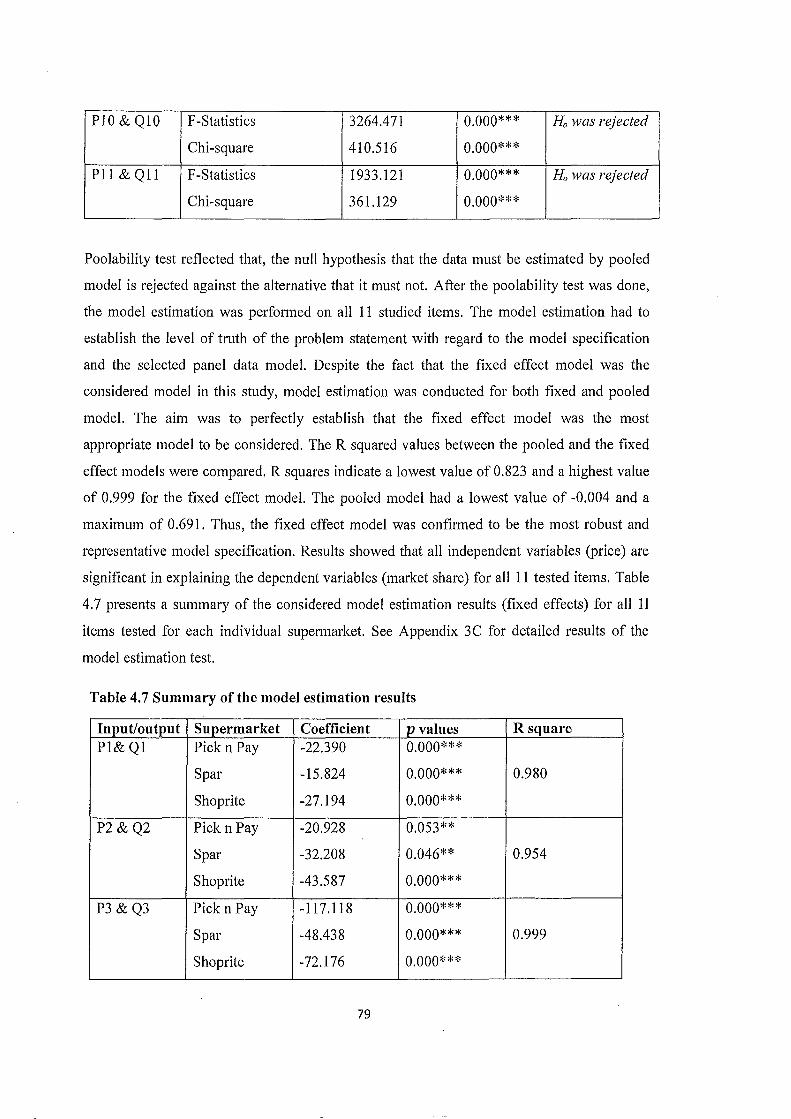
P10 & Q10 F -Statistics 3264.471 0.000*** Ho was rejected
Chi-square 410.516 0.000***
Pll & Qll F -Statistics 1933.121 0.000*** Ho was rejected
Chi-square 361.129 0.000***
Poolability test reflected that, the null hypothesis that the data must be estimated by pooled
model is rejected against the alternative that it must not. After the poolability test was done,
the model estimation was performed on all 11 studied items. The model estimation had to
establish the level of truth of the problem statement with regard to the model specification
and the selected panel data model. Despite the fact that the fixed effect model was the
considered model in this study, model estimation was conducted for both fixed and pooled
model. The aim was to perfectly establish that the fixed effect model was the most
appropriate model to be considered. The R squared values between the pooled and the fixed
effect models were compared. R squares indicate a lowest value of 0.823 and a highest value
of 0.999 for the fixed effect model. The pooled model had a lowest value of -0.004 and a
maximum of 0.691. Thus, the fixed effect model was confitmed to be the most robust and
representative model specification. Results showed that all independent variables (price) are
significant in explaining the dependent variables (market share) for all 11 tested items. Table
4.7 presents a summary of the considered model estimation results (fixed effects) for all 11
items tested for each individual supermarket. See Appendix 3C for detailed results of the
model estimation test.
Table 4. 7 Summary of the model estimation results
Input/output Supermarket Coefficient p values R square P1&Ql Pick n Pay -22.390 0.000***
Spar -15.824 0.000*** 0.980
Shoprite -27.194 0.000***
P2&Q2 PicknPay -20.928 0.053**
Spar -32.208 0.046** 0.954
Shop rite -43.587 0.000***
P3 &Q3 Pick n Pay -117.118 0.000***
Spar -48.438 0.000*** 0.999
Shoprite -72.176 0.000***
79
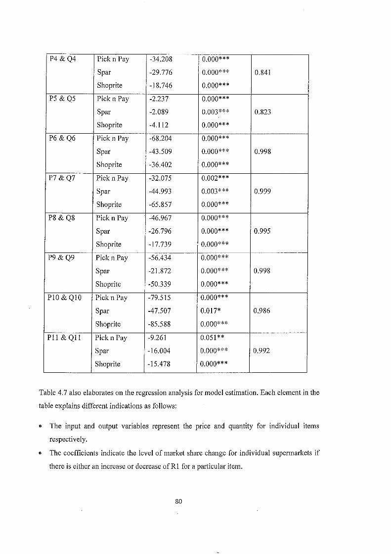
P4&Q4 Pickn Pay -34.208 0.000***
Spar . -29.776 0.000*** 0.841
Shoprite -18.746 0.000***
P5 &Q5 Pick n Pay -2.237 0.000***
Spar -2.089 0.003*** 0.823
Shoprite -4.112 0.000***
P6 &Q6 Pick n Pay -68.204 0.000***
Spar -43.509 0.000*** 0.998
Shoprite -36.402 0.000***
P7 &Q7 Pick n Pay -32.075 0.002***
Spar -44.993 0.003*** 0.999
Shoprite -65.857 0.000***
P8&Q8 Pick n Pay -46.967 0.000***
Spar -26.796 0.000*** 0.995
Shoprite -17.739 0.000***
P9&Q9 Pick n Pay -56.434 0.000***
Spar -21.872 0.000*** 0.998
Shoprite -50.339 0.000***
P10 & Q10 Pick n Pay -79.515 0.000***
Spar -47.507 0.017* 0.986
Shoprite -85.588 0.000***
P11 & Qll Pick n Pay -9.261 0.051**
Spar -16.004 0.000*** 0.992
Shoprite -15.478 0.000***
Table 4.7 also elaborates on the regression analysis for model estimation. Each element in the
table explains different indications as follows:
• The input and output variables represent the price and quantity for individual items
respectively.
• The coefficients indicate the level of market share change for individual supermarkets if
there is either an increase or decrease of R1 for a particular item.
80

• The p values as earlier indicated represents the level of probability of whether the null
hypothesis or alternative hypothesis is true.
• The adjusted R squares indicate the percentage level at which the dependent variable was
explained by the independent variable.
To further elaborate on the interpretation of table 4.7, if taking into consideration input and
output variable (P 1 & Q 1) for instance, the coefficient indicates that a R1 increase in the
price for White Star maize meal (5kg) by any of the sampled supermarkets against
competitors, sales will decrease by 22, 15 and 27 units for Pick n Pay, Spar and Shoprite
respectively. Likewise a R1 decrease in the price for White Star maize meal (5kg) by any of
the sampled supermarkets against competitors will increase sales by 22, 16 and 27 units for
Pick n Pay, Spar and Shoprite respectively.
The p values of Pick n Pay (0.000), Spar (0.000) and Shoprite (0.000) indicates the level of
significance of the independent variable (price) in explaining the dependent variable (market
share) for sampled supermarkets for White Star maize meal (5 kg) is 0% for Pick n Pay, Spar
and Shoprite. The adjusted R square of 0.980 indicates that 98% of the variation in market
share for sampled supermarkets for White Star maize meal (5kg) is explained by price. This
means that only 2% of the variations in market share for sampled supermarkets are explained
by other determinants excluded from the analysis such as quality and advertising. The same
explanations hold for all other tested items in table 4.7.
4.3.3 Interpretation of normality test results
The normality test was one of the diagnostic tests conducted. The normality test was aimed at
measuring if regression residuals are normally distributed. The null hypothesis proves that the
residuals are normally distributed while the alternative hypothesis holds that residuals are not
normally distributed. For the null hypothesis to be accepted, the p value has to be 2::0.05. If
the p value is < 0.05, then the null hypothesis is rejected and the alternative hypothesis
accepted. The normality test was done between the dependent variable (turn-over) and the
independent variable (price) for each individual item (11 items) per supermarket. See
Appendix 3D for detailed result of the normality test for all sampled supermarkets. Table 4.8,
4.9 and 4.10 reflect the outcome of the normality tests for individual supermarket.
81
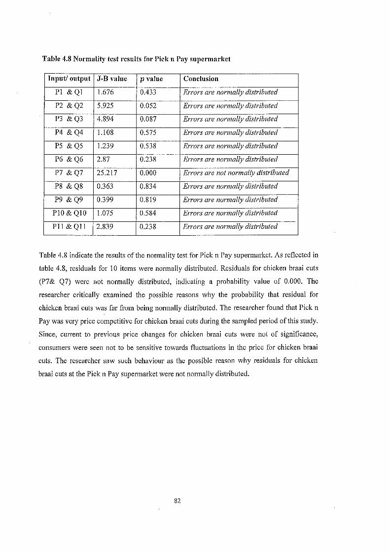
Table 4.8 Normality test results for Pick n Pay supermarket
Input/ output J-B value p value Conclusion
P1 & Q1 1.676 0.433 Errors are normally distributed
P2 &Q2 5.925 0.052 Errors are normally distributed
P3 &Q3 4.894 0.087 Errors are normally distributed
P4 &Q4 1.108 0.575 Errors are normally distributed
P5 &Q5 1.239 0.538 Errors are normally distributed
P6 &Q6 2.87 0.238 Errors are normally distributed
P7 &Q7 25.217 0.000 Errors are not normally distributed
P8 &Q8 0.363 0.834 Errors are normally distributed
P9 &Q9 0.399 0.819 Errors are normally distributed
P10 & Q10 1.075 0.584 Errors are normally distributed
Pll & Qll 2.839 0.238 Errors are normally distributed
Table 4.8 indicate the results of the normality test for Pick n Pay supermarket. As reflected in
table 4.8, residuals for 10 items were normally distributed. Residuals for chicken braai cuts
(P7& Q7) were not normally distributed, indicating a probability value of 0.000. The
researcher critically examined the possible reasons why the probability that residual for
chicken braai cuts was far from being normally distributed. The researcher found that Pick n
Pay was very price competitive for chicken braai cuts during the sampled period of this study.
Since, cu!Tent to previous price changes for chicken braai cuts were not of significance,
consumers were seen not to be sensitive towards fluctuations in the price for chicken braai
cuts. The researcher saw such behaviour as the possible reason why residuals for chicken
braai cuts at the Pick n Pay supermarket were not normally distributed.
82

Table 4.9 Normality test results for Spar supermarket
Input/ output J-B value p value Conclusion
Pl & Q1 1.421 0.491 Errors are normally distributed
P2 &Q2 2.921 0.233 Errors are normally distributed
P3 &Q3 2.711 0.258 Errors are normally distributed
P4 &Q4 7.568 0.023 Errors are not normally distributed
P5 &Q5 0.297 0.862 Errors are normally distributed
P6 &Q6 3.253 0.197 Errors are normally distributed
P7 &Q7 3.158 0.206 Errors are normally distributed
P8 &Q8 6.215 0.045(0.05) Errors were assumed to be normally distributed
P9 &Q9 1.200 0.549 Errors are normally distributed
P10 & Q10 2.079 0.353 Errors are normally distributed
Pll & Qll 2.839 0.242 Errors are normally distributed
As reflected in table 4.9, residuals for 9 items were normally distributed. Golden delicious
apples, (P8 & Q8) was assumed to be normally distributed based on a p value result of 0.045,
converted to 0.05. This is because the rule for the diagnostic test holds that the null
hypothesis should be considered if p-value is 2 0.05. Thus, it can be concluded that errors
were normally distributed for 10 items for the Spar supermarket. However, residuals for Lays
potato chips (P4 & Q4) were not normally distributed with ap value< 0.05.
Table 4.10 Normality test results for Shoprite supermarket
Input/ output J-B value p value Conclusion
P1 & Q1 5.126 0.077 Errors are normally distributed
P2 &Q2 1.093 0.579 Errors are normally distributed
P3 &Q3 0.740 0.691 Errors are normally distributed
P4 &Q4 0.752 0.687 Errors are normally distributed
P5 &Q5 1.347 0.510 Errors are normally distributed
P6 &Q6 1.749 0.417 Errors are normally distributed
P7 &Q7 4.409 0.110 Errors are normally distributed
P8 &Q8 2.094 0.351 Errors are normally distributed
P9 &Q9 0.769 0.681 Errors are normally distributed
83

P10 & Q10 3.535 0.171 Errors are normally distributed
P11&Qll 1.854 0.396 Errors are normally distributed
As reflected in table 4.1 0, residuals for all 11 items were normally distributed with a p value
> 0.05.
4.3.4 Results and interpretation for serial correlation test
A serial correlation test was done between the residuals for the dependent variable and the
residuals for the independent variable for each individual item (11 items) per supermarket.
For the serial correlation test, the null hypothesis holds that residuals are not serially
correlated. On the other hand, the alternative hypothesis confirms that residuals are serially
correlated. Just like the normality test, in order not to reject the null hypothesis, the p value
has to be ;::: 0.05. If the p value is< 0.05, then the null hypothesis is to be rejected. It should
be noted that the test for serial correlation using the Correllogram Q-Statistics usually
involves more than one lag. In this study serial correlation was estimated for first lags. The
serial correlation test was estimated at first difference of analysed item data. See Appendix
3D for detailed serial correlation results. Tables 4.11,4.12 and 4.13 reflect the outcome of the
serial correlation test for individual items for Pick n Pay, Spar and Shoprite supermarkets
respectively.
Table 4.11 Serial correlation results for Pick n Pay supermarket
Input & p value p value p value p value p value output for lag for lag for lag for lag for lag Conclusion
1 2 3 4 5 P1 & Q1 0.419 0.336 0.282 0.431 0.428 No serial correlation detected P2&Q2 0.091 0.201 0.360 0.155 0.140 No serial correlation detected P3 &Q3 0.242 0.217 0.108 0.192 0.288 No serial correlation detected P4&Q4 0.113 0.283 0.452 0.304 0.414 No serial correlation detected P5 &Q5 0.055 0.116 0.199 0.325 0.294 No serial correlation detected P6&Q6 0.972 0.684 .0.342 0.489 0.520 No serial correlation detected P7 &Q7 0.688 0.808 0.934 0.978 0.993 No serial correlation detected P8 &Q8 0.226 0.295 0.444 0.611 0.701 No serial correlation detected P9&Q9 0.939 0.929 0.984 0.623 0.717 No serial correlation detected P10 & Q10 0.058 0.081 0.063 0.120 0.059 No serial correlation detected P11 & Qll 0.401 0.697 0.853 0.882 0.877 No serial correlation detected
Results reflected in table 4.11 indicate that there is no serial correlation in the regression
results for all 11 items for the Pick n Pay supermarket. 84

Table 4.12 Serial correlation results for Spar supermarket
Input & p value p value p value p value p value output for lag for lag for lag for lag for lag Conclusion
1 2 3 4 5 P1 & Q1 0.407 0.472 0.677 0.798 0.783 No serial correlation detected P2&Q2 0.412 0.611 0.739 0.820 0.669 No serial correlation detected P3 &Q3 0.478 0.182 0.297 0.358 0.486 No serial correlation detected P4&Q4 0.546 0.661 0.647 0.738 0.818 No serial correlation detected P5 &Q5 0.731 0.905 0.968 0.751 0.860 No serial correlation detected P6&Q6 0.754 0.504 0.458 0.533 0.677 No serial correlation detected P7 &Q7 0.396 0.660 0.161 0.236 0.353 No serial correlation detected P8 &Q8 0.809 0.572 0.729 0.752 0.845 No serial correlation detected P9&Q9 0.070 0.182 0.145 0.118 0.068 No serial correlation detected P10 & Q10 0.337 0.455 0.616 0.668 0.681 No serial correlation detected Pll & Qll 0.336 0.459 0.068 0.067 0.118 No serial correlation detected
Similar to Pick n Pay, results in table 4.12 (Spar supermarket) indicate that there was no trace
of a serial correlation in the regression results for all 11 items for the Spar supermarket since
all p values were;:::: 0.05. Hence, the null hypothesis which assumes no presence of a serial
correlation was accepted for all items.
Table 4.13 Serial correlation results for Shoprite supermarket
Input & p value p value p value p value p value output for lag for lag for lag for lag for lag Conclusion
1 2 3 4 5 P1 &Q1 0.952 0.081 0.165 0.227 0.081 No serial correlation detected P2&Q2 0.495 0.779 0.714 0.718 0.814 No serial correlation detected P3 &Q3 0.703 0.871 0.861 0.929 0.967 No serial correlation detected P4&Q4 0.089 0.079 0.074 0.081 0.063 No serial correlation detected P5 &Q5 0.579 0.501 0.462 0.585 0.635 No serial correlation detected P6&Q6 0.908 0.955 0.944 0.073 0.111 No serial correlation detected P7 &Q7 0.312 0.569 0.137 0.231 0.290 No serial correlation detected P8 &Q8 0.054 0.058 0.110 0.110 0.069 No serial correlation detected P9&Q9 0.266 0.510 0.370 0.067 0.053 No serial correlation detected P10 & Q10 0.455 0.756 0.895 0.945 0.965 No serial correlation detected Pll &Ql1 0.291 0.501 0.284 0.214 0.148 No serial correlation detected
Results in table 4.13 indicate the absence of a serial correlation in the regression results for
al111 tested items at Shoprite. This reflects an acceptance of the null hypothesis.
85

4.3.5 Results and interpretation for heteroscedasticity
The heteroscedasticity test was aimed at determining if any form of heterogeneity exists with
the regressions disturbance in the model estimation outcomes for all 11 items tested. If
heteroscedasticity exists, the null hypothesis, H0 , which assumes that residuals/disturbances
are homoscedastic, is rejected. The White's cross section was used to remedy the
heteroscedasticity. Hence, the researcher concluded that no heteroscedasticity existed since
results from the model estimation were all homoskedastic.
4.3.6 Forecasting of model estimation
Forecasting was done for each individual regression of the model estimation. Hadavandi et
a!. (20 11) indicate that it is important to forecast each individual cross section in a panel data
analysis, because the effect of the identified problem varies across each cross section. Baltagi
(2006:20) further maintained forecasting for more than one cross section as accurate, only
through the fixed effect model. This has been proven in other panel data studies like that of
Lee (2009). Forecasting was done in this study to show how accurate were regression models
in predicting the value of quantity demanded.
Forecasting results is represented in appendix 3.F. The blue and the red line reflect the actual
versus the fitted values. The first, second and third relationships in the figures represent Pick
n Pay, Spar and Shoprite supermarkets respectively. With regards to the outcome from
forecasting, the model of this study was concluded accurate since the predicted or forecasted
values mimic the actual values. Thus, the model can be used for forecasting future quantity
demand for a specified price for a product.
4.4 CONCLUSION
In this chapter, the analysis and interpretation of results were presented and displayed.
Results from unit root tests, poolability tests, model estimations, normality tests, serial
correlation and heteroscedasticity tests were all reported. The next chapter provides
recommendations which include a proposed pricing decision support system (figure 5.1) and
conclusions with regard to the findings of the empirical research and the literature study.
86
CHAPTERS
RECOMMENDATIONS AND CONCLUSIONS
5.1 INTRODUCTION
The study sought to increase awareness on the impact of pricing regarding market share gain
or loss for FMCG retailers in the Ngaka Modiri Molema district. The three largest district
supermarkets, Pick n Pick, Spar and Shoprite were the participants in this study. This chapter
discusses the summary of chapters, findings in this study, recommendations and conclusion.
5.2 SUMMARY OF THE STUDY
Chapter one presented a general introduction and background of the study. In the
introduction, a brief discussion was done on the current continuous changes in prices of
commodities and how it affects consumer purchases. The research motivation which was
based on limited research in the pricing discipline was also outlined. A background of the
study area was also indicated. A initial literature study was also done. The literature study
was based on the marketing mix elements, pricing as a key marketing mix element and the
role of pricing in influencing market share. The problem statement was examined with
respect to results from other studies and the situation in Ngaka Modiri district. Chapter one
also presented the research objectives, research questions, methods and design, data analysis
techniques, limitations and general organisation of the study.
Chapter two presented the review of literature relevant to the study. The theoretical
framework which underpinned the study were discussed and focused on the marketing and
marketing mix elements, the pricing decision-making process under which different pricing
methods, strategies and policies were discussed. Other internal and external elements
influencing pricing decisions and unethical pricing decisions were also presented. The
influence of the price indices as the main determinant of pricing was elaborated with the aid
of the time change Le'vy model. Finally, the relationship between price and market share,
and the advantages of being a market share dominant were discussed.
Chapter three presented the research design and strategy of the empirical study. The study
made use of a quantitative design and an exploratory strategy. The target population,
sampling type and criteria as well as the data sourcing process were theorised and discussed.
The description of variables used, model specification and modification to the context of the
87

study were also discussed. Chapter three also discussed how the analytical techniques were
applied and elaborates on the ethical considerations of the study.
Chapter four focused on data analysis, interpretation and presentation of findings from the
empirical research. Results from linear regressions were all interpreted and presented in this
chapter. Linear regression results were reported for the unit root, poolability and diagnostic
tests. Chapter five presents the research findings, based on the relevancy to the research
objectives. Chapter five also proposes recommendations and a general conclusion with
respect to the research findings.
5.3 DISCUSSION OF RESEARCH FINDINGS
Considering that only secondary sources of data were used in this study, the research
objectives were used in determining the findings from the empirical investigation. The
research objectives were:
• To examine the impact of pricing on the market share of the largest three grocery retailers
in the Ngaka Modiri Molema district.
• To investigate the type of pricing decisions made by the largest three grocery retailers in
the Ngaka Modiri Molema district.
• To examine the challenges faced by these supermarkets in making pricing decisions.
• To determine the influence of these pricing decisions, their consumers' behaviour and
market share performance.
• To determine the importance of market share for the Ngaka Modiri Molema grocery
supermarkets.
• To recommend possible pricing decision majors that could be use by the Ngaka Modiri
Molema retailers to gain market share.
5.3.1 Research objective 1
The research objective was aimed at examining the impact of pricing on the market share of
the largest three grocery retailers in the Ngaka Modiri Molema district.
Pricing plays a major role in market share gain or loss among supermarkets in the Ngaka
Modiri Molema district. All three sampled supermarkets in this study tested positive that
pricing is the major determinant for market share. Results from the regression analysis
indicated that a Rl,OO increase or decrease in the price of a product by a supermarket will
88

also lead to an increase or decrease in the market share of that product. Thus, the findings
revealed that the higher the market share of a supermarket in a particular product, the more
moderate was its price compared to its competitors. This meant the model assumption of this
study MSVu= flo+ (31~1 + &u formula (3.2), that price plays a major role in influencing the
market share ofNgaka Modiri grocery retailers was positive. However, findings also revealed
that there is heterogeneity in the relationship between price and market share among the
sampled supermarket brands. In other words, pricing decisions are customised for each
sampled supermarket. Thus, the influence of price on the market share was seen to be unique
for each sampled supermarkets.
5.3.2 Research objective 2
Objective two was aimed at investigating the type of pricing decisions made by the three
largest grocery retailers in the Ngaka Modiri Molema district.
Without observing scanner data from the sampled supermarket stores, it might be tempting to
conclude that all pricing decisions are determined at head office level. It was discovered that
supermarket stores also contribute in deciding the final price to consumers. Individual stores
are allowed the right to increase or decrease price within a minimum and maximum price set
by the head office. The findings pointed out that the sampled supermarkets operate on pricing
methods such as competitive-based pricing and customer-based and pricing policies such as
product pricing and promotional pricing.
• Competitive pricing
The findings indicated that pricing decisions for supermarket brands were strongly associated
with all. dimensions of competitors' pricing decisions. Based on results Pick n Pay and
Shoprite supermarkets were mainly seen to rival each other in pricing for all tested items in
this study.
• Customer-based
Analysed data also suggest that supermarkets were also making a pricing decision based on
the characteristics of their target market. If regression results and data for the Spar
supermarket are evaluated, outcomes reveal that pricing decision for Spar supermarket were
mainly done based on its customers rather than competitive action. Spar supermarket was
89
seen to practice less competitive pricing compared to Shoprite and Pick n Pay. This could be
as a result of loyal customers who perceive Spar to be the most efficient supermarket.
• Product pricing
Findings highlight that supermarket pricing decisions were based on the elasticity of
products. Supermarkets were seen to be very cautious in setting prices for elastic products
such as White Star, Tastic rice and Chicken braai cuts. This is because these products had
substitutes that consumers could tend to with regards to increase in price. Alternatively, less
attention was put on others such as Stuyvesant cigarettes with an inelastic demand.
• Loss leader pricing
Results also reveal that retailers implemented a temporary pricing system. Prices were kept
very low for a particular product for a particular period. The aim of such pricing is to create
excitement among consumers and consequently an increase in market share for this product
for a short-term.
5.3.3 Research objective 3
This objective set out to examine the challenges faced by sampled supermarkets in making
pricing decisions.
Primary pricing challenges include the following: Emerging growth of other grocery sectors
and insufficient data support systems. Market conditions were seen to be a major challenge
for supermarkets in making pricing decisions.
• Emerging growth of the informal grocery sector
If critically examined, it is evident from the data that the prices of tested items of sampled
supermarkets are strongly competing with those in other grocery sectors. A good example is
the informal home-based retail grocery stores known as Spaza shops. According to Charman
et al. (2012:49), recent continuous change of the Spaza retail sector, from survivalism to
entrepreneurial mode it is becoming a site for fierce price competition with supermarkets in
the Ngaka Modiri Molema district.
• Insufficient data information
Another issue that was experience as a challenge to supermarkets pricing decision, was the
lack of reliable stored data information for future decision making. For instance, the
90
researcher originally had a list of 20 items that were to be tested for regression relationship.
The researcher ended up with a list of 11 items as a result of insufficient data from 9 items.
These mentioned items were then removed from the study. Existing price information can
contribute to the analysing of consumer behaviour and also tracking complex mechanics of
inter-store competition. This tendency also serves as motivation for record keeping of pricing
decisions over time.
e Current market conditions and managerial skills
The sharp depreciation of the rand against all major currencies in the world is a major
challenge for South African retailers in general. This crisis creates a major challenge for
pricing decisions for all three supermarket stores in this study. Shama (2006:43) indicates that
price is the most important element that consumers consider during volatile economic
periods. Radical pricing decisions became necessary for survival in these extreme economic
fluctuations. Delatolas and Jacobson (2012:2-3) states that most often, such decisions are not
appropriately made due to lack of managerial experience in the pricing discipline.
5.3.4 Research objective 4
Objective four was aimed at determining the influence of implemented pricing decisions by
supermarkets on their consumers' behaviour and market share pe1jormance.
Findings from the regression results revealed that consumers measure price transparency
among retailers in order to make a purchase decision. Results reflect that a supermarket with
the most moderate pricing for a certain product has the highest market share for that product.
It was evident, based on the data that an increase in price will affect consumers' behaviour
negatively and consequently, loss in market share. Likewise, a decrease in the price of a
product will affect consumers' behaviour positively and consequently gain market share.
Austin and Gravelle (2008:1) say consumers are very conscious of any change in price by a
retailer, and this will affect their purchase decision. Thus, it can be concluded that the general
Ngaka Modiri Molema consumer is very aware of price settings and changes by supermarket
management with high knowledge levels of unacceptable pricing.
5.3.5 Research objective 5
The fifth objective was aimed at determining the importance of market share for Ngaka
Modiri grocery supermarkets.
91

The fifth objective was to determine the importance of market share for Ngaka Modiri
Molema grocery supermarkets. The findings from results revealed that market share
domination is very important for supermarkets in the Ngaka Modiri Molema district.
Outcome from data analyses indicate that, extensive price wars were initiated by
supermarkets for products in which they had a dominant share of the market. Gehrig et a!.
(2009) argue that retailers with a dominant market share in a product, use aggressive price
offers to destroy even already existing customer relationships between its competitors and
their consumers. Bode and Scharafi (2007) state that it is impmiant to have a strong market
share position in the market because organisations with a better market share have an edge
over their competitors in formulating or executing business strategies. Extensive price wars
were initiated by supermarkets for products in which they had a dominant share of the
market.
5.4 GENERAL CONCLUSIONS
The general conclusions drawn from the empirical research are based on results from the
regression analysis. A conclusion can be drawn that price plays a major role in the gain or
loss of market share among FMCG retailers in the Ngaka Modiri Molema district. However,
there are differences (heterogeneities) in the manner in which pricing will impact on the
market share of individual retailers. Results from the empirical research of the three sampled
supermarkets in this study tested positive for these findings. This means the model
specification and the considered panel data model were accurate with regard to the identified
problem of the study. Hence, the main objective of this study to find whether price plays a
role in influencing the market share gain or loss was positive. However questions can be
raised on the influence of other determinants of market share in the Ngaka Modiri Molema
FMCG sector. Thus, it should be noted that even though this study was aimed at the role of
price, it did not reject the influence of other determinants of market share gain or loss among
Ngaka Modiri Molema retailers.
Thus, critics can argue the effectiveness of the role of price in influencing market share if
other determinants (error term) such as distribution are not taken into full consideration in the
model specification of this study. However, the use of the panel data analysis technique
helped in arriving at a solution to such criticisms. Regression results from the model
estimation gave an indication of all product purchases that were not influenced by price but
by other determinants over the study period. Results of purchases not influenced by price are
92
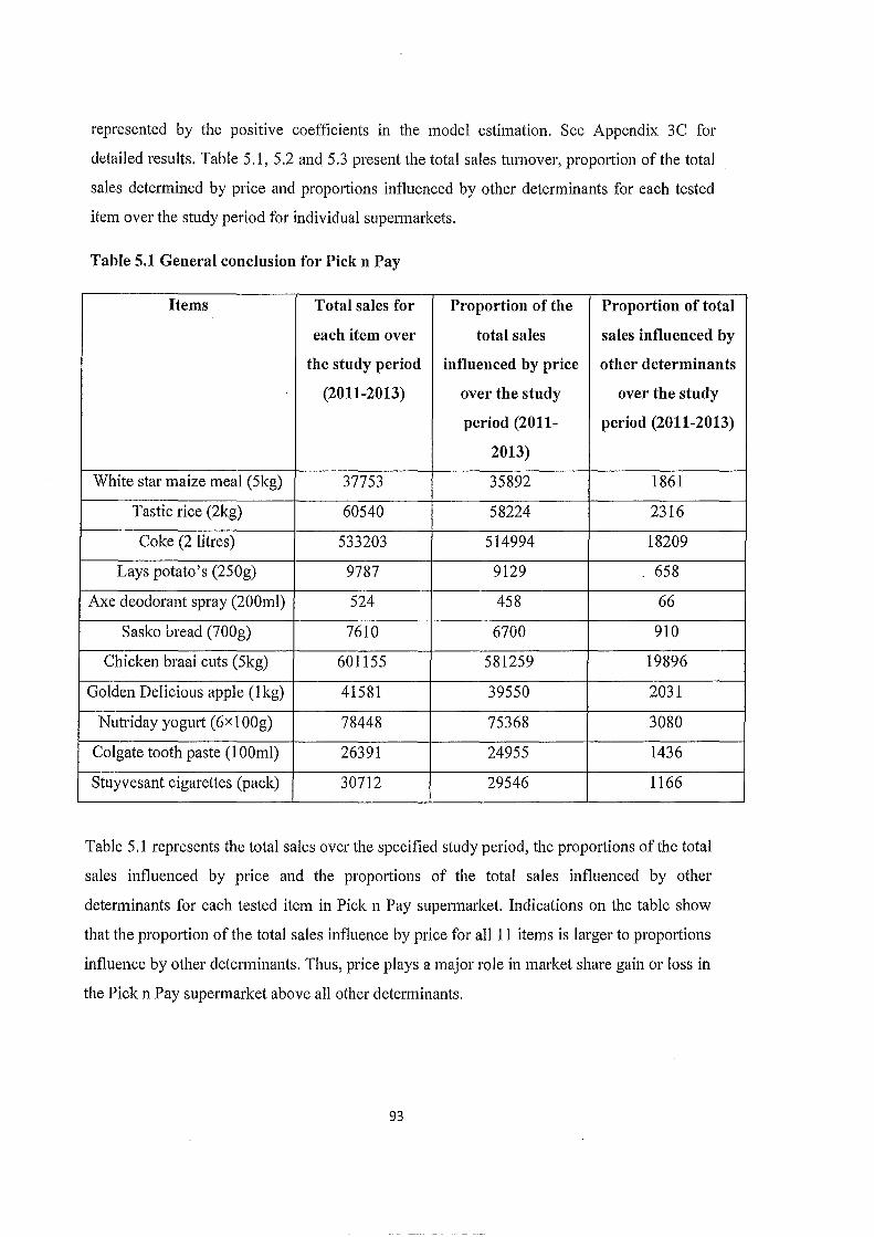
represented by the positive coefficients in the model estimation. See Appendix 3C for
detailed results. Table 5.1, 5.2 and 5.3 present the total sales turnover, proportion of the total
sales determined by price and propmiions influenced by other determinants for each tested
item over the study period for individual supermarkets.
Table 5.1 General conclusion for Pick n Pay
Items Total sales for Proportion of the Proportion of total
each item over total sales sales influenced by
the study period influenced by price other determinants
(2011-2013) over the study over the study
period (2011- period (2011-2013)
2013)
White star maize meal (5kg) 37753 35892 1861
Tastic rice (2kg) 60540 58224 2316
Coke (2 litres) 533203 514994 18209
Lays potato's (250g) 9787 9129 658
Axe deodorant spray (200ml) 524 458 66
Sasko bread (700g) 7610 6700 910
Chicken braai cuts (5kg) 601155 581259 19896
Golden Delicious apple (1kg) 41581 39550 2031
Nutriday yogmi (6x100g) 78448 75368 3080
Colgate tooth paste (1 OOml) 26391 24955 1436
Stuyvesant cigarettes (pack) 30712 29546 1166
Table 5.1 represents the total sales over the specified study period, the proportions of the total
sales influenced by price and the proportions of the total sales influenced by other
determinants for each tested item in Pick n Pay supermarket. Indications on the table show
that the proportion of the total sales influence by price for all 11 items is larger to proportions
influence by other determinants. Thus, price plays a major role in market share gain or loss in
the Pick n Pay supermarket above all other determinants.
93

Table 5.2 General conclusion for Spar
Items Total sales for Proportion of the Proportion of total
each item total sales influenced sales influenced by
over the study by price over the other determinants
period study period (2011- over the study period
(2011-2013) 2013) (2011-2013)
White star maize meal (Skg) 2000 1382 618
Tastic rice (2kg) 41438 39511 1927
Coke (2 litres) 62506 59315 3191
Lays potato's (250g) 8198 7627 571
Axe deodorant spray (200ml) 247 190 57
Sasko bread (700g) 5054 4525 529
Chicken braai cuts ( 5kg) 23887 21554 2333
Golden delicious apple (lkg) 10452 9745 707
Nutriday yogurt (6xlOOg) 14998 14262 736
Colgate tooth paste (1 OOml) 15059 14222 837
Stuyvesant cigarettes (pack) 77666 77010 656
Table 5.2 represents the total sales over the specified study period, the proportions of the total
sales influenced by price and the proportions of the total sales influenced by other
determinants for each tested item in Spar supermarket. Indications on the table show that the
proportion of the total sales influence by price for all 11 items is larger to proportions
influence by other determinants. Thus, price plays a major role in market share gain or loss in
the Spar supermarket above all other determinants.
94
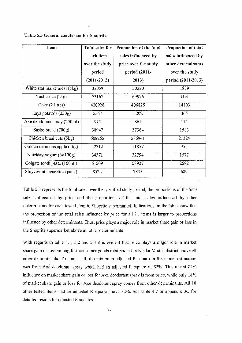
Table 5.3 General conclusion for Shoprite
Items Total sales for Proportion of the total Proportion of total
each item sales influenced by sales influenced by
over the study price over the study other determinants
period period (2011- over the study
(2011-2013) 2013) period (2011-2013)
White star maize meal (5kg) 32059 30220 1839
Tastic rice (2kg) 73167 69976 3191
Coke (2 litres) 420928 406825 14103
Lays potato's (250g) 5567 5202 365
Axe deodorant spray (200ml) 975 861 114
Sasko bread (700g) 38947 37364 1583
Chicken braai cuts (5kg) 608265 586941 21324
Golden delicious apple (1kg) 12312 11857 455
Nutriday yogurt (6x100g) 34371 32794 1577
Colgate tooth paste (1 OOml) 61509 58927 2582
Stuyvesant cigarettes (pack) 8524 7835 689
Table 5.3 represents the total sales over the specified study period, the proportions of the total
sales influenced by price and the proportions of the total sales influenced by other
determinants for each tested item in Shoprite supermarket. Indications on the table show that ·
the proportion of the total sales influence by price for all 11 items is larger to proportions
influence by other determinants. Thus, price plays a major role in market share gain or loss in
the Shoprite supermarket above all other determinants
With regards to table 5.1, 5.2 and 5.3 it is evident that price plays a major role in market
share gain or loss among fast consumer goods retailers in the Ngaka Modiri district above all
other determinants. To sum it all, the minimum adjusted R square in the model estimation
was from Axe deodorant spray which had an adjusted R square of 82%. This meant 82%
influence on market share gain or loss for Axe deodorant spray is from price, while only 18%
of market share gain or loss for Axe deodorant spray comes from other determinants. All 10
other tested items had an adjusted R square above 82%. See table 4.7 or appendix 3C for
detailed results for adjusted R squares.
95

5.5 RECOMMENDATIONS
The researcher suggests that FMCG retailers in the Ngaka Modiri Molema should consider
implementing the following recommendations to solve the identified problem of this study.
5.5.1 Recommendation with regard to objective 1 (impact of pricing on the market share).
Empirical findings indicate that pricing is a pivotal component for market share gain or loss
amongst FMCG retailers in the Ngaka Modiri Molema district. Thus, it is important that the
marketing strategy of retailers should carefully outline pricing implementation plans. Pricing
implementation plans should consider income levels of different target segments in the target
population within the target market in order to build consumer loyalty and consequent
increase in market share.
5.5.2 Recommendation with regard to objective 2 (pricing decisions made by grocery
retailers).
Retailers should develop pricing strategies that will fit the financial abilities of their targeted
segments. Implementing pricing strategies such as the loss leader is not advisable. Loss
leader may lead to unfavourable outcomes such as price wars. In such time consumers
develop the tendency of waiting for the next price promotion in order to make a purchase.
5.5.3 Recommendation with regard to objective 3 (challenges faced by sampled
supermarkets in making pricing decisions).
• Competitive pricing is always a factor in every industry. Retailers should monitor the
pricing action of its competitors and competitive action should be reviewed regularly.
• Making appropriate pricing decisions requires the existence of relevant and factual
pricing data. Track records of previous pricing decisions should be available to serve as
basis for future pricing decision making by retailers. Supermarket management should
implement relevant training programmes to assist supermarket employees in managing
price information. Supermarkets should adopt an effective communication approach
between the head office and supermarket stores.
• Supermarkets should adopt an effective communication approach between the head office
and supermarket stores. This will enable the formulation of pricing decisions that will be
mindful of both short-term and long-term price unce1iainties in the market.
96
5.5.4 Recommendation with regard to objective 4 (the influence of implemented
supermarket pricing decisions on consumers' behaviour and market share pe1jormance).
Retailers in the Ngaka Modiri Molema district should consider pricing decisions based on the
price related behaviour of the target consumers. Consumers are in general very price
sensitive, and should be taken into consideration by retailers when determining prices.
Retailers may also develop the Every-Day-Low Pricing (EDLP) strategy that involves
consistent temporary price cuts for all product categories in the store. This strategy has been
recommended for developing excellent consumer loyalty by marketers in general. The
strategy also makes consumers less price sensitive even in cases of major increases in prices.
5.5.5 Recommendations with regard to objectives 5 (the importance of market share for
Ngaka Modiri Molema grocery supermarkets).
Empirical results revealed that market share is important for FMCG retailers to attain
competitive advantage against rivals. Indications from results show that a supermarket that
had a dominant market share for a product did launch an intensive price war against its
competitors. Thus, it is important that retailers give more attention to pricing in order to
increase market share and possibly become a market share dominant against rivals.
5.5.6 Recommendations with regard to objectives 6 (proposing a pricing decision support
system that could be use by the Ngaka Modiri Molema retailers to gain market share).
Based on the findings and literature, a relevant and practical applicable pricing guideline
structure is recommended for use by retailers when determining product prices. This
suggested guideline structure is based and adopted from a model developed by Kehagias and
Skourtis (2009) represented on figure (2.4) on page 24. The suggested guideline structure,
applicable to this study is presented in Figure 5 .1.
97

Internal determinants
• Supermarkets pricing capabilities
• Supermarket's pricing philosophy
• Managerial pricing skills
• Price elasticity of a supermarket's
products
• Price coordination
• Price deals from manufacturers
External determinants
• Market conditions
o Consumer price index
o Economic crisis
• Price competition and promotion
o Competitor deal frequency
o Price deal durations
11 Product category
o Substitutes of product
o Product necessity
• Consumer factor
o Price sensitivity of consumers
o Cross-price sensitivity
Product category Pricing strategy/policy Main pricing objective II Convenience product Increase price/ II m The pricing decision II
II Shopping product high price made should lead to II Speciality product II Decrease 111 price/ market share gain • Preferential product low price
Figure 5.1 Pricing decision support system for Ngaka Modiri retailers
Adopted from (Kehagias & Skourtis 2009)
This framework assumes that pricing dimensions and pricing determinants are strongly
connected. Hence, it is important that Ngaka Modiri Molema FMCG retailers should
simultaneously consider both pricing dimensions and pricing determinants in developing
pricing decisions. The framework indicates some internal and external factors that Ngaka
Modiri Molema retailers should consider when making pricing decisions. The framework
further suggested that a pricing decision for any product category in the FMCG industry will
involve either an increase or decrease in price. However, whatever pricing decision a retailer
selects, the objective should be towards market share gain.
98

5.5.6.1 Requirements for the framework application
In order to apply this framework, the following are required:
• Availability of actual and applicable data on pricing information.
• Skilful managers with effective ability in transforming pricing information into decision
models. The success of a framework usually depends on the interactive ability of users of
the framework.
111 Access to technological software that can permit estimations of variables. Software
should be flexible enough to accept future adjustments in the case of unforeseen events.
5.5.6.2 Steps for estimating the framework
The following steps are required for the analysis of variables in the framework:
111 Set pricing objectives aimed at market share gain.
• Creating a formula with respect to considered pricing parameters as a function of market
share.
• Testing the hypotheses.
111 Transmitting results from hypotheses testing to pricing decisions.
111 Implementing the pricing decisions and also making sure prices on shelves reflect results
from analysis.
5.5.6.3 Advantages of the proposed framework
111 It will enable fast consumer goods retailers in the Ngaka Modiri Molema district to select
the most appropriate pricing strategies and policies for their target market.
• It fits accurately in the Ngaka Modiri Molema fast consumer goods retail sector. Its
implementation is straight and forward and easy to understand.
99
5.5.6.4 Drawbacks of the proposed framework
• There might be issues of limited information with respect to new products and actions of
competitors. However, it is important to have a contingency plan for handling such
shortcomings.
• The application of the model may not permit accurate price decision making in different
industries.
• Most fast consumer goods retailers in the Nkaga Modiri Molema district may lack
analytical abilities in handling most dynamics in the model. However, skills can be
improved through training programmes.
5.6 CONCLUSION
The problem identified in this study was the lack of awareness among retailers in the Ngaka
Modiri Molema district on the role of price in market share gain or loss. Thus, the main aim
of this study was to increase the level of awareness of the influence of price on market share
gain or loss among Ngaka Modiri Molema retailers. After conducting an empirical research
through a panel data analysis on the three largest supermarkets in the Ngaka Modiri Molema
district, results reflect that price plays a major role in market share gain or loss among
retailers in the Ngaka Modiri Molema district in general. The researcher recommends that
retailers should dedicate more attention on pricing in order to increase their market share.
Lastly, the researcher saw the need to create a framework that could also assist Ngaka Modiri
Molema retailers in making effective pricing decisions-by developing a pricing decision
support system. It is hoped that the findings of this study will encourage retailers to take
pricing seriously and will also implement the propose pricing decision support system in
making more appropriate and effective pricing decisions in order to improve their market
shares.
100

REFERENCES
Adcock, D., Halborg, A. & Ross, C. 2001. Marketing principles and practice. 41hed. London:
Pearson Educational Limited.
Ahmetoglu, G., Dawes, J. & Furnham, A. 2010. Pricing practices: Their effects on consumer
behaviour and welfare. London: Mountainview Learning Limited.
Ailawadi, K.L., Donald, R.L. & Scott, A.N. 2003. Revenue premium as an outcome measure
of brand equity, Journal of Marketing, ( 67): 1-17.
Alexander, M. 2012. Microsoft Acess 2007: data analysis. Indiana, U.SA: Wiley Blackwell.
Alkali, M. & Is a, A.H. 2012. Assessing the influence of external environmental factors on the
performance of small business manufacturing enterprise in Bauchi state Nigeria.
Interdisciplinary journal of contemporary research in business, 4(7):97-111.
Armstrong, J.S. & Green, K.C. 2007. Competitor-oriented objectives: the myth of market
share. International journal of business, 12(1 ): 116-134.
Asteriou, D. & Hall, S. 2007. Applied econometric: A modern approach using eviews and
Microsoft. New York: Macmillan Palgrave.
Asteriou, D. & Hall, S. 2011. Applied econometric: 2nd ed. New York: Macmillan Palgrave.
Aucremanne, L. & Dhyne, E. 2004. How frequently do price? Evidence based on the micro
data underlying the Belgian CPl. European Central Bank working paper series (no: 331 ).
Austin, A.D. & Gravelle, J.G. 2008. Does pricing transparency improve market efficiency?
Implications of empirical evidence in other markets of the health sector. CRS Report for
Congress.
Avlonitis, G.J., Indounas, K.S. & Gounaris, S.P. 2005. Pricing objectives over the service life
cycle: Some empirical evidence. European journal of marketing, 39 (5/6):696-714.
Avlonitis, G.F. & Indounas, K.A. 2004. Pricing strategy and practice. Impact of market
structure on pricing objectives of service firms. Journal of product and brand management,
13(5):343-358.
101

Axarloglou, K. 2007. Thick market, market competition and pricing dynamics: Evidence
from retailers. Journal of managerial and decision economics, 28(7):669-677.
Babatunde, 0. & Oluntunla, G. 2006. Pricing strategy as a determinant of market share in the
soft drink industry. (A case ofNigerian bottling company).
Babbie, E. 2010. The practice of social research. lih ed. Belmont,U.SA: Cengage learning.
Bafana, M. 2012. Chief executive officer's report. Invest Northwest Annual report 201/2012.
Balakrishnan, R. & Mahanta, V. 2004. Break in the call, brand equity. The economic times
review, August 18 Mumbai.
Balcombe, K. 2009-2010. The nature and determinants of volatility in agriculture prices: An
empirical study from 1962-2008. Commodity market review:l-24.
Ballasy, L. 2004. Marketing for the recruitment of mentors: A work book for finding and
attracting volunteers, Portland: NWP regional educational laboratory.
Baltagi, B.H. 2005. Econometric analysis of panel data. 3rd ed. Chichester: John wiley &
Sons.
Baltagi, B.H. 2008. Econometric analysis of panel data. 4th ed, Chichester: John wiley &
Sons.
Baltagi, B.H. 2009. A companion to econometric analysis of panel data. Chichester: John
wiley & Sons.
Baltagi, B.H. 2006. Deutsche Bundesbank 18th spring conference on "New development in
economic forecasting" in Frankfurt Germany series 1, No:25.
Beletski, T. 2006. Inflation-linked products and optimal investment with macro derivatives.
Kaiserslautern: Kaiserslautern University of Technology. (PHD thesis in mathematics).
Bickman, L. & Rog, D. 2009. The sage handbook of applied social research methods. 2nded.
California: Sage publications.
Blonde, B. & VanDamme, I. 2010. Retail growth and consumer changes in a declining urban
economy: Antwerp. Economic history review, 63(3):638-663.
Blyth, J. 2006. Principles and practice of marketing. London: Thompson Learning.
102

Bode, S. & Scharifi, 0. 2007. Market share and dominant market share position in the case of
emissions trading: An economic analysis based on U.S., European and Japanese competition
law. Carbon and climate law review (2): 103-116.
Bogopane, L.P. 2012. A qualitative assessment of the evaluation and monitoring processes of
the integrated development planning (IDP) in the Ngaka Modiri Molema District-Northwest
province, South Africa. Journal of social science, 32(1):91-100.
Bond, P. & Goldstein, I. 2012. Government intervention and information aggregation by
prices.
Boukhari, E.A., Yabouri, E.M., Ktaibi, E.H. & Naji, J. 2007. International; trade export
costing project: Factors affecting the price of a product.
Briggs, A.R.J. & Coleman, M. 2007. Research Methods in Education Leadership and
Management. 2nd ed. Great Britain: SAGE.
Bruweri, J.P. & Watkins, A. 2010. Sustainability of the fast moving consumer goods retail
SMMEs. African journal of business management, 4(16):3550-3555.
Cameron, S. 2005. Econometrics. Berkshire: McGraw Hill Education.
Cant, M. 2005. Pricing management. 2°ded. Claremont: New African Books (pty) Ltd.
Cant, M., Heerden, C. & Ngambi, H. 2010. Marketing management: A South African
perspective. 1 sted. Cape Town: Juta & CO.
Can·, P. & Wu, L. 2004. Time-Change Le'vy Process and option pricing. Journal of financial
economics, (71):113-141.
Charm an, A., Petersen, L. & Piper, L. 2012. From local survivalism to foreign
entrepreneurship: The transformation of Spaza sector in Delft. Cape town: Transformation
78.
CIM (Chartered Institute of Marketing). 2009. Marketing and the 7p's: A brief summary of
marketing and how it works.
Chopra, S. & Meindl, P. 2010. Supply chain management. Strategy, planning and operation.
4th ed. New Jersey: Pearson.
103
Claessen, S., Kose, M.A. & Terrones, M. E. 2009. What happens during recessions, crunches
and bust? Economic Policy, (60-62):653-700.
Cohen, L., Manion, L. & Marrison, K. 2011. Research Methods In Education. ih ed.
published by Routledge.
Colander, D.C. 2004. Macroeconomics. 51hed. New York: McGraw-Hill.
Constantinides, E. 2006. The marketing mix revisited towards the 21st century. Journal of
marketing management, (22):407-438.
Conway, L.S. & Powell, R.R. 2010. Basic research methods for librarians. California.
Greenwood.
Creswell, J.W. 2009. Research Design. Qualitative, quantitative and mixed methods
approaches. 3rd ed. SAGE Publications ltd.
Creswell, J.W. & Clark, P.V.L. 2007. Designing and Conducting Mixed Methods Research.
Thousand Oaks, CA: SAGE Publications.
De Jagar, N. 2004. The living standard measure as a market segmentation tool for selected
retailers. Potchefstroom. Northwest University. (Dissertation in masters of commerce).
Delatos, A. & Jacobson, C. 2012. Obstacles when implementing a value based pricing
strategy: A case study-Volvo construction equipment. Linnaeus University. (Bachelor degree
in business administration).
Depken, C.A. 2006. Micro~economics: A self-teaching guide. California: McGraw-Hill.
Derby, R. 2013. Recovering market share a big task for Pick n' Pay.
wrvw. bdlive. co.za/opinion /columnists/203/04/24/recovering -market share-a-big-task-for
pick-n-pay. 10p.m, 24 August: 2013.
Dirkie, U. 2012. Success stories. Section One. Invest Northwest Annual report 2010/2011.
Donaldson, B. 2007. Sales management principles, process and practice. 3rd ed. New York:
Palgrave Macmillan.
Dovey, K. & White, R. (2005). Learning about learning in knowledge-intense organizations.
Learnin.Org., 12(3):15.
104
Drew, C.J., Hardman, M.L. & Hosp, J.L. 2008. Designing and Conducting Research
Education: SAGE Publications.
Drummond, G. & Ensor, I. 2005. Introduction to marketing concepts. 1 sted. Burlington:
Elsevier.
Du Plessis, S. & Smith, B. 2007. South African growth revival after 1994. Stellenbosch
Economic working paper.
Dutta, S., Zbaracki, M.J. & Bergen, M. 2003. Pricing process as a capability: A resource
based perspective. Strategic management journal, (24):615-630.
EAUGP (Economic Analysis Unit Gauteng Provinnce). 2012. The retail industry on the rise
m South Africa.Gauteng Provincial Treasury quarterly Treasury bulletin.
www.treasury.gpg.gov.za!..IQBJ%!20 the% 20 Retail% industry %20on.l3 September 2013.
Edmond, A.W. & Kenedy, E.T. 2013. An applied reference guide to research design.
Quantitative, qualitative and mixed method. SAGE.
Egan, I. 2007. Marketing communication. ls1ed. London: Thomson.
Els, J. 2013. New CPI measures increases S.A inflation rate by 0~2% for 2013 real threat
from expensive oil and weak rand.
Emprise, W. 2008. The concept of price in economics. http:llwww.helium.co/items/891170-
the concept-of..price-in-economics [9 march 2013].
Erikson, K. & Simpson, B. 2007. Deception and price m a marker with asymmetric
information. Judgement and decision making, 2(1):23-28.
Ernst & Young. 2004. Global pricing trends. http:/!wtl'w.2.evcom.ch/publicationslitems/rcp
pricingtrends2004-report/en. pdf 15 July 2013.
Esclana, N.S., Diginis, C., Plessis, R., Machado, R., Mpinganjira, M., Mcintee, H., Kloppers,
R. S. & Theron, D. 2012. Introduction to marketing. 41hed. Cape Town: JUTA & Company
Ltd.
Etro, F. 2007. The economics of competition policy and dominant market share position:
Stockholm network experts' series on intellectual property and competition.
105
EI (Euromonitor International). 2012. Grocery retailers m South. http://
www.eurominotor. com/grocerv -retailers-in-south-a{r;calreport. (09 April /20 13).
Evans, B. 2012. International comparison of the formula effect between the CPI and RPI.
Office ofNational Statistics.
Farshid, M.M. & Amir, F. 2012. The influence of marketing strategy elements on market
share of firms. International journal of fundamental psychology and social sciences, 2 (1):19-
24.
Fenwick, D. & Astin, J. 2009. Practical guide to producing consumer price indices. New
York and Geneva: United Nation.
Ferrel, O.C. & Hartline, M.D. 2008. Marketing strategy, 41hed. Natorp Boulevard, U.S.A:
Thamson Learning Inc.
Ferrel, O.C. & Hartline, M.D. 2011. Marketing management strategies. 51hed, Canada:
Cengage learning.
Fok, D. & Franses, P.H. 2000. Forecasting marketing shares from Models for sales. Erasmus
report series research in management.
Fouche, D. & Wilkinson; S. 2012. South African retail and consumer products outlook 2012-
2016 .http;l/ww.pwc. coo.za/en-ZA/zal assets/pdf/retail-and-consumers-product-outlook-2012-
2-16pdf 11 October 2013.
Francis, E. 2002. Rural livelihoods, institutions and vulnerability in Madibogo, Northwest of
South Africa. Development studies working paper. (Series issn 1470-23220).
Furrier, 0., Alexander, M.T. & Sudharshan, D. 2007. The impact of resource strategy
correspondence on marketing performance- financial performance - tradeoffs. Journal of
strategic marketing, (15):161-183.
Ganfoldolfo, D. 2009. From marketing mix to E- marketing mix, A literature overview and
classification. International journal of business and management, 4(9): 17-24.
Garrett, K. 2011. Relevant to ACCA qualification. Studying paper 3. Business strategy and
pncmg.
106
Gaunaris, S. & Stathakopoulos, V. 2004. Antecedents and consequences of brand loyalty: An
empirical study. Journal of brand management, 11(4):283-306.
Gehrig, T., Shy, 0. & Stenbacka, R. 2009. Market dominance and behaviour-based pricing
under horizontal and vertical differentiation. JEL classification L 1, L41.
Gerdeman, D. 2011. Getting the marketing mix right. Harvard business school
http://hbswk.hbs,edulitem/6828.html. 22 June 2013.
Goi, C.L. 2006. Marketing mix: A review of 'p'.
~ttp://wwvv.arraydev.com/commerce/JiBc/2005-08/goi. 12 November 2013.
Goi, C. L. 2009. A review of marketing mix: 4Ps or more? International journal of marketing
studies, 1(1):2-15.
Gratton, C. & Jones, I. 2010. Research Methods for Sports Studies. 2nd ed. Routledge.
Gujarati, D.N & Porter, D.C 2009. Basic econometrics. 51h ed. Boston: McGraw-Hill Irwin.
Guruprakash, R. & Sohn, T.H. 2008. A dissertation submitted to the engineering systems
division in the partial fulfilment for the degree masters engineering in logistics.
Massachusetts Institute ofTechnoiogy.
Hadavandi, E., Ghanbari, A., Mirjani, M. & Abbasians, S. 2011. An econometric panel data
based approach for housing price forecasting in Iran. International journal of housing
markets and analysis. 4(1):70-83.
Helfat, C.E. & Lieberman, M. 2002. The birth of capabilities: Market entry and importance of
pre history. Industrial and corporate change. 11 ( 4): 725-760.
Hill, P. 2004. An introduction to consumer price index methodology. The World Bank
consumer price index manual: Theory and practices. Geneva: International Labour Office.
ISBN 92-2-113699-x.
Hinterhuber, A. & Liozu, S. 2012. Is time to rethink your pricing strategy. MIT Sloan
management review (summer 2012 release).
Hoeffler, S. & Keller, K.L. 2003. The marketing advantage of strong brands. Journal of
brand management, 10(6):421-445.
107

Holmberg, S.L. & Cummings, J.L. 2009. Building successful strategic alliances: Strategic
process and analytical tool for selecting partner industries and firms. Long range planning.
4(2):164-193.
Hunt, S.D. & Arnett, D.B. 2006. Does marketing success lead to market success? Journal of
business research, (59):820-828.
Indounas, K. & Avlonitis, G.J. 2009. Pricing objectives and their antecedents in the services
sector. Journal of service marketing. 20(3):342-374.
Issler, J.V. & Lima, L.R. 2008. A panel data approach to econometric forecasting: The
biases- corrected average forecast..
Jayne, M.E. & Dipboye, R.L. 2004. Leverage diversity to improve business perfmmance.
Research findings and recommendations for organisations. Human resource management.
43(4):409-424.
Jehle, G.A. & Reny, P.J. 2011. Advanced microeconomic theory. 3rd ed. Harlow, New York:
financial times/Prentice-hall.
Johnson, B. & Christensen, L. 2008. Educational Research.Quantitative, qualitative, and
mixed approaches. 3rded. SAGE Publications.
Jooste, C., Berndt, A., Klopper, H. & Herbst, F. 2005. Product management. 2nd ed. Pretoria:
VAN SCHAlK.
Jooste, C., Berndt, A., Klopper, H. & Herbst, F. 2010. Product management. 3rd ed. Pretoria:
VAN SCHAlK.
Kanagal, N. 2009. Role of relationship marketing in competitive market strategy. Journal of
management and marketing research, (2): 1-17.
Kazmi, S. 2007. Marketing management text and cases. 1 sted. New Delhi: Excel Books.
Kehagias, J. & Skourtis, E. 2009. Pricing strategy and practice: Plaiting pricing in to product
categories and corporate objectives. Journal of product & brand management, 18(1 ):67 -76.
Khan, S. 2011. Marketing mix strategy adaptation: A retail organisation's response to global
economic downturn. Cape Peninsula University of Technology. (Masters dissertation in
technology marketing).
108
Klenow, P.J. & Willis, J.L. 2007. Sticky information and sticky prices. Journal ofmonetary
economics, (54):79-99.
Kotabe, M. & Helsen, K. (2004). Global marketing management. 3rd ed. New Jersey: Wiley
& Sons.
Kotler, P. & Armstrong, G. 2010. Global and South African perspective: Principles of
marketing. 1 sted. Cape Town: Pearson Education.
Kotler, P. & Keller, L.K. 2012. A framework for marketing management. 5th ed. Edinburg:
Pearson.
Kotler, P., Wong, V., Saunders, J.D. & Armstrong, G. 2005. Principles of marketing. 41h
European ed. Prentice-Hall.
Kunst, R. M. (2012). Econometric forecasting. Paper from university of Vienna and Institute
of Advanced Study.
Lamb, C.W., Hair, J.F., McDaniel, C., Boshoff, C. & Terblanche, N.S. (2009). Marketing 3rd
South African ed. Cape Town: Oxford University press.
Lancaster, G. & Reynolds, P. 2005. Management of marketing.l sted. Burlington: Elsevier.
Lawrence, E. & Lawrence, R. 2008. South African trade policy matters: Trade performance
and trade policy. National Bearu of Economics Research (NBER) working paper.
Lee, I. & Kim, B.C. 2013. Relationship between innovation and market share: Evidence from
global LCD industry. Industry and innovation, 20(1):1-21.
Lee, C. & Griffith, D.A. 2004. The marketing strategy-performance relationship in an export
driven developing economy: A Korean illustration. International Marketing Review,
21(3):321-334.
Lee, C.L. 2009. Housing price volatility and its determinants. International journal of
housing market and analysis. 2(3):293-308.
Lee Y.J. 2006. Diagnostic testing for dynamic panel data methods. JEL C4, C3.
Levy, M. & Weitze, B. 2007. Retail management. 61hed. New York: McGraw Hill/ Irwin.
109

Liu, Y. & Yang, R. 2009. Competing loyalty programs: Impact of market saturation, market
share and category expandability. Journal ofmarketing, (73):93-108.
Luarin, P. & Lin, H.H. 2003. A customer loyalty model for E-service context. Journal of
electronic commerce research, 4 (4):156-167.
Mamoun, N.A. 2011. The 7p's classification of the services marketing mix. Journal of
business administration. (1).
Mariri, T. & Chipunza, C. 2009. Instore shopping environment and impulse buying. African
journal of marketing management, 1 ( 4): 102-108.
Maxwell, J.A. (2012) A Realist Approach for Qualitative Research. SAGE Publicaions.
McCarthy, E.J. 1964. Basic marketing: A managerial approach. Homewood: IL:Irwin.
McGregor, G. 2010. Shoprite vs Pick n' Pay: The showdown.
www. fin24. com/companies/shoprfte-vs-pick-n-pav-the-showdown-20 1005 09. 15 April 2013.
Meldrum, M. & McDonald, M. 2007. Marketing in a nutshell: key concepts for non
specialists. 1st ed. Burlington: Elsevier.
Miller, R. 2011. Office for budget responsibility working paper no:2. The long-run difference
between the RPI and CPI inflation.
Mills, D.Q. 2009. The World financial crisis of2008-2010: What happened, who is to blame?
Mohammadian, M. & Habibi, E.S. 2012. The impact of marketing mix on attracting audience
to the cinema. International business and management journal. 5(1):99-106.
Mohr, P. & Fourie, L. 2004. Economics for South African students. 3rd ed: VAN SCHAlK.
Mohr. P, & Fourie. L. 2007. Economics for South African students. 4thed: VAN SCHAlK.
Mojaki, M. 2012/2013. NgakaModiriMolema district: Top-layer service delivery and budget
implementation plan report.
Mokgele, M. 2012/2013. Ngaka Modiri District Municipality. Draft top-layer service delivery
and budget implementation plan.
Moller, K. 2006. The Marketing Mix Revisited: Towards the 21st Century Marketing by E.
Constantinides. Journal of Marketing Management, 22(3):439-450.
110

Moutinho, L. & Chien, C. 2008. Problems in marketing: Applying key concepts and
techniques. 2nded. London: SAGE Publications.
Mouton, J. 2002. How to succeed in your Masters and Doctorial studies. Pretoria: Van
Schaik.
Mullikin, J.L. & Petty, R.D. 2011. Marketing tactics discouraging price search: Deception
and competition. Journal of business research, (64):67-73.
Munusamy, J. & Hoo, W.C. 2008. Relationship between marketing mix strategy and
consumer motive: An empirical study in major TESCO stores. Unitar E- journal, 4(2):41-56.
Myers, J.L., Well, A.D. & Lorch, R.F. 2010. Research design and statistical analysis. 3rd ed:
Routledge.
Ndagijimana, U. & Musonera, E. 2012. An examination of factors that affect pricing
decisions for export markets.
Neuman, W.L. 2003. Social Research Methods: Qualitative and Quantitative approaches.
Boston: Pearson Education.
Ngaka Modiri Molema District Integrated Development Plan (NMMDIDP) (2013/14).
Nierop, E.V., Herpen, E.V. & Sloot, L. 2011. The relationship between Instore marketing and
observed of sustainable products: A shopper marketing view. New economics papers.
Nissan, E. 2003. Relative market power versus concentration as a measure of market
dominance: Property and liability insurance. Journal ofinsurance issues, 26(2):129-141.
Nopiah, Z.M., Lennie, A., Abdullah, S., Nuawi, M.Z., Nuryazmin, A.Z. & Bahrain, M.N.
2010. The use of autocorrelation function in the seasonality analysis for fatigue strain data.
Journal of Asian scientific research, 2(11 ):782-788.
ONS (Office, for National Statistics United Kingdom). 2012. Consumer price indices
technical manual.
Officer, L.H. 2013. What was the consumer price index then? A data study.
111

Olawale, F. & Garwe, D. 2010. Obstacles to the Growth of New Small and Medium
Enterprises in South Africa: A Principal Component Analysis Approach. African Journal of
Business Management, 4 (5):729-738.
Palley, T.I. 2004. From Keynesianism to Neoliberalism: Shifting paradigms in economics.
Pel!inen, I. 2003. Making price decisions in tourism enterprises. Hospitality management,
(22):217-235.
PilE (Institute for International Economics Paper). A new trade plan for South Africa. Mail &
Guardian [5/ 22/ 2008].
Pindyck, R. & Rubinefeld, D. 2013. Microeconomics. 8111ed. New Jersey: Pearson Learning.
Pitner, I. 2007. Business economics - What is supply and demand. http://
www.imddebusiness360.com/index.php/busi. 18 July 2013.
Plessis, P.J. & Rousseau, G. G. 2007. Buying behaviour. Understanding consumer psychology
and marketing. 41hed. Cape town: Oxford University press.
Punch, K.F. 2009. Introduction to Research Methods in Education. New Delhi: SAGE
Publications.
Purushotam, N. 2011. Store attributes preference in selecting a store: A study of large scale
retail stores in South Africa. Journal of business and behavioural sciences, 23(3):66-81.
Rajasekar, S., Philominathan, P. & Chinnathambi, V. 2013. Research methodology.
arXiv:physics/0601 009V3[physics.ed-ph].6 February 2014.
Rapsomanikis, G. & Sarris, A. 2009-2010. Food and agriculture organisation of the united
nation. Commodity market review, Introduction: ix-xvii.
Roger, B.J. 2009. Market-based management: Strategies for growing customer value and
profitability. 51hed. New Jersey: Pearson Educational International.
Roger, B.M. 2003. An investigation into how marketers cope with an environment of high
complexity and turbulence with special reference to the South African environment. Rhodes
University. (Dissertation in doctor of philosophy).
112

Rohani, A. & Nazari, M. 2012. Impact of dynamic pricing strategies on consumer behaviour.
Journal of management research. 4(4):143-159.
Rossman, G.B. & Marshall, C. 2011. Designing qualitative research. 5th ed. Los Angeles:
SAGE Publication.
Reviere, J. 2009. Price concept in econom1cs. Http:llwww.helium.com/items/207879-the
concept-of-price-in-economics_[15 March 20 13].
Sahay, A. 2007. How to reap higher profits with dynamic pricing. MIT Sloan management
review, (48):53-60.
Sarin, S. & O'Connor, G.C. 2009. First among Equals: The "?ffect of Team Leader
Characteristics on the Internal Dynamics of Cross-Functional Product Development Teams.
Journal Product Innovation and Management, (26): 188-205.
Scheer, L.V. 2010. The South African cherry picking consumer's price knowledge and
gender issues. Problems and perspectives in management, 8(3):193-199.
Schindler, R.M. 2012. Pricing strategies: A marketing approach. 151ed. California: SAGE
Publications.
Shama, A. 2006. Marketing best practice: Latest tools and techniques. New York: Select
Knowledge.
Shankar, A.C. & Chin, K.K. 2011. A study of the relationship between marketing mix and
customer retention for herbal coffee in Malaysia. 2nd international conference of business
and economic research proceeding.
Sherrington, M. 2003. Added Value: The Alchemy of Brand-Led Growth. Basingstoke:
Palgrave Macmillan.
Simon, H. 2009. Hidden champion of the 21st century: Success strategies of unknown world
market leaders. 1 sted. Bonn: Springer Publishers.
Sinha, A.K. & Mishra, S.K. 2011. Factors affecting ethical decision making in corporate
setting. Purushartha: Journal of management ethics and spirituality, 5(1):135-153.
Smith, C.H., Bless, C. & Sithole, S.L. 2013. Fundamentals of social research methods: An
African perspective. 51hed. Cape Town: Juta and company Ltd.
113

Smith, L.L. 2002. Economies and markets as complex systems. Business economics, 1-4(37):
46-68.
Smith, T.J. 2011. Pricing strategy: Piercing the veil of value exchange. Ivey business journal.
1-4.
Smyth, H. & Skitmore, M. 2006. Pricing in construction work: A marketing view point.
Snieskiene, G. & Pridotkiene, J. 2010. Export pricing objectives and factors influencing
them. Economics and management (15):248-254.
Southern Africa Legal Information Institute (SAFLII) (2012). South Africa: Ngaka Modiri
High Court in Mafikeng. httpllwww.sajlii.org.za/cases/zanwite/2012.[17 July, 2013,
10.40a.m].
Spaku, P. & Mojaki, M.E. 2012. Ngaka Modiri Molema district municipality annual report
2011-2102. httpllwww.nmdm.gov.za/Annual Report final/ 2011-2012.pdf. 6 Apri12013.
Stat S.A CS (Statistics South Africa Community survey). 2007. Basic results North-West :
Report No. 03-01-28. http,'/lwww.stassa.gov.za/publications./P03ol/2007.pdf 18 April 2014.
Stat S.A CPISMM (Statistics South Africa CPI Sources and Methods Manual). 2009. Release
V.1 February'--http: /lwww.statsssa.gov.zalcpi/documents/CP !-sources -method.pdf 17 May
2013.
Stat S.A CPISMM (Statistics South Africa CPI Sources and Methods Manual). 2013. Release
V .2 February. 20 March 2013.
Strydom, J.W., Erasmus, B.J. & Kloppers, S.R. 2013. Introduction to business management.
9th ed. Cape town: Oxford university press for Southern Africa.
Stucki, A. 2009. Internal and external factors influencing the implementation and diffusion of
the open innovation model: The case of the postal sector. Paper presented at the 3rd global
postal research and educational network conference.
Studenmund, A.H. 2011. Using econometrics: A practical guide. 61hed. Boston: Addison
wesley.
Sunil, G. & Steenburgh, T.J. 2008. Allocating marketing resources. Working paper 08-069.
114
Sychrova, L. 2012. Evaluation of approaches using the product life cycle. Economic and
management, 17(4):34-48.
The Report South Africa. 2008. The South African Economy. Oxford: Oxford business
school.
Thomas, D.R. 2003. A General Inductive Approach for Qualitative Data Analysis, school of
population health. University of Auckland.
Todeva, E. & Knoke, D. 2005. Strategic alliances and model of collaboration. Management
decision, 43(1):123-148.
Trochim, W.M.K. 2006. Research Methods Knowledge Base. revised 2°ded. Cincinnati, OH:
Atomic Dog publishing.
USAID (United State Agency for International Development). 2009. Adjusting prices for
inflation and creating prices indices. Pews Net markets guidance No,3.
Venter, P. & Van Rensburg, M.J. 2009. Strategic marketing: Theory and application for
competitive advantage. 1 81ed. Cape Town: Oxford University press.
Veryzer, R.W. 2003. Discontinuous Innovation and the New Product Development Process.
Jounal of product innovation and Management, 15(4): 304-321.
Wee, T.T.T. & Ming, M.C.H. 2003. Leveraging on symbolic values and meanings m
branding, Journal of Brand Management, (1 0)3 :208-18.
Weitze, B. & Wensley, R. 2005. Hand book of marketing. 2°ded. London: SAGE
Publications.
Westerland, J. & Breitung, J. 2010. Lessons from a decade ofiPS and LLC*.
White House and Associates. 2007. The South African agri-food market report. Prepared for
high commission of Canadian trade.
White, C.J. 2002. Research Methods and techniques. New York: Harper Colloins College.
Whiteside, A., Bentley, P.S., Danko, D., Portele, C., Herring, J.R., Matheus, A., Pearall, R. &
Reff, B. 2008. The specification model-modular specification: Annex to OGC policy and
procedures- The specification model- structuring an OGC specification to encourage
implementation. Open Geospatial Consortium Inc.
115
Wiid, J. 2012. Fundamentals of Merchandising. I 51ed. Cape Town: Juta & Company Ltd.
Wilson, E, 2009. School-based research: a guide for education student: New Delhi: SAGE
Publications.
Wong, H.K. & Ellis, P.D. 2007. Is marketing orientation affected by the product life cycle?
Journal ofworld business, 42(2):145-156.
Wood, M. 2008. Applying commercial marketing theory to social marketing: A trade of 4p's.
Social marketing quarterly, (14)1:76-85.
Wooldridge, J.M. 2006. Introductory econometric: A modem approach. 3rd ed. Ohio: South
Westem cotlege.
Wooldridge, J.M. (2009). Introductory econometric: A modem approach. 41h ed, Ohio, South
Westem college.
W oolworths. 2009. Annual report 2008/2009 http://wwvv.woolwotihsholdings.co.za/investor/annual repmi.asp. 6 August 2013.
116

Appendix 1
HUMAN Ri'SfARtH E fHIC> COMMITIEE
~ Proof of Rf:'~Jtch Pto-'P<J~a.l Acc<?-phnt~:J nHJ1\ Lt..• :ittllmlth:'11 with the .appllc.ntion (P'Ir~!'i£' tfifN to
yi)!H de-p,;.;rimPntrll ft:S"'"'~tth ((lmtHlth:e for lit'k.--vant dtltUn1f':ntation).
Please complete all informatlo11 below:
SECTION A:
Title, initials, surname:
:~rtmMt:
ielaphone:
j Supervisor:
' Co~supervlsor:
Pur~ of reU;lfch:
Honours
MMf!!n>
1 fln(i41<fl!IJI mll'il ~<f•~•Hoo>l
i
21'194lSS
School of Management Sci~nces
Rewbmls•ion u
,Pf'il 1(7{) (J\ 0 f\.1tHAr·fmU tv:~~· t (rntr·nt\· r'ffr·,! Wi fdfH~.d \h~Jtf..' df
1;11/h'Unutl..f·C\ in t/,>~• Nudku !d:Jdiri Dt\trnt of U1f North V/i'".t ,ufl!v/tl•''
Scr:ttf! AftnJJ
u
117

P/.,os& answer f!ach question by ticking the appropriate box1:
i'P,
'j
it;'
. i'·-dli;f, lJlh
11-.q , t ddr•->~ di';.' IJ-Ii'IJ;·u!:Hh' '/dJi-<~•1,1/de! 1.! !!!LJb!H kr
\'/Jfh fl',llllll!l) ()( ·,l{iJP; i'H'Iif:;j pf
n 1.1~ tr w;~, , li r-\~Nl;
\ •,111! >1 ·:·lt1L, 1;, 11, l!JI', 1 ( .. 1',~1.-!1.'
\l11• <1 \Jjh'lollli•H ,if J :j,JJ\i~tt'."}F',' •,·q Ill tkli .._1(; tn
i' h· H,i!•~ ·fi ~~'< lj :t11d( f\1\ ··.ll·W·! ~.-1(•/llh•'{\ nf '.dt
Ftl(•jf.Hl\", !c L;t'" jl-i!l HI H1~' •;(1,d~· ';dhc.l,l 1iu1q 1 :\ ,·.~·;,r .it 111. t·t!w' ·-J , , 1',\>tt t~h;;:·1 · .• tll••n nr f1•··-·r:lt'•J
.Jr. \!'-~lull 1 ~~ t·l IJ<~•:•;~,l·f!', ,-,tu-,Jt r1
ll.i!d', lt,-,,.j!f VI• J!I'IH
~·J!IJ1 1 il-:,h•lr:d f(, !11• :•hH1j' !'·HthJj:JII(; ''f ,·.,dlfl!,, ',hJtiy ln•/Jivt• Jil\',l',!','l' tntlrJ',J\'•' 0!
ll<Jfr't1!1 ttl·,)! lllltl!.l! Pl•'•r qhH·-, nl d~!J ~.did 1"1 olJI'f' plr.·o;;, ;;f, lh'.l' hlfl,,qH ,j) (;j ;;r\t fi) l't Pi.:t~11li 111lt'r 1.';_·ntrnn'
_I) V/1!1 ''")diJr rlW~'I!h ;,,tlv. ftl:;n f••,;•;f:1!.tld,, <"··1 . .:t1d !,UI••!a•n >~l1nn hH
Hn(1
) t\1 11Lh11 ...-op•nt<, ut ,,ny t-'illi>~ ~111d /l,J utfi.r.~-d to p.11hr q:'1t1r,·:,.
[
1 h.t•.·p ?f•nif P~r_l f'\1/JU\ M.H'IhH 1
\Jf r·v.(qr.idtHlt• 1.'tl!d!e5 ,·.n,J t~n! f,Jnl(!li:.!( \Sith !lw X '-'ULI(')JI·i·•, !nr !\r'\·('·lf~ h I"II1,L"; ,·'~1-.t;;!r t'd Pn•f,·•n
CrH.dJi tilt> nt th• \t1NU \l\1' !t~kv.trlf l• .ld>:1!!lH ·li!fJdllillenf •rlLf l'!llOh'r't'f.
Lr .JI)~' 1llf·t.'f IP·.tdhttr:ll llr:·•,•,•r·'•l I Jlfi'r :r:~1 !,y/!l'>v\JLt•d .tl lit•." f.HPjt'· { L,- I> fjiJI!'/1+,·
.i/k::c{.,•d li~· HH•, h fJI lf1 i1 li .. t.-J h,·Jf!t'
1/LdtwJ'nbl.r grtM~p$ ,,
1-'1· }i'·
d' 'l
•!r .j,, 'il''
q l I''
lr•io,\\1·, 1•'1 •, ro, • lllr,,-,;
'I
118
,,

fl J'PIJ d!l\\'•~·n .. d no tu .dl LVH-''>1tcl~>•. ·.ull!r•Jl til'-' <,Ut!l}Jlt'kU ;~nj S!qtH.:d lutrn ,·~·tit Vl~~ut t1t\(< IL(}I~,tr.H>Ofl
•_ltlidt:llh :.IJuu!d ~~..·tu1n rJ (Gj}y' ril-e L:;trn ,Hln .,,_l\1!!11~ d ~vJth tlwu d;·>',;;·tl.Jtl\tn/\lwc,h
to
.\'llil thf· t'!l"ttf,tl LH·t:d l·y ·,·Lui pluf!1)~.ttl This. doei not m'lan that you cannot do tht?
r<>search, only that your proposal will """d to b<' llppmv<~d by tho R<><<lilrch Ethic• Committee.
,f,.~.l!ildHHI t.f tfw •.pt~, di· l"o•,!Jr· fq th1"• dt~, Ln.~lH•n let til',• IJ'".:.to!t l;•/ the p.1nrd t'J:t !hf~ !'I(Jl•~::.·~al
f•;*e..:•tlri<J
, owl!" t .-d Y' '"' ;tlul·,·. This. lndud~' providing appropriat" lnformatlon sheets and consent
fonns, and en1uring the' coofldt?nt1ality in the storage and Ui€' of data. /~P'I ·.1qndv.tnt 1 hmq~' 1n
j
/I
(.
Sl>!nalure:
Outt'l
119

Appendix2
f; mJJil: l'nttrs .K,uL:un:a:~ n'A-lt ru: l<l
fnternct hur-·i'A'PW nwu .!!.-
08/04/2013
TO WHOM IT MAY CONCERN
This Is to conflnn that Mr. Bem~dict Ateba is an MCom in Management student at our university. He is required to undertake research In management ffilated aspects In both public and private ~ctors. His focos i5 on the impact of pricing strategy on the market share of retailers. His study will be delimited to the Ngaka Modin Molema District Municipality. Mr. Ateba is under instruction to conform to the ethical requirements prescribed for such studies and to protect the interests of all participants.
We humbly request that you provide h.lm with too necessary assistance and information lo complete his re~arch. He Is available on mobile number 0736902154 and also on e·mall: [email protected].
Yours truly,
~·/J .II " ··hit .. ~g~ ~--Dr. F. Kadama
Programme coordinator.
120

Appendix 3
Results from regression analysis
3A. UNIT ROOT TESTS
Test for price data for all items across all cross sections
Group unit root test: Summary Series: PP_Pl, SP_Pl, SH_Pl, PP _PlO, SP_PlO, SH_PlO, PP _Pll,
SP_Pll, SH_Pll, PP_P2, SP_P2, SH_P2, PP_P3, SP_P3, SH_P3, PP_P4, SP_P4, SH_P4, PP_PS, SP_PS, SH_PS,PP_P6, SP_P6, SH_P6, PP_P7, SP_P7, SH_P7, PP_PS, SP_PS, SH_PS, PP_P9, SP_P9, SH_P9
Date: 02/14/14 Time: 07:45 Sample: 2011M01 2013M12 Exogenous variables: Individual effects Automatic selection of maximum lags Automatic lag length selection based on SIC: 0 to 4 Newey-West automatic bandwidth selection and Bartlett kernel
Method Statistic Prob.**
Null: Unit root (assumes common unit root process) Levin, Lin & Chu t* -2.17127 0.0150
Null: Unit root (assumes individual unit root process)
Im, Pesaran and Shin W-stat -5.46766 0.0000 ADF - Fisher Chi-square 148.373 0.0000. PP - Fisher Chi-square 107.981 0.0009
Cross-sections
33
33 33 33
**Probabilities for Fisher tests are computed using an asymptotic Chi -square distribution. All other tests assume asymptotic normality.
Obs
997
997 997 1023
Test for quantity data for all items across all cross sections
Group unit root test: Summary Series: PP_Ql, SP_Ql, SH_Ql, PP_QlO, SP_QlO, SH_QlO, PP_Qll,
SP_Qll, SH_Qll, PP_Q2, SP_Q2, SH_Q2, PP_Q3, SP_Q3, SH_Q3, PP_Q4, SP_Q4, SH_Q4, PP_QS, SP_QS, SH_QS, PP_Q6, SP_Q6, SH_Q6, PP_Q7, SP_Q7, SH_Q7, PP_QS, SP_QS, SH_QS, PP_Q9, SP_Q9, SH_Q9
Date: 02/14/14 Time: 07:48 Sample: 2011M01 2013Ml2 Exogenous variables: Individual effects Automatic selection of maximum lags Automatic lag length selection based on SIC: 0 to 6 Newey-West automatic bandwidth selection and Bartlett kernel
Method Statistic Prob.**
Null: Unit root (assumes common unit root process)
Levin, Lin & Chu t* -3.10129 0.0010
Null: Unit root (assumes individual unit root process)
Im, Pesaran and Shin W-stat -4.87158 0.0000 ADF- Fisher Chi-square 137.863 0.0000
121
Crosssections
33
33 33
Obs
987
987 987
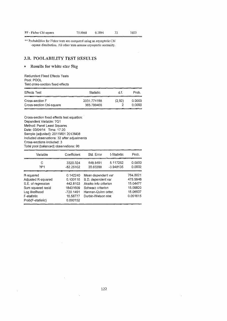
PP -Fisher Chi-square 75.9068 0.1894 33
* * Probabilities for Fisher tests are computed using an asymptotic Chi -square distribution. All other tests assume asymptotic normality.
3.B. POOLABILITY TEST RESULTS
• Results for white star 5kg
Redundant Fixed Effects Tests Pool: POOL Test cross-section fixed effects
Effects Test Statistic
Cross-section F Cross-section Chi-square
2031.774188 365.799466
Cross-section fixed effects test equation: Dependent Variable: ?Q1 Method: Panel Least Squares Date: 03/04/14 Time: 17:20 Sample (adjusted): 2011 M01 2013M08 Included observations: 32 after adjustments Cross-sections included: 3 Total pool (balanced) observations: 96
d. f.
(2,92) 2
Variable Coefficient Std. Error t-Statistic
c 3320.324 648.8491 5.117252 ?P1 -82.25102 20.83288 -3.948135
R-squared 0.142240 Mean dependent var Adjusted R-squared 0.133115 S.D.dependentvar S.E. of regression 442.8103 Akaike info criterion Sum squared resid 18431609 Schwarz criterion Log likelihood -720.1491 Hannan-Quinn criter. F -statistic 15.58777 Durbin-Watson stat Prob(F-statistic) 0.000152
122
1023
Pro b.
0.0000 0.0000
Pro b.
0.0000 0.0002
764.8021 475.5946 15.04477 15.09820 15.06637 0.051615

• Results for Tastic rice 2kg
Redundant Fixed Effects Tests Pool: POOL Test cross-section fixed effects
Effects Test
Cross-section F Cross-section Chi-square
Cross-section fixed effects test equation: Dependent Variable: ?02 Method: Panel Least Squares Date: 03/04/14 Time: 17:29
Statistic
937.920143 294.038721
d. f.
(2,92) 2
Sample (adjusted): 2011 M01 2013M08 Included observations: 32 after adjustments Cross-sections included: 3 Total pool (balanced) observations: 96
Variable Coefficient Std. Error t-Statistic
c 717.8780 570.9241 1.257396 ?P2 54.52602 28.07702 1.942016
R-squared 0.038574 Mean dependent var Adjusted R-squared 0.028346 S.D. dependentvar S.E. of regression 415.9801 Akaike info criterion Sum squared resid 16265706 Schwarz criterion Log likelihood -714.1487 Hannan-Quinn criter. F-statistic 3.771427 Durbin-Watson stat Prob(F-statistic) 0.055129
123
Pro b.
0.0000 0.0000
Pro b.
0.2117 0.0551
1823.552 422.0041 14.91977 14.97319 14.94136 0.081238

• Coke 2 liters
Redundant Fixed Effects Tests Pool: POOL
. Test cross-section fixed effects
Effects Test Statistic
Cross-section F Cross-section Chi-square
357176.08267 8
859.917269
Cross-section fixed effects test equation: Dependent Variable: ?Q3 Method: Panel Least Squares Date: 03/04/14 Time: 17:32 Sample (adjusted): 2011 M01 2013M08 Included observations: 32 after adjustments Cross-sections included: 3 Total pool (balanced) observations: 96
d.f.
(2,92) 2
Variable Coefficient Std. Error !-Statistic
c 46487.64 6758.370 6.878529 ?P3 -2640.274 495.3084 -5.330567
R-squared 0.232120 Mean dependent var Adjusted R-squared 0.223951 S.D. dependent var S.E. of regression 5555.429 Akaike info criterion Sum squared resid 2.90E+09 Schwarz criterion Log likelihood -962.9705 Hannan-Quinn criter. F-statistic 28.41494 Durbin-Watson stat Prob(F-statistic) 0.000001
124
Prob.
0.0000 0.0000
Pro b.
0.0000 0.0000
10588.71 6306.277 20.10355 20.15698 20.12515 0.123422
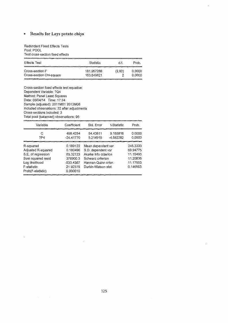
• Results for Lays potato chips
Redundant Fixed Effects Tests Pool: POOL Test cross-section fixed effects
Effects Test
Cross-section F Cross-section Chi-square
Cross-section fixed effects test equation: Dependent Variable: ?Q4 Method: Panel Least Squares Date: 03/04/14 Time: 17:34
Statistic
181.957288 153.649621
d.f.
(2,92) 2
Sample (adjusted): 2011 M01 2013M08 Included observations: 32 after adjustments Cross-sections included: 3 Total pool (balanced) observations: 96
Variable Coefficient Std. Error !-Statistic
c 498.4254 54.43811 9.155816 ?P4 -24.41770 5.214915 -4.682282
R-squared 0.189122 Mean dependent var Adjusted R-squared 0.180496 S.D. dependent var S.E. of regression 63.32123 Akaike info criterion Sum squared resid 376900.3 Schwarz criterion Log likelihood -533.4367 Hannan-Quinn criter. F-statistic 21.92376 Durbin-Watson stat P rob( F -statistic) 0.000010
125
Pro b.
0.0000 0.0000
Prob.
0.0000 0.0000
245.3333 69.94775 11.15493 11.20836 11.17653 0.146853
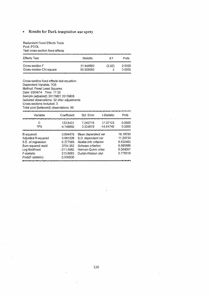
• Results for Dark temptation axe spray
Redundant Fixed Effects Tests Pool: POOL Test cross-section fixed effects
Effects Test
Cross-section F Cross-section Chi-square
Cross-section fixed effects test equation: Dependent Variable: ?Q5 Method: Panel Least Squares Date: 03/04/14 Time: 17:35 Sample (adjusted): 2011 M01 2013M08 Included observations: 32 after adjustments Cross-sections included: 3 Total pool (balanced) observations: 96
Statistic
31.844660 50.503095
d.f.
(2,92) 2
Variable Coefficient Std. Error t-Statistic
c 123.6421 7.242715 17.07123 ?P5 -4.748892 0.324879 -14.61740
R-squared 0.694476 Mean dependent var Adjusted R-squared 0.691226 S.D.dependentvar S.E. of regression 6.277588 Akaike info criterion Sum squared resid 3704.362 Schwarz criterion Log likelihood -311.5582 Hannan-Quinn criter. F-statistic 213.6683 Durbin-Watson stat Prob(F -statistic) 0.000000
126
Prob.
0.0000 0.0000
Pro b.
0.0000 0.0000
18.18750 11.29724 6.532462 6.585886 6.554057 0.779318

• Results for Sasko bread
Redundant Fixed Effects Tests Pool: POOL Test cross-section fixed effects
Effects Test Statistic
Cross-section F Cross-section Chi-square
19987.053140 583.343755
Cross-section fixed effects test equation: Dependent Variable: ?Q6 Method: Panel Least Squares Date: 03/04/14 Time: 17:37 Sample (adjusted): 2011 M01 2013M08 Included observations: 32 after adjustments Cross-sections included: 3 Total pool (balanced) observations: 96
d. f.
(2,92) 2
Variable Coefficient Std. Error t-Statistic
c 1100.345 762.6572 1.442778 ?P6 -58.37161 75.66281 -0.771470
R-squared 0.006292 Mean dependent var Adjusted R-squared -0.004280 S.D.dependentvar S.E. of regression 506.9713 Akaike info criterion Sum squared resid 24159872 Schwarz criterion Log likelihood -733.1392 Hannan-Quinn criter. F -statistic 0.595166 Durbin-Watson stat Prob(F-statistic) 0.442363
127
Pro b.
0.0000 0.0000
Prob.
0.1524 0.4424
513.3333 505.8900 15.31540 15.36882 15.33699 0.000813
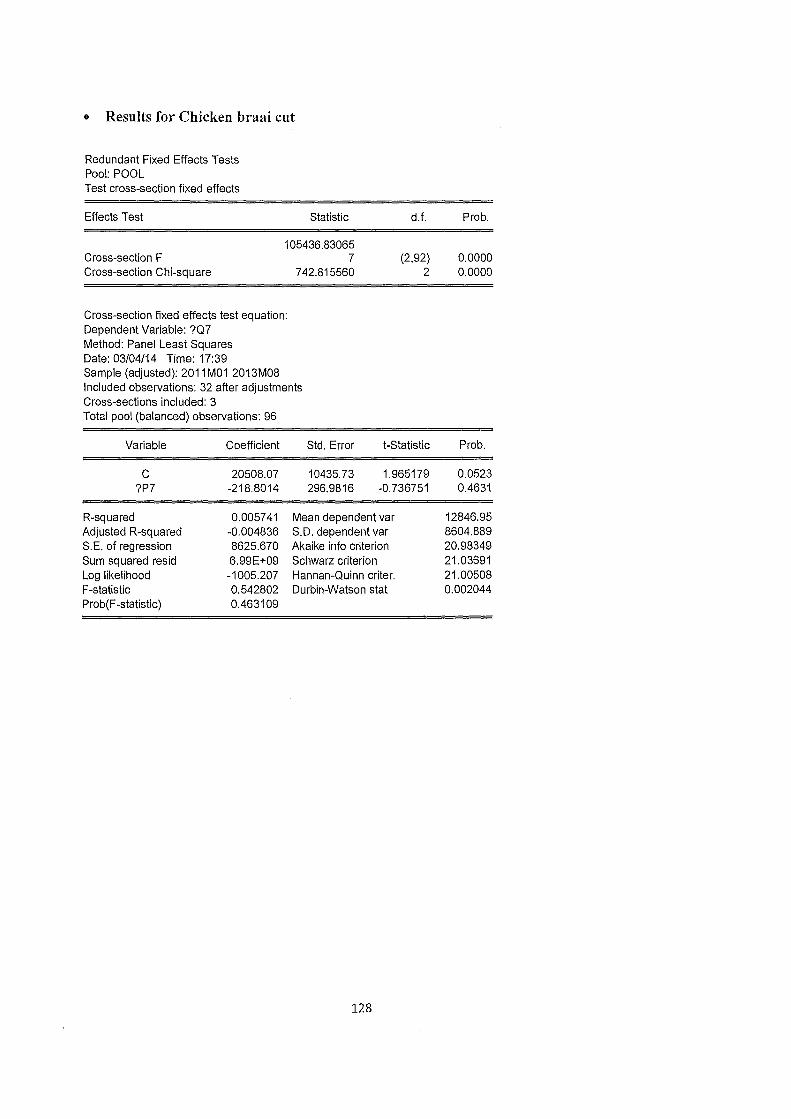
• Results for Chicken braai cut
Redundant Fixed Effects Tests Pool: POOL Test cross-section fixed effects
Effects Test Statistic
Cross-section F Cross-section Chi-square
105436.83065 7
742.815560
Cross-section fixed effects test equation: Dependent Variable: ?Q7 Method: Panel Least Squares Date: 03/04/14 Time: 17:39 Sample (adjusted): 2011 M01 2013M08 Included observations: 32 after adjustments Cross-sections included: 3 Total pool (balanced) observations: 96
d.f.
(2,92) 2
Variable Coefficient Std. Error t-Statistic
c 20508.07 10435.73 1.965179 ?P7 -218.8014 296.9816 -0.736751
R-squared 0.005741 Mean dependent var Adjusted R-squared -0.004836 S.D. dependentvar S.E. of regression 8625.670 Akaike info criterion Sum squared resid 6.99E+09 Schwarz criterion Log likelihood -1005.207 Hannan-Quinn criter. F-statistic 0.542802 Durbin-Watson stat Prob(F -statistic) 0.463109
128
Pro b.
0.0000 0.0000
Prob.
0.0523 0.4631
12846.95 8604.889 20.98349 21.03691 21.00508 0.002044

• Results for Apple golden
Redundant Fixed Effects Tests Pool: POOL Test cross-section fixed effects
Effects Test
Cross-section F Cross-section Chi-square
Cross-section fixed effects test equation: Dependent Variable: ?08 Method: Panel Least Squares Date: 03/04/14 Time: 17:40
Statistic
5858.160710 466.058034
d. f.
(2,92) 2
Sample (adjusted): 2011 M01 2013M08 Included observations: 32 after adjustments Cross-sections included: 3 Total pool (balanced) observations: 96
Variable Coefficient Std. Error !-Statistic
c 425.5414 306.0771 1.390308 ?P8 11.48194 20.08926 0.571546
R-squared 0.003463 Mean dependent var Adjusted R-squared -0.007138 S.D. dependent var S.E. of regression 507.2193 Akaike info criterion Sum squared resid 24183510 Schwarz criterion Log likelihood -733.1861 Hannan-Quinn criter. F-statistic 0.326665 Durbin-Watson stat Prob(F-statistic) 0.568994
129
Pro b.
0.0000 0.0000
Prob.
0.1677 0.5690
597.9583 505.4186 15.31638 15.36980 15.33797 0.014433
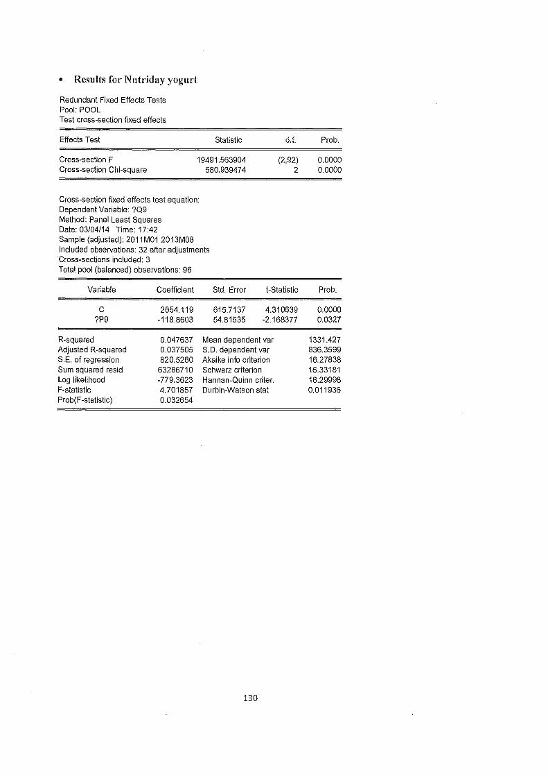
• Results for Nutriday yogurt
Redundant Fixed Effects Tests Pool: POOL Test cross-section fixed effects
Effects Test Statistic
Cross-section F Cross-section Chi-square
19491.563904 580.939474
Cross-section fixed effects test equation: Dependent Variable: ?Q9 Method: Panel Least Squares Date: 03/04/14 Time: 17:42 Sample (adjusted): 2011 M01 2013M08 Included observations: 32 after adjustments
·Cross-sections included: 3 Total pool (balanced) observations: 96
d.f.
(2,92) 2
Variable Coefficient Std. Error t-Statistic
c 2654.119 615.7137 4.310639 ?P9 -118.8603 54.81535 -2.168377
R-squared 0.047637 Mean dependent var Adjusted R-squared 0.037505 S.D. dependent var S.E. of regression 820.5260 Akaike info criterion Sum squared resid 63286710 Schwarz criterion Log likelihood -779.3623 Hannan-Quinn criter. F-statistic 4.701857 Durbin-Watson stat Prob(F-statistic) 0.032654
130
Pro b.
0.0000 0.0000
Pro b.
0.0000 0.0327
1331.427 836.3599 16.27838 16.33181 16.29998 0.011936

• Results for Colgate triple action lOOml
Redundant Fixed Effects Tests Pool: POOL Test cross-section fixed effects
Effects Test Statistic
Cross-section F Cross-section Chi-square
3264.470959 410.515617
Cross-section fixed effects test equation: Dependent Variable: ?Q10 Method: Panel Least Squares Date: 03/04/14 Time: 17:43 Sample (adjusted): 2011 M01 2013M08 Included observations: 32 after adjustments Cross-sections included: 3 Total pool (balanced) observations: 96
d.f.
(2,92) 2
Variable Coefficient Std. Error t-Statistic
c 1588.072 715.4660 2.219633 ?P10 -66.87639 92.42891 -0.723544
R-squared 0.005538 Mean dependent var Adjusted R-squared -0.005041 S.D. dependent var S.E. of regression 629.1474 Al<aike info criterion Sum squared resid 37207690 Schwarz criterion Log likelihood -753.8666 Hannan-Quinn criter. F-statistic 0.523516 Durbin-Watson stat Prob(F-statistic) 0.471142
131
Prob.
0.0000 0.0000
Pro b.
0.0288 0.4711
1072.490 627.5677 15.74722 15.80065 15.76882 0.002016

• Results for Styvensant cigarette
Redundant Fixed Effects Tests Pool: POOL Test cross-section fixed effects
Effects Test Statistic
Cross-section F Cross-section Chi-square
1933.120887 361.129597
Cross-section fixed effects test equation: Dependent Variable: ?011 Method: Panel Least Squares Date: 03/04/14 Time: 17:45 Sample (adjusted): 2011 M01 2013M08 Included observations: 32 after adjustments Cross-sections included: 3 Total pool (balanced) observations: 96
d.f.
(2,92) 2
Variable Coefficient Std. Error t -Statistic
c 3221.895 195.0336 16.51969 ?P11 -108.5957 7.712576 -14.08034
R-squared 0.678364 Mean dependent var Adjusted R-squared 0.674943 S.D.dependentvar S.E. of regression 191.6792 Akaike info criterion Sum squared resid 3453648. Schwarz criterion Log likelihood -639.7666 Hannan-Quinn criter. F-statistic 198.2561 Durbin-Watson stat Prob(F-statistic) 0.000000
132
Prob.
0.0000 0.0000
Pro b.
0.0000 0.0000
489.6042 336.1980 13.37014 13.42356 13.39173 0.214066

3. C. RESULTS FOR MODEL ESTIMATION
• Results for White star 5kg
Dependent Variable: ?Q 1 Method: Pooled Least Squares Date: 02114/14 Time: 07:31 Sample (adjusted): 2011M01 2013M08 Included observations: 32 after adjustments Cross-sections included: 3 Total pool (balanced) observations: 96
Variable Coefficient
pp --C 1861.557 SP _--C 618.5133 SH_--C 1839.378
PP_--PP _P1 -22.39002 SP_--SP_P1 -15.82375 SH_--SH_P1 -27.19350
R-squared 0.981431 Adjusted R-squared 0.980400 S.E. of regression 66.58396 Sum squared resid 399008.2 Log likelihood -536.1728 F -statistic 951.3669 Prob(F-statistic) 0.000000
e Results for Tastic rice 2kg
Dependent Variable: ?Q2 Method: Pooled Least Squares Date: 02/14/14 Time: 07:33 Sample (adjusted): 2011M01 2013M08 Included observations: 32 after adjustments Cross-sections included: 3 Total pool (balanced) observations: 96
Variable Coefficient
PP_--C 2316.963 SP --C 1927.147 SH_--C 3191.666
PP_--PP_P2 -20.92787 SP_--SP_P2 -32.20833 SH_--SH_P2 -43.58722
R-squared 0.956290 Adjusted R-squared 0.953861 S.E. ofregression 90.64619 Sum squared resid 739505.8 Log likelihood -565.7888 F -statistic 393.8015 Prob(F-statistic) 0.000000
Std. Error t -Statistic
193.0216 9.644297 147.8682 4.182870 213.4389 8.617818 6.327171 -3.538709 4.611937 -3.431042 6.919501 -3.929979
Mean dependent var S.D. dependent var Akaike info criterion Schwarz criterion Hannan-Quinn criter. Durbin-Watson stat
Std. Error t-Statistic
218.2133 10.61788 313.4294 6.148584 196.1173 16.27427 10.64828 -1.965376 15.94699 -2.019712 9.411896 -4.631078
Mean dependent var S.D. dependent var Akaike info criterion Schwarz criterion Hannan-Quinn criter. Durbin-Watson stat
133
Pro b.
0.0000 0.0001 0.0000 0.0006 0.0009 0.0002
764.8021 475.5946 11.29527 11.45554 11.36005 0.230685
Pro b.
0.0000 0.0000 0.0000 0.0525 0.0464 0.0000
1823.552 422.0041 1 1.91227 12.07254 11.97705 0.124068
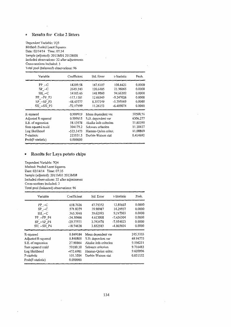
e Results for Coke 2 litters
Dependent Variable: ?Q3 Method: Pooled Least Squares Date: 02/14/14 Time: 07:34 Sample (adjusted): 2011M01 2013M08 Included observations: 32 after adjustments Cross-sections included: 3 Total pool (balanced) observations: 96
Variable Coefficient
PP_--C 18209.58 SP_--C 2649.343 SH_--C 14103.46
PP_--PP_P3 -117.1181 SP_--SP_P3 -48.43777 SH_--SH_P3 -72.17599
R-squared 0.999919 Adjusted R-squared 0.999915 S.E. of regression 58.13578 Sum squared resid 304179.2 Log likelihood -523.1473 F -statistic 223551.5 Prob(F -statistic) 0.000000
Std. Error t-Statistic
167.6107 108.6421 120.6405 21.96065 148.9860 94.66302 12.66549 -9.247026 8.357149 -5.795969 11.26153 -6.409074
Mean dependent var S.D. dependent var Akaike info criterion Schwarz criterion Hannan-Quinn criter. Durbin-Watson stat
• Results for Lays potato chips
Dependent Variable: ?Q4 Method: Pooled Least Squares Date: 02/14/14 Time: 07:35 Sample (adjusted): 2011M01 2013M08 Included observations: 32 after adjustments Cross-sections included: 3 Total pool (balanced) observations: 96
Variable Coefficient
PP_--C 658.7636 SP --C 571.8379 SH_--C 365.3048
PP_--PP_P4 -34.30466 SP_--SP_P4 -29.77571 SH_--SH_P4 -18.74638
R-squared 0.849184 Adjusted R-squared 0.840805 S.E. of regression 27.90864 Sum squared resid 70100.30 Log likelihood -452.6981 F-statistic 101.3504 Prob(F-statistic) 0.000000
Std. Error t-Statistic
47.71352 13.80665 39.98987 14.29957 39.62993 9.217903 4.613008 -7.436504 3.743478 -7.954023 3.852583 -4.865924
Mean dependent var S.D. dependent var Akaike info criterion Schwarz criterion Hannan-Quinn criter. Durbin-Watson stat
134
Pro b.
0.0000 0.0000 0.0000 0.0000 0.0000 0.0000
10588.71 6306.277 11.02390 11.18417 11.08869 0.414692
Pro b.
0.0000 0.0000 0.0000 0.0000 0.0000 0.0000
245.3333 69.94775 9.556211 9.716483 9.620996 0.831152

• Results for dark temptation axe spray
Dependent Variable: ?Q5 Method: Pooled Least Squares Date: 02/14/14 Time: 07:36 Sample (adjusted): 2011M01 2013M08 Included observations: 32 after adjustments Cross-sections included: 3 Total pool (balanced) observations: 96
Variable Coefficient
PP_--C 66.78853 SP_--C 57.23437 SH_--C 114.2824
PP_--PP_P5 -2.236935 SP_--SP_P5 -2.089184 SH_--SH_P5 -4.112419
R-squared 0.832211 Adjusted R-squared 0.822890 S.E. of regression 4.754386 Sum squared resid 2034.377 Log likelihood -282.7907 F -statistic 89.27771 Prob(F -statistic) 0.000000
• Results for Sasko bread
Dependent Variable: ?Q6 Method: Pooled Least Squares Date: 02/14/14 Time: 07:37 Sample (adjusted): 2011M01 2013M08 Included observations: 32 after adjustments Cross-sections included: 3 Total pool (balanced) observations: 96
Variable Coefficient
PP_--C 910.5599 SP_--C 529.7779 SH_--C 1583.617
PP_--PP_P6 -68.20437 SP_--SP_P6 -43.50996 SH_--SH_P6 -36.40209
R-squared 0.998035 Adjusted R-squared 0.997926 S.E. of regression 23.03997 Sum squared resid 47775.61 Log likelihood -434.2944 F -statistic 9142.136 Prob(F-statistic) 0.000000
Std. Error t -Statistic
11.64550 5.735137 16.62954 3.441728 12.47598 9.160192 0.515383 -4.340332 0.700744 -2.981380 0.610759 -6.733296
Mean dependent var S.D. dependent var Akaike info criterion Schwarz criterion Hannan-Quinn criter. Durbin-Watson stat
Std. Error t-Statistic
66.96954 13.59663 80.11542 6.612683 49.99498 31.67553 6.797135 -10.03428 7.793676 -5.582726 4.948856 -7.355658
Mean dependent var S.D. dependent var Akaike info criterion Schwarz criterion Hannan-Quinn criter. Durbin-Watson stat
135
Pro b.
0.0000 0.0009 0.0000 0.0000 0.0037 0.0000
18.18750 11.29724 6.016474 6.176745 6.081258 0.953103
Pro b.
0.0000 0.0000 0.0000 0.0000 0.0000 0.0000
513.3333 505.8900 9.172800 9.333071 9.237584 0.409994

• Results for chicken braai cut 2kg
Dependent Variable: ?Q7 Method: Pooled Least Squares Date: 02114114 Time: 07:38 Sample (adjusted): 2011M01 2013M08 Included observations: 32 after adjustments Cross-sections included: 3 Total pool (balanced) observations: 96
Variable Coefficient
PP_--C 19896.40 SP --C 2333.041 SH_--C 21324.06
PP_--PP_P7 -32.07535 SP --SP P7 -44.99279 SH_--SH_P7 -65.85707
R-squared 0.999595 Adjusted R-squared 0.999572 S.E. of regression 177.9475 Sum squared resid 2849879. Log likelihood -630.5432 F -statistic 44410.36 Prob(F -statistic) 0.000000
• Results for Apple golden
Dependent Variable: ?Q8 Method: Pooled Least Squares Date: 02/14/14 Time: 07:39 Sample (adjusted): 20 liMO! 2013M08 Included observations: 32 after adjustments Cross-sections included: 3 Total pool (balanced) observations: 96
Variable Coefficient
PP_--C 2031.343 SP_--C 707.4897 SH_--C 455.6344
PP_--PP_P8 -46.96698 SP_--SP_P8 -26.79567 SH --SH P8 -17.73894
R-squared 0.995540 Adjusted R-squared 0.995293 S.E. of regression 34.67649 Sum squared resid 108221.3 Log likelihood -473.5422 F-statistic 4018.321 Prob(F-statistic) 0.000000
Std. Error !-Statistic
356.9119 55.74598 537.1419 4.343435 314.9592 67.70420 10.27059 -3.123028 15.20639 -2.958808 8.912143 -7.389588
Mean dependent var S.D. dependent var Akaike info criterion Schwarz criterion Hannan-Quinn criter. Durbin-Watson stat
Std. Error !-Statistic
44.06493 46.09885 54.26310 13.03814 30.60197 14.88905 2.800070 -16.77350 3.345038 -8.010573 2.246348 -7.896790
Mean dependent var S.D. dependent var Akaike info criterion Schwarz criterion Hannan-Quinn criter. Durbin-Watson stat
136
Pro b.
0.0000 0.0000 0.0000 0.0024 0.0039 0.0000
12846.95 8604.889 13.26132 13.42159 13.32610 0.179135
Pro b.
0.0000 0.0000 0.0000 0.0000 0.0000 0.0000
597.9583 505.4186 9.990462 10.15073 10.05525 0.528956

• Results for Nutriday yogurt
Dependent Variable: ?Q9 Method: Pooled Least Squares Date: 02/14/14 Time: 07:39 Sample (adjusted): 2011M01 2013M08 Included observations: 32 after adjustments Cross-sections included: 3 Total pool (balanced) observations: 96
Variable Coefficient
PP_--C 3080.189 SP_--C 736.4009 SH_--C 1577.689
PP_--PP_P9 -56.43366 SP_--SP_P9 -21.87201 SH_--SH_P9 -50.33908
R-squared 0.998309 Adjusted R-squared 0.998215 S.E. of regression 35.33726 Sum squared resid 112384.9 Log likelihood -475.3543 F -statistic 10625.25 Prob(F -statistic) 0.000000
Std. Error !-Statistic
61.56200 50.03393 53.66633 13.72184 58.52727 26.95648 5.497534 -10.26527 4.354700 -5.022622 5.816931 -8.653890
Mean dependent var S.D. dependent var Akaike info criterion Schwarz criterion Hannan-Quinn criter. Durbin-Watson stat
• Results for colgate triple action
Dependent Variable: ?Q10 Method: Pooled Least Squares Date: 02/14/14 Time: 07:40 Sample (adjusted): 2011M01 2013M08 Included observations: 32 after adjustments Cross-sections included: 3 Total pool (balanced) observations: 96
Variable Coefficient
PP_--C 1436.715 SP_--C 837.0783 SH_--C 2582.683
PP_--PP_P10 -79.51547 SP _--SP _P1 0 -47.50671 SH_--SH_PlO -85.58821
R-squared 0.986529 Adjusted R-squared 0.985780 S.E. of regression 74.83565 Sum squared resid 504033.7 Log likelihood -547.3885 F -statistic 1318.157 Prob(F -statistic) 0.000000
Std. Error t-Statistic
159.4925 9.008037 151.0829 5.540522 135.0030 19.13056 20.65116 -3.850412 19.50937 -2.435071 17.40891 -4.916345
Mean dependent var S.D. dependent var Akaike info criterion Schwarz criterion Hannan-Quinn criter. Durbin-Watson stat
137
Pro b.
0.0000 0.0000 0.0000 0.0000 0.0000 0.0000
1331..427 836.3599 10.02821 10.18849 10.09300 0.494860
Pro b.
0.0000 0.0000 0.0000 0.0002 0.0169 0.0000
1072.490 627.5677 11.52893 11.68920 11.59371 0.146461

• Result for styvensant cigarette
Dependent Variable: ?Q II Method: Pooled Least Squares Date: 02/14/I4 Time: 07:41 Sample (adjusted): 2011M01 2013M08 Included observations: 32 after adjustments Cross-sections included: 3 Total pool (balanced) observations: 96
Variable Coefficient
PP_--C 1166.1I2 SP_--C 656.8708 SH --C 689.1853
PP_--PP_PI I -9.260898 SP_--SP _P11 -16.00399 SH_--SH_P11 -I5.47764
R-squared 0.992650 Adjusted R-squared 0.992241 S.E. of regression 29.61322 Sum squared resid 78924.84 Log likelihood -458.3894 F -statistic 2430.908 Prob(F-statistic) 0.000000
Std. Error t -Statistic
104.3544 I 1.17453 84.15951 7.805070 I01.3027 6.803230 4.677219 -1.980001 3.245616 -4.930957 3.703389 -4.179317
Mean dependent var S.D. dependent var Akaike info criterion Schwarz criterion Hannan-Quinn criter. Durbin-Watson stat
3. D. NORMALITY TEST RESULTS
Pro b.
0.0000 0.0000 0.0000 0.0508 0.0000 O.OOOI
489.6042 336.1980 9.674780 9.835052 9.739565 0.234254
White star 5 kg (Pl & Ql) for individual supermarkets
8
6
4
2
-125 -100 -75 -50 -25 0 25 50 75 100 125
138
Series: RESIDPP _ Sample 2011 M01 2013M12 Observations 32
Mean Median Maximum Minimum Std. Dev. Skewness Kurtosis
Jarque-Bera Probability
2.64e-13 3.406863 107.9193
-113.2842 62.35488
-0.105627 1.898978
1.675839 0.432610

7 Series: RESIDSP _
6 Sample 2011 M01 2013M12 Observations 32
5 Mean 1.32e-13 Median -0.638692
4 Maximum 16.60039 Minimum -20.89040
3 Std. Dev. 9.320414 Skewness -0.348739
2 Kurtosis 2.238943
Jarque-Bera 1.420910 Probability 0.491421
0 -20 -15 -10 -5 0 5 10 15
16 Series: RESIDSH_
14 Sample 2011 M01 2013M12 Observations 32
12 Mean -1.63e-13
10 Median 55.44526 Maximum 83.15501
8 Minimum -182.6515 Std. Dev. 94.31983
6 Skewness -0.854162
4 Kurtosis 2.037831
2 Jarque-Bera 5.125518 Probability 0.077092
-150 -100 -50 0 50 100
Tastic rice (P2 & Q2) Results for individual supermarkets
8~----------------------------------------------. Series: RESIDPP _
7 Sample 2011M01 2013M12 Observations 32
6
Mean -5.20e-14 5 Median 10.93642
Maximum 94.25068 4 Minimum -156.6152
Std. Dev. 56.66005 3 Skewness -0.975433
Kurtosis 3.798496
Jarque-Bera 5.924636 Probability 0.051699
-150 -125 -100 -75 -50 -25 0 25 50 75 100
12,-------------------------------------------------, Series: RESIDSP Sample 2011 M01-2013M12 Observations 32
Mean 1.01e-13 Median -17.61474 Maximum 231.6978 Minimum -149.9281 Std. Dev. 128.4907 Skewness 0.294644 Kurtosis 1.644668
Ja rq ue-Be ra 2.912246 Probability 0.233138
-100 -50 0 50 100 150 200 250
139

6
5
4
3
2
-150 -125 -100 -75 -50 -25 0 25 50 75 100
Coke (P3 & Q3) results for individual supermarkets
8
6
4
2
0~----r-~~----+----+----+-~-+~~+----+----~ -250 -200 -150 -100 -50 0 50 100 150 200
20
140
Series: RESIDSH_ Sample 2011 M01 2013M12 Observations 32
Mean Median Maximum Minimum Std. Dev. Skewness Kurtosis
-4.94e-13 1.142185 99.40385
-150.0089 64.30239
-0.224890 2.214181
Jarque-Bera 1 .093086 Probability 0.578948
Series: RESIDPP Sample 2011 M01 2013M12 Observations 32
Mean Median Maximum Minimum Std. Dev. Skewness Kurtosis
1.77e-12 7.151215 165.9221
-231.2133 86.50343
-0.861554 3.837315
Jarque-Bera 4.893599 Probability 0.086570
Series: RESIDSP _ Sample 2011 M01 2013M12 Observations 32
Mean Median Maximum Minimum Std. Dev. Skewness Kurtosis
Jarque-Bera Probability
9.17e-14 -4.729331 45.86388
-32.38590 23.14594 0.545326 2.081376
2.711192 0.257794

6
5
4
3
2
8 Series: RESIDSH_
7 Sample 2011 M01 2013M12 Observations 32
6
Mean 1.96e-13 5 Median -0.715896
Maximum 64.78114 4 Minimum -101.9846
Std. Dev. 42.35158 3 Skewness -0.356454
Kurtosis 2.782996 2
Jarque-Bera 0.740438 Probability 0.690583
0 -125 -100 -75 -50 -25 0 25 50 75
Lays Potato onion chips (P4 & Q4) individual supermarket results
-80 -70 -60 -50 -40 -30 -20 -10 0 10 20 30 40 50 60
-50 -40 -30 -20 -10 0 10 20 30 40 50 60
141
Series: RESIDPP _ Sample 2011 M01 2013M12 Observations 32
Mean 9.34e-14 Median 3.787566 Maximum 59.84060 Minimum -70.75545 Std. Dev. 34.06646 Skewness -0.114660 Kurtosis 2.117524
Jarque-Bera 1.108468 Probability 0.574512
Series: RESIDSP _ Sample 2011 M01 2013M12 Observations 32
Mean 1.24e-13 Median 0.045989 Maximum 53.62140 Minimum -48.37860 Std. Dev. 18.18463 Skewness 0.027543 Kurtosis 5.381824
Jarque-Bera 7.568158 Probability 0.022730
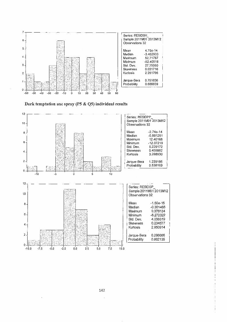
7
6
5
4
3
2
0
,---
r---
r---
,------- 1-c--
. l . ~ -60 -50 -40 -30 -20 -10 0 10 20 30 40 50 60
Series: RESIDSH_ Sample 2011 M01 2013M12 Observations 32
Mean Median Maximum Minimum Std. Dev. Skewness Kurtosis
4.75e-14 -3.462933 52.71787
-52.40518 27.75060 0.031716 2.251766
Jarque-Bera 0.751836 Probability 0.686659
Dark temptation axe spray (PS & QS) individual results
-10 -5 0 5 10
Series: RESIDPP _ Sample 2011 M01 2013M12 Observations 32
Mean Median Maximum Minimum Std. Dev. Skewness Kurtosis
Jarque-Bera Probability
-2.74e-14 -0.881251 12.40168
-12.07219 5.229172 0.459862 3.288930
1.239166 0.538169
Series: RESIDSP _
10 Sample 2011 M01 2013M12 Observations 32
8
6
4
2
0~~~~~_,~~-r--~~~_,~~-r~--~--~
-10.0 -7.5 -5.0 -2.5 0.0 2.5 5.0 7.5 10.0
142
Mean Median Maximum Minimum Std. Dev. Skewness Kurtosis
Jarque-Bera Probability
-1.50e-15 -0.301468 9.378134
-8.272322 4.038319 0.234577 2.950914
0.296686 0.862135
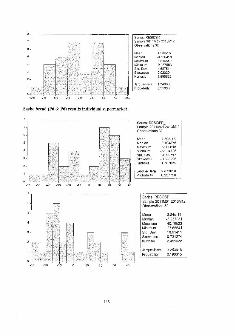
8
7
6
5
4
3
2
0 II I -10.0 -7.5 -5.0 -2.5 0.0 2.5 5.0 7.5 10.0
Sasko bread (P6 & P6) results individual supermarket
7
6
5
4
3
2
~0 ~0 40 ~0 ~0 ~0 0 10 20 30 40
6
5
4
3
2
Series: RESIDSH_ Sample 2011M01 2013M12 Observations 32
Mean 4.33e-15 Median -0.536418 Maximum 8.816549 Minimum -9.187583 Std. Dev. 4.687514 Skewness 0.020204 Kurtosis 1.995825
Jarque-Bera 1.346668 Probability 0.510005
Series: RESIDPP _ Sample 2011 M01 2013M12 Observations 32
Mean Median Maximum Minimum Std. Dev. Skewness Kurtosis
1.89e-13 9.104876 38.00618
-51.94126 26.99717
-0.398296 1.767035
Jarque-Bera 2.873018 Probability 0.237756
Series: RESIDSP _ Sample 2011M01 2013M12 Observations 32
Mean Median Maximum Minimum Std. Dev. Skewness Kurtosis
Jarque-Bera Probability
3.84e-14 -6.957081 40.79523
-27.65641 19.61411 0.731274 2.451622
3.253018 0.196615
o~~~~=+~+=~~~=P~~~~~+--.--~=r~ -30 -20 -10 0 10 20 30 40
143

8 Series: RESIDSH_
7 Sample 2011 M01 2013M12 Observations 32
6
Mean 2.43e-13 5 Median 2.240631
Maximum 35.44168 4 Minimum -40.19430
Std. Dev. 20.67821 3 Skewness -0.324753
Kurtosis 2.056341 2
Jarque-Bera 1.749800 Probability 0.416904
-50 -40 -30 -20 -10 0 10 20 30
Chicken braai cut (P7 & Q7) results individual supermarkets
14 Series: RESIDPP
12 Sample 2011M01 2013M12 Observations 32
10 Mean 5.24e-12 Median 35.30110
8 Maximum 110.8014 Minimum -312.3120
6 Std. Dev. 117.1059 Skewness -1.872772
4 Kurtosis 5.209938
2 Jarque-Bera 25.21723 Probability 0.000003
0 -350 -300 -250 -200 -150 -100 -50 0 50 100 150
7 Series: RESIDSP
6 Sample 2011M01 2013M12 Observations 32
5 Mean 5.76e-13 Median -36.52848
4 Maximum 227.6922 Minimum -146.7433
3 Std. Dev. 117.4023 Skewness 0.569496
2 Kurtosis 1.965063
Jarque-Bera 3.157866 Probability 0.206195
0 -150 -100 -50 0 50 100 150 200 250
144
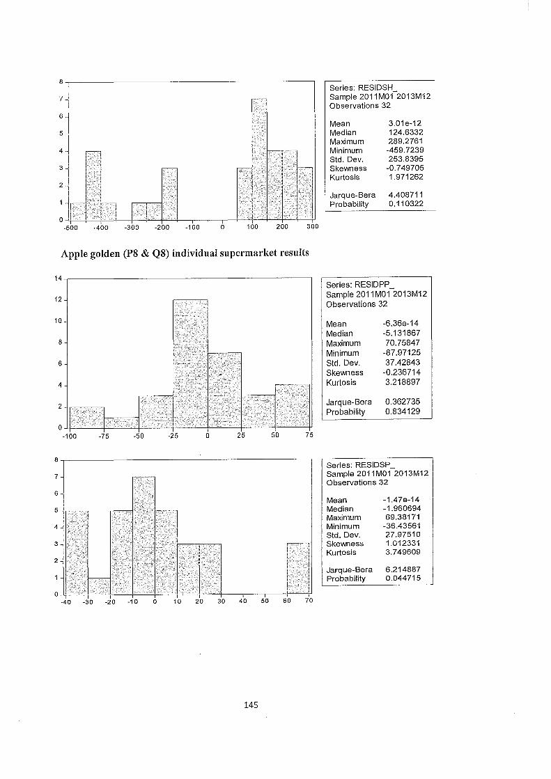
8
7
6
5
4
3
2
-500 -400
Apple golden (P8 & Q8) individual supermarket results
12
10
8
6
4
2
0~-----+~----~--~~~--~~--~~~-+--~~ -100 -75 -50 -25 0 25 50 75
8,----------------------------------------------
7
6
5
4
3
:~~rl -40 -30 -20 -1 0 0 10 20 30 40 50 60 70
145
Series: RESIDSH_ Sample 2011 M01 2013M12 Observations 32
Mean 3.01e-12 Median 124.6332 Maximum 289.2761 Minimum -459.7239 Std. Dev. 253.8395 Skewness -0.749705 Kurtosis 1.971262
Jarque-Bera 4.408711 Probability 0.110322
Series: RESIDPP Sample 2011 M01 2013M12 Observations 32
Mean Median Maximum Minimum Std. Dev. Skewness Kurtosis
Jarque-Bera Probability
-6.36e-14 -5.131867 70.75847
-87.97125 37.42843
-0.236714 3.218897
0.362735 0.834129
Series: RESIDSP _ Sample 2011M01 2013M12 Observations 32
Mean Median Maximum Minimum Std. Dev. Skewness Kurtosis
Jarque-Bera Probability
-1.47e-14 -1.960694 69.38171
-36.43561 27.97510 1.012331 3.749609
6.214887 0.044715

Series: RESIDSH_ Sample 2011M01 2013M12 Observations 32
Mean -2.55e-14 Median -6.414212 Maximum 71.05548 Minimum -52.46665 Std. Dev. 36.15960 Skewness 0.177221 Kurtosis 1.798079
Jarque-Bera 2.093656 Probability 0.351049
Nutriday yogurt (P9 & Q9) results for individual supermarkets
8,-------------------------------------------~
7
6
5
4
3
2
-70 -60 -50 -40 -30 -20 -10 0 10 20 30 40 50 60
8,-------------------------------------------~
7
6
5
4
3
2
-100 -80 -60 -40 -20 0 20 40 60
146
Series: RESIDPP _ Sample 2011 M01 2013M12 Observations 32
Mean Median Maximum Minimum Std. Dev. Skewness Kurtosis
1.25e-13 -1.874270 51.65356
-63.41634 24.02085
-0.128443 3.483236
Jarque-Bera 0.399343 Probability 0.819000
Series: RESIDSP _ Sample 2011M01 2013M12 Observations 32
Mean Median Maximum Minimum Std. Dev. Skewness Kurtosis
3.93e-14 3.376495 55.90562 -92.34749 37.85614
-0.454391 2.727390
Jarque-Bera 1.200270 Probability 0.548738

8 Series: RESIDSH_
7 Sample 2011 M01 2013M12 Observations 32
6
Mean 3.71e-13 5 Median 0.333989
Maximum 75.70175 4 Minimum -81.29825
Std. Dev. 40.18995 3 Skewness -0.049778
Kurtosis 2.247087 2
Jarque-Bera 0.769052 Probability 0.680773
0~~~~---+~~+---~~--~--~~--~--~ -100 -75 -50 -25 0 25 50 75 100
Colgate triple action (PlO & QlO) results for individual supermarket
9
8
7
6
5
4
3
2
0 -75 -50 -25 0 25 50 75 100
6
5
4
3
2
147
Series: RESIDPP _ Sample 2011M01 2013M12 Observations 32
Mean 1.27e-13 Median -5.128194 Maximum 89.19551 Minimum -72.98511 Std. Dev. 44.73115 Skewness 0.369644 Kurtosis 2.490354
Jarque-Bera 1.075048 Probability 0.584193
Series: RESIDSP _ Sample 2011M01 2013M12 Observations 32
Mean Median Maximum Minimum Std. Dev. Skewness Kurtosis
Jarque-Bera Probability
-2.04e-14 -21.87237 171.7550
-172.3319 98.44991 0.196781 1.814695
2.079784 0.353493

10~----------------------------------------~
8
6
4
2
0~~~--+-~+-~r---~~--~~-+---r--~--~ -125 -100 -75 -50 -25 0 25 50 75 100 125 150
Series: RESIDSH_ Sample 2011 M01 2013M12 Observations 32
Mean Median Maximum Minimum Std. Dev. Skewness Kurtosis
2.76e-13 -30.11287 148.9489
-100.6393 67.57139 0.703579 2.180619
Jarque-Bera 3.535308 Probability 0.170733
Styvensant cigarette (Pll & Qll) results for individual supermarket
9,-----------------------------------------.
8
7
6
5
4
3
2
0 -40 -30 -20 -10 0 10 20 30 40 50 60
7
6
5
4
3
2
-70 -60 -50 -40 -30 -20 -10 0 10 20 30 40 50 60 70
148
Series: RESIDPP _ Sample 2011 M01 2013M12 Observations 32
Mean Median Maximum Minimum Std. Dev. Skewness Kurtosis
2.52e-13 -1.723729 51.53540
-35.68191 19.70429 0.700801 3.434047
Jarque-Bera 2.870511 Probability 0.238055
Series: RESIDSP _ Sample 2011M01 2013M12 Observations 32
Mean Median Maximum Minimum Std. Dev. Skewness Kurtosis
Jarque-Bera Probability
1.47e-14 -13.84504 63.22899 -63.92107 39.15091 0.190488 1.591203
2.839802 0.241738

8
7
6
5
4
3
2
o~~-r~~~~----~--+-~+---4---~~-r~~ -40 -30 -20 -10 0 10 20 30 40 50 60
3.E. RESULTS FOR THE SERIAL
CORRELATION TEST
• White star results
Results for Pick n Pay
Date: 02/26/14 Time: 17:05 Sample: 2011M01 2013M12 Included observations: 31
Autocorrelation Partial Correlation
. I* . . I* .
. I* . I . I* .
. I* . I . I*.
. I . I . *I .
. I*. I . I* .
Results for Shoprite
Date: 02/26/14 Time: 17:06 Sample: 2011 M01 2013M12 Included observations: 31
I I I
Autocorrelation Partial Correlation
. I* . I . I*.
. *I . I . *I .
. I . I . I* .
. I . I . *I .
. *I . I . *I .
AC PAC Q-Stat
0.138 0.138 0.6534 2 0.208 0.193 2.1821 3 0.212 0.171 3.8196 4 0.008 -0.074 3.8223 5 0.165 0.108 4.8988
AC PAC Q-Stat
1 0.142 0.142 0.6867 2 -0.152 -0.176 1.5016 3 0.024 0.078 1.5230 4 -0.060 -0.110 1.6590 5 -0.142 -0.102 2.4558
149
Series: RESIDSH_ Sample 2011 M01 2013M12 Observations 32
Mean 3.67e-14 Median -2.411267 Maximum 53.55607 Minimum -37.32421 Std. Dev. 24.99820 Skewness 0.451439 Kurtosis 2.241505
Jarque-Bera 1.854006 Probability 0.395738
Prob
0.419 0.336 0.282 0.431 0.428
Prob
0.407 0.472 0.677 0.798 0.783
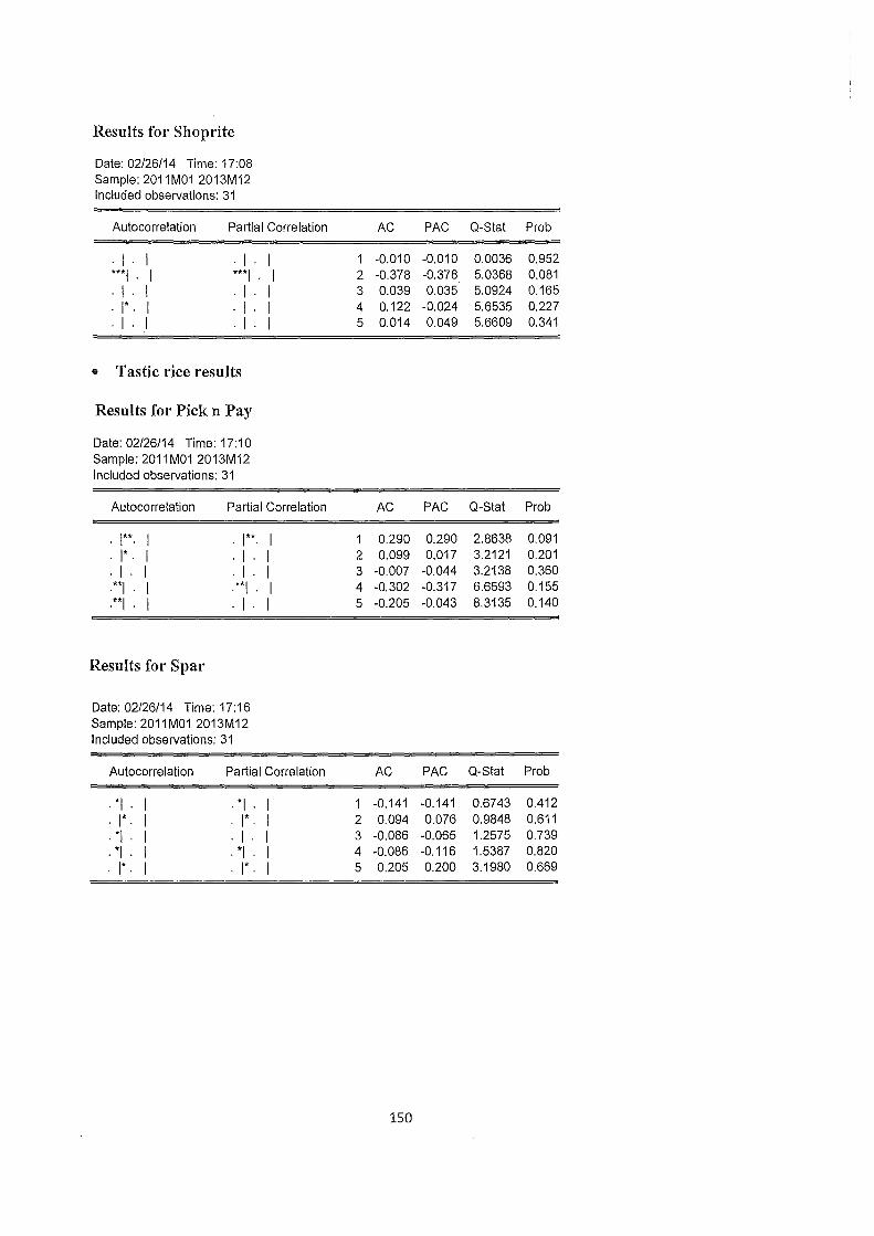
Results for Shoprite
Date: 02/26/14 Time: 17:08 Sample: 2011M01 2013M12 Included observations: 31
Autocorrelation Partial Correlation
. I . I . I . I ***I . I ***I . I . I . I . I . I . I* . I . I . I . I . I . I . I
e Tastic rice results
Results for Pick n Pay
Date: 02/26/14 Time: 17:10 Sample: 2011M01 2013M12 Included observations: 31
Autocorrelation Partial Correlation
. 1**. I . 1** .
. I* . I . I .
. I . I . I .
.**1 . I . **I .
.**1 . I . I .
Results for Spar
Date: 02/26/14 Time: 17:16 Sample: 2011M01 2013M12 Included observations: 31
I I I I I
Autocorrelation Partial Correlation
. *I . I . *I . I
. I*. I . I*. I
. *I . I . I . I
. *I . I . *I . I
. I*. I . I* . I
AC PAC Q-Stat Prob
-0.010 -0.010 0.0036 0.952 2 -0.378 -0.378 5.0368 0.081 3 0.039 0.035 5.0924 0.165 4 0.122 -0.024 5.6535 0.227 5 0.014 0.049 5.6609 0.341
AC PAC Q-Stat Prob
1 0.290 0.290 2.8638 0.091 2 0.099 0.017 3.2121 0.201 3 -0.007 -0.044 3.2138 0.360 4 -0.302 -0.317 6.6593 0.155 5 -0.205 -0.043 8.3135 0.140
AC PAC Q-Stat Prob
-0.141 -0.141 0.6743 0.412 2 0.094 0.076 0.9848 0.611 3 -0.086 -0.065 1.2575 0.739 4 -0.086 -0.116 1.5387 0.820 5 0.205 0.200 3.1980 0.669
150
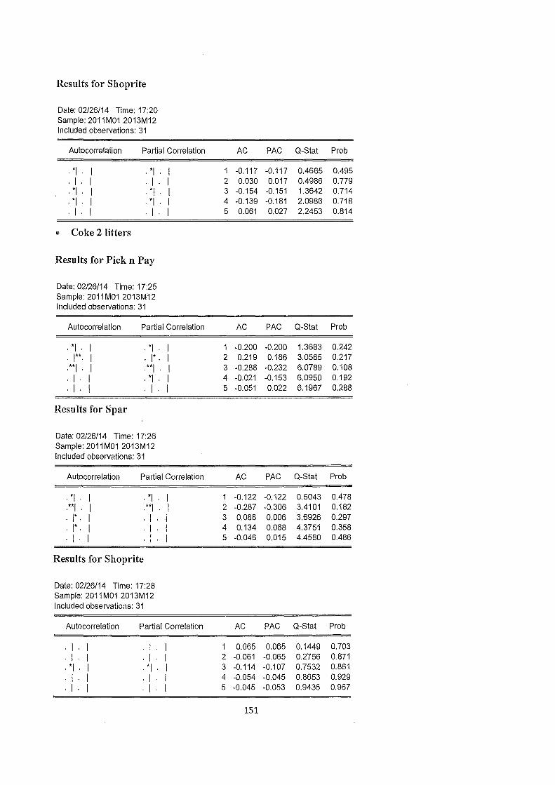
Results for Shoprite
Date: 02/26/14 Time: 17:20 Sample: 2011M01 2013M12 Included observations: 31
Autocorrelation Partial Correlation AC PAC Q-Stat Prob
. *I . I . *I . I -0.117 -0.117 0.4665 0.495
. I . I . I . I 2 0.030 0.017 0.4986 0.779
. *I . I . *I . I 3 -0.154 -0.151 1.3642 0.714
. *I . I . *I . I 4 -0.139 -0.181 2.0986 0.718
. I . I . I . I 5 0.061 0.027 2.2453 0.814
e Coke 2 litters
Results for Pick n Pay
Date: 02/26/14 Time: 17:25 Sample: 2011M01 2013M12 Included observations: 31
Autocorrelation Partial Correlation AC PAC Q-Stat Prob
. *I . I . *I . I -0.200 -0.200 1.3683 0.242
. I**. I . I*. I 2 0.219 0.186 3.0565 0.217
. **I . I .**1 . I 3 -0.288 -0.232 6.0789 0.108
. I . I . *I . I 4 -0.021 -0.153 6.0950 0.192
. I . I . I . I 5 -0.051 0.022 6.1967 0.288
Results for Spar
Date: 02/26/14 Time: 17:26 Sample: 2011M01 2013M12 Included observations: 31
Autocorrelation Partial Correlation AC PAC Q-Stat Prob
. *I . I . *I . I -0.122 -0.122 0.5043 0.478
.**1 . I .**1 . I 2 -0.287 -0.306 3.4101 0.182
. I* . I I I 3 0.088 0.006 3.6926 0.297
. I* . I I I 4 0.134 0.068 4.3751 0.358
. I . I I I 5 -0.046 0.015 4.4580 0.486
Results for Shoprite
Date: 02/26/14 Time: 17:28 Sample: 2011M01 2013M12 Included observations: 31
Autocorrelation Partial Correlation AC PAC Q-Stat Prob
. I . I . I . I 1 0.065 0.065 0.1449 0.703
. I . I . I . I 2 -0.061 -0.065 0.2756 0.871
. *I . I . *I . I 3 -0.114 -0.107 0.7532 0.861
. I . I . I . I 4 -0.054 -0.045 0.8653 0.929
. I . I . I . I 5 -0.045 -0.053 0.9436 0.967
151
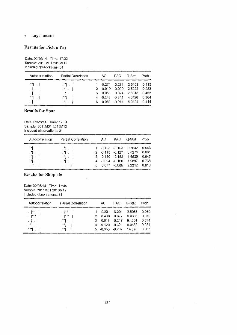
• Lays potato
Results for Pick n Pay
Date: 02/26/14 Time: 17:32 Sample: 2011M01 2013M12 Included observations: 31
Autocorrelation Partial Correlation AC PAC Q-Stat Prob
.**1 . I . **I . -0.271 -0.271 2.5102 0.113
. I . I . *I . I 2 -0.019 -0.099 2.5222 0.283
. I . I . I . I 3 0.055 0.024 2.6318 0.452
.**1 . I .**1 . I 4 -0.242 -0.241 4.8426 0.304
. I . I . *I . I 5 0.066 -0.074 5.0124 0.414
Results for Spar
Date: 02/26/14 Time: 17:34 Sample: 2011M01 2013M12 Included observations: 31
Autocorrelation Partial Correlation AC PAC Q-Stat Prob
. *I . I . *I . 1 -0.103 -0.103 0.3642 0.546
. *I . I . *I . I 2 -0.115 -0.127 0.8276 0.661
. *I . I . *I . I 3 -0.150 -0.182 1.6539 0.647
. *I . I . *I . I 4 -0.094 -0.160 1.9897 0.738
. I* . I I . I 5 0.077 -0.005 2.2212 0.818
Results for Shoprite
Date: 02/26/14 Time: 17:45 Sample: 2011M01 2013M12 Included observations: 31
Autocorrelation Partial Correlation AC PAC Q-Stat Prob
. 1**. I . 1** . 1 0.291 0.291 2.8965 0.089
. I*** I . I*** 2 0.430 0.377 9.4088 0.079
. I . I .**1 3 0.018 -0.217 9.4201 0.074
. *I . I .**1 4 -0.120 -0.321 9.9662 0.081 ***I . I .**I 5 -0.353 -0.282 14.870 0.063
152

Ill Axe spray
Results for Pick n Pay
Date: 02/26/14 Time: 17:48 Sample: 2011M01 2013M12 Included observations: 31
Autocorrelation Partial Correlation AC PAC Q-Stat Prob
.**I . I .**1 . -0.344 -0.344 4.0307 0.045
. *I . I .**1 . 2 -0.089 -0.235 4.3118 0.116
. *I . I .**I . 3 -0.096 -0.258 4.6515 0.199
. I . I .**1 . I 4 -0.006 -0.221 4.6527 0.325
. I*. I . I . I 5 0.194 0.056 6.1324 0.294
Results for Spar
Date: 02/26/14 Time: 17:50 Sample: 2011M01 2013M12 Included observations: 31
Autocorrelation Partial Correlation AC PAC Q-Stat Prob
. I . I . I . I 1 -0.059 -0.059 0.1180 0.731
. I . I . I . I 2 -0.048 -0.052 0.1995 0.905
. I . I . I . I 3 0.039 0.033 0.2541 0.968
.**1 . I .**I . I 4 -0.210 -0.209 1.9178 0.751
. I . I I . I 5 -0.008 -0.029 1.9201 0.860
Results for Shoprite
Date: 02/26/14 Time: 17:53 Sample: 2011 M01 2013M12 Included observations: 31
Autocorrelation Partial Correlation AC PAC Q-Stat Prob
. *I . I . *I . I -0.095 -0.095 0.3083 0.579
. *I . I . *I . I 2 -0.175 -0.185 1.3830 0.501
. I*. I . I* . I 3 0.181 0.150 2.5770 0.462
. *I . I . *I I 4 -0.083 -0.089 2.8401 0.585
. *I . I . *I . I 5 -0.121 -0.084 3.4207 0.635
153

II Sasko bread
Results for Pick n Pay
Date: 02/26/14 Time: 17:55 Sample: 2011 M01 2013M12 Included obseNations: 31
Autocorrelation Partial Correlation AC PAC Q-Stat Prob
. I . I . I . I -0.006 -0.006 0.0012 0.972
. *I . I . *I . I 2 -0.146 -0.147 0.7582 0.684
. **I . I .**1 . I 3 -0.266 -0.274 3.3442 0.342
. I . I . I . I 4 0.046 0.011 3.4254 0.489
. I* . I . I . I 5 0.141 0.071 4.2093 0.520
Results for Spar
Date: 02/26/14 Time: 17:58 Sample: 2011M01 2013M12 Included obseNations: 31
Autocorrelation Partial Correlation AC PAC Q-Stat Prob
. I . I . I . I -0.054 -0.054 0.0982 0.754
. I*. I . I* . I 2 0.190 0.188 1.3708 0.504
. *I . I . *I . I 3 -0.183 -0.171 2.5978 0.458
. I*. I . I* . I 4 0.121 0.080 3.1482 0.533
. I . I I . I 5 0.002 0.074 3.1483 0.677
Results for Shoprite
Date: 02/26/14 Time: 18:01 Sample: 2011 M01 2013M12 Included obseNations: 31
Autocorrelation Partial Correlation AC PAC Q-Stat Prob
. I . I . I . I 1 -0.020 -0.020 0.0134 0.908
. I . I . I . I 2 -0.047 -0.048 0.0921 0.955
. *I . I . *I . I 3 -0.089 -0.091 0.3816 0.944 ***I . I ****I . I 4 -0.465 -0.477 8.5777 0.073 . *I . I . *I . I 5 -0.097 -0.196 8.9467 0.111
154

Cl Chicken braai cut
Results for Pick n Pay
Date: 02/26/14 Time: 18:05 Sample: 2011M01 2013M12 Included observations: 31
Autocorrelation Partial Correlation AC PAC Q-Stat Prob
. *I . I . *I . I 1 -0.069 -0.069 0.1610 0.688
. I*. I . I*. I 2 0.087 0.082 0.4258 0.808
. I . I . I . I 3 0.012 0.023 0.4308 0.934
. I . I . I I 4 0.021 0.016 0.4473 0.978
. I . I . I . I 5 -0.018 -0.019 0.4607 0.993
Results for Spar
Date: 02/26/14 Time: 18:09 Sample: 2011M01 2013M12 Included observations: 31
Autocorrelation Partial Correlation AC PAC Q-Stat Prob
. *I . I . *I . I -0.145 -0.145 0.7193 0.396
. I . I . I . I 2 0.056 0.036 0.8318 0.660
.**1 . I .**1 . I 3 -0.344 -0.338 5.1567 0.161
. *I . I .**1 . I 4 -0.101 -0.223 5.5428 0.236
. I . I I . I 5 -0.003 -0.049 5.5432 0.353
Results for Shoprite
Date: 02/26/14 Time: 18:14 Sample: 2011M01 2013M12 Included observations: 31
Autocorrelation Partial Correlation AC PAC Q-Stat Prob
. *I . I . *I . I -0.173 -0.173 1.0242 0.312
. I . I . I . I 2 0.054 0.025 1.1281 0.569 ***I . I .**1 . I 3 -0.347 -0.344 5.5288 0.137 . I . I . *I . I 4 0.043 -0.082 5.5990 0.231 . I*. I . I* . I 5 0.121 0.143 6.1719 0.290
155
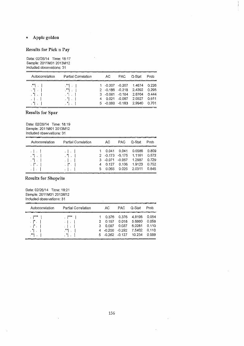
• Apple golden
Results for Pick n Pay
Date: 02/26/14 Time: 18:17 Sample: 2011M01 2013M12 Included observations: 31
Autocorrelation Partial Correlation AC PAC Q-Stat Prob
.**1 . I .**1 . -0.207 -0.207 1.4674 0.226
. *I . I .**I . 2 -0.166 -0.218 2.4392 0.295
. *I . I . *I . 3 -0.081 -0.184 2.6764 0.444
. I . I . *I . I 4 0.021 -0.097 2.6927 0.611
. *I . I . *I . I 5 -0.088 -0.183 2.9940 0.701
Results for Spar
Date: 02/26/14 Time: 18:19 Sample: 2011 M01 2013M12 Included observations: 31
Autocorrelation Partial Correlation AC PAC Q-Stat Prob
. I . I . I . I 1 0.041 0.041 0.0586 0.809
. *I . I . *I . I 2 -0.173 -0.175 1.1161 0.572
. *I . I . I . I 3 -0.071 -0.057 1.2987 0.729
. I* . I . I* . I 4 0.127 0.106 1.9123 0.752
. I . I . I . I 5 0.055 0.025 2.0311 0.845
Results for Shoprite
Date: 02/26/14 Time: 18:21 Sample: 2011 M01 2013M12 Included observations: 31
Autocorrelation Partial Correlation AC PAC Q-Stat Prob
. I*** I . I*** I 0.376 0.376 4.8195 0.054
. I*. I . I . I 2 0.157 0.018 5.6860 0.058
. I* . I . I . I 3 0.097 0.037 6.0281 0.110
. *I . I .**1 . I 4 -0.200 -0.292 7.5402 0.110
.**1 . I . *I . I 5 -0.262 -0.127 10.234 0.069
156

G Nutriday yogurt
Results for Pick n Pay
Date: 02/26/14 Time: 18:29 Sample: 2011 M01 2013M12 Included observations: 31
Autocorrelation Partial Correlation AC PAC Q-Stat Prob
. I . . I . -0.013 -0.013 0.0058 0.939
. I . . I . 2 -0.063 -0.064 0.1475 0.929
. I . . I . 3 -0.018 -0.020 0.1592 0.984
.**1 . .**1 . 4 -0.255 -0.261 2.6189 0.623
. I*. . I* . 5 0.083 0.077 2.8909 0.717
Results for Spar
Date: 02/26/14 Time: 18:31 Sample: 2011M01 2013M12 Included observations: 31
Autocorrelation Partial Correlation AC PAC Q-Stat Prob
. 1**. I . 1**. I 1 0.310 0.310 3.2727 0.070
. I . I . *I . I 2 -0.062 -0.175 3.4084 0.182
.**1 . I . *I . I 3 -0.233 -0.179 5.3950 0.145
.**1 . I . *I . I 4 -0.228 -0.120 7.3608 0.118
.**1 . I .**1 . I 5 -0.272 -0.241 10.272 0.068
Results for Shoprite
Date: 02/26/14 Time: 18:33 Sample: 2011M01 2013M12 Included observations: 31
Autocorrelation Partial Correlation AC PAC Q-Stat Prob
. I*. I . I*. 0.190 0.190 1.2349 0.266
. I . I . *I . 2 -0.056 -0.096 1.3467 0.510
.**1 . I . *I . 3 -0.222 -0.201 3.1411 0.370 ***I . I .**1 . 4 -0.386 -0.337 8.7843 0.067 .**1 . I .**1 . 5 -0.293 -0.253 12.167 0.053
157

& Colgate Triple action
Results for Pick n Pay
Date: 02/26/14 Time: 18:38 Sample: 2011 M01 2013M12 Included observations: 31
Autocorrelation Partial Correlation AC PAC Q-Stat Prob
0**1 0 .**1 ° -00325 -00325 305970 Oo058 0 *I 0 .**1 ° I 2 -00202 -00344 500337 Oo081 0 1**0 I 0 I 0 I 3 00250 00063 703086 Oo063 0 I 0 I 0 I* 0 I 4 00021 00103 703245 00120 .**1 ° I 0 *I 0 I 5 -00290 -00201 100637 00059
Results for Spar
Date: 02/26/14 Time: 18:40 Sample: 2011 M01 2013M12 Included observations: 31
Autocorrelation Partial Correlation AC PAC Q-Stat Prob
0 *I 0 I 0 *I 0 I 1 -00164 -00164 009213 00337 0 *I 0 I 0 *I 0 I 2 -00136 -00168 105766 0.455 0 I* 0 I 0 I 0 I 3 00077 00025 107951 00616 0 1* 0 I 0 I* 0 I 4 00123 00127 203722 Oo668 0 *I 0 I 0 *I 0 I 5 -00138 -00082 301257 Oo681
Results for Shoprite
Sample: 2011 M01 2013M12 Included observations: 31
Autocorrelation Partial Correlation AC PAC Q-Stat Prob
0 *I 0 I 0 *I 0 I 1 -00128 -00128 005587 0.455 0 I 0 I 0 I 0 I 2 -00001 -00018 005587 00756 0 I 0 I 0 I 0 I 3 00036 00034 006069 Oo895 0 I 0 I I 0 I 4 00062 00072 007503 00945 0 1* 0 I 0 I* 0 I 5 00075 00095 009717 00965
158
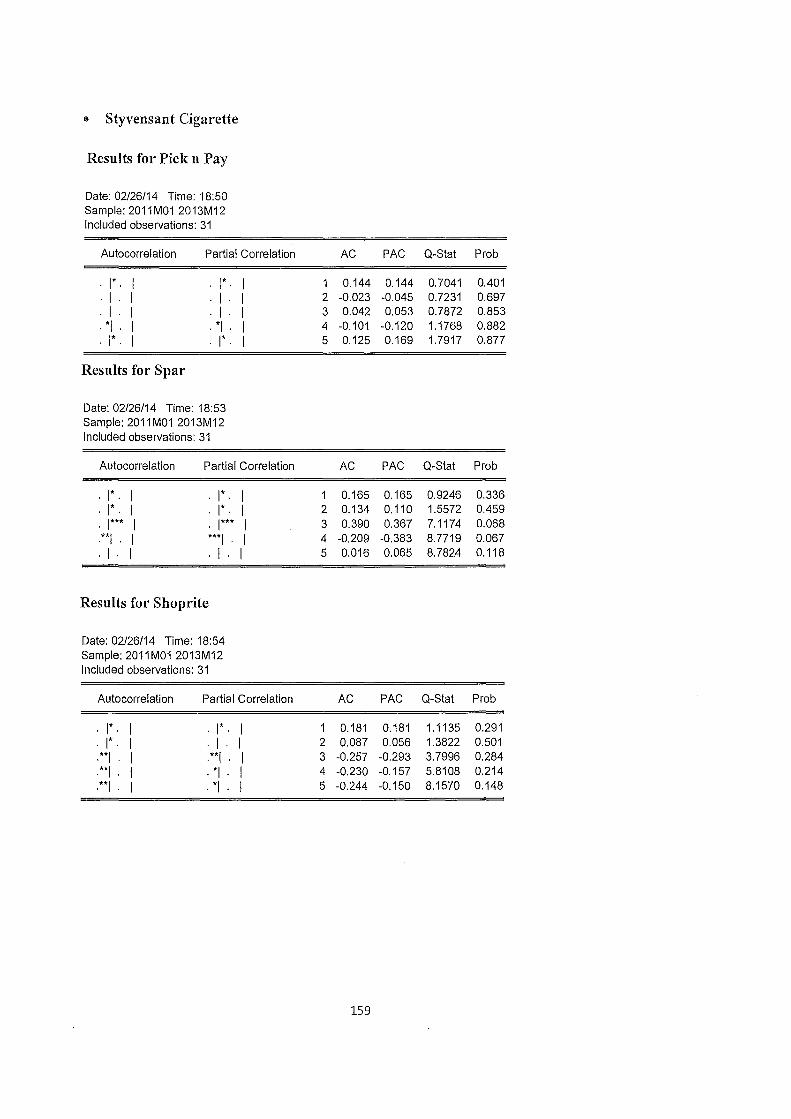
• Styvensant Cigarette
Results for Pick n Pay
Date: 02/26/14 Time: 18:50 Sample: 2011M01 2013M12 Included observations: 31
Autocorrelation Partial Correlation AC PAC Q-Stat Prob
. I*. I . I*. I 0.144 0.144 0.7041 0.401
. I . I . I . I 2 -0.023 -0.045 0.7231 0.697
. I . I . I . I 3 0.042 0.053 0.7872 0.853
. *I . I . *I . I 4 -0.101 -0.120 1.1768 0.882
. I*. I . I*. I 5 0.125 0.169 1.7917 0.877
Results for Spar
Date: 02/26/14 Time: 18:53 Sample: 2011 M01 2013M12 Included observations: 31
Autocorrelation Partial Correlation AC PAC Q-Stat Prob
. I* . I . I* . I 0.165 0.165 0.9246 0.336
. I* . I . I* . I 2 0.134 0.110 1.5572 0.459
. I*** I . I*** I 3 0.390 0.367 7.1174 0.068
.**I . I ***I . I 4 -0.209 -0.383 8.7719 0.067
. I . I . I . I 5 0.016 0.065 8.7824 0.118
Results for Shoprite
Date: 02/26/14 Time: 18:54 Sample: 2011M01 2013M12 Included observations: 31
Autocorrelation Partial Correlation AC PAC Q-Stat Prob
. I* . I . I* . I 1 0.181 0.181 1.1135 0.291
. I* . I . I . I 2 0.087 0.056 1.3822 0.501
.**I . I .**I . I 3 -0.257 -0.293 3.7996 0.284
.**1 I . *I . I 4 -0.230 -0.157 5.8108 0.214
.**1 . I . *I . I 5 -0.244 -0.150 8.1570 0.148
159
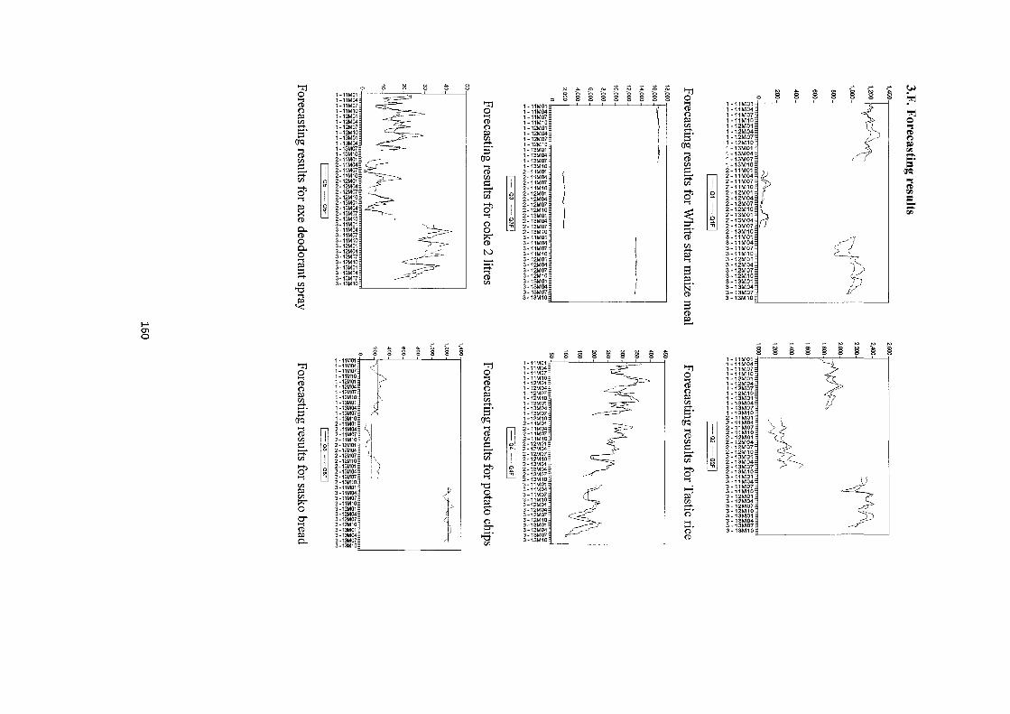
'Tj 0 <5 t5 ~ "' g;
0 1-11M01 ~
i i i 0
§ A "' "' 'Tj
..... 1-11M04
1: § § 8 § § 8 8 8 8 § ~ ~ w
('D 1-11M07 'Tj 0 0 0 0 ~
0 1-11M10 0 1-11M01 ..... 1-11M01
~ 1-12M01 1-11M04
\ ('D 1-11M04
~ fJJ 1-12M04 ..... 1-11M07 0
.--.. 1-12M07 ('D 1-11M10 ~
1-11M07 "!!j
s- 1-12M10 0 1-12M01 fJJ
1-11M10 0
1-13M01 ~ 1-12M04
l .--.. 1-12M01 ""!
(Jq 1-13M04 fJJ 1-12M07 s- 1-12M04 f) .--.. 1-12M07
('D
..... 1-13M07 s- 1-12M10 (Jq 1-12M10 ~
('D 1-13M10 1-13M01 1-13M01
:.:1
fJJ
~ l:ll::ii
~ (Jq 1-13M04 ..... 1-13M04 ~? 1:1.1
::::: 1-13M07 ('D 1-13M07 -
2-11M07 ..... 1-13M10 fJJ
r, ... :::;:' 2-11M10
('D 2-11M01 ::::: 1-13M10 =
fJJ 2-12M01 fJJ
~ 2-11M04
2-11M01
8' 2-12M04 ::::: 2-11M07
:::;:'
~ 2-11M04
(JQ
2-12M07 :::;:' 2-11M10 fJJ 2-11M07 ~
..... 2-12M10 2-12M01 b'
2-11M10
2-13M01 fJJ 2-12M04
2-12M01 1:1.1
~ 2-13M04 b' 2-12M07 ..... 2-12M04 = 2-13M07
2-12M10 2-12M07 2-12M10 -
('D 2-13M10 ' ..... 2-13M01 ~ rz
3-11M01 0 2-13M04 2-13M01
0-. 3-11M04
:li 0
2-13M07 :::;" 2-13M04
('D 3-11M07 2-13M10
2-13M07
0 3-11M10 ?;"' 3-11M01
§-. 2-13M10
0-. 3-12M01 ('D 3-11M04
3-11M01
3-12M04
3-11M04 {i 0 tv 3-11M07 fJJ
..... 3-12M07 3-11M10 s- 3-11M07
~ 3-12M10 - 3-12M01
3-11M10
= 3-13M01 ~ .
-~
3-12M04 ..... 3-12M01
.--.. 3-13M04 3-12M07 s 3-12M04
3-13M07 --- ('D 3-12M10 3-12M07
fJJ 3-13M10 fJJ 3-13M01 ~ 3-12M10
"0 3-13M04 N- 3-13M01 / ..... 3-13M07
3-13M04
~ 3-13M10
('D 3-13M07
s 3-13M10
('D ~ ...... -O'l
0
8 g g g § ~ ~ 8 § 8 gJ § ~ § § § § ~ i § 'Tj
1-11M01 g; 8 s 8 §
1-11M04 'Tj 1-11M01 1-11M01
0 1-11M07 1-11M04 < 1-11M04
} ..... 1-11M10 0 1-11M07 'Tj 1-11M07
('D ~=g~~~ ..... 1-11M10 0 1-11M10
0 ('D 1-12M01 ..... 1-12M01
~ 1-12M07:l 0 1-12M04
('D 1-12M04
fJJ 1-12M10"" ~ 1-12M07 0 1-12M07
.--.. 1-13M01 fJJ 1-12M10 ~ 1-12M10
s- 1-13M04 .--.. 1-13M01 /_;$-
1-13M01
1-13M07 s- 1-13M04 fJJ 1-13M04 .--..
(Jq 1-13M10 1-13M07
,...._ 1-13M07
l::::~ 1 (Jq 1-13M10 = 1-13M10
..... 2-11M01 (Jq
2-11M01
~l> ('D .....
~ '"""" J ~ 2-11M04
fJJ ~ ' '"" ' ('D 2-11M07 ..... 2-11M07
t~J~J? ( fJJ 2-11M10
::::: 2-11M10
('D 2-12M01
:::;:' 2-12M04 ::::: 2-12M01 fJJ 2-12M04 -~~ 2-12M07
1 :::;:' 2-12M04 - = 2-12M07
fJJ 2-12M10 fJJ ~=~~~~ ::;:' 2-12M10
8' 2-13M01§ I ? 8' 2-13M01 __?
fJJ 2-13M01
2-13M04'"' 2-13M04 2-13M04
..... 2-13M073 I ) 8' 2-13M07
..... 2-13M07 2-13M10
2-13M10 2-13M10 fJJ 3-11M01 "0 3-11M01
..... 3-11M01
~ 3-11M04
~ 3-11M04 cr:· 3-11M04
~ fJJ 0 >--3 3-11M07
?;"' 3-11M07 .--.. 3-11M07
3-11M10
3-11M10 ~ 3-11M10 ~ 3-12M01
0 3-12M01 3-12M01
~ fJJ 3-12M04
3-12M04 0 3-12M04 .--.. 3-12M07
cr" 3-12M07 3-12M07 0- 3-12M10 ~$ ..... 3-12M10 0 3-12M10
3-13M01
('D 3-13M01 :::;" 3-13M01 ..... 3-13M04
~ 3-13M04 j -a- 3-13M04 0- 3-13M07
0-. 3-13M07 ... 3-13M07
3-13M1D
3-13M10§ fJJ 3-13M10
('D
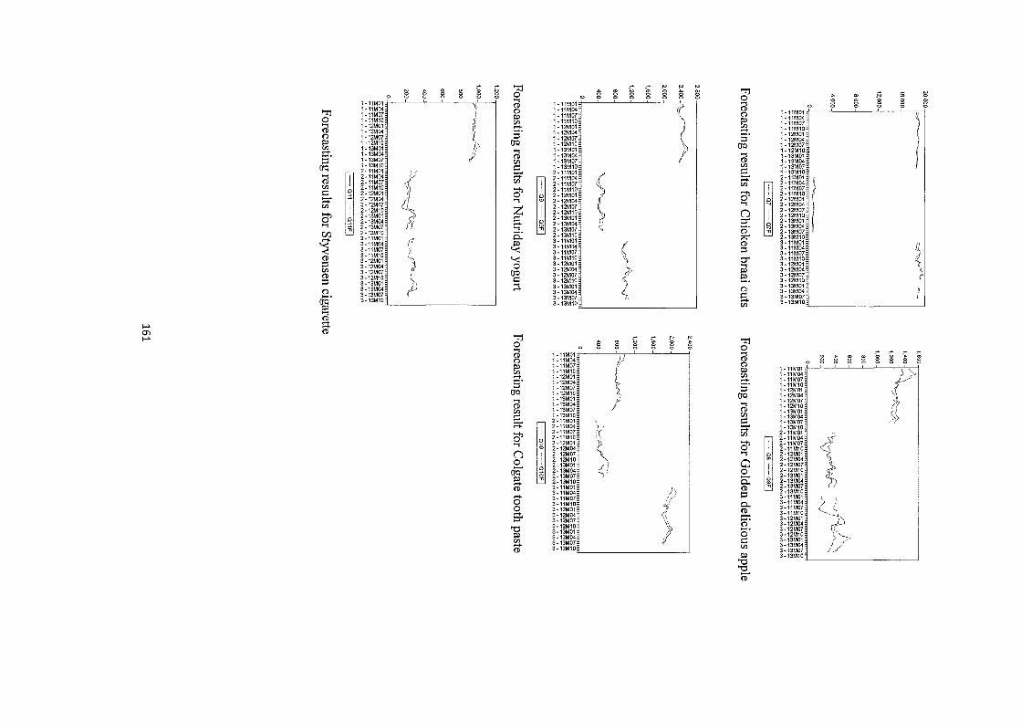
"Tj § "' "' "Tj t5 8 8 8 8 § ~ 8 8 ~ § ~ § .. ~
~ ! 0 0 0 § § § ..... 1 ~11M01 ..... 0 1-11M01
1 (I)
~ (I) 1-11M04 () 1-11M04 () 1-11M01
I "Tj 1-11M07 !;; 1-11M07
!;; 1-11M04 0 1-11M10 {, 1-11M10 1-11M07 ..... 1-12M01
l ...... 1-12M01 ...... 1-11M10 (I) 1-12M04 ::;- 1-12M04
::;- 1-12M01 () 1-12M07 1-12M07 1-12M04 !:l' 1-12M10 (Jq 1-12M10 (Jq 1-12M07 }r' 1-13M01 1-12M10 rJ) 1-13M01 ..... ..... 1-13M01 ...... 1-13M04 jJ (I) 1-13M04
(I) 1-13M04 ::;- 1-13M07 rJ) 1-13M07 rJ) 1-13M07 1-13M10 :::: 1-13M10 :::: 1-13M10
(Jq
~ l11WJ t :::;:' 2-11M01
t :::;:' 2-11M01 .....
rJ)
~ 2-11M04
rJ)
~ 2-11M04 (I) 2-11M07 2-11M07 2-11M07 rJ) 2-11M10
8' 2-11M10
8' 2-11M10 :::: 2-12M01 ) 2-12M01 2-12M01 :::;:' 2-12M04 ..... 2-12M04 ..... 2-12M04 2-12M07 z 2-12M07 2-12M07
rJ) 2-12M10 2-12M10 (1 2-12M10 8' 2-13M01 a 2-13M01 ::r' 2-13M01 2-13M04 2-13M04 a- 2-13M04 ..... 2-13M07 ..... 2-13M07 2-13M07 2-13M10 0.: 2-13M10 :;-;-' 2-13M10 [/). 3-11M01
[ 3-11M01
t (I) 3-11M01
} ......
3-11M04 ~ 3-11M04 := 3-11M04 '-< 3-11M07 3-11M07 3-11M07 < 3-11M10 '-< 3-11M10 0" 3-11M10 (I) 3-12M01 3-12M01 ..... 3-12M01 := 3-12M04
~ 0 3-12M04 !:l' 3-12M04 rJ) 3-12M07 (Jq 3-12M07 !:l' 3-12M07 (I) 3-12M10 :::: 3-12M10 -- 3-12M10
3-13M01 := 3-13M01 :::+ 3-13M01 () 3 -13MD4 () 3-13M04 3-13M04 a 3-13M07 3-13M07 3-13M07 3-13M10 ciO- 3-13M10 3-13M10 rJ)
!:l' ..... (I)
!-> :::+: (I)
"Tj "' "' O'l ..
~ ~ § ~ "Tj !-> 0 0 g g 0 ..... ..... g 8 m g § ~
.. "' (I) 1-11M01
J (I) g g g () 1-11M04 () 0
!:l' 1-11M07 !:l' 1-11M01
rJ) 1-11M10 rJ) 1-11M04
::t- 1-12M01 ...... 1-11M07 1-12M04 ::;- 1-11M10 := 1-12M07 1-12M01 (Jq 1-12M10 (Jq 1-12M04 ..... 1-13M01 ..... 1-12M07
(I) 1-13M04 (I) 1-12M10
1-13M07 1-13M01 rJ) 1-13M10 rJ) 1-13M04 ::::
~ l::::~
~ :::: 1-13M07 :::;:' :::;:' 1-13M10
2-11M07 rJ) 2-11M01 8' 2-11M10
~ ,,,.. 2-12M01 8' 2-11M07 ..... 2-12M04 2-11M10
(1 2-12M07 ..... 2-12M01 2-12M04 0 2-12M10 0 2-12M07 2-13M01 2-12M10 oq 2-13M04 0 2-13M01 2-13M07 0: 2-13M04 ~ 2-13M10
(I) 2-13M07 (I) 3-11M01 f) 2-13M10 3-11M04 := 3-11M01 ...... 3-11M07 0... 3-11M04 0 3-11M10
3-11M07 0 3-12MD1 ~ 3-11M10 st 3-12M04 ...... 3-12M01 3-12M07
/> () 3-12M04
"0 3-12M10 c;- 3-12M07 3-13M01 3-12M10 !:l' 3-13M04 :::: 3-13M01 rJ) 3-13M07 rJ) 3-13M04 ......
3-13M10 3-13M07 (I)
~ 3-13M10
"0 (p'
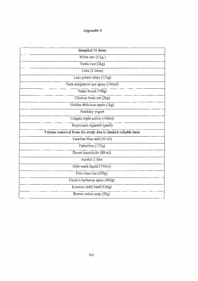
Appendix 4
Sampled 11 items
White star ( 5 kg )
Tastic rice (2kg)
Coke (2 litres)
Lays potato chips (125g)
Dark temptation axe spray (lOOml)
Sasko bread (700g)
Chicken braai cut (2kg)
Golden delicious apple (lkg)
Nutriday yogurt
Colgate triple action (1 OOml)
Stuyvesant cigarette (pack)
9 items removed from the study due to limited reliable data
Vaseline blue seal (50 ml)
Palmolive (175g)
Doom insecticide (80 ml)
Sunfoil 2 litre
Dish wash liquid (750ml)
Five roses tea (250g)
Uncle's barbecue spice (400g)
Knorrox chilli beef (120g)
Brown onion soup (50g)
162
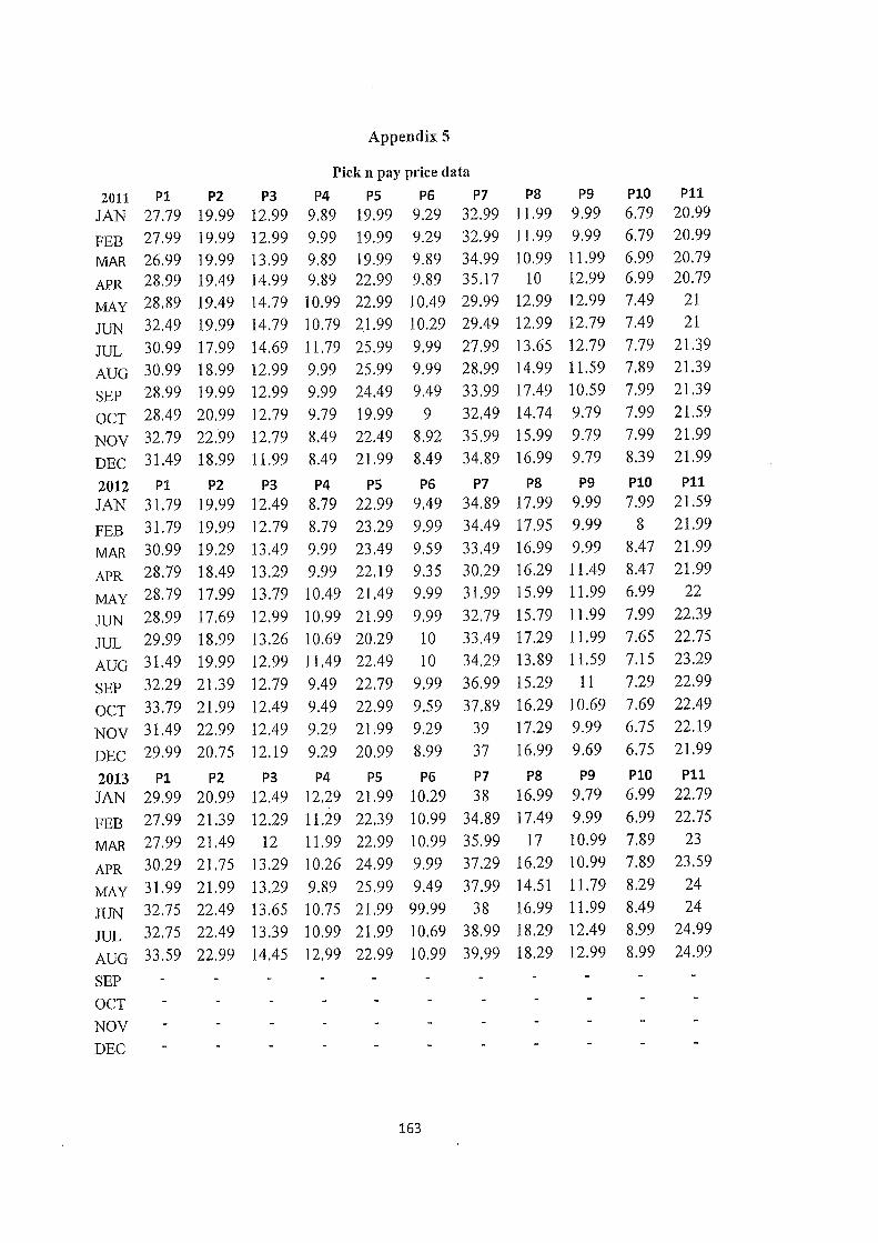
Appendix 5
Pick n pay price data
2011 P1 P2 P3 P4 PS P6 P7 P8 P9 P10 P11 JAN 27.79 19.99 12.99 9.89 19.99 9.29 32.99 11.99 9.99 6.79 20.99 FEB 27.99 19.99 12.99 9.99 19.99 9.29 32.99 11.99 9.99 6.79 20.99 MAR 26.99 19.99 13.99 9.89 19.99 9.89 34.99 10.99 11.99 6.99 20.79 APR 28.99 19.49 14.99 9.89 22.99 9.89 35.17 10 12.99 6.99 20.79 MAY 28.89 19.49 14.79 10.99 22.99 10.49 29.99 12.99 12.99 7.49 21 JUN 32.49 19.99 14.79 10.79 21.99 10.29 29.49 12.99 12.79 7.49 21 JUL 30.99 17.99 14.69 11.79 25.99 9.99 27.99 13.65 12.79 7.79 21.39 AUG 30.99 18.99 12.99 9.99 25.99 9.99 28.99 14.99 11.59 7.89 21.39 SEP 28.99 19.99 12.99 9.99 24.49 9.49 33.99 17.49 10.59 7.99 21.39 OCT 28.49 20.99 12.79 9.79 19.99 9 32.49 14.74 9.79 7.99 21.59 NOV 32.79 22.99 12.79 8.49 22.49 8.92 35.99 15.99 9.79 7.99 21.99 DEC 31.49 18.99 11.99 8.49 21.99 8.49 34.89 16.99 9.79 8.39 21.99
2012 P1 P2 P3 P4 PS P6 P7 P8 P9 P10 P11 JAN 31.79 19.99 12.49 8.79 22.99 9.49 34.89 17.99 9.99 7.99 21.59 FEB 31.79 19.99 12.79 8.79 23.29 9.99 34.49 17.95 9.99 8 21.99 MAR 30.99 19.29 13.49 9.99 23.49 9.59 33.49 16.99 9.99 8.47 21.99 APR 28.79 18.49 13.29 9.99 22.19 9.35 30.29 16.29 11.49 8.47 21.99 MAY 28.79 17.99 13.79 10.49 21.49 9.99 31.99 15.99 11.99 6.99 22 JUN 28.99 17.69 12.99 10.99 21.99 9.99 32.79 15.79 11.99 7.99 22.39 JUL 29.99 18.99 13.26 10.69 20.29 10 33.49 17.29 11.99 7.65 22.75 AUG 31.49 19.99 12.99 11.49 22.49 10 34.29 13.89 11.59 7.15 23.29 SEP 32.29 21.39 12.79 9.49 22.79 9.99 36.99 15.29 11 7.29 22.99 OCT 33.79 21.99 12.49 9.49 22.99 9.59 37.89 16.29 10.69 7.69 22.49 NOV 31.49 22.99 12.49 9.29 21.99 9.29 39 17.29 9.99 6.75 22.19 DEC 29.99 20.75 12.19 9.29 20.99 8.99 37 16.99 9.69 6.75 21.99
2013 P1 P2 P3 P4 PS P6 P7 P8 P9 P10 P11 JAN 29.99 20.99 12.49 12.29 21.99 10.29 38 16.99 9.79 6.99 22.79 FEB 27.99 21.39 12.29 11.29 22.39 10.99 34.89 17.49 9.99 6.99 22.75 MAR 27.99 21.49 12 11.99 22.99 10.99 35.99 17 10.99 7.89 23 APR 30.29 21.75 13.29 10.26 24.99 9.99 37.29 16.29 10.99 7.89 23.59
MAY 31.99 21.99 13.29 9.89 25.99 9.49 37.99 14.51 11.79 8.29 24 JUN 32.75 22.49 13.65 10.75 21.99 99.99 38 16.99 11.99 8.49 24 JUL 32.75 22.49 13.39 10.99 21.99 10.69 38.99 18.29 12.49 8.99 24.99 AUG 33.59 22.99 14.45 12.99 22.99 10.99 39.99 18.29 12.99 8.99 24.99
SEP
OCT NOV DEC
163
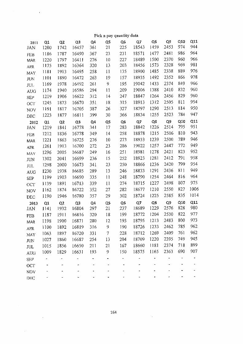
Pick n pay quantity data
2011 Ql Q2 Q3 Q4 QS QG Q7 Q8 Q9 QlO Qll
JAN 1200 1742 16457 361 21 225 18543 1459 2453 974 944
FEB 1186 1787 16490 367 23 231 18571 1477 2481 986 964 MAR 1220 1797 16411 276 10 227 18489 1500 2370 960 966 APR 1175 1892 16364 320 13 203 18456 1573 2328 969 981 MAY 1181 1913 16495 258 11 135 18900 1485 2338 889 976 JUN 1101 1890 16472 263 19 157 18935 1492 2352 866 978 JUL 1169 1978 16492 261 9 195 19042 1433 2374 849 966
AUG 1174 1940 16586 294 11 209 19006 1388 2410 832 960
SEP 1219 1906 16622 312 14 OCT 1245 1873 16670 351 18
NOV 1191 1817 16705 387 26 DEC 1223 1877 16811 399 30
2012 Ql Q2 Q3 Q4 QS
JAN 1219 1841 16778 341 17
FEB 1212 1836 16778 349 14 MAR 1221 1863 16725 276 10 APR 1261 1913 16700 272 23 MAY 1296 2005 16687 249 16
JUN 1302 2041 16699 236 15 JUL 1298 2000 16673 341 23
AUG 1230 1938 16685 289 13 SEP 1199 1903 16690 335 11
OCT 1139 1891 16713 339 11 NOV 1162 1874 16722 352 27
DEC 1190 1946 16780 357 29
2013 Ql
JAN 1141
FEB 1187 MAR 1198 APR 1100
:MAY 1063 JUN 1027
JUL 1015
AUG 1009
SEP
OCT
NOV DEC
Q2 Q3 Q4
1932 16804 297
1911 16816 320 1900 16871 280 1892 16819 316
1897 16720 331 1860 16687 254 1856 16650 211
1829 16631 193
QS
21
18 12
9 7 13
21
9
164
24 7 1884 7 1264 2456 829 960 315 18913 1312 2505 811 954
327 18797 1290 2513 814 950 366 18834 1255 2523 784 947
QG Q7 Q8 Q9 QlO Qll
283 18842 1226 2514 795 951
258 18878 1215 2506 810 943 273 18933 1239 2500 789 946 286 19022 1257 2447 772 949 251 18981 1278 2421 823 952
252 18923 1281 2412 791 958 250 18866 1236 2420 799 954
246 18833 1291 2436 811 949
248 18790 1254 2464 816 964
274 18715 1227 2498 807 975 282 18677 1210 2550 827 1006 302 18724 1225 2585 835 1014
QG
237
199 193 190
228 204
167 150
Q7 Q8 Q9 QlO Qll
18689 1229 2576 828 980 18772 1204 2530 822 977 18795 1213 2483 800 973 18726 1233 2462 785 962
18712 1269 2409 761 962 18709 1220 2395 749 945
18660 1181 2374 718 899 18575 1165 2363 690 907

Spar price data
2011 P1 P2 P3 P4 PS P6 P7 P8 P9 P10 P11 JAN 28.92 20.25 14.99 8.99 22 9.85 34.29 14.19 9.99 6.92 25 FEB 28.92 20.25 16.99 8.99 22 9.85 34.49 14.19 9.99 6.92 25 MAR 28.92 20.25 16.99 8.99 22 10.29 37 13.99 12.49 6.92 25 APR 29.65 19.75 14.99 9.99 23.99 10.29 34.99 14.63 13.49 6.92 25.99 MAY 32.95 19.75 14.99 9.45 23.99 9.89 32.19 13.41 13.49 7.51 25.99 JUN 32.49 19.75 14.99 9.99 23.99 9.89 31.29 13.41 13.49 7.51 25.99 JUL 28.9 17.99 14.21 8.99 25.99 9.85 29.99 15.99 13.49 8.52 27 AUG 27 18.99 13.79 8.99 25.99 9.85 34.49 15.99 12.45 8.52 27
SEP 27 20.15 13.79 8.99 24 9.85 35.39 17.99 12.45 8.52 27
OCT 29.99 20.99 13.29 10.45 24 9.85 37.17 16.99 9.99 .8 25.45
NOV 32 18.99 13.79 10.45 22.79 10 37.99 15.99 9.99 8 . 25.45
DEC 31 18.99 13.17 9.99 22.79 10 37.99 15.99 9.99 7.99 25.45
2012 P1 P2 P3 P4 PS P6 P7 P8 P9 P10 P11 JAN 32.92 19.99 13 10.99 23.71 10.49 36.99 17.99 12.45 7.99 25.99 FEB 32.99 19.99 13 9.99 23.71 10.49 36.99 17.79 12.45 7.45 25.99 MAR 32.99 19.79 14.45 9.99 23.49 9.85 34.99 15.99 13.49 8.79 25.99 APR 32.95 18.99 14.45 9.99 24 9.85 34.79 15.99 13.49 8.79 27 MAY 32.95 17.99 16.95 10.45 24 9.85 31.99 14.95 13.49 8.99 27 JUN 33.99 17.99 16.95 10.45 24 9.99 32.99 14.95 13.99 7.89 27 JUL 33.99 17.99 13.99 10.45 24.29 11.69 32.99 15.99 13.99 7.89 27.49 AUG 34.79 19.99 13.45 12.99 24.29 11.69 34.29 13.99 13.99 7.89 27.49 SEP 34.79 21.49 13.45 12.74 23.99 11.45 35 13.99 12.99 6.99 27.49 OCT 35 21.49 13 12.74 22.99 9.99 35 18.99 12.49 6.99 22.49 NOV 33.37 18.99 12.99 9.99 21.35 9.99 37.99 18.99 9.99 6.99 22.19 DEC 33.37 18.99 12.99 9.99 21.35 9.89 37.99 15.99 9.99 6.99 21.99
2013 P1 P2 P3 P4 PS P6 P7 P8 P9 P10 P11 JAN 28.99 20.25 13.17 9.99 24 9.99 38 19.99 9.99 6.99 22.79 FEB 28.99 20.25 13.17 10.98 24.19 10.49 37.99 19.99 12.99 7.65 25.99 MAR 28.99 21.49 13.99 10.98 25.29 10.49 34.99 14.99 12.99 7.65 25.99 APR 33.79 18.99 14.95 11 25.29 10.89 34.99 14.99 12.49 8.69 24.49 MAY 34.79 18.99 14.95 12.49 25.99 10.39 35.45 14.99 12.49 8.69 27 JUN 34.79 17.99 14.99 12.89 22.99 10.45 35.75 17.74 13.49 6.99 27.49 JUL 35.59 19.99 14.99 12.89 22.99 10.45 35.49 17.14 12.14 6.99 27.49 AUG 35.59 20.39 14.99 12.99 22.99 10.69 36.48 17.59 11 7.32 28.49
SEP OCT NOV DEC
165

2011 Ql JAN 50
FEB 66
MAR 61
APR 43
MAY 36 JUN 30
JUL 59
AUG 86
SEP 88
OCT 65
NOV 53
DEC 65
2012 Ql JAN 58
FEB 57
MAR 57
APR 60
MAY 61
JUN 47
JUL 44
AUG 39
SEP 34
OCT 30
NOV 46
DEC 63
2012 Ql JAN 88
FEB 101
MAR 116
APR 91
MAY 82 JUN 84
JUL 76
AUG 64
SEP
OCT
NOV
DEC
Spar sales data
Q2 Q3 Q4
1127 1912 266
1130 1864 306
1125 1862 337
1147 1900 328
1159 1909 281
1166 1917 274
1211 1928 308
1180 1959 300
1156 1966 318
1120 2003 260
1190 1960 249
1225 2011 256
Q2 Q3 Q4 1200 2009 245
1208 2019 267
1219 1936 276
1288 1930 288
1340 1845 269
1372 1841 266
1411 1953 272
1366 2000 190
1314 2004 188
1322 2045 192
1390 2049 226
1453 2066 257
Q2 Q3 Q4 1391 2052 272
1380 2048 253
1358 1990 253
1432 1922 244
1500 1914 210
1550 1899 199
1515 1899 186
1493 1894 162
QS
9 4
3 2
2
6 4 1 8
13
17
19
QS
11 7 9 6 3 4 4 3 7 9 12
16
QS
9 12
4 6
3
8
11
15
166
QG 78
82
65
57
100
112
123
133
134
134
97
91
QG 88
76
91
104
118 114
108
197
200
222
246
268
QG 272
268
253
231
256
248
251
237
Q7 Q8 970 393
967 392
896 402
934 297
982 312
1008 343
1045 260
931 248
903 185
864 196
653 231
641 315
Q7 Q8 674 285
678 276
715 292
731 309
790 324
753 319
721 331
685 374
679 401
650 333
598 299
582 358
Q7 Q8 587 314
579 302
612 380
625 418
611 412
607 399
618 388
598 364
Q9 QlO Q11 482 336 320
520 366 299
485 370 307
447 408 290
403 394 247
378 392 249
349 367 212
391 351 187
444 358 196
482 362 216
526 380 221
560 406 228
Q9 QlO Q11 520 418 215
489 423 224
444 409 226
437 393 207
451 381 187
435 445 191
426 493 167
416 477 153
430 513 168
437 567 245
488 606 271
502 614 306
Q9 QlO Q11
522 610 312
501 617 289
506 605 283
511 596 291
498 584 267
493 605 272
509 612 266
516 601 254
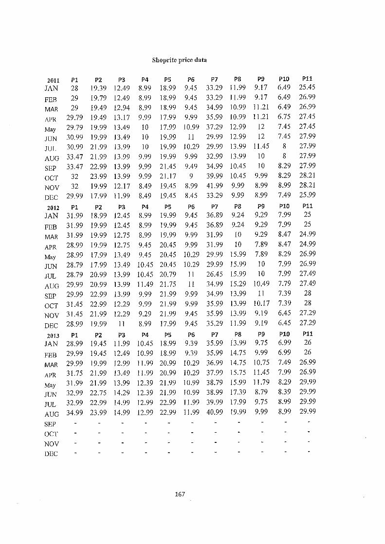
Shoprite price data
2011 Pl P2 P3 P4 PS P6 P7 P8 P9 PlO Pll JAN 28 19.39 12.49 8.99 18.99 9.45 33.29 11.99 9.17 6.49 25.45 FEB 29 19.79 12.49 8.99 18.99 9.45 33.29 11.99 9.17 6.49 26.99 MAR 29 19.49 12.94 8.99 18.99 9.45 34.99 10.99 11.21 6.49 26.99 APR 29.79 19.49 13.17 9.99 17.99 9.99 35.99 10.99 11.21 6.75 27.45 May 29.79 19.99 13.49 10 17.99 10.99 37.29 12.99 12 7.45 27.45 JUN 30.99 19.99 13.49 10 19.99 11 29.99 12.99 12 7.45 27.99 JUL 30.99 21.99 13.99 10 19.99 10.29 29.99 13.99 11.45 8 27.99 AUG 33.47 21.99 13.99 9.99 19.99 9.99 32.99 13.99 10 8 27.99 SEP 33.47 22.99 13.99 9.99 21.45 9.49 34.99 10.45 10 8.29 27.99 OCT 32 23.99 13.99 9.99 21.17 9 39.99 10.45 9.99 8.29 28.21 NOV 32 19.99 12.17 8.49 19.45 8.99 41.99 9.99 8.99 8.99 28.21 DEC 29.99 17.99 11.99 8.49 19.45 8.45 33.29 9.99 8.99 7.49 25.99
2012 Pl P2 P3 P4 PS P6 P7 P8 P9 PlO Pll
JAN 31.99 18.99 12.45 8.99 19.99 9.45 36.89 9.24 9.29 7.99 25
FEB 31.99 19.99 12.45 8.99 19.99 9.45 36.89 9.24 9.29 7.99 25
MAR 31.99 19.99 12.75 8.99 19.99 9.99 31.99 10 9.29 8.47 24.99
APR 28.99 19.99 12.75 9.45 20.45 9.99 31.99 10 7.89 8.47 24.99 May 28.99 17.99 13.49 9.45 20.45 10.29 29.99 15.99 7.89 8.29 26.99 JUN 28.79 17.99 13.49 10.45 20.45 10.29 29.99 15.99 10 7.99 26.99 JUL 28.79 20.99 13.99 10.45 20.79 11 26.45 15.99 10 7.99 27.49 AUG 29.99 20.99 13.99 11.49 21.75 11 34.99 15.29 10.49 7.79 27.49 SEP 29.99 22.99 13.99 9.99 21.99 9.99 34.99 13.99 11 7.39 28 OCT 31.45 22.99 12.29 9.99 21.99 9.99 35.99 13.99 10.17 7.39 28 NOV 31.45 21.99 12.29 9.29 21.99 9.45 35.99 13.99 9.19 6.45 27.29 DEC 28.99 19.99 11 8.99 17.99 9.45 35.29 11.99 9.19 6.45 27.29
2013 Pl P2 P3 P4 PS P6 P7 P8 P9 PlO Pll JAN 28.99 19.45 11.99 10.45 18.99 9.39 35.99 13.99 9.75 6.99 26 FEB 29.99 19.45 12.49 10.99 18.99 9.39 35.99 14.75 9.99 6.99 26 MAR 29.99 19.99 12.99 11.99 20.99 10.29 36.99 14.75 10.75 7.49 26.99 APR 31.75 21.99 13.49 11.99 20.99 10.29 37.99 15.75 11.45 7.99 26.99 May 31.99 21.99 13.99 12.39 21.99 10.99 38.79 15.99 11.79 8.29 29.99 JUN 32.99 22.75 14.29 12.39 21.99 10.99 38.99 17.39 8.79 8.39 29.99 JUL 32.99 22.99 14.99 12.99 22.99 11.99 39.99 17.99 9.75 8.99 29.99
AUG 34.99 23.99 14.99 12.99 22.99 11.99 40.99 19.99 9.99 8.99 29.99
SEP OCT NOV
DEC
167

Shoprite sales data
2011 Ql Q2 Q3 Q4
JAN 1023 2262 13100 232
FEB 966 2258 13111 220 MAR 958 2264 13177 218 APR 871 2260 13150 204 MAY 883 2273 13112 187 JUN 826 2281 13109 171 JUL 814 2200 13062 166 AUG 853 2180 13058 163 SEP 864 2100 13053 163 OCT 817 1996 13056 170 NOV 810 2321 13174 195 DEC 1077 2400 13208 214
2012 Ql Q2 Q3 Q4
JAN 1037 2381 13259 200 FEB 1033 2322 13262 198 MAR 1046 2311 13248 195
APR 1089 2323 13244 171 MAy 1116 23 7 6 13182 166
JUN 1133 2411 13175 134 JUL 1137 2340 13146 117 AUG 1107 2342 13138 109 SEP 1083 2289 13133 127 OCT 1036 2271 13219 151 NOV 1016 2325 13227 186 DEC 1103 2399 13311 225
QS Q6 Q7 Q8 Q9 QlO Qll
29 1231 18714 200 1080 2051 290 31 1257 18689 197 1091 2081 240 31 1249 18560 231 1053 2076 243 38 1221 18593 247 1039 2109 227 43 1186 18420 217 982 2094 231 39 1143 19113 194 977 2069 237 35 1170 19182 183 964 1998 246 34 1193 18985 157 993 1975 246 30 1236 18600 200 1017 1953 239 27 1264 18412 263 1031 1966 233 36 1266 18376 332 1072 1888 229 41 1292 19200 461 1126 1915 259
QS Q6 Q7 Q8 Q9 QlO Qll
37 1215 19032 501 1099 1891 273 38 1219 19003 519 1100 1877 284
38
35 33 39 32 26 22 19 22 37
1196 19347 530
1190 19388 531 1201 19530 400 1198 19611 388 1165 19719 380 1161 19309 391 1218 19225 443 1222 19187 460 1250 19158 500 1256 19145 611
1103 1820 303
1208 1794 312 1230 1811 288 1150 1843 292 1137 1851 281 1084 1872 287 993 1897 255 999 1913 257 1075 1930 266 1120 1986 291
2013 Ql Q2 Q3 Q4 QS Q6 Q7 Q8 Q9 QlO Qll
JAN 1111 2406 13364 212 30 1259 19153 576 1097 1930 321 FEB 1101 2401 13213 212 27 1258 19150 521 1105 1911 325
MAR 1096 2397 13155 183 24 1233 19115 514 1062 1888 325
APR 1047 2309 13103 180 26 1232 19075 490 990 1851 319
MAY 1040 2283 13080 151 20 1214 18866 465 984 1837 260
JUN 1000 2217 13063 146 23 1219 18841 431 1133 1831 217
JUL 1006 2169 13025 98 18 1169 18810 419 1145 1812 221
AUG 960 2100 13011 103 15 1164 18757 360 1132 1789 227
SEP
OCT
NOV
DEC
168

Top Related
Copyright © 2022 FDOKUMEN

