arX

iv:a

stro

-ph/

0002

512v

1 2

9 Fe

b 20

00

The Detection of Multimodal Oscillations on α UMa

D. Buzasi

Space Sciences Laboratory, University of California, Berkeley, CA 94720

J. Catanzarite, R. Laher, T. Conrow, D. Shupe

Infrared Processing and Analysis Center, California Institute of Technology, MS 100-22,

Pasadena, CA 91125

T. N. Gautier III

Jet Propulsion Laboratory, California Institute of Technology, MS 100-22, Pasadena, CA 91125

T. Kreidl

Information Technology Services and Department of Physics and Astronomy, Box 5100, Northern

Arizona University, Flagstaff, AZ 86011

and

D. Everett

NASA/Goddard Space Flight Center, Greenbelt, MD 20771

ABSTRACT

We have used the star camera on the WIRE satellite to observe the K0 III star

α UMa, and we report the apparent detection of 10 oscillation modes. The lowest

frequency mode is at 1.82 µHz, and appears to be the fundamental mode. The mean

spacing between the mode frequencies is 2.94 µHz, which implies that all detected

modes are radial. The mode frequencies are consistent with the physical parameters of

a K0 III star, if we assume that only radial modes are excited. Mode amplitudes are

100 − 400 µmag, which is consistent with the scaling relation of Kjeldsen & Bedding

(1995).

Subject headings: star — oscillations: stars — individual

1. Introduction

Over the past few decades, our understanding of the interior of the Sun – its thermodynamic

structure, internal rotation, and dynamics – has been revolutionized by the technique of

helioseismology, the study of the frequencies and amplitudes of seismic waves that penetrate deep

into the solar interior (Leibacher et al. 1985; Duvall et al. 1988; Schou et al. 1998). The high

– 2 –

quality of the modeling in the solar case is made possible by the large number (≈ 107) of modes

visible in the Sun. Unfortunately, the lack of spatial resolution inherent in stellar observations

limits the number of detectable modes in stars to only a few (those with low degree l). Nonetheless,

successful detection of even a few modes has the potential to provide greatly improved values for

fundamental stellar parameters such as mass, abundance, and age (Gough 1987; Brown et al.

1994)

While oscillations have been successfully detected on roAp stars, δ Scuti stars, and white

dwarfs, these stars all show oscillation amplitudes several orders of magnitude larger than is

expected from solar-like stars. More recently, however, a number of authors (Hatzes & Cochran

1994a, 1994b; Edmonds & Gilliland 1996) have reported the detection of periodic variability at

levels of a few hundred m s−1 and/or several millimagnitudes in a number of K giants. However,

each detection is of only a single mode, and multimodal oscillations have yet to be unambiguously

detected in any cool star other than the Sun.

In March 1999, NASA launched the Wide-Field Infrared Explorer satellite, with the intent

of carrying out an infrared sky survey to better understand galaxy evolution. Unfortunately,

within days of launch the primary science instrument on WIRE failed due to loss of coolant.

However, the satellite itself continues to function nearly perfectly, and in May we began a program

of asteroseismology using the WIRE’s onboard 52 mm aperture star camera. Below we report

WIRE’s probable detection of multimodal oscillations on a cool star, which is the first of its kind.

2. Instrument Description and Data Reduction Technique

The WIRE satellite star camera, a Ball Aerospace model CT-601, consists of a 512 × 512

SITe CCD with 27µm pixels (1 arc minute on the sky) and gain of 15 e−/ADU, fed by a 52 mm,

f/1.75 refractive optical system. The read noise of the system is 30 electrons. The pixel data is

digitized with a 16 bit ADC, and up to five 8 × 8 pixel fields can be digitized and transmitted to

the ground. For this work, we used only one field, which permitted us to read out the CCD at a

rate of 10 Hz. The stellar image is somewhat defocused, but essentially all of the light falls on the

central 2 × 2 pixel spot. The spectral response of the system is governed entirely by the response

of the CCD plus the optical system, and is approximately equivalent to the V+R bandpass.

The WIRE satellite is in a sun-synchronous orbit which, when combined with constraints

imposed by the solar panels, limits pointing to two strips, each approximately ±30◦ wide, located

perpendicular to the Earth-Sun line. In addition, continuous observing is not possible. Early in

the program, we were able to obtain only 7 or 8 minutes worth of data during every 96-minute

orbit. Later, after viewing constraints were relaxed (which involved scheduling software and

onboard data-table modifications), observing efficiency rose to as much as 40 minutes per target

per orbit – up to two targets are possible during any orbit. Thus, with integrations every 0.1 s, we

acquired continuous data segments of up to 24,000 observations.

– 3 –

Bias correction was performed on board the satellite, and further data reduction was

accomplished using software developed at IPAC. Each 8 × 8 pixel field was extracted by summing

the flux in the central 4 × 4 pixel region. Although scattered light in the field is limited by the

one-meter sun-shield mounted on the star camera, we performed a background subtraction using

the flux from a 20-pixel octagonal annulus surrounding the central region of the image. Finally,

we converted our fluxes to an instrumental magnitude. After removal of thermal effects (see

below), the rms noise in the final reduced time series was typically comparable to the 1.8 mmag

noise expected from pure photon statistics, although non-Poisson noise is certainly present as well.

The lack of a good flat field for the instrument was a concern, which we dealt with by rejecting

those frames in which the mean centroid of the stellar image lay more than 4σ from the mean

position, where σ is the mean standard deviation of the image centroid. This criterion applied

to approximately 3.8% of the observations, and the vast majority of these observations were at

the start or end of an orbital segment. Overall, the satellite displayed excellent attitude stability

during our run, with σ measured to be typically 0.7 arc sec or less (Laher et al. 2000).

3. Observations and Data Analysis

α UMa was the primary target for WIRE from 18 May through 23 June 1999. It is a K0 III

star (Taylor 1999) with an angular diameter of 6.79 mas (Hall 1996; Bell 1993). At the Hipparcos

distance of 38 pc, this corresponds to a stellar radius of 28 R⊙, in substantial agreement with the

earlier value of 25 R⊙ derived by Bell (1993). The effective temperature of the star is variously

reported as Te = 3970 K to Te = 4660 K (Cayrel de Stroebel 1992), with the latter value being

the most recent (Taylor 1999).

α UMa is a member of a binary system, with a total system mass of 5.94 M⊙ (Soderhjelm

1999). The spectral type of α UMa B is somewhat unclear, with F7 V most often cited in the

literature (see, e.g., the SAO catalog). However, on the basis of IUE observations, Kondo, Morgan,

& Modisette (1977) estimate the secondary to be “late A” (see also Ayres, Marstad, & Linsky

1981). In either case, however, the secondary makes only a small contribution (≈ 6%) to the

total system luminosity, and should show oscillation frequencies quite different from those of the

primary.

During the observation period, WIRE made a total of 4, 036, 448 observations of α UMa,

after removal of those observations with poor pointing characteristics. The data were first phased

at the period of the spacecraft, to determine if any obvious instrumental periodicities existed.

This phasing showed the existence of a strong sinusoidal variation, with amplitude ≈ 8 mmag. A

thermistor is mounted on the star camera, and examination of data from this thermistor showed

that these variations were in fact correlated with temperature variations of a few tenths of a

degree. Although a thermoelectric cooler (TEC) is mounted on the CCD, the star tracker thermal

design lowered the CCD temperature below the default setpoint, so the TEC never actually

turned on. In order to reduce the impact of this signal on our data analysis, we prewhitened the

– 4 –

data by fitting and subtracting from the entire time series a sinusoid constrained to have the

satellite orbital period (the phase was allowed to vary). The best-fit sinusoid has an amplitude of

8.63 mmag, and its subtraction results in an rms residual of 2.05 mmag, compared to the 1.84

mmag expected from photon statistics. We also explored other means of fitting and removing

the thermal signature, including high-order polynomial fits to the phased data. Such approaches,

while more complex than sine fitting, did not lead to any appreciable improvement in the fit, and

were therefore discarded. The use of any of these thermal fitting procedures did not affect the

peaks in the amplitude spectrum described below. In fact, these peaks were visible even before

the application of any fit to the thermal variation, though removal of the thermal signature, by

removing the largest single peak, did help to render them more easily visible.

Data from the first portion of the run (18 May - 7 June) were all in short (t < 8 minutes)

segments, which obviously extended over a short range of orbital phase (≈ 0.08). We were

concerned that including these data in our sine fit would bias the result, so we decided to exclude

them from our analysis. In addition, NASA responded to our expressed concern about the TEC

by lowering the set point on 18 June, and the CCD behavior subsequent to this had not yet

reached an equilibrium point before the end of our run. Thus, we excluded data taken after

18 June from the analysis as well, leaving only the 8 June – 18 June window of approximately

9.2 × 105 s. Shortening the time series clearly adversely affects our frequency resolution, but we

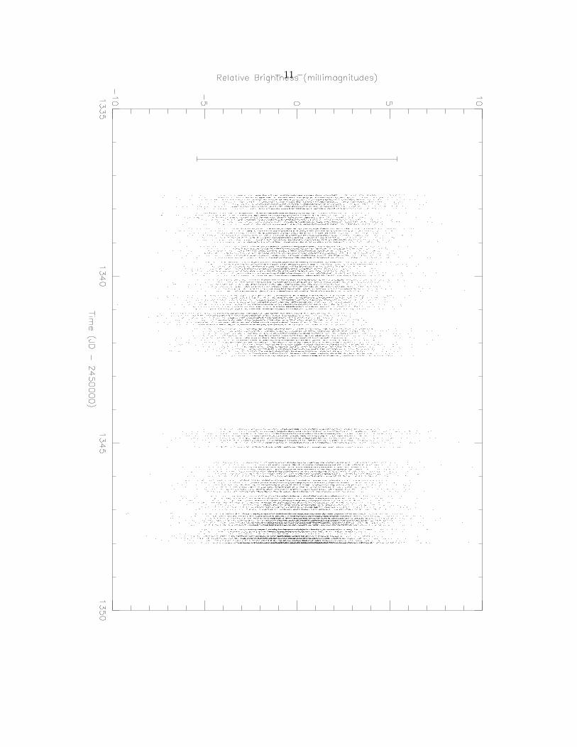
felt that confidence in the data quality was the overriding issue. The data that were subjected to

analysis are shown in Figure 1, after removal of the thermal variation.

Data were searched for periodicities using Discrete Fourier Transform (DFT; Foster 1996),

Lomb-Scargle periodogram (Scargle 1982; Horne & Baliunas 1986), and epoch-folding techniques

(Davies 1990) which are essentially equivalent to phase dispersion modulation (PDM; see

Stellingwerf 1978; Schwarzenberg-Czerny 1998). The Scargle periodogram analysis was conducted

as described in Scargle (1982; see also Hatzes & Cochrane 1994ab); the data were windowed using

a Parzen function and the resulting periodogram was oversampled by a factor of 8 in frequency

space. The DFT analysis was similarly oversampled, and implemented the CLEAN algorithm of

Roberts, Lehar, & Dreher (1987) to remove alias peaks. When using the DFT, the data were

windowed using a Parzen function, and 100 iterations of CLEAN were performed. Due to its

relative slowness, epoch-folding analysis was conducted only within the frequency range of interest,

as identified by the Scargle and DFT analysis, and was used only to aid in interpretation of the

results from the other two algorithms. In the discussion that follows, we will concentrate on the

Lomb-Scargle periodogram results, though, in general, the three techniques gave similar results.

Figure 2 shows the window function for the time series. The upper frequency limit for the

figure has been arbitrarily set at 5 mHz to enhance the visibility of the amplitude spectrum at

frequencies near 1 mHz, while the lowest frequencies are shown in the inset. No significant features

are present in the window function above 5 mHz. The large evenly spaced peaks correspond to the

satellite orbital frequency and its aliases.

– 5 –

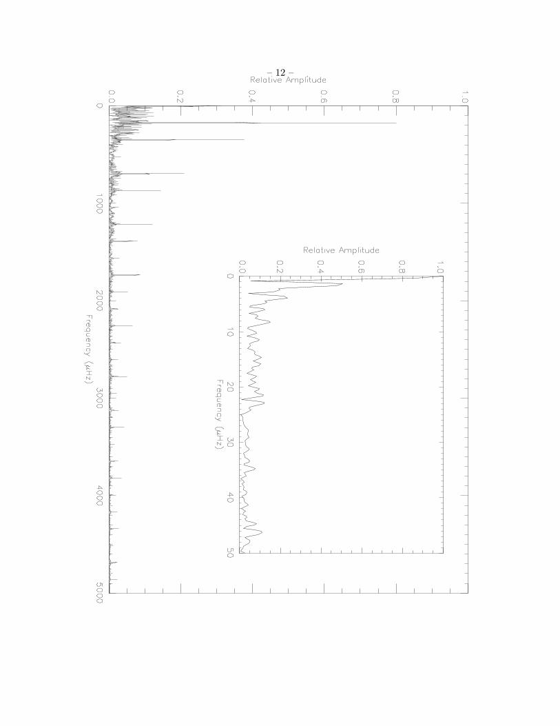
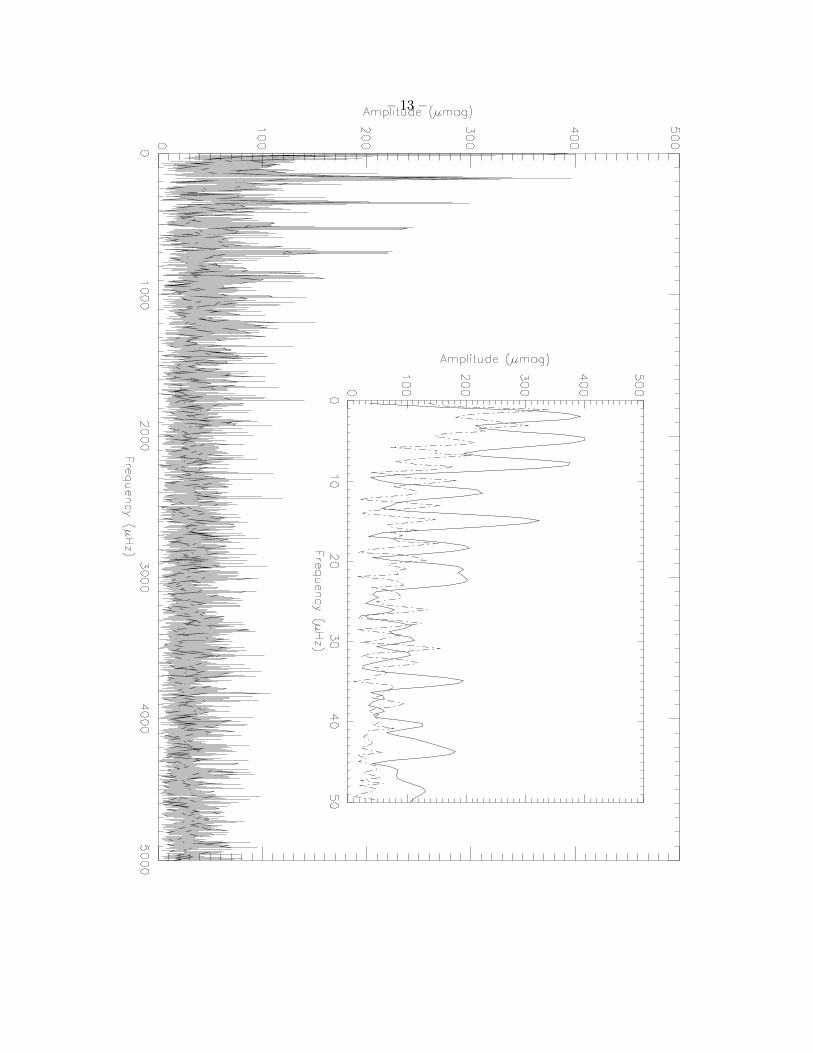
The Lomb-Scargle periodogram for the time series is shown in Figure 3 on the same frequency

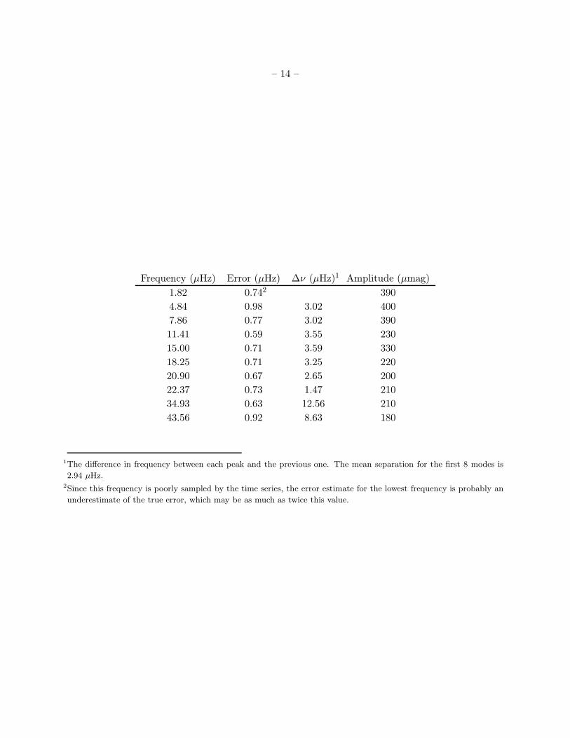
scale as the window function. The low-frequency inset shows ten significant peaks, and the

frequencies and amplitudes of these peaks are given in Table 1 (derived from Lorentzian fits), along

with conservative formal error estimates derived from the half-width of the periodogram peaks.

We note that periodograms of portions of the time series (halves and thirds) give results similar

to that of the whole, with decreased frequency resolution, and that sine fits to these frequencies

show coherent phasing in these different portions.

Unfortunately, the implementation of the on-board data collection on WIRE means that we

lack simultaneous observations of a comparison star, and are thus essentially performing absolute

photometry with an instrument not designed for that purpose. However, we have observed stars

other than α UMa, and the sun-synchronous orbit of WIRE implies that most instrumental effects

should be similar for all sources. The dashed line in the Figure 3 inset shows the periodogram from

a time series of α Leo, a B7 V star not expected to show significant low-frequency oscillations.

The α Leo data set, which was obtained from 23 May through 3 June 1999, consists of segments

similar in length to those of α UMa, has similar rms noise to the α UMa time series, and was

reduced in exactly the same manner. Our object here is not to perform analysis of the α Leo data

(which might well benefit from a different approach than we have used for α UMa), but rather

to show that the particular low frequency peaks in the periodogram of α UMa do not arise from

either instrumental effects or the data reduction procedure itself. The larger peaks in the α Leo

periodogram may arise from an imperfect removal of both long-term and orbital variations; none

show coherent phasing across different segments of the time series. The dissimilarity of the two

periodograms increases our confidence that the peaks visible in the α UMa periodogram are due to

the star itself, although it is of course possible that the instrumental behavior changes significantly

for different targets.

As is apparent from Figures 2 and 3, the family of peaks visible at low frequencies is repeated

at higher frequencies, which leads to the difficulty of determining which set of peaks is the correct

one. We can easily eliminate peaks above ≈ 200 µHz by examining the summed power spectrum

of the individual orbital segments, which shows no significant power at these frequencies. We are

therefore left with the problem of selecting between the set of peaks in the ≈ 2− 50 µHz range and

the similar set around 200 µHz. We believe that the low-frequency peaks are the physical solution

and the higher-frequency set an alias for the following two reasons:

1. The low-frequency peaks are always of larger amplitude than the alias peaks. While

a resonance of stochastic noise with an alias frequency can enhance an individual alias

peak such that it is larger than the corresponding true peak, this is unlikely to occur

simultaneously for multiple peaks. We have performed simulations which confirm this

reasoning.

2. Hatzes (1999, private communication) has searched for oscillations in α UMa using

ground-based spectroscopic methods. He reports finding frequencies of 1.36 and 6.0 µHz (the

– 6 –

latter less convincingly), although his observing run was too short to lend much confidence

to the exact values. While not identical to the frequencies we report here, these frequencies

are certainly comparable to our lower-frequency peaks rather than to the alias peaks.

Though neither of these factors is conclusive on its own, we believe that together they indicate

that we are on solid ground interpreting the observed peaks in the amplitude spectrum as stellar

oscillations. Of course, it remains possible that the observed variations are due to instrumental

effects or to non-oscillatory stellar phenomena such as granulation.

4. Interpretation

Below we discuss the astrophysical implications of our results. A more detailed discussion, in

the context of a complete stellar interiors model for α UMa A, can be found in Guenther et al.

(1999).

4.1. Mode Frequencies and Spacings

The frequency of the fundamental mode is determined primarily by structure in the envelope

and so its determination requires a complete stellar model. However, we can easily determine the

range in which it should lie. The fundamental period P0 is given by (Christy 1966; 1968)

Q0 = P0

√

ρ

ρ⊙(1)

where Q0 should lie between the value of 0.038 for a polytrope with γ = 4/3 and 0.116 (for

γ = 5/3). Using the values of R = 28R⊙ from interferometry and the mass M ≈ 4M⊙ appropriate

to a K0 giant yields a fundamental mode of between 2.8 and 8.6 days. The lowest frequency that

we see corresponds to a period of 6.35 days, so we identify it as the fundamental mode for α UMa.

As noted above, the average mode spacing for the first 8 modes is 2.94 µHz. The last two

modes have much larger spacings, which we interpret as signifying that we are not detecting all

of the possible oscillation modes for the star, presumably because they are not excited to large

amplitudes. The large separation ∆ν0 is related to the mean stellar density, as shown by Cox

(1980):

∆ν0 = 135

(

ρ

ρ⊙

)1/2

µHz (2)

Using the values appropriate to a typical K0 giant yields a predicted spacing of 1.82 µHz, about

half the observed value. Once again, this discrepancy can be accounted for by assuming that

all modes are not excited. In particular, if only even or odd-valued radial n modes are excited,

we would expect the observed large separation to be twice the predicted value. The simplest

– 7 –

explanation is then that only the l = 0 modes are excited, and the frequencies we observe

correspond to radial oscillations of the star.

4.2. Mode Amplitudes

The Kjeldsen & Bedding (1995) scaling law

δL/L =L/L⊙

(λ/550 nm)(Te/5777 K)2(M/M⊙)× 5.1µmag (3)

predicts oscillation amplitudes of ≈ 500 µmag for α UMa, which is essentially in agreement with

our results. It should be noted that the WIRE data are obtained in white light and, consequently,

phase differences in the oscillation amplitudes as a function of wavelength would tend to combine

to reduce the observed amplitude. Consequently, it is not surprising that the observed amplitudes

are somewhat smaller than those predicted by theory. In addition, of course, extending a

relationship derived for lower main sequence stars to giants is a risky enterprise! Nonetheless, the

near-agreement between theory and observation may imply that the excitation mechanism for

oscillations in α UMa is fundamentally similar to the solar mechanism (presumably convection;

see, e.g. Bogdan et al 1993), unlike oscillations observed in other K giants, which show amplitudes

an order of magnitude greater than those we have detected.

We gratefully acknowledge the support of Dr. Harley Thronson and Dr. Phillipe Crane at

NASA Headquarters for making this unusual use of WIRE possible. J.C., T.C., R.L., T.G., and

D.S. would like to thank Drs. Carol Lonsdale and Perry Hacking for the opportunity to work with

them on the WIRE project, and their support of the WIRE asteroseismology effort. The hard

work of many people, including the WIRE operations and spacecraft teams at GSFC, and the

timeline generation team team at IPAC, was essential to making this project a reality. We would

also like to acknowledge the contributions of the anonymous referee, whose criticisms helped to

greatly improve the presentation of our results.

– 8 –

REFERENCES

Ayres, T.R., Marstad, N.C., & Linsky, J.L. 1981, ApJ247, 545.

Bell, R.A. 1993, MNRAS, 264, 345.

Bogdan, T.J., Cattaneo, F., & Malagoli, A. 1993, ApJ, 307, 316.

Brown, T.M., Christensen-Dalsgaard, J., Weibel-Mihalas, B., & Gilliland, R.L. 1994, ApJ, 427,

1013.

Brown, T., Kennelly, E., Korzennik, S., Nisenson, P., Noyes, R., & Horner, S. 1997, ApJ, 475,322.

Cayrel de Stroebel, G., Hauck, B., Francois, P., Thevenin, F., Friel, E., Mermilliod, M., & Borde,

S. 1992, A&AS, 95, 273.

Christy, R.F. 1966, ARA&A, 4, 353.

Christy, R.F. 1968, QJRAS, 9, 13.

Cox, J.P. 1980, Theory of Stellar Pulsations (Princeton: Princeton University Press).

Davies, S.R. 1990, MNRAS, 244, 93.

Duvall, T.L., Harvey, J.W., Libbrecht, K.G., Popp, B.D., & Pomerantz, M.A. 1988, ApJ, 3234,

1158

Edmonds, P.D. & Gilliland, R.L. 1996, ApJ, 464, 157.

Foster, G. 1996, ApJ, 111, 541.

Gough, D.O. 1987, Nature, 326, 257.

Guenther, D.B, Demarque, P., Buzasi, D., Catanzarite, T., Laher, R., Conrow, T., & Kreidl, T.

1999, ApJ, submitted.

Hall, J.C. 1996, PASP, 108, 313.

Hatzes, A.P. & Cochran, W.D. 1994, ApJ, 422, 366.

Hatzes, A.P. & Cochran, W.D. 1994, ApJ, 432, 763.

Horne, J.H. & Baliunas, S.L. 1986, ApJ, 302, 757.

Kjeldsen, H, & Bedding, T.R. 1995, A&A, 293, 87.

Kjeldsen, H., Bedding, T.R., Vishum, M, & Frandsen, S. 1995, ApJ, 109, 1313.

Kjeldsen, H., Bedding, T.R., Frandsen, S., & Dall, T.H. 1999, MNRAS, 303, 579.

Kondo, Y., Morgan, T.H., & Modisette, J.L. 1977, PASP, 89, 163.

Laher, R., et al. 2000, in Proceedings, 10th AAS/AIAA Space Flight Mechanics Meeting, in press.

Leibacher, J.W., Noyes, R.W., Toomre, J., & Ulrich, R.K. 1985, Scientific American, 253, 34.

Roberts, D.H., Lehar, J., & Derher, J.W. 1987, ApJ, 93, 968.

Scargle, J.D. 1982, ApJ, 263, 835.

– 9 –

Schou, J., et al. 1998, ApJ, 505, 390.

Schwarzenberg-Czerny, A., 1998, MNRAS, 301, 831.

Soderhjelm, S. 1999, A&A, 341, 121.

Stellingwerf, R.F. 1978, ApJ, 224, 953.

Taylor, B.J. 1999, A&AS, 134, 523.

This preprint was prepared with the AAS LATEX macros v4.0.

– 10 –

Fig. 1.— The thermally corrected and mean subtracted time series of observations of α UMa. Each

vertical stripe visible in the figure corresponds to one spacecraft orbit (about 96 minutes). The

error bar shown represents the ±3σ Poisson noise based on pure photon statistics.

Fig. 2.— The window function for the α UMa time series shown in Figure 1.

Fig. 3.— The Scargle periodogram of the time series in Figure 1. The dashed line in the inset

represents the periodogram of a comparable time series of α Leo.

– 11 –

– 12 –

– 13 –

– 14 –

Frequency (µHz) Error (µHz) ∆ν (µHz)1 Amplitude (µmag)

1.82 0.742 390

4.84 0.98 3.02 400

7.86 0.77 3.02 390

11.41 0.59 3.55 230

15.00 0.71 3.59 330

18.25 0.71 3.25 220

20.90 0.67 2.65 200

22.37 0.73 1.47 210

34.93 0.63 12.56 210

43.56 0.92 8.63 180

1The difference in frequency between each peak and the previous one. The mean separation for the first 8 modes is

2.94 µHz.2Since this frequency is poorly sampled by the time series, the error estimate for the lowest frequency is probably an

underestimate of the true error, which may be as much as twice this value.